Ensemble Subsurface Modeling Using Grid Computing Technology

Ensemble Subsurface Modeling Using Grid Computing Technology

Xin Li1,2, Zhou Lei1, Christopher D White1,2, Gabrielle Allen1, Guan Qin4, Frank T-C. Tsai3

1Center for Computation & Technology, Louisiana State University, USA 2Department of Petroleum Engineering, Louisiana State University, USA

3Department of Civil and Environmental Engineering, Louisiana State University, USA 4Institute of Scientific Computing, Texas A &M University, USA

[email protected]; [email protected]; [email protected]; [email protected]; [email protected], [email protected]

Abstract Ensemble Kalman Filter (EnKF) uses a randomized

ensemble of subsurface models for error and uncertainty estimation. However, the complexity of geological models and the requirement of a large number of simulation runs make routine applications extremely difficult due to expensive computation cost. Grid computing technologies provide a cost-efficient way to combine geographically distributed computing resources to solve large-scale data and computation intensive problems. Hence, we design and implement a grid-enabled EnKF solution to ill-posed model inversion problems for subsurface modeling. It has been integrated into the ResGrid, a problem solving environment aimed at managing distributed computing resources and conducting subsurface-related modeling studies. Two synthetic cases in reservoir studies indicate that the enhanced ResGrid efficiently performs EnKF inversions to obtain accurate, uncertainty-ware predictions on reservoir production. This grid-enabled EnKF solution is also being applied for data assimilation of large-scale groundwater hydrology nonlinear models. The ResGrid with EnKF solution is open-source and available for downloading. 1. Introduction

The economic impact of inaccurate predictions is substantial, especially in petroleum industry which is notorious for its investment with high risk. Model inversion is important for value determination of model parameters and making accurate predictions [1]. It is used to of calibrate subsurface properties (e.g., porosity, permeability, and hydraulic conductivity) in a subsurface simulation model. By this way, the computed values of observables, such as rates, pressures (or head), and saturations, at different observation locations are in reasonable agreement with actual measurements of those quantities. Commonly, engineers manually adjust model parameters to minimize the square of the mismatch of

all measurements and computed values. Nowadays, the increase in sensor deployment in oil and gas wells for monitoring pressure, temperature, resistivity, and/or flow rate (i.e., ‘‘smart/intelligent wells”) has added impetus to continuous model updating. Instead of simultaneously using all recorded data to generate an appropriate reservoir flow model, it has become important to capture reservoir flow information by incorporating real time data. Automatic and real time adjustment procedure is needed for efficient model inversion.

The Ensemble Kalman Filter (EnKF) method [2] reduces a nonlinear minimization problem in a huge parameter space by changing objective function minimization with multiple local minima to a statistical minimization problem in the ensemble space. It searches for the mean rather than the mode of the posterior probability density function (pdf), avoids getting trapped in local minima like gradient methods, and thus is a promising methodology for various model inversion problems, such as reservoir modeling and groundwater modeling. Furthermore, the EnKF provides an ideal setting for operational reservoir monitoring and prediction with its updating features. This method is extensive adopted not only for model inversion, but also for uncertainty assessment, optimization, control, and so on.

The EnKF method is processing-intensive due to iterative simulations of a large number of subsurface models. Large datasets (comprising model and state vectors) must be transferred from ensemble-specific simulation process to the Kalman gain or uncertainty assessment process, and back to ensemble process at each assimilation iteration. The ensemble members of one data assimilation iteration are loosely organized with independency, which motivates us to pursue large-scale real-time data assimilation using grid computing technologies.

Grid computing technologies [3] provide large-

scale computing capability with cost efficiency by cooperating geographically distributed, heterogeneous, and self-administrative resources. Execution reliability and iteration synchronization are two major challenges to conduct EnKF process across a grid. In a grid computing environment, EnKF performance may be constrained by the slowest computing resource and some ensemble members’ results may be lost due to system failure on distributed resources and/or vulnerable network connection. We present a grid-enabled EnKF solution which reduces waiting time on synchronization and increases execution reliability for EnKF processing. This solution is built on the DA-TC (Dynamic Assignment with Task Container) execution model [4], which is implemented on user space and no requirement for system configuration/software installations on remote sites.

The remainder of this paper is organized as follows. EnKF model inversion is briefly outlined in Section 2. Section 3 demonstrates two subsurface modeling applications using EnKF. Section 4 describes the grid-enabled EnKF solution we present. Successful petroleum applications are described as use cases in Section 5. In the end, Section 6 summarizes the concluding remarks and future directions. 2. EnKF Model Inversion

EnKF method is a Monte-Carlo implementation of a Bayesian update problem: Given a pdf (probability distribution function) of the state of a modeled system (the prior, often called the forecast in geosciences) and data likelihood, the Bayes theorem is used to obtain the pdf after data likelihood has been taken into account (the posterior, often called the analysis). The Bayesian update is combined with advancing model in time, incorporating new data from time to time. The original Kalman Filter [5] assumes that all pdfs are Gaussian (the Gaussian assumption) and provides linear correction for the mean and the covariance matrix by the Bayesian update, as well as a formula for advancing the covariance matrix in time provided the system is linear. However, maintaining the covariance matrix is not feasible computationally for high-dimensional systems. For this reason, EnKFs were developed. EnKFs represent the distribution of system state using a collection of state vectors, called an ensemble, and replace covariance matrix by sample covariance computed from the ensemble. The ensemble is

operated with as if it was a random sample, although the ensemble members are not independent indeed - the EnKF ties them together. One advantage of EnKFs is that advancing the pdf in time is achieved by simply advancing each member of the ensemble.

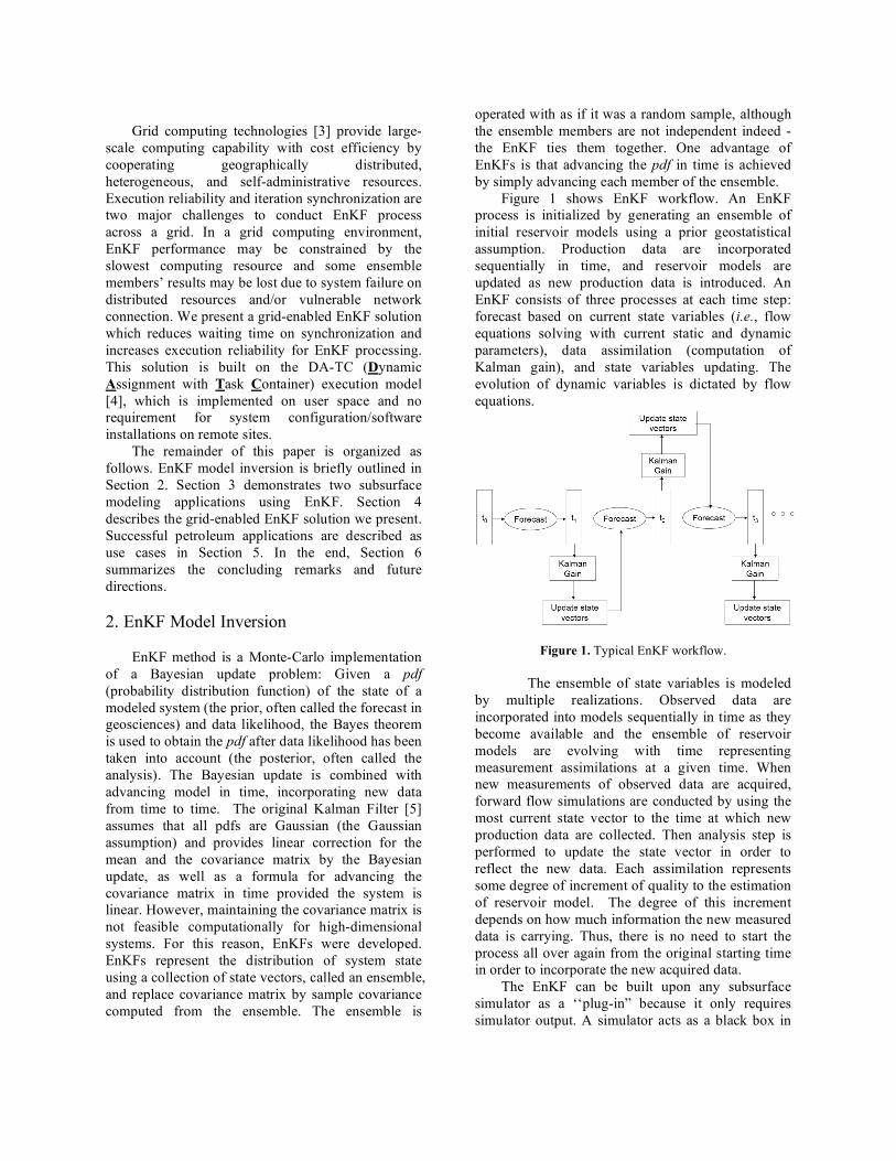
Figure 1 shows EnKF workflow. An EnKF process is initialized by generating an ensemble of initial reservoir models using a prior geostatistical assumption. Production data are incorporated sequentially in time, and reservoir models are updated as new production data is introduced. An EnKF consists of three processes at each time step: forecast based on current state variables (i.e., flow equations solving with current static and dynamic parameters), data assimilation (computation of Kalman gain), and state variables updating. The evolution of dynamic variables is dictated by flow equations.

Figure 1. Typical EnKF workflow.

The ensemble of state variables is modeled by multiple realizations. Observed data are incorporated into models sequentially in time as they become available and the ensemble of reservoir models are evolving with time representing measurement assimilations at a given time. When new measurements of observed data are acquired, forward flow simulations are conducted by using the most current state vector to the time at which new production data are collected. Then analysis step is performed to update the state vector in order to reflect the new data. Each assimilation represents some degree of increment of quality to the estimation of reservoir model. The degree of this increment depends on how much information the new measured data is carrying. Thus, there is no need to start the process all over again from the original starting time in order to incorporate the new acquired data.

The EnKF can be built upon any subsurface simulator as a ‘‘plug-in” because it only requires simulator output. A simulator acts as a black box in

the process of EnKF. Thus, EnKF method coding is significantly simpler than traditional gradient-based history matching methods where complicated coding of sensitivity calculations is required for different simulators and access to simulator source code is needed [6, 7, 8, 9]. Another advantage of EnKF is that it provides an ensemble of Ne reservoir models all of which assimilate up-to-date production data with computer time of approximately Ne flow simulations. Because CPU time for data assimilation is very small compared to flow simulation, it can be done at user local machine(s). 3. Subsurface Modeling Applications 3.1. Reservoir Modeling

Most data assimilation problems in petroleum reservoir engineering are highly non-linear, characterized by many variables. EnKF starts with an ensemble of initial reservoir models, sampled from the prior pdf of model state. State vector, ),,,( 21 Neyyyy !!!= , is categorized into

three parts as T

jjjj mgmfmy ))(,)(,(= , where j denotes realization index, m static parameters (reservoir properties, e.g., permeability and porosity) based on the initial knowledge of a reservoir, )(mf dynamic parameters (e.g., pressure and saturation) assumed to be certain at the initial stage,

)(mg observation variables (e.g., well production data). Observation variables are kept in the state vector for the purpose of building a linear relation between the state vector and the observed data. The model states and the associated uncertainty are integrated in time using a reservoir simulator. Updating can be carried out when any observation is available. The updated states are calculated through the Kalman filter formula:

),,2,1)(( ,,,,,, e

p

kjkkjobske

p

kj

u

kj NjyHdKyy !!!="+= [1] Where the superscript u denotes updating, p forecasting, },{ kjobsd observed data perturbed by noise, H observation operator with only zeros and ones as its entries simply equivalent to picking out the corresponding observation variables from the state vector,

keK

, the Kalman is given as

1

,,,,,, )( !+= kD

T

kkeYp

k

T

k

p

keYke CHCHHCK [2] Here,

keYC

,, is the covariance matrix among the

ensemble members and kD

C,

is the covariance matrix among the observation data.

Tp

k

p

jk

N

j

p

k

p

jk

e

p

keY yyyyN

Ce

))((1

1,

1

,,, !!!

= "=

[3] Equation (3) shows that only mean and variance are involved in a update step. If the distribution of model parameters and dynamic variables are not Gaussian distribution, non-physical values, such as saturation profile, are generated. To solve it, water front arrival time for water front grid block is involved in state vector:

NjwNjwNjwNjwNjwjw

NjjNjjNjjj

SSSSSS

PPkky

,,1,,,,,,,1,,1,,

,1,,1,,1,

,,,,,,,,

,,,,,,,,,(

2211!!!!!!!!!

!!!!!!!!!=

+"

##

[4] where N1 and N2 are the starting and the ending gridblocks of the front area, respectively. Eqn. 1, 2 and 3 are used to update the state vector at Eqn 4. After update step, the water front arrival time should be back transformed to saturation profiles. The process is often called re-parameterization with EnKF. 3.2. Groundwater Hydrology

Continuous decline in ground water levels and the projected increases in ground water need a scientific, systematic management plan to protect ground water from saltwater intrusion without causing environmental detriment. To achieve this goal, the development of a multi-objective saltwater intrusion management model with the optimized conjunctive use of surface water and ground water using large-scale simulation is needed [10].

The governing equations of groundwater resource (Eqn. 5) have several model parameters which are not directly measurable and must be estimated by an inverse procedure using historical groundwater head and salinity concentration observations. The influence of each parameter is quantified through a sensitivity analysis. The parameters with high degree of sensitivities with respect to ground water head and salinity observations are further identified using a formal inverse procedure. The iterative stochastic approach

used by EnKF is applied to estimate transmissivity and head distributions in heterogeneous aquifers. The process is similar to that used in petroleum application. The aquifer responses such as pressure head are measured at some locations at various time intervals. The purpose is to continuously characterize the aquifer properties and to predict its performance and uncertainty at future time.

The transient fluid flow in aquifers satisfying the following governing equation:

t

txhStxgtxhxK ss

!

!=+"#"

),(),()],()([ [5]

subject to the initial and boundary conditions: ,),()0,( 0 DxxHxh != [6]

,),,(),(

DxtxHtxh !"= [7]

,),,()(),()( Ns xtxQxnthxK !"#=$% [8]

where ),( txg is the source/sink term, ),( txh is the pressure head, )(0 xH is the initial head in the domain D, H(x,t) is the head at Dirichlet boundary segments, )(xK

s is the hydraulic conductivity,

),( txQ is the flux across Neumann boundary segments, )(xn is an outward vector normal to the boundary, and

sS is the specific storage. The

hydraulic conductivity )(xKs

is like permeability used in petroleum application is treated as random space function.

sS is assumed deterministic constant.

The above equation is solved to get )(xKs

, which is a random function. The method used can be Monte Carlo (i.e., EnKF) or moment-equation approaches. Hydraulic conductivity )(xK

s is log

normal distribution as permeability, )(xY is given as follows.

),()()](ln[)( 0xYxYxKsxY !+== [9]

where )(0 xY is the mean, )(xY ! is the zero-mean fluctuation. Suppose there are

YN direct

measurements of log hydraulic conductivity and hN

pressure head measurements and measured at some time intervals. The data assimilation process the stochastic differential flow equation is solved forward with time by using the KLME (Karhunen-Loeve based moment equation) method [11], which indicates the potential applicability to high resolution, large-scale predictive models. In this method, the hydraulic conductivity field is treated as a random spatial function and is decomposed using the KL

(Karhunen-Loeve) expansion. The pressure head is expanded using the perturbative polynomial expansion. On the basis of these expansions, the higher-order terms are truncated and the KLKF (KL Kalman Filter) is based on the first-order approximation of the pressure head. The KLKF utilizes a number of principal modes to propagate the statistics of the state vector. The forward step can be solved accurately and efficiently using the KLME, which can be solved in parallel using the existing flow model. The data assimilation step is operated based on the state statistics given by the forward step and the observations. 4. Implementing Grid-Enabled EnKF

The ResGrid toolkit [12] was designed to manage distributed computing resources across a grid and conduct subsurface-related modeling studies, including response surface modeling and sensitivity analysis. The ResGrid portal provides a web-based entry point for reservoir engineers to access the grid, concealing many complexities and technical details of simulation specification, job scheduling, and resource management from end users. We extend the functionality of the ResGrid by presenting a grid-enabled EnKF solution. The implementation of the solution is based on the DA-TC execution model. We introduce this execution model briefly before describing the solution of the grid-enabled EnKF. 4.1. DA-TC Execution Model

The DA-TC model introduces task container (TC) concept. A TC is viewed as a normal job to a local resource scheduling system. It is submitted into a queue, waiting for resource allocation. The local scheduler allocates resources to a TC under its own scheduling policies. Resources are released after a TC execution ends. From task execution perspective, a TC is a host environment. It provides a standardized method to manage the lifecycle of task execution on any participating cluster. Each task is associated with task metadata. A TC retrieves task execution requirements from metadata and takes actions to perform a task, including stagein, invocation, task termination, task execution monitoring, stageout, etc. A TC is a lightweight environment. It can be easily deployed and launch any existing ‘‘legacy” task executables on participating clusters.

An application execution agent (AEA) is employed to conduct dynamic task assignment in the

DA-TC execution model. AEA maintains a queue of tasks waiting for execution. A task container reports any status changes of itself and its running task(s) to AEA. According to the runtime status of task containers, AEA takes actions to assign tasks to different task containers. Certain task scheduling algorithms are adopted by AEA. Each task assigned on a TC (or say, a participating cluster) does not need to wait for resource allocation in the local scheduling system since the TC already holds the required resources. The tasks assigned onto a TC can be guaranteed quick execution.

Figure 2 shows the interaction diagram between AEA and TC. To carry out an application execution, the first thing for AEA to do is to submit TCs to participating clusters. The submitted TCs are placed as normal jobs at the end of the scheduling queues on participating clusters, waiting for resource allocation by local resource management systems. One participating cluster may host multiple task containers, according to different load balancing strategies adopted by AEA. After a TC obtains the required computing resources from a local scheduling system, it communicates with AEA for task assignment. First, the TC sends AEA a message to claim that it is ready to run a task. Second, AEA updates TC status table and then a task (or more) is selected, based on application workflow management strategies. Third, task stage in, execution, and stage out are performed, and the status tables associated with tasks and TCs on AEA are updated. After a task is completed successfully, AEA and TC are ready for the execution of next task.

Figure 2 The interaction diagram between AEA and TC. ‘‘R” denotes running and ‘‘Q” queuing. ‘‘Other” delegates the jobs submitted by other users.

The dynamic task assignment strategy and the task container technology in the DA-TC model essentially improve QoS of application execution in a multicluster grid environment from three major aspects: 1) Application turnaround time is significantly reduced due to dynamically load balancing; 2) Application execution reliability is upgraded as task assignment is based on resource runtime status; 3) Monitoring and steering of application execution is greatly improved. More details can be seen [4]. 4.2. Grid-Enabled EnKF Solution

Taking advantages of the DA-TC execution model, things become much easier. One of challenging issues for implementing grid-enabled EnKF is efficient simulation synchronization. In each EnKF iteration, simulations are dispatched onto geographically distributed computing resources. Typically, it is very hard to predict the completion time of each simulation due to self administration of participating resources. Filter execution and task assignment for next iteration have to wait until all simulation results are returned. The DA-TC execution model provides excellent feature for simulation synchronization. AEA in the DA-TC checks the status of each tasks and task containers to decide whether or not the current iteration of EnKF is completed.

Another issue on implementing grid-enabled EnKF is how to handle waiting time on remote queues for each iteration. In the traditional grid execution model [13], jobs submitted have to follow scheduling policies on remote sites, waiting for resource allocation from the end of queues. Overall execution time of an EnKF process with amount of iterations would be unbearably long due to waiting in the queue sat each iteration. Through the DA-TC model, once the required resources are allocated at the first iteration, task containers hold resources until the whole EnKF process is done and the following iterations can be executed without waiting.

Figure 3 illustrates the logic to implement the grid-enabled EnKF. After each task assignment via the DA TC model carries out, the statement, whether or not all tasks are assignment are assigned and all task containers are ready, is examined by checking the task and container status tables in the DA-TC. If the answer is no, the process on task assignment continues. If the answer is yes, an application-specific Kalman filter provided by application researchers is invoked. This filter program analyzes simulation results and concludes whether further

iteration(s) is needed or not. If the results are not acceptable, new task set and corresponding data set are generated as well as task assignment continues.

Figure 3 The logic of the grid-enabled EnKF solution. 4.3. Model Inversion Scenario with ResGrid

The grid-enabled EnKF solution is seamless integrated with the basic services provided by the ResGrid, such as resource broking service, data archive service, and ResGrid portal. Figure 4 illustrates the model inversion scenario within the ResGrid. The steps are as followed:

1. A user logs in the EnKF manager and retrieves a GSI certificate from a proxy server. The certificate authorizes the user to access grid resources and implement secure data transfer.

2. Using EnKF managers to generate initial ensemble, Ne set of reservoir properties by filling the Gaussian semi-varigram and conditional data of reservoir in form. Then, stochastic simulation is accomplished automatically.}

3. ResGrid service is launched and ensemble state vectors are built into the reservoir models. DA-TC takes effect to submit simulations to grid. If it is not the first time step, all the state vectors are filled with updated information.

4. The grid-enabled EnKF solution waits until all the simulation tasks of the ensemble finish. The state vectors are abstracted from

output of Ne simulations. ResGrid archive brings all the state variables from remote resources to local machine.

5. The EnKF solution searches water front area from saturation profiles of all ensemble, predetermines time window for current assimilation step, and resubmits simulation jobs of the model with new time window by launching DA-TC again.

6. GridFTP brings time window back for all water front area grid blocks, and build up state vectors with model parameters, pressure, saturation and water front arrival time, compute the Kalman gain.

7. The solution updates the state vectors and back transforms the water front arrival time to saturation profile.

8. If the current time step is the final step, then do the forecast and uncertainty analysis. Otherwise, go back to Step 3.

Figure 4. Flowchart of reservoir model inversion by EnKF in the ResGrid 4.4. Computation Cost

In the DA-TC execution model, once a task container has been allocated resources, it persists as a job on remote resource and therefore retains the resources until all forecast of all members assigned to the container are completed. Thus, all runs assigned to a container have only one queue wait and dynamic task assignment makes the containers with fast speed execute more tasks (dynamic load balancing); with many members and assimilations per container, this greatly reduces the total queue time. The total

computation time is the simulation time for all ensemble models, plus time for Kalman gain calculation at the update steps, plus queue waiting time (from job submission to execution) at grid clusters. The example study has 400 ensemble members. Assimilation occurs every 10 days up to 100 days in the case study. If there are nonphysical values generated for updated saturation (e.g., ]1,0[!S ) or other state variables in assimilation step, the simulator is restarted from the previous step with the model parameter vector from the current update. Iterations are applied until the updated state vector satisfies the pre-defined physical bound.

Take an example. The maximum iterations are set to ten. Ten iterations are expected to be adequate based on EnKF for similar models [14]. According to our experience, the average iteration requirement is two. The number of simulation runs for this example is 400 ! 1 (1 forecast + 2 iterations) ! 10 (assimilation times) =12,000 synchronized updates. Average processor time per simulation is 10 minutes; the computational time is about 83 days using 1 processor. In our case, all the simulations are submitted to 256, 15, or 14-processor clusters (running a mix of Linux and AIX). We use 5 to 10 containers depending on cluster size, and each container uses 1 processor; thus the execution time is ~100 hours. Assuming queue waiting time is 5 hours for each forecast step, the total time for EnKF processing is 100+5 = 105 hours using the DA-TC execution model because there is only one wait. The total time will increase to 100+5!10 =150 hours if DA-TC is not used and the queue is re-entered for each forecast step. The queue waiting time depends on the grid cluster status, and may range from minutes to days. If the production history is quite long, the accumulated queue time will increase and negate the computational gains of grid computing. 5. Case Study 5.1. 1D Buckley-Levertt water-flooding problem

A one dimensional 32-grid reservoir model is

defined with no dip. The model contains one injector I1 at grid 1 to inject water and one producer P1 at grid 32 to produce oil. Eight non-uniform reservoir models are generated from LU Decomposition. The porosity is normal distributed and the permeability is log-normally distributed. The porosity is assumed with mean 0.2 and standard deviation of 0.04. ln(k) has a mean of 5.5 (when k is in md. 1 md =

0.9896233!10-12 m2) and standard deviation of 0.5. The two variables are correlated with cross-correlation coefficient of 0.5. The ranges of the two variables are 18 grid blocks and variogram model is exponential. Then a ‘‘true” porosity and permeability field with unconditional LU Decomposition [15] is created. One hundred porosity and permeability fields are generated by LUSIM.

Bottom-hole pressure constrained for the injector I1 is 4500 psig. And 1500 psig is the Bottom-hole pressure constrains for producer P1. The measurement is generated by using the ‘‘true” porosity and permeability, and adds noise to the simulation results. Measurement is assimilated once for 68 days after the water front at 21st. The data to be assimilated here are water injection rate, oil producer rate, water cut and the water saturation at grid 21. Measurement errors are assumed to be Gaussian with mean 0 and standard deviation of 5% of magnitude of the observed data in rates, 1% in the water saturation.

From Section 2, it seems that EnKF may not work very well when the state vector is strongly non-linear then non-Gaussian. The EnKF may lead to non-physical saturation values. In this part, the re-parameterization with EnKF is applied. The re-parameterization method comes from the fact that the water saturation distribution outside water front area exhibits a Gaussian behavior, whiles the distribution in the water front area, and has a bimodal distribution. Based on the fact, the re-parameterization needs to be done only for the front area where the Grid-block water saturation distribution shows a strong non-Gaussian character. The new approach uses water front arrival time but saturation as the state vector, because the non-Gaussian saturation distributions are primarily observed near the water front.

The first assimilation time is 30 days. The water front area is from grid block 8 to 16. In order to obtain the entire distribution of water arrival time at water front area, reservoir simulator must run to 60 days (time window) to let water front of each realization pass through the front area. The statistics of the front area is always represented by the time of water arrival. In this way, the model state can be better approximated by a Gaussian distribution, and then the EnKF updating can be used without losing information. The updated saturation profiles from the traditional EnKF and EnKF with re-parameterization are compared in Figure 5. Although the variances of saturation estimation by two methods have decreased, the oscillation of saturation profiles of traditional EnKF is substantial and many updated saturation values are beyond the physical bounds may result in problems for assimilating future data. But the EnKF

with re-parameterization has no such kind of problem. The improved EnKF has been applied in grid-enable workflow. %

(a) Before EnKF

(b) The traditional EnKF

(c) The EnKF with re-parameterization

Figure 5. Initial and update porosity ensemble with the reference denoted by the bold curve. 5.2 2D Water-flooding problems

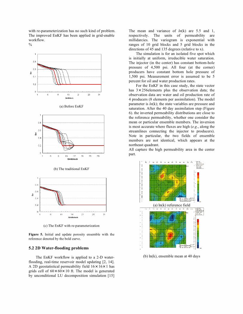
The EnKF workflow is applied to a 2-D water-flooding, real-time reservoir model updating [2, 14]. A 2D geostatistical permeability field 16!16!1 has grids cell of 60!60!10 ft. The model is generated by unconditional LU decomposition simulation [15]

The mean and variance of ln(k) are 5.5 and 1, respectively. The units of permeability are millidarcies. The variogram is exponential with ranges of 10 grid blocks and 5 grid blocks in the directions of 45 and 135 degrees (relative to x).

The simulation is for an isolated five spot which is initially at uniform, irreducible water saturation. The injector (in the center) has constant bottom-hole pressure of 4,500 psi. All four (at the corner) producers have constant bottom hole pressure of 1,500 psi. Measurement error is assumed to be 5 percent for oil and water production rates.

For the EnKF in this case study, the state vector has 3!256elements plus the observation data; the observation data are water and oil production rate of 4 producers (8 elements per assimilation). The model parameter is ln(k); the state variables are pressure and saturation. After the 40 day assimilation step (Figure 6). the inverted permeability distributions are close to the reference permeability, whether one consider the mean or particular ensemble members. The inversion is most accurate where fluxes are high (e.g., along the streamlines connecting the injector to producers). Note in particular, the two fields of ensemble members are not identical, which appears at the northeast quadrant. All capture the high permeability area in the center part.

(a) ln(k) reference field

(b) ln(k), ensemble mean at 40 days

(c) ln(k), member

(d) ln(k), member 350 at 150 at 40 days (0.75pv mobile) 40 days(0.75pv mobile) 6. Conclusions and future work

We present a grid-enabled EnKF solution, built on the DA-TC execution model that aims to incorporate grid resources with application reliability improvement and turnaround time reduction for each EnKF’s iteration. This solution already has been integrated into the ResGrid, a grid middleware toolkit for subsurface-related modeling studies. Using the enhanced ResGrid toolkit, we have conducted the traditional and re-parameterization EnKF for continuous updating of reservoir models to assimilate real-time production data. Re-parameterization with EnKF can solve the non-linearity and non-Gaussianity problem in oil and system. From this study, we can draw the following conclusions:

1) EnKF is efficient and robust for real-time reservoir updating to assimilate up-to-date production data.

2) By introducing the re-parameterization in the EnKF updating process, more accurate models are attained, resulting in better matching of production data and more accurate predictions. Also, the filter updating process becomes stable.

3) The EnKF application to groundwater resource scheme would be easy to implement, yet very efficient in grid environment.

There are two major directions for our future work. First, the functionality of the grid-enabled EnKF solution will be enhanced and seamlessly integrated into the ResGrid ensemble manager. When new data arrive, users intervene with a request, or

sensor-driven alarms will be relayed to the grid, the ensemble manager will initiate a new round of inversion and update parameter sets, parameter uncertainty ranges, and prediction uncertainty ranges. The updated prediction uncertainties will be used to update alarm parameters. Second, we will explore a wider range of applications areas (e.g., weather forecast and earth sciences) to take advantages of our EnKF solution and grid computing resources. Acknowledgements

This project is sponsored by the U.S. Department of Energy (DOE) under Award Number DE-FG02-04ER46136 and the Board of Regents, Louisiana State University, under Contract No. DOE/LEQSF (2004-07). Reference [1] A. Tarantola, “Inverse problem theory and methods for model parameter estimation,” Society for Industrial and Applied Mathematics, Philadelphia, 2005. [2] G. Evensen, “The Ensemble Kalman filter: theoretical formulation and practical implementation,” Ocean Dyn., vol. 53, no. 4, pp. 334–367, 2003. [3] I. Foster, C. Kesselman, and S. Tuecke, “The anatomy of the grid: enabling scalable virtual organizations,” International Journal of High Performance Computing Applications, pp. 200-222, 2001, 15 (3). [4] Z. Lei, M. Xie, and et al., “Efficient application execution management in multicluster grids,” in The 8th IEEE/ACM International Conference on Grid Computing (Grid 2007), 2007 (submitted) [5] P. S. Maybeck, “Stochastic models, estimation, and control,” Vol. 1 of Mathematics in Science and Engineering, Academic Press, Inc, New York, 1979. [6] J.L. Landa and R.N. Horne, “A procedure to integrate well test data,reservoir performance history and 4-d seismic information into a reservoir description,” in SPE Annual Technical Conference and Exhibition, San Antonio,TX, October 1997, SPE 38653. [7] N. He, A.C. Reynolds, and D.S. Oliver, “Three-dimensional reservoir description from multiwell pressure data and prior information,” in SPE Annual Technical Conference and Exhibition, Denver,CO, October 1996, SPE 36509. [8] F. Zhang and A. C. Reynolds, “Optimization algorithms for automatic history”, in 8th European Conference on the Mathematics of Oil Recovery, 2002. [9] R. Li, A.C. Reynolds, and D.S. Oliver, “Sensitivity coefficient for three-phase history matching,” Journal of Canadian Petroleum Technology, pp. 70-777, 2003. [10] F. T-C. Tsai, “Geophysical parameterization and parameter structure identification using natural neighbors in groundwater inverse problems,” Journal of Hydrology, vol. 308, pp. 269-283, 2005.

[11] D. Zhang, Z. Lu, and Y. Chen, “Dynamic reservoir data assimilation with an efficient, dimension-reduced kalman filter,” SPE Journal, pp. 108-117, Mar 2007. [12] Z. Lei, D. Huang, and et al., “Resgrid: A grid-aware toolkit for reservoir uncertainty analysis leveraging,” in IEEE International Symposium on Cluster Computing and the Grid (CCGrid06), Singapore, May 2006. [13] D. Katz, J.C. Jacob, and et al, “Comparison of two methods for building astronomical image mosaics on a grid,” in Proceedings of International Conference on Parallel Processing 2005 Workshops, 2005. [14] Y. Gu and D. S. Oliver, “History match of the punq-s3 reservoir model using the ensemble kalman filter,” SPE Journal, pp. 217–224, June 2005. [15] P. Goovaerts, “Geostatistics for Natural Resources Evaluation,” Applied Geostatistics Series, Oxford University Press, Oxford, 1997.