Ensemble dispersion forecasting—Part II: application and evaluation

Atmospheric Environment 38 (2004) 4619–4632

ARTICLE IN PRESS

*Correspond

E-mail addr

1352-2310/$ - se

doi:10.1016/j.at

Ensemble dispersion forecasting—Part II:application and evaluation

S. Galmarinia,*, R. Bianconib, R. Addisc, S. Andronopoulosd, P. Astrupe,J.C. Bartzisd, R. Bellasiob, R. Buckleyc, H. Championf, M. Chinol, R. D’Amoursg,E. Davakisd, H. Eleveldh, H. Glaabi, A. Manningf, T. Mikkelsene, U. Pechingerj,

E. Polreichj, M. Prodanovak, H. Slaperh, D. Syrakovk, H. Teradal,L. Van der Auweram

a IES/REM, Joint Research Center, European Commission, TP 441 21020 Ispra, ItalybEnviroware srl, C.Dir. Colleoni, Pzo Andromeda 1 20041 Agrate Brianza, ItalycSavannah River Technology Center, Savannah River Site, Aiken, SC 29808, USA

dNCSR Demokritos, Environmental Research Laboratory, 15310 Aghia Paraskevi Attikis, GreeceeRIS /O. National Laboratory, Wind Energy Dep, P.O. Box 49, DK-4000, Roskilde, Denmark

fMet Office, FitzRoy Road, Exeter EX1 3PB, United KingdomgCanadian Metorological Centre, 2121 Voie de Service Nord, Rte Transcan., Dorval QC, Canada H9P 1J3

hRIVM, Laboratory of Radiation Research, P.O. Box 1, Bilthoven, NetherlandsiGerman Weather Service (DWD), P.O. Box 10 04 65, 63004 Offenbach a.M., GermanyjZentralanstalt fuer Meteorologie und Geodynamik, A-1191 Vienna, Hohe Warte 38, Austria

kNMHI, 66 Tzarigradsko shaussee, Sofia 1784, BulgarialJAERI, 2-4 Shirakata-shirane, Tokai, Naka, Ibaraki, 319-1195, Japan

mKMI, Ringlaan 3, 1180 Brussels, Belgium

Received 16 January 2004; received in revised form 16 May 2004; accepted 26 May 2004

Abstract

The data collected during the long-range European tracer experiment (ETEX) conducted in 1994, are used to

estimate quantitatively the ensemble dispersion concept presented in Part I. The modeling groups taking part to the

ENSEMBLE activities (see, Part I) repeated model simulations of the dispersion of ETEX release 1 and the model

ensemble is compared with the monitoring data. The scope of the comparison is to estimate to what extent the ensemble

analysis is an improvement with respect to the single model results and represents a superior analysis of the process

evolution.

r 2004 Elsevier Ltd. All rights reserved.

Keywords: Ensemble dispersion modeling; European tracer experiment; Model evaluation

1. Introduction

Very few tracer experiments were conducted to date

that cover spatial scales of the order of few thousands of

ing author.

ess: [email protected] (S. Galmarini).

e front matter r 2004 Elsevier Ltd. All rights reserve

mosenv.2004.05.031

kilometers and that can be used for the evaluation of

model simulations. Among them the ANATEX (Clark

et al., 1988; Draxler and Heffter, 1989; Stunder and

Draxler, 1989; Heffter and Draxler, 1989), CAPTEX

(Ferber et al., 1986) and the European tracer experiment

(ETEX). ETEX, organized by the European Commis-

sion, the World Meteorological Organization and the

d.

ARTICLE IN PRESSS. Galmarini et al. / Atmospheric Environment 38 (2004) 4619–46324620

International Atomic Energy Agency was conducted in

1994. It consisted of the release from a location in

western France of a passive tracer (PMCH) that was

detected by a network of 168 samplers distributed from

Norway to Switzerland and eastward, all the way to the

Polish-Ukraine border (Fig. 1). Two distinct releases

were performed under different weather conditions

(usually referred to as ETEX-1 and ETEX-2, Girardi

et al., 1998). The ETEX-1 release took place in ‘‘well-

behaved’’ weather conditions and led to a large number

of non-zero samples at ground level. So far it has been

the most investigated release, often used for model

evaluation (Van Dop and Nodop, 1998).

With the aim of evaluating the ensemble dispersion

concept presented in Galmarini et al. (2004, Part I of this

paper), the ETEX-1 release has been chosen as case

study. This paper will develop around the following

issues:

* Simulation of the ETEX-1 release by long-range

dispersion models operational at several meteorolo-

gical services and environmental protection agencies

in Europe and world wide and participating to the

ENSEMBLE project (Bianconi et al., 2004; Galmar-

ini et al., 2004)* Use of the ETEX-1 data to evaluate the ensemble

dispersion indicators presented in Part I.* Comparison of the ensemble analysis with single

deterministic model realizations.

The scope of this investigation is the quantitative

assessment of ensemble dispersion analysis and the

verification of the usefulness of ensemble dispersion

prediction in the absence of experimental evidence. The

results obtained will be discussed in the context of long

-500000 0 500000 1000000 1500000

5000000

5500000

6000000

6500000

7000000

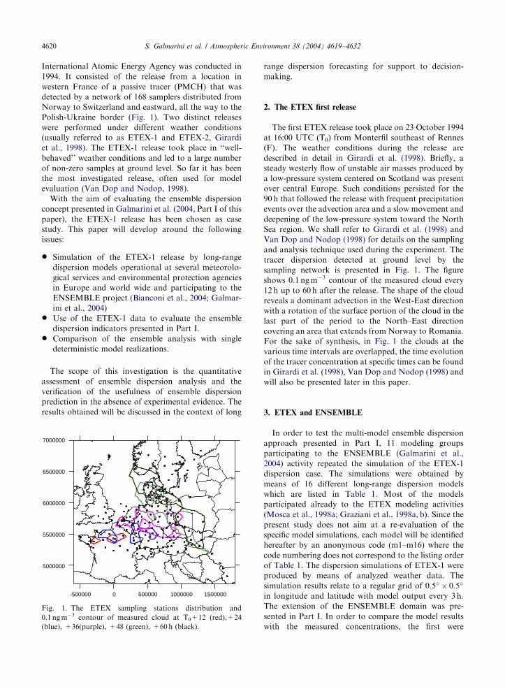
Fig. 1. The ETEX sampling stations distribution and

0.1 ngm�3 contour of measured cloud at T0+12 (red),+24

(blue), +36(purple), +48 (green), +60h (black).

range dispersion forecasting for support to decision-

making.

2. The ETEX first release

The first ETEX release took place on 23 October 1994

at 16:00 UTC (T0) from Monterfil southeast of Rennes

(F). The weather conditions during the release are

described in detail in Girardi et al. (1998). Briefly, a

steady westerly flow of unstable air masses produced by

a low-pressure system centered on Scotland was present

over central Europe. Such conditions persisted for the

90 h that followed the release with frequent precipitation

events over the advection area and a slow movement and

deepening of the low-pressure system toward the North

Sea region. We shall refer to Girardi et al. (1998) and

Van Dop and Nodop (1998) for details on the sampling

and analysis technique used during the experiment. The

tracer dispersion detected at ground level by the

sampling network is presented in Fig. 1. The figure

shows 0.1 ngm�3 contour of the measured cloud every

12 h up to 60 h after the release. The shape of the cloud

reveals a dominant advection in the West-East direction

with a rotation of the surface portion of the cloud in the

last part of the period to the North–East direction

covering an area that extends from Norway to Romania.

For the sake of synthesis, in Fig. 1 the clouds at the

various time intervals are overlapped, the time evolution

of the tracer concentration at specific times can be found

in Girardi et al. (1998), Van Dop and Nodop (1998) and

will also be presented later in this paper.

3. ETEX and ENSEMBLE

In order to test the multi-model ensemble dispersion

approach presented in Part I, 11 modeling groups

participating to the ENSEMBLE (Galmarini et al.,

2004) activity repeated the simulation of the ETEX-1

dispersion case. The simulations were obtained by

means of 16 different long-range dispersion models

which are listed in Table 1. Most of the models

participated already to the ETEX modeling activities

(Mosca et al., 1998a; Graziani et al., 1998a, b). Since the

present study does not aim at a re-evaluation of the

specific model simulations, each model will be identified

hereafter by an anonymous code (m1–m16) where the

code numbering does not correspond to the listing order

of Table 1. The dispersion simulations of ETEX-1 were

produced by means of analyzed weather data. The

simulation results relate to a regular grid of 0.5� � 0.5�

in longitude and latitude with model output every 3 h.

The extension of the ENSEMBLE domain was pre-

sented in Part I. In order to compare the model results

with the measured concentrations, the first were

ARTICLE IN PRESS

Table 1

Models involved in the ETEX-ENSEMBLE activity

Institute Dispersion model Type NWP data

Canadian Meteorological Centre CANERM E GEM Global

Deutscher Wetterdienst GME-LPDM L DWD-GME

LM-LPDM L DWD-LM

Institut Royal Meteorologique de Belgique BPaM4D L ECMWF

Japan Atomic Energy Research Institute WSPEEDI (Ishikawa, 1994;

Chino et al., 1995)

L MM5

Meteo-France MEDIA E ARPEGE

MEDIA-nested E ARPEGE-ALADIN

Met Office (UK) NAME L UM

National Centre for Scientific Research ‘‘Demokritos’’

(G)

DIPCOT L ECMWF

DIPCOT P ECMWF

National Institute of Meteorology and Hydrology (BG) EMAP E DWD-GME

Risø National Laboratory (DK) RODOS-LSMC P DMI-HIRLAM

RODOS-MATCH L-E DMI-HIRLAM

RIVM, Laboratory of Radiation Research (NL) NPKPUFF v.1.1.17 L HIRLAM

NPKPUFF v.2.0.7 (Eleveld,

2002)

L ECMWF

Savannah River Westinghouse (US) LPDM L RAMS3a

Zentralanstalt fuer Meteorologie und Geodynamik (A) TAMOS L ECMWF T319L50

TAMOS L ECMWF T319L50

L stands for Lagrangian particle model, E for Eulerian model, P for Puff model. The last table column lists the NWP model from

which atmospheric circulation data originated.

S. Galmarini et al. / Atmospheric Environment 38 (2004) 4619–4632 4621

integrated over a period of 3 h to reproduce the sampling

time used during the tracer experiment. The measured

concentrations were interpolated to the ENSEMBLE

grid resolution for a direct comparison with the model

results. The interpolation (Watson and Philip, 1984)

consisted of a classical triangulation of the measure-

ments at sampling stations and linear interpolation to

the regular grid nodes. The minimum value is

0.001 ngm�3, which corresponds to the tracer detection

limit.

4. Single deterministic model performances

In order to evaluate the multi-model ensemble

approach we first present the behavior of single model

results when compared to the ETEX data. For the sake

of synthesis, Table 2 gives the Figure of Merit in Space

(FMS) of each of the model and the Median Model

(Section 5.2) compared to the measurements. The FMS

(Mosca et al., 1998b) is the estimate of the overlap (in

percentage) at a given time between the modeled and the

measured clouds at a defined concentration threshold (in

this case, >0.1 ngm�3). Table 2 clearly shows a

variability of the FMS as a function of time for a

specific model, which in some cases can be very large

(for example m5 shows a maximum overlap of 36% at

12 h after the release and a minimum of 5% 24h later).

A large variability is also present model wise for a

specific time interval like in the case of T0+6 with 82%

coverage by m14 and 20% by m3 and m6. The values

presented in Table 2 are also plotted in Fig. 2. The figure

highlights the presence of a group of models with

coherent behavior and the presence of four outliers

namely m4 and m5, m8, m15. The outliers will not be

discarded from the analysis since their results will serve

the scope of demonstrating their effect on the ensemble

analysis. All model results will therefore be considered in

the ensemble treatments presented in the next sections.

A more comprehensive assessment of the single model

performance is given through a global analysis. It relates

the statistical analysis of all couples of measured-

modeled concentration values, at all spatial locations

of the domain, and at all times. The three statistical

parameters FA2, FA5 and FOEX have been selected for

this analysis (Mosca et al., 1998b). FA2 and FA5 give

the percentage of model results within a factor of 2 and

5, respectively of the corresponding measured value,

while FOEX gives in percentage of modeled concentra-

tion values that overestimate (positive) or underestimate

(negative) the corresponding measurement. Table 3

shows the three parameters values calculated for all

models. The values of FA2, FA5 and FOEX for m4

indicate that something went wrong in the simulation

since all values are larger than a factor of 5 and they all

overestimate the measured data. This shows that an

error has occurred during the simulation (for example a

mistake in the definition of the release rate). The results

ARTICLE IN PRESS

Table 2

FMS (in %) of single model (m1–m16) and median model against measured data. Results every 6 h from release start. Threshold value

1.0 e�10 gm�3

Model T0+6 T0+12 T0+18 T0+24 T0+30 T0+36 T0+42 T0+48 T0+54 T0+60

m1 29 32 33 33 30 34 33 45 46 47

m2 73 22 37 31 30 29 30 44 43 41

m3 20 37 30 33 29 30 36 44 39 36

m4 26 19 25 25 19 25 25 32 32 35

m5 35 36 21 17 9 5 11 25 18 12

m6 20 20 26 27 26 24 31 44 42 36

m7 50 37 33 27 32 31 29 45 39 36

m8 41 23 20 16 13 19 23 29 22 22

m9 33 39 29 29 31 27 39 48 38 29

m10 41 32 34 32 33 38 35 46 45 41

m11 45 48 31 27 36 33 36 45 47 30

m12 56 30 31 23 21 26 34 44 42 38

m13 33 27 29 25 31 36 38 50 38 36

m14 82 32 28 28 32 28 35 48 41 41

m15 43 26 27 20 20 16 19 25 20 26

m16 30 23 15 22 23 19 23 25 12 14

Median Model 62 39 38 29 31 36 43 56 47 43

0

10

20

30

40

50

60

70

80

90

T0+6 T0+12 T0+18 T0+24 T0+30 T0+36 T0+42 T0+48 T0+54 T0+60

Time intervals from release start T0

FMS

(%)

m1 m2m3 m4m5 m6m7 m8m9 m10m11 m12m13 m14m15 m16mm

Fig. 2. Time evolution of FMS presented in Table 2. Data

every 6 h from release start.

Table 3

Percentage of couple measured-modeled data within a factor of

2 (FA2) and 5 (FA5). Results for models m1–m16 and median

model. All measured-modeled data couples at all times and

points in space have been considered. The last column (FOEX)

gives the percentage of over-prediction (>0) or under-

predictions (o0)

Model FA2[%] FA5[%] FOEX[%]

m1 14.25 37.65 77

m2 22.01 45.91 61

m3 19.13 42.04 55

m4 0 0 100

m5 13.02 32.72 71

m6 22.91 47.37 2

m7 19.98 42.91 36

m8 8.11 18.08 �42m9 16.47 37.47 11

m10 15.11 35.32 17

m11 15.9 37.76 14

m12 21 42.43 34

m13 21.94 45.66 50

m14 12.34 28.35 56

m15 15.89 34.65 11

m16 21.97 44.39 36

Median Model 24.14 48.38 15

S. Galmarini et al. / Atmospheric Environment 38 (2004) 4619–46324622

of m4 were however retained and treated together with

the others since they will allow us to show the robustness

of the ensemble dispersion technique.

5. Evaluation of the multi-model ensemble dispersion

indicators

In this section we will evaluate two ensemble

indicators presented in Part I, namely the Agreement

in Threshold Level and the Agreement in Percentile

Level. Further to that the concept of Median Model will

be introduced as part of the ensemble analysis.

5.1. Agreement in threshold level

The agreement in threshold level (ATL) indicator is

used for the ensemble analysis of the ETEX case study.

In particular we will focus on its application to time-

integrated concentration (TIC). As presented in Part I,

ATL gives the spatial distribution of the models

ARTICLE IN PRESSS. Galmarini et al. / Atmospheric Environment 38 (2004) 4619–4632 4623

agreement in simulating that a pre-defined threshold

level is exceeded. Fig. 3 gives the time evolution of the

ATL for TIC every 12 h and for a threshold of

0.1 nghm�3. The figure also shows the 0.1 nghm�3

contour of measured cloud (hatched surface). The

distribution of models agreement shows the presence

of a large region where 30–100% of the 16 models agree

in simulating a threshold excedance. At the external

fringes of this region for all time intervals, the presence

of areas of low model-agreement (yellow colors) can be

seen. This area shows that a number of models over

predict the extension of the cloud where TIC is equal or

larger than the pre-defined threshold. The overlap of the

measured cloud shows a remarkable coincidence with

the high agreement (>70%) region during all the

simulated period. Apart for the case T0+24 where the

composite modeled cloud appears to move faster and

more to the northeast than the measured cloud, in all

other case, there is no region were the measured cloud

overlaps with the low agreement area. This indicates

that there is not a single or few models (outliers) that

perform better than the ensemble. The result points in

the direction of considering the high agreement region as

a reliable result bearing a considerable degree of

confidence for the determination of the spatial coverage

of the cloud. Such a possibility was partly anticipated in

Galmarini et al. (2001) where ideal case studies were

analyzed but no quantitative evaluation was provided.

Another important aspect highlighted in Fig. 3 is the

chance of gross error that the analysis of a single model

result can produce. The last panel of Fig. 3 shows the

ATL of TIC at T0+60 h for the same threshold level.

This time, however, the hatched area relates to the result

of model m8. As one can see, this model is responsible

for the region of low agreement in the forefront of the

cloud. An analysis of the dispersion based on this single

model results would lead to a large overestimate of the

cloud distribution. When a higher threshold value is

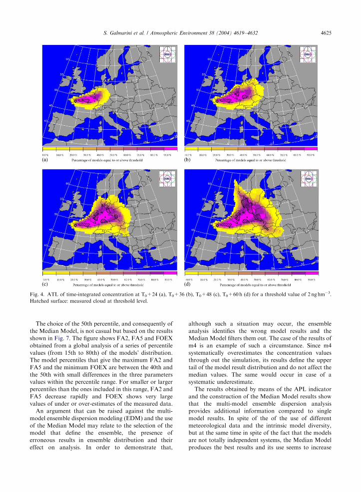
considered the results do not change. Fig. 4 gives the

time evolution of the ATL of TIC at T0+24, +36, +48,

+60h for a threshold value of 2 ngm�3. The threshold

value is 20 times larger than the one selected for Fig. 4

and is used here to identify ‘‘hot spots’’. In spite of the

patchiness of the measured cloud compared to the

composite modeled one, the figure shows a clear overlap

of the first with the high agreement region. The results of

Figs. 3 and 4 are even more remarkable if one considers

that the atmospheric dispersion models used to simulate

the case are not strictly speaking independent systems.

As a matter of fact they share several aspects, which

relate to the meteorological fields used as well as

approaches to modeling atmospheric dispersion pro-

cesses. In spite of these aspects, the model results seem

also to show a character of complementarity that allows

obtaining a result closer to what was measured when a

model composite is considered. This aspect will be

discussed further on. The results presented show that the

ATL is a good indicator for combining several model

results in a spatial analysis and that the high agreement

region gives a good indication of the cloud spatial

coverage.

5.2. Agreement in percentile level and the Median Model

Fig. 5 shows the results of the ETEX measurement

and agreement in percentile level (APL) (50th and 75th)

for surface air concentration at T0+24, +48, +60 h. As

presented in Part I, for a given variable, time and a given

percentile value (in this case 50th and 75th), the APL

gives the variable distribution corresponding to the

defined percentile of models. The comparison of the

clouds relating to the 50th and 75th percentile of model

results with the measured cloud shows an overestimate

of both the cloud size and concentration values by the

75th percentile, while the 50th percentile agrees well with

the measured cloud. This is particularly evident at

T0+48 and T0+60 where the measured ‘‘hot spots’’ are

also present in the APL (50th) cloud. Furthermore the

spatial distribution of the low concentration values

remarkably resembles the measured one. A certain

degree of overestimation in the spatial distribution of

the cloud is also present in the APL (50th) plot at

T0+24, though much more reduced with respect to APL

(75th).

Fig. 6 gives the overlap of the 0.01 ngm�3 cloud at

T0+24, 48, 60 h, produced by the best performing model

(m2 as from the results of Tables 2 and 3), the measured

cloud and the APL (50th) cloud. It clearly appears that

the overlap between the last two is larger than the

overlap between the single model cloud and the

measured one. When other concentration levels are

considered, the horizontal concentration gradient ob-

tained with APL is much closer to the one of the

measure cloud when compared to the result of the single

model. The results of Figs. 5 and 6 indicate that the 50th

percentile of model results may be more representative

of the actual cloud evolution than the 75th percentile

and the single models. In order to prove it we

have calculated the FMS of what will be called the

Median Model. The Median Model results are ob-

tained by calculating the median of all model results

at all time steps and in all grid nodes. The FMS of

the Median Model calculated every 6 h are presented

in Table 2. As one can see the FMS is indeed higher

than the single model results at almost all time inter-

vals, as also depicted in Fig. 2. In order to generalize

the analysis of the Median Model results, the

global analysis was also conducted as given in Table 3.

FA2 and FA5 are systematically higher that the

single model values. FOEX is not the minimum

value (obtained from m15 results) though the fourth

smallest.

ARTICLE IN PRESS

Fig. 3. ATL of time-integrated concentration at T0+12 (a), +24 (b), +36 (c), +48 (d), +60h (e) Threshold level 0.1 nghm�3. Colors

distribution of ATL obtained from all model results. Hatched surface in the first five panels from upper left: measured cloud at

threshold level. (f) Hatched surface cloud modeled by m8 at threshold level.


ARTICLE IN PRESS

Fig. 4. ATL of time-integrated concentration at T0+24 (a), T0+36 (b), T0+48 (c), T0+60h (d) for a threshold value of 2 ng hm�3.

Hatched surface: measured cloud at threshold level.


The choice of the 50th percentile, and consequently of

the Median Model, is not casual but based on the results

shown in Fig. 7. The figure shows FA2, FA5 and FOEX

obtained from a global analysis of a series of percentile

values (from 15th to 80th) of the models’ distribution.

The model percentiles that give the maximum FA2 and

FA5 and the minimum FOEX are between the 40th and

the 50th with small differences in the three parameters

values within the percentile range. For smaller or larger

percentiles than the ones included in this range, FA2 and

FA5 decrease rapidly and FOEX shows very large

values of under or over-estimates of the measured data.

An argument that can be raised against the multi-

model ensemble dispersion modeling (EDM) and the use

of the Median Model may relate to the selection of the

model that define the ensemble, the presence of

erroneous results in ensemble distribution and their

effect on analysis. In order to demonstrate that,

although such a situation may occur, the ensemble

analysis identifies the wrong model results and the

Median Model filters them out. The case of the results of

m4 is an example of such a circumstance. Since m4

systematically overestimates the concentration values

through out the simulation, its results define the upper

tail of the model result distribution and do not affect the

median values. The same would occur in case of a

systematic underestimate.

The results obtained by means of the APL indicator

and the construction of the Median Model results show

that the multi-model ensemble dispersion analysis

provides additional information compared to single

model results. In spite of the of the use of different

meteorological data and the intrinsic model diversity,

but at the same time in spite of the fact that the models

are not totally independent systems, the Median Model

produces the best results and its use seems to increase

ARTIC

LEIN

PRES

S

Fig. 5. Comparison of APL and measured surface concentration at T0+24, +48, +60h. APL values at 50th percentile and 75th percentile of model results.

S.

Ga

lma

rini

eta

l./

Atm

osp

heric

En

viron

men

t3

8(

20

04

)4

61

9–

46

32

4626

ARTICLE IN PRESS

Fig. 6. Comparison of Median Model, best single model results

and measurements. Variable: surface concentration; Red best

single model result; yellow Median Model; orange ETEX

measurements.

-50

-40

-30

-20

-10

0

10

20

30

40

50

0 10 20 30 40 50 60 70 80 90 100

FA5

FA2

FOEX

%

Percentiles

Fig. 7. FA2, FA5 and FOEX obtained from global analysis of

various percentile models.


the reliability of the single model realization. As one can

see the use of the Median Model does not penalize the

user of a very good model and it is very convenient for

the user of a poor performing one. One should bare in

mind that model performance can be a case-dependent

property of the model, therefore in the absence of

measurements for model validation nobody can say a-

priori whether a model forecast will be reliable or not. In

general the results obtained with the Median Model

seem to be more conservative than those produced by

single models.

Once again the ensemble analysis tends to indicate a

complementarity of the various model simulations in

producing the Median Model results. When combined in

the Median Model, the single model results provide an

estimate that is superior to the single deterministic

model simulation. The concept of complementarity of

model results needs however to be demonstrated. In a

set of 16 model simulations, the presence of two sets of

constantly good model results in the ensemble may bias

the analysis and the whole concept, since they would

always contribute to the definition of the Median

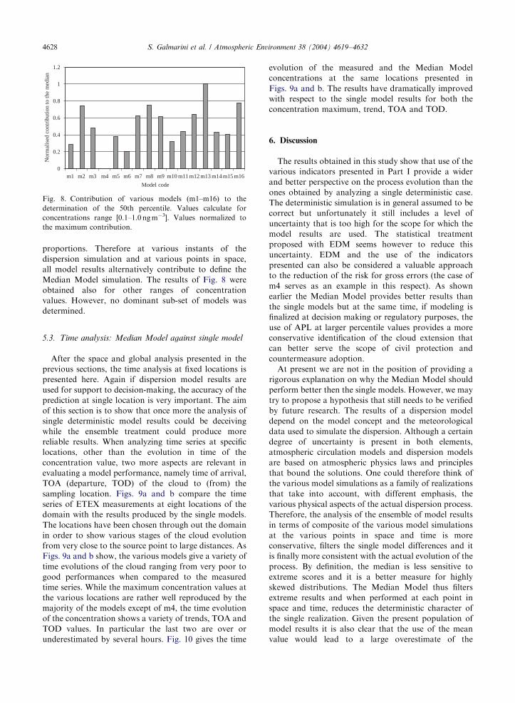
Model. In order to show that no specific model result

dominates, we have determined the relative contribution

of all the models to the median. Having selected a

representative range of concentration values defining the

ETEX measured data (0.1–1.0 ngm�3), the number of

times a specific model contributes to the median

definition was calculated, regardless of the point in

space or the instant in time in which this happens. The

results are presented in the histogram of Fig. 8 where the

contributions are normalized by the maximum value

obtained. Apart from m4 that never contributes to the

median as expected, all the other models do with varying

ARTICLE IN PRESS

0

0.2

0.4

0.6

0.8

1

1.2

m1 m2 m3 m4 m5 m6 m7 m8 m9 m10 m11 m12 m13 m14 m15 m16

Model code

Nor

mal

ised

con

trib

utio

n to

the

med

ian

Fig. 8. Contribution of various models (m1–m16) to the

determination of the 50th percentile. Values calculate for

concentrations range [0.1–1.0 ngm�3]. Values normalized to

the maximum contribution.


proportions. Therefore at various instants of the

dispersion simulation and at various points in space,

all model results alternatively contribute to define the

Median Model simulation. The results of Fig. 8 were

obtained also for other ranges of concentration

values. However, no dominant sub-set of models was

determined.

5.3. Time analysis: Median Model against single model

After the space and global analysis presented in the

previous sections, the time analysis at fixed locations is

presented here. Again if dispersion model results are

used for support to decision-making, the accuracy of the

prediction at single location is very important. The aim

of this section is to show that once more the analysis of

single deterministic model results could be deceiving

while the ensemble treatment could produce more

reliable results. When analyzing time series at specific

locations, other than the evolution in time of the

concentration value, two more aspects are relevant in

evaluating a model performance, namely time of arrival,

TOA (departure, TOD) of the cloud to (from) the

sampling location. Figs. 9a and b compare the time

series of ETEX measurements at eight locations of the

domain with the results produced by the single models.

The locations have been chosen through out the domain

in order to show various stages of the cloud evolution

from very close to the source point to large distances. As

Figs. 9a and b show, the various models give a variety of

time evolutions of the cloud ranging from very poor to

good performances when compared to the measured

time series. While the maximum concentration values at

the various locations are rather well reproduced by the

majority of the models except of m4, the time evolution

of the concentration shows a variety of trends, TOA and

TOD values. In particular the last two are over or

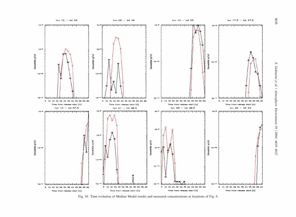
underestimated by several hours. Fig. 10 gives the time

evolution of the measured and the Median Model

concentrations at the same locations presented in

Figs. 9a and b. The results have dramatically improved

with respect to the single model results for both the

concentration maximum, trend, TOA and TOD.

6. Discussion

The results obtained in this study show that use of the

various indicators presented in Part I provide a wider

and better perspective on the process evolution than the

ones obtained by analyzing a single deterministic case.

The deterministic simulation is in general assumed to be

correct but unfortunately it still includes a level of

uncertainty that is too high for the scope for which the

model results are used. The statistical treatment

proposed with EDM seems however to reduce this

uncertainty. EDM and the use of the indicators

presented can also be considered a valuable approach

to the reduction of the risk for gross errors (the case of

m4 serves as an example in this respect). As shown

earlier the Median Model provides better results than

the single models but at the same time, if modeling is

finalized at decision making or regulatory purposes, the

use of APL at larger percentile values provides a more

conservative identification of the cloud extension that

can better serve the scope of civil protection and

countermeasure adoption.

At present we are not in the position of providing a

rigorous explanation on why the Median Model should

perform better then the single models. However, we may

try to propose a hypothesis that still needs to be verified

by future research. The results of a dispersion model

depend on the model concept and the meteorological

data used to simulate the dispersion. Although a certain

degree of uncertainty is present in both elements,

atmospheric circulation models and dispersion models

are based on atmospheric physics laws and principles

that bound the solutions. One could therefore think of

the various model simulations as a family of realizations

that take into account, with different emphasis, the

various physical aspects of the actual dispersion process.

Therefore, the analysis of the ensemble of model results

in terms of composite of the various model simulations

at the various points in space and time is more

conservative, filters the single model differences and it

is finally more consistent with the actual evolution of the

process. By definition, the median is less sensitive to

extreme scores and it is a better measure for highly

skewed distributions. The Median Model thus filters

extreme results and when performed at each point in

space and time, reduces the deterministic character of

the single realization. Given the present population of

model results it is also clear that the use of the mean

value would lead to a large overestimate of the

ARTICLE IN PRESS

Fig. 9. Time evolution of atmospheric concentration produced by single model at some locations of the modeling domain (colored

lines). Measure concentration (blue line with stars).


concentration levels and it would result inappropriate.

In our view the median is more representative indicator

of the ensemble results and adequate when no a priori

indication is available on the representativeness of the

statistical sample and its distribution. Eventually,

provided a larger population of model results, the

ARTIC

LEIN

PRES

S

Fig. 10. Time evolution of Median Model results and measured concentrations at locations of Fig. 9.

S.

Ga

lma

rini

eta

l./

Atm

osp

heric

En

viron

men

t3

8(

20

04

)4

61

9–

46

32

4630

ARTICLE IN PRESSS. Galmarini et al. / Atmospheric Environment 38 (2004) 4619–4632 4631

skewness of the distribution would reduce, thus making

the median tend to the mean.

7. Conclusions

The ensemble dispersion modeling technique, pre-

sented in Part I, has been evaluated. The European

Tracer Experiment case study was simulated by a

number of modeling groups participating to the

ENSEMBLE activities. A total number of 16 long-

range atmospheric dispersion models where used, those

are based on different approaches to atmospheric

dispersion modeling and make use of different atmo-

spheric circulation data. All model used are operational

modeling system used for the prediction of the evolution

of accidental releases of harmful materials to the

atmosphere. The evaluation of the EDM technique

mainly focused on the global analyses and the indicators

for the spatial analysis introduced in Part I, namely ATL

and APL. In the case of ATL the measured cloud

appears to compare very well with the regions of high

agreement of models thus showing that the use of this

indicator allows the identification of the region where

the dispersing cloud is most likely to be. The use of the

APL indicator has outlined that the cloud correspond-

ing to the 50th percentile value of model results agrees

well with the measured cloud. A more detailed analysis

has confirmed that percentile values between the 40th

and 50th are the ones that produced at best the

evolution of the measured cloud. The Median Model

results (obtained using the 50th percentile of all model

results at all time and points in space) have been shown

to be superior to all single model ones in reproducing the

measured cloud. The analysis of the contribution of the

single models in defining the 50th percentile has shown

that no dominant sub set of models exists but that all

models contribute, with different proportion, to the

definition of the Median Model results. This showing

that a clear character of complementarity exists among

the model results. An analysis of the model results at

specific locations as a function of time (time analysis)

shows that while the single models produce a wide

spectrum of time evolution of the concentration, the

Median Model, on the contrary, provides a more

accurate reproduction of the concentration trend and

estimate of the cloud persistence at the sampling

location. While in Part I and in this paper the

methodology has been presented and evaluated with

the ETEX case only, future investigation should relate

to the application to other case studies for which

measurements are available, for example ETEX-2

(Girardi et al., 1998) and the accidental release of

Algesiras (E) (Voght et al., 1998; Baklanov and

Sorensen, 2001; Galmarini et al., 2001). Furthermore

the conclusions presented in this paper should be

generalized and placed in a more rigorous theoretical

framework.

References

Baklanov, A., Sorensen, J.H., 2001. Parameterisation of radio-

nuclide deposition in atmospheric long-range transport

modeling. Physics and Chemistry of the Earth (B) 26 (10),

787–799.

Bianconi, R., Galmarini, S., Bellasio, R., 2004. A WWW-based

decision support system for the management of accidental

releases of radionuclides in the atmosphere. Environmental

Modelling and Software. in press.

Chino, M., Ishikawa, H., Yamazawa H., Nagai, H., Moriuchi,

S., 1995. WSPEEDI (Worldwide version of SPEEDI): A

computer code system for the prediction of radiological

impacts on Japanese due to a nuclear accident in foreign

countries, JAERI1334, Japan Atomic Energy Research

Institute (JAERI) 54pp.

Clark, T.L., Cohn, R.D., Seilkop, S.K., Draxler, R.R., Heffter,

J.L., 1988. Comparison of modelled and measured tracer

gas concentrations during the Across North America Tracer

Experiment (ANATEX). Proceedings, 17th International

Technical Meeting of NATO-CCMS on Air Pollution

Modelling and its Application, Cambridge, UK, 19–22

September. CERC Ltd., Cambridge, UK.

Draxler, R.R., Heffter, J.L. (Eds.), 1989. Across North America

Tracer Experiment (ANATEX) volume I: Description,

ground-level sampling at primary sites, and meteorology.

NOAA Tech Memo ERL ARL-167, Air Resources

Laboratory, Silver Spring, MD, 83p.

Eleveld, H., 2002. Improvement of atmospheric dispersion

models using RIVM’s Model Validation Tool. Proceedings

of 8th International Conference on Harmonisation within

Atmospheric Dispersion Modelling for Regulatory Pur-

poses, Sofia, Bulgaria, 14–17 October 2002, pp. 29–33.

Ferber, G.J., Heffter, J.L., Draxler, R.R., Lagomarsino, R.J.,

Thomas, F.L., Dietz, R.N., Benkovitz, C.M., 1986. Cross-

Appalachian tracer experiment (CAPTEX-83). Final Re-

port. NOAA Tech. Memo ERL ARL-142, Air Resources

Laboratory, Silver Spring, MD, 60p.

Galmarini, S., Bianconi, R., Bellasio, R., Graziani, G., 2001.

Forecasting the consequences of accidental releases of

radionuclides in the atmosphere from ensemble dispersion

modelling. Journal of Environmental Radioactivity 57,

203–219.

Galmarini, S., Bianconi, R., Klug, W., Mikkelsen, T., Addis,

R., Andronopoulos, S., Astrup, P., Baklanov, A., Bartniki,

J., Bartzis, J.C., Bellasio, R., Bompay, F., Buckley, R.,

Bouzom, M., Champion, H., D’Amours, R., Davakis, E.,

Eleveld, H., Geertsema, G.T., Glaab, H., Kollax, M.,

Ilvonen, M., Manning, A., Sørensen, J.H., Pechinger, U.,

Persson, C., Polreich, E., Potemski, S., Prodanova, M.,

Saltbones, J., Slaper, H., Sofiev, M.A., Syrakov, D., Van

der Auwera, L., Valkama, I., Zelazny, R., 2004. Ensemble

dispersion modelling, part I: concept, approach and

indicators. Atmospheric Environment, submitted for

publication.

Girardi, F., Graziani, G., van Veltzen, D., Galmarini, S.,

Mosca, S., Bianconi, R., Bellasio, R., Klug, W.(Eds.), 1998.

ARTICLE IN PRESSS. Galmarini et al. / Atmospheric Environment 38 (2004) 4619–46324632

The ETEX project. EUR Report 181-43 EN. Office for

official publications of the European Communities,

Luxembourg, 108pp.

Graziani, G., Mosca, S., Klug, W., 1998a. Real–time long–

range dispersion model evaluation of ETEX first release.

EUR 17754/EN. Luxembourg: Office for Official Publica-

tions of the European Commission.

Graziani, G., Klug, W., Galmarini, S., Grippa, G., 1998b.

Real–time long–range dispersion model evaluation of

ETEX second release. EUR 17755/EN. Luxembourg:

Office for Official Publications of the European

Commission.

Heffter, J.L., Draxler, R.R., 1989. Across North America

Tracer Experiment (ANATEX) vol. III: sampling at tower

and remote sites. NOAA Tech Memo ERL ARL-175, Air

Resources Laboratory, Silver Spring, MD, 67p.

Ishikawa, H., 1994. Development of worldwide version of

system for prediction of environmental emergency dose

information: WSPEEDI, (III) revised numerical models,

integrated software environment and verification. Journal of

Nuclear Science and Technology 31 (9), 69–978.

Mosca, S., Bianconi, R., Bellasio, R., Graziani, G., Klug, W.,

1998a. ATMES II - Evaluation of long-range dispersion

models using data of the 1st ETEX release. EUR 17756 EN,

Office for Official Publications of the European Commu-

nities, Luxembourg, ISBN 92-828-3655-X, 458pp.

Mosca, S., Graziani, G., Klug, W., Bellasio, R., Bianconi, R.,

1998b. A statistical methodology for the evaluation of long-

range dispersion models: an application to the ETEX

exercise. Atmospheric Environment 32, 4307–4324.

Stunder, B.J.B., Draxler, R.R., 1989. Across North America

Tracer Experiment (ANATEX), vol. II: aircraft-based

sampling. NOAA Tech Memo ERL ARL-177, Air Re-

sources Laboratory, Silver Spring, MD, 29p.

Van Dop, H., Nodop, K., (Eds.), 1998. ETEX. A European Tra-

cer Experiment. Atmospheric Environment (24), 4089-4378.

Voght, P.J., Bopanz, B.M., Aluzzi, F.J., Basket, R.L., Sullivan,

P.J., 1998. ARAC simulation of the Algesiras, Spain, steel-

meal cs-137 release. ARAC Lawrence Livermore National

Laboratory.

Watson, D.F., Philip, G.M., 1984. Triangle-based interpola-

tion. Mathematical Geology 16 (8), 779–795.

Ensemble dispersion forecasting—Part II: application and evaluation

Documents