Ensemble Algorithms and Analytic Combinatorics in RNA ...

HAL Id: tel-03219977https://tel.archives-ouvertes.fr/tel-03219977v1

Submitted on 6 May 2021 (v1), last revised 19 May 2021 (v2)

HAL is a multi-disciplinary open accessarchive for the deposit and dissemination of sci-entific research documents, whether they are pub-lished or not. The documents may come fromteaching and research institutions in France orabroad, or from public or private research centers.

L’archive ouverte pluridisciplinaire HAL, estdestinée au dépôt et à la diffusion de documentsscientifiques de niveau recherche, publiés ou non,émanant des établissements d’enseignement et derecherche français ou étrangers, des laboratoirespublics ou privés.

Distributed under a Creative Commons Attribution| 4.0 International License

Ensemble Algorithms and Analytic Combinatorics inRNA Bioinformatics and Beyond

yann Ponty

To cite this version:yann Ponty. Ensemble Algorithms and Analytic Combinatorics in RNA Bioinformatics and Beyond.Bioinformatics [q-bio.QM]. Université Paris-Saclay, 2020. tel-03219977v1

https://tel.archives-ouvertes.fr/tel-03219977v1

http://creativecommons.org/licenses/by/4.0/

http://creativecommons.org/licenses/by/4.0/

https://hal.archives-ouvertes.fr

Ensemble Algorithms and Analytic Combinatorics

in RNA Bioinformatics and Beyond

Yann Ponty

An Habilitation à Diriger des Recherches thesis of Paris-Saclay Université,defended on May 22nd 2020 and evaluated by:

Cédric CHAUVE, Simon Fraser University, CanadaLéonid CHINDELEVITCH, Imperial College London, UK

Johanne COHEN, CNRS/Université Paris-SaclayPhilippe DUCHON, Université de Bordeaux

Ivo HOFACKER, University of Vienna, AutricheDaniel MERKLE, University of South Denmark

Cyril NICAUD, Université Paris-Est, Marne la ValléePeter STADLER, University of Leipzig, Germany

Abstract

Predictive Bioinformatics represents a major field of applications for combinatorialoptimization techniques. Very often, an ensemble perspective, which not only con-sider the optimal solution but also fully embraces the set of suboptimal solutions,needs to be adopted. In this Habilitation à Diriger des Recherches, I present a seriesof algorithmic and combinatorial contributions, inspired by problems and questionsarising in the study of RiboNucleic Acids (RNAs), in particular pertaining to theirstructural properties at the thermodynamic equilibrium.

I first describe a collection of generic and applied algorithmic techniques, enablingthe efficient computation of statistical properties within search spaces. Such com-putations can be exact, or rely on unbiased estimates produced, using constrainedsampling strategies, and are founded on on a combinatorial (re-)interpretation ofdynamic programming schemes. I then adopt a purely combinatorial point of viewover search spaces, and establish asymptotic properties of classes of discrete objectsarising in Bioinformatics, showcasing the unreasonable power of (a subset of) analyticcombinatorics. Finally, I conclude with a collection of algorithmic results, obtainedthrough the application of a wide array of techniques, in the context of RNA design,a field focused on combinatorial problems that are at the same time original, difficult,and relevant to the modern goals of biology and medicine.

1

Contents

1 Introduction 51.1 Predictive Bioinformatics and its foundations . . . . . . . . . . . . . . . . . 51.2 A crash course into RNA structure prediction . . . . . . . . . . . . . . . . . 7

1.2.1 RNA structure . . . . . . . . . . . . . . . . . . . . . . . . . . . . . . . 81.2.2 RNA folding prediction models and paradigms . . . . . . . . . . . 91.2.3 The secondary structure . . . . . . . . . . . . . . . . . . . . . . . . . 111.2.4 RNA 2D structure prediction from thermodynamic principles . . . 13

1.3 Outline . . . . . . . . . . . . . . . . . . . . . . . . . . . . . . . . . . . . . . . 16

2 Ensemble dynamic programming: techniques and analyses 172.1 A formal framework and basic algorithms . . . . . . . . . . . . . . . . . . . 19

2.1.1 Dynamic programming as a rewriting system . . . . . . . . . . . . 202.1.2 Search space and suitability for ensemble applications . . . . . . . 222.1.3 Classic optimization . . . . . . . . . . . . . . . . . . . . . . . . . . . 24

2.2 Exact computation of Ensemble properties . . . . . . . . . . . . . . . . . . 252.2.1 Computing the partition function. . . . . . . . . . . . . . . . . . . . 262.2.2 Probabilities in Boltzmann-Gibbs distributions (inside-outside) . . 272.2.3 Ensemble centroid and Maximum Expected Accuracy (MEA) . . . 292.2.4 General moments of additive scores [150] . . . . . . . . . . . . . . . 312.2.5 Classified DP with the Discrete Fourier Transform (DFT) [173, 174] 34

2.3 Probabilistic estimates . . . . . . . . . . . . . . . . . . . . . . . . . . . . . . 372.3.1 Foreword: On the number of samples [165] . . . . . . . . . . . . . . 382.3.2 Statistical sampling . . . . . . . . . . . . . . . . . . . . . . . . . . . . 392.3.3 Non redundant sampling [118, 133, 165] . . . . . . . . . . . . . . . . 412.3.4 Adaptive sampling of constrained sequences [18, 90, 158] . . . . . . 45

2.4 Applications of ensemble dynamic programming . . . . . . . . . . . . . . 482.4.1 (Recursive) simple type pseudoknots and kissing hairpins [150] . . 492.4.2 Dual partition functions and evolutionary robustness of RNAs . . 512.4.3 Unambiguous tree alignments [32, 33] . . . . . . . . . . . . . . . . . 53

3 RNA design 563.1 Why do we design RNAs? . . . . . . . . . . . . . . . . . . . . . . . . . . . . 58

3.1.1 The potential of RNA design for statistical evolutionary studies . . 59

2

3.1.2 The different flavors of RNA design . . . . . . . . . . . . . . . . . . 593.2 Exact combinatorial negative design [85, 86] . . . . . . . . . . . . . . . . . . 61

3.2.1 Basic results . . . . . . . . . . . . . . . . . . . . . . . . . . . . . . . . 623.2.2 Design as a tree coloring problem . . . . . . . . . . . . . . . . . . . 633.2.3 Structure-approximating design . . . . . . . . . . . . . . . . . . . . 65

3.3 Stochastic positive design under constraints . . . . . . . . . . . . . . . . . . 663.3.1 Sampling from the dual-partition function [117, 158, 160] . . . . . . 673.3.2 Avoiding and forcing motifs [210] . . . . . . . . . . . . . . . . . . . 693.3.3 Multiple structures and extended design principles [88, 90] . . . . 71

4 Constrained random generation through rejection and beyond 734.1 It’s not you, it’s me: The unreasonable power of rejection . . . . . . . . . . 76

4.1.1 Correcting a (bounded) bias . . . . . . . . . . . . . . . . . . . . . . . 774.1.2 Complexity aspects . . . . . . . . . . . . . . . . . . . . . . . . . . . . 78

4.2 Rejecting in dimension one and then some. . . . . . . . . . . . . . . . . . . . 814.2.1 (Combinatorial) Boltzmann sampling . . . . . . . . . . . . . . . . . 814.2.2 Multidimensional Boltzmann sampling . . . . . . . . . . . . . . . . 824.2.3 Beyond simplicity . . . . . . . . . . . . . . . . . . . . . . . . . . . . . 88

4.3 Applications of multidimensional sampling . . . . . . . . . . . . . . . . . . 894.3.1 Controlling the GC-content [88, 90, 158, 160, 192, 193] . . . . . . . . 894.3.2 Dinucleotides content of protein-coding RNAs [209]. . . . . . . . . 90

4.4 Redundancy in weighted sampling and countermeasures . . . . . . . . . . 924.4.1 Collisions in weighted languages [58, 78] . . . . . . . . . . . . . . . 92

5 Asymptotic properties of RNA secondary structures and other trees 965.1 Basic tools in enumerative and analytic combinatorics . . . . . . . . . . . . 97

5.1.1 Context-free languages. . . . . . . . . . . . . . . . . . . . . . . . . . 975.1.2 Enumeration and generating functions. . . . . . . . . . . . . . . . . 995.1.3 Basic singularity analysis . . . . . . . . . . . . . . . . . . . . . . . . 1015.1.4 Useful extensions and shortcuts . . . . . . . . . . . . . . . . . . . . 105

5.2 Asymptotic combinatorics of RNA secondary structures . . . . . . . . . . . 1115.2.1 Expected 5’–3’ distance [38] . . . . . . . . . . . . . . . . . . . . . . . 1135.2.2 RNA network properties [180] . . . . . . . . . . . . . . . . . . . . . 1155.2.3 RNA shapes: Abstract representations of structures [120] . . . . . . 1195.2.4 Enumerating designable structures [206] . . . . . . . . . . . . . . . 123

6 Conclusion and perspectives 127

Bibliography 129

3

Foreword

The French academic system has enjoyed a long and eventful history, leading to manycharming pecularities. One such specificity is the requirement of junior tenured scientiststo successfully defend an Habilitation à Diriger des Recherches (HDR) before being allowedsupervisedoctoral candidates in anofficial capacity. Aspart of the requirements for suchadefense, the candidate produces amanuscript summarizing the research results obtainedsince his PhD. This is my contribution towards applying for anHDR in Computer Scienceat Université Paris-Sud. The individual nature of the evaluation dictates the use of thefirst-person singular, but an overwhelming majority of those results hinge critically oncontributions froma community of collaborators, which I have attempted to acknowledgeprofusely.

The structure, ambition, scope and length of an HDR vary substantially between disci-plines, institutions, and followpersonal aesthetics. Somewill elicit to contribute a generalintroduction for a collection of articles, while others will interlace past results with novelresearch material, trying to use the opportunity to outline general theories. Some willembrace the diversity of their past contributions, while others will strive to provide aunified perspective over research projects spanning one to two decades.

My ambition for this document is, by formalizing some of the intuitions underlyingmy past contributions, to reveal their triviality and, more seriously, contribute firmfoundations for the systematic design and analysis of algorithms in RNA Bioinformaticsand beyond. Mymain focus is therefore on the description of techniques, either classic inother fields or contributed over the course of my young career as a scientist, showcasingtheir power and level of generality by a brief description of their application in the contextof RNA bioinformatics.

For these reasons, and partly because compact does not necessarily mean simple, Iapologize in advance to the casual reader for explanations and digressions which mayappear, at times, unnecessarily technical. It is unfortunately the price to pay to achievemy intended goal of using this document to lay out stable and explicit foundations forfutures contributions to Bioinformatics.

4

Chapter 1

Introduction

Bioinformatics as a field of study is the poster child of interdisciplinarity. It is uni-fied by an overarching objective to automate the processing and analysis of biologicaldata, and plays an essential part in the production of knowledge in modern Biology. Inthe context of Molecular Biology, it is informed by models stemming from Biophysicsand Chemistry, quantitatively parameterized by computational methods in Statisticsand Probability theory (Machine Learning), or analyzed at a theoretical level usingTheoretical Physics and Discrete Mathematics techniques. Such quantitative models,typically in conjunction with parsimony arguments, represent the foundations of predic-tive algorithmic methods.

1.1 Predictive Bioinformatics and its foundations

Predictive Bioinformatics strives to produce methods which, from empirical data, pre-dict phenomena far beyond our capacity for direct observations. Examples of suchlimitations include events that occur at the nanometer scale, in the distant past, or whoseobservation significantly interferes with (e.g. kill) a living system of interest. Given anestablished model, consistent with current biological knowledge, predictive methods inbioinformatics embrace some notion of search space induced by the input data. Theyelect one or several element(s) of the search space by maximizing some notion of score,usually analogous to a probability, provided by the model. The produced solution con-stitutes a best bet under (possibly implicit) assumptions of the model. Such methods aretypically trained on reference data sets, for which a ground-truth is known, to calibrate awidely-varying set of parameters, and validated on independent data sets as an empiricaltest of their accuracy and, importantly, capacity of generalization.

Once a predictive method has been deemed satisfactory, a leap of faith occurs, follow-ing which the model and method are treated as uniformly correct. The subsequentpredictions are considered as reflective of Nature itself, and treated as primary data in

5

5 0 5 10 15X

4

2

0

2

4

6

8

10

Y

Feature FAFeature

FB

Feature FA

FeatureFB

Opt (MFE)

Clusters centroids

Ensemble centroid

6 4 2 0 2 4 6X

6

4

2

0

2

4

6

YFeature FA

FeatureFB

Feature FA

FeatureFB

Ensemble centroid

Opt (MFE)

B – Fragmented ensembleA – Concentrated ensemble

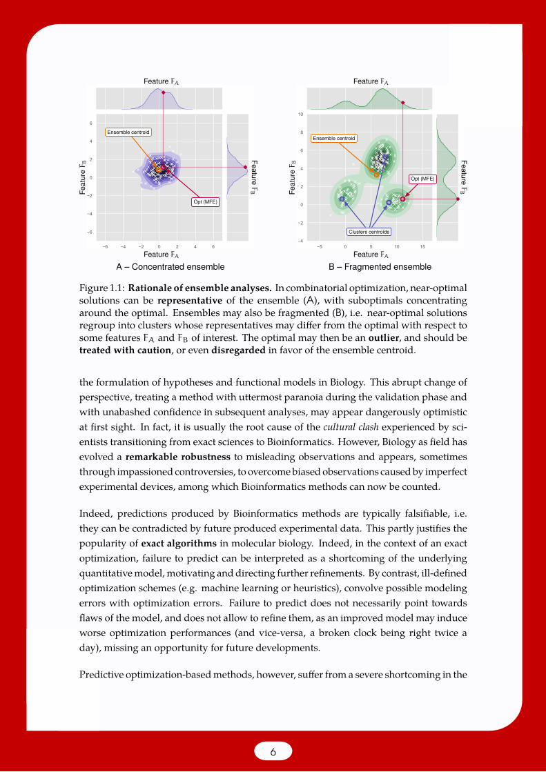
Figure 1.1: Rationale of ensemble analyses. In combinatorial optimization, near-optimalsolutions can be representative of the ensemble (A), with suboptimals concentratingaround the optimal. Ensembles may also be fragmented (B), i.e. near-optimal solutionsregroup into clusters whose representatives may differ from the optimal with respect tosome features FA and FB of interest. The optimal may then be an outlier, and should betreated with caution, or even disregarded in favor of the ensemble centroid.

the formulation of hypotheses and functional models in Biology. This abrupt change ofperspective, treating a method with uttermost paranoia during the validation phase andwith unabashed confidence in subsequent analyses, may appear dangerously optimisticat first sight. In fact, it is usually the root cause of the cultural clash experienced by sci-entists transitioning from exact sciences to Bioinformatics. However, Biology as field hasevolved a remarkable robustness to misleading observations and appears, sometimesthrough impassioned controversies, to overcomebiased observations causedby imperfectexperimental devices, among which Bioinformatics methods can now be counted.

Indeed, predictions produced by Bioinformatics methods are typically falsifiable, i.e.they can be contradicted by future produced experimental data. This partly justifies thepopularity of exact algorithms in molecular biology. Indeed, in the context of an exactoptimization, failure to predict can be interpreted as a shortcoming of the underlyingquantitativemodel, motivating anddirecting further refinements. By contrast, ill-definedoptimization schemes (e.g. machine learning or heuristics), convolve possible modelingerrors with optimization errors. Failure to predict does not necessarily point towardsflaws of the model, and does not allow to refine them, as an improved model may induceworse optimization performances (and vice-versa, a broken clock being right twice aday), missing an opportunity for future developments.

Predictive optimization-basedmethods, however, suffer from a severe shortcoming in the

6

context of combinatorial search spaces. Indeed, they ultimately output a single solution,presumed to be optimally-likely in some sense. However, the dominating nature ofthe proposed solution may show limited robustness to, even modest, changes of theobjective function, whose parameters are usually learned from data and thus subjectto experimental errors. Moreover, an optimal solution may be poorly representative ofthe subspace of near-optimal solutions, so that it may be more advisable to consider asuboptimal – representative – solution rather than an optimal – non-representative – one.

These observations constitute themainmotivations behind the development of ensemblemethods in combinatorial Bioinformatics, treating the whole search space as an objectof study rather than merely solving a needle in a haystack optimization problem. To thatpurpose, a probability distribution is postulated over the search space, and probabilisticanalyses areperformed.Theoptimal solutionmay remain relevant, but ensemblemethodsallow to go further, and assess notions of support for any given solution, or how distantfeatures of the optimal solution are from the centroid of the ensemble. Indeed, as shownin Figure 1.1, ensembles associated with a given instance may either be concentratedaround the optimal, or fragmented, leading to multiple clusters of diverse solutions, andmultimodal distributions for features of interest.

1.2 A crash course into RNA structure prediction

The Bioinformatics of RiboNucleic Acids (RNAs) represent a very natural realm ofapplication, and a source of constant inspiration, for ensemble analyses.

RNA constitutes a category of biomolecules, abstracted as sequence of nucleotidesAde-nine (A), Cytosine (C), Guanine (G) and Uracil (U), initially transcribed from a DNAtemplate and further processed before reaching their cellular environment. They canform stable complexes with proteins, but also DNA and other RNAs, allowing themto regulate genetic expression. They can also perform enzymatic functions, i.e. pro-cess other molecules (or themselves), act as biosensors by undergoing conformationalchanges upon binding with small metabolites, and store the entire genetic material ofcertain viruses (e.g. HIV, SARS, 2019 nCoV).

Their dual capacity to store and process information is unmatched, leading currenttheories in evolution to considerRNAas themost likely candidate at theorigin of life [93].Such a versatility, illustrated in Figure 1.2, not only stems from the combinatorial nature ofRNA sequences but also from its capacity to adopt one or several well-defined structures,driving the specificity of its interactions with other actors of the cellular world.

7

DNA

RNA

Proteins

Transcription

TranslationRegulation

Transfer

Participates

Maturation

Car

rier

Synthesis 0

500

1000

1500

2000

2500

3000

3500

Num. RFAM Families

B – Evolution of RNA familiesA – Basic RNA functions

RNA functions:• Messenger• Translation• Regulation• Enzyme• Catalytic• . . .

Figure 1.2: Beyond coding for proteins, a growing list of RNA functions. The versatilityof RNA (A) is confirmed by the sustained growth (B) of the number of functional familiesin the RFAM database [84, 106], a majority of which are not coding for proteins, andassociated with a conserved well-defined secondary structure.

1.2.1 RNA structure

Following Tinoco and Bustamante [184], RNA is believed to fold in a hierarchical fashionwhere canonical base pairs, mediated by hydrogen bonds, initially form a tree-likearchitecture called the secondary structure. Later in the folding process, the secondarystructure is completed by complex topological motifs, including pseudoknots and non-canonical base pairs andmotifs [114, 115]. Due to its combinatorial nature, the secondarystructure is found at the core of successful computational methods for predicting the 3Dstructure of RNA [131]. It also supports the discovery of new functional families ofnon-coding RNAs, RNAs that do not (only) encode a protein, but (also) act directlyon their environment through participation in catalytic and/or regulatory functions. Aconserved consensus secondary structure is indeed a central object for many families inthe RFAM database [84, 106], and a crucial element of the design of covariancemodels [62]used to find homologous RNAs across sequenced genomes.

At a 3D level, structuremodeling is tackled using amixture of comparativemethods [134]and low-throughput/high resolution experimental techniques such as X-ray crystallogra-phy, Nuclear Magnetic Resonance (NMR), or Cryogenic ElectronMicroscopy (Cryo-EM).However, those techniques are extremely time-consuming, and require a preparation ofmolecules that may either not be feasible for certain RNAs, or can interfere with thefolding process itself. These difficulties induce a growing gap between the number offunctional families (±3000 as of Jan 2020), many of which requiring the adoption of aspecific structure, and the number of families with experimentally-resolved 3D modelavailable for at least one of their members (99 as of Jan 2020).

Recently, high throughput/low resolution alternatives have been proposed in the form

8

of improved chemical probing protocols, notoriously including SHAPE probing [47,176, 198]. Those methods expose RNA to a chemical reagent, whose affinity towardsindividual nucleotides depend on the structure (and therefore partly reveal it, albeitin a stochastic and highly noisy fashion) and can be quantified using DNA and RNAsequencing technologies. The end-result of those methods are 1D reactivity profilesthat are not sufficient to fully characterize a structure, but greatly informative for further(computational) modeling.

1.2.2 RNA folding prediction models and paradigms

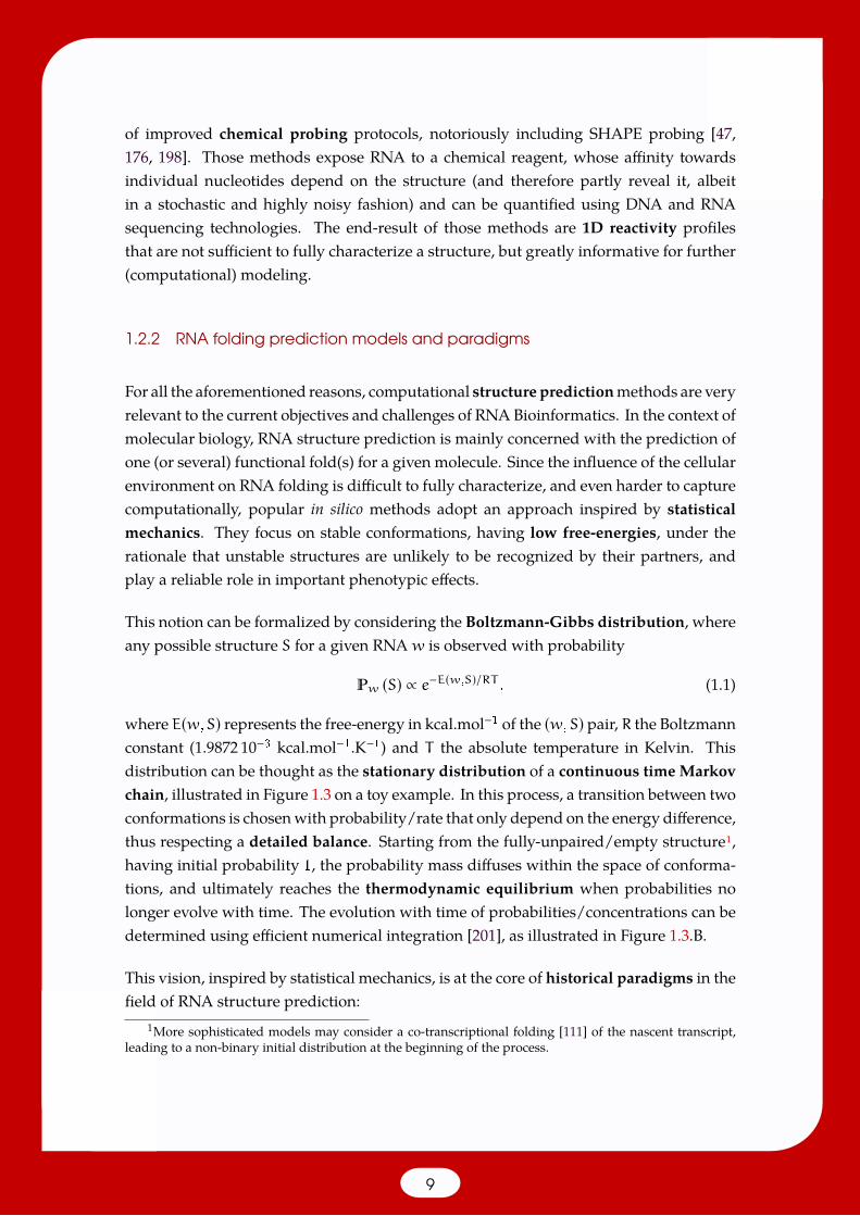
For all the aforementioned reasons, computational structure predictionmethods are veryrelevant to the current objectives and challenges of RNA Bioinformatics. In the context ofmolecular biology, RNA structure prediction is mainly concerned with the prediction ofone (or several) functional fold(s) for a given molecule. Since the influence of the cellularenvironment on RNA folding is difficult to fully characterize, and even harder to capturecomputationally, popular in silico methods adopt an approach inspired by statisticalmechanics. They focus on stable conformations, having low free-energies, under therationale that unstable structures are unlikely to be recognized by their partners, andplay a reliable role in important phenotypic effects.

This notion can be formalized by considering the Boltzmann-Gibbs distribution, whereany possible structure S for a given RNA w is observed with probability

w (S) ∝ e−E(w,S)/RT , (1.1)

where E(w,S) represents the free-energy in kcal.mol−1 of the (w,S) pair, R the Boltzmannconstant (1.9872 10−3 kcal.mol−1.K−1) and T the absolute temperature in Kelvin. Thisdistribution can be thought as the stationary distribution of a continuous time Markovchain, illustrated in Figure 1.3 on a toy example. In this process, a transition between twoconformations is chosenwith probability/rate that only depend on the energy difference,thus respecting a detailed balance. Starting from the fully-unpaired/empty structure1,having initial probability 1, the probability mass diffuses within the space of conforma-tions, and ultimately reaches the thermodynamic equilibrium when probabilities nolonger evolve with time. The evolution with time of probabilities/concentrations can bedetermined using efficient numerical integration [201], as illustrated in Figure 1.3.B.

This vision, inspired by statistical mechanics, is at the core of historical paradigms in thefield of RNA structure prediction:

1More sophisticated models may consider a co-transcriptional folding [111] of the nascent transcript,leading to a non-binary initial distribution at the beginning of the process.

9

Pro

ba

bil

ity

/Co

nc

en

tra

tio

n

Time0

1

0.5

Equilibrium

MFEEnzymatic degradation

RNA half life

B

A

C

DA

B

DC

A – Kinetic LandscapeContinuous-time Markov chain

B – Evolution of concentrations

Figure 1.3: RNA folding paradigms. The process of RNA folding can be abstracted asa Continuous Time Markov Chain (CTMC – A), over a discrete state space consisting of(a subset of) the secondary structures adopted by an RNA. Starting from an initial distri-bution, typically assigning full probability to the open chain, kinetic studies attempt tocharacterize the evolution of the probability distribution with time (B). At the thermody-namic equilibrium, the stationary distribution of the CMTC is reached and probabilitiescease to evolvewith time. Themost probable structure is then themost stable one, i.e. theMFE structure. However, RNAdegradationmay occur before the equilibrium is reached,and the dominant structures at finite time may represent more promising candidates forfunctional hypotheses.

MFE paradigm. Early computational methods for structure prediction [95, 143, 213] fo-cused their effort on producing (one of) the optimally stable, or Mininum Free-Energy (MFE), structure(s), under the rationale that the MFE structure has highestprobability at the thermodynamic equilibrium;

Boltzmann ensemble paradigm. While optimal, the probability of the MFE structurealone can be abysmally small, and decreases exponentially with the RNA length.The MFE structure can therefore be overwhelmed, at the thermodynamic equilib-rium, by a set of alternative structures having comparable stability and, possibly,very different characteristics. This motivates studies of the expected propertiesin the Boltzmann-Gibbs distribution, hinging on an efficient computation of thepartition function [130]

Z

∑S

e−E(w,S)/RT .

When these properties diverge from those of the MFE, it may be more relevantto consider structures that are more accurate representatives of the ensemble ofstructures. One such structure is the Maximum Expected Accuracy structure [55,121], the structure minimizing some notion of expected distance to the rest of theensemble. Alternatively a statistically representative, Boltzmann distributed, setof structures can be randomly generated, clustered at a structural level to identify

10

alternative conformations, and eliminate outliers. A centroid structure can then beelected for each cluster [52];

The kinetics paradigm. More recently, there has been a growing awareness of the impor-tance of out-of-equilibrium effects in the function(s) carried out by RNA. Indeed,in a cellular context, RNA is constantly transcribed and degraded by enzymes.Depending on the precise dynamics of these concurrent processes, a population ofRNAs may simply be degraded before reaching its stationary distribution, so thethermodynamic paradigm may not provide an accurate picture of the functionalstructure. This generally applies to RNAs whose energy landscapes feature sub-stantial barriers, leading to a slow convergence towards the equilibrium. Kineticsanalyses are thus concerned with the structural behavior of RNA before reachingthe equilibrium.

Examples of kinetics effects are suspected to include riboswitches, bistables RNAswhich are observerd in on and off conformations in the presence/absence of a lig-and, a small molecule, believed to have insufficient contribution to the free-energyto invert the relative stabilities of the on and off states. Current models are thusbased on kinetics, and postulate that the ligand modifies an energy barrier, lead-ing to a faster/slower convergence towards the thermodynamic equilibrium [65].More generally, co-transcriptional folding, the folding of RNA during transcrip-tion, reveals the importance of kinetic effects. Indeed, this phenomenon would bewithout effect at the thermodynamic equilibrium, since the stationary distributionof a (ergodic) Markov chain does not depend on its initial distribution, so it wouldshould not matter at the equilibrium.

In the rest of this document, I will mainly focus on algorithmic strategies relevant tothe MFE and Boltzmann equilibrium paradigms, although certain were have designedwith kinetics analysis in mind [133, 180]. Kinetics analyses are indeed much moretime-consuming, and are associated with computational problems that are routinely NP-hard [126]. Efficient heuristics and methods for analyzing kinetics are, however, theobject of ongoing projects within the RNA Bioinformatics community.

1.2.3 The secondary structure

A RNA secondary structure of size n represents the outcome of a folding process,and focuses on a subset of base-pairs, mediated by hydrogen bonds. For essentiallycomputational reasons [3, 123, 175] this definition forbids crossing base pairs, also calledpseudoknots due to their ability to induce complex topologies [205]. Moreover, anynucleotide can only be involved in a single base pair, since additional partners wouldinvolve non-canonical edges [114]. Finally, most definitions rule out base pairs between

11

G

C

G

G

A

U

UU

AgCUC

AG

u

u

G

G

G A

G A G C

g

C

C

A

G

A

c

U

g

A A

g

A

P

c

U

G

G

AG g

U

C

c U G U G

u P

C

G

a

UC

CACAG

A

A

U

U

C

G

C

A

C

CA

1

10

20

30

40

50

60

70

76

A – (Outer-planar) graphsHamiltonian-path,

∆(G)≤3, 2-connected

(((((((..((((........))))((((((.......))))))....(((((.......))))))))))))....

B – Dot-bracket notation

C – Mountain plot

G C G G A U U U A g C U C A G u u G G G A G A G C g C C A G A c U g A A g A P c U G G A G g U C c U G U G u P C G a U C C A C A G A A U U C G C A C C A

1 10 20 30 40 50 60 70 76

D – Non-crossing arc-annotated sequences

GCGGA

UU

UA

g

C

U

C

A

G

u

u

G

G

G

A

G

A

G

C

g

C

CA

GA

cU

gA A g A P c U G

GA

Gg

UC

c

U

G

U

G

u

P

C

G

a

U

C

C

A

C

A

G

A

AU

UC

GC

ACCA

1

10

20

30

40

50

60

70

76

E – Non-crossing chords diagrams

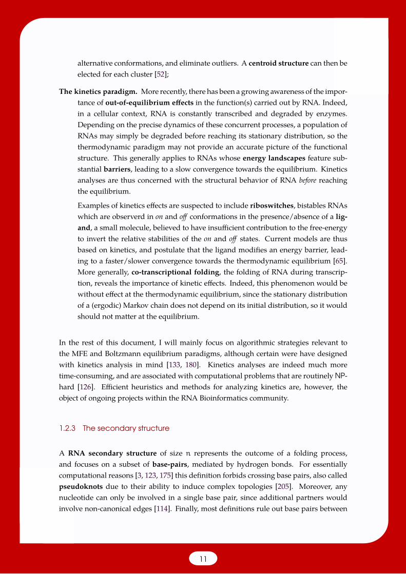
Figure 1.4: Various representations for RNA secondary structures.

proximate positions, due to steric effects inducing geometric constraints, leading to aminimal number θ of unpaired positions between paired positions.

Definition 1.2.1 (RNA secondary structure): An RNA secondary structure S oflength n is a set of base-pairs (i, j), 1 ≤ i < j ≤ n, such that:

• Each position is monogamous, ∀(i, j) , (i′, j′) ∈ S : i, j ∩ i′, j′ ;• Minimal distance θ between paired nucleotides, ∀(i, j) ∈ S : j − i > θ;• No pseudoknot allowed, ∀(i, j), (i′, j′) ∈ S, i < i′ : (j′ < j) or (j < i′).

The conformational space associated with a sequence of length n is simply Sn, the setof secondary structures over n nucleotides.

In typical ab initio RNA structure prediction problems, the input is a sequence of nu-cleotides w ∈ A,C,U,G?. This space of secondary structure is then usually restrictedto structures consisting of canonical base pairs B : G,C, A,U, G,U. In otherwords, for any valid secondary structure S ∈ S one has:

∀(i, j) ∈ S : wi,wj ∈ B.

The secondary structure can be drawn in a variety of ways, as illustrated by Figure 1.4,many of which being supported by our popular software VARNA, developed in collabo-ration with Kevin Darty and Alain Denise [44].

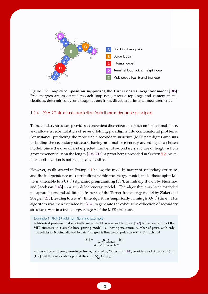
The stability of a secondary structure is assessed using a free-energy model. The mostpopular such model is the Turner nearest-neighbor free-energy model [185], which as-sociates experimentally-determined free-energy contributions to structuralmotifs, calledloops (see Figure 1.5). The energy of any given secondary structure is then additivelydefined, i.e. obtained by summing the contributions of the various loops appearing inthe structure.

12

1

10

20

30

40

43

AA

AA

AA

A AB

C

E

D

DA Stacking base pairs

B Bulge loops

C Internal loops

D Terminal loop, a.k.a. hairpin loop

E Multiloop, a.k.a. branching loop

Figure 1.5: Loop decomposition supporting the Turner nearest neighbor model [185].Free-energies are associated to each loop type, precise topology and content in nu-cleotides, determined by, or extrapolations from, direct experimental measurements.

1.2.4 RNA 2D structure prediction from thermodynamic principles

The secondary structureprovides a convenient discretizationof the conformational space,and allows a reformulation of several folding paradigms into combinatorial problems.For instance, predicting the most stable secondary structure (MFE paradigm) amountsto finding the secondary structure having minimal free-energy according to a chosenmodel. Since the overall and expected number of secondary structure of length n bothgrow exponentially on the length [194, 212], a proof being provided in Section 5.2, brute-force optimization is not realistically feasible.

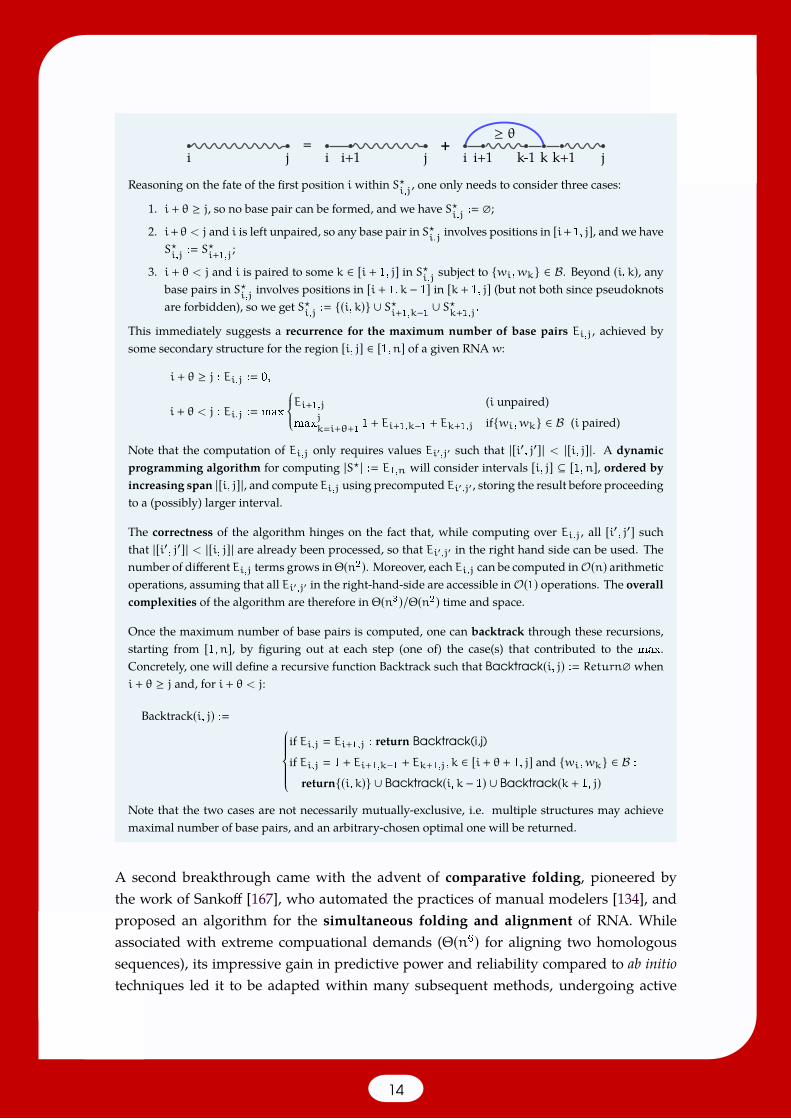
However, as illustrated in Example 1 below, the tree-like nature of secondary structure,and the independence of contributions within the energy model, make those optimiza-tions amenable to a Θ(n3) dynamic programming (DP), as initially shown by Nussinovand Jacobson [143] in a simplified energy model. The algorithm was later extendedto capture loops and additional features of the Turner free-energy model by Zuker andStiegler [213], leading to aΘ(n4) time algorithm (empirically running inΘ(n3) time). Thisalgorithm was then extended by [204] to generate the exhaustive collection of secondarystructures within a free-energy range ∆ of the MFE structure.

Example 1: RNA BP folding – Running exampleA historical problem, first efficiently solved by Nussinov and Jacobson [143] is the prediction of theMFE structure in a simple base pairing model, i.e. having maximum number of pairs, with onlynucleotides in B being allowed to pair. Our goal is thus to compute some S? ∈ Sn such that

|S? | maxS∈Snsuch that

∀(i,j)∈S,wi,wj∈B|S|.

A classic dynamic programming scheme, inspired by Waterman [194], considers each interval [i, j] ⊂[1,n] and their associated optimal structure S?

i,jfor [i, j]:

13

i j=

i i+1 j+

i+1i kk-1 k+1 j

≥ θ

Reasoning on the fate of the first position iwithin S?i,j

, one only needs to consider three cases:

1. i + θ ≥ j, so no base pair can be formed, and we have S?i,j

: ;2. i+θ < j and i is left unpaired, so any base pair in S?

i,jinvolves positions in [i+1, j], and we have

S?i,j

: S?i+1,j

;

3. i + θ < j and i is paired to some k ∈ [i + 1, j] in S?i,j

subject to wi,wk ∈ B. Beyond (i,k), anybase pairs in S?

i,jinvolves positions in [i + 1, k − 1] in [k + 1, j] (but not both since pseudoknots

are forbidden), so we get S?i,j

: (i,k) ∪ S?i+1,k−1 ∪ S?k+1,j.

This immediately suggests a recurrence for the maximum number of base pairs Ei,j, achieved bysome secondary structure for the region [i, j] ∈ [1,n] of a given RNA w:

i + θ ≥ j : Ei,j : 0,

i + θ < j : Ei,j : max

Ei+1,j (i unpaired)

maxjki+θ+1

1 + Ei+1,k−1 + Ek+1,j ifwi,wk ∈ B (i paired)

Note that the computation of Ei,j only requires values Ei′,j′ such that |[i′, j′]| < |[i, j]|. A dynamicprogramming algorithm for computing |S? | : E1,n will consider intervals [i, j] ⊆ [1,n], ordered byincreasing span |[i, j]|, and compute Ei,j using precomputed Ei′,j′ , storing the result before proceedingto a (possibly) larger interval.

The correctness of the algorithm hinges on the fact that, while computing over Ei,j, all [i′, j′] suchthat |[i′, j′]| < |[i, j]| are already been processed, so that Ei′,j′ in the right hand side can be used. Thenumber of different Ei,j terms grows inΘ(n2). Moreover, each Ei,j can be computed inO(n) arithmeticoperations, assuming that all Ei′,j′ in the right-hand-side are accessible inO(1) operations. The overallcomplexities of the algorithm are therefore in Θ(n3)/Θ(n2) time and space.

Once the maximum number of base pairs is computed, one can backtrack through these recursions,starting from [1,n], by figuring out at each step (one of) the case(s) that contributed to the max.Concretely, one will define a recursive function Backtrack such that Backtrack(i, j) : Return wheni + θ ≥ j and, for i + θ < j:

Backtrack(i, j) :

if Ei,j Ei+1,j : return Backtrack(i,j)

if Ei,j 1 + Ei+1,k−1 + Ek+1,j,k ∈ [i + θ + 1, j] and wi,wk ∈ B :

return(i,k) ∪ Backtrack(i,k − 1) ∪ Backtrack(k + 1, j)Note that the two cases are not necessarily mutually-exclusive, i.e. multiple structures may achievemaximal number of base pairs, and an arbitrary-chosen optimal one will be returned.

A second breakthrough came with the advent of comparative folding, pioneered bythe work of Sankoff [167], who automated the practices of manual modelers [134], andproposed an algorithm for the simultaneous folding and alignment of RNA. Whileassociated with extreme compuational demands (Θ(n6) for aligning two homologoussequences), its impressive gain in predictive power and reliability compared to ab initiotechniques led it to be adapted within many subsequent methods, undergoing active

14

developments [128, 179, 199, 200].

A revolution came with the McCaskill [130] algorithm, which championed a transitiontowards the Boltzmann ensemble paradigm. Namely, McCaskill observed that thepartition function

Z

∑S

e−E(w,S)/RT

could be computed in essentially Θ(n3) time, through a simple change of algebra tothe dynamic programming equations of [213]. Moreover, he showed that the samedecomposition could be adapted into an instance of the inside/outside algorithm[10,113], leading to a Θ(n4) algorithm for computing the base-pair probabilities withinthe Boltzmann ensemble. Such ensemble properties provide a notion of support forstructures predicted in theMFE paradigm [127], but also allow to predict a structure thatmore adequately represents the ensemble than the MFE, such as the Maximal ExpectedAccuracy structure [55, 121].

The flexibility, and scope of applications, of ensemble methods was greatly extended bythe contribution byDing andLawrence [51] of a stochastic backtrack algorithm, allowingto produce a random, Boltzmann distributed, secondary structure in time Θ(n2). Thisenabled the implementation of statistical estimators for many features, including somethat cannot be captured by dynamic programming. This also paved the way for astatistical estimation of the dominant conformations within the Boltzmann ensemble,using a combination of sampling and clustering [52], used by subsequent methods [177].

Finally, a strong emphasis has been recently put on the development of integrativemeth-ods that exploit the availability of (partial/noisy) experimental information. In the early2000s, enzymatic and chemical probingdatawere integrated ashard constraintsbyMath-ews et al. [129]withinDP equations for RNAstructure prediction. Following the develop-ment of quantitative experimental methods, such as the SHAPE technologies [176, 198],probing data are now incorporated as soft constraints, a.k.a.pseudo-energieswithin DPschemes for prediction. Such energy terms can be thought as shifting the Boltzmannensemble towards areas of greater compatibility with the reactivity profiles producedby the probing experiments.

15

1.3 Outline

In this manuscript, I attempt to provide an unifying view on the algorithmic and theo-retical concepts, used in a series of personal (frequently collaborative) contributions inBioinformatics, Theoretical Computer Science and Discrete Mathematics. Those contri-butions are of different nature, and address a variety of objects of study, yet they share aconsideration of ensembles of combinatorial objects, and are based on an interpretationof enumerations schemes as algorithmic principles.

In Chapter 2, I reformulate ensemble dynamic programming algorithms, contributed inthe context of Bioinformatics within a unified framework. My contributions draw on astrong connection between (ensemble) dynamic programming and enumerative combi-natorics, and put a strong emphasis on the design of dynamic programming schemes,whose productions are bĳectively associated with an ensemble of objects of interest.

Chapter 3 focuses more specifically on algorithmic methods for RNA design, the algo-rithmic construction of new RNA sequences achieving a certain function, here throughthe adoption of a given structure. In this context, I revisit the classic inverse foldingof RNA at under (essentially) a base pair maximization model, and show families fordesign can be approximated in an original sense. I also develop a vision inspired byrandom generation for the positive design problem, where one attempts to favor theaffinity towards a given fold.

Chapter 4 describes rejection-based techniques and algorithms for a controlled randomgeneration of combinatorial objects. Again, the initial focus is to present those techniquesin an application-agnostic setting, later to describe some of their applications in Bioin-formatics. Finally, I mention some analyses of the, arguably uninformative, redundancywithin samples and the shortcomings of a rejection-based strategy to overcome it.

Finally, Chapter 5 summarizes a series of analyses focusing on the asymptotic propertiesof objects occurring in (RNA) bioinformatics. Those include RNA secondary structures,for which a careful application of analytic combinatorics principles allow to derive prop-erties in the homopolymer model, but also other objects with connection to the designand analysis of algorithms.s

16

Chapter 2

Ensemble dynamic programming:techniques and analyses

Following Bellman [14], a dynamic programming algorithm is usually stated as a systemof recursive equations, relating the optimal value of an objective function over a certainargument, or problem, to a set of its values over other arguments, or sub-problems. Ad-ditionally, such an equation has induce an acyclic computation, meaning that the set ofarguments that are used by following the recursive calls, can be totally ordered in a waythat is consistent with the left-to-right transitions in the system. Such a definition over-looks an important aspect of a dynamic programming scheme: the semantics associatedwith the choice of one of the available left-to-right transitions.

In this manuscript, we adopt a perspective dually inspired by enumerative combina-torics, where the choice of a derivation provides partial information regarding the finalsolution. Such an enumerative perspective allows to define notions of unambiguity, cor-rectness and completeness with respect to a given search space which, if fulfilled by aDP scheme, unlock a variety of algorithms to make statements regarding the ensembleof solutions. Such analyses go beyond the optimization of an objective functions, andattempt to answer selected questions involving the ensemble of candidate solutions:

• What is the support of an optimal solution?

• What is the number of near-optimal solutions?

• Are all near-optimal solutions similar? how diverse are they?

• What is the centroid solution, i.e. most similar to other near-optimal solutions?

• What are the average properties of near optimal solutions?

• Which distributions of properties are expected within near optimal solutions?

Such questions require the definition of a probability distribution, assigning proba-bilities to elements of the search space increasingly with their value for the objectivefunction.

17

Ensemble analyses, whose first instances can probably be traced back to the origins ofNatural Language Processing [10, 188], enjoy a great popularity in Bioinformatics. Inparticular, the early age of RNA bioinformatics saw seminal contributions from scientistswith a strong combinatorial culture in Discrete Mathematics, Theoretical Physics andComputer Science, including Michael Waterman [194], Michael Zuker [212, 213], DavidSankoff [167],Walter Fontana, Peter Stadler, Peter Schuster and IvoHofacker [74, 95, 96]. . .

The popularity of ensemble analyses in RNABioinformatics also stems directly from theirorigin in statisticalmechanics, inspiring the seminal contribution of JohnMcCaskill [130]who turned a popular DP scheme for energy minimization into an algorithm to computethepartition functionof theBoltzmann ensemble. This central quantity allowed toderiveexpected properties of RNA at the thermodynamic equilibrium, starting with the basepairing probabilities, which have become central to modern methods for comparativefolding of RNA [199, 200], based on a simultaneous folding and alignment of RNAspioneered by David Sankoff [167].

In this context, my efforts have been focusing, on: i) the design of novel DP schemesamenable to ensemble analyses, associated with challenges of variable technicality; andii) the development of new techniques to enable, or accelerate, ensemble analyses.

Outline. Section 2.1 describes a unifying framework for ensemble dynamic program-ming, used in Section 2.2 to reformulate classic and novel tools to perform an exactcomputation of ensemble properties. Section 2.3 focuses on statistical sampling, pro-viding estimates for, possibly complex, Ensemble properties. Finally, Section 2.4 presentsa selection of algorithms and results obtained in various areas of Bioinformatics usingthis general framework.

The following summarizes, and attempts to unify, contributions described within thefollowing list of articles published in journals and/or presented at conferences.

Associated contributions

J. Waldispühl and Y. Ponty. An unbiased adaptive sampling algorithm for the exploration of RNA mutationallandscapes under evolutionary pressure. Journal of Computational Biology, 18(11):1465–79, Nov. 2011

J. Waldispühl and Y. Ponty. An unbiased adaptive sampling algorithm for the exploration of RNAmutational landscapes underevolutionary pressure. In RECOMB 2011, volume 6577 of Lecture Notes in Computer Science, pages 501–515, Vancouver, Canada,Mar. 2011. Springer Berlin / Heidelberg

Y. Ponty and C. Saule. A Combinatorial Framework for Designing (Pseudoknotted) RNA Algorithms. In WABI2011, Saarbrucken, Germany, 2011

S. Sheikh, R. Backofen, and Y. Ponty. Impact Of The Energy Model On The Complexity Of RNA Folding WithPseudoknots. In CPM 2012, volume 7354 of Combinatorial Pattern Matching, pages 321–333, Helsinki, Finland, July2012. Juha Kärkkäinen, Springer

18

P. Rinaudo, Y. Ponty, D. Barth, and A. Denise. Tree decomposition and parameterized algorithms for RNAstructure-sequence alignment including tertiary interactions and pseudoknots. In WABI 2012, tba, Ljubljana,Slovenia, Sept. 2012. University of Ljubljana

E. Senter, S. Sheikh, I. Dotu, Y. Ponty, and P. Clote. Using the Fast Fourier Transform to Accelerate the Computa-tional Search for RNA Conformational Switches. PLoS ONE, 7(12):e50506, Dec. 2012

E. Senter, S. Sheikh, I. Dotu, Y. Ponty, and P. Clote. Using the Fast Fourier Transform to accelerate the computational search forRNA conformational switches (extended abstract). In RECOMB 2013, Beĳing, China, Apr. 2013

V. Reinharz, Y. Ponty, and J. Waldispühl. Using Structural and Evolutionary Information to Detect and CorrectPyrosequencing Errors in Noncoding RNAs. Journal of Computational Biology, 20(11):905–19, Nov. 2013

V. Reinharz, Y. Ponty, and J. Waldispühl. A linear inside-outside algorithm for correcting sequencing errors in structured RNAsequences. In RECOMB 2013, Beĳing, China, Apr. 2013

C. Chauve, Y. Ponty, and J. P. P. Zanetti. Evolution of genes neighborhood within reconciled phylogenies: anensemble approach. BMC Bioinformatics, 16(Suppl 19):S6, Dec. 2015

C. Chauve, Y. Ponty, and J. P. P. Zanetti. Evolution of genes neighborhoodwithin reconciled phylogenies: an ensemble approach.In BSB 2014, volume 8826 ofAdvances in Bioinformatics and Computational Biology, pages 49–56, Belo Horizonte, Brazil, Oct. 2014.Springer

A. Rajaraman, C. Chauve, and Y. Ponty. Assessing the robustness of parsimonious predictions for gene neigh-borhoods from reconciled phylogenies. In ISBRA 2015, volume 9096, pages 260–271, Norfolk, Virginia, UnitedStates, June 2015

E. Jacox, C. Chauve, G. J. Szöllösi, Y. Ponty, and C. Scornavacca. ecceTERA: Comprehensive gene tree-species treereconciliation using parsimony. Bioinformatics, 32(13):2056–2058, July 2016

V. Reinharz, Y. Ponty, and J. Waldispühl. Combining structure probing data on RNA mutants with evolutionaryinformation reveals RNA-binding interfaces. Nucleic Acids Research, 44(11):e104 – e104, 2016

W. Duchemin, Y. Anselmetti, M. Patterson, Y. Ponty, S. Bérard, C. Chauve, C. Scornavacca, V. Daubin, and E. Tan-nier. DeCoSTAR: Reconstructing the ancestral organization of genes or genomes using reconciled phylogenies.Genome Biology and Evolution, 9(5):1312–1319, 2017

J. Deforges, S. De Breyne, M. Ameur, N. Ulryck, N. Chamond, A. Saaidi, Y. Ponty, T. Ohlmann, and B. Sargueil.Two ribosome recruitment sites direct multiple translation events within HIV1 Gag open reading frame. NucleicAcids Research, 45(12):7382–7400, July 2017

C. Chauve, J. Courtiel, and Y. Ponty. Counting, generating, analyzing and sampling tree alignments. InternationalJournal of Foundations of Computer Science, 29(5):741–767, 2018

C. Chauve, J. Courtiel, and Y. Ponty. Counting, generating and sampling tree alignments. In ALCOB 2016, volume 9702, pages53–64, Trujillo, Spain, 2016. Springer

S. Hammer, W. Wang, S. Will, and Y. Ponty. Fixed-parameter tractable sampling for RNA design with multipletarget structures. BMC Bioinformatics, 20(1):209, Dec. 2019

S. Hammer, Y. Ponty, W. Wang, and S. Will. Fixed-Parameter Tractable Sampling for RNA Design with Multiple TargetStructures. In RECOMB 2018, Paris, France, 2018

2.1 A formal framework and basic algorithms

In order to refactor both classic and novel dynamic programming-based algorithms, weintroduce a formal framework. Largely inspired from Juraj Michalik’s PhD [132], it canbe seen as an operational version of the declarative proposal of Giegerich and Touzet [81],modelingdynamic-programmingprocesses as inverse coupled term-rewriting systems [108].Some of its features were previously introduced in collaboration with Cédric Saule [150],based on an oriented hypergraph framework pioneered by Finkelstein and Roytberg [66],independently pursued byHuang andChiang in the context of natural language process-

19

ing [98]. It is also worth mentioning a substantial overlap with the book of Miklos [135]dedicated to the complexity of counting and sampling, of which our framework coverssome of the easier (polynomially-solvable) cases.

2.1.1 Dynamic programming as a rewriting system

Denote byw an instance (e.g. sequence, tree, graph. . . ) of a combinatorial problem. Aninstance implicitly defines a discrete universe Uw, of which the search space Ωw ⊂ Uwof a combinatorial algorithm is a subset. Next, we need to describe how elements of thesearch space are decomposed, or conversely generated, by recursive constructors.

Definition 2.1.1 (Constructor): A constructor of arity k is a function λ : Uk → Uthat returns/creates a novel element the search spaceΩ from k elements ofΩ.

In other words, a constructor is a function that assembles a candidate solution from acollection of (smaller) candidate solutions to subproblems. Constructors with zero arity,i.e. constant functions, are called atoms and constitute base cases in the classic recursiveexposition of dynamic programming. To mark this distinction between a constructor λseen as a function, e.g. used to label the nodes of terms (see definition below), and itsevaluation, we use the notation λ ; v. Denote byΛ the set of all constructors for a givenDP scheme.

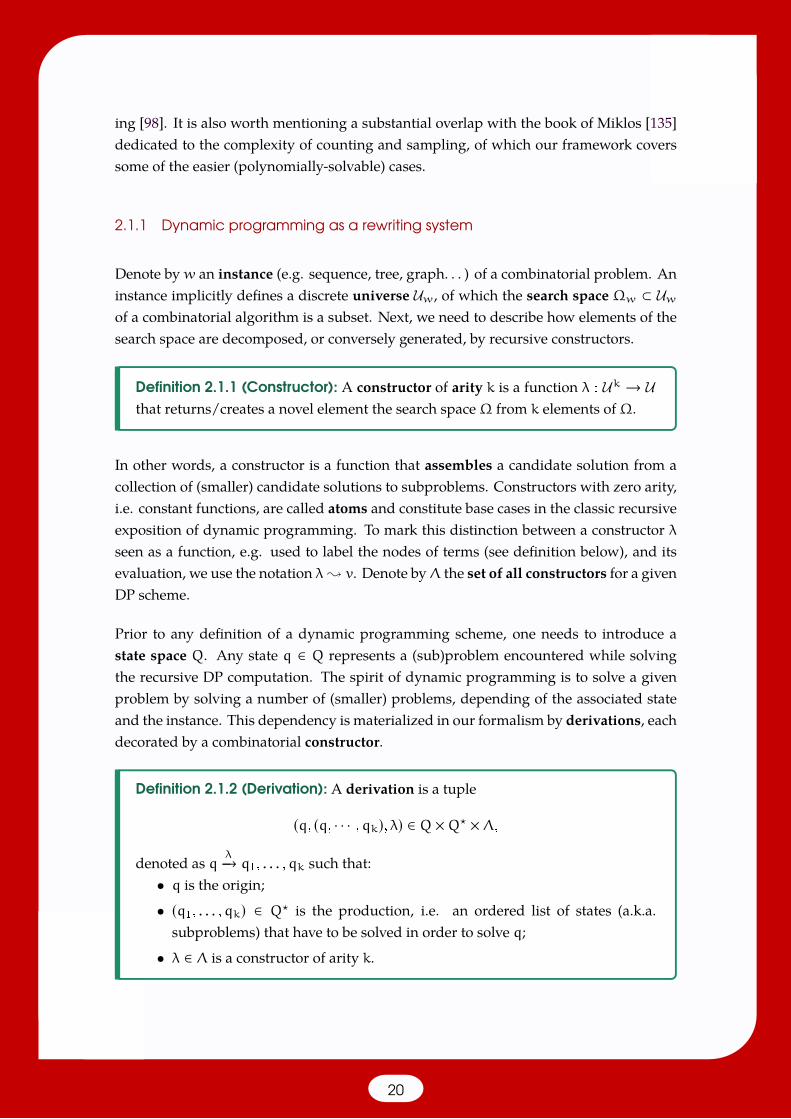
Prior to any definition of a dynamic programming scheme, one needs to introduce astate space Q. Any state q ∈ Q represents a (sub)problem encountered while solvingthe recursive DP computation. The spirit of dynamic programming is to solve a givenproblem by solving a number of (smaller) problems, depending of the associated stateand the instance. This dependency is materialized in our formalism by derivations, eachdecorated by a combinatorial constructor.

Definition 2.1.2 (Derivation): A derivation is a tuple

(q, (q, · · · ,qk), λ) ∈ Q ×Q? ×Λ,

denoted as qλ−→ q1, . . . ,qk such that:

• q is the origin;

• (q1, . . . ,qk) ∈ Q? is the production, i.e. an ordered list of states (a.k.a.subproblems) that have to be solved in order to solve q;

• λ ∈ Λ is a constructor of arity k.

20

We can now define a (combinatorial) dynamic programming scheme as a system ofequations, coupled with a derivation system.

Definition 2.1.3 (Dynamic Programming Scheme): A dynamic programmingscheme ∆ is a tuple (Q,qw, δ), where:

• Q is the state space;

• qw ∈ Q is the initial state;

• δ ⊂ Q × Q? × Λ is an acyclic, i.e. non transitively self-referential, set ofderivations.

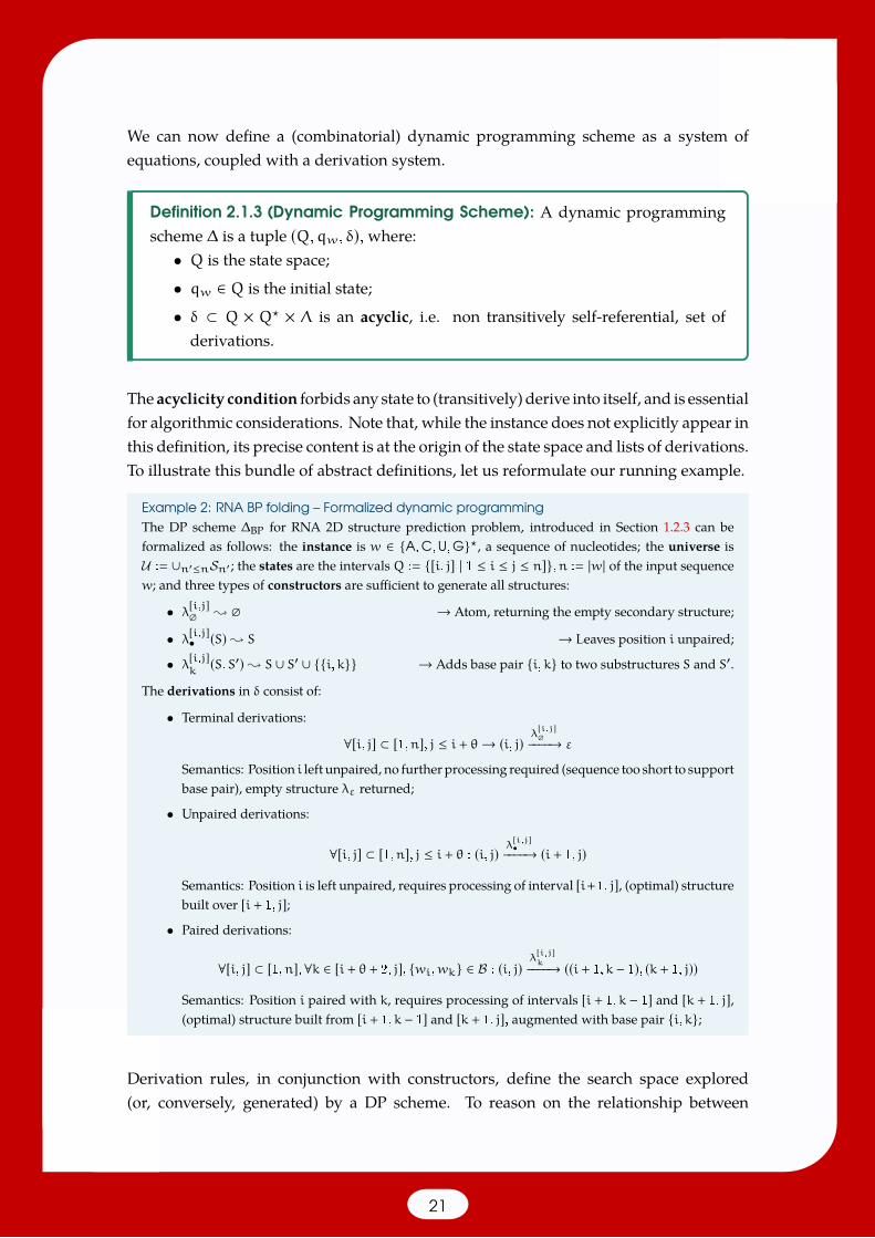
The acyclicity condition forbids any state to (transitively) derive into itself, and is essentialfor algorithmic considerations. Note that, while the instance does not explicitly appear inthis definition, its precise content is at the origin of the state space and lists of derivations.To illustrate this bundle of abstract definitions, let us reformulate our running example.

Example 2: RNA BP folding – Formalized dynamic programmingThe DP scheme ∆BP for RNA 2D structure prediction problem, introduced in Section 1.2.3 can beformalized as follows: the instance is w ∈ A,C,U,G?, a sequence of nucleotides; the universe isU : ∪n′≤nSn′ ; the states are the intervals Q : [i, j] | 1 ≤ i ≤ j ≤ n],n : |w| of the input sequencew; and three types of constructors are sufficient to generate all structures:

• λ[i,j] ; → Atom, returning the empty secondary structure;

• λ[i,j]• (S); S → Leaves position i unpaired;

• λ[i,j]k(S,S′); S ∪ S′ ∪ i,k → Adds base pair i,k to two substructures S and S′.

The derivations in δ consist of:

• Terminal derivations:

∀[i, j] ⊂ [1,n], j ≤ i + θ→ (i, j) λ[i,j]−−−−→ ε

Semantics: Position i left unpaired, no further processing required (sequence too short to supportbase pair), empty structure λε returned;

• Unpaired derivations:

∀[i, j] ⊂ [1,n], j ≤ i + θ : (i, j) λ[i,j]•−−−−→ (i + 1, j)

Semantics: Position i is left unpaired, requires processing of interval [i+1, j], (optimal) structurebuilt over [i + 1, j];

• Paired derivations:

∀[i, j] ⊂ [1,n],∀k ∈ [i + θ + 2, j], wi,wk ∈ B : (i, j)λ[i,j]k−−−−→ ((i + 1,k − 1), (k + 1, j))

Semantics: Position i paired with k, requires processing of intervals [i + 1,k − 1] and [k + 1, j],(optimal) structure built from [i + 1, k − 1] and [k + 1, j], augmented with base pair i,k;

Derivation rules, in conjunction with constructors, define the search space explored(or, conversely, generated) by a DP scheme. To reason on the relationship between

21

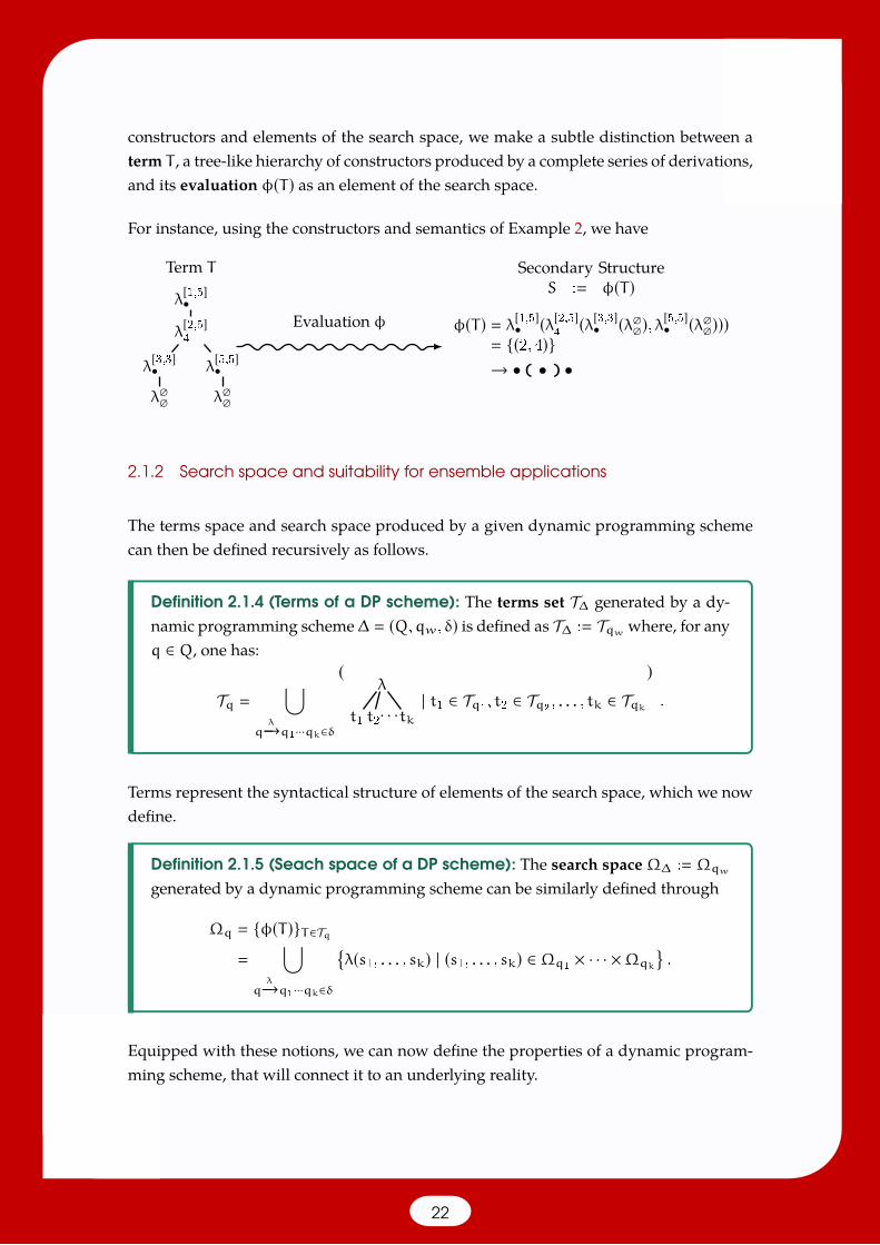
constructors and elements of the search space, we make a subtle distinction between aterm T , a tree-like hierarchy of constructors produced by a complete series of derivations,and its evaluation φ(T ) as an element of the search space.

For instance, using the constructors and semantics of Example 2, we have

λ[1,5]•

λ[2,5]4

λ[3,3]•

λ

λ[5,5]•

λ

Term T

φ(T ) λ[1,5]• (λ[2,5]4(λ[3,3]• (λ), λ[5,5]• (λ)))

(2, 4)→ • ( • ) •

Secondary StructureS : φ(T )

Evaluation φ

2.1.2 Search space and suitability for ensemble applications

The terms space and search space produced by a given dynamic programming schemecan then be defined recursively as follows.

Definition 2.1.4 (Terms of a DP scheme): The terms set T∆ generated by a dy-namic programming scheme∆ (Q,qw, δ) is defined as T∆ : Tqw where, for anyq ∈ Q, one has:

Tq

⋃qλ−→q1···qk∈δ

λ

t1 t2· · ·tk| t1 ∈ Tq1 , t2 ∈ Tq2 , . . . , tk ∈ Tqk

.

Terms represent the syntactical structure of elements of the search space, which we nowdefine.

Definition 2.1.5 (Seach space of a DP scheme): The search spaceΩ∆ : Ωqw

generated by a dynamic programming scheme can be similarly defined through

Ωq φ(T )T∈Tq

⋃qλ−→q1···qk∈δ

λ(s1, . . . , sk) | (s1, . . . , sk) ∈ Ωq1 × · · · ×Ωqk

.

Equipped with these notions, we can now define the properties of a dynamic program-ming scheme, that will connect it to an underlying reality.

22

Definition 2.1.6 (Completeness and unambiguity of a DP scheme): A DPscheme ∆ (Q,qw, δ) is:

1. Unambiguous if and only if every element of the search space can be gener-ated in only one way, i.e. φ is bĳective between T∆ andΩ∆;

2. Complete with respect to a targeted search space Ω? if and only if everyelement inΩ? is considered by ∆, i.e. one hasΩ∆ Ω?.

These two notions are crucial for ensemble applications of application. Indeed, in combi-nation, they allow to use a given DP scheme to extract relevant properties of a preexistingsearch space.

Let us now distinguish elements within the search spaces, by introducing scoring func-tions thatwillmapnumerical valueswith each constructors and, in turn, to terms/elementsof the search space

Definition 2.1.7 (Additive scoring function): An additive scoring function f :

Λ → associates a numerical value to each constructor, such that the score f(T )of a term T ∈ T is defined as

f(T ) : f(φ(T )) :∑λ∈T

f(λ).

An important property of a dynamic programming scheme lies is its ability to emulate agiven function defined over its search space, by using a suitable scoring of its construc-tors/derivations. Such function could represent an objective function in the context ofan optimization, or help induce a desired probability distribution over the search space.

Definition 2.1.8 (Correctness of a DP scheme): Let ∆ be a DP scheme, coupledwith a scoring function f : Λ→ . A pair (∆, f) is correct, with respect to a givenfunction F : Ω∆ → , if and only if F(φ(T )) f(T ),∀T ∈ T .

By extension, we say that a DP scheme ∆ is correct with respect to a function F if andonly if there exists a scoring function f such that (∆, f) is correct.

Example 3: RNA BP folding – Unambiguity/completeness/correctnessThe unambiguity of ∆BP can be proven by considering two terms T and T ′, T , T ′. Consider the firstposition from the root where constructors λ and λ′, such that λ , λ′ are found in T and T ′ respectively.Since their paths to the root encounter the same constructors, λ and λ′ are of the form λ

[i,j]k

or λ[i,j]•(but not λ[i,j] , since then both would be⇒ λ λ′). Since two constructors irrevocably induce differentpartners for position i, their associated structures S : φ(T ) and S′ : φ(T ′) differ by at least one base

23

pair, and we have S , S′, implying the non-ambiguity of ∆BP.

The completeness of ∆BP requires that any structure S ∈ Sn can be generated by the evaluation ofsome term in Tq. This can be established by induction of the length n ≥ Θ+2 of the interval, assumingthat, for all [i′, j′] ∈ Q such that n′ : j′ − i′ + 1 < n, one has Ωn′ Sn′ . Now, consider an interval[i, j], j − i + 1 n and a structure S ∈ Sn, and discuss the partner of i in S: if i is unpaired, thenS •S′ with |S′ | < n, so S′ is generated by T ′ ∈ T[i+1,j] and T : λ

[i,j]• (T ′) ∈ T[i,j] such that φ(T ) S;

if i is paired to some k, then S (S′)S′′ with |S′ | + |S′′ | < n, so S′ and S′′ are generated by termsT ′ ∈ T[i+1,k−1] and T ′′ ∈ T[k+1,j] respectively, so T : λ

[i,j]k(T ′, T ′′) ∈ T[i,j] such that φ(T ) S.

The correctness of ∆BP requires that, for any secondary structure in the search space, the numberof base-pairs is obtained by adding numerical values mapped to constructors. This is possible since,for any term T evaluated as φ(T ) S, the number of base pairs in S coincides with the number ofconstructors of type λ[i,j]

kin T , so the scoring function f : λ→ defined as

f(λ[i,j]• ) f(λ[i,j] ) 0 and f(λ[i,j]k)

−1 if wi,wk ∈ B (valid base pair)

+∞ otherwise.

Remark 2.1.1:Note that our assumption of scoring schemes that are additively-defined on construc-tors/transitions represents a limitations in expressivity in comparison to themore general evaluationalgebra considered in algebraic dynamic programming and its extensions [80, 81, 169, 211]. How-ever, general algebras do not allow a smooth transition from optimization to ensemble analyses,so we (slightly) limit the scope of our framework rather than burden our proofs and theorems.Moreover, the current framework captures, without any complexity overhead, every applications ofdynamic programming known to this author in Bioinformatics.

2.1.3 Classic optimization

With this final notion of correctness being defined, we can finally turn to a more algorith-mic dimension of dynamic programming, initially focusing on optimization problems,an historical focus of dynamic programming since its initial pioneering by Bellman [14].

Problem 1 (DP-based optimization):Input: A dynamic programming scheme ∆ and a scoring function f, such that(∆, f) is correct with respect to an objective function F : Ω∆ → Output: Some element s? ∈ S∆ such that F(s?) maxs∈S∆ F(s)

Unsurprisingly, this problem can be solved using dynamic programming, using an algo-rithm consisting of the following steps:

24

1. Matrix filling: For all state q ∈ Q, traversed in preorder, compute

mq : max

qλ−→q1,...,qk∈δ

f(λ) +k∑i1

mqi (2.1)

2. Backtracking: Return B(qw), recursively defined for any q ∈ Q as:

B(q) : λ(B(q1), . . . ,B(qk)), ifmq f(λ) +k∑i1

mqi ,qλ−→ q1, . . . ,qk ∈ δ

Note that the preorder in Step 1 always exists due to the acyclicity of derivations. Thetime complexity of this step is inO(|Q|+α? × |δ|), α? : maxd∈δ α(d) for α(d) the arity ofa derivation d, i.e. the number of states in its production. The memoization of computedvalues mq requires Θ(|Q|) memory. These complexities hold for the whole algorithm,since Step 2 involves recursingover atmost |Q| states (due to acyclicity), and its complexityis typically orders of magnitude below the requirements of Step 1.

Example 4: RNA BP folding – Energy minimizationLet us illustrate Equation (2.1) in the context of ∆BP, the DP scheme of RNA BP folding. For base-pair maximization, the objective function is F(S) : |S|, achieved by a scoring function f such thatf(λ[i,j]k) 1 if (wi,wk) ∈ B;−∞ otherwise, and f(λ[i,j]• ) f(λ[i,j] ) 0. We get

m[i,j] max

f(λ[i,j] ) if i + θ ≥ j . [i, j] λ[i,j]−−−−→

f(λ[i,j]• ) +m[i+1,j] if i + θ < j . [i, j] λ[i,j]•−−−−→ [i + 1, j]

maxk f(λ[i,j]k) +m[i+1,j] +m[k+1,j] if i + θ < j . [i, j] λ

[i,j]k−−−−→ [i + 1,k − 1], [k + 1, j]

max

0 if i + θ ≥ jm[i+1,j] if i + θ < jmax

jki+θ+1

1 +m[i+1,j] +m[k+1,j] if i + θ < j ∧ (wi,wk) ∈ Bin which one recognizes the classic DP equation reminded in Section 1.2.3.

2.2 Exact computation of Ensemble properties

In many applications of ensemble dynamic programming, one attempts to analyze aspecific subset of the search space. Examples abound in RNA bioinformatics wherean integer-valued feature function, additively defined with respect to the dynamic pro-gramming scheme, partition of the secondary structureswith respect to their free-energy,base-pair distance to one or several references structure(s). . .

25

2.2.1 Computing the partition function.

A ubiquitous quantity of interest is the partition function, whose definition requiresintegrating over the whole search space, and is used as a normalization term withinensemble studies. As observed by McCaskill [130], the optimization algorithm of anyunambiguous DP scheme can be adapted to compute the partition function, through asimple algebraic substitution. Namely, it suffices to substitute (min/max,+) → (+,×),coupled with a suitable exponentiation of energy contributions to compute the partitionfunction from the MFE recursions. This observation has given rise to systematic studiesdecorrelating the DP scheme from its algebra [80, 97] with a specific focus on semi-ringalgebras [135, 138].

Problem 2 (Partition function):Input: An unambiguous DP scheme ∆ and a scoring f, such that (∆, f) is correctwith respect to an energy function E : Ω∆ → ; β ∈ a constant

Output: The partition function Z∆ ofΩ∆, defined as

Z∆

∑s∈Ω∆

e−β·E(s)

The above problem can be solved by returning Z∆ : Zqw , following the computation,for all state q ∈ Q, of

Zq

∑s∈Ωq

e−β·E(s).

Those quantities can be computed recursively (in preorder), using

Zq :∑


e−β·E(λ) ×k∏i1

Zqi . (2.2)

The time complexity of this computation is inO(|Q| +α? × |δ|), α? being the max arity ofa constructor, and requires Θ(|Q|)memory.

Example 5: RNA BP folding – Partition functionA reasonable energy function is defined as E(S) : −|S|, and implicitly used inNussinov-Jacobson [143]scheme. It is achieved by an eponymous scoring functionE such thatE(λ[i,j]

k) −1 if (wi,wk) ∈ B;+∞

otherwise, and E(λ[i,j]• ) f(λ[i,j] ) 0. We get

Z[i,j] :∑

1 if i + θ ≥ jZ[i+1,j] if i + θ < j∑jki+θ+1

eβ × Z[i+1,j] × Z[k+1,j] if i + θ < j ∧ (wi,wk) ∈ B.

26

The validity of the final result, i.e. the fact that Z[1,n] ∑S∈Sn e−β.E(S), is a direct consequence of the

unambiguity, completeness and correctness properties of ∆BP. The time and space complexities are inΘ(n3) and Θ(n2) respectively.

2.2.2 Probabilities in Boltzmann-Gibbs distributions (inside-outside)

In many relevant contexts, the elements of a search space Ω can be assumed to follow aBolzmann-Gibbs distribution, where the probability of any s ∈ Ω is such that

(s) e−β·E(s)

Z (2.3)

where E represents an energy score, and β a constant (analogous to a temperature), andZ is the partition function. In such a context, the probabilities of individual elementsinduce average properties (e.g. base-pair probabilities) that are extremely relevant toensemble analyses.

Definition 2.2.1 (Unicity of a constructor): A constructor λ ∈ Λ is uniquewithina DP scheme ∆ if it occurs at most once in each term T ∈ T∆.

Under the unicity condition, the probability of a constructor λ can be obtained by sum-ming the individual probabilities of search space elements that result from its application(or, equivalently, the terms that contain λ). Fortunately, this property can be computedefficiently using a suitable dynamic programming scheme, as stated below.

Problem 3 (Boltzmann probability of constructor(s)):Input: Unambiguous DP scheme ∆ + scoring f, correct w.r.t. energy function E;β ∈ a constant; and a set C ⊂ Λ of unique constructors

Output: The Boltzmann probabilities of constructors in C:

∀λ ∈ C : (λ ∈ T ) ∑T∈T∆s.t. λ∈T

e−β·E(φ(T ))

Z∆(2.4)

This problem, which generalizes the computation of production probabilities in prob-abilistic context-free grammars, is tackled by a variant of the inside-outside algo-rithm [10, 113]. The algorithm is based on the observation that, for any monitoredconstructor λ?, any term T? ∈ Tλ? : T ∈ T∆ | λ ∈ T can be decomposed into:

1. a derivation d : qλ?−−→ q1, . . . ,qk labeled by an occurrence of λ?;

2. an outside part, a partial term in Tq ∈ T∆, truncated on an occurrence of q (leftunderived). Let us denote byOq the set of outside parts leading to q;

27

3. several insideparts, i.e. individual continuations of the derivationprocess, startingfrom q1, . . . ,qk. Denote as Iq1 , . . . ,Iqk the set of inside parts generated fromq1, . . . ,qk respectively;

Under the unicity condition, this decomposition is unambiguous. Moreover, the respec-tive energy contributions of the three parts are independently contributing to the energy,and it follows that Zλ? , the partition function restricted to Tλ? , obeys

Zλ? :∑T∈Tλ?

e−β.E(T )

∑qλ?−−→q1,...,qk∈δ

e−β.E(λ?) × ©«

∑Tq∈Oq

e−β.E(Tq)ª®¬×

k∏i1

©«∑Ti∈Iqi

e−β.E(Ti)ª®¬

∑qλ?−−→q1,...,qk∈δ

e−β.E(λ?) × Yq ×

k∏i1

Zqi (2.5)

where Yq :∑Tq∈Oq e

−β.E(Tq) is the outside partition function. Note that, when Yq isknown, the above equation allows to simultaneously compute the partition functions Zλfor all monitored unique constructors, through a single pass over the derivations.

The computation of Yq itself can also be performed by inverting the dynamic pro-gramming scheme, going from a given state back to the root while allowing the furtherderivation of siblings found along the way. The outside partition function Yq of a nodecan be computed using dynamic programming using infix order, i.e. starting from theroot qw and processing the ancestors of a node before itself, through

Yq :

1 if q qw (root)∑qp

λ−→q∈δs.t. q∈q

e−β.E(λ) × Yqp ×∏kq′∈qq′,q

Zq′ otherwise. (2.6)

Overall, the inside-outside algorithm solving Problem 3 can be stated as:

• Using Equation (2.2), compute the inside partition function Zq for all state q ∈ Qin preorder; → O(|Q| + α? × |δ|) time

• Using Equation (2.6), compute the outside partition function Yq for all state q ∈ Qin infix order; → O(|Q| + α? × |δ|) time

• Iterate over derivations qλ−→ q1 · · ·qk ∈ δ to compute (Zλ)λ∈C, initially set to 0. If

λ ∈ C, update Zλ ← Zλ + e−βE(λ?)Yq

∏ki1Zqi ; → O(α? × |δ| + |C|) time

• Finally, the algorithm returns (λ ∈ T ) : Zλ/Zqw ,∀λ ∈ C.The algorithm runs in time O(|Q| + |C| + α? × |δ|), α? being the maximum arity of aconstructor, and requires storage for O(|Q| + |C|) numbers.

28

Example 6: RNA BP folding – BP probabilitiesIn the context of RNA, the inside/outside algorithm can be used to compute base-pair probabilities,as done by McCaskill [130]. Inside contributions/partition functions are computed as detailed inExample 5, using E(λ[i,j]

k) −1 if (wi,wk) ∈ B;+∞ otherwise and E(λ[i,j]• ) f(λ[i,j] ) 0. The

monitored constructors are all λ[i,j]k

, each unique as a position i cannot be assigned twice.

The outside contributions Yq are then computed through a specialization of Equation (2.6):

Y[i,j] :∑

1 if [i, j] [1,n]Y[i−1,j] if i − 1 ≥ 1∑i−Θ−1i′1 eβ × Y[i′,j] × Z[i′+1,i−2] if (wi′ ,wi−1) ∈ B;∑nj′j+1 e

β × Y[i,j′] × Z[i+1,j′] if (wi−1,wj+1) ∈ B.

We finally obtain the probabilities of constructors through a specialization of Equation (2.5)

(λ[i,j]k∈ T

):

eβ×Y[i,j]×Z[i+1,k−1]×Z[k+1,j]

Z[1,n] if(wi,wk) ∈ B0 otherwise

Summing over all values of j, we get the probability of a base-pairs (i,k), k − i > θ

((i,k) ∈ S) :n∑j≥k

(λ[i,j]k∈ T

)

The probabilities of all base pairs can then be computed the inside/outside, in Θ(n3) time, and Θ(n2)space by computing the probabilities of constructors on the flywithin the above sum.

Remark 2.2.1 (Beyond unique features): Remark that, in the case where λ is not unique, i.e. itoccurs more than once in a term, the output of the above algorithm is no longer the probabilityof occurrence, but the expected number of occurrences of λ in a random, Boltzmann-distributed,term. This quantity may be of interest, for instance when trying to assess expected properties of theBolzmann ensembles, since it allows the simultaneous computation of many expected features in asingle pass.

2.2.3 Ensemble centroid and Maximum Expected Accuracy (MEA)

The probabilities computed in Problem 3 allow to assess a notion of support for theindividual features (e.g. base pairs, helices...) of a solution within the Boltzmann-Gibbsdistribution. Thus, they can beused to assess how representative a given solution is of theBoltzmann-Gibbs ensemble. In particular, when s? is the minimum free-energy solution,we know that s? achieves maximal probability in the Boltzmann-Gibbs distribution.

However, in absolute terms, the probability of s? may be (and usually is) abysmally small,and does not allow in itself to distinguish between two very different situations:

1. The solution s? is surroundedbya familyof similar suboptimal solutions s′1, s′

2. . .,

having very similar features (e.g. |s?, s′i| ≤ η for some notion of distance), overtak-

29

ing the probability distribution ( (s?) +∑i

(s′i

) 1 − ε);

2. The solution s?, even supplemented by similar suboptimals, is highly dominatedby dissimilar solutions in the Boltzmann ensemble ( (s?) +∑

i (s′i

) ε).

A possible way to distinguish between those two worlds, consists in computing an ex-pected distance of s? to a random solution in the ensemble.

Definition 2.2.2 (Weighted distance between solutions): Given two solutionss, s′ ∈ Ω resulting from the applications of sets of unique constructors C

λ1, · · · , λk and C′ λ′1, · · · , λ′k′ respectively. Then the distance |s, s′ | betweens and s′ is defined as

|s, s′ |µ

∑λ∈Λ

πλ × (1λ∈C − 1λ∈C′)2

where π : Λ→ + is a collection of weights.

Since constructors represent atomic operations that build a given element of the searchspace (e.g. adding a base pair, declaring a nucleotide unpaired. . . ), this notion of distancerepresents a natural way to represent popular distance metrics.

Equipped with a notion of distance, we can now define the centroid of the Boltzmann-Gibbs ensemble [55, 87] as its most central element, i.e. the solution having minimumexpected distance to a, Boltzmann-distributed, elements of the search space.

Problem 4 (Centroid solution):Input: Unambiguous DP scheme ∆ + scoring f, correct w.r.t. function E; β ∈ aconstant; and a weighted distance |?, ?|µOutput: Solution s? ∈ Ω∆ minimizing the expected distance to the ensemble:

s? argmins∈Ω∆

∑s∈Ω∆

(s′) × |s, s′ |µ (2.7)

Fortunately, the expected distance to the ensemble of any given candidate solution s ∈ Ωcan be reexpressed as a simple sum over the Boltzmann probabilities of constructors.

30

Indeed, one has∑s′∈Ω∆

(s′) × |s, s′ |µ

∑s′∈Ω∆

(s′) ×∑λ∈Λ

πλ × (1λ∈s − 1λ∈s′)2

∑λ∈Λλ∈s

πλ × (λ < T ) +∑λ∈Λλ<s

πλ × (λ ∈ T )

∑λ∈Λλ∈s

πλ × ( (λ < T ) − (λ ∈ T )) +∑λ∈Λ

πλ × (λ ∈ T ) (2.8)

Since the rightmost sum no longer depends on s, finding the solution that minimizesthe expected distance is equivalent to finding a solution that optimizes the leftmost sum.Following this observation, one can solve Problem4by executing the following algorithm:

1. Compute the Boltzmann probabilities of constructors used by the weighted dis-tance, i.e. solve Problem 3 with C : λ ∈ Λ | πλ , 0;

2. Find s ∈ Ω∆ that minimizes the leftmost term of Equation 2.8, i.e. solve Problem 1,maximizing the objective function F : Λ→ such that

F(λ) : πλ × ( (λ ∈ T ) − (λ < T )) πλ × (2 (λ ∈ T ) − 1) (2.9)

Example 7: RNA BP folding – Centroid computationWe consider the classic base-pair distance as the distance to be minimized, and accordingly replaceall constructors λ[i,j]

kwith new simplified constructors λ(i,k) and λ(i) which respectively represent

occurrences of a base pair (i,k) and an unpaired position i, irrespectively of their context [i, j] ofcreation (since the context of a base pair should not contribute to the distance). We set the weightof all constructors to 0 except for π(λ(i,k)) 1 in the distance definition, and compute the base-pairprobabilities pi,j : ((i, j) ∈ S) as shown in Section 2.2.2.

Then, we solve Problem 1 in this new setting, i.e. compute the recurrence

c[i,j] max

0 if i + θ ≥ jc[i+1,j] if i + θ < jmax

jki+θ+1

(2pi,k − 1) + c[i+1,j] + c[k+1,j] if i + θ < j ∧ (wi,wk) ∈ Bto get the least distance of a structure to the ensemble (up to a constant, i.e. the rightmost term in (2.9))A classic backtrack allows to recover the centroid secondary stucture.

A Maximum Expected Accuracy (MEA) solution [121] can be obtained in a very similar fashion bysimplifying the objective function of Equation (2.9) to F(λ) : πλ × (λ ∈ T ), with πλBP : 2γ forbase-pairing constructors, and πλUnp. : 1 for unpaired constructors.

2.2.4 General moments of additive scores [150]

Given an additive scoring function F, it is a natural question to ask for the induceddistribution of F under a Boltzmann Gibbs distribution. Since most such distributionsare typically Gaussian, a first task is to compute the expected value µ∆(F) and variance

31

σ∆(F) of F, respectively defined as µ∆(F) : (F(T )) and

σ∆(F) :√ ∑T∈T∆

(T ) · (F(T ) − µ∆(F))2 √ (F(T )2) − (F(T ))2.

In order to capture characteristics of more general distributions, one may consider themoments of the distribution, defined as (F(T )) , (

F(T2)) . . ., previously considered byMiklos, Meyer and Borbala [136] specifically for the free-energy. The cross-moments (F1(T )n1 .F2(T )n2 · · · ) of multiple functions are also of potential interest, as their com-putation allows to derive the Pearson correlation ρ∆(F1, F2) of two functions F1 and F2through

ρ∆(F1, F2) ((F1(T ) − µ∆(F1)) × (F2(T ) − µ∆(F2)))σ∆(F1) × σ∆(F2)

(F1(T ) × F2(T )) − (F1(T )) × (F2(T ))√

(F1(T )2) − (F1(T ))2 ×√ (F2(T )2) − (F2(T ))2

so the correlation can be computed from the evaluation of (F1(T )n1 × F2(T )n2) for allvalues of (n1,n2) ∈ (1, 0), (0, 1), (2, 0), (0, 2), (1, 1).

In a collaborationwith Cédric Saule [150], we have considered the computation of generalcross-moments within dynamic programming schemes.

Problem 5 ((Cross) moments of a DP scheme):Input: Unambiguous DP scheme ∆ + scoring f, correct w.r.t. function E; β ∈ ;and scoring functions (F1, . . . , Fp)with associated degrees (γ?

1, . . . ,γ?p)

Output: The (cross) moment γ?1, . . . ,γ?p for F1, . . . , Fp :

mγ?1···γ?

p : (F1(T )γ?

1 × · · · × Fp(T )γ?p

)

∑T∈T∆

(T )p∏i1

Fi(T )γ?i (2.10)

A reexpression of our result [150] states thatmγ1,...,γp can be computed as

mγ1···γpq :

∑qλ−→q1···qk∈δ

e−β.E(λ)∑

λ1+τ1,1···τ1,kγ1...

λp+τp,1···τp,kγp

p∏i1

Fi(λ)λi(

γi

τi,1 · · · τi,k

) k∏j1

mτ1,j···τp,jqj . (2.11)

This expression,whoseunderlying intuition isprobablyhard todecipher at first sight, is infact strongly inspired by the partial pointing operator in enumerative combinatorics [50,69]. Its main underlying idea is to modify the DP scheme ∆, introducing of a controlledambiguity, into aDP scheme∆γ1,...,γp designed to generate pointed/weighted versionsof the original terms.

32

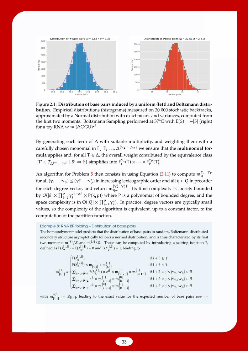
15.0 17.5 20.0 22.5 25.0 27.5 30.0 32.5#Base pairs

0

500

1000

1500

2000

2500

3000

3500Fr

eque

ncy

Distribution of #base pairs ( = 22.57 = 2.38)

25 30 35 40#Base pairs

0

500

1000

1500

2000

2500

3000

Freq

uenc

y

Distribution of #base pairs ( = 32.51 = 2.61)

Figure 2.1: Distribution of base pairs inducedby a uniform (left) andBoltzmanndistri-bution. Empirical distributions (histograms) measured on 20 000 stochastic backtracks,approximated by a Normal distribution with exact means and variances, computed fromthe first two moments. Boltzmann Sampling performed at 37°C with E(S) −|S| (right)for a toy RNA w : (ACGU)25.

By generating each term of ∆ with suitable multiplicity, and weighting them with acarefully chosen monomial in F1, F2 . . ., ∆γ1,...,γp we ensure that the multinomial for-mula applies and, for all T ∈ ∆, the overall weight contributed by the equivalence classT ′ ∈ T∆γ1,...,γp | S′⇔ S simplifies into Fγ1

1(T ) × · · · × Fγpp (T ).

An algorithm for Problem 5 then consists in using Equation (2.11) to compute mγ1···γpq

for all (γ1 · · ·γp) ≤ (γ?1 · · ·γ?p) in increasing lexicographic order and all q ∈ Q in preorderfor each degree vector, and return mγ

?1···γ?

pqw . Its time complexity is loosely bounded

by O(|δ| ×∏p

i1γ?i1+α? × P(k,p)) where P is a polynomial of bounded degree, and the

space complexity is in Θ(|Q| ×∏p

i1γ?i). In practice, degree vectors are typically small

values, so the complexity of the algorithm is equivalent, up to a constant factor, to thecomputation of the partition function.

Example 8: RNA BP folding – Distribution of base pairsThe homopolymermodel predicts that the distribution of base-pairs in random, Boltzmann-distributedsecondary structure asymptotically follows a normal distribution, and is thus characterized by its firsttwo moments m1/Z and m2/Z . Those can be computed by introducing a scoring function F,defined as F(λ[i,j]• ) F(λ[i,j] ) 0 and F(λ[i,j]

k) 1, leading to

m1[i,j]

F(λ[i,j] ) if i + θ ≥ 1

F(λ[i,j]• ) ×m0[i,j] +m1[i,j] if i + θ < 1∑j

ki+θ+1F(λ[i,j]k) × eβ ×m0[i+1,j] ×m

0[k+1,j] if i + θ < j ∧ (wi,wk) ∈ B∑j

ki+θ+1eβ ×m1[i+1,j] ×m

0[k+1,j] if i + θ < j ∧ (wi,wk) ∈ B∑j

ki+θ+1eβ ×m0[i+1,j] ×m

1[k+1,j] if i + θ < j ∧ (wi,wk) ∈ B

with m0[i,j] : Z[i,j], leading to the exact value for the expected number of base pairs µBP :

33

m1[1,n]/Z[1,n]. A similar equation can be derived for the second moment

m2

[i,j]

0 if i + θ ≥ 1

m2

[i,j] if i + θ < 1∑jki+θ+1

eβ × F(λ[i,j]k)2 ×m0

[i+1,j] ×m0

[k+1,j] if i + θ < j ∧ (wi,wk) ∈ B∑jki+θ+1

eβ × 2 × F(λ[i,j]k)1 ×m1

[i+1,j] ×m0


eβ × 2 × F(λ[i,j]k)1 ×m0

[i+1,j] ×m1


eβ × 2 ×m1

[i+1,j] ×m1


eβ ×m2

[i+1,j] ×m0


eβ ×m0

[i+1,j] ×m2

[k+1,j] if i + θ < j ∧ (wi,wk) ∈ B

from which we get the standard deviation σBP :√m2

[1,n]/Z[1,n] − µ2BP

2.2.5 Classified DP with the Discrete Fourier Transform (DFT) [173, 174]

In some situations, precise aspects of the distribution are of interest, and cannot be easilycaptured by summary statistics. For instance, Freyhult et al [75] partition the BoltzmannEnsemble according to the distance to a reference secondary structure. Considering thedistribution of distance, they observe bimodal (an even trimodal) distributions that theyinterpret as potential evidences for the presence of multistable RNAs. Other examplesin RNA bioinformatics include the classification of sequences/structures with respect totheir Hamming distance to a wild-type sequence, to assess the mutational robustnessof concrete RNAs [191], the computation of the density of states, i.e. the distribution offree-energies within an RNA [43], or the projection of energy landscapes with respect tothe unfolded and native states [119].

Those instances can be expressed as a specialized version of classified dynamic program-ming, where additional parameters are used to partition the search space.

Problem 6 (Classified partition function):Input: Unambiguous DP scheme ∆ + scoring f, correct w.r.t. function E; β ∈ ;and an additive scoring functions F : Λ→ + with V : maxT∈T∆ F(T )Output: The classified partition function Z [v], 0 ≤ v ≤ V , defined as

Z [v] : (F(T ) v) × Z∆

∑T∈T

s.t. F(T )v

e−β.E(T )

A classic approach, used in many works including the above references, would consistin adapting the dynamic programming scheme through explicit convolution products,

34

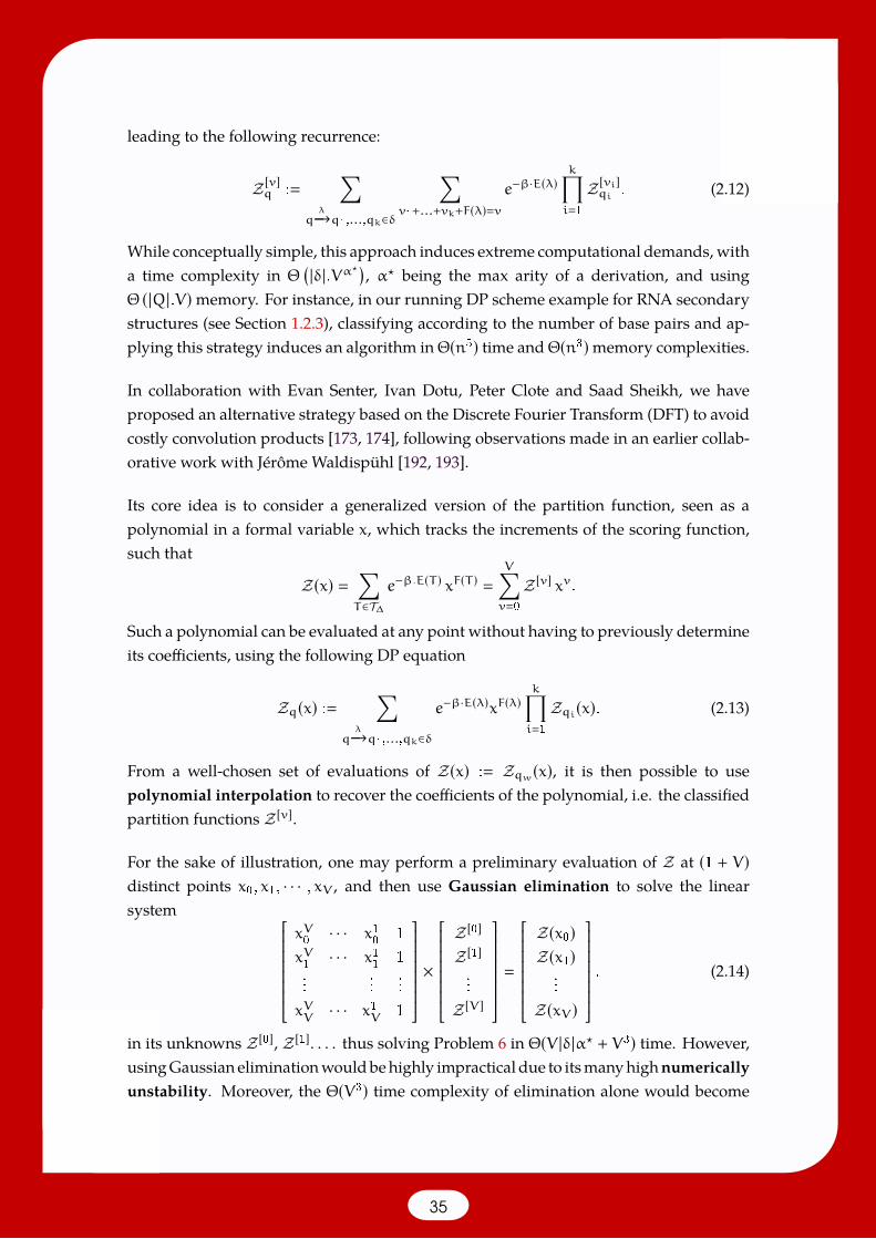
leading to the following recurrence:

Z [v]q :∑


∑v1+...+vk+F(λ)v

e−β·E(λ)k∏i1

Z [vi]qi . (2.12)

While conceptually simple, this approach induces extreme computational demands, witha time complexity in Θ

(|δ|.Vα? ) , α? being the max arity of a derivation, and usingΘ (|Q|.V)memory. For instance, in our running DP scheme example for RNA secondarystructures (see Section 1.2.3), classifying according to the number of base pairs and ap-plying this strategy induces an algorithm inΘ(n5) time andΘ(n3)memory complexities.

In collaboration with Evan Senter, Ivan Dotu, Peter Clote and Saad Sheikh, we haveproposed an alternative strategy based on the Discrete Fourier Transform (DFT) to avoidcostly convolution products [173, 174], following observations made in an earlier collab-orative work with Jérôme Waldispühl [192, 193].

Its core idea is to consider a generalized version of the partition function, seen as apolynomial in a formal variable x, which tracks the increments of the scoring function,such that

Z(x) ∑T∈T∆

e−β.E(T ) xF(T ) V∑v0

Z [v] xv.

Such a polynomial can be evaluated at any point without having to previously determineits coefficients, using the following DP equation

Zq(x) :∑


e−β·E(λ)xF(λ)k∏i1

Zqi(x). (2.13)

From a well-chosen set of evaluations of Z(x) : Zqw(x), it is then possible to usepolynomial interpolation to recover the coefficients of the polynomial, i.e. the classifiedpartition functions Z [v].

For the sake of illustration, one may perform a preliminary evaluation of Z at (1 + V)distinct points x0, x1, · · · , xV , and then use Gaussian elimination to solve the linearsystem

xV0· · · x1

01

xV1· · · x1

11

......

...

xVV· · · x1

V1

×

Z [0]Z [1]...

Z [V]

Z(x0)Z(x1)

...

Z(xV )

. (2.14)

in its unknowns Z [0], Z [1]. . . . thus solving Problem 6 in Θ(V |δ|α? + V3) time. However,usingGaussian eliminationwouldbehighly impractical due to itsmanyhighnumericallyunstability. Moreover, the Θ(V3) time complexity of elimination alone would become

35

Algorithm 1: Fast Fourier Transform

Result: The Fourier transform of x, a vector [yj ∑m−1k0 xkω

jkm | j ∈ [0,m − 1]]

Function FFT(Coefficients x,m |x| 2d):ifm 1 then return y;ω← 1;(xeven, xodd) ← ([x0, . . . , xm−2], [x1, . . . , xm−1]);(yeven, yodd) ← (FFT(xeven), FFT(xodd));for k← 1 to m/2 − 1 do

yk ← yevenk

+ω × yoddk

;yk+m/2 ← yeven

k−ω × yodd

k;

ω← ω ×ωn;return [y0,y1, . . . ,ym−1]

unreasonable for larger ranges of values for F, needed to emulate several scoring functionsas pointed out in Remark 2.2.2 below.

Enters the (Inverse)DiscreteFourierTransform (IDFT) [41, 42]whichallows, inO(m logm)time, to recover the coefficients x : (x0, . . . , xm−1) of a polynomial P(x) of degreem − 1,m 2d, from its evaluation at the m-th roots of the unity. Indeed, let ωm : e2πi/m,then the relationship between x and y : P(ωkm)m−1k0

remarkably simplifies

∀0 ≤ k < m : xk 1

m

m−1∑j0

yj ×ω−jkm . (2.15)

Moreover, evaluating all coefficients in x can be achieved much faster than the Θ(n2)algorithm suggested by the above equation, using the Fast Fourier Transform to speedup the evaluation to Θ(n logn).

To use the inverse DFT and interpolate Z(x), thus efficiently solving Problem 6, we firsttrivially extend Equation (2.13) to support complex arguments. Then we proceed to themain algorithm:

1. Round V + 1 upwards tom 2d,d ∈ , the closest power of 2;

2. Evaluate Z(ω0m),Z(ω1

m), . . . ,Z(ωm−1m ) → y0,y1, . . . ,ym−1 withωm e2πi/m;

3. Apply the FFT Algorithm 1 to [y0,y1, . . . ,ym−1] to obtain[x′k :

m−1∑j0

yjωjkm

]m−1k0

.

Notice from Equation (2.15) that x′m−k mxk,∀k ∈ [1,m − 1] and x′

0 mx0;

4. Return[Z [v] :

x′φ(v)n | v ∈ [0,V],φ(0) 0 and φ(v > 0) V + 1 − v

].

36

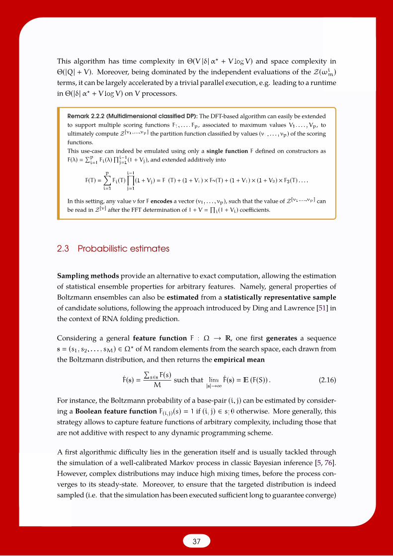
This algorithm has time complexity in Θ(V |δ| α? + V logV) and space complexity inΘ(|Q| + V). Moreover, being dominated by the independent evaluations of the Z(ωim)terms, it can be largely accelerated by a trivial parallel execution, e.g. leading to a runtimein Θ(|δ| α? + V logV) on V processors.

Remark 2.2.2 (Multidimensional classified DP): The DFT-based algorithm can easily be extendedto support multiple scoring functions F1, . . . , Fp, associated to maximum values V1, . . . ,Vp, toultimately compute Z[v1,...,vp] the partition function classified by values (v1, . . . , vp) of the scoringfunctions.This use-case can indeed be emulated using only a single function F defined on constructors asF(λ) ∑p

i1Fi(λ)

∏i−1j1(1 + Vj), and extended additively into

F(T ) p∑i1

Fi(T )i−1∏j1

(1 + Vj) F1(T ) + (1 + V1) × F2(T ) + (1 + V1) × (1 + V2) × F3(T ) . . . .

In this setting, any value v for F encodes a vector (v1, . . . , vp), such that the value of Z[v1,...,vp] canbe read in Z[v] after the FFT determination of 1 + V

∏i(1 + Vi) coefficients.

2.3 Probabilistic estimates

Sampling methods provide an alternative to exact computation, allowing the estimationof statistical ensemble properties for arbitrary features. Namely, general properties ofBoltzmann ensembles can also be estimated from a statistically representative sampleof candidate solutions, following the approach introduced by Ding and Lawrence [51] inthe context of RNA folding prediction.

Considering a general feature function F : Ω → , one first generates a sequences (s1, s2, . . . , sM) ∈ Ω? ofM random elements from the search space, each drawn fromthe Boltzmann distribution, and then returns the empirical mean

F(s) ∑s∈s F(s)M

such that lim|s|→∞

F(s) (F(S)) . (2.16)

For instance, the Boltzmann probability of a base-pair (i, j) can be estimated by consider-ing a Boolean feature function F(i,j)(s) 1 if (i, j) ∈ s; 0 otherwise. More generally, thisstrategy allows to capture feature functions of arbitrary complexity, including those thatare not additive with respect to any dynamic programming scheme.

A first algorithmic difficulty lies in the generation itself and is usually tackled throughthe simulation of a well-calibrated Markov process in classic Bayesian inference [5, 76].However, complex distributions may induce high mixing times, before the process con-verges to its steady-state. Moreover, to ensure that the targeted distribution is indeedsampled (i.e. that the simulation has been executed sufficient long to guarantee converge)

37

requires highly-technical analyses [152] that do not appear to lend themselves to genericalgorithmic design.

This section focuses on an alternative, where an unambiguous dynamic programmingscheme for the partition function (but not necessarily with respect to the feature function)is used for the generation. Probabilities for each of the transitions are precomputed, sothat generated objects are independent and follow the targeted distribution. This can beseen as an instance of the recursive method in random generation [71, 197].

2.3.1 Foreword: On the number of samples [165]

The choice of thenumber of samples is criticalwhenusing sampling to estimate statisticalproperties. This number should be large enough to yield accurate estimates, but lowenough to preserve efficiency. Historically, and in many subsequent works, a sample sizeof 1 000 structures was proposed [51], somewhat irrespectively of the precise context.However, such a one size fits all approach may not yield accurate results, motivating thefollowing discussion and recommendations.

The empirical mean estimator represents a sum of independent variables, meaning thatclassic concentration inequalities apply with minimal modifications. In particular, theHoeffding inequality implies that, for any feature F:

(|F(S) − (F(S)) | ≥ ε

)≤ 2 exp

(−2mε2c

), (2.17)

where ε is a tolerated absolute error level, S is a random sample of size m and c :

(maxS(F(S)) −minS(F(S)))2 is a trivial upper bound of the variance of the feature. Notethat when a feature function takes binary values 0/1, e.g. when estimating a probability,then one has c 1. Equation (2.17) can be used to build a confidence interval at level(1 − α), for any value α ∈ [0, 1], and we get:[

F(S) −√

c

2mlog

(2

α

), F(S) +

√c

2mlog

(2

α

)].

This means that, over multiple estimations from sampled elements, at least a fraction(1 − α) of the runs will produce errors smaller than

√c2m log

(2α

). This function can be

inverted (numerically) to estimate the number m of samples that achieve an absoluteerror bounded by ε at least (1 − α) of the times.

We report in Table 2.1 typical sample sizes required to achieve a given precision withreasonable probability when estimating probabilities (i.e. expectations of 0/1-valuedfeatures). For instance, to reach a 90% chance of estimating a base pair probabilitywithin 0.5% of its true value, a total of 59 915 structures should be generated. In

38

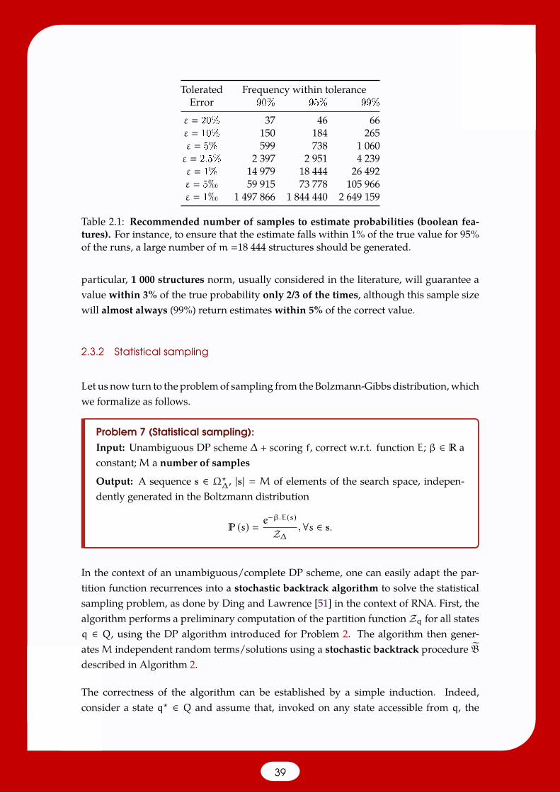
Tolerated Frequency within toleranceError 90% 95% 99%

ε 20% 37 46 66ε 10% 150 184 265ε 5% 599 738 1 060ε 2.5% 2 397 2 951 4 239ε 1% 14 979 18 444 26 492ε 5h 59 915 73 778 105 966ε 1h 1 497 866 1 844 440 2 649 159

Table 2.1: Recommended number of samples to estimate probabilities (boolean fea-tures). For instance, to ensure that the estimate falls within 1% of the true value for 95%of the runs, a large number ofm 18 444 structures should be generated.

particular, 1 000 structures norm, usually considered in the literature, will guarantee avalue within 3% of the true probability only 2/3 of the times, although this sample sizewill almost always (99%) return estimates within 5% of the correct value.

2.3.2 Statistical sampling

Let us now turn to the problemof sampling from the Bolzmann-Gibbs distribution, whichwe formalize as follows.

Problem 7 (Statistical sampling):Input: Unambiguous DP scheme ∆ + scoring f, correct w.r.t. function E; β ∈ aconstant;M a number of samples

Output: A sequence s ∈ Ω?∆, |s| M of elements of the search space, indepen-

dently generated in the Boltzmann distribution

(s) e−β.E(s)

Z∆,∀s ∈ s.

In the context of an unambiguous/complete DP scheme, one can easily adapt the par-tition function recurrences into a stochastic backtrack algorithm to solve the statisticalsampling problem, as done by Ding and Lawrence [51] in the context of RNA. First, thealgorithm performs a preliminary computation of the partition function Zq for all statesq ∈ Q, using the DP algorithm introduced for Problem 2. The algorithm then gener-atesM independent random terms/solutions using a stochastic backtrack procedure Bdescribed in Algorithm 2.

The correctness of the algorithm can be established by a simple induction. Indeed,consider a state q? ∈ Q and assume that, invoked on any state accessible from q, the

39

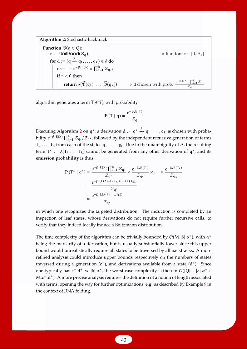
Algorithm 2: Stochastic backtrack

Function B(q ∈ Q):r← UnifRand(Zq) . Random r ∈ [0,Zq[for d : (q λ−→ q1, . . . ,qk) ∈ δ do

r← r − e−β·E(λ) ×∏ki1Zqi ;

if r < 0 then

return λ(B(q1), . . . , B(qk)) . d chosen with prob. e−β·E(λ)×∏k

i1 ZqiZq

algorithm generates a term T ∈ Tq with probability

(T | q) e−β.E(T )

Zq

Executing Algorithm 2 on q?, a derivation d : q?λ−→ q1, · · · ,qk is chosen with proba-

bility e−β·E(λ)∏ki1Zqi/Zq? , followed by the independent recursive generation of terms

T1, . . . , Tk from each of the states q1, . . . ,qk. Due to the unambiguity of ∆, the resultingterm T? : λ(T1, . . . , Tk) cannot be generated from any other derivation of q?, and itsemission probability is thus

(T? | q?) e−β·E(λ)∏k

i1ZqiZq?

× e−β.E(T1)

Zq1× · · · × e

−β.E(Tk)

Zqk

e−β·(E(λ)+E(T1)+...+E(Tk))

Zq?

e−β·E(λ(T1,...,Tk))

Zq?

in which one recognizes the targeted distribution. The induction is completed by aninspection of leaf states, whose derivations do not require further recursive calls, toverify that they indeed locally induce a Boltzmann distribution.

The time complexity of the algorithm can be trivially bounded by O(M.|δ|.α?), with α?

being the max arity of a derivation, but is usually substantially lower since this upperbound would unrealistically require all states to be traversed by all backtracks. A morerefined analysis could introduce upper bounds respectively on the numbers of statestraversed during a generation (c+), and derivations available from a state (d+). Sinceone typically has c+.d+ |δ|.α?, the worst-case complexity is then in O(|Q| + |δ|.α? +

M.c+.d+). Amore precise analysis requires the definition of a notion of length associatedwith terms, opening the way for further optimizations, e.g. as described by Example 9 inthe context of RNA folding.

40

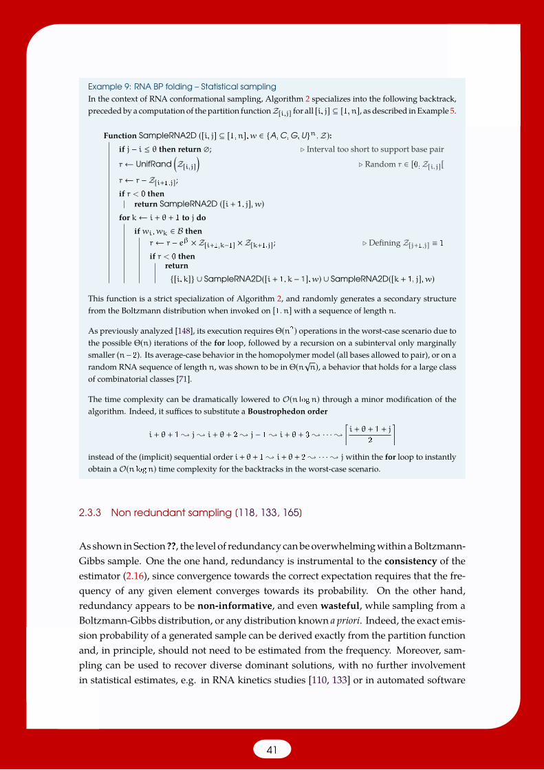
Example 9: RNA BP folding – Statistical samplingIn the context of RNA conformational sampling, Algorithm 2 specializes into the following backtrack,precededby a computation of the partition functionZ[i,j] for all [i, j] ⊆ [1,n], as described inExample 5.

Function SampleRNA2D ([i, j] ⊆ [1,n],w ∈ A,C,G,Un,Z):if j − i ≤ θ then return ; . Interval too short to support base pair

r← UnifRand(Z[i,j]

). Random r ∈ [0,Z[i,j][

r← r −Z[i+1,j];if r < 0 then

return SampleRNA2D ([i + 1, j],w)for k← i + θ + 1 to j do

if wi,wk ∈ B thenr← r − eβ ×Z[i+1,k−1] ×Z[k+1,j]; . Defining Z[j+1,j] ≡ 1

if r < 0 thenreturn[i,k] ∪ SampleRNA2D([i + 1,k − 1],w) ∪ SampleRNA2D([k + 1, j],w)

This function is a strict specialization of Algorithm 2, and randomly generates a secondary structurefrom the Boltzmann distribution when invoked on [1,n]with a sequence of length n.

As previously analyzed [148], its execution requires Θ(n2) operations in the worst-case scenario due tothe possible Θ(n) iterations of the for loop, followed by a recursion on a subinterval only marginallysmaller (n−2). Its average-case behavior in the homopolymer model (all bases allowed to pair), or on arandom RNA sequence of length n, was shown to be in Θ(n√n), a behavior that holds for a large classof combinatorial classes [71].

The time complexity can be dramatically lowered to O(n logn) through a minor modification of thealgorithm. Indeed, it suffices to substitute a Boustrophedon order

i + θ + 1 ; j ; i + θ + 2 ; j − 1 ; i + θ + 3 ; · · ·;⌈i + θ + 1 + j

2

⌉

instead of the (implicit) sequential order i+ θ+ 1 ; i+ θ+ 2 ; · · ·; jwithin the for loop to instantlyobtain a O(n logn) time complexity for the backtracks in the worst-case scenario.

2.3.3 Non redundant sampling [118, 133, 165]

Asshown inSection ??, the level of redundancy canbeoverwhelmingwithin aBoltzmann-Gibbs sample. One the one hand, redundancy is instrumental to the consistency of theestimator (2.16), since convergence towards the correct expectation requires that the fre-quency of any given element converges towards its probability. On the other hand,redundancy appears to be non-informative, and even wasteful, while sampling from aBoltzmann-Gibbs distribution, or any distribution known a priori. Indeed, the exact emis-sion probability of a generated sample can be derived exactly from the partition functionand, in principle, should not need to be estimated from the frequency. Moreover, sam-pling can be used to recover diverse dominant solutions, with no further involvementin statistical estimates, e.g. in RNA kinetics studies [110, 133] or in automated software

41

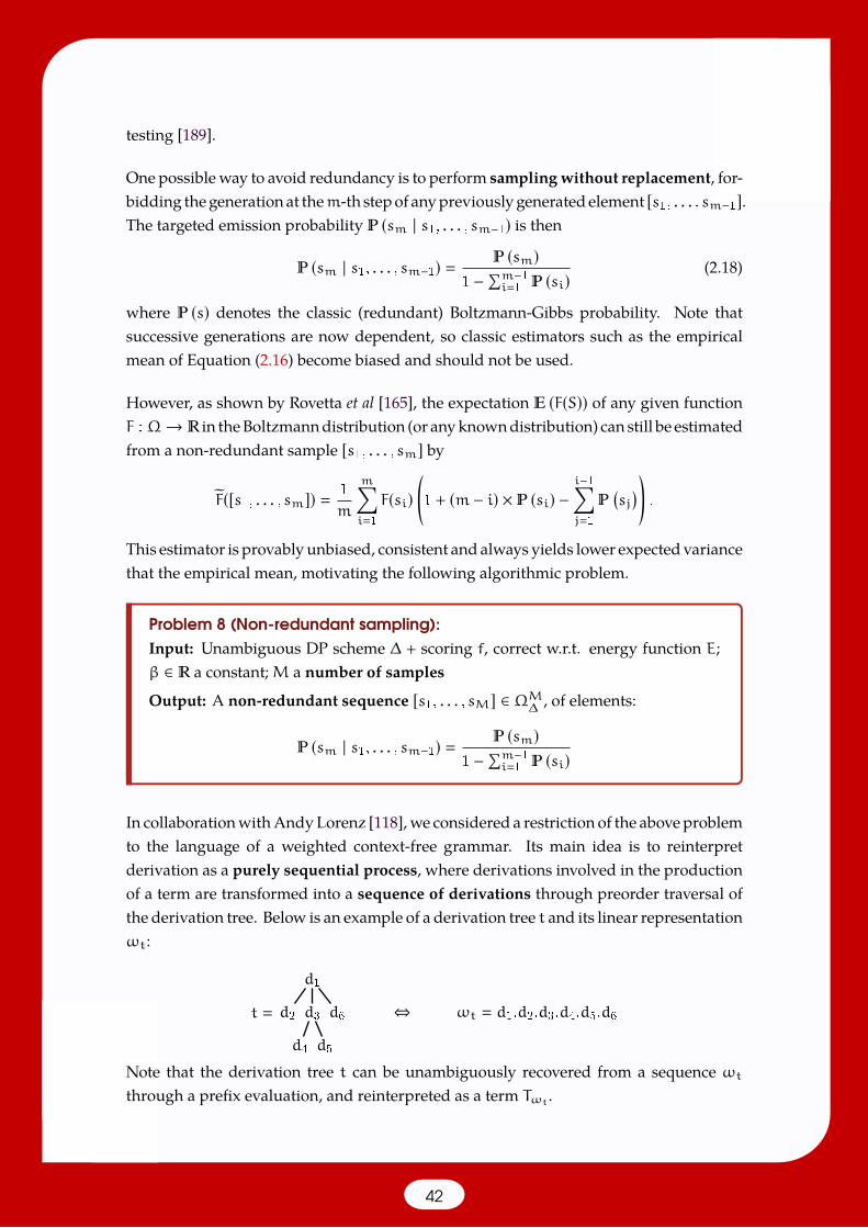
testing [189].

One possibleway to avoid redundancy is to perform samplingwithout replacement, for-bidding thegenerationat them-th stepof anypreviouslygeneratedelement [s1, . . . , sm−1].The targeted emission probability (sm | s1, . . . , sm−1) is then

(sm | s1, . . . , sm−1) (sm)1 −∑m−1

i1 (si)(2.18)

where (s) denotes the classic (redundant) Boltzmann-Gibbs probability. Note thatsuccessive generations are now dependent, so classic estimators such as the empiricalmean of Equation (2.16) become biased and should not be used.

However, as shown by Rovetta et al [165], the expectation (F(S)) of any given functionF : Ω→ in theBoltzmanndistribution (or anyknowndistribution) can still be estimatedfrom a non-redundant sample [s1, . . . , sm] by

F([s1, . . . , sm]) 1

m

m∑i1

F(si)(1 + (m − i) × (si) −

i−1∑j1

(sj

)).

This estimator is provablyunbiased, consistent and always yields lower expectedvariancethat the empirical mean, motivating the following algorithmic problem.

Problem 8 (Non-redundant sampling):Input: Unambiguous DP scheme ∆ + scoring f, correct w.r.t. energy function E;β ∈ a constant;M a number of samples

Output: A non-redundant sequence [s1, . . . , sM] ∈ ΩM∆ , of elements:

(sm | s1, . . . , sm−1) (sm)1 −∑m−1

i1 (si)

In collaborationwithAndyLorenz [118], we considered a restriction of the aboveproblemto the language of a weighted context-free grammar. Its main idea is to reinterpretderivation as a purely sequential process, where derivations involved in the productionof a term are transformed into a sequence of derivations through preorder traversal ofthe derivation tree. Below is an example of a derivation tree t and its linear representationωt:

d1

d2 d3

d4 d5

d6t ⇔ ωt d1.d2.d3.d4.d5.d6

Note that the derivation tree t can be unambiguously recovered from a sequence ωtthrough a prefix evaluation, and reinterpreted as a term Tωt .

42

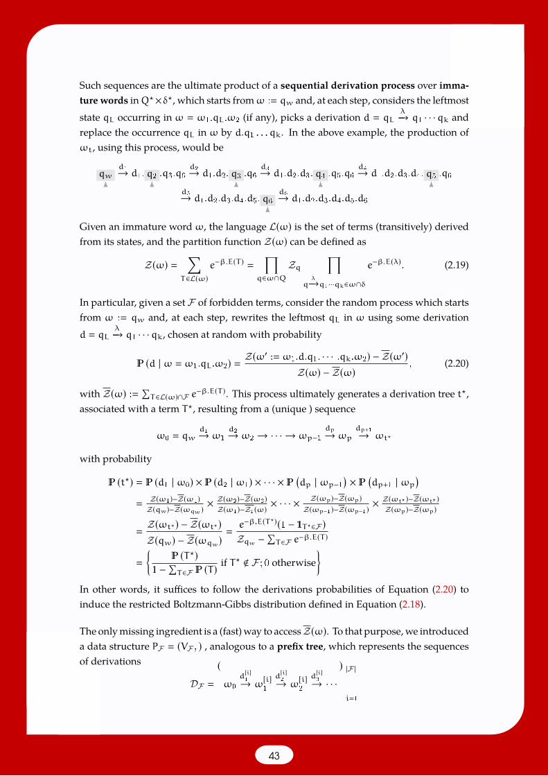
Such sequences are the ultimate product of a sequential derivation process over imma-turewords inQ?×δ?, which starts fromω : qw and, at each step, considers the leftmoststate qL occurring in ω ω1.qL.ω2 (if any), picks a derivation d qL

λ−→ q1 · · ·qk andreplace the occurrence qL in ω by d.q1 . . . qk. In the above example, the production ofωt, using this process, would be

qwd1→ d1. q2 .q3.q6

d2→ d1.d2. q3 .q6d3→ d1.d2.d3. q4 .q5.q6

d4→ d1.d2.d3.d4. q5 .q6

d5→ d1.d2.d3.d4.d5. q6d6→ d1.d2.d3.d4.d5.d6

Given an immature word ω, the language L(ω) is the set of terms (transitively) derivedfrom its states, and the partition function Z(ω) can be defined as

Z(ω) ∑

T∈L(ω)e−β.E(T )

∏q∈ω∩Q

Zq∏

qλ−→q1···qk∈ω∩δ

e−β.E(λ). (2.19)

In particular, given a set F of forbidden terms, consider the random process which startsfrom ω : qw and, at each step, rewrites the leftmost qL in ω using some derivationd qL

λ−→ q1 · · ·qk, chosen at random with probability

(d | ω ω1.qL.ω2) Z(ω′ : ω1.d.q1. · · · .qk.ω2) − Z(ω′)Z(ω) − Z(ω)

, (2.20)

with Z(ω) : ∑T∈L(ω)∩F e−β.E(T ). This process ultimately generates a derivation tree t?,

associated with a term T?, resulting from a (unique ) sequence

ω0 qwd1→ ω1

d2→ ω2 → · · · → ωp−1dp→ ωp

dp+1→ ωt?

with probability

(t?) (d1 | ω0) × (d2 | ω1) × · · · × (dp | ωp−1

) × (dp+1 | ωp

)

Z(ω1)−Z(ω1)Z(qw)−Z(ωqw )

× Z(ω2)−Z(ω2)Z(ω1)−Z1(ω) × · · · ×

Z(ωp)−Z(ωp)Z(ωp−1)−Z(ωp−1) ×

Z(ωt? )−Z(ωt? )Z(ωp)−Z(ωp)

Z(ωt?) − Z(ωt?)Z(qw) − Z(ωqw)

e−β.E(T?)(1 − 1T?∈F )Zqw −

∑T∈F e−β.E(T )

(T?)

1 −∑T∈F (T )

if T? < F ; 0 otherwise

In other words, it suffices to follow the derivations probabilities of Equation (2.20) toinduce the restricted Boltzmann-Gibbs distribution defined in Equation (2.18).

The onlymissing ingredient is a (fast)way to accessZ(ω). To that purpose, we introduceda data structure PF (VF , ) , analogous to a prefix tree, which represents the sequencesof derivations

DF

ω0

d[i]1→ ω

[i]1

d[i]2→ ω

[i]2

d[i]3→ · · ·

|F |i1

43

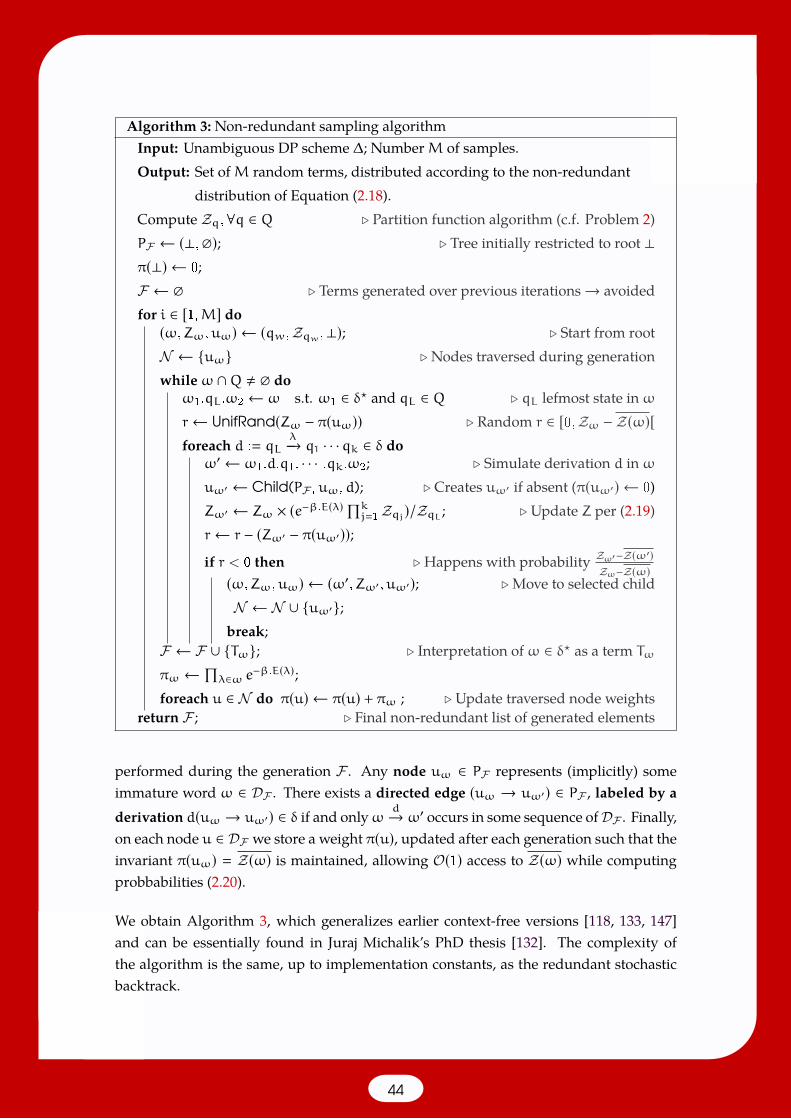
Algorithm 3: Non-redundant sampling algorithmInput: Unambiguous DP scheme ∆; NumberM of samples.Output: Set ofM random terms, distributed according to the non-redundant

distribution of Equation (2.18).Compute Zq,∀q ∈ Q . Partition function algorithm (c.f. Problem 2)PF ← (⊥,); . Tree initially restricted to root ⊥π(⊥) ← 0;F ← . Terms generated over previous iterations→ avoidedfor i ∈ [1,M] do(ω,Zω,uω) ← (qw,Zqw ,⊥); . Start from rootN ← uω . Nodes traversed during generationwhileω ∩Q , do

ω1.qL.ω2 ← ω s.t. ω1 ∈ δ? and qL ∈ Q . qL lefmost state inωr← UnifRand(Zω − π(uω)) . Random r ∈ [0,Zω − Z(ω)[foreach d : qL

λ−→ q1 · · ·qk ∈ δ doω′← ω1.d.q1. · · · .qk.ω2; . Simulate derivation d inωuω′ ← Child(PF ,uω,d); . Creates uω′ if absent (π(uω′) ← 0)Zω′ ← Zω × (e−β.E(λ)∏k

j1Zqj)/ZqL ; . Update Z per (2.19)r← r − (Zω′ − π(uω′));if r < 0 then . Happens with probability Zω′−Z(ω′)

Zω−Z(ω)(ω,Zω,uω) ← (ω′,Zω′,uω′); .Move to selected childN ← N ∪ uω′;break;

F ← F ∪ Tω; . Interpretation ofω ∈ δ? as a term Tω

πω ←∏λ∈ω e−β.E(λ);

foreach u ∈ N do π(u) ← π(u) + πω ; . Update traversed node weightsreturn F ; . Final non-redundant list of generated elements

performed during the generation F . Any node uω ∈ PF represents (implicitly) someimmature word ω ∈ DF . There exists a directed edge (uω → uω′) ∈ PF , labeled by aderivation d(uω → uω′) ∈ δ if and onlyω

d→ ω′ occurs in some sequence ofDF . Finally,on each node u ∈ DF we store a weight π(u), updated after each generation such that theinvariant π(uω) Z(ω) is maintained, allowing O(1) access to Z(ω) while computingprobbabilities (2.20).

We obtain Algorithm 3, which generalizes earlier context-free versions [118, 133, 147]and can be essentially found in Juraj Michalik’s PhD thesis [132]. The complexity ofthe algorithm is the same, up to implementation constants, as the redundant stochasticbacktrack.

44

Remark 2.3.1 (Rejection-based non-redundant sampling): In theuniformdistribution (β 0),a rejection-based sampling constitutes a reasonable alternative to produce M unique elements.Indeed, the search space is typically exponential |Ω| ≈ ζn for some ζ > 1. A classic coupon collectoranalysis shows that the expected number of generations to get |Ω| distinct elements, is |Ω|.H|Ω|with Hm

∑mi1 1/i ∈ Θ(logn) the m-th harmonic number. Moreover, the expected number of

generation is an increasing function ofM, and is bounded byM log |Ω| ∈ Θ(M.n). In other words,a repeated generation of elements until M distinct elements are produced has Θ(M.n) expectedtime in a uniform distribution, i.e. non-redundancy sampling only induces a linear overhead incomparison with the redundant one.In Boltzmann-Gibbs sampling, however, the overhead is expected to grow exponentially with n, soa rejection-based strategy is exponentially less efficient than Algorithm 3.

2.3.4 Adaptive sampling of constrained sequences [18, 90, 158]

As shown in Section 2.2.5, using explicit convolutions to compute the classified partitionfunction quickly becomes prohibitively costly when (combinations of) expressive scoringfunctions are considered. Unfortunately, such a computation would be required toperform a constrained sampling, by adapting the stochastic backtrack of Section 2.3.2 torestrict the generation to objects having a value of interest.

As an alternative, in collaboration with Olivier Bodini [18], we introduced a multidi-mensional Boltzmann sampling method, also called adaptive sampling in the contextof Bioinformatics applications [193] (due to the ubiquity of Boltzmann in Bionformatics,leading to an overloaded nomenclature). This method is inspired both by the versatilityof rejection methods in random generation (see Section 4.1), and by the typical concen-tration of distributions for additive parameters. This concentration is illustrated in 1D byFigure 2.1 for the number of base pairs in RNA, and in 2D by Figure 2.2 for two types ofbase pairs distinguishable in the basic Nussinov DP scheme.

Problem 9 (Constrained sampling):Input: Unambiguous DP scheme ∆ + scoring f, correct w.r.t. function E; β ∈ ;scoring functions F1, . . . , Fk : Λ → + with V : maxT∈T∆ F(T ) associated withobjective values v?

1, . . . , v?

k∈ k; and number of samplesM

Output: A collection C : [s1, . . . , sM] of random, Boltzmann-distributed w.r.t. E,elements ofΩ∆ such that

Fi(sj) v?i ,∀sj ∈ C,∀i ∈ [1,k]. (2.21)

Rather than computing the costly convolution products described in Equation (2.12), weintroduced a rejection based approach called multidimensional Boltzmann sampling,

45

Num. unstacked

(US) BPs

0

5

10

15

20

Num. maybe-stacked (MS) BPs0 10 20 30 40 50

Freq

uenc

y

0

200

400

600

800

1000

πUS 1, πMS 1

πUS 10, πMS 1

πUS 1, πMS 10

πUS 0, πMS 10

πUS 0, πMS 0

Figure 2.2: Impact of weights on the distribution of base pairs in RNA 2D folding.We distinguish maybe-stacked base pairs (MS), i.e. involving both ends (i, j) of aninvestigated interval [i, j] (alt. such that j+ 1 is base paired) from other base pairs, calledunstacked (US). Those two contributions can be distinguished on the classic Nussinov-Jacobson DP scheme, such that a weighted distribution can be induced.

whose principles are further described in Section 4.2.2. At its core, one uses aweightingschemewhere numerical values (π1, . . . ,πk) are associated to scoring functions, inducinga weighted distribution

π1,...,πk (T ) e−β.E(T )

∏ki1 π

Fi(T )i

Zπ1,...,πk

(2.22)

where Zπ1,...,πk is the weighted equivalent of the partition function.

Sampling within a weighted distribution can be done using Algorithm 2 based on aunifying scoring function E? that aggregates all the contributions of individual features,such that

E?(T ) :∑λ∈T

E(λ) −∑ki1 Fi(λ) × logπi

β E(T ) − Fi(T ) ×

∑ki1 logπi

β.

This generation is coupled with a rejection step, which filters out the objects that do notfulfill the constraints described in Equation (2.21).

A crucial observation is that, in many cases, the successive choices performed duringa stochastic backtrack can be interpreted as a large collection of independent events(i.e. occurrences of constructors), associated with bounded values of which the scor-ing functions are just the sum. The central limit theorem thus applies, and inducesdistributions that are (multidimensional) normal (a.k.a. Gaussian) with relatively lowvariance/co-variance values. In particular, once the weights are calibrated such that

µi : π1,...,πk (Fi(S)) v?i ,∀i ∈ [1,k],

46

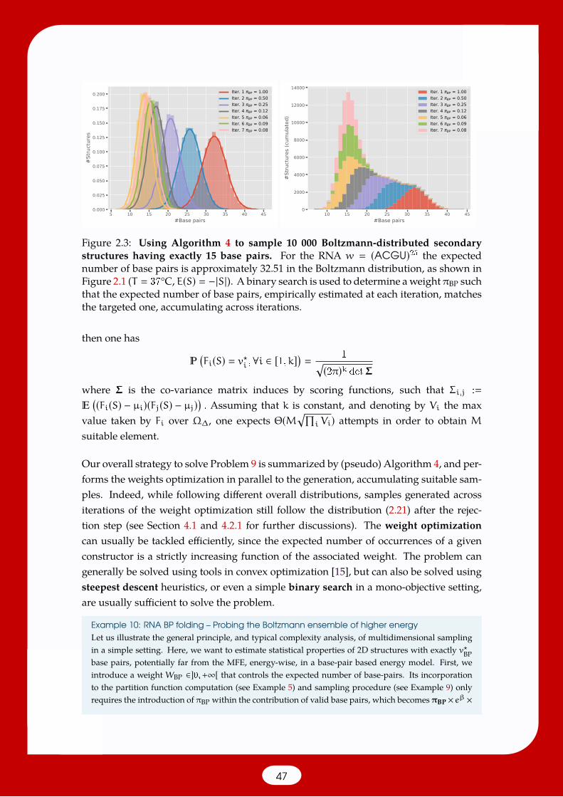
5 10 15 20 25 30 35 40 45#Base pairs

0.000

0.025

0.050

0.075

0.100

0.125

0.150

0.175

0.200#S

truct

ures

Iter. 1 BP = 1.00Iter. 2 BP = 0.50Iter. 3 BP = 0.25Iter. 4 BP = 0.12Iter. 5 BP = 0.06Iter. 6 BP = 0.09Iter. 7 BP = 0.08

10 15 20 25 30 35 40 45#Base pairs

0

2000

4000

6000

8000

10000

12000

14000

#Stru

ctur

es (c

umul

ated

)

Iter. 1 BP = 1.00Iter. 2 BP = 0.50Iter. 3 BP = 0.25Iter. 4 BP = 0.12Iter. 5 BP = 0.06Iter. 6 BP = 0.09Iter. 7 BP = 0.08

Figure 2.3: Using Algorithm 4 to sample 10 000 Boltzmann-distributed secondarystructures having exactly 15 base pairs. For the RNA w (ACGU)25 the expectednumber of base pairs is approximately 32.51 in the Boltzmann distribution, as shown inFigure 2.1 (T 37°C, E(S) −|S|). A binary search is used to determine aweight πBP suchthat the expected number of base pairs, empirically estimated at each iteration, matchesthe targeted one, accumulating across iterations.

then one has

(Fi(S) v?i ,∀i ∈ [1,k]

)

1√(2π)k detΣ

where Σ is the co-variance matrix induces by scoring functions, such that Σi,j :

((Fi(S) − µi)(Fj(S) − µj)) . Assuming that k is constant, and denoting by Vi the max

value taken by Fi over Ω∆, one expects Θ(M√∏i Vi) attempts in order to obtain M

suitable element.

Our overall strategy to solve Problem 9 is summarized by (pseudo) Algorithm 4, and per-forms the weights optimization in parallel to the generation, accumulating suitable sam-ples. Indeed, while following different overall distributions, samples generated acrossiterations of the weight optimization still follow the distribution (2.21) after the rejec-tion step (see Section 4.1 and 4.2.1 for further discussions). The weight optimizationcan usually be tackled efficiently, since the expected number of occurrences of a givenconstructor is a strictly increasing function of the associated weight. The problem cangenerally be solved using tools in convex optimization [15], but can also be solved usingsteepest descent heuristics, or even a simple binary search in a mono-objective setting,are usually sufficient to solve the problem.

Example 10: RNA BP folding – Probing the Boltzmann ensemble of higher energyLet us illustrate the general principle, and typical complexity analysis, of multidimensional samplingin a simple setting. Here, we want to estimate statistical properties of 2D structures with exactly v?BPbase pairs, potentially far from the MFE, energy-wise, in a base-pair based energy model. First, weintroduce a weight WBP ∈]0,+∞[ that controls the expected number of base-pairs. Its incorporationto the partition function computation (see Example 5) and sampling procedure (see Example 9) onlyrequires the introduction of πBP within the contribution of valid base pairs, which becomes πBP × eβ ×

47

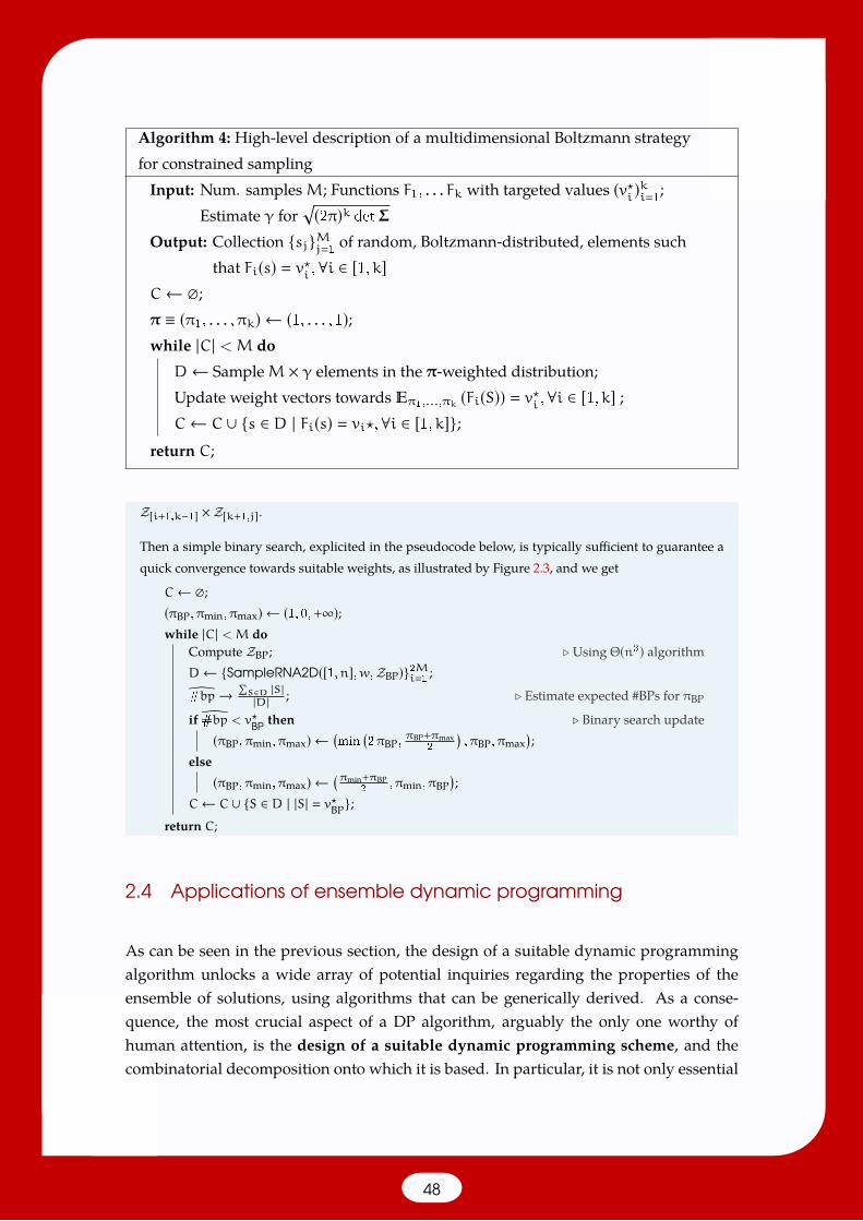
Algorithm 4: High-level description of a multidimensional Boltzmann strategyfor constrained samplingInput: Num. samplesM; Functions F1, . . . Fk with targeted values (v?

i)ki1

;Estimate γ for

√(2π)k detΣ

Output: Collection sjMj1 of random, Boltzmann-distributed, elements suchthat Fi(s) v?i ,∀i ∈ [1,k]

C← ;π ≡ (π1, . . . ,πk) ← (1, . . . , 1);while |C| < M do

D← SampleM × γ elements in the π-weighted distribution;Update weight vectors towards π1,...,πk (Fi(S)) v?i ,∀i ∈ [1,k] ;C← C ∪ s ∈ D | Fi(s) vi?,∀i ∈ [1,k];

return C;

Z[i+1,k−1] ×Z[k+1,j].

Then a simple binary search, explicited in the pseudocode below, is typically sufficient to guarantee aquick convergence towards suitable weights, as illustrated by Figure 2.3, and we get

C← ;(πBP,πmin,πmax) ← (1, 0,+∞);while |C| < M do

Compute ZBP; . Using Θ(n3) algorithmD← SampleRNA2D([1,n],w,ZBP)2Mi1 ;#bp→ ∑

S∈D |S||D| ; . Estimate expected #BPs for πBP

if #bp < v?BP then . Binary search update(πBP,πmin,πmax) ←

(min

(2πBP,

πBP+πmax2

),πBP,πmax

);

else(πBP,πmin,πmax) ←

(πmin+πBP2

,πmin,πBP);

C← C ∪ S ∈ D | |S| v?BP;return C;

2.4 Applications of ensemble dynamic programming

As can be seen in the previous section, the design of a suitable dynamic programmingalgorithm unlocks a wide array of potential inquiries regarding the properties of theensemble of solutions, using algorithms that can be generically derived. As a conse-quence, the most crucial aspect of a DP algorithm, arguably the only one worthy ofhuman attention, is the design of a suitable dynamic programming scheme, and thecombinatorial decomposition onto which it is based. In particular, it is not only essential

48

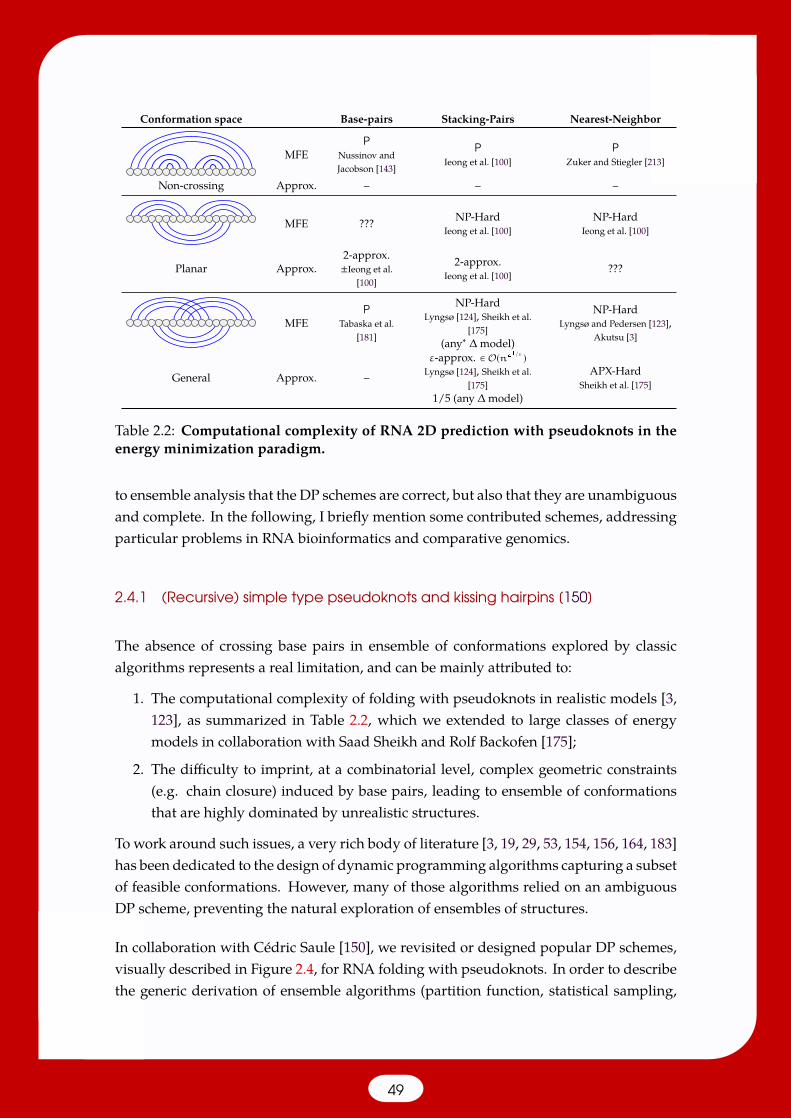
Conformation space Base-pairs Stacking-Pairs Nearest-Neighbor

MFEP

Nussinov andJacobson [143]

PIeong et al. [100]

PZuker and Stiegler [213]

Non-crossing Approx. – – –

MFE ??? NP-HardIeong et al. [100]

NP-HardIeong et al. [100]

Planar Approx.2-approx.±Ieong et al.

[100]

2-approx.Ieong et al. [100]

???

MFEP

Tabaska et al.[181]

NP-HardLyngsø [124], Sheikh et al.

[175](any∗ ∆model)

NP-HardLyngsø and Pedersen [123],

Akutsu [3]

General Approx. –

ε-approx. ∈ O(n41/ε )Lyngsø [124], Sheikh et al.

[175]1/5 (any ∆model)

APX-HardSheikh et al. [175]

Table 2.2: Computational complexity of RNA 2D prediction with pseudoknots in theenergy minimization paradigm.

to ensemble analysis that the DP schemes are correct, but also that they are unambiguousand complete. In the following, I briefly mention some contributed schemes, addressingparticular problems in RNA bioinformatics and comparative genomics.

2.4.1 (Recursive) simple type pseudoknots and kissing hairpins [150]

The absence of crossing base pairs in ensemble of conformations explored by classicalgorithms represents a real limitation, and can be mainly attributed to:

1. The computational complexity of folding with pseudoknots in realistic models [3,123], as summarized in Table 2.2, which we extended to large classes of energymodels in collaboration with Saad Sheikh and Rolf Backofen [175];

2. The difficulty to imprint, at a combinatorial level, complex geometric constraints(e.g. chain closure) induced by base pairs, leading to ensemble of conformationsthat are highly dominated by unrealistic structures.

To work around such issues, a very rich body of literature [3, 19, 29, 53, 154, 156, 164, 183]has been dedicated to the design of dynamic programming algorithms capturing a subsetof feasible conformations. However, many of those algorithms relied on an ambiguousDP scheme, preventing the natural exploration of ensembles of structures.

In collaboration with Cédric Saule [150], we revisited or designed popular DP schemes,visually described in Figure 2.4, for RNA folding with pseudoknots. In order to describethe generic derivation of ensemble algorithms (partition function, statistical sampling,

49

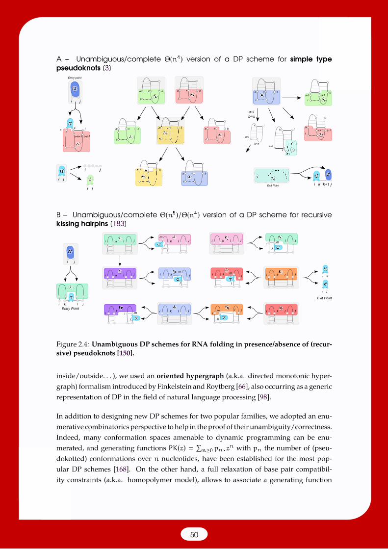
A – Unambiguous/complete Θ(n4) version of a DP scheme for simple typepseudoknots [3]

a x b

i

a x b

i

a x b

i

a x b

i

a x b

i

a

b=j-1

i

k j

Entry point

x=k+1

ji

a x b

i

b-1x+1i

a

a-1 x+1b

i

i j

i j

i ji k k+1 jExit Point

a=i

k j

x

b=x

a=i

a=i

k j

b=x

B – Unambiguous/complete Θ(n5)/Θ(n4) version of a DP scheme for recursivekissing hairpins [183]

ji

i jk l i jk l

i jk l

i jk l i jk l

i jk l

Entry Point

i jk l

i

j

l mk

mjk l

ii

jlm

k

i jk

l

mi jk

l

m

ijlm

k

i k

l j

Exit Point

Figure 2.4: Unambiguous DP schemes for RNA folding in presence/absence of (recur-sive) pseudoknots [150].

inside/outside. . . ), we used an oriented hypergraph (a.k.a. directed monotonic hyper-graph) formalism introduced by Finkelstein andRoytberg [66], also occurring as a genericrepresentation of DP in the field of natural language processing [98].

In addition to designing new DP schemes for two popular families, we adopted an enu-merative combinatorics perspective to help in theproof of their unambiguity/correctness.Indeed, many conformation spaces amenable to dynamic programming can be enu-merated, and generating functions PK(z) ∑

n≥0 pn, zn with pn the number of (pseu-dokotted) conformations over n nucleotides, have been established for the most pop-ular DP schemes [168]. On the other hand, a full relaxation of base pair compatibil-ity constraints (a.k.a. homopolymer model), allows to associate a generating function

50

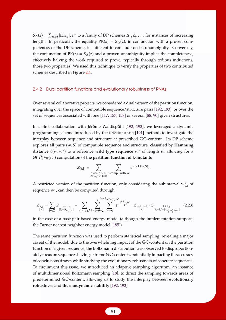
S∆(z) ∑n≥0 |Ω∆n |, zn to a family of DP schemes ∆1,∆2, . . . for instances of increasing

length. In particular, the equality PK(z) S∆(z), in conjunction with a proven com-pleteness of the DP scheme, is sufficient to conclude on its unambiguity. Conversely,the conjunction of PK(z) S∆(z) and a proven unambiguity implies the completeness,effectively halving the work required to prove, typically through tedious inductions,those two properties. We used this technique to verify the properties of two contributedschemes described in Figure 2.4.

2.4.2 Dual partition functions and evolutionary robustness of RNAs

Over several collaborative projects, we considered a dual version of the partition function,integrating over the space of compatible sequence/structure pairs [192, 193], or over theset of sequences associated with one [117, 157, 158] or several [88, 90] given structures.

In a first collaboration with Jérôme Waldispühl [192, 193], we leveraged a dynamicprogramming scheme introduced by the RNAMutants [191] method, to investigate theinterplay between sequence and structure at prescribed GC-content. Its DP schemeexplores all pairs (w,S) of compatible sequence and structure, classified by Hammingdistance δ(w,w?) to a reference wild type sequence w? of length n, allowing for aΘ(n5)/Θ(n3) computation of the partition function of k-mutants

Z[k] :∑

w∈Σn s. t.δ(w,w?)k

∑S comp. withw

e−β.E(w,S).

A restricted version of the partition function, only considering the subinterval w?i,j

ofsequence w?, can then be computed through

Zi,j[k]

∑b∈Σ

Z i+1,j[k−δw?

i,b]

+

∑b,b′∈Σ2

j∑li+θ+1

k−δw?iw?l,bb′∑

k′0e−

β.Eb,b′RT · Zi+1,l−1

[k′]· Z l+1,j[k−k′−δw?

iw?l,bb′]

(2.23)

in the case of a base-pair based energy model (although the implementation supportsthe Turner nearest-neighbor energy model [185]).

The same partition function was used to perform statistical sampling, revealing a majorcaveat of the model: due to the overwhelming impact of the GC-content on the partitionfunction of a given sequence, the Boltzmann distribution was observed to disproportion-ately focus on sequences having extremeGC-contents, potentially impacting the accuracyof conclusions drawn while studying the evolutionary robustness of concrete sequences.To circumvent this issue, we introduced an adaptive sampling algorithm, an instanceof multidimensional Boltzmann sampling [18], to direct the sampling towards areas ofpredetermined GC-content, allowing us to study the interplay between evolutionaryrobustness and thermodynamic stability [192, 193].

51

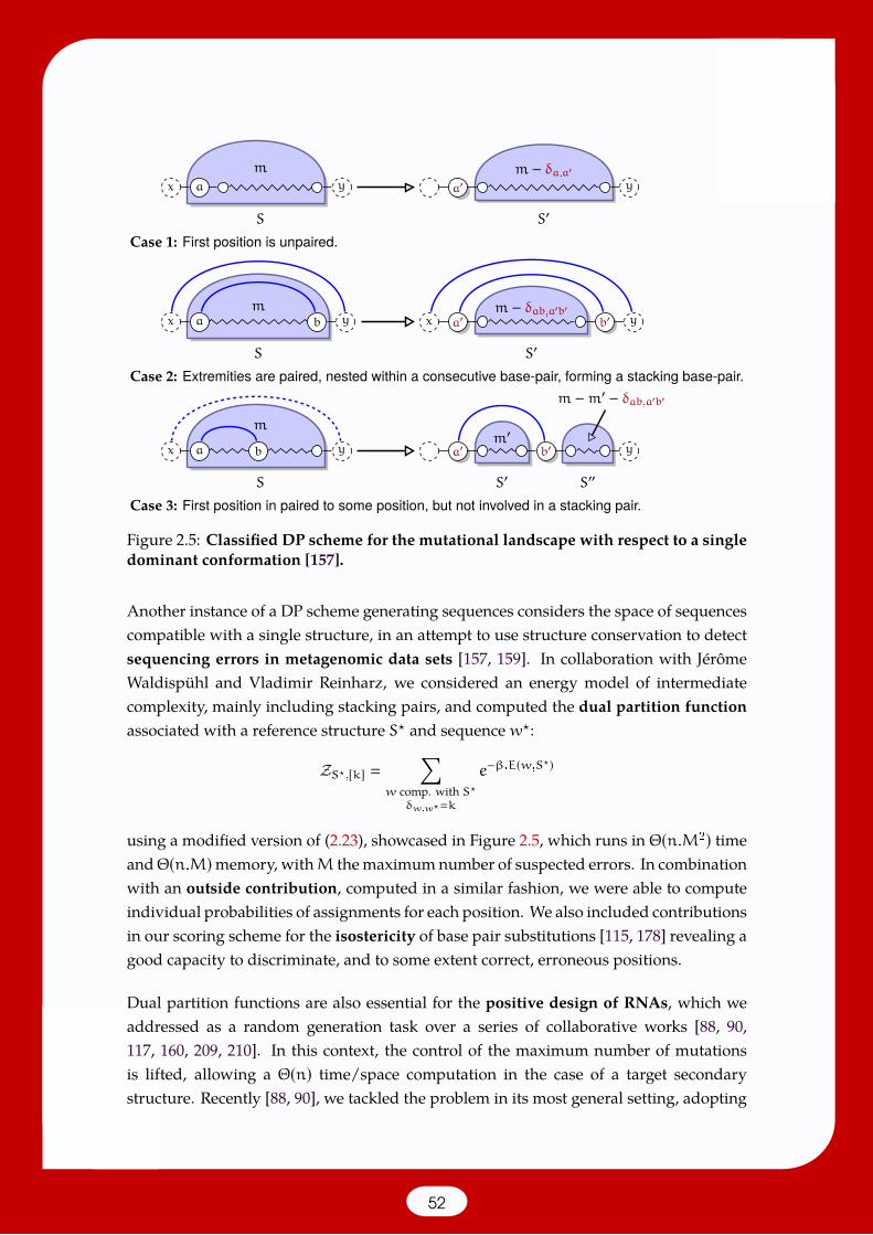
ax y

m

Case 1: First position is unpaired.

a′ y

m − δa,a′

a bx ym

Case 2: Extremities are paired, nested within a consecutive base-pair, forming a stacking base-pair.

a′ b′x ym − δab,a′b′

a bx y

m

Case 3: First position in paired to some position, but not involved in a stacking pair.

a′ b′ ym′

S

S

S

S′

S′

S′ S′′

m −m′ − δab,a′b′

Figure 2.5: Classified DP scheme for the mutational landscape with respect to a singledominant conformation [157].

Another instance of a DP scheme generating sequences considers the space of sequencescompatible with a single structure, in an attempt to use structure conservation to detectsequencing errors in metagenomic data sets [157, 159]. In collaboration with JérômeWaldispühl and Vladimir Reinharz, we considered an energy model of intermediatecomplexity, mainly including stacking pairs, and computed the dual partition functionassociated with a reference structure S? and sequence w?:

ZS?,[k] ∑

w comp. with S?δw,w?k

e−β.E(w,S?)

using a modified version of (2.23), showcased in Figure 2.5, which runs in Θ(n.M2) timeandΘ(n.M)memory, withM themaximumnumber of suspected errors. In combinationwith an outside contribution, computed in a similar fashion, we were able to computeindividual probabilities of assignments for each position. We also included contributionsin our scoring scheme for the isostericity of base pair substitutions [115, 178] revealing agood capacity to discriminate, and to some extent correct, erroneous positions.

Dual partition functions are also essential for the positive design of RNAs, which weaddressed as a random generation task over a series of collaborative works [88, 90,117, 160, 209, 210]. In this context, the control of the maximum number of mutationsis lifted, allowing a Θ(n) time/space computation in the case of a target secondarystructure. Recently [88, 90], we tackled the problem in its most general setting, adopting

52

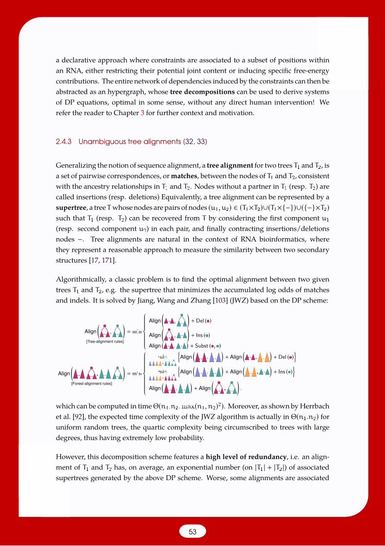
a declarative approach where constraints are associated to a subset of positions withinan RNA, either restricting their potential joint content or inducing specific free-energycontributions. The entire network of dependencies induced by the constraints can then beabstracted as an hypergraph, whose tree decompositions can be used to derive systemsof DP equations, optimal in some sense, without any direct human intervention! Werefer the reader to Chapter 3 for further context and motivation.

2.4.3 Unambiguous tree alignments [32, 33]

Generalizing the notion of sequence alignment, a tree alignment for two trees T1 and T2, isa set of pairwise correspondences, ormatches, between the nodes of T1 and T2, consistentwith the ancestry relationships in T1 and T2. Nodes without a partner in T1 (resp. T2) arecalled insertions (resp. deletions) Equivalently, a tree alignment can be represented by asupertree, a tree T whosenodes are pairs of nodes (u1,u2) ∈ (T1×T2)∪(T1×−)∪(−×T2)such that T1 (resp. T2) can be recovered from T by considering the first component u1(resp. second component u2) in each pair, and finally contracting insertions/deletionsnodes −. Tree alignments are natural in the context of RNA bioinformatics, wherethey represent a reasonable approach to measure the similarity between two secondarystructures [17, 171].

Algorithmically, a classic problem is to find the optimal alignment between two giventrees T1 and T2, e.g. the supertree that minimizes the accumulated log odds of matchesand indels. It is solved by Jiang, Wang and Zhang [103] (JWZ) based on the DP scheme:

Align(

,

)[Tree-alignment rules]

min

Align(

,

)+ Del ( )

Align(

,

)+ Ins ( )

Align(

,)+ Subst ( , )

Align(

,

)[Forest-alignment rules]

min

min=

Align

(,

)+ Align

(,

)+ Del ( )

min

=

Align

(,

)+ Align

(,

)+ Ins ( )

Align(

,

)+ Align

(,

).

which can be computed in timeΘ(n1.n2. max(n1,n2)2). Moreover, as shown byHerrbachet al. [92], the expected time complexity of the JWZ algorithm is actually in Θ(n1.n2) foruniform random trees, the quartic complexity being circumscribed to trees with largedegrees, thus having extremely low probability.

However, this decomposition scheme features a high level of redundancy, i.e. an align-ment of T1 and T2 has, on average, an exponential number (on |T1 | + |T2 |) of associatedsupertrees generated by the above DP scheme. Worse, some alignments are associated

53

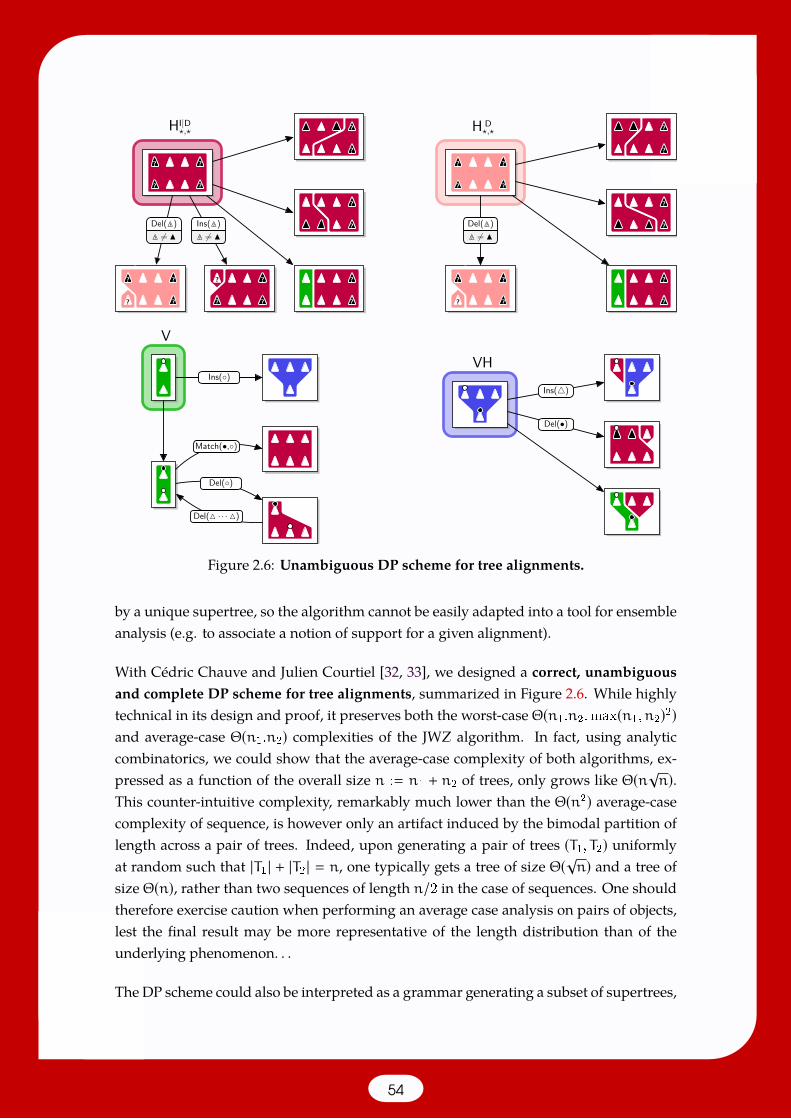
HI|D?,?

?

?

?

?

?

?

?

?

?

?

?

??

?

??

?

?

?? ?

??

Ins(M? )M? 6= N

Del(M? )M? 6= N

?

?

?

?

H D?,? ?

?

?

?

?

?

?

?

?

?

Del(M? )M? 6= N

V

Del()

Del(M · · · M)

Match(•,)

Ins()VH

Del(•)

Ins(4)

Figure 2.6: Unambiguous DP scheme for tree alignments.

by a unique supertree, so the algorithm cannot be easily adapted into a tool for ensembleanalysis (e.g. to associate a notion of support for a given alignment).

With Cédric Chauve and Julien Courtiel [32, 33], we designed a correct, unambiguousand complete DP scheme for tree alignments, summarized in Figure 2.6. While highlytechnical in its design and proof, it preserves both the worst-case Θ(n1.n2. max(n1,n2)2)and average-case Θ(n1.n2) complexities of the JWZ algorithm. In fact, using analyticcombinatorics, we could show that the average-case complexity of both algorithms, ex-pressed as a function of the overall size n : n1 + n2 of trees, only grows like Θ(n√n).This counter-intuitive complexity, remarkably much lower than the Θ(n2) average-casecomplexity of sequence, is however only an artifact induced by the bimodal partition oflength across a pair of trees. Indeed, upon generating a pair of trees (T1, T2) uniformlyat random such that |T1 | + |T2 | n, one typically gets a tree of size Θ(√n) and a tree ofsize Θ(n), rather than two sequences of length n/2 in the case of sequences. One shouldtherefore exercise caution when performing an average case analysis on pairs of objects,lest the final result may be more representative of the length distribution than of theunderlying phenomenon. . .

The DP scheme could also be interpreted as a grammar generating a subset of supertrees,

54

bĳectively associated with tree alignments, and we used analytic combinatorics tech-niques to derive asymptotic properties of alignments (e.g. average #matches, number. . . ).The same could be done for the (redundant) family of supertrees produced by the JWZDP scheme, and taking the ratio gave the expected number of supertrees, generated byJWZ for each alignment, confirming the exponential level of ambiguity.

55

Chapter 3

RNA design

Thegoodperformances ofRNAstructureprediction, especially at the secondary structurelevel, suggest harnessing their underlying models and methods to perform a rationaldesign of RNAs, broadly defined here as the construction of novel nucleotide sequencesachieving one (or several) predefined function(s). In the context of my work, a strongemphasis is put on the development of computational methods for an automated RNAdesign.

The originality of my contributions, spanning several distinct collaborations, lies in theadoption of a random generation perspective over the positive and, to some extent,negative design of RNA. Additionally, I have attempted to revisit negative design ina minimal setting, amenable to exact (if partial) combinatorial analysis, uncovering apromising, yet unexploited, notion of approximate design, that could lead to futuredevelopments.

Outline. I first describe in Section 3.1 the motivation, and various use-cases for RNAdesign. Section 3.2 describes partial exact solutions for a combinatorial version of theNP-hard inverse folding. Finally, Section 3.3 presents an original contribution to positivedesign based on a constrained random generation, surprisingly providing a satisfactoryinitialization steps for negative design.



A. Levin, M. Lis, Y. Ponty, C. W. O’Donnell, S. Devadas, B. Berger, and J. Waldispühl. A global sampling approachto designing and reengineering RNA secondary structures. Nucleic Acids Research, 40(20):10041–10052, Nov.2012

56

Y. Zhou, Y. Ponty, S. Vialette, J. Waldispühl, Y. Zhang, and A. Denise. Flexible RNA design under structure andsequence constraints using formal languages. In ACM-BCB 2013, Bethesda, Washigton DC, United States, Sept.2013

V. Reinharz, Y. Ponty, and J. Waldispühl. A weighted sampling algorithm for the design of RNA sequences withtargeted secondary structure and nucleotide distribution. Bioinformatics, 29(13):i308–15, July 2013

V. Reinharz, Y. Ponty, and J. Waldispühl. A weighted sampling algorithm for the design of RNA sequences with targetedsecondary structure and nucleotides distribution. In ISMB/ECCB 2013, Berlin, Germany, July 2013

Y. Zhang, Y. Ponty, M. Blanchette, E. Lecuyer, and J. Waldispühl. SPARCS: a web server to analyze (un)structuredregions in coding RNA sequences. Nucleic Acids Research, 41(Web Server issue):W480–5, July 2013

M. Drory Retwitzer, V. Reinharz, Y. Ponty, J. Waldispühl, and D. Barash. incaRNAfbinv : a web server for thefragment-based design of RNA sequences. Nucleic Acids Research, 44(W1):W308 – W314, 2016

J. Hales, A. Héliou, J. Manuch, Y. Ponty, and L. Stacho. Combinatorial RNA Design: Designability and Structure-ApproximatingAlgorithm inWatson-Crick andNussinov-Jacobson EnergyModels. Algorithmica, 79(3):835–856,2017

J.Hales, J.Manuch, Y. Ponty, andL. Stacho. Combinatorial RNADesign:Designability andStructure-ApproximatingAlgorithm.In CPM 2015, Ischia Island, Italy, June 2015

A. Churkin, M. D. Retwitzer, V. Reinharz, Y. Ponty, J. Waldispühl, and D. Barash. Design of RNAs: comparingprograms for inverse RNA folding. Briefings in Bioinformatics, 19(2):350–358, Jan. 2018



H.-T. Yao, C. Chauve, M. Regnier, and Y. Ponty. Exponentially few RNA structures are designable. In ACM-BCB2019, pages 289–298, Niagara-Falls, United States, 2019. ACM Press

57

3.1 Why do we design RNAs?

At a fundamental level, designing RNAs represents the ultimate stress-test for our un-derstanding of how RNA folds and acts on its environment. In this setting, one designsRNA sequences expected to fold into a predefined structure with respect to a folding pre-diction model. Synthesizing the resulting sequences, and using experimental methodsto verify the actual adoption of the desired structure, one either validates the model orreveals some of its flaws, fueling and prioritizing further developments. Indeed, misfold-ing designedRNAs reveal gaps in our energymodels and descriptors of the conformationspaces used by predictive algorithms. A similar strategy can be more generally used totest functional hypotheses involving the structure of RNA.

Molecular design also represents one of the primitives of synthetic biology, and RNAshave been used as biosensors [65], regulators, nano-material. . . Some naturally-occurringRNAs are sufficiently stable to fold in a modular fashion, enabling a copy/paste approachthat simply combines existing RNAs. However, such a strategy is hindered, in an invivo context, by the competition of artificial and endogenous RNAs, and by the intrinsicdifficulty to produce orthogonal constructs over a limited number of available architec-tures. A rational design, coupled with an experimental filtering phase, is thus likely torepresent the method of choice for future endeavors in RNA-based synthetic biology.

At a (primarily) sequence-based level, design is essential for future developments ofRNA-based therapeutics. For instance, the recent discovery of viable treatments basedon RNA interference is fueled by an understanding of how small RNAs can interfere withselected messenger RNAs to activate or inhibit them. In this context, an optimizationof the nucleotide sequence of small interfering RNAs, akin to a design task, is crucialto ensure its efficacy and selectivity, mitigating the risk of side-effects for the drugs.Similarly, the specificity of genetic contents targeted by CRISPR-based editing, an thusits limited toxicity, is ensured by a redesign of guide RNAs. More generally, the adoptionof a stable structure is very often a prerequisite for the interaction of RNAs with selectedproteins [45], and are therefore crucial for the functionality of designedRNAs in a cellularcontext.

Design also helps in the search for homologousRNAs. Indeed, inmultiple RNA families,selective pressure mostly applies at the structure level, hindering the discovery of newoccurrences of a givenRNAgeneswithin the sameorganism (paralogs) or across availablegenomes (orthologs). If a structural model is known, and if the number of identifiedhomologs is limited, a natural approach is to enrich homologs with sequences designedas to fold into the shared structure, in order to cover a larger proportion of the (neutral)sequence space.

58

3.1.1 The potential of RNA design for statistical evolutionary studies

I believe that RNA design should be systematically used within families of structuredRNAs to assess the significance of observed phenomena. Indeed, a popular strategyconsists in analyzing multiple sequence alignments of RNAs, and interpret quantitativeobservations in the light of an accepted pressures. To that purpose, one uses statisticaltests to refute the hypothesis that the observation is merely induced by establishedproperties. For instance, in the context of messenger RNAs, codon bias and the flankingof ORFs by start/stop codons should be accounted for when drawing consequences fromthe distribution of k-mers.

However, in the context of structural RNAs, most analyses only indirectly capture theoverall stability (free-energy) of transcripts through a preservation of the dinucleotidecontent, based on the observation that sequences sharing a dinucleotide compositiontend to have similar free-energy in their most stable 2D conformation. However, noth-ing prevents alternative dinucleotides compositions from achieving the same expectedfree-energy, so the distribution considered by classic tests is arguably too narrow to con-vincingly refute the hypothesis that an observed phenomenon can be imputed to theoverall MFE stability (rather than be indicative of a new, yet to be explained, selectivepressure).

Moreover, most families of functional RNAs not only share a comparable stability, butalso share the adoption of a common functional structure. In this context, the significanceof a property (e.g. overrepresentation of a motif, hypothesized as involved in amolecularrecognition mechanism) should be assessed within the set of sequences that are believedfold into the common structure (+ additional established properties). In other words,one should be able to perform a random generation of RNA designs in order to suitablyassess a notion of significance.

3.1.2 The different flavors of RNA design

RNA design targets a wide diversity of biological functions and, as such, encompassesof wide array of computational tasks. Two dominant paradigms dominate current com-putational approaches.

3.1.2.1 Positive design

Positive design can be loosely defined as focusing on to propensity of produced RNAsto achieve a certain function. In a structural context, positive design usually involves

59

generating one or several sequences having good affinity (i.e. stability ≈minimum free-energy) towards a targeted structure. Amore functional perspectivewill also consider thepresence/absence of sequences motifs, or the affinity towards interacting with anothermolecule, as assessed by an energymodel (e.g. RNA/DNAorRNA/RNA interactions) ora probabilistic model (e.g. protein/RNA interactions). This may include compositionalbiases, such as the GC-content.

3.1.2.2 Negative design

Negative design tasks loosely focus on the specificity of produced sequences, attemptingto avoid unwanted functions, interactions, structures. . . From a computational perspec-tive, such tasks are usually harder than the one induced by positive design. Indeed,they typically require solving an inverse combinatorial problem, generally formulatedas follows.

Problem 10 (Inverse combinatorial problem):Input: Expected output y? and objective function f.

Output: Instance x such thaty | f(y; x) max

y′f(y′; x)

y?.

The difficulty of those problems stems from the potential difficulty of optimizing theobjective function, so that the natural decision version of the problem may not evenbelong in NP. Moreover, even when the optimization (coupled with the production of acertificate for the unicity of the optimal solution) can be performed in polynomial time,the inverse problem can still be NP-hard [20].

In the context of structural RNA design, negative design is usually referred to as theinverse folding problem, and historically consists in producing a nucleotide sequence,predicted to (uniquely) fold into a targeted structure with respect to the Minimum Free-Energy (MFE) criterion. Variants of the inverse folding problem consider the minimiza-tion of various notions of defects, including the: MFE defect, the free-energy differencebetween the target andMFE structure (or first suboptimal structure if the target andMFEstructures coincide); probability defect, the Boltzmann probability for the sequence toadopt an alternative structure; or the ensemble defect, the expected base-pair distancebetween the target and a random structure in the Boltzmann-Gibbs distribution.

60

3.1.2.3 Computational approaches

Due to the robust NP-hardness of inverse folding [20, 91, 172], the dominant paradigm,shared by multiple computational approaches [7, 9, 28, 77, 89, 95, 116, 208], combinean initial generation of seed sequences, akin to a (sometimes very rudimentary) positivedesign, with further rounds of optimizationusing a local search. Inverse folding has alsobeen tackled using a variety of metaheuristics, including genetic algorithms [63, 64, 125],ant-colony optimization [107]. . .

Finally, the imperfect nature of the objectives of RNA design has left the door open formachine learning, recently attracting the predatory attention of neural networks [166]and/or crowdsourcing [109], with modest performances and disputable rationales.

3.2 Exact combinatorial negative design [85, 86]

The computational hardness of inverse folding, which had essentially eluded a wholecommunity for almost three decades, was finally rigorously established in 2018 by Bonnetet al. [20].

It was preceded by an effort worthy of a mention by Schnall-Levin et al. [172], whogeneralized the RNA design problem into the inverse Viterbi problem, consisting offiguring out a sequence w, in a probabilistic grammar such as a e.g. Hidden MarkovModel (HMMs) or a Stochastic Context-Free Grammar (SCFG), such that a predefinedsequence of states is themost likely parsing forw. The problemwas found to be NP-hard,even for HMMs, leading the authors to argue on an implied hardness of RNA design,since RNA folding can be viewed as a special case of SCFG parsing. However, while thehardness of the inverse Viterbi problem for SCFGs clearly follows from their result, it didnot imply the hardness of the problem for a given input grammar, as is the case in RNAdesign.

Over the course of a collaboration with Jozef Hales, Alice Héliou, Jan Manuch andLadislav Stacho [85, 86], we investigated aminimal installment of negative design, aimingto provide partial characterization for the space of designable structures. Namely, weconsider the Watson-Crick energy model, initially restricting admissible base pairs toA,U and G,C. In this restricted context, inverse folding greatly simplifies and weget the following formulation.

61

Problem 11 (Watson-Crick combinatorial design):Input: Secondary Structure S? over n nucleotides

Output: Sequence w such that

∀S ∈ Sn compatible with w,S , S? : |S| < |S? |.

Bonnet et al. [20] showed that a slightly restricted version of the problem, forcing theassignment of predefined nucleotides to positions inw, is NP-hard. We thus focused ourefforts on characterizing of designable subclasses of structures.

3.2.1 Basic results

Our results require a reminder of the representation for the secondary structure, illus-trated in Figure 3.1. Such a representation abstracts a structure as a tree, rooted in avirtual node, with other nodes either being base-pairs nodes (labeled by interacting po-sitions) or unpaired nodes positions (labeled by a single position). We define the innerdegree of a node as its number of base pair neighbors. For instance, the node 4-37 inFigure 3.1 has inner degree 3.

Theorem 1 (Basic designable classes): Any structure S, represented as a tree, candesigned in linear time as soon as (at least one) of the following conditions is met:

1. Each node in S has inner degree at most two;

2. S is saturated (no unpaired base) + any node has inner degree at most four;

Moreover,weestablished that the set ofdesignable structures is closedunderk-stuttering.In otherwords, if a structure S, represented as a dot-parenthesisword S1.S2 . . . Sn, admitsa known design w : w1.w2 . . . wn, then

wk1 .wk2 . . . w

kn is a design for Sk1 .S

k2 . . . S

kn,∀k > 0.

The stuttering operation can also be described at the tree level, and essentially (up torenumbering of nodes) amounts to: i) duplicating each unpaired node k times; and ii)replacing any base pair node with a sequence of base pair nodes of length k.

We also identified two undesignable motifs, a.k.a. local obstructions , whose presenceis sufficient to forbid any design for the structure. Namely, it is probably impossibleto design any structure containing a multiloop with degree ≥ 5 (m5 motif), or withdegree ≥ 3 with ≥ 1 unpaired base(s) (m3 motif). Such motifs are universal to anyversion of design, as they are essentially a consequence of the local nature of classic

62

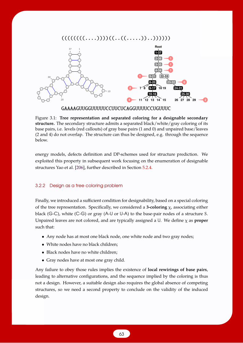
1

1

1

1

2

4

0

2

Root

1-37

2-36

3-35

4-34

5-21

6-20

7 8 9-17

10-16

11 12 13 14 15

18 19

22-33

23-32

24-31

25-30

26 27 28 29

1

10

20

30

37

((((((((....))))((..((.....))..))))))

GAAAAGUUGGUUUUUCCUUCUCAGGUUUUCCUGUUUC

Figure 3.1: Tree representation and separated coloring for a designable secondarystructure. The secondary structure admits a separated black/white/gray coloring of itsbase pairs, i.e. levels (red callouts) of gray base pairs (1 and 0) and unpaired base/leaves(2 and 4) do not overlap. The structure can thus be designed, e.g. through the sequencebelow.

energy models, defects definition and DP-schemes used for structure prediction. Weexploited this property in subsequent work focusing on the enumeration of designablestructures Yao et al. [206], further described in Section 5.2.4.

3.2.2 Design as a tree coloring problem

Finally, we introduced a sufficient condition for designability, based on a special coloringof the tree representation. Specifically, we considered a 3-coloring χ, associating eitherblack (G-C), white (C-G) or gray (A-U or U-A) to the base-pair nodes of a structure S.Unpaired leaves are not colored, and are typically assigned a U. We define χ as propersuch that:

• Any node has at most one black node, one white node and two gray nodes;

• White nodes have no black children;

• Black nodes have no white children;

• Gray nodes have at most one gray child.

Any failure to obey those rules implies the existence of local rewirings of base pairs,leading to alternative configurations, and the sequence implied by the coloring is thusnot a design. However, a suitable design also requires the global absence of competingstructures, so we need a second property to conclude on the validity of the induceddesign.

63

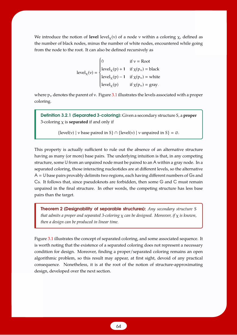
We introduce the notion of level levelχ(v) of a node v within a coloring χ, defined asthe number of black nodes, minus the number of white nodes, encountered while goingfrom the node to the root. It can also be defined recursively as

levelχ(v)

0 if v Root

levelχ(p) + 1 if χ(pv) black

levelχ(p) − 1 if χ(pv) white

levelχ(p) if χ(pv) gray.

where pv denotes the parent of v. Figure 3.1 illustrates the levels associatedwith a propercoloring.

Definition 3.2.1 (Separated 3-coloring):Given a secondary structure S, aproper3-coloring χ is separated if and only if

level(v) | v base paired in S ∩ level(v) | v unpaired in S .

This property is actually sufficient to rule out the absence of an alternative structurehaving as many (or more) base pairs. The underlying intuition is that, in any competingstructure, some U from an unpaired nodemust be paired to an A within a gray node. In aseparated coloring, those interacting nucleotides are at different levels, so the alternativeA U base pairs provably delimits two regions, each having different numbers of Gs andCs. It follows that, since pseudoknots are forbidden, then some G and C must remainunpaired in the final structure. In other words, the competing structure has less basepairs than the target.

Theorem 2 (Designability of separable structures): Any secondary structure Sthat admits a proper and separated 3-coloring χ can be designed. Moreover, if χ is known,then a design can be produced in linear time.

Figure 3.1 illustrates the concept of separated coloring, and some associated sequence. Itis worth noting that the existence of a separated coloring does not represent a necessarycondition for design. Moreover, finding a proper/separated coloring remains an openalgorithmic problem, so this result may appear, at first sight, devoid of any practicalconsequence. Nonetheless, it is at the root of the notion of structure-approximatingdesign, developed over the next section.

64

4

5

8 7

5

6

6

4

4

6

9

7

5

7

7

4

Root

1-55

2-54

3-53

4-52

34-51

35-50

41-49

42-48

4746

4544

43

36-40

3938

37

17-33

18-3231

30

21-29

22-28

2726

2524

23

20

19

5-16

6-15

7-14

8-13

121110

9

1

10

20 30

40

50

55

1) Target structure 2) Greedy proper coloring

Root

1-55

2-54

3-53

4-52

34-51

•35-50

41-49

42-48

47

46

45

44

43

36-40

39

38

37

17-33

18-32

31

30

21-29

22-28

27

26

25

24

23

20

19

5-16

6-15

7-14

8-13

•12

1110

9

3) Separated proper coloring

1

10

20

30

40

50

59

4) Designable structure

Figure 3.2: Execution of the structure-approximating design algorithm. An admissibletarget structure (1) is represented as a tree, and decorated into a proper 3-coloring bya greedy algorithm (2). A separated proper coloring (3) is obtained by adding selectednodes (dotted) to prevent direct adjacency and assign different parities for gray andunpaired nodes. The resulting coloring guarantees a linear-time design for a structure(4) that only differs by a few base pairs (purple) from the target.

3.2.3 Structure-approximating design

While it remains unclear how a separated coloring can be efficiently found, it is easy toadapt a proper, yet non-separated, coloring into a separated one through the insertionof a limited number of nodes. Indeed, one can insert a small number of additional basepaired nodes in order to separate gray paired and unpaired nodes, i.e. assigning themdifferent levels to ensure the separated nature of the resulting coloring. This strategyworks for any tree that avoids the m5 and m3 motifs, noted that the presence of thosemotifs remains unchanged by the addition of base pairs.

A first idea, not necessarily optimally parsimonious, consists in offsetting gray nodes toeven levels, and unpaired nodes to odd levels. This can be done, for any structure Savoidingm5 andm3 , in three steps:

1. Produce a initial greedy proper coloring of the tree:• Assign to the (≥ 4) children of the root, colors black→white→gray→gray in

this order, and descend recursively into its children;• On any internal nodes, colored in black (resp. white and gray), assign colors

b→g→g (resp. w→g→g and b→w→g) to its children;

2. Correct the coloring into a separated one:• Insert a black paired node to prevent any direct adjacency between a gray

paired node and an unpaired leaf. Note that such cases only arise for graynodes associated with isolated base pairs;

• Traversing the nodes of the tree in preorder, duplicate the parent of any graynode at odd level, or unpaired node at even level (the parent of such nodes isprovably either black or white).

65

After executing this algorithm on a structure S, one obtains a tree/coloring pair (S′,χ′)where χ′ is separated. Moreover, at most two base pairs are added to each of the helicesof S (brought down to one base pairs in the absence of isolated base pairs).

Theorem 3 (Approximated design): Given a structure S (resp. with no isolated basepair) avoidingm5 andm3 , then a designable structure S′ can be obtained by adding ≤ 2

(resp. ≤ 1) base pair(s) to each helix in S.Moreover, S′ can be built, and designed for, in linear time.

In practice, the number of added base-pairs usually remains modest, as shown in Fig-ure 3.2. Future extensions of this work include the design of algorithms for adding aminimal collection of base pairs to make the structure/coloring separated.

More importantly, we believe that the separatedproperty shouldfindanatural equivalentin more sophisticated energymodels, including as the Turner energymodel [185]. A firstextension of our main results to virtually any weighted base-pair model substantiatesthis hope.

Proposition 4 (Extension to weighted models): Theorems 1, 2 and 3 hold in anyenergy model that is defined additively on base pairs, each having individual free-energycontributions:

E(G,C) E(C,G) → α,E(A,U) E(U,A) → β and E(G,U) E(U,G) → γ

such that α,β < γ.

3.3 Stochastic positive design under constraints

In the context of positive design, computational objectives are typically sufficiently simpleto be amenable to a random generation. Such an approach is preferable to a one-shotresolution of the constraints imposed by the model of functions, for a variety of reasons:

• Positive design is typically used to generate an initial sequence, the seed sequenceof existing methods based on meta-heuristics. Generating the initial at randomthus helps meta-heuristics (local search, or genetic algorithms) overcome barriersin the objective function;

• Although currently underexploited, statistics derived from a set of random designsprovide information on a null model for RNA evolution, allowing to assess thesignificance of observed phenomenon [151, 209];

66

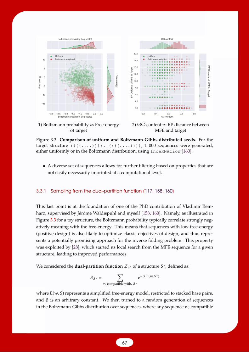
3.0 2.5 2.0 1.5 1.0 0.5 0.0 0.5Boltzmann probability (log scale)

15

10

5

0

5

10

Free

ene

rgy

UniformBoltzmann weighted

Boltzmann probability (log scale)

Free energy

1) Boltzmann probability vs Free-energyof target

0.2 0.4 0.6 0.8 1.0GC content

0.0

2.5

5.0

7.5

10.0

12.5

15.0

17.5

20.0

BP D

ista

nce

of M

FE to

Tar

get

UniformBoltzmann weighted

GC contentBP D

istance of MFE to Target

2) GC-content vs BP distance betweenMFE and target

Figure 3.3: Comparison of uniform and Boltzmann-Gibbs distributed seeds. For thetarget structure ((((....))))..((((....)))), 1 000 sequences were generated,either uniformly or in the Boltzmann distribution, using IncaRNAtion [160].

• A diverse set of sequences allows for further filtering based on properties that arenot easily necessarily imprinted at a computational level.

3.3.1 Sampling from the dual-partition function [117, 158, 160]

This last point is at the foundation of one of the PhD contribution of Vladimir Rein-harz, supervised by Jérôme Waldispühl and myself [158, 160]. Namely, as illustrated inFigure 3.3 for a toy structure, the Boltzmann probability typically correlate strongly neg-atively meaning with the free-energy. This means that sequences with low free-energy(positive design) is also likely to optimize classic objectives of design, and thus repre-sents a potentially promising approach for the inverse folding problem. This propertywas exploited by [28], which started its local search from the MFE sequence for a givenstructure, leading to improved performances.

We considered the dual-partition function ZS? of a structure S?, defined as:

ZS?

∑w compatible with. S?

e−β.E(w,S?)

where E(w,S) represents a simplified free-energy model, restricted to stacked base pairs,and β is an arbitrary constant. We then turned to a random generation of sequencesin the Boltzmann-Gibbs distribution over sequences, where any sequence w, compatible

67

with S?, is emitted with probability

(w | S?) e−β.E(w,S?)

ZS?.

We refer the reader to Chapter 2.3.4 for the algorithmic aspects of computing the dualpartition function, and performing the stochastic backtrack required for the sampling.

Remark 3.3.1: Note that, while it constitutes an approximation of the established Turner energymodel [185], our stacking-based model correlates very well with the former, and virtually does notimpact the above probability. In particular, the lack of support for multiple loops provably does notimpact the distribution. Indeed, the contribution EM of a multiple loop within the Turner modeldepends on its structural characteristics, but remains independent of its precise nucleotide content.Including such a contribution to our energy model would therefore increase the Boltzmann factorof any sequence by a factor e−β.EM , homogeneous across sequences. Meanwhile, the partitionfunction would be inflated by the exact same factor e−β.EM , so that the two terms would cancel inthe emission probability, leaving it unchanged.

This approach generates sequences which not only have, unsurprisingly, lower free-energies than those produced by uniform sampling, but also much larger Boltzmannprobabilities, as illustrated by the left panel of Figure 3.3. However, further analyses(Figure 3.3, right panel) reveal that this increased suitability to the objectives of designcomes at the cost of a drift of the GC-content towards high values (typically 75-80%).This drift is problematic since as wild-type sequences within living organisms oftenpresentmediumor lowGC-content, presumably to offer better transcription rates and/orstructural plasticity [54].

As a countermeasure, we introduced a rejection strategy, an instance of multidimen-sional Boltzmann sampling (see Section 2.3.4 and 4.2.2), to generate sequences at a con-strained GC-content, introducing a weight xgc to induce a distribution

xgc (w | S?) ∝ x|w|G+|w|Cgc × e−β.E(w,S?).

As shown in Figure 3.4, the drift of Boltzmann-generated sequences towards high GCcontents can be counterbalanced, while preserving much better free-energies than in-duced by the Boltzmann distribution. Moreover, this strategy induces Boltzmann prob-abilities that are much higher than induced by a uniform sampling, as well as a muchbetter proportion of sequences adopting the target structure as its MFE. In other words,this positive design strategy constitutes a promising approach, possibly in combinationwith further local optimizations, for negative design.

68

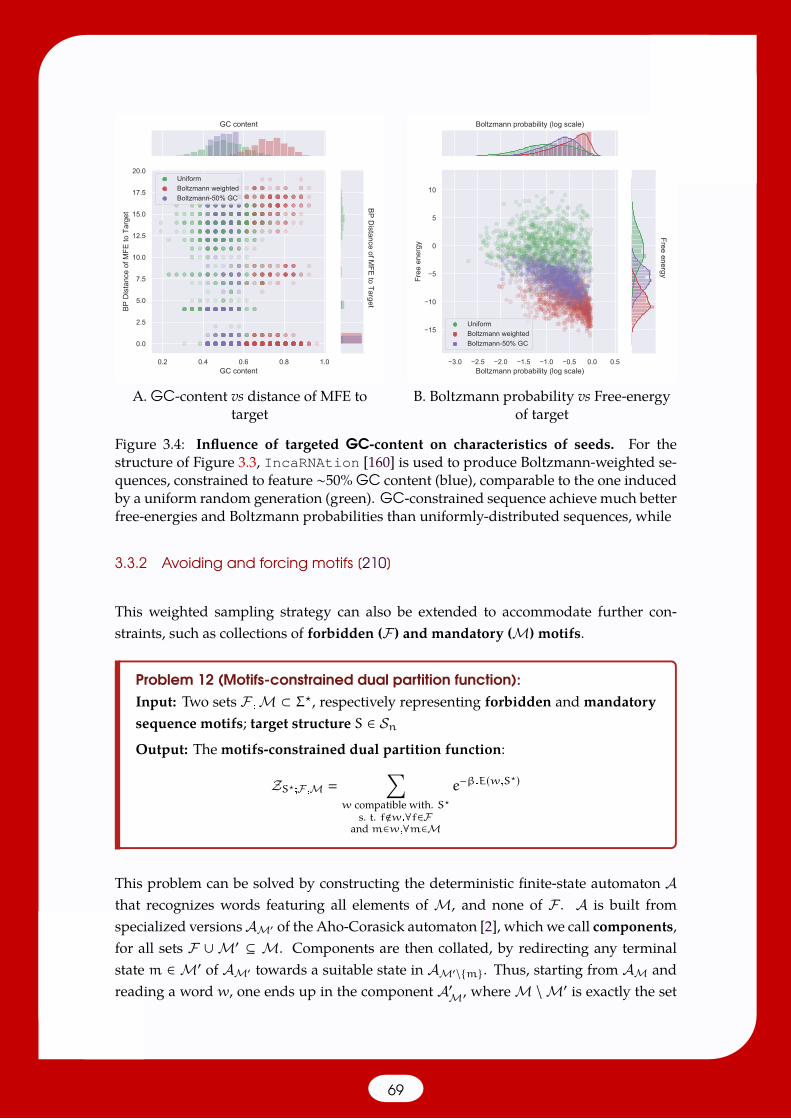
0.2 0.4 0.6 0.8 1.0GC content

0.0

2.5

5.0

7.5

10.0

12.5

15.0

17.5

20.0

BP D

ista

nce

of M

FE to

Tar

get

UniformBoltzmann weightedBoltzmann-50% GC

GC content

BP Distance of M

FE to Target

A. GC-content vs distance of MFE totarget

3.0 2.5 2.0 1.5 1.0 0.5 0.0 0.5Boltzmann probability (log scale)

15

10

5

0

5

10

Free

ene

rgy

UniformBoltzmann weightedBoltzmann-50% GC

Boltzmann probability (log scale)Free energy

B. Boltzmann probability vs Free-energyof target

Figure 3.4: Influence of targeted GC-content on characteristics of seeds. For thestructure of Figure 3.3, IncaRNAtion [160] is used to produce Boltzmann-weighted se-quences, constrained to feature ∼50% GC content (blue), comparable to the one inducedby a uniform random generation (green). GC-constrained sequence achieve much betterfree-energies and Boltzmann probabilities than uniformly-distributed sequences, while

3.3.2 Avoiding and forcing motifs [210]

This weighted sampling strategy can also be extended to accommodate further con-straints, such as collections of forbidden (F) and mandatory (M) motifs.

Problem 12 (Motifs-constrained dual partition function):Input: Two sets F ,M ⊂ Σ?, respectively representing forbidden and mandatorysequence motifs; target structure S ∈ SnOutput: Themotifs-constrained dual partition function:

ZS?;F ,M

∑w compatible with. S?

s. t. f<w,∀f∈Fandm∈w,∀m∈M

e−β.E(w,S?)

This problem can be solved by constructing the deterministic finite-state automaton Athat recognizes words featuring all elements of M, and none of F . A is built fromspecialized versionsAM′ of the Aho-Corasick automaton [2], which we call components,for all sets F ∪M′ ⊆ M. Components are then collated, by redirecting any terminalstate m ∈M′ of AM′ towards a suitable state in AM′\m. Thus, starting from AM andreading a word w, one ends up in the component A′M, where M \M′ is exactly the set

69

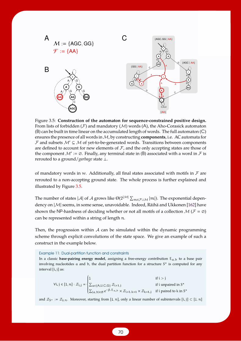
ε

A

AG

G

A

G

G

ε

A

AG

G

Aε

GG

A

A

ε

A

A

C,G,U

C

G

CG

⊥

AGC, GG | AA

AGC | AAGG | AA

AA

A

A

A A

M : AGC, GGF : AA

A

ε

A

AA

A

AG

AGC

C

G

A

G

GG

G

G

B

C

Figure 3.5: Construction of the automaton for sequence-constrained positive design.From lists of forbidden (F) and mandatory (M) words (A), the Aho-Corasick automaton(B) can be built in time linear on the accumulated length ofwords. The full automaton (C)ensures the presence of allwords inM, by constructing components, i.e. ACautomata forF and subsets M′ ⊆M of yet-to-be-generated words. Transitions between componentsare defined to account for new elements of F , and the only accepting states are those ofthe component M′ : . Finally, any terminal state in (B) associated with a word in F isrerouted to a ground/garbage state ⊥.

of mandatory words in w. Additionally, all final states associated with motifs in F arererouted to a non-accepting ground state. The whole process is further explained andillustrated by Figure 3.5.

The number of states |A| of A grows like Θ(2|M|∑m∈F∪M |m|). The exponential depen-dency on |M| seems, in some sense, unavoidable. Indeed, Räihä andUkkonen [162] haveshown the NP-hardness of deciding whether or not all motifs of a collection M (F )can be represented within a string of length n.

Then, the progression within A can be simulated within the dynamic programmingscheme through explicit convolutions of the state space. We give an example of such aconstruct in the example below.

Example 11: Dual-partition function and constraintsIn a classic base-pairing energy model, assigning a free-energy contribution Ea,b to a base pairinvolving nucleotides a and b, the dual partition function for a structure S? is computed for anyinterval [i, j] as:

∀i, j ∈ [1,n] : Zi,j

1 if i > j∑a∈A,U,C,G Zi+1,j if i unpaired in S?∑(a,b)∈B e−β.Ea,b ×Zi+1,k+1 ×Zk+1,j if i paired to k in S?

and ZS? : Z1,n. Moreover, starting from [1,n], only a linear number of subintervals [i, j] ⊂ [1,n]

70

is reached by the computation, so the recurrence can be computed in linear-time using dynamicprogramming.

Then we consider the adjunction of sequence constraints, forcing the presence/absence of motifsM/Fmodeled by an automaton A with state space Q, transition function δ and final states F ⊂ Q. Itcan be achieved by convolving the dynamic-programming schemes and the automaton A, essentiallysimulating its transitions. For all pair of states q,q′ ∈ Q and indices i, j ∈ [1,n], one has :

Zq→q′

i,j

0 if i > j and q , q′

1 if i > j and q q′∑a∈A,U,C,G Z

δ(q,a)→q′i+1,j

if i unpaired in S?∑(a,b)∈B

∑q′′∈Q

e−β.Ea,b ×Zδ(q,a)→q′′i+1,k+1

×Zδ(q′′,b)→q′k+1,j

if i paired to k in S?

where Zq→q′

i,jrepresents the dual partition function, restricted to wordsw that are: i) compatible with

the interval [i, j] in S?; and ii) starting from a state q, one ends in q′ upon reading w in A.

3.3.3 Multiple structures and extended design principles [88, 90]

In the previous section, the computation of the dual partition functionwas greatly helpedby the tree-like nature of the secondary structure, inducing recurrences at the origin ofour dynamic-programming schemes. The presence of complex networks of constraints,for instance induced by multiple secondary structures for multistable RNAs [65] or toprevent the extension of helices [91], breaks the subtructure property induced by a singlesecondary structure, and impedes the design of efficient algorithms.

In collaboration with Stefan Hammer, Wei Wang and Sebastian Will [88, 90], we consid-ered a generalized version of the dual partition function, wheremultiple target structuresS?,S? . . . S?m are jointly considered, and the energy of a sequence is additively definedon a collection of functions (F1, F2, . . . , Fk), called contribution. Each contribution F ob-serves a setdep(F) ⊂ [1,n] of positions in the designed sequence, and returns a numericalvalues accordingly. In other words, each contribution is a function F : Σ|dep(F)| → ,whose values accumulate to define the energy of any given sequence.

Problem 13 (General dual partition function):Input: Length n; Collection of contributions F : [F1, F2, . . . , Fk]; Collection oftarget structures S? : [S?

1,S?

2. . . S?m].

Output: The generalized dual partition function:

ZS?,F

∑w∈Σm such that

w comp. with. S?,∀S?∈S?e−β.F(w)

where F(w) ∑ki1 Fi([wp | p ∈ dep(Fi)]).

71

3.3.3.1 Complexity aspects

Complexity-wise, the problem is generally NP-hard, as it specializes into a variant ofnegative design studied by, and proven NP-hard, by Hellmuth et al. [91]. Namely, theauthors introduced extended shapes, possibly described as secondary structures whosebase-pairs are partitioned into regular base pairs, which should be populated by validpairs of nucleotides, and pseudo-edges which should not be pairable. Given severalsuch extended shapes, the Min-Edge-Deletion in Shapes (MES) problem asks for theminimal number of (regular or pseudo) edges to delete before a satisfying sequenceassignment can be found, i.e. such that nucleotides on regular edges (i, j) (resp. pseudoedges (i,j)) forming valid pairs in B (resp. invalid pairs in U : AA,CC,GG,UU).This problem essentially constitutes a specialization of the above problem, obtainedby: i) setting S? : ; ii) Choosing suitable contributions F(i,j)(a,b) −1(a,b)∈B andF(i,j)(a,b) −1(a,b)∈U. In this setting, Z,F

∑w e−β.#DelEdges(w), and the existence of a

sequence violating k edges can be decided from the dual partition function in polynomialtime (e.g. through interpolation, or increasing β so that co-optimal overwhelm thepartition function).

Moreover, in a uniform setting (F : ), a key object is the dependency graph GS of acollection of structures S? : [S?

1, . . . ,S?m] of length n, defined as

GS : ([1,n],∪mi1Si).

This graph is simply the union of the graphs of secondary structures, and must bebipartite for the collection to admit any design [73].

Theorem 5 (Independent set and multidesign): Given several secondary struc-tures S? : [S?

1, . . . ,S?m] such that GS is bipartite, the dual partition function ZS?,

is exactly twice the number of independent sets in GS.

It follows that computing the general partition function is as hard as counting the num-ber of independent sets in a bipartite graph (#BIS), a thoroughly-studied #P-hardproblem [79].

Finally, we described in Hammer et al. [88, 90] a general Fixed Parameter Tractablesolution. The entire network of contributions is jointly considered, and automaticallytransformed into a set of DP equations through a tree decomposition. Resulting DPschemes contrast with most of the schemes described in this document due to the au-tomated nature of their design, but also due to their optimality in some well-definedsense.

72

Chapter 4

Constrained random generation throughrejection and beyond

Generic approaches for the random generation of combinatorial objects rely on the exis-tence of a specification for the combinatorial class. However, the design of a specificationfor a given combinatorial class can be a highly complex task, or altogether be provablyimpossible for a given a restricted set of constructors. In the case of combinatorial classesthat are naturally expressible as languages, one can use classic pumping-lemma to ruleout the existence of regular or context-free specifications. However, such results do notpreclude the existence of a grammar for a language, which itself would be in bĳectionwith the language of interest, as shown in the following example.

Example 12: Copy languageConsider the 3-copy language

L3C an.bn.cn | n ∈ A textbook application of the pumping lemma (algebraic version) shows that the language is notcontext-free: there is no context-free grammar that generates L3C. However, the language

L3 (a.b.c)n | n ∈

can be generated using a context-free grammar (or even a simpler finite-state automaton), and admitsa trivial bĳection with L3C. Such a bĳection may simply push occurrences of a (resp. b and c) to thebeginning (resp. ending andmiddle), preserving the relative order within occurrences of a given letter.This transform can is easily reversible, and can be implemented in linear time.

Combinatorial properties of languages can be used to rule out any suchworkaround and,more generally, establish the unsuitability of classes of grammars for the generation ofsome languages.

For instance, Flajolet [67] showed that some context-free language are intrinsically am-biguous, i.e. any grammar that generates such a language must be ambiguous. Indeed,languages generated from a context-free grammar are associated with ordinary gener-ating functions that are algebraic. However, certain context-free languages are known

73

to admit transcendental generating functions, and thus cannot admit an unambiguouscontext-free grammar, as shown in Example 13.

Example 13: A simple intrinsically ambiguous languagea

Consider the language

LIA w ∈ a,b, c? | |w|a , |w|b or |w|b , |w|c.

It is generated by a context-free grammar (axiom S) S → Ta<b | Tb<a | Tb<c | Tc<b, which breaksdown the language into four (overlapping, thus inducing an ambiguous grammar) sub languages thatare context free, and whose union covers all possible cases. For instance, the non-terminal Ta<b istasked with generating the language

La<b w ∈ a,b, c? | |w|a < |w|b

using the following set of production rules

Ta<b → a Tab b Ta<b | b Tab a Ta<b | b Ta<b | b Tab | c Ta<bTab → a Tab b Tab | b Tab a Tab | c Tab | ε

which essentially amounts to a case distinction based on the first encountered character, reminiscent ofa first passage decomposition. Similar productions rules can be obtained for the languages generated byTb<a, Tb<c and Tc<b respectively, establishing the context-free nature of LIA.

To study the generating function of LIA, remark that LIA a,b, c? \ LIA, where

LIA w ∈ a,b, c? | |w|a |w|b |w|c

. The ordinary generating functions SIA(z) and SIA(z) are thus related through

SIA(z) 1

1 − 3 z− SIA(z).

Remind that algebraic generating functions are closed under addition/subtraction, so SIA(z) is algebraiconly if SIA(z) is algebraic itself. However, SIA(z) can be expressed explicitly as

SIA(z) ∑n≥0

(3n

n,n,n

)z3n.

It follows from Stirling’s expansion that, for n ≡ 0 mod 3, one has

[zn]SIA(z) n!

(n/3)! × (n/3)! × (n/3)! 3 × 3n

2π × n (1 +O(1/n)).

Such an asymptotic expansion is not compatible with the universal asymptotic form of coefficientsof rational/algebraic generating functions, as seen in the Flajolet/Sedgewick bible [69], or a recentlyrefined result by Banderier and Drmota [11] (see Remark 5.1.2).

SIA(z) is therefore not algebraic, and neither is SIA(z). Since generating functions associated withunambiguous context-free grammars are either rational or algebraic, we conclude that no such grammarexists, and LIA is context-free, yet intrinsically ambiguous.

aExample borrowed from the magisterial exposition of Cyril Nicaud.

More generally, combinatorial classes associated with transcendental generating func-tions, regardless of their language-theoretic properties, cannot be modeled using thestandard operators introduced by the symbolic method. In this chapter, we remind,

74

http://algo.inria.fr/pfac/PFAC/Program_files/nicaud.pdf

generalize and exploit versatile rejection principles for the generation of constrainedcombinatorial objects which are hard to specify (at least in their constrained version).

Outline. Section4.1 starts by reminding thegeneral objectives andprinciples of rejectionmethods for random generation. Section 4.2 describes the main principles behind thegeneral technique called multidimensional Boltzmann sampling, whose application toselected problems in Bioinformatics is described in Section 4.3. Section 4.4 provides ananalysis of the level of redundancy within weighted samples, and describes possiblecountermeasures to such an unproductive phenomenon.



M. Bousquet-Mélou and Y. Ponty. Culminating paths. DiscreteMathematics and Theoretical Computer Science,10(2):125–152, 2008

A. Denise, Y. Ponty, and M. Termier. Controlled non uniform random generation of decomposable structures.Theoretical Computer Science, 411(40-42):3527–3552, 2010

O. Bodini and Y. Ponty. Multi-dimensional Boltzmann Sampling of Languages. In AOFA 2010, volume AM ofDMTCS Proceedings, pages 49–64, Vienna, Austria, June 2010. Discrete Mathematics and Theoretical ComputerScience

D. Gardy and Y. Ponty. Weighted random generation of context-free languages: Analysis of collisions in randomurn occupancy models. In GASCOM 2010, page 14pp, Montréal, Canada, Sept. 2010. LACIM, UQAM

J. Waldispühl and Y. Ponty. An unbiased adaptive sampling algorithm for the exploration of RNA mutationallandscapes under evolutionary pressure. Journal of Computational Biology, 18(11):1465–79, Nov. 2011

J. Waldispühl and Y. Ponty. An unbiased adaptive sampling algorithm for the exploration of RNAmutational landscapes underevolutionary pressure. In RECOMB 2011, volume 6577 of Lecture Notes in Computer Science, pages 501–515, Vancouver, Canada,Mar. 2011. Springer Berlin / Heidelberg

J. Du Boisberranger, D. Gardy, and Y. Ponty. The weighted words collector. In AOFA 2012, volume AQ, pages243–264, Montreal, Canada, June 2012. DMTCS

C. Banderier, O. Bodini, Y. Ponty, and H. Tafat. On the diversity of pattern distributions in rational language. InANALCO 2012, pages 107–116, Kyoto, Japan, Jan. 2012. Omnipress

A. Lorenz and Y. Ponty. Non-redundant random generation algorithms for weighted context-free languages.Theoretical Computer Science, 502:177–194, Sept. 2013

Y. Ponty. Non-redundant random generation from weighted context-free languages. In GASCOM 2008, page 12pp, Bibbiena,Italy, 2008

V. Reinharz, Y. Ponty, and J. Waldispühl. A weighted sampling algorithm for the design of RNA sequences withtargeted secondary structure and nucleotide distribution. Bioinformatics, 29(13):i308–15, July 2013

V. Reinharz, Y. Ponty, and J. Waldispühl. A weighted sampling algorithm for the design of RNA sequences with targetedsecondary structure and nucleotides distribution. In ISMB/ECCB 2013, Berlin, Germany, July 2013

Y. Zhang, Y. Ponty, M. Blanchette, E. Lecuyer, and J. Waldispühl. SPARCS: a web server to analyze (un)structuredregions in coding RNA sequences. Nucleic Acids Research, 41(Web Server issue):W480–5, July 2013

J. Lumbroso, M. Mishna, and Y. Ponty. Taming reluctant random walks in the positive quadrant. In GASCOM2016, volume 59 of Electronic Notes in Discrete Mathematics, pages 99 – 114, Bastia, France, 2017

75

J. Michálik, H. Touzet, and Y. Ponty. Efficient approximations of RNA kinetics landscape using non-redundantsampling. In ISMB/ECCB 2017, volume 33, pages i283 – i292, Prague, Czech Republic, 2017



4.1 It’s not you, it’s me: The unreasonable power of rejection

Before we move any further, let us define precisely the problem of random generation.We are tasked with the random generation of objects of size n within a challenging classA (i.e. hard to specify, e.g. using a grammar), according to a predefined probabilitydistribution p?w.

Problem 14 (Random generation for A):Input: Numberm of objects

Output: Sequence of [w1, . . . ,wm] ∈ Am such that

A (W w) p?w.

The provable inexistence of a specification can be frequently circumvented at a reasonablecost through a rejection strategy. Itsmain idea is to consider another simpler setB, chosento enforce the following properties:

1. Correctness: A ⊆ B (or A ⊆ B′, admitting a computable bĳection with B);2. Effectiveness: Objects from B can be generated (uniformly) at random;

3. Efficiency: The distribution over B is reasonably close to its target over A.

In this setting, the rejection algorithm consists in an iterated generation of objects froma superset B ⊇ A, discarding any object in B \ A, until an object of A is obtained andreturned.

The subsequent rejections act as a conditioning, and the emission probability pw of agiven object w ∈ A simply becomes

pw B (W w | W ∈ A) B (W w)B (W ∈ A)

B (W w)∑w′∈A

B (W w′)

where B (W w) indicates the probability of generating w using the above-mentionedgenerator for B.

76

Typically, when a uniform distribution p?w 1/|A| is targeted, and enforced over B bythe initial generator, one has B (W w) 1/|B |, and the emission probability simplifiesinto

pw 1/|B ||A|/|B |

1

|A| p?w.

In other words, a uniform generator for B readily yields a uniform generator for A.

This correctness generalizes beyond uniform distributions, to any case where the gen-erated and targeted probability distributions are proportional over A:

∃κ ∈ such that ∀w ∈ A, B (W w) p?w

κ(4.1)

where p?w denotes the targeted probability distribution. Again, the emission probabilitysimplifies into

pw p?w/κ∑

w′∈Ap?w/κ

p?w,

and the rejection generator enforces the targeted probability distribution.

4.1.1 Correcting a (bounded) bias

A similar strategy can be used when the distribution of B, renormalized overA (i.e. afterrejection), does not fully coincide with the targeted distribution:

∃w ∈ A such that pw , p?w.

Denote as w the object in A which is most unfavorably discriminated against by theinitial generation, such that

w : argminw∈A

δ(w) with δ(w) : pwp?w

.

Then, following the ideas of [142], the rejection algorithm is coupled with an additionalrejection step, accepting the generated w ∈ Awith probability

qw δ(w)δ(w) ≤ 1 (4.2)

and rejecting it otherwise. The emission probability p′w of the combined rejection is then

p′w pw × qw∑

w′∈Apw′ × qw′

p?w∑

w′∈Ap?w′

p?w

so that any generator for B such that B (W w) > 0,∀w ∈ A, can be used (potentiallyat the cost of frequent rejections) to generate from Awithin the targeted distribution.

77

4.1.2 Complexity aspects

Given the existence of unbounded sequences of rejections the worst-case complexity ofrejection generators is infinite. However, such scenarios are associated with abysmallysmall probabilities and, overall, populate a negligible proportion of the probability space,so worst-case analyses provides little insight into the concrete requirements of rejection-based methods. It is thus arguably more relevant to consider the trade-off between costand probability, and average-case complexities are thus usually sought to measure thepractical complexity of generators.

The main contributing factor to the average-case complexity usually resides in the re-peated (discarded) calls to the generator for B. Denote by T the number of attempts, i.e.the number of time the generator for B must be called before generating an object fromthe targeted distribution over A, then we generally have

(T ) 1∑w′′∈A

B (W w′′) × qw′′

≤ 1

B (W ∈ A) ×p?w

B (W w) ×p?w⊕

B (W w⊕) ,

with w⊕ maxw∈A δ(w) being the object whose emission probability is the most posi-tively biased in comparison to the targeted distribution.

Note that, when the uniform distribution is targeted over A, and exactly enforced overB, we have qw 1, ∀w ∈ A, and the expected number of attempts greatly simplifies into

(T ) |B ||A| .

Example 14: 2D walks with small steps [122]Many types of 2D walks are associated with non-algebraic generating functions when confined to thepositive quadrant.

For instance, Mishna and Rechnitzer [137] showed that the generating function of positive 2D walkstaking steps in S ,, is not D-finite and, in particular, non-algebraic. However, the numberwn of such walks taking n steps admits an asymptotic equivalent in

cn κ 3n +O(√8n)

where κ 0.173 . . . is a computable constant.

Now consider the set of unconstrained walks over ,,n, consisting of exactly 3n objects. Atrivial algorithm for the uniform generation simply chooses n steps, each one uniformly at random.

Clearly, the set of unconstrained walks (set B) includes the set of positive 2D walks (setA). A rejectionalgorithm can then be envisioned, generating unconstrained walks from B until a positive walks fromA is found. The expected number of attempts from this rejection algorithm is then asymptotically

78

equivalent to

(T ) |B ||A| 3n

κ 3n≈ 5.77 . . .

an, in particular, does not grow with n, leading to a linear-time rejection algorithm.

With Marni Mishna and Jérémie Lumbroso, we generalized this strategy [122] to more complex smallsteps set S ⊂ [−1, 0, 1] × [−1, 0, 1], crucially allowing for an efficient generation in cases of reluctantwalks, i.e. walks having a natural attraction, called drift, towards the axes. This tendency to violatethe positivity condition in turn leads to a number of positive walks exponentially smaller than |S |n,thus rejecting from unconstrained walks would yield an exponential expected time algorithm.

However, it as been shown in Duraj [61] that the number wn of positive 2D walks is such that wn ∈Θ(αn nβ), for two constants α < |S | and β that only depend on the step set S. Moreover, thisexponential growth constant α is shared by a well-chosen half-plane, including the positive quarter-plane, whose slope m can be determined numerically (or even exactly). When such a slope m isrational, then the projection of the steps onto the chosen-plane is a rational number, and efficientrandom generation algorithms for 1D positive walks can be used to generate walks in the half plane.Those walks are then lifted onto the 2D plane, and an additional rejection step ensures positivity at the2D level.

Since the exponential growth of the 1D and 2D walks coincide, then the rejection only contributes anadditional polynomial factor. In otherwords, the algorithm that generates 1D positivewalks and rejectsthose that escape the 2D positive quadrant, has expected time per generation bounded by a polynomialin n.

Finally, we consider the computational complexity, expressed in an arbitrary unit (#arith-metic operations, bit-complexity [49]), and denoted as a random variable C.

In simple – yet frequent – cases, objects of a fixed size n are generated, and the timecomplexity c(w) required by the generation of an object can be seen as deterministic andonly depending on n. Denoting by c(n) the complexity of generating objects in B, onegets

(C) c(n)B (W ∈ A) (4.3)

More generally, the average-case complexity of the rejection algorithm follows

(C) B (c(W))B (W ∈ A) (4.4)

where W is a random object in B. This formula also holds when the expected costof generating objects in A and B \ A differ, owing to the additivity, in expectation, of(dependent) random variables.

Example 15: Anticipated rejection/Florentine algorithm for Motzkin walks [13]An example of such an analysis can be found in the generation of prefixes of Motzkin walks, i.e.random positive paths using,→ and steps, associate to 2D vectors (+1,+1), (+1, 0) and (+1,−1)respectively. The textbook algorithm, proposed by Barcucci, Pinzani and Sprugnoli [13], uses anefficient anticipated rejection scheme. Its algorithmic part is straightforward, and simply consists,starting from 0, of choosing ↑,→ or ↓with equal probability at each stage, rejecting the prefix as soon

79

as a negative ordinates is reached, until a requested length n is reached.

The analysis of its average-case complexity is slightly more involved. The expected number of attemptsdepends on the asymptotics of the numbers of positive paths (An) and unconstrained paths (Bn)respectively. While we clearly have |Bn | 3n, it is a folklore result that |An | ∈ Θ

(3n√n

), so the

probability of accepting an object is

B (W ∈ A) |A|n|B|n ∈ Θ(1/√n).

The expected number of attempts thus grows in Θ(√n) and a classic rejection scheme, generating a nstep unconstrained walk followed by a positivity test, would yield and overall complexity in Θ(n√n).

Anticipated rejection has a sizable impact on the expected generation cost, but its analysis cost isslightly more involved. Denote by bn the number of positive walks of length n, and by dn the numberof positive walks ending in (n, 0). Being rejected before reaching n steps means having a positive prefixending at (k, 0) of size k < n steps, followed by a step, with a cost of k rejections being incurred bysuch a rejection. The expected cost of a generation is therefore given by

(c(W)) ∑k<n

kdk−13k

+ nbn

3n,

where the first term denotes the expected cost of (anticipated) rejections, and the second term denotingthe contribution of positive paths. It then follows from

dn ∈ Θ(3n

n√n

)and bn ∈ Θ

(3n√n

),

that the first term is bounded by a constant, while the second grows like Θ(√n), and thus

(c(W)) ∈ Θ(√n).

A direct application of (4.4) allows us to conclude that the overall average-case complexity isΘ(n). Thisresult is optimal (up to constants) since the number of bits required despite an expectedΘ(√n) numberof attempts.

A similar reasoning, and complexity speedup, more generally holds for a very large classof combinatorial structures obtained by step-wise extensions, such that the extension ofa rejected object is itself rejected, as shown by Denise [48].

Example 16: Culminating paths [21]Using anticipated rejection, to spare the cost of rejecting a fully-generated object, was crucial in thedesign, with Mireille Bousquet-Mélou, of an efficient algorithm for the uniform generation of culmi-nating paths [21]. A culminating path is a unidimensional walk which takes steps +1 and −1, starts atposition 0, and must both: 1) remain positive; and 2) be culminating, i.e. reaches its maximum heighton its final step.

Now consider the mirror image of a positive walk, obtained by reversing its sequence of steps, andnote that it is now culminating (but may not be positive). It follows that any culminating path w oflength n can be factored into w w⊥.w>, where w⊥ is a positive path of size dn/2e, and w> is themirror image of some positive path of length bn/2c. In other words, the set Bn : W⊥dn/2e ×W>bn/2c ,whereW⊥n (resp. W>n) is the set of positive (resp. culminating) walks of length n, represents a supersetof An the set of culminating walks of length n.

80

Using the kernel method, we could establish that |An | ∈ Θ(2n/n) [21], and it is a folklore result that|W⊥m | |W>m | ∈ Θ(2n/

√n), so that the expected number of attempts is asymptotically

(T )

W⊥dn/2e × W>bn/2c

|An | ∈ Θ (1) .

Moreover, the generation of a positive walk, or its reversal can be done in linear expected time usinganticipated rejection. Overall, we get that the simple algorithm that generates two half walks, reversesthe second one, and glues them together, restarting until the result is a culminating path, has linearaverage-case complexity.

4.2 Rejecting in dimension one and then some. . .

4.2.1 (Combinatorial) Boltzmann sampling

Boltzmann sampling [60] can be seen as a special instance of rejection sampling. Itrevisits the random generation of combinatorial objects of a given size n described bya specification B. Instead of precomputing the number of objects accessible throughlocal alternatives using costly convolution products, it initially relaxes the size constraint,drawing objects of any size in B until an object of suitable size is found.

More precisely, a Boltzmann generator emits an objectω ∈ B with probability

x (W ω) x|ω|

B(x) (4.5)

where B(z) is the generating function of B and x is a real-valued Boltzmann parameter.Such a distribution can be seen as a special instance of the Boltzmann distribution instatistical mechanics, where the free-energy of an object ω ∈ B is arbitrarily set toE(w) : −kT log x|ω|. This leads to associating a Boltzmann factor of eE(w)/kT x|ω|

to each object , in which one recognizes the distribution of Equation (4.5).

A careful tuning of x ensures a reasonable probability of acceptance and, in turn, anaverage-case complexity scaling in O(n2) for generating an object of size n (generatingan object of approximate size in [(1 − ε) · n, (1 + ε) · n] can be performed in Θ(n) time).

The appeal of Boltzmann samplers to a large subset of the Analysis of Algorithms (AOfA)community, can be attributed to two main factors:

• The elegance, and relative simplicity, of its algorithmic aspects: As shown in Ta-ble 4.1, generators for Cartesian products are deceptively simple to express. Theirimplementation, however, requires an evaluation of the Boltzmann Oracle, thevalue of the generating functions. While this task is relatively trivial when a closedform (or, generally, computable) formula is known for the generating function, its

81

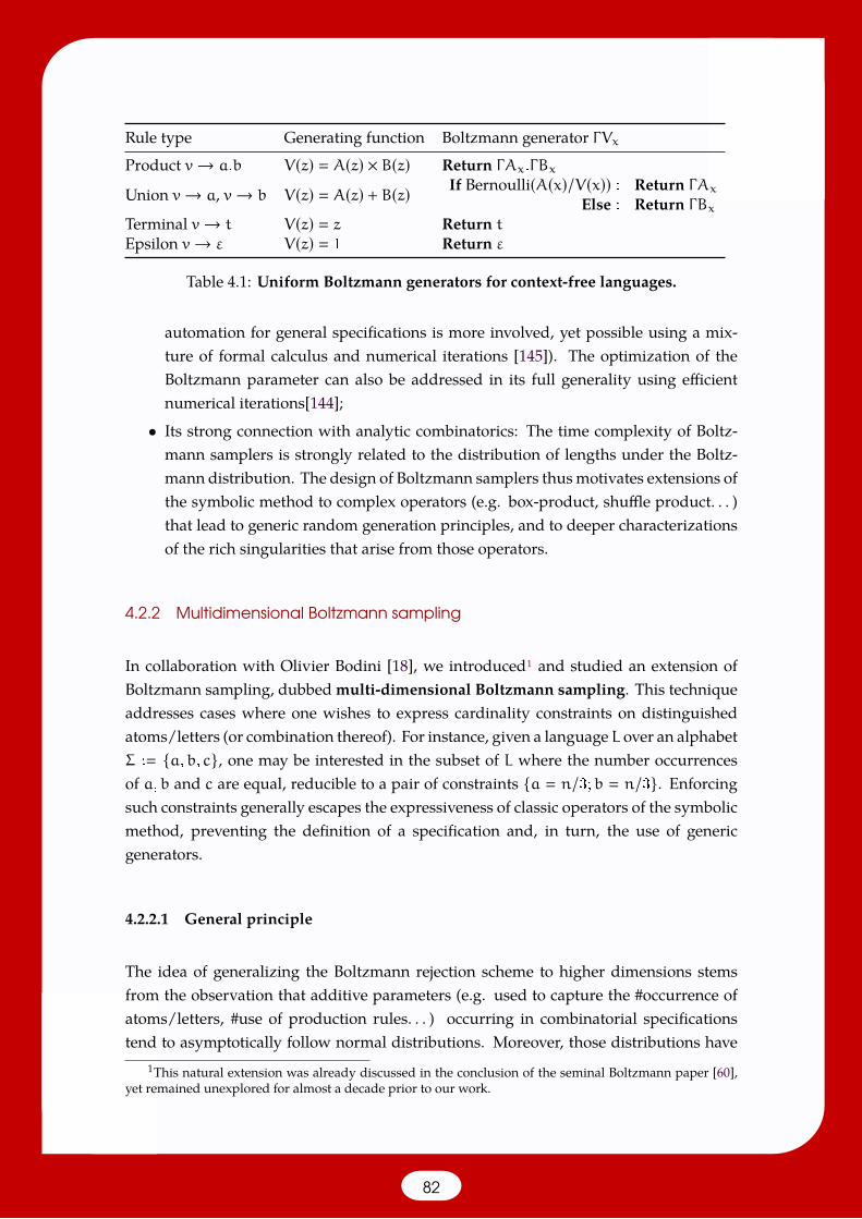
Rule type Generating function Boltzmann generator ΓVxProduct v→ a.b V(z) A(z) × B(z) Return ΓAx.ΓBx

Union v→ a, v→ b V(z) A(z) + B(z) If Bernoulli(A(x)/V(x)) : Return ΓAxElse : Return ΓBx

Terminal v→ t V(z) z Return tEpsilon v→ ε V(z) 1 Return ε

Table 4.1: Uniform Boltzmann generators for context-free languages.

automation for general specifications is more involved, yet possible using a mix-ture of formal calculus and numerical iterations [145]). The optimization of theBoltzmann parameter can also be addressed in its full generality using efficientnumerical iterations[144];

• Its strong connection with analytic combinatorics: The time complexity of Boltz-mann samplers is strongly related to the distribution of lengths under the Boltz-mann distribution. The design of Boltzmann samplers thusmotivates extensions ofthe symbolic method to complex operators (e.g. box-product, shuffle product. . . )that lead to generic random generation principles, and to deeper characterizationsof the rich singularities that arise from those operators.

4.2.2 Multidimensional Boltzmann sampling

In collaboration with Olivier Bodini [18], we introduced1 and studied an extension ofBoltzmann sampling, dubbedmulti-dimensional Boltzmann sampling. This techniqueaddresses cases where one wishes to express cardinality constraints on distinguishedatoms/letters (or combination thereof). For instance, given a language L over an alphabetΣ : a,b, c, one may be interested in the subset of L where the number occurrencesof a,b and c are equal, reducible to a pair of constraints a n/3;b n/3. Enforcingsuch constraints generally escapes the expressiveness of classic operators of the symbolicmethod, preventing the definition of a specification and, in turn, the use of genericgenerators.

4.2.2.1 General principle

The idea of generalizing the Boltzmann rejection scheme to higher dimensions stemsfrom the observation that additive parameters (e.g. used to capture the #occurrence ofatoms/letters, #use of production rules. . . ) occurring in combinatorial specificationstend to asymptotically follow normal distributions. Moreover, those distributions have

1This natural extension was already discussed in the conclusion of the seminal Boltzmann paper [60],yet remained unexplored for almost a decade prior to our work.

82

linear mean and variance. Such distributions are typically robust to the introductionof weights, also called parameters in subsequent work, which can be used to shift themeans, thus providing a probabilistic control over the average composition of generatedobjects.

Once fitted to match desired expectations, a rejection algorithm performs a weightedrandom generation, only accepting objects with suitable composition. The concentrationof the distribution usually induces a polynomial expected number of attempts, typicallygrowing in Θ(nk/2)when k is the number of cardinality constraints. Let us illustrate ourgeneral approach with a brief introductory example.

Example 17: Multidimensional Boltzmann sampler for balanced Motzkin languageConsider the Motzkin language M ⊆ (,), •? of well-parenthesized expressions interleaved withdots, formally defined as :

M ω ∈ (,), •? | |ω|( |ω|) and |ω′ |( ≥ |ω′ |),∀ω′ v ω (ω′ prefix ofω) .

This language is context-free, and generated by the grammar:

S→ ( S ) S | • S | ε

Now, consider the balanced Motzkin languageM2B the subset of the Motzkin words featuring exactly50% of dots (•), i.e.

M2B

ω ∈M | (|ω| ≡ 0 mod 2) and |ω|• |ω|

2

Clearly, M2B is not context-free. Moreover, the targeted 1/2 proportion of dots (•) characters differssubstantially from the 1/3 proportion expected in large uniformly-distributed Motzkin words [50]. Itfollows fromDrmota’s theorem [56] that a naive rejection algorithm, generating words of length n fromM until a word inM2B is obtained, would require a number of attempts growing exponentially withn.

However, as previously described [50], a weight π ∈ + can be associated to the dot (•), to induce aweighted distribution ontoM, in which the emission probabilities become

π (W ω) π|ω|•∑ω′∈M π|ω′ |•

. (4.6)

Generating within such a distribution can be performed in time essentially O(n logn), after a precom-putation in O(n1+o(1)), using generic generators [50].

The expected proportion of dots then becomes a function of π, allowing the user to shift the mean bychanging the value of π. Namely, the asymptotic proportion of dots is given by

π (|W |•) π

2 + π(1 +O(1/√n))

and thus achieves the targeted 1/2 for π 2. More importantly, if follows from the multidimensionalversion of Drmota’s theorem [56] that, within the weighted version ofM, the number of dots asymp-totically follows a normal distribution with mean n/2, variance σn, for some positive constant σ. Theprobability of generating a word inM2B is thus in Θ(1/√n).

Now, consider the rejection algorithm which repeatedly generates words in M of length n from theweighted distribution (4.6), setting π 2, until a word inM2B is obtained. This algorithm is uniform

83

within the restriction ofM2B towords of sizen. Moreover, its expected number of attempts is inΘ(√n),leading to an overall complexity in Θ(n√n logn).

4.2.2.2 Problem statement and algorithm

Theproblemaddressed bymultidimensional Boltzmann sampling is the uniform randomgeneration of words/objects of size n satisfying:

• Specification/grammar C for a combinatorial class over atoms t1, t2. . . (a.k.a. let-ters, or terminal symbols);

• Composition constraints of the form |W |tin

ri ∈ [0, 1]ki1

(4.7)

for a subset of k atoms, denoted t1, . . . , tk for the sake of convenience.A multidimensional Boltzmann sampler [18] then proceeds in three stages:

1. Calibration of weights/parameters π1,π2 . . ., chosen such thatµi :

π1,π2... (|W |ti)n

ri ∈ [0, 1]ki1

(4.8)

2. Random generation of objects from C within the π-weighted distribution

π1,π2... (W ω) ∏ki1 π

|ω|Zii

[zn]C(z;π1,π2, . . .) (4.9)

where C(z;u1,u2 . . .) represents the multivariate (weighted) generating functionmarking the occurrences of the atoms

Cπ(z;u1,u2...) ∑w∈C

z|w|k∏i1

π|w|tii

u|w|tii

(4.10)

3. Rejection of objects having unsuitable composition (and size) until adequate onesare produced.

The requirement of an exact size n for the generated objects can be relaxed to acceptwords having more diverse lengths in [(1 − ε) · n, (1 + ε) · n] for some constant ε > 0.Similarly, wordswhose composition departs slightly from the expressed constraints, suchthat #ti/n ∈ [ri − ε′, ri + ε′], can be deemed acceptable.

84

Remark 4.2.1: Note that these relaxed statements only enforce uniformity within a givensize/composition class, and do not constrain the respective probabilities of two objects havingdifferent length/composition. Such a slight bias is generally deemed acceptable in contexts wherestatistical estimates are computed from generated structures.Moreover those emission probabilities could, in principle, be corrected by a subsequent rejectionto ensure an overall uniform distribution, as described above in Equation (4.2). However, thisadditional rejection would increase the expected complexity by an exponential factor, roughly equalto (∏imax(πi, 1/πi))2εn.

Weight calibration. This step can be performed using two distinct approaches:

• Symbolically, it is often possible to find a simple expression relating the asymptoticproportion of each atom to the weight. For instance, in context-free languagesgenerated by strongly-connected grammars, the dominant singularity is alwaysof square-root type, and the dominant singularity ρπ1,π2... can be expressed as afunction of the weights. The expected composition is then given by

limn→∞ (|W |ti/n | |W | n) −πi

∂∂πiρπ1,π2...

ρπ1,π2...,∀i ∈ [1,k].

This system can then be solved to obtain a closed-form formula, expressing thesolution weights as a function of the targeted proportions, as shown in Example 17and [50].

• Numerically, an iteration was initially proposed [18], whose efficient convergencewas conditioned by the choice of a suitable initial weight vector.

This work was later revisited by Bendkowski, Bodini and Dovgal [15], leadingto a more general and efficient solution. In their work, the authors were able toreformulate the calibration as a convex optimization problem, solved using theinterior-point method of Nesterov and Nemirovskii [140] in time polynomial to theinverse of the required precision. The authors completed their studywith estimatesfor the precision required to ensure a good acceptance probability, leading to anoverall polynomial tuning of multidimensional Boltzmann sampling.

Whenever feasible, a symbolic approach is arguablymore elegant and efficient, leading toa trivial algorithm for computing the weights. Unfortunately, it is easy to find exampleswhere such a strategy involves solving systemswhose complexity lies beyond the currentcapacities of symbolic mathematical engines (e.g. Maple, Mathemagix or Mathematica).Moreover, it does not represent a good approach for languages consisting of words offixed size (e.g. representing the search space of a combinatorial problem for a giveninstance), since the associated generating functions typically have very complex close-form expressions (if any), are hard tomanipulate, and have infinite radius of convergence.In such cases, numerical iterations represent the method of choice.

85

Rule type Precomputation Recursive generator ΓVn

Product v→ a.b vn ← ∑ni0 ai × bn−i

Choose K with prob. (K k) ak×bn−k

vnReturn ΓAk.ΓBn−k

Union v→ a, v→ b vn ← an + bnIf Bernoulli(an/vn) : Return ΓA

Else : Return ΓBx

Terminal v→ t vn ←π(t) if n 1

0 otherwiseReturn t

Epsilon v→ ε vn ←1 if n 0

0 otherwiseReturn ε

Table 4.2: Weighted generators for context-free constructors, with π(t) denoting theweight associated with a terminal letter/atom t. Remark that, in the case of products,the convolution can be restricted to values of i in [1,n − 1] if the grammar is in ε-free form. Such a form can be assumed without loss of generality, and greatly easesthe implementation by avoiding ill-defined equations, associated with non-productivecircular dependencies in the precomputation.

Weighted random generation. Generating within a weighted distribution is arguablythe easiest part of multidimensional Boltzmann sampling.

Using the recursivemethod, weights can straightforwardly incorporated in classic recur-rences, allowing to precompute the weights accessible through local alternatives. Thoseweights can, in turn, be used to derive probabilities that induce the weighted distribu-tion described in Equation (4.9). Table 4.2 summarizes some of the constructors usedin the context of context-free languages. The computation of those recurrences can beoptimized using properties of holonomic generating functions, leading to an overall com-plexity inO(mn logn+n1+o(1)) for the generation ofmwords of length n in the weighteddistribution of Equation (4.9), as discussed in Denise et al [50].

Weighted Boltzmann samplers can also be adapted from their uniform counterparts. Tothat purpose, it suffices to substitute, in the generators of Table 4.1,weighted generatingfunctions defined as

Cπ(z) ∑ω∈C

z|ω|k∏i1

π|ω|tii

, (4.11)

instead of the ordinary ones used within classic Boltzmann sampling. As shown inDenise et al [50], such weighted generating functions are the solutions of systems offunctional equations that is almost identical to those of Table 4.1, except for the additionof weights within terminal rules v→ t, namely

(Ordinary gen. fun.) C(z) z → (Weighted gen. fun.) Cπ(z) π(t) × z (4.12)

where π(t) denotes the weight of an atom t. For any given weight vector, the Boltzmannparameter calibration can

86

4.2.2.3 Average-case complexity analysis

A usual with rejection-based samplers, the worst-case complexity is infinite, so we in-vestigate the average-case complexity as the relevant metric to assess the efficiency of asampler. In general, the probability to draw an objectω ∈ C having suitable composition

(|ω|t1 n · r1, |ω|t2 n · r2 . . .) ∈ k

in the atoms (t1, t2 . . .) is given by

(|W |ti n · ri,∀i ∈ [1,k] | |W | n)

∑ω∈C s.t. |ω|n,|ω|tiri·n,∀i∈[1,k]

k∏i1

π|ω|tii

∑s.t. |ω|n

k∏i1

π|ω|tii

(4.13)

[znun·r1

1un·r22

. . .]Cπ(z;π1.u1,π2.u2...)[zn]Cπ(z;π1,π2...) (4.14)

whereCπ(z;u1,u2...) represents themultivariate generation function introduced inEqua-tion (4.10). The expected number of attempts is simply obtained as the inverse of theprobability of acceptance, i.e. by exchanging the numerator and denominator in Equa-tion (4.14).

Simple type grammars. For simple type grammars, associated with strongly con-nected aperiodic specifications, the multivariate version of the Drmota Theorem [56]applies toweighted specifications [50], and the composition in the k elected atoms followsa k-dimensional Gaussian limiting distributions, centered on the expectation of Equa-tion (4.7) [56]. More precisely, the coefficients of the weighted multivariate generatingfunction admit the following asymptotic equivalent:

[znum1

1um2

2. . .]Cπ(z;π1 u1,π2 u2 . . .)

κπ1,π2... ρ−nπ1,π2...

2k/2 nk/2 n√n

(e−nΞπ1,π2... +O

(1√n

))

where κπ1,π2... is a constant of both n and k, ρπ1,π2... is the dominant singularity, and

Ξπ1,π2... :

k∑i1

k∑j1

δ(i,j)π1,π2... × (µi −mi/n) × (µj −mj/n). (4.15)

The Ξπ1,π2... term essentially grows quadratically with k, and depends both on thedeviation of the requested composition to the expected one (µ1,µ2 . . .), and of valuesδ(i,j)π1,π2... that are related to the variance/co-variance matrix of the system. Remark that,

upon a successful clibration of the weights (µi ri), Ξπ1,π2... vanishes at (mi n · ri)ki1so one has

[znun·r11

un·r22

. . .]Cπ(z;π1 u1,π2 u2 . . .) κπ1,π2... ρ

−nπ1,π2...

2k/2 nk/2 n√n

(1 +O

(1√n

))

87

Moreover from the Drmota-Lalley-Woods Theorem [56, 112, 202] (see Theorem ??) weknow that similar conditions lead a square root type singularity to dominate the ordi-nary generating function, inducing the following universal asymptotic equivalent for thecoefficients

[zn]Cπ(z;π1,π2 . . .) λπ1,π2... ρ

−nπ1,π2...

n√n

(1 +O

(1√n

)).

The expected number of attempts probability of drawing an object of suitable composi-tion, assuming successful calibration is then asymptotically equivalent to

π1,π2,...(T ) [zn]Cπ(z;π1,π2 . . .)

[znunr11

unr22

. . .]Cπ(z;π1 u1,π2 u2 . . .) (4.16)

2k/2 nk/2(λπ1,π2...

κπ1,π2...+O

(1√n

))∈ Θ

(2k/2nk/2

). (4.17)

4.2.3 Beyond simplicity

The validity of those complexities extends beyond simple type grammars, and applies toany specification whose associated dominant singularity is unique, and arises from thecontribution of a single connected component for the chosen weight assignment. It alsoapplies to periodic systems such that, beyond a certain size N

[zn]C(z) , 0⇔ n ≡ 0 [p] for all n > N

for someperiodp > 1 through a simple rewriting of the grammar, coupledwith a suitablechange of variables.

However, general extensions of those complexities beyond strongly-connected systemsappear very challenging. Indeed relaxing the connectivity constraint gives rise to manycounter-examples, and may even induce bimodal distributions that cause an exponentialdependency onn for the number of attempts. In fact, wewere able to design an algorithmwhich constructs and return a specification whose limiting distribution for a dedicatedatom follows an arbitrary discrete (univariate) distribution, specified by a user as part ofthe input [12].

Remark 4.2.2:Empirically, in theworst case scenario of anabysmally small probability of acceptance,estimates for the expectedwaiting time can be refinedduring the execution of the rejection algorithm.Upon reaching the conclusion of impending doom, an exact recursive algorithm [49] can then beelected.

88

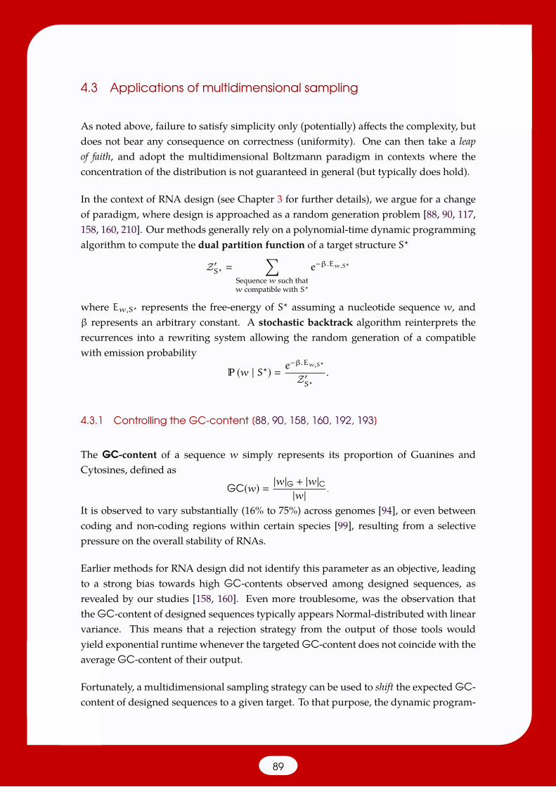
4.3 Applications of multidimensional sampling

As noted above, failure to satisfy simplicity only (potentially) affects the complexity, butdoes not bear any consequence on correctness (uniformity). One can then take a leapof faith, and adopt the multidimensional Boltzmann paradigm in contexts where theconcentration of the distribution is not guaranteed in general (but typically does hold).

In the context of RNA design (see Chapter 3 for further details), we argue for a changeof paradigm, where design is approached as a random generation problem [88, 90, 117,158, 160, 210]. Our methods generally rely on a polynomial-time dynamic programmingalgorithm to compute the dual partition function of a target structure S?

Z′S?

∑Sequencew such thatw compatible with S?

e−β.Ew,S?

where Ew,S? represents the free-energy of S? assuming a nucleotide sequence w, andβ represents an arbitrary constant. A stochastic backtrack algorithm reinterprets therecurrences into a rewriting system allowing the random generation of a compatiblewith emission probability

(w | S?) e−β.Ew,S?

Z′S?

.

4.3.1 Controlling the GC-content [88, 90, 158, 160, 192, 193]

The GC-content of a sequence w simply represents its proportion of Guanines andCytosines, defined as

GC(w) |w|G + |w|C|w| .

It is observed to vary substantially (16% to 75%) across genomes [94], or even betweencoding and non-coding regions within certain species [99], resulting from a selectivepressure on the overall stability of RNAs.

Earlier methods for RNA design did not identify this parameter as an objective, leadingto a strong bias towards high GC-contents observed among designed sequences, asrevealed by our studies [158, 160]. Even more troublesome, was the observation thatthe GC-content of designed sequences typically appears Normal-distributed with linearvariance. This means that a rejection strategy from the output of those tools wouldyield exponential runtime whenever the targeted GC-content does not coincide with theaverage GC-content of their output.

Fortunately, a multidimensional sampling strategy can be used to shift the expected GC-content of designed sequences to a given target. To that purpose, the dynamic program-

89

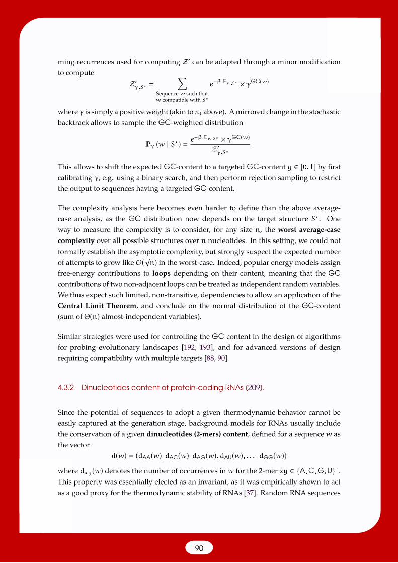
ming recurrences used for computing Z′ can be adapted through a minor modificationto compute

Z′γ,S?

∑Sequencew such thatw compatible with S?

e−β.Ew,S? × γGC(w)

whereγ is simply a positiveweight (akin toπt above). Amirrored change in the stochasticbacktrack allows to sample the GC-weighted distribution

γ (w | S?) e−β.Ew,S? × γGC(w)

Z′γ,S?

.

This allows to shift the expected GC-content to a targeted GC-content g ∈ [0, 1] by firstcalibrating γ, e.g. using a binary search, and then perform rejection sampling to restrictthe output to sequences having a targeted GC-content.

The complexity analysis here becomes even harder to define than the above average-case analysis, as the GC distribution now depends on the target structure S?. Oneway to measure the complexity is to consider, for any size n, the worst average-casecomplexity over all possible structures over n nucleotides. In this setting, we could notformally establish the asymptotic complexity, but strongly suspect the expected numberof attempts to grow likeO(√n) in the worst-case. Indeed, popular energy models assignfree-energy contributions to loops depending on their content, meaning that the GCcontributions of two non-adjacent loops can be treated as independent random variables.We thus expect such limited, non-transitive, dependencies to allow an application of theCentral Limit Theorem, and conclude on the normal distribution of the GC-content(sum of Θ(n) almost-independent variables).

Similar strategies were used for controlling the GC-content in the design of algorithmsfor probing evolutionary landscapes [192, 193], and for advanced versions of designrequiring compatibility with multiple targets [88, 90].

4.3.2 Dinucleotides content of protein-coding RNAs [209].

Since the potential of sequences to adopt a given thermodynamic behavior cannot beeasily captured at the generation stage, background models for RNAs usually includethe conservation of a given dinucleotides (2-mers) content, defined for a sequence w asthe vector

d(w) (dAA(w),dAC(w),dAG(w),dAU(w), . . . ,dGG(w))where dxy(w) denotes the number of occurrences in w for the 2-mer xy ∈ A,C,G,U2.This property was essentially elected as an invariant, as it was empirically shown to actas a good proxy for the thermodynamic stability of RNAs [37]. Random RNA sequences

90

preserving a given 2-mers content can be uniformly generated as random Eulerian path,using the dinucleotide shuffling algorithm of Altschul and Erickson [6].

However, in the context of studying a protein-coding RNA m, a background modelshould ideally capture all knownproperties, to assess the statistical significance of a givenphenomenon. Therefore, in addition to the 2-mers content, emitted sequences shouldalso preserve the reference protein P(m), encoded as an amino-acids sequence. Thisconstraints allows for substitutions of codons (non-overlapping 3-mers), each encodingan amino-acid, such that the resulting sequence m′ is said to be synonymous to m. Inshort, given a coding sequence m, |m| ≡ 0 [3], we must generate, uniformly at random,one or several RNA sequences synonymous tom′ such as

d(m) d(m′) and P(m) P(m′).

Here, P(·) denotes the conversion of a coding RNA into a sequence of amino acids,achieved by a simple morphism

P(xyz.w) → aaxyz.P(w) and P(ε) → ε

where aaxyz represents the amino-acid associated with the codon xyz ∈ A,C,G,U3.

Due to the highly non-sequential nature of the Altschul and Erickson algorithm [6], thereis little hope of adapting it to enforce synonymous substitutions. However, synonymoussequences can be modeled as a simple linear language L(m), defined by

L(ε) ε and L(xyz.w) x′y′z′ | aax′y′z′ aaxyz × L(w).

A predefined 2-mers content can then be enforced using multidimensional Boltzmannsampling, using 15 dimensions to represent the number of occurrences of each butone of the 2-mers (the last one being indirectly captured as the complement to thelength). Aweights vector µ : (µxy)xy∈A,C,G,U2 is then introduced, defining a weighteddistribution

µ (m′ | m) ∏xy∈A,C,G,U2 µ

|m′ |xyxy

Zµ,m(4.18)

whereZµ,m ≡

∑m′ s.t.

P(m)P(m′)

∏xy∈A,C,G,U2

µ|m′ |xyxy

Theabovepartition function canbe computed in linear-timeusingdynamicprogramming

Zµ,abc.w;α :∑

a′b′c′∈A,C,G,U3s.t. aaa′b′c′aaabc

Zµ,w;c′ ×∏

xy∈A,C,G,U2µ|αabc|xyxy

with Zµ,ε;α : 1 and Zµ,m ≡ Zµ,m;ε. A stochastic sampling algorithm can then beadapted in a straightforward manner to sample with respect to the distribution (4.18),

91

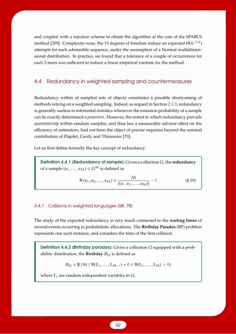
and coupled with a rejection scheme to obtain the algorithm at the core of the SPARCSmethod [209]. Complexity-wise, the 15 degrees of freedom induce an expected Θ(n15/2)attempts for each admissible sequence, under the assumption of a Normal multidimen-sional distribution. In practice, we found that a tolerance of a couple of occurrences foreach 2-mers was sufficient to induce a linear empirical runtime for the method.

4.4 Redundancy in weighted sampling and countermeasures

Redundancy within of sampled sets of objects constitutes a possible shortcoming ofmethods relying on aweighted sampling. Indeed, as argued in Section 2.3.3, redundancyis generally useless in inferential statistics whenever the emission probability of a samplecan be exactly determined a posteriori. However, the extent to which redundancy prevailsquantitatively within random samples, and thus has a measurable adverse effect on theefficiency of estimators, had not been the object of precise inquiries beyond the seminalcontribution of Flajolet, Gardy and Thimonier [70].

Let us first define formally the key concept of redundancy.

Definition 4.4.1 (Redundancy of sample):Given a collectionΩ, the redundancyof a sample (e1, . . . , eM) ∈ ΩM is defined as

R (e1, e2, . . . , eM) M

|(e1, e2, . . . , eM)| − 1 (4.19)

4.4.1 Collisions in weighted languages [58, 78]

The study of the expected redundancy is very much connected to the waiting times ofseveral events occurring in probabilistic allocations. The Birthday Paradox (BP) problemrepresents one such instance, and considers the time of the first collision.

Definition 4.4.2 (Birthday paradox): Given a collectionΩ equipped with a prob-ability distribution, the Birthday BΩ is defined as

BΩ (M | R(E1, . . . ,EM−1) 0 ∧R(E1, . . . ,EM) > 0)

where Ei are random independent variables inΩ.

92

For instance, in the uniform distribution overΩ, one has

(Collision at time i | e1, . . . , ei−1) |eji−1j1 ||Ω| <

BΩ|Ω| ,∀i ≤ BΩ

and it follows that, after BΩ generations, one has

(#Collisions) < BΩ × BΩ|Ω| ∈ O(1)

and we conclude that (R(e1, . . . , eBΩ)) → 0 for asymptotically large collectionsΩ.

Another setting of interest is that of the Coupon Collector (CC) problem, the time whichconsiders the expected sample size before the full collection is obtained.

Definition 4.4.3 (Coupon Collector):Given a collectionΩ equippedwith a prob-ability distribution, the Coupon Collector CΩ is defined as

CΩ (M | e1, . . . , eM Ω) (4.20)

It can be shown that the expected redundancy is an increasing function of M, so it isnatural to bound the redundancy is by that of the full collection, namely

(R(e1, . . . , eM) | e1, . . . , eM Ω) CΩ|Ω| − 1.

In collaboration with Danièle Gardy and Jérémie du Boisberranger [58, 78], we revis-ited these quantities attempting to obtain precise specialization of the general results ofFlajolet, Gardy and Thimonier [70] in the specific context of weighted languages.

4.4.1.1 Main results

LetC be a specification generating a languageL, with a collection π of weights associatedwith atoms. We denote by π∇n (resp. π∇n) theminimal (resp. maximal)weight of a wordin Ln. Consider the weighted generating function

Cπ(z) ∑ω∈L

πiz|ω|

∑n≥0

µπ,nz|ω|

and denote by ρπ its dominant singularity. Finally let us define the k-th moment of aπ-weighted distribution as

αk,n

mn∑i1

pki

∑w∈Ln π(w)kµπ,nk

µπk,n

µπ,nk. (4.21)

We consider the following conditions:

93

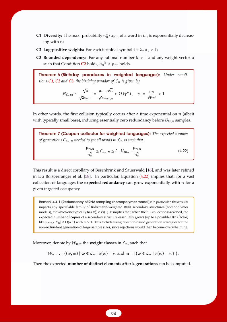
C1 Diversity: The max. probability π4n/µπ,n of a word in Ln is exponentially decreas-ing with n;

C2 Log-positive weights: For each terminal symbol t ∈ Σ, πt > 1;

C3 Bounded dependency: For any rational number k > 1 and any weight vector πsuch that Condition C2 holds, ρπk < ρπk holds.

Theorem 6 (Birthday paradoxes in weighted languages): Under condi-tions C1, C2 and C3, the birthday paradox of Ln is given by

BLn;π ∼√π√

2α2,n

µπ,n√π√

2µπ2,n

∈ Ω (γn) , γ :ρπ√ρπ2

> 1

In other words, the first collision typically occurs after a time exponential on n (albeitwith typically small base), inducing essentially zero redundancy before BΩ;π samples.

Theorem 7 (Coupon collector for weighted languages): The expected numberof generations CLn;π needed to get all words in Ln is such that

µπ,n

π∇n≤ CLn;π ≤ 2 ·Hmn ·

µπ,n

π∇n(4.22)

This result is a direct corollary of Berenbrink and Sauerwald [16], and was later refinedin Du Boisberranger et al. [58]. In particular, Equation (4.22) implies that, for a vastcollection of languages the expected redundancy can grow exponentially with n for agiven targeted occupancy.

Remark 4.4.1 (Redundancy of RNA sampling (homopolymer model)): Inparticular, this resultsimpacts any specifiable family of Boltzmann-weighted RNA secondary structures (homopolymermodels), forwhichone typically hasπ∇n ∈ O(1). It implies that,when the full collection is reached, theexpected number of copies of a secondary structure essentially grows (up to a possible Θ(n) factor)like µπ,n/|Ln | ∈ Θ(αn) with α > 1. This forbids using rejection-based generation strategies for thenon-redundant generation of large sample sizes, since rejections would then become overwhelming.

Moreover, denote byWn,π the weight classes in Ln, such that

Wn,π : (w,m) | ω ∈ Ln : π(ω) w andm |ω ∈ Ln | π(ω) w| .

Then the expected number of distinct elements after k generations can be computed.

94

Theorem 8 (Distinct weighted words): The expected number of distinct wordsafter k generations is given by

(|e1, . . . , ek|) ∑

(w,m)∈Wn,π

m ·(1 −

(1 − w

µπ,n

)k)

∑(w,m)∈Wn,π

m ·(1 − e− w

µπ,nk)+O(1).

A similar results holds for the coverage C of a sample (e1, . . . , ek), defined as

C(e1, . . . , ek) ∑e∈e1,...,ek π(e)

µπ,n(4.23)

which represents the proportion of the distribution that has already been sampled.

Theorem 9 (Coverage of weighted words): The expected coverage of a set ofdistinct words after k generations is given by

(C(e1, . . . , ek)) ∑

(w,m)∈Wn,π

m · wµπ,n

·(1 −

(1 − w

µπ,n

)k).

Since there are atmost (n+1)|Σ| different compositions/classes ofweights, the expressionsof Theorems 8 and 9 can be computed in polynomial time algorithms from theweighted-classified partition functions µπ,n, also known as the density of states.

Since redundancy can become overwhelming, it is natural to pursue algorithmic coun-termeasures. More precisely, the above result shows that the algorithmic problem ofsampling without replacement from a weighted language cannot be efficiently tackledusing rejection, motivating an unranking approach [118], or a modified instance of therecursive method [118, 147], illustrated in Section 2.3.3 and used to build RNA kineticslandscapes [133].

95

Chapter 5

Asymptotic properties of RNA secondarystructures and other trees

The tree-like nature of RNA secondary structures not only makes it an excellent play-ground for dynamic programming, but also enables the study of its generic asymptoticproperties. Suchworkgoback to the very earlydays ofRNAbioinformatics, withpioneer-ing works fromWaterman [194], Zuker and Sankoff [212], Viennot and Vauchaussade deChaumont [187], Hofacker [96], Bundschuh andHwa [24], Nebel [139], Clote [36], Reidysand Jin [104], and others too numerous to mention exhaustively. While initially moti-vated by algorithmic [194] and evolutionary [212] considerations, the field has graduallyturned towards questions in statistical mechanics, adressing the behavior of RNA at thethermodynamic equilibrium, as exemplified by the work of Bundschuh andHwa [25]. Inthis context, asymptotic enumerations can be used to elucidate the equilibriumpropertiesof random large homopolymers, including their dependency to changes of temperatures(phase transitions [23, 26]).

In the homopolymer model, nucleotides are anonymized, so that any pair can formbase pairs, inducing structural motifs that are equally contributing to the stabilization oftheir conformation. Implicitly, this amounts to coarsely abstract an RNA as its length n.While such a simplificationmay appear bold at first sight, many of the properties derivedfrom this model are robust to the incorporation/perturbations of the energy model, orcan be used as a first step to recover the dependency on an actual nucleotide content(heteropolymer model) [24, 212].

This chapter summarizes some contributed asymptotic analyses, using techniques inenumerative and analytic combinatorics, to address questions in algorithmic analysisand design [33, 148, 150], RNA thermodynamics [38], network properties [180], anddesign/evolution [206]. In the interest of self-completeness, we start by reminding basictools and notions. A magisterial exposition, including much more versatile techniques,can however (and should!) be sought in the Flajolet/Sedgewick bible [69].

96

Outline. In this short chapter, I first remind in Section 5.1 some basic concepts, toolsand principles in analytics combinatorics and, in Section 5.2, I describe the application ofthose techniques to selected problems involving the secondary structure of RNA.



W. A. Lorenz, P. Clote, and Y. Ponty. Asymptotics of RNA shapes. Journal of Computational Biology, 15(1):31–63, 2008

Y. Ponty. Efficient sampling of RNA secondary structures from the Boltzmann ensemble of low-energy: Theboustrophedon method. Journal of Mathematical Biology, 56(1-2):107–127, 2008

Y. Ponty and C. Saule. A Combinatorial Framework for Designing (Pseudoknotted) RNA Algorithms. In WABI2011, Saarbrucken, Germany, 2011

P.Clote, Y. Ponty, and J.-M. Steyaert. Expecteddistance between terminal nucleotides ofRNAsecondary structures.Journal of Mathematical Biology, 65(3):581–99, Sept. 2012

C. Chauve, J. Courtiel, and Y. Ponty. Counting, generating, analyzing and sampling tree alignments. InternationalJournal of Foundations of Computer Science, 29(5):741–767, 2018

D. Surujon, Y. Ponty, andP.Clote. Small-worldnetworks andRNAsecondary structures. Journal of computationalbiology : a journal of computational molecular cell biology, 26(1):16–26, Jan. 2019

H.-T. Yao, C. Chauve, M. Regnier, and Y. Ponty. Exponentially few RNA structures are designable. In ACM-BCB2019, pages 289–298, Niagara-Falls, United States, 2019. ACM Press

5.1 Basic tools in enumerative and analytic combinatorics

Analyzing the asymptotic enumerative behavior of a combinatorial class can be done bythe following four-step program, referred to as the symbolic method in the pioneeringwork of the late Philippe Flajolet:

1. Find a unambiguously grammar/specification that generates the objects;

2. Translate the grammar into a system of functional equations;

3. Solve the system and identify the dominant singularities;

4. Use some automatic Theorem to extract the leading term for the asymptotic equiv-alent for the number of objects of size n.

5.1.1 Context-free languages.

A combinatorial class is a, possibly infinite, setAwhere every object a ∈ A has a length|a|, and such that the restriction An to objects of A having any given length n is finite.

97

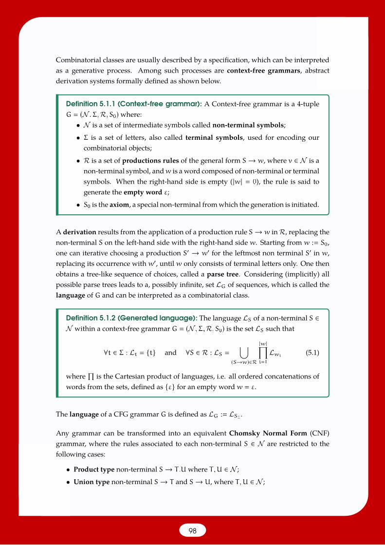
Combinatorial classes are usually described by a specification, which can be interpretedas a generative process. Among such processes are context-free grammars, abstractderivation systems formally defined as shown below.

Definition 5.1.1 (Context-free grammar): A Context-free grammar is a 4-tupleG (N ,Σ,R,S0)where:

• N is a set of intermediate symbols called non-terminal symbols;

• Σ is a set of letters, also called terminal symbols, used for encoding ourcombinatorial objects;

• R is a set of productions rules of the general form S→ w, where v ∈ N is anon-terminal symbol, andw is a word composed of non-terminal or terminalsymbols. When the right-hand side is empty (|w| 0), the rule is said togenerate the empty word ε;

• S0 is the axiom, a special non-terminal fromwhich the generation is initiated.

A derivation results from the application of a production rule S→ w inR, replacing thenon-terminal S on the left-hand side with the right-hand side w. Starting from w : S0,one can iterative choosing a production S′ → w′ for the leftmost non terminal S′ in w,replacing its occurrence with w′, until w only consists of terminal letters only. One thenobtains a tree-like sequence of choices, called a parse tree. Considering (implicitly) allpossible parse trees leads to a, possibly infinite, set LG of sequences, which is called thelanguage of G and can be interpreted as a combinatorial class.

Definition 5.1.2 (Generated language): The language LS of a non-terminal S ∈N within a context-free grammar G (N ,Σ,R,S0) is the set LS such that

∀t ∈ Σ : Lt t and ∀S ∈ R : LS

⋃(S→w)∈R

|w|∏i1

Lwi (5.1)

where∏

is the Cartesian product of languages, i.e. all ordered concatenations ofwords from the sets, defined as ε for an empty word w ε.

The language of a CFG grammar G is defined as LG : LS0 .

Any grammar can be transformed into an equivalent Chomsky Normal Form (CNF)grammar, where the rules associated to each non-terminal S ∈ N are restricted to thefollowing cases:

• Product type non-terminal S→ T .Uwhere T ,U ∈ N ;

• Union type non-terminal S→ T and S→ U, where T ,U ∈ N ;

98

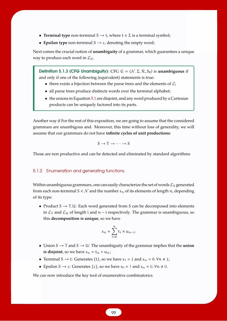
• Terminal type non-terminal S→ t, where t ∈ Σ is a terminal symbol;

• Epsilon type non-terminal S→ ε, denoting the empty word;

Next comes the crucial notion of unambiguity of a grammar, which guarantees a uniqueway to produce each word in LG.

Definition 5.1.3 (CFG Unambiguity): CFG G (N ,Σ,R,S0) is unambiguous ifand only if one of the following (equivalent) statements is true:

• there exists a bĳection between the parse trees and the elements of L;• all parse trees produce distincts words over the terminal alphabet;

• the unions in Equation 5.1 are disjoint, and anywordproducedby aCartesianproducts can be uniquely factored into its parts.

Another way if For the rest of this exposition, we are going to assume that the consideredgrammars are unambigous and. Moreover, this time without loss of generality, we willassume that our grammars do not have infinite cycles of unit productions:

S→ T → · · · → S

Those are non productive and can be detected and eliminated by standard algorithms

5.1.2 Enumeration and generating functions.

Withinunambiguousgrammars, one can easily characterize the set ofwordsLS generatedfrom each non-terminal S ∈ N and the number sn of its elements of length n, dependingof its type:

• Product S→ T .U: Each word generated from S can be decomposed into elementsin LT and LU of length i and n − i respectively. The grammar is unambiguous, sothis decomposition is unique, so we have

sn

n∑i0

ti × un−i;

• Union S→ T and S→ U: The unambiguity of the grammar implies that the unionis disjoint, so we have sn tn + un;

• Terminal S→ t: Generates t, so we have s1 1 and sn 0,∀n , 1;

• Epsilon S→ ε: Generates ε, so we have s0 1 and sn 0,∀n , 0.

We can now introduce the key tool of enumerative combinatorics.

99

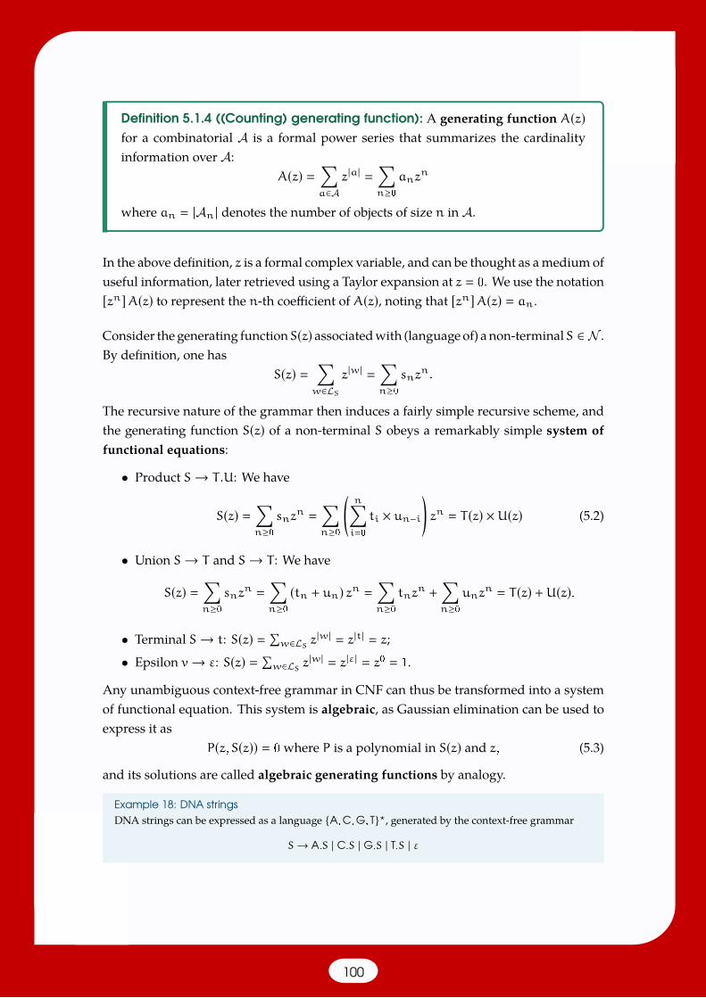
Definition 5.1.4 ((Counting) generating function): A generating function A(z)for a combinatorial A is a formal power series that summarizes the cardinalityinformation over A:

A(z) ∑a∈A

z|a| ∑n≥0

anzn

where an |An | denotes the number of objects of size n in A.

In the above definition, z is a formal complex variable, and can be thought as amedium ofuseful information, later retrieved using a Taylor expansion at z 0. We use the notation[zn]A(z) to represent the n-th coefficient of A(z), noting that [zn]A(z) an.

Consider the generating functionS(z) associatedwith (languageof) a non-terminalS ∈ N .By definition, one has

S(z) ∑w∈LS

z|w| ∑n≥0

snzn.

The recursive nature of the grammar then induces a fairly simple recursive scheme, andthe generating function S(z) of a non-terminal S obeys a remarkably simple system offunctional equations:

• Product S→ T .U: We have

S(z) ∑n≥0

snzn

∑n≥0

(n∑i0

ti × un−i)zn T (z) ×U(z) (5.2)

• Union S→ T and S→ T : We have

S(z) ∑n≥0

snzn

∑n≥0(tn + un) zn

∑n≥0

tnzn+

∑n≥0

unzn T (z) +U(z).

• Terminal S→ t: S(z) ∑w∈LS z

|w| z|t| z;

• Epsilon v→ ε: S(z) ∑w∈LS z

|w| z|ε| z0 1.

Any unambiguous context-free grammar in CNF can thus be transformed into a systemof functional equation. This system is algebraic, as Gaussian elimination can be used toexpress it as

P(z,S(z)) 0 where P is a polynomial in S(z) and z, (5.3)

and its solutions are called algebraic generating functions by analogy.

Example 18: DNA stringsDNA strings can be expressed as a language A,C,G, T?, generated by the context-free grammar

S→ A.S | C.S | G.S | T.S | ε

100

This grammar can be transformed in the CNF grammar for illustrative purposes

S→ S′ | E S′→ T .S T → T ′ | T ′′ T ′→ a | c T ′′→ g | ta→ A c→ C g→ G t→ T E→ ε

The transforms described above, coupled with minor simplifications, lead to the following system

S(z) 4z × S(z) + 1 1

1 − 4z

which can be solved to obtainS(z) 1

1 − 4z

∑n≥0

4n zn.

Remark 5.1.1: In general, algebraic systems associatedwith context-free grammars are non-linear, sothat conjugate solutions may exist. However, only one will admit positive integers as its coefficients.

5.1.3 Basic singularity analysis

Finding a closed-form expression for sn, the coefficients of S(z), is generally a highlyinvolved task (although such a form always exists [11]). An easier alternative is to useanalytic combinatorics to extract a simple asymptotic equivalent for sn. Singularityanalysis simplifies this problem by focusing on the singularities of S(z), i.e. points of thecomplex plane where the generating function ceases to be analytic.

Of particular interest are the dominant singularities, i.e. singularities of smallest modu-lus that are the main contributors to the coefficients. From Pringsheim’s Theorem [69, pp240], we know that at least one of them lies on the real axis for non negative series. More-over, only limited types of singularities may occur in algebraic generating functions. Thisleads to predictable behaviors for the coefficients, and allows to bypass complex analysis(almost) entirely thanks to automatic theorems.

Rule type Language Coefficients Generating function

Product S→ T .U LS LT × LU sn ∑ni0 ti × un−i S(z) T (z) ×U(z)

Union S→ T , S→ U LS LT⋃LU sn tn + un S(z) T (z) +U(z)

Terminal S→ t LS t sn

1 if n 1

0 otherwiseS(z) z

Epsilon S→ ε LS ε sn

1 if n 0

0 otherwiseS(z) 1

Table 5.1: Generated languages, enmerations and ordinary (counting) generating func-tions for unambiguous Chomsky Normal Form grammars.

101

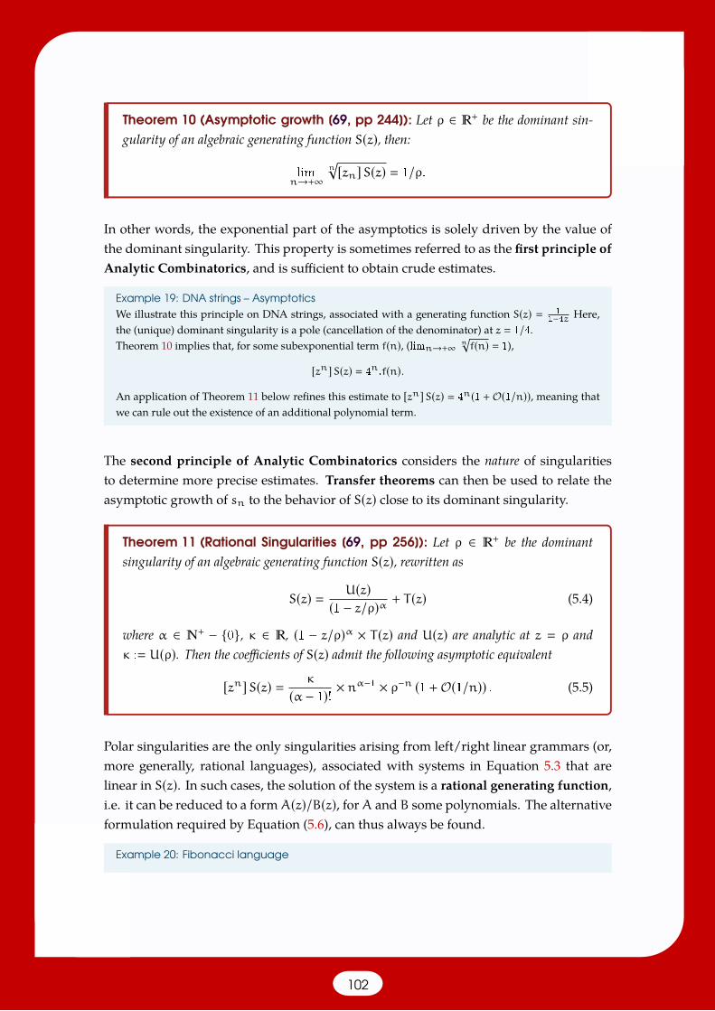
Theorem 10 (Asymptotic growth [69, pp 244]): Let ρ ∈ + be the dominant sin-gularity of an algebraic generating function S(z), then:

limn→+∞

n√[zn]S(z) 1/ρ.

In other words, the exponential part of the asymptotics is solely driven by the value ofthe dominant singularity. This property is sometimes referred to as the first principle ofAnalytic Combinatorics, and is sufficient to obtain crude estimates.

Example 19: DNA strings – AsymptoticsWe illustrate this principle on DNA strings, associated with a generating function S(z) 1

1−4z Here,the (unique) dominant singularity is a pole (cancellation of the denominator) at z 1/4.Theorem 10 implies that, for some subexponential term f(n), (limn→+∞ n

√f(n) 1),

[zn]S(z) 4n.f(n).

An application of Theorem 11 below refines this estimate to [zn]S(z) 4n(1 +O(1/n)), meaning thatwe can rule out the existence of an additional polynomial term.

The second principle of Analytic Combinatorics considers the nature of singularitiesto determine more precise estimates. Transfer theorems can then be used to relate theasymptotic growth of sn to the behavior of S(z) close to its dominant singularity.

Theorem 11 (Rational Singularities [69, pp 256]): Let ρ ∈ + be the dominantsingularity of an algebraic generating function S(z), rewritten as

S(z) U(z)(1 − z/ρ)α + T (z) (5.4)

where α ∈ + − 0, κ ∈ , (1 − z/ρ)α × T (z) and U(z) are analytic at z ρ andκ : U(ρ). Then the coefficients of S(z) admit the following asymptotic equivalent

[zn]S(z) κ

(α − 1)! × nα−1 × ρ−n (1 +O(1/n)) . (5.5)

Polar singularities are the only singularities arising from left/right linear grammars (or,more generally, rational languages), associated with systems in Equation 5.3 that arelinear in S(z). In such cases, the solution of the system is a rational generating function,i.e. it can be reduced to a formA(z)/B(z), forA and B some polynomials. The alternativeformulation required by Equation (5.6), can thus always be found.

Example 20: Fibonacci language

102

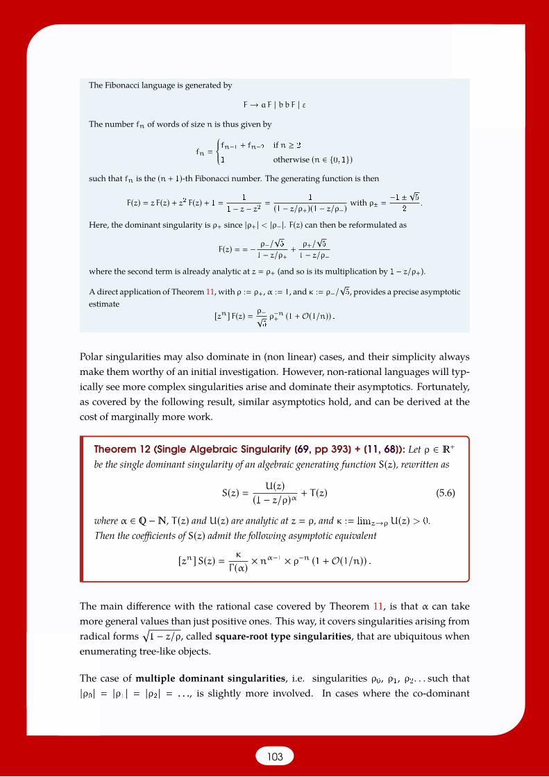
The Fibonacci language is generated by

F→ a F | bb F | ε

The number fn of words of size n is thus given by

fn

fn−1 + fn−2 if n ≥ 2

1 otherwise (n ∈ 0, 1)

such that fn is the (n + 1)-th Fibonacci number. The generating function is then

F(z) z F(z) + z2 F(z) + 1 1

1 − z − z2 1

(1 − z/ρ+)(1 − z/ρ−) with ρ± −1 ± √5

2.

Here, the dominant singularity is ρ+ since |ρ+ | < |ρ− |. F(z) can then be reformulated as

F(z) − ρ−/√5

1 − z/ρ+ +ρ+/√5

1 − z/ρ−where the second term is already analytic at z ρ+ (and so is its multiplication by 1 − z/ρ+).

A direct application of Theorem 11, with ρ : ρ+, α : 1, and κ : ρ−/√5, provides a precise asymptotic

estimate[zn] F(z) ρ−√

5ρ−n+ (1 +O(1/n)) .

Polar singularities may also dominate in (non linear) cases, and their simplicity alwaysmake them worthy of an initial investigation. However, non-rational languages will typ-ically see more complex singularities arise and dominate their asymptotics. Fortunately,as covered by the following result, similar asymptotics hold, and can be derived at thecost of marginally more work.

Theorem 12 (Single Algebraic Singularity [69, pp 393] + [11, 68]): Let ρ ∈ +

be the single dominant singularity of an algebraic generating function S(z), rewritten as

S(z) U(z)(1 − z/ρ)α + T (z) (5.6)

where α ∈ −, T (z) and U(z) are analytic at z ρ, and κ : limz→ρU(z) > 0.Then the coefficients of S(z) admit the following asymptotic equivalent

[zn]S(z) κ

Γ (α) × nα−1 × ρ−n (1 +O(1/n)) .

The main difference with the rational case covered by Theorem 11, is that α can takemore general values than just positive ones. This way, it covers singularities arising fromradical forms

√1 − z/ρ, called square-root type singularities, that are ubiquitous when

enumerating tree-like objects.

The case of multiple dominant singularities, i.e. singularities ρ0, ρ1, ρ2. . . such that|ρ0 | |ρ1 | |ρ2 | . . ., is slightly more involved. In cases where the co-dominant

103

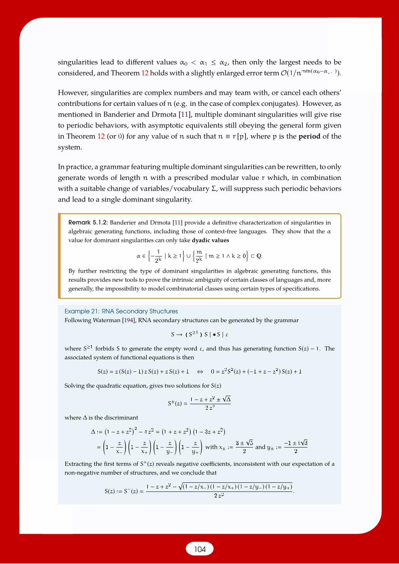
singularities lead to different values α0 < α1 ≤ α2, then only the largest needs to beconsidered, and Theorem 12 holds with a slightly enlarged error termO(1/nmin(α0−α1,1)).

However, singularities are complex numbers and may team with, or cancel each others’contributions for certain values of n (e.g. in the case of complex conjugates). However, asmentioned in Banderier and Drmota [11], multiple dominant singularities will give riseto periodic behaviors, with asymptotic equivalents still obeying the general form givenin Theorem 12 (or 0) for any value of n such that n ≡ r [p], where p is the period of thesystem.

In practice, a grammar featuringmultiple dominant singularities can be rewritten, to onlygenerate words of length n with a prescribed modular value r which, in combinationwith a suitable change of variables/vocabulary Σ, will suppress such periodic behaviorsand lead to a single dominant singularity.

Remark 5.1.2: Banderier and Drmota [11] provide a definitive characterization of singularities inalgebraic generating functions, including those of context-free languages. They show that the αvalue for dominant singularities can only take dyadic values

α ∈− 1

2k| k ≥ 1

∪

m

2k| m ≥ 1 ∧ k ≥ 0

⊂ .

By further restricting the type of dominant singularities in algebraic generating functions, thisresults provides new tools to prove the intrinsic ambiguity of certain classes of languages and, moregenerally, the impossibility to model combinatorial classes using certain types of specifications.

Example 21: RNA Secondary StructuresFollowing Waterman [194], RNA secondary structures can be generated by the grammar

S→ (S≥1 )S | •S | ε

where S≥1 forbids S to generate the empty word ε, and thus has generating function S(z) − 1. Theassociated system of functional equations is then

S(z) z (S(z) − 1) z S(z) + z S(z) + 1 ⇔ 0 z2S2(z) + (−1 + z − z2)S(z) + 1

Solving the quadratic equation, gives two solutions for S(z)

S±(z) 1 − z + z2 ± √∆2 z2

where ∆ is the discriminant

∆ :(1 − z + z2)2 − 4 z2

(1 + z + z2

) (1 − 3z + z2

)

(1 − z

x−

) (1 − z

x+

) (1 − z

y−

) (1 − z

y+

)with x± :

3 ± √52

and y± :−1 ± i√3

2

Extracting the first terms of S+(z) reveals negative coefficients, inconsistent with our expectation of anon-negative number of structures, and we conclude that

S(z) : S−(z) 1 − z + z2 −√(1 − z/x−) (1 − z/x+) (1 − z/y−) (1 − z/y+)

2 z2.

104

The function admits singularities for z ∈ x−, x+,y−,y+, and is analytic everywhere else in . Thedominant singularity is ρ : x− as it has smallest modulus, and we can rewrite S(z) as

S 1 − z + z2

2z2− 1

(1 − z/ρ)−1/2×U(z) with U(z) :

√(1 − z/x+) (1 − z/y−) (1 − z/y+)

2 z2

where U(z) can verified to be analytic at z ρ, and reaches the following value

κ : U(ρ) √12√5 − 20

(7 − 3√5) ×

√3 +√5

√15 + 7

√5

2.

A direct application of Theorem 12, with α −1/2, gives the final asymptotic equivalent:

[zn]S(z) κ

2√π× ρ−n

n√n(1 +O(1/n))

This asymptotic first-order estimate is remarkably accurate, and is already within 1% of the true countfor RNAs of length 250 nts, and keeps on getting better and better to reach asymptotic equality.

5.1.4 Useful extensions and shortcuts

5.1.4.1 Ensemble properties using multivariate gen. fun. and derivatives

So far, generating functions have only provided valuable information on the number ofwords of size n within a language. However, in many cases, the asymptotic growth ofsn [zn]S(z) is arguably less relevant to a downstream application than the expectedproperties of a word inLn. To study such properties, one needs to (transiently) introducea bivariate generating functions, which not only considers the length of an object, butalso some additional property, here called a feature.

Namely, consider atomic contributions frr∈R, associating a (possibly null) numericvalue to the production rules of a grammar.

Definition 5.1.5 (Additive feature): An additive feature F : L → is definedadditively based on a set of atomic contributions such as, for all w ∈ L generatedby a unique parse tree pw, one has

F(w) ∑r∈pw

f(r).

Features naturally include the number of occurrences |w|t of a given letter t ∈ Σ in awordw. More complex features may require the design of an ad hoc grammar to accommodatehighly-specific atomic contributions.

This allows to define the bivariate generating function of a language with respect to a

105

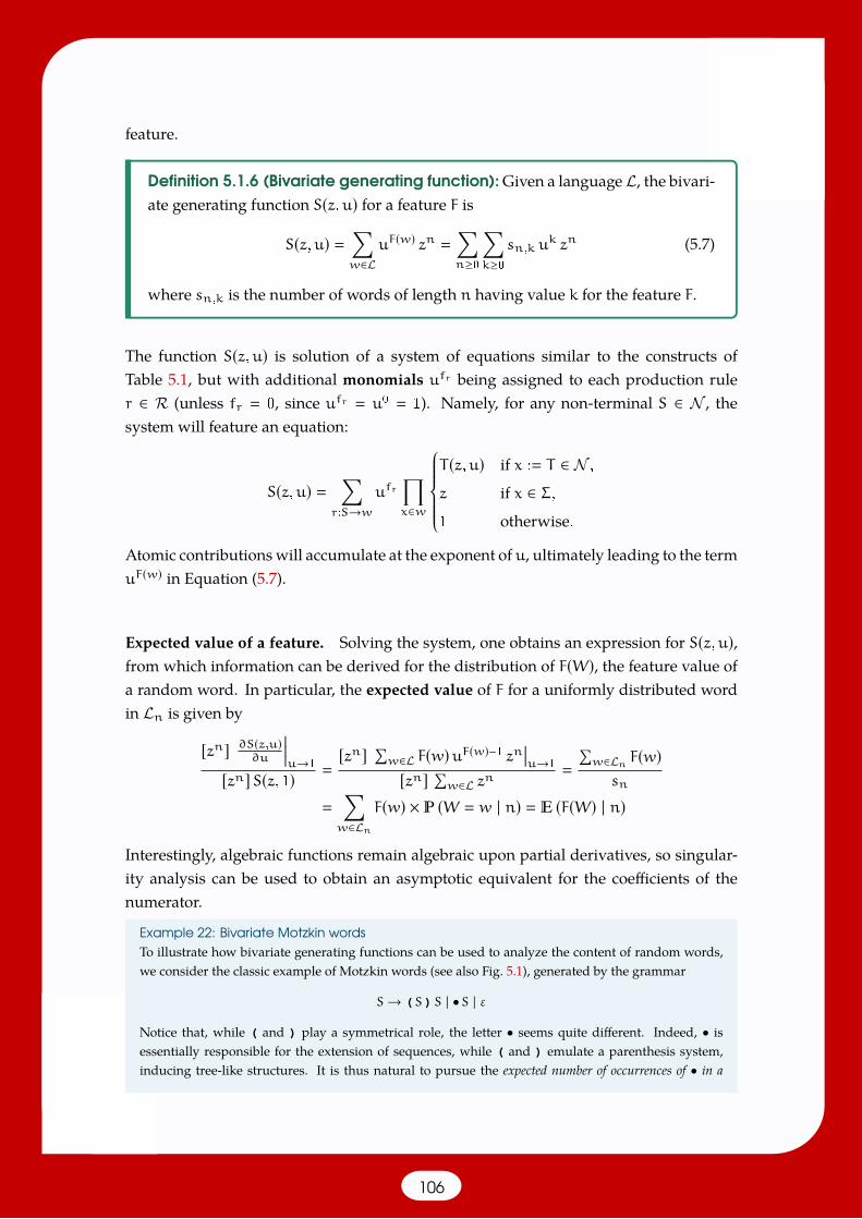
feature.

Definition 5.1.6 (Bivariate generating function): Given a languageL, the bivari-ate generating function S(z,u) for a feature F is

S(z,u) ∑w∈L

uF(w) zn

∑n≥0

∑k≥0

sn,k uk zn (5.7)

where sn,k is the number of words of length n having value k for the feature F.

The function S(z,u) is solution of a system of equations similar to the constructs ofTable 5.1, but with additional monomials ufr being assigned to each production ruler ∈ R (unless fr 0, since ufr u0 1). Namely, for any non-terminal S ∈ N , thesystem will feature an equation:

S(z,u) ∑r:S→w

ufr∏x∈w

T (z,u) if x : T ∈ N ,

z if x ∈ Σ,1 otherwise.

Atomic contributionswill accumulate at the exponent of u, ultimately leading to the termuF(w) in Equation (5.7).

Expected value of a feature. Solving the system, one obtains an expression for S(z,u),from which information can be derived for the distribution of F(W), the feature value ofa random word. In particular, the expected value of F for a uniformly distributed wordin Ln is given by

[zn] ∂S(z,u)∂u

u→1

[zn]S(z, 1) [zn] ∑

w∈L F(w)uF(w)−1 znu→1

[zn] ∑w∈L zn

∑w∈Ln F(w)sn

∑w∈Ln

F(w) × (W w | n) (F(W) | n)

Interestingly, algebraic functions remain algebraic upon partial derivatives, so singular-ity analysis can be used to obtain an asymptotic equivalent for the coefficients of thenumerator.

Example 22: Bivariate Motzkin wordsTo illustrate how bivariate generating functions can be used to analyze the content of random words,we consider the classic example of Motzkin words (see also Fig. 5.1), generated by the grammar

S→ (S)S | •S | ε

Notice that, while ( and ) play a symmetrical role, the letter • seems quite different. Indeed, • isessentially responsible for the extension of sequences, while ( and ) emulate a parenthesis system,inducing tree-like structures. It is thus natural to pursue the expected number of occurrences of • in a

106

uniformly-distributed word of size n.

First, we define the atomic features as the number of occurrences of • produced by each derivation:

r1 : S→ (S)S ⇒ fr1 0 r2 : S→ •S ⇒ fr2 1 r3 : S→ ε ⇒ fr3 0

Then we translate the grammar into a system of functional equations involving by the bivariate gener-ating function

S(z,u) z2 u0 S(z,u)2 + z u1 S(z,u) + u0 z2 S(z,u)2 + z uS(z,u) + 1

Solving the system gives

S(z,u) ∑n≥0

∑k≥0

sn,kukzn

1 − zu −√(1 − uz − 2z)(1 − uz + 2z)

2z2

One then derives by u, and set u 1, to obtain the generating function counting the total number ofoccurrences of •within Motzkin words of length n.

∂S(z,u)∂u

− z

2z2+

√1 − uz − 2z

4z√1 − uz + 2z

+

√1 − uz + 2z

4z√1 − uz − 2z

∂S(z,u)∂u

u→1

− z

2z2+

√1 − 3z

4z√1 + z

+

√1 + z

4z√1 − 3z

− z

2z2+(1 − 3z) + (1 + z)

4z√1 + z × √1 − 3z

− z

2z2+

1 − z2z√1 + z

× 1√1 − 3z

The resulting (mono variate) generating function features two singularities at z 1/3 and z −1respectively, so the dominant one is ρ 1/3. Applying Theorem 12 with α 1/2 andU(z) √1 + z/2zgives the following equivalent

[zn] ∂S(z,u)∂u

u→1

1 − ρ

2ρ√1 + ρ

√π

ρ−n√n(1 +O(1/n))

On the other hand, for the denominator we have

S(z, 1) S(z) 1 − z −√(1 − 3z)(1 + z)2z2

⇒ [zn]S(z) √1 + ρ

4ρ2√π

ρ−n

n√n(1 +O(1/n))

Taking the ratio finally gives the expected number of occurrences of the letter •

(|W |• | n) [zn] ∂S(z,u)∂u

u→1

[zn]S(z)

1−ρ2ρ√1+ρ√π

ρ−n√n(1 +O(1/n))

√1+ρ

4ρ2√π

ρ−nn√n(1 +O(1/n))

n2ρ (1 − ρ)1 + ρ

(1 +O(1/n)) n

3(1 +O(1/n))

Quite surprisingly, the asymptotic proportion of • is exactly 1/3, and so are those of ( and ) (havingequal number of occurrences), despite the highly asymmetrical roles played by the three letters.

Remark 5.1.3 (Higher Order Moments): By iterating the partial derivative (compensating with ueach time), higher moments can be extracted in a similar manner, granting access to the variance,skewness, kurtosis of the feature distribution induced by the uniform distribution over words oflength n.

107

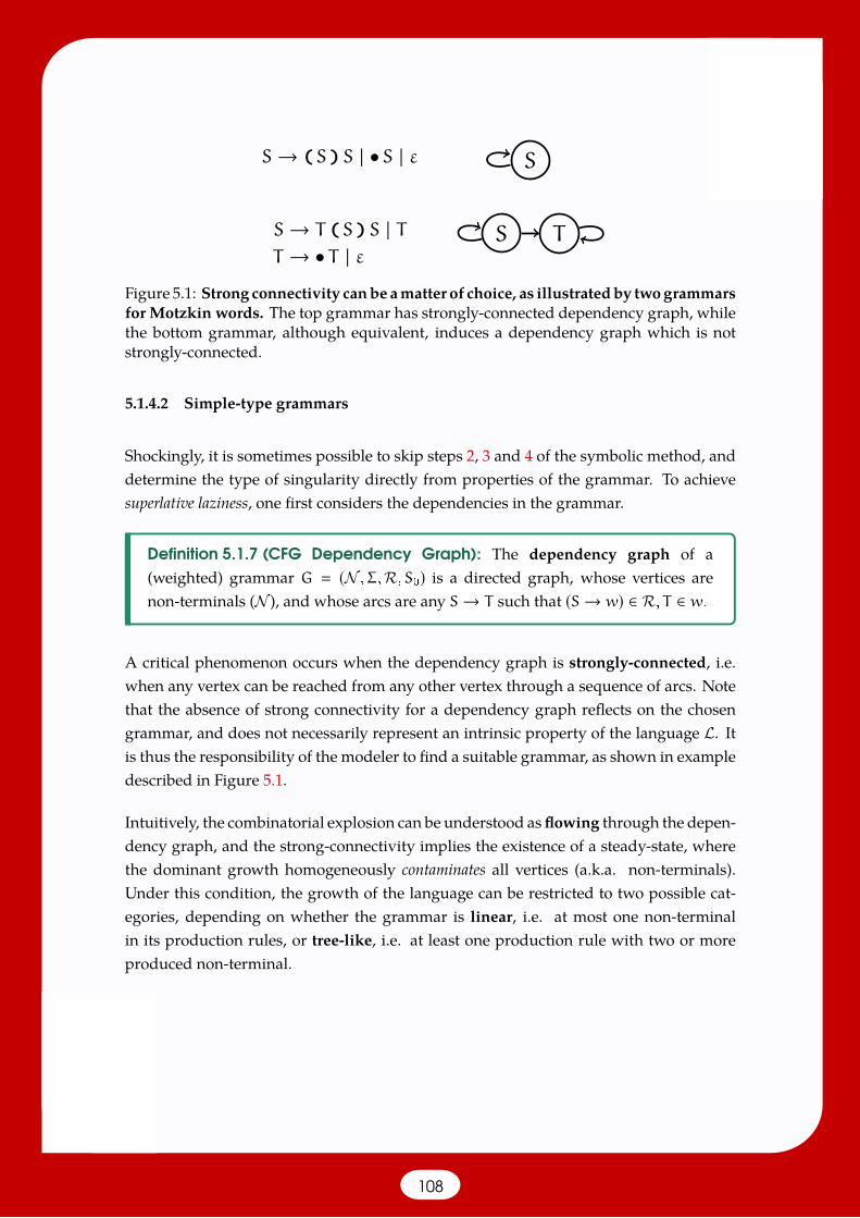
S→ (S )S | •S | ε S

S→ T (S )S | TT → • T | ε

S T

Figure 5.1: Strong connectivity canbe amatter of choice, as illustratedby twogrammarsfor Motzkin words. The top grammar has strongly-connected dependency graph, whilethe bottom grammar, although equivalent, induces a dependency graph which is notstrongly-connected.

5.1.4.2 Simple-type grammars

Shockingly, it is sometimes possible to skip steps 2, 3 and 4 of the symbolic method, anddetermine the type of singularity directly from properties of the grammar. To achievesuperlative laziness, one first considers the dependencies in the grammar.

Definition 5.1.7 (CFG Dependency Graph): The dependency graph of a(weighted) grammar G (N ,Σ,R,S0) is a directed graph, whose vertices arenon-terminals (N ), and whose arcs are any S→ T such that (S→ w) ∈ R, T ∈ w.

A critical phenomenon occurs when the dependency graph is strongly-connected, i.e.when any vertex can be reached from any other vertex through a sequence of arcs. Notethat the absence of strong connectivity for a dependency graph reflects on the chosengrammar, and does not necessarily represent an intrinsic property of the language L. Itis thus the responsibility of the modeler to find a suitable grammar, as shown in exampledescribed in Figure 5.1.

Intuitively, the combinatorial explosion can be understood as flowing through the depen-dency graph, and the strong-connectivity implies the existence of a steady-state, wherethe dominant growth homogeneously contaminates all vertices (a.k.a. non-terminals).Under this condition, the growth of the language can be restricted to two possible cat-egories, depending on whether the grammar is linear, i.e. at most one non-terminalin its production rules, or tree-like, i.e. at least one production rule with two or moreproduced non-terminal.

108

Theorem 13 (Strongly-connected Asymptotics: Perron-Frobenius [69, pp343] + Drmota-Lalley-Woods [56, 112, 202] ): Given a CFG G (N ,Σ,R,S0)with strongly-connected dependency graph, only the following two types of dominantsingularities may occur:

• If G is linear, then the dominant singularity ρ is a simple pole, i.e. there existsU(z) and T (z), both analytic at z ρ, with U(ρ) , 0 such that:

S(z) U(z)1 − z/ρ + T (z) ⇒ [zn]S(z) U(ρ) × ρ−n(1 +O(1/n));

• If G is tree-like, then the dominant singularity ρ has square-root type, i.e. thereexists U(z) and T (z) analytic at z ρ, k : limn→+∞U(ρ) , 0, such that:

S(z) −U(z) ×√1 − z/ρ + T (z) ⇒ [zn]S(z) κ

2√π× ρ

−n

n√n(1 +O(1/n)).

Such stereotyped asymptotics are immensely useful to study languages with large gram-mars, for which human patience and symbolic calculus can both reach their respectivelimits. In this case, computing the first coefficients of the generating function, e.g. usingthe recurrences of Figure 5.1, would allow to estimate κ and ρ to a sufficient precision inmost applied contexts.

5.1.4.3 Weighted languages and asymptotics

Another extension, crucial in applied contexts, considers the introduction of weights,and was explored in a collaboration with Alain Denise and Michel Termier [50].

Definition 5.1.8 (Weighted grammar): A Weighted Language is generated by acontext-free grammar G (N ,Σ,R,S0), coupled with aweight vector π, associat-ing a weight πt to each terminal t ∈ Σ.

The weight π(w) of a word w ∈ Σ? is defined by

π(w) |w|∏i1

πwi .

The overall weight of a language L is then typically the quantity of interest, encapsulatedin a weighted generating function

Sπ(z) ∑w∈L

π(w) zn

∑n≥0

∑w∈Ln

π(w) zn

∑n≥0

sn zn

109

where sn now represents the accumulatedweight of all words of lengthn inL. Weightedgenerating functions associated with unambiguous grammars are the solutions of analgebraic system of functional equations. Those can be obtained using a slightlymodifiedversion of the constructs in Table 5.1, where terminals rules now account for theirrespective weight:

(Ordinary gen. fun.) S(z) z → (Weighted gen. fun.) Sπ(z) πt × z. (5.8)

While Sπ(z) can be of interest in itself, e.g. as its coefficients representpartition functions,one can also adopt an alternative probabilistic view and think of the weights as inducinga Boltzmann-Gibbs distribution over the class of words of size n.

Definition 5.1.9 (Weighted distribution): Let G (N ,Σ,R,S0,π) be an unam-biguous CFG, generating a language L, and n be a length, theweighted distribu-tion is defined such that:

π (w | n) ∏|w|i1πwi

[zn]Sπ(z) π(w)sn

where sn [zn]Sπ ∑w∈Ln π(w).

The association of weights to terminal symbols (or, equivalently, to individual produc-tions, as we showed [149]) grants more flexibility to the modeler in the design of aspecification, particularly when weights are non-rational reals. Examples abound whenreal-valued weights are needed, e.g. when weights are optimized to achieve a targetedcomposition, or when classic Boltzmann-Gibbs distributions of the form (w) ∝ e−Ew/βare being investigated.

Moreover, their associated generating functions remain the solutions of algebraic systemsof equations, so the entire armada of analytic combinatorics can be leveraged to analyzetheir asymptotic behavior.

Proposition 14 (Asymptotics of Weighted Languages): The asymptotic equiva-lents of Theorems 10, 11, 12, and 13 hold for weighted generating functions.

Example 23: Expected number of secondary structures per RNA [212]The number of secondary structures of length n [194] only represents a crude upper bound for thenumber of secondary structures compatible with a given RNA sequence w, |w| n. indeed, canonicalbase-pairs can only form between pairs of nucleotides in

B (A,U), (U,A), (G,C), (C,G), (G,U), (U,G),

forbidding certain secondary structures to form for certain sequences.

While the precise number of such structures vary substantially depending on the actual sequence,

110

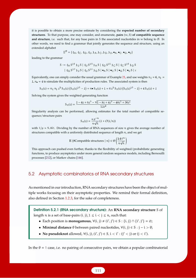
it is possible to obtain a more precise estimate by considering the expected number of secondarystructures. To that purpose, one may consider, and enumerate, pairs (w,S) of compatible sequenceand structure, i.e. such that, for any base pairs in S the associated nucleotides in w belong to B. Inother words, we need to find a grammar that jointly generates the sequence and structure, using anextended alphabet

ΣB (A,(C,(G,(U,)A,)C,)G,)U, •A, •C, •G, •Uleading to the grammar

S→ (A S≥1 )U S | (U S

≥1 )A S | (G S≥1 )C S | (C S

≥1 )G S

| (G S≥1 )U S | (U S

≥1 )G S | •A S | •C S | •G S | •U S | ε

Equivalently, one can simply consider the usual grammar of Example 21, and use weights π( 6,π)

1,π• 4 to simulate the multiplicities of production rules. The associated system is then

Sπ(z) π( π) z2 Sπ(z)(Sπ(z)≥1 − 1

)+ π•Sπ(z) + 1 6 z2 Sπ(z)

(Sπ(z)≥1 − 1

)+ 4Sπ(z) + 1

Solving the system gives the weighted generating function

Sπ(z) 1 − 4z + 6z2 −√1 − 8z + 4z2 − 48z3 + 36z4

12z2

Singularity analysis can be performed, allowing estimates for the total number of compatible se-quence/structure pairs

Sπ(z) κ ρ−n

n√n(1 +O(1/n))

with 1/ρ ≈ 8.164. Dividing by the number of RNA sequences of size n gives the average number ofstructures compatible with a uniformly distributed sequence of length n, and we get

(#Compatible structures | n) ∈ Θ (

2.04n

n√n

)

This approach can pushed even further, thanks to the flexibility of weighted/probabilistic generatingfunctions, to produce asymptotics under more general random sequence models, including Bernouilliprocesses [212], or Markov chains [146].

5.2 Asymptotic combinatorics of RNA secondary structures

Asmentioned in our introduction, RNAsecondary structures have been the object ofmul-tiple works focusing on their asymptotic properties. We remind their formal definition,also defined in Section 1.2.3, for the sake of completeness.

Definition 5.2.1 (RNA secondary structure): An RNA secondary structure S oflength n is a set of base-pairs (i, j), 1 ≤ i < j ≤ n, such that:

• Each position is monogamous, ∀(i, j) , (i′, j′) ∈ S : i, j ∩ i′, j′ ;• Minimal distance θ between paired nucleotides, ∀(i, j) ∈ S : j − i > θ;• No pseudoknot allowed, ∀(i, j), (i′, j′) ∈ S, i < i′ : (j′ < j) or (j < i′).

In the θ 1 case, i.e. no pairing of consecutive pairs, we obtain a popular combinatorial

111

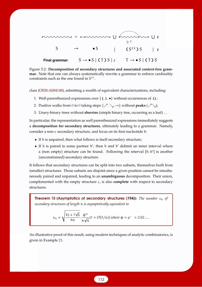
≥ 1

= ⋃⋃ε

S •S (S≥1 )S ||→ ε

Final grammar: S→ •S | ( T )S | ε T → •S | ( T )SFigure 5.2: Decomposition of secondary structures and associated context-free gram-mar. Note that one can always systematically rewrite a grammar to enforce cardinalityconstraints such as the one found in S≥1.

class (OEIS:A004148), admitting a wealth of equivalent characterizations, including:

1. Well-parenthesized expressions over (,), • without occurrences of ();

2. Positive walks from 0 to 0 taking steps ,,→ without peaks ();

3. Unary-binary trees without sherries (simple binary tree, occurring as a leaf). . .

In particular, the representation as well parenthesized expressions immediately suggestsa decomposition for secondary structures, ultimately leading to a grammar. Namely,consider a non-ε secondary structure, and focus on its first nucleotide b:

• If b is unpaired, then what follows is itself secondary structure;

• If b is paired to some partner b′, then b and b′ delimit an inner interval wherea (non empty) structure can be found. Following the interval [b,b′] is another(unconstrained) secondary structure.

It follows that secondary structures can be split into two subsets, themselves built from(smaller) structures. Those subsets are disjoint since a given position cannot be simulta-neously paired and unpaired, leading to an unambiguous decomposition. Their union,complemented with the empty structure ε, is also complete with respect to secondarystructures.

Theorem 15 (Asymptotics of secondary structures [194]): The number sn ofsecondary structures of length n is asymptotically equivalent to

sn

√15 + 7

√5

8π.φn

n√n(1 +O(1/n)) where φ ρ−1 ≈ 2.62 . . .

An illustrative proof of this result, using modern techniques of analytic combinatorics, isgiven in Example 21.

112

https://oeis.org/A004148

5.2.1 Expected 5’–3’ distance [38]

A first application of the above principles considers the 5’–3’ distance, i.e. the graphdistance induced by a(n ensemble of) secondary structure(s) between the ends of anRNA.

Definition 5.2.2 (5’–3’ distance): Given an RNA secondary structure S, the 5’–3’ distance, graph distance induced by a(n ensemble of) secondary structure(s)between the ends of an RNA

Yoffe et al [207] argued that a small distance, independent of RNA length, between the twoends of RNA single-stranded molecules. The authors claimed that such a small distancewas intrinsic to linear polymers, a claim supported by a heuristic argument arising frompolymerphysics, andempirically from the systematicMFE foldingof randomlygeneratedRNAs under various compositions. Such a short distance is indeed deemed crucial tothe effective circularization of Eukaryotic messengers RNAs [196] through RNA-proteinsand protein-protein complexes.

In collaboration with Peter Clote and Jean-Marc Steyaert [38], we decided to revisit thisclaim at three different levels: Theoretically, by checking its asymptotic validity in thehomopolymer model; Algorithmically, by introducing a Θ(n3) dynamic programmingalgorithm to compute the expected 5’-3’ distance for a given sequence at the thermo-dynamic equilibrium; Empirically, by computing the graph distance on a collection ofRNAs of documented structures.

Our asymptotic analysis relies on the design of a grammar which, by identifying nu-cleotides on the 5’ to 3’ shortest path, allowed the derivation of a bivariate generatingfunction for the 5’–3’ distance. We achieved this by a classic, if technical, application ofthe symbolic method. Essentially, we duplicated the production rules, distinguishingrules that generate the exterior bases from those whose content is nested within somebase pair, and are as such not relevant to the expected 5’–3’ distance. A similar reason-ing allowed to capture general values for the minimum distance θ between two pairedpositions, and we obtained the following grammar:

Sθ → [Rθ]Sθ | Sθ | ε; Tθ → (Rθ)Tθ | • Tθ | ε; Rθ → (Rθ)Tθ | • Rθ | •θ (5.9)

Translating into a system of bivariate functional equation, one obtains

Sθ(z,u) z2u2Rθ(z)Sθ(z,u) + zuSθ(z,u) + 1

Tθ(z) z2Rθ(z)Tθ(z) + zTθ(z) + zθRθ(z) z2Rθ(z)Tθ(z) + zRθ(z) + zθ.

113

Solving the system gives the bivariate generating function

Sθ(z,u) ∑n≥0

∑k≥0

sk,n;θ uk zn

1

1 − zu − u2(1−2z+zθ+2−√∆θ)2(1−z)

(5.10)

with sk,n;θ the number of secondary structures of length n, with minimum base pairdistance θ, and having k nucleotides on the exterior face, and

∆θ 1 − 4z + 4z2 − 2zθ+2 + 4zθ+3 − 4zθ+4 + z2θ+4. (5.11)

In particular, one gets

Sθ(z, 1) 1 − 2z + 2z2 + 2zθ − zθ+2 − √∆θ(1 − z)2z2 .

Next, we use the classic bivariate analysis

Eθ(z) ∂Sθ(z,u)∂u

u1

P(z) − (2 − 5z + 4z2 − 2zθ+2 + zθ+3)√∆θ

2(1 − z)2z4

such that en : [zn]Eθ(z) is the accumulated number of exterior bases across all RNAsof length n, and P(z) is a polynomial of degree θ + 4, whose precise value bears noconsequence on the asymptotics. Applying Theorem 12, one gets

[zn]Sθ(z, 1) ∼ − 1

(1 − ρ)2ρ2 × [zn]

√∆θ (5.12)

[zn]Eθ(z) ∼ −(2 − 5ρ + 4ρ2 − 2ρθ+2 + ρθ+3

)2(1 − ρ)2ρ4 × [zn]

√∆θ. (5.13)

where ρ is the shared dominant singularity of Sθ(z) and Eθ, i.e. the root of ∆θ havingsmallest modulus (real by Pringsheim). We obtain the following result by taking the ratioof estimates (5.13) and (5.12) to obtain the expected number of bases on the exterior base,to which we subtract 1 to obtain the graph distance.

Theorem 16 (Expected 5’-3’ distance - Homopolymer model [38]): The ex-pected 5′ − 3′ distance Dn over all RNA secondary structures of length n, assumingminimum distance θ between paired nucleotides, is given by

Dn [zn]Eθ(z)[zn]Sθ(z, 1) − 1

2 − 5ρ + 3ρ2 + ρ3 − 2ρθ+2 + ρθ+3

(1 − ρ) ρ2 (1 +O(1/n)) (5.14)

where ρ is the smallest modulus root of

∆θ : 1 − 4z + 4z2 − 2zθ+2 + 4zθ+3 − 4zθ+4 + z2θ+4. (5.15)

As suspected by Yoffe et al [207], the expected value is constant, small and stable todifferent values of θ. Of particular interest are the following numerical approximations,

114

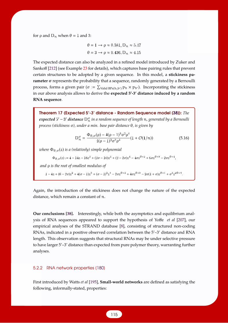
for ρ and Dn when θ 1 and 3:

θ 1→ ρ ≈ 0.381,Dn ≈ 5.47

θ 3→ ρ ≈ 0.436,Dn ≈ 4.15

The expected distance can also be analyzed in a refined model introduced by Zuker andSankoff [212] (see Example 23 for details), which captures base pairing rules that preventcertain structures to be adopted by a given sequence. In this model, a stickiness pa-rameter σ represents the probability that a sequence, randomly generated by a Bernoulliprocess, forms a given pair (σ :

∑Valid BPs(b,b′) pb × pb′). Incorporating the stickiness

in our above analysis allows to derive the expected 5’-3’ distance induced by a randomRNA sequence.

Theorem 17 (Expected 5’-3’ distance - Random Sequence model [38]): Theexpected 5′ − 3′ distanceDσn in a random sequence of length n, generated by a Bernoulliprocess (stickiness σ), under a min. base pair distance θ, is given by

Dσn Φθ,σ(ρ) − 4(ρ − 1)3σ2ρ4

4(ρ − 1)3σ2ρ4 (1 +O(1/n)) (5.16)

where Φθ,σ(z) is a (relatively) simple polynomial

Φθ,σ(z) : 4 − 14z − 18z2 + (2σ − 10)z3 + (2 − 2σ)z4 − 4σzθ+2 + 6σzθ+3 − 2σzθ+4,

and ρ is the root of smallest modulus of

1 − 4z + (6 − 2σ)z2 + 4(σ − 1)z3 + (σ − 1)2z4 − 2σzθ+2 + 4σzθ+3 − 2σ(1 + σ)zθ+4 + σ2z2θ+4.

Again, the introduction of the stickiness does not change the nature of the expecteddistance, which remain a constant of n.

Our conclusions [38]. Interestingly, while both the asymptotics and equilibrium anal-ysis of RNA sequences appeared to support the hypothesis of Yoffe et al [207], ourempirical analyses of the STRAND database [8], consisting of structured non-codingRNAs, indicated in a positive observed correlation between the 5’–3’ distance and RNAlength. This observation suggests that structural RNAs may be under selective pressureto have larger 5’–3’ distance than expected from pure polymer theory, warranting furtheranalyses.

5.2.2 RNA network properties [180]

First introduced by Watts et al [195], Small-world networks are defined as satisfying thefollowing, informally-stated, properties:

115

• the shortest path distance between any two nodes is “small”, e.g. six degrees ofseparation between any two persons;

• the average clustering coefficient is large, e.g. friends of a person tend to be friendsof each other.

Small-world networks are ubiquitous in biology, sociology, and information technology;examples abound, including the neural network ofC. elegans [195], the gene co-expressionin S. cerevisiae [186], protein folding networks [22, 170]. . . For additional examples, seethe excellent review of Albert and Barabási [4]. In particular, Wuchty [204] observed asmall-world property for the low energy RNA secondary structure network of E. coli phe-tRNA, and hypothesized this property to be crucial for the structural kinetics induced bytRNA modifications.

In collaboration with Defne Surujon and Peter Clote [180], we investigated asymptoticproperties of theRNAnetwork, the ensemble of all RNA secondary structures connectedby amove set.

Definition 5.2.3 (Move set): Given an RNA length n, a move set

MS M1,M2, . . .

is a collection ofmoves, i.e. functionsM : Sn → P(Sn).

For any structure S ∈ Sn, the execution of a move returns structures M(S) ⊂ Sn, eachresulting from the application of a (small) perturbation to S. Popular moves [72], in thecontext of a structure S, include:

• Addition of a base pair (i′, j′) such that S ∪ (i′, j′) is a valid structure;

• Removal of a base pair (i, j) ∈ S;• Shift of (i, j) ∈ S into (i′, j′), i i′ or j j′, only if resulting in a valid structure;

We considered two move sets:

• MS1 : Addition,Removal;• MS2 : Addition,Removal, Shift

Notice that, while individual moves may not be reversible, MS1 and MS2 are bothsymmetric, and allow to define a notion of neighborhood crucial to the definition of anetwork.

116

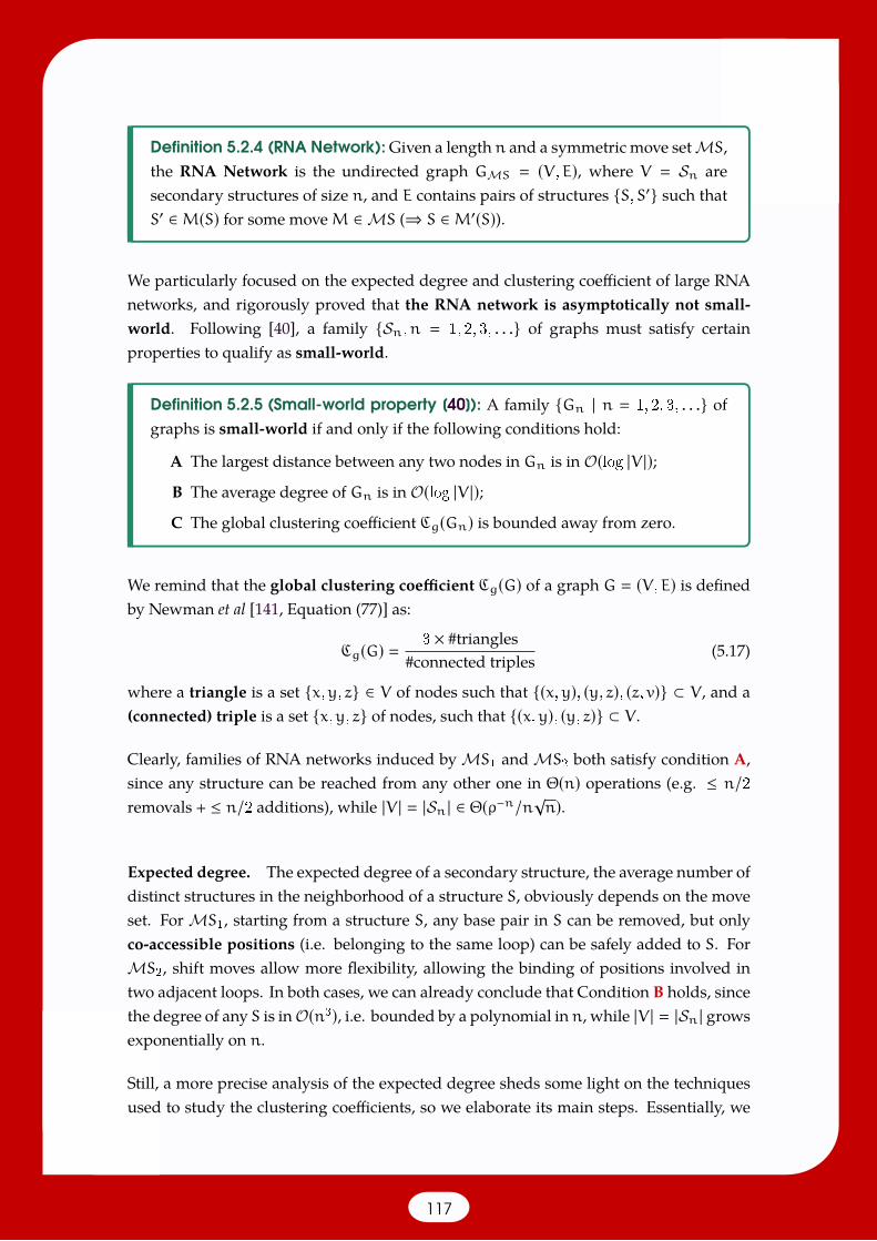
Definition 5.2.4 (RNA Network): Given a length n and a symmetric move setMS,the RNA Network is the undirected graph GMS (V,E), where V Sn aresecondary structures of size n, and E contains pairs of structures S,S′ such thatS′ ∈M(S) for some moveM ∈MS (⇒ S ∈M′(S)).

We particularly focused on the expected degree and clustering coefficient of large RNAnetworks, and rigorously proved that the RNA network is asymptotically not small-world. Following [40], a family Sn,n 1, 2, 3, . . . of graphs must satisfy certainproperties to qualify as small-world.

Definition 5.2.5 (Small-world property [40]): A family Gn | n 1, 2, 3, . . . ofgraphs is small-world if and only if the following conditions hold:

A The largest distance between any two nodes in Gn is in O(log |V |);B The average degree of Gn is in O(log |V |);C The global clustering coefficient Cg(Gn) is bounded away from zero.

We remind that the global clustering coefficient Cg(G) of a graph G (V,E) is definedby Newman et al [141, Equation (77)] as:

Cg(G) 3 × #triangles#connected triples (5.17)

where a triangle is a set x,y, z ∈ V of nodes such that (x,y), (y, z), (z, v) ⊂ V , and a(connected) triple is a set x,y, z of nodes, such that (x,y), (y, z) ⊂ V .

Clearly, families of RNA networks induced by MS1 and MS2 both satisfy condition A,since any structure can be reached from any other one in Θ(n) operations (e.g. ≤ n/2removals + ≤ n/2 additions), while |V | |Sn | ∈ Θ(ρ−n/n

√n).

Expected degree. The expected degree of a secondary structure, the average number ofdistinct structures in the neighborhood of a structure S, obviously depends on the moveset. For MS1, starting from a structure S, any base pair in S can be removed, but onlyco-accessible positions (i.e. belonging to the same loop) can be safely added to S. ForMS2, shift moves allow more flexibility, allowing the binding of positions involved intwo adjacent loops. In both cases, we can already conclude that Condition B holds, sincethe degree of any S is inO(n3), i.e. bounded by a polynomial in n, while |V | |Sn | growsexponentially on n.

Still, a more precise analysis of the expected degree sheds some light on the techniquesused to study the clustering coefficients, so we elaborate its main steps. Essentially, we

117

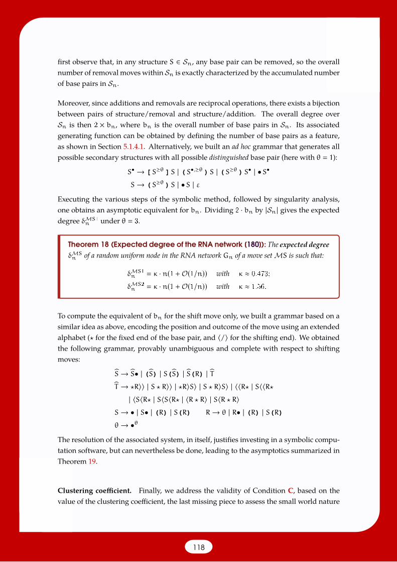
first observe that, in any structure S ∈ Sn, any base pair can be removed, so the overallnumber of removal moveswithin Sn is exactly characterized by the accumulated numberof base pairs in Sn.

Moreover, since additions and removals are reciprocal operations, there exists a bĳectionbetween pairs of structure/removal and structure/addition. The overall degree overSn is then 2 × bn, where bn is the overall number of base pairs in Sn. Its associatedgenerating function can be obtained by defining the number of base pairs as a feature,as shown in Section 5.1.4.1. Alternatively, we built an ad hoc grammar that generates allpossible secondary structures with all possible distinguished base pair (here with θ 1):

S• → [S≥θ ]S | (S•,≥θ )S | (S≥θ )S• | •S•S→ (S≥θ )S | •S | ε

Executing the various steps of the symbolic method, followed by singularity analysis,one obtains an asymptotic equivalent for bn. Dividing 2 · bn by |Sn | gives the expecteddegree δMS1n under θ 3.

Theorem 18 (Expected degree of the RNA network [180]): The expected degreeδMSn of a random uniform node in the RNA network Gn of a move set MS is such that:

δMS1n κ · n(1 +O(1/n)) with κ ≈ 0.473;

δMS2n κ · n(1 +O(1/n)) with κ ≈ 1.56.

To compute the equivalent of bn for the shift move only, we built a grammar based on asimilar idea as above, encoding the position and outcome of the move using an extendedalphabet (? for the fixed end of the base pair, and 〈/〉 for the shifting end). We obtainedthe following grammar, provably unambiguous and complete with respect to shiftingmoves:

S→ S• | (S) | S(S) | S(R) | TT → ?R〉〉 | S ? R〉〉 | ?R〉S〉 | S ? R〉S〉 | 〈〈R? | S〈〈R?| 〈S〈R? | S〈S〈R? | 〈R ? R〉 | S〈R ? R〉

S→ • | S• | (R) | S(R) R→ θ | R• | (R) | S(R)θ→ •θ

The resolution of the associated system, in itself, justifies investing in a symbolic compu-tation software, but can nevertheless be done, leading to the asymptotics summarized inTheorem 19.

Clustering coefficient. Finally, we address the validity of Condition C, based on thevalue of the clustering coefficient, the last missing piece to assess the small world nature

118

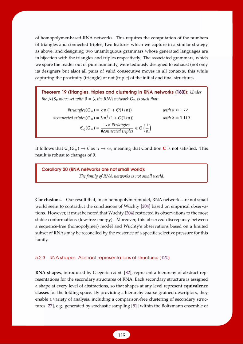
of homopolymer-based RNA networks. This requires the computation of the numbersof triangles and connected triples, two features which we capture in a similar strategyas above, and designing two unambiguous grammars whose generated languages arein bĳection with the triangles and triples respectively. The associated grammars, whichwe spare the reader out of pure humanity, were tediously designed to exhaust (not onlyits designers but also) all pairs of valid consecutive moves in all contexts, this whilecapturing the proximity (triangle) or not (triple) of the initial and final structures.

Theorem 19 (Triangles, triples and clustering in RNA networks [180]): Underthe MS2 move set with θ 3, the RNA network Gn is such that:

#triangles(Gn) κn (1 +O(1/n)) with κ ≈ 1.22

#connected triples(Gn) λn2 (1 +O(1/n)) with λ ≈ 0.112

Cg(Gn) 3 × #triangles#connected triples

∈ Θ(1

n

)

It follows that Cg(Gn) → 0 as n → ∞, meaning that Condition C is not satisfied. Thisresult is robust to changes of θ.

Corollary 20 (RNA networks are not small world):The family of RNA networks is not small world.

Conclusions. Our result that, in an homopolymer model, RNA networks are not smallworld seem to contradict the conclusions of Wuchty [204] based on empirical observa-tions. However, it must be noted thatWuchty [204] restricted its observations to the moststable conformations (low-free energy). Moreover, this observed discrepancy betweena sequence-free (homopolymer) model and Wuchty’s observations based on a limitedsubset of RNAsmay be reconciled by the existence of a specific selective pressure for thisfamily.

5.2.3 RNA shapes: Abstract representations of structures [120]

RNA shapes, introduced by Giegerich et al [82], represent a hierarchy of abstract rep-resentations for the secondary structures of RNA. Each secondary structure is assigneda shape at every level of abstractions, so that shapes at any level represent equivalenceclasses for the folding space. By providing a hierarchy coarse-grained descriptors, theyenable a variety of analysis, including a comparison-free clustering of secondary struc-tures [27], e.g. generated by stochastic sampling [51] within the Boltzmann ensemble of

119

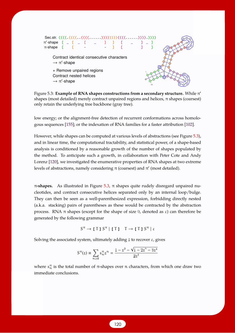
Sec.str. ((((.((((..((((......))))))))((((......)))).))))π′-shape [ _ [ _ [ _ ] ] [ _ ] _ ]π-shape [ [ - - ] [ ] ]

Contract identical consecutive characters→ π′-shape

+ Remove unpaired regionsContract nested helices→ π′-shape

Figure 5.3: Example of RNA shapes constructions from a secondary structure. While π′shapes (most detailed) merely contract unpaired regions and helices, π shapes (coarsest)only retain the underlying tree backbone (gray tree).

low energy; or the alignment-free detection of recurrent conformations across homolo-gous sequences [155]; or the indexation of RNA families for a faster attribution [102].

However, while shapes can be computed at various levels of abstractions (see Figure 5.3),and in linear time, the computational tractability, and statistical power, of a shape-basedanalysis is conditioned by a reasonable growth of the number of shapes populated bythe method. To anticipate such a growth, in collaboration with Peter Cote and AndyLorenz [120], we investigated the enumerative properties of RNA shapes at two extremelevels of abstractions, namely considering π (coarsest) and π′ (most detailed).

π-shapes. As illustrated in Figure 5.3, π shapes quite rudely disregard unpaired nu-cleotides, and contract consecutive helices separated only by an internal loop/bulge.They can then be seen as a well-parenthesized expression, forbidding directly nested(a.k.a. stacking) pairs of parentheses as these would be contracted by the abstractionprocess. RNA π shapes (except for the shape of size 0, denoted as ε) can therefore begenerated by the following grammar

Sπ → [ T ]Sπ | [ T ] T → [ T ]Sπ | ε

Solving the associated system, ultimately adding 1 to recover ε, gives

Sπ(z) ≡∑n≥0

sπnzn

1 − z2 −√1 − 2z2 − 3z4

2z2

where sπn is the total number of π-shapes over n characters, from which one draw twoimmediate conclusions.

120

[[[][]][][]][] ( ) ( . ) .

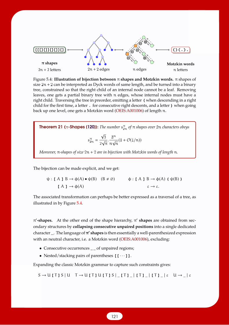
2n + 2 letters 2n + 2 edges n edges n lettersMotzkin wordsπ shapes

(

)(

.

).

Figure 5.4: Illustration of bĳection between π shapes and Motzkin words. π shapes ofsize 2n+ 2 can be interpreted as Dyck words of same length, and be turned into a binarytree, constrained so that the right child of an internal node cannot be a leaf. Removingleaves, one gets a partial binary tree with n edges, whose internal nodes must have aright child. Traversing the tree in preorder, emitting a letter (when descending in a rightchild for the first time, a letter . for consecutive right descents, and a letter )when goingback up one level, one gets a Motzkin word (OEIS:A001006) of length n.

Theorem 21 (π-Shapes [120]): The number sπ2n of π shapes over 2n characters obeys

sπ2n

√3

2√π.3n

n√n(1 +O(1/n))

Moreover, π-shapes of size 2n + 2 are in bĳection with Motzkin words of length n.

The bĳection can be made explicit, and we get:

ψ : [ A ] B→ φ(A) •ψ(B) (B , ) φ : [ A ] B→ φ(A) ( ψ(B) )[ A ]→ φ(A) ε→ ε.

The associated transformation can perhaps be better expressed as a traversal of a tree, asillustrated in by Figure 5.4.

π′-shapes. At the other end of the shape hierarchy, π′ shapes are obtained from sec-ondary structures by collapsing consecutive unpaired positions into a single dedicatedcharacter_. The language ofπ′ shapes is then essentially awell-parenthesized expressionwith an neutral character, i.e. a Motzkin word (OEIS:A001006), excluding:

• Consecutive occurrences _ _ of unpaired regions;

• Nested/stacking pairs of parentheses [[ · · ·]].Expanding the classic Motzkin grammar to capture such constraints gives:

S→ U[ T ]S | U T → U[ T ]U[ T ]S | _[ T ] _ | [ T ] _ | [ T ] _ | ε U→ _ | ε

121



Solving the generating function, one gets

Sπ′(z) A(z) − B(z)

√∆

C(z) with ∆ : 1 − 2 z2 − 6 z3 − 5 z4 − 6 z5 − z6 + 2 z7 + z8,

andA(z), B(z) and C(z) are polynomials, non-null at z ρ the dominant singularity (alsosmallest root of ∆).

Theorem 22 (π′-Shapes [120]): The number sπ′n of π′ shapes over n characters obeys

sπ′n κ

γn

n√n(1 +O(1/n)) where γ :

1

ρ≈ 2.41 and κ : lim

z→ρB(z)

2√πC(z) ≈ 0.985.

The chosen level of abstractions for shapes has therefore a strong impact on the numberof representatives of the RNA folding landscapes. At the coarsest level, the number ofπ-shapes only grows in Θ(1.73n/n√n), while the more informative π′-shapes induce acombinatorial explosion in Θ(2.41n/n√n).

Refined estimates for shapes compatible with a sequence. The total number of shapesovern characters represents a very crude upper bound for the expected number of shapesreturned by a predictive method when executed on an RNA consisting of n nucleotides.Indeed, certain sequences may not support the helices required to build a given shape.Ideally, one would therefore like to compute the expected number of shapes compatiblewith a sequence of length n. However, this turned out to be very challenging, due toapparently intrinsic difficulties to establish a suitable specification.

Indeed, computing an asymptotic equivalent for the expected number of shapes seemsbeyond the current reach of the symbolic method. For instance, contrary to RNA sec-ondary structures, it does not seempossible to formulate an unambiguous grammars thatenumerates all compatible shapes/sequences pairs. This is due to the fact that severalsecondary structures, all compatible with a given sequence and substantially different,may share a common shape at one or several levels, as shown below:

ACUACAGUGGUAGUACUUUAGAAUGUCUUAGA

S1 .(((..(((....))))..))..((...)).. → π(S1) [][] π(S1) _[_[]_]_[]_

S2 ((....)).((...))................ → π(S2) [][] π(S2) []_[]_

S3 (((((....)))))..((((((...)))))). → π(S3) [][] π(S3) []_[]_

More modestly, it is possible to refine our initial upper bound, by considering the min-imum length of a sequence supporting a given shape. For instance, hairpin loops,identified by motifs [], are subject to a minimum distance θ, and thus can be thought toconsume θ+2 nucleotides. We can capture this phenomenon by replacing each occurrenceof ε in the above grammars, indicating the occurrence of a hairpin loop by •θ. Summing

122

over shapes associated with minimum size smaller than n, one obtains much refinedestimates.

Theorem 23 (Expected number of shapes [120]): The expected number eπn (resp.eπ′n ) of π shapes (resp. π′ shapes), compatible with an RNA of length n under a min base

pairing distance θ 3, obeys:

eπn ≤1.28 × 1.81n

n√n

(1 +O(1/n)) eπ′n ≤

2.44 × 1.32n

n√n

(1 +O(1/n))

While these upper bound are considerably tighter than the total number of shapes oflength n, they still appear overly pessimistic in comparison to the empirical observationsof Voss et al [190]. In this work, the authors conjectured growths inΘ(1.1n) andΘ(1.16n)for π and π′ shapes respectively, motivating the development of new analysis techniquesfor this pragmatic class of conformational descriptors.

5.2.4 Enumerating designable structures [206]

The inverse folding of RNA, i.e. the computational search for an RNA sequence thatfolds stably and preferentially into a target structure, is a classic test piece in RNA bioin-formatics. Its motivation arises from applications ranging from synthetic biology [182]to RNA therapeutics [203] through systems biology [65] and nanotechnologies [83]. Itis NP-hard even under very simple energy models [20], and is typically approached at apractical level through a large collection of methods, based on metaheuristics, constraintprogramming or random generation paradigms [34].

Since the overarching goal of RNA design is to produce functional molecules, it is tempt-ing to adopt an inverted perspective on the RNA design, and treat the limitations in-duced by popular sequence generation models as constraints weighing on evolutionitself. Indeed, the sequence/structure relationship in RNA is used as a metaphor forthe genotype/phenotype map in theoretical evolutionary studies [105] (neutral networktheory). In this context, the total [194] or expected [212] number of secondary structuresis used as a baseline to quantify the phenotype space, the set of functions achieved by agene/molecule. However, this set is largely overestimated since many structures cannotbe adopted as a functional structure, e.g. due to their intrinsic unstability.

In collaboration with Hua-Ting Yao, Cédric Chauve and Mireille Régnier [206], we ad-dressed the quantification of designable structures, i.e. structures for which no RNAsequence is deemed acceptable which respect to the objectives of inverse folding. Morespecifically, following the seminal work of Dirks et al [54], notions of defects are used asobjectives for design. Defect metrics quantify, for a given candidate candidate sequence,

123

the existence of competitive alternative structures to the target structure. Examplesinclude the free-energy defect, the free-energy difference, for a candidate sequence, be-tween the target structure and its best competitor; or the probabily defect, the overallBolzmann probability of not adopting the target structure at the thermodynamic equi-librium. This allows to define a design criterion, which only accepts sequences whosedefect does not exceed some predefined tolerance ε > 0 for the defect D.

Definition 5.2.6 (Designable secondary structure): Given a defect D and a tol-erance ε > 0, a secondary structure S? ∈ Sn is designable if and only if there existsw ∈ Σn such that D(w,S?) < ε.

Since their computation requires the joint considerationof: i) a realistic energymodel [185];and ii) the entire space of alternative structures, the computation of defects usually in-volves the execution of a dynamic programming algorithm. Due to their reliance ondynamic programming, all modern notions of defect are monotonous with respect toloops. Namely, as soon as a sequence/structure pair exceeds a certain defect tolerancewithin a (combination of) loop(s), coined a local obstruction, it cannot be extended intoa larger structure sequence that would meet tolerance. This fact was already observed byAguirre-Hernández et al [1], identifying two local obstructions for the free-energy defect,and by Hales et al [86] in a base pair maximization model. We verified the ubiquity ofobstructions, proposing a brute force algorithm running in Θ(Φk4kk3), Φ (1 +

√5)/2

(a.k.a. the golden ratio), for computing the intrinsic defect of all (combinations of) loopsover k nucleotides, ultimately resulting in a list F of local obstructions for a given defectand threshold.

Remark 5.2.1: Regardless of the chosen defect, the existence of a polynomial time algorithm for theenumeration all local obstructions would be highly surprising. Indeed, the existence of a completelist of obstructions of size n, having cardinality polynomial on n, would suggest a polynomial-timealgorithm, using basic motif search in trees, for the decision version of the NP-hard inverse foldingproblem [20]. Possible alternatives, such as fixed-parameter algorithms, remain a possibility thatcould be worthy of being explored.

From a collection F of local obstructions, the next step is to consider the restricting effectof forbidden motifs on the structure/phenotype space. To that purpose, we adopted atree representation, where the occurrence of a motif m ∈ F within a structure can beexpressed as the exactmatch of a treemotif associatedwithm, as illustrated by Figure 5.5.It is well-known that motifs in trees asymptotically occur a number of time linear onthe tree size, almost irrespectively of their precise definition, and that forbidding somemotif induces a decay of the exponential growth [35, 39]. The following result ensuesimmediately.

124

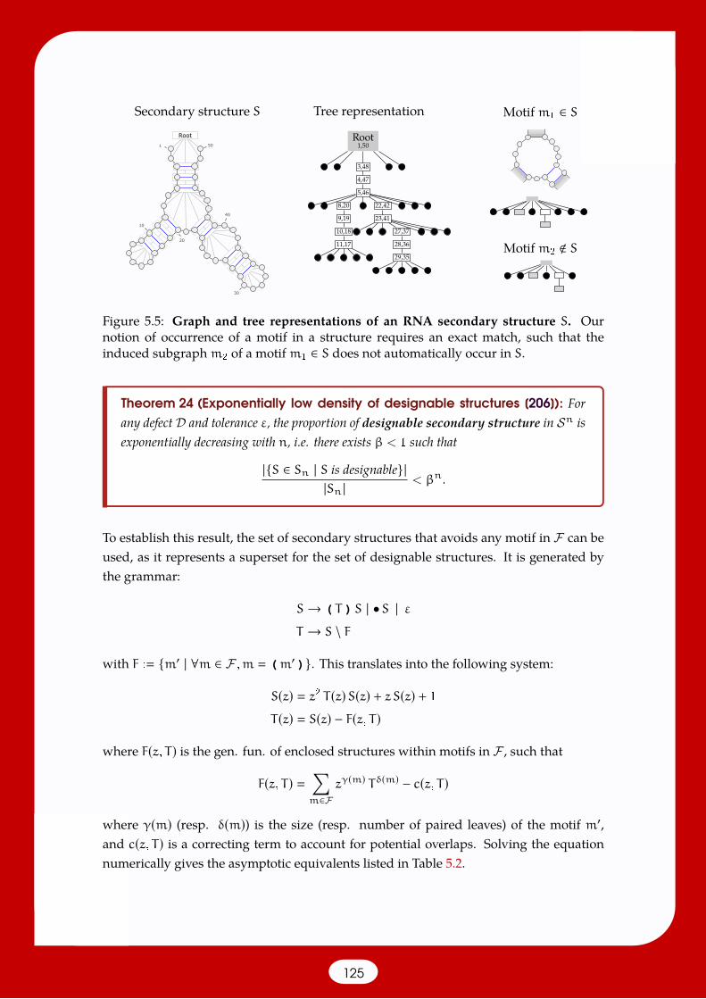
1

10

20

30

40

50

Root

Secondary structure S

Root1,50

3,48

4,47

5,46

8,20 22,42

9,19

10,18

11,17

23,41

27,37

28,36

29,35

Tree representation Motifm1 ∈ S

Motifm2 < S

Figure 5.5: Graph and tree representations of an RNA secondary structure S. Ournotion of occurrence of a motif in a structure requires an exact match, such that theinduced subgraphm2 of a motifm1 ∈ S does not automatically occur in S.

Theorem 24 (Exponentially low density of designable structures [206]): Forany defectD and tolerance ε, the proportion of designable secondary structure in Sn isexponentially decreasing with n, i.e. there exists β < 1 such that

|S ∈ Sn | S is designable||Sn | < βn.

To establish this result, the set of secondary structures that avoids any motif in F can beused, as it represents a superset for the set of designable structures. It is generated bythe grammar:

S→ ( T )S | •S | εT → S \ F

with F : m′ | ∀m ∈ F ,m (m′ ). This translates into the following system:

S(z) z2 T (z)S(z) + z S(z) + 1

T (z) S(z) − F(z, T )

where F(z, T ) is the gen. fun. of enclosed structures within motifs in F , such that

F(z, T ) ∑m∈F

zγ(m) Tδ(m) − c(z, T )

where γ(m) (resp. δ(m)) is the size (resp. number of paired leaves) of the motif m′,and c(z, T ) is a correcting term to account for potential overlaps. Solving the equationnumerically gives the asymptotic equivalents listed in Table 5.2.

125

#Local Asymptotic Proportion of designable structures? (upper bound)Defect ε obstructions ρ equivalent Equiv. P10 (%) P50 (%) P100 (%) P200 (%) P500 (%) P1000 (%)

Free-energy 1 104 0.449 Θ(2.226n

n√n

)0.973n 76.1 25.4 6.48 4.19·10−1 1.14·10−4 1.30·10−10

Probability .5 117 0.450 Θ(2.224n

n√n

)0.972n 75.3 24.2 5.84 3.41·10−1 6.81·10−5 4.64·10−11

Probability .1 152 0.460 Θ(2.176n

n√n

)0.95n 59.9 7.69 0.59 3.51·10−3 7.27·10−10 5.29·10−21

Probability .01 174 0.481 Θ(2.078n

n√n

)0.908n 38.1 0.80 6.44·10−3 4.14·10−7 1.10· 10−19 1.22·10−40

Table 5.2: Consequence of obstructions of size up to 12 on proportion of designablesecondary structures. (?) Proportions of designable sequences computed using an as-sumption of equal constants for the asymptotic leading terms of the number of secondarystructures, respectively allowing and forbidding local obstructions.

126

Chapter 6

Conclusion and perspectives

In this Habilitation, I have attempted to provide a unified perspective over a seriesof contributions in ensemble dynamic programming, random generation, analysis anddesign of algorithms with applications in Bioinformatics, focusing on RNA folding fromthermodynamic principles and RNA folding.

These research projects, spanning more than a decade of research, more than a dozenof distinct collaborations and 50+ manuscripts published in journals and selective con-ference, have allowed me to draw fruitful connections between my initial backgroundin computer science and discrete applied mathematics, and my growing expertise andvisibility in RNA Bioinformatics. Beyond their absolute value as scientific contributionsand tools for the community, they have contributed to build a level of clarity in my objec-tives, and positioningwith respect tomy communities, allowingme to (more) confidentlyenvision the future mentoring of young researchers.

Current projects. Over the next couple of years, my research will foreseeably be ded-icated to two main projects in RNA bioinformatics, namely the connection betweendesign and RNA evolution and the integrative structure prediction informed by prob-ing data, under respective grants from the French Agence Nationale de la Recherche(Decrypted and PaRNAssus projects) awarded for the two projects for the 2020–2024period.

In the former, we will explore with Simona Cocco, Rémi Monasson and Bruno Sargueilto which extent modernmethods in evolutionary analysis, based on the concept of directinformation, can be used to recover andunravel designprinciples resulting fromnegativeselective pressures. I also wish to revisit negative design as a null model for assessingthe significance of observations, as mentioned in Chapter 3. This will require revisitingthe controlled random generation of a NP-hard problem, hopefully helped by my recententhusiasm for parameterized complexity algorithms.

127

The latter project, implemented in collaboration with Ronny Lorenz and Bruno Sargueil,attempts to define newmethods to exploit information produced in unconventional set-tings for RNA probing. Those include probing experiments in different ionic conditionswhere pseudoknots are suspected (or new tests to assess their presence), produced usingdiverse reagents revealing different aspects of RNA architectures or acting with differ-ent speeds. One of the requirements for such an endeavor is the design of polynomialDP-based classes of pseudoknots, using conceptual tools introduced in Chapter 2, ef-ficient and focusing on geometrically-feasible structures, enabling reasonable ensembleanalyses.

At a more methodological level, I am increasingly convinced that an efficient pursue offinalized projects in RNA Bioinformatics requires to limit the distraction represented bythe implementation/debugging of complex DP algorithms (by students having limitedexperience and patience). For this reason, I plan to invest some of my time to thedevelopment of a generic DP framework to allow the production of efficient low-levelcode from a generic DP description. Existing frameworks are indeed either unsufficientlygeneric, or not easily amenable to support desirable features like random generation.Such a development would also provide motivation to explore connections with formalcalculus, from which some of my contributions are already directly originating (throughenumerative combinatorics).

Finally, the recent development of methods combining sampling and clustering, follow-ingDing et al. [52] have led us to identify strong limitations in performances, experiencedwhen using both agglomerative and divisive algorithms for unsupervised machine. Iam therefore currently venturing in the darkest pits of machine learning, hoping to findtechniques (e.g. embeddings) that will allow an efficient processing of large sampledsets of structure, hoping to increase the robustness, and reproducibility of downstreamanalyses.

Team development. This decade since my PhD has finally allowed to grow as a scien-tist, from the postdoc-like status associated with a junior researcher CNRS position, tosecuring my own research fundings and supervising my student, and finally to takingthe acting (2016) and permanent (2017–2018) scientific lead of the AMIBio team at LIX,culminating in the recent recruitment of Sebastian Will.

128

Bibliography

[1] R. Aguirre-Hernández, H. H. Hoos, andA. Condon. Computational RNA secondary structure design:empirical complexity and improved methods. BMC Bioinformatics, 8:34, 2007.

[2] A. V. Aho and M. J. Corasick. Efficient string matching: an aid to bibliographic search. Communica-tions of the ACM, 18(6):333–340, jun 1975.

[3] T. Akutsu. Dynamic programming algorithms for RNA secondary structure prediction with pseudo-knots. Discrete Applied Mathematics, 104(1):45 – 62, 2000.

[4] R. Albert and A.-L. Barabási. Statistical mechanics of complex networks. Reviews of modern Physics,74:47–97, 2002.

[5] D. Aldous. On the markov chain simulation method for uniform combinatorial distributions andsimulated annealing. Probability in the Engineering and Informational Sciences, 1(1):33–46, 1987.

[6] S. F. Altschul and B. W. Erickson. Significance of nucleotide sequence alignments: a method forrandom sequence permutation that preserves dinucleotide and codon usage. Molecular biology andevolution, 2:526–538, Nov. 1985.

[7] M. Andronescu, A. P. Fejes, F. Hutter, H. H. Hoos, and A. Condon. A new algorithm for RNAsecondary structure design. Journal of Molecular Biology, 336(3):607–624, 2004.

[8] M. Andronescu, V. Bereg, H. H. Hoos, and A. Condon. RNA strand: the RNA secondary structureand statistical analysis database. BMC bioinformatics, 9:340, Aug. 2008.

[9] A. Avihoo, A. Churkin, and D. Barash. RNAexinv: An extended inverse RNA folding from shape andphysical attributes to sequences. BMC Bioinformatics, 12(1):319, 2011.

[10] J. K. Baker. Trainable grammars for speech recognition. The Journal of the Acoustical Society ofAmerica, 65(S1):S132–S132, 1979.

[11] C. Banderier and M. Drmota. Formulae and asymptotics for coefficients of algebraic functions. Com-binatorics, Probability and Computing, 24(1):1–53, 2015.

[12] C. Banderier, O. Bodini, Y. Ponty, and H. Tafat. On the diversity of pattern distributions in rationallanguage. In ANALCO 2012, pages 107–116, Kyoto, Japan, Jan. 2012. Omnipress.

[13] E. Barcucci, R. Pinzani, and R. Sprugnoli. The random generation of directed animals. TheoreticalComputer Science, 127(2):333–350, 1994.

[14] R. Bellman. The theory of dynamic programming. Bulletin of the American Mathematical Society,60(6):503–515, 1954.

[15] M. Bendkowski, O. Bodini, and S. Dovgal. Polynomial tuning of multiparametric combinatorialsamplers. In 2018 Proceedings of the FifteenthWorkshop onAnalyticAlgorithmics andCombinatorics(ANALCO), pages 92–106. SIAM, 2018.

[16] P. Berenbrink and T. Sauerwald. The weighted coupon collector’s problem and applications. In 15thInternational Computing and Combinatorics Conference (COCOON’10), 2009.

[17] G. Blin, A. Denise, S. Dulucq, C. Herrbach, and H. Touzet. Alignments of RNA structures. IEEE/ACMTrans. Comput. Biology Bioinform., 7(2):309–322, 2010.

[18] O. Bodini and Y. Ponty. Multi-dimensional Boltzmann Sampling of Languages. In AOFA 2010,volume AM of DMTCS Proceedings, pages 49–64, Vienna, Austria, June 2010. Discrete Mathematicsand Theoretical Computer Science.

129

[19] M. Bon and H. Orland. TT2NE: a novel algorithm to predict RNA secondary structures with pseudo-knots. Nucleic Acids Research, 39(14):e93–e93, 05 2011.

[20] É. Bonnet, P. Rzażewski, and F. Sikora. Designing RNA secondary structures is hard. In Research inComputational Molecular Biology 22nd Annual International Conference, RECOMB 2018, volume10812 of Lecture Notes in Computer Science, pages 248–250, Paris, 2018. Springer.

[21] M. Bousquet-Mélou and Y. Ponty. Culminating paths. Discrete Mathematics and Theoretical Com-puter Science, 10(2):125–152, 2008.

[22] G. R. Bowman and V. S. Pande. Protein folded states are kinetic hubs. Proc. Natl. Acad. Sci. U.S.A.,107(24):10890–10895, June 2010.

[23] R. Bundschuh and R. Bruinsma. Melting of branched RNA molecules. Physical review letters, 100(14):148101, 2008.

[24] R. Bundschuh and T. Hwa. RNA secondary structure formation: A solvable model of heteropolymerfolding. Phys. Rev. Lett., 83:1479–1482, Aug 1999.

[25] R. Bundschuh and T. Hwa. Statistical mechanics of secondary structures formed by random RNAsequences. Physical review. E, Statistical, nonlinear, and soft matter physics, 65:031903, Mar. 2002.

[26] R. Bundschuh and T. Hwa. Phases of the secondary structures of RNA sequences. EPL (EurophysicsLetters), 59(6):903, 2002.

[27] H. A. Burbano and E. Andrade. Analysis of tRNA abstract shapes of precursor/derivative aminoacids in archaea. Gene, 396:75–83, July 2007.

[28] A. Busch and R. Backofen. INFO-RNA—a fast approach to inverse RNA folding. Bioinformatics, 22(15):1823–31, 2006.

[29] S. Cao and S. Chen. Predicting RNA pseudoknot folding thermodynamics. Nucleic Acids Research,34(9):2634–2652, 2006.

[30] C. Chauve, Y. Ponty, and J. P. P. Zanetti. Evolution of genes neighborhood within reconciled phyloge-nies: an ensemble approach. In BSB 2014, volume 8826 ofAdvances in Bioinformatics and ComputationalBiology, pages 49–56, Belo Horizonte, Brazil, Oct. 2014. Springer.

[31] C. Chauve, Y. Ponty, and J. P. P. Zanetti. Evolution of genes neighborhood within reconciled phyloge-nies: an ensemble approach. BMC Bioinformatics, 16(Suppl 19):S6, Dec. 2015.

[32] C. Chauve, J. Courtiel, and Y. Ponty. Counting, generating and sampling tree alignments. In ALCOB2016, volume 9702, pages 53–64, Trujillo, Spain, 2016. Springer.

[33] C. Chauve, J. Courtiel, and Y. Ponty. Counting, generating, analyzing and sampling tree alignments.International Journal of Foundations of Computer Science, 29(5):741–767, 2018.

[34] A. Churkin, M. D. Retwitzer, V. Reinharz, Y. Ponty, J. Waldispühl, and D. Barash. Design of RNAs:comparing programs for inverse RNA folding. Briefings in Bioinformatics, 19(2):350–358, Jan. 2018.

[35] F. Chyzak, M. Drmota, T. Klausner, and G. Kok. The distribution of patterns in random trees.Combinatorics, Probability and Computing, 17(1):21–59, 2008.

[36] P. Clote. Combinatorics of saturated secondary structures of RNA. Journal of computational biology: a journal of computational molecular cell biology, 13:1640–1657, Nov. 2006.

[37] P. Clote, F. Ferré, E. Kranakis, and D. Krizanc. Structural RNA has lower folding energy than randomRNA of the same dinucleotide frequency. RNA (New York, N.Y.), 11:578–591, May 2005.

[38] P. Clote, Y. Ponty, and J.-M. Steyaert. Expected distance between terminal nucleotides of RNA sec-ondary structures. Journal of Mathematical Biology, 65(3):581–99, Sept. 2012.

[39] G. Collet, J. David, and A. Jacquot. Random sampling of ordered trees according to the number ofoccurrences of a pattern. Submitted, 2018.

[40] R. Cont and E. Tanimura. Small-world graphs: characterization and alternative constructions. Adv.in Appl. Probab., 40(4):939–965, 2008.

[41] J. Cooley and J. Tukey. An algorithm for the machine calculation of complex fourier series. Mathe-matics of Computation, 19(90):297–301, 1965.

[42] J. Cooley, P. Lewis, and P. Welch. The finite Fourier transform. IEEE Transactions on Audio andElectroacoustics, 17(2):77–85, June 1969.

130

[43] J. Cupal, I. L. Hofacker, and P. F. Stadler. Dynamic programming algorithm for the density of states ofRNA secondary structures. In Proceedings of the German Conference on Bioinformatics, GCB, pages184–186, Leipzig, Germany, Sept. 1996.

[44] K. Darty, A. Denise, and Y. Ponty. VARNA: Interactive drawing and editing of the RNA secondarystructure. Bioinformatics, 25(15):1974–5, Aug. 2009.

[45] N. S. de Groot, A. Armaos, R. Graña-Montes, M. Alriquet, G. Calloni, R. M. Vabulas, and G. G.Tartaglia. RNA structure drives interaction with proteins. Nature Communications, 10(1), jul 2019.

[46] J. Deforges, S. De Breyne, M. Ameur, N. Ulryck, N. Chamond, A. Saaidi, Y. Ponty, T. Ohlmann, andB. Sargueil. Two ribosome recruitment sites direct multiple translation events within HIV1 Gag openreading frame. Nucleic Acids Research, 45(12):7382–7400, July 2017.

[47] K. E. Deigan, T. W. Li, D. H. Mathews, and K. M. Weeks. Accurate SHAPE-directed RNA structuredetermination. Proc Natl Acad Sci U S A, 106(1):97–102, 2009.

[48] A. Denise. Génération aléatoire et uniforme de mots. Discrete Mathematics, 156:69–84, 1996.

[49] A. Denise and P. Zimmermann. Uniform random generation of decomposable structures usingfloating-point arithmetic. Theoretical Computer Science, 218(2):233 – 248, 1999.

[50] A. Denise, Y. Ponty, and M. Termier. Controlled non uniform random generation of decomposablestructures. Theoretical Computer Science, 411(40-42):3527–3552, 2010.

[51] Y. Ding and C. E. Lawrence. A statistical sampling algorithm for RNA secondary structure prediction.Nucleic acids research, 31:7280–7301, Dec. 2003.

[52] Y. Ding, C. Y. Chan, and C. E. Lawrence. RNA secondary structure prediction by centroids in aboltzmann weighted ensemble. RNA (New York, N.Y.), 11:1157–1166, Aug. 2005.

[53] R. Dirks and N. Pierce. A partition function algorithm for nucleic acid secondary structure includingpseudoknots. J Comput Chem, 24:1664–1677, 2003.

[54] R. M. Dirks, M. Lin, E. Winfree, and N. A. Pierce. Paradigms for computational nucleic acid design.Nucleic Acids Research, 32(4):1392–1403, 2004.

[55] C. B. Do, D. A. Woods, and S. Batzoglou. Contrafold: RNA secondary structure prediction withoutphysics-based models. Bioinformatics (Oxford, England), 22:e90–e98, July 2006.

[56] M. Drmota. Systems of functional equations. Random Structures and Algorithms, 10(1-2):103–124,1997.

[57] M. Drory Retwitzer, V. Reinharz, Y. Ponty, J. Waldispühl, and D. Barash. incaRNAfbinv : a web serverfor the fragment-based design of RNA sequences. Nucleic Acids Research, 44(W1):W308 – W314,2016.

[58] J. Du Boisberranger, D. Gardy, andY. Ponty. Theweightedwords collector. InAOFA2012, volumeAQ,pages 243–264, Montreal, Canada, June 2012. DMTCS.

[59] W. Duchemin, Y. Anselmetti, M. Patterson, Y. Ponty, S. Bérard, C. Chauve, C. Scornavacca, V. Daubin,and E. Tannier. DeCoSTAR: Reconstructing the ancestral organization of genes or genomes usingreconciled phylogenies. Genome Biology and Evolution, 9(5):1312–1319, 2017.

[60] P. Duchon, P. Flajolet, G. Louchard, and G. Schaeffer. Boltzmann samplers for the random generationof combinatorial structures. Combinatorics, Probability and Computing, 13(4-5):577–625, 2004.

[61] J. Duraj. Random walks in cones: The case of nonzero drift. Stochastic Processes and their Applica-tions, 124(4):1503–1518, apr 2014.

[62] S. R. Eddy and R. Durbin. RNA sequence analysis using covariance models. Nucleic Acids Research,22(11):2079–2088, 1994.

[63] A. Esmaili-Taheri andM.Ganjtabesh. Erd: a fast and reliable tool forRNAdesign including constraints.BMC bioinformatics, 16:20, Jan. 2015.

[64] A. Esmaili-Taheri, M. Ganjtabesh, and M. Mohammad-Noori. Evolutionary solution for the RNAdesign problem. Bioinformatics, 30(9):1250–1258, 2014.

[65] S. Findeiß, M. Etzel, S. Will, M. Mörl, and P. F. Stadler. Design of artificial riboswitches as biosensors.Sensors (Basel, Switzerland), 17(9):E1990, Aug. 2017.

131

[66] A. V. Finkelstein and M. A. Roytberg. Computation of biopolymers: a general approach to differentproblems. Biosystems, 30(1-3):1–19, 1993.

[67] P. Flajolet. Analytic models and ambiguity of context-free languages. Theoretical Computer Science,49:283–309, 1987.

[68] P. Flajolet and A. M. Odlyzko. Singularity analysis of generating functions. SIAM J. Discrete Math.,3(2):216–240, 1990.

[69] P. Flajolet and R. Sedgewick. Analytic combinatorics. cambridge University press, New York, NY, USA,1 edition, 2009. ISBN 0521898064, 9780521898065.

[70] P. Flajolet, D. Gardy, and L. Thimonier. Birthday paradox, coupon collectors, caching algorithms andself-organizing search. Discrete Applied Mathematics, 39(3):207 – 229, 1992.

[71] P. Flajolet, P. Zimmermann, and B. V. Cutsem. A calculus for the random generation of labelledcombinatorial structures. Theoretical Computer Science, 132(1):1 – 35, 1994.

[72] C. Flamm,W. Fontana, I. Hofacker, and P. Schuster. RNA folding at elementary step resolution. RNA,6:325–338, 2000.

[73] C. Flamm, I. L. Hofacker, S. Maurer-Stroh, P. F. Stadler, and M. Zehl. Design of multistable RNAmolecules. RNA (New York, N.Y.), 7:254–265, Feb 2001.

[74] W. Fontana, P. F. Stadler, E. G. Bornberg-Bauer, T. Griesmacher, I. L. Hofacker, M. Tacker, P. Tarazona,E. D. Weinberger, and P. Schuster. RNA folding and combinatory landscapes. Phys. Rev. E, 47:2083–2099, Mar 1993.

[75] E. Freyhult, V. Moulton, and P. Clote. Boltzmann probability of RNA structural neighbors andriboswitch detection. Bioinformatics (Oxford, England), 23:2054–2062, Aug. 2007.

[76] D. Gamerman and H. F. Lopes. Markov chain Monte Carlo: stochastic simulation for Bayesian inference.Chapman and Hall/CRC, 2006.

[77] J. A. Garcia-Martin, P. Clote, and I. Dotu. RNAiFOLD: a constraint programming algorithm for RNAinverse folding and molecular design. Journal of Bioinformatics and Computational Biology, 11(2):1350001, 2013.

[78] D. Gardy and Y. Ponty. Weighted random generation of context-free languages: Analysis of collisionsin random urn occupancy models. In GASCOM 2010, page 14pp, Montréal, Canada, Sept. 2010.LACIM, UQAM.

[79] Q. Ge and D. Štefankovič. A graph polynomial for independent sets of bipartite graphs. Combina-torics, Probability and Computing, 21(05):695–714, 2012.

[80] R.Giegerich andC.Meyer. Algebraicdynamicprogramming. In InternationalConferenceonAlgebraicMethodology and Software Technology, pages 349–364. Springer, 2002.

[81] R. Giegerich and H. Touzet. Modeling dynamic programming problems over sequences and treeswith inverse coupled rewrite systems. Algorithms, 7(1):62–144, Mar 2014.

[82] R. Giegerich, B. Voss, and M. Rehmsmeier. Abstract shapes of RNA. Nucleic acids research, 32:4843–4851, 2004.

[83] S. Grabbe, H. Haas, M. Diken, L. M. Kranz, P. Langguth, and U. Sahin. Translating nanoparticulate-personalized cancer vaccines into clinical applications: case study with RNA-lipoplexes for the treat-ment of melanoma. Nanomedicine (London, England), 11:2723–2734, Oct. 2016.

[84] S. Griffiths-Jones, A. Bateman, M. Marshall, A. Khanna, and S. R. Eddy. RFAM: an RNA familydatabase. Nucleic Acids Research, 31(1):439–441, 2003.

[85] J. Hales, J. Manuch, Y. Ponty, and L. Stacho. Combinatorial RNADesign: Designability and Structure-Approximating Algorithm. In CPM 2015, Ischia Island, Italy, June 2015.

[86] J. Hales, A. Héliou, J. Manuch, Y. Ponty, and L. Stacho. Combinatorial RNA Design: Designabilityand Structure-Approximating Algorithm in Watson-Crick and Nussinov-Jacobson Energy Models.Algorithmica, 79(3):835–856, 2017.

[87] M. Hamada, H. Kiryu, K. Sato, T. Mituyama, and K. Asai. Prediction of RNA secondary structureusing generalized centroid estimators. Bioinformatics (Oxford, England), 25:465–473, Feb. 2009.

[88] S. Hammer, Y. Ponty, W.Wang, and S.Will. Fixed-Parameter Tractable Sampling for RNADesignwithMultiple Target Structures. In RECOMB 2018, Paris, France, 2018.

132

[89] S. Hammer, C. Günzel, M. Mörl, and S. Findeiß. Evolving methods for rational de novo design offunctional RNA molecules. Methods, 161:54 – 63, 2019.

[90] S. Hammer, W. Wang, S. Will, and Y. Ponty. Fixed-parameter tractable sampling for RNA design withmultiple target structures. BMC Bioinformatics, 20(1):209, Dec. 2019.

[91] M. Hellmuth, D. Merkle, and M. Middendorf. Extended shapes for the combinatorial design of RNAsequences. International journal of computational biology and drug design, 2:371–384, 2009.

[92] C. Herrbach, A. Denise, and S. Dulucq. Average complexity of the Jiang-Wang-Zhang pairwise treealignment algorithm and of a RNA secondary structure alignment algorithm. Theor. Comput. Sci.,411(26-28):2423–2432, 2010.

[93] P. G. Higgs and N. Lehman. The RNA world: molecular cooperation at the origins of life. NatureReviews Genetics, 16(1):7–17, nov 2014.

[94] F. Hildebrand, A. Meyer, and A. Eyre-Walker. Evidence of selection upon genomic gc-content inbacteria. PLoS genetics, 6:e1001107, Sept. 2010.

[95] I. L. Hofacker, W. Fontana, P. F. Stadler, L. S. Bonhoeffer, M. Tacker, and P. Schuster. Fast foldingand comparison of RNA secondary structures. Monatshefte für Chemie/Chemical Monthly, 125(2):167–188, 1994.

[96] I. L. Hofacker, P. Schuster, and P. F. Stadler. Combinatorics of RNA secondary structures. DiscreteApplied Mathematics, 88(1-3):207–237, 1998.

[97] C. Höner zu Siederdissen. Sneaking around concatmap: Efficient combinators for dynamic program-ming. SIGPLAN Not., 47(9):215–226, Sept. 2012.

[98] L. Huang and D. Chiang. Better k-best parsing. In Proceedings of the Ninth International Workshopon Parsing Technology, pages 53–64. Association for Computational Linguistics, 2005.

[99] L. D. Hurst and A. R. Merchant. High guanine-cytosine content is not an adaptation to high temper-ature: a comparative analysis amongst prokaryotes. Proceedings. Biological sciences, 268:493–497,Mar. 2001.

[100] S. Ieong,M. yangKao, T.wahLam,W. kin Sung, and S.mingYiu. PredictingRNAsecondary structureswith arbitrary pseudoknots by maximizing the number of stacking pairs. Journal Of ComputationalBiology, 10(6):981–995, 2003.

[101] E. Jacox, C. Chauve, G. J. Szöllösi, Y. Ponty, and C. Scornavacca. ecceTERA: Comprehensive genetree-species tree reconciliation using parsimony. Bioinformatics, 32(13):2056–2058, July 2016.

[102] S. Janssen, J. Reeder, andR.Giegerich. Shape based indexing for faster search of RNA family databases.BMC bioinformatics, 9:131, Feb. 2008.

[103] T. Jiang, L. Wang, and K. Zhang. Alignment of trees - an alternative to tree edit. Theor. Comput. Sci.,143(1):137–148, 1995.

[104] E. Y. Jin and C. M. Reidys. Asymptotic enumeration of RNA structures with pseudoknots. Bulletinof mathematical biology, 70:951–970, May 2008.

[105] T. Jörg, O. C. Martin, and A. Wagner. Neutral network sizes of biological RNA molecules can becomputed and are not atypically small. BMC bioinformatics, 9:464, Oct. 2008.

[106] I. Kalvari, J. Argasinska, N. Quinones-Olvera, E. P. Nawrocki, E. Rivas, S. R. Eddy, A. Bateman, R. D.Finn, and A. I. Petrov. Rfam 13.0: shifting to a genome-centric resource for non-coding RNA families.Nucleic acids research, 46:D335–D342, Jan. 2018.

[107] R. Kleinkauf, M. Mann, and R. Backofen. antaRNA: ant colony-based RNA sequence design. Bioin-formatics (Oxford, England), 31:3114–3121, Oct. 2015.

[108] J. W. Klop, M. Bezem, and R. De Vrĳer. Term rewriting systems. Cambridge University Press, 2001.

[109] R. V. Koodli, B. Keep, K. R. Coppess, F. Portela, E. participants, and R. Das. Eternabrain: Auto-mated RNA design through move sets and strategies from an internet-scale RNA videogame. PLOSComputational Biology, 15(6):1–22, 06 2019.

[110] M. Kucharík, I. L. Hofacker, P. F. Stadler, and J. Qin. Basin hopping graph: a computational frameworkto characterize RNA folding landscapes. Bioinformatics (Oxford, England), 30:2009–2017, July 2014.

[111] D. Lai, J. R. Proctor, and I. M.Meyer. On the importance of cotranscriptional RNA structure formation.RNA, 19(11):1461–1473, oct 2013.

133

[112] S. P. Lalley. Finite range random walk on free groups and homogeneous trees. The Annals ofProbability, pages 2087–2130, 1993.

[113] K. Lari and S. J. Young. The estimation of stochastic context-free grammars using the inside-outsidealgorithm. Computer Speech and Language, 4:35–56, 1990.

[114] N. B. Leontis and E. Westhof. Geometric nomenclature and classification of RNA base pairs. RNA, 7(4):499–512, 2001.

[115] A. Lescoute, N. B. Leontis, C. Massire, and E. Westhof. Recurrent structural RNA motifs, isostericitymatrices and sequence alignments. Nucleic acids research, 33:2395–2409, 2005.

[116] A. Levin,M. Lis, Y. Ponty, C.W.O’Donnell, S. Devadas, B. Berger, and J.Waldispühl. Aglobal samplingapproach to designing and reengineering RNA secondary structures. Nucleic Acids Research, 40(20):10041–52, 2012.

[117] A. Levin,M. Lis, Y. Ponty, C.W.O’Donnell, S. Devadas, B. Berger, and J.Waldispühl. Aglobal samplingapproach to designing and reengineering RNA secondary structures. Nucleic Acids Research, 40(20):10041–10052, Nov. 2012.

[118] A. Lorenz and Y. Ponty. Non-redundant random generation algorithms for weighted context-freelanguages. Theoretical Computer Science, 502:177–194, Sept. 2013.

[119] R. Lorenz, C. Flamm, and I. L. Hofacker. 2d projections of RNA folding landscapes. In German Con-ference on Bioinformatics 2009, pages 11–20, Martin Luther University Halle-Wittenberg, Germany,Sept. 2009.

[120] W. A. Lorenz, P. Clote, and Y. Ponty. Asymptotics of RNA shapes. Journal of Computational Biology,15(1):31–63, 2008.

[121] Z. J. Lu, J.W.Gloor, andD.H.Mathews. ImprovedRNAsecondary structure prediction bymaximizingexpected pair accuracy. RNA, 15(10):1805–1813, Oct. 2009.

[122] J. Lumbroso, M. Mishna, and Y. Ponty. Taming reluctant random walks in the positive quadrant. InGASCOM 2016, volume 59 of Electronic Notes in Discrete Mathematics, pages 99 – 114, Bastia, France,2017.

[123] R. B. Lyngsø and C. N. Pedersen. RNA pseudoknot prediction in energy-based models. Journal ofcomputational biology : a journal of computational molecular cell biology, 7:409–427, 2000.

[124] R. Lyngsø. Complexity of pseudoknot prediction in simple models. In Proceedings of ICALP, 2004.

[125] R. B. Lyngsø, J. W. Anderson, E. Sizikova, A. Badugu, T. Hyland, and J. Hein. FRNAkenstein: multipletarget inverse RNA folding. BMC Bioinformatics, 13:260, 2012.

[126] J. Maňuch, C. Thachuk, L. Stacho, and A. Condon. NP-completeness of the energy barrier problemwithout pseudoknots and temporary arcs. Natural Computing, 10(1):391–405, nov 2010.

[127] D. H. Mathews. Using an RNA secondary structure partition function to determine confidence inbase pairs predicted by free energy minimization. RNA, 10(8):1178–1190, jul 2004.

[128] D. H.Mathews andD.H. Turner. Dynalign: an algorithm for finding the secondary structure commonto two RNA sequences. Journal of Molecular Biology, 317(2):191–203, mar 2002.

[129] D. H. Mathews, M. D. Disney, J. L. Childs, S. J. Schroeder, M. Zuker, and D. H. Turner. Incorporatingchemical modification constraints into a dynamic programming algorithm for prediction of RNAsecondary structure. Proc Natl Acad Sci U S A, 101(19):7287–92, 2004.

[130] J. S. McCaskill. The equilibrium partition function and base pair binding probabilities for RNAsecondary structure. Biopolymers: Original Research on Biomolecules, 29(6-7):1105–1119, 1990.

[131] Z. Miao, RNA-Puzzles Consortium, and E. Westhof. RNA-Puzzles Round III: 3D RNA structureprediction of five riboswitches and one ribozyme. RNA, 23:655–672, 2017.

[132] J. Michalik. Non-redundant sampling in RNA bioinformatics. PhD thesis, Interface Graduate school –Université Paris-Saclay, 2019.

[133] J. Michálik, H. Touzet, and Y. Ponty. Efficient approximations of RNA kinetics landscape using non-redundant sampling. In ISMB/ECCB 2017, volume 33, pages i283 – i292, Prague, Czech Republic,2017.

[134] F. Michel and E. Westhof. Modelling of the three-dimensional architecture of group i catalytic intronsbased on comparative sequence analysis. Journal of Molecular Biology, 216(3):585–610, dec 1990.

134

[135] I. Miklós. Computational Complexity of Counting and Sampling. Discrete Mathematics and Its Applica-tions. Chapman and Hall/CRC, feb 2019.

[136] I. Miklós, I. M. Meyer, and B. Nagy. Moments of the boltzmann distribution for RNA secondarystructures. Bull Math Biol, 67(5):1031–1047, Sep 2005.

[137] M. Mishna and A. Rechnitzer. Two non-holonomic lattice walks in the quarter plane. TheoreticalComputer Science, 410(38-40):3616–3630, 2009.

[138] M. Mohri. Semiring frameworks and algorithms for shortest-distance problems. J. Autom. Lang.Comb., 7(3):321–350, Jan. 2002.

[139] M. E. Nebel. Combinatorial properties of RNA secondary structures. Journal of ComputationalBiology, 9(3):541–573, 2002.

[140] Y. Nesterov and A. Nemirovskii. Interior-point polynomial algorithms in convex programming, volume 13.Siam, 1994.

[141] M. E. Newman, S. H. Strogatz, and D. J. Watts. Random graphs with arbitrary degree distributionsand their applications. Phys. Rev. E, 64(2):026118, August 2001.

[142] C.Nicaud andD.Gouyou-Beauchamps. Randomgenerationusing binomial approximations.DiscreteMathematics & Theoretical Computer Science, 2010.

[143] R. Nussinov and A. B. Jacobson. Fast algorithm for predicting the secondary structure of single-stranded RNA. Proceedings of the National Academy of Sciences of the United States of America,77:6309–6313, Nov. 1980.

[144] C. Pivoteau. Génération aléatoire de structures combinatoires : méthode de Boltzmann effective. phdthesis,Université Pierre et Marie Curie - Paris VI, 2008.

[145] C. Pivoteau, B. Salvy, and M. Soria. Algorithms for combinatorial structures: Well-founded systemsand newton iterations. Journal of Combinatorial Theory, Series A, 119(8):1711–1773, nov 2012.

[146] Y. Ponty. Models for structured genomic sequences, random generation and applications. Theses, UniversitéParis Sud - Paris XI, Nov. 2006.

[147] Y. Ponty. Non-redundant random generation from weighted context-free languages. In GASCOM2008, page 12pp, Bibbiena, Italy, 2008.

[148] Y. Ponty. Efficient sampling of RNAsecondary structures from theBoltzmann ensemble of low-energy:The boustrophedon method. Journal of Mathematical Biology, 56(1-2):107–127, 2008.

[149] Y. Ponty. Rule-weighted and terminal-weighted context-free grammars have identical expressivity.Research report, 2012.

[150] Y. Ponty and C. Saule. A Combinatorial Framework for Designing (Pseudoknotted) RNAAlgorithms.In WABI 2011, Saarbrucken, Germany, 2011.

[151] Y. Ponty,M. Termier, andA.Denise. GenRGenS: Software forGenerating RandomGenomic Sequencesand Structures. Bioinformatics, 22(12):1534–1535, 2006.

[152] J. G. Propp andD. B.Wilson. Exact samplingwith coupledmarkov chains and applications to statisticalmechanics. Random Structures & Algorithms, 9(1-2):223–252, 1996.

[153] A. Rajaraman, C. Chauve, andY. Ponty. Assessing the robustness of parsimonious predictions for geneneighborhoods from reconciled phylogenies. In ISBRA 2015, volume 9096, pages 260–271, Norfolk,Virginia, United States, June 2015.

[154] J. Reeder and R. Giegerich. Design, implementation and evaluation of a practical pseudoknot foldingalgorithm based on thermodynamics. BMC Bioinformatics, 5:104, 2004.

[155] J. Reeder and R. Giegerich. Consensus shapes: an alternative to the sankoff algorithm for RNAconsensus structure prediction. Bioinformatics (Oxford, England), 21:3516–3523, Sept. 2005.

[156] C. M. Reidys, F. W. D. Huang, J. E. Andersen, R. C. Penner, P. F. Stadler, and M. E. Nebel. Topologyand prediction of RNA pseudoknots. Bioinformatics, 27(8):1076–1085, Apr 2011.

[157] V. Reinharz, Y. Ponty, and J. Waldispühl. A linear inside-outside algorithm for correcting sequencingerrors in structured RNA sequences. In RECOMB 2013, Beĳing, China, Apr. 2013.

135

[158] V. Reinharz, Y. Ponty, and J. Waldispühl. A weighted sampling algorithm for the design of RNAsequences with targeted secondary structure and nucleotides distribution. In ISMB/ECCB 2013,Berlin, Germany, July 2013.

[159] V. Reinharz, Y. Ponty, and J. Waldispühl. Using Structural and Evolutionary Information to Detectand Correct Pyrosequencing Errors in Noncoding RNAs. Journal of Computational Biology, 20(11):905–19, Nov. 2013.

[160] V. Reinharz, Y. Ponty, and J. Waldispühl. A weighted sampling algorithm for the design of RNAsequences with targeted secondary structure and nucleotide distribution. Bioinformatics, 29(13):i308–15, July 2013.

[161] V. Reinharz, Y. Ponty, and J. Waldispühl. Combining structure probing data on RNA mutants withevolutionary information reveals RNA-binding interfaces.NucleicAcidsResearch, 44(11):e104 – e104,2016.

[162] K.-J. Räihä and E. Ukkonen. The shortest common supersequence problem over binary alphabet isNP-complete. Theoretical Computer Science, 16(2):187–198, 1981.

[163] P. Rinaudo, Y. Ponty, D. Barth, and A. Denise. Tree decomposition and parameterized algorithms forRNA structure-sequence alignment including tertiary interactions and pseudoknots. In WABI 2012,tba, Ljubljana, Slovenia, Sept. 2012. University of Ljubljana.

[164] E. Rivas and S. Eddy. A dynamic programming algorithm for RNA structure prediction includingpseudoknots. J Mol Biol, 285:2053–2068, 1999.

[165] C. Rovetta, J. Michálik, R. Lorenz, A. Tanzer, and Y. Ponty. Non-Redundant Sampling and StatisticalEstimators for RNA Structural Properties at the Thermodynamic Equilibrium. working paper orpreprint, Sept. 2019.

[166] F. Runge, D. Stoll, S. Falkner, and F. Hutter. Learning to design RNA. In International Conference onLearning Representations, 2019.

[167] D. Sankoff. Simultaneous solution of the RNA folding, alignment and protosequence problems. SIAMJournal on Applied Mathematics, 45(5):810–825, 1985.

[168] C. Saule, M. Régnier, J.-M. Steyaert, and A. Denise. Counting RNA pseudoknotted structures. Journalof computational biology : a journal of computational molecular cell biology, 18:1339–1351, Oct.2011.

[169] G. Sauthoff, M. Möhl, S. Janssen, and R. Giegerich. Bellman’s gap—a language and compiler fordynamic programming in sequence analysis. Bioinformatics, 29(5):551–560, 2013.

[170] A. Scala, L. Nunes Amaral, and M. Barthélémy. Small-world networks and the conformation space ofa short lattice polymer chain. Europhys. Lett., 55(4):594–600, 2001.

[171] S. Schirmer andR. Giegerich. Forest alignmentwith affine gaps and anchors, applied in RNA structurecomparison. Theor. Comput. Sci., 483:51–67, 2013.

[172] M. Schnall-Levin, L. Chindelevitch, and B. Berger. Inverting the Viterbi algorithm: an abstractframework for structure design. In Machine Learning, Proceedings of the Twenty 9, 2008, pages904–911, 2008.

[173] E. Senter, S. Sheikh, I. Dotu, Y. Ponty, and P. Clote. Using the Fast Fourier Transform to Accelerate theComputational Search for RNA Conformational Switches. PLoS ONE, 7(12):e50506, Dec. 2012.

[174] E. Senter, S. Sheikh, I. Dotu, Y. Ponty, and P. Clote. Using the Fast Fourier Transform to acceleratethe computational search for RNA conformational switches (extended abstract). In RECOMB 2013,Beĳing, China, Apr. 2013.

[175] S. Sheikh, R. Backofen, and Y. Ponty. Impact Of The Energy Model On The Complexity Of RNAFolding With Pseudoknots. In CPM 2012, volume 7354 of Combinatorial Pattern Matching, pages321–333, Helsinki, Finland, July 2012. Juha Kärkkäinen, Springer.

[176] M. J. Smola, G. M. Rice, S. Busan, N. A. Siegfried, and K. M. Weeks. Selective 2’-hydroxyl acylationanalyzed byprimer extension andmutational profiling (SHAPE-MaP) for direct, versatile and accurateRNA structure analysis. Nat Protoc, 10:1643–1669, 2015.

[177] A. Spasic, S. M. Assmann, P. C. Bevilacqua, and D. H. Mathews. Modeling RNA secondary structurefolding ensembles using SHAPE mapping data. Nucleic Acids Res, 46(1):314–323, 2017.

136

[178] J. Stombaugh, C. L. Zirbel, E. Westhof, and N. B. Leontis. Frequency and isostericity of RNA basepairs. Nucleic acids research, 37:2294–2312, Apr. 2009.

[179] D. Sundfeld, J. H. Havgaard, A. C. M. A. de Melo, and J. Gorodkin. Foldalign 2.5: multithreadedimplementation for pairwise structural RNA alignment. Bioinformatics, 32(8):1238–1240, dec 2015.

[180] D. Surujon, Y. Ponty, and P. Clote. Small-world networks and RNA secondary structures. Journal ofcomputational biology : a journal of computational molecular cell biology, 26(1):16–26, Jan. 2019.

[181] J. E. Tabaska, R. B. Cary, H. N. Gabow, and G. D. Stormo. An RNA folding method capable ofidentifying pseudoknots and base triples. Bioinformatics, 14(8):691–699, 1998.

[182] M. K. Takahashi and J. B. Lucks. A modular strategy for engineering orthogonal chimeric RNAtranscription regulators. Nucleic Acids Research, 41(15):7577–7588, 2013.

[183] C. Theis, S. Janssen, and R. Giegerich. Prediction of RNA secondary structure including kissinghairpin motifs. In Algorithms in Bioinformatics, pages 52–64, Berlin, Heidelberg, 2010. SpringerBerlin Heidelberg. ISBN 978-3-642-15294-8.

[184] I. Tinoco and C. Bustamante. How RNA folds. J Mol Biol, 293(2):271–81, Oct 1999.

[185] D. H. Turner and D. H. Mathews. NNDB: the nearest neighbor parameter database for predictingstability of nucleic acid secondary structure. Nucleic acids research, 38(Database issue):D280–D282,Jan. 2010.

[186] V. VanNoort, B. Snel, andM.A.Huynen. The yeast coexpression network has a small-world, scale-freearchitecture and can be explained by a simple model. EMBO Rep., 5(3):280–284, March 2004.

[187] G. Viennot and M. Vauchaussade de Chaumont. Enumeration of RNA secondary structures bycomplexity. In Mathematics in Biology and Medicine, pages 360–365, Berlin, Heidelberg, 1985.Springer Berlin Heidelberg. ISBN 978-3-642-93287-8.

[188] A. Viterbi. Error bounds for convolutional codes and an asymptotically optimumdecoding algorithm.IEEE Transactions on Information Theory, 13(2):260–269, apr 1967.

[189] F. Voisin and M.-C. Gaudel. Drawing uniformly at random in dynamic sets of paths. HAL preprint,Oct. 2019.

[190] B. Voss, R. Giegerich, and M. Rehmsmeier. Complete probabilistic analysis of RNA shapes. BMCbiology, 4:5, Feb. 2006.

[191] J. Waldispühl, S. Devadas, B. Berger, and P. Clote. Efficient algorithms for probing the RNAmutationlandscape. PLoS computational biology, 4:e1000124, Aug. 2008.

[192] J. Waldispühl and Y. Ponty. An unbiased adaptive sampling algorithm for the exploration of RNAmutational landscapes under evolutionary pressure. In RECOMB 2011, volume 6577 of Lecture Notesin Computer Science, pages 501–515, Vancouver, Canada, Mar. 2011. Springer Berlin / Heidelberg.

[193] J. Waldispühl and Y. Ponty. An unbiased adaptive sampling algorithm for the exploration of RNAmutational landscapes under evolutionary pressure. Journal of Computational Biology, 18(11):1465–79, Nov. 2011.

[194] M. Waterman. Secondary structure of single-stranded nucleic acids. Advances in Mathematics:Supplementary Studies, 1:167–212, 1978.

[195] D. J. Watts and S. H. Strogatz. Collective dynamics of ’small-world’ networks. Nature, 393(6684):440–442, June 1998.

[196] S. E.Wells, P. E. Hillner, R. D. Vale, andA. B. Sachs. Circularization ofmRNAby eukaryotic translationinitiation factors. Molecular cell, 2:135–140, July 1998.

[197] H. S. Wilf. A unified setting for sequencing, ranking, and selection algorithms for combinatorialobjects. Advances in Mathematics, 24:281–291, 1977.

[198] K. A. Wilkinson, E. J. Merino, and K. M. Weeks. Selective 2’-hydroxyl acylation analyzed by primerextension (SHAPE): quantitative RNA structure analysis at single nucleotide resolution. Nat Protoc,1:1610–1616, 2006.

[199] S.Will, T. Joshi, I. L.Hofacker, P. F. Stadler, andR. Backofen. LocaRNA-p: accurate boundarypredictionand improved detection of structural RNAs. RNA (New York, N.Y.), 18:900–914, May 2012.

137

[200] S. Will, C. Otto, M. Miladi, M. Möhl, and R. Backofen. Sparse: quadratic time simultaneous alignmentand folding of RNAs without sequence-based heuristics. Bioinformatics (Oxford, England), 31:2489–2496, Aug. 2015.

[201] M. T. Wolfinger, W. A. Svrcek-Seiler, C. Flamm, I. L. Hofacker, and P. F. Stadler. Efficient computationof RNA folding dynamics. Journal of Physics A: Mathematical and General, 37(17):4731–4741, apr2004.

[202] A. R. Woods. Coloring rules for finite trees, and probabilities of monadic second order sentences.Random Structures & Algorithms, 10(4):453–485, 1997.

[203] S. Y.Wu, G. Lopez-Berestein, G. A. Calin, andA. K. Sood. RNAi therapies: Drugging the undruggable.Science Translational Medicine, 6(240):240ps7, 2014.

[204] S. Wuchty. Small worlds in RNA structures. Nucleic. Acids. Res., 31(3):1108–1117, February 2003.

[205] A. Xayaphoummine, T. Bucher, F. Thalmann, andH. Isambert. Prediction and statistics of pseudoknotsin RNA structures using exactly clustered stochastic simulations. Proc. Natl. Acad. Sci. U. S. A., 100(26):15310–15315, 2003.

[206] H.-T. Yao, C. Chauve, M. Regnier, and Y. Ponty. Exponentially few RNA structures are designable. InACM-BCB 2019, pages 289–298, Niagara-Falls, United States, 2019. ACM Press.

[207] A. M. Yoffe, P. Prinsen, W. M. Gelbart, and A. Ben-Shaul. The ends of a large RNA molecule arenecessarily close. Nucleic acids research, 39:292–299, Jan. 2011.

[208] J. N. Zadeh, B. R. Wolfe, and N. A. Pierce. Nucleic acid sequence design via efficient ensemble defectoptimization. Journal of Computational Chemistry, 32(3):439–52, 2011.

[209] Y. Zhang, Y. Ponty, M. Blanchette, E. Lecuyer, and J. Waldispühl. SPARCS: a web server to analyze(un)structured regions in coding RNA sequences. Nucleic Acids Research, 41(Web Server issue):W480–5, July 2013.

[210] Y. Zhou, Y. Ponty, S. Vialette, J. Waldispühl, Y. Zhang, and A. Denise. Flexible RNA design understructure and sequence constraints using formal languages. In ACM-BCB 2013, Bethesda, WashigtonDC, United States, Sept. 2013.

[211] C. H. zu Siederdissen, S. J. Prohaska, and P. F. Stadler. Algebraic dynamic programming over generaldata structures. BMC bioinformatics, 16(19):S2, 2015.

[212] M. Zuker and D. Sankoff. RNA secondary structures and their prediction. Bulletin of mathematicalbiology, 46(4):591–621, 1984.

[213] M. Zuker and P. Stiegler. Optimal computer folding of large RNA sequences using thermodynamicsand auxiliary information. Nucleic Acids Research, 9(1):133–148, 1981.

138

Ensemble Algorithms and Analytic Combinatorics in RNA ...

Documents