4/16/2017 11:19:38 PM Page 1 of 37 ENSC 894 – G100: COMMUNICATION NETWORKS PERFORMANCE ANALYSIS OF WI-FI USING NS-2 Spring 2017 FINAL PROJECT Project Web Page: http://www.sfu.ca/~csa96/894 Submitted by Team 5: CHARANJOT SINGH (301295964) [email protected] YOUSRA WAKIL (301298273) [email protected]

Welcome message from author
This document is posted to help you gain knowledge. Please leave a comment to let me know what you think about it! Share it to your friends and learn new things together.
Transcript

4/16/2017 11:19:38 PM Page 1 of 37
ENSC 894 – G100: COMMUNICATION NETWORKS
PERFORMANCE ANALYSIS OF WI-FI USING NS-2
Spring 2017
FINAL PROJECT
Project Web Page: http://www.sfu.ca/~csa96/894
Submitted by Team 5:
CHARANJOT SINGH (301295964)
YOUSRA WAKIL (301298273)

4/16/2017 11:19:38 PM Page 2 of 37
Abstract
Wireless Fidelity (Wi-Fi) is widely used for wireless communication and is based on IEEE
(Institute of Electrical and Electronics Engineers) 802.11 standard. Wi-Fi allows multiple users
to transmit data from one place to another using high frequency radio waves. Nowadays, many
devices such as smart-phones, laptops, tablets and other wireless devices can be connected
through a single wireless (Wi-Fi) Network. Also, Quality of Service (QoS) is a major factor to
support a number of applications that use the Wi-Fi network, so in this regard QoS parameters
need to be analyzed for a better performance. The main purpose of this project is to compute and
analyze the QoS parameters of Wi-Fi network such as throughput, packet loss rate, end-to-end
delay, and jitter during Voice over Internet Protocol (VoIP) using network simulator 2 (ns-2). In
this project, we initiated voice calls and group chats between multiple users along with the
movement of one of the user during the voice call. The results obtained demonstrate that Wi-Fi
provides better performance and QoS for small area networks.

4/16/2017 11:19:38 PM Page 3 of 37
TABLE OF CONTENTS
Abstract…………………………………………………………………….................................. 2
Acknowledgement……………………………………………………………………................. 4
Acronyms……………………………………………………………………............................... 5
List of Figures……………………………………………………………………........................ 6
1. Introduction……………………………………………………………………......................7
2. Background knowledge…………………………………………………………………….. 8
2.1. Related Work………………………………………………………………................... 8
2.2. Wi-Fi Network topology………………..………………………………………..…….. 8
3. Network Simulator 2 (ns-2) ………………………………………………………………... 9
4. Design Implementation……………………………………………………………………. 10
4.1. Wi-Fi topology implementation in ns-2…………………………...………………..… 10
4.2. Simulation Details……………………………………………...……..………………. 12
4.2.1. Simulation Scenarios………………………………......................................... 12
4.3. Performance Parameters…..…………………………………………………….…..... 13
5. Results………………………………………………………………………………..…….. 14
5.1. Throughput…………………………………………………………………………..... 14
5.2. Packet Loss Rate……………………………………………………………………… 15
5.3. End-to-end Delay……………………………………………………………………... 16
5.4. Jitter…………………………………………………………………………………… 17
6. Discussions and Conclusion……………………………………………………………..... 19
6.1. Challenges…………………………………………………………………………….. 19
6.1.1. Wi-Fi Hierarchy………………………………………..................................... 19
6.1.2. Data Calculation and Plotting Graphs…………………………………............ 19
6.2. Improvements ………………………………………………………………………... 19
6.3. Future Work ………………………………………………………………………….. 20
6.4. Conclusion ………………………………………………………………………........ 20
7. References………………………………………………………………………………….. 21
Appendix A ……………………………………………………………………………………. 22
Appendix B ………………………………………………………………………………......... 35

4/16/2017 11:19:38 PM Page 4 of 37
Acknowledgement
This project would not have been possible without the support of several thoughtful and
generous individuals. We would like to acknowledge and extend our gratitude to our course
instructor - Prof. Ljiljana Trajkovic who has provided tremendous insight and guidance both
within and outside of the realm of communication networks. We would also like to extend our
sincere thanks to our course TA, Zhida Li for his help throughout the semester. Further, we
would like to thank ENSC help for their support and resolving all the technical issues in using
ns-2.
Our deepest gratitude goes to our families for their unconditional love, encouragement, advice,
and support throughout our lives.
YOUSRA WAKIL
CHARANJOT SINGH

4/16/2017 11:19:38 PM Page 5 of 37
ACRONYMS
Wi-Fi Wireless Fidelity
IEEE Institute for Electrical and Electronics Engineers
VoIP Voice over Internet Protocol
QoS Quality of Service
ns-2 Network Simulator-2
LTE Long Term Evolution
BSS Basic Service Set
ESS Extended Service Set
DS Distribution System
SS Station Services
DSS Distribution System Services
MAC Medium Access Control
MSDU MAC Service Data Unit Delivery
TCP Transmission Control Protocol
UDP User Datagram Protocol
FTP File Transfer Protocol
HTTP Hyper Text Transfer Protocol
DSR Dynamic Source Routing
OTcl Object-oriented Tool Command Language
WLAN Wireless Local Area Network
CBR Constant Bit Rate
MOS Mean Opinion Score
PPS Packets Per Second
4/16/2017 11:19:38 PM Page 6 of 37
List of Figures
Figure 1. Wi-Fi Network Topology
Figure 2. Basic Architecture of Ns-2
Figure 3. NAM window
Figure 4. Wi-Fi topology implementation in ns-2
Figure 5. Wi-Fi topology with user movement
Figure 6. Throughput Versus Simulation Time
Figure 7. Packet Loss Rate Versus Simulation Time
Figure 7(a). Zoomed view of Packet Loss Rate during user movement
Figure 7(b). Zoomed view of Packet Loss Rate during group chats
Figure 8. Delay Versus Simulation Time
Figure 8(a). Zoomed view of Delay during voice calls initiation
Figure 8(b). Zoomed view of Delay during node movement
Figure 8(c). Zoomed view of Delay observed during group chats
Figure 9. Jitter Versus Simulation Time
Figure 9(a). Zoomed view of Jitter during voice calls initiation
Figure 9(b). Zoomed view of Jitter during node movement
Figure 9(c). Zoomed views of Jitter observed during group chats

4/16/2017 11:19:38 PM Page 7 of 37
1. Introduction
Wi-Fi stands for “Wireless Fidelity” which is one of the popular wireless technologies and
allows various devices to exchange and transfer data wirelessly over the network, hence
providing high speed internet connections. Moreover, Wi-Fi is based on IEEE 802.11 Standard.
Its operating speed is 54Mbps while the operating range is few hundred feet (100-300 feet). Wi-
Fi has a variety of applications and is mainly implemented in office and home networks.
Voice over Internet Protocol (VoIP) is widely used for the delivery of long distance voice
communications over the Internet by converting analog audio signals into digital data for the
purpose of transmitting over the Internet. All VoIP packets are made up of two components:
voice samples and IP/UDP/RTP headers. Although the voice samples are compressed by the
Digital Signal Processor (DSP) and can vary in size based on the codec used, these headers are a
constant 40 bytes in length. We used G.711 (64 Kbps) codec and bitrates where the Mean
Opinion Score (MOS) is 4.1, voice payload size is 160 bytes and the frequency of the packets
sent are 50 PPS (Packets per Second) [8]. VoIP services have various benefits over the
traditional telephone services. One of the benefit is the low cost of phone calls which is
beneficial for large enterprises that manage large number of calls on daily basis. Also, multi-
functionality is another advantage of VoIP. Features like call forwarding, speed dialing etc.
provide more enhanced call processing opportunities that can lead to higher productivity.
Moreover, portability is another benefit of VoIP as it enables a user to make and receive calls
from any location using the same phone number. Further, the scalability of a VoIP network
provides a better management of business communication by involving multiple users into a
VoIP package.
The major objective of this project is to analyze the performance of Wi-Fi by implementing
VoIP in Wi-Fi using the network simulator (ns-2). For this purpose, in this project we will first
initiate long distance voice calls between two user nodes that are connected to two different
server branches. Then, we will initiate group chats between user nodes that are connected to
different access points. Moreover, we will include the movement of a user node during the voice
call. For all these scenarios, we will observe the Quality of Service (QoS) parameters such as
throughput, packet loss rate, end-to-end delay, and jitter and analyze the performance of Wi-Fi
networks.

4/16/2017 11:19:38 PM Page 8 of 37
2. Background Knowledge
2.1. Related Work:
Extensive work has been done to analyze the performance of Wi-Fi networks. Eric Swanlund,
Paven Loodu, Sunny Chowdhury simulated a wireless network using ns-2 in which five mobile
nodes are connected to two access points and certain number of packets are transferred to
analyze the efficiency of Wi-Fi network [1]. Jay Kim, Jack Zheng, Paniz Bertsch presented video
streaming over Wi-Fi using Riverbed Modeler and observed the performance of Wi-Fi network
when a mobile user was utilizing video stream [2].
In another work, A. Ezreik and A. Gheryani designed and simulated a wireless network using ns-
2 and analyzed the QoS parameters and concluded that the network’s performance is initially
transient but after certain time it gets stable [3]. Further, Cheng Jie, Tian Lin, and Yawen
presented VoIP performance of City-Wide Wi-Fi and Long Term Evolution (LTE) in which the
QoS parameters of the two technologies are compared during voice calling [4].
2.2. Wi-Fi Network Topology:
The Wi-Fi network topology is shown in figure 1. The devices connected to the wireless network
are called stations and when two or more stations communicate with each other they form a
Basic Service Set (BSS) and are connected to an access point. Access points are devices that
create the Wi-Fi microwaves for the mobile devices to detect and connect to, for the purpose of
sending data to the servers. Moreover, Extended Service Set (ESS) is a set of two or more BSSs
which form a single hub network. In order to connect two or more BSSs, a Distribution System
(DS) is used. DS must support various services which are the Station Services (SS) and
Distribution System Services (DSS). Some of the services of DSS is station mobility while the
others deal with distribution and integration of services when getting data from a sender and
delivering it to the intended receiver. Station Services usually deal with the users’ identity by
providing services such as authentication, de-authentication, privacy, and MAC (Medium Access
Control) Service Data Unit (MSDU) delivery.
Figure 1. Wi-Fi Network Topology [5]

4/16/2017 11:19:38 PM Page 9 of 37
3. Network Simulator 2 (ns-2)
Ns (Network Simulator) is a series of discrete event network simulators and its main purpose is
in the area of network research. It also provides support to protocols like Transmission Control
Protocol (TCP), User Datagram Protocol (UDP), File Transfer Protocol (FTP), Hyper Text
Transfer Protocol (HTTP), and Dynamic Source Routing (DSR) for simulation. Moreover, it
simulates over the wired and wireless networks. The version ns-2 works at the packet level and
uses Tcl as its scripting language.
The basic architecture of ns-2 is shown in figure 2 [7]. Ns-2 consists of two languages, the first
one is C++ which describes the internal mechanism of the simulation objects, while the second
one is Object-oriented Tool Command Language (OTcl) which sets up simulation by assembling
and configuring the objects, and by scheduling discrete events. Moreover, TclCL is used to link
C++ and OTcl. The simulation scenarios are described in the Tcl script which is executed by
typing ns on the command window. The nam window in ns-2 shown in figure 3 displays the
simulation scenarios which are defined in the Tcl script [6].
Figure 2. Basic Architecture of Ns-2[7]
Figure 3. NAM window [6]

4/16/2017 11:19:38 PM Page 10 of 37
4. Design Implementation
4.1. Wi-Fi Topology Implementation in ns-2:
We have implemented VoIP in Wi-Fi using ns-2 (version 2.35). The Wi-Fi topology is shown in
figure 4.
Figure 4. Wi-Fi topology implementation in ns-2
As seen in the figure 4, six mobile users User 0, User 1, User 2, User 3, User 4, and User 5 are
connected to two different Access Points (APs) i.e., Access Point (0) and Access Point (1),
where User 0, User 1 and User 2 are connected to Access Point (0) while User 3, User 4, and
User 5 are connected to Access Point (1). Each mobile user connects to its access point to
communicate with other users. For instance, in our simulation scenario the users connect to the
access points for initiating voice calls and group chats.
An Access Point is a station that transmits and receives wireless radio signals and connects users
to other users within the network. Moreover, it can also serve as a point of interaction between
the Wireless Local Area Network (WLAN) and a fixed wired network. Also, multiple users
within a defined network area can be served by a single access point. The hardware of an access
point consists of radio transceivers, antennas, and device firmware. An example of a wireless
access point is hotspot which is commonly used in large cities mostly in public places in which
wireless users can connect to Internet without the need of attachment to a specific network for
that moment. Access points are also used to provide connectivity in office and home networks
allowing users to work anywhere in home or office and stay connected to the home or office
networks.

4/16/2017 11:19:38 PM Page 11 of 37
Then, the two access points are connected to four routers which make up the path for the data to
travel in order to access the servers. The Access Point (0) is connected to router (0) and router
(1), while the Access Point (1) is connected to router (2) and router (3). The purpose of a router
is to find the next network point to which data should be forwarded towards its destination. For
instance, if a certain router goes down, the path for the data to travel is updated so that not to use
the broken router. Moreover, a router can support hundreds of simultaneous users. Also, a router
acts like a firewall with its ability to block, monitor, control and filter incoming and outgoing
network traffic.
Further, the routers are connected to two servers which are the devices that provide connected
users with Internet access. The router (0) and router (1) are connected to server (0), while router
(2) and router (3) are connected to server (1). A server provides services for a network by
processing requests and delivering data to other clients over a local area network or the Internet.
In our simulation scenario, when voice calls and group chats are initiated between the users the
data is passed to the server which then handles this task in order to allow users to voice call and
group chat over the Internet. Also, for the Wi-Fi simulation in ns-2 we picked G.711 (64 Kbps)
codec and bitrates where the Mean Opinion Score (MOS) is 4.1, voice payload size is 160 bytes
and the frequency of the packets sent are 50 PPS (Packets per Second) [8].
We have implemented the movement of a mobile node is our simulation scenario. The topology
in ns-2 when a mobile node moves from one place to another is shown is figure 5. As compared
with the topology in figure 4, User 0 moves from one location to another during the simulation
which is shown by figure 5.
Figure 5. Wi-Fi topology with user movement

4/16/2017 11:19:38 PM Page 12 of 37
4.2. Simulation Details:
We have defined the following design options for the mobile nodes in our simulation:
set val(chan) Channel/WirelessChannel ;# channel type
set val(prop) Propagation/TwoRayGround ;# radio-propagation model
set val(netif) Phy/WirelessPhy ;# network interface type
set val(mac) Mac/802_11 ;# MAC type
set val(ifq) Queue/DropTail/PriQueue ;# interface queue type
set val(ll) LL ;# link layer type
set val(ant) Antenna/OmniAntenna ;# antenna model
set val(ifqlen) 50 ;# max packet in ifq
set val(nn) 6 ;# number of mobilenodes
set val(rp) DSDV ;# routing protocol
set val(x) 400 ;# X dimension of topography
set val(y) 400 ;# Y dimension of topography
set val(stop) 1200 ;# time (20 minutes) of simulation end
We have implemented VoIP in Wi-Fi by using User Datagram Protocol (UDP). Moreover, UDP
agents and sinks are attached to the user devices to send and receive voice data between users.
The packet size has been set to 512 bytes. Constant Bit Rate (CBR) traffic generators are used to
generate the traffic. CBR traffic is attached to UDP agents to simulate voice data between the
users. The CBR data rate has been set to 600 kbps. Also, simulation data is collected using the
Loss Monitor class which is attached to the sinks and allow us to monitor packets arrival time,
number of packets, number of loss packets and the number of bytes received for a specific sink.
Moreover, the sampling time is set to 0.9 seconds.
4.2.1. Simulation Scenarios:
We have implemented three cases for VoIP in Wi-Fi using ns-2 which is described below.
a. Voice calls between users:
In our simulation for the implementation of VoIP we first initiated one to one long distance voice
calls from 1 minute to 20 minutes between user nodes that are connected to different server
branches i.e. User 0 which belongs to server (0) is connected to User 3 which belongs to server
(1). Also, User 2 which belongs to server (0) is connected to User 5 which belongs to server (1).
b. Movement of a user node:
During the simulation User 0 is moving between 5 to 8 minutes while other users are at a fixed
position.
c. Group chats between users:
Then, we initiated group chats between User 0, User 1, User 3, and User4 which start at 10
minutes and end at 15 minutes.

4/16/2017 11:19:38 PM Page 13 of 37
4.3. Performance Parameters:
We have analyzed the following Quality of Service (QoS) parameters in Wi-Fi network:
4.3.1. Throughput:
Throughput is one of the important factors to evaluate the QoS in Wi-Fi which is the rate at
which the data is successfully delivered over a communication channel. In other words,
throughput is defined as the rate of successful packet delivery. Throughput is calculated by
storing number of bytes received by a sink. The number of bytes received is detected by the sink
Loss Monitor and are stored in variables. So, the throughput is calculated by number of bytes
received and then multiplying by 8 to convert from bytes to bits, dividing by 1000000 which
achieve Mbits, after that dividing by current time which gets Mbits/sec as shown in Eq. (1).
𝑇𝑟𝑜𝑢𝑔𝑝𝑢𝑡 = 𝑛𝑜. 𝑜𝑓 𝑏𝑦𝑡𝑒𝑠 𝑟𝑒𝑐𝑒𝑖𝑣𝑒𝑑 × 8
𝑡𝑖𝑚𝑒 × 1000000 (1)
4.3.2. Packet Loss Rate:
Packet Loss Rate occurs when the data from one node fails to reach the destination node and is
calculated by storing the number of packets lost by the sink in a variable which is then divided
by the current time to achieve packets lost per second as shown in Eq. (2).
𝑃𝑎𝑐𝑘𝑒𝑡 𝐿𝑜𝑠𝑠 𝑅𝑎𝑡𝑒 = 𝑛𝑢𝑚𝑏𝑒𝑟 𝑜𝑓 𝑝𝑎𝑐𝑘𝑒𝑡𝑠 𝑙𝑜𝑠𝑡
𝑡𝑖𝑚𝑒 (2)
4.3.3. End-to-end Delay:
Another important parameter is end-to-end delay which is the time taken by a packet to travel
from source to destination in a network. End-to-end delay is calculated by taking the time last
packet is received and subtracting it with that packet sent time and then dividing by the total
number of packets received which is given by Eq. (3).
𝐸𝑛𝑑 − 𝑡𝑜 − 𝑒𝑛𝑑 𝐷𝑒𝑙𝑎𝑦 = 𝑙𝑎𝑠𝑡 𝑝𝑎𝑐𝑘𝑒𝑡 𝑟𝑒𝑐𝑒𝑖𝑣𝑒𝑑 𝑡𝑖𝑚𝑒 − 𝑝𝑎𝑐𝑘𝑒𝑡 𝑠𝑒𝑛𝑡 𝑡𝑖𝑚𝑒
𝑡𝑜𝑡𝑎𝑙 𝑝𝑎𝑐𝑘𝑒𝑡𝑠 𝑟𝑒𝑐𝑒𝑖𝑣𝑒𝑑 (3)
4.3.4. Jitter:
The last parameter that we have evaluated in our simulation is jitter which is the variation in the
delay of received packets.
𝐽𝑖𝑡𝑡𝑒𝑟 = 𝑑𝑒𝑙𝑎𝑦 𝑜𝑓 𝑐𝑢𝑟𝑟𝑒𝑛𝑡 𝑝𝑎𝑐𝑘𝑒𝑡 𝑟𝑒𝑐𝑒𝑖𝑣𝑒𝑑 − 𝑑𝑒𝑙𝑎𝑦 𝑜𝑓 𝑝𝑟𝑒𝑣𝑖𝑜𝑢𝑠 𝑝𝑎𝑐𝑘𝑒𝑡 𝑟𝑒𝑐𝑒𝑖𝑣𝑒𝑑 (4)
4/16/2017 11:19:38 PM Page 14 of 37
5. Results
We plotted our results on MATLAB R2014a by loading the trace files generated in ns-2 of
performance parameters in MATLAB.
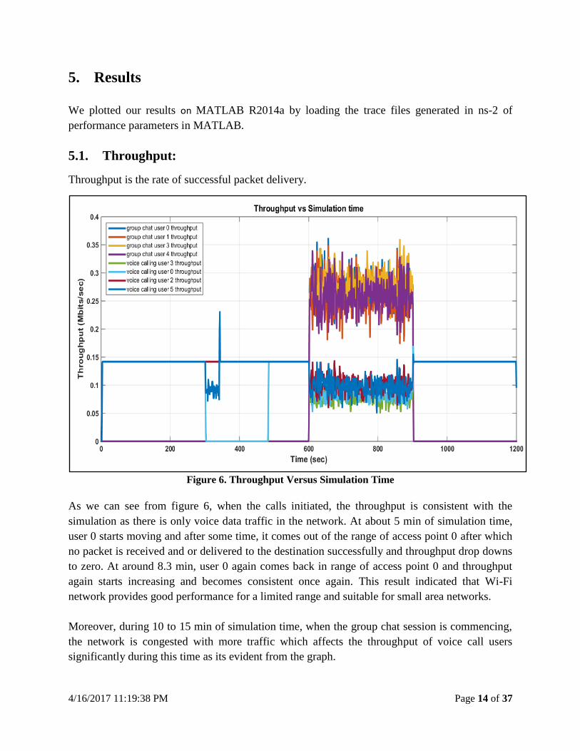
5.1. Throughput:
Throughput is the rate of successful packet delivery.
Figure 6. Throughput Versus Simulation Time
As we can see from figure 6, when the calls initiated, the throughput is consistent with the
simulation as there is only voice data traffic in the network. At about 5 min of simulation time,
user 0 starts moving and after some time, it comes out of the range of access point 0 after which
no packet is received and or delivered to the destination successfully and throughput drop downs
to zero. At around 8.3 min, user 0 again comes back in range of access point 0 and throughput
again starts increasing and becomes consistent once again. This result indicated that Wi-Fi
network provides good performance for a limited range and suitable for small area networks.
Moreover, during 10 to 15 min of simulation time, when the group chat session is commencing,
the network is congested with more traffic which affects the throughput of voice call users
significantly during this time as its evident from the graph.
4/16/2017 11:19:38 PM Page 15 of 37
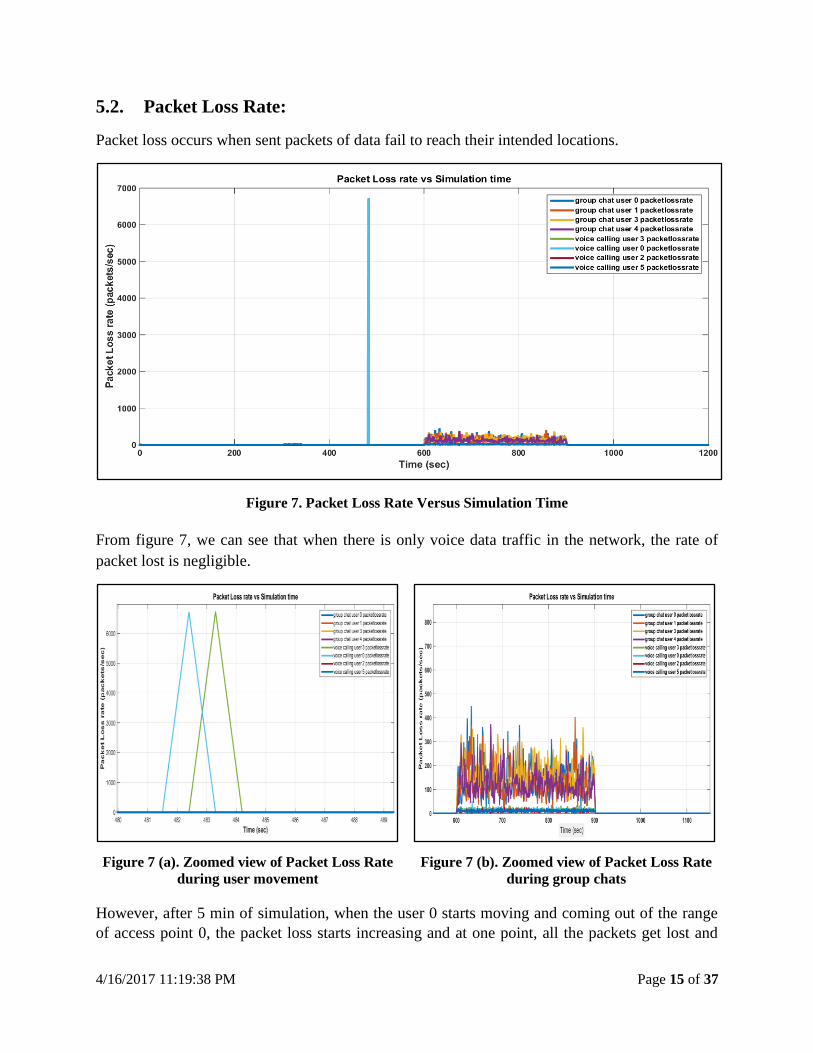
5.2. Packet Loss Rate:
Packet loss occurs when sent packets of data fail to reach their intended locations.
Figure 7. Packet Loss Rate Versus Simulation Time
From figure 7, we can see that when there is only voice data traffic in the network, the rate of
packet lost is negligible.
Figure 7 (a). Zoomed view of Packet Loss Rate
during user movement
Figure 7 (b). Zoomed view of Packet Loss Rate
during group chats
However, after 5 min of simulation, when the user 0 starts moving and coming out of the range
of access point 0, the packet loss starts increasing and at one point, all the packets get lost and

4/16/2017 11:19:38 PM Page 16 of 37
packet loss rate reaches the peak value. However, as soon as user 0 again comes back in the
range of access point 0, the packet drop rate starts decreasing and once again becomes negligible.
Also, we can see that when the group chat sessions introduced in the simulation, there is
significantly more stress on both the wired and wireless links to transfer more packets which also
increases the packet loss significantly during this time.
5.3. End-to-end Delay:
End to End Delay is the amount of time it takes for a packet to transmit from its source to
destination.
Figure 8. End-to-end Delay Versus Simulation time
Figure 8 (a). Zoomed view of Delay during voice
calls initiation
Figure 8 (b). Zoomed view of Delay during node
movement

4/16/2017 11:19:38 PM Page 17 of 37
Figure 8(c). Zoomed view of Delay observed during group chats
The significant spikes in the delays as shown in the zoomed views are due to contention window
adjustments when two or more nodes try to send data across the network simultaneously.
5.4. Jitter:
Jitter is the difference in the delays of the packets received.
Figure 9. Jitter Versus Simulation time

4/16/2017 11:19:38 PM Page 18 of 37
The zoomed views of the Jitter plot are shown below:
Figure 9 (a). Zoomed view of Jitter during voice
calls initiation
Figure 9 (b). Zoomed view of Jitter during node
movement
Figure 9(c). Zoomed views of Jitter observed during group chats
The spikes shown in the zoomed views in the jitter plot correspond to the end-to-end delays. The
significant spikes in delays at the beginning of the voice calls are due to contention window
adjustments. When the group chats session is introduced in the simulation, the network is
tolerant to jitter increase and is almost approximately negligible between 0.05 and 0.15 sec with
slight variations during this time.

4/16/2017 11:19:38 PM Page 19 of 37
6. Discussions and Conclusion
6.1. Challenges:
For this project, many difficulties and obstacles occurred before we were finally able to collect
the correct data for our simulations. First and foremost, in order to have Wi-Fi simulations to be
implemented into ns-2, we first needed to install ns-2.35 which consequently resulted in many
errors when making and configuring ns-2as we were new to this simulator. After many attempts
and searches through forums we were finally able to iron out the errors and have ns-2 running
successfully onto our Windows based machines. Next, in order to implement VoIP calls
successfully using Wi-Fi in ns-2 we first needed to understand the network topology. This
involved understanding the jobs and functions of Wi-Fi network topology before creating it in
ns-2. In particular, we needed to know the transfer speeds and other parameters of access points,
routers, servers and mobile nodes, as well as their individual functions in the transferring of data
packets.
6.1.1. Wi-Fi Hierarchy
For the Wi-Fi simulations, we needed to use domains and clusters in order for ns-2 to correctly
understand and simulate our designed Wi-Fi topology. Understanding how domains and clusters
work in ns-2 required much research and time.
6.1.2. Data Calculation and Plotting Graphs
Although a quick Google search could result in methods to calculate throughput, packet loss rate,
end-to-end delay and jitter, it was difficult to implement those methods into ns-2 for our
simulations. Furthermore, after we concluded that the computed simulated data in the trace files
were indeed correct, plotting graphs using MATLAB required a new level of knowledge in order
to display the simulation results with extended zoom view for readers to understand the
performance of Wi-Fi.
6.2. Improvements:
Although the essence of Wi-Fi has been simulated, there is still much that can be improved in
this project. Firstly, a better Wi-Fi topology should be constructed because the current network
topology only uses 4 routers and 2 servers. A more realistic simulation will have many more
routers making up the path for packets to travel. Secondly, the multicast function in ns-2 should
be used for group chatting instead of currently used individual UDP setup. The current setup
utilizes many UDPs and attaches them to every single user node in order to send packets of data.
With the multicast function in ns-2 there will be no need for such redundancy, but much more
time will have to be invested into the project in order to understand and be able to use the
multicasting functionality of ns-2.

4/16/2017 11:19:38 PM Page 20 of 37
6.3. Future Work:
In future, we planned to evaluate the performance of Wi-Fi by considering more realistic
situations with increased complexity of the network topology i.e. by adding more routers, servers
and mobile nodes. Also, we will consider simulating VoIP for video calling by using Real-time
Transport Protocol (RTP) to analyze the performance of Wi-Fi network using QoS parameters in
the next phase of this project.
6.4. Conclusion:
In this project, we have brought forth ns-2 simulations of VoIP calling using Wi-Fi, currently the
most widely used network technology in homes and small area networks. Using the capabilities
of ns-2, we have successfully simulated and collected data from the Wi-Fi topology. Finally, we
analyzed the simulation results to evaluate the performance of Wi-Fi by computing the QoS
parameters of throughput, packet loss rate, end-to-end delay, and jitter during voice calls over the
internet and group chats between multiple users. We observed that MOS values in VoIP over
Wi-Fi are only good if the receiver is within range of the access point and receives good signal
quality. The MOS score for voice quality also depends on the voice codec used. G.711 (64 Kbps)
codec and bitrates we picked is the good choice as the MOS score under ideal conditions is much
higher and more importantly G.711 is much more tolerant to jitter increase or packet loss. In
other words, the results obtained demonstrate that Wi-Fi provides better performance and QoS
for small area networks and is one of the reasons that still it is the most widely used technology
for wireless connectivity to the Internet when lingering in small networks such as homes, schools
and offices.

4/16/2017 11:19:38 PM Page 21 of 37
7. References
[1] Eric Swanlund, PavenLoodu, Sunny Chowdhury, “Analysis and Performance Evaluation
of a Wi-Fi Network using ns-2,” School of Engineering Science, Simon Fraser
University, 2013.
[2] Jay Kim, Jack Zheng, PanizBertsch, “Video Streaming over Wi-Fi,” School of
Engineering Science, Simon Fraser University, 2015.
[3] A. Ezreik and A. Gheryani, “Design and simulation of wireless networks using ns-2,” in
Proc. International Conference on Computer Science and Information Technology,
Singapore, pp.1–5, April 2012.
[4] Cheng Jie Ou, Tian Lin Yang, Yawen Chen, “VoIP Performance of City-Wide Wi-Fi and
LTE,” School of Engineering Science, Simon Fraser University, 2014.
[5] IEEE 802.11 Architecture. Available Online:
http://www.tutorial-reports.com/wireless/wlanwifi/wifi_architecture.php
[6] Tutorial for the Network Simulator ns. Available Online:
http://www.isi.edu/nsnam/ns/tutorial/index.html
[7] NS-2 Architecture. Available Online: http://www.tutorialsweb.com/ns2/NS2-1.htm
[8] CISCO, “Voice Over IP - Per Call Bandwidth Consumption,” Available Online:
http://www.cisco.com/c/en/us/support/docs/voice/voice-quality/7934-bwidth-
consume.html

4/16/2017 11:19:38 PM Page 22 of 37
Appendix A
Tcl Script for VoIP in Wi-Fi using ns-2:
# ========Define options========#
set val(chan) Channel/WirelessChannel ;#Channel Type
set val(prop) Propagation/TwoRayGround ;# radio-propagation model
set val(netif) Phy/WirelessPhy ;# network interface type
set val(mac) Mac/802_11 ;# MAC type
set val(ifq) Queue/DropTail/PriQueue ;# interface queue type
set val(ll) LL ;# link layer type
set val(ant) Antenna/OmniAntenna ;# antenna model
set val(ifqlen) 50 ;# max packet in ifq
set val(nn) 6 ;# number of mobilenodes
set val(rp) DSDV ;# routing protocol
set val(rp) DSR ;# routing protocol
set val(x) 400 ;# X dimension of topography
set val(y) 400 ;# Y dimension of topography
set val(stop) 1200 ;# time (20 min) of simulation end
# ========WIFI 802.11g Settings========#
set opt(wifi_bw) 54Mb ;# link BW on wifi net
Phy/WirelessPhy set Pt_ 0.25622777 ;#transmit power
Phy/WirelessPhy set L_ 1.0 ;#System loss factor
Phy/WirelessPhy set bandwidth_ 1 ;#opt(wifi_bw)
Phy/WirelessPhy set freq_ 2.472e9 ;#channel-13. 2.472GHz
Phy/WirelessPhy set CPThresh_ 10.0; #reception of simultaneous packets
Phy/WirelessPhy set CSThresh_ 5.011872e-12 ;#carrier sensing threshold
Phy/WirelessPhy set RXThresh_ 5.82587e-09 ;#reception threshold
Mac/802_11 set dataRate_ $opt(wifi_bw)
Mac/802_11 set basicRate_ 24Mb ;#for broadcast packets
# ========Jitter Trace ========#
set j0 [open jitter01.tr w]
set j1 [open jitter02.tr w]
set j2 [open jitter03.tr w]
set j3 [open jitter04.tr w]
set jg0 [open jitterg01.tr w]
set jg1 [open jitterg02.tr w]
set jg2 [open jitterg03.tr w]
set jg3 [open jitterg04.tr w]
# ========Throughput Trace ========#
set f0 [open out02.tr w]
set f1 [open out12.tr w]
set f2 [open out22.tr w]
set f3 [open out32.tr w]
set g0 [open outg0.tr w]
set g1 [open outg1.tr w]
set g2 [open outg2.tr w]
set g3 [open outg3.tr w]

4/16/2017 11:19:38 PM Page 23 of 37
# ========Packet Loss Trace ========#
set f4 [open lost02.tr w]
set f5 [open lost12.tr w]
set f6 [open lost22.tr w]
set f7 [open lost32.tr w]
set g4 [open lostg4.tr w]
set g5 [open lostg5.tr w]
set g6 [open lostg6.tr w]
set g7 [open lostg7.tr w]
# ========Packet Delay Trace ========#
set f8 [open delay02.tr w]
set f9 [open delay12.tr w]
set f10 [open delay22.tr w]
set f11 [open delay32.tr w]
set g8 [open delayg8.tr w]
set g9 [open delayg9.tr w]
set g10 [open delayg10.tr w]
set g11 [open delayg11.tr w]
# ========Initialize Flags========#
set previous 0
set previous1 0
set previous2 0
set previous3 0
set previousg0 0
set previousg1 0
set previousg2 0
set previousg3 0
set delaynow 0
set delaynow1 0
set delaynow2 0
set delaynow3 0
set delaynowg0 0
set delaynowg1 0
set delaynowg2 0
set delaynowg3 0
set holdtime 0
set holdseq 0
set holdtime1 0
set holdseq1 0
set holdtime2 0
set holdseq2 0
set holdtime3 0
set holdseq3 0
set holdtimeg0 0
set holdseqg0 0
set holdtimeg1 0
set holdseqg1 0
set holdtimeg2 0

4/16/2017 11:19:38 PM Page 24 of 37
set holdseqg2 0
set holdtimeg3 0
set holdseqg3 0
set holdrate1 0
set holdrate2 0
set holdrate3 0
set holdrate4 0
set holdrateg0 0
set holdrateg1 0
set holdrateg2 0
set holdrateg3 0
set ns [new Simulator]
set tracefd [open voip_wifi.tr w]
set namtrace [open voip_wifi.nam w]
$ns trace-all $tracefd
$ns namtrace-all-wireless $namtrace $val(x) $val(y)
# ======== Set up topography object========#
set topo [new Topography]
$topo load_flatgrid $val(x) $val(y)
create-god [expr $val(nn) + 8]
# ======== Configure the nodes========#
$ns node-config -adhocRouting $val(rp) \
-llType $val(ll) \
-macType $val(mac) \
-ifqType $val(ifq) \
-ifqLen $val(ifqlen) \
-antType $val(ant) \
-propType $val(prop) \
-phyType $val(netif) \
-wiredRouting ON \
-channelType $val(chan) \
-topoInstance $topo \
-agentTrace ON \
-routerTrace ON \
-macTrace OFF \
-movementTrace ON
$ns node-config -addressType hierarchical
AddrParams set domain_num_ 4 ;# number of domains
lappendcluster_num 1 2 1 2 ;# number of clusters in each domain
AddrParams set cluster_num_ $cluster_num
lappendeilastlevel 2 1 4 2 1 4 ;# number of nodes in each cluster
AddrParams set nodes_num_ $eilastlevel ;# of each domain
$ns color 1 Yellow
$ns color 2 Green
$ns color 3 Blue
$ns color 4 Purple

4/16/2017 11:19:38 PM Page 25 of 37
# ========router nodes========#
set rn(0) [$ns node {0.0.0}]
$rn(0) label "router 0"
$rn(0) set X_ 0.0
$rn(0) set Y_ 250.0
$rn(0) set Z_ 0.0
$rn(0) color brown
set rn(1) [$ns node {1.0.0}]
$rn(1) label "router 1"
$rn(1) set X_ 0.0
$rn(1) set Y_ 200.0
$rn(1) set Z_ 0.0
$rn(1) color red
set rn1(0) [$ns node {2.0.0}]
$rn1(0) label "router 2"
$rn1(0) set X_ 300.0
$rn1(0) set Y_ 250.0
$rn1(0) set Z_ 0.0
$rn1(0) color brown
set rn1(1) [$ns node {3.0.0}]
$rn1(1) label "router 3"
$rn1(1) set X_ 300.0
$rn1(1) set Y_ 200.0
$rn1(1) set Z_ 0.0
$rn1(1) color red
# ========server nodes========#
set sn_adr {0.0.1 2.0.1}
for {set i 0} {$i< 2} { incri} {
set sn($i) [$ns node [lindex $sn_adr $i]]
$sn($i) label "Server $i"
$sn($i) color green
}
$sn(0) set X_ 0.0
$sn(0) set Y_ 300
$sn(0) set Z_ 0.0
$sn(1) set X_ 300.0
$sn(1) set Y_ 300.0
$sn(1) set Z_ 0.0
# ========base stations========#
set bs(0) [$ns node {1.1.0}]
$bs(0) label "AccessPoint(0)"
$bs(0) random-motion 0
$bs(0) set X_ 0.0
$bs(0) set Y_ 100.0
$bs(0) set Z_ 0.0
$bs(0) color blue
set bs(1) [$ns node {3.1.0}]
$bs(1) label "AccessPoint(1)"
$bs(1) random-motion 0

4/16/2017 11:19:38 PM Page 26 of 37
$bs(1) set X_ 300.0
$bs(1) set Y_ 100.0
$bs(1) set Z_ 0.0
$bs(1) color blue
# ========wired links========#
$ns duplex-link $sn(0) $rn(0) 5Gb 2ms DropTail
$ns duplex-link $rn(0) $rn(1) 5Gb 2ms DropTail
$ns duplex-link $rn(1) $bs(0) 500Mb 2ms DropTail
$ns duplex-link $sn(1) $sn(0) 5Gb 100ms DropTail
$ns duplex-link $sn(1) $rn1(0) 5Gb 2ms DropTail
$ns duplex-link $rn1(0) $rn1(1) 5Gb 2ms DropTail
$ns duplex-link $rn1(1) $bs(1) 500Mb 2ms DropTail
$ns node-config -wiredRouting OFF mobile nodes
set adr {1.1.1 1.1.2 1.1.3 3.1.1 3.1.2 3.1.3}
set n(0) [$ns node [lindex $adr 0]]
set n(1) [$ns node [lindex $adr 1]]
set n(2) [$ns node [lindex $adr 2]]
set n(3) [$ns node [lindex $adr 3]]
set n(4) [$ns node [lindex $adr 4]]
set n(5) [$ns node [lindex $adr 5]]
for {set i 0} {$i< 6} { incri} {
$n($i) label "User $i"
}
$n(0) base-station [AddrParams addr2id [$bs(0) node-addr]]
$n(1) base-station [AddrParams addr2id [$bs(0) node-addr]]
$n(2) base-station [AddrParams addr2id [$bs(0) node-addr]]
$n(3) base-station [AddrParams addr2id [$bs(1) node-addr]]
$n(4) base-station [AddrParams addr2id [$bs(1) node-addr]]
$n(5) base-station [AddrParams addr2id [$bs(1) node-addr]]
# ========Provide initial location of mobilenodes========#
$n(0) set X_ 50.0
$n(0) set Y_ 100.0
$n(0) set Z_ 0.0
$n(1) set X_ 0.0
$n(1) set Y_ 50.0
$n(1) set Z_ 0.0
$n(2) set X_ -50.0
$n(2) set Y_ 100.0
$n(2) set Z_ 0.0
$n(3) set X_ 350.0
$n(3) set Y_ 100.0
$n(3) set Z_ 0.0
$n(4) set X_ 300.0
$n(4) set Y_ 50.0

4/16/2017 11:19:38 PM Page 27 of 37
$n(4) set Z_ 0.0
$n(5) set X_ 250.0
$n(5) set Y_ 100.0
$n(5) set Z_ 0.0
# ========Set a UDP connection between n(0) and n(3)========#
set udp1(1) [new Agent/UDP]
set udp1(2) [new Agent/UDP]
$udp1(1) set class_ 0
$udp1(2) set class_ 1
$udp1(1) set fid_ 1
$udp1(2) set fid_ 2
set sink11 [new Agent/LossMonitor]
set sink12 [new Agent/LossMonitor]
$ns attach-agent $n(0) $udp1(1)
$ns attach-agent $n(3) $sink11
$ns connect $udp1(1) $sink11
$ns attach-agent $n(3) $udp1(2)
$ns attach-agent $n(0) $sink12
$ns connect $udp1(2) $sink12
set cbr1(1) [new Application/Traffic/CBR]
$cbr1(1) set packetSize_ 512
$cbr1(1) set interval_ 0.03
$cbr1(1) set class_ 0
$cbr1(1) attach-agent $udp1(1)
set cbr1(2) [new Application/Traffic/CBR]
$cbr1(2) set packetSize_ 512
$cbr1(2) set interval_ 0.03
$cbr1(2) set class_ 1
$cbr1(2) attach-agent $udp1(2)
$ns at 1.0 "$cbr1(1) start"
$ns at 1.0 "$cbr1(2) start"
# user 0 movement
$ns at 300.0 "$n(0) setdest 100.0 100.0 20.0"
$ns at 480.0 "$n(0) setdest 50.0 100.0 20.0"
$ns at 1199.0 "$cbr1(1) stop"
$ns at 1199.0 "$cbr1(2) stop"
# ========Set up UDP connection between n(2) and n(5)========#
set udp2(1) [new Agent/UDP]
set udp2(2) [new Agent/UDP]
$udp2(1) set class_ 0
$udp2(2) set class_ 1
$udp2(1) set fid_ 1
$udp2(2) set fid_ 2
set sink21 [new Agent/LossMonitor]
set sink22 [new Agent/LossMonitor]
$ns attach-agent $n(2) $udp2(1)
$ns attach-agent $n(5) $sink21
$ns connect $udp2(1) $sink21
$ns attach-agent $n(5) $udp2(2)

4/16/2017 11:19:38 PM Page 28 of 37
$ns attach-agent $n(2) $sink22
$ns connect $udp2(2) $sink22
set cbr2(1) [new Application/Traffic/CBR]
$cbr2(1) set packetSize_ 512
$cbr2(1) set interval_ 0.03
$cbr2(1) set class_ 0
$cbr2(1) attach-agent $udp2(1)
set cbr2(2) [new Application/Traffic/CBR]
$cbr2(2) set packetSize_ 512
$cbr2(2) set interval_ 0.03
$cbr2(2) set class_ 1
$cbr2(2) attach-agent $udp2(2)
$ns at 1.0 "$cbr2(1) start"
$ns at 1.0 "$cbr2(2) start"
$ns at 1199.0 "$cbr2(1) stop"
$ns at 1199.0 "$cbr2(2) stop"
# ========Setup connections for group chat ========#
set sinkGC0 [new Agent/LossMonitor]
set sinkGC1 [new Agent/LossMonitor]
set sinkGC2 [new Agent/LossMonitor]
set sinkGC3 [new Agent/LossMonitor]
$ns attach-agent $n(0) $sinkGC0
$ns attach-agent $n(1) $sinkGC1
$ns attach-agent $n(3) $sinkGC2
$ns attach-agent $n(4) $sinkGC3
for {set i 0} {$i< 12} {incri} {
set udpGC($i) [new Agent/UDP]
}
$ns attach-agent $n(0) $udpGC(0)
$ns attach-agent $n(0) $udpGC(1)
$ns attach-agent $n(0) $udpGC(2)
$ns connect $udpGC(0) $sinkGC1
$ns connect $udpGC(1) $sinkGC2
$ns connect $udpGC(2) $sinkGC3
$ns attach-agent $n(1) $udpGC(3)
$ns attach-agent $n(1) $udpGC(4)
$ns attach-agent $n(1) $udpGC(5)
$ns connect $udpGC(3) $sinkGC0
$ns connect $udpGC(4) $sinkGC2
$ns connect $udpGC(5) $sinkGC3
$ns attach-agent $n(3) $udpGC(6)
$ns attach-agent $n(3) $udpGC(7)
$ns attach-agent $n(3) $udpGC(8)
$ns connect $udpGC(6) $sinkGC0
$ns connect $udpGC(7) $sinkGC1
$ns connect $udpGC(8) $sinkGC3
$ns attach-agent $n(4) $udpGC(9)
$ns attach-agent $n(4) $udpGC(10)
$ns attach-agent $n(4) $udpGC(11)
$ns connect $udpGC(9) $sinkGC0

4/16/2017 11:19:38 PM Page 29 of 37
$ns connect $udpGC(10) $sinkGC1
$ns connect $udpGC(11) $sinkGC2
for {set i 0} {$i< 12} {incri} {
set cbrGC($i) [new Application/Traffic/CBR]
$cbrGC($i) set packetSize_ 480
$cbrGC($i) set interval_ 0.03
$cbrGC($i) set class_ $i
$cbrGC($i) attach-agent $udpGC($i)
$ns at 600.0 "$cbrGC($i) start"
$ns at 900.0 "$cbrGC($i) stop"
}
$ns at 0.0 "record"
proc record {} {
global sink11 sink12 sink21 sink22 sinkGC0 sinkGC1 sinkGC2 sinkGC3 f0 f1 f2 f3 f4 f5 f6 f7
holdtime0 holdseq0 holdtime1 holdseq1 holdtime2 holdseq2 holdtime3 holdseq3 f8 f9 f10 f11 holdrate1
holdrate2 holdrate3 holdrate4 g0 g1 g2 g3 g4 g5 g6 g7 g8 g9 g10 g11 holdtimeg0 holdtimeg1 holdtimeg2
holdtimeg3 holdseqg0 holdseqg1 holdseqg2 holdseqg3 holdrateg0 holdrateg1 holdrateg2 holdrateg3 j0 j1
j2 j3 jg0 jg1 jg2 jg3 previous previous1 previous2 previous3 previousg0 previousg1 previousg2
previousg3 delaynow0 delaynow1 delaynow2 delaynow3 delaynowg0 delaynowg1 delaynowg2
delaynowg3
set ns [Simulator instance]
set time 0.9 ;#Set Sampling Time to 0.9 Sec
set bw0 [$sinkGC0 set bytes_]
set bw1 [$sinkGC1 set bytes_]
set bw2 [$sinkGC2 set bytes_]
set bw3 [$sinkGC3 set bytes_]
set bwg0 [$sink11 set bytes_]
set bwg1 [$sink12 set bytes_]
set bwg2 [$sink21 set bytes_]
set bwg3 [$sink22 set bytes_]
set bw4 [$sinkGC0 set nlost_]
set bw5 [$sinkGC1 set nlost_]
set bw6 [$sinkGC2 set nlost_]
set bw7 [$sinkGC3 set nlost_]
set bwg4 [$sink11 set nlost_]
set bwg5 [$sink12 set nlost_]
set bwg6 [$sink21 set nlost_]
set bwg7 [$sink22 set nlost_]
set bw8 [$sinkGC0 set lastPktTime_]
set bw9 [$sinkGC0 set npkts_]
set bw10 [$sinkGC1 set lastPktTime_]
set bw11 [$sinkGC1 set npkts_]
set bw12 [$sinkGC2 set lastPktTime_]
set bw13 [$sinkGC2 set npkts_]
set bw14 [$sinkGC3 set lastPktTime_]
set bw15 [$sinkGC3 set npkts_]
set bwg8 [$sink11 set lastPktTime_]
set bwg9 [$sink11 set npkts_]
set bwg10 [$sink12 set lastPktTime_]

4/16/2017 11:19:38 PM Page 30 of 37
set bwg11 [$sink12 set npkts_]
set bwg12 [$sink21 set lastPktTime_]
set bwg13 [$sink21 set npkts_]
set bwg14 [$sink22 set lastPktTime_]
set bwg15 [$sink22 set npkts_]
if { $bw9 > $holdseq } {
set delaynow [expr ($bw8 - $holdtime)/($bw9 - $holdseq)]
} else { setdelaynow [expr ($bw9 - $holdseq)]
}
if { $bwg9 > $holdseqg0 } {
set delaynowg0 [expr ($bwg8 - $holdtimeg0)/($bwg9 - $holdseqg0)]
} else { set delaynowg0 [expr ($bwg9 - $holdseqg0)]
}
if { $bw11 > $holdseq1 } {
set delaynow1 [expr ($bw10 - $holdtime1)/($bw11 - $holdseq1)]
} else {set delaynow1 [expr ($bw11 - $holdseq1)]
}
if { $bwg11 > $holdseqg1 } {
set delaynowg1 [expr ($bwg10 - $holdtimeg1)/($bwg11 - $holdseqg1)]
} else { set delaynowg1 [expr ($bwg11 - $holdseqg1)]
}
if { $bw13 > $holdseq2 } {
set delaynow2 [expr ($bw12 - $holdtime2)/($bw13 - $holdseq2)]
} else {set delaynow2 [expr ($bw13 - $holdseq2)]
}
if { $bwg13 > $holdseqg2 } {
set delaynowg2 [expr ($bwg12 - $holdtimeg2)/($bwg13 - $holdseqg2)]
} else { set delaynowg2 [expr ($bwg13 - $holdseqg2)]
}
if { $bw15 > $holdseq3 } {
set delaynow3 [expr ($bw14 - $holdtime3)/($bw15 - $holdseq3)]
} else {set delaynow3 [expr ($bw15 - $holdseq3)]
}
if { $bwg15 > $holdseqg3 } {
set delaynowg3 [expr ($bwg14 - $holdtimeg3)/($bwg15 - $holdseqg3)]
} else {set delaynowg3 [expr ($bwg15 - $holdseqg3)]
}
set now [$ns now]
# ========Record Bit Rate in Trace Files========#
puts $f0 "$now [expr (($bw0+$holdrate1)*8)/(2*$time*1000000)]"
puts $f1 "$now [expr (($bw1+$holdrate2)*8)/(2*$time*1000000)]"
puts $f2 "$now [expr (($bw2+$holdrate3)*8)/(2*$time*1000000)]"
puts $f3 "$now [expr (($bw3+$holdrate4)*8)/(2*$time*1000000)]"
puts $g0 "$now [expr (($bwg0+$holdrateg0)*8)/(2*$time*1000000)]"
puts $g1 "$now [expr (($bwg1+$holdrateg1)*8)/(2*$time*1000000)]"
puts $g2 "$now [expr (($bwg2+$holdrateg2)*8)/(2*$time*1000000)]"
puts $g3 "$now [expr (($bwg3+$holdrateg3)*8)/(2*$time*1000000)]"

4/16/2017 11:19:38 PM Page 31 of 37
# ======== Record Packet Loss Rate in Trace File========#
puts $f4 "$now [expr $bw4/$time]"
puts $f5 "$now [expr $bw5/$time]"
puts $f6 "$now [expr $bw6/$time]"
puts $f7 "$now [expr $bw7/$time]"
puts $g4 "$now [expr $bwg4/$time]"
puts $g5 "$now [expr $bwg5/$time]"
puts $g6 "$now [expr $bwg6/$time]"
puts $g7 "$now [expr $bwg7/$time]"
# ========Record Packet Delay in File========#
if { $bw9 > $holdseq } {
puts $f8 "$now [expr ($bw8 - $holdtime)/($bw9 - $holdseq)]"
} else {puts $f8 "$now [expr ($bw9 - $holdseq)]"
}
if { $bw11 > $holdseq1 } {
puts $f9 "$now [expr ($bw10 - $holdtime1)/($bw11 - $holdseq1)]"
} else {puts $f9 "$now [expr ($bw11 - $holdseq1)]"
}
if { $bw13 > $holdseq2 } {
puts $f10 "$now [expr ($bw12 - $holdtime2)/($bw13 - $holdseq2)]"
} else {puts $f10 "$now [expr ($bw13 - $holdseq2)]"
}
if { $bw15 > $holdseq3 } {
puts $f11 "$now [expr ($bw14 - $holdtime3)/($bw15 - $holdseq3)]"
} else {puts $f11 "$now [expr ($bw15 - $holdseq3)]"
}
if { $bwg9 > $holdseqg0 } {
puts $g8 "$now [expr ($bwg8 - $holdtimeg0)/($bwg9 - $holdseqg0)]"
} else {puts $g8 "$now [expr ($bwg9 - $holdseqg0)]"
}
if { $bwg11 > $holdseqg1 } {
puts $g9 "$now [expr ($bwg10 - $holdtimeg1)/($bwg11 - $holdseqg1)]"
} else {puts $g9 "$now [expr ($bwg11 - $holdseqg1)]"
}
if { $bwg13 > $holdseqg2 } {
puts $g10 "$now [expr ($bwg12 - $holdtimeg2)/($bwg13 - $holdseqg2)]"
} else {puts $g10 "$now [expr ($bwg13 - $holdseqg2)]"
}
if { $bwg15 > $holdseqg3 } {
puts $g11 "$now [expr ($bwg14 - $holdtimeg3)/($bwg15 - $holdseqg3)]"
} else {puts $g11 "$now [expr ($bwg15 - $holdseqg3)]"
}
# ========Record Jitter in Trace Files========#
puts $j0 "$now [expr (($delaynow - $previous ) + ($delaynowg0 - $previousg0))]"
puts $j1 "$now [expr (($delaynow1 - $previous1 ) + ($delaynowg1 - $previousg1))]"
puts $j2 "$now [expr (($delaynow2 - $previous2 ) + ($delaynowg2 - $previousg2))]"
puts $j3 "$now [expr (($delaynow3 - $previous3 ) + ($delaynowg3 - $previousg3))]"

4/16/2017 11:19:38 PM Page 32 of 37
# ========Reset Variables========#
$sinkGC0 set bytes_ 0
$sinkGC1 set bytes_ 0
$sinkGC2 set bytes_ 0
$sinkGC3 set bytes_ 0
$sinkGC0 set nlost_ 0
$sinkGC1 set nlost_ 0
$sinkGC2 set nlost_ 0
$sinkGC3 set nlost_ 0
$sink11 set bytes_ 0
$sink12 set bytes_ 0
$sink21 set bytes_ 0
$sink22 set bytes_ 0
$sink11 set nlost_ 0
$sink12 set nlost_ 0
$sink21 set nlost_ 0
$sink22 set nlost_ 0
set holdtime $bw8
set holdseq $bw9
set holdtime1 $bw10
set holdseq1 $bw11
set holdtime2 $bw12
set holdseq2 $bw13
set holdtime3 $bw14
set holdseq3 $bw15
set holdtimeg0 $bwg8
set holdseqg0 $bwg9
set holdtimeg1 $bwg10
set holdseqg1 $bwg11
set holdtimeg2 $bwg12
set holdseqg2 $bwg13
set holdtimeg3 $bwg14
set holdseqg3 $bwg15
set holdrate1 $bw0
set holdrate2 $bw1
set holdrate3 $bw2
set holdrate4 $bw3
set holdrateg0 $bwg0
set holdrateg1 $bwg1
set holdrateg2 $bwg2
set holdrateg3 $bwg3
# ========group chat========#
if { $bw9 > $holdseq } {
set previous [expr ($bw8 - $holdtime)/($bw9 - $holdseq)]
} else { set previous [expr ($bw9 - $holdseq)]
}
if { $bw11 > $holdseq1 } {
set previous1 [expr ($bw10 - $holdtime1)/($bw11 - $holdseq1)]
} else { set previous1 [expr ($bw11 - $holdseq1)]
}

4/16/2017 11:19:38 PM Page 33 of 37
if { $bw13 > $holdseq2 } {
set previous2 [expr ($bw12 - $holdtime2)/($bw13 - $holdseq2)]
} else { set previous2 [expr ($bw13 - $holdseq2)]
}
if { $bw15 > $holdseq3 } {
set previous3 [expr ($bw14 - $holdtime3)/($bw15 - $holdseq3)]
} else { set previous3 [expr ($bw15 - $holdseq3)]
}
if { $bwg9 > $holdseqg0 } {
set previousg0 [expr ($bwg8 - $holdtimeg0)/($bwg9 - $holdseqg0)]
} else { set previousg0 [expr ($bwg9 - $holdseqg0)]
}
if { $bwg11 > $holdseqg1 } {
set previousg1 [expr ($bwg10 - $holdtimeg1)/($bwg11 - $holdseqg1)]
} else { set previousg1 [expr ($bwg11 - $holdseqg1)]
}
if { $bwg13 > $holdseqg2 } {
set previousg2 [expr ($bwg12 - $holdtimeg2)/($bwg13 - $holdseqg2)]
} else { set previousg2 [expr ($bwg13 - $holdseqg2)]
}
if { $bwg15 > $holdseqg3 } {
set previousg3 [expr ($bwg14 - $holdtimeg3)/($bwg15 - $holdseqg3)]
} else { set previousg3 [expr ($bwg15 - $holdseqg3)]
}
$ns at [expr $now+$time] "record" ;# Schedule Record after $time interval sec
}
# ========defining heads Color change while moving node moves ========#
$ns at 1.0 "$n(0) delete-mark n(0)"
$ns at 1.0 "$n(0) add-mark n(0) yellow circle"
$ns at 1.0 "$n(3) delete-mark n(3)"
$ns at 1.0 "$n(3) add-mark n(3) yellow circle"
$ns at 1.0 "$n(2) delete-mark n(2)"
$ns at 1.0 "$n(2) add-mark n(2) green circle"
$ns at 1.0 "$n(5) delete-mark n(5)"
$ns at 1.0 "$n(5) add-mark n(3) green circle"
# ========Define node initial position in nam========#
for {set i 0} {$i< $val(nn)} { incri } {
$ns initial_node_pos $n($i) 20; # defines the node size for nam
}
# ========Tell nodes when the simulation ends========#
for {set i 0} {$i< $val(nn) } { incri } {
$ns at $val(stop) "$n($i) reset";
}
# ========Ending nam and the simulation========#
$ns at $val(stop) "$ns nam-end-wireless $val(stop)"
$ns at $val(stop) "stop"
$ns at 1200.00 "puts \"end simulation\" ; $ns halt"

4/16/2017 11:19:38 PM Page 34 of 37
proc stop {} {
global ns tracefd namtrace f0 f1 f2 f3 f4 f5 f6 f7 f8 f9 f10 f11 g0 g1 g2 g3 g4 g5 g6 g7 g8
g9 g10 g11 j0 j1 j2 j3 jg0 jg1 jg2 jg3
# Close Trace Files
close $f0
close $f1
close $f2
close $f3
close $f4
close $f5
close $f6
close $f7
close $f8
close $f9
close $f10
close $f11
close $g0
close $g1
close $g2
close $g3
close $g4
close $g5
close $g6
close $g7
close $g8
close $g9
close $g10
close $g11
close $j0
close $j1
close $j2
close $j3
close $jg0
close $jg1
close $jg2
close $jg3
# ========Open Network Animator========#
exec nam voip_wifi.nam&
# ========Reset Trace File========#
$ns flush-trace
close $tracefd
close $namtrace
exit 0
}
puts "Starting Simulation..."
$ns run

4/16/2017 11:19:38 PM Page 35 of 37
Appendix B
MATLAB Code for Simulation Plots:
% Plotting Throughput
a=load('out02.tr');
b=load('out12.tr');
c=load('out22.tr');
d=load('out32.tr');
e=load('outg0.tr');
f=load('outg1.tr');
g=load('outg2.tr');
h=load('outg3.tr');
x1=a(:,1);
y1=a(:,2);
x2=b(:,1);
y2=b(:,2);
x3=c(:,1);
y3=c(:,2);
x4=d(:,1);
y4=d(:,2);
x5=e(:,1);
y5=e(:,2);
x6=f(:,1);
y6=f(:,2);
x7=g(:,1);
y7=g(:,2);
x8=h(:,1);
y8=h(:,2);
plot(x1,y1,x2,y2,x3,y3,x4,y4,x5,y5,x6,y6,x7,y7,x8,y8);
legend('group chat user 0 throughput','group chat user 1 throughput','group chat user 3 throughput','group
chat user 4 throughput','voice calling user 3 throughput','voice calling user 0 throughput','voice calling
user 2 throughput','voice calling user 5 throughput');
xlabel('Time(sec)');
ylabel('Throughput(Mbits/sec)');
title('Throughput vs Simulation time');
% Plotting Packet Loss rate
clear all;
clc;
a=load('lost02.tr');
b=load('lost12.tr');
c=load('lost22.tr');
d=load('lost32.tr');
e=load('lostg4.tr');
f=load('lostg5.tr');
g=load('lostg6.tr');

4/16/2017 11:19:38 PM Page 36 of 37
h=load('lostg7.tr');
x1=a(:,1);
y1=a(:,2);
x2=b(:,1);
y2=b(:,2);
x3=c(:,1);
y3=c(:,2);
x4=d(:,1);
y4=d(:,2);
x5=e(:,1);
y5=e(:,2);
x6=f(:,1);
y6=f(:,2);
x7=g(:,1);
y7=g(:,2);
x8=h(:,1);
y8=h(:,2);
plot(x1,y1,x2,y2,x3,y3,x4,y4,x5,y5,x6,y6,x7,y7,x8,y8);
legend('group chat user 0 packetlossrate','group chat user 1 packetlossrate','group chat user 3
packetlossrate','group chat user 4 packetlossrate','voice calling user 3 packetlossrate','voice calling user 0
packetlossrate','voice calling user 2 packetlossrate','voice calling user 5 packetlossrate');
xlabel('Time (sec)');
ylabel('Packet Loss rate (packets/sec)');
title('Packet Loss rate vs Simulation time');
% Plotting End-to-end Delay
clear all;
clc;
a=load('delay02.tr');
b=load('delay12.tr');
c=load('delay22.tr');
d=load('delay32.tr');
e=load('delayg8.tr');
f=load('delayg9.tr');
g=load('delayg10.tr');
h=load('delayg11.tr');
x1=a(:,1);
y1=a(:,2);
x2=b(:,1);
y2=b(:,2);
x3=c(:,1);
y3=c(:,2);
x4=d(:,1);
y4=d(:,2);
x5=e(:,1);
y5=e(:,2);
x6=f(:,1);
y6=f(:,2);
x7=g(:,1);

4/16/2017 11:19:38 PM Page 37 of 37
y7=g(:,2);
x8=h(:,1);
y8=h(:,2);
plot(x1,y1,x2,y2,x3,y3,x4,y4,x5,y5,x6,y6,x7,y7,x8,y8);
legend('group chat user 0 delay','group chat user 1 delay','group chat user 3 delay','group chat user 4
delay','voice calling user 3 delay','voice calling user 0 delay','voice calling user 2 delay','voice calling user
5 delay');
xlabel('Time (sec)');
ylabel('Delay (sec)');
title('End-to-end Delay vs Simulation time');
% Plotting results of Jitter for voice call users
clear all;
clc;
a=load('jitter01.tr');
b=load('jitter02.tr');
c=load('jitter03.tr');
d=load('jitter04.tr');
x1=a(:,1);
y1=a(:,2);
x2=b(:,1);
y2=b(:,2);
x3=c(:,1);
y3=c(:,2);
x4=d(:,1);
y4=d(:,2);
plot(x1,y1,x2,y2,x3,y3,x4,y4);
legend('Jitter-user0','Jitter-user3','Jitter-user2','Jitter-user5');
xlabel('Time (sec)');
ylabel('Jitter (sec)');
title('Jitter vs Simulation time');
Related Documents


