Enrique Gallardo Vizcaino - ERA

Graph-Based Simulator for Steam-Assisted Gravity Drainage Reservoir Management

by

Enrique Gallardo Vizcaino

A thesis submitted in partial fulfillment of the requirements for the degree of

Doctor of Philosophy

in

Mining Engineering

Department of Civil and Environmental Engineering University of Alberta

© Enrique Gallardo Vizcaino, 2019

ii

Abstract

Petroleum reservoir managers must make decisions about projects (e.g. infill drilling and/or

operational strategies) with uncertain economic results due to imperfect knowledge of the

reservoir geometry and properties. Their decision-making workflows should actively

manage the geological uncertainty. This requires transferring the geological uncertainty to

probability distributions of a response variable suitable for decision-making and use of a

decision criterion that considers the reservoir manager’s preferences toward the project’s

return-risk trade-off. This is challenging in petroleum reservoir management because

transferring the geological uncertainty is time and computationally expensive. Moreover,

common decision-making criteria do not consider preferences toward the geological risk

of the projects.

This dissertation improves reservoir management decision-making practices in steam-

assisted gravity drainage (SAGD) projects by introducing: 1) A novel graph-based

simplified physics simulator, called APDS, that efficiently transfers the geological

uncertainty into steam-chamber evolution paths that can directly support SAGD reservoir

management or be converted to a monetary response variable, and 2) A decision-making

criterion consistent with the utility theory framework that combines Mean-Variance

Criterion (MVC) and Stochastic Dominance Rules (SDR) to guide the decision process.

APDS is formulated and implemented using graph theory, simplified porous media flow

equations, heat transfer concepts and ideas from discrete simulation. It works on

homogeneous and heterogeneous reservoirs and is computationally efficient enough to be

applied over multiple geostatistical realizations. A case study performed with a realistic

multi-realization geological model validates the predictive capabilities of APDS. Visual

iii

and numerical comparisons with the results obtained from a conventional full physics

thermal flow simulation are satisfactory. APDS was 3 orders of magnitude faster than the

conventional simulator to model the steam-chamber expansion and to provide predictions

of reservoir response. The reduction in the precision of the results is deemed acceptable.

Another case study demonstrates that APDS can complement methodologies for

assimilation of 4D-seismic dynamic data to improve reservoir characterization.

This thesis also demonstrates that MVC-SDR is a viable criterion for decision making

under geological uncertainty. MVC-SDR does not rely on a specific utility function and

leads to decisions that are considered rational to risk-averse reservoir managers. The

shortcoming is a reduced ability to rank projects with very similar value. Two examples

illustrate the use of MVC-SDR, the first one relates to the selection of a SAGD well-pad

to be drilled from a set of several possible options, and the second one considers the

problem of finding the best vertical location for a SAGD well-pair project in a target

volume.

iv

Preface

Parts of this thesis have been previously published or are in the publication process.

Chapters 2, 3 and 5 are composed in part by Gallardo & Deutsch (2018). Approximate

Physics Discrete Simulation of the Steam-Chamber Evolution in SAGD. Published in SPE

Journal.

Chapter 4 is composed in part by Gallardo & Deutsch (2019). Decision Making in

Presence of Geological Uncertainty with Mean-Variance Criteria and Stochastic

Dominance Rules. Submitted to SPE Journal of Reservoir Evaluation & Engineering:

Formation Evaluation.

v

To my wife Sonia and my sons Enrique and Esteban.

Remember my words ten years ago: “my life belongs to all three of you”.

vi

Acknowledgments

I would like to express my deep gratitude to Dr. Clayton V. Deutsch for being my mentor

during my studies at the University of Alberta. His lessons and example have enriched my

professional and personal life.

I would also like to thank the members of my supervisory committee, Dr. Jeffery

Boisvert and Dr. Yashar Pourrahimian. Their comments and feedback improved the quality

of this dissertation.

I acknowledge the financial support provided by members of the Centre for

Computational Geostatistics and the Colombian National Oil Company, Ecopetrol.

vii

Table of Contents

1 Graph-Based Simulator for Steam Assisted Gravity Drainage Reservoir

Management ........................................................................................................................ 1

1.1 Introduction ...................................................................................................... 1

1.2 Petroleum Reservoir Management Decision-Making Workflow ..................... 2

1.3 Problem Setting ................................................................................................ 3

1.4 Proposed Approach........................................................................................... 4

1.4.1 Graph-Base Steam-Chamber Simulator for Transfering the Geological

Uncertainty in SAGD Projects .................................................................................... 4

1.4.2 Mean-Variance Criteria and Stochastic Dominance Rules to Consider the

Geological Risk-Reward trade-off .............................................................................. 5

1.5 Dissertation Outline ...................................................................................... 6

2 SAGD Steam-Chamber Modeling with APDS: Formulation ..................................... 8

2.1 Introduction ...................................................................................................... 8

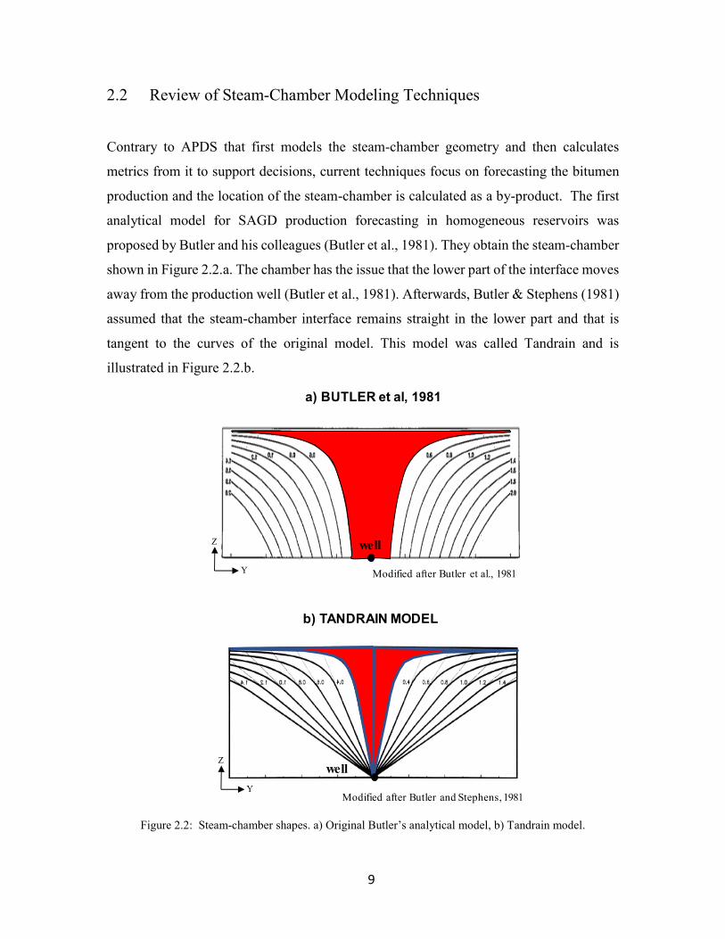
2.2 Review of Steam-Chamber Modeling Techniques ........................................... 9

2.3 Steam Chamber Evolution Posed as a Shortest Path Problem ....................... 12

2.4 APDS Formulation ......................................................................................... 13

2.4.1 Graph ....................................................................................................... 13

2.4.2 Propagation Algorithm ............................................................................ 14

2.4.3 Ranking Function .................................................................................... 16

2.4.4 APDS Outputs ......................................................................................... 19

2.5 APDS Pseudo Code .................................................................................... 20

2.6 Step-wise Procedure ....................................................................................... 22

2.7 APDS Time Complexity ................................................................................. 26

2.8 Potential Applications..................................................................................... 27

viii

2.8.1 SAGD Well-pair Location. ..................................................................... 27

2.8.2 SAGD Operation. .................................................................................... 27

2.8.3 4D-Seismic Integration. .......................................................................... 28

2.8.4 SAGD Geomechanics. ............................................................................ 28

2.9 Discussion ................................................................................................... 28

3 APDS: Implementation and Validation ................................................................... 30

3.1 Introduction .................................................................................................... 30

3.2 APDS Assumptions and Simplifications ........................................................ 30

3.2.1 Sinks, Parent Sink and Sink Angle (β) .................................................... 31

3.2.2 Transversal Area (At) .............................................................................. 33

3.2.3 Kinematic Viscosity in the Heated Volume (υhv) .................................. 33

3.2.4 Permeability ............................................................................................ 35

3.2.5 Steam-chamber Interface Velocity .......................................................... 35

3.3 APDS prototype computer program ............................................................... 37

3.4 APDS Validation ............................................................................................ 38

3.4.1 Geological Model .................................................................................... 39

3.4.2 SAGD Project .......................................................................................... 40

3.4.3 Steam-chambers from STARS and APDS .............................................. 41

3.4.4 Metrics from STARS and APDS ............................................................ 48

3.4.5 Computational Time ................................................................................ 58

3.5 Discussion ................................................................................................... 58

3.5.1 APDS Level of Physics ........................................................................... 58

3.5.2 APDS Validation ..................................................................................... 60

3.5.3 APDS Prototype and Computational Time ............................................. 60

4 Mean-Variance Criterion and Stochastic Dominance Rules for PRM ..................... 62

4.1 Introduction .................................................................................................... 62

ix

4.2 Decision-Making Model in Presence of Geological Uncertainty ................... 63

4.2.1 Set of Feasible Actions or Projects. ........................................................ 63

4.2.2 Set of Outcomes ...................................................................................... 64

4.2.3 Preferences and Concept of Rationality .................................................. 65

4.3 Utility Theory in PRM ................................................................................ 67

4.4 Mean Variance Criterion and Stochastic Dominance Rules ....................... 68

4.4.1 The Mean-Variance Criterion (MVC)..................................................... 69

4.4.2 Stochastic Dominance Rules (SDR) ....................................................... 71

4.5 MVC and SDR in PRM .................................................................................. 77

4.6 Example of MVC-SDR Methodology ............................................................ 77

4.7 Discussion ...................................................................................................... 81

5 Case-Study: SAGD Vertical Well Placement ........................................................... 82

5.1 Introduction .................................................................................................... 82

5.2 SAGD Vertical Placement Well Problem ................................................... 82

5.2.1 Problem Setting ....................................................................................... 82

5.2.2 Set of Feasible Actions ............................................................................ 83


5.2.4 Transffering the Geological Uncertainty with APDS ............................. 85

5.2.5 MVC ........................................................................................................ 91

5.2.6 SDR ......................................................................................................... 93

5.3 Computational Time ....................................................................................... 95

5.4 Discussion ................................................................................................... 95

6 Case Study: SAGD Reservoir Characterization with APDS .................................... 97

6.1 Introduction .................................................................................................... 97

6.2 Assessment of Geostatistical Anomaly Enforcement with APDS .............. 98


x

6.2.2 Assesing SAGD Reservoir Characterization Improvement with APDS102

6.2.3 APDS Modeling of Steam-Chamber in Point Bar Systems .................. 111

6.2.4 Computational Time .............................................................................. 115

6.3 Discussion ................................................................................................. 115

7 Summary of Contributions and Future Work ......................................................... 117

7.1 Summary of Contributions ........................................................................... 117

7.1.1 APDS Formulation ................................................................................ 118

7.1.2 APDS Implementation and Validation .................................................. 119

7.1.3 Decision-Making Criterion for Active Management of Geological

Uncertainty .............................................................................................................. 120

7.1.4 Assisting 4D-Seismic Integration in Reservoir Characterization ......... 121

7.2 Limitations and Future Work ....................................................................... 122

7.2.1 Production Oil Forecast ......................................................................... 123

7.2.2 Steam-Oil Ratio (SOR) Forecast ........................................................... 124

7.2.3 Oil Relative Permeability (Kro) ............................................................ 125

7.2.4 Cells with High Initial Water Saturation (Swi) ..................................... 127

7.2.5 Assisting the Ensemble Kalman Filter (EnKF) Technique with APDS 128

7.2.6 Coupling APDS with a Thermal Wellbore Simulator ........................... 129

7.2.7 APDS Applications ............................................................................... 129

7.2.8 APDS Computational Efficiency .......................................................... 129

7.2.9 Decision-Maker Position on Geological Risk ....................................... 130

7.2.10 Value of Seismic Information on SAGD projects ............................. 131

References ....................................................................................................................... 132

Appendix A ..................................................................................................................... 142

A.1 Dependencies, Requirements and Licenses .................................................. 142

A.1.1 Dependencies and Requirements .......................................................... 142

xi

A.1.2 Licenses ................................................................................................. 143

A.2 APDS Workflow........................................................................................... 149

A.3 APDS Programs ............................................................................................ 157

A.3.1 Graph Generator Module Programs ......................................................... 157

A.3.2 Steam-Chamber Module Programs .......................................................... 166

A.3.3 Post-processing Module Programs ........................................................... 175

Appendix B ..................................................................................................................... 177

xii

List of Figures

Figure 1.1: Components of a Petroleum Reservoir Management Decision-Making

workflow. ............................................................................................................................ 2

Figure 2.1: Steam-assisted gravity drainage (SAGD) process (obtained from Peacock

(2010))................................................................................................................................. 8

Figure 2.2: Steam-chamber shapes. a) Original Butler’s analytical model, b) Tandrain

model................................................................................................................................... 9

Figure 2.3: Steam-chamber with imposed geometry. a) Inverted triangle model, b) Circular

model................................................................................................................................. 10

Figure 2.4: Steam-chamber from semi-analytical models. a) Butler (1985) semi-analytical

model, b) Heidari et al. (2009) semi-analytical model. .................................................... 11

Figure 2.5: Illustration of a 2D-grid geological model represented as a graph. .............. 14

Figure 2.6: APDS propagation mechanism. Red shapes are not part of APDS. They were

drawn to help visualizing the steam-chamber expansion. Edge labels omitted in this figure

are shown in Figure 2.5. .................................................................................................... 15

Figure 2.7: Steam-chamber interface and temperature distribution (modified after Butler

(1991))............................................................................................................................... 18

Figure 2.8: APDS Outputs: a) Ordered sequence of nodes, b) Steam-chamber model, c)

Cumulative steam-chamber volume. ................................................................................ 19

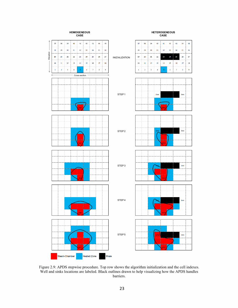
Figure 2.9: APDS stepwise procedure. Top row shows the algorithm initialization and the

cell indexes. Well and sinks locations are labeled. Black outlines drawn to help visualizing

how the APDS handles barriers. ....................................................................................... 23

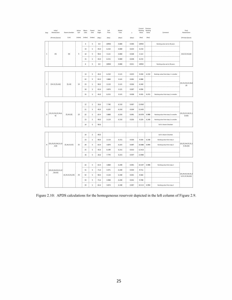
Figure 2.10: APDS calculations for the homogeneous reservoir depicted in the left column

of Figure 2.9. ..................................................................................................................... 25

Figure 2.11: APDS calculations for the heterogeneous reservoir depicted in the right

column of Figure 2.9. ........................................................................................................ 26

Figure 3.1: Bitumen flowing downward from cell A to the well will pass through one of

the sinks (red cells). The angle between cell A and one sink cell is called sink angle. This

figure shows two possible sink angles β1 and β2. .......................................................... 31

xiii

Figure 3.2: The bitumen path depends on the relative position between the cell, the well

and the barriers. In figures a and b, the steam-chamber approaches cell A from the left-side

and the sink 1 is marked as Parent Sink of A. In figure c, the steam-chamber approaches

cell A from the right-side and the sink 2 is marked as Parent Sink of A .......................... 32

Figure 3.3: The transversal side (𝑺𝒕) concept used in APDS. .......................................... 33

Figure 3.4: The advance of the steam-chamber interface at a velocity U is determined by

the difference between 𝑞𝑖𝑛 and 𝑞𝑜𝑢𝑡. .............................................................................. 36

Figure 3.5: The advance of the steam-chamber interface is determined by the difference

between the flowing in (𝑞𝑖𝑛) and flowing out (𝑞𝑜𝑢𝑡) rates. ............................................ 37

Figure 3.6: Structure of the APDS prototype.................................................................... 38

Figure 3.7: Illustration of one realization of the geological model. .................................. 39

Figure 3.8: Temperature and compositional dependent relative permeability curves

(CMG’s SAGD guide (2013). ........................................................................................... 41

Figure 3.9: APDS and STARS steam-chamber after 5 years. .......................................... 42

Figure 3.10: Cross-section A and B selected to compare STARS and APDS. ................. 42

Figure 3.11: Cross-section A comparing APDS and STARS for 5 years. ........................ 44

Figure 3.12: Cross-section B comparing APDS and STARS for 5 years. ........................ 45

Figure 3.13: Steam-chamber location after 5 years generated by STARS and APDS. ... 46

Figure 3.14: Vertical cross-sections along the axis of the SAGD well-pair. Arrows mark

the location of cross-sections plotted in Figure 3.15. ....................................................... 47

Figure 3.15: Vertical cross-sections every 300 meters perpendicular to the axis of the

SAGD well-pair. ............................................................................................................... 47

Figure 3.16: Conformance Index histogram. .................................................................... 48

Figure 3.17: COP forecasts from STARS after 5 years for 50 realizations. ..................... 49

Figure 3.18: Histograms of COP from STARS for years 1 to 5 (Y1 to Y5). ................... 49

Figure 3.19: Histogram of SCHV from STARS after 5 years. ......................................... 50

Figure 3.20: a) Cumulative SCHV from APDS, b) Histogram of SCHV from APDS after

5 years. .............................................................................................................................. 51

Figure 3.21: Scatter plots of COP from STARS forecasts from years 1 to 5. .................. 52

Figure 3.22: Scatter plots of rank of realizations based on COP from STARS from years 1

to 5. ................................................................................................................................... 53

xiv

Figure 3.23: a) Scatter plot of COP from STARS and APDS from SCHV, b) Scatter plot

of COP from STARS ranks and SCHV from APDS ranks. ............................................. 54

Figure 3.24: a) Scatter plot of SCHV from STARS and SCHV from APDS. b) Scatter plot

of SCHV ranks from STARS and SCHV ranks from APDS............................................ 56

Figure 3.25: a) Scatter plot of COP from STARS after 5 years and SCHV from APDS after

7 years. b) Scatter plot SCHV ranks from STARS after 5 years and SCHV ranks from

APDS after 7 years............................................................................................................ 57

Figure 3.26: Conceptual level of physics of different transfers functions for SAGD. ..... 59

Figure 3.27: Parallelization computing scheme for APDS. Note that the output are

cumulative distribution functions (CDF) of the response variables, one per each SAGD

project. .............................................................................................................................. 61

Figure 4.1: Components of a Petroleum Reservoir Management Decision-Making

workflow. .......................................................................................................................... 63

Figure 4.2: Types of utility functions, 𝑢(𝑥). .................................................................... 67

Figure 4.3: Illustration of Markowitz´s efficient frontier (Modified after Johnstone &

Lindley (2013)). ................................................................................................................ 69

Figure 4.4: MVC criterion fails to discern which project is preferred between A and B. 70

Figure 4.5: Project 𝐹 dominates project 𝐺 by FSD because F(x) ≤ 𝐺(x), ∀x. .................. 72

Figure 4.6: a) Since CDFs cross each other, there is not FSD, b) Although CDFs touch each

other, 𝐹 dominates 𝐺 by FSD. ......................................................................................... 73

Figure 4.7: a) 𝐹 dominates 𝐺 by SSD, b) Neither F nor G dominates the other by SSD. 74

Figure 4.8: 𝐹 dominates 𝐺 by SSD (Modified after Levy (2016)). .................................. 75

Figure 4.9: Stochastic Dominance Matrix. ....................................................................... 76

Figure 4.10: SAGD well-pad locations and assumed net present value probability

distribution functions. ....................................................................................................... 78

Figure 4.11: Red dots are projects on the efficient frontier. Project B dominates D, L and

H because it has higher mean and less variance. .............................................................. 78

Figure 4.12: PDF (top) and CDF (bottom) of projects on the efficient frontier. After FSD,

projects I and F should be discarded. Projects A, B and K remain in the efficient set. .... 79

Figure 4.13: Integral of CDF for projects A, B and K. After SSD, project B should be

discarded. Projects A and K remain in the efficient set. ................................................... 80

xv

Figure 4.14: Stochastic Dominance Matrix ...................................................................... 80

Figure 5.1: Target volume for vertical placement case study. .......................................... 83

Figure 5.2: Description of vertical placement well location challenge. a) Location #1 has

ineffective well length, b) Location #2 intersects low-placed barriers, c) Location #3 has a

small hydrocarbon column. ............................................................................................... 84

Figure 5.3: Cross-section through the target volume on several geostatistical realizations.

........................................................................................................................................... 85

Figure 5.4: Heated hydrocarbon volume forecast for wells in level 5 of target volume. . 88

Figure 5.5: Heated hydrocarbon volume forecast for wells in level 6 of target volume. . 88

Figure 5.6: Box-plots of heated hydrocarbon volume for wells in target zone. ............... 89

Figure 5.7: Steam-chamber of well located in second quadrant and level 2. The long

ineffective well section has a negative effect on the steam-chamber development. ........ 90

Figure 5.8: Steam-chamber of well located in second quadrant and level 7. ................... 90

Figure 5.9: Steam-chamber of well located in second quadrant and level 10. Note the large

amount of unrecoverable bitumen below the producer well. ............................................ 91

Figure 5.10: Efficient frontier and dominated locations after MVC. ............................... 92

Figure 5.11: Stochastic Dominance Matrix. W33, W34 and W27 dominates by FSD and/or

SSD the remaining well locations. .................................................................................... 93

Figure 5.12: Mean-Standard Deviation space. MVC-SDR results on an optimum set with

3 locations. EF = {W33, W34, W27} ............................................................................... 94

Figure 6.1: Reservoir realization of the pre-enforced geological model for the entire

drainage area. The figure indicates the well-pair volume extracted for this case study. .. 99

Figure 6.2: Reservoir realization of the pre-enforced geological model for the extracted

well-pair volume used in the case study. ........................................................................ 100

Figure 6.3: a) Vertical cross-section of pre-enforced geological model showing location of

well-pair and net-reservoir and non-net reservoir distribution. b) Sketch of the steam-

chamber obtained from 4D-seismic. c) The absence of the steam-chamber in net-reservoir

sections near the wells represent potential anomalies. .................................................... 101

Figure 6.4: Vertical cross-section of: a) Pre-enforced realization showing location of

anomalies Type -1. b) Post-enforced realization showing enforced barriers. ................. 103

xvi

Figure 6.5: Vertical cross-section of: a) Pre-enforced realization showing location of

anomalies Type -1. b) Post-enforced realization showing enforced barriers. ................. 104

Figure 6.6: Vertical cross-section of post-enforced realization showing: a) 4D-seismic

steam-chamber and anomalies Type -1, b) APDS steam-chamber and anomalies Type -1,

and c) Comparison of the steam-chambers. .................................................................... 105

Figure 6.7: 3D-steam-chambers modeled with APDS for a 3 year period on six post-

enforced geostatistical realizations. ................................................................................ 107

Figure 6.8: Vertical cross-sections along the axis of the well-pair showing the steam-

chamber modeled with APDS for 3 years on 6 post-enforced realizations. ................... 108

Figure 6.9: Probability of steam-chamber presence after 3 years. .................................. 109

Figure 6.10: Probability of steam-chamber presence modeled at six different years. .... 110

Figure 6.11: Upward-fining HIS packages with hypothetical gamma ray log (Modified

after Labrecque et al. (2011)).......................................................................................... 111

Figure 6.12: Vertical cross-section of one reservoir model used by Yi Su et al. (2017) in

the thermal flow simulations. Permeability scale was not presented in original figure.

(Modified after Yi Su et al. (2017)). ............................................................................... 112

Figure 6.13: Vertical cross-section of post-enforced realization showing the steam-

chamber every 6 months. Years 1 and 2. ........................................................................ 113

Figure 6.14: Vertical cross-section of post-enforced realization showing the steam-

chamber every 6 months. Years 2 to 5. ........................................................................... 114

Figure A.1: Workflow to run APDS. ............................................................................. 149

xvii

List of Tables

Table 2.1: Typical Athabasca oil-sand parameters used in the stepwise procedure

(Modified after Cokar et al. (2013)). ................................................................................ 24

Table 3.1: Reservoir simulation parameters. .................................................................... 40

Table 3.2: Statistics from APDS and STARS. .................................................................. 53

Table 4.1: Payoff matrix for projects F and G (Modified after Levy and Sarnat (1970)).

........................................................................................................................................... 70

Table 5.1: Typical design parameters for a 30,000 BPD SAGD project. (Obtained from

CERI (2018)). ................................................................................................................... 86

Table 5.2: Supply cost summary for a 30,000 BPD SAGD project. (Obtained from CERI

(2018))............................................................................................................................... 87

xviii

List of Symbols

Symbol Description

𝐴𝑖 area of the steam-chamber interface, 𝑚2

𝐴𝑜𝑏 area in contact with the overburden, 𝑚2

𝐴𝑡 transversal area in the direction of the sink, 𝑚2

𝑏 exponent in Cardwell and Parson’s equation for relative permeability,

dimensionless

𝐸[∙] Expected value operator

𝑔 gravity constant, 𝑚

𝑠2

𝑘𝑎𝑏𝑠 absolute permeability, 𝑚2

𝑘𝑜 effective oil permeability, 𝑚2

𝑘𝑟𝑜 relative oil permeability, 𝑚2

𝑘𝑟𝑤 relative water permeability, 𝑚2

𝐾 thermal conductivity of the reservoir, W

𝑚 °𝐶

𝑚 Butler’s temperature-viscosity exponent, dimensionless

𝑀 volumetric heat capacity of the reservoir, J

𝑘𝑔 °𝐶

𝑞𝑜 oil rate, 𝑚3

𝑠

𝑞𝑡 total rate, 𝑚3

𝑠

𝑞𝑤 water rate, 𝑚3

𝑠

𝑄𝑜 cumulative recoverable oil, 𝑚3

𝑄𝑜𝑣𝑏 heat loss to the overburden, 𝐽

𝑄𝑠𝑐ℎ heat to expand the steam chamber, 𝐽

𝑄𝑠𝑡𝑔 heat storage ahead of the steam-chamber interface, 𝐽

𝑆𝑜𝑖 initial oil saturation, fraction

𝑆𝑜𝑟 residual oil saturation, fraction

𝑆𝑡 transversal side, 𝑚

xix

𝑆𝑜 oil saturation

𝑆𝑤𝑖 initial water saturation

𝑆𝑜_5𝑦 oil saturation at year 5

𝑆𝑜𝑟̅̅ ̅̅ average residual oil saturation, fraction

𝑆𝑤 water saturation, fraction

𝑆𝑤∗ normalized water saturation, fraction

𝑆𝑤𝑖𝑟𝑟 irreducible water saturation, fraction

sin (β) sine function of the angle β, dimensionless

𝑇 temperature, °𝐶

𝑇𝑟 initial reservoir temperature, °𝐶

𝑇𝑠𝑡 steam temperature, °𝐶

𝑢(𝑥) utility function

𝑈 steam-chamber velocity in the direction normal to the interface, 𝑚

𝑠

𝑉𝑐 cell bulk volume, 𝑚3

𝛼 reservoir thermal diffusivity, 𝑚2

𝑠

β sink angle, radians

𝛿 heat-penetration depth, 𝑚

ε small random number to break ties in APDS implementation, 𝑑𝑎𝑦

∆𝑆𝑜 recoverable oil saturation, fraction

𝜇𝑅(𝑇) viscosity ratio at temperature (𝑇), dimensionless

𝜇𝑜𝑖𝑙 dynamic oil viscosity, 𝑚𝑃𝑎 𝑠

𝜇𝑤𝑎𝑡𝑒𝑟 dynamic water viscosity, 𝑚𝑃𝑎 𝑠

𝜐 kinematic viscosity, 𝑚3

𝑠

𝜐ℎ𝑣 kinematic viscosity in the heated volume, 𝑚3

𝑠

𝜐𝑠𝑡 kinematic viscosity at steam temperature, 𝑚3

𝑠

𝜐𝑤𝑎𝑡𝑒𝑟 kinematic water viscosity, 𝑚3

𝑠

𝜉 normal distance to the steam-chamber interface, 𝑚

ρ Pearson’s correlation coefficient

xx

𝜌𝑜 oil density, 𝑘𝑔/𝑚3

𝜌𝑠 Spearman’s correlation coefficient

∅ porosity, fraction

xxi

List of Abbreviations

Abbreviation Description

2D two dimensional

3D three dimensional

4D four dimensional

APDS approximate physics discrete simulator

ART anomaly recognition tool

bbl barrel

BPD barrel per day

CAD Canadian dollar

CCG centre for computational geostatistics

CDF cumulative distribution function

CERI Canadian energy research institute

CI conformance index

CMG computer modeling group

COP cumulative oil production

EF efficient frontier

EnKF ensemble Kalman filter

FSD first-degree stochastic dominance

HTPG hierarchical truncated plurigaussian

IHS inclined heterolithic strata

MVC mean-variance criterion

NPV net present value

PDF probability density function

PPMT projection pursuit multivariate transform

PRM petroleum reservoir management

R risk tolerance parameter

SAGD steam-assisted gravity drainage

xxii

SCHV steam-chamber bitumen volume

SDM stochastic dominance matrix

SDR stochastic dominance rules

SGS sequential Gaussian simulation

SOR steam-oil ratio

SSD second-degree stochastic dominance

US$ American dollar

UTF underground test facility

VOI value of information

WTI west Texas intermediate

1

1 Graph-Based Simulator for Steam Assisted Gravity Drainage

Reservoir Management

1.1 Introduction

Petroleum reservoir managers must make decisions about projects (e.g. infill drilling and/or

operational strategies) with uncertain economic results due to imperfect knowledge of the

geometry and properties of the reservoir. This geological uncertainty can be characterized

by a set of geostatistical realizations that taken all together form a geological model (Pyrcz

& Deutsch, 2014). Geostatistics provides well established methods to generate geological

models (Caers, 2011; Chiles & Delfiner, 2012; Deutsch & Journel, 1998; Goovaerts, 1997;

Pyrcz & Deutsch, 2014) but the information embedded in them is only partially used.

The substandard practice can be linked to three causes: the high dimensionality of the

space of feasible projects that must be searched to find the best project; the time and

computational cost of transferring the geological uncertainty into a suitable response

variable for decision making; and the lack of a practical decision-making criterio that

actively manajest the risk that arises from the geological uncertainty.

This research tackles the last two causes in the context of the steam-assisted gravity

drainage (SAGD) recovery technology. SAGD is a thermal recovery process in which heat

is injected in the reservoir to lower the bitumen viscosity and produce it by gravity. The

empty pore-space left behind by the bitumen is replaced by steam creating a steam-chamber

in the subsurface. A graph-based simplified physics simulator is developed for efficiently

transferring the geological uncertainty into steam-chamber evolution paths that can directly

support SAGD reservoir management or be converted to a monetary response variable to

input decision-making workflows.

Additionally, a decision-making criterion for active geological risk management is

introduced. The criterion is consistent with the utility theory framework and combines

Mean-Variance Criterion (MVC) and Stochastic Dominance Rules (SDR) to guide the

decision process. Searching the high dimensional space of feasible projects in petroleum

reservoir management (PRM) is out of the scope of this thesis.

2

1.2 Petroleum Reservoir Management Decision-Making Workflow

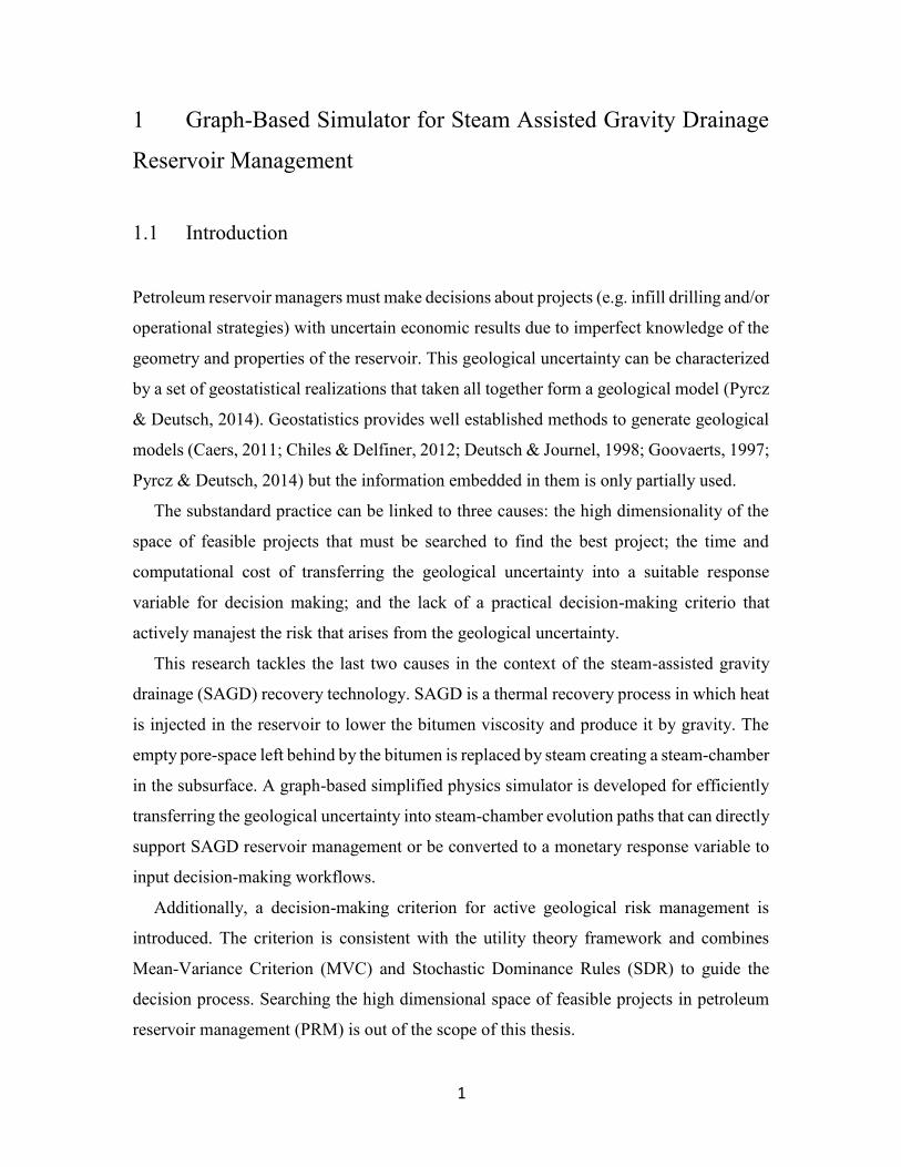
To clarify the jargon of the dissertation and further define the extent of this research, the

PRM decision-making workflow is illustrated on Figure 1.1 in the framework of a formal

rational decision-making under uncertainty model with four elements: a set of feasible

actions, a set of outcomes, a preference ordering of the outcomes and one concept of

rationality that governs the decision process (Stirling, 2012).

Figure 1.1: Components of a Petroleum Reservoir Management Decision-Making workflow.

The Set of feasible actions represents the set of projects from which a choice must be

made by the reservoir manager. The type of project that a reservoir manager is concerned

with ranges from the selection of type, number and location of wells to the definition of an

entire field development plan.

The Set of outcomes refers to the consequences of every project under analysis. The

results cannot be anticipated with certainty because they depend on unknown reservoir

properties. Defining the set of outcomes requires performing two complex and demanding

tasks, one is to build a geological model and the other is to process the projects and the

geological model through a transfer function (e.g. dynamic flow simulation and cash flow)

to obtain a probability distribution of the response variable that will be used to make the

decisions.

The Preferences and the concept of rationality are required to choose from multiple

options with different distributions of value. After transferring the geological uncertainty,

selecting a project from the set of feasible actions is equivalent to make a choice between

the probability distributions of the response variable (Johnstone & Lindley, 2013). To make

that choice, the investor’s preferences over the space of outcomes can be encoded in a

Geological model

ProjectsTransfer ofgeological

uncertainty

Economicmodel

Decision CriteriaRankedprojects

Set of feasible actions

Set of outcomesRisk-Reward Preferences

Inputs Output

3

utility function (Kochenderfer, 2015) . A decision maker will make a “rational” decision,

if he selects a project that maximizes expected utility.

This research focuses on the components of the PRM decision-making workflow

highlighted on Figure 1.1, that is, transferring the geological uncertainty in SAGD projects

and formulating a decision-making rule that considers the geological risk.

1.3 Problem Setting

Reservoir managers of SAGD projects are familiar with a decision-making workflows that

does not conform to the managerial principle of considering the risk and reward trade-off,

even though the decisions involve significant geological uncertainty. Yet, optimal

decision-making is sensitive to the dynamic reservoir response and to geological

uncertainty. Decisions that do not consider geological uncertainty may be suboptimal.

One reason for this situation is that reservoir managers often have tight timeframes to

make their decisions. For example, projects are constrained by rig contract schedules or

must be executed during favorable weather condition windows. Therefore, they cannot wait

for the excessive computational time that takes processing projects and all the geostatistical

realizations through a full physics flow simulator to feed their decision-making workflows.

Moreover, being SAGD a thermal recovery process, the complex combination of heat and

flow transport phenomena makes the numerical simulation even more time-demanding

than for conventional displacement techniques (Majdi Yazdi & Jensen, 2014) exacerbating

the problem of timely transferring of the geological uncertainty for decision making

purposes.

When the set of realizations is processed through a reasonable transfer function, the

projects are customarily selected based on the maximum expected monetary value

criterion, not on the maximum expected utility criterion. The maximum monetary expected

value rule is a special case in the utility theory framework that assigns a risk neutral linear

utility function to the decision maker. As a consequence, the approach considers that the

reservoir manager is only concerned about the returns of the projects and not the associated

risks (Levy 2016). In this situation, the effort of using many geostatistical realizations may

not be completely compensated by the quality of the decision.

4

The following example of deficiencies found in the technical literature support the

research undertaken in this thesis: (1) despite having a geological model, only one scenario

is chosen to be further processed through the dynamic flow simulator (e.g. Alusta et al.

2012), (2) clustering or ranking techniques are applied to select a small set of realizations

that are then post-processed (e.g. Sarma et al. 2013). The propagation of the geological

through the whole workflow is not undertaken; and, (3) after geological uncertainty

transferring the projects are selected based on the maximum expected monetary value

criterion, not on the maximum expected utility criterion (e.g. Shirangi and Durlofsky

2015).

1.4 Proposed Approach

1.4.1 Graph-Base Steam-Chamber Simulator for Transfering the Geological

Uncertainty in SAGD Projects

SAGD is a thermal recovery technique that uses gravity as the driving force to produce

heavy oil. Steam is injected in the reservoir through a horizontal injector well to heat the

bitumen and decrease its viscosity. The heated bitumen becomes mobile and drains by

gravity to a producer well completed below the injector well. As the bitumen moves down,

the steam moves up to occupy the pore space creating an expanding steam-chamber

(Butler, 1991).

SAGD performance in terms of oil production and steam consumption is intrinsically

coupled with the expansion rate and the geometry of the steam-chamber. For that reason,

since the conception of SAGD in the 1980’s, understanding and modeling the evolution of

the steam-chamber has been an important research topic.

Notwithstanding the extensive research, current techniques for modeling the steam-

chamber have shortcomings that limit their practical implementation, especially when

many possible SAGD projects need to be evaluated. Analytical and semi-analytical SAGD

models (Butler, 1985; Butler, Mcnab, & Lo, 1981; Butler & Stephens, 1981) predict the

movement of the steam-chamber but only for idealized homogeneous reservoirs. Others

authors modified the Butler’s model by imposing specific steam-chamber shapes; for

5

example, triangular (Reis, 1992) and circular (Azad & Chalaturnyk, 2012). 4D-seismic

images provide reliable information about the steam-chamber location but is not by itself

a predictive method. Full physics thermal flow simulation is perhaps the best method to

predict the expansion of the steam-chamber but is too computationally demanding and time

consuming to assess SAGD projects that requires evaluating a large number of alternatives.

For instance, thermal flow simulation is impractical to evaluate the response of a SAGD

well-pair location over a set of geostatistical realizations or for considering many possible

SAGD well-pair locations over large areas.

A novel graph-based algorithm named Approximate Physics Discrete Simulator

(hereafter APDS) is proposed in this dissertation for SAGD geological uncertainty

transferring. APDS efficiently integrates Darcy’s Law, material balance and heat transfer

concepts to represent the reservoir and emulate the flow of the bitumen and the steam in

SAGD. APDS models the steam-chamber evolution as a shortest-path problem where the

objective is to find the minimum travel time for the steam to move from the well to the

remaining connected nodes in the graph. The problem is solved using a propagation

mechanism inspired in the algorithm proposed by Dijkstra (1959) to find the one-to-all

shortest-paths in a graph. The output is a model of the steam-chamber expansion through

time. APDS works with heterogeneous reservoirs and is computationally efficient.

Additionally, working on the hypothesis that the performance of SAGD projects is

strongly linked to the size, shape and rate of growing of the steam-chamber, this research

demonstrates that a response variable obtained from APDS on a multi-realization

geological model, is a suitable input for a decision-making workflow. The goodness of the

chosen variable is measured through its degree of correlation to a pair of metrics calculated

from a full physics thermal flow simulator.

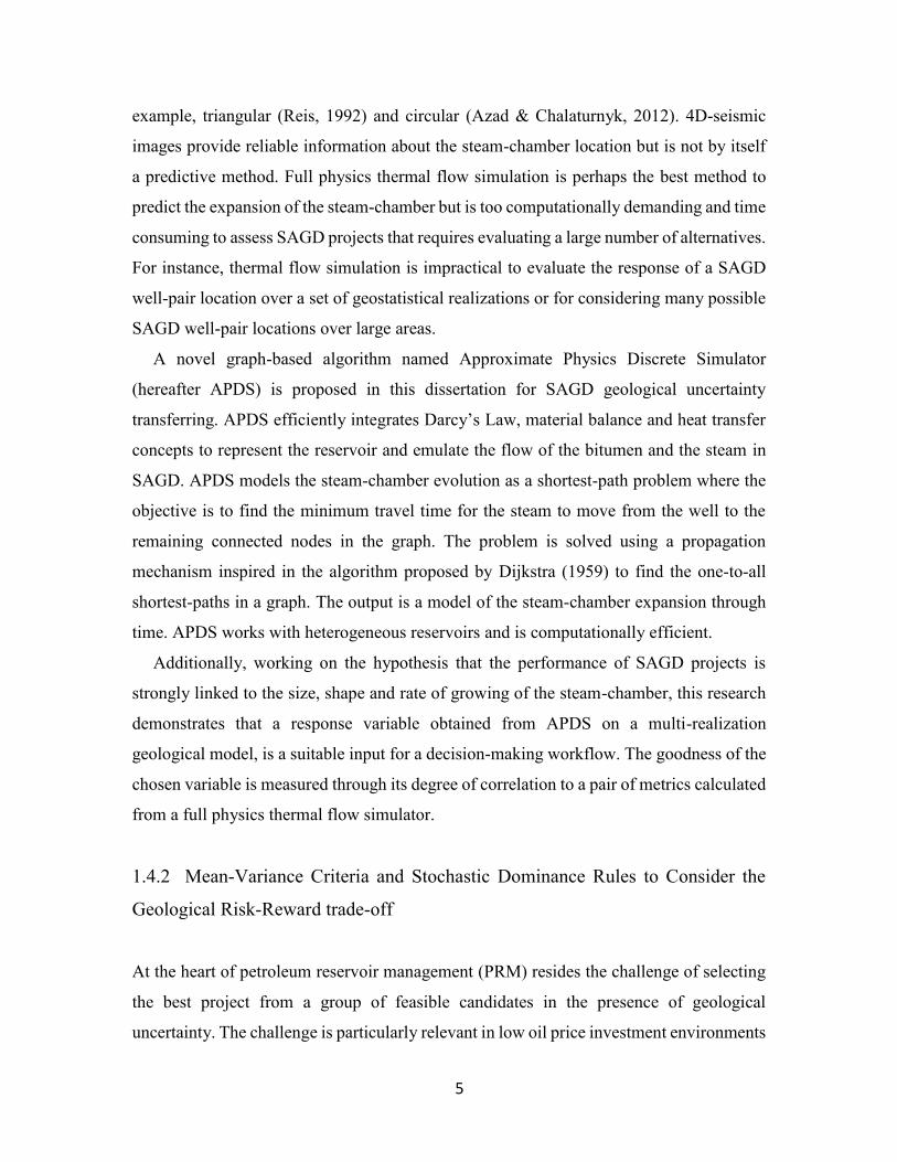
1.4.2 Mean-Variance Criteria and Stochastic Dominance Rules to Consider the

Geological Risk-Reward trade-off

At the heart of petroleum reservoir management (PRM) resides the challenge of selecting

the best project from a group of feasible candidates in the presence of geological

uncertainty. The challenge is particularly relevant in low oil price investment environments

6

where many upstream projects are economically marginal and must be optimized.

Companies are now more cautious. Investors are aware that they should consider not only

the rewards of the projects, but also their risks. For these reasons, the selection of the

projects to be implemented in the field should consider the geological risk and the capacity

of the companies to tolerate it. The decision-making criterion adopted ultimately

determines which project is selected and implemented.

A decision-making criterion for active geological risk management is formulated and

implemented. The criterion is consistent with the utility theory framework and combines

Mean-Variance Criterion (MVC) and Stochastic Dominance Rules (SDR) to guide the

decision process. It differs from other researches that applied the utility framework to PRM

(Güyagüler & Horne, 2004; Ozdogan & Horne, 2006) because a specific utility function is

not required. Projects selected using MVC-SDR are reasonable to all risk-averse reservoir

managers. The shortcoming is a reduced ability to rank projects with very similar

cumulative distribution function response variables. The thesis demonstrates that MVC-

SDR is a viable criterion for SAGD decision-making under geological uncertainty.

1.5 Dissertation Outline

Chapter 2 presents the APDS formulation and its components: the graph, the propagation

algorithm and the ranking function. This chapter also discusses the relationship between

the SAGD steam-chamber expansion and the shortest path problem found in the study of

transportation networks (Deo & Pang, 1984). It also describes a pseudocode to implement

APDS and a stepwise execution example for a homogeneous and a heterogeneous

reservoir.

Chapter 3 is devoted to the APDS implementation and validation. The chapter first

describes the assumptions made to implement an APDS prototype in the Python

programming language. After that, it presents a case-study performed with a realistic multi-

realization geological model demonstrating that the APDS steam-chamber and metrics

calculated from it compares satisfactorily with results obtained from full physics thermal

flow simulation.

7

Chapter 4 introduces the MVC-SDR decision-making criterion for PRM problems.

First, PRM problems are stated in terms of a formal decision-making model under

uncertainty. Then, concepts of projects, geological uncertainty characterization, transfer of

geological uncertainty, preferences over the outcomes and utility theory are discussed.

After that, the theory of MVC and SDR are introduced to PRM. The chapter ends with one

conceptual example explaining how these two criteria works together.

Chapter 5 presents a case-study where the reservoir manager must decide the location

of a SAGD horizontal well-pair inside a target volume. It is a representative problem

commonly found in the exploitation of oil sands in Western Canada. The case-study uses

APDS to transfer the geological uncertainty and then uses MVC-SDR as decision-making

criterion.

Chapter 6 presents a case-study that illustrates how APDS efficiently assists a

geostatistical-anomaly enforcement methodology (Hadavand & Deutsch, 2017) to

integrate 4D-seismic information to SAGD reservoir characterization.

Chapter 7 discusses the merits and shortcomings of APDS and MVC-SDR to support

SAGD decision-making workflows. It also presents research avenues for future works and

concludes the thesis.

The thesis includes several appendices with the Python code implementing APDS.

8

2 SAGD Steam-Chamber Modeling with APDS: Formulation

2.1 Introduction

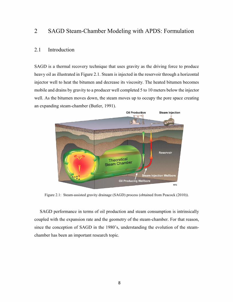
SAGD is a thermal recovery technique that uses gravity as the driving force to produce

heavy oil as illustrated in Figure 2.1. Steam is injected in the reservoir through a horizontal

injector well to heat the bitumen and decrease its viscosity. The heated bitumen becomes

mobile and drains by gravity to a producer well completed 5 to 10 meters below the injector

well. As the bitumen moves down, the steam moves up to occupy the pore space creating

an expanding steam-chamber (Butler, 1991).

Figure 2.1: Steam-assisted gravity drainage (SAGD) process (obtained from Peacock (2010)).

SAGD performance in terms of oil production and steam consumption is intrinsically

coupled with the expansion rate and the geometry of the steam-chamber. For that reason,

since the conception of SAGD in the 1980’s, understanding the evolution of the steam-

chamber has been an important research topic.

9

2.2 Review of Steam-Chamber Modeling Techniques

Contrary to APDS that first models the steam-chamber geometry and then calculates

metrics from it to support decisions, current techniques focus on forecasting the bitumen

production and the location of the steam-chamber is calculated as a by-product. The first

analytical model for SAGD production forecasting in homogeneous reservoirs was

proposed by Butler and his colleagues (Butler et al., 1981). They obtain the steam-chamber

shown in Figure 2.2.a. The chamber has the issue that the lower part of the interface moves

away from the production well (Butler et al., 1981). Afterwards, Butler & Stephens (1981)

assumed that the steam-chamber interface remains straight in the lower part and that is

tangent to the curves of the original model. This model was called Tandrain and is

illustrated in Figure 2.2.b.

Figure 2.2: Steam-chamber shapes. a) Original Butler’s analytical model, b) Tandrain model.

b) TANDRAIN MODEL

Modified after Butler and Stephens, 1981

well

a) BUTLER et al, 1981

Z

Y

Z

Y

Modified after Butler et al., 1981

well

10

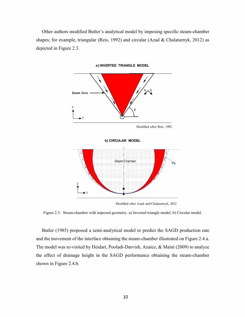
Other authors modified Butler’s analytical model by imposing specific steam-chamber

shapes; for example, triangular (Reis, 1992) and circular (Azad & Chalaturnyk, 2012) as

depicted in Figure 2.3.

Figure 2.3: Steam-chamber with imposed geometry. a) Inverted triangle model, b) Circular model.

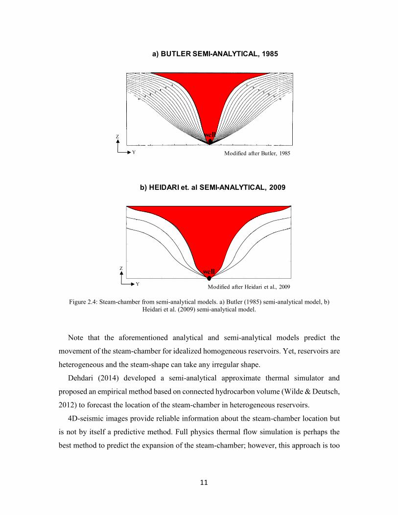
Butler (1985) proposed a semi-analytical model to predict the SAGD production rate

and the movement of the interface obtaining the steam-chamber illustrated on Figure 2.4.a.

The model was re-visited by Heidari, Pooladi-Darvish, Azaiez, & Maini (2009) to analyze

the effect of drainage height in the SAGD performance obtaining the steam-chamber

shown in Figure 2.4.b.

b) CIRCULAR MODEL

Modified after Azad and Chalaturnyk, 2012

Modified after Reis, 1992

a) INVERTED TRIANGLE MODEL

Z

Y

Z

Y

11

Figure 2.4: Steam-chamber from semi-analytical models. a) Butler (1985) semi-analytical model, b)

Heidari et al. (2009) semi-analytical model.

Note that the aforementioned analytical and semi-analytical models predict the

movement of the steam-chamber for idealized homogeneous reservoirs. Yet, reservoirs are

heterogeneous and the steam-shape can take any irregular shape.

Dehdari (2014) developed a semi-analytical approximate thermal simulator and

proposed an empirical method based on connected hydrocarbon volume (Wilde & Deutsch,

2012) to forecast the location of the steam-chamber in heterogeneous reservoirs.

4D-seismic images provide reliable information about the steam-chamber location but

is not by itself a predictive method. Full physics thermal flow simulation is perhaps the

best method to predict the expansion of the steam-chamber; however, this approach is too

Z

Y

well

Modified after Butler, 1985

a) BUTLER SEMI-ANALYTICAL, 1985

wellZ

YModified after Heidari et al., 2009

b) HEIDARI et. al SEMI-ANALYTICAL, 2009

12

computationally demanding and time consuming to be used in SAGD projects that require

evaluating a large number of alternatives in a timely manner.

2.3 Steam Chamber Evolution Posed as a Shortest Path Problem

APDS uses graph theory to model the reservoir and the steam-chamber evolution through

time. Since the work of Fatt (1956) pore-scale networks models have been extensively used

to study the flow of fluids in porous media with the goal of predicting macroscopic

transport properties from pore-scale parameters (Oren, Bakke, & Arntzen, 1998). However,

the use of graphs proposed in this dissertation at the macroscopic scale of the cells of the

numerical model to predict a mega-scale reservoir response such as the steam-chamber in

SAGD is novel in the technical literature.

Modeling the evolution of the steam-chamber has similarities with the shortest- path

problem found in the study of transportation networks (Deo and Pang, 1984). In

transportation, the objective is to find the minimum distance from one given location to

another destination or to all other destinations in a network. Usually the distances between

vertices are known before hand and the path-length is the sum of the length of intermediate

edges or arcs. However, the notion of distance can be generalized to represent other

properties of the path being traversed, such as minimum travel time (Deo and Pang, 1984).

In steam-chamber SAGD modeling, the objective is to find the path with the minimum

travel time for the steam to move from the well to all connected nodes in the graph. This is

also the path with the least resistance for the heated bitumen to flow toward the producer

well. Different to the transportation network case, how fast or slow the bitumen can move

between two nodes in the graph is not known beforehand. This has to be calculated during

the steam-chamber growth. APDS solves this problem using a propagation mechanism

inspired in the algorithm proposed by Dijkstra (1959) to find the one-to-all shortest-paths

in a graph. The output is a model of the steam-chamber expansion through time. The next

section presents how APDS uses graph theory, Darcy’s Law, material balance and heat

transfer concepts to represent the reservoir and efficiently emulate the flow of the bitumen

and the steam in SAGD. APDS works in homogeneous and heterogeneous reservoirs.

13

2.4 APDS Formulation

APDS has three main components: a graph, a propagation algorithm and a ranking

function. They are integrated to obtain the steam-chamber evolution. These components

are described below.

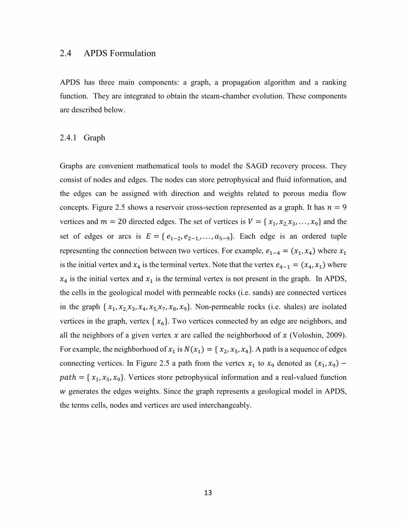
2.4.1 Graph

Graphs are convenient mathematical tools to model the SAGD recovery process. They

consist of nodes and edges. The nodes can store petrophysical and fluid information, and

the edges can be assigned with direction and weights related to porous media flow

concepts. Figure 2.5 shows a reservoir cross-section represented as a graph. It has 𝑛 = 9

vertices and 𝑚 = 20 directed edges. The set of vertices is 𝑉 = { 𝑥1, 𝑥2,𝑥3, . . . , 𝑥9} and the

set of edges or arcs is 𝐸 = { 𝑒1−2, 𝑒2−1,, . . . , 𝑎5−9}. Each edge is an ordered tuple

representing the connection between two vertices. For example, 𝑒1−4 = (𝑥1, 𝑥4) where 𝑥1

is the initial vertex and 𝑥4 is the terminal vertex. Note that the vertex 𝑒4−1 = (𝑥4, 𝑥1) where

𝑥4 is the initial vertex and 𝑥1 is the terminal vertex is not present in the graph. In APDS,

the cells in the geological model with permeable rocks (i.e. sands) are connected vertices

in the graph { 𝑥1, 𝑥2,𝑥3, 𝑥4, 𝑥5,𝑥7, 𝑥8, 𝑥9}. Non-permeable rocks (i.e. shales) are isolated

vertices in the graph, vertex { 𝑥6}. Two vertices connected by an edge are neighbors, and

all the neighbors of a given vertex 𝑥 are called the neighborhood of 𝑥 (Voloshin, 2009).

For example, the neighborhood of 𝑥1 is 𝑁(𝑥1) = { 𝑥2, 𝑥5, 𝑥4}. A path is a sequence of edges

connecting vertices. In Figure 2.5 a path from the vertex 𝑥1 to 𝑥9 denoted as (𝑥1, 𝑥9) −

𝑝𝑎𝑡ℎ = { 𝑥1, 𝑥5, 𝑥9}. Vertices store petrophysical information and a real-valued function

𝑤 generates the edges weights. Since the graph represents a geological model in APDS,

the terms cells, nodes and vertices are used interchangeably.

14

Figure 2.5: Illustration of a 2D-grid geological model represented as a graph.

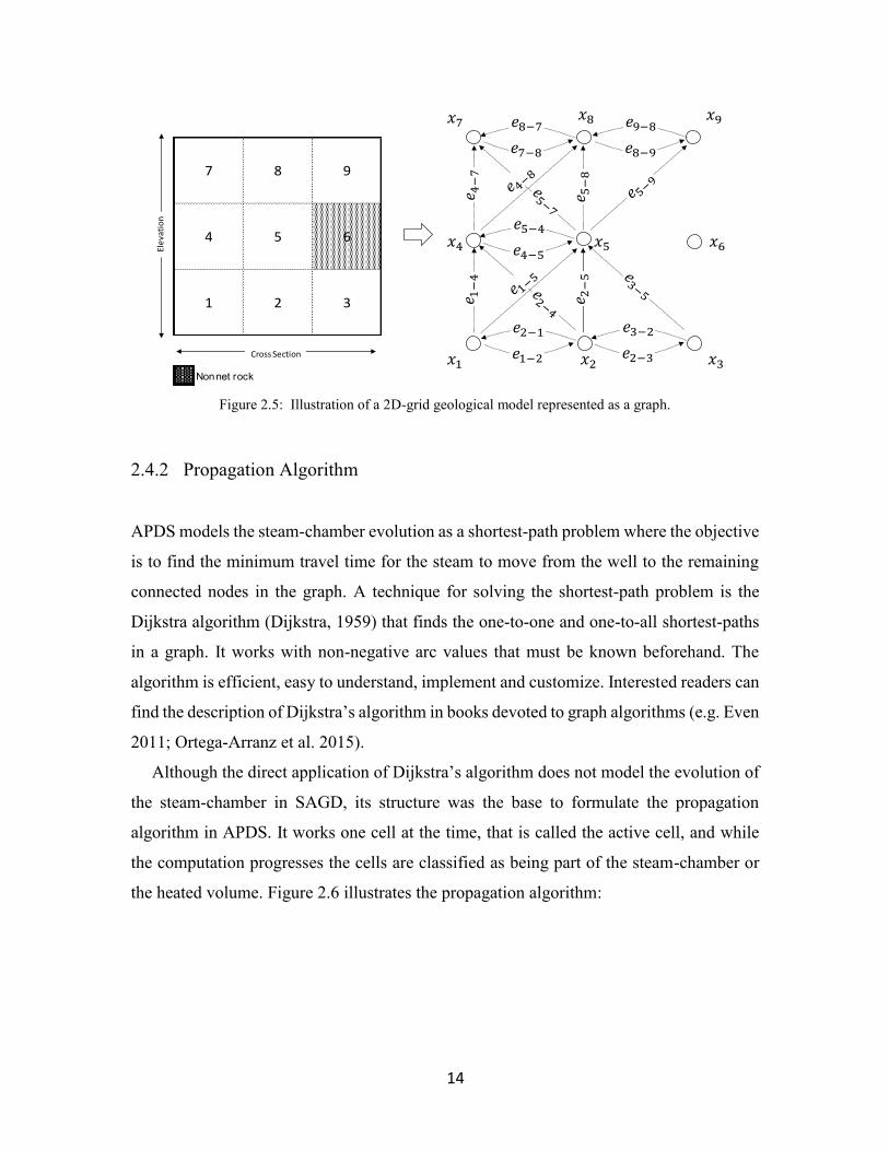
2.4.2 Propagation Algorithm

APDS models the steam-chamber evolution as a shortest-path problem where the objective

is to find the minimum travel time for the steam to move from the well to the remaining

connected nodes in the graph. A technique for solving the shortest-path problem is the

Dijkstra algorithm (Dijkstra, 1959) that finds the one-to-one and one-to-all shortest-paths

in a graph. It works with non-negative arc values that must be known beforehand. The

algorithm is efficient, easy to understand, implement and customize. Interested readers can

find the description of Dijkstra’s algorithm in books devoted to graph algorithms (e.g. Even

2011; Ortega-Arranz et al. 2015).

Although the direct application of Dijkstra’s algorithm does not model the evolution of

the steam-chamber in SAGD, its structure was the base to formulate the propagation

algorithm in APDS. It works one cell at the time, that is called the active cell, and while

the computation progresses the cells are classified as being part of the steam-chamber or

the heated volume. Figure 2.6 illustrates the propagation algorithm:

7 8 9

4 5 6

1 2 3

Non net rock

Ele

vati

on

Cross Section 𝑥1 𝑥2

𝑥8 𝑥9𝑥7

𝑥3

𝑥4 𝑥5 𝑥6

𝑒5−4

𝑒4−5

𝑒 5−8

𝑒8−7

𝑒7−8

𝑒9−8

𝑒8−9

𝑒 4−7

𝑒 1−4

𝑒 2−5

𝑒2−1

𝑒1−2

𝑒3−2

𝑒2−3

15

Figure 2.6: APDS propagation mechanism. Red shapes are not part of APDS. They were drawn to help

visualizing the steam-chamber expansion. Edge labels omitted in this figure are shown in Figure 2.5.

𝑥1 𝑥2

𝑥8 𝑥9𝑥7

𝑥3

𝑥4 𝑥5 𝑥6

Step 1 Step 2

Step 3 Step 4

Step 5

Steam Chamber Heated Zone

𝑥1 𝑥2

𝑥8 𝑥9𝑥7

𝑥3

𝑥4 𝑥5 𝑥6

𝑥1 𝑥2

𝑥8 𝑥9𝑥7

𝑥3

𝑥4 𝑥5 𝑥6

𝑥1 𝑥2

𝑥8 𝑥9𝑥7

𝑥3

𝑥4 𝑥5 𝑥6

𝑥1 𝑥2

𝑥8 𝑥9𝑥7

𝑥3

𝑥4 𝑥5 𝑥6

16

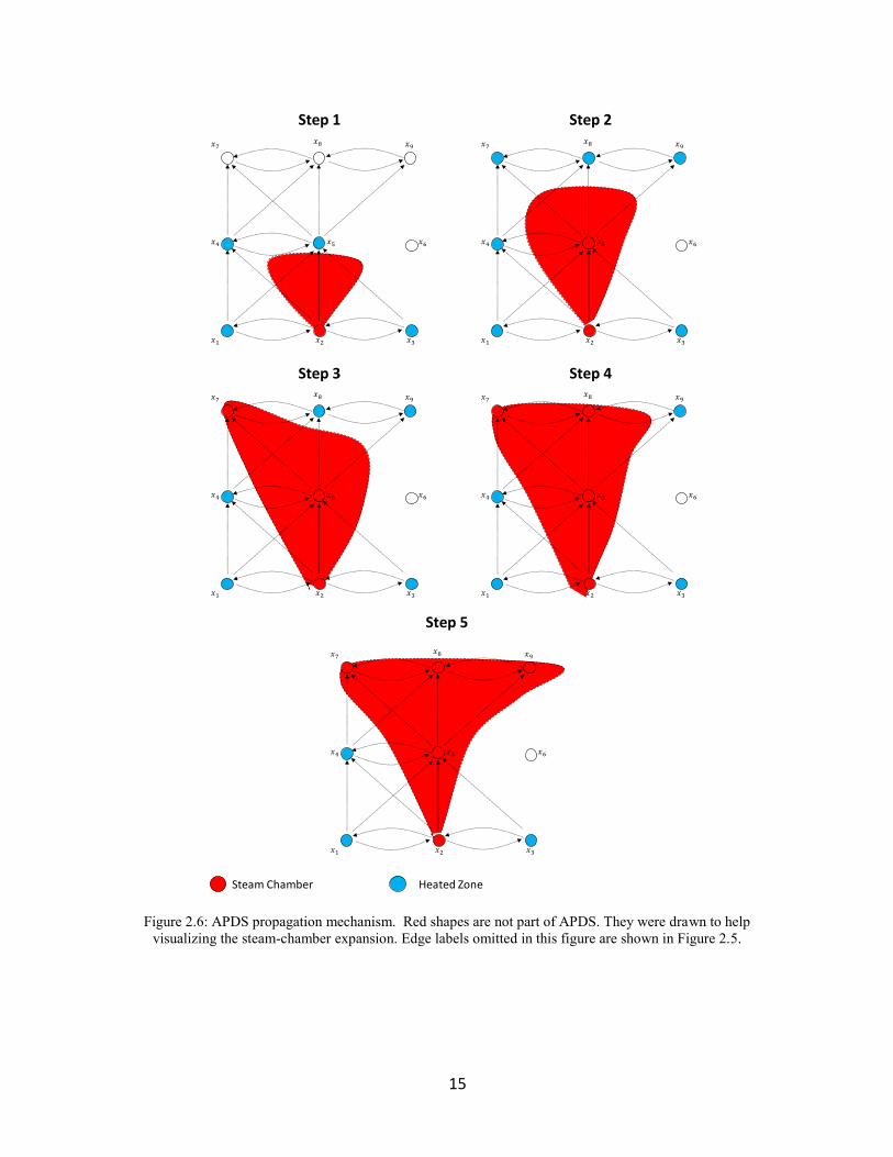
To initialize the algorithm, the producer well location is provided, vertex 𝑥2 in

this example. At step 1, heated bitumen drains through the vertex 𝑥2 and steam

concurrently fill-up the empty pore-space expanding the steam-chamber. Vertex

𝑥2 becomes part of the red colored steam-chamber. Now, bitumen can drain

from the neighborhood 𝑁(𝑥2) = { 𝑥1, 𝑥3, 𝑥4, 𝑥5} that becomes part of the blue

colored heated volume. The travel time for the edges

{𝑒2−1,𝑒2−3, 𝑒2−4, 𝑒2−5} connecting 𝑥2 with its neighborhood is calculated with

the ranking function explained in section 2.2.3.

At step 2, bitumen drains from the vertex in the heated volume through the edge

with the lowest travel time, edge 𝑒2−5 in this case, and the vertex 𝑥5 is added

to the steam-chamber . Now, bitumen can also drain from the neighborhood

𝑁(𝑥5) = {𝑥4, 𝑥7, 𝑥8, 𝑥9} that is added to the heated volume.

The algorithm progresses until all vertices connected to 𝑥2 are processed. Note

that the isolated vertex 𝑥6 will not be part of the steam-chamber. Figure 2.6

shows three additional steps. The red filled shape was added to highlight the

steam-chamber generated by the propagation algorithm.

Observe that the order in which the cells are added to the steam-chamber is intended to

reflect the evolution of the steam-chamber in the subsurface.

2.4.3 Ranking Function

The ranking function to calculate the travel time plays a key role in the propagation

algorithm. It maps the petrophysical properties, the fluid properties and the local

geometrical features of the reservoir model into ranking values - edge weights in graph

terminology - that governs the development of the steam chamber.

The ranking function is the sum of two components, the cell time and the model time.

It has the units of time.

17

2.4.3.1 Cell Travel Time

Cell travel time measures how long it takes to drain movable bitumen from one cell to an

adjacent cell in the direction of a sink. Cell travel times are computed independently for

every edge without a reference time; however, because these values are based on Darcy’s

Law, material balance and heat transfer concepts, they are comparable across different

locations in the reservoir. In other words, no matter their location in the reservoir model,

two cells with the same petrophysical, fluid and geometrical properties will have the same

cell travel time.

Darcy’s Law (Equation 2.1) and material balance at the cell scale (Equation 2.2) are

used for the cell travel time. The formulation assumes that gravity is the only driving force

(Butler et al., 1981). Chapter 3 demonstrates that the current APDS implementation is

consistent with a heat transfer mechanism by conduction with a steady state temperature

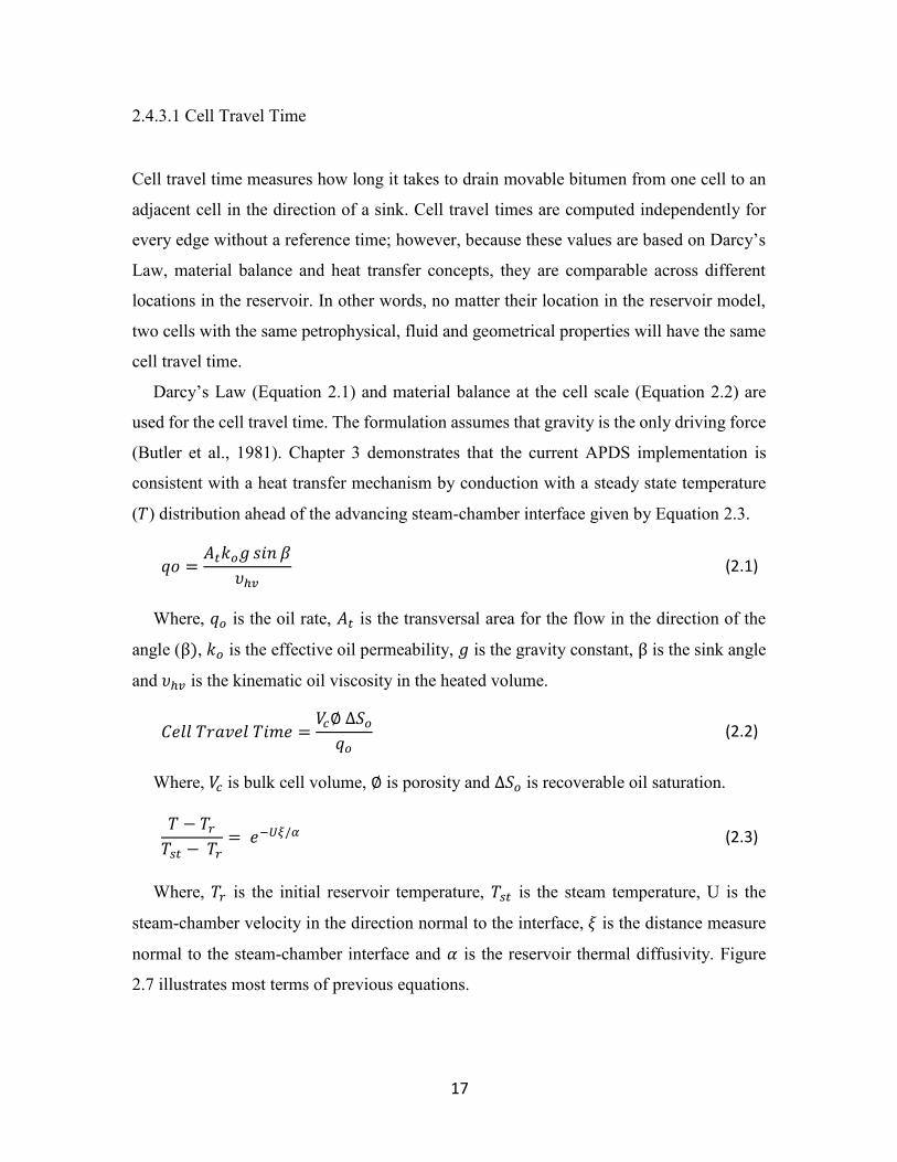
(𝑇) distribution ahead of the advancing steam-chamber interface given by Equation 2.3.

𝑞𝑜 =𝐴𝑡𝑘𝑜𝑔 𝑠𝑖𝑛 𝛽

𝜐ℎ𝑣

(2.1)

Where, 𝑞𝑜 is the oil rate, 𝐴𝑡 is the transversal area for the flow in the direction of the

angle (β), 𝑘𝑜 is the effective oil permeability, 𝑔 is the gravity constant, β is the sink angle

and 𝜐ℎ𝑣 is the kinematic oil viscosity in the heated volume.

𝐶𝑒𝑙𝑙 𝑇𝑟𝑎𝑣𝑒𝑙 𝑇𝑖𝑚𝑒 =𝑉𝑐∅ ∆𝑆𝑜𝑞𝑜

(2.2)

Where, 𝑉𝑐 is bulk cell volume, ∅ is porosity and ∆𝑆𝑜 is recoverable oil saturation.

𝑇 − 𝑇𝑟𝑇𝑠𝑡 − 𝑇𝑟

= 𝑒−𝑈𝜉/𝛼

(2.3)

Where, 𝑇𝑟 is the initial reservoir temperature, 𝑇𝑠𝑡 is the steam temperature, U is the

steam-chamber velocity in the direction normal to the interface, 𝜉 is the distance measure

normal to the steam-chamber interface and 𝛼 is the reservoir thermal diffusivity. Figure

2.7 illustrates most terms of previous equations.

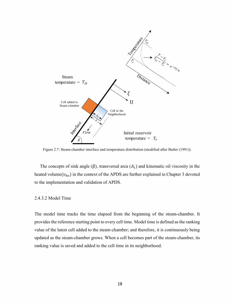
18

Figure 2.7: Steam-chamber interface and temperature distribution (modified after Butler (1991)).

The concepts of sink angle (β), transversal area (𝐴𝑡) and kinematic oil viscosity in the

heated volume(𝜐ℎ𝑣) in the context of the APDS are further explained in Chapter 3 devoted

to the implementation and validation of APDS.

2.4.3.2 Model Time

The model time tracks the time elapsed from the beginning of the steam-chamber. It

provides the reference starting point to every cell time. Model time is defined as the ranking

value of the latest cell added to the steam-chamber; and therefore, it is continuously being

updated as the steam-chamber grows. When a cell becomes part of the steam-chamber, its

ranking value is saved and added to the cell time in its neighborhood.

𝜉

U

𝐹𝑙𝑜𝑤

Cell in the

Neighborhood

Cell added to

Steam-chamber

𝛽

Steam

temperature = 𝑇𝑠𝑡

Initial reservoir

temperature = 𝑇𝑟

19

2.4.4 APDS Outputs

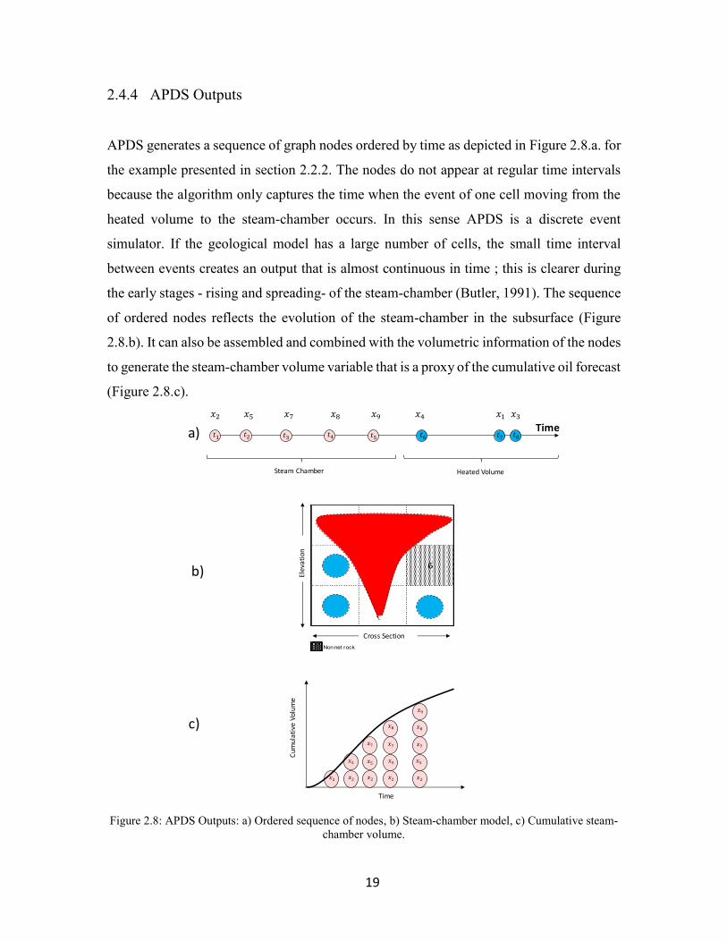
APDS generates a sequence of graph nodes ordered by time as depicted in Figure 2.8.a. for

the example presented in section 2.2.2. The nodes do not appear at regular time intervals

because the algorithm only captures the time when the event of one cell moving from the

heated volume to the steam-chamber occurs. In this sense APDS is a discrete event

simulator. If the geological model has a large number of cells, the small time interval

between events creates an output that is almost continuous in time ; this is clearer during

the early stages - rising and spreading- of the steam-chamber (Butler, 1991). The sequence

of ordered nodes reflects the evolution of the steam-chamber in the subsurface (Figure

2.8.b). It can also be assembled and combined with the volumetric information of the nodes

to generate the steam-chamber volume variable that is a proxy of the cumulative oil forecast

(Figure 2.8.c).

Figure 2.8: APDS Outputs: a) Ordered sequence of nodes, b) Steam-chamber model, c) Cumulative steam-

chamber volume.

7 8 9

4 5 6

1 2 3

Non net rock

Elev

atio

n

Cross Section

𝑥2

𝑥5

𝑥2 𝑥2 𝑥2 𝑥2

𝑥5 𝑥5 𝑥5

𝑥7 𝑥7 𝑥7

𝑥8 𝑥8

𝑥9

Time

Cu

mu

lati

ve V

olu

me

𝑥1𝑥2 𝑥8 𝑥9𝑥7 𝑥3𝑥4𝑥5Time

Steam Chamber Heated Volume

𝑡1 𝑡2 𝑡3 𝑡4 𝑡5 𝑡6 𝑡7 𝑡8a)

b)

c)

20

The following sections present pseudocode for APDS and a stepwise execution example

for a homogeneous and a heterogeneous reservoir.

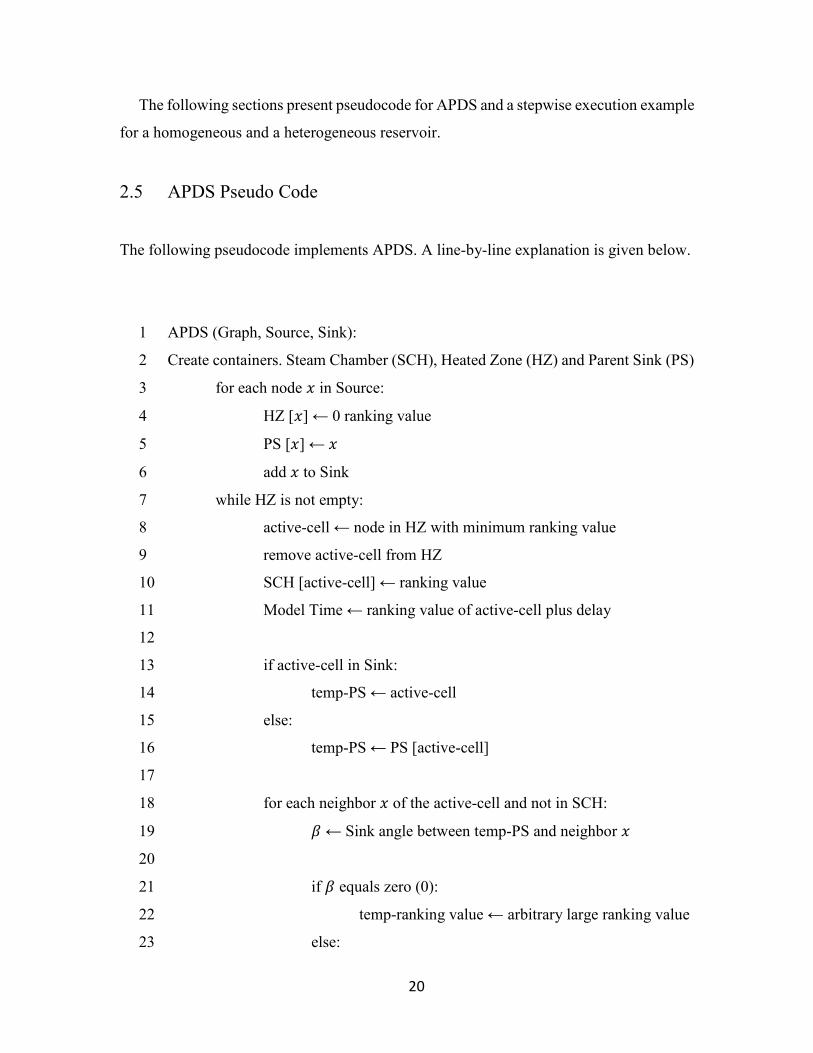
2.5 APDS Pseudo Code

The following pseudocode implements APDS. A line-by-line explanation is given below.

1 APDS (Graph, Source, Sink):

2 Create containers. Steam Chamber (SCH), Heated Zone (HZ) and Parent Sink (PS)

3 for each node 𝑥 in Source:

4 HZ [𝑥] ← 0 ranking value

5 PS [𝑥] ← 𝑥

6 add 𝑥 to Sink

7 while HZ is not empty:

8 active-cell ← node in HZ with minimum ranking value

9 remove active-cell from HZ

10 SCH [active-cell] ← ranking value

11 Model Time ← ranking value of active-cell plus delay

12

13 if active-cell in Sink:

14 temp-PS ← active-cell

15 else:

16 temp-PS ← PS [active-cell]

17

18 for each neighbor 𝑥 of the active-cell and not in SCH:

19 𝛽 ← Sink angle between temp-PS and neighbor 𝑥

20

21 if 𝛽 equals zero (0):

22 temp-ranking value ← arbitrary large ranking value

23 else:

21

24 temp-ranking value = Model Time + Cell Time + ∈

25

26 if 𝑥 not in HZ:

27 HZ [𝑥] ← temp-ranking value

28 PS [𝑥] ← temp-PS

29

30 if 𝑥 in HZ and temp-ranking value < HZ [𝑥]:

31 HZ [𝑥] ← temp-ranking value

32 PS [𝑥] ← temp-PS

33

34 return SCH [ ]

Pseudocode description:

Line 1. APDS inputs are: (1) a Graph, the reservoir mathematical model, (2) the Source,

a list of indexes of the cells intersected by the production wells. The source is not limited

to one set of adjacent cells, for that reason, APDS can handled multiple well locations, and

(3) the Sink, a list of indexes pointing all the cells that could behave like sinks in the

reservoir.

Line 2. APDS maintains three containers: (1) the Steam Chamber (SCH), for preserving

the order in which the cells are added to the steam chamber and their ranking values, (2)

the Heated Zone (HZ), a priority queue with cells ordered according to the raking values,

and (3) the Parent Sink (PS), for tracking the parent sink history of every node in the graph.

Lines 3 to 6: APDS initialization. All nodes in Source are assigned to HZ with an initial

raking value of zero (0). Note that any other convenient ranking value can be used to

initialize APDS. Moreover, every cell in the Source can have its own initialization value.

This property is useful to model SAGD well-pairs that enters in production at different

times. All nodes in Source are also defined with their own PS and added to the Sink.

Line 7. The main loop of the algorithm. APDS will run until exhausting all nodes in the

HZ.

22

Lines 8 to 10. The node with the minimum ranking value is extracted from the HZ,

labeled as the active-cell and added to SCH.

Line 11. Model time is updated to be the active-cell ranking value plus a delay.

Line 13 to 16. If the active-cell is a sink, it is assigned temporarily as the neighborhood

parent sink. If the active-cell is not a sink, the neighborhood temporarily inherits the active-

cell parent sink.

Line 17. Loop through the neighborhood of the active-cell

Line 19. Calculate the sink angle.

Line 22. If the sink angle is zero (0), the time to mobilize bitumen from a cell to its PS

tends to infinite. For that reason, the implementation assigns an arbitrary large ranking

value, so the cell will be placed at the end of the priority queue HZ.

Line 24. If the sink angle is not zero (0), the ranking value plus 𝜖 is calculated. 𝜖 is a

very small random number introduced in the APDS implementation to break ties between

cells having the same raking value.

Lines 26 to 28. If the cell is visited for the first time, it is added to HZ with its raking

value and PS.

Lines 30 to 32. If the cell is already in HZ and the newer calculated ranking value is

smaller to the previously stored value, the raking value and the PS are updated.

Consequently, the cell will jump positions in the priority queue HZ.

Line 34. APDS exits when the HZ is exhausted and returns SCH.

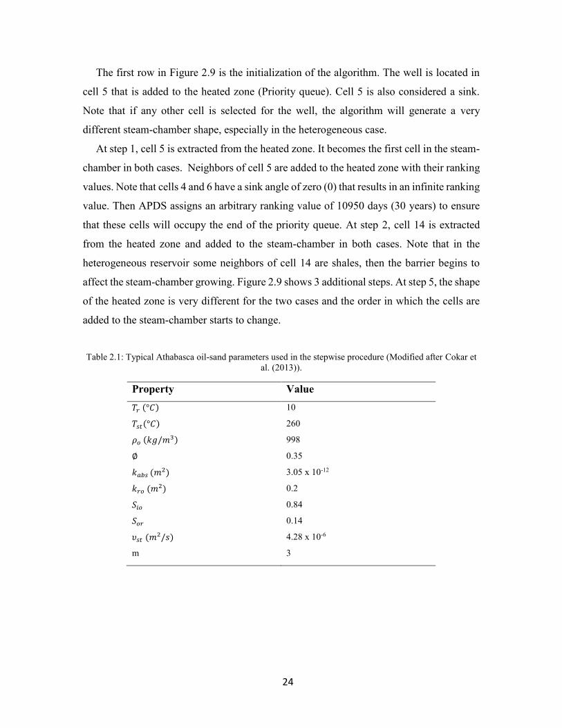
2.6 Step-wise Procedure

The application for a cross-section in a homogeneous and a heterogeneous reservoir shown

in Figure 2.9 is intended to further explain the pseudocode and how it deals with the

presence of barriers. The example uses typical Athabasca oil-sand parameters (Cokar,

Kallos, & Gates, 2013) listed in Table 2.1. The cell size is 1m x 1m x 1m in x, y and z

directions, respectively. Figure 2.10 and Figure 2.11 show detailed calculations.

23

Figure 2.9: APDS stepwise procedure. Top row shows the algorithm initialization and the cell indexes.

Well and sinks locations are labeled. Black outlines drawn to help visualizing how the APDS handles

barriers.

HOMOGENEOUS

CASE

HETEROGENEOUS

CASE

INIZIALIZATION

STEP 1

STEP 2

STEP 3

STEP 4

STEP 5

Ele

vatio

n

Cross-section

5 5

24

The first row in Figure 2.9 is the initialization of the algorithm. The well is located in

cell 5 that is added to the heated zone (Priority queue). Cell 5 is also considered a sink.

Note that if any other cell is selected for the well, the algorithm will generate a very

different steam-chamber shape, especially in the heterogeneous case.

At step 1, cell 5 is extracted from the heated zone. It becomes the first cell in the steam-

chamber in both cases. Neighbors of cell 5 are added to the heated zone with their ranking

values. Note that cells 4 and 6 have a sink angle of zero (0) that results in an infinite ranking

value. Then APDS assigns an arbitrary ranking value of 10950 days (30 years) to ensure

that these cells will occupy the end of the priority queue. At step 2, cell 14 is extracted

from the heated zone and added to the steam-chamber in both cases. Note that in the

heterogeneous reservoir some neighbors of cell 14 are shales, then the barrier begins to

affect the steam-chamber growing. Figure 2.9 shows 3 additional steps. At step 5, the shape

of the heated zone is very different for the two cases and the order in which the cells are

added to the steam-chamber starts to change.

Table 2.1: Typical Athabasca oil-sand parameters used in the stepwise procedure (Modified after Cokar et

al. (2013)).

Property Value

𝑇𝑟 (°𝐶) 10

𝑇𝑠𝑡(°𝐶) 260

𝜌𝑜 (𝑘𝑔/𝑚3) 998

∅ 0.35

𝑘𝑎𝑏𝑠 (𝑚2) 3.05 x 10-12

𝑘𝑟𝑜 (𝑚2) 0.2

𝑆𝑖𝑜 0.84

𝑆𝑜𝑟 0.14

𝜐𝑠𝑡 (𝑚2/𝑠) 4.28 x 10-6

m 3

25

Figure 2.10: APDS calculations for the homogeneous reservoir depicted in the left column of Figure 2.9.

Step

Initial

Heated Zone Steam-chamber

Active

Cell

Nbors.

Cells

Parent

Sink

Sink

Angle

Cell

Time

Model

Time ε

Current

Ranking

Value

Previous

Ranking

Value Comment

Final

Heated Zone

(Pririoty Queue) (List) (Index) (Index) (Index) (deg.) (day) (days) (days) (day) (day) (Pririoty Queue)

4 5 0.0 10950 0.000 0.004 10950 Ranking value set to 30 years

13 5 45.0 6.210 0.000 0.023 6.210

14 5 90.0 3.121 0.000 0.028 3.121

15 5 45.0 6.215 0.000 0.028 6.215


13 5 45.0 6.210 3.121 0.023 9.330 6.210 Ranking value from step 1 is smaller

22 5 63.4 3.868 3.121 0.001 6.988

23 5 90.0 3.119 3.121 0.026 6.240

24 5 63.4 3.874 3.121 0.007 6.994


12 5 26.6 7.740 6.210 0.007 13.950

21 5 45.0 6.225 6.210 0.039 12.435



14 5 90.0 3.100 0.007 Cell in Steam-Chamber

14 5 90.0 3.124 0.031 Cell in Steam-Chamber

23 5 90.0 3.119 6.215 0.026 9.334 6.240 Ranking value from step 2


25 5 45.0 6.199 6.215 0.013 12.413

16 5 26.6 7.770 6.215 0.037 13.984


31 5 71.6 3.471 6.240 0.034 9.711

32 5 90.0 3.124 6.240 0.031 9.364

33 5 71.6 3.468 6.240 0.031 9.708


2 {14,13,15,4,6} 14{13,15,23,22,24,4

,6}

1 {5} 5 {14,13,15,4,6}{5}

{5,14}

4{15,23,22,24,21,12

,4,6}15

{23,22,24,25,21,1

2,16,4,6}

3{13,15,23,22,24,4,

6}13

{15,23,22,24,21,1

2,4,6}{5,14,13}

{5,14,13,15}

5

{23,22,24,25,21,12

,16,4,6}

23{22,24,32,33,31,2

5,21,12,16,4,6}{5,14,13,15,23}

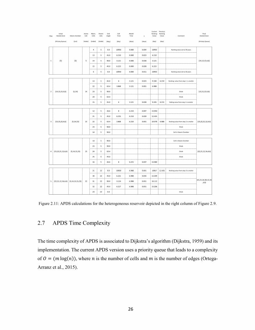
26

Figure 2.11: APDS calculations for the heterogeneous reservoir depicted in the right column of Figure 2.9.

2.7 APDS Time Complexity

The time complexity of APDS is associated to Dijkstra’s algorithm (Dijkstra, 1959) and its

implementation. The current APDS version uses a priority queue that leads to a complexity

of 𝑂 = (𝑚 log(𝑛)), where 𝑛 is the number of cells and 𝑚 is the number of edges (Ortega-

Arranz et al., 2015).

Step

Initial

Heated Zone Steam-chamber

Active

Cell

Nbors.

Cells

Parent

Sink

Sink

Angle

Cell

Time

Model

Time ε

Current

Ranking

Value

Previous

Ranking

Value Comment

Final

Heated Zone

(Pririoty Queue) (List) (Index) (Index) (Index) (deg.) (day) (days) (days) (day) (day) (Pririoty Queue)


13 5 45.0 6.210 0.000 0.023 6.210

14 5 90.0 3.121 0.000 0.028 3.121

15 5 45.0 6.215 0.000 0.028 6.215


13 5 45.0 6 3.121 0.023 9.330 6.210 Ranking value from step 1 is smaller

22 5 63.4 3.868 3.121 0.001 6.988

23 5 90.0 Shale

24 5 63.4 Shale

15 5 45.0 6 3.121 0.028 9.335 6.215 Raking value from step 1 is smaller

12 5 26.6 8 6.210 0.007 13.950

21 5 45.0 6.225 6.210 0.039 12.435


23 5 90.0 Shale

14 5 90.0 Cell in Steam-Chamber

14 5 90.0 Cell in Steam-chamber

23 5 90.0 Shale

24 5 63.4 Shale

25 5 45.0 Shale

16 5 26.6 8 6.215 0.037 13.984

21 22 0.0 10950 6.988 0.001 10957 12.435 Ranking value from step 3 is smaller

30 22 45.0 6.221 6.988 0.034 13.209

31 22 90.0 3.124 6.988 0.031 10.112

32 22 45.0 6.217 6.988 0.031 13.206

23 22 0.0 Shale

5 {22,21,12,16,4,6} 22{31,21,32,30,12,16

,4,6}{5,14,13,15,23}

4 {15,22,21,12,4,6} 15 {22,21,12,16,4,6}

3 {13,15,22,4,6} 13 {15,22,21,12,4,6}{5,14,13}

{5,14,13,15}

2 {14,13,15,4,6} 14 {13,15,22,4,6}

1 {5} 5 {14,13,15,4,6}{5}

{5,14}

27

2.8 Potential Applications

APDS has a straightforward mathematical formulation to secure an efficient computational

implementation; it is not intended as a replacement for a full physics thermal simulator.

APDS is mainly envisioned to be a cost-effective transfer function to support decision

making models that considers geological uncertainty. APDS is especially suitable for

guiding decisions in SAGD that can be make based on the geometry and growth rate of the

steam-chamber. In this context, some potential applications are described below.

2.8.1 SAGD Well-pair Location.

The oil production and steam consumption in SAGD depend on the steam-chamber

evolution that is a consequence of the relative position between the well-pairs and the

barriers in the reservoir. While the location of the well-pairs is an engineering decision, the

location of the barriers is uncertain. APDS allows to test every candidate well-pair location

through the geostatistical realizations to obtain a cumulative distribution function (CDF)

of the steam-chamber size at a time of interest. These CDFs are used to decide about the

well-pair location.

2.8.2 SAGD Operation.

SAGD performance can be affected by reservoir layers with high permeability and low oil

saturation that might increase heat losses and affect the steam-chamber growth (C. Wang

& Leung, 2015). These layers are called lean zones and their analysis is often addressed

using numerical simulation (e.g. Xu et al. 2014; Wang and Leung 2015) with the limitations

imposed by the computational cost of this technique. APDS applied on geostatistical

realizations allows to identify areas where the steam-chamber has higher probability of

contacting lean zones. An estimation of the time in which the contact might occur is also

readily available. This information helps to anticipate operational pressure strategies to

control heat losses, and to consider using flow control devices.

28

2.8.3 4D-Seismic Integration.

4D-seismic provides reliable images of the steam-chamber. These images might reveal

anomalies by the absence or unexpected location of the steam-chamber that can be enforced

into geostatistical realizations to improve reservoir characterization (Hadavand & Deutsch,

2017). Analyzing the effect of the geostatistical-anomaly enforcement methodology

requires comparing the estimation of the steam-chamber before and after applying the

enforcement through all the geostatistical realizations (Hadavand & Deutsch, 2017). APDS

is efficient enough to perform this task and serve as a tool for assisting 4D-seismic

integration in SAGD reservoir characterization.

2.8.4 SAGD Geomechanics.

The geomechanical response of a reservoir to SAGD processes is influenced by steam-

chamber growth that impact the stress and strain field in situ (Chalaturnyk & Li, 2004).

Deformations of the reservoir and caprock can yield to failure of both, affecting the safety

of SAGD operations (Pathak, Tran, & Kumar, 2014). Assessing caprock integrity requires

considering the steam-chamber dimensions, the pay thickness (Collins, 2007) and the

reservoir heterogeneity, among other factors. The uncertainty associated with caprock

integrity due to reservoir heterogeneity has been study using coupled geomechanics

thermal reservoir simulation (e.g. Pathak et al. 2014), but computational time is even longer

than in conventional thermal simulation. APDS provides continuous measures of steam-

chamber dimensions, such as volume, height and width, that can enrich analysis of the

uncertainty associated with caprock integrity.

2.9 Discussion

The APDS was conceived to support workflows that requires the assessment of many

SAGD projects. For example, quantification of the impact on a SAGD performance of the

geological uncertainty represented in a set of geostatistical realizations, or scanning vast

areas in the early development of SAGD fields. For this reason, APDS is intended to be

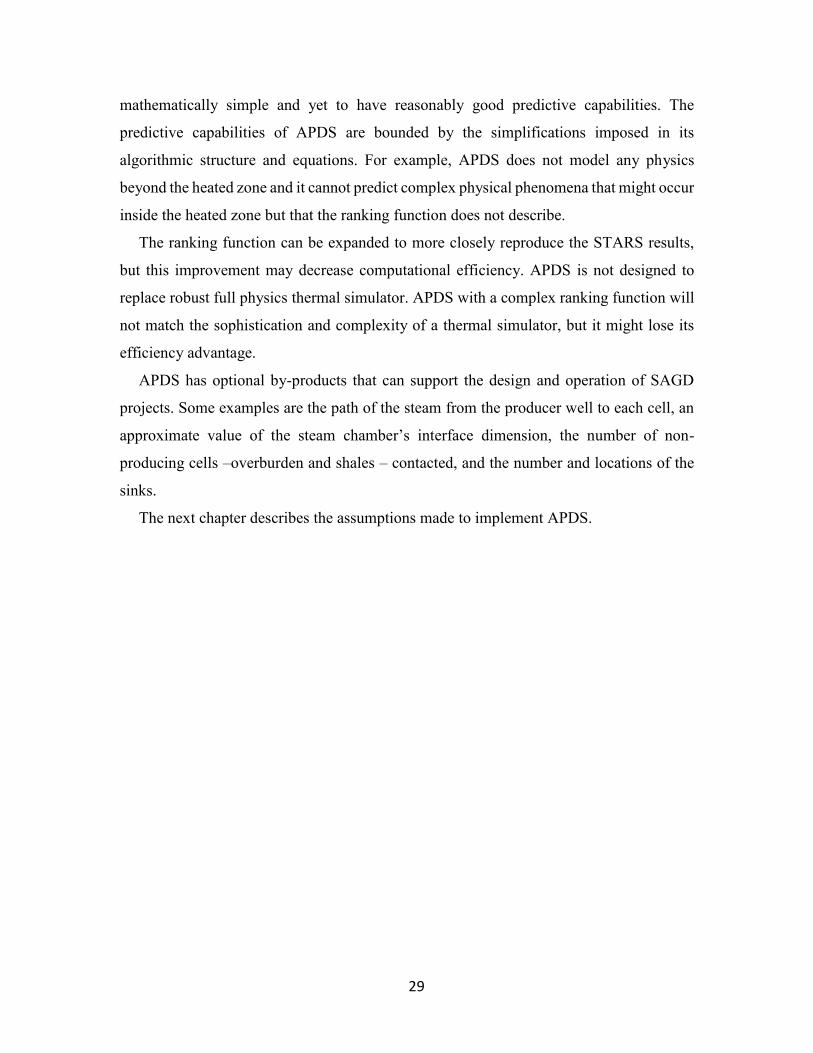
29

mathematically simple and yet to have reasonably good predictive capabilities. The

predictive capabilities of APDS are bounded by the simplifications imposed in its

algorithmic structure and equations. For example, APDS does not model any physics

beyond the heated zone and it cannot predict complex physical phenomena that might occur

inside the heated zone but that the ranking function does not describe.

The ranking function can be expanded to more closely reproduce the STARS results,

but this improvement may decrease computational efficiency. APDS is not designed to

replace robust full physics thermal simulator. APDS with a complex ranking function will

not match the sophistication and complexity of a thermal simulator, but it might lose its

efficiency advantage.

APDS has optional by-products that can support the design and operation of SAGD

projects. Some examples are the path of the steam from the producer well to each cell, an

approximate value of the steam chamber’s interface dimension, the number of non-

producing cells –overburden and shales – contacted, and the number and locations of the

sinks.

The next chapter describes the assumptions made to implement APDS.

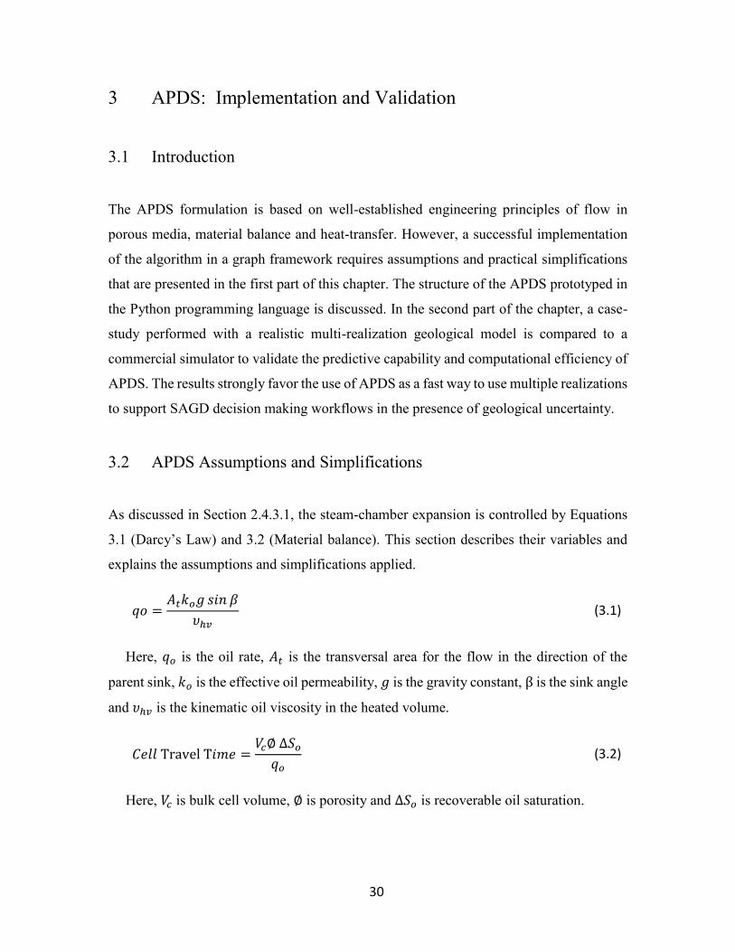
30

3 APDS: Implementation and Validation

3.1 Introduction

The APDS formulation is based on well-established engineering principles of flow in

porous media, material balance and heat-transfer. However, a successful implementation

of the algorithm in a graph framework requires assumptions and practical simplifications

that are presented in the first part of this chapter. The structure of the APDS prototyped in

the Python programming language is discussed. In the second part of the chapter, a case-

study performed with a realistic multi-realization geological model is compared to a

commercial simulator to validate the predictive capability and computational efficiency of

APDS. The results strongly favor the use of APDS as a fast way to use multiple realizations

to support SAGD decision making workflows in the presence of geological uncertainty.

3.2 APDS Assumptions and Simplifications

As discussed in Section 2.4.3.1, the steam-chamber expansion is controlled by Equations

3.1 (Darcy’s Law) and 3.2 (Material balance). This section describes their variables and

explains the assumptions and simplifications applied.

𝑞𝑜 =𝐴𝑡𝑘𝑜𝑔 𝑠𝑖𝑛 𝛽

𝜐ℎ𝑣

(3.1)

Here, 𝑞𝑜 is the oil rate, 𝐴𝑡 is the transversal area for the flow in the direction of the

parent sink, 𝑘𝑜 is the effective oil permeability, 𝑔 is the gravity constant, β is the sink angle

and 𝜐ℎ𝑣 is the kinematic oil viscosity in the heated volume.

𝐶𝑒𝑙𝑙 Travel T𝑖𝑚𝑒 =𝑉𝑐∅ ∆𝑆𝑜𝑞𝑜

(3.2)

Here, 𝑉𝑐 is bulk cell volume, ∅ is porosity and ∆𝑆𝑜 is recoverable oil saturation.

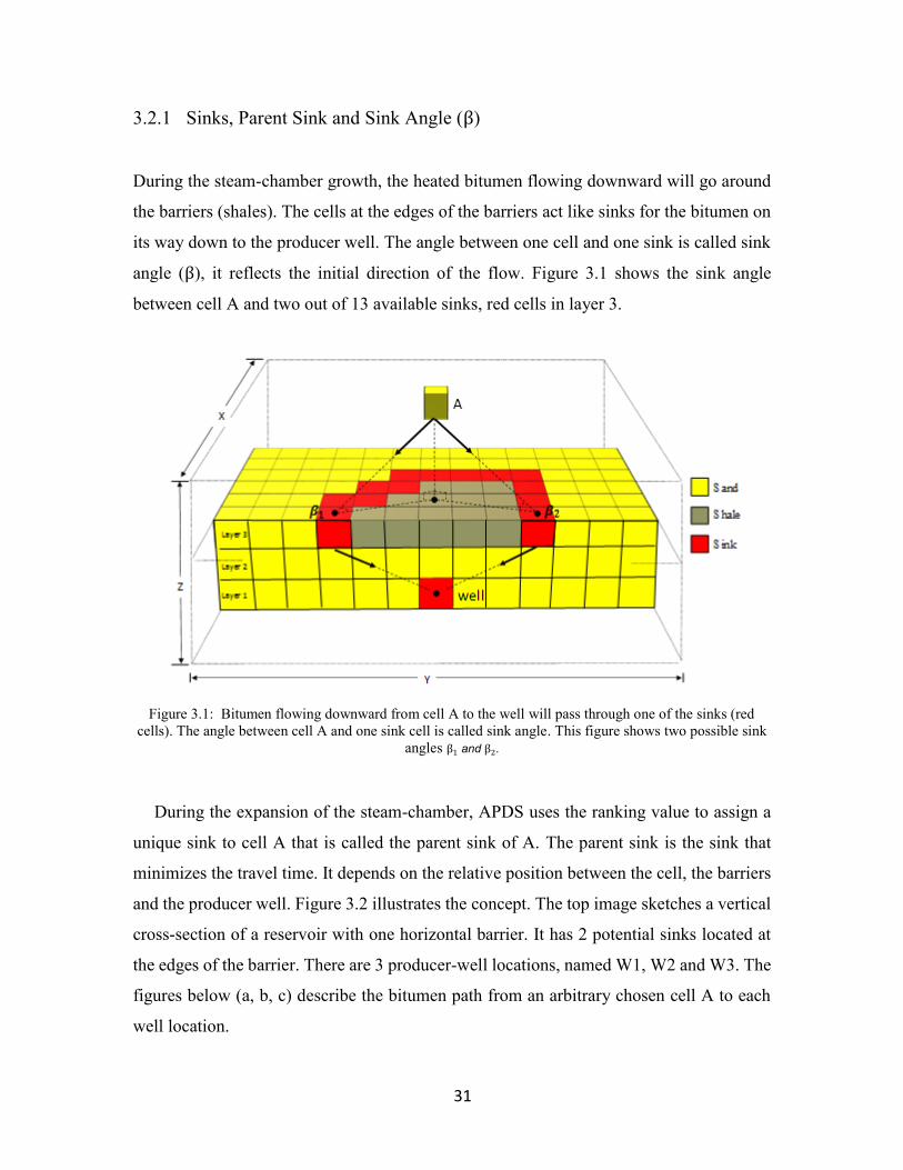
31

3.2.1 Sinks, Parent Sink and Sink Angle (β)

During the steam-chamber growth, the heated bitumen flowing downward will go around

the barriers (shales). The cells at the edges of the barriers act like sinks for the bitumen on

its way down to the producer well. The angle between one cell and one sink is called sink

angle (β), it reflects the initial direction of the flow. Figure 3.1 shows the sink angle

between cell A and two out of 13 available sinks, red cells in layer 3.

Figure 3.1: Bitumen flowing downward from cell A to the well will pass through one of the sinks (red

cells). The angle between cell A and one sink cell is called sink angle. This figure shows two possible sink

angles β1 and β2.

During the expansion of the steam-chamber, APDS uses the ranking value to assign a

unique sink to cell A that is called the parent sink of A. The parent sink is the sink that

minimizes the travel time. It depends on the relative position between the cell, the barriers

and the producer well. Figure 3.2 illustrates the concept. The top image sketches a vertical

cross-section of a reservoir with one horizontal barrier. It has 2 potential sinks located at

the edges of the barrier. There are 3 producer-well locations, named W1, W2 and W3. The

figures below (a, b, c) describe the bitumen path from an arbitrary chosen cell A to each

well location.

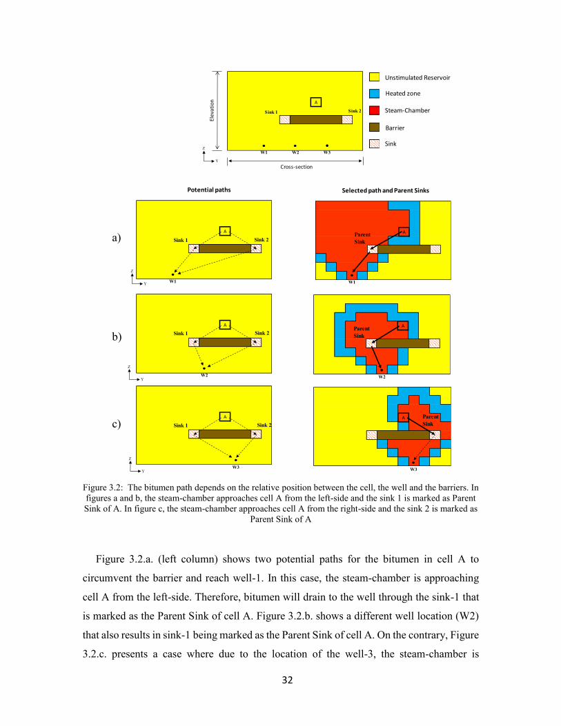
32

Figure 3.2: The bitumen path depends on the relative position between the cell, the well and the barriers. In

figures a and b, the steam-chamber approaches cell A from the left-side and the sink 1 is marked as Parent

Sink of A. In figure c, the steam-chamber approaches cell A from the right-side and the sink 2 is marked as

Parent Sink of A

Figure 3.2.a. (left column) shows two potential paths for the bitumen in cell A to

circumvent the barrier and reach well-1. In this case, the steam-chamber is approaching

cell A from the left-side. Therefore, bitumen will drain to the well through the sink-1 that

is marked as the Parent Sink of cell A. Figure 3.2.b. shows a different well location (W2)

that also results in sink-1 being marked as the Parent Sink of cell A. On the contrary, Figure

3.2.c. presents a case where due to the location of the well-3, the steam-chamber is

A

W1

Sink 1 Sink 2

A

W2

Parent

Sink

A

W3

Parent

Sink

AParent

Sink

W1

A

W2

Sink 1 Sink 2

A

W3

Sink 1 Sink 2

Potential paths Selected path and Parent Sinks

Z

Y

Z

Y

Z

Y

A

W1 W2 W3

Sink 1 Sink 2

Elev

atio

n

Cross-section

Z

Y

a)

b)

c)

Sink

Barrier

Steam-Chamber

Heated zone

Unstimulated Reservoir

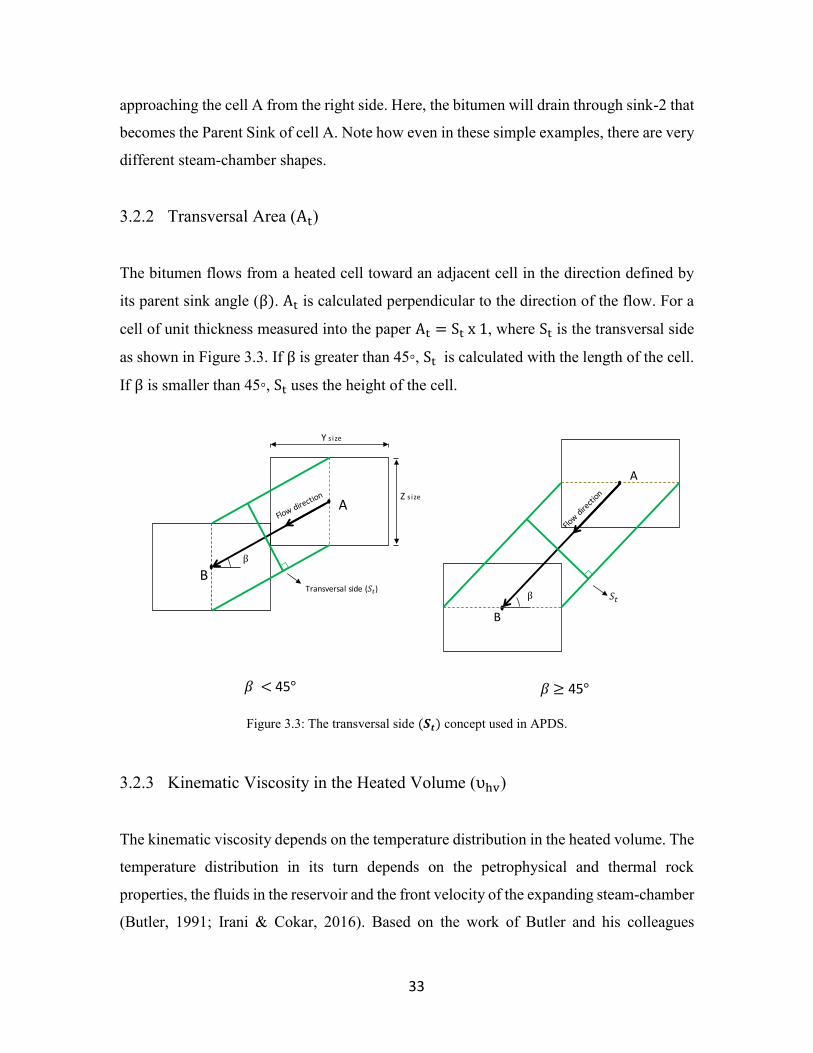
33

approaching the cell A from the right side. Here, the bitumen will drain through sink-2 that

becomes the Parent Sink of cell A. Note how even in these simple examples, there are very

different steam-chamber shapes.

3.2.2 Transversal Area (At)

The bitumen flows from a heated cell toward an adjacent cell in the direction defined by

its parent sink angle (β). At is calculated perpendicular to the direction of the flow. For a

cell of unit thickness measured into the paper At = St x 1, where St is the transversal side

as shown in Figure 3.3. If β is greater than 45◦, St is calculated with the length of the cell.

If β is smaller than 45◦, St uses the height of the cell.

Figure 3.3: The transversal side (𝑺𝒕) concept used in APDS.

3.2.3 Kinematic Viscosity in the Heated Volume (υhv)

The kinematic viscosity depends on the temperature distribution in the heated volume. The

temperature distribution in its turn depends on the petrophysical and thermal rock

properties, the fluids in the reservoir and the front velocity of the expanding steam-chamber

(Butler, 1991; Irani & Cokar, 2016). Based on the work of Butler and his colleagues

β

Transversal side (𝑆𝑡)

A

B

Z s ize

Y s ize

A

B

β

𝛽 45° 𝛽 45°

𝑆𝑡

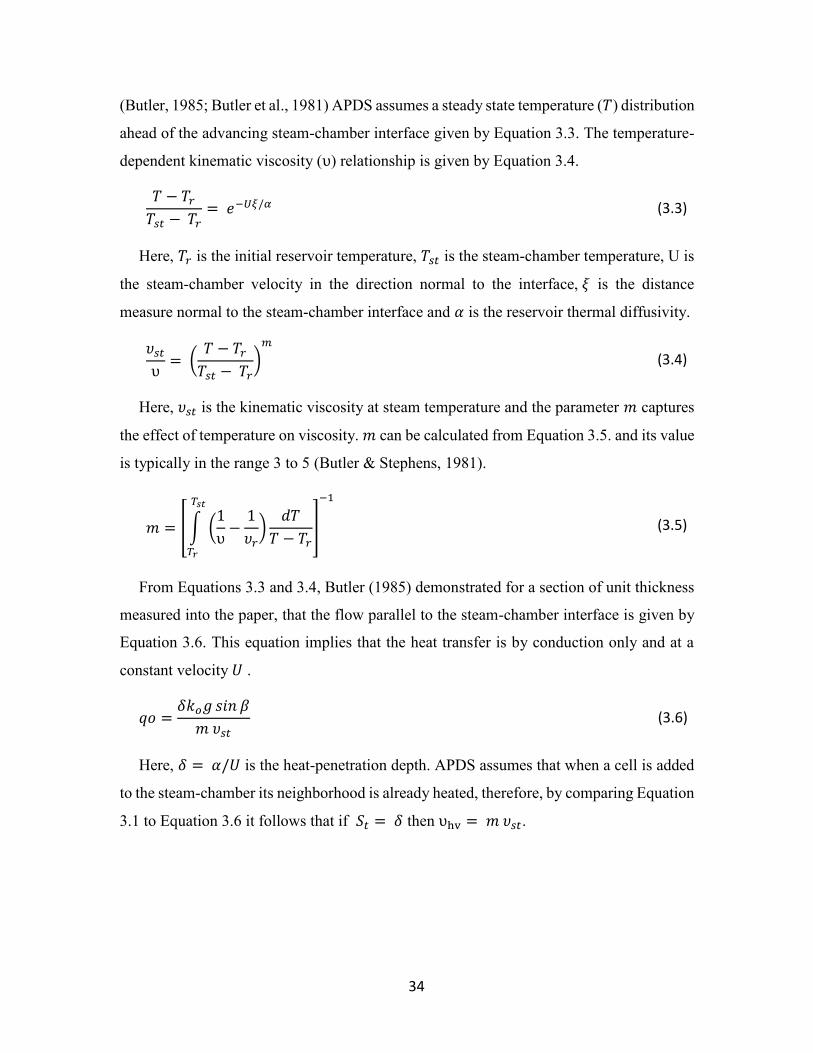
34

(Butler, 1985; Butler et al., 1981) APDS assumes a steady state temperature (𝑇) distribution

ahead of the advancing steam-chamber interface given by Equation 3.3. The temperature-

dependent kinematic viscosity (υ) relationship is given by Equation 3.4.


= 𝑒−𝑈𝜉/𝛼 (3.3)

Here, 𝑇𝑟 is the initial reservoir temperature, 𝑇𝑠𝑡 is the steam-chamber temperature, U is

the steam-chamber velocity in the direction normal to the interface, 𝜉 is the distance

measure normal to the steam-chamber interface and 𝛼 is the reservoir thermal diffusivity.

𝜐𝑠𝑡υ= (


)𝑚

(3.4)

Here, 𝜐𝑠𝑡 is the kinematic viscosity at steam temperature and the parameter 𝑚 captures

the effect of temperature on viscosity. 𝑚 can be calculated from Equation 3.5. and its value

is typically in the range 3 to 5 (Butler & Stephens, 1981).

𝑚 = [∫ (1

υ−1

𝜐𝑟)

𝑇𝑠𝑡

𝑇𝑟

𝑑𝑇

𝑇 − 𝑇𝑟]

−1

(3.5)

From Equations 3.3 and 3.4, Butler (1985) demonstrated for a section of unit thickness

measured into the paper, that the flow parallel to the steam-chamber interface is given by

Equation 3.6. This equation implies that the heat transfer is by conduction only and at a

constant velocity 𝑈 .

𝑞𝑜 =𝛿𝑘𝑜𝑔 𝑠𝑖𝑛 𝛽

𝑚 𝜐𝑠𝑡 (3.6)

Here, 𝛿 = 𝛼/𝑈 is the heat-penetration depth. APDS assumes that when a cell is added

to the steam-chamber its neighborhood is already heated, therefore, by comparing Equation

3.1 to Equation 3.6 it follows that if 𝑆𝑡 = 𝛿 then υhv = 𝑚 𝜐𝑠𝑡.

35

3.2.4 Permeability

Permeability anisotropy impacts the steam-chamber expansion and hence the SAGD

project performance (Azom & Srinivasan, 2013; Sharma, Khataniar, Patil, Kamath, &

Dandekar, 2002). During the SAGD process, the interface angle of the steam-chamber

continuously changes, and because the bitumen flows parallel to it, it is reasonable to

conclude that the relative influence of the vertical permeability (𝐾𝑣) and horizontal

permeability (𝐾ℎ) on the bitumen flow is also continuously changing. This is a local

phenomenon. At any given time, there are sectors of the steam-chamber’s edge where 𝐾𝑣

dominates over 𝐾ℎ, and others where the contrary occurs. To account for this phenomenon,

APDS implements the permeability model given by Equation 3.7.

𝐾𝛽 = 𝐾𝑣 sin2 𝛽 + 𝐾ℎ cos

2 𝛽 (3.7)

Here, 𝐾𝑣 and 𝐾ℎ are the permeability in the vertical and the horizontal direction,

respectively. 𝐾𝛽 is the permeability in the direction of the angle 𝛽.

Azom & Srinivasan (2011) derived this permeability model by resolving the SAGD

flow in the direction of the resultant gravity head. They concluded that Equation 3.7 is

mathematically in agreement with Butler’s analytical model.

3.2.5 Steam-chamber Interface Velocity

APDS works one cell at a time, and once a grid-cell has been classified as part of the steam-

chamber it is not processed again. This mechanism is myopic about the future evolution of

the steam-chamber and overestimates the interface velocity. A deceleration exponent

applied to the model time variable introduced in Section 2.4.3.2 corrects this

overestimation.

Figure 3.4 illustrates the cause of the overestimation. It shows the rate of bitumen

flowing in (𝑞𝑖𝑛) and flowing out (𝑞𝑜𝑢𝑡) of a cell in the heated zone. Note that the advance

of the steam-chamber interface at a velocity 𝑈 is only possible if 𝑞𝑜𝑢𝑡 > 𝑞𝑖𝑛 . In other

words, the advance of the interface is determined by the difference in the rates, and not

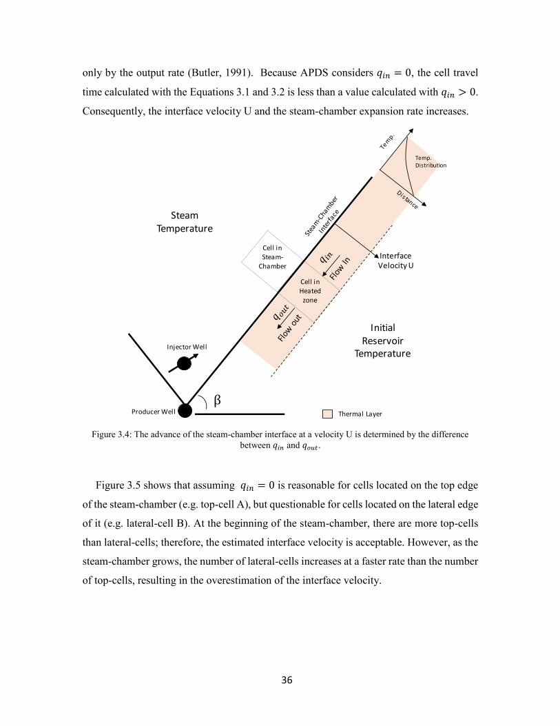
36

only by the output rate (Butler, 1991). Because APDS considers 𝑞𝑖𝑛 = 0, the cell travel

time calculated with the Equations 3.1 and 3.2 is less than a value calculated with 𝑞𝑖𝑛 > 0.

Consequently, the interface velocity U and the steam-chamber expansion rate increases.

Figure 3.4: The advance of the steam-chamber interface at a velocity U is determined by the difference

between 𝑞𝑖𝑛 and 𝑞𝑜𝑢𝑡.

Figure 3.5 shows that assuming 𝑞𝑖𝑛 = 0 is reasonable for cells located on the top edge

of the steam-chamber (e.g. top-cell A), but questionable for cells located on the lateral edge

of it (e.g. lateral-cell B). At the beginning of the steam-chamber, there are more top-cells

than lateral-cells; therefore, the estimated interface velocity is acceptable. However, as the

steam-chamber grows, the number of lateral-cells increases at a faster rate than the number

of top-cells, resulting in the overestimation of the interface velocity.

Initial Reservoir

Temperature

Temp. Distribution

β

Steam Temperature

Producer Well

Injector Well

Interface Velocity U

Cell in Steam-

Chamber

Cell in Heated

zone

Thermal Layer

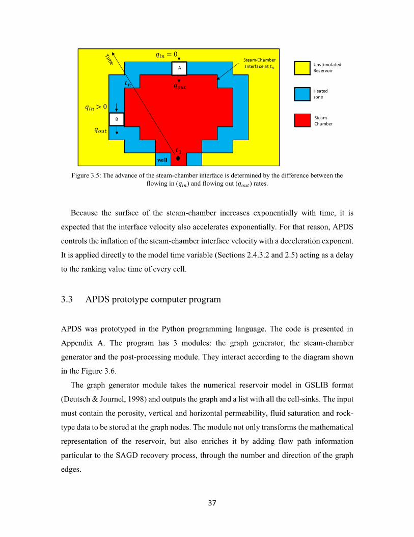
37

Figure 3.5: The advance of the steam-chamber interface is determined by the difference between the

flowing in (𝑞𝑖𝑛) and flowing out (𝑞𝑜𝑢𝑡) rates.

Because the surface of the steam-chamber increases exponentially with time, it is

expected that the interface velocity also accelerates exponentially. For that reason, APDS

controls the inflation of the steam-chamber interface velocity with a deceleration exponent.

It is applied directly to the model time variable (Sections 2.4.3.2 and 2.5) acting as a delay

to the ranking value time of every cell.

3.3 APDS prototype computer program

APDS was prototyped in the Python programming language. The code is presented in

Appendix A. The program has 3 modules: the graph generator, the steam-chamber

generator and the post-processing module. They interact according to the diagram shown

in the Figure 3.6.

The graph generator module takes the numerical reservoir model in GSLIB format

(Deutsch & Journel, 1998) and outputs the graph and a list with all the cell-sinks. The input

must contain the porosity, vertical and horizontal permeability, fluid saturation and rock-

type data to be stored at the graph nodes. The module not only transforms the mathematical

representation of the reservoir, but also enriches it by adding flow path information

particular to the SAGD recovery process, through the number and direction of the graph

edges.

well

Steam-Chamber

Interface at 𝑡𝑛

𝑞𝑖𝑛 = 0

𝑞𝑖𝑛 > 0

B

A

Steam-Chamber

Heated zone

Unstimulated Reservoir

𝑡1

𝑡𝑛 𝑞𝑜𝑢𝑡

𝑞𝑜𝑢𝑡

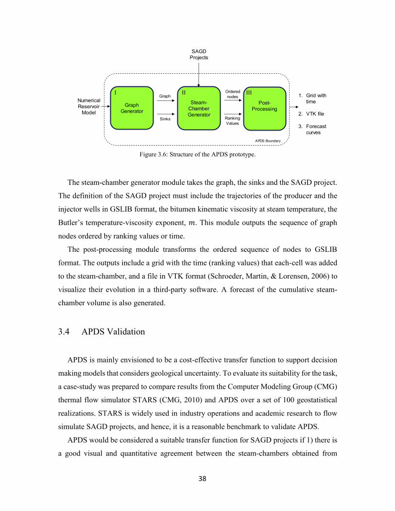
38

Figure 3.6: Structure of the APDS prototype.

The steam-chamber generator module takes the graph, the sinks and the SAGD project.

The definition of the SAGD project must include the trajectories of the producer and the

injector wells in GSLIB format, the bitumen kinematic viscosity at steam temperature, the

Butler’s temperature-viscosity exponent, 𝑚. This module outputs the sequence of graph

nodes ordered by ranking values or time.

The post-processing module transforms the ordered sequence of nodes to GSLIB

format. The outputs include a grid with the time (ranking values) that each-cell was added

to the steam-chamber, and a file in VTK format (Schroeder, Martin, & Lorensen, 2006) to

visualize their evolution in a third-party software. A forecast of the cumulative steam-

chamber volume is also generated.

3.4 APDS Validation

APDS is mainly envisioned to be a cost-effective transfer function to support decision

making models that considers geological uncertainty. To evaluate its suitability for the task,

a case-study was prepared to compare results from the Computer Modeling Group (CMG)

thermal flow simulator STARS (CMG, 2010) and APDS over a set of 100 geostatistical

realizations. STARS is widely used in industry operations and academic research to flow

simulate SAGD projects, and hence, it is a reasonable benchmark to validate APDS.

APDS would be considered a suitable transfer function for SAGD projects if 1) there is

a good visual and quantitative agreement between the steam-chambers obtained from

Steam-

Chamber

Generator

Graph

Generator

Post-

Processing

Graph

Sinks

Ordered

nodes

Ranking

Values

1. Grid with

time

2. VTK file

3. Forecast

curves

SAGD

Projects

Numerical

Reservoir

Model

APDS Boundary

I II III

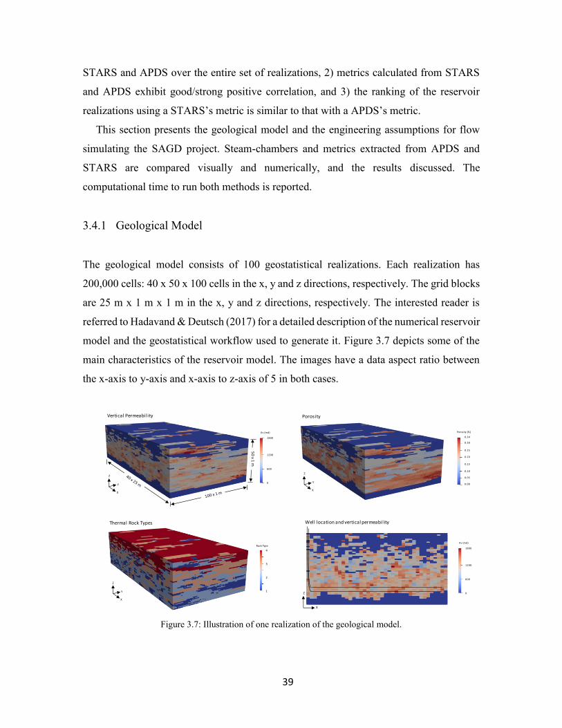
39

STARS and APDS over the entire set of realizations, 2) metrics calculated from STARS

and APDS exhibit good/strong positive correlation, and 3) the ranking of the reservoir

realizations using a STARS’s metric is similar to that with a APDS’s metric.

This section presents the geological model and the engineering assumptions for flow

simulating the SAGD project. Steam-chambers and metrics extracted from APDS and

STARS are compared visually and numerically, and the results discussed. The

computational time to run both methods is reported.

3.4.1 Geological Model

The geological model consists of 100 geostatistical realizations. Each realization has

200,000 cells: 40 x 50 x 100 cells in the x, y and z directions, respectively. The grid blocks

are 25 m x 1 m x 1 m in the x, y and z directions, respectively. The interested reader is

referred to Hadavand & Deutsch (2017) for a detailed description of the numerical reservoir

model and the geostatistical workflow used to generate it. Figure 3.7 depicts some of the

main characteristics of the reservoir model. The images have a data aspect ratio between

the x-axis to y-axis and x-axis to z-axis of 5 in both cases.

Figure 3.7: Illustration of one realization of the geological model.

0

1800

600

1200

Kv (md)

Well location and vertical permeability

X

Z1

2

3

4

Rock Type

Thermal Rock Types

X

Z

Y

0.00

0.05

0.10

0.15

0.20

0.25

0.30

0.34

Porosity (%)

Porosity

X

Z

Y0

1800

600

1200

Kv (md)

Vertical Permeability

X

Z

Y

50

x 1 m

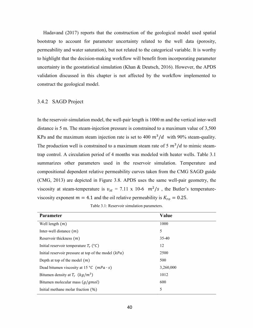
40

Hadavand (2017) reports that the construction of the geological model used spatial

bootstrap to account for parameter uncertainty related to the well data (porosity,

permeability and water saturation), but not related to the categorical variable. It is worthy

to highlight that the decision-making workflow will benefit from incorporating parameter

uncertainty in the geostatistical simulation (Khan & Deutsch, 2016). However, the APDS

validation discussed in this chapter is not affected by the workflow implemented to

construct the geological model.

3.4.2 SAGD Project

In the reservoir-simulation model, the well-pair length is 1000 m and the vertical inter-well

distance is 5 m. The steam-injection pressure is constrained to a maximum value of 3,500

KPa and the maximum steam injection rate is set to 400 𝑚3/𝑑 with 90% steam-quality.

The production well is constrained to a maximum steam rate of 5 𝑚3/𝑑 to mimic steam-

trap control. A circulation period of 4 months was modeled with heater wells. Table 3.1

summarizes other parameters used in the reservoir simulation. Temperature and

compositional dependent relative permeability curves taken from the CMG SAGD guide

(CMG, 2013) are depicted in Figure 3.8. APDS uses the same well-pair geometry, the

viscosity at steam-temperature is 𝜐𝑠𝑡 = 7.11 x 10-6 𝑚2/𝑠 , the Butler’s temperature-

viscosity exponent 𝑚 = 4.1 and the oil relative permeability is 𝐾𝑟𝑜 = 0.25.

Table 3.1: Reservoir simulation parameters.

Parameter Value

Well length (𝑚) 1000

Inter-well distance (𝑚) 5

Reservoir thickness (𝑚) 35-40

Initial reservoir temperature 𝑇𝑟 (°𝐶) 12

Initial reservoir pressure at top of the model (𝑘𝑃𝑎) 2500

Depth at top of the model (𝑚) 500

Dead bitumen viscosity at 15 °𝐶 (𝑚𝑃𝑎 ∙ 𝑠) 3,260,000

Bitumen density at 𝑇𝑟 (𝑘𝑔/𝑚3) 1012

Bitumen molecular mass (𝑔/𝑔𝑚𝑜𝑙) 600

Initial methane molar fraction (%) 5

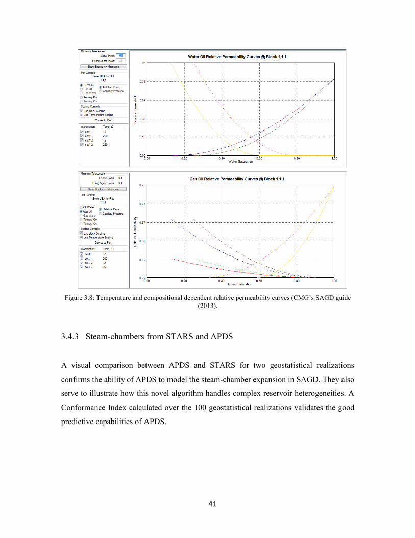
41

Figure 3.8: Temperature and compositional dependent relative permeability curves (CMG’s SAGD guide

(2013).

3.4.3 Steam-chambers from STARS and APDS

A visual comparison between APDS and STARS for two geostatistical realizations

confirms the ability of APDS to model the steam-chamber expansion in SAGD. They also

serve to illustrate how this novel algorithm handles complex reservoir heterogeneities. A

Conformance Index calculated over the 100 geostatistical realizations validates the good

predictive capabilities of APDS.

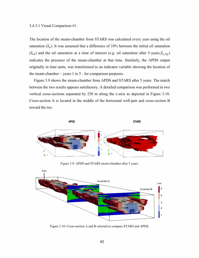
42

3.4.3.1 Visual Comparison #1.

The location of the steam-chamber from STARS was calculated every year using the oil

saturation (𝑆𝑜). It was assumed that a difference of 10% between the initial oil saturation

(𝑆𝑜𝑖) and the oil saturation at a time of interest (e.g. oil saturation after 5-years,𝑆𝑜_5𝑦)

indicates the presence of the steam-chamber at that time. Similarly, the APDS output

originally in time units, was transformed to an indicator variable showing the location of

the steam-chamber – years 1 to 5 - for comparison purposes.

Figure 3.9 shows the steam-chamber from APDS and STARS after 5 years. The match

between the two results appears satisfactory. A detailed comparison was performed in two

vertical cross-sections separated by 250 m along the x-axis as depicted in Figure 3.10.

Cross-section A is located in the middle of the horizontal well-pair and cross-section B

toward the toe.

Figure 3.9: APDS and STARS steam-chamber after 5 years.

Figure 3.10: Cross-section A and B selected to compare STARS and APDS.

Year

5

4

3

2

1

APDS STARS

1

2

3

4

5

YearX-section A

X-section B

Wells

43

Cross-section A in Figure 3.11 shows from the bottom to the top the steam-chamber

evolution for 5 years. The left and right columns show the results from STARS and APDS,

respectively.

A visual comparison demonstrates a close agreement between the STARS and the

APDS results in this cross-section. At the beginning, the APDS steam-chamber does not

rise as quickly, but soon it reaches a similar growth rate to the STARS’s steam-chamber.

The APDS steam-chamber evolves honoring the reservoir heterogeneity. For example, a

long barrier located at the right-side of the cross-section reduces the vertical growth of the

chamber between years 2 and 3 causing it to rise asymmetrically to the left of the cross-

section. The STARS results confirm this complex behavior. Figure 3.11 shows that the

good agreement in shape and size is maintained through the studied time horizon.

Figure 3.12 shows cross-section B; again, there is a good agreement between the

STARS and APDS results. Note that cross-section B has a different geometric pattern than

cross-section A. In this case, two long stair-stepped barriers located at the left of the cross-

section inhibit the movement of the steam. Figure 3.12 illustrates how APDS predicts the

impact of these obstacles in a similar way to STARS. Once more, the good agreement in

the shape and size is maintained through the studied time horizon.

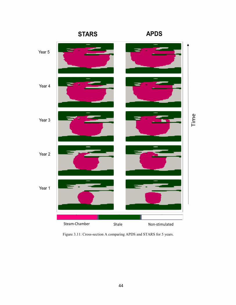
44

Figure 3.11: Cross-section A comparing APDS and STARS for 5 years.

Steam-Chamber Shale Non-stimulated

Year 1

Year 2

Year 4

Year 3

Year 5

Tim

e

STARS APDS

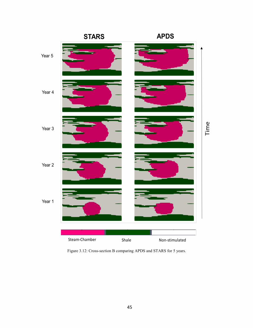
45

Figure 3.12: Cross-section B comparing APDS and STARS for 5 years.

Steam-Chamber Shale Non-stimulated

Year 1

Year 2

Year 4

Year 3

Year 5

Tim

e

STARS APDS

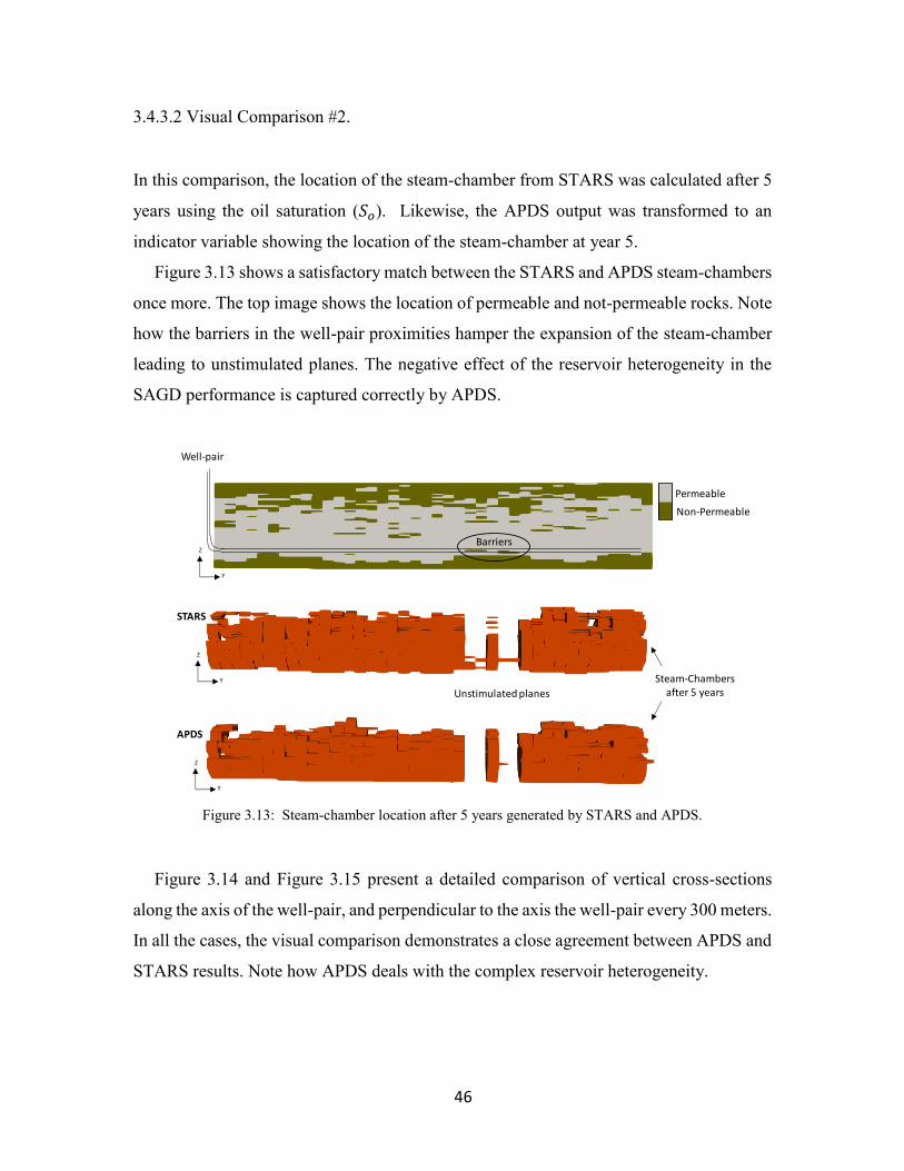
46

3.4.3.2 Visual Comparison #2.

In this comparison, the location of the steam-chamber from STARS was calculated after 5

years using the oil saturation (𝑆𝑜). Likewise, the APDS output was transformed to an

indicator variable showing the location of the steam-chamber at year 5.

Figure 3.13 shows a satisfactory match between the STARS and APDS steam-chambers

once more. The top image shows the location of permeable and not-permeable rocks. Note

how the barriers in the well-pair proximities hamper the expansion of the steam-chamber

leading to unstimulated planes. The negative effect of the reservoir heterogeneity in the

SAGD performance is captured correctly by APDS.

Figure 3.13: Steam-chamber location after 5 years generated by STARS and APDS.

Figure 3.14 and Figure 3.15 present a detailed comparison of vertical cross-sections

along the axis of the well-pair, and perpendicular to the axis the well-pair every 300 meters.

In all the cases, the visual comparison demonstrates a close agreement between APDS and

STARS results. Note how APDS deals with the complex reservoir heterogeneity.

Barriers

Unstimulated planes

APDS

STARS

Well-pair

Y

Z

Y

Z

Y

Z

Non-Permeable

Permeable

Steam-Chambersafter 5 years

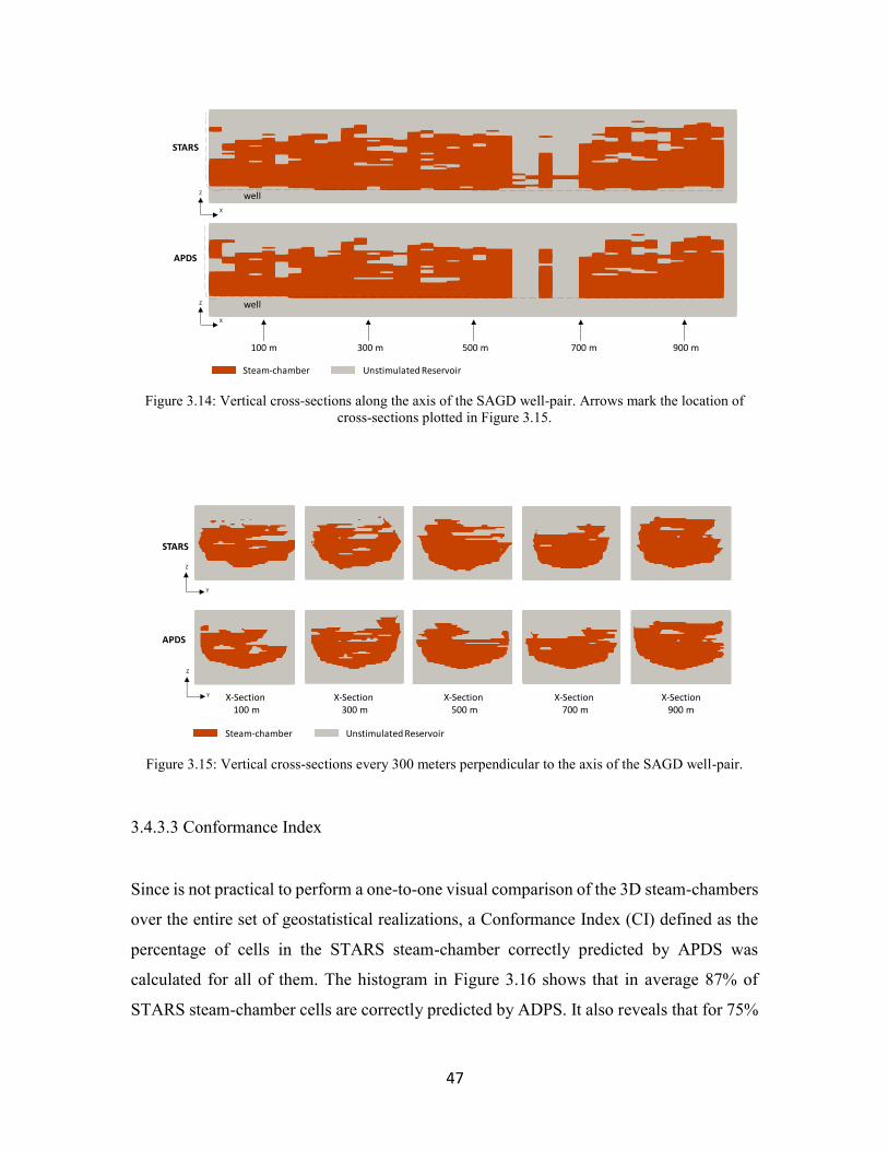
47

Figure 3.14: Vertical cross-sections along the axis of the SAGD well-pair. Arrows mark the location of

cross-sections plotted in Figure 3.15.

Figure 3.15: Vertical cross-sections every 300 meters perpendicular to the axis of the SAGD well-pair.

3.4.3.3 Conformance Index

Since is not practical to perform a one-to-one visual comparison of the 3D steam-chambers

over the entire set of geostatistical realizations, a Conformance Index (CI) defined as the

percentage of cells in the STARS steam-chamber correctly predicted by APDS was

calculated for all of them. The histogram in Figure 3.16 shows that in average 87% of

STARS steam-chamber cells are correctly predicted by ADPS. It also reveals that for 75%

APDS

STARS

100 m 300 m 500 m 700 m 900 m

X

Z

X

Z well

well

Unstimulated ReservoirSteam-chamber

X-Section 100 m

X-Section 300 m

X-Section 500 m

X-Section 700 m

X-Section 900 m

Y

Z

APDS

STARS

Y

Z

Unstimulated ReservoirSteam-chamber

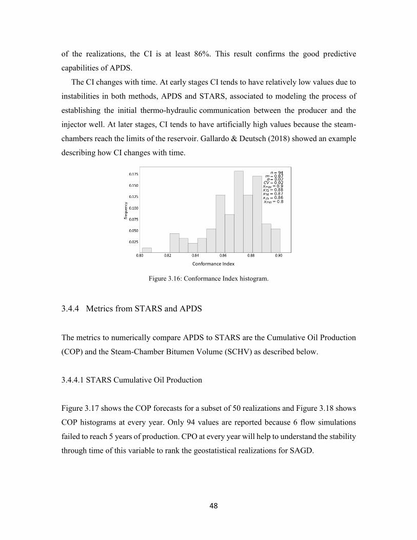
48

of the realizations, the CI is at least 86%. This result confirms the good predictive

capabilities of APDS.

The CI changes with time. At early stages CI tends to have relatively low values due to

instabilities in both methods, APDS and STARS, associated to modeling the process of

establishing the initial thermo-hydraulic communication between the producer and the

injector well. At later stages, CI tends to have artificially high values because the steam-

chambers reach the limits of the reservoir. Gallardo & Deutsch (2018) showed an example

describing how CI changes with time.

Figure 3.16: Conformance Index histogram.

3.4.4 Metrics from STARS and APDS

The metrics to numerically compare APDS to STARS are the Cumulative Oil Production

(COP) and the Steam-Chamber Bitumen Volume (SCHV) as described below.

3.4.4.1 STARS Cumulative Oil Production

Figure 3.17 shows the COP forecasts for a subset of 50 realizations and Figure 3.18 shows

COP histograms at every year. Only 94 values are reported because 6 flow simulations

failed to reach 5 years of production. CPO at every year will help to understand the stability

through time of this variable to rank the geostatistical realizations for SAGD.

Conformance Index

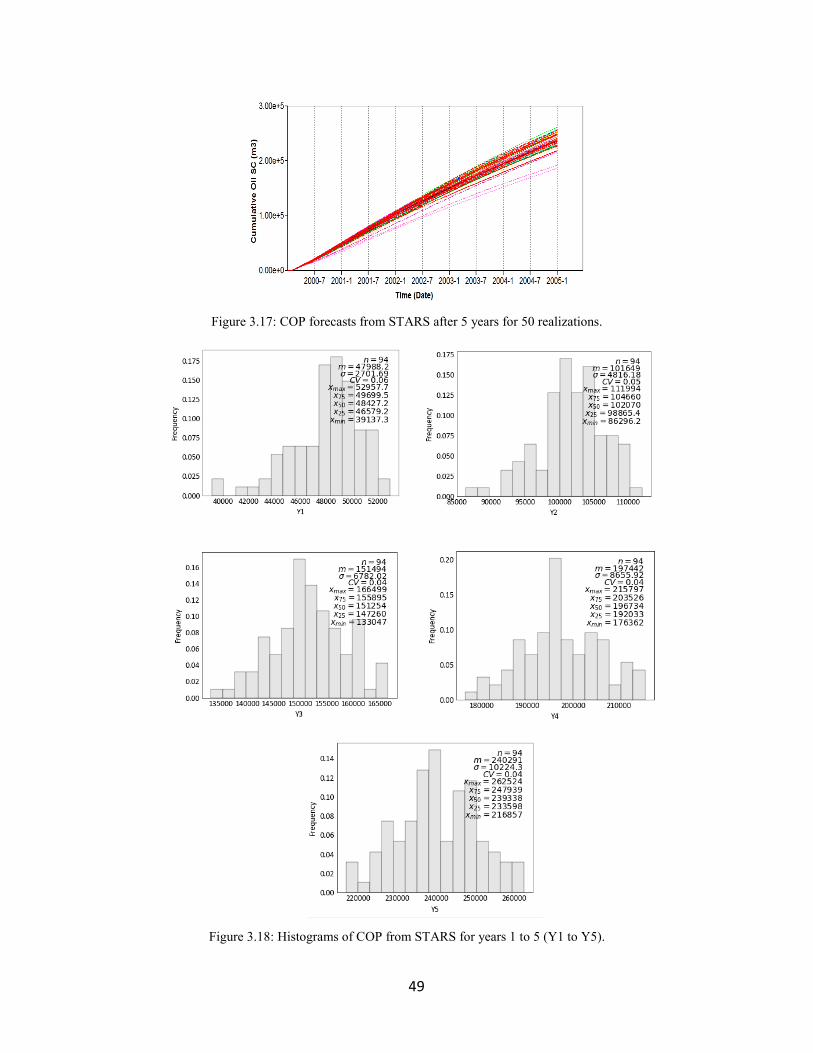
49

Figure 3.17: COP forecasts from STARS after 5 years for 50 realizations.

Figure 3.18: Histograms of COP from STARS for years 1 to 5 (Y1 to Y5).

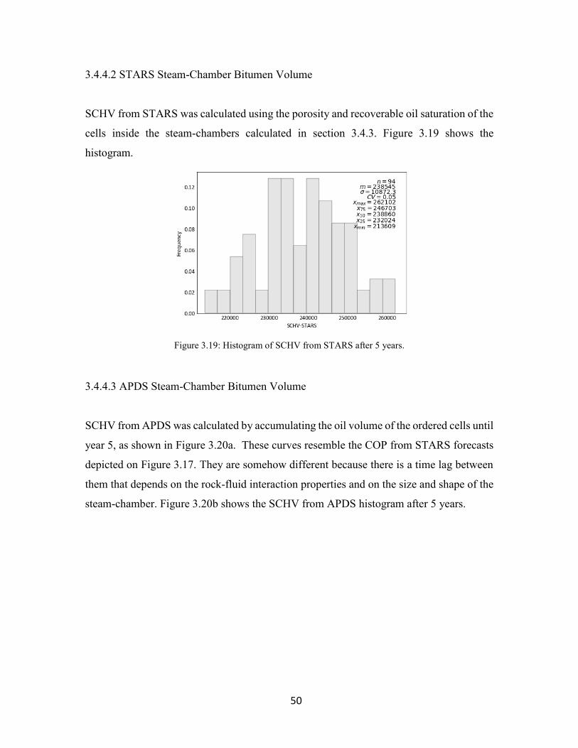
50

3.4.4.2 STARS Steam-Chamber Bitumen Volume

SCHV from STARS was calculated using the porosity and recoverable oil saturation of the

cells inside the steam-chambers calculated in section 3.4.3. Figure 3.19 shows the

histogram.

Figure 3.19: Histogram of SCHV from STARS after 5 years.

3.4.4.3 APDS Steam-Chamber Bitumen Volume

SCHV from APDS was calculated by accumulating the oil volume of the ordered cells until

year 5, as shown in Figure 3.20a. These curves resemble the COP from STARS forecasts

depicted on Figure 3.17. They are somehow different because there is a time lag between

them that depends on the rock-fluid interaction properties and on the size and shape of the

steam-chamber. Figure 3.20b shows the SCHV from APDS histogram after 5 years.

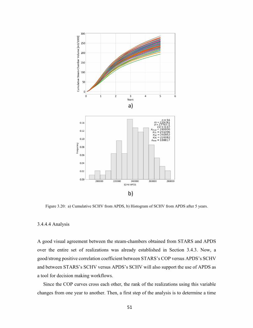
51

Figure 3.20: a) Cumulative SCHV from APDS, b) Histogram of SCHV from APDS after 5 years.

3.4.4.4 Analysis

A good visual agreement between the steam-chambers obtained from STARS and APDS

over the entire set of realizations was already established in Section 3.4.3. Now, a

good/strong positive correlation coefficient between STARS’s COP versus APDS’s SCHV

and between STARS’s SCHV versus APDS’s SCHV will also support the use of APDS as

a tool for decision making workflows.

Since the COP curves cross each other, the rank of the realizations using this variable

changes from one year to another. Then, a first step of the analysis is to determine a time

a)

b)

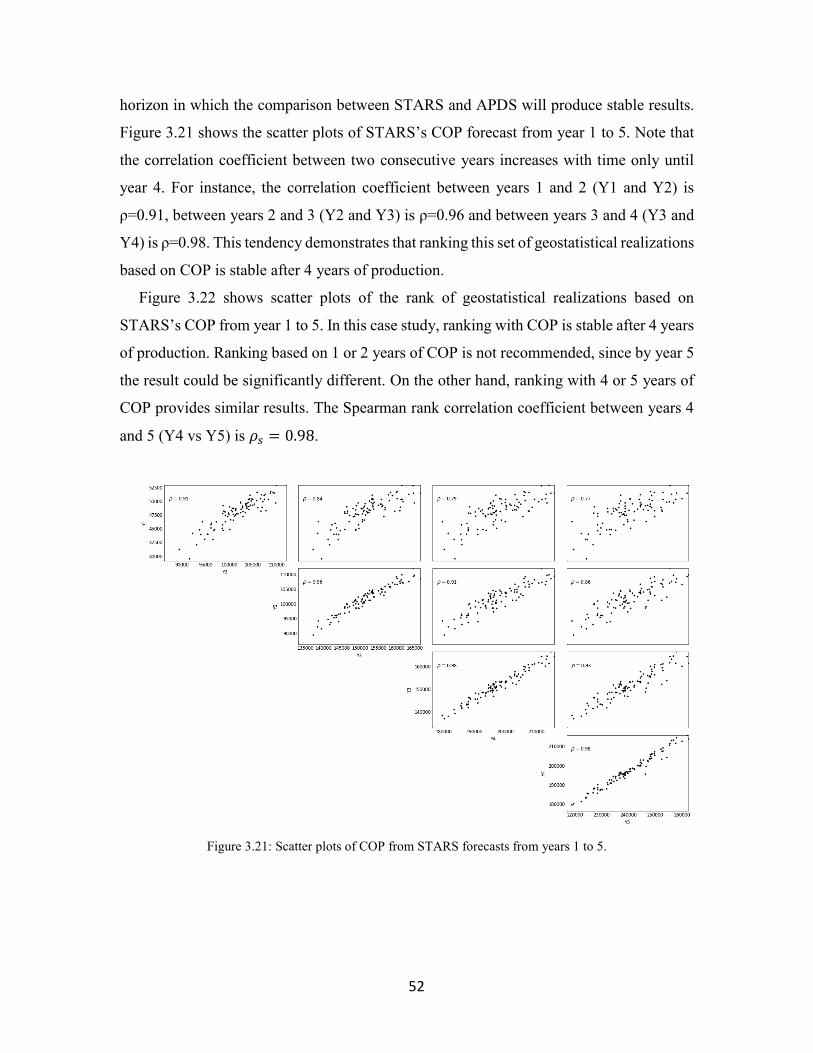
52

horizon in which the comparison between STARS and APDS will produce stable results.

Figure 3.21 shows the scatter plots of STARS’s COP forecast from year 1 to 5. Note that

the correlation coefficient between two consecutive years increases with time only until

year 4. For instance, the correlation coefficient between years 1 and 2 (Y1 and Y2) is

ρ=0.91, between years 2 and 3 (Y2 and Y3) is ρ=0.96 and between years 3 and 4 (Y3 and

Y4) is ρ=0.98. This tendency demonstrates that ranking this set of geostatistical realizations

based on COP is stable after 4 years of production.

Figure 3.22 shows scatter plots of the rank of geostatistical realizations based on

STARS’s COP from year 1 to 5. In this case study, ranking with COP is stable after 4 years

of production. Ranking based on 1 or 2 years of COP is not recommended, since by year 5

the result could be significantly different. On the other hand, ranking with 4 or 5 years of

COP provides similar results. The Spearman rank correlation coefficient between years 4

and 5 (Y4 vs Y5) is 𝜌𝑠 = 0.98.

Figure 3.21: Scatter plots of COP from STARS forecasts from years 1 to 5.

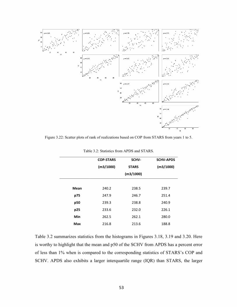
53

Figure 3.22: Scatter plots of rank of realizations based on COP from STARS from years 1 to 5.

Table 3.2: Statistics from APDS and STARS.

COP-STARS

(m3/1000)

SCHV-

STARS

(m3/1000)

SCHV-APDS

(m3/1000)

Mean 240.2 238.5 239.7

p75 247.9 246.7 251.4

p50 239.3 238.8 240.9

p25 233.6 232.0 226.1

Min 262.5 262.1 280.0

Max 216.8 213.6 188.8

Table 3.2 summarizes statistics from the histograms in Figures 3.18, 3.19 and 3.20. Here

is worthy to highlight that the mean and p50 of the SCHV from APDS has a percent error

of less than 1% when is compared to the corresponding statistics of STARS’s COP and

SCHV. APDS also exhibits a larger interquartile range (IQR) than STARS, the larger

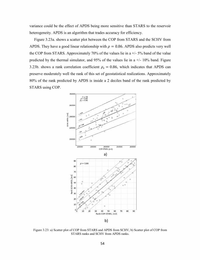
54

variance could be the effect of APDS being more sensitive than STARS to the reservoir

heterogeneity. APDS is an algorithm that trades accuracy for efficiency.

Figure 3.23a. shows a scatter plot between the COP from STARS and the SCHV from

APDS. They have a good linear relationship with 𝜌 = 0.86. APDS also predicts very well

the COP from STARS. Approximately 70% of the values lie in a +/- 5% band of the value

predicted by the thermal simulator, and 95% of the values lie in a +/- 10% band. Figure

3.23b. shows a rank correlation coefficient 𝜌𝑠 = 0.86, which indicates that APDS can

preserve moderately well the rank of this set of geostatistical realizations. Approximately

80% of the rank predicted by APDS is inside a 2 deciles band of the rank predicted by

STARS using COP.

Figure 3.23: a) Scatter plot of COP from STARS and APDS from SCHV, b) Scatter plot of COP from

STARS ranks and SCHV from APDS ranks.

a)

b)

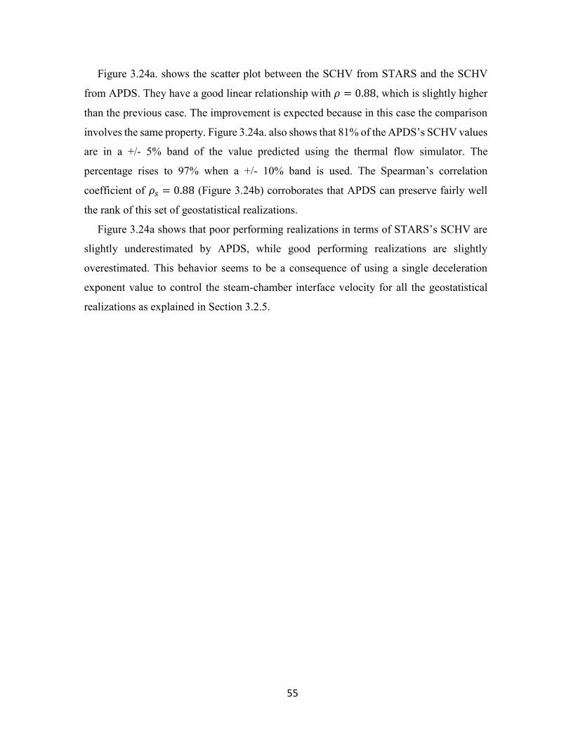
55

Figure 3.24a. shows the scatter plot between the SCHV from STARS and the SCHV

from APDS. They have a good linear relationship with 𝜌 = 0.88, which is slightly higher

than the previous case. The improvement is expected because in this case the comparison

involves the same property. Figure 3.24a. also shows that 81% of the APDS’s SCHV values

are in a +/- 5% band of the value predicted using the thermal flow simulator. The

percentage rises to 97% when a +/- 10% band is used. The Spearman’s correlation

coefficient of 𝜌𝑠 = 0.88 (Figure 3.24b) corroborates that APDS can preserve fairly well

the rank of this set of geostatistical realizations.

Figure 3.24a shows that poor performing realizations in terms of STARS’s SCHV are

slightly underestimated by APDS, while good performing realizations are slightly

overestimated. This behavior seems to be a consequence of using a single deceleration

exponent value to control the steam-chamber interface velocity for all the geostatistical

realizations as explained in Section 3.2.5.

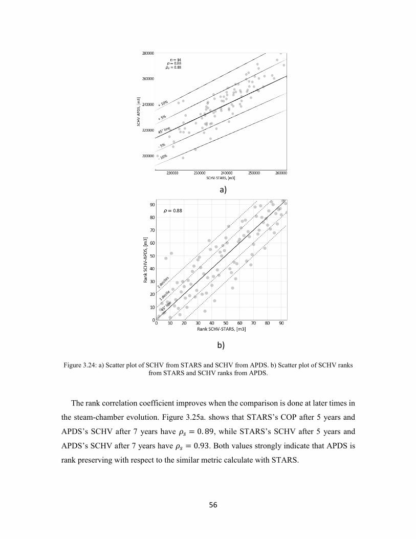
56

Figure 3.24: a) Scatter plot of SCHV from STARS and SCHV from APDS. b) Scatter plot of SCHV ranks

from STARS and SCHV ranks from APDS.

The rank correlation coefficient improves when the comparison is done at later times in

the steam-chamber evolution. Figure 3.25a. shows that STARS’s COP after 5 years and

APDS’s SCHV after 7 years have 𝜌𝑠 = 0. 89, while STARS’s SCHV after 5 years and

APDS’s SCHV after 7 years have 𝜌𝑠 = 0.93. Both values strongly indicate that APDS is

rank preserving with respect to the similar metric calculate with STARS.

a)

b)

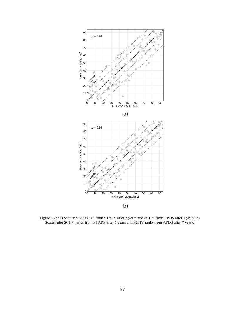
57

Figure 3.25: a) Scatter plot of COP from STARS after 5 years and SCHV from APDS after 7 years. b)

Scatter plot SCHV ranks from STARS after 5 years and SCHV ranks from APDS after 7 years.

a)

b)

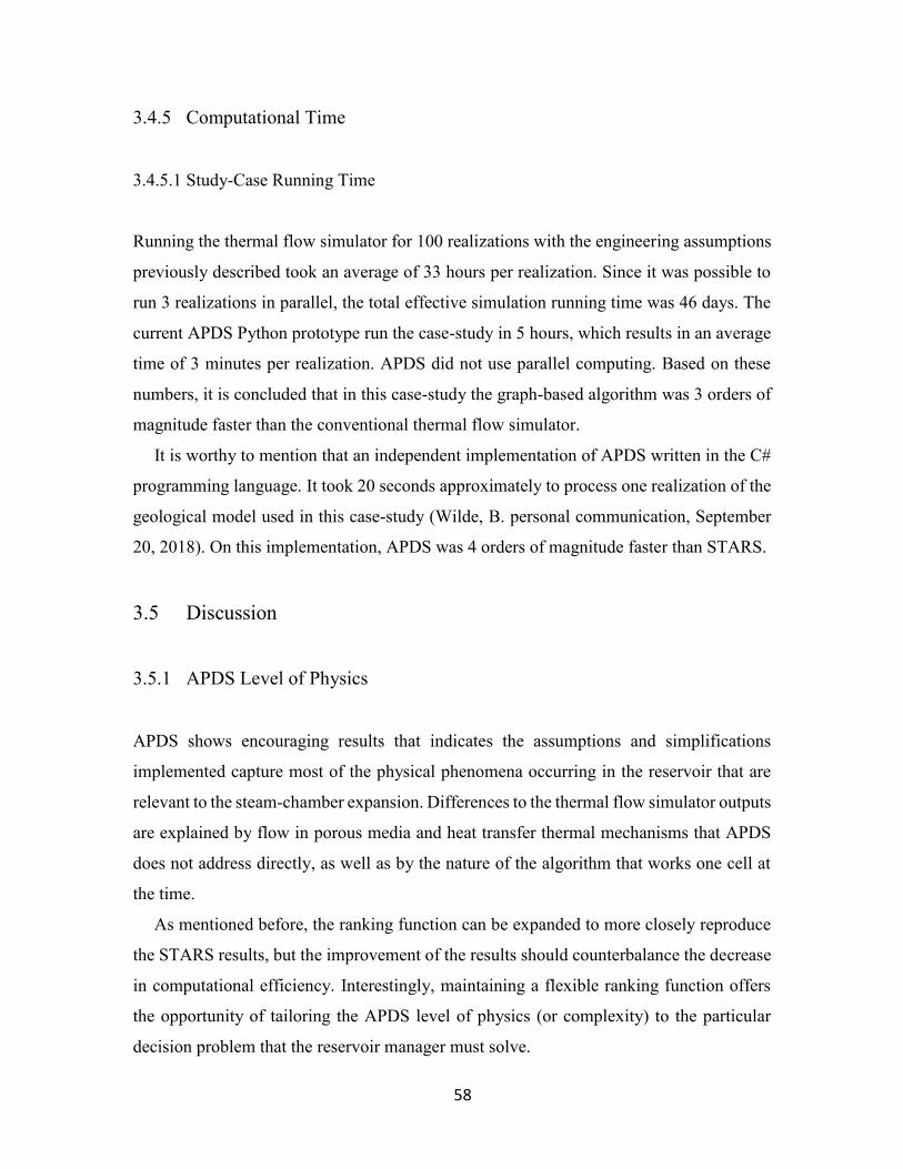
58

3.4.5 Computational Time

3.4.5.1 Study-Case Running Time

Running the thermal flow simulator for 100 realizations with the engineering assumptions

previously described took an average of 33 hours per realization. Since it was possible to

run 3 realizations in parallel, the total effective simulation running time was 46 days. The

current APDS Python prototype run the case-study in 5 hours, which results in an average

time of 3 minutes per realization. APDS did not use parallel computing. Based on these

numbers, it is concluded that in this case-study the graph-based algorithm was 3 orders of

magnitude faster than the conventional thermal flow simulator.

It is worthy to mention that an independent implementation of APDS written in the C#

programming language. It took 20 seconds approximately to process one realization of the

geological model used in this case-study (Wilde, B. personal communication, September

20, 2018). On this implementation, APDS was 4 orders of magnitude faster than STARS.

3.5 Discussion

3.5.1 APDS Level of Physics

APDS shows encouraging results that indicates the assumptions and simplifications

implemented capture most of the physical phenomena occurring in the reservoir that are

relevant to the steam-chamber expansion. Differences to the thermal flow simulator outputs

are explained by flow in porous media and heat transfer thermal mechanisms that APDS

does not address directly, as well as by the nature of the algorithm that works one cell at

the time.

As mentioned before, the ranking function can be expanded to more closely reproduce

the STARS results, but the improvement of the results should counterbalance the decrease

in computational efficiency. Interestingly, maintaining a flexible ranking function offers

the opportunity of tailoring the APDS level of physics (or complexity) to the particular

decision problem that the reservoir manager must solve.

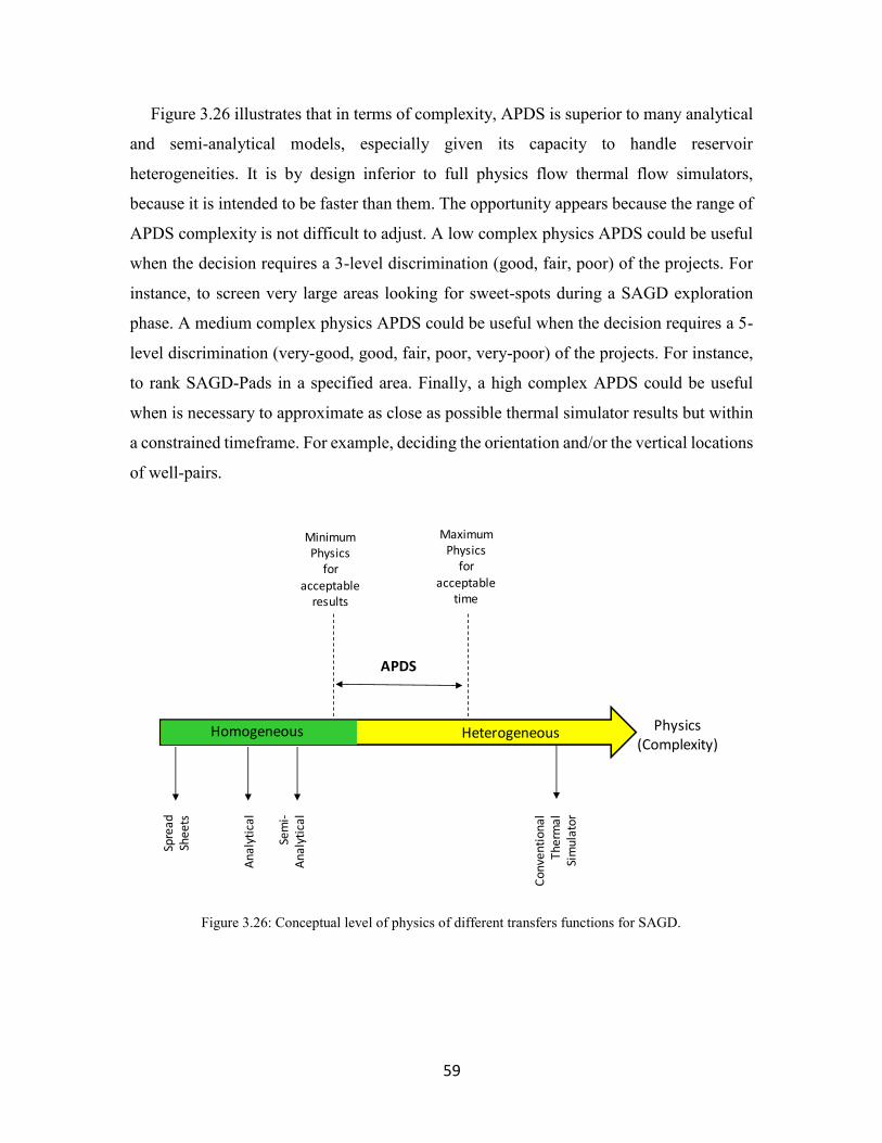
59

Figure 3.26 illustrates that in terms of complexity, APDS is superior to many analytical

and semi-analytical models, especially given its capacity to handle reservoir

heterogeneities. It is by design inferior to full physics flow thermal flow simulators,

because it is intended to be faster than them. The opportunity appears because the range of

APDS complexity is not difficult to adjust. A low complex physics APDS could be useful

when the decision requires a 3-level discrimination (good, fair, poor) of the projects. For

instance, to screen very large areas looking for sweet-spots during a SAGD exploration

phase. A medium complex physics APDS could be useful when the decision requires a 5-

level discrimination (very-good, good, fair, poor, very-poor) of the projects. For instance,

to rank SAGD-Pads in a specified area. Finally, a high complex APDS could be useful

when is necessary to approximate as close as possible thermal simulator results but within

a constrained timeframe. For example, deciding the orientation and/or the vertical locations

of well-pairs.

Figure 3.26: Conceptual level of physics of different transfers functions for SAGD.

Physics(Complexity)

Co

nve

nti

on

al

Th

erm

al

Sim

ula

tor

APDS

Minimum Physics

foracceptable

results

MaximumPhysics

for

acceptabletime

Spre

ad

Shee

ts

An

aly

tica

l

Sem

i-A

na

lyti

cal

Homogeneous Heterogeneous

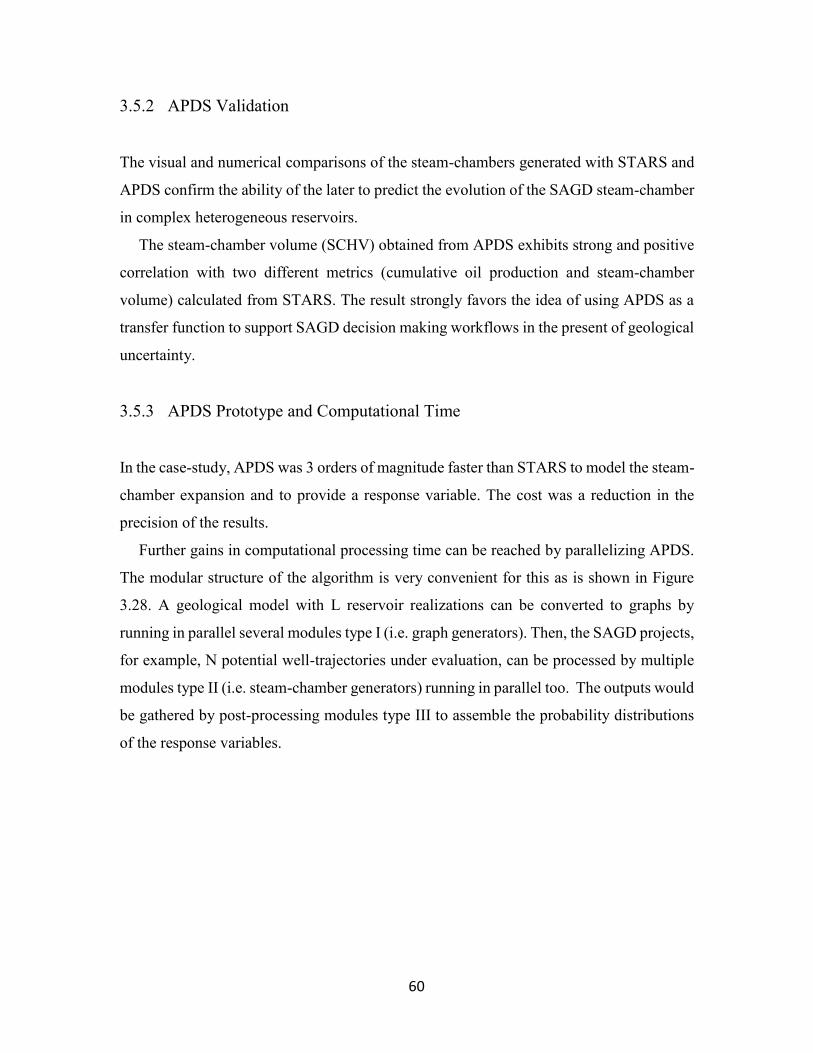
60

3.5.2 APDS Validation

The visual and numerical comparisons of the steam-chambers generated with STARS and

APDS confirm the ability of the later to predict the evolution of the SAGD steam-chamber

in complex heterogeneous reservoirs.

The steam-chamber volume (SCHV) obtained from APDS exhibits strong and positive

correlation with two different metrics (cumulative oil production and steam-chamber

volume) calculated from STARS. The result strongly favors the idea of using APDS as a

transfer function to support SAGD decision making workflows in the present of geological

uncertainty.

3.5.3 APDS Prototype and Computational Time

In the case-study, APDS was 3 orders of magnitude faster than STARS to model the steam-

chamber expansion and to provide a response variable. The cost was a reduction in the

precision of the results.

Further gains in computational processing time can be reached by parallelizing APDS.

The modular structure of the algorithm is very convenient for this as is shown in Figure

3.28. A geological model with L reservoir realizations can be converted to graphs by

running in parallel several modules type I (i.e. graph generators). Then, the SAGD projects,

for example, N potential well-trajectories under evaluation, can be processed by multiple

modules type II (i.e. steam-chamber generators) running in parallel too. The outputs would

be gathered by post-processing modules type III to assemble the probability distributions

of the response variables.

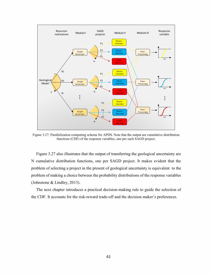
61

Figure 3.27: Parallelization computing scheme for APDS. Note that the output are cumulative distribution

functions (CDF) of the response variables, one per each SAGD project.

Figure 3.27 also illustrates that the output of transferring the geological uncertainty are

N cumulative distribution functions, one per SAGD project. It makes evident that the

problem of selecting a project in the present of geological uncertainty is equivalent to the

problem of making a choice between the probability distributions of the response variables

(Johnstone & Lindley, 2013).

The next chapter introduces a practical decision-making rule to guide the selection of

the CDF. It accounts for the risk-reward trade-off and the decision maker’s preferences.

GeologicalModel

GraphGenerator

GraphGenerator

GraphGenerator

Steam-chamber

Steam-chamber

Steam-chamber

SAGD projects

Reservoirrealizations Module I Module II

Steam-chamber

Steam-chamber

Steam-chamber

Steam-chamber

Steam-chamber

Steam-chamber

P1

P2

PN

P1

P2

PN

P1

P2

PN

R1

R2

RL

Post-Processing

Post-Processing

Post-Processing

Module IIIResponsevariable

CDF

CDF

CDF

N

N

N

L

……

…

… …

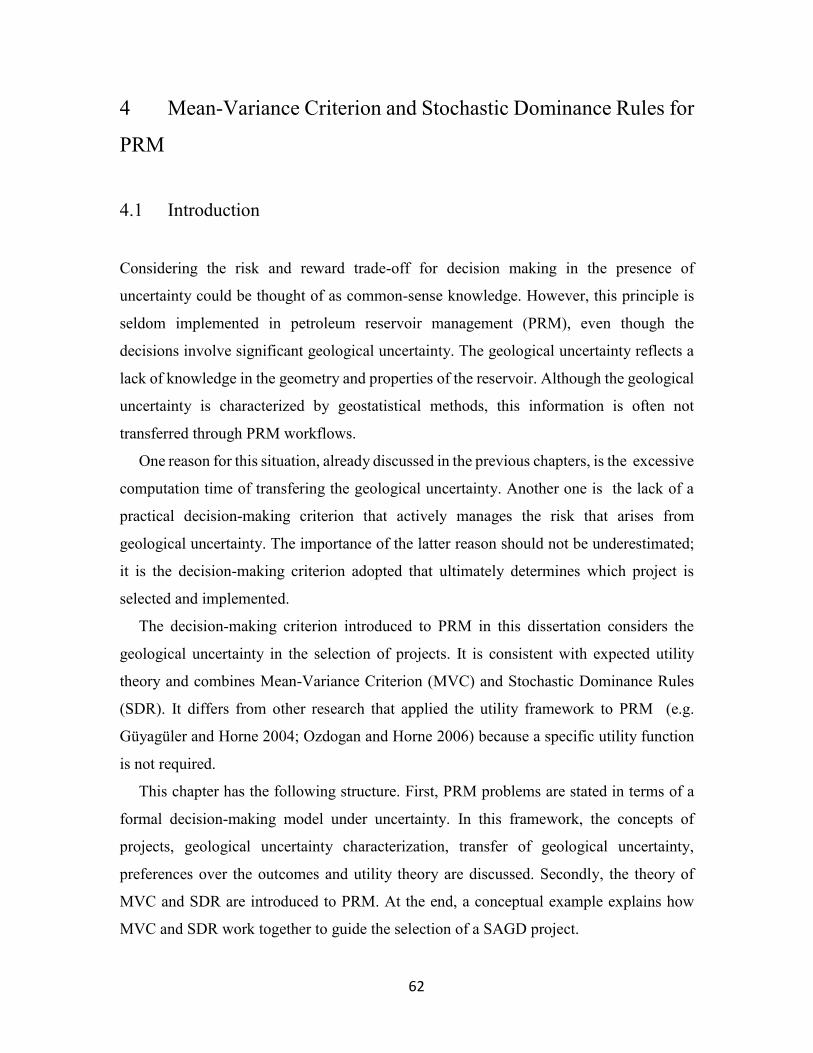
62

4 Mean-Variance Criterion and Stochastic Dominance Rules for

PRM

4.1 Introduction

Considering the risk and reward trade-off for decision making in the presence of

uncertainty could be thought of as common-sense knowledge. However, this principle is

seldom implemented in petroleum reservoir management (PRM), even though the

decisions involve significant geological uncertainty. The geological uncertainty reflects a

lack of knowledge in the geometry and properties of the reservoir. Although the geological

uncertainty is characterized by geostatistical methods, this information is often not

transferred through PRM workflows.

One reason for this situation, already discussed in the previous chapters, is the excessive

computation time of transfering the geological uncertainty. Another one is the lack of a

practical decision-making criterion that actively manages the risk that arises from

geological uncertainty. The importance of the latter reason should not be underestimated;

it is the decision-making criterion adopted that ultimately determines which project is

selected and implemented.

The decision-making criterion introduced to PRM in this dissertation considers the

geological uncertainty in the selection of projects. It is consistent with expected utility

theory and combines Mean-Variance Criterion (MVC) and Stochastic Dominance Rules

(SDR). It differs from other research that applied the utility framework to PRM (e.g.

Güyagüler and Horne 2004; Ozdogan and Horne 2006) because a specific utility function

is not required.

This chapter has the following structure. First, PRM problems are stated in terms of a

formal decision-making model under uncertainty. In this framework, the concepts of

projects, geological uncertainty characterization, transfer of geological uncertainty,

preferences over the outcomes and utility theory are discussed. Secondly, the theory of

MVC and SDR are introduced to PRM. At the end, a conceptual example explains how

MVC and SDR work together to guide the selection of a SAGD project.

63

4.2 Decision-Making Model in Presence of Geological Uncertainty

Figure 4.1 shows a PRM workflow translated to the words of a formal decision-making

model under uncertainty with four elements: a set of feasible actions that represent the

projects from which a choice must be made by the reservoir manager, a set of outcomes

that refers to the consequences of every project under analysis, a preference ordering of the

outcomes and a concept of rationality or decision rules that governs the decision process

(Stirling, 2012). These components are described below.

Figure 4.1: Components of a Petroleum Reservoir Management Decision-Making workflow.

4.2.1 Set of Feasible Actions or Projects.

The set of contender projects from which the reservoir manager must make a choice is the

space of feasible actions of the decision-making model. There are many different types of

projects that a reservoir manager is concerned with including drilling a single producer

well or defining the integrated development of several fields (SPE, 2007). Notwithstanding

the differences, all projects have an intrinsic geological spatial nature.

The spatial nature of the projects leads to a space of feasible actions that is often

extremely high dimensional. For instance, the well location problem in a 3D grid has a

combinatorial nature that even for small cases quickly leads to an intractable number of

configurations. da Cruz (2000) explained how the number of possible combinations of 10

wells in a 30 x 30 grid is in the order of 1029.

The dimension of the space of feasible actions in PRM makes it impractical to perform

an exhaustive global search for selection purposes. Optimization algorithms including

Genetic Algorithms (Goldberg, 1989) and Particle Swarm Optimization (Kennedy &

Geological model

ProjectsTransfer ofgeological

uncertainty

Economicmodel

Decision CriteriaRankedprojects

Set of feasible actions

Set of outcomesRisk-Reward Preferences

Inputs Output

64

Eberhart, 1995) have been studied (Echeverria-Ciurri, Conn, Mello, & Onwunalu, 2012;

Isebor, Echeverría-Ciaurri, & Durlofsky, 2013; H. Wang, Echeverría-Ciaurri, Durlofsky,

& Cominelli, 2012).

In some cases, accepted reservoir engineering principles can eliminate many possible

projects from consideration and thus the set of feasible actions may be a well-defined set

of contenders (Raiffa & Schlaifer, 1961).

4.2.2 Set of Outcomes

The results of the projects cannot be anticipated with certainty because they depend on the

unknown reservoir properties. Defining the set of outcomes requires performing two

complex and demanding tasks, one is to build a geological model and the other is to process

the projects and the geological model through transfer functions (e.g. conventional flow

simulation or APDS) to obtain a probability distribution of the response variable that will

be used to make the decision.

4.2.2.1 The Geological Model

The geological model is a set of geostatistical realizations that taken all together provides

an assessment of the geological uncertainty (Pyrcz & Deutsch, 2014). By construction,

every realization in the geological model is an equally likely to be drawn representation of

the reservoir; and yet, any one realization could never be an accurate representation of the

true reservoir.

The methodology and software to generate geological models of petroleum reservoirs

are mature and well established. An up to the date collection and explanation of the

geostatistical simulation techniques can be found in Pyrcz & Deutsch (2014). There are

other important references devoted to the theory and practice of geostatistics and its

algorithms (Caers, 2011; Chiles & Delfiner, 2012; Deutsch & Journel, 1998; Goovaerts,

1997).

65

4.2.2.2 Transfer of Geological Uncertainty

Transferring the geological uncertainty to a production forecast (that might be later

converted to a monetary value) is achieved by running a full physics flow simulator on

each geostatistical realization with the set of projects being assessed (da Cruz, 2000). An

optimization framework is considered when this comprehensive approach is too

computationally demanding and time consuming.

An alternative to the full physics flow simulator is to run a relatively simpler and faster

flow model such as streamline simulation or a simplified physics model (Pyrcz & Deutsch,

2014). The precision of the results will be compromised but the relative ranking of the

realizations may be preserved. If a good correlation between the response variable obtained

from the alternative method and the result obtained by the full physics dynamic simulator

can be demonstrated, then the cumulative density function of the faster method would be

suitable to assist decision making.

Experimental design and response surfaces (Damsleth, Hage, & Volden, 1992) have

been explored to obtain the distribution of the response variable, but the process requires

careful calibration with the dynamic flow simulator and it is impractical to be used over a

set of realizations. Ranking the realizations through a quick-to-calculate transfer function

and selecting a few representative realizations for post-processing with a more complex

transfer function is a common practice (Pyrcz & Deutsch, 2014), but since all the

realizations are equally probable and any one realization could be misleading this method

should be used very carefully. Computing a static measure such as recoverable

hydrocarbon volume in place or a measure of connectivity of the reservoir-quality rock for

all the realizations is also valuable to understand the global characteristics of the geological

model (Pyrcz & Deutsch, 2014).

4.2.3 Preferences and Concept of Rationality

Preferences and the concept of rationality are the foundation of a decision-making model.

After transferring the geological uncertainty, selecting a project from the set of feasible

66

actions is equivalent to make a choice between the probability distributions of the chosen

response variable (Johnstone & Lindley, 2013).

To make that choice, the investor’s preferences over the space of outcomes can be

encoded in a utility function (Kochenderfer, 2015). A decision maker will make a rational

decision if he chooses a project that maximizes the expected utility. A decision-making

model to support PRM should belong to the utility theory framework to fully take

advantage of the quantification of the geological uncertainty.

The concept of maximum expected value as an optimal criterion for decision making

under uncertainty was proposed by the mathematicians Blaise Pascal and Pierre de Fermat

in the 17th century (Machina, 1987). Although appealing, this criterion does not explain

real decisions under uncertainty, especially with asymmetric consequences of risk

associated with large projects.

The concepts of the utility function and the maximum expected utility were proposed

by Daniel Bernoulli in 1738. However, only in 1947, John von Neumann and Oskar

Morgenstern developed the formal theory of expected utility (Von Neumann &

Morgenstern, 2007). They demonstrated axiomatically that the preferences of a decision

maker can be encoded in a real-valued utility function. Then, a rational decision maker

must act as if their objective is to maximize the expected utility (Johnstone & Lindley,

2013).

In PRM the decision-making problem can be formulated as:

argmax𝑎𝜖𝐴

𝐸[𝑢(𝑥(𝑎, 𝑤))] = argmax𝑎𝜖𝐴

∫ 𝑓(𝑥(𝑎, 𝑤)) ∙ 𝑢(𝑥(𝑎, 𝑤))dx (4.1)

Here, 𝑎 represents projects from the set of feasible actions 𝐴; 𝑤 represents realizations

from the geological model; x(𝑎, 𝑤) represents the payoff calculated after transferring the

geological uncertainty; 𝑓(𝑥(∙)) is the probability density function of 𝑥(∙) and 𝑢(𝑥(∙)) is

the utility function. Equation 4.1 emphasizes that the payoff of 𝑥(∙) depends on the

decisions 𝑎𝜖𝐴 and on the geological uncertainty characterized by a set of geostatistical

realizations 𝑤.

The utility function is difficult to quantify in practice; however, as shown in Figure 4.2,

they can be classified in three groups according to the preferences of the decision maker:

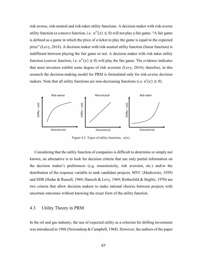
67

risk-averse, risk-neutral and risk-taker utility functions. A decision maker with risk-averse

utility function (a concave function, i.e. 𝑢′′(𝑥) ≤ 0) will not play a fair game. “A fair game

is defined as a game in which the price of a ticket to play the game is equal to the expected

prize” (Levy, 2016). A decision maker with risk-neutral utility function (linear function) is

indifferent between playing the fair game or not. A decision maker with risk-taker utility

function (convex function, i.e. 𝑢′′(𝑥) 0) will play the fair game. The evidence indicates

that most investors exhibit some degree of risk aversion (Levy, 2016); therefore, in this

research the decision-making model for PRM is formulated only for risk-averse decision

makers. Note that all utility functions are non-decreasing functions (i.e. 𝑢′(𝑥) 0).

Figure 4.2: Types of utility functions, 𝑢(𝑥).

Considering that the utility function of companies is difficult to determine or simply not

known, an alternative is to look for decision criteria that use only partial information on

the decision maker’s preferences (e.g. monotonicity, risk aversion, etc.) and/or the

distribution of the response variable to rank candidate projects. MVC (Markowitz, 1959)

and SDR (Hadar & Russell, 1969; Hanoch & Levy, 1969; Rothschild & Stiglitz, 1970) are

two criteria that allow decision makers to make rational choices between projects with

uncertain outcomes without knowing the exact form of the utility function.

4.3 Utility Theory in PRM

In the oil and gas industry, the use of expected utility as a criterion for drilling investment

was introduced in 1968 (Newendorp & Campbell, 1968). However, the authors of the paper

Uti

lity

–u

(x)

Outcome (x) Outcome (x) Outcome (x)

Uti

lity

–u

(x)

Uti

lity

–u

(x)

Risk-averse Risk-takerRisk-neutral

68

commented that implementing utility theory was problematic because there were no

effective methods to construct or determine a decision maker’s utility curve.

This problem remains unsolved. Walls (1995) assumed an exponential utility function,

𝑢(𝑥) = −𝑒−𝑥/𝑅, and proposed inferring the risk tolerance parameter, 𝑅, using an industry

specific questionnaire or by reconstructing the risky alternatives that were selected by the

firm for capital allocations (Walls, 2005). To circumvent the problem of inferring 𝑅, some

authors perform sensitivity analysis over a range of R to evaluate the robustness of the

decisions to different risk attitudes (Güyagüler & Horne, 2004; Ozdogan & Horne, 2006).

Begg, Bratvold, & Campbell (2003) and Bratvold, Begg, & Campbell (2003) provide an

extensive review of utility theory, and introduced indifference curves to portfolio decision-

making in the oil and gas industry. They assumed risk-averse investors with exponential

utility functions in their research.

4.4 Mean Variance Criterion and Stochastic Dominance Rules

MVC and SDR are two approaches for making choices without a complete knowledge of

the decision maker’s utility function (Hadar and Russell 1969). The MVC is the

cornerstone of the construction of Markowitz’s efficient frontier (Markowitz, 1959) in

modern portfolio selection theory. It allows the construction of efficient portfolios based

on the maximization of a function of expected return and of its variability (Levy & Sarnat,

1970). SDR is suitable for ranking response variable distribution functions with limited

information of the decision maker’s preferences.

SDR is superior to MVC when the task is to compare two distributions. SDR is inferior

to the MVC when the task is to construct efficient portfolios by combining individual assets

(Levy, 2016). Note that the optimization algorithm proposed by Markowitz cannot be

applied to the selection of petroleum reservoir projects under geological uncertainty

because they have very limited divisibility. For example, one well cannot be further divided

into smaller parts, therefore it is meaningless to calculate an efficient portfolio containing

fractions of different wells.

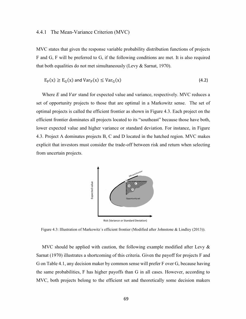
69

4.4.1 The Mean-Variance Criterion (MVC)

MVC states that given the response variable probability distribution functions of projects

F and G, F will be preferred to G, if the following conditions are met. It is also required

that both equalities do not met simultaneously (Levy & Sarnat, 1970).

EF(x) EG(x) and VarF(x) ≤ VarG(x) (4.2)

Where 𝐸 and 𝑉𝑎𝑟 stand for expected value and variance, respectively. MVC reduces a

set of opportunity projects to those that are optimal in a Markowitz sense. The set of

optimal projects is called the efficient frontier as shown in Figure 4.3. Each project on the

efficient frontier dominates all projects located to its “southeast” because those have both,

lower expected value and higher variance or standard deviation. For instance, in Figure

4.3. Project A dominates projects B, C and D located in the hatched region. MVC makes

explicit that investors must consider the trade-off between risk and return when selecting

from uncertain projects.

Figure 4.3: Illustration of Markowitz´s efficient frontier (Modified after Johnstone & Lindley (2013)).

MVC should be applied with caution, the following example modified after Levy &

Sarnat (1970) illustrates a shortcoming of this criteria. Given the payoff for projects F and

G on Table 4.1, any decision maker by common sense will prefer F over G, because having

the same probabilities, F has higher payoffs than G in all cases. However, according to

MVC, both projects belong to the efficient set and theoretically some decision makers

Opportunity setExp

ecte

d v

alu

e

Risk (Variance or Standard Deviation)

A

BC

D

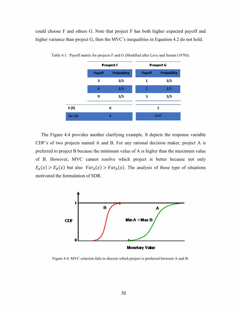
70

could choose F and others G. Note that project F has both higher expected payoff and

higher variance than project G, then the MVC’s inequalities in Equation 4.2 do not hold.

Table 4.1: Payoff matrix for projects F and G (Modified after Levy and Sarnat (1970)).

The Figure 4.4 provides another clarifying example. It depicts the response variable

CDF’s of two projects named A and B. For any rational decision maker, project A is

preferred to project B because the minimum value of A is higher than the maximum value

of B. However, MVC cannot resolve which project is better because not only

𝐸𝐴(𝑥) > 𝐸𝐵(𝑥) but also 𝑉𝑎𝑟𝐴(𝑥) > 𝑉𝑎𝑟𝐵(𝑥). The analysis of these type of situations

motivated the formulation of SDR.

Figure 4.4: MVC criterion fails to discern which project is preferred between A and B.

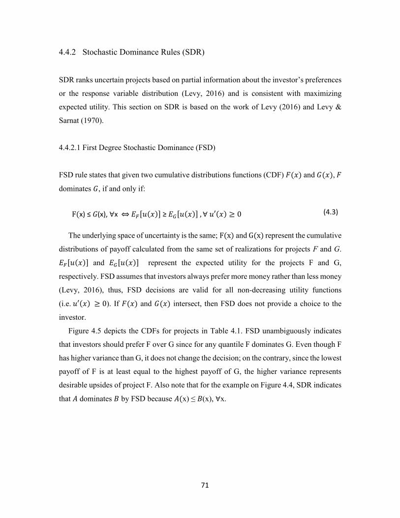
71

4.4.2 Stochastic Dominance Rules (SDR)

SDR ranks uncertain projects based on partial information about the investor’s preferences

or the response variable distribution (Levy, 2016) and is consistent with maximizing

expected utility. This section on SDR is based on the work of Levy (2016) and Levy &

Sarnat (1970).

4.4.2.1 First Degree Stochastic Dominance (FSD)

FSD rule states that given two cumulative distributions functions (CDF) 𝐹(𝑥) and 𝐺(𝑥), 𝐹

dominates 𝐺, if and only if:

F(x) ≤ 𝐺(x), ∀x ⇔𝐸𝐹[𝑢(𝑥)] ≥ 𝐸𝐺[𝑢(𝑥)] , ∀ 𝑢′(𝑥) 0 (4.3)

The underlying space of uncertainty is the same; F(x) and G(x) represent the cumulative

distributions of payoff calculated from the same set of realizations for projects F and G.

𝐸𝐹[𝑢(𝑥)] and 𝐸𝐺[𝑢(𝑥)] represent the expected utility for the projects F and G,

respectively. FSD assumes that investors always prefer more money rather than less money

(Levy, 2016), thus, FSD decisions are valid for all non-decreasing utility functions

(i.e. 𝑢′(𝑥) 0). If 𝐹(𝑥) and 𝐺(𝑥) intersect, then FSD does not provide a choice to the

investor.

Figure 4.5 depicts the CDFs for projects in Table 4.1. FSD unambiguously indicates

that investors should prefer F over G since for any quantile F dominates G. Even though F

has higher variance than G, it does not change the decision; on the contrary, since the lowest

payoff of F is at least equal to the highest payoff of G, the higher variance represents

desirable upsides of project F. Also note that for the example on Figure 4.4, SDR indicates

that 𝐴 dominates 𝐵 by FSD because 𝐴(x) ≤ 𝐵(x), ∀x.

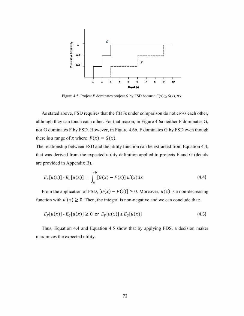
72

Figure 4.5: Project 𝐹 dominates project 𝐺 by FSD because F(x) ≤ 𝐺(x), ∀x.

As stated above, FSD requires that the CDFs under comparison do not cross each other,

although they can touch each other. For that reason, in Figure 4.6a neither F dominates G,

nor G dominates F by FSD. However, in Figure 4.6b, F dominates G by FSD even though

there is a range of 𝑥 where 𝐹(𝑥) = 𝐺(𝑥).

The relationship between FSD and the utility function can be extracted from Equation 4.4,

that was derived from the expected utility definition applied to projects F and G (details

are provided in Appendix B).

𝐸𝐹[𝑢(𝑥)] - 𝐸𝐺[𝑢(𝑥)] = ∫ [𝐺(𝑥) − 𝐹(𝑥)] 𝑢′(𝑥)𝑑𝑥 𝑏

𝑎

(4.4)

From the application of FSD, [𝐺(𝑥) − 𝐹(𝑥)] 0. Moreover, 𝑢(𝑥) is a non-decreasing

function with 𝑢′(𝑥) 0. Then, the integral is non-negative and we can conclude that:

𝐸𝐹[𝑢(𝑥)] - 𝐸𝐺[𝑢(𝑥)] 0 or 𝐸𝐹[𝑢(𝑥)] ≥ 𝐸𝐺[𝑢(𝑥)] (4.5)

Thus, Equation 4.4 and Equation 4.5 show that by applying FDS, a decision maker

maximizes the expected utility.

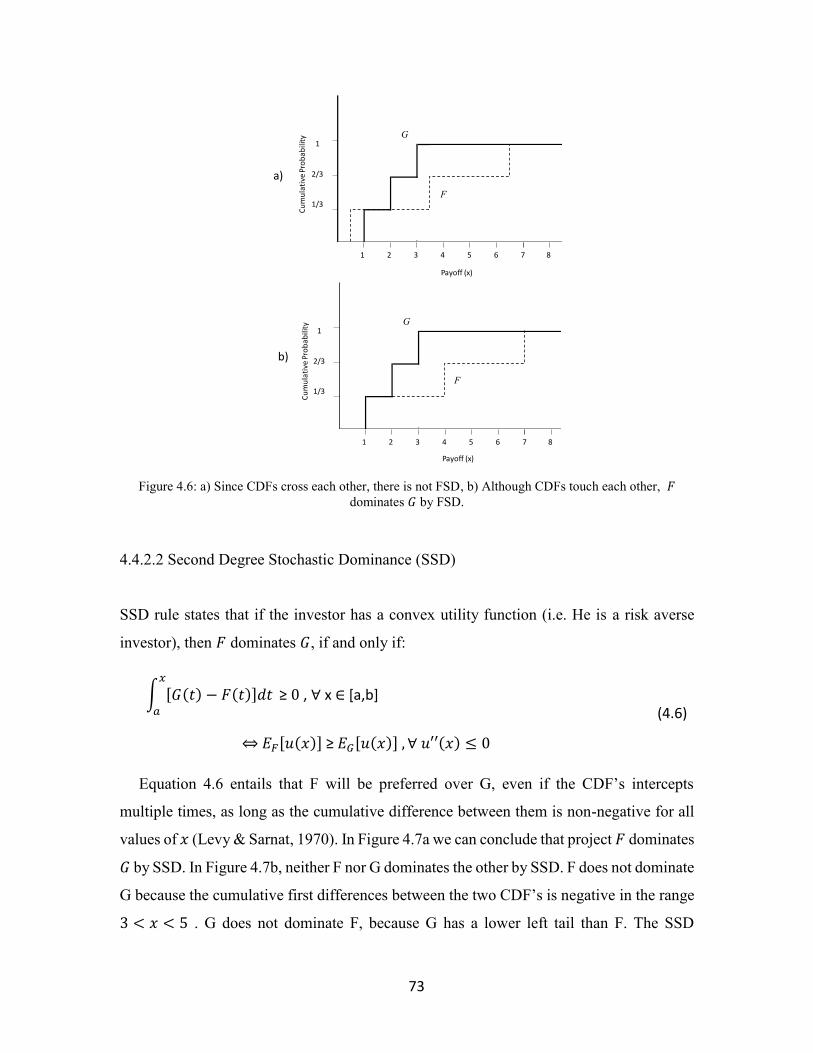
73

Figure 4.6: a) Since CDFs cross each other, there is not FSD, b) Although CDFs touch each other, 𝐹

dominates 𝐺 by FSD.

4.4.2.2 Second Degree Stochastic Dominance (SSD)

SSD rule states that if the investor has a convex utility function (i.e. He is a risk averse

investor), then 𝐹 dominates 𝐺, if and only if:

∫ [𝐺(𝑡) − 𝐹(𝑡)]𝑑𝑡 𝑥

𝑎

≥ 0 , ∀ x ∈ [a,b]

⇔𝐸𝐹[𝑢(𝑥)] ≥ 𝐸𝐺[𝑢(𝑥)] , ∀ 𝑢′′(𝑥) ≤ 0

(4.6)

Equation 4.6 entails that F will be preferred over G, even if the CDF’s intercepts

multiple times, as long as the cumulative difference between them is non-negative for all

values of 𝑥 (Levy & Sarnat, 1970). In Figure 4.7a we can conclude that project 𝐹 dominates

𝐺 by SSD. In Figure 4.7b, neither F nor G dominates the other by SSD. F does not dominate

G because the cumulative first differences between the two CDF’s is negative in the range

3 𝑥 5 . G does not dominate F, because G has a lower left tail than F. The SSD

G

F

1

2/3

1/3

1 2 3 4 5 6 7 8

Cu

mu

lati

ve P

rob

abili

ty

Payoff (x)

F

G

F

1

2/3

1/3

1 2 3 4 5 6 7 8

Cu

mu

lati

ve P

rob

abili

ty

Payoff (x)

F

a)

b)

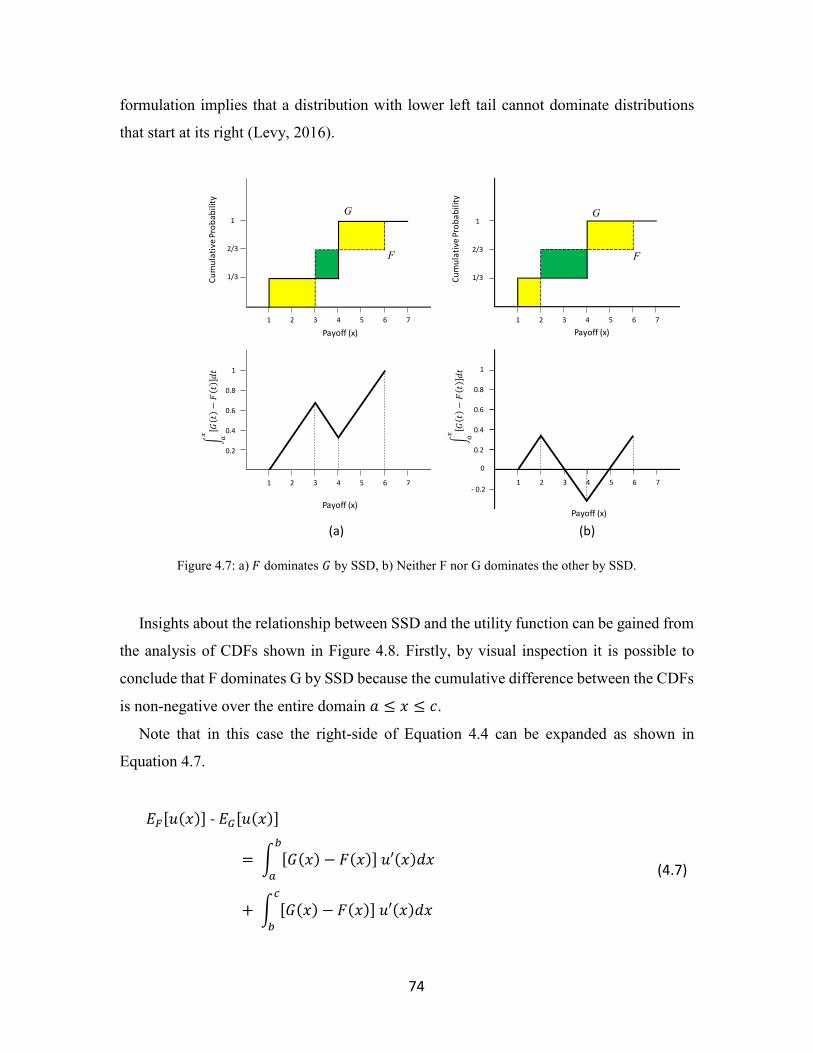
74

formulation implies that a distribution with lower left tail cannot dominate distributions

that start at its right (Levy, 2016).

Figure 4.7: a) 𝐹 dominates 𝐺 by SSD, b) Neither F nor G dominates the other by SSD.

Insights about the relationship between SSD and the utility function can be gained from

the analysis of CDFs shown in Figure 4.8. Firstly, by visual inspection it is possible to

conclude that F dominates G by SSD because the cumulative difference between the CDFs

is non-negative over the entire domain 𝑎 ≤ 𝑥 ≤ 𝑐.

Note that in this case the right-side of Equation 4.4 can be expanded as shown in

Equation 4.7.

𝐸𝐹[𝑢(𝑥)] - 𝐸𝐺[𝑢(𝑥)]

= ∫ [𝐺(𝑥) − 𝐹(𝑥)] 𝑢′(𝑥)𝑑𝑥 𝑏

𝑎

+ ∫ [𝐺(𝑥) − 𝐹(𝑥)] 𝑢′(𝑥)𝑑𝑥 𝑐

𝑏

(4.7)

1 2 3 4 5 6 7

1 2 3 4 5 6 7

1

2/3

1/3

1

0.8

0.6

0.4

0.2

Cu

mu

lati

ve P

rob

abili

ty

Payoff (x)

Payoff (x)

∫𝐺𝑡−𝐹𝑡𝑑𝑡

𝑥

𝑎

G

F

(a)

1 2 3 4 5 6 7

1 2 3 4 5 6 7

1

2/3

1/3

1

0.8

0.6

0.4

0.2

- 0.2

0

Cu

mu

lati

ve P

rob

ab

ility

Payoff (x)

Payoff (x)


𝑥 𝑎

G

F

(b)

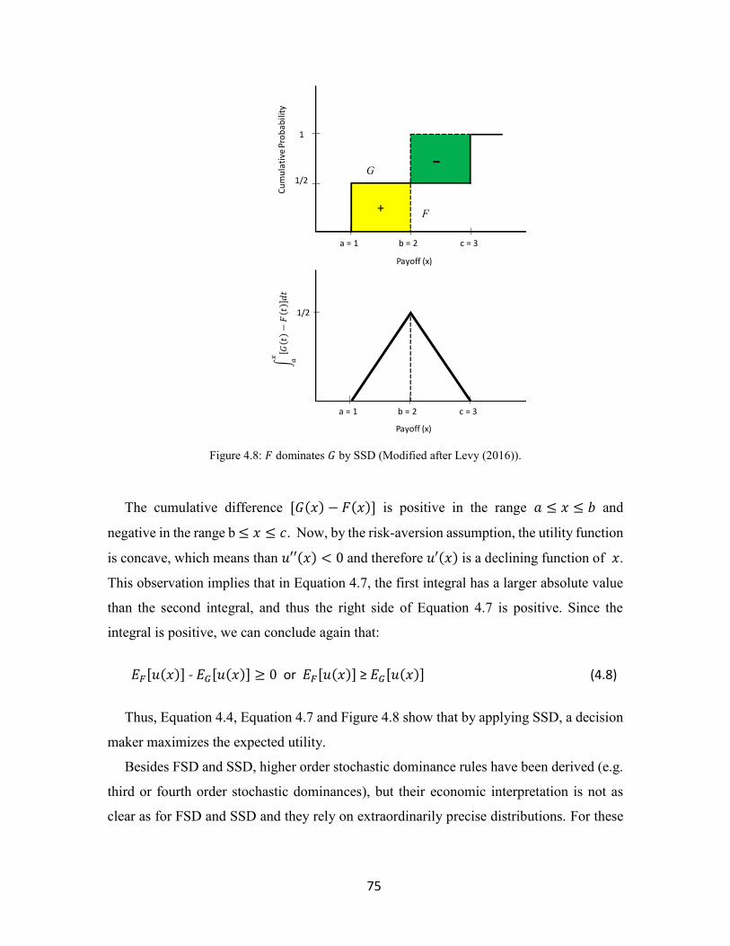
75

Figure 4.8: 𝐹 dominates 𝐺 by SSD (Modified after Levy (2016)).

The cumulative difference [𝐺(𝑥) − 𝐹(𝑥)] is positive in the range 𝑎 ≤ 𝑥 ≤ 𝑏 and

negative in the range b ≤ 𝑥 ≤ 𝑐. Now, by the risk-aversion assumption, the utility function

is concave, which means than 𝑢′′(𝑥) 0 and therefore 𝑢′(𝑥) is a declining function of 𝑥.

This observation implies that in Equation 4.7, the first integral has a larger absolute value

than the second integral, and thus the right side of Equation 4.7 is positive. Since the

integral is positive, we can conclude again that:

𝐸𝐹[𝑢(𝑥)] - 𝐸𝐺[𝑢(𝑥)] 0 or 𝐸𝐹[𝑢(𝑥)] ≥ 𝐸𝐺[𝑢(𝑥)] (4.8)

Thus, Equation 4.4, Equation 4.7 and Figure 4.8 show that by applying SSD, a decision

maker maximizes the expected utility.

Besides FSD and SSD, higher order stochastic dominance rules have been derived (e.g.

third or fourth order stochastic dominances), but their economic interpretation is not as

clear as for FSD and SSD and they rely on extraordinarily precise distributions. For these

Cu

mu

lati

ve P

rob

abili

ty

G

F+

-

Payoff (x)

a = 1 b = 2 c = 3

1

1/2

Payoff (x)

a = 1 b = 2 c = 3


𝑥

𝑎

1/2

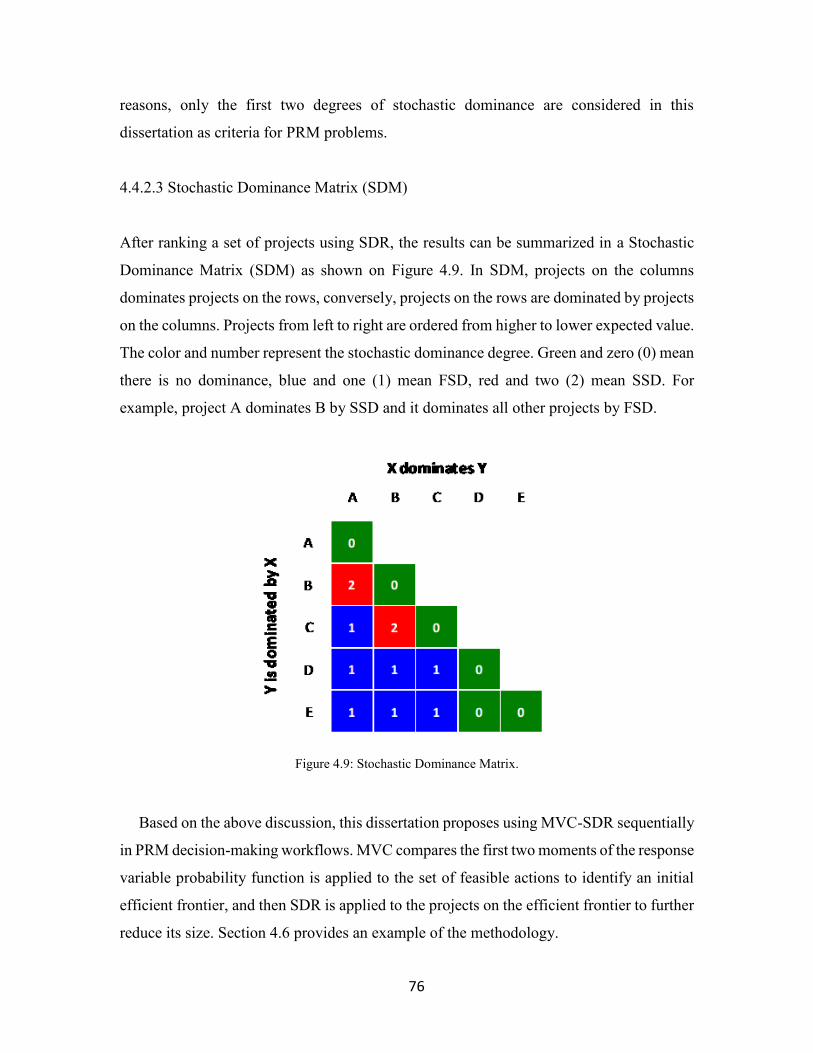
76

reasons, only the first two degrees of stochastic dominance are considered in this

dissertation as criteria for PRM problems.

4.4.2.3 Stochastic Dominance Matrix (SDM)

After ranking a set of projects using SDR, the results can be summarized in a Stochastic

Dominance Matrix (SDM) as shown on Figure 4.9. In SDM, projects on the columns

dominates projects on the rows, conversely, projects on the rows are dominated by projects

on the columns. Projects from left to right are ordered from higher to lower expected value.

The color and number represent the stochastic dominance degree. Green and zero (0) mean

there is no dominance, blue and one (1) mean FSD, red and two (2) mean SSD. For

example, project A dominates B by SSD and it dominates all other projects by FSD.

Figure 4.9: Stochastic Dominance Matrix.

Based on the above discussion, this dissertation proposes using MVC-SDR sequentially

in PRM decision-making workflows. MVC compares the first two moments of the response

variable probability function is applied to the set of feasible actions to identify an initial

efficient frontier, and then SDR is applied to the projects on the efficient frontier to further

reduce its size. Section 4.6 provides an example of the methodology.

77

4.5 MVC and SDR in PRM

In the oil and gas industry, portfolio theory optimization (Markowitz, 1959) that is based

on MVC was proposed to support budget allocations and investment/divestment decisions

that result in efficient portfolios of assets (Bratvold et al., 2003; Edwards, 1993). However,

while this method developed for financial instruments is readily applicable to assets, it

cannot be used directly to solve project selection problems in the presence of geological

uncertainty. Capolei, Suwartadi, Foss, & Jørgensen (2015) implemented an objective

function based on MVC to identify the efficient frontier of a production optimization

problem in the presence of geological uncertainty and suggested the Sharpe ratio to trade-

off risk and return. The efficient frontier in their work represents different operational

strategies to maximize the net present value (NPV) of a waterflooding project. In the case

study, they reported the issue that the strategy obtained with MVC and the Sharpe ratio has

a maximum NPV that was smaller than the minimum NPV of one competing strategy in

the efficient frontier. Chang, Bouzarkouna, & Devegowda (2015) implemented a mean-

variance approach to find the solution of well placement problems considering geological

uncertainty. They obtained an efficient frontier but did not try to further reduce its size. As

far as the author knows, MVC-SDR have not been previously implemented to solve PRM

problems.

4.6 Example of MVC-SDR Methodology

This example is designed to explain the MVC-SDR methodology step by step. The next

chapter presents a realistic case-study that integrates APDS to MVC-SDR to guide the

solution of a representative SAGD problem commonly found in the exploitation of oil

sands.

Consider the problem of selecting one SAGD well-pad to be drilled from a set of thirteen

possible options illustrated in Figure 4.10. It is assumed that a geological model is available

and that the probability density function (PDF) of the response variable (net present value

in this case) is also available by transferring the geological uncertainty through flow

simulation (or APDS) and economic modeling for every realization for all well pads.

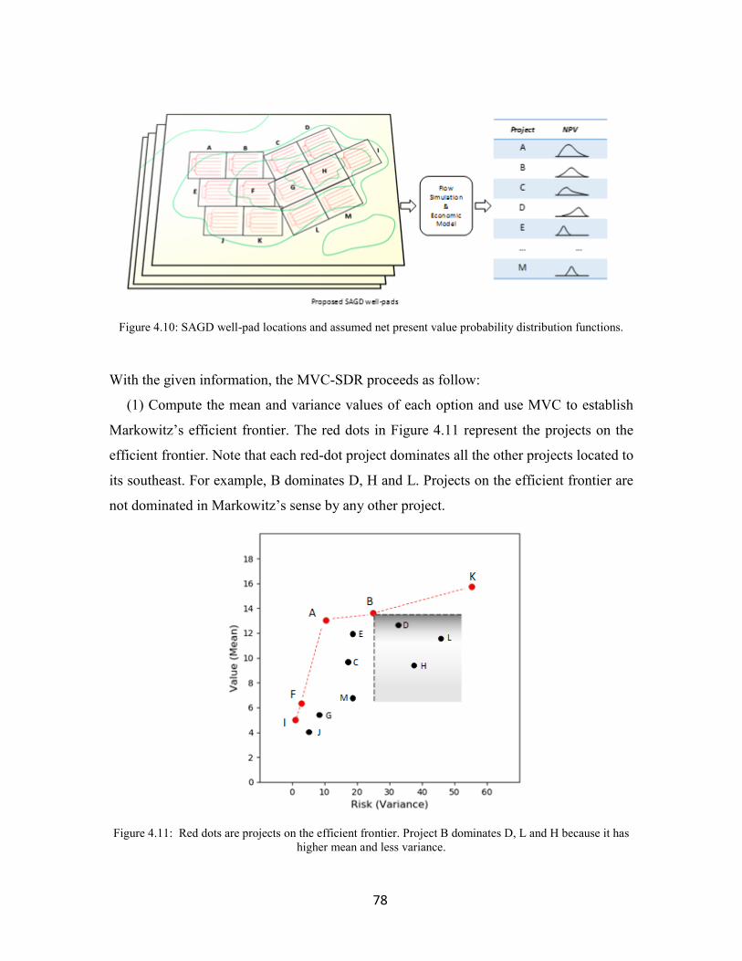
78

Figure 4.10: SAGD well-pad locations and assumed net present value probability distribution functions.

With the given information, the MVC-SDR proceeds as follow:

(1) Compute the mean and variance values of each option and use MVC to establish

Markowitz’s efficient frontier. The red dots in Figure 4.11 represent the projects on the

efficient frontier. Note that each red-dot project dominates all the other projects located to

its southeast. For example, B dominates D, H and L. Projects on the efficient frontier are

not dominated in Markowitz’s sense by any other project.

Figure 4.11: Red dots are projects on the efficient frontier. Project B dominates D, L and H because it has

higher mean and less variance.

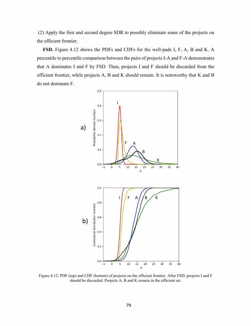
79

(2) Apply the first and second degree SDR to possibly eliminate some of the projects on

the efficient frontier.

FSD. Figure 4.12 shows the PDFs and CDFs for the well-pads I, F, A, B and K. A

percentile to percentile comparison between the pairs of projects I-A and F-A demonstrates

that A dominates I and F by FSD. Then, projects I and F should be discarded from the

efficient frontier, while projects A, B and K should remain. It is noteworthy that K and B

do not dominate F.

Figure 4.12: PDF (top) and CDF (bottom) of projects on the efficient frontier. After FSD, projects I and F

should be discarded. Projects A, B and K remain in the efficient set.

F A

B

K

I F A B K

I

a)

b)

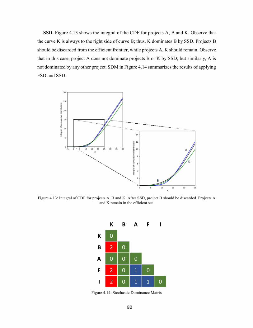
80

SSD. Figure 4.13 shows the integral of the CDF for projects A, B and K. Observe that

the curve K is always to the right side of curve B; thus, K dominates B by SSD. Projects B

should be discarded from the efficient frontier, while projects A, K should remain. Observe

that in this case, project A does not dominate projects B or K by SSD; but similarly, A is

not dominated by any other project. SDM in Figure 4.14 summarizes the results of applying

FSD and SSD.

Figure 4.13: Integral of CDF for projects A, B and K. After SSD, project B should be discarded. Projects A

and K remain in the efficient set.

Figure 4.14: Stochastic Dominance Matrix

K B A F I

K 0

B 2 0

A 0 0 0

F 2 0 1 0

I 2 0 1 1 0

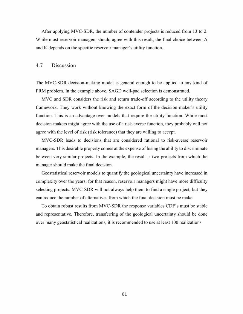
81

After applying MVC-SDR, the number of contender projects is reduced from 13 to 2.

While most reservoir managers should agree with this result, the final choice between A

and K depends on the specific reservoir manager’s utility function.

4.7 Discussion

The MVC-SDR decision-making model is general enough to be applied to any kind of

PRM problem. In the example above, SAGD well-pad selection is demonstrated.

MVC and SDR considers the risk and return trade-off according to the utility theory

framework. They work without knowing the exact form of the decision-maker’s utility

function. This is an advantage over models that require the utility function. While most

decision-makers might agree with the use of a risk-averse function, they probably will not

agree with the level of risk (risk tolerance) that they are willing to accept.

MVC-SDR leads to decisions that are considered rational to risk-averse reservoir

managers. This desirable property comes at the expense of losing the ability to discriminate

between very similar projects. In the example, the result is two projects from which the

manager should make the final decision.

Geostatistical reservoir models to quantify the geological uncertainty have increased in

complexity over the years; for that reason, reservoir managers might have more difficulty

selecting projects. MVC-SDR will not always help them to find a single project, but they

can reduce the number of alternatives from which the final decision must be make.

To obtain robust results from MVC-SDR the response variables CDF’s must be stable

and representative. Therefore, transferring of the geological uncertainty should be done

over many geostatistical realizations, it is recommended to use at least 100 realizations.

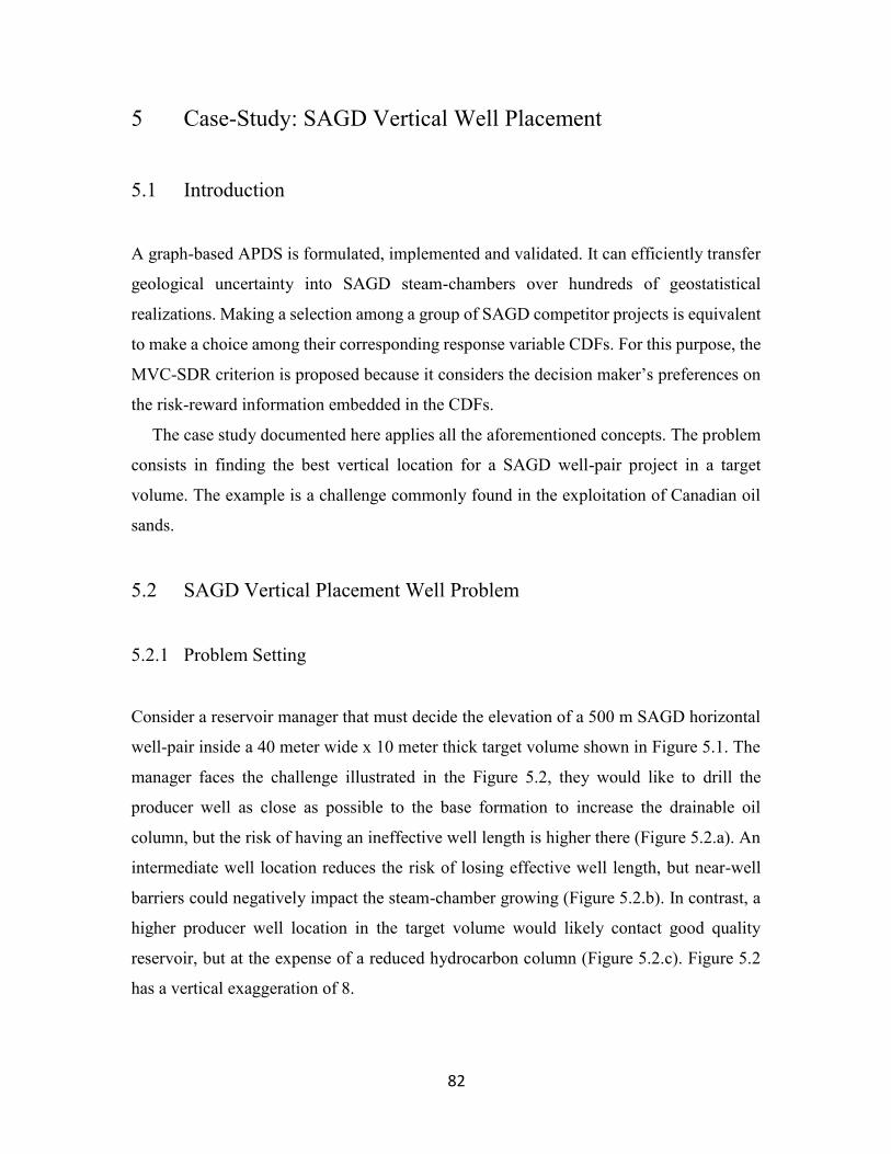
82

5 Case-Study: SAGD Vertical Well Placement

5.1 Introduction

A graph-based APDS is formulated, implemented and validated. It can efficiently transfer

geological uncertainty into SAGD steam-chambers over hundreds of geostatistical

realizations. Making a selection among a group of SAGD competitor projects is equivalent

to make a choice among their corresponding response variable CDFs. For this purpose, the

MVC-SDR criterion is proposed because it considers the decision maker’s preferences on

the risk-reward information embedded in the CDFs.

The case study documented here applies all the aforementioned concepts. The problem

consists in finding the best vertical location for a SAGD well-pair project in a target

volume. The example is a challenge commonly found in the exploitation of Canadian oil

sands.

5.2 SAGD Vertical Placement Well Problem

5.2.1 Problem Setting

Consider a reservoir manager that must decide the elevation of a 500 m SAGD horizontal

well-pair inside a 40 meter wide x 10 meter thick target volume shown in Figure 5.1. The

manager faces the challenge illustrated in the Figure 5.2, they would like to drill the

producer well as close as possible to the base formation to increase the drainable oil

column, but the risk of having an ineffective well length is higher there (Figure 5.2.a). An

intermediate well location reduces the risk of losing effective well length, but near-well

barriers could negatively impact the steam-chamber growing (Figure 5.2.b). In contrast, a

higher producer well location in the target volume would likely contact good quality

reservoir, but at the expense of a reduced hydrocarbon column (Figure 5.2.c). Figure 5.2

has a vertical exaggeration of 8.

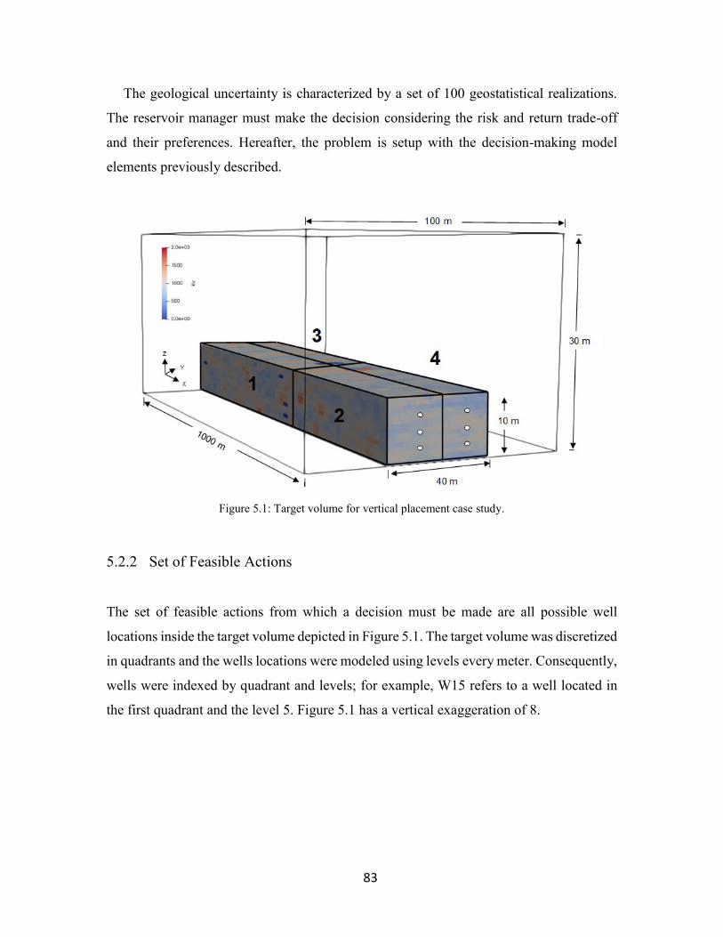
83

The geological uncertainty is characterized by a set of 100 geostatistical realizations.

The reservoir manager must make the decision considering the risk and return trade-off

and their preferences. Hereafter, the problem is setup with the decision-making model

elements previously described.

Figure 5.1: Target volume for vertical placement case study.

5.2.2 Set of Feasible Actions

The set of feasible actions from which a decision must be made are all possible well

locations inside the target volume depicted in Figure 5.1. The target volume was discretized

in quadrants and the wells locations were modeled using levels every meter. Consequently,

wells were indexed by quadrant and levels; for example, W15 refers to a well located in

the first quadrant and the level 5. Figure 5.1 has a vertical exaggeration of 8.

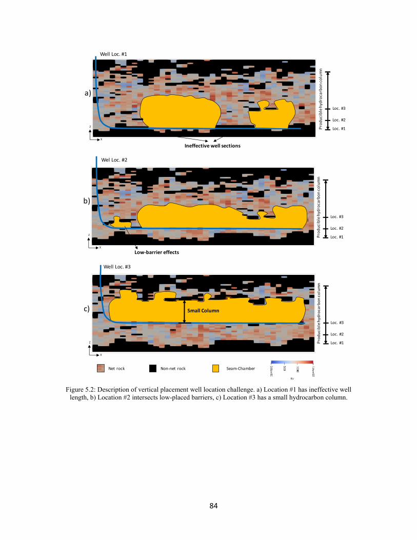
84

Figure 5.2: Description of vertical placement well location challenge. a) Location #1 has ineffective well

length, b) Location #2 intersects low-placed barriers, c) Location #3 has a small hydrocarbon column.

X

Z

Non-net rockNet rock

X

Z

X

Z

Seam-Chamber

Ineffective well sections

Wel Loc. #2

Well Loc. #1

Pro

du

cib

le h

ydro

carb

on

co

lum

n

Well Loc. #3

Loc. #1

Loc. #2

Loc. #3

Low-barrier effects

Small Column

Pro

du

cib

le h

ydro

carb

on

co

lum

n

Loc. #1

Loc. #2

Loc. #3

Pro

du

cib

le h

ydro

carb

on

co

lum

n

Loc. #1

Loc. #2

Loc. #3

a)

b)

c)

85


The geological model with 100 reservoir realizations is described in Section 3.4.1. Figure

5.3 shows some cross-sections through the target volume from different geostatistical

realizations.

Figure 5.3: Cross-section through the target volume on several geostatistical realizations.

5.2.4 Transffering the Geological Uncertainty with APDS

APDS was used to transfer the geological uncertainty. After modeling the steam-chamber

for 5 years, the heated hydrocarbon volume (also called heated steam-chamber volume -

SCHV) was calculated and converted to a monetary value using a net present value per

barrel (NPV/bbl) of 5 US$/bbl. The NPV/bbl is based on the supply costs study for a 30,000

BPD SAGD project published by the Canadian Energy Research Institute (CERI, 2018)

and assuming a WTI price of 65 US$/bbl. The typical design parameters of a 30,000 BPD

SAGD project with its supply cost summary are reported in Tables 5.1 and 5.2 (CERI,

2018) , respectively.

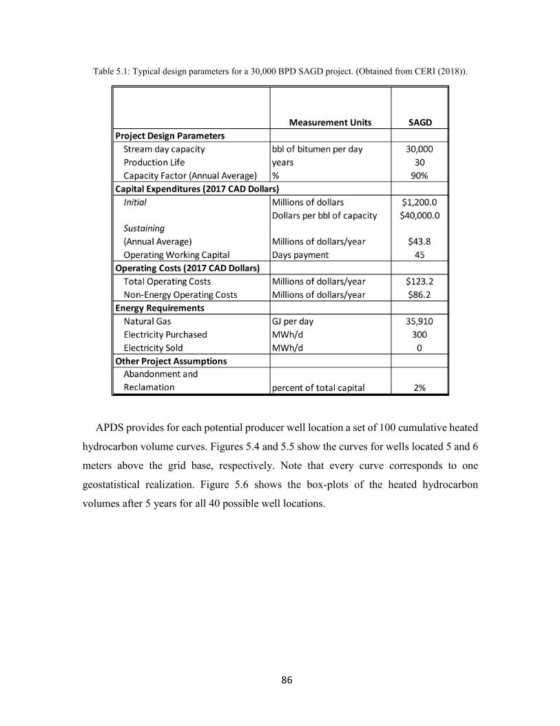
86

Table 5.1: Typical design parameters for a 30,000 BPD SAGD project. (Obtained from CERI (2018)).

APDS provides for each potential producer well location a set of 100 cumulative heated

hydrocarbon volume curves. Figures 5.4 and 5.5 show the curves for wells located 5 and 6

meters above the grid base, respectively. Note that every curve corresponds to one

geostatistical realization. Figure 5.6 shows the box-plots of the heated hydrocarbon

volumes after 5 years for all 40 possible well locations.

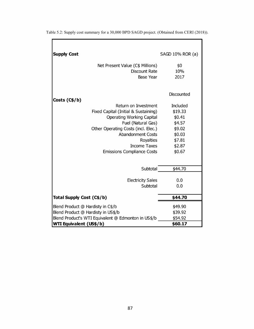
87

Table 5.2: Supply cost summary for a 30,000 BPD SAGD project. (Obtained from CERI (2018)).

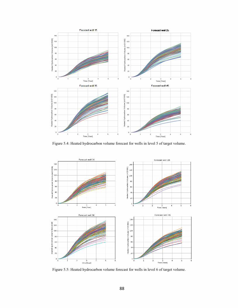
88

Figure 5.4: Heated hydrocarbon volume forecast for wells in level 5 of target volume.

Figure 5.5: Heated hydrocarbon volume forecast for wells in level 6 of target volume.

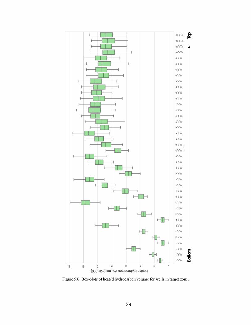
89

Figure 5.6: Box-plots of heated hydrocarbon volume for wells in target zone.

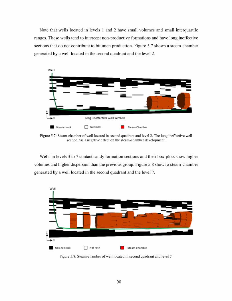
90

Note that wells located in levels 1 and 2 have small volumes and small interquartile

ranges. These wells tend to intercept non-productive formations and have long ineffective

sections that do not contribute to bitumen production. Figure 5.7 shows a steam-chamber

generated by a well located in the second quadrant and the level 2.

Figure 5.7: Steam-chamber of well located in second quadrant and level 2. The long ineffective well

section has a negative effect on the steam-chamber development.

Wells in levels 3 to 7 contact sandy formation sections and their box-plots show higher

volumes and higher dispersion than the previous group. Figure 5.8 shows a steam-chamber

generated by a well located in the second quadrant and the level 7.

Figure 5.8: Steam-chamber of well located in second quadrant and level 7.

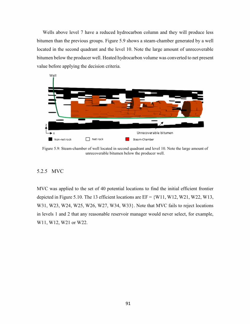
91

Wells above level 7 have a reduced hydrocarbon column and they will produce less

bitumen than the previous groups. Figure 5.9 shows a steam-chamber generated by a well

located in the second quadrant and the level 10. Note the large amount of unrecoverable

bitumen below the producer well. Heated hydrocarbon volume was converted to net present

value before applying the decision criteria.

Figure 5.9: Steam-chamber of well located in second quadrant and level 10. Note the large amount of

unrecoverable bitumen below the producer well.

5.2.5 MVC

MVC was applied to the set of 40 potential locations to find the initial efficient frontier

depicted in Figure 5.10. The 13 efficient locations are EF = {W11, W12, W21, W22, W13,

W31, W23, W24, W25, W26, W27, W34, W33}. Note that MVC fails to reject locations

in levels 1 and 2 that any reasonable reservoir manager would never select, for example,

W11, W12, W21 or W22.

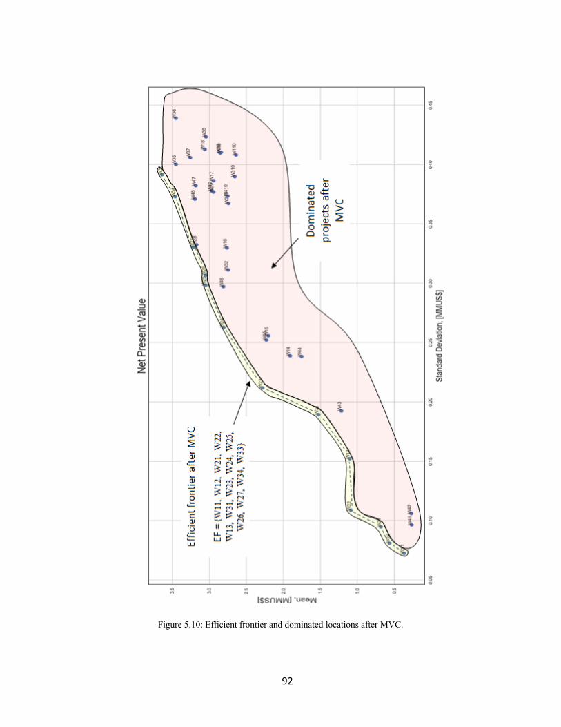
92

Figure 5.10: Efficient frontier and dominated locations after MVC.

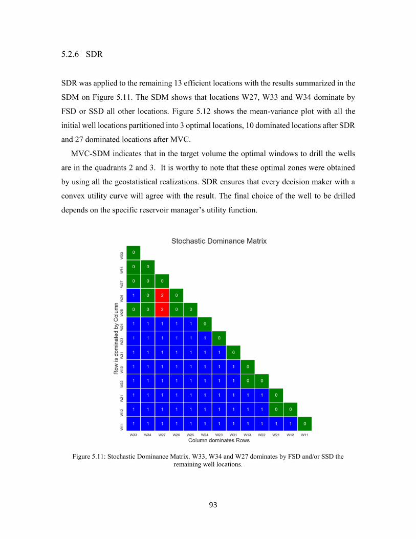
93

5.2.6 SDR

SDR was applied to the remaining 13 efficient locations with the results summarized in the

SDM on Figure 5.11. The SDM shows that locations W27, W33 and W34 dominate by

FSD or SSD all other locations. Figure 5.12 shows the mean-variance plot with all the

initial well locations partitioned into 3 optimal locations, 10 dominated locations after SDR

and 27 dominated locations after MVC.

MVC-SDM indicates that in the target volume the optimal windows to drill the wells

are in the quadrants 2 and 3. It is worthy to note that these optimal zones were obtained

by using all the geostatistical realizations. SDR ensures that every decision maker with a

convex utility curve will agree with the result. The final choice of the well to be drilled

depends on the specific reservoir manager’s utility function.

Figure 5.11: Stochastic Dominance Matrix. W33, W34 and W27 dominates by FSD and/or SSD the

remaining well locations.

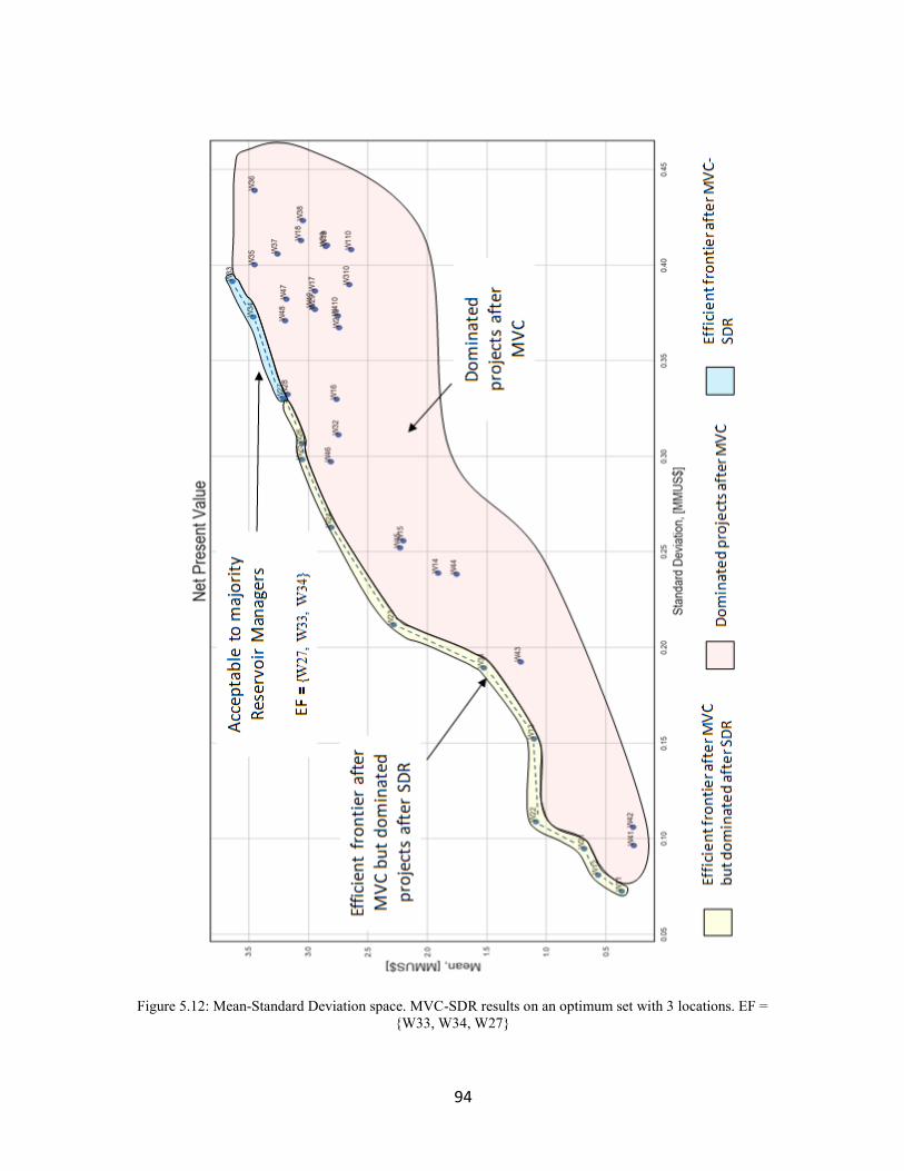
94

Figure 5.12: Mean-Standard Deviation space. MVC-SDR results on an optimum set with 3 locations. EF =

{W33, W34, W27}

95

5.3 Computational Time

40 potential well locations were assessed through the entire set of 100 geostatistical

realizations resulting in a total of 4,000 steam-chamber models. The current APDS Python

prototype runs the case-study in 13 hours, which is an average time of 11.7 seconds per

steam-chamber modeled.

The analysis benefited from the modular design of the algorithm, because the graphs

had been already generated for the validation study presented in Section 3.4. Moreover,

considering that the standard operation of a SAGD well-pair is around 10 years (Zhao,

Law, & Coates, 2003), additional computational time was saved by modeling the steam-

chamber only for 15 years.

5.4 Discussion

This case study shows that the combined MVC-SDR criterion is viable for decision making

under geological uncertainty. It also confirms that APDS is an efficient transfer function

for SAGD projects.

In the example, MVC-SDR reduced the initial set from 40 candidate well locations to 3

possible well locations. The final set of locations should be acceptable to risk-averse

reservoir managers given the reward-risk trade-off preference assumptions underlying the

formulation of the MVC-SDR criterion. The definitive selection of a single location

requires knowing the particular reservoir manager’s utility function.

The examples presented in this case study and in Section 4.6 make manifest that the

MVC-SDR criterion do not always lead to a single project; for that reason, the criterion are

primarily applicable to problems with a well-defined finite set of decision options. It is not

suitable for problems that use optimization algorithms for searching extremely large

combinatorial decision spaces.

The workflow presented in this case study can also be applied to solve other SAGD

problems, such as selecting the length and orientation of the producer-injector well-pair or

analyzing the producer-injector inter-well distance.

96

Regarding computational time, the APDS prototype took on average 11.7 seconds to

model each steam-chamber without using parallel computing. This processing time appears

encouraging to undertake problems with larger finite decision spaces. However, is not yet

efficient enough to embed APDS into an closed-loop field optimization work flow (e.g.

Echeverria-Ciurri et al. 2012; Wang et al. 2012; Shirangi and Durlofsky 2015). It is

recommended to look for substantial efficiency gains in the scale of 1-3 additional orders

of magnitude compared to a conventional thermal flow simulator. The obvious first step is

to use a compiled language such as C, C++, C# or Fortran and to take advantage of the

graphs staying very similar for small changes in well locations.

97

6 Case Study: SAGD Reservoir Characterization with APDS

6.1 Introduction

The APDS capability of modeling the steam-chamber propagation, that is the dynamic

response of the reservoir to the steam injection, motivates using APDS as a companion tool

of methodologies for 4D-seismic data integration in SAGD reservoir characterization.

Time-lapse seismic, or 4D-seismic, is an important source of dynamic data for

monitoring heavy-oil reservoirs. It captures changes in the subsurface conditions caused

by SAGD operations that are reliable manifestations of the steam-chamber presence. The

analysis of seismic attributes recorded at different times might reveal anomalies by the

absence or unexpected location of the steam that can be enforced into geostatistical

realizations to improve reservoir characterization (Hadavand & Deutsch, 2017).

A practical methodology for enforcing these anomalies in geostatistical reservoir

models was proposed by Hadavand & Deutsch (2017). They implemented the technique

on a real SAGD project located in the Athabasca region, northeastern Alberta, Canada

(Hadavand et al., 2018). Assessing the effect of the geostatistical-anomaly enforcement

methodology requires comparing the estimation of the steam-chamber before and after

applying the enforcement through all the geostatistical realizations. This procedure cannot

be performed with full physics thermal flow simulators due its computational cost.

However, APDS is efficient enough to perform this task and serve as a tool for assisting

4D-seismic integration in SAGD reservoir characterization.

Additionally, this case study uses a high resolution realistic geological model that

represents the fluvial and estuarine depositional system of the McMurray (Ranger &

Gingras, 2010). It exhibits sectors of blocky clean sands with horizontal barriers/baffles of

different lengths, and sectors with heterogeneous inclined layers alternating shale and

sands. The complexity of the reservoir model illustrates how APDS handles complex

geological settings.

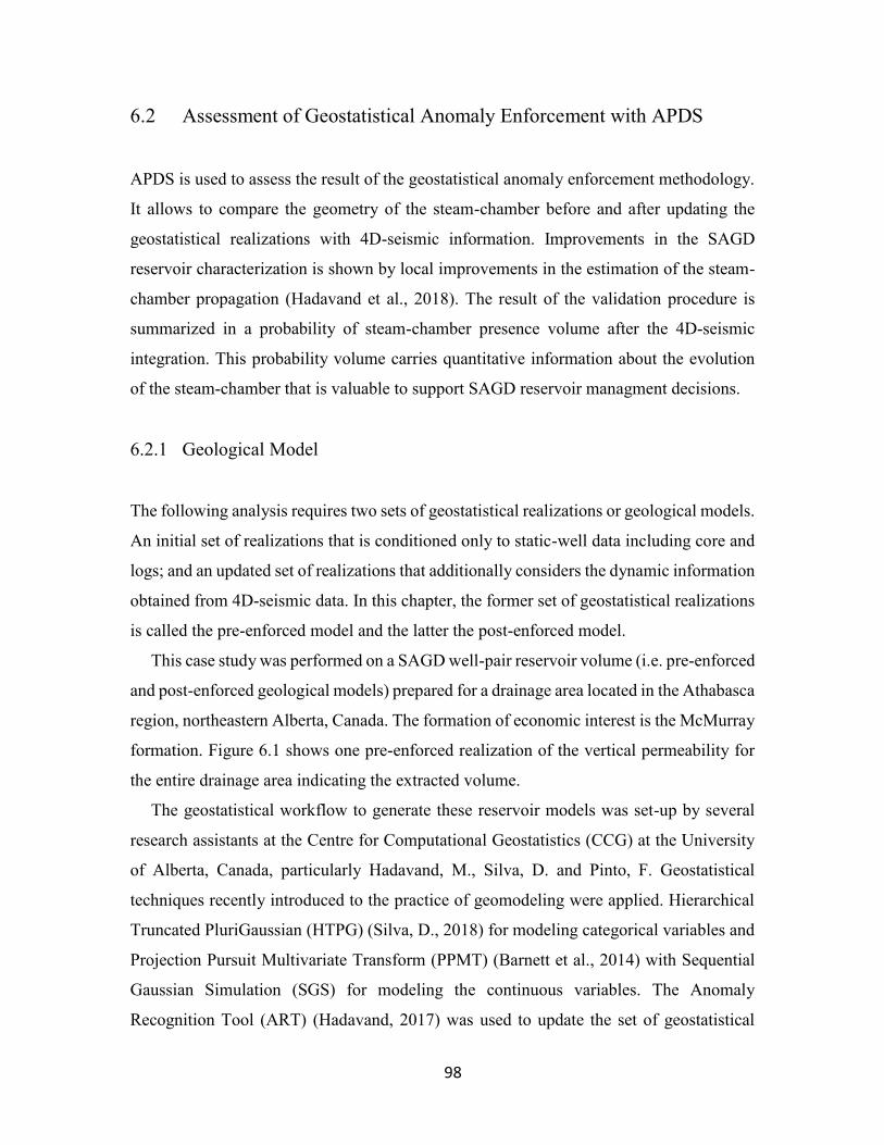
98

6.2 Assessment of Geostatistical Anomaly Enforcement with APDS

APDS is used to assess the result of the geostatistical anomaly enforcement methodology.

It allows to compare the geometry of the steam-chamber before and after updating the

geostatistical realizations with 4D-seismic information. Improvements in the SAGD

reservoir characterization is shown by local improvements in the estimation of the steam-

chamber propagation (Hadavand et al., 2018). The result of the validation procedure is

summarized in a probability of steam-chamber presence volume after the 4D-seismic

integration. This probability volume carries quantitative information about the evolution

of the steam-chamber that is valuable to support SAGD reservoir managment decisions.


The following analysis requires two sets of geostatistical realizations or geological models.

An initial set of realizations that is conditioned only to static-well data including core and

logs; and an updated set of realizations that additionally considers the dynamic information

obtained from 4D-seismic data. In this chapter, the former set of geostatistical realizations

is called the pre-enforced model and the latter the post-enforced model.

This case study was performed on a SAGD well-pair reservoir volume (i.e. pre-enforced

and post-enforced geological models) prepared for a drainage area located in the Athabasca

region, northeastern Alberta, Canada. The formation of economic interest is the McMurray

formation. Figure 6.1 shows one pre-enforced realization of the vertical permeability for

the entire drainage area indicating the extracted volume.

The geostatistical workflow to generate these reservoir models was set-up by several

research assistants at the Centre for Computational Geostatistics (CCG) at the University

of Alberta, Canada, particularly Hadavand, M., Silva, D. and Pinto, F. Geostatistical

techniques recently introduced to the practice of geomodeling were applied. Hierarchical

Truncated PluriGaussian (HTPG) (Silva, D., 2018) for modeling categorical variables and

Projection Pursuit Multivariate Transform (PPMT) (Barnett et al., 2014) with Sequential

Gaussian Simulation (SGS) for modeling the continuous variables. The Anomaly

Recognition Tool (ART) (Hadavand, 2017) was used to update the set of geostatistical

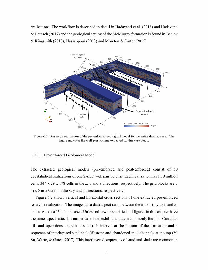
99

realizations. The workflow is described in detail in Hadavand et al. (2018) and Hadavand

& Deutsch (2017) and the geological setting of the McMurray formation is found in Baniak

& Kingsmith (2018), Hassanpour (2013) and Moreton & Carter (2015).

Figure 6.1: Reservoir realization of the pre-enforced geological model for the entire drainage area. The

figure indicates the well-pair volume extracted for this case study.

6.2.1.1 Pre-enforced Geological Model

The extracted geological models (pre-enforced and post-enforced) consist of 50

geostatistical realizations of one SAGD well pair volume. Each realization has 1.78 million

cells: 344 x 29 x 178 cells in the x, y and z directions, respectively. The grid blocks are 5

m x 5 m x 0.5 m in the x, y and z directions, respectively.

Figure 6.2 shows vertical and horizontal cross-sections of one extracted pre-enforced

reservoir realization. The image has a data aspect ratio between the x-axis to y-axis and x-

axis to z-axis of 5 in both cases. Unless otherwise specified, all figures in this chapter have

the same aspect ratio. The numerical model exhibits a pattern commonly found in Canadian

oil sand operations, there is a sand-rich interval at the bottom of the formation and a

sequence of interlayered sand-shale/siltstone and abandoned mud channels at the top (Yi

Su, Wang, & Gates, 2017). This interlayered sequences of sand and shale are common in

Extracted well-pair volume

Producer-Injector well pairs

Delineation wells

0 2000 4000 6000 8000

Kv (md)

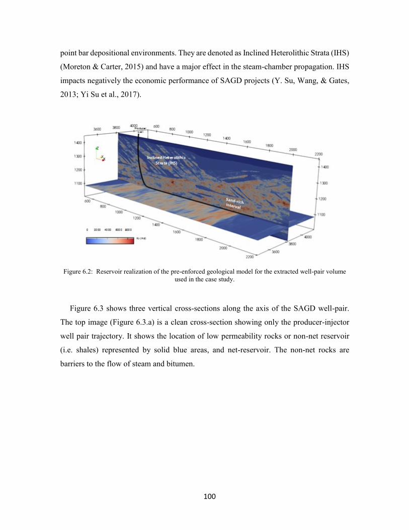
100

point bar depositional environments. They are denoted as Inclined Heterolithic Strata (IHS)

(Moreton & Carter, 2015) and have a major effect in the steam-chamber propagation. IHS

impacts negatively the economic performance of SAGD projects (Y. Su, Wang, & Gates,

2013; Yi Su et al., 2017).

Figure 6.2: Reservoir realization of the pre-enforced geological model for the extracted well-pair volume

used in the case study.

Figure 6.3 shows three vertical cross-sections along the axis of the SAGD well-pair.

The top image (Figure 6.3.a) is a clean cross-section showing only the producer-injector

well pair trajectory. It shows the location of low permeability rocks or non-net reservoir

(i.e. shales) represented by solid blue areas, and net-reservoir. The non-net rocks are

barriers to the flow of steam and bitumen.

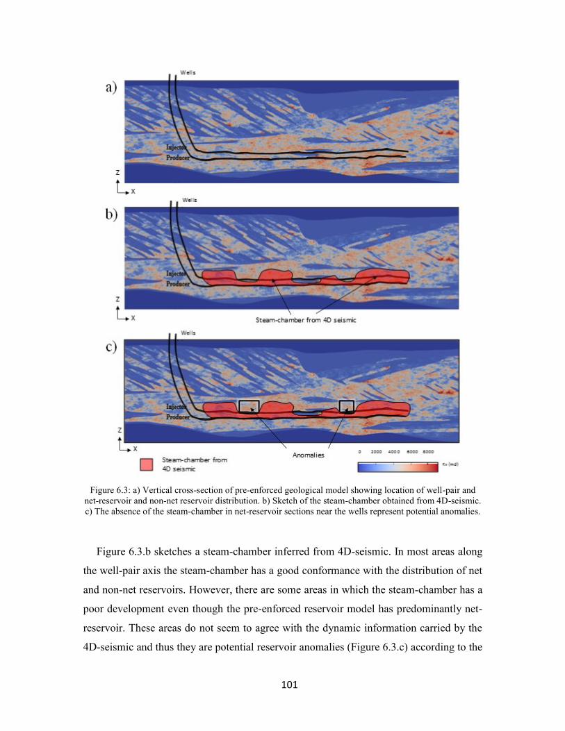
101

Figure 6.3: a) Vertical cross-section of pre-enforced geological model showing location of well-pair and

net-reservoir and non-net reservoir distribution. b) Sketch of the steam-chamber obtained from 4D-seismic.

c) The absence of the steam-chamber in net-reservoir sections near the wells represent potential anomalies.

Figure 6.3.b sketches a steam-chamber inferred from 4D-seismic. In most areas along

the well-pair axis the steam-chamber has a good conformance with the distribution of net

and non-net reservoirs. However, there are some areas in which the steam-chamber has a

poor development even though the pre-enforced reservoir model has predominantly net-

reservoir. These areas do not seem to agree with the dynamic information carried by the

4D-seismic and thus they are potential reservoir anomalies (Figure 6.3.c) according to the

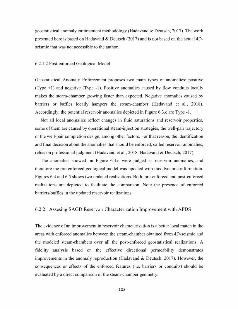
102

geostatistical anomaly enforcement methodology (Hadavand & Deutsch, 2017). The work

presented here is based on Hadavand & Deutsch (2017) and is not based on the actual 4D-

seismic that was not accessible to the author.

6.2.1.2 Post-enforced Geological Model

Geostatistical Anomaly Enforcement proposes two main types of anomalies: positive

(Type +1) and negative (Type -1). Positive anomalies caused by flow conduits locally

makes the steam-chamber growing faster than expected. Negative anomalies caused by

barriers or baffles locally hampers the steam-chamber (Hadavand et al., 2018).

Accordingly, the potential reservoir anomalies depicted in Figure 6.3.c are Type -1.

Not all local anomalies reflect changes in fluid saturations and reservoir properties,

some of them are caused by operational steam-injection strategies, the well-pair trajectory

or the well-pair completion design, among other factors. For that reason, the identification

and final decision about the anomalies that should be enforced, called reservoir anomalies,

relies on professional judgment (Hadavand et al., 2018; Hadavand & Deutsch, 2017).

The anomalies showed on Figure 6.3.c were judged as reservoir anomalies, and

therefore the pre-enforced geological model was updated with this dynamic information.

Figures 6.4 and 6.5 shows two updated realizations. Both, pre-enforced and post-enforced

realizations are depicted to facilitate the comparison. Note the presence of enforced

barriers/baffles in the updated reservoir realizations.

6.2.2 Assesing SAGD Reservoir Characterization Improvement with APDS

The evidence of an improvement in reservoir characterization is a better local match in the

areas with enforced anomalies between the steam-chamber obtained from 4D-seismic and

the modeled steam-chambers over all the post-enforced geostatistical realizations. A

fidelity analysis based on the effective directional permeability demonstrates

improvements in the anomaly reproduction (Hadavand & Deutsch, 2017). However, the

consequences or effects of the enforced features (i.e. barriers or conduits) should be

evaluated by a direct comparison of the steam-chamber geometry.

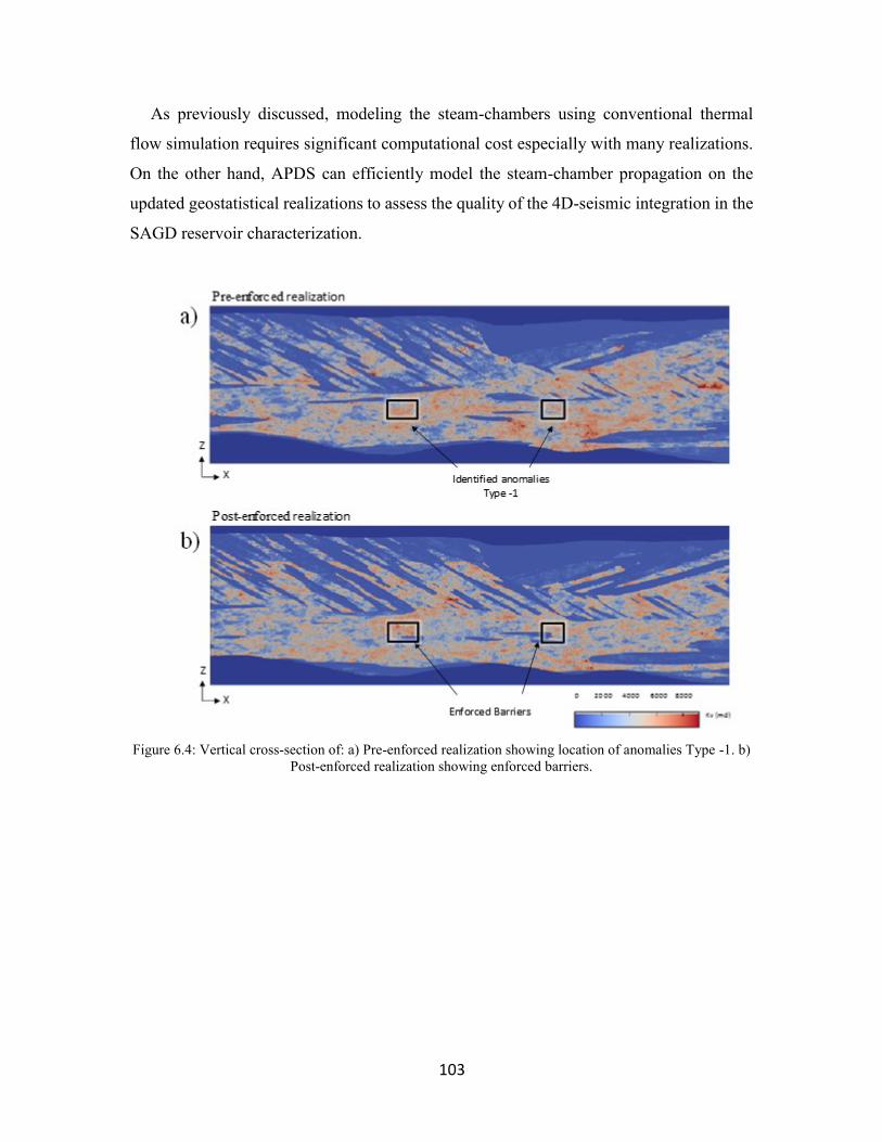
103

As previously discussed, modeling the steam-chambers using conventional thermal

flow simulation requires significant computational cost especially with many realizations.

On the other hand, APDS can efficiently model the steam-chamber propagation on the

updated geostatistical realizations to assess the quality of the 4D-seismic integration in the

SAGD reservoir characterization.

Figure 6.4: Vertical cross-section of: a) Pre-enforced realization showing location of anomalies Type -1. b)

Post-enforced realization showing enforced barriers.

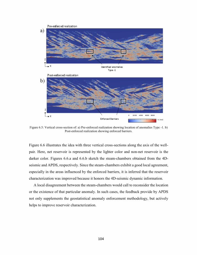
104

Figure 6.5: Vertical cross-section of: a) Pre-enforced realization showing location of anomalies Type -1. b)

Post-enforced realization showing enforced barriers.

Figure 6.6 illustrates the idea with three vertical cross-sections along the axis of the well-

pair. Here, net reservoir is represented by the lighter color and non-net reservoir is the

darker color. Figures 6.6.a and 6.6.b sketch the steam-chambers obtained from the 4D-

seismic and APDS, respectively. Since the steam-chambers exhibit a good local agreement,

especially in the areas influenced by the enforced barriers, it is inferred that the reservoir

characterization was improved because it honors the 4D-seismic dynamic information.

A local disagreement between the steam-chambers would call to reconsider the location

or the existence of that particular anomaly. In such cases, the feedback provide by APDS

not only supplements the geostatistical anomaly enforcement methodology, but actively

helps to improve reservoir characterization.

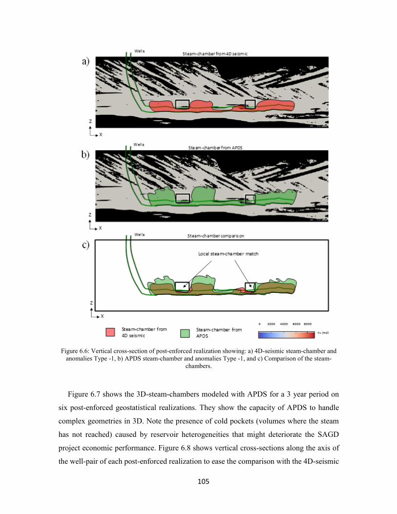
105

Figure 6.6: Vertical cross-section of post-enforced realization showing: a) 4D-seismic steam-chamber and

anomalies Type -1, b) APDS steam-chamber and anomalies Type -1, and c) Comparison of the steam-

chambers.

Figure 6.7 shows the 3D-steam-chambers modeled with APDS for a 3 year period on

six post-enforced geostatistical realizations. They show the capacity of APDS to handle

complex geometries in 3D. Note the presence of cold pockets (volumes where the steam

has not reached) caused by reservoir heterogeneities that might deteriorate the SAGD

project economic performance. Figure 6.8 shows vertical cross-sections along the axis of

the well-pair of each post-enforced realization to ease the comparison with the 4D-seismic

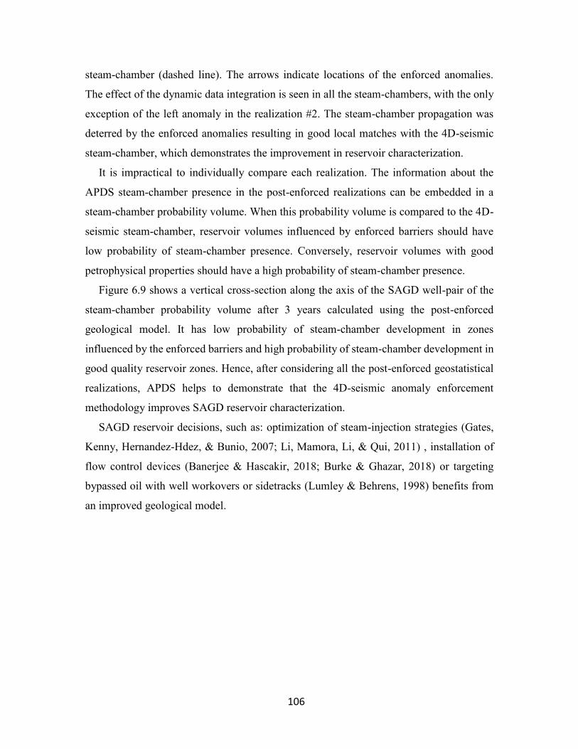
106

steam-chamber (dashed line). The arrows indicate locations of the enforced anomalies.

The effect of the dynamic data integration is seen in all the steam-chambers, with the only

exception of the left anomaly in the realization #2. The steam-chamber propagation was

deterred by the enforced anomalies resulting in good local matches with the 4D-seismic

steam-chamber, which demonstrates the improvement in reservoir characterization.

It is impractical to individually compare each realization. The information about the

APDS steam-chamber presence in the post-enforced realizations can be embedded in a

steam-chamber probability volume. When this probability volume is compared to the 4D-

seismic steam-chamber, reservoir volumes influenced by enforced barriers should have

low probability of steam-chamber presence. Conversely, reservoir volumes with good

petrophysical properties should have a high probability of steam-chamber presence.

Figure 6.9 shows a vertical cross-section along the axis of the SAGD well-pair of the

steam-chamber probability volume after 3 years calculated using the post-enforced

geological model. It has low probability of steam-chamber development in zones

influenced by the enforced barriers and high probability of steam-chamber development in

good quality reservoir zones. Hence, after considering all the post-enforced geostatistical

realizations, APDS helps to demonstrate that the 4D-seismic anomaly enforcement

methodology improves SAGD reservoir characterization.

SAGD reservoir decisions, such as: optimization of steam-injection strategies (Gates,

Kenny, Hernandez-Hdez, & Bunio, 2007; Li, Mamora, Li, & Qui, 2011) , installation of

flow control devices (Banerjee & Hascakir, 2018; Burke & Ghazar, 2018) or targeting

bypassed oil with well workovers or sidetracks (Lumley & Behrens, 1998) benefits from

an improved geological model.

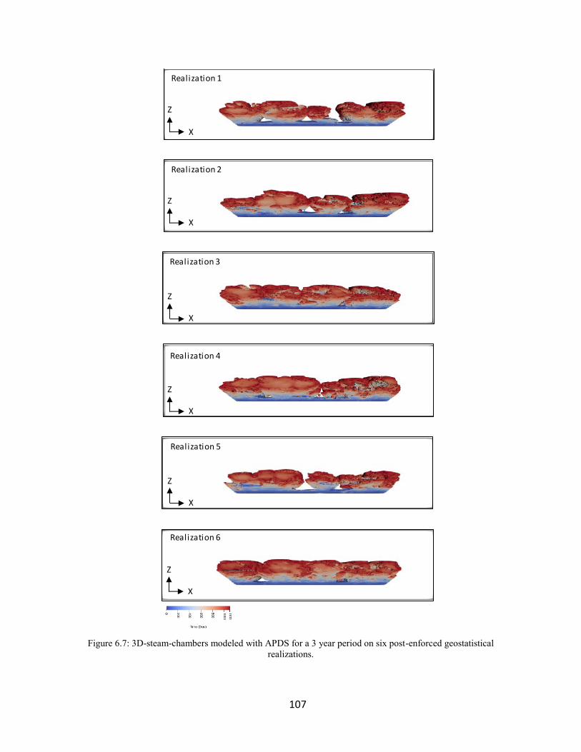
107

Figure 6.7: 3D-steam-chambers modeled with APDS for a 3 year period on six post-enforced geostatistical

realizations.

Realization 1

Z

X

Realization 2

Z

X

Realization 3

Z

X

Realization 4

Z

X

Realization 5

Z

X

Realization 6

Z

X

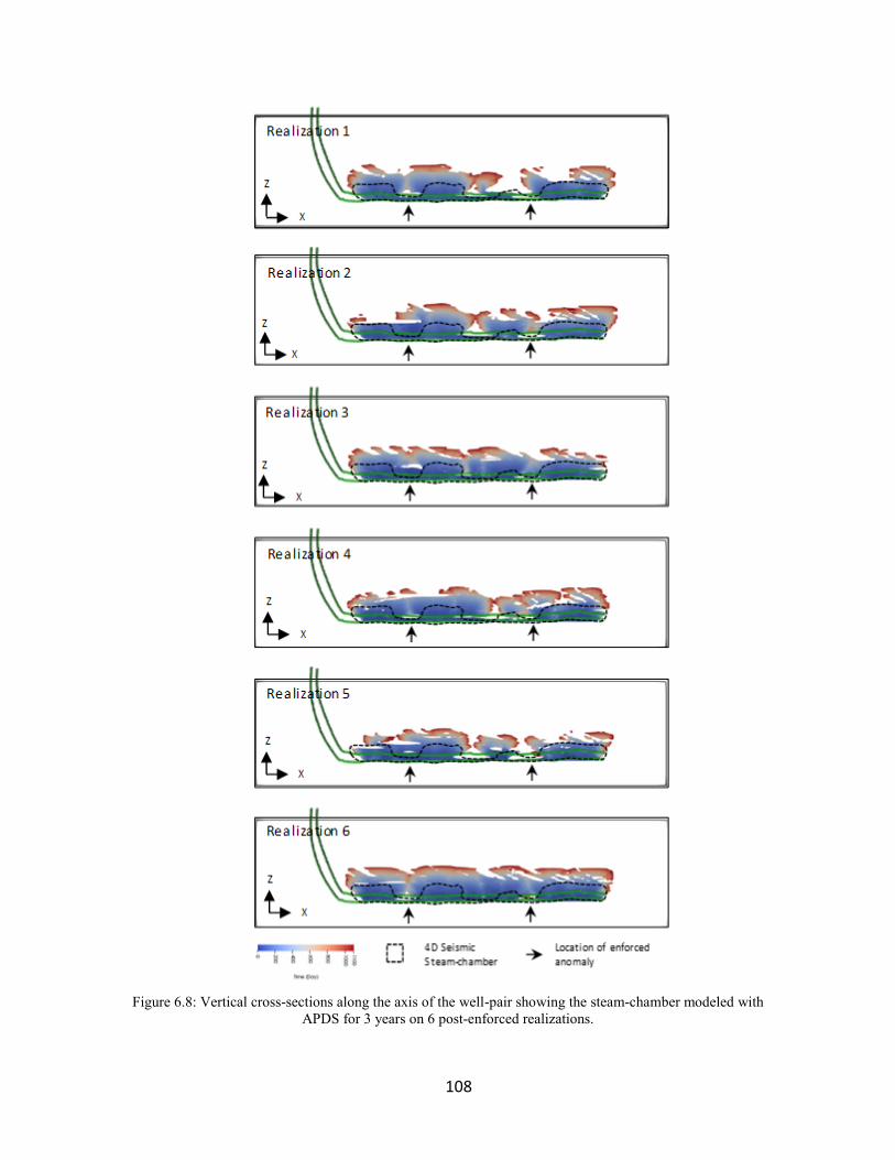
108

Figure 6.8: Vertical cross-sections along the axis of the well-pair showing the steam-chamber modeled with

APDS for 3 years on 6 post-enforced realizations.

109

Figure 6.9: Probability of steam-chamber presence after 3 years.

APDS has the capability of modeling the steam-chamber in an almost continuous

timeline. This makes it is easy to generate images of the probability of steam-chamber

presence at any time of interest. For instance, Figure 6.10 condenses information about the

first 5 years of steam-chamber propagation and also includes the tenth year. Note that

APDS shows that the negative impact of the enforced barriers in the steam-chamber

expansion is stronger at earlier times, and the impact diminishes as time advances.

Nowadays is common practice to monitor the SAGD steam-chamber with periodical

seismic surveys. For instance, in the 4D-seismic integration field-case study of the

Surmont project located in the Athabasca region, northeastern Alberta, Canada, (Hadavand

et al., 2018) reported eight seismic surveys, one baseline and seven monitors. The resulting

set of seven incremental 4D-seismic data and APDS would almost certainly enhance the

assimilation of the dynamic data in the reservoir characterization workflow. Even more, if

a good agreement between the initial 4D-seismic data sets and APDS is demonstrated, there

is a venue for optimizing the frequency of the seismic survey recording. The economic

impact would be a reduction of the overall SAGD project operational cost.

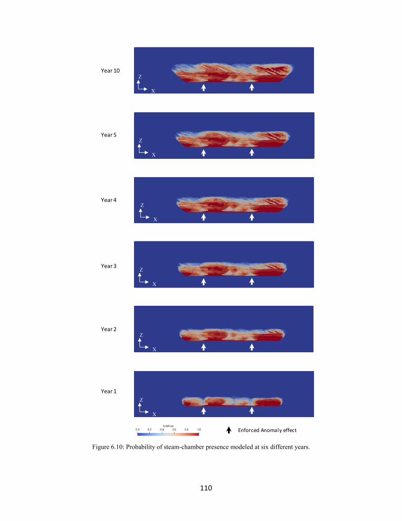
110

Figure 6.10: Probability of steam-chamber presence modeled at six different years.

Year 1

Year 2

Year 3

Year 4

Year 5

Year 10Z

X

Z

X

Z

X

Z

X

Z

X

Z

X

Enforced Anomaly effect

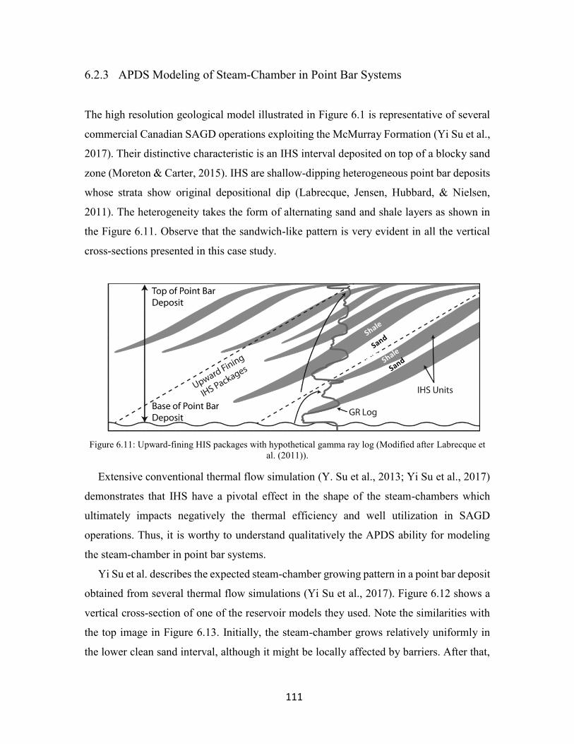
111

6.2.3 APDS Modeling of Steam-Chamber in Point Bar Systems

The high resolution geological model illustrated in Figure 6.1 is representative of several

commercial Canadian SAGD operations exploiting the McMurray Formation (Yi Su et al.,

2017). Their distinctive characteristic is an IHS interval deposited on top of a blocky sand

zone (Moreton & Carter, 2015). IHS are shallow-dipping heterogeneous point bar deposits

whose strata show original depositional dip (Labrecque, Jensen, Hubbard, & Nielsen,

2011). The heterogeneity takes the form of alternating sand and shale layers as shown in

the Figure 6.11. Observe that the sandwich-like pattern is very evident in all the vertical

cross-sections presented in this case study.

Figure 6.11: Upward-fining HIS packages with hypothetical gamma ray log (Modified after Labrecque et

al. (2011)).

Extensive conventional thermal flow simulation (Y. Su et al., 2013; Yi Su et al., 2017)

demonstrates that IHS have a pivotal effect in the shape of the steam-chambers which

ultimately impacts negatively the thermal efficiency and well utilization in SAGD

operations. Thus, it is worthy to understand qualitatively the APDS ability for modeling

the steam-chamber in point bar systems.

Yi Su et al. describes the expected steam-chamber growing pattern in a point bar deposit

obtained from several thermal flow simulations (Yi Su et al., 2017). Figure 6.12 shows a

vertical cross-section of one of the reservoir models they used. Note the similarities with

the top image in Figure 6.13. Initially, the steam-chamber grows relatively uniformly in

the lower clean sand interval, although it might be locally affected by barriers. After that,

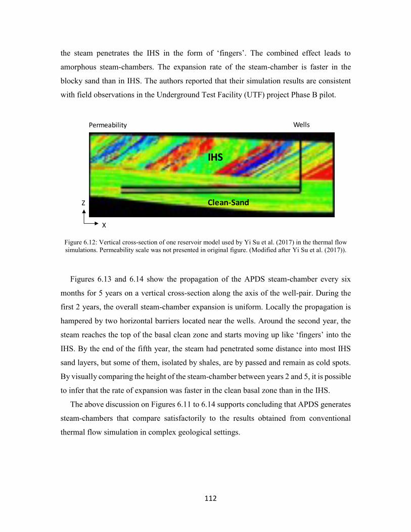
112

the steam penetrates the IHS in the form of ‘fingers’. The combined effect leads to

amorphous steam-chambers. The expansion rate of the steam-chamber is faster in the

blocky sand than in IHS. The authors reported that their simulation results are consistent

with field observations in the Underground Test Facility (UTF) project Phase B pilot.

Figure 6.12: Vertical cross-section of one reservoir model used by Yi Su et al. (2017) in the thermal flow

simulations. Permeability scale was not presented in original figure. (Modified after Yi Su et al. (2017)).

Figures 6.13 and 6.14 show the propagation of the APDS steam-chamber every six

months for 5 years on a vertical cross-section along the axis of the well-pair. During the

first 2 years, the overall steam-chamber expansion is uniform. Locally the propagation is

hampered by two horizontal barriers located near the wells. Around the second year, the

steam reaches the top of the basal clean zone and starts moving up like ‘fingers’ into the

IHS. By the end of the fifth year, the steam had penetrated some distance into most IHS

sand layers, but some of them, isolated by shales, are by passed and remain as cold spots.

By visually comparing the height of the steam-chamber between years 2 and 5, it is possible

to infer that the rate of expansion was faster in the clean basal zone than in the IHS.

The above discussion on Figures 6.11 to 6.14 supports concluding that APDS generates

steam-chambers that compare satisfactorily to the results obtained from conventional

thermal flow simulation in complex geological settings.

Z

X

Wells

Clean-Sand

IHS

Permeability

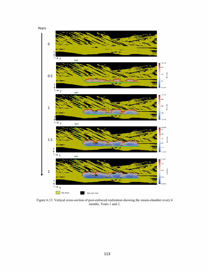
113

Figure 6.13: Vertical cross-section of post-enforced realization showing the steam-chamber every 6

months. Years 1 and 2.

0

0.5

1

1.5

2

Years

WellWell

Well

Well

Well

Z

X

Z

X

Z

X

Z

X

Z

X

Net Rock Non-net rock

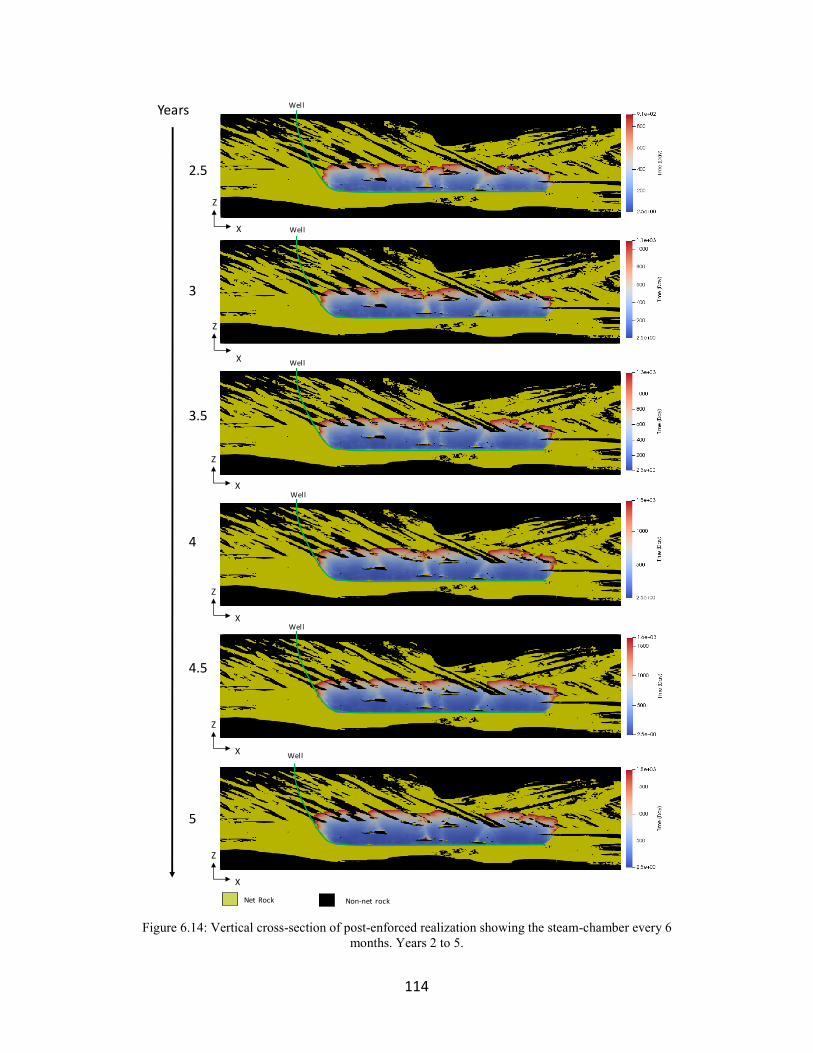
114

Figure 6.14: Vertical cross-section of post-enforced realization showing the steam-chamber every 6

months. Years 2 to 5.

2.5

Years Well

3.5

Well

Z

X

3

Well

Z

X

Z

X

4

Well

Z

X

4.5

Well

Well

Z

X

5

Z

X

Net Rock Non-net rock

115

6.2.4 Computational Time

Running this case-study for 50 post-enforced realizations took 2.8 hours, that is, an average

of 3.4 minutes per steam-chamber modeled. Steam-chambers were modeled for 15 years.

The total computational time was allocated 77 % building the graphs and 23% modeling

the steam-chambers. The result indicates that when looking for efficiency gains, the APDS

graph generator module is a candidate for parallel computing.

6.3 Discussion

This case study demonstrates how 4D-Seismic Anomaly Enforcement methodology and

APDS complement each other to improve geostatistical SAGD reservoir modeling. The

updated models are expected to improve SAGD reservoir decisions related to optimization

of steam-injection strategies, installation of flow control devices and/or execution of well

workovers or sidetracks among others. Better informed reservoir manager decisions should

increase the profitability of SAGD operations.

The probability of steam-chamber presence volume is introduced. It condenses in one

single image the information about the steam-chamber location of an entire set of

geostatistical realizations. APDS easily captures in a sequence of images the steam-

chamber propagation at any time period of interest. An obvious choice is to match these

probability volumes with the recording time of seismic monitoring surveys to improve the

assimilation of dynamic data in the SAGD reservoir characterization. In this line of

reasoning, APDS might also help to quantify the value of information (VOI) of the seismic

surveys. Reservoir managers could optimize the number and frequency of seismic data

acquisition, resulting in a reduction of the projects operational costs.

The APDS ability to predict the steam-chamber location in a complex point bar

depositional system is discussed. The qualitative analysis is encouraging regarding the

APDS outputs, because the general expected expansion steam-chamber pattern found by

other researches (Y. Su et al., 2013; Yi Su et al., 2017) using conventional thermal flow

simulation is correctly reproduced. As a future work, it is desirable running the

116

conventional simulator in the post-enforced geological model to perform a precise

quantitative comparison.

Regarding computational time, the APDS prototype takes an average of 3 minutes to

model each steam-chamber without using parallel computing. Around 77 % of the time is

consumed by the graph generator module. Using parallel computing for this module is an

easy to implement option to reduce computational time in a few factors. However, as

mentioned in Section 5.4, to obtain substantial efficiency gains measurable in terms of

orders of magnitude, the initial approach is to re-engineer APDS using a compiled

programming language.

117

7 Summary of Contributions and Future Work

This chapter summarizes the main contributions of the dissertation. It discusses strengths

and limitations of the APDS algorithm and the proposed MVC-SDR decision-making

criterion. Ideas for future work are provided to expand this research.

7.1 Summary of Contributions

At the heart of petroleum reservoir management (PRM) resides the challenge of selecting

the best project from a group of feasible candidates in the presence of geological

uncertainty. The challenge is particularly relevant in low oil price investment environments

where many upstream projects are economically marginal and must be optimized.

Companies are now more cautious. Investors are aware that they should consider not only

the rewards of the projects, but also their risks. For these reasons, the selection of the

projects to be implemented in the field should consider the geological risk and the capacity

of the companies to tolerate it.

This thesis advocates for decision-making workflows in reservoir management that

actively manage the geological uncertainty. That is, the geological uncertainty is

transferred to probability distributions of the response variable, and the decision criteria

that governs the final selection considers the decision maker’s preferences toward the

project’s return-risk trade-off.

In the context of the SAGD recovery technology, this thesis contributes to improve

reservoir management decision-making practices in several ways. 1) The formulation,

implementation and validation of a graph-based simplified physics simulator named

APDS, for efficiently transferring the geological uncertainty into steam-chamber evolution

paths that can directly support SAGD reservoir management or be converted to a monetary

response variable to input decision-making workflows, 2) the introduction and validation

of a practical decision-making criterion consistent with the utility theory framework that

combines MVC-SDR for active geological risk management, and 3) the thesis

demonstrates that APDS can complement a 4D-seismic integration methodology to

118

improve reservoir characterization. Reservoir manager decisions supported on a better

geological model should increase the profitability of SAGD operations.

7.1.1 APDS Formulation

SAGD is a thermal recovery process to produce bitumen from oil-sands. In this technology,

steam is injected in the reservoir to reduce the viscosity of the bitumen that drains by

gravity to a production well. In the subsurface, a steam-chamber evolves and grows with

time. Understanding the geometry and rate of growth of the steam-chamber is necessary to

manage an economically successful SAGD project; for that reason, Chapter 2 of this thesis

formulates a graph-based algorithm called APDS to model the steam-chamber evolution.

It uses graph theory, simplified porous media flow equations, heat transfer concepts and

ideas from discrete simulation.

Even though graph theory has been used since 1956 (Fatt, 1956) to model the flow of

fluids in porous media at pore-scale to predict macroscopic transport properties (Oren et

al., 1998), the use of graphs proposed in this dissertation at the macroscopic scale of the

cells of the numerical model to predict a large scale reservoir response such as the steam-

chamber in SAGD is a novel contribution to the technical literature.

Chapter 2 formulates APDS, presents the pseudocode of the algorithm, and a step-wise

application example that demonstrates how the steam-chamber evolution is predicted in

homogeneous and heterogeneous reservoirs. APDS is intended to be mathematically

simple and yet to have reasonably good predictive capabilities; for that reason, it will not

match the sophistication and complexity of a conventional thermal flow simulator.

However, APDS formulation is flexible enough to allow adjusting the complexity of the

algorithm to the problem at hand and the timeframe available to provide a solution. Section

7.3 in future work, later in this chapter, offers specific ideas to expand the physical

complexity modeled in APDS.

Finally, Chapter 2 discusses the use of APDS in SAGD projects to support operational

strategies, geomechanical analysis, well-pair location decision making and 4D-seismic

integration. The case studies in Chapters 5 and 6 successfully demonstrate the last two

applications.

119

7.1.2 APDS Implementation and Validation

Being mathematically sound and based on well-established engineering principles of flow

in porous media, material balance and heat-transfer does not guarantee a practical,

successful or immediate implementation. Sometimes, there is a time gap between the

formulation of an algorithm and its implementation and/or adoption. To mention one

example, the principles of streamline simulation were stablished in 1934 (Muskat &

Wyckoff, 1934), but according to Batycky, Blunt, & Thiele (1997) the technology only

resurfaces to the reservoir simulation practice in the nineties after the introduction of the

practical concept of time of flight along the streamlines (Pollock, 1988).

In the case of APDS, its successful implementation requires assumptions and practical

simplifications that must be compatible with the graph-based structure of the algorithm.

The implementation presented in Chapter 3 is considered a contribution to the practice of

SAGD reservoir simulation on its own. In the future, starting from the same APDS

formulation presented in this thesis, other researches might suggest different assumptions

and/or simplifications to implement the algorithm.

A case study performed with a realistic multi-realization geological model validates the

predictive capabilities of APDS. Visual and numerical comparisons with the results

obtained from a conventional full physics thermal flow simulation are satisfactory. APDS

was 3 orders of magnitude faster than the conventional simulator to model the steam-

chamber expansion and to provide predictions of reservoir response. The cost was a

reduction in the precision of the results. These results favor using APDS to support SAGD

decision making workflows in the presence of geological uncertainty.

Finally, Chapter 3 discusses the APDS prototype written in the Python programming

language. The structure of the prototype with 3 modules (graph generator, steam-chamber

generator and post-processing) is convenient to further reduce computational running time

by parallelizing APDS.

120

7.1.3 Decision-Making Criterion for Active Management of Geological

Uncertainty

Reservoir managers want to select and implement projects that add value. The selection is

difficult because project performance depends on the geological uncertainty. The

geological uncertainty can be quantified with geostatistical methods, but this information

is not often used because the decision-making models are not always formulated to exploit

the geological risk.

Chapter 4 of this dissertation claims that for PRM, the decision process must be guided

by a criterion tuned to the risk-reward preferences of the companies. For that reason, a

decision-making criterion consistent with the utility theory framework is formulated and

introduced. The proposed criterion ranks the projects to be implemented by combining

MVC and SDR optimality criteria. The main advantages of the MVC-SDR model are that

(1) it does not rely on a specific utility function and (2) the results are reasonable to all risk-

averse reservoir managers. The shortcoming is a reduced ability to rank projects with very

similar CDFs.

This thesis presents two examples that demonstrate MVC-SDR as a viable criterion for

decision making under geological uncertainty. The first example in Chapter 4 considers the

problem of selecting one SAGD well-pad to be drilled from a set of several possible

options. It is designed intentionally simple with the goal of explaining the MVC-SDR

methodology step by step. The second example in Chapter 5 considers the problem of

finding the best vertical location for a SAGD well-pair project in a target volume. This

example uses a realistic geological model and showed that APDS was computationally

efficient enough to model 4000 steam-chambers in 13 hours. This is a reasonable

computational time for supporting problems that require transferring the geological

uncertainty over a well-defined finite set of decision options.

The examples show that the MVC-SDR criterion do not always lead to a single project;

for that reason, it not suitable for problems that use optimization algorithms for searching

extremely large combinatorial decision spaces. MVC-SDR will not always help reservoir

managers to find a single optimum project, but they can reduce considerably the number

121

of alternatives from which the final decision must be make. The final choice depends on

the specific reservoir manager’s utility function.

7.1.4 Assisting 4D-Seismic Integration in Reservoir Characterization

4D-seismic is an important source of dynamic data for monitoring heavy-oil reservoirs. It

provides images of the SAGD steam-chamber at different times that might reveal

anomalies caused by barriers/baffles and conduits. These anomalies can be enforced into

geostatistical realizations using the practical integration of 4D-seismic methodology

proposed by Hadavand & Deutsch (2017).

Chapter 6 demonstrates with a realistic case study, that after the geostatistical anomaly

enforcement, APDS can efficiently model the steam-chamber propagation on the updated

geostatistical realizations to assess the quality of the 4D-seismic integration in the SAGD

reservoir characterization. In fact, APDS not only supplements the geostatistical anomaly

enforcement methodology, but it actively helps to improve reservoir characterization by

providing valuable feedback about the location of the anomalies. The updated models are

expected to improve SAGD reservoir decisions related to optimization of steam-injection

strategies, installation of flow control devices and/or execution of well workovers or

sidetracks among others.

Chapter 6 also introduces the probability of steam-chamber presence volume. This

practical contribution permits to condensate in one single image the information about the

steam-chamber location of an entire set of geostatistical realizations. The APDS capability

of modeling the steam-chamber in an almost continuous timeline makes it is easy to

generate probability volumes at any time of interest. They can be synchronized with the

recording time of seismic monitoring surveys to improve the assimilation of dynamic data

in the reservoir characterization.

122

7.2 Limitations and Future Work

Reflections on the limitations of APDS and MVC-SDR are included in the closing section

of each chapter. This final section recalls some of those limitations, discusses new ones,

but mainly focusses on offering specific ideas to overcome them.

Future works that might improve the methods and algorithms developed on this thesis

or build upon the results obtained include:

Improve current APDS outputs or develop new ones. For instances, production oil

forecast and steam-oil-ratio forecast.

Improve or expand the APDS physical complexity to offer higher flexibility without

affecting the computational efficiency. For example: include relative permeabilities

curves, improve handling of high-water saturation cells or develop a new two-phase

APDS algorithm.

Integrate APDS to well-established methodologies to improve reservoir

characterization, such as the Ensemble Kalman Filter (EnKF).

Couple APDS with models that describe aspects of the SAGD physics not

considered in the ranking function, for example, the steam properties variations

along the injector wellbore trajectory.

Develop additional case studies applying APDS to larger or more complex SAGD

problems. For example, study the optimization of SAGD-Pads placement.

Improve APDS computational efficiency

Regarding the decision-making model: calibrate the decision-maker’s position on

risks coming from the geological uncertainty and use APDS to determine the value

of information (VOI) of monitoring seismic surveys.

These future work ideas are described in the next sections.

123

7.2.1 Production Oil Forecast

APDS combines the sequence of graph nodes ordered by time with their volumetric

information to approximate the cumulative oil forecast. The calculation requires the

recoverable oil saturation (∆𝑆𝑜) of every cell; that is, the difference between the initial oil

saturation (𝑆𝑜𝑖) and the residual oil saturation (𝑆𝑜𝑟). 𝑆𝑜𝑖 is available from the input

geological model, but 𝑆𝑜𝑟 must be assumed.

APDS assumes that when a cell is heated, all its recoverable oil is produced

instantaneously. This assumption causes discrepancies to the conventional thermal

simulator results, because the oil saturation (𝑆𝑜) is a time-dependent variable. The oil

saturation remaining in the steam-chamber changes through time until it reaches 𝑆𝑜𝑟.

Implementing the time-dependent average 𝑆𝑜𝑟̅̅ ̅̅ proposed by Cardwell & Parsons (1949)

might improve the APDS oil production forecast.

𝑆𝑜𝑟̅̅ ̅̅ =(𝑏 − 1)

𝑏(𝜐𝑠𝜙𝑍

𝑏𝑘𝑔𝑡)1/(𝑏−1)

(7.1)

Here, 𝑆𝑜𝑟̅̅ ̅̅ is the average residual oil saturation after time t, 𝜐𝑠 is the kinematic viscosity

of the oil at the steam temperature, 𝜙 is the porosity, Z is the drainage height, 𝑘 is the

permeability, 𝑔 is the gravity constant, and 𝑏 is the exponent in Cardwell and Parson’s

equation for relative permeability, 𝑘𝑟 = 𝑆𝑏. After applying a typical value for 𝑏 of 3.5

(Butler, 1991), the average residual oil saturation in the steam-chamber after a time (t) can

be approximate by:

𝑆𝑜𝑟̅̅ ̅̅ = 0.43 (𝜐𝑠𝜙ℎ

𝑘𝑔𝑡)0.4

(7.2)

Note that the variable Z was replaced by the height of the steam-chamber h that can be

calculated at any time 𝑡 from APDS.

124

7.2.2 Steam-Oil Ratio (SOR) Forecast

SOR is a key economic performance indicator of a SAGD project. The current APDS

implementation does not provide the steam consumption of the process. However, all the

inputs to estimate the SOR are readily available from APDS.

After calculating the oil production forecast, the steam consumption can be estimated

by adding the heat to expand the steam-chamber, the head storage ahead of the interface of

the steam-chamber and the head loss to the over-burden. The following equations from

Butler (1991).

7.2.2.1 Heat to Expand the Steam-chamber (𝑄𝑠𝑐ℎ)

The heat to raise the steam-chamber from the reservoir temperature to the steam-

temperature is calculated with the following equation,

𝑄𝑠𝑐ℎ =𝑄𝑜

∅∆𝑆𝑜𝑀(𝑇𝑠𝑡 − 𝑇𝑟)

(7.3)

Where, 𝑇𝑠𝑡 and 𝑇𝑟 are the steam temperature and the initial reservoir temperature,

respectively. 𝑀 is the volumetric heat capacity of the reservoir, 𝑄𝑜 is the cumulative

recoverable oil, ∅ is the porosity and ∆𝑆𝑜 is the recoverable oil saturation.

Note that APDS provides 𝑄𝑜, ∆𝑆𝑜 was discussed in Section 7.3.1, ∅,𝑀, 𝑇𝑟 are inputs

from the geological model, and 𝑇𝑠𝑡 is set by the reservoir manager.

7.2.2.2 Heat Storage Ahead of the Steam-chamber Interface (𝑄𝑠𝑡𝑔)

The heat to raise the oil temperature ahead of the steam-chamber from 𝑇𝑟 to 𝑇𝑠𝑡 is calculated

with the following equation,

𝑄𝑠𝑡𝑔 =𝐾𝐴𝑖𝑈(𝑇𝑠𝑡 − 𝑇𝑟)

(7.4)

125

Where, 𝐾 is the thermal conductivity of the reservoir, 𝐴𝑖 is the area of the steam-

chamber interface, 𝑈 is the interface velocity, and 𝑇𝑟 and 𝑇𝑠𝑡 were previously defined. To

solve this equation, APDS provides estimate values of 𝐴𝑖 and 𝑈.

7.2.2.3 Heat Loss to the Overburden (𝑄𝑜𝑣𝑏)

The heat losses to the overburden above the steam-chamber is calculated with the following

equation,

𝑄𝑜𝑣𝑏 =4

3𝐾𝐴𝑜𝑏(𝑇𝑠𝑡 − 𝑇𝑟)√

𝑡

𝜋𝛼

(7.5)

Where, 𝐴𝑜𝑏 is the area in contact with the overburden at the time 𝑡, 𝛼 is the thermal

diffusivity of the overburden and the other variables were previously defined. To solve this

equation, APDS provides estimate values 𝐴𝑜𝑏.

7.2.3 Oil Relative Permeability (Kro)

The travel cell time is one component of the APDS ranking function that controls the

steam-chamber propagation. After combining Equations 2.1 and 2.2 it can be expressed as,

𝑇𝑟𝑎𝑣𝑒𝑙 𝐶𝑒𝑙𝑙 𝑡𝑖𝑚𝑒 = (𝑉𝑐∅ ∆𝑆𝑜) (𝜐ℎ𝑣

𝐴𝑡𝑘𝑜𝑔 𝑠𝑖𝑛 𝛽)

(7.6)

Where all variables in this equation were previously defined. Note the effective oil

permeability (𝑘𝑜) variable in the denominator. APDS currently uses a constant oil relative

permeability value (𝑘𝑟𝑜) in the range 0.2 to 0.4 to convert the absolute oil permeability

(𝑘𝑎𝑏𝑠) to 𝑘𝑜. This simplification should cause differences from the results obtained with a

thermal flow simulation.

SAGD is a thermal recovery process where high temperatures impact 𝑘𝑟𝑜. Therefore, it

is worthy to expand the APDS physics with an oil/water relative permeability correlation

at the edge of the steam-chamber. The following correlation proposed by Mosavat,

Mohsenzadeh, & Al-Wahaibi (2016) that modifies Corey’s equation could render good

results. Corey’s correlation is given by.

126

𝑘𝑟𝑤 = (𝑆𝑤∗ )4

(7.7)

𝑘𝑟𝑜 = (1 − 𝑆𝑤∗2) (1 − 𝑆𝑤

∗ )2

(7.8)

Where, 𝑘𝑟𝑤 is water relative permeability, 𝑆𝑤 water saturation and 𝑆𝑤∗ is the normalized

water saturation that depends on the irreducible water saturation 𝑆𝑤𝑖𝑟𝑟. The equation of 𝑆𝑤∗

is,

𝑆𝑤∗ = (

𝑆𝑤 − 𝑆𝑤𝑖𝑟𝑟1 − 𝑆𝑤𝑖𝑟𝑟

)

(7.9)

Mosavat et al. (2016) developed the following temperature-dependent oil/water relative

permeability correlations that are function of water saturation and oil-water viscosity ratio.

They reported that the correlations were obtained from curve-fitting SAGD experimental

data publicly available.

𝑘𝑟𝑤 = 𝑆𝑤∗𝑎

(7.10)

𝑘𝑟𝑜 = (1 − 𝑆𝑤∗𝑏) (1 − 𝑆𝑤

∗ )𝑐

(7.11)

The parameters 𝑎, 𝑏, 𝑐 are given by,

𝑎 = 1.32 + 0.00123𝜇𝑅 − 7.47 ∗ 10−7𝜇𝑅

2

(7.12a)

𝑏 = 1.02 − 0.000298𝜇𝑅 − 1.38 ∗ 10−7𝜇𝑅

2

(7.12b)

𝑐 = 2.22 + 0.00318𝜇𝑅 − 1.22 ∗ 10−6𝜇𝑅

2

(7.12c)

𝜇𝑅(𝑇) = (𝜇𝑜𝑖𝑙𝜇𝑤𝑎𝑡𝑒𝑟

)𝑇

(7.13)

127

Where, 𝜇𝑅(𝑇) is the viscosity ratio at temperature (𝑇). 𝜇𝑜𝑖𝑙 and 𝜇𝑤𝑎𝑡𝑒𝑟 are the oil and

water viscosity in 𝑐𝑃 at temperature 𝑇, respectively.

Implementing the 𝑘𝑟𝑜 correlation should improve the APDS results, so they better match

a full physics thermal flow simulator. However, using a 𝑘𝑟𝑜 curve might result in

mathematical instabilities in cells with initial high-water saturation. In such cases, 𝑘𝑟𝑜 will

tend to zero and the travel cell time given by Equation 7.6 will tend to infinity. To overcome

this issue, it is suggested to include in the APDS implementation a condition to assign very

large ranking values to cells with travel cell time that tends to infinite.

It is recommended to search and test other oil/water relative permeability correlations

that could be available in the technical literature. The correlation that better compares to

the conventional full physics thermal flow simulator should be implemented.

7.2.4 Cells with High Initial Water Saturation (Swi)

APDS classifies cells with initial water saturation (Swi) above a user-defined cut-off, as

isolated nodes in the graph, so they are treated like shales. This approximation is not

completely satisfactory. Reservoir layers with initial high-water saturation slow-down the

steam-chamber propagation, and after the connate water is drained, the steam can pass

through them.

Regarding cells with high Swi , a practical and more flexible alternative to the current

APDS assumptions, it is to calculate the travel cell time using water properties or oil

properties, depending on a pre-defined water saturation condition. For example, if 𝑆𝑤𝑖 >

40% , then:

𝑇𝑟𝑎𝑣𝑒𝑙 𝐶𝑒𝑙𝑙 𝑡𝑖𝑚𝑒 = (𝑉𝑐∅ ∆𝑆𝑤) (𝜐𝑤𝑎𝑡𝑒𝑟

𝐴𝑡𝑘𝑎𝑏𝑠𝑘𝑟𝑤𝑔 𝑠𝑖𝑛 𝛽) (7.14)

All variables in this equation were previously defined. If 𝑆𝑤 ≤ 40%, then Equation

7.6 is used.

A more complex solution to high Swi zones involves implementing a fractional flow

model that considers both, oil and water saturations, into the travel cell time equation. As

a starter point for future research, the fractional flow between one cell and its neighbors,

128

after neglecting the effect of the capillary pressure, can be calculated with the following

equation (Butler, 1991).

𝑓𝑤 =𝑞𝑤𝑞𝑡=

1 − 𝜑

1 +𝜇𝑤𝑘𝑟𝑤

𝑘𝑟𝑜𝜇𝑜

(7.15)

Where,

φ =𝑘𝑎𝑏𝑠𝑘𝑟𝑜𝐴𝑡∆𝜌𝑔𝑠𝑖𝑛𝛽

𝑞𝑡𝜇𝑜 (7.16)

Where 𝑞𝑤, 𝑞𝑡 are water and oil flow rate, respectively. All other variables in these

equations were previously defined. How to combine these equations with a material

balance of both fluids (oil and water) at the cell-scale in a consistent way with other APDS

assumptions is not solved yet. However, a solution of this type would certainly render a

better representation of the actual physical phenomena occurring at the edge of the steam-

chamber and it would be an important advance in the APDS formulation.

7.2.5 Assisting the Ensemble Kalman Filter (EnKF) Technique with APDS

EnKF is an inverse-modelling local optimization technique intended for sequential

assimilation of static and dynamic into a model (Aanonsen, Nævdal, Oliver, Reynolds, &

Vallès, 2009). It consists of two recursive steps, the forecast step to propagate state

variables as a function of the updated parameters from one timestep to another, and the

analysis or updating step for data assimilation (Zagayevskiy & Deutsch, 2015).

EnKF was applied to assimilate time-lapse temperature observations and 4D-seismic

data in SAGD reservoir characterization by Zagayevskiy & Deutsch (2015). They

discussed two challenges to implement EnKF. It requires an ensemble with a large number

of geostatistical realizations, and they all need to be processed during the forecast step. The

forecast step can be performed with a full-physics thermal flow simulator but is

computationally too expensive. Using APDS should reduce drastically the computational

overburden of running the forecast step with a marginal loss in the quality of the estimate.

129

A case study intended to explore the advantages and limitations of assisting EnKF with

APDS is suggested.

7.2.6 Coupling APDS with a Thermal Wellbore Simulator

APDS assumes a uniform pressure profile along the injector wellbore. However, in SAGD

projects, the pressure difference between the heel and toe of a long horizontal steam

injector due to frictional losses can be significative. These pressure differences can affect

the development of the shape of the steam chamber (Tan, Butterworth, & Yang, 2002).

It is anticipated that coupling a thermal wellbore simulator to APDS will improve the

ability of the latter to predict the steam-chamber propagation. As a starter point for this

research path, the following literature about modeling thermal wellbore conditions in

SAGD is suggested (Ju & Zhao, 2016; Oballa, Coombe, & Buchanan, 1997; Tan et al.,

2002; Vander Valk & Yang, 2007). The challenge is making compatible existing thermal

wellbore simulators with the APDS formulation.

7.2.7 APDS Applications

The APDS applications discussed in this thesis used geological models representing SAGD

well-pair volumes. To further test the limits of the APDS predictive capabilities and assess

its potential use in commercial SAGD projects, additional case studies using larger scales

are required.

In this regard, a challenging problem worthy of being revisited having APDS as a

companion tool, is the placement of SAGD surface production pads and subsurface

drainage areas to maximize the economic potential of an area tackled by Manchuk &

Deutsch (2013).

7.2.8 APDS Computational Efficiency

The case studies presented in this thesis indicate that APDS is around 3 orders of magnitude

faster than conventional full-physics thermal flow simulators to model the steam-chamber

130

expansion and to provide a response variable. This processing time appears encouraging to

undertake problems with large finite decision spaces. However, is not yet efficient enough

to embed APDS into a full-scale field optimization work flow. It is recommended to look

for substantial efficiency gains in the scale of 1-3 additional orders of magnitude compared

to a conventional thermal flow simulator. It is suggested to program APDS using a

compiled language such as C, C++, C# or Fortran. Moreover, the structure of the program

must ensure that APDS can be parallelized.

7.2.9 Decision-Maker Position on Geological Risk

The MVC-SDR criterion is primarily applicable to problems with a well-defined finite set

of decision options. It helps reservoir managers to reduce the number of alternatives from

which the decision must be made, but at the end, the final choice depends on the specific

reservoir manager’s utility function. Utility functions are also required as objective

functions to account for geological uncertainty in closed-loop field optimization work

flows. The reservoir manager’s position on risk should be explicitly embedded in a utility

function, so the PRM decision-making problem can be generically formulated as:

argmax𝑎𝜖𝐴

𝐸[𝑢(𝑥(𝑎, 𝑤))] = argmax𝑎𝜖𝐴

∫ 𝑓(𝑥(𝑎, 𝑤)) ∙ 𝑢(𝑥(𝑎, 𝑤))dx (7.17)

Where, 𝑎 represents projects from the set of feasible actions 𝐴; 𝑤 represents realizations

from the geological model; x(𝑎, 𝑤) represents the payoff calculated after transferring the

geological uncertainty; 𝑓(𝑥(∙)) is the probability density function of 𝑥(∙) and 𝑢(𝑥(∙)) is

the utility function.

Because there is no clear method to determine a decision maker’s utility function, it is

recommended to follow a pragmatic approach similar to Güyagüler & Horne (2004) and

Ozdogan & Horne (2006). That is, the utility function is assumed to be exponential, 𝑢(𝑥) =

−𝑒−𝑥/𝑅, and the position on risk of the reservoir manager, represented by the risk tolerance

parameter 𝑅, is calibrated performing a sensitivity analysis over a range of R. In the case

of SAGD decision-making problems, this procedure will benefit from the APDS efficiency,

131

because it requires transferring the geological uncertainty over the set of geostatistical

realizations, as many times as needed for the calibration of the R parameter.

7.2.10 Value of Seismic Information on SAGD projects

The APDS probability of steam-chamber presence volumes condense the information

about the steam-chamber location of an entire set of geostatistical realizations. They can

be estimated at the recording time of different seismic monitoring surveys to improve the

assimilation of dynamic data in reservoir characterization.

The bitumen forecast provided by APDS can be used to quantity the value of

information as incremental 4D-seismic data become available (Hadavand, 2017).

However, since the steam-consumption is the largest operational cost in SAGD projects, it

is recommended to develop and validate the procedure to obtain the Steam-Oil Ratio (SOR)

forecast from APDS (Section 7.3.2) before undertaking this VOI problem.

132

References

Aanonsen, S. I., Nævdal, G., Oliver, D. S., Reynolds, A. C., & Vallès, B. (2009). The

Ensemble Kalman Filter in Reservoir Engineering- A Review. SPE Journal, 14(03),

393–412. https://doi.org/10.2118/117274-PA

Alusta, G. A., Mackay, E. J., Fennema, J., Armih, K., & Collins, I. R. (2012). EOR vs.

Infill Well Drilling: Field application of new decision making technique. In SPE

Kuwait International Petroleum Conference and Exhibition. Kuwait City, Kuwait:

Dec. 10-12. https://doi.org/10.2118/163298-MS

Azad, A., & Chalaturnyk, R. J. (2012). An Improved SAGD Analytical Simulator: Circular

Steam Chamber Geometry. Journal of Petroleum Science and Engineering, 82–83,

27–37. https://doi.org/10.1016/j.petrol.2012.01.003

Azom, P. N., & Srinivasan, S. (2011). Modeling the Effect of Permeability Anisotropy on

the Steam-Assisted Gravity Drainage (SAGD) Process. In Canadian Unconventional

Resources Conference. Calgary, Alberta, Ca. https://doi.org/10.2118/149274-MS

Azom, P. N., & Srinivasan, S. (2013). Modeling the Effect of Permeability Anisotropy on

the Steam-Assisted Gravity Drainage (SAGD) Process in Multi-Layered Reservoirs.

In SPE Heavy Oil Conference Canada. Calgary, Alberta, Ca.

https://doi.org/10.2118/149274-MS

Banerjee, S., & Hascakir, B. (2018). Flow Control Devices in SAGD Completion Design:

Enhanced Heavy Oil/ Bitumen Recovery through Improved Thermal Efficiency.

Journal of Petroleum Science and Engineering, 169(May), 297–308.

https://doi.org/10.1016/j.petrol.2018.05.064

Baniak, G. M., & Kingsmith, K. G. (2018). Sedimentological and Stratigraphic

Characterization of Cretaceous Upper McMurray Deposits in the Southern Athabasca

Oil Sands, Alberta, Canada. AAPG Bulletin, 102(2), 309–332.

https://doi.org/10.1306/0502171619317010

Batycky, R. P., Blunt, M. J., & Thiele, M. R. (1997). A 3D Field-Scale Streamline-Based

Reservoir Simulator. SPE Reservoir Engineering, 12(04), 246–254.

https://doi.org/SPE 36726

Begg, S. H., Bratvold, R. B., & Campbell, J. M. (2003). Shrinks Or Quants: Who Will

133

Improve Decision-Making. In Proceedings of SPE Annual Technical Conference and

Exhibition. Denver, Colorado: Oct. 5-8. https://doi.org/10.2523/84238-MS

Bratvold, R. B., Begg, S. H., & Campbell, J. M. (2003). Even Optimists Should Optimize.

In Proceedings of SPE Annual Technical Conference and Exhibition. Denver,

Colorado: Oct. 5-8. https://doi.org/10.2118/84329-MS

Burke, L., & Ghazar, C. (2018). Flow Control Devices in SAGD - A System-Based

Technology Solution. In SPE Thermal Well Integrity and Design Symposium. Banff,

Alberta, Canada.: Nov. 27-29. https://doi.org/10.2118/193353-MS

Butler, R. M. (1985). A New Approach to the Modelling of Steam-Assisted Gravity

Drainage. Journal of Canadian Petroleum Technology, 24(03), 42–51.

https://doi.org/10.2118/85-03-01

Butler, R. M. (1991). Thermal Recovery of Oil and Bitumen. Englewood Cliff, New Jersey:

Prentice-Hall. Retrieved from https://books.google.ca/books?id=_6RTAAAAMAAJ

Butler, R. M., Mcnab, G. S., & Lo, H. Y. (1981). Theoretical Studies on the Gravity

Drainage of Heavy Oil During in-situ Steam Heating. The Canadian Journal of

Chemical Engineering, 59(4), 455–460. https://doi.org/10.1002/cjce.5450590407

Butler, R. M., & Stephens, D. J. (1981). The Gravity Drainage of Steam-Heated Heavy Oil

to Parallel Horizontal Wells. Journal of Canadian Petroleum Technology, 20(2), 90–

96. https://doi.org/10.2118/81-02-07

Caers, J. (2011). Modeling Uncertainty in the Earth Sciences (1st ed.). Hoboken, NJ:

Wiley-Blackwell.

Capolei, A., Suwartadi, E., Foss, B., & Jørgensen, J. B. (2015). A Mean-Variance

Objective for Robust Production Optimization in Uncertain Geological Scenarios.

Journal of Petroleum Science and Engineering, 125, 23–37.

https://doi.org/10.1016/j.petrol.2014.11.015

Cardwell, W. T., & Parsons, R. L. (1949). Gravity Drainage Theory. Transactions of the

AIME, 179(01), 199–215. https://doi.org/10.2118/949199-G

CERI. (2018). Canadian Oil Sands Supply Costs and Development Projects. Calgary,

Alberta, Ca.

Chalaturnyk, R. J., & Li, P. (2004). When Is It Important to Consider Geomechanics in

SAGD Operations? Journal of Canadian Petroleum Technology, 43(4), 53–61.

134

https://doi.org/10.2118/04-08-discussion

Chang, Y., Bouzarkouna, Z., & Devegowda, D. (2015). Multi-objective Optimization for

Rapid and Robust Optimal Oilfield Development Under Geological Uncertainty.

Computational Geosciences, 19(4), 933–950. https://doi.org/10.1007/s10596-015-

9507-6

Chiles, J.-P., & Delfiner, P. (2012). Geostatistics: Modeling Spatial Uncertainty. (S. S. W.

Walter A. Shewhart, Ed.), Wiley series in probability and statistics (2nd ed.). Oxford:

Wiley-Blackwell. Retrieved from

http://onlinelibrary.wiley.com/book/10.1002/9781118136188

CMG. (2010). STARS User’s Guide. Calgary, Alberta: Computer Modelling Group Ltd.

CMG. (2013). CMG’s SAGD Guide. Calgary, Alberta: Computer Modelling Group Ltd.

Cokar, M., Kallos, M. S., & Gates, I. D. (2013). A New Thermogeomechanical Theory for

Gravity Drainage in Steam-Assisted Gravity Drainage. SPE Journal, 18(4), 736–742.

https://doi.org/10.2118/163136-PA

Collins, P. M. (2007). Geomechanical Effects on the SAGD Process. SPE Reservoir

Evaluation & Engineering, 10(4), 367–375. https://doi.org/10.2118/97905-PA

da Cruz, S. P. (2000). Reservoir Management Decision-Making in the Presence of

Geological Uncertainty. Stanford University, United States. Retrieved from

https://pangea.stanford.edu/ERE/pdf/pereports/PhD/Cruz00.pdf

Damsleth, E., Hage, A., & Volden, R. (1992). Maximum Information at Minimum Cost: A

North Sea Field Development Study With an Experimental Design. Journal of

Petroleum Technology, (December), 1350–1356. https://doi.org/10.2118/23139-PA

Dehdari, V. (2014). Development and Applications of a Semi-Analytical Approximate

Thermal Simulator. Universty of Alberta, Canada.

Deo, N., & Pang, C. ‐ Y. (1984). Shortest-Path Algorithms: Taxonomy and Annotation.

Networks, 14(2), 275–323. https://doi.org/10.1002/net.3230140208

Deutsch, C. V, & Journel, A. G. (1998). GSLIB. Geostatistical Software Library and User’s

Guide (2nd ed.). New York: Oxford University Press.

Dijkstra, E. W. (1959). A Note on Two Problems in Connection with Graphs. Numerische

Mathematik. https://doi.org/10.1007/BF01386390

Echeverria-Ciurri, D., Conn, A. R., Mello, U. T., & Onwunalu, J. E. (2012). Integrating

135

Mathematical Optimization and Decision Making in Intelligent Fields. In SPE

Intelligent Energy International 2012 (Vol. 1). Utrecht, The Nerthenland: 27-29

March. https://doi.org/10.2118/149780-MS

Edwards, R. A. (1993). Applying Financial Portfolio Theory to the Analysis of Producing

Properties.

Even, S. (2011). Graph Algorithms. (G. Even, Ed.). Cambridge: Cambridge University

Press. https://doi.org/10.1017/CBO9781139015165

Fatt, I. (1956). The Network Model of Porous Media. Petroleum Transactions, AIME, 207,

144–181.

Gallardo, E. C., & Deutsch, C. V. (2018). Approximate Physics-Discrete Simulation of the

Steam-Chamber Evolution in Steam-Assisted Gravity Drainage. SPE Journal,

Preprint(Preprint), 15. https://doi.org/10.2118/194016-PA

Gates, I. D., Kenny, J., Hernandez-Hdez, I. L., & Bunio, G. L. (2007). Steam Injection

Strategy and Energetics of Steam-Assisted Gravity Drainage. SPE Reservoir

Evaluation & Engineering, 10(01), 19–34. https://doi.org/10.2118/97742-PA

Goldberg, D. E. (1989). Genetic Algorithms in Search, Optimization, and Machine

Learning. Reading, MA: Addison-Wesley.

Goovaerts, P. (1997). Geostatistics for Natural Resources Evaluation. Applied

geostatistics series. New York: Oxford University Press.

Güyagüler, B., & Horne, R. N. (2004). Uncertainty Assessment of Well-Placement

Optimization. SPE Reservoir Evaluation & Engineering, 7(1), 24–32.

https://doi.org/10.2118/87663-pa

Hadar, J., & Russell, W. R. (1969). Rules for Ordering Uncertain Prospects. American

Economic Review, 59(1), 25–34. https://doi.org/10.1126/science.151.3712.867-a

Hadavand, M. (2017). Integration of 4D Seismic Data in Reservoir Characterization with

Facies Parameter Uncertainty. University of Alberta, Canada.

Hadavand, M., Carmichael, P., Dalir, A., Rodriguez, M., Silva, D. F. S., & Deutsch, C. V.

(2018). Integration of 4D Seismic in Steam-Assisted-Gravity-Drainage Reservoir

Characterization. SPE Reservoir Evaluation & Engineering, (June 2017), 1–16.

https://doi.org/10.2118/191359-PA

Hadavand, M., & Deutsch, C. V. (2017). A Practical Methodology For Integration of 4D

136

Seismic in Steam-Assisted-Gravity-Drainage Reservoir Characterization. SPE

Reservoir Evaluation & Engineering, 20(2), 353–362.

https://doi.org/10.2118/184390-PA

Hanoch, G., & Levy, H. (1969). The Efficiency Analysis of Choices Involving Risk.

Review of Economic Studies, 36(3), 107–335. https://doi.org/10.2307/2296431

Hassanpour, R. . (2013). Grid-free Facies Modelling of Inclined Heterolitic Strata in

McMurray Formation. University of Alberta, Alberta, Canada.

Heidari, M., Pooladi-Darvish, M., Azaiez, J., & Maini, B. (2009). Effect of Drainage

Height and Permeability on SAGD Performance. Journal of Petroleum Science and

Engineering, 68(1–2), 99–106. https://doi.org/10.1016/j.petrol.2009.06.020

Irani, M., & Cokar, M. (2016). Discussion on the Effects of Temperature on Thermal

Properties in the Steam-Assisted-Gravity-Drainage (SAGD) Process. Part 1: Thermal

Conductivity. SPE Journal, 21(2), 334–352. https://doi.org/10.2118/178426-PA

Isebor, O. J., Echeverría-Ciaurri, D., & Durlofsky, L. J. (2013). Generalized Field

Development Optimization Using Derivative-Free Procedures. In SPE Reservoir

Simulation Symposium. The Woodlands, Texas: 1-4 February.

https://doi.org/10.2118/163631-PA

Johnstone, D., & Lindley, D. (2013). Mean–Variance and Expected Utility: The Borch

Paradox. Statistical Science, 28(2), 223–237. https://doi.org/10.1214/12-STS408

Ju, N., & Zhao, G. (2016). A Calculation Model for Steam Property Variation Along

Wellbore Trajectory in SAGD Processes. In Society of Petroleum Engineers - SPE

Latin America and Caribbean Heavy and Extra Heavy Oil Conference 2016. Lima,

Peru: Oct. 19-20. https://doi.org/10.2118/181155-MS

Kennedy, J., & Eberhart, R. (1995). Particle Swarm Optimization. In N. 27- Dec.1 (Ed.),

Neural Networks, 1995. Proceedings., IEEE International Conference on (Vol. 4).

Perth, WA, Australia. https://doi.org/10.1109/ICNN.1995.488968

Khan, K. D., & Deutsch, C. V. (2016). Practical Incorporation of Multivariate Parameter

Uncertainty in Geostatistical Resource Modeling. Natural Resources Research, 25(1),

51–70. https://doi.org/10.1007/s11053-015-9267-y

Kochenderfer, M. J. (2015). Decision Making Under Uncertainty : Theory and

Application. MIT Lincoln Laboratory series. Cambridge, Massachusetts: The MIT

137

Press. Retrieved from http://ieeexplore.ieee.org/servlet/opac?bknumber=7288640

Labrecque, P. A., Jensen, J. L., Hubbard, S. M., & Nielsen, H. (2011). Sedimentology and

Stratigraphic Architecture of a Point Bar Deposit, Lower Cretaceous McMurray

Formation, Alberta, Canada. Bulletin of Canadian Petroleum Geology, 59(2), 147–

171. https://doi.org/10.2113/gscpgbull.59.2.147

Levy, H. (2016). Stochastic Dominance: Investment Decision Making Under Uncertainty

(3rd ed.). New York: Springer. https://doi.org/10.1007/978-3-319-21708-6

Levy, H., & Sarnat, M. (1970). Portfolio Selection and Investors Utility: A Graphical

Analysis. Applied Economics, 2(2), 113–119.

https://doi.org/10.1080/00036847000000020

Li, W., Mamora, D. D., Li, Y., & Qui, F. (2011). Numerical Investigation of Potential

Injection Strategies to Reduce Shale Barrier Impacts on SAGD Process. Journal of

Canadian Petroleum Technology, 50(3), 57–64. https://doi.org/10.2118/133298-PA

Lumley, D. E., & Behrens, R. A. (1998). Practical Issues of 4D Seismic Reservoir

Monitoring: What an Engineer Needs to Know. SPE Reservoir Evaluation &

Engineering, 1(06), 528–538. https://doi.org/10.2118/53004-PA

Machina, M. J. (1987). Choice Under Uncertainty: Problems Solved and Unsolved.

Journal of Economic Perspectives, 1(1), 121–154. https://doi.org/10.1257/jep.1.1.121

Majdi Yazdi, M., & Jensen, J. L. (2014). Fast Screening of Geostatistical Realizations for

SAGD Reservoir Simulation. Journal of Petroleum Science and Engineering, 124,


Manchuk, J. G., & Deutsch, C. V. (2013). Optimization of Drainage-Area Configurations

to Maximize Recovery from SAGD Operations. Journal of Canadian Petroleum

Technology, 52(3), 233–242. https://doi.org/10.2118/165573-PA

Markowitz, H. M. (1959). Portfolio Selection. Efficient Diversification of Investments.

New York: John Wiley & Sons, Inc.

Moreton, D. J., & Carter, B. J. (2015). Characterizing Alluvial Architecture of Point Bars

within the McMurray Formation, Alberta, Canada, for Improved Bitumen Resource

Prediction and Recovery. Developments in Sedimentology (1st ed., Vol. 68). Elsevier

B.V. https://doi.org/10.1016/B978-0-444-63529-7.00016-X

Mosavat, N., Mohsenzadeh, A., & Al-Wahaibi, Y. (2016). Estimating Oil/Water Relative

138

Permeability at SAGD Steam Chamber Edge. In SPE Heavy Oil Conference and

Exhibition. Kuwait City, Kuwait: Dec. 6-8. https://doi.org/10.2118/184132-MS

Muskat, M., & Wyckoff, R. D. (1934). A Theoretical Analysis of Water-flooding

Networks. Transactions of the AIME, 107(01), 62–76.

https://doi.org/10.2118/934062-G

Newendorp, P. D., & Campbell, J. M. (1968). SPE Criterion for Drilling Investments.

Society of Petroleum Engineers of AIME.

Oballa, V., Coombe, D. A., & Buchanan, L. (1997). Aspects of Discretized Wellbore

Modelling Coupled to Compositional/Thermal Simulation. Journal of Canadian

Petroleum Technology, 36(4), 45–51. https://doi.org/10.2118/97-04-04

Oren, P.-E., Bakke, S., & Arntzen, O. J. (1998). Extending Predictive Capabilities to

Network Models. SPE Journal, 3(04), 324–336. https://doi.org/10.2118/52052-PA

Ortega-Arranz, H., Llanos R., D., & Gonzalez-Escribano, A. (2015). The Shortest-Path

Problem: Analysis and Comparison of Methods. Morgan & Claypool.

https://doi.org/DOI 10.2200/S00618ED1V01Y201412TCS001

Ozdogan, U., & Horne, R. (2006). Optimization of Well Placement Under Time-Dependent

Uncertainty. SPE Reservoir Evaluation & Engineering, 9(April), 26–29.

https://doi.org/10.2118/90091-PA

Pathak, V., Tran, D., & Kumar, A. (2014). Quantifying the Uncertainty Associated with

Caprock Integrity during SAGD using Coupled Geomechanics Thermal Reservoir

Simulation. In SPE Heavy Oil Conference-Canada. Calgary, Alberta: 10-12 June.

https://doi.org/10.2118/170130-MS

Peacock, M. J. (2010). Athabasca Oil Sands: Reservoir Characterization and its Impact on

Thermal and Mining Opportunities. Geological Society, London, Petroleum Geology

Conference Series, 7(1), 1141–1150. https://doi.org/10.1144/0071141

Pollock, D. W. (1988). Semianalytical Computation of Path Lines for Finite-Difference

Models. Groundwater, 26(6), 743–750. https://doi.org/10.1111/j.1745-

6584.1988.tb00425.x

Pyrcz, M. J., & Deutsch, C. V. (2014). Geostatistical Reservoir Modeling (2nd ed.). New

York : Oxford University Press. Retrieved from

http://login.ezproxy.library.ualberta.ca/login?url=http://search.ebscohost.com/login.

139

aspx?direct=true&db=cat03710a&AN=alb.8111105&site=eds-live&scope=site

Raiffa, H., & Schlaifer, R. (1961). Applied Statistical Decision Theory. Studies in

managerial economics. Boston: Division of Research, Graduate School of Business

Administration, Harvard University.

Ranger, M. J., & Gingras, M. (2010). Geology of the Athabasca Oil Sands: Field Guide &

Overview. Canadian Society of Petroleum Geologists. Retrieved from

https://books.google.com.co/books?id=ZKwCswEACAAJ

Reis, J. C. (1992). A Steam Assisted Gravity Drainage Model for Tar Sands: Linear

Geometry. Journal of Canadian Petroleum Technology, 31(10), 14–20.

https://doi.org/10.2118/92-10-01

Rothschild, M., & Stiglitz, J. E. (1970). Increasing Risk: I. A Definition. Journal of

Economic Theory, 2(3), 225–243. https://doi.org/10.1016/0022-0531(70)90038-4

Sarma, P., Chen, W. H., & Xie, J. (2013). Selecting Representative Models from a Large

Set of Models. In SPE Reservoir Simulation Symposium. The Woodlands, Texas: Feb.

18-20. https://doi.org/10.2118/163671-MS

Schroeder, W., Martin, K., & Lorensen, B. (2006). The Visualization Toolkit (4th ed.).

Kitware.

Sharma, B. C., Khataniar, S., Patil, S. L., Kamath, V. A., & Dandekar, A. Y. (2002). A

Simulation Study of Novel Thermal Recovery Methods in the Ugnu Tar Sand

Reservoir, North Slope, Alaska. In SPE Western Regional/AAPG Pacific Section Joint

Meeting. Anchorage, Alaska: May. 20-22. https://doi.org/10.2118/76729-MS

Shirangi, M. G., & Durlofsky, L. J. (2015). Closed-Loop Field Development Optimization

Under Uncertainty. In SPE Reservoir Simulation Symposium. Houston, Texas: Feb.

23-25. https://doi.org/10.2118/173219-MS

Stirling, W. C. (2012). Theory of Conditional Games. New York: Cambridge University

Press. Retrieved from

http://assets.cambridge.org/97811070/11748/cover/9781107011748.jpg

http://catdir.loc.gov/catdir/enhancements/fy1201/2011041577-b.html

http://catdir.loc.gov/catdir/enhancements/fy1201/2011041577-d.html

http://catdir.loc.gov/catdir/enhancements/fy1201/20110

Su, Y., Wang, J., & Gates, I. D. (2017). SAGD Pad Performance in a Point Bar Deposit

140

with a Thick Sandy Base. Journal of Petroleum Science and Engineering, 154(April),


Su, Y., Wang, J. Y., & Gates, I. D. (2013). SAGD Well Orientation in Point Bar Oil Sand

Deposit Affects Performance. Engineering Geology, 157, 79–92.

https://doi.org/10.1016/j.enggeo.2013.01.019

Tan, T. B., Butterworth, E., & Yang, P. (2002). Application of a Thermal Simulator with

Fully Coupled Discretized Wellbore Simulation to SAGD. Journal of Canadian

Petroleum Technology, 41(1), 25–30. https://doi.org/10.2118/02-01-01

Vander Valk, P. ., & Yang, P. (2007). Investigation of Key Parameters in SAGD Wellbore

Desing and Operation. Journal of Canadian Petroleum Technology, 46(6).

https://doi.org/10.1007/BF01210950

Voloshin, V. I. (2009). Introduction to Graph Theory. New York: Nova Science

Publishers, Inc. Retrieved from

http://login.ezproxy.library.ualberta.ca/login?url=http://search.ebscohost.com/login.

aspx?direct=true&db=nlebk&AN=393233&site=ehost-live&scope=site

Von Neumann, J., & Morgenstern, O. (2007). Theory of Games and Economic Behavior :

60th Anniversary Commemorative Edition (Vol. 60th anniv). Princeton: Princeton

University Press. Retrieved from

http://login.ezproxy.library.ualberta.ca/login?url=https://search.ebscohost.com/login.

aspx?direct=true&db=e000xna&AN=509721&site=ehost-live&scope=site

Walls, M. R. (1995). Corporate Risk Tolerance and Capital Allocation: A Practical

Approach to Implementing an Exploration Risk Policy. Journal of Petroleum

Technology, (April), 307–311. https://doi.org/10.2118/28281-PA

Walls, M. R. (2005). Corporate Risk-Taking and Performance: A 20 Year Look at the

Petroleum Industry. Journal of Petroleum Science and Engineering, 48(3–4), 127–

140. https://doi.org/10.1016/j.petrol.2005.06.009

Wang, C., & Leung, J. (2015). Characterizing the Effects of Lean Zones and Shale

Distribution in Steam-Assisted-Gravity-Drainage Recovery Performance. SPE

Reservoir Evaluation & Engineering, 18(03), 329–345.

https://doi.org/10.2118/170101-PA

Wang, H., Echeverría-Ciaurri, D., Durlofsky, L., & Cominelli, A. (2012). Optimal Well

141

Placement Under Uncertainty Using a Retrospective Optimization Framework. SPE

Journal, 17(01), 112–121. https://doi.org/10.2118/141950-PA

Wilde, B., & Deutsch, C. V. (2012). Calculating an Improved Connected Hydrocarbon

Volume with Line-of-sight for Ranking Realizations by SAGD Performance.

Edmonton, Canada.

Xu, J., Chen, Z., Cao, J., & Li, R. (2014). Numerical Study of the Effects of Lean Zones

on SAGD Performance in Periodically Heterogeneous Media. In SPE Heavy Oil

Conference-Canada. Calgary, Alberta: 10-12 June. https://doi.org/10.2118/170138-

MS

Zagayevskiy, Y., & Deutsch, C. V. (2015). Assimilation of Time-Lapse Temperature

Observations and 4D-Seismic Data with the EnKF in SAGD Petroleum Reservoirs.

Journal of Canadian Petroleum Technology, 54(3), 164–182.

https://doi.org/10.2118/174547-PA

Zhao, L., Law, D. H. S., & Coates, R. (2003). Numerical Study and Economic Evaluation

of SAGD Wind-Down Methods. Journal of Canadian Petroleum Technology, 42(1),

53–57. https://doi.org/10.2118/03-01-05

142

Appendix A

Computer Programs

This appendix presents the APDS prototype written in the Python programming language.

The prototype is a collection of programs organized in 3 modules: Graph generator, Steam-

chamber generator and Post-processing (Figure 3.6). APDS programs are self-documented,

they have a heading describing the function of the program, the inputs and outputs. In the

codes, star symbols (***) indicates the start and the end of the program, and text inside

number symbols (###), or after them, are explanatory comments. This appendix has the

following structure:

1. Section A.1 presents the dependencies, requirements and licenses.

2. Section A.2 presents a workflow to run APDS.

3. Section A.3 contains the programs.

A.1 Dependencies, Requirements and Licenses

A.1.1 Dependencies and Requirements

APDS requires Python 3.X or higher such as the Anaconda distribution from Continuum

Analytics, https://www.continuum.io/downloads. The following packages are required:

NumPy- Python math library - http://www.numpy.org/

SciPy - Python math library - http://www.scipy.org/

Pandas - Python data analysis library - http://pandas.pydata.org/

Spyder – Python environment with MATLAB-like features -

https://pypi.python.org/pypi/spyder

pqdict 1.0.0 - Dictionary Priority Queues. - https://pypi.python.org/pypi/pqdict/

pygeostat is recommended from https://ccgsrv.geostats.ualberta.ca/ccgkb/doku.php

https://www.continuum.io/downloads

https://pypi.python.org/pypi/pqdict/

https://ccgsrv.geostats.ualberta.ca/ccgkb/doku.php

143

A.1.2 Licenses

A.1.2.1 CCG Software Terms of Use for APDS and pygeostat

Pygeostat Python code is licensed under CCG Software Terms of Use, which are copied below. Use and Support of

Software from the Centre for Computational Geostatistics (CCG). Last Revised August 30, 2016.

The Centre for Computational Geostatistics (CCG) at the University of Alberta has evolved over the years, yet the

basic idea remains the same: organizations provide research funding for access to research results. CCG software is

intellectual property of CCG; the following principles apply to the use and support of CCG software.

1. Openness within the CCG Community

All researchers within CCG share all software developed at the CCG openly within the CCG community. All

software aims for high standards, but many programs are works in progress.

2. Support of CCG Software

There is no support provided for CCG software. CCG researchers may address questions and reports of errors

and deficiencies. CCG Research Partners receive greater consideration.

3. Software Use for Short Courses and the Citation Program in Applied Geostatistics Course participants use

CCG software for exercises and projects, but should not use the software for commercial application outside

of the CCG community after the training course.

4. Use in Commercial Software

A CCG member may embed CCG software within commercial software that they develop or apply, if they

take responsibility for the product.

5. Software Use if a CCG Member Drops Support

It is an expectation of the CCG community that former CCG members discontinue the use of CCG software

embedded within their practices and applications, unless they were the developer.

6. Software Use by the Developer

A particular researcher within CCG can distribute their software as they see fit. Special care is required for

derivative works built on previous CCG software.

7. Released Software

Certain software is released as part of journal publications or on our website. Such software is released and licensed

under https://creativecommons.org/licenses/by-nc-nd/4.0/

**************************************************************************************

The following text should be disclosed within CCG code and when CCG code is executed: This software is the

intellectual property of the Centre for Computational Geostatistics (CCG). It is made available to the CCG community,

but no support is provided. For more information, please refer to the terms of use on http://www.ccgalberta.com/software-

terms-of-use.

**************************************************************************************

THE SOFTWARE IS PROVIDED "AS IS", WITHOUT WARRANTY OF ANY KIND, EXPRESS OR IMPLIED,

INCLUDING BUT NOT LIMITED TO THE WARRANTIES OF MERCHANTABILITY, FITNESS FOR A

https://creativecommons.org/licenses/by-nc-nd/4.0/

144

PARTICULAR PURPOSE AND NONINFRINGEMENT. IN NO EVENT SHALL THE AUTHORS OR COPYRIGHT

HOLDERS BE LIABLE FOR ANY CLAIM, DAMAGES OR OTHER LIABILITY, WHETHER IN AN ACTION OF

CONTRACT, TORT OR OTHERWISE, ARISING FROM, OUT OF OR IN CONNECTION WITH THE SOFTWARE

OR THE USE OR OTHER DEALINGS IN THE SOFTWARE.

**************************************************************************************

Subroutines from GSLIB are redistributed under the license from GSLIB:

**************************************************************************************

Copyright (C) 2003, Statios Software and Services Incorporated. All rights reserved.

This program has been modified from the one distributed in 1996 (see below). This version is also distributed in the

hope that it will be useful, but WITHOUT ANY WARRANTY. Compiled programs based on this code may be

redistributed without restriction; however, this code is for one developer only. Each developer or user of this source code

must purchase a separate copy from Statios. Copyright (C) 1996, The Board of Trustees of the Leland Stanford Junior

University. All rights reserved.

**************************************************************************************

The programs in GSLIB are distributed in the hope that they will be useful, but WITHOUT ANY WARRANTY. No

author or distributor accepts responsibility to anyone for the consequences of using them or for whether they serve any

particular purpose or work at all, unless he says so in writing. Everyone is granted permission to copy, modify and

redistribute the programs in GSLIB, but only under the condition that this notice and the above copyright notice remain

intact.

A.1.2.2 MIT License for pddict

From: https://pqdict.readthedocs.io/en/latest/intro.html#license

From: https://opensource.org/licenses/MIT

Permission is hereby granted, free of charge, to any person obtaining a copy of this software and associated

documentation files (the "Software"), to deal in the Software without restriction, including without limitation the rights

to use, copy, modify, merge, publish, distribute, sublicense, and/or sell copies of the Software, and to permit persons to

whom the Software is furnished to do so, subject to the following conditions:

The above copyright notice and this permission notice shall be included in all copies or substantial portions of the

Software.







https://pqdict.readthedocs.io/en/latest/intro.html#license

https://opensource.org/licenses/MIT

145

A.1.2.3 NumPy License

From: http://www.numpy.org/license.html

Copyright © 2005-2018, NumPy Developers. All rights reserved.

Redistribution and use in source and binary forms, with or without modification, are permitted provided that the

following conditions are met:

Redistributions of source code must retain the above copyright notice, this list of conditions and the following

disclaimer.

Redistributions in binary form must reproduce the above copyright notice, this list of conditions and the following

disclaimer in the documentation and/or other materials provided with the distribution.

Neither the name of the NumPy Developers nor the names of any contributors may be used to endorse or promote

products derived from this software without specific prior written permission.

THIS SOFTWARE IS PROVIDED BY THE COPYRIGHT HOLDERS AND CONTRIBUTORS “AS IS” AND

ANY EXPRESS OR IMPLIED WARRANTIES, INCLUDING, BUT NOT LIMITED TO, THE IMPLIED

WARRANTIES OF MERCHANTABILITY AND FITNESS FOR A PARTICULAR PURPOSE ARE DISCLAIMED.

IN NO EVENT SHALL THE COPYRIGHT OWNER OR CONTRIBUTORS BE LIABLE FOR ANY DIRECT,

INDIRECT, INCIDENTAL, SPECIAL, EXEMPLARY, OR CONSEQUENTIAL DAMAGES (INCLUDING, BUT

NOT LIMITED TO, PROCUREMENT OF SUBSTITUTE GOODS OR SERVICES; LOSS OF USE, DATA, OR

PROFITS; OR BUSINESS INTERRUPTION) HOWEVER CAUSED AND ON ANY THEORY OF LIABILITY,

WHETHER IN CONTRACT, STRICT LIABILITY, OR TORT (INCLUDING NEGLIGENCE OR OTHERWISE)

ARISING IN ANY WAY OUT OF THE USE OF THIS SOFTWARE, EVEN IF ADVISED OF THE POSSIBILITY

OF SUCH DAMAGE.

A.1.2.4 ScyPy License

From: https://www.scipy.org/scipylib/license.html

Copyright © 2001, 2002 Enthought, Inc.

All rights reserved.

Copyright © 2003-2013 SciPy Developers.





disclaimer.

http://www.numpy.org/license.html

https://www.scipy.org/scipylib/license.html

146



Neither the name of Enthought nor the names of the SciPy Developers may be used to endorse or promote products

derived from this software without specific prior written permission.

THIS SOFTWARE IS PROVIDED BY THE COPYRIGHT HOLDERS AND CONTRIBUTORS “AS IS” AND



IN NO EVENT SHALL THE REGENTS OR CONTRIBUTORS BE LIABLE FOR ANY DIRECT, INDIRECT,

INCIDENTAL, SPECIAL, EXEMPLARY, OR CONSEQUENTIAL DAMAGES (INCLUDING, BUT NOT LIMITED

TO, PROCUREMENT OF SUBSTITUTE GOODS OR SERVICES; LOSS OF USE, DATA, OR PROFITS; OR

BUSINESS INTERRUPTION) HOWEVER CAUSED AND ON ANY THEORY OF LIABILITY, WHETHER IN

CONTRACT, STRICT LIABILITY, OR TORT (INCLUDING NEGLIGENCE OR OTHERWISE) ARISING IN ANY

WAY OUT OF THE USE OF THIS SOFTWARE, EVEN IF ADVISED OF THE POSSIBILITY OF SUCH DAMAGE.

A.1.2.5 Pandas License

From: http://pandas.pydata.org/pandas-docs/stable/overview.html#license

BSD 3-Clause License

Copyright (c) 2008-2012, AQR Capital Management, LLC, Lambda Foundry, Inc. and PyData Development Team.





disclaimer.



Neither the name of the copyright holder nor the names of its contributors may be used to endorse or promote products

derived from this software without specific prior written permission.

THIS SOFTWARE IS PROVIDED BY THE COPYRIGHT HOLDERS AND CONTRIBUTORS "AS IS" AND



IN NO EVENT SHALL THE COPYRIGHT HOLDER OR CONTRIBUTORS BE LIABLE FOR ANY DIRECT,

INDIRECT, INCIDENTAL, SPECIAL, EXEMPLARY, OR CONSEQUENTIAL DAMAGES (INCLUDING, BUT

NOT LIMITED TO, PROCUREMENT OF SUBSTITUTE GOODS OR SERVICES; LOSS OF USE, DATA, OR

PROFITS; OR BUSINESS INTERRUPTION) HOWEVER CAUSED AND ON ANY THEORY OF LIABILITY,

WHETHER IN CONTRACT, STRICT LIABILITY, OR TORT (INCLUDING NEGLIGENCE OR OTHERWISE)

ARISING IN ANY WAY OUT OF THE USE OF THIS SOFTWARE, EVEN IF ADVISED OF THE POSSIBILITY

OF SUCH DAMAGE.

http://pandas.pydata.org/pandas-docs/stable/overview.html#license

147

A.1.2.6 Python License

From: https://docs.python.org/3/license.html#psf-license-agreement-for-python-release

PSF LICENSE AGREEMENT FOR PYTHON 3.7.1¶

1. This LICENSE AGREEMENT is between the Python Software Foundation ("PSF"), and the Individual or

Organization ("Licensee") accessing and otherwise using Python 3.7.1 software in source or binary form and its

associated documentation.

2. Subject to the terms and conditions of this License Agreement, PSF hereby grants Licensee a nonexclusive,

royalty-free, world-wide license to reproduce, analyze, test, perform and/or display publicly, prepare

derivative works, distribute, and otherwise use Python 3.7.1 alone or in any derivative version, provided,

however, that PSF's License Agreement and PSF's notice of copyright, i.e., "Copyright © 2001-2018 Python

Software Foundation; All Rights Reserved" are retained in Python 3.7.1 alone or in any derivative version

prepared by Licensee.

3. In the event Licensee prepares a derivative work that is based on or incorporates Python 3.7.1 or any part

thereof, and wants to make the derivative work available to others as provided herein, then Licensee hereby

agrees to include in any such work a brief summary of the changes made to Python 3.7.1.

4. PSF is making Python 3.7.1 available to Licensee on an "AS IS" basis. PSF MAKES NO

REPRESENTATIONS OR WARRANTIES, EXPRESS OR IMPLIED. BY WAY OF EXAMPLE, BUT

NOT LIMITATION, PSF MAKES NO AND DISCLAIMS ANY REPRESENTATION OR WARRANTY

OF MERCHANTABILITY OR FITNESS FOR ANY PARTICULAR PURPOSE OR THAT THE USE OF

PYTHON 3.7.1 WILL NOT INFRINGE ANY THIRD PARTY RIGHTS. 5. PSF SHALL NOT BE LIABLE

TO LICENSEE OR ANY OTHER USERS OF PYTHON 3.7.1 FOR ANY INCIDENTAL, SPECIAL, OR

CONSEQUENTIAL DAMAGES OR LOSS AS A RESULT OF MODIFYING, DISTRIBUTING, OR

OTHERWISE USING PYTHON 3.7.1, OR ANY DERIVATIVE THEREOF, EVEN IF ADVISED OF THE

POSSIBILITY THEREOF.

6. This License Agreement will automatically terminate upon a material breach of its terms and conditions.

7. Nothing in this License Agreement shall be deemed to create any relationship of agency, partnership, or

joint venture between PSF and Licensee. This License Agreement does not grant permission to use PSF

trademarks or trade name in a trademark sense to endorse or promote products or services of Licensee, or

any third party.

8. By copying, installing or otherwise using Python 3.7.1, Licensee agrees to be bound by the terms and

conditions of this License Agreement.

https://docs.python.org/3/license.html#psf-license-agreement-for-python-release


148

A.1.2.7 Spyder License

From: https://pypi.org/project/spyder/. Spyder was released under MIT License (MIT)

From https://opensource.org/licenses/MIT

Permission is hereby granted, free of charge, to any person obtaining a copy of this software and associated

documentation files (the "Software"), to deal in the Software without restriction, including without limitation the rights

to use, copy, modify, merge, publish, distribute, sublicense, and/or sell copies of the Software, and to permit persons to

whom the Software is furnished to do so, subject to the following conditions:

The above copyright notice and this permission notice shall be included in all copies or substantial portions

of the Software.







https://pypi.org/project/spyder/


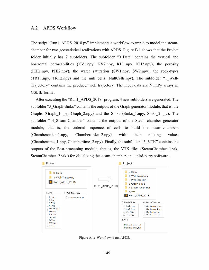
149

A.2 APDS Workflow

The script “Run1_APDS_2018.py” implements a workflow example to model the steam-

chamber for two geostatistical realizations with APDS. Figure B.1 shows that the Project

folder initially has 2 subfolders. The subfolder “0_Data” contains the vertical and

horizontal permeabilities (KV1.npy, KV2.npy, KH1.npy, KH2.npy), the porosity

(PHI1.npy, PHI2.npy), the water saturation (SW1.npy, SW2.npy), the rock-types

(TRT1.npy, TRT2.npy) and the null cells (NullCells.npy). The subfolder “1_Well-

Trajectory” contains the producer well trajectory. The input data are NumPy arrays in

GSLIB format.

After executing the “Run1_APDS_2018” program, 4 new subfolders are generated. The

subfolder “3_Graph-Sinks” contains the outputs of the Graph generator module, that is, the

Graphs (Graph_1.npy, Graph_2.npy) and the Sinks (Sinks_1.npy, Sinks_2.npy). The

subfolder “ 4_Steam-Chamber” contains the outputs of the Steam-chamber generator

module, that is, the ordered sequence of cells to build the steam-chambers

(Chamberorder_1.npy, Chamberorder_2.npy) with their ranking values

(Chambertime_1.npy, Chambertime_2.npy). Finally, the subfolder “ 5_VTK” contains the

outputs of the Post-processing module, that is, the VTK files (SteamChamber_1.vtk,

SteamChamber_2.vtk ) for visualizing the steam-chambers in a third-party software.

Figure A.1: Workflow to run APDS.

Project

0_Data 1_Well-Trajectory

Project

3_Graph-Sinks 4_Steam-Chamber

5_VTK

Run1_APDS_2018

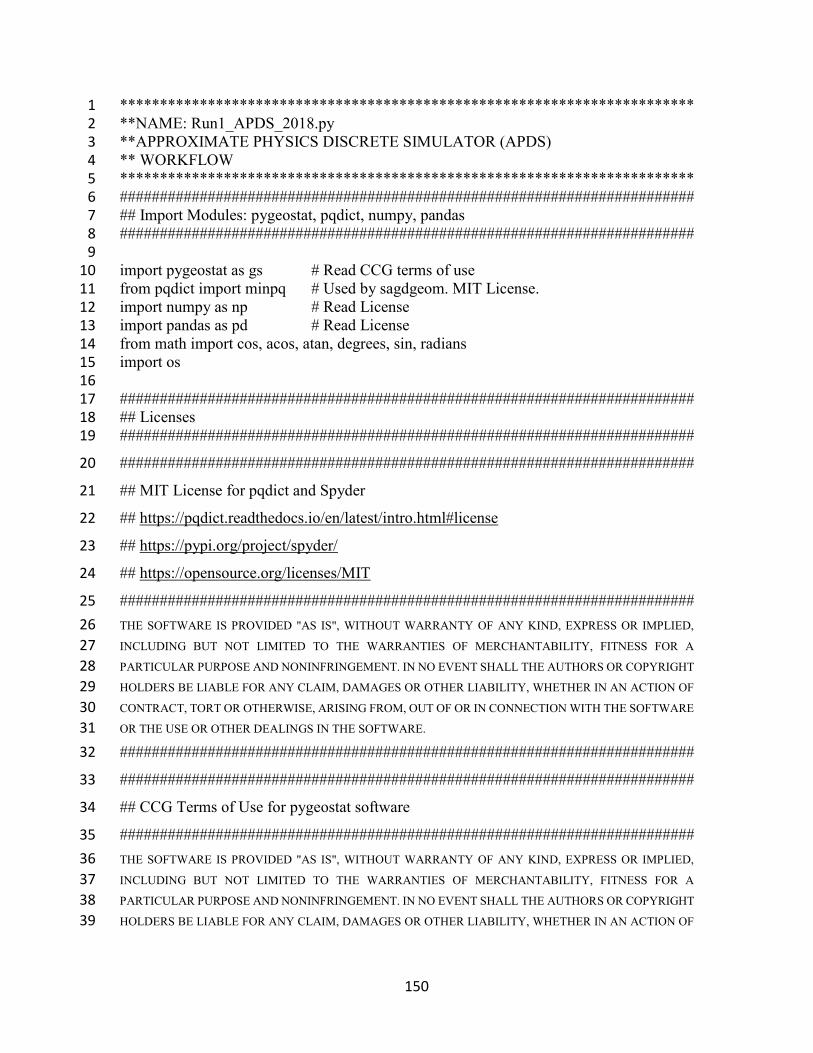
150

************************************************************************ 1 **NAME: Run1_APDS_2018.py 2 **APPROXIMATE PHYSICS DISCRETE SIMULATOR (APDS) 3 ** WORKFLOW 4 ************************************************************************ 5 ########################################################################6 ## Import Modules: pygeostat, pqdict, numpy, pandas 7 ######################################################################## 8 9 import pygeostat as gs # Read CCG terms of use 10 from pqdict import minpq # Used by sagdgeom. MIT License. 11 import numpy as np # Read License 12 import pandas as pd # Read License 13 from math import cos, acos, atan, degrees, sin, radians 14 import os 15 16 ######################################################################## 17 ## Licenses 18 ######################################################################## 19

######################################################################## 20

## MIT License for pqdict and Spyder 21

## https://pqdict.readthedocs.io/en/latest/intro.html#license 22

## https://pypi.org/project/spyder/ 23

## https://opensource.org/licenses/MIT 24

######################################################################## 25

THE SOFTWARE IS PROVIDED "AS IS", WITHOUT WARRANTY OF ANY KIND, EXPRESS OR IMPLIED, 26

INCLUDING BUT NOT LIMITED TO THE WARRANTIES OF MERCHANTABILITY, FITNESS FOR A 27

PARTICULAR PURPOSE AND NONINFRINGEMENT. IN NO EVENT SHALL THE AUTHORS OR COPYRIGHT 28

HOLDERS BE LIABLE FOR ANY CLAIM, DAMAGES OR OTHER LIABILITY, WHETHER IN AN ACTION OF 29

CONTRACT, TORT OR OTHERWISE, ARISING FROM, OUT OF OR IN CONNECTION WITH THE SOFTWARE 30

OR THE USE OR OTHER DEALINGS IN THE SOFTWARE. 31

######################################################################## 32

########################################################################33

## CCG Terms of Use for pygeostat software 34

######################################################################## 35

THE SOFTWARE IS PROVIDED "AS IS", WITHOUT WARRANTY OF ANY KIND, EXPRESS OR IMPLIED, 36

INCLUDING BUT NOT LIMITED TO THE WARRANTIES OF MERCHANTABILITY, FITNESS FOR A 37

PARTICULAR PURPOSE AND NONINFRINGEMENT. IN NO EVENT SHALL THE AUTHORS OR COPYRIGHT 38

HOLDERS BE LIABLE FOR ANY CLAIM, DAMAGES OR OTHER LIABILITY, WHETHER IN AN ACTION OF 39

https://pqdict.readthedocs.io/en/latest/intro.html#license

https://pypi.org/project/spyder/


151

CONTRACT, TORT OR OTHERWISE, ARISING FROM, OUT OF OR IN CONNECTION WITH THE SOFTWARE 40

OR THE USE OR OTHER DEALINGS IN THE SOFTWARE. 41

######################################################################## 42

43

########################################################################44

## Python License 45

## https://docs.python.org/3/license.html#psf-license-agreement-for-python-release 46

######################################################################## 47

PSF is making Python 3.7.1 available to Licensee on an "AS IS" basis. PSF MAKES NO REPRESENTATIONS OR 48

WARRANTIES, EXPRESS OR IMPLIED. BY WAY OF EXAMPLE, BUT NOT LIMITATION, PSF MAKES NO 49

AND DISCLAIMS ANY REPRESENTATION OR WARRANTY OF MERCHANTABILITY OR FITNESS FOR 50

ANY PARTICULAR PURPOSE OR THAT THE USE OF PYTHON 3.7.1 WILL NOT INFRINGE ANY THIRD 51

PARTY RIGHTS. 5. PSF SHALL NOT BE LIABLE TO LICENSEE OR ANY OTHER USERS OF PYTHON 3.7.1 52

FOR ANY INCIDENTAL, SPECIAL, OR CONSEQUENTIAL DAMAGES OR LOSS AS A RESULT OF 53

MODIFYING, DISTRIBUTING, OR OTHERWISE USING PYTHON 3.7.1, OR ANY DERIVATIVE THEREOF, 54

EVEN IF ADVISED OF THE POSSIBILITY THEREOF. 55

###################################################################################### 56

57

########################################################################58

## numPy License 59

## http://www.numpy.org/license.html 60

######################################################################## 61

62

THIS SOFTWARE IS PROVIDED BY THE COPYRIGHT HOLDERS AND CONTRIBUTORS “AS IS” AND ANY 63

EXPRESS OR IMPLIED WARRANTIES, INCLUDING, BUT NOT LIMITED TO, THE IMPLIED WARRANTIES 64

OF MERCHANTABILITY AND FITNESS FOR A PARTICULAR PURPOSE ARE DISCLAIMED. IN NO EVENT 65

SHALL THE COPYRIGHT OWNER OR CONTRIBUTORS BE LIABLE FOR ANY DIRECT, INDIRECT, 66

INCIDENTAL, SPECIAL, EXEMPLARY, OR CONSEQUENTIAL DAMAGES (INCLUDING, BUT NOT LIMITED 67

TO, PROCUREMENT OF SUBSTITUTE GOODS OR SERVICES; LOSS OF USE, DATA, OR PROFITS; OR 68

BUSINESS INTERRUPTION) HOWEVER CAUSED AND ON ANY THEORY OF LIABILITY, WHETHER IN 69

CONTRACT, STRICT LIABILITY, OR TORT (INCLUDING NEGLIGENCE OR OTHERWISE) ARISING IN ANY 70

WAY OUT OF THE USE OF THIS SOFTWARE, EVEN IF ADVISED OF THE POSSIBILITY OF SUCH DAMAGE. 71

72

########################################################################73

## scyPy License 74

## https://www.scipy.org/scipylib/license.html 75

######################################################################## 76


http://www.numpy.org/license.html

https://www.scipy.org/scipylib/license.html

152

THIS SOFTWARE IS PROVIDED BY THE COPYRIGHT HOLDERS AND CONTRIBUTORS “AS IS” AND ANY 77



SHALL THE REGENTS OR CONTRIBUTORS BE LIABLE FOR ANY DIRECT, INDIRECT, INCIDENTAL, 80

SPECIAL, EXEMPLARY, OR CONSEQUENTIAL DAMAGES (INCLUDING, BUT NOT LIMITED TO, 81

PROCUREMENT OF SUBSTITUTE GOODS OR SERVICES; LOSS OF USE, DATA, OR PROFITS; OR BUSINESS 82

INTERRUPTION) HOWEVER CAUSED AND ON ANY THEORY OF LIABILITY, WHETHER IN CONTRACT, 83

STRICT LIABILITY, OR TORT (INCLUDING NEGLIGENCE OR OTHERWISE) ARISING IN ANY WAY OUT 84

OF THE USE OF THIS SOFTWARE, EVEN IF ADVISED OF THE POSSIBILITY OF SUCH DAMAGE. 85

86

########################################################################87

## Pandas License 88

## http://pandas.pydata.org/pandas-docs/stable/overview.html#license 89

######################################################################## 90

91

THIS SOFTWARE IS PROVIDED BY THE COPYRIGHT HOLDERS AND CONTRIBUTORS "AS IS" AND ANY 92



SHALL THE COPYRIGHT HOLDER OR CONTRIBUTORS BE LIABLE FOR ANY DIRECT, INDIRECT, 95

INCIDENTAL, SPECIAL, EXEMPLARY, OR CONSEQUENTIAL DAMAGES (INCLUDING, BUT NOT LIMITED 96

TO, PROCUREMENT OF SUBSTITUTE GOODS OR SERVICES; LOSS OF USE, DATA, OR PROFITS; OR 97

BUSINESS INTERRUPTION) HOWEVER CAUSED AND ON ANY THEORY OF LIABILITY, WHETHER IN 98

CONTRACT, STRICT LIABILITY, OR TORT (INCLUDING NEGLIGENCE OR OTHERWISE) ARISING IN ANY 99

WAY OUT OF THE USE OF THIS SOFTWARE, EVEN IF ADVISED OF THE POSSIBILITY OF SUCH DAMAGE. 100

101

######################################################################## 102

103

########################################################################104 ## Folders with Outputs. Example of Workflow 105 ######################################################################## 106 107 if not os.path.exists ('2_Preprocesing'): 108 os.makedirs ('2_Preprocesing') 109 110 if not os.path.exists ('3_Graph-Sinks'): # For Graphs and Sinks 111 os.makedirs ('3_Graph-Sinks') 112 113 if not os.path.exists ('4_Steam-Chamber'): # For Chambertime and Chamberorder 114 os.makedirs ('4_Steam-Chamber') 115 116 if not os.path.exists ('5_VTK'): # For VTK files 117

http://pandas.pydata.org/pandas-docs/stable/overview.html#license

153

os.makedirs ('5_VTK') 118 119 ########################################################################120 ## Create Paths for Input and Output Data 121 ######################################################################## 122 123 datapath = '0_Data/' 124 wellpath = '1_Well-Trajectory/' 125 procpath = '2_Preprocesing/' 126 graphpath = '3_Graph-Sinks/' 127 stchpath = '4_Steam-Chamber/' 128 vtkpath = '5_VTK/' 129 130 131 ########################################################################132 ## Grid Definition 133 ######################################################################## 134 135 grdstr="""40 1 25 - nx, xmn, xsiz 136 100 1 1 - ny , ymn , ysiz 137 50 1 1 - nz , zmn , zsiz """ 138 139 griddef = gs.GridDef (gridstr = gridstr) 140 141 nx = griddef.nx # For convenience 142 ny = griddef.ny 143 nz = griddef.nz 144 xsiz = griddef.xsiz 145 ysiz = griddef.ysiz 146 zsiz = griddef.zsiz 147 148 ########################################################################149 ## Constant, Conversion Factors 150 ######################################################################## 151 m3ToStb = 6.28981 # Convert m3 to bbl 152 Resid_So = 0.25 # APDS input. Residual Oil Saturation 153 kvCutoff = 200 # kv Cut-off in md 154 BulkCellVol = xsiz*ysiz*zsiz*m3ToStb # Bulk cell volume in m3 155 156 ########################################################################157 ## Load Well Trajectories 158 ######################################################################## 159 160 well1= np.load (wellpath + 'ProdWellTrajectory.npy') # Producer Well 161 well2 = range(0,0) # Range (0,0) if there is one well 162 source = load2wells(well1,well2) 163

154

injtracj = range (0,0) # Injector well trajectory 164 165 ########################################################################166 ## Loop for 1 to N Geostatistical Realizations 167 ######################################################################## 168 169 NReal = [1,2] # List of realization indexes. This example has 2 realizations 170 171 for i in NReal: 172 173 ####################################################################### 174 ## Load Input Data 175 ####################################################################### 176 177 APDSRT = np.load (datapath + 'TRT%i.npy'%(i)) # Rock Type 178 APDSPhi = np.load (datapath + 'PHI%i.npy'%(i)) # Porosity 179 APDSKv = np.load (datapath + 'KV%i.npy'%(i)) # KV 180 APDSKh = np.load (datapath + 'KH%i.npy'%(i)) # KH 181 APDSSw = np.load (datapath + 'SW%i.npy'%(i)) # SW 182 APDSNull = np.load (datapath + 'NullCells.npy') # 1 – 0 183 184 ####################################################################### 185 ## Creating a Data-Frame 186 ####################################################################### 187 188 df = pd.DataFrame ({'Kv':APDSKv, 189 'Kh':APDSKh,'RT':APDSRT,'Phi':APDSPhi,'Sw':APDSSw,'Null':APDSNull}) 190 191 ####################################################################### 192 ## Processing Rock-types (‘RTGraph’) to obtain a binary variable, (1) for net-rock and 193 ## (0) for non-net rock, to input the Graph Generator 194 ## The Hydrocarbon Cell Volume (HCV) is calculated 195 ## A dataframe is not necessary, but is convenient to work with Pandas 196 ####################################################################### 197 198 df ['RTGraph'] = df ['RT'] 199 df ['RTGraph'][df ['RTGraph'] == 5] = 0 # Rock Type 5 is shale. Code as 0 200 df ['RTGraph'][df ['RTGraph'] != 0] = 1 # Rock Types 2,3,4 != 0 are now 1 201 df ['RTGraph'][df ['Kv'] <= KvCutoff] = 0 # Apply Kv Cut-off 202 df ['RTGraph'][df ['Kv'] > KvCutoff] = 1 # Apply Kv Cut-off 203 df ['RTGraph'] = df ['RTGraph']* df['Null'] # Apply Null Cells 204 df ['HCV'] = BulkCellVol*df['Phi']*((1-df ['Sw']) - Resid_So) 205 df ['HCV'][df ['HCV'] < 0] = 0 # If HCV is negative, then replace by zero 206 207 208 ####################################################################### 209

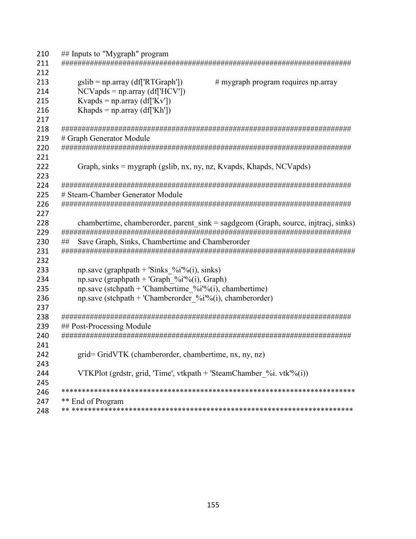
155

## Inputs to "Mygraph" program 210 ####################################################################### 211 212 gslib = np.array (df['RTGraph']) # mygraph program requires np.array 213 NCVapds = np.array (df['HCV']) 214 Kvapds = np.array (df['Kv']) 215 Khapds = np.array (df['Kh']) 216 217 ####################################################################### 218 # Graph Generator Module 219 ####################################################################### 220 221 Graph, sinks = mygraph (gslib, nx, ny, nz, Kvapds, Khapds, NCVapds) 222 223 ####################################################################### 224 # Steam-Chamber Generator Module 225 ####################################################################### 226 227 chambertime, chamberorder, parent_sink = sagdgeom (Graph, source, injtracj, sinks) 228 ####################################################################### 229 ## Save Graph, Sinks, Chambertime and Chamberorder 230 ######################################################################## 231 232 np.save (graphpath + 'Sinks_%i'%(i), sinks) 233 np.save (graphpath + 'Graph_%i'%(i), Graph) 234 np.save (stchpath + 'Chambertime_%i'%(i), chambertime) 235 np.save (stchpath + 'Chamberorder_%i'%(i), chamberorder) 236 237 ####################################################################### 238 ## Post-Processing Module 239 ####################################################################### 240 241 grid= GridVTK (chamberorder, chambertime, nx, ny, nz) 242 243 VTKPlot (grdstr, grid, 'Time', vtkpath + 'SteamChamber_%i. vtk'%(i)) 244 245 ************************************************************************ 246 ** End of Program 247 ** *********************************************************************248

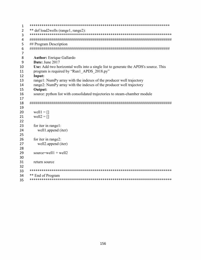
156

*********************************************************************** 1 ** def load2wells (range1, range2): 2 ************************************************************************ 3 ######################################################################## 4 ## Program Description 5 ####################################################################### 6 7 Author: Enrique Gallardo 8 Date: June 2017 9 Use: Add two horizontal wells into a single list to generate the APDS's source. This 10 program is required by “Run1_APDS_2018.py” 11 Input: 12 range1: NumPy array with the indexes of the producer well trajectory 13 range2: NumPy array with the indexes of the producer well trajectory 14 Output: 15 source: python list with consolidated trajectories to steam-chamber module 16 17 ######################################################################## 18 19 well1 = [] 20 well2 = [] 21 22 for iter in range1: 23 well1.append (iter) 24 25 for iter in range2: 26 well2.append (iter) 27 28 source=well1 + well2 29 30 return source 31 32 ************************************************************************ 33 ** End of Program 34 ************************************************************************35

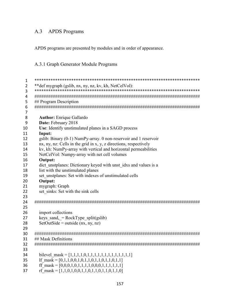
157

A.3 APDS Programs

APDS programs are presented by modules and in order of appearance.

A.3.1 Graph Generator Module Programs

************************************************************************ 1 **def mygraph (gslib, nx, ny, nz, kv, kh, NetCelVol): 2 ************************************************************************ 3 ######################################################################## 4 ## Program Description 5 ######################################################################## 6 7 Author: Enrique Gallardo 8 Date: February 2018 9 Use: Identify unstimulated planes in a SAGD process 10 Input: 11 gslib: Binary (0-1) NumPy-array. 0 non-reservoir and 1 reservoir 12 nx, ny, nz: Cells in the grid in x, y, z directions, respectively 13 kv, kh: NumPy-array with vertical and horizontal permeabilities 14 NetCelVol: Numpy-array with net cell volumes 15 Output: 16 dict_unstplanes: Dictionary keyed with unst_idxs and values is a 17 list with the unstimulated planes 18 set_unstplanes: Set with indexes of unstimulated cells 19 Output: 20 mygraph: Graph 21 set_sinks: Set with the sink cells 22 23 ######################################################################## 24 25 import collections 26 keys_sand,_= RockType_split(gslib) 27 SetOutSide = outside (nx, ny, nz) 28 29 ######################################################################## 30 ## Mask Definitions 31 ######################################################################## 32 33 bilevel_mask = [1,1,1,1,0,1,1,1,1,1,1,1,1,1,1,1,1,1] 34 lf_mask = [0,1,1,0,0,1,0,1,1,0,1,1,0,1,1,0,1,1] 35 ff_mask = [0,0,0,1,0,1,1,1,1,0,0,0,1,1,1,1,1,1] 36 rf_mask = [1,1,0,1,0,0,1,1,0,1,1,0,1,1,0,1,1,0] 37

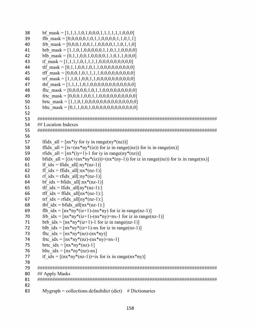
158

bf_mask = [1,1,1,1,0,1,0,0,0,1,1,1,1,1,1,0,0,0] 38 flb_mask = [0,0,0,0,0,1,0,1,1,0,0,0,0,1,1,0,1,1] 39 frb_mask = [0,0,0,1,0,0,1,1,0,0,0,0,1,1,0,1,1,0] 40 brb_mask = [1,1,0,1,0,0,0,0,0,1,1,0,1,1,0,0,0,0] 41 blb_mask = [0,1,1,0,0,1,0,0,0,0,1,1,0,1,1,0,0,0] 42 tf_mask = [1,1,1,1,0,1,1,1,1,0,0,0,0,0,0,0,0,0] 43 tlf_mask = [0,1,1,0,0,1,0,1,1,0,0,0,0,0,0,0,0,0] 44 tff_mask = [0,0,0,1,0,1,1,1,1,0,0,0,0,0,0,0,0,0] 45 trf_mask = [1,1,0,1,0,0,1,1,0,0,0,0,0,0,0,0,0,0] 46 tbf_mask = [1,1,1,1,0,1,0,0,0,0,0,0,0,0,0,0,0,0] 47 fltc_mask = [0,0,0,0,0,1,0,1,1,0,0,0,0,0,0,0,0,0] 48 frtc_mask = [0,0,0,1,0,0,1,1,0,0,0,0,0,0,0,0,0,0] 49 brtc_mask = [1,1,0,1,0,0,0,0,0,0,0,0,0,0,0,0,0,0] 50 bltc_mask = [0,1,1,0,0,1,0,0,0,0,0,0,0,0,0,0,0,0] 51 52 ######################################################################## 53 ## Location Indexes 54 ######################################################################## 55 56 lfidx_all = [nx*iy for iy in range(ny*(nz))] 57 ffidx_all = [ix+(nx*ny*(iz)) for iz in range((nz)) for ix in range(nx)] 58 rfidx_all = [nx*(iy+1)-1 for iy in range(ny*(nz))] 59 bfidx_all = [(ix+(nx*ny*(iz)))+(nx*(ny-1)) for iz in range((nz)) for ix in range(nx)] 60 lf_idx = lfidx_all[:ny*(nz-1)] 61 ff_idx = ffidx_all[:nx*(nz-1)] 62 rf_idx = rfidx_all[:ny*(nz-1)] 63 bf_idx = bfidx_all[:nx*(nz-1)] 64 tlf_idx = lfidx_all[ny*(nz-1):] 65 tff_idx = ffidx_all[nx*(nz-1):] 66 trf_idx = rfidx_all[ny*(nz-1):] 67 tbf_idx = bfidx_all[nx*(nz-1):] 68 flb_idx = [nx*ny*(iz+1)-(nx*ny) for iz in range(nz-1)] 69 frb_idx = [nx*ny*(iz+1)-(nx*ny)+nx-1 for iz in range(nz-1)] 70 brb_idx = [nx*ny*(iz+1)-1 for iz in range(nz-1)] 71 blb_idx = [nx*ny*(iz+1)-nx for iz in range(nz-1)] 72 fltc_idx = [nx*ny*(nz)-(nx*ny)] 73 frtc_idx = [nx*ny*(nz)-(nx*ny)+nx-1] 74 brtc_idx = [nx*ny*(nz)-1] 75 bltc_idx = [nx*ny*(nz)-nx] 76 tf_idx = [(nx*ny*(nz-1))+ix for ix in range(nx*ny)] 77 78 ######################################################################## 79 ## Apply Masks 80 ######################################################################## 81 82 Mygraph = collections.defaultdict (dict) # Dictionaries 83

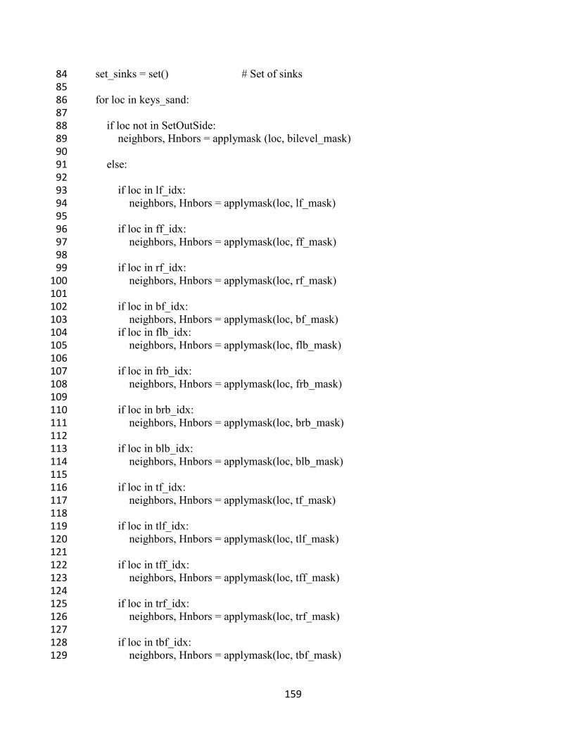
159

set_sinks = set() # Set of sinks 84 85 for loc in keys_sand: 86 87 if loc not in SetOutSide: 88 neighbors, Hnbors = applymask (loc, bilevel_mask) 89 90 else: 91 92 if loc in lf_idx: 93 neighbors, Hnbors = applymask(loc, lf_mask) 94 95 if loc in ff_idx: 96 neighbors, Hnbors = applymask(loc, ff_mask) 97 98 if loc in rf_idx: 99 neighbors, Hnbors = applymask(loc, rf_mask) 100 101 if loc in bf_idx: 102 neighbors, Hnbors = applymask(loc, bf_mask) 103 if loc in flb_idx: 104 neighbors, Hnbors = applymask(loc, flb_mask) 105 106 if loc in frb_idx: 107 neighbors, Hnbors = applymask(loc, frb_mask) 108 109 if loc in brb_idx: 110 neighbors, Hnbors = applymask(loc, brb_mask) 111 112 if loc in blb_idx: 113 neighbors, Hnbors = applymask(loc, blb_mask) 114 115 if loc in tf_idx: 116 neighbors, Hnbors = applymask(loc, tf_mask) 117 118 if loc in tlf_idx: 119 neighbors, Hnbors = applymask(loc, tlf_mask) 120 121 if loc in tff_idx: 122 neighbors, Hnbors = applymask(loc, tff_mask) 123 124 if loc in trf_idx: 125 neighbors, Hnbors = applymask(loc, trf_mask) 126 127 if loc in tbf_idx: 128 neighbors, Hnbors = applymask(loc, tbf_mask) 129

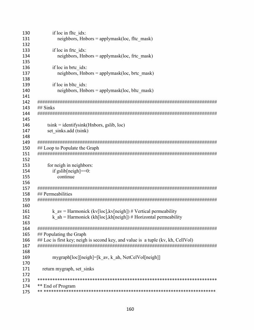
160

if loc in fltc_idx: 130 neighbors, Hnbors = applymask(loc, fltc_mask) 131 132 if loc in frtc_idx: 133 neighbors, Hnbors = applymask(loc, frtc_mask) 134 135 if loc in brtc_idx: 136 neighbors, Hnbors = applymask(loc, brtc_mask) 137 138 if loc in bltc_idx: 139 neighbors, Hnbors = applymask(loc, bltc_mask) 140 141 ######################################################################## 142 ## Sinks 143 ######################################################################## 144 145 tsink = identifysink(Hnbors, gslib, loc) 146 set_sinks.add (tsink) 147 148 ######################################################################## 149 ## Loop to Populate the Graph 150 ######################################################################## 151 152 for neigh in neighbors: 153 if gslib[neigh]==0: 154 continue 155 156 ######################################################################## 157 ## Permeabilities 158 ######################################################################## 159 160 k_av = Harmonick (kv[loc],kv[neigh]) # Vertical permeability 161 k_ah = Harmonick (kh[loc],kh[neigh]) # Horizontal permeability 162 163 ######################################################################## 164 ## Populating the Graph 165 ## Loc is first key; neigh is second key, and value is a tuple (kv, kh, CellVol) 166 ######################################################################## 167 168 mygraph[loc][neigh]=[k_av, k_ah, NetCelVol[neigh]] 169 170 return mygraph, set_sinks 171 172 ************************************************************************ 173 ** End of Program 174 ** *********************************************************************175

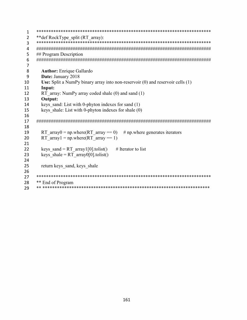
161

************************************************************************ 1 **def RockType_split (RT_array): 2 ************************************************************************ 3 ######################################################################## 4 ## Program Description 5 ######################################################################## 6 7 Author: Enrique Gallardo 8 Date: January 2018 9 Use: Split a NumPy binary array into non-reservoir (0) and reservoir cells (1) 10 Input: 11 RT_array: NumPy array coded shale (0) and sand (1) 12 Output: 13 keys_sand: List with 0-phyton indexes for sand (1) 14 keys_shale: List with 0-phyton indexes for shale (0) 15 16 ######################################################################## 17 18 RT_array0 = np.where(RT_array == 0) # np.where generates iterators 19 RT_array1 = np.where(RT_array == 1) 20 21 keys_sand = RT_array1[0].tolist() # Iterator to list 22 keys_shale = RT_array0[0].tolist() 23 24 return keys_sand, keys_shale 25 26 ************************************************************************ 27 ** End of Program 28 ** *********************************************************************29

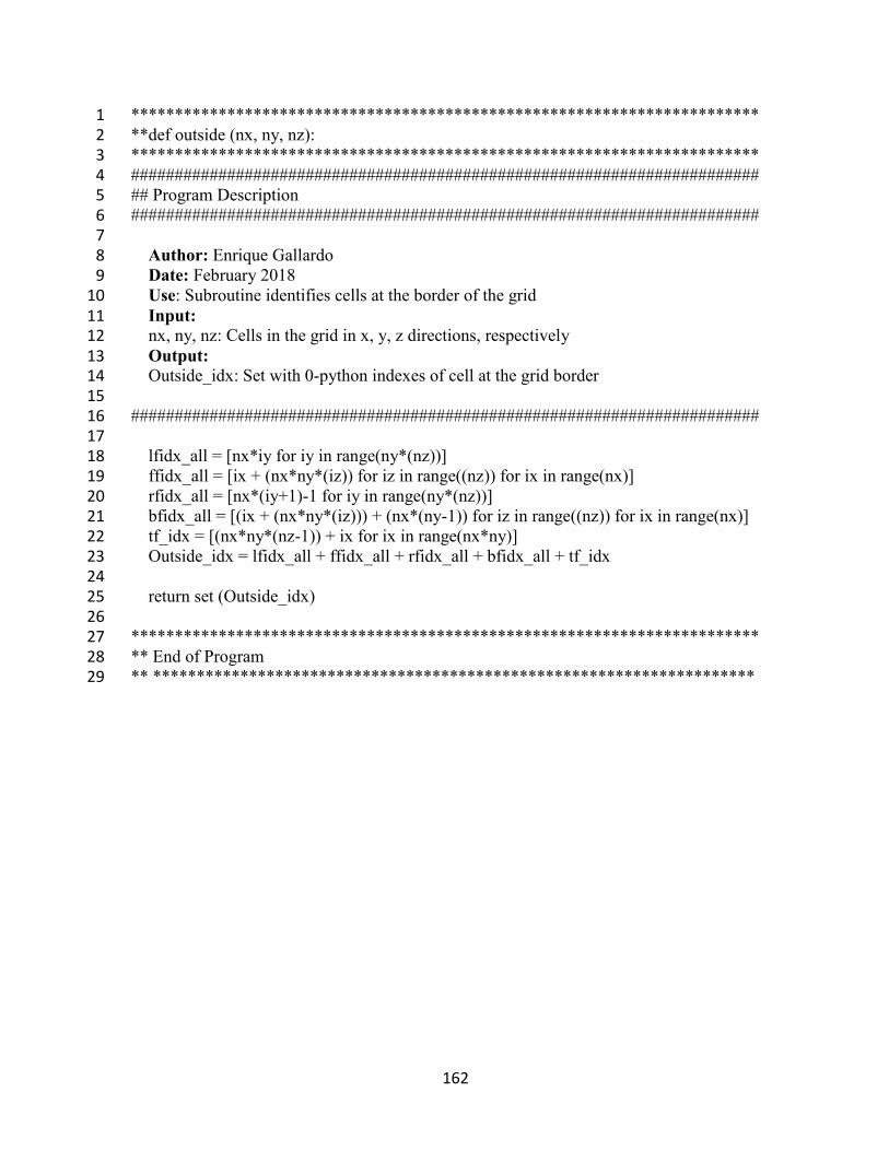
162

************************************************************************ 1 **def outside (nx, ny, nz): 2 ************************************************************************ 3 ######################################################################## 4 ## Program Description 5 ######################################################################## 6 7 Author: Enrique Gallardo 8 Date: February 2018 9 Use: Subroutine identifies cells at the border of the grid 10 Input: 11 nx, ny, nz: Cells in the grid in x, y, z directions, respectively 12 Output: 13 Outside_idx: Set with 0-python indexes of cell at the grid border 14 15 ######################################################################## 16 17 lfidx_all = [nx*iy for iy in range(ny*(nz))] 18 ffidx_all = [ix + (nx*ny*(iz)) for iz in range((nz)) for ix in range(nx)] 19 rfidx_all = [nx*(iy+1)-1 for iy in range(ny*(nz))] 20 bfidx_all = [(ix + (nx*ny*(iz))) + (nx*(ny-1)) for iz in range((nz)) for ix in range(nx)] 21 tf_idx = [(nx*ny*(nz-1)) + ix for ix in range(nx*ny)] 22 Outside_idx = lfidx_all + ffidx_all + rfidx_all + bfidx_all + tf_idx 23 24 return set (Outside_idx) 25 26 ************************************************************************ 27 ** End of Program 28 ** *********************************************************************29

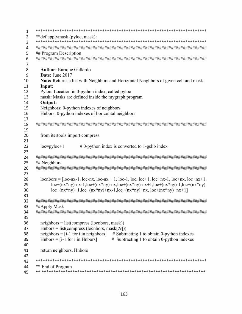
163

************************************************************************ 1 **def applymask (pyloc, mask): 2 ************************************************************************3 ######################################################################## 4 ## Program Description 5 ######################################################################## 6 7 Author: Enrique Gallardo 8 Date: June 2017 9 Note: Returns a list with Neighbors and Horizontal Neighbors of given cell and mask 10 Input: 11 Pyloc: Location in 0-python index, called pyloc 12 mask: Masks are defined inside the mygraph program 13 Output: 14 Neighbors: 0-python indexes of neighbors 15 Hnbors: 0-python indexes of horizontal neighbors 16 17 ######################################################################## 18 19 from itertools import compress 20 21 loc=pyloc+1 # 0-python index is converted to 1-gslib index 22 23 ######################################################################## 24 ## Neighbors 25 ######################################################################## 26 27 locnbors = [loc-nx-1, loc-nx, loc-nx + 1, loc-1, loc, loc+1, loc+nx-1, loc+nx, loc+nx+1, 28 loc+(nx*ny)-nx-1,loc+(nx*ny)-nx,loc+(nx*ny)-nx+1,loc+(nx*ny)-1,loc+(nx*ny), 29 loc+(nx*ny)+1,loc+(nx*ny)+nx-1,loc+(nx*ny)+nx, loc+(nx*ny)+nx+1] 30 31 ######################################################################## 32 ##Apply Mask 33 ######################################################################## 34 35 neighbors = list(compress (locnbors, mask)) 36 Hnbors = list(compress (locnbors, mask[:9])) 37 neighbors = [i-1 for i in neighbors] # Subtracting 1 to obtain 0-python indexes 38 Hnbors = [i-1 for i in Hnbors] # Subtracting 1 to obtain 0-python indexes 39 40 return neighbors, Hnbors 41 42 ************************************************************************ 43 ** End of Program 44 ** *********************************************************************45

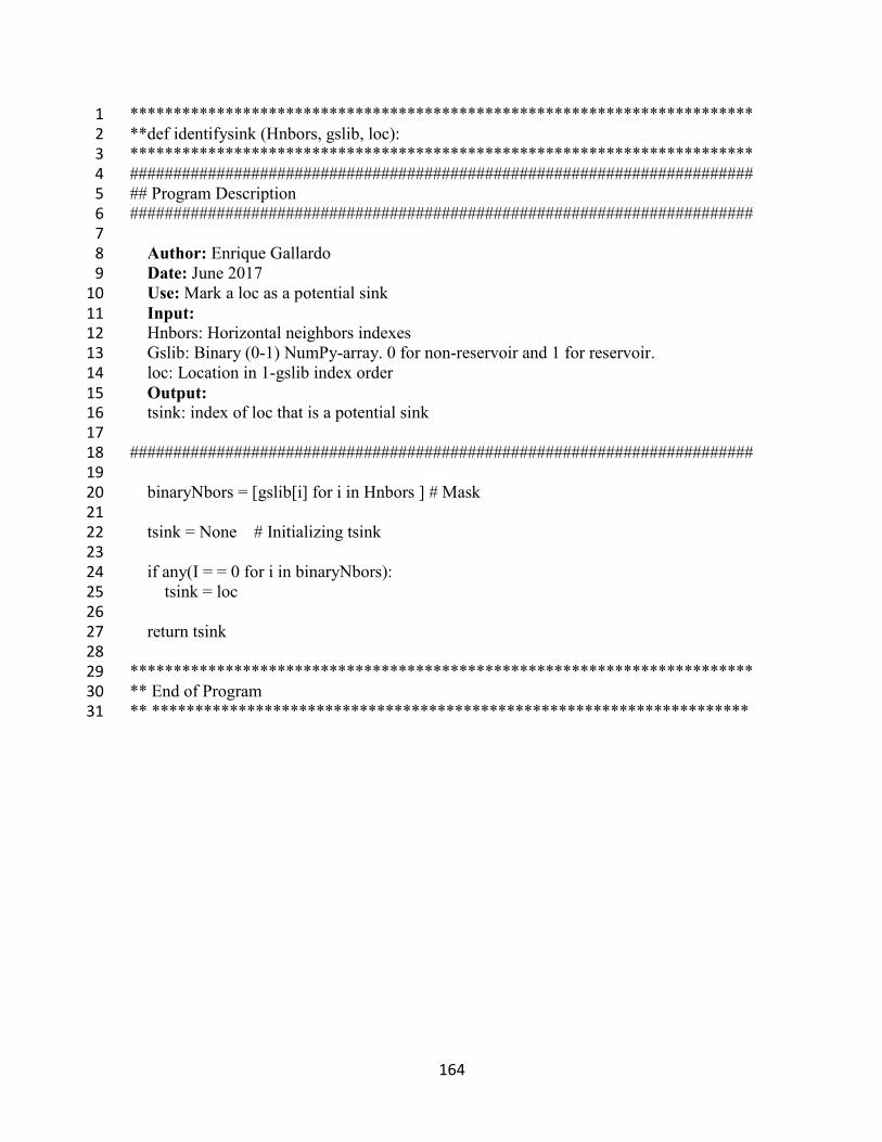
164

************************************************************************ 1 **def identifysink (Hnbors, gslib, loc): 2 ************************************************************************ 3 ######################################################################## 4 ## Program Description 5 ######################################################################## 6 7 Author: Enrique Gallardo 8 Date: June 2017 9 Use: Mark a loc as a potential sink 10 Input: 11 Hnbors: Horizontal neighbors indexes 12 Gslib: Binary (0-1) NumPy-array. 0 for non-reservoir and 1 for reservoir. 13 loc: Location in 1-gslib index order 14 Output: 15 tsink: index of loc that is a potential sink 16 17 ######################################################################## 18 19 binaryNbors = [gslib[i] for i in Hnbors ] # Mask 20 21 tsink = None # Initializing tsink 22 23 if any(I = = 0 for i in binaryNbors): 24 tsink = loc 25 26 return tsink 27 28 ************************************************************************ 29 ** End of Program 30 ** *********************************************************************31

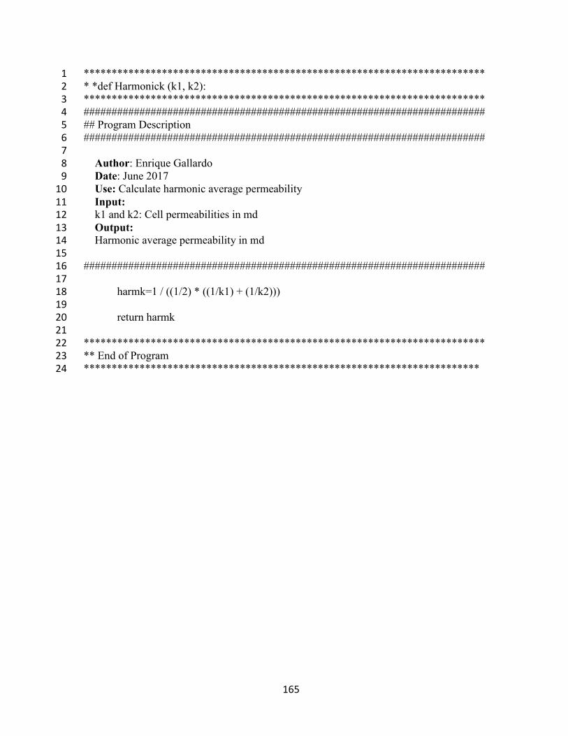
165

************************************************************************ 1 * *def Harmonick (k1, k2): 2 ************************************************************************ 3 ######################################################################## 4 ## Program Description 5 ######################################################################## 6 7 Author: Enrique Gallardo 8 Date: June 2017 9 Use: Calculate harmonic average permeability 10 Input: 11 k1 and k2: Cell permeabilities in md 12 Output: 13 Harmonic average permeability in md 14 15 ######################################################################## 16 17 harmk=1 / ((1/2) * ((1/k1) + (1/k2))) 18 19 return harmk 20 21 ************************************************************************ 22 ** End of Program 23 ***********************************************************************24

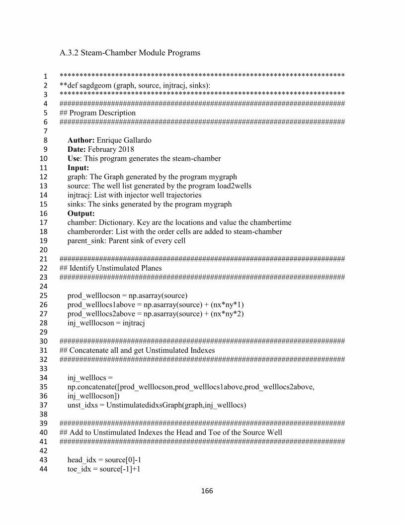
166

A.3.2 Steam-Chamber Module Programs

************************************************************************ 1 **def sagdgeom (graph, source, injtracj, sinks): 2 ************************************************************************ 3 ######################################################################## 4 ## Program Description 5 ######################################################################## 6 7 Author: Enrique Gallardo 8 Date: February 2018 9 Use: This program generates the steam-chamber 10 Input: 11 graph: The Graph generated by the program mygraph 12 source: The well list generated by the program load2wells 13 injtracj: List with injector well trajectories 14 sinks: The sinks generated by the program mygraph 15 Output: 16 chamber: Dictionary. Key are the locations and value the chambertime 17 chamberorder: List with the order cells are added to steam-chamber 18 parent_sink: Parent sink of every cell 19 20 ######################################################################## 21 ## Identify Unstimulated Planes 22 ######################################################################## 23 24 prod_welllocson = np.asarray(source) 25 prod_welllocs1above = np.asarray(source) + (nx*ny*1) 26 prod_welllocs2above = np.asarray(source) + (nx*ny*2) 27 inj_welllocson = injtracj 28 29 ######################################################################## 30 ## Concatenate all and get Unstimulated Indexes 31 ######################################################################## 32 33 inj_welllocs = 34 np.concatenate([prod_welllocson,prod_welllocs1above,prod_welllocs2above, 35 inj_welllocson]) 36 unst_idxs = UnstimulatedidxsGraph(graph,inj_welllocs) 37 38 ######################################################################## 39 ## Add to Unstimulated Indexes the Head and Toe of the Source Well 40 ######################################################################## 41 42 head_idx = source[0]-1 43 toe_idx = source[-1]+1 44

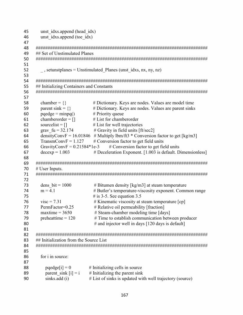
167

unst_idxs.append (head_idx) 45 unst_idxs.append (toe_idx) 46 47 ######################################################################## 48 ## Set of Unstimulated Planes 49 ######################################################################## 50 51 _ , setunstplanes = Unstimulated_Planes (unst_idxs, nx, ny, nz) 52 53 ######################################################################## 54 ## Initializing Containers and Constants 55 ######################################################################## 56 57 chamber = {} # Dictionary. Keys are nodes. Values are model time 58 parent sink = {} # Dictionary. Keys are nodes. Values are parent sinks 59 pqedge = minpq() # Priority queue 60 chamberorder = [] # List for chamberorder 61 sourcelist = [] # List for well trajectories 62 grav_fu = 32.174 # Gravity in field units [ft/sec2] 63 densityConvF = 16.01846 # Multiply lbm/ft3 * Conversion factor to get [kg/m3] 64 TransmConvF = 1.127 # Conversion factor to get field units 65 GravityConvF = 0.21584*1e-3 # Conversion factor to get field units 66 decexp = 1.003 # Deceleration Exponent. [1.003 is default. Dimensionless] 67 68 ######################################################################## 69 # User Inputs. 70 ######################################################################## 71 72 dens_bit = 1000 # Bitumen density [kg/m3] at steam temperature 73 m = 4.1 # Butler’s temperature-viscosity exponent. Common range 74 # is 3-5. See equation 3.5 75 visc = 7.31 # Kinematic viscosity at steam temperature [cp] 76 PermFactor=0.25 # Relative oil permeability [fraction] 77 maxtime = 3650 # Steam-chamber modeling time [days] 78 preheattime = 120 # Time to establish communication between producer 79

# and injector well in days [120 days is default] 80 81 ######################################################################## 82 ## Initialization from the Source List 83 ######################################################################## 84 85 for i in source: 86 87 pqedge[i] = 0 # Initializing cells in source 88 parent_sink [i] = i # Initializing the parent sink 89 sinks.add (i) # List of sinks is updated with well trajectory (source) 90

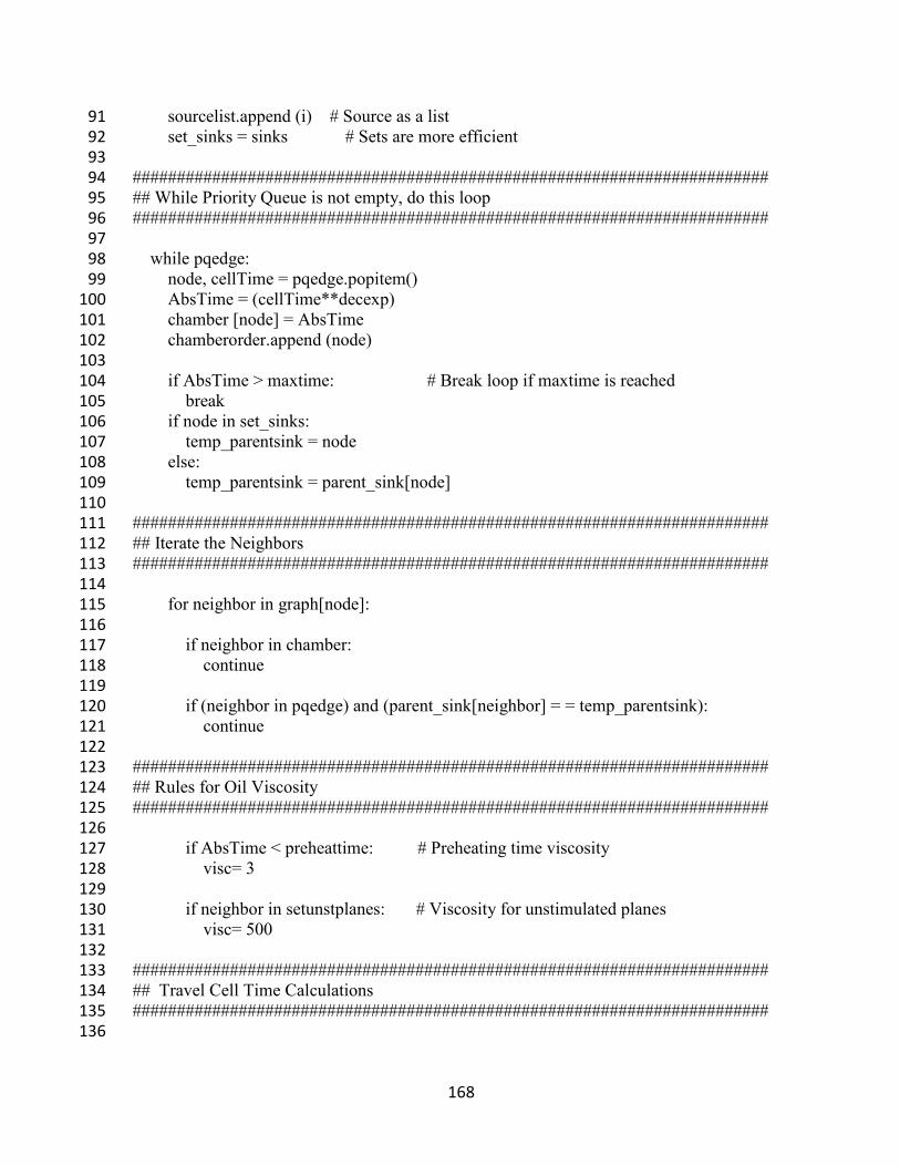
168

sourcelist.append (i) # Source as a list 91 set_sinks = sinks # Sets are more efficient 92 93 ######################################################################## 94 ## While Priority Queue is not empty, do this loop 95 ######################################################################## 96 97 while pqedge: 98 node, cellTime = pqedge.popitem() 99 AbsTime = (cellTime**decexp) 100 chamber [node] = AbsTime 101 chamberorder.append (node) 102 103 if AbsTime > maxtime: # Break loop if maxtime is reached 104 break 105 if node in set_sinks: 106 temp_parentsink = node 107 else: 108 temp_parentsink = parent_sink[node] 109 110 ######################################################################## 111 ## Iterate the Neighbors 112 ######################################################################## 113 114 for neighbor in graph[node]: 115 116 if neighbor in chamber: 117 continue 118 119 if (neighbor in pqedge) and (parent_sink[neighbor] = = temp_parentsink): 120 continue 121 122 ######################################################################## 123 ## Rules for Oil Viscosity 124 ######################################################################## 125 126 if AbsTime < preheattime: # Preheating time viscosity 127 visc= 3 128 129 if neighbor in setunstplanes: # Viscosity for unstimulated planes 130 visc= 500 131 132 ######################################################################## 133 ## Travel Cell Time Calculations 134 ######################################################################## 135 136

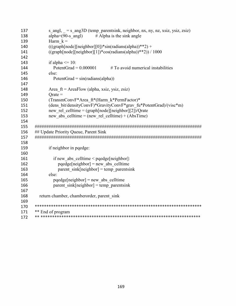
169

s_angl, _ = s_ang3D (temp_parentsink, neighbor, nx, ny, nz, xsiz, ysiz, zsiz) 137 alpha=(90-s_angl) # Alpha is the sink angle 138 Harm_k = 139 (((graph[node][neighbor][0])*sin(radians(alpha))**2) + 140 ((graph[node][neighbor][1])*cos(radians(alpha))**2)) / 1000 141 142 if alpha <= 10: 143 PotentGrad = 0.000001 # To avoid numerical instabilities 144 else: 145 PotentGrad = sin(radians(alpha)) 146 147 Area_ft = AreaFlow (alpha, xsiz, ysiz, zsiz) 148 Qrate = 149 (TransmConvF*Area_ft*(Harm_k*PermFactor)* 150 (dens_bit/densityConvF)*GravityConvF*grav_fu*PotentGrad)/(visc*m) 151 new_rel_celltime = (graph[node][neighbor][2])/Qrate 152 new_abs_celltime = (new_rel_celltime) + (AbsTime) 153 154 ######################################################################## 155 ## Update Priority Queue, Parent Sink 156 ######################################################################## 157 158 if neighbor in pqedge: 159 160 if new_abs_celltime < pqedge[neighbor]: 161 pqedge[neighbor] = new_abs_celltime 162 parent_sink[neighbor] = temp_parentsink 163 else: 164 pqedge[neighbor] = new_abs_celltime 165 parent_sink[neighbor] = temp_parentsink 166 167 return chamber, chamberorder, parent_sink 168 169 ************************************************************************ 170 ** End of program 171 ** *********************************************************************172

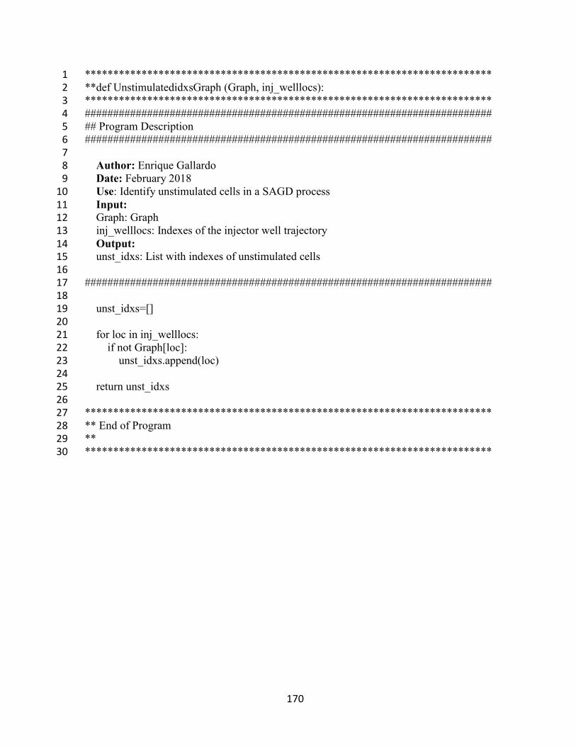
170

************************************************************************ 1 **def UnstimulatedidxsGraph (Graph, inj_welllocs): 2 ************************************************************************ 3 ######################################################################## 4 ## Program Description 5 ######################################################################## 6 7 Author: Enrique Gallardo 8 Date: February 2018 9 Use: Identify unstimulated cells in a SAGD process 10 Input: 11 Graph: Graph 12 inj_welllocs: Indexes of the injector well trajectory 13 Output: 14 unst_idxs: List with indexes of unstimulated cells 15 16 ######################################################################## 17 18 unst_idxs=[] 19 20 for loc in inj_welllocs: 21 if not Graph[loc]: 22 unst_idxs.append(loc) 23 24 return unst_idxs 25 26 ************************************************************************ 27 ** End of Program 28 ** 29 ************************************************************************30

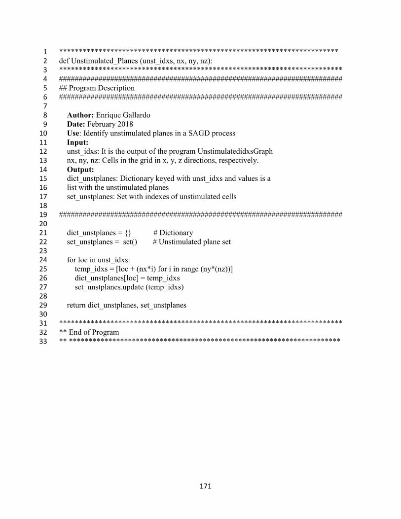
171

*********************************************************************** 1 def Unstimulated_Planes (unst_idxs, nx, ny, nz): 2 ************************************************************************ 3 ######################################################################## 4 ## Program Description 5 ######################################################################## 6 7 Author: Enrique Gallardo 8 Date: February 2018 9 Use: Identify unstimulated planes in a SAGD process 10 Input: 11 unst_idxs: It is the output of the program UnstimulatedidxsGraph 12 nx, ny, nz: Cells in the grid in x, y, z directions, respectively. 13 Output: 14 dict_unstplanes: Dictionary keyed with unst_idxs and values is a 15 list with the unstimulated planes 16 set_unstplanes: Set with indexes of unstimulated cells 17 18 ######################################################################## 19 20 dict_unstplanes = {} # Dictionary 21 set_unstplanes = set() # Unstimulated plane set 22 23 for loc in unst_idxs: 24 temp_idxs = [loc + (nx*i) for i in range (ny*(nz))] 25 dict_unstplanes[loc] = temp_idxs 26 set_unstplanes.update (temp_idxs) 27 28 return dict_unstplanes, set_unstplanes 29 30 ************************************************************************ 31 ** End of Program 32 ** *********************************************************************33

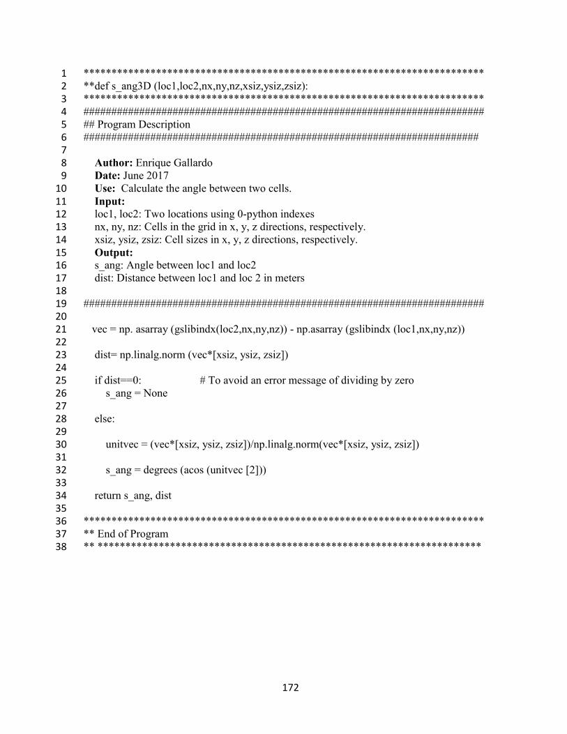
172

************************************************************************ 1 **def s_ang3D (loc1,loc2,nx,ny,nz,xsiz,ysiz,zsiz): 2 ************************************************************************ 3 ######################################################################## 4 ## Program Description 5 ####################################################################### 6 7 Author: Enrique Gallardo 8 Date: June 2017 9 Use: Calculate the angle between two cells. 10 Input: 11 loc1, loc2: Two locations using 0-python indexes 12 nx, ny, nz: Cells in the grid in x, y, z directions, respectively. 13 xsiz, ysiz, zsiz: Cell sizes in x, y, z directions, respectively. 14 Output: 15 s_ang: Angle between loc1 and loc2 16 dist: Distance between loc1 and loc 2 in meters 17 18 ######################################################################## 19 20 vec = np. asarray (gslibindx(loc2,nx,ny,nz)) - np.asarray (gslibindx (loc1,nx,ny,nz)) 21 22 dist= np.linalg.norm (vec*[xsiz, ysiz, zsiz]) 23 24 if dist==0: # To avoid an error message of dividing by zero 25 s_ang = None 26 27 else: 28 29 unitvec = (vec*[xsiz, ysiz, zsiz])/np.linalg.norm(vec*[xsiz, ysiz, zsiz]) 30 31 s_ang = degrees (acos (unitvec [2])) 32 33 return s_ang, dist 34 35 ************************************************************************ 36 ** End of Program 37 ** *********************************************************************38

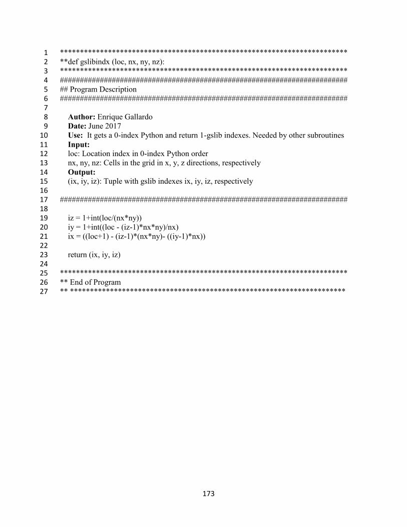
173

************************************************************************1 **def gslibindx (loc, nx, ny, nz): 2 ************************************************************************ 3 ######################################################################## 4 ## Program Description 5 ######################################################################## 6 7 Author: Enrique Gallardo 8 Date: June 2017 9 Use: It gets a 0-index Python and return 1-gslib indexes. Needed by other subroutines 10 Input: 11 loc: Location index in 0-index Python order 12 nx, ny, nz: Cells in the grid in x, y, z directions, respectively 13 Output: 14 (ix, iy, iz): Tuple with gslib indexes ix, iy, iz, respectively 15 16 ######################################################################## 17 18 iz = 1+int(loc/(nx*ny)) 19 iy = 1+int((loc - (iz-1)*nx*ny)/nx) 20 ix = ((loc+1) - (iz-1)*(nx*ny)- ((iy-1)*nx)) 21 22 return (ix, iy, iz) 23 24 ************************************************************************ 25 ** End of Program 26 ** *********************************************************************27

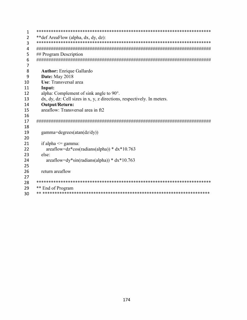
174

************************************************************************ 1 **def AreaFlow (alpha, dx, dy, dz): 2 ************************************************************************ 3 ######################################################################## 4 ## Program Description 5 ######################################################################## 6 7 Author: Enrique Gallardo 8 Date: May 2018 9 Use: Transversal area 10 Input: 11 alpha: Complement of sink angle to 90°. 12 dx, dy, dz: Cell sizes in x, y, z directions, respectively. In meters. 13 Output/Return: 14 areaflow: Transversal area in ft2 15 16 ######################################################################## 17 18 gamma=degrees(atan(dz/dy)) 19 20 if alpha <= gamma: 21 areaflow=dz*cos(radians(alpha)) * dx*10.763 22 else: 23 areaflow=dy*sin(radians(alpha)) * dx*10.763 24 25 return areaflow 26 27 ************************************************************************ 28 ** End of Program 29 ** *********************************************************************30

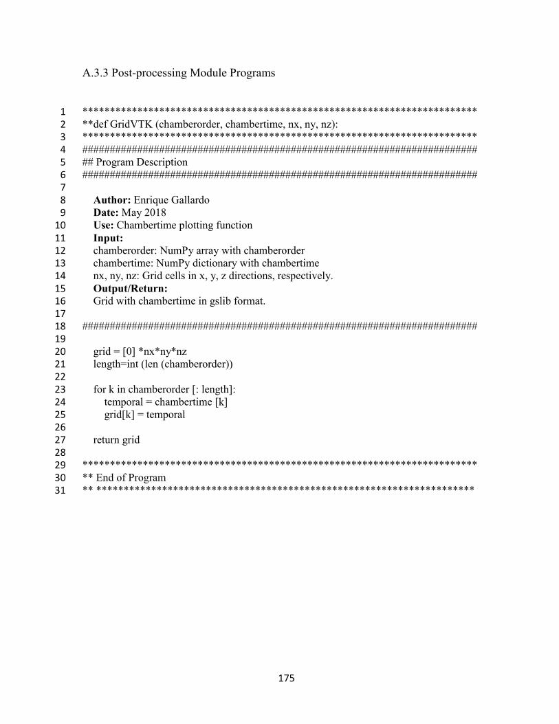
175

A.3.3 Post-processing Module Programs

************************************************************************1 **def GridVTK (chamberorder, chambertime, nx, ny, nz): 2 ************************************************************************ 3 ######################################################################## 4 ## Program Description 5 ######################################################################## 6 7 Author: Enrique Gallardo 8 Date: May 2018 9 Use: Chambertime plotting function 10 Input: 11 chamberorder: NumPy array with chamberorder 12 chambertime: NumPy dictionary with chambertime 13 nx, ny, nz: Grid cells in x, y, z directions, respectively. 14 Output/Return: 15 Grid with chambertime in gslib format. 16 17 ######################################################################## 18 19 grid = [0] *nx*ny*nz 20 length=int (len (chamberorder)) 21 22 for k in chamberorder [: length]: 23 temporal = chambertime [k] 24 grid[k] = temporal 25 26 return grid 27 28 ************************************************************************ 29 ** End of Program 30 ** *********************************************************************31

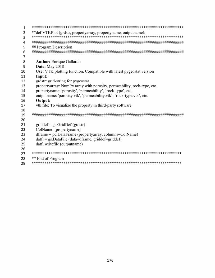
176

************************************************************************1 **def VTKPlot (grdstr, propertyarray, propertyname, outputname): 2 ************************************************************************ 3 ######################################################################## 4 ## Program Description 5 ######################################################################## 6 7 Author: Enrique Gallardo 8 Date: May 2018 9 Use: VTK plotting function. Compatible with latest pygeostat version 10 Input: 11 grdstr: grid-string for pygeostat 12 propertyarray: NumPy array with porosity, permeability, rock-type, etc. 13 propertyname: 'porosity', ‘permeability’, ‘rock-type’, etc. 14 outputname: 'porosity.vtk', ‘permeability.vtk’, ‘rock-type.vtk’, etc. 15 Output: 16 vtk file: To visualize the property in third-party software 17 18 ######################################################################## 19 20 griddef = gs.GridDef (grdstr) 21 ColName=[propertyname] 22 dframe = pd.DataFrame (propertyarray, columns=ColName) 23 datfl = gs.DataFile (data=dframe, griddef=griddef) 24 datfl.writefile (outputname) 25 26 *********************************************************************** 27 ** End of Program 28 *********************************************************************** 29

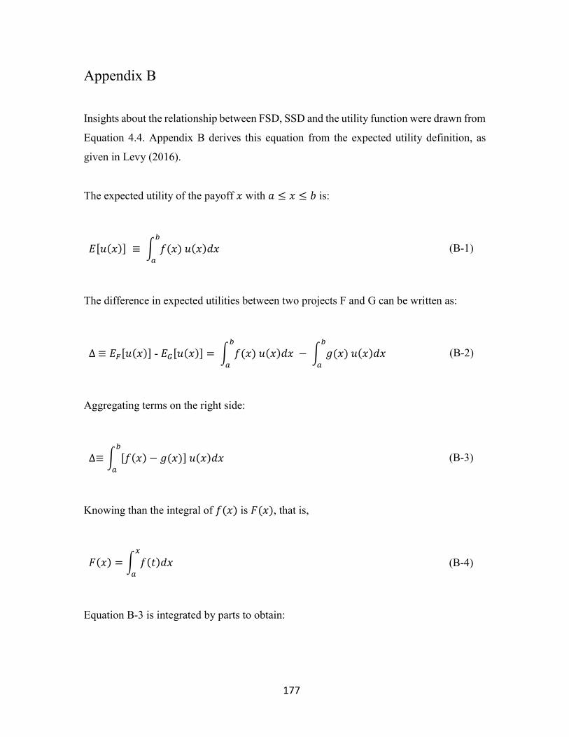
177

Appendix B

Insights about the relationship between FSD, SSD and the utility function were drawn from

Equation 4.4. Appendix B derives this equation from the expected utility definition, as

given in Levy (2016).

The expected utility of the payoff 𝑥 with 𝑎 ≤ 𝑥 ≤ 𝑏 is:

𝐸[𝑢(𝑥)] ≡ ∫ 𝑓(𝑥) 𝑢(𝑥)𝑑𝑥 𝑏

𝑎

(B-1)

The difference in expected utilities between two projects F and G can be written as:

∆ ≡ 𝐸𝐹[𝑢(𝑥)] - 𝐸𝐺[𝑢(𝑥)] = ∫ 𝑓(𝑥) 𝑢(𝑥)𝑑𝑥 𝑏

𝑎

− ∫ 𝑔(𝑥) 𝑢(𝑥)𝑑𝑥 𝑏

𝑎

(B-2)

Aggregating terms on the right side:

∆≡ ∫ [𝑓(𝑥) − 𝑔(𝑥)] 𝑢(𝑥)𝑑𝑥 𝑏

𝑎

(B-3)

Knowing than the integral of 𝑓(𝑥) is 𝐹(𝑥), that is,

𝐹(𝑥) = ∫ 𝑓(𝑡)𝑑𝑥 𝑥

𝑎

(B-4)

Equation B-3 is integrated by parts to obtain:

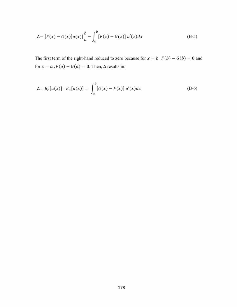
178

∆= [𝐹(𝑥) − 𝐺(𝑥)]𝑢(𝑥)|𝑏

𝑎− ∫ [𝐹(𝑥) − 𝐺(𝑥)] 𝑢′(𝑥)𝑑𝑥

𝑏

𝑎

(B-5)

The first term of the right-hand reduced to zero because for 𝑥 = 𝑏 , 𝐹(𝑏) − 𝐺(𝑏) = 0 and

for 𝑥 = 𝑎 , 𝐹(𝑎) − 𝐺(𝑎) = 0. Then, ∆ results in:

∆= 𝐸𝐹[𝑢(𝑥)] - 𝐸𝐺[𝑢(𝑥)] = ∫ [𝐺(𝑥) − 𝐹(𝑥)] 𝑢′(𝑥)𝑑𝑥 𝑏

𝑎

(B-6)

Enrique Gallardo Vizcaino - ERA

Documents