Enhancing disjunctive logic programming systems by SAT checkers

Page 1

Artificial Intelligence 151 (2003) 177–212

www.elsevier.com/locate/artint

Enhancing disjunctive logic programming systemsby SAT checkers ✩

Christoph Koch a,∗, Nicola Leone b, Gerald Pfeifer a

a Institut für Informationssysteme, Technische Universität Wien, A-1040 Wien, Austriab Department of Mathematics, University of Calabria, 87030 Rende (CS), Italy

Received 1 May 2002

Abstract

Disjunctive logic programming (DLP) with stable model semantics is a powerful nonmonotonicformalism for knowledge representation and reasoning. Reasoning with DLP is harder than withnormal (∨-free) logic programs, because stable model checking—deciding whether a given modelis a stable model of a propositional DLP program—is co-NP-complete, while it is polynomial fornormal logic programs.

This paper proposes a new transformation ΓM(P), which reduces stable model checking toUNSAT—i.e., to deciding whether a given CNF formula is unsatisfiable. The stability of a model Mof a program P thus can be verified by calling a Satisfiability Checker on the CNF formula ΓM(P).The transformation is parsimonious (i.e., no new symbol is added), and efficiently computable, asit runs in logarithmic space (and therefore in polynomial time). Moreover, the size of the generatedCNF formula never exceeds the size of the input (and is usually much smaller). We complement thistransformation with modular evaluation results, which allow for efficient handling of large real-worldreasoning problems.

The proposed approach to stable model checking has been implemented in DLV—a state-of-the-art implementation of DLP. A number of experiments and benchmarks have been run using SATZ asSatisfiability checker. The results of the experiments are very positive and confirm the usefulness ofour techniques. 2003 Elsevier B.V. All rights reserved.

✩ A preliminary version of this paper has been presented at IJCAI’99 [1]. This work was supported by theEuropean Commission under project INFOMIX, project no. IST-2001-33570, and under project ICONS, projectno. IST-2001-32429.

* Corresponding author.E-mail addresses:[email protected] (C. Koch), [email protected] (N. Leone),

[email protected] (G. Pfeifer).

0004-3702/$ – see front matter 2003 Elsevier B.V. All rights reserved.

doi:10.1016/S0004-3702(03)00078-X

Page 2

178 C. Koch et al. / Artificial Intelligence 151 (2003) 177–212

Keywords:Disjunctive logic programming; Nonmonotonic reasoning; Head-cycle-free programs; Answer set

programs; Stable model checking

1. Introduction

Disjunctive logic programming (DLP) with the stable model semantics is a powerfulnonmonotonic formalism for knowledge representation and common sense reasoning [2–5]. DLP has a very high expressive power [6]—it allows to express all problems in thecomplexity class �P

2 (i.e., NPNP). It is well known that many important nonmonotonicreasoning and AI problems are �P

2 -complete [7–12], and that nonmonotonic reasoningsystems using the stable model semantics are currently among the most efficient declarativesystems that can deal with such problems. Moreover, many complex problems can berepresented in a simple and easy-to-understand fashion [13,14] using DLP with the stablemodel semantics.

Roughly, a DLP program is a set of disjunctive rules, i.e., clauses of the form

a1 ∨ · · · ∨ an← b1 ∧ · · · ∧ bk ∧¬bk+1 ∧ · · · ∧ ¬bm

with a possibly empty body (i.e., m � 0). The intuitive reading of such a rule is “If allb1, . . . , bk are true and all bk+1, . . . , bm are false,1 then at least one atom in a1, . . . , anmust be true.” Atoms a1, . . . , an, b1, . . . , bm may contain variables but no function terms.A clause with an empty head (i.e., n = 0) and a nonempty body is called an integrityconstraint and is read as “At least one atom in b1, . . . , bk must be false or at least one atomin bk+1, . . . , bm must be true.” (i.e., the body of the constraint must be false). The intendedmodels of a DLP program (i.e., the semantics of the program) are subset-minimal modelswhich are “grounded” in a precise sense. They are called stable modelsor answer sets[2,5].

The DLP language allows for a fully declarative programming style, which is calledanswer set programming(ASP). The idea of answer set programming is to represent a givencomputational problem by a DLP program whose stable models (answer sets) correspondto solutions, and then use a DLP system to find such a solution [15].

Example 1.1. Consider 3-Colorability, a well-known NP-complete problem from graphtheory, which closely relates to the problem of coloring a map with a minimal number ofcolors such that no two neighboring countries are assigned the same color.

Given a graph, the problem is to decide whether there exists an assignment of one ofthree colors (say, red, green, or blue) to each node such that adjacent nodes always havedifferent colors.

1 Throughout this paper, ¬ intuitively denotes negation-as-failure, rather than classical negation.

Page 3

C. Koch et al. / Artificial Intelligence 151 (2003) 177–212 179

Suppose that the graph is represented by a set of facts F using a unary predicate

node(X) and a binary predicate arc(X,Y ). Then, the following DLP program (incombination with F) computes all 3-Colorings (as stable models) of that graph.

r1: color(X, red)∨ color(X,green)∨ color(X,blue)← node(X),

r2: ← color(X1,C)∧ color(X2,C)∧ arc(X1,X2).

Rule r12 expresses that each node must either be colored red, green, or blue; due tominimality of the stable models, a node cannot be assigned more than one color. Thesubsequent integrity constraint checks that no pair of adjacent nodes (connected by anarc) is assigned the same color.

Thus, there is a one-to-one correspondence between the solutions of the 3-Coloringproblem and the stable models of F ∪ {r1, r2}. The graph is 3-colorable if and only ifF ∪ {r1, r2} has some stable model.

Answer set programming has recently found a number of promising applications:Several tasks in information integration require complex reasoning capabilities, which areexplored in the INFOMIX project (funded by the European Commission, project IST-2002-33570). Another EC-funded project, ICONS (IST-2001-32429), employs a DLP system asintelligent query engine for knowledge management. The Polish company Rodan SystemsS.A. uses a DLP system in a tool for the detection of price manipulations and unauthorizeduses of confidential information, which is used by the Polish securities and exchangecommission. ASP solvers are used also for decision support in the Space Shuttle [16], forproduct and software configuration tasks [17,18], for model checking applications [19],and more.

The high expressive power—a key reason for the success of disjunctive logicprogramming—is paid for by high computational complexity. Indeed, as for the othermain nonmonotonic formalisms like Default Logic or Circumscription, reasoning withDLP (under stable model semantics) is very hard. The high complexity of DLP reasoningstems from two sources: On the one hand the exponential number of possible models(model candidates), and on the other hand from the hardness of stable model checking—deciding whether a given model is a stable model of a propositional DLP program—whichis co-NP-complete. The hardness of this problem has discouraged the implementation ofDLP engines.

Indeed, at the time being only few systems—namely DLV [13] and GnT/Smodels [20]—are available which fully support (function-free) DLP with the stable model semantics.

In this paper, we study the stable model checking problem to provide efficient methodsfor its implementation. We come up with a new transformation which reduces stable modelchecking to Unsatisfiability (UNSAT)—that is, to deciding whether a given CNF formulais unsatisfiable. This is the complement of Satisfiability (SAT), a problem for which veryefficient systems have been developed in AI during the last decade.

Besides providing an elegant characterization of stable models which sheds new lighton their intrinsic nature, the proposed transformation has a strong practical impact. Indeed,

2 Variable names start with an upper case letter and constants start with a lower case letter.

Page 4

180 C. Koch et al. / Artificial Intelligence 151 (2003) 177–212

by using this transformation, the huge amount of work done in AI on the design and

implementation of efficient algorithms for checking Satisfiability can be profitably usedfor the implementation of DLP engines supporting stable model semantics. In a sensethis transformation thus opens “new frontiers” in the implementation of Disjunctive LogicProgramming.

In addition we derive new modularity properties of stable models which permit the useof modular evaluation techniques for stable model checking. Those prove extremely usefulin the light of co-NP-completeness results for that task.

We have implemented the proposed technique in the DLP system DLV, and performeda number of experiments and benchmarks.

In sum, the main contributions of this paper are the following:

• We define a new transformation from stable model checking for general DLP withnegation to UNSAT of propositional CNF formulas. We prove the correctness of thetransformation. The transformation is parsimonious (i.e., it does not add any newsymbol) and efficiently computable, since it runs in LOGSPACE (and therefore inpolynomial time). Moreover, the size of the generated CNF formula never exceeds thesize of the input (and is usually much smaller because many rules are simplified orremoved).• We present some new results based on the application of modular evaluation

techniques to our approach, which allow for further efficiency improvements bysplitting the process of stable model checking. Instead of checking the stability ofthe model at once on the entire program, the model is split into components that areindependently checked for stability on the respective subprograms.• We realize our approach in the DLP system DLV—a state-of-the-art implementation of

disjunctive logic programming—by using the efficient Davis–Putnam procedure SATZ[21] as the Satisfiability checker to solve UNSAT.• We compare our approach with the GnT system and with the original stable-model

checking method of DLV. We highlight the main differences of the methods, and wecarry out an experimental activity over a number of �P

2 -complete problems. Theresults of the experiments witness the efficiency of our approach to stable modelchecking—DLV with our new strategy outperforms the competing systems.

It is worth noting that, since stable model checking of DLP programs generalizesminimal model checking for Horn CNF formulas, our results can be employed also forreasoning with minimal models or circumscription over these formulas.

The DLV system, which implements the results described in this paper, can bedownloaded from http://www.dlvsystem.com/. From the same Web page, one can alsoretrieve the benchmark problems that we used in our experiments.

The paper is organized as follows. Section 2 first provides definitions of syntax andsemantics of DLP with the stable model semantics. After that we give further examples ofusing DLP for a couple of knowledge representation problems. In Section 3, we outlinepreviously known results on stable model checking. Section 4 presents our main result,the transformation from stable model checking to UNSAT. Section 5 applies modularityproperties of DLP programs in the context of our transformation. Section 6 briefly

Page 5

C. Koch et al. / Artificial Intelligence 151 (2003) 177–212 181

describes our implementation, compares our approach to other stable model checking

methods, and presents benchmark problems used and results obtained in our experiments.Finally, Section 7 addresses a number of further related works and draws our conclusions.

2. Disjunctive logic programming with stable model semantics

In this section, we provide an overview of (function-free) disjunctive logic programmingwith stable model semantics [2,14,22,23].

2.1. Syntax

A variable or constant is a term. An atom is of the form a(t1, . . . , tn), where a is apredicateof arity n� 0 and t1, . . . , tn are terms. A literal is either a positive literalp or anegative literal¬p, where p is an atom.

A (disjunctive) rule r is a clause of the form

a1 ∨ · · · ∨ an← b1 ∧ · · · ∧ bk ∧¬bk+1 ∧ · · · ∧ ¬bm, n� 1, m� 0,

where a1, . . . , an, b1, . . . , bm are atoms and r needs to be safe, i.e., each variable occurringin r must appear in one of the positive body literals b1, . . . , bk . The disjunction a1∨· · ·∨anis the headof r , while the conjunction b1 ∧ · · · ∧ bk ∧ ¬bk+1 ∧ · · · ∧ ¬bm is the bodyof r . We denote by H(r) the set {a1, . . . , an} of the head atoms, and by B(r) the set{b1, . . . , bk,¬bk+1, . . . ,¬bm} of the body literals. B+(r) (respectively, B−(r)) denotesthe set of atoms occurring positively (respectively, negatively) in B(r), i.e., B+(r) ={b1, . . . , bk} andB−(r)= {bk+1, . . . , bm}. Constraintsare special rules with an empty head(n= 0), written as

← b1 ∧ · · · ∧ bk ∧¬bk+1 ∧ · · · ∧ ¬bm, m� 1,

which we define as syntactic sugaring equivalent to a rule a← b1 ∧ · · · ∧ bk ∧ ¬bk+1 ∧· · · ∧¬bm∧¬a for some new nullary (i.e., propositional) atom a. A (disjunctive) program(also called DLP program) is a set of rules (and constraints). A¬-free (respectively,∨-free)program is called positive(respectively, normal). An atom, a literal, a rule, a constraint, ora program, respectively, is groundif no variables appear in it. A finite ground program isalso called a propositionalprogram.

2.2. Stable model semantics

Now let P be a program. The Herbrand universeUP (in the function-free case) of Pis the set of constants that appear in the program.3 The Herbrand baseBP of P is the setof all possible ground atoms that can be constructed from the predicates appearing in therules of P and the terms occurring in UP . Given a rule r occurring in P , a ground instanceof r is a rule obtained from r by replacing every variable X in r by σ(X), where σ is a

3 If no constants appear in the program, then one is added arbitrarily.

Page 6

182 C. Koch et al. / Artificial Intelligence 151 (2003) 177–212

mapping from the variables occurring in r to the terms in UP . We denote by ground(P)

the set of all the ground instances of the rules occurring in P .

A (total) interpretationfor P is a set of ground atoms, that is, an interpretation is asubset I of BP . A ground positive literal A is true (respectively, false) with respect to I ifA ∈ I (respectively, A /∈ I ). A ground negative literal ¬A is true w.r.t. I if A is false w.r.t.I ; otherwise ¬A is false w.r.t. I .

Let r be a rule in ground(P). The head of r is true with respect to I if H(r) ∩ I �= ∅.The body of r is true w.r.t. I if all body literals of r are true w.r.t. I (i.e., B+(r)⊆ I andB−(r)∩ I = ∅) and is falsew.r.t. I otherwise. The rule r is satisfied(or true) w.r.t. I if itshead is true w.r.t. I or its body is false w.r.t. I .

A modelfor P is an interpretation M for P such that every rule r ∈ ground(P) is true(and the body of each ground constraint is false) w.r.t. M . A model M for P is minimalif no model N for P exists such that N is a proper subset of M . The set of all minimalmodels for P is denoted by MM(P).

The first proposal for assigning a semantics to a disjunctive logic program appears in[24], which presents a model-theoretic semantics for positive programs. According to [24],the semantics of a program P is described by the set MM(P) of the minimal models forP . Observe that every positive program P admits at least one minimal model, that is, forevery positive program P , MM(P) �= ∅ holds.

Example 2.1.4 For the positive program P1 = {a ∨ b←}, the interpretations {a} and {b}are its minimal models (MM(P)= {{a}, {b}}).

For the program P2 = {a ∨ b←; b← a; a← b}, {a, b} is the only minimal model.

As far as general programs (that is, programs where negation may appear in the bodies)are concerned, a number of semantics have been proposed [2,3,24–29] (see [30,31] forcomprehensive surveys). A generally acknowledged semantics for DLP programs is theextension of the stable model semantics [32,33] to take into account disjunction [2,3].Given a program P and an interpretation I , the Gelfond–Lifschitz(GL) transformationofP w.r.t. I , denoted PI , is the set of positive rules defined as follows:

PI = {a1 ∨ · · · ∨ an← b1 ∧ · · · ∧ bk |a1 ∨ · · · ∨ an← b1 ∧ · · · ∧ bk ∧¬bk+1 ∧ · · · ∧ ¬bmis in ground(P) and bi /∈ I , for all k + 1 � i �m

}.

Clearly, if P is positive, then PI coincides with ground(P). It turns out that for positiveprograms, minimal and stable models coincide.

Definition 2.2 [2,3]. Let I be an interpretation for a program P . I is a (disjunctive) stablemodelfor P if I ∈MM(PI ) (i.e., I is a minimal model of the positive program PI ).

4 For simplicity, we often use propositional examples, in which the programs coincide with their groundinstantiations, throughout most of this paper. However, all results and algorithms apply equally to the generalcase of (function-free) disjunctive programs with variables.

Page 7

C. Koch et al. / Artificial Intelligence 151 (2003) 177–212 183

Example 2.3. Let P = {a ∨ b← c; b← ¬a ∧ ¬c; a ∨ c← ¬b} and I = {b}. Then,

PI = {a ∨ b← c; b←}. It is easy to verify that I is a minimal model for PI . Thus, I is astable model for P .

2.3. Knowledge representation in DLP

Next we give two examples of how to use DLP for solving complicated reasoningproblems, notably the Hamiltonian Path problem and a case of Network Diagnosis.

Example 2.4. Hamiltonian Path is a classical NP-complete problem from the area of graphtheory:

Given an undirected graph G= (V ,E), where V is the set of vertices of G and E isthe set of arcs, and a node a ∈ V of this graph, does there exist a path of G starting ata and passing through each node in V exactly once?

Suppose that the graph G is specified by using two predicates node(X) and arc(X,Y ),5

and the starting node is specified by the unary predicate start which contains only a singletuple. Then, the following program Php solves the Hamiltonian Path problem.

inPath(X,Y )∨ outPath(X,Y )← reached(X)∧ arc(X,Y );← node(X)∧¬reached(X);

reached(X)← start(X);reached(X)← inPath(Y,X);

← inPath(X,Y )∧inPath(X,Y1)∧ Y �= Y1;

← inPath(X,Y )∧inPath(X1, Y )∧X �=X1.

The first rule guesses a subset S ⊆E of all given arcs to be in the path, while the rest ofthe program checks whether that subset S constitutes a Hamiltonian Path.

The first constraint enforces that all nodes V in the graph are reached from the startingnode in the subgraph induced by S and also ensures that this subgraph is connected. Thetwo rules after this constraint define reachability from the starting node with respect to theset of arcs S.

The final two constraints check whether the set of arcs S selected by inPathmeets thefollowing requirements, which any Hamiltonian Path must satisfy: There must not be twoarcs starting at the same node, nor may there be two arcs ending in the same node.

If the input graph and the starting node are specified by a set F of facts (with predicatesnode, arc, and start), then there is a one-to-one correspondence between the solutions of the

5 Predicate arc is symmetric, since undirected arcs are bidirectional.

Page 8

184 C. Koch et al. / Artificial Intelligence 151 (2003) 177–212

Fig. 1. A computer network.

Hamiltonian Path problem and the stable models of F ∪Php. The graph has an HamiltonianPath if and only if F ∪Php has some stable model.

Example 2.5 (Abduction). Consider the computer network depicted in Fig. 1. We make theobservation that, sitting at machine a, which is online, we cannot reach machine e. Whichmachines are offline?

This can be easily modeled as the program Pnet= 〈Hypnet,Obsnet,LPnet〉, where thetheory LPnet is

LPnet={reaches(X,X)← node(X)∧¬offline(X);reaches(X,Z)← reaches(X,Y )∧ connected(Y,Z)∧¬offline(Z);connected(a, b); connected(b, c); connected(b, d); connected(c, e);connected(d, e); node(a); node(b); node(c); node(d); node(e)

}and the set of hypotheses (that each node maybe offline) is encoded as

Hypnet={offline(x)∨ not_offline(x) | x is a network node

}.

Observations are encoded as constraints

Obsnet={← offline(a); ← offline(b); ← reaches(a, e)

},

where positive observations x would be encoded as constraints ← ¬x . The five stablemodels of Pnet contain the explanations

E1 ={offline(c),offline(d)

},

E2 ={offline(e)

},

E3 ={offline(c),offline(e)

},

E4 ={offline(d),offline(e)

},

E5 ={offline(c),offline(d),offline(e)

}as subsets, respectively.

The program shown in this example can be refined to subset minimal diagnosis(onlyresulting in explanationsE1 and E2) using a slightly more involved encoding and minimalcardinality diagnosis (with the single “most probable” explanation E2) using DLP withweak constraints[34].

Page 9

C. Koch et al. / Artificial Intelligence 151 (2003) 177–212 185

3. Previous results on stable model checking

Next we review some known results on stable model checking, the problem ofdetermining whether a modelM of a disjunctive logic program P is stable. We refer to [23]for a more detailed discussion of these issues.

3.1. Stable models and unfounded sets

In this section, we present a characterization of the stable models of disjunctive logicprograms in terms of unfounded sets. This characterization will be used to prove thecorrectness of our reduction from stable model checking to UNSAT in the next section.The characterization is obtained by slight modifications of the results presented in [23].In particular, by providing the notion of unfounded sets directly for total (2-valued)interpretations, we obtain a simpler characterization than in [23], where unfounded setswere defined w.r.t. partial (3-valued) interpretations.

Definition 3.1 (Definition 3.1 in [23]). Let I be a total interpretation for a programP . A setX ⊆ BP of ground atoms is an unfounded setfor P w.r.t. I if, for each rule r ∈ ground(P)such that X ∩H(r) �= ∅, at least one of the following conditions holds:

C1 (B+(r) �⊆ I)∨ (B−(r)∩ I �= ∅), that is, the body of r is false w.r.t. I .C2 B+(r)∩X �= ∅, that is, some positive body literal belongs to X.C3 (H(r)−X)∩ I �= ∅, that is, an atom in the head of r , distinct from the elements in X,

is true w.r.t. I .

Example 3.2. Let P = {a ∨ b←} and I = {a, b}. Due to Condition 3, both {a} and {b} areunfounded sets of I w.r.t. P .

Definition 3.3. An interpretation I for a program P is unfounded-free iff no non-emptysubset of I is an unfounded set for P w.r.t. I .

The unfounded-free condition singles out precisely the stable models.

Proposition 3.4 (Theorem 4.6 in [23]). LetM be a model for a programP . M is a stablemodel forP iff M is unfounded-free.

Example 3.5. Let P = {a ∨ b←}. M1 = {a} is a stable model of P , since there is no non-empty subset of M1 which is an unfounded set. As shown in Example 3.2, M2 = {a, b} isnot unfounded-free, and therefore it is not a stable model.

3.2. A tractable class: HCF programs

In this section, we discuss the special case of DLP programs having the so-called head-cycle-free property. Informally, this property ensures that there is no recursion throughdisjunction, allowing for an efficient stable-model checking method.

Page 10

186 C. Koch et al. / Artificial Intelligence 151 (2003) 177–212

Fig. 2. Graphs (a) DGP1and (b) DGP2

.

With every program P , we associate a directed graph DGP = (N ,E), called thedependency graphof P which has the following properties: (i) Each predicate of P isa node in N . (ii) There is a directed arc in E from a node a to a node b iff there is a rule rin P such that a and b are the predicates of a positive literal appearing in B(r) and H(r),respectively.

The graph DGP singles out the dependencies of the head predicates of a rule on thepositive predicates in the body of that rule.6

Example 3.6. Consider the program P1 consisting of the following rules:

a ∨ b← c← a c← b.

The dependency graph DGP1 of P1 is depicted in Fig. 2(a). (Note that, since the sampleprograms are propositional, the nodes of the sample graphs in Fig. 2 are atoms, as atomscoincide with predicates in this case.)

Consider now program P2, obtained by adding to P1 the rules

d ∨ e← a d← e e← d ∧¬b.The dependency graph DGP2 is shown in Fig. 2(b).

The dependency graphs allow us to single out head-cycle-free (HCF) programs [35,36]:A program P is HCF iff there is no clause r in P such that two predicates occurring in thehead of r are in the same cycle of DGP .

Example 3.7. The dependency graphs given in Fig. 2 reveal that program P1 ofExample 3.6 is HCF and that program P2 is not HCF, as rule d ∨ e← a contains twopredicates in its head that belong to the same cycle of DGP2 .

Definition 3.8. Let P be a program and I an interpretation. Then we define an operatorRP,I as follows:

RP,I : 2BP → 2BP ,

X �→ {a ∈X | ∀r ∈ ground(P) with a ∈H(r),

B(r) ∩ (¬.I ∪X) �= ∅ or(H(r)− {a})∩ I �= ∅}

where ¬.I denotes the set of (ground) literals {¬l | l ∈ I }.

6 Note that negative literals do not cause an arc in DGP .

Page 11

C. Koch et al. / Artificial Intelligence 151 (2003) 177–212 187

It is easy to see that the above operator RP,I is monotonic. Moreover, given a set X ⊆

BP , it is obvious that the sequence R0 = X, Rn =RP,I (Rn−1) decreases monotonicallyand converges finitely to a limit that we denote by Rω

P,I (X). As shown in [23], given aprogram P and a model M (in fact, the result holds for interpretations in general) of P , allunfounded sets (of P w.r.t. M) contained in M are subsets of Rω

P,M(M).

Proposition 3.9. Let P be a program7 andM be a model forP . Then,RωP,M(M) = ∅

implies thatM is unfounded-free w.r.t.P .

In the case that a program P is head-cycle-free, a model M of P is unfounded-free ifand only if Rω

P,M(M)= ∅.

Proposition 3.10 (Theorem 6.9 in [23]). Let P be an HCF program andM a totalinterpretation for it. ThenM is unfounded-free iffRω

P,M(M)= ∅.

It has been shown that for head-cycle-free programs Model Checking can be performedin polynomial time.

Corollary 3.11 (Corollary 6.10 in [23]). LetP be a propositional HCF program andM bea model forP . Recognizing whetherM is a stable model is polynomial.

Example 3.12. Given the HCF program P containing the first five rules of program P2 ofExample 3.6, i.e.,

a ∨ b← c← a c← b

d ∨ e← a d← e

and the model M = {a, c, d}. We have RP,M(M) = {c, d} and R2P,M(M) = RP,M({c,

d})= ∅=RωP,M(M). Thus, M is a stable model of P as stated by Proposition 3.10.

3.3. Modularity properties

In this section, we summarize the main modular evaluation result of [23], which is alsorelated to the work in [6,37].

Given a program P , we denote by DGP the graph of the strongly connected componentsof DGP (i.e., the graph obtained by collapsing the strongly connected components ofDGP ). The subprogram subp(Q,P) corresponding to a component Q of that graph isdefined as the set of rules r ∈ P with H(r)∩Q �= ∅. By I

Qwe denote the set of all atoms

of a component Q that are true w.r.t. an interpretation I , i.e., I ∩Q.Basically, the unfounded-free property (and, consequently, stable-model checking) may

be verified independently for each of the component subprograms of a program P , and amodel is unfounded-free iff it is unfounded-free w.r.t. each of the individual subprograms.

7 This program does not need to be HCF.

Page 12

188 C. Koch et al. / Artificial Intelligence 151 (2003) 177–212

-for

Fig. 3. Graph DGP2.

Proposition 3.13. LetP be a program, andI an interpretation forP . I is not unfoundedfree iff there exists a nodeQ of DGP such that I

Qcontains a non-empty unfounded set

subp(Q,P) w.r.t. I .

Example 3.14. Consider program P2 of Example 3.6 once again:

a ∨ b← c← a c← b

d ∨ e← a d← e e← d ∧¬b.The component dependency graph DGP2 is shown in Fig. 3.

Interpretation M = {a, b, c, d, e} is clearly a model of P2. For the node Q = {b} ofDGP2 we have M

Q= {b}, and subp(Q,P2) = {a ∨ b}. Since subp(Q,P2) has unfounded

sets {a} and {b} w.r.t. M , the model M is not stable.

This property allows us to check the unfounded-freeness (and, therefore, the stability)of a model M in a modular way as described in the following section.

3.4. A stable model checking algorithm

The combination of the results of the previous subsections yields the modular modelchecking algorithm shown in Fig. 4. This algorithm has been proposed in [23] andimplemented in the DLV system (this method is referred to as Old Checker inSection 6).

Roughly, we first compute the component dependency graph DGP of the program.Then, we visit the nodes of DGP (that is, the components of P) in sequence. For eachnode Q of DGP , we compute the fixpoint of the R operator for the nodes M

Q(i.e., those

nodes of the component that are true w.r.t. the model M) and the subprogram of Q. Ifthis fixpoint is empty, the component is certain to be unfounded-free. Otherwise, we checkwhether this fixpoint (which is all we need to check inside the component Q) containsa non-empty unfounded set for subp(Q,P) with respect to M or not. If this is not thecase for any of the nodes of the component dependency graph DGP (i.e., no non-emptyunfounded set has been found), then M is stable (since it is unfounded-free); otherwise, Mis not stable.

As shown in [23], the algorithm of Fig. 4 is correct:

Proposition 3.15. LetP be a DLP program andM be a model forP . Then,M is a stablemodel ofP iff unfounded-free(P,M)—i.e., the algorithm of Fig.4—returns true.

This method has two main advantages:

Page 13

C. Koch et al. / Artificial Intelligence 151 (2003) 177–212 189

Function unfounded-free(P : Program; M : SetOfAtoms): Boolean;

var X,Y,Q: SetOfAtoms;begin

compute DGP ;for each node Q of DGP

X :=Rωsubp(Q,P),M(

MQ )

if X �= ∅ thenif subp(Q,P) is HCF then return False;else (* Computation of non-HCF components*)

for each Y ⊆X with Y �= ∅ doif Y is an unfounded set for subp(Q,P)

w.r.t. M then return False;end for;

end if;end if;

end for;return True;

end;

Fig. 4. The old model checking algorithm of DLV.

(1) Since the subprograms are evaluated one-at-a-time, the evaluation method is selectedaccording to the characteristics of the subprogram. This way, head-cycle free subpro-grams are always evaluated efficiently, and the inefficient part of the computation islimited only to the non-HCF subprograms.

(2) In order to check the stability (i.e., the unfounded-freeness)of a componentQ, only therules of the subprogram subp(Q,P) are to be considered. All remaining rules of P areirrelevant for this purpose. Consequently, the stability check is applied on several smallsubprograms rather than on a big one, with evident advantages from the perspective ofcomplexity.8

4. From stable model checking to UNSAT

In this section we present a reduction from stable model checking to UNSAT, thecomplement of Satisfiability (SAT). SAT is among the best researched problems in AIand several efficient algorithms and systems have been developed for solving SAT (andthus UNSAT as well).

Recall that a CNF formula over a set A of atomic propositions is a conjunctionof the form φ = c1 ∧ · · · ∧ cn, where c1, . . . , cn are clauses over A. Without loss ofgenerality, in this paper a clause c = a1 ∨ · · · ∨ am ∨ ¬b1 ∨ · · · ∨ ¬br will be written as

8 Recall that the stability check is co-NP-hard, and requires an amount of time of the order of 2|P | in the worstcase. If P consists of two non-HCF subprograms A and B, then |P| = |A| + |B|, and the modular evaluationtechnique requires an amount of time of the order of 2|A| + 2|B| , which may be sensibly smaller than 2|A|+|B| .

Page 14

190 C. Koch et al. / Artificial Intelligence 151 (2003) 177–212

Input: A ground DLP program P and a model M for P .

Output: A propositional CNF formula ΓM(P) over M .var P ′: DLP Program; S: Set of Clauses;begin1. Delete from P each rule whose body is false w.r.t. M ;2. Remove all negative literals from the (bodies of the) remaining rules;3. Remove all false atoms (w.r.t. M) from the heads of the resulting rules;4. S := ∅;5. Let P ′ be the program resulting from steps 1–3;6. for each rule a1 ∨ · · · ∨ an← b1 ∧ · · · ∧ bm in P ′ do7. S := S ∪ { b1 ∨ · · · ∨ bm← a1 ∧ · · · ∧ an };8. end for;9. ΓM(P) := ∧

c∈S c ∧ (∨x∈M x );

10. output ΓM(P)end.

Fig. 5. The transformation ΓM(P).

a1∨ · · ·∨ am← b1∧ · · ·∧ br ; a CNF formula φ thus is a conjunction of such implications.(The usual form of writing CNFs can be immediately obtained by transforming each clauseci from above to a disjunction of literals.)

A formula φ over A is satisfiableif there exists a truth assignment to the propositionsof A which makes φ true; otherwise, φ is unsatisfiable(or inconsistent).

UNSAT is the following decision problem:

Given a CNF formula φ, is it true that φ is unsatisfiable?

Our reduction from stable model checking to UNSAT is implemented by the algorithmshown in Fig. 5. In order to clarify the steps performed in the transformation, we will usethe following running example.

Example 4.1. Let P be the program

a ∨ b ∨ c← a← b a← c b← a ∧¬c.Consider the model M1 = {a, b} of P . In the first step of the algorithm shown in Fig. 5,the rule a← c is deleted. In the second step, ¬c is removed from the body of the last ruleof P , while the third step removes c from the head of the first rule. Thus, after step 3,the program becomes {a ∨ b←; a← b; b← a}. Steps 4–8 switch the bodies and theheads of the rules, yielding the set of clauses S = {← a ∧ b; b← a; a← b}. Finally,step 9 constructs the conjunction of the clauses in S plus the clause a ∨ b←. Therefore,the output of the algorithm is

ΓM1(P)= (← a ∧ b)∧ (b← a)∧ (a← b)∧ (a ∨ b←).

Now consider the modelM2 = {a, c}. Here, the first three steps simplify P to {a∨c←;a← c}. Steps 4–8 swap the heads and bodies of the rules resulting in {← a ∧ c; c← a},and step 9 adds a ∨ c ←. So the outcome for M2 is ΓM2(P) = (← a ∧ c) ∧ (c ←a)∧ (a ∨ c←).

Page 15

C. Koch et al. / Artificial Intelligence 151 (2003) 177–212 191

Theorem 4.2. Given a modelM for a ground DLP programP , let ΓM(P) be the CNFl

l

formula computed by the algorithm of Fig.5 on inputP andM. Then,M is a stable modefor P if and only ifΓM(P) is unsatisfiable.

In the remainder of this section we demonstrate Theorem 4.2 (i.e., we show thecorrectness of our ΓM(P) reduction). We proceed in an incremental way, dividing theΓM(P) transformation into three steps, and showing the correctness of each of these. Asmentioned before, we will use Example 4.1 as a running example to illustrate each of thesesteps.

Definition 4.3. Let P be a DLP program and M be a model for P . Define the simplifiedversionαM(P) of P w.r.t. M as:

αM(P)={a1 ∨ · · · ∨ am← b1 ∧ · · · ∧ bn | r ∈ ground(P) and

{a1, . . . , am} =H(r)∩M and

{b1, . . . , bn} = B+(r) and

B(r) is true w.r.t. M}.

It is easy to see that αM(P) coincides with the program P ′ obtained by steps 1–3 ofFig. 5. Observe that every rule in αM(P) has a non-empty head. Indeed, if, for someinterpretation M and program P , αM(P) would contain a rule r with an empty head,then M would not be a model for P , as the rule of P corresponding to r would have a truebody and a false head. Moreover, the simplified program αM(P) is positive (¬-free) and itonly contains atoms that are true w.r.t. M .

Next, we observe that αM(P) is equivalent to P as far as the stability of M is concerned.

Lemma 4.4. LetP be a DLP program andM be a model forP . Then,M is a stable modefor P if and only if it is a stable model forαM(P).

Proof. C1, C2, and C3 refer to the three unfoundedness conditions from Definition 3.1.Therefore, we rewrite Definition 3.1 to define unfounded sets X ⊆ M as those setssatisfying

∧r∈P ((H(r)∩X= ∅)∨C1 ∨C2 ∨C3).

Now we partition P into two sets, P ′ and P − P ′, where P ′ = {r ∈ P |B(r) is falsew.r.t. M}. We claim that for all X ⊆ M ,

∧r∈P ′((H(r)∩X = ∅) ∨ C1 ∨ C2 ∨ C3) ∧∧

r∈(P−P ′)((H(r) ∩X = ∅) ∨ C1 ∨ C2 ∨ C3) equals∧

r∈αM(P)((H(r) ∩X = ∅) ∨ C1 ∨C2 ∨C3).

Clearly, for every rule r in P ′, C1 = (B(r) is false w.r.t. M) is true. Therefore, theconjunction over these rules which is shown above is true and can be eliminated. Thecorresponding rules do not exist in αM(P).

For the remaining rules (i.e., those from P −P ′), there exists a one-to-one relationshipto the rules in αM(P) that where derived from them. Here, for each pair (r1 ∈ (P − P ′),r2 ∈ αM(P)) of corresponding rules, each pair of conditions in the disjunctions associatedto the rules has the same values. It is easy to see that (H(r1)∩X = ∅)= (H(r2)∩X = ∅)since H(r1)∩M =H(r2) and X ⊆M . We also know that both for P−P ′ and for αM(P),

Page 16

192 C. Koch et al. / Artificial Intelligence 151 (2003) 177–212

C1 is always false. The value of C2 is equal for all pairs (r1, r2) because B+(r1)= B+(r2),

and finally, regarding C3, H(r1)∩M =H(r2) ∩M .

But this was all we had to show to demonstrate that X ⊆M is an unfounded set ofP if and only if it is an unfounded set of αM(P). Lemma 4.4 follows directly fromDefinition 3.3 and Proposition 3.4. ✷Example 4.5. Consider P and the two models M1 and M2 from Example 4.1. M1 is astable model for P , while M2 is not. Indeed,M1 is a stable model for αM1(P)= {a∨b←;a← b; b← a} and M2 is not a stable model for αM2(P)= {a ∨ c←; a← c}.

Next, we show that by simply swapping the heads and bodies of the rules of thesimplified program αM(P), we get a set of clauses whose models correspond to theunfounded sets of P w.r.t. M .

Definition 4.6. Let P be a DLP program and M be a model for P . Define βM(P) as thefollowing set of clauses over M:

βM(P)={b1 ∨ · · · ∨ bm← a1 ∧ · · · ∧ an |a1 ∨ · · · ∨ an← b1 ∧ · · · ∧ bm ∈ αM(P)

}.

Observe that βM(P) coincides with the set of clauses S constructed after steps 1–8 ofFig. 5.

Lemma 4.7. LetP be a ground DLP program,M a model forP , andX ⊆M. ThenX isa model forβM(P) iff it is an unfounded set forP w.r.t.M.

Proof. We know that X ⊆M is an unfounded set of M w.r.t. αM(P) if and only if foreach rule in αM(P) either H(r) ∩ X = ∅ or at least one of the three conditions C1–C3 from Definition 3.1 is true. Condition C1 is always false because all rules in αM(P)have true bodies. Therefore, X is an unfounded set of M iff

∧r∈αM(P)((H(r) ∩ X =∅) ∨ (B+(r) ∩ X �= ∅) ∨ ((H(r) − X) ∩M �= ∅)). For all rules in αM(P), the bodies

are positive and all atoms in the heads are true w.r.t. M . Furthermore, H(r) ∩ X = ∅ issubsumed by H(r)−X �= ∅, since for all rules in αM(P), H(r) �= ∅. Because of that, wecan simplify our requirements for X to be an unfounded set to

∧r∈αM(P)((B(r) ∩ X �=∅) ∨ (H(r) − X �= ∅)), which equals

∧r∈αM(P)((

∨b∈B(r) b ∈ X) ∨ (

∨h∈H(r) h /∈ X)).

Therefore, finding the unfounded sets of M w.r.t. αM(P) is equal to computing the modelsof

∧r∈αM(P)((

∨b∈B(r) b)∨ (

∨h∈H(r)¬h)). ✷

Example 4.8. βM1(P) is {← a ∧ b; b← a; a← b}. The only subset of M1 which is amodel of βM1(P) is ∅ and M1 is thus unfounded-free. Indeed, ∅ is the only unfounded setfor M1 w.r.t. P .βM2(P) is equal to {← a∧ c; c← a}.M2 has two subsets, ∅ and {c}, which are models

of βM2(P). Indeed these are precisely the unfounded sets for M2 w.r.t. P .

We are now in the position to demonstrate our main theorem.

Page 17

C. Koch et al. / Artificial Intelligence 151 (2003) 177–212 193

Proof of Theorem 4.2. In the following, we show that ΓM(P) is unsatisfiable iff M is

.

unfounded-free. The statement will then directly follow from Proposition 3.4.It is easy to see that the output ΓM(P) of the algorithm of Fig. 5 coincides with the

conjunction of all clauses in βM(P) and the clause ∨x∈Mx . From Lemma 4.7, the modelsof βM(P) are precisely the unfounded sets of P w.r.t. M . Therefore, the models of ΓM(P)are exactly the non-empty unfounded sets of P w.r.t. M , since every model of ΓM(P) mustsatisfy also the clause ∨x∈Mx , which states that at least one element of M has to be truein any model of ΓM(P). Thus, M contains no non-emptyunfounded set for P (i.e., it isunfounded-free) iff ΓM(P) has no model (i.e., it is unsatisfiable). ✷Example 4.9. M1 = {a, b} is a stable model for P . Indeed,

ΓM1(P)= (← a ∧ b)∧ (b← a)∧ (a← b)∧ (a ∨ b←)

is unsatisfiable. M2 = {a, c}, on the other hand, is not stable for P .

ΓM2(P)= (← a ∧ c)∧ (c← a)∧ (a ∨ c←)

is satisfied by the model {c}.

The next theorem shows that ΓM(P) is also an efficient transformation.

Theorem 4.10. Given a modelM for a ground DLP programP , let ΓM(P) be the CNFformula computed by the algorithm of Fig.5 on inputP andM. Then, the following holds

(1) |ΓM(P)|� |P | + |M|.(2) ΓM(P) is a parsimonious transformation.(3) ΓM(P) is LOGSPACE computable fromP andM.

Proof. ΓM(P) is the conjunction of the clauses in βM(P) plus the disjunction of thepropositions in M . The size of βM(P) is equal to the size of αM(P), which is smallerthan or equal to the size of P . Thus, |ΓM(P)|� |P | + |M|.ΓM(P) is clearly parsimonious, as it is a formula over the propositions of M only.Finally, it is easy to see that ΓM(P) can be computed by a LOGSPACE Turing Machine.

Indeed, ΓM(P) can be generated by dealing with one rule of P at a time, without storingany intermediate data apart from a fixed number of indices. ✷

The ΓM(P) transformation, reducing stable-model checking to UNSAT, suggests astraightforward way to implement a stable-model checker, namely

External Function SAT(Φ: CNF): Boolean;

Function unfounded-free(P : Program; M: SetOfAtoms): Boolean;begin

if SAT(ΓM(P)) then return False;else return True;

end;

Page 18

194 C. Koch et al. / Artificial Intelligence 151 (2003) 177–212

Thus, we compute the unfounded-free property using an existing SAT solver by

n

checking whether for a program P and a model M , the transformation ΓM(P) isunsatisfiable.

Theorem 4.11. Given a programP and a modelM for P , the above-stated functiounfounded-free returns true iffM is a stable model ofP .

Proof. Immediate from Theorem 4.2. ✷

5. Enhancing the SAT-based approach to stable model checking by modularity

As we have seen, the task of checking the stability condition of DLP can be transformedto UNSAT, a problem that is fairly well known and for which sophisticated algorithmsexist, although, like stable model checking per se, it is still co-NP-complete.

In this section, we exploit two important properties of the problem of checking theunfounded-freeness property of DLP programs: On the one hand, we know that for theimportant class of head-cycle-free (HCF) programs this computation can be done inpolynomial time. On the other hand, we know that a form of modular evaluation is possible.To that end, we combine the RP,M operator and modularity results described in Section 3with our transformation. Apart from a new practical stable model checking algorithm,which we present in Section 5.2 and which is an improvement over the algorithm of Fig. 4in Section 3, we provide various minor equivalence results for combinations of our basicbuilding blocks for simplification, namely the Γ transformation, the RP,M operator, andmodularity. Given the additional degree of freedom introduced with the Γ transformationof Section 4, this discussion is clearly needed.

First, however, we introduce a slightly generalized version of our transformationpresented in the previous section.

5.1. ParameterizingαM(P) andΓM(P)

The transformation presented in this section has a separate parameter allowing to makeuse of knowledge regarding which ground atoms may occur in unfounded sets and whichatoms may not. We will later make use of this in the context of modular evaluation and forthe efficient evaluation of head-cycle-free programs.

Definition 5.1. Let P be a program, M be a model for P , and let X be a set such thatX ⊆M . We define the simplified version of P using M and X as:

αM,X(P)={a1 ∨ · · · ∨ am← b1 ∧ · · · ∧ bn | r ∈ ground(P) and

{a1, . . . , am} =H(r)∩M and

{b1, . . . , bn} = B+(r)∩X and

B(r) is true w.r.t. M and

H(r)∩M ⊆X}.

Page 19

C. Koch et al. / Artificial Intelligence 151 (2003) 177–212 195

Analogously to αM,X(P), we can extend the full transformation ΓM(P) of Fig. 5 by an

additional parameter to filter out atoms that are known not to be in any unfounded sets.

Definition 5.2. Let P be a program, M be a model for P , and let X be a set such thatX ⊆M . The transformation ΓM,X(P) is defined as

ΓM,X(P)={∨x∈X

x

}∪ {

b1 ∨ · · · ∨ bm← a1 ∧ · · · ∧ an |a1 ∨ · · · ∨ an← b1 ∧ · · · ∧ bm ∈ αM,X(P)

}.

Of course, both αM(P) and ΓM(P) are special cases of αM,X(P) and ΓM,X(P),respectively, where X = M . We generalize Lemma 4.4 and Theorem 4.2 to thetransformations αM,X(P) and ΓM,X(P).

Lemma 5.3. Given a programP , a modelM for P , and a setX ⊆M s.t. it is known thatfor each unfounded setU ofM w.r.t.P , U ⊆X.9

(1) M is unfounded-free forP iff it is unfounded-free forαM,X(P).(2) ΓM(P) is satisfiable if and only ifΓ ′M,X(P) is satisfiable.

Proof. (1) Remember the known equivalence between the unfounded sets of αM(P) andthe models of βM(P). Since no atom in M −X is in an unfounded set of αM(P), no atomin M − X may be in a model of βM(P). Thus, we may remove those atoms from theheads of clauses in βM(P) (and thus the bodies of rules in αM(P)) and may remove allclauses from βM(P) whose bodies contain atoms in M−X (these bodies must be “false”).Translated back to the perspective of αM(P), this results in αM,X(P).

(2) Follows trivially from (1) and Theorem 4.2. ✷Example 5.4. By Lemma 5.3, we can combine the transformation αM,X(P) withRω

P,M(M), which is of course guaranteed to subsume all unfounded sets of M w.r.t. P .Let

P = {a ∨ b; a← b; b← a ∧ c; c←} and M = {a, b, c}.We have αM(P)=P and Rω

P,M(M)= {a, b}. Here,

αM,RωP,M (M)(P)= {a ∨ b; a← b; b← a}

and

ΓM,RωP,M (M)(P)= {← a ∧ b; b← a; a← b} ∪ {a ∨ b},

which is unsatisfiable, as is

ΓM(P)= {← a, b; b← a; c∨ a← b; ← c} ∪ {a ∨ b ∨ c}.

9 Trivially, this property holds for X=M .

Page 20

196 C. Koch et al. / Artificial Intelligence 151 (2003) 177–212

5.2. A dynamically-modular stable-model checker

The modular evaluation result of Proposition 3.13 allows to reduce the task ofcomputing the unfounded-freeness property for programs to computing it over the (oftenmuch smaller) strongly connected components of their dependency graph.

By combining Proposition 3.13 with Lemma 5.3, we obtain that a model M isunfounded-free w.r.t. a program P iff for all components in the dependency graph DGP ,Γ ′M,M

Q

(subp(Q,P)) is unsatisfiable. It is clear that the modularity result applies also

to the simplified versions of programs. In particular, it applies to αM(P) as well toαM,Rω

P,M (M)(P), instead of just P . The components of such simplified programs maybe fewer and much smaller than the components of the dependency graph of the non-simplified program. A program as a whole is unfounded-free iff each of the transformedsubprograms is unsatisfiable.

These ideas now need to be combined. Fig. 6 shows an algorithm for model checkingwhich incorporates our results. Initially, we start by computing the fixpoint Rω

P,M(M).The reason for this is that Rω

P,M(M) can be computed in linear time, which eliminatesthe need to save time by splitting the program. Also, some rules may be contained inseveral component subprograms, and by keeping the program together, we even save time.Furthermore, by computing the dependency graph on the simplified version of P , there is achance that the program is split into smaller components. In the simplification, some rulesmay have been removed that contributed to the arcs in the dependency graph.

Function unfounded-free(P : Program; M : SetOfAtoms): Boolean;var P ′: Program;

X,Y,Q: SetOfAtoms;begin

X :=RωP,M(M);

if X= ∅ then return True;if P is HCF then return False;P ′ := αM,X(P);compute DGP ′ ;for each node Q of DGP ′

if subp(Q,P ′) is HCF thenY := Rω

subp(Q,P ′),M(M);

if Y �= ∅ then return False;else (* Computation for non-HCF components*)

compute ΓM,Q(subp(Q,P ′));if SAT(ΓM,Q(subp(Q,P ′))) then return False;

end if;end for;return True;

end;

Fig. 6. The new algorithm for checking the unfounded-free property.

Page 21

C. Koch et al. / Artificial Intelligence 151 (2003) 177–212 197

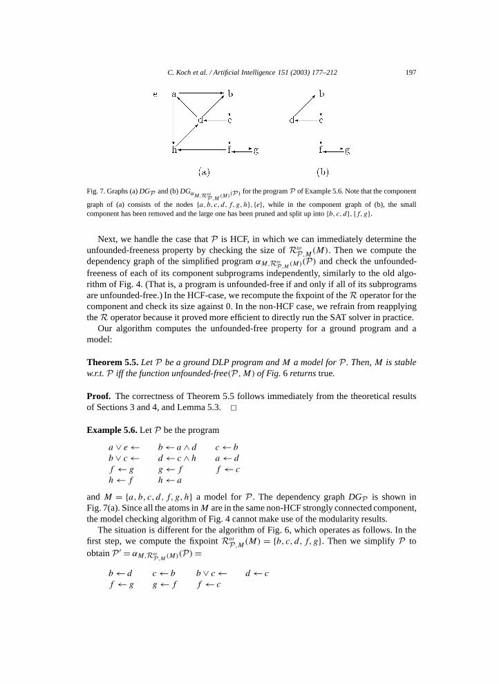
Fig. 7. Graphs (a) DGP and (b) DGαM,RωP,M

(M)(P) for the program P of Example 5.6. Note that the component

graph of (a) consists of the nodes {a,b, c, d,f,g,h}, {e}, while in the component graph of (b), the smallcomponent has been removed and the large one has been pruned and split up into {b, c, d}, {f,g}.

Next, we handle the case that P is HCF, in which we can immediately determine theunfounded-freeness property by checking the size of Rω

P,M(M). Then we compute thedependency graph of the simplified program αM,Rω

P,M (M)(P) and check the unfounded-freeness of each of its component subprograms independently, similarly to the old algo-rithm of Fig. 4. (That is, a program is unfounded-free if and only if all of its subprogramsare unfounded-free.) In the HCF-case, we recompute the fixpoint of the R operator for thecomponent and check its size against 0. In the non-HCF case, we refrain from reapplyingthe R operator because it proved more efficient to directly run the SAT solver in practice.

Our algorithm computes the unfounded-free property for a ground program and amodel:

Theorem 5.5. LetP be a ground DLP program andM a model forP . Then,M is stablew.r.t.P iff the function unfounded-free(P,M) of Fig. 6 returnstrue.

Proof. The correctness of Theorem 5.5 follows immediately from the theoretical resultsof Sections 3 and 4, and Lemma 5.3. ✷Example 5.6. Let P be the program

a ∨ e← b← a ∧ d c← b

b ∨ c← d← c ∧ h a← d

f ← g g← f f ← c

h← f h← a

and M = {a, b, c, d, f, g,h} a model for P . The dependency graph DGP is shown inFig. 7(a). Since all the atoms inM are in the same non-HCF strongly connected component,the model checking algorithm of Fig. 4 cannot make use of the modularity results.

The situation is different for the algorithm of Fig. 6, which operates as follows. In thefirst step, we compute the fixpoint Rω

P,M(M) = {b, c, d, f, g}. Then we simplify P toobtain P ′ = αM,Rω

P,M (M)(P)=b← d c← b b ∨ c← d← c

f ← g g← f f ← c

Page 22

198 C. Koch et al. / Artificial Intelligence 151 (2003) 177–212

with the dependency graph shown in Fig. 7(b). DGP ′ has two strongly connected

components, Q1 = {b, c, d} and Q2 = {f,g}. Q1 is not HCF, but unfounded-free asΓ ′M,Q1

(subp(Q1,P ′))=d← b; b← c; ← b ∧ c; c← d; b ∨ c∨ d←

is unsatisfiable. Q2 is head-cycle-free and unfounded-free, with

Rωsubp(Q2,P ′),Q2

(Q2)= ∅.Thus, M is a stable model of P .

We conclude this section with one more remark on our stable model checking algorithm.We made use of Proposition 3.10, which provides an efficient method for checking the

unfounded-freeness of head-cycle-free programs by checking whether RωP,M(M) is the

empty set, in the algorithm of Fig. 4, where we also combined it with modularity results.At the first glance it may seem that if the component dependency graph of αM,Rω

P,M (M)(P)contains a head-cycle-free component, M is not a stable model. Unfortunately, thefollowing counter-example shows that this is not true in general.

Example 5.7. Let P be the program

a← b b← a a← c c ∨ d← c← d d← c

and M = {a, b, c, d} a model for P . We have αM(P)=P and RωP,M(M)=M . One of the

strongly connected components, Q = {a, b}, is head-cycle-free with subp(Q,P)= {a←b; b← a; a← c}. Reapplying the R operator on Q results in ∅, though, which is correct,because M is the unique stable model of P .

Thus, computing subcomponents of a program may lead to rules “breaking apart” whichmay permit further simplifications using the RP,M operator. This shows why for HCFcomponents, we have to re-apply the R operator, as we do in the algorithm of Fig. 6.

6. Implementation, comparisons and benchmarks

In order to test the usefulness of our proposal, we have implemented our method in theDLV system. DLV [13,38] is a knowledge representation system based on disjunctive logicprogramming which has been developed at Technische Universität Wien. Recent compar-isons [13,39,40] have shown that DLV is nowadays a state-of-the-art implementation ofdisjunctive logic programming.

The computational engine of DLV implements the theoretical results achieved in [23].Roughly, the system consists of two main modules: the Model Generator and the ModelChecker (MC). The former produces stable-model candidates, whose stability is thenchecked by the latter.

We have replaced the original Model Checker of DLV by a new module implementingthe results of the previous sections, performed various benchmarks, and compared theexecution times.

Page 23

C. Koch et al. / Artificial Intelligence 151 (2003) 177–212 199

In addition to DLV, we have evaluated GnT [20] (an extension of Smodels [41,42]),

which is, to the best of our knowledge, the only publicly available system apart from DLVwhich supports full (function-free) disjunctive logic programming under the stable modelsemantics.

In the remainder of this section, we compare the (disjunctive) stable-model checkingmethods considered and their differences, and report on the experiments we have carriedout.

6.1. Comparative overview of disjunctive stable-model checking methods

In this section, we briefly recall the disjunctive stable-model checking methods weconsider, and we discuss their main differences.

We have tested the following systems and methods for stable model checking (the labelsbelow will be used in the benchmark figures).

• (Old Checker) The DLV system with its original Model Checker using thealgorithm of Fig. 4 which employs the modularity results from [23].Its strong points are the efficient evaluation of head-cycle-free (HCF) programs [35,36]and the use of modular evaluation techniques. Indeed, HCF programs are evaluated inpolynomial time and, if the program is not HCF, the inefficient part of the computationis limited only to those subprograms which are not HCF (while the polynomialtime algorithm is applied to the HCF subprograms). Polynomial space and singleexponential time bounds are always guaranteed.• (DLVnew) This is the algorithm depicted in Fig. 6 and described in Section 5.2. Here,

we again summarize its main ideas.Given a program P and a model M to be checked for stability, an implementationof the transformation of Fig. 5 generates the CNF formula ΓM(P), which is thensubmitted to a satisfiability checker. If the SAT checker returns true (ΓM(P) issatisfiable), then M is not a stable model of P ; otherwise (ΓM(P) is unsatisfiable),M is a stable model of P . For checking satisfiability of ΓM(P), we have used SATZ[21]—an efficient implementation of the Davis–Putnam procedure [43]—customizedfor our setting.Furthermore, this stable model checking method is enhanced by modular evaluationtechniques derived from the combination of Lemma 4.4 with the modularity results of[23]. Roughly, given P andM , P is first simplified (steps 1–3 of Fig. 5) resulting in theprogram αM(P). The subprograms of αM(P) are then evaluated one after the other.10

A polynomial time method is applied to HCF subprograms (as in Old Checker),while the transformation to SAT is applied to non-HCF subprograms.• (GnT) The GnT system [20] is a disjunctive extension of the system Smodels [41,

42]. (It is included in the Smodels distribution [44] under the name of example4.)Once a stable-model candidate M for a (disjunctive) program P has been generated, a

10 Note that the subprograms of αM(P) are smaller in general than the subprograms of P , since thesimplification process may break components.

Page 24

200 C. Koch et al. / Artificial Intelligence 151 (2003) 177–212

disjunction-free logic program P(M) is generated from P and M . The stable models

of P(M) are the models of PM which are strictly contained in M .11 Therefore, Mis a stable model of P if and only if P(M) has no stable model. The logic programP(M) is evaluated by a self call to (another instance of) Smodels; if no stable modelsare generated then M is stable. In our benchmarks, we have used Smodels 2.26, whichwas the current version at that time. Recently Smodels 2.27 was released which fixesan unrelated bug and packaging issues only; we verified that this does not affectperformance and thus did not re-run all benchmarks.

Comparing our approach (i.e., DLVnew) to the stable model checking method of GnT,we observe the following main differences:

(1) The method implemented in GnT can be seen as the dual method of our approach.Indeed, through P(M) GnT tries to generate directly a model M ′ of PM which isstrictly contained in M (disproving the minimality of M). In contrast, through theCNF formula ΓM(P) we try to build a non-empty unfounded set X contained inM , which witnesses the non-minimality of M without building explicitly the modelcontained in M (the existence of such an unfounded set X implies that M − X is amodel of PM ).

(2) In GnT, the stable model check is performed by a call to a logic programmingsystem (Smodels); while we employ a SAT checker (over ΓM(P)) to check thestability.

(3) GnT always uses the same model checking strategy whatever is the input program.Instead, we make some syntactic checks, and adopt specialized algorithms for somesyntactically recognizable classes of programs. In particular, our model checker worksin polynomial time if the input program is head-cycle-free.

(4) To our knowledge, GnT checks the stability of a model candidate M at once, andit does not employ any modular evaluation techniques; while an important featureof our approach is the use of the dynamic modular evaluation techniques (seeSection 5), which limit the inefficient part of the computation only to the componentswhich are still not head-cycle-free after that a simplification has been applied on theprogram.

The DLVnew method enhances Old Checker in the following respects.

• In DLVnew, the hard (non-HCF) subprograms are evaluated by calling a SAT checkeron a suitable CNF formula (ΓM(P)); while an enumeration of the possible unfoundedsets is performed in Old Checker.• DLVnew implements more advanced modularity techniques, which allow for a finer

splitting the stability check in subtasks (in general, DLVnew deals with smallersubprograms, thanks to the dynamic modularity technique).

11 Recall that PM denotes the Gelfond–Lifschitz transformation of P w.r.t. M (see Section 2).

Page 25

C. Koch et al. / Artificial Intelligence 151 (2003) 177–212 201

6.2. Benchmark problems and data

In order to generate co-NP-hard model checking instances which can be used toevaluate the differences between various model checking techniques, we needed to performbenchmarks of �P

2 -hard problems. Finding a suitable set of hard instances was not easy,since only a few experimental works have been done so far on �P

2 -complete problems, andsystematic studies to single out cross-over points similar to those done for Satisfiability arestill missing.

We have considered two problems for benchmarks:

• Quantified Boolean Formulas (2QBF), and• Strategic Companies (STRATCOMP).

For 2QBF we could exploit previous works studying hard instances; while forSTRATCOMP there was no such a study, the instances previously used for benchmarksappear very easy to solve (as pointed out also in [20]), and we had to single out harderinstances experimentally (this is to be considered a further side-contribution of this paper).

6.2.1. 2QBFOur first benchmark problem residing on the second level of the polynomial hierarchy

is 2QBF, which is well known to be �P2 -complete [45]. The problem here is to decide

whether a quantified Boolean formula (QBF) Φ = ∃X∀Yφ, where X and Y are disjointsets of propositional variables and φ = C1 ∨ · · · ∨ Ck is a 3DNF formula over X ∪ Y , isvalid.

The transformation from 2QBF to disjunctive logic programming is a slightly alteredform of a reduction used in [46]. The propositional disjunctive logic program Pφ producedby the transformation requires 2 ∗ (|X| + |Y |) + 1 propositional predicates (with onededicated predicate w), and consists of the following rules.

(1) Rules of the form v ∨ v for each variable v ∈X ∪ Y .(2) Rules of the form y←w; y←w for each variable y ∈ Y .(3) Rules of the form w ← v1 ∧ · · · ∧ vm ∧ vm+1 ∧ · · · ∧ vn for each conjunction

v1 ∧ · · · ∧ vm ∧¬vm+1 ∧ · · · ∧ ¬vn in φ.(4) The rule←¬w.

The 2QBF formula Φ is valid iff PΦ has a stable model [46].

Example 6.1. The formula Φ = ∃x∀y[(¬x ∧ y)∨ (¬y ∧ x)] translates into

PΦ = {x ∨ x; y ∨ y; y←w; y←w; w← x ∧ y; w← y ∧ x; ←¬w}.PΦ does not have a stable model, thus the QBF φ is not valid. (To check this manually, itis simpler to verify that ¬Φ = ∀x∃y: x↔ y is valid.)

In disjunctive logic programming, unlike SAT-based programming, programs should bekept separated from data. One designs a program encoding the problem at hand, which

Page 26

202 C. Koch et al. / Artificial Intelligence 151 (2003) 177–212

is then fixed and allows you to solve all problem instances which are provided by set

of facts. In our benchmarks, we adhere to the above principle, and clearly separate theencoding from the problem instance. To this end, we create the following disjunctive logicprogram Pqbf:

T (X)∨ F(X)← Exists(X);T (X)∨ F(X)← Forall(X);

T (X)←w ∧ Forall(X);F(X)←w ∧ Forall(X);

w←Conjunct(X,Y,Z,Na,Nb,Nc)∧T (X)∧ T (Y )∧ T (Z)∧ F(Na)∧ F(Nb)∧ F(Nc);

T (true)←; F(false)←; ←¬w.A 2QBF instance Φ = ∃X∀Yφ is encoded by the following set FΦ of facts:

• Exists(v), for each existential variable v ∈X.• Forall(v), for each universal variable v ∈ Y .• Conjunct(x1, x2, x3, y1, y2, y3), for each conjunct l1 ∧ l2 ∧ l3 in φ, where (i) if li is

a positive atom li then xi = vi , otherwise xi = “true”, and (ii) if li is a negated atom¬vi , then yi = vi , otherwise xi = “false”.

The 2QBF instance Φ is valid if and only if Pqbf ∪ FΦ has a stable model.We generated two different kinds of data sets following two works presented in the

literature. Each data set was randomly generated. In both cases the number of ∀-variablesis equal to the number of ∃-variables (that is, |X| = |Y |) and each conjunct contains atleast two universal variables.12 In the first case, the number of clauses equals the overallnumber of variables (that is, |X| + |Y |); in the second case, suggested by Gent and Walsh[47], the number of clauses is

√((|X|+ |Y |)/2). In the following, we will refer to instances

generated according to the first schema simply as QBF, those generated according to thesecond schema as QBFGW.

6.2.2. Strategic companies (STRATCOMP)This problem has been introduced by [48] in the context of Default Logic. It is a �P

2 -complete problem from the business domain.

The Strategic Companies Problem is defined as follows: A holding owns companies,each of which produces some goods. Moreover, several companies may have jointcontrol over another company. Now, some of these companies should be sold, under twoconstraints: All goods can be still produced, and no company is sold which would still becontrolled by the holding after the transaction. A company is strategicif it belongs to astrategic set, which is a minimal set of companies satisfying these constraints. Using ourformalism, these sets can be expressed by the following natural program:

12 In conjunction with the second variable ratio, this constitutes the so-called Model A whose hardness hasbeen experimentally evaluated in [47].

Page 27

C. Koch et al. / Artificial Intelligence 151 (2003) 177–212 203

strategic(C1)∨ strategic(C2)∨ strategic(C3)∨ strategic(C4)

← produced_by(P,C1,C2,C3,C4)

strategic(C)← controlled_by(C,C1,C2,C3,C4)∧ strategic(C1)

∧ strategic(C2)∧ strategic(C3)∧ strategic(C4).

Here the atom strategic(C) means that C is a strategic company, the atom produced_by(P,C1,C2,C3,C4) that product P is produced by companies C1, C2, C3 and C4, andcontrolled_by(C,C1,C2,C3,C4) that a company C is jointly controlled by companies C1,C2, C3 and C4. We have released the constraints imposed in [48], where each product isproduced by at most two companies and each company is jointly controlled by at most threeother companies, to at most four producers per product and four controllers per company(in principle these numbers can be increased arbitrarily). We experimentally determinedthat releasing these constraints allows us to generate harder instances on average.

The problem now is to determine whether a given company c is strategic or not (i.e., ifthe fact strategic(c) is true in at least one stable model of the program above).

Note that this problem cannot be expressed by a fixed normal (∨-free) logic programuniformly on all collections of facts over the predicates produced_by and controlled_byunless NP = �P

2 , which is highly unlikely. Thus, Strategic Companies is an example ofa relevant problem where the full expressive power of disjunctive logic programming isreally needed.

We have generated tests with instances for n companies (5 � n� 170), 3n products, 10uniform randomly chosen controlled_by relations per company, and uniform randomlychosen produced_by relations. To make the problem harder, we are only consideringstrategic sets containing two fixed companies (1 and 2, without loss of generality) usingthe constraints:

←¬strategic(1)

←¬strategic(2).

6.2.3. Results and discussionOur experiments were run on an Athlon/1200 with 512 MB of main memory under

FreeBSD 4.4, using the GCC 2.95.3 C++ compiler.For each problem size we have generated 50 random instances as indicated in the

respective descriptions, and for each such instance we allowed a maximum running timeof 7200 seconds (two hours). In the graphs displaying the benchmark results, the line ofa system stops whenever some problem instance was not solved in the maximum allowedtime.

In this framework, we ran two series of benchmarks: In the first series, we comparedour new model checking strategy (DLVnew) against the old model checking strategy of DLV(Old Checker). In the second series, we compared DLVnew against the GnT system.

6.2.4. DLVnew vs.Old CheckerWe used Old Checker and DLVnew to compute the first stable model of the program

(which determines the solution of the decision problem—see above) and summed up the

Page 28

204 C. Koch et al. / Artificial Intelligence 151 (2003) 177–212

total time spent for model checking.13 Thus, we obtained a precise comparison of the

efficiency of the two model checking strategies.

The results of the experiments comparing DLVnew vs. Old Checker are displayedin Fig. 8. The graphs on the left sides display the average (over the 50 instances of thesame size) time spent for model checking; while the graphs on the right sides display themaximum time spent for model checking. In particular, the graphs on the top, mid andbottom of the figure refer to the QBF, QBFGW, and STRATCOMP instances. (Averageand Maximum) Execution times (expressed in CPU seconds) are reported on the verticalaxis, while the horizontal axis displays the problem-instance size (number of propositionalvariables for QBF problems; number of companies for STRATCOMP). Note that, inall figures of this section, the vertical axis is in a logarithmic scale, and we have cutrespectively, rounded all values below 0.01 s.

The graphs of Fig. 8 show very clearly the strong impact of the new strategy on theefficiency of the model checker of DLV. DLVnewis significantly faster than Old Checkerin each of the three experiments. Both the average model checking time, and the maximummodel checking time of Old Checker are always higher than the respective times ofDLVnew. The lines of Old Checker stop much earlier than those of DLVnew, evidencingthat some instance of small size is not solvable by DLV using the original model checkingstrategy; while, DLV with the new strategy performs much better, and is able to solve allinstances of significantly larger sizes.

6.2.5. DLVnew vs.GnTIn the second series of experiments, we compare DLVnew and GnT. Due to the

completely different model generation strategies of these systems which may lead to avery different number of stable model candidates (and thus stable model checks), we solvethe decision problem whether any stable model exists (thus looking for one stable model),as before; but we consider the total execution times.In other words, we check whether theversion of DLV, implementing the model checking techniques proposed in this paper, iscompetitive with the GnT system on �P

2 -complete problems.The results are displayed by the six graphs of Fig. 9 in the same way as in Fig. 8. In

general, DLVnew outperforms GnT in all benchmark problems. However, the results arevery different in the three experiments. On STRATCOMP, the performance of the twosystems are basically the same up to the instance size of 115 companies. But instance-size115 is the last size where GnT can solve all of the 50 instances; while DLVnewgoes beyondsolving many further instances. GnT performs relatively well also on the first kind ofQBF instances. Instead, the difference between GnT and DLVnew becomes very impressiveon QBFGW, where GnT stops at size 25; while DLVnew solves all instances of size 1200employing less than 17 seconds on average.

13 Note that the computation of 1 stable model requires m� 1 calls to the Model Checker (m− 1 is the numberof calls on models which are not stable).

Page 29

C. Koch et al. / Artificial Intelligence 151 (2003) 177–212 205

Fig. 8. DLVnew vs. Old Checker: Model checking times for first stable model.

Page 30

206 C. Koch et al. / Artificial Intelligence 151 (2003) 177–212

Fig. 9. DLVnew vs. GnT: Total running times for first stable model.

Page 31

C. Koch et al. / Artificial Intelligence 151 (2003) 177–212 207

7. Related work and conclusion

7.1. Further related work

There is not much work in the literature on efficient methods for stable model checkingof disjunctive logic programs. The work more closely related to our method is probablythe one by Ben-Eliyahu-Zohary and Palopoli [36], since it focuses on efficient methods for(minimal) model checking.14

Based on the seminal work by Ben-Eliyahu and Dechter [35] where the notion of head-cylce-freeness (HCF) was introduced, Ben-Eliyahu-Zohary and Palopoli [36] describean efficient algorithm to compute minimal models of head-cycle-free theories and logicprograms and use this algorithm to compute one (arbitrary) stable model of a stratifiedhead-cycle-free DLP program in linear time. Our Rω

P,M(M) operator extends this to non-stratified input and we also use Rω

P,M(M) to (possibly) simplify problems that are notHCF before applying more expensive techniques.

The dynamic modular evaluation techniques employed by our algorithm to check thestability condition (see Section 5.2) extends [35] and [36] in that it allows us to apply anefficient model checking procedure also to programs which are not head-cycle-free ini-tially, but become such once they are simplified w.r.t. the model to be checked for stability.

There are several other works on computational aspects of DLP, which do not focus onstable model checking, though, and thus we only briefly mention them for completeness:

Fernández and Minker [49] employ a fixpoint characterization to evaluate stratifiedprograms, using so called model-trees which encode finite families of interpretations.

Another algorithm for computing stable models which uses a bottom-up strategyis presented by Brass and Dix in [25]. Their algorithm first computes the “residualprogram”—a program where no positive literals appear in the rules’ bodies—which isequivalent to the original program under stable model semantics. Stable models are thencomputed on (a simple extension of) Clark’s completion of the residual program.

Also Dix and Müller have implemented various semantics of disjunctive logic programsbased on abstract properties [50], but their procedure applies only to stratified programs.

Stuber’s bottom-up approach [51], finally, works similar to DLV and GnT in thatit employs a procedure analogous to Davis–Putnam [43], using case analysis andsimplification. Like DLV and GnT, and unlike the approaches mentioned above, Stuber’sprocedure only requires polynomial space and avoids the generation of duplicate (stable)models. Instead of performing a model check for every model found, this approachperforms (co-NP-hard) checks already as part of the backtracking model computation.Stuber leaves the concrete implementation of these checks as an open issue, but in generalhis algorithm may require exponential time for checking even if the program is HCF whileour procedure for checking stability is always polynomial on such programs.

Polynomial space complexity is a crucial requirement both for logic programming basedas well as deductive database systems, cf. [52], and of the approaches above that are ableto deal with hard input, only DLV, GnT, and Stuber’s meet this property.

14 Recall that stable models coincide with minimal models on positive disjunctive logic programs, and, also ongeneral disjunctive programs, minimal model checking is the hard task of stable model checking.

Page 32

208 C. Koch et al. / Artificial Intelligence 151 (2003) 177–212

Several approaches to the implementation of answer set programming systems like AS-

SAT [53], CCALC [54], cmodels [55], DCS [56], DeReS [57], DisLog [58], DisLoP [59],NoMoRe [60], QUIP [61], Smodels [41], and XSB [62], including the two systems de-scribed and evaluated in the previous section, namely DLV/Old Checker [13,14,63] andGnT [20], are evidently in connection to our paper as well.

7.2. Summary

As evidenced before by practical examples, disjunctive logic programming (DLP) withthe stable model semantics is a powerful knowledge representation and nonmonotonicreasoning formalism. Reasoning with DLP is harder than with disjunction-free logicprograms because stable model checking(that is, deciding whether a given model is astable model of a propositional DLP program) is co-NP-complete.

The model checking component is an essential part of nonmonotonic reasoning systemsfollowing the stable model semantics which can deal with �P

2 -complete problems. In thispaper, we have proposed a new, efficient transformation ΓM(P), which reduces stablemodel checking to UNSAT. The rationale of this is that UNSAT is the prototypical andbest-researched co-NP-complete problem. By this step, the best special-purpose algorithmsand systems for UNSAT can be used to solve the stable model checking problem. Thus, ourwork allows for a very substantial improvement of model checking performance of DLPsystems. This in turn has significant repercussions on the efficiency frontier of AI systemsfor �P

2 -complete problems overall.The proposed approach to stable model checking has been implemented in DLV—a

state-of-the-art implementation of DLP which is publicly available for a large number ofplatforms, and a number of experiments and benchmarks have been run using SATZ—oneof the best SAT solvers currently available—as an engine for stable model checking. Theresults of the experiments are very positive and confirm the usefulness of our techniques.

As future work, we plan to further improve the integration of model checking withthe other reasoning modules of DLV (in particular, model generation) and to add modelchecking heuristics; for instance, we want to exploit unfounded sets (evidenced by modelsviolating the UNSAT check) to guide the model generation process. Many other possibleheuristics are awaiting experimental evaluation; indeed, we are not aware of any existingwork on heuristics for �P

2 problems.Our experiments are a first foray into benchmarking �P

2 -hard problems in the contextof DLP. We see a strong need for further studies on cross-over points for problems such asSTRATCOMP and QBF, the prototypical problem of this complexity class. Although�P

2 isa practically important complexity class that characterizes a large number of nonmonotonicreasoning problems, nothing is known on this front to date. In the light of this, theexperimental data provided with this paper are a valuable contribution of their own.

Acknowledgements

We thank Wolfgang Faber for insightful discussions on both theoretical issues and thedesign and implementation of the DLV system. We are indebted to the remaining current

Page 33

C. Koch et al. / Artificial Intelligence 151 (2003) 177–212 209

and former members of the DLV team, in particular Francesco Calimeri, Tina Dell’Armi,

Thomas Eiter, Georg Gottlob, Giovambattista Ianni, Giuseppe Ielpa, Cristinel Mateis,Simona Perri, Axel Polleres, and Francesco Scarcello.

Appendix A

The RP,M operator of Definition 3.8 efficiently (more specifically, in linear time [36])evaluates the stability condition for HCF programs and usually greatly reduces the set ofpossible unfounded sets that need to be checked for non-HCF programs. In this appendix,we discuss some interesting properties of this operator. We first show that the definition ofRP,M for simplified programs αM(P) is simpler and more intuitive than the original one.

Definition A.1. Let αM(P) be the simplified version of a program P , as described inDefinition 4.3. We define the RαM(P),M operator as follows:

RαM(P),M : 2BP → 2BP ,

X �→ {a ∈X |� ∃r ∈ αM(P) with

(H(r)= {a})∧ (

B(r) ∩X = ∅)}.Note that we use a set-based notation for H(r), and trivial disjunctions of the type

a ∨ · · · ∨ a in heads are of course only represented by a single occurrence of a in H(r).Further below, we will assume without loss of generality that such trivial disjunctions donot occur in our programs.

Proposition A.2. LetP be a program andM a model ofP . Then,

RωP,M(M)=Rω

αM(P),M(M).

Example A.3. P = {a∨b; c← b}, M = {b, c}. αM(P)= {b; c← b}. In the first iterationof RαM(P),M , b is removed. In the second, c is deleted and Rω

αM(P),M(M)=RωP,M(M)=

∅. Thus, M is a stable model of P .

Proof. Suppose RωP,M(M) �= Rω

αM(P),M(M). Then, the expressions (∀r ∈ ground(P)with a ∈ H(r), (B(r) is false w.r.t. M) ∨ (B(r) ∩ X �= ∅) ∨ ((H(r) − {a}) ∩M �= ∅))and ( � ∃r ∈ αM(P) with (B(r) ∩X = ∅)∧ (H(r)= {a})) must not be equivalent. The firstexpression can be rewritten as � ∃r ∈ ground(P) with a ∈H(r)∧ (B(r) is true w.r.t. M)∧(B(r)∩X = ∅)∧ (H(r)∩M = {a}). We know that in αM(P) every rule body is true w.r.t.M and H(r) ⊆ M . Hence, the two expressions above are equivalent and Rω

P,M(M) =RωαM(P),M(M). ✷It is easy to see that the RαM(P),M operator of Definition A.1 is the converse of

the classical direct consequence operator TP . Starting from “facts” in αM(P), TαM(P)computes all atoms in M −Rω

P,M(M) (which certainly cannot be in any unfounded set),i.e., Rω

P,M(M)∪T ωαM(P)(∅)=M and Rω

P,M(M)∩T ωαM(P)(∅)= ∅. Finally, note that if we

abbreviate RωP,M(M) as X, we have Rω

αM,X(P)(X) = X. Therefore, we cannot obtain aneven better (that is, smaller) fixpoint by iteratively applying αM,X(P) and the R operator.

Page 34

210 C. Koch et al. / Artificial Intelligence 151 (2003) 177–212

References

[1] C. Koch, N. Leone, Stable model checking made easy, in: T. Dean (Ed.), Proceedings of IJCAI-99,Stockholm, Sweden, Morgan Kaufmann, San Mateo, CA, 1999, pp. 70–75.

[2] M. Gelfond, V. Lifschitz, Classical negation in logic programs and disjunctive databases, New GenerationComput. 9 (1991) 365–385.

[3] T.C. Przymusinski, Stable semantics for disjunctive programs, New Generation Comput. 9 (1991) 401–424.[4] C. Baral, M. Gelfond, Logic programming and knowledge representation, J. Logic Programming 19/20

(1994) 73–148.[5] C. Baral, Knowledge Representation, Reasoning and Declarative Problem Solving, Cambridge University

Press, Cambridge, 2003.[6] T. Eiter, G. Gottlob, H. Mannila, Disjunctive datalog, ACM Trans. Database Syst. 22 (3) (1997) 364–418.[7] G. Gottlob, Complexity results for nonmonotonic logics, J. Logic Comput. 2 (3) (1992) 397–425.[8] T. Eiter, G. Gottlob, The complexity of logic-based abduction, J. ACM 42 (1) (1995) 3–42.[9] T. Eiter, G. Gottlob, On the complexity of propositional knowledge base revision, updates, and counterfac-

tuals, Artificial Intelligence 57 (2–3) (1992) 227–270.[10] H. Turner, Polynomial-length planning spans the polynomial hierarchy, in: S. Flesca, S. Greco, G. Ianni, N.

Leone (Eds.), Proceedings of the 8th European Conference on Artificial Intelligence (JELIA), in: LectureNotes in Computer Science, Vol. 2424, Springer, Berlin, 2002, pp. 111–124.

[11] C. Baral, V. Kreinovich, R. Trejo, Computational complexity of planning and approximate planning in thepresence of incompleteness, Artificial Intelligence 122 (1–2) (2000) 241–267.

[12] E. Dantsin, T. Eiter, G. Gottlob, A. Voronkov, Complexity and expressive power of logic programming,ACM Comput. Surv. 33 (3) (2001) 374–425.

[13] T. Eiter, N. Leone, C. Mateis, G. Pfeifer, F. Scarcello, The KR system dlv: Progress report, comparisons andbenchmarks, in: A.G. Cohn, L. Schubert, S.C. Shapiro (Eds.), Proceedings Sixth International Conferenceon Principles of Knowledge Representation and Reasoning (KR-98), Trento, Italy, Morgan Kaufmann, SanMateo, CA, 1998, pp. 406–417.

[14] T. Eiter, W. Faber, N. Leone, G. Pfeifer, Declarative problem-solving using the DLV system, in: J. Minker(Ed.), Logic-Based Artificial Intelligence, Kluwer Academic, Dordrecht, 2000, pp. 79–103.

[15] V. Lifschitz, Answer set planning, in: D.D. Schreye (Ed.), Proceedings of the 16th International Conferenceon Logic Programming (ICLP-99), Las Cruces, NM, MIT Press, Cambridge, MA, 1999, pp. 23–37.

[16] M. Nogueira, M. Balduccini, M. Gelfond, R. Watson, M. Barry, An A-prolog decision support system forthe Space Shuttle, in: G. Gupta (Ed.), Proceedings of the 1st International Workshop on Practical Aspectsof Declarative Languages (PADL-99), in: Lecture Notes in Computer Science, Vol. 1551, Springer, Berlin,1999, pp. 169–183.

[17] T. Soininen, I. Niemelä, Developing a declarative rule language for applications in product configuration,in: G. Gupta (Ed.), Proceedings of the 1st International Workshop on Practical Aspects of DeclarativeLanguages (PADL-99), in: Lecture Notes in Computer Science, Vol. 1551, Springer, Berlin, 1999, pp. 305–319.

[18] T. Syrjänen, A rule-based formal model for software configuration, Technical Report A55, Digital SystemsLaboratory, Department of Computer Science, Helsinki University of Technology, Espoo, Finland, 1999.

[19] K. Heljanko, I. Niemelä, Bounded LTL model checking with stable models, in: T. Eiter, W. Faber,M. Truszczynski (Eds.), Proceedings 6th International Conference, Logic Programming and NonmonotonicReasoning, LPNMR-01, Vienna, Austria, in: Lecture Notes in Artificial Intelligence, Vol. 2173, Springer,Berlin, 2001, pp. 200–212.

[20] T. Janhunen, I. Niemela, P. Simons, J.-H. You, Partiality and disjunctions in stable model semantics, in:A.G. Cohn, F. Giunchiglia, B. Selman (Eds.), Proceedings of the Seventh International Conference onPrinciples of Knowledge Representation and Reasoning (KR-2000), Breckenridge, CO, Morgan Kaufmann,San Mateo, CA, 2000, pp. 411–419.

[21] C.M. Li, Anbulagan, Heuristics based on unit propagation for satisfiability problems, in: Proceedings ofIJCAI-97, Nagoya, Japan, 1997, pp. 366–371.

[22] J. Lobo, J. Minker, A. Rajasekar, Foundations of Disjunctive Logic Programming, MIT Press, Cambridge,MA, 1992.

Page 35

C. Koch et al. / Artificial Intelligence 151 (2003) 177–212 211

[23] N. Leone, P. Rullo, F. Scarcello, Disjunctive stable models: Unfounded sets, fixpoint semantics and

computation, Inform. and Comput. 135 (2) (1997) 69–112.

[24] J. Minker, On indefinite data bases and the closed world assumption, in: D. Loveland (Ed.), Proceedings6th Conference on Automated Deduction (CADE-82), in: Lecture Notes in Computer Science, Vol. 138,Springer, New York, 1982, pp. 292–308.

[25] S. Brass, J. Dix, Disjunctive semantics based upon partial and bottom-up evaluation, in: L. Sterling (Ed.),Proceedings of the 12th Internat. Conf. on Logic Programming, Tokyo, MIT Press, Cambridge, MA, 1995,pp. 199–213.

[26] T. Przymusinski, Stationary semantics for disjunctive logic programs and deductive databases, in:Proceedings of North American Conference on Logic Programming, Austin, TX, 1990, pp. 40–62.

[27] T. Przymusinski, Static semantics for normal and disjunctive logic programs, Ann. Math. ArtificialIntelligence 14 (1995) 323–357.

[28] K. Ross, The well-founded semantics for disjunctive logic programs, in: W. Kim, J.-M. Nicolas, S. Nishio(Eds.), Deductive and Object-Oriented Databases, Elsevier Science, Amsterdam, 1990, pp. 385–402.

[29] C. Sakama, Possible model semantics for disjunctive databases, in: Proceedings First Internat. Conf. onDeductive and Object-Oriented Databases (DOOD-89), Kyoto, Japan, North-Holland, Amsterdam, 1989,pp. 369–383.

[30] K. Apt, N. Bol, Logic programming and negation: A survey, J. Logic Programming 19/20 (1994) 9–71.[31] J. Dix, Semantics of logic programs: Their intuitions and formal properties. An overview, in: Logic, Action

and Information. Proceedings of the Konstanz Colloquium in Logic and Information (LogIn-92), DeGruyter,Berlin, 1995, pp. 241–329.

[32] M. Gelfond, V. Lifschitz, The Stable Model Semantics for Logic Programming, in: Logic Programming:Proceedings Fifth Internat. Conference and Symposium, Seattle, WA, MIT Press, Cambridge, MA, 1988,pp. 1070–1080.

[33] N. Bidoit, C. Froidevaux, Negation by default and unstratifiable logic programs, Theoret. Comput. Sci. 78(1991) 85–112.

[34] F. Buccafurri, N. Leone, P. Rullo, Enhancing disjunctive datalog by constraints, IEEE Trans. KnowledgeData Engrg. 12 (5) (2000) 845–860.

[35] R. Ben-Eliyahu, R. Dechter, Propositional semantics for disjunctive logic programs, Ann. Math. ArtificialIntelligence 12 (1994) 53–87.

[36] R. Ben-Eliyahu-Zohary, L. Palopoli, Reasoning with minimal models: Efficient algorithms and applications,Artificial Intelligence 96 (1997) 421–449.

[37] V. Lifschitz, H. Turner, Splitting a logic program, in: P. Van Hentenryck (Ed.), Proceedings of the 11thInternational Conference on Logic Programming (ICLP-94), Santa Margherita Ligure, Italy, MIT Press,Cambridge, MA, 1994, pp. 23–37.

[38] T. Eiter, N. Leone, C. Mateis, G. Pfeifer, F. Scarcello, A deductive system for nonmonotonic reasoning,in: J. Dix, U. Furbach, A. Nerode (Eds.), Proceedings of the 4th International Conference on LogicProgramming and Nonmonotonic Reasoning (LPNMR-97), Dagstuhl, Germany, in: Lecture Notes inArtificial Intelligence, Vol. 1265, Springer, Berlin, 1997, pp. 363–374.

[39] E. Erdem, Applications of logic programming to planning: Computational experiments, unpublished draft,http://www.cs.utexas.edu/users/esra/papers.html, 1999.

[40] P. Nicolas, New generation systems for nonmonotonic reasoning, Presentation at LPNMR-01, Vienna,Austria, September 2001.

[41] I. Niemelä, P. Simons, T. Syrjänen, Smodels: A system for answer set programming, in: C. Baral,M. Truszczynski (Eds.), Proceedings of the 8th International Workshop on Nonmonotonic Reasoning(NMR-2000), Breckenridge CO, 2000.

[42] I. Niemelä, P. Simons, Smodels—An implementation of the stable model and well-founded semantics fornormal logic programs, in: J. Dix, U. Furbach, A. Nerode (Eds.), Proceedings of the 4th InternationalConference on Logic Programming and Nonmonotonic Reasoning (LPNMR-97), Dagstuhl, Germany, in:Lecture Notes in Artificial Intelligence, Vol. 1265, Springer, Berlin, 1997, pp. 420–429.

[43] M. Davis, H. Putnam, A computing procedure for quantification theory, J. ACM 7 (1960) 201–215.[44] P. Simons, Smodels homepage, http://www.tcs.hut.fi/Software/smodels/, 1999.[45] C.H. Papadimitriou, Computational Complexity, Addison-Wesley, Reading, MA, 1994.

Page 36

212 C. Koch et al. / Artificial Intelligence 151 (2003) 177–212

[46] T. Eiter, G. Gottlob, On the computational cost of disjunctive logic programming: Propositional case, Ann.

Math. Artificial Intelligence 15 (3/4) (1995) 289–323.

[47] I. Gent, T. Walsh, Beyond NP: The QSAT phase transition, in: Proceedings of AAAI-99, Orlando, FL, 1999,pp. 648–653.

[48] M. Cadoli, T. Eiter, G. Gottlob, Default logic as a query language, IEEE Trans. Knowledge Data Engrg. 9 (3)(1997) 448–463.

[49] J. Fernández, J. Minker, Bottom-up computation of perfect models for disjunctive theories, J. LogicProgramming 25 (1) (1995) 33–51.

[50] J. Dix, M. Müller, Implementing semantics of disjunctive logic programs using fringes and abstractproperties, in: L.-M. Pereira, A. Nerode (Eds.), Proceedings of the Second International Workshop on LogicProgramming and Nonmonotonic Reasoning (LPNMR-93), Lisbon, Portugal, MIT Press, Cambridge, MA,1993, pp. 43–59.

[51] J. Stuber, Computing stable models by program transformation, in: P. Van Hentenryck (Ed.), Proceedingsof the 11th Internat. Conference on Logic Programming, Santa Margherita Ligure, Italy, MIT Press,Cambridge, MA, 1994, pp. 58–73.

[52] I. Niemelä, P. Simons, Efficient implementation of the well-founded and stable model semantics, in:M.J. Maher (Ed.), Proceedings of the 1996 Joint International Conference and Symposium on LogicProgramming (ICLP-96), Bonn, Germany, MIT Press, Cambridge, MA, 1996, pp. 289–303.

[53] F. Lin, Y. Zhao, ASSAT: Computing answer sets of a logic program by SAT solvers, in: Proceedings ofAAAI-02, Edmonton, AB, AAAI Press/MIT Press, Cambridge, MA, 2002, p. 112.

[54] N. McCain, H. Turner, Satisfiability planning with causal theories, in: A.G. Cohn, L. Schubert, S.C.Shapiro (Eds.), Proceedings Sixth International Conference on Principles of Knowledge Representation andReasoning (KR-98), Trento, Italy, Morgan Kaufmann, San Mateo, CA, 1998, pp. 212–223.

[55] Y. Babovich, Cmodels homepage, http://www.cs.utexas.edu/users/tag/cmodels.html, 2002.[56] D. East, M. Truszczynski, dcs: An implementation of DATALOG with constraints, in: C. Baral,

M. Truszczynski (Eds.), Proceedings of the 8th International Workshop on Non-Monotonic Reasoning(NMR-2000), Breckenridge, CO, 2000.

[57] P. Cholewinski, V.W. Marek, M. Truszczynski, Default reasoning system DeReS, in: Proceedings ofInternational Conference on Principles of Knowledge Representation and Reasoning (KR-96), Cambridge,MA, Morgan Kaufmann, San Mateo, CA, 1996, pp. 518–528.

[58] D. Seipel, H. Thöne, DisLog—A system for reasoning in disjunctive deductive databases, in: A. Olivé (Ed.),Proceedings International Workshop on the Deductive Approach to Information Systems and Databases(DAISD-94), Universitat Politecnica de Catalunya (UPC), 1994, pp. 325–343.

[59] C. Aravindan, J. Dix, I. Niemelä, DisLoP: A research project on disjunctive logic programming, AICommunications—The European Journal on Artificial Intelligence 10 (3/4) (1997) 151–165.

[60] C. Anger, K. Konczak, T. Linke, NoMoRe: A system for non-monotonic reasoning, in: T. Eiter, W. Faber,M. Truszczynski (Eds.), Proceedings 6th International Conference, Logic Programming and NonmonotonicReasoning, LPNMR-01, Vienna, Austria, in: Lecture Notes in Artificial Intelligence, Vol. 2173, Springer,Berlin, 2001, pp. 406–410.

[61] U. Egly, T. Eiter, H. Tompits, S. Woltran, Solving advanced reasoning tasks using quantified Booleanformulas, in: Proceedings of AAAI-00, Austin, TX, AAAI Press/MIT Press, Cambridge, MA, 2000,pp. 417–422.

[62] P. Rao, K.F. Sagonas, T. Swift, D.S. Warren, J. Freire, XSB: A system for efficiently computing well-foundedsemantics, in: J. Dix, U. Furbach, A. Nerode (Eds.), Proceedings of the 4th International Conference onLogic Programming and Non-Monotonic Reasoning (LPNMR-97), Dagstuhl, Germany, in: Lecture Notesin Artificial Intelligence, Vol. 1265, Springer, Berlin, 1997, pp. 2–17.

[63] N. Leone, C. Pizzuti, P. Rullo, Efficient evaluation of a class of ordered logic programs, Data and KnowledgeEngineering 23 (2) (1997) 185–213.