ENHANCED MODIFIED BARK SPECTRAL DISTORTION (EMBSD): AN OBJECTIVE SPEECH QUALITY MEASURE BASED ON AUDIBLE DISTORTION AND COGNITION MODEL ________________________________________________________________________ A Dissertation Submitted to the Temple University Graduate Board ________________________________________________________________________ in Partial Fulfillment of the Requirement for the Degree DOCTOR OF PHILOSOPHY ________________________________________________________________________ by Wonho Yang May, 1999

Welcome message from author
This document is posted to help you gain knowledge. Please leave a comment to let me know what you think about it! Share it to your friends and learn new things together.
Transcript
ENHANCED MODIFIED BARK SPECTRAL DISTORTION (EMBSD):
AN OBJECTIVE SPEECH QUALITY MEASURE BASED ON
AUDIBLE DISTORTION AND COGNITION MODEL
________________________________________________________________________
A Dissertation
Submitted to
the Temple University Graduate Board
________________________________________________________________________
in Partial Fulfillment
of the Requirement for the Degree
DOCTOR OF PHILOSOPHY
________________________________________________________________________
by
Wonho Yang
May, 1999

ii

iii
ABSTRACT
An objective speech quality measure estimates speech quality of a test
utterance without the involvement of human listeners. Recently, the performance
of objective speech quality measures has been greatly improved by adopting
auditory perception models derived from psychoacoustic studies. These
measures estimate perceptual distortion of test speech by comparing it with the
original speech in a perceptually relevant domain. These types of measures are
called perceptual domain measures.
Recently, the Speech Processing Lab at Temple University developed a
perceptual domain measure called the Modified Bark Spectral Distortion
(MBSD). The MBSD measure extended the Bark Spectral Distortion (BSD)
measure by incorporating noise masking threshold into the algorithm to
differentiate audible and inaudible distortions. The performance of the MBSD is
comparable to that of the International Telecommunication Union –
Telecommunication standardization sector (ITU-T) Recommendation P.861 for
speech data with various coding distortions. Since the MBSD uses
psychoacoustic results derived using steady-state signals such as sinusoids, the
performance of the MBSD has been examined by scaling the noise masking
iv
threshold and omitting the spreading function in noise masking threshold
calculation.
Based on experiments with Time Division Multiple Access (TDMA) data
containing distortions encountered in real network applications, the performance
of the MBSD has been further enhanced by modifying some procedures and
adding a new cognition model. The Enhanced MBSD (EMBSD) shows significant
improvement over the MBSD for TDMA data. Also, the performance of the
EMBSD is better than that of the ITU-T Recommendation P.861 for TDMA data.
The performance of the EMBSD was compared to various other objective
speech quality measures with the speech data including a wide range of
distortion conditions. The EMBSD showed clear improvement over the MBSD
and had the correlation coefficient of 0.89 for the conditions of MNRUs, codecs,
tandem cases, bit errors, and frame erasures.
Objective speech quality measures are evaluated by comparing the
objective estimates with the subjective test scores. The Mean Opinion Score
(MOS) has been the usual subjective speech quality test used to evaluate
objective speech quality measures because MOS is the most common subjective
measure used to evaluate speech compression codecs. However, current
objective speech quality measures estimate subjective scores by comparing the
test speech to the original speech. This approach has more in common with the
Degradation Mean Opinion Score (DMOS) test than with the MOS test. Recent

v
experiments performed at Nortel Networks in Ottawa also have indicated that
the current objective speech quality measures are better correlated with the
DMOS scores than with the MOS scores. So, it is more appropriate to evaluate
current objective speech quality measures with DMOS scores.
The correlation between the objective estimates and the subjective scores
has been used as a performance parameter for evaluation of objective speech
quality measures. However, it is inappropriate to compare the correlation
coefficients of an objective speech quality measure for different speech data
because the correlation coefficient of an objective speech quality measure
depends on the distribution of the subjective scores in the speech database.
Accordingly, the Standard Error of the Estimates (SEE) is proposed as a
performance parameter for evaluation of objective speech quality measures. The
SEE is an unbiased statistic providing an estimate of the deviation from the
regression line between two variables. The SEE has several advantages over the
correlation coefficient as a performance parameter for examining the
performance of objective measures.

vi
ACKNOWLEDGMENTS
I would like to give thanks to God who has guided me. I am very grateful
to my parents, Kwon-Doo and Cha-Soon, my wife, Seon Bae, and my two
children, Jacob and Jin for their endless support for me during my graduate
studies.
I want to give a special thank to Dr. Robert Yantorno for his
encouragement and guidance during this research. This research has been
especially rewarding because of his encouragement.
I would like to thank the committee members, Dr. Dennis Silage, Dr. Micha
Hohenberger, Dr. Athina Petropulu, and Dr. Elizabeth Kennedy for their
valuable comments.
I am indebted to Peter Kroon of Lucent Technologies, Joshua Rosenbluth
of AT&T, and Steve Voran of the US Department of Commerce for providing
speech data sets for this research.
I am also very grateful to Leigh Thorpe of Nortel Networks for giving me
an opportunity to work on the project that provided material and inspiration for
some of the work presented here.

vii
TABLE OF CONTENTS
Page
ABSTRACT . . . . . . . . . . . . . . . . . . . . . . . . . . . . . . . . . . . . . . . . . . . . . . . . . . . . . . . . . . iii
ACKNOWLEDGMENTS . . . . . . . . . . . . . . . . . . . . . . . . . . . . . . . . . . . . . . . . . . . . . . vi
LIST OF TABLES . . . . . . . . . . . . . . . . . . . . . . . . . . . . . . . . . . . . . . . . . . . . . . . . . . . . . xi
LIST OF FIGURES . . . . . . . . . . . . . . . . . . . . . . . . . . . . . . . . . . . . . . . . . . . . . . . . . . . .xiii
CHAPTER
1. INTRODUCTION . . . . . . . . . . . . . . . . . . . . . . . . . . . . . . . . . . . . . . . . . . . . . 1
2. BACKGROUND . . . . . . . . . . . . . . . . . . . . . . . . . . . . . . . . . . . . . . . . . . . . . . 10
2.1. Subjective Speech Quality Measures . . . . . . . . . . . . . . . . . . . . . 10
2.1.1. Mean Opinion Score . . . . . . . . . . . . . . . . . . . . . . . . . . . 11
2.1.2. Degradation Mean Opinion Score . . . . . . . . . . . . . . . . 13
2.2. Objective Speech Quality Measures . . . . . . . . . . . . . . . . . . . . . . 14
2.2.1. Time Domain Measures . . . . . . . . . . . . . . . . . . . . . . . . 17
2.2.1.1. Signal-to-Noise Ratio . . . . . . . . . . . . . . . . . . . 17
2.2.1.2. Segmental Signal-to-Noise Ratio . . . . . . . . . . 19

viii
2.2.2. Spectral Domain Measures . . . . . . . . . . . . . . . . . . . . . . 20
2.2.2.1. Log Likelihood Ratio Measures . . . . . . . . . . 21
2.2.2.2. LPC Parameter Measures . . . . . . . . . . . . . . . . 22
2.2.2.3. Cepstral Distance Measures . . . . . . . . . . . . . . 24
2.2.2.4. Weighted Slope Spectral Distance Measures . . . . . . . . . . . . . . . . . . . . . 26
2.2.3. Psychoacoustic Results . . . . . . . . . . . . . . . . . . . . . . . . . 27
2.2.3.1. Critical Bands . . . . . . . . . . . . . . . . . . . . . . . . . . 28
2.2.3.2. Masking Effects . . . . . . . . . . . . . . . . . . . . . . . . 30
2.2.3.3. Equal-Loudness Contours . . . . . . . . . . . . . . . 33
2.2.4. Perceptual Domain Measures . . . . . . . . . . . . . . . . . . . . 36
2.2.4.1. Bark Spectral Distortion . . . . . . . . . . . . . . . . . 37
2.2.4.2. Perceptual Speech Quality Measure . . . . . . . 40
2.2.4.3. PSQM+ . . . . . . . . . . . . . . . . . . . . . . . . . . . . . . . 41
2.2.4.4. Measuring Normalizing Blocks . . . . . . . . . . 43
2.2.4.5. Perceptual Analysis Measurement System . . . . . . . . . . . . . . . . . . . 44
2.2.4.6. Qvoice . . . . . . . . . . . . . . . . . . . . . . . . . . . . . . . . 45
2.2.4.7. Telecommunication Objective Speech Quality Assessment . . . . . . . . . . . . . . 46
3. EVALUATION OF OBJECTIVE SPEECH QUALITY MEASURES . . . 48
3.1. Evaluation With MOS Versus DMOS . . . . . . . . . . . . . . . . . . . . 50

ix
3.2. Correlation Analysis . . . . . . . . . . . . . . . . . . . . . . . . . . . . . . . . . . . 55
3.3. Standard Error of Estimates . . . . . . . . . . . . . . . . . . . . . . . . . . . . . 57
4. MODIFIED BARK SPECTRAL DISTORTION . . . . . . . . . . . . . . . . . . . . . 63
4.1. Algorithm of MBSD . . . . . . . . . . . . . . . . . . . . . . . . . . . . . . . . . . . 64
4.2. Search for a Proper Metric of MBSD . . . . . . . . . . . . . . . . . . . . . 71
4.3. Effect of Noise Masking Threshold in MBSD . . . . . . . . . . . . . . 72
4.4. Performance of MBSD With Coding Distortions . . . . . . . . . . . 74
5. IMPROVEMENT OF MBSD . . . . . . . . . . . . . . . . . . . . . . . . . . . . . . . . . . . . 76
5.1. Scaling Noise Masking Threshold . . . . . . . . . . . . . . . . . . . . . . . 77
5.2. Using the First 15 Loudness Vector Components . . . . . . . . . . 80
5.3. Normalizing Loudness Vectors . . . . . . . . . . . . . . . . . . . . . . . . . . 83
5.4. Deletion of the Spreading Function in the Calculation of the Noise Masking Threshold . . . . . . . . . . . . . . 84
5.5. A New Cognition Model Based on Postmasking Effects . . . . 85
6. ENHANCED MODIFIED BARK SPECTRAL DISTORTION . . . . . . . . 91
7. PERFORMANCE OF THE EMBSD MEASURE . . . . . . . . . . . . . . . . . . . . 94
7.1. Performance of the EMBSD With Speech Data I . . . . . . . . . . . 95
7.2. Performance of the EMBSD With Speech Data II . . . . . . . . . 100
7.3. Performance of the EMBSD With Speech Data III . . . . . . . . . 104
8. FUTURE RESEARCH . . . . . . . . . . . . . . . . . . . . . . . . . . . . . . . . . . . . . . . . 113
REFERENCES . . . . . . . . . . . . . . . . . . . . . . . . . . . . . . . . . . . . . . . . . . . . . . . . . . . . . . 116

x
BIBLIOGRAPHY . . . . . . . . . . . . . . . . . . . . . . . . . . . . . . . . . . . . . . . . . . . . . . . . . . . . 121
APPENDIX
A. MATLAB PROGRAM OF MBSD . . . . . . . . . . . . . . . . . . . . . . . . . . . . . . . . . . . . 127
B. C PROGRAM OF EMBSD . . . . . . . . . . . . . . . . . . . . . . . . . . . . . . . . . . . . . . . . . . 134
C. GLOSSARY . . . . . . . . . . . . . . . . . . . . . . . . . . . . . . . . . . . . . . . . . . . . . . . . . . . . . . 162

xi
LIST OF TABLES
Table Page
1. MOS and Corresponding Speech Quality . . . . . . . . . . . . . . . . . . . . . . . . . . . . 12
2. DMOS and Corresponding Degradation Levels . . . . . . . . . . . . . . . . . . . . . . 13
3. Critical-Band Rate and Critical Bandwidths Over Auditory Frequency Range . . . . . . . . . . . . . . . . . . . . . . . . . . . . . . . . . . . . . . . . . . . . . . . . 29
4. Correlation Coefficients with the MOS and the MOS Difference for Speech Coding Distortion . . . . . . . . . . . . . . . . . . . . . . . . . . . . . . . . . . . . . . 53
5. Performance of the MBSD for Various Metrics . . . . . . . . . . . . . . . . . . . . . . . . 72
6. Correlation Coefficients of the MBSD with Different Frame Sizes and Speech Classes . . . . . . . . . . . . . . . . . . . . . . . . . . . . . . . . . . . . . . . . . . 75
7. Correlation Coefficients of MBSD II and Other Measures for Speech Data with Coding Distortions . . . . . . . . . . . . . . . . . . . . . . . . . . . . 79
8. Correlation Coefficients and SEE of Objective Quality Measures With Speech Data I . . . . . . . . . . . . . . . . . . . . . . . . . . . . . . . . . . . . . . . . . . . . . . . 99
9. Correlation Coefficients and SEE of Objective Quality Measures Versus MOS With Speech Data II . . . . . . . . . . . . . . . . . . . . . . . . . . . . . . . . . 103
10. Correlation Coefficients of Various Objective Quality Measures With Speech Data III . . . . . . . . . . . . . . . . . . . . . . . . . . . . . . . . . . . . . . . . . . . . 106
11. Standard Error of the Estimates of Various Objective Quality Measures With Speech Data III . . . . . . . . . . . . . . . . . . . . . . . . . . . . . . . . . . 109
12. Standard Error of the Estimates of Various Objective Quality

xii
Measures for Target Condition Groups (Group 1, 2, and 3) of Speech Data III . . . . . . . . . . . . . . . . . . . . . . . . . . . . . . . . . . . . . . . . . . . . . . 110
13. Standard Error of the Estimates of Various Objective Quality Measures for Target Condition Groups (Group 5 and 6) of Speech Data III . . . . . . . . . . . . . . . . . . . . . . . . . . . . . . . . . . . . . . . . . . . . . . 111
14. Standard Error of the Estimates of Various Objective Quality Measures for Non-Target Condition Groups (Group 4 and 7) of Speech Data III . . . . . . . . . . . . . . . . . . . . . . . . . . . . . . . . . . . . . . . . . . . . . . 112

xiii
LIST OF FIGURES
Figure Page
1. Current Objective Speech Quality Measures Based on Both Original and Distorted Speech . . . . . . . . . . . . . . . . . . . . . . . . . . . . . . . . . . . . . . 3
2. Basic Structure of Objective Speech Quality Measures . . . . . . . . . . . . . . . . . 15
3. Level of Test Tone Just Masked by Critical-Band Wide Noise . . . . . . . . . . 32
4. Equal-Loudness Contours for Pure Tones in a Free Sound Field . . . . . . . . 34
5. A System for Evaluating Performance of Objective Speech Quality Measures . . . . . . . . . . . . . . . . . . . . . . . . . . . . . . . . . . . . . . . . . . . . . . . . 48
6. A System Illustrating the Procedural Difference Between Objective Measures and the MOS test . . . . . . . . . . . . . . . . . . . . . . . . . . . . . . . . . . . . . . . . 52
7. Performance of Current Objective Quality Measures With Both MOS and DMOS . . . . . . . . . . . . . . . . . . . . . . . . . . . . . . . . . . . . . . . . . . . . 54
8. Transformation of Objective Estimates With a Regression Curve . . . . . . . 56
9. Scatterplots of an Objective Measure With Two Different Sets of Speech Data . . . . . . . . . . . . . . . . . . . . . . . . . . . . . . . . . . . . . . . . . . . . . . . . . . . . . 60
10. Scatterplot Illustrating That Correlation Coefficient of a Certain Condition Group . . . . . . . . . . . . . . . . . . . . . . . . . . . . . . . . . . . . . . . . . . . . . . . . 62
11. Block Diagram of the MBSD Measure . . . . . . . . . . . . . . . . . . . . . . . . . . . . . . 65
12. MBSD Versus MOS Difference (Without Noise Masking Threshold) . . . 73
13. MBSD Versus MOS Difference (With Noise Masking Threshold) . . . . . . 74

xiv
14. Performance of the MBSD for Speech Data With Coding Distortions Versus the Scaling Factor of the Noise Masking Threshold . . . . . . . . . . . . 78
15. Performance of the MBSD With the First 15 Loudness Components . . . . 81
16. Two Different Temporal Distortion Distributions With the Same Average Distortion Value . . . . . . . . . . . . . . . . . . . . . . . . . . . . . . . . . . . . . . . . 86
17. Performance of the MBSD With a new Cognition Model as a Function of Cognizable Unit for the Postmasking Factor of 80 . . . . . . . 89
18. Performance of the MBSD With a new Cognition Model as a Function of Postmasking Factor for the Cognizable Unit of 10 Frames . . . . . . . . . . . . . . . . . . . . . . . . . . . . . . . . . . . . . . . . . . . . . . . . . . . . 89
19. Block Diagram of the EMBSD Measure . . . . . . . . . . . . . . . . . . . . . . . . . . . . . 92
20. Objective Measures of P.861, MNB2, MBSD, and EMBSD Versus MOS Scores for Speech Data I . . . . . . . . . . . . . . . . . . . . . . . . . . . . . . 96
21. Transformed Objective Estimates of P.861, MNB2, MBSD, and EMBSD Versus MOS Scores for Speech Data I . . . . . . . . . . . . . . . . . . . 97
22. Transformed Objective Estimates of P.861, MNB2, MBSD, and EMBSD Versus MOS Difference for Speech Data I . . . . . . . . . . . . . . . 98
23. Objective Measures of P.861, MNB2, MBSD, and EMBSD Versus MOS Scores for Speech Data II . . . . . . . . . . . . . . . . . . . . . . . . . . . . 101
24. Transformed Objective Estimates of P.861, MNB2, MBSD, and EMBSD Versus MOS Scores for Speech Data II . . . . . . . . . . . . . . . . . 102
25. Transformed Objective Estimates of EMBSD Versus MOS DMOS for Speech Data III . . . . . . . . . . . . . . . . . . . . . . . . . . . . . . . . . . . . . . 108
26. Performance of the EMBSD Against MOS for the Target Conditions of Speech Data III . . . . . . . . . . . . . . . . . . . . . . . . . . 114
1
CHAPTER 1
INTRODUCTION
Today’s telecommunications and computer networks are eventually going
to converge into a common broadband network system in which efficient
integration of voice, video, and data services will be required. As the data
network becomes ubiquitous, the integration of voice and data services over the
data network will benefit users as well as service providers. Digital
representation of voice and video signals makes a common broadband network
system possible. In this environment, it is highly desirable that speech be coded
very efficiently to share limited network resources such as bandwidth in an
efficient way. Typically, efficient digital representation of speech results in
reduced quality of the decoded speech. The main goal of speech coding research
is to simultaneously reduce the bit rate and complexity, and maintain the
original speech quality [Jayant and Noll, 1984]. Among the performance
parameters for development of speech coders, bit rate and complexity can be
directly calculated from the coding algorithm itself, but a measurement of speech
quality is usually performed by human listeners. Such listening tests are
expensive, time-consuming, and difficult to administer. In addition, such tests
seldom provide much insights into the factors which may lead to improvements
in the evaluated systems [Quackenbusch et al., 1988].

2
As voice communication systems have been rapidly changing, there is
increasing interest in the development of a robust objective speech quality
measure that correlates well with subjective speech quality measures. Although
objective speech quality measures are not expected to completely replace
subjective speech quality measures, a good objective speech quality measure
would be a valuable assessment tool for speech codec development and for
validation of communication systems using speech codecs. An objective speech
quality measure could be used to improve speech quality in such systems as
Analysis-By-Synthesis (ABS) speech coders [Sen and Holmes, 1994]. Objective
speech quality measures may eventually have a role to play in the selection of
speech codecs for certain applications.
An ideal objective speech quality measure should be able to assess the
quality of distorted speech by simply observing a small portion of the speech in
question, with no access to the original (or reference) speech [Quackenbusch et
al., 1988]. An attempt to implement such a measure was the Output-Based
Quality (OBQ) measure [Jin and Kubicheck, 1996]. Since the OBQ examines only
the output speech to measure the distortion, it needs to construct an internal
reference database capable of covering a wide range of human speech variations.
It is a particularly challenging problem to construct such a complete reference
database. The performance of the OBQ was unreliable both for vocoders and for
various adverse conditions such as channel noise and Gaussian noise [Jin and

3
Kubicheck, 1996]. Consequently, current objective speech quality measures base
their estimates on using both the original and distorted speech, as shown in
Figure 1.
Figure 1. Current Objective Speech Quality Measures Based on Both Original and Distorted Speech.
A voice processing system can be regarded as a distortion module, as shown in
Figure 1. Distortion could be caused by speech codecs, background noise,
channel impairments such as bit errors and frame erasures, echoes, and delays.
Voice processing systems are assumed to degrade the quality of the original
DISTORTIONORIGINAL
SPEECH
S1
DISTORTED
SPEECH
S2
OBJECTIVE
SPEECH QUALITY
MEASURE
SPEECH QUALITY
OF S2

4
speech in the current objective speech quality measures. However, it has been
shown that the output speech of a voice processing system sometimes sounds
better than the input speech with background noise for some processes (e.g.
Enhanced Variable Rate Codec (EVRC)). The current objective speech quality
measures do not take into consideration such situations.
Over the years, numerous objective speech quality measures have been
proposed and used for the evaluation of speech coding devices as well as
communication systems. These measures can be classified according to the
domain in which they estimate the distortion: time domain, spectral domain, and
perceptual domain. Time domain measures are usually applicable to analog or
waveform coding systems in which the goal is to reproduce the waveform.
Signal-to-Noise Ratio (SNR) and Segmental SNR (SNRseg) are typical time
domain measures. Spectral domain measures are more reliable than time-domain
measures and less sensitive to the occurrence of time misalignments between the
original and the distorted speech. These measures have been thoroughly
reviewed and evaluated in [Quackenbusch et al., 1988]. Most spectral domain
measures are closely related to speech codec design, and use the parameters of
speech production models. Their performance is limited both by the constraints
of the speech production models used in codecs and by the failure of speech
production models to adequately describe the listeners’ auditory response.
5
Recently, researchers in the development of objective speech quality
measures have begun to base their techniques on psychoacoustic models. Such
measures are referred to as perceptual domain measures. Based as they are on
models of human auditory perception, perceptual domain measures would
appear to have the best chance of predicting subjective quality of speech. These
measures transform the speech signal into a perceptually relevant domain
incorporating human auditory models. Several perceptual domain measures are
reviewed and their strengths and weakness are discussed.
The Speech Processing Lab at Temple University developed a perceptual
domain measure, the Modified Bark Spectral Distortion (MBSD) measure [Yang
et al., 1997]. The MBSD is a modification of the Bark Spectral Distortion (BSD)
measure [Wang et al., 1992]. Noise masking threshold has been incorporated into
the MBSD to differentiate audible and inaudible distortions. The performance of
the MBSD was comparable to the ITU-T Recommendation P.861 for speech data
with coding distortions [Yang et al., 1998] [Yang and Yantorno, 1998]. The noise
masking threshold calculation is based on the results of psychoacoustic
experiments using steady-state signals such as single tones and narrow band
noise rather than speech signals. It may not be appropriate to use this noise
masking threshold for non-stationary speech signals; therefore, the performance
of the MBSD has been studied by scaling the noise masking threshold. The

6
MBSD has been improved by scaling the noise masking threshold by the factor of
0.7 for speech data with coding distortions [Yang and Yantorno, 1999].
Speech coding is only one area where distortions of the speech signal can
occur. There are presently other situations where distortions of the speech signal
can take place, e.g., cellular phone systems, and in this environment there can be
more than one type of distortion. Also, there are other distortions encountered in
real network applications such as codec tandeming, bit errors, frame erasures,
and variable delays. Recently, the performance of the MBSD has been examined
with Time Division Multiple Access (TDMA) speech data generated by AT&T.
The data was collected in real network environments, and have given valuable
insights into how the MBSD may be improved. Based on the results of these
experiments, the MBSD has been further improved, resulting in the development
of the Enhanced MBSD (EMBSD). The performance of the EMBSD is better than
that of the ITU-T Recommendation P.861 for TDMA speech data.
Objective speech quality measures are evaluated by comparing the
objective estimates with the subjective test scores. The Mean Opinion Score
(MOS) has been the usual subjective speech quality test used to evaluate
objective speech quality measures. In a MOS test, listeners are not provided with
an original speech sample and rate the overall speech quality of the distorted
speech sample. However, objective speech quality measures estimate subjective
scores by comparing the distorted speech to the original speech, which has more

7
in common with a Degradation Mean Opinion Score (DMOS) test in which
listeners listen to an original speech sample before each distorted speech sample.
An evaluation was performed using MOS difference data (MOS of original
speech – MOS of distorted speech) because no DMOS data were available [Yang
et al., 1998] [Yang and Yantorno, 1999]. The objective speech quality measures
showed better correlation with MOS difference than with MOS. More recently,
current perceptual objective speech quality measures were evaluated with both
MOS and DMOS at Nortel Networks in Ottawa [Thorpe and Yang, 1999]. These
results show that current objective speech quality measures are better correlated
with DMOS scores than with MOS scores.
The Pearson product-moment correlation coefficient has been used as a
performance parameter for evaluation of objective speech quality measures.
However, the correlation coefficient has some shortcomings that can be helped
by considering some additional measures of performance. For instance,
comparing performance with the different groups of conditions is difficult
because the groups have different types of distortions, different value ranges,
and small number of data points. Also, the correlation coefficient is highly
sensitive to outliers. For the same reasons, it would be inappropriate to compare
the correlation coefficients of an objective speech quality measure for different
speech database.

8
So, the Standard Error of the Estimates (SEE) has been proposed as a new
performance estimator for evaluation of objective speech quality measures. The
SEE is an unbiased statistic for the estimate of the deviation from the best-fitting
curve between the objective estimates and the actual subjective scores. The SEE
has several advantages over the correlation coefficient as a performance
parameter. It is independent of the distribution of the subjective scores of a
speech data, so it is possible to compare the SEE with one data set to that of
another data set. This would be also very useful when analyzing the
performance over a certain distortion condition. The SEE also provides the
performance of an objective speech quality measure in terms of confidence
interval of objective estimates. This information could be very useful to users
who want to understand the capability of an objective speech quality measure to
predict subjective scores.
Chapter 2 introduces various objective speech quality measures and
discusses their strengths and weakness. Chapter 3 deals with evaluation of
objective speech quality measures. Conventional evaluation of objective speech
quality measures has been analyzed and a new evaluation scheme with DMOS
and the SEE has been proposed. The MBSD measure is described in Chapter 4
and several experiments of the MBSD for improvement with TDMA data are
discussed in Chapter 5. The EMBSD measure is presented in Chapter 6 and its
performance with three different speech data sets is analyzed and compared to

9
other perceptual objective speech quality measures in Chapter 7. Future research
in this exciting field is discussed in Chapter 8.

10
CHAPTER 2
BACKGROUND
The goal of any objective speech quality measure is to predict the scores of
a subjective speech quality measure representing listeners’ responses to the
distorted speech. Two subjective speech quality measures frequently used in
telecommunications systems are introduced in this chapter. Various objective
speech quality measures are then reviewed according to the domain in which
they estimate the distortion. Both advantages and disadvantages of each
objective quality measure are discussed.
2.1. Subjective Speech Quality Measures
Speech quality measures based on ratings by human listeners are called
subjective speech quality measures. These measures play an important role in the
development of objective speech quality measures because the performance of
objective speech quality measures is generally evaluated by their ability to
predict some subjective quality assessment. Human listeners listen to speech and
rate the speech quality according to the categories defined in a subjective test.
The procedure is simple but it usually requires a great amount of time and cost.
11
These subjective quality measures are based on the assumption that most
listeners’ auditory responses are similar so that a reasonable number of listeners
can represent all human listeners. To perform a subjective quality test, human
subjects (listeners) must be recruited, and speech samples must be determined
depending on the purpose of the experiments. After collecting the responses
from the subjects, statistical analysis is performed for the final results. A
comprehensive review of subjective quality measures is available in the literature
[Quackenbush et al., 1988]. Two subjective speech quality measures used
frequently to estimate performance for telecommunication systems are the Mean
Opinion Score (MOS, also known as absolute category rating) [Voiers, 1976], and
Degradation Mean Opinion Score (DMOS, also known as degradation category
rating) [Thorpe and Shelton, 1993] [Dimolitsas et al., 1995].
2.1.1. Mean Opinion Score (MOS)
MOS is the most widely used method in the speech coding community to
estimate speech quality. This method uses an Absolute Category Rating (ACR)
procedure. Subjects (listeners) are asked to rate the overall quality of a speech
utterance being tested without being able to listen to the original reference, using

12
the following five categories as shown in Table 1. The MOS score of a speech
sample is simply the mean of the scores collected from listeners.
Table 1. MOS and Corresponding Speech QualityRating Speech Quality
5 Excellent4 Good3 Fair2 Poor1 Bad
An advantage of the MOS test is that listeners are free to assign their own
perceptual impression to the speech quality. At the same time, this freedom
poses a serious disadvantage because individual listeners’ “goodness” scales
may vary greatly [Voiers, 1976]. This variation can result in a bias in a listener’s
judgments. This bias could be avoided by using a large number of listeners. So,
at least 40 subjects are recommended in order to obtain reliable MOS scores [ITU-
T Recommendation P.800, 1996].

13
2.1.2. Degradation Mean Opinion Score (DMOS)
In the DMOS, listeners are asked to rate annoyance or degradation level
by comparing the speech utterance being tested to the original (reference). So, it
is classified as the Degradation Category Rating (DCR) method. The DMOS
provides greater sensitivity than the MOS, in evaluating speech quality, because
the reference speech is provided. Since the degradation level may depend on the
amount of distortion as well as distortion type, it would be difficult to compare
different types of distortions in the DMOS test. Table 2 describes the five DMOS
scores and their corresponding degradation levels.
Table 2. DMOS and Corresponding Degradation LevelsRating Degradation Level
5 Inaudible4 Audible but not annoying3 Slightly annoying2 Annoying1 Very annoying
Thorpe and Shelton (1993) compared the MOS with the DMOS in
estimating the performance of eight codecs with dynamic background noise
[Thorpe and Shelton, 1993]. According to their results, the DMOS technique can

14
be a good choice where the MOS scores show a floor (or ceiling) effect
compressing the range. However, the DMOS scores may not provide an estimate
of the absolute acceptability of the voice quality for the user.
2.2. Objective Speech Quality Measures
An ideal objective speech quality measure would be able to assess the
quality of distorted or degraded speech by simply observing a small portion of
the speech in question, with no access to the original speech [Quackenbush et al.,
1988]. One attempt to implement such an objective speech quality measure was
the Output-Based Quality (OBQ) measure [Jin and Kubicheck, 1996]. To arrive at
an estimate of the distortion using the output speech alone, the OBQ needs to
construct an internal reference database capable of covering a wide range of
human speech variations. It is a particularly challenging problem to construct
such a complete reference database. The performance of OBQ was unreliable
both for vocoders and for various adverse conditions such as channel noise and
Gaussian noise.
Current objective speech quality measures base their estimates on both the
original and the distorted speech even though the primary goal of these
15
measures is to estimate MOS test scores where the original speech is not
provided.
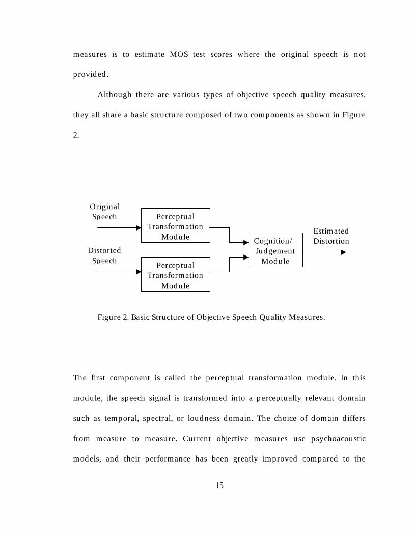
Although there are various types of objective speech quality measures,
they all share a basic structure composed of two components as shown in Figure
2.
Figure 2. Basic Structure of Objective Speech Quality Measures.
The first component is called the perceptual transformation module. In this
module, the speech signal is transformed into a perceptually relevant domain
such as temporal, spectral, or loudness domain. The choice of domain differs
from measure to measure. Current objective measures use psychoacoustic
models, and their performance has been greatly improved compared to the
PerceptualTransformation
Module
PerceptualTransformation
Module
OriginalSpeech
DistortedSpeech
EstimatedDistortionCognition/
JudgementModule

16
previous measures that did not incorporate psychoacoustic responses. The
second component is called the cognition/judgement module. This module
models listeners’ cognition and judgment of speech quality in the subjective test.
After the original and the distorted speech are converted into a perceptually
relevant domain, through the perceptual transformation module, the
cognition/judgment module compares the two perceptually transformed signals
in order to generate an estimated distortion. Some measures use a simple
cognition/judgment module like average Euclidean distance while others use a
complex one such as an artificial neural network or fuzzy logic. Recently,
researchers in this field have been focusing on this module because they realize
that a simple distance metric cannot cover the wide range of distortions
encountered in modern voice communication systems. The potential benefits of
including this module are not yet fully understood.
Objective speech quality measures can be classified according to the
perceptual domain transformation module being used, and these are: time
domain measures, spectral domain measures, and perceptual domain measures.
In the following sections, these classes of measures are briefly reviewed.

17
2.2.1. Time Domain Measures
Time domain measures are usually applicable to analog or waveform
coding systems in which the goal is to reproduce the waveform itself. Signal-to-
noise ratio (SNR) and segmental SNR (SNRseg) are well known time domain
measures [Quackenbush et al., 1988]. Since speech waveforms are directly
compared in time domain measures, synchronization of the original and
distorted speech is extremely important. If the waveforms are not synchronized,
the results of these measures will have little to do with the distortions introduced
by the speech processing system. Since current sophisticated codecs are designed
to generate the same sound of the original speech using speech production
models rather than simply reproducing the original speech waveform, these time
domain measures cannot be used in those applications.
2.2.1.1. Signal-to-Noise Ratio (SNR)
This measure is only appropriate for measuring the distortion of the
waveform coders that reproduce the input waveform. The SNR is very sensitive
to the time alignment of the original and distorted speech. If not synchronized,
18
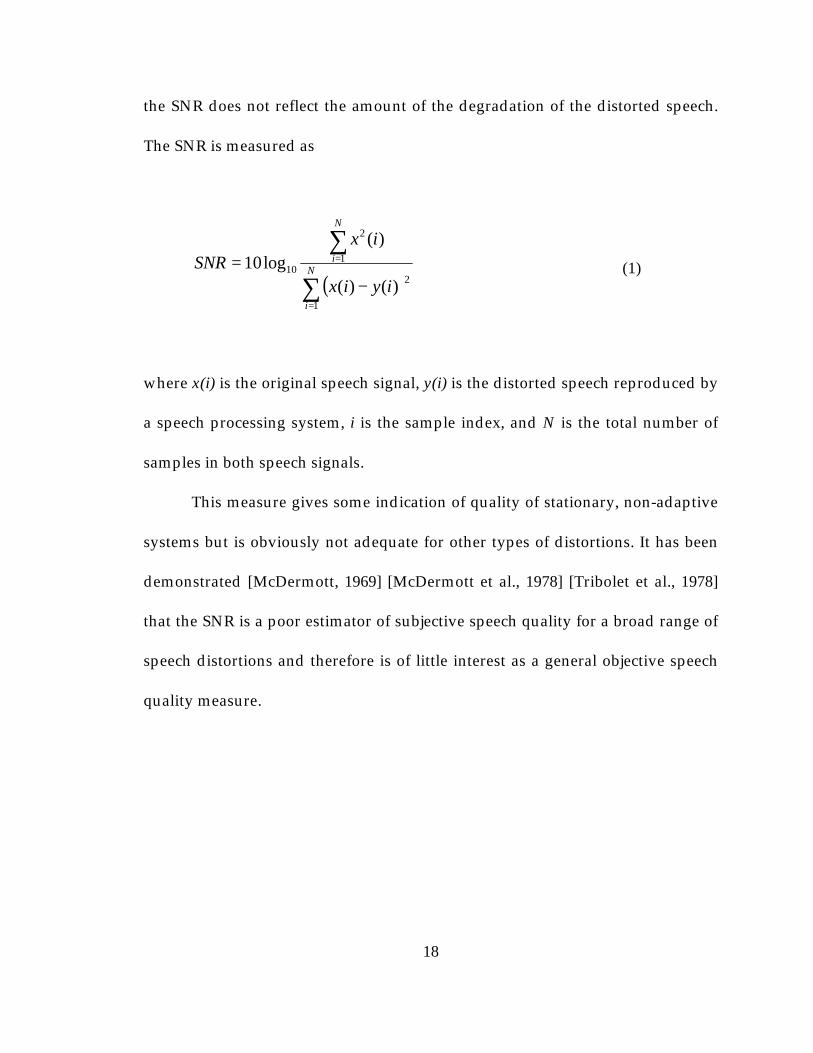
the SNR does not reflect the amount of the degradation of the distorted speech.
The SNR is measured as
( )∑
∑
=
=
−= N
i
N
i
iyix
ixSNR
1
2
1
2
10
)()(
)(log10 (1)
where x(i) is the original speech signal, y(i) is the distorted speech reproduced by
a speech processing system, i is the sample index, and N is the total number of
samples in both speech signals.
This measure gives some indication of quality of stationary, non-adaptive
systems but is obviously not adequate for other types of distortions. It has been
demonstrated [McDermott, 1969] [McDermott et al., 1978] [Tribolet et al., 1978]
that the SNR is a poor estimator of subjective speech quality for a broad range of
speech distortions and therefore is of little interest as a general objective speech
quality measure.

19
2.2.1.2. Segmental Signal-to-Noise Ratio (SNRseg)
The most popular class of the time-domain measures is the segmental
signal-to-noise ratio (SNRseg). SNRseg is defined as an average of the SNR
values of short segments. The performance of SNRseg is a good estimator of
speech quality for waveform coders [Noll, 1974] [Barnwell and Voiers, 1979], but
its performance is poor for vocoders where the goal is to generate the same
speech sound rather than to produce the speech waveform itself. SNRseg can be
formulated as
( )∑ ∑−
=
−+
=
−=
1
0
1
2
2
10)()(
)(log
10 M
m
NNm
Nmi iyix
ix
MSNRseg (2)
where x(i) is the original speech signal, y(i) is the distorted speech reproduced by
a speech processing system, N is the segment length and M is the number of
segments in the speech signal. The length of segments is typically 15 to 20 ms.
The above definition of SNRseg poses a problem if there are intervals of
silence in the speech utterance. In segments in which the original speech is nearly
zero, any amount of noise can give rise to a large negative signal-to-noise ratio
for that segment, which could appreciably bias the overall measure of SNRseg.

20
This problem is resolved by including the SNR of the frame only if the frame’s
energy is above a specified threshold [Quackenbusch et al., 1988].
Even though SNRseg is a poor estimator of subjective speech quality for
vocoders, it is still the most widely used objective quality measure for vocoders
[Voran and Sholl, 1995].
2.2.2. Spectral Domain Measures
Several spectral domain measures have been proposed in the literature
including the log likelihood ratio measures [Itakura, 1975] [Crochiere et al., 1980]
[Juang, 1984], the Linear Predictive Coding (LPC) parameter distance measures
[Barnwell et al., 1978] [Barnwell and Voiers, 1979], the cepstral distance
measures [Gray and Markel, 1976] [Tohkura, 1987] [Kitawaki et al., 1988], and
the weighted slope spectral distance measure [Klatt, 1976] [Klatt, 1982]. These
distortion measures are generally computed using speech segments typically
between 15 and 30 ms long. They are much more reliable than the time-domain
measures and less sensitive to the occurrence of time misalignments between the
original and the coded speech [Quackenbush et al., 1988]. However, most
spectral domain measures are closely related to speech codec design and use the
parameters of speech production models. Their ability to adequately describe the

21
listeners’ auditory response is limited by the constraints of the speech production
models.
2.2.2.1. Log Likelihood Ratio (LLR) Measures
The LLR is referred to as the Itakura distance measure. The LLR distance
for a speech segment is based on the assumption that a speech segment can be
represented by a p-th order all-pole linear predictive coding (LPC) model of the
form
∑=
+−=p
mxm nuGmnxanx
1
][][][ (3)
where x[n] is the n-th speech sample, am (for m = 1, 2, …, p) are the coefficients of
an all-pole filter, Gx is the gain of the filter and u[n] is an appropriate excitation
source for the filter. The speech waveform is windowed to form frames 15 to 30
ms in length. The LLR measure then is defined as
=
Tyyy
Txyx
aRa
aRaLLR rr
rr
log (4)

22
where xar
is the LPC coefficient vector (1, -ax(1), -ax(2), . . ., -ax(p)) for the original
speech x[n], yar
is the LPC coefficient vector (1, -ay(1), -ay(2), . . ., -ay(p)) for the
distorted speech y[n], and yR is the autocorrelation matrix for the distorted
speech.
Since the LLR is based on the assumption that the speech signals are well
represented using an all-pole model, the performance of the LLR is limited by the
distortion conditions where this assumption is valid [Crochiere et al., 1980]. This
assumption may not be valid if the original speech is passed through a voice
communication system that significantly changes the statistics of the original
speech.
2.2.2.2. LPC Parameter Measures
Motivated by linear prediction of speech [Markel and Gray, 1976],
objective speech quality measures can compare the parameters of the linear
prediction vocal tract models of the original and distorted speech. The
parameters used in LPC parameter measures can be the prediction coefficients,
or transformations of the predictor coefficients such as area ratio coefficients.

23
Linear prediction analysis is performed over 15 to 30 ms frames to obtain LPC
parameters which are used for the computation of distortion.
Barnwell et al. (1978) have proposed parameter distance measures of the
form
pN
i
pymiQxmiQ
NmpQd
1
1
),,(),,(1
),,(
−= ∑
=(5)
where d(Q,p,m) is the distance measure of the analysis frame m, p is the power in
the norm, and N is the order of the LPC analysis [Barnwell et al., 1978] [Barnwell
and Voiers, 1979]. Q(i,m,x) and Q(i,m,y) are the i-th parameters of the
corresponding frames of the original and distorted speech, respectively. The
distance measure for each frame is summed for all frames as follows:
∑
∑
=
== M
m
M
m
mW
mpQdmWpD
1
1
)(
),,()()( (6)
where D(p) is the resultant estimated distortion, M is the total number of frames,
and W(m) is a weight associated with the distance measure for the m-th frame.
The weighting could, for example, be the energy in the reference analysis frame.

24
Barnwell et al. (1978) have investigated this measure with various forms of LPC
parameters [Barnwell et al., 1978]. Among them, the log area ratio measure has
been reported to have the highest correlation with subjective quality. Eq. (6) is a
general formula that other objective speech quality measures can use in the
calculation of a distortion value for a test sample.
2.2.2.3. Cepsrtal Distance (CD) Measures
The cepstral distance (CD) is another form of LPC parameter measure,
because linear prediction coefficients also can be used to compute cepstral
coefficients of the overall difference between an original and a corresponding
coded speech cepstrum. The cepstrum computed from the LPC coefficients,
unlike that computed directly from the speech waveform, results in an estimate
of the smoothed speech spectrum [Kitawaki et al., 1988]. This can be written as
∑∞
=
−=
1
)()(
1log
k
kzkczA
(7)
where A(z) is the LPC analysis filter polynomial, c(k) denotes the k-th cepstral
coefficient, and z can be set equal to e-jw. Also, there is another way to calculate

25
the cepstral coefficients from the linear predictor coefficients [Markel and Gray,
1976]:
∑−
=
−−=−1
1
)()()()()(n
k
kakncknnnannc for n = 1, 2, 3, . . . (8)
where a(0) = 1 and a(k) = 0 for k > p. In this expression, the a(k) is the linear
predictor coefficients and p is the order of the linear predictor. The cepstral
coefficients are computed recursively from Eq. (8).
An objective speech quality measure based on the cepstral coefficients
computes the distortion of a frame [Gray and Markel, 1976] [Kitawaki et al., 1982]:
[ ] [ ]2
1
1
22 )()(2)0()0(),2,,(
−+−= ∑
=
L
kyxyxyx kckcccmccd (9)
where d is the L2 distance for frame m and cx(k) and cy(k) are the cepstral
coefficients for the original and distorted speech, respectively. The final
distortion is calculated over all frames using Eq. (6).

26
2.2.2.4. Weighted Slope Spectral Distance Measure
A speech spectrum can be analyzed using a filter bank. Klatt (1976) uses
thirty-six overlapping filters of progressively larger bandwidths to estimate the
smoothed short-time speech spectrum every 12 ms [Klatt, 1976]. The filter
bandwidths approximate critical bands in order to give equal perceptual weight
to each band [Zwicker, 1961]. Rather than using the absolute spectral distance
per band to estimate distortion, Klatt (1982) uses a weighted difference between
the spectral slopes in each band [Klatt, 1982]. This method assumes that spectral
variation plays an important role in human perception of speech quality.
In this measure, the spectral slope is first computed in each critical band as
follows:
)()1()(
)()1()(
kVkVkS
kVkVkS
yyy
xxx
−+=
−+=(10)
where Vx(k) and Vy(k) are the original and distorted spectra in decibels, Sx(k) and
Sy(k) are the first order slopes of these spectra and k is the critical band index.
Next, a weight for each band is calculated based on the magnitude of the
spectrum in that band. Klatt computes the weight using a global spectral
maximum as well as a local spectral maximum. The weight is larger for those

27
bands whose spectral magnitude is closer to the global or local spectral maxima.
The spectral distortion is computed for a frame as
( ) [ ]236
1
)()()()( ∑=
−+−=k
yxyxspl kSkSkWKKKmd (11)
where Kx and Ky are related to the overall sound pressure level of the original
and distorted speech and Kspl is a parameter that can be varied. The overall
distortion is obtained by averaging the spectral distortion over all frames in an
utterance.
2.2.3. Psychoacoustic Results
Since current objective speech quality measures are based on
psychoacoustic results, this section reviews those psychoacoustic results
frequently used in current objective quality measures. Psychoacoustics is the
study of the quantitative correlation of acoustical stimuli and human hearing
sensations. Zwicker and Fastl (1990) have summarized the extensive results of
psychoacoustic facts and models based on experimental data [Zwicker and Fastl,
1990]. The important psychoacoustic results used in objective speech quality

28
measures are: frequency selectivity, nonlinear response of human hearing
system, masking effects, critical band concept, and loudness.
2.2.3.1. Critical Bands
The critical-band concept is important for describing hearing sensations. It
was used in so many models and hypotheses that a unit was defined, leading to
the so-called critical-band rate scale. This scale is based on the fact that our
hearing system analyses a broad spectrum into parts that correspond to critical
bands. It is well known that the inner ear performs the very important task of
frequency separation; energy from different frequencies is transferred to and
concentrated at different places along the basilar membrane. So, the inner ear can
be regarded as a system composed of a series of band-pass filters each with an
asymmetrical shape of frequency response. The center frequencies of these band-
pass filters are closely related to the critical band rates.
Table 3 shows critical band rate, lower and upper limit of the critical
bands [Zwicker and Fastl, 1990]. The critical bandwidth remains approximately
100 Hz up to a center frequency of 500 Hz, and a relative bandwidth of 20% for
center frequencies above 500 Hz.

29
Critical-band rate has the unit “Bark” in memory of Barkhausen, a
scientist who introduced the “phon”, a value describing loudness level for which
the critical band plays an important role. The relationship between critical-band
rate, z, and frequency, f, is important for understanding many characteristics of
the human ear.
Table 3. Critical-Band Rate and Critical Bandwidths Over Auditory Frequency Range. Critical-Band Rate, z, Lower(fl) and Upper(fu) Frequency Limit of Critical Bandwidths, ∆fG, Centered at fc
z (Bark) fl, fu (Hz) fc (Hz) ∆fG (Hz)0 0 50 1001 100 150 1002 200 250 1003 300 350 1004 400 450 1105 510 570 1206 630 700 1407 770 840 1508 920 1000 1609 1080 1170 190
10 1270 1370 21011 1480 1600 24012 1720 1850 28013 2000 2150 32014 2320 2500 38015 2700 2900 45016 3150 3400 55017 3700 4000 70018 4400 4800 90019 5300

30
In many cases an analytic expression is useful to describe the dependence
of critical-band rate and of critical bandwidth over the whole auditory frequency
range [Zwicker, 1961]. The following two expressions have proven useful:
2)5.7/arctan(5.3)76.0arctan(13 ffz += (12)
[ ] 69.024.117525 ffG ++=∆ (13)
where z is the critical band rate, f is the frequency in kHz, and ∆fG is the critical
bandwidth in Hz.
2.2.3.2. Masking Effects
Auditory masking is the occlusion of one sound by another loud sound.
This may happen if the sounds are simultaneous, or a loud sound can obliterate a
sound closely following, or preceding it. Masking effects are differentiated
according to temporal regions of masking relative to the presentation of the
masker stimulus. Premasking takes place during the period of time before the
masker is presented. Premasking plays a relatively secondary role, because the
effect lasts only 20 ms, and therefore is usually ignored. Postmasking occurs

31
during the time the masker is not present. The effects of postmasking correspond
to a decay of the effect of the masker. Postmasking lasts longer than 100 ms and
ends after about a 200 ms delay. Both premasking and postmasking are referred
to as non-simultaneous masking. On the other hand, simultaneous masking
occurs when the masker and test sound are presented simultaneously.
To measure these effects quantitatively, the masked threshold is usually
determined. The masked threshold is the sound pressure level of a test sound
(usually a sinusoidal test tone), necessary to be just audible in the presence of a
masker. Masked threshold, in all but a very few special cases, always lies above
the absolute hearing threshold; it is identical to the absolute hearing threshold
when the frequencies of the masker and the test sound are very different. The
masked threshold depends on both the sound pressure level of the masker as
well as the duration of the test sound. The dependence of masking effects on
duration shows that the masked threshold of a test tone for duration of 200 ms is
equal to that of long lasting sounds. For duration shorter than 200 ms, the
masked threshold increases at a rate of 10 dB per decade as the duration
decreases. This behavior can be ascribed to the temporal integration of the
hearing system [Zwicker and Fastl, 1990].
Among the experiments on auditory masking, the threshold of pure tones
masked by critical-band wide noise is interesting. Figure 3 shows this masked
threshold at center frequencies of 0.25, 1, and 4 kHz. The level of each masking

32
noise is 60 dB and the corresponding bandwidths of the noises are 100, 160, and
700 Hz, respectively. Note that the slopes of the noises above and below the
center frequency of each filter are very steep. The frequency dependence of the
threshold masked by the 250 Hz narrow band noise seems to be broader. Also,
the maximum of the masking threshold shows the tendency to be lower for
higher center frequencies of the masker, although the level of the narrow-band
masker is 60 dB at all center frequencies.
Figure 3. Level of Test Tone Just Masked by Critical-Band Wide Noise WithLevel of 60 dB, and Center Frequencies of 0.25, 1, and 4 kHz. TheBroken Curve is the Threshold in Silence [Zwicker and Fastl, 1990].

33
2.2.3.3. Equal-Loudness Contours
Loudness belongs to the category of intensity sensations. Loudness is the
sensation that corresponds most closely to the sound intensity of the stimulus.
Loudness can be measured by answering the question of how much louder (or
softer) a sound is heard relative to a standard sound. In psychoacoustics, the 1
kHz tone is the most common standard sound. The level of 40 dB of a 1 kHz tone
is supposed to give the reference for loudness sensation, i.e. 1 sone. For loudness
evaluations, the subject searches for the level increment that leads to a sensation
that is twice as loud as that of the starting level. The average of many
measurements of this kind indicates that the level of the 1 kHz tone in a plane
field has to increase by 10 dB in order to enlarge the sensation of loudness by a
factor of two. So, the sound pressure level of 40 dB of the 1 kHz tone has to be
increased to 50 dB in order to double the loudness, which corresponds to 2 sones.
In addition to loudness, loudness level is also important. The loudness
level is not only a sensation value but belongs somewhere between sensation and
a physical value. It was introduced in the twenties by Barkhausen to characterize
the loudness sensation of any sound with physical values. The loudness level of a
sound is the sound pressure level of a 1 kHz tone in a plane wave that is as loud
as the sound. The unit of loudness level is “phon”. Using the above definition,
the loudness level can be measured for any sound, but best known are the

34
loudness levels for different frequencies of pure tones. A set of lines which
connect points of equal loudness in the hearing area are called equal-loudness
contours. Equal-loudness contours for pure tones are shown in Figure 4.
Figure 4. Equal-Loudness Contours for Pure Tones in a Free Sound Field.The Parameter is Expressed in Loudness Level, LN and Loudness, N[Zwicker and Fastl, 1990].

35
The sound pressure level of 40 dB at 1 kHz tone corresponds to 40 phons
as well as to 1 sone. The threshold in silence, where the limit of loudness
sensation is reached, is also an equal-loudness contour, shown with a dashed
line. The equal-loudness contours are almost parallel to the threshold in silence.
However, at low frequencies, equal-loudness contours become shallower with
high levels. The most sensitive area of threshold in silence is the frequency range
between 2 and 5 kHz corresponding to a dip in all equal-loudness contours. As
shown in Figure 4, loudness depends on the sound intensity as well as the
frequency of a tone.
The relationship between loudness level and loudness sensation is
formulated as follows [Bladon, 1981]:
10/)40(2 −= PS if P > 40 (14.1)
( ) 642.240/PS = if P < 40 (14.2)
where P is the loudness level in phon and S is the loudness in sone.

36
2.2.4. Perceptual Domain Measures
Most spectral domain measures are closely related to speech codec design,
and use the parameters of speech production models. Their performance is
limited by the constraints of the speech production models used in codecs. In
contrast to the spectral domain measures, perceptual domain measures are based
on models of human auditory perception. These measures transform speech
signal into a perceptually relevant domain such as bark spectrum or loudness
domain, and incorporate human auditory models. Perceptual domain measures
appear to have the best chance of predicting subjective quality of speech.
Recently, researchers in this field have begun to consider that the
cognition/judgement model plays an important role in estimating subjective
quality. However, since most of current cognition models are based on the
optimization with one type of speech data, the performance of those measures
may not function properly with different speech data. Also, these measures
would have the risk of not describing perceptually important effects relevant to
speech quality but simply curve-fitting by parameter optimization [Hauenstein,
1998].

37
2.2.4.1. Bark Spectral Distortion (BSD)
BSD was developed at the University of California, Santa Barbara [Wang
et al., 1992]. It was essentially the first objective measure to incorporate
psychoacoustic responses. Its performance was quite good for speech coding
distortions as compared to traditional objective measures such as time domain
measures and spectral domain measures. BSD has become a good candidate for a
highly correlated objective quality measure according to several researchers
[Lam et al., 1996] [Meky and Saadawi, 1996] [Voran and Sholl, 1995]. The BSD
measure is based on the assumption that speech quality is directly related to
speech loudness, which is a psychoacoustical term defined as the magnitude of
auditory sensation. In order to calculate loudness, the speech signal is processed
using the results of psychoacoustic measurements, which include critical band
analysis, equal-loudness preemphasis, and intensity-loudness power law.
BSD estimates the overall distortion by using the average Euclidean
distance between loudness vectors of the reference and of the distorted speech.
When BSD was used initially, the non-silence portions composed of voiced and
unvoiced regions were processed. It was found that its performance was
enhanced when only the voiced portions are considered in the estimation of
distortion. Later versions of the algorithm processed only voiced segments.

38
Wang et al. (1992) were motivated by the method of calculating an
objective measure for signal degradation based on the measurable properties of
auditory perception [Schroeder et al., 1979], and developed the Bark Spectral
Distortion (BSD) measure [Wang et al., 1992].
Their approach is outlined below. First, a nonlinear frequency
transformation from Hertz, f, to bark, b, is made via the relation [Schroeder et al.,
1979]
)6/sinh(600 bf = (15)
which transforms the original power spectral density function X(f) to a critical
band density function Y(b). The function Y(b) is smeared by a prototype critical
band filter F(b) given by [Bladon, 1981]:
[ ] 5.0210 )(196.05.17)(5.77)(log10 αα −+−−−= bbbF (16)
with α = 0.215. The smearing is conceived of as a convolution operation between
F(b) and Y(b) which yields a continuous spectrum D(b). The fact that the ear is
not equally sensitive to the amount of energy at different frequencies is exploited
next. The well-known equal loudness level curves [Robinson and Dadson, 1956]

39
have been used to translate the sound pressure level (SPL) in dB to loudness
levels in phons. The increase of approximately 10 phons of loudness level is
required to make the subjective loudness double for the loudness level greater
than 40 phons. A phon-to-sone conversion is performed using Eq. (14) to generate
a Bark spectrum S(i). Then, the BSD measure is defined as the average of BSD(k)
with
[ ]2
1
)()()( )()(∑=
−=N
i
ky
kx
k iSiSBSD (17)
where N is the number of critical bands, and )()( iS kx and )()( iS k
y are the Bark
Spectra in the i-th critical band for the k-th frame corresponding to the original
and the distorted speech, respectively.
BSD works well in cases where the distortion in voiced regions represents
the overall distortion, because it processes voiced regions only; for this reason,
voiced regions must be detected. BSD uses a traditional metric, Euclidean
distance, in the cognition module, but the developers did not validate the use of
this metric.
40
2.2.4.2. Perceptual Speech Quality Measure (PSQM)
PSQM was developed by PTT Research in 1994 [Beerends and
Stemerdink, 1994]. It can be considered as a modified version of the Perceptual
Audio Quality Measure (PAQM) which is an objective audio quality measure
also developed at PTT Research [Beerends and Stemerdink, 1992]. Recognizing
that the characteristics of speech and music are different, PSQM was optimized
for speech by modifying some of the procedures of PAQM. PSQM has been
adopted as ITU-T Recommendation P.861 [ITU-T Recommendation P.861, 1996].
Its performance has been shown to be relatively robust for coding distortions.
PSQM transforms the speech signal into the loudness domain, modifying
some parameters in the loudness calculation in order to optimize performance.
PSQM does not include temporal or spectral masking in its calculation of
loudness. PSQM applies a nonlinear scaling factor to the loudness vector of
distorted speech. The scaling factor is obtained using the loudness ratio of the
reference and the distorted speech in three frequency bands. The difference
between the scaled loudness of the distorted speech and the loudness of the
reference speech is called noise disturbance. The final estimated distortion is an
averaged noise disturbance over all the frames processed. PSQM disregards or
applies a small weight to silence portions in the calculation of distortion.

41
PSQM uses psychoacoustic results of loudness calculation to transform
speech into the perceptually relevant domain. It modifies the procedure of
loudness calculation in order to optimize its performance. This modification
could be justified by considering that in psychoacoustic experiments, steady-
state signals (sinusoids) were used instead of real speech. PSQM also considers
the role of distortions in silence portions on overall speech quality. Even though
its performance is relatively robust over coding distortions, its performance may
not be robust enough to apply to a broader range of distortions.
2.2.4.3. PSQM+
PSQM+ was developed by KPN Research in 1997 [Beerends, 1997]. The
performance of PSQM+ is improved over that of the P.861 (PSQM) for loud
distortions and temporal clipping by some simple modifications to the cognition
module. PSQM+ can be applied to a wider range of distortions as an objective
measure than PSQM.
PSQM+ uses the same perceptual transformation module as PSQM.
Similar to PSQM, PSQM+ transforms the speech signal into the modified
loudness domain, and does not include temporal or spectral masking in its
calculation of loudness. In order to improve the performance for the loud

42
distortions like temporal clipping, an additional scaling factor is introduced
when the overall distortion is calculated. This scaling factor makes the overall
distortion proportional to the amount of temporal clipping distortion. Otherwise,
the cognition module is the same as PSQM.
PSQM+ adopts a simple algorithm in the cognition module to improve the
performance of PSQM. The poor performance of PSQM for distortions like
temporal clipping is caused by the procedure calculating a scaling factor. The
scaling factors are determined by the ratio of the energy of the distorted speech
and the reference speech. This scaling factor scheme of PSQM works very well
when a distortion results in additional energy. However, if a distortion results in
reduced energy such as temporal clipping, which removes some of the signal
energy, the estimate of distortion is proportionally smaller, and PSQM
underestimates the actual distortion. Therefore, PSQM+ uses a simple
modification to adopt an additional scaling factor to compensate for this effect.
PSQM+ resolves one performance issue of PSQM on distortions such as
temporal clipping. However, the performance of PSQM+ may be questioned for
other different types of distortions.

43
2.2.4.4. Measuring Normalizing Blocks (MNB)
MNB was developed at the US Department of Commerce in 1997 [Voran,
1997]. It emphasizes the important role of the cognition module for estimating
speech quality. MNB models human judgment on speech quality with two types
of hierarchical structures. It has showed relatively robust performance over an
extensive number of different speech data sets.
MNB transforms speech signals into an approximate loudness domain
through frequency warping and logarithmic scaling. MNB assumes that these
two factors play the most important role in modeling human auditory response.
The algorithm generates an approximated loudness vector for each frame. MNB
considers human listener’s sensitivity to the distribution of distortion, so it uses
hierarchical structures that work from larger time and frequency scales to
smaller time and frequency scales. MNB employs two types of calculations in
deriving a quality estimate: time measuring normalizing blocks (TMNB) and
frequency measuring normalizing blocks (FMNB). Each TMNB integrates over
frequency scales and measures differences over time intervals while the FMNB
integrates over time intervals and measures differences over frequency scales.
After calculating 11 or 12 MNBs, these MNBs are linearly combined to estimate
overall speech distortion. The weights for each MNB were optimized with a
training data set.
44
Since there has been little research on the cognition model in the
evaluation of speech quality, some procedures of MNB are not fully understood.
MNB does not generate a distortion value for each frame since each MNB is
integrated over frequency or time intervals. Its performance may depend upon
the scope of training data sets.
2.2.4.5. Perceptual Analysis Measurement System (PAMS)
PAMS was developed by British Telecom (BT) in 1998 [Hollier and Rix,
1998]. PAMS aims to achieve robustness and consistency in predicting subjective
ratings by careful extraction and selection of parameters describing speech
degradation and constrained mapping to subjective quality.
A parameter set, in which each parameter increases with increasing
degradation, is generated. The best set of parameters is selected with a training
procedure. The parameter set used in PAMS has not been specified in the
literature. A linear mixture of monotonic quadratic functions for the selected
parameters is used for mapping to subjective quality. The quadratic functions are
constrained to be monotonically increasing with increasing value of parameters.
The optimum coefficients of the functions are obtained with a training
procedure.

45
PAMS uses a concept of mapping from the parameter domain to
subjective quality domain. PAMS describes a general approach in predicting
subjective quality. It is flexible in adopting other parameters if they are
perceptually important.
The performance of the PAMS depends upon the designer’s intuition in
extracting candidate parameters as well as selecting parameters with a training
data set. Since the parameters are usually not independent of each other, it is not
easy to optimize both the parameter set and the associated mapping function. So,
extensive computation is performed during training.
2.2.4.6. QVoice
QVoice was developed by ASCOM for predicting speech quality in mobile
communication systems. QVoice uses artificial neural networks and fuzzy logic
techniques to estimate listener’s judgment of subjective quality. It is a popular
tool used to test mobile communications systems in the field.
Unlike other perceptual domain measures, QVoice considers the LPC
cepstral coefficients over a fixed duration of speech sample (5 seconds) as
perceptually significant parameters. The difference between the LPC cepstral
coefficient matrices of the reference and distorted speech is fed into a trained

46
artificial neural network to estimate degradation. Fuzzy logic is used to predict
the subjective score using the estimated degradation. Nonlinear processing of
listeners’ judgment of speech quality is emulated by artificial neural network and
fuzzy logic. The parameters of the cognition module are optimized by training
the system with speech samples and associated subjective ratings data.
The motivation for using LPC cepstral coefficients for parameters has not
been validated in QVoice. It can only estimate the overall speech quality, and
does not provide any estimate of the temporal variations of speech quality. Since
a neural network technique is used, its performance strongly depends upon the
similarity between the test cases making up the samples and training data.
2.2.4.7. Telecommunication Objective Speech Quality Assessment (TOSQA)
TOSQA was developed by Deutsche Telekom (DT) Berkom in 1997
[Berger, 1997]. TOSQA considers the special feature of the MOS test, where
subjects compare the speech being tested with a mental reference rather than
comparing it to the original (undistorted) speech.
TOSQA calculates a modified reference loudness pattern of the original
speech. In this reference pattern, the loudness components which have little
influence on speech quality are reduced. TOSQA uses a dynamic frequency

47
warping to obtain the bark spectrums. The distortion value in TOSQA is based
on the similarity between reference and distorted speech rather than the distance
between them.
TOSQA has been designed to take into account the structural difference
between the MOS test and objective speech quality measures. However, Berger
did not explain how to identify the perceptually irrelevant components [Berger,
1997].

48
CHAPTER 3
EVALUATION OF OBJECTIVE SPEECH QUALITY MEASURES
A reliable evaluation of any system is generally an essential part for
development and improvement of that system. The task of evaluating the
validity of objective speech quality measures is discussed in this chapter. Since
the goal of objective speech quality measures is to replace subjective procedures,
the predictability of the latter by the former is an appropriate vehicle for
evaluation [Quackenbusch et al., 1988].
Figure 5. A System for Evaluating Performance of Objective Speech QualityMeasures.
Distortions
OriginalSpeech
DistortedSpeech
ObjectiveMeasure
SubjectiveMeasure
CorrelationAnalysis
ObjectiveEstimates
SubjectiveEstimates
PerformanceParameters

49
A system for evaluating the performance of objective speech quality
measures can be described as shown in Figure 5. Original speech is usually a set
of phonetically balanced sentences spoken by both males and females. Distorted
speech is generated by processing the original speech through various distortion
conditions. These distortion conditions can be coding distortions, channel
impairments, amplitude variations, temporal clipping, delays, and so on.
Although an ideal objective speech quality measure would be able to assess the
quality of speech without access to the original speech, current objective speech
quality measures base their estimates on both the original and distorted speech.
Subjective speech quality measures can estimate the quality of speech with only
the distorted speech, or with both the original and distorted speech (described by
the broken line in Figure 5) according to the test method used. For instance, the
MOS test estimates the quality of the distorted speech with the distorted speech
only, while the DMOS test estimates the quality of the distorted speech with both
the original and distorted speech. Objective speech quality measures have been
conventionally evaluated using MOS scores. However, objective speech quality
measures estimate subjective scores by comparing the distorted speech to the
original speech. This approach has much more in common with a DMOS test
than a MOS test. Therefore, it is worthwhile to examine the performance of
objective speech quality measures with DMOS as well as MOS.

50
After an objective speech quality measure is applied to the original and
distorted speech, statistical analysis is performed to determine how well the
objective speech quality measure predicts the subjective test results. The
correlation coefficient between the objective speech quality measures and the
subjective speech quality measures has been conventionally used as a figure-of-
merit for comparing objective speech quality measures. However, the correlation
coefficient has some shortcomings that can be compensated by considering some
additional measures of performance. Therefore, another figure-of-merit, the
standard error of the estimate (SEE), is employed to compensate for those
shortcomings of the correlation coefficient. The SEE is an unbiased statistic for
estimating of the deviation from the best-fitting curve between two variables.
The SEE has several advantages over the correlation coefficient as a figure-of-
merit for evaluation of objective speech quality measures, as will be discussed
later.
3.1. Evaluation With MOS Versus DMOS
A good objective speech quality measure should estimate the quality of a
distorted speech accurately. However, how can we verify that an objective
speech quality measure is good? The answer to this question is to compare the
51
estimated quality of an objective measure with the actual quality of a distorted
speech set obtained from subjective tests. Since the MOS test is the most widely
used subjective test in the speech coding community, the performance of
objective speech quality measures has been assessed with the correlation
between these measures and the MOS scores. No one has raised a question as to
the validity of using MOS scores for the evaluation of objective speech quality
measures simply because the goal of objective speech quality measures was to
predict the MOS scores. However, when we compare the procedure of the MOS
test and the basic approach of objective speech quality measures, there is a
procedural difference between them. In a MOS test, listeners are not provided
with an original speech sample, and rate the overall speech quality of the
distorted speech sample. However, objective speech quality measures estimate
subjective scores by comparing the distorted speech to the original speech, as
discussed before. Although this procedural difference between objective speech
quality measures and the MOS test has been noted in the literature [Yang et al.,
1997] [Berger, 1997] [Yang et al., 1998] [Voran, 1999], there has been no attempt to
apply this information to the evaluation of objective speech quality measures.
This procedural difference can result in incorrect evaluation of objective speech
quality measures, especially when the original speech samples are degraded. As
a simple illustration, assume that original speech degraded by background noise

52
is transmitted through a transparent system, so that the output speech is exactly
the same as the input speech, as shown in Figure 6.
Figure 6. A System Illustrating the Procedural Difference Between ObjectiveMeasures and the MOS Test: When the Degraded Reference Speech isTransmitted by a Transparent System.
For this situation, the objective speech quality measure will regard the quality of
the output speech as “excellent” because there is no degradation. However, the
MOS scores of the output speech would be classified as “bad”. This discrepancy
has nothing to do with the actual performance of objective speech quality
TransparentSystem
DegradedSpeech
DegradedSpeech
ObjectiveMeasure
MOS
No distortions
Bad quality

53
measure, rather it is caused by the procedural difference between the MOS
[absolute category rating (ACR)] and the DMOS [degradation category rating
(DCR)].
In order to exclude the problem of procedural difference, it has been
proposed that the DCR subjective test would be more appropriate for evaluation
of objective speech quality measures because the approach of objective speech
quality measures is analogous to that of DMOS [Yang et al., 1997] [Yang et al.,
1998] [Yang and Yantorno, 1999]. In the evaluation of objective speech quality
measures, Yang et al. (1998) used MOS difference data (MOS of original speech –
MOS of distorted speech) instead of DMOS data because no DMOS data were
available. They compared the correlation coefficients of prospective objective
speech quality measures with the MOS as well as with the MOS difference for
each speech file [Yang and Yantorno, 1999]. It should be noted that the objective
speech quality measures used in this experiment showed better correlation with
the MOS difference than with the MOS, as shown in Table 4.
Table 4. Correlation Coefficients with the MOS and the MOS Difference forSpeech Coding Distortion (Correlation Analyses with each SpeechSample) [Yang and Yantorno, 1999]
Objective Measures MOS MOS differencePSQM 0.8731 0.8933MNB1 0.7958 0.8319MNB2 0.8140 0.8478MBSD 0.8782 0.9001
MBSD II 0.9041 0.9252

54
Recently, current perceptual objective speech quality measures have been
evaluated with both MOS and DMOS at Nortel Networks in Ottawa [Thorpe and
Yang, 1999]. The results have shown that current objective speech quality
measures are better correlated with DMOS scores than with MOS scores. The
results have been summarized in Figure 7. These results suggest that a DCR
subjective test such as DMOS is more appropriate for evaluation of objective
speech quality measures due to the procedural difference between objective
speech quality measures and the MOS test. This observation also provides
insight into the development of a new model for objective speech quality
measures appropriate in real network applications which will be discussed later.
Figure 7. Performance of Current Objective Quality Measures with both MOS and DMOS [Thorpe and Yang, 1999].
0.8690.822 0.808
0.866
0.967 0.957 0.937 0.945
0
0.2
0.4
0.6
0.8
1
A B C D
Objective Measures
Co
rrel
atio
n C
oef
fici
ent
MOS DMOS

55
3.2. Correlation Analysis
After an objective speech quality measure is applied to the original and
distorted speech to generate the estimates of subjective scores, statistical analysis
is performed to determine how well it predicts the subjective test results. The
correlation coefficient has been conventionally used as a performance parameter
for evaluation of objective speech quality measures. The correlation coefficient
(also called Pearson product-moment correlation) is formulated as
2
12
11
2
2
11
2
111
)()()()(
)()()()(
−
−
−
=
∑∑∑∑
∑∑∑
====
===
N
i
N
i
N
i
N
i
N
i
N
i
N
i
iYiYNiXiXN
iYiXiYiXN
r (18)
where X(i) are the subjective scores, Y(i) are the corresponding objective
estimates, and N is the number of distortion conditions.
Since this correlation analysis assumes that the two measures are linearly
related, pre-processing is required before calculating the correlation coefficient if
the two measures are not linearly related. If the two measures are not linearly
related, as shown in Figure 8 (a), the best monotonic fitting function between
them is obtained from regression analysis. Figure 8 (b) shows the scatterplot of

56
the measure after the estimates of the objective measures are transformed with
the regression curve. Then, the correlation coefficient between the subjective
measures and the transformed estimates of the objective measure is calculated
using Eq. (18). The closer to +1 the correlation coefficient is, the better the
objective speech quality measure is at predicting the subjective rating.
(a) (b)
Figure 8. Transformation of Objective Estimates With a Regression Curve; (a) Objective Estimates and Subjective Estimates are not Linearly
Related, (b) Objective Estimates are Transformed With the Regression Curve.
The correlation coefficient has some shortcomings. Comparing
performance with the different groups of conditions is difficult because the
y = 1.7715Ln(x) + 2.3288
1
1.5
2
2.5
3
3.5
4
4.5
5
1 1.5 2 2.5 3 3.5 4 4.5 5
MOS
MO
S E
stim
ate
1
1.5
2
2.5
3
3.5
4
4.5
5
1 1.5 2 2.5 3 3.5 4 4.5 5
MOS
Tra
nsf
orm
ed M
OS
Est
imat
e

57
groups may have different types of distortions, different value ranges, and small
numbers of data points. Also, the correlation coefficient is highly sensitive to
outliers. For the same reasons, it would be inappropriate to compare the
correlation coefficients of an objective speech quality measure for different
speech data. The shortcomings outlined above can be overcome by considering
another performance parameter, the standard error of the estimates.
3.3. Standard Error of Estimates (SEE)
The standard error of the estimates (SEE) can compensate for some
shortcomings of the correlation coefficient as a figure-of-merit. The SEE is an
unbiased statistic for the estimate of the deviation from the regression line
between objective estimates and the actual subjective scores. The SEE is defined
as
( )
2
)()(1
2
−
−=
∑=
N
iQiQS
N
iso
est (19)

58
where the Qo(i) are the objective estimates, the Qs(i) are the subjective ratings,
and N is the number of data points. The SEE is the square root of the average
squared error of prediction of objective measures, representing the accuracy of
prediction.
The SEE can be obtained from the standard deviation (σs) of the subjective
scores and the correlation coefficient (r) between the objective estimates and the
subjective scores. An alternate formula for the SEE is
( )2
1 2
−−=
N
NrS sest σ (20)
where N is the number of data points. The SEE is related to the correlation
coefficient as well as the standard deviation of the subjective scores. For the same
correlation coefficient, the SEE tends to decrease as the variation of the subjective
scores gets smaller and the number of data points increases.
The SEE value characterizes predictability of objective speech quality
measures in terms of the error of the subjective scores in a statistically
meaningful way. The SEE value (Sest) would lead to the expectation that for a
given objective speech quality measure, the estimated subjective scores of
approximately 68% of the new speech samples will fall between ±Sest of their
actual subjective scores. Extending the range to twice Sest, it is expected that

59
approximately 95% of objective estimates will fall between ±2Sest of their actual
subjective scores. In other words, the SEE provides the performance of an
objective speech quality measure in terms of confidence interval of objective
estimates. This information would be very useful to users who want to
understand the capability of an objective speech quality measure to predict
subjective scores.
The SEE has another advantage over the correlation coefficient as a figure-
of-merit. Since it considers the distribution of the subjective scores of a speech
data base, the SEE of the objective measure with one set of data can be compared
to that with another set, which may not be valid for the correlation coefficient.
Also, the SEE with a certain condition group can be compared to that with a
different condition group, using Eq. (19). These kinds of comparisons would be
very useful to analyze the performance of the objective speech quality measures,
suggesting that the SEE would be a valuable figure-of-merit. Although the SEE
has been mentioned as an appropriate figure-of-merit [Quackenbusch et al.,
1988], it has not been used widely.
The advantages of the SEE as a figure-of-merit over the correlation
coefficient can be illustrated with the following simple illustration. Figure 9
shows two scatterplots of an objective speech quality measure with two different
sets of data. The speech data of Figure 9 (a) have a relatively large standard

60
deviation of subjective estimates (σsa = 1.60) while the speech data of Figure 9 (b)
have a relatively small standard deviation (σsb = 1.22).
(a) (b)
Figure 9. Scatterplots of an Objective Measure With Two Different Sets of Speech Data; (a) Speech Data With a Relatively Large Standard
Deviation, (b) Speech Data With a Relatively Small StandardDeviation.
The correlation coefficients of the objective measure are 0.95 with speech data set
(a), and 0.92 with speech data set (b). However, the SEE values of the objective
measure are 0.57 for speech data set (a), and 0.51 for speech data set (b). The
correlation coefficient with speech data set (a) has increased due to the relatively
large standard deviation although the prediction error with speech data set (a) is
1
1.5
2
2.5
3
3.5
4
4.5
5
1 1.5 2 2.5 3 3.5 4 4.5 5
Subjective Estimates
Ob
ject
ive
Est
imat
es
1
1.5
2
2.5
3
3.5
4
4.5
5
1 1.5 2 2.5 3 3.5 4 4.5 5
Subjective Estimates
Ob
ject
ive
Est
imat
es

61
larger than that with speech data set (b). So, it is not meaningful to compare the
correlation coefficients of the objective measure with different speech data. Since
SEE considers the distribution of the subjective scores of a speech data, it is
possible to compare performance of an objective measure with different speech
data using the SEE values.
When the performance of the objective measure is analyzed for a certain
condition group, the correlation coefficient calculated with the data points of that
group is not meaningful because the range of subjective scores, as well as the
number of data points in a group, are usually small. More importantly, this
analysis cannot consider the regression line of all data points. This phenomenon
is illustrated with Figure 10. The correlation coefficient of all of the data points is
0.87 while the correlation coefficient of the square data points is -0.86. It is
evident that this correlation coefficient of the square points themselves is
meaningless. However, it is possible to determine how much errors the objective
measure may make for the square data points by comparing the SEE of the
square data points (1.14) with that of all the data points (0.58).
As shown above with illustrations, the SEE will be a valuable figure-of-
merit to analyze the performance of objective speech quality measures. The SEE
characterize predictability of objective speech quality measures. Using the SEE, it
is possible to compare performance of an objective quality measure with one set
of speech data set to that with other speech data set.

62
Figure 10. Scatterplot Illustrating That Correlation Coefficient of a Certain Condition Group (Square Points).
1
1.5
2
2.5
3
3.5
4
4.5
5
1 1.5 2 2.5 3 3.5 4 4.5 5
Subjective Estimates
Ob
ject
ive
Est
imat
es

63
CHAPTER 4
MODIFIED BARK SPECTRAL DISTORTION (MBSD)
The MBSD has been developed in the Speech Processing Lab at Temple
University [Yang et al., 1997] [Yang et al., 1998]. It can be classified as a
perceptual domain measure that transforms the speech signal into a perceptually
relevant domain which incorporates human auditory models. The MBSD is a
modification of the BSD [Wang et al., 1992] in which the concept of a noise
masking threshold is incorporated, that differentiates audible and inaudible
distortions. The MBSD uses the same noise masking threshold as that used in
transform coding of audio signals [Johnston, 1988]. The MBSD assumes that
loudness differences below the noise masking threshold are not audible and
therefore are excluded in the calculation of the perceptual distortion. This new
addition of the noise masking threshold replaces the empirically derived
distortion threshold value used in the BSD.
This chapter begins with the description of major processing modules of
the MBSD measure. The performance of the MBSD is examined with several
different types of experiments. First, various different distortion metrics are
examined to search for a proper metric to be used in the MBSD measure. Second,
the effect of the noise masking threshold for the performance of the MBSD is
illustrated. Third, the performance of the MBSD is investigated with various

64
frame sizes and different speech classes (voiced, unvoiced, and transient). All of
these experiments were performed with a speech database where distortions
were caused by various coders. This database was provided by Lucent
Technologies.
4.1. Algorithm of MBSD
The block diagram of the MBSD measure is shown in Figure 11 [Yang et
al., 1997]. The MBSD computes the distortion frame by frame, with the frame
length of 320 samples using 50% overlap. Each frame is weighted by a Hanning
window, and x(n) and y(n) denote the n-th frame of the original and distorted
speech, respectively. Lx(n) and Ly(n) are the loudness vectors of the n-th frame of
the original and distorted speech, respectively. Dxy(n) is the loudness difference
between Lx(n) and Ly(n), and NMT(n) is the noise masking threshold calculated
from the original speech.
In order to compute the perceptual distortion of the n-th frame, MBSD(n),
an indicator of perceptible distortion of the n-th frame, M(n,i), is used where i is
the i-th critical band. When the distortion is perceptible, M(n,i) is 1, otherwise
M(n,i) is 0.

65
Figure 11. Block Diagram of the MBSD Measure.
The indicator of perceptible distortion is obtained by comparing the i-th
loudness difference of the n-th frame (Dxy(n,i)) to the noise masking threshold
(NMT(n,i)) as follows
M(n,i) = 0, if Dxy(n,i) ≤ NMT(n,i) (21.1)
M(n,i) = 1, if Dxy(n,i) > NMT(n,i) (21.2)
DistortedSpeech
OriginalSpeech
LoudnessCalculation
LoudnessCalculation
Noise MaskingThreshold
Computation
CompareLoudness
Computationof Perceptual
Distortion
x(n)y(n)
Ly(n) Lx(n)
x(n)
Dxy(n)
NMT(n)
MBSD(n)

66
The perceptual distortion of the n-th frame is defined as the sum of the loudness
difference which is greater than the noise masking threshold and is formulated
as:
∑=
=18
4
),(),()(i
xy inDinMnMBSD (22)
where M(n,i) and Dxy(n,i) denote the indicator of perceptible distortion and the
loudness difference in the i-th critical band for the n-th frame, respectively.
MBSD(n) is the perceptual distortion of the n-th frame. The first three loudness
components have not been used in calculating the distortion of a frame, because
these components are assumed to be filtered out in wired telephone networks.
The final MBSD value is calculated by averaging the MBSD(n) using only the
non-silence frames.
There are two major processing steps in the MBSD algorithm: loudness
calculation and noise masking threshold computation. The loudness calculation
transforms speech signal into loudness domain. In order to transform a non-
silence frame into loudness domain, a frame is processed as follows: (i) critical
band analysis, (ii) application of spreading function, (iii) equal-loudness
preemphasis in loudness level (phon), and (iv) transformation of loudness level

67
(phon) into loudness scale (sone). The actual MBSD programs are given in
Appendix A (Matlab code).
(i) Critical band analysis
After the power spectrum of a non-silence frame is obtained using FFT,
the power spectrum is then partitioned into critical bands, according to Table 3 in
Chapter 2. Since the bandwidth of telephone networks is approximately 3.4 kHz,
18 critical bands are used for the MBSD calculations. The energy in each critical
band is summed as
∑=
=u
l
f
ff
fPiB )()( for i = 1 to 18 (23)
where fl is the lower boundary of critical band i, fu is the upper boundary of
critical band i, P(f) is the power spectrum, and B(i) is the energy in critical band i.
(ii) Application of spreading function
The spreading function is used to estimate the effects of masking across
critical bands [Schroeder et al., 1979].
First, a matrix S(i,j) is calculated for the spreading function as

68
( ) ( )2474.015.17474.05.781.15),( +−+−+−+= jijijiS , for 25≤− ij (24)
where i is the bark frequency of the masked signal, and j is the bark frequency of
the masking signal.
Then, the critical band spectrum, B(i), is multiplied with S(i,j) as follows
∑=
=18
1
)(),()(j
jBjiSiC (25)
The value of C(i) denotes the spread critical band spectrum of i-th critical band.
(iii) Equal-loudness preemphasis in loudness level
After obtaining the spread critical band spectrum, it is converted into dB
scale and the loudness level of each critical band is obtained according to the
equal-loudness contours as shown in Figure 4. Data points in between the
contours are interpolated. The actual dB scales of each critical band for loudness
levels can be found in the programs of Appendix A.
(iv) Transformation of loudness level (phon) into loudness scale (sone)
As a final step, the spread critical spectrum in loudness level is
transformed into loudness scale [Bladon, 1981]

69
642.2
40)(
)(
=
iDiL if D(i) < 40 (26.1)
( )40)(1.02)( −= iDiL if D(i) ≥ 40 (26.2)
where L(i) is the loudness of the critical band i, and D(i) is the spread critical
spectrum in loudness level of the critical band i.
The noise masking threshold is estimated by critical band analysis,
spreading function application, the noise masking threshold calculation, and
absolute threshold consideration [Johnston, 1988]. The first two procedures are
the same as described above. The noise masking threshold calculation considers
tone masking noise and noise masking tone [Scharf, 1970] [Hellman, 1972]
[Schroeder et al., 1979].
Tone-masking noise is estimated as (14.5 + i) dB below the spread critical
spectrum in dB, C(i), where i is the bark frequency. The noise masking a tone is
estimated as 5.5 dB below C(i) uniformly across the spread critical spectrum. In
order to apply the tone masking noise and the noise masking tone, the Spectral
Flatness Measure (SFM) is used to determine if the signal is close to noise or tone.
The SFM is defined as the ratio of the geometric mean (Gm) of the power
spectrum to the arithmetic mean (Am) of the power spectrum. The SFM is
converted into decibels as follows

70
Am
GmSFM dB 10log10= (27)
and a coefficient of tonality, α is defined as
= 1,min
maxdB
dB
SFM
SFMα (28)
where SFMdBmax is set to –60 dB for the entirely tonelike signal. An SFMdB of 0 dB
indicates a signal that is completely noiselike.
The offset (O(i)) in decibels for the masking energy in each critical band is
calculated using the coefficient of tonality, α as
O(i) = α(14.5 + i) + (1 - α)5.5 (29)
The coefficient of tonality, α, is used to weight geometrically the two threshold
offsets, (14.5 + i) dB for tone masking noise and 5.5 dB for noise masking tones.
The noise masking threshold is obtained by subtracting the offset (O(i))
from the spread critical spectrum (C(i)) in dB. If any critical band has a calculated
noise masking threshold lower than the absolute threshold, it is changed to the
absolute threshold for that critical band.

71
4.2. Search for a Proper Metric of MBSD
There are two major differences between the conventional BSD and the
MBSD. First, the MBSD uses the noise masking threshold for the determination
of audible distortion, while the BSD uses an empirically determined power
threshold. Second, the computation of distortion in the BSD is different from that
of the MBSD. In the BSD, the squared Euclidean distance was used for the
distortion metric, but it was never determined if this was the most appropriate
metric. In order to determine a proper metric, which will match the human
perception of distortion in the MBSD, various metrics were examined [Yang et
al., 1998]. These metrics were limited by the variations of the first and the second
norms. For the experiments, the following equation was used:
( )∑ ∑= =
=
N
n
K
i
mxy inDinM
NMBSD
1 1
),(),(1
(30)
where N is the number of the frames processed, K is the number of critical bands,
M(n,i) is the i-th indicator of perceptual distortion of the n-th frame, and Dxy(n,i)
is the i-th loudness difference of the n-th frame. The results of the experiments are
summarized in Table 5. These results indicate the importance of a proper metric.
Depending on the metric, the correlation coefficient could vary from 0.01 to 0.03.
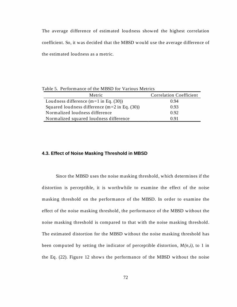
72
The average difference of estimated loudness showed the highest correlation
coefficient. So, it was decided that the MBSD would use the average difference of
the estimated loudness as a metric.
Table 5. Performance of the MBSD for Various MetricsMetric Correlation Coefficient
Loudness difference (m=1 in Eq. (30)) 0.94Squared loudness difference (m=2 in Eq. (30)) 0.93Normalized loudness difference 0.92Normalized squared loudness difference 0.91
4.3. Effect of Noise Masking Threshold in MBSD
Since the MBSD uses the noise masking threshold, which determines if the
distortion is perceptible, it is worthwhile to examine the effect of the noise
masking threshold on the performance of the MBSD. In order to examine the
effect of the noise masking threshold, the performance of the MBSD without the
noise masking threshold is compared to that with the noise masking threshold.
The estimated distortion for the MBSD without the noise masking threshold has
been computed by setting the indicator of perceptible distortion, M(n,i), to 1 in
the Eq. (22). Figure 12 shows the performance of the MBSD without the noise

73
masking threshold. According to Figure 12, the MBSD without the noise masking
threshold overestimates some distortions because it simply uses the loudness
difference without considering perceptual distortion. Figure 13 shows the
performance of the MBSD with the noise masking threshold using the same
speech data set as used for Figure 12. It shows clearly that the overestimated
distortion has been decreased and the MBSD with the noise masking threshold
gives a higher correlation with subjective quality measure. Therefore, the noise
masking threshold plays an important role in estimating perceptually relevant
distortion of objective speech quality measure.
Figure 12. MBSD Versus MOS Difference (Without Noise Masking Threshold [Yang and Yantorno, 1998]).
0
10
20
30
40
50
60
0 0.5 1 1.5 2 2.5 3
MOS Difference
Dis
tort
ion

74
Figure 13. MBSD Versus MOS Difference (With Noise Masking Threshold [Yang and Yantorno, 1998]).
4.4. Performance of MBSD With Coding Distortions
The performance of the MBSD has been examined with different frame
sizes and speech classes. Although the BSD showed the better performance by
processing voiced regions of a speech utterance, it may not be justifiable to
exclude some portions of speech segments. Therefore, it is worthwhile to
investigate the performance of the MBSD with different frame sizes and speech
classes. Table 6 summarizes the performance of the MBSD with different frame
sizes and speech classes. The frame size was varied from 40 samples
(corresponding to 5 ms) to 400 samples (corresponding to 50 ms). The speech
0
5
10
15
20
25
30
35
40
0 0.5 1 1.5 2 2.5 3
MOS Difference
Dis
tort
ion

75
signal was classified by hand-labeling: silence, voiced, unvoiced, and transitional
regions of speech.
Table 6. Correlation Coefficients of the MBSD with Different Frame Sizes and Speech Classes
FRAME SIZE (samples)Speech Class40 80 160 240 320 400
Voiced 0.96 0.96 0.96 0.95 0.95 0.95Unvoiced 0.60 0.66 0.69 0.72 0.74 0.75Transitional 0.63 0.73 0.79 0.82 0.71 0.67Non-silence 0.94 0.96 0.96 0.96 0.96 0.95
According to the results, it should be noted that the performance of the MBSD is
not very sensitive to the frame size variation in the range between 40 samples
and 400 samples for speech classes of voiced and non-silence regions. Since the
speech database in these experiments are coding distortions, the performance
with voiced regions is almost same as that of the non-silence regions. However, if
there are distortions such as bit errors or frame erasures occurring in the
unvoiced regions, the MBSD will have a better performance if the non-silence
regions are processed. On the other hand, it would be better to process the MBSD
with larger frame size if the performance is not very sensitive to frame size in
order to reduce computational complexity. So, the MBSD has been programmed
to process non-silence regions with a frame size of 320 samples.

76
CHAPTER 5
IMPROVEMENT OF MBSD
The performance of the MBSD was comparable to the ITU-T
Recommendation P.861 for speech data with coding distortions [Yang et al.,
1998] [Yang and Yantorno, 1998]. The noise masking threshold calculation is
based on psychoacoustic experiments using steady-state signals such as single
tones and narrow band noise rather than speech signals. It may not be
appropriate to use the noise masking threshold based on psychoacoustic
experiments for speech signals which are nonstationary, therefore, the
performance of the MBSD has been studied by scaling the noise masking
threshold.
Speech coding is only one area where distortions of the speech signal can
occur. There are presently other situations where distortions of the speech signal
can take place, e.g., cellular phone systems, and in this environment there can be
more than one type of distortion. Also, there are other distortions encountered in
real network applications, such as codec tandeming, bit errors, frame erasures,
and variable delays. Recently, the performance of the MBSD has been examined
with TDMA speech data generated by AT&T, in the following ways: use of the
first 15 loudness components in the calculation of distortion; development of a
new cognition model based on postmasking effects; normalization of loudness

77
vectors; and deletion of the spreading function in noise masking threshold
calculation.
5.1. Scaling Noise Masking Threshold
The MBSD measure estimates perceptible distortion in the loudness
domain, taking into account the noise masking threshold used in the transform
coding of audio signals [Johnston, 1988]. Since the noise masking threshold
plays an important role in the calculation of perceptible distortion of the MBSD,
it is worthwhile to examine if the noise masking threshold is valid. Precisely
speaking, the use of the psychoacoustically derived noise masking threshold has
not been validated for speech. The psychoacoustic results are based on steady-
state signals such as sinusoids, rather than speech signals which contain a series
of tones. Consequently, the noise masking threshold taken directly from the
psychoacoustics literature may not be appropriate for estimating perceptible
distortion in speech signals. As a first step in understanding the importance of
the role of the noise masking threshold in the objective speech quality measures,
the performance of the MBSD has been examined by scaling the noise masking
threshold.

78
In the calculation of the MBSD value, the indicator of the i-th perceptible
distortion of the n-th frame (M(n,i)) is determined by comparing the i-th loudness
difference of the n-th frame (Dxy(n,i)) to the i-th noise masking threshold of the n-
th frame (NMT(n,i)). Instead of using the indicator of perceptible distortion as
outlined in Eq. (21), a scaling factor (β) was applied to the noise masking
threshold as follows:
M(n,i) = 0, if Dxy(n,i) ≤ βNMT(n,i) (31.1)
M(n,i) = 1, if Dxy(n,i) > βNMT(n,i) (31.2)
Figure 14. Performance of the MBSD for Speech Data With Coding Distortions Versus the Scaling Factor of the Noise Masking Threshold.
0.84
0.86
0.88
0.9
0.92
0.94
0.96
0.98
1
0 0.2 0.4 0.6 0.8 1
Scaling Factor
Co
rrel
atio
n C
oef
fici
ent
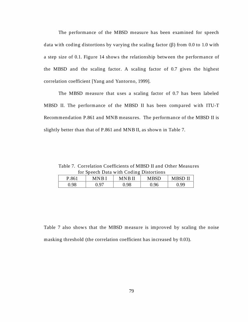
79
The performance of the MBSD measure has been examined for speech
data with coding distortions by varying the scaling factor (β) from 0.0 to 1.0 with
a step size of 0.1. Figure 14 shows the relationship between the performance of
the MBSD and the scaling factor. A scaling factor of 0.7 gives the highest
correlation coefficient [Yang and Yantorno, 1999].
The MBSD measure that uses a scaling factor of 0.7 has been labeled
MBSD II. The performance of the MBSD II has been compared with ITU-T
Recommendation P.861 and MNB measures. The performance of the MBSD II is
slightly better than that of P.861 and MNB II, as shown in Table 7.
Table 7. Correlation Coefficients of MBSD II and Other Measures for Speech Data with Coding Distortions
P.861 MNB I MNB II MBSD MBSD II0.98 0.97 0.98 0.96 0.99
Table 7 also shows that the MBSD measure is improved by scaling the noise
masking threshold (the correlation coefficient has increased by 0.03).

80
5.2. Using the First 15 Loudness Vector Components
Although the MBSD has been improved by scaling the noise masking
threshold for the speech data with various coding distortions [Yang and
Yantorno, 1999], it has not been tested with other distortions. When the
performance of the MBSD was examined with TDMA data generated by AT&T,
the MBSD showed a correlation coefficient of 0.76, which was unsatisfactory.
This result has motivated to improve the MBSD by performing the following
experiments.
The following experiments described were performed using TDMA data.
This data was collected in real network environments, and gave valuable insights
to improve the MBSD. Some of the basic aspects of the MBSD algorithm have
been tested to determine if they are perceptually important or relevant for the
TDMA data, as well as to ensure that any changes had no adverse affects on the
MBSD with respect to speech coding distortions.
As described in Chapter 4, the MBSD algorithm did not use the first 3
components of loudness vectors in the calculation of a distortion value, because
these components were assumed to be filtered out in wired telephone networks.
Since the perceptual importance of these three loudness components has not
been tested, the performance of the MBSD is examined with the first 15 loudness
components.

81
(a) (b)
(c) (d)
Figure 15. Performance of the MBSD With the First 15 Loudness Components;(a) Performance of the Original MBSD for TDMA Data, (b)Performance of the MBSD With the First 15 Loudness Components forTDMA Data, (c) Performance of the Original MBSD for Speech CodingDistortions, (d) Performance of the MBSD With the First 15 LoudnessComponents for Speech Coding Distortions.
r = 0.76
1
1.5
2
2.5
3
3.5
4
4.5
5
1 1.5 2 2.5 3 3.5 4 4.5 5
MOS
Tra
nsf
orm
ed M
OS
Est
imat
e
r = 0.79
1
1.5
2
2.5
3
3.5
4
4.5
5
1 1.5 2 2.5 3 3.5 4 4.5 5
MOS
Tra
nsf
orm
ed M
OS
Est
imat
e
r = 0.95
1
1.5
2
2.5
3
3.5
4
4.5
5
1 1.5 2 2.5 3 3.5 4 4.5 5
MOS
Tra
nsf
orm
ed M
OS
Est
imat
e
r = 0.97
1
1.5
2
2.5
3
3.5
4
4.5
5
1 1.5 2 2.5 3 3.5 4 4.5 5
MOS
Tra
nsf
orm
ed M
OS
Est
imat
e

82
As shown in Figure 15 (a) and (b), the MBSD with the first 15 loudness
components showed better correlation than the original MBSD, with an increase
in the correlation coefficient of 0.03.
The performance of the MBSD with the first 15 loudness components has
also been examined with speech coding distortions. The MBSD with the first 15
loudness components has shown better correlation with the subjective scores for
speech coding distortions, as well. Therefore, these results indicate that it is more
appropriate to include the first 15 loudness components in the calculation of
perceptible distortion. Eq. (22) in the MBSD algorithm is changed as follows
∑=
=K
ixy inDinMnMBSD
1
),(),()( (32)
where M(n,i) and Dxy(n,i) denote the indicator of perceptible distortion and the
loudness difference in the i-th critical band for the n-th frame, respectively.
MBSD(n) is the perceptual distortion of the i-th frame. K is the number of critical
band used in the MBSD measure, and is set to 15.

83
5.3. Normalizing Loudness Vectors
When the MBSD is used to calculate the loudness difference for a frame,
the loudness difference between the distorted and original speech has been
obtained without normalizing these loudness vectors. Without normalization of
the two loudness vectors, the difference could contain perceptually irrelevant
portions. Therefore, the performance of the MBSD is examined using
normalization of these loudness vectors. For normalization, the ratio of the total
loudness of the original speech frame to the total loudness of the distorted
speech frame is used as
( ))()(
)(
)(
1
1 iLjL
jL
iL yK
jy
K
jx
y
∑
∑
=
== for i = 1, . . , K (33)
where Lx(j) and Ly(j) are the j-th component of the loudness vector of original
speech and distorted speech, respectively. )(iLy is the i-th component of the
normalized loudness vector of the distorted speech. K is set to 15.
The correlation coefficient of the MBSD with normalization was increased
by 0.01. The MBSD with normalization performed slightly better than the MBSD
without normalization of loudness vectors.

84
5.4. Deletion of the Spreading Function in the Calculation of the Noise
Masking Threshold
When the noise masking threshold is calculated, the spreading function is
applied to estimate the effects of masking across critical bands [Johnston, 1988].
The derivation of this spreading function is based on psychoacoustic
experiments using steady-state signals such as sinusoids rather than speech
signals. Therefore, it could be worthwhile to perform some experiments with the
MBSD in which the noise masking threshold is calculated without the spreading
function. The correlation coefficient of the modified MBSD without the spreading
function increased by 0.02. Although the improvement was not significant, the
spreading function appeared to give adverse affects on the performance of the
MBSD.
Although the effects of masking across critical bands play an important
role for transform coding of audio signals, these masking effects appear to have
adverse affects for the MBSD measure to predict the subjective ratings.

85
5.5. A New Cognition Model Based on Postmasking Effects
The MBSD uses a simple cognition model to calculate the distortion value.
The distortion value for an entire test speech utterance was obtained by
averaging over all non-silence frames. This simple cognition model is based on
two assumptions: (1) non-silence segments represent speech quality of an entire
test speech utterance; in other words, there is no distortion in silence segments or
the distortion of silence segments is perceptually the same as that of non-silence
segments, and (2) the variance of distortion values in an entire test speech
utterance is small enough to be well represented by its mean. The first
assumption is often invalid when background noise is added to the reference
speech utterance. Most importantly, the second assumption is not valid for
distortions such as bit errors or frame erasures encountered in real network
environments, where the distortion values are not evenly distributed and more
likely to be bursty.
Although the average distortion values of two speech utterances would be
the same, human listeners will perceive their speech quality differently
depending upon the temporal distribution of the distortion values. As an
extreme example, shown in Figure 16, case (A) and (B) have the same average
distortion value. However, the temporal distributions of their distortion values
are very different. The distortion values of case (A) are evenly distributed, but

86
case (B) has one large distortion among small distortion values. Human listeners
would perceive that case (B) has much more degradation than case (A).
Figure 16. Two Different Temporal Distortion Distributions With the Same Average Distortion Value; (A) Even Distribution, (B) Bursty Distribution.
For a better cognition model, two psychoacoustic results [Zwicker and
Fastl, 1990] have been incorporated: (1) the hearing system integrates the sound
intensity over a period of 200 ms, and (2) premasking is relatively short, while
postmasking can last longer than premasking. According to these psychoacoustic
results, it may not be appropriate to directly use the distortion value obtained
0
2
4
6
8
10
12
1 2 3 4 5 6 7 8 9 10
Frame(A)
Dis
tort
ion
0
2
4
6
8
10
12
1 2 3 4 5 6 7 8 9 10
Frame(B)
Dis
tort
ion

87
using 40 ms frames. So, a new cognition model is developed incorporating these
psychoacoustic results.
Several terms are defined for a new cognition model. A cognizable
segment is defined as a set of consecutive frames corresponding to
approximately 200 ms. A cognizable unit (v) is defined as the number of frames
in a cognizable segment. Perceptual distortion (P(j)) is defined as a maximum
distortion value over a cognizable segment. Postmasking distortion (Q(j)) is
defined as the amount of the previous cognizable distortion masking the current
perceptual distortion. Cognizable distortion (C(j)) is defined as the largest value
between the current perceptual distortion and the postmasking distortion. Then,
the final distortion value of test speech utterance is the average over the
cognizable distortions. The cognizable distortion as measured by using
postmasking is assumed to contribute to listeners’ response on speech quality
even when there is no distortion at the current perceptual distortion.
The following equations formally define the final distortion value,
EMBSD.
∑=
=U
j
jCU
EMBSD1
)(1
(34)
( ))(),(max)( jQjPjC = (35)

88
( ) ( )( )
+−
+−+−=
vjvMBSD
jvMBSDjvMBSDjP
)1(...,
,2)1(,1)1(max)( (36)
where C(j), P(j), and Q(j) are the cognizable distortion, the perceptual distortion,
and the postmasking distortion of the j-th cognizable segment, respectively. U is
the total number of cognizable segments and v is the cognizable unit. MBSD(i) is
the same as defined in Eq. (32).
As an initial attempt to model the postmasking effect for the calculation of
postmasking distortion, λ% of the previous cognizable distortion is assumed to
contribute postmasking effect on the current cognizable segment. Let us call λ the
postmasking factor. So, the postmasking distortion (Q(j)) of the j-th cognizable
segment is defined as
)1(100
)( −= jCjQλ
(37)
In order to adopt the new cognition model, the cognizable unit (v) and the
postmasking factor (λ) must be determined. Using TDMA data, the best values of
these two parameters were searched as follows. First, the cognizable unit was
varied from 1 to 20 frames for a fixed postmasking factor of 80.

89
Figure 17. Performance of the MBSD With a new Cognition Model as a Function of Cognizable Unit for the Postmasking Factor of 80.
Figure 18. Performance of the MBSD With a new Cognition Model as a Function of Postmasking Factor for the Cognizable Unit of 10 Frames.
0.86
0.865
0.87
0.875
0.88
0.885
0 5 10 15 20
Frame
Co
rrel
atio
n c
oef
fici
ent
0.855
0.86
0.865
0.87
0.875
0.88
0.885
0 10 20 30 40 50 60 70 80 90 100
Postmasking Factor
Co
rrel
atio
n c
oef
fici
ent

90
As shown in Figure 17, the best result occurs at the cognizable unit of 10
frames. Since the measure used the frame length of 320 samples (corresponding
to 40ms) with 50% overlap, the cognizable unit of 10 frames approximately
corresponds to 200 ms, which is consistent with the psychoacoustic result that
the hearing system integrates the sound intensity over a period of 200 ms
[Zwicker and Fastl, 1990].
In order to determine the postmasking factor, similar experiments were
performed. The postmasking factor was varied from 0 to 100 for the cognizable
unit of 10 frames. As shown in Figure 18, the best result occurs at the
postmasking factor of 80.
According to the results of these experiments, a new cognition model with
a cognizable unit of 10 frames and a postmasking factor of 80 has been adopted
to improve the MBSD.

91
CHAPTER 6
ENHANCED MODIFIED BARK SPECTRAL DISTORTION (EMBSD)
The EMBSD is an enhancement of the MBSD measure in which some
procedures of the MBSD have been modified and a new cognition model has
been used. Some of the basic aspects of the MBSD algorithm have been examined
using TDMA data, as described in Chapter 5. The MBSD was modified using
information obtained from the experiments with TDMA data, the result is the
EMBSD. These modifications are summarized as follows:
(1) using only the first 15 loudness components to calculate loudness difference,
as shown in Eq. (32),
(2) normalizing loudness vectors before calculating loudness difference, as
shown in Eq. (33),
(3) deleting the spreading function in the calculation of noise masking threshold,
(4) adopting a new cognition model based on postmasking effects, as described
in Section 5.5.
The block diagram of the EMBSD measure is shown in Figure 19. The
EMBSD computes the distortion frame-by-frame, with the frame length of 320
samples overlapping by a half frame. Each frame is weighted by a Hanning
window. Here, x(n) and y(n) denote the n-th frame of the original and distorted

92
speech, respectively. Lx(n) and Ly(n) are the normalized loudness vectors of the n-
th frame of the original and distorted speech, respectively. Dxy(n) is the loudness
difference between Lx(n) and Ly(n), and NMT(n) is the noise masking threshold
calculated from the original speech without the spreading function. The new
cognitive model uses the distortion value of the n-th frame, MBSD(n) to calculate
the estimated distortion.
Figure 19. Block Diagram of the EMBSD Measure.
DistortedSpeech
OriginalSpeech
LoudnessCalculation
LoudnessCalculation
Modified Noise Masking Threshold
Computation
LoudnessComparison
Computationof Perceptual
Distortion
x(n)y(n)
Ly(n) Lx(n)
x(n)
Dxy(n)
NMT(n)
MBSD(n)
Normalization
CognitionModel
EstimatedDistortion

93
The loudness calculation of a frame is the same as that of the MBSD, as
described in Section 5.1. The loudness vector of distorted speech is normalized
before computing the loudness difference, as described in Eq. (32). The noise
masking threshold is computed with original speech without the spreading
function. The perceptual distortion is computed using the first 15 loudness
components where the loudness difference is greater than the noise masking
threshold. Finally, a new cognitive model is used to calculate the estimated
distortion of the distorted speech. The actual EMBSD program written in C code
is given in Appendix B.

94
CHAPTER 7
PERFORMANCE OF THE EMBSD MEASURE
The performance of the EMBSD measure has been evaluated with three
different sets of speech data, and compared with the MBSD, ITU-T
Recommendation P.861, and the MNB measures.
The first speech data set (Speech Data I) was generated by Lucent
Technologies. The distortion conditions in this speech data were coding
distortions. There were five Modulated Noise Reference Unit (MNRU) conditions
and nine different types of speech codecs such as ADPCM, GSM, IS-54, FS-1016,
LD-CELP, CELP, and so on. MNRU is the condition of Gaussian noise where the
power levels of noise is varied according to the power levels of the speech signal
to keep a constant SNR over the entire speech utterance.
The second speech data set (Speech Data II) was generated by AT&T. The
data was collected from real network environments. All data were recorded over
in-service TDMA and AMPS RF links in 1994 in a mobile environment. There
were forty-nine different types of distortions encountered in real network
environments with seven MNRU conditions.
The third speech data set (Speech Data III) was generated by Nortel
Networks. This speech data contains a relatively wide range of distortion
conditions such as MNRUs, various codecs, various tandeming cases, temporal

95
shifting and clipping, bit errors, frame erasures, and amplitude variations
[Thorpe and Yang, 1999]. Some distortion conditions, such as temporal shifting
and clipping, and amplitude variations, are not usually used for the evaluation of
objective quality measures. This speech data has subjective ratings of both MOS
and DMOS.
The performance of the objective quality measures has been evaluated
using both the correlation coefficient (r) and the standard error of the estimates
(SEE) (as discussed in section 3.2 and 3.3).
7.1. Performance of the EMBSD with Speech Data I
Figure 20 shows the scatterplots of P.861, MNB2, the MBSD, and the
EMBSD with Speech Data I. Each point indicates the results of the average of the
various objective quality estimates and the associated MOS for each condition.
Because objective quality measures generate a distortion number, the smaller the
result of objective measures, the higher the MOS score. As shown in Figure 20,
the range of the distortion values of the various objective quality measures is
different and some objective estimates are not linearly related to the MOS scores.
Therefore, the results of the objective quality measures were transformed to have

96
a linear relation with the MOS scores using the regression curve. Figure 21 shows
the scatterplots of the transformed objective estimates against the MOS scores.
(a) (b)
(a) (b)
(c) (d)
Figure 20. Objective Measures of P.861, MNB2, MBSD, and EMBSD Versus MOS Scores for Speech Data I.
0
5
10
15
20
25
1 1.5 2 2.5 3 3.5 4 4.5 5
MOS
MB
SD
0
1
2
3
4
5
6
7
8
1 1.5 2 2.5 3 3.5 4 4.5 5
MOS
P.8
61
0
1
2
3
4
5
6
1 1.5 2 2.5 3 3.5 4 4.5 5
MOS
MN
B2
0
1
2
3
4
5
6
7
8
1 1.5 2 2.5 3 3.5 4 4.5 5
MOS
EM
BS
D

97
(a) (b)
(c) (d)
Figure 21. Transformed Objective Estimates of P.861, MNB2, MBSD, and EMBSD Versus MOS Scores for Speech Data I.
1
1.5
2
2.5
3
3.5
4
4.5
5
1 1.5 2 2.5 3 3.5 4 4.5 5
MOS
Tra
nsf
orm
ed M
BS
D
1
1.5
2
2.5
3
3.5
4
4.5
5
1 1.5 2 2.5 3 3.5 4 4.5 5
MOS
Tra
nsf
orm
ed P
.861
1
1.5
2
2.5
3
3.5
4
4.5
5
1 1.5 2 2.5 3 3.5 4 4.5 5
MOS
Tra
nsf
orm
ed M
NB
2
1
1.5
2
2.5
3
3.5
4
4.5
5
1 1.5 2 2.5 3 3.5 4 4.5 5
MOS
Tra
nsf
orm
ed E
MB
SD

98
(a) (b)
(c) (d)
Figure 22. Transformed Objective Estimates of P.861, MNB2, MBSD, and EMBSD Versus MOS Difference for Speech Data I.
0
0.5
1
1.5
2
2.5
3
0 0.5 1 1.5 2 2.5 3
MOS Difference
Tra
nsf
orm
ed M
BS
D
0
0.5
1
1.5
2
2.5
3
0 0.5 1 1.5 2 2.5 3
MOS Difference
Tra
nsf
orm
ed P
.861
0
0.5
1
1.5
2
2.5
3
0 0.5 1 1.5 2 2.5 3
MOS Difference
Tra
nsf
orm
ed M
NB
2
0
0.5
1
1.5
2
2.5
3
0 0.5 1 1.5 2 2.5 3
MOS Difference
Tra
nsf
orm
ed E
MB
SD

99
Since current objective quality measures estimate the speech quality by
comparing the distorted speech to the original speech, which is similar to DMOS
test, the performance parameters of these measures were also calculated against
the MOS difference (MOS of original speech – MOS of distorted speech) [Yang et
al., 1998], because the DMOS scores were not available. Figure 22 shows the
scatterplots of the transformed objective estimates against the MOS difference.
The performance parameters of the objective quality measures against
subjective ratings for both the MOS scores and the MOS difference were
calculated using the transformed objective estimates. Table 8 summarizes these
results.
Table 8. Correlation Coefficients and SEE of Objective Quality Measures With Speech Data I
Correlation Coefficient SEEMOS MOS
DifferenceMOS MOS
DifferenceMBSD 0.95 0.96 0.22 0.21P.861 0.98 0.98 0.14 0.14
MNB2 0.98 0.98 0.13 0.13EMBSD 0.98 0.98 0.15 0.15
The correlation coefficients for P.861, MNB2, and EMBSD were the same. These
measures account for approximately 96% of the variance in the subjective ratings.

100
The SEE values were slightly different, but their small differences are not
statistically significant. The EMBSD showed some improvement over the MBSD
with Speech Data I and the performance of the EMBSD is comparable to those of
P.861 and MNB2 for Speech Data I.
7.2. Performance of the EMBSD with Speech Data II
Figure 23 shows the scatterplots of the MBSD, EMBSD, and P.861 with
Speech Data II. As with Speech Data I, the results of the objective quality
measures were transformed to have a linear relation with the MOS scores using
the regression curve. Figure 24 shows the scatterplots of the transformed
objective estimates against the MOS scores. Inspection of the scatterplots shows
that correlations of the objective quality measures with Speech Data II are lower
than those with Speech Data I. Also, it is clear that the EMBSD showed better
correlation than the MBSD. Since the DMOS scores were not available for Speech
Data II, the analysis against the DMOS scores was not performed. The analysis
against the MOS difference could not be performed because the MOS scores of
the original speech samples were not available for Speech Data II.

101
(a) (b)
(c) (d)
Figure 23. Objective Measures of P.861, MNB2, MBSD, and EMBSD Versus MOS scores for Speech Data II.
0
1
2
3
4
5
6
7
8
9
1 1.5 2 2.5 3 3.5 4 4.5 5
MOS
P.8
61
0
1
2
3
4
5
6
7
8
9
10
1 1.5 2 2.5 3 3.5 4 4.5 5
MOS
EM
BS
D
0
5
10
15
20
25
30
1 1.5 2 2.5 3 3.5 4 4.5 5
MOS
MB
SD
0
1
2
3
4
5
6
7
1 1.5 2 2.5 3 3.5 4 4.5 5
MOS
MN
B2

102
(a) (b)
(c) (d)
Figure 24. Transformed Objective Estimates of P.861, MNB2, MBSD, and EMBSD Versus MOS Scores for Speech Data II.
1
1.5
2
2.5
3
3.5
4
4.5
5
1 1.5 2 2.5 3 3.5 4 4.5 5
MOS
Tra
nsf
orm
ed M
BS
D
1
1.5
2
2.5
3
3.5
4
4.5
5
1 1.5 2 2.5 3 3.5 4 4.5 5
MOS
Tra
nsf
orm
ed E
MB
SD
1
1.5
2
2.5
3
3.5
4
4.5
5
1 1.5 2 2.5 3 3.5 4 4.5 5
MOS
Tra
nsf
orm
ed P
.861
1
1.5
2
2.5
3
3.5
4
4.5
5
1 1.5 2 2.5 3 3.5 4 4.5 5
MOS
Tra
nsf
orm
ed M
NB
2

103
The performance parameters of the objective quality measures against
subjective ratings of the MOS scores were calculated using the transformed
objective estimates. Table 9 summarizes these results.
Table 9. Correlation Coefficients and SEE of Objective Quality Measures Versus MOS With Speech Data II
Correlation Coefficient SEEP.861 0.83 0.51
MNB2 0.74 0.67MBSD 0.76 0.61
EMBSD 0.87 0.41
The correlation results of each objective quality measure for Speech Data II were
much lower than those for Speech Data I. This result reflects the fact that the
performance of these measures depends on the type of distortion. The
performance of the EMBSD shows clear improvement over the MBSD for Speech
Data II. The correlation coefficient of the EMBSD is nominally higher than that of
P.861. The EMBSD value accounts for around 76% of the variance in the
subjective MOS scores. The P.861 value accounts for about 69% of the variance in
the subjective MOS scores. The SEE value of the EMBSD is smaller than that of
P.861 by around 0.1. Speech Data II was one of the most challenging data sets for
objective quality measures. Since Speech Data II were recorded in real network

104
environments, the performance of objective quality measures for Speech Data II
can be considered as the accuracy of these measures when they are actually
applied in the real network applications. Although the performance of the
EMBSD was not still satisfactory for real network applications, it certainly
showed promising results for Speech Data II.
7.3. Performance of the EMBSD Measure with Speech Data III
The distortion conditions of Speech Data III can be classified into seven
groups: MNRUs (Group 1), coders on clean channel (Group 2), tandem cases
(Group 3), temporal shifting and front-end clipping (Group 4), bit errors (Group
5), frame erasures (Group 6), and level variations (Group 7).
Group 1 includes MNRU conditions with a range of 5 dB to 35 dB. In
Group 2, various coding distortions are included. Speech compression codecs
were chosen based on contrasting algorithms, and covering a wide range of bit
rates. The bit rates of these codecs range from 2.4 Kb/s to 64 Kb/s. Group 3
covers some plausible tandeming cases that might be encountered in GSM,
TDMA, and CDMA networks. In tandeming cases, several codecs are processed
in series. Group 4 contains temporal shifting (which may occur due to variable
jitter buffers in voice-over-IP networks) and front-end clipping (which may occur

105
where voice activated switching or discontinuous transmission features are
used). In Group 5, codecs of GSM and TDMA networks are subjected to bit error
rates of 1, 2, or 3%. Group 6 contains frame erasures at similar rates (1, 2, or 3%)
for codecs in wireless networks as well as voice over IP. These conditions are
included to determine the performance of objective measures on the channel
impairments of different types of networks. In Group 7, speech levels were
varied in the original material, which was then processed through an automatic
gain control (AGC). Some conditions in Group 7 also have front-end clipping.
The test condition groups can be divided into two types: (1) target
conditions distortions usually intended to be evaluated using objective quality
measures (Group 1, 2, 3, 5, and 6), and (2) non-target conditions distortions
not usually intended to be evaluated using these measures (Group 4 and 7). The
condition groups were broken up into these two types because some of the test
conditions (the non-target conditions) are outside the set of distortions that
objective measures are generally intended to address. These conditions were
included to investigate the generalizability of the measures to common network
impairments and artifacts. The performance of the measures examined is
evaluated against all the conditions, as well as against each type (target and non-
target) separately.
Table 10 summarizes the correlation coefficients of various objective
quality measures against overall conditions, as well as against target conditions

106
[Thorpe and Yang, 1999]. The correlation coefficients between the objective
estimates and the subjective scores were calculated after transforming the
objective estimates with the regression curve obtained from the scatterplot of
target conditions. The name of each measure has not been released because of the
project agreement. These objective quality measures appeared to correlate better
with DMOS than with MOS. This result may follow from the procedural
difference between current objective speech quality measures and MOS test.
Table 10. Correlation Coefficients of Various Objective Quality Measures With Speech Data III [Thorpe and Yang, 1999]
Overall Conditions (60) Target conditions (49)MeasureMOS DMOS MOS DMOS
A 0.87 0.97 0.88 0.95B 0.85 0.96 0.86 0.94C 0.56 0.65 0.89 0.94D 0.86 0.92 0.83 0.87E 0.90 0.95 0.87 0.96F 0.86 0.94 0.84 0.91
MBSD 0.24 0.29 0.76 0.82EMBSD 0.54 0.65 0.89 0.94
The analysis results show that the EMBSD estimates are well correlated
with subjective DMOS ratings for the target conditions, but appear to have poor
correlation for the overall case. The EMBSD value of the target conditions

107
accounts for about 79% (for MOS) and 88% (for DMOS) of the variance in the
subjective ratings. Correlations for the overall case were much lower and the
EMBSD was able to predict only about 30~40% of the variation in the actual
listener ratings.
Figure 25 shows the scatterplots of the transformed EMBSD against MOS
and DMOS. Inspection of the scatterplots shows that the poor performance in the
overall case is accounted for by the non-target conditions. The MOS estimates of
the temporal shifting and clipping conditions (Group 4) were widely spread,
while being rated high by the listeners. Since the EMBSD assumes that the
distorted speech is synchronized with the original speech, the EMBSD estimates
of Group 4 are meaningless because the measure has compared the wrong
frames to estimate speech quality.
Also, the AGC conditions (Group 7) were given high MOS estimates,
while being rated lower by the listeners. Most objective quality measures showed
results similar to that for Group 7. This result is caused by the underlying
assumption of current objective speech quality measures, that is, the quality of
input speech is always excellent. In order to improve performance of objective
quality measures for such conditions, a new model would be necessary. If only
the target conditions are considered, then the EMBSD is an effective objective
quality measure.

108
Figure 25. Transformed Objective Estimates of EMBSD Versus MOS and DMOS for Speech Data III.
The results of Table 10 clearly show that current objective quality
measures are actually performing better at predicting the DMOS scores rather
than the MOS scores because all of the measures showed better correlation with
DMOS than with MOS. This is not a surprising result because current objective
quality measures estimate subjective scores by comparing the distorted speech to
the original speech, which is analogous to DMOS test.
Table 11 shows the SEE values for overall, target, and non-target
conditions. The number in the parenthesis indicates the number of conditions.
Note that the SEE value indicates how much the estimates values deviate from
1
1.5
2
2.5
3
3.5
4
4.5
5
1 1.5 2 2.5 3 3.5 4 4.5 5
MOS
Tra
nsf
orm
ed M
OS
Est
imat
e
Target Non-target
1
1.5
2
2.5
3
3.5
4
4.5
5
1 1.5 2 2.5 3 3.5 4 4.5 5
DMOS
Tra
nsf
orm
ed D
MO
S E
stim
ate
Target Non-target

109
the actual values. So, the smaller the SEE, the better the performance of the
objective quality measure. The SEE measure shows a similar tendency in
performance as shown for correlation coefficients. Note that the SEE values of the
EMBSD for the non-target cases are high (the corresponding result for the
correlation analysis is not available because of the small number of data points).
This result indicates that the EMBSD is not yet prepared for the non-target
conditions. However, the EMBSD presently is one of the best predictors of
subjective ratings for the target conditions in Speech Data III among the
measures evaluated. Also, the EMBSD shows better performance for both target
and non-target conditions than the MBSD.
Table 11. Standard Error of the Estimates of Various Objective Quality Measures With Speech Data III [Thorpe and Yang, 1999]
Overall (60) Target (49) Non-target (11)MeasureMOS DMOS MOS DMOS MOS DMOS
A 0.44 0.26 0.36 0.27 0.76 0.23B 0.50 0.29 0.41 0.29 0.87 0.33C 0.74 0.81 0.32 0.28 1.72 1.97D 0.48 0.46 0.43 0.46 0.73 0.49E 0.43 0.30 0.36 0.24 0.70 0.53F 0.43 0.31 0.41 0.35 0.56 0.09
MBSD 1.03 1.19 0.48 0.49 2.36 2.80EMBSD 0.78 0.85 0.32 0.31 1.83 2.04

110
Table 12 shows the SEE for three target condition groups (Group 1, 2, and
3). The EMBSD measure showed better performance for Group 1 and 3 against
both MOS and DMOS among these measures. The prediction errors of the
EMBSD for Group 2 were large compared to the results with other condition
groups.
Table 12. Standard Error of the Estimates of Various Objective Quality Measures for Target Condition Groups (Group 1, 2, and 3) of Speech Data III [Thorpe and Yang, 1999]
Group 1 (7) Group 2 (12) Group 3 (12)MeasureMOS DMOS MOS DMOS MOS DMOS
A 0.44 0.32 0.34 0.27 0.51 0.30B 0.43 0.20 0.43 0.36 0.58 0.37C 0.48 0.28 0.33 0.33 0.38 0.24D 0.44 0.45 0.57 0.56 0.41 0.47E 0.48 0.25 0.45 0.27 0.43 0.29F 0.37 0.17 0.38 0.31 0.59 0.53
MBSD 0.37 0.46 0.66 0.77 0.62 0.47EMBSD 0.27 0.29 0.43 0.45 0.36 0.24
Table 13 shows the SEE for other target condition groups (Groups 5 and
6). The EMBSD measure showed relatively small prediction errors for Groups 5
and 6 against both MOS and DMOS as compared to all the other measures.
According to Table 12 and Table 13, the EMBSD measure showed relatively

111
promising results over other measures for the target conditions except probably
Group 2.
Table 13. Standard Error of the Estimates of Various Objective Quality Measures for Target Condition Groups (Group 5 and 6) of Speech Data III [Thorpe and Yang, 1999]
Group 5 (5) Group 6 (13)MeasureMOS DMOS MOS DMOS
A 0.30 0.33 0.31 0.29B 0.35 0.34 0.33 0.26C 0.37 0.49 0.29 0.26D 0.60 0.76 0.41 0.42E 0.27 0.27 0.28 0.25F 0.41 0.38 0.40 0.35
MBSD 0.26 0.27 0.39 0.41EMBSD 0.25 0.34 0.31 0.32
Table 14 shows the SEE for the non-target condition groups (Groups 4 and
7). The SEE values of the EMBSD for Group 4 were much higher against both
MOS and DMOS because the EMBSD did not take time alignments between the
sentences into account. The performance of the EMBSD on Group 4 could be
improved by adopting dynamic time alignment algorithms. Most measures did
not consider the conditions of Group 7, where original speech samples were
distorted. Since there is a possibility that the output speech of a voice processing

112
system sounds better than the input speech, the objective measures must take
into consideration this kind of distortion, in the future.
Table 14. Standard Error of the Estimates of Various Objective Quality Measures for Non-Target Condition Groups (Group 4 and 7) of Speech Data III [Thorpe and Yang, 1999]
Group 4 (8) Group 7 (3)MeasureMOS DMOS MOS DMOS
A 0.32 0.11 2.15 0.62B 0.44 0.22 2.38 0.82C 1.90 2.39 2.25 0.84D 0.56 0.47 1.69 0.94E 0.80 0.45 0.76 1.14F 0.18 0.10 1.64 0.14
MBSD 2.89 3.37 0.55 1.51EMBSD 2.16 2.49 1.52 0.63

113
CHAPTER 8
FUTURE RESEARCH
There are several possible areas of research related to the EMBSD
objective speech quality measure.
First, the EMBSD measure regards the loudness difference above the noise
masking threshold as audible distortion, and does not take into consideration the
relative significance of these components. It is well known in the speech coding
community that the spectral peaks (formants) are more important than the
spectral valleys. Therefore, if a perceptually relevant weighting scheme is
applied to the loudness difference for spectral peaks and valleys above the noise
masking threshold, the EMBSD might be further improved.
Second, the EMBSD measure has been developed based on the
assumption that both the distorted and the original speech are time-aligned. In
real applications, it is rare to have both the distorted and the original speech
synchronized. Also, variable delays between the consecutive non-silence
segments are common in current packet networks. For instance, such variable
delays occur due to variable jitter buffers on voice transmission over IP
networks. Without proper time alignment pre-processing, the result of objective
quality measures would be meaningless. Therefore, a reliable and effective time
alignment algorithm should be used as pre-processing.

114
Third, the EMBSD measure showed relatively good performance over
several target conditions according to the experiments with Speech Data III.
Among these target conditions, the EMBSD showed relatively larger prediction
error for Group 2 (codecs), as shown in Figure 26.
Figure 26. Performance of the EMBSD Against MOS for the Target Conditions of Speech Data III.
It could be worthwhile to examine the coding distortion types that the
EMBSD did not perform well. After identifying these coding distortions, the
EMBSD could be further improved by reducing the prediction errors on these
0
0.05
0.1
0.15
0.2
0.250.3
0.35
0.4
0.45
0.5
Group 1 Group 2 Group 3 Group 5 Group 6
Condition Group
SE
E

115
coding distortions while ensuring that any changes will have no adverse affects
on the performance of the EMBSD with other distortions.
Finally, the EMBSD did not consider the distortion conditions where
original speech samples are distorted. Since there is a possibility that the output
speech of a voice processing system sounds better than the input speech, the
EMBSD measure must take into consideration this kind of distortion in the
future.

116
REFERENCES
[Barnwell et al., 1978] T. P. Barnwell III, A. M. Bush, R. M. Mersereau, and R. W.Shafer, “Speech Quality Measurement,” Final Report, RADC-TR-78-122,May 1978.
[Barnwell and Voiers, 1979] T. P. Barnwell III and W. D. Voiers, “An analysis ofobjective measures for user acceptance of voice communication systems,”Final Report, DCA100-78-C-0003, Sep. 1979.
[Beerends and Stemerdink, 1992] J. G. Beerends and J. A. Stemerdink, “Aperceptual audio quality measure based on a psychoacoustic soundrepresentation,” J. Audio Eng. Soc., vol. 40, pp. 963-978, Dec. 1992.
[Beerends and Stemerdink, 1994] J. G. Beerends and J. A. Stemerdink, “Aperceptual speech quality measure based on a psychoacoustic soundrepresentation,” J. Audio Eng. Soc., vol. 42, pp. 115-123, Mar. 1994.
[Beerends, 1997] J. G. Beerends, “Improvement of the P.861 perceptual speechquality measure,” ITU-T SG12 COM-20E, December, 1997.
[Berger, 1997] J. Berger, “TOSQA – Telecommunication objective speech qualityassessment,” ITU-T SG12 COM-34E, December, 1997.
[Bladon, 1981] R. Bladon, “Modeling the judgment of vowel quality differences,”J. Acoust. Soc. Am., vol. 69. pp. 1414-1422, Dec. 1979.
[Crochiere et al., 1980] R. E. Crochiere, J. E. Tribolet, and L. R. Rabiner, “Aninterpretation of the Log Likelihood Ratio as a measure of waveform coderperformance,” IEEE Trans. Acoust., Speech and Signal Processing, vol.ASSP-28, no. 3, Jun. 1980.
[Dimolitsas et al., 1995] S. Dimolitsas, F. L. Corcoran, and C. Ravishankar,“Dependence of opinion scores on listening sets used in degradationcategory rating assessment,” IEEE Trans. on Speech and Audio Processing,vol. 3, no. 5, pp.421-424, Sept. 1995.

117
[Gray and Markel, 1976] A H. Gray and J. D. Markel, “Distance measures forspeech processing,” IEEE Trans. Acoust., Speech and Signal Processing, vol.ASSP-24, pp. 380-391, Oct. 1976.
[Hauenstein, 1998] M. Hauenstein, “Application of Meddis’ inner hair-cell modelto the prediction of subjective speech quality,” Proc. ICASSP, pp. 545-548,1998.
[Hellman, 1972] R. P. Hellman, “Asymmetry of masking between noise andtone,” Perception and Psychophysics, vol. 11, pp. 241-246, 1972.
[Itakura, 1975] F. Itakura, “Minimum prediction residual principle applied tospeech recognition,” IEEE Trans. Acoust., Speech and Signal Processing,vol. ASSP-23, no. 1, pp. 67-72, Feb. 1975.
[ITU-T Recommendation P.800, 1996] Methods for subjective determination oftransmission quality, Geneva, 1996.
[ITU-T Recommendation P.861, 1996] Objective quality measurement oftelephone-band (300-3400 Hz) speech codecs, Geneva, 1996.
[Jayant and Noll, 1984] N. S. Jayant and P. Noll, Digital Coding of Waveforms:Principles and Applications to Speech and Video, Prentice Hall, 1984.
[Jin and Kubicheck, 1996] C. Jin and R. Kubicheck, “Vector QuantizationTechniques for Output-Based Objective Speech Quality,” Proc. 1996ICASSP, pp.491-494, 1996.
[Johnston, 1988] J. Johnston, “Transform coding of audio signals using perceptualnoise criteria,” IEEE J. on Select. Areas in Commun., vol. SAC-6, pp.314-323,1988.
[Juang, 1984] B. H. Juang, “On using the Itakura-Saito measure for speech coderperformance evaluation,” AT&T Bell Laboratories Tech. Jour., vol. 63, no. 8,pp. 1477-1498, Oct. 1984.
[Kitawaki et al., 1982] N. Kitawaki, K. Itoh, and K. Kakei, “Speech quality ofPCM system in digital telephone system,” Electronics and Communicationin Japan, vol. 65-A, no. 8, pp. 1-8, 1982.

118
[Kitawaki et al., 1988] N. Kitawaki, H. Nagabuchi, and K. Itoh, “Objective qualityevaluation for low-bit-rate speech coding systems,” IEEE J. Select. AreasCommun., vol. 6, pp.242-248, Feb. 1988.
[Klatt, 1976] D. H. Klatt, “A digital filter bank for spectral matching,” Proc. 1976IEEE ICASSP, pp. 573-576, Apr. 1976.
[Klatt, 1982] D. H. Klatt, “Prediction of perceived phonetic distance from critical-band spectra: a first step,” Proc. 1982 IEEE ICASSP, Paris, pp. 1278-1281,May 1982.
[Lam et al., 1996] K. Lam, O. Au, C. Chan, K. Hui, and S. Lau, “Objective speechquality measure for cellular phone,” ICASSP, vol. 1, pp. 487-490, 1996.
[Markel and Gray, 1976] J. D. Markel and A. H. Gray, Linear Prediction of Speech,New York: Springer-Verlag, 1976.
[McDermott, 1969] B. J. McDermott, “Multidimensional analysis of circuit qualityjudgment,” J. of Acoustical Society of America, vol. 45, no.3, pp. 774-781,1969.
[McDermott et al., 1978] B. J. McDermott, C. Scaglia, and D. J. Goodman,“Perceptual and objective evaluation of speech processed by adaptivedifferential PCM,” IEEE ICASSP, Tulsa, pp. 581-585, Apr. 1978.
[Meky and Saadawi, 1996] M. M. Meky and T. N. Saadawi, “A perceptually-based objective measure for speech coders using abductive network,”ICASSP, vol. 1, pp. 479-482, 1996.
[Noll, 1974] P. W. Noll, “Adaptive quantization in speech coding systems,” IEEEInternational Zurich Seminar, Oct. 1974.
[Quackenbush et al., 1988] S. R. Quackenbush, T. P. Barnwell III, and M. A.Clements, Objective Measures of Speech Quality, Prentice Hall, EnglewoodCliffs, 1988.
[Robinson and Dadson, 1956] D. Robinson and R. Dadson, “A redetermination ofthe equal-loudness relations for pure tones,” Brit. J. Appl. Physics, vol. 7,pp. 166-181, 1956.

119
[Sen and Holmes, 1994] D. Sen and W. H. Holmes, “Perceptual enhancement ofCELP speech coders,” ICASSP, vol. 2, pp. 105-108, 1994.
[Scharf, 1970] B. Scharf, Foundations of Modern Auditory Theory, New York,Academic, 1970.
[Schroeder et al., 1979] M. R. Schroeder, B. S. Atal, and J. L. Hall, “Optimizingdigital speech coders by exploiting masking properties of the human ear,” J.Acoust. Soc. Am., vol. 66. pp. 1647-1652, Dec. 1979.
[Thorpe and Shelton, 1993] L. A. Thorpe and B. Shelton, “Subjective testmethodology: MOS vs. DMOS in evaluation of speech coding algorithms,”IEEE Speech Coding Workshop, pp.73-74 St. Adele, Quebec, Canada, 1993.
[Thorpe and Yang, 1999] L. Thorpe and W. Yang, “Performance of currentperceptual objective speech quality measures,” submitted to IEEE SpeechCoding Workshop, 1999.
[Tohkura, 1987] Y. Tohkura, “A weighted cepstral distance measure for speechrecognition,” IEEE Trans. Acoust., Speech and Signal Processing, vol. ASSP-35, pp. 1414-1422, Oct. 1987.
[Tribolet et al., 1978] J. M. Tribolet, P. Noll, B. J. McDermott, and R. E. Crochiere,“A study of complexity and quality of speech waveform coders,” IEEEICASSP, Tulsa, pp. 586-590, Apr. 1978.
[Voiers, 1976] W. D. Voiers, “Methods of Predicting User Acceptance of VoiceCommunication Systems,” Final Report, DCA100-74-C-0056, Jul. 1976.
[Voran and Sholl, 1995] S. Voran and C. Sholl, “Perception-based objectiveestimators of speech quality,” IEEE Speech Coding Workshop, pp. 13-14,Annapolis, 1995.
[Voran, 1997] S. Voran, “Estimation of perceived speech quality using measuringnormalizing blocks,” IEEE Speech Coding Workshop, pp. 83-84, PoconoManor 1997.
[Wang et al., 1992] S. Wang, A. Sekey, and A. Gersho, “An objective measure forpredicting subjective quality of speech coders,” IEEE J. Select. AreasCommun., vol. 10, pp. 819-829, June 1992.

120
[Yang et al., 1997] W. Yang, M. Dixon, and R. Yantorno, “A modified barkspectral distortion measure which uses noise masking threshold,” IEEESpeech Coding Workshop, pp. 55-56, Pocono Manor, 1997.
[Yang et al., 1998] W. Yang, M. Benbouchta, and R. Yantorno, “Performance of amodified bark spectral distortion measure as an objective speech qualitymeasure,” IEEE ICASSP, pp.541-544, Seattle, 1998.
[Yang and Yantorno, 1998] W. Yang and R. Yantorno, “Comparison of twoobjective speech quality measures: MBSD and ITU-T recommendationP.861,” IEEE MMSP, pp.426-431, Redondo Beach, 1998.
[Yang and Yantorno, 1999] W. Yang and R. Yantorno, “Improvement of MBSDby scaling noise masking threshold and correlation analysis with MOSdifference instead of MOS,” IEEE ICASSP, pp. 673-676, Phoenix, 1999.
[Zwicker, 1961] E. Zwicker, “Subdivision of the audible frequency range intocritical bands,” J. Acoust. Soc. Amer., vol. 33, no. 4, p. 248. Feb. 1961.
[Zwicker and Fastl, 1990] E. Zwicker and H. Fastl, Psychoacoustics Facts andModels, Springer-Verlag, 1990.

121
BIBLIOGRAPHY
[Barnwell et al., 1978] T. P. Barnwell III, A. M. Bush, R. M. Mersereau, and R. W.Shafer, “Speech Quality Measurement,” Final Report, RADC-TR-78-122,May 1978.
[Barnwell and Voiers, 1979] T. P. Barnwell III and W. D. Voiers, “An analysis ofobjective measures for user acceptance of voice communication systems,”Final Report, DCA100-78-C-0003, Sep. 1979.
[Beerends and Stemerdink, 1992] J. G. Beerends and J. A. Stemerdink, “Aperceptual audio quality measure based on a psychoacoustic soundrepresentation,” J. Audio Eng. Soc., vol. 40, pp. 963-978, Dec. 1992.
[Beerends and Stemerdink, 1994] J. G. Beerends and J. A. Stemerdink, “Aperceptual speech quality measure based on a psychoacoustic soundrepresentation,” J. Audio Eng. Soc., vol. 42, pp. 115-123, Mar. 1994.
[Beerends, 1997] J. G. Beerends, “Improvement of the P.861 perceptual speechquality measure,” ITU-T SG12 COM-20E, December, 1997.
[Berger, 1997] J. Berger, “TOSQA – Telecommunication objective speech qualityassessment,” ITU-T SG12 COM-34E, December, 1997.
[Bladon, 1981] R. Bladon, “Modeling the judgment of vowel quality differences,”J. Acoust. Soc. Am., vol. 69. pp. 1414-1422, Dec. 1979.
[BNR, 1982] Bell Northern Research, “Evaluation of nonlinear distortion via thecoherence function,” Contribution to CCITT, COM-XII-no. 60-E, Apr. 1982.
[Coetzee and Barnwell, 1989] H. J. Coetzee and T. P. Barnwell III, “An LSP basedspeech quality measure,” IEEE ICASSP, pp. 596-599, 1989.
[Crochiere et al., 1980] R. E. Crochiere, J. E. Tribolet, and L. R. Rabiner, “Aninterpretation of the Log Likelihood Ratio as a measure of waveform coderperformance,” IEEE Trans. Acoust., Speech and Signal Processing, vol.ASSP-28, no. 3, Jun. 1980.

122
[Dimolitsas et al., 1995] S. Dimolitsas, F. L. Corcoran, and C. Ravishankar,“Dependence of opinion scores on listening sets used in degradationcategory rating assessment,” IEEE Trans. on Speech and Audio Processing,vol. 3, no. 5, pp.421-424, Sept. 1995.
[Fant, 1973] G. Fant, Speech Sounds and Features, The MIT Press, Cambridge, 1973.
[Gray and Markel, 1976] A H. Gray and J. D. Markel, “Distance measures forspeech processing,” IEEE Trans. Acoust., Speech and Signal Processing, vol.ASSP-24, pp. 380-391, Oct. 1976.
[Hauenstein, 1998] M. Hauenstein, “Application of Meddis’ inner hair-cell modelto the prediction of subjective speech quality,” IEEE ICASSP, pp. 545-548,1998.
[Hecker and Williams, 1966] M. H. L. Hecker and C. E. Williams, “Choice ofreference conditions for speech preference tests,” Journal of AcousticalSociety of America, vol. 39, no. 5, pp. 946-952, Nov. 1966.
[Hellman, 1972] R. P. Hellman, “Asymmetry of masking between noise andtone,” Perception and Psychophysics, vol. 11, pp. 241-246, 1972.
[Hermansky, 1990] H. Hermansky, “Perceptual linear predictive (PLP) analysisof speech,” Journal of Acoustical Society of America, vol. 87, pp. 1738-1752,Apr. 1990.
[Hollier and Rix, 1998] M. Hollier and A. Rix, “Robust design methodology fortelephony assessment models,” ITU-T SG12 D.031, February, 1998.
[Itakura, 1975] F. Itakura, “Minimum prediction residual principle applied tospeech recognition,” IEEE Trans. Acoust., Speech and Signal Processing,vol. ASSP-23, no. 1, pp. 67-72, Feb. 1975.
[ITU-T Recommendation P.800, 1996] Methods for subjective determination oftransmission quality, Geneva, 1996.
[ITU-T Recommendation P.861, 1996] Objective quality measurement oftelephone-band (300-3400 Hz) speech codecs, Geneva, 1996.
[Jayant and Noll, 1984] N. S. Jayant and P. Noll, Digital Coding of Waveforms:Principles and Applications to Speech and Video, Prentice Hall, 1984.
123
[Jin and Kubicheck, 1996] C. Jin and R. Kubicheck, “Vector QuantizationTechniques for Output-Based Objective Speech Quality,” Proc. 1996ICASSP, pp.491-494, 1996.
[Johnston, 1988] J. Johnston, “Transform coding of audio signals using perceptualnoise criteria,” IEEE J. on Select. Areas in Commun., vol. SAC-6, pp.314-323,1988.
[Juang, 1984] B. H. Juang, “On using the Itakura-Saito measure for speech coderperformance evaluation,” AT&T Bell Laboratories Tech. Jour., vol. 63, no. 8,pp. 1477-1498, Oct. 1984.
[Kitawaki et al., 1982] N. Kitawaki, K. Itoh, and K. Kakei, “Speech quality ofPCM system in digital telephone system,” Electronics and Communicationin Japan, vol. 65-A, no. 8, pp. 1-8, 1982.
[Kitawaki et al., 1988] N. Kitawaki, H. Nagabuchi, and K. Itoh, “Objective qualityevaluation for low-bit-rate speech coding systems,” IEEE J. Select. AreasCommun., vol. 6, pp.242-248, Feb. 1988.
[Klatt, 1976] D. H. Klatt, “A digital filter bank for spectral matching,” Proc. 1976IEEE ICASSP, pp. 573-576, Apr. 1976.
[Klatt, 1982] D. H. Klatt, “Prediction of perceived phonetic distance from critical-band spectra: a first step,” Proc. 1982 IEEE ICASSP, Paris, pp. 1278-1281,May 1982.
[Kubin et al., 1993] G. Kubin, B. S. Atal and W. B. Kleijn, “Performance of noiseexcitation for unvoiced speech,” IEEE Speech Coding Workshop, pp. 35-36,1993.
[Lalou, 1990] J. Lalou, “The information index: An objective measure of speechtransmission performance,” Ann. Telelccommun., vol. 45, pp. 47-65, Jan.1990.
[Lam et al., 1996] K. Lam, O. Au, C. Chan, K. Hui, and S. Lau, “Objective speechquality measure for cellular phone,” ICASSP, vol. 1, pp. 487-490, 1996.

124
[Ma, 1992] C. Ma, Psychophysical and Signal-processing Aspects of SpeechRepresentation, Ph.D. thesis, Eindhoven University of Technology,Eindhoven, The Netherlands, 1992.
[Markel and Gray, 1976] J. D. Markel and A. H. Gray, Linear Prediction of Speech,New York: Springer-Verlag, 1976.
[McDermott, 1969] B. J. McDermott, “Multidimensional analysis of circuit qualityjudgment,” J. of Acoustical Society of America, vol. 45, no.3, pp. 774-781,1969.
[McDermott et al., 1978] B. J. McDermott, C. Scaglia, and D. J. Goodman,“Perceptual and objective evaluation of speech processed by adaptivedifferential PCM,” IEEE ICASSP, Tulsa, pp. 581-585, Apr. 1978.
[Meky and Saadawi, 1996] M. M. Meky and T. N. Saadawi, “A perceptually-based objective measure for speech coders using abductive network,”ICASSP, vol. 1, pp. 479-482, 1996.
[Moore, 1989] B. C. J. Moore, An Introduction to the Psychology of Hearing,Academic Press, London, 1989.
[Noll, 1974] P. W. Noll, “Adaptive quantization in speech coding systems,” IEEEInternational Zurich Seminar, Oct. 1974.
[O’Shaughnessy, 1987] D. O’Shaughnessy, Speech Communication, AcademicPress, London, 1987.
[Quackenbush et al., 1988] S. R. Quackenbush, T. P. Barnwell III, and M. A.Clements, Objective Measures of Speech Quality, Prentice Hall, EnglewoodCliffs, 1988.
[Papamichalis, 1987] P. E. Papamichalis, Practical Approaches to Speech Coding,Prentice Hall, Englewood Cliffs, 1987.
[Robinson and Dadson, 1956] D. Robinson and R. Dadson, “A redetermination ofthe equal-loudness relations for pure tones,” Brit. J. Appl. Physics, vol. 7,pp. 166-181, 1956.
[Sen and Holmes, 1994] D. Sen and W. H. Holmes, “Perceptual enhancement ofCELP speech coders,” IEEE ICASSP, vol. 2, pp. 105-108, 1994.

125
[Sen et al., 1993] D. Sen, D. H. Irving and W. H. Holmes, “Use of an auditorymodel to improve speech coders,” IEEE ICASSP, vol. 2, pp. 411-414, 1993.
[Scharf, 1970] B. Scharf, Foundations of Modern Auditory Theory, New York,Academic, 1970.
[Schroeder et al., 1979] M. R. Schroeder, B. S. Atal, and J. L. Hall, “Optimizingdigital speech coders by exploiting masking properties of the human ear,” J.Acoust. Soc. Am., vol. 66. pp. 1647-1652, Dec. 1979.
[Skoglund et al., 1997] J. Skoglund, W. B. Kleijn, and P. Hedelin, “Audibility ofpitch-synchronously modulated noise,” IEEE Speech Coding Workshop, pp.51-52, Pocono Manor, 1997.
[Terhardt, 1979] E. Terhardt, “Calculating virtual pitch,” Hearing Research, vol.1, pp. 155-182, Mar., 1979.
[Thorpe and Shelton, 1993] L. A. Thorpe and B. Shelton, “Subjective testmethodology: MOS vs. DMOS in evaluation of speech coding algorithms,”IEEE Speech Coding Workshop, pp.73-74 St. Adele, Quebec, Canada, 1993.
[Thorpe and Yang, 1999] L. Thorpe and W. Yang, “Performance of currentperceptual objective speech quality measures,” submitted to IEEE SpeechCoding Workshop, 1999.
[Tohkura, 1987] Y. Tohkura, “A weighted cepstral distance measure for speechrecognition,” IEEE Trans. Acoust., Speech and Signal Processing, vol. ASSP-35, pp. 1414-1422, Oct. 1987.
[Tribolet et al., 1978] J. M. Tribolet, P. Noll, B. J. McDermott, and R. E. Crochiere,“A study of complexity and quality of speech waveform coders,” IEEEICASSP, Tulsa, pp. 586-590, Apr. 1978.
[Voiers, 1976] W. D. Voiers, “Methods of Predicting User Acceptance of VoiceCommunication Systems,” Final Report, DCA100-74-C-0056, Jul. 1976.
[Voran and Sholl, 1995] S. Voran and C. Sholl, “Perception-based objectiveestimators of speech quality,” IEEE Speech Coding Workshop, pp. 13-14,Annapolis, 1995.

126
[Voran, 1997] S. Voran, “Estimation of perceived speech quality using measuringnormalizing blocks,” IEEE Speech Coding Workshop, pp. 83-84, PoconoManor 1997.
[Voran, 1999] S. Voran, “Objective estimation of perceived speech quality, part I:development of the measuring normalizing block technique,” IEEETransactions on Speech and Audio Processing, in Press, 1999.
[Wang et al., 1992] S. Wang, A. Sekey, and A. Gersho, “An objective measure forpredicting subjective quality of speech coders,” IEEE J. Select. AreasCommun., vol. 10, pp. 819-829, June 1992.
[Yang et al., 1997] W. Yang, M. Dixon, and R. Yantorno, “A modified barkspectral distortion measure which uses noise masking threshold,” IEEESpeech Coding Workshop, pp. 55-56, Pocono Manor, 1997.
[Yang et al., 1998] W. Yang, M. Benbouchta, and R. Yantorno, “Performance of amodified bark spectral distortion measure as an objective speech qualitymeasure,” IEEE ICASSP, pp.541-544, Seattle, 1998.
[Yang and Yantorno, 1998] W. Yang and R. Yantorno, “Comparison of twoobjective speech quality measures: MBSD and ITU-T recommendationP.861,” IEEE MMSP, pp.426-431, Redondo Beach, 1998.
[Yang and Yantorno, 1999] W. Yang and R. Yantorno, “Improvement of MBSDby scaling noise masking threshold and correlation analysis with MOSdifference instead of MOS,” IEEE ICASSP, pp. 673-676, Phoenix, 1999.
[Zwicker, 1961] E. Zwicker, “Subdivision of the audible frequency range intocritical bands,” J. Acoust. Soc. Amer., vol. 33, no. 4, p. 248. Feb. 1961.
[Zwicker and Fastl, 1990] E. Zwicker and H. Fastl, Psychoacoustics Facts andModels, Springer-Verlag, 1990.
[Zwicker and Terhardt, 1980] E. Zwicker and E. Terhardt, “Analyticalexpressions for critical-band rate and critical bandwidth as a function offrequency,” Journal of Acoustical Society of America, vol. 68, pp. 1523-1525,Nov. 1980.

127
APPENDIX A
MATLAB PROGRAM OF MBSD
%%%%%%%%%%%%%%%%%%%%%%%%%%%%%%%%%%%%%%%%%%%%%%%%%%%%%%%%%%%%%%%%%%%%%%% %% MODIFIED BARK SPECRAL DISTORTION MEASURE %% %% FILE NAME: MBSD.M %% DEVELOPER: WONHO YANG %% %%%%%%%%%%%%%%%%%%%%%%%%%%%%%%%%%%%%%%%%%%%%%%%%%%%%%%%%%%%%%%%%%%%%%%%
nlength = 320; % FRAME SIZE OF 20ms IN SAMPLESN = 1024; % FFT LENGTHflag1 = 0; % INITIALIZATION FOR ABSOLUTE THRESHOLDw = hanning(nlength); % HANNING WINDOW
filename = ’f1.mat’;processed = 0; % NONSILENCE FRAMES PROCESSEDBf = 1:18; % CRITICAL BANDSmbsd = 0; % MBSD DISTORTION OF A FRAME
eval(['load c:\spdat\orig\',filename]) % READ ORIGINAL FILE (filename : "c:\spdat\orig\f1.mat")original = samples'; % ORIGINAL SPEECHclear samples
eval(['load c:\spdat\dist\' filename]) % READ DISTORTED FILE (filename : "c:\spdat\dist\f1.mat")distorted = samples'; % DISTORTED SPEECHclear samples
if length(original) < length(distorted)LL = length(original); % LENGTH OF SPEECH SAMPLES
elseLL = length(distorted);
end
b1 = 1; % BEGINNING OF A FRAMEb2 = nlength; % END OF A FRAME
while b2 < LL
% FRAMINGx = original(b1:b2); % ORIGINAL FRAMEz = distorted(b1:b2); % DISTORTED FRAME
% CHECK FOR SILENCE/NON-SILENCEif ( sum(x.^2) < 1000 )
flag = 0; % SILENCE FRAMEelse

128
flag = 1; % NON-SILENCE FRAMEend
if flag == 1 % PROCESS NON-SILENCE FRAMES
% HANNING WINDOWINGxw = w' .* x;zw = w' .* z;
% POWER SPECTRUM[XX, freq] = fft_n01(N, xw);[ZZ, freq] = fft_n01(N, zw);
% BARK SPECTRUM[B_XX, bark] = bk_frq02(Bf, freq, XX);[B_ZZ, bark] = bk_frq02(Bf, freq, ZZ);
% ABSOLUTE HEARING THRESHOLDif flag1 == 0
Abs_thresh = thrshld2(freq,bark);flag1 = 1;
end
% SPREAD BARK SPECTRUMC_XX = spread2(Bf, B_XX);C_ZZ = spread2(Bf, B_ZZ);
% CONVERTING SPREAD BARK SPECTRUM INTO PHON SCALEP_XX = dbtophon(C_XX);P_ZZ = dbtophon(C_ZZ);
% SPECTAL FLATNESS MEASUREalpha = sfm1(XX);
% Noise Masking Thresholdnorm = XX(1);Offset_XX = thresh2(Bf, alpha, 10*log10(C_XX), norm);Noise_Th = last_th(Bf, Offset_XX, Abs_thresh);P_NT = dbtophon(10.^(Noise_Th/10));
% CONVERTING INTO LOUDNESSS_XX = phtosn(P_XX);S_ZZ = phtosn(P_ZZ);S_NT = phtosn(P_NT);
% CALCULATING THE INDICATOR OF PERCEPTIBLE DISTORTIONMask = mark(abs(S_ZZ-S_XX), S_NT);
ttm3 = ediff2(S_XX, S_ZZ, Mask, 1); % MBSD FOR A FRAME
mbsd = mbsd + ttm3; % SUM OF MBSD VALUES
processed = processed + 1; % NUMBER OF FRAMES PROCESSED
129
end % END OF IF
b1 = b1 + nlength/2; % 50% OF OVERLAPPINGb2 = b2 + nlength/2; % 50% OF OVERLAPPING
end % END OF WHILE
MBSD = mbsd/processed % MBSD VALUE FOR A DISTORTED SPEECH
% END OF MBSD.M
%% FILE NAME: FFT_N01.M%function [XX, freq] = fft_n01 (N, xwv)% PERFORMS AN N POINT FFT
X = fft (xwv', N);XX = X .* conj(X) / N;freq = 4000 * (0:((N/2)-1)) / (N/2);XX (((N/2)+1):N) = [ ];XX (2:(N/2)) = 2 * XX (2:(N/2));
% END OF FFT_N01.M
%% FILE NAME: BK_FRQ02.M%function [B_XX, bark] = bk_frq02(Bf, freq, XX)% COMPUTES CRITICAL BANDS IN THE BARK SPECTRUM
% CRITICAL BANDS FROM "FOUNDATION OF MODERN AUDITORY THEORY"bark(1) = 0;bark(2) = 100;bark(3) = 200;bark(4) = 300;bark(5) = 400;bark(6) = 510;bark(7) = 630;bark(8) = 770;bark(9) = 920;bark(10) = 1080;bark(11) = 1270;bark(12) = 1480;bark(13) = 1720;bark(14) = 2000;bark(15) = 2320;bark(16) = 2700;bark(17) = 3150;bark(18) = 3700;

130
bark(19) = 4400;
for i=2:19B_XX(i-1)=sum(XX(bark(i-1)<=freq & freq<bark(i)));end
% END OF BK_FRQ02.M
%% FILE NAME: THRSHLD2.M%function Abs_Thr = thrshld2(freq, bark)% ESTIMATE THE THRESHOLD OF HEARING IN dB BY THE FORMULA OF Terhardt%% thrshld(f) = { 3.64(f/1000)^(-0.8) - 6.5exp[-0.6(f/1000 - 3.3)^2]% + 0.001(f/1000)^4 }%% THIS FORMULA PRODUCES THRESHOLD OF HEARING IN dB% REFERENCE: Terhardt, E., Stoll, G. and Seewann, M, "Algorithm for% extraction of pitch and pitch salience from complex tone% tonal signals", J. Acoust. Soc. Am., vol. 71(3), Mar., 1982
f1 = freq(2:length(freq))/1000;L(1) = 0;L(2:length(freq)) = 3.64./(f1.^0.8) - 6.5*exp(-0.6*(f1-3.3).^2) + 0.001*f1.^4;
L1 = L(2:length(freq));for i = 2:19
B_XX = L1(bark(i-1)<=freq(2:length(freq)) & freq(2:length(freq)) <bark(i));
if B_XX ~= [] Abs_Thr(i-1) = mean(B_XX);else Abs_Thr(i-1) = 0;end
end
% END OF THRSHLD2.M
%% FILE NAME: SPREAD2.M%function C = spread2(Bf, Bi)% COMPUTES THE SPREAD CRITICAL BAND SPECTRUM, USING THE SPREADING% FUNCTIONS
% SPREADING FUNCTIONfor i = Bf for j = Bf

131
S(i,j) = 10 .^((15.81+7.5 * ((i-j)+0.474)-17.5 * (1+((i-j)+0.474) .^2) .^0.5)/10); endend
% SPREAD CRITICAL BAND SPECTRUM IS CALCULATED% ROW VECTOR CONTAINING THE COLUMNAR SUM OF ELEMENTSC = S*Bi';
% END OF SPREAD2.M
%% FILE NAME: DBTOPHON.M%function P_XX = dbtophon(Ci)% CONVERT SPREAD BARK SPECTRUM INTO PHON SCALE
load a:\MBSD\equal.mat % EQUAL-LOUDNESS CONTOURS
T = 10*log10(Ci(4:18)); % COMPUTE BARK 4 TO 18 ONLY IN dB
for i = 1:1:15j = 1;while T(i) >= eqlcon(j,i)
j = j + 1;if j == 16
fprintf(1,'ERROR\n')end
endif j == 1
P_XX(i) = phons(1);else
t1 = (T(i) - eqlcon(j-1,i))/(eqlcon(j,i) - eqlcon(j-1,i));P_XX(i) = phons(j-1) + t1*(phons(j) - phons(j-1));
endend
% END OF DBTOPHON.M
%% FILE NAME: SFM1.M%function alpha = sfm1 (XX)% INPUT : POWER SPECTRUM% COMPUTES SPECTRAL FLATNESS MEASURE AS FOLLOWS:% FOR alpha = 1, SFM <= -60 dB ENTIRELY TONE-LIKE SIGNAL%% FOR alpha = 0, SFM >= 0 dB ENTIRELY NOISE-LIKE SIGNAL

132
Am = mean(XX);G = sum(log10(XX))/length(XX);Gm = 10^G;SFM_dB = (10 * log10 (Gm/Am));SFM_dB_max = -60;alpha = min((SFM_dB/SFM_dB_max), 1);
% END OF SFM1.M
%% FILE NAME: THRESH2.M%function Norm_Spread = thresh2 (Bf, alpha, Ci, norm)% RECEIVES Ci IN dB AND CALCULATES NOISE MASKING THRESHOLD ESTIMATE
i = Bf;Oi= alpha * (14.5 + i) + (1 - alpha) * 5.5;
Norm_Spread = Ci - Oi';
% END OF THRESH2.M
%% FILE NAME: LAST_TH.M%function Noise_Th = last_th (Bf, Offset_XX, Abs_thresh)% COMPUTES THE NOISE MASKING THRESHOLD CONSIDERING THE% ABSOLUTE THRESHOLD
for i = Bf if Offset_XX(i) < Abs_thresh(i)
Noise_Th(i) = Abs_thresh(i); else
Noise_Th(i) = Offset_XX(i); endend
% END OF LAST_TH.M
%% FILE NAME: PHTOSN.M%function S_XX = phtosn(P_XX)% CONVERT LOUDNESS LEVEL (PHON SCALE) INTO LOUDNESS (SONE SCALE)
for i = 1:1:15if P_XX(i) >= 40
S_XX(i) = 2^((P_XX(i) - 40)/10);

133
elseS_XX(i) = (P_XX(i)/40)^2.642;
endend
% END OF PHTOSN.M
%% FILE NAME: MARK.M%function Mask = mark(S_YY, S_NT)% GENERATES THE INDICATOR OF PERCEPTIBLE DISTORTIONMask = zeros(18,1);
for i = 4:1:18if S_YY(i-3) > S_NT(i-3)
Mask(i) = 1; % PERCEPTIBLE DISTORTIONelse
Mask(i) = 0; % IMPERCEPTIBLE DISTORTIONend
end
% END OF MARK.M
%% FILE NAME: EDIFF2.M%function BSD1 = ediff2(S_XX, S_YY, Mask, flag)% CALCULATES THE MBSD VALUE FOR A FRAME
if flag == 0T = sum(S_XX);
elseT = 1;
end;
for i = 1:1:15s(i) = Mask(i+3)*(abs(S_XX(i)-S_YY(i))/T);
end
BSD1 = mean(s);
% EMD OF EDIFF2.M

134
APPENDIX B
C PROGRAM OF EMBSD
/**********************************************************************
FILE NAME: EMBSD.C DEVELOPER: YANG, WONHO
USAGE: embsd original distorted flag where embsd : command for running the program original : filename of original speech distorted : filename of distorted speech flag : flag for speech data format (0 for MSB-LSB; 1 for LSB-MSB)
EXAMPLE: mbsd f1.d f1_coder.d 0**********************************************************************/
#include <stdio.h>#include <stdlib.h>#include <math.h>#include "embsd.h"#include "embsd_s.c"
main( argc, argv )int argc;char *argv[];{
FILE *fp1, *fp2, *fp3; /* FILE POINTERS */char *FLAG; /* FLAG FOR DATA FORMAT */int i;int j;
int p; int q;
int flag;int tframe; /* TOTAL NUMBER OF FRAMES TO BE PROCESSED */double distortion;double MBSD; /* MBSD VALUE */double alpha;double pre_MBSD;
double temp1;double pcount;
if ( argc >= 3 ) { /* THERE MUST BE AT LEAST TWO PARAMETERS */
if (( fp1 = fopen( *++argv, "rb" )) == NULL ) {/* OPEN THE ORIGINAL SPEECH FILE */
printf("ERROR : can't open %s!!\n", *argv );return 1;
}

135
if (( fp2 = fopen( *++argv, "rb" )) == NULL ) {/* OPEN THE DISTORTED SPEECH FILE */
printf("ERROR : can't open %s!!\n", *argv );return 1;
} else {
fp3 = fopen("result.res","a");
if ( argc == 4 )FLAG = *++argv; /* FLAG FOR DATA FORMAT */
elseFLAG = "0"; /* DEFAULT */
prepare_for_normalization( fp1, fp2, FLAG );
tframe = 1 + floor( (Nz - FRAME)/(FRAME/2) ); /* TOTAL NUMBER OF FRAMES */
initialization( fp1, fp2, tframe, FLAG );
read_original_speech( fp1, FLAG, 2 );/* READ ONE FRAME OF ORIGINAL SPEECH */
read_distorted_speech( fp2, FLAG, 2 );/* READ ONE FRAME OF DISTORTED SPEECH */
pcount = 0.0;distortion = 0.0;
pre_MBSD = 0.0; p = 0; q = 0; temp1 = 0.0;
for ( i = 0; i < tframe; i++ ) {
normalize();
flag = check_frame(); /* CHECK IF THE FRAME IS TO BE PROCESSED */
if ( flag == 1 ) { /* FOR NON-SILENCE FRAME */
/* POWER SPECTRUM */ fft_n01( 0 );
fft_n01( 1 );
/* BARK SPECTRUM */bk_frq( 0 ); /* FOR ORIGINAL */bk_frq( 1 ); /* FOR DISTORTED */
for ( j = 0; j < 18; j++ ) { CX[j] = BX[j];
CY[j] = BY[j];

136
}
/* BARK SPECTRUM IN PHON SCALE */dbtophon( 0 ); /* FOR ORIGINAL */dbtophon( 1 ); /* FOR DISTORTED */
alpha = sfm();/* SPECTRAL FLANESS MEASURE*/
thresh2( alpha );/* NOISE MASKING THRESHOLD IN dB */
dbtophon( 2 ); /* NOISE MASKING THRESHOLD */
/* CONVERSION OF PHON LEVEL INTO SONE LEVEL */phontoson( 0 ); /* FOR ORIGINAL */phontoson( 1 ); /* FOR DISTORTED */phontoson( 2 );
/* FOR NOISE MASKING THRESHOLD */
MBSD = measure(); /* MBSD FOR A FRAME */
/* COGNITION MODEL */p++;
if ( temp1 < MBSD ) temp1 = MBSD; if ( p == 10 || q > 0 ) { pre_MBSD *= T_FACTOR; if ( pre_MBSD < temp1 ) pre_MBSD = temp1; distortion += pre_MBSD; p = 0; q = 0; temp1 = 0.0; pcount++; }
}
else { /* FOR SILENCE FRAME */q++;if ( p > 0 || q == 10 ) {
pre_MBSD *= T_FACTOR; distortion += pre_MBSD; p = 0; q = 0; temp1 = 0.0; pcount++; }
}
read_original_speech( fp1, FLAG, 1 );/* READ A HALF FRAME OF ORIGINAL SPEECH */

137
read_distorted_speech( fp2, FLAG, 1 );/* READ A HALF FRAME OF DISTORTED SPEECH */
} /* END OF FOR */
fclose( fp1 );fclose( fp2 );
fprintf(fp3, "%5.1f\n", distortion/pcount);
fclose( fp3 ); return 0;
} /* END OF ELSE */
} /* END OF IF */ return 1;
} /* END OF PROGRAM */

138
/**********************************************************************
FILE NAME: EMBSD.H DEVELOPER: YANG, WONHO
**********************************************************************/
#include <stdio.h>#include <stdlib.h>#include <math.h>
#define FRAME 320 /* FRAME SIZE IN SAMPLES */#define PI 3.14159265358979323846#define NORM 1000.0 /* NORM AMPLITUDE */#define BSIZE 18 /* NUMBER OF BARK FREQUENCIES */#define FSIZE 512 /* HALF OF FFT SIZE */#define N 1024 /* FFT SIZE */#define TWOPI (2*3.14159265358979323846)#define SQRTHALF 0.70710678118654752440#define OFFSET 0 /* HEADER LENGTH IN BYTES */#define T_FACTOR 0.8
double XMEAN; /* DC OFFSET OF ORIGINAL SPEECH */double YMEAN; /* DC OFFSET OF DISTORTED SPEECH */double XRMS; /* RMS VALUE OF ORIGINAL SPEECH */double YRMS; /* RMS VALUE OF DISTORTED SPEECH */double XTHRESHOLD; /* SILENCE THRESHOLD FOR PROCESSING */double YTHRESHOLD; /* SILENCE THRESHOLD FOR PROCESSING */double W[FRAME]; /* HANNING WINDOW */double FREQ[FSIZE]; /* FREQUENCY SCALE */double Abs_thresh[BSIZE]; /* ABSOLUTE HEARING THRESHOLD IN BARK */int X[FRAME]; /* ORIGINAL SPEECH */int Y[FRAME]; /* DISTORTED SPEECH */double XX[FRAME]; /* NORMALIZED ORIGINAL SPEECH */double YY[FRAME]; /* NORMALIZED DISTORTED SPEECH */double PSX[FSIZE]; /* POWER SPECTRUM OF ORIGINAL */double PSY[FSIZE]; /* POWER SPECTRUM OF DISTORTED */double BX[BSIZE]; /* BARK SPECTRUM OF ORIGINAL */double BY[BSIZE]; /* BARK SPECTRUM OF DISTORTED */double CX[BSIZE]; /* SPREAD BARK SPECTRUM OF ORIGINAL */double CX1[BSIZE]; /* SPREAD BARK SPECTRUM FOR NMT */double CY[BSIZE]; /* SPREAD BARK SPECTRUM OF DISTORTED */double PX[BSIZE-3];
/* SPREAD BARK SPECTRUM OF ORIGINAL IN PHON SCALE */double PY[BSIZE-3];
/* SPREAD BARK SPECTRUM OF DISTORTED IN PHON SCALE */double PN[BSIZE-3];
/* SPREAD BARK SPECTRUM OF NOISE IN PHON SCALE */double SX[BSIZE-3]; /* SPECIFIC LOUDNESS OF ORIGINAL */double SY[BSIZE-3]; /* SPECIFIC LOUDNESS OF DISTORTED */double SN[BSIZE-3]; /* SPECIFIC LOUDNESS OF NOISE */double CNMT[BSIZE];
/* NOISE MASKING THRESHOLD IN SPREAD BARK SPECTRUM */double ABS_TH[BSIZE]; /* ABSOLUTE HEARING THRESHOLD */

139
double Nx; /* NUMBER OF SAMPLES IN ORIGINAL SPEECH */double Ny; /* NUMBER OF SAMPLES IN DISTORTED SPEECH */double Nz; /* NUMBER OF SAMPLES TO BE COMPARED */int cur_run = 0;double *sncos = NULL;
double WEIGHT[15] = {1,1,1,1,1,1,1,1,1,1,1,1,1,1,1};
int BARK[BSIZE+1] = {0, 100, 200, 300, 400, 510, 630, 770, 920,1080, 1270,1480, 1720, 2000, 2320, 2700,3150, 3700, 4400 };
/* BARK FREQUENCY */
double eqlcon[13][15] = /* EQUAL-LOUDNESS CONTOURS */{ {12,7,4,1,0,0,0,-0.5,-2,-3,-7,-8,-8.5,-8.5,-8.5}, {20,17,14,12,10,9.5,9,8.5,7.5,6.5,4,3,2.5,2,2.5}, {29,26,23,21,20,19.5,19.5,19,18,17,15,14,13.5,13,13.5}, {36,34,32,30,29,28.5,28.5,28.5,28,27.5,26,25,24.5,24,24.5}, {45,43,41,40,40,40,40,40,40,39.5,38,37,36.5,36,36.5}, {53,51,50,49,48.5,48.5,49,49,49,49,48,47,46.5,45.5,46}, {62,60,59,58,58,58.5,59,59,59,59,58,57.5,57,56,56}, {70,69,68,67.5,67.5,68,68,68,68,68,67,66,65.5,64.5,64.5}, {79,79,79,79,79,79,79,79,78,77.5,76,75,74.5,73,73}, {89,89,89,89.5,90,90,90,89.5,89,88.5,87,86,85.5,84,83.5}, {100,100,100,100,100,99.5,99,99,98.5,98,96,95,94.5,93.5,93}, {112,112,112,112,111,110.5,109.5,109,108.5,108,106,105,104.5,103, 102.5}, {122,122,121,121,120.5,120,119,118,117,116.5,114.5,113.5,113,111, 110.5}};
double phons[13]= /* LOUDNESS LEVELS (PHON SCALES) */{0.0,10.0,20.0,30.0,40.0,50.0,60.0,70.0,80.0,90.0,100.0,110.0,120.0};
/* FUNCTIONS */void hanning_window( void );void check_original_speech1( FILE * );void check_distorted_speech1( FILE * );int read_speech_sample( FILE *, char * );void check_original_speech2( FILE *, char * );void check_distorted_speech2( FILE *, char * );void find_original_rms( FILE *, char * );void find_distorted_rms( FILE *, char * );void read_header( FILE *, FILE * );void read_original_speech( FILE *, char *, int );void read_distorted_speech( FILE *, char *, int );void normalize( void );void silence_threshold( FILE *, FILE *, int, char * );double sfm( void );void thresh2( double );void init_sincos( void );double s_sin( int );double s_cos( int );void scramble_real( double * );void fft_real_to_hermitian( double * );

140
void fft_n01( int );void bk_frq( int );void thrshld( void );void dbtophon( int );void phontoson( int );double measure( void );void prepare_for_normalization( FILE *, FILE *, char * );void initialization( FILE *, FILE *, int, char * );int check_frame( void );

141
/**********************************************************************
FILE NAME: EMBSD_S.C DEVELOPER: YANG, WONHO
**********************************************************************/
void hanning_window()/* THIS FUNCTION CALCULATES HANNING WINDOW */{ extern double W[FRAME]; int i;
for ( i = 0; i < FRAME; i++ )W[i] = 0.5*(1.0-cos(2.0*PI*(i+1.0)/(FRAME+1.0)));
}
void check_original_speech1( fp )FILE *fp;/* THIS FUNCTION READS AN ORIGINAL BINARY SPEECH FILE AND FIND OUT THE NUMBER OF SAMPLES IN THAT FILE */{ extern double Nx; /* NUMBER OF SAMPLES IN ORIGINAL SPEECH */ int t; double k;
k = 0.0; while( !feof( fp ) ) { t = getc( fp ); /* GET 2 BYTES */
t = getc( fp ); k++;
} Nx = k - (double)OFFSET; rewind( fp );}
void check_distorted_speech1( fp )FILE *fp;/* THIS FUNCTION READS AN ORIGINAL BINARY SPEECH FILE AND FIND OUT THE NUMBER OF SAMPLES IN THAT FILE */{ extern double Ny; int t; double k;
k = 0.0; while( !feof( fp ) ) {
t = getc( fp ); /* GET 2 BYTES */t = getc( fp );
k++; } Ny = k - (double)OFFSET;

142
rewind( fp );}
int read_speech_sample( fp, FLAG )FILE *fp;char *FLAG;/* THIS FUNCTION READS A SPEECH SAMPLE FROM A FILE */{ int MSB, LSB, sign, n, n1, t; int check = 0x00ff;
if ( *FLAG == '0' ) { /* MSB-LSB FORMAT */MSB = getc( fp ); /* GET ONE BYTE */LSB = getc( fp ); /* GET ONE BYTE */
sign = MSB; sign = sign >> 7; if ( sign == 0 ) /* POSITIVE */
n = MSB; else { /* NEGATIVE */
t = ~MSB;n = t & check;n = -1 * n;
}
if ( sign == 1 ) { /* NEGATIVE */t = ~LSB;n1 = t & check;n1 = -1 * n1 - 1;n = n * 256 + n1;
} else /* POSITIVE */
n = n * 256 + LSB;
} /* END OF IF */
else { /* LSB-MSB FORMAT */ LSB = getc( fp ); /* GET ONE BYTE */
MSB = getc( fp ); /* GET ONE BYTE */
sign = MSB; sign = sign >> 7; if ( sign == 0 ) /* POSITIVE */ n = MSB;
else { /* NEGATIVE */ t = ~MSB;
n = t & check;n = -1 * n;
}
if ( sign == 1 ) { /* NEGATIVE */ t = ~LSB;
n1 = t & check;
143
n1 = -1 * n1 - 1; n = n * 256 + n1; }
else /* POSITIVE */n = n * 256 + LSB;
} /* END OF ELSE */
return n;
}
void check_original_speech2( fp, FLAG )FILE *fp;char *FLAG;/* THIS FUNCTION READS A BINARY SPEECH FILE AND FIND OUT DC OFFSET OF THE SPEECH SIGNAL */{ extern double XMEAN; extern double Nz; int n; double k; double temp1 = 0.0;
k = 0.0;
while( k < Nz + (double)OFFSET ) {n = read_speech_sample( fp, FLAG );
if ( k >= OFFSET ) temp1 += (double)n; /* SUM */ k++;
} /* END OF WHILE */
XMEAN = temp1 / ( k - (double)OFFSET ); /* MEAN */ rewind( fp );}
void check_distorted_speech2( fp, FLAG )FILE *fp;char *FLAG;/* THIS FUNCTION READS A BINARY SPEECH FILE AND FIND OUT DC OFFSET OF THE SPEECH SIGNAL */{ extern double YMEAN; extern double Nz; int n; double k; double temp1 = 0.0;
k = 0.0;

144
while( k < Nz + (double)OFFSET ) { n = read_speech_sample( fp, FLAG );
if ( k >= OFFSET ) temp1 += (double)n; /* SUM */ k++; } /* END OF WHILE */ YMEAN = temp1 / ( k - (double)OFFSET ); /* MEAN */ rewind( fp );}
void find_original_rms( fp, FLAG )FILE *fp;char *FLAG;/* THIS FUNCTION READS A BINARY SPEECH FILE AND FIND OUT RMS VALUE OF THE SPEECH SIGNAL */{ extern double XMEAN; /* DC OFFSET OF ORIGINAL SPEECH */ extern double XRMS; /* RMS VALUE OF ORIGINAL SPEECH */ extern double Nz; int n; double k; double temp1; double temp2 = 0.0;
k = 0.0; while( k < Nz + (double)OFFSET ) {
n = read_speech_sample( fp, FLAG );
if ( k >= OFFSET ) { temp1 = (double)n - XMEAN;
temp2 += temp1 * temp1; }
k++;
} /* END OF WHILE */ XRMS = sqrt(temp2 /( k - (double)OFFSET)); rewind( fp );}
void find_distorted_rms( fp, FLAG )FILE *fp;char *FLAG;/* THIS FUNCTION READS A BINARY SPEECH FILE AND FIND OUT RMS VALUE OF THE SPEECH SIGNAL */{ extern double YMEAN; /* DC OFFSET OF DISTORTED SPEECH */ extern double YRMS; /* RMS VALUE OF DISTORTED SPEECH */ extern double Nz; int n; double k; double temp1;

145
double temp2 = 0.0;
k = 0;
while( k < Nz + (double)OFFSET ) {n = read_speech_sample( fp, FLAG );
if ( k >= OFFSET ) { temp1 = (double)n - YMEAN;
temp2 += temp1 * temp1; }
k++; } /* END OF WHILE */ YRMS = sqrt(temp2 / ( k - (double)OFFSET )); rewind( fp );}
void read_header( fp1, fp2 )FILE *fp1;FILE *fp2;/* THIS FUNCTION READS HEADER OF BINARY SPEECH FILES */{ int t; int k;
k = 0; while( k < OFFSET ) { t = getc( fp1 ); /* GET ONE BYTE */
t = getc( fp1 ); /* GET ONE BYTE */t = getc( fp2 ); /* GET ONE BYTE */t = getc( fp2 ); /* GET ONE BYTE */
k++; } /* END OF WHILE */}
void read_original_speech( fp, FLAG, p )FILE *fp;char *FLAG;int p; /* p = 1 FOR READING REAR HALF FRAME
p = 2 FOR READING A FRAME *//* THIS PROGRAM READS A BINARY SPEECH FILE IN WHICHA SAMPLE IS A 2 BYTE INTEGER AS AN INPUT AND WRITESTHOSE INTEGERS. THESE 2 BYTES ARE STORED IN MSB-LSBOR LSB-MSB. IF SAMPLES ARE STORED IN MSB-LSB, FLAGSHOULD BE "0". OTHERWISE, FLAG SHOULD BE "1".IF flag IS 0, THIS PROGRAM READS THE ORIGINAL SPEECH.IF flag IS 1, THIS PROGRAM READS THE DISTORTED SPEECH. */
{ extern int X[FRAME]; int n; int k;

146
int i;
k = 0; if ( p == 1 ) /* READING HALF FRAME */ for ( i = 0; i < FRAME/2; i++ ) /* OVERLAPPED HALF FRAME */ X[i] = X[i+FRAME/2];
while( k < p * (FRAME/2) ) { n = read_speech_sample( fp, FLAG );
if ( p == 1 ) X[(FRAME/2)+k] = n;
/* STORE A SPEECH SAMPLES IN AN ARRAY */ else
X[k] = n;
k++; } /* END OF WHILE */}
void read_distorted_speech( fp, FLAG, p )FILE *fp;char *FLAG;int p; /* p = 1 FOR READING REAR HALF FRAME
p = 2 FOR READING A FRAME */
/* THIS PROGRAM READS A BINARY SPEECH FILE IN WHICHA SAMPLE IS A 2 BYTE INTEGER AS AN INPUT AND WRITESTHOSE INTEGERS. THESE 2 BYTES ARE STORED IN MSB-LSBOR LSB-MSB. IF SAMPLES ARE STORED IN MSB-LSB, FLAGSHOULD BE "0". OTHERWISE, FLAG SHOULD BE "1".IF flag IS 0, THIS PROGRAM READS THE ORIGINAL SPEECH.IF flag IS 1, THIS PROGRAM READS THE DISTORTED SPEECH. */
{ extern int Y[FRAME]; int n; int k; int i;
k = 0; if ( p == 1 ) for ( i = 0; i < FRAME/2; i++ ) Y[i] = Y[i+FRAME/2];
while( k < p * (FRAME/2) ) {n = read_speech_sample( fp, FLAG );
if ( p == 1 )Y[(FRAME/2)+k] = n;
/* STORE A SPEECH SAMPLES IN AN ARRAY */ else
Y[k] = n;
147
k++;
} /* END OF WHILE */}
void normalize()/* THIS FUNCTION NORMALIZE TWO INPUT SIGNALS */{
extern int X[FRAME]; /* ORIGINAL SPEECH */extern int Y[FRAME]; /* DISTORTED SPEECH */extern double XX[FRAME]; /* NORMALIZED ORIGINAL SPEECH */extern double YY[FRAME]; /* NORMALIZED DISTORTED SPEECH */extern double XMEAN;extern double YMEAN;extern double XRMS;extern double YRMS;int i;
for ( i = 0; i < FRAME; i++ ) {XX[i] = (double)X[i] - XMEAN;YY[i] = (double)Y[i] - YMEAN;
}for ( i = 0; i < FRAME; i++ ) {
XX[i] = NORM * XX[i] / XRMS;YY[i] = NORM * YY[i] / YRMS;
}}
void silence_threshold( fp1, fp2, tframe, FLAG )FILE *fp1;FILE *fp2;int tframe;char *FLAG;
/* THIS FUNCTION DETERMINES THE THRESHOLD FOR A SILENCE FRAME */{
extern double W[FRAME];extern double XX[FRAME];extern double YY[FRAME];extern double XTHRESHOLD; /* SILENCE THRESHOLD FOR PROCESSING */extern double YTHRESHOLD; /* SILENCE THRESHOLD FOR PROCESSING */int i, j;double xenergy, max_xenergy;
double yenergy, max_yenergy;
read_header( fp1, fp2 );
max_xenergy = 0.0;max_yenergy = 0.0;
read_original_speech( fp1, FLAG, 2 ); read_distorted_speech( fp2, FLAG, 2 );

148
for ( j = 0; j < tframe; j++ ) { normalize();
xenergy = 0.0; yenergy = 0.0;
for ( i = 0; i < FRAME; i++ ) {xenergy += (XX[i] * W[i])*(XX[i] * W[i]);
yenergy += (YY[i] * W[i])*(YY[i] * W[i]);}if ( xenergy > max_xenergy )
max_xenergy = xenergy; if ( yenergy > max_yenergy )
max_yenergy = yenergy;
read_original_speech( fp1, FLAG, 1 );read_distorted_speech( fp2, FLAG, 1 );
}
XTHRESHOLD = pow(10.0, -1.5) * max_xenergy; /* 15dB BELOW */YTHRESHOLD = pow(10.0, -3.5) * max_yenergy; /* 35dB BELOW */
rewind( fp1 ); rewind( fp2 );}
double sfm()/* USING POWER SPECTRUM OF ORIGINAL SPEECH, THIS FUNCTION COMPUTES THE SPECTRAL FLATNESS MEASURE.
for alpha = 1, SFM <= -60 dB : entirely tone-like signalfor alpha = 0, SFM >= 0 dB : entirely noise-like signal
*/
{extern double PSX[FSIZE]; /* POWER SPECTRUM OF ORIGINAL */double alpha;double a_mean; /* ALGEBRAIC MEAN */double g_mean; /* GEOMETRIC MEAN */int i;double sum1, sum2;double sfm_db, sfm_db_ratio;double t;
sum1 = 0.0;sum2 = 0.0;for ( i = 0; i < FSIZE; i++ ) {
sum1 += PSX[i];sum2 += log10( PSX[i] );
}a_mean = sum1 / (double)FSIZE;t = sum2 / (double)FSIZE;g_mean = pow( 10.0, t );

149
sfm_db = 10.0 * log10( g_mean / a_mean );sfm_db_ratio = sfm_db / -60.0;
if ( sfm_db_ratio < 1 )alpha = sfm_db_ratio;
elsealpha = 1;
return alpha;
}
void thresh2( alpha )double alpha;/* USING SPREAD BARK SPECTRUM IN DB, THIS FUNCTIONCALCULATES NOISE MASKING THRESHOLD */
{ extern double CX[BSIZE]; /* SPREAD BARK SPECTRUM OF ORIGINAL */ extern double CNMT[BSIZE];
/* NOISE MASKING THRESHOLD IN SPREAD SPECTRUM */ extern double ABS_TH[BSIZE]; int i; double t, tt;
for ( i = 0; i < BSIZE; i++ ) { t = alpha * ( 14.5 + (double)i + 1.0 ) + ( 1.0 - alpha ) * 5.5; tt = 10.0 * log10(CX[i]) - t;
if ( tt < ABS_TH[i] ) CNMT[i] = pow(10.0, ABS_TH[i]/10.0); else CNMT[i] = pow(10.0, tt/10.0);
}}
/* fft_real.c** Routines for split-radix, real-only transforms.These routines are adapted from [Sorenson 1987] * * When all x[j] arereal the standard DFT of (x[0],x[1],...,x[N-1]),* call it x^, has theproperty of Hermitian symmetry: x^[j] =x^[N-j].Thus we only need to find the set (x^[0].re, x^[1].re,..., x^[N/2].re,x^[N/2-1].im, ..., x^[1].im) * which, like the original signal x, has Nelements.* The two key routines perform forward (real-to-Hermitian)FFT, and * backward (Hermitian-to-real) FFT, respectively. For example,the* sequence: fft_real_to_hermitian(x, N);
fftinv_hermitian_to_real(x, N); is an identity operation on thesignal x. To convolve twopure-real signals x and y, one does:fft_real_to_hermitian(x, N);fft_real_to_hermitian(y, N);mul_hermitian(y, x, N);fftinv_hermitian_to_real(x, N); and x is thepure-real cyclic convolution of x and y. */

150
void init_sincos(){
extern int cur_run;extern double *sncos;int j;
double e = TWOPI / N;
if ( N <= cur_run )return;
cur_run = N;
if ( sncos )free( sncos );
sncos = (double *)malloc(sizeof(double) * ( 1 + ( N >> 2 )));
for ( j = 0; j <= ( N >> 2 ); j++ )sncos[j] = sin( e * j );
}
double s_sin( n )int n;{
extern int cur_run;extern double *sncos;int seg = n / (cur_run >> 2);
switch (seg) { case 0:
return (sncos[n]);case 1:
return (sncos[(cur_run >> 1) - n]);case 2:
return (-sncos[n - (cur_run >> 1)]);case 3:
return (-sncos[cur_run - n]); }}
double s_cos( n )int n;{
extern int cur_run;int quart = (cur_run >> 2);
if (n < quart) return (s_sin(n + quart));
return (-s_sin(n - quart));}

151
void scramble_real( x )double *x;{
register int i, j, k;double tmp;
for ( i = 0, j = 0; i < N - 1; i++ ) {if ( i < j ) { tmp = x[j]; x[j] = x[i]; x[i] = tmp;}k = N / 2;while ( k <= j ) { j -= k; k >>= 1;}j += k;
}}
void fft_real_to_hermitian( z )double *z;
/* * Output is {Re(z^[0]),...,Re(z^[n/2),Im(z^[n/2-1]),...,Im(z^[1]). * This is a decimation-in-time, split-radix algorithm. */{
extern int cur_run;register double cc1, ss1, cc3, ss3;register int is, id, i0, i1, i2, i3, i4, i5, i6, i7, i8, a, a3,
b, b3, nminus = N - 1, dil, expand;register double *x, e;int nn = N >> 1;double t1, t2, t3, t4, t5, t6;register int n2, n4, n8, i, j;
init_sincos();expand = cur_run / N;scramble_real( z );x = z - 1; /* FORTRAN compatibility. */is = 1;id = 4;do {
for ( i0 = is; i0 <= N; i0 += id) { i1 = i0 + 1; e = x[i0]; x[i0] = e + x[i1]; x[i1] = e - x[i1];}is = ( id << 1 ) - 1;id <<= 2;

152
} while ( is < N );
n2 = 2;while ( nn >>= 1 ) {
n2 <<= 1;n4 = n2 >> 2;n8 = n2 >> 3;is = 0;id = n2 << 1;do { for ( i = is; i < N; i += id ) {
i1 = i + 1;i2 = i1 + n4;i3 = i2 + n4;i4 = i3 + n4;t1 = x[i4] + x[i3];x[i4] -= x[i3];x[i3] = x[i1] - t1;x[i1] += t1;if ( n4 == 1 )
continue;i1 += n8;i2 += n8;i3 += n8;i4 += n8;t1 = ( x[i3] + x[i4] ) * SQRTHALF;t2 = ( x[i3] - x[i4] ) * SQRTHALF;x[i4] = x[i2] - t1;x[i3] = -x[i2] - t1;x[i2] = x[i1] - t2;x[i1] += t2;
} is = (id << 1) - n2; id <<= 2;} while ( is < N);
dil = N / n2;a = dil;for ( j = 2; j <= n8; j++ ) { a3 = ( a + ( a << 1 )) & nminus; b = a * expand; b3 = a3 * expand; cc1 = s_cos(b); ss1 = s_sin(b); cc3 = s_cos(b3); ss3 = s_sin(b3); a = (a + dil) & nminus; is = 0; id = n2 << 1;
do {for ( i = is; i < N; i += id ) {
i1 = i + j;i2 = i1 + n4;i3 = i2 + n4;

153
i4 = i3 + n4;i5 = i + n4 - j + 2;
i6 = i5 + n4; i7 = i6 + n4; i8 = i7 + n4; t1 = x[i3] * cc1 + x[i7] * ss1; t2 = x[i7] * cc1 - x[i3] * ss1;
t3 = x[i4] * cc3 + x[i8] * ss3; t4 = x[i8] * cc3 - x[i4] * ss3; t5 = t1 + t3; t6 = t2 + t4;
t3 = t1 - t3; t4 = t2 - t4;
t2 = x[i6] + t6; x[i3] = t6 - x[i6]; x[i8] = t2;
t2 = x[i2] - t3; x[i7] = -x[i2] - t3;
x[i4] = t2; t1 = x[i1] + t5; x[i6] = x[i1] - t5;
x[i1] = t1; t1 = x[i5] + t4;
x[i5] -= t4; x[i2] = t1;}is = (id << 1) - n2;id <<= 2;
} while ( is < N );} /* END OF for */
} /* END OF while */} /* END OF function */
void fft_n01( flag )/* CALCULATE POWER SPECTRUM IF flag IS 0, CALCULATE POWER SPECTRUM OF ORIGINAL SPEECH IF flag IS 1, CALCULATE POWER SPECTRUM OF DISTORTED SPEECH */int flag;{
extern double W[FRAME]; /* HANNING WINDOW */extern double FREQ[FSIZE]; /* FREQUENCY SCALE */extern double XX[FRAME]; /* NORMALIZED ORIGINAL SPEECH */extern double YY[FRAME]; /* NORMALIZED DISTORTED SPEECH */extern double PSX[FSIZE]; /* POWER SPECTRUM OF ORIGINAL */extern double PSY[FSIZE]; /* POWER SPECTRUM OF DISTORTED */int i;double xxa[N];double x[N];double t;
if ( flag == 0 )for ( i = 0; i < FRAME; i++ )

154
x[i] = XX[i] * W[i];else
for ( i = 0; i < FRAME; i++ )x[i] = YY[i] * W[i];
for ( i = FRAME; i < N; i++ )x[i] = 0.0;
fft_real_to_hermitian( x );
for ( i = 0; i < N; i++ ){
if ( i == 0 ) /* || i == FSIZE/2 ) */xxa[i] = x[i] * x[i] / (double)N;
elsexxa[i] = ( x[i]*x[i] + x[N-i]*x[N-i] ) / (double)N;
if ( i > 0 )xxa[i] *= 2.0;
}
for ( i = 0; i < FSIZE; i++ ) {t = 8000.0/ (double)N;FREQ[i] = i * t;if ( flag == 0 )
PSX[i] = xxa[i];else
PSY[i] = xxa[i];}
}
void bk_frq( flag )int flag;/* Computes Critcal Bands in the Bark Spectrum */{
extern int BARK[BSIZE+1]; extern double FREQ[FSIZE];
extern double PSX[FSIZE]; /* POWER SPECTRUM OF ORIGINAL */extern double PSY[FSIZE]; /* POWER SPECTRUM OF DISTORTED */extern double BX[BSIZE]; /* BARK SPECTRUM OF ORIGINAL */extern double BY[BSIZE]; /* BARK SPECTRUM OF DISTORTED */
int i,j;
if ( flag == 0 ) { for ( i = 0; i < BSIZE; i++ ) BX[i] = 0.0;
for ( i = 0; i < BSIZE; i++ ) for( j = 0; j < FSIZE; j++ )
if( BARK[i] <= FREQ[j] && FREQ[j] < BARK[i+1] )/* redo this freq j */BX[i] += PSX[j];

155
}else { for ( i = 0; i < BSIZE; i++ )
BY[i] = 0.0;
for ( i = 0; i < BSIZE; i++ ) for( j = 0; j < FSIZE; j++ )
if( BARK[i] <= FREQ[j] && FREQ[j] < BARK[i+1] )/* redo this freq j */BY[i] += PSY[j];
}}
void thrshld()
/* Estimate the threshold of hearing in dB by the formula of Terhardt
thrshld(f) = { 3.64(f/1000)^(-0.8) - 6.5exp[-0.6(f/1000 - 3.3)^2] + 0.001(f/1000)^4 }
This Formula produces threshold of hearing in dB Reference : Terhardt, E., Stoll, G. and Seewann, M, "Algorithm for
extraction of pitch and pitch salience from complex tonal signals", J. Acoust. Soc. Am., vol. 71(3), Mar., 1982
*/{
extern double Abs_thresh[BSIZE];/* ABSOLUTE HEARING THRESHOLD IN BARK */
extern int BARK[BSIZE+1]; /* BARK FREQUENCY */extern double FREQ[FSIZE]; /* FREQUENCY SCALE */
int k = 0; int i; int j; double f; double L[FSIZE]; double xox, xox1, xox2, SUM;
SUM = 0.0; for( i = 0; i < FSIZE-1; i++ ) {
f = FREQ[i+1]/1000.0;xox = f * f;xox *= xox;xox = 0.001 * xox;xox1 = pow( f, 0.8);xox1 = 3.64 / xox1;xox2 = f - 3.3;xox2 *= xox2;xox2 = .6 * xox2;xox2 = -1.0 * xox2;xox2 = 6.5 * exp( xox2 );L[i+1] = xox1 - xox2 + xox;
}

156
L[0] = 0.0;
for( i = 1; i <= 18; i++ ){
for( j = 1; j < FSIZE; j++ ){
if ( BARK[i-1] <= FREQ[j] && FREQ[j] < BARK[i] ){ SUM += L[j];
k++; }
else { SUM = 0.0; k = 1;}
} Abs_thresh[i-1] = SUM / k;}
}
void dbtophon( flag )/* CONVERT SPREAD BARK SPECTRUM INTO PHON SCALE */int flag;{
extern double CX[BSIZE]; /* SPREAD BARK SPECTRUM OF ORIGINAL */extern double CY[BSIZE]; /* SPREAD BARK SPECTRUM OF DISTORTED */extern double CNMT[BSIZE];
/* NOISE MASKING THRESHOLD IN SPREAD BARK SPECTRUM */extern double PX[BSIZE-3];
/* SPREAD BARK SPECTRUM OF ORIGINAL IN PHON SCALE */extern double PY[BSIZE-3];
/* SPREAD BARK SPECTRUM OF DISTORTED IN PHON SCALE */extern double PN[BSIZE-3];
/* SPREAD BARK SPECTRUM OF NOISE IN PHON SCALE */int i;int j;double t1;double T[BSIZE-3]={0};
if ( flag == 0 ) { /* FOR ORIGINAL SPEECH */for( i = 0; i < BSIZE-3; i++ )
T[i] = 10.0 * log10( CX[i] );
for( i = 0; i < BSIZE-3; i++ ){j = 0;while( T[i] >= eqlcon[j][i] )
j++;if( j == BSIZE-3 ) break;if( j == 0 )
PX[i] = phons[0];else {

157
t1 = ( T[i] - eqlcon[j-1][i] ) / ( eqlcon[j][i]- eqlcon[j-1][i] );
PX[i] = phons[j-1] + t1 * (phons[j] - phons[j-1]);
}}
}
else if ( flag == 1 ) { /* FOR DISTORTED SPEECH */for( i = 0; i < BSIZE-3; i++ )
T[i] = 10.0 * log10( CY[i] );
for( i = 0; i < BSIZE-3; i++ ){j = 0;while( T[i] >= eqlcon[j][i] )
j++;if( j == BSIZE-3 ) break;if( j == 0 )
PY[i] = phons[0];else {
t1 = ( T[i] - eqlcon[j-1][i] ) / ( eqlcon[j][i]- eqlcon[j-1][i] );
PY[i] = phons[j-1] + t1 * (phons[j] - phons[j-1]);
}}
}
else { /* FOR NOISE MASKING THRESHOLD */for( i = 0; i < BSIZE-3; i++ )
T[i] = 10.0 * log10( CNMT[i] );
for( i = 0; i < BSIZE-3; i++ ){j = 0;while( T[i] >= eqlcon[j][i] )
j++;if( j == BSIZE-3 ) break;if( j == 0 )
PN[i] = phons[0];else {
t1 = ( T[i] - eqlcon[j-1][i] ) / ( eqlcon[j][i]- eqlcon[j-1][i] );
PN[i] = phons[j-1] + t1 * (phons[j] - phons[j-1]);
}}
}
}
158
void phontoson( flag )/* CONVERT LOUDNESS LEVEL (PHON SCALE) INTO LOUDNESS (SONE SCALE) */int flag;{
extern double PX[BSIZE-3];/* SPREAD BARK SPECTRUM OF ORIGINAL IN PHON SCALE */
extern double PY[BSIZE-3];/* SPREAD BARK SPECTRUM OF DISTORTED IN PHON SCALE */
extern double PN[BSIZE-3];/* SPREAD BARK SPECTRUM OF NOISE IN PHON SCALE */
extern double SX[BSIZE-3];/* SPECIFIC LOUDNESS OF ORIGINAL */
extern double SY[BSIZE-3];/* SPECIFIC LOUDNESS OF DISTORTED */
extern double SN[BSIZE-3];/* SPECIFIC LOUDNESS OF NOISE */
int i;double xox;
if ( flag == 0 ) { /* FOR ORIGINAL SPEECH */for( i = 0; i < BSIZE-3; i++ )
if( PX[i] >= 40.0 ){xox = PX[i] - 40.0;xox *= 0.1;SX[i] = pow( 2.0, xox );
}else{
xox = PX[i] / 40.0;SX[i] = pow( xox, 2.642 );
} }
else if ( flag == 1 ) { /* FOR DISTORTED SPEECH */for( i = 0; i < BSIZE-3; i++ )
if( PY[i] >= 40.0 ){xox = PY[i] - 40.0;xox *= 0.1;SY[i] = pow( 2.0, xox );
}else{
xox = PY[i] / 40.0;SY[i] = pow( xox, 2.642 );
} }
else { /* FOR NOISE MASKING THRESHOLD */for( i = 0; i < BSIZE-3; i++ ) if( PN[i] >= 40.0 ){
xox = PN[i] - 40.0;xox *= 0.1;SN[i] = pow( 2.0, xox );
}else{
xox = PN[i] / 40.0;

159
SN[i] = pow( xox, 2.642 );}
}
}
double measure()/* METRIC ESTIMATING DISTORTION */{
extern double SX[BSIZE-3];/* SPECIFIC LOUDNESS OF ORIGINAL */
extern double SY[BSIZE-3];/* SPECIFIC LOUDNESS OF DISTORTED */
extern double SN[BSIZE-3];/* SPECIFIC LOUDNESS OF NOISE MASKING THRESHOLD */
int i; double dist = 0.0; double temp; double x; double ww; double w1;
double temp1, temp2; extern double WEIGHT[15];
temp1 = 1.0; temp2 = 1.0;
for ( i = 0; i < 15; i++ ) { temp1 += SX[i]; temp2 += SY[i]; } w1 = temp1 / temp2;
dist = 0.0;
for ( i = 0; i < BSIZE-3; i++ ) {ww = w1;
temp = fabs( SX[i] - ww*SY[i] ); x = temp - SN[i];
if ( x > 0.0 ) dist += WEIGHT[i]*x; }
return dist;}
void prepare_for_normalization( fp1, fp2, FLAG )FILE *fp1;FILE *fp2;char *FLAG;{

160
extern double Nx; /* NUMBER OF SAMPLES OF ORIGINAL */extern double Ny; /* NUMBER OF SAMPLES OF DISTORTED */extern double Nz; /* NUMBER OF SAMPLES TO BE COMPARED */
check_original_speech1( fp1 ); check_distorted_speech1( fp2 );
if ( Nx < Ny )Nz = Nx;
elseNz = Ny;
check_original_speech2( fp1, FLAG );check_distorted_speech2( fp2, FLAG );
find_original_rms( fp1, FLAG );find_distorted_rms( fp2, FLAG );
}
void initialization( fp1, fp2, tframe, FLAG )FILE *fp1;FILE *fp2;int tframe;char *FLAG;{
int i;double t;
extern double FREQ[FSIZE];
for ( i = 0; i < FSIZE; i++ ) {t = 8000.0/ (double)N;FREQ[i] = i * t;
}
hanning_window(); /* HANNING WINDOW */thrshld(); /* ABSOLUTE HEARING THRESHOLD */silence_threshold( fp1, fp2, tframe, FLAG );
}
int check_frame(){
extern double W[FRAME];extern double XX[FRAME]; /* NORMALIZED ORIGINAL SPEECH */extern double YY[FRAME]; /* NORMALIZED DISTORTED SPEECH */extern double XTHRESHOLD; /* SILENCE THRESHOLD FOR PROCESSING */extern double YTHRESHOLD; /* SILENCE THRESHOLD FOR PROCESSING */double xenergy;
double yenergy; int i;
int flag;
xenergy = 0.0;

161
yenergy = 0.0;for ( i = 0; i < FRAME; i++ ) {
xenergy += (XX[i] * W[i])*(XX[i] * W[i]); yenergy += (YY[i] * W[i])*(YY[i] * W[i]);
}
if ( xenergy > XTHRESHOLD && yenergy > YTHRESHOLD )flag = 1;
elseflag = 0;
return flag;
}

162
APPENDIX C
GLOSSARY
ABS coders : Analysis-By-Synthesis coders
ACR: Absolute Category Rating
ADPCM: Adaptive Differential Pulse Code Modulation
AGC: Automatic Gain Control
AMPS: Advanced Mobile Phone Service
BSD: Bark Spectral Distortion
BT: British Telecom
CD: Cepstral Distance
CDMA: Code Division Multiple Access
CELP: Codebook Excitation Linear Prediction
DCR: Degradation Category Rating
DMOS: Degradation Mean Opinion Score
DT: Deutsche Telekom
EMBSD: Enhanced Modified Bark Spectral Distortion
EVRC: Enhanced Variable Rate Codec
FMNB: Frequency Measuring Normalizing Blocks
GSM: Global System for Mobile Telecommunications
IP: Internet Protocol
ITU: Internaltional Telecommunication Union

163
LLR: Log Likelihood Ratio
MBSD: Modified Bark Spectral Distortion
MNB: Measuring Normalizing Blocks
MNRU: Modulated Noise Reference Unit
MOS: Mean Opinion Score
OBQ measure: Output-Based Quality measure
PAMS: Perceptual Analysis Measurement System
PAQM: Perceptual Audio Quality Measure
PSQM: Perceptual Speech Quality Measure
RF: Radio Frequency
SEE: Standard Error of the Estimates
SFM: Spectral Flatness Measure
SNR: Signal-to-Noise Ratio
SNRseg: Segmental Signal-to-Noise Ratio
SPL: Sound Pressure Level
TDMA: Time Division Multiple Access
TMNB: Time Measuring Normalizing Blocks
TOSQA: Telecommunication Objective Speech Quality Assessment
Related Documents


![Research on Speech Endpoint Detection Algorithm …hancement of spectral subtraction speech is realized [14] [15] [16]. 3. The BARK Subband Variance in Frequency Domains The function](https://static.cupdf.com/doc/110x72/5e618cb05de74307da221176/research-on-speech-endpoint-detection-algorithm-hancement-of-spectral-subtraction.jpg)