ABBREVIATIONS OF ORGANIZATIONS AIAA AISC API ASCE ASME ASTM AWS SEM American Institute of Aeronautics and Astronautics American Institute of Steel Construction American Petroleum Institute American Society of Civil Engineers American Society of Mechanical Engineers American Society for Testing and Materials American Welding Society Society for Experimental Mechanics ABBREVIATIONS O!: UNITS O!: MEASURE AND OTHER TERMS allow allowable av average cr critical F.S. factor of safety ft foot, feet hp horsepower Hz hertz (cycles per second) in inch, inches k kip(s) kg kilogram(s) kip kilopound (1000 lb) ksi kips per square inch lb pound(s) (from Latin libra, meaning weight) m meter, metre, 1000 mm (millimeters) N newton NA neutral axis Pa pascal psi pounds per square inch rad radian rpm revolutions per minute ult ultimate yp yield point, yield stress ROMAN LETTER SYMBOLS area bounded by center line of the perimeter of a thin tube A area, area of cross section Afghj partial area of beam cross-sectional area b breadth, width c distance from neutral axis or from center of twist to extreme fiber d diameter, distance, depth E modulus of elasticity in tension or compression F g h I J K k L M m N P P Q q R S S s T t u u v w w w z GREEK LETTER SYMBOLS e (alpha) -/ (gamma) A (delta) e (epsilon) 0 (theta) K (kappa) k (lambda) r (nu) p (rho) cr (sigma) 'r (tau) qb (phi) to (omega) force, flexibility, allowable stress (AISC notation) frequency, computed stress (AISC notation) modulus of elasticity in shear acceleration of gravity height, depth of beam moment of inertia of cross-sectional area polar moment of inertia of circular cross-sectional area stress concentration factor, effective length factor for columns spring constant, constant length moment, bending moment, mass plastic moment mass, moment caused by virtual unit force number of revolutions per minute force, concentrated load pressure intensity, axial force due to unit force first or statical moment of area Afhj around neutral axis distributed load intensity, shear flow reaction, radius elastic section-modulus (S = l/c) S-shape (standard) steel beam second(s) radius, radius of gyration torque, temperature thicknesss, width, tangential deviation strain energy internal force caused by virtual unit load, axial or radial displacement shear force (often vertical), volume deflection of beam, velocity total weight, work W-shape (wide flange) steel beam weight or load per unit of length plastic section modulus coefficient of thermal expansion, general angle shear strain, weight per unit volume total deformation or deflection, change of any designated function normal strain slope angle for elastic curve, angle of inclination of line on body curvature eigenvalue in column buckling problems Poisson's ratio radius, radius of curvature tensile or compressive stress (i.e., normal stress) shear stress total angle of twist, general angle angular velocity NON-ACTIVATED VERSION www.avs4you.com

Engineering Mechanics of Solids (Popov)
Dec 01, 2015
na
Welcome message from author
This document is posted to help you gain knowledge. Please leave a comment to let me know what you think about it! Share it to your friends and learn new things together.
Transcript
ABBREVIATIONS OF ORGANIZATIONS
AIAAAISC
APIASCE
ASMEASTM
AWSSEM
American Institute of Aeronautics and AstronauticsAmerican Institute of Steel ConstructionAmerican Petroleum InstituteAmerican Society of Civil EngineersAmerican Society of Mechanical EngineersAmerican Society for Testing and MaterialsAmerican Welding SocietySociety for Experimental Mechanics
ABBREVIATIONS O!: UNITS O!: MEASURE AND OTHER TERMS
allow allowableav average
cr critical
F.S. factor of safetyft foot, feet
hp horsepowerHz hertz (cycles per second)
in inch, inchesk kip(s)
kg kilogram(s)kip kilopound (1000 lb)ksi kips per square inch
lb pound(s) (from Latin libra, meaning weight)m meter, metre, 1000 mm (millimeters)N newton
NA neutral axisPa pascal
psi pounds per square inchrad radian
rpm revolutions per minuteult ultimateyp yield point, yield stress
ROMAN LETTER SYMBOLS
� area bounded by center line of the perimeter of a thin tubeA area, area of cross section
Afghj partial area of beam cross-sectional areab breadth, widthc distance from neutral axis or from center of twist to extreme fiberd diameter, distance, depth
E modulus of elasticity in tension or compression
F
ghI
JK
kL
M
m
NP
P
RSS
s
Tt
uu
v
ww
w
z
GREEK LETTER SYMBOLS
e� (alpha)-/ (gamma)
A (delta)e (epsilon)0 (theta)K (kappa)k (lambda)r (nu)p (rho)
cr (sigma)'r (tau)
qb (phi)to (omega)
force, flexibility, allowable stress (AISC notation)frequency, computed stress (AISC notation)modulus of elasticity in shearacceleration of gravityheight, depth of beammoment of inertia of cross-sectional areapolar moment of inertia of circular cross-sectional areastress concentration factor, effective length factor for columnsspring constant, constantlengthmoment, bending moment, massplastic momentmass, moment caused by virtual unit forcenumber of revolutions per minuteforce, concentrated loadpressure intensity, axial force due to unit forcefirst or statical moment of area Af�hj around neutral axisdistributed load intensity, shear flowreaction, radiuselastic section-modulus (S = l/c)S-shape (standard) steel beamsecond(s)radius, radius of gyrationtorque, temperaturethicknesss, width, tangential deviationstrain energyinternal force caused by virtual unit load, axial or radial displacementshear force (often vertical), volumedeflection of beam, velocitytotal weight, workW-shape (wide flange) steel beamweight or load per unit of lengthplastic section modulus
coefficient of thermal expansion, general angleshear strain, weight per unit volumetotal deformation or deflection, change of any designated functionnormal strainslope angle for elastic curve, angle of inclination of line on bodycurvature
eigenvalue in column buckling problemsPoisson's ratioradius, radius of curvaturetensile or compressive stress (i.e., normal stress)shear stresstotal angle of twist, general angleangular velocity
NON-ACTIVATEDVERSIONwww.avs4you.com
NON-ACTIVATEDVERSIONwww.avs4you.com
PRENTICE-HALL INTERNATIONAL SERIESIN CIVIL ENGINEERING AND ENGINEERING MECHANICS
William J, Hall, Editor
NON-ACTIVATEDVERSIONwww.avs4you.com
Popov, E. P. (Egor Paul)Engineering mechanics of solids / Egor P. Popov.
p. cm. -- (Prentice-Hall international series in civilengineering and engineering mechanics)
Bibliography: p.Includes index.ISBN 0-13-279258-3I. Strength of materials. I. Title. II. Series.
TA405.P677 1990620. I' 12--dc20 89-8860
CIP
Editorial/production supervision: Sophie PapanikolaouInterior design: Jules Perlmutter; Off-Broadway GraphicsCover design: Bruce KenselaarManufacturing buyer: Mary NoonanCover Illustration: Artist's Conception of stress transformation. See figure 8-16
� 1990 by Prentice-Hall, Inc.A Division of Simon & ShusterEnglewood Clifs, New Jersey 07632
All rights reserved. No part of this book may bereproduced, in any form or by any means,without permission in writing from the publisher.
Printed in the United States of America10987654321
ISBN 0-13-279258-3
Prentice-Hall International (UK) Limited, LondonPrentice-Hall of Australia Pty. Limited, SydneyPrentice-Hall Canada Inc., TorontoPrentice-Hall Hispanoamericana, S.A., MexicoPrentice-Hall of India Private Limited, New DelhiPrentice-Hall of Japan, Inc., To�3'oSimon & Schuster Asia Pte. Ltd., Singapore
Abbreviations and Symbols: See Inside Front CoverPreface
Part A
1-21-3
*'1-5
Part B
Part
*'1-12*'1-13*'1-14
1-1 Introduction
Method of SectionsDefiffition of StressStress TensorD�erential Equations of Equilibrium
$T�$$ ANALY$1$ �P �ALLY
1-6 Stresses on Inclined Sections in �iallyLoaded Bars
1-7 M�imum Nomal Stress in �i�y Loaded Bars1-8 Shear Stresses
1-9 Analysis for Normal and Shear Stresses
D�T�NISTIC AND P�OBABIHST�CD�Si�N BAS�S
�cl�c� �o�n�s�:oblc�s
XV
347
11
'12
121619
22
3438475O52
NON-ACTIVATEDVERSIONwww.avs4you.com

vi Contents
2-1 Introduction
Part A
2-22-32-42-52-62-72-82-9
2-10'2-11'2-12
*'2-13
Part B
2-142-152-16
*'2-17
2-18
'2-19
Normal Strain
Stress-strain RelationshipsHooke's Law
Further Remarks on Stress-strain RelationshipsOther Idealizations of Constitutive RelationsDeformation of Axially Loaded BarsPoisson's RatioThermal Strain and DeformationSaint-Venant's Principle and Stress ConcentrationsElastic Strain Energy for Uniaxial StressDeflections by the Energy MethodDynamic and Impact Loads
General ConsiderationsForce Method of AnalysisIntroduction to the Displacement MethodDisplacement Method with Several Degrees ofFreedom
Introduction to Statically Indeterminate NonlinearProblems
Alternative Differential Equation Approachfor DeflectionsProblems
Oyfincer3-1 Introduction
Part A 0ONST�TUTIVE RELATIONSHIPS FOR3-2 Stress-strain Relationships for Shear3-3 Elastic Strain Energy for Shear Stresses
6O
606264676871828486919496
99
99100106
108
112
125127
139141
Part B
**3-4**3-5
3-63-7
**3-8
Part O
3-9'3-10
Part D
*'3-11*'3-12*'3-13*'3-14
AND HOOKE'$ LAW
Mathematical Definition of StrainStrain TensorGeneralized Hooke's Law for Isotropic MaterialsE, G and v R61ationshipssDilatation and Bulk Modulus
THiN-WALLED PRESSURE V�SSELS
Cylindrical and Spherical Pressure VesselsRemarks on Thin-walled Pressure Vessels
IntroductionSolution of the General ProblemSpecial CasesBehavior of Ideally Plastic Thick-walled CylindersProblems
4-1 Introduction
4-2 Application of the Method of Sections
Part A
4-34-44-5
4-64-74-8
*4-9*'4-10
*'4-11*'4-12
Part B
4-13
Contents
143145146150
157
159160165167171
Basic Assumptions for Circular MembersThe Torsion FormulaRemarks on the Torsion FormulaDesign of Circular Members in TorsionStress ConcentrationsAngle-of-twist of Circular MembersStatically Indeterminate ProblemsAlternative Differential Equation Approachfor Torsion Problems
Energy and Impact LoadsShaft Couplings
TORSIION OF INELASTIC 011ROULAR BARS
Shear Stresses and Deformations in Circular Shaftsin the Inelastic Range
175175
17717818�185187189194
197199201
202
202
vii
NON-ACTIVATEDVERSIONwww.avs4you.com
viii Contents
Part C TORSION OF $OHD NONCIRCULAR
'4-14 Solid Bars of any Cross Section*'4-15 Warping of Thin-Walled Open Sections
Part D TORSION O�: THIN-WALLED TUBULAR
'4-16 Thin-walled Hollow MembersProblems
5
5-1 Introduction
Part A
'5-2*5-3*5-4*5-5
CALCULATION OF REACTIONSDiagrammatic Conventions for SupportsDiagrammatic Conventions for LoadingClassification of BeamsCalculation of Beam Reactions
Part
5-65-75-85-9
5-10
SH�=AR, AND B�:NDING MO�dENTApplication of the Method of SectionsAxial Force in BeamsShear in BeamsBending Moment in BeamsAxial-Force, Shear, and Bending-MomentDiagrams
Part o
5-11
5-125-135-14
5-15*'5-16
SHEAR AND BENDING MOMENTSBY INTEGRATION
Differential Equations of Equilibrium for a BeamElement
Shear Diagrams by Integration of the LoadMoment Diagrams by Integration of the ShearEffect of Concentrated Moment on MomentDiagramsMoment Diagram and the Elastic CurveSingularity FunctionsProblems
207
21!
213217
224
225226228230
234
240
248
248250252
258261263269
Pure Iending and Iendingwith ial Ii=orce$
6-1 Introduction
Part A
6-26-3
*6-46-5
*6-6*6-7
**6-8**6-9
6-10
Part B
6-116-12
'6-13*'6-14
BENDING O�; BEAMS WITH SY�'dMETffiCCROSS SECTIONS
The Basic Kinematic AssumptionThe Elastic Flexure FormulaComputation of the Moment of InertiaApplications of the Flexure FormulaStress ConcentrationsElastic Strain Energy in Pure BendingBeams Composite Cross SectionCurved Bars
Inelastic Bending of Beams
WITH AXIAL LOADS
Bending about both Principal AxesElastic Bending with Axial LoadsInelastic Bending with Axial LoadsBending of Beams with Unsymmetric (Arbitrary)Cross Section
Part o
'6-15'6-16
AREA MOMENTS OF INERTIA
Area Moments and Products of InertiaPrincipal Axes of InertiaProblems
7-1
Part A
7-27-37-4
'7-5*7-6
7-77-8
Shear Stresses inand Ielated
Introduction
SHEAR STRESSES IN
�elimina� Rem�ksShe� FlowThe Shear-stress Fomula for BetasWa�age of Plane Sections Due to She�Some Limitations of the She�-stress FormulaShe� Stresses in Beam FlangesShear Center
Contents
280280
281283289293297299301306311
319324333
336
340
34034l343
357
�57
357361367373378380382
JX
NON-ACTIVATEDVERSIONwww.avs4you.com
x Contents
7-9 Combined Direct and Torsional Shear Stresses*'7-10 Stresses in Closely Coiled Helical Springs*'7-11 Deflection of Closely Coiled Helical Springs
Problems
8-1 Introduction
Part A
8-28-3
8-48-5
*8-7
**8-88-9
The Basic ProblemTransformation of Stresses in Two-dimensionalProblems
Principal Stresses in Two-dimensional ProblemsMaximum Shear Stresses in Two-dimensionalProblemsMohr's Circle of St3ess for Two-dimensionalProblemsConstruction of Mohr's Circles for StressTransformation
Principal Stresses for a General State of StressMohr's Circle for a General State of Stress
Part B
8-108-11
*'8-12
'8-13'8-14
Strains in Two DimensionsTransformation of Strain in Two DimensionsAlternative Derivation for Strain Transformationin Two DimensionsMohr's Circle for Two-dimensional Strain
Part �
8-158-16
'8-178-18
8-198-20
Introductory RemarksMaximum Shear-Stress TheoryMaximum Distortion-Energy TheoryComparison of Maximum-Shear and Distortion-Energy Theories for Plane StressMaximum Normal Stress TheoryComparison of Yield and Fracture CriteriaProblems
386
391
403
4O3
403
40?409
410
414
417424426
43O
430430
43343.5
44'�
44!
444
448449450453
-9-1
Part A
9-29-3
*'9-4
Part �
Introduction
ELASTII� ST�:SS ANALYS�SState of Stress for Some Basic CasesComparative Accuracy of Beam SolutionsExperimental Methods of Stress Analysis
9-5 Design of Axially Loaded Members9-6 Design of Torsion Members9-7 Design Criteria for Prismatic Beams9-8 Design of Prismatic Beams9-9 Design of Nonprismatic Beams
9-10 Design of Complex MembersProblems
10-1 Introduction
Part A
10-210-3
*'10-410-510-610-7
�/'10-810-9
'10-10'10-11'10-12
Moment-Curvature RelationGoverning Differential EquationAlternative D�rivation of the Governing EquationAlternative Forms of the Governing EquationBoundary ConditionsDirect-Integration SolutionsSingularity Functions for BeamsDeflection by SuperpositionDeflection in Unsymmetrical BendingEnergy Method for Deflections and ImpactInelastic Deflection of Beams
**Part B
*'10-13*'10-14*'10-15
�;THOD
Introduction to the Moment-Area MethodMoment-Area TheoremsStatically Indeterminate BeamsProblems
Contents
459
46!466
470
470471472475480482485
498
499
499501504505505507523525529531535
537
xi
NON-ACTIVATEDVERSIONwww.avs4you.com
xii Contents
11-1 Introduction
'11-2 Examples of Instability11-3 Criteria for Stability of Equilibrium
Part A
11-411-5
11-611-7
'11-8'11-9
*'11-10
Part B
'11-11'11-12'11-13'11-14
BUCKLING THEORY FO� COLU�/INS
Euler Load for Columns with Pinned EndsEuler Loads for Columns with Different EndRestraintsLimitations of the Euler FormulasGeneralized Euler Buckling-Load FormulasEccentric Loads and the Secant FormulaBeam-Columns
Alternative Differential Equations for Beam-Columns
General ConsiderationsConcentrically Loaded ColumnsEccentrically Loaded ColumnsLateral Stability of BeamsProblems
12-1 Introduction
Part A
12-212-3
Part B
'12-412-512-612-7
*'12-8*'12-9
Elastic Strain EnergyDisplacements by Conservation of Energy
VIIRTUAL WORK �ETHODS
Virtual Work PrincipleVirtual Forces for DeflectionsVirtual Force Equations for Elastic SystemsVirtual Forces for Indeterminate ProblemsVirtual Displacements for EquilibriumVirtual Work for Discrete Systems
574574
583
�83
585588590592596
600
605608616623623
634
635
535537
638642644650651657
Part C
'12-10'1�-11
'12-12'12-13
*'12-14
General RemarksStrain Energy and Complementary Strain-EnergyTheoremsCastigliano's TheoremsStatically Indeterminate SystemsElastic Energy'for Buckling LoadsProblems
$TA'IIOALL� INDE'ERIINA'E
'13-1
Part A
'13-2'13-3'13-4'13-5'13-6'13-7
Part B
'13-8'13-9
Introduction
ELASTIC �/IETHODS OF ANALYSISTwo Basic Methods for Elastic AnalysisForce MethodFlexibility Coefficients ReciprocityIntroduction to the Displacement MethodFurther Remarks on the Displacement MethodStiffness Coefficients Reciprocity
PLASTIC L�/HT ANALYS�$
Plastic Limit Analysis of BeamsContinuous Beams and FramesProblems
APPENDICES: TABLES
ANSWERS TO ODD-NU�/IBERED PROBLEMSINDEX
Conversion Factors between U.S. Customary andSI Units: See Inside Back Cover
Contents
661
661665670674676
686
687
687687690697700703
708
70�
7�3
Xlll
NON-ACTIVATEDVERSIONwww.avs4you.com

This book is an update of two of the author's earlier texts, Mechanics ofMaterials (Prentice-Hall, Inc., 2nd Ed., 1976) and Introduction to Me-chanics of Solids (Prentice-Hall, Inc., 1968). It was felt important to sup-plement the traditional topics with some exposure to newly emergingdisciplines. Among these, some treatment of the probabilistic basis forstructural analysis, modest exposure to the matrix methods, and illustra-tions using the method of finite elements are discussed. Further, to con-form with the more mathematical trend in teaching this subject, morerigorous treatment is selectively provided. A few more advanced topicshave also been introduced. As a result, the book is larger than its pred-ecessors. This has an advantage in that the user of this text has a largerchoice for study, according to needs. Moreover, experience shows thatthe serious student retains the text for use as a reference in professionallife.
This book is larger than what can easily be covered in a one quarteror one-semester course. Therefore, it should prove useful for a follow-up course on the subject ht an intermediate level. As an aid in selectingtext material for a basic course that is consecutive, with no gaps in thelogical development of the subject, numerous sections, examples, andproblems marked with a ** can be omitted, To a lesser extent, this alsoapplies to material marked with a *. These guides to possibilities for dele-tion are provided throughout the text. In a few instances, suggestions foran alternative sequence in studying the subject are also given. The textis carefully integrated by means of cross-referencing.
It is the belief of the author that the serious student, because of thewealth of available material in the text, even in an abbreviated course,should become more knowledgeable. Several illustrations can be men-tioned in this regard. For example, while the student is studying the al-lowable stress design of axially loaded members in Chapter 1, a mereglance at Fig. 1-26, showing histograms for two materials, should revealthe limitations of such a design. The same is true for the student studyingthin-walled pressure vessels; even a superficial examination of Fig. 3-24suggests why limitations are place by the ASME on the use of elementary
NON-ACTIVATEDVERSIONwww.avs4you.com

xvi Preface
formulas for thin-walled pressure vessels. Modest exposure to some ma-trix solutions and illustrations obtained using finite-element methodsshould arouse interest. Some exposure to the plastic-limit-state methodsgiven in the last section of the last chapter warrants attention. In the handsof an instructor, these side issues can be discussed in a minimum of timeand brought in wherever desired. Next, some remarks on the philosophyof the subject and issues of possible controversy are raised.
Chapter 2 forms the cornerstone of the subject and has to be studiedcarefully. The introduced concepts are repeatedly used in the remainderof the text. Further, the sequence of study for this chapter can be varied,depending on preference. For example, by studying Section 2-19 imme-diately following Section 2-7, the distinction between statically deter-minate and indeterminate systems becomes less important. This approachcan be useful in introducing the displacement method of analysis. Thetext as written, however, follows the traditional approach. The suggestedvariation in the sequence would probably require assistance from an in-structor.
The more controversial issue encountered in developing this text dealswith the adopted shear sign convention for beams. The one used is thor-oughly entrenched in U.S. practice; however, it is in conflict with theright-hand sign convention for aXes. If needed, it can easily be modifiedfor use with a. computer. The engineering sign convention for shear used,in addition to its virtually universal use in design, requires no sign changesin consecutive integrations. Experience has shown that fewer mistakesare made in using it in hand calculations.
The introduction of Mohr's circles of stress and strain presented a prob-lem. Whereas the basic algebra and comprehensive meaning of the con-struction of the circles is the same, two alternative methods are in generaluse, and there are strong advocates for each method. Therefore, bothapproaches are developed; the choice of procedure is left to the reader,with the alternative one remaining as a reference.
In the preparation of this book, over 30 people at more than a dozenuniversities contributed to its development. Among these, W. Bickford(ASU)?, M. E. Criswell (CSU), J. Dempsey (CU), H. D. Eberhart (UCBand UCSB), J. J. Tuma (ASU), and G. A. Wempner (GIT), reviewed theentire manuscript and offered numerous valuable suggestions; F. Filippou(UCB), J. L. Lubliner (UCB), and A. C. Scordelis (UCB) provided muchencouragement and made useful suggestions for Clarifying the text; A.
Preface
der Kiureghian (UCB) provided valuable assistance for the section onprobabilistic methods in Chapter 1; M. D. Engelhardt (UTA), L. R.Herrmann (UCD), and J. M. Ricles (UCSD) gave useful suggestions forChapter 2; E. L. Wilson (UCB) offered useful comments on Chapter 4;S. B. Dong (UCLA) encouraged more rigorous development for treatmentof composite beams resulting in significant improvements; Y. F. Dafalias(UCD) suggested useful refinements for Chapter 8; J. L. Meek (UQ) en-couraged presentation of the matrix method in Chapter 12; and C. W.Roeder (UW) carefully reviewed Chapter 13 and provided useful sugges-tions.
In addition to these, the following also greatly contributed to the de-velopment of the text: M. S. Agbabian (USC), H. Astaneh (UCB), D.O.Brush (UCD), A. K. Chopra (UCB), F. Hauser (UCB), J. M. Kelly(UCB), P. Monteiro (UCB), F. Moffitt (UCB), J. L. Sackman (UCB), R.Stephen (UCB), R. L. Taylor (UCB), and G. Voyiadjis (LSU). Dr. K. C.Tsai (NTU) provided valuable assistance in supervising the assembly ofproblem solutions for the first nine chapters, the remainder was compiledby J-H. Shen (UCB). Among the proceeding, M. D. Engelhardt, R. L.Taylor, J. M. Ricles also assisted with the preparation of finite elementresults for figures 2-31, 7-13, 7-14, 9-7 and 9-8.
The author sincerely thanks all and feels a debt of gratitude to each formany suggested improvements. The author also thanks his collaboratorson one of the earlier books, Drs. S. Nagarajan and Z. A. Lu, who indi-rectly contributed to this text also.
In producing this book, Douglas Humphrey and Sophie Papanikolaouof Prentice-Hall spared no effort in preparing an excellent publication.Lastly, as in all previous books, the author again is deeply indebted tohis wife, Irene, for unstinting support and continual help'with the man-uscript.
EaoR P. PoPovBerkeley, California
t Letters in parentheses identify the following universities: ASU, Arizona StateUniversity; CSU, Colorado State University; CU, Clemson University; GIT,Georgia Institute of Technology; LSU, Louisiana State University; NTU, Na-tional Taiwan University; UCB, University of California, Berkeley; UCD, Uni-versity of California at Davis; UCLA, University of California at Los Angeles;UCSB, University of California at Santa Barbara; USC, University of SouthernCalifornia; UTA, University of Texas, Austin; UQ, University of Queensland;and UW, University of Washington.
xvii
NON-ACTIVATEDVERSIONwww.avs4you.com
NON-ACTIVATEDVERSIONwww.avs4you.com
ter
1-1. Introduction
In all engineering construction, the component parts of a structure or amachine must be assigned definite physical sizes. Such parts must beproperly proportioned to resist the actual or probable forces that may beimposed upon them. Thus, the walls of a pressure vessel must be of ad-equate strength to withstand the internal pressure; the floors of a buildingmust be sufficiently strong for their intended purpose; the shaft of a ma-chine must be of adequate size to carry the required torque; a wing of anairplane must safely withs.tand the aerodynamic loads that may come uponit in takeoff, flight, and landing. Likewise, the parts of a composite struc-ture must be rigid enough so as not to deflect or "sag" excessively whenin operation under the imposed loads. A floor of a building may be strongenough but yet may deflect excessively, which in some instances maycause misalignment of manufacturing equipment, or in other cases resultin the cracking of a plaster ceiling attached underneath. Also a membermay be so thin or slender that, upon being subjected to compressive load-ing, it will collapse through buckling, i.e., the initial configuration of amember may become unstable. The ability to determine the maximumload that a slender column can carry before buckling occurs or the safelevel of vacuum that can be maintained by a vessel is of great practicalimportance.
In engineering practice, such requirements must be met with the min-imum expenditure of a given material. Aside from cost, at times--as inthe design of satellites--the feasibility and success of the whole missionmay depend on the weight of a package. The subject of mechanics of
NON-ACTIVATEDVERSIONwww.avs4you.com
Stress, Axial Loads, and Safety Concepts
�naterials, or the strength of�naterials, as it has been traditionally calledin the past, involves analytical methods for determining the strength,stiffness (deformation characteristics), and stability of the various load-carrying members. Alternately, the subject may be called the �nechanicsof solid defor�nable bodies, or simply �nechanics of solids.
Mechanics of solids is a fairly old subject, generally dated from thework of Galileo in the early part of the seventeenth century. Prior to hisinvestigations into the behavior of solid bodies under loads, constructorsfollowed precedents and empirical rules. Galileo was the first to attemptto explain the behavior of some of the members under load on a rationalbasis. He studied members in tension and compression, and notablybeams used in the construction of hulls of ships for the Italian navy. Ofcourse, much progress has been made since that time, but it must benoted in passing that much is owed in the development of this subject tothe French investigators, among whom a group of outstanding men suchas Coulomb, Poisson, Navier, St. Venant, and Cauchy, who worked atthe break of the nineteenth century, has left an indelible impression onthis subject.
The subject of mechanics of solids cuts broadly across all branches ofthe engineering profession with remarkably many applications. Its meth-ods are needed by designers of offshore structures; by civil engineers inthe design of bridges and buildings; by mining engineers and architecturalengineers, each of whom is interested in structures; by nuclear engineersin the design of reactor components; by mechanical and chemical engi-neers, who rely upon the methods of this subject for the design of ma-chinery and pressure vessels; by metallurgists, who need the fundamentalconcepts of this subject in order to understand how to improve existingmaterials further; finally, by electrical engineers, who need the methodsof this subject because of the importance of the mechanical engineeringphases .of many portions of electrical equipment. Engineering mechanicsof solids, contrasted with the mathematical theory of continuum me-chanics, has characteristic methods all its own, although the two ap-proaches overlap. It is a definite discipline and one of the most funda-mental subjects of an engineering curriculum? standing alongside suchother basic subjects as fluid mechanics, thermodynamics, as well as elec-trical theory.
The behavior of a member subjected to forces depends not only on thefundamental laws of Newtonian mechanics that govern the equilibriumof the forces, but also on the mechanical characteristics of the materialsof which the member is fabricated. The necessary information regardingthe latter comes from the laboratory, where materials are subjected tothe action of accurately known forces and the behavior of test specimensis observed with particular regard to such phenomena as the occurrenceof breaks, deformations, etc. Determination of such phenomena is a vital
Sec.'l-2. Method of Sections
part of the subject, but this branch is left to other books. I Here the endresults of such investigations are of interest, and this book is concernedwith the analytical or mathematical part of the subject in contradistinctionto experimentation. For these reasons, it is seen that mechanics of solidsis a blended science of experiment and Newtonian postulates of analyticalmechanics. It is presumed that the reader has some familiarity in both ofthese areas. In the development of this subject, statics plays a particularlydominant role.
This text will be limited to the simpler topics of the subject. In spiteof the relative simplicity of the methods employed here, the resultingtechniques are unusually useful as they apply to a vast number of tech-nically important problems.
The subject matter can be mastered best by solving numerous problems.The number of basic formulas necessary for the analysis and design ofstructural and machine members by the methods of engineering mechanicsof solids is relatively small; however, throughout this study, the readermust develop an ability to visualize a problem and the nature of the quan-tities being computed. Complete, carefidly drawn diagrammatic sketchesof problems to be solved will pay large dividends in a quicker and morecomplete masterly of this subject.
There are three major parts in this chapter. The general concepts ofstress are treated first. This is followed with a particular case of stressdistribution in axially loaded members. Strength design criteria based onstress are discussed in the last part of the chapter.
1=2. Method of SectionsOne of the main problems of engineering mechanics of solids is the in-vestigation of the internal resistance of a body, that is, the nature of forcesset up within a body to balance the effect of the externally applied forces.For this purpose, a uniform method of approach is employed. A completediagrammatic sketch of the member to be investigated is prepared, onwhich all of the external forces acting 6n a body are shown at their re-spective points of application. Such a sketch is called afi'ee-body diagram.All forces acting on a body, including the reactive forces caused by the
� W. D. Callister, Materials Science and Engineering (New York: Wiley, 1985).J. F. Shackelford, Introduction to Materials Science for Eng#�eers (New York:Macmillan, 1985). L. H. Van Vlack, Materials Science for Engineers, 5th ed.,Reading, MA: Addison-Wesley, 1985).
NON-ACTIVATEDVERSIONwww.avs4you.com

4 Stress, Axial Loads, and Safety Concepts Sec. t-3. Definition of Stress 5
B C
P� p,,(a)
$1
(b)
P3
(c)
Fig. t-t Sectioning of abody.
supports and the weight 2 of the body itself, are considered external forces.Moreover, since a stable body at rest is in equilibrium, the forces actingon it satisfy the equations of static equilibrium. Thus, if the forces actingon a body such as shown in Fig. 1-1(a) satisfy the equations of staticequilibrium and are all shown acting on it, the sketch represents a free-body diagram. Next, since a determination of the internal forces causedby the external ones is one of the principal concerns of this subject, anarbitrary section is passed through the body, completely separating it intotwo parts. The result of such a process can be seen in Figs. 1-1(b) and(c), where an arbitrary plane ABCD separates the original solid body ofFig. 1-1(a) into two distinct parts. This process will be referred to as themethod of sections. Then, if the body as a whole is in equilibrium, anypart of it must also be in equilibrium. For such parts of a body, however,some of the forces necessary to maintain equilibriummust act at the cutsection. These considerations lead to the following fundamental conclu-sion: the externally applied forces to one side of an arbitrm�y cut mustbe balanced by the #zternal forces developed at the cut, or, briefly, theexternal forces are balanced by the internal forces. Later it will be seen
that the cutting planes will be oriented in particular directions to fit specialrequirements. However, the method of sections will be relied upon as afirst step in solving all problems where internal forces are being inves-tigated.
In discussing the method of sections, it is significant to note that somemoving bodies, although not in static equilibrium, are in dynamic equi-librium. These problems can be reduced to problems of static equilibrium.First, the acceleration a of the part in question is computed; then it ismultiplied by the mass m of the body, giving a force F = ma. If the forceso computed is applied to the body at its mass center in a direction op-posite to the acceleration, the dynamic problem is reduced to one ofstatics. This is the so-called d'Alembertprinciple. With this point of view,all bodies can be thought of as being instantaneously in a state of staticequilibrium. Hence, for any body, whether in static or dynamic equilib-rium, a free-body diagram can be prepared on v�hich the necessary forcesto maintain the body as a whole in equilibrium can be shown. From thenon, the problem is the same as discussed before.
1-3. Definition of Stress
In general, the internal forces acting on infinitesimal areas of a cut are ofvarying magnitudes and directions, as was shown earlier in Figs. 1-1(b)and (c), and as is again shown in Fig. 1-2(a). These forces are vectorial
2 Strictly speaking, the weight of the body� or, more generally, the inertial forcesdue to acceleration, etc., are "body forces," and act throughout the body in amanner associated with the units of volume of the body. However, in most in-stances, these body forces can be considered as external loads acting through thebody's center of mass.
P1
(a) (b)
in nature and they maintain the externally applied forces in equilibrium.In mechanics of solids it is particularly significant to determine the in-tensity of these forces on the various portions of a section as resistanceto deformation and to forces depends on these intensities. In general, theyvary from point to point and are inclined with respect to the plane of thesection. It is advantageous to resolve these intensities perpendicular andparallel to the section investigated. As an example, the components of aforce vector Ap acting on an area AA are shown in Fig. 1-2(b). In thisparticular diagram, the section through the body is perpendicular to thex axis, and the directions .of AP.� and of the normal to AA'coincide. Thecomponent parallel to the section is further resolved into componentsalong the y and z axes.
Since the components of the intensity of force per unit area--i.e., ofstress--hold true only at a point, the mathematical definition 3 of stressis
�r= = lim AP., APy AP�aa-,o AA 'r.�y = lim and 'r= = lim' aa--,0 AA a,4-�o AA
where, in all three cases, the first subscript of �r (tau) indicates that theplane perpendicular to the x axis is considered, and the second designatesthe direction of the stress component. In the next section, all possiblecombinations of subscripts for stress will be considered.
The intensity of the force perpendicular to or normal to the section iscalled the nortnal stress at a point. It is customary to refer to normalstresses that cause traction or tension on the surface of a section as tensilestresses. On the other hand, those that are pushing against it are cotn-pressire stresses. In this book, normal stresses will usually be designatedby the letter cr (sigma) instead of by a double subscript on -r. A single
3 As AA -� 0, some question from the atomic point of view exists in definingstress in this manner. However, a homogeneous (uniform) model for nonhomo-geneous matter appears to have worked well.
Fig. t-2 Sectioned body: (a)free body with some internalforces, (b) enlarged viewwith components of Ap.
NON-ACTIVATEDVERSIONwww.avs4you.com
6 Stress, Axial Loads, and Safety Concepts
subscript then suffices to designate the direction of the axis. The othercomponents of the intensity of force act parallel to the plane of the ele-mentary area. These components are called shear' or shear#zg stresses.Shear stresses will be always designated by
The reader should form a clear mental picture of the stresses callednormal and those called shearing. To repeat, normal stresses result fromforce components perpendicular to the plane of the cut, and shear stressesresult from components tangential to the plane of the cut.
It is seen from the definitions that since they represent the intensity offorce on an area, stresses are measured in units of force divided by unitsof area. In the U.S. customary system, units for stress are pounds persquare inch, abbreviated psi. In many cases, it will be found convenientto use as a unit of force the coined word kip, meaning kilopound, or 1000lb. The stress in kips per square inch is abbreviated kM. It should be notedthat the unit pound referred to here implies a pound-force, not a pound-mass. Such ambiguities are avoided in the modernized version of themetric system referred to as the International System of Units or SI units. 4SI units are being increasingly adopted and will be used in this text alongwith the U.S. customary system of units in order to facilitate a smoothtransition. The base units in SI.are meter 5 (m) for length, kilogram (kg)for mass, and second (s) for time. The derived unit for area is a square�neter (m2), and for acceleration, a tneter pet' second squared (m/s2). Theunit of force is defined as a unit mass subjected to a unit acceleration,i.e., kilogram-meter pet' second squared (kg-m/s2), and is designated anewton (N). The unit of stress is the newton pet' square meter (N/m2),also designated a pascal (Pa). Multiple and submultiple prefixes repre-senting steps of 1000 are recommended. For example, force can be shownin millinewtons (1 mN = 0.001 N), newtons, or kilonewtons (1 kN = 1000N), length in mill#neters (1 mm = 0.001 m), meters, or kilo�neters (1 km= 1000 m), and stress in kilopascals (1 kPa = 103 Pa), megspascals
(1 MPa = 106 Pa), or gigspascals (1 GPa = 109 Pa), etc. 6The stress expressed numerically in units of N/m 2 may appear to be
unusually small to those familiar with the U.S. customary system of units.This is because the force of 1 newton is small in relation to a pound-force,and 1 square meter is associated with a much larger area than 1 squareinch. Therefore, it is often more convenient in most applications to thinkin terms of a force of 1 newton acting on 1 square millimeter. The unitsfor such a quantity are N/mm 2, or, in preferred notation, megapascals(MPa).
4 From the French, Syst6me International d'Unit6s.s Also spelled metre.a A detailed discussion of SI units, including conversion factors, rules for SI
style, and usage can be found in a comprehensive guide published by the AmericanSociety for Testing and Materials as ASTM Standard for Metric Practice E-380-86. For convenience, a short table of conversion factors is included on the insideback cover.
Sec. t-4. Stress Tensor
Some conversion factors from U.S. customary to SI units are given onthe inside of the back cover. It may be useful to note that approximately1 in = 25 mm, 1 pound-force �- 4.4 newtons, and 1 psi --� 7000 Pa.
It should be emphasized that stresses multiplied by the respective areason which they act give forces. At an imaginao, section, a vector sum ofthese forces, called stress resultants, keeps a body in equilibrium. Inengineering mechanics of.solid, the stress resultants at a selected sectionare generally determined first, and then, using established formulas,stresses are determined.
1-4. Stress Tensor
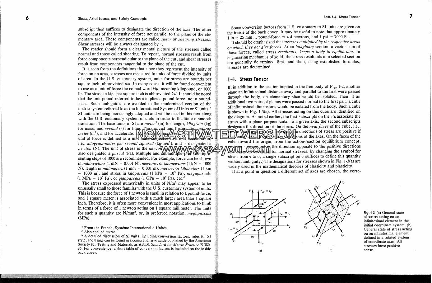
If, in addition to the section implied in the free body of Fig. I-2, anotherplane an infinitesimal distance away and parallel to the first were passedthrough the body, an elementary slice would be isolated. Then, if anadditional two pairs of planes were passed normal to the first pair, a cubeof infinitesimal dimensions would be isolated from the body. Such a cubeis shown in Fig. 1-3(a). All stresses acting on this cube are identified onthe diagram. As noted earlier, the first subscripts on the -r's associate thestress with a plane perpendicular to a given axis; the second subscriptsdesignate the direction of the stress. On the near faces of the cube, i.e.,on the faces away from the origin, the directions of stress are positive ifthey coincide with the positive directions of the axes. On the faces of thecube toward the origin, from the action-reaction equilibrium concept,positive stresses act in the direction opposite to the positive directionsof the axes. (Note that for normal stresses, by changing the symbol forstress from -r to �, a single subscript on cr suffices to define this quantitywithout ambiguity.) The designations for stresses shown in Fig. 1-3(a) arewidely used in the mathematical theories of elasticity and plasticity.
If at a point in question a different set of axes are chosen, the corre-
(a) (b)
(7/
7
Fig. t-3 (a) General stateof stress acting on aninfinitesimal element in theinitial coordinate system. (b)General state of stress actingon an infinitesimal elementdefined in a rotated systemof coordinate axes. Allstresses have positivesense.
NON-ACTIVATEDVERSIONwww.avs4you.com

8 Stress, Axial Loads, and Safety Concepts
sponding stresses are as shown in Fig. 1-3(b). These stresses are related,but are not generally equal, to those shown in Fig. 1-3(a). The processof changing stresses from one set of coordinate axes to another is termedstress transformation. The state of stress at a point which can be definedby three components on each of the three mutually perpendicular (or-thogonal) axes in mathematical terminology is called a tensor. Precisemathematical processes apply for transforming tensors, includingstresses, from one set of axes to another. A simple case of stress trans-formation will be encountered in the next section, and a more completediscussion is given in Chapter 8.
An examination of the stress symbols in Fig. 1-3(a) shows that thereare three normai stresses: -r.�.� = �.�, -ryy -= %, 'rzz =- �z; and six shearingstresses: ,.�y, -ry.�, -ryz, -r�y, ,,..�, -r.�z. By contrast, a force vector P has onlythree components: P.�, Py, and P�. These can be written in an orderlymanner as a column vector:
(1-1a)
Analogously, the stress components can be assembled as follows:
(l-lb)
This is a matrix representation of the stress tensor. It is a second-ranktensor requiring two indices to identify its elements or components. Avector is a first-rank tensor, and a scalar is a zero-rank tensor. Sometimes,for brevity, a stress tensor is written in indicial notation as 'ri�, where itis understood that i andj can assume designations x, y, and z as noted inEq. (l-lb).
Next, it will be shown that the stress tensor is symmetric, i.e., *i� ='r�i. This follows directly from the equilibrium requirements for an element.For this purpose, let the dimensions of the infinitesimal element be dx,dy, and dz, and sum the moments of forces about an axis such as the zaxis in Fig. 1-4. Only the stresses entering the problem are shown in thefigure. By neglecting the infinitesimals of higher order, 7 this process isequivalent to taking the moment about the z axis in Fig. 1-4(a) or, aboutpoint C in its two-dimensional representation in Fig. 1-4(b). Thus,
7 The possibility of an infinitesimal change in stress from one face of the cubeto another and the possibility of the presence of body (inertial) forces exist. Byfirst considering an element Ax A3' �z and proceeding to the limit, it can be shownrigorously that these quantities are of .higher order and therefore negligible.
Sec. t-4. Stress Tensor
'iry xB
C
Fig. t-4 Elements in pure shear.
Mc = 0 � + + (.ry.�)(dx dz)(dy) - (Txy)(dy dz)(dx) = 0
where the expressions in parentheses correspond respectively to stress,area, and moment arm. Simplifying,
(1-2)
Similarly, it can be shown that -r.� = -r� and -ry� = 'l'zy. Hence, the sub-scripts for the shear stresses are commutative, i.e., their order may beinterchanged, and the stre. ss tensor is symmetric.
The implication of Eq. 1-2 is very important. The fact that subscriptsare commutative signifies that shear stresses on mutually perpendicularplanes of an infinitesimal element are numerically equal, and � M� = 0is not satisfied by a single pair of shear stresses. On diagrams, as in Fig.1-4(b), the arrowheads of the shear stresses must meet at diametricallyopposite corners of an element to satisfy equilibrium conditions.
In most subsequent situations considered in this text, more than twopairs of shear stresses will seldom act on an element simultaneously.Hence, the subscripts used before to identify the planes and the directionsof the shear stresses become superfluous. In such cases, shear stresseswill be designated by -r without any subscripts. However, one must re-member that shear stresses always occur in two pairs.
This notation simplification can be used to advantage for the state ofstress shown in Fig. 1-5. The two-dimensional stress shown in the figureis referred to as plane stress. In matrix representation such a stress canbe written as
9
NON-ACTIVATEDVERSIONwww.avs4you.com
t0 Stress, Axial Loads, and Safety Concepts
{a)
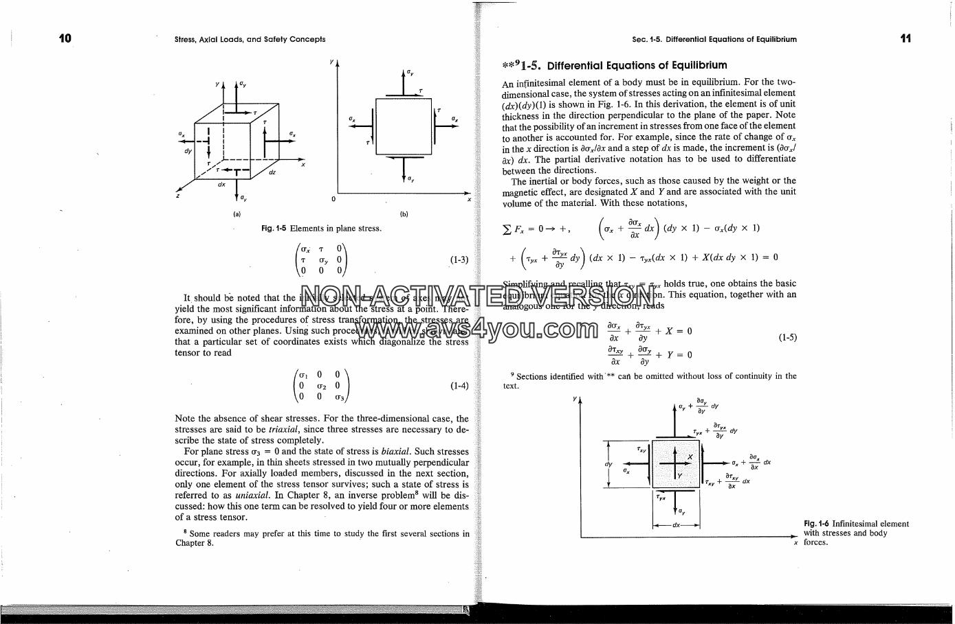
Fig. t-5 Elements in plane stress.
(b)
(1-3)
It. should b� noted that the initially selected system of axes may notyield the most significant information about the stress at a point. There-fore, by using the procedures of stress transformation, the stresses areexamined on other planes. Using such procedures, it will be sho�vn laterthat a particular set of coordinates exists which diagonalize the stresstensor to read
(1-4)
Note the absence of shear stresses. For the three-dimensional case, thestresses are said to be triaxial, since three stresses are necessary to de-scribe the state of stress completely.
For plane stress �3 = 0 and the state of stress is biaxial. Such stressesoccur, for example, in thin sheets stressed in two mutually perpendiculardirections. For axially loaded members, discussed in the next section,only one element of the stress tensor survives; such a state of stress isreferred to as uniaxial. In Chapter 8, an inverse problem 8 will be dis-cussed: how this one term can be resolved to yield four or more elementsof a stress tensor.
8 Some readers may prefer at this time to study the first several sections inChapter 8.
Sec. t.5. Differential Equations of Equilibrium
*'91-5. Differential Equations of EquilibriumAn in.�nitesimal element of a body must be in equilibrium. For the two-dimensional case, the system of stresses acting on an infinitesimal element(dx)(dy)(1) is shown in Fig. 1-6. In this derivation, the element is of unitthickness in the direction perpendicular to the plane of the paper. Notethat the possibility of an increment in stresses from one face of the elementto another is accounted for. For example, since the rate of change of �xin the x direction is O�x/Ox and a step of dx is made, the increment is (0�/Ox) dx. The partial derivative notation has to be used to differentiatebetween the directions.
The inertial or body forces, such as those caused by the weight or themagnetic effect, are designated X and Y and are associated with the unitvolume of the material. With these notations,
( O�'�dx)(dy x 1)-�(dyx 1)�F� = 0---> +, � + Ox
+ 'ry� + Oy dy (dx x 1) - xy�(dx x 1) +X(dxdy x 1) = 0Simplifying and recalling that ,� = -ry� holds true, one obtains the basicequilibrium equation for the x direction. This equation, together with ananalogous one for the y direction, reads
0o� 0'ryx--+ +x=oOx Oy (1-5)
O� +__ + Y=0Ox Oy
9 Sections identified with'** ca�l be omitted without loss of continuity in thetext.
Y
l �7y-F-�ydyI ary�
dy x + � dx
Fig. t-6 Infinitesimal elementwith stresses and body
x forces.
NON-ACTIVATEDVERSIONwww.avs4you.com

t2 Stress, Axial Loads, and Safety Concepts Sec. t-6. Stresses on Inclined Sections in Axially Loaded Bars t3
The moment equilibrium of the element requiring � Mz = 0 is assuredby having -r.� = -ry.�.
It can be shown that for the three-dimensional case, a typical equationfrom a set of three is
� OTyx OTz. rOo� + + + X = 0Ox Oy �z
Note that in deriving the previous equations, mechanical properties ofthe material have not been used. This means that these equations areapplicable whether a material is elastic, plastic, or viscoelastic. Also it isvery important to note that there are not enough equations of equilibriumto solve for the unknown stresses. In the two-dimensional case, given byEq. 1-5, there are three unknown stresses, �.�, %, and %,., and only twoequations. For the three-dimensional case, there are six stresses, but onlythree equations. Thus, all problems in stress analysis are internally stat-ically intractable or indetermb�ate. A simple example as to how a staticequilibrium equation is supplemented by kinematic requirements and me-chanical properties of a material for the solution of a problem is givenin Section 3-14. In engineering mechanics of solids, such as that presentedin this text, this indeterminacy is eliminated by introducing appropriateassumptions, which is equivalent to having additional equations.
A numerical procedure that involves discretizing a body into a largenumber of small finite elements, instead of the infinitesimal ones as above,is now 6ften used in complex problems. Such finite element analyses relyon high-speed electronic computers for solving large systems of simul-taneous equations. In the finite element method, just as in the mathe-matical approach, the equations of statics are supplemented by the kin-ematic relations and mechanical properties of a material. A few examplesgiven later in this book show comparisons among the "exact" solutionsof the mathematical theory of elasticity, and those found using the finiteelement technique and/or conventional solutions based on the methodsof engineering mechanics of solids.
1-�. Stresses on Inclined Sections in Axially Loaded BarsThe traditional approach of engineering mechanics of solids will be usedfor determining the internal stresses on arbitrarily inclined sections inaxially loaded bars. The first steps in this procedure are illustrated in Fig.1-7. Here, since. an axial force P is applied on the right end of a prismatic
P a
(a)
y
(c)
Fig. 1-7 Sectioning of a prismatic bar on arbitrary planes.
bar, for equilibrium, an equal but opposite force P must act on the leftend. To distinguish. between the applied force and the reaction, a slashis drawn across the reaction force vector P. This form of identificationof reactions will be used frequently in this text. Finding the reactions isusually the Errst essential 'step in S9!ving. a problem.
In the problem at hand, after the roactive force P is determined, free-body diagrams for the bar segments, isolated by sections such as a-a orb-b, are prepared. In both cases, the force P required for equilibrium isshown at the sections. However, in order to obtain the conventionalstresses, which are the most convenient ones in stress analysis, the forceP is replaced by its components along the selected axes. A wavy linethrough the vectors P indicates their replacement by components. Forillustrative purposes, little is gained by considering the case shown in Fig.1-7Co) requiring three force components. The analysis simply becomesmore cumbersome. Instead, the case shown in Fig. 1-7(c), having onlytwo components of P in the plane of symmetry of the bar cross section,is considered in detail. One of these components is normal to the section;the other is in the plane of the section.
As an example of a detailed analysis of stresses in a bar on inclinedplanes, consider two sections 90 degrees apart perpendicular to the barsides, as shown in Fig. l~8(a). The section a-a is at an angie 0 with the
NON-ACTIVATEDVERSIONwww.avs4you.com

P
(c)
Stress, Axial Loads, and Safety Concepts
� bJ
(a)
P
� Centraid
ofareaACross section
Y' �,� p cosy x'x
P
(e)
00(d)
P cos 2 eA
1'0_90'
-90 �
�P sin e cos 0A
--P sin 2 eA
(f) (g)
Fig. t-8 Sectioning of a prismatic bar on mutually perpendicular planes.
vertical. An isolated part of the bar to the left of this section is shown inFig. 1-8(b). Note that the normal to the section coinciding with the x axisalso forms an angle 0 with the x axis. The applied force, the reaction, aswell as the equilibrating force P at the section all act through the centroidof the bar section. As shown in Fig. 1-8(b), the equilibrating force P isresolved into .two components: the normal force component, P cos 0, andthe shear component, P sin 0. The area of the inclined cross section isA/cos 0. Therefore, the normal stress (T0 and the shear stress 'to are givenby the following two equations:
force P cos 0 P= -- cos 2 0 (1-6)(T o -- area A/cos 0 A
and
�tO --P sin 0 P .= - s�n 0 cos 0 (1-7)
A/cos 0 A
Sec. t-6. Stresses on Inclined Sections in Axially Loaded Bars
The negative sign in Eq. 1-7 is used to conform to the sign conventionfor shear stresses introduced earlier. See, for example, Fig. 1-5. The needfor a negative sign is evident by noting that the shear force P sin 0 actsin the dii:ection opposite to that of the y axis.It is important to note that the basic procedure of engineering mechanicsof solids used here gives the average or mean stress at a section. Thesestresses are determined from the axial forces necessary for equilibriumat a section. Therefore they hlways satisfy statics. However based on theadditional requirements of kinematics (geometric deformations) and me-chan'ical properties of a material, large local stresses are known to arisein the proximity of concentrated forces. This also occurs at abrupt changesin cross-sectional areas. The average stresses at a section are accurateat a distance about equal to the depth of the member from the concentratedforces or abrupt changes in cross-sectional area. The use of this simplifiedprocedure will be rationalized in Section 2-10 as Saint Venant's principle.
Equations 1-6 and 1-7 show that the normal and shear stresses varywith the angle 0. The sense of these stresses is shown in Figs. 1-8(c) and(d). The normal stress (To reaches its maximum value for 0 = 0 �, i.e.,when the section is perpendicular to the axis of the rod. The shear stressthen correspondingly would be zero. This leads to the conclusion that themaximu m normal stress (Truax in an axially loaded bar can be simply de-termined from the following equation:
P (1-8)(Truax = O'r = --' A
where P is the applied force, and A is the cross-sectional area of the bar.Equations 1-6 and 1-7 also show that for 0 = +-90 �, both the normal
and the shear stresses vanish. This is as it should be, since no stressesact along the top and bott6m free boundaries (surfaces) of the bar.
To find the maximum shear stress acting in a bar, one must differentiateEq. 1-7 with respect to 0, and set the derivative equal to zero. On carryingout this operation and simplifying the results, one obtains
tan 0 = + 1 (1-9)
leading to the conclusion that 'truax OCCurS on planes of either + 45 � or-45 � with the axis of the bar. Since the sense in which a shear stressacts is usually immaterial, on substituting either one of the above valuesof 0 into Eq. 1-7, one finds
P (T-� (1-10)'tmax -- 2A 2
Therefore, the maximum shear stress in an axially loaded bar is only half
t5
NON-ACTIVATEDVERSIONwww.avs4you.com
Stress, Axial Loads, and Safety Concepts Sec. t-7. Maximum Normal Stress In Axially Loaded Bars 17
as large as the maximum normal stress. The variation of-to with 0 can bestudied using Eq. 1-7.
Following the same procedure, the normal and shear stresses can befound on the section b-b. On noting that the angle locating this planefrom the vertical is best measured clockwise, instead of counterclockwiseas in the former case, this angle should be treated as a negative quantityin Eq. 1-7. Hence, the subscript -(90 � - 0)= 0 - 90 � will be used indesignating the stresses. From Fig. 1-8(e), one obtains
P sin 0 P- sin �- 0 (1-11)cr0-9oo A/sin 0 A
P cos 0 P
and 'ro-9oo A/sin 0 A sin 0 cos 0 (1-12)
Note that in this case, since the direction of the shear force and the yaxis have the same sense, the expression in Eq. 1-12 is positive. Equation1-12 can be obtained from Eq. 1-7 by substituting the angle 0 - 90 �. Thesense of �o_9o o and ,0_9o o is shown in Fig. 1-8(f).
The combined results of the analysis for sections a-a and b-b are shownon an infinitesimal element in Fig. 1-8(g). Note that the normal stresseson the adjoining element faces are not equal, whereas the shear stressesare. The latter finding is in complete agreement with the earlier generalcoficlusion reached in Section 1-4, showing that shear stresses on mutuallyperpendicular planes must be equal.
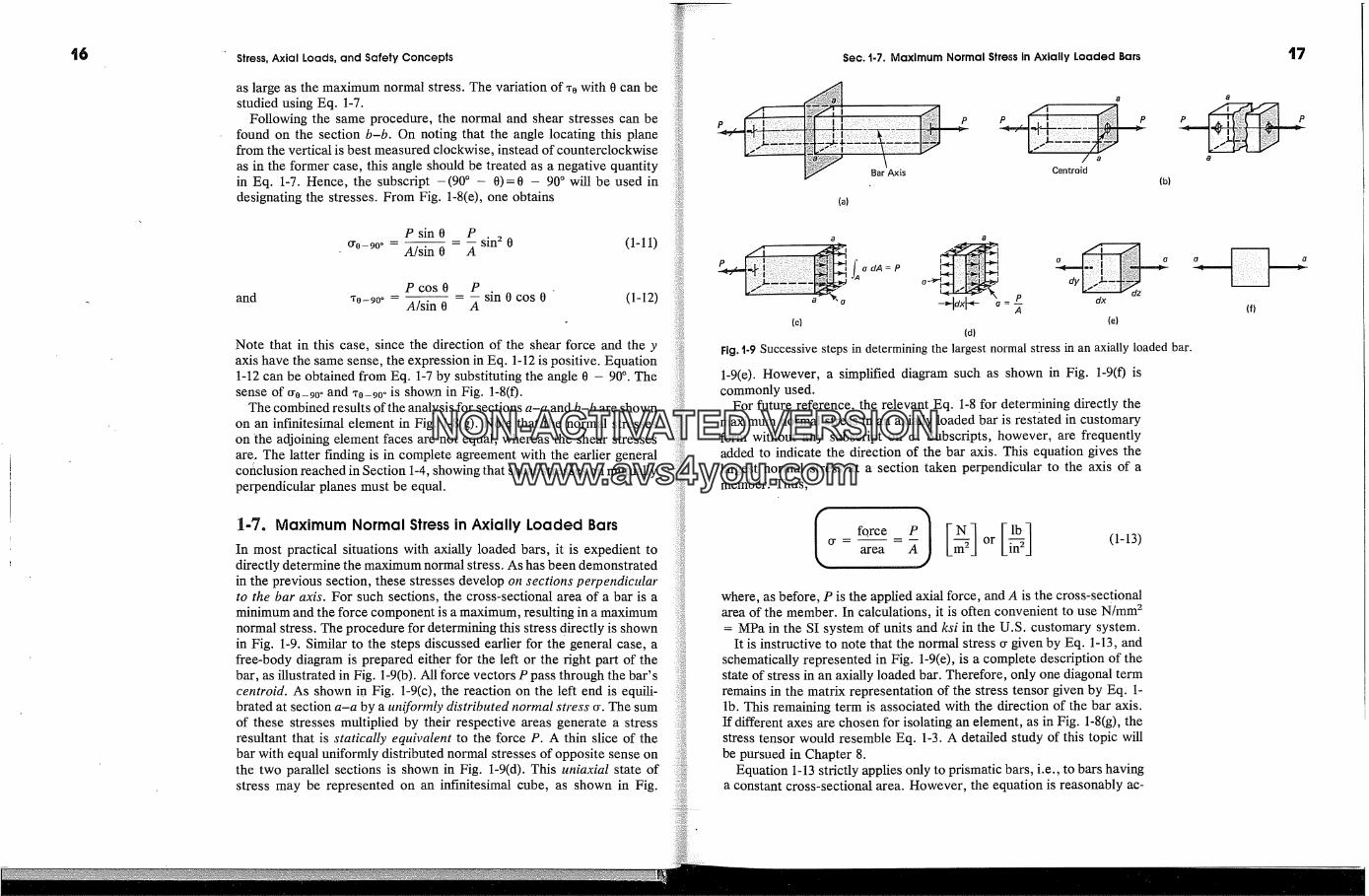
1-7. Maximum Normal Stress in Axially Loaded BarsIn most practical situations with axially loaded bars, it is expedient todirectly determine the maximum normal stress. As has been demonstratedin the previous section, these stresses develop on sections pe�7�endicularto the bar axis. For such sections, the cross-sectional area of a bar is aminimum and the force component is a maximum, resulting in a maximumnormal stress. The procedure for determining this stress directly is shownin Fig. 1-9. Similar to the steps discussed earlier for the general case, afree-body diagram is prepared either for the left or the fight part of thebar, as illustrated in Fig. 1-9(b). All force vectors P pass through the bar'scentroid. As shown in Fig. 1-9(c), the reaction on the left end is equili-brated at section a-a by a uniformly distributed normal stress �. The sumof these stresses multiplied by their respective areas generate a stressresultant that is statically equivalent to the force P. A thin slice of thebar with equal uniformly distributed normal stresses of opposite sense onthe two parallel sections is shown in Fig. 1-9(d). This uniaxial state ofstress may be represented on an infinitesimal cube, as shown in Fig.
Bar Axis
(a)
Centtold
P P
(b)
P f.qodA=Pdy
dz
a -�dx�- = P dxA
(c) (e)(d)
Fig. t-9 Successive steps in determining the largest normal stress in an axially loaded bar.
1-9(e). However, a simplified diagram such as shown in Fig. 1-9(f) iscommonly used.
For future reference, the relevant Eq. 1-8 for determining directly themaximum normal stress in an axially loaded bar is restated in customaryform without any subscript on �. Subscripts, however, are frequentlyadded to indicate the direction of the bar axis. This equation gives thelargest normal stress at a section taken perpendicular to the axis of amember. Thus,
-- or�- area i-� (1-13)
where, as before, P is the applied axial force, and A is the cross-sectionalarea of the member. In calculations, it is often convenient to use N/mm 2= MPa in the SI system of units and ksi in the U.S. customary system.
It is instructive to note that the normal stress � given by Eq. 1-13, andschematically represented in Fig. 1-9(e), is a complete description of thestate of stress in an axially loaded bar. Therefore, only one diagonal termremains in the matrix representation of the stress tensor given by Eq. l-lb. This remaining term is associated with the direction of the bar axis.If different axes are chosen for isolating an element, as in Fig. 1-8(g), thestress tensor would resemble Eq. 1-3. A detailed study of this topic willbe pursued in Chapter 8.
Equation 1-13 strictly applies only to prismatic bars, i.e., to bars havinga constant cross-sectional area. However, the equation is reasonably ac-
(f)
NON-ACTIVATEDVERSIONwww.avs4you.com
t8
a
(a)
Section
M = Pe P
(b)
Fig. 1-10 A member witha nonuniform stressdistribution at Section a-a.
Fig. 141 Bearing stressesoccur between the block andpier as well as between thepier and soil.
Stress, Axial Loads, and Safety Concepts
curate for slightly tapered members. �o For a discussion of situations wherean abrupt change in the cross-sectional area occurs, causing severe per-turbation in stress, see Section 2-10.
As noted before, the stress resultant for a uniformly distributed stressacts through the centroid of a cross-sectional area and assures the equi-librium of an axially loaded member. If the loading is more complex, suchas that, for example, for the machine part shown in Fig. 1-10, the stressdistribution is nonuniform. Here, at section a-a, in addition to the axialforce P, a bending couple, or moment, M must also be developed. Suchproblems will be treated in Chapter 6.
Similar reasoning applies to axially loaded compression members andEq. 1-13 can be used. However, one must exercise additional care whencompression members are investigated. These may be so slender that theymay not behave in the fashion considered. For example, an ordinary fish-ing rod under a rather small axial compression force has a tendency tobuckle sideways and could collapse. The consideration of such instabilityof compression members is deferred until Chapter 11. Equation 1-13 isapplicable only for axially loaded co�npression tne�nbers that are ratherchunky, i.e., to short blocks. As will be shown in Chapter 11, a blockwhose least dimension is approximately one-tenth of its length may usu-ally be considered a short block. For example, a 2 by 4 in wooden piecemay be 20 in long and still be considered a short block.
Sometimes compressive stresses arise where one body is supported byanother. If the resultant of the applied forces coincides with the centroidof the contact area between the two bodies, the intensity of force, orstress, between the two bodies can again be determined from Eq. 1-13.It is customary to refer to this normal stress as a bearing stress. Figure1-11, where a short block bears on a concrete pier and the latter bears
on the soil, illustrates such a stress. Numerous similar situations arise inmechanical problems under washers used for distributing concentratedforces� These bearing stresses can be approximated by dividing the ap-plied force P by the corresponding contact area giving a useful nominalbearing stress.
In accepting Eq. 1-13, it must be kept in mind that the material's be-havior is ideal&ed. Each and every particle of a body is assumed to con-tribute equally to the resistance of the force. A perfect homogeneity ofthe material is implied by such an assumption. Real materials, such asmetals, consist of a great many grains, whereas wood is fibrous. In realmaterials, some particles will contribute more to the resistance of a forcethan others. Ideal stress distributions such as shown in Figs. 1-9(d) and(e) actually do not exist if the scale chosen is sufficiently small. The truestress distribution varies in each particular cas.e and is a highly irregular,
jagged affair somewhat, as shown in Fig. 1-12(a). However, on the av-
For accurate solutions for tapered bars, see S. P. Timoshenko, and J. N.Goodier, Theory of Elasticity, 3rd ed. (New York: McGraw-Hill, 1970) 109.
Sec. t-8. Shear Stresses t9
. Tension
Compression
(a) (c)
(b)
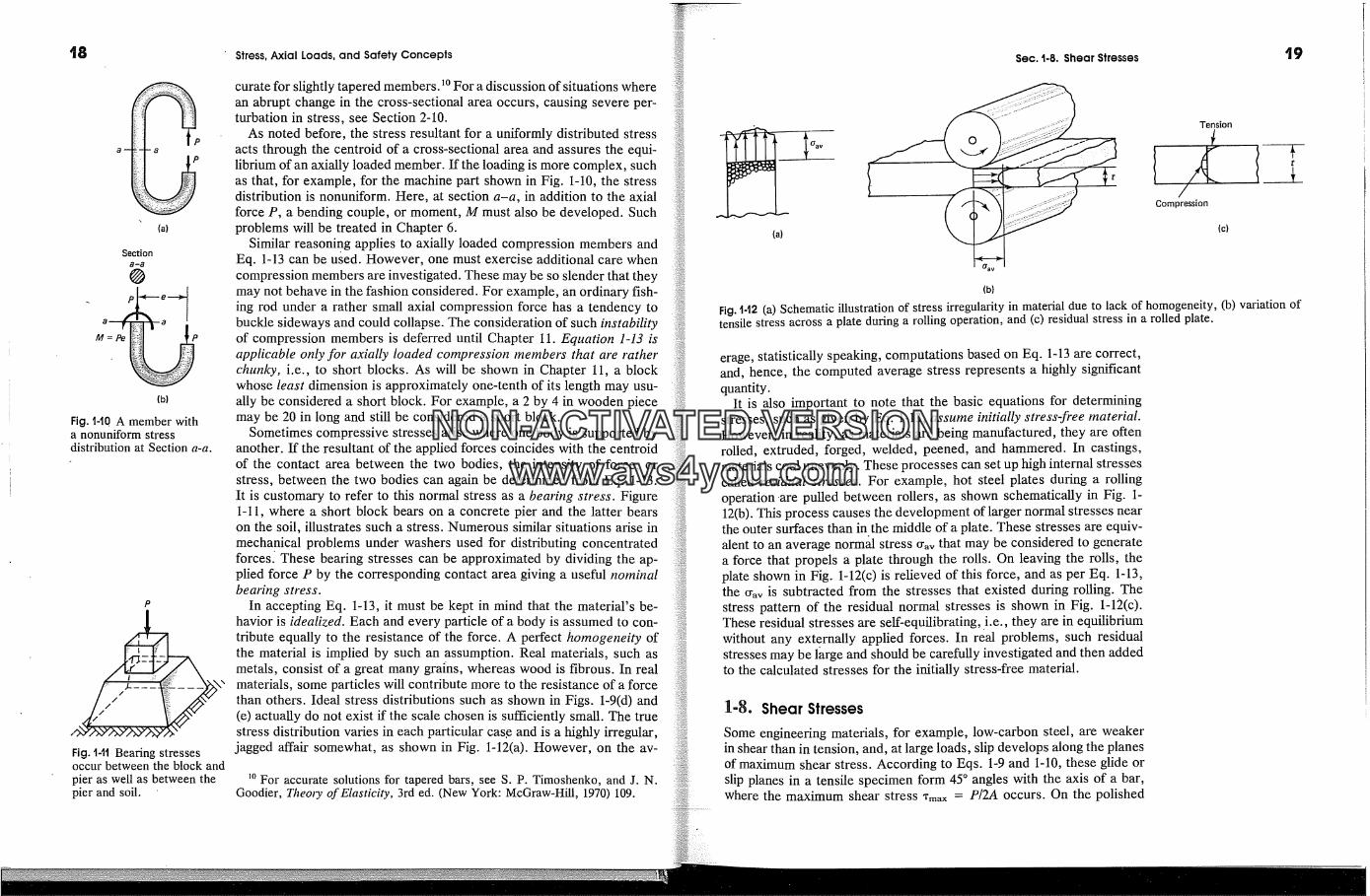
Fig. t-t2 (a) Schematic illustration of stress irregularity in material due to lack of homogeneity, (b) variation oftensile stress across a plate during a rolling operation, and (c) residual stress in a rolled plate.
erage, statistically speaking, computations based on Eq. 1-13 are correct,and, hence, the computed average stress represents a highly significantquantity.
It is also important to note that the basic equations for determiningstresses, such as given by Eq. 1-13, assume initially stress-fi'ee material.However, in reality, as materials are being manufactured, they are oftenrolled, extruded, forged, welded, peened, and hammered. In castings,materials cool unevenly. These processes can set up high internal stressescalled residual stresses. For example, hot steel plates during a rollingoperation .are pulled between rollers, as shown schematically in Fig. 1-12(b). This process causes the development of larger normal stresses nearthe outer surfaces than in the middle of a plate. These stresses are equiv-alent to an average normal stress flay that may be considered to generatea force that propels a plate through the rolls. On leaving the rolls, theplate shown in Fig. 1-12(c) is relieved of this force, and as per Eq. 1-13,the flay is subtracted from the stresses that existed during rolling. Thestress pattern of the residual normal stresses is shown in Fig. 1-12(c).These residual stresses are self-equilibrating, .i.e., they are in equilibriumwithout any externally applied forces. In real problems, such residualstresses may be large and should be carefully investigated and then addedto the calculated stresses for the initially stress-free material.
1-8. Shear Stresses
Some engineering materials, for example, low-carbon steel, are weakerin shear than in tension, and, at large loads, slip develops along the planesof maximum shear stress. According to Eqs. 1-9 and 1-10, these glide orslip planes in a tensile specimen form 45 � angles with the axis of a bar,where the maximum shear stress Xm� = P/2A occurs. On the polished
NON-ACTIVATEDVERSIONwww.avs4you.com
Stress, Axial Loads, and Safety Concepts Sec. t-8. Shear Stresses
P/2 __
P/2
(a) (d)
e
(b) (e)
a,ba
a � a, b PTav Tar
(c) (f)
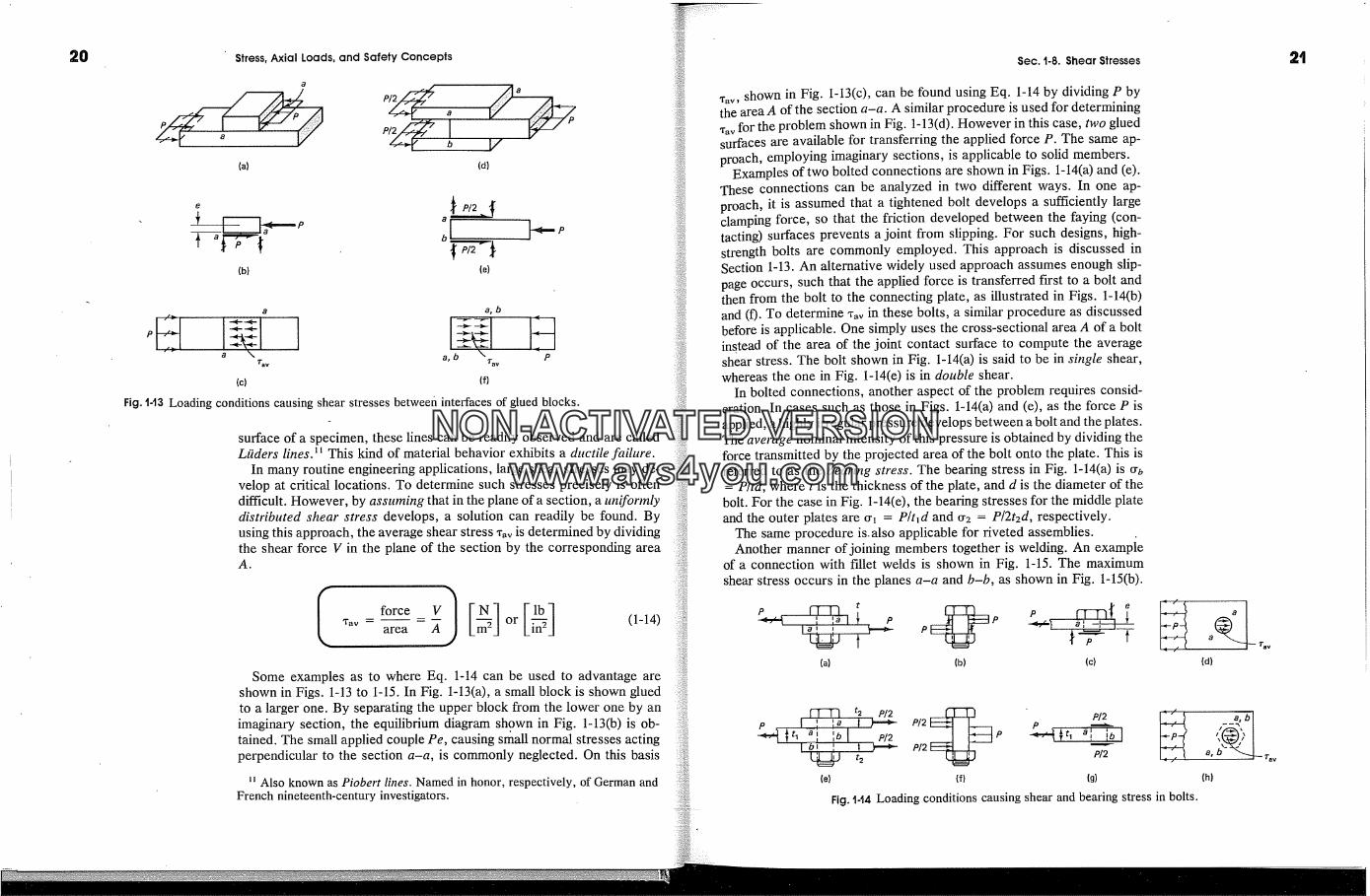
Fig. 1-t3 Loading conditions causing shear stresses between interfaces of glued blocks.
surface of a specimen, these lines can be readily observed and are calledLaders lines. � � This kind of matehal behavior exhibits a ductile failure.
In many routine engineering applications, large shear stresses may de-velop at critical locations. To determine such stresses precisely is oftendifficult. However, by assuming that in the plane of a section, a uniformlydistributed shear stress develops, a solution can readily be found. Byusing this approach, the average shear stress *av is determined by dividingthe shear force V in the plane of the section by the corresponding areaA.
= or i-�area (1-14)
Some examples as to where Eq. 1-14 can be used to advantage areshown in Figs. 1-13 to 1-15. In Fig. 1-13(a), a small block is shown gluedto a larger one. By separating the upper block from the lower one by an
imaginary section, the equilibrium diagram shown in Fig. 1-13(b) is ob-tained. The small applied couple Pe, causing sn�all normal stresses actingperpendicular to the section a-a, is commonly neglected. On this basis
� Also known as Piobert lines. Named in honor, respectively, of German andFrench nineteenth-century investigators.
,�v, shown in Fig. 1-13(c), can be found using Eq. 1-14 by dividing P bythe area A of the section a-a. A similar procedure is used for determining,� for the problem shown in Fig. 1-13(d). However in this case, two gluedsurfaces are available for transferring the applied force P. The same ap-proach, employing imaginary sections, is applicable to solid members.
Examples of two bolted connections are shown in Figs. 1-14(a) and (e).These connections can be analyzed in two different ways. In one ap-proach, it is assumed that a tightened bolt develops a sufficiently largeclamping force, so that the friction developed between the laying (con-tacting) surfaces prevents a joint from slipping. For such designs, high-strength bolts are commonly employed. This approach is discussed inSection 1-13. An alternative widely used approach assumes enough slip-page occurs, such that the applied force is transferred first to a bolt andthen from the bolt to the connecting plate, as illustrated in Figs. 1-14(b)and (f). To determine 'r� in these bolts, a similar procedure as discussedbefore is applicable. One simply uses the cross-sectional area A of a boltinstead of the area of the joint contact surface to compute the averageshear stress. The bolt shown in Fig. 1-14(a) is said to be in single shear,whereas the one in Fig. 1-14(e) is in double shear.
In bolted connections, another aspect of the problem requires consid-eration. In cases such as those in Figs. 1-14(a) and (e), as the force P isapplied, a highly irregular pressure develops between a bolt and the plates.The average nominal intensity of this pressure is obtained by dividing theforce transmitted by the projected area of the bolt onto the plate. This isreferred to as the bearing stress. The beating stress in Fig. 1-14(a) is 0.b= P/td, where t is the thickness of the plate, and d is the diameter of the
bolt. For the case in Fig. 1-14(e), the beating stresses for the middle plateand the outer plates are 0.� = P/hd and 0'2 = P/2t2d, respectively.
The same procedure is. also applicable for fiveted assemblies.Another manner of joining members together is welding. An exampie
of a connection with fillet welds is shown in Fig. 1-15. The maximumshear stress occurs in the planes a-a and b-b, as shown in Fig. 1-15(b).
(a) (b) (c)
� � P/2-----T�! '� � � PI2
� t2 P/2(e) (f)
Fig. l-t4 Loading conditions causing shear and bearing stress in bolts.
(d)
(h)
NON-ACTIVATEDVERSIONwww.avs4you.com

22
Fig. t45 Loading conditioncausing critical shear in twoplanes of fillet welds.
Stress, Axial Loads, and Safety Concepts
Weld
-----I] a�/b 45�Section c-c
(a) (b)
The capacity of such welds is usually given in units of force per unit lengthof weld. Additional discussion on welded connections is given in Section1-14.
]-9. Analysis for Normal and Shear StressesOnce the axial force P or the shear force V, as well as the area A, aredetermined in a given problem, Eqs. 1-13 and 1-14 for normal and shearstresses can be readily applied. These equations giving, respectively, themaximum magnitudes of normal and shear stress are particularly impor-tant as they appraise the greatest imposition on the strength of a material.These greatest �tresses occur at a section of �n#d�nt,n cross-sectional areaand/or the greatest axial force. Such sections are called critical sections.The critical section for the particular arrangement being analyzed canusually be found by inspection. However, to determine the force P or Vthat acts through a member is usually a more difficult task. In the majorityof problems treated in this text, the latter information is obtained fromstatics.
For the equilibrium of a body in space, the equations of statics requirethe fulfillment of the following conditions:
Ee. = 0EF,, = 0E/=o = o,j
(1-15)
The first column of Eq. 1-15 states that the sum of all forces acting on abody in any (x, y, z) direction must be zero. The second column notesthat the summation of moments of all forces around any axis parallel toany (x, y, z) direction must also be zero for' equilibrium. In a planarproblem, i.e., all members and forces lie in a single plane, such as the x-y plane, relations � F� = 0, � M.� = 0, and � M.,, = 0, while still valid,are trivial.
Sec. t-9. Analysis for Normal and Shear Stresses 23
These equations of statics are directly applicable to deformable solidbodies. The deformations tolerated in engineering structures are usuallynegligible in comparison with the overall dimensions of structures. There-fore, for the purposes of obtaining the forces in members, the initial un-deformned dbnensions of �ne�nbers are used in computations.
If the equations of statics suffice for determining the external reactionsas well as the internal stress resultants, a structural system is staticall),deter�ninate. An example is shown in Fig. 1-16(a). However, if for thesame beam and loading conditions, additional supports are provided, asin Figs. 1-16(b) and (c), the number of independent equations of staticsis insufficient to solve for the reactions. In Fig. 1-16(b), any one of thevertical reactions can be removed and the structural system remains stableand tractable. Similarly, any two reactions can be dispensed with for thebeam in Fig. 1-16(c). Both of these beams are statically indeterminate.The reactions that can be removed leaving a stable system statically de-termi.nate are superfluous or redundant. Such redundancies can also arisewithin the internal system of forces. Depending on the number of theredundant internal forces or reactions, the system is said to be indeter-minate to the first degree, as in Fig. 1-16(b), to the second degree, as inFig. 1-16(c), etc. Multiple degrees of statical indeterminacy frequentlyarise in practice, and one of the important objectives of this subject is toprovide an introduction to the methods of solution for such problems.Procedures for solving such problems will be introduced gradually be-ginning with the next chapter. Problems with multiple degrees of inde-termin. acy are considered in Chapters 10, 12, and 13.
Equations 1-15 should already be familiar to the reader. However, seweral examples where they are applied will now be given, emphasizingsolution techniques generally used in engineering mechanics of solids.These statically determinate examples will serve as an informal reviewof some of the principles of statics and will show applications of Eqs. 1-13 and 1-14.
Additional examples for determining shear stresses in bolts and weldsare given in Sections 1-13 and 1-14.
/
(a) (b) (c)
Fig. M6 [dentic� be� with identical loadin[ bavi�[ different suppo� conditions: (a) staticallydeterminate, (b) statically indeterminate to the first de[tee, (c) statically i�dete�inate to the secondde�ee.
NON-ACTIVATEDVERSIONwww.avs4you.com

Fig. 1-15 Loading conditioncausing critical shear in twoplanes of fillet welds.
Stress, Axial Loads, and Safety Concepts
Weld
-'-'1 a� �b� c Section c-c
(a) (b)
The capacity of such welds is usually given in units of force per unit lengthof weld. Additional discussion on welded connections is given in Section1-14.
1-9. Analysis for Normal and Shear StressesOnce the axial force P or the shear force V, as well as the area A, aredetermined in a given problem, Eqs. 1-13 and 1-14 for normal and shearstresses can be readily applied. These equations giving, respectively, themaximum magnitudes of normal. and shear stress are particularly impor-tant as they appraise the greatest imposition on the strength of a material.These greatest'stresses occur at a section of �nini�nt,n cross-sectional areaand/or the greatest axial force. Such sections are called critical sections.The critical section for the particular arrangement being analyzed canusually be found by inspection. However, to determine the force P or Vthat acts through a member is usually a more difficult task. In the majorityof problems treated in this text, the latter information is obtained fromstatics.
For the equilibrium of a body in space, the equations of statics requirethe fulfillment of the following conditions:
IEe.,=0 Eu.=01Ee:=0 Euz=0(1-15)
The first column of Eq. 1-15 states that the sum of all forces acting on abody in any (x, y, z) direction must be zero. The second column notesthat the summation of moments of all forces around any axis parallel toany (x, y, z) direction must also be zero for' equilibrium. In a planarproblem, i.e., all members and forces lie in a single plane, such as the x-y plane, relations � F� = 0, � M� = 0, and � My = 0, while still valid,are trivial.
Sec. 1-9. Analysis for Normal and Shear Stresses
These equations of statics are directly applicable to deformable solidbodies. The deformations tolerated in engineering structures are usuallynegligible in comparison with the overall dimensions of structures. There-fore, for the purposes of obtaining the forces in members, the initialdeformed dimensions of members are used in computations.
If the equations of statics suffice for determining the external reactionsas well as the internal stress resultants, a structural system is staticall),determinate. An example is shown in Fig. 1-16(a). However, if for thesame beam and loading conditions, additional supports are provided, asin Figs. 1-16(b) and (c), the number of independent equations of staticsis insufficient to solve for the reactions. In Fig. 1-16(b), any one of thevertical reactions can be removed and the structural system remains stableand tractable. Similarly, any two reactions can be dispensed with for thebeam in Fig. 1-16(c). Both of these beams are statically indeterminate.The reactions that can be removed leaving a stable system statically de-termi.nate are superfluous or redundant. Such redundancies can also arisewithin the internal system of forces. Depending on the number of theredundant internal forces or reactions, the system is said to be indeter-minate to the first degree, as in Fig. 1-16(b), to the second degree, as inFig. 1-16(c), etc. Multiple degrees of statical indeterminacy frequentlyarise in practice, and one of the important objectives of this subject is toprovide an introduction to the methods of solution for such problems.Procedures for solving such problems will be introduced gradually be-ginning with the next chapter. Problems with multiple degrees of inde-termin. acy are considered in Chapters 10, 12, and 13.
Equ. ations 1-15 should already be familiar to the reader. However, sev-eral examples where they are applied will now be given, emphasizingsolution techniques generally used in engineering mechanics of solids.These statically determinate examples will serve as an informal reviewof some of the principles of statics and will show applications of Eqs. 1-13 and 1-14.
Additional examples for determining shear stresses in bolts and weldsare given in Sections 1-13 and 1-14.
7F F
(a) (b) (c)
Fig. t-t6 Identical beam with identical loading having different support conditions: (a) staticallydeterminate, (b) statically indeterminate to the first degree, (c) statically indeterminate to the seconddegree.
NON-ACTIVATEDVERSIONwww.avs4you.com
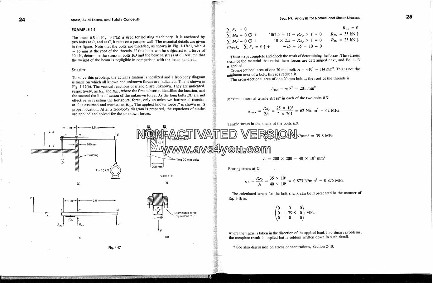
Stress, Axial Loads, and Safety Concepts
EXAMPLE
The beam BE in Fig. 1-17(a) is used for hoisting machinery. It is anchored bytwo bolts at B, and at C, it rests on a parapet wall. The essential details are givenin the figure. Note that the bolts are threaded, as shown in Fig. 1-17(d), with d= 16 mm at the root of the threads. If this hoist can be subjected to a force of10 kN, determine the stress in bolts BD and the bearing stress at C. Assume thatthe weight of the beam is negligible in comparison with the loads handled.
Solution
To solve this proble m, the actual situation is idealized and a free-body diagramis made on which all known and unknown forces are indicated. This is shown inFig. 1-17(b). The vertical reactions of B and C are unknown. They are indicated,respectively, as R m. and Rcy, where the first subscript identifies the location, andthe second the line of action of the unknown force. As the long bolts BD are noteffective in resisting the horizontal force, only an unknown horizontal reactionat C is assumed and marked as Rc.�. The applied known force P is shown in itsproper location. After a free-body diagram is prepared, the equations of staticsare applied and solved for the unknown forces.
D
(a)
2.5 m �
� 200 mm
/ Building
P=10kN�
E
r�l I
� 200X300mmfinished timber
�2:� Two 20-mm bolts
View a-a
(c)
x
(b) (d)
Fig. t-t7
Sec. t-9. Analysis for Normal and Shear Stresses
�F�, =0� MB = 0 � + 10(2.5 + 1) - Rcy X 1 = 0� Md = 0 � + 10 x 2.5 - RBy X 1 = 0Check: �Fy = 0�'+ -25 + 35- 10 = 0
Rcy = 35 kN ?RBy = 25 kN $
These steps complete and check the work of determining the forces. The variousareas of the material that resist these forces are determined next, and Eq. 1-13is applied. �
Cross-sectional area of one 20-mm bolt: A = 'n'102 = 314 mm 2. This is not theminimum area of a bolt; threads reduce it.
The cross-sectional area of one 20-mm bolt at the root of the threads is
Anet = 11' 82 = 201 mm 2
Maximum normal tensile stress? in each of the two bolts BD:
RBy 25 x 103O'm� = '2.4 2 x 201
= 62 N/mm 2 = 62 MPa
Tensile stress in the shank of the bolts BD:
25 x 1032 x 314
= 39.8 N/mm 2 = 39.8 MPa
Contact area at C:
A = 200 x 200 = 40 x 10 gmm 2
Bearing stress at C:
Rcy 35 X 103O- b � �_.A 40 x 103
= 0.875 N/mm 2 = 0.875 MPa
The calculated stress for the bolt shank can be represented in the manner ofEq. l-lb as
+39.8 MPa0
where the y axis is taken in the direction of the applied load. In ordinary problems,the complete result is implied but is seldom written down in such detail.
See also discussion on stress concentrations, Section 2-10.
NON-ACTIVATEDVERSIONwww.avs4you.com
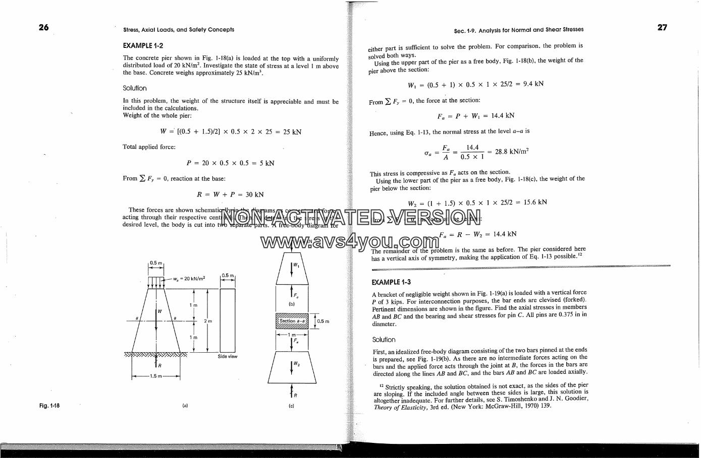
Stress, Axial Loads, and Safety Concepts Sec. t-9. Analysis for Normal and Shear Stresses
Fig. 1-t8
EXAMPLE t-2
The concrete pier shown in Fig. 1-18(a) is loaded at the top with a uniformlydistributed load of 20 kN/m 2. Investigate the state of stress at a level 1 m abovethe base. Concrete weighs approximately 25 kN/m 3.
Solution
In this problem, the weight of the structure itself is appreciable and must beincluded in the calculations.Weight of the whole pier:
W =' [(0.5 + 1.5)/2] x 0.5 x 2 x 25 = 25 kN
Total applied force:
P = 20 x 0.5 x 0.5 = 5kN
From � F�. = 0, reaction at the base:
R = W + P = 30kN
These forces are shown schematically in the diagrams as concentrated forcesacting through their respective centroids. Then, to determine the stress at thedesired level, the body is cut into two separate parts. A free-body diagram for
, ,� � ...__w.�= 20kN/m2 0.�,.�
�1.5� Sideview
P=SkN
L
I�Section a-a( .5 m
(c)
either part is sufficient to solve the problem. For comparison, the problem issolved both ways.
Using the upper part of the pier as a free body, Fig. 1-18(b), the weight of thepier above the section:
W� = (0.5 + 1) x 0.5 x 1 x 25/2 = 9.4kN
From � F). = 0, the force at the section:
Fa = P + W� = 14.4kN
Hence, using Eq. 1-13, the normal stress at the level a-a is
Fa 14.4cr� = -- - = 28.8 kN/m 2A 0.5x 1
This stress is compresslye as F, acts on the section.Using the lower part of the pier as a free body, Fig. 1-18(c), the weight of the
pier below the section:
W2 = (1 + 1.5) x 0.5 x 1 x 25/2 = 15.6 kN
From � Fy = 0, the force at the section:
F� = R - W2 = 14.4 kN
The remainder of the problem is the same as before. The pier considered herehas a vertical axis of symmetry, making the application of Eq. 1-13 possible. �2
EXAMPLE t-3
A bracket of negligible weight shown in Fig. 1-19(a) is loaded with a vertical forceP of 3 kips. For interconnection purposes, the bar ends are clevised (forked).Pertinent dimensions are shown in the figure. Find the axial stresses in membersAB and BC and the bearing and shear stresses for pin C. All pins are 0.375 in indiameter.
Solution
First, an idealized free-body diagram consisting of the two bars pinned at the endsis prepared, see Fig. 1-19(b). As there are no intermediate forces acting on thebars and the applied force acts through the joint at B, the forces in the bars aredirected along the lines AB and BC, and the bars AB and BC are loaded axially.
�2 Strictly speaking, the solution obtained is not exact, as the sides of the pierare sloping. If the included angle between these sides is large, this solution isaltogether inadequate. For further details, see S. Timoshenko and J. N. Goodier,Them�y of Elasticity, 3rd ed. (New York: McGraw-Hill, 1970) 139.
NON-ACTIVATEDVERSIONwww.avs4you.com
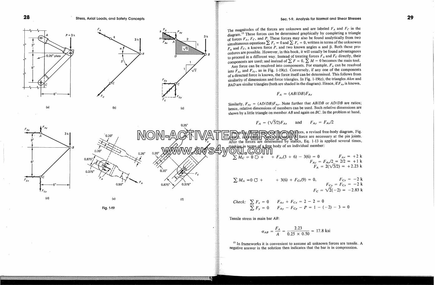
28 Stress, Axial Loads, and Safety Concepts
A P=3k
I
' � 025plate�*� �
(a) {b}
(d)
B
0.20"
/0.20" 0.25"
o.8,5,,
(e)
Fig. 1-t9
m�/:A__�� 2 3k
FA�A��nz1�7�8Fc
(c)
0.25"
0.20"� Fc
(f)
Sec. t-9. Analysis for Normal and Shear Stresses
The magnitudes of the forces are unknown and are labeled FA and F� in thediagram.�3 These forces can be determined graphically by completing a triangleof forces FA, Fc, and P. These forces may also be found analytically from twosimultaneous equations � F:. = 0 and � F.,. = 0, written in terms of the unknownsFA and Fc, a known force P, and two known angles ct and fl. Both these pro-cedures are possible. However, in this book, it will usually be found advantageousto proceed in a different way. Instead of treating forces FA and Fc directly, theircomponents are used; and instead of � F = 0, � M = 0 becomes the main tool.
Any force can 15e resolved into components. For example, FA can be resolvedinto F,t� and FAy, as in Fig. 1-19(c). Conversely, if any one of the componentsof a directed force is known, the force itself can be determined. This follows fromsimilarity of dimensions and force triangles. In Fig. 1~19(c), the triangles Akin andBAD are similar triangles (both are shaded in the diagram). Hence, if F,� is known,
FA = (AB/DB)FA.�
Similarly, Fay = (AD/DB)FAx. Note further that AB/DB or AD/DB are ratios;hence, relative dimensions of members can be used. Such relative dimensions areshown by a little triangle on member AB and again on BC. In the problem at hand,
FA = (X/�/2)FA.� and FAy = FA.d2
Adopting the procedure of resolving forces, a revised free-body diagram, Fig.1-19(d), is prepared. Two components of force are necessary at the pin joints.After the forces are determined by statics, Eq. 1-13 is applied several times,thinking in terms of a free body of an individual member:
�Mc=00+ + FA.�(3 + 6) -- 3(6) = 0 FA.� = +2 kFay = Fa.d2 = 2/2 = +1 k
FA = 2(X/�/2) = +2.23 k
�MA =00 + + 3(6) + Fc�(9) = 0, Fc.� = -2 kFc>, = Fc.� = -2 k
Fc = X/�(-2) = -2.83 k
Check: � F;, = 0EFy=O
FA.� + Fc� = 2 - 2 = 0FAy -- Fcy - P = 1 - (-2) - 3 = 0
Tensile stress in main bar AB:
FA 2.23A 0.25 x 0.50
17.8 ksi
�3 In frameworks it is convenient to assume all unknown forces are tensile. Anegative answer in the solution then indicates that the bar is in compression.
29
NON-ACTIVATEDVERSIONwww.avs4you.com

3O Stress, Axial Loads, and Safety Concepts
Tensile stress in clevis of bar AB, Fig. 1-19(e):
FA 2.23(ffAB)clev|s = = = 1 1.2 ksi
Anet 2 x 0.20 x (0.875 - 0.375)
Compressive stress in main bar BC:
(YBC --Fc 2.83
A 0.875 x 0.25- 12.9 ksi
In the compression member, the net section at the clevis need not be investigated;see Fig. 1-19(f) for- the transfer of forces. The bearing stress at the pin is morecritical. Bearing between pin C and the clevis:
Fc 2.83orb -- -- -- = 18.8 ksi
Abearing 0.375 x 0.20 x 2
Bearing between the pin C and the main plate:
Fc 2.83orb -- A 0.375 X 0.25 - 30.2 ksi
Double shear in pin C:
Fc 2.83-r - - - 12.9 ksi
A 2'rr(0.375/2) 2
For a complete analysis of this bracket, other pins should be investigated. How-ever, it can be seen by inspection that the other pins in this case are stressedeither the same amount as computed or less.
F�
[� t FcyFc [--------a
Fig. 1-20
The advantages of the method used in the last example for finding forcesin members should now be apparent. It can also be applied with successin a problem such as the one shown in Fig. 1-20. The force F,� transmittedby the curved member AB acts through points A and B, since the forcesapplied at A and B must be collinear..By resolving this force at A', thesame procedure can be followed. Wavy lines through F,� and Fc indicatethat these forces are replaced by the two components shown. Alterna-tively, the force F,� can be resolved at A, and since F4y = (y/X)FA�, theapplicatio n of � Mc = 0 yields FAx.
In frames, where the applied forces do not act through a joint, proceedas before as far as possible. Then isolate an individual member, and usingits free-body diagram, complete the determination of forces. If inclinedforces are acting on the structure, resolve them into convenient com-ponents.
Sec. MO. Member Strength as a Design Criterion 3t
C DETERMINISTIC AND PROBABILISTICDESIGN BASES
1-10. Member Strength as a Design CriterionThe purpose for calculating stresses in members of a structural systemis [o compare them with the experimentally determined material strengthsin order to assure desired performance. Physical testing of materials in alaboratory provides information regarding a material's resistance tostress. In a laboratory, specimens of known material, manufacturing pro-cess, and heat treatment are carefully prepared to desired dimensions.Then these specimens are subjected to successively increasing knownforces. In the most widely used test, a round rod is subjected to tensionand the specimen is loaded until it finally ruptures. The force necessaryto cause rupture is called the ultbnate load. By dividing this ultimate loadby the original cross-sectional area of the specimen, the uhitnate strength(stress) of a material is obtained. Figure 1-21 shows a testing machineused for this purpose. Figure 1-22 shows a tension-test specimen. The
Fig. t-2t Universal testingmachine (Courtesy of MTSSystems Corporation).
Fig. t-22 A typical tensiontest specimen of mild steelbefore and after fracture.
NON-ACTIVATEDVERSIONwww.avs4you.com
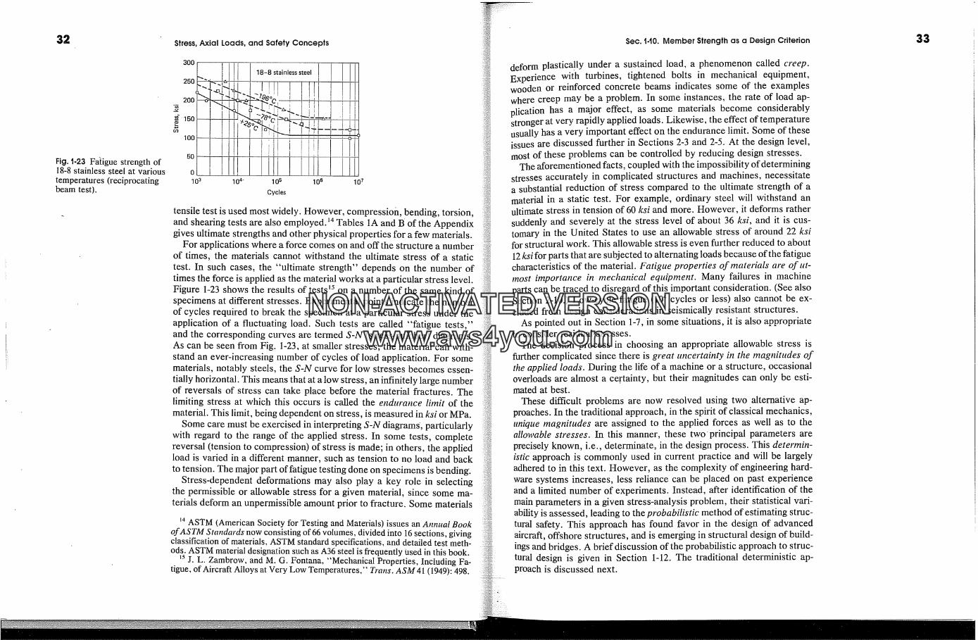
Stress, Axial Loads, and Safety Concepts Sec. t.t0. Member Strength as a Design Criterion
Fig. t-23 Fa[igue strength of18-8 stainless steel at various
temperatures (reciprocatingbeam test).
300
250
200
150
100
50
0
103 104- 10 s 10 s 107Cycles
tensile test is used most widely. However, compression, bending, torsion,and shearing tests are also employed. �4 Tables 1A and B of the Appendixgives ultimate strengths and other physical properties for a few materials.
For applications where a force comes on and off the structure a numberof times, the materials cannot withstand the ultimate stress of a statictest. In such cases, the "ultimate strength" depends on the number oftimes the force is applied as the material works at a particular stress level.Figure 1-23 shows the results of tests �5 on a number of the same kind ofspecimens at different stresses. Experimental points indicate the numberof cycles required to break the specimen at a particular stress under theapplication of a fluctuating load. Such tests are called "fatigue tests,"and the corresponding curves are termed S-N (stress-number) diagrams.As can be seen from Fig. 1-23, at smaller stresses, the material can with-stand an ever-increasing number of cycles of load application. For somematerials, notably steels, the S-N curve for low stresses becomes essen-tially horizontal. This means that at a low stress, an infinitely large numberof reversals of stress can take place before the material fractures. Thelimiting stress at which this occurs is called the endurance li�nit of thematerial. This limit, being dependent on stress, is measured in ksi or MPa.
Some care must be exercised in interpreting S-N diagrams, particularlywith regard to the range of the applied stress. In some tests, completereversal (tension to compression) of stress is made; in others, the appliedload is varied in a different manner, such as tension to no load and backto tension. The major part of fatigue testing done on specimens is bending.
Stress-dependent deformations may also play a key role in selectingthe permissible or allowable stress for a given material, since some ma-terials deform an unpermissible amount prior to fracture. Some materials
�4 ASTM (American Society for Testing and Materials) issues an Amzual Bookof ASTM Standards now consisting of 66 volumes, divided into 16 sections, givingclassification of materials, ASTM standard specifications, and detailed test meth-ods. ASTM material designation such as A36 steel is frequently Used in this book.
t-� J. L. Zambrow, and M. G. Fontana, "Mechanical Properties, Including Fa-tigue, of Aircraft Alloys at Very Low Temperatures," Trans. ASM 41 (1949): 498.
deform plastica!ly under a sustained load, a phenomenon called creep.Experience with turbines, tightened bolts in mechanical equipment,wooden or reinforced concrete beams indicates some of the exampleswhere creep may be a problem. In some instances, the rate of load ap-plication has a major effect, as some materials become considerablystronger at very rapidly applied loads. Likewise, the effect of temperatureusually has a very important effect on the endurance limit. Some of theseissues are discussed further in Sections 2-3 and 2-5. At the design level,most of these problems can be controlled by reducing design stresses.
The aforementioned facts, coupled with the impossibility of determiningstresses accurately in complicated structures and machines, necessitatea substantial reduction of stress compared to the ultimate strength of amaterial in a static test. For example, ordinary steel will withstand anultimate stress in tension of 60 ksi and more. However, it deforms rathersuddenly and severely at the stress level of about 36 ksi, and it is cus-tomary in the United States to use an allowable stress of around 22 ksifor structural work. This allowable stress is even further reduced to about12 ksi for parts that are subjected to alternating loads because of the fatiguecharacteristics of the material. Fatigue properties of materials are of ttt-tnost i�nportance in �nechanical equip�nent. Many failures in machineparts can be traced to disregard of this important consideration. (See alsoSection 2-10.) Low-cycle fatigue (104 cycles or less) also cannot be ex-cluded from design considerations in seismically resistant structures.
As pointed out in Section 1-7, in some situations, it is also appropriateto consider residual stresses.
The decision process in choosing an appropriate allowable stress isfurther complicated since there is great uncertainty in the �nagnitudes ofthe applied loads. During the life of a machine or a structure, occasionaloverloads are almost a ce.rtainty, but their magnitudes can only be esti-mated at best.
These difficult problems are now resolved using two alternative ap-proaches. In the traditional approach, in the spirit of classical mechanics,unique magnitudes are assigned to the applied forces as well as to theallowable stresses. In this manner, these two' principal parameters areprecisely known, i.e., determinate, in the design process. This deter�nin-istic approach is commonly used in current practice and will be largelyadhered to in this text. However, as the complexity of engineering hard-ware systems increases, less reliance can be placed on past experienceand a limited number of experiments. Instead, after identification of themain parameters in a given stress-analysis problem, their statistical vari-ability is assessed, leading to the probabilistic method of estimating struc-tural safety. This approach has found favor in the design of advancedaircraft, offshore structures, and is emerging in structural design of build-ings and bridges. A brief discussion of the probabilistic approach to struc-tural design is given in Section 1-12. The traditional deterministic ap-proach is discussed next.
NON-ACTIVATEDVERSIONwww.avs4you.com
Stress, Axial Loads, and Safety Concepts Sec. 14t. Deterministic Design of Members
1-11. Deterministic Design of Members: Axially LoadedBars
In the deterministic design of members, a stress resultant is determinedat the highest stressed section using conventional mechanics. For axiallyloaded bars, it means determining the largest internal axial force P at aminimum cross section. Then, for the selected material, an allowablestress O'a,o,v must be chosen.
Professional engineering groups, large companies, as well as city, state,and federal authorities, prescribe or recommend 16 allowable stresses fordifferent materials, depending on the application. Often such stresses arecalled the allowhble fiber �7 stresses.
Since according to Eq. 1-13, stress times area is equal to a force, theallowable and ultimate stresses may be converted into the allowable andultimate forces or "loads," respectively, that a member can resist. Alsoa significant ratio may be formed:
ultimate load for a memberallowable load for a member
This is the basic definition of the factor of safety, F.S. This ratio mustalways be greater than unity. Traditionally this factor is recast in termsof stresses as
maximum useful material strength (stress)allowable stress
and is widely used not only for axially loaded members, but also for anytype of member and loading conditions. As will become apparent fromsubsequent reading, whereas this definition of F.S. in terms of elasticstresses is satisfactory for some cases, it can be misleading in others.
In the aircraft industry, the term factor of safety is replaced by another,defined as
ultimate load1
design load
�6 For example, see the American Institute of Steel Construction Manual,Building Construction Code of any large city, ANC-5 Strength of Ah'craft Ele-ments issued by the Army-Navy Civil Committee on Aircraft Design Criteria,etc.
�7 The adjective fiber in this sense is used for two masons. Many original ex-periments were made on wood, which is fibrous in character. Also, in severalderivations that follow, the concept of a continuous filament or fiber in a memberis a convenient device for visualizing its action.
and is known as the margin ofsafeO'. In the past, this ratio was usuallyrecast to read
ultimate stress
maximum stress caused by the design load-1
The newer analytical methods, some of which will be pointed out inthe' text as they occur, can provide reasonable estimates of the ultimateloads for complex systems and should be used in the basic definition ofF.S. as well as of margin of safety. For example, for static loadings,instead of designing members at working loads using allowable stress, analternative approach consisting of selecting member sizes for their ulti-mate or limit load is becoming widely adopted. In such cases, the ultimateload is usually obtained by multiplying the working loads by a suitablychosen load factors. For bars in simple tension or compression, this leadsto the same results. Significantly different results may be obtained in manyother cases where inelastic behavior is more complex. In this text, how-ever, the customary allowable stress design (ASD) approach will belargely followed.
The application of the ASD approach for axially loaded members isboth simple and direct. From Eq. 1-13, it follows that the required netarea A of a member is
A = --O'allow
(1-16)
where P is the applied axial force, and tr�no,, is the allowable stress. Equa-tion 1-16 is generally applicable to tension members and short compres-sion blocks. For slender compression members, the question of their sta-bility arises and the methods discussed in Chapter 11 must be used.
The simplicity of Eq. 1-16 is unrelated to its importance. A large numberof problems requiring its use occurs in practice. The following problemsillustrate some application of Eq. 1-16 as well as provide additional reviewin statics.
EXAMPLE t-4
Reduce the size of bar AB in Example 1-3 by using a better material such aschrome-vanadium steel. The ultimate strength of this steel is approximately 120ksi. Use a factor of safety of 2.5.
NON-ACTIVATEDVERSIONwww.avs4you.com
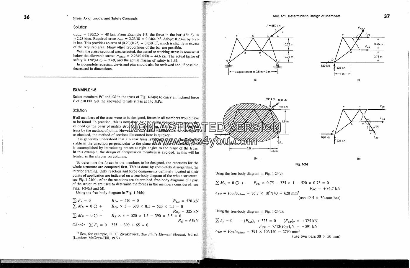
$6 Stress, Axial Loads, and Safety Concepts
Solution
orano,� = 120/2.5 = 48 ksi. From Example 1-3, the force in the bar AB: FA =+2.23 kips. Required area: Anet = 2.23/48 = 0.0464 in 2. Adopt: 0.20-in by 0.25-
in bar. This provides an area of (0.20)(0.25) = 0.050 in 2, which is slightly in excessof the required area. Many other proportions of the bar are possible.
With the cross-sectional area selected, the actual or working stress is somewhatbelow the allowable stress: O'actual �i 2.23/(0.050) = 44.6 ksi. The actual factor ofsafety is 120/(44.6) = 2.69, and the actual margin of safety is 1.69.
In a complete redesign, clevis and pins should also be reviewed and, if possible,decreased in dimensions.
EXAMPLE 'i-5
Select members FC and CB in the truss of Fig. 1-24(a) to carry an inclined forceP of 650 kN. Set the allowable tensile stress at 140 MPa.
Solution
If all members of the truss were to be designed, forces in all members would haveto be found. In practice, this is now done by employing computer programs de-veloped on the basis of matrix structural analysis �8 or by directly analyzing thetruss by the method of joints. However, if only a few members are to be designedor checked, the method of sections illustrated here is quicker.
It is generally understood that a planar truss, such as shown in the figure, isstable in the direction perpendicular to the plane of the paper. Practically, thisis accomplished by introducing braces at right angles to the plane of the truss.In this example, the design of compression members is avoided, as this will betreated in the chapter on columns.
To determine the forces in the members to be designed, the reactions for thewhole' structure are computed first. This is done by completely disregarding theinterior framing. Only reaction and force components definitely located at theirpoints of application are indicated on a free-body diagram of the whole structure;see Fig. 1-24(b). After the reactions are determined, free-body diagrams of a partof the structure are used to determine the forces in the members considered; seeFigs. 1-24(c) and (d).
Using the free-body diagram in Fig. 1-24(b):
�F.� = 0�ME = 0� +
�Mz�=0� +
Check: � Fy = 0
Rm - 520 = 0 Rz�x = 520 kNRDy X 3 - 390 x 0.5 - 520 x 1.5 = 0
RDy = 325 kNRE X 3 + 520 x 1.5 -- 390 X 2.5 = 0
RE = 65kN325 - 390 + 65 = 0
�8 See, for example, O. C. Zienkiewicz, The Fitrite Element Method, 3rd ed.(London: McGraw-Hill, 1977).
Sec. 1-1t. Deterministic Design of Members $7
650 kN
� \ 0.75 m
(c)
Rox
,,r 2.5 m
390 kN 650 kN
r/520 kN F C Fc�
520 kN f325 kN Fc�
(b) (d)
Fig. t-24
Using the free-body diagram in Fig. 1-24(c):
�MA = OG + Frc X 0.75 + 325 x 1 - 520 X 0.75 = 0F�-c = + 86.7 kN
A�c = F�c/cr�now = 86.7 x 10³/140 = 620 mm 2(use 12.5 x 50-mm bar)
Using the free-body diagram in Fig. 1-24(d):
� Fy = 0 --(FcB)y q- 325 = 0 (FcB)y = + 325 kNFc� = ��(FcB)y/3 = q- 391 kN
Ac� = Fc�/cr�now = 391 x 103/140 = 2790 mm 2(use two bars 30 x 50 mm)
NON-ACTIVATEDVERSIONwww.avs4you.com
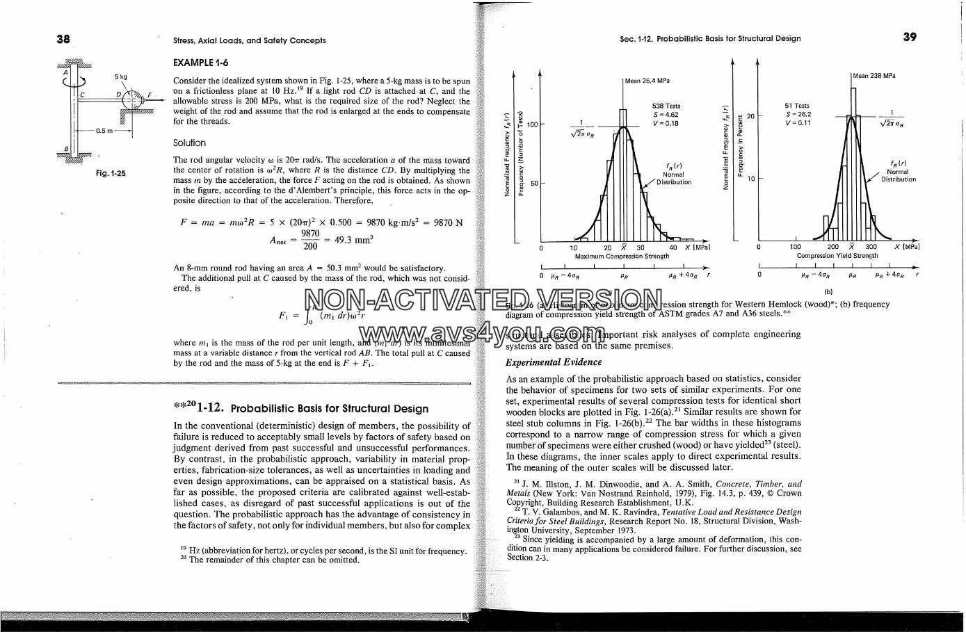
38
AC-0.5 m
Fig. t-25
Stress, Axial Loads, and Safety Concepts
EXAMPLE �-6
Consider the idealized system shown in Fig. 1-25, where a 5-kg mass is to be spun'on a frictionless plane at 10 Hz. �9 If a light rod CD is attached at C, and theallowable stress is 200 MPa, what is the required size of the rod? Neglect theweight of the rod and assume that the rod is enlarged at the ends to compensatefor the threads.
Solution
The rod angular velocity to is 20�r rad/s. The acceleration a of the mass towardthe center of rotation is to2R, where R is the distance CD. By multiplying themass m by the acceleration, the force F acting on the rod is obtained. As shownin the figure, according to the d'Alembert's principle, this force acts in the op-posite direction to that of the acceleration. Therefore,
F = ma = mto2R = 5 x (20�r) 2 x 0.500 = 9870 kg.m/s 2 = 9870 N9870
Anet - -- - 49.3 mm 2200
An 8-mm round rod having an area A = 50.3 mm 2 would be satisfactory.The additional pull at C caused by the mass of the rod, which was not consid-
ered, is
F� = J-/ (/n� dr)to2rwhere m� is the mass of the rod per unit length, and (m� dr) is its infinitesimalmass at a variable distance r from the vertical rod AB. The total pull at C causedby the rod and the mass of 5-kg at the end is F + F�.
*'2�1-12. Probabilistic Basis for Structural DesignIn the conventional (deterministic) design of members, the possibilityfailure is reduced to acceptably small levels by factors of safety based onjudgment derived from past successful and unsuccessful performances.By contrast, in the probabilistic approach, variability in material prop-erties, fabrication-size tolerances, as well as uncertainties in loading andeven design approximations, can be appraised on a statistical basis. Asfar as possible, the proposed criteria are calibrated against well-estab-lished cases, as disregard of past successful applications is out of thequestion. The probabilistic approach has the/tdvantage of consistency inthe factors of safety, not only for individual members, but also for complex
�9 Hz (abbreviation for hertz), or cycles per second, is the SI unit for frequency.2o The remainder of this chapter can be omitted.
Sec. 142. Probabilistic Basis for Structural Design 39
. JMean25.4MPar� 538 TestsI11 s = 4'62
v=o.8
I/I III I't fR{r)
l,,o[ ,,,,,,,_,orm,
20
10
51 Tests
S = 26.2V= 0.11
200
Mean 238 MPa
'vI� O'R
I
0 10 20 � 30 40 X [MPa] 0 100Maximum Compression Strength Compression Yield Strength
I I I I I [ �. I I I I I I I0 fir -- 40 R fIR fIR + 40 R r 0 fIR -- 40 R fIR S1R + 40 a
t f�(r)
300 X [MPa]
r
(a) (b)
Fig. t-26 (a) Histogram of maximum compression strength for Western Hemlock (wood)*; (b) frequencydiagram of compression yield strength of ASTM grades A7 and A36 steels.**
structural assemblies. Important risk analyses of complete engineeringsystems are based on the same premises.
Experimental EvidenceAs an example of the probabilistic approach based on statistics, considerthe behavior of specimens for two sets of similar experiments. For oneset, experimental results of several compression tests for identical shortwooden blocks are plotted in Fig. 1-26(a)? Similar results are shown forsteel stub columns in Fig. 1-26(b). 22 The bar widths in these histogramscorrespond to a narrow range of compression stress for which a givennumber of specimens were either crushed (wood) or have yielded 23 (steel).In these diagrams, the inner scales apply to direct experimental results.The meaning of the outer scales will be discussed later.
2� j. M. Illston, J. M. Dinwoodie, and A. A. Smith, Concrete, Timber, andMetals (New York: Van Nostrand Reinhold, 1979), Fig. 14.3, p. 439, � CrownCopyright, Building Research Establishment, U.K.
2� T. V. Galambos, and M. K. Ravindra, Tentative Load and Resistance DesignCriteria for Steel Buildings, Research Report No. 18, Structural Division, Wash-ington University, September 1973.
23 Since yielding is accompanied by a large amount of deformation, this con-dition can in many applications be considered failure. For further discussion, seeSection 2-3.
NON-ACTIVATEDVERSIONwww.avs4you.com
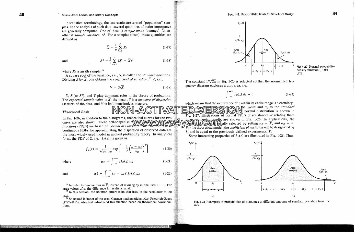
4O Stress, Axial Loads, and Safety Concepts
In statistical terminology, the test results are termed "population" sam-ples. In the analysis of such data, several quantities of major importanceare generally computed. One of these is sa/nple/nean (average), X; an-other is sa/nple variance, S 2. For n samples (tests), these quantities aredefined as
= 1 X; x, (1-17)II i=l
and S2 = 1 � (Xi �)2 (1-18)II i=1
where Xi is an ith sample. TMA square root of the variance, i.e., S, is called the standard deviation.
of vartaaon,- V, i.e.,Dividing S by X, one obtains the coefficient � � ,5
V = S/X (1-19)
X, S (or S2), and V play dominant roles in the theory of probability.The expected sa�nple value is X, the mean; S is a measure of dispersion(scatter) of the data, and V is its 'dimensionless measure.
Theoretical Basis
In Fig. 1-26, in addition to the histograms, theoretical curves for the twocases are also shown. These bell-shaped curves of probability density
fimctions (PDFs) are based on normal or Gaussian 26 distribution. Thesecontinuous PDFs for approximating the dispersion of observed data arethe most widely used model in applied probability theory. In analyticalform, the PDF of Z, i.e., �z(Z), is given as
1 exp[ 1 (z-�z'� 2] (1-20)fz(z): V'2�r� - � crz / ]
where p�z = f_+� Z�z(Z) dz (1-21)
and tr} J�_+� (z " dz (1-22)= - p.z)-fz(z)
24 In order to remove bias in X, instead of dividing by n, one uses n - 1. Forlarge values of n, the difference in results is small.
25 In this section, the notation differs from that 'used in the remainder of thetext.
26. So named in honor of the great German mathematician Karl Friedrich Gauss(1777-1855), who first introduced this function based on theoretical considera-tions.
Sec. 1-t2. Probabilistic Basis for Structural Design 4t
fz(z)
Area
Fz (zO
z� Fig. t-27 Normal probabilitydensity function (PDF)of Z.
The constant 1/X/� in Eq. 1-20 is selected so that the normalized fre-quency diagram encloses a unit area, i.e.,
+�fz(z) dz = 1 (1-23)which means that the occurrence ofz within its entire range is a certainty.
In the previous equations [[z is the mean and Crz is the standarddeviation. A typical PDF of Z with normal distribution is shown inFig. 1-27. Illustrations of normal PDFs of resistances R relating themto experimental results are shown in Fig. 1-26. In a__pplications, thetheoretical model is usually selected by setting [[z = X, and �rz = S.For the theoretical model, the coefficient of variation will be designated bygz and is equal to the previously defined experimental V.
Some interesting properties of �z(Z) are illustrated in Fig. 1-28. Thus,
fz(z)
1
fz(z)
1
Area0.00135
(a) (b)
Fig. 1-28 Examples of probabilities of outcomes at different amounts of standard deviation from themean.
NON-ACTIVATEDVERSIONwww.avs4you.com

42 Stress, Axial Loads, and Safety Concepts
from Fig. 1-28(a), it can be seen that the probability of the occurrence ofan outcome between one standard deviation on either side of the meanis 68.27%. Whereas, as shown in Fig. 1-28(b), between two standard de-viations on either side of the mean, this value becomes 95.45%. The areasenclosed under the curve tails that are three standard deviations from themean are only 0.135% of the total outcomes. As will become apparentlater, the small number of outcomes likely to take place under �z(Z) sev-eral standard deviations away from the mean is of the utmost importancein appraising structural safety.
Practical F ortnulations
For a probabilistic appraisal of the structural safety of a member or astructure, one.must have a statistically determined resistance PDF fRO'),such as discussed before, and a corresponding load effect PDF. Againstatistical studies show that since the loads are susceptible to variations,their effect on a member or a structure can be expressed in probabilisticform. Such load effects, resembling fRO'), will be designated as fo(q).For a given member or a structure, these functions define the behaviorof the same critical parameter such as a force, stress, or deflection. Twosuch functions probabilistically .defining the load effect fQ(q) and theresistance f�(r) for a force acting on a member are shown in Fig. 1-29.For purposes Of illustration, it is assumed that the load effect fQ(q) hasa larger standard deviation, i.e., larger dispersion of the load, than thatfor the member resistance.
In conventional (deterministic) design, the load magnitudes are usuallyset above the observed mean. This condition is represented by Q,, in Fig.1-29. On the other hand, in order to avoid possible rejections, a supplier
will typically provide a material with an average strength slightly greaterthan specified. For this reason, calculated nominal member resistance Rnwould be below the mean. On this basis, the conventional factor of safetyis simply defined as Rn/Qn.
In reality, both Q and R are uncertain quantities and there is no uniqueanswer to the safety problem. To illustrate the interaction between thetwo main variables in Fig. 1-31, �,�(r) is shown along the horizontal axisand ��(q) is plotted along the vertical axis. For the ensemble of an infinitenumber of possible outcomes, a line at 45 � corresponding to R = Q dividesthe graph into two regions. For R > Q, no failure can occur. For example,for the range of small and large outcomes Q�, Q2, Q3, the resistanceoutcomes, respectively, R�, R2, R3 suffice to preserve the integrity of amember. However, for outcomes Q3 and R� with a common point at Dand falling in the region where R < Q, a failure would take place.
While enlightening, the above process is difficult to apply in practice.Fortunately, however, it can be mathematically demonstrated that fornormal distribution of R and Q their difference, i.e., R - Q, is also anormal distribution. In this manner, the information implied in Fig. 1-30
Sec. %t2. Probabilistic Basis for Structural Design
fo(q)Load
0 n
fR (r)Resistance
city)q or�r
Load or resistance
Fig. 1-29 Probability densityfunctions for the two mainrandom variables (load andresistance).
x/
Load
Q>R�Qs Unsafe
0 R� R 2 R 3
Fig. �-30 Probabilisticdefinition of s�e and unsafestructural regions.
can be compressed into a single normal PDF such as that shown in Fig.1-3 l(a). In this diagram the probability of failure, p f, is given by the areaunder the tail of the curve to the left of the origin. A possible magnitudeof apf may be surmised from Fig. 1-28(b). A member would survive inall instances to the right of the origin.
As can be seen from Fig. 1-31 (a), [3 cry_ o = Ix�- o, where [3 is a constantand crR-o is standard deviation. For applications, this relation can be putinto a more convenient form by noting that the variance of a linear functionof two independent normal variables, cry_ o, is the sum of the variances
fR-o(X)[ flnJRJo)(X)Failure Survival Failure
0 $ZR-O
Survival
43
R>QSafe
.- fR(r)
Htn (RIO)
(RIO) '�'
(a) {b)
Fig. 1-3t (a) Normal and (b) lognormal probability density functions.
Resistance
NON-ACTIVATEDVERSIONwww.avs4you.com
Stress, Axial Loads, and Safety Concepts Sec. t-t2. Probabilistic Basis for Structural Design
of its parts. 27 Moreover, since variance is a square of standard deviation.one has the following expression for the safety index [3.
[3 _ [.I,R-- Q _ [.LR --
where o'R and �r o are, respectively, the standard deviations for the resis-tance R and the load effect O. A larger [3 results in fewer failures, andthus, a more conservative design.
An alternative appoach for establishing the formulation for the safetyindex [3 can be based on the more widely used concept of the factor ofsafety defined as the ratio R/Q. This approach is particularly useful whenthe distributions of R and Q are skewed and the lognormal distribution 2srather than the normal is appropriate. In this formulation, for reasons of:;mathematical convenience, it is preferable to work with the logarithmthe ratio R/Q, Fig. 1-31 (b). By carrying out this approach and making useof first order, mean-value approximations, the expression for the safety'index, [3, reads
. [3�V'a7e/,----3--�.�V,a-�-�e-�-�--� (1-26)where, as before, �x� and �xc2 are the mean values for the respective func-tions, and g� and go_) are, respectively, the coefficients of variation for Rand O.
It c'�n be noted that Eqs. 1-24 and 1-26 resemble each other. A graphical:interpretation for a solution based on the use of In(R/Q) is shown inl-3!(b). Analogous to the first approach, the probability of failure Ps
given by the area under the tail of the curve to the left of the origin.routine applications, a [3 on the order of 3 is considered appropriate.
it must be recognized that the safety index, [3, is only a relative measureof reliability and cannot be considered exact. Nevertheless, uncertainties
27 A. H-S. Ang, and W. H. Tang, Probability Concepts in Engineering Planningand Design, Vol. 1 (New York: John Wiley and Sons, 1975).
28 Lognormal distribution for a random variable R is defined as
f�e(r) = X/9-�-� �er exp - � �, �e (1-�)
where XR = In �R/�/I + g,� and � = In(1 + g,�) are, respectively, the meanstandard deviation of In R. Similar expressions apply for �o(q). However.lognormal R and Q, it can be shown that Z = In(Q/R) has the normalSee A. H-S. Ang and W. H. Tang, Probabilio, Concepts #7 Eng#�eeringand Design. Vol. 2--Decision, Risk, and Reliabilio, (New York: Wiley, 1983).
in design variables can be explicitly included by using the coefficients ofvariation in the design parameters, resulting in more consistent reliabilityof structures and machines.
In �ddition to the failure limit states emphasized before, the probabi-listic approach is suitable for other situations. Important among these arethe serviceability limit states. Among these, control of maximum deflec-tions or limitations on undesirable vibrations can also be treated in prob-abilistic terms.
EXAMPLE t-7
Consider two kinds of loading to be suspended by steel tension rods. In bothcases, a nominal permanent, or dead load, D,,, is 5 kips. In one case, however,a nominal intermittent, or live load, L,, is 1 kip, whereas in the other, L;, is 15kips. Assume that for the design of these rods, American Institute of Steel Con-struction (AISC) provisions for the design of buildings using ASTM Grade A36steel apply.
(a) Determine the cross-sectional areas for the rods using the conventionalallowable stress design (ASD) approach, for which cr�,o,� = 22 ksi. 29
(b) Find the cross-sectional areas for the same rods using an approach deducedfrom the basics of probabilistic concepts. According to AISC/LRFD, -�� thisrequires the use of the following relation:
k
qbR,, > � �iQi (1-27)i=1
where R� is the nominal strength of the structure, and qb < 1 is the resistancefactor such that qbR,, is the design resistance of the member; the load factors� > 1 account for possible overloads over the nominal load effect Q�. Sincein this case only two fypes of loading are considered, Eq. 1-27 reduces to
qbR,� > 1.2D, + 1.6L, (1-28)
where, according to the code for this case, qb is 0.90, �'s are 1.2 and 1.6,and the yield strength of the steel, cry�, is 36 ksi.
(c) For the four solutions found before, calculate the corresponding safetyindices, [3, using Eq. 1-26. This equation is based on lognormal distributionfor the variables associated with the load and resistance per AISC/LRFD.
Solution
(a) Since the total axial force P is caused by the dead and live loads, P = D,,+ L,, and, on applying Eq. 1-16, the required areas are
29 AISC, Manual of Steel Construction, 9th ed. (Chicago, 1989).3o AISC, Mattteal of Steel Construction, Load and Resistance Factor Design
(LRFD), 1st ed. (Chicago: 1986).
NON-ACTIVATEDVERSIONwww.avs4you.com
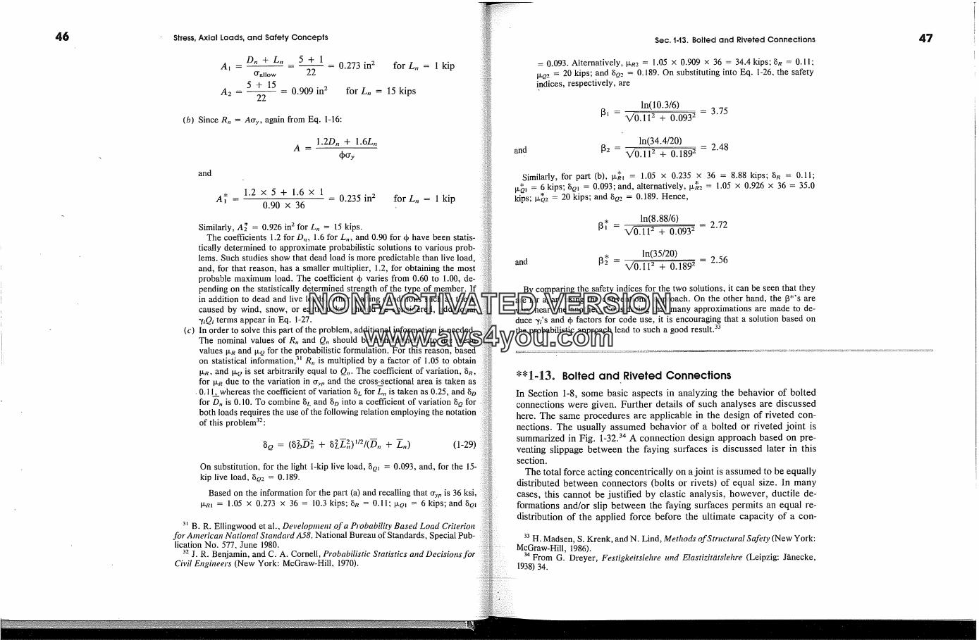
46 Stress, Axial Loads, and Safety Concepts
A� - D, + Ln 5 + 1 = 0.273 in 2 for L, = 1 kip�ra,,ow 22
5+15A2 - -- = 0.909 in 2 for Ln = 15 kips
22
(b) Since R,, = A%., again from Eq. 1-16:
1.2D,, + 1.6L,
and
A� = 1.2 x 5 + 1.6 x 1 = 0.235in 2 forLn = 1 kip0.90 x 36
Similarly, A� = 0.926 in 2 for L, = 15 kips.The coefficients 1.2 for D,, 1.6 for L, and 0.90 for qb have been statis-
tically determined to approximate probabilistic solutions to various prob-lems. Such studies show that dead lead is more predictable than live lead,and, for that reason, has a smaller multiplier, 1.2, for obtaining the mostprobable maximum lead. The coefficient qb varies from 0.60 to 1.00, de-pending on the statistically determined strength of the type of member. Ifin addition to dead and live loads, other loading conditions such as thosecaused by wind, snow, or earthquakes should be considered, additional�'�Qi terms appear in Eq. 1-27.
(c) In order to solve this part of the problem, additional information is needed.The nominal values of R, and Q,, should be transformed into the meanvalues �R and �c) for the probabilistic formulation. For this reason, basedon statistical information, 3� R, is multiplied by a factor of 1.05 to obtain�R, and �c� is set arbitrarily equal to Q,,. The coefficient of variation, B�,for � due to the variation in %., and the cross-sectional area is taken as
�0.1 I, whereas the coefficient of variation BL for �,, is taken as 0.25, and Befor D,, is 0.10. To combine BL and Be into a coefficient of variation B o forboth loads requires the use of the following relation employing the notationof this problem32:
2 --� '> --'> 1/'> --aQ = (aDD7� + gEL7,) -fiD,, + (1-29)
On substitution, for the light 1-kip live lead, Bo� = 0.093, and, for the 15-kip live lead, Be2 = 0.189.
Based on the information for the part (a) and recalling that %., is 36 ksi,�m = 1.05 x 0.273 x 36 = 10.3 kips; B� = 0.11; p�a� = 6 kips; and Ba!
3� B. R. Ellingwood et al., Development.ofa Probability Based Load Criterionfor American National Standard A58, National Bureau of Standards, Special Pub-
lication No. 577, June 1980.32 j. R. Benjamin, and C. A. Cornell, Probabilistic Statistics and Decisions for
Civil Engineers (New York: McGraw-Hill, 1970).
and
Sec. 1-13. Bolted and Riveted Connections
= 0.093. Alternatively, �R2 = 1.05 x 0.909 x 36 = 34.4 kips; Be = 0.11-�a2 = 20 kips; and Be_, = 0.189. On substituting into Eq. 1-26, the safetyindices, respectively, are
ln(10.3/6) - 3.75[31 = X,/0.112 + 0.0932
ln(34.4/20) - 2.48[32 = %/0.112 + 0.1892
Similarly, for part (b), p� = 1.05 x 0.235 x 36 = 8.88 kips; Be = 0.11;[� 6 kips; Bo� = 0.093; and, alternatively, * = 1.05 x 0.926 x 36 = 35.0kips; �2 = 20 kips; and BQ2 = 0.189. Hence,
� ln(8.88/6) = 2.72[3� = %/0.112 + 0.0932
and ln(35/20) - 2.56%/0.112 + 0.1892By comparing the safety indices for the two solutions, it can be seen that they
are far apart using the conventional approach. On the other hand, the [3"s arevery near one another. Considering that many approximations are made to de-duce �,/s and qb factors for code use, it is encouraging that a solution based onthe probabilistic approach lead to such a good result?
*'1-13. Bolted and Riveted Connections
In Section 1-8, some basic aspects in analyzing the behavior of boltedconnections were given. Further details of such analyses are discussedhere. The same procedures are applicable in the design of riveted con-nections. The usually assumed behavior of a bolted or riveted joint issummarized in Fig. 1-32. TM A connection design approach based on pre-venting slippage between the faying surfaces is discussed later in thissection.
The total force acting concentrically on a joint is assumed to be equallydistributed between connectors (bolts or rivets) of equal size. In manycases, this cannot be justified by elastic analysis, however, ductile de-formations and/or slip between the faying surfaces permits an equal re-distribution of the applied force before the ultimate capacity of a con-
� H. Madsen, S. Krenk, and N. Lind, Methods of Stractural Safety (New York:McGraw-Hill, 1986).
34 From G. Dreyer, Festigkeitslehre und Elastizitiitslehre (Leipzig: J/�necke,1938) 34.
NON-ACTIVATEDVERSIONwww.avs4you.com

48 Stress, Axial Loads, and Safety Concepts
Fig. t-32 Assumed actionfor a bolted or a rivetedconnection.-
Shearing plane I�i
Bearin planes
Fig. 1-33 Bending of platescommonly neglected in lap
joints.
nection is reached. This assumption has been justified on the basis oftests?
In contrast to the illustration shown in Fig. 1-32, in simple lap joints,the connectors are in single shear, and the plates near' the connector tendto bend to maintain the axial force concentric. However, bending in theconnected plates is commonly neglected (see Fig. 1-33). Numerous boltedconnections of this type are used in steel construction, and riveted onesare used for joining aluminum alloy sheets in aircraft.
When connectors are arranged as shown in Fig. 1-34(a), determiningthe net section in tension poses no difficulty. However, if the rows forbolt holes are closely spaced and staggered, as shown in Fig. 1-34(b), azig-zag tear may be more likely to occur than a tear across the normalsection b-b. Methods for treating such cases are available? It is alsonecessary to have a sufficient edge distance e to prevent a shear failureacross the c-c planes shown in Fig. 1-34(c).
An illustration of a failure in bearing is given in Fig. 1-35. Although theactual stress distribution is very complex, as noted in Section 1-8, inpractice, it is approximated on the basis of an average bear#zg stressacting over the projected area of the connector's shank onto a plate, i.e.,
35 A conclusive experimental verification of this assumption may be found inthe paper by R. E. Davis, G. B. Woodruff, and H. E. Davis, "Tension Tests ofLarge Riveted Joints," Trans. ASCE 105 (1940): 1193.
3a For details, for example, see AISC, Manual of Steel Construction, 9th ed.(Chicago, 1989).
(e) (b) (c)
Fig. 1-34 Possible modes of failure in bolted joints (connections): (a) net section,(b) zig-zag tear, and (c) tear out due to insufficient edge (end) distance along lines
Sec. t-t3. Bolted and Riveted Connections
(a)
(b)
d
(c)
on area td. It is difficult to justify this procedure theoretically. However,the allowable bearing stress is determined from experiments and is in-terpreted on the basis of this average stress acting on the projected areaof a rivet. Therefore, the inverse process used in design is satisfactory.
In the previous design approach, the frictional resistance between thefaying surfaces at the connectors has been neglected. However, if theclamping force developed by a connector is both sufficiently large andreliable, the capacity of a joint can be determined on the basis of thefriction force between the faying surfaces. This condition is illustrated inFig. 1-36. With the use of high-strength bolts with yield strength on theorder of 100 ksi (700 MPa), this is an acceptable method_ in structural steeldesign. The required tightening of such bolts is usually specified to beabout 70 percent of their tensile strength. For the purposes of simplifiedanalysis, an allowable shear stress based on the nominal area of a bolt isspecified. These stresses are based on experiments. This enables the de-sign of connections using high-strength bolts to be carried out in the samemanner as that for ordinary bolts or rivets.
The procedure for analyzing bearing-type bolted and riveted joints bythe AISC/LRFD probabilistically based approach remains essentially the
Washer Bolt grip ' . T-- --p
I �xxxxx� .xxxxxxxxx�xxx,',�F---�- pressure on � resistance�_�//� the plate Initial to thebolt force P
Washer Bolt length tension(a) (b)
Fig. t-36
49
Fig. t-35 (a),(b) Illustrationof a bearing failure, and(c) assumed stressdistribution.
NON-ACTIVATEDVERSIONwww.avs4you.com
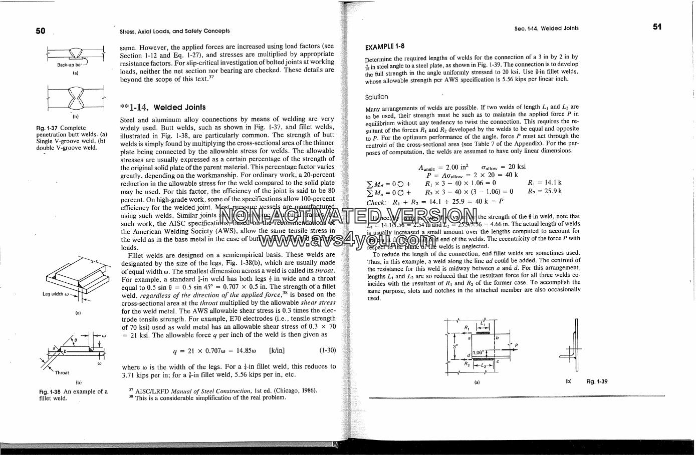
5O Stress, Axial Loads, and Safety Concepts Sec. t-14. Welded Joints 5t
Back-u�(a)
(b)
Fig. t-37 Completepenetration butt welds. (a)Single V-groove weld, (b)double V-groove weld.
(a)
(b)
Fig. ;I-38 An example of afillet weld.
same. However, the applied forces are increased using load factors (seeSection 1-12 and Eq. 1-27), and stresses are multiplied by appropriateresistance factors. For slip-critical investigation of bolted joints at workingloads, neither the net section nor bearing are checked. These details arebeyond the scope of this text?
*'1-14. Welded Joints
Steel and aluminum alloy connections by means of welding are verywidely used. Butt welds, such as shown in Fig. 1-37, and fillet welds,illustrated in Fig. 1-38, are particularly common. The strength of buttwelds is simply found by multiplying the cross-sectional area of the thinnerplate being connected by the allowable stress for welds. The allowablestresses are usually expressed as a certain percentage of the strength ofthe original solid plate of the parent material. This percentage factor variesgreatly, depending on the workmanship. For ordinary work, a 20-percentreduction in the allowable stress for the weld compared to the solid platemay be used. For this factor, the efficiency of the joint is said to be 80percent. On high-grade work, some of the specifications allow 100-percentefficiency for the welded joint. Most pressure vessels are manufacturedusing such welds. Similar joints are used in some structural frames. Insuch work, the AISC specifications, based on the recommendations ofthe American Welding Society (AWS), allow the same tensile stress inthe weld as in the base metal in the case of butt welds subjected to staticloads.
Fillet welds are designed on a semiempirical basis. These welds aredesignated by the size of the legs, Fig. 1-38(b), which are usually madeof equal width co. The smallest dimension across a weld is called its throat.For example, a standard i-in weld has both legs � in wide and a throatequal to 0.5 sin 0 = 0.5 sin 45 � = 0.707 x 0.5 in. The strength of a filletweld, regardless of the direction of the applied force, 38 is based on thecross-sectional area at the throat multiplied by the allowable shear stressfor the weld metal. The AWS allowable shear stress is 0.3 times the elec-trode tensile strength. For example, E70 electrodes (i.e., tensile strengthof 70 ksi) used as weld metal has an allowable shear stress of 0.3 x 70= 21 ksi'. The allowable force q per inch of the weld is then given as
q = 21 x 0.707co = 14.85co [k/in] (1-30)
where co is the width of the legs. For a i-in fillet weld, this reduces to3.71 kips per in; for a i-in fillet weld, 5.56 kips per in, etc.
37 AISC/LRFD Manual of Steel Construction, 1st ed. (Chicago, 1986).38 This is a considerable simplification of the real problem.
EXAMPLEDetermine the required ler�gths of welds for the connection of a 3 in by 2 in by� in steel angle to a steel plate, as shown in Fig. 1-39. The connection is to developthe full strength in the angle uniformly stressed to 20 ksi. Use i-in fillet welds,whose allowable strength per AWS specification is 5.56 kips per linear inch.
Solution
Many arrangements of welds are possible. If two welds of length L� and L2 areto be used, their strength must be such as to maintain the applied force P inequilibrium without any tendency to twist the connection. This requires the re-sultant of the forces R� and R2 developed by the welds to be equal and oppositeto P. For the optimum performance of the angle, force P must act through thecentroid of the cross-sectional area (see Table 7 of the Appendix). For the pur-poses of computation, the welds are assumed to have only linear dimensions.
Aangle = 2.00 in 2 O'allo w = 20 ksiP = Acra.ow = 2 x 20 = 40k
�Ma=07 + Rl x 3-40 x 1.06=0 R� = 14.1k� M� = 0 � + R2 x 3 - 40 x (3 - 1.06) = 0 R2 = 25.9 kCheck: R� + R2 = 14.1 + 25.9 = 40k = P
Hence, by using the specified value for the strength of the i-in weld, note thatL� = 14.1/5.56 = 2.54 in and L2 = 25.9/5.56 = 4.66 in. The actual length of weldsis usually increased a small amount over the lengths computed to account forcraters at the beginning and end of the welds. The eccentricity of the force P withrespect to the plane of the welds is neglected.
To reduce the length of the connection, end fillet welds are sometimes used.Thus, in this example, a weld along the line ad could be added. The centroid ofthe resistance for this weld is midway between a and d. For this arrangement,lengths L� and L2 are so re�luced that the resultant force for all three welds co-incides with the resultant of R� and R2 of the former case. To accomplish thesame purpose, slots and notches in the attached member are also occasionallyused.
d 1.06'� r-
(b) Fig. t-39
NON-ACTIVATEDVERSIONwww.avs4you.com
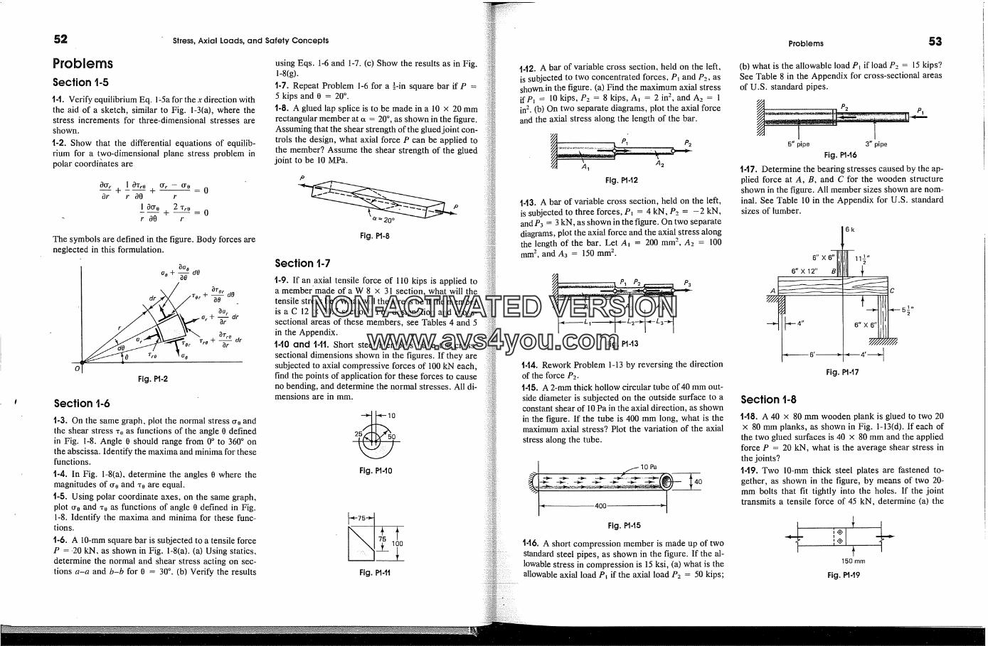
52 Stress, Axial Loads, and Safety Concepts
Problems
Section t-5
1-1. Verify equilibrium Eq. l:5a for the x direction withthe aid of a sketch, similar to Fig. l-3(a), where thestress increments for three-dimensional stresses areshown.
1-2. Show that the differential equations of equilib-rium for a two-dimensional plane stress problem inpolar coordihates are
0[J'._._�r2r' I 0Tr0 O'r --o,. ;W +-- -oI'
I Ocro 2 *rer O0 r
The symbols are defined in the figure. Body forces areneglected in this formulation.
go 0% + -�- ao
/ �TOr\dr�(�/7�r+-� dO_
/ / � � x art� dr
�0 �o �%
Fig. �-2
Section
t-3. On the same graph, plot the normal stress froandthe shear stress ,, as functions of the angle 0 definedin Fig. 1-8. Angle 0 should range from 0 � to 360 � onthe abscissa. Identify the maxima and minima for thesefunctions.
1-4. In Fig. l-8(a), determine the angles 0 where themagnitudes of {r, and ,o are equal.t-5. Using polar coordinate axes, on the same graph,plot {r0 and �'o as functions of angle 0 defined in Fig.1-8. Identify the maxima and minima for these func-
tions.
t-6. A 10-mm square bar is subjected to a tensile forceP = -20 kN, as shown in Fig. 1-8(a). (a) Using statics,determine the normal and shear stress acting on sec-tions a-a and b-b for 0 = 30 �. (b) Verify the results
using Eqs. 1-6 and 1-7. (c) Show the results as in Fig.1-8(g).
t-7. Repeat Problem 1-6 for a �-in square bar if P =5 kips and 0 = 20 �.t-8. A glued lap splice is to be made in a 10 x 20 mmrectangular member at a = 20 �, as shown in the figure.Assuming that the shear strength of the glued joint con-trols the design, what axial force P can be applied tothe member? Assume the shear strength of the glued
joint to be 10 MPa.
c� � 20 �
Fig. PI-8
Section t-7
t-9. If an axial tensile force of 110 kips is applied toa member' made of a W 8 x 31 section, what will thetensile stress be? What will the stress be if the memberis a C 12 x 20.7 section? For designation and cross-sectional areas of these members, see Tables 4 and 5in the Appendix.t-10 and 1-11. Short steel members have the cross-sectional dimensions shown in the figures. If they aresubjected to axial compresslye forces of 100 kN each,find the points of application for these forces to causeno bending, and determine the normal stresses. All di-mensions are in mm.
Fig. DI-10
Fig. Pt-tt
t42. A bar of variable cross section, held on the left,is subjected to two concentrated forces, P� and P2, asshown. in the figure. (a) Find the maximum axial stressifp� = 10 kips, P2 = 8 kips, A� = 2 in 2, and A_� = 1in 2. (b) On two separate diagrams, plot the axial forceand the axial stress along the length of the bar.
Pl P2
A� A2Fig. P1-12
t-13. A bar of variable cross section, held on the left,is subjected to three forces, P� = 4 kN, P2 = --2 kN,and P3 = 3 kN, as shown in the figure. On two separatediagrams, plot the axial force and the axial stress alongthe length of the bar. Let A� = 200 mm 2, A2 = 100mm 2, andA3 = 150mm 2.
P3
A 1 A2 A3
Fig. PI-t3
144. Rework Problem 1~13 by reversing the directionof the force P2.1-15. A 2-mm thick hollow circular tube of 40 mm out-side diameter is subjected on the outside surface to aconstant shear of 10 Pa in the axial direction, as shownin the figure. If the tube is 400 mm long, what is themaximum axial stress? Plot the variation of the axialstress along the tube.
140
400
Fig. PI-t5
1-t6. A short compression member is made up of twostandard steel pipes, as shown in the figure. If the al-lowable stress in compression is 15 ksi, (a) what is theallowable axial load P� if the axial load P2 = 50 kips;
Problems 53
(b) what is the allowable load P� if load P2 = 15 kips?See Table 8 in the Appendix for cross-sectional areasof U.S. standard pipes.
P2 Pl
I5" pipe 3" pipe
Fig. P1-t6
t-t7. Determine the bearing stresses caused by the ap-plied force at A, B, and C for the wooden structureshown in the figure. All member sizes shown are nom-inal. See Table 10 in the Appendix for U.S. standardsizes of lumber.
6k
6" X 16" X 12"
--�1�4'"6'-------.� -"�--- 4'Fig. PM7
c
Section t-8
1-18. A 40 x 80 mm wooden plank is glued to two 20x 80 mm planks, as shown in Fig. 1-13(d). If each of
the two glued surfaces is 40 x 80 mm and the appliedforce P = 20 kN, what is the average shear stress inthe joints?t-19. Two 10-mm thick steel plates are fastened to-gether, as shown in the figure, by means of two 20-mm bolts that fit tightly into the holes. If the jointtransmits a tensile force of 45 kN, determine (a) the
l �0 mm
Fig. Pt-19
NON-ACTIVATEDVERSIONwww.avs4you.com
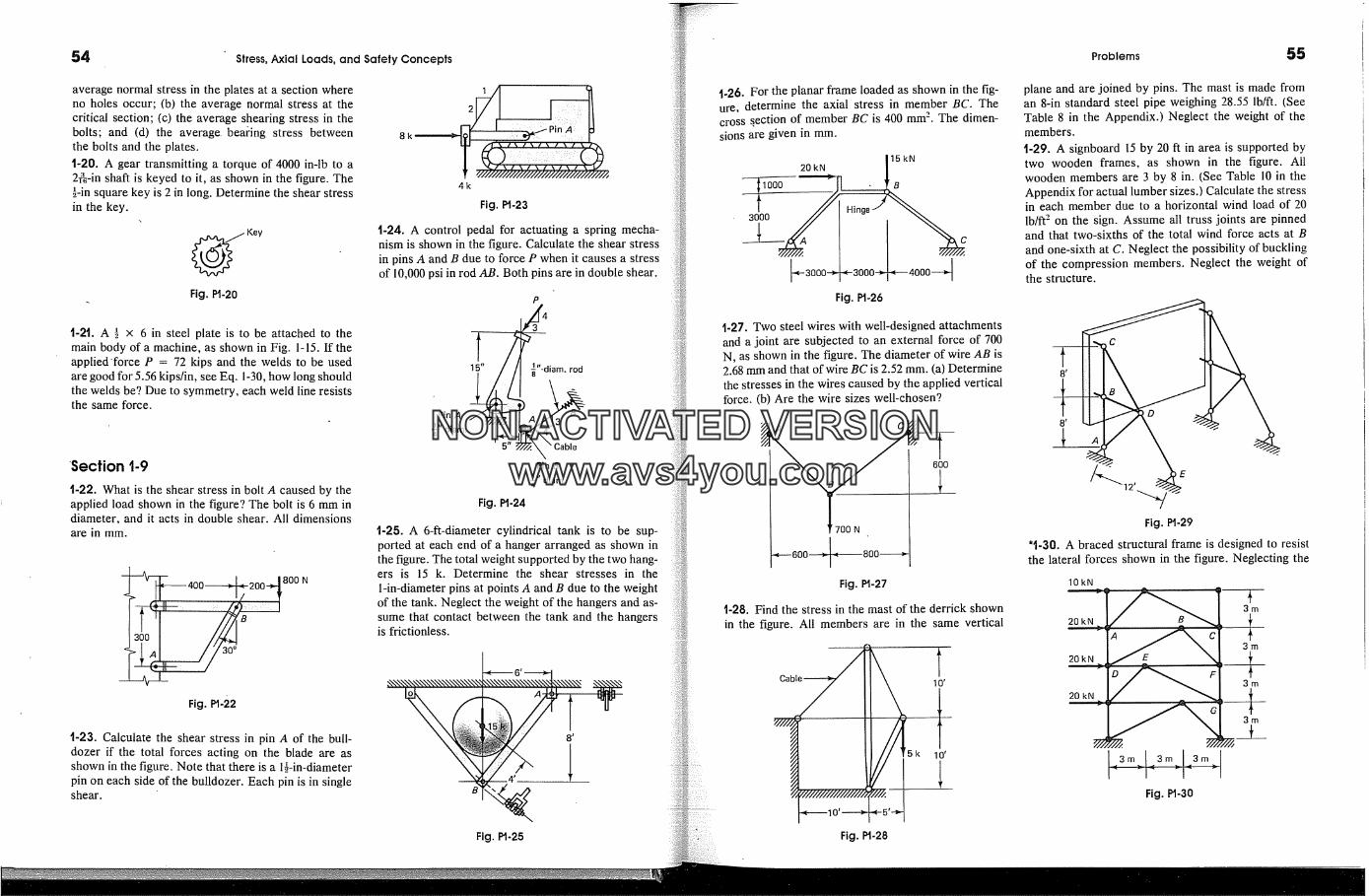
54 Stress, Axial Loads, and Safety Concepts
average normal stress in the plates at a section whereno holes occur; (b) the average normal stress at thecritical section; (c) the average shearing stress in thebolts; and (d) the average. beai'ing stress betweenthe bolts and the plates.1-20. A gear transmitting a torque of 4000 in-lb to a2�-in shaft is keyed to it, as shown in the figure. The�-in square key is 2 in long. Determine the shear stressin the key.
KeyFig. Pt-20
1-2t. A � x 6 in steel plate is to be attached to themain body of a machine, as shown in Fig. 1-15. If theapplied'force P = 72 kips and the welds to be usedare good for 5.56 kips/in, see Eq. 1-30, how long shouldthe welds be? Due to symmetry, each weld line resiststhe same force.
'Section t-9
1-22. What is the shear stress in bolt A caused by theapplied load shown in the figure? The bolt is 6 mm indiameter, and it acts in double shear. All dimensionsare in min.
�-'� 400�200� 800
Fig. Pt-22
t-23. Calculate the shear stress in pin A of the bull-dozer if the total forces acting on the blade are asshown in the figure. Note that there is a l�-in-diameterpin on each side of the bulldozer. Each pin is in singleshear.
! /////////////////////////////////////,4k
Fig. Pt-23
1-24. A control pedal for actuating a spring mecha-nism is shown in the figure. Calculate the shear stressin pins A and B due to force P when it causes a stressof 10,000 psi in rod AB. Both pins are in double shear.
' p-� "diam. rod
�' CablePin B
1. di7 am.
Fig. Pt-24
1-25. A 6-ft-diameter cylindrical tank is to be sup-ported at each end of a hanger arranged as shown inthe figure. The total weight supported by the two hang-ers is 15 k. Determine the shear stresses in the
1-in-diameter pins at points A and B due to the weightof the tank. Neglect the weight of the hangers and as-sume that contact between the tank and the hangersis frictionless.
8 t
Fig. Pt-25
t-26. For the planar frame loaded as shown in the fig-ure, determine the axial stress in member BC. Thecross s. ection of member BC is 400 mm 2. The dimen-sions are given in mm.
20 kN
.�-3000-�
Hing�L�C.15 kN
-�-3000 � < 4000Fig. Pt-26
t-27. Two steel wires with well-designed attachmentsand a joint are subjected to an external force of 700N, as shown in the figure. The diameter of wire AB is2.68 mm and that of wire BC is 2.52 mm. (a) Determinethe stresses in the wires caused by the applied verticalforce. (b) Are the wire sizes well-chosen?
T 700 N
�,t 600 �-< 800----*'-Fig. Pt-27
t-28. Find the stress in the mast of the derrick shownin the figure. All members are in the same vertical
Fig. Pt-28
Problems
plane and are joined by pins. The mast is made froman 8-in standard steel pipe weighing 28.55 lb/ft. (SeeTable 8 in the Appendix.) Neglect the weight of themembers.
t-29. A signboard 15 by 20 ft in area is supported bytwo wooden frames, as shown in the figure. Allwooden members are 3 by 8 in. (See Table 10 in theAppendix for actual lumber sizes.) Calculate the stressin each member due to a horizontal wind load of 20Ib/ft 2 on the sign. Assume all truss joints are pinnedand that two-sixths of the total wind force acts at Band one-sixth at C. Neglect the possibility of bucklingof the compression members. Neglect the weight ofthe structure.
Fig. DI-29
'1-30. A braced structural frame is designed to resistthe lateral forces shown in the figure. Neglecting the
10kN
20 kN
20 kN
20 kN
Fig. Pt-30
NON-ACTIVATEDVERSIONwww.avs4you.com
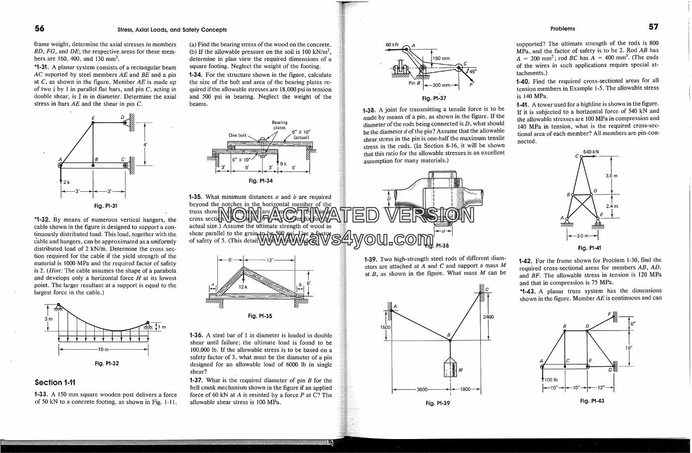
56 Stress, Axial Loads, and Safety Concepts
frame weight, determine the axial stresses in membersBD, FG, and DE; the respective areas for these mem-bers are 160, 400, and 130 mm 2.'1-31. A planar system consists of a rectangular beamAC suported by steel members AE and BE and a pinat C, as shown in the figure. Member AE is made upof two r� by I in parallel flat bars, and pin C, acting indouble shear, is � in in diameter. Determine the axialstress in bars AE and the shear in pin C.
'� 3' � �- 3' �Fig. Pt-31
't-32. By means of numerous vertical hangers, thecable shown in the figure is designed to support a con-finuously distributed load. This load, tosether with the�able and han�ers, can be approximated as a uniformlydistributed load of 2 kN/m. Determine the cross sec-tion required [or the cable if the yield strength o[ thematerial is 1000 MPa and the required [actor of safetyis 2. (Hfi�: The cable assumes the shape of a parabolaand develops only a horizontal [orce � at Rs lowestpoinL The larser resultant at a support is equal to thelarsest [orce in the cable.)
rn
10 m �"lFig. F�1-32
Section 1-11
1-33. A 150 mm square wooden post delivers a forceof 50 kN to a concrete footing, as shown in Fig. 1-11.
(a) Find the bearing stress of the wood on the concrete.(b) If the allowable pressure on the soil is 100 kN/m 2,determine in plan view the required dimensions of asquare footing. Neglect the weight of the footing.t-34. For the structure shown in the figure, calculatethe size of the bolt and area of the bearing plates re-quired if the allowable stresses are 18,000 psi in tensionand 500 psi in bearing. Neglect the weight of thebeams.
Bearingplates
// 6" X 10"
One bolt .,,�/ / (actual)
Fig. Pt-34
t-35. What minimum distances a and b are requiredbeyond the notches in the horizontal member of thetruss shown? All members are nominally 8 by 8 in incross section. (See Table 10 in the Appendix for theactual size.) Assume the ultimate strength of wood inshear parallel to the grain to be 500 psi. Use a factorof safety of 5. (This detail is not recommended.)
Fig. Pt-35
1-36. A steel bar of 1 in diameter is loaded in doubleshear until failure; the ultimate load is found to be100,000 lb. If the allowable stress is to be based on a
safety factor of 3, what must be the diameter of a pindesigned for an allowable load of 6000 lb in singleshear?
1-31. What is the required diameter of pin B for thebell crank mechanism shown in the figure if an appliedforce of 60 kN at A is resisted by a force P at C? Theallowable shear stress is 100 MPa.
60kN t,.2� A
-.,Fig. Pt[37
t.38. A joint for transmitting a tensile force is to bemade by means of a pin, as shown in the figure. If thediameter of the rods being connected is D, what shouldbe the diameter d of the pin? Assume that the allowableshear. stress in the pin is one-half the maximum tensilestress in the rods. (In Section 8-16, it will be shownthat this ratio for the allowable stresses is an excellentassumption for many materials.)
Fig. Pt.38
t-39. Two high-strength steel rods of different diam-eters are attached at A and C and support a mass Mat B, as shown in the figure. What mass M can be
1500 A /.3600
2400
Fig. Pt-39
Problems �7
supported? The ultimate strength of the rods is 800MPa, and the factor of safety is to be 2. Rod AB hasA = 200 mm2; rod BC has A = 400 mm 2. (The endsof the wires in such applications require special at-tachments.)1-40. Find the required cross-sectional areas for alltension members in Example 1-5. The allowable stressis 140 MPa.
1-4t. A tower used for a highline is shown in the figure.If it is subjected to a horizontal force of 540 kN andthe allowable stresses are 100 MPa in compression and140 MPa in tension, what is the required cross-sec-tional area of each member? All members are pin-con-nected.
540 kN
3.0 rn vFig. Pt-41
t-42. For the frame shown for Problem 1-30, find therequired cross-sectional areas for members AB, AD,and BF. The allowable stress in tension is 120 MPaand that in compression is 75 MPa.'t-43. A planar truss system has the dimensionsshown in the figure. Member AE is continuous and can
Fig. Pt-43
NON-ACTIVATEDVERSIONwww.avs4you.com

58 ' Stress, Axial Loads, and Safety Concepts
resist bending. All joints are pinned. Determine thediameter required for tension member AB to carry theapplied force at A. The allowable stress is 20 ksi.'1-44. A planar frame has .the dimensions shown inthe figure. Members AC and DF are continuous andcan resist bending. All joints are pinned. Determinethe diameter required of a high-strength steel rod formember CD. Assume that the ultimate strength for therod is 1250 MPa and that the efficiency of the end at-tachments is-80%. The safety factor for the rod is 2.
D 20 kN
2m
2m
'2m
Fig. Pt-44
'%45. To support a load P = 180 kN, determine thenecessary diameter for rods AB and AC for the tripodshown in the figure. Neglect the weight of the structureand assume that the joints are pin-connected. No al-lowance has to be made for threads. The allowabletensile stress is 125 MPa. All dimensions are in meters.
A
R�ds,l��
Fig. Pt-45
*%46. A pin-connected frame for supporting a forceP is shown in the figure. Stress cr in both members ABand BC is to be the same. Determine the angle a nec-essary to achieve the minimum weight of construction.Members AB and BC have a constant cross section.
< L ct�) P
Fig. Pt-46
t-47. Three equal 0.5-kg masses hre attached to a 10-mm-diameter wire, as shown in the figure, and are ro-tated around a vertical axis, as shown in Fig. 1-25, ona frictionless plane at 4 Hz. Determine the axialstresses in the three segments of the wire and plot theresults on a diagram as a function of r. Consider themasses to be concentrated as points.
"<-'0.6 m--�0.6 m-�i< 0.6 m-�- 1Fig. P1-47
't-48. A bar of constant cross-sectional area A is ro-tated around one of its ends in a horizontal plane witha constant angular velocity o�. The unit weight of thematerial is "1. Determine the variation of the stress cralong the bar and plot the result on a diagram as afunction of r.
r �LFig. Pt.48
Section 1-12
t-49. Rework Example 1-7 for D. = L. = 10 kips.With the help of this additional solution, what conclu-
sions can be drawn regarding the ASD and LRFD de-sign approaches?
Section 1-131-50. Find the capacity of tension member AB of theFink truss shown in the figure if it is made from two3 by 2 by � in angles (see Table 7 in the Appendix)attached to a �-in-thick gusset plate by four �-in high-
�4n diameter holes. The allowablestrength bolts in "�'stresses are 22 ksi in tension, 15 ksi in shear, and 87ksi in bearing on the angles as well as the gusset.
D C
(a)
P2 P�p;�O�O 1,02'�..Z 2 angles
7//-7' 3" x 2" 1 75"� I I � Section 1-1
ooooo I' I P4 Gusset 3/8"
Detail at A ' thick
(b)
Fig. 1�1'50
%5L Find the capacity of a standard connection for aW 12 x 36 beam shown in the figure. The connection
Problems 59
consists of two 4 x 3� x � in angles, each 8� in long;� in high-strength bolts spaced 3 in apart are used in
-in holes. Use the allowable stresses given in Prob-lem 1-50.
W12X36
Fig. P1-5t
t-52. A structural multiple-riveted lap joint, such asis shown in the figure, is designed for a 42-kip load.The plates are { in thick by 10 in wide. The rivets in{-in holes are { in. (a) What is the shear stress in themiddle rivet? (b) What are the tensile stresses in theupper plate in rows 1-1 and 2-29.
o 9 o I2o,
Fig. 1�1-52
Section 144
t-53. Rework Example 1-8 for an 8 x 6 x � in angleusing �- n fdlet welds.
NON-ACTIVATEDVERSIONwww.avs4you.com
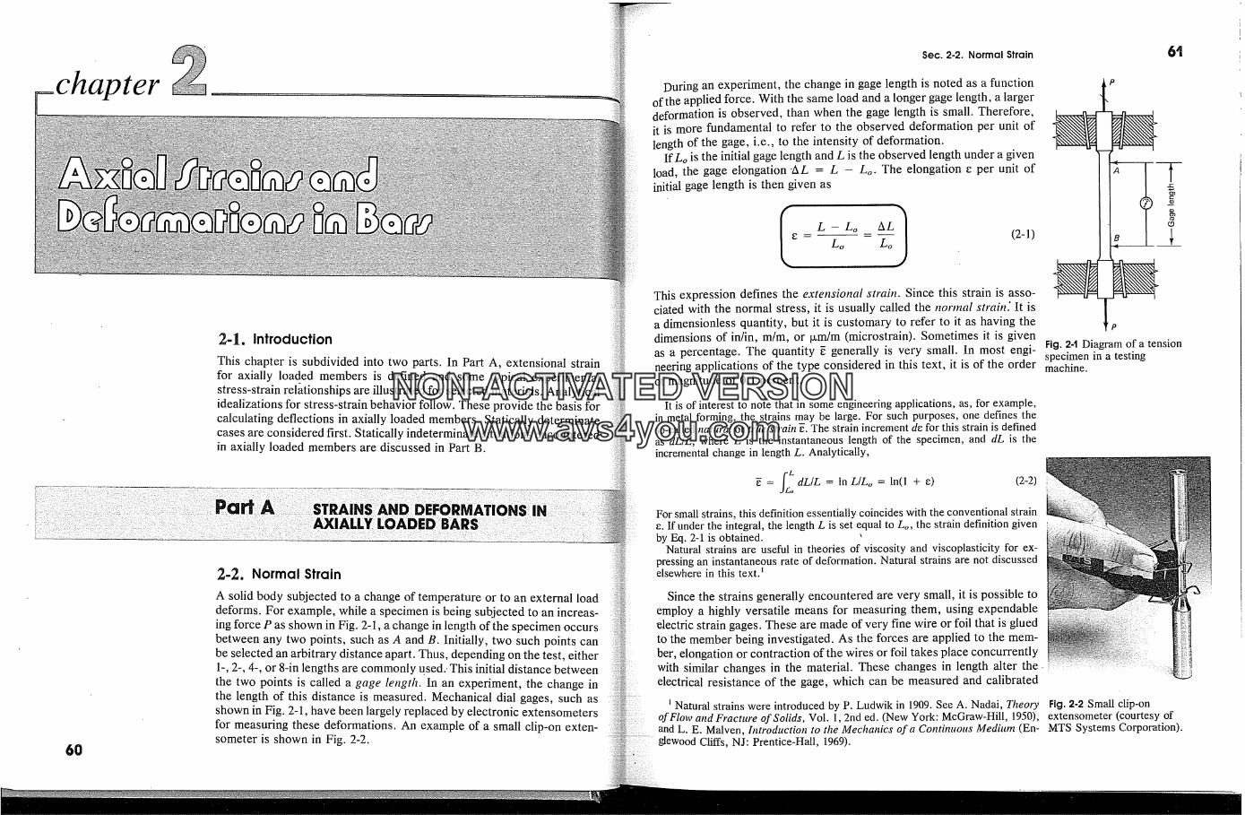
60
pter
2-1. Introduction
This chapter is subdivided into two parts. In Part A, extensional strainfor axially loaded members is defined and some typical experimentalstress-strain relationships are illustrated for selected materials. Analyticalidealizations for stress-strain behavior follow. These provide the basis forcalculating deflections in axially loaded members. Statically determinatecases are considered first. Statically indeterminate situations encounteredin axially loaded members are discussed in Part B.
2-2. Normal Strain
A solid body subjected to a change of temperature or to an external loaddeforms. For example, while a specimen is being subjected to an increas-ing force P as shown in Fig. 2-1, a change in length of the specimen occursbetween any two points, such as A and B. Initially, two such points canbe selected an arbitrary distance apart. Thus, depending on the test, either1-, 2-, 4-, or 8-in lengths are commonly used.. This initial distance betweenthe two points is called a gage length. In an experiment, the change inthe length of this distance is measured. Mechanical dial gages, such asshown in Fig. 2-1, have been largely replaced by electronic extensometersfor measuring these deformations. An example of a small clip-on exten-someter is shown in Fig. 2-2.
Sec. 2-2. Normal Strain
During an experiment, the change in gage length is noted as a functionof the applied force. With the same load and a longer gage length, a largerdeformation is observed, than when the gage length is small. Therefore,it is more fundamental to refer to the observed deformation per unit oflength of the gage, i.e., to the intensity of deformation.
IfLo is the initial gage length and L is the observed length under a givenload, the gage elongation 'AL = L - Lo. The elongation e per unit ofinitial gage length is then given as
(2-1)
This expression defines the extensional strain. Since this strain is asso-ciated with the normal stress, it is usually called the nor/nal strain.' It isa dimensionless quantity, but it is customary to refer to it as having thedimensions of in/in, m/m, or txm/m (microstrain). Sometimes it is givenas a percentage. The quantity � generally is very small. In most engi-neering applications of the type considered in this text, it is of the orderof magnitude of 0. I percent.
It is of interest to note that in some engineering applications, as, for example,in metal forming, the strains may be large. For such purposes, one defines theso-called natural or true strabz �. The strain increment de for this strain is definedas dL/L, where L is the instantaneous length of the specimen, and dL is theincremental change in length L. Analytically,
� = dL/L = In L/Lo = In(1 + e)o
(2-2)
For small strains, this definition essentially coincides with the conventional straine. If under the integral, the length L is set equal to Lo, the strain definition givenby Eq. 2-1 is obtained. �
Natural strains are useful in theories of viscosity and viscoplasticity for ex-pressing an instantaneous rate of deformation. Natural strains are not discussedelsewhere in this text?
Since the strains generally encountered are very small, it is possible toemploy a highly versatile means for measuring them, using expendableelectric strain gages. These are made of very fine wire or foil that is gluedto the member being investigated. As the forces are applied to the mem-ber, elongation or contraction of the wires or foil takes place concurrentlywith similar changes in the material. These changes in length alter theelectrical resistance of the gage, which can be measured and calibrated
t Natural strains were introduced by P. Ludwik in 1909. See A. Nadai, Theoryof Flow and Fracture of Solids, Vol. 1, 2nd ed. (New York: McGraw-Hill, 1950),and L. E. Malven, Introduction to the Mechanics of a Continuous Medium (En-glewood Cliffs, N J: Prentice-Hall, 1969).
6t
P
Fig. 2-'1 Diagram of a tensionspecimen in a testingmachine.
Fig. 2-2 Small clip-onextensometer (courtesy ofMTS Systems Corporation).
NON-ACTIVATEDVERSIONwww.avs4you.com
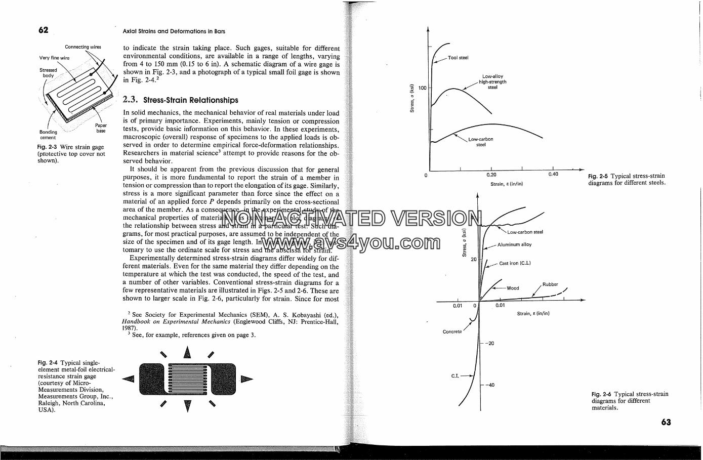
Axial Strains and Deformations in Bars
Connecting wires
Veryfinewire .�'�
/ - -Y paperBonding basecement
Fig. 2-3 Wife strain gage(protective top cover notshown).
Fig. 2-4 Typical single-element metal-foil electrical-resistance strain gage(courtesy of Micro-Meas. urements Division,Measurements Group, Inc.,Raleigh, North Carolina,USA).
to indicate the strain taking place. Such gages, suitable for differentenvironmental conditions, are available in a range of lengths, varyingfrom 4 to 150 mm (0.15 to 6 in). A schematic diagram of a wire gage isshown in Fig. 2-3, and a photograph of a typical small foil gage is shownin Fig. 2-4. 2
2.3. Stress-Strain RelationshipsIn solid mechanics, the mechanical behavior of real materials under loadis of primary importance. Experiments, mainly tension or compressiontests, provide basic information on this behavior. In these experiments,macroscopic (overall) response of specimens to the applied loads is ob-served in order to determine empirical force-deformation relationships.Researchers in material science 3 attempt to provide reasons for the ob-served behavior.
It should be apparent from the previous discussion that for generalpurposes, it is more fundamental to report the strain of a member intension or compression than to report the elongation of its gage. Similarly,stress is a more significant parameter than force since the effect on amaterial of an applied force P depends primarily on the cross-sectionalarea of the member. As a consequence, in the experimental study of themechanical properties of matedhals, it is customary to plot diagrams ofthe relationship between stress and strain in a particular test. Such dia-grams, for most practical purposes, are assumed to be independent of thesize of the specimen and of its gage length. In these diagrams, it is cus-tomary to use the ordinate scale for stress and the abscissa for strain.
Experimentally determined stress-strain diagrams differ widely for dif-ferent materials. Even for the same material they differ depending on thetemperature at which the test was conducted, the speed of the test, anda number of other variables. Conventional stress-strain diagrams for afew representative materials are illustrated in Figs. 2-5 and 2-6. These areshown to larger scale in Fig. 2-6, particularly for strain. Since for most
2 See Society for Experimental Mechanics (SEM), A. S. Kobayashi (ed.),Handbook on Experimental Mechanics (Englewood Cliffs, NJ: Prentice-Hall,1987).
3 See, for example, references given on page 3.
100
�Tool steelLow-alloy
t;elnt"Low�car�
steel
I t0.20 0.40
Strain, � (in/in)
20�,Cast iron(C.I.)� /�Wood /Rubber
0.01 0 0.01
Concrete/ Strain,�(in/in)- -20
C.I./ --40
Fig. 2-5 Typical stress-straindiagrams for different steels.
Fig. 2-6 Typical stress-straindiagrams for differentmaterials.
65
NON-ACTIVATEDVERSIONwww.avs4you.com
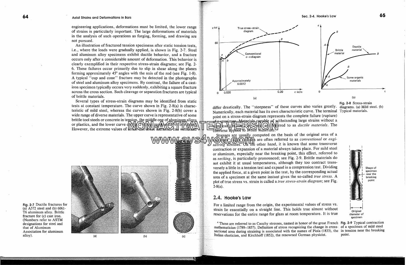
64
Fig. 2-7 Ductile fractures for(a) A572 steel and (b) 6061-T6 aluminum alloy. Brittlefracture for (c) cast iron.(Numbers refer to ASTMdesignations for steel andthat of AluminumAssociation for aluminumalloy).
Axial Strains and Deformations in Bars
engineering applications, deformations must be limited, the lower rangeof strains is particularly important. The large deformations of materialsin the analysis of such operations as forging, forming, and drawing arenot pursued.
An illustration of fractured tension specimens after static tension tests,i.e., where the loads were gradually applied, is shown in Fig. 2-7. Steeland aluminum alloy specimens exhibit ductile behavior, and a fractureoccurs only after a considerable amount of deformation. This behavior isclearly exemplified in their respective stress-strain diagrams; see Fig. 2-6. These failures occur primarily due to slip in shear along the planesforming approximately 45 � angles with the axis of the rod (see Fig. 1-8).A typical "cup and cone" fracture may be detected in the photographsof steel and aluminum alloy specimens. By contrast, the failure of a cast-iron specimen typically occurs very suddenly, exhibiting a square fractureacross the cross section. Such cleavage or separation fractures are typicalof brittle materials.
Several types of stress-strain diagrams may be identified from statictests at constant temperature. The curve shown in Fig. 2-8(a) is charac-teristic of mild steel, whereas the curves shown in Fig. 2-8(b) cover awide range of diverse materials. The upper curve is representative of somebrittle tool steels or concrete in tension, the middle one of aluminum alloysor plastics, and: the lower curve of Fig. 2-8(b) is representative of rubber.However, the extreme values of strain that these materials can withstand
(a) (b) (c)
Sec. 2-4. Hooke's Law 65
oksi1True stress-strain
diagram
//� Conv�ptio0al� �di�m
Approximately0.0012
0 0.020 0.20 � in/in(a)
B
A/ Ductile� B ri�l�a I material x"�
�A� materials
differ drastically. The "steepness" of these curves also varies greatly.Numerically, each material has its own characteristic curve. The terminalpoint on a stress-strain diagram represents the complete failure (rupture)of a specimen. Materials capable of withstanding large strains without asignificant increase in stress are referred to as ductile /naterials. Theconverse applies to brittle materials.
Stresses are usually computed on the basis of the original area of aspecimen4; such stresses are often referred to as conventional or engi-neering stresses. On the other hand, it is known that some transversecontraction or expansion of a material always takes place. For mild steelor aluminum, especially near the breaking point, this effect, referred toas necking, is particularly-pronounced; see Fig. 2-9. Brittle materials donot exhibit it at usual temperatures, although they too contract trans-versely a little in a tension test and expand in a compression test. Dividingthe applied force, at a given point in the test, by the corresponding actualarea of a specimen at the same instant gives the so-called trtte stress. Aplot of true stress vs. strain is called a true stress-strain diagram; see Fig.2-8(a).
2.4. Hooke's Law
For a limited range from the origin, the experimental values of stress vs.strain lie essentially on a straight line. This holds true almost withoutreservations for the entire range for glass at room temperature. It is true
(b)
Fig. 2-8 Stress-straindiagrams. (a) Mild steel. (b)Typical materials.
I I
Shape ofI specimenI neartheI breakingI point1
I
Originaldiameter of
specimen
4 These are referred to as Cauchy stresses, named in honor of the great French Fig. 2-9 Typical contractionmathematician (1789-1857). Definition of stress recognizing the change in cross- of a specimen of mild steelsectional area during straining is associated with the names of Piola (1833), the in tension near the breakingItalian elasticJan, and Kirchhoff (1852), the renowned German physicist. point.
NON-ACTIVATEDVERSIONwww.avs4you.com
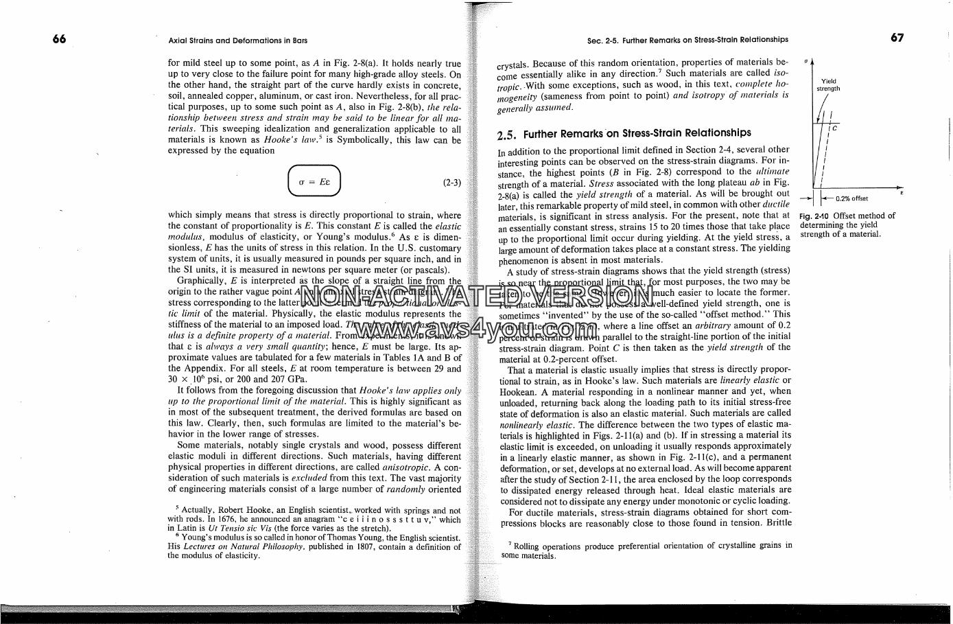
66 Axial Strains and Deformations in Bars
for mild steel up to some point, as A in Fig. 2-8(a). It holds nearly trueup to very close to the failure point for many high-grade alloy steels. On
the other hand, the straight part of the curve hardly exists in concrete,soil, annealed copper, aluminum, or cast iron. Nevertheless, for all prac-tical purposes, up to some such point as A, also in Fig. 2-8(b), the rela-tionship between stress and strain may be said to be l#�ear for all ma-terials. This sweeping idealization and generalization applicable to allmaterials is known as Hooke's law/ is Symbolically, this law can beexpressed by the equation
(2-3)
which simply means that stress is directly proportional to strain, wherethe constant of proportionality is E. This constant E is called the elasticmodulus, modulus of elasticity, or Young's modulus. 6 As e is dimen-sionless, E has the units of stress in this relation. In the U.S. customarysystem of units, it is usually measured in pounds per square inch, and inthe SI units, it is measured in newtons per square meter (or pascals).
Graphically, E is interpreted as the slope of a straight line from theorigin to the rather vague point A on a uniaxial stress-strain diagram. Thestress corresponding to the latter point is termed the proportional or elas-tic litnit of the material. Physically, the elastic modulus represents thestiffness of the material to an imposed load. The value of the elastic mod-alles is a definite property of a material. From experiments, it is knownthat e is always a very small qaantity; hence, E must be large. Its ap-proximate values are tabulated for a few materials in Tables 1A and B ofthe Appendix. For all steels, E at room temperature is between 29 and30 x 106 psi, or 200 and 207 GPa.
It f�llows from the foregoing discussion that Hooke's law applies onlyup to the proportional litnit of the material. This is highly significant asin most of the subsequent treatment, the derived formulas are based onthis law. Clearly, then, such formulas are limited to the material's be-havior in the lower range of stresses.
Some materials, notably single crystals and wood, possess differentelastic moduli in different directions. Such materials, having differentphysical properties in different directions, are called anisotropic. A con-sideration of such materials is excluded from this text. The vast majorityof engineering materials consist of a large number of randomly oriented
'� Actually, Robert Hooke, an English scientist,. worked with springs and notwith rods. In 1676, he announced an anagram "c e i i i n o s s s t t u v," whichin Latin is Ut Tensio sic Vis (the force varies as the stretch).
� Young's modulus is so called in honor of Thomas Young, the English scientist.His Lectures on Natural Philosophy, published in 1807, contain a definition ofthe modulus of elasticity.
Sec. 2-5. Further Remarks on Stress-Strain Relationships
crystals. Because of this random orientation, properties of materials be-come essentially alike in any direction. 7 Such materials are called iso-tropic.-With some exceptions, such as wood, in this text, complete ho-mogeneity (sameness from point to point) and isotropy of materials isgenerally assumed.
2.5. Further Remarks 'on Stress-Strain RelationshipsIn addition to the proportional limit defined in Section 2-4, several otherinteresting points can be observed on the stress-strain diagrams. For in-stance, the highest points (B in Fig. 2-8) correspond to the ldtimatestrength of a material. Stress associated with the long plateau ab in Fig.2-8(a) is called the yield strength of a material. As will be brought outlater, this remarkable property of mild steel, in common with other ductilematerials, is significant in stress analysis. For the present, note that atan essentially constant stress, strains 15 to 20 times those that take pl.aceup to the proportional limit occur during yielding. At the yield stress, alarge amount of deformation takes place at a constant stress. The yieldingphenomenon is absent in most materials.
A study of stress-strain diagrams shows that the yield strength (stress)is so near the proportional limit that, for most purposes, the two may betaken to be the same. However, it is much easier to locate the former.For materials that do not possess a well-defined yield strength, one issometimes "invented" by the use of the so-called "offset method." Thisis illustrated in Fig. 2-10, where a line offset an arbitrm�y amount of 0.2percent of strain is drawn parallel to the straight-line portion of the initialstress-strain diagram. Point C is then taken as the yield strength of thematerial at 0.2-percent offset.
That a material is elastic usually implies that stress is directly propor-tional to strain, as in Hooke's law. Such materials are linearly elastic orHookean. A material responding in a nonlinear manner and yet, whenunloaded, returning back along the loading path to its initial stress-freestate of deformation is also an elastic material. Such materials are callednonlinearly elastic. The difference between the two types of elastic ma-terials is highlighted in Figs. 2-1 l(a) and (b). If in stressing a material itselastic limit is exceeded, on unloading it usually responds approximatelyin a linearly elastic manner, as shown in Fig. 2-11(c), and a permanentdeformation, or set, develops at no external load. As will become apparentafter the study of Section 2-11, the area enclosed by the loop correspondsto dissipated energy released through heat. Ideal elastic materials areconsidered not to dissipate any energy under monotonic or cyclic loading.
For ductile materials, stress-strain diagrams obtained for short com-pressions blocks are reasonably close to those found in tension. Brittle
* Rolling operations produce preferential orientation of crystalline grains insome materials.
Yieldstrength
v/--� �- 0.2% offsetFio. 240 Offset method ofdetermining the yieldstrength of a material.
67
NON-ACTIVATEDVERSIONwww.avs4you.com

Permanent Elastic(a) (b)set recovery
Dissipatedelergy
E
(c)
Fig. 2-1t Stress-strain diagrams: (a) linear elastic material, (b) nonlinear elastic material, and (c) inelastic orplastic material.
P materials, such as cast iron and concrete are very weak in tension butnot in compression. For these materials, the diagrams differ considerably,depending on the sense of the applied force.
It is well to note that in some of the subsequent analyses, it will beadvantageous to refer to elastic bodies and systems as springs. Sketchessuch as shown in Fig. 2-12 are frequently used in practice for interpretingthe physical behavior of mechanical systems.
P
P
(a)
(b)
Fig. 2-t2 Linear (Hookean)and nonlinear springresponse.
2.6. Other Idealizations of Constitutive Relations
In an increasingly larger number of technical problems, stress analysesbased on the assumption of linearly elastic behavior are insufficient. Forthis reason, several additional stress-strain relations are now in generaluse. Such relations are frequently referred to as constitutive relations orlaws. The three idealized stress-strain relations shown in Fig. 2-13 areencountered particularly often. The two shown in Figs. 2-13(a) and (b)will be used in this text; the one in Fig. 2-13(c) is often more realistic,however, its use is considerably more complicated and generally will beavoided because of the introductory nature of this book.
The idealized �-e relationship shown in Fig. 2-13(a) is applicable toproblems in which the elastic strains can be neglected in relation to theplastic ones. This occurs if plastic (inelastic) strains are dominant. Per-fectly (ideally) plastic behavior means that a large amount of unboundeddeformation can take place at a constant stress. The idealization shownin Fig. 2-13(b) is particularly useful if both the elastic and plastic strainshave to be included. This situation frequently arises in analysis. Both ofthe previous idealizations are patterned after the behavior of low-carbonsteel (see Figs. 2-6 and 2-8), where at �he yield stress %,�,, a substantialplateau in the stress-strain diagram is generally observed. In both in-stances, it is assumed that the mechanical properties of the material arethe same in tension and in compression, and %,,, = [ -%, I. It is alsoassumed that during unloading, the material behaves elastically. In such
68
Sec. 2-6. Other Idealizations of Constitutive Relations 69
i II
II
Gyp
//
/
(a) (b) (c)
Fig. 2-t3 Idealized stress-strain diagrams: (a) rigid-perfectly plastic material; (b) elastic-perfectly plasticmaterial; and (c) elastic-linearly hardening material.
a case, a stress.can range and terminate anywhere between +%,, and-%,�. For moderate amounts of plastic straining, this assumption is in
good agreement with experimental observations.The �-e idealization shown in Fig. 2-13(c) provides a reasonable ap-
proximation for many materials and is more accurate than the previousmodels over a wider range of strain. Beyond the elastic range, on anincrease in strain, many materials resist additional stress, a phenomenonreferred to as strain hardening.
In some refined analyses, the stress-strain idealization shown in Fig.2-13 may not be sufficiently accurate. Fortunately, with the use of com-puters, much better modeling of constitutive relations for real material ispossible. For completeness, one such well-known algebraic formulationfollows. In as much as implementation of such formulations requires aconsiderable amount of computer programming, this approach is not in-tended for general use in this text.
An equation capable of representing a wide range of stress-strain curveshas been developed by Ramberg and Osgood. s This equation 9 is
e � +3 (__�'�" (2-4)�o Cro � \fro/
where eo, �o, and n are characteristic constants for a material. The con-stants eo and �o correspond to the yield point, which, for all cases other
8 W. Ramberg and W. R. Osgood, Description of Stress-Strain Curves by ThreeParameters, National Advisory Committee on Aeronautics, TN 902, 1943.
9 The coefficient 3/7 is chosen somewhat arbitrarily; different values have beenused in some investigations. In this formulation, a discontinuity in the functionarises when n = m.
NON-ACTIVATEDVERSIONwww.avs4you.com
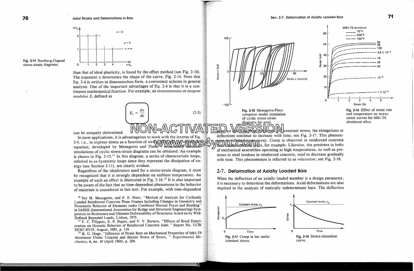
7O
Fig. 244 Ramberg-Osgoodstress-strain. diagrams.
Axial Strains and Deformations in Bars
n=2
2
0 1 2 3 4 �/%
than that of ideal plasticity, is found by the offset method (see Fig. 2-10).The exponent n determines the shape of the curve, Fig. 2-14. Note thatEq. 2-4 is written in dimensionless form, a convenient scheme inanalysis. One of the important advantages of Eq. 2-4 is that it is a con-tinuous mathematical function. For example, an instantaneous or tangentmoduhts Et defined as
(2-5)
can be uniquely determined.In most applications, it is advantageous to work with the inverse of Eq.
2-4, i.e., to express stress as a function of strain. With the aid of such anequation, developed by Menegotto and Pinto, m remarkably accuratesimulations of cyclic stress-strain diagrams can be obtained. An exampleis shown in Fig. 2-15. I� In this diagram, a series of characteristic loops,referred to as hysteretic loops since they represent the dissipation of en-ergy (see Section 2-11), are clearly evident.
Regardless of the idealization used for a stress-strain diagram, it mustbe recognized that it is strongly dependent on ambient temperature. Anexample of such an effect is illustrated in Fig. 2-16. �2 It is also imlto be aware of the fact that no time-dependent phenomena in the behaviorof materials is considered in this text. For example, with time-dependent
�o See M. Manegotto, and P. E. Pinto, "Method of Analysis for CyclicallyLoaded Reinforced Concrete Plane Frames Including Changes in Geometry andNonelastic Behavior of Elements under Combined Normal Force and Bending"in IABSE (International Association for Bridge and Structural Engineering) Sposium on Resistance and Ultimate Deformability of Structures Acted on by Well-Defined Repeated Loads, Lisbon, 1973.
� F. C. Filippou, E. P. Popov, and V. V. Bert,ero, "Effects of Bond Deteri-oration on Hysteric Behavior of Reinforced Concrete Joint." Report No. UCB!EERC-83/19, August, 1983, p. 119.
�.2 K. G. Hoge, "Influence of Strain Rate on Mechanical Properties of 6061-T6Aluminum Under Uniaxial and Biaxial States of Stress, "Experimental Me-chanics, 6, no. 10 (April 1966), p. 204.
Sec. 2-7. Deformation of Axially Loaded Bars 7t
100
-lOO
60
50��, 40
� 30
trai� (mm/�,10
Fig. 245 Menegotto-Pintocomputer model simulationof cyclic stress-straindiagrams for steel.
6061-T6 aluminum
�75�F..... 500�F�.�700�F
6528130
4.8 X 10 -a
18
-- 54
23
10 -s
! !
--.-- -1 X10 -s
I I I �,2 3 4 5
Strain (%)
Fig. 2-t6 Effect of strain rateand temperature on stress-strain curves for 6061-T6aluminum alloy.
behavior and a member subjected to a constant stress, the elongations ordeflections continue to increase with time; see Fig. 2-17. This phenom-enon is referred to as creep. Creep is observed in reinforced concretefloors and in turbine discs, for example. Likewise, the prestress in boltsof mechanical assemblies operating at high temperatures, as well as pre-stress in steel tendons in reinforced concrete, tend to decrease graduallywith time. This phenomenon is referred to as relaxation; see Fig. 2-18.
2-7. Deformation of Axially Loaded BarsWhen the deflection of an axially loaded member is a design parameter,it is necessary to determine the deformations. Axial deformations are alsorequired in the analysis of statically indeterminate bars. The deflection
Constant stress,
0 Time
Fig. 2-17 Creep in bar underconstant stress.
o oConstant strain,
Time
Fig. 2-18 Stress-relaxationcurve.
NON-ACTIVATEDVERSIONwww.avs4you.com

72
Fig. 2-t9 An axially loadedbar
Axial Strains and Deformations in Bars
�:u�!�P�a JOB
(a)
(b)
P.
characteristics of bars also provide necessary information for determiningthe stiffness of systems in mechanical vibration analysis.
Consider the axially loaded bar shown in Fig. 2-19(a) for deriving arelation for axial bar deformation. The applied forces Pi, P2, and P3 areheld in equilibrium by the force P4. The cross-sectional area A of the baris permitted to gradually change. The change in length that takes placein the bar between points B and D due to the applied forces is to bedetermined.
In order to formulate the relation, Eq. 2-1 for the normal strain is recastfor a differential element dx. Thus the normal strain e.� in the x directionis
(2-6)
where, due to the applied forces, u is the absolute displacement of a pointon a bar from an initial fixed location in space, and du is the axial de-formation of the infinitesimal element. This is the governing differentialequation for axially loaded bars.
It is to be noted that the deformations considered in this text are gen-erally veo' small (infinitesimal). This should become apparent from nu-merical examples throughout this text. Therefore in calculations the b�itial(undeformed) dimensions of members can be used for calculating defor-mations. In the following derivation this permits the use of the initiallength L, between points such as B and D in Fig. 2-19, rather than itsdeformed length.
Rearranging Eq. 2-6 as du = e.� dx, assuming the origin of x at B, andintegrating,
Sec. 2-7. Deformation of Axially Loaded Bars
du = u(L) - u(O) = e.� dx
where u(L) = ur� and u(O) = UB are the absolute or global displacementsof points D and B, respectively. As can be seen from the figure, u(0) isa rigid body axial translation of the bar. The difference between thesedisplacements is the change in length A between points D and B. Hence
(2-7)
Any appropriate constitutive relations can be used to define e.�.For linearly elastic materials, according to Hooke's law, e.� = �.dE,
Eq. 2-3, where �.� = P. dA.�, Eq. 1-13. By substituting these relations Jr/toEq. 2-7 and simplifying,
(2-8)
where A is the change in length of an elastic bar of length L, and the force?.� = P(x), the cross-sectional area A.� = A(x), and the elastic modulusE.� = E(x)�can vary along the length of a bar.
Procedure SummaryIt should be emphasized that the central theme in engineering me-
chanics of solids consists of repeatedly applying three basic concepts. Indeveloping the theory for axially loaded bars these basic concepts can besummarized as follows:
1. Equilibrium conditions are used for determining the internal resistingforces at a section, first introduced in Chapter 1. As shown later inthis chapter, this may require solution of a statically indeterminateproblem.
2. Geo/net/7 ofdefor/nation is used in deriving the change in length ofa bar due to axial forces by assuming that sections initially perpen-dicular to the axis of a bar remain perpendicular after straining, seeFig. 2-19(b).
3. Material properties (constitutive relations) are used in relating axialnormal stresses to axial normal strain and permit calculation of axialdeformations between sections.
Solutions based on this theory give correct average stresses at a section,
see Section 1-6. However, at concentrated forces and abrupt changes in
73
NON-ACTIVATEDVERSIONwww.avs4you.com

74
(a)
(b)
(c)
{d)
(e)
Axial Strains and Deformations in Bars
cross section irregular local stresses (and strains) arise. Only at distancesabout equal to the depth of the member from such disturbances are thestresses and strains in agreement with the developed theory.solutions based on the concepts of engineering mechanics of solids arebest suited for relatively slender members. The use of this simplified pro-cedure is rationalized in Section 2-10 as Saint-Venant's principle.
Several examples showing application of Eq. 2-8 follow.
EXAMPLE 2-t
Consider bar BC of constant cross-sectional area A and of length L shown in Fig.2-20(a). Determine the deflection of the free end, caused by the application of aconcentrated force P. The elastic modulus of the material is E.
Solution
The deformed bar is shown in Fig. 2-20(b). Conceptually, it is often convenientto think of such elastic systems as springs; see Fig. 2-20(e).
A free-body diagram for an isolated part of the loaded bar to the left ofarbitrary section a-a is shown in Fig. 2-20(c). From this diagram, it can be con-cluded that the axial force P.� is the same everywhere and is equal to P. It is giventhat A.� = A, a constant. By applying Eq. 2-8,
C ForceI P' -� (f) o LP Axial force
C'
(g) AE
0 LAxial strain
Displacement
(hi A-0 L
Axial displacement
PL
AE
Fig. 2-20
Sec. 2-7. Deformation of Axially Loaded Bars
A.�E - AE �-� x = A-�
Hence, I pL] (2-9)
A graphic interpretation of the solution is shown in Figs. 2-20(f)-(h). The con-stant axial bar strain follows by dividing the constant axial force P by AE. Sincethe axial strain is constant, the displacements of the points on the bar increasedirectly with the distance from the origin ofx at a constant rate. No displacementis possible at the left end.
It is seen from Eq. 2-9 that the deflection of the rod is directly proportional tothe applied force and the length and is inversely proportional to A and E.
Since Eq. 2-9 frequently occurs in practice, it is meaningful to recast it into-thefollowing form:
P = (AE/L) A (2-10)
This equation is related to the familiar definition for the spring constant orsti�ess k reading
k = p/A [lb/in] or [N/m] (2-11)
This constant represents the force required to produce a unit deflection, i.e., A= 1. Therefore, for an axially loaded ith bar or bar segment of length Li and
constant cross section,
I ki=AiE---]1Li(2-12)
and the analogy between such a bar and a spring shown in Fig. 2-20(e) is evident.The reciprocal of k defines the flexibility �, i.e.,
� = 1/k = A/p [in/lb] or [N/m] (2-13)
The constant � represents the deflection resulting from the application of a unitforce, i.e., P = 1.
For the particular case of an axially loaded ith bar of constant cross section,
Zif, - (2-14)
AiE�
75
NON-ACTIVATEDVERSIONwww.avs4you.com
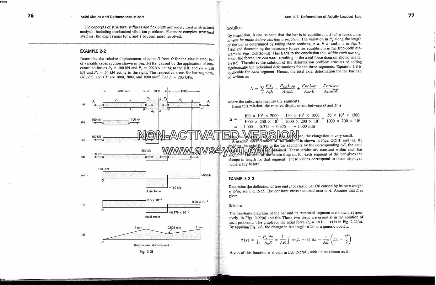
76 Axial Strains and Deformations in Bars
The concepts of structural stiffness and flexibility are widely used in structuralanalysis, including mechanical-vibration problems. For more complex structuralsystems, the expressions for k and f become more involved.
EXAMPLE 2-2
Determine the relative displacement of point D from O for the elastic steel barof variable cross section shown in Fig. 2-21(a) caused by the application of con-centrated forces P� = 100 kN and P3 = 200 kN acting to the left, and P2 = 250kN and P4 = 50 kN acting to the right. The respective areas for bar segmentsOB, BC, and CD are 1000, 2000, and 1000 mm 2. Let E = 200 GPa.
(a)
(b)
(c)
(d)
(e) �
(f)
2000 mm
A� a100kN' :O
250 kN-- 150 kN
250 kN 200 kN,o kN
+100 kN
,
oAxial force
+50 kN
0.5 X 10 -3 0.25 X 10 -3
Axial strain
(g)
I mm 0.625 mm 1 mm
Relative axial displacement
Fig. 2-2t
Sec. 2.7. Deformation of Axially Loaded Bars
Soldion
By inspection, it can be seen that the bar is in equilibrium. Such a check mustahvays be made before starting a problem. The variation in P,. along the lengthof the bar is determined by taking three sections, a-a, b-b, and c-c in Fig. 2-21(a) and determining the necessary forces for equilibrium in the free-body dia-grams in Figs. 2-21(b)-(d). This leads to the conclusion that withh� each bar seg-ment, the forces are constant, resulting in the axial force diagram shown in Fig.2-21(e). Therefore, the solution of the deformation problem consists of addingalgebraically the individual deformations for the three segments. Equation 2-9 isapplicable for each segment. Hence, the total axial deformation for the bar canbe written as
PcoLco
� P�L� Po�Lo� P�cL�c + .__A = . AlE = AoBE + ABcE AcZ>EKwhere the subscripts identify the segments.
Using this relation, the relative displacement between O and D is
100 x 103 x 2000 150 x 103 x 1000 50 x 103 x 1500A = + 1000 x 200 x 103 - 2000 x 200 x 103 + 1000 x 200 x 103
= +1.000 - 0.375 + 0.375 = + 1.000 mm
Note that in spite of large stresses in the bar, the elongation is very small.A graphic interpretation of the solution is shown in Figs. 2-21(0 and (g). By
dividing the axial forces in the bar segments by the corresponding AE, the axialstrains along the bar are obtained. These strains are constant within each barsegment. The area of the strain diagram for each segment of the bar gives thechange in length for that segment. These values correspond to those displayednumerically before.
EXAMPLE 2-3
Determine Lhe deflection of free end B of elastic bar OB caused by its own weightw lb/in; see Fig. 2-22. The constant cross-sectional area is A. Assume that E isgiven.
Soldion
The free-body diagrams of the bar and its truncated segment are shown, respec-tively, in Figs. 2-22(a) and (b). These two steps are essential in the solution ofsuch problems. The graph for the axial force P.� = w(L - x) is in Fig. 2-22(c).By applying Eq. 2-8, the change in bar length A(x) at a generic point x,
= 1 - x) dx = -_�o A.,E AE
A plot of this function is shown in Fig. 2-22(d), with its maximum as B.
77
NON-ACTIVATEDVERSIONwww.avs4you.com
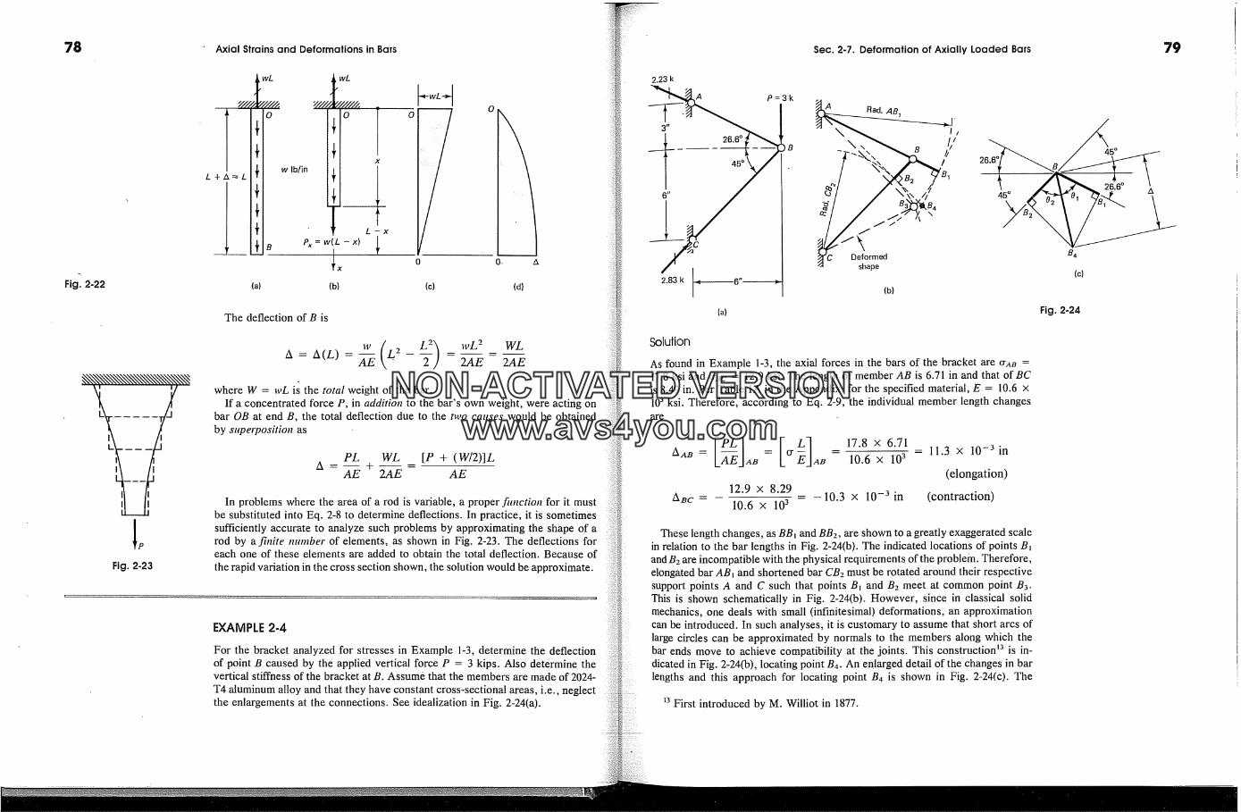
78
Fig. 2.22
I i
L I -- _ --I I
II II
Fig. 2-23
Axial Strains and Deformations in Bars
�wL }wL FwL4 2.23k
�x 0 0- A(a) (b) (c) (d)
The deflection of B is
LwL 2 WL2AE 2AE
where W = wL is the total weight of the bar.If a concentrated force P, in addition to the bar's own weight, were acting on
bar OB at end B, the total deflection due to the two causes would be obtainedby superposition as
PL WL [P + (W/2)]LA = + 2AE = AE
In problems where the area of a rod is variable, a proper fitnction for it mustbe substituted into Eq. 2-8 to determine deflections. In practice, it is sometimessufficiently accurate to analyze such problems by approximating the shape of arod by a finite number of elements, as shown in Fig. 2-23. The deflections foreach one of these elements are added to obtain the total deflection. Because ofthe rapid variation in the cross section shown, the solution would be approximate.
.__�...��,,,,,.� P=3k
2.83k �-----6" �"(a)
EXAMPLE 2-4
For the bracket analyzed for stresses in Example 1-3, determine the deflectionof point B caused by the applied vertical force P = 3 kips. Also determine thevertical stiffness of the bracket at B. Assume that the members are made of 2024-T4 aluminum alloy and that they have constant cross-sectional areas, i.e., neglectthe enlargements at the connections. See idealization in Fig. 2-24(a).
Sec. 2-7. Deformation of Axially Loaded Bars 79
� B�C �e�formedshape (c)
(b)
Fig. 2-24
Solution
As found in Example 1-3, the axial forces in the bars of the bracket are CrA� =17.8 ksi and Crac = 12.9 ksi. The length of member AB is 6.71 in and that of BCis 8.49 in. Per Table 1A in the Appendix, for the specified material, E = 10.6 x10³ ksi. Therefore, according to Eq. 2-9, the individual member length changes
are
17.8 x 6.71
10.6 x 10 3
12.9 x 8.29
ABc- 10.6 X 10³ -- 10.3 X 10 -3 in
-- 11.3 x 10 -3 in
(elongation)
(contraction)
These length changes, as BB� and BB2, are shown to a greatly exaggerated scalein relation to the bar lengths in Fig. 2-24(b). The indicated locations of points B�and B2 are incompatible with the physical requirements of the problem. Therefore,elongated bar AB� and shortened bar CB2 must be rotated around their respectivesupport points A and C such that points B� and B2 meet at common point B3.This is shown schematically in Fig. 2-24(b). However, since in classical solidmechanics, one deals with small (infinitesimal) deformations, an approximationcan be introduced. In such analyses, it is customary to assume that short arcs oflarge circles can be approximated by normals to the members along which thebar ends move to achieve compatibility at the joints. This construction �3 is in-dicated in Fig. 2-24(b), locating point B4. An enlarged detail of the changes in barlengths and this approach for locating point B4 is shown in Fig. 2-24(c). The
First introduced by M. Williot in 1877.
NON-ACTIVATEDVERSIONwww.avs4you.com

8O Axial Strains and Deformations in Bars
required numerical results can be obtained either graphically or by using trigo-nometry. Here the latter procedure is followed.
If A is the deflection or displacement of point B to position B4, Fig. 2-24(c),and changes in bar lengths ABc= BB2 and AAB = BB�,
cos 02 and lAB = I COS 01
On forming equal ratios for both sides of these equations, substituting the nu-merical values for A�c and AA� found earlier, and simplifying, one obtains
However, since
it follows that
and
Therefore,
cos 02 IBc 10.3 X 10 -3.... 0.912cos 0� lAB 11.3 X 10 -3
02 = 180 � - 45 � - 26.6 � - 0� = 108.4 �
cos 02 = cos 108.4 � cos 0� + sin 108.4 � sin 0,
coscos 01
- cos 108.4 � + sin 108.4 � tan 0, = 0.912
tan 0� = 1.29
Based on this result,
and O� = 52.2 �
I = IAa/cos 0� = 18.4 x 10 -3 in
forming an angle of 11.2 � with the vertical.Since Arm = A cos 11.2 � = 18.0 x 10 -3 in, the vertical stiffness of the bracket
is given by the spring constant
P 3
lvert 18.0 X 10 -3 - 167 kips/in
This problem contains geometric nonlinearity in displacement, which has beenneglected; therefore, fghe solution is accurate only for. small deformations, a com-mon practice for many engineering problems.
Sec. 2-7. Deformation of Axially Loaded Bars
A O C
�' '� L -
(c)
lb)
Fig. 2-25
**EXAMPLE 2-5
Two hinge-ended elastic bars of equal lengths and cross-sectional areas attachedto immovable supports are joined in the middle by a pin, as shown in Fig. 2-25(a).Initially, points A, B, and C are on a straight line. Determine the vertical deflectionA of point C as a function of applied force P. Consider small deflections only.
Solution
The given structural system is incapable of supporting any vertical force in itsinitial configuration. Therefore, equilibrium of the system in a slightly deflectedcondition must be examined, Fig. 2-25(b), where initial bar lengths L become L*.For this position of the bars, one can write an equation of equilibrium for jointC' and express elongations of the bars via two different paths. One such relationfor elongation of each bar follows from Eq. 2-9 and the other from purely geo-metric considerations. On these bases, from equilibrium,
P = 2T sin 0
andTL*
AE- L* - L = L* - L'cos0
Hence, T = AE(1 - cos 0)
On substituting this expression for T into the first equation,
8t
�-.............. P = 2AE(1 - cos 0) sin 0
NON-ACTIVATEDVERSIONwww.avs4you.com
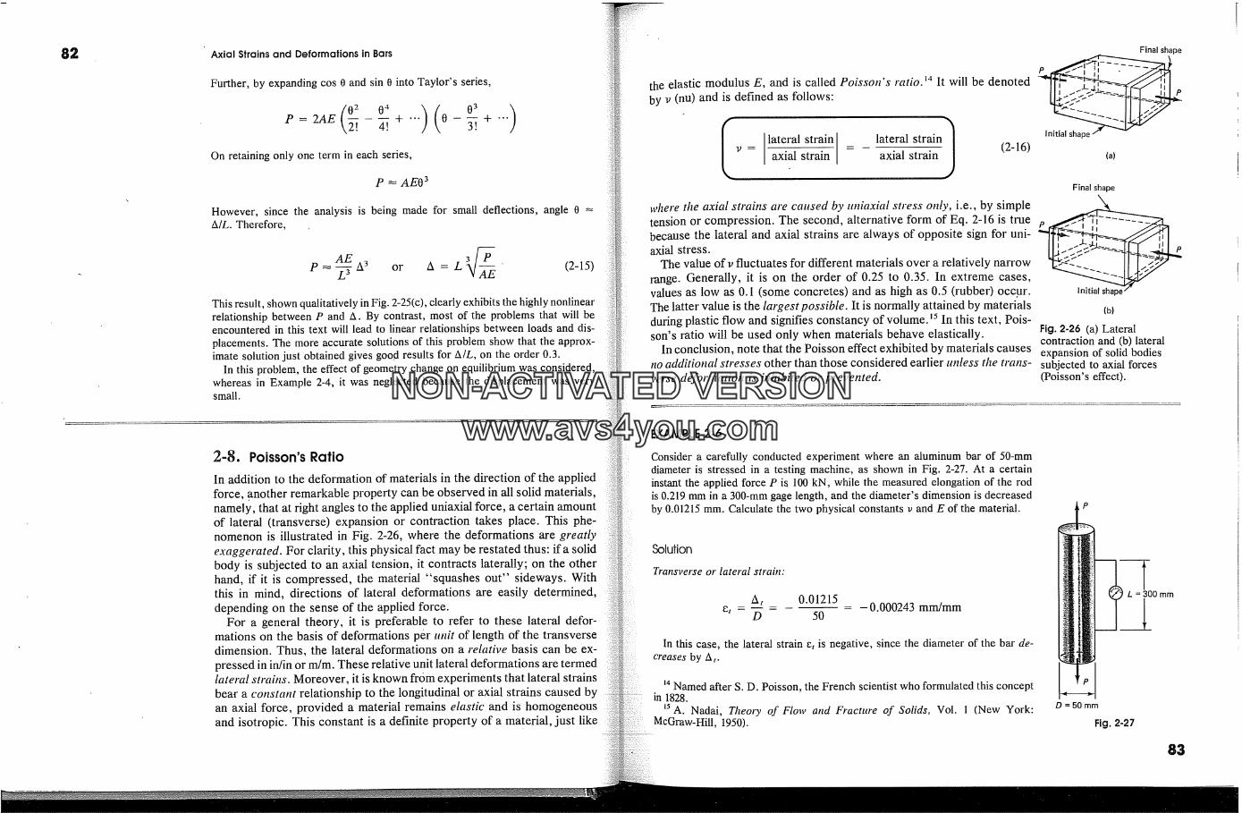
82 Axial Strains and Deformations in Bars
Further, by expanding cos 0 and sin 0 into Taylor's series,
)( )e = 2AE 7., - + ... 0-7.,+...
On retaining only one term in each series,
p � AEO 3
However, since the analysis is being made for small deflections, angleA/L. Therefore,
AE A3 � ' (2-15)P � � or A = L AEThis result, shown qualitatively in Fig. 2-25(c), clearly exhibits the highly nonlinearrelationship between P and A. By contrast, most of the problems that will beencountered in this text will lead to linear relationships between loads and dis-placements. The more accurate solutions of this problem show that the approx-imate solution just obtained gives good results for A/L, on the order 0.3.
In this problem, the effect of geometry change on equilibrium was considered,whereas in Example 2-4, it was neglected because the displacement was verysmall.
2-8. Poisson's Ratio
In addition to the deformation of materials in the direction of the appliedforce, another remarkable property can be observed in all solid materials,namely, that at right angles to the applied uniaxial force, a certain amountof lateral (transverse) expansion or contraction takes place. This phe-nomenon is illustrated in Fig. 2-26, where the deformations are greatlyexaggerated. For clarity, this physical fact may be restated thus: if a solidbody is subjected to an axial tension, it contracts laterally; on the otherhand, if it is compressed, the material "squashes out" sideways. Withthis in mind, directions of lateral deformations are easily determined,depending on the sense of the applied force.
For a general theory, it is preferable to refer to these lateral defor-mations on the basis of deformations per unit of length of the transversedimension. Thus, the lateral deformations on a relative basis can be ex-pressed in in/in or m/m. These relative unit lateral deformations are termedlateral strains. Moreover, it is known from experiments that lateral strainsbear a constant relationship to the longitudinal or axial strains caused byan axial force, provided a material remains elastic and is homogeneousand isotropic. This constant is a definite property of a material, just like
the elastic modulus E, and is called Poisson's ratio. �4 It will be denotedby v (nu) and is defined as follows:
I Ilateralstrain lateralstrain1v = 'a�al st� - axial strain (2-16)
where the axial strains are caused by uniaxial stress only, i.e., by simpletension or compression. The second, alternative form of Eq. 2-16 is truebecause the lateral and axial strains are always of opposite sign for uni-axial stress.
The value of v fluctuates for different materials over a relatively narrowrange. Generally, it is on the order of 0.25 to 0.35. In extreme cases,values as low as 0.1 (some concretes) and as high as 0.5 (rubber) occur.The latter value is the largest possible. It is normally attained by materialsduring plastic flow and signifies constancy of volume. 15 In this text, Pois-
Final shape
P P
(a)
Final shape
(b}
son's ratio will be used only when materials behave elastically. Fig. 2-26 (a) Lateralcontraction and (b) lateralIn conclusion, note that the Poisson effect exhibited by materials causes expansion of solid bodies
no additional stresses other than those considered earlier anless the trans- subjected to axial forcesverse deformation is inhibited or prevented. (Poisson's effect).
EXAMPLE 2-6
Consider a carefully conducted experiment where an aluminum bar of 50-mmdiameter is stressed in a testing machine, as shown in Fig. 2-27. At a certaininstant the applied force P is 100 kN, while the measured elongation of the rodis 0.219 mm in a 300-mm gage length, and the diameter's dimension is decreasedby 0.01215 mm. Calculate the two physical constants v and E of the material.
Solution
Transverse or lateral strain:
0.01215..... 0.000243 mm/mm
50
In this case, the lateral strain et is negative, since the diameter of the bar de-creases by/X,.
�4 Named after S. D. Poisson, the French scientist who formulated this conceptin 1828.
�s A. Nadai, Theory of Flow and Fracture of Solids, Vol. 1 (New York:McGraw-Hill, 1950).
/. = 300 mm
D = 50 mm
Fig. 2-27
83
NON-ACTIVATEDVERSIONwww.avs4you.com
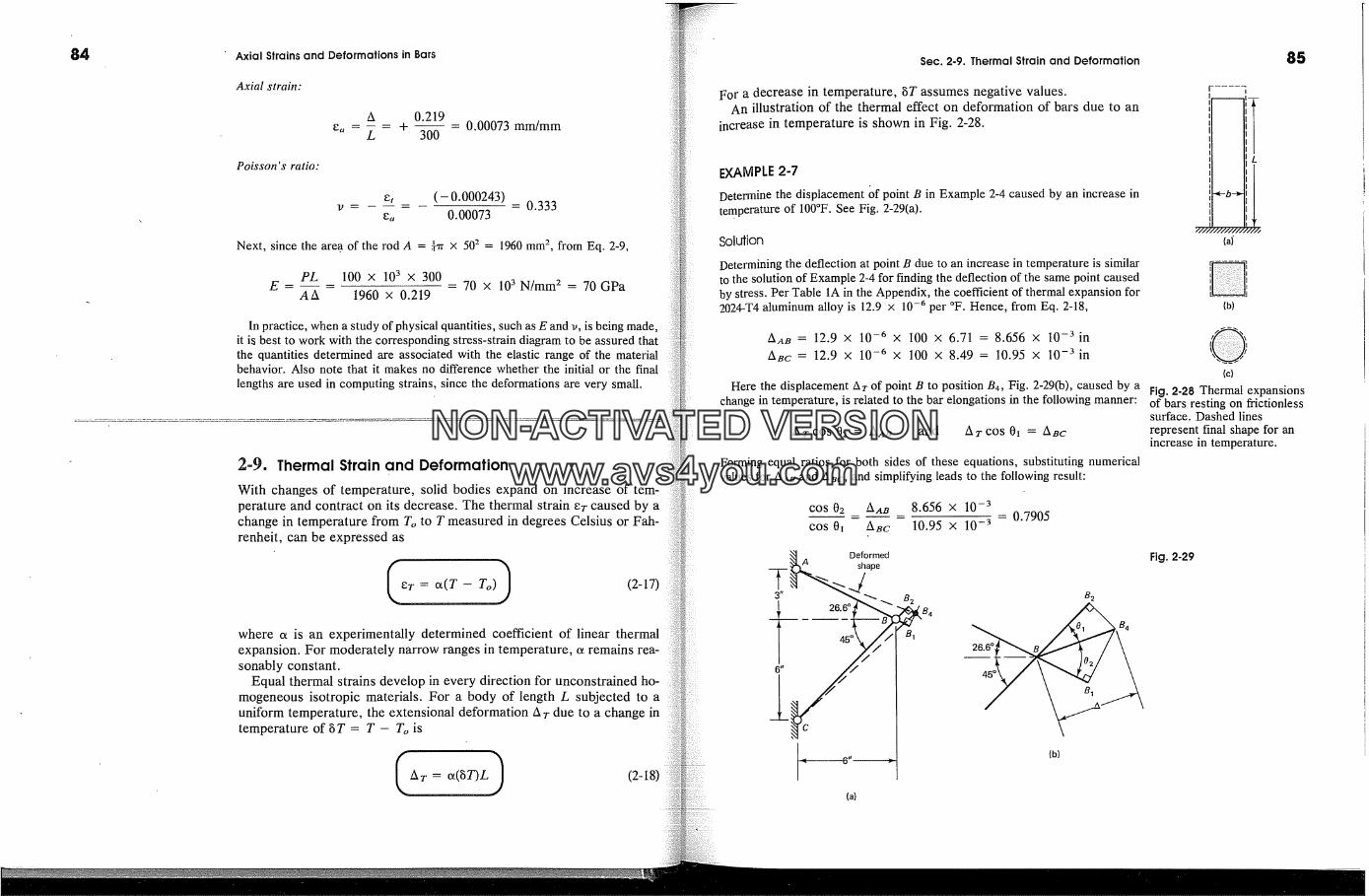
Axial Strains and Deformations in Bars Sec. 2.9. Thermal Strain and Deformation 85Axial strain:
A 0.219e,, = - = + - 0.00073 mm/mm
L 300
Poisson's ratio:
e, ( - 0.000243)v .... - 0.333
e,, 0.00073
Next, since the area of the rod A = �x x 502 = 1960 mm 2, from Eq. 2-9,
PL 100 X 103 X 300E- - =70x
AA 1960 X 0.219103 N/mm 2 = 70 GPa
In practice, when a study of physical quantities, such as E and v, is being made,it is best to work with the corresponding stress-strain diagram to be assured thatthe quantities determined are associated with the elastic range of the materialbehavior. Also note that it makes no difference whether the initial or the finallengths are used in computing strains, since the deformations are very small.
2-9. Thermal Strain and Deformation
With changes of temperature, solid bodies expand on increase of tem-perature and contract on its decrease. The thermal strain er caused by achange in temperature from To to T measured in degrees Celsius or Fah-renheit, can be expressed as
(2-17)
where o� is an experimentally determined coefficient of linear thermalexpansion. For moderately narrow ranges in temperature, c� remains rea-sonably constant.
Equal thermal strains develop in every direction for unconstrained ho-mogeneous isotropic materials. For a body of length L subjected to auniform temperature, the extensional deformation A r due to a change intemperature of � T = T - To is
At = a(gT)L.) (2-18)
For a decrease in temperature, bT assumes negative values.An illustration of the thermal effect on deformation of bars due to an
increase in temperature is shown in Fig. 2-28.
EXAMPLE 2-7Determine the displacement Of point B in Example 2-4 caused by an increase intemperature of 100�F. See Fig. 2-29(a).
Soldion
Determining the deflection at point B due to an increase in temperature is similarto the solution of Example 2-4 for finding the deflection of the same point causedby stress. Per Table 1A in the Appendix, the coefficient of thermal expansion for2024-T4 aluminum alloy is 12.9 x 10 -6 per �F. Hence, from Eq. 2-18,
AAB = 12.9 x 10 -6 X 100 X 6.71 = 8.656 x 10 -3 inABc= 12.9 x 10 -6 X 100 X 8.49 = 10.95 X 10 -3 in
Here the displacement At of point B to position B4, Fig. 2-29(b), caused by achange in temperature, is related to the bar elongations in the following manner:
Ar cos 02 = A,�_a and Ar cos 0� = ABc
Forming equal ratios for both sides of these equations, substituting numericalvalues for AAa and Aac, and simplifying leads to the following result:
COS 02 AAB 8.656 X 10 -3cos 0� A�c 10.95 X 10 -3
(a)
= 0.7905
8 2
26.6oB�� B�(b)
� 1I I
l
(b)
(c)
Fig. 2-28 Thermal expansionsof bars resting on frictionlesssurface. Dashed linesrepresent final shape for anincrease in temperature.
Fig. 2-29
NON-ACTIVATEDVERSIONwww.avs4you.com

86 Axial Strains and Deformations in Bars
Here, however, 02 = 45 � + 26.6 � - 0� = 71.6 � - 0�; therefore,
cos 02 = cos 71.6 � cos 02 + sin 71.6 � sin 0z
COS 02and -- - cos 71.6 � + sin 71.6 � tan 0� = 0.7905
COS 0 �
and 02 = 26.6 �Hence, tan 02 = 0.500
Based on this result,
�A T �-- ABc/COS 01 = 12.2 X 10 -3 in
forming an angle of 45 � - 0� = 18.4 � with the horizontal.It is interesting to note that the small displacement Ar is �)f comparable order
of magnitude to that found due to the applied vertical force P in Example 2-4.
2-10. Saint-Venant's Principle and Stress ConcentrationsThe analysis of axially loaded bars based on engineering mechanics ofsolids is very accurate for bars of constant cross section when transmittinguniformly distributed end forces. For such ideal conditions stresses andstrains are uniform everywhere. In reality, however, applied forces oftenapproximate concentrated forces, and the cross sections of members canchange abruptly. This causes stress and strain disturbances in the prox-imity of such forces and changes in cross sections. In the past thesesituations were studied analytically using the mathematical theo�3, of elas-ticity. In such an approach, the behavior of two or three dimensionalinfinit.esimal elements is formulated and the conditions of equilibrium,deformation and mechanical properties of material �6 are satisfied subjectto the prescribed boundary conditions. More recently a powerful nu-merical procedure has been developed, where a body is subdivided intoa discrete number of finite elements, such as squares or cubes, and theanalysis is carried out with a computer. This is called the finite elementmethod of analysis. The end results of analyses by either one of thesetwo methods can be very effectively used to supplement solutions in en-gineering mechanics of solids. An example showing the more accuratesolutions by these two advanced methods for the nature of stress distri-bution at concentrated force follows. These solutions provide comparisonwith those found by applying the method of engineering mechanics ofsolids.
A short block is shown in Fig. 2-30(a) acted upon by concentrated forcesat its ends. Analyzing this block for stresses as a two dimensional problem
�6 These are the same basic concepts as use i�neering mechanics of solids.
Sec. 2.10. Saint-Venant's Principle and Stress Concentrations
P
2.575
(b)
P
1.38703,,
P
Oma x = 1.027oav{d)
(a)
Fig. 2-30 Stress distribution near a concentrated force in a rectangular elastic plate.
using the methods of the theory of elasticity gives the results shown inFigs. 2-30(b), (c), and (d). 17 The average stress �av as given by Eq. 1-13is also shown on these diagrams. From these it can be noted that at asection a distance b/4 from an end, Fig. 2-30(b), the maximum normalstress greatly exceeds the average. For a purely elastic material the max-imum stress theoretically becomes infinite right under the concentratedforce, since a finite force acts on a zero area. In real situations, however,a truly concentrated force is not possible and virtually all materials exhibitsome plastic behavior; therefore the attainment of an infinite stress isimpossible.
It is important to note two basic aspects from this solution. First, theaverage stress for all cases, being based on conditions of equilibrium, isalways correct. Second, the normal stresses at a distance equal to thewidth of the member are essentially uniform.
The second observation illustrates the famed Sa#zt-Venant's principle.It was enunciated by the great French elastician in 1855. In commonengineering terms it simply means that the manner of force applicationon stresses is important only in the vicinity of the region where the forceis applied. This also holds true for the disturbances caused by changesin cross section. Consciously or unconciously this principle is nearly al-ways applied in idealizing load carrying systems.
Using the finite element method,�8 the results of a solution for the sameproblem are shown in Fig. 2-31. The initial undeformed mesh into whichthe planar block is arbitrarily subdivided, and the greatly exaggerateddeformed mesh caused by the applied force are shown in Fig. 2-31(a). Byplacing the mesh on rollers as shown, only the upper half of the block
27 S. Timoshenko, and J. N. Goodier, Treaty of Elasticity, 3rd. ed., New York:McGraw-Hill, 1970, p. 60. Fig. 2-30 is adapted from this source.
�8 For this subject see for example, O. C. Zienkiewicz, The Finite ElementMethod, 3rd ed. (London: McGraw-Hill Ltd., 1977). K. J. Bathe and E. L. Wilson,Numerical Methods in Finite Element Analysis (Englewood Cliffs, N.J.: Prentice-Hall, 1976). R. H. Gallagher, Finite Element Fundamentals (Englewood Cliffs,N.J.: Prentice-Hall, 1975).
87
NON-ACTIVATEDVERSIONwww.avs4you.com
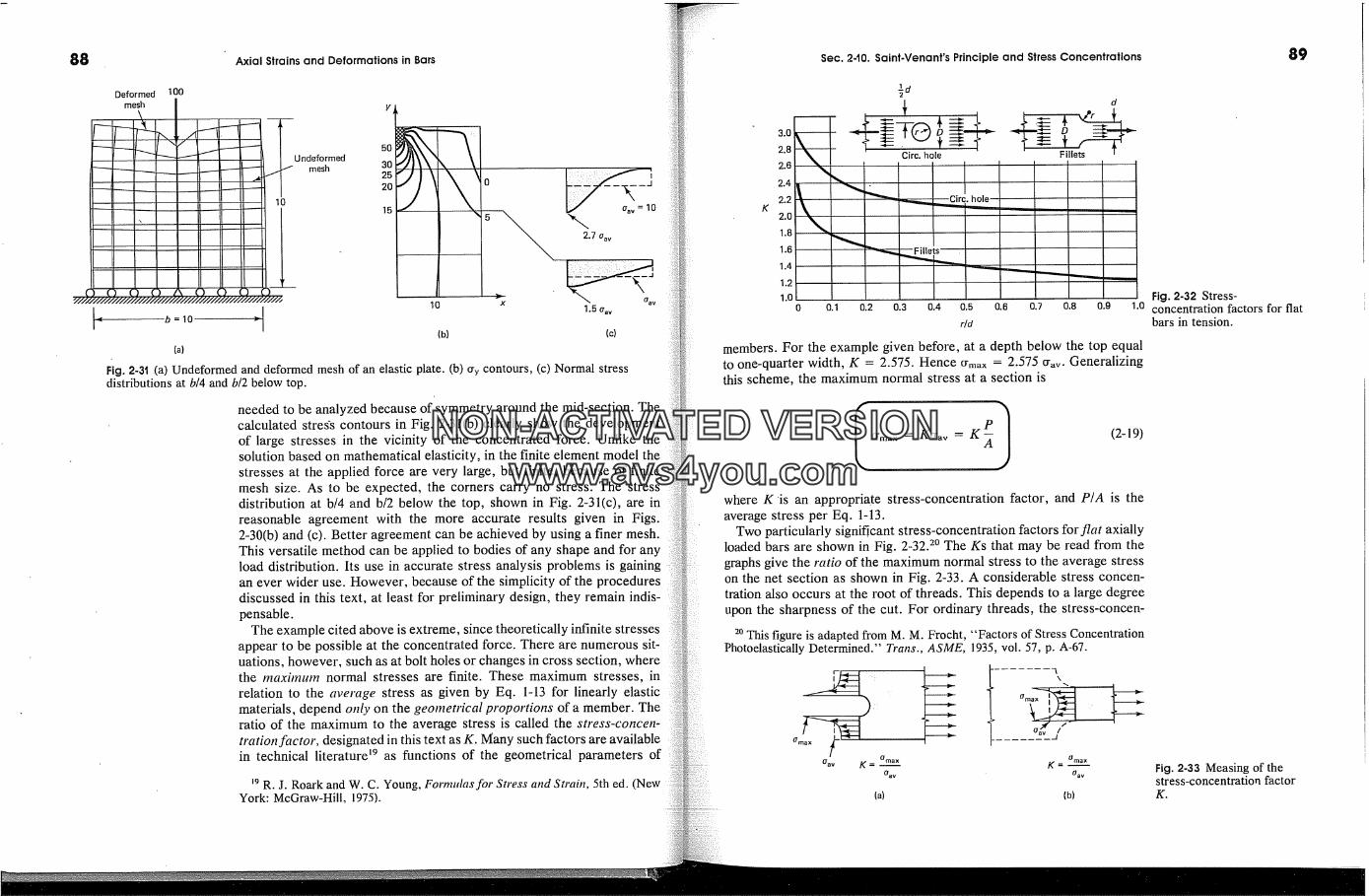
88 Axial Strains and Deformations in Bars
Deformed 100
mesh
...f2..� .... .O....c.L...�;....?....t.?.....?.... 2...
ndeformedmesh
Y
3025
10 x
2.7 o.v
1.5 %v
(a)
Fig. 2-3t .(a) Undeformed and deformed mesh of an elastic plate. (b) cry contours, (c) Normal stressdistributions at b/4 and b/2 below top.
needed to be analyzed because of symmetry around the mid-section. Thecalculated stress contours in Fig. 2-31(b) clearly show the developmentof large stresses in the vicinity of the concentrated force. Unlike thesolution based on mathematical elasticity, in the finite element model thestresses at the applied force are very large, but finite, because of finitemesh size. As to be expected, the corners carry no stress. The stressdistribution at b/4 and b/2 below the top, shown in Fig. 2-31(c), are inreasonable agreement with the more accurate results given in Figs.2-30(b) and (c). Better agreement can be achieved by using a finer mesh.This versatile method can be applied to bodies of any shape and for anyload distribution. Its use in accurate stress analysis problems is gainingan ever wider use. However, because of the simplicity of the proceduresdiscussed in this text, at least for preliminary design, they remain indis-pensable.
The example cited above is extreme, since theoretically infinite stressesappear to be possible at the concentrated force. There are numerous sit-uations, however, such as at bolt holes or changes in cross section, wherethe maximum normal stresses are finite. These maximum stresses, inrelation to the average stress as given by Eq. 1-13 for linearly elasticmaterials, depend only on the geometrical proportions of a member. Theratio of the maximum to the average stress is called the stress-concen-tration factor, designated in this text as K. Many such factors are availablein technical literature 19 as functions of the geometrical parameters of
�9 R. J. Roark and W. C. Young, Formulas for Stress andStrain, 5th ed. (NewYork: McGraw-Hill, 1975).
Sec. 240. Saint-Venant's Principle and Stress Concentrations 89
K
3.0
2.8
2.6
2.4
2.2
2.0
1.8
1.6
1.4
1.2
1.00 0.1 0.2 0.3 0.4 0.5 0.6 0.7 0.8 0.9
rid
Fig. 242 Stress-1.0 concentration factors for flat
bars in tension.
members. For the example given before, at a depth below the top equalto one-quarter width, K = 2.575. Hence �m�x = 2.575 �. Generalizingthis scheme, the maximum normal stress at a section is
'max=Kg�=KP-P-1A(2-19)
,)
Oav K = �maxgav
where K 'is an appropriate stress-concentration factor, and P/A is theaverage stress per Eq. 1-13.
Two particularly signScant stress-concentration factors for flat axiallyloaded bars are shown in Fig. 2-32? The Ks that may be read from thegraphs give the ratio of the maximum normal stress to the average stresson the net section as shown in Fig. 2-33. A considerable stress concen-tration also occurs at the root of threads. This depends to a large degreeupon the sharpness of the cut. For ordinary threads, the stress-concen-
�0 This figure is adapted from M. M. Frocht, "Factors of Stress ConcentrationPhotoelastically Determined." Trans., ASME, 1935, vol. 57, p. A-67.
\
K =
(a) (b)
Fig. 243 Measing of thestress-concentration factorK.
NON-ACTIVATEDVERSIONwww.avs4you.com
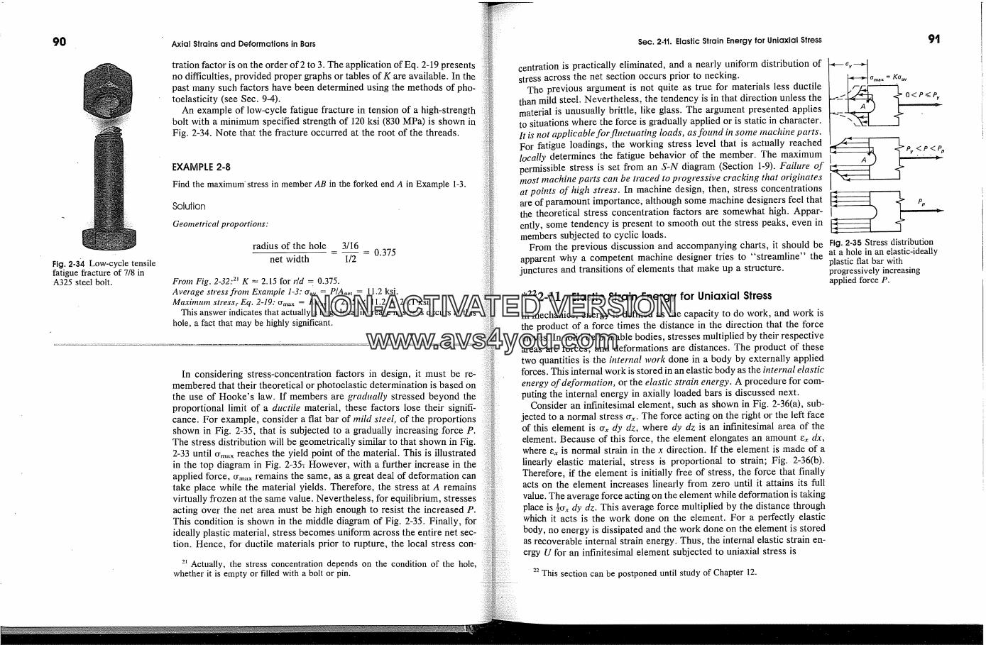
9O Axial Strains and Deformations in Bars
tration factor is on the order of 2 to 3. The application of Eq. 2-19 presentsno difficulties, provided proper graphs or tables of K are available. In thepast many such factors have been determined using the methods of pho-toelasticity (see Sec. 9-4).
An example of low-cycle fatigue fracture in tension of a high-strengthbolt with a minimum specified strength of 120 ksi (830 MPa) is shown inFig. 2-34. Note that the fracture occurred at the root of the threads.
Fig. 2-3� Low-cycle tensilefatigue fracture of 7/8 inA325 steel bolt.
EXAMPLE 2-8
Find the maximumstress in member AB in the forked end A in Example 1-3.
Soldion
Geometrical proportions:
radius of the hole 3/16- - 0.375
net width 1/2
From Fig. 2-32? K �- 2.15 for r/d = 0.375.Average stress fi'om Example 1-3: Crav = P/A,et = 11.2 ksi.Maxhnum stressr Eq. 2-19: Crmax = Kcrav = 2.15 x 11.2 = 24.1 ksi.
This answer indicates that actually a large local increase in stress occurs at thishole, a fact that may be highly significant.
In considering stress-concentration factors in design, it must be re-membered that their theoretical or photoelastic determination is based onthe use of Hooke's law. If members are gradually stressed beyond theproportional limit of a ductile material, these factors lose their signifi-cance. For example, consider a flat bar of mild steel, of the proportionsshown in Fig. 2-35, that is subjected to a gradually increasing force P.The stress distribution will be geometrically similar to that shown in Fig.2-33 until O'ma x reaches the yield point of the material. This is illustratedin the top diagram in Fig. 2-35: However, with a further increase in theapplied force, ffmax remains the same, as a great deal of deformation cantake place while the material yields. Therefore, the stress at A remainsvirtually frozen at the same value. Nevertheless, for equilibrium, stressesacting over the net area must be high enough to resist the increased P.This condition is shown in the middle diagram of Fig. 2-35. Finally, forideally plastic material, stress becomes uniform across the entire net sec-tion. Hence, for ductile materials prior to rupture, the local stress con-
2� Actually, the stress concentration depends on the condition of the hole,whether it is empty or filled with a bolt or pin.
Sec. 24t. Elastic Strain Energy for Uniaxial Stress
centration is practically eliminated, and a nearly uniform distribution ofstress across the net section occurs prior to necking.
The previous argument is not quite as true for materials less ductilethan mild steel. Nevertheless, the tendency is in that direction unless thematerial is unusually brittle, like glass. The argument presented appliesto situations where the force is gradually applied or is static in character.It is not applicable for fiuctuating loads, as found in some machine parts.For fatigue loadings, the working stress level that is actually reachedlocally determines the fatigue behavior of the member. The maximumpermissible stress is set from an S-N diagram (Section 1-9). Failure ofmost machine parts can be traced to progressive cracking that originatesat points of high stress. In machine design, then, stress concentrationsare of paramount importance, although some machine designers feel thatthe theoretical stress concentration factors are somewhat high. Appar-ently, some tendency is present to smooth out the stress peaks, even inmembers subjected to cyclic loads.
From the previous discussion and accompanying charts, it should beapparent why a competent machine designer tries to "streamline" the
junctures and transitions of elements that make up a structure.
� 222-11. Elastic Strain Energy for Uniaxial StressIn mechanics, energy is defined as the capacity to do work, and work isthe product of a force times the distance in the direction that the forcemoves. In solid deformable bodies, stresses multiplied by their respectiveareas are forces, and deformations are distances. The product of thesetwo quantities is the internal work done in a body by externally appliedforces. This internal work is stored in an elastic body as the internal elasticenergy of deformation, or the elastic strain energy. A procedure for com-puting the internal energy in axially loaded bars is discussed next.
Consider an infinitesimal element, such as shown in Fig. 2-36(a), sub-jected to a normal stress �.�. The force acting on the right or the left faceof this element is � dy dz, where dy dz is an infinitesimal area of theelement. Because of this force, the element elongates an amount e.� dx,where e.� is normal strain in the x direction. If the element is made of alinearly elastic material, stress is proportional to strain; Fig. 2-36(b).Therefore, if the element is initially free of stress, the force that finallyacts on the element increases linearly from zero until it attains its fullvalue. The average force acting on the element while deformation is takingplace is �-�� .� dy dz. This average force multiplied by the distance throughwhich it acts is the work done on the element. For a perfectly elasticbody, no energy is dissipated and the work done on the element is storedas recoverable internal strain energy. Thus, the internal elastic strain en-ergy U for an infinitesimal element subjected to uniaxial stress is
22 This section can be postponed until study of Chapter 12.
Fig. 2.35 Stress distributionat a hole in an elastic-ideallyplastic flat bar withprogressively increasingapplied force P.
NON-ACTIVATEDVERSIONwww.avs4you.com

Axial Strains and Deformations in Bars Sec. 2-tt. Elastic Strain Energy for Uniaxial Stress
Fig. 246 (a) An element inuniaxial tension and (b) aHookean stress-straindiagram.
x
z
E
(a) (b)
dU = 2 :,dydz x e:,dx = ��xexdxdydz =average distance
force
work
(2-20)
where dV is the volume of the element.By recasting Eq. 2-20, one obtains the strain energy stored in an elastic
body per unit volume of the material, or its strain-energy density Uo.Thus,
d U o'xexUo- d�- 2 (2-21)
This expression may be graphically interpreted as an area under the in-clined line on the stress-strain diagram; Fig. 2-36(b). The correspondingarea enclosed by the inclined line and the vertical axis is called the com-plementre3, energy, a concept to be used in Chapter 12. For linearly elasticmaterials, the two areas are equal. Expressions analogous to Eq. 2-21apply to the normal stresses %. and � and to the corresponding normalstrains ey and e:.
Since in the elastic range, Hooke's law applies, �.� = Ee.�, Eq. 2-21may be written as
dU Ee} ty}Uo- dV- 2 - 2E (2-22)
0r U = f� dVol(2-23)
These forms of the equation for the elastic strain energy are convenientin applications, although they mask the dependence of the energy expres-sion on force and distance.
For a particular material, substitution into Eq. 2-22 of the value of thestress at the proportional limit gives an index of the material's ability tostore or absorb energy without permanent deformation. The quantity sofound is called the modtthts of resilience and is used to differentiate ma-terials for applications where energy must be absorbed by members. Forexample, a steel with a proportional limit of 30,000 psi and an E of 30 x106 psi has a modulus of resilience of �2/2E = (30,000)2/2(30)106 = 15 in-lb/in 3, whereas a good grade of Douglas fir, having a proportional limitof 6450 psi and an E of 1,920,000 psi has a modulus of resilience of (6,450)2/(1,920,000) = 10.8 in-lb/inL
By reasoning analogous to that before, the area under a complete stress-strain diagram, Fig. 2-37, gives a measure of a material's ability to absorbenergy up to fracture and is called its toughness. The larger the total areaunder the stress-strain diagram, the tougher the material. In the inelasticrange, only a small part of the energy absorbed by a material is recover-able. Most of the energy is dissipated in permanently deforming the ma-terial and is lost in heat. The energy that may be recovered when a spec-imen has been stressed to some such point as A in Fig. 2-37(b) isrepresented by the triangle ABC. Line AB of this triangle is parallel toline OD, since all materials essentially behave elastically upon the releaseof stress.
Strongermaterial
DissipatedR
Permanentset JT _,l�e resilience(a)
Fig. 247 Some typical properties of materials.
Toughermaterial
(b)
c
Hyperelasticresilience
NON-ACTIVATEDVERSIONwww.avs4you.com

94
(a)
2A
(b)
Fig. 2-38
Axial Strains and Deformations in Bars
EXAMPLE 2-9
Two elastic bars, whose proportions are shown in Fig. 2-38, are to absorb thesame amount of energy delivered by axial forces. Neglecting stress concentra-tions, compare the stresses in the two bars. The cross-sectional area of the leftbar is A, and that of the right bar is A and 2A as shown.
Soldion
The bar shown in Fig. 2-38(a) is of uniform cross-sectional area, therefore, thenormal stress ch is constant throughout. Using Eq. 2-23 and integrating over thevolume V of the bar, one can write the total energy for the bar as
fv0.I ' fv 0.7where A is the cross-sectional area of the bar, and L is its length.
The bar shown in Fig. 2-38(b) is of variable cross section. Therefore, if thestress or2 acts in the lower part of the bar, the stress in the upper part is tEO' 2 .
Again, by using Eq. 2-23 and integrating over the volume of the bar, it is foundthat the total energy that this bar will absorb in terms of the stress or2 is
0.2 0.� dV + � dVU2 = �-� dV = � owerpart 2E pperpart0.� (0'2/2)2 2A AL- 2E + 2E
If both bars are to absorb the same amount of energy, U� = U2 and
AL) = AL or 0.2 = 1.2650.�Hence, for the same energy load, the stress in the "reinforced" bar is 26.5
percent higher than in the plain bar. The enlargement of the cross-sectional areaover a part of the bar is actually detrimental. This situation is not found in thedesign of members for static loads.
� 2-12. Deflections by the Energy MethodThe principle of conservation of energy may be very effectively used forfinding deflections of elastic members due to applied forces. Generalmethods for accomplishing this will be discussed in Chapter 12. Here amore limited objective, determining the deflection caused by the appli-cation of a single axial force, is considered. For such a purpose, theinternal strain energy U for a member is simply equated to the externalwork W,, due to the applied force, i.e.,
Sec. 2-t2. Deflections by the Energy Method
(2-24)
In this treatment, it is assumed that the external force is graduallyapplied. This means that, as it is being applied, its full effect on a memberis reached in a manner similar to that shown in Fig. 2-36(b) for stress.Therefore, the external work We is equal to one-half of the total forcemultiplied by the deflection in the direction of the force action. In thenext section, this approach will be generalized for dynamic loads.
EXAMPLE 2-t0
Find the deflection of the free end of an elastic rod of constant cross-sectionalarea A and length L due to axial force P applied at the free end.
Soldion
If force P is gradually applied to the rod, external work, W,. = �pA, where A isthe deflection of the end of the rod. The expression for the internal strain energyU of the rod was found in Example 2-9, and since cr� = P/A, it is
U = 0.7 AL p2L2E 2AE
Then, from We = U,
p A p2L PL- and A = --
2 . 2AE AE
which is the same as Eq. 2-9.
The use of Eq. 2-24 can be extended to bar systems consisting of severalmembers. Since internal strain energy is a positive scalar quantity, theenergies for the several members can be simply added arithmetically. Thistotal strain energy U can then be equated to the external work W�, causedby one force for finding the deflection in the direction of that force. Toillustrate, for the bracket shown in Fig. 2-24 for Example 2-4,
1 P,�BLAB 1 P�cLBc 1U- + .... pA
2 AABE 2 AacE 2
where the subscripts refer to members. A solution of this equation givesdeflection A of force P.
95
NON-ACTIVATEDVERSIONwww.avs4you.com

96 Axial Strains and Deformations in Bars
This method is extended in Chapter 12 to solution of problems withany number of applied forces for finding the deflections at any point inany direction.
*'232-13. Dynamic and Impact LoadsA freely falling weight, or a moving body, that strikes a structure deliverswhat is called a dynamic or impact load or force. Problems involving suchforces may be analyzed rather simply on the basis of the following ideal-izing assumptions:
1. Materials behave elastically, and no dissipation of energy takes placeat the point of impact or at the supports owing to local inelasticdeformation of materials.
2. The inertia of a system resisting an impact may be neglected.3. The deflection of a system is directly proportional to the magnitude
of the applied force whether a force is dynamically or statically ap-plied.
Then, using the principle of conservation of energy, it may be furtherassumed that at the instant a moving body is stopped, its kinetic energyis completely transformed into the internal strain energy of the resistingsystem. At thi� instant, the maximum deflection of a resisting systemoccurs and vibrations begin. However, since only maximum stresses anddeflections are of primary interest, this subject will not be pursued.
As an example of a dynamic force applied to an elastic system, considera falling weight striking a spring. This situation is illustrated in Fig. 2-39(a), where a weight W falls from a height h above the free length of aspring. This system represents a vet�y general case, since conceptually,
23 This is an optional section.
External work of Strain energyfalling weight of spring
Ast Amax
Deflection
(a) (b) (c)
Fig. 2-39 Behavior of an elastic system under an impact force.
Sec. 2-t3. Dynamic and Impact Loads
evenly elastic system may be treated as an equivalent sprh�g. Using thespring constant k, the static deflection A.�t of the spring due to the weightW is As, = W/k. Similarly, the maximum dynamic deflection Amax =pay,/k, where Pdyn iS the maximum dynamic force experienced by thespring. Therefore, the dynamic force in terms of the weight W and thedeflections of the spring is
AmaxPdyn = As----� W (2-25)
This relationship is shown in Fig. 2-39(b).At the instant the spring deflects its maximum amount, all energy of
the falling weight is transformed into the strain energy of the spring. There-fore, an equation representing the equality of external work to ,.'nternalstrain energy may be written as
1
W(h + Amax) = �Pdyn Amax (2-26)
A graphical interpretation of this equation is shown in Fig. 2-39(c). Notethat a factor of one-half appears in front of the strain-energy expression,since the spring takes on the load gradually. Then, from Eq. 2-25,
1 (A max) 2W(h + Amax) -- -- W
2 Ast
or (Amax) 2 -- 2Ast Ama x -- 2h Ast = 0
hence
Ama x �- Ast q- '�/(hst) 2 q- 2h As,
or Amax = Ast 1 + + AstJ (2-27)and again using Eq. 2-25,
Pdyn = W (1 + + �j (2-28)Equation 2-27 gives the maximum deflection occurring in a spring struckby a weight W falling from a height h, and Eq. 2-28 giveg the maximum
97
NON-ACTIVATEDVERSIONwww.avs4you.com
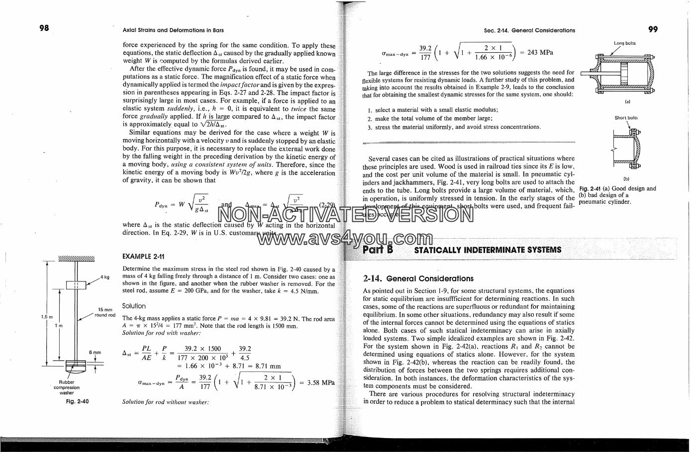
98
-- _F __�4 kg15 mm
� round rodm
I 6mmRubber
compressionwasher
Fig. 2-40
1.5 m
Axial Strains and Deformations in Bars
force experienced by the spring for the same condition. To apply theseequations, the static deflection A st caused by the gradually applied knownweight W is computed by the formulas derived earlier.
After the effective dynamic force Pdyn is found, it may be used in com-putations as a static force. The magnification effect of a static force whendynamically applied is termed the impact factor and is given by the expres-sion in parentheses appearing in Eqs. 2-27 and 2-28. The impact factor issurprisingly large in most cases. For example, if a force is applied to anelastic system suddenly, i.e., h = 0, it is equivalent to twice the sameforce gradually applied. If h is large compared to A st, the impact factoris approximately. equal to �st.
Similar equations may be derived for the case where a weight Wmoving horizontally with a velocity v and is suddenly stopped by an elasticbody. For this purpose, it is necessary to replace the external workby the falling weight in the preceding derivation by the kinetic energya moving body, using a consistent system of units. Therefore, since thekinetic energy of a moving body is Wv2/2g, where g is the accelerationof gravity, it can be shown that
l)2 . �/ 112Pdyn = W �-st and Amax = Ast gAst (2-29)where A.�t is the static deflection caused by W acting in thedirection. In Eq. 2-29, W is in U.S. customary units.
EXAMPLE 2-tt
Determine the maximum stress in the steel rod shown in Fig. 2-40 caused by amass of 4 kg falling freely through a distance of 1 m. Consider two cases: one asshown in the figure, and another when the rubber washer is removed. Forsteel rod, assume E = 200 GPa, and for the washer, take k = 4.5 N/mm.
Solufion
The 4-kg mass applies a static force P = ma = 4 x 9.81 = 39.2 N. The rod areaA = 'rr x 152/4 = 177 mm 2. Note that the rod length is 1500 mm.Sohttion for rod with washer:
PL P 39.2 x 1500 39.2
Ast --AE + k 177 x 200 x 103 + 4.5= 1.66 x 10 -3 + 8.71 = 8.71 mm
39.(ffmax--dyn- A 17� 1 + 1 + 8.71 x = 3.58 MPa
Solution for rod without washer:
Sec. 2-t4. General Considerations 99
O'max--dyn -- 177 1 + 1 + 1.66 x -6 = 243 MPaThe large difference in the stresses for the two solutions suggests the need for
flexible systems for resisting dynamic loads. A further study of this problem, andtaking into account the results obtained in Example 2-9, leads to the conclusionthat for obtaining the smallest dynamic stresses for the same system, one should:
1-. select a material with a small elastic modulus;2. make the total volume of the member large;3. stress the material uniformly, and avoid stress concentrations.
Several cases can be cited as illustrations of practical situations wherethese principles are used. Wood is used in railroad ties since its E is low,and the cost per unit volume of the material is small. In pneumatic cyl-inders and jackhammers, Fig. 2-41, very 10ng bolts are used to attach the
Long bolts
(a)
Short bolts
(b)
ends to the tube. Long bolts provide a large volume of material, which, Fig. 2-4t (a) Good design andin operation, is uniformly stressed in tension. In the early stages of the (b) bad design of adevelopment of this equipment, short bolts were used, and frequent fail- pneumatic cylinder.ures occurred.
244. General Considerations
As pointed out in Section 1-9, for some structural systems, the equationsfor static equilibrium are insuffficient for determining reactions. In suchcases, some of the reactions are superfluous or redundant for maintainingequilibrium. In some other situations, redundancy may also result if someof the internal forces cannot be determined using the equations of staticsalone. Both cases of such statical indeterminacy can arise in axiallyloaded systems. Two simple idealized examples are shown in Fig. 2-42.For the system shown in Fig. 2-42(a), reactions R� and R2 cannot bedetermined using equations of statics alone. However, for the systemshown in Fig. 2-42(b), whereas the reaction can be readily found, thedistribution of forces between the two springs requires additional con-sideration. In both instances, the deformation characteristics of the sys-tem components must be considered.
There are various procedures for resolving structural indeterminacyin order to reduce a problem to statical determinacy such that the internal
NON-ACTIVATEDVERSIONwww.avs4you.com

tO0 .
Fig. 2-42 Examples of (a)external staticalindeterminancy, and (b)internal staticalindeterminancy.
Axial Strains and Deformations in Bars
forces can readily be found. Common 'to all of these procedures, the samethree basic concepts encountered before are applied, and must be satis-fied:
1. Equilibrium conditions for the system must be assured both in thelocal and global sense.
2. Geo�netric co�npatibi[ity among the deformed parts of a body andat the boundaries must be satisfied.
3. Constitutive relations (stress-strain relations) for the materials of thesystem must be complied with.
Two general methods for solving simpler problems will be presented.The approach in one of these methods consists of first removing and thenrestoring a redundant reaction such that the compatibility condition at theboundaries is satisfied. This is the force method of analysis, since solutionis obtained directly for the unknown reaction forces. Alternatively,compatibility of displacements of adjoining members and at thearies is maintained throughout the loading process, and solution for dis-placements are obtained from equilibrium equations. This is the displace-merit method of analysis.
It is important to reiterate that'in any one of these methods, the fun-damental problem consists of fulfilling the three basic requirements: equi-librium, compatibility, and conformity with constitutive relations. Thesequence in which they are applied is immaterial.
2-15. Force Method of Analysis
As an example of the force method of analysis, consider the linearly elasticaxially loaded bar system shown in Fig. 2-43. The initially undeformedbars are shown in Fig. 2-43(a) with zig-zag lines as a reminder that theycan be treated as springs. On applying force P at B, reactions R� and R2develop at the ends and the system deforms, as shown in Fig. 2-43(b).Since only one nontrivial equation of statics is available for determiningthe two reactions, this system is statically indeterminate to the first de-gree. Here the upward direction of the applied force P, as well as thatassumed for R � and R2, coincides with the positive direction of the x axis.For this reason, these quantities will be treated as positive. With this signconvention, if an applied force acts downward, it would be taken asative. A calculated reaction with a negative sign signifies that it acts inthe opposite direction from the assumed. Adherence to this signtion is desirable, although in axially loaded bar problems, it is notsince the directions of deflections and reactions can be usually seeninspection. However, for computer solutions', as well as for the morecomplex problems discussed in Chapter 13, a strict adherence to a selectedsign convention becomes necessary.
In applying the force method to axially loaded bars, one of the
Sec. 245. Force Method of Analysis
(a) (b) (c) (d)
is temporarily removed, making the system statically determinate. Herean arbitrary choice is made to remove the upper reaction R�, permittingthe system of two bar segments to deform, as shown in Fig. 2-43(c). Sucha simplified structural system is referred to as the prbnao, syste�n, since,from the point of view of statics, it can, by itself, carry the applied load.(However, from the point of view of strength, the redundant reaction maybe necessary and, thus, in the actual field situation, cannot be removed.)Note that only the bottom bar segment is stressed here. Therefore, thesame axial deformation/Xo, occurs at A, at the top of bar, as at point B.Then if the flexibility of the lower elastic bar is f2, the deflection
Ao = f2P (2-30)
This result, shown in Fig. 2-43(c), violates the geometric boundary con-dition at A. In order to comply, the deflection a i caused by R � acting onthe unloaded bar ABC is found next; see Fig. 2-43(d). This deflection iscaused by the stretching of both bars. Therefore, if the flexibilities ofthese bars are f� and f2, Fig. 2-43(a), the deflection
A� = (f� + f2)R� (2-31)
The compatibility of deformations at A is then achieved by requiring that
Ao + A�= 0� (2-32)
Fig. 2-43 Force (flexibility)method of elastic analysis fora statically indeterminateaxially loaded bar.Deformations are greatlyexaggerated.
NON-ACTIVATEDVERSIONwww.avs4you.com
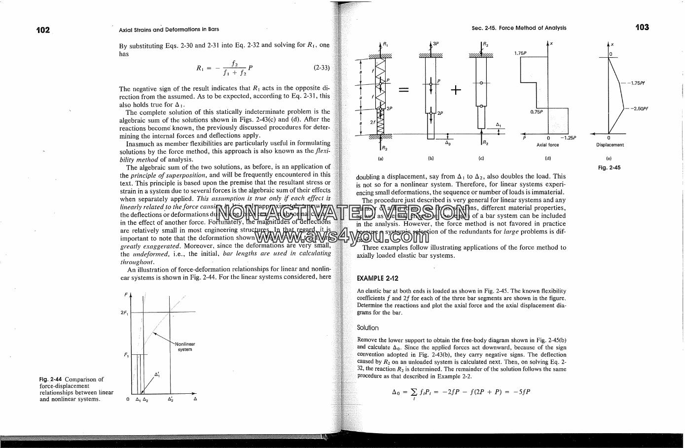
Fig..2-44 Comparison offorce-displacementrelationships between linearand nonlinear systems.
Axial Strains and Deformations in Bars
By substituting Eqs. 2-30 and 2-31 into Eq. 2-32 and solving for R�, onehas
f,_R� = ---P (2-33)
f, + f2
The negative sign of the result indicates that R t acts in the opposite di-rection from the assumed. As to be expected, according to Eq. 2-31, thisalso holds true for A �.
The complete solution of this statically indeterminate problem is thealgebraic sum of the solutions shown in Figs. 2-43(c) and (d). After thereactions becom6 known, the previously discussed procedures for deter-mining the internal forces and deflections apply.
Inasmuch as member flexibilities are particularly useful in formulatingsolutions by the force method, this approach is also known as the flexi-bility tnethod of analysis.
The algebraic sum of the two solutions, as before, is an application ofthe principle ofsuperposition, and will be frequently encountered in thistext. This principle is based upon the premise that the resultant stressstrain in a system due to several forces is the algebraic sum of their effectswhen separately applied. This assumption is true only if each effectlinearly related to the force causing it. It is only approximately true whe�the deflections 0r deformations due to one force cause an abnormal chanin the effect of another force. Fortunately, the magnitudes of deflectionsare relatively small in most engineering structures. In that regard, itimportant to note that the deformation shown in Figs. 2-43(b) to (d)greatly exaggerated. Moreover, since the deformations are verythe undeformed, i.e., the initial, bat' lengths are ased in calculat#�gthroaghout.
An illustration of force-deformation relationships for linear and nonlin-ear systems is shown in Fig. 2-44. For the linear systems considered, here
F
2F�
F 1
"Nonlinealsystem
R1N �x3P
{P -F
Sec. 2-15. Force Method of Analysis
R 2
R 2
1.75P
I
0.75P IP 0 - 1,25P
Axial force
(a) (b) (c) (d)
doubling a displacement, say from A � to A2, also doubles the load. Thisis not so for a nonlinear system. Therefore, for linear systems experi-encing small deformations, the sequence or number of loads is immaterial.
The procedure just described is very general for linear systems and anynumber of axial loads, bar cross sections, different material properties,as well as thermal effects on the length of a bar system can be includedin the analysis. However, the force method is not favored in practicebecause a systemic selection of the redundants for large problems is dif-ficult.
Three examples follow illustrating applications of the force method toaxially loaded elastic bar systems.
EXAMPLE 2-12
An elastic bar at both ends is loaded as shown in Fig. 2-45. The known flexibilitycoefficients f and 2f for each of the three bar segments are shown in the figure.Determine the reactions and plot the axial force and the axial displacement dia-grams for the bar.
Solution
Remove the lower support to obtain the free-body diagram shown in Fig. 2-45(b)and calculate A 0. Since the applied forces act downward, because of the signconvention adopted in Fig. 2-43(b), they carry negative signs. The deflectioncaused by R2 on an unloaded system is calculated next. Then, on solving Eq. 2-32, the reaction R2 is determined. The remainder of the solution follows the sameprocedure as that described in Example 2-2.
Ao = � f,P, = -2fP - f(2P + P) = -5fPi
i03
-1.75Pf
t---2.50Pf
0
Displacement
{e)
Fig. 2-45
NON-ACTIVATEDVERSIONwww.avs4you.com
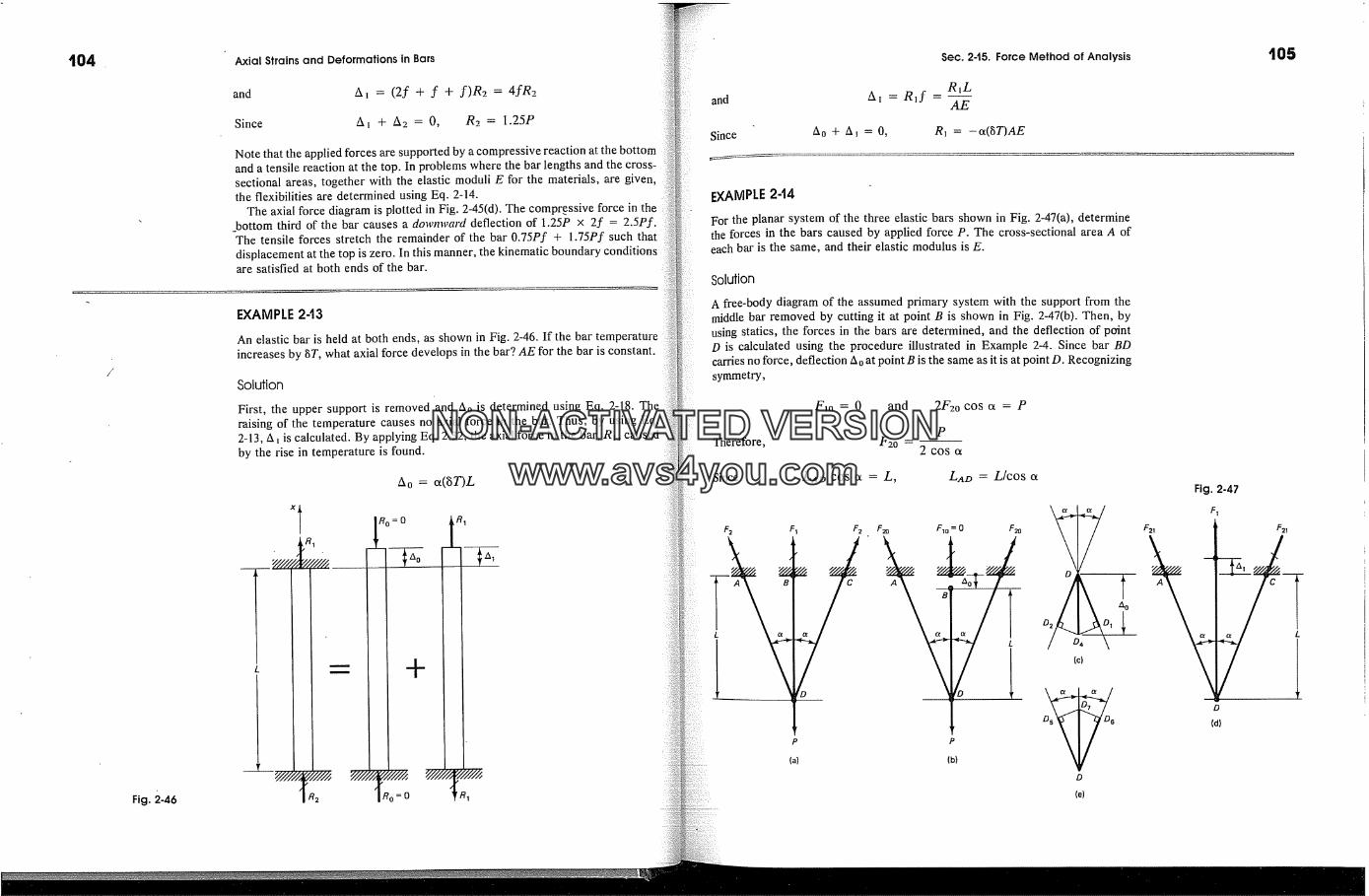
104 Axial Strains and Deformations in Bars Sec. 2-15. Force Method of Analysis 105
Fig. 2.46
and A, = (2f + f + f)R2 = 4fR2
Since A� -F A2 = 0, R2 = 1.25P
Note that the applied forces are supported by a compressive reaction at the bottomand a tensile reaction at the top. In problems where the bar lengths and the cross-sectional areas, together with the elastic moduli E for the materials, are given,the flexibilities are determined using Eq. 2-14.
The axial force diagram is plotted in Fig. 2-45(d). The compr.essive force in the_bottom third of the bar causes a downward deflection of 1.25P x 2f = 2.5Pf.
The tensile forces stretch the remainder of the bar 0.75P� + 1.75P� such thatdisplacement at the top is zero. In this manner, the kinematic boundary conditionsare satisfied at both ends of the bar.
EXAMPLE 2-13
An elastic bar is held at both ends, as shown in Fig. 2-46. If the bar temperatureincreases by �T, what axial force develops in the bar? AE for the bar is constant.
Solution
First, the upper support is removed and A0 is determined using Eq. 2-18. Theraising of the temperature causes no axial force in the bar. Thus, by using Eq.2-13, A � is calculated. By applying Eq. 2-32, the axial force in the bar, R�, causedby the rise in temperature is found.
Ao = et(gT)L
Ro=O
=0 rR 1
and
Since
R�LA� = R�f -
AE
A0 + A� = 0, R� = -ot(�T)AE
EXAMPLE 2-14
For the planar system of the three elastic bars shown in Fig. 2-47(a), determinethe forces in the bars caused by applied force P. The cross-sectional area A ofeach bar is the same, and their elastic modulus is E.
Solution
A free-body diagram of the assumed primary system with the support from themiddle bar removed by cutting it at point B is shown in Fig. 2-47(b). Then, byusing statics, the forces in the bars are determined, and the deflection of pcfintD is calculated using the procedure illustrated in Example 2-4. Since bar BDcarries no force, deflection �0 at point B is the same as it is at point D. Recognizingsymmetry,
F�0 = 0 and 2F20 cos et = P
PTherefore, F20 -
2 cos et
Since L4z� cos et = L, L4t� = L/cos etFig. 2-47
F�
F2 F� F2 Fm Fm=0 F20 F21 L
P P
{a) (b)
D
(e)
NON-ACTIVATEDVERSIONwww.avs4you.com
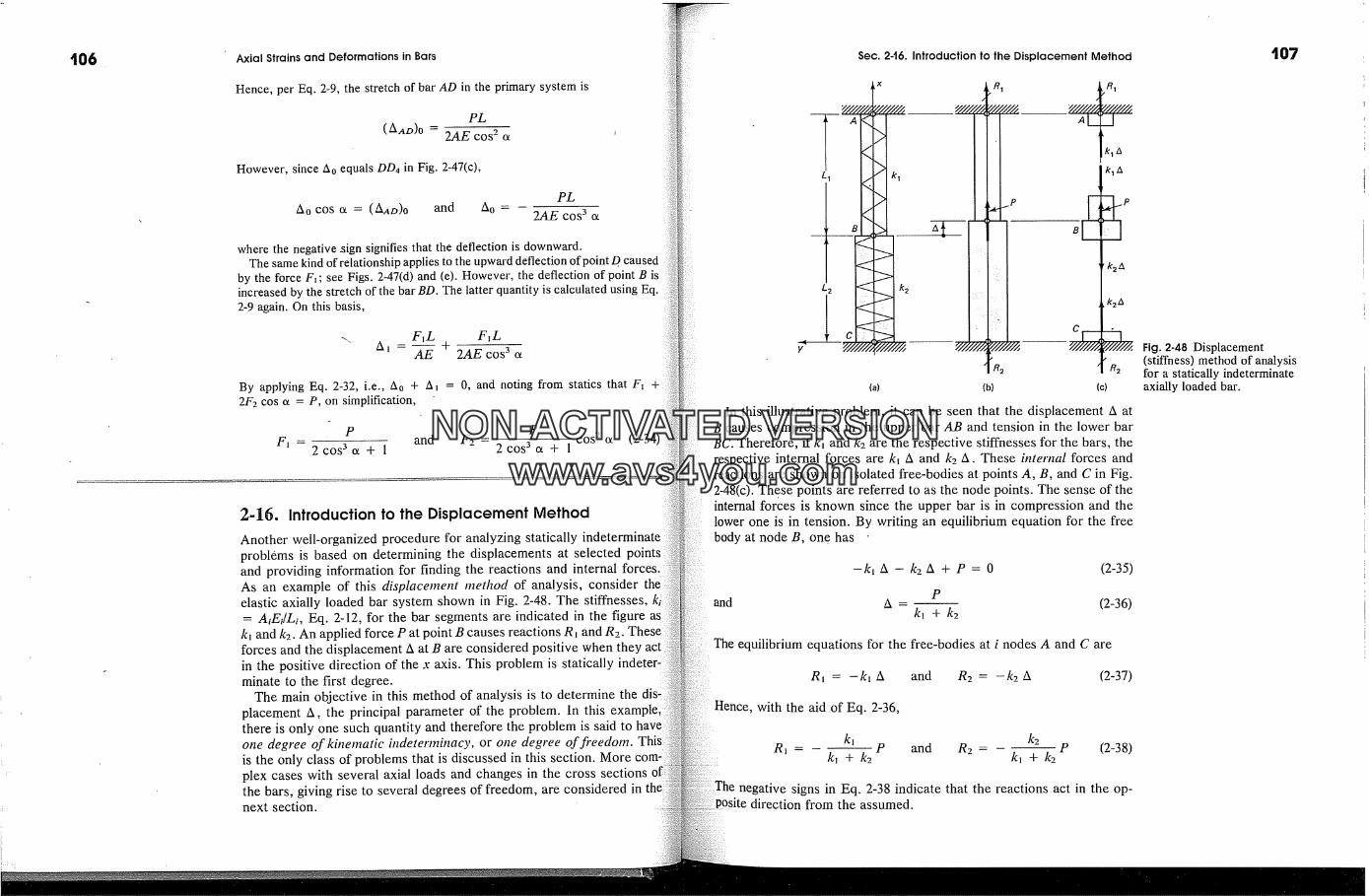
t06 Axial Strains and Deformations in Bars
Hence, per Eq. 2-9, the stretch of bar AD in the primary system is
PL
(A,�D)O -- 2AE cos 2 a
However, since Ao equals DD4 in Fig. 2-47(c),
Ao cos a = (AAO)O and Ao -PL
2AE cos 3 c�
where the negative sign signifies that the deflection is downward.The same kind of relationship applies to the upward deflection of point D caused
by the force F�; see Figs. 2-47(d) and (e). However, the deflection of point B isincreased by the stretch of the bar BD. The latter quantity is calculated using Eq.2-9 again. On this basis,
F�L F�LA � -- AE + 2AE cos 3ix
By applying Eq. 2-32, i.e., A0 + A1 = 0, and noting from statics that F� +2F2 cos a = P, on simplification,
P and F, = PF� = 2cos 3a + 1 - 2cos 3a + lC�S'-a (2-34)
2-16. Introduction to the Displacement Method
Another well-organized procedure for analyzing statically indeterminateproblems is based on determining the displacements at selected pointsand providing information for finding the reactions and internal forces.As an example of this displacement method of analysis, considerelastic axially loaded bar system shown in Fig. 2-48. The stiffnesses,= AiEi/Li, Eq. 2-12, for the bar segments are indicated in the figure as
k� and k2. An applied force P at point B causes reactions R� and R2.forces and the displacement A at B are considered positive when they actin the positive direction of the x axis. This problem is statically indeter-minate to the first degree.
The main objective in this method of analysis is to determine theplacement A, the principal parameter of the problem. In this e�mthere is only one such quantity and therefore the problem is said toone degree of kinematic indeterminacy, or one degree of fi'eedom. Thi s:is the only class of problems that is discussed in this section. Moreplex cases with several axial loads and changes in the cross sectionsthe bars, giving rise to several degrees of freedom, are considered innext section.
Sec. 2-16. Introduction to the Displacement Method
x R� R�/?/A///��///////, __ __
(a) (b)
kaA
R2
(c)
In this illustrative problem, it can be seen that the displacement A atB causes compression in the upper bar AB and tension in the lower barBC. Therefore, if k� and k2 are the respective stiffnesses for the bars, therespective internal forces are k� A and k2 A. These internal forces andreactions are shown on isolated free-bodies at points A, B, and C in Fig.2-48(c). These points are referred to as the node points. The sense of theinternal forces is known since the upper bar is in compression and thelower one is in tension. By writing an equilibrium equation for the freebody at node B, one has
and
-k� A - k2 A -3- P = 0 (2-35)
PA - (2-36)
k� + k2
The equilibrium equations for the flee-bodies at i nodes A and C are
R� = -k� A and R2 = -k2 A (2-37)
Hence, with the aid of Eq. 2-36,
k� k2R� = P and R2 - -- P (2-38)
k� + k2 k� + k2
negative signs in Eq. 2-38 indicate that the reactions act in the op-direction from the assumed.
t07
Fig. 2-48 Displacement(stiffness) method of analysisfor a statically indeterminateaxially loaded bar.
NON-ACTIVATEDVERSIONwww.avs4you.com
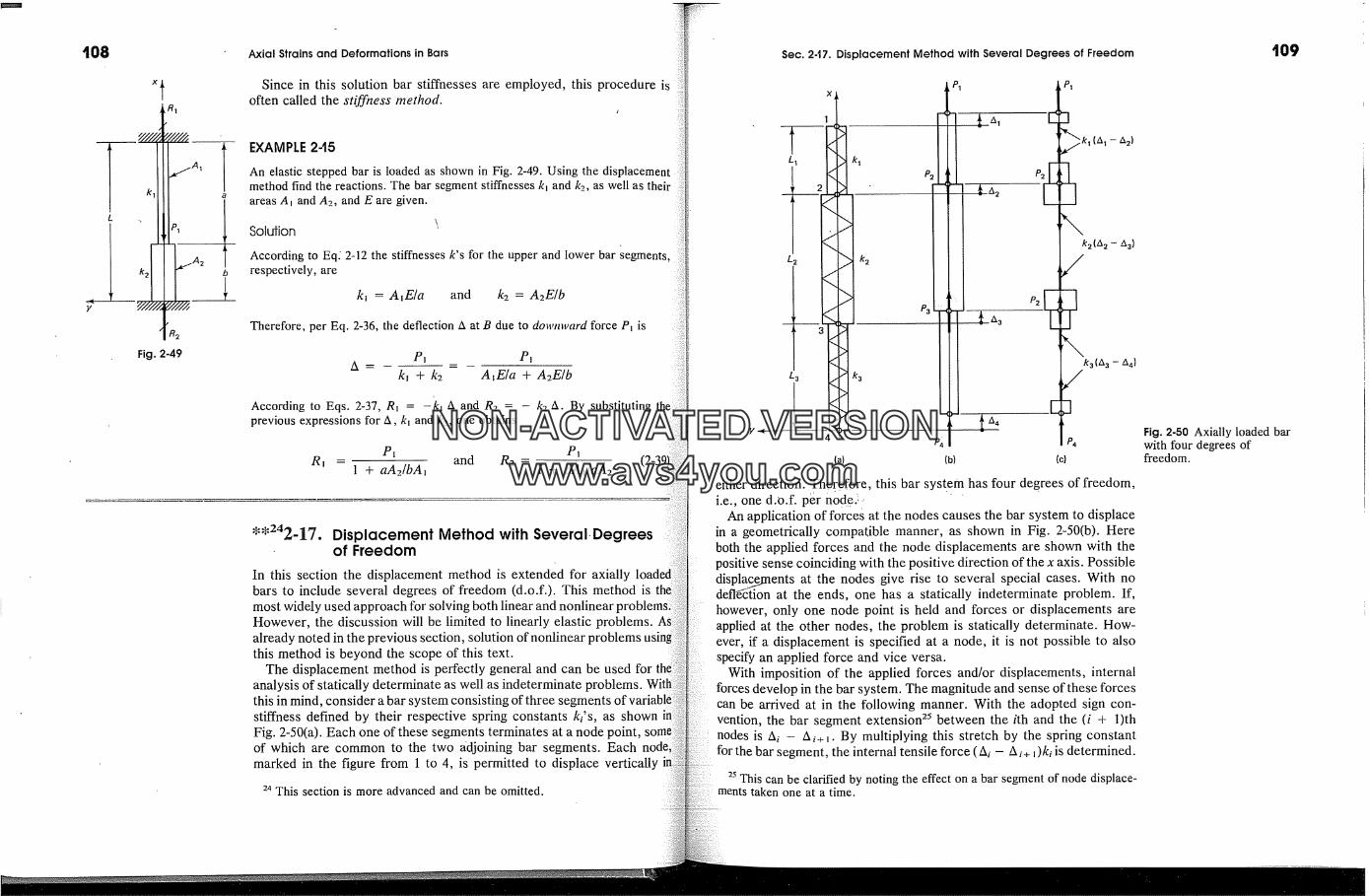
t08
k 1
Fig, 2-49
Axial Strains and Deformations in Bars
Since in this solution bar stiffnesses are employed, this procedure isoften called the stiffness/nethod.
Sec. 2-t7. Displacement Method with Several Degrees of Freedom
EXAMPLE 2-15
An elastic stepped bar is loaded as shown in Fig. 2-49. Using the displacementmethod find the reactions. The bar segment stiffnesses k� and k2, as well as theirareas A� and A2, and E are given.
Soldion
According to Eql 2-12 the stiffnesses k's for the upper and lower bar segmentsrespectively, are
k� = A�E/a and k2 = A2E/b
Therefore, per Eq. 2-36, the deflection A at B due to downward force P� is
P]k� + k2 A�E/a + A2E/b
-k�A andR2 =According to Eqs. 2-37, Rt =previous expressions for A, k� and k2, one obtains
*'242.17 '
-- k2 A. By substituting the
P� P�R� - and R2 = (2-3[
1 + aA2/bA� 1 + bA�/aA2
P3
y�
Displacement Method with Several. Degreesof Freedom
(a)
P4
(b)
P2[[
�,�k� (A�- A2)
k 2 (A 2 --
k3(A 3 -- A4)
,/LJ
P.
(c)
In this section the displacement method is extended for axiallybars to include several degrees of freedom (d.o.f.). This method ismost widely used approach for solving both linear and nonlinear tHowever, the discussion will be limited to linearly elastic problems.already noted in the previous section, solution of nonlinear problemsthis method is beyond the scope of this text.
The displacement method is perfectly general and can be used foranalysis of statically determinate as well as indeterminate problems.this in mind, consider a bar system consisting of three segmentsstiffness defined by their respective spring constants ki's, as shown
either direction. Therefor e, this bar system has four degrees of freedom,i.e., one d.o.f. per node.:-' ' '
An application of forces at the nodes causes the bar system to displacein a geometrically compatible manner, as shown in Fig. 2-50(b). Hereboth the applied forces and the node displacements are shown with thepositive sense coinciding with the positive direction of the x axis. Possibledispla�ce�rnents at the nodes give rise to several special cases. With nodefl�Etion at the ends, one has a statically indeterminate problem. If,however, only one node point is held and forces or displacements areapplied at the other nodes, the problem is statically determinate. How-ever, if a displacement is specified at a node, it is not possible to alsospecify an applied force and vice versa.
With imposition of the applied forces and/or displacements, internalforces develop in the bar system. The magnitude and sense of these forcescan be arrived at in the following manner. With the adopted sign con-vention, the bar segment extension 25 between the ith and the (i + l)th
Fig. 2-50(a). Each one of these segments terminates at a node point, nodes is Ai - A,+,. By multiplying this stretch by the spring constant
ofwhicharecommontothetwoadjoiningbarsegments.Eachnod�r�iiiforthebarsegment,theinternaltensileforce(az--A/+�)k/isdetermined.markedinthefigurefrom1to4,ispermittedtodisplaceverticallyi 2�Thiscanbeclarifiedbynotingtheeffectonabarsegmentofnodedisplace-24 This section is more advanced and can be omitted. ments taken one at a time.
t09
Fig. 2-50 Axially loaded barwith four degrees offreedom.
NON-ACTIVATEDVERSIONwww.avs4you.com
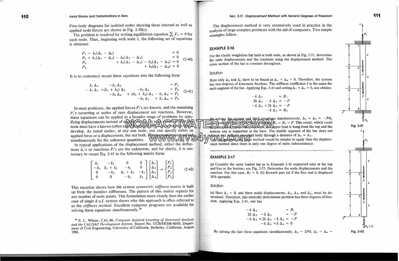
11o Axial Strains and Deformations in Bars
Free-body diagrams for isolated nodes showing these internal as well asapplied node forces are shown in Fig. 2-50(c).
The problem is resolved by writing equilibrium equation � F.� = 0 foreach node. Thus, beginning with node 1, the following set of equationsis obtained:
P, - k�(A� - A2) = 0P2 + k�(A� - A2) - k2(A2 - A3) = 0P3 + k2(A2 - A3) -- k3(A3 -- A4) : 0P4 + k3(A3 -- A4) : 0
� (2-40)
It is to customary recast these equations into the following form
kl A� -kl A2 = P�- k� A� +(k, + k2) A2 -k2 A3 = P2
-k2 A2 + (k2 + k3) A3 -- k3 A4 = P3 (2-41)-- k3 A 3 + k3 A 4 = P4
In most problems, the applied forces Pi's are known, and the remainingPi's occurring at nodes of zero displacement are reactions. However,these equations can be applied tO a broader range of problems by spec-ifying displacements instead of applied forces. In such cases, at least onenode must have a known (often zero) displacement where a reaction woulddevelop. As noted earlier, at any one node, one can specify either anapplied force or a displacement, but not both. These equations are solvedsimultaneously for the unknown quantities.
In typical applications of the displacement method, either the deflec-tions A/s or reactions P/s are the unknowns, and for clarity, it is cus-tomary to recast Eq. 2-41 in the following matrix form:
k� -k� 0-kl k� + k2 -k2
0 -k2 k2 + k30 0 -k3
-k3 A3L4l L:l(2-42)
This equation shows how the system symmetric stiffizess matrix isup from the member stiffnesses. The pattern of this matrix repeatsany number of node points. This formulation more clearly than the earliercase of single d.o.f. system shows why this approach is often referredas the stifflyess method. Excellent computer programs are available forsolving these equations simultaneously?
26 E. L. Wilson, CAL-86, Computer Assisted Learning of Structuraland the CAL/SAP Development System, Report No. UCB/SESM-86/05,ment of Civil Engineering, University of California, Berkeley, California,1986.
Sec. 2-17. Displacement Method with Several Degrees of Freedom
The displacement method is very extensively used in practice in theanalysis of large complex problems with the aid of computers. Two simpleexarnp. les follow.
EXAMPLE 2-16
For the elastic weightless bar' held at both ends, as shown in Fig. 2-5 l, determinethe node displacements and the reactions using the displacement method. Thecross section of the bar is constant throughout.
Solution
Here only A2 and A3 have to be found as A� = A4 = 0. Therefore, the systemhas two degrees of kinematic freedom. The stiffness coefficient k is the same foreach segment of the bar. Applying Eqs. 2-41 and setting A � = A4 = 0, one obtains
-k A2 = R�2k A2 -k A3 = -P
-k A2 +2k A3 = -P-k A3 = R2
By solving the second and third equations simultaneously, A2 = A3 = -P/k,then from the first and the last equations, R� = R2 = P. This result, which couldbe anticipated, means that, in effect, the upper load is hung from the top and thebottom one is supported at the base. The middle segment of the bar does notdistort and deflects as a rigid body through a distance of A2 = A3.
In this problem, the force method would be simpler to apply than the displace-ment method since there is only one degree of static indeterminacy.
EXAMPLE 2-17
(a) Consider the same loaded bar as in Example 2-16 supported only at the topand free at the bottom; see Fig. 2-52. Determine the node displacements and thereaction. For this case, R� = 0. (b) Rework part (a) if the free end is displaced3P/k upwards.
Solution
(a) Here A� = 0, and three nodal displacements, A2, A3, and A4, must be de-termined. Therefore, this statically determinate problem has three degrees of free-dom. Applying Eqs. 2-41, one has
-k A2 = R�2k A2 -k A3 = -P
-k A2 +2k A3 -k A4 = -P-k A3 +k A4 = 0
By solving the last three equations simultaneously, A2 = 2P/k, A3 = A4 =
a k
a k
Fig. 2-51
a k
a k
a k
Fig. 2-52
1'il
=o
NON-ACTIVATEDVERSIONwww.avs4you.com
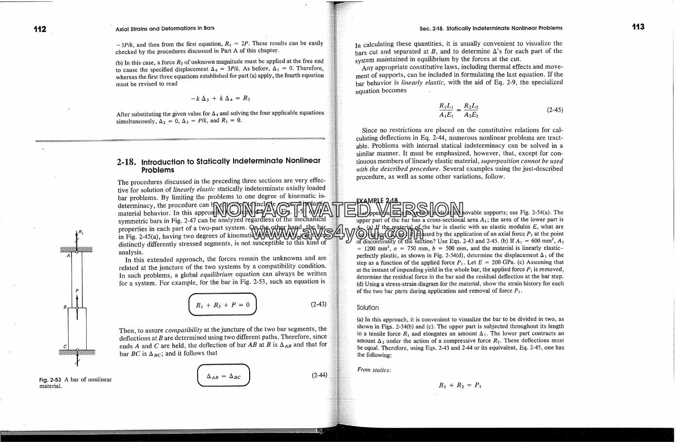
11:1 Axial Strains and Deformations in Bars
-3P/k, and then from the first equation, R� = 2P. These results can be easilychecked by the procedures discussed in Part A of this chapter.(b) In this case, a force R2 of unknown magnitude must be applied at the free endto cause the specified displacement A4 = 3P/k. As before, A� = 0. Therefore,whereas the first three equations established for part (a) apply, the fourth equationmust be revised to read
-kA3 + kA4 = R2
After substituting the given value for �4 and solving the four applicable equationssimultaneously, �2 _= 0, �3 = P/k, and R� = 0.
Fig.'2-53 A bar of nonlinearmaterial.
2-18. Introduction to Statically Indeterminate NonlinearProblems
The procedures discussed in the preceding three sections are very effec-tive for solution of linearly elastic statically indeterminate axially loadedbar problems. By limiting the problems to one degree of kinematic in-determinacy, the procedure can be extended to include cases of inelasticmaterial behavior. In this approach, the stepped bar in Fig. 2-53 orsymmetric bars in Fig. 2-47 can be analyzed regardless of the mechanicalproperties in each part of a two-part system. On the other hand, the barin Fig. 2-45(a), having two degrees of kinematic indeterminacy and threedistinctly differently stressed segments, is not susceptible to this kind ofanalysis.
In this extended approach, the forces remain the unknowns andrelated at the juncture of the two systems by a compatibility condition.In su6h problems, a global eqtdlibrittm equation can always be writtenfor a system. For example, for the bar in Fig. 2-53, such an equation is
R�+ R2+ P = 0) (2-43)
Then, to assure cotnpatibility at the juncture of the two bar segments, thedeflections at B are determined using two different paths. Thereforeends A and C are held, the deflection of bar AB at B is A4B and that forbar BC is ABc; and it follows that
Sec. 248. Statically Indeterminate Nonlinear Problems
In calculating these quantities, it is usually convenient to visualize thebars cut and separated at B, and to determine A's for each part of thesystem maintained in equilibrium by the forces at the cut.
Any appropriate constitutive laws, including thermal effects and move-ment of supports, can be included in formulating the last equation. If thebar behavior is linearly elastic, with the aid of Eq. 2-9, the specializedequation becomes
R�L� R2L2-- = -- (2-45)A�E� A2E2
Since no restfictions are placed on the constitutive relations for cal-culating deflections in Eq. 2-44, numerous nonlinear problems are tract-able. Problems with internal statical indeterminacy can be solved in asimilar manner. It must be emphasized, however, that, except for con-tinuous members of linearly elastic material, superposition cannot be usedwith the described procedure. Several examples using the just-descfibedprocedure, as well as some other variations, follow.
EXAMPLE 248
A stepped bar is held at both ends at immovable supports; see Fig. 2-54(a). Theupper part of the bar has a cross-sectional area A�; the area of the lower part isA2. (a) If the material of the bar is elastic with an elastic modulus E, what arethe reactions R� and R2 caused by the application of an axial force P� at the pointof discontinuity of the section? Use Eqs. 2-43 and 2-45. (b) If A� = 600 mm 2, A2= 1200 m m2, a = 750 mm, b = 500 mm, and the material is linearly elastic-
perfectly plastic, as shown in Fig. 2-54(d), determine the displacement A � of thestep as a function of the applied force P�. Let E = 200 GPa. (c) Assuming thatat the instant of impending yield in the whole bar, the applied force P� is removed,determine the residual force in the bar and the residual deflection at the bar step.(d) Using a stress-strain diagram for the material, show the strain history for eachof the two bar parts during application and removal of force P�.
Solution
(a) In this approach, it is convenient to visualize the bar to be divided in two, asshown in Figs. 2-54(b) and (c). The upper part is subjected throughout its lengthto a tensile force R� and elongates an amount A�. The lower part contracts anamount A2 under the action of a compressive force R2. These deflections mustbe equal. Therefore, using Eqs. 2-43 and 2-44 or its equivalent, Eq. 2-45, one hasthe following:
From statics:
R� + R2 = P�
113
NON-ACTIVATEDVERSIONwww.avs4you.com
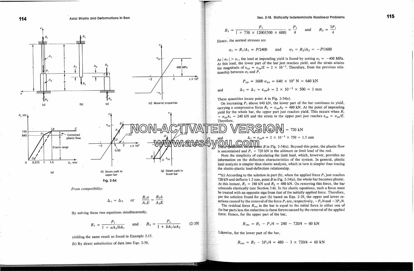
114 Axial Strains and Deformations in Bars
R� . R�
(a) (b)
A 2 R2
x/////4 '///x
400 MPa
2 gX 10 a
(d) Material properties
P1
720
640
B C
A ,� :"�'"" Contained
/ plasticflow--lastic range
0 0.375 I 1.5 64 mm
Oyp
A�,,1.33DL�I �
� 2 �X 1030.50
00.752 '� X 10 a
(e) (f) Strain path inupper bar
Fig. 2-54
(g) Strain path inlower bar
From compatibility:
gl aA� = A 2 or AlE
R2bA2E
By solving these two equations simultaneously,
P� P�R� = 1 + aA2/bA� and - R2 - 1 + bA1/aA2 (2-39)
yielding the same result as found in Example 2-15.(b) By direct substitution of data into Eqs. 2-39,
Sec. 2-t8. Statically Indeterminate Nonlinear Problems
P� P� 3P�R� = 1 + 750 x 1200/(500 x 600) 4 and R2 4
Hence, the normal stresses are
cr� = R�/A� = P/2400 and or2 -- R2/A2 - -P/1600
As [ cr2 I > crY, the load at impending yield is found by setting cr2 = -400 MPa.At this load, the lower part of the bar just reaches yield, and the strain attainsthe magnitude of �yp = cryp/E = 2 x 10 -3. Therefore, from the previous rela-tionship between cr2 and P,
Pyp = 1600 tryp = 640 x 103 N = 640 kN
and A 2 = A� = �ypb = 2 x 10 -3 x 500 = 1 mm
These quantities locate point A in Fig. 2-54(e).On increasing P� above 640 kN, the lower part of the bar continues to yield,
carrying a compressive force R2 = CrypA2 = 480 kN. At the point of impendingyield for the whole bar, the upper part just reaches yield. This occurs when R�= CrypAl = 240 kN and the strain in the upper part just reaches gyp = CrypiE.
Therefore,
P� = R� + R2 = 720 kN
and /x� = eypa = 2 x 10 -3 X 750 = 1.5 Inm
These quantities locate point B in Fig. 2-54(e). Beyond this point, the plastic flowis uncontained and P� = 720 kN is the ultimate or limit load of the rod.
Note the simplicity of calculating the limit load, which, however, provides noinformation on the deflection characteristics of the system. In general, plasticlimit analysis is simpler than 'elastic analysis, which in turn is simpler than tracingthe elastic-plastic load-deflection relationship.
**(c) According to the solution in part (b), when the applied force P� just reaches720 kN and deflects 1.5 mm, point B in Fig. 2-54(e), the whole bar becomes plastic.At this instant, R� = 240 kN and R2 = 480 kN. On removing this force, the barrebounds elastically (see Section 2-6). In the elastic equations, such a force mustbe treated with an opposite sign from that of the initially applied force. Therefore,per the solution found for part (b) based on Eqs. 2-39, the upper and lower re-actions caused by the removal of the force P� are, respectively, - P�/4 and - 3P�/4.
The residual force Rr� in the bar is equal to the initial force in either one ofthe bar parts less the reduction in these forces caused by the removal of the appliedforce. Hence, for the upper part of the bar,
R�e� = R� - P�/4 = 240 - 720/4 = 60 kN
Lik.ewise, for the lower part of the bar,
R�e� = R2 - 3P�/4 = 480 - 3 x 720/4 = 60 kN
115
NON-ACTIVATEDVERSIONwww.avs4you.com
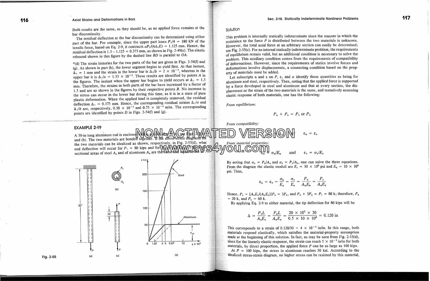
116 Axial Strains and Deformations in Bars
Both results are the same, as they should be, as no applied force remains at thebar discontinuity.
The residual deflection at the bar discontinuity can be determined using eitherpart of the bar. For example, since the upper part loses P�/4 = 180 kN of thetensile force, based on Eq. 2-9, it contracts aPt/(4A�E) = 1.125 mm. Hence, theresidual deflection is 1.5 - 1.125 = 0.375 mm, as shown in Fig. 2-49(e). The elasticrebound shown in this figure by the dashed line BD is parallel to OA.*(d) The strain histories for the two parts of the bar are given in Figs. 2-54(f) and(g). As shown in part (b), the lower segment begins to yield first. At that instant,/x� = 1 mm and the strain in the lower bar is A�/b = 2 x 10 -3, whereas in theupper bar it is /x �/a = 1.33 x 10 -3. These results are identified by points A inthe figures. The ins{ant when the upper bar begins to yield occurs at /x� = 1.5mm. Therefore, the strains in both parts of the bar have increased by a factor of1.5 and are so shown in the figures by their respective point.s B. No increase inthe stress can occur in the lower bar during this time, as it is in a state of pureplastic deformation. When the applied load is completely removed, the residualdeflection /x� = 0.375 mm. Hence, the corresponding residual strains A�/a and/x �/b are, respectively, 0.50 x 10 -3 and 0.75 x 10 -3 m/m. The correspondingpoints are identified by points D in Figs. 2-54(f) and (g).
EXAMPLE 2-19
A 30-in long atun�inum rod is enclosed within a steel-alloy tube; see Figs. 2-55(a)and (b). The two materials are bonded together. If the stress-strain diagrams forthe two materials can be idealized as shown, respectively, in Fig. 2-55(d), whatend deflection will occur for P� = 80 kips and for P2 = 125 kips? The cross-sectional areas of steel As and of aluminum A� are the same and equal to 0.5 in 2.
Fig. 2-55 (a)
A s
o ksi
20C
(b)150
dx� 100
(c)
Steel
iAluminum
//
1.67 4 5 6.67 10 tX10
(d)
Sec. 2.18. Statically Indeterminate Nonlinear Problems
Solution
This problem is internally statically indeterminate since the manner in which theresistahce to the force P is distributed between the two materials is unknown.However, the total axial force at an arbitrary section can easily be determined;see Fig. 2-55(c). For an internal statically indeterminate problem, the requirementsof equilibrium remain valid, but an additional condition is necessary to solve theproblem. This auxiliary condition comes from the requirements of compatibilityof deformations. However, since the requirements of statics involve forces anddeformations involve displacements, a connecting condition based on the prop-erty of materials must be added.
Let subscripts a and s on P, e, and cr identify these quantities as being foraluminum and steel, respectively. Then, noting that the applied force is supportedby a force developed in steel and aluminum and that at every section, the dis-placement or the strain of the two materials is the same, and tentatively assumingelastic response of both materials, one has the following:
From equilibrium:
Pa + Ps = P�orP2
From compatibility:
Aa = As or �a �' Es
From material properties:
and es = crdEs
By noting that cr� = P�/A� and crs= PdAs, one can solve the three equations.From the diagram the elastic moduli are Es = 30 x 10 a psi and E� = 10 x 10 apsi. Thus,
era Ors Pa Ps
Hence, Ps = [A�Ed(A�E�)]P� = 3P�, and P� + 3Pa = P� = 80 k; therefore, P�=20k, andP� = 60k.
By applying Eq. 2-9 to either material, the tip deflection for 80 kips will be
PsL PaL 20 x 103 x 30A - - = 0.120 in
AsEs AaEa 0.5 x 10 x 106
This corresponds to a strain of 0.120/30 = 4 x 10 -3 in/in. In this range, bothmaterials respond elastically, which satisfies the material-property assumptionmade at the beginning of this solution. In fact, as may be seen from Fig. 2-55(d),since for the linearly elastic response, the strain can reach 5 x 10 -3 in/in for bothmaterials, by direct proportion, the applied force P can be as large as 100 kips.
At P = 100 kips, the stress in aluminum reaches 50 ksi. According to thestress-strain diagram, no higher stress can be resisted by this material,
117
NON-ACTIVATEDVERSIONwww.avs4you.com
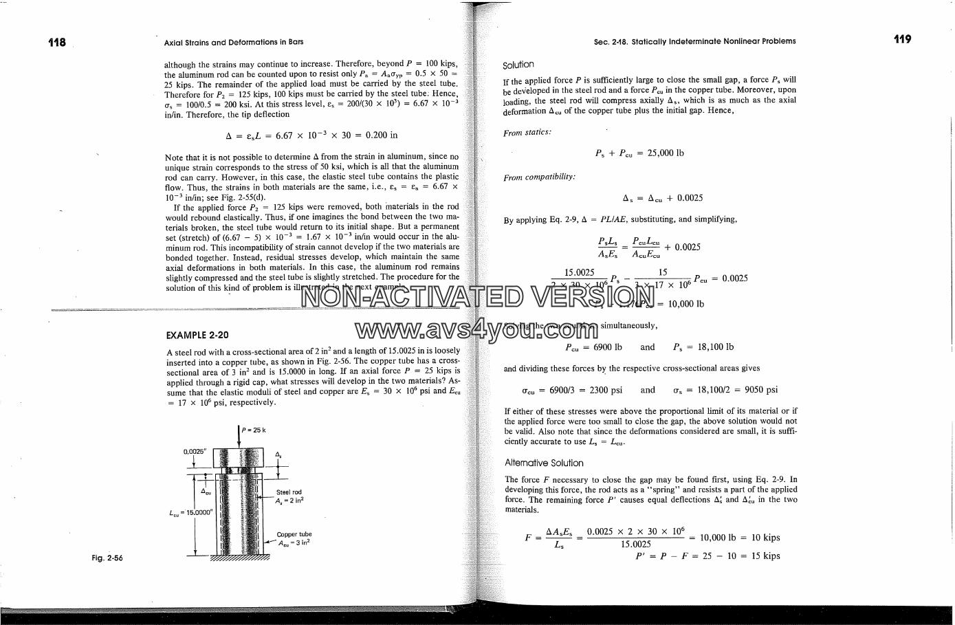
Fig. 2-56
Axial Strains and Deformations in Bars
although the strains may continue to increase. Therefore, beyond P = 100 kips,the aluminum rod can be counted upon to resist only Pa = Aao'yp = 0.5 X 50 =25 kips. The remainder of the applied toad must be carried by the steel tube.Therefore for P2 = 125 kips, 100 kips must be carried by the steel tube: Hence,crs= 100/0.5 = 200 ksi. At this stress level, e� = 200/(30 x 103) = 6.67 x 10 -3in/in. Therefore, the tip deflection
A = esL = 6.67 x 10 -3 x 30 = 0.200 in
Note that it is not possible to determine/x from the strain in aluminum, since nounique strain corresponds to the stress of 50 ksi, which is all that the aluminumrod can carry. However, in this case, the elastic steel tube contains the plasticflow. Thus, the strains in both materials are the same, i.e., es = �a = 6.67 x10 -3 in/in; see Fig. 2-55(d).
If the applied force P2 = 125 kips were removed, both materials in the rodwould rebound elastically. Thus, if one imagines the bond between the two ma-terials broken, the steel tube would return to its initial shape. But a permanentset (stretch) of (6.67 - 5) x 10 -3 = 1.67 x 10 -3 in/in would occur in the alu-minum rod. This incompatibility of strain cannot develop if the two materials arebonded together. Instead, residual stresses develop, which maintain the sameaxial deformations in both materials. In this case, the aluminum rod remainsslightly compressed and the steel tube is slightly stretched. The procedure for thesolution of this kind of problem is illustrated in the next example.
EXAMPLE 2-20
A steel rod with a cross-sectional area of 2 in 2 and a length of 15.0025 in is looselyinserted into a copper tube, as shown in Fig. 2-56. The copper tube has a cross-sectional area of 3 in 2 and is 15.0000 in long. If an axial force P = 25 kips isapplied through a rigid cap, what stresses will develop in the two materials? As-sume that the elastic moduli of steel and copper are Es = 30 x 10 6 psi and Ecu= 17 x 10 6 psi, respectively.
0.0025"
P=25k
Lcu =
Steel rod
A s = 2 in 2
Coppertube= 3 in 2
Solution
Sec. 248. Statically Indeterminate Nonlinear Problems
If the applied force P is sufficiently large to close the small gap, a force P� willbe developed in the steel rod and a force Pc, in the copper tube. Moreover, uponloading, the steel rod will compress axially A�, which is as much as the axialdeformation Ac, of the copper tube plus the initial gap. Hence,
From statics:
From compatibility:
Ps + Pcu = 25,000 lb
As = Ac. + 0.0025
By applying Eq. 2-9, A = PL/AE, substituting, and simplifying,
- + 0.0025
15.0025 15
2 x 30 x 106Ps - 3 x 17 x 106Pc" = 0.0025Ps- 1.176Pc, = 10,000 lb
Solving the two equations simultaneously,
Pcu = 6900 lb and Ps = 18,100 lb
and dividing these forces by the respective cross-sectional areas gives
crcu = 6900/3 = 2300 psi and ors = 18,100/2 = 9050 psi
If either of these stresses were above the proportional limit of its material or ifthe applied force were too small to close the gap, the above solution would notbe valid. Also note that since the deformations considered are small, it is suffi-ciently accurate to use Ls = Lc,.
Alternative Solution
The force F necessary to close the gap may be found first, using Eq. 2-9. Indeveloping this force, the rod acts as a "spring" and resists a part of the appliedforce. The remaining force P' causes equal deflections A� and A�, in the twomaterials.
AAsEs 0.0025 x 2 x 30 x 106F .... 10,000 lb = 10 kips
Ls 15.0025P' =P- F= 25 - 10 = 15 kips
119
NON-ACTIVATEDVERSIONwww.avs4you.com

Fig. 2-57
Axial Strains and Deformations in Bars
Then if P's is the force resisted by the steel rod, in addition to the force F, andP�u is the force carried by the copper tube,
From statics:
p; +p' = P' = 15cu
From compatibility:
cu orP;LsAsEs Ac,E�
15.0025 P' = 15 p, P' 17 ,2 x 30 x 106 s 3 x 17 x 106 .... = 20 PsBy solving the two appropriate equations simultaneously, it is found tha t P�u =6.9 kips and P's = 8.1 kips, or Ps = P} + F = 18.1 kips.
If (cryp)s = 40 ksi and (cryp)c� = 10 ksi, the limit lead for this assembly can bedetermined as follows:
Pull = (Cryp)sAs +'(ffyp)cuAcu = 110 kips
At the ultimate lo&d, both materials yield, therefore, the small discrepancy in theinitial lengths of the parts is of no consequence.
EXAMPLE 2-21
A copper tube 12-in long and having a cross-sectional area of 3 in 2 is placedbetween two very rigid caps made of Invar27; see Fig. 2-57(a). Four �-in steelbolts are symmetrically arranged parallel to the axis of the tube and are lightly
27 Invar is a steel alloy which at ordinary temperatures has an a � 0 and forthis reason is used in the best grades of surveyor's tapes and watch springs.
Elastic deformations
Thermal d�
Finalposition
(a)
Sec. 2-t8. Statically Indeterminate Nonlinear Problems
tightened. Find the stress in the tube if the temperature of the assembly is raisedfrom60 �Fto 160�F. LetE� = 17 x 106 psi, Es = 30 x 106 psi, a� = 9.1 x10 -6 p.er �F, and a� = 6.5 x 10 -6 per �F.
Solution
If the copper tube and the steel bolts were free to expand, the axial thermalelongations shown in Fig. 2�57(b) would take place. However, since the axialdeformation of the tube must be the same as that of the bolts, the copper tubewill be pushed back and the bolts will be pulled out so that the net deformationswill be the same. Moreover, as can be established by considering a free body ofth� assembly above some arbitrary section such as A-A in Fig. 2-57(a), the com-presslye force P� in the copper tube and the tensile force P� in the steel boltsare equal. Hence,
From statics:
P�u = Ps = P
From compatibility:
This kinematic relation, on the basis of Fig. 2-57(b) with the aid of Eqs. 2-18and 2-9, becomes
P�uLcu PsLsa�(gT)L�u A�uE�u = as(gT)L� +
or, since L� = L�, �T = 100 � and 0.442 in 2 is the cross section of one bolt,
9.1 x 10 -6 X 100 -Pcu
3 x 17 x 106
= 6.5 X 10 -6 X 100 +Ps
4 x 0.442 x 30 x 10 a
By solving the two equations simultaneously, P = 6750 lb. Therefore, the stressin the copper tube is crc� = 6750/3 = 2250 psi.
The kinematic expression just used may also be set up on the basis of thefollowing statement: the differential expansion of the two materials due to thechange in temperature is accommodated by or is equal to the elastic deformationsthat take place in the two materials.
EXAMPLE 2-22
A steel bolt having a cross-sectional area A� = 1 in 2 is used to grip two steelwashers of total thickness, L, each having the cross-sectional area A2 = 9 in2;see Fig. 2-58(a). If the bolt in this assembly is tightened initially so that its stress
NON-ACTIVATEDVERSIONwww.avs4you.com
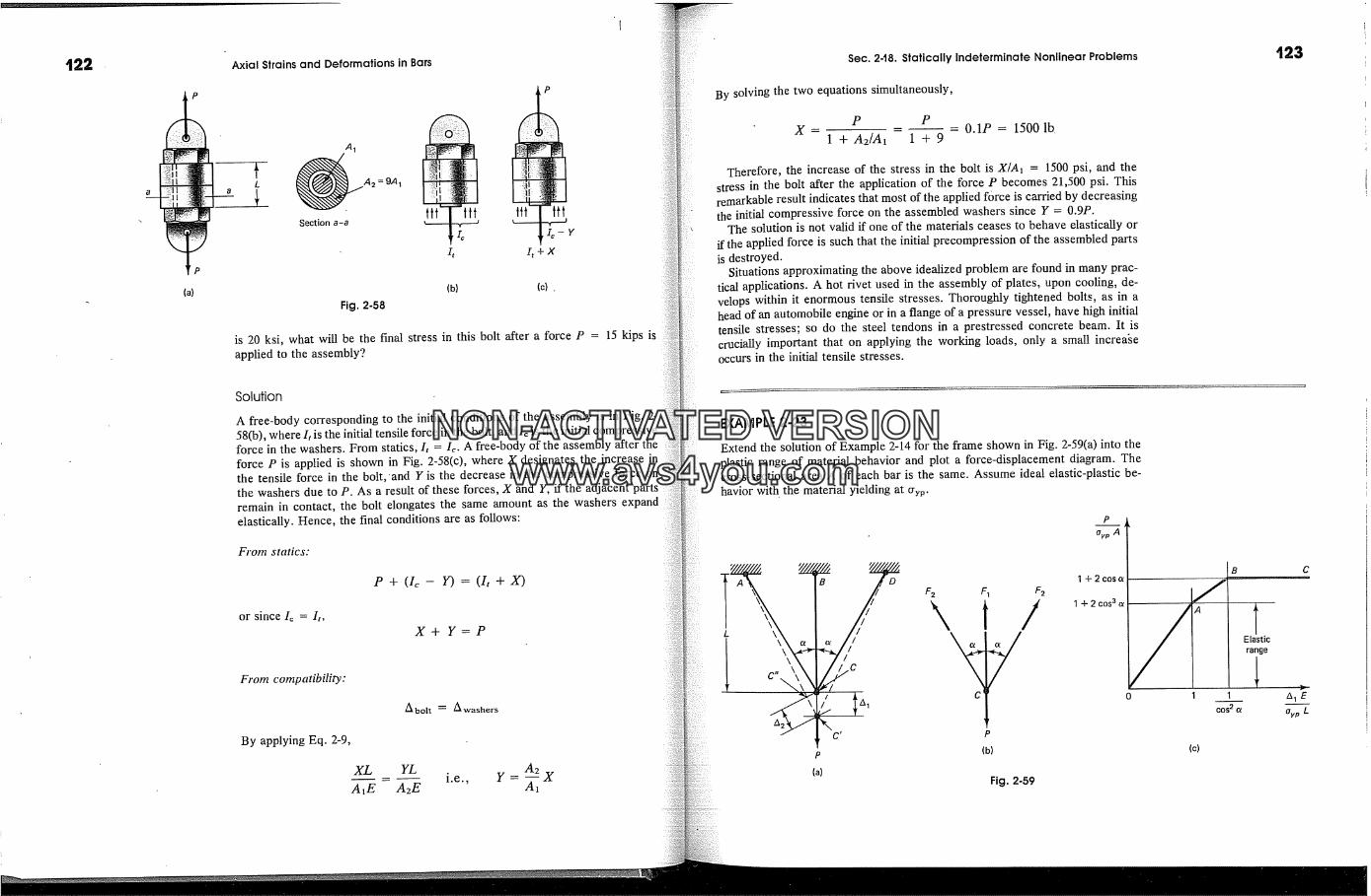
1:22
P
(a)
Axial Strains and Deformations in Bars
ml
Section a-a
= 9A 1
ttt--tft ttt tit
h h- Yh h+x
(b) (c) .
Fig. 2-58
is 20 ksi, what will be the final stress in this bolt after a force P = 15 kips isapplied to the assembly?
Solution
A free-body corresponding to the initial conditions of the assembly is in Fig. 2-58(b), where It is the initial tensile force in the bolt, and Ic is the initial compressiveforce in the washers. From statics, It = Io A free-body of the assembly after theforce P is applied is shown in Fig. 2-58(c), where X designates the increase inthe tensile force in the bolt,'and Y is the decrease in the compressive force onthe washers due to P. As a result of these forces, X and Y, if the adjacent partsremain in contact, the bolt elongates the same amount as the washers expandelastically. Hence, the final conditions are as follows:
From statics:
P + (I�- Y) = (I, +X)
or since Ic = I,,X+Y=P
From compatibility:
By applying Eq. 2-9,
Abolt � Awasher s
XL YL
A� - A2EA2
Sec. 2-t8. Statically Indeterminate Nonlinear Problems
By solving the two equations simultaneously,P P
X - = 0.1P = 1500 lb.1 + A2/A� 1 + 9
Therefore, the increase of the stress in the bolt is X/A� = 1500 psi, and thestress in the bolt after the application of the force P becomes 21,500 psi. Thisremarkable result indicates that most of the applied force is carried by decreasingthe initial compressive force on the assembled washers since Y = 0.9P.
The solution is not valid if one of the materials ceases to behave elastically orif the applied force is such that the initial procompression of the assembled partsis destroyed.
Situations approximating the above idealized problem are found in many prac-tical applications. A hot rivet used in the assembly of plates, upon cooling, de-velops within it enormous tensile stresses. Thoroughly tightened bolts, as in ahead of an automobile engine or in a flange of a pressure vessel, have high initialtensile stresses; so do the steel tendons in a prostressed concrete beam. It iscrucially important that on applying the working loads, only a small increa�eoccurs in the initial tensile stresses.
123
EXAMPLE 2-23
Extend the solution of Example 2-14 for the frame shown in Fig. 2-59(a) into theplastic range of material behavior and plot a force-displacement diagram. Thecross-sectional area A of each bar is the same. Assume ideal elastic-plastic be-havior with the material yielding at crvp.
P
Ovp A
B DA '�
o� /
//
c'
P
(a)
F 2 F,
x,
c
F2
P
(b)
Fig. 2-59
I + 2 cosa
I + 2 cos 3 a
B
COS 20�
(c)
Elasticrange
AlEO�,p L
NON-ACTIVATEDVERSIONwww.avs4you.com

Axial Strains and Deformations in Bars
Solution
The equilibrium equation for forces atjoint C, Fig. 2-59(c), recognizing symmetry,is
F� + 2F2cosat = P
The compatibility equation at joint C, Fig. 2-59(a), relating the elongations inbars AC' and DC' with that of bar BC' is
A 2 = A� COS at
In both of these equations, it is assumed that the deformations are small.ever, these equations hold true whether the bar material behaves elasticallyplastically.
By noting that the inclined bars are L/(cos ct) long, using Eq. 2-9 and the es-tablished compatibility equation,
F2[L/cos at] F�LAE AE
--cosat or F2 = F�cos 2at
By substituting the last expression into the equilibrium equation at joint C, andsimplifying leads-to the same results as found in Example 2-14:
P and F2 P- cos 2 at (2-34)F� = 1 + 2c0s 3at. 1 + 2c0s 3atIt is seen from this solution that the maximum force occurs in the vertical bar.
At the impending yield Fl = crypA, and, per Eq. 2.9, A � = crypL/E. By substitutingF, = crypA into the left side of Eq. 2-34, the force P = crypA(1 + 2 cos 3 a) atthe limit of elastic behavior is obtained. This value of P occurring at A � = CrypL/E is identified by point A in Fig. 2-59(c).
By increasing force P above the first yield in the vertical bar, force F� = crvpAremains constant, and the equation of statics at joint C is sufficient for determiningforce F2 until the stress in the inclined bars reaches Cryp. This occurs when F2 =CryvA. At the impending yield in the inclined bars, and the vertical bar alreadyyielding, the joint C equilibrium equation gives P = CrypA(1 q- 2 cos ct). Thiscondition corresponds to the plastic litnit load for the system. Note that the pro-cedure of finding this load is rather simple, as the system is statically determinatewhen the limit load is reached. In Chapter 13, such a limit load is associated withthe concept of the collapse mechanism.
At the impending yield in the inclined bars, per Eq. 2-9, A2 = (CrypiE)[L/cos or]and A � = A2/cos ct = CrypL/(E cos 2 cO. This value of A � locates the abscissa forpoint B in Fig. 2-59(c). Beyond this point, all bars continue to yield without boundbased on ideal plasticity.
Sec. 2-19. Differential Equation Approach for Deflections
,.282-19. Alternative Differential Equation Approach forDeflections
In Section 2-7, the axial deflection u of a bar was in essence determinedby solving a first-order differential ex = du/dx, Eq. 2-6. It is instructiveto reformulate this problem as a second-order equation. Such an equationfor linearly elastic materials follows from two observations. First, since,in general, du/dx = � = cr?E = P/AE, one has
p = AE�x x (2-46)
The second relation is based on the equilibrium requirements for an in-finitesimal element of an axially loaded bar. For this purpose, considera typical element such as that in Fig. 2-60, where all forces are sho�vnwith a positive sense according to the previously adopted sign convention.Since�Fx = 0ordP +p�dx = 0, and
dx - P � �n (2-47)
This equation states that the rate of change with x of the internal axialforce P is equal to the negative of the applied force p�. On this 'basis,assuming AE constant,
�xx = AE �xx or AE dx 2 - p� (2-48)
2a This section is optional; can be studied after Section 2-7 before the accom-panying examples.
Px lb perunit length
p P+dP
� -dx �
't25
Fig. 2-60 Infinitesimalelement of an axially loadedbar.
NON-ACTIVATEDVERSIONwww.avs4you.com
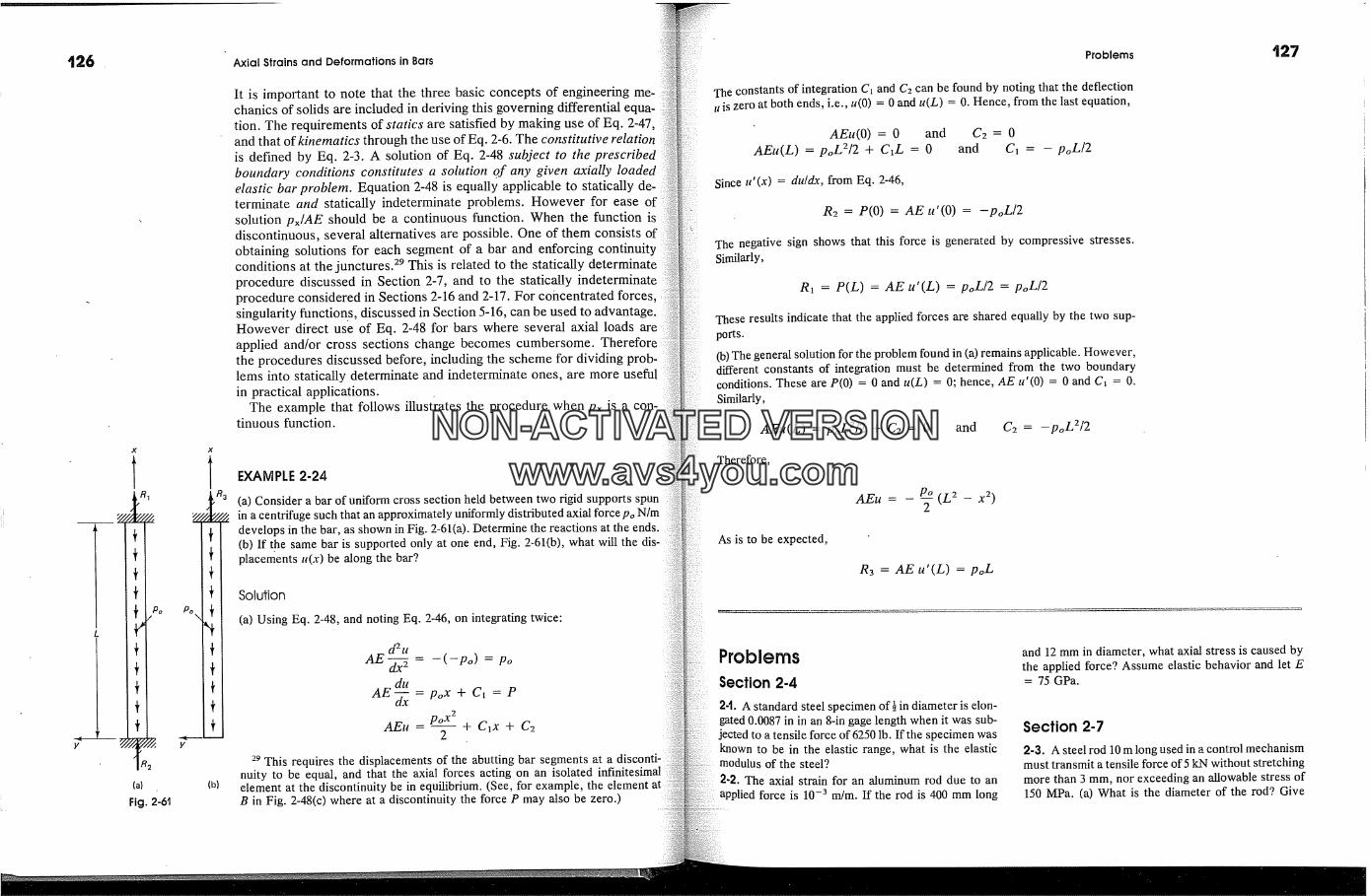
x
(a)
Fig. 2-61
Po\
X
R3
(b)
Axial Strains and Deformations in Bars
Itisimportanttonotethatthethreebasicconceptsofengineeringme-chanics of solids are included in deriving this governing differential equa-tion. The requirements of statics are satisfied by making use of Eq. 2-47,and that of kinematics through the use of Eq. 2-6. The constitutive relationis defined by Eq. 2-3. A solution of Eq. 2-48 subject to the prescribedboundary conditions constitutes a solution of any given axially loadedelastic bar problem. Equation 2-48 is equally applicable to statically de-terminate and statically indeterminate problems. However for ease ofsolution px/AE should be a continuous function. When the function isdiscontinuous, several alternatives are possible. One of them consists ofobtaining solutions for each segment of a bar and enforcing continuityconditions at the junctures? This is related to the statically determinateprocedure discussed in Section 2-7, and to the statically indeterminateprocedure considered in Sections 2-16 and 2-17. For concentrated forces,singularity function. s, discussed in Section 5-16, can be used to advantage.However direct use of Eq. 2-48 for bars where several axial loads areapplied and/or cross sections change becomes cumbersome. Thereforethe procedures discussed before, including the scheme for dividing prob-lems into statically determinate and indeterminate ones, are more usefulin practical applications.
The example that follows illustrates the procedure when px is a con-tinuous function.
EXAMPLE 2-24
(a) Consider a bar of uniform cross section held between two rigid supports spunin a centrifuge such that an approximately uniformly distributed axial force po N/mdevelops in the bar, as shown in Fig. 2-61(a). Determine the reactions at the ends.(b) If the same bar is supported only at one end, Fig. 2-61(b), what will the dis-placements u(x) be along the bar?
Solution
(a) Using Eq. 2-48, and noting Eq. 2-46, on integrating twice:
d e uAE �x2 = -(-Po) = po
du
AE �xx = pox + C� = Ppox 2
AEu - + Cix + C22
29 This requires the displacements of the abutting bar segments at anuity to be equal, and that the axial forces acting on an isolated infinitesimalelement at the discontinuity be in equilibrium. (See, for example, the elementB in Fig. 2-48(c) where at a discontinuity the force P may also be zero.)
Problems
The constants of integration C� and C2 can be found by noting that the deflectiontt is zero at both ends, i.e., u(0) = 0 and u(L) = 0. Hence, from the last equation,
AEu(0) = 0 and C2 = 0AEu(L) = poL2/2 + C�L = 0 and C� = - poL/2
Since u'(x) = du/dx, from Eq. 2-46,
R2 = P(O) = AE u'(O) = -poL/2
The negative sign shows that this force is generated by compressive stresses.Similarly,
R� = P(L) = AE u'(L) = poL/2 = poL/2
These results indicate that the applied forces are shared equally by the two sup-ports.
(b) The general solution for the problem found in (a) remains applicable. However,different constants of integration must be determined from the two boundaryconditions. These are P(O) -- 0 and u(L) -- O; hence, AE u'(O) = 0 and C� -- O.Similarly,
AEu(L) = poL2/2 + C2 = 0 and C2 = -poL2/2
Therefore,
AEu - PO (L 2_ x 2)2
As is to be expected,
R3 =AEu'(L) = poL
ProblemsSection 2-4
2-t. A standard steel specimen of� in diameter is elon-gated 0.0087 in in an 8-in gage length when it was sub-
jected to a tensile force of 6250 lb. If the specimen wasknown to be in the elastic range, what is the elasticmodulus of the steel?2-2. The axial strain for an aluminum rod due to anapplied force is 10 -3 m/m. If the rod is 400 mm long
and 12 mm in diameter, what axial stress is caused bythe applied force? Assume elastic behavior and let E
= 75 GPa.
Section 2-7
2-3. A steel rod 10 m long used in a control mechanismmust transmit a tensile force of 5 kN without stretchingmore than 3 mm, nor exceeding an allowable stress of150 MPa. (a) What is the diameter of the rod? Give
NON-ACTIVATEDVERSIONwww.avs4you.com

Axial Strains and Deformations in Bars
the answer to the nearest millimeter. E = 210 GPa.Does strength or stiffness of the rod control the design?(b) Find the spring constant for the rod.2-4. Revise the data in Example 2-2 to read as follows:P� = 10 kips, P3 = 100 kips, and P4 = 30 kips, andthe bar segments AB, BC, and CD are, respectively,4-, 2-. and 3-ft long. Then find (a) the force P2 nec-essary for equilibrium and (b) the total elongation ofrod AD. The cross-sectional area of the rod from A toBis 1 in 2, from B to C is 4 in 2, and from C to D is 2in 2. Let E = 30 x 103 ksi. (c) Plot the axial displace-ment diagram along the bar.2-$. Find the axial spring constant for the bar of vari-able cross section in Example 2-2.2-6. Assume that segments L�, Z2, and L3 of the cir-cular member of variable cross section in Problem1-13 are, respectively, 600, 500, and 400 mm long. Plotthe axial force, the axial strain, and the axial displace-ment diagrams along the bar length E = 200 GPa.2-7. Find the axial spring constant for the bar in Prob-lem 2-6.
2-8. A solid bar 50 mm in diameter and 2000 mm longconsists of a steel and an aluminum part fastened to-gether as shown in the figure. When axial force P isapplied to the system, a strain gage attached to the
-aluminum indicates an axial strain of 873 IJ.m/m. (a)Determine the magnitude of applied force P. (b) If thesystem behaves elastically, find the total elongation ofthe bar. Let Es, = 210 GPa, and E^� = 70 GPa.
60"
Fig. P2-9
100"
240. In a California oil field, a very long steelpipe got stuck in hard clay (see figure). It was nec-essary to determine at what depth this occurred.engineer on the job ordered the pipe subjected tolarge upward tensile force. As a result of thistion, the pipe came up elastically 2 ft. At the same time,the pipe elongated 0.0014 in in an 8-in gage length.Approximately where was the pipe stuck? Assume thatthe cross-sectional area of the pipe was constant andthat the media surrounding the pipe hindered the elas-tic deformation of the pipe very little in a static test.
Fig. P2-8
2-9. Two wires are connected to a rigid bar, as shownin the figure. The wire on the left is of steel, having A= 0.10 in �- and E = 30 x 106 psi. The aluminum-alloy
wire on the right has A = 0.20 in 2 and E = 10 x 106psi. (a) If a weight W = 2000 lb is applied as shown,how much will it deflect due to the stretch in the wires?(b) Where should the weight be located such that thebar would remain horizontal?
Pipe
Clay �
derrick
Fig. P2-10
2-1t. A wall bracket is constructed as shown in thefigure. All joints may be considered pin-connected.Steel rod AB has a cross-sectional area of 5 mm 2. Mem-ber BC is a rigid beam. If a 1000-mm diameter fric-
� 1800 �
rum
2400
Pinnedjoint
Fig. P2-'11
tionless drum weighing 500 kg is placed in the positionshown, what will be the elongation of rod AB? Let E= 200 GN/m 2.2-t2. Determine the shortening of steel tubularspreader bar AB due to application of tensile forces atC and D. The cross-sectional area of the tube is 100mm 2. Let E = 200 GPa.
Fig. P2-'12
'2-13. Determine the elongation in rod AB in Problem1-43 if it is made of 0.125-in-diameter aluminum-alloywire. Let E = 10 x 103 ksi.'2-'14. Determine the elongation in the 20-mm-diam-eter high-strength steel rod CD for the frame in Prob-lem 1-44. Let E = 200 GPa.
2-'15. A rigid machine part AD is suspended by doublehangers AE and BF, as shown in the figure. The hang-ers are made of cold-worked Monel Alloy (Ni-Cu)whose elastic modulus E = 180 GPa. This materialyields at approximately 600 MPa. The cross-sectionalarea is 50 mm 2 for hanger pair AE and 100 mm 2 forhanger pair BF. Determine the deflection that wouldoccur at D by applying a downward force of 10 kN atC. Check hanger stresses to assure that an elastic so-lution is applicable. Sketch deflected member AD,greatly exaggerating the vertical displacements (since
Problems
Fig. P245
vertical displacements are small, the.horizontal dis-placements are negligibly small).2-'16. A planar mechanical system consists of two rigidbars, BD and EG, and three rods, AB, CF, and EH,as shown in the figure. On application of force P at Gthe stress in all rods is 15 ksi. Each rod is 20 in. long.(a) Determine the vertical deflection of points B, D,E, and G caused by the application of force P = 300lb. (Since vertical displacements are small, the hori-zontal displacements are negligibly small.) (b) Showthe deflected shape for the system, greatly exagger-ating the vertical displacements. Let E = 30 x 103 ksi.
20"� C20" E /-� �F G20" I P=300Ibr
Fig. P246
2-]7..Jr in �xampie 2-3, the rod is a ] in � �umi�umb� weighJag ].12 lb/It, what s�ou]d its length bethe free end to elongate 0.250 in under its ow� weight?� = ]0 x ]0 �gsi.2-]8. W�at will be t�e deQecdoa of the free end of therod in �xamgJe 2-3 �, instead of �ooke's law,stress-straJ� relatio�s�ig is � = �g", w�ere n is aher dependent on the progenies of the material?2-]9. A rod of two d�erent cross-sectional areasmade of soft cogget and is subjected to a tensile load
NON-ACTIVATEDVERSIONwww.avs4you.com
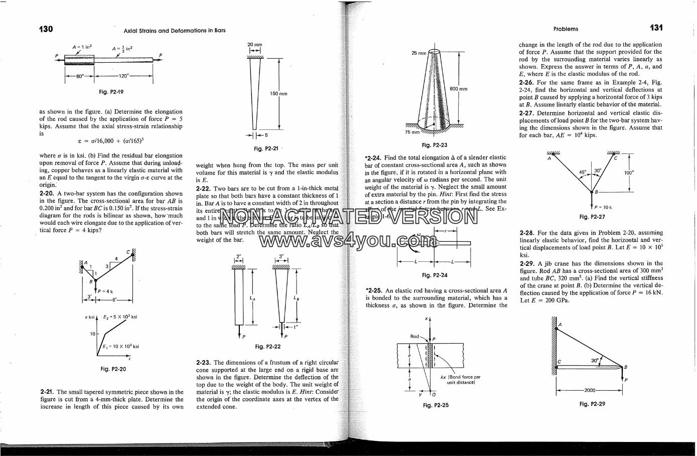
t30 Axial Strains and Deformations in Bars
A = 1 in 2 A = � in 2/e' �' P
Fig. P249
as shown in the figure. (a) Determine the elongationof the rod caused by the application of force P = 5kips. Assume that the axial stress-strain relationshipis
� = call6,000 + (cr/165) 3
where cr is in ksi. (b) Find the residual bar elongationupon removal of force P. Assume that during unloa.d-ing, copper behaves as a linearly elastic material withan E equal to the tangent to the virgin cr-e curve at theorigin.'2-20. A two-bar system has the configuration shownin the figure. The cross-sectional area for bar AB is0.200 in 2 and for bar BC is 0.150 in 2. If the stress-straindiagram for the rods is bilinear as shown, how 'muchwould each wire elongate due to the application of ver-tical force P = 4 kips?
-A 4-54-
' �P =4k '3�8' �
oksi� E2 =5 X 10³ ksi
10Ei--�10X103ksiFig. P2-20
2-2'i. The small tapered symmetric. piece shown in thefigure is cut from a 4-mm-thick plate. Determine theincrease in length of this piece caused by its own
20 rnmI�1i�1
150 rn
Fig. P2-2i '
weight when hung from the top. The mass per unitvolume for this material is 'y and the elastic moduluis E.
2-22. Two bars are to be cut from a 1-in-thick metalplate so that both bars have a constant thickness ofin. Bar A'is to have a constant width of 2 in throughoutits entire length. Bar B is to be 3 in wide at theand 1 in wide at the bottom. Each bar is to be subjectedto the same load P. Determine the ratio LA/LB so thatboth bars will stretch the same amount. Neglect theweight of the bar.
Fig. P2-22
2-23. The dimensions of a frustum of a rightcone supported at the large end on a rigid baseshown in the figure. Determine the deflection of thetop due to the weight of the body. The unit weightmaterial is 'y; the elastic modulus is E. H�nt:the origin of the coordinate axes at the vertex ofextended cone.
25 mm
600 mm
75 rnrn
Fig. P2-23
'2-24. Find the total elongation A of a slender elasticbar of constant cross-sectional area A, such as shownin the figure, if it is rotated in a horizontal plane withan angular velocity of to radians per second. The unitweight of the material is % Neglect the small amountof extra material by the pin. Hint: First find the stressat a section a distance r from the pin by integrating theeffect of the inertial forces between r and L. See Ex-ample 1-6.
Fig. P2-24
'2-25. An elastic rod having a cross-sectional area Ais bonded to the surrounding material, which has athickness a, as shown in the figure. Determine the
Rod �
i�o rceper� y�O unitdistance)
Fig. P2-25
Problems
change in the length of the rod due to the applicationof force P. Assume that the support provided for therod by the surrounding material varies linearly asshown. Express the answer in terms of P, A, a, andE, where E is the elastic modulus of the rod.2-26. For the same frame as in Example 2-4, Fig.2-24, find the horizontal and vertical deflections atpoint B caused by applying a horizontal force of 3 kipsat B. Assume linearly elastic behavior of the material.2-27. Determine horizontal and vertical elastic dis-placements of load point B for the two-bar system hav-ing the dimensions shown in the figure. Assume thatfor each bar, AE = 104 kips.
100"
Fig. P2-27
2-28. For the data given in Problem 2-20, assuminglinearly elastic behavior, find the horizontal and ver-tical displacements of load point B. Let E = 10 x 103ksi.
2-29. A jib crane has the dimensions shown in thefigure. Rod AB has a cross-sectional area of 300 mm 2and tube BC, 320 mm 2. (a) Find the vertical stiffnessof the crane at point B. (b) Determine the vertical de-flection caused by the application of force P = 16 kN.Let E = 200 GPa.
2000Fig. P2-29
NON-ACTIVATEDVERSIONwww.avs4you.com
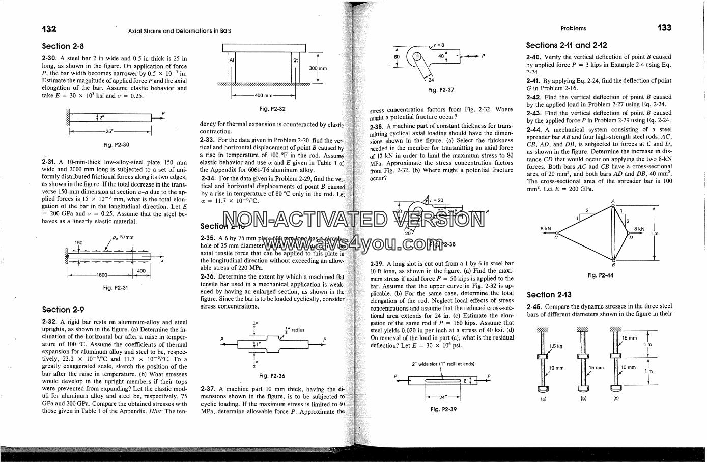
Axial Strains and Deformations in Bars
Section 2-8
2-30. A steel bar 2 in wide and 0.5 in thick is 25 inlong, as shown in the figure. On application of forceP, the bar width becomes narrower by 0.5 x 10 -3 in.Estimate the magnitude of applied force P and the axialelongation of the bar. Assume elastic behavior andtake E = 30 x 10 3 ksi and v = 0.25.
Fig. P2-30
2-3t, A 10-mm-thick low-alloy-steel plate 150 mmwide and 2000 mm long is subjected to a set of uni:formly distributed frictional forces along its two edges,as shown in the figure. If the total decrease in the trans-verse 150-mm dimension at section a-a due to the ap-plied forces is 15 x 10 -3 mm, what is the total elon-gation of the bar in the longitudinal direction. Let E
= 200 GPa and v = 0.25. Assume that the steel be-haves as a linearly elastic material.
150 _�Px N/mm16oo �] �4oo�
Fig. P2-31
Section 2-9
2-32. A rigid bar rests on aluminum-alloy and steeluprights, as shown in the figure. (a) Determine the in-clination of the horizontal bar after a raise in temper-ature of 100 �C. Assume the coefficients of thermalexpansion for aluminum alloy and steel to be, respec-tively, 23.2 x 10⁻⁶/�C and 11.7 x 10⁻⁶/�C. To agreatly exaggerated scale, sketch the position of thebar after the raise in temperature. (b) What stresseswould develop in the upright members if their topswere prevented from expanding? Let the elastic mod-uli for aluminum alloy and steel be, respectively, 75GPa and 200 GPa. Compare the obtained stresses withthose given in Table 1 of the Appendix. Hint: The ten-
Fig. P2-32
dency for thermal expansion is counteracted bycontraction.
2-33. For the data given in Problem 2-20, find thetical and horizontal displacement of point B causeda rise in temperature of 100 �F in the rod. As:elastic behavior and use a and E given in Table 1the Appendix for 6061-T6 aluminum alloy.
2-34. For the data given in Problem 2-29, find thetical and horizontal displacements of point Bby a rise in temperature of 80 �C only in the rod.a = 11.7 x 10⁻⁶/�C.
Section 2-'10
2-35. A 6 by 75 mm plate 600 mm long has a circulmhole of 25 mm diameter located in its center. Find theaxial tensile force that can be applied to this platethe longitudinal direction without exceeding anable stress of 220 MPa.
2-36. Determine the extent by whichtensile bar used in a mechanical application isened by having an enlarged section, as shown infigure. Since the bar is to be loaded cyclically,stress concentrations.
2 !" radiusP P
1 � I
2
Fig. P2-36
2-37. A machine part 10 mm thick, having themensions shown in the figure, is to be subjected tocyclic loading. If the maximum stress is limited toMPa, determine allowable force P. Approximate
24
Fig. P2-37
stress concentration factors from Fig. 2-32. Wheremight a potential fracture occur?2-38. A machine part of constant thickness for trans-mitting cyclical axial loading should have the dimen-sions shown in the figure. (a) Select the thicknessneeded in the member for transmitting an axial forceof 12 kN in order to limit the maximum stress to 80MPa. Approximate the stress concentration factorsfrom Fig. 2-32. (b) Where might a potential fractureoccur?
Fig. P2-38
�P
2-39. A long slot is cut out from a 1 by 6 in steel bar10 ft long, as shown in the figure. (a) Find the maxi-mum stress if axial force P =' 50 kips is applied to thebar. Assume that the upper curve in Fig. 2-32 is ap-plicable. (b) For the same case, determine the totalelongation of the rod. Neglect local effects of stressconcentrations and assume that the reduced cross-sec-tional area extends for 24 in. (c) Estimate the elon-gation of the same rod if P = 160 kips. Assume thatsteel yields 0.020 in per inch at a stress of 40 ksi. (d)On removal of the load in part (c), what is the residualdeflection? Let E = 30 x 106 psi.
2" wide slot (1"radii at ends)
c,_.+ IFig. P2-39
Problems t33
Sections 24'1 and 242
2-40. Verify the vertical deflection of point B causedby applied force P = 3 kips in Example 2-4 using Eq.2-24.
2-41. By applying Eq. 2-24, find the deflection of pointG in Problem 2-16.
2-42. Find the vertical deflection of point B causedby the applied load in Problem 2-27 using Eq. 2-24.2-43. Find the vertical deflection of point B causedby the applied force P in Problem 2-29 using Eq. 2-24.2-44. A mechanical system consisting of a steelspreader bar AB and four high-strength steel rods, AC,CB, AD, and DB, is subjected to forces at C and D,as shown in the figure. Determine the increase in dis-tance CD that would occur on applying the two 8-kNforces. Both bars AC and CB have a cross-sectionalarea of 20 mm 2, arid both bars AD and DB, 40 mm 2.The cross-sectional area of the spreader bar is 100mm 2. Let E = 200 GPa.
A
kN� 1 2
1
B
Fig. P2-44
Section 2-`13
2-45. Compare the dynamic stresses in the three steelbars of different diameters shown in the figure in their
1.5 kg
10 turn
(a) (b)
15 mm
115 mm. 1F0mm1T�n
(c)
NON-ACTIVATEDVERSIONwww.avs4you.com

Axial Strains and Deformations in Bars Problems
response to 1.5-kg masses falling freely through a dis-tance of 1 m. Let E = 200 GPa. Assume no energy isdissipated through plastic deformation of the impactsurfaces, nor at points of high local stresses occurringat supports.
2-46. Determine the stiffness required in the. spring,for the system shown in the figure, for stopping a massof 1 kg moving at a velocity of 3 rn/sec such that, duringimpact, the spring deflection would not exceed 20 mm.Neglect frictional effects.
Fig. P2-46
Section 2-t5
2-47. An elastic bar of variable cross section, held atboth ends, is loaded as shown in the figure. The flex-ibilities.of the bar segments are �/2, �, and �. Deter-mine the reactions, and plot the axial-force and axial-
. displacement diagrams.
Fig. P2-47
2-48. Consider the same elastic bar of variable cross-sectional area shown in the two alternative figures.Determine deflection A,b at a caused by the applica-tion of a unit force at b, and show that it is equal to
A2 L/4 t Il./4 1
A�I 1lb L/4L/47////////. /// ///,. �/////, 7�
Fig. P2-48
Ab,, the deflection at b due to the application of a unitforce at a. LetA� = 2A2. (In Section 13-4, it is shownthat this relationship is true in general for elastic sys-tems. It is widely used in analysis. This conclusion canbe reached by inspection for staticallybars.)
2-49. Consider the bar given in Example 2-2 and as-sume that ends A and D are held and that P2 =kN and P3 = 200 kN act in the directions shown. (a)Determine the reactions. (b) Plot the axial force,strain, and axial displacement diagrams.2-50. If in Problem 2-49, in addition to the appliedforces, there is a drop in temperature of 100 �F, whatreactions would develop at the supports? Let a =
x 10-6/�F.
2-51. For the 2-in 2 constant cross-sectional elastic barshown in the figure, (a) determine the reactions, and(b) plot the axial-force, axial-strain, and axial-displace-ment diagrams. Let E = 10 x 103 ksi.
downward force of 5 kN, as shown in the figure. Ini-tially, this force is equally distributed among the threewires. The stresses in the wires are well within thelinearly'elastic range of material behavior. (a) Deter-mine the forces in the wires caused by a temperaturedrop of 50 �C in the right wire. Properties of the wires:A--- 10mm 2, L = 2000mm, E= 200 x 103N/mm 2,a = 12.5 x 10⁻⁶/�C. (b) At what change in temper-ature in the middle wire would it become slack?
Fig. P2-51
2-52. If a load of 1 kip is applied to a rigid bar sus-pended by three wires as shown in the figure,force will be resisted by each wire? The outside wire�are aluminum (E = 10 7 psi). The inside wire is(E = 30 x 106 psi). Initially, there is no slack in thewire.
Alum. wiresA = 0.3 in 2L = 25'
Steel wire
A = 0.2 in 2/. = 50'
Fig. P2-52
2-53. Three identical equally spaced steel wirestached to a rigid bar support a mass M developing a
Fig. P2-53
2-54. Initially, on applying a 3-kN force to a rigid barhung by three parallel wires (see the figure), all threewires become taut. What additional forces would de-velop in the wires if the left wire slips out 3 mm fromits support. Each of the steel wires is 2000 mm long,has a cross-sectional area of 10 mm 2, and an elasticmodulus of 200 GPa.
-�--200 � � 200 >
1P=3kN
Fig. P2-54
2-55. Rework Example 2-14 by changing the bar in-clination angles a to 30 � and taking the cross-sectionalarea of bar BD as 2A. The cross sections of bars ADand DC remain equal to A.
Section 2-t6
2-56. An elastic bar held at both ends is loaded by anaxial force P, as shown in the figure. Cross section Aof the bar is constant. (a) Determine the reactions aridinterpret the results in relation to the position of theapplied force. (b) Plot the axial displacement diagramassuming that E is known.
Fig. P2-56
2-57. For symmetrically arranged springs in parallel,the combined spring constant k = �n ki; see figure(a). Justify that for the springs in series, as in figure(b), the system spring constant k follows from 1/k =� 1/ki, or, alternatively, � = �n fi, where � is sys-tem flexibility, and �i the flexibility of an ith spring.
IP
Fig. P2-57
(b)
2-58. A symmetrical arrangement of springs is at-tached to a rigid bar and carries an applied force P, asshown in the figure. (a) Find the reactions. Hint: Use
: k� = 300 N/mm
k2 = 200 N/mm
k� = 250 N/mmP = 6.2 kN
Fig. P2-58
NON-ACTIVATEDVERSIONwww.avs4you.com

i36 Axial Strains and Deformations in Bars Problems i37
the relationships given in Problem 2-57. (b) How is thetotal deflection distributed between the upper twosprings?2-59. Rework Problem 2-52 using the displacementmethod.
2-60. An elastic bar of variable cross section and heldat both ends is axially loaded, as shown 'in the figure.The cross-sectional area of the small part is A and ofthe larger, 2A. (a) Using the displacement method, findthe reactionS. (b) Plot a qualitative axial-displacementdiagram. Hint: Use the relationship given in Problem2-57 for determining the combined stiffness of the barsegments to the left of P.
Fig. P2-60
'2-6t. A bar of constant thickness and held at bothends hgs the geometry shown in the figure. Determinethe reactions caused by the axially applied force P.Hint: First find the stiffness for the tapered part of thebar.
-7-
L/2 � < L/2 � �Fig. P2-61
2-62. A rigid bar is hinged at end A and, in addition,is supported on three identical springs, each havingstiffness k. (a) What is the degree of statical indeter-minacy of this system? (b) How many degrees of free-
Fig. P2-62
dom are there? (c) Find the forces acting onsprings.2-6:3. A rigid bar is supported by a pin at A andlinearly elastic wires atB and C, as shown in the fThe area of the wire at B is 60 mm 2 and for the one iC is 120 mm 2. Determine the reactions at A, B, andcaused by applied force P = 6 kN.
-500o5+500o-
1000
Fig. P2-63
2-64. Five steel rods, each having a cross-sectionalarea of 500 mm 2, are assembled in a symmetrical man-ner, as shown in the figure. Assume that the steel be-haves as a linearly elastic material with E = 200 GPa.Determine the deflection of joint A due to downwardforce P = 2 MN. Assume that, initially, the rods aretaut.
/ Z////�///Z///,�/////////////,
Fig. P2-64
Section 2-t7
2-65. An elastic bar of variable cross section and heldat both ends is axially loaded at several points, asshown in the figure. The cross section for the largerarea is 2A, and for the smaller, A. (a) Compare the:::degrees of kinematic and static indeterminacies. (b)Determine the reactions if P� = 3P, P2 = 2P, and P3= P. (c) Plot axial-force diagram.
Fig. P2-65
2-66. Rework Problem 2-65 after removing force P�.Hint: The degree of kinematic indeterminacy can bereduced by using a relationship given in Problem 2-57.
Section 2-t82-67. A material possesses a nonlinear stress-strainrelationship given as cr = Ke n, where K and n are ma-terial constants. If a rod made of this material and ofconstant area A is initially fixed at both ends and isthen loaded as shown in the figure, how much of ap-plied force P is carried by the left support?
� a � � bFig. P2-67
2-68. A rod is fixed at A and loaded with an axial forceP, as shown in the figure. The material is elastic-per-fectly plastic, with E = 200 GPa and a yield stress of200 MPa. Prior to.loading, a. gap of 2 mm exists be-tween the end of the rod and fixed support C. (a) Plotthe load-displacement diagram for the load point as-suming P increases from zero to its ultimate value forthe rod. The cross section from A to B is 200 mm 2 andthat from B to C is 100 mm 2. (b) What will be the re-sidual displacement of point B upon release of the ap-plied force?
-�l�- 2 mm
I-�--250mm---�250 mm �Fig. P2-68
2-69. The cross section of a short reinforced concretecolumn is as shown in the figure. Four 1-in round bars
Fig. P2-69
serve as reinforcement. (a) Determine the instanta-neous elastic strength of the column based on allow-able stresses. (b) Estimate the ultimate (plastic)strength of the column. Assume that both materials areelastic-perfeCtly plastic. For steel, let Cra,o�, = 24 ksi,Cryp = 60 ksi and E = 30 x 106 psi, and for concrete,Crano�, = 2000 psi, Cryp = 3600 psi and E = 2 x 10⁶psi. (It has been shown experimentally that when steelyields, the concrete "yield" strength is approximately0.85cru�t, where Cru, is the ultimate compresslyestrength of an unreinforced cylindrical specimen of thesame material, age, and curing conditions. In order toachieve ductile behavior of columns, the use of lateralties or spiral reinforcement is essential.)2-70. A rigid platform rests on two aluminum bars (E= 10 7 psi) each 10.000 in long. A third bar made ofsteel (E = 30 x 106 psi) and standing in the middle is9.995 in long. (a) What will be the stress in the steelbar if a force P of 100 kips is applied on the platform?(b) How much do the aluminum bars shorten? (c) Whatwill be the ultimate (plastic) strength for the system if(ffyp)Al = 40 ksi and (Cryv)St = 60 ksi?
P
AI St !AI
L
A = 2 in 2
A=4in 2
A = 2 in 2
Fig. P2-70
NON-ACTIVATEDVERSIONwww.avs4you.com

t38 Axial Strains and Deformations in Bars
2-7t. A force P = 1 kN is applied to a rigid bar sus-pended by three wires, as shown in the figure. Allwires are of equal size and the same material. For eachwir�, A = 80 mm 2, E =. 200 GPa, and L = 4 m. If,initially, there were no slack in the wires, how will theapplied load distribute between the wires?
�///////////, 2'///////////,
200 100 100mm mm mm
4000mm
F
�PFig. P2.71
2-72. An aluminum rod 7 in long, having two differentcross-sectional areas, is inserted into a steel link, asshown in the figure. If at 60 �F no axial force exists inthe aluminum rod, what will be the magnitude of thisforce when the temperature rises to 160 �F? E^, =� 107psi hnd ct^� = 12.0 x 10⁻⁶/�F; Est = 30 x 106 psi andCtst = 6.5 x 10⁻⁶/�F.
Steel link: area of each bar parallel0.30 in 2 to rod is 0.35 in 2
Aluminum
rod, 0.40 in 2
2-73. An aluminum tube is axially compressed be-tween the two heavy nuts of a steel bolt, as shownthe figure. If it is known that the axial stress in thesleeve at 80 �C is 20 MPa, at what temperature doesthis prestress become zero? For the aluminum tube:A = 1000mm 2, E= 70 x 103MPa, andct = 23.2 x10 -6 per �C. For the steel bolt: A = 500 mm 2, E200 x 103 MPa, and ct = 11.7 x 10 -6 per �C.
Aluminum tube
� _ Steelbolt
� 100 �_ ' SectionFig. P2-73
2-74. Rework Example 2-23 after assuming that theelastic modulus E1 for the middle bar is threesmaller than that for the outside bars, i.e., E2 = E3 =3E�.
2-75. Plot the load-deflection diagram for joint A inProblem 2-64 caused by the applied force P,that the yield stress for the material cryp = 250 MPa.
Section 2-t9*2-76. Rework Problem 2-25 using Eq. 2-48.2-77. Rework Problem 2-24 using Eq. 2-48.*2-78. Rework Problem 2-56 using Eq. 2-48 and con-tinuity conditions or singularity functions.
Fig. P2-72
pter
3-1. Introduction
In addition to the normal strain discussed in the previous chapter in con-nection with axially loaded bars, in general, a body may also be subjectedto shear strains. For the purposes of deformation analysis, such strainsmust be related to the applied shear stress. This topic is discussed in PartA of this chapter. In Part B, general mathematical definitions for normaland shear strains are given. Then, by employing the method of super-position, the generalized Hooke's law is synthesized, relating stressesand strains for a three-dimensional state of stress. Next, in Part C, thin-walled pressure vessels and shells of revolution are considered. The gen-eralized Hooke's law is 'employed for the deformation analysis of theseimportant elements of construction. In the concluding part, Part D, asolution for thick-walled cylinders is developed. This illustrates a solutionof a typical boundary-value problem in the mathematical theory of elas-ticity, and, at the same time, provides bounds on the applicability of theequations established for thin-walled pressure vessels using engineeringsolid mechanics.
CONSTITUTIVE RELATIONSHIPS FORSHEAR
3.2. Stress-Strain Relationships for ShearIn addition to the normal strains related to the axial strains in barsdiscussed in Chapter 2, a body may be subjected to shear stresses thatcause shear deformations. An example of such deformations is shown in
t39
NON-ACTIVATEDVERSIONwww.avs4you.com
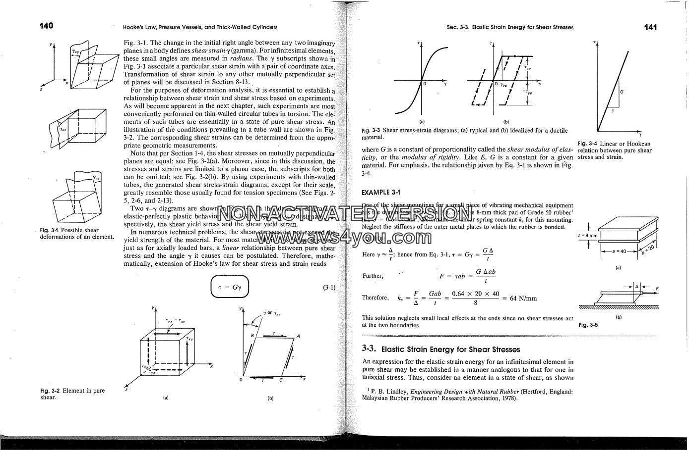
140
z
Fig. 3-1 Possible sheardeformations of an element.
Fig. 3-2 Element in pureshear.
Hooke'sLaw,PressureVessels,andThick.WalledCylinders '�Fig. 3-1. The change in the initial right angle between any two imaginaryplanes in a body defines shear strain �t (gamma). For infinitesimal elementsthese small angles are measured in radians. The �/ subscripts shownFig. 3-1 associate a particular shear strain with a pair of coordinateTransformation of shear strain to any other mutually perpendicularof planes will be discussed in Section 8-13.
For the purposes of deformation analysis, it is essential to establishrelationship between shear strain and shear stress based on experimentsAs will become apparent in the next chapter, such experiments are moconveniently performed on thin-walled circular tubes in torsion. Thements of such tubes are essentially in a state of pure shear stress. Anillustration of the conditions prevailing in a tube wall are shown in3-2. The corresponding shear strains can be determined from thepriate geometric measurements.
Note that per Section 1-4, the shear stresses on mutually perpendiculaplanes are equal; see Fig. 3-2(a). Moreover, since in this discussion,stresses and strains are limited to a planar case, the subscripts forcan be omitted; see Fig. 3-2(b). By using experiments with thin-walledtubes, the generated shear stress-strain diagrams, except for their scalegreatly resemble those usually found for tension specimens (See Figs. 2-5, 2-6, and 2-13).
Two ,-�/di_agrams are shown in Fig. 3-3. In the idealized diagram of
elastic-perfectly plastic behavior, Fig. 3-3(b), ,yp and �/yp designate, re-spectively, the shear yield stress and the shear yield strain.
In numerous technical problems, the shear stresses do not exceed theyield strength of the material. For most materials in this range of stress,
just as for axially loaded bars, a linear relationship between pure shearstress and the angle �/ it causes can be 'postulated. Therefore, mathe-
matically,extensionofHooke'slawforshearstressandstrainreadsy
(a)
o � c
(b)
Sec. 3-3. Elastic Strain Energy for Shear Stresses
//
I It�J
(a) (b)
Fig. 3-3 Shear stress-strain diagrams; (a) typical and (b) idealized for a ductilematerial.
where G is a constant of proportionality called the shear modulus of elas-ticity, or the modulus of rigidity. Like E, G is a constant for a givenmaterial. For emphasis, the relationship given by Eq. 3-1 is shown in Pig.3-4.
t41
Fig. 3-4 Linear or Hookeanrelation between pure shearstress and strain.
EXAMPLE 3-t
One of the shear mountings for a small piece of vibrating mechanical equipmenthas the dimensions shown in Fig. 3-5. The 8-mm thick pad of Grade 50 rubber �has G = 0.64 N/mm 2. Determine the shear spring constant ks for this mounting.Neglect'the stiffness of the outer metal plates to which the rubber is bonded.
Solution
A GA
Here 3' �'�; hence from Eq. 3-1, x = Cry - t
Further, '�- F = ,ab - G Aabt
F Gab 0.64 x 20 x 40Therefore, ks - - - = 64 N/mm
A t 8
This solution neglects small local effects at the ends since no shear stresses actat the two boundaries.
(a)
,x F
(b)
Fig. 3-5
3-3. Elastic Strain Energy for Shear StressesAn expression for the elastic strain energy for an infinitesimal element inpure shear may be established in a manner analogous to that for one inuniaxial stress. Thus, consider an element in a state of shear, as shown
� P. B. Lindley, Engineering Design with Natural Rubber (Hertford, England:Malaysian Rubber Producers' Research Association, 1978).
NON-ACTIVATEDVERSIONwww.avs4you.com
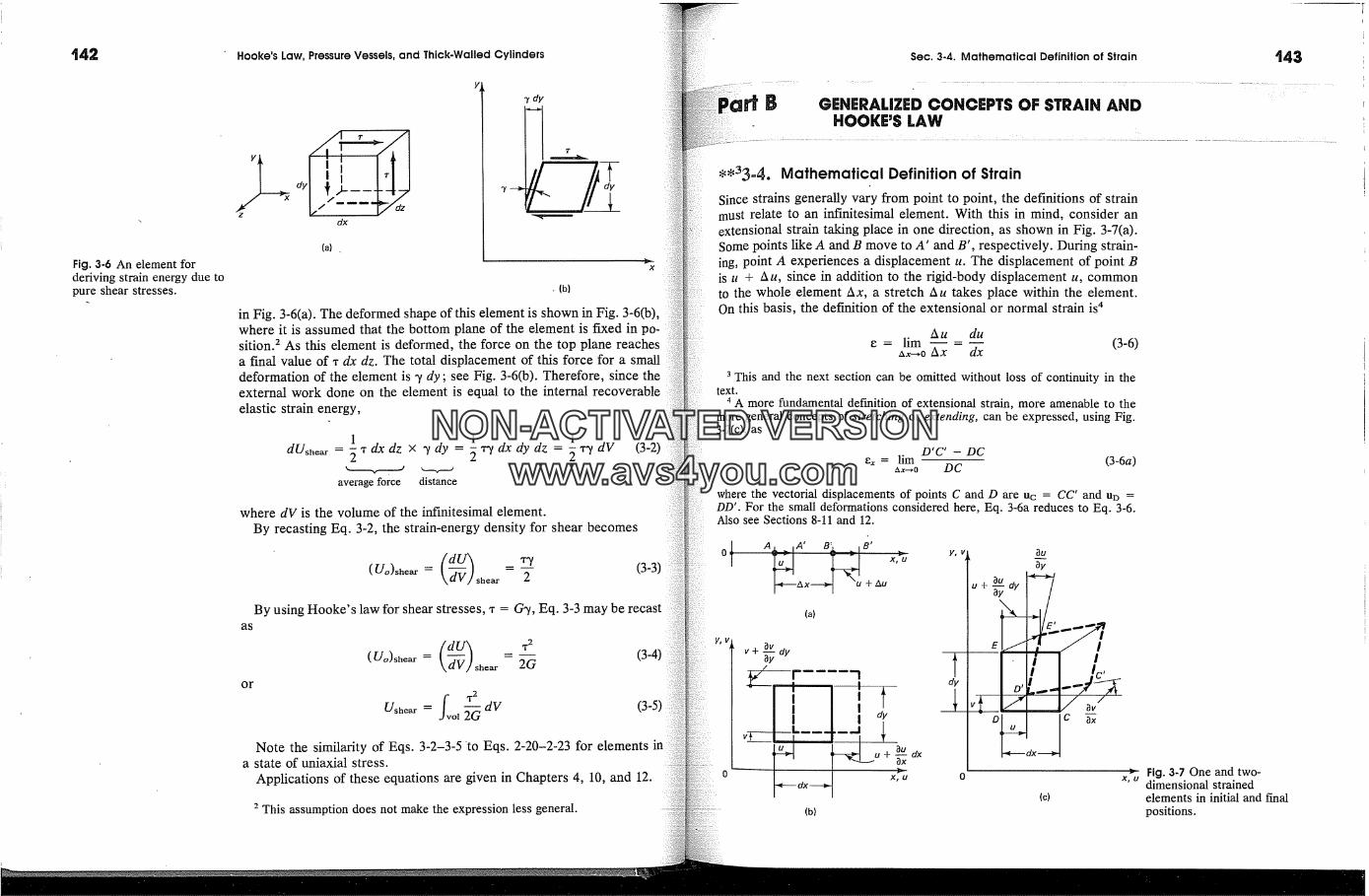
Fig. 3-6 An element forderiving strain energy due topure shear stresses.
Hooke's Law, Pressure Vessels, and Thick. Walled Oylinders
(a) .
x
� (b)
in Fig. 3-6(a). The deformed shape of this element is shown in Fig. 3-6(b),where it is assumed that the bottom plane of the element is fixed in po-sition. 2 As this element is deformed, the force on the top plane reachesa final value of � dx dz. The total displacement of this force for a smalldeformation of the element is '� dy; see Fig. 3-6(b). Therefore, since theexternal work done on the element is equal to the internal recoverableelastic strain energy,
1 1 1dUshear = �'r dx dz x '� dy = � � dx dy dz =
average force distance
(3 -2)
where dV is the volume of the infinitesimal element.By recasting Eq. 3-2, the strain-energy density for shear becomes
shear 2 (3-3)By using Hooke's law for shear stresses, � = G',/, Eq. 3-3 may be recast
as
(U�)she�r= �-� she�r--2G (3-4)or
Ushe� = fv dV (3-5)ol
Note the similarity of Eqs. 3-2-3-5 'to Eqs. 2-20-2-23 for elements ina state of uniaxial stress.
Applications of these equations are given in Chapters 4, 10, and 12.
2 This assumption does not make the expression less general.
Sec. 3.4. Mathematical Definition of Strain �43
GENERALIZED CONCEPTS OF STRAIN ANDNOOKE'S LAW
**33-4. Mathematical Definition of StrainSince strains generally vary from point to point, the definitions of strainmust relate to an infmitesimal element. With this in mind, consider anextensional strain taking place in one direction, as shown in Fig. 3-7(a).Some points like A and B move to A' and B', respectively. During strain-ing, point A experiences a displacement u. The displacement of point Bis tt q- A u, since in addition to the rigid-body displacement u, commonto the whole element Ax, a stretch Au takes place within the element.On this basis, the definition of the extensional or normal strain is 4
A u du� = lim - (3-6)
,�.�-.,o A x dx
3 This and the next section can be omitted without loss of continuity in thetext.
4 A more fundamental definition of extensional strain, more amenable to themore general concepts of stretching or extending, can be expressed, using Fig.3-7(c), as
D' C' - DCex = lim (3-6a)ax�o DE
where the vectorial displacements of points C and D are Uc = CC' and un =DD'. For the small deformations considered here, Eq. 3-6a reduces to Eq. 3-6.Also see Sections 8-11 and 12.
I A, ,A' B� ., B'0 U ' X, U
Ax + Au
(a)
�v
�+ �dy! 1
dy
8x
X� Udx
(b)
y, V
�U
.+�dy
(c)
� Fig. 3-7 One and two-x, u dimensional strained
elements in initial and finalpositions.
NON-ACTIVATEDVERSIONwww.avs4you.com
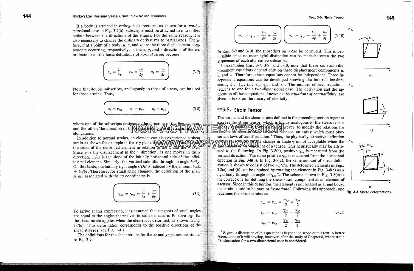
t44 Hooke'sLaw,PressureVessels,andThick.WalledCylindersIf a body is strained in orthogonal directions, as shown for a two-di-mensional case in Fig. 3-7(b), subscripts must be attached to e to differ-entiate between the directions of the strains. For the same reason, it isalso necessary to change the ordinary derivatives to partial ones. There-fore, if at a point of a body, u, v, and w are the three displacement com-ponents occurring, respectively, in the x, y, .and z directions of the co-ordinate axes, the basic definitions of normal strain become
Ou Ov
ax Ox Oy (3-7)
Note that double subscripts, analogously to those of stress, can be usedfor these strains. Thus,
(3-8)
where one of the subscripts designates the direction of the line element,and the other, 'the direction of the displacement. Positive signs apply toelongations.
In addition to normal strains, an element can also experience a shearstrain as shown for example in the x-y plane in Fig. 3-7(c). This inclinesthe sides of the deformed element in relation to the x and the y axes.Since v is the displacement in the y direction, as one moves in the xdirection, Ov/Ox is the slope of the initially horizontal side of the infini-tesimal element. Similarly, the vertical side tilts through an angle Ou/Oy.On this basis, the initially right angle CDE is reduced by the amount Ov/Ox+ Ou/Oy. Therefore, for small angle changes, the definition of the
strain associated with the xy coordinates is
Ov + (3-9)'7�y = '7yx Ox Oy,
To arrive at this expression, it is assumed that tangents of small anglesare equal to the angles themselves in radian measure. Positive sign forthe shear strain applies when the element is deformed, as shown in Fig.3-7(c). (This deformation corresponds to the positive directions of theshear stresses; see Fig. 1-4.)
The definitions for the shear strains for the xz and yz planes are similarto Eq. 3-9:
Sec. 3.5. Strain Tensor
'Yxz = 'Y= Ox + Oz 'Yyz 'Y� Oy + Oz (3-10)
In Eqs. 3-9 and 3-10, the subscripts on '� can be permuted. This is per-missible since no meaningful distinction can be made between the twosequences of each alternative subscript.
In examining Eqs. 3-7, 3-9, and 3-10, note that these six strain-dis-placement equations depend only on three displacement components u,v, and w. Therefore, these equations cannot be independent. Three in-dependent equations can be developed showing the interrelationshipsamong e,.x, eyy, ezz , '�xy, '�yz, and -�=. The number of such equationsreduces to one for a two-dimensional case. The derivation and the ap-plication of these equations, known as the equations of compatibility, aregiven in texts on the theory of elasticity.
**3-5. Strain Tensor
The normal and the shear strains defined in the preceding section togetherexpress the strain tensor, which is highly analogous to the stress tensoralready discussed. It is necessary, however, to modify the relations forthe shear strains in order to have a tensor, an entity which must obeycertain laws of transformation. 5 Thus, the physically attractive definitionof the shear strain as the change in angle -� is not acceptable when theshear strain is a component of a tensor. This heuristically may be attrib-uted to the following. In Fig. 3-8(a), positive -�y is measured from thevertical direction. The same positive -�y is measured from the horizontaldirection in Fig. 3-8(b). In. Fig. 3-8(c), the same amount of shear defor-mation is shown to consist of two '�y/2's. The deformed elements in Figs.3-8(a) and (b) can be obtained by rotating the element in Fig. 3-8(c) as arigid body through an angle of '�y/2. The scheme shown in Fig. 3-8(c) isthe correct one for defining the shear-strain component as an element ofa tensor. Since in this definition, the element is not rotated as a rigid body,the strain is said to be pure or #'rotational. Following this approach, oneredefines the shear strains as
2 2
�y� = �, _ �'yz _ �%, (3-11)2 2
�zx = �xz -- --2 2
5 Rigorous discussion of this question is beyond the scope of this text. A betterappreciation of it will develop, however, after the study of Chapter 8, where straintransformation for a two-dimensional case is considered.
(a)
(b}x
x
(c)
Fig. 3-8 Shear deformations.
NON-ACTIVATEDVERSIONwww.avs4you.com
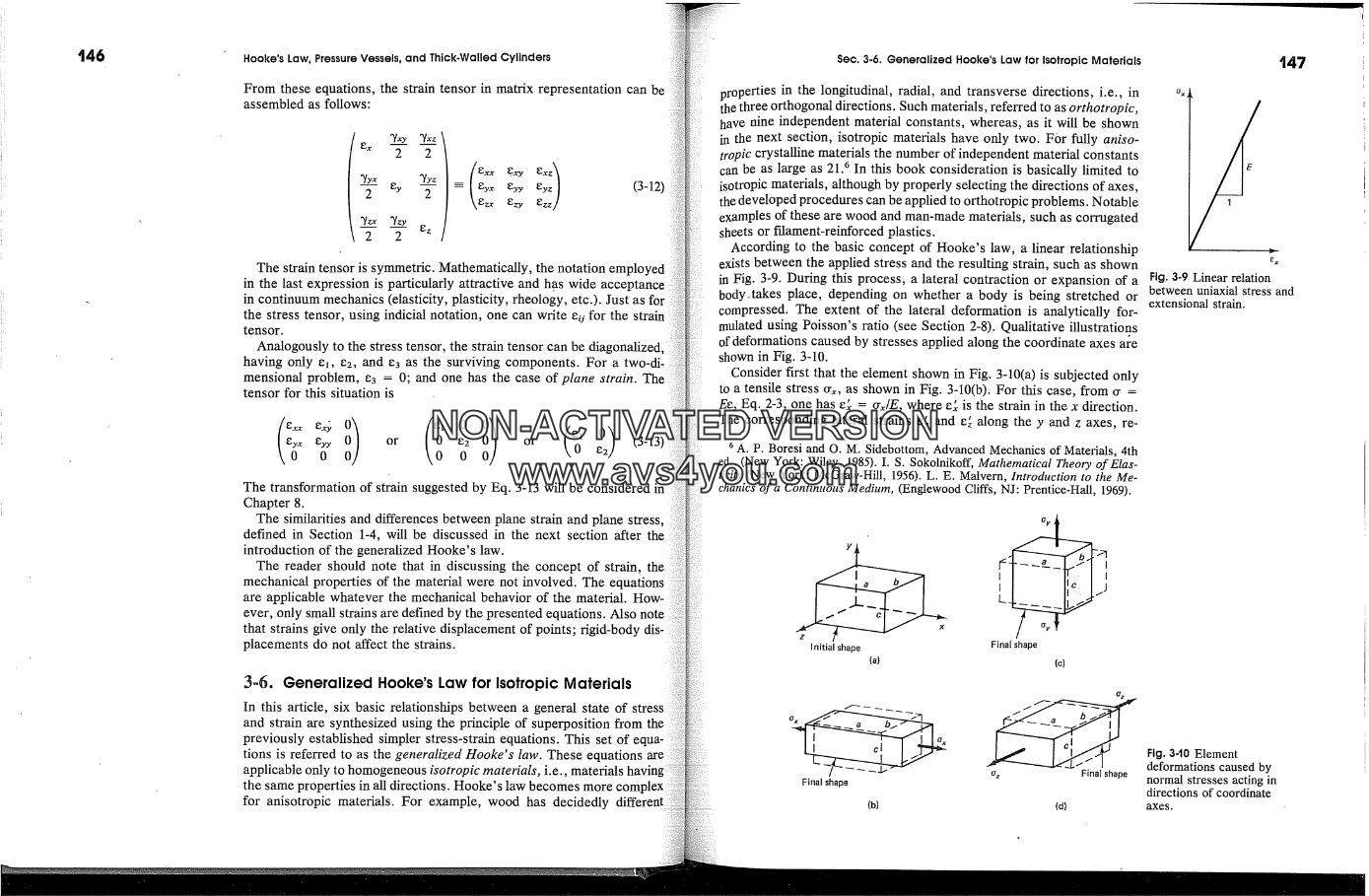
t46 Hooke's Law, Pressure Vessels, and Thick-Walled Cylinders
From these equations, the strain tensor in matrix representation can beassembled as follows:
?yx ?yz �xx e.� �xz�� �yx Eyy �yz� (3-12)
The strain tensor is symmetric. Mathematically, the notation employedin the last expression is particularly attractive and has wide acceptancein continuum mechanics (elasticity, plasticity, rheology, etc.). Just as forthe stress tensor, using indicial notation, one can write e u for the straintensor.
Analogously to the stress tensor, the strain tensor can be diagonalized,having only el, e2, and e3 as the surviving components. For a two-di-mensional problem, e3 = 0; and one has the case of plane strain. Thetensor for this situation is
(:; i) (i'�i) o)x �yy or g2 or0 0 e2
(3-13)
The transformation of strain suggested by Eq. 3-13 will be considered inChapter 8.
The similarities and differences between plane strain and plane stress,defined in Section 1-4, will be discussed in the next section after theintroduction of the generalized Hooke's law.
The reader should note that in discussing the concept of strain, themechanical properties of the material were not involved. The equationsare applicable whatever the mechanical behavior of the material. How-ever, only small strains are defined by the presented equations. Also notethat strains give only the relative displacement of points; rigid-bodyplacements do not affect the strains.
3-6. Generalized Hooke's Law for Isotropic MaterialsIn this article, six basic relationships between a general state of stressand strain are synthesized using the principle of superposition frompreviously established simpler stress-strain equations. This set of ections is referred to as the generalized Hooke's law. These equationsapplicable only to homogeneous isotropic materials, i.e., materials havingthe same properties in all directions. Hooke's lawfor anisotropic materials. For example, wood has decidedly
Sec. 3-6. Generalized Hooke's Law for Isotropic Materials
properties in the longitudinal, radial, and transverse directions, i.e., inthe three orthogonal directions. Such materials, referred to as orthotropic,have nine independent material constants, whereas, as it will be shownin the next section, isotropic materials have only two. For fully aniso-tropic crystalline materials the number of independent material constantscan be as large as 21.6 In this book consideration is basically limited toisotropic materials, although by properly selecting the directions of axes,the developed procedures can be applied to orthotropic problems. Notableexamples of these are wood and man-made materials, such as corrugatedsheets or fdament-reinforced plastics.
According to the basic concept of Hooke's law, a linear relationshipexists between the applied stress and the resulting strain, such as shownin Fig. 3-9. During this process, a lateral contraction or expansion of abody.takes place, depending on whether a body is being stretched orcompressed. The extent of the lateral deformation is analytically for-mulated using Poisson's ratio (see Section 2-8). Qualitative illustrationsof deformations caused by stresses applied along the coordinate axes areshown in Fig. 3-10.
Consider first that the element shown in Fig. 3-10(a) is subjected onlyto a tensile stress O'x, as shown in Fig. 3-10(b). For this case, from o' =Ee, Eq. 2-3, one has e�' = �rx/E, where e�' is the strain in the x direction.The corresponding lateral strains � and � along the y and z axes, re-
6 A. P. Boresi and O. M. Sidebottom, Advanced Mechanics of Materials, 4thed., (New York: Wiley, 1985). I. S. Sokolnikoff, Mathematical Theory of Elas-ticity (New York: McGraw-Hill, 1956). L. E. Malvern, Introduction to the Me-chanics of a Continuous Medium, (Englewood Cliffs, NJ: Prentice-Hall, 1969).
Initial shape Final shape(a) (c)
[ � '"'�� % FinalshapeFinal shape
(b) (d)
147
�x
Fig. 3.9 Linear relationbetween uniaxial stress andextensional strain.
Fig. 340 Elementdeformations caused bynormal stresses acting indirections of coordinateaxes.
NON-ACTIVATEDVERSIONwww.avs4you.com
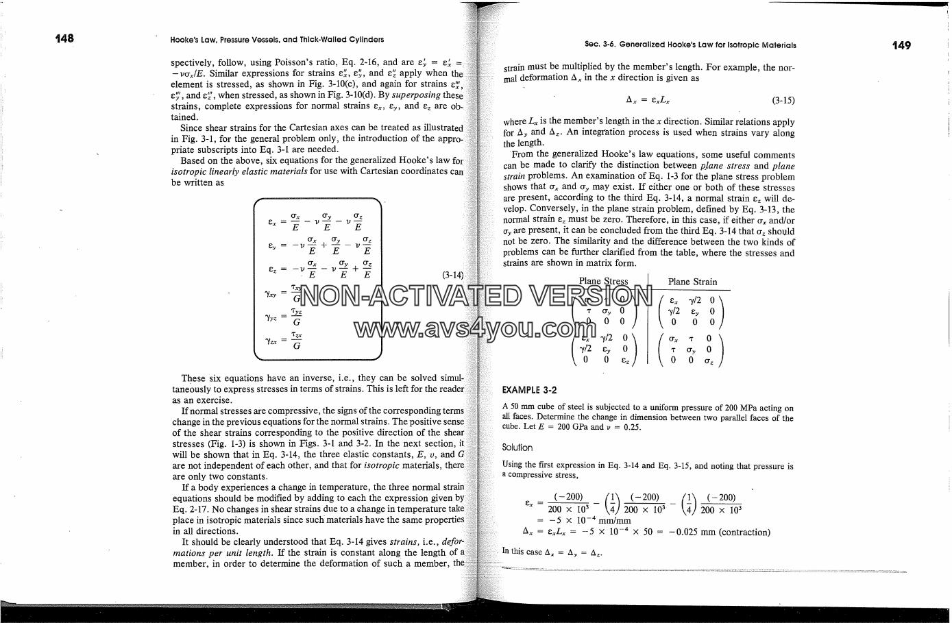
t48 Hooke's Law, Pressure Vessels, and Thick-Walled Cylinders
spectively, follow, using Poisson's ratio, Eq. 2-16, and are e� =-V�rx/E. Similar expressions for strains e�, e�, and e� apply when the
element is stressed, as shown in Fig. 3-10(c), and again for strainse�', and e�', when stressed, as shown in Fig. 3-10(d). By superposing thesestrains, complete expressions for normal strains ex, ey, and e� aretained.
Since shear strains for the Cartesian axes can be treated asin Fig. 3-1, for the general problem only, the introduction of thepriate subscripts into Eq. 3-1 are needed.
Based on the above, six equations for the generalized Hooke's lawisotropic linearly elastic materials for use with Cartesian coordinatesbe written as
O'x O'y O'zE
O'x O'y
O'x O'y O' z
(3-1<
These six equations have an inverse, i.e., they can be solvedtaneously to express stresses in terms of strains. This is left for theas an exercise.
If normal stresses are compressive, the signs of the corresponding term�change in the previous equations for the normal strains. The positive senseof the shear strains corresponding to the positive direction of thestresses (Fig. 1-3) is shown in Figs. 3-1 and 3-2. In the next section, itwill be shown that in Eq. 3-14, the three elastic constants, E, v, andare not independent of each other, and that for isotropic materials,are only two constants.
If a body experiences a change in temperature, the three normalequations should be modified by adding to each the expression givenEq. 2-17. No changes in shear strains due to a change in temperatureplace in isotropic materials since such materials have the samein all directions.
It should be clearly understood that Eq. 3-14 gives strains, i.e.,mations per unit length. If the strain is constant along the length ofmember, in order to determine the deformation of such a member,
Sec. 3-6. Generalized Hooke's Law for Isotropic Materials
strain must be multiplied by the member's length. For example, the nor-mal deformation Ax in the x direction is given as
Ax = exLx (3-15)
where Lx is the member's length in the x direction. Similar relations applyfor Ay and A�. An integration process is used when strains vary alongthe length.
'From the generalized Hooke's law equations, some useful commentscan be made to clarify the distinction between pJane stress and planestrain problems. An examination of Eq. 1-3 for the plane stress problemshows that Crx and o'y may exist. If either one or both of these stressesare present, according to the third Eq. 3-14, a normal strain e� will de-velop. Conversely, in the plane strain problem, defined by Eq. 3-13, thenormal strain e� must be zero. Therefore, in this case, if either O'x and/or% are present, it can be concluded from the third Eq. 3-14 that cr� shouldnot be zero. The similarity and the difference between the two kinds ofproblems can be further clarified from the table, where the stresses andstrains are shown in matrix form.
Plane Stress
( �rxv 0)v o'y 00 0 0
'�/2 ey0 0 e�
Plane Strain
e�,-�/20)-�/2 ey 00 0 0
,r c& 00 0
149
EXAMPLE 3-2
A 50 mm cube of steel is subjected to a uniform pressure of 200 MPa acting onall faces. Determine the change in dimension between two parallel faces of thecube. Let E = 200 GPa and v = 0.25.
Solution
Using the Errst expression in Eq. 3-14 and Eq. 3-15, and noting that pressure isa compressive stress,
e�, = 200 x 105 - 200 X 10 3 -- 200 x 10 i= --5 X 10 -4 mm/mm
Ax = �xZx = -5 x 10 -4 x 50 = -0.025 mm (contraction)
In this case A� = Ay = Az.
NON-ACTIVATEDVERSIONwww.avs4you.com
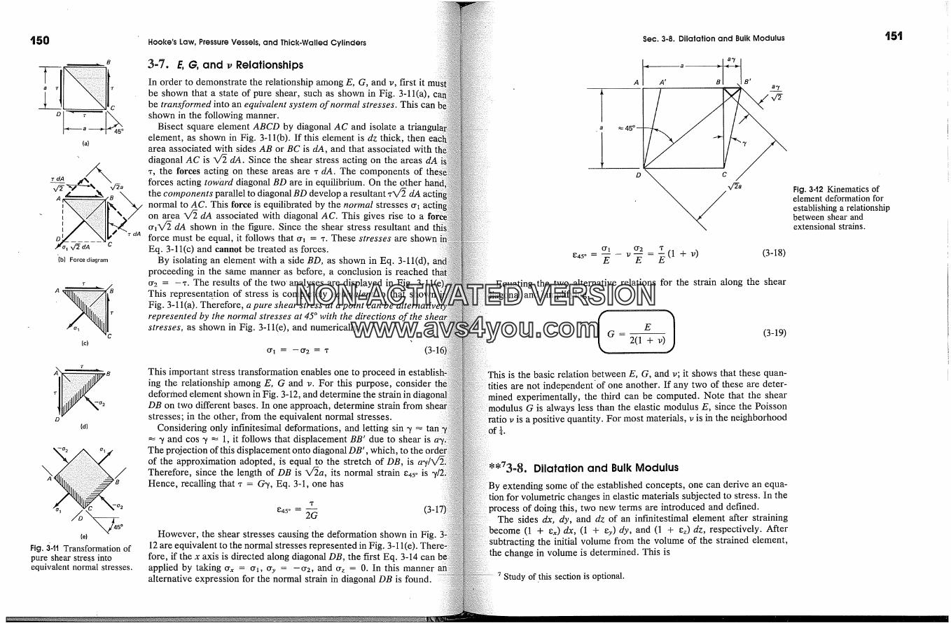
t50
B
(�)
'(b) Force diagram
(c)
�A�� B(d)
-o 2
(e)
Fig. 3-1t Transformation ofpure shear stress intoequivalent normal stresses.
Hooke's Law, Pressure Vessels, and Thick.Walled Cylinders
3-7. E, G, and v RelationshipsIn order to demonstrate the relationship among E, G, and v, first itbe shown that a state of pure shear, such as shown in Fig. 3~11(a),be transformed into an equivalent system of normal stresses. This can'shown in the following manner.
Bisect square element ABCD by diagonal AC and isolate a trianelement, as shown in Fig. 3-11(b). If this element is dz thick, thenarea associated with sides AB or BC is dA, and that associated withdiagonal AC is V� dA. Since the shear stress acting on the areas dA� , the forces acting on these areas are �' dA. The components offorces acting toward diagonal BD are in equilibrium. On the otherthe components parallel to diagonal BD develop a resultant �'V� dA actnormal to AC. This force is equilibrated by the normal stresses 00�on area X,� dA associated with diagonal AC. This gives rise to a00�X/� dA shown in the figure. Since the shear stress resultant and t�force must be equal, it follows that 00� = �'. These stresses are shownEq. 3-11(c) and cannot be treated as forces.
By isolating an element with a side BD, as shown in Eq. 3-11(d),proceeding in the same manner as before, a conclusion is reached002 = -�'. The results of the two analyses are displayed in Fig.This representa. tion of stress is completely equivalent to that shownFig. 3-1 l(a). Therefore, a pure shear stress at a point can be alternativerepresented by the normal stresses at 45 � with the directions of thestresses, as shown in Fig. 3-11(e), and numerically,
001 � --0�2 � 'r
This important stress transformation enables one to proceed in establi:ing the relationship among E, G and v. For this purpose, considerdeformed element shown in Fig. 3-12, and determine the strain inDB on two different bases. In one approach, determine strain fromstresses; in the other, from the equivalent normal stresses.
Considering only infinitesimal deformations, and letting sin -� �� � and cos � -�- 1, it follows that displacement BB' due to shear isThe projection of this displacement onto diagonal DB', which, to theof the approximation adopted, is equal to the stretch of DB, isTherefore, since the length of DB is V�a, its normal strain �45� isHence, recalling that �' = C,W, Eq. 3-1, one has
e45o = �-� (3-15However, the shear stresses causing the deformation shown in Fig.
12 are equivalent to the normal stresses represented in Fig. 3-1 l(e).fore, if the x axis is directed along diagonal DB, the first Eq. 3-14applied by taking 00�, = 00�, cry = -002, and 00z = 0. In this manneralternative expression for the normal strain in diagonal DB is found.
Sec. 3-8. Dilatation and Bulk Modulus
001 002 T
E v E = � (1 + v) (3-18)
Equating the two alternative relations for the strain along the shearand 'simplifying,
2(1 + v)(3-19)
is the basic relation between E, G, and v; it shows that these quan-tities are not independent'of one another. If any two of these are deter-
experimentally, the third can be computed. Note that the shearG is always less than the elastic modulus E, since the Poissona positive quantity. For most matedhals, v is in the neighborhood
4.
Dilatation and Bulk Modulus
extending some of the established concepts, one can derive an equa-for volumetric changes in elastic matedhals subjected to stress. In the
process of doing this, two new terms are introduced and defined.The sides dx, dy, and dz of an infinitestimal element after straining
become (1 + e�,) dx, (1 + %) dy, and (1 + ez) dz, respectively. Afterg the initial volume from the volume of the strained element,
change in volume is determined. This is
Study of this section is optional.
t5t
Fig. 342 Kinematics ofelement deformation forestablishing a relationshipbetween shear andextensional strains.
NON-ACTIVATEDVERSIONwww.avs4you.com
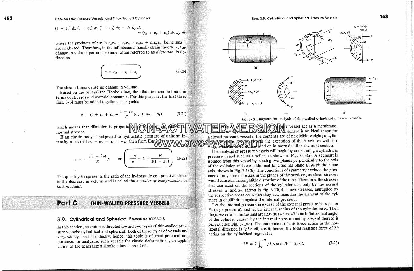
�52 Hooke's Law, Pressure Vessels, and Thick-Walled Cylinders Sec. 3.9. Cylindrical and Spherical Pressure Vessels(1 + e�,) dx (1 + ey) dy (1 + ez) dz - dxdydz
� (e� + ey + ez) dx dy
where the products of strain e.�ey + eyez + eze�, + e�,eyez, being smallare neglected. Therefore, in the infinitesimal (small) strain theory, e,change in volume per unit volume, often referred to as dilatation, isfined as
e = ex+ ey+The shear strains cause no change in volume.
Based on the generalized Hooke's law, the dilatation c an be foundterms of stresses and material constants. For this purpose, the firstEqs. 3-14 must be added together. This yields
1 - 2v
e = ex + ey + ez - E--(cr.� + cry + cr0 (3-21
which means that dilatation is proportional to the algebraic sum ofnormal stresses.
If an elastic body is subjected to hydrostatic pressure of uniformtensity p, so that cry, = cry = cr� = -p, then from Eq. 3-21,
e = E P or = k -e 3(1 - 2v
The quantity k represents the ratio of the hydrostatic compressiveto the decrease in volume and is called the modulus of compression,bulk modulus.
3-9. Cylindrical and Spherical Pressure VesselsIn this section, attention is directed toward two .types of thin-walledsure vessels: cylindrical and spherical. Both of these types of vesselsvery- widely used in industry; hence, this topic is of great practical im?portance. In analyzing such vessels for elastic deformations, ancation of the generalized Hooke's law is required.
r I = Inside
oa p�� pLri dO_ r;dius
(a)
P/r� �lA=P 0��,x� pAl=2P 2e��o�A = P P
(d) (e) (f)Fig. 3-13 Diagrams for analysis of thin-walled cylindrical pressure vessels.
The walls of an ideal thin-walled pressure vessel act as a membrane,i.e., no bending of the walls takes place. A sphere is an ideal shape fora closed pressure vessel if the contents are of negligible weight; a cylin-drical vessel is also good with the exception of the junctures with theends, a matter to be commented on in more detail in the next section.
The analysi s of pressure vessels will begin by considering a cylindricalpressure vessel such as a boiler, as shown in Fig. 3~13(a). A segment isisolated from this vessel by passing two planes perpendicular to the axisof the cylinder and one additional longitudinal plane through the sameaxis, shown in Fig. 3-13(b). The conditions of symmetry exclude the pres-ence of any shear stresses in the planes of the sections, as shear stresseswould cause an incompatible distortion of the tube. Therefore, the stressesthat can exist on the sections of the cylinder can only be the normalstresses, cr! and cr2, shown in Fig. 3-13(b). These stresses, multiplied bythe respective areas on which they act, maintain the element of the cyl-inder in equilibrium against the internal pressure.
Let the internal pressure in excess of the external pressure be p psi orPa (gage pressure), and let the internal radius of the cylinder be ri. Thenthe force on an infinitesimal area Lri dO (where dO is an infinitesimal angle)of the cylinder caused by the internal pressure acting normal thereto ispLri dO; see Fig. 3-13(c). The component of this force acting in the hor-izontal direction is (pLr� dO) cos 0; hence, the total resisting force of 2Pacting on the cylindrical segment is
2P = 2 pLri cos dO = 2pr�L (3-23)
O2
NON-ACTIVATEDVERSIONwww.avs4you.com
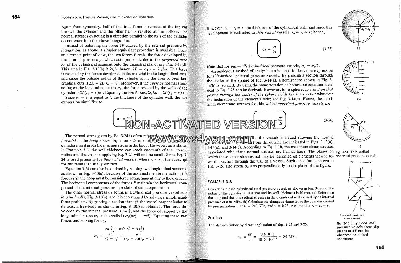
Hooke's Law, Pressure Vessels, and Thick.Walled Cylinders
Again from symmetry, half of this total force is resisted at the topthrough the cylinder and the other half is resisted at the bottom.normal stresses 0-2 acting in a direction parallel to the axis of the cdo not enter into the above integration.
Instead of obtaining the force 2P caused by the internal pressureintegration, as above, a simpler equivalent procedure is available.an alternate point of view, the two forces P resist the force developedthe internal pressure p, which acts perpendicular to the projected areA� of the cylindrical segment onto the diametral plane; see Fig. 3-13(This area in Fig. 3-13(b) is 2riL; hence, 2P = A�p = 2riLp. Thisis resisted by the forces developed in the material in the longitudinal cutand since the outside radius of the cylinder is to, the area of bothgitudinal cuts is 2A = 2L(ro - ri). Moreover, if the averageacting on the longitudinal cut is 0-2, the force resisted by the walls of tcylinder is 2L(ro - ri)0-�. Equating the two forces, 2riLp = 2L(ro - ri)0.
Since ro - ri is equal to t, the thickness of the cylinder wall, theexpression simplifies' to
The normal stress given by Eq. 3-24 is often referred to as the circu'ferential or the hoop stress. Equation 3-24 is valid only for thin-wcylinders, as it gives the average stress in the hoop. However, as isin Example 3-6, the wall thickness can reach one-tenth of the interadius and the error in applying Eq. 3-24 will still be small. Since Eq.24 is used primarily for thin-walled vessels, where ri � to, thefor the. radius is usually omitted.
Equation 3-24 can also be derived by passing two longitudinalas shown in Fig. 3-13(e). Because of the assumed membrane action.forces P in the hoop must be considered acting tangentially to the cThe horizontal components of the forces P maintain the horizontalponent of the internal pressure in a state of static equilibrium.
The other normal stress 0-2 acting in a cylindrical pressure vessellongitudinally, Fig. 3-13(b), and it is determined by solving a simpleforce problem. By passing a section through the vessel peri:its axis, a free-body as shown in Fig. 3-13(0 is obtained. The forceveloped by the internal pressure is p�rr�, and the force developed by thelongitudinal stress 0-2 in the walls is 0-2(�rr� - �rr�2). Equating theseforces and solving for 0-2,
0-2 -- I
p�rrT = 0-2(xPo - �rrT)prT prT
(ro + r)(ro- ri)
Etowever, ro - r� = t, the thickness of the cylindrical wall, and since thisdevelopment is restricted to thin-walled vessels, ro � r� �- r; hence,
(3 -25)
Note that for thin-walled cylindrical pressure vessels, 0.2 � 0.#2.An analogous method of analysis can be used to derive an expression
for thin-walled spherical pressure vessels. By passing a section throughcenter of the sphere of Fig. 3-14(a), a hemisphere shown in Fig. 3-
is isolated. By using the same notation as before, an equation iden-to Eq. 3-25 can be derived. However, for a sphere, any section that
�asses through the center of the sphere yields the same result whateverthe inclination of the element's side; see Fig. 3-14(c). Hence, the maxi-mum membrane stresses for thin-walled spherical pressure vessels are
(3-26)
(a)
(b)
Infinitesimal elements for the vessels analyzed showing the normalstresses 0-� and 0-2 viewed from the outside are indicated in Figs. 3-13(a),3-14(a), and 3-14(c). According to Eq. 1-10, the maximum shear stresses
.ociated with these normal stresses are half as large. The planes on Flg. 3-t4 Thin-walled
Consider a closed cylindrical steel pressure vessel, as shown in Fig. 3-13(a). Theradius of the cylinder is 1000 mm and its wall thickness is 10 mm. (a) Determinethe hoop and the longitudinal stresses in the cylindrical wall caused by an internalpressure of 0.80 MPa. (b) Calculate the change in diameter of the cylinder causedby pressurization. Let E = 200 GPa, and v = 0.25. Assume that r� � ro � r.
Which these shear stresses act may be identified on elements viewed to- spherical pressure vessel.ward a section through the wall of a vessel. Such a section is shown in -*----t
Fig.3-15.Thestress0'2actsperpendicularlytotheplaneofthefigure. o�-�
Solution
The stresses follow by direct application of Eqs. 3-24 and 3-25:
pr = 0.8 x 1 80MPa0'2 = t 10 x 10 -3
Planes of maximumshear stresses
Fig. 3-15 In yielded steelpressure vessels shear slipplanes at 45 � can beobserved on etchedspecimens.
'55
NON-ACTIVATEDVERSIONwww.avs4you.com
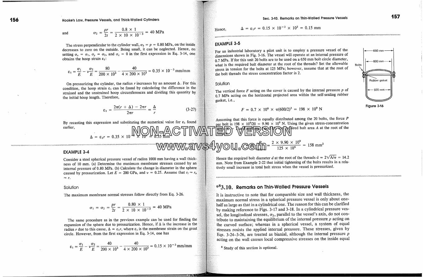
Hooke's Law, Pressure Vessels, and Thick. Walled Cylinders Sec. 3.10. Remarks on Thin.Walled Pressure Vessels
pr 0.8 x 1 Hence, A = e�r = 0.15 x 10 -3 x 103 = 0.15 mmand 0'2 = 2t 2 x 10 x 10 -3 = 40 MPa
The stress perpendicular to the cylinder wall, or3 = p = 0.80 MPa, on the insi.d EXA[VIFdecreases to zero on the outside. Being small, it can be neglected. Hence, �ne �setting cr� = cry, %. = or2, and cr� = 0 in the first expression in Eq. 3-14, o For an industrial laboratory a pilot unit is to employ a pressure vessel of thedimensions shown in Fig. 3-16. The vessel will operate at an internal pressure ofobtains the hoop strain el: .7 MPa. If for this unit 20 bolls are to be used on a 650 mm bolt circle diameter,
what is the required bolt diameter at the root of the threads? Set the allowable0'� 0'2 80 40 = 0.35 x 10 -3 mm/mm in tension for the bolts at 125 MPa; however, assume that at the root of
el = � - v� - 200 x 103 4 x 200 x 103 the bolt threads the stress concentration factor is 2.
On pressurizing the cylinder, the radius r increases by an amount A. For thi�condition, the hoop strain el can be found by calculating the difference instrained and the unstrained hoop circumferences and dividing this quantitythe initial h6op length. Therefore,
2�r(r + A) -- 2�rr A= -- (3-27gl = 2�xr r
By recasting this expression and substituting the numerical value for elearlier,
0.35 x 10 -3 x 103 = 0.35 mm
EXAMPLE 3-4
Consider a steel spherical pressure vessel of radius 1000 mm having a wallness of 10 mm. (a) Determine the maximum membrane stresses caused byinternal pressure of 0.80 MPa. lb) Calculate the change in diameter in thecaused by pressurization. Let E = 200 GPa, and v = 0.25. Assume that ri �
ution
vertical force F acting on the cover is caused by the internal pressure p of0.7 MPa acting on the horizontal projected area within the seif-sealhng rubber
gasket, i.e.,
F = 0.7 x 10⁶ x 'i1(600/2) 2 = 198 x 109 N
that this force is equally distributed among the 20 bolts, the force Pper bolt is 198 x 109/20 = 9.90 x 10⁹ N. Using the given stress-concentration
factor K = 2 and applying Eq. 2-19, the required bolt area A at the root of the
x 9.90 x 109= 158 mm 2
125 x 106
Hence the required bolt diameter d at the root of the threads d = 2X/-� = 14.2min. Note from Example 2-22 that initial tightening of the bolts results in a rela-tively small increase in total bolt stress when the vessel is pressurized.
Bolts
650 mm -----�
600 mm----�-
Rubber gasket
� 500 mm --�,
Figure 3-t6
Solution
The maximum membrane normal stresses follow directly from Eq. 3-26.
pr 0.80 x 10'1 = 0'2 2t 2 x 10 x 10 -3 = 40 MPa
The same procedure as in the previous example can be used for findingexpansion of the sphere due to pressurization. Hence, if A is the increase in theradius r due to this cause, A = e�r, where el is the membrane strain on thecircle. However, from the first expression in Eq. 3�14, one has
0'1 0'2 40 40el=�-v E-200x 103 4x200x 103
= 0.15 x 10⁻³mm/mm
Remarks on Thin-Walled Pressure Vesselsis instructive to note that for comparable size and wall thickness, the
maximum normal stress in a spherical pressure vessel is only about one-half as large as that in a cylindrical one. The reason for this can be clarifiedby making reference to Figs. 3-17 and 3-18. In a cylindrical pressure ves-
the longitudinal stresses, 0'2, parallel to the vessel's axis, do not con-tribute to maintaining the equilibrium of the internal pressure p acting onthe curved surface; whereas in a spherical vessel, a system of equalstresses resists the applied internal pressure. These stresses, given byEqs. 3-24-3-26, are treated as biaxial, although the internal pressure pacting on the wall causes local compressive stresses on the inside equal
Study of this section is optional.
NON-ACTIVATEDVERSIONwww.avs4you.com
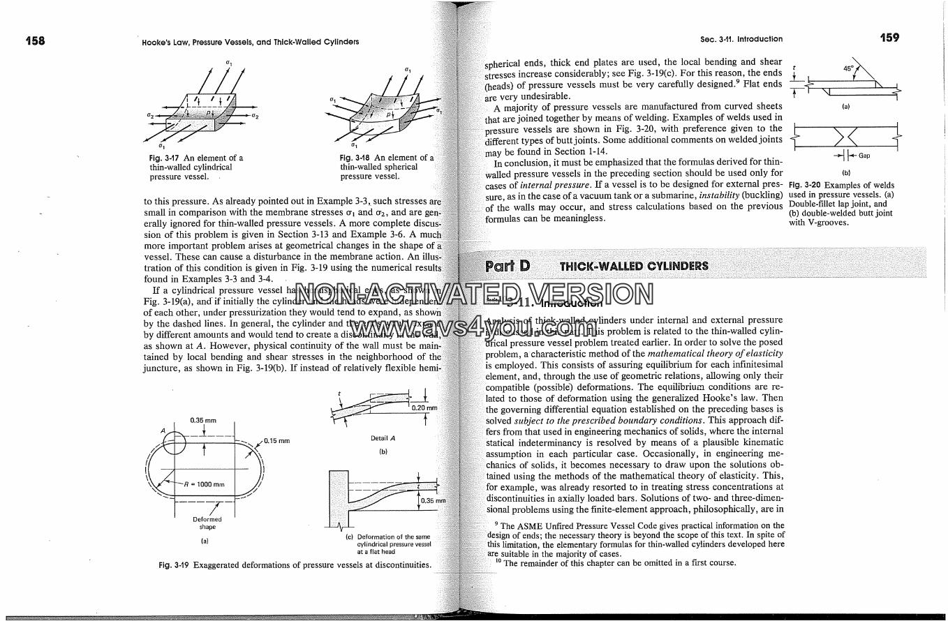
Hooke's Law, Pressure Vessels, and Thick. Walled Cylinders
o 1
Fig. 3-t7 An element of athin-walled cylindricalpressure vessel.
Fig. 3-t8 An element ofthin-walled sphericalpressure vessel.
to this pressure. As already pointed out in Example 3-3,. such stressessmall in comparison with the membrane stresses 0.� and 0'2, and areerally ignored for thin-walled pressure vessels. A more completesion of this problem is given in Section 3-13 and Example 3~6. Amore important problem arises at geometrical changes in the shape of�vessel. These can cause a disturbance in the membrane action. Antration of this condition is given in Fig. 3-19 using the numericalfound in Examples 3-3 and 3-4.
If a cylindrical pressure vessel has hemispherical ends, as shownFig. 3-19(a), and' if initially the cylinder and the heads wereof each other, under pressufization they would tend to expand, asby the dashed lines. In general, the cylinder and the ends wouldby different amounts and would tend to create a discontinuity in the wall}as shown at A. However, physical continuity of the wall must betained by local bending and shear stresses in the neighborhood ofjuncture, as shown in Fig. 3-19(b). If instead of relatively flexible
0.35 mm
�R = 1000 mm
Deformed
shape
(a)
Detail A
(b)
(c) Deformation of the samecylindrical pressure vesselat a flat head
Fig. 3-t9 Exaggerated deformations of pressure vessels at discontinuities.
Sec. 3-�. Introduction
erical ends, thick end plates are used, the local bending and shearses increase considerably; see Fig. 3-19(c). For this reason, the ends
(heads) of pressure vessels must be very carefully designed. 9 Flat endsvery undesirable.
A majority of pressure vessels are manufactured from curved sheetsare joined together by means of welding. Examples of welds used in
pressure vessels are show.n in Fig. 3-20, with preference given to thedifferent types of butt joints. Some additional comments on welded joints
be found in Section 1-14.In conclusion, it must be emphasized that the formulas derived for thin-
pressure vessels in the preceding section should be used only for:ases of internal pressure. If a vessel is to be designed for external pres-
as in the case of a vacuum tank or a submarine, instability (buckling)the walls may occur, and stress calculations based on the previous
ulas can be meaningless.
Introduction
Analysis of thick-walled cylinders under internal and external pressurediscussed in this part. This problem is related to the thin-walled cylin-
pressure vessel problem treated earlier. In order to solve the posedproblem, acharacteristic method of the mathematical theory of elasticity
is employed. This consists of assuring equilibrium for each infinitesimaland, through the .use of geometric relations, allowing only their
(possibl�) deformations. The equilibrium conditions are re-to those of deformation using the generalized Hooke's law. Then
the governing differential equation established on the preceding bases issubject to the prescribed boundary conditions. This approach dif-
from that used in engineering mechanics of solids, where the internalstatical indeterminancy is resolved by means of a plausible kinematic
assumption in each particular case. Occasionally, in engineering me-chanics of solids, it becomes necessary to draw upon the solutions ob-
tained using the methods of the mathematical theory of elasticity. This,was already resorted to in treating stress concentrations at
discontinuities in axially loaded bars. Solutions of two- and three-dimen-problems using the finite-element approach, philosophically, are in
9 The ASME Unfired Pressure Vessel Code gives practical information on theof ends; the necessary theory is beyond the scope of this text. In spite of
limitation, the elementary formulas for thin-walled cylinders developed heresuitable in the majority of cases.
�o The remainder of this chapter can be omitted in a first course.
t
(a)
(b)
Fig. 3-20 Examples o� weldsused in pressure vessels. (a)Double-fillet lap joint, and(b) double-welded butt jointwith V-grooves.
NON-ACTIVATEDVERSIONwww.avs4you.com
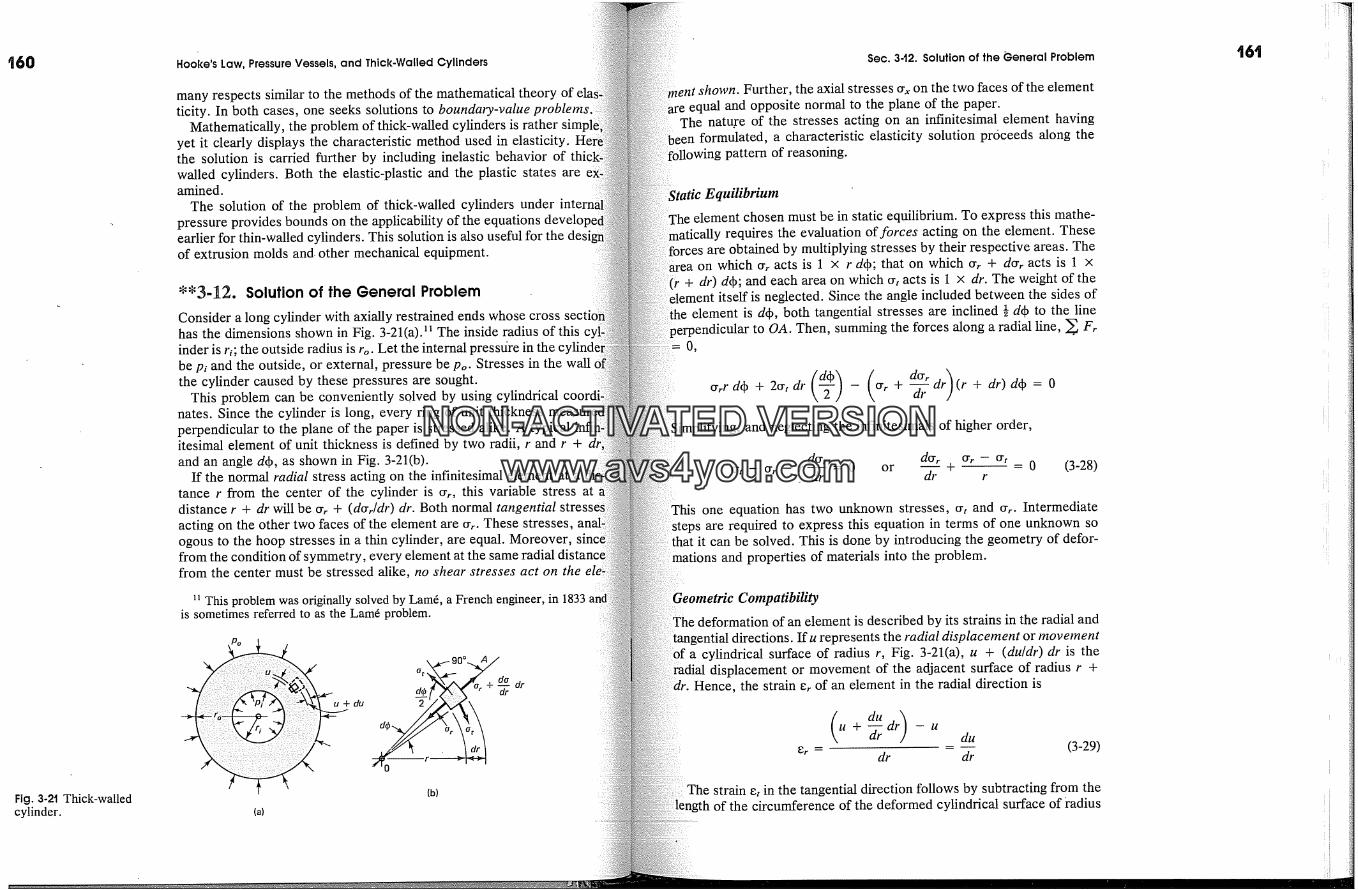
t60
FiG. 3-21 Thick-walledcylinder.
Hooke's Law, Pressure Vessels, and Thick-Walled Cylinders
many respects similar to the methods of the mathematical theory ofticity. In both cases, one seeks solutions to boundary-value problems
Mathematically, the problem of thick-walled cylinders is ratheryet it clearly displays the characteristic method used in elasticity.the solution is carried further by including inelastic behavior of thi,wailed cylinders. Both the elastic-plastic and the plastic states areamined.
The solution of the problem of thick-wailed cylinders underpressure provides bounds on the applicability of the equationsearlier for thin-wailed cylinders. This solution is also useful for the desiof extrusion molds and. other mechanicai equipment.
**342. Solution of the General Problem
Consider a long cylinder with axially restrained ends whose crosshas the dimensions shown in Fig. 3-21(a). � The inside radius of thisinder is ri; the outside radius is ro. Let the internal presst/re in the c'be pi and the outside, or external, pressure be po. Stresses in the wall,the cylinder caused by these pressures are sought.
This problem can be conveniently solved by using cylindricalnates. Since the cylinder is long, every ring of unit thicknessperpendicular to the plane of the paper is stressed alike. A typicaiitesimai element of unit thickness is defined by two radii, r and r +and an angle dqb, as shown in Fig. 3-21(b).
If the normal radial stress acting on the infinitesimal element at atance r from the center of the cylinder is err, this variable stress atdistance r + dr will be crr q- (do'r/dr) dr. Both normal tangentialacting on the other two faces of the element are err. These stresses,ogous to the hoop stresses in a thin cylinder, are equal. Moreover,from the condition of symmetry, every element at the same radifrom the center must be stressed aiike, no shear stresses act on the
� This problem was originally solved by Lamfi, a French engineer, inis sometimes referred to as the Lamfi problem.
(a)
u+du
(b)
Sec. 3-t2. Solution of the General Problem
zent shown. Further, the axial stresses cry, on the two faces of the elementequai and opposite normal to the plane of the paper.
The nature of the stresses acting on an infinitesimal element havingformulated, a characteristic elasticity solution pr6ceeds along the
pattern of reasoning.
Equilibriumelement chosen must be in static equilibrium. To express this mathe-
requires the evaiuation of forces acting on the element. These:es are obtained by multiplying stresses by their respective areas. The
on which err acts is 1 x r dqb; that on which err + dcrr acts is 1 x+ dr) dqb; and each area on which crt acts is 1 x dr. The weight of the
itself is neglected. Since the angle included between the sides ofthe element is dqb, both tangential stresses are inclined � dqb to the line
�erpendicular to OA. Then, summing the forces aiong a radiai line, � Fr0,
crrr dqb + 2crt dr - crr + � dr (r + dr) dqb = 0
Simplifying, and neglecting the infinitesimais of higher order,
dcrr dcrr Crr- Crtcr t -- crr -- r-�F- F = 0 or d�--Z- + -- = 0 (3-28)r
one equation has two unknown stresses, fit and cry. Intermediateare required to express this equation in terms of one unknown so
it can be solved. This is done by introducing the geometry of defor-and properties of materiais into the problem.
:tric CompatibilityThe deformation of an element is described by its strains in the radial and
. directions. Ifu represents the radial displacement or movementa cylindricai surface of radius r, Fig. 3-21(a), u + (du/dr) dr is the
displacement or movement of the adjacent surface of radius r +Hence, the strain er of an element in the radial direction is
du )u + �rr dr - u du(3-29)
dr dr
The strain et in the tangentiai direction follows by subtracting from theof the circumference of the deformed cylindrical surface of radius
'16'1
NON-ACTIVATEDVERSIONwww.avs4you.com
�62 Hooke's Law, Pressure Vessels, and Thick. Walled Cylinders Sec. 3d2. Solution of the General Problem
r + u the circumference of the unstrained cylinder of radius r andthe difference by the latter length. Hence,
2�x(r + u) - 2�w' u2�xr r
Note that Eqs. 3-29 and 3-30 give strains expressed in terms ofunknown variable u.
Properties of MaterialThe generalized Hooke's law relating strains to stresses is given by3-14, and can be restated here in the form �2
1
�;r = �_�(O'r -- ]JO't -- l/O'x)1
1
(3-31
However, in the case of the thick-walled cylinder with axiallydeformation, the problem is one of plane strain, i.e., e�, = 0. Theequation then leads to a relation for the axial stress as
O' x = V(O' r q- O't)
Introducing this result into Eqs. 3-31 and 3-32 and solving themtaneously gives expressions for stresses O'r and crt in terms of strains:
EO' r �- [(1 -- lJ)�;r q-
(1 + v)(1 - 2v)E
(1 + v)(1 - 2v)
These equations bring the plane strain condition into the problemelastic material.
Formation of the Differential EquationNow the equilibrium equation, Eq. 3-28, can be expressed in termsone variable u. Thus, one eliminates the strains �;r and e, from Eqs.
�2 Since an infinitesimal cylindrical element includes an infinitesimal antween two of its sides, it can be treated as if it were an element in acoordinate system.
3-36 by expressing them in terms of the displacement u, as given bys. 3-29 and 3-30; then the radial and tangential stresses are
fir = (1 + v)(1 - 2v) (1 - v)�r + v(3-37)
(1 - v)(1 - 2v) V�rr
by substituting these values into Eq. 3-28 and simplifying, the desireddifferential equation is obtained:
dr 2 + = 0k r dr r 2(3-38)
of the Differential Equationcan be verified by substitution, the general solution of Eq. 3-38, which
the radial displacement u of any point on the cylinder, is
u = A�r+ A2/r� (3-39)
the constants A� and A2 must be determined from the conditionsthe boundaries of the body.
Unfortunately, for the determination of the constants A� and A2, theu is not known at either the inner or the outer boundary of
the cylinder's wall. However, the known pressures are equal to the radialStresses acting on the elements at the respective radii. Hence,
O'r(l'i) = --pi and err(to) = -po (3-40)
the minus signs are used to indicate compressive stresses. More-)Ver, since u as given by Eq. 3-39 and du/dr = A� - A2/r 2 can be sub-
into the expression for O'r given by Eq. 3-37, the boundary con-given by Eqs. 3-37 become
fir(r/) = --pi = (1 + v)(1 - 2v) A� - (1 - 2v)E ICrr(ro) = -po = (1 + v)(1 - 2v) A� - (1 - 2v)
(3-41)
NON-ACTIVATEDVERSIONwww.avs4you.com
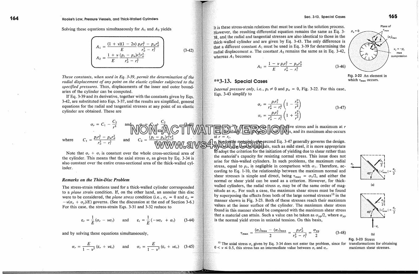
t64 Hooke's Law, Pressure Vessels, and Thick. Walled Cylinders
Solving these equations simultaneously for A� and A2 yields
A1=(1+v)(1-2v)piri2-por2o1E r� - r/2
A2 = 1 + v (Pi - po)ri2ro 2'E r2o - ri 2
These constants, when used in Eq. 3-39, permit the determinationradial displacement of any point on the elastic cylinder subjected tospecified pressures. Thus, displacements of the inner and outeraries of the cylinder can be computed.
If Eq. 3-39 and its derivative, together with the constants given by Ec3-42, are substituted into Eqs. 3-37, and the results are simplified,equations for the radial and tangential stresses at any point of an elascylinder are obtained. These are
C2 C2O'r �' Cl r2 and crt = C� + -w (3-43F-
-- - po)riwhere C� - piti2 P�r2� (pl 2ra - rt 2 and C2 =� t'7� -- r/2
Note that O' r '� fit is constant over the whole cross-sectional areathe cylinder. This means that the axial stress cry, as given by Eq. 3-34also constant over the entire cross-sectional area of the thick-walledinder.
Remarks on the Thin-Disc Problem
The stress-strain relations used for a thick-walled cylinder corresto a plane strain condition. If, on the other hand, an annular thin discwere to be considered, the plane stress condition (i.e., cry, = 0 and e�, =-v(�.� + c&,)/E) governs. (See the discussion at the end of Section 3-6.'
For this case, the stress-strain Eqs. 3-31 and 3-32 reduce to
1 1
8r = �_�(O'r -- l/O't) and �, = � (-vcrr + err)
and by solving these equations simultaneously,
E E
�'r - 1 - v 2 (er q- vet) and or, - 1 - 1/2 (�;t q- ]Yer)
Sec. 3.13. Special Cases '165
It is these stress-strain relations that must be used in the solution process.However, the resulting differential equation remains the same as Eq. 3-38, and the radial and tangential stresses are also identical to those in the
.walled cylinder and are given by Eq. 3-43. The only difference isthat a different constant A� must be used in Eq. 3-39 for determining the
radial displacement u. The constant A2 remains the same as in Eq. 3-42,A� becomes
1 - vp�ri 2 - por2oA� - E r2� _ r�2 (3-46)
*'3-13. Special Casespressure only, i.e., pt � 0 and po = 0, Fig. 3-22. For this case,
s. 3-43 simplify to
- -Pir/2- (1-�) (3-47,O'r r2o -- r/2
/ro2/r 2 � 1, fir is �ways a compressive stress and is m�imum at r
= r�. Similarly, ,� is �ways a tensile stress, and its max�um �so occursatr= ri.
For brittle mater,s, the second Eq. 3-47 gener�y governs the design.However, for ductile materies, such as m�d steel, it is more appropriate
adopt the criterion for the iffitiation of yielding due to shear rather thanmated�'s capacity for resisting normal stress. This issue does not
�ise for thin-w�ed cylinders. In such problems, the m�imum radi�stress equal to pt, i5 negli�ble in comparison with ,�. Therefore, ac-
to Eq. 1-10, the relationship between the m�imum norm� andshear stresses is simple and dkect, being *m� = *�/2, and either thenomal or she� yield can be used as a criterion. However, for thick-
cylinders, the radial stress �r may be of the same order of mag-as *t. For such a case, the maximum shear stress must be found
by supe�osing the effects from both of the l�ge nom� stresses �3 in themanner shown in Fig. 3-23. Both of these stresses reach their maximumv�ues at the inner surface of the cylinder. The m�imum shear stress
found in this manner should be comp�ed with the m�imum shear stressthat a material can attain. Such a v�ue can be taken as ffyp/2, where ffypis the no� yield stress in uni�ial tension. On this basis,
(fit)max -- (fir)max p,r2o -- O'yp- -- (3-48)Tmax = 2 r2o - r/2 2
Po =0
Plane ofTrnax
Or = --Pimax
Fig. 3.22 An element inwhich *m� occurs.
Fig. 3.23 Stress13 The axial stress cr z given by Eq. 3-34 does not enter the problem, since for transformations for obtaining
0 < � < 0.5, this stress has an intermediate value between or, and err. maximum shear stresses.
NON-ACTIVATEDVERSIONwww.avs4you.com
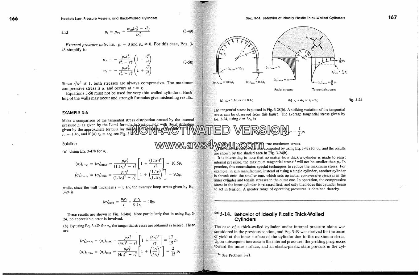
'Hooke's Law, Pressure Vessels, and Thick-Walled Cylinders Sec. 3.t4. Behavior of Ideally Plastic Thick-Walled Cylinders �67t66
and0'y(ro -
Pi = Pyp -- 2r2o
External pressure only, i.e., pi = 0 and po � O. For this case, Eqs.43 simplify to
O'r -- -P�"--�2�-(1 -'r/�r2o- r/2 �) (3-5�
Since r�/r 2 -< 1, both stresses are always compressive. Thecompressive stress is crt and occurs at r = ri.
Equations 3-50 must not be used for very thin-walled �ylinders.ling of the walls may occur and strength formulas give misleading
EXAMPLE 3-6
Make a comparison of the tangential stress distribution caused by thepressure pl as given by the Lam6 formula in Section 3-12 with thegiven by the appro_ximate formula for thin-walled cylinders of Section 3-9 ifro = 1.1r�, and if(b) ro = 4r4 see Fig. 3-24.
Solution
(a) Using Eq. 3-47b for or,,
p,,.�2 [ (1.1r,)2']= 2 = 10.5pi(O"t)r=r i = (O't)max (1.1ri)2 _ r/2 1 q- ri(0',) .... �-- (O")min -- (1.lr'� �- F/2 1 + kl.lr, j j = 9.5p,
while, since the wall thickness t = 0.1r�, the average hoop stress given by3-24 is
pir_�i_ pirl -- 10pi(cr,)avg = t O.lriThese results are shown in Fig. 3-24(a). Note particularly that in using Eq.
24, no appreciable error is involved.
(b) By using Eq. 3-47b for or,, the tangential stresses are obtained as before. Theseare
piri2 [ (4ri)21 17(O"t)r=ri = (O't)max -- (4ri�7- r� 1 + r�2 j = �-� pi(0',) .... = (O")min -- (4ri� -� ri 2 k4riJ J = �-� p'
(at)av = 10pi
)max = 10.5pi
(ar)rnin = 0
({/t)rnin = 9.5Pi(at)max = Pi
Radial stresses
5(at)av = �Pi
- '�Pl
Tangential stresses
(a) G = 1.1q or t=O. lq (b) q =4q�rt i=3 0
stress is plotted in Fig. 3-28(b). A striking variation of the tangentialcan be observed from this figure. The average tangential stress given by
3-24, using t = 3r�, is
(Crt)a v = piri 5 1t = �-�Pi = 5Pi
stress is nowhere near the true maximum stress.The radial stresses were also computed by using Eq. 3-47a for err, and the results
shown by the shaded area in Fig. 3-24(b).It is interesting to note that no matter how thick a cylinder is made to resist
pressure, the maximum tangential stress �4 will not be smaller than p�. Inthis necessitates spe. cial techniques to reduce the maximum stress. Forin gun manufacture, instead of using a single cylinder, another cylinder
shrunk onto the smaller one, which sets up initial compressive stresses in theand tensile stresses in the outer one. In operation, the compressive
inner cylinder is released first, and only then does this cylinder beginact in tension. A greater range of operating pressures is obtained thereby.
Behavior of Ideally Plastic Thick-WalledCylinders
case of a thick-walled cylinder under internal pressure alone wasin the previous section, and Eq. 3-49 was derived for the onset
yield at the inner surface of the cylinder due to the maximum shear.2uent increase in the internal pressure, the yielding progresses
the outer surface, and an elastic-plastic state prevails in the cyl-
]4 See Problem 3-21.
Fig. 3-24
NON-ACTIVATEDVERSIONwww.avs4you.com
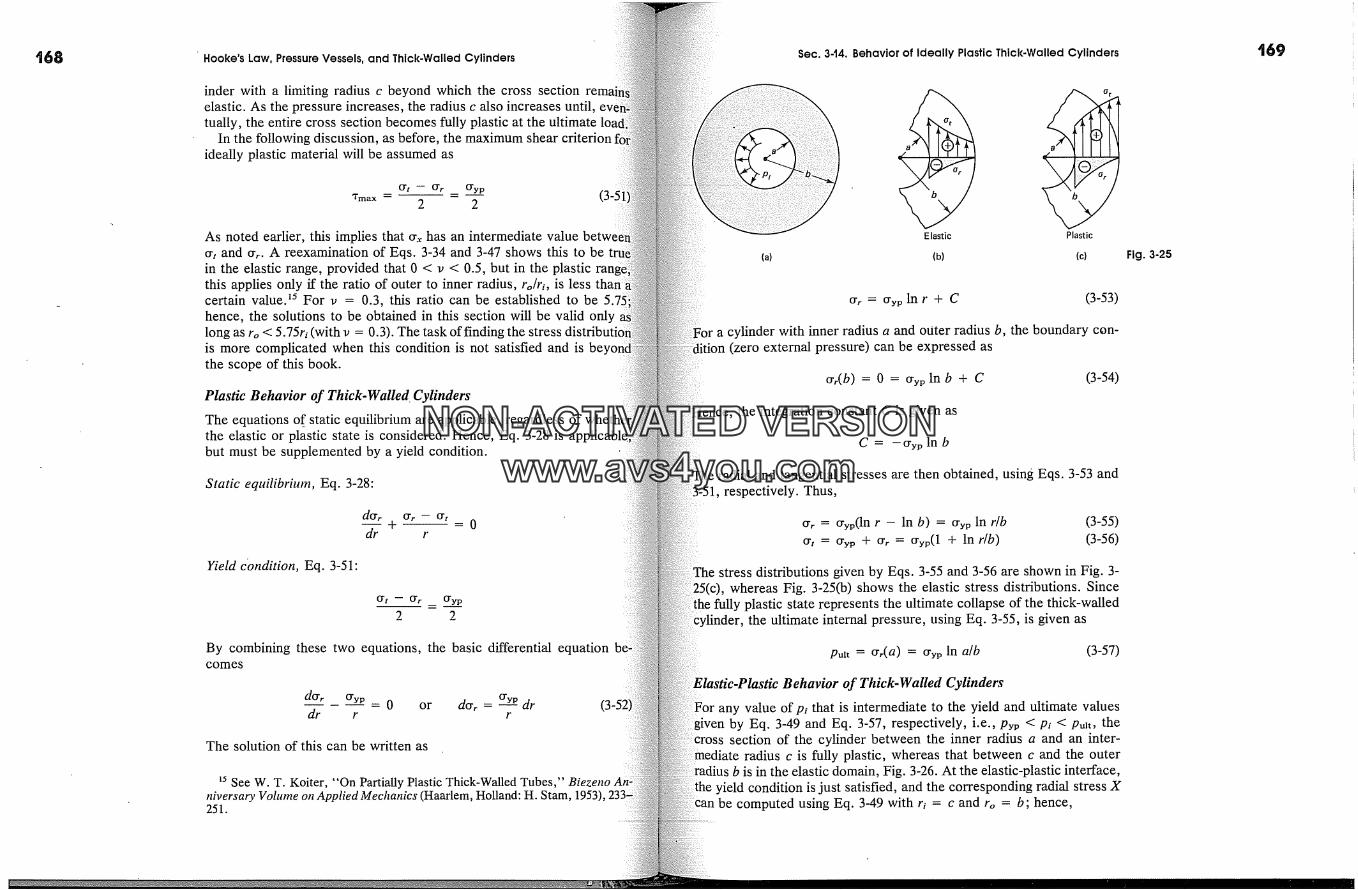
�68 Hooke's Law, Pressure Vessels, and Thick. Walled Cylinders Sec. 344. Behavior of Ideally Plastic Thick-Walled Cylindersinder with a limiting radius c beyond which the cross sectionelastic. As the pressure increases, the radius c also increases until,tually, the entire cross section becomes fully plastic at the ultimate
In the following discussion, as before, the maximum shear criterionideally plastic material will be assumed as
fit -- fir fiyp- (3-51*max -- 2 2
As noted earlier, this implies that fi�, has an intermediate value betweifi, and fir. A reexamination of Eqs. 3-34 and 3-47 shows this to bein the elastic range, provided that 0 < v < 0.5, but in the plastic ranthis applies only if the ratio of outer to inner radius, ro/rt, is lesscertain value. �5 For v = 0.3, this ratio can be established to be 5.75hence, the solutions to be obtained in this section will be valid onlylong as ro < 5.75r� (with v = 0.3). The task of finding the stressis more complicated when this condition is not satisfied and is be'the scope of this book.
Plastic Behavior of Thick-Walled Cylinders
The equations of static equilibrium are applicable, regardless ofthe elastic or plastic state is considered. Hence, Eq. 3-28 isbut must be supplemented by a yield condition.
Static equilibriu/n, Eq. 3-28:
dfir fir -- fitdr r
Yield condition, Eq. 3-51:
fit -- fir fiyp
By combining these two equations, the basic differential equationcomes
dfir fiYP = 0 or dfir = fiy__ppdrdr r r
The solution of this can be written as
�5 See W. T. Koiter, "On Partially Plastic Thick-Walled Tubes," Biezenoniversary Volume on Applied Mechanics (Haarlem, Holland: H. Stam, 1953), 232251.
Elastic Plastic
(a) (b) (c)
fir(b) = 0 = fiyp In b + C
Hence, the integration constant C is given as
C = --fiyp In b
fir = fiyp lB r + C (3-53)
cylinder with inner radius a and outer radius b, the boundary con-(zero external pressure) can be expressed as
(3-54)
radial and tangential stresses are then obtained, using Eqs. 3-53 andrespectively. Thus,
fir = fiyp0n r -- In b) = fiyp in r/bfit = fiyp 3c fir = fiyp(1 q- In r/b)
(3-55)(3-56)
stress distributions given by Eqs. 3-55 and 3-56 are shown in Fig. 3-25(c), whereas Fig. 3-25(b) shows the elastic stress distributions. Since
plastic state represents the ultimate collapse of the thick-walledthe ultimate internal pressure, using Eq. 3-55, is given as
pult = fir(a) = fiyp In a/b (3-57)
Behavior of Thick-Walled Cylindersany value of pt that is intermediate to the yield and ultimate values
given by Eq. 3-49 and Eq. 3-57, respectively, i.e., pyp < pt < pult, thecross section of the cylinder between the inner radius a and an inter-
radius c is fully plastic, whereas that between c and the outerb is in the elastic domain, Fig. 3-26. At the elastic-plastic interface,
yield condition is just satisfied, and the corresponding radial stress XCan be computed using Eq. 3-49 with r� = c and ro = b; hence,
Fig. 3-25
NON-ACTIVATEDVERSIONwww.avs4you.com
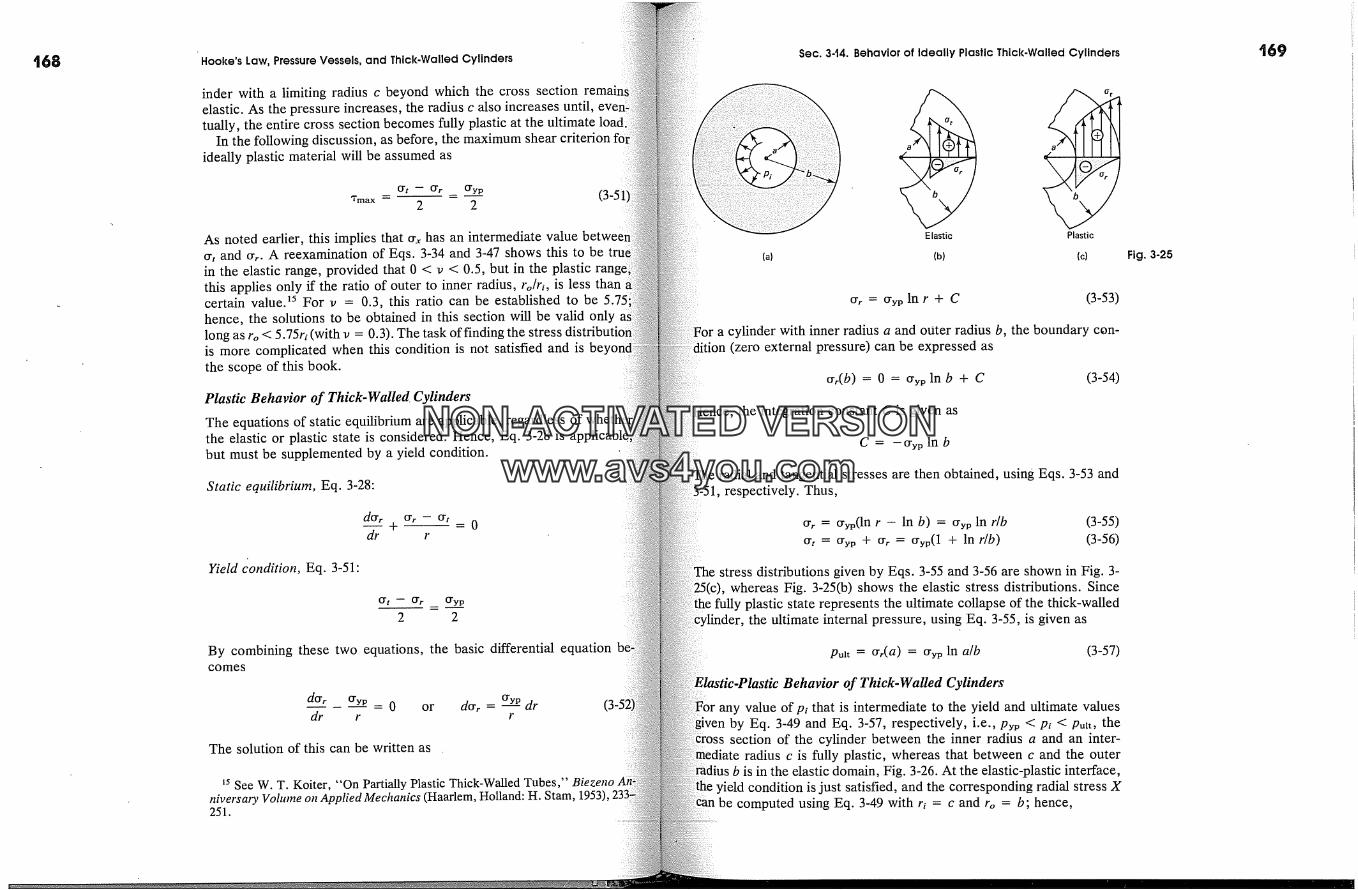
�68 ' Hooke's Law, Pressure Vessels, and Thick-Walled Cylinders Sec. 3-t4. Behavior of Ideally Plastic Thick.Walled Cylindersinder with a limiting radius c beyond which the cross sectionelastic. As the pressure increases, the radius c also increases until,tually, the entire cross section becomes fully plastic at the ultimate load
In the following discussion, as before, the maximum shear criterionideally plastic material will be assumed as
fit -- fir -- fiyp (3-51)'rmax = 2 2
As noted earlier, this implies that fi� has an intermediate value betwe�fi, and fir. A reexamination of Eqs. 3-34 and 3-47 shows this to be tru.in the elastic range, provided that 0 < v < 0.5, but in the plastic ranthis applies only if the ratio of outer to inner radius, ro/ri, is less thancertain value? For v = 0.3, this ratio can be established to behence, the solutions to be obtained in this section will be valid onlylong as ro < 5.75ri (with v = 0.3). The task of finding the stressis more complicated when this condition is not satisfied and is be'the scope of this book.
Plastic Behavior of Thick-Walled CylindersThe equations of static equilibrium are appl/cable, regardlessthe elastic or plastic state is considered. Hence, Eq. 3-28 isbut must be supplemented by a yield condition.
Static equilibriutn, Eq. 3-28:
dfir fir -- fit--+--=0
dr r
Yield condition, Eq. 3-51:
fit -- fir fiyp
2 2
By combining these two equations, the basic differential equationcomes
dfir fiYP = 0 or dfir = fiY__2 drdr r r
The solution of this can be written as
�5 See W. T. Koiter, "On Partially Plastic Thick-Walled Tubes," Biezeno Ainiversa�y Volume on Applied Mechanics (Haarlem, Holland: H. Stam251.
Elastic Plastic
(a) (b) (c)
fir = fiyp In r + C (3-53)
a cylinder with inner radius a and outer radius b, the boundary con-(zero external pressure) can be expressed as
fir(b) = 0 = fiyp In b + C (3-54)
Hence, the integration constant C is given as
C = --fiyp In b
radial and tangential stresses are then obtained, using Eqs. 3-53 andrespectively. Thus,
fir = fiyp(ln r - in b) = fiyp in dbfit = fiyp + fir = fiyp(1 + In rib)
(3-55)(3-56)
stress distributions given by Eqs. 3-55 and 3-56 are shown in Fig. 3-whereas Fig. 3-25(b) shows the elastic stress distributions. Since
plastic state represents the ultimate collapse of the thick-walledcylinder, the ultimate internal pressure, using Eq. 3-55, is given as
Pult = fir(a) = fiyp In a/b (3-57)
Behavior of Thick-Walled Cylinders
any value of p� that is intermediate to the yield and ultimate valuesby Eq. 3-49 and Eq. 3-57, respectively, i.e., pyp <� pi � pult, thesection of the cylinder between the inner radius a and an inter-
radius c is fully plastic, whereas that between c and the outerb is in the elastic domain, Fig. 3-26. At the elastic-plastic interface,
yield condition is just satisfied, and the corresponding radial stress Xbe computed using Eq. 3-49 with r� = c and ro = b; hence,
Fig. 3-25
NON-ACTIVATEDVERSIONwww.avs4you.com
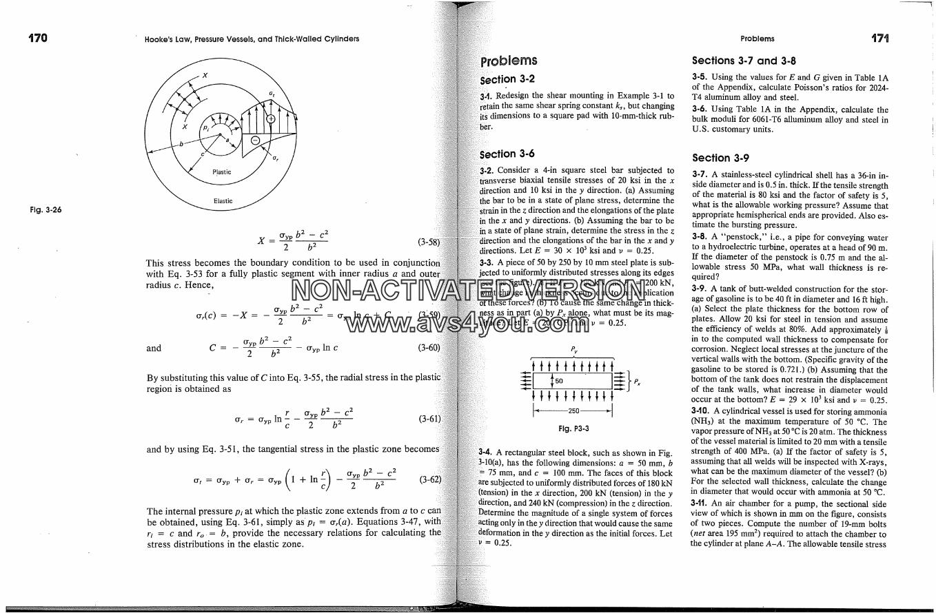
�70 Hooke's Law, Pressure Vessels, and Thick. Walled Cylinders Problems
Fig. 3-26
x
X- crvp b2 -- c22 b 2
This stress becomes the boundary condition to be used inwith Eq. 3-53 for a fully plastic segment with inner radius a and outradius c. Hence,
err(C) = -X = Cryp b 2 - c 22 b2 -- Gyp Inc + C
and C = O-yp b 2 - c 22 b 2 Crvp In c
By substituting this value of C into Eq. 3-55, the radial stress in theregion is obtained as
O' r = O'yp Inr Gyp b 2 -- c 2c 2 b 2
and by using Eq. 3-51, the tangential stress in the plastic zone becomes
(O' t = Cryp "Jc O' r = Cryp 1 + In O'yp2 b 2
The internal pressure pi at which the plastic zone extends from a to cbe obtained, using Eq. 3-61, simply as'pi = err(a). Equations 3-47,ri = c and ro.-- b, provide the necessary relations for calculatingstress distributions in the elastic zone.
}blerns
,ction 3-2
Redesign the shear mounting in Example 3-1 tothe same shear spring constant ks, but changing
dimensions to a square pad with 10-mm-thick rub-
'ion 3-6
Consider a 4-in square steel bar subjected tobiaxial tensile stresses of 20 ksi in the x
and 10 ksi in the y direction. (a) Assuming: bar to be in a state of plane stress, determine the
in the z direction and the elongations of the platethe x and y directions. (b) Assuming the bar to bea state of plane strain, determine the stress in the z
and the elongations of the bar in the x and yLet E = 30 x 103 ksi and v = 0.25.
A piece of 50 by 250 by 10 mm steel plate is sub-to uniformly distributed stresses along its edges
(see the figure). (a) IfPx = 100 kN and Py = 200 kN,change in thickness occurs due to the application
'these forces? (b) To cause the same change in thick-ness as in part (a) by P�, alone, what must be its mag-
Let E = 200 GPa and v = 0.25.
Fig. P3-3
3-4. A rectangular steel block, such as shown in Fig.has the foilowing dimensions: a = 50 mm, b
75 mm, and c = 100 mm. The faces of this blockected to uniformly distributed forces of 180 kN
(tension) in the x direction, 200 kN (tension) in the yand 240 kN (compression) in the z direction.
the magnitude of a single system of forcesin the y direction that would cause the same
in the y direction as the initial forces. Let0.25.
Sections 3-7 and 3-8
3-5. Using the values for E and G given in Table 1Aof the Appendix, calculate Poisson's ratios for 2024-T4 aluminum alloy and steel.3-6. Using Table 1A in the Appendix, calculate thebulk moduli for 6061-T6 alluminum alloy and steel inU.S. customary units.
Section 3-9
3-7. A stainless-steel cylindrical shell has a 36-in in-side diameter and is 0.5 in. thick. If the tensile strengthof the material is 80 ksi and the factor of safety is 5,what is the allowable working pressure? Assume thatappropriate hemispherical ends are provided. Also es-timate the bursting pressure.3-8. A "penstock," i.e., a pipe for conveying waterto a hydroelectric turbine, operates at a head of 90 m.If the diameter of the penstock is 0.75 m and the al-lowable stress 50 MPa, what wall thickness is re-quired?3-9. A tank of butt-welded construction for the stor-age of gasoline is to be 40 ft in diameter and 16 ft high.(a) Select the plate thickness for the bottom row ofplates. Allow 20 ksi for steel in tension and assumethe efficiency of welds at 80%. Add approximately �in to the computed wall thickness to compensate forcorrosion. Neglect local stresses at the juncture of thevertical walls with the bottom. (Specific gravity of thegasoline to be stored is 0.721.) (b) Assuming that thebottom of the tank does not restrain the displacementof the tank walls, what increase in diameter wouldoccur at the bottom? E = 29 x 103 ksi and v = 0.25.3-t0. A cylindrical vessel is used for storing ammonia(NH3) at the maximum temperature of 50 �C. Thevapor pressure of NH3 at 50 �C is 20 atm. The thicknessof the vessel material is limited to 20 mm with a tensilestrength of 400 MPa. (a) If the factor of safety is 5,assuming that all welds will be inspected with X-rays,what can be the maximum diameter of the vessel? (b)For the selected wall thickness, calculate the changein diameter that would occur with ammonia at 50 �C.3-11. An air chamber for a pump, the sectional sideview of which is shown in mm on the figure, consistsof two pieces. Compute the number of 19-mm bolts(net area 195 mm 2) required to attach the chamber tothe cylinder at plane A-A. The allowable tensile stress
NON-ACTIVATEDVERSIONwww.avs4you.com
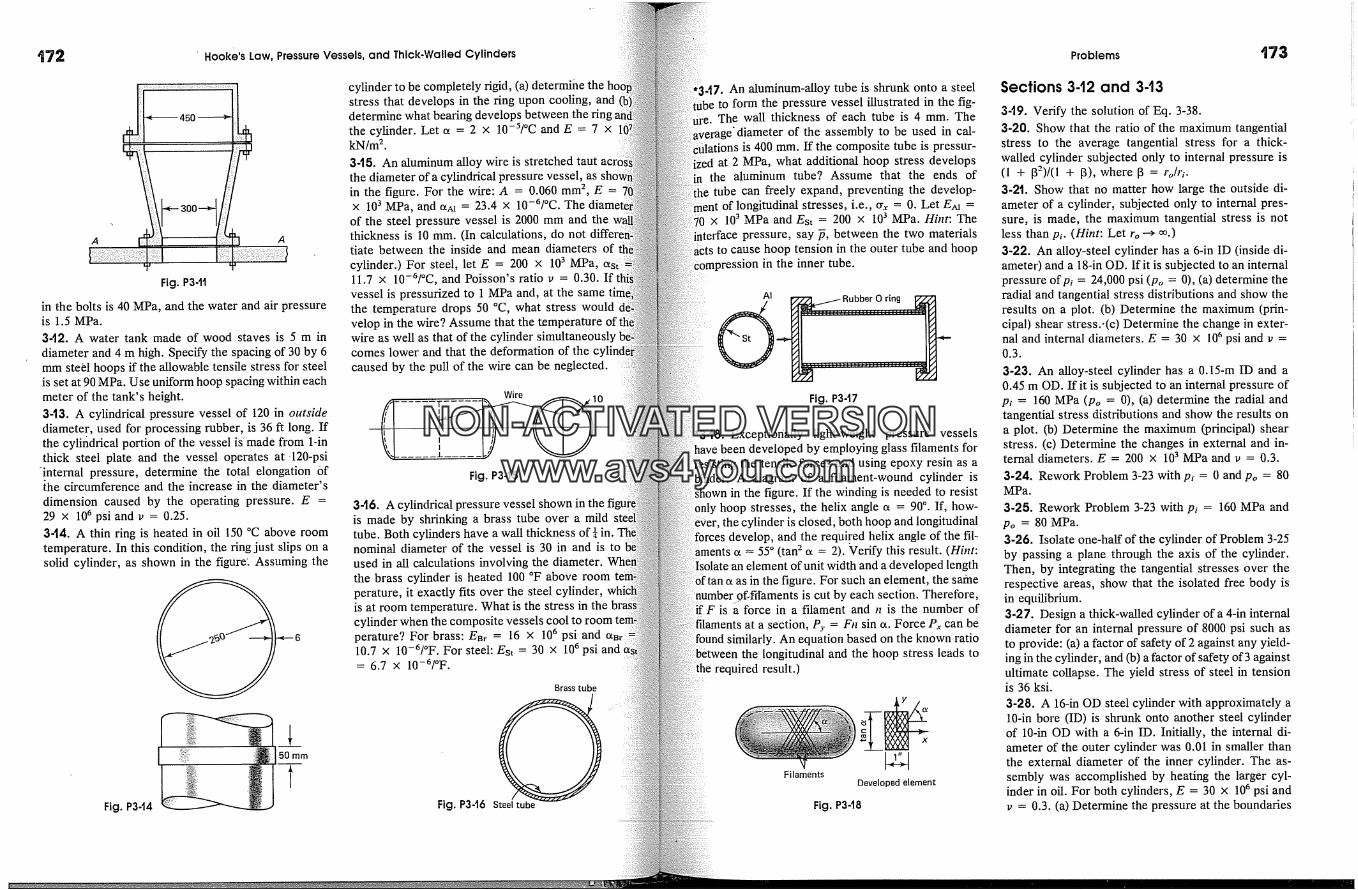
'72 � Hooke's Law, Pressure Vessels, and Thick.Walled Cylinders
A A
Fig. P34t
in the bolts is 40 MPa, and the water and air pressureis 1.5 MPa.
3-t2. A water tank made of wood staves is 5 m indiameter and 4 m high. Specify the spacing of 30 by 6mm ste�l hoops if the allowable tensile stress for steelis set at 90 MPa. Use uniform hoop spacing within eachmeter of the tank's height.3-t3. A cylindrical pressure vessel of 120 in outsidediameter, used for processing rubber, is 36 ft long. Ifthe cylindrical portion of the vessel is made from 1-inthick steel plate and the vessel operates at-120-psi
'internal pressure, determine the total elongation Of�he circumference and the increase in the diameter'sdimension caused by the operating pressure. E =29 x 106 psi and v = 0.25.3-t4. A thin ring is heated in oil 150 �C above roomtemperature. In this condition, the ring just slips on asolid cylinder, as shown in the figure: Assuming the
6
Fig. P3-t4
50 mm
cylinder to be completely rigid, (a) determire thestress that develops in the ring upon cooling, anddetermine what bearing develops between the rinthe cylinder. Let a = 2 x 10-s/�C and E = 7 xkN/m 2.3-t5. An aluminum alloy wire is stretched tautthe diameter of a cylindrical pressure vessel, asin the figure. For the wire: A = 0.060 mm 2, E =
X 103 MPa, and a^t = 23.4 x 10-a/�C. Theof the steel pressure vessel is 2000 mm and thethickness is 10 mm. (In calculations, do nottiate between the inside and mean diameters ofcylinder.) For steel, let E = 200 x 103 MPa,11.7 x 10-a/�C, and Poisson's ratio v = 0.30. Ifthiivessel is pressurized to 1 MPa and, at the samethe temperature drops 50 �C, what stress wouldvelop in the wire? Assume that the temperature oftwire as well as that of the cylindercomes lower and that the deformation of thecaused by the pull of the wire can be neglected.
Wire
Fig. P345
3-'16. A cylindrical pressure vessel shown in the fiis made by shrinking a brass tube over a mildtube. Both cylinders have a wall thickness of-}nominal diameter of the vessel is 30 in and is toused in all calculations involving the diameter.the brass cylinder is heated 100 �F above roomperature, it exactly fits over the steel cylinder,is at room temperature. What is the stress in thecylinder when the composite vessels cool to roomperature? For brass: EBr = 16 X 106 psi and10.7 x 10-6/�F. For steel: Est = 30 X 106 psi and= 6.7 x 10⁻⁶/�F.
Brass tube
Fig. P346 Steel tube
-t7. An aluminum-alloy tube is shrunk onto a steelto form the pressure vessel illustrated in the fig-The wall thickness of each tube is 4 mm. The
'diameter of the assembly to be used in cal-s is 400 mm. If the composite tube is pressur-
at 2 MPa, what additional hoop stress developsthe aluminum tube? Assume that the ends of
tube can freely expand, preventing the develop-of longitudinal stresses, i.e., cry, = 0. Let E^� =
x 103 MPa and Est = 200 x 103 MPa. Hint: Theinterface pressure, say �, between the two materials
to cause hoop tension in the outer tube and hoop;sion in the inner tube.
Fig. P347
;-18. Exceptionally light-weight pressure vesselsbeen developed by employing glass filaments for
the tensile forces and using epoxy resin as abinder. A diagram of a filament-wound cylinder is
in the figure. If the winding is needed to resist0nly hoop stresses, the helix angle a = 90 �. If, how-
the cylinder is closed, both hoop and longitudinal'ces develop, and the requi.red helix angle of the fil-
aments e� � 55 � (tan'- a = 2). Verify this result. (Hint:element of unit width and a developed length
as in the figure. For such an element, the sameis cut by each section. Therefore,
if F is a force in a filament and n is the number ofa section, Py = Fn sin �. Force P.� can be
y. An equation based on the known ratiothe longitudinal and the hoop stress leads to
the required result.)
Filaments
x
Developed element
Fig. P348
Problems '173
Sections 3-12 and 343
3-19. Verify the solution of Eq. 3-38.3-20. Show that the ratio of the maximum tangentialstress to the average tangential stress for a thick-walled cylinder subjected only to internal pressure is(1 + [32)/(1 + [3), where [3 = roh'i.3-2t. Show that no matter how large the outside di-ameter of a cylinder, subjected only to internal pres-sure, is made, the maximum tangential stress is notless than p�. (Hint: Let ro -->3-22. An alloy-steel cylinder has a 6-in ID (inside di-ameter) and a 18-in OD. If it is subjected to an internalpressure ofpi = 24,000 psi (p,, = 0), (a) determine theradial and tangential stress distributions and show theresults on a plot. (b) Determine the maximum (prin-cipal) shear stress.-(c) Determine the change in exter-nal and internal diameters. E = 30 x 106 psi and v =0.3.
3-23. An alloy-steel cylinder has a 0.15-m ID and a0.45 m OD. If it is subjected to an internal pressure ofpi = 160 MPa (po = 0), (a) determine the radial andtangential stress distributions and show the results ona plot. (b) Determine the maximum (principal) shearstress. (c) Determine the changes in external and in-ternal diameters. E = 200 x 103 MPa and v = 0.3.3-24. Rework Problem 3-23 with p� = 0 and po = 80MPa.
3-25. Rework Problem 3-23 with p� = 160 MPa andPo = 80 MPa.3-26. Isolate one-half of the cylinder of Problem 3-25by'passing 'a plane through the axis of the cylinder.Then, by integrating the tangential stresses over therespective areas, show that the isolated free body isin equilibrium.3-27. Design a thick-walled cylinder of a 4-in internaldiameter for an internal pressure of 8000 psi such asto provide: (a) a factor of safety of 2 against any yield-ing in the cylinder, and (b) a factor of safety of 3 againstultimate collapse. The yield stress of steel in tensionis 36 ksi.
3-28. A 16-in OD steel cylinder with approximately a10-in bore (ID) is shrunk onto another steel cylinderof 10-in OD with a 6-in ID. Initially, the internal di-ameter of the outer cylinder was 0.01 in smaller thanthe external diameter of the inner cylinder. The as-sembly was accomplished by heating the larger cyl-inder in oil. For both cylinders, E = 30 x 106 psi andv = 0.3. (a) Determine the pressure at the boundaries
NON-ACTIVATEDVERSIONwww.avs4you.com

� Hooke's Law, Pressure Vessels, and Thick-Walled Cylinders
between the two cylinders. (Hint: The elastic increasein the diameter of the outer cylinder with the elasticdecrease in the diameter of the inner cyclinder accom-modates the initial interference between the two cyl-inders.) (b) Determine the 'tangential and radialstresses caused by the pressure found in part (a). Showthe results on a plot. (c) Determine the internal pres-sure to which the composite cylinder may be subjectedwithout exceeding a tangential stress of 20,000 psi inthe inner cylinder. (Hint: After assembly, the cylindersact as one unit. The initial compressive stress in theinner cylinder is released first.) (d) Superpose the tan_-gential stresses found in part (b) with the tangentialstresses resulting from the internal pressure found inpart (c). Show the results on a plot.
3-29. Set up the differential equation for a thinrotating with an angular velocity of to rad/s. Theweight of the material is % Hint: Consider an elemas in Fig. 3-21(b) and add an inertia term.
Section 3-14
3-30. For a thick-walled cylinder of inner radius aouter radius b = 2a, (a) calculate the internalat which the elastic-plastic boundary is at r = 1.5 a(b) determine the radial and tangential stressbutions due to the internal pressure found in partand show them on a plot, and (c) calculate thecollapse load. Assume the material to befectly plastic, with a yield stress of 250 MPa.
-][. Introduction
Detailed methods of analysis for determining stresses and deformationsaxially loaded bars were presented in the first two chapters. Analogous
for members subjected to torques about their longitudinal axes�re developed in this chapter. The constitutive relations for shear dis-
tssed in the preceding chapter will be employed for this purpose. Theare confined to the effect of a single type of action, i.e.,
a torque causing a twist or torsion in a member. Members subjectedsimultaneously to torque and bending, frequently occurring in practice,
treated in Chapter 9.By far, the major part of this chapter is devoted to the considerationmembers having circular. cross sections, either solid or tubular. Solution
of such elastic and inelastic problems can be obtained using the proce-dures of engineering mechanics of solids. For the solution of torsion prob-
having noncircular cross sections, methods of the mathematical the-ory of elasticity (or finite elements) must be employed. This topic is briefly
in order to make the reader aware of the differences in suchfrom that for circular members. Further, to lend emphasis to
the difference in the solutions discussed, this chapter is subdivided intoparts. It should be noted, however, that in practice, members
for transmitting torque, such as shafts for motors, torque tubes for powerequipment, etc., are predominantly circular or tubular in cross section.Therefore, numerous applications fall within the scope of the formulasderived in this chapter.
Application of the Method of Sectionsengineering solid mechanics, in analyzing members for torque, re-
gardless of the type of cross section, the basic method of sections (Sectionis employed. For the torsion problems discussed here, there is only
NON-ACTIVATEDVERSIONwww.avs4you.com
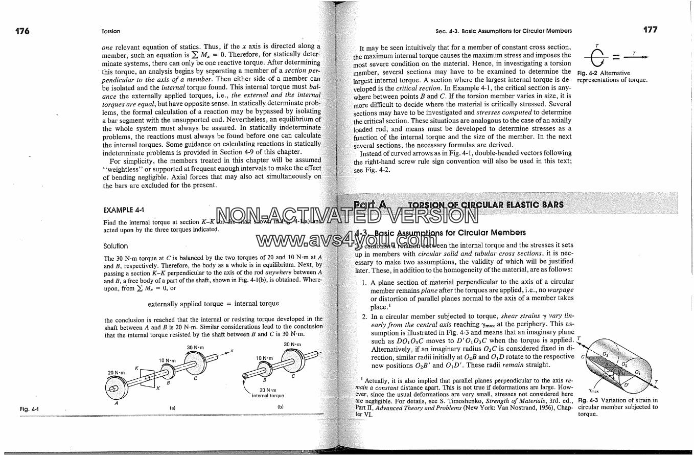
'Torsion Sec. 4.3. Basic Assumptions for Circular Members
Fig. 4-1
one relevant equation of statics. Thus, if the x axis is directed alongmember, such an equation is � M�, = 0. Therefore, for staticallyminate systems, there can only be one reactive torque. After
' this torque, an analysis begins by separating a member of a section pe�pendicular to the axis of a member. Then either side of a memberbe isolated and the internal torque found. This internal torque mustance the externally applied torques, i.e., the external and the interntorques are equal, but have opposite sense. In statically determinate'lems, the formal calculation of a reaction may be bypassed by isolatina bar segment with the unsupported end. Nevertheless, an equilibriumthe whole system must always be assured. In staticallyproblems, the reactions must always be found before one canthe internal torques. Some guidance on calculating reactions inindeterminate problems is provided in Section 4-9 of this chapter.
For simplicity, the members treated in this chapter will be"weightless" or supported at frequent enough intervals to makeof bending negligible. Axial forces that may also act simultaneouslythe bars are excluded for the present.
EXAMPLE 4-t
Find the internal t�rque at section K-K for the shaft shown in Fig. 4-1(a)acted upon by the three torques indicated.
Solution
The 30 N.m torque at C is balanced by the two torques of 20 and 10 N.m atand B, respectively. Therefore, the body as a whole is in equilibrium. Next,passing a section K-K perpendicular to the axis of the rod an3and B, a free body of a part of the shaft, shown in Fig. 4-1(b), is obtained.upon, from �, Mx = O, or
externally applied torque = internal torque
the conclusion is reached that the internal or resisting torque developed inshaft between A and B is 20 N.m. Similar considerations lead to thethat the internal torque resisted by the shaft between B and C is 30 N.m.
30 N.m 30 N-m
20 N-mK
10 N.m
BK
C
10 N-m
A
CB
20 N.minternal torque
(a) (b)
It may be seen intuitively that for a member of constant cross section,the maximum internal torque causes the maximum stress and imposes the
host severe condition on the material. Hence, in investigating a torsionseveral sections may have to be examined to determine the
internal torque. A section where the largest internal torque is de-:d is the critical section. In Example 4-1, the critical section is any-between points B and C. If the torsion member varies in size, it is
ore difficult to decide where the material is critically stressed. Severalmay have to be investigated and stresses computed to determine
;critical section. These situations are analogous to the case of an axiallyrod, and means must be developed to determine stresses as a
of the internal torque and the size of the member. In the next�eral sections, the necessary formulas are derived.
Instead of curved arrows as in Fig. 4-1, double-headed vectors followingright-hand screw rule sign convention will also be used in this text;Fig. 4-2.
T
Fig. 4-2 Alternativerepresentations of torque.
4-3. Basic Assumptions for Circular Membersestablish a relation between the internal torque and the stresses it sets
up in members with circular solid and tubular cross sections, it is nec-to make two assumptions, the validity of which will be justified
in addition to the homogeneity of the material, are as follows:
1. A plane section of material perpendicular to the axis of a circularmember remains plane after the torques are applied, i.e., no warpageor distortion of parallel planes normal to the axis of a member takesplace. �
2. In a circular member subjected to torque, shear strains � vary fin-early from the central axis reaching �m�,, at the periphery. This as-sumption is illustrated in Fig. 4-3 and means that an imaginary planesuch as DO�03C moves to D'O�03C when the torque is applied.Alternatively, if an imaginary radius 03C is considered fixed inrection, similar radii initially at 02B and O�D rotate to the respectivenew positions 02B' and OLD'. These radii remain straight.
Actually, it is also implied that parallel planes perpendicular to the axis re- ra constant distance apart. This is not true if deformations are large. How-since the usual deformations are very small, stresses not considered here %,�x
negligible. For details, see S. Timoshenko, Strength of Materials, 3rd. ed., Fig. 4-3 Variation of strain inAdvanced Theory and Problems (New York: Van Nostrand, 1956), Chap- circular member subjected to
VI. torque.
NON-ACTIVATEDVERSIONwww.avs4you.com
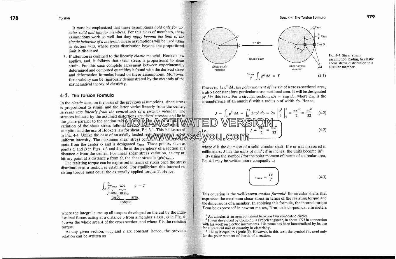
Torsion Sec. 4.4. The Torsion Formula
It must be emphasized that these assumptions hold only forcular solid and tubular members. For this class of members,assumptions work so well that they apply beyond the limitelastic behavior of a material. These assumptions will be usedin Section 4-13, where stress distribution beyond the proFlimit is discussed.If attention is confined to the linearly elastic material, Hooke'sapplies, and, it follows that shear stress is proportional 'tostrain. For this case complete agreement betweendetermined and computed quantities is found with the derivedand deformation formulas based on these assumptions.their validity can be rigorously demonstrated by the methods ofmathematical theory of elasticity.
4-4. The Torsion Formula
In the elastic case, on the basis of the previous assumptio'ns, sinceis proportional to strain, and the latter varies linearly from thestresses vary linearly fi'om the central axis of a circular member.stresses induced by the assumed distortions are shear stresses and liethe plane parallel to the section taken normal to the axis of a rod.variation of the-shear stress follows directly from the shear-strainsumption and the use of Hooke's law for shear, Eq. 3-1. This isin Fig. 4-4. Unlike the case of an axially loaded rod, this stress isuniform intensity. The maximum shear stress occurs at points mostmote from the center O and is designated q-max. These points, suchpoints C and D in Figs. 4-3 and 4-4, lie at the periphery of a sectiondistance c from the center. For linear shear stress variation, at anybitrary point at a distance p from O, the shear stress is (D/C)q-max.
The 'resisting torque can be expressed in terms of stress once thedistribution at a section is established. For equilibrium this internalsisting torque must equal the externally applied torque T. Hence,
f�P �Tmax dm p = T,stress� area,
,force arm,to�'que
where the integral sums up all torques developed on the cut by theitesimal forces acting at a distance p from a m.ember's axis, O in Fig.4, over the whole area A of the cross section, and where T is thetorque.
At any given section, q'max and c are constant; hence, therelation can be written as
Trnax
D' rmax
r=G7 Cord
Hooke's law
Shear strain Shear stress dAvariation variation
q-max fA p2 dA = T (4-1)c
However, fA p2 dA, the polar/noment of inertia of a cross-sectional area,is also a constant for a particular cross-sectional area. It will be designated
! J in this text. For a circular section, dA = 2�xp dp, where 2�xp is theumference of an annulus 2 with a radius p of width dp. Hence,
fAfo c [-� i 'iTc4J = 92 dA = 2'I103 dp= 2�r - 2
-]� qTC4ITd4)aid 4
32(4-2)
(4-2)
d is the diameter of a solid circular shaft. If c or d is measured inJ has the units of mm 4; if in inches, the units become in 4.
By using the symbol J for the polar moment of inertia of a circular area,Eq. 4-1 may be written more compactly as
(4-3)
equation is the well-known torsion formula 3 for circular shafts thatexpresses the maximum shear stress in terms of the resisting torque and
dimensions of a member. In applying this formula, the internal torquebe expressed 4 in newton-meters, N-m, or inch-pounds, c in/neters
2 An annulus is an area contained between two concentric circles.It was developed by Coulomb, a French engineer, in about 1775 in connection
work on electric instruments. His name has been immortalized by its usea practical unit of quantity in electricity.1 N-m is equal to 1 joule (J). However, in this text, the symbol J is used only
the polar moment of inertia of a section.
Fig. 4-4 Shear strainassumption leading to elasticshear stress distribution in acircular member.
NON-ACTIVATEDVERSIONwww.avs4you.com

�SO Torsion Sec. 4-4. The Torsion Formula
Fig. 4-5 Variation of stress inan elastic circular tube.
or inches, and J in m 4 or in 4. Such usage makes the units of the torsshear stress
or pascals (Pa) in SI units, or
[in-lb] [in] [lb 1[in 4] =
or psi in the U.S. customary units.A more general relation than Eq. 4-3 for a shear stress, ,, at any
a distance p from the center of a section is
p Tpc
Equations 4-3 and 4-4 are applicable with equal rigor tosince the same assumptions as used in the previous derivation apply.is necessary, however, to modify J. For a tube, as may be seen4-5, the limits of integration for Eq. 4-2 extend from b to c. Hence,a circular tube,
j = fAp2dA = fi2,lr@3dp _ 'Itc4 �b42 2
or stated otherwise: J for a circular tube equals +J for a solidthe outer diameter and -J for a solid shaft using the inner diameter.
For. very thin tubes, ifb is nearly equal to c, and c - b = t, theof the tube, J reduces to a simple approximate expression:
J � 2xrR3a�t
where Ray = (b + c)/2, which is sufficiently accurate in sometions.
Tmin Truax
r=G�7
r = G2'7
?c
{a) lb)
If a circular bar is made from two different materials bonded together,shown in Fig. 4-6(a), the same strain assumption applies as for a solid
For such a case, through Hooke's law, the shear-stress distri-becomes as in Fig. 4-6Co). If the shear modulus for the outer stifferG� and that of the inner softer core is G2, the ratio of the respective
shear stresses on a ring of radius OB is G�/G2.
Summary
For the torsion problem of circular shafts the three basic concepts ofmechanics of solids as used above may be summarized in the
manner:
1. Equilibrium conditions are used for determining the internal resistingtorques at a section.
2. Geometry of deformation (kinematics) is postulated such that shearstrain varies linearly from the axis of a shaft.
3. Material properties (constitutive relations) are used to relate shearstrains to shear stregses and permit calculation of shear stresses ata section.
a linear elastic case using Hooke's law is considered in the precedingdiscussion. This is extended to non-linear material behavior in Section 4-
13.
These basic concepts are used for determining both stresses and angles-of circular shafts. However, similar to the case for axially loaded
large local stresses arise at points of application of concentratedues or changes in cross section. According to Saint-Venant's principle
the stresses and strains are accurately described by the developed theoryonly beyond a distance about equal to the diameter of a shaft from theselocations. Typically local stresses are determined by using stress con-
factors.
Fig. 4-6 Elastic behavior of acircular member in torsionhaving an inner core of softmaterial.
NON-ACTIVATEDVERSIONwww.avs4you.com
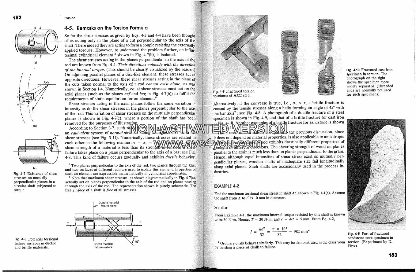
A B
(a)
Truax
(c)
Fig, 4-7 Existence of shearstresses on mutuallyperpendicular planes in acircular shaft subjected totorque.
Fig. �4.8 Potential torsionalfailure surfaces in ductileand brittle materials.
Torsion
4=5. Remarks on the Torsion Formula
So far the shear stresses as given by Eqs. 4~3 and 4-4 have been thouof as acting only in the plane of a cut perpendicular to the axis ofshaft. There indeed they are acting to form a couple resisting theapplied torques. However, to understand the problem further, antesimal cylindrical element, 5 shown in Fig.�4-7(b), is isolated.
The shear stresses acting in the planes Phrpendicular to the axis ofrod are known from Eq. 4-4. Their' directions coincide with the directof the internal torque. (This should be clearly visualized by the readOn adjoining parallel planes of a disc-like element, these stresses actopposite directions. However, these shear stresses acting in the planethe cuts taken normal to the axis of a rod cannot exist alone, asshown in Section 1-4. Numerically, equal shear stresses must act onaxial planes (such as the planes aef and bcg in Fig. 4-7(b)) to fullallrequirements of static equilibrium for an element. 6
Shear stresses acting in the axial planes follow the same variationintensity as do the shear stresses in the planes perpendicular to theof the rod. This variation of shear stresses on the mutually pertplanes is shown in Fig. 4-7(c), where a portion of the shaft hasremoved for the purposes of illustration.
According to. Section 3-7, such shear stresses can be transan equivalent system of normal stresses acting at angles of 45 � withshear stresses (see Fig. 3-11). Numerically, these stresses are relatedeach other in the following manner: , = ch = -or2. Therefore, ifshear strength of a material is less than its strength in tension, afailure takes place on a plane perpendicular to the axis of a bar; see4-8. This kind of failure occurs gradually and exhibits ductile
5 Two planes perpendicular to the axis of the rod, two planes through theand two surfaces at different radii are used to isolate this element. Propertiessuch an element are expressible mathematically in cylindrical coordinates.
6 Note that maximum shear stresses, as shown diagrammatically in Fig.actually act on planes perpendicular to the axis of the rod and on planesthrough the axis of the rod. The representation shown is purely schematic.free surface of a shaft is fi'ee of all stresses.
� Ductile material
failure planeT T
Brittle materialfailure surface
4-9 Fractured torsionspecimen of A322 steel.
if the converse is true, i.e., ch < *, a brittle fracturo isby the tensile stresses along a helix forming an angle of 45 � with
the bar axis 7; see Fig. 4-8. A photograph of a ductile fracture of a steelis shown in Fig. 4-9, and that of a brittle fracture for cast �ron
in Fig. 4-10. Another examples of a brittle fracture for sandstone is shownFig. 4-11.
The stress transformation brought into the previous discussion, sincedoes not depend on material properties, is also applicable to anisotropic
For example, wood exhibits drastically different properties ofin different directions. The sheafing strength of wood on planes
to the grain is much less than on planes perpendicular to the grain.although equal intensities of shear stress exist on mutually per-
planes, wooden shafts of inadequate size fail longitudinallyaxial planes. Such shafts are occasionally used in the process in-
Fig. 4-t0 Fractured cast ironspecimen in torsion. Thephotograph on fhe rightshows the specimen morewidely separated. (Threadedends are normally not usedfor such specimens).
4-2
the maximum torsional shear stress in shaft AC shown in Fig. 4-1(a). Assumeshaft from A to C is 10 mm in diameter.
From Example 4-1, the maximum internal torque resisted by this shaft is knownbe 30 N.m. Hence, T = 30 N-m, and c = d/2 = 5 mm. From Eq. 4-2,
1�d 4 'i� X 10 4J = 32 32 982 mm 4 Fig. 4-tt Part of fractured
sandstone core specimen inOrdinary chalk behaves similarly. This may be demonstrated in the classroom torsion. (Experiment by D.
twisting a piece of chalk to failure. Pirtz).'83
NON-ACTIVATEDVERSIONwww.avs4you.com
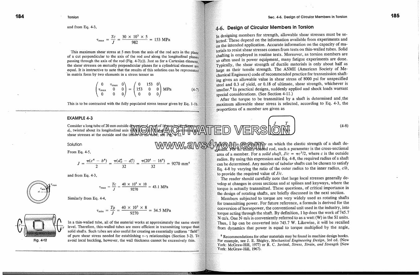
Torsion Sec. 4.6. Design of Circular Members in Torsion
Fig. 442
and from Eq. 4-3,
Tc 30 x 103 x 5Tmax -- -- --� 153 MPa
J 982
This maximum shear stress at 5 mm from the axis of the rod acts in theof a cut perpendicular to the axis of the rod and along the longitudinalpassing through the axis of the rod (Fig. 4-7(c)). Just as for a Cartesian elethe shear stresses on mutually perpendicular planes for a cylindrical'equal. It is instructive to note that the results of this solution can be
'in matrix form by two elements in a stress tensor as
� 0 = 1 3 0 MPao o
This is to be contrasted with the fully populated stress tensor given by Eq.
Tmax
EXAMPLE 4-3
Consider a long tube of 20 mm outside diameter, do, and of 16 mm inside diad�, twisted about its longitudinal axis with a torque T of 40 N.m. Determine ishear stresses at the outside and the inside of the tube; see Fig. 4-12.
Solution
From Eq. 4-5,
,ii.(C 4 _ b 4) ,r(d4o _ &4) ,17(204 _ 164)J .... 9270 mm 4
2 32 32
and fi-om Eq. 4-3,
Tc 40 x 103 x 10- = 43.1 MPa'rm�,�- j 9270
Similarly from Eq. 4-4,
Tmin --Tp 40 x 103 x 8
- = 34.5 MPaJ 9270
In a thin-walled tube, all of the material works at approximately the samelevel. Therefore, thin-walled tubes are more efficient in transmitting torquesolid shafts. Such tubes are also useful for.creating an essentially uniformof pure shear stress needed for establishing ?-,/relationships (Section 3-2).avoid local buckling, however, the wall thickness cannot be excessively
Design of Circular Members in Torsiondesigning members for strength, allowable shear stresses must be se-
These depend on the information available from experiments andthe intended application. Accurate information on the capacity of ma-
; to resist shear stresses comes from tests on thin-walled tubes. Solidis employed in routine tests. Moreover, as torsion members are
often used in power equipment, many fatigue experiments are done.the shear strength of ductile materials is only about half as
as their tensile strength. The ASME (American Society of Me-Engineers) code of recommended practice for transmission shaft-
ing gives an allowable value in shear stress of 8000 psi for unspecifiedand 0.3 of yield, or 0.-18 of ultimate, shear strength, whichever is
allertl In practical designs, suddenly applied and shock loads warrantconsiderations. (See Section 4-11.)
�fter the torque to be transmitted by a shaft is determined and.theallowable shear stress is selected, according to Eq. 4-3, the
�ortions of a member are given as
(4-8)
J/c is the parameter on which the elastic strength of a shaft de-For an axially loaded rod, such a parameter is the cross-sectional
trea of a member. For a solid shaft, J/c = �rc3/2, where c is the outsideBy using this expression and Eq. 4-8, the required radius of a shaft
�be determined. Any number of tubular shafts can be chosen to satisfyEq. 4-8 by varying the ratio of the outer radius to the inner radius, c/b,
provide the required value of J/c.The reader should carefully note that large local stresses generally de-
at changes in cross sections and at splines and keyways, where theue is actually transmitted. These questions, of critical importance indesign of rotating shafts, are briefly discussed in the next section.
Members subjected to torque are very widely used as rotating shaftsfor transmitting power. For future reference, a formula is derived for theconversion of horsepower, the conventional unit used in the industry, into
torque acting through the shaft. By definition, 1 hp does the work of 745.7One N.m/s is conveniently referred to as a watt (W) in the SI units.
1 hp can be converted into 745.7 W. Likewise, it will be recalleddynamics that power is equal to torque multiplied by the angle,
8 Recommendations for other materials may be found in machine design books.example, see J. E. Shigley, Mechanical Engineering Design, 3rd ed. (New
McGraw-Hill, 1977) or R. C. Juvinal, Stress, Strain, and Strength (NewMcGraw-Hill, 1967).
NON-ACTIVATEDVERSIONwww.avs4you.com
Torsion
measured in radians, through which the shaft rotates per unit of time.a shaft rotating with a frequency of f Hz, 9 the angle is 2�rf rad/s.if a shaft were transmitting a constant torque T measured in N.m, itdo 2�rfT N.m of work per second. Equating this to the horsepowerplied
hp x 745.7 = 2�rfT [N.m/s]
119 x hpor r = [N.m]
f
159 x kWor T = [N.m]
f
where � is the frequency in hertz of the shaft transmitting the horsehp, or kilowatts, kW. These equations convert the applied power 'applied torque.
In the U.S. customary system of units, 1 hp does work of 550 if-lbsecond, or 550 x 12 x 60 in-lb per minute. If the shaft rotates at N(revolutions per minute), an equation similar to those above can betained:
63,000x hp[in_lb]lN
EXAMPLE 4-4
Select a solid shaft for a 10-hp motor operating at 30 Hz. The maximumstress is limited to 55 MPa.
Solution
From Eq. 4-9,
and from Eq. 4-8,
119 x hp 119 x 10f 30
- 39.7N.m
J ,'ITC 3C 2
J T 39.7 X 10 3...... 722 mm 3C Tma x 55
2 J' 2 x 722or c 3 ..... = 460 mm 3
9 1 hertz (Hz) = 1 cycle per second (cps).
Sec. 4-7. Stress Concentrations
c = 7.72 mm or d = 2c = 15.4 mm.�ractical purposes, a 16-mm shaft would probably be selected.
MPLE 4-5
�,elect solid shafts to transmit 200 hp each without exceeding a shear stress ofpsi. One of these shafts operates at 20 rpm and the other at 20,000 rpm.
iution
4-11,1 applies to the low-speed shaft and 2 to the high-speed shaft. From
T� - hp x 63,000 _ 200 x 63,000 = 630,000 in-lbN� 20
T2 = 630 in-lb
!FrOm Eq. 4-8,
J� T� 630,000- -- = 63 in 3C Tmax 10,000
J� �d� �(- -- or d� = 63) = 321 in 3c 16 �
Hence, d� = 6.85 in and d2 = 0.685 in
This example illustrates the reason for the modem tendency to use high-speedmachines in mechanical equipment. The difference in size of the two shafts is
Further savings in-the weight of the material can be effected by usingtubes.
Stress Concentrations
uations 4-3, 4-4, and 4-8 apply only to solid and tubular circular shaftsthe material behaves elastically. Moreover, the cross-sectional
along the shaft should remain reasonably constant. If a gradualVariation in the diameter takes place, the previous equations give satis-
solutions. On the other hand, for stepped shafts where the di-ameters of the adjoining portions change abruptly, large perturbations of
stresses take place. High local shear stresses occur at points awaythe center of the shaft. Methods of determining these local concen-
of stress are beyond the scope of this text. However, by formingratio of the true maximum shear stress to the maximum stress given by
�.q. 4-3, a torsional stress-concentration factor can be obtained. An anal-
NON-ACTIVATEDVERSIONwww.avs4you.com

�88 Torsion Sec. 4.8. Angle.of-Twist of Circular Members
Fig. 443 Torsional stress-concentration factors incircular shafts of twodiameters.
Fig. 4-14 Circular shaft with akeyway.
3.4
I X,�'2'�=7
I i
3.0
2.6
K 2.2
1.8
1.4
1.0
0 0.08 O. 16 0.24r
d/2
ogous method was used for obtaining the stress-concentration factorsaxially loaded members (Section 2-10). These factors depend onlygeometry of a member. Stress-concentration factors for varioustions of stepped round shafts are shown in Pig. 4-13. ��
To obtain the actual stress at a geometrical discontinuity of ashaft, a curve for a particular D/d is selected in Pig. 4-13. Then,sponding to the given r/(d/2) ratio, the stress-concentration factor Kread from the curve. Lastly, from the definition of/{, the actualshear stress is obtained from the modified Eq. 4-3
where the shear stress Tc/J is determined for the smaller shaft.A study of stress-concentration factors shown in Pig. 4-13
the need for a generous fillet radius r at all sections where a transitionthe shaft diameter is made.
Considerable stress increases also occur in shafts at oil holes andkeyways for attaching pulleys and gears to the shaft. A shaftfor a key, Fig. 4-14, is no longer a circular member. However,to the procedures suggested by the ASME, in ordinary design,tations for shafts with keyways may be made using Eq. 4-3 or 4-8 ,the allowable shear stress must be reduced by 25%. Thiscompensates for the stress concentration and reduction in cro,.area.
Because of some inelastic or nonlinear response in real matedhals,�0 This figure is adapted from a paper by L. S. Jacobsen,
Concentrations in Shafts of Circular and Variable Diameter," Trans. ASME(1925): 632.
msons analogous to those pointed out in Section 2-10, the theoretical'�ss concentrations based on the behavior of linearly elastic matedhal
tend to.be somewhat high.
Angle.of-Twist of Circular Membersthis section, attention will be directed to a method for determining the
-of-twist for solid and tubular circular elastic shafts subjected toloading. The interest in this problem is at least threefold. First,
is important to predict the twist of a shaft per se since at times it is notto design it only to be strong enough: it also must not deform
Then, magnitudes of angular rotations of shafts are neededthe torsional vibration analysis of machinery. Finally, the angular twistmembers is needed in dealing with statically indeterminate torsional
problems.According to assumption 1 stated in Section 4-3, planes perpendicular
� the axis of a circular rod do not warp. The elements of a shaft undergodeformation of the type shown in Fig. 4-15(b). The shaded element is
in its undistorted form in Fig. 4-15(a). From such a'shaft, a typicalent of length dx is shown isolated in Fig. 4-16 similar to Fig. 4-3.
In the element shown, a line on its surface such as CD is initially parallelthe axis of the shaft. After the torque is applied, it assumes a new
)osition CD'. At the same time, by virtue of assumption 2, Section 4-3,radius OD remains straight and rotates through a small angle dqb to a new
�osition OD'.Denoting the small angle DCD' by �/m�x, from geometry, one has two
alternative expressions for the arc DD':
(a)
(b)
Fig. 445 Circular shaft (a)before and (b) after torque isapplied.
arc DD' = 'ymax dx or arc DD' = dqb c
both angles are small and are measured in radians. Hence,
�/�, dx = dqb c (4-13)
only in the zone of an infinitesimal "tube" of constant max-�mum shear stress *m�x. Limiting attention to linearly elastic response
makes Hooke's law applicable. Therefore, according to Eq. 3-1, the angle�/m= is proportional to *m�x, i.e., �/ma,, = *m�x/G. Moreover, by Eq. 4-3,
= Tc/J. Hence, �/m�x = Tc/(JG). � By substituting the latter expres-sion into Eq. 4-13 and simplifying, the governing differential equation forthe angle-of-twist is obtained.
The foregoing argument can be carried out in terms of any % which pro- 'truaxgressively becomes smaller as the axis of the rod is approached. The only dif- Fig. 446 Deformation of aference in derivation consists in taking an arc corresponding to BD an arbitrary circular bar element due to
p from the center of the shaft and using Tp/J instead of Tc/J for �. torque.
NON-ACTIVATEDVERSIONwww.avs4you.com

A B
Fig.
Torsion
dqb T Tdx- or dqb =dx JG JG
This gives the relative angle-of-twist of two adjoining sections antesimal distance dx apart. To find the total angle-of-twist qb betweentwo sections A and B on a shaft a finite distance apart, the rotation:all elements must be summed. Hence, a general expression for theof-twist between any two sections of a shaft of a linearly elasticis
'qb: qbB-qb4= f; dqb=f; JxGwhere qbB and qb4 are, respectively, the global shaft rotations at en&,and A. The rotation at A may not necessarily be zero. In this e(the internal torque T�, and the polar moment of inertia J�, may varythe length of a shaft. The direction of the angle of twist qb coincidesthe direction of the applied torque T.
Equation 4-15 is valid for both solid and hollow circular shafts,follows from thb assumptions used in the derivation. The angle qb issured in radians. Note the great similarity of this relation to Eq. 2-7the deformation of axially loaded rods. The following threeillustrate applications of these concepts.
EXAMPLE 4-6
Find the relative rotation of section B-B with respect to section A-A of theelastic' shaft shown in Fig. 4-17 when a constant torque T is beingthrough it. The polar moment of inertia of the cross-sectional area J is
Solution
In this case, T.� = T and Jx = J; hence, from Eq. 4-15,
J�G JG JG JG
In applying Eq. 4-16, note particularly that the angle qb must be expressedradians. Also observe the great similarity of this relation to Eq. 2-9, A =
Sec. 4-8. Angle.of. Twist of Circular Members
axially loaded bars. Here qb <=> A, T <=> P, J � A, and G � E. Analogous to2-9, Eq. 4-16 can be recast to express the torsional spring constant, or tor-
�al stiffness, kt as
(4-17)
This constant represents the torque required to cause a rotation of 1 radian, i.e.,1. It depends only on the material properties and size of the member. As
axially loaded bars, one can visualize torsion members as springs; see Fig. 4-
reciprocal of k, defines the torsional flexibility ft. Hence, for a circularor hollow shaft,
1 L [rad� [rad]ft = kt- JG Lin-lbJ or LN.m j (4-18)constant defines the rotation resulting from application of a unit torque, i.e.,
= 1. On multiplying by the torque T, one obtains Eq. 4-16.If in the analysis, a shaft must be subdivided into a number of regions, appro-
identifying subscripts should be attached to the definitions given by Eqs.-17 and 4-18. For example, for the ith segment of a bar, one can write (kt)i =
Gi/mi and (f t)i = mi/JiGi.The previous equations are widely used in mechanical vibration analyses of
nission shafts, including crank shafts. n These equations are also useful forstatically indeterminate problems, considered in the next section. These
are required in the design of members for torsional stiffness when it issential to limit the arhount'of twist. For such applications, note that J, rather
the J/c used in strength calculations, is the governing parameter. In axiallyproblems, the cross-sectional area A serves both purposes.
Lastly, it should be noted that since in a torsion test, qb, T, L, and J can bemeasured or calculated from the dimensions of a specimen, the shear modulus
for a specimen can be determined from Eq. 4-16 since G ='TL/Jcb.
191
Fig. 4-t8 Schematicrepresentation of _a� torsionspring.
4-7
Consider the stepped shaft shown in Fig. 4-19(a) rigidly attached to a wall at E,and determine the angle-of-twist of the end A when the two torques at B and at
are applied. Assume the shear modulus G to be 80 GPa, a typical value for
12 According to S. P. Timoshenko, Vibration Problems in Engineering, 2d ed.York: Van Nostrand, 1937), in 1902, H. Frahm, a German engineer, was
Errst to recognize and study this important problem.
NON-ACTIVATEDVERSIONwww.avs4you.com
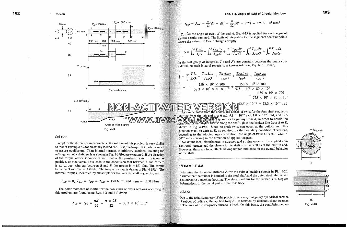
Torsion
25 mm
a-a b-b
1250 I
(a) -'I
T o = 1000 N.m
_
200. J �300 ram_ 1. 500 mm
(c) TIN-m][0
15o ITorque diagram
1150
� X 103 rad
(d) 0
-23.3
A B C D E
-13.5 -12.5
Angle-of-twist diagram
Fig. 4-t9
x
Solution
Except for the difference in parameters, the solution of this problem isto that of Example 2-2 for an axially loaded bar. First, the torque at E isto assure equilibrium. Then internal torques at arbitrary sections,left segment of a shaft, such as shown in Fig. 4-19(b), are examined. If theof the torque vector T coincides with that of the positive x axis, it is takenpositive, or vice versa. This leads to the conclusion that between A and Bis no torque, whereas between B and D the torque is + 150 Nm. Thebetween D and E is + 1150 Nm. The torque diagram is drawn in Fig. 4-19(c).internal torques, identified by subscripts' for the various shaft segments,
TA� = O, Teo = Tec = Tco = 150 N.m, and To� = 1150 N.m
The polar moments of inertia for the two kinds of cross sectionsthis problem are found using Eqs. 4-2 and4-5 giving
J� = J�c - --�d 4 � X 254
32 32-- - 38.3 x 103 mm 4
Sec. 4.8. Angle.of-Twist of Circular Members
'It 4 'It 4JCD = JDE = �(do - &4) = �-�(50 - 254) = 575 x 103 mm 4To f�nd the angle-of-twist of the end A, Eq. 4-15 is applied for each segment
the results summed. The limits of integration for the segments occur at pointsthe values of T or J change abruptly.
qb = JxG = J� + + -- +.Je J�cG JcDG JD�G
the last group of integrals, T's and J's are constant between the limits con-so each integral reverts to a known solution, Eq. 4-16. Hence,
�i TiLi_ T�L� +_= . JiGi J�G J�cG150 x 103 x 200
=0+
TecLec Tcz�Lcz� Tz��Lz��q---q---
Jcz�G Jz>�G
150 X 103 X 30038.3 x 103 x 80 x 103 + 575 + 103 x 80 x 103
1150 x 103 x 500+
575 x 1� x 80 x 103
= 0 + 9.8 x 10 -3 + 1.0 x 10 -3 + 12.5 x 10 -3 = 23.3 x 10 -3 rad
As can be noted from the above, the angles-of-twist for the four shaft segmentsstarting from the left end are: 0 rad, 9.8 x 10 -3 rad, 1.0 x 10 -3 rad, and 12.5
10 -3 rad. Summing these quantities beginning from A, in order to obtain thefor the angle-of-twist along the shaft, gives the broken line from A to E,
shown in Fig. 4-19(d). Since no shaft twist can occur at the built-in end, thismust be zero at E, as required by the boundary condition. Therefore,
to the adopted sign convention, the angle-of-twist at A is -23.3 x0 -3 rad occurring in the direction of applied torques.
No doubt local disturbances in stresses and strains occur at the applied con-centrated torques and the change in the shaft size, as well as at the built-in end.
these are local effects having limited influence on the overall behaviorthe shaft.
4-8
Determine the torsional stiffness k, for the rubber bushing shown in Fig. 4-20.that the rubber is bonded to the steel shaft and the outer steel tube, which
is attached to a machine housing. The shear modulus for the rubber is G. Neglectin the metal parts of the assembly.
Solution
;ymmetry of the problem, on every imaginary cylindrical surfacer, the applied torque T is resisted by constant shear stresses
area of the imaginary surface is 2�rrL. On this basis, the equilibrium equa-
193
(a)
(b)
Fig. 4-20
NON-ACTIVATEDVERSIONwww.avs4you.com
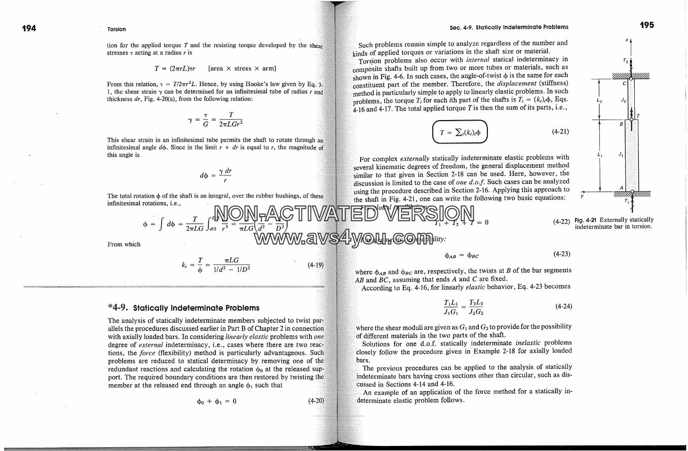
Torsion
tion for the applied torque T and the resisting torque developed by thestresses x acting at a radius r is
T = (2xrL)?r [area x stress x arm]
From this relation, x = T/2�rr2L. Hence, by using Hooke's law given by Ec1, the shear strain � can be determined for an infinitesimal tube of radiusthickness dr, Fig. 4-20(a), from the following relation:
� T
�/ - G - 2�rLGr 2
This shear strain in an infinitesimal tube permits the shaft to rotate throughinfinitesimal angle dqb. Since in the limit r + dr is equal to. r, thethis angle is
dqb = �/drr
The total rotation qb of the shaft is an integral, over the rubber bushings,infinitesimal rotations, i.e.,
From which
T �rLG �
k, - qb - 1/d 2 - 1/D 2 (4-1
*4-9. Statically Indeterminate ProblemsThe analysis of statically indeterminate members subjected to twistallels the procedures discussed earlier in Part B of Chapter 2 in c�with axially loaded bars. In considering linearly elastic problemsdegree of external indeterminacy, i.e., cases where there are twotions, the force (flexibility) method is particularly advantageous.problems are reduced to statical determinacy by removing one ofredundant reactions and calculating the rotation qbo at the releasedport. The required boundary conditions are then restored bymember at the released end through an angle qb� such that
qbo+ qb� = 0
Sec. 4-9. Statically Indeterminate Problems
Such problems remain simple to analyze regardless of the number andkinds of applied torques or variations in the shaft size or material.
Torsion problems also occur with bzternal statical indeterminacy in�dsite shafts built up from two or more tubes or materials, such as
;hown in Fig. 4-6. In such cases, the angle-of-twist qb is the same for eachpart of the member. Therefore, the displacement (stiffness)
particularly simple to apply to linearly elastic problems. In such�roblems, the torque Ti for each ith part of the shafts is Ti = (kt)iqb, Eqs.
and 4-17. The total applied torque Tis then the sum of its parts, i.e.,
T = �i(kt)iO) (4-21)
For complex externally statically indeterminate elastic problems withkinematic degrees of freedom, the general displacement method
.imilar to that given in Section 2-18 can be used. Here, however, tileis limited to the case of one d.o.f. Such cases can be analyzed
the procedure described in Section 2-16. Applying this approach toshaft in Fig. 4-21, one can write the following two basic equations:
For global equilibrium:
T� + T2 + T = 0 (4-22)
For geometric compatibility:
qbAB = qbBc (4-23)
qbA� and qb�c are, r.espectively, the twists at B of the bar segmentsand BC, assuming that ends A and C are fixed.
According to Eq. 4-16, for linearly elastic behavior, Eq. 4-23 becomes
T�L� T2L2-- - (4-24)J� G� J2G2
shear moduli are given as G� and G2 to provide for the possibilitydifferent materials in the two parts of the shaft.
Solutions for one d.o.f. statically indeterminate inelastic problemsfollow the procedure given in Example 2-18 for axially loaded
bars.The previous procedures can be applied to the analysis of statically
bars having cross sections other than circular, such as dis-in Sections 4-14 and 4-16.
example of an application of the force method for a statically in-elastic problem follows.
195
x
L� J2
Fig. 4-2t Externally staticallyindeterminate bar in torsion.
NON-ACTIVATEDVERSIONwww.avs4you.com

Torsion Sec. 4-40. Differential Equation Approach for Torsion Problems
Fig. 4-22
2� mm
(b}
(d)
1000 N*m
500 mm �ITo
TN,m[.0-142� X 103 rad
Torque diagram
1008
(e)
EXAMPLE 4-9
B C D0
-11,6 -11,1 -11,0Angle-of-twist diagram
E
Assume that the stepped shaft of Example 4-7, while loaded in the sameis now built-in at both ends, as shown in Fig. 4-22. Determine the endand plot the torque diagram for the shaft. Apply the force method.
Solution
There are two unknown reactions, T,� and TE. One of them can be consideredredundant, and, arbitrarily, reaction T,� is removed..This results in thediagram shown in Fig. 4-22(b). The solution.to Example 4-7 gives the endqbo = 23.3 x 10 -3 rad.
Fi'om Example 4-7, J,�c = 38.3 x 103 mm 2 and JcE= 575 x 103 mm 2.applying T,� to the tinloaded bar, as shown in Fig. 4-22(c), end rotation qb� atA is found using Eq. 4-16.
Hence,
'3 450 800 )--TiLi TAX103 8.3x103x80x103 +575x103x80x 103= (147 x 10 -6 + 17 x 10-6)TA = 164 x 10-6TA rad
T,� has the units of N.m.Eq. 4-20 and defining rotation in the direction of T,� as positive, one has
-23.3 x 10 -3 + 164 x 10-6TA = 0
TA = 142N.m and TB = 1150 -- 142 = 1008N.m
The torque diagram for the shaft is shown in Fig. 4-22(d). As in Fig. 4-19(c) of4-7, if the direction of the internal torque vector T on the left part of
isolated shaft segment coincides with that of the positive x axis, it is taken asiSitive. Note that most of the applied torque is resisted at the end E. Since the
from A to C is more flexible than from C to E, only a small torque develqpsA.
Calculating the angles-of-twist for the four segments of the shafts, as in Examplethe angle-of-twist diagram along the shaft, Fig. 4-22(e), can be obtained.
of this diagram is left as an exercise for the reader.) The angle-of-wist at A and E must be zero from the prescribed boundary conditions. As to
expected, the shaft twists in the direction of the applied torques.Whereas this problem is indeterminate only to the first degree, it has three
kinematic degrees of freedom. Two of these are associated with the appliedtorques and one with the change in the shaft size. Therefore, an application of
displacement method would be more cumbersome, requiring three simul-taneous equations.
Alternative Differential Equation Approach forTorsion Problems
const, ant JG, Eq. 4-14 can be recast into a second-order differentialPreliminary to this step, consider an element, shown in .Fig. 4-
subjected to the end torques Tand T + dTand to an applied distributedue t�, having the units of in-lb/in or N.m/m. By using the right-hand
This and the next two sections can be omitted.
in-lb/in
x �-< dxT+ dT
Fig. 4-23 Infinitesimalelement of a circular barsubjected to torque.
NON-ACTIVATEDVERSIONwww.avs4you.com
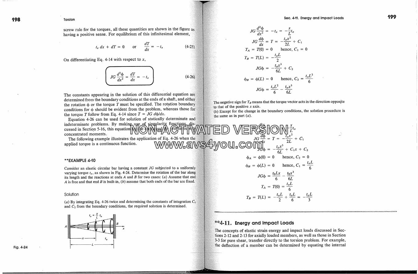
Fig. 4-24
Torsion
screw rule for the torques, all these quantities are shown inhaving a positive sense. For equilibrium of this infinitesimal element.
dT
t� dx + dT = 0 or dx t�
On differentiating Eq. 4-14 with respect to x,
I JGd24 dT - tx1dx 2 dx
The constants appearing in the solution of this differential equationdetermined from the boundary conditions at the ends of a shaft,the rotation 4 or the torque T must be specified. The rotationconditions for 4 should be evident from the problem, wl-/ereas thosethe torque T follow from Eq. 4-14 since T = JG d4/dx.
Equation 4-26 can be used for solution of statically determinateindeterminate problems. By making use of singularity functions,cussed in Section 5-16, this equation can be employed for problemsconcentrated moments.
The following example illustrates the application of Eq. 4-26 whenapplied torque is a continuous function.
**EXAMPLE 4-t0
Consider an elastic circular bar having a constant JG subjected to avarying torque &, as shown in Fig. 4-24. Determine the rotation of the bar al �nits length and the reactions at ends A and B for two cases: (a) Assume thatA is free and that end B is built-in, (b) assume that both ends of the bar
Solution
(a) By integrating Eq. 4-26 twice and determining the constants of integrationand C2 from the boundary conditions, the required solution is determined.
A
X � t o
Sec. 441. Energy and Impact Loads
d24 xJG dx� - tx = -�to
d4 tox �J G �xx = T - 2�- + C �
TA = T(0) = 0 hence, C� = 0toL
TB = T(L) =2
toX 3JG4 = - 6�- + C2
toL 24B = 4(L) = 0 hence, C2 =� 6
toZ 2 toX 3JG4 = -� - �6�-
means that the torque vector acts in the direction oppos.itethat of the positive x axis.
Except for the change in the boundary conditions, the solution procedure issame as in part (a).
JG d24dx 2
d4J G �xx
JG4
= 4(0)
JG4
= T(L)
x
to x2=T= ---+C�
2L
to x3= --- + C�x + C2
6L= 0 hence, C2 = 0
toL= 0 hence, C� =
6
toLx toX 36 6L
toLT(O) -
6
toL toL+--
2 6toL
3
199
Energy and Impact Loadsconcepts of elastic strain energy and impact loads discussed in Sec-
ions 2-12 and 2-13 for axially loaded members, as well as those in Sectionpure shear, transfer directly to the torsion problem'. For example,
deflection of a member can be determined by equating the internal
NON-ACTIVATEDVERSIONwww.avs4you.com

200
p
dA = 2�rp dp c rma'�
Fig. 4-5
Truax
Torsion
shear strain energy U.�h for a member to the external work W,. due to thapplied force, Eq. 2-24. This concept can be applied to static problemi(Example 2-10), as well as for elementary solutions of dynamic t
EXAMPLE 4-tt
(a) Find the energy absorbed by an elastic circular shaft subjected to a constartorque in terms of maximum shear stress and the volume of material: see Fig.25. (b) Find the rotation of the end of an elastic circular shaft with respect tobuilt-in end when a torque T is applied at the free end.
Solution
(a) The shear stress in an elastic circular shaft subjected to a torque varies linearbfrom the longitudinal axis. Hence, the shear stress acting on an element atdistance 0 from the center of the cross section is 'rm�xO/c. Then, using Eq.and integrating over the volume V of the rod L inches long, one obtains
Ush = 9�dV = Jv 2�--�c 2 2�rpdpL,�ax 2�rL/o p3 dp ,7,�x 2�rL c4= 2G c 2 = 2G c 2 4n'Tnax
= vol2G
If there were uniform shear stress throughout the member, a more efficientrangement for absorbing energy would be obtained. Rubber bushings4-8) with their small G values provide an excellent device for absorbingtorques from a shaft.(b) If t. orque T is gradually applied to the shaft, the external work We =where (b is the angular rotation of the free end in radians. The expression forinternal train energy Ush, which was found in part (a), may be written in aconvenient form by noting that �rm�, = Tc/J, the volume of the rod �rc2L, and= 'rrC4/2. Thus,
'r�x (1�vol ) T2c21 T2LUsh = 2G - 2J2G 2 'trc2L = ZIGThen, from We = Ush
Tqb T2 L TL2 ZIG and qb JG
which is the same as Eq. 4-16.
Sec. 4-t2. Shaft Couplings
-12. Shaft Couplingsuently, situations arise where the available lengths of shafting are
lon� enough. Likewise, for maintenance or assembly reasons, it isdesirable to make up a long shaft from several pieces. To join the
:es of a shaft together, the so-called ranged shaft couplings of the typein Fig. 4-26 are used. When bolted together, such couplings arerigid, to differentiate them from another type called flexible that
vides for misalignament of adjoining shafts. The latter type is almost/ used to join the shaft of a motor to the driven equipment. Here
rigid-type couplings are considered. The reader is referred to ma-:hine-design texts and manufacturer's catalogues for the other type.
For rigid couplings, it is customary to assume that shear strains in thebolts vary directly (linearly) as their distance from the axis of the shaft.
between the flanges is neglected. Therefore, analogous to theproblem of circular shafts, if the bolts are of the same mater. ial,
tic shear stresses in the bolts also vary linearly as their respectivefrom the center of a coupling. The shear stress in any one bolt
assumed to be uniform and is governed by the distance from its centerto the center of the coupling. Then, if the shear stress in a bolt is multiplied
its cross-sectional area, the force in a bolt is found. On this basis, forfor bolts of equal size in two "bolt circles," the forces on the
located by the respective radii a and b are as shown in Fig. 4-26(c).The moment of the forces developed by the bolt3 around the axis of ashaft gives the torque capacity of a coupling.
The previous reasoning is the same as that used in deriving the torsionformula for circular shafts, except that, instead of a continuous cross
a discrete number of points is considered. This analysis is crude,since stress concentrations are undoubtedly present at the points of con-
of the bolts with the fl&nges of a coupling.The outlined method of analysis is valid only for the case of a couplingwhich the bolts act primarily in shear. However, in some couplings,
the bolts are tightened so much that the coupling acts in a different fashion.initial tension in the bolts is great enough to cause the entire coupling
act in friction. Under these circumstances, the suggested analysis is
(a)
Bolts
(b)
Fig. 4-26 Flanged shaft coupling.
(c)
20't
NON-ACTIVATEDVERSIONwww.avs4you.com
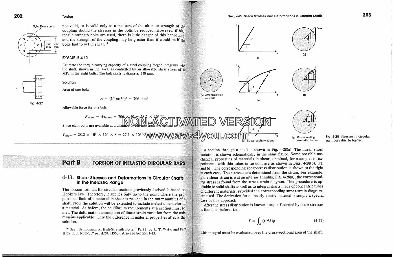
202
Eight 30-mm bolts
Fig. 4-27
Torsion
not valid, or is valid only as a measure of the ultimate strengthcoupling should the stresses in the bolts be reduced. However, iftensile strength bolts are used, there is little danger of this hapand the strength of the coupling may be greater than it would be if ibolts had to act in shear. 14
EXAMPLE 4-t2
Estimate the torque-carrying capacity of a steel coupling forged integrallythe shaft, shown in Fig. 4-27, as controlled by an allowable shear stressMPa in the eight bolts. The bolt circle is diameter 240 mm.
Solution
Area of one bolt:
A = (1/4)�r(30) 2 = 706 mm 2
Allowable force for one bolt:
Pano�, = A%no�, = 706 x 40 = 28.2 x 10³N
Since eight bolt� are available at a distance of 120 mm from the central axis
r�now = 28.2 x 103 x 120 x 8 = 27.1 x 10⁶N.mm = 27.1 x 10³
443. Shear Stresses and Deformations in Circularin the Inelastic Range
The torsion formula for circular sections previously derived is ba�Hooke's law. Therefore, it applies 0nly up to the point where theportional limit of a matedhal in shear is reached in the outer annulusshaft. Now the solution will be extended to include inelastica matedhal. As before, the equilibrium requirements at a sectionmet. The deformation assumption of linear strain variation from theremains applicable. Only the difference in matedhal properties affectssolution.
�4 See "Symposium on High-Strength Bolts," Part I, by L. T. Wyly, andII by E. J. Ruble, Proc. AISC (1950). Also see Section 1-13.
Sec. 4-t3. Shear Stresses and Deformations in Circular Shafts
� (e)(b)
Assumed strainvariation
(c)
(f)
(d) Stress-strain relations(g) Corresponding
stress distribution
section through a shaft is shown in Fig. 4-28(a). The linear strainis shown schematically in the same figure. Some possible me-
properties of materials in shear, obtained, for example, in ex-periments with thin tubes in torsion, are as shown in Figs. 4-28(b), (c),
(d). The corresponding shear-stress distribution is shown to the fightcase. The stresses ate determined from the strain. For example,
shear strain is a at an interior annulus, Fig. 4-28(a), the correspond-stress is found from the stress-strain diagram. This procedure is ap-
as well as to integral shafts made of concentric tubesmatedhals, provided the corresponding stress-strain diagrams
The derivation for a linearly elastic matedhal is simply a specialof this approach.
After the stress distribution is known, torque T cardhed by these stressesas before, i.e.,
T = fA ('r dA)p (4-27)integral must be evaluated over the cross-sectional area of the shaft.
203
Fig. 4-28 Stresses in circularmembers due to torque.
NON-ACTIVATEDVERSIONwww.avs4you.com

Torsion Sec. 4.'13. Shear Stresses and Deformations in Circular Shafts 205Elastic stress distribution
Inelasticstressdistribution
Fig. 4-29 For thin-walledtubes the difference betweenelastic and inelastic stressesfs small.
Although the shear-stress distribution after the elastic limit is ex(is nonlinear and the elastic torsion formula, Eq. 4-3, does not apply,sometimes used to calculate a fictitious stress for the ultimate torque.computed stress is called the modulus of rupture; see the largestof the dashed lines on Figs. 4-28(0 and (g). It serves as a roughthe ultimate strength of a material in torsion..For a thin-walled tube,stress distribution is very nearly the same regardless of the mecproperties of the material; see Fig. 4-29. For this reason,with thin-walled tubes are widely used in establishing the shearstrain ?-�/diagrams.
If a shaft is strained into the inelastic range and the appliedthen removed, every "imaginary" annulus rebounds elastically.of the differences in the strain paths, which cause permanent set i nmaterial, residual stresses develop. This process will be illustratedof the examples that follow.
For determining the rate of twist of a circular shaft or tube, Eq.can be used in the following form:
dx c
Here either the maximum shear strain at c or the strain at pafrom the stre�s-strain diagram must be used.
EXAMPLE 4-13
A solid steel shaft of 24-mm diameter is so severely twisted that only andiameter elastic core remains on the inside, Fig. 4-30(a). If the materialcan be idealized, as shown in Fig. 4-30(b), what residual stresses androtation will remain upon release of the applied torque? Let G = 80 GPa.
Solution
To begin, the magnitude of the initially applied torque andof twist must be determined. The stress distribution corresponding to thecondition is shown in Fig. 4-30(c). The stresses vary linearly from 0 to 160when 0 -< 9 -< 4 ram; the stress is a conskant 160 MPa for 9 > 4 ram. Ec4-27 can be used to determine the applied torque T. The release of torqueelastic stresses, and Eq. 4-3 applies; see Fig. 4-30(d). The difference 1:two stress distributions, corresponding to no external torque, gives thestresses.
+ (160)2*rp 2 dp= (16 + 558) x 103 N.mm = 574 x 103 N.mm
(a)
r MPat160 [- �,
7,/,'2 d �7X 10 3
(b)
MPa
/
51 MPa
89.7 MPa
3 MPa
Elastoplastic stress '(d) Elastic rebound'ibution stresses
89.7 MPa ' 51 MPa
(e) Residual stresses
the small contribution to the total of the first integral.
Tc 574 x 103 x 12?max -- -- = 211 MPa
J (�r/32) X 244~
At p = 12 ram, 7'residual = 211 - 160 = 51 MPa.Two alternative residual stress diagrams are shown in Fig. 4-30(e). For clarity,
results are replotted from the vertical line. In the entire shaded portionthe residual torque is clockwise; an exactly equal residual torque
in the opposite direction in the inner portion of the shaft. : 'The initial rotation is best determined by calculating the twist of the elastic
At 9 = 4 mm, � = 2 x t0 -3. The' elastic rebound of the shaft is given by4-16. The difference between the inelastic and the elastic twists gives the
rotation per unit length of shaft. If the initial torque is reapplied in theSame direction, the shaft responds elastically.
hzelastic:
dqb % 2 X 10 -3dx p,� 4 x 10 -3
- 0.50 rad/m
Elastic:
T
- JG574 x 103 X 103
(�r/32) x 244 X 80 X 103= 0.22 rad/m
Fig. 4-30NON-ACTIVATEDVERSIONwww.avs4you.com
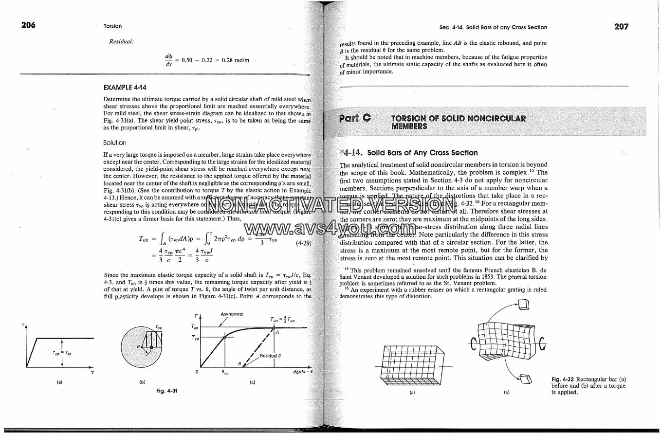
2O6 Torsion
Residual:
dO = 0.50 - 0.22 = 0.28 rad/mdx
Typ � Tpl
(a)
EXAMPLE 4-t4
Determine the ultimate torque carried by a solid circular shaft of mild steelshear stresses above the proportional limit are reached essentiallyFor mild steel, the shear stress-strain diagram can be idealized to that shownFig. 4-31(a). The shear yield-point stress, Typ, is to be taken as being theas the proportional'limit in shear, %�.
Solution
If a very large torque is imposed on a member, large strains takeexcept near the center. Corresponding to the large strains for the idealizedconsidered, the yield-point shear stress will be reached everywhere exceptthe center. However, the resistance to the applied torque offered by thelocated near the center of the shaft is negligible as the corresponding p'sFig. 4-31(b). (See the contribution to torque T by the elastic action in4-13.) Hence, it can be assumed with a sufficient degree of accuracy that a consshear stress Typ i_s acting everywhere on the section considered. The torqueresponding to this condition may be considered the ultimate limit torque.4-31(c) gives a firmer basis for this statement.) Thus,
f� fo c 2�C3Tult = ('rypdA)p = 2'Irp2'ryp do = --�Typ4 Typ TfC 4 4 TypJ3 c 2 3 c
Since ihe maximum elastic torque capacity of a solid shaft is Typ = TypJ/c,4-3, and Tuft is � times this value, the remaining torque capacity after yieldof that at yield. A plot of torque T vs. 0, the angle of twist per unit distance,full plasticity develops is shown in Figure 4-31(c). Point A corresponds to
T Asymptote
T�.--
4Tui t = � Tvp
//
/ ResidualO
do/dx
(b) (c)
Fig. 4-3t
Sec. 4.t4. Solid Bars of any Cross Section
found in the preceding example, line AB is the elastic rebound, and pointi is the residual 0 for the same problem.
It should be noted that in machine members, because of the fatigue properties� mat�rials, the ultimate static capacity of the shafts as evaluated here is often' minor importance.
(a)
44. Solid Bars of Any Cross Sectiontreatment of solid noncircular members in torsion is beyond
scope of this book. Mathematically, the problem is complex. �s Thefirst two assumptions stated in Section 4-3 do not apply for noncircular
bers. Sections perpendicular to the axis of a member warp when atorque is applied. The nature of the distortions that take place in a rec-
section can be surmised from Fig. 4-32. �6 For a rectangular mem-ber, the comer elements do not distort at all. Therefore shear stresses at
the corners are zero; they are maximum at the midpoints of the long sides.Figure 4-33 shows the shear-stress distribution along three radial linesemanating from the center. Note particularly the difference in this stressdistribution compared with that of a circular section. For the latter, the
is a maximum at the most remote point, but for the former, theis zero at the most remote point. This situation can be clarified by
problem remained unsolved until the famous French elastician B. deVenant developed a solution for such problems in 1853. The general torsion
is sometimes referred to as the St. Venant problem.�6 An experiment with a rubber eraser on which a rectangular grating is ruled
this type of distortion.
(b)
207
Fig. 4-32 Rectangular bar (a)before and (b) after a torqueis applied.
NON-ACTIVATEDVERSIONwww.avs4you.com
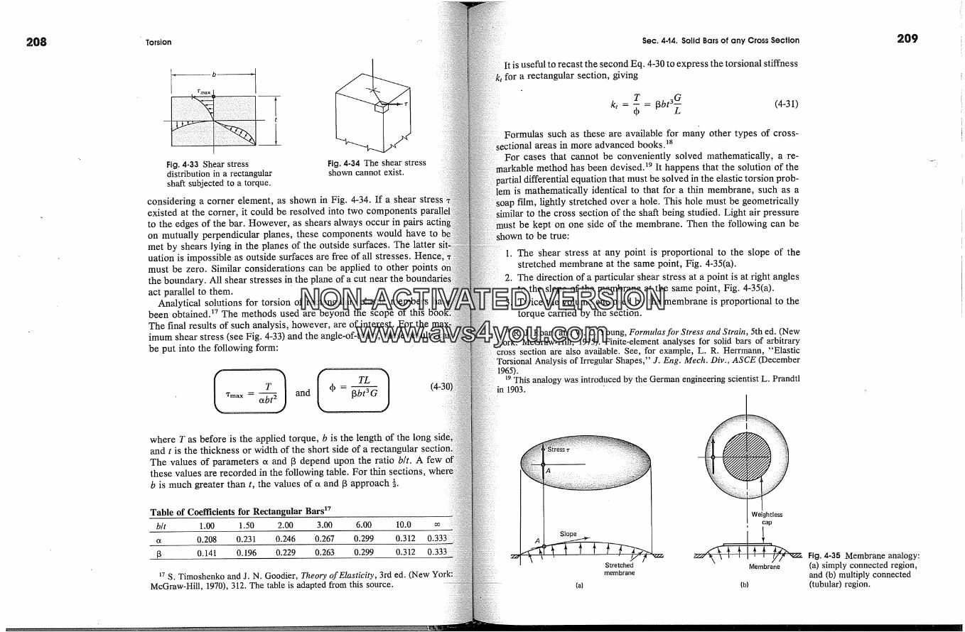
208 Torsion Sec. 4-t4. Solid Bars of any Cross Section 209
Fig. 4-33 Shear stressdistribution in a rectangularshaft subjected to a torque.
Fig. 4-34 The shear stressshown cannot exist.
considering a comer element, as shown in Fig. 4-34. If a shear stresexisted at the corner, it could be resolved into two componentsto the edges of the bar. However, as shears always occur in pairson mutually perpendicular planes, these components would have tomet by shears lying in the planes of the outside surfaces. The latteruation is impossible as outside surfaces are free of all stresses.must be zero. Similar considerations can be applied to other pointsthe boundary. All shear stresses in the plane of a cut nearact parallel to them.
Analytical solutions for torsion of rectangular, elastic membersbeen obtained? The methods used are beyond the scope of thisThe final results of such analysis, however, are of interest. For theimum shear stress (see Fig. 4-33) and the angle-of-twist, these resultsbe put into the following form:
*max -- c�T and 4) - [3
where T as before is the applied torque, b is the length of the longand t is the thickness or width of the short side of a rectangularThe values of parameters c� and [3 depend upon the ratio b/t. A fewthese values are recorded in the following table. For thin sections,b is much greater than t, the values of c� and [3 approach �.
Table of Coefficients for Rectangular Bars x7b/t 1.00 1.50 2.00 3.00 6.00 10.0 m� 0.208 0.231 0.246 '0.267 0.299 0.312�. 0.141 0.196 0.229 0.263 0.299 0.312 0.333
�7 S. Timoshenko and J. N. Goodier, Theory of Elasticity, 3rd ed. (NewMcGraw-Hill, 1970), 312. The table is adapted from this source.
t is useful to recast the second Eq. 4-30 to express the torsional stiffnessfor a rectangular section, giving
T [3bt3� (4-31)k, - 4) -Formulas such as these-are available for many other types of cross-
areas in more advanced books.�SFor cases that cannot be conveniently solved mathematically, a re-
tble method has been devised.�9 It happens that the solution of thetifferential equation that must be solved in the elastic torsion prob-
lem is mathematically identical to that for a thin membrane, such as afilm, lightly stretched over a hole. This hole must be geometrically
similar to the cross section of the shaft being studied. Light air pressuremust be kept on one side of the membrane. Then the following can be
to be true:
1. The shear stress at any point is proportional to the slope of thestretched membrane at the same point, Fig. 4-35(a).
2. The direction of a particular shear stress at a point is at right anglesto the slope of the membrane at the same point, Fig. 4-35(a).
3. Twice the volume enclosed by the membrane is proportional to thetorque carried by the section.
�s R. J. Roark and W. C. Young, Formulas for Stress and Strain, 5th ed. (NewMcGraw-Hill, 1975). Finite-element analyses for solid bars of arbitrary
section are also available. See, for example, L. R. Herrmann, "ElasticTorsional Analysis of Irregular Shapes," J. Eng. Mech. Div., ASCE (December
�9 This analogy was introduced by the German engineering scientist L. Prandtlin 1903.
(a)
Stretchedmembrane
Weightlesscap
,<�[' � � '�'d'x� Fig. 4-35 Membrane analogy:Membrane (a) simply connected region,
and (b) multiply connectedlb) (tubular) region.
NON-ACTIVATEDVERSIONwww.avs4you.com
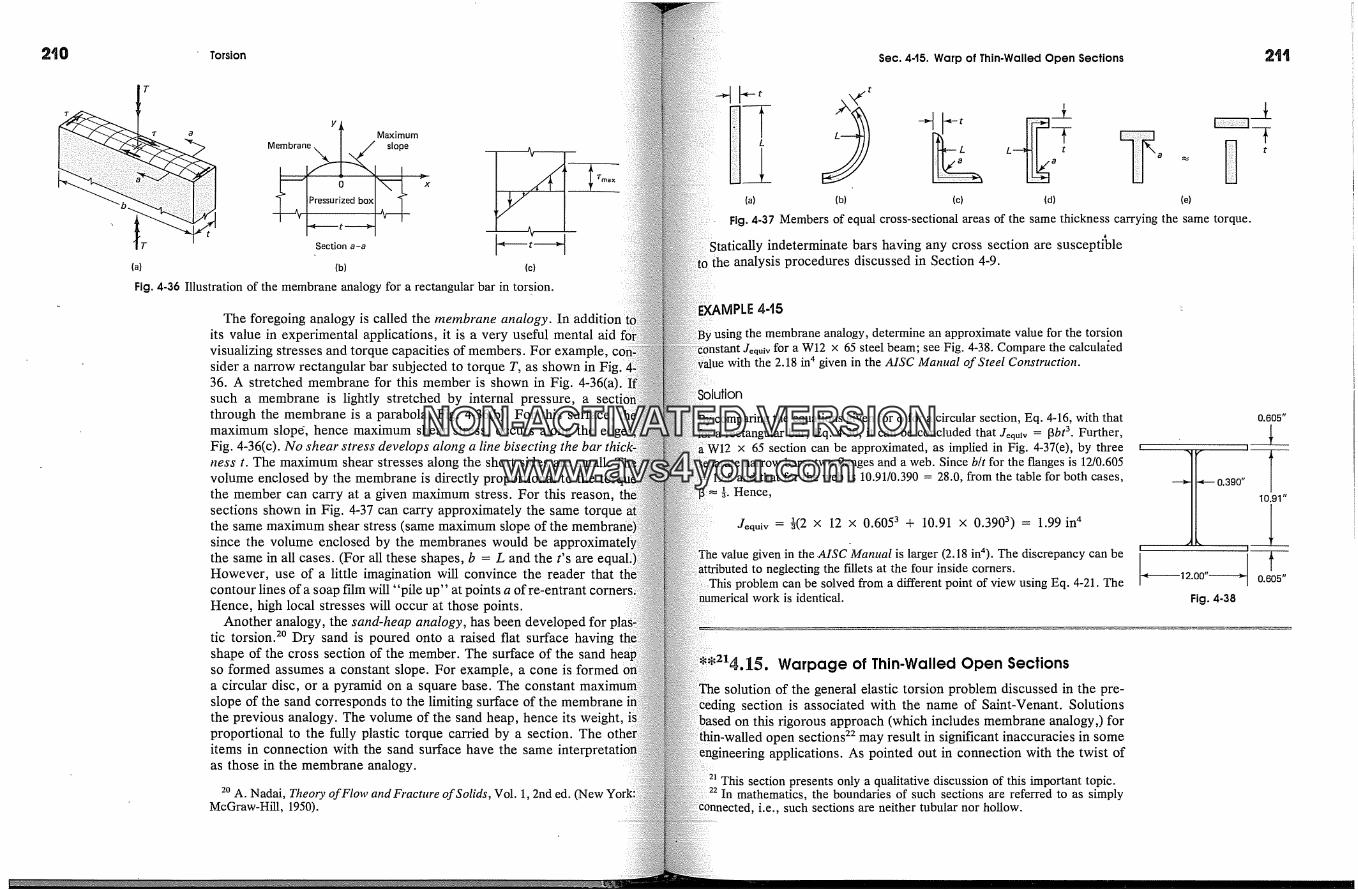
Torsion Sec. 4-15. Warp of Thin-Walled Open Sections
�' a Y � MaximumMembran��,_.x� ' slope
ized box
t �-�----tSection
(a) (b) (c)
Fig. 4-36 Illustration of the membrane analogy for a rectangular bar in torsion.
The foregoing analogy is called the membrane analogy. In additionits value in experimental applications, it is a very useful mental aidvisualizing stresses and torque capacities of members. For example,sider a narrow rectangular bar subjected to torque T, as shown in36. A stretched membrane for this member is shown in Fig. 4-36(a).such a membrane is lightly stretched by internal pressure, athrough the membrane is a parabola, Fig. 4-36(b). For this surfacemaximum slop6, hence maximum shear stress, occurs along theFig. 4-36(c). No shear' stress develops along a line bisecting the bat'hess t. The maximum shear stresses along the short sides are small.volume enclosed by the membrane is directly proportional to thethe member can carry at a given maximum stress. For this reason,sections shown in Fig. 4-37 can carry approximately the same torquethe same maximum shear stress (same maximum slope of thesince the volume enclosed by the membranes would bethe same in all cases. (For all these shapes, b = L and the t's are e�However, use of a litfie imagination will convince the reader thatcontour lines of a soap film will "pile up" at points a of re-entrantHence, high local stresses will occur at those points.
Another analogy, the sand-heap analogy, has been developed fortic torsion? Dry sand is poured onto a raised flat surface havingshape of the cross section of the member. The surface of the sandso formed assumes a constant slope. For example, a cone is formeda circular disc, or a pyramid on a square base. The constantslope of the sand corresponds to the limiting surface of the membranethe previous analogy. The volume of the sand heap, hence its weight,proportional to the fully plastic torque carried by a section. Theitems in connection with the sand surface have the sameas those in the membrane analogy.
2o A. Nadai, Theory of Flow andFracture of Solids, Vol. 1, 2nd ed.McGraw-Hill, 1950).
�-t ,k�- t
(a) (b) (c) (d) (e)
Fig. 4-37 Members of equal cross-sectional areas of the same thickness carrying the same torque.
indeterminate bars having any cross section are susceptible)the analysis procedures discussed in Section 4-9.
MPLE 4-t5
using the membrane analogy, determine an approximate value for the torsionJ�quiv for a W12 x 65 steel beam; see Fig. 4-38. Compare the calcula{ed
with the 2.18 in 4 given in the AISC Manual of Steel Construction.
�Jtion
comparing the equations given for 4� for a circular section, Eq. 4-16, with that?oP a rectangular bar, Eq. 4-30, it can be concluded that J�qu�v = f3bt 3. Further,
�W12 x 65 section can be approximated, as implied in Fig. 4-37(e), by threeseparate narrow bars: two flanges and a web. Since b/t for the flanges is 12/0.605
and that for the web is 10.91/0.390 = 28.0, from the table for both cases,�. Hence,
Jequiv = �(2 x 12 x 0.6053 + 10.91 x 0.3903) = 1.99 in 4
value given in the .AISC Manual is larger (2.18 in4). The discrepancy can beto neglecting the ffilets at the four inside corners.
problem can be solved from a different point of view using Eq. 4-21. Thenumerical work is identical.
0.605"
I '
�--0.390"10.91"
,,J
2.00" � O.E!5"Fig. 4-38
Warpage of Thin.Walled Open Sectionssolution of the general elastic torsion problem discussed in the pre-
section is associated with the name of Saint-Venant. Solutionsthis rigorous approach (which includes membrane analogy,) for
thin-walled open sections 22 may result in significant inaccuracies in someapplications. As pointed out in connection with the twist of
This section presents only a qualitative discussion of this important topic.In mathematics, the boundaries of such sections are referred to as simply
i.e., such sections are neither tubular nor hollow.
NON-ACTIVATEDVERSIONwww.avs4you.com
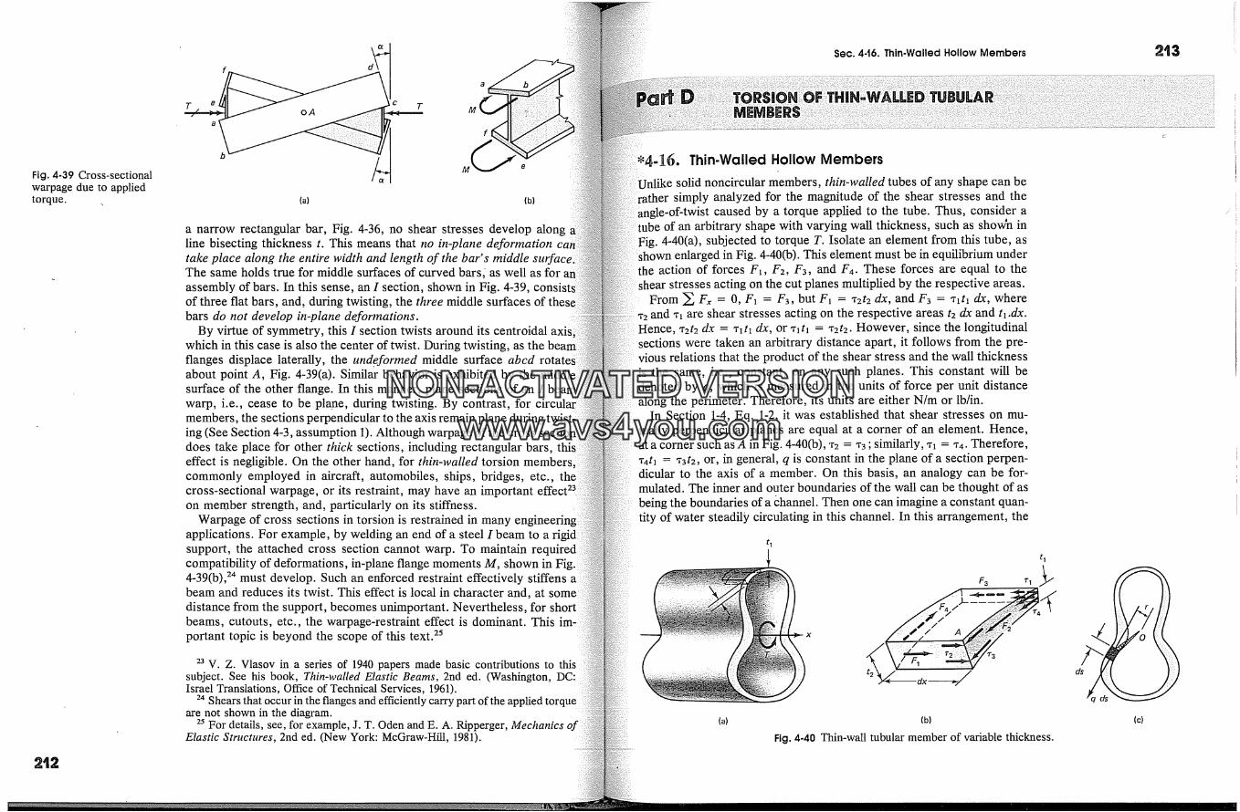
Sec, 4-t6. Thin-Walled Hollow Members 2t3
Fig. 4-39 Cross-sectionalwarpage due to appliedtorque.
2t2
oAc T
(a) (b)
a narrow rectangular bar, Fig. 4-36, no shear stresses develop alongline bisecting thickness t. This means that no in-plane deformationtake place along the entire width and length of the bar' s middle smfaceiThe same holds true for middle surfaces of curved bars/as well as for:assembly of bars. In this sense, an I section, shown in Fig. 4-39,of three flat bars, and, during twisting, the three middle surfaces of thes�bars do not develop in-plane deformations.
By virtue of symmetry, this I section twists around its centroidal axis:which in this case is also the center of twist. During twisting, as theflanges displace laterally, the undeformed middle surface abcd rotateabout point A, Fig. 4-39(a). Similar behavior is exhibited by thesurface of the other flange. In this manner, plane sections of an Iwarp, i.e., cease to be plane, during twisting. By contrast, formembers, the sections perpendicular to the axis remaining (See Section 4-3, assumption 1). Although warpage of the crossdoes take place for other thick sections, including rectangular bars,effect is negligible. On the other hand, for thin-walled torsion membencommonly employed in aircraft, automobiles, ships, bridges, etc.,cross-sectional warpage, or its restraint, may have an important effect 23on member strength, and, particularly on its stiffness.
Warpage of cross sections in torsion is restrained in many engineeringapplications. For example, by welding an end of a steel I beam to a rigidsupport, the attached cross section cannot warp. To maintain requiredcompatibility of deformations, in-plane flange moments M,'shown in Fig.4-39(b), TM must develop. Such an enforced restraint effectively stiffens abeam and reduces its twist. This effect is local in character and, at somedistance from the support, becomes unimportant. Nevertheless, for short:beams, cutouts, etc., the warpage:restraint effect is dominant. This 'portant topic is beyond the scope of this text?
23 V. Z. Vlasov in a series of 1940 papers made basic contributions tosubject. See his book, Thin-walled Elastic Beams, 2nd ed. (Washington,Israel Translations, Office of Technical Services, 1961).
24 Shears that occur in the flanges and efficiently carry part of the applied torqueare not shown in the diagram.
25 For details, see, for example, J. T. Oden and E. A. Ripperget, Mechanics ofElastic Structures, 2nd ed. (New York: McGraw-Hill, 1981).
-16. Thin-Walled Hollow Members
solid noncircular members, thin-walled tubes of any shape can besimply analyzed for the magnitude of the shear stresses and the
-of-twist caused by a torque applied to the tube. Thus, consider aube of an arbitrary shape with varying wall thickness, such as shov�n in
Fig. 4-40(a), subjected to torque T. Isolate an element from this tube, asshown enlarged in Fig. 4-40(b). This element must be in equilibrium under
action of forces Fz, F2, F3, and F4. These forces are equal to thehear stresses acting on the cut planes multiplied by the respective areas.
From � F�, = 0, F� = F3, but F� = 1'2t2 dx, and F3 = �t� dx, where� 2 and � are shear stresses acting on the respective areas t2 dx and t�.dx.Hence, x2t2 dx = ?� t� dx, or �t� = 1'2t2. However, since the longitudinalsections were taken an arbitrary distance apart, it follows from the pre-vious relations that the product of the shear stress and the wall thicknessis the same, i.e., constant, on any such planes. This constant will bedenoted by q, which is measured in the units of force per unit distancealong the perimeter. Therefore, its units are either N/m or lb/in.
In Section 1-4, Eq. 1-2, it was established that shear stresses on mu-tually perpendicular planes are equal at a corner of an element. Hence,at a corner such as A in Fig. 4-40(b), 'r2 = �'3; similarly, �z = �4. Therefore,'r4tl = w3t2, or, in general, q is constant in the plane of a section perpen-dicular to the axis of a member. On this basis, an analogy can be for-mulated. The inner and outer boundaries of the wall can be thought of asbeing the boundaries of a �hannel. Then one can imagine a constant quan-tity of water steadily circulating in this channel. In this arrangement, the
F3
t 1
2
(a)
Fig. 4-40 Thin-wall tubular member of variable thickness.
(c)
NON-ACTIVATEDVERSIONwww.avs4you.com
2t4 Torsion Sec. 446. Thin.Walled Hollow Members
quantity of water flowing through a plane across the channel is constBecause of this analogy, the quantity q has been termed the shear
Next consider the cross section of the tube as shown in Fig. 4-40�The force per unit distance of the perimeter of this tube, by virtue ofprevious argument, is constant and is the shear flow q. This shearmultiplied by the length ds of the perimeter gives a force q ds perential length. The product of this infinitesimal force q ds and rsome convenient point such as O, Fig. 4~40(c), gives the contributionan element to the resistance of applied torque T. Adding orthis,
T = � rq dswhere the integration process is carried around the tube along theline of the perimeter. Since for a tube, q is a constant, this equationbe written as
T= qfrdsInstead of carrying out the actual integration, a simple inter
of the integral is available. It can be seen from Fig. 4~40(c) that r dstwice the value of the shaded area of an infinitesimal triangle of altitr and base ds. Hence, the complete integral is twice the wholebounded by the center line of the perimeter of the tube. Defining thisby a special symbol (�), one obtains
T
T = 2(�)q or q - 2(�)This equation 26 applies only to thin-walled tubes. The area (�) isproximately an average of the two areas enclosed by the inside andoutside surfaces of a tube, or, as noted, it is an area enclosed by theline of the wall's contour. Equation 4-34 is not applicable at all if theis slit, when Eqs. 4-30 should be used.
Since for any tube, the shear flow q given by Eq. 4-34 is constant,the definition of shear flow, the shear stress at any point of a tubethe wall thickness is t is
26 Equation 4-34 is sometimes called Bredt's formula in honor of theengineer who developed it.
In the elastic range, Eqs. 4-34 and 4-35 are applicable to any shape ofFor inelastic behavior, Eq. 4-35 applies only if thickness t is con-
analysis of tubes of more than one cell is beyond the scope ofbook. 27
For linearly elastic materials, the angle of twist for a hollow tube canfound by applying the principle of conservation of energy, Eq. 2-24.
this derivation, it is convenient to introduce the angle-of-twist per unitof the tube defined as 0 = dqb/dx. The elastic shear strain energy
the tube should also be per unit length of the tube. Hence, Eq. 3-5the elastic strain energy here reduces to Ush = J'vo� (,2/2G) dV, where= 1 x t ds. By substituting Eq. 4-35 and then Eq. 4-34 into this relation
simplifying,
-- T 2 T 2 ds
Usa �' � 8Q2G-----'--� ds - 8(�2� � 5- (4-36)in the last expression, the constants are taken outside the integral.
Equating this relation to the external work per unit length of memberas We = TO/2, the governing differential equation becomes:
dqb T � ds0 = dx - 4(�2G -�' (4-37)Here again it is useful to recast Eq. 4-37 to express the torsional stiffnessfor a thin-walled hollow tube. Since for a prismatic tube subjected to
a constant torque, 4> = 0L,
kt - qb- � ds/t (4-38)
cross-sectional warpage discussed in Section 4-15 is not very im-portant for tubular members. Analysis of statically indeterminate tubular
members follows the procedures discussed earlier.
F. XAMPLE 4-t6
Example 4-3 using Eqs. 4-34 and 4-35. The tube has outside and insideof 10 and 8 ram, respectively, and the applied torque is 40 N.m.
The mean radius of the tube is 9 mm and the wall thickness is 2 mm. Hence,
27 j. T. Oden, and E. A. Ripperger, Mechanics of Elastic Structures, 2nd ed.York: McGraw-Hill, 1981).
NON-ACTIVATEDVERSIONwww.avs4you.com

*Torsion Problems
t12.7 mm
20mmJFig. 4-t
q _ T 40 X 103 -- 39.3 MPax- t 2(�)t- 2,r x 92 x 2
Note that by using Eqs. 4-34 and 4-35, only one shear stress is obtained and t�it is just about the average of the two stresses computed in Example 4-3.thinner the walls, the more accurate the answer, .or vice versa.
It is interesting to note that a rectangular tube, shown in Fig. 4-41, with athickness of 2 mm, for the same torque will have nearly the same shear stressthat of the circular tube. This is so because its enclosed area is about the
as the (� of the circular tube. However, some local stress concentrationsbe present at the inside (reentrant) corners of a square tube.
EXAMPLE 4-t7
An aluminum extrusion has the cross section shown in Fig. 4-42� If torque300 N.m is applied, (a) determine the maximum shear stresses that would de,in the three different parts of the member, and (b) find the torsional stiffnessthe member. Neglect stress concentrations.
4
Solution
The cross section consists essentially of three parts: a circular knob (�), a �tangular bar (�), and a rectangular hollow box with variable wall-thickness,During application of torque T, each one of these elements rotates throughsame angle qb, and therefore each element resists a torque (kt)iqb. Hence,to Eq. 4-21, the total torque resisted by the member is the sum of these quantitieifor the three parts. The expressions for (kt)[s for the parts areby Eqs. 4-17, 4-31, and 4-38. These constants are
(kt)� = J G _ 'rr x 104 G _ 1.57 x 10⁴ GL 2 L L
3 G G G(k,)2 = [3bt � = 0.263 x 30 x 103� = 0.789 x 10⁴�(kt)3 = 4Q2 G_ 4 x (40 x 20) 2 G 6.98 x 10⁴ G
ds/t L (40 + 2 x 20)/3 + 40/4 � = �where all numerical values are in mm. In evaluating the integral intion, it is assumed that the 4 mm thickness of the box extends for 40 mm.
By adding the stiffnesses for the parts, the member torsional stiffness �= 9.34 x 10⁴G/L.
The applied torque is distributed among the three parts in a ratio(kt)i/� (kt)i. On this basis, the torques are 300 x (1.57 x 104G/L)/(9.34104G/L) = 50.4 N.m for the knob, 25.3 N-m for the bar, and 224 N.m for
box. The maximum stresses in each of the parts are determined using,tively, Eqs. 4-3, 4-30, and 4-34.
Tc 50.4 X 103 X 10X�-max .... 32.1 MPaJ � X 104/2
T 25.3 x 103= 31.6 MPa*2-m� = e�bt 5 = 0.267 x 30 x 102
T 224 x 103= 46.7 MPa
*3-m� - 2(�)t 2 x 40 x 20 x 3Stress Tl-max Occurs along the perimeter of the knob, T2.ma x at the midheight of
and 'r3.max in the 3-mm walls of the tube. Due to the approximations m?de,stresses cannot be considered precise. In mechanical applications, stress
concentrations may be particularly important. Membrane analogy can be used togreat advantage to determine the location of stress concentrations. Generous fil-lets at reentrant comers can be a remedy.
Member torsional stiffness found in this manner, such as needed for vibrationtsis and for the solution of statically indeterminate elastic problems, would
sufficiently accurate since local effects such as stress concentrations play a� or role.
Probeores4-4 ond 4.5
The solid cylindrical shaft of variable size, as;hown in mm on the figure, is acted upon by the tor-
ques indicated. What is the maximum torsional stressthe shaft, and between what two pulleys does it
4-2. A 6-in diameter core of 3 in radius is bored outfrom a 9-in diameter solid circular shaft. What per-centage of the torsional strength is lost by this oper-ation?
4-6
4-3. A solid circular shaft of 2-in diameter is to beby a hollow circular tube. If the outside di-
mbe is limited to 3 in, what must be theof the tube for the same linearly elastic ma-
terial working at the same maximum stress? Determinethe ratio of weights for the two shafts.
55 N'm
� - 880 N-m
' �2000�Fig. P44
4-4. A 120-ram-diameter solid-steel sh�t �ansmits400 kW at 2 Hz. (a) Detemine the maximum shearstress. �) What would be the requked sh� diameterto operate at 4 Hz at the same m�imum s�ess?4-5. A motor, through a set of ge�s, drives a linesh�t, as shown in the figure, at 630 �m. Thi�y hp �edelivered to a machine on the right; 90 hp on the left.
NON-ACTIVATEDVERSIONwww.avs4you.com

� Torsion
90h��� M�t�r30hp30' >1
Fig. P4-5
Select a solid round shaft of the same size throughout.The allowable shear stress is 5750 psi.4-6. (a) Design a hollow steel shaft to transmit 300 hpat 75 rpm without exceeding a shear stress of 6000 psi.Use- 1.2:1 as the ratio of the outside diameter to theinside diameter. (b) What solid shaft could be usedinstead?
4-7. A 100-hp motor is driving a line shaft through gearA at 26.3 rpm. Bevel gears at B and C drive rubber-cement mixers. If the power requirement of the mixerdriven by gear B is 25 hp and that of C is 75 hp, whatare the required shaft diameters? The allowable shearstress in the shaft is 6000 psi. A sufficient number ofbearing� is provided to avoid bending.
d.� A [] d�:z C
� 20 � �- 10'-:-�Fig. P4-7
Section 4-7
4-8. A solid circular shaft of 150 mm diameter is ma-chined down to a diameter of 75 mm along a part ofthe shaft. If, at the transition point of the two diam-eters, the fillet radius is 12 mm, what maximum shearstress is developed when a torque of 2700 N.m is ap-plied to the shaft? What will the maximum shear stressbe if the fillet radius is reduced to 3 mm?
4-.9. Find the required fillet radius for the juncture ofa 6-iri diameter shaft with a 4-in diameter segment ifthe shaft transmits 110 hp at 100 rpm and the maximumshear stress is limited to 8000 psi.
Section 4-8
4-10. What must be the length ofa 5-mm diaineterminum wire so that it could be twisted throughcomplete revolution without exceeding a shearof 42 MPa? G = 27 GPa.
4-1t. The solid 50-mm-diameter steel line shaft sin the figure is driven by a 30-hp motor at 3 Hz.Find the maximum torsional stresses in sections ABBC, CD, and DE of the shaft. (b)angle of twist between A and E. Let G = 84 GPa.
30 hp
Bearing ��5hpoff N � 15hpoff 10hpoff
Fig. P4-tt
4-12. A hollow steel rod 6 in long is used asspring. The ratio of inside to outside diameters isThe required stiffness for this spring is � of a deper 1 in-lb of torque. (a) Determine the outsideameier of this rod. G = 12 x 106 psi. (b) What istorsional spring constant for this rod?4-t3. A solid aluminum-alloy shaft 50 mm inand 1000 mm long is to be replaced by ashaft of the same outer diameter such that theshaft would neither exceed twice the maximumstress nor the angle of twist of the aluminum shaft. (a)What should be the inner radius of the tubularshaft? Let GAI = 28 GPa and Gst = 84 GPa. (b)of the two criteria governs?4-14. Two gears are attached to twosteel shafts, as shown jn the figure. The gear at B
/� 3000mm
Fig. P4446000 mm
200-ram pitch diameter; the gear at C, a 400-mm pitchThrough what angle will end A turn if at A
a torqu.e of 560 N.m is applied and end D of the secondis prevented from rotating? G = 84 GPa.
-15. A circular steel shaft of the dimensions shownthe figure is subjected to three torques: T] = 28 k-
T2 = -8 k-in, and T3 = 10 k-in. (a) What is theof twist of the right end due to the applied tor-
ues. (b) Plot the angle-of-twist diagram along theLet G = 12 x 106 psi.
1" diam.bore
Fig. P445
A dynamometer is employed to calibrate the re-an exhaust fan at 20 Hz.
dynamometer consists of a 12-mm-diameter solidshaft and two disks attached to the shaft 300 mm apart,
as shown in the figure. One disk is fastened through atube at the input end; the other is near the output end.
The relative displacement of these two disks as viewedstroboscopic light was found to be 6 � 0'. Compute
power input in hp required to operate the fan atthe given speed. Let G = 84 GPa.
300 mm
Motor
12 mm
Dynamometer
Fig, P446
Fan
A solid tapered steel shaft is rigidly fastened tosupport at one end and is subjected to a torque
at the other end (see the figure). Find the angular
Problems
Fig. P447
rotation of the free end if d] = 6 in, d2 = 2 in, L =20 in, and T = 27,000 in-lb. Assume that the usualassumptions of strain in prismatic circular shafts sub-
jected to torque apply, and let G = 12 x 106 psi. (b)Determine the torsional flexibility of the shaft.4-18. A thin-walled elastic frustum of a cone has thedimensions shown in the figure. (a) Determine the tor-sional stiffness of this member, i.e., the magnitude oftorque per unit angle of twist. The shearing modulusfor the material is G. (b) What is the torsional flexibilityof this member?
1/2�r"Wallthickness
1" diam.
diam.
Fig. P448
449. The loading on a control torque tube for an ail-eron of an airplane may be idealized by a uniformlyvarying torque t� = kx in-lb/in, where k is a constant(see the figure). Determine the angle of twist of thefree end. Assume JG to be constant.
Fig. P449
*4-20. A torque applied to a circular shaft is idealizedas uniformly varying from the built-in end, see the fig-
NON-ACTIVATEDVERSIONwww.avs4you.com

")20 Torsion
A
'N.m/m
Fig. P4-20
ure. Determine the angle of twist of the right end. Thetorsional rigidity JG of the shaft is constant.'4-21. A 2000-mm long circular shaft attached at one-end_and free at the other is subjected to a linearly vary-ing distributed torque along its length, as shown in thefigure. The torsional rigidity JG of the shaft is con-stant. Determine the angle of twist at the free endcaused by the applied torque.
2000--�
Fig. P4-2t
Section 4-9
4-22. An aluminum-alloy tube is shrunk onto a steelrod, forming a shaft that acts as a unit. This shaft is40 in long and has the cross section shown in the figure.Assume elastic behavior and let Est = 3E, u = 30 x103 ksi. (a) What stresses would be caused by applying
a torque T = 200 k-in? Show the shear stress distri-
Steel
Fig. P4-22
bution on a graph. (b) Determine the torsionaland flexibility of the shaft.4-23. A tube of 50-ram outside diameter andthickness is attached at the ends by means offlanges to a solid shaft of 25-mm diameter, as showin the figure. If both the tube and the shaft areof the same linearly elastic material, what partapplied torque T is carried by the tube?
25 2
T I � 500 . �"Fig. P4-23
4-24. Assume that in Problem 4-23, prior tothe rigid end plates, the shaft is subjected toof 200 N-m and maintained in this condition
welding process. What residual torque will remainthe shaft upon release of the applied torque?4-25. Using the displacement method, determinereactions for the shaft shown in Fig. 4-21 for thelowing data: T = 40 k-in, L� = 15 in, L2 = 10 in,= .2�r in 4, J2 = ,r/2 in 4, and G� = G2 = G = 12103 ksi. Also plot the angle-of-twist diagram forshaft along its length.4-26. Consider the same elastic stepped circularshown in the two alternative figures. Using themethod, determine the angle of twist qb,b at a
T N
(a)
(b)
Fig. P4-26
the application of a unit torque at b, and show thatit is equal to qbba, the angle-of-twist at b due to the
of a unit torque at a. Let J� = 3J2. (See2-:�8.)(a) Using the force method, determine the re-
:tions for the circular stepped shaft shown in the fig-The applied torques are T� = 600 lb-in, T2 = 500
and T3 = 200 lb-in. Th� shaft diameters are d�2.83 in and d2 = 2.38 in. (b) Plot the angle-of-twist
� for the shaft along its length. Let E = 10 x103 ksi.
dl d 2� � I T' T2 �, , T3
Fig. P4-27
An elastic circular shaft attached at both endsis subjected to a uniformly distributed torque to per
length along one-half of its length, as shown infigure. (a) Using the force method, find the reac-
(b) Determine the angle of maximum twist andthe angle-of-twist diagram along the shaft length.torsional rigidity JG of the shaft is constant.
t o .
Fig. P4-28
Assume that the shaft in Problem 4-20 is at-tached at both ends. (a) Using the force method, de-
the reactions. (b) Find the angle of maximumand plot the angle-of-twist diagram along the
shaft length.
4.t0
Rework Problem 4-20 using Eq. 4-26.Rework Problem 4-21 using Eq. 4-26.
Using Eq. 4-26 and continuity conditions (see2-19) or singularity functions, determine the
at the built-in ends caused by the application
Problems 22�1
Fig. P4-32
of torque T� ;. see the figure. Plot the torque T(x) andthe angle-of-twist q>(x) diagrams.*4-33. Using Eq. 4-26 and continuity conditions (seeSection 2-19) or singularity functions, determine thereactions caused by a uniformly distributed torque toalong one-half of the shaft length, as shown in the fig-ure for Problem 4-28. Sketch the angle-of-twist dia-gram along the shaft length.
Section 4-'i'i
4-34. A circular stepped shaft has the dimensionsshown in the figure. (a) Using an energy method, de-termine the angle of twist at the loaded end. G is given.(b) Check the result using Eq. 4-16.
--3 d
Fig. P4-34
Section 4-'i2
4-35. A coupling is made with eight �-in-diameterhigh-strength bolts located on a 10-in-diameter bolt cir-cle. (a) Calculate the torque that can be transmitted bythis coupling if the allowable shear stress in the boltsis 10,500 psi. (b) Find the hp that can be transmittedwhen the shaft and couplings are rotating at 250 rpm.4-36. A flange coupling has six bolts having a cross-sectional area of 0.2 in 2 each in a 8-in-diameter boltcircle, and six bolts having a cross sectional area of0.5 in 2 each in a'5-in-diameter bolt circle. If the allow-able shear stress in the bolt is 16 ksi, what is the torquecapacity of this coupling?
Section 443
4-37. A specimen of an SAE 1060 steel bar of 20-mmdiameter and 450-mm length failed at a torque of 900
NON-ACTIVATEDVERSIONwww.avs4you.com
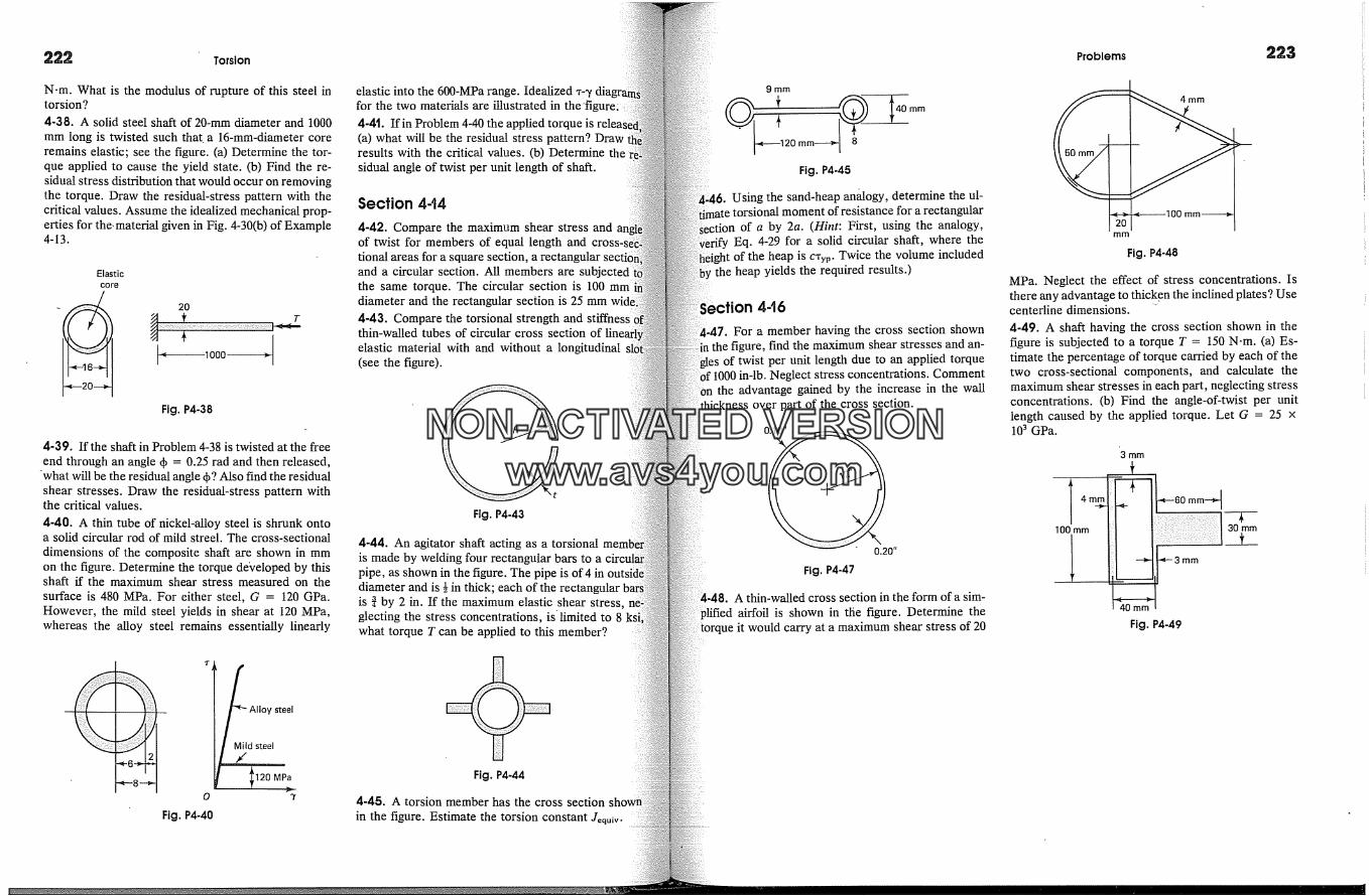
Torsion Problems 223
N-m. What is the modulus of rupture of this steel intorsion?
4-38. A solid steel shaft of 20-ram diameter and 1000mm long is twisted such that. a 16-mm-diameter coreremains elastic; see the figure. (a) Determine the tor-que applied to cause the yield state. (b) Find the re-sidual stress distribution that would occur on removingthe torque. Draw the residual-stress pattern with thecritical values. Assume the idealized mechanical prop-erties for the� material given in Fig. 4-30(b) of Example4-13.
Elasticcore
2OT
Fig. P4-38
4-39. If the shaft in Problem 4-38 is twisted at the freeend through an angle qb = 0.25 rad and then released,
'what will be the residual angle qb? Also find the residualshear stresses. Draw the residual-stress pattern withthe critical values.
4-40. A thin tube of nickel-alloy steel is shrunk ontoa solid circular rod of mild streel. The cross-sectionaldimensions of the composite shaft are shown in mmon the figure. Determine the torque deYeloped by thisshaft if the maximum shear stress measured on thesurface is 480 MPa. For either steel, G = 120 GPa.However, the mild steel yields in shear at 120 MPa,whereas the alloy steel remains essentially linearly
o
Fig. P4-40
�AlloysteelMild steel
120 MPa
elastic into the 600-MPa range. Idealized x--� diafor the two materials are illustrated in the figure:4-4t. If in Problem 4-40 the applied torque is relea(a) what will be the residual stress pattern? Drawresults with the critical values. (b) Determine thesidual angle of twist per unit length of shaft.
Section 4-14
4-42. Compare the maximum shear stress and anof twist for members of equal length and cross-tional areas for a square section, aand a circular section. All members are
the same torque. The circular section is 100 mmdiameter and the rectangular section is 25 mm4-43. Compare the torsional strength and stiffnethin-wailed tubes of circular cross section of lira
elastic material with and without a longitudinal(see the figure).
Fig. P4-43
4-44. An agitator shaft acting as a torsionalis made by welding four rectangular bars to apipe, as shown in the figure. The pipe is of 4 indiameter and is � in thick; each of the rectangularis { by 2 in. If the maximum elastic shear stress,glecting the stress concentrations, is'limited to 8what torque T can be applied to this member?
Fig. P4-44
4-45. A torsion member has the cross sectionin the figure. Estimate the torsion constant Jequiv.
9ram
i< 120mm--� 8Fig. P4-45
Using the sand-heap an�.logy, determine the ul-�,torsional moment of resistance for a rectangular
of a by 2a. (Hint: First, using the analogy,Eq. 4-29 for a solid circular shaft, where theof the heap is CXyp. Twice the volume included
the heap yields the required results.)
on 4-16
For a member having the cross section shownfigure, find the maximum shear stresses and an-
of twist per unit length due to an applied torque1000 in-lb. Neglect stress concentrations. Comment
the advantage gained by the increase in the wallthickness over part of the cross section.
0.20"
Fig. P4-47
A thin-walled cross section in the form of a sim-airfoil is shown in the figure. Determine the
torque it would carry at a maximum shear stress of 20
-� ,,100 mm �
Fig. P4-48
MPa. Neglect the effect of stress concentrations. Isthere any advantage to thicken the inclined plates? Usecenterline dimensions. -4-49. A shaft having the cross section shown in thefigure is subjected to a torque T = 150 N.m. (a) Es-timate the percentage of torque carried by each of thetwo cross-sectional components, and calculate themaximum shear stresses in each part, neglecting stressconcentrations. (b) Find the angle-of-twist per unitlength caused by the applied torque. Let G = 25 x103 GPa.
'3 mm
100 mm 30 mm
:ram
Fig. P4-49
NON-ACTIVATEDVERSIONwww.avs4you.com

?chapterSec. 5-2. Diagrammatic Conventions for Supports
�ems will be fully analyzed for these quantities. Special procedures todeveloped in subsequent chapters are required for determining reac-
in.statically indeterminate problems for complete solutions. Exten-ion to members in three-dimensional systems, where there are six pos-
internal force components, will be introduced in later chapters asand will rely on the reader's knowledge of statics. In such prob-
at a section of a member there can be: an axial force, two sheartwo bending moment components, and a torque.
5=][. Introduction
The effect of axial forces and torsion on straight members was treatedthe preceding chapters. There are other types of forces to whichmay be subjected. In many instances in structural and machine desimembers must resist forces applied laterally or transversely toSuch members are called beams. The main members supportingbuildings are beams, just.as an axle of a car is a beam. Many shaftsmachinery act simultaneously as torsion members and as beams.modern materials, the beam is a dominant member of construction.determination of the system of internal forces necessary for eqof any beam segment will be the main objective of this chapter.
For. the axially or torsionally loaded members previouslyonly one internal force was required at an arbitrary section to satisfyconditions of equilibrium. However, even for a beam with all forces ithe same plane, i.e., a planar beam problem, a system of threeforce components can develop at a section. These are the axial force,shear, and the bending moment. Determining these quantities isof this chapter.
The chapter is divided into three parts. In Part A, methods forlating reactions are reviewed; in Parts B and C, two different �for calculating the internal shear and bending moment and theirrepresentations along a beam are discussed. At the end of Part C,optional topic on singularity functions for solving such problems isdueed.
Attention will be largely confined to consideration of singlewhich, for convenience, will be shown in the horizontal position.discussion of related problems of planar frames resisting axialshears, and bending moments is also given. Only statically
;.2. Diagrammatic Conventions for Supportsplanar structures it is essential to adopt diagrammatic con-
for their supports and loadings inasmuch as several kinds ofand a great variety of loads are possible. An adherence to such
inventions avoids much confusion and minimizes the chances of makingThese conventions form the pictorial language of engineers.
types of supports are recognized for planar structures. These areby the kind of resistance they offer to the forces. One type ofphysically realized by a roller or a link. It is capable of resisting
in only one specific line of action. The link shown in Fig. 5-1(a)can resist a force only in the direction of line AB. The roller in Fig. 5-
can resist only a vertical force, whereas the rollers in Fig. 5-1(c) canonly a force that acts perpendicular to the plane CD. This type of
�ort will be usually represented in this text by rollers as shown in Figs.and (c), and it will be understood that a roller support is capable
a force in either direction 2 along the line of action of theTo avoid this ambiguity, a schematic link will be occasionally
to indicate that the reactive force may act in either directionFig. 5-4). A reaction of this type. corresponds to a single unknown
equations of statics are applied. For inclined reactions, the ratiothe two components is fixed (see Example 1-3).
type of support that may be used is a pin. In construction,a support is realized by using a detail shown in Fig. 5-2(a). In thissuch supports will be represented diagrammatically, as shown in
This and the next three sections are an informal review of statics.2 This imples that in the actual design, a link must be provided if the reaction
y from the beam; in other words, the beam is not allowed to lift off fromsupport at A in Fig. 5-1(b). In this figure, it may be helpful to show the roller
top ' the beam in the case of a downward reaction in order to make it clearconstrained against moving vertically at the support. This practice
will be followed in the text.
(a)
Roller
IRA
(c)
Fig, 5-1 Link and roller typesof supports. (']'he onlypossible lines of action of thereactions are shown by thedashed lines.)
NON-ACTIVATEDVERSIONwww.avs4you.com
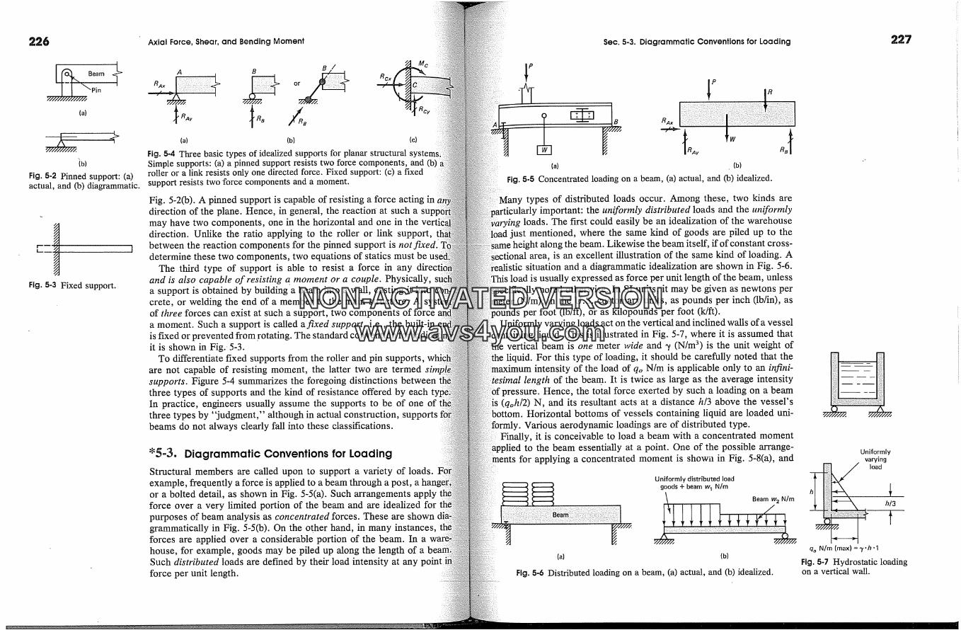
L� BeamI I;,,////j/////////"�'Pin
(a)
�b)Fig. 5-2 Pinned support: (a)actual, and (b) diagrammatic.
Fig. 5-3 Fixed support.
Axial Force, Shear, and Bending Moment
A BRcx
(a) (b) (c)
Fig. 5-4 Three basic types of idealized supports for planar structuralSimple supports: (a) a pinned support resists two force components, and lb)roller or a link resists only one directed force. Fixed support: (c) a fixedsupport resists two force components and a moment.
Fig. 5~2(b). A pinned support is capable of resisting a force acting indirection of the plane. Hence, in general, the reaction at such amay have two components, one in the horizontal and one in thedirection. Unlike the ratio applying to the roller or link support,between the reaction components for the pinned support is notdetermine these two components, two equations of statics must be u.�
The third type of support is able to resist a force in anyand is also capable of resisting a moment or a couple. Physically,a support is obtained by building a beam into a wall, casting it intocrete, or welding the end of a member to the main structure. A sof three forces can exist at such a support, two components of forcea moment. Such a support is called afixed support, i.e., the built-inis fixed or prevented from rotating. Theit is shown in Fig.. 5-3.
To differentiate fixed supports from the roller and pin supports,are not capable of resisting moment, the latter two are termedsupports. Figure 5-4 summarizes the foregoing distinctions betweenthree types of supports and the kind of resistance offered by eachIn practice, engineers usually assume the supports to be of one ofthree types by "judgment," although in actual construction, supportsbeams do not always clearly fall into these classifications.
'5-3. Diagrammatic Conventions for LoadingStructural members are called upon to support a variety of loads.example, frequently a force is applied to a beam through a post, aor a bolted detail, as shown in Fig. 5~5(a). Such arrangements applyforce over a very limited portion of the beam and are idealized forpurposes of beam analysis as concentrated forces. These are showngrammatically in Fig. 5~5(b). On the other hand, in many instancesforces are applied over a considerable portion of the beam. In ahouse, for example, goods may be piled up along the length of aSuch distributed loads are defined by their load intensity at any point iforce per unit length.
Sec. 5-3. Diagrammatic Conventions for Loading
P
(a)
�P RRAx
(b)
Fig. 5-5 Concentrated loading on a beam, (a) actual, and lb) idealized.
types of distributed loads occur. Among these, two kinds areimportant: the uniformly distributed loads and the uniformly
loads. The first could easily be an idealization of the warehousejust mentioned, where the same kind of goods are piled up to the
along the beam. Likewise the beam itself, if of constant cross-area, is an excellent illustration of the same kind of loading. A
istic situation and a diagrammatic idealization are shown in Fig. 5-6.load is usually expressed as force per unit length of the beam, unless
noted otherwise. In SI units, it may be given as newtons per(N/m); in the U.S. customary units, as pounds per inch (lb/in), as
per foot (lb/ft), or as kilopounds per foot (k/ft).Uniformly varying loads act on the vertical and inclined walls of a vessel
Containing liquid. This is illustrated in Fig. 5-7, where it is assumed thatvertical beam is one meter wide and �/(N/m 3) is the unit weight ofliquid. For this type of loading, it should be carefully noted that the
intensity of the load of qo N/m is applicable only to an infini-length of the beam. It is twice as large as the average intensity
Hence, the total force exerted by such a loading on a beam(qoh/2) N, and its resultant acts at a distance h/3 above the vessel's
bottom. Horizontal bottoms of vessels containing liquid are loaded uni-formly. Various aerodynamic loadings are of distributed type.
Finally, it is conceivable to load a beam with a concentrated momentto the beam essentially at a point. One of the possible arrange-
for applying a concentrated moment is shown in Fig. 5-8(a), andUniformly
varyingload
(a} (b)
227
Fig. 5-6 Distributed loading on a beam, (a) actual, and lb) idealized.
qo N/m (max) = 3,'h '1
Fig. 5-7 Hydrostatic loadingon a vertical wall.
NON-ACTIVATEDVERSIONwww.avs4you.com
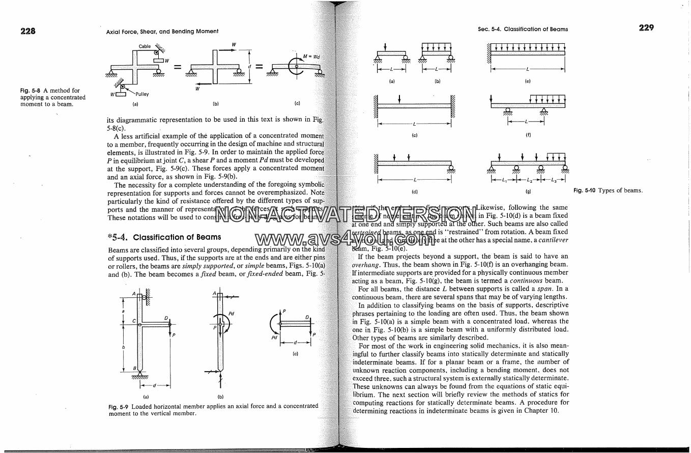
228
Fig. 5-8 A method forapplying a concentratedmoment to a beam.
Axial Force, Shear, and Bending Moment
;�Pulley 1,1/
1,1/
(b) (c)
its diagrammatic representation to be used in this text is shown in5-8(c).
A less artificial example of the application of a concentratedto a member, frequently occurring in the design of machine andelements, is illustrated in Fig. 5-9. In order to maintain the appliedP in equilibrium at joint C, a shear P and a moment Pd mtat the support, Fig. 5-9(c). These forces apply a concentratedand an axial force, as shown in Fig. 5-9(b).
The necessity for a complete understanding of the foregoingrepresentation for supports and forces cannot be overemphasized.particularly the kind of resistance offered by the different types ofports and the manner of representation of the forces at suchThese notations will be used to construct free-body diagrams
*54. Classification of Beams
Beams are classified into Several groups, depending primarily onof supports used. Thus, if the supports are at the ends and are eitheror rollers, the beams are simply supported, or simple beams, Figs.and (b). The beam becomes a fixed beam, or fixed-ended beam, Fig.
A
B
A
(c)
{a) {b)
Fig. 5-9 Loaded horizontal member applies an axial force and a concentratedmoment to the vertical member.
(a) (b)
Sec. 5-4. Classification of Beams
(c) (f)
(d) (g)
i0(c), if the ends have fixed supports. Likewise, following the sameScheme of nomenclature, the beam shown in Fig. 5-10(d) is a beam fixed
one end and simply supported at the other. Such beams are also calledted beams, as one end is "restrained" from rotation. A beam fixed
at one end and completely free at the other has a special name, a cantileverFig. 5-10(e).
the beam projects beyond a support, the beam is said to have anThus, the beam shown in Fig. 5-10(f) is an overhanging beam.
If intermediate supports are. provided for a physically continuous memberas a beam, Fig. 5-10(g), the beam is termed a continuous beam.
For all beams, the distance � between supports is called a span. In athere are several spans that may be of varying lengths.
In addition to classifying beams on the basis of supports, descriptivepertaining to the loading are often used. Thus, the beam shown
Fig. 5-10(a) is a simple beam with a concentrated load, whereas thein Fig. 5-10(b) is a simple beam with a uniformly distributed load.
types of beams are similarly described.For most of the work in engineering solid mechanics, it is also mean-
to further classify beams into statically determinate and staticallyate beams. If for a planar beam or a frame, the number of
reaction components, including a bending moment, does notexceed three, such a structural system is externally statically determinate.
unknowns can always be found from the equations of static equi-librium. The next section will briefly review the methods of statics for
:omputing reactions for statically determinate beams. A procedure formg reactions in indeterminate beams is given in Chapter 10.
229
Fig. 540 Types of beams.
NON-ACTIVATEDVERSIONwww.avs4you.com

230 Axial Force, Shear, and Bending Moment
*5-5. Calculation of Beam ReactionsAll subsequent work with beams in this chapter will begin with demination of the reactions. When all of the forces are applied in onethree equations of static equilibrium are available for the analysis.are � Fx = 0, � Fy = 0, and � Mz = 0, and have already been discus,.in Chapter 1. For straight beams in the horizontal position, the x axis �be taken in a horizontal direction, the y axis in the upward verticalrection, and the z axis normal to the plane of the paper. Theof these equations to several beam problems is illustrated in theexamples and is intended to serve as a iThe deformation'of beams, being small, is neglected when theof statics are applied. For stable beams, the small amountthat does take place changes the points of application of the forcesperceptibly.
EXAMPLE 5-'1
Find the reactions at the supports for a simple beam loaded as shown in Fi11(a). Neglect the weight of the beam.
Solution
The leading of the beam is already given in diagrammatic form. The nature ofsupports is examined next, and the unknown components of these reactiorclearly indicated on the diagram. The beam, with the unknown reactionponents and all the applied forces, is redrawn in Fig. 5-11(b) to emphasizeimportant step in constructing a free-body diagram. In order tothe applied forces and reactions, following the suggestion made in Sectionslashes are drawn across the reaction force vectors.
At A, two unknown reaction components may exist, since the end isThe reaction at B can act only in a vertical direction since the end is on aThe points of application of all forces are carefully noted. Aftergram of the beam is made, the equations of statics are applied tosolution.
�Fx = 0 R�L��MA = 0� + 200 + 100 x 0.2 + 160 x 0.3 --RB x 0.4
RB = + 670� M� = 0� + R^y x 0.4 + 200 - 100 x 0.2 - 160 x 0.1
RAy = --410
Check: �F:, = 0�' + -410- 100 - 160 + 670
Note that � F.� = 0 uses one of the three independent equations ofthus, only two additional reaction-components can be determined from
200 N.m160 N
(a)
Sec. 5.5. Calculation of Beam Reactions
200N.m I100N ] 16�N
RA� 1-� 0.4 m > I RB
(b)
Fig. 5-tt
If more unknown reaction components or moments exist at the support, the prob-becomes statically indeterminate.
.Xlote that the concentrated moment applied at C enters only into the expressionsthe summation of moments. The positive sign of Rs indicates that its direction
�been correctly assumed in Fig. 5-11(b). The opposite is the case of R.4y, andvertical reaction at A acts downward. A check on the arithmetical work is
if the calculations are made as shown.
Solution
computing reactions, some engineers prefer to make calculations in the mannerin Fig. 5-12. Fundamentally, this involves the use of the same principles.
the details are different. The reactions for every force are determined onea time. The total reaction is obtained by summing these reactions. This pro-
permits a running check of the computations as they are performed. Fort force, the sum of its reactions is equal to the force itself. For example, for
160-N force, it is easy to see that the upward forces of 40 N and 120 N totalN. On the other hand, the concentrated moment at C, being a couple, is
by a couple. It causes an upward force of 500 N at the fight reaction andof 500 N at the left reaction.
�00 x
100 x (0.2)/(0.4) =i60 x (0.1)/(0.4) =
500 N
200N.m IlOON 1180N�c�
R� } i 'R�0.4 m
1/(0.4) = 500 N50 N40 N
g0 N
R� 410 N �
t �MA=0500 N = 200 X 1/(0.4)
50 N = 100 X (0.2)/(0.4)120 N = 160 X (0.3)/(0.41
R�= 670 NFig. 5-t2
(moment)(100 N force){ 160 N force)
NON-ACTIVATEDVERSIONwww.avs4you.com

232 Axial Force, Shear, and Bending Moment Sec. 5.5. Calculation of Beam Reactions
Fig. 5-t3
q. = 10 kN/m
_,-crlqT
_ 1P-sX3X 10=15kN
RAx
R'�'f -�X3=2 m5m
(b)
EXAMPLE 5-2
Find the reactions for the partially loaded beam with a uniformly varyingshown in Fig. 5-13(a). Neglect the weight of the beam.
Solution
An examination-of the supporting conditions indicates that there areknown reaction components; hence, the beam is statically determinate.and the applied load are shown in Fig. 5-13Co). Note particularly that thefiguration of the member is not important for computing the reactions.shaped outline, bearing no i-esemblance to the actual beam, is indicated tophasize this point. However, this new body is supported at points A andsame manner as the original beam.
For calculating the reactions, the distributed load is replaced by anconcentrated force P. It acts through the centroid of the distributed forces.pertinent quantities are marked on the working sketch, Fig. 5-13Co). Afterbody diagram is prepared, the solution follows by applying the equationsequilibrium.
�F.� = 0 R/� = 0�M/� = 07+ + 15 x 2 - RB x 5 = 0 RB = 6� M� = OG+ - RAy x 5 + 15 x 3 = 0 R/�y = 9
-9+ 15-6
EXAMPLE 5-3
Determine the reactions at A and B for the beam shown in Fig. 5-14(a)applied force.
(a)
4k
RAy
�/3k5k B Rax
(b)
Iution
y diagram is shown in Fig. 5-14(b). At A, there are two unknown re-components, RA� and R,�.�.. At B, the reaction RB acts normal to the sup-
10rting plane and constitutes a single unknown. It is expedient to replace thisby the two components R�.,. and RB.�, which in this particular problem are
equal. Similarly, it is best to replace the inclined force with the twocomponents shown. These steps reduce the problem to one where all forces are
cal. This is of great convenience in applying the equationstuilibrium.
MA=0G+iM�=0G +
,F� = 0--� +
4x3-R m. x12=ORAy X 12 - 4 x 9 = 0RAx -- 3 - 1 = 0
R�,= lkt = I g�.� IRAy = 3 k 1R ,�.� = 4 k--*R,� = X,/42 + 32 = 5 kR� = Vff7+ 12 = �/�k
+3-4+1=0
h#�ges or p#medjoints are introduced into beams and frames.is capable of transmitting only horizontal and vertical forces. No moment
be transmitted at a hingedjoh�t. Therefore, the point where a hinge occursa particularly convenient location for "separation" of the structure into parts
�oses of computing the reactions. This process is illustrated in Fig. 5-15.part of the beam so separated is treated independently. Each hinge provides
axis around which moments may be taken to determine reactions. The
Fig. 5-t4
NON-ACTIVATEDVERSIONwww.avs4you.com
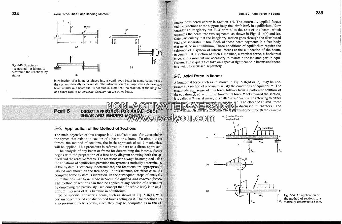
234 Axial Force, Shear, and Bending Moment Sec. 5-7. Axial Force in Beams 235
Fig. 545 Structures"separated" at hinges todetermine the reactions bystatics.
�( L �1 -� -a �. 2
B
� (c)(b)
introduction of a hinge or hinges into a continuous beam in many casesthe system statically determinate. The introduction of a hinge into a deterrbeam results in a beam that is not stable. Note that the reaction at the hitone beam acts in an opposite dh'ection on the other beam.
5-{�. Application of the Method of SectionsThe main objective of this chapter is to establish means for detethe forces that exist at a section of a beam or a frame. To obtainforces, the method of sections, the basic approach of solidwill be applied. This procedure is referred to here as a direct
The analysis of any beam or frame for determining the internalbegins with thd preparation of a free-body diagram showing both theplied and the reactive forces. The reactions can aiwa3the equations of equilibrium provided the system is staticall3If the system is statically indeterminate, the reactions arelabeled and shown on the free-body. In this manner, for either case,complete force system is identified. In the subsequent stepsno distinction has to be made between the applied and reactiveThe method of sections can then be applied at any section of aby employing the previously used concept that if a whole body is inlibrium, any part of it is likewise in equilibrium.
To be specific, consider a beam, such as shown in Fig. 5-16(a),certain concentrated and distributed forces acting on it. Thealso presumed to be known, since they may be computed as in the
considered earlier in Section 5-5. The externally applied forcesthe reactions at the support keep the whole body in equilibrium. Nowider an imaginary cut X-X normal to the axis of the beam, which
the beam into two segments, as shown in Figs. 5-16(b) and (c).particularly that the imaginary section goes through the distributed
and separates it too. Each of these beam segments is a free-bodymust be in equilibrium: These conditions of equilibrium require the
stence of a system of internal forces at the cut section of the beam.In general, at a section of such a member, a vertical force, a horizontal
and a moment are necessary to maintain the isolated part in equi-[m. These quantities take on a special significance in beams and there-will be discussed separately.
Axial Force in Beams
horizontal force such as P, shown in Fig. 5-16(b) or (c), may be nec-;sary at a section of a beam to satisfy the conditions of equilibrium. The
and sense of this force follows from a particular solution ofequation � Fx = 0. If the horizontal force P acts toward the section,called a thrust; if away, it is called axial tension. In referring to either
�these forces, the term axial force is used. The effect of an axial forcea section of a member has already been discussed in Chapters 1 and
was shown that it is imperative to apply this force through the centroid
(a)
(b)
(c)
W� (total uniformlyvarying load)
�'� /P�2( t�ta''�ad)
M
P2 P
P�
W2 B
the method of sections to alR,�v /RB statically determinate'beam.
NON-ACTIVATEDVERSIONwww.avs4you.com

236 Axial Force, Shear, and Bending Moment 237of the cross-sectional area of a member to avoid bending. Similarly,the line of action of the axial force will always be directed throucentroid of the beam's cross-sectional area.
Any section along a beam may be examined for the magnitude ofaxial force in the previous manner. The tensile force at a section istomarily taken positive. The axial force (thrust) at section X-X in Fi5-16(b) and (c) is equal to the horizontal force P2.
5-8. Shear in Beams
In general, to maintain a segment of a beam, such as that shown in5-16(b), in equilibrium, there must be an internal vertical force � atcut to satisfy the equation � Fy = 0. This internal force �,angles to the axis of the beam, is called the shear, or shear force.shear is numerically equal to the algebraic sum of all the verticalponents of the external forces acting on the isolated segment,opposite in direction. Given the qualitative data shownin Fig. 5-16(b)is opposite in direction to the downward load to the left of the secThis shear may �also be computed by considering the right-hand seshown in Fig. 5-16(c). It is then equal numerically and isdirection to the sum of all the vertical forces, including the verticaction components, to the right of the section. Whether the risegment or the left is used to determine the shear at a section is 'terial--arithmetical simplicity governs. Shears at any other sectionbe computed similarly.
At this time, a significant observation must be made. The sameshown in Figs. 5-16(b) and (c) at the section X-X is opposite inin the two diagrams. For that part of the downward load W� to theof section X-X, the beam at the section provides an upwardmaintain vertical forces in equilibrium. Conversely, the loaded [the beam exerts a downward force on the beam, as shown in Fig. 5-16{At a section, "two directions" of shear must be differentiated, deupon which segment of the beam is considered. This follows fromfamiliar action-reaction concept of statics and has occurred earliercase of an axially loaded rod, and again in the torsion problem.
The direction of the shear at section X-X would be reversed indiagrams if the distributed load W� were acting upward. Fretsimilar reversal in the direction of shear takes place at one sectionanother along a beam. Therefore, the adoption of a signnecessary to differentiate between the two possible directions ofThe definition of positive shear is illustrated in Fig. 5-17. Ainternal force V acting at a section on an isolated left segment ofbeam, as in Fig. 5-17(a), or an upward force V acting at the sameon the right segment of the beam, as in Fig. 5-17(b), correspondsitive shear. Positive shears are shown in Fig. 5-17(c) for an elementlated from a beam by two sections, and again in Fig. 5-17(d). The
Resultant of all forces(including reactions)
,�" to theleftofsection+V
Beamelement
(c)
Arbitrarysection + V
section X-X of Fig. 5-16(a) is a negative shear. Note that in additioni specifying the direction of a shear V, it is essential to associate it with
side of a section, Fig. 5-17(c). This is also true with stresses.discussion in Sections 1-3 and 1-4.)
selected sign convention for shear in this book is the one generallyHistorically, it appears tO be based on directing the coordinate axes
shown in Fig. 5-18(a). A few books 3 reverse the direction of positiveto be consistent with the direction �f axes in Fig. 5-18(b).
Bending Moment in Beamsshear and axial forces at a section of a beam satisfy only two
uations of equilibrium: � Fx = 0 and � Fy = 0. The remaining con-of static equilibrium for a planar problem is � M� = 0. This, in
can be satisfied only by developing a couple or an internal re-moment within the cross-sectional area of the cut to counteract
moment caused by the external forces. The internal resisting momentact in a direction opposite to the external moment to satisfy the
governing equation � M� = 0. It follows from the same equation thatmagnitude of the internal resisting moment equals the external mo-
These moments tend to bend a beam in the plane of the loads andusually referred as bending moments.
To determine an internal bending moment maintaining a beam segment. equilibrium, either the left- or the right-hand part of a beam free-body
S. H. Crandall, N. C. Dahl, and T. J. Lardner, An Introduction to the Me-tSolids, 2nd ed. (New York: McGraw-Hill, 1978). J. L. Merriam, Stat-
2nd ed. (New York: Wiley, 1971). E. P. Popov, Introduction to MechanicsSolids, (Englewood Cliffs, NJ: Prentice-Hall, 1968).
Fig. 5-t7 Definition ofpositive shear.
+v
(a)
y
(b)
Fig. 548 Positive sense ofshear and bending momentdefined in (a) is used in thistext with coordinates shownin (b). �
NON-ACTIVATEDVERSIONwww.avs4you.com

238 Axial Force, Shear, and Bending Moment Sec. 5-9. Bending Moment in Beams 23 {)
can be used, as shown in Figs. 5-16(b) and (c). The magnitude ofbending moment is found by the summation of the moments causedall forces multiplied by their respective arms. The internal forces VP, as well as the applied couples, must be included in the sum. Into exclude the moments caused by V and P, it is advantageous tothe point of intersection of these two internal forces as the point arotwhich the moments are summed. This point lies on the centroidalthe beam cross section. In Figs. 5~16(b) and (c), the internalmoment may be physically interpreted as a pull on the top fibers ofbeam and a push on the lower ones.
If the load W�in Fig. 5-16(a) were acting in the opposite direction,resisting moments in Figs. 5-16(b) and (c) would reverse. This andsituations require the adoption of a sign convention for the bendingmerits. This convention is associated with a definite physicalthe beam. For example, in Figs. 5-16(b) and (c), the internalshown cause tension in the upper part of the beam and comlower. This tends to increase the length of the top surface of theand to contract the lower surface. A continuous occurrence of suchments along the beam makes the beam deform convex upwards,"shed water." Such bending moments are assigned a negative sign.versely, a positive moment is defined as one that produces compre.,in the top part and tension in the lower part of a beam's crossUnder such circumstances, the beam assumes a shape thatwater." For example, a simple beam supporting a group offorces deflects down as shown in exaggerated form in Fig. 5-19(a),suggested by physical intuition. De�mitions for positive and nebending moments are shown in Figs. 5-19(b) and (c). Note that, astshears V, in addition to the sense of M, it is also essential tothe moment for a particular side of a section.
+M +M
Fibers in Fibers intension compression
+M +M+M
{b)
{a)
Fig. 549 Definition of bending moment signs.
-M
Yll 3m -9 kN
- 2 m--�
)' 10 kN/m
(a)
x
A
-�-i3
15k�kN/m
9 kN
� 2 -� < 2
(c)
(b)
EXAMPLE 5-4
;ider earlier Example 5-2 and determine the internal system of forces at sec-a-a and b-b; see Fig. 5-20(a).
SOlution
free-body for the member, including reactions, is shown in Fig. 5-20(a). A free-to the left of section a-a in Fig. 5-20(b) shows the maximum ordinate for
isolated part of the applied load. Using this information,
1 2
v, = -9 + � x 2 x � x 10 = -2.33kN1 2 1
M, = -9 x 2 +� x 2 x � x 10 x � x 2 = -13.6kN.m
forces are shown with correct sense in the figure.Jy to the left of section b-b is shown in Fig. 5-20(c), and to the right,
Fig. 5-20(d). It is evident that the second free-body is simpler for calculations,directly
Fig. 5.20
NON-ACTIVATEDVERSIONwww.avs4you.com
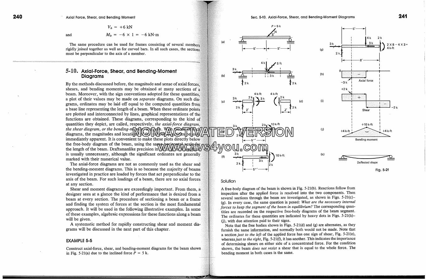
240 Axial Force, Shear, and Bending Moment Sec. 5.t0. Axial. Force, Shear, and Bending.Moment Diagrams
Vb = +6kN
and Mb = -6 x 1 = -6kN.mThe same procedure can be used for frames consisting of several memb�
rigidly joined together as well as for curved bars. In all such cases, the secti6fimust be perpendicular to the axis of a member.
5-10. Axial-Force, Shear, and Bending-MomentDiagrams
By the methods discussed before, the magnitude and sense of axial foshears, and bending moments may be obtained at many sections ofbeam. Moreover, with the sign conventions adopted for thesea plot of their values may be made on separate diagrams.. On suchgrams, ordinates may be laid off equal to the computed q�antitiesa base line representing the length of a beam. When these ordinateare plotted and interconnected by lines, graphical representations offunctions are obtained. These diagrams, corresponding to the kindquantities they depict, are called,. respectively, the axial-forcethe shear diagram, or the bending-moment diagram. With the aid ofdiagrams, the magnitudes and locations of the various quantities becorimmediately apparent. It is convenient to make these plots directlythe free-body diagram of the beam, using the same horizontal scalethe length of the beam. Draftsmanlike precision in making suchis usually unnecessary, although the significant ordinates aremarked with their numerical value.
The axial-force diagrams are not as commonly used as the shearthe bending-moment diagrams. This is so because the majorityinvestigated in practice are loaded by forces that act perpendicular toaxis of the beam. For such loadings of a beam, there are no axialat any section.
Shear and moment diagrams are exceedingly important. From them,designer sees at a glance the kind of performance that is desired frombeam at every section. The procedure of sectioning a beam or aand finding the system of forces at the section is the mostapproach. It will be used in the following illustrative examples. Inof these examples, algebraic expressions for these functions along awill be given.
A systematic method for rapidly constructing shear and momentgrams will be discussed in the next part of this chapter.
EXAMPLE 5-5
Construct axial-force, shear, and bending-moment diagrams for the beamin Fig. 5-21(a) due to the inclined force P = 5 k.
{a)
P=Sk
3k
.[2k
(g)
I I I
I i, � I t'� (h)
i 113k I�'2k
(d) (i)
4 k-ft 4 k-ft
3k 2k
2 k T�.2, �Jr-- � � 2tII
3 k Ii 2 kj-�O k-ft,-';-�- -J
J� 5-II
i 4 kl
I
3k
2k,J'I
J� III
o
-[I 2X8-4X3=4 k-ft
Axial force-3 k I
I+2 k I
(j)
Shear
+10 k-ft
+4 k-ft +4 k-ft
Bending moment
2k
(k)
Deflected shape
Fig. 5-21
Solution
A free-body diagram of the beam is shown in Fig. 5-21(b). Reactions follow frominspection after the applied force is resolved into the two components. Thenseveral sections through the beam are investigated, as shown in Figs. 5-21(c)-(g). In every case, the same question is posed: What are the necessary internal
forces to keep the segment of the beam in equilibrium? The corresponding quan-tifies are recorded on the respective free-body diagrams of the beam segment.The ordinates for these quantifies are indicated by heavy dots in Figs. 5-21(h)-(j), with due attention paid to their signs.
Note that the free bodies shown in Figs. 5-21(d) and (g) are alternates, as theyfurnish the same information, and normally both would not be made. Note thata section just to the left of the applied force has one sign of shear, Fig. 5-21(e),whereas just to the right, Fig. 5-21(f), it has another. This indicates the importanceof determining shears on either side of a concentrated force. For the conditionshown, the beam does not resist a shear that is equal to the whole force. Thebending moment in both cases is the same.
NON-ACTIVATEDVERSIONwww.avs4you.com

:242 � Axial Force, Shear, and Bending Moment
In this particular case, after a few individual points have been Jthe three diagrams in Figs. 5-21(h)-(j), the behavior of the respectiveacross the whole length of the beam may be reasoned out. Thus, althoughsegment of the beam shown in Fig. 5-21(c) is 2 ft long, it may vary in lenanywhere from zero to first to the left of the applied force, and no change inshear and the axial force occurs. Hence, the ordinates in Figs. 5-21(h) andremain constant for this segment of the beam. On the other hand, themoment depends directly on the distance from the support; hence, it variesearly, as shown in Fig. 5-21(j). Similar reasoning applies to the segmentin Fig. 5-21(d), enabling one to complete the three diagrams on the riside. The use of the free-body of Fig. 5-21(g) for completing the diagram tofight of center yields. the same result.
The sign of a bending moment, per Figs. 5-19(b) and (c), defines the sensewhich a beam bends. Since, in this problem, throughout the beam length,moments are positive, the beam curves to "retain water." In order tothis physical behavior some analysts find it advantageous to draw a shortline directly on the moment diagram, as shown in Fig. 5-21(j), to ifidicatemanner in which a beam or a beam segment curves.
Sometimes, in addition to or instead of the shear or moment diaexpressions for these functions are necessary. For the origin of x at the leftof the beam, the following relations apply:
V= +2k for0<x<5V= -2k for5<x< 10
M= +2x k-ft for0-<x-< 5M = +2x- 4(x- 5) = +20- 2xk-ft for5-<x-< 10
These expressions can be easily established by mentally replacing theof 2 ft and 8 ft, respectively, in Figs. 5-21(c) and (g) by an x.
EXAMPLE 5-6
Determine axial-force, shear, and bending-moment diagrams for theloaded with an inclined force at the end; see Fig. 5-22(a).
Solution
First, the inclined force is replaced by the two components shown in Fig.and the reactions are determined. The three unknowns at the support followthe familiar equations of statics. This completes the free-body diagram shownFig. 5-22(b). Completeness in indicating all of these forces is of the utmost
portance.A segment of the beam is shown in Fig. 5~22(c); from this segment, it may
seen that the axial force and the shear force remain the same regardlessdistance x. On the other hand, the bending moment is a variable quantity.summation of moments around C gives PL - Px acting in the directionThis represents a negative moment. The moment at the support isnegative bending moment as it tends to pull on the upper fibers of the beam.three diagrams are plotted in Figs. $-22(d)-(f).
(a) *
Sec. 540. Axial. Force, Shear, and Bending-Moment Diagrams
(d)
H L >1 0 Axial force
Shear
(f)
p PLf P I \PL - Px -PL Moment
Deflected shape Fig. 5-22
EXAMPLE 5-7
Construct shear and bending-moment diagrams for the beam loaded with theforces shown in Fig. 5-23(a).
Solution
An arbitrary section at a distance x from the left support isolates the beam segmentshown in Fig. 5-23(b). This section is applicable for any value of x just to the left
(a)
(b)
{-,+---a >l
, ,� p,[
(d)
(e)
o
Shear
Fig. 5-23 Moment
243
NON-ACTIVATEDVERSIONwww.avs4you.com

244 ' Axial Force, Shear, and Bending Moment Sec. 5-10. Axial-Force, Shear, and Bending-Moment Diagrams
of the applied force P. The shear, regardless of the distance from the suremains constant and is +P. The bending moment varies linearly from theport, reaching a maximum of +Pa.
An arbitrary section applicable anywhere between the two applied forcesshown in Fig. 5-23(c). No shear force is necessary to maintain equilibriumsegment in this part of the beam. Only a constant bending moment of + Pa mube resisted by the beam in this zone. Such a state of bending or flexure ispure bending.
Shear and bending-moment diagrams for this loading condition are shownFigs. 5-23(d) and (e). No axial-force diagram is necessary, as there is noforce at any section of the beam.
EXAMPLE 5-8
Plot shear and a bending-moment diagrams for a simple beam with adistributed load; see Fig. 5-24.
Solution
The best way of solving this problem is to write algebraic expressions forquantities sought. For this purpose, an arbitrary section taken at a distancethe left support is used to isolate the segment shown in Fig. 5-24(b). Sinceapplied load is continuously distributed along the beam, this section isand applies to any section along the length of the beam.
The shear V is equal to the left upward reaction less the load to the left of thsection. The internal bending moment M resists the moment caused by theaction on the left less the moment caused by the forces to the left of thesection. The summation of moments is performed around an axis at the
w o N/m
'� L �
} woLoF>---...
-�%L
r,,, -I v= �Wo�. - WoX
(b)
Moment
(d)
Fig. 5-24
customary to isolate the left-hand segment, similar expressions mayobtained by considering the right-hand segment of the beam, with due attention
sign conventions. The plot of the V and M functions is shown in Figs. 5-and (d).
MPLE 5-9
� the beam in Example 5-4, shown in Fig. 5-25(a), express the shear V and themoment M as a function of x along the horizontal member.
SolutionUnlike the preceding example, in this case, a load discontinuity occurs at x = 3
Therefore, the solution is determined in two parts for each of which the func-V and M are continuous. A free-body diagram for the beam segment under
load is shown in Fig. 5-25(b), and for the remainder, in Fig. 5-25(c). Therequired expressions for 0 < x < 3 are
V(x) = -9 + x 10 = -9 + �x kN
M(x) = -9x + x 10 = -9x + �x kN.m
For 3 < x < 5,
V(x) = -9 + 15 = +6kNM(x) = -9x + 15(x - 2) = 6x - 30 kN.m
To obtain the last expression, it would have been a little simpler to use a free-body diagram similar to Fig. 5-20(d).
This problem can also be solved using the singularity functions discussed inSection 5-16.
Y�--3 m� 10�kN/m
6kN'�I kN
-� 5m �
(b)
Fig. 5.25
1�k.�� .�..M(x)V(x)
90 N
< 2 --�J�-�
(c)
NON-ACTIVATEDVERSIONwww.avs4you.com
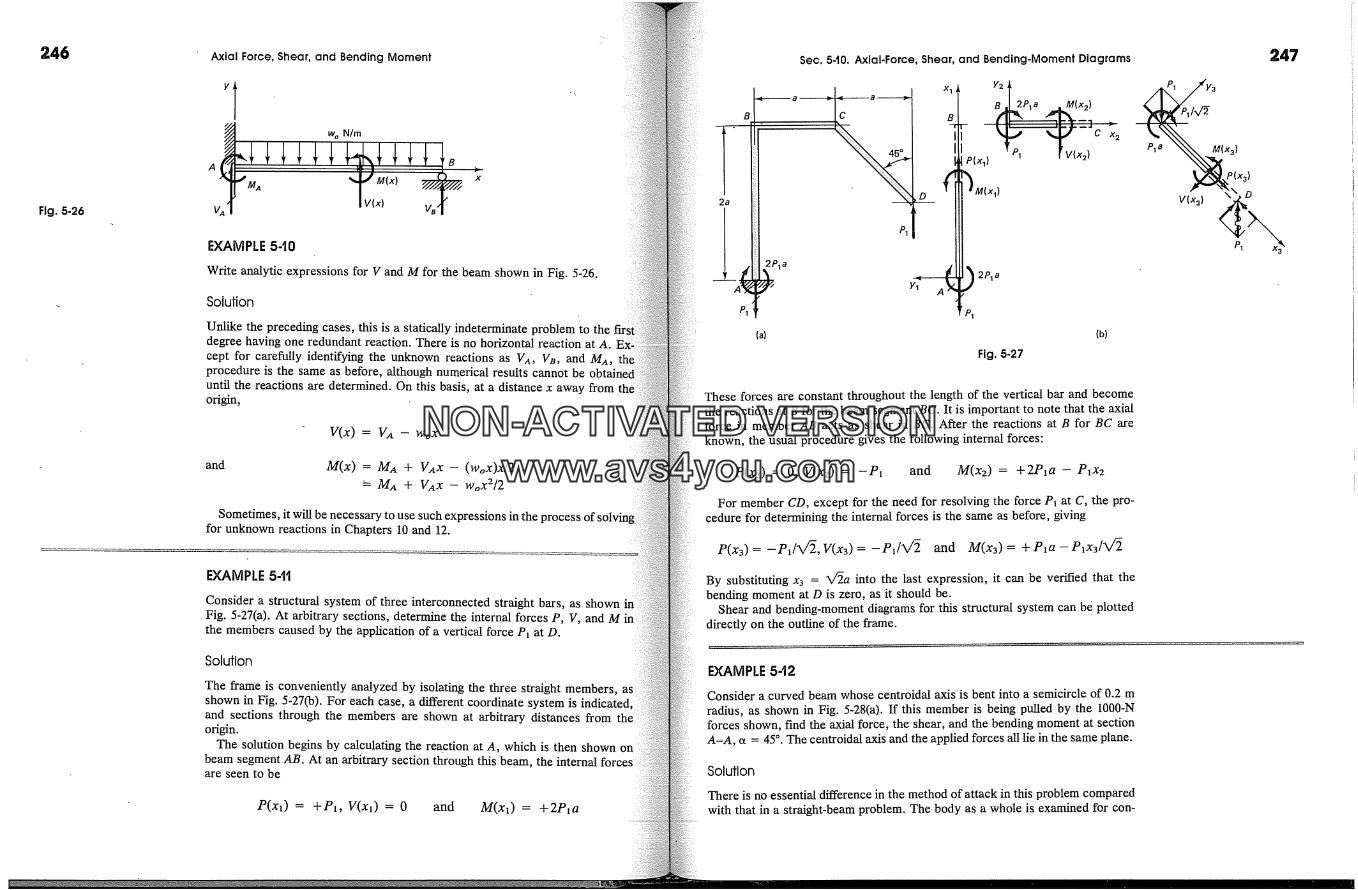
246
Fig, 5-26
Axial Force, Shear, and Bending Moment
V,. I V(x) V.'�'
EXAMPLE 5-t0
Write analytic expressions for V and M for the beam shown in Fig. 5-26.
Solution
Unlike the preceding cases, this is a statically indeterminate proble m to thedegree having one redundant reaction. There is no horizontal reaction at A.cept for carefully identifying the unknown reactions as VA, VB, and MA,procedure is the same as before, although numerical results cannot be obtaiuntil the reactions are determined. On this basis, at a distance x away fromorigin,
V(x) = V.� - wox
and M(x) = MA + VAx - (WoX)X/2�- Mn + V�x - WoX2/2
Sometimes, it will be necessary to use such expressions in the process of solvin gfor unknown reactions in Chapters 10 and 12.
EXAMPLE 54�
Consider a structural system of three interconnected straight bars, as shownFig. 5-27(a). At arbitrary sections, determine the internal forces P, V, and Mthe members caused by the application of a vertical force P� at D.
Solution
The frame is conveniently analyzed by isolating the three straight members,shown in Fig. 5-27(b). For each case, a different coordinate system is indicated,and sections through the members are shown at arbitrary distances from theorigin.
The solution begins by calculating the reaction at A, which is then shown onbeam segment AB. At an arbitrary section through this beam, the internal forcesare seen to be
P(x�) = +P�, V(x�) = 0 and M(x�) = +2P�a
B
Sec. 5.10. Axial-Force, Shear, and Bending.Moment Diagrams
2P�a
X 1
P(x�)
('�M(x,)D
y�� 2P�a(a) (b)
Fig. 5-:27
2,47
'� &
Pl�a� x3)
V(xa)�pl'�xa
These forces are constant throughout the length of the vertical bar and becomethe reactions at B for the beam segment BC. It is important to note that the axialforce in member AB acts as shear in BC. After the reactions at B for BC areknown, the usual procedure gives the following internal forces:
P(x2) = 0, V(x2) = -P� and M(X2) = +2P�a - PlX2
For member CD, except for the need for resolving the force P� at C, the pro-cedure for determining the internal forces is the same as before, giving
P(x3) = -P�/V�, V(x3) = -P�/V� and M(x3) = + P�a - P�x3/V�By substituting x3 = X/�a into the last expression, it can be verified that thebending moment at D is zero, as it should be.
Shear and bending-moment diagrams for this structural system can be plotteddirectly on the outline of the frame.
EXAMPLE 542
Consider a curved beam whose centroidal axis is bent into a semicircle of 0.2 mradius, as shown in Fig. 5-28(a). If this member is being pulled by the 1000-Nforces shown, find the axial force, the shear, and the bending moment at sectionA-A, ct = 45 �. The centroidal axis and the applied forces all lie in the same plane.
Solution
There is no essential difference in the method of attack in this problem comparedwith that in a straight-beam problem. The body as a whole is examined for con-
NON-ACTIVATEDVERSIONwww.avs4you.com
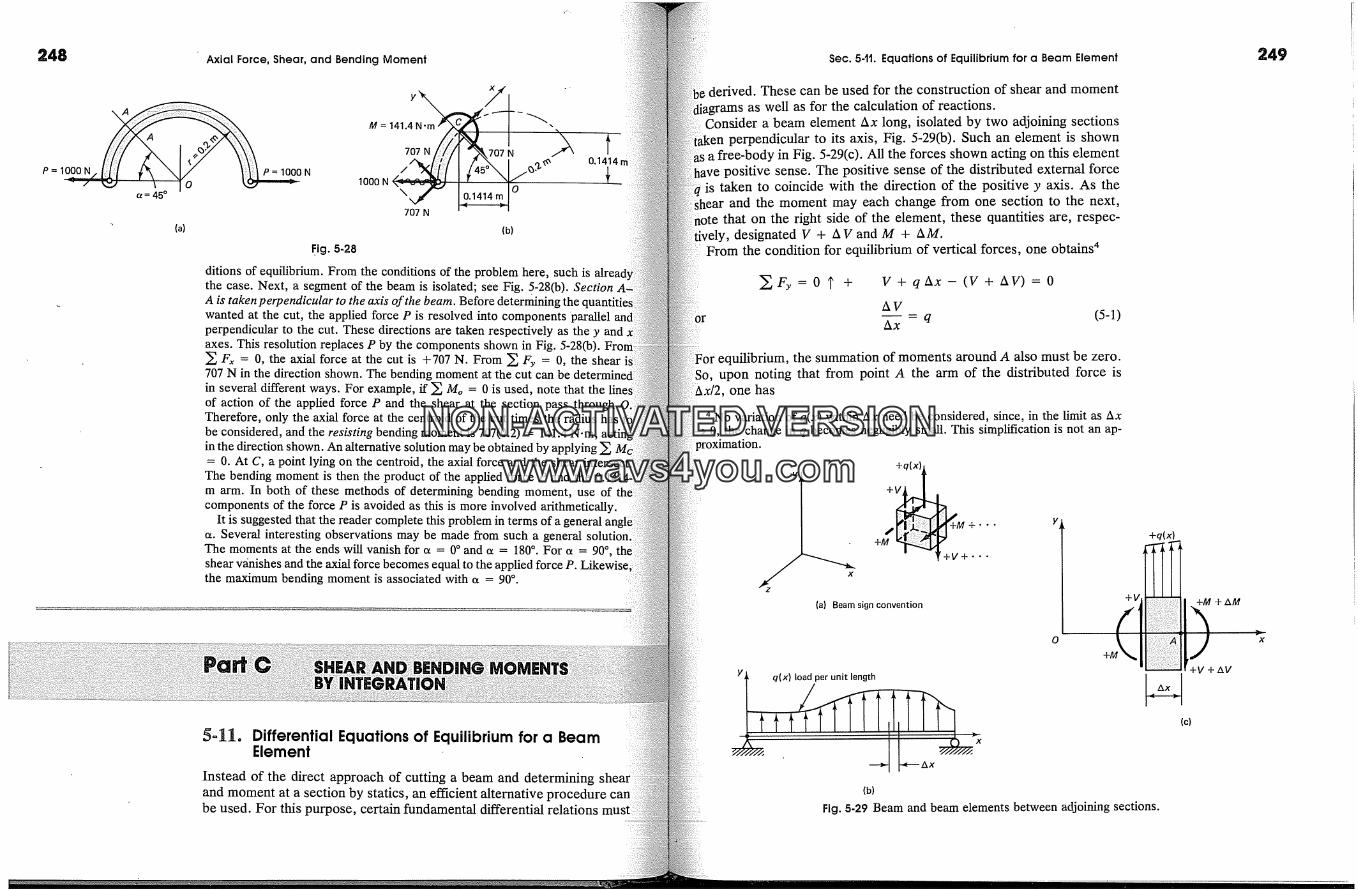
248 Axial Force, Shear, and Bending Moment Sec. 5-tt. Equations of Equilibrium for a Beam Element
P=Ic� = 45 �
(a)
Eig. 5-28
ditions of equilibrium. From the conditions of the problem here, such isthe case. Next, a segment of the beam is isolated; see Fig. 5-28(b). SectionA is taken perpendicular to the axis of the beam. Before determining thewanted at the cut, the applied force P is resolved into components parallelperpendicular to the cut. These directions are taken respectively as the y andaxes. This resolution replaces P by the components shown in Fig. 5-28(b).� Fx = 0, the axial force at the cut is +707 N. From � Fy = 0, the shear L,707 N in the direction shown. The bending moment at the cut canin several different ways. For example, if � Mo = 0 is used, note that the lineof action of the applied force P and the shear at the section pass throughTherefore, only the axial force at the centroid of the cut times the radius hasbe considered, and the resisting bending moment is 707(0.2) = 141.4 N.m,in the direction shown. An alternative solution may be obtained by applying �= 0. At C, a point lying on the centroid, the axial force and the shear intersectl
The bending moment is then the product of the applied force P and the 0.141�m arm. In both of these methods of determining bending moment, use ofcomponents of the force P is avoided as this is more involved
It is suggested that the reader complete this problem in terms of a generala. Several interesting observations may be made from such a general solution.The moments at the ends will vanish for a = 0 � and a = 180 �. For a = 90 �,shear vanishes and the axial force becomes equal to the applied force P. Likewisethe maximum bending moment is associated with a = 90 �.
5=]]� Differential Equations of Equilibrium for a BeamElement
Instead of the direct approach of cutting a beam and determining shearand moment at a section by statics, an efficient alternative procedurebe used. For this purpose, certain fundamental differential
derived. These can be used for the construction of shear and momentas well as for the calculation of reactions.
Consider a beam element Ax long, isolated by two adjoining sectionsperpendicular to its axis, Fig. 5-29(b). Such an element is shown
a free-body in Fig. 5-29(c). All the forces shown acting on this elementhave positive sense. The positive sense of the distributed external force
is taken to coincide with the direction of the positive y axis. As the�ar and the moment may each change from one section to the next,
that on the right side of the element, these quantities are, respec-designated V + A V and M + AM.
From the condition for equilibrium of vertical forces, one obtains 4
T + V+ qAx- (V+ AV) = 0
AV
Ax = q (5-1)
For equilibrium, the summation of moments around A also must be zero.So, upon noting that from point A the arm of the distributed force is
one has
4 No variation of q(x) within Ax need be considered, since, in the limit as AxO, the change in q becomes negligibly small. This simplification is not an ap-
Proximation.
Y +q(x)�
� +'" y+M �"�+v + �
(a) Beam sign convention
Y (qx)loadperuni�(b)
Flg. 5-29 Beam and beam elements between adjoining sections.
+q(x)
(c)
NON-ACTIVATEDVERSIONwww.avs4you.com
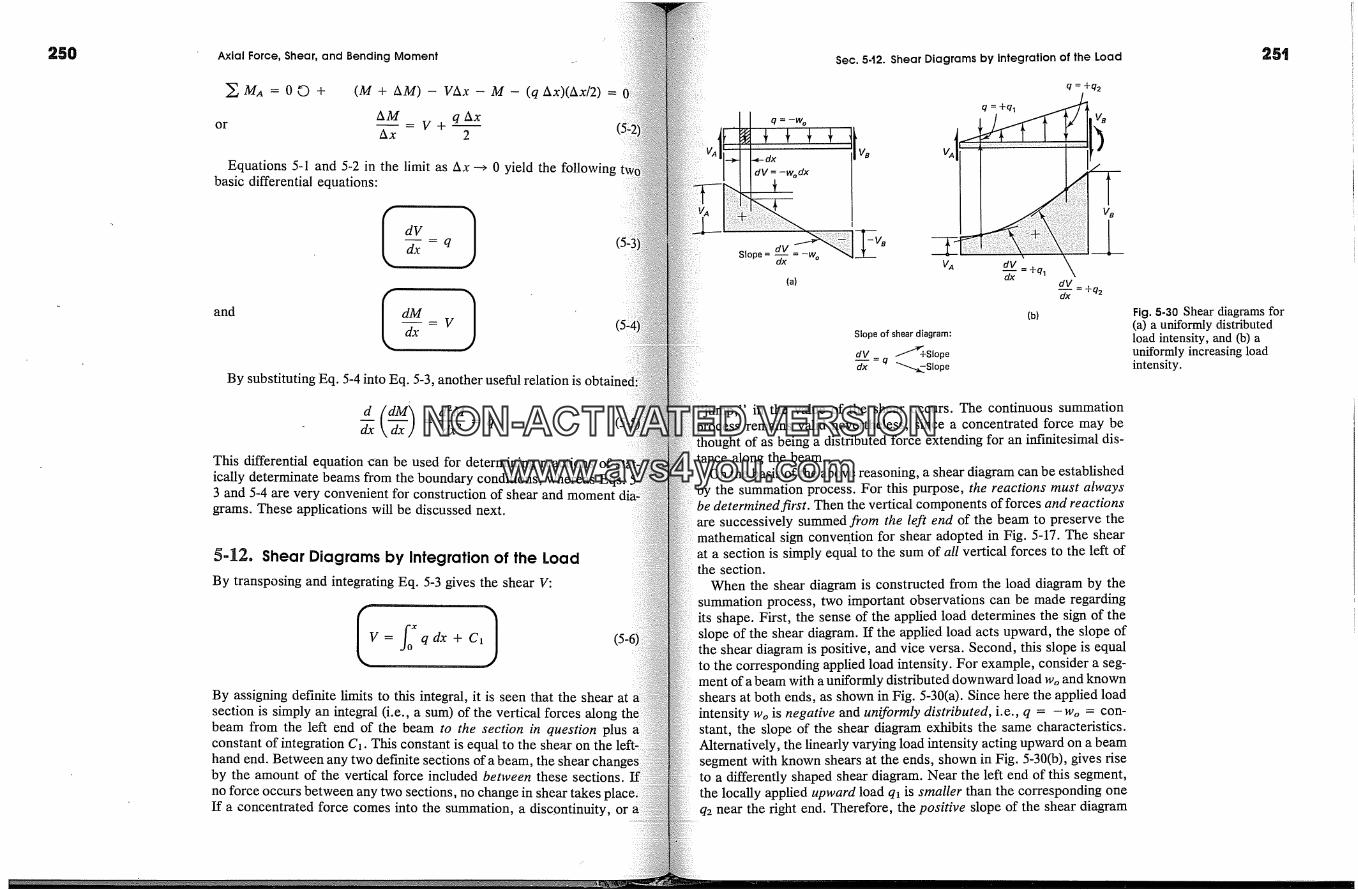
250 Axial Force, Shear, and Bending Moment . Sec. 542. Shear Diagrams by Integration of the Load
=o�+ (M + AM) - VAx - M - (q Ax)(Ax/2) =
AM q Ax=V+�
Ax 2
Equations 5-1 and 5-2 in the limit as Ax --> 0 yield the followingbasic differential equations:
I dvand I )
By substituting Eq. 5-4 into Eq. 5-3, another useful relation is
dx dx 2 =q
This differential equation can be used for determining reactions ofically determinate beams from the boundary conditions, whereas Eqs.3 and 5-4 are very convenient for construction of shear and momentgrams. These applications will be discussed next.
5-12. Shear Diagrams by Integration of the LoadBy transposing and integrating Eq. 5-3 gives the shear V:
By assigning definite limits to this integral, it is seen that the shear atsection is simply an integral (i.e., a sum) of the vertical forces alongbeam from the left end of the beam to the section in question plusconstant of integration C�. This constant is equal to the shear on thehand end. Between any two def'mite seciions of a beam, the shearby the amount of the vertical force included between these sections.no force occurs between any two sections, no change in shear takes'If a concentrated force comes into the summation, a discontinuity, or
-dx
dV = -wodx
Slope = d__�V=-wodx
(a)
Slope of shear diagram:
dV �Slopedx - q ""---..�.Slope
q = +q2
dV�xx = +ql
dVdx - +q2
(b)
"jump," in the value of the shear occurs. The continuous summationcess remains valid nevertheless, since a concentrated force may be
of as being a distributed force extending for an infinitesimal dis-tance along the beam.
On the basis of the above reasoning, a shear diagram can be establishedby the summation process. For this purpose, the reactions must alwaysbe determined first. Then the vertical components of forces and reactionsare successively summed from the left end of the beam to preserve themathematical sign convention for shear adopted in Fig. 5-17. The shearat a section is simply equal to the sum of all vertical forces to the left ofthe section.
When the shear diagram is constructed from the load diagram by thesummation process, two important observations can be made regardingits shape. First, the sense of the applied load determines the sign of theslope of the shear diagram. If the applied load acts upward, the slope ofthe shear diagram is positive, and vice versa. Second, this slope is equalto the corresponding applied load intensity. For example, consider a seg-ment of a beam with a uniformly distributed downward load Wo and knownshears at both ends, as shown in Fig. 5-30(a). Since here the applied loadintensity Wo is negative and uniformly distributed, i.e., q = -Wo = con-stant, the slope of the shear diagram exhibits the same characteristics.Alternatively, the linearly varying load intensity acting upward on a beamsegment with known shears at the ends, shown in Fig. 5-30(b), gives riseto a differently shaped shear diagram. Near the left end of this segment,the locally applied upward load q� is smaller than the corresponding oneq2 near the fight end. Therefore, the positive slope of the shear diagram
Fig. 5-30 Shear diagrams for(a) a uniformly distributedload intensity, and (b) auniformly increasing loadintensity.
NON-ACTIVATEDVERSIONwww.avs4you.com
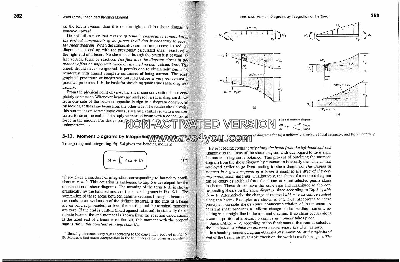
Axial Force, Shear, and Bending Moment
on the left is smaller than it is on the right, and the shear diaconcave upward.
Do not fail to note that a mere systematic consecutive summathe vertical components of the forces is all that is necessary tothe shear diagram. When the consecutive summation process isdiagram must end up with the previously calculated shearthe right end of a beam. No shear acts through the beam justlast vertical force or reaction. The fact that the diagram closes inmanner offers an important check on the arithmetical calculations.check should never be ignored. It permits one to obtain solutionspendently with al. most complete assurance of being correct. Thegraphical procedure of integration outlined before is verypractical problems. It is the basis for sketching qualitative shear,rapidly.
From the physical point of view, the shear sign convention- is notplotely consistent. Whenever beams are analyzed, a shear diafrom one side of the beam is opposite in sign to a diagramby looking at the same beam from the other side. The reader should �this statement on some simple cases, such as a cantilever with atrated force at the end and a simply supported beam with aforce in the middle. For design purposes, the sign of the shear isunimportant.
5-13. Moment Diagrams by Integration of the ShearTransposing and integrating Eq. 5-4 gives the bending moment
where C2 is a constant of integration corresponding to boundarytions at x = 0. This equation is analogous to Eq. 5-6 developed forconstruction of shear diagrams. The meaning of the term V dx isgraphically by the hatched areas of the shear diagrams in Fig. 5-31.summation of these areas between definite sections through a beamresponds to an evaluation of the definite integral. If the ends of aare on rollers, pin-ended, or free, the starting and the terminalare zero. If the end is built-in (fixed against rotation), in staticallyminate beams, the end moment is known from the reactionIf the fixed end of a beam is on the left, this moment with thesign is the initial constant of integration C2.
5 Bending moments carry signs according to the convention adopted19. Moments that cause compression in the top fibers of the beam are
Sec. 543. Moment Diagrams by Integration of the Shear 253
dMIdx = -V�
� -M B
dM�=- V1dx(a)
MB
dM.� = V� dx
Slope of moment diagram:
dM_ V /+Slopedx '"'----�-Slope
Fig. 541 Shear and moment diagrams for (a) a uniformly distributed load intensity, and (b) a uniformlyincreasing load intensity.
By proceeding continuously along the beam from the left-hand end andthe areas of the shear diagram with due regard to their sign,
moment diagram is obtained. This process of obfaining the momentfrom the shear difigram by summation is exactly the same as that
earlier to go from loading to shear diagrams. The change inmoment in a given segment of a beam is equal to the area of the cor-
�onding shear diagram. Qualitatively, the shape of a moment diagrambe easily established from the slopes at some selected points along
beam. These slopes have the same sign and magnitude as the cor-shears on the shear diagram, since according to Eq. 5-4, dM/
= V. Alternatively, the change of moment dM = V dx can be studiedthe beam. Examples are shown in Fig. 5-31. According to these
variable shears cause nonlinear variation of the moment. Aconstant shear produces a uniform change in the bending moment, re-sulting in a straight line in the moment diagram. If no shear occurs along
portion of a beam, no change in moment takes place.Since dM/dx = V, according to the fundamental theorem of calculus,
the maximum or minimum moment occurs where the shear is zero.In a bending-moment diagram obtained by summation, at the right-hand
end of the beam, an invaluable check on the work is available again. The
NON-ACTIVATEDVERSIONwww.avs4you.com
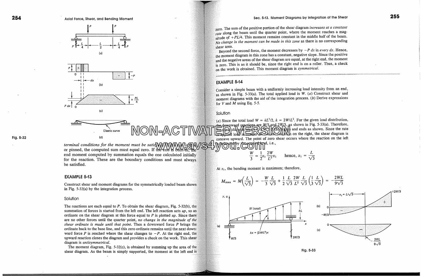
:254
Fig. 5-32
Axial Force, Shear, and Bending Moment
LP' --2--
(a)
I{I
o
(c)
-p
PL
Elastic curve
(d)
terminal conditions for the moment must be satisfied. If the end isor pinned, the computed sum must equal zero. If the end is built-in,end moment computed by summation equals the one calculated init:for the reaction. These are the boundary conditions and mustbe satisfied.
EXAMPLE 5-t3
Construct shear and moment diagrams for the symmetrically loadedin Fig. 5-32(a) by the integration process.
Solution
The reactions are each equal to P. To obtain the shear diagram, Fig. 5-32(b),summation of forces is started from the left end. The left reaction acts up, soordinate on the shear diagram at this force equal to P is plotted up. Sinceare no other forces until the quarter point, no change in the magnitude of tshear ordinate is made until that point. Then a downward force P bringsordinate back to the base line, and this zero ordinate remains until the nextward force P is reached where the shear changes to -P. At the right end,upward reaction closes the diagram and provides a check on the work. Thisdiagram is antisymmetrical.
The moment diagram, Fig. 5-32(c), is obtained by summing up the areashear diagram. As the beam is simply supported, the moment at the left
Sec. 5.13. Moment Diagrams by Integration of the Shear
The sum of the positive portion of the shear diagram increases at a constantalong the beam until the quarter point, where the moment reaches a mag-
: of +PL/4. This moment remains constant in the middle half of the beam.cha)Ige in the moment can be made in this zone as there is no corresponding
area.
the second force, the moment decreases by -P dx in eve�3' dr. Hence,diagram in this zone has a constant, negative slope. Since the positive
areas of the shear diagram are equal, at the right end, the momentzero. This is as it should be, since the right end is on a roller. Thus, a check
the work is obtained. This moment diagram is symmetrical.
MPLE 5-t4
a simple beam with a uniformly increasing load intensity from an end,shown in Fig. 5-33(a). The total applied load is W. (a) Construct shear and
diagrams with the aid of the integration process. (b) Derive expressionsV and M using Eq. 5-5.
Solution
Since the total load W = kL2/2, k = 2W/L 2. For the given load distribution,the downward reactions are W/3 and 2W/3, as shown in Fig. 5-33(a). Therefore,
shear diagram given in Fig. 5-33(b) begins and ends as shown. Since the rateload is smaller on the left end than on the right, the shear diagram is
upward. The point of zero shear occurs where the reaction on the leftis balanced by the applied load, i.e.,
W 1 2W L�- = �x�-�7x� hence, x� - V�
the bending moment is maximum; therefore,
W L
35 + 1 L 2W L (� L) _ 2WL2v'� L � �-� � 9V'�
kx = (2W/L�)x2W/3
(b)
(c)
o
-W/3
Fig. 5-33
2WL
9v'�
255
+2W/3
NON-ACTIVATEDVERSIONwww.avs4you.com
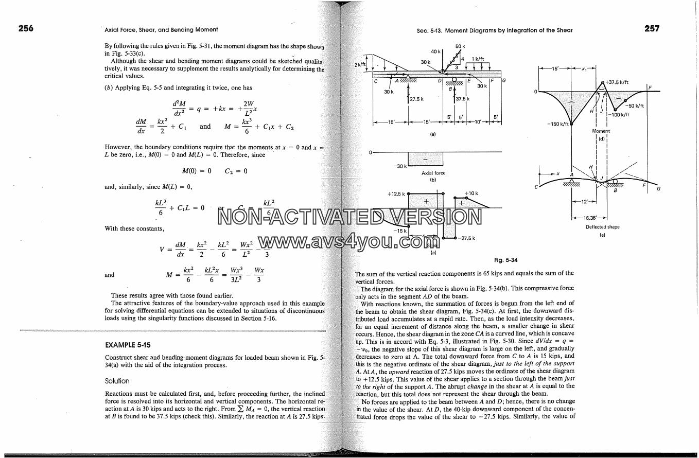
256 ' Axial Force, Shear, and Bending Moment Sec. 5-t3. Moment Diagrams by Integration of the Shear 257
By following the rules given in Fig. 5-31, the moment diagram has the shapein Fig. 5-33(c).
Although the shear and bending moment diagrams could be sketchedtively, it was necessary to supplement the results analytically forcritical values.
(b) Applying Eq. 5-5 and integrating it twice, one has
dM kx 2
d2M 2Wdx 2 - q= +kx= +'�-x
kx 3+ C� and M = + C�x + C2
6
However, the boundary conditions require that the moments at x = 0 and xL be zero, i.e., M(0) = 0 and M(L) = 0. Therefore, since
M(0) = 0 C2 = 0
and, similarly, since M(L) = 0,
kZ 3 kZ 2-- + C�L = 0 or C� =
6 6
With these constants,
dM. kx 2 kL 2 Wx 2 Wdx 2 6 L 2 3
and M =kx 2 kL 2x Wx 3 Wx
6 6 3L 2 3
These results agree with those found earlier.The attractive features of the boundary-value approach used in this
for solving differential equations can be extended to situationsloads using the singularity functions discussed in Section 5-16.
EXAMPLE 5-t5
Construct shear and bending-moment diagrams for loaded beam shown in Fig.34(a) with the aid of the integration process.
Solution
Reactions must be calculated first, and, before proceeding further, theforce is resolved into its horizontal and vertical components. Theaction at A is 30 kips and acts to the right. From � M,� = 0, theat B is found to be 37.5 kips (check this). Similarly, the reaction at A is 27.5 kip
50 k40 k
1 k/ft30k
C D G
30 k t27.5k 37.5 k
(a)
-30 k
Axial force
(b)
+12.5 k +10 k
-151
�-27.5 k
Shear
(c)
Fig. 5-34
sum of the vertical reaction components is 65 kips and equals the sum of theforces.
diagram for the axial force is shown in Fig. 5-34(b). This compresslye forceacts in the segment AD of the beam.
known, the summation of forces is begun from the left end ofthe beam to obtain the shear diagram, Fig. 5-34(c). At ftrst, the downward dis-
load accumulates at a rapid rate. Then, as the load intensity decreases,an equal increment of distance along the beam, a smaller change in shear
the shear diagram in the zone CA is a curved line, which is concave�. This is in accord with Eq. 5-3, illustrated in Fig. 5-30. Since dV/dx = q =Wo, the negative slope of this shear diagram is large on the left, and gradually
to zero at A. The total downward force from C to A is 15 kips, andthis is the negative ordinate of the shear diagram, just to the left of the support
the upward reaction of 27.5 kips moves the ordinate of the shear diagram+ 12.5 kips. This value of the shear applies to a section through the beam just
right of the support A. The abrupt change in the shear at A is equal to thebut this total does not represent the shear through the beam.
are applied to the beam between A and D; hence, there is no changethe value of the shear. At D, the 40-kip downward component of the concen-
:rated force drops the value of the shear to -27.5 kips. Similarly, the value of
-15'�-- Xl-'-�
� �37.5k/ft IFo-150 k/ff� I
� Moment
�(d) �B
�12'�
� 16.36'�
Deflected shape(e)
NON-ACTIVATEDVERSIONwww.avs4you.com
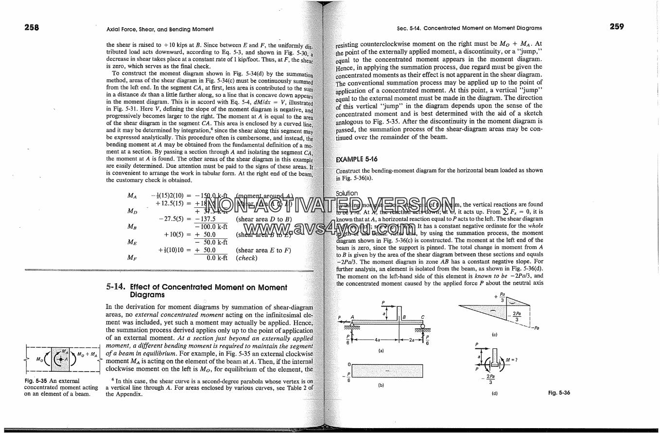
258
FIG.'5-35 An externalconcentrated moment actingon an element of a beam.
Axial Force, Shear, and Bending Moment
the shear is raised to + 10 kips at B. Since between E and F, thetributed load acts downward, according to Eq. 5-3, and shown in Fig.decrease in shear takes place at a constant rate of 1 kip/foot. Thus,is zero, which serves as the final check.
To construct the moment diagram shown in Fig. 5-34(d) by themethod, areas of the shear diagram in Fig. 5-34(c) must be continuouslyfrom the left end. In the segment CA, at ftrst, less area is contributed to thein a distance dx than a little farther along, so a line that is concave downin the moment diagram. This is in accord with Eq. 5-4, dM/dx = V,in Fig. 5-31. Here V, defining the slope of the moment diagram is negativeprogressively becomes larger to the fight. The moment at A is equal to theof the shear diagram in the segment CA. This area is enclosed by a curvedand it may be determined by integration, 6 since the shear along thisbe expressed analytically. This procedure often is cumbersome, andbending moment at A may be obtained from the fundamental definition of ament at a section. By passing a section through A and isolating the segmentthe moment at A is found. The other areas of the shear d!agram in thisare easily determined. Due attention must be paid to the signs of these areais convenient to arrange the work in tabular form. At the right end of thethe customary check is obtained.
MA --�(15)2(10) = --150.0 k-ft (moment around A)+ 12.5(15) = + 187.5 (shear area A to D)
MD + 37.5 k-ft-27.5(5) = - 137.5 (shear area D to B)
MB - 100.0 k-ft+ 10(5) = + 50.0 (shear area B to E)
ME - 50.0 k-ft+�(10)10 = + 50.0 (shear area E to F)
MF 0.0 k-ft (check)
5-]4. Effect of Concentrated Moment on MomentDiagrams
In the derivation for moment diagrams by summation ofareas, no external concentrated moment acting on the infinitesimalment was included, yet such a moment may actually be applied.the summation process derived applies only up to theof an external moment. At a section just beyond an externallymoment, a different bending moment is required to maintain theof a beam in equilibrium. For example, in Fig. 5-35 an externalmoment MA is acting on the element of the beam at A. Then, if theclockwise moment on the left is Mo, for equilibrium of the element,
6 In this case, the shear curve is a second-degree parabola whosea vertical line through A. For areas enclosed by various curves, see Tablethe Appendix.
Sec. 5.t4. Concentrated Moment on Moment Diagrams
counterclockwise moment on the right must be Mo + MA. Atpoint of the externally applied moment, a discontinuity, or a "jump,"
to the concentrated moment appears in the moment diagram.in applying the summation process, due regard must be given the
their effect is not apparent in the shear diagram.conventional summation process may be applied up to the point of
of a concentrated moment. At this point, a vertical "jump"to the external moment must be made in the diagram. The direction
this vertical "jump" in the diagram depends upon the sense of theOncentrated moment and is best determined with the aid of a sketch
to Fig. 5-35. After the discontinuity in the moment diagram isthe summation process of the shear-diagram areas may be con-
over the remainder of the beam.
:EXAMPLE 546
bending-moment diagram for the horizontal beam loaded as shown� Fig. 5-36(a).
ution
! taking moments about either end of the beam, the vertical reactions are foundbe P/6. At A, the reaction acts down; at C, it acts up. From � Fx = 0, it is
that at A, a horizontal reaction equal to P acts to the left. The shear diagramdrawn next; see Fig. 5-36(b). It has a constant negative ordinate for the whole
of the beam. After this, by using the summation process, the momentshown in Fig. 5-36(c) is constructed. The moment at the left end of the
is zero, since the support is pinned. The total change in moment from Ais given by the area of the shear diagram between these sections and equals
�2Pa/3. The moment diagram in zone AB has a constant negative slope. Forfurther analysis, an element is isolated from the beam, as shown in Fig. 5-36(d).
The moment on the left-hand side of this element is known to be -2Pa/3, andconcentrated moment caused by the applied force P about the neutral axis
A B C
(a)
(b)
.p (c)
P
_ 2Pa3
(d)
=?
Fig. 5-36
259
NON-ACTIVATEDVERSIONwww.avs4you.com
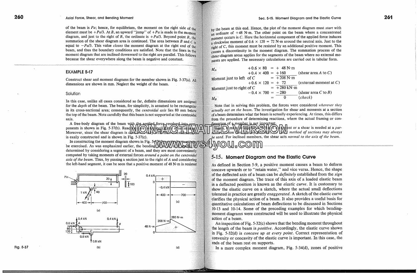
Axial Force, Shear, and Bending Moment
of the beam is Pa; hence, for equilibrium, the moment on the rigfit sideelement must be +Pal3. AtB, an upward "jump" of +Pa is made in the�diagram, and just to the right of B, the ordinate is +Pa/3. Beyond pointsummation of the shear diagram area is continued. The area between Bequal to -Pa/3. This value closes the moment diagram at the right endbeam, and thus the boundary conditions are satisfied. Note that the linesmoment diagram that are inclined downward to the right are parallel. Thisbecause the shear everywhere along the beam is negative and constant.
EXAMPLE 5-� 7
Construct shear ar/d moment diagrams for the member shown in Fig.dimensions are shown in mm. Neglect the weight of the beam.
Solution
In this case, unlike all cases considered so far, definite dimensions are assfor the depth of the beam. The beam, for simplicity, is assumed to bein its cross-sectional area; consequently, the centroidal axis lies 80 mmthe top of the beam. Note carefully that this beam is not supported at theaxis.
A free-body diagram of the beam with the applied force resolved intponents is shown in Fig. 5-37(b). Reactions are computed in the usualMoreover, since'the shear diagram is concerned only with the verticalis easily constructed and is shown in Fig. 5-37(c).
In constructing the moment diagram shown in Fig. 5-37(d), particular care�be exercised. As was emphasized earlier, the bending moments may alwaysdetermined by considering a segment of a beam, and they are mostcomputed by taking moments of external forces around a point on the cemaxis of the beam. Thus, by passing a section just to the right of A andthe left-hand segment, it can be seen that a positive moment of 48 N.m
�7/'///////////////� /////////////////� 20
(a)
0.6 kN 1� 0.8 kN
48N.m
o
280 N 'm
Fig. 5-37 (b) (d)
Sec. 5-t5. Moment Diagram and the Elastic Curve
beam at this end. Hence, the plot of the moment diagram must start withof +48 N.m. The other point on the beam where a concentrated
o. ccurs is C. Here the horizontal component of the applied force inducesmoment of 0.6 x. 120 = 72 N.m around the neutral axis. Just to the
i0f C, this moment must be resisted by an additional positive moment. Thisa discontinuity in the moment diagram. The summation process of the
areas applies for the segments of the beam where no external mo-are applied. The necessai'y calculations are carried out in tabular form.
+0.6x80 = + 48N.m+0.4x400 = +160
ust to left of C = + 208 N-m+0.6 x 120 = + 72
ust to right of C =-0.4 x 700 =
= 0
(shear area A to C)
(external moment at C)+280 kN.m
- 280 (shear area C to B)(check)
Note that in solving this problem, the forces were considered wherever theyact on the beam. The investigation for shear and moments at a section
a beam determines what the beam is actually experiencing. At times, this differsthe procedure of determining reactions, where the actual framing or con-
of a member is not important.it must be emphasized that if a moment or a shear is needed at a par-
section through any member, the basic method of sections may ahvays; used. For inclined members, the shear acts normal to the axis of the beatn.
Moment Diagram and the Elastic Curvedefined in Section 5-9, .a positive moment causes a beam to deform
upwards or to "retain water," and vice versa. Hence, the shapedeflected axis of a beam can be definitely established from the sign
moment diagram. The trace of this axis of a loaded elastic beama deflected position is known as the elastic curve. It is customary to
the elastic curve on a sketch, where the actual small deflectionspractice are greatly exaggerated. A sketch of the elastic curve
the physical action of a beam. It also provides a useful basis forcalculations of beam deflections to be discussed in Sections
[0-13 and 10-14. Some of the preceding examples for which bending-diagrams were constructed will be used to illustrate the physical
of a beam.
g. 5-32(c) shows that the bending moment throughoutlength of the beam is positive. Accordingly, the elastic curve shown
Fig. 5-32(d) is concave up at every point. Correct representation ofor concavity of the elastic curve is important. In this case, the
of the beam rest on supports.a more complex moment diagram, Fig. 5~34(d), zones of positive
NON-ACTIVATEDVERSIONwww.avs4you.com
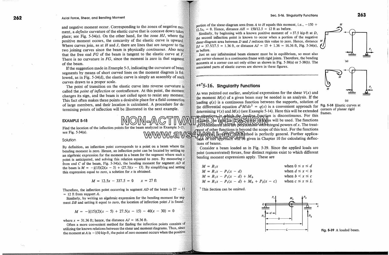
262 Axial Force, Shear, and Bending Moment
and negative moment occur. Corresponding to the zones of negativement, a definite curvature of the elastic curve that is concave downplace; see Fig. 5-34(e). On the other hand, for the zone HJ,positive moment occurs, the concavity of the elastic curve isWhere curves join, as at H and J, there are lines that are tangenttwo joining curves since the beam is physically continuous. Alsothat the free end FG of the beam is tangent to the elastic curveThere is no curvature in FG, since the moment is zero in thatof the beam.
If the suggestion made in Example 5-5, indicating the curvature of lsegments by means of short curved lines on the moment diagramlowed, as in Fig. 5-34(d), the elastic curve is simply an assemblycurves drawn to a proper scale.
The point of transition on the elastic curve into reverse curvaturecalled the point of inflection or contraflexure. At this point, thechanges its sign, and the beam is not called upon to resist anyThis fact often makes these points a deskable place for a field connectof large members, and their location is calculated. A proceduretermining points of inflection will be illustrated in the next
EXAMPLE 5-t8
Find the location of the inflection points for the beam analyzed in Example 5-1see Fig. 5-34(a)
Solution
By definition, an inflection point corresponds to a point on a beambending moment is zero. Hence, an inflection point can be located byan algebraic expression for the moment in a beam for the segment wherepoint. is anticipated, and solving this relation equated to zero. Byfrom end C of the beam, Fig. 5-34(e), the bending moment for segmentthe beam is M = -�(15)(2)(x - 5) + (27.5)(x - 15). By simplifying andthis expression equal to zero, a solution for x is obtained.
M = 12.5x - 337.5 = 0 x = 27 ft
Therefore, the inflection point occurring in segment AD of the beam is 27= 12 ft from support A.
Similarly, by writing an algebraic expression for the bending moment forment DB and setting it equal to zero, the location of inflection point J is
M = -�(15)(2)(x - 5) + 27.5(x - 15) - 40(x - 30) = 0
where x = 31.36 ft; hence, the distance AJ = 16.36 ft.Often a more convenient method for finding the inflection points
utilizing the known relations between the shear and moment diagrams. Thusthe moment at A is - 150 kip-ft, the point of zero moment occurs when the
Sec. 5-t6. Singularity Functions
of the shear-diagram area from A to H equals this moment, i.e., - 150 +12.5x� = 0. Hence, distance AH = 150/12.5 = 12 ft as before.
Similarly, by beginning with a known positive moment of + 37.5 kip-ft at D,secofid inflection point is known to occur when a portion of the negative
�r-cliagram area between D and J reduces this value to zero. Hence, distance-- 37.5/27.5 = 1.36 ft, or distance AJ = 15 + 1.36 = 16.36 ft, Fig. 5-34(e),
before.as any infinitesimal beam element must be in equilibrium, so must also
, comer element in a continuous frame with rigid joints. Therefore, the bendingat a comer can act only either as shown in Fig. 5-38(a) or 5-38(b). The
parts of elastic curves are shown in these figures.
g-16. Singularity Functionswas pointed out earlier, analytical expressions for the shear V(x) andmoment M(x) of a given beam may be needed in an analysis. If the
q(x) is a continuous function between the supports, solution ofdifferential equation d2m/dx 2 = q(x) is a convenient approach for
V(x) and M(x) (see Example 5-14). Here this will be extendedsituations in which the loading function is discontinuous. For this
the notation of operational calculus will be used. The functionsconsidered here are polynomials with integral powers ofx. The treat-
of other functions is beyond the scope of this text. For the functionshowever, the method is perfectly general. Further applica-
of this approach will be given in Chapter 10 for calculating deflec-iions of beams.
Consider a beam loaded as in Fig. 5-39. Since the applied loads are3int (concentrated) forces, four distinct regions exist to which different
moment expression� apply. These are
M = RlXM =Rlx-P�(x- d)M = R�x-P�(x- d) + MoM = R�x - P�(x - d) + Mo + P2(x - c)
7 This Section can be omitted.
when 0 -< x -< dwhen d -< x < bwhen b < x < c
when c -< x -< L
, P2
263
(a)
(b)
Fig. 5.38 Elastic curves atcomers of planar rigidframes.
Fig. 5-39 A loaded beam.
NON-ACTIVATEDVERSIONwww.avs4you.com
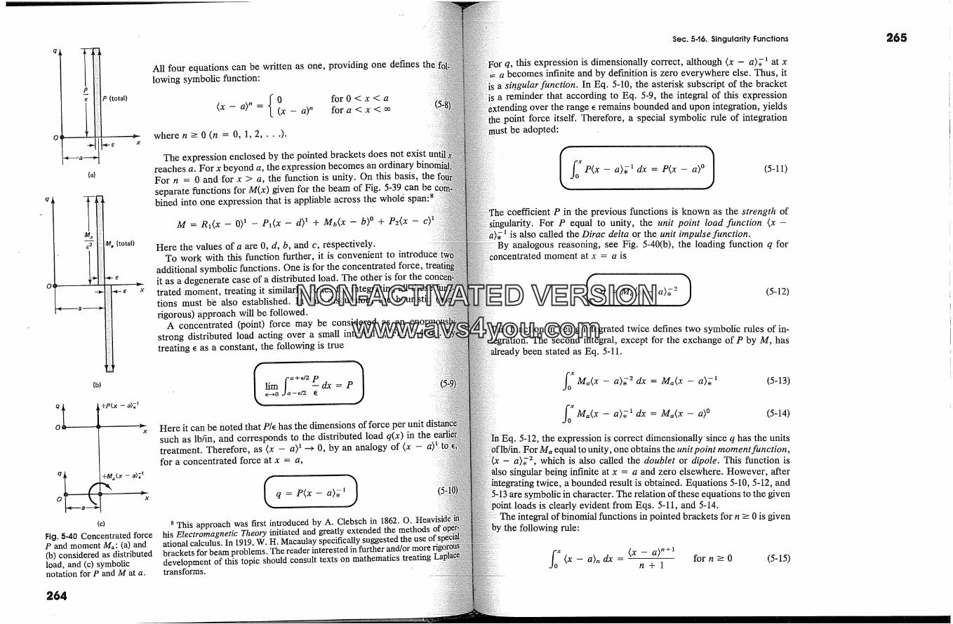
P (total)
(a)
x
m a-� Ma (total)
(b)
+P(x -
0 x
(c)
Fig. 5-40 Concentrated forceP and moment Ma: (a) and(b) considered as distributedload, and (c) symbolicnotation for P and M at a.
264
All four equations can be written as one, providing one de�meslowing symbolic function:
(x- a)� = {0 forO<x<a(x- a) � fora<x<�
wheren->0(n = 0,1,2 .... ).
The expression enclosed by the pointed brackets does not existreaches a. For x beyond a, the expression becomes an ordinaryFor n = 0 and-for x > a, the function is unity. On this basis,separate functions for M(x) given for the beam of Fig. 5-39 can belbined into one expression that is appliable across the whold
M = R�(x - O? - P�(x - d) � + Mb(X -- b) � + P2(x -- C)!
Here the values of a are 0, d, b, and c, respectively.To work with this function further, it is convenient to
additional symbolic functions. One is for the concentrated force,it as a degenerate case of a distributed load. The other is for thetrated moment, treating it similarly. Rules for integrating alltions must b� also established. In this discussion, the heuristic Irigorous) approach will be followed.
A concentrated (point) force may be considered as anstrong distributed load acting over a small interval e, Fig.treating e as a constant, the following is true
e--�O .Ja-�2 �
Here it can be noted that P/� has the dimensions of force persuch as lb/in, and corresponds to the distributed load q(x) in thetreatment. Therefore, as (x - a) � -> 0, by an analogy of (x -for a concentrated force at x = a,
q = P(x - a)��)8 This approach was first introduced by A. Clebsch in 1862. O.
his Electromagnetic Theory initiated and greatly extended the methods ofational calculus. In 1919, W. H. Macaulay specifically suggested the use of sbrackets for beam problems. The reader interested in further and/ordevelopment of this topic should consult texts on mathematics treatingtransforms.
Sec. 5.t6. Singularity Functions
this expression is dimensionally correct, although (x - a)� -� at xbecomes infinite and by definition is zero everywhere else. Thus, it
sin. guIarfunction. In Eq. 5-10, the asterisk subscript of the bracketa reminder that according to Eq. 5-9, the integral of this expression
over the range e remains bounded and upon integration, yieldspoint force itself. Therefore, a special symbolic rule of integration
be adopted:
I� P<x- a)�"dx=P(x- a)�1 (5-11)
coefficient P in the previous functions is known as the strength oft. For P equal to unity, the unit point load fimction (x -
is also called the Dirac delta or the unit impulse fimction.analogous reasoning, see Fig. 5-40(b), the loading function q for
recentrated moment at x = a is
(5-12)
function in being integrated twice defines two symbolic rules of in-The second integral, except for the exchange of P by M, has
been stated as Eq. 5-11.
�'M,(x - a)�-2 dx = M,(x - a)� � (5-13)
fi M,(x - a)� �dx = M,(x - a) � (5-14)
Eq. 5-12, the expression is correct dimensionally since q has the unitsFor M, equal to unity, one obtains the unit point moment function,
-- a)� 2, which is also called the doublet or dipole. This function is�so being infinite at x = a and zero elsewhere. However, after
twice, a bounded result is obtained. Equations 5-10, 5-12, andare symbolic in character. The relation of these equations to the given
loads is clearly evident from Eqs. 5-11, and 5-14.The integral of binomial functions in pointed brackets for n -> 0 is given
the following rule:
(x - a)n dx = (x - a) n+�� n + 1 for n > 0 (5-15)
265
NON-ACTIVATEDVERSIONwww.avs4you.com
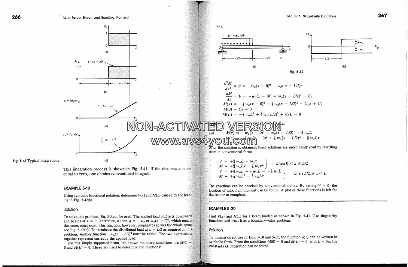
266
Fig. 5.4'1 Typical integrations.
Axial Force, Shear, and Bending Moment
(a)
qo
(b)
ql=:qod�[ 1 ' (x - a) 1
o- }-'"(c)
x
� -(x -
(d)
This integration process is shown in Fig. 5-41. If the distance a isequal to zero, one obtains conventional integrals.
EXAMPLE 5-t9
Using symbolic functional notation, determine V(x) and M(x) caused by theing in Fig. 5-42(a).
Solution
To solve this problem, Eq. 5-5 can be used. The applied load q(x) actsand begins at x = 0. Therefore, a term q = -wo or wo(x - 0) �, whichthe same, must exist. This function, however, propagates across the wholesee Fig. 5-42(b). To terminate the distributed load at x = L/2 as required inproblem, another function +wo(x - L/2) � must be added. The twotogether represent correctly the applied load.
For this simply supported beam, the known boundary conditions are M(0)0 and M(L) = 0. These are used to determine the reactions:
+y �
q = -w o lb/in
- L/2 � -'
(a)
Sec. 5-16. Singularity Functions
Fig. 5-42
+q
o
i L/24(b)
267
+w�x
�Mdx 2 - q = -wo(x - O) � + wo( x - LI2) �
dM--= V= -wo(x- O) � + wo(x - LI2) 1 + C1
dx
m(x) = -� Wo(X - 0) 2 + � Wo(X - L/2) 2 + C�x + C2M(O) = C2 = 0
M(L) = -� woZ 2 + � wo(L/2) 2 + CiL = 0
Hence, Ci = +as poL
V(x) = -Wo(X - O) � + Wo(X - L/2) � + as woLM(x) = -� Wo(X - 0) 2 + � Wo(X - L/2) 2 + as woLx
the solution is obtained, these relations are more easily read by rewritingin conventional form:
V = +-�woL - Wo.X }M +-� woLx - � wox 2 when 0 < x < LI2
V = +aswoL- �woL = -�woL}M +� woL 2 - � woLx when L/2 <- x < Lreactions can be checked by conventional statics. By setting V = 0, the
of maximum moment can be found. A plot of these functions is left forto complete.
EXAMPLE 5-20
V(x) and M(x) for a beam loaded as shown in Fig. 5-43. Use singularityfunctions and treat it as a boundary-value problem.
making direct use of Eqs. 5-10 and 5-12, the function q(x) can be written inform. From the conditions M(0) = 0 and M(L) = 0, with L = 3a, the
of integration can be found:
NON-ACTIVATEDVERSIONwww.avs4you.com
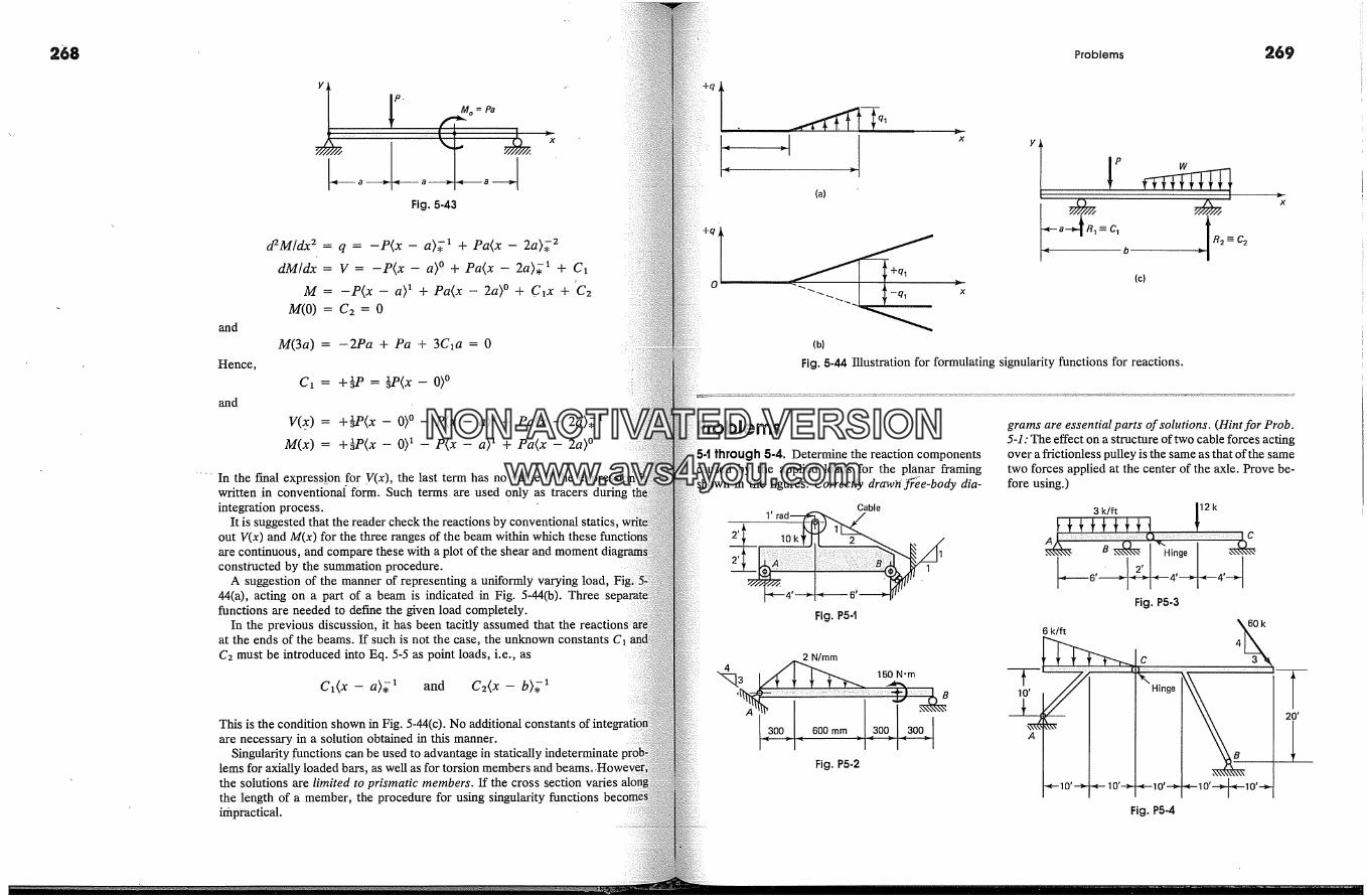
268
Fig. 5-43
and
Hence,
and
aeM/dx 2 = q = -P(x - a); � + Pa(x - 2a)� 2dM/dx = V = -P(x - a} � + Pa(x - 2a)� � + C�
M = -P(x - a) � + Pa(x - 2a} � + C�x + :C2M(O) = C2 = 0
M(3a) = -2Pa + Pa + 3C�a = 0
C,= �
V(_x) = +�-aP(x- 0} �- P(x - a} � + Pa(x - 2a}; �M(x) = +�P(x - O) � - P(x - a} � + Pa(x - 2a} �
In the final expression for y(x), the last term has no value if thewritten in conventional form. Such terms. are used only as tracers duringintegration process.
It is suggested that the reader check the reactions by conventional statics.out V(x) and M(x) for the three ranges of the beam within which theseare continuous, and compare these with a plot of the shear and momentconstructed by the summation procedure.
A suggestion of the manner of representing a uniformly varying load, Fig44(a), acting on a part of a beam is indicated in Fig. 5-44(b). Threefunctions are needed to define the given load completely.
In the previous discussion, it has been tacitly assumed that theat the ends of the beams. If such is not the case, the unknown constantsC2 must be introduced into Eq. 5-5 as point loads, i.e., as
C�(x - a)� 1 and C2(x - b)� -�
This is the condition shown in Fig. 5-44(c). No additional constantsare necessary in a solution obtained in this manner.
Singularity functions can be used to advantage in statically indeterminatelems for axially loaded bars, as well as for torsion members andthe solutions are limited to prismatic members. If the crossthe length of a member, the procedure for using singularity functionsimpractical.
-q ,
Problems 269
(a)
(b)
a � C�-=-%
b
(c)
Fig. 5-44 Illustration for formulating signularity functions for reactions.
through 5-4. Determine the reaction componentsby the applied loads for the planar framing
in the figures. Correctly draw}z' f�ke-body dia-Cable
Fig. P54
_ 2 N/mm
'x�3 {� 150 N'm,
L300�. 600ram [ 300 300JI- rl- =1 rl
Fig. P5-2
grams are essential parts of solutions. (Hint for Prob.5-1: The effect on a structure of two cable forces actingover a frictionless pulley is the same as that of the sametwo forces applied at the center of the axle. Prove be-fore using.)
3 k/f[ / 12 k
Fig, P5-3
6k/f[ C 4�k'1
{-<--10' --� -<-- 10'� 10'--� -<-- 10"�'� O,--�-Fig. P5-4
NON-ACTIVATEDVERSIONwww.avs4you.com
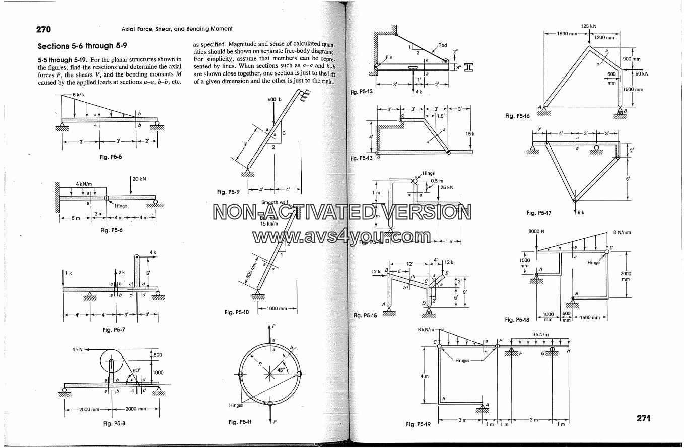
270 Axial Force, Shear, and Bending Moment
Sections 5.6 through 5-9
5-5 through 549. For the planar structures shown inthe figures, find the reactions and determine the axialforces P, the shears V, and the bending moments Mcaused by the applied loads at sections a-a, b-b, etc.
-- -- 6 k/ft
Fig. P5-5
4 kN/m �20 kN
I [ Hinge I3m -]� 5 m��- 4 m �4 m--�
Fig. P5-6
4k
lk �2k
Fig. P5-7
5 �
4kN-�
2000mm�
-� t 500
2000mm �IFig. P5-8
as specified. Magnitude and sense of calculatedtides should be shown on separate free-bodyFor simplicity, assume that members can besented by lines. When sections such as a-a andare shown close together, one section is just toof a given dimension and the other is just to the
a 3
Fig. P5*9 �---4'-'�' 4'---�Smooth wall
Barmass �x
15kg/��2
Fig. P5-t0 F1000 mm--�
Hin
Fig.
P
a tt
P
/Rod2 2"/Pin 2 ��
P543 �
Fig. P5.14
25 kN
g. P5-15
12k �
A D
8 kN/m--
C
m
Fig. P5d9
Fig. P5-16
125 kN
'�---1800mm �1200mm>
mm
900 mm
1500 mm
Fig. P5-t7 T 9 k
Fig. P5-t8 ' mm
H s
I lm Ilm
8 N/mm
C
2000mm
1500 mm-*'
6 kN/m
�/.F G H
� 3m �
NON-ACTIVATEDVERSIONwww.avs4you.com
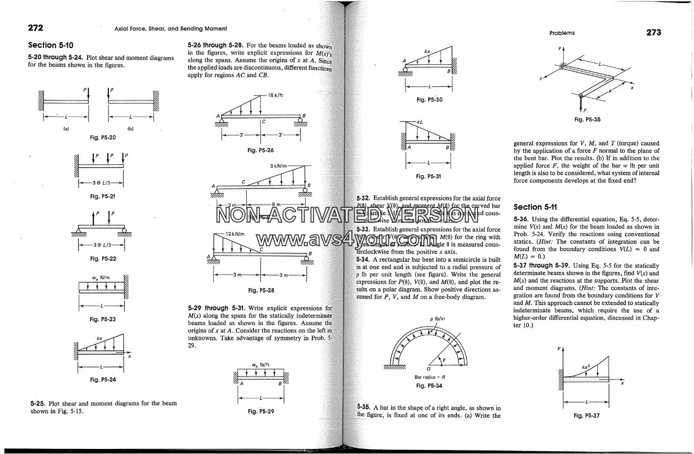
272 Axial Force, Shear, and Bending Moment
Section 5-10
5-20 through 5-24. ?lot shear and moment diagramsfor the beams shown in the figures.
5-26 through 5-28. For the beams loaded asin the figures, write explicit expressions foralong the spans. Assume the origins of x at A.the applied loads are discontinuous.apply for regions AC and CB.
(a) (b)
Fig. P5-20
Fig. P5-2t
t p [P
� 3 @ L/3 �Fig. P5-22
w o N/m �/,
Fig. P5-23
------ L �. xFig. P5-24
5-25. Plot shear and moment diagrams for the beamshown in Fig. 5-15.
- 3' > � 3'-----�Fig. P5-26
Fig. P5-27
A
Fig. P5-28
3m,
5-29 through 5-3t. Write explicitM(x) along the spans for the staticallybeams loaded as shown in the figures.origins ofx at A. Consider the reactions on theunknowns. Take advantage of symmetry in29.
w o Ib/ft
Fig� �5-29
Fig. P5�30
Fig. P5-31
Establish general expressions for the axial forceshear V(0), and moment M(0) for the curved bar
a Example 5-12, Fig. 5-28. Angle 0 is measured coun-the positive x axis.
Establish general expressions for the axial forceshear V(0), and moment M(0) for the ring withhinges of Prob. 5-11. Angle 0 is measured coun-
from the positive x axis.A rectangular bar bent into a semicircle is built
one end and is subjected to a radial pressure ofper unit length (see figure). Write the general
for P(0), V(0), and M(0), and plot the re-on a polar diagram. Show positive directions as-
P, V, and M on a free-body diagram.
p lb/in
Bar radius = R
Fig. P5-34
A bar in the shape of a right angle, as shown infigure, is fixed at one of its ends. (a) Write the
Problems
y
� L
z
Fig. P5-35
27:
general expressions for V, M, and T (torque) causedby the application of a force F normal to the plane ofthe bent bar. Plot the results. (b) If in addition to theapplied force F, the weight of the bar w lb per unitlength is also to be considered, what system of internalforce components develops at the fixed end?
Section 541
5-36. Using the differential equation, Eq. 5-5, deter-mine V(x) and M(x) for the beam loaded as shown inProb. 5-24. Verify the reactions using conventionalstatics. (Hint: The constants of integration can befound from the boundary conditions V(L) = 0 andM(L) = 0.)5-37 through 5-39. Using Eq. 5-5 for the staticallydeterminate beams shown in the figures, find V(x) andM(x) and the reactions at the supports. Plot the shearand moment diagrams. (Hint: The constants of inte-gration are found from the boundary conditions for Vand M. This approach cannot be extended to staticallyindeterminate beams, which require the use of ahigher-order differential equation, discussed in Chap-ter 10.)
Fig. P5-37
NON-ACTIVATEDVERSIONwww.avs4you.com
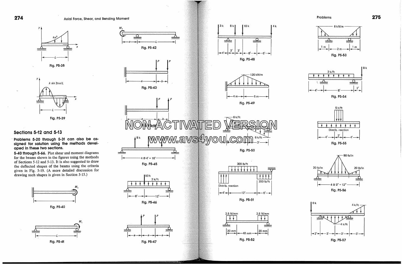
274 Axial Force, Shear, and Bending Moment
Fig. P5-38
k sin 2�rx/L
Fig. P5-39
Sections 5-12 and 543
-Problems 5-20 through 5-3t can also be as-signed for solution using the methods devel-oped in these two sections.5-40 through 5-66. Plot shear and moment diagramsfor the beams shown in the figures using the methodsof Sections 5-12 and 5-13. It is also suggested to drawthe deflected shapes of the beams using the criteriagiven in Fig. 5-19. (A more detailed discussion fordrawing such shapes is given in Section 5-15.)
Fig. P5-40
M1
Fig. P5-42
�-----a > -- bJFig. P5-43-
�ig. P5-4�
8k 112k 18k4@4'= 16'
Fig. P5-45
50 k 2 k/ft
Fig. P5-46
Fig. P5-41 Fig. P5-47
Fig. P5-48
Fig. P5-49
I / 6k/� �,6k/�k��ff�'"�---3' --' -� 3'Fig. P5-50
4k
300 Ib/ft
Distrib.reaction 200Ib/ftFig. P5-51
2.5 N/mm 2.5 N/mm
!�;m._m,<40ram r,2�-0m�!'Fig. P5-52
Problems
. m_� -� 2m 1�Fig. P5-53
2 k/ft /8 k
> -� 8' > �2'�Fig. P5-54
5 k/ft
Fig. P5-55
4@3 "= 12"Fig. P5-56
Fig. P5-57
275
NON-ACTIVATEDVERSIONwww.avs4you.com

276 Axial Force, Shear, and Bending Moment
2qo
Fig. P5-58
qo qo
2q�1/Fig. P5-59
10 kN/m
Fig. P5-60
qo
Fig. P5-61
300 lb200 Ib/ft
Fig. P5-63
�.1.� 400 Ib/ft
Fig. P5-64
20kN 5kN/m
Fig, P5-65
Hinge
Fig. P5-66
5-67, A sm�Qgu�e. �lot she� and momeQt dia�ams
20 kN/m
� 3m�3mFig. P5-62
Water level 1.5 k/ft
Fig. P5-67
15k
The load distribution for a small single-enginemay be idealized as shown in the fig-
In this diagram, vector A represents the weightthe 'engine; B, the uniformly distributed cabin
C, the weight of the aft fuselage; and D, thefrom the tail control surfaces. The upward
;E are developed by the two longerons from theUsing this data, constrLtct plausible, qualitative
� and moment diagrams for the fuselage.
Fig. P5-68
The moment diagram for a beam supported atand B is shown in the figure. How is the beam
loaded?
+55 k-ft // +65 k-h:
A B
Fig. P5-69
The redundant moment over support B for theshown in the figure can be shown to be -400by the methods discussed in Chapter 10. Plot
and moment diagrams for this beam.
100 k N/m
I,, ,
!� 8m----�8 m �Fig. P5-70
Problems 277
5-7t through 5-73. For the structural systems shownin the figures, plot the axial force P, shear V, and mo-ment M diagrams. Note that the axial force and shearcontribute to the equilibrium of forces at a joint in bentmembers (see Fig. 5-27).
,�200mm 200mm ! 200mmFig. P5-7t
Cables
Fig. P5-72
160 kN
3 wall
-Fig. P5-73
5-74. For member DF of the frame in Prob. 1-44, plotthe axial force, shear, and moment diagrams causedby the applied force.
Sections 5-14 and 5-15
5-75 through 5-8t. For the structural systems shownin the figures, plot the axial force P, shear V, and mo-
NON-ACTIVATEDVERSIONwww.avs4you.com
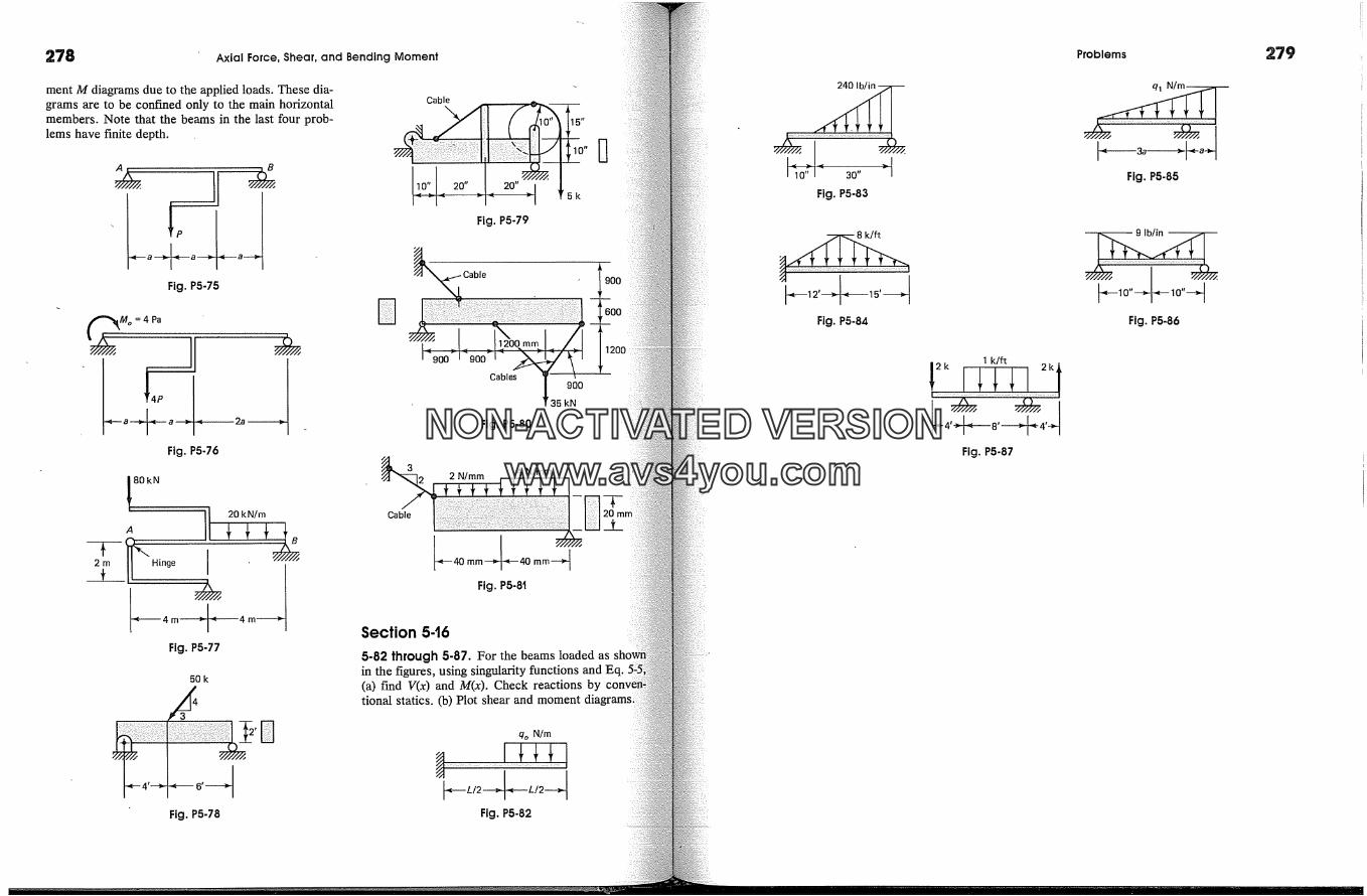
278 Axial Force, Shear, and Bending Moment
ment M diagrams due to the applied loads. These dia-grams are to be contimed only to the main horizontalmembers. Note that the beams in the last four prob-lems have finite depth.
Fig. P5-75
M o = 4 Pa '
Fig. P5-76
80kNA
2�--�m� '�HingeB
Fig. P5-77
50 k
3
Cable
Fig. P5-79
Cables
Fig. P5-80
900
' 35 kN
900
600
1200
2 N/mm 4 N/mm
Cable
Fig. P5-8t
Section 5-16
5-82 through 5-87. For the beams loaded asin the figures, using singularity functions and Eq.(a) find V(x) and M(x). Check reactions bytional statics. (b) Plot shear and moment
qo N/m
3o" "Fig. P5-83
Fig. P5-84
Fig. P5-87
Problems
Fig. P5-85
-- 9 lb/in --
Fig. P5-86
279
Fig. P5-78 Fig. P5-82
NON-ACTIVATEDVERSIONwww.avs4you.com
_ chapterSec. 6-2. The Basic Kinematic Assumption
�e of this chapter. A better appreciation of the instability phenomenonresult after the study of column buckling in Chapter 11.
28O
6-1o Introduction
In the previous chapter, it was shown that a system of internalconsisting of an axial force, a shear force, and a bending momentdevelop in planar frames and beams. The stresses caused bwere already discussed in Chapter 1. The stresses due to bendingconsidered in this chapter. For this treatment, it is convenient tothe chapter into two parts. In Part A, only members havingcross sections and subjected to bending in the plane of symmetryconsidered. Both elastic and inelastic stress distributions caused bying are discussed. Stress distribution in curved bars is also included.Part B, the problem is generalized to include unsymmetric bendingmembers with symmetric cross sections as well as bending ofof arbitrary cross section. Consideration is also given to problemsbending occurs in the presence of axial forces. For completeness, acussion on area moments of inertia for arbitrary crossin Part C.
For simplicity, members will generally be shown as beams in azontal position. When a segment of a beam is in equilibrium underaction of bending moments alone, such a condition is referred to asbending, orfiexure. A cantilever loaded with a concentratedthe end, or a segment of a beam between the concentrated forcesshown in Fig. 5-23, are examples of pure bending. Studies in subsetchapters will show that usually the bending stresses in slender beamsdominant. Therefore, the formulas derived in this chapter forare directly applicable in numerous design situations.
It is important to note that some beams by virtue of theiror lack of lateral support may become unstable under an applied loadmay buckle laterally and collapse. Such beams do not come within
The Basic Kinematic Assumption
the simplified engineering theory of bending, to establish the relationthe applied bending moment, the cross-sectional properties of a
and the internal stresses and deformations, the approach appliedin the torsion problem is again employed. This requires, first, that
a plausible deformation assumption reduce the internally statically in-problem to a determinate one; second, that the deformations
strains be related to stresses through the appropriate stress-strain; and, finally, that the equilibrium requirements of external and
forces be met. The key kinematic assumption for the deformationa beam as used in the simplified theory is discussed in this section. A
of this assumption forms the basis for the theories of platesmd shells.
For present purposes, consider a horizontal prismatic beam having asection with avertical axis of symmetry; see Fig. 6-1(a). A horizontal
line through the centroid of the cross section will be referred to as thetxis of a beam. Next, consider a typical element of the beam between
two planes perpendicular to the beam axis. In side view, such an elementidentified in the figure as abcd. When such a beam is subjected to equal
end moments Mz acting around the z axis, Fig. 6-1(b), this beam bendsin the plane of symmetry, and the planes initially perpendicular to the
beam axis slightly tilt. Nevertheless, the lines such as ad and bc becomingand b' c' remain straight. � This observation forms the basis for the
fundamental hypothesis 2 of the flexure theory. It may be stated thus: planesections through a beam taken normal to its axis remain plane after the
beam is subjected to bending.� This can be demonstrated by using a rubber model with a ruled grating drawn
it. Alternatively, thin vertical rods passing through the rubber block can beIn the immediate vicinity of the applied moments, the deformation is more
However, in accord with the St. Venant's principle (Section 2-10), thisis only a local phenomenon that rapidly dissipates.
2 This hypothesis with an inaccuracy was first introduced by Jacob Bernoulli1645-1705), a Swiss mathematician. At a later date a great Swiss mathematician,
Euler (1707-1783), who largely worked in Russia and Germany, madetmportant use of this concept. This assumption is often referred to as the Ber-
noulli-Euler hypothesis. In the correct final form, it dates back to the writings ofFrench engineering educator M. Navier (1785-1836).
NON-ACTIVATEDVERSIONwww.avs4you.com
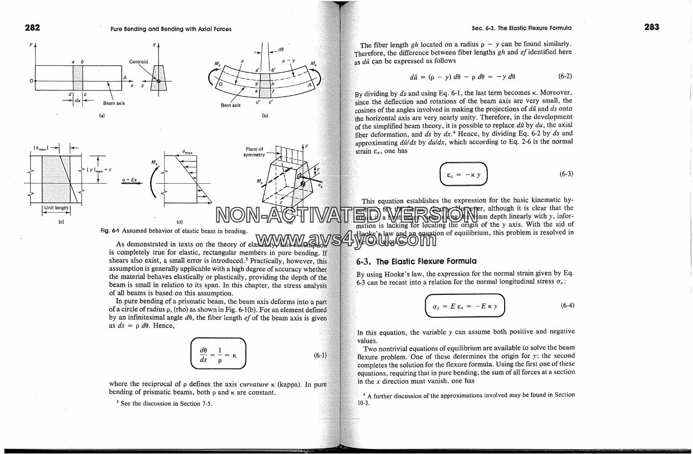
282
--� Beamaxis
Pure Bending and Bending with Axial Forces
Bent axis
(a)
p
d t
�b,d�p-y
(b)
�.�nit lengt�(c)
I Y Imax = C
a= EEl_
M z
OmaxPlane of
(d) (e)
Fig. 6-1 Assumed behavior of elastic beam in bending.
As demonstrated in texts on the theory of elasticity, thisis completely true for elastic, rectangular members in pure bending;shears also exist, a small error is introduced. 3 Practically, however,assumption is generally applicable with a high degree ofthe material behaves elastically or plastically, providing the depth ofbeam. is small in relation to its span. In this chapter, the stress anal'of all beams is based on this assumption.
In pure bending of a prismatic beam, the beam axis deforms into aof a circle of radius p, (rho) as shown in Fig. 6-1(b). For anby an infinitesimal angle d0, the fiber length ef of the beam axis isas ds = 0 dO. Hence,
where the reciprocal of p defines the axis curvature K (kappa). Inbending of prismatic beams, both p and K are constant.
3 See the discussion in Section 7-5.
Sec. 6-3. The Elastic Flexure Formula
The fiber length gh located on a radius p - y can be found similarly.the difference between fiber lengths gh and ef identified here
dfi can be expressed as follows
dfi = (p- y) d0- pd0 = -yd0 (6-2)
t dividing by ds and using Eq. 6-1, the last term becomes K. Moreover,the deflection and rotations of the beam axis are very small, the
:osines of the angles involved in making the projections of dfi and ds ontothe horizontal axis are very nearly unity. Therefore, in the development
the simplified beam theory, it is possible to replace dfi by du, the axialiber deformation, and ds by dx. 4 Hence, by dividing Eq. 6-2 by ds and
d�ds by du/dx, which according to Eq. 2-6 is the normale�,, one has
(6-3)
This equation establishes the expression for the basic kinematic hy-for the flexure theory. However, although it is clear that the
train in a bent beam varies along the beam depth linearly with y, infor-nation is lacking for locating the origin of the y axis. With the aid of
�oke's law and an equation of equilibrium, this problem is resolved innext section.
The Elastic Flexure Formula
using Hooke's law, th.e expression for the normal strain given by Eq.can be recast into a relation for the normal longitudinal stress or.,.'
(6-4)
this equation, the variable y can assume both positive and negative
Two nontrivial equations of equilibrium are available to solve the beamproblem. One of these determines the origin for y: the second
completes the solution for the flexure formula. Using the first one of theseequations, requiring that in pure bending, the sum of all forces at a section
the x direction must vanish, one has
4 A further discussion of the approximations involved may be found in Section
283
NON-ACTIVATEDVERSIONwww.avs4you.com
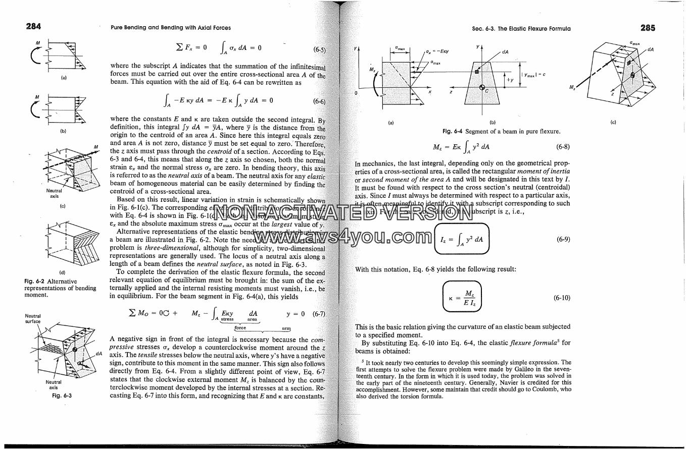
(a)
(b)
M
Neutralaxis
(c)
(d)
Fig. 6-2 Alternativerepresentations of bendingmoment.
Neutralsurface
Neutralaxis
Fig. 6-3
Pure Bending and Bending with Axial Forces
�, F.� = 0 /AO-�dA = 0where the subscript A indicates that the summation of the infinitesforces must be carded out over the entire cross-sectional area A ofbeam. This equation with the aid of Eq. 6-4 can be rewritten as
/A -E Ky dA = -E K fA Y dA = 0where the constants E and � are taken outside the second integral.definition, this integral .fy dA = yA, where y is the distance fro morigin to the centreid of an area A. Since here this integral equalsand area A is not zero, distance y must be set .equal tothe z axis must pass through the centreid of a section'. According to6-3 and 6-4, this means that along the z axis so chosen, both thestrain e�, and the normal stress cry, are zero. In bending theory, thisis referred to as the neutral axis of a beam. The neutral axis for anybeam of homogeneous material can be easily determined by findingcentreid of a cross-sectional area.
Based on this result, linear variation in strain is schematicallyin Fig. 6-1(c). The corresponding elastic stress distribution in accordwith Eq. 6-4 is shown in Fig. 6-1(d). Both the absolute maximume�, and the absolute maximum stress Crm�x occur at the largest value of;
Alternative representations of the elastic bending stress distributiona beam are illustrated in Fig. 6-2. Note the need for awareness thatproblem is three-dimensional, although for simplicity, two-dimensi�representations are generally used. The locus of a neutral axislength of a beam defines the neutral surface, as noted in Fig. 6-3.
To complete the derivation of the elastic flexure formula, therelevant equation of equilibrium must be brought in: the sum of theternally applied and the internal resisting moments must vanish, i.e.,in equilibrium. For the beam segment in Fig. 6-4(a), this yields
� Mo = OG + Mz - fAErY dA y = 0stress area �
A negative sign in front of the integral is necessary because thepressive stresses cry, develop a counterclockwise moment aroundaxis. The tensile stresses below the neutral axis, where y's have a nesign, contribute to this moment in the same manner. Thisdirectly from Eq. 6-4. From a slightly different point of view, Eq.states that the clockwise external moment Mz is balanced by theterclockwise moment developed by the internal stresses at a section.casting Eq. 6-7 into this form, and recognizing that E and � are c�
Sec. 6-3. The Elastic Flexure Formula
a� = -Et<yI Ymax I = c
X z
(a) (b)
Fig. 6.4 Segment of a beam in pure flexure.
Mz = E� fA y2 dA (6-8)In mechanics, the last integral, depending only on the geometrical prop-
of a cross-sectional area, is called the rectangular moment of inertiaor second moment of the area A and will be designated in this text by I.
must be found with respect to the cross section's neutral (centroidal)Since I must always be determined with respect to a particular axis,
is often meaningful to identify it with a subscript corresponding to suchaxis. For the case considered, this subscript is z, i.e.,
�Iz=/Ay2dA1 (6-9)this notation, Eq. 6-8 yields the following result:
(6-10)
rhis is the basic relation giving the curvature of an elastic beam subjecteda specified moment.
By substituting Eq. 6-10 into Eq. 6-4, the elastic flexure formula 5 foris obtained:
5 It took nearly two centuries to develop this seemingly simple expression. TheErrst attempts to solve the flexure problem were made by Galileo in the seven-
century. In the form in which it is used today, the problem was solved inearly part of the nineteenth century. Generally, Navier is credited for this
. some maintain that credit should go to Coulomb, whoderived the torsion formula.
(c)
285
Omax
NON-ACTIVATEDVERSIONwww.avs4you.com
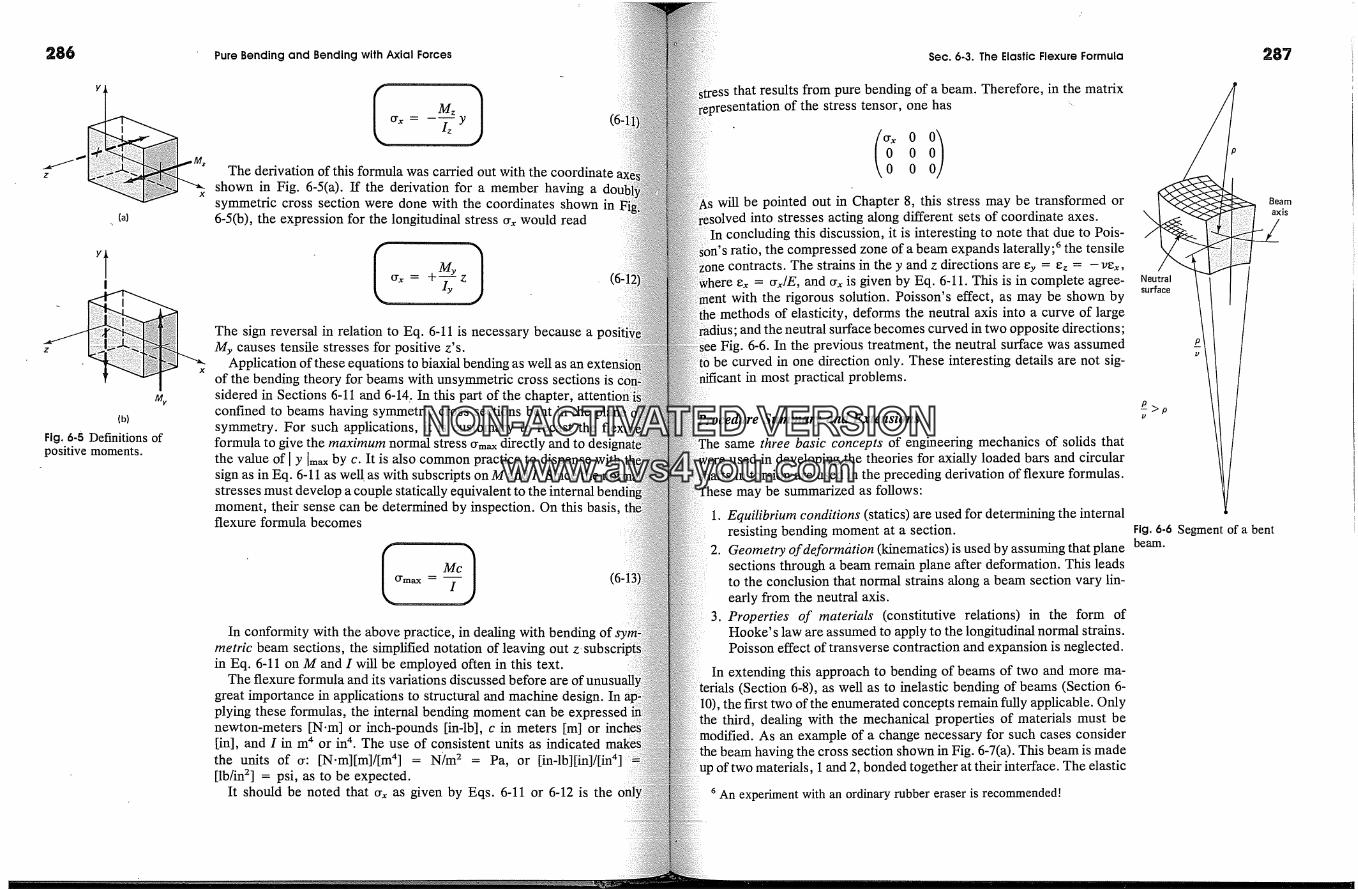
286
(a)
(b)
Fig. 6 -5 Definitions ofpositive moments.
Pure Bending and Bending with Axial Forces
Crx = -�zy (6:1
The derivation of this formula was carried out with the coordinateshown in Fig. 6-5(a). If the derivation for a member having asymmetric cross section were done with the coordinates shown in6-5(b), the expression for the longitudinal stress crx would read
O'x= M ZlThe sign reversal in relation to Eq. 6-11 is necessary because aMy causes tensile stresses for positive z's.
Application of these equations to biaxial bending as well as anof the bending theory for beams with unsymmetric cross sections issidered in Sections 6-11 and 6-14. In this part of the chapter,confined to beams having symmetric cross sections bent in thesymmetry. For such applications, it is customary to recast theformula to give the maximum normal stress Crm�x directly and to desithe value of l y Im�,, by c. It is also common practice to dispense withsign as in Eq. 6-11 as well as with subscripts onM and I. Sincestresses must develop a couple statically equivalent to themoment, their sense can be determined by inspection. On this basis,flexure formula becomes
(6-1!
In conformity with the above practice, in dealing withmetric beam sections, the simplified notation of leaving outin Eq. 6-11 on M and I will be employed often in this text.
The flexure formula and its variations discussed before aregreat importance in applications to structural and machine design. Inplying these formulas, the internal bending moment can be expressednewton-meters IN.m] or inch-pounds [in-lb], c in meters [m] or[in], and I in m 4 or in 4. The use of consistent units as indicatedthe units of or: [N.m][m]/[m 4] = N/m2 = Pa, or [in-lb][in]/[in 4][lb/in 2] = psi, as to be expected.
It should be noted that crx as given by Eqs. 6-11 or 6-12 is the
Sec. 6-3. The Elastic Flexure Formula
that results from pure bending of a beam. Therefore, in the matrixof the stress tensor, one has
will be pointed out in Chapter 8, this stress may be transformed or�solved into stresses acting along different sets of coordinate axes.
In concluding this discussion, it is interesting to note that due to Pois-ratio, the compressed zone of a beam expands laterally; 6 the tensile
contracts. The strains in the y and z directions are ey = e� = -vex,ex = �x/E, and crx is given by Eq. 6-11. This is in complete agree-
with the rigorous solution. Poisson's effect, as may be shown bymethods of elasticity, deforms the neutral axis into a curve of large
and the neutral surface becomes curved in two opposite directions;Fig. 6-6. In the previous treatment, the neutral surface was assumed
be curved in one direction only. These interesting details are not sig-in most practical problems.
wedure Summary and Extensionssame three basic concepts of engineering mechanics of solids that
used in developing the theories for axially loaded bars and circulars in torsion are used in the preceding derivation of flexure formulas.
may be summarized as follows:
1. Equilibrium conditions (statics) are used for determining the internalresisting bending moment at a section.
2. Geometry ofdeform�ition (kinematics) is used by assuming that planesections through a beam remain plane after deformation. This leadsto the conclusion that normal strains along a beam section vary lin-early from the neutral axis.
3. Properties of materials (constitutive relations) in the form ofHooke's law are assumed to apply to the longitudinal normal strains.Poisson effect of transverse contraction and expansion is neglected.
In extending this approach to bending of beams of two and more ma-(Section 6-8), as well as to inelastic bending of beams (Section 6-
the first two of the enumerated concepts remain fully applicable. Onlythe third, dealing with the mechanical properties of materials must be
As an example of a change necessary for such cases considerthe beam having the cross section shown in Fig. 6-7(a). This beam is madeup of two materials, 1 and 2, bonded together at their interface. The elastic
6 An experiment with an ordinary rubber eraser is recommended!
287
Beamaxis
Neutralsurface
Fig. 6.6 Segment of a bentbeam.
NON-ACTIVATEDVERSIONwww.avs4you.com
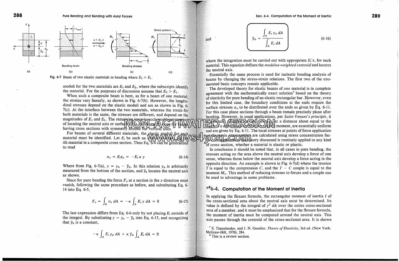
288
(a)
Fig. 6-7
Pure Bending and Bending with Axial Forces
o=E 1 �
o = E 2 E
Stress
Mz
Bending strain Bending stresses
(b) (c)
Beam of two elastic materials in bending where E2 > E�.(d)
moduli for the two materials are E1 and E2, where the-subscriptsthe material. For the purposes of discussion assume that E2
When such a composite beam is bent, as for a beam of onethe strains vary linearly, as shown in Fig. 6~7(b). However, thedinal stresses depend on the elastic moduli and are as shown in7(c). At the interface between the two materials, whereas the strainboth materials is the same, the stresses are different, and depend onmagnitudes of E� and E2. The remaining issue in such problems cons:of locating the neutral axis or surface. This can be easily done forhaving cross sections with symmetry around the vertical axes.
For beams of several different materials, the elastic moduli formaterial must be identified. Let Ei be such an elastic modulus forith material in a composite cross section. Then Eq. 6-4 can be gto read
Crx = Ei�x = -Ei K y
Where from Fig. 6-7(a), y = Yb -- Yb. In this relation Yb ismeasured from the bottom of the section, and yb locates the neutralas shown.
Since for pure bending the force Fx at a section in the x directionvanish, following the same procedure as before, and substituting Eq.14 into Eq. 6-5,
The last expression differs from Eq. 6-6 only by not placing Ei outsidethe integral. By substituting y = yu - yu into Eq. 6-15, and recothat Yb is a constant,
-}c /A Ei Yb dA + }c Yb fA Ei dA = 0
Sec. 6-4. Computation of the Moment of Inertia
Yb -- /A Ei dA (6-16)
the integration must be carried out with appropriate E?s, for eachThis equation defines the modulus-weighted centroid and locates
neutral axis.Essentially the same process is used for inelastic bending analysis of
by changing the stress-strain relations. The first two of the enu-basic concepts remain applicable.
developed theory for elastic beams of one material is in completewith the mathematically exact solution 7 based on the theory
pure bending of an elastic rectangular bar. However, eventhis limited case, the boundary conditions at the ends require the
stresses Crx to be distributed over the ends as given by Eq. 6-11.)r this case plane sections through a beam remain precisely plane after
However, in usual applications, per Saint-Venant's principle, itis generally assumed that the stresses, at a distance about equal to thedepth of a member away from the applied moment, are essentially uniform
given by Eq. 6-11. The local stresses at points of force applicationin cross section are calculated using stress concentration fac-
In applications the theory discussed is routinely applied to any kindof cross section, whether a material is elastic or plastic.
In conclusion it should be noted that, in all cases in pure bending, thestresses acting on the area above the neutral axis develop a force of one
whereas those below the neutral axis develop a force acting in thedirection. An example is shown in Fig. 6~7(d) where the tension
T is equal to the compression C, and the T - C couple.is equal to themoment Mz. This method of reducing stresses to forces and a couple can
be used to advantage in some problems..
Computation of the Moment of InertiaIn applying the flexure formula, the rectangular moment of inertia I ofthe cross-sectional area about the neutral axis must be determined. Its
is defined by the integral of y2 dA over the entire cross-sectionalarea of a member, and it must be emphasized that for the flexure formula,
moment of inertia must be computed around the neutral axis. Thisixis passes through the centroid of the cross-sectional area. It is shown
7 S. Timoshenko, and J. N. Goodier, Theory of Elasticity, 3rd ed. (New York:1970), 284.
8 This is a review section.
289
NON-ACTIVATEDVERSIONwww.avs4you.com

290 Pure Bending and Bending with Axial Forces Sec. 6-4. Computation of the Moment of Inertia
Fig. 6-8 Area for deriving theparallel-axis theorem.
in Sections 6-15 and 6-16 that for symmetric cross sections, theaxis is perpendicular to the axis of symmetry. The moment ofaround such an axis is either a maximum or a minimum, and forreason, this axis is one of the principal axes for an area. Thefor determining centroids and moments of inertia of areas arethoroughly discussed in texts on statics. 9 However, forthey are reviewed in what follows.
The first step in evaluating I for an area is to find its centroidintegration of y2 dA is then performed with respect to the horizontal ipassing through the area's centroid. In applications of the flexure fothe actual integration over areas is necessary for only a fewshapes, such as rectangles, triangles, etc. Values of moments offor some simple shapes may be found in texts on statics as well as. instandard civil or mechanical engineering handbook (also see Tablethe Appendix). Most cross-sectional areas used may be dividedcombination of these simple shapes. To find I for an areaseveral simple shapes, the parallel-axis theorem (sometimes calledtransfer formula) is necessary; its development follows.
Consider that the area A shown in Fig. 6-8 is a part of a complexof a cross section of a beam in flexure. The centroidal axis zc for thisis at a distance dz from the centroidal z axis for the wholearea. Then, by definition, the moment of inertia Izc of the area Aits zc axis is
Itc = �AY2� (6-1
On the other hand, the moment of inertia It of the same area Athe z axis is
Iz = �A (y� + dz)2dABy squaring the quantities in the parentheses and placing theoutside the integrals,
Iz = fA y2�dA + 2dz �A yC dA + d�2 �A dAHere the first integral according to Eq. 6-17 is equal to Izc, theintegral vanishes as y� passes through the centroid of A, and theintegral reduces to Ad� 2. Hence,
9 For example, see J. L. Meriam and L. G. Kraige, EngineeringVol. 1, Statics, 2nd ed. (New York: Wiley, 1986).
Iz = Izc+ Adz2� (6-18)
is the parallel-axis theorem. It can be stated as follows: the moment'inertia of an area around any axis is equal to the moment of inertia of
the same area around a parallel axis passing through the area's centroid,the product of the same area and the square of the distance between
the two axes.In calculations, Eq. 6-18 must be applied to each part into which a
�ss-sectional area has been subdivided and the results summed to obtainIz for the whole section, i.e.,
It (whole section) = �(Izc + Ad� 2) (6-18a)
process is completed, the z subscript may be dropped in treatingof symmetric cross sections.
The following examples illustrate the method of computing I directlyintegration for two simple areas. Then an application of the parallel-
theorem to a composite area is given. Values for I for commerciallyfabricated steel beams, angles, and pipes are given in Tables 3 to 8 of theAppendix.
EXAMPLE 6-t
the moment of inertia around the horizontal axis passing through the centroidfor the rectangular area shown in Fig. 6-9.
The centroid of this section lies at the intersection of the two axes of symmetry.Here it is convenient to take dA as b dy. Hence,
.J-hi2 y2b dy = b+hi2 bh 3--h/2 12
C bh3h �i�b3h)expressions are used frequently, as rectangular beams are common.
y
Fig. 6-9
NON-ACTIVATEDVERSIONwww.avs4you.com

292 Pure Bending and Bending with Axial Forces Sec. 6-5. Applications of the Flexure Formula 293
y�
28.3
Fig. 6-t0
Fig. 6-11
EXAMPLE 6-2
Find the moment of inertia about a diameter for a circular area of radius c;Fig. 6-10.
Solution
To find I for a circle, first note that D 2 = Z 2 + y2, as may be seen from the fiThen using the definition of J, noting the symmetry around both axes, andEq. 4-2,
J= f,�p2.dA = f,�(Y2+z2) dA= f,�y2dA+ f,�z2dA= + Iy=
= --J_2 4
In mechanical applications, circular shafts often act as beams; hence, Eq.20 will be found useful. For a tubular shaft, the moment of inertia of theinterior must be subtracted from the last expression.
EXAMPLE 6-3
Determine the moment of inertia I around the horizontal axis for the areain mm in Fig. 6-11 for use in the flexure formula.
Solution
As the moment of inertia is for use in the flexure formula, it must bearound the axis through the centroid of the area. Hence, the centroid of themust be found first. This is most easily done by treating the entire outerand deducting the hollow interior from it. For convenience, the work isout in tabular form. Then the parallel-axis theorem is used to obtain I.
60
y [ram]Area A [mm 2] (from bottom) Ay
Entire area 40 x 60 = 2400 30 72 000Hollow interior -20 x 30 = -600 35 -21 000
�A = 1800mm 2 �Ay = 51000
� Ay 51 000800
- 28.3 mm from bottom
,. the entire area:
bh 3 40 x 603Izc = 1-�- = 12 - 72 x 104 mm 4
Ad 2 = 2400(30 - 28.3) 2 = 0.69 X 104 mm 4I� = 72.69 x 104 mm 4
the hollow interior:
bh 3 20 X 30312 12
Ad 2 = 600(35 - 28.3) 2 =Iz=
composite section:
4.50 x 104 mm 4
2.69 x 104 mm 4
7.19 x 104 mm 4
Iz = (72.69 - 7.19)104 = 65.50 x 104 mm 4
Note particularly that in applying the parallel-axis theorem, each element ofcomposite area contributes two terms to the total I. One term is the moment
' inertia of an area around its own centroidal axis, the other term is due to thetransfer of its axis to the centroid of the whole area. Methodical work is the prime
in solving such problems correctly.
6-5. Applications of the Flexure Formulalargest stress at a section of a beam is given by Eq. 6-13, O'max =
and in most practical problems, it is this maximum stress that hasbe determined. Therefore, it is desirable to make the process of de-
g O'max as simple as possible. This can be accomplished by notingboth I and c are constants for a given section of a beam. Hence,
is a constant. Moreover, since this ratio is only a function of the cross-dimensions of a beam, it can be uniquely determined for any
area. This ratio is called the elastic section modulus of awill be designated by S. With this notation, Eq. 6-13 becomes
O'max--� (6-21)stated otherwise
maximum bending stress =bending moment
elastic section modulus
NON-ACTIVATEDVERSIONwww.avs4you.com

Pure Bending and Bending with Axial Forces
If the moment of inertia I is measured in in 4 (or m 4) and c in inS is measured in in 3 (or m3). Likewise, ifM is measured in in-lb (orthe units of stress, as before, become psi (or N/m2). It bearsthat the distance c as used here is measured from the neutral axis tomost remote fiber of the beam. This makes I/c = S a minimum,consequently M/S gives the maximum stress. The efficient sectionsresisting elastic bending have as large an S as possible for aof material. This is accomplished by locating as much of thepossible far from the neutral axis.
The use of the elastic section modulus in Eq. 6-21 correspondswhat to the use of the area termA in Eq. 1-13 (or = P/A). However,the maximum flexural stress on a section is obtained from Eq.whereas the stress computed from Eq. 1-13 holds true across thesection of a member.
Equation 6-21 is widely used in practice because of its simplicity.facilitate its use, section moduli for many manufactured crossare tabulated in handbooks. Values for a few steel sections are givenlTables 3 to 8 in the Appendix. Equation 6-21 is particularlyfor the design of beams. Once the maximum bending moment foris determined and an allowable stress is decided upon, Eq. 6-21 maysolved for the required section modulus. This information is sufficientqselect a beam. However, a detailed consideration of beam designdelayed until Chapter 9. This is necessary inasmuch as a shearwhich in turn causes stresses, usually also acts at a beam section.interaction of the various kinds of stresses must be considered first
gain complete insight into the problem.The following two examples illustrate calculations for bending
at specified sections, where, in addition to bending moments, shearsalso required for equilibrium. As shown in the next chapter, theof small or moderate shears does not significantly affect thestresses in slender beams. Both moment and shear frequentlythe same section simultaneously.
EXAMPLE 6-4
A 300 by 400 mm wooden cantilever beam weighing 0.75 kN/m carries anconcentrated force of 20 kN at the end, as shown in Fig. 6-12(a). Determinemaximum bending stresses at a section 2 m from the free end.
Solution
A free-body diagram for a 2-m segment of the beam is shown in Fig.keep this segment in equilibrium requires a shear of 20 - (0.75 x 2) = 18.5and a bending moment of(20 x 2) - (0.75 x 2 x 1) = 38.5Both of these quantities are shown with their proper sense in.Fig. 6-12(c).distance from the neutral axis to the extreme fibers c = 200 mm. Thi�to both the tension and the compression fibers.
Sec. 6-5. Applications of the Flexure Formula
r�=20 kN0.75 kN/m
--L
(a)
.I
300mm
rn
(b)
Fig. 6-t2
�20kN �0.75kN/m
(c)
Eq. 6-19:
bh 3 300 X 4003It .... 16 x 108 mm
12 12
Eq. 6-13:
Mc 38.5 X 106 X 200Crm�x I 16 X 108 = +4.81 MPa
From the sense of the bending moment shown in Fig. 6-12(c), the top fibers ofare seen to be in compression and the bottom ones in tension. In the
,riven, the positive sign applies to the tensile stress and the negative signapplies to the compressive stress. Both of these stresses decrease at a linear rate
toward the neutral axis, where the bending stress is zero. The normal stresseson infinitesimal elements at A and B are shown in Fig. 6-12(d). It is im-
� learn to make such a representation of an element as it will be frequentlyChapters 8 and 9.
Soldion
If only the maximum stress is desired, the equation involving the section modulusmay be used. The section modulus for a rectangular section in algebraic form is
I bh 3 2 bh 2s .... (6-22)
c 12 h 6
[n this problem, S = 300 x 4002/6 = 8 x 106 mm 3, and by Eq. 6-21,
M 38.5 X 10 6O'max- S 8 X 10⁶ 4.81 MPa
solutions lead to identical results.
295
Pa
(d)
NON-ACTIVATEDVERSIONwww.avs4you.com
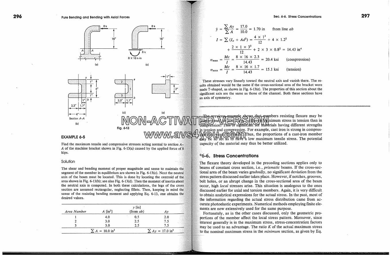
296 Pure Bending and Bending with Axial Forces
8k
16"
.�8k8 X 16 k-in
(a)
8k
Section A-A
(b)
I? .v_ i?':1
(d) (e)
Fig. 6-t3
EXAMPLE
Find the maximum tensile and compressive stresses acting normal toA of the machine bracket shown in Fig. 6-13(a) caused by the applied forcekips.
Solution
The shear and bending moment of proper magnitude and sense tosegment of the member in equilibrium are shown in Fig. 6-13(c). Next the:axis of the beam must be located. This is done by locating the centroidarea shown in Fig. 6-13(b); see also Fig. 6-13(d). Then the momentthe neutral axis is computed. In both these calculations, the legs of thesection are assumed rectangular, neglecting fillets. Then, keeping in mindsense of the resisting bending moment and applying Eq. 6-13, one obtainsdesired values.
y [in]Area Number A [in 2] (from ab) Ay
1 4.0 0.5 2.02 3.0 2.5 7.53 3.0 2.5 7.5
� A = 10.0 in 2 � Ay = 17.0 in3
Sec. 6-6. Stress Concentrations
� Ay 17.0:P- E� = 10.---� = 1.70 in from line ab
4xl 3I= �(Io +Ad 2)- 12 + 4 x 1.2 2
2xlx3 3+ + 2 x 3 x 0.82 = 14.43in 4
12.Mc 8 x 16 x 2.3
�m�x - - = 20.4 ksi (compression)I 14.43
Mc 8 x 16 x 1.7O'max -� = = 15.1 ksi (tension)
I 14.43
These stresses vary linearly toward the neutral axis and vanish there. The re-obtained would be the same if the cross-sectional area of the bracket were
led, as shown in Fig. 6-13(e). The properties of this section about theaxis are the same as those of the channel. Both these sections have
axis of symmetry.
previous example shows that members resisting flexure may be�ortioned so as to have a different maximum stress in tension than in
This is significant for materials having different strengthstension and compression. For example, cast iron is strong in compres-
and weak in tension. Thus, the proportions of a cast-iron memberbe so set as to have a low maximum tensile stress. The potential
of. the material may thus be better utilized.
Stress Concentrations
flexure theory developed in the preceding sections applies only tobeams of constant cross section, i.e., prismatic beams. If the cross-sec-
area of the beam varies gradually, no significant deviation from the3attern discussed earlier takes place. However, if notches, grooves,
holes, or an abrupt change in the cross-sectional area of the beamhigh local stresses arise. This situation is analogous to the ones
earlier for axial and torsion members. Again, it is very difficultto obtain analytical expressions for the actual stress. In the past, most of
Ihe information regarding the actual stress distribution came from ac-photoelastic experiments. Numerical methods employing finite ele-are now extensively used for the same purpose.
Fortunately, as in the other cases discussed, only the geometric pro-of the member affect the local stress pattern. Moreover, since
generally is in the maximum stress, stress-concentration factorsbe used to an advantage. The ratio K of the actual maximum stress
to the nominal maximum stress in the �nin#num section, as given by Eq.
297
NON-ACTIVATEDVERSIONwww.avs4you.com
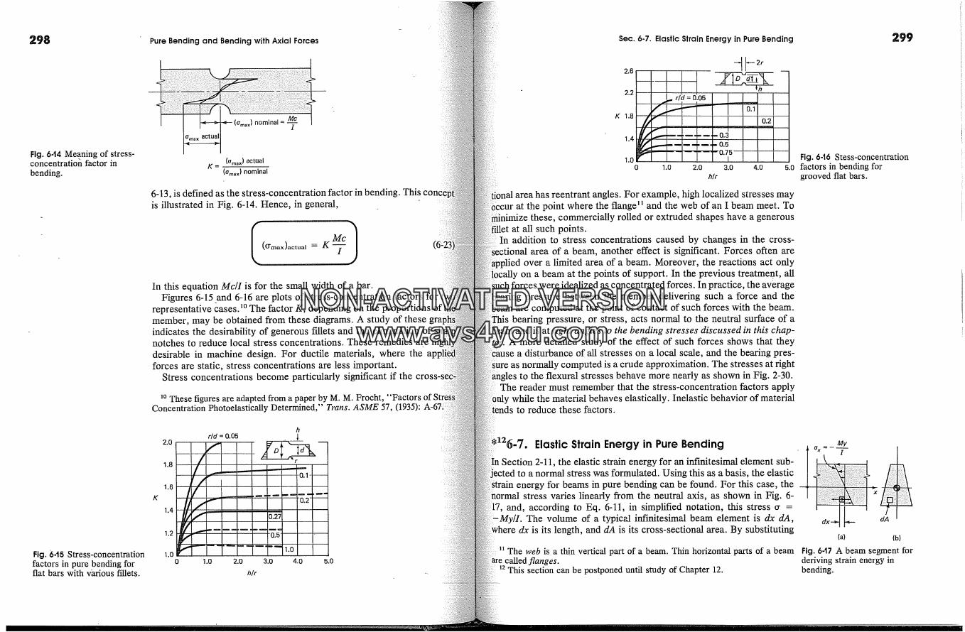
298 Pure Bending and Bending with Axial Forces Sec. 6-7. Elastic Strain Energy in Pure Bending
Fig. 644 Meaning of stress-concentratioh factor inbending.
Fig. 6-t5 Stress-concentrationfactors in pure bending forflat bars with vhrious Eftlets.
Me
(ama x) nominal = 'T
(amax) actualK=
(ama x ) nominal
6-13, is defined as the stress-concentration factor in bending. Thisis illustrated in Fig. 6-14. Hence, in general,
(O'max)actual
In this equation Mc/I is for the small width of a bar.Figures 6-15 and 6-16 are plots of stress-concentration factors for
representative �ases. �o The factor K, depending on the proportions of imember, may be obtained from these diagrams. A study of these grapindicates the desirability of generous fillets and the elimination ofnotches to reduce local stress concentrations. These remediesdesirable in machine design. For ductile materials, where the �forces are static, stress concentrations are less �mportant.
Stress concentrations become particularly significant if the
�o These figures are adapted from a paper by M. M. Frocht, "FactorsConcentration Photoelastically Determined," Trans. ASME 57, (1935):
K
2.0
1.8
1.6
1.4
1.2
1.00
h
rid = 0.05 �
0.2
0.27
0.5
.... 1.01.0 2.0 3.0 4.0 5.0
h/r
.. r/d = 0.05� � 0.1
,�'� 0.2
'� ........ 0.75
2.2
K 1.8
1.4
1.00 1.0 2.0 3.0 4.0 5.0
h�
area has reentrant angles. For example, high localized stresses mayat the point where the range � and the web of an I beam meet. To
these, commercially rolled or extruded shapes have a generousat all such points.
In addition to stress concentrations caused by changes in the cross-,nal area of a beam, another effect is significant. Forces often are
over a limited area of a beam. Moreover, the reactions act onlyon a beam at the points of support. In the previous treatment, all
�uch forces were idealized as concentrated forces. In practice, the averagepressure between the member delivering such a force and the
are computed at the point of contact of such forces with the beam.bearing pressure, or stress, acts normal to the neutral surface of a
beam and is at right angles to the bending stresses discussed in this chap-A more detailed study of the effect of such forces shows that they
a disturbance of all stresses on a local scale, and the bearing pres-sure as normally computed is a crude approximation. The stresses at right
to the flexural stresses behave more nearly as shown in Fig. 2-30.The reader must remember that the stress-concentration factors apply
while the material behaves elastically. Inelastic behavior of materialto reduce these factors.
:�26=7. Elastic Strain Energy in Pure BendingSection 2-11, the elastic strain energy for an infinitesimal element sub-
ected to a normal stress was formulated. Using this as a basis, the elasticenergy for beams in pure bending can be found. For this case, the
stress varies linearly from the neutral axis, as shown in Fig. 6-17, and, according to Eq. 6-11, in simplified notation, this stress cr =
The volume of a typical infinitesimal beam element is dx dA,dx is its length, and dA is its cross-sectional area. By substituting
n The web is a thin vertical part of a beam. Thin horizontal parts of a beamcalled flanges.
n This section can be postponed until study of Chapter 12.
Fig. 6.t6 Stess-concentrationfactors in bending forgrooved flat bars.
MyI
dA
(a) (b)
Fig. 6-t7 A beam segment forderiving strain energy inbending.
NON-ACTIVATEDVERSIONwww.avs4you.com
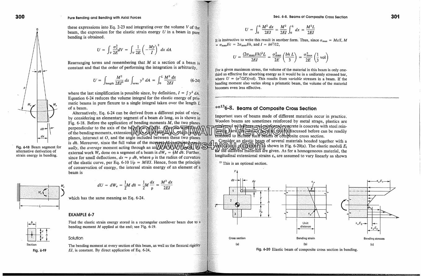
300
Fig. 6-18 Beam segment foralternative derivation ofstrain energy in bending.
Section
Fig. '6-'19
Pure Bending and Bending with Axial Forces
these expressions into Eq. 2-23 and integrating over the volume V ofbeam, the expression for the elastic strain energy U in a beam inbending is obtained.
J� 2E
Rearranging terms and remembering that M at a section of aconstant and that the order of performing the integration is
U'= -- dx y2 dA =ngth 2EI 2 ea 2EI
where the last simplification is possible since, by deflation, I = f y2Equation 6-24 reduces the volume integral for the elastic energy ofmatic beams in pure flexure to a single integral taken over theof a beam.
Alternatively, -Eq. 6�24 can be derived from a different point ofby considering an elementary segment of a beam dx long, as isFig. 6-18. Before the application of bending moments M, the twoperpendicular to the axis of the beam are parallel. After theof the bendingmoments, extensions of the same two planes, whichplanes, intersect at O, and the angle included between these twois dO. Moreover, since the full value of the moment M is attainedually, the average 'moment acting through an angle dO is �M. Hence,external work We done on a segment of a beam is dWe = �M dO:since for small deflections, dx � O dO, where � is the radius ofof the elastic curve, per Eq. 6-10 1/p = M/EL Hence, from theof conservation of energy, the internal strain energy of an elementbeam is
dU = dWe = l�M dO = l�M dX - M2 dxp 2EI
which has the same meaning as Eq. 6-24.
EXAMPLE 6-7
Find the elastic strain energy stored in a rectangular cantilever beam duebending moment M applied at the end; see Fig. 6-19.
Soldion
The bending moment at every section of this beam, as well as the flexuralEl, is constant. By direct application of Eq. 6-24,
Sec. 6-8. Beams of Composite Cross Section
� M 2 dx M 2 fz M2LU= 2EI - 2EI-to dx- 2EIinstructive to write this result in another form: 'Thus, since O'ma x ----- Mc/I, M
= 2CrmaxI/h, and I = bh3/12,
(2ffmaxI/h)2Z.=ff2max(bh_�)= O'2max(31_VOl)2EI 2E 2E
given maximum stress, the volume of the material in this beam is only one-as effective for absorbing energy as it would be in a uniformly stressed bar,
U = (tr2/2E)(voD. This results from variable stresses in a beam. If themoment also varies along a prismatic beam, the volume of the material
even less effective.
Beams of Composite Cross Section
uses of beams made of different materials occur in practice.�den beams are sometimes reinforced by metal straps, plastics are
and reinforced concrete is concrete with steel rein-bars. The elastic bending theory discussed before can be readily
to include such beams of composite cross section.an elastic beam of several materials bonded together with a
axis of symmetry as shown in Fig. 6-20(a). The elastic moduli Eithe different materials are given. As for a homogeneous material, the
extensional strains ex are assumed to vary linearly as shownThis is an optional section.
Cross section
(a)
0� �x
Unitdistance
Bending strain
(b)
Fig. 6-20 Elastic beam of composite cross section in bending.
Bending stresses
(c)
30'
NON-ACTIVATEDVERSIONwww.avs4you.com

302 Pure Bending and Bending with Axial Forces
in Fig. 6-20(b). The neutral axis for this section, passing through theulus-weighted centroid, is located by the distance Yb and canusing Eq. 6-16. The stresses shown in Fig. 6-20(c) follow from Eq.At the interfaces between two materials, depending on the relativeof their Ei's, a sharp discontinuity in stress magnitudes arises.
Following the same procedure as in Eq. 6-7, the resisting bendingment
Mz = K fA Eiy2 dA = K(EI)*where the curvature K, being constant for the section, is takenthe integral, and (E/)* defines symbolically the value of thethe middle expression. Hence
mz
(E/)*
and by substituting this relation into Eqs. 6-3 and 6-14,
Mz E M�e�,=-(E/),y and cr�,=- i(-�Ywhere the last expression is an analogue to Eq. 6-11, and can bediately specialized for a homogeneous beam.
In calculations of bending of composite cross sections, sometimesuseful to introduce the concept of an equivalent or transformedsectional area in one material. This requires arbitrary selection oference Ei, defined here as Eref. Using this notation the integral in15, for constant curvature �, can be recast as follows:
Ely dA = Eref Y�r� dA = Erie y(ni dA) = 0
where ni dA = (Ei/E�e) dA. Therefore a beam of composite crosscan be considered to have the mechanical properties of thematerial, provided the differential areas dA are multiplied by hi, theof Ei to Erie. After transforming a cross section in this manner,tional elastic analysis is applicable. In transformed sections thevary linearly from the neural axis in all materials. The actual stressesobtained for the reference material, whereas the stresses in thematerials must be multiplied by
This procedure is illustrated on the two examples that follow.
Sec. 6-8. Beams of Composite Cross Section
-t250 mm
Neutral axis
10mm � 20 X 150= 3000mm 4(a) (b) (c)
Fig. 6-2t
7.5 = 150/20
150�mm _1
�PLE 6-8
a composite beam of the cross-sectional dimensions shown in Fig. 6-The upper 150 by 250 mm part is wood, E,� = 10 GPa; the lower 10 by 150
mm strap is steel, Es = 200 GPa. If this beam is subjected to a bending moment'30 kN.m around a horizontal axis, what are the maximum stresses in the steel
wood?
ilution
as E�e. Then n� = EdEw = 20. Hence the transformed cross sectionas in Fig. 6-21(b) with the equivalent width of steel equal to 150 x 20 = 3000
The centtold and moment of inertia around the centroidal axis for this trans-section are, respectively,
150 x 250 x 125 + 10 x 3000 x 255= 150 x 250 + 10 x 3000 = 183mm (from the top)
150 x 2503 3000 x 103- + 150x 250x 582+ + 10 x 3000 x722
12 12= 478 x 10 6 mm 4
stress in the wood is
Mc 0.03 X 109 X 183(O'w)m�x I 478 X 10 6 11.5 MPa
maximum stress in the steel is
(O'�)m�x = no-,� = 20 x0.03 x 109 X 77
478 x 10 6= 96.7 MPa
klternative Solution
ielect E� as E�r. Then nw = Ew/E� = 1/20, and the transformed section is as in6-21(c).
303'
NON-ACTIVATEDVERSIONwww.avs4you.com
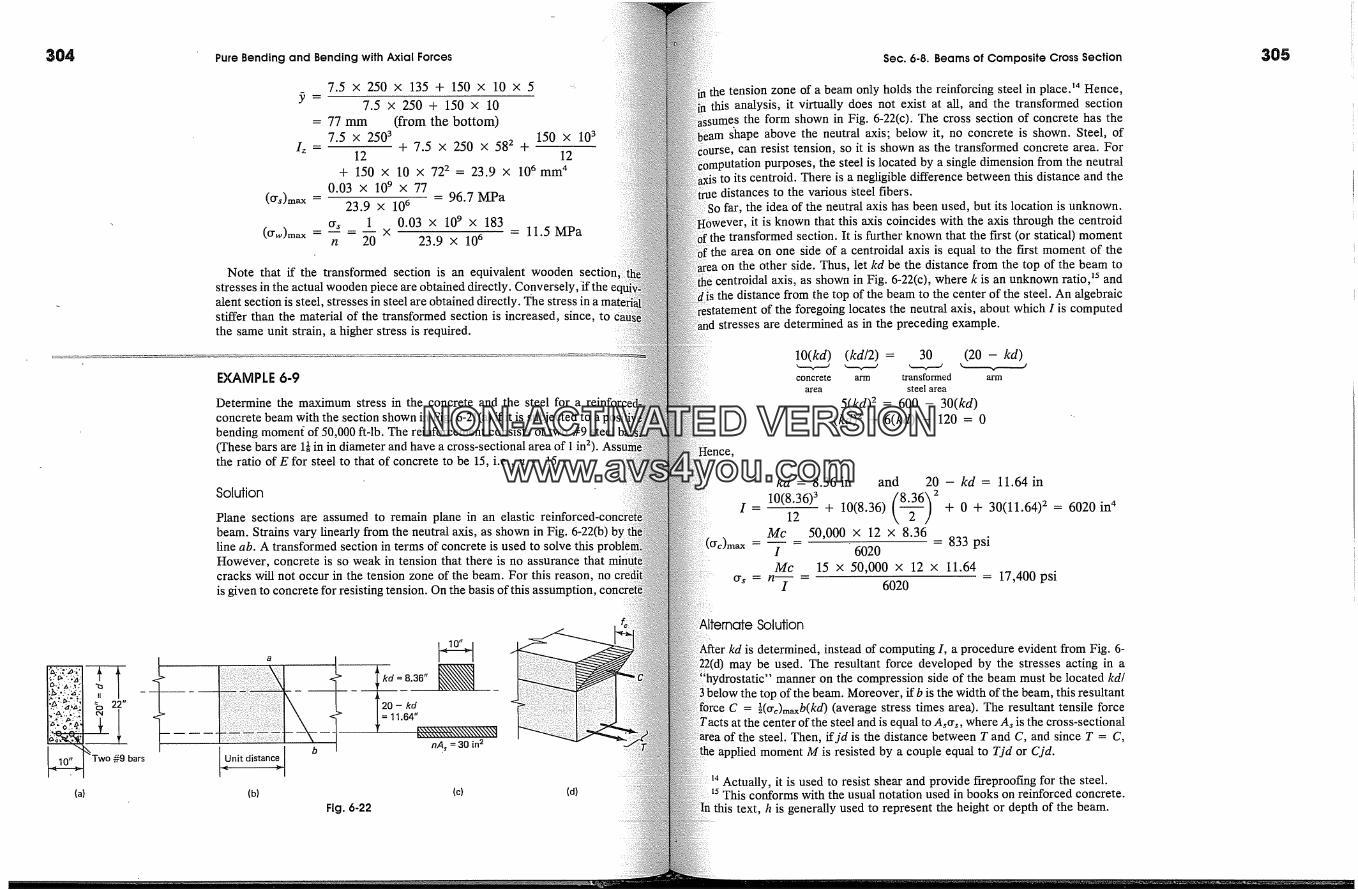
304 Pure Bending and Bending with Axial Forces
7.5 x 250 x 135 + 150 x 10 x 5
7.5 x 250 + 150 x 10= 77 mm (from the bottom)
7.5 x 2503 150 x 103Iz- + 7.5 x 250 x 582 +
12 12+ 150 x 10 x 722 = 23.9 x 106mm 4
0.03 x 109 x 77(crs)m�x = 23.9 X 106 = 96.7 MPa
ors 1 0.03 x 109 x 183(Crw)m�x n 20 x 23.9 X 106 11.5 MPa
Note that if the transformed section is an equivalent wooden sectionstresses in the actual wooden piece are obtained directly. Conversely, 'if thealent section is steel, stresses in steel are obtained directly. The stress instiffer than the material of the transformed section is increased, since, tothe same unit strain, a higher stress is required.
EXAMPLE 6-9
Determine the maximum stress in the concrete and the steel for aconcrete beam with the section shown in Fig. 6-21(a) if it is subjected to abending momeni of 50,000 ft-lb. The reinforcement consists of two #9 steel(These bars are 1� in in diameter and have a cross-sectional area of 1 in 2'the ratio of E for steel to that of concrete to be 15, i.e., n = 15.
Solution
Plane sections are assumed to remain plane in an elasticbeam. Strains vary linearly from the neutral axis, as shown in Fig. 6-22(b) byline ab. A transformed section in terms of concrete is used to solve thisHowever, concrete is so weak in tension that there is no assurance thatcracks will not occur in the tension zone of the beam. For this reason, nois given to concrete for resisting tension. On
a
Unit distance
(b)
20 - kd
; I hA, = 30 in 2
Fig. 6-22(c) (d)
Sec. 6-8. Beams of Composite Cross Section
the tension zone of a beam only holds the reinforcing steel in place? Hence,this analysis, it virtually does not exist at all, and the transformed sectionsumes the form shown in Fig. 6-22(c). The cross section of concrete has the
�hape above the neutral axis; below it, no concrete is shown. Steel, ofcan resist tension, so it is shown as the transformed concrete area. For
purposes, the steel is located by a single dimension from the neutralto its centreid. There is a negligible difference between this distance and thedistances to the various �teel fibers.
far, the idea of the neutral axis has been used, but its location is unknown.However, it is known that this axis coincides with the axis through the centreid
the transformed section. It is further known that the fn:st (or statical) momentthe area on one side of a centroidal axis is equal to the first moment of the
on the other side. Thus, let kd be the distance from the top of the beam tocentroidal axis, as shown in Fig. 6-22(c), where k is an unknown ratio, �5 andthe distance from the top of the beam to the center of the steel. An algebraic
of the foregoing locates the neutral axis, about which I is computedstresses are determined as in the preceding example.
10(kd) (kd12) = 30 (20 - kd)concrete arm transformed arm
area steel area
5(kd) 2 = 600 - 30(kd)(kd) 2 + 6(kd) - 120 = 0
I
kd = 8.36 in and 20 - kd = 11.64 in
10(8.367 (8�6) �-12 + 10(8.36) -- + 0 + 30(11.64) 2 = 6020 in 4Mc 50,000 x 12 x 8.36
I 6020 = 833 psiMc 15 x 50,000 x 12 x 11.64
= 17,400 psi6020
Solution
kd is determined, instead of computing I, a procedure evident from Fig. 6-may be used. The resultant force developed by the stresses acting in a
;hydrostatic" manner on the compression side of the beam must be located kd/below the top of the beam. Moreover, if b is the width of the beam, this resultant
C = �(cr�)m�,b(kd) (average stress times area). The resultant tensile forcesteel and is equal to A�cr�, where A� is the cross-sectional
the steel. Then, ifjd is the distance between T and C, and since T = C,applied moment M is resisted by a couple equal to Tjd or Cjd.
Actually, it is used to resist shear and provide fireproofing for the steel.� This conforms with the usual notation used in books on reinforced concrete.
In this text, h is generally used to represent the height or depth of the beam.
305
NON-ACTIVATEDVERSIONwww.avs4you.com
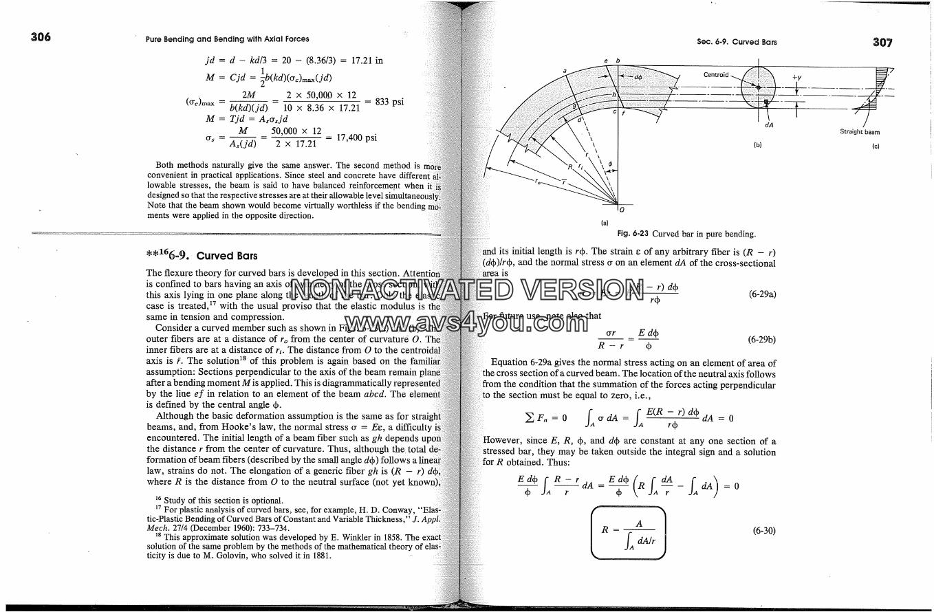
306 Pure Bending and Bending with Axial Forces
jd = d - kd/3 = 20 - (8.36/3) = 17.21 in
M = Cjd = �b(kd)(�c)m�x(jd)2M 2 x 50,00.0 x 12
(O�)m�,, -- -- = 833 psib(kd)(jd) 10 x 8.36 x 17.21M = Tjd = As�sjd
M 50,000 x 12o-s = -- - = 17,400 psi
A�(jd) 2 x 17.21
Both methods naturally give the same answer. The second method isconvenient in practical applications. Since steel and concrete havelowable stresses, the beam is said to have balanced reinforcement whendesigned so that the respective stresses are at their allowable level simuttaneouNote that the beam shown would become virtually worthless if the bendingments were applied in the opposite direction.
Curved BarsThe flexure theory for curved bars is developed in this section.is confined to bars having an axis of symmetry of the cross section,this axis lying in one plane along the length of the bar. Only thecase is treated, �7 with the usual proviso that the elastic modulus issame in tension and compression.
Consider a curved member such as shown in Figs. 6-23(a) and (b).outer fibers are at a distance of ro from the center of curvatur60.inner fibers are at a distance of r�. The distance from O to theaxis is L The solution �8 of this problem is again based on theassumption: Sections perpendicular to the axis of the beam remainafter a bending moment M is applied. This is diagrammaticallyby the line ef in relation to an element of the beam abcd. Theis defined by the central angle qb.
Although the basic deformation assumption is the same as for straibeams, and, from Hooke's law, the normal stress tr = Ee, a difficultyencountered. The initial length of a beam fiber such as gh dependsthe distance r from the center of curvature. Thus, although the. totalformation of beam fibers (described by the small angle dqb) followslaw, strains do not. The elongation of a generic fiber gh is (R - r)where R is the distance from O to the neutral surface (not yet
�6 Study of this section is optional.�7 For plastic analysis of curved bars, see, for example, H. D. Conway,
tic-Plastic Bending of Curved Bars of Constant and Variable Thickness.Mech. 27/4 (December 1960): 733-734.
is This approximate solution was developed by E. Wintaler in 1858. Thesolution of the same problem by the methods of the mathematical theory ofticity is due to M. Golovin, who solved it in 1881.
e b
Sec. 6-9. Curved Bars
Centroid
.\\
\
\\ (b)
o
(a)
Fig. 6-23 Curved bar in pure bending.
its initial length is rqb. The strain e of any arbitrary fiber is (R - r)b)/rqb, and the normal stress tr on an element dA of the cross-sectional
area is
� = Ee = E (R - r) dqbrqb (6-29a)For future use, note also that
trr E dqb-- - (6-29b)
R - r qb
Equation 6-29a gives the normal stress acting on an element of area ofsection of a curved beam. The location of the neutral axis follows
from the condition that the summation of the forces acting perpendicularthe section must be equal to zero, i.e.,
�F.=0 fA ,y a_A = fA E(R - r) d4�rqb dA = 0since E, R, qb, and dqb are constant at any one section of a
bar, they may be taken outside the integral sign and a solutionobtained. Thus:
oo ---7-- oo --- aA =0
(6-30)
307
+y
Straight beam
(c)
NON-ACTIVATEDVERSIONwww.avs4you.com
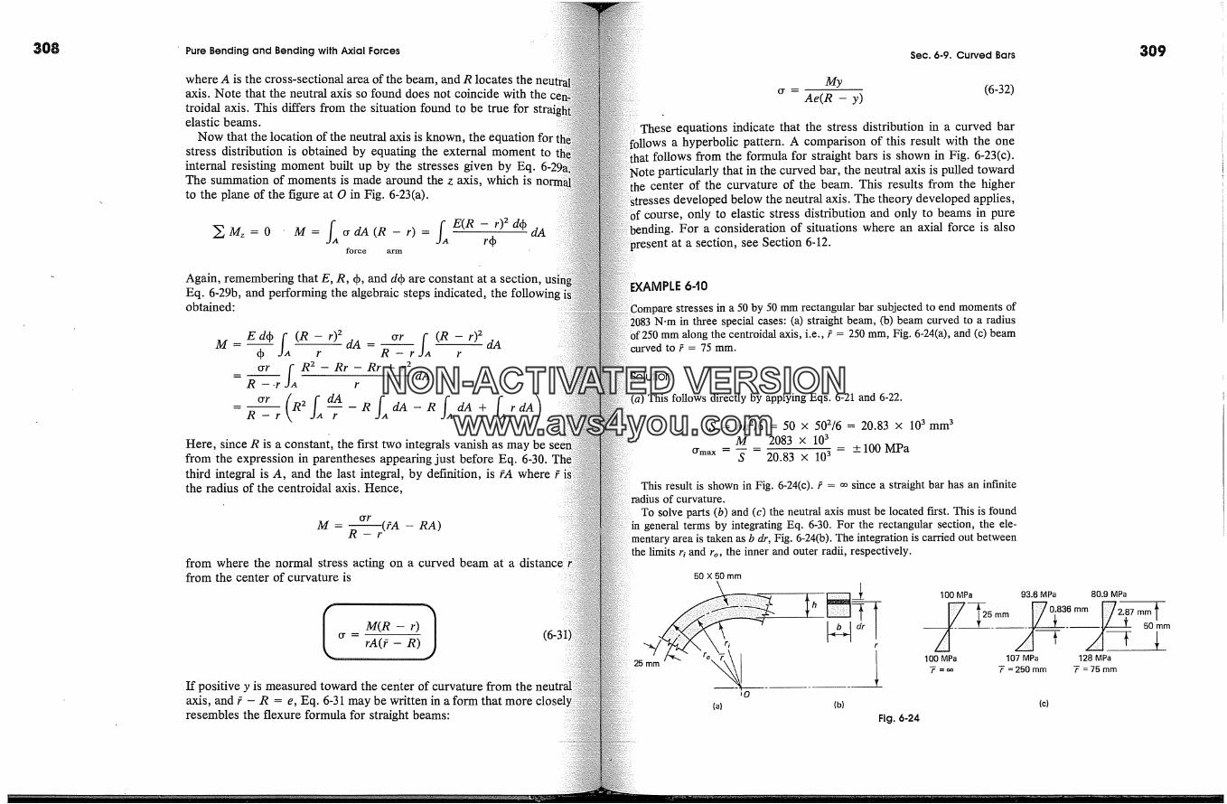
308 Pure Bending and Bending with Axial Forces
where A is the cross-sectional area of the beam, and R locates theaxis. Note that the neutral axis so found does not coincide with thetroidal axis. This differs from the situation found to be true forelastic beams.
Now that the location of the neutral axis is known, the equation forstress distribution is obtained by equating the external moment tointernal resisting moment built up by the stresses given by Eq.The summation of moments is made around the z axis, which isto the plane of the figure at O in Fig. 6-23(a).
� Mz=O M= /,�cr dA (R- r)= f,� E(R - r) 2 dqbforce arm
Again, remembering that E, R, qb, and dqb are constant at a section,Eq. 6-29b, and performing the algebraic steps indicated, the followingobtained:
M = E dqb f,� (R - r)2 dA - �r f,� (R - r)2 dA� r R---r r
err f,� g 2 - Rr - Rr + r 2- dAR �-r r
_ err (R2fAdA_RfAdA_RfAdA + fArdA)R-r r
Here, since R is a constant, the first two integrals vanish as may befrom the expression in parentheses appearing just before Eq. 6-30.third integral is A, and the last integral, by definition, is ?A wherethe radius of the centroidal axis. Hence,
O't"M - .(?A - RA)
from where the normal stress acting on a curved beam at afrom the center of curvature is
I M(R- r)1or- rA(?- R)
If positive y is measured toward the center of curvature from theaxis, and ? - R = e, Eq. 6-31 may be written in aform that moreresembles the flexure formula for straight beams:
Sec. 6-9. Curved Bars
Mycr- (6-32)
Ae(R - y)
These equations indicate that the stress distribution in a curved bara hyperbolic pattern. A comparison of this result with the one
follows from the formula for straight bars is shown in Fig. 6-23(c).particularly that in the curved bar, the neutral axis is pulled toward
center of the curvature of the beam. This results from the higherStresses developed below the neutral axis. The theory developed applies,
course, only to elastic stress distribution and only to beams in pureFor a consideration of situations where an axial force is also
at a section, see Section 6-12.
309
tVIPLE 6-'10
�are stresses in a 50 by 50 mm rectangular bar subjected to end moments of2083 N.m in three special cases: (a) straight beam, (b) beam curved to a radius
the centroidal axis, i.e., i = 250 mm, Fig. 6-24(a), and (c) beam:urved to ? = 75 mm.
Solution
This follows directly by applying Eqs. 6-21 and 6-22.
S = bh2/6 = 50 x 502/6 = 20.83 x 103 mm 3M 2083 x 103
- +100 MPacrm�x S 20.83 x 10³
This result is shown in Fig. 6-24(c). ? = oo since a straight bar has an infiniteof curvature.
To solve parts (b) and (c) the neutral axis must be located first. This is foundm general terms by integrating Eq. 6-30. For the rectangular section, the ele-
mentary area is taken as b dr, Fig. 6-24(b). The integration is carried out betweenlimits r� and ro, the inner and outer radii, respectively.
50 X 50 mm
�0
(a) (b)Fig. 6-24
100 MPa 93.6 MPa 80.9 MPa
� -v {----v 60ram/I-T
100 MPa 107 MPa 128 MPa7' = .o 7' = 250 mm 7' = 75 mm
(c)
NON-ACTIVATEDVERSIONwww.avs4you.com
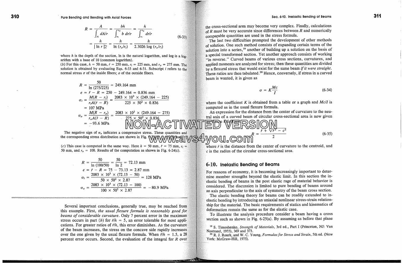
Pure Bending and Bending with Axial Forces
A bh h
h h h
I In r Ir? In (ro/ri) 2.3026 log (ro/rt)
where h is the depth of the section, In is the natural logarithm, and log is aarithm with a base of 10 (common logarithm).(b) For this case, h = 50 mm, ? = 250 mm, rt = 225 mm, and re = 275 mm.solution is obtained by evaluating Eqs. 6-33 and 6-31. Subscript i refers tonormal stress � of the inside fibers; o of the outside fibers.
g m
e =
O'i =
50- 249.164 mm
In (275/225)? - R = 250 - 249.164 = 0.836 mmM(R - ri) 2083 x 103 x (249.164 - 225)riA(? - R) 225 x 502 x 0.836107 MPa
M(R - re) 2083 x 103 x (249.164 - 275)roA(b - R) 275 x 502 x 0.836
- 93.6 MPa
The negative sign of ere indicates a compressive stress. These quantitiesthe corresponding stress distribution are shown in Fig. 6-24(c); ? = 250 mm.
(c) This case is computed in the same way. Here h = 50 mm, ? = 75 ram, ri:50 mm, and re = 100. Results of the computation as shown in Fig. 6-24(c).
50 50R = --- - 72.13mm
In (100/50) In 2e = g- R = 75 - 73.13 = 2.87mm
2083 x 103 x (72.13 - 50)o-i = 50 x 502 x 2.87 = 128 MPa
2083 x 103 x (72.13 - 100)�'� = 100 x 502 x 2.87 = -80.9 MPa
Several important conclusions, generally true, may be reachedthis example. First, the usual flexure formula is reasonably goodbeams of considerable curvature. Only 7 percent error in thestress occurs in part (b) for ?/h = 5, an error tolerable for mostcations. For greater ratios of ?/h, this error diminishes. As theof the beam increases, the stress on the concave side rapidly 'over the one given by the usual flexure formula. When ?/h = 1.5, apercent error occurs. Second, the evaluation of the integral for R
Sec. 6-10. Inelastic Bending of Beams
cross-sectional area may become very complex. Finally, calculationsmust be very accurate since differences between R and numerically
quantities are used in the stress formula.last two difficulties prompted the development of other methods
solution. One such method consists of expanding certain terms of theinto a series? another of building up a solution on the basis of
special transformed section. Yet another approach consists of workingreverse." Curved beams of various cross sections, curvatures, and
moments are analyzed for stress; then these quantities are divideda flexural stress that would exist for the same beam if it were straight.
: ratios are then tabulated? Hence, conversely, if stress in a curvedbeam is wanted, it is given as
K Mc� = (6-34)I
ere the coefficient K is obtained from a table or a graph and Mc/I isas in the usual flexure formula.
An expression for the distance from the center of curvature to the neu-axis of a curved beam of circular cross-sectional area is now given
for future reference:
p+ V�.2 - c 2R = (6-35)
2
where ? is the distance from the center of curvature to the centroid, andc is the radius of the circular cross-sectional area.
6-10. Inelastic Bending of Beamsreasons of economy, it is becoming increasingly important to deter-
mine member strengths beyond the elastic limit. In this section the in-bending of beams in the post elastic rage of material behavior is
considered. The discussion is limited to pure bending of beams aroundaxis perpendicular to the axis of symmetry of the beam cross section.
The elastic bending theory for beams can be readily extended to in-introducing an uniaxial nonlinear stress-strain relation-
ship for the material. The basic requirements of statics and kinematics ofremain the same as for the elastic case.
To illustrate the analysis procedure consider a beam having a crosssuch as shown in Fig. 6-25(a). By assuming as before that plane
19 S. Timoshenko, Strength of Materials, 3rd ed., Part I (Princeton, NJ: VanNostrand, 1955), 369 and 373.
20 R. J. Roark, and W. C. Young, Formulas for Stress and Strain, 5th ed. (NewYork: McGraw-Hill, 1975).
NON-ACTIVATEDVERSIONwww.avs4you.com

Pure Bending and Bending with Axial Forces Sec. 640. Inelastic Bending of Beams
(a) Beam section
M z
Y4
�5
�_ Unit �length- I'- 1
(b) Bending strain
Y5
0 2 --
�5 �4
01 --
�1 E2 �3
-- O 4
(c) Stress-strain diagram
m �5 (/5
o3
(d) Bending stresses (e)
Fig. 6-25 Inelastic bending of beam.
sections remain plane after deformation, the longitudinal normalvary linearly as in Fig. 6-25(b). For the several selected strains.... es in this diagram, the correponding stresses 0.�, 0-2 ..... 0-5defined on the given stress-strain diagram in Fig. 6-25(c). A plot ofstresses along a section establishes a possible stress distribution inbeam along the curved line AB as illustrated in Fig. 6-25(d). (Exceptvertical scale, this line precisely corresponds to the curved line instress-strain diagram.) These stresses, acting on the correspondingof the cross section, develop a compressive force C above theaxis, and a tensile force T below it. When T = C, a correct locationthe neutral axis is found. This condition is equivalent to thethat at a section
fA 0- dA = 0where 0- is the normal bending stress acting on a section.
Finding the location of the neutral axis such that T = C may requiretrial-and-error process, although direct procedures have been devised
some cross sections. TM After the neutral axis is correctly located, the: bending moment Mz at the same section is known to be C(a +
or T(a + b), see Fig. 6-25(d). Alternatively, in the form of a generalequation,
Mz = -� cry dA (6-37)The problem is greatly simplified if the beam cross section is symmetric
horizontal axis and material properties are the same in tensionFor these conditions it is known a priori that the neutral
passes through the centroid of the section, and Eq. 6-37 can be di-applied. The behavior of such a beam in bending is shown quali-
in Fig. 6-26. A sequence of progressively increasing strains as-�ciated with plane sections is shown in Fig. 6-26(b). These maximum
define the maximum stresses in the outer fibers of the beam, Fig.resulting in progressively increasing bending stresses.
As can be seen from Figs. 6-26(a) and (c), the maximum attainable stress0-3. The instantaneous stress distribution in the beam associated with
0-3, for this brittle material, is given by the curved line AB in Fig. 6-26(c).in routine experiments the nominal stress in the extreme fibers
often computed by applying the elastic flexure formula, Eq. 6-13, usingthe experimentally determined ultimate bending moment. The stress so
2� A. Nadai, Theory of Flow andFracture of Solids, vol. ! (New York: McGraw-Hill, 1950), 356.
Propordonallimit
Fracture
E1 �2 �3
(b)
01 0 2 0 3
(a) c B
(c)
Fig. 6-26 Rectangular beamin bending exceeding theproportional limit of thematerial.
NON-ACTIVATEDVERSIONwww.avs4you.com
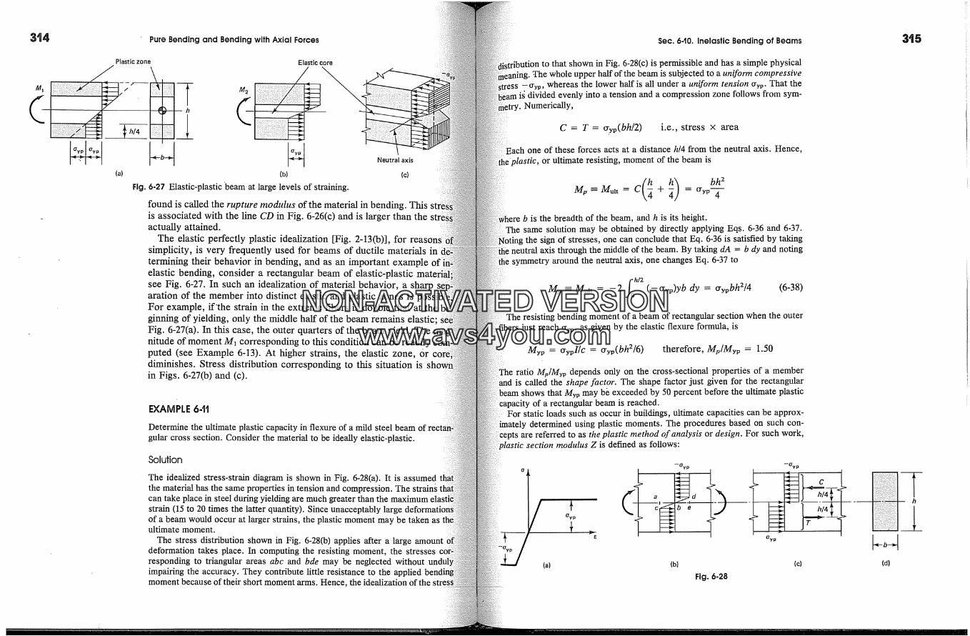
Pure Bending and Bending with Axial Forces Sec. 6.t0. Inelastic Bending of BeamsPlastic zone
I(a)
Elastic core
M2
Fig.
�� Neutralaxis(b) (c)
6-27 Elastic-plastic 'beam at large levels of straining.
found is called the rupture modulus of the material in bending. Thisis associated with the line CD in Fig. 6-26(c) and is larger than theactually attained.
The elastic perfectly plastic idealization [Fig. 2-13(b)], for reasonssimplicity, is very frequently used for beams of ductile materials intermining their behavior in bending, and as an important exampleelastic bending, consider a rectangular beam of elastic-plasticsee Fig. 6-27. In such an idealization of material behavior, a sharparation of the member into distinct elastic and plastic zones isFor example, if'the strain in the extreme fibers is double that at theginning of yielding, only the middle half of the beam remains elastic;Fig. 6-27(a). In this case, the outer quarters of the beam yield. Thenltude of moment M� corresponding to this condition can be readilyputed (see Example 6-13). At higher strains, the elastic zone, 6rdiminishes. Stress distribution corresponding to this situation isin Figs. 6-27(b) and (c).
EXAMPLE 6-tt
Determine the ultimate plastic capacity in flexure of a mild steel beamgular cross section. Consider the material to be ideally elastic-plastic.
Soldion
The idealized stress-strain diagram is shown in Fig. 6-28(a). It is assumedthe material has the same properties in tension and compression. The strain�can take place in steel during yielding are much greater than the maximumstrain (15 to 20 times the latter quantity). Since unacceptably largeof a beam would occur at larger strains, the plastic moment may be taken asultimate moment.
The stress distribution shown in Fig. 6-28(b) applies after a large amountdeformation takes place. In computing the resisting moment, the stressesresponding to triangular areas abc and bde may be neglected withoutimpairing the accuracy. They contribute little resistance to the appliedmoment because of their short moment arms. Hence, the idealization of the stress
to that shown in Fig. 6-28(c) is permissible and has a simple physical-The whole upper half of the beam is subjected to a uniform compressive
-crvp, whereas the lower half is all under a uniform tension crvp. That thedivided evenly into a tension and a compression zone follows from sym-
Numerically,
C = T = o.yp(bh/2) i.e., stress x area
Each one of these forces acts at a distance hi4 from the neutral axis. Hence,or ultimate resisting, moment of the beam is
(� �) bh2Mp � Muir = C + = o.yp- 4
is the breadth of the beam, and h is its height.The same solution may be obtained by directly applying Eqs. 6-36 and 6-37.
NOting the sign of stresses, one can conclude that Eq. 6-36 is satisfied by takingneutral axis through the middle of the beam. By taking dA = b dy and notingsymmetry around the neutral axis, one changes Eq. 6-37 to
oh/2Mp - Mult = - 2 (- o.yp)yb dy = o.ypbh2/4 (6-38)
bending moment of a beam of rectangular section when the outerust reach crv�, as given by the elastic flexure formula, is
Myp = o-ypI/c = o-yp(bh2/6) therefore, Mp/Myp = 1.50
The ratio Mp/Mvp depends only on the cross-sectional properties of a memberis called the shape factor. The shape factor just given for the rectangular
shows that Myp may b& exceeded by 50 percent before the ultimate plasticof a rectangular beam is reached.
For static loads such as occur in buildings, ultimate capacities can be approx-imately determined using plastic moments. The procedures based on such con-
are referred to as the plastic method of analysis or design. For such work,section modulus Z is defined as follows:
Oyp
E
(a) (b) (c)Fig. 6-28
(d)
NON-ACTIVATEDVERSIONwww.avs4you.com
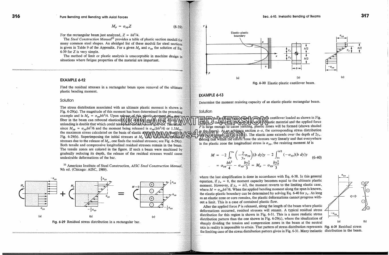
Pure Bending and Bending with Axial Forces Sec. 6-10. Inelastic Bending of Beams
Mp -� O-ypZ
For the rectangular beam just analyzed, Z = bh2/4.The Steel Construction Manual 22 provides a table of plastic section moduli
many common steel shapes. An abridged list of these moduli for steel secis given in Table 9 of the Appendix. For a given M s and Cryp the solution of i6-39 for Z is very simple.
The method of limit or plastic analysis is unacceptable in machinesituations where fatigue properties of the material are important.
O'yp
EXAMPLE 6-t2
Find the residual stresses in a rectangular beam upon removal of theplastic bending moment.
Solution
The stress distribution associated with an ultimate plastic moment is shownFig. 6-29(a). The magnitude of this moment has been determined in theexample and is M s = crypbh2/4. Upon release of this plastic moment M s,fiber in the beam can rebound elastically. The material elastic range duringunloading is double that which could take place initially (see Fig. 2-13).since Myp = crypbh2/6 and the moment being released is cryp(bh2[4) orthe maximum stress calculated on the basis of elastic action is �cryp, as shownFig. 6-29(b). Superimposing.the initial stresses at M s with the elasticstresses due to the release ofM�, one finds the residual stresses; see Fid.Both tensile and compressive longitudinal residual stresses remain in theThe tensile zones are colored in the figure. If such a beam were machinedgradually reducing its depth, the release of the residual stresses wouldundesirable deformations of the bar.
22 American Institute of Steel Construction, AISC Steel Construction Manual9th ed. (Chicago: AISC, 1989).
I
Oy p
(b)
Fig. 6.29 Residual stress distribution in a rectangular bar.
Elastic-plasticboundaW
a
(b)
Fig. 6-30 Elastic-plastic cantilever beam.
643
)etermine the moment resisting capacity of an elastic-plastic rectangular beam.
Solution
To make the problem more definite, consider a cantilever loaded as shown in Fig.6-30(a). If the beam is made of ideal elastic-plastic material and the applied force
P is large enough to cause yielding, plastic zones will be formed (shown shadedthe figure). At an arbitrary section a-a, the corresponding stress distribution
be as shown in Fig. 6-30(c). The elastic zone extends over the depth of 2yo.that within the elastic zone the stresses vary linearly and that everywhere
the plastic zone the longitudinal stress is crvv, the resisting moment M is
= - - (- Cryp)(b dy)y
bh 2 by2o by2o= �YP'4 �YP-�- = Me - �YP' 3
(6-40)
the last simplification is done in accordance with Eq. 6-38. In this generalif yo = 0, the moment capacity becomes equal to the ultimate plastic
moment. However, if yo = h/2, the moment reverts to the limiting elastic case,= c�v, bh2/6. When the applied bending moment along the span is known,
the elastic-plastic boundary can be determined by solving Eq. 6-40 for yo. As longan elastic zone or core remains, the plastic deformations cannot progress with-
out a limit. This is a case of contained plastic flow.After the applied force P is released, along the length of the beam where plastic
deformations occurred, residual stresses will remain. A typical residual stressfor this region is shown in Fig. 6-31. This is a more realistic stress
distribution pattern than the one shown in Fig. 6-29(c), where the idealization ofdividing the tension and compression zones in the beam at the neutral
axis in reality is impossible to attain. That pattern of stress distribution representsg case of the stress distribution pattern given in Fig. 6-31. Many inelastic
(c)
(a) (b)
Fig. 6-31 Residual stressdistribution in the beam.
NON-ACTIVATEDVERSIONwww.avs4you.com

Pure Bending and Bending with Axial Forces
materials tend to have a stress-strain relationship such as shown in Fig.The residual stress pattern for such materials would resemble the stressbetween curved line AB and straight line CD of Fig. 6-26(c).
EXAMPLE 6-t4
Determine the plastic moment strength for the reinforced concrete beam inample 6-9. Assume that the steel reinforcement yields at 40,000 psi and thatultimate strength of concrete f� = 2500 psi.
Solution
When the reinforcing steel begins to yield, large deformations commence.is taken to be the ultimate capacity of steel; hence, T,u = Ascryp.
At the ultimate or plastic moment, experimental evidence indicates thatcompressive stresses in concrete can be approximated by the rectangularblock shown in Fig. 6-32. 23 It is customary to assume the average stress incompressive stress block to be 0.85f;. On this basis, keeping in mind that= C,�t, one has
Yult = gypAs = 40,000 x 2 = 80,000 lb =C.�t 80,000k'd - = = 3.77 in
0.85��b 0.85 x 2,500 x 10M�t = T�t(d - k'd/2) = 80,000(20 - 3.77/2)/12 = 121,000 ft-lb
23 For further details, see P.M. Ferguson, J. E. Breen, and J. O. J'�sa,forced Concrete Fundamentals, 5th ed. (New York: Wiley, 1988), or R. ParkT. Paulay, Reinforced Concrete Structures (New York: Wiley, 1975).
Probablestress
distribution
Muir
Assumedstress
distribution
Gyp
(a) (b)
Fig. 6-32
Sec. 6.1t. Bending About Both Principal Axes
l. Bending About Both Principal Axes 24a simple example of skew or unsymmetrical pure bending, considerrectangular beam shown in Fig. 6-33. The applied moments M act in
abcd. By using the vector representation for M shown in Fig.this vector forms an angle c� with the z axis and can be resolved
, the two components, My and Mz. Since the cross section of this beamsymmetry about both axes, the formulas derived in Section 6-3 are
applicable. Because of symmetry, the product of inertia for thisis zero, and the orthogonal axes shown are the principal axes for
cross section. This also holds true for the centroidal axes of singlyareas. (For details see Sections 6-15 and 6-16.)
By assuming elastic behavior of the material, a superposition of the.ses caused by My and Mz is the solution to the problem. Hence, using
s. 6-11 and 6-12,
Mzy Myz�.� = --- + -- (6-41)
all terms have the previously defined meanings.
24 Some readers may prefer to study Section 6-14 fkst, and then consider thisas a special case.
c
M
Y
(a) (b)
Fig. 6-33 Unsymmetrical bending of a beam with doubly symmetric cross section.
NON-ACTIVATEDVERSIONwww.avs4you.com
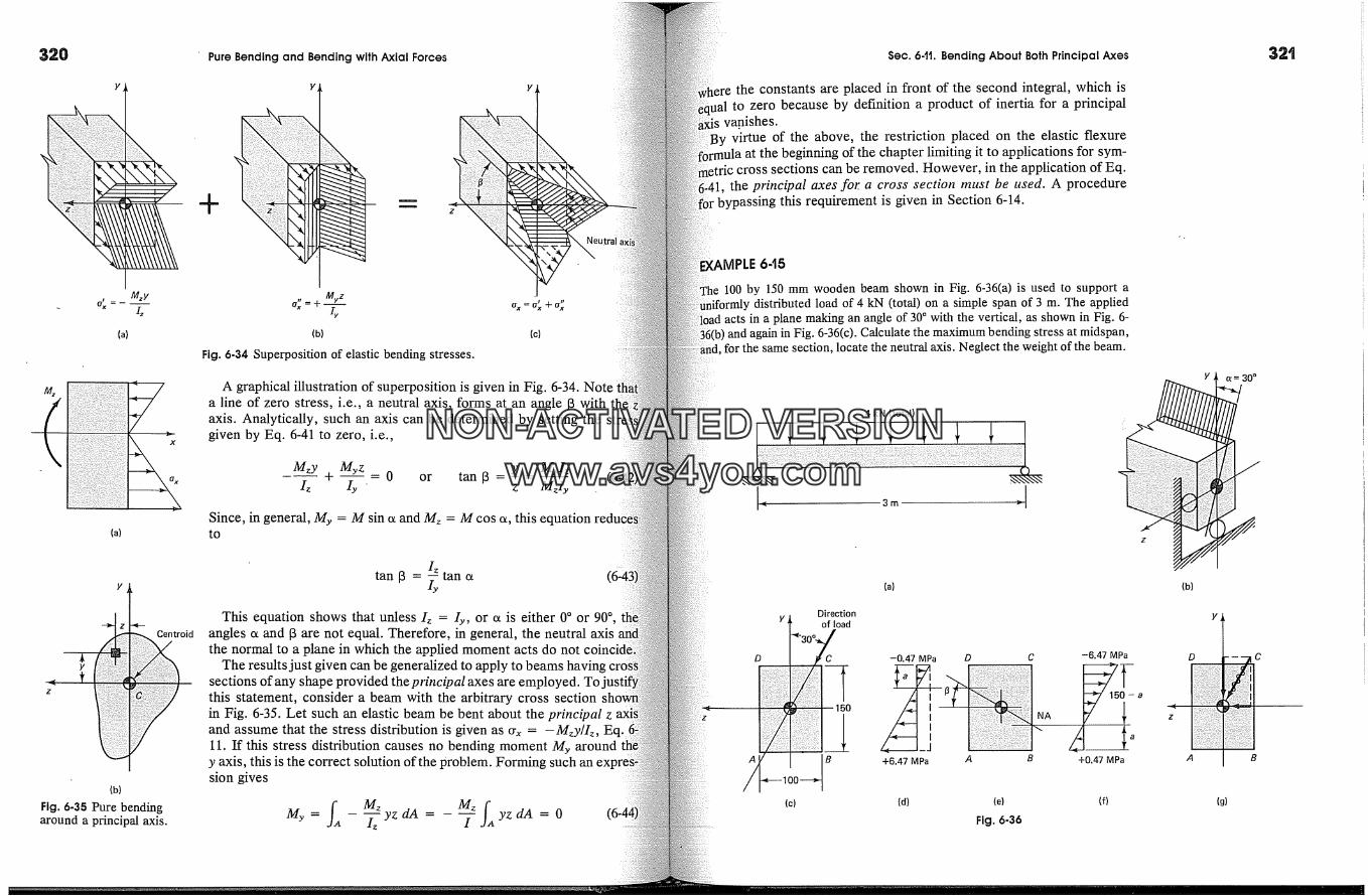
320
Mzy
(a)
Centroid
Y
(b)
Fig. 6-35 Pure bendingaround a principal axis.
Pure Bending and Bending with Axial Forces
Y,
+ =
. _ Myz
(b) (c)
Fig. 6-34 Superposition of elastic bending stresses.
A graphical illustration of superposition is given in Fig. 6-34. Notea line of zero stress, i.e., a neutral axis, forms at an angle [3 withaxis. Analytically, such an axis can be determined by setting thegiven by Eq. 6-41 to zero, i.e.,
Mzy Myz y Mylz--- +-- = 0 or tan [3- ---Iz Iy' z Mzly
Since, in general, My = M sin e� and Mz = M cos e�, this equationto
tan [3 = � tan e�This equation shows that unless I� = Iy, or e� is either 0 � or 90 �,
angles e� and [3 are not equal. Therefore, in general, the neutral axisthe normal to a plane in which the applied moment acts do not
The results just given can be generalized to apply to beams having cros!sections of any shape provided the principal axes are employed. TOthis statement, consider a beam with the arbitrary cross sectionin Fig. 6-35. Let such an elastic beam be bent about the principal zand assume that the stress distribution is given as crx = -M�y/I�, Eq.11. If this stress distribution causes no bending moment My around
y axis, this is the correct solution of the problem. Forming such ansion gives
My= - -�z yz dA = I yz dA = 0
Sec. 6-tt. Bending About Both Principal Axes
the constants are placed in front of the second integral, which isto zero because by definition a product of inertia for a principal
vanishes.virtue of the above, the restriction placed on the elastic flexure
. at the beginning of the chapter limiting it to applications for sym-cross sections can be removed. However, in the application of Eq.
the principal axes for a cross section must be used. A procedurebypassing this requirement is given in Section 6-14.
�PLE 645
100 by 150 mm wooden beam shown in Fig. 6-36(a) is used to support adistributed load of 4 kN (total) on a simple span of 3 m. The applied
in a plane making an angle of 30 � with the vertical, as shown in Fig. 6-and again in Fig. 6-36(c). Calculate the maximum bending stress at midspan,
for the same section, locate the neutral axis. Neglect the weight of the beam.
4 kN (total)
J< 3m �'
DirectionY
of load
(a)
D -0.47 MPa D C -6.47 MPa
150
150 - a
B +6.47 MPa A B +0.47 MPa
(c) (d) (e) (f)Fig. 6-36
a = 30 �
(b)
D
(g)
32'
c
NON-ACTIVATEDVERSIONwww.avs4you.com
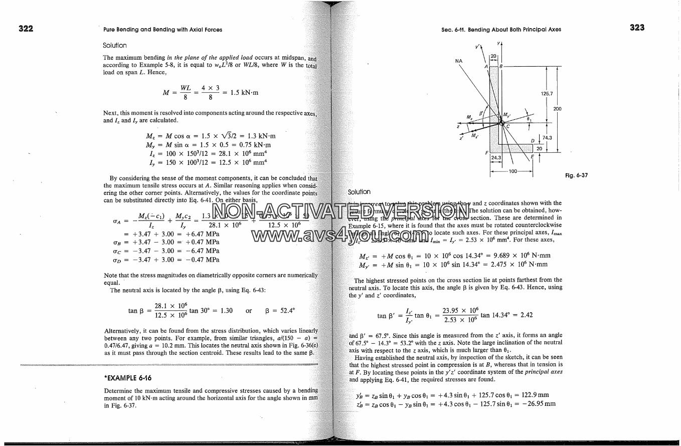
322 Pure Bending and Bending with Axial Forces Sec. 6-It, Bending About Both Principal Axes 323
Solution
The maximum bending in the plane of the applied load occurs at midspanaccording to Example 5-8, it is equal to woL2/8 or WL/8, where W is theload on span L. Hence,
WL 4x3M .... 1.5 kN.m
8 8
Next, this moment is resolved into components acting around the res[and I� and Iy are calculated.
Mz = M cos tx = 1.5 x X/-�/2 = 1.3 kN.mMy = M sin tx = 1.5 x 0.5 = 0.75 kN.m
Iz = 100 x 1503/12 = 28.1 x 10 6 mm 4Iy = 150 x 1003/12 = 12.5 x 10 6 mm 4
By considering the sense of the moment components, it can be concluded ithe maximum tensile stress occurs at A. Similar reasoning applies whenering the other corner points. Alternatively, the values for the coordinatecan be substituted directly into Eq. 6,41. On either basis,
M�(:-ci) Myc2 1.3 x 106 x 75era = Iz + Iy 28.1 X 106
= +3.47 + 3.00 = +6.47 MPa
ere = + 3.47 - 3.00 =' + 0.47 MPacrc = -3.47 - 3.00 = -6.47 MPacrz> = -3.47 + 3.00 = -0.47 MPa
0.75 x 106 x 50+
12.5 x 10 6
Note that the stress magnitudes on diametrically oppositeequal.
The neutral axis is located by the angle [3, using Eq. 6-43:
28.1 x 10 6tan [3 - 12.5 x 10⁶ tan 30 � = 1.30 or [3 = 52.4 �
Alternatively, it can be found from the stress distribution, which variesbetween any two points. For example, from similar triangles, a/(150 - a)0.47/6.47, giving a = 10.2 mm. This locates the neutral axis shown in Fig.as it must pass through the section centroid. These results lead to the same
*EXAMPLE 646
Determine the maximum tensile and compressive stresses caused by amoment of 10 kN-m acting around the horizontal axis for the angle shown inin Fig. 6-37.
NA Y'�
125.774.3
100 ,. t�s incorrect to solve this problem using the y and z coordinates shown with the
formulas developed so far in the text. The solution can be obtained, how-ever, using the principal axes for the cross section. These are determined in
Example 6-15, where it is found that the axes must be rotated counterclockwisean angle 0� = 14.34 � to locate such axes. For these principal axes, Im�x
= 23.95 x 106 mm 4 and Imin = Iy, = 2.53 x 106 mm 4. For these axes,
+M cos 0� = 10 x 106 COS 14.34 � = 9.689 x 10 6 N.mm+M sin 0� = 10 x 10 6 sin 14.34 � = 2.475 x 10 6 N.mm
highest stressed points on the cross section lie at points farthest from theTo locate this axis, the angle [3 is given by Eq. 6-43. Hence, using
and z' coordinates,
Iz, 23.95 X 10 6tan [3' =�y, tan0� = 2.53 x 10⁶ tan 14.34 � = 2.42
[3' = 67.5 �. Since this angle is measured from the z' axis, it forms an angle- 14.3 � = 53.2 � with the z axis. Note the large inclination of the neutral
with respect to the z axis, which is much larger than 0�.established the neutral axis, by inspection of the sketch, it can be seen
that the highest stressed point in compression is at B, whereas that in tension is: F. By locating these points in the y'z' coordinate system of the principal axes
applying Eq. 6-41, the required stresses are found.
y� = zesin0z + yecos0� = +4.3 sin0� + 125.7cos 0� = 122.9mmzb = z� cos 0� - y� sin 0� = +4.3 cos 0� - 125.7 sin 0� = -26.95 mm
Fig. 6-37
NON-ACTIVATEDVERSIONwww.avs4you.com
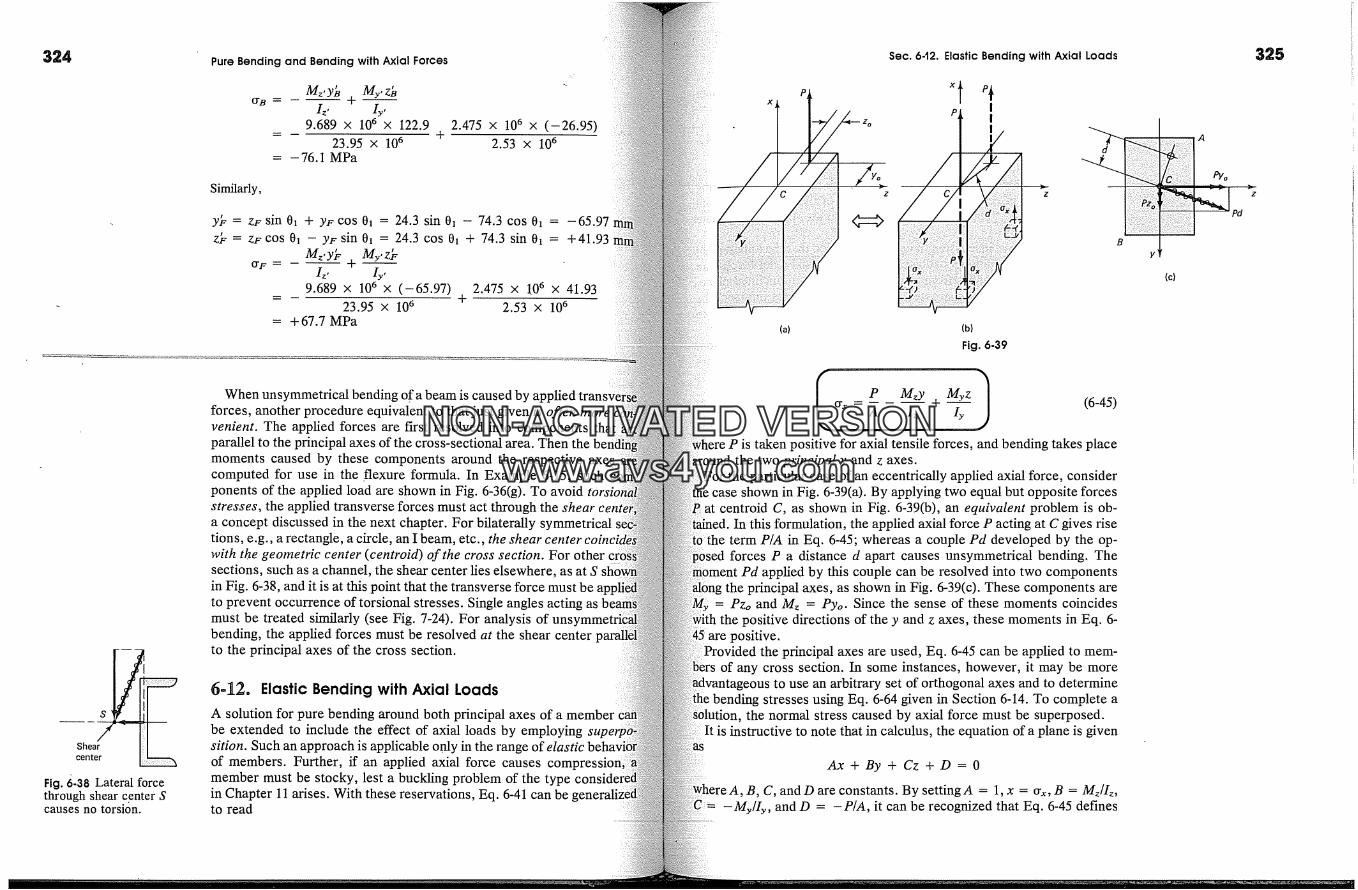
324
Fig. 6-38 Lateral forcethrough shear center Scauses no torsion.
Pure Bending and Bending with Axial Forces
O'B = + --
9.689 x 106 X 122.923.95 x 10 6
= - 76.1 MPa
2.475 x 10⁶ x (-26.95)+
2.53 x 10 6
Similarly,
Yb = zF sin 0� + yF cos 0� = 24.3 sin 0� - 74.3 cos 0� = -65.97zb = z� cos 0� - y� sin 0� = 24.3 cos 0� + 74.3 sin 0� = +41.93
mz,yj� my,z�
9.689 x 10⁶ X (--65.97) 2.475 X !06 X 41.9323.95 x 10 6 2.53 X 10 6
= + 67.7 MPa
When unsymmetrical bending of a beam is caused by applied transvforces, another procedure equivalent to that just given is often morevenient. The applied forces are first resolved into componentsparallel to the principal axes of the cross-sectional area. Then themoments caused by these components around the respective axesicomputed for use in the flexure formula. In Example 6-15, suchponents of the applied load are shown in Fig. 6-36(g). To avoidstresses, the applied transverse forces must act through the shear centa concept discussed in the next chapter. For bilaterally symmetricaltions, e.g., a rectangle, a circle, an I beam, etc., the shear centerwith the geometric center (centroid) of the cross section. For othersections, such as a channel, the shear center lies elsewhere, as at Sin Fig. 6-38, and it is at this point that the transverse force mustto prevent occurrence of torsional stresses. Single angles acting asmust be treated similarly (see Fig. 7-24). For analysis of uns'bending, the applied forces must be resolved at the shear centerto the principal axes of the cross section.
6-12. Elastic Bending with Axial LoadsA solution for pure bending around both principal axes of a memberbe extended to include the effect of axial loads by employingsition. Such an approach is applicable only in the range of elasticof members. Further, if an applied axial force causesmember must be stocky, lest a buckling problem of the typein Chapter 11 arises. With these reservations, Eq. 6-41 can beto read
z
Sec. 6-t2. Elastic Bending with Axial Loads
x tp I
I
d
(b)
Fig. 6-39
I P Mzy Myz1crx = A � + -�y (6-45)P is taken positive for axial tensile forces, and bending takes place
the two principal y and z axes.the particular case of an eccentrically applied axial force, consider
case shown in Fig. 6-39(a). By applying two equal but opposite forcesat centroid C, as shown in Fig. 6-39(b), an equivalent problem is ob-
In this formulation, the applied axial force P acting at C gives riseterm P/A in Eq. 6-45; whereas a couple Pd developed by the op-forces P a distance d apart causes unsymmetrical bending. The
Pd applied by this couple can be resolved into two componentsthe principal axes, as shown in Fig. 6-39(c). These components are
Pzo and M� = Pyo. Since the sense of these moments coincidesthe positive directions of the y and z axes, these moments in Eq. 6-
�are positive.the principal axes are used, Eq. 6-45 can be applied to mem-
of any cross section. In some instances, however, it may be moreto use an arbitrary set of orthogonal axes and to determine
bending stresses using Eq. 6-64 given in Section 6-14. To complete athe normal stress caused by axial force must be superposed.
It is instructive to note that in calculus, the equation of a plane is given
Ax + By + Cz + D=O
B, C, andD are constants. By settingA = 1, x = cry,, B = M�/I�,-My/Iy, and D = -P/A, it can be recognized that Eq. 6-45 defines
(c)
325
z
NON-ACTIVATEDVERSIONwww.avs4you.com
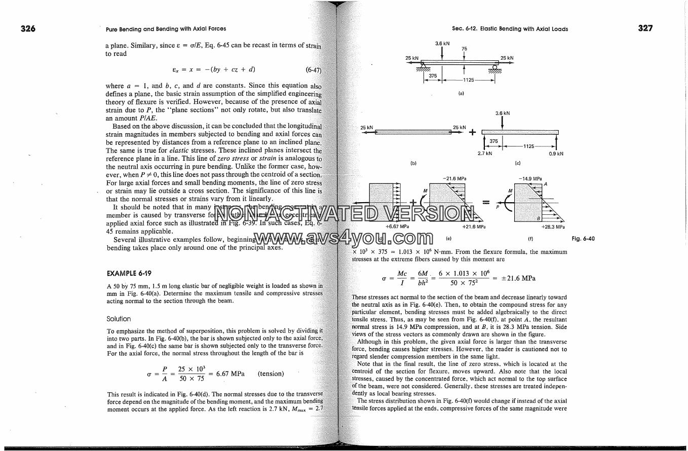
326 Pure Bending and Bending with Axial Forces Sec. 6-12. Elastic Bending with Axial Loads
a plane. Similary, since e = rifE, Eq. 6-45 can be recast in terms of:to read
e�, = x = -(by + cz + d)
where a = 1, and b, c, and d are constants. Since this equationdefines a plane, the basic strain assumption of the simplifiedtheory of flexure is verified. However, because of the presence ofstrain due to P, the "plane sections" not only rotate, but also translaan amount P/AE.
Based on the above discussion, it can be concluded that the Ionstrain magnitudes in members subjected to bending and axial forces ibe represented by distances from a reference plane to an inclinedThe same is true for elastic stresses. These inclined planes intersectreference plane in a line. This line of zero stress or strain is analothe neutral axis occurring in pure bending. Unlike the former case,ever, when P � 0, this line does not pass through the centroid of a secFor large axial forces and small bending moments, the line of zeroor strain may lie outside a cross section. The significance of thisthat the normal stresses or strains vary from it linearly.
It should be noted that in many instances, the bending momentmember is caused by transverse forces rather than by anapplied axial force such as illustrated in Fig. 6-39. In such cases, Ec45 remains applicable.
Several illustrative examples follow, beginning with situationsbending takes place only around one of the principal axes.
EXAMPLE 6-19
A 50 bY 75 mm, 1.5 m long elastic bar of negligible weight is loaded asmm in Fig. 6-40(a). Determine the maximum tensile and compressiveacting normal to the section through the beam.
Solution
To emphasize the method of superposition, this problem is solved byinto two parts. In Fig. 6-40(b), the bar is shown subjected only to the axialand in Fig. 6-40(c) the same bar is shown subjected only to the transverseFor the axial force, the normal stress throughout the length of the bar is
P 25 x 103cr- - - 6.67 MPa (tension)
A 50 x 75
This result is indicated in Fig. 6-40(d). The normal stresses due to theforce depend on the magnitude of the bending moment, and the maximummoment occurs at the applied force. As the left reaction is 2.7 kN, Mmax
3.6 kN
25 kN �
�-x375.� � 1125 -
25 kN
.I(a)
3,6kN
2.7 kN 0.9 kN
(b) (c)
-21.6 MPa -14.9 MPa
M M+
+6.67 MPa +21.6 MPa +28.3 MPa
10 3
(d) (e) (f)
x 375 = 1.013 x 10 6 N.mm. From the flexure formula, the maximumat the extreme fibers caused by this moment are
Mc 6M. 6 x 1.013 x 106cr- - - = +21.6 MPa
I bh 2 50 x 752
act normal to the section of the beam and decrease linearly towardneutral axis as in Fig. 6-40(e). Then, to obtain the compound stress for any
element, bending stresses must be added algebraically to the directstress. Thus, as may be seen from Fig. 6-40(f), at point A, the resultant
stress is 14.9 MPa compression, and at B, it is 28.3 MPa tension. Sideof the stress vectors as commonly drawn are shown in the figure.
in this problem, the given axial force is larger than the transverseforce, bending causes higher stresses. However, the reader is cautioned not to
slender compression members in the same light.Note that in the final result, the line of zero stress, which is located at the
of the section for flexure, moves upward. Also note that the localcaused by the concentrated force, which act normal to the top surface
beam, were not considered. Generally, these stresses are treated indepen-as local bearing stresses.
stress distribution shown in Fig. 6-40(f) would change if instead of the axials applied at the ends, compressive forces of the same magnitude were
Fig. 6-40
NON-ACTIVATEDVERSIONwww.avs4you.com

328
�'=75
(a)
Pure Bending and Bending with Axial Forces
acting on the member. The maximum tensile stress would be reduced to 14.9from 28.3 MPa, which would be deskable in a beam made of a materialtension and carrying a transverse load. This idea is utilized in prestressedstruction. Tendons made of high-strength steel rods or cable passingbeam with anchorages at the ends are used to precompress concrete beams.artificially applied fomes inhibit the development of tensile stresses. Prestrealso has been used in racing-car frames.
175
**EXAMPLE 648
A 50 by 50 mm elastic bar bent into a U shape, as in Fig. 6-41(a); isby two opposing forces P of 8.33 kN each. Determine the maximum normal ,.occurring at section A-B.
Solution
The section to be investigated is in the curved region of the bar, but thisno essential difference in the procedure. First, a segment of the bar isa free-body, as shown in Fig. 6-41(b). At section A-B, the axial force,the centroid of the section, and the bending moment necessary to maintainlibrium are determined. Then, each element of the force system is con,.separately. The stress caused by th� axial forces is
P 8.33 X 10³� -- -- -- 3.33 MPa (compression)
A 50 x 50
and is shown in the first diagram of Fig. 6-41(c). The normal stresses causedthe bending moment may be obtained by using Eq. 6-31. However, for thisbent to a 75-mm radius, the solution is already known from Examplestress distribution corresponding to this case is shown in the second diaFig. 6-41(c). By superposing the results of these two solutions, thestress' distribution is obtained. This is shown in the third diagram of Fig.The maximum compressive stress occurs atA and is 131 MPa. An is{for point A is shown in Fig. 6-41(d). Shear stresses are absent at
8.33 kN --
2083 N-m
(b)
Fig. 6-4t
250
3.33 MPa 128 MPa
+80.9 MPa
(c)
kN
131 MP�a�141 MPa(d)
77.6
131
Sec. 642. Elastic Bending with Axial Loads
i Shear force is necessary to maintain equilibrium of the segment shown in Fig.The relative insignificance of the stress caused by the axial force is strik-
329
Problems similar to the above commonly occur in machine design.C clamps, frames �f punch presses, etc. illustrate the variety of
to which the foregoing methods of analysis must be applied.
�LE 649
having a rectangular cross section at the base, as showns. 6-42(a) and (b). Determine the maximum eccentricity e such that the stress
caused by the applied force P is zero.
�lB
Pe
ution (b) b
in order to maintain applied force P in equilibrium, there must be an axial com- �,_P and a moment Pe at the base having the senses shown. The stressby the axial force is � = -P/A = -P/bh, whereas the largest tensile
t'""'t t ttt;tress caused by bending is O'max = Mc/I = M/S = 6Pelbh 2, where bh2/6 is the (c)section modulus of the rectangular cross section. To satisfy the condition
having stress at B equal to zero, it follows that
(d)P 6Pe h
� = bh + bh 2 = 0 or e = -emeans that if force P is applied at a distance of h/6 from the centroidal tel
of the cross section, the.stress at B is just zero. Stress distributions acrossbase corresponding, respectively, to the axial force and bending moment are Fig. 6-42 Location of force P
in Figs. 6-42(c) and (d), and their algebraic sum in Fig. 6-42(e). causing zero stress at B.
the above problem, if force P were applied closer to the centroid ofsection, a smaller bending moment would be developed at section A-
and there would be some compression stress at B. The same argumentbe repeated for the force acting to the right of the centroidal axis.
a practical rule, much used by the early designers of masonrymay be formulated thus:/f the resultant of all vertical forces
within the middle third of the rectangular cross section, there is noin the material at that section. It is understood that the resultant
in a vertical plane containing one of the axes of symmetry of thecross-sectional area.
The foregoing discussion may be generalized in order to apply to anysystem of forces acting on a member. The resultant of these forces
NON-ACTIVATEDVERSIONwww.avs4you.com

330 Sec. 6.t2. Elastic Bending with Axial Loads
Resultant
6 2
Fig. 6-43 Resultant causingno tension at B.
P
75
(a)
D
(c)
Pure Bending and Bending with Axial Forces
may be made to intersect the plane of the cross section, as isFig. 6-43. At the point of intersection of this resultant with theit may be resolved into horizontal and vertical components. If thecomponent of the resultant fulf�s the conditions of the formerno tension will be developed at point B, as the horizontalcauses only shear stresses. Hence, a more general "middle-third"may be stated thus: there will be no tension at a section of a mema rectangular cross section if the resultant of the forces above this sintersects one of the axes of symmetry of the section within thethird.
EXAMPLE 6-20
Find the stress distribution at section ABCD for the block �hown in mm �n.6-44(a) if P = 64 kN. At the same section, locate the line of zero stress. Nethe weight of the block.
Solution
In this problem, it is somewhat simpler to recast Eq. 6-45 with the aid of22, defining the elastic section modulus S = I/c as bh2/6. The normal
500
(b)
/- +2.8 MPa
125 +11.4 MPa
-14.2MPa 'A,//�-5.7 MPa
zero
(d)
Fig. 6-44
Ith comer of the block can be found directly from such a transformed equa-This equation reads
P Mz + My (6-48)A St Sy
Sz = bh2/6, and Sy = hb2/6.forces acting on section ABCD, Fig. 6-44(c), are P = -64 x 10 3 N, My
-64 x 103 x 150 = -9.6 x 10⁶ N.mm, and M� = -64 x 103 x (75 + 75)x 106 N-nlm. The cross-sectional area has the following properties: A
150 x 300 = 45 x 10 3 mm 2, Sz = 300 x 1502/6 = 1.125 x 106 mm 3, and SyX 3002/6 = 2.25 X 10 6 mm 3.
normal stresses at the comers are found using Eq. 6-48, assigning signsthe stresses caused by moments by inspection. For example, from Fig. 6-
it can be seen that due to My, the stresses at comers A and D are com-;ive. Other cases are treated similarly. Using this approach,
64 x 103 9.6 x 10⁶ 9.6 x 10645 x 103 1.125 x 10⁶ 2.25 x 106
= -1.42 - 8.53 - 4.27 = -14.2 MPaorb = -1.42 - 8.53 + 4.27 = -5.7 MPacrc = -1.42 + 8.53 + 4.27 = +11.4 MPacrz) = -1.42 + 8.53 - 4.27 = +2.8 MPa
stresses are shown in Fig. 6-44(d). The ends of these four stress vectorsA', B', C', and D' lie in the plane A'B'C'D'. The vertical distance between
ABCD and A'B'C'D' defines the total stress at any point on the crossThe intersection of plane A'B'C'D' with plane ABCD locates the line of
stress FE.
By drawing a line B'C" parallel to BC, similar triangles C'B'C" and C'EC arethus, the distance �E = [11.4/(11.4 + 5.7)]150 = 100 mm. Similarly,
is found to be 125 mm. Points E and F locate the line of zero stress.weight of the block is neglected, the stress distribution on any other section
to ABCD is the same.
6-21
zone over which the vertical downward force Po may be applied to theweightless block shown in Fig. 6-45(a) without causing any tensile
at the section A-B.
force P = -Po is placed at an arbitrary point in the first quadrant of the yze system shown. Then the same reasoning used in the preceding example
this position of the force, the greatest tendency for a tensile stressatA. With P = -Po, M� = +PoY, and My = -Poz, setting the stress at
NON-ACTIVATEDVERSIONwww.avs4you.com

Fig. 6-45 .
Pure Bending and Bending with Axial Forces
xI Poz b/6
h/6
(a)
�y
(b)
A equal to zero fulf'fils the limiting condition of the problem. Using Eq. 6-45the stress at A to be' expressed as
- Po (PoY)( - b/2) ( - Poz)( - h/2)era = 0 - +
A Izz Iyy
Po Poy PoZ _ 0or --�- + b-�h/6 + bh2/6z y
Simplifying, h/6 + � = 1which is an equation of a straight line. It shows that when z = 0, y = b/6;when y = O, z -- hi6. Hence, this line may be represented by line CD in Fig.45(b). A vertical force may be applied to the block anywhere on this line and tstress a�A will be zero. Similar lines may be established for the otherof the section; these are shown in Fig. 6-45(b). If force P is applied on anyof these lines or on any line parallel to such a line toward the centtoldsection, there will be no tensile stress at the corresponding coruer. Hence,P may be applied anywhere within the ruled area in Fig. 6-45(b) withouttensile stress at any of the four coruers or anywhere else. This zone of thesectional area is called the kern of a section. By limiting the possible locationthe force to the�lines of symmetry of the rectangular cross section, thefound in this example verify the "middle-third" rule discussed in Example
EXAMPLE 6-22
Consider a "weightless" rigid block resting' on a linearly elastic foundationcapable of transmitting any tensile stresses, as shown in Fig. 6-46(a).the stress distribution in the foundation when applied force P is so placed thatpart of the block lifts off.
Sec. 6-t3. Inelastic Bending with Axial Loads
)lution
sume that only a portion AB of the foundation of length x and width b is effectiveresisting applied force P. This corresponds to the colored area in Fig. 6-46(c).
stress along line B-B is zero by definition. Hence, the following equation forstress at B may be written.
P (�) 6trB= xb + P - k �x � 0,,x/2 - k is the eccentricity of the applied force with r6spect to the centroidal
of the shaded contact area, and bx2/6 is its section modulus. By solving forit is found that x = 3k and the pressure distribution will be "triangular," as
shown in Fig. 6-46(b) (why?). As k decreases, the intensity of pressure on lineincreases; when k is zero, the block becomes unstable.
Problems such as this arise, for example, in the design of foundations for chim-as no tensile stresses can develop at the contact surface of a concrete pad
soil. Similar problems arise in foundations for heavy machinery. Similarcan be applied where a number of forces are acting on a member and
contact area is of any shape.
;o13. Inelastic Bending with Axial LoadsIn Section 6-10, it is pointed out that the basic kinematic assumption thatplane sections through a beam taken normal to its axis remain plane aftera beam is bent remains valid even if the material behaves inelastically.Similary, plane sections perpendicular to a beam axis move along it par-allel to themselves when an inelastic member is loaded axially. For smalldeformations, the normal strains corresponding to these actions can besuperposed. As a result of-such superposition, a plane defined by EqJ 6-47 can be formulated. Such general analysis of inelastic beams is rathercumbersome and is not considered in this text? Here' attention is Confinedto a planar case.
The superposition of strains for a planar member simultaneously sub-ected to an axial force P and a bending moment M is shown schematically
in Fig. 6-47. For clarity, the strains are greatly exaggerated. Superpositionof strains due to P and M moves a plane section axially and rotates it asshown. If axial force P causes strain larger than any strain of oppositesign that is caused by M, the combined strains will not change their signwithin a section.
By supplementing these basic kinematic assumptions with the stress-strain relations and conditions of equilibrium, one can solve either elasticor inelastic problems. It is important to note, however, that superposition
� M. S. Aghbabian and E. P. Popov, "Unsymmetrical Bending of RectangularBeams Beyond the Elastic Limit," Proceedings, First U.S. National Congressof Applied Mechanics (Michigan: Edwards Bros., 1951), 579-584.
333
P
A
(a)
(b)
A
A
P
Fig. 6-46 Stresses betweentwo contacting surfaces thatdo not transmit tensileforces.
NON-ACTIVATEDVERSIONwww.avs4you.com
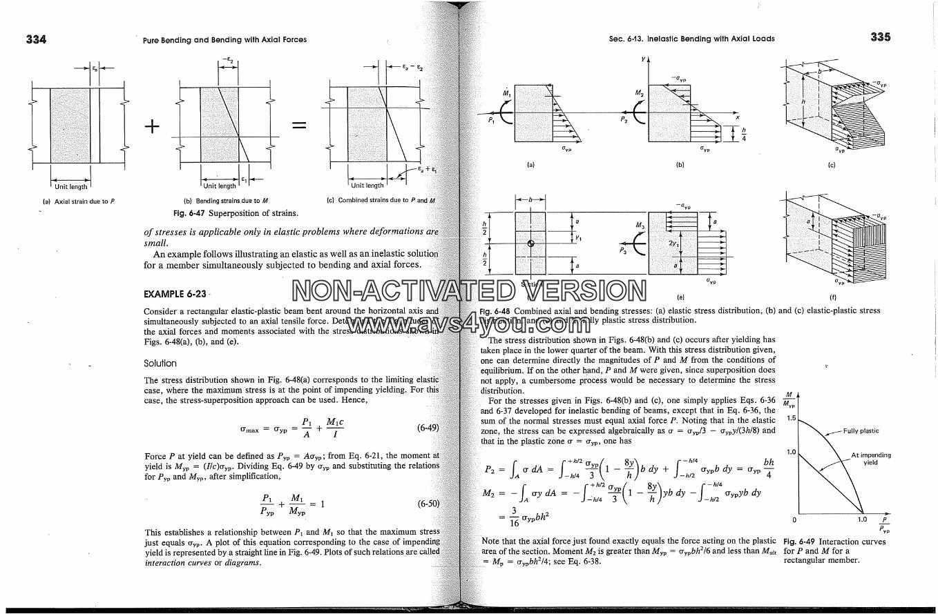
334
(a) Axial strain due to P
Pure Bending and Bending with Axial Forces
Unit'� �1�(b) Bending strains due to M
Fig. 6-47 Superposition of strains.
�Jnitlength�(c) Combined, strains due to P and
of stresses is applicable only in elastic problems where deformationssmall.
An example follows illustrating an elastic as well as an inelasticfor a member simultaneously subjected to bending and axial forces.
EXAMPLE 6-23-
Consider a rectangular elastic-plastic beam bent around the horizontal axissimultaneously subjected to an axial tensile force. Determine thethe axial forces and moments associated with the stress distributions shownFigs. 6-48(a), (b), and (e).
Solution
The stress distribution shown in Fig. 6-48(a) corresponds to the limitingcase, where the maximum stress is at the point of impending yielding.case, the stress-superposition approach can be used. Hence,
P1 MlCcrmax �-' cryp = �' q' I
Force P at yield can be deemed as Pyp = Acryp; from Eq. 6-21, theyield is myp = (I[c)O'yp. Dividing Eq. 6-49 by cryp and substituting thefor Pyp and Myp, after simplification,
P� M�
Pyp Myp
This establishes a relationship between P� and M� so that the maximumjust equals cryp. A plot of this equation corresponding to the case ofyield is represented by a straight line in Fig. 6-49. Plots of such relationsinteraction curves or diagrams.
Sec. 6.t3. Inelastic Bending with Axial Loads
y
M 2
P2 x
(a) (b) (c)
335
P3
M 3
OypSection %
(d) (e) (f)
�p
Fig. 6-48 Combined axial and bending stresses: (a) elastic stress distribution, (b) and (c) elastic-plastic stressdistribution, and (e) and (f) fully plastic stress distribution.
The stress distribution shown in Figs. 6-48(b) and (c) occurs after yielding hastaken place in the lower quarter of the beam. With this stress distribution given,
�ne can determine directly the magnitudes of P and M from the conditions ofequilibrium. If on the other hand, P and M were given, since superposition does
apply, a cumbersome process would be necessary to determine the stressdistribution.
For the stresses given in Figs. 6-48(b) and (c), one simply applies Eqs. 6-366-37 developed for inelastic bending of beams, except that in Eq. 6-36, the
of the normal stresses must equal axial force P. Noting that in the elasticthe stress can be expressed algebraically as cr = cryp/3 - crypy/(3h/8) and
that in the plastic zone cr = crvp, one has
fA ;+h/2 cr3yp( BE) ;--hi4 bh= cr dA = 1 - b dy q' crypb dy = --J -- h/4 J -- h/2 CrYP 4
-- crypyb dy= - cry dm= Jdh14 1 -- yb dy --J-h�23
= 1'-� crypbh2Note that the axial force just found exactly equals the force acting on the plastic
1.0 \ X _Atir�iPE�;ding
0 1.0 p
PypFig. 6-49 Interaction curves
of the section. Moment M2 is greater than Myp = crypbh2/6 and less than Muir for P and M for aM v = crvobh2/4; see Eq. 6-38. rectangular member.
NON-ACTIVATEDVERSIONwww.avs4you.com
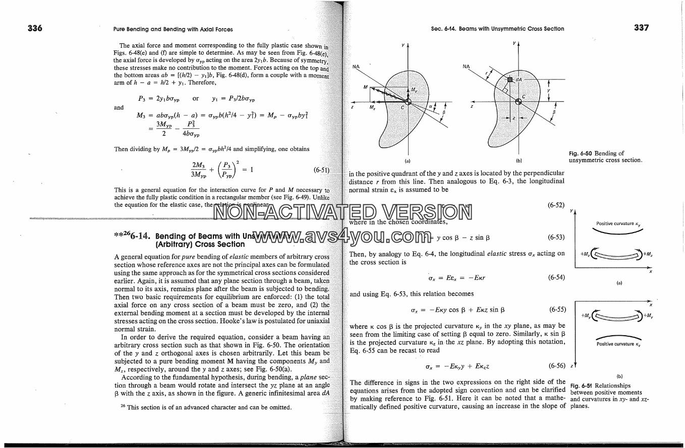
336 Pure Bending and Bending with Axial Forces
The axial force and moment corresponding to the fully plastic caseFigs. 6-48(e) and (0 are simple to determine. As may be seen �om Fig.the axial force is developed by cryp acting on the area 2y�b. Becausethese stresses make no contribution to the moment. Forces acting on the tothe bottom areas ab = [(h/2) - y�]b, Fig. 6-48(d), form a couple with a mearm of h - a = h/2 + y�. Therefore,
P3 = 2ylbCryp or y� = P3/2bcryp
M3 = abcryp(h - a) = Crypb(h2/4 - y�) = Mp - Crypby�3myp P3 �
2 4bcryp
and
Then dividing by M s = 3Myp/2 = crvpbh2/4 and simplifying, one obtains
+ = IThis is a general equation for the interaction curve for P and M neces:achieve the fully plastic condition in a rectangular member (see Fig. 6-49).the equation for the elastic case, the relation is nonlinear.
(6,51
*'266-14. Bending of Beams with Unsymmetric[Arbitrary] Cross Section
A general equation for pure bending of elastic members of arbitrary cro �.section whose reference axes are not the principal axes can beusing the same approach as for the symmetrical cross sectionsearlier. Again, it is assumed that any plane section through a beam,normal to its axis, remains plane after the beam is subjected toThen two basic requirements for equilibrium are enforced: (1) theaxial force on any cross section of a beam must be zero, and (2)external bending moment at a section must be developed by thestresses acting on the cross section. Hooke's law isnormal strain.
In order to derive the required equation, consider a beam. havingarbitrary cross section such as that shown in Fig. 6-50. Theof the y and z orthogonal axes is chosen arbitrarily. Let this beamsubjected to a pure bending moment M having the components MyMz, respectively, around the y and z axes; see Fig. 6-50(a).
According to the fundamental hypothesis, during bending, a planetion through a beam would rotate and intersect the yz plane at an[3 with the z axis, as shown in the figure. A generic infinitesimal area
26 This section is of an advanced character and can be omitted.
Sec. 6.t4. Beams with Unsymmetric Cross Section 337
z � zfi
(a) (b)
in the positive quadrant of the y and z axes is located by the perpendicularr from this line. Then analogous to Eq. 6-3, the longitudinal
normal strain ex is assumed to be
Fig. 6-50 Bending ofunsymmetric cross section.
aere in the chosen coordinates,
r =ycos[3 - zsin[3
(6-52)
(6-53)
by analogy to Eq. 6-4, the longitudinal elastic stress crx acting onthe cross section is
Positive curvature
Crx = Eex = - EKr
and using Eq. 6-53, this relation becomes
(6-54)(a)
cr.� = -E�y cos [3 + E� sin [3 (6-55)
where K cos [3 is the projected curvature Ky in the xy plane, as may beseen from the limiting case of setting [3 equal to zero. Similarly, K sin [3
the projected curvature �z inthe xz plane. By adopting this notation,Eq. 6-55 can be recast to read
Positive curvature
Crx = --EKyy + EKzZ (6-56) z'(b)
The difference in signs in the two expressions on the right side of the Fig. 6-5t Relationshipsequations arises from the adopted sign convention and can be clarified between positive moments
making reference to Fig. 6-51. Here it can be noted that a mathe- and curvatures in xy-and xz-matically defined positive curvature, causing an increase in the slope of planes.
x
x
NON-ACTIVATEDVERSIONwww.avs4you.com

Pure Bending and Bending with Axial Forces
a bent beam with an increase' in the distance from the origin,to two different cases. In the xy plane, positive curvature andbending moments have the same sense. The opposite is true inplane. Hence, the normal stresses Crx due to these two curvaturesbe of opposite sign.
By having an analytic expression for or:,, Eq. 6-56, the conditionthe sum of all forces in the x direction must equal zero, i.e., � Fxcan be written as
f crxdA = -EKy f y + EKz f z dA =OThis equation is identically satisfied provided that the coordinateare taken with their origin at the centraid of the cross section. Thiswas anticipated and the arbitrary orthogonal axes in Fig. 6-50 arepassing through the centraid C of the cross section.
By imposing the conditions of moment equilibrium at a section.moment component equations can be written requiring thatapplied moment around either axis is balanced by the internalstresses. One of these equations pertains to the moments aroundaxis; the other, around the y axis.. Hence, as previously defined,the known applied moment component around the z axis and My isknown applied moment component around the y axis, one has thelowing two equations:
mz=f-*yaA=Eyfy2dA-EzfyzdAand
My=f+*zda=-Eyfyz+Ezfz2where. the constants are taken outside the integrals in the expressionsthe right. The meaning of these integrals is discussed in SectionAccording to Eq. 6-66, these integrals define the moments andof inertia for a cross sectional area as I�, Iy, and Iy�, permitting thecasting of the last two equations as
EI�% - EIy�Kz = M�and
Solving these two equations simultaneously gives
(6-61
and
E�y = +
Sec. 6-t4. Beams with Unsymmetric Cross Section
substituting these constants in Eq. 6-56, the expression for the elasticstress cry, for any beam cross section with arbitrarily directed
hal coordinate axes is
or:,= - /yI�-� y + /y/z-Iy2� z (6-64)is the generalized flexure formula� If the principal axes for a cross
are used, where Iyz is zero, this equation simplifies to Eq. 6-41.setting Eq. 6-64 equal to zero, the angle {3 for locating the neutral
� in the arbitrary coordinate system is obtained, giving
y Mylz + Mzlyztan {3 z M�Iy + Mylyz (6-65)
the principal axes, this equation reverts to Eq. 6-43.
EXAMPLE 6-24
the general equation for elastic bending stress, verify the stresses found atPoints B and F for the angle of Example 6-16 shown in mm in Fig. 6-52. Show
that these stresses are, respectively, the minimum and the maximum. The appliedMz = 10 kN.m.
Solution
Example 6-25, it is found that Iz = 22.64 x 10 a n]1114, Iy = 3.84 x 10 a mm 4,and Iyz = 5.14 x 10 � mm 4. Substituting these values and Mz = +10 kN-m intoEq. 6-64, and defining, respectively, the coordinates of points B and F as (125.7,
and (-74�3, 24.3), one h/�s
10 x 106 X 3.84 x 10 6orb = 3.84 x 22.64 x 1012 - 5.142 X 1012 X 125.7
10 X 106 X 5.14 X 106+ X 4.3
3.84 X 22.64 X 10 �2 -- 5.142 X 10 �2= --0.6345 X 125.7 + 0.8493 X 4.3 = --76.1 MPa
-0.6345 x (-74.3) + 0.8943 x 24.3 = +67.8 MPa
To show that these stresses are the minimum and the maximum, respectively,locate the neutral axis using Eq. 6-65, giving
10 x 106 X 5.14 x 10 6tan {3 = 10 x 106 X 3.84 x 10 6 = 1�34 or {3 = 53.3 �
A
339
I125.7
74.3
Iylz - Iy2z By sketching this line on the given cross section, it is evident by inspection Fig. 6-52
NON-ACTIVATEDVERSIONwww.avs4you.com

340 Pure Bending and Bending with Axial Forces Sec. 6.t6. Principal Axes of Inertia
y
Z �
Fig. 6-53 Rotation ofcoordinate axe�.
that the farthest distances measured perpendicular to NA are associatedpoints B and F. Therefore, the largest stresses occur at these points.
Some minor discrepancies among the results given in Example 6-16 and iniexample are due to roundoff errors.
'276=115. Area Moments and Products of InertiaMoments of inertia, or second moments of area around the z axisalready encountered in connection with symmetric cross sections.this concept is generalized for two orthogonal axes for anyshape. With the yz coordinates chosen as shown in Fig. 6-53, b3the moments and product of inertia of an area are given as
f f' fIz = ya dA Iy = z a dA and Iyz = yz dA (6:
Note that these axes are chosen to pass through the centroid C ofarea. The use of such centroidal axes is essential in the solution ofb�
problems. It is also important to note that the product of inertia v;either for doubly or singly symmetric areas; see Fig. 6-54� Thisbe seen by referring to Fig. 6-54(b), where, due to symmetry, fory(+z) dA, there is a y(-z) dA, and their sum vanishes.
In Section 6-4, it was shown that in calculating moments of inertiasymmetric cross sections having complex areas, it issubdivide such areas into simple parts for which the momentsare available in formulas. Then by applying the parallel-axiseach part and adding, Eq. 6-18a, the moment of inertia for thesection is obtained. By making reference to the general case shownFig. 6-55, it can be concluded that the previously developed formula,6-18, for the transfer of a moment of inertia for an area from the zc toz axis remains applicable. Moreover, except for a change insimilar formula applies for transferring a moment of inertia from theto the y axis. Therefore, the following two formulas for the transferaxes are available for the moments of inertia:
and
= +27 This is an optional part of the chapter.
andIycare,respectively,momentsofinertiaaroundthezcand &axes, A is the area considered, and dz and dy are, respectively, the
an.ces from C to the axes z and y.By starting with the definition for the product of inertia, Eq. 6-66, and
following the same procedure as before for I� and Iy, the transfer-of-axisfor the product of inertia, after simplifications, becomes
Iyz= f (Y�+d�)(z�+dy)dA=Iyczc+Adydz (6-68)Iyc� is the product of inertia of the area A around the centroidaland Zc axes.
As noted earlier, the respective expressions given by Eqs. 6-18, 6-67,6-68 for all parts of a complex area should be summed to obtain Iy,
and Iyz for the whole cross section.
� 6-16. Principal Axes of Inertiathe previous discussion, the yz centroidal axes for an area of a general
were chosen arbitrarily. Therefore, it is important to investigatethe moments and product of inertia change if these orthogonal axes
rotated. This is shown in Fig. 6-53, where the axes are rotated throughan angle 0, forming a new set ofy'z' coordinates. Generally, the momentsand product of inertia corresponding to these axes are different from the
of Iy, I�, and Iy�. In order to transform these quantities from oneset of coordinates to another, one notes that
y' = CP + PS = y cos O + zsin0z' = NR -RS = z cos O -ysin0
Then, based on the definitions for moments and product of inertia givenin Eqs. 6-66,
f (y')2 dA =; (ycos 0 + Z sin 0)2dA= cos2 0 f y2 dA + sin2 0 f z2 dA + 2 sin O cos O f yz dO= I� cos 2 0 + Ix sin 2 0 + 2Iyz sin 0 cos 0
1 + cos 20 1 - cos 20
= I� 2 + 13, 2 + Iyz sin 20
Hence, on using trigonometric identities,
cos 20 + Iy� sin 20 (6-69)
z
+y
(b)
Fig. 6-54 (a) Doubly and (b)singly symmetric crosssections.
y
dA
Fig. 6-55 Parallel transfer ofaxes.
NON-ACTIVATEDVERSIONwww.avs4you.com
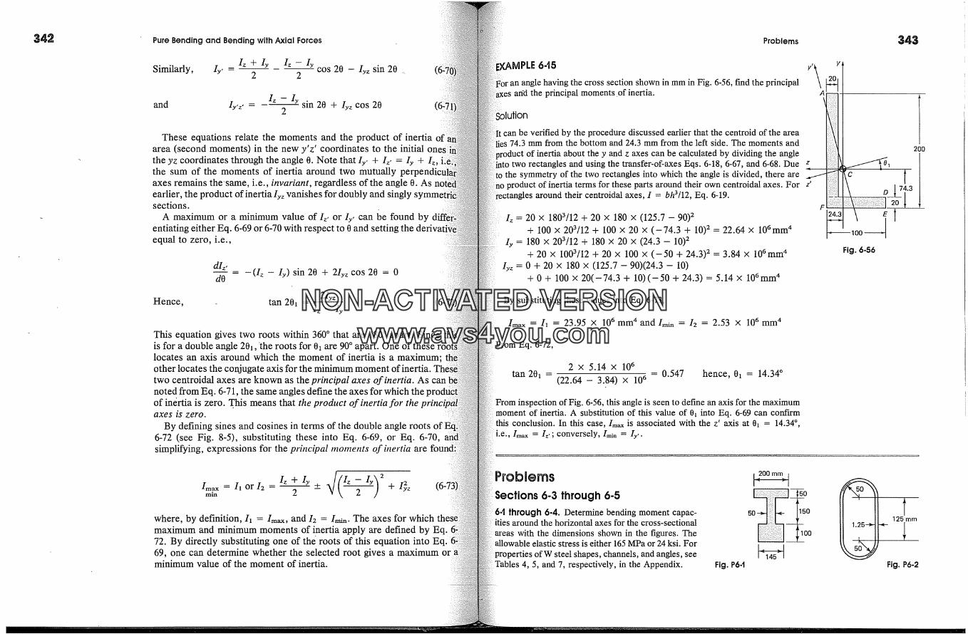
Pure Bending and Bending with Axial Forces Problems
Similarly, Iy, - 2 2-- cos 20 - Iyz sin 20
Iz - Iy sin 20 + Iy� cos 20and IY'�' = 2
These equations relate the moments and the product of inertia ofarea (second moments) in the new y'z' coordinates to the initial onesthe yz coordinates through the angle 0. Note that Iy, + I�, I� + I�,the sum of the moments of inertia around two mutuallyaxes remains the'same, i.e., invariant, regardless of the angle 0. Asearlier, the product of inertia Iyz vanishes for doubly and singly s�sections.
A maximum or a minimum value of Iz, or Iy, can be found byentiating either Eq. 6-69 or 6-70 with respect to 0 and settingequal to zero, i.e.,
d/z td�- - (I� - Iy) sin 20 + 2Iy� cos 20 = 0
Hence, tan 20� - 2Iy�
This equation gives two roots within 360 � that are 180 � apart. Sinceis for a double angle 20�, 'the roots for 01 are 90 � apart. One of theselocates an axis around which the moment of inertia is a maximum;other locates the conjugate axis for the minimum moment of inertia.two centroidal axes are known as the principal axes of inertia. As cannoted from Eq. 6-71, the same angles define the axes for which theof inertia is zero. This means that the product of inertia for theaxes is zero.
By defining sines and cosines in terms of the double angle roots6-72 (see Fig. 8-5), substituting these into Eq. 6-69, or Eq. 6-70,simplifying, expressions for the prbzcipal moments of inertia are
Im�x = 11 or I2 /z + Iy + +min 2
where, by definition, I� = Im�x, and/2 = Im�n- The axes for whichmaximum and minimum moments of inertia apply are defined by Eq.72. By directly substituting one of the roots of this equation into Eq,69, one can determine whether the selected root gives a maximumminimum value of the moment of inertia.
MPLE 645
the cross section shown in mm in Fig. 6-56, find the principalarfd the principal moments .of inertia.
ution
can be verified by the procedure discussed earlier that the centroid of the arealies 74.3 mm from the bottom and 24.3 mm from the left side. The moments and
of inertia about the y and z axes can be calculated by dividing the angleinto two rectangles and using the transfer-of-axes Eqs. 6-18, 6-67, and 6-68. Due z
the symmetry of the two rectangles into which the angle is divided, there areno product of inertia terms for these parts around their own centroidal axes. For z'
around their centroidal axes, I = bh3/12, Eq. 6-19.
Iz = 20 x 1803/12 + 20 X 180 X (125.7 -- 90) 2+ 100 x 203/12 + 100 X 20 X (--74.3 + 10) 2 = 22.64 x 106mm 4
Iy = 180 x 203/12 + 180 x 20 x (24.3 - 10) 2+ 20 x 1003/12 + 20 x 100 x (-50 + 24.3) 2 = 3.84 x 106mm 4
Iyz = 0 + 20 x 180 x (125.7 - 90)(24.3 - 10)+ 0 + 100 x 20(-74.3 + 10)(-50 + 24.3) = 5.14 x 106mm 4
By substituting these values into Eq. 6-73,
Im�x = I� = 23.95 x 10 6 mm 4 and Imin = 12 = 2.53 x 10 6 mm 4
Eq. 6-72,
2 x 5.14 x 10 6
tan 20� (22.64 - 3.84) x 10 6 0.547 hence, 0� 14.34 �From inspection of Fig. 6-56, this angle is seen to define an axis for the maximummoment of inertia. A substitution of this value of 0� into Eq. 6-69 can confirm
conclusion. In this case, Imx is associated with the z' axis at 0� = 14.34 �,i.e., Im�x = It'; conversely, Im� = Iy,.
200
C
Fig. 6-56
Sections 6-3 through 6-56-t through 6-4. Determine bending moment capac-ities around the horizontal axes for the cross-sectionalareas with the dimensions shown in the figures. Theallowable elastic stress is either 165 lV[Pa or 24 ksi. Forproperties of W steel shapes, channels, and angles, seeTables 4, 5, and 7, respectively, in the Appendix. Fig. P6-t
5O
50
150
100
Fig. P6-2
NON-ACTIVATEDVERSIONwww.avs4you.com
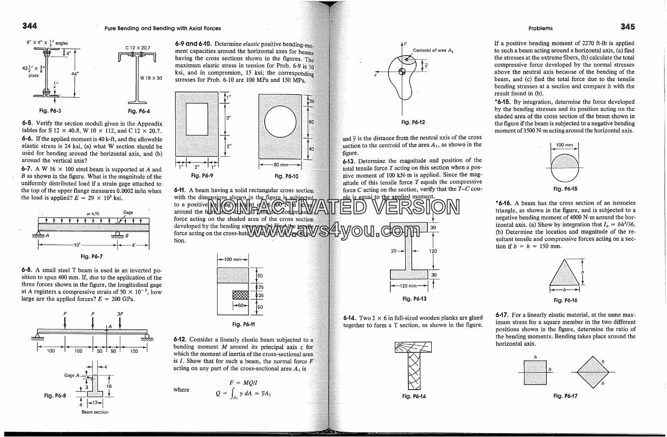
344
6"X4"X� angles
43 �"� x�plate 44"
4
Fig. P6-3 Fig. P6-4
6-5. Very the section modu� �ven in the Append�tables for S 12 x 40.8, W 10 x 112, and C 12 x 20.7.6-6. �the appHed moment is 40 k-�, and the �owableelastic stress is 24 ksi, (a) what W section should beused for bend�g �ound the hofizont� �is, and �)�ound the ve�ic� �is?
6-7. A W 16 x 100 steel beam is supposed at A andB as shown in the fi�re. �at is the magffitude of theunffor�y distributed load ff a strain gage attached tothe top of the upper flange measures 0.0002 �in whenthe load is applied? E = 29 x 10 � ksi.
Fig. P6-7
6-8. A small steel T beam is used in an inverted po-sition to span 400 mm. If, due to the application of thethree forces shown in the figure, the longitudinal gageat A registers a compresslye strain of 50 x 10 -3, howlarge are the applied forces? E = 200 GPa.
P P 3P
<too ood
4Fig.P6-�geA
4
Beam section
Pure Bending and Bending with Axial Forces
6-9 and 6-t0. Determine elastic positive bendJC 12 X 20.7ment capacities around the horizontal axes for
� �] having the cross sections shown in the figureS�maximum elastic stress in tension for Prob. 6-9ksi, and in compression, 15 ksi; the corres
w �8 x 50 stresses for Prob. 6-10 are 100 MPa and 150
Fig. P6-9 Fig. P6-t0
64t. A beam having a solid rectangular crosswith the dimensions shown in the figure isto a positive bending moment of 16 000 N.maround the horizontal axis. (a) Find theforce acting on the shaded area of the crossdeveloped by the bending stresses. (b) Find theforce acting on the cross-hatched area of the crosstion.
k100 mm-�
>25
Fig. P6-11
642. Consider a linearly elastic beam subjectedbending moment M around its principal axis zwhich the moment of inertia of the cross-sectiois I. Show that for such a beam, the normal forceacting on any part of the cross-sectional area A�
whereF = MQ/I
Q = y dA = yA�
y
Centroid of area
Fig. P6-12
y is the distance from the neutral axis of the crossthe centroid of the area A�, as shown in the
643. Determine the magnitude and position of thetensile force T acting on this section when a pos-
itive moment of 100 kN-m is applied. Since the mag-tde of this tensile force T equals the compresslye
C acting on the section, verify that the T-C cou-is equal to the applied moment.
30
120
.l30
Fig. P6-13
6-t4. Two 2 x 6 in full-sized wooden planks are gluedtogether to form a T section, as shown in the figure.
Fig. P6-t4
Problems 345
If a positive bending moment of 2270 ft-lb is appliedto such a beam acting around a horizontal axis, (a) findthe stresses at the extreme fibers, (b) calculate the totalcompresslye force developed by the normal stressesabove the neutral axis because of the bending of thebeam, and (c) find the total force due to the tensilebending stresses at a section and compare it with theresult found in (b).*645. By integration, determine the force developedby the bending stresses and its position acting on theshaded area of the cross section of the beam shown in
the figure if the beam is subjected to a negative bendingmoment of 3500 N-m acting around the horizontal axis.
100 mm
Fig. P6-15
'6-t6. A beam has the cross section of an isoscelestriangle, as shown in the figure, and is subjected to anegative bending moment of 4000 N-m around the hor-izontal axis. (a) Show by integration that Io = bh3/36.(b) Determine the location and magnitude of the re-suitant tensile and compresslye forces acting on a sec-tion ifb = h = 150 mm.
h
Fig. P6-16
6-t7. For a linearly elastic material, at the same max-imum stress for a square member in the two differentpositions shown in the figure, determine the ratio ofthe bending moments. Bending takes place around thehorizontal axis.
Fig. P6-17
NON-ACTIVATEDVERSIONwww.avs4you.com
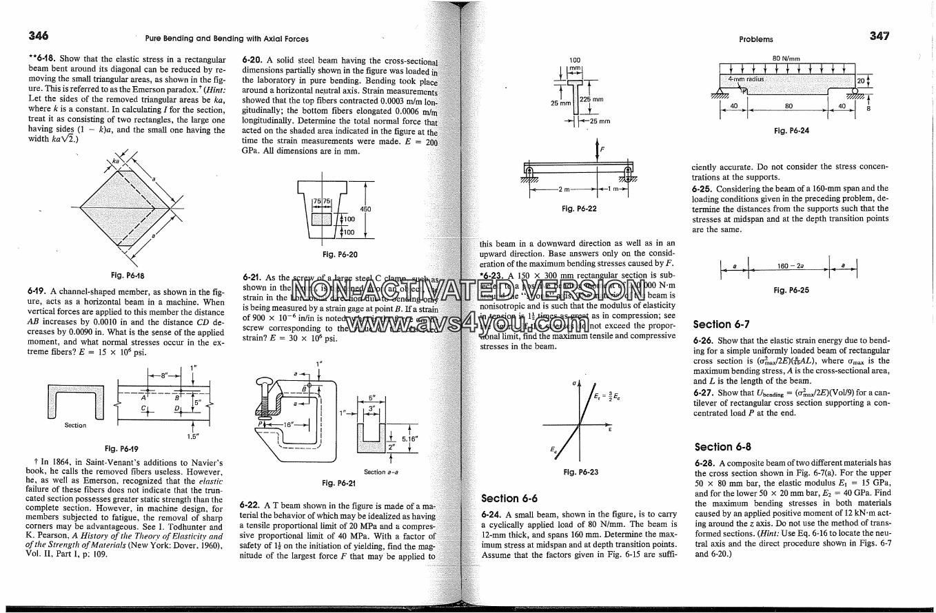
346 Pure Bending and Bending with Axial Forces
*'6-18. Show that the elastic stress in a rectangularbeam bent around its diagonal can be reduced by re-moving the small triangular areas, as shown in the fig-ure. This is referred to as the Emerson paradox.* (Hint:Let the sides of the removed triangular areas be ka,where k is a constant. In calculating I for the section,treat it as consisting of two rectangles, the large onehaving sides (1 - k)a, and the small one having thewidth kava.)
Fig. P6-t8
649. A channel-shaped member, as shown in the fig-ure, acts as a horizontal beam in a machine. Whenvertical forces are applied to this member the distanceAB increases by 0.0010 in and the distance CD de-creases by 0.0090 in. What is the sense of the appliedmoment, and what normal stresses occur in the ex-treme fibers? E = 15 x 10 6 psi.
Fig. P6-t9
? In 1864, in Saint-Venant's additions to Navier'sbook, he calls the removed fibers useless. However,he, as well as Emerson, recognized that the elasticfailure of these fibers does not indicate that the trun-cated section possesses greater static strength than thecomplete section. However, in machine design, formembers subjected to fatigue, the removal of sharpcorners may be advantageous. See I. Todhunter andK. Pearson, A HistoL3, of the Theoo, of Elasticity andof the Strength of Materials (New York: Dover, 1960),Vol. II, Part I, p: 109.
6-20. A solid steel beam having thedimensions partially shown in the figurethe laboratory in pure bending. Bending tookaround a horizontal neutral axis. Strain measuremeshowed that the top fibers contracted 0.0003 m/mgitudinally; the bottom fibers elongated 0.0006longitudinally. Determine the total normal forceacted on the shaded area indicated in the figuretime the strain measurements were made. E =GPa. All dimensions are in mm.
Fig. P6-20
6-2t. As the screw of a large steel C clamp,shown in the figure, is tightened upon an object,strain in the horizontal direction due to bendingis being measured by a strain gage at point B. Ifaof 900 x 10 -6 in/in is noted, what is the force onscrew corresponding to the value of thestrain? E = 30 x 106 psi.
Section a-a
Fig. P6-21
l T-5.16"
6-22. A T beam shown in the figure is made of aterial the behavior of which may be idealized asa tensile proportional limit of 20 MPa and accsive proportional limit of 40 IV[Pa. With a factorsafety of 1� on the initiation of yielding, find thenitude of the largest force F that may be applied
100mm
25m-2[-m�22im,m
Fig. P6-22
beam in a downward direction as well as in andirection. Base answers only on the consid-
of the maximum bending stresses caused by F.A 150 x 300 mm rectangular section is sub-
ected to a positive bending moment of 240 000 N-mthe "strong" axis. The material of the beam is
nonisotropic and is such that the modulus of elasticityin tension is 1� times as great as in compression; seethe figure. If the stresses do not exceed the propor-tional limit, find the maximum tensile and compressivestresses in the beam.
Fig. P6-23
Section 6-6
6-24. A small beam, shown in the figure, is to carrya cyclically applied load of 80 N/mm. The beam is12-mm thick, and spans 160 mm. Determine the max-imum stress at midspan and at depth transition points.Assume that the factors given in Fig. 6-15 are suffi-
Problems
80 N/mm
347
80
Fig. P6-24
ciently accurate. Do not consider the stress concen-trations at the supports.6-25. Considering the beam of a 160-mm span and theloading conditions given in the preceding problem, de-termine the distances from the supports such that thestresses at midspan and at the depth transition pointsare the same.
-�[4 160- 2a �q�Fig. P6-25
Section 6.7
6-26. Show that the elastic strain energy due to bend-ing for a simple uniformly loaded beam of rectangularcross section is (cr2m=/2E)(�-�tL), where Crm= is themaximum bending stress, A is the cross-sectional area,and L is the length of the beam.6-27. Show that Ube,di,g = (cr2m�/2E)(Vol/9) for a can-tilever of rectangular cross section supporting a con-centrated load P at the end.
Section 6-8
6-28. A composite beam of two different materials hasthe cross section shown in Fig. 6-7(a). For the upper50 x 80 mm bar, the elastic modulus El = 15 GPa,and for the lower 50 x 20 mm bar, E2 = 40 GPa. Findthe maximum bending stresses in both materialscaused by an applied positive moment of 12 kN-m act-ing around the z axis. Do not use the method of trans-formed sections. (Hint: Use Eq. 6-16 to locate the neu-tral axis and the direct procedure shown in Figs. 6-7and 6-20.)
NON-ACTIVATEDVERSIONwww.avs4you.com

Pure Bending and Bending with Axial Forces - Problems
6-29. Consider a composite beam whose cross sectionis made from three different materials bonded to-gether, as shown in Fig. 6-20(a). Bar 1 is 40 x 20 mmand has an elastic modulus E� = 15 GPa; bar 2 is 60
x 40 mm with E2 = 10 GPai and bar 3 is 20 x 20 mmwith E3 = 30 GPa. Determine the maximum bendingstresses in each of the three materials caused by anapplied moment of 10 kN.m acting around the z axis.Do not use the method of transformed sections; seethe hint in the preceding problem.6-30 ond �-31. Using transformed sections, deter-mine the maximum bending stresses in each of the twomaterials for the composite beams shown in the figureswhen subjected to positive bending moments of 80kN-m each. Est = 210 GPa and E�u = 70 GPa. (Hint
for-Prob. 6-31: For an ellipse with semiaxes a and b,I = 'rrab3/4 around the major centroidal axis.)
75 mm
Fig. P6-30
Steel inside core
Fig. P6-3t
6-32 and 6-33. Determine the allowable bending mo-ment around horizontal neutral axes for the compositebeams of wood and steel plates having the cross-sec-tional dimensions shown in the figures. Materials arefastened so that they act as a unit. Est = 30 x 106 psiand E,� = 1.2 x 10⁶ psi. The allowable bendingstresses are trst = 20 ksi and trw = 1.2 ksi.
Fig. P6-32 Fig. P6-33
6-34. A 150-mm thick concrete slab isreinforced with steel bars, as shown in t he figure, 1termine the allowable bending moment perof this slab. Assume n = 12 and the allowablefor steel and concrete as 150 MN/m 2 and 8respectively.
10-mm � bars 25 mm80 mm on centers
Fig. P6-34
6-35. A beam has the cross section shown in theure, and is subjected to a positive bending momentcauses a tensile stress in the steel of 20 ksi. If nwhat is the value of the bending moment?
Fig. P6-35
Section 6.9
6-36. Rework Example 6-10 by changing h to6-37. Derive Eq. 6-35.6-38. What is the largest bending moment thatbe applied to a curved bar, such as shown in Fig.23(a), with ? = 3 in, if it has a circular cross-setarea of 2-in diameter and the allowable stress is 12
Section 6.'10
6-39 through 6-43. Find the ratios Mu�JMypbeams having the cross sections shown in the fiBending occurs around the horizontal axes.idealized elastic-plastic behavior as in Example
Fig. P6-39 Fig. P6-40
W8 X 18
Fig. P6-4t
300
1Fig. P6-42
Fig. P6-43
Find the ultimate moment capacity for a beamthe cross section shown for Prob. 6-1. Assume
hat the material yields in tension and in compression200 MPa.
�-45. A steel I beam subjected to pure bending de-velops a longitudinal strain of - 1.6 x 10 -3 in the topflange in the location shown on the figure. (a) What
Gage 20
!
2O
Fig. P6-45
bending moment causes this strain? Assume ideal elas-tic-plastic material behavior with E = 200 GPa and tryp= 240 MPa. (b) What residual strain would remain in
the gage upon release of the applied load? (c) Drawthe residual stress pattern.6-46. An I beam is made up from three steel plateswelded together as shown in the figure. The flangesare o� stronger steel than the web. (a) What bendingmoment would the section develop when the largeststresses in the flanges just reach yield? The stress-strain properties 0f the two steels can be idealized asshown on the diagram. (b) Draw the residual stresspattern.
20
I I�--� I
'4o400 MPa(flanges)
240 MPa
E = 200 GPa
Fig. P6-46
6-47. A small sandwich beam spanning 400 mm ismade up by bonding two aluminum alloy strips to analloy steel bar, as shown in the figure. The idealizedstress-strain diagrams are shown in the figure. Whatis the magnitude of the applied bending moment if itcauses -7.5 x 10 -3 longitudinal strain in the gageglued to the top of the aluminum alloy strip?
AI --
St
AI-
a [MPa]Gage
40
� 350
Beam section 0 5 X 10 -3 g
Fig. P6-47
6-48. On applying a bending moment around the hor-izontal axis to the T beam having the dimensions
NON-ACTIVATEDVERSIONwww.avs4you.com
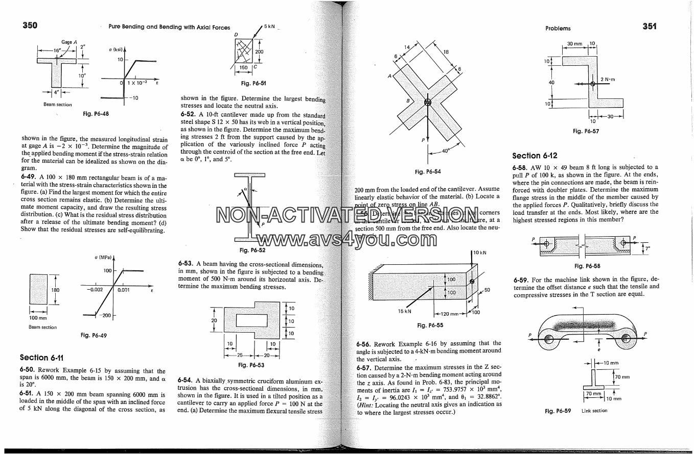
350
Gage A
10"
Beam section
PureBendingandBendingwithAxialForces� 5kN_X 10 -3 � Fig. P6-51
Fig. P6-48
shown in the figure, the measured longitudinal strainat gage A is -2 x 10 -3. Determine the magnitude ofthe_ applied bending moment if the stress-strain relationfor the material can be idealized as shown on the dia-gram.
6-49. A 100 x 180 mm rectangular beam is of a ma-terial with the stress-strain characteristics shown in thefigure. (a) Find the largest moment for which the entirecross section remains elastic. (b) Determine the ulti-mate moment capacity, and draw the resulting stressdistribution. (c) What is the residual stress distributionafter a �release of the ultimate bending moment? (d)Show that the residual stresses are self-equilibrating.
180
a (MPa
10(
Fig. P6-49
0.001 e
100 mm
Beam section
Section 6-11
6-50. Rework Example 6-15 by assuming that thespan is 6000 mm, the beam is 150 x 200 mm, and ctis 20 � .
6-51. A 150 x 200 mm 'beam spanning 6000 mm isloaded in the middle of the span with an inclined forceof 5 kN along the diagonal of the cross section, as
shown in the figure. Determine the largeststresses and locate the neutral axis.
6-52. A 10-ft cantilever made up from thesteel shape S 12 x 50 has its web in a verticalas shown in the figure. Determine the maximum b{ing stresses 2 ft from the support caused by theplication of the variously inclined force Pthrough the centroid of the section at the free endct be 0 �, 1 �, and 5 �.
Fig. P6-52
6-53. A beam having the cross-sectionalin mm, shown in the figure is subjected to a bendmoment of 500 N-m around its horizontal axis.termine the maximum bending stresses.
20 10
Fig. P6-53
6-54. A biaxially. symmetric cruciform aluminum ex-trusion has the cross-sectional dimensions, inshown in the figure. It is used in a tilted position ascantilever to carry an applied force P = 100 N atend. (a) Determine the maximum flexural tensile stress
A<
18
6
B
Fig. P6-54
200 mm from the loaded end of the cantilever. Assumeelastic behavior of the material. (b) Locate a
of zero stress on line AB.
�-55. Determine the bending stresses at the coruersthe cantilever loaded, as shown in the figure, at a
mm from the free end. Also locate the neu-tral axis.
10kN
15 kN 00
Fig. P6-55
6-56. Rework Example 6-16 by assuming that thesubjected to a 4-kN.m bending moment around
vertical axis.
6-57. Determine the maximum stresses in the Z sec-caused by a 2-N.m bending moment acting around
the z axis. As found in Prob. 6-83, the principal mo-ments of inertia are I� = Iz, = 753.9757 x 103 mm 4,
= Iy, = 96.0243 x 103 mm 4, and 0� = 32.8862 ��Locating the neutral axis gives an indication as
where the largest stresses occur.)
Problems
Fig. P6-57
Section 6-t2
6-58. AW 10 x 49 beam 8 ft long is subjected to apull P of 100 k, as shown in the figure. At the ends,where the pin connections are made, the beam is rein-forced with doubler plates. Determine the maximumflange stress in the middle of the member caused bythe applied forces P. Qualitatively, briefly discuss theload transfer at the ends. Most likely, where are thehighest stressed regions in this member?
Fig. P6-58
6-59. For the machine link shown in the figure, de-termine the offset distance e such that the tensile andcompressive stresses in the T section are equal.
p P
Fig. P6-59
7�-m� lO mmLink section
NON-ACTIVATEDVERSIONwww.avs4you.com

352 Pure Bending and Bending with Axial Forces
6-60. A frame for a punch press has the proportionsshown in the figure. What force P can be applied tothis frame controlled by the stresses in the sectionssuch as a-a, if the allowable stresses are 4,000 psi intension and 12,000 psi in compression?
Section a-a
Fig. P6-60
6-61. A force of 169.8 k is applied to bar BC at C, asshown in the figure. Find the maximum stress actingnormal 'to section a-a. Member BC is made from apiece of 6 by 6 in steel bar. Neglect the weight of thebar.
structure shown in the figure. The cross section at Stion a-a is that of a solid circular bar of 2-in d
6-63. Compute the maximum compressive stressing normal to section a-a for the structure shownthe figure. Post AB has a 12 by 12 in crossNeglect the weight of the structure.
Cable
Cable
'9k
12'
169.8 k
'' C/
�aFig. P6-6t
6-62. Calculate the maximum compressire stress act-ing on section a-a caused by the applied load for the
707 lb Fig. P6-62
Fig. P6-63
6-64. In order to obtain the magnitude of an eccenvertical force F on a tee-shaped steel column,gages are attached at A and B, as shown in the fiDetermine the force F if the longitudinal strain at A-100 x 10 -6 in/in and atB is -800 x 10 -6 in/in.= 30 x 106 psi and G = 12 x 106 psi. The
sectional area of the column is 24 in 2.
Centroid
A B
3" ,
Fig. P6-64
'6-65. A bar having a 100 x 100 mm cross sectionsubjected to a force F, as shown in the figure.
A B
2OO
D
mm
Fig. P6-65
longitudinal stresses on the extreme fibers at two sec-200 mm apart are determined experimentally to
cr�t = 0; orb = -30 MPa; crc = -24 MPa; and crD= -6 IV[Pa. Determine the magnitude of the vertical
and horizontal components of force F.6-66. A rectangular vertical member fixed at the baseis loaded as shown in the figure. Find the location for
gage on member face AB such that no longitudinalstrain would occur due to the application of force P= 6 kN. Does the answer depend on the magnitude
P? Assume elastic behavior. All dimensions
are given in mm.
Gage-� ' T�PseVcit�'�na"dFig. P6.66
6-67. An inclined tensile force F is applied to an alu-minum alloy bar such that its line of action goes
centroid of the bar, as shown in mm in the(The detail of the attachment is not shown.)
What is the magnitude of force F if it causes a Iongi-
1
2
F
500
F I� 13��,
GageA
Top view
Fig. P6-67
tudinal strain of +20 x 10 -6 in the gage atA? Assumethat the bar behaves as a linearly elastic material andlet E = 70 GPa.
6-68. A magnesium alloy bar is bonded to a steel barof the same size forming a beam having the cross-sec-tional dimensions in mm shown in the figure. (a) If onapplication of an eccentric axial force P, the upperlongitudinal gage measures a compressive strain of 2
x 10 -3, and the lower one, a tensile strain of 2 x10 -3, what is the magnitude of applied force P? As-sume elastic behavior of the materials with EMg = 45GPa and Est = 200 GPa. (b) Where would one haveto apply axial force P to cause no bending? (It is in-teresting to note that this locates the neutral axis forthis beam.)
Mg 20
St
Gage
Fig. P6-68
20
353
NON-ACTIVATEDVERSIONwww.avs4you.com
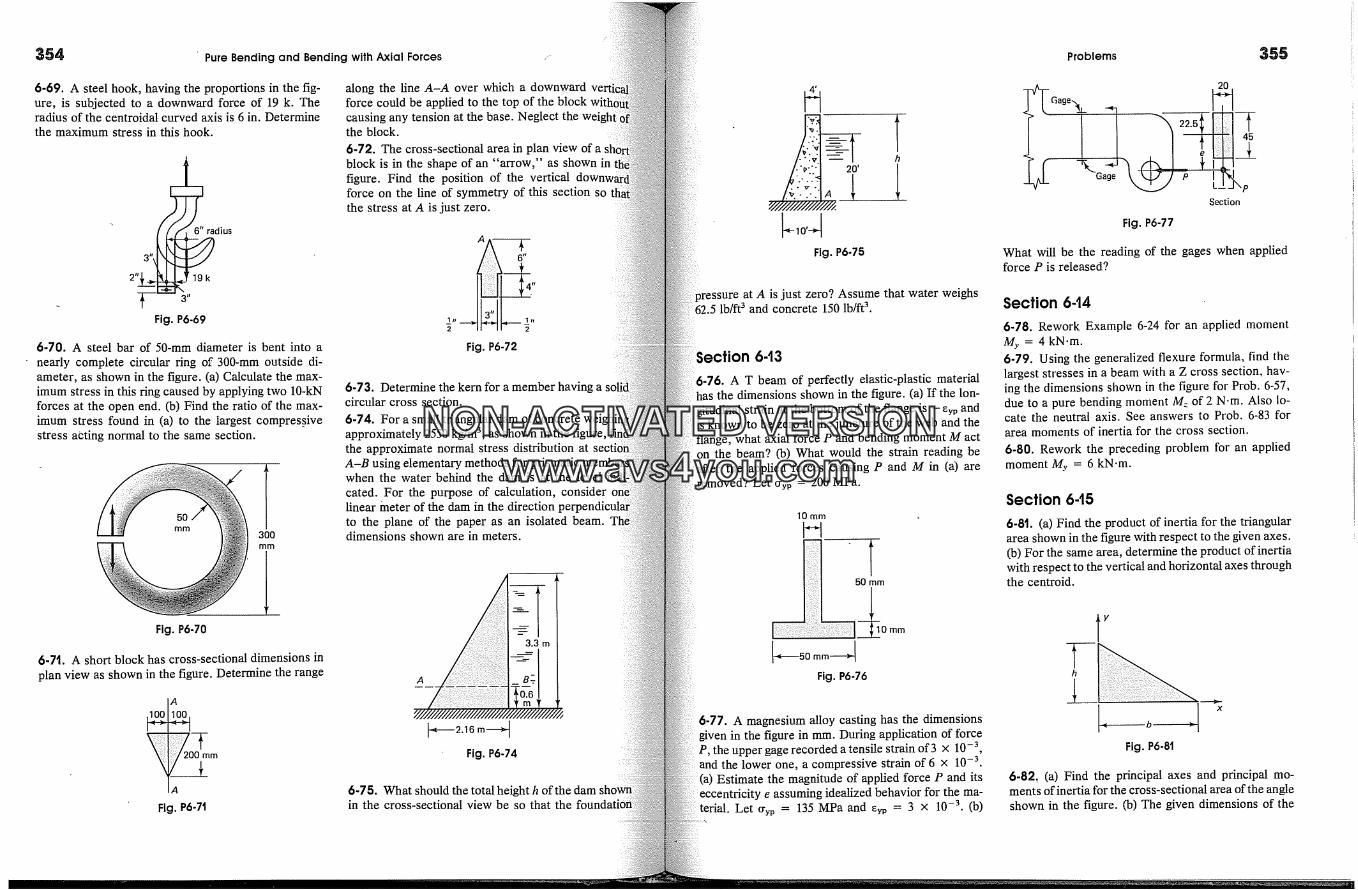
354 ,� Problems 355Pure Bending and Bending with Axial Forces
6-69. A steel hook, having the proportions in the fig-ure, is subjected to a downward force of 19 k. Theradius of the centroidal curved axis is 6 in. Determinethe maximum stress in this hook.
�dius3" Fig. P6-69
6-70. A steel bar of 50-ram diameter is bent into anearly complete circular ring of 300-ram outside di-ameter, as shown in the figure. (a) Calculate the max-imum stress in this ring caused by applying two 10-kNforces at the open end. Co) Find the ratio of the max-imum stress found in (a) to the largest compres_sivestress acting normal to the same section.
300
along the line A-A over which a downwardforce could be applied to the top of the blockcausing any tension at the base. Neglect thethe block.
6-72. The cross-sectional area in plan view ofblock is in the shape of an "arrow," as shown infigure. Find the position of the verticalforce on the line of symmetry of this section sothe stress at A is just zero.
Fig. P6-72
6-73. Determine the kern for a member having acircular cross section.
6-74. For a small triangular damapproximately 2550 kg/m 3, as shown in the figure, f'm(the approximate normal stress distribution atA-B using elementary methods for prismaticwhen the water behind the dam is at the levelcated. For the purpose of calculation, considerlinear meter of the dam in the directionto the plane of the paper as an isolated beam.dimensions shown are in meters.
Fig. P6-70
6-7t. A short block has cross-sectional dimensions inplan view as shown in the figure. Determine the range
Fig. P6-7t
2.16 m---�Fig. P6-74
6-75. What should the total height hin the cross-sectional view be so that the
Fig. P6-75
pressure at A is just zero? Assume that water weighslb/ft 3 and concrete 150 lb/ft 3.
Section 6.t36-76. A T beam of perfectly elastic-plastic material
has the dimensions shown in the figure. (a) If the Ion-strain at the bottom of the flange is - eyp and
is known to be zero at the juncture of the web and theflange, what axial force P and bending moment M acton the beam? (b) What would the strain reading beafter the applied forces causing P and M in (a) areremoved? Let tryp = 200 IV[Pa.
10 mm
50 mm
-50 mm �Fig. P6-76
10 mm
6-77. A magnesium alloy casting has the dimensionsgiven in the figure in mm. During application of force
the upper gage recorded a tensile strain of 3 x 10 -3,and the lower one, a compressive strain of 6 x 10 -3.
Estimate the magnitude of applied force P and itse assuming idealized behavior for the ma-
tedfl. Let tryp = 135 MPa and eyp = 3 x 10 -3. (b)
Section
Fig. P6-77
What will be the reading of the gages when appliedforce P is released?
Section 644
6-78. Rework Example 6-24 for an applied momentM_,. = 4 kN.m.6-79. Using the generalized flexure formula, find thelargest stresses in a beam with a Z cross section, hav-ing the dimensions shown in the figure for Prob. 6-57,due to a pure bending moment M: of 2 N.m. Alsocate the neutral axis. See answers to Prob. 6-83 forarea moments of inertia for the cross section.6-80. Rework the preceding problem for an appliedmoment My = 6 kN.m.
Section 6-t5
6-8t. (a) Find the product of inertia for the triangulararea shown in the figure with respect to the given axes.(b) For the same area, determine the product of inertiawith respect to the vertical and horizontal axes throughthe centroid.
y
xFig. P6-8t
6-82, (a) Find the principal axes and principal mo-ments of inertia for the cross-sectional area of the angieshown in the figure. (b) The given dimensions of the
NON-ACTIVATEDVERSIONwww.avs4you.com
Pure Bending and Bending with Axial Forces
Fig. P6-82
cross section, except for small radii at the ends and afillet, correspond to the cross-sectional dimensions ofan 8 x 6 x 1 in angle listed in Table 7 of the Appendix.Using the information given in that table, calculate theprincipal moments of inertia and compare with the re-sults found in (a). (Hint: Note that per Section 11-6and Example 11-2, Imin = Ar2min. The r listed in Table7 for the z axis is rmin. Further, from the invariance
condition, Imi, + Ira= = Ix' + Iy, = Ix + Iy,one can readily solve for Imx.)6-83. For the Z cross section shown in the figuredetermine area moments of inertia Iy, I�, and Lobtain the directions of the principal axes andmoments of inertia.
Fig. P6-83
ter
!-1. Introduction
This chapter is divided into two parts. Part A, the major part, is devoteda study of shear stresses in beams caused by transverse shear. The
related problem of attaching separate longitudinal parts of a beam bymeans of bolts, gluing, or welding is also considered. In Part B, super-position of direct shear stresses of the type discussed in Part A with thosecaused by torque, as in springs, is treated. This problem is analogous tothat encountered in the previous chapter in the study of beams simul-taneously subjected to bending and axial forces.
The discussion in this chapter is largely limited to elastic analyses, themost widely used approach in the solution of the type of problems con-sidered.
?.2. Preliminary RemarksIn deriving the torsion and the flexure formulas, the same sequence ofreasoning was employed. First, a strain distribution was assumed acrossthe section; next, properties of the material were brought in to relate thesestrains to stresses; and, finally, the equations of equilibrium were usedto establish the desired relations. However, the development of theexpression linking the shear force and the cross-sectional area of a beamto the stress follows a different path. The previous procedure cannot be
357
NON-ACTIVATEDVERSIONwww.avs4you.com
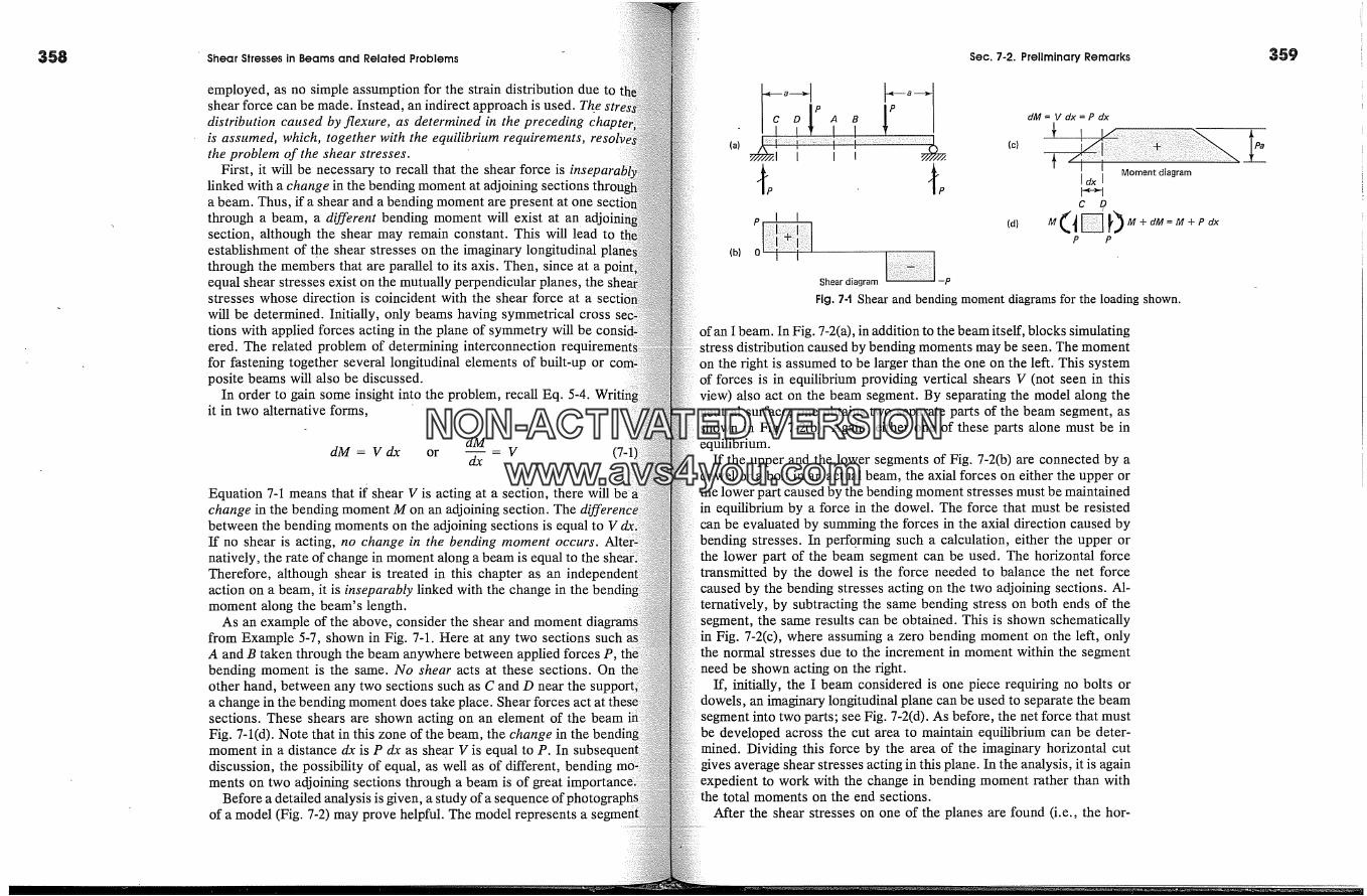
Shear Stresses in Beams and Related Problems Sec. 7-2. Prellminary Remarks
employed, as no simple assumption for the strain distribution due toshear force can be made. Instead, an indirect approach is used. Thedistribution caused by flexure, as determined in the preceding chais assumed, which, together with the equilibrium requirements,the problem of the shear stresses.
First, it will be necessary to recall that the shear force is inselinked with a change in the bending moment at adjoining sectionsa beam. Thus, if a shear and a bending moment are present at onethrough a beam, a different bending moment will exist at an adsection, although the shear may remain constant. This will lead toestablishment of the shear stresses on the imaginary longitudinalthrough the members that are parallel to its axis. Then, since at aequal shear stresses exist on the mutually perpendicular planes, thestresses whose direction is coincident with the shear force at a se�will be determined. Initially, only beams having symmetrical crosstions with applied forces acting in the plane of symmetry will be consiered. The related problem of determining interconnection reqfor fastening together several longitudinal elements of built-up orposite beams will also be discussed.
In order to gain some insight into the problem, recall Eq. 5-4.it in two alternative forms,
dM
dM = V dx or dx - V (7-1
Equation 7-1 means that if shear V is acting at a section, there willchange in the bending moment M on an adjoining section. Thebetween the bending moments on the adjoining sections is equal toIf no shear is acting, no change in the bending moment occurs.natively, the rate of change in moment along a beam is equal toTherefore, although shear is treated in this chapter as anaction on a beam, it is inseparably linked with the change in themoment along the beam's length.
As an example of the above, consider the shear and momentfrom Example 5-7, shown in Fig. 7-1. Here at any two sectionsA and B taken through the beam anywhere between applied forces P,bending moment is the same. No shear acts at these sections. Onother hand, between any two sections such as C and D near thea change in the bending moment does take place. Shear forces actsections. These shears are shown acting on an element of the beamFig. 7-1(d). Note that in this zone of the beam, the change in themoment in a distance dx is Pdx as shear V is equal to P. In subse�discussion, the possibility of equal, as well as of different, bendingmerits on two adjoining sections through a beam is of great
Before a detailed analysis is given, a studyof a model (Fig. 7-2) may prove helpful. The model represents a
(a)c D[P A B [P
p I I
(b) 0
(c)
(d)
dM= V dx = P dx
Moment diagram
C D
? ?
Shear diagram -- -P
Fig. 7-t Shear and bending moment diagrams for the loading shown.
of an I beam. In Fig. 7-2(a), in addition to the beam itself, blocks simulatingstress distribution caused by bending moments may be seen. The momenton the right is assumed to be larger than the one on the left. This systemof forces is in equilibrium providing vertical shears V (not seen in thisview) also act on the beam segment. By separating the model along theneutral surface, one obtains two separate parts of the beam segment, asshown in Fig. 7-2(b). Again, either one of these parts alone must be inequilibrium.
If the upper and the lower segments of Fig. 7-2(b) are connected by adowel or a bolt in an actual beam, the axial forces on either the upper orthe lower part caused by the bending moment stresses must be maintainedin equilibrium by a force in the dowel. The force that must be resistedcan be evaluated by summing the forces in the axial direction caused bybending stresses. In peffqrming such a calculation, either the upper orthe lower part of the beam segment can be used. The horizontal forcetransmitted by the dowel is the force needed to balance the net forcecaused by the bending stresses acting on the two adjoining sections. Al-ternatively, by subtracting the same bending stress on both ends of thesegment, the same results can be obtained. This is shown schematicallyin Fig. 7-2(c), where assuming a zero bending moment on the left, onlythe normal stresses due to the increment in moment within the segmentneed be shown acting on the right.
If, initially, the I beam considered is one piece requiring no bolts ordowels, an imaginary longitudinal plane can be used to separate the beamsegment into two parts; see Fig. 7-2(d). As before, the net force that mustbe developed across the cut area to maintain equilibrium can be deter-mined. Dividing this force by the area of the imaginary horizontal cutgives average shear stresses acting in this plane. In the analysis, it is againexpedient to work with the change in bending moment rather than withthe total moments on the end sections.
After the shear stresses on one of the planes are found (i.e., the hor-
k
NON-ACTIVATEDVERSIONwww.avs4you.com
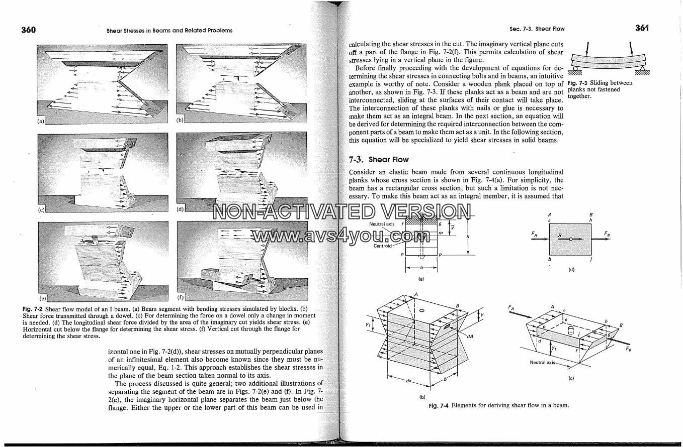
360 Shear Stresses in Beams and Related Problems
(a)
(c)
(e)
Fig. 7-2 Shear flow model of an I beam. (a) Beam segment with bending stresses simulated by blocks. (b)Shear force transmitted through a dowel. (c) For determining the force on a dowel only a change in momentis needed. (d) The longitudinal shear force divided by the area of the imaginary cut yields shear stress. (e)Horizontal cut below the flange for determining the shear stress. (f) Vertical cut through the flange fordetermining the shear stress.
izontal one in Fig. 7-2(d)), shear stresses on mutually perpendicularof an infinitesimal element also become known since they must bemerically equal, Eq. 1-2. This approach establishes the shear stressesthe plane of the beam section taken normal to its axis.
The process discussed is quite general; two additional illustrationsseparating the segment of the beam are in Figs. 7-2(e) and (f). In Fig.2(e), the imaginary horizontal plane separates the beam just belowflange. Either the upper or the lower part of this beam can be used
Sec. 7-3. Shear Flow
calculating the shear stresses in the cut. The imaginary vertical plane cutsa part of the flange in Fig. 7-2(f). This permits calculation of shear
lying in a vertical plane in the figure.Before finally proceeding with the development of equations for de-
termining the shear stresses in connecting bolts and in beams, an intuitiveexample is worthy of note. Consider a wooden plank placed on top of
another, as shown in Fig. 7-3. If these planks act as a beam and are not;rconnected, sliding at the surfaces of their contact will take place.
interconnection of these planks with nails or glue is necessary tohake them act as an integral beam. In the next section, an equation will
be derived for determining the required interconnection between the com-ponent.parts of a beam to make them act as a unit. In the following section,
this equation will be specialized to yield shear stresses in solid beams.
�-3. Shear Flow
nsider an elastic beam made from several continuous longitudinalplanks whose cross section is shown in Fig. 7-4(a). For simplicity, thebeam has a rectangular cross section, but such' a limitation is not nec-
essary. To make this beam act as an integral member, it is assumed that
!
Neutral axis f
Centroid /
(a)
A
h A
B F A A
(b)
Neutral �
(c)
Fig. 7-4 Elements for deriving shear flow in a beam.
Fig. 7-3 Sliding betweenplanks not fastenedtogether.
Bh
(d)
hB
NON-ACTIVATEDVERSIONwww.avs4you.com
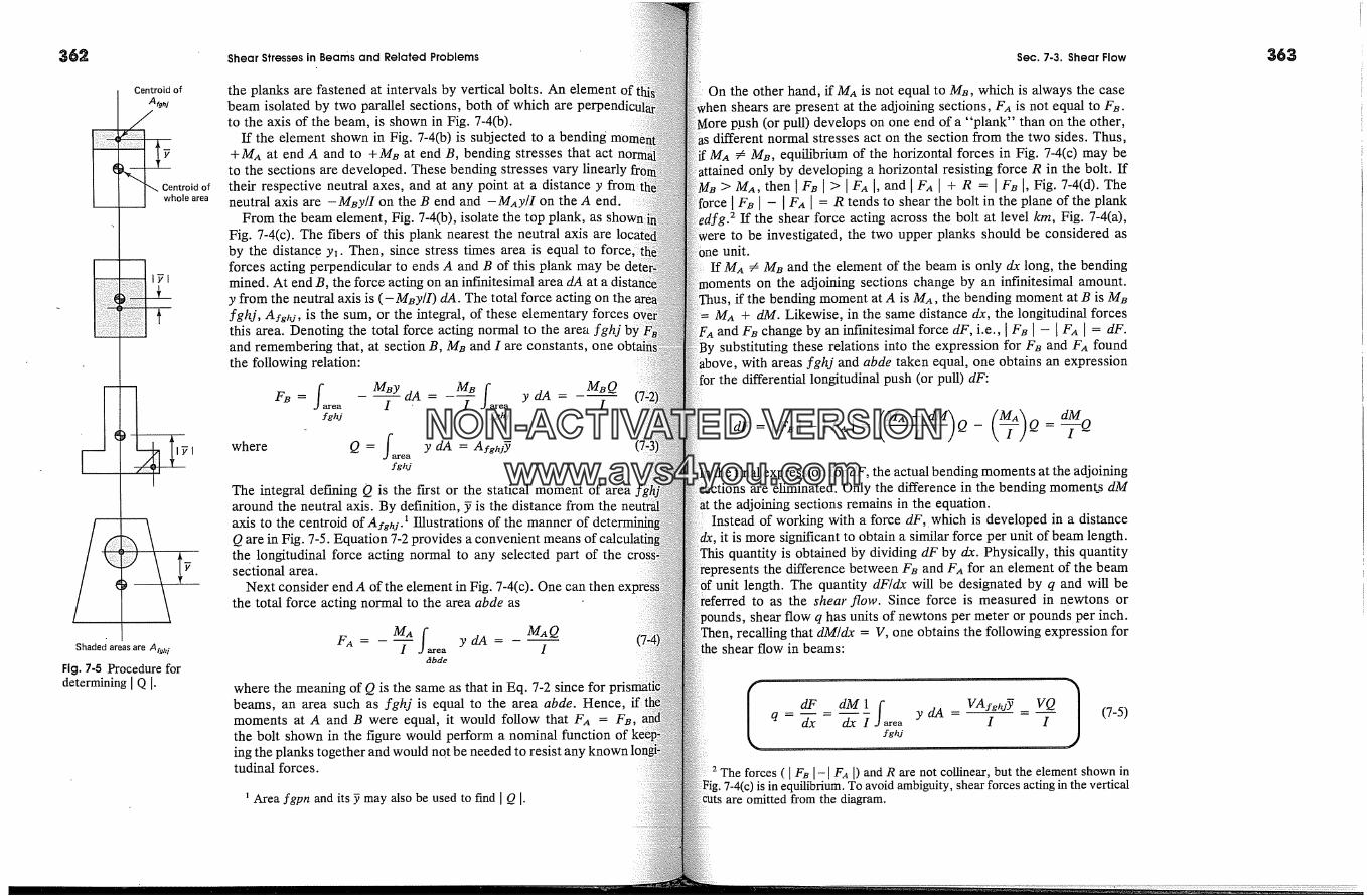
362 Shear Stresses in Beams and Related Problems Sec. 7-3. Shear Flow
Centroid of
A fghi
.�ehntroidofole area
Shade� areas are AfghiFig. 7-5 Procedure fordetermining Q [.
the planks are fastened at intervals by vertical bolts. An element of'beam isolated by two parallel sections, both of which areto the axis of the beam, is shown in Fig. 7~4(b).
If the element shown in Fig. 7-4(b) is subjected to a bending+MA at end A and to +MB at end B, bending stresses that act
to the sections are developed. These bending stresses vary linearlytheir respective neutral axes, and at any point at a distance yneutral axis are -MBy/I on the B end and --MAy/I on the A end.
From the beam element, Fig. 7-4(b), isolate the top plank, asFig. 7-4(c). The fibers of this plank nearest the neutral axis areby the distance y�. Then, since stress times area is equal to forceforces acting perpendicular to ends A and B of this plank may bemined. At end B, the force acting on an infinitesimal area dA aty from the neutral axis is (-M�y/I) dA. The total force acting on thefghj, Aighj, is the sum, or the integral, of these elementary forcesthis area. Denoting the total force acting normal to the area fghjand remembering that, at section B, M� and I are constants, onethe following relation:
L M�y dA= M�s L MBQFa= I -I .... ydA= Iea ea
fghj fghj
where y dA = AighjYfghj
The integral deeming Q is the first or the statical moment of areaaround the neutral axis. By definition, y is the distance from theaxis to the centroid of Afgh? Illustrations of the mannerQ are in Fig. 7-5. Equation 7-2 provides a convenient meansth e longitudinal force acting normal to any selected part of thesectional area.
Next consider end A of the element in Fig. 7-4(c). One canthe total force acting normal to the area abde as
MA far MAQFA = I ea y dA = I&bde
where the meaning of Q is the same as that in Eq. 7-2 since forbeams, an area such as fghj is equal to the area abde. Hence, ifmoments at A and B were equal, it would follow that FA = F�,the bolt shown in the figure would perform a nominal functioning the planks together and would not be needed to resist anytudinal forces.
Area fgpn and its y may also be used to find I Q I.
On the other hand, if MA is not equal to Ma, which is always the caseshears are present at the adjoining sections, FA is not equal to Fa.push (or pull) develops on one end of a "plank" than on the other,
different normal stresses act on the section from the two sides. Thus,MA � MB, equilibrium of the horizontal forces in Fig. 7-4(c) may be
only by developing a horizontal resisting force R in the bolt. If> MA, then ] F� ] > lEA I, and I FA I + R = I F� [, Fig. 7-4(d). The
I I - I Fa I ---- R tends to shear the bolt in the plane of the plank.2 If the shear force acting across the bolt at level km, Fig. 7-4(a),
to be investigated, the two upper planks should be considered asunit.
If MA � Ma and the element of the beam is only dx long, the bendingtents on the adjoining sections change by an infinitesimal amount.
if the bending moment at A is MA, the bending moment at B is MBMa + riM. Likewise, in the same distance dx, the longitudinal forcesand Fa change by an infinitesimal force dF, i.e., [ F� I - I Fa I = dF.
By substituting these relations into the expression for Fa and FA foundwith areas �ghj and abde taken equal, one obtains an expression
the differential longitudinal push (or pull) dF:
dF:lFz�l-IFAl= (MA+ dM t (--�)I Q- Q= Q
the final expression for dF, the actual bending moments at the adjoiningare eliminated. Only the difference in the bending moments dM
the adjoining sections remains in the equation.Instead of working with a force dF,. which is developed in a distance
it is more significant to obtain a similar force per unit of beam length.quantity is obtained by dividing dF by dx. Physically, this quantity
the difference between FB and FA for an element of the beamunit length. The quantity dF/dx will be designated by q and will be
to as the shear flow. Since force is measured in newtons or�ounds, shear flow q has units of newtons per meter or pounds per inch.
recalling that dM/dx = V, one obtains the following expression forshear flow in beams:
I dF dMlf� VAigh.�YVQ1- ydA- I Iq dx dxI(7-5)
The forces ( I FB I-I Fz I) and R are not collinear, but the element shown inis in equilibrium. To avoid ambiguity, shear forces acting in the vertical
are omitted from the diagram.
NON-ACTIVATEDVERSIONwww.avs4you.com

Shear Stresses in Beams and Related Problems
In this equation, ! is the moment of interia of the entire cross~starea around the neutral axis, just as it does in the flexure formulawhich it came. The total shear force at the section investigated isresented by V, and the integral of y dA for determining. Qover the cross-sectional area of the beam to one side of this area at,q is investigated.
In retrospect, note carefully that Eq. %5 was derived on thethe elastic flexure formula, but no term for a bending momentin the final expressions. This resulted from the fact that only thein the bending moments at the adjoining sections had to beand the latter quantity is linked with shear V. Shear V wasfor dM/dx, andthis masks the origin of the established relations. Ec7-5 is very useful in determining the necessary interconnectionthe elements making up a beam. This will be illustrated by
EXAMPLE 7-t
Two long wooden planks form a T section of a beam, as shown in mm in6(a). If this beam transmits a constant vertical shear of 3000 N, find the nec{spacing of the nails between the two planks to make the beam act as a unit. Asithat the allowable shear force per nail is 700 N.
Solution
In attacking such problems, the analyst must ask: What part of a beamtendency to slide longitudinally from the remainder? Here this occurs in theof contact of the two planks; Eq. 7-5 must be applied to determine the shearin this plane. To do this, the neutral axis of the whole section and itsinertia around the neutral axis must be found. Then as Vis known and Qas the statical moment of the area of the upper plank around the neutralmay be determined. The distance yc from the top to the neutral axis is
50x200x25+50x200x 150= 87.5 mmYc= 50 x 200 + 50 x 200
200 x 503 50 x 2003I- + 50 x 200 x 62.52 + + 50 x 200 x
12 12= 113.54 x 106mm 4
Q = AighjY .---- 50 x 200 x (87.5 -- 25) = 625 x 103 mm 3VQ _ 3000 x 625 x 103 = 16.5 N/mmq - I 113.54 X 10⁶
Thus, a force of 16.5 N/mm must be transferred from one plank tothe length of the beam. However, from the data given, each nail is caresisting a force of 700 N; hence, one nail is adequate for transmitting700/16.5 = 42 mm of the beam length. As shear remains constant at theutive sections of the beam, the nails should be spaced throughout attervals.
Sec. 7-3. Shear Flow
-I62.5
NA
I-;I-;1'-la
162.5
(b)
ution for an Alternative Arrangement of Planks
instead of using the two planks as before, a beam of the same cross sectionmade from five pieces, Fig. 7-6(b), a different nailing schedule would be
uired.
To begin, the shear flow between one of the outer 25 by 50 mm planks and thethe beam is found, and although the contact surface a-a is vertical,
procedure is the same. The push or pull on an element is built up in the same
Fig. 7-6
Q = AsgiUY = 25 x 50 x 62.5 = 78.1 x 103 mm 3VQ 3000 x 78.1 x 103 = 2.06 N/mmq = I = 113.5 X 10⁶
the same nails as before are used to join the 25 by 50 mm piece to the 50 bymm piece, they may be 700/2.06 = 340 mm apart. This nailing applies to both
To determine the shear flow between the 50 by 250 mm vertical piece and eitherof the 50 by 50 mm pieces, the whole 75 by 50 mm area must be used to
Q. It is the difference of pushes (or pulls) on this whole area that causesunbalanced force that must be transferred at the surface b-b:
Q = AsghjY = 75 X 50 X 62.5 = 234 X 103 mm 3VQ 3000 x 234 x 103
q - �- - 113.4 X 106 = 6.19 N/mmshould be spaced at 700/6.19 = 113 mm, intervals along the length of the
�eam in both sections b-b. These nails should be driven in first, then the 25 byput on.
�LE 7-2
)le beam on a 6-m span carries a load of 3 kN/m including its own weight.cross section is to be made from several wooden pieces, as is shown
365
NON-ACTIVATEDVERSIONwww.avs4you.com
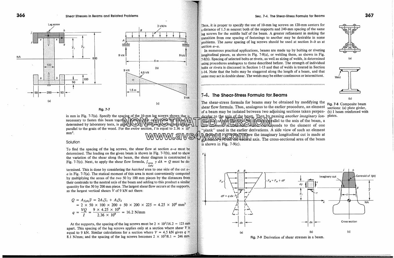
366 Shear Stresses in Beams and Related Problems Sec. 7-4. The Shear-Stress Formula for Beams
NA
5O[-
Lag screw
200---�50�-
500
(a)
6m
(b)
A
9kNl9 kN
4.5 kN
(c)
9
Fig. 7-7
in mm in Fig. 7-7(a). Specify the spacing of the 10-mm lag screws shown tnecessary to fasten this beam together. Assume that one 10-mm lag screw, idetermined by laboratory tests, is good for 2 kN when transmittingparallel to the grain of the wood. For the entire section, I is equal to 2.36 xmm 2.
Solution
To find the spacing of. the lag screws, the shear flow at section a-adetermined. The loading on the given beam is shown in Fig. 7-7(b), and tothe variation of the shear along the beam, the shear diagram isFig; 7-7(c). Next, to apply the shear flow formula, f�ea Y dA = Q must
fghj
terrained. This is done by considering the hatched area to one side of thea in Fig. 7-7(a). The statical moment of this area is most convenientlyby multiplying the areas of the two 50 by 100 mm pieces by the distancestheir centroids to the neutral axis of the beam and adding to this productquantity for the 50 by 200 mm piece. The largest shear flow occurs at theas the largest vertical shears V of 9 kN act there:
Q = AsghZY = 2A�y� + A2Y2= 2 x 50 x 100 x 200 + 50 x 200 x 225 = 4.25 x 10⁶
VQ 9 x 4.25 x 109 16.2 N/mmq = I = 2.36 x 109 =
At the supports, the spacing of the lag screws must be 2 x 10³/16.2 =apart. This spacing of the lag screws applies only at a section where shearequal to 9 kN. Similar calculations for a section where V = 4.5 kN gives8.1 N/mm; and the spacing of the lag screws becomes 2 x 10³/8.1 = 246
it is proper to specify the use of 10-mm lag screws on 120-mm centers fordistance of 1.5 m nearest both of the supports and 240-mm spacing of the same
screws for the middle half of the beam. A greater refinement in making thefrom one spacing of fastenings to another may be desirable in some
The same spacing of lag screws should be used at section b-b as at:tion a-a.
In numerous practical applications, beams are made up by bolting or rivetingpieces, as shown-in Fig. 7-8(a), or welding them, as shown in Fig.
Spacing of selected bolts or rivets, as well as sizing of welds, is determinedprocedures analogous to those described before. The strength of individualor rivets is discussed in Section 1-13 and that of welds is treated in Section
.14. Note that the bolts may be staggered along the length of a beam, and that' act in double shear. The welds may be either continuous or intermittent.
'-4. The Shear-Stress Formula for.Beams
shear-stress formula for beams may be obtained by modifying the;ar flow formula. Thus, analogous to the earlier procedure, an element
beam may be isolated between two adjoining sections taken perpen-to the axis of the beam. Then by passing another imaginal7 Ion-
section through this element parallel to the axis of the beam, aelement is obtained, which corresponds to the element of one
'plank" used in the earlier derivations. A side view of such an elementshown in Fig. 7-9(a), where the imaginary longitudinal cut is made at
� distance y� from the neutral axis. The cross-sectional area of the beamshown in Fig. 7-9(c).
(a)
(b)
Fig. 7-8 Composite beamsections: (a) plate girder,(b) I beam reinforced withplates.
A B
�_] L--�
(a)
Fa= FA + dF d�y�� ImaginarycutYl
h
[-Centroid of fgh/
� dx � Cross section
(b)
Fig. 7-9 Derivation of shear stresses in a beam.
(c)
NON-ACTIVATEDVERSIONwww.avs4you.com

368 Shear Stresses in Beams and Related Problems Sec. 7-4. The Shear-Stress Formula �or Beams
If shear forces exist at the sections through the beam, a differenting moment acts at section A than at B. Hence, more push ordeveloped on one side of the partial area fghj than on the other,before, this longitudinal force in a distance dx is
I ea y dA -� AsghiY Qyghj
In a solid beam, the force resisting dF may be developed onlyplane of the longitudinal.cut taken parallel to the axis of the beam.fore, assuming that the shear stress, is uniformly distributed 3 ssection of width t, the shear stress in the longitudinal plane maytained by dividing dF by the area t dx. This yields the horizontalstress ,. For an infinitesimal element, however, numerically equalstresses 4 act on the mutually perpendicular planes; see Fig. 7-9Co).the same relation gives simultaneously the longitudinal shear stressthe shear stress in the plane of the vertical section at the Ioncut. 5
dF dM A�ehiydx t dx It
This equation may be simplified, since according to Eq. 7-1, dM/dxand by Eq. %5, q = VQ/I. Hence,
I VAfghjy_VQ q 1* - It I�- - t
Equation 7-6 is the important formula for the shear stresses in
3 This procedure is best suited to situations where the section sides areand are away from significant changes in the shape of the cross section.limitations see Section 7-6.
4 Note that the sense of positive, agrees with the positive sense for V inadopted in Section 5-8.
5 The presence of y in this relation may be explained differently. If theis present at a section through a beam, the moments at the adjoiningM and M + dM. The magnitude of M is irrelevant for determining thestresses. Hence, alternately, no moment need be considered at one sectionthe adjoining section, a bending moment dM is assumed to act. Then on aarea of the section, such as the shaded area in Fig. 7-9(c), this bendindM will cause an average normal stress (dM)y/I, as given byIn the latter relation, y locates the fiber that is at an average distance fromneutral axis in the partial area of a section. Multiplying (dM)y/I by thearea of the section leads to the same expression for dF as before.
6 This formula was derived by D. I. Jouravsky in 1855. Its developmentprompted by observing horizontal cracks in wood ties on several of thebridges between Moscow and St. Petersburg.
the shear stresses at the longitudinal cut. As before, V is the total' force at a section, and I is the moment of inertia of the whole cross-,n.al area about the neutral axis. Both V and I are constant at a section
h a beam. Here Q is the statical moment around the neutral axispartial area of the cross section to one side of the imaginary lon~
cut, and y is the distance from the neutral axis of the beam tocentroid of the partial area Afghj. Finally, t is the width of the im-
longitudinal cut, which is usually equal to the thickness or width'the member. The shear stress at different longitudinal cuts through the
assumes different values as the values of Q and t for such sections
Care must be exercised in making the longitudinal cuts preparatory forin Eq. 7-6. The proper sectioning of some cross-sectional areas of
is shown in Figs. 7-10(a), (b), (d), and (e). The use of inclinedplanes shotfid be avoided unless the section is made across a small
When the axis of symmetry of the cross-sectional area of theis vertical and in the plane of the applied forces, the longitudinal
are usually made horizontally. In such cases, the solution of Eq. 7~simultaneous values of horizontal and vertical shear stresses, as
planes are mutually perpendicular, Eq. 1-2. The latter stresses actthe plane of the transverse section through the beam. Collectively, these
stresses resist the shear force at the same section, thus satisfyingrelation of statics, � Fy = 0. The validity of this statement for a
case will be proved in Example 7-3.For thin members only, Eq. 7-6 may be used to determine the shear
;ses with a cut such as f-g of Fig. 7-10(b). These shear stresses acta vertical plane and are directed perpendicularly to the plane of the
Matching shear stresses act horizontally; see Fig. 7-10(c). Thesestresses act in entirely different directions than those obtained by
horizontal cuts, such as �-g in Figs. 7-10(a) and (d). As thesestresses do not contribute directly to the resistance of vertical shear
their significance will be discussed in Section 7-7.
/ h h g
(c)
(a) (b)
NA
h
Centroid of cross-hatched area
(d) (e)
Fig. 740 Sectioning for partial areas of cross sections for computing shear stresses.
NON-ACTIVATEDVERSIONwww.avs4you.com

370 Shear Stresses in Beams and Related Problems
Procedure Summary
The same three basic concepts of engineering mechanics of solidsfore are used in developing the formula for shear stresses in beams.ever, their use is less direct.
1. Equilibrium conditions are used(a) for determining the shear at a section,(b) by using the relationship between the shear and the
change in bending moment along a span, and(c) by determining the force at a longitudinal section of a
element for obtaining the average shear stress.2. Geometry of deformation, as in pure bending, is assumed such
plane sections remain plane after deformation, leading toclusion that normal strains in a section vary linearly fromaxis. Since, due to shear, the cross sections do not remainbut warp, this assumption is less accurate than for pureHowever, for small and moderate magnitudes of shear, andmembers, this assumption is satisfactory.
3. Material properties are considered to obey Hooke's law,extension to other constitutive relations is possible forsolutions.
These conditions treat the problem as one-dimensional, andsumed geometry of deformation is insensitive to the effects oftrated forces and/or changes in the cross-sectional areas of beams.fore again reliance is largely placed on Saint-Venant's principle. Inwords, only at distances beyond the member depth from suchbances are the solutions accurate. Therefore solutions are bestslender members; see Section %5. Further, rigorous solutionsfor wide longitudinal sections, solutions are somewhat inaccuratecomplex warpage of their cross sections near the sides.
An application of Eq. 7-6 for determining shear stresses in a rectanbeam is given next. Based on the results obtained in thisgeneral discussion follows of the effect of shear on warpage ofplane sections in beams. Then two additional examples onof Eq. %6 are provided.
EXAMPLE 7-3
Derive an expression for the shear-stress distribution in a beam of solidgular cross section transmitting a vertical shear V.
Solution
The cross-sectional area of the beam is shown in Fig. 7-11(a). A longitudinal ithrough the beam at a distance y� from the neutral axis isolates the partialfghj of the cross section. Here t = b and the infinitesimal area
Sec. 7-4. The Shear-Stress Formula for Beams
v
NA
I_J
(a) (b) (c) (d)
Fig. 7-tl
, be conveniently expressed as b dy. By applying Eq. 7-6, the horizontal shearess is found at level y� of the beam. At the same cut, numerically equal vertical
stresses act in the plane of the cross section, Eq. 1-2.
VQ _ V f� rx - It It � y dA =fghj
fyha by dy
- (7-7)
equation shows that in a beam of rectangular cross section, both the hor-izontal and the vertical shear stresses vary parabolically. The maximum value of
shear stress is obtained When y� is equal to zero. In the plane of the crossFig. 7-11(b), this is diagrammatically represented by *tax at the neutral
beam. At increasing distances from the neutral axis, the shear stressesdiminish. At the upper and lower boundaries of the beam, the shear
cease to exist as y� = + h/2. These values of the shear stresses at thelevels of the beam may be represented by the parabola shown in Fig. 7-
il(c). An isometric view of the beam with horizontal and vertical shear stressesshown in Fig. 7-11(d).To satisfy the condition of statics, � Fy = 0, at a section of the beam, the sum
the vertical shear stresses, times their respective areas dA must be equalthe vertical shear V. That this is the case may be shown by integrating, dA
Over the whole cross-sectional area A of the beam, using the general expressionfound before.
NON-ACTIVATEDVERSIONwww.avs4you.com
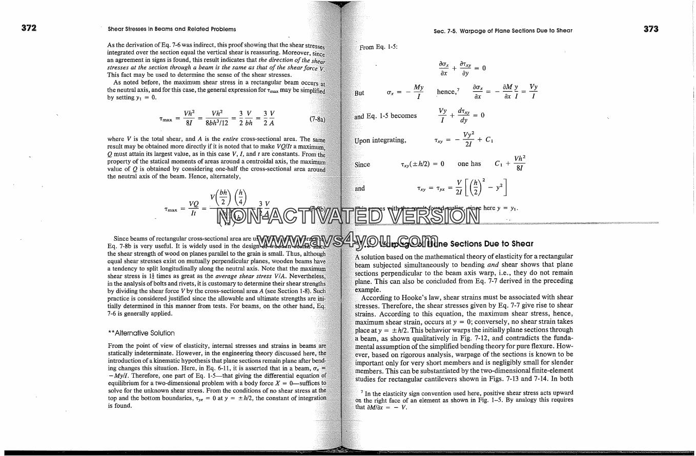
372 Shear Stresses in Beams and Related Problems
As the derivation of Eq. 7-6 was indirect, this proof showing that the shearintegrated over the section equal the vertical shear is reassuring. Moreover,an agreement in signs is found, this result indicates that the directionstresses at the section through a beam is the same as that of the shearThis fact may be used to determine the sense of the shear stresses.
As noted before, the maximum shear stress in a rectangular beamthe neutral axis, and for this case, the general expression forby setting y� = 0.
�rmax --Vh 2 Vh 2 3 V 3 V
81 8bh3/12 2 bh 2 A
where V is the total shear, and A is the entire cross-sectional area. Theresult may be obtained more directly if it is noted that to make VQ/ItQ must attain its largest value, as in this case V, I, and t are bonstants.property of the statical moments of areas around a centroidal axis, thevalue of Q is obtained by considering one-half the cross-sectional areathe neutral axis of the beam. Hence, alternately,
VQ .v(b�) (h�) 3VTmax -- I�- - [bh3\ - 2 A (74
Since beams of rectangular cross-sectional area are used frequently inEq. 7-8b is very useful. It is widely used in the design of wooden beamsthe shear strength of wood on planes parallel to the grain is small. Thus,equal shear stresses exist on mutually perpendicular planes, wooden beam:a tendency to split longitudinally along the neutral axis. Note that theshear stress is 1� times as great as the average shear stress V/A. Neverthei�in the analysis of bolts and rivets, it is customary to determine their shearby dividing the shear force V by the cross-sectional area A (see Section 1-8).practice is considered justified since the allowable and ultimate strengthstially determined in this manner from tests. For beams, on the other7-6 is generally applied.
**Alternative Solution
From the point of view of elasticity, internal stresses and strains instatically indeterminate. However, in the engineering theory discussed here:introduction of a kinematic hypothesis that plane sections remain planeing changes this situation. Here, in Eq. 6-11, it is asserted that in a beam,-My/I. Therefore, one part of Eq. 1-5--that giving the differential e�
equilibrium for a two-dimensional problem with a body force X =solve for the unknown shear stress. From the conditions of no shear stresstop and the bottom boundaries, ,yx = 0 at y = +h/2, the constant ofis found.
Sec. 7-5. Warpage of Plane Sections Due to Shear
?rom Eq. 1-5:
c9O'x + &rxy = 0Ox Oy
:But trx = My hence, ?I
Ocrx aM y VyOx Ox I I
Eq. 1-5 becomes
integrating,Vy 2
21+ C�
;ince ,�y(+h/2) = 0 one hasVh 2
C 1 + --81
'rxy = 'ryx = � _ y2agrees with the result found earlier, since here y = Yl.
5. Warpage of Plane Sections Due to Shear� solution based on the mathematical theory of elasticity for a rectangular
beam subjected simultaneously to bending and shear shows that planeperpendicular to the beam axis warp, i.e., they do not remain
This can also be coficluded from Eq. 7-7 derived in the preceding
to Hooke's law, shear strains must be associated with shearTherefore, the shear stresses given by Eq. 7-7 give rise to shear
According to this equation, the maximum shear stress, hence,strain, occurs at y = 0; conversely, no shear strain takes
= + h/2. This behavior warps the initially plane sections throughbeam, as shown qualitatively in Fig. 7-12, and contradicts the funda-
assumption of the simplified bending theory for pure flexure. How-based on rigorous analysis, warpage of the sections is known to be
Lmportant only for very short members and is negligibly small for slenderThis can be substantiated by the two-dimensional finite-element
studies for rectangular cantilevers shown in Figs. 7-13 and 7-14. In both
In the elasticity sign convention used here, positive shear stress acts upwardthe right face of an element as shown in Fig. 1-5. By analogy this requires
OM/Ox = - V.
373
NON-ACTIVATEDVERSIONwww.avs4you.com
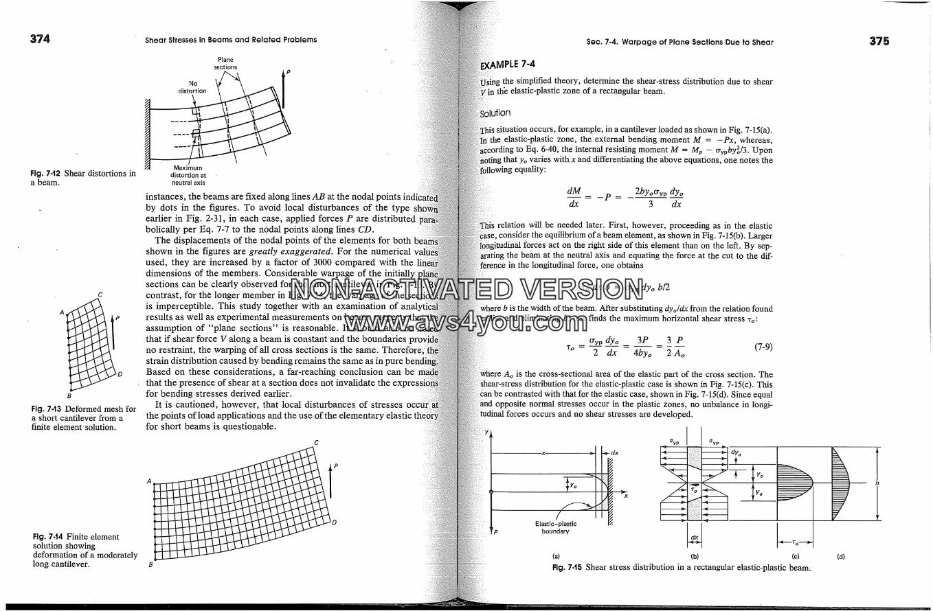
374
Fig. 7-t2 Shear distortions ina beam.
A
Fig. 7-t3 Deformed mesh fora short cantilever from afinite element solution.
Fig. '744 Finite elementsolution showingdeformation of'a moderatelylong cantilever.
Shear Stresses in Beams and Related Problems
Planesections
[Maximum
distortion atneutral axis
instances, the beams are fixed along lines AB at the nodal points indby dots in the figures. To avoid local disturbances of the typeearlier in Fig. 2-31, in each case, applied forces P arebolically per Eq. 7-7 to the nodal points along lines CD.
The displacements of the nodal points of the elements for bothshown in the figures are greatly exaggerated. For the numericalused, they are increased by a factor of 3000 compared with thedimensions of the members. Considerable warpage of the initiallysections can be clearly observed for the short cantilever in Fig. 7-13�contrast, for the longer member in Fig. 7-14, the warpage of theis imperceptible. This study together with an examination ofresults as well as experimental measurements on beams suggestsassumption of "plane sections" is reasonable. It should also bethat if shear force V along a beam is constant and the boundariesno restraint, the warping of all cross sections is the same.strain distribution caused by bending remains the same as in pureBased on these considerations, a far-reaching conclusion can bethat the presence of shear at a section does not invalidatefor bending stresses derived earlier.
It is cautioned, however, that local disturbances of stressesthe points of load applications and the use of the elementary elasticfor short beams is questionable.
c
P
A
B
Sec. 7-4. Warpage of Plane Sections Due to Shear
MPLE 7-4
the simplified theory, determine the shear-stress distribution due to shearr in the elastic-plastic zone of a rectangular beam.
ution
situation occurs, for example, in a cantilever loaded as shown in Fig. 7-15(a).the elastic-plastic zone, the external bending moment M = -Px, whereas,
to Eq. 6-40, the internal resisting moment M = M v - crypby�o/3. Uponthat yo varies with x and differentiating the above equations, one notes the
equality:
dM = _p = 2byoo'yp dyodx 3 dx
relation will be needed later. First, however, proceeding as in the elasticconsider the equilibrium of a beam element, as shown in Fig. 7-15(b). Larger
forces act on the right side of this element than on the left. By sep-the beam at the neutral axis and equating the force at the cut to the dif-
ference in the longitudinal force, one obtains
'ro dx b = 0'yp dyo b/2
the width of the beam. After substituting dyo/dx from the relation foundhating b, one finds the maximum horizontal shear stress %:
tryp dyo 3P 3 P'to ..... (7-9)
2 dx 4byo 2 Ao
Ao is the cross-sectional area of the elastic part of the cross section. Thedistribution for the elastic-plastic case is shown in Fig. 7-15(c). This
case, shown in Fig. 7-15(d). Since equalopposite normal stresses occur in the plastic zones, no unbalance in longi-
tudinal forces occurs and no shear stresses are developed.
/ IElastic-plastic
boundary
x
Oyp
(a) (b) (c)
Fig. 745 Shear stress distribution in a rectangular elastic-plastic beam.
375
(d)
NON-ACTIVATEDVERSIONwww.avs4you.com
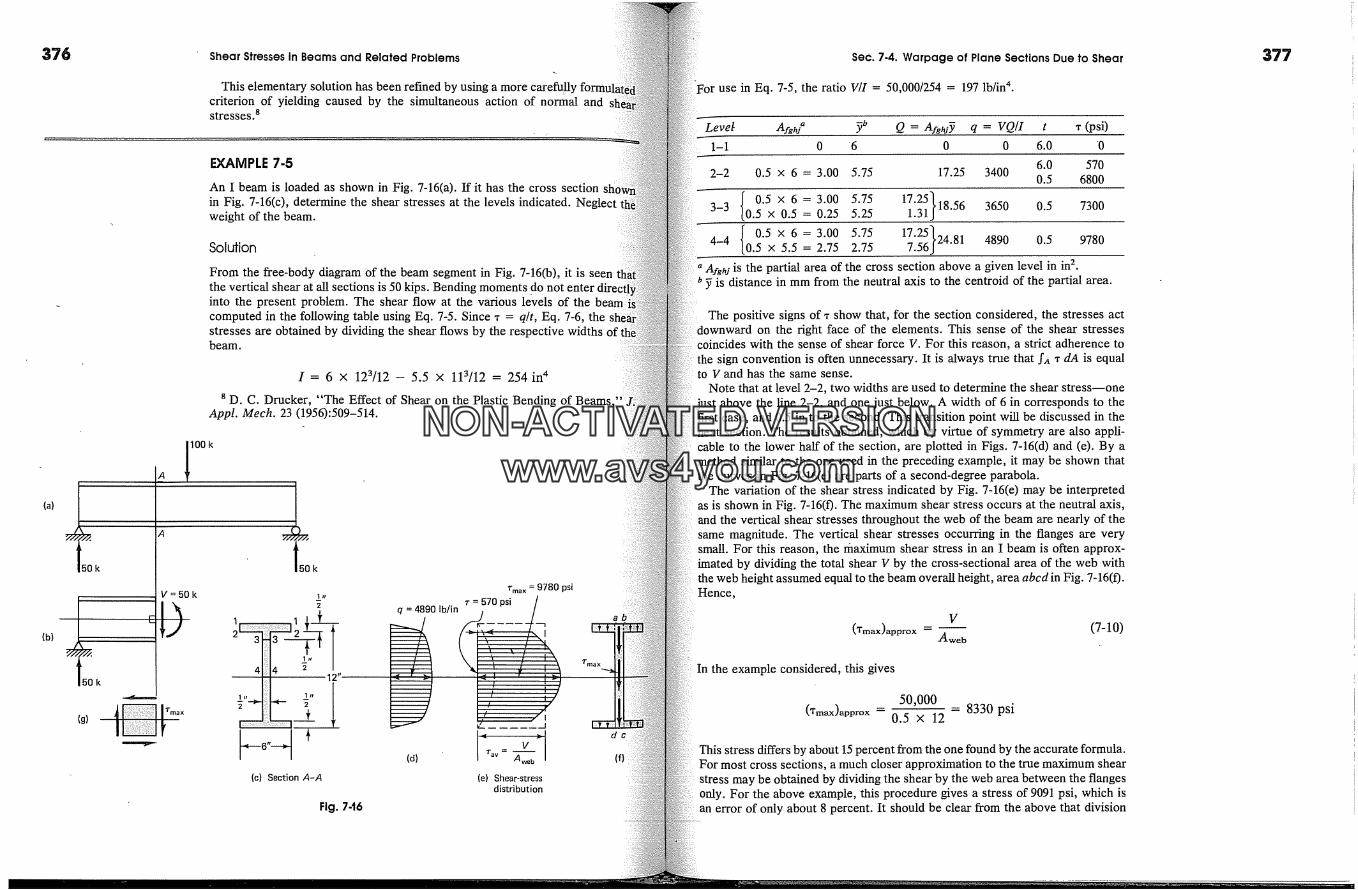
376 Shear Stresses in Beams and Related Problems
This elementary solution has been refined by using a more carefullycriterion of yielding caused by the simultaneous action of normal andstresses. 8
EXAMPLE 7-5
An I beam is loaded as shown in Fig. 7-16(a). If it has the cross sectionin Fig. 7-16(c), determine the shear stresses at the levels indicated. Neglectweight of the beam.
Solution
From the free-body diagram of the beam segment in Fig. 7-16(b), it is seenthe vertical shear at all sections is 50 kips. Bending moments d � not enterinto the present problem. The shear flow at the various levels of the beamcomputed in the following table using Eq. 7-5. Since x = q/t, Eq. 7-6, thestresses are obtained by dividing the shear flows by the respective widths ofbeam.
(a)
(b)
A 100k
I = 6 x 123/12 - 5.5 x 113/12 = 254 in 4
8 D. C. Drucker, "The Effect of Shear on the Plastic Bending of Beams.Appl. Mech. 23 (1956):509-514.
V=50k
(g)
�k
Fig. 7-t6
q = 4890 lb/in
(d)
rma x = 9780 psir = 570 psi
(e) Shear-stressdistribution
(c) Section A-A
Sec. 7-4. Warpage of Plane Sections Due to Shear
�For use in Eq. 7-5, the ratio V/I = 50,000/254 = 197 lb/in 4.
Level Arab? ? Q = Afghi7 q = VQ/I t x (,psi)1-1 0 '6 0 0 6.0 '0
6.0 5702-2 0.5 x 6 = 3.00 5.75 17.25 3400 0.5 6800
= 17'25}18.56 3650 0.5 7300I 0.5 x 6 3.00 5.753-3 [0.5 x 0.5 0.25 5.25 1.31
= 17'25}24.81 4890 0.5 9780I 0.5 x 6 3.00 5.754-4 [0.5 x 5.5 2.75 2.75 7.56"A�ghj is the partial area of the cross section above a given level in in2o0 y is distance in mm from the neutral axis to the centraid of the partial area.
The positive signs of x show that, for the section considered, the stresses actdownward on the right face of the elements. This sense of the shear stresses
dncides with the sense of shear force V. For this reason, a strict adherence tothe sign convention is often unnecessary. It is always true that fAx dA is equalto V and has the same sense.
Note that at level 2-2, two widths are used to determine the shear stress--onejust above the line 2-2, and one just below. A width of 6 in corresponds to thefirst case, and 0.5 in to the second. This transition point will be discussed in thenext section. The results obtained, which by virtue of symmetry are also appli-cable to the lower half of the section, are plotted in Figs. 7-16(d) and (e). By amethod similar to the one used in the preceding example, it may be shown thatthe curves in Fig. 7-16(e) are parts of a second-degree parabola.
The variation of the shear stress indicated by Fig. 7-16(e) may be interpretedas is shown in Fig. 7-16(0. The maximum shear stress occurs at the neutral axis,and the vertical shear stresses throughout the web of the beam are nearly of thesame magnitude. The vertical shear stresses occurring in the flanges are verysmall. For this reason, the maximum shear stress in an I beam is often approx-imated by dividing the total shear V by the cross-sectional area of the web withthe web height assumed equal to the beam overall height, area abcdin Fig. 7-16(0.Hence,
v
('rmax)appr�x -- Aweb (7-10)In the example considered, this gives
50,000('rmax)appr�x 0.5 X 12 8330 psi
This stress differs by about 15 percent from the one found by the accurate formula.For most cross sections, a much closer approximation to the true maximum shearstress may be obtained by dividing the shear by the web area between the flangesonly. For the above example, this procedure gives a stress of 9091 psi, which isan error of only about 8 percent. It should be clear from the above that division
377
NON-ACTIVATEDVERSIONwww.avs4you.com

378 Shear Stresses in Beams and Related Problems Sec. 7-6. Some Limitations of the Shear-Stress Formula
of V by the whole cross-sectional area of the beam to obtain the shearnot permissible.
An element of the beam at the neutral axis is shown in Fig. 7-16(g). At3-3 and 2-2, bending stresses, in addition to the shear stresses, act on thefaces of the elements. No shear stresses and only bending stresses act onielements at level 1-1.
J2
570 psi
i70 psi
Fig. 7-t7 Boundaryconditions are not satisfiedat the levels 2-2.
The sides of cross sections were assumed to be parallel in all th e:ceding examples. If they are not parallel, both Q and t varysection level, and the maximum shear stress may not occur at theaxis. However, using Eq. 7-6, the maximum average shear stres..always be found. For example it can be shown that for aangular cross section such a maximum shear stress is midwaythe apex and the base. For such cross sections, the stresses varya longitudinal section, and are particularly inaccurate near thesides; see Fig. 7-18. Similar results may develop at longitudinaltaken at an angle with the axes.
The same procedures as described before are used for determining 1gitudinal shear stresses in composite beams at bonded or glued
*7-6. Some' Limitations of the Shear-Stress FormulaThe shear-stress formula for beams is based on the flexureHence, all of the limitations imposed on the flexure formula apply,material is assumed to be elastic with the same elastic modulus inas in compression. The theory developed applies only to straightMoreover, there are additional limitations that are not present in theure formula. Some of these will be discussed now.
Consider a section through the I beam analyzed in Example 7-5.of the results of this analysis are reproduced in Fig. 7-17. Thestresses computed earlier for level 1-1 apply to the infinitesimala. The vertical shear stress is zero for this element. Likewise, nostresses exist on the top plane of the beam. This is as it should be,the top surface of the beam is a free surface. In mathematical Tthis means that the conditions at the boundary are satisfied. Forof rectangular cross section, the situation at the boundaries is
A different condition is found when the shear stressesthe I beam at levels 2-2 are scrutinized. The shear stresses wereto be 570 psi for the elements such as b or c shown in the figure.requires matching horizontal shear stresses on the inner surfaces oftflanges. However, the latter surfaces must be free of the shear stress{as they are free boundaries of the beam. This leads to athat cannot be resolved by the methods of engineering mechanicsids. The more advanced techniques of the mathematical theory of
(a)
yA
VO / \
(b)
or three-dimensional finite-element analysis must be used to obtainsolution.
Fortunately, the above defect of the shear-stress formula for beams isThe vertical shear stresses in the flanges are small. The large
stresses occur in the web and, for all practical purposes, are cor-given by Eq. 7-6. No appreciable error is involved by using the
derived in this chapter for thin-walled members, and the majoritybelong to this group. Moreover, as stated earlier, the solution
for the shear stresses for a beam with a rectangular cross section is cor-
In mechanical applications, circular shafts frequently act a� beams.beams having a solid circular cross section form an important
These beams are not "thin-walled." An examination of the bound-conditions for circular members, Fig. 7-18(a), leads to the conclusion
shear stresses are present, they must act parallel to the bound-,. As no matching shear stress can exist on the free surface of a beam,
shear stress component can act normal to the boundary. However,to Eq. 7-6, vertical shear stresses of equal intensity act at every
such as ac in Fig. 7-18(b). This is incompatible with the boundaryfor elements a and c, and the solution indicated by Eq. 7-6 is
Fig..748 Modification ofshear stresses to satisfy theboundary conditions.
NON-ACTIVATEDVERSIONwww.avs4you.com
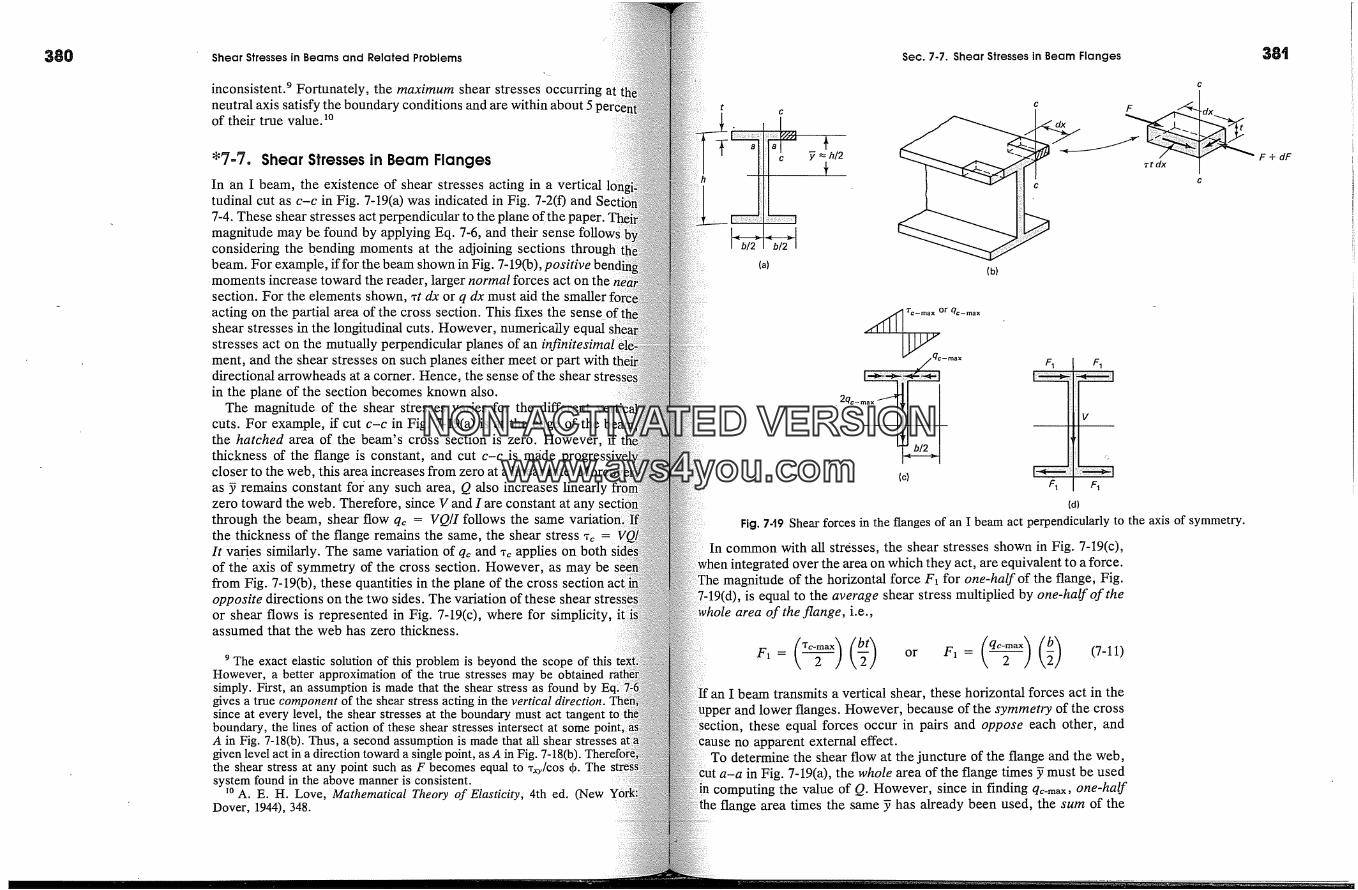
380 Shear Stresses in Beams and Related Problems
inconsistent. 9 Fortunately, the maximum shear stresses occuz�Jngneutral axis satisfy the boundary conditions and are within about 5of their true value. 2o
*7-7. Shear Stresses in Beam FlangesIn an I beam, the existence of shear stresses acting in a verticaltudinal cut as c-c in Fig. 7-19(a) was indicated in Fig. 7-2(f) and7-4. These shear stresses act perpendicular to the plane of the paper.magnitude may be found by applying Eq. 7-6, and their senseconsidering the bending moments at the adjoining sections throubeam. For example, if for the beam shown in Fig. 7-19Co), positive b�moments increase toward the reader, larger normal forces act on thensection. For the elements shown, ,t dx or q dx must aid the smalleracting on the partial area of the cross section. This fixes the senseshear stresses in the longitudinal cuts. However, numerically equalstresses act on the mutually perpendicular planes of an infinitesimalment, and the shear stresses on such planes either meet or part withdirectional arrowheads at a corner. Hence, the sense of the shear stin the plane of the section becomes known also.
The magnitude of the shear siresses varies for the differentcuts. For example, if cut c-c in Fig. 7-19(a) is at the edge of thethe hatched area of the beam's cross section is zero. However,thickness of the flange is constant, and cut c-c is madecloser to the web, this area increases from zero at a linear rate.as y remains constant foi any such area, Q also increases linearlyzero toward the web. Therefore, since V and I are constant at anythrough the beam, shear flow qc = VQ/I follows the samethe thickness of the flange remains the same, the shear stress ,c = 1It varies similarly. The same variation of q� and ,� applies on bothof the axis of symmetry of the cross section. However, as may befrom Fig. 7-19Co), these quantities in the plane of the cross sectionopposite directions on the two sides. The variation of theseor shear flows is represented in Fig. 7-19(c), where for simplicity,assumed that the web has zero thickness.
9 The exact elastic solution of this problem is beyond the scope of thisHowever, a better approximation of the true stresses may be obtainedsimply. First, an assumption is made that the shear stress as found bygives a true component of the shear stress acting in the vertical direction.since at every level, the shear stresses at the boundary must act tangentboundary, the lines of action of these shear stresses intersect at someA in Fig. 7-18(b). Thus, a second assumption is made that all shear stressesgiven level act in a direction toward a single'point, as A in Fig. 7-18(b).the shear stress at any point such as F becomes equal to ?,/cos (b. Thesystem found in the above manner is consistent.
z0 A. E. H. Love, Mathematical Theory of Elasticity, 4th ed. (NewDover, 1944), 348.
h
c � � h/2
(a)
Sec. 7-7. Shear Stresses in Beam Flanges
(b)
c
C ff
rt dx J
(c)
Fig. 749 Shear forces in the flanges of an I beam act perpendicularly to the axis of symmetry.In common with all stresses, the shear stresses shown in Fig. 7-19(c),
integrated over the area on which they act, are equivalent to a force.magnitude of the horizontal force F� for one-half of the flange, Fig.
19(d), is equal to the average shear stress multiplied by one-half of thearea of the flange, i.e.,
F�= (?�:�)(b_�) or F]= (q�:�x)(�) (7-11)I beam transmits a vertical shear, these horizontal forces act in the
lower flanges. However, because of the symmetry of the crosssection, these equal forces occur in pairs and oppose each other, and
cause no apparent external effect.To determine the shear flow at the juncture of the flange and the web,
in Fig. 7-19(a), the whole area of the flange times y must be usedcomputing the value of Q. However, since in finding qc-m�, one-half
flange area times the same y has already been used, the sum of the
F+dF
NON-ACTIVATEDVERSIONwww.avs4you.com
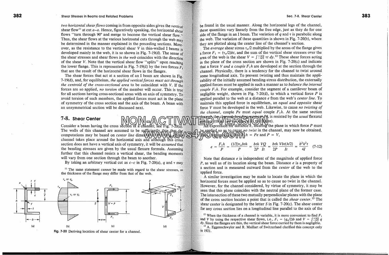
382 Shear Stresses in Beams and Related Problems Sec. 7-8. Shear Center 383
8
two horizontal shear flows coming in from opposite sides gives theshear flow n at cut a-a. Hence, figuratively speaking, the horizontalflows "turn through 90 � and merge to become the vertical shear flo�Thus, the shear flows at the various horizontal cuts through the webbe determined in the manner explained in the preceding sections.over, as the resistance to the vertical shear V in thin-walled Ideveloped mainly in the web, it is so shown in Fig. 7-19(d). The senthe shear stresses and shear flows in the web coincides with theof the shear V. Note that the vertical shear flow "splits" uponthe lower flange. This is represented in Fig. 7-19(d) by the twothat are the result of the horizontal shear flows in the flanges.
The shear forces that act at a section of an I beam are shown in7-19(d), and, for equilibrium, the applied vertical forces must actthe centroid of the cross-sectional area to be coincident with V. Ifforces are so apphed, no torsion of the member will occur. This isfor all sections having cross-sectional areas with an axis ofavoid torsion of such members, the applied forces must act in theof symmetry of the cross section and the axis of the beam. A beaman unsymmetrical section will be discussed next.
Shear Center
Consider a beam having the cross section of a channel; see Fig. 7-201The walls of this channel are assumed to be sufficiently thin thatcomputations may be based on center line dimensions. Bendingchannel takes place around the horizontal axis and although thissection does not have a vertical axis of symmetry, it will be assumedthe bending stresses are given by the usual flexure formula.further that this channel resists a vertical shear, the bendingwill vary from one section through the beam to another.
By taking an arbitrary vertical cut as c-c in Fig. 7-20(a), q and �
n The same statement cannot be made with regard to the shear stressesithe thickness of the flange may differ from that of the web.
rf or qt
r� orq�
F1
(b) (c)
Fig. 7-20 Deriving location of shear center for a channel.(d)
found in the usual manner. Along the horizontal legs of the channel,quantities vary linearly from the free edge, just as they do for one
of the flange in an I beam. The variation of q and, is parabolic alongweb. The variation of these quantities is shown in Fig. 7-20(b), where
are plotted along the center line of the channel's section.shear stress ,a/2 multiplied by the areas of the flange gives
force Fz = (�'d2)bt, and .the sum of the vertical shear stresses over thea of the web is the shear V = r+h/2 � dy.�2J--h/2 'fl- These shear forces acting
the plane of the cross section are shown in Fig. 7-20(c) and indicatea force V and a couple F�h are developed at the section through the
Physically, there is a tendency for the channel to twist aroundlongitudinal axis. To prevent twisting and thus maintain the appli-
' of the initially assumed bending-stress distribution, the externallybe applied in such a manner as to balance the internal
�le F�h. For example, consider the segment of a cantilever beam ofweight, shown in Fig. 7-20(d), to which a vertical force P is
parallel to the web at a distance e from the web's center line. T 9this applied force in equilibrium, an equal and opposite shear
V must be developed in the web. Likewise, to cause no twisting ofchannel, couple Pe must equal couple F�h. At the same section
the channel, bending moment PL is resisted by the usual flexural(these are not shown in the figure).
expression for distance e, locating the plane in which force P mustapplied so as to cause no twist in the channel, may now be obtained:
remembering that F�h = Pe and P = V,
F]h (1/2),�bth bth VQ bth Vbt(h/2) b2h2te ...... (7-12)
P P 2P It 2P It 41
Note that distance e is 'independent of the magnitude of applied forceas well as of its location along the beam. Distance e is a property of
section and is measured outward from the center of the web to theforce.
A similar investigation may be made to locate the plane in which themust be applied so as to cause no twist in the channel.
for the channel considered, by virtue of symmetry, it may bethat this plane coincides with the neutral plane of the former case.
of these two mutually perpendicular planes with the planecross section locates a point that is called the shear center. J3 The
center is designated by the letter S in Fig. 7-20(c). The shear centercross section lies on a longitudinal line parallel to the axis of the
]2 When the thickness of a channel is variable, it is more convenient to find F]V by using the respective shear flows, i.e., F] = (qa/2)b and V = c+h/2J-hi2 q
�. Since the flanges are thin, the vertical shear force carried by them is negligible.Eggenschwyter and R. Maillart of Switzerland clarified this concept only
1921.
NON-ACTIVATEDVERSIONwww.avs4you.com
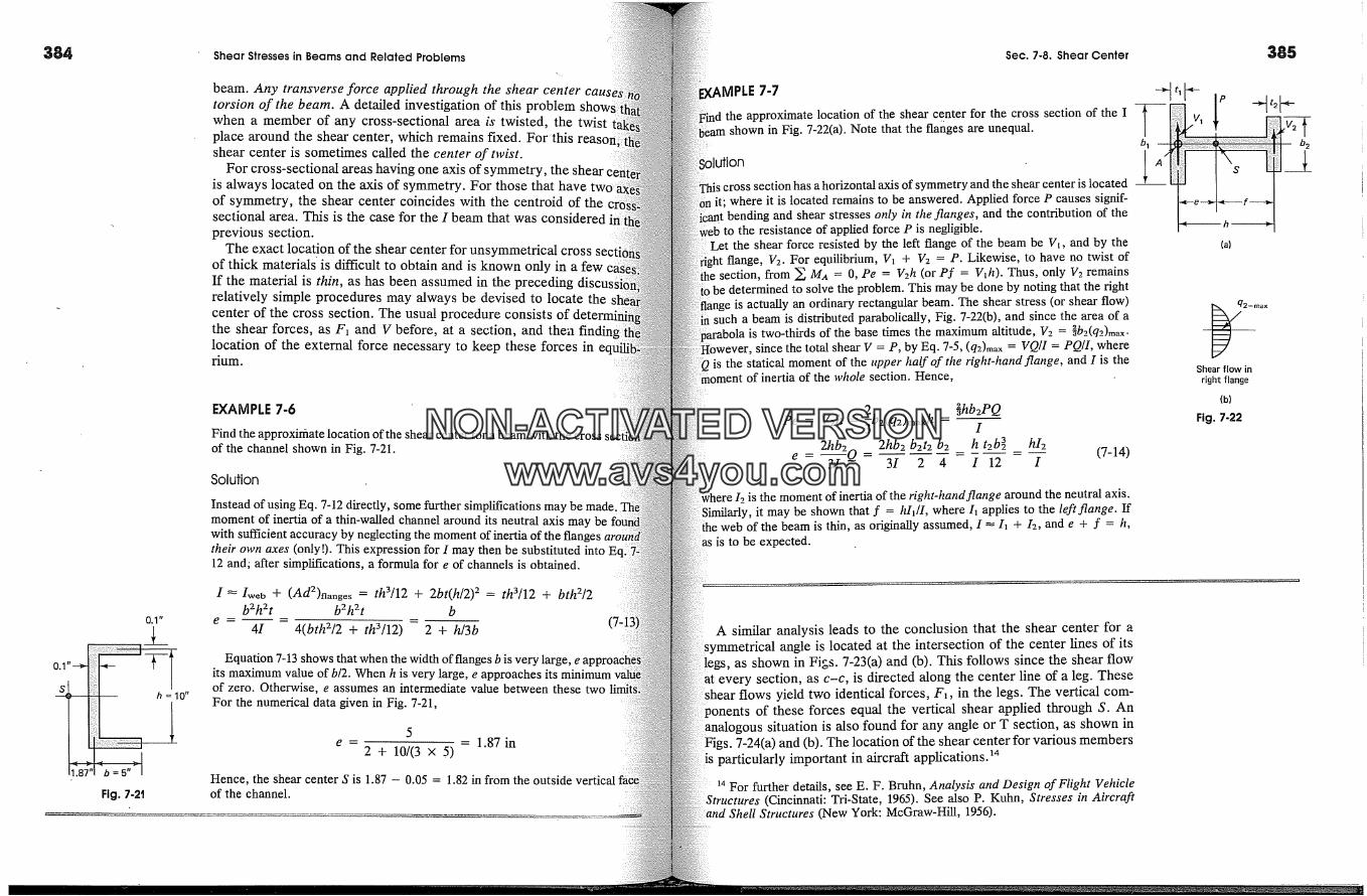
384
Fig. 7.2t
10"
Shear Stresses in Beams and Related Problems
beam. Any transverse force applied through the shear center catorsion of the beam. A detailed investigation of this problemwhen a member of any cross-sectional area is twisted, the twistplace around the shear center, which remains fixed. For this reaso nshear center is sometimes called the center of twist.
For cross-sectional areas having one axis of symmetry, the shearis always located on the axis of symmetry. For those that haveof symmetry, the shear center coincides with the centreid of thesectional area. This is the case for the I beam that was consideredprevious section.
The exact location of the shear center for unsymmetrical crossof thick materials ' is difficult to obtain and is known only in a fewIf the material is thin, as has been assumed in the precedingrelatively simple procedures may always be devised to locate thecenter of the cross section. The usual procedure consists ofthe shear forces, as F� and V before, at a section, and then findinlocation of the external force necessary to keep these forces inrium.
EXAMPLE 7-6
Find the approxirfiate location of the shear center for a beam with the crossof the channel shown in Fig. 7-21.
Solution
Instead of using Eq. 7-12 directly, some further simplifications may be made.moment of inertia of a thin-walled channel around its neutral axis maywith sufficient accuracy by neglecting the moment of inertia of the flangestheir own axes (only!). This expression for I may then be substituted into Eq.12 and; after simplifications, a formula for e of channels is obtained.
I �/web + (Ad2)nanges = th3/12 + 2bt(h/2) 2 = th3/12 + bth2/2b2h2t b2h2t b
41 4(bth2/2 + th3/12) 2 + h/3b (7-1
Equation 7-13 shows that when the width of flanges b is very large,its maximum value of b/2. When h is very large, e approaches its minimumof zero. Otherwise, e assumes an intermediate value between these twoFor the numerical data given in Fig. 7-21,
e = = 1.87 in2 + 10/(3 x 5)
Hence, the shear center S is 1.87 - 0.05 = 1.82 in from the outsideof the channel.
Sec. 7-8. Shear Center
PLE 7-7
the approximate location of the shear center for the cross section of the Ishown in Fig. 7-22(a). Note that the flanges are unequal.
>lution
is cross section has a horizontal axis of symmetry and the shear center is locatedit; where it is located remains to be answered. Applied force P causes signif-
bending and shear stresses only in the flanges, and the contribution of theWeb to the resistance of applied force P is negligible.
Let the shear force resisted by the left flange of the beam be V�, and by theV2. For equilibrium, V� + V2 = P. Likewise, to have no twist of
section, from � M,� = 0, Pe = V2h (or Pf = V�h). Thus, only V2 remainsbe determined to solve the problem. This may be done by noting that the right
actually an ordinary rectangular beam. The shear stress (or shear flow)such a beam is distributed parabolically, Fig. 7-22(b), and since the area of a
is two-thirds of the base times the maximum altitude, V2 = �b2(q2)max.since the total shear V = P, by Eq. 7-5, (q2)max = VQ[I = PQ[I, where
is the statical moment of the upper half of the right-hand flange, and I is theof inertia of the whole section. Hence,
2 h �hb2PQPe = V2h = �b2(q2)m�,, - I2hb2_ 2hb2 b2t2 b2 h t2b� 3 hi2
e=-� -Q= 31 2 7=7'12 - I (7-14)
12 is the moment of inertia of the right-hand flange around the neutral axis.it may be shown that f = hI�/I, where I� applies to the left flange. If
web of the beam is thin, as originally assumed, I � I� + 12, and e + � = h,as is to be expected.
A similar analysis leads to the conclusion that the shear center for aangle is located at the intersection of the center lines of its
legs, as shown in Figs. 7-23(a) and (b). This follows since the shear flowevery section, as c-c, is directed along the center line of a leg. These
shear flows yield two identical forces, F�, in the legs. The vertical com-ponents of these forces equal the vertical shear applied through S. An
situation is also found for any angle or T section, as shown inFigs. 7-24(a) and (b). The location of the shear center for various members
particularly important in aircraft applications. 14�4 For further details, see E. F. Bruhn, Analysis and Design of Flight Vehicle
(Cincinnati: Tri-State, 1965). See also P. Kuhn, Stresses in AircraftStructures (New York: McGraw-Hill, 1956).
385
(a)
Shear flow inright flange
(h)
Fig. 7-22NON-ACTIVATEDVERSIONwww.avs4you.com
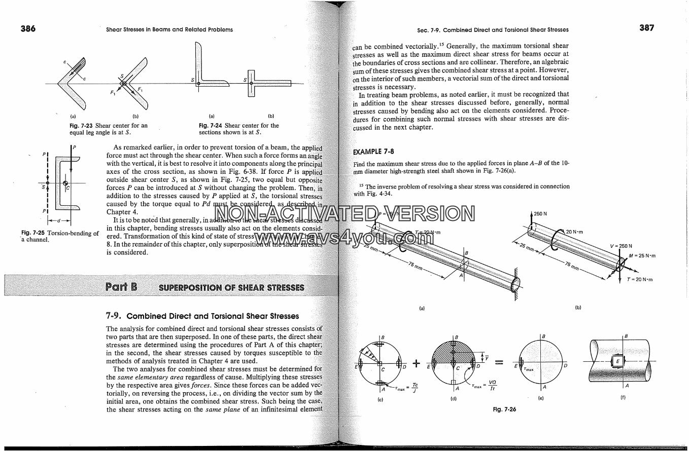
386 Shear Stresses in Beams and Related Problems Sec� 7-9. Combined Direct and Torsional Shear Stresses 387
c�
{�) {�)
Fig. 7-23 Shear center for anequal leg angle is at S.
(a) {b)
Fig. 7-24 Shear center for thesections shown is at S.
P
Fig. 7-25 Torsion-bending ofa channel.
As remarked earlier, in order to prevent torsion of a. beam, theforce must act through the shear center. When such a force forms an:with the vertical, it is best to resolve it into components alo�.g theaxes of the cross section, as shown in Fig. 6-38. If force P isoutside shear center S, as shown in Fig. 7-25, two equal butforces P can be introduced at S without changing the problem.addition to the stresses caused by P applied at S, the torsionalcaused by the torque equal to Pd must be considered, asChapter 4.
It is to be noted that generally, in addition to the shear stresses discuin this chapter, bending stresses usually also act on the elements conered. Transformation of this kind of state of stress is discussed
8. In the remainder of this chapter, only superposition of the shearis considered.
7-9. Combined Direct and Torsional Shear Stresses
The analysis for combined direct and torsional shear stresses consiststwo parts that are then superposed. In one of these parts, the directstresses are determined using the procedures of Part A of thisin the second, the shear stresses caused by torques susceptiblemethods of analysis treated in Chapter 4 are used.
The two analyses for combined shear stresses must be determinedthe same elementary area regardless of cause. Multiplying theseby the respective area gives forces. since these forces cantorially, on reversing the process, i.e., on dividing the vector sum binitial area, one obtains the combined shear stress. Such being thethe shear stresses acting on the same plane of an inf'mitesimal
an be combined vectorially.�5 Generally, the maximum torsional shear�.sses as well as the maximum direct shear stress for beams occur at
ihe boundaries of cross sections and are collinear. Therefore, an algebraicof these stresses gives the combined shear stress at a point. However,
� of such members, a vectorial sum of the direct and torsionalStresses is necessary.
In treating beam problems, as noted earlier, it must be recognized thataddition to the shear stresses discussed before, generally, normal
;ses caused by bending also act on the elements considered. Proce-for combining such normal stresses with shear stresses are dis-
�ssed in the next chapter.
VIPLE 7-8
the maximum shear stress due to the applied forces in plane A-B of the 10-diameter high-strength steel shaft shown in Fig. 7-26(a).
25 The inverse problem of resolving a shear stress was considered in connectionwith Fig. 4-34.
N 250 N
T= 20 N'm 20 N-m
{a) (b)
� B(c) (d) (e)
Fig. 7-26
V=250N
M = 25 N-m
T=20 N-m
iA
(f)
NON-ACTIVATEDVERSIONwww.avs4you.com
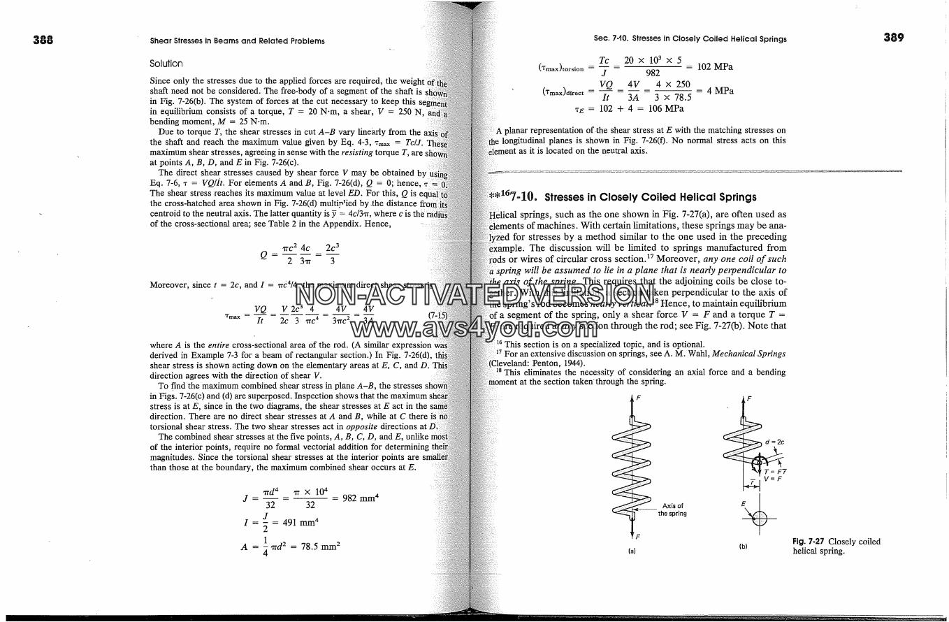
Shear Stresses in Beams and Related Problems
Solution
Since only the stresses due to the applied forces are required, theshaft need not be considered. The free-body of a segment of the shaft isin Fig. 7-26(b). The system of forces at the cut necessary to keep thisin equilibrium consists of a torque, T = 20 N.m, a shear, V = 250bending moment, M = 25 N.m.
Due to torque T, the shear stresses in cut A-B vary linearly from thethe shaft and reach the maximum value given by Eq. 4-3, �m�, = Tc/J.maximum shear stresses, agreeing in sense with the resisting torque T, areat points A, B, D, and E in Fig. 7-26(c).
The direct shear stresses caused by shear force V may be obtained byEq. 7-6, � = VQ/[t. For elements A and B, Fig. 7-26(d), Q = 0; hence,The shear stress reaches its maximum value at level ED. For this, Q isthe cross-hatched area shown in Fig. 7-26(d) multipqed by.the distancecentraid to the neutral axis. The latter quantiW is y = 4c/3�r, where c is theof the cross-sectional area; see Table 2 in the Appendix. Hence,
� rc 2 4c 2C 3Q= 2 3,r 3
Moreover, since t = 2c, and I = ,lrb4/4, the maximum direct shear stress
VQ _ V 2C 3 4 _ 4�V _ 4VIt 2c 3 TfC 4 31rC 2 3A
where A is the entire cross-sectional area of the rod. (A similar expressionderived in Example 7-3 for a beam of rectangular section.) In Fig. 7-26(d),shear stress is shown acting down on the elementary areas at E, C, and D.direction agrees with the direction of shear V.
To find the maximum combined shear stress in plane A-B, the stressesin Figs. 7-26(c) and (d) are superposed. Inspection shows that the maximum sstress is at E, since in the two diagrams, the shear stresses at E act in thedirection. There are no direct shear stresses at A and B, while at C theretorsional shear stress. The two shear stresses act in opposite directions
The combined shear stresses at the five points, A, B, C, D, and E,of the interior points, require no formal vectorial addition formagnitudes. Since the torsional shear stresses at the interior points arethan those at the boundary, the maximum combined shear occurs at E.
�d 4 � x 104J .... 982 1111114
32 32J
I = - = 491 mm 42
A = � 'rrd 2 = 78.5 mm 2
Sec. 7-10. Stresses in Closely Coiled Helical Springs
Tc 20 X 103 X 5(Tmax)torsio n -- -- = 102 MPa
J 982
VQ 4V 4 x 250(*m�,,)ai�eot .... 4 MPa
It 3A 3 x 78.5
� E= 102 + 4 = 106MPa
representation of.the shear stress at E with the matching stresses onlongitudinal planes is shown in Fig. 7-26(0. No normal stress acts on this
it is located on the neutral axis.
*a7-10. Stresses in Closely Coiled Helical Springssprings, such as the one shown in Fig. 7-27(a), are often used as
of machines. With certain limitations, these springs may be ana-for stresses by a method similar to the one used in the preceding
The discussion will be limited to springs manufactured fromor wires of circular cross section? Moreover, any one coil of such
will be assumed to lie in a plane that is nearly petI)endicular toaxis of the spring. This requires that the adjoining coils be close to-
With this limitation, a section taken perpendicular to the axis ofspring's rod becomes nearly vertical. �8 Hence, to maintain equilibrium
a segment of the spring, only a shear force V = F and a torque T =quired at any section through the rod; see Fig. 7-27(b). Note that
This section is on a specialized topic, and is optional.discussion on springs, see A.M. Wahl, Mechanical Springs
Penton, 1944).This eliminates the necessity of considering an axial force and a bending
at the section taken' through the spring.
F F
d =2c
T= F7V=F
Axisof �the spring
F
(b)(a)
Fig. 7-27 Closely coiledhelical spring.
389
NON-ACTIVATEDVERSIONwww.avs4you.com
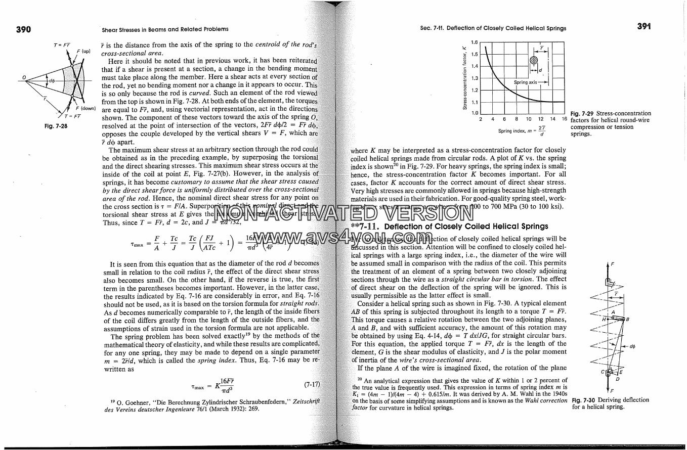
390
T = FT
Fig. 7-28
F (up)
F (down)
FT
Shear Stresses in Beams and Related Problems
? is the distance from the axis of the spring to the centroid of thecross-sectional area.
Here it should be noted that in previous work, it has beenthat if a shear is present at a section, a change in the bendingmust take place along the member. Here a shear acts at everythe rod, yet no bending moment nor a change in it appears to occur.is so only because the rod is curved. Such an element of the rodfrom the top is shown in Fig. 7-28. At both ends of the element, the tonare equal to by, and, using vectorial representation, act in theshown. The component of these vectors toward the axis of the springresolved at the point of intersection of the vectors, 2by drb/2 = byopposes the couple developed by the vertical shears V = F, which? d4) apart.
The maximum shear stress at an arbitrary section through the rodbe obtained as in the preceding example, by superposing the torsi oand the direct shearing stresses. This maximum shear stress occurs at'inside of the coil at point E, Fig. 7-27(b). However, in thesprings, it has become customa,7 to assume that the shear stressby the direct shear force is uniformly distributed over thearea of the rod. Hence, the nominal direct shear stress for anythe cross section is, = F/A. Superposition of this nominal direct andtorsional shear stress at E gives the maximum combined shearThus, since T = by, d = 2c, and J = 'rrd4/32,
,m� =� +-f = J + 1 ,rrd 3 + 1It is seen from this equation that as the diameter of the rod d
small in relation to the coil radius ?, the effect of the direct shearalso becomes small. On the other hand, if the reverse is true, theterm in the parentheses becomes important. However, in the latterthe results indicated by Eq. 7-16 are considerably in error, and Eq.should not be used, as it is based on the torsion formula for straightAs d becomes numerically comparable to ?, the length of the insideof the coil differs greatly from the length of the outside fibers, andassumptions of strain used in the torsion formula are not applicable.
The spring problem has been solved exactly m by the methodsmathematical theory of elasticity, and while these resultsfor any one spring, they may be made to depend on a singlem = 27/d, which is called the spring index. Thus, Eq. 7-16 may bewritten as
= K 16by (7-1'rmax ,rd--��9 O. Goehner, "Die Berechnung Zylindrischer Schraubenfedern,"
des Vereins deutscher Ingenieure 76/1 (March 1932): 269.
Sec. 7-tt. Deflection of Closely Coiled Helical Springs 39'
1.6
�.4
�.3
1.2
1.1
1.0
k Springaxis---�
2 4 6 8 10 12 14
27Spring index, m = �
Fig. 7-29 Stress-concentrationfactors for helical round-wirecompression or tensionsprings.
K may be interpreted as a stress-concentration factor for closelyiled helical springs made from circular rods. A plot of K vs. the spring
shown TM in Fig. 7-29. For heavy springs, the spring index is small;hence, the stress-concentration factor K becomes important. For all
factor K accounts for the correct amount of direct shear stress.; high stresses are commonly allowed in springs because high-strength
are used in their fabrication. For good-quality spring steel, work-ing shear stresses range anywhere from 200 to 700 MPa (30 to 100 ksi).
Deflection of Closely Coiled Helical Springs
completeness, the deflection of closely coiled helical springs will beIlscussed in this section. Attention will be confined to closely coiled hel-
springs with a large spring index, i.e., the diameter of the wire willassumed small in comparison with the radius of the coil. This permits
treatment of an element of a spring between two closely adjoiningthrough the wire as a straight circular bar in torsion. The effect
direct shear on the deflection of the spring will be ignored. This ispermissible as the latter effect is small.
Consider a helical spring such as shown in Fig. 7-30. A typical elementof this spring is subjected throughout its length to a torque T = bY.
torque causes a relative rotation between the two adjoining planes,and B, and with sufficient accuracy, the amount of this rotation may
by using Eq. 4-14, d4) = T dx/JG, for straight circular bars.this equation, the applied torque T = bY, dx is the length of the
G is the shear modulus of elasticity, and J is the polar momentinertia of the wire's cross-sectional area.
If the plane A of the wire is imagined fixed, the rotation of the plane
20 An analytical expression that gives the value of K within 1 or 2 percent oftrue value is frequently used. This expression in terms of spring index rn is
(4rn - 1)/(4rn - 4) + 0.615/rn. It was derived by A.M. Wahl in the 1940sof some simplifying assumptions and is known as the Wahl correction
for curvature in helical springs.
D
Fig. 7-30 Deriving deflectionfor a helical spring.
NON-ACTIVATEDVERSIONwww.avs4you.com
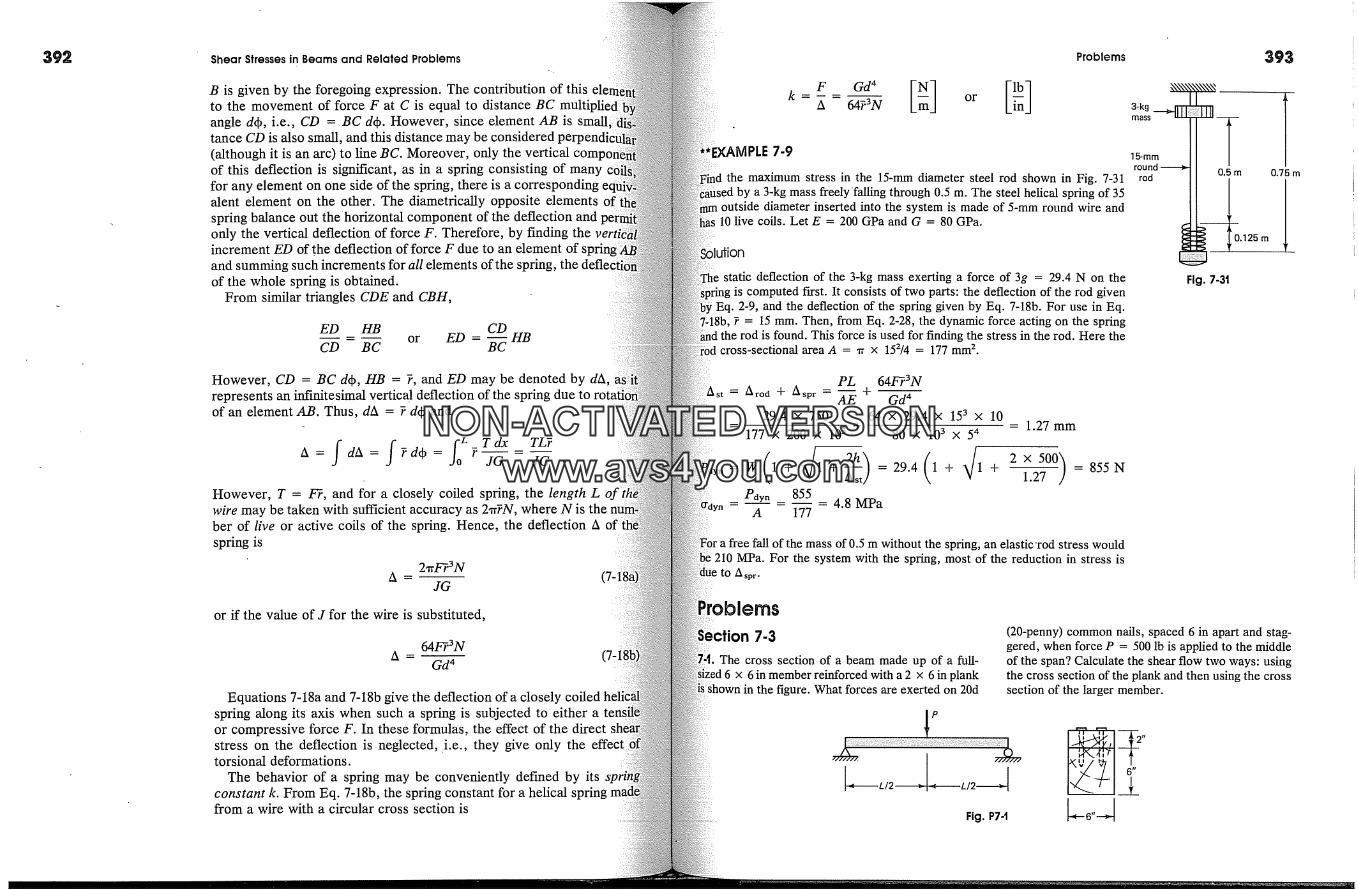
392 Shear Stresses In Beams and Related Problems
B is given by the foregoing expression. The contribution of thisto the movement of force F at C is equal to distance BC multipliedangle d4�, i.e., CD = BC d4�. However, since element AB istance CD is also small, and this distance may be considered(although it is an arc) to line BC. Moreover, only the verticalof this deflection is significant, as in a spring consisting of manyfor any element on one side of the spring, there is a coxesalent element on the other. The diametrically opposite elementsspring balance out the horizontal component of the deflection andonly the vertical deflection of force F. Therefore, by finding theincrement ED of the deflection of force F due to an element of sand summing such increments for all elements of the spring,of the whole spring is obtained.
From similar triangles CDE and CBH,
ED HB CD
CD = B-� or ED =�-�HB
However, CD = BC d4�, HB = ?, and ED may be denoted by dA,represents an infinitesimal vertical deflection of the springof an element AB. Thus, dA = ? dqb and
A = dA = ?dqb = ? JG JG
However, T = F�, and for a closely coiled spring, the length L of �wire may be taken with sufficient accuracy as 2,r�N, where N is theber of live or active coils of the spring. Hence, the deflection Aspring is
A - 2�F�3�N (7-1JG
or if the value of J for the wire is substituted,
64F�3NA -- --
Gd 4
Equations 7-18a and 7-18b give the deflection of a closely coiledspring along its axis when such a spring is subjected to either aor compressive force F. In these formulas, the effect of the directstress on the deflection is neglected, .i.e., they give only the effecttorsional deformations.
The behavior of a spring may be conveniently def'med by itsconstant k. From Eq. 7-18b, the spring constant for a helical springfrom a wire with a circular cross section is
Problems
A - 6473� or �n
*EXAMPLE 7-9
the maximum stress in the 15-mm diameter steel rod shown in Fig. 7-31a 3-kg mass freely'falling through 0.5 m. The steel helical spring of 35
outside diameter inserted into the system is made of 5-mm round wire and10 live coils. Let E = 200 GPa and G = 80 GPa.
static deflection of the 3-kg mass exerting a force of 3g = 29.4 N on theis computed first. It consists of two parts: the deflection of the rod given
Eq. 2-9, and the deflection of the spring given by Eq. 7-18b. For use in Eq.�18b, ? = 15 mm. Then, from Eq. 2-28, the dynamic force acting on the spring
the rod is found. This force is used for finding the stress in the rod. Here thecross-sectional area A = �r x 152/4 = 177 mm 2.
�.125mFig. 7-3t
PL 64F?3N�--- A ro d q- A spr = � q- Gd�
29.4 x 750 64 x 29.4 x 153 x 10+ = 1.27 mm
177 x 200 x 103 80 x 103 x 54
= W (1 + �1 + 2�t�t)=29.4 (1 + �/1 + 2x 500hPdyn 855 4.8 MPa
A 177
a free fall of the mass of 0.5 m without the spring, an elastic'rod stress would210 MPa. For the system with the spring, most of the reduction in stress is
to Asp r.
'robiems
7-3
The cross section of a beam made up of a full-x 6 in member reinforced with a 2 x 6 in plank
shown in the figure. What forces are exerted on 20d
(20-penny) common nails, spaced 6 in apart and stag-gered, when force P = 500 lb is applied to the middleof the span? Calculate the shear flow two ways: usingthe cross section of the plank and then using the crosssection of the larger member.
Fig. P74
NON-ACTIVATEDVERSIONwww.avs4you.com

394
7-2. The shear diagram for the box beam supportinga uniformly distributed load is conservatively approx-imated for design by the stepped diagram shown in thefigure. If the beam is nailed together with 16d (16-penny) box nails from four full-sized pieces, as shownin the cross section, what nail spacing should be usedalong the span? Assume that each nail is good for 75lb in shear.
Shear Stresses in Beams and Related Problems
shown, determine the bolt spacing for thegion of the span. The bolts are arranged inthe allowable shear force per high-strength bolt iskN.
7-5. A wooden box beam, made up from 2-inboards, has the dimensions shown � the figure.beam transmits a vertical shear of 760 lb, whatbe the longitudinal spacing of the nails (a)
2" necting board A with boards B and C, and (b)� necting board D with boards B and C?
Fig. P7-2
900 lb..... 1 600 lb
II
IIL ....
Shear diagram
7-3. A- 10-in square box beam is to be made from four2-in thick wood pieces. Two possible designs are con-sidered, as shown in the figure. Moreover, the designshown in (a) can be turned 90 � in the application. (a)Select the design requiting the minimum amount ofnailing for transmitting shear. (b) If the shear to betransmitted by this member is 620 lb, what is the nailspacing for the best design? The nailing is to be donewith 16d (16-penny) box nails that are good for 50 lbeach in shear.
(b)(a)
Fig. P7-3
7-4. A beam is loaded so that the moment diagramvaries, as shown in the figure. For the cross section
Fig. P7-4
Fig. P7-5
7-6. Two'W 8 x 67 beams are arranged asthe figure. Determine the bending and shearof this member if the allowable bending stressand the shear capacity of each bolt is 20 k. Theare arranged in pairs and are spaced 6 in on
Fig. P7-6
7-7. A plate girder is made up from two 14 xplates, four 6 x 4 x � in angles, and a 39� xplate, as shown in the figure. If at the section
Fig. P7-7
a total vertical shear of 150 k is transmitted, whatthe spacing of rivets A and B? For the girder
und the neutral axis, I is .14,560 in 4. Assume �a-ins and note that one rivet is good for 6.63 k in single
13.25 k in double shear, and 11.3 k in beatinga �-in plate.
A simply supported beam has a cross section con-of a C 12 x 20.7 and a W 18 x 50 fastened
' 4a-in-diameter bolts spaced longitudinally 6apart in each row, as shown in the figure. If this
is loaded with a downward concentrated force
112 k in the middle of the span, what is the shearin the bolts? Neglect the weight of the beam.
moment of inertia I of the whole member aroundneutral axis is 1120 in 4.
6.78"
t11.50"
Fig. P7-8
Machined channel-like caps are attached to aform the beam cross section shown in the fig-
The interconnecting 10-mm-diameter rivets are' 80 mm on center. If the allowable
stress for the rivets is 50 MPa, what is the al-shear for this section?
3plat
fig. P?.9
A T-flange girder is used to support a 900-kN10ad in the middle of a 7-m simple span. The dimen-
ions of the girder are given in the figure in a cross-
Problems
5O
�00 mrn_.�Fig. P7-t0
395
sectional view. If the 22-mm-diameter rivets arespaced 125 mm apart longitudinally, what shear stresswill be developed in the rivets by the applied loading?The moment of inertia of the girder around ;the neutralaxis is approximately 4300 x 106 mm 4.
Sections 7.4 and 7-5
7-tt. Show that a formula, analogous to Eq. 7-8a, forbeams having a solid circular cross section of area Ais *max = �V/A.
742. Show that a formula, analogous to Eq. 7-8a, forthin-walled circular tubes acting as beams having a netcross-sectional area A is *m�x = 2V/A.743. A T beam has the cross section shown in thefigure. Calculate the shear stresses for the indicatedsix horizontal sections when the beam transmits a ver-tical shear of 240 kN. Plot the results as in Fig. 7-16(e).
--150--�[12--3
4--
6
50 mm
Fig. P7-t3
',50
150
7-'14. A box beam has the cross section shown in thefigure. Calculate shear stresses at several horizontalsections when the beam bending moment changesalong the beam at the rate of 500 kN.m/m and plot theresults as in Fig. 7-16(e).
NON-ACTIVATEDVERSIONwww.avs4you.com
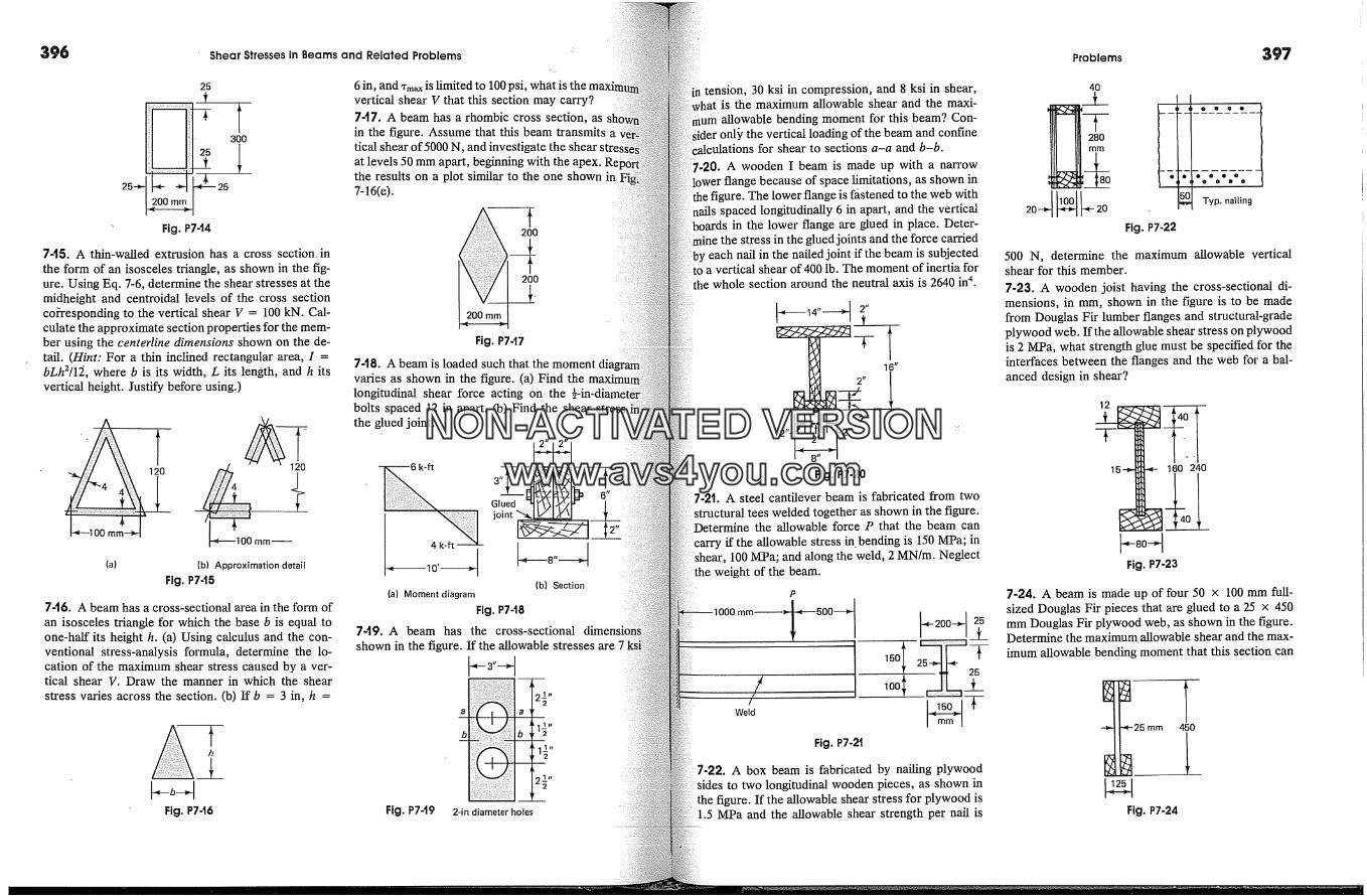
396
25-�
200 mm
Shear Stresses in Beams and Related Problems
25
300
-�--� 25
6 in, and Tmax is limited to 100 psi, what is thevertical shear V that this section may carry?7-17. A beam has a rhombic cross section, asin the figure. Assume that this beam transmits a �tical shear of 5000 N, and investigate the shear slat levels 50 mm apart, beginning with the apex.the results on a plot similar to the one shown in7-16(e).
Fig. P7-t4
745. A thin-walled extrusion has a cross section. inthe form of an isosceles triangle, as shown in the fig-ure. Using Eq. 7-6, determine the shear stresses at themidheight and centroidal levels of the cross sectionco?responding to the vertical shear V = 100 kN. Cal-culate the approximate section properties for the mem-ber using the centerline dimensions shown on the de-tail. (Hint: For a thin inclined rectangular area, I =bLh2/12, where b is its width, L its length, and h itsvertical height. Justify before using.)
120 �(a) (b) Approximation detail
Fig. P745
746. A beam has a cross-sectional area in the form ofan isosceles triangle for which the base b is equal toone-half its height h. (a) Using calculus and the con-ventional stress-analysis formula, determine the lo-cation of the maximum shear stress caused by a ver-tical shear V. Draw the manner in which the shearstress varies across the section. (b) If b = 3 in, h =
Fig. P746
Fig. P747
748. A beam is loaded such that the momentvaries as shown in the figure. (a) Find thelongitudinal shear force acting on-thebolts spaced 12 in apart. (b) Find the shear stressthe glued joint.
k-ft
Gluedjoint
(b) Section(a) Moment diagram
Fig. P7-t8
749. A beam has the cross-sectionalshown in the figure. If the allowable
Fig. P7-t9 2-in diameter holes
tension, 30 ksi in compression, and 8 ksi in shear,is the maximum allowable shear and the maxi-
um allowable bending moment for this beam? Con-onl� the vertical loading of the beam and confine
s for shear to sections a-a and b-b.A wooden I beam is made up with a narrow
of space limitations, as shown inthe figure. The lower flange is ffistened to the web with
spaced longitudinally 6 in apart, and the verticalboards in the lower flange are glued in place. Deter-
e the stress in the glued joints and the force carried' each nail in the nailed joint if the beam is subjected
to a vertical shear of 400 lb. The moment of inertia forwhole section around the neutral axis is 2640 in 4.
I' 14"---� 2"
16"
2"�82�2" 2" 'Fig. P7-20
7-21. A steel cantilever beam is fabricated from twostructural tees welded together as shown in the figure.
Determine the allowable force P that the beam cancarry if the allowable stress in. bending is 150 MPa; in
100 MPa; and along the weld, 2 MN/m. Neglectweight of the beam.
P
mm � � 500--�
Fig, P7-2�
7-22, A box beam is fabricated by nailing plywoodto two longitudinal wooden pieces, as shown in
the figure. If the allowable shear stress for plywood is1.5 MPa and the allowable shear strength per nail is
Problems 397
40
Fig. P7-22
� � � o
Typ. nailing
500 N, determine the maximum allowable verticalshear for this member.
7-23. A wooden joist having the cross-sectional di-mensions, in mm, shown in the figure is to be madefrom Douglas Fir lumber flanges and structural-gradeplywood web. If the allowable shear stress on plywoodis 2 MPa, what strength glue must be specified for theinterfaces between the flanges and the web for a bal-anced design in shear?
1 -,*- 160 240
Fig. P7-23
7-24. A beam is made up of four 50 x 100 mm full-sized Douglas Fir pieces that are glued to a 25 x 450mm Douglas Fir plywood web, as shown in the figure.Determine the maximum allowable shear and the max-imum allowable bending moment that this section can
-*'25 mm 450
Fig. P7-24
NON-ACTIVATEDVERSIONwww.avs4you.com
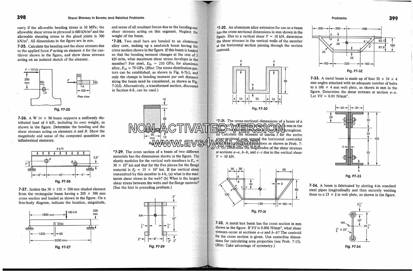
398 Shear Stresses in Beams and Related Problems
carry if the allowable bending stress is 10 MPa; theallowable shear stress in plywood is 600 kN/m 2 and theallowable sheafing stress in the glued joints is 300kN/m 2. All dimensions in the figure are in ram.7-25. Calculate the bending and the shear stresses dueto the applied force P acting on element A for the can-tilever shown in the figure, and show these stressesacting on an isolated sketch of the element.
P = 10'kN �
200
Plan view
Fig. P7-25
7-26. A W 14 x 90 beam supports a uniformly dis-tributed load of 4 ldft, including its own weight, asshown in the figure. Determine the bending and theshear stresses acting on elements A and B. Show themagnitude and sense of the computed quantities oninfinitesimal elements.
4 k/ft
7"i
Fig. P7-26
7-27. Isolate the 50 x 150 x 200 mm shaded elementfrom the rectangular beam having a 200 x 300 mmcross section and loaded as shown in the figure. On afree-body diagram, indicate the location, magnitude,
____� 100kN 3001800 mm mm
R-5o200 50
3000 mm
Fig. P7-27
and sense of all resultant forces due to the bendinshear stresses acting on this segment.weight of the beam.*7-28. Two steel bars are bonded to an alualloy core, making up a sandwich beamcross section shown in the figure. If this beam isso that the bending moment changes at the ratekN.m/m, what maximum shear stress developsmember? For steel, Est = 210 GPa; foralloy, E^� = 70 GPa. (Hint: The stress distributiontern can be established, as shown in Fig. 6-7(c)only the change in bending moment peralong the beam need be considered, as shown in7-2(d). Alternatively, a transformed section,in Section 6-8, can be used.) '
10
T
[�mm� 10
Fig. P7-28
'7-29. The cross section of a beam of twomaterials has the dimensions shownelastic modulus for the vertical web members30 x 103 ksi and that for the five pieces formaterial is E.r = 15 x 103 ksi. If the verticaltransmitted by this member is 4 k, (a) what isimum shear stress in the web? (b) What is theshear stress between the webs and the ran(See the hint in preceding problem.)
NA
Fig. P7-29
;-30. An aluminum alloy extrusion for use as a beam. the cross-sectional dimensions in mm shown in the
Due to a vertical shear V = 10 kN, determine�hear stresses in the vertical walls of the member
the horizontal section passing through the section
4 4
--T
Fig. P7-30
'-3'1. The cross-sectional dimensions of a beam of aare given in mm in the
figure. The member material is 3 mm thick throughout.Calculate the moment of inertia I for the entire
area around the horizontal centroidalUse centerline dimensions as shown in Prob. 7-
(b) Determine the magnitudes of the shear stressesa-a, b-b, and c-c due to the vertical shear
= 10kN.
100
Fig. P7-3t
A metal box beam has the cross section in mmin the figure. If V/I is 0.006 N/mm 4, what shear
occur at sections a-a and b-b? The centtoldthe cross section is given. Use centerline dimen-
for calculating area properties (see Prob. 7-15).Take advantage of symmetry.)
Problems 399
"-200�200--� .-.,t 400a ,,
20�'Fig. P7-32
7-33. A metal beam is made up of four 30 x 24 x 4mm angles attached with an adequate number of boltsto a 100 x 4 mm web plate, as shown in mm in thefigure. Determine the shear stresses at section a-a.Let VII = 0.01 N/mm 4.
Fig. P7-33
7-34. A beam is fabricated by slotting 4-in standardsteel pipes longitudinally and then securely weldingthem to a 23 x fl in web plate, as shown in the figure.
2 TM
Fig. P7-34
NON-ACTIVATEDVERSIONwww.avs4you.com

400 'Shear Stresses in Beams and Related Problems - Problems
I of the composite section around the neutral axis is1018 in 4. If at a certain section, this beam transmits avertical shear of 40 k, determine the shear stress in thepipe and in the web plate at a level 10 in above theneutral axis.
Sections 7-7 and 7.8
7-35. A beam having a cross section with the dimen-sions in mm shown in the figure is in a region wherethere is a constant, positive vertical shear of 100 kN.(a) Calculate the shear flow q acting at each of the foursections indicated in the figure. (b) Assuming a posi-tive bending moment of 27 kN.m at one section and alarger moment at the adjoining section 10 mm away,drav� isometric sketches of each segment of the beamisolated by the sections 10 mm apart and the four sec-tions shown in the figure, and on the sketches indicate
. all forces acting on the segments. Neglect verticalshear stresses in the flanges.
b 120-�nc d
Fig. P7-35
7-36. A beam having the cross section with the di-mensions shown in the figure transmits a vertical shear
Fig. P7-36
V = 7 k applied through the shear center. (a)mine the shear stresses at sections a-a, b-b,c. I around the neutral axis is 35.7 in n. Theof the material is � in throughout. (b) Sketch thestress distribution along the centerline7-37 through 7-40. Determine the location of �shear center for the beams having thedimensions shown in the figures. All members arebe considered thin-walled, and calculations shouldbased on the centerline dimensions.
Fig. P7-37
2o-q
--� <--2 50 mm
r- �
'<----4010 mm
80 rnm
2
I� 10 turn
Fig. P7-38
Fig. P7-40
Fig. P7-39
60
60
40
r.4t. Show that for the Z cross section shown in(a) of the figure, the shear center lies on the ver-
section's centroid. Dem-istratin� that the force resultant due to the internal
flow is zero in each flange constitutes a proof.Apply vertical shear force Vy shown in the fig-
Since the position of the shear center is indepen-of the magnitude of sheat Vy, it can be chosen
Likewise, it is the rate of change in M, asFig. 7-2(d), rather than its magnitude that is of im-
Therefore, let the change in moment AM in
a unit span distance be Vy x 1 = 10 lb-in. Using thisAM, calculate the stresses along the centerline of theZ section using the generalized flexure formula, Eq.6-64. Such calculations should verify the normal stressdistribution shown in part (b) of the figure. By inte-grating these stresses along the section centerline, asin Fig. 7-20(b), the shear flow in the plane of the sectionis found, part (c) of the figure. The force resultantsbased on these shears vanish in both flanges.) Notethat for the given section, It = 2.133 in 4, Iy = 0.533in 4, and Iyz = 0.800 in 4.
line
(a)
NA
21.40 psi
-21.40 psi
2psi(b)
Fig. P7-4�1
0.357
1.07
1.07
0.357
Shear flow (lb/in)
(c)
-- 3.21
Show that for the Z cross section in the pro-the shear center lies on the horizontal
through the section's centroid. Demon-that an applied horizontal force is equally di-
between the two flange� constitutes a solution)roblem. (Hint: Apply a horizontal force Vz, say
to 10 lb, through the section's centroid, and as�roblem, calculate the normal stresses
shear stresses in the plane of the cross section.shear stresses along the section
centerline is useful in the solution. Note that the re-sultant shear force in the web is zero.)7-43 and 7-44. Determine the location of the shearcenter for the beams with idealized cross sections
shown in the figures. Neglect the areas of the platesconnecting the longitudinal stringers, each one ofwhich has an effective area A concentrated at a pointfor resisting longitudinal forces. There are two suchareas in Fig. P7-43 and eight in Fig. P7-44. (This kindof idealization is often used in aircraft design.)
Fig. P7-43
o
(are) a Fig. P7-44
NON-ACTIVATEDVERSIONwww.avs4you.com
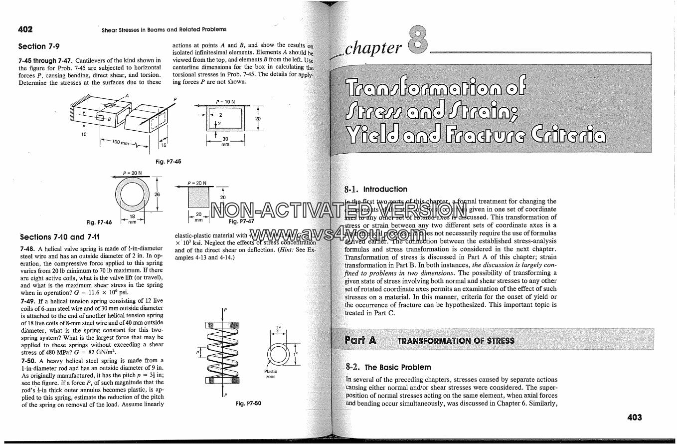
402 Shear Stresses in Beams and Related Problems
Section 7-9
7-45 through 7-47. Cantilevers of the kind shown inthe figure for Prob. 7-45 are subjected to horizontalforces P, causing bending, direct shear, and torsion.Determine the stresses at the surfaces due to these
actions at points A and B, and show theisolated infinitesimal elements. Elements Aviewed from the top, and elements B from the left.centerline dimensions for the box intorsional stresses in Prob. 7-45. The details foring forces P are not shown.
Fig. P7-45
Fig.P7-46�Sections 7-t0 and 74t
7-48. A helical valve spring is made of �-in-diametersteel wire and has an outside diameter of 2 in. In op-eration, the compressive force applied to this springvaries from 20 lb minimum to 70 lb maximum. If thereare eight active coils, what is the valve lift (or travel),and what is the maximum shear stress in the springwhen in operation? G = 11.6 x 10 6 psi.7-49. If a helical tension spring consisting of 12 livecoils of 6-mm steel wire and of 30 mm outside diameteris attached to the end of another helical tension springof 18 live coils of 8-mm steel wire and of 40 mm outsidediameter, what is the spring constant for this two-spring system? What is the largest force that may beapplied to these springs without exceeding a shearstress of 480 MPa? G = 82 GN/m 2.7-50. A heavy helical steel spring is made from a1-in-diameter rod and has an outside diameter of 9 in.As originally manufactured, it has the pitch p = 3� in;see t.he figure. If a force P, of such magnitude that therod's �-in thick outer annulus becomes plastic, is ap-plied to this spring, estimate the reduction of the pitchof the spring on removal of the load. Assume linearly
P=10N
20
P =20 N
20kmmq Fig. P7-47elastic-plastic material with *vp = 50 ksi, and G =x' 103 ksi. Neglect the effects of stress
and of the direct shear on deflection. (Hint: Seeamples 4-13 and 4-14.)
P
Fig. P7-50
Plastic
Introduction
the first two parts of this chapter, a formal treatment for changing thecomponents of the state of stress or strain given in one set of coordinate
to any other set of rotated axes is discussed. This transformation ofor strain between any two different sets of coordinate axes is a
process and does not necessarily require the use of formulasearlier. The connection between the established stress-analysis
formulas and stress transformation is considered in the next chapter.of stress is discussed in Part A of this chapter; strain
in Part B. In both instances, the discussion is largely con-to problems in two dimensions. The possibility of .transforming a
involving both normal and shear stresses to any otherof rotated coordinate axes permits an examination of the effect of such
stresses on a material. In this manner, criteria for the onset of yield oroccurrence of fracture can be hypothesized. This important topic is
in Part C.
The Basic Problem
several of the preceding chapters, stresses caused by separate actionseither normal and/or shear stresses were considered. The super-
stresses acting on the same element, when axial forcesoccur simultaneously, was discussed in Chapter 6. Similarly,
403
NON-ACTIVATEDVERSIONwww.avs4you.com
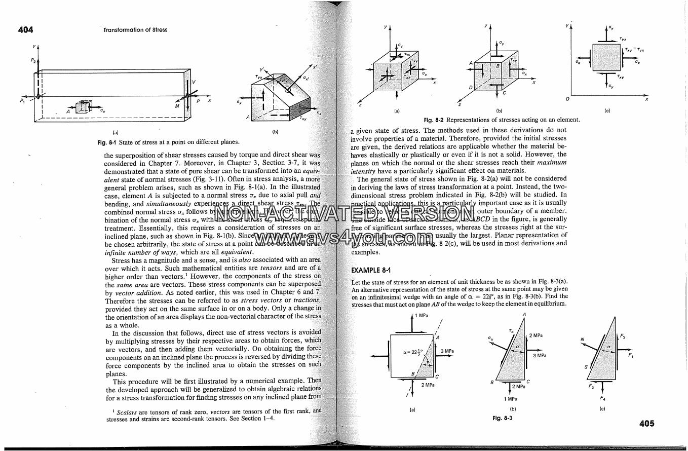
4O4
A
Transformation of Stress
o x
o x
Fig. 84 State of stress at a point on different planes.
the superposition of shear stresses caused by torque and direct shearconsidered in Chapter 7. Moreover, in Chapter 3, Section 3-7, itdemonstrated that a state of pure shear can be transformed into analent state of normal stresses (Fig. 3-11). Often in stress analysis, ageneral problem arises, such as shown in Fig. 8-1(a). In the illu..case, element A is subjected to a normal stress rrx due to axial pullbending, and simultaneously experiences a direct shear stresscombined normal stress rrx follows by superposition. However,bination of the normal stress rr� with the shear stress x� requires streatment. Essentially, this requires a consideration of stresses oninclined plane, such as shown in Fig. 8-1(b). Since an inclined planebe chosen arbitrarily, the state of stress at a point can be describedinfinite number of ways, which are all equivalent.
Stress has a magnitude and a sense, and is also associated withover which it acts. Such mathematical entities are tensors and arehigher order than vectors. � However, the components of the stressthe same area are vectors. These stress components can be superposby vector addition. As noted earlier, this was used in Chapter 6Therefore the stresses can be referred to as stress vectors orprovided they act on the same surface in or on a body. Only athe orientation of an area displays the non-vectorial character of theas a whole.
In the discussion that follows, direct use of stress vectors isby multiplying stresses by their respective areas to obtain forces,are vectors, and then adding them vectorially. On obtaining thecomponents on an inclined plane the process is reversed by dividingforce components by the inclined area to obtain the stresses onplanes.
This procedure will be first illustrated by a numerical example.the developed approach will be generalized to obtain algebraicfor a stress transformation for finding stresses on any inclined
� Scalars are tensors of rank zero, vectors are tensors of the first rankstresses and strains are second-rank tensors. See Section 1-4.
o x
�z z
A
D
Oy
c
o x
(a)
Fig. 8-2 Representations of stresses acting on an element.
given state of stress. The methods used in these derivations do notproperties of a material. Therefore, provided the initial stresses
are given, the derived relations are applicable whether the material be-elastically or plastically or even if it is not a solid. However, the
on which the normal or the shear stresses reach their maximumhave a particularly significant effect on materials.
The general state of stress shown in Fig. 8-2(a) will not be consideredin deriving the laws of stress transformation at a point. Instead, the two-
dimensional stress problem indicated in Fig. 8-2(b) will be studied. Inapplications, this is a particularly important case as it is usually
sible to select a critical element at an outer boundary of a member.outside face of such an element, as ABCD in the figure, is generallyof significant surface stresses, whereas the stresses right at the sur-acting parallel to it are usually the largest. Planar representation of
as shown in Fig. 8-2(c), will be used in most derivations andxamples.
(c)
�LE 8-t
state of stress for an element of unit thickness be as shown in Fig. 8-3(a).the state of stress at the same point may be given
an infinitesimal wedge with an angle of ot = 22� �, as in Fig. 8-3(b). Find thet must act on plane AB of the wedge to keep the element in equilibrium.
t l MPa // A� 5 o= r� 2 MPa
� c�=22� . _� 3MPa
- /[ 2 MPa/
(a)
I MPa
(b)
Fig. 8-:3
N
s)
I-(c)
F 1
405
NON-ACTIVATEDVERSIONwww.avs4you.com
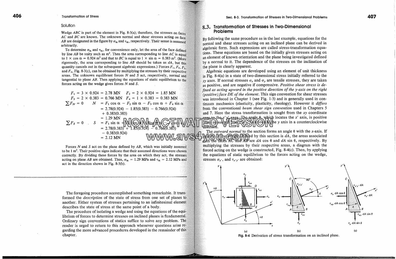
406 Transformation of Stress
Solution
Wedge ABC is part of the element in Fig. 8-3(a); therefore, the stresses onAC and BC are known. The unknown normal and shear stresses acting onAB are designated in the figure by crc� and *c�, respectively. Their sense is aarbitrarily.
To determine crc� and 'rc�, for convenience only, let the area of the face.by line AB be unity such as m 2. Then the area corresponding to line AC isto 1 x cos ot = 0.924 m 2 and that to BC is equal to 1 x sin ot = 0.383 m 2.rigorously, the area corresponding to line AB should be taken as dA,quantity cancels out in the subsequent algebraic expressions.) Forces F�,and F4, Fig. 8-3(c), can be obtained by multiplying the stresses by theirareas. The unknown equilibrant forces N and S act, respectively,tangential to plane AB. Then applying the equations of static eq�forces acting on the wedge gives forces N and S.
F� = 3 x 0.924 =F3 = 2 x 0.383 =
�F�v = 0 N =
�Fs = 0 S
2.78 MN F2 = 2 x 0.924 = 1.85 MN0.766MN F4 = 1 x 0.383 = 0.383F� cos ot- F2 sin ot- F3 cos ot + F4
= 2.78(0.924) - 1.85(0.383) - 0.766(0.924)+ 0.383(0.383)
= 1.29 MN
= F� sin o� + F2 cos o� - F3 sin o� - F4= 2.78(0.383) + 1.85(0.924) - 0.766(0.383)
- 0.383(0.924)= 2.12 MN
Forces N and S act on the plane defined by A_B, which was initiallyto be 1 m 2. Their positive signs indicate that their assumed directions werecorrectly. By dividing these forces by the area on which they act, theacting on plane AB are obtained. Thus, crc� = 1.29 MPa and *c� = 2.12act in the direction shown in Fig. 8-3(b).
The foregoing procedure accomplished something remarkable. Itformed the description of the state of stress from one set ofanother. Either system of stresses pertaining to an infinitesimaldescribes the state of stress at the same point of a body.
The procedure of isolating a wedge and using the equations of the eclibrium of forces to determine stresses on inclined planes isOrdinary sign conventions of statics Suffice to solve any problem.reader is urged to return to this approach whenever questions arisegarding the more advanced procedures developed in the remainderchapter.
Sec. 8-3. Transformation of Stresses in Two-Dimensional Problems
3. Transformation of Stresses in Two-DimensionalProblems
follbwing the same procedure as in the last example, equations for theand shear stresses acting on an inclined plane can be derived in
form. Such expressions are called stress-transformation equa-These equations are based on the initially given stresses acting on
element of known orieniation and the plane being investigated defineda normal to it. The dependence of the stresses on the inclination of'plane is clearly apparent.
equations are developed using an element of unit thicknessFig. 8-4(a) in a state of two-dimensional stress initially referred to theaxes. If normal stresses trx and try are tensile stresses, they are takenpositive, and are negative if compresslye. Positive shear stress is de-
�ed as acting upward in the positive direction of the y-axis on the right�ositive)face DE of the element. This sign convention for shear stresses
introduced in Chapter 1 (see Fig. 1-3) and is generally used in con-mechanics (elasticity, plasticity, rheology). However it differs
the conventional beam shear sign convention used in Chapters 57. Here the stress transformation is sought from the xy coordinate
to the x'y' axes. The angle 0, which locates the x' axis, is positivemeasured from the x axis toward the y axis in a counterclockwise
The outward normal to the section forms an angle 0 with the x-axis. Ifan area of the wedge isolated by this section is dA, the areas associated
the faces AC and AB are dA cos 0 and dA sin 0, respectively. Bythe stresses by their respective areas, a diagram with the
on the wedge is constructed, Fig. 8-4(c). Then, by applyingequations of static equilibrium to the forces acting on the wedge,
Stresses trx,, and *x,y, are Obtained:
Oy
x �
+0
(a)
c
A B
o x dA cos 0
rx� dA cos O'
Fig. 8-4 Derivation of stress transformation on an inclined plane.
407
dA
dA
B
� rxy dA sin0ry dA sin 0
(c)
NON-ACTIVATEDVERSIONwww.avs4you.com
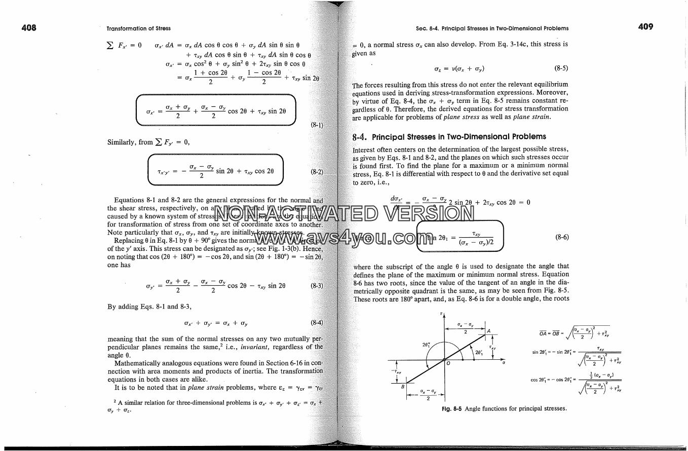
408 Transformation of Stress Sec. 8-4. Principal Stresses in Two. Dimensional Problems 409
cry, dA = cr� dA cos 0 cos 0 + try dA sin 0 sin 0+ �y dA cos 0 sin 0 + �y dA sin 0 cos
cry,, = cr� cos 2 0 + try sin 2 0 + 2,r� sin 0 cos 01 + cos 20 1 - cos 20 "
=cr� 2 +try 2 +X�y
crY' - 2 2 cos 20 + �r�y sin 20
Similarly, from � Fy, = O,
I cr�- trysin20+�ycos201*x'y' = 2
Equations 8-1 and 8-2 are the general expressions for the normalthe shear stress, respectively, on any plane located by the anglecaused by a known system of stresses. These relations are thefor transformation of stress from one set of coordinate axes to
Note particularly that crx, Cry, and ,�y are initially known stresses.Replacing 0 in Eq. 8-1 by 0 + 90 � gives the normal stress in the
of the y' axis. This stress can be designated as Cry,; see Fig. 1-3(b).on noting that cos (20 + 180 �) = - cos 20, and sin (20 + 180 �) = -one has
-- cos 20 - ,�y sin 20CrY'- 2 2
By adding Eqs. 8-1 and 8-3,
meaning that the sum of the normal stresses on any twopendicular planes remains the same, 2 i.e., invariant, regardlessangle 0.
Mathematically analogous equations were found in Section 6-16nection with area moments and products of inertia. Theequations in both cases are alike.
It is to be noted that in plane strain problems, where e� = y�
2 A similar relation for three-dimensional problems is crx, + cry. + crz' =cry + crz-
0, a normal stress Crx can also develop. From Eq. 3-14c, this stress isgiven as
Crz = v(Cr� + %) (8-5)
: forces resulting from this stress do not enter the relevant equilibriumused in deriving .stress-transformation expressions. Moreover,
virtue of Eq. 8-4, the Cr� + Cry term in Eq. 8-5 remains constant re-of 0. Therefore, the derived equations for stress transformation
applicable for problems of plane stress as well as plane strain.
;-4. Principal Stresses in Two-Dimensional Problemsoften centers on the determination of the largest possible stress,
given by Eqs. 8-1 and 8-2, and the planes on which such stresses occurfound first. To find the plane for a maximum or a minimum normal
Eq. 8-1 is differential with respect to 0 and the derivative set equalzero, i.e.,
dCr�---2'= Cr� - Cry 2 sin 20 + 2X�y cos 20 = 0dO 2
tan 20� - (Crx _ %)/2 (8-6)
the subscript of the angle 0 is used to designate the angle thatdefines the plane of the maximum or mini_mum normal stress. Equation
has two roots, since the value of the tangent of an angle in the dia-opposite quadrant is the same, as may be seen from Fig. 8-5.
are 180 � apart, and, as Eq. 8-6 is for a double angle, the roots
Fig. 8-5 Angle functions for principal stresses.
OA = OB =
sin 20'� = - sin 20';
cos 20'� = - cos 20';
NON-ACTIVATEDVERSIONwww.avs4you.com

Transformation of Stress Sec. 8-5. Maximum Shear Stresses in Two-Dimensional Problems
of 0� are 90 � apart. One of these roots locates a plane on which the rnaimum normal stress acts; the other locates the corresponding planethe minimum normal stress. To distinguish between these two rootsprime and double prime notation is used.
Before evaluating these stresses, carefully observe that if theof planes on which no shear stresses act is wanted, Eq. 8-2 must beequal to zero. This yields the same relation as that in Eq. 8-6.an important conclusion is reached: on planes on which maximum,minimum normal stresses occur, there are no shear stresses. Theseare called the principal planes of stress, and the stresses acting onplanes--the maximum and minimum normal stresses--are called thecipal stresses.
The magnitudes of the principal stresses can be obtained bythe values of the sine and cosine functions corresponding to theangle given by Eq. 8-6 into Eq. 8-1. Then the results arethe expression for the maximum normal stress (denoted by cry)minimum normal stress (denoted by cr2) becomes
(crx')max = crl or2 = -- --mi�_ 2 � + *�
where the positive sign in front of the square root must be used tocr� and the negative sign to obtain cr2. The planes on which these stre.,act can be determined by using Eq. 8-6. A particular root of Eq.substituted into Eq. 8-1 will check the result found from Eq. 8-4the same time will locate the plane on which this principal stress act:
Maximum Shear Stresses in Two-DimensionalProblems
If crx, Cry, and ,�y are known for an element, the shear stress on anydefined by an angle 0 is given by Eq. 8-2, and a study similar to themade before for the normal stresses may be made for the shearThus, similarly, to locate the planes on which the maximum or theimum shear stresses act, Eq. 8-2 must be differentiated with res�and the derivative set equal to zero. When this is carried out andresults are simplified,
the subscript 2 is attached to 0 to designate the plane on which theshear stress is a maximum or a minimum. Like Eq. 8-6, Eq. 8-8 has two
.which again may be distinguished by attaching to 02 a prime or aprime notation. The two planes defined by this equation are mu-
perpendicular. Moreover, the value of tan 202 given by Eq. 8-8 isnegative reciprocal of the value of tan 20� in Eq. 8-6. Hence, the roots
:the double angles of Eq. 8-8 are 90 � away from the corresponding roots8-6. This means that the angles that locate the planes of maximum
�minimum shear stress form angles of 45 � with the planes of the principalses. A substitution into Eq. 8-2 of the sine and cosine functions cor-
�onding to the double angle given by Eq. 8-8 and determined in aanalogous to that in Fig. 8-5 gives the maximum and the minimum
of the shear stresses. These, after simplifications, are
,rma x = -+- q- ,r2xym�, 2
(8-9)
Thus, the maximum shear stress differs from the minimum shear stressonly in sign. Moreover, since the two roots given by Eq. 8-8 locate planes
apart, this result also means that the numerical values of the shearstresses on the mutually perpendicular planes are the same. This conceptwas repeatedly used after being established in Section 1-4. In this deri-vation, the difference in sign of the two shear stresses arises from theconvention for locating the planes on which these stresses act. From the
point of view, these signs have no meaning, and for this reason,shear stress regardless of sign will often be called the maximum
shear stress.The definite sense of the shear stress can always be determined by
substitution of the particular root of 02 into Eq. 8-2. A positiveshear stress indicates that it acts in the direction assumed in Fig. 8-4(b),and vice versa. The determination of the maximum shear stress is of
� materials that are weak in shear strength. This willbe discussed further in the Part C of this chapter.
Unlike the principal stresses for which no shear stresses occur on theprincipal planes, the maximum shear stresses act on planes that are usu-ally not free of normal stresses. Substitution of 02 from Eq. 8-8 into Eq.8-1 shows that the normal stresses that act on the planes of the maximum
stresses are
(8-1o)
NON-ACTIVATEDVERSIONwww.avs4you.com
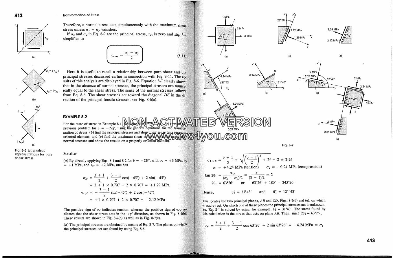
4t2
x
(a)
F
= I r�, I
(b)
02= I rx�, I
Iraqi(c)
Fig. 8-6 Equivalentrepresentations for pureshear stress.
Transformation of Stress
Therefore, a normal stress acts simultaneously with the maximumstress unless crx + cry vanishes.
If crx and cry in Eq. 8-9 are the principal stress, ,�y is zero and E(simplifies to
'rmax -- 2
Here it is useful to recall a relationship between pure shear andiprincipal stresses discussed earlier in connection with Fig. 3-11.sults of this analysis are displayed in Fig. 8-6. Equationthat in the absence of normal stresses, the principal stresses areically equal to the shear stress. The sense of the normal stressesfrom Eq. 8-6. The shear stresses act toward the diagonal DF in thlrection of the principal tensile stresses; see Fig. 8-6(a).
EXAMPLE 8-2
For the state of-stress in Example 8-1, reproduced in Fig. 8-7(a), (a)2OlOprevious problem for 0 = - �.�, using the general equations for the
mation of stress; (b) fmd the principal stresses and show their sense on aoriented element; and (c) find the maximum shear stresses with thenormal stresses and show the results on a properly oriented element.
Solution
- 222, with 'crx = + 3(a) By directly applying Eqs. 8-1 and 8-2 for 0 = ��= + 1 MPa, and x, = +2 MPa, one has
3+1 3-1
crY' - 2 + � c�s(-45�) + 2 sin(-45 �)= 2 + 1 x 0.707 - 2 x 0.707 = +1.29MPa
3-1-- sin(- 45 �) + 2 cos(- 45 �),r�,y, = 2
= +1 x 0.707 + 2 x 0.707 = +2.12MPa
The positive sign of crx, indicates tension; whereas the positive signdicates that the shear stress acts in the +y' direction, as shown in Fig.These results are shown in Fig. 8-7(b) as .well as in Fig. 8-7(c).
(b) The principal stresses are obtained by means of Eq. 8-7. The planesthe principal stresses act are found by using Eq. 8-6.
1 MPa
(a)
x �
VlPa
31�43 '
/
/
2 MPa
Y
22030 '
,,1Pa
0.24 MPa21�4;'
(e)
Y�'2�.��MPaX t
(b)
x t
2 MPa
2.24 MPa
(g)
(c)
4.24 MPa
0.24 MPa
(f)2.24 MPa
(h)
Fig. 8-7
3 + 1 + + 22 = 2 + 2.24crl or2 -- 2 -
cr� = +4.24 MPa (tension) cr2 = -0.24 MPa (compression)
tan 20� - 'r� 2 = 2(cr� - cry)/2 (3 - 1)/2
20� = 63o26 ' or 63o26 ' + 180 � = 243o26 '
31043 ' and 0K = 121o43 '
the two principal planes, AB and CD, Figs. 8-7(d) and (e), on whichand {r2 act. On which one of these planes the principal stresses act is unknown.
Eq. 8-1 is solved by using, for example, 0[ = 31o43 '. The stress found bythis calculation is the stress that acts on plane AB. Then, since 20[ = 63�26 ',
3+1
2
3-1
-- + � cos 63�26 ' + 2 sin 63o26 ' = +4.24 MPa = cr�
2 MPa
(i)
2.24 MPa
2 MPa
4'!3
NON-ACTIVATEDVERSIONwww.avs4you.com
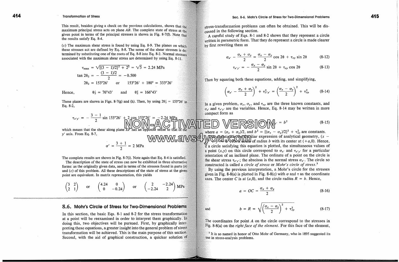
Transformation of Stress Sec. 8-6. Mohr's Circle of Stress for Two-Dimensional Problems
This result, besides giving a check on the previous calculations, showsmaximum principal stress acts on plane AB. The complete state of stressgiven point in terms of the principal stresses is shown in Fig. 8-7(f). Notethe results satisfy Eq. 8-4.
(c) The maximum shear stress is found by using Eq. 8-9. The planes onthese stresses act are defined by Eq. 8-8. The sense of the shear Stressestermined by substituting one of the roots of Eq. 8-8 into Eq. 8-2. Normalassociated with the maximum shear stress are determined by using Eq.
Tma x �- 'V/[(3 -- 1)/2] 2 + 22 = X/� = 2.24 MPa(3 - 1)/2
tan 202 - - 0.5002
202 = 153o26 ' or 153026 ' + 180 � = 333o26 '
Hence, 0� = 76043 ' and 0[ = 166043 '
These planes are shown in Figs. 8-7(g) and (h). Then, by using 20� =Eq. 8-2,
3-1
2-- sin153�26� + 2 cos 153�26 ' = -2.24MPa
which means that the shear along plane EF has an opposite sense to thaty' axis. From Eq. 8-7,
3+1or' - - 2 MPa
2
The complete results are shown in Fig. 8-7(i). Note again that Eq. 8-4The description of the state of stress can now be exhibited in three
forms: as the originally given data, and in terms of the stresses found inand (c) of this problem. All these descriptions of the state of stress at thepoint are equivalent. In matrix representation, this yields
(32 21) or .(4'024 _00.24) or (_22.24-2�24)
g.6. Mohr's Circle of Stress for Two-Dimensional
In this section, the basic Eqs. 8-1 and 8-2 for the stressat a point will be reexamined in order to interpret themdoing this, two objectives will be pursued. First, by graphicallypreting these equations, a greater insight into the general pr�transformation will be achieved. This is the main purpose of thisSecond, with the aid of graphical construction, a quicker
;s-transformation problems can often be obtained. This will be dis-;ed in the following section.
c .areful study of Eqs. 8-1 and 8-2 shows that they represent a circlein parametric form. That they do represent a circle is made clearer
Errst rewriting them as
crx + cry _ crx - try cos 20 + *.�y sin 20 (8-12)2 2
cr.� - try sin 20 + %:5 cos 20 (8-13)Tx'y' = 2
by squaring both these equations, adding, and simplifying,
( (cry, + 'r},y, cr� - try2 = � + �� (8-14)
a given problem, cry, %, and ,�y are the three known constants, andand ,�,y, are the variables. Hence, Eq. 8-14 may be written in more
form as
(fix, - a) 2 + �}'y' = b 2 (8-15)
a = (cr.� + cry)/2, and b 2 = [(fix - cry)/2] 2 + �'2xy are constants.equation is the familiar expression of analytical geometry, (x -
q_ y2 = b 2, for a circle of radius b with its center at (+a,0). Hence,circle satisfying this equation is plotted, the simultaneous values of
Point (x,y) on this circle correspond to crx, and ,�,y, for a particularof an inclined plane. The ordinate of a point on the circle is
shear stress ,�,y,; the abscissa is the normal stress cry,. The circle sois called a circle of stress or Mohr' s circle of stress. 3
using the previous interpretation, a Mohr's circle for the stressesin Fig. 8-8(a) is plotted in Fig. 8-8(c) with cr and, as the coordinateThe center C is at (a,0), and the circle radius R = b. Hence,
a = OC - cr� + cry (8-16)2
4(b =R = �crx- try + (8-17)
coordinates for point A on the circle correspond to the stresses in8-8(a) on the right face of the element. For this face of the element,
It is so named in honor of Otto Mohr of Germany, who in 1895 suggested itsstress-analysis problems.
NON-ACTIVATEDVERSIONwww.avs4you.com
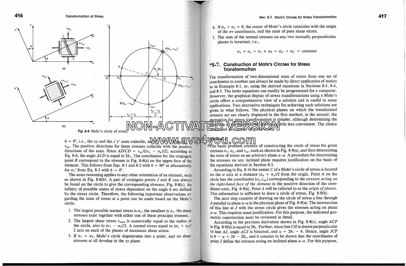
4'6 Transformation of Stress
, +'r m,
A(o,. r.�,)
(a)
B(%, -r,�,)
(b)x
0 x + Oy2
Fig. 8-8 Mohr's circle of stress.(c)
0 = 0 �, i.e., the xy and the x'y' axes coincide, and crx, = cry,, and �;� �y. The positive directions for these stresses coincide with thedirections of the axes. Since AD/CD = ,�y/[(cr� - cry)/2],Eq. 8-6, the angle ACD is equal to 20�. The coordinates for thepoint B correspond to the stresses in Fig. 8-8(a) on the upper faceelement. This follows from Eqs. 8-1 and 8-2 with 0 = 90 � orfor cry' from Eq. 8-3 with 0 = 0 �.
The same reasoning apphes to any other orientation of an elementas shown in Fig. 8-8(b). A pair of conjugate points J and K canbe found on the circle to give the corresponding stresses, Fig. 8-8(c).infinity of possible states of stress dependent on the angle 0 areby the stress circle. Therefore, the following importantgarding the state of stress at a point can be made based on thecircle.
1. The largest possible normal stress is cr�; the smallest is cr2. Nostresses exist together with either one of these principal
2. The largest shear stress �m�,, is numerically equal to thethe circle, also to (cr� - cr2)/2. A' normal stress equal to (cr� +2 acts on each of the planes of maximum shear stress.
3. If cr� = cr2, Mohr's circle degenerates into a point, and nostresses at all develop in the xy plane.
Sec. 8-7. Mohr's Circles for Stress Transformation
Ifcr� + cry = 0, the center of Mohr's circle coincides with the originof the cr, coordinates, and the state of pure shear exists.The sum of the normal stresses on any two mutually perpendicularplanes is invariant, i.e.,
crx + cry = oh + cr2 = o'x, + cry, = constant
1-7. Construction of Mohr's Circles for StressTransformation
transformation of two-dimensional state of stress from one set ofto another can always be made by direct application of statics
in Example 8-1, or, using the derived equations in Sections 8-3, 8-4,1 8-5. The latter equations can readily be programmed for a computer.
the graphical display of stress transformations using a Mohr'soffers a comprehensive view of a solution and is useful in some
Two alternative techniques for achieving such solutions arein what follows. The physical planes on which the transformed
:sses act are clearly displayed in the Errst method; in the second, thestress transformation is simpler, although determining the
of the transformed stress is a little less convenient. The choice'method is a matter of preference.
1
basic problem consists of constructing the circle of stress for givencry, cry, and ,�, such as shown in Fig. 8-9(a), and then determining
state of stress on an arbitrary plane a-a. A procedure for determiningstresses on any inclined plane requires justification on the basis ofequations derived in gection 8-3.
According to Eq. 8-16 the center C ofa Mohr's circle of stress is locatedthe cr axis at a distance (cr� + cry)/2 from the origin. Point A on the
has the coordinates (cr�,,�y) corresponding to the stresses acting onright-hand face of the element in the positive direction of the coor-
axes, Fig. 8-9(a). Point A will be referred to as the origin of planes.information is sufficient to draw a circle of stress, Fig. 8-9(b).
The next step consists of drawing on the circle of stress a line throughplane a-a in the physical plane of Fig. 8-9(a). The intersection
this line at J with the stress circle gives the stresses acting on planeThis requires some justification. For this purpose, the indicated geo-
construction must be reviewed in detail.According to the previous derivation shown in Fig. 8-8(c), angle ACF
8-9(b) is equal to 20�. Further, since line CH is drawn perpendicularline A J, angle ACJ is bisected, and a = 20� - 0. Hence, angle JCF
is 0 - a = 20 - 20�, and it remains to be shown that the coordinates ofJoint J define the stresses acting on inclined plane a-a. For this purpose,
NON-ACTIVATEDVERSIONwww.avs4you.com

4�8 Transformation of Stress Sec. 8.7. Mohr's Circles for Stress Transformation
0.y
(a)
0.x
Originof planes
H
o* x q- 0.y
Radius CA =
(c) (d) (b)
Fig. 8-9 Construction of Mohr's circle for determining stresses on an arbitrary plane.
one notes from Fig. 8-9(b) that if R is the radius of a circle, R cos 20(crx - cry)/2 and R sin 20� � ,�y. Then, forming expressions for the
and shear stresses at J based on the construction of the circle in Fi9(b) and making use of trigonometric identities for double angles, one
crj -- crx + cry + R cos (20 - 202)2
cr� + cry + R (cos 20 cos 202 + sin 20 sin 2002
cr� + cry + cr� - cry cos 20 + %:y sin 202 2
and
*s = R sin(20 - 20�) = R sin 20 cos 20� - R cos 20 sin 20�
= + cr� - cry sin 20 - �y cos 202(8�
Except for the sign of ,j, the last eXPressions are identical to E�1 and 8-2, and, therefore, define the stresses acting on the elementin the upper right quadrant of Fig. 8-9(b). The hatched side of thisis parallel to line AJ on the stress circle, which is parallel to line
8-9(a). However, since the sign of ,j is opposite to that in the basicEq. 8-2, a special rule for the direction of shear stress
to.be introduced.For this purpose, consider the in/tial data for the element shown in Fig.
where all stresses are shown with positive sense. By isolating the:ar stresses acting on the vertical faces, Fig. 8-9(c), it can be seen that
�ese stresses alone cause a countercloclavise couple. By consideringemanating from the origin of planes A, for the first case, Fig. 8-9(c),
circle is intersected at E, whereas for the second case, Fig. 8-9(d), itintersected at G. This can be generalized into a rule: if the point of
;ction of a line emanating from the origin of planes A intersects theircle above the cr axis, the shear stresses on the opposite sides of an
cause a clockwise couple. Conversely, if the point of intersectionbelow the cr axis, the shear stresses on the opposite sides cause a
terclockwise couple. According to this rule, the shear stresses at JFig. 8-9(b) act with a clockwise sense.
This general procedure is illustrated for two particularly importantFor the data given in Fig. 8-10(a), the principal stresses are found
in Fig. 8-10(b), and the maximum shear stresses are found in Fig. 8-10(c).0.y
(a)
Coordinates for A
O' x + O'yOC =2
B
'rxy
0' 2
[ 'rmin { = '/'max
'Fmi n
(b) (c)Fig. 840 Determining principal normal and maximal shear stresses.
2
l'ma x
ax +o r2
� Tmax
NON-ACTIVATEDVERSIONwww.avs4you.com

42O Transformation of Stress
For the first case, it is known that the extreme values on the abs,cq and or2, give the principal stresses. Connecting these pointsorigin of planes A locates the planes on which these stresses act.0� can be determined by trigonometry. Either one of the two solusufficient to obtain the complete solution shown on the elementright.
The magnitudes of the maximum absolute shear stresses arebe given by the radius of the Mohr's circle. As shown in Fig.these stresses are located above and below C. Connecting thesewith the origin of planes A determines the planes on which theseact. The corresponding elements are shown in the upper twothe elements, where the associated mean normal stresses are alsocated. Either one of these solutions with the aid of equilibriumis sufficient for the complete solution shown on the bottomthe figure.
Method 2
The state of stress in the xy coordinate system is shown in Fig.The origin for these coordinates is arbitrarily chosen at the centerinfinitesimal element. The objective is to transform the given stress�those in the rotated set ofx'y' axes as shown in Figs. 8-11(a) andusing Mohr's circle.
As before, the center C of the Mohr's circle is located at (crx +Again the right hand face of the element def'mes crx and ,� useda point on the circle. HOWever,
if ,� > 0, it is plotted downwards at cry, andif ,� < 0, it is plotted upwards at
This in effect amounts to directing the positive � axis downward,shown in Fig. 8-1 l(c). The coordinates of cr� and ** locate thepoint Ac on the circle. This point corresponds to point A in theconstruction; see Fig. 8-8. However, because of the oppositeof the positive � axes, whereas points A and Ac are related, theythe same. Point B�, conjugate to point A�, can be located on theas shown in Fig. 8-11(c). The double angle 20, follows from
Next the diameter A�B� is rotated through an angle 20 in the same serothat the x' axis is rotated through the angle 0 with respect to the xThen the new point A� determines the stresses cry, and ,x,y, onhand face of the element in Fig. 8-11(b). Note that for the casethe shear stress ,r�,y, is negative, since at �r�, it is above the cr axis.considerations apply to the conjugate.point B� defining the stressesthe plane normal to the y' axis.
The expressions for cry, and ,�,y, can be formulated from thetion of the Mohr's circle shown in Fig. 8-11(c) using Eqs. 8-16After simplfications, these relations, except for the sign ofto the basic stress transformation relations, Eqs. 8-1 and 8-2.
+o
o x
Sec. 8-7. Mohr's Circles for Stress Transformation
(c)
Oy,
8-19.
(b)
X t Train
Tmax
(d)
of the Mohr'� circle is justified. For proof modify Eqs. 8-18
for determining the principal normal stress is shown in Fig.After drawing a Mohr's circle the principal stresses cq and or2 areThe required rotation 0� of the axes in the direction of theseis obtained by calculating the double angle 20� from the diagram.
the principal shear stresses are given by the coordinates of theon a circle at their extreme values on the, axis. The required
02 of these axes is obtained by calculating the double angle 202the diagram.
1 is used in the two examples that follow.
8-3
the state of stress shown in Fig. 8-12(a), transform it (a) into the principaland (b) into the maximum shear stresses and the associated normalShow the results for both cases on properly oriented elements. Use
1.
42'!
Fig. 84t Alternativeconstruction of Mohr's circleof stress. Stresses onarbitrary and principalnormal and shear planes areshown in (c) and (d),respectively.
NON-ACTIVATEDVERSIONwww.avs4you.com
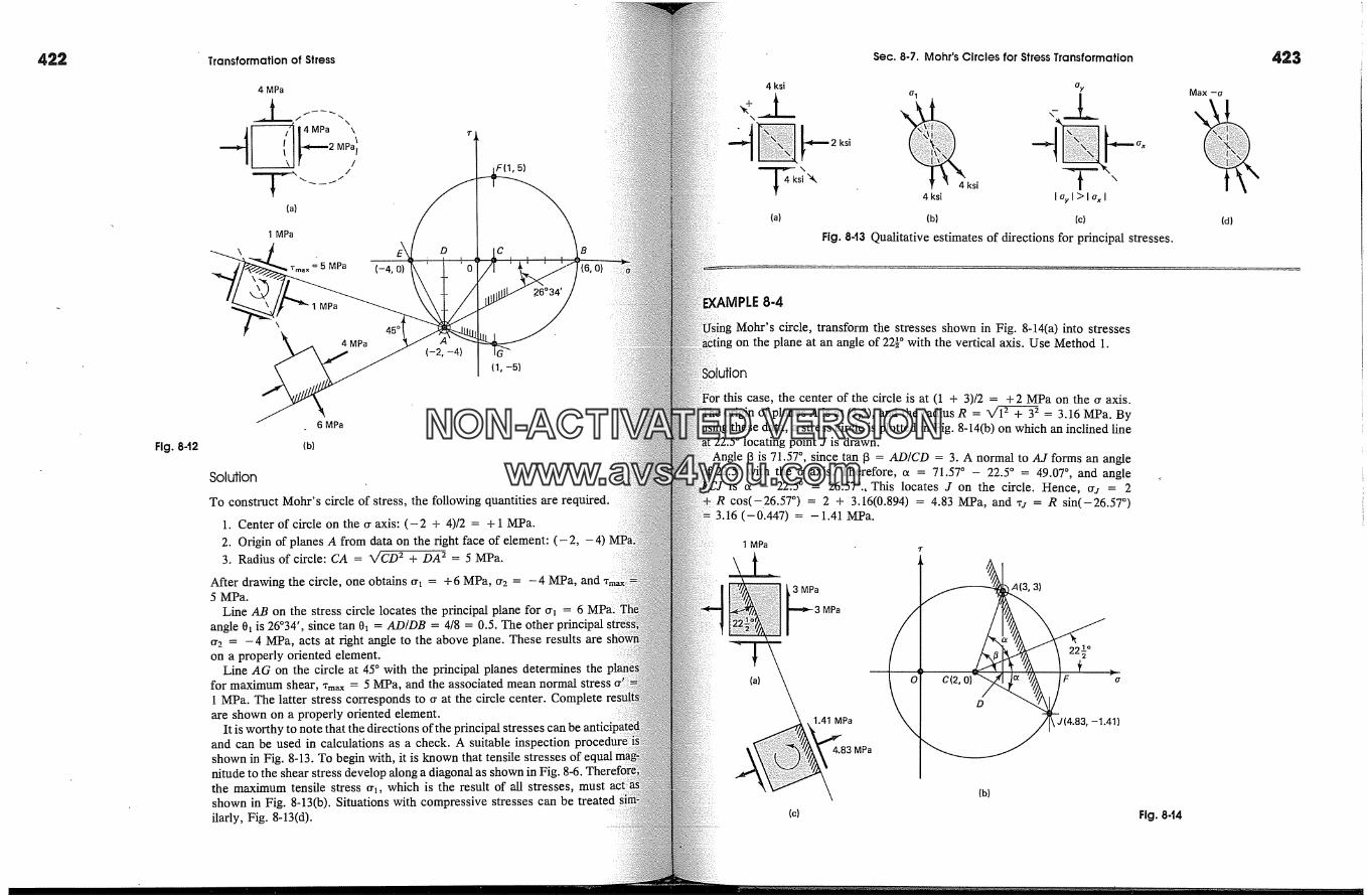
Fig. 8-t2
Transformation of Stress
4 MPa
MPa�i/
/
1 MPa
'rm� x = 5 MPaE� D C
F(1, 5)
MPa
4 MPa
45 �
(-2, -4)(1, -5)
6 MPa
(b)
Solution
To construct Mohr's circle of stress, the following quantities are required.
1. Center of circle on the cr axis: (-2 + 4)/2 = + 1 MPa.2. Origin of planes A from data on the right face of element: (-2, -4)3. Radius of circle: CA = X/CD 2 + DA 2 = 5 mPa.
After drawing the circle, one obtains cr� = +6 MPa, or2 = -4 MPa,5 MPa.
Line AB on the stress circle locates the principal plane for cr� = 6angle 0� is 26�34 ', since tan 01 = AD/DB = 4/8 = 0.5. The other principalor2 = -4 MPa, acts at right angle to the above plane. These results areon a properly oriented element.
Line AG on the circle at 45 � with the principal planes determines thefor maximum shear, Xm� = 5 MPa, and the associated mean normal stress1 MPa. The latter stress corresponds to cr at the circle center. Completeare shown on a properly oriented element.
It is worthy to note that th e directions of the principal stresses can beand can be used in calculations as a check. A suitable inspectionshown in Fig. 8-13. To begin with, it is known that tensile stresses of ecnitude to the shear stress develop along a diagonal as shown in Fig.the maximum tensile stress cry, which is the result of all stresses, mustshown in Fig. 8-13(b). Situations with compressive stresses can beilarly, Fig. 8-13(d).
Sec. 8-7. Mohr's Circles for Stress Transformation
4 ksi
-- �2 ksisi X,
(a)
01
x,ksi
4 ksi 1% I > Iax I
(b) (c)
Fig. 843 Qualitative estimates of directions for principal stresses.
Max -o
\
�LE 8-4
Mohr's circle, transform the stresses shown in Fig. 8-14(a) into stresseson the plane at an angle of 22� � with the vertical axis. Use Method 1.
,lufion
this case, the center of the circle is at (1 + 3)/2 = + 2 MPa on the cr axis.of planes A is at (3,3), and the radius R = � + 32 = 3.16 MPa. By
these data, a stress circle is plotted in Fig. 8-14(b) on which an inclined linet 22.5 � locating point J is drawn.
�3 is 71.57 �, since tan 13 = AD/CD = 3. A normal to AJ forms an angle.'22.5 � with the cr axis. Therefore, ot = 71.57 � - 22.5 � = 49.07 �, and angle
is ot- 22.5 � = 26.57�., This locates J on the circle. Hence, crj = 2R cos(-26.57 �) = 2 + 3.16(0.894) = 4.83 MPa, and xj = R sin(-26.57 �)3.16 (-0.447) = -1.41 MPa.
1 MPa
(a)
3 MPa; �3 MPa
I
1.41 MPa
4.83 MPa t\J(4.83,-1.41)(b)
(c) Fig. 8-t4
423
(d)
NON-ACTIVATEDVERSIONwww.avs4you.com

4[24[ Transformation of Stress Sec, 8-8. Principal Stresses for a General State of Stress 425
Fig. 8d5 Tetrahedron forderiving a principal stress onan oblique plane.
These results are shown on a properly oriented element in Fig. 8-14(c).?j is negative, the shear stresses are shown acting counterclockwise.
Again it should be remarked that the equations for stressidentical in form to the equations for determining the principal axes andof inertia of areas (Section 6-12). Therefore, Mohr's circle can be confinding these equations. 4
**$8-8. Principal Stresses for a General State ofTraditionally, in an introductory text on solid mechanics,largely confined to stresses in two dimensions. Since, however, theical elements studied are always three-dimensional, for cornis desirable to consider the consequences of three-dimensionalitytransformations. The concepts developed in this section have anon the discussion that follows in this chapter, as well as on someconsidered in the next chapter.
Consider a general state of stress and define an infinitesimalhedron 6 as shown in Fig. 8-15(a). Instead of considering an inclinedin the xy coordinate system, as before for a wedge, the unknownare sought on an arbitrary oblique plane ABC in the threexyz coordinate system. A set of known stresses on the other threeof the mutually perpendicular planes of the tetrahedron is given.stresses are the same as shown earlier in Fig. 1-3(a).
A unit normal n to the oblique plane defines its orientation. This4 See J. L. Meriam, and L. G. Kraige, Statics, 2nd ed. (New York:
1986).5 This section is more advanced and can be omitted.a A tetrahedron was first introduced in the study of stress
the gre.at French mathematician A. L. Cauchy in the 1820s.
rl
rxy
l
'ry z
{a)
lb}
is identified by its direction cosines l, m, and n, where cos a =� = m, and cos �/= n. The meaning of these quantities is illustrated
Fig. 8-14(b). From the same figure, it can be noted that since l 2 q- n 2and d 2 + m 2 = 1,
I2 + m2 + n2 = 1) (8-20)
if the inf'mitesimal area ABC is defined as dA�c =- dA, thenthree areas of the tetrahedron along the coordinate axes, identified
subscripts, are dABoc = dA l, dAAoc = dA m, and dAAoB =7
luilibrium equations for the tetrahedron can now be written bythe stresses given in Fig. 8-15(a) by the respective areas es-
For simplicity, it will be assumed that only a normal stressa principal stress, is acting on face ABC. The components;. of the
normal force (�rndA) are obtained by resolving it along theaxes using the direction cosines, Fig. 8-15(b). On this basis,
� Fx = 0 ( �r adA ) l - �r x dA l - , �y dA m - � �z dA n = 0�Fy = 0 (�r, dA)m - �ry dam - ,�zdAn - ,�dAl = 0 (8-21)�F� = 0 (�rndA)n - �r�dAn - ,�dAl - ,y�dAm = 0
changing signs, and regrouping terms,
(�r� - �r,)l + ,�ym + ,�n = 0� �I + (�ry - crn)m + ,y�n = 0,�I +',�m + (�r� - �r,)n = 0
(8-22)
virtue of Eq. 8-20, all three direction cosines cannot be zero. However,: system of linear homogeneous equations has a nontrivial solution if
only if the determinant of the coefficients of l, m, and n vanishes.
'rxy �ry -- �r n 'ryz'rxz 'ryz Crz -- Crn
= o (8-23)
!These areas are the projection of dA on the respective coordinate planes. Toconsider the two-dimensional wedge shown in Fig. 8-A and compare the
two different paths. Let the area associated with side AC be AAC,the corrresponding wedge height be AB. Then the wedge volume is AAcAB/
the other hand, if the area for the side CB is Ac�, and the wedge height is0 = ABI, the volume is Ac�ABI/2. By equating the volumes and simpli-
AAC = Ac�l. By carrying out this procedure in three dimensions, the re-given above can be justified.
A
Fig. 8-A
0
B x
NON-ACTIVATEDVERSIONwww.avs4you.com
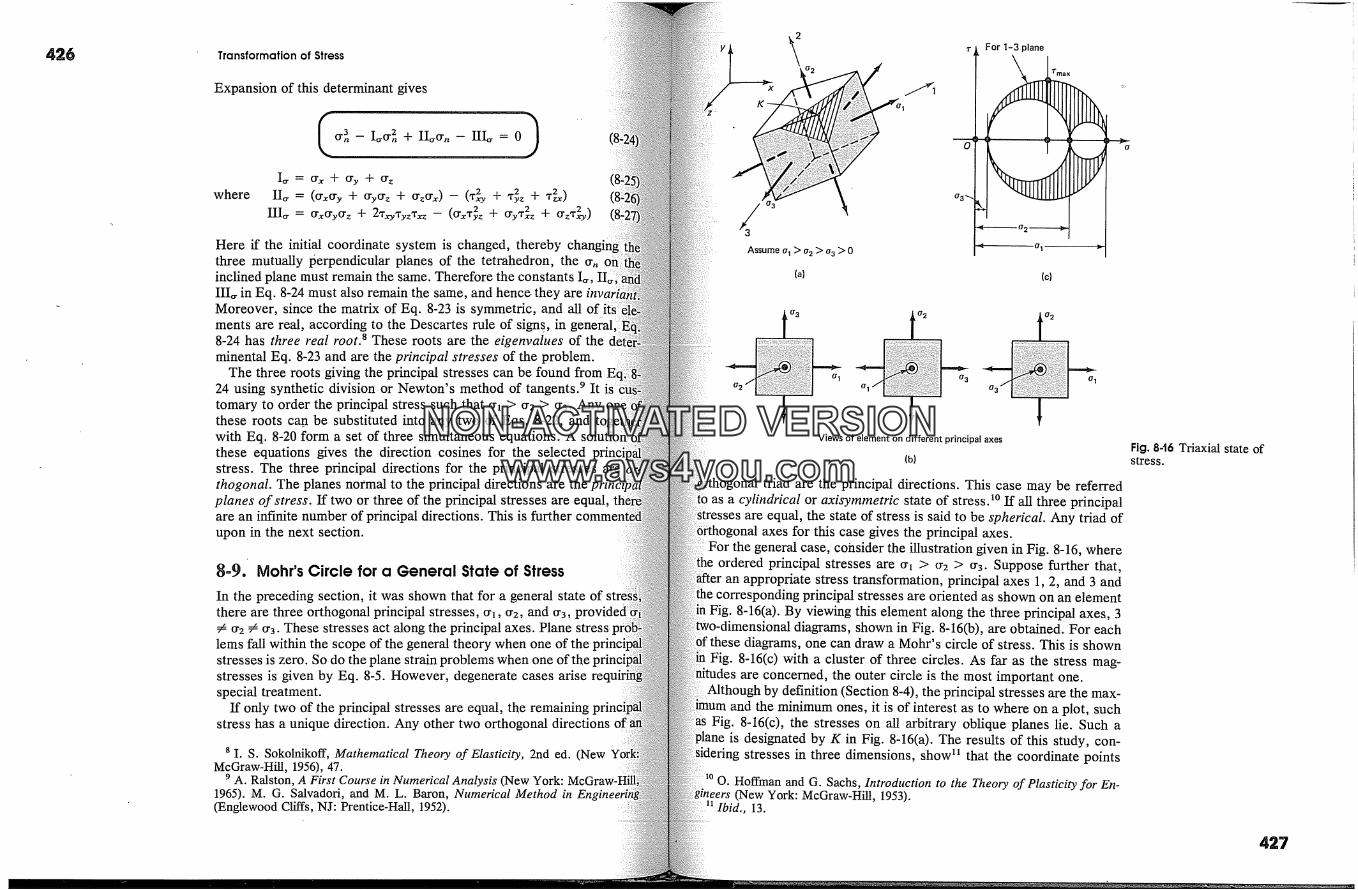
Transformation of Stress
Expansion of this determinant gives
� I.cr2. + II�rcr. HI. 0)where
Here ff the initial coordinate system is changed, therebythree mutually perpendicular planes of the tetrahedron, the crninclined plane must remain the same. Therefore the constantsIII� in Eq. 8-24 must also remain the same, and hence they areMoreover, since the matrix of Eq. 8-23 is symmetric, and all ofments are real, according to the Descartes rule of signs., in general8-24 has three real root. 8 These roots are the eigenvalues of theminental Eq. 8-23 and are the principal stresses of the problem.
The three roots giving the principal stresses can be found from24 using synthetic division or Newton's method of tangents. 9 Ittomary to order the principal stress such that cr� > cr2 > cr3. Anythese roots cart_ be substituted into any two of Eqs. 8-22, andwith Eq. 8-20 form a set of three simultaneous equations. Athese equations gives the direction cosines for the selectedstress. The three principal directions for the principal stresses arethogonal. The planes normal to the principal directions are the
planes of stress. If two or three of the principal stresses are equal,are an infinite number of principal directions. This is furtherupon in the next section.
�-9.' Mohr's Circle for a General State of StressIn the preceding section, it was shown that for a general state ofthere are three orthogonal principal stresses, cry, cr2, and cr3,� cr2 � cr3. These stresses act along the principal axes. Plane stresslems fall within the scope of the general theory when one of thestresses is zero. So do the plane strain problems when one of thestresses is given by Eq. 8-5. However, degenerate cases arise recspecial treatment.
If only two of the principal stresses are equal, the remainingstress has a unique direction. Any other two orthogonal directions
8 I. S. Sokolnikoff, Mathematical Theory of Elasticity, 2nd ed. (NewMcGraw-Hill, 1956), 47.
9 A. Ralston, A First Course in Numerical Analysis (New York:1965). M. G. Salvadori, and M. L. Baron, Numerical Method in En(Englewood Cliffs, NJ: Prentice-Hall, 1952).
3
Assume
r For 1-3 plane
'Fma x
0 3
(c)
o* 3 o 2
o 3
Views of element on different principal axes
(b)
17 2
O 1
triad are the principal directions. This case may be referredas a cylindrical or axisymmetric state of stress. �o If all three principal
are equal, the state of stress is said to be spherical. Any triad ofaxes for this case gives the principal axes.
For the general case, cobsider the illustration given in Fig. 8-16, whereordered principal stresses are cr� > cr2 > cr3. Suppose further that,
an appropriate stress transformation, principal axes 1, 2, and 3 and;ponding principal stresses are oriented as shown on an element
8-16(a). By viewing this element along the three principal axes, 3diagrams, shown in Fig. 8-16(b), are obtained. For each
these diagrams, one can draw a Mohr's circle of stress. This is shownFig. 8-16(c) with a cluster of three circles. As far as the stress mag-
are concerned, the outer circle is the most important one.by definition (Section 8-4), the principal stresses are the max-
and the minimum ones, it is of interest as to where on a plot, suchFig. 8-16(c), the stresses on all arbitrary oblique planes lie. Such a
is designated by K in Fig. 8-16(a). The results of this study, con-stresses in three dimensions, show � that the coordinate points
O. Hoffman and G. Sachs, Introduction to the Theory of Plasticity for En-(New York: McGraw-Hill, 1953).
13.
Fig. 846 Triaxial state ofstress.
427
NON-ACTIVATEDVERSIONwww.avs4you.com

428 Transformation of Stress
for all possible planes lie either on one of the three circles or in anbetween them, shown hatched in Fig. 8-16(c). A series of circles iswithin this area having their centers on the cr axis by holding anythe direction cosines constant. Therefore, it is conven/ent to referthree circles drawn as the principal stress circles. The largest ofthe major principal stress circle.
Inasmuch as all stresses in their various transformations mayrole in causing either yield or breakdown of a material, it is often'tive to plot all three principal circles of stress, as shown in Fig. 8-16Two examples of this kind follow. In making such plots, the decases, when two or all principal stresses are equal, must be keptFor such cases, a Mohr's circle becomes a point.
EXAMPLE 8-5
For the data of Example 8-3, repeated in Fig. 8-17(a), constrUct threeprincipal circles of stress by viewing an element from three principalAssume that this is a plane stress problem.
Solution
The principal stresses for this problem in two dimensions have alreadytermined in Example 8-3. The results are repeated in Fig. 8-17(b). Since thiSiplane stress problem, the stress in the direction normal to the paper iscomplete state of stress showing all principal stresses is in Fig. 8-17(c).two-dimensional diagrams of:the element viewed from different directionsFigs. 8-17(d)-(f). The cluster of three Mohr's principal circles is shown in8-17(g).
If the given stresses were for aplane strain problem, the middle principalinstead of being zero, per Eq. 8-5, would be or2 = v(6 - 4) = + 2v, wherePoisson's ratio.
EXAMPLE 8-6
For the plane stress shown in Fig. 8-18(a), draw the three Mohr's principaldiagrams and determine the state of stress for maximum shear.
Solution
Two of the principal stresses are given; the third is zero, as this is a planeproblem. The three principal stress circles are shown in Fig. 8-18(b):-Theimum shear stress occurs in the planes shown in Fig. 8-18(c). This stresssociated with point D on the major principal circle, and in physicalis given in Fig. 8-18(d).
This type of problem occurs in pressure-vessel analyses, where it isto recognize that large shear stresses may arise.
�-�L� P�MPa
,F(a)
6 MPa
4 mPa
(b)
MPa C
(c)
6 MPa
MPa
(a)
hear
planes
MPa
(c)
26034 '
5 MPa
5 MPa
E K
(-4B(6,O)
(g)
6 MPa
4 MPa
6 MPa
4 MPa
(d) (e) (f)
Fig. 8-t7
--c
4MPa
MPa
(d) Fig. 8-t8 429
NON-ACTIVATEDVERSIONwww.avs4you.com
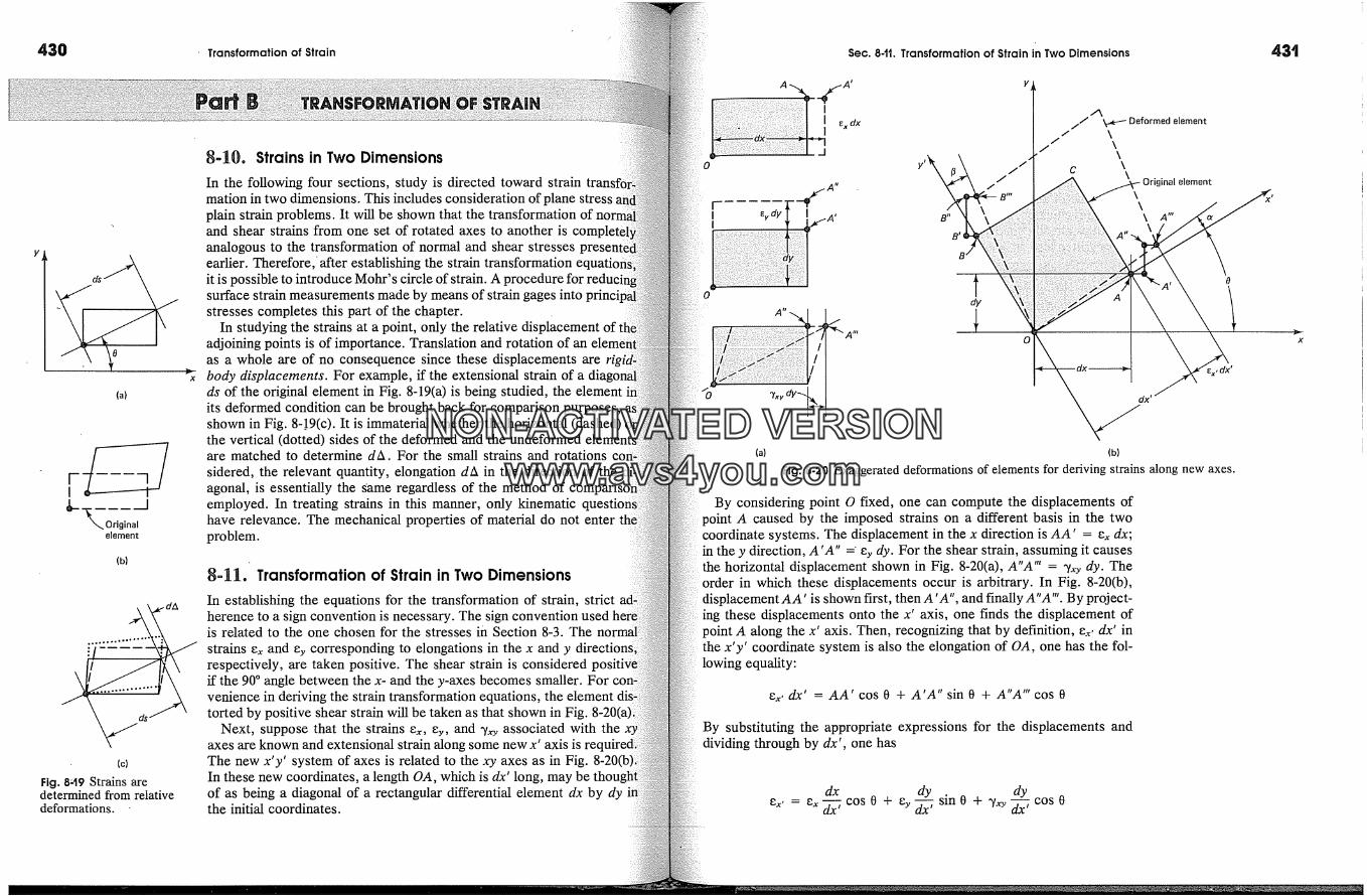
430 � Transformation of Strain Sec. 8-tt. Transformation of Strain in Two Dimensions 431
Y�
(a)
v
�- % Original jelement
(b)
dA
(c)
Fig. 8�t9 Strains aredetermined from relativedeformations.
8=10. Strains in Two Dimensions
In the following four sections, study is directed toward strain trammarion in two dimensions. This includes consideration of plane stress �,plain strain problems. It will be shown that the transformation ofand shear strains from one set of rotated axes to another is completelanalogous to the transformation of normal and shear stresses tearlier. Therefore/after establishing the strain transformationit is possible to introduce Mohr's circle of strain. A procedure forsurface strain measurements made by means of strain gages intostresses completes this part of the chapter.
In studying the strains at a point, only the relative displacement ofadjoining points is of importance. Translation and rotation of an elemas a whole are of no consequence since these displacements arebody displacements. For example, if the extensional strain of ads of the original element in Fig. 8-19(a) is being studied, the elementits deformed condition can be brought back for comparison purposes,shown in Fig. 8-!9(c). It is immaterial whether the horizontal (dashed)the vertical (dotted) sides of the deformed and the undeformedare matched to determine dA. For the small strains and rotationssidered, the relevant quantity, elongation dA in the direction of theagonal, is essentially the Same regardless of the method ofemployed. In treating strains in this manner, only kinematic q�have relevance. The mechanical properties of material do not enterproblem.
8-11. Transformation of Strain in Two Dimensions
In establishing the equations for the transformation of strain, strictherence to a sign convention is necessary. The sign convention usedis related to the one chosen for the stresses in Section 8-3. Thestrains e�, and ey corresponding to elongations in the x and y directionsrespectively, are taken positive. The shear strain is considered ];if the 90 � angle between the x- and the y-axes becomes smaller. Forvenience in deriving the strain transformation equations, the elementtorted by positive shear strain will be taken as that shown in Fig.
Next, suppose that the strains e�,, ey, and %:y associated with theaxes are known and extensional strain along some new x' axis isThe new x'y' system of axes is related to the xy axes as in Fig.In these new coordinates, a length OA, which is dx' long, mayof as being a diagonal of a rectangular differential element dx by dythe initial coordinates.
FI %dy'I
Deformed element
\ inal element
(a) (b)
Fig. 8-20 Exaggerated deformations of elements for deriving strains along new axes.
By considering point O �Lxed, one can compute the displacements ofpoint A caused by the imposed strains on a different basis in the twocoordinate systems. The displacement in the x direction is AA' = e�, dx;in the y direction, A'A" =' ey dy. For the shear strain, assuming it causesthe horizontal displacement shown in Fig. 8-20(a), A"A"' = �?�y dy. The
in which these displacements occur is arbitrary. In Fig. 8-20(b),displacement AA' is shown first, then A 'A", and finally A"A'". By project-ing these displacements onto the x' axis, one finds the displacement ofpoint A along the x' axis. Then, recognizing that by definition, e.�, dx' inthe x'y' coordinate system is also the elongation of OA, one has the fol-lowing equality:
e�,, dx' = AA' cos O + A'A" sin O + A"A'" cos O
By substituting the appropriate expressions for the displacements anddividing through by dx', one has
dx dy sin 0 + �,,,y dye�,, = e�, dx----7 cos 0 + ey dx----7 dx----7 cos 0
x
NON-ACTIVATEDVERSIONwww.avs4you.com
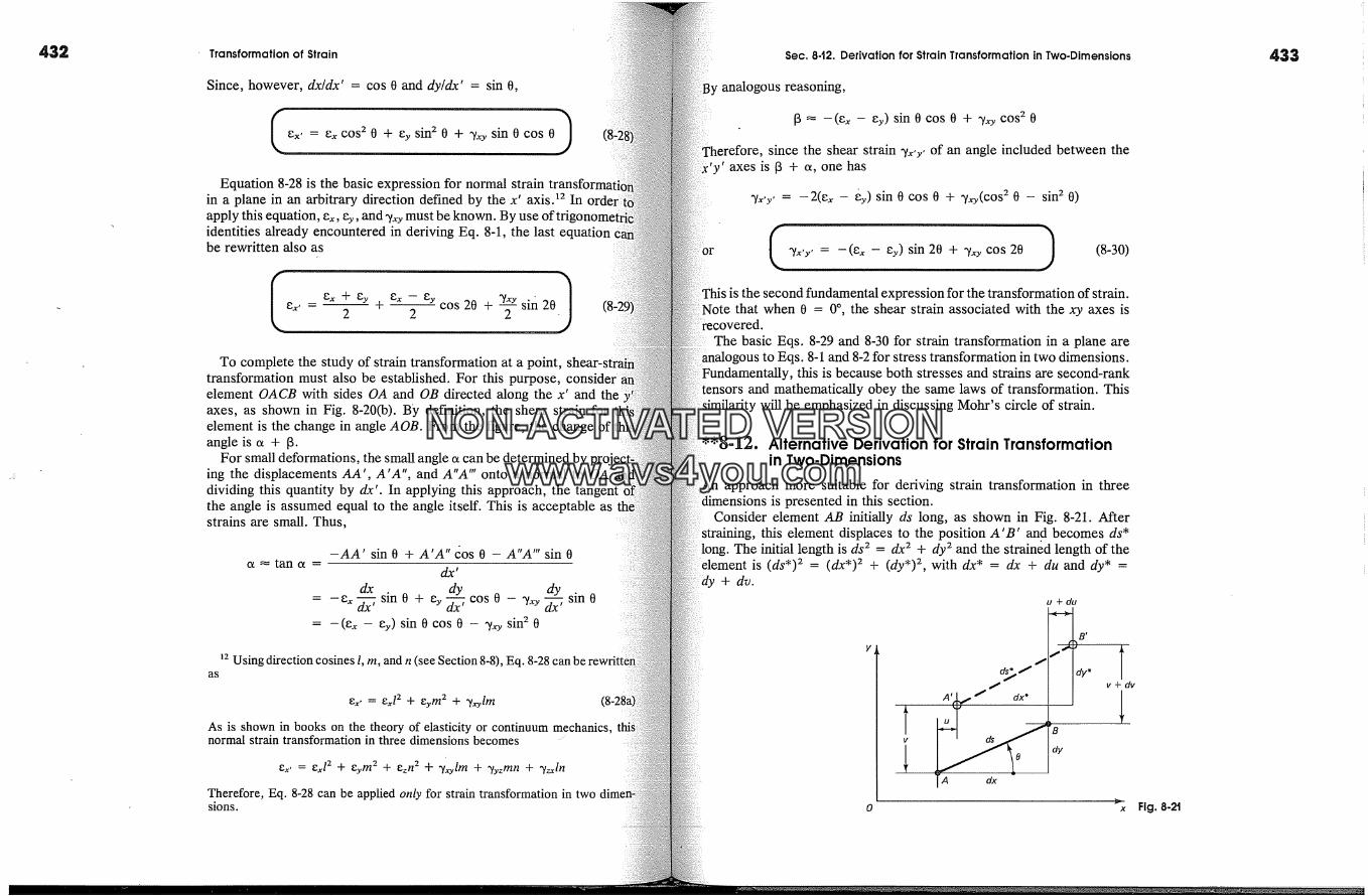
432 Transformation of Strain Sec. 8.t2. Derivation for Strain Transformation in Two-Dimensions 433
Since, however, dxldx' = cos 0 and dyldx' = sin 0,
ex,= excos20 + eysin20 +�xysin0cos0)Equation 8-28 is the basic expression for normal strain transfor
in a plane in an arbitrary direction defined by the x' axis. �2 Inapply this equation, e�,, ey, and yxy must be known. By use oftriidentities already encountered in deriving Eq. 8-1, the last equationbe rewritten also as
cos 20 + sin 20
To complete the study of strain transformation at a point,transformation must also be established. For this purpose, considerelement OACB with sides OA and OB directed along the x' and theaxes, as shown in Fig. 8-20(b). By definition, the shear strain forelement is the change in angle AOB. From the figure, the changeangle is o� + [3.
For small deformations, the small angle o� can be determined bying the displacements AA', A'A", and A"A"' onto a normal to OAdividing this quantity by dx'. In applying this approach, thethe angle is assumed equal to the angle itself. This is acceptable asstrains are small. Thus,
-AA' sin 0 + A'A" cos 0 - A"A"' sin 0tan o� =
dx'
dx dy dy= -�x'Sin� + �y�COS�- �x, Sin�= -(�- �y) sin�cos� - %�ysin �
�2 Using direction cosines l, m, and n (see Section 8-8), Eq. 8-28 can be:as
gx' = gxl 2 + gym 2 + �l. Im
As is shown in books on the theory of elasticity or continuum mechanics,normal strain transformation in three dimensions becomes
8x' = 8xl 2 + 8ym 2 + ezn 2 + �l�lm + ?yzmn + ?z�lnTherefore, Eq. 8-28 can be applied only for strain transformation in twosions.
analogous reasoning,
[3 '�' --(1� x -- �y) sin 0 cos 0 + yxy cos 2 0
since the shear strain ?x'y' of an angle included between the,' axes is [3 + o�, one has
�,y, = -2(e� - �y) sin 0 cos 0 + �y(COS 2 0 - sin 2 0)
( �,y, = -(e�- ey)sin20 + �xyCOS20) (8-30)the second fundamental expression for the transformation of strain.
Note that when 0 = 0 �, the shear strain associated with the xy axes is
The basic Eqs. 8-29 and 8-30 for strain transformation in a plane areto Eqs. 8-1 and 8-2 for stress transformation in two dimensions.
y, this is because both stresses and strains are second-rankand mathematically obey the same laws of transformation. This
will be emphasized in discussing Mohr's circle of strain.
*'8-12. Alternative Derivation for Strain Transformationin Two. Dimensions
An approach more suitable for deriving strain transformation in threeis presented in this section.
Consider element AB initially ds long, as shown in Fig. 8-21. Afterthis element displaces to the position A'B' and becomes ds*
The initial length is ds 2 = dx 2 + dy 2 and the strained length of theis (ds*) 2 = (dx*) 2 + (dy*) 2, with dx* = dx + du and dy* =
+ dv.
o
u +du
ud� B�1A dx
1v + dv
x Fig, 8-2'1
NON-ACTIVATEDVERSIONwww.avs4you.com
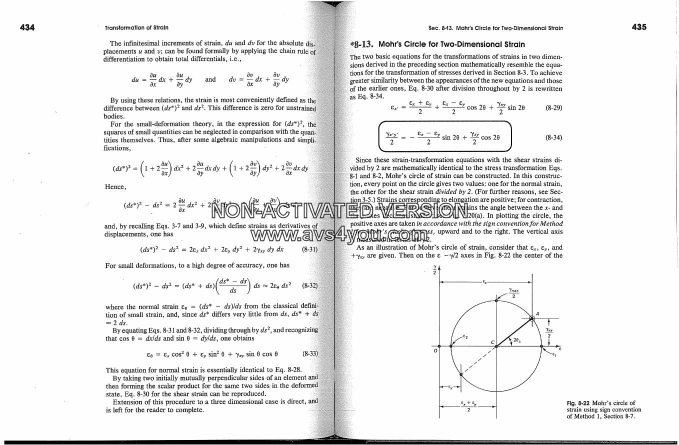
4�34� Transformation of Strain Sec. 8-t3. Mohr's Circle for Two-Dimensional Strain 4�35
The infinitesimal increments of strain, du and dv for the absoluteplacements u and v; can be found formally by applying the chaindifferentiation to obtain total differentials, i.e.,
__ Oudu = OU dx + dyoxand _ Ovdv = OV dx +
Ox Oy
By using these relations, the strain is most conveniently defined asdifference between (ds*) 2 and ds 2. This difference is zero forbodies.
For the small-deformation theory, in the expression for (ds*) 2,squares of small quantities can be neglected in comparison with the,tities themselves. Thus, after some algebraic manipulations andfications,
(ds*) 2 = 1 + OxJ dx2 + 2��dxdy + (l + Oy/ dy2 + 2 0�dxHence,
ox dy2 + 2 + ax dyand, by recalling Eqs. 3-7 and 3�9, which define strains as derivative sdisplacements, one has
(ds*) 2 - ds 2 = 2e�, dx 2 + 2ey dy 2 + 2'yxy dy dx
For small deformations, to a high degree of accuracy, one has
ds)( ds* z ds) ds ds'-(ds*) 2 - ds 2 = (ds* + �, dswhere the normal strain e0 = (ds* - ds)/ds from the classicaltion of small strain, and, since ds* differs very little from ds, ds*
By equating Eqs. 8-31 and 8-32, dividing through by ds 2, and recolthat cos 0 = dx/ds and sin 0 = dy/ds, one obtains
(8,3
�;0 = �;x COS2 0 q- [2y sin 2 0 + 3'-�y sin 0 cos 0
This equation for normal strain is essentially identical to Eq. 8-28.By taking two initially mutually perpendicular sides of an element
then forming the scalar product for the same two sides in thestate, Eq. 8-30 for the shear strain can be reproduced.
Extension of this procedure to a three dimensional case is direct,is left for the reader to complete.
-13. Mohr's Circle for Two-Dimensional Strain
two basic equations for the transformations of strains in two dimen-derived in the preceding section mathematically resemble the equa-
; for the transformation of stresses derived in Section 8-3. To achievebetween the appearances of the new equations and those
the earlier ones, Eq. 8-30 after division throughout by 2 is rewrittenEq. 8-34.
e�,, - 2 � cos 2t3 + sin 213 (8-29)
-/�,,y,_ e�,- eysin20+� cos20I (8-34)2 2
Since these strain-transformation equations with the shear strains di-by 2 are mathematically identical to the stress transformation Eqs.
and 8-2, Mohr's circle of strain can be constructed. In this construc-every point on the circle gives two values: one for the normal strain,
other for the shear strain divided by 2. (For further reasons, see Sec-Strains corresponding to elongation are positive; for contraction,
are negative. For positive shear strains the angle between the x- andthe y-axes becomes smaller; see Fig. 8-20(a). In plotting the circle, the
itive axes are taken in accordance with the sign convention for MethodMohr's circle of stress, upward and to the right. The vertical axis
measured in terms of-//2.As an illustration of Mohr's circle of strain, consider that e�,, �y, and
+-/.�y are given. Then on the e --//2 axes in Fig. 8-22 the center of the
2Fig. 8-22 Mohr's circle ofstrain using sign conventionof Method 1, Section 8-7.
NON-ACTIVATEDVERSIONwww.avs4you.com
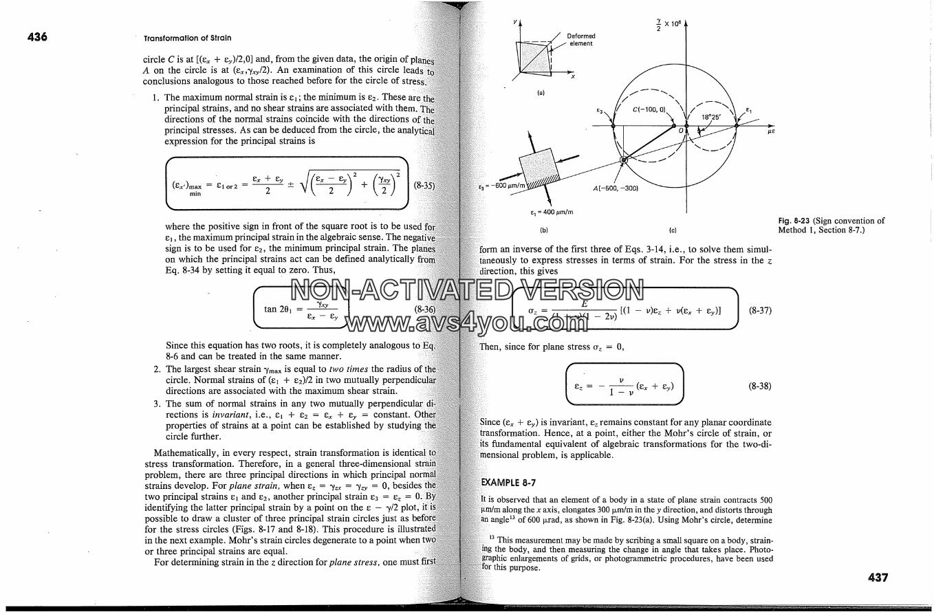
436 Transformation of Strain
circle C is at [(ex + ey)/2,0] and, from the given data, the origin ofA on the circle is at (ex,-y.�/2). An examination of this circleconclusions analogous to those reached before for the circle of
1. The maximum normal strain is e�; the minimum is e2. These areprincipal strains, and no shear strains are associated with them.directions of the normal strains coincide with the directionsprincipal stresses. As can be deduced from the circle, theexpression for the principal strains is
gx' �' E1 or2 -- -- 2 + + --
where the positive sign in front of the square root is to be us{e�, the maximum principal strain in the algebraic sense.sign is to be used for e2, the minimum principal strain. Theon which the principal strains act can be defined analytically:Eq. 8-34 by setting it equal to zero. Thus,
Since this equation has two roots, it is completely8-6 and can be treated in the same manner.
The largest shear strain ymax is equal to two times the radius of tcircle. Normal strains of (e� + e2)/2 in two mutuallydirections are associated with the maximum shear strain.
The sum of normal strains in any two mutually perpendicular directions is invariant, i.e., e� + e2 �- gx -I- gy �--- constant.properties of strains at a point can be established bycircle further.
Mathematically, in every respect, strain transformation isstress transformation. Therefore, in a general three-dimensionalproblem, there are three principal directions in which principalstrains develop. For plane strain, when ez = �x = �zy = 0,two principal strains e� and e2, another principal strain e3 = ez 0:identifying the latter principal strain by a point on the e - �/2possible to draw a cluster of three principal strain circles just asfor the stress circles (Figs. 8-17 and 8-18). This procedure isin the next example. Mohr's strain circles degenerate to a pointor three principal strains are equal.
For determining strain in the z direction for plane stress, one must t
Deformed
(a)
')' X1062
18o25 ,\
C(-lOO, o)
= -600 �m/m A(-500, -300)
400 #m/m
(b) (c)
an inverse of the first three of Eqs. 3-14, i.e., to solve them simul~to express stresses in terms of strain. For the stress in the zthis gives
o-z = (1 + v)(1 - 2v)[(1 - v)e� + v(e� + ey)] (8-37)
since for plane stress cr� = 0,
'= �' (e�+ e�)11 --u(8-38)
(e� + ey) is invariant, e� remains constant for any planar coordinateHence, at a point, either the Mohr's circle of strain, or
fundamental equivalent of algebraic transformations for the two-di-problem, is applicable.
EXAMPLE 8-7
is observed that an element of a body in a state of plane strain contracts 500along the x axis, elongates 300 p.m/m in the y direction, and distorts through
angle �3 of 600 p. rad, as shown in Fig. 8-23(a). Using Mohr's circle, determine
This measurement may be made by scribing a small square on a body, strain-the body, and then measuring the change in angle that takes place. Photo-
enlargements of grids, or photogrammetric procedures, have been usedthis purpose.
Fig. 8-23 (Sign convention ofMethod 1, Section 8-7.)
437
NON-ACTIVATEDVERSIONwww.avs4you.com
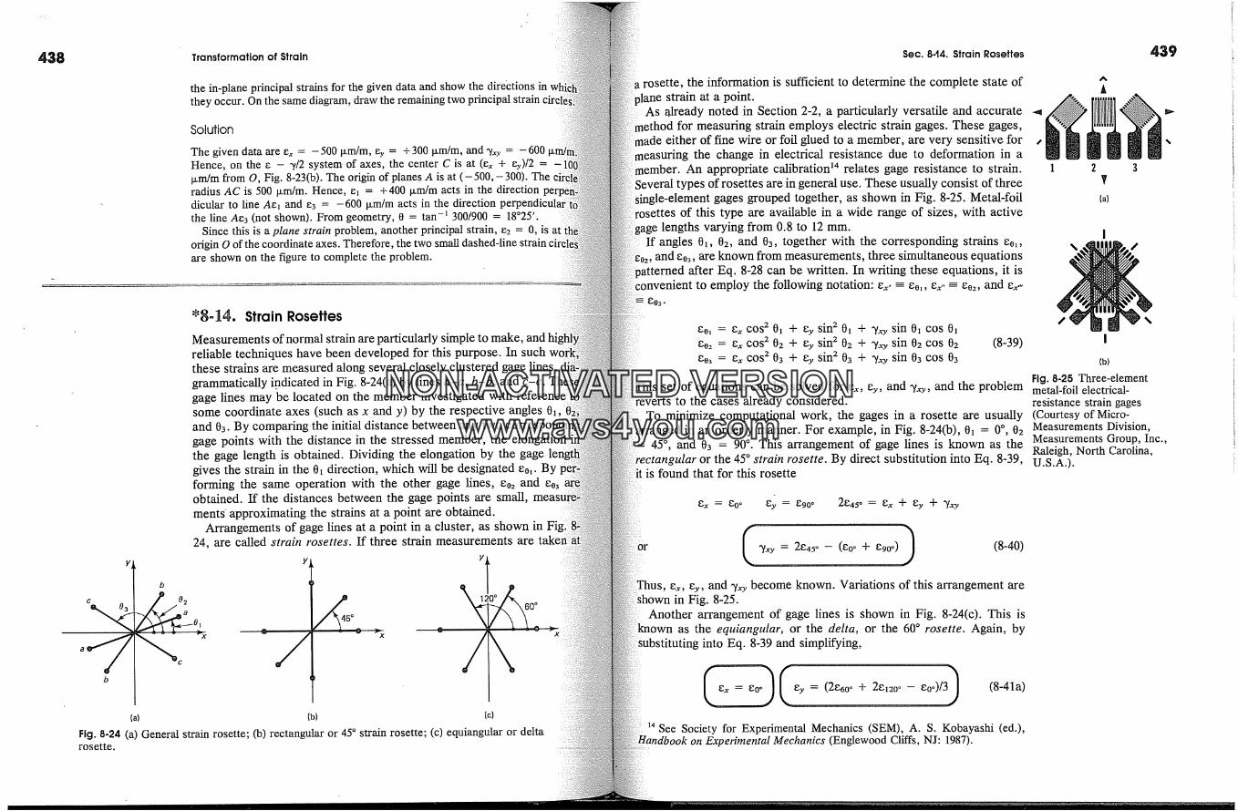
438 Transformation of Strain
the in-plane principal strains for the given data and show the directions inthey occur. On the same diagram, draw the remaining two principal strain
Solution
The given data are e, = -500 I�m/m, e>. = + 300 I�m/m, and �o. = -600Hence, on the e - �//2 system of axes, the center C is at (e� + �)/2 =I�m/m from O, Fig. 8-23(b). The origin of planes A is at (-500,- 300).radius AC is 500 I�m/m. Hence, e� = +400 I�m/m acts in the directiondicular to line Ae� and e3 = -600 i�m/m acts in the directionthe line Ae3 (not shown). From geometry, 0 = tan -� 300/900 = 18o25 '.
Since this is a plane strain problem, another principal strain, e2 = 0, isorigin O of the coordinate axes. Therefore, the two small dashed-lineare shown on the figure to complete the problem.
'8-14. Strain Rosettes
Measurements of normal strain are particularly simple to make,reliable techniques have been developed for this purpose. In suchthese strains are measured along several closely clustered gagegrammatically indicated in Fig. 8-24(a) by lines a-a, b-b, and c-c.gage lines may be located on the member investigated with reference:some coordinate axes (such as x and y) by the respective angles 0�and 03. By comparing the initial distance between any two corresgage points with the distance in the stressed member, thethe gage length is obtained. Dividing the elongation by the gagegives the strain in the 0� direction, which will be designated eo,. Byforming the same operation with the other gage lines, �o2 and eo3obtained. If the distances between the gage points are small,ments approximating the strains at a point are obtained.
Arrangements of gage lines at a point in a cluster, as shown in24, are called strain rosettes. If three strain measurements are
Y bc oil o2b
� 445�,� ,�X
60 �
(a) (b) (c)
Fig. 8-24 (a) General strain rosette; (b) rectangular or 45 � strain rosette; (c) equiangular or deltarosette.
Sec. 8-t4. Strain Rosettes
rosette, the information is sufficient to determine the complete state ofstrain at a point.
As .already noted in Section 2-2, a particularly versatile and accurate,d for measuring strain employs electric strain gages. These gages,either of fine wire or foil glued to a member, are very sensitive for
measuring the change in electrical resistance due to deformation in a)er. An appropriate calibration TM relates gage resistance to strain.
of rosettes are in general use. These usually consist of threegages grouped together, as shown in Fig. 8-25. Metal-foil
rosettes of this type are available in a wide range of sizes, with activelengths varying from 0.8 to 12 mm.
If angles 0�, 02, and 03, together with the corresponding strainsand eo3, are known from measurements, three simultaneous equations
Patterned after Eq. 8-28 can be written. In writing these equations, it isto employ the following notation: ex' = eo,, ex,, = eo2, and
E;O 3 �
E;0, = E;x COS 2 01 "1- E;y sin 2 01 --I- '�xy sin 0� cos 0�E;02 = E;x COS 2 02 "1- E;y sin 2 02 --I- '�xy sin 02 COS 02e03 = ex COS 2 03 + ey sin 2 03 + �'� sin 0� cos 03
(8-39)
set of equations can be solved for e�, ey, and y.�y, and the problemreverts to the cases already considered.
To minimize computational work, the gages in a rosette are usuallyarranged in an orderly manner. For example, in Fig. 8-24(b), 0� = 0% 02
45 �, and 03 = 90 �. This arrangement of gage lines is known as theular or the 45 � strain rosette. By direct substitution into Eq. 8-39,
it is found that for this rosette
gx = E;O� gy = �90 � 2�45 � = �x + �y + 'Yxy
C 'y.ry= 2�45�-- (g0�+ g90�)� (8-40)
Fhus, ex, ey, and -/�y become known. Variations of this arrangement arein Fig. 8-25.
Another arrangement of gage lines is shown in Fig. 8-24(c). This isas the equiangular, or the delta, or the 60 � rosette. Again, by
into Eq. 8-39 and simplifying,
(8-41a)
See Society for Experimental Mechanics (SEM), A. S. Kobayashi (ed.),Experimental Mechanics (Englewood Cliffs, NJ: 1987).
439
1 2 3�
(a)
(b)
Fig. 8-25 Three-elementmetal-foil electrical-resistance strain gages(Courtesy of Micro-Measurements Division,Measurements Group, Inc.,Raleigh, North Carolina,U.S.A.).
NON-ACTIVATEDVERSIONwww.avs4you.com
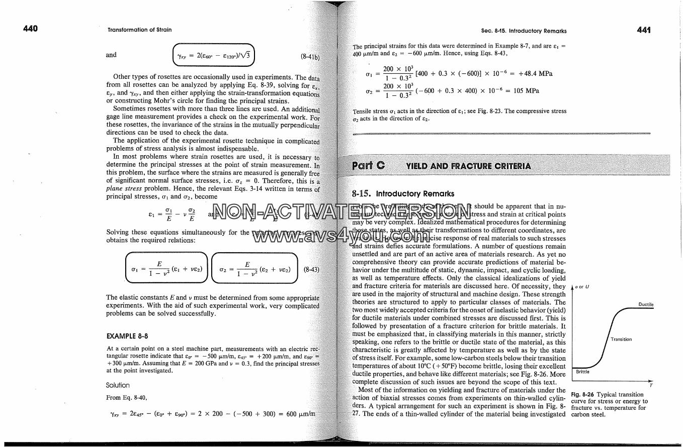
44O Transformation of Strain
and (%,0,= 2(�60�- �120o)/X/�)Other types of rosettes are occasionally used in experiments. The
from all rosettes can be analyzed by applying Eq. 8-39, solvingey, and y�y, and then either applying theor constructing Mohr's circle for finding the principal strains.
Sometimes rosettes with more than three lines are used. Angage line measurement provides a check on the experimental work.these rosettes, the invariance of the strains in the mutuallydirections can be used to check the data.
The application of the experimental rosette technique inproblems of stress analysis is almost indispensable.
In most problems where strain rosettes are used, it is necessdetermine the principal stresses at the point of strain measurement!this problem, the surface where the strains are measured isof significant normal surface stresses, i.e. 0.z = 0. Therefore, thisplane stress problem. Hence, the relevant Eqs. 3-14 written inprincipal stresses, 0.� and 0-2, become
0-.�1 _ 0-2 0-2 0- !e� = E v'� and �2 = E V E
Solving these equations simultaneously for the principal stresses,obtains the required relations:
E E
� - 1 - v 2(e! + re2) 0-2 = 1 - v 2(e2 + ue2)
The elastic constants E and v must be determined from someexperiments. With the aid of such experimental work, veryproblems can be solved successfully.
EXAMPLE 8-8
At a certain point on a steel machine part, measurements with antangular rosette indicate that Coo = -500 I�m/m, e45. = + 200 I�m/m, and+ 300 I�m/m. Assuming that E = 200 GPa and v = 0.3, find the
at the point investigated.
Solution
From Eq. 8-40,
'Yxy = 2�45 � -- (G0 � + �90 �) ---- 2 x 200 - (-500 + 300) = 600
Sec. 8-t5. Introductory Remarks
principal strains for this data were determined in Example 8-7, and are el =t�m/m and e2 = -600 i�m/m. Hence, using Eqs. 8-43,
200 x 1030-� - 1 - 0.3 2 [400 + 0.3 x (-600)] x 10 -6 = +48.4 MPa
200 x 10 �0-2- 1 - 0.32 (-600 + 0.3 x 400) x 10 -6 = 105MPa
stress .� acts in the direction of el; see Fig. 8-23. The compressive stressacts in the direction of e2.
;-15. Introductory Remarks�rom the preceding study of the text, it should be apparent that in nu-
technical problems, the state of stress and strain at critical points/ be very complex. Idealized mathematical procedures for determining
states, as well as their transformations to different coordinates, arethe precise response of real materials to such stresses
strains defies accurate formulations. A number of questions remainand are part of an active area of materials research. As yet no
theory can provide accurate predictions of material be-havior under the multitud.e of static, dynamic, impact, and cyclic loading,
well as temperature effects. Only the classical idealizations of yieldfracture criteria for materials are discussed here. Of necessity, they
used in the majority of structural and machine design. These strengthare structured to apply to particular classes of materials. The
for the onset of inelastic behavior (yield)for ductile materials under combined stresses are discussed first. This is
by presentation of a fracture criterion for brittle materials. Itbe emphasized that, in classifying materials in this manner, strictly
one refers to the brittle or ductile state of the material, as thisstic is greatly affected by temperature as well as by the stateself. For example, some low-carbon steels below their transition
)eratures of about 10�C ( + 50�F) become brittle, losing their excellentproperties, and behave like different materials; see Fig. 8-26. More
discussion of such issues are beyond the scope of this text.Most of the information on yielding and fracture of materials under the
of biaxial stresses comes from experiments on thin-walled cylin-A typical arrangement for such an experiment is shown in Fig. 8-
The ends of a thin-walled cylinder of the material being investigated
oor U
Ductile
n
Brittle
T
Fig. 8.26 Typical transitioncurve for stress or energy tofracture vs. temperature forcarbon steel.
NON-ACTIVATEDVERSIONwww.avs4you.com
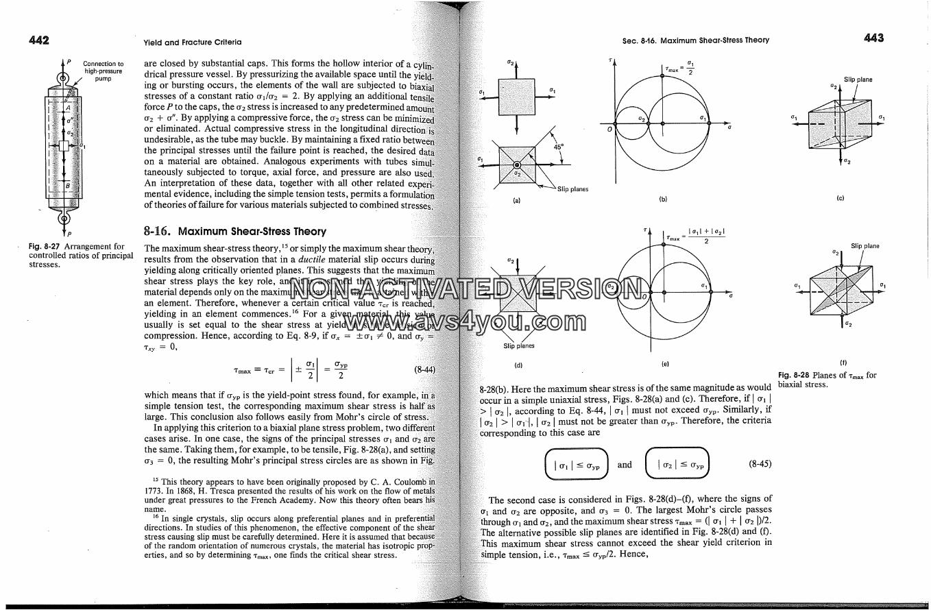
P Connection tohigh-pressure
pump
P
Fig. 8-27 Arrangement forcontrolled ratios of principalstresses.
Yield and Fracture Criteria
are closed by substantial caps. This forms the hollow interior of adrical pressure vessel. By pressurizing the available space until theing or bursting occurs, the elements of the wall are subjected tostresses of a constant ratio 00�/002 = 2. By applying an additionalforce P to the caps, the 0�2 stress is increased to any predetermined002 + 00". By applying a compresslye force, the 002 stress can beor eliminated. Actual compressive stress in the longitudinal direlundesirable, as the tube may buckle. By maintaining a fixed ratiothe principal stresses until the failure point is reached, the desiredon a material are obtained. Analogous experiments with tubestaneously subjected to torque, axial force, and pressure are alsoAn interpretation of these data, together with all other relatedmental evidence, including the simple tension tests, permitsof theories of failure for various materials subjected to combined stre
g-](�. Maximum Shear-Stress TheoryThe maximum shear-stress theory,�5 or simply the maximum shear tresults from the observation that in a ductile material slip occursyielding along critically oriented planes. This suggests thatshear stress plays the key role, and it is assumed that yieldingmaterial depends only on the maximum shear stress that is attained �an element. Therefore, whenever a certain critical value *or isyielding in an element commences. � For a given material, thisusually is set equal to the shear stress at yield in simplecompression. Hence, according to Eq. 8-9, if 00x = +00� � 0, andT�y = O,
Tmax� Tcr = I q- 00YP- 2
which means that if 00yp is the yield-point stress found, for example;simple tension test, the corresponding maximum shear stress islarge. This conclusion also follows easily from Mohr's circle of
In applying this criterion to a biaxial plane stress problem, twocases arise. In one case, the signs of the principal stresses 00� andthe same. Taking them, for example, to be tensile, Fig. 8-28(a), and003 = 0, the resulting Mohr's principal stress circles are as shown
�5 This theory appears to have been originally proposed by C. A.1773. In 1868, H. Tresca presented the results of his work on the flow of
under great pressures to the French Academy. Now this theory oftenname.
�6 In single crystals, slip occurs along preferential planes and indirections. In studies of this phenomenon, the effective component of thestress causing slip must be carefully determined. Here it is assumedof the random orientation of numerous crystals, the material has isotropicerties, and so by determining ?m�, one finds the critical shear stress.
{7 2
(a)
45 �
Slip planes
Sec. 8-t6. Maximum Shear-Stress Theory
1
'/'max = -�
(/1
(b)
(/2
Slip planes
{d) (e)
Here the maximum shear stress is of the same magnitude as wouldoccur in a simple uniaxial stress, Figs. 8-28(a) and (c). Therefore, if l 00� [
I 002 I, according to Eq. 8-44, 100 I must not exceed 00yp. Similarly, if1 0021 > 100'1, 10021 must not be greater than 00yp. Therefore, the criteriaCorresponding to this case are
(,00011<:00yp,)and 10021<:00y (8-45)
The second case is considered in Figs. 8-28(d)-(f), where the signs ofand 002 are opposite, and 003 = 0. The largest Mohr's circle passes
h 00� and 002, and the maximum shear stress ?m� = (I 00� I + 1002 I)/2.alternative possible slip planes are identified in Fig. 8-28(d) and (f).
maximum shear stress cannot exceed the shear yield criterion intension, i.e., *m� --< 00yp/2. Hence,
443
Slip plane0 2
(/1
'o 2
(c)
Slip plane0 2
(/1 01
0 2
(f)
Fig. 8-28 Planes of Tma x forbiaxial stress.
NON-ACTIVATEDVERSIONwww.avs4you.com

444
0 2
Oyp
B(-1, -1) -1
Fig. 8.29 Yield criterionbased on maximum shearstress.
A(1, 1)
01
Oyp
Yield and Fracture Criteria
or, for impending yield,
0-1 0'2=+1
0'yp 0'yp
A plot of this .equation gives the two sloping lines shown inDividing Eqs. 8-45 by 0'yp puts them into the same form as Eq.These modified equations, 0'1/0'yp � � l, and 0'2/0'yp �- -I� 1,spectively, in Fig. 8-29 as two vertical and two horizontal lines.by treating 0'1/0'yp and 0'2/0'yp as coordinates of a point 'in thisstress space, some important conclusions can be reached.
If a point defmed by 0'1/0'yp and 0'2/0'yp falls on the hexagonFig. 8-29, a material begins and continues to yield. No such stresscan lie outside the hexagon because one of the three yield criteriations given before for perfectly plastic material would be violated.stress points falling within the hexagon indicate that a materialelastically.
Note that, according to the maximum shear theory, if hydrostatic ten��or compressive stresses are added, i.e., stresses such that 0'� =0'�, no change in the material response is predicted. Adding these stresmerely shifts the Mohr's Circles of stress along the 0' axis and ?maxthe same. Also note that since the maximum shear stresses are
on planes irrespective of material directional properties, it is implicitthe material is isotropic.
The derived yield criterion for perfectly plastic material is oftento as the Tresca yield condition and is one of the widely used law�plasticity.
'8-17. Maximum Distortion-Energy TheoryAnother widely accepted criterion of yielding for ductile isotropicterials is based on energy concepts.�7 In this approach, the totalenergy is divided into two parts: one associated with thechanges of the material, and the other causing shear distortions. B'ing the shear distortion energy at yield point in simple tension tounder combined stress, the yield criterion for combined stress isIlshod.
]7 The first attempt to use the total energy as the criterion of �by E. Beltrami of Italy in 1885. In its present form, the theory wasM. T. Huber of Poland in 1904 and was further developed andvon Mises (1913) and H. Hencky (1925), both of Germany and the
Sec. 8-t7. Maximum Distortion-Energy Theory
In order to derive the expression giving the yield condition for combinedthe procedure of resolving the general state of stress must be em-
This is based on the concept of superposition. For example, it isssible to consider the stress tensor of the three principal stresses--0'�,
a2, and 0'3--to consist of two additive component tensors. The elements' one component tensor are defined as the mean "hydrostatic" stress:
(8-47)
elements of the other tensor are (0'] - �), (0'2 - �), and (0'3 - �).this in matrix representation, one has
000) 0 0)0 0'2 = � + 0 0'2 - � 0 (8-48)0 0 0'3 0 0 0 0'3 - �
resolution of the general state of stress is shown schematically in8-30. The special case of resolving the uniaxial state of the stress in
has been carried a step further. The sum of the stresses in Figs.nd (g) corresponds to the last tensor of Eq. 8-48.
For the three-dimensional state of stress, the Mohr's circle for the first
0 2 - o� �
o3 03 - �
(a) (b) (c)General state of stress
= + +
(d) (e) (f) (g)Uniaxial state of stress
Fig. 8-30 Resolution of principal stresses into spherical (dilatational) and deviatoric (distortional)stresses.
445
NON-ACTIVATEDVERSIONwww.avs4you.com
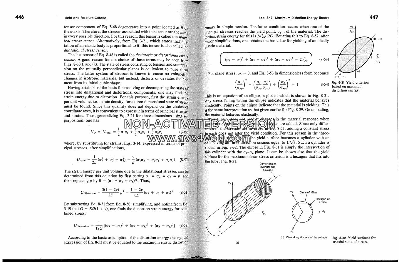
446 Yield and Fracture Criteria
tensor component of Eq. 8-48 degenerates into a point located atthe 0. axis. Therefore, the stresses associated with this tensor are thein every possible direction. For this reason, this tensor is called the.ical stress tensor. Alternatively, from Eq. 3-21, which states thattation of an elastic body is proportional to 5, this tensor is also calle,dilatational stress tensor. :
The last tensor of Eq. 8-48 is called the deviatoric or distortionaltensor. A good reason for the choice of these terms may be seenFigs. 8-30(f) and (g). The state of stress consisting of tension andsion on the mutually perpendicular planes is equivalent to purestress. The latter system of stresses is known to cause nochanges in isotropic materials, but instead, distorts or deviatesment from its initial cubic shape.
Having established the basis for resolving or decomposing thestress into dilatational and distortional components, One maystrain energy due to distortion. For this purpose, first the strainper unit volume, i.e., strain density, for a three-dimensional state ofmust be found. Since this quantity does not depend on thecoordinate axes, it is convenient to express it in terms of principaland strains. Thus, generalizing Eq. 2-21 for three-dimensions usinperposition, one has
1 1 1
go = W,o,a, = + 0.22 + 5 0.33where, by substituting for strains, Eqs. 3-14, expressed in terms ofcipal stresses, after simplifications,
1
U,oa, = + + -- (0.,0.2 + 0.-0.3 +The strain energy per unit volume due to the dilatational stressesdetermined from this equation by first setting 0.� = 0-2 = 0.3 = p,then replacing p by 5 = (0.� + 0.2 + 0.3)/3. Thus,
3(1 - 2v) 1 - 2vUdilatation -- P' -- --(0.1 q- 0.2 q- 0.3) 2
2E 6E
By subtracting Eq. 8-51 from Eq. 8-50, simplifying, and noting from l3-19 that G = E/2(1 + v), one finds the distortion strain energybined stress:
1Udistortion --
12G-- --[(0.1 -- 0.2) 2 q- (0.2 -- 0.3) 2 q- (0.3 -- 0.1) 2 ]
According to the basic assumption of the distortion-energyexpression of Eq. 8-52 must be equated to the maximum elastic
Sec. 8-t7. Maximum Distortion-Energy Theory
in simple tension. The latter condition occurs when one of thestresses reaches the yield point, 0.yp, of the material. The dis-
strain energy for this is 20.2yp/12G. Equating this to Eq. 8-52, aftersimplifications, one obtains the basic law for yielding of an ideally
astic material:
(0.1-- 0.2)2 q-(0.2-- 0.3)2 q-(0.3-- 0.1)2 = 20.2yp) (8-53)�lane stress, 0.3 = 0, and Eq. 8-53 in dimensionless form becomes
0.1 0.1 0.2 0.2-- - + = 1 (8-54)
is an equation of an ellipse, a plot of which is shown in Fig. 8-31.stress falling within the ellipse indicates that the material behaves
Points on the ellipse indicate that the material is yielding. This;ame interpretation as that given earlier for Fig. 8-29. On unloading,
material behaves elastically.This theory does not predict changes in the material response when
�drostatic tensile or compressive stresses are added. Since only differ-of the stresses are involved in Eq. 8-53, adding a constant stress
each does not alter the yield condition. For this reason in the three-stress space, the yield surface becomes a cylinder with an
having all three direction cosines equal to 1/X/�. Such a cylinder isin Fig. 8-32. The ellipse in Fig. 8-31 is simply the intersection of
cylinder with the 0.,-0.2 plane. It can be shown also that the yieldfor the maximum shear stress criterion is a hexagon that fits into
tube, Fig. 8-31. Center line ofcylinder and
hexagon
o 2
o,� Circle of Mises�X� / Hexagon of
///1�/' � Tresca//// - � �103 / 03
'"--/ (b) View along the axis of the cylinder(a)
447
1
-1
(-1, -1)
Fig. 8-3t Yield criterionbased on maximumdistortion energy.
1
Oyp
Fig. 8-32 Yield surfaces fortriaxial state of stress.
NON-ACTIVATEDVERSIONwww.avs4you.com

448
o 2
--Oyp
0�p/2
To�sion
Fig. 8-33 Comparison ofTresca and van Mises yieldcriteria.
Yield and Fracture Criteria
The fundamental relation given by Eq. 8-53 may also beformulating the second invariant, Eq. 8-26, of the deviatoric stressesby the last matrix in Eq. 8-48. Such an approach is generallythe mathematical theory of plasticity. The derivation given beforegreater emphasis to physical behavior. As can be noted from theof Eq. 8-53 and the accompanying Figs. 8-31 and 8-32, it isfunction, making it attractive in analytical and numericalThis widely used constitutive equation for perfectly plastic mateftoften referred to as the Huber-Hencky-Mises or simply the vanyield condition. �8
Both the maximum shear stress and the distortion energyditions have been used in the study of viscoelastic phenomenacombined stress. Extension of these ideas to strain hardening materitis also possible. Such topics, however, are beyond the scope of this
8-18. Comparison of Maximum-Shear and Distorti�Energy Theories for Plane Stress
Plane stress problems occur especially frequently in practice andlargely emphasized in this text. Therefore, it is useful to make aparison between the two most widely used yield criteria for ductil eterials for this case. The maximum shear-stress criterion directstention to the �aximum shear stress in an element. The distortion-ecriterion does this in a more comprehensive manner by considerinthree dimensions the energy caused by shear deformations. Sincestresses are the main parameters in both approaches, the difference'tween the two is not large. A comparison between them for planeis shown in Fig. 8-33. Here the Tresca hexagon for the maximumstress theory and the van Mises ellipse for the maximumtheory have the meanings already described. Either one of the linesa criterion for yield for a perfectly plastic material. Yield of asaid to begin whenever either uniaxial or biaxial stresses reach theing lines. If a stress point for the principal stresses 0.� and 0-2 fallsthese curves, a material behaves elastically. Since no strainbehavior (see Fig. 2-13) is included in these mathematicalstress points can lie outside the curves, as yielding continued atlevel given by the curves. More advanced theories are notthis text. �9
It can be seen from Fig. 8-33 that the discrepancy betweentheories is not very large, the maximum shear-stress theory being 'eral more conservative. As to be expected, the uniaxial stresses
�8 In the past, this condition has been also referred to as thestress theoo,. See A. Nadai, Theory of Flow and Fracture of SolidsMcGraw-Hill, 1950), 104, or A. P. Boresi and O.M. Sidebottom,chanics of Materials, 4th ed. (New York: Wiley, 1985), 18.
�9 K. Washizu, Variational Methods in Elasticirv and Plasticity, 2nd ed.York: Pergamon, 1975). L. E. Malvern, Introduction to the Mechanics of atinuous Mediutn (New York: Prentice-Hall, 1969).
Sec. 8-20. Comparison of Yield and Fracture Criteria
are equal to those corresponding to simple tension or compression.i is assumed that these basic stresses are of equal magnitude. The yield
.in the second and fourth quadrant indicate smaller strengths atthan that for uniaxial stresses. The largest discrepancy occurs when
principal stresses are equal but of opposite sign. This conditionfor example, in torsion of thin-walled tubes. According to theshear-stress theory, when +0-! = -T-0-2, these stresses at yield
reach only _0.yp/2. The maximum distortion-energy theory limits thistress to 0-yp/�//3 = 0.5770-yp. Points corresponding to these stresses are
g. 8-33. These values of yield in shear stress are frequentlyin design applications.
[9. Maximum Normal Stress Theorymaximum normal stress theory or simply the maximum stress
asserts that failure or fracture of a material occurs when thenormal stress at a point reaches a critical value regardless of
other stresses. Only the largest principal stress must be determined� this criterion. The critical value of stress 0-u�t is usually determined
a tensile experiment, where the failure of a specimen is defined to beexcessively large elongation or fracture. Usually, the latter is im-
Experimental evidence indicates that this theory applies well to brittlein all ranges of stresses, providing a tensile principal stress
Failure is characterized by the separation, or the cleavage, frae-This mechanism of failure differs drastically from the ductile frae-which is accompanied by large deformations due to slip along the
of maximum shear stress.
maximum stress theory can be interpreted on graphs as the otherThis is done in Fig. 8-34. Failure occurs if points fall on the
Unlike the previous theories, this stress criterion gives a boundedof the stress space.
Comprison of Yield and Fracture Criteriaof some classical experimental results with the yield and
criteria presented before is shown in Fig. 8-35. 2] Note the par-good agreement between the maximum distortion-energy theory
experimental results for ductile materials. However, the maximum
This theory is generally credited to W. J. M. Rankine, an eminent British(1820-1872). An analogous theory based on the maximum strain, rather
stress, being the basic criterion of failure was proposed by the great FrenchB. de Saint-Venant (1797-1886). Experimental evidence does not car-
the latter approach.The experimental points shown on this figure are based on classical exper-
by several investigators. The figure is adapted from a compilation madeG. Murphy, Advanced Mechanics of Materials (New York: McGraw-Hill,
83.
(/2
o
B(-1, -1) -1
(a)
o 2
o3
(b)
Fig. 8-34 Fracture envelopebased on maximum stresscriterion.
,A{1, 1)
Oult
NON-ACTIVATEDVERSIONwww.avs4you.com

45O
Fig. 8-35 Comparison ofyield and fracture criteriawith test data.
Yield and Fracture Criteria
I!
I%
Cast iron \�SteelCopperAluminum
02 MaximumMaximum -- distortion energy
normal stress �u�t
Z/3�. Maximum�/ shear stress/-1.0 0 .// 1.0
normal stress theory appears to be best for brittle materials andunsafe for ductile materials.
All the theories for uniaxial stress agree since the simple tension iis the standard of comparison. Therefore, if one of the principalat a point is large in comparison with the other, all theories givethe same results. The discrepancy between the criteria is greatestsecond and fourth quadrants, when both princil;equal.
In the development of the theories discussed before, it hassumed that the properties of material in tension andalike--the plots shown in several of the preceding figures have twoof symmetry. On the other hand, it is known that some materialsrocks, cast iron, concrete, and soils have drastically differentdepending on the sense of the applied stress. This is the greatest flaw:applying the classical idealizations to materials having largein their mechanical behavior in tension and compression. An earlyto adopt the maximum shear theory to achieve better agreementexperiments was made by Duguet in 1885. 22 The improvedognizes the higher strengths of brittle materials in biaxialthan in tension. Therefore, the region in biaxial tension in thestress space is made smaller than it is for biaxial compression; see8-36. In the second and fourth quadrant, a linear change betweenof the above regions is assumed. A. A. Griffith, 23 in a sense,
22 A. Nadai, Theory of Flow and Fractu're of Solids (New York:1950).
23 A. A. Griffith, "The Phenomena of Rupture and Flow of Sohds,"sophical Transactions of the Royal SocieO, of London, Series A, 1920,163-198.
Sec. 8.20. Comparison of Yield and Fracture Criteria
Griffith
02/0 c
t" O
%Duguet
o I
; 01[0C
,o
-1
Fig. 8-36 Plausible fracture Fig. 8-37 Dashed curvecriteria for brittle shows analytical fit formaterials. three different strength
concretes.
,n for the previous observations by introducing the idea of sur-energy at microscopic cracks and showing the greater seriousness
tensile stresses compared with compressive ones with �espect to fail-tre. According to this theory, an existing crack will rapidly propagate if
available elastic strain energy release rate is greater than the increasei n the surface energy of the crack. The original Griffith concept has been
expanded by G. R. Irwin. 24 Careful recent experimental re-on concrete specimens of different strengths strongly corroborates
approach, Fig. 8-37. 25 This work now has been extended to includehardening effects, and has been implemented for use with a com-
26
Another important attempt for rationalizing fracture of materials havingproperties in tension and compression is due to Mohr. 27 In this
approach, several different experiments must be conducted on the sameFor example, if the results of experiments in tension, compres-
and shear are available, the results can be represented on the sameusing their respective largest principal stress circles, as shown in Fig.
8-38(a). The points of contact of the envelopes with the stress circlesdefine the state of stress at a fracture. For example, if such a point is A
G. R. Irwin, "Fracture Mechanics," Proceedings, First Symposium onStructural Mechanics (Long Island City, NY: Pergamon, 1958), 557. Also
A Symposium on Fracture Toughness Testing and Its Applications, AmericanSociety for Testing and Materials Special Technical Publication No. 381 (Phila-
PA: American Society for Testing and Materials and Washington, DC:eronautics and Space Administration, 1965).
2� Adapted from H. Kupfer, and K. Gerstle, "Behavior of Concrete UnderStresses," J. Eng. Mech. Div. ASCE, 99 (1973): EM4, 863.
26 C. Bedard, and M.D. Kotsovos, "Application of NLFEA to Concrete Struc-J. Struct. Div. ASCE, 111 (ST12) (1985). Z. P. Bag-ant, ed., Mechanics
C Geomaterials: Rocks, Concrete, Soils (Chinchester: Wiley, 1985).As noted earlier, Otto Mohr was also principally responsible for the devel-
stress circle beating his name.
451
NON-ACTIVATEDVERSIONwww.avs4you.com

452 Yield and Fracture Criteria
O.
(a)
�Failureplane
(b) At A (or A')
Failure� plane
0 2
(d)
-- O c
0 3
(c) At B (or B')
' Fig. 8-38 (a) Mohr envelopes, (b) failure planes at A and A', (c) failure planes at B and B', (d) Mohrsolution in principal stress space.
(or ,4'), the stresses and the plane(s) on which they act can be foundthe established procedure for Mohr's circle of stress (Section 8-7).corresponding planes for points ,4 or ,4' are shown in Fig. 8-38(b),material such as duraluminum does fracture in tension at a flat angkshown. Similarly, by relating the fracture planes to either point Bthe fracture occurs at a steep angle characteristic of concrete ctested in compression, Fig. 8-38(c). Such agreements withsupport the assumed approach.
The data from Fig. 8-38(a) can be replotted in the principal stressas in Fig. 8-38(d). Since in the first quadrant, the minimum principal0'3 = 0, and in the third quadrant, 0-3 = 0 is the maximum principalper Figs. 8-28(a)-(c), in these quadrants, the fracture lines in thestress space are similar to those of Fig. 8~29. Moreover, if thestrengths in tension and compression are the same, a hexagonto that shown in Fig. 8-29 is obtained. However, whereas theFig. 8-29 gives a yield condition for ductile materials, in the presenttext, it defines a fracture criterion for brittle materials.
Extrapolation of Mohr envelopes beyond the range of test dataadvisable. In many applications, this may mean that parts of thecircles for tension and compression should be taken as envelope
Problems
nterpolation along the failure envelopes between these two partial endtress circles is justified, and a stress circle for other conditions can be
between them. When more extensive data are lacking conserva-�traight-line envelopes can be used.
The use of straight lines for asymptotes has a rational basis and has�een found particularly advantageous in soil mechanics. For a loose gran-
media such as sand, the straight-line Mohr envelopes correspond tothe limiting condition of dry friction, p. = tan (b, Fig. 8-39. Any circle
to the envelope, as at B, gives the state of critical stress. If somei can be developed by the media, the origin O is moved to the
such that at zero stress, the ? intercept is equal to the cohesion. Asbasically cannot transmit tensile stresses, in specialized literature it
customary to direct the compression axis to the right.Unlike the maximum distortion-energy theory, the fracture theory
based on Mohr envelopes, using the largest principal stress circles, neg-lects dependence on the intermediate principal stress.
Sometimes the yield and fracture criteria discussed before are incon-to apply. In such cases, interaction curves such as in Fig. 7-6 can
be used to advantage. Experimentally determined curves of this type,complicated by a local or buckling phenomenon, are equivalent to
strength criteria discussed here.In the design of members in the next chapter, departures will be made
strict adherence to the yield and fracture criteria established here,unquestionably, these theories provide the rational basis for
453
2
Fig. 8-39 Mohr envelopesfor cohesionless granularmedia.
8-2Infinitesimal elements A� B, C, D, and E are
the figures for two different members. Drawelement separately, and on the isolated element,
P1 [P2� I-]A
/� B
(a)
indicate the stress acting on it. For each stress, clearlyshow its direction and sense by arrows, and state theformula one would use in its calculation. Neglect theweight of the members.
Fig. P8-t (b)
NON-ACTIVATEDVERSIONwww.avs4you.com
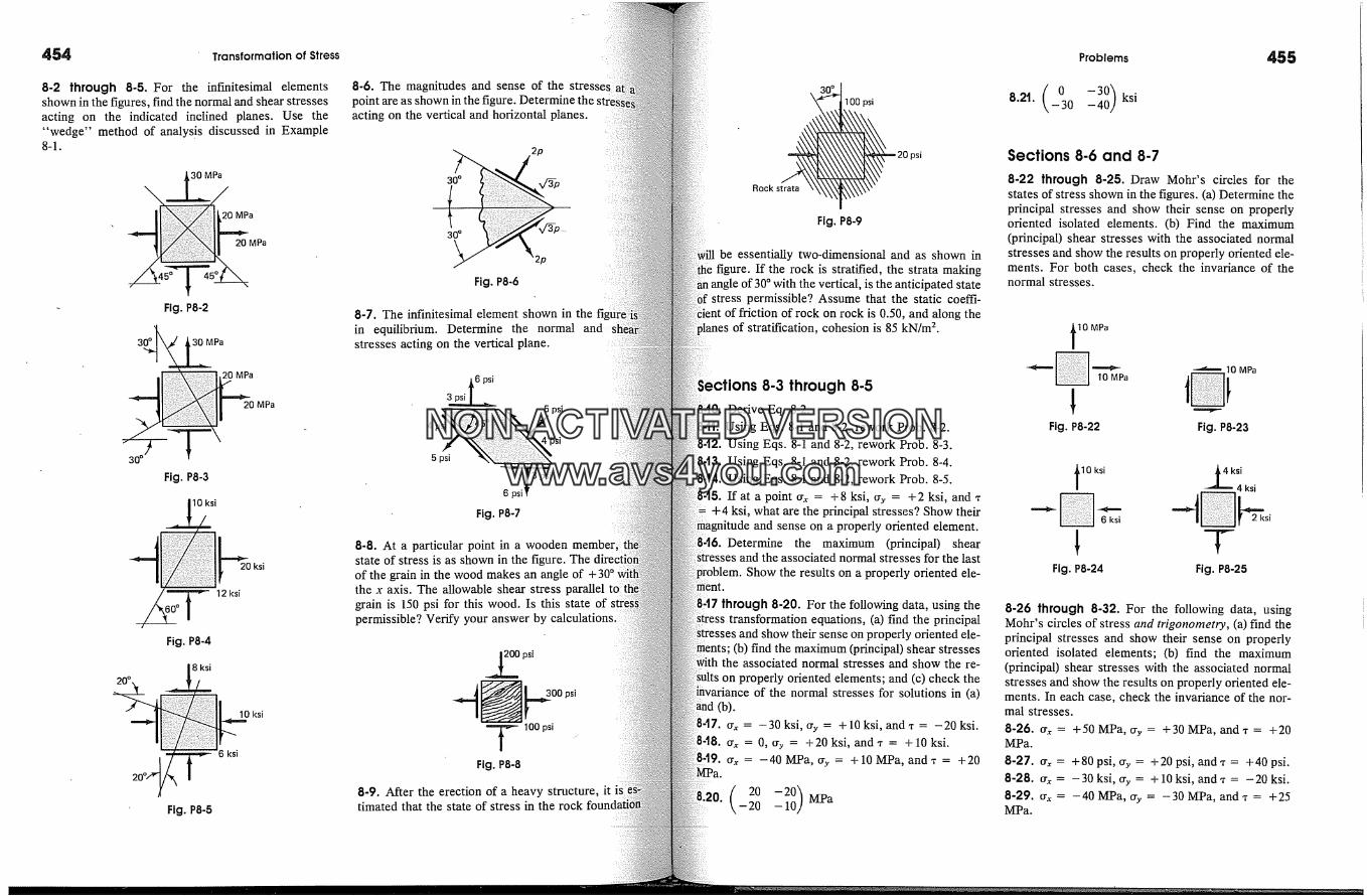
454 Transformation of Stress
8-2 through 8-5. For the infinitesimal elementsshown in the figures, find the normal and shear stressesacting on the indicated inclined planes. Use the"wedge" method of analysis discussed in Example8-1.
30 MPa
20 MPa
20 MPa
Fig. P8-2
30�.� Pa20 MPa
20 MPa
Fig. P8-3
10 ksi
20 ksi
Fig. P8-4
8 ksi
10 ksi
ksi
Fig. P8-5
8-6. The magnitudes and sense of the strepoint are as shown in the figure. Determine theacting on the vertical and horizontal planes.
30 � x,/�p
30 �
2p
Fig. P8-6
8-7. The infinitesimal element shown in thein equilibrium. Determine the normal andstresses acting on the vertical plane.
6 psi3 psi _5 psi
5 psi
l psi
6psi�Fig. P8-7
8-8. At a particular point in a wooden member!state of stress is as shown in the figure. Theof the grain in the wood makes an angle of + 30 �the x axis. The allowable shear stress parallelgrain is 150 psi for this wood. Is this state ofpermissible? Verify your answer by calculations.
.�psi
1oopsiFig. P8-8
8-9. After the erection of a heavy structure, it i stimated that the state of stress in the rock
30 �
Fig. P8-9
be essentially two-dimensional and as shown infigure. If the rock is stratified, the strata making
vertical, is the anticipated statestress permissible? Assume that the static coeffi-
of friction of rock on rock is 0.50, and along theof stratification, cohesion is 85 kN/m 2.
;ections 8-3 through 8-5840. Derive Eq. 8-2.
Using Eqs. 8-1 and 8-2, rework Prob. 8-2.Using Eqs. 8-1 and 8-2, rework Prob. 8-3.Using Eqs. 8-1 and 8-2, rework Prob. 8-4.Using Eqs. 8-1 and 8-2, rework Prob. 8-5.If at a point trx = + 8 ksi, %. = + 2 ksi, and 'r
+4 ksi, what are the principal stresses? Show theirand sense on a properly oriented element.
8-t6. Determine the maximum (principal) shearthe associated normal stresses for the last
Show the results on a properly oriented ele-
through 8-20. For the following data, using thetransformation equations, (a) find the principal
show their sense on properly oriented ele-(b) find the maximum (principal) shear stresses
associated normal stresses and show the re-on properly oriented elements; and (c) check the
mvariance of the normal stresses for solutions in (a)(b).
-17. trx = -30 ksi, try = +10 ksi, and 'r = -20 ksi.trx = 0, try = +20 ksi, and.r = +10 ksi.
�19. trx = -40 MPa, try = +10 MPa, and, = +20
(_�00 -�g) MPa
Problems
8.21. ( 0 -30) ksi-30 -40
455
Sections 8-6 and 8-7
8-22 through 8-25. Draw Mohr's circles for thestates of stress shown in the figures. (a) Determine theprincipal stresses and show their sense on properlyoriented isolated elements. (b) Find the maximum(principal) shear stresses with the associated normalstresses and show the results on properly oriented ele-ments. For both cases, check the invariance of thenormal stresses.
10 MPa10 MPa
Fig. P8-22
� 10 MPa
Fig. P8-23
10 ksi6 ksi
Flg. P8-24
k si4 ksi
2 ksi
Fig. P8-25
8-26 through 8-32. For the following data, usingMohr's circles of stress and trigonometry, (a) find theprincipal stresses and show their sense on properlyoriented isolated elements; (b) find the maximum(principal) shear stresses with the associated normalstresses and show the results on properly oriented ele-ments. In each case, check the invariance of the nor-mat stresses.
8-26. trx = + 50 MPa, try = + 30 MPa, and 'r = + 20MPa.
8-27. tr� = +80 psi, try = +20 psi, and.r = +40 psi.8-28. trx = - 30 ksi, try = + 10 ksi, and 'r = - 20 ksi.8-29. tr� = -40 MPa, try = -30 MPa, and 'r = +25MPa.
NON-ACTIVATEDVERSIONwww.avs4you.com

456 Transformation of Stress
8-30. � = -15MPa, 0.y = +35MPa, and,= +60MPa.
8-31. 0.� = +20 ksi, 0.y = 0, and, = -15 ksi.8-32. 0.� = 0, 0.y = -20 ksi, and, = -10 ksi.8-33 through 8-36. For the following data, usingMohr's circles of stress, determine the normal andshear stresses acting on the planes defined by the givenangle 0. Show the results on isolated elements.8-33. 0..� =if, = 0,0.� = 0.2 = -20ksi, for0 = +30 � .*8-34. Rework Prob. 8-4 with 0 = +30 �.
*8-35. Rework Prob. 8-2 for 0 = +45 �.
8-36. 0.x = 0.>. = 0, 'r = -20 ksi, for 0 = 20 �.8-37. For the data shown for Prob. 8-6, using Mohr'scircle of stress, find the principal stresses and showthe results on a properly oriented element.8-38. For the data shown for Prob. 8-7, using Mohr'scircle of stress, find the principal stresses and the ori-entation of the planes on which these act.*8-39. Using Mohr's circle, determine the angle be-tween the right-hand face of the element shownin thefigure and the plane or planes where the normal stressis zero. Check the result using the "wedge" method.Show 'the stresses with proper sense on the rotatedelement(s).
_�2ksi-6 ksi
3 ksiFig. P8-39
8-40. A clevice transmits a force F to a bracket, asshown in the figure. Stress analysis of this bracketgives the following stress components acting on ele-ment A: 1000 psi due to bending, 1500 psi due to axialforce, and 600 psi due to shear. (Note that these arestress magnitudes only; their directions and sensesmust be determined by inspection.) (a) Indicate theresultant stresses on a drawing of the isolated elementA. (b) Using Mohr's circle for the state of stress foundin (a), determine the principal stresses and the maxi-mum shear stresses with the associated normal
stresses. Show the results on properly oriented ele-ments.
A
Fig. P8-40
8-4t. At point A on an unloaded edge of anbody, oriented as shown in the figure with respect!the x-y axes, the maximum shear stress iskN/m 2. (a) Find the principal stresses, and (b)mine the state of stress on an element orientedits edges parallel to the x-y axes. Show the result� ia drawing of the element at A.
y
4 3
�..
Fig. P8-4t
Sections 8-8 and 8-9
8-42. Determine the principal stresses andrections for the following stress tensor:
2 ksi2
Use the procedure discussed in Section 8-8. Therection cosines should be normalized. (Thiscan also be solved using the equations for stressformation discussed in Sections 8-4 and 8-7.)
-43. For the following stress tensor, determine (a)stress invariants, (b) the principal stresses, and (c)direction of the largest principal stress. The direc-
cosines for this principal stress should be nor-
(_410 4
- 6 -� MPa6 8 14'
-44. For the data in Prob. 8-26, determine the prin-stresses and draw the three principal circles of
tress.
For the data in Prob. 8-28, determine the prin-stresses and draw the three principal circles of
;ections 8-11 and 8-t2
-46. Rederive Eq. 8-28 by assuming that the shearoccurs first, then the deformation in the
direction, and finally the deformation in the x direc-
8-47. With the aid of Fig. 8-20, show that
13 = -(ex - ey) sin 0 cos 0 + �,� cos 2 0
If the unit strains are e� = -120 I�m/m, ey =~ 1120 I�m/m, and 3' = - 200 I�m/m, what are the prin-
strains and in which directions do they occur?s. 8-35 and 8-36.
8-49. If the unit strains are e� = -800 i�m/m, ey =i�m/m, and 3' = + 800 I�m/m, what are the prin-
strains and in which direction do they occur? UseEqs. 8-35 and 8-36.
For the following strain tensor, using theanalogous to that described in Section 8-8 for
transformation, determine (a) the principaland (b) the directions of the maximum and min-
principal strains.
- 10V� 5 [�m/m0 0 -20
843
-51. Rework Prob. 8-48 using Mohr's circle of strain.-52. ReworkProb. 8-49 usingMohr's circle of strain.
Problems 457
Section 8-14
8-53. The measured strains for a rectangular rosette,attached to a stressed steel member, are e0o = -220I�m/m, 845* = + 120 I�m/m, and e�oo = +220 I�m/m.What are the principal stresses and in which directionsdo they act? E = 30 x 106 psi and v = 0.3.8-54. The measured strains for an equiangular rosette,attached to a stressed aluminum alloy member, are= +400 i�m/m, e6oo = +400 I�m/m, and e�2oo = -600
I�m/m. What are the principal stresses and in whichdirections do they act? E = 70 GPa and v = 0.25.8-55. The data for a strain rosette with four gage linesattached to a stressed aluminum alloy member are= - 120 i�m/m, 845 � = +400 �m/m, 890 � = + 1120 I�m/
m, and e�35o = + 600 I�m/m. Check the consistency ofthe data. Then determine the principal stresses and thedirections in which they act. Use the values of E andv given in Prob. 8-54.8-56. At a point in a stressed elastic plate, the follow-ing information is known: maximum shear strain �m�= 500 I�m/m, and the sum of the normal stresses on
two perpendicular planes passing through the point is27.5 MPa. The elastic properties of the plate are E =200 GPa, G = 80 GPa, and v = 0.25. Calculate themagnitude of the principal stresses at the point.
Section 847
8-57. Recast the stress tensor given in Prob. 8-43 intothe spherical and the deviatoric stress tensors.
Section 8-18
8-58. In classical experiments on plasticity, a two-di-mensional stress field is often obtained by subjectinga thin-walled tube simultaneously to an axial force anda torque. The results of such experiments are reportedon 0.x-'r, plots. If only 0.x and 'r, stresses are studied,how would the theoretical curves based on the Tresca
and on the yon Mises yield criteria look on such a plot?Derive the two required equations and sketch the re-sults on a diagram.8-59. Ordinarily the Tresca and yon Mises yieldstresses are made to coincide in simple tension. Thisgives rise to a discrepancy for pure shear. If, instead,the yield condition is assumed to be the same in shear,what discrepancy will result for simple tension and for0.1 � 0'2?
NON-ACTIVATEDVERSIONwww.avs4you.com
458 Yield and Fracture Criteria
8-60. A critical element develops the principalstresses, tr�, tr2, and tr3, in the ratio 5:2: -1, i.e., thestresses are 5p, 2p, and -p, where p is a parameter.Such loadings are called radial. If this element is sub-
jected to this loading condition, determine the maxi-mum magnitudes the stresses may reach before yield-ing (a) according to the Tresca yield criterion, and (b)according to the yon Mises criterion. Assume that thematerial yields in tension at 60 ksi.
8-6t. A metal bar is being compressed alonbetween two rigid walls such that e3 = 0 and or2This process causes an axial stress tr� and nostresses. Determine the apparent yield value ofthe material in a conventional compression testhibits a yield strength trvp and Poisson's ratiosume that the material is governed by the yonyield condition. Find an alternative expressionTresca condition is postulated.
Introduction
for determining the state of stress in elastic members tradi-considered in an introductory text on mechanics of solids have
been derived in previous chapters. Usually, they give either a normal orshear stress caused by a single force component acting at a section of
For linearly elastic materials, the main formulas are sum-
1. Normal stresses
(a) due to an axial force
(b) due to bending � straight members cr = ---
o symmetricalcurved bars cr =
2. Shear stresses(a) due to torque � circular shaft
P
� rectangular shaft Tma x -�-
� closed thin-walled tube ? = --
(b) due to shear force in a beam
(1-13)
My(6-11)
I
My(6-32)
Ae(R - y)
* = -- (4-4)J
T
otbt 2 (4-30)T
2(�t (4-34, 4-35)VQ
? = It (7-6)superposition of normal stresses caused by axial forces and bending
y using these formulas was discussed in Chapter 6. Like-the superposition of shear stresses caused by torque and direct shear
459
NON-ACTIVATEDVERSIONwww.avs4you.com

Fig. 94 A staticallyindeterminate problem.
Elastic Stress Analysis and Design
acting simultaneously was considered in Chapter 7. In thisconsequences of the simultaneous occurrence of normal andstresses are examined with the aid of the stress-transformationdeveloped in Chapter 8. This condition commonly occurs in beamltransmission shafts.
In applying the above formulas, particularly in the analysis orof mechanical equipment, stress-concentration factors must be intro((see Sections 2-10, 4-7, and 6-6). Because of the problem of fatimonly occurring in such cases, reduced stresses are employed.consideration must also be given to dynamic loading (see Section:4-11, and 6-7). For such loadings, if occurring in milliseconds,able stresses may be significantly increased.
This chapter is entirely devoted to elastic problems, an approachcommonly used at usual working loads. In Part A, the statesome basic cases is discussed from the point of view of stressmations.
The elastic design of members is considered in Part B.stress-analysis formulas listed before are applicable to bothterminate and indeterminate problems, discussion will be limited toically determinate cases. There are at least two reasons for this.the more frequently occurring statically indeterminate problemsbeams; these are treated beginning with the next chapter. Second,significantly, �he design of statically indeterminate systems intheir stress analysis is necessarily complex. As an example,elastic bar of variable cross section, fixed at both ends, andan axial force P, as shown in Fig. 9-1. If the cross-sectional areasupper and lower parts of the bar are given, reactions R� and R2 canfound routinely using the procedures discussed in Chapter 2. Afterreaction is known, the problem becomes statically determine, andstresses can be found in. the usual manner. However, if thisindeterminate system were to be designed, even this s�mplebecome involved. Generally, in a design problem, only the appliedP and the boundary conditions would be known. By varying thesectional areas of the bar, an infinite number of solutions isAdditional constraints in the realm of structural or machine designerally enter the problem. Such problems are, therefore, nothere.
It is to be emphasized that only the problem of elastic stresses issidered in this chapter. Some elastic designs may be governedthe stiffness or the possible instability of a system. Thecommonly arises in deflection control and vibration problems; thein lateral instability of members.
The main purpose of this chapter is to provide greater insightmeaning of stress analysis by solving additional problems. Theretraordinarily many cases where applications of the basic formulas
' gineering mechanics of solids listed before lead to useful results. No
Sec. 9-2. State of Stress for Some Basic Cases
principles are developed in this chapter. However, some simpleprocedures for prismatic beams are given.
is essential to recognize that in all elastic stress-analysis and designthe material is assumed to be initially stress free. In many
materials, significant residual stresses may be present. Thesebe caused by the manufacturing processes employed: rolling, weld-
ing, forging, temperature or hydration shrinkage, etc. (see Fig. 1-12). Init is the combination of the residual stresses with those due to
that cause the initial yield and/or fracture of a member.some engineering applications, estimates of residual stresses present
formidable problem.
L2. State of Stress for Some Basic Casesstate of stress for four basic cases in the form of examples is con-
in this section. By means of Mohr's principal circles of stress,states of stress at a point are exhibited graphically. From such rep-
the critical stresses can be seen readily and related to the,r fracture criteria discussed in the preceding chapter. The four cases
pertain to the uniaxial stress, biaxial stress such as occurs inpressure vessels, torsional stresses in circular tubes, and beam
caused by bending and shear. Because of the greater complexitylast problem, some aspects of the solution accuracy are discussed
the next section.
EXAMPLE 94
2onsider a state of stress in an axially loaded bar and construct the three principalof stress. Relate the critical stresses to yield and fracture criteria.
maximum principal stress trt in an axially loaded bar can be found using Eq.1-8. The remaining two principal stresses are each equal to zero, i.e., tr2 = tr3 =
The basic infinitesimal element for this case, together with its three planaris shown in Fig. 9-2(a). The principal circles of stress are drawn in Fig.
9-2(b). Since th and tr2�_�_e equal, Mohr's circle for these stresses degeneratesa point. For clarity, however, it is shown in the diagram by a small circle of
diameter.For this case, the maximum shear stress is equal to tr�/2, whereas the maximum
stress is at. Therefore, the manner in which a material fails depends on
461
NON-ACTIVATEDVERSIONwww.avs4you.com

iC
�1/2
B
iC
0 O2� 0 3 C 01
(a)
Rg. 9-2 �ohr's circles for auniaxial state of stress.
Omin
O1�O2=O3=0
(b)
its relative strengths in these two properties. As already pointed out in2-3 and illustrated in Fig. 2-7, a brittle material (cast iron) fails by afracture. This is so because it is weaker in tension than in shear. The
true for a ductile material. The cup and cone fractures shown in Fig. 2-7and aluminum occur approximately along the planes forming a 45 � angleaxis of the specimen. These planes are identified by dashed lines in theon the right in Fig. 9-2(a). Greater refinements on the mechanism ofpossible by considering the behavior of single crystals within a material.
EXAMPLE 9-2
Consider a state of stress in a'thin-walled cylindrical pressure vessel andthe three principal circles of stress. Relate the results to a yield
Solution
According to Eqs. 3-24 and 3-25, the ratio of the hoop stress �q to the Ionstress tr2 is approximately 2. These are the principal stresses as no shearact on the corresponding planes. The third principal stress tr3 equals theor internal pressure p, which may be taken as zero since it is small intr� and tr2. A typical infinitesimal element for the vessel and three planarare shown in Fig. 9-3(a). The principal stress circles are shown in Fig.maximum shear stress is found on the major stress circle passingorigin O and tr�. Its magnitude is th/2. The planes on which the maximumstresses act are identified by dashed lines in the lower right element.if only the principal stresses cr� and or2 were considered,would only be half as large. In design, the yield criterion based on thedistortion theory (see Section 8-18) can also be used.
Construction of pressure vessels from brittle materials is generallysuch materials provide no accommodation nor warning of failure throughbefore fracture.
It is interesting to note that for a thin-walled spherical pressure vessel,or2, and the corresponding principal stress circle degenerates into a point.theless, the maximum shear stress is cry/2 since the third principal stress is
462
Sec. 9-2. State of Stress for Some Basic Cases 463
o 1p�0
A--
p�0
01
(a)
VlPLE 9-3
Examine the state of stress in a circular tube subjected to a torque by constructingprincipal circles of stress. Relate the results to yield and fracture criteria.
O� � 0 2 � 0 30 2=a�/2; 0 3�0
(b)
Fig. 9-3 Mohr's circles forstresses in a cylindrical wallof a pressure vessel.
;olution
The shear stresses for this case can be found using Eq. 4-4. A typical infinitesimalof the tube and three planar views are shown in Fig. 9-4(a). Here the
Tmax = T O
c
x e
B A �
A � e C
--.,t..--.- B B X
01 � 0 2 � 0 3(a) 01 = i'ma x = TO; 0 2 = O; 0 3 = --01
(b)
Fig. 9-4 Mohr's circles for stresses in a circular tube subjected to torque.
NON-ACTIVATEDVERSIONwww.avs4you.com
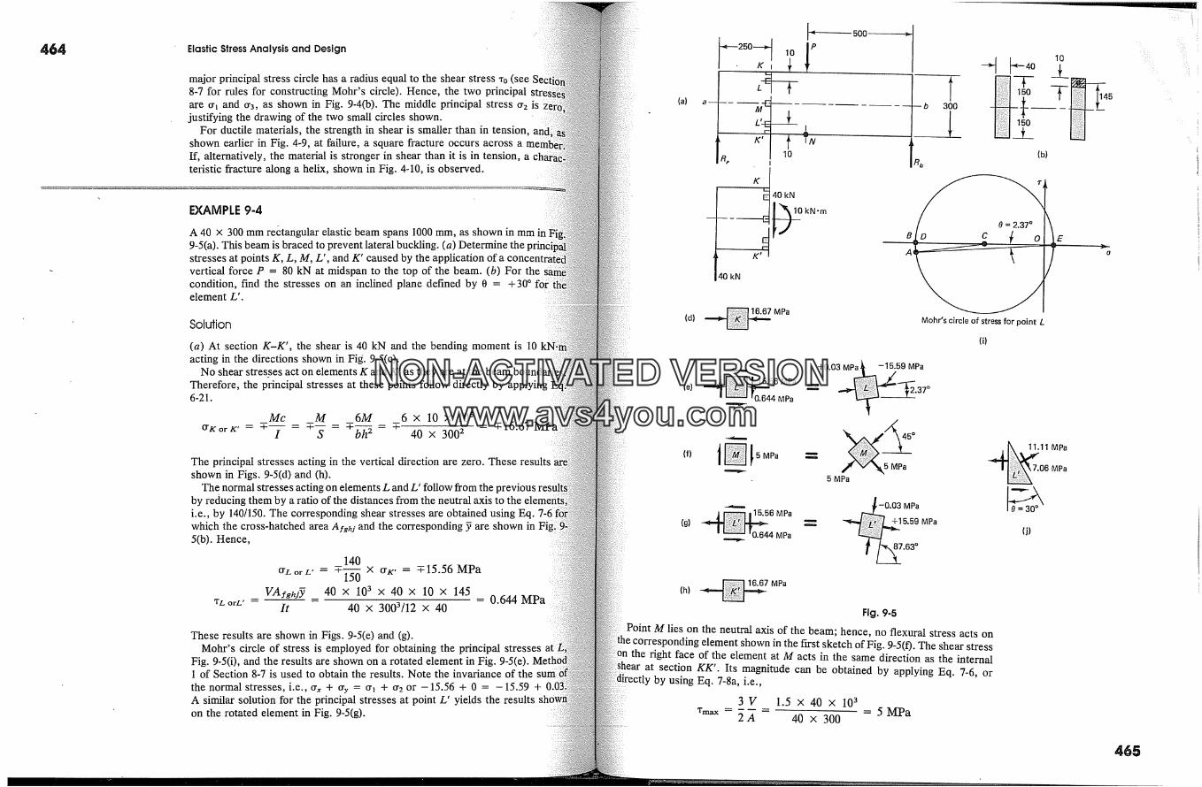
464 Elastic Stress Analysis and Design
major principal stress circle has a radius equal to the shear stress xo (see8-7 for rules for constructing Mohr's circle). Hence, the two principalare cr� and cr3, as shown in Fig. 9-4(b). The middle principal stress cr2 is
justifying the drawing of the two small circles shown.For ductile materials, the strength in shear is smaller than in tension,
shown earlier in Fig. 4-9, at failure, a square fracture occurs across a meIf, alternatively, the material is stronger in shear than it is in tension, ateristic fracture along a helix, shown in Fig. 4-10, is observed.
EXAMPLE 9-4
A 40 x 300 mm rectangular elastic beam spans 1000 mm, as shown in mm in9-5(a). This beam is braced to prevent lateral buckling. (a) Determine thestresses at points K, L, M, L', and K' caused by the application of a concevertical force P = 80 kN at midspan to the top of the beam. (b) For thecondition, find the stresses on an inclined plane defined by 0 = +30 �element Z'.
Solution
(a) At section K-K', the shear is 40 kN and the bending moment is 10acting in the directions shown in Fig. 9-5(c).
No shear stresses act on elements K and K' as they are at the beam bouTherefore, the principal stresses at these points follow directly by6-21.
Mc M 6M 6 x 10 x 106O'K�rK' = '�' I = -T-� = -T-� = -T- 40 X 3002 = -T-16.67
The principal stresses acting in the vertical direction are zero. Theseshown in Figs. 9-5(d) and (h).
The normal stresses acting on elements L and L' follow from the previousby reducing them by a ratio of the distances from the neutral axis to the elei.e., by 140/150. The corresponding shear stresses are obtained using Eq. 7-6which the cross-hatched area Afghj and the corresponding y are shown in Fig.5(b). Hence,
TL orL' -- --
140
cr�.or �., = -T-l- � x cry:, = -T-15.56 MPaVAfghjY _ 40 X 103 X 40 X 10 X 145 = 0.644 MPa
It 40 x 3003/12 x 40
These results are shown in Figs. 9-5(e) and (g).Mohr's circle of stress is employed for obtaining the principal stresses
Fig. 9-5(i), and the results are shown on a rotated element in Fig. 9-5(e).1 of Section 8-7 is used to obtain the results. Note the invariance of the
the normal stresses, i.e., crx + cry = cr! + cr2 or -15.56 + 0 = -15.59 +A similar solution for the principal stresses at point L' yields the resultson the rotated element in Fig. 9-5(g).
(a)
(d)
(e)
�---250�J 10 1P� K i �r
K
I
E 40 kN
-500
40 kN
[*-4o
-- 16.67 MPa
A
Mohr's circle of stress for point
+0.03 MPa, -15.59 MPa
6 MPa �MPa � ;2'37�
(i)
lO
(b)
E
(f) t __ 5 MPa
15.56 MPa(g) �
0.644 MPa
5 MPa
45 �
5 MPa1..11 MPa
06 MPa
(i)
-- 16.67 MPa(h)
Fig. 9-5
Point M lies on the neutral axis of the beam; hence, no flexural stress acts oncorresponding element shown in the Errst sketch of Fig. 9-5(0. The shear stress
the right face of the element at M acts in the same direction as the internalat section KK'. Its magnitude can be obtained by applying Eq. 7-6, or
by using Eq. 7-8a, i.e.,
3 V 1.5 x 40 x 103Tmax = 2 A 40 x 300 = 5 MPa
465
NON-ACTIVATEDVERSIONwww.avs4you.com

466
Fig. 9-6 (a) Behavior of themajor principal stress oh. (b)Behavior of the minorprincipal stress �2.
Elastic Stress Analysis and Design
71 =0
87.63 �r� 0.03 MPa
_ � �5 MPa2.37 �
6.67 MPa ~ � i K'
(a)
J 16.67
2.37 �
87.63�-�
15.59 MPa
M
�:5 MPa� 0.03 MPa
a 2 =0
(b)
The pure shear stress transformed into the principal stresses'according6 is shown on a rotated element in Fig. 9-5(f).
It is significant to further examine qualitatively the results obtained. Forpurpose, the computed principal stresses actbzg on the corresponding 1shown in Figs. 9-6(a) and (b). In Fig. 9-6(a), the characteristic behavior ofmajor (tensile) principal stress at a section of a rectangular beam can beThis stress progressively diminishes in magnitude from a maximum valueto zero at K. At the same time, the corresponding directions of elthrough 90 �. A similar observation can be made regarding the minor (comprincipal stress �_ shown in Fig. 9-6(b).
(b) To find the stresses acting on a plane of 0 = +30 � through point L',application of Eqs. 8-1 and 8-2 using the stresses shown on the left ele:Fig. 9-5(g) and 20 = 60 � is made.
+ 15.56 + 15.56+ -- cos 60 � + (-0.644) sin 60 � = +11.11or0- 2 2
- 15.56 .-- sin 60 � + (-0.644) cos 60 � = -7.06 MPaTO -- 2
These results are shown in Fig. 9-50). The sense of the sheafing stress 'r0 'posite to that shown in Fig. 8-4(b), since the computed quantity is negative."wedge technique" explained in Example 8-1 or the Mohr's circleSection 8-7 can be used to obtain the same results.
9-3. Comparative Accuracy of Beam SolutionsThe solution in the previous example for a beam considering flexureshear is based on stresses initially obtained using the conventionalmulas of engineering mechanics of solids. These formulas aresentially assuming that plane sections in a beam remaining. Since this basic assumption is not entirely true in all cases,solutions can be referred to as elementary. Therefore, it is
Sec. 9-3. Comparative Accuracy of Beam Solutions 467
are the obtained results with a more accurate solution. Such a com-
parison is made here with a finite-element solution, shown in Fig. 9-7.Because of the symmetry of the problem, only one-half of the beam was
using 450 finite elements. ZThe contour lines for the principal stresses are shown in Fig. 9-7(a).
point lying on a stress contour has a principal stress of the sameand sign, with tensile stresses being positive. In this diagram,
the major principal stresses are shown by black lines, and the minor prin-�al stresses are shown in color. Comparisons between the elementary
finite-element solutions of the normal stress distribution across sec-K-K' are shown in Fig. 9-7(b) and that for the shear stress in Fig.
The agreement is seen to be excellent. However, section K-K' isbetween the applied concentrated force P and the concen-
ed reaction R,. At these points, locally large perturbations in stressesresembling those shown earlier in Figs. 2-30 and 2-31. However,
to the Saint-Venant principle, local stresses rapidly diminisha regular statically equivalent stress pattern sets in. In practice, large;ses at concentrated forces are reduced by applying them over anto obtain an acceptable bearing pressure. Theoretically, in an elastic
the stress at a concentrated force is infinite. In reality, some plastic
� This solution was obtained using the FEAP computer program developed byL. Taylor employing isoparametric four-node elements. An automatic mesh-
technique enables the use of graduated smaller elements at concen-forces, where the stresses vary more rapidly than elsewhere. Conventional
in the FEAP program were used in the previous solutions cited.Since in a two-dimensional plate of finite thickness, the in-plane stresses vary
across the thickness, in the FEAP formulation, the average values ofstresses through the plate thickness are used. Such stresses are called gen-
plane stresses.
Symm. abt. �
K -25
300 -10i-15 i -5-251 +5
+25;
� K
< 500 mm
P
-25
-15
-5
'N
(a)
/-16.6 MPa
(-16.67)
(b)
15.3 MPa(16.67)
�, Finite 5.0 MPa
element I //� (5.0)solution
J /J �,ElementaryL�' solution
Shear stress
(c)
Fig. 9-7 (a) Principal stress contours for Example 9-4 beam determined by finite elements. (b) and (c))aftsons between elementary and finite element solutions for normal and shear stresses at section K-K'.
elementary solutions in (b) and (c) are given in parentheses).
NON-ACTIVATEDVERSIONwww.avs4you.com
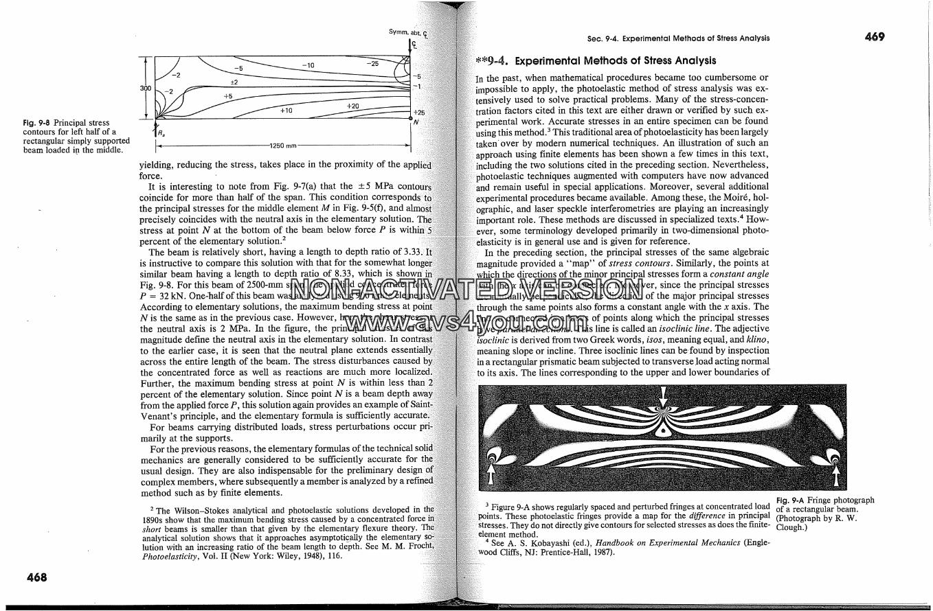
Symm.Sec. 9�4. Experimental Methods of Stress Analysis 469
Fig. 9-8 Principal stresscontours for left half of arectangular simply supportedbeam loaded i�n the middle.
468
-5 � -10 -25-+2
3001250 mm
yielding, reducing the stress, takes place in the proximity of theforce.
It is interesting to note from Fig. 9-7(a) that the +5 MPacoincide for more than half of the span. This condition correstthe principal stresses for the middle element M in Fig. 9~5(0, andprecisely coincides with the neutral axis in the elementary solution.stress at point N at the bottom of the beam below force P ispercent of the elementary solution. 2
The beam is relatively short, having a length to depth ratio of 3.1is instructive to compare this solution with that for the somewhatsimilar beam having a length to depth ratio of 8.33, which is shownFig. 9-8. For this beam of 2500~mm span, the applied concentratedP = 32 kN. One--half of this beam was analyzed using 900 finiteAccording to elementary solutions, the maximum bending stress atN is the same as in the previous case. However, here the shear stresthe neutral axis is 2 MPa. In the figure, the principal stresses ofmagnitude define the neutral axis in the elementary solution. Into the earlier case, it is seen that the neutral plane extendsacross the entire length of the beam. The stress disturbances causedthe concentrated force as well as reactions are much moreFurther, the maximum bending stress at point N is within lesspercent of the elementary solution. Since point N is a beam depthfrom the applied force P, this solution again provides an exampleVenant's principle, and the elementary formula is sufficiently
For beams carrying distributed loads, stress perturbations occurmarily at the supports.
For the previous reasons, the elementary formulas of themechanics are generally considered to be sufficiently accurate forusual design. They are also indispensable for the preliminarycomplex members, where subsequently a member is analyzed bymethod such as by finite elements.
2 The Wilson-Stokes analytical and photoelastic solutions developed in1890s show that the maximum bending stregs caused by a concentratedshort beams is smaller than that given by the elementary flexure theory.analytical solution shows that it approaches asymptotic_ally thelution with an increasing ratio of the beam length to depth. See M. M.Photoelasticity, Vol. II (New York: Wiley, 1948), 116.
Experimental Methods of Stress AnalysisIn the past, when mathematical procedures became too cumbersome or
)ossible to apply, the photoelastic method of stress analysis was ex-.y used to solve practical problems. Many of the stress-concen-
tration factors cited in this text are either drawn or verified by such ex-ental work. Accurate stresses in an entire specimen can be found
Using this method. 3 This traditional area ofphotoelasticity has been largely'over by modem numerical techniques. An illustration of such an
approach using finite elements has been shown a few times in this text,the two solutions cited in the preceding section. Nevertheless,
photoelastic techniques augmented with computers have now advancedremain useful in special applications. Moreover, several additional
procedures became available. Among these, the Moir�, hol-�hic, and laser speckle interferometries are playing an increasingly
role. These methods are discussed in specialized texts. 4 How-some terminology developed primarily in two-dimensional photo-
y is in general use and is given for reference.In the preceding section, the principal stresses of the same algebraic
magnitude provided a "map" of stress contours. Similarly, the points atwhich the directions of the minor principal stresses form a constant angle
with the x axis can be connected. Moreover, since the principal stressesmutually perpendicular, the direction of the major principal stresses
the same points also forms a constant angle with the x axis. Theso connected is a locus of points along which the principal stresses
�arallel directions. This line is called an isoclinic line. The adjective'linic is derived from two Greek words, isos, meaning equal, and klino,
slope or incline. Three isoclinic lines can be found by inspectionin a rectangular prismatic beam subjected to transverse load acting normalto its axis. The lines corresponding to the upper and lower boundaries of
Fig. 9-A Fringe photograph3 Figure 9-A shows regularly spaced and perturbed fringes at concentrated load of a rectangular beam.
These photoelastic fringes provide a map for the difference in principal �hotograph by R. W.rhey do not directly give contours for selected stresses as does the finite- Clough.)
method.4 See A. S. Kobayashi (ed.), Handbook on Experimental Mechanics (Engle-
Cliffs, NJ: Prentice-Hall, 1987).
NON-ACTIVATEDVERSIONwww.avs4you.com
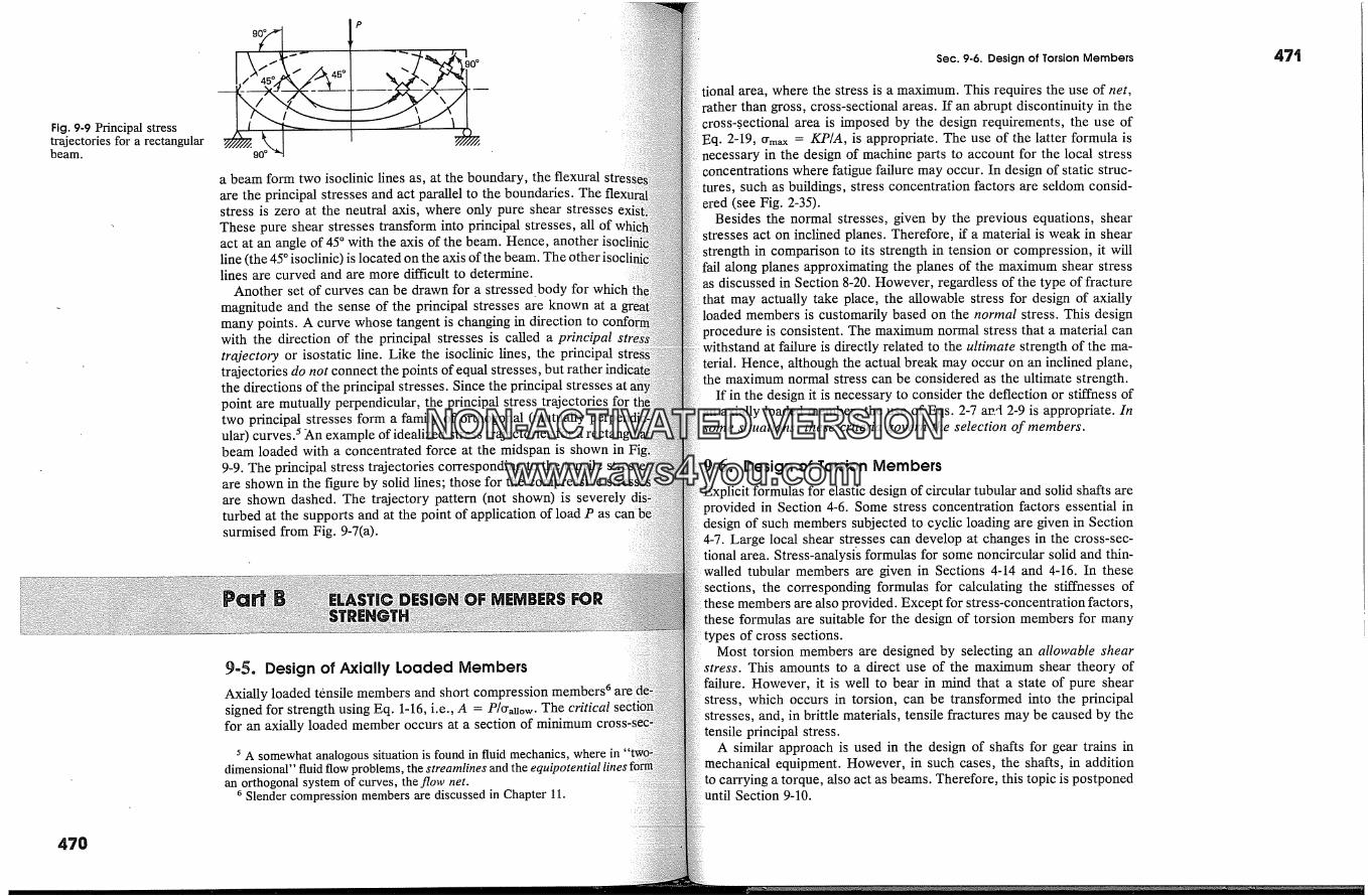
Fig. 9-9 Principal stresstrajectories for a rectangularbeam.
470
P
a beam form two isoclinic lines as, at the boundary, the flexuralare the principal stresses and act parallel to the boundaries. Thestress is zero at the neutral axis, where only pure shear stressesThese pure shear stresses transform into principal stresses, all ofact at an angle of 45 � with the axis of the beam. Hence, another iso.line (the 45 � isoclinic) is located on the axis of the beam. The other ilines are curved and are more difficult to determine.
Another set of curves can be drawn for a stressedbody for whichmagnitude and the sense of the principal stresses are known at amany points. A curve whose tangent is changing in direction towith the direction of the principal stresses is called a principaltrajectory or isostatic line. Like the isoclinic lines, the principaltrajectories do not connect the points of equal stressesthe directions of the principal stresses. Since the principal stresses atpoint are mutually perpendicular, the principal stress trajectories fortwo principal stresses form a family of orthogonal (mutuallyular) curves. 5 An example of idealized stress trajectories for a rectanbeam loaded with a concentrated force at the midspan is shown in9-9. The principal stress trajectories corresponding to the tensileare shown in the figure by solid lines; those for the compressiveare shown dashed. The trajectory pattern (not shown) is severelyturbed at the supports and at the point of application of load P as cansurmised from Fig. 9-7(a).
9-5. Design of Axially Loaded MembersAxially loaded t�nsile members and short compression members 6signed for strength using Eq. 1-16, i.e., A = P/cr�uow. The criticalfor an axially loaded member occurs at a section of minimum
5 A somewhat analogous situation is found in fluid mechanics, where indimensional" fluid flow problems, the streamlines and the equitan orthogonal system of curves, the flow net.
6 Slender compression members are discussed in Chapter 11.
Sec. 9-6. Design of Torsion Members
tional area, where the stress is a maximum. This requires the use of net,rather than gross, cross-sectional areas. If an abrupt discontinuity in thecross-.sectional area is imposed by the design requirements, the use ofEq. 2-19, Crm� = KP/A, is appropriate. The use of the latter formula isnecessary in the design of machine parts to account for the local stressconcentrations where fatigue failure may occur. In design of static struc-tures, such as buildings, stress concentration factors are seldom consid-ered (see Fig. 2-35).
Besides the normal stresses, given by the previous equations, shearstresses act on inclined planes. Therefore, if a material is weak in shear
strength in comparison to its strength in tension or compression, it willalong planes approximating the planes of the maximum shear stress
as discussed in Section 8-20. However, regardless of the type of fracturemay actually take place, the allowable stress for design of axially
loaded members is customadhly based on the normal stress. This designprocedure is consistent. The maximum normal stress that a matedhal can
withstand at failure is directly related to the ultimate strength of the ma-rienee, although the actual break may occur on an inclined plane,
the maximum normal stress can be considered as the ultimate strength.If in the design it is necessary to consider the deflection or stiffness of
axially loaded member, the use of Eqs. 2-7 ae..'t 2-9 is appropriate. Insome situations, these criteria govern the selection of members.
)-6. Design of Torsion MembersExplicit formulas for elastic design of circular tubular and solid shafts areprovided in Section 4-6. Some stress concentration factors essential indesign of such members subjected to cyclic loading are given in Section4-7. Large local shear stresses can develop at changes in the cross-see-
area. Stress-analysi� formulas for some noncircular solid and thin-walled tubular members are given in Sections 4-14 and 4-16. In these
sections, the corresponding formulas for calculating the stiffnesses ofthese members are also provided. Except for stress-concentration factors,these formulas are suitable for the design of torsion members for manytypes of cross sections.
Most torsion members are designed by selecting an allowable shearThis amounts to a direct use of the maximum shear theory of
) failure. However, it is well to bear in mind that a state of pure shearstress, which occurs in torsion, can be transformed into the principalstresses, and, in brittle matedhals, tensile fractures may be caused by thetensile principal stress.
A similar approach is used in the design of shafts for gear trains inmechanical equipment. However, in such cases, the shafts, in additionto carrying a torque, also act as beams. Therefore, this topic is postponeduntil Section 9-10.
47i
NON-ACTIVATEDVERSIONwww.avs4you.com
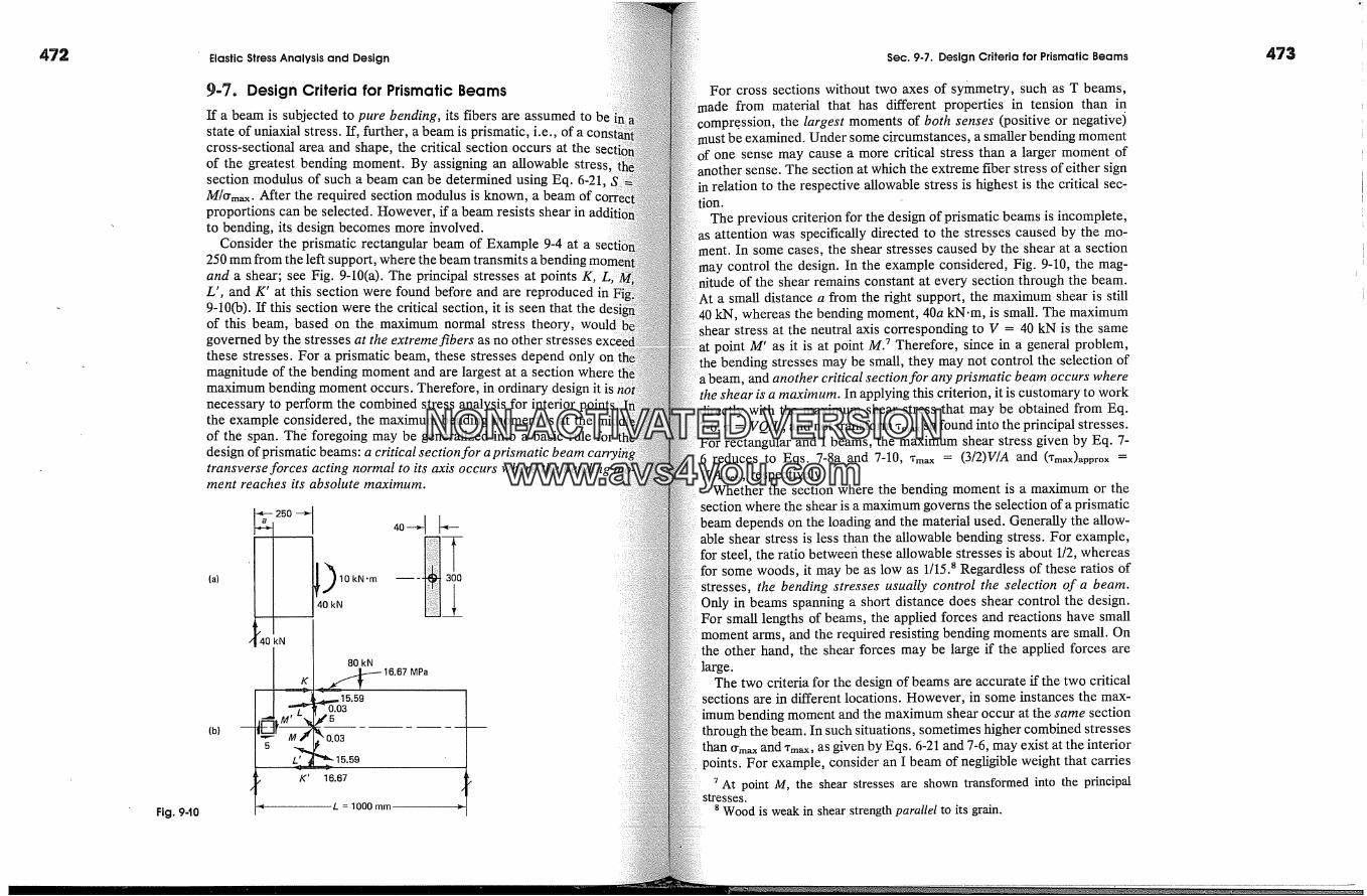
472
Fig. 940
Elastic Stress Analysis and Design
9-'7� Design Criteria for Prismatic BeamsIf a beam is subjected to pure bending, its fibers are assumed to bestate of uniaxial stress. If, further, a beam is prismatic, i.e., of across-sectional area and shape, the critical section occurs at theof the greatest bending moment. By assigning an allowable stress�section modulus of such a beam can be determined using Eq. 6-21,M/�m�. After the required section modulus is known, a beam of,proportions can be selected. However, if a beam resists shear into bending, its design becomes more involved.
Consider the prismatic rectangular beam of Example 9-4 at a250 mm from the left support, where the beam transmits a bendinand a shear; see Fig. 9-10(a). The principal stresses at points K, LL', and K' at this section were found before and are reproduced in9-10(b). If this section were the critical section, it is seen that theof this beam, based on the maximum normal stress theory,governed by the stresses at the extreme fibers as no other stresses,these stresses. For a prismatic beam, these stresses depend only o nmagnitude of the bending moment and are largest at a section wheremaximum bending moment occurs. Therefore, in ordinary design it isnecessary to perform the combined stress analysis for interior �the example considered, the maximum bending moment is at theof the span. Th� foregoing may be generalized into a basic rule fordesign of prismatic beams: a critical section for a ltransverse forces acting normal to its axis occurs where the bendinment reaches its absolute maximum.
(a)
(b)
260
40 kN
5
K'
10kN'm�,0 kN
80 kN
�..� 16.67 MPa
"'"*'"'- 15.59
16.67
L = 1000 mm
Sec. 9.7. Design Criteria for Prismatic Beams
For cross sections without two axes of symmetry, such as T beams,made from material that has different properties in tension than incompre. ssion, the largest moments of both senses (positive or negative)
tst be examined. Under some circumstances, a smaller bending momentof one sense may cause a more critical stress than a larger moment of
sense. The section at which the extreme fiber stress of either signrelation to the respective allowable stress is highest is the critical sec-
The previous criterion for the design of prismatic beams is incomplete,as attention was specifically directed to the stresses caused by the mo-
tent. In some cases, the shear stresses caused by the shear at a sectionmay control the design. In the example considered, Fig. 9-10, the mag-nitude of the shear remains constant at every section through the beam.
At a small distance a from the fight support, the maximum shear is still40 kN, whereas the bending moment, 40a kN.m, is small. The maximumshear stress at the neutral axis corresponding to V = 40 kN is the same
point M' as it is at point M. 7 Therefore, since in a general problem,the bending stresses may be small, they may not control the selection of
and another critical section for any prismatic beam occurs wherethe shear is a maximum. In applying this criterion, it is customary to workdirectly with the maximum shear stress that may be obtained from Eq.
= VQ/It, and not transform *m� SO found into the principal stresses.For rectangular and I beams, the maximum shear stress given by Eq. 7-6 reduces to Eqs. 7-8a and 7-10, *m� = (3/2)V/A and (Tmax)appro x =
respectively.Whether the section where the bending moment is a maximum or the
section where the shear is a maximum governs the selection of a prismaticbeam depends on the loading and the material used. Generally the allow-able shear stress is less than the allowable bending stress. For example,for steel, the ratio betweefi these allowable stresses is about 1/2, whereasfor some woods, it may be as low as 1/15. 8 Regardless of these ratios ofstresses, the bending stresses usually control the selection of a beam.Only in beams spanning a short distance does shear control the design.
small lengths of beams, the applied forces and reactions have smalland the required resisting bending moments are small. On
the other hand, the shear forces may be large if the applied forces arelarge.
The two criteria for the design of beams are accurate if the two criticalsections are in different locations. However, in some instances the max-imum bending moment and the maximum shear occur at the same sectionthrough the beam. In such situations, sometimes higher combined stressesthan O'm� and *m�, as given by Eqs. 6-21 and 7-6, may exist at the interiorpoints. For example, consider an I beam of negligible weight that carries
? At point M, the shear stresses are shown transformed into the principalstresses.
8 Wood is weak in shear strength parallel to its grain.
473
NON-ACTIVATEDVERSIONwww.avs4you.com
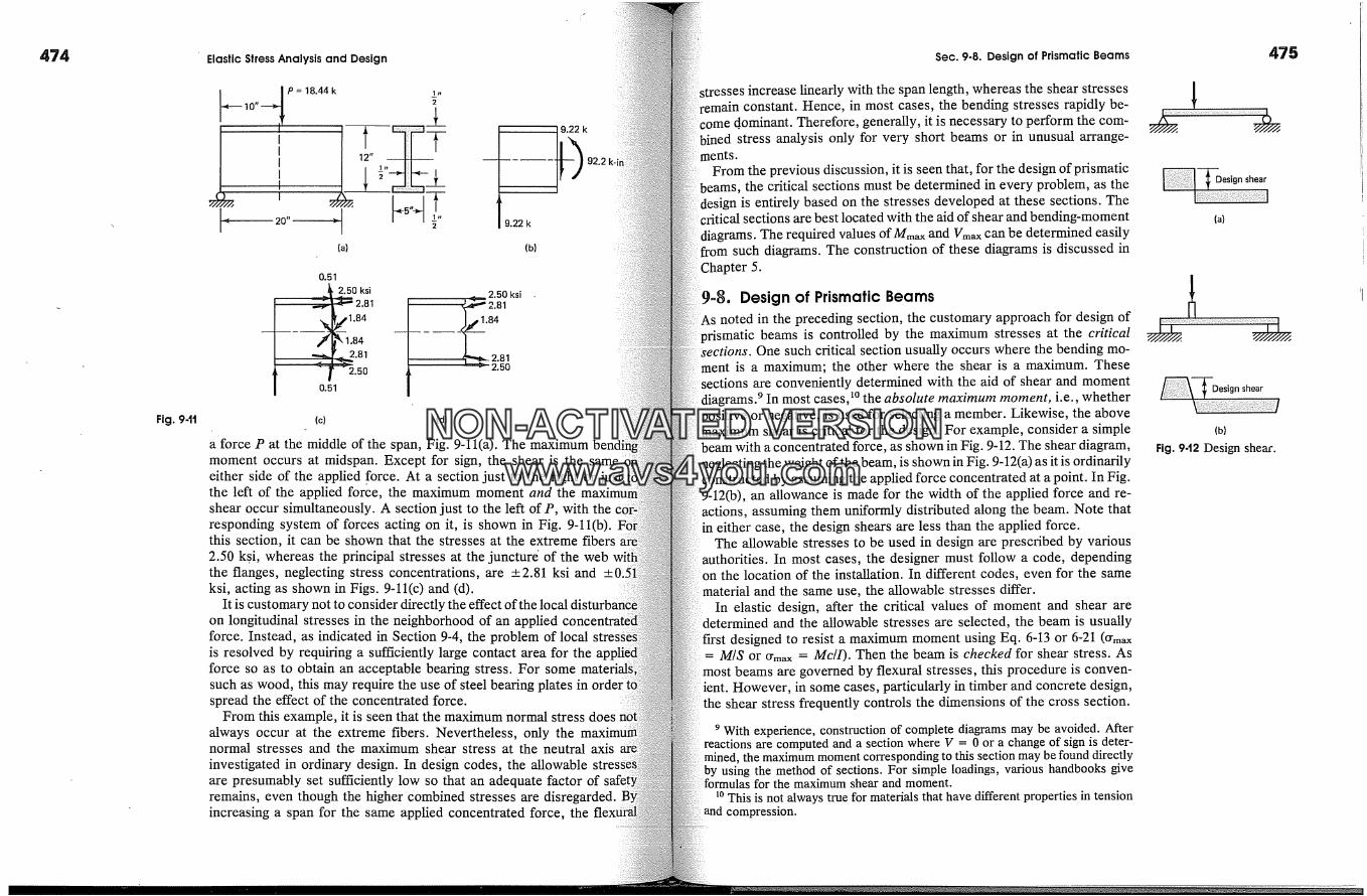
474 Elastic Stress Analysis and Design Sec. 9-8. Design of Prismatic Beams 475
.�__10,,4 P=18.44k1'
20" - 2
(a)
0.51
2.50 ksi
...-r .81
�, 1.84
� _ 2.81
� �.500.5'
9.22 k
(b)
Fig. 9-11 (c) (d)
2.50 ksi�� 2.81
a force P at the middle of the span, Fig. 9-11(a). The maximummoment occurs at midspan. Except for sign, the shear is the sameeither side of the applied force. At a section just to the right orthe left of the applied force, the maximum moment and theshear occur simultaneously. A section just to the left of P, with theresponding system of forces acting on it, is shown in Fig. 9-11(b).this section, it can be shown that the stresses at the extreme2.50 k�i, whereas the principal stresses at the juncturd of the webthe flanges, neglecting stress concentrations, are +2.81 ksi and +0ksi, acting as shown in Figs. 9-11(c) and (d).
It is customary not to consider directly the effect of the localon longitudinal stresses in the neighborhood of an applied cornforce. Instead, as indicated in Section 9-4, the problem of localis resolved by requiring a sufficiently large contact area for theforce so as to obtain an acceptable bearing stress. For somesuch as wood, this may require the use of steel bearing plates inspread the effect of the concentrated force.
From this example, it is seen that the maximum normal stress doesalways occur at the extreme fibers. Nevertheless, only thenormal stresses and the maximum shear stress at the neutral axisinvestigated in ordinary design. In design codes, the allowableare presumably set sufficiently low so that an adequate factor ofremains, even though the higher combined stresses are disregarded.increasing a span for the same applied concentrated force, the
;ses increase linearly with the span length, whereas the shear stresses:emain constant. Hence, in most cases, the bending stresses rapidly be-
come d. ominant. Therefore, generally, it is necessary to perform the com-stress analysis only for very short beams or in unusual arrange-
ments.From the previous discussion, it is seen that, for the design of prismatic
beams, the critical sections must be determined in every problem, as thedesign is entirely based on the stresses developed at these sections. Thecritical sections are best located with the aid of shear and bending-momentdiagrams. The required values of Mm� and Vm�x can be determined easilyfrom such diagrams. The construction of these diagrams is discussed in
5.
9-8. Design of Prismatic Beamsnoted in the preceding section, the customary approach for design of
prismatic beams is controlled by the maximum stresses at the critical;ctions. One such critical section usually occurs where the bending mo-
is a maximum; the other where the shear is a maximum. Thesesections are conveniently determined with the aid of shear and momentdiagrams. 9 In most cases, �� the absolute maximum moment, i.e., whetherpositive or negative, is used for selecting a member. Likewise, the abovemaximum shear is critical for the design. For example, consider a simple
beam with a concentrated force, as shown in Fig. 9-12. The shear diagram,;the weight of the beam, is shown in Fig. 9-12(a) as it is ordinarily
constructed by assuming the applied force concentrated at a point. In Fig.9-12(b), an allowance is made for the width of the applied force and re-actions, assuming them uniformly distributed along the beam. Note thatin either case, the design shears are less than the applied force.
The allowable stresses to be used in design are prescribed by variousauthorities. In most cases, the designer must follow a code, depending
the location of the installation. In different codes, even for the samematerial and the same use, the allowable stresses differ.
In elastic design, after the critical values of moment and shear areand the allowable stresses are selected, the beam is usually
designed to resist a maximum moment using Eq. 6-13 or 6-21 (O'm�= M/S or rrm� = Mc/I). Then the beam is checked for shear stress. As
most beams are governed by flexural stresses, this procedure is conven-ient. However, in some cases, particularly in timber and concrete design,
shear stress frequently controls the dimensions of the cross section.
9 With experience, construction of complete diagrams may be avoided. Afterreactions are computed and a section where V = 0 or a change of sign is deter-mined, the maximum moment corresponding to this section may be found directlyby using the method of sections. For simple loadings, various handbooks give
for the maximum shear and moment.�0 This is not always true for materials that have different properties in tension
and compression.
Design shear
(a)
Design shear
(b)
Fig. 9-12 Design shear.NON-ACTIVATEDVERSION
www.avs4you.com
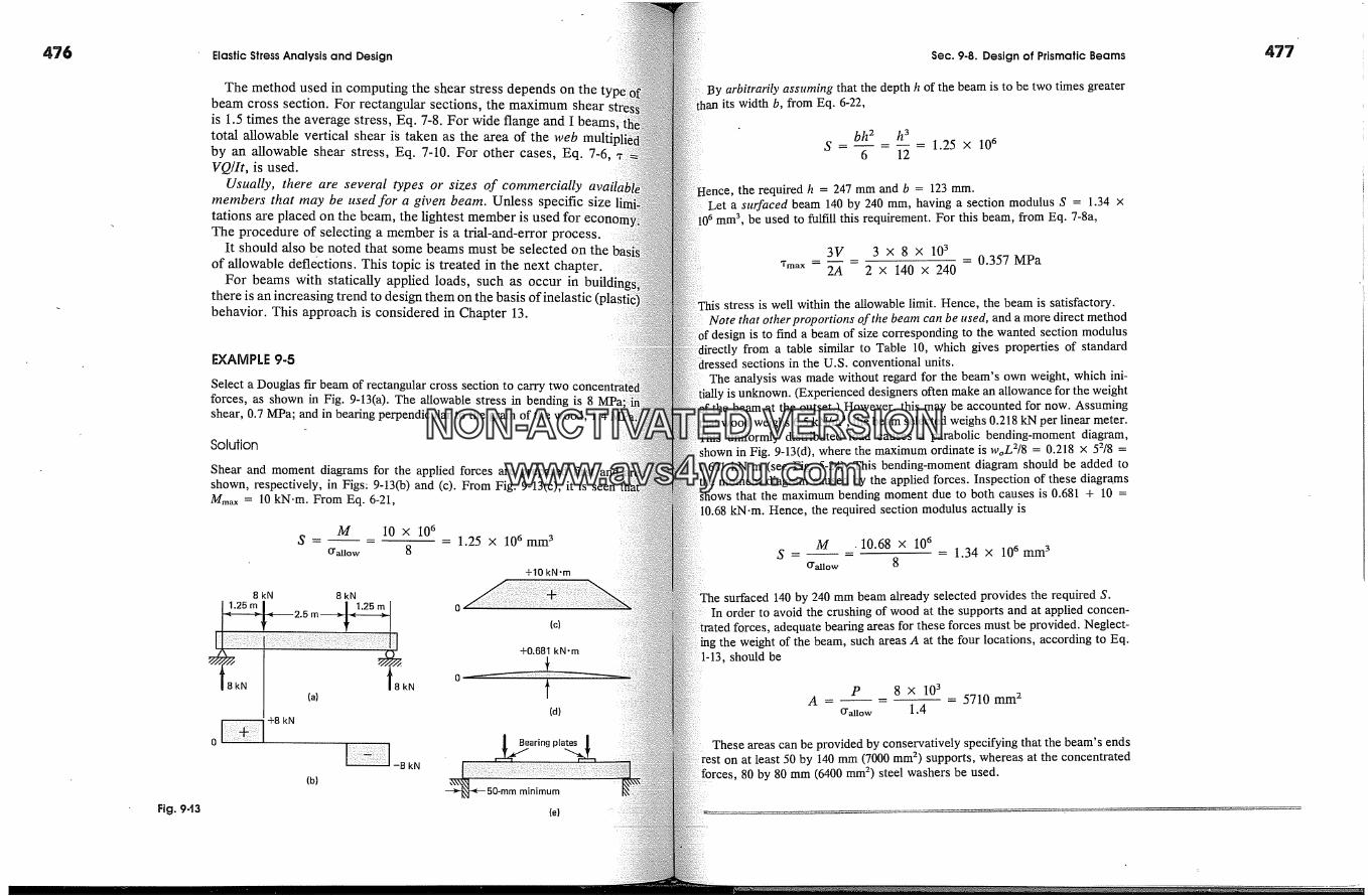
476 Elastic Stress Analysis and Design Sec. 9-8. Design of Prismatic Beams 477
The method used in computing the shear stress depends on thebeam cross section. For rectangular sections, the maximum shearis 1.5 times the average stress, Eq. 7-8. For wide flange and I beamsitotal allowable vertical shear ig taken as the area of the webby an allowable shear stress, Eq. %10. For other cases, Eq. 7~6,VQ/It, is used.
Usually, there are several types or sizes of commerciallymembers that may be used for a given beam. Unless specific sizetations are placed on the beam, the lightest member is used for ectThe procedure of selecting a member is a trial-and-error process.
It should also be noted that some beams must be selected on theof allowable defldctions. This topic is treated in the next chapter.
For beams with statically applied loads, such as occur in builthere is an increasing trend to design them on the basis of inelasticbehavior. This approach is considered in Chapter 13.
EXAMPLE 9-5
Select a Douglas fir beam of rectangular cross section to carry twoforces, as shown in Fig. 9-13(a). The allowable stress in bending is 8shear, 0.7 MPa; and in bearing perpendicular to the grain of the wood, 1.4
Solution
Shear and moment diagrams for the applied forces are prepared first and ishown, respectively, in Figs: 9-13(b) and (c). From Fig. 9-13(c), it isMm� = 10 kN.m. From Eq. 6-21,
M 10 x 106S = - - 1.25 x 10 amm 3
�allow 8
+10 kN 'm
8 kN 8 kN
� '25m�--I' 2�m I o
okN
-- -B kN
(b)
(c)
+0.681 kN-m
(d)
Bearing plates
minimum
By arbitrarily assutning that the depth h of the beam is to be two times greaterits width b, from Eq. 6-22,
bh 2 h 3=--= 1.25 x 10⁶
6 12
the required h = 247 mm and b = 123 mm.Let a staraced beam 140 by 240 mm, having a section modulus S = 1.34 x
106 mm 3, be used to fulfill this requirement. For this beam, from Eq. 7-8a,
3V 3 X 8 X 103- = 0.357 MPa
*m� - 2A 2 x 140 x 240
stress is well within the allowable limit. Hence, the beam is satisfactory.Note that other proportions of the beam can be used, and a more direct method
is to find a beam of size corresponding to the wanted section modulusfrom a table similar to Table 10, which gives properties of standard
:ssed sections in the U.S. conventional units.The analysis was made without regard for the beam's own weight, which ini-
tially is unknown. (Experienced designers often make an allowance for the weightof the beam at the outset.) However, this may be accounted for now. Assuming
that wood weighs 6.5 kN/m 3, the beam selected weighs 0.218 kN per linear meter.This uniformly distributed load causes a parabolic bending-moment diagram,
in Fig. 9-13(d), where the maximum ordinate is woL2[8 = 0.218 x 52/8 =0.681 kN-m (see Fig. 5-24). This bending-moment diagram should be added to
moment diagram caused by the applied forces. Inspection of these diagramsthat the maximum bending moment due to both causes is 0.681 + 10 =
�.68 kN.m. Hence, the required section modulus actually is
M .10.68 x 106S - = 1.34 x 106 mm 3
O'allo w 8
surfaced 140 by 240 mm beam already selected provides the required S.In order to avoid the crushing of wood at the supports and at applied coneen-
forces, adequate bearing areas for these forces must be provided. Neglect-ing the weight of the beam, such areas A at the four locations, according to Eq.1-13, should be
P 8 x 10³A 5710 mm 2
tral�o,� 1.4
These areas can be provided by conservatively specifying that the beam's endson at least 50 by 140 mm (7000 mm 2) supports, whereas at the concentrated
80 by 80 mm (6400 mm 2) steel washers be used.
Fig. 9-'13 (e) ........... ,--�=
NON-ACTIVATEDVERSIONwww.avs4you.com

478
Fig. 9-14
k
(a)
(b)
Fig. 9-t5
Elastic Stress Analysis and Design
2 k/ft
A
6.4 k 25.6 k
(a)
+10.24 k-ft
0
+6,4 k+12.0 k
0 -36
� (c)-13,6 k
(b)
EXAMPLE 9-6
Select an I beam or a wide-flange steel beam to support the load shown in9-14(a). For the beam, creator, = 24 ksi' and *�uo�, = 14.5 ksi.
Solution
The shear and the bending-moment diagrams for the loaded beam are shownFigs. 9-14(b) and (c), respectively. The maximum moment is 36 k-ft. From6-21,
36 x 12S = - 18.0 in 3
24
Examination of Tables 3 and 4 in the Appendix shows that this requirement fa section modulus is met by a 10-in S section weighing 24.7 lb/ft (S = I/c =in3). However, a lighter 8-in wide-flange W section weighing 24 lb/ft (S =in 3) also is adequate. Therefore, for reasons of economy, the lighter W8section will be used. The beam weight is small in comparison with theloads and will be neglected in calculations.
From Fig. 9-14(b), Vm� = 13.6 kips. Hence, from Eq. 7-10,
V 13.6(Tmax)approx .... 7.00 ksiA,�eb 0.245 x 7.93
This stress is below the allowable value, and the selected beam isAt the supports or concentrated forces, S and wide-flange beams
checked for crippling of the webs. This phenomenon is illustrated at theof Fig. 9-15(a). Crippling of the webs is more critical for members with thinthan direct bearing of the flanges, which may be investigated as in theexample. To preclude crippling, a design rule is specified by the AISC. It
Sec. 9-8. Design of Prismatic Beams
the direct stress on area, (a + k)t at the ends and (a� + 2k)t at the interiormust not exceed 0.750'yp. In these expressions, a and a� are the respective
s of beating of the applied forces at exterior or interior portions of a beam,Fig. 9-1](b), t is the thickness of the web, and k is the distance from the outer
of a flange to the toe of the web Eftlet. The values of k and t are tabulatedmanufacturers' catalogues.
For this example, assuming gyp = 36 ksi, the minimum widths of the supports,to the rule, are as follows:
support A:
27(a + k)t = 6.4 ora = 0.09 in
support B:
27(al + 2k)t = 25.6 oral = 2.12 in
27(a + 7/8) x 0.245 = 6.4
27(a� + 2 x 7/8) x 0.245 = 25.6
requirements can easily be met in an actual case.
479
The preceding two examples illustrate the design of beams whose crosshave two axes of symmetry. In both cases, the bending moments
the design, and, since this is usually true, it is significant towhich members are efficient in flexure. A concentration of as much
material as possible away from the neutral axis results in the best sectionsresisting flexure, Fig. 9-16(a). Material concentrated near the outside
works at a high stress. For this reason, I-type sections, which ap-proximate this requirement, are widely used in practice.
The previous statements apply for materials having nearly equal prop-in tension and compiession. If this is not the case, a deliberate shiftneutral axis from the midheight position is desirable. This accounts
wide use oft and channel sections for such materials (see Example6-5).
Finally, two other items warrant particular attention in the design ofbeams. In many cases, the loads for which abeam is designed are transient
character. They may be placed on the beam all at once, piecemeal, orlocations. The loads, which are not a part of the "dead weight"
structure itself, are called live loads. They must be so placed as tothe highest possible stresses in a beam. In many cases, the place-
ment may be determined by inspection. For example, in a simple beama single moving load, the placement of the load at midspan causes
largest bending moment, whereas placing the same load very near tocauses the greatest shear. For most building work, the live load,
supposedly provides for the most severe expected loading condi-is specified in building codes on the basis of a load per unit floorMultiplying this live load by the spacing of parallel beams gives the
()
(a) (b)
Fig. 9-t6 (a) Efficient and (b)inefficient sections forflexure.
NON-ACTIVATEDVERSIONwww.avs4you.com
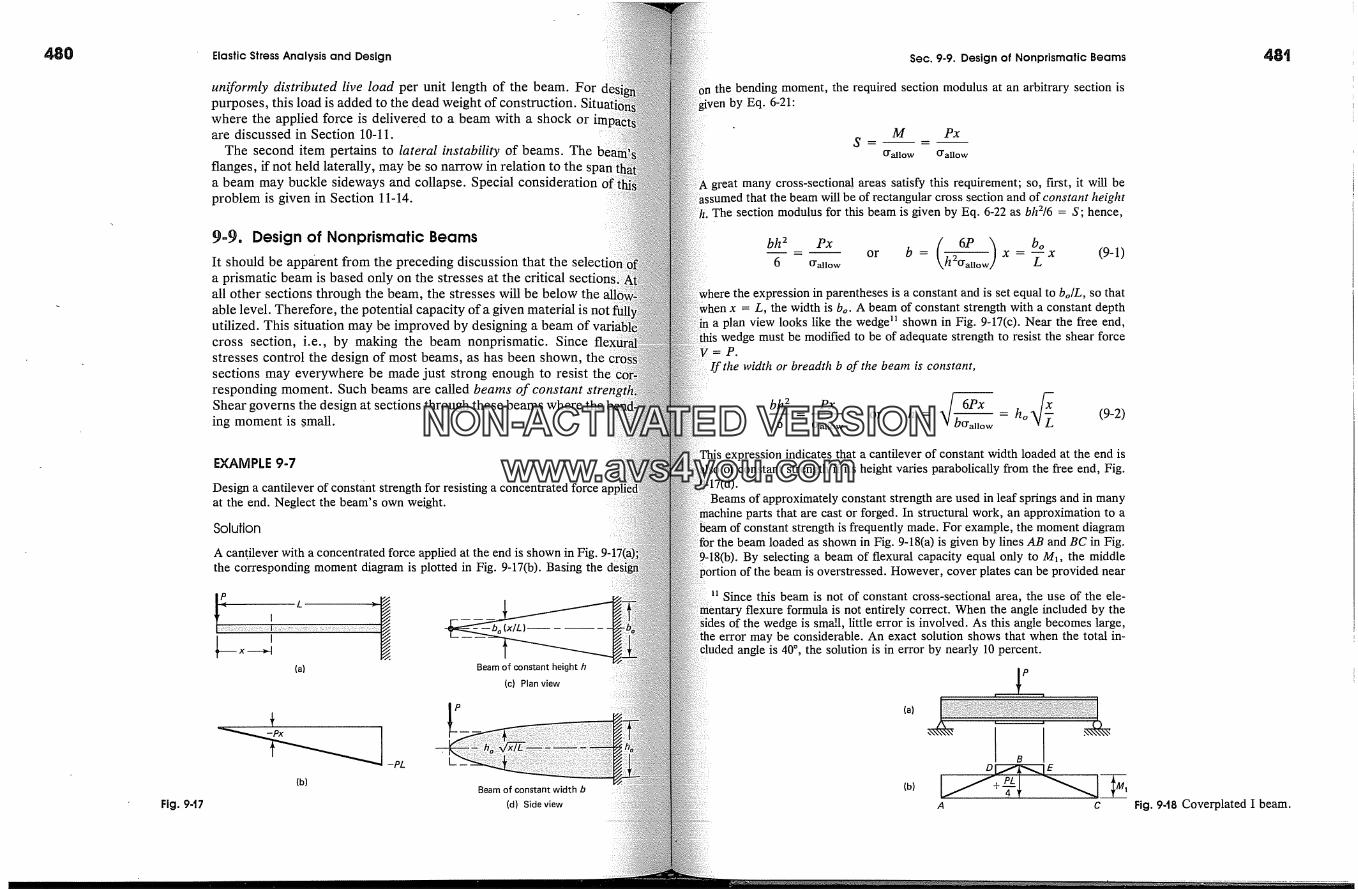
48O
Fig. 9-17
Elastic Stress Analysis and Design
uniformly distributed live load per unit length of the beam. Forpurposes, this load is added to the dead weight of construction.where the applied force is delivered to a beam with a shock orare discussed in Section 10-11.
The second item pertains to lateral instability of beams. Theflanges, if not held laterally, may be so narrow in relation to thea beam may buckle sideways and collapse. Special consideration,problem is given in Section 11-14.
9-9. Design of Nonprismatic BeamsIt should be apparent from the preceding discussion that the sole.a prismatic beam is based only on the stresses at the criticalall other sections through the beam, the stresses will be below theable level. Therefore, the potential capacity of a given material is not:utilized. This situation may be improved by designing a beam ofcross section, i.e., by making the beam nonprismatic. Sincestresses control the design of most beams, as has been shown, thesections may everywhere be made just strong enough to resist theresponding moment. Such beams are called beams of constant strohShear governs the design at sections through these beams where the b�ing moment is .small.
EXAMPLE 9-7
Design a cantilever of constant strength for resistingat the end. Neglect the beam's own weight.
Solution
A cantilever with a concentrated force applied at the end is shown in Fig.the corresponding moment diagram is plotted in Fig. 9-17(b). Basing the
(x/L) m
(a) Beam of constant height h(c) Plan view
-PL L(b)
Beam of constant width b
(d) Side view
Sec. 9-9. Design of Nonprismatic Beams
the bending moment, the required section modulus at an arbitrary section isby Eq. 6-21:
M Px
O'allow CTallow
great many cross-sectional areas satisfy this requirement; so, first, it will bethat the beam will be of rectangular cross section and of constant height
The section modulus for this beam is given by Eq. 6-22 as bh2/6 = S; hence,
----- or b = 2�nan x =�-x (9-1)the expression in parentheses is a constant and is set equal to bo/L, so that
= L, the width is bo. A beam of constant strength with a constant deptha plan view looks like the wedge u shown in Fig. 9-17(c). Near the free end,
wedge must be modified to be of adequate strength to resist the shear forcem P.
If the width or breadth b of the beam is constant,
bh2 Px �f 6Px �- -- or h = - h o (9-2)6 Crylow � bg'allow
This expression indicates that a cantilever of constant width loaded at the end isalso of constant strength ff its height varies parabolically from the free end, Fig.
Beams of approximately constant strength are used in leaf springs and in manyparts that are cast or forged. In structural work, an approximation to a
beam of constant strength is frequently made. For example, the moment diagramthe beam loaded as shown in Fig. 9-18(a) is given by lines AB and BC in Fig.
-18(b). By selecting a beam of flexural capacity equal only to M�, the middle'the beam is overstressed. However, cover plates can be provided near
Since this beam is not of constant cross-sectional area, the use of the ele-flexure formula is not entirely correct. When the angle included by the
of the wedge is small, little error is involved. As this angle becomes large,error may be considerable. An exact solution shows that when the total in-
angie is 40 �, the solution is in error by nearly 10 percent.
(a)
(b)
I BD--
Fig. 948 Coverplated I beam.
NON-ACTIVATEDVERSIONwww.avs4you.com
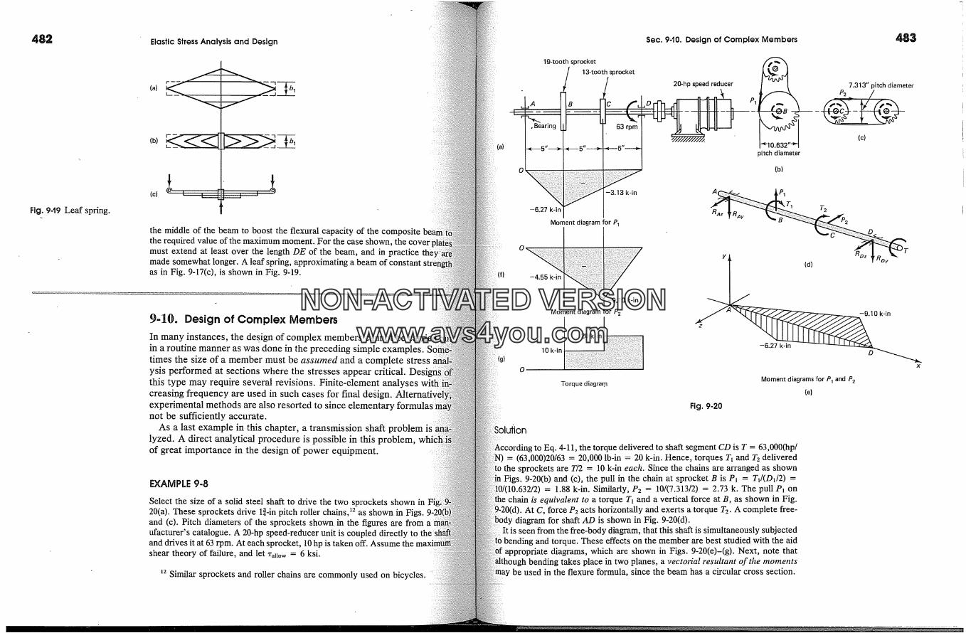
482 Elastic Stress Analysis and Design Sec. 9-t0. Design of Complex Members
Fig. 9-t9 Leaf spring.
(b)
(c)
the middle of the beam to boost the flexural capacity of the compositethe required value of the maximum moment. For the case shown, the cover imust extend at least over the length DE of the beam, and in practicemade somewhat longer. A leaf spring, approximating a beam of constantas in Fig. 9-17(c), is shown in Fig. 9-19.
9-10. Design of Complex MembersIn many instances, the design of complex members cannot be carriedin a routine manner as was done in the preceding simple examples.times the size of a member must be assumed and a complete stressysis performed at sections where the stresses appear critical. Desithis type may require several revisions. Finite-element analysescreasing frequency are used in such cases for final design.experimental methods are also resorted to since elementai3not be sufficiently accurate.
As a last example in this chapter, a transmission shaft problem 'lyzed. A direct analytical procedure is possible in this problem,of great importance in the design of power equipment.
F. XAM PLE 9-8
Select the size of a solid steel shaft to drive the two sprockets shown in20(a). These sprockets drive l{-in pitch roller chains, �2 as shown in Figs.and (c). Pitch diameters of the sprockets shown in the figures are fromufacturer's catalogue. A 20-hp speed-reducer unit is coupled directly toand drives it at 63 rpm. At each sprocket, 10 hp is taken off. Assume theshear theory of failure, and let x�atow = 6 ksi.
�2 Similar sprockets and roller chains are commonly used on bicycles.
1g-tooth sprocket13-tooth sprocket
20-hp speed reducerP2
7.313" pitch diameter
0
-3.13 k-in
-6.27 k-in
Moment diagram for P1
A
pitch diameter
(b)
(c)
-4.55 k-in
-9.10 k-in
Moment diagram forP 2
20 k-in
10 k-in
Torque diagra .m
Y� (d) ov-6.27 k-in
x
Moment diagrams for P1 and P2
(e)
Fig. 9-20
to Eq. 4-11, the torque delivered to shaft segment CD is T = 63,000(hp/= (63,000)20/63 = 20,000 lb-in = 20 k-in. Hence, torques T� and T2 delivered
the sprockets are T/2 = 10 k-in each. Since the chains are arranged as shownFigs. 9-20(b) and (c), the pull in the chain at sprocket B is P� = T�/(D1/2) =
= 1.88 k-in. Similarly, P2 = 10/(7.313/2) = 2.73 k. The pull P� onis equivalent to a torque T� and a vertical force at B, as shown in Fig.
At C, force P2 acts horizontally and exerts a torque T2. A complete free-diagram for shaft AD is shown in Fig. 9-20(d).
It is seen from the free-body diagram, that this shaft is simultaneously subjectedand torque. These effects on the member are best studied with the aid
appropriate diagrams, which are shown in Figs. 9~20(e)-(g). Next, note thatbending takes place in two planes, a vectorial resultant of the moments
be used in the flexure formula, since the beam has a circular cross section.
NON-ACTIVATEDVERSIONwww.avs4you.com
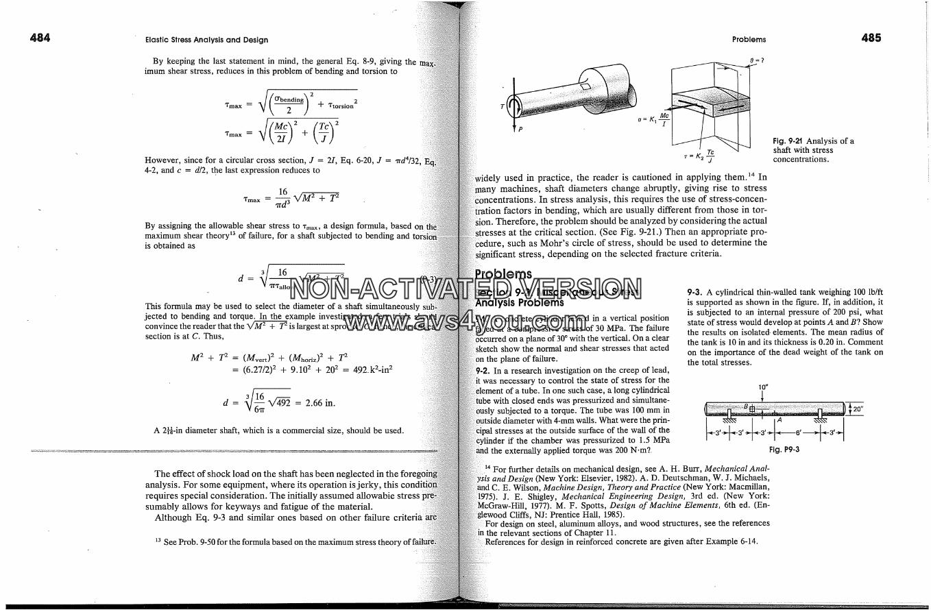
484 Elastic Stress Analysis and Design
By keeping the last statement in mind, the general Eq. 8-9, giving theimum shear stress, reduces in this problem of bending and torsion to
be ding q_ Tt�rsi�n 2
57 +
However, since for a circular cross section, J = 21, Eq. 6-20, J = 'rrdn/3Z4-2, and c = d/2, the last expression reduces to
16_ __ X/M 2 + T 2
�rd 3
By assigning the allowable shear stress to *m�, a design formula, based ontmaximum shear theory n of failure, for a shaft subjected to bending andis obtained as
'�I 16 T2d = �owVU2 +This formula may be used to select the diameter of a shaft simultaneously
jected to bending and torque. In the example investigated, a few trialsconvince the reader that the � + T 2 is largest at sprocket C; hence, thesection is at C. Thus,
M 2 + T 2 = (Mvert) 2 + (Mhoriz) 2 q- T 2= (6.27/2) 2 + 9.102 + 202 = 492.k2~in 2
�16d = �-� X/q� = 2.66 in.A 2�-in diameter shaft, which is a commercial size, should be used.
The effect of shock load on the shaft has been neglectedanalysis. For some equipment, where its operation is jerky, thisrequires special consideration. The initially assumed allowabie stresssumably allows for keyways and fatigue of the material.
Although Eq. 9-3 and similar ones based on other failure
�3 See Prob. 9-50 for the formula based on the maximum
Problems
0=?
485
Mc
o=
used in practice, the reader is cautioned in applying them. �4 Inmachines, shaft diameters change abruptly, giving rise to stress
:entrations. In stress analysis, this requires the use of stress~concen-factors in bending, which are usually different from those in tor-
Therefore, the problem should be analyzed by considering the actual.,sses at the critical section. (See Fig. 9-21.) Then an appropriate pro-
:edure, such as Mohr's circle of stress, should be used to determine theant stress, depending on the selected fracture criteria.
roblems
0-2. Miscellaneous StressProblems
M. A concrete cylinder tested in a vertical positionat a compressive stress of 30 MPa. The failure
Occurred on a plane of 30 � with the vertical. On a clearshow the normal and shear stresses that acted
the plane of failure.9-2. In a research investigation on the creep of lead,
necessary to control the state of stress for theof a tube. In one such case, a long cylindrical
closed ends was pressurized and simultane-tsly subjected to a torque. The tube was 100 mm in
� with 4-mm walls. What were the prin-at the outside surface of the wall of the
if the chamber was pressurized to 1.5 MPathe externally applied torque was 200 N-m?.
�4 For further details on mechanical design, see A. H. Burr, Mechanical Anal-and Design (New York: Elsevier, 1982). A. D. Deutschman, W. J. Michaels,C. E. Wilson, Machine Design, Theory and Practice (New York: Macmillan,
J. E. Shigley, Mechanical Engineering Design, 3rd ed. (New York:McGraw-Hill, 1977). M. F. Spotts, Design of Machine Elements, 6th ed. (En-
Cliffs, NJ: Prentice Hall, 1985).design on steel, aluminum alloys, and wood structures, see the referencesrelevant sections of Chapter 11.
References for design in reinforced concrete are given after Example 6-14.
Fig. 9-2t Analysis of ashaft with stressconcentrations.
9-3. A cylindrical thin-walled tank weighing 100 lb/ftis supported as shown in the figure. If, in addition, itis subjected to an internal pressure of 200 psi, whatstate of stress would develop at points A and B? Showthe results on isolated-elements. The mean radius ofthe tank is 10 in and its thickness is 0.20 in. Comment
on the importance of the dead weight of the tank onthe total stresses.
AI'*j� 8'-�3'�Fig. P9-3
20"
NON-ACTIVATEDVERSIONwww.avs4you.com
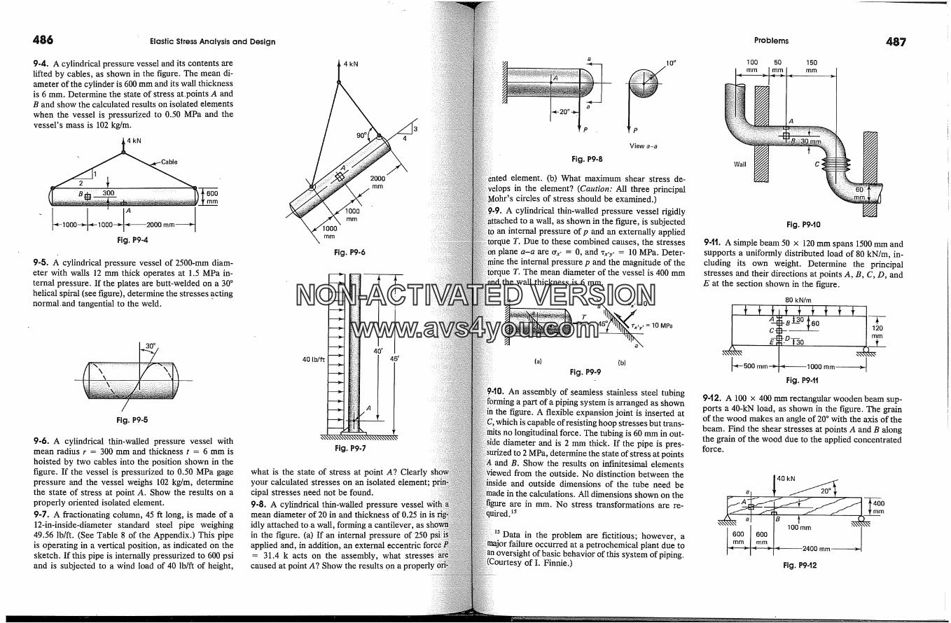
486 Elastic Stress Analysis and Design
9-4. A cylindrical pressure vessel and its contents arelifted by cables, as shown in the figure. The mean di-ameter of the cylinder is 600 mm and its wall thicknessis 6 mm. Determine the state of stress at.points A andB and show the calculated results on isolated elementswhen the vessel is pressurized to 0.50 MPa and thevessel's mass is 102 kg/m.
4kN
2
300
L1000-�10C )4 2000mm -Fig. P9-4
600mm
9-5. A cylindrical pressure vessel of 2500-mm diam-eter with walls 12 mm thick operates at 1.5 MPa in-ternal pressure. If the plates are butt-welded on a 30 �helical spiral (see figure), determine the stresses _actingnorma[ and tangential to the weld.
4kN
90 �
2000mm
lOOOmm
� ooomm
Fig. P9-6
40'40 lb/h: 45'
Fig. P9-5
9-6. A cylindrical thin-walled pressure vessel withmean radius r = 300 mm and thickness t = 6 mm is
hoisted by two cables into the position shown in thefigure. If the vessel is pressurized to 0.50 MPa gagepressure and the vessel weighs 102 kg/m, determinethe state of stress at point A. Show the results on aproperly oriented isolated element.9-7. A fractionating column, 45 ft long, is made of a12-in-inside-diameter standard steel pipe weighing
49.56 lb/ft. (See Table 8 of the Appendix.) This pipeis operating in a vertical position, as indicated on thesketch. If this pipe is internally pressurized to 600 psiand is subjected to a wind load of 40 lb/ft of height,
Fig. P9-7
what is the state of stress at point A? Clearlyyour calculated stresses on an isolated elementcipal stresses need not be found.9-8. A cylindrical thin-wailed pressure vesselmean diameter of 20 in and thickness of 0.25 inidly attached to.a wall, forming a cantilever, asin the figure. (a) If an internal pressure of 250applied and, in addition, an= 31.4 k acts on the assembly, what
caused at point A? Show the results on a
Fig. P9-8
10"
View a-a
element. (b) What maximum shear stress de-�s in the element? (Caution: All three principal
circles of stress should be examined.)A cylindrical thin-walled pressure vessel rigidly
a wall, as shown in the figure, is subjectedan internal pressure of p and an externally applied
T. Due to these combined causes, the stressesa-a are or.,, = 0, and x. vy, = 10 MPa. Deter-
the internal pressure p and the magnitude of theae T. The mean diameter of the vessel is 400 mm
thickness is 6 mm.
4��y, =10MPa(a) (b)
Fig. P9-9
An assembly of seamless stainless steel tubingpart of a piping system is arranged as shown
figure. A flexible expansion joint is inserted atwhich is capable of resisting hoop stresses but trans-
no longitudinal force. The tubing is 60 mm in out-diameter and is 2 mm thick. If the pipe is pres-
to 2 MPa, determine the state of stress at pointsB. Show the results on infinitesimal elements
from the outside. No distinction between theinside and outside dimensions of the tube need bemade in the calculations. All dimensions shown on the
are in mm. No stress transformations are re-15
Data in the problem are fictitious; however, aor failure occurred at a petrochemical plant due to
of this system of piping.of I. Finnie.)
Problems 487
100 50 150mm
A
C-
-<--500 mm--�
Fig. P9-10
9-1t. A simple beam 50 x 120 mm spans 1500 mm andsupports a uniformly distributed load of 80 kN/m, in-cluding its own weight. Determine the principalstresses and their directions at points A, B, C, D, and
E at the section shown in the figure.80 kN/m
-B -7--- T I 120
"O-�o �__�'� 1000 mm �
Fig. P941
9-12. A 100 x 400 mm rectangular wooden beam sup-ports a 40-kN load, as shown in the figure. The grainof the wood makes an angle of 20 � with the axis of thebeam. Find the shear stresses at points A and B alongthe grain of the wood due to the applied concentratedforce.
r 600 600�rnrn_ I mm
40 kN
'� 2400mm �Fig. P9-12
NON-ACTIVATEDVERSIONwww.avs4you.com
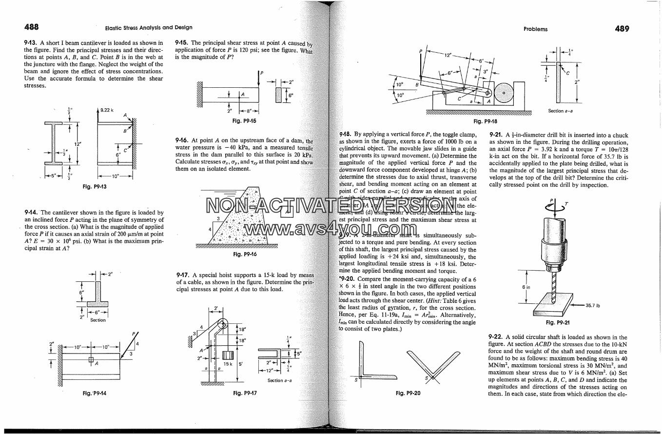
Elastic Stress Analysis and Design
943. A short I beam cantilever is loaded as shown inthe figure. Find the principal stresses and their direc-tions at points A, B, and C. Point B is in the web atthe juncture with the flange. Neglect the weight of thebeam and ignore the effect of stress concentrations.Use the accurate formula to determine the shearstresses.
9.22 kA
1 c /
Fig. P943
944. 'The cantilever shown in the figure is Ioafied byan inclined force P acting in the plane of symmetry ofthe cross section. (a) What is the magnitude of appliedforce P if it causes an axial strain of 200 p,m/m at pointA? E = 30 x 106 psi. (b) What is the maximum prin-cipal strain at A?
945. The principal shear stress at point Aapplication of force P is 120 psi; see the figure.is the magnitude of P?
PFig. P9-15
946. At point A on the upstream face of awater pressure is -40 kPa, and a measuredstress in the dam parallel to this surface is 20Calculate stresses trx, try, and ** at that �them on an isolated element.
A
4 3
Fig. P9-t6
947. A special hoist supports a 15-k load byof a cable, as shown in the figure. Determine thecipal stresses at point A due to this load.
Section
2" � 10" 10" 4
FIg.'P9-t4
Section a-a
Fig. P9-17
Fig. P9-18
By applying a vertical force P, the toggle clamp,shown in the figure, exerts a force of 1000 lb on a
object. The movable jaw slides in a guideprevents its upward movement. (a) Determine the
of the applied vertical force P and thedeveloped at hinge A; (b)
the stresses due to axial thrust, transverseand bending moment acting on an element at
C of section a-a; (c) draw an element at point'with sides parallel and perpendicular to the axis of
and show the stresses acting on the ele-and (d) using Mohr's circle, determine the larg-
principal stress and the maximum shear stress at
A 2~in-diameter shaft is simultaneously sub-to a torque and pure bending. At every section
the largest principal stress caused by theloading is +24 ksi and, simultaneously, the
longitudinal tensile stress is + 18 ksi. Deter-the applied bending moment and torque.
Compare the moment-carrying capacity of a 6<6 x � in steel angle in the two different positions
the figure. In both cases, the applied verticalacts through the shear center. (Hint: Table 6 gives
the least radius of gyration, r, for the cross section.per Eq. 11-19a, Imin = Ar2mi,. Alternatively,
can be calculated directly by considering the angleconsist of two plates.)
Fig. P9-20
Problems 489
Section a-a
9-2t. A �-in-diameter drill bit is inserted into a chuckas shown in the figure. Duri ng the drilling operation,an axial force P = 3.92 k and a torque T = 10�r/128k-in act on the bit. If a horizontal force of 35.7 lb isaccidentally applied to the plate being drilled, what isthe magnitude of the largest principal stress that de-velops at the top of the drill bit? Determine the criti-cally stressed point on the drill by inspection.
PT
6 in
Fig. P9-2t
9-22. A solid circular shaft is loaded as shown in thefigure. At section ACBD the stresses due to the 10-kNforce and the weight of the shaft and round drum arefound to be as follows: maximum bending stress is 40MN/m 2, maximum torsional stress is 30 MN/m 2, andmaximum shear stress due to V is 6 MN/m 2. (a) Setup elements at points A, B, C, and D and indicate themagnitudes and directions of the stresses acting onthem. In each case, state from which direction the ele-
NON-ACTIVATEDVERSIONwww.avs4you.com
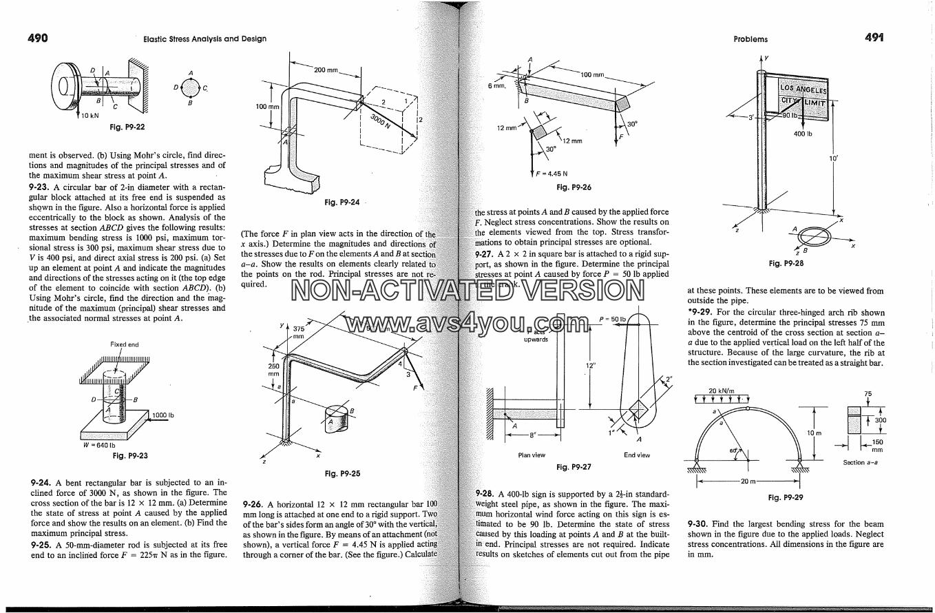
490 Elastic Stress Analysis and Design Problems
Fig. P9-22
ment is observed. (b) Using Mohr's circle, find direc-tions and magnitudes of the principal stresses and ofthe maximum shear stress at point A.9-23. A circular bar of 2-in diameter with a rectan-gular block attached at its free end is suspended asshqwn in the figure. Also a horizontal force is appliedeccentrically to the block as shown. Analysis of thestresses at section ABCD gives the following results:maximum bending stress is 1000 psi, maximum tor-sional stress is 300 psi, maximum shear stress due toV is 400 psi, and direct axial stress is 200 psi. (a) Setup an element at point A and indicate the magnitudesand directions of the stresses acting on it (the top edgeof the element to coincide with section ABCD). (b)Using Mohr's circle, find the direction and the inag-nitude of the maximum (principal) shear stresses andthe associated normal stresses at point A.
200 mm
100 mm2 1 ?
iii
Fig. P9-24 �
(The force F in plan view acts in the directionx axis.) Determine the magnitudes and directthe stresses due to F on the elements A and B ata-a. Show the results on elements clearlythe points .on the rod. Principal stresses arequired.
500 mm
Fixed end
250mm
B
1000 lb
14/= 640 lb
Fig. P9-23
9-24. A bent rectangular bar is subjected to an in-clined force of 3000 N, as shown in the figure. Thecross section of the bar is 12 x 12 mm. (a) Determinethe state of stress at point A caused by the appliedforce and show the results on an element. (b) Find themaximum principal stress.9-25. A 50-mm-diameter rod is subjected at its freeend to an inclined force F = 225�r N as in the figure.
x
Fig. P9-25
9-26. A horizontal 12 x 12 mm rectangularmm long is attached at one end to a rigid support.of the bar's sides form an angle of 30 � withas shown in the figure. By means of an attachmentshown), a vertical force F = 4.45 N is appliedthrough a coruer of the bar. (See the figure.)
6 min.
100 mm
mm�k
'12�12 mm� F = 4.45 N
Fig. P9-26
30 �
stress at points A and B caused by the applied forceNeglect stress concentrations. Show the results on
elements viewed from the top. Stress transfor-to obtain principal stresses are optional.
A 2 x 2 in square bar is attached to a rigid sup-as shown in the figure. Determine the principal
at point A caused by force P = 50 lb appliedthe crank.
P actsupwards
Plan view
400 lb
Fig. P9-28
at these points. These elements are to be viewed fromoutside the pipe.
501� '9-29.Forthecircularthree-hingedarchribshown�= inthefigure,determinetheprincipalstresses75mmabove the centroid of the cross section at section a-a due to the applied ve.rtical load on the left half of thestructure. Because of the large curvature, the rib at
l[z' thesectioninvestigatedcanbetreatedasastraightbar.20 kN/m
tttttt't
mmEnd view
A 400-lb sign is supported by a 2�-in standard-steel pipe, as shown in the figure. The maxi-
horizontal wind force acting on this sign is es-to be 90 lb. Determine the state of stress
by this loading at points A and B at the built-Principal stresses are not required. Indicate
on sketches of elements cut out from the pipe
Fig. P9-29
9-30. Find the largest bending stress for the beamshown in the figure due to the applied loads. Neglectstress concentrations. All dimensions in the figure arein mm.
NON-ACTIVATEDVERSIONwww.avs4you.com
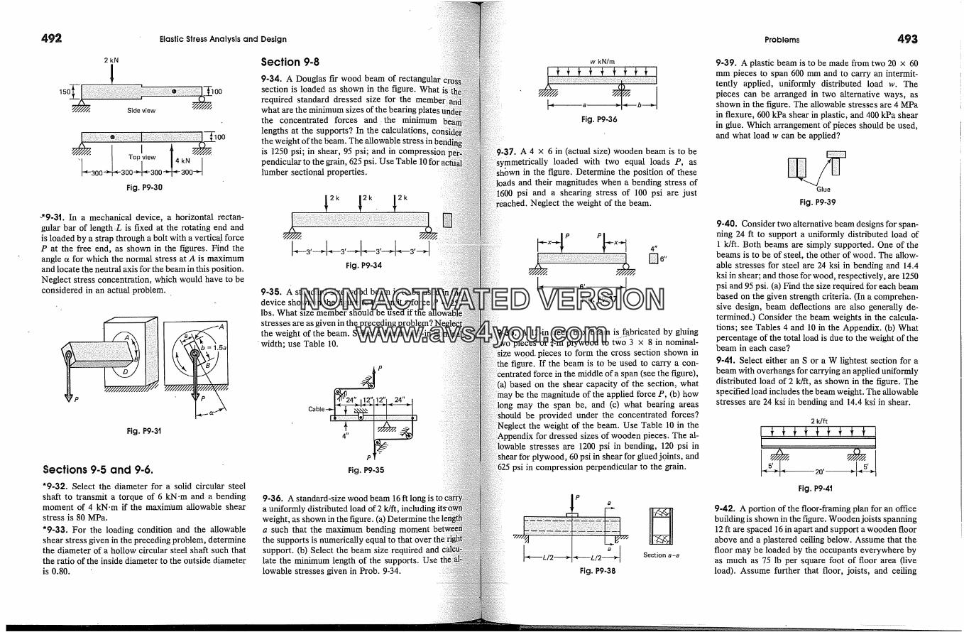
492 Elastic Stress Analysis and Design Problems 493
2kN
Side view
.k� 00opvlew �4kN �
ooJooJ:oolFig. P9-30
-'9-31. In a mechanical device, a horizontal rectan-gular bar of length-L is fixed at the rotating end andis loaded by a strap through a bolt with a vertical forceP at the free end, as shown in the figures. Find theangle c� for which the normal stress at A is maximumand locate the neutral axis for the beam in this position.Neglect stress concentration, which would have to beconsidered in an actual problem.
tp
\b = 1.5�
Fig. P9-3t
Sections 9.5 and 9-6.
'9-32. Select the diameter for a solid circular steelshaft to transmit a torque of 6 kN.m and a bendingmoment of 4 kN.m if the maximum allowable shearstress is 80 MPa.
'9-33. For the loading condition and the allowableshear stress given in the preceding problem, determinethe diameter of a hollow circular steel shaft such thatthe ratio of the inside diameter to the outside diameteris 0.80.
Section 9-8
9-34. A Douglas fir wood beam of rectansection is loaded as shown in the figure. Whatrequired standard dressed size for thewhat are the minimum sizes of the bearingthe concentrated forces and the minimumlengths at the supports? In the calculations,the weight of the beam. The allowable stress in iis 1250 psi; in shear, 95 psi; and inpendicular to the grain, 625 psi. Use Table 10 forlumber sectional properties.
Fig. P9-34
9-35. A standard-size wood beam is to be useddevice shown in the figure to transmit a force Plbs. What size member should be used fithe
stresses are as given in the preceding �the weight of the beam. Select a beam of 3-in
'width; use Table 10.
�24" 112"112"1 24"
Fig. P9-35
9-36. A standard-size wood beam 16 ft longa uniformly distributed load of 2 k/if,weight, as shown in the figure. (a) Ia such that the maximum bending momentthe supports is numerically equal to that over theisupport. (b) Select the beam size requiredlate the minimum length of the supports. Uselowable stresses given in Prob. 9-34.
w kN/m
Fig. P9-36
A 4 x 6 in (actual size) wooden beam is to besymmetrically loaded with two equal loads P, as
in the figure. Determine the position of these,ads and their magnitudes when a bending stress of
psi and a shearing stress of 100 psi are justNeglect the weight of the beam.
Fig. P9-37
A 12-in deep box beam i?..f�bricated by gluingpieces of �a-in plywood to two 3 x 8 in nominal-
�ze wood-pieces to form the cross section shown infigure. If the beam is to be used to carry a con-
Centrated force in the middle of a span (see the figure),(a) based on the shear capacity of the section, what
be the magnitude of the applied force P, (b) howmay the span be, and (c) what bearing areas
be provided under the concentrated forces?Neglect the weight of the beam. Use Table 10 in the
dressed sizes of wooden pieces. The al-stresses are 1200 psi in bending, 120 psi in
plywood, 60 psi in shear for glued j0ints, andpsi in compression perpendicular to the grain.
"*----L/2 a �,Fig. P9-38
Section a-a
9-39. A plastic beam is to be made from two 20 x 60mm pieces to span 600 mm and to carry an intermit-tently applied, uniformly distributed load w. Thepieces can be arranged in two alternative ways, asshown in the figure. The allowable stresses are 4 MPain flexure, 600 kPa shear in plastic, and 400 kPa shearin glue. Which arrangement of pieces should be used,and what load w can be applied?
Glue
Fig. P9-39
9-40. Consider two alternative beam designs for span-ning 24 ft to support a uniformly distributed load of1 k/ft. Both beams are simply supported. One of the
beams is to be of steel, the other of wood. The allow-able stresses for steel are 24 ksi in bending and 14.4ksi in shear; and those for wood, respectively, are 1250psi and 95 psi. (a) Find the size required for each beambased on the given strength criteria. (In a comprehen-sive design, beam deflections are also generally de-termined.) Consider the beam weights in the calcula-tions; see Tables 4 and 10 in the Appendix. (b) Whatpercentage of the total load is due to the weight of thebeam in each case?
9-4t. Select either an S or a W lightest section for abeam with overhangs for carrying an applied uniformlydistributed load of 2 k/ft, as shown in the figure. Thespecified load includes the beam weight. The allowablestresses are 24 ksi in bending and 14.4 ksi in shear.
2 k/ft
Fig. P9-4t
9-42. A portion of the floor-framing plan for an officebuilding is shown in the figure. Wooden joists spanning12 ft are spaced 16 in apart and support a wooden floorabove and a plastered ceiling below. Assume that thefloor may be loaded by the occupants everywhere byas much as 75 lb per square foot of floor area (liveload). Assume further that floor, joists, and ceiling
NON-ACTIVATEDVERSIONwww.avs4you.com
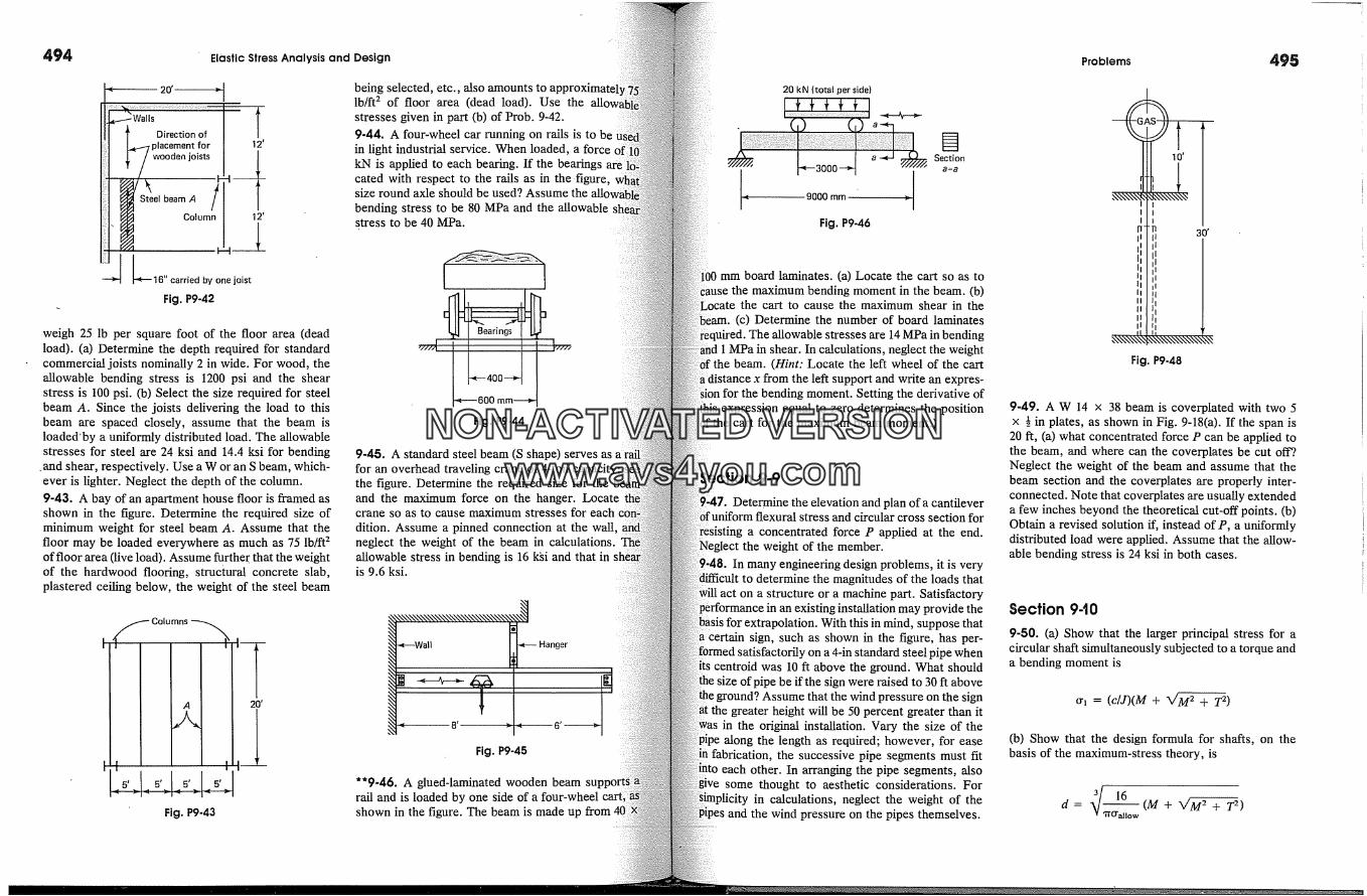
494 Elastic Stress Analysis and Design
20' �
Direction ofplacement for
� / wooden joists�j�/S�eelbeamA /
Column6" carriedby onejoist
Fig. P9-42
weigh 25 lb per square foot of the floor area (deadload). (a) Determine the depth required for standardcommercial joists nominally 2 in wide. For wood, theallowable bending stress is 1200 psi and the shearstress is 100 psi. (b) Select the size required for steelbeam A. Since the joists delivering the load to thisbeam are spaced closely, assume that the beam isloaded'by a uniformly distributed load. The allowablestresses for steel are 24 ksi and 14.4 ksi for bending
.and shear, respectively. Use a W or an S beam, which-ever is lighter. Neglect the depth of the column.9-43. A bay of an apartment house floor is framed asshown in the figure. Determine the required size ofminimum weight for steel beam A. Assume that thefloor may be loaded everywhere as much as 75 lb/ft 2of floor area (live load). Assume further that the weightof the hardwood flooring, structural concrete slab,plastered ceiling below, the weight of the steel beam
-- Columns �
Fig. P9-43
being selected, etc., also amounts to approximatellb/ft 2 of floor area (dead load). Use thestresses given in part (b) of Prob. 9-42.9-44. A four-wheel car running on rails is to bein light industrial service. When loaded, a forcekN is applied to each beating. If the bearingscated with respect to the rails as in the �figure,size round axle should be used? Assume the allowbending stress to be 80 MPa and the allowablestress to be 40 MPa.
.... 4 I- ....
mm--
Fig. P9-44
9-45. A standard steel beam (S shape) serves asfor an overhead traveling crane of 4-ton capacity;the figure. Determine the required size for theand the maximum force on the hanger. Locatecrane so as to cause maximum stresses for each
dition. Assume a pinned connection at the wall,neglect the weight of the beam in calculations.allowable stress in bending is 16 k�i and that inis 9.6 ksi.
Wall 1 � Hanger
8' � � 6' �
Fig. P9-45
**9-46. A glued-laminated wooden beamrail and is loaded by one side of a four-wheelshown in the figure. The beam is made up
20 kN (total per side)
9000mm �Fig. P9-46
Section
mm board laminates. (a) Locate the cart so as to: the maximum bending moment in the beam. (b)
the cart to cause the maximum shear in the(c) Determine the number of board laminates
The allowable stresses are 14 MPa in bending1 MPa in shear. In calculations, neglect the weight
'the beam. (Hint: Locate the left wheel of the carta distance x from the left support and write an expres-
for the bending moment. Setting the derivative ofhis expression equal to zero determines the position
'the cart for the maximum beam moment.)
9-9
Determine the elevation and plan of a cantileverflexural stress and circular cross section for
a concentrated force P applied at the end.the weight of the member.
In many engineering design problems, k is verydetermine the magnitudes of the loads that
act on a structure or a machine part. Satisfactoryan existing installation may provide the
xtrapolation. With this in mind, suppose thatsign, such as shown in the figure, has per-
satisfactorily on a 4-in standard steel pipe whenits centroid was 10 ft above the ground. What should
size of pipe be fithe sign were raised to 30 ft abovethat the wind pressure on the sign
greater height will be 50 percent greater than itin the original installation. Vary the size of thealong the length as required; however, for ease
in fabrication, the successive pipe segments must fitother. In arranging the pipe segments, also
some thought to aesthetic considerations. Forin calculations, neglect the weight of the
and the wind pressure on the pipes themselves.
Problems
Fig. P9-48
30'
495
9-49. A W 14 x 38 beam is coverplated with two 5x � in plates, as shown in Fig. 9-18(a). If the span is
20 ft, (a) what concentrated force P can be applied tothe beam, and where can the coverplates be cut off?.Neglect the weight of the beam and assume that thebeam section and the coverplates are properly inter-connected. Note that coverplates are usually extendeda few inches beyond the theoretical cut-off points. (b)Obtain a revised solution if, instead of P, a uniformlydistributed load were applied. Assume that the allow-able bending stress is 24 ksi in both cases.
Section 9-t0
9-50. (a) Show that the larger principal stress for acircular shaft simultaneously subjected to a torque anda bending moment is
ch = (c/J)(M + � + T 2)
(b) Show that the design formula for shafts, on thebasis of the maximum-stress theory, is
�/ 16d = �/'rrtr�,ow (M + V�- + T 2)
NON-ACTIVATEDVERSIONwww.avs4you.com
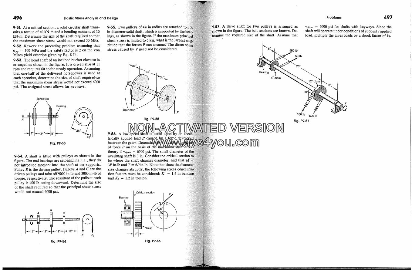
496 Elastic Stress Analysis and Design
9-5�. At a critical section, a solid circular shaft trans-mits a torque of 40 kN-m and a bending moment of 10kN-m. Determine the size of the shaft required so thatthe maximum shear stress would not exceed 50 MPa.
9-52. Rework the preceding problem assuming thatCryp = 100 MPa and the safety factor is 2 on the vonMises yield criterion given by Eq. 8-54.9-53. The head shaft of an inclined bucket elevator isarranged as shown in the figure. It is driven at A at 11rpm and reqQires 60 hp for steady operation. Assumingthat one-half of the delivered horsepower is used ateach sprocket, determine the size of shaft required sothat the maximum shear stress would not exceed 6000psi. The assigned stress allows for keyways.
9-55. Two pulleys of 4�r in radius are attachedin-diameter solid shaft, which is supported byings, as shown in the figure. If the maximumshear stress is limited to 6 ksi, what is the largestnitude that the forces F can assume. 9 The directstress caused by V need not be considered.
Sprockets
8" L 24"J 8"Fig. P9-53
9-54. A shaft is fitted with pulleys as shown in thefigure. The end bearings are self-aligning, i.e., they donot introduce moment into the shaft at the supports.Pulley B is the driving pulley. Pulleys. A and C are thedriven pulleys and take off 9000 in-lb and 3000 in-lb oftorque, respectively. The resultant of the pulls at eachpulley is 400 lb acting downward. Determine the sizeof the shaft required so that the principal shear stresswould not exceed 6000 psi.
Bearings
Fig. P9-55
9-56. A low-speed shaft is acted upon by antrically applied load P caused by a forcebetween the gears. Determineof force P on the basis of the maximumtheory if X�ow = 6500 psi. The small diameteroverhung shaft is 3 in. Consider thebe where the shaft changes diameter, and that3P in-lb and T = 6P in-lb. Note that since thesize changes abruptly, the following stresstion factors must be considered: K� = 1.6 inand K2 = 1.2 in torsion.
Bearing �Critical secti�n I
Fig. P9-56
9-57. A drive shaft for two pulleys is arranged asin the figure. The belt tensions are known. De-
the required size of the shaft. Assume that
450 lb
Bearing
8" diam
Problems 497
X�,o� = 6000 psi for shafts with keyways. Since theshaft will operate under conditions of suddenly appliedload, multiply the given loads by a shock factor of 1�.
50 lb
1001b 600 lbFig. P9-57
T
NON-ACTIVATEDVERSIONwww.avs4you.com

chapterSec. 10-2. Moment-Curvature Relation
deflection of only a few points on a beam or a frame are required.this reason, it can be used to advantage in the solution of statically
problems and for deflection check. An excellent insight intokinematics of deformations is obtained by using this method.
deflection analysis of slender beams in the presence of axial com-sive forces in some instances may cause a profound increase in de-
causing member instability. This topic is considered in the next
499
Introduction
The axis of a beam deflects from its initial position underforces. Accurate values for these 'beam deflections are sought inpractical cases: elements of machines must be sufficiently rigid tomisalignment and to maintain dimensional accuracy under lead;ings, floor beams cannot deflect excessively to av. oid the undesirablechological effect of flexible floors on occupants and to minimize ordistress in brittle-finish materials; likewise, information oncharacteristics of members is essential in the study of vibrations ofchines as well as of stationary and flight structures. Deflections areused in analyses of statically indeterminate problems.
This.chapter has two parts. The governing differential equation for:deflection of beams is derived in Part A, and the different typesary conditions are identified. Several illustrative examples followferent kinds of loading and boundary conditions. This includesindeterminate beams, presenting no special difficulties using thismatical approach. A section on the application of singularityprovided for symbolic solutions for differential equations havingtinuous loading functions along a span. Methods for solvingsuperposition as well as calculation of deflections for uns'ing are also presented.
An energy method for calculating beam deflections and theimpact loads are briefly introduced. Part A concludes with aof the inelastic deflection of beams. These results are essentialthe plastic collapse limit states consideied in Chapter 13.
Part B is devoted to the discussion of statically determinate andideterminate beams using the moment-area method, also called themoment method. This specialized procedure is particularly c
[0-2. Moment-Ourvature Relation
deflections due to bending are determined from deformations takingalong a span. These are based on the kinematic hypothesis that
during bending, plane sections through a beam remain plane. This hy-was first introduced in Section 6-2 in deriving the flexure formula
beams having symmetric cross sections, and extended in Section 6-to beams of arbitrary cross section for bending about either or both
axes. For the present, it will be assumed that bending takesonly about one of the principal axes of the cross section. Such a
is illustrated in Fig. 10-1, where it is further assumed that the radiusp of the elastic curve can change along the span. Except for
slightly greater generality, the derivation that follows leads to the same
Principal axes
(b)
Centroid
(a)
o
Elastic curve
Ic)
Fig. 104 Deformation of a beam in bending.
A � a �
(d)
b
NON-ACTIVATEDVERSIONwww.avs4you.com
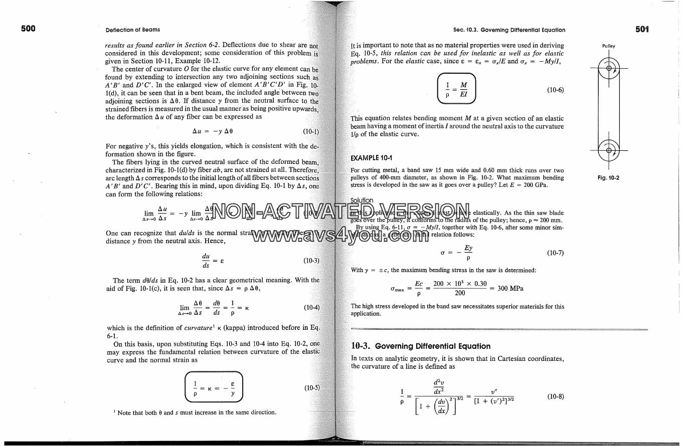
5OO Deflection of Beams
results as found earlier in Section 6-2. Deflections due to shear are �considered in this development; some consideration of thisgiven in Section 10-11, Example 10-12.
The center of curvature O for the elastic curve for any element can'found by extending to intersection any two adjoining sectionsA'B' and D'C'. In the enlarged view of element A'B'C'D' in Fig.l(d), it can be seen that in a bent beam, the included angie'betweenadjoining sections is A0. If distance y from the neutral surface tostrained fibers is measured in the usual manner as being [the deformation Au of any fiber can be expressed as
Au = --y A0
For negative y's, this yields elongation, which is consistent with theformation shown in the figure.
The fibers lying in the curved neutral surface of the deformedcharacterized in Fig. 10-1(d) by fiber ab, are not strained at all.arc length A s corresponds to the initial length of all fibers between �A'B' and D'C'. Bearing this in mind, upon dividing Eq. 10-1 by As,can form the following relations:
A u A 0 du dOlira -- = -y lim or --= -ya�.o AS a�-,o �ss ds �ss
One can recognize that du/ds is the normal strain in a beam fiberdistance y from the neutral axis. Hence,
du
The term dO/ds in Eq. 10-2 has a clear geometrical meaning.aid of Fig. 10-1(c), it is seen that, since As = p A0,
A0 dO 1hm - =-= K
a�.o As ds p
which is the definition of curvature � K (kappa) introduced before in6-1.
On this basis, upon substituting Eqs. 10~3 and 10-4 into Eq.may express the fundamental relation between curvature of thecurve and the normal strain as
Note that both 0 and s must increase in the same direction.
Sec. t0.3. Governing Differential Equation
important to note that as no material properties were used in deriving10-5, this relation can be used for inelastic as well as for elastic
For the elastic case, since e = e�, = cr�,/E and cry, = -My/1,
(10-6)
This equation relates bending moment M at a given section of an elasticbeam having a moment of inertia I around the neutral axis to the curvature
1/p of the elastic curve.
EXAM P L E t 0dcutting metal, a band saw 15 mm wide and 0.60 mm thick runs over two
,s of 400-mm diameter, as shown in Fig. 10-2. What maximum bendingstress is developed in the saw as it goes over a pulley? Let E = 200 GPa.
Pulley
Fig. t0-2
this apphcation, the material must behave elastically. As the thin saw bladepulley, it conforms to the radius of the pulley; hence, p �- 200 mm.
By using Eq. 6-11, cr = -My/1, together with Eq. 10-6, after some minor sim-a generally useful relation follows:
cr = - -- (10-7)P
y = +--c, the maximum bending stress in the saw is determined:
Ec 200 X 103 X 0.30
p 200= 300MPa
high stress developed in the band saw necessitates superior materials for thisapplication.
10-3. Governing Differential Equationtexts on analytic geometry, it is shown that in Cartesian coordinates,
curvature of a line is defined as
d2v1 dx 2 v"
-- = [ (�__)2]3/2= [1 + (V,)213/2 (10-8)P 1+
NON-ACTIVATEDVERSIONwww.avs4you.com
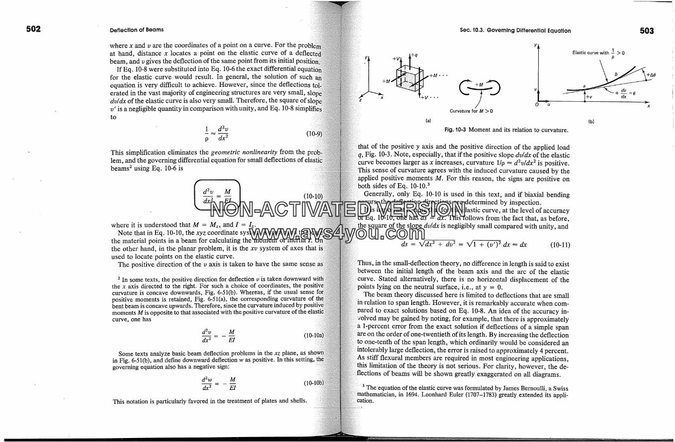
502 Deflection of Beams
where x and v are the coordinates of a point on a curve. For theat hand, distance x locates a point on the elastic curve of abeam, and v gives the deflection of the same point from its initial
If Eq. 10-8 were substituted into Eq. 10-6 the exact differential ecfor the elastic curve would result. In general, the solution of suchequation is very difficult to achieve. However, since the deflectionserated in the vast majority of engineering structures are very small,dv/dx of the elastic curve is also very small. Therefore, the sq�v' is a negligible quantity in comparison with unity, and Eq.to
1 d2v
p dx 2This simplification eliminates the geometric nonlinearity from thelem, and the governing differential equation for small deflections of �beams 2 using Eq. 10-6 is
I d2v=�I��dx 2(10-]
where it is understood that M = Mz, and I = Iz.Note that in Eq. 10-10, the xyz coordinate system is employed to
the material points in a'beam for calculating the moment of inertia I.the other hand, in the planar problem, it is the xv system of axesused to locate points on the elastic curve.
The positive direction of the v axis is taken to have the same sense
2 In some texts, the positive direction for deflection v is taken downwardthe x axis directed to the right. For such a choice of coordinates, thecurvature is concave downwards, Fig. 6-51(b). Whereas, if the usual sensepositive moments is retained, Fig. 6-51(a), the corresponding curvature ofbent beam is concave upwards. Therefore, since the curvature inducedmoments M is opposite to that associated with the pccurve, one has
d2v Mdx 2 EI
Some texts analyze basic beam deflection problems in the xz plane, asin Fig. 6-51(b), and define downward deflection w as positive. In this setting,governing equation also has a negative sign:
d2w Mdx 2 E1
This notation is particularly favored in the treatment of plates and shells.
Sec. t0.3. Governing Differential Equation
(a)
Curvature for M > 0
y�Elastic curve with I > 0
P
+ dv�xx = 0
(b)
Fig. 10-3 Moment and its relation to curvature.
of the positive y axis and the positive direction of the applied loadFig. 10-3. Note, especially, that if the positive slope dv/dx of the elastic
CUrve becomes larger as x increases, curvature 1/p �- d2v/dx 2 is positive.This sense of curvature agrees with the induced curvature caused by the
positive moments M. For this reason, the signs are positive onsides of Eq. 10-10. 3
Generally, only Eq. 10-10 is used in this text, and if biaxial bendingoccurs, the deflection directions are determined by inspection.
It is important to note that for the elastic curve, at the level of accuracyof Eq. 10-10, one has ds = dx. This follows from the fact that, as before,the square of the slope dv/dx is negligibly small compared with unity, and
ds = X/dx 2 + dv 2 = X/1 + (v') 2 dx = dx (10-11)
Thus, in the small-deflection theory, no difference in length is said to existthe initial length of the beam axis and the arc of the elastic
Stated alternatively, there is no horizontal displacement of thelying on the neutral surface, i.e., at y = 0.
The beam theory discussed here is limited to deflections that are smallrelation to span length. However, it is remarkably accurate when com-
to exact solutions based on Eq. 10-8. An idea of the accuracy in-may be gained by noting, for example, that there is approximately
1-percent error from the exact solution if deflections of a simple spanthe order of one-twentieth of its length. By increasing the deflection
to one-tenth of the span length, which ordinarily would be considered andeflection, the error is raised to approximately 4 percent.
stiff flexural members are required in most engineering applications,limitation of the theory is not serious. For clarity, however, the de-
flections of beams will be shown greatly exaggerated on all diagrams.
The equation of the elastic curve was formulated by James Bernoulli, a Swissin 1694. Leonhard Euler (1707-1783) greatly extended its appli-
503
x
NON-ACTIVATEDVERSIONwww.avs4you.com
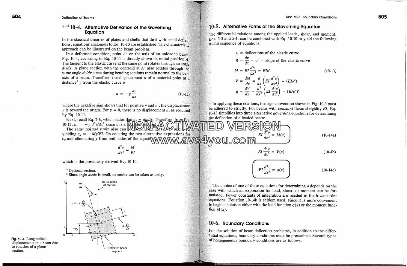
504 505
Fig. t0-4 Longitudinaldisplacements in a beam dueto rotation of a planesection.
Deflection of Beams
*'4�[{�-4. Alternative Derivation of the GoverningEquation
In the classical theories of plates and shells that deal with smalltions, equations analogous to Eq. 10-10 are established. The charactedapproach can be illustrated on the beam problem. ,.
In a deformed condition, point A' on the axis of an unloadedFig. 10-4, according to Eq. 10-11 is directly above its initialThe tangent to the elastic curve at the same point rotates through andv/dx. A plane section with the centroid at A' also rotatessame angle dv/dx since during bending sections remain normal to theaxis of a beam. Therefore, the displacement u of a material pointdistance s y from the elastic curve is
where the negative sign shows that for positive y and v',u is toward the origin. For y = 0, there is no displacement u, asby Eq. 10-11.
Next, recall Eq. 2-6, which states that e� = du/dx. Therefore, from10-12, e� = -y d2v/dx 2 since v is a function ofx only.
The same normal strain also can be found from Eqs. 3-14 andyielding e� = -My/E1. On equating the two alternative expressionse� and eliminating y from both sides of the equation,
d2v Mdx 2 E1
which is the previously derived Eq. 10-10.
Optional section.Since angle dv/dx is small, its cosine can be taken as unity.
Initial plane
d_�v �.�ofsectiondx
u = -y -�
v +d_�v
Deflected beamsegment
Sec. 10-6. Boundary Conditions
�-5. Alternative Forms of the Governing Equationdifferential relations among the applied loads, shear, and moment,
s. 5�3 and 5-4, can be combined with Eq. 10-10 to yield the followingsequence of equations:
v = deflections of the elastic curvedv
= -- = v' = slope of the elastic curve0 dxd2v
m = EI.� =EIv"
V- dM_ d EI � =(EIv")'dV d2 (d2v)q- dx - dx 2 EI � =(EIv")"
(10-13)
these relations, the sign convention shown in Fig. 10-3 mustadhered to strictly. For beams with constant flexural rigidity El, Eq.
simplifies into three alternative governing equations for determiningdeflection of a loaded beam:
�'�d2vEI � = M(x)
d3v= V(x)
(10-14a)
(10-4b)
(10-14c)
choice of one of these equations for determining v depends on thewith which an expression for load, shear, or moment can be for-
Fewer constants of integration are needed in the lower-orderEquation 10-14b is seldom used, since it is more convenient
a solution either with the load function q(x) or the moment func-m(x).
.0-6. Boundary Conditionsthe solution of beam-deflection problems, in addition to the differ-
equations, boundary conditions must be prescribed. Several types'homogeneous boundary conditions are as follows:
NON-ACTIVATEDVERSIONwww.avs4you.com
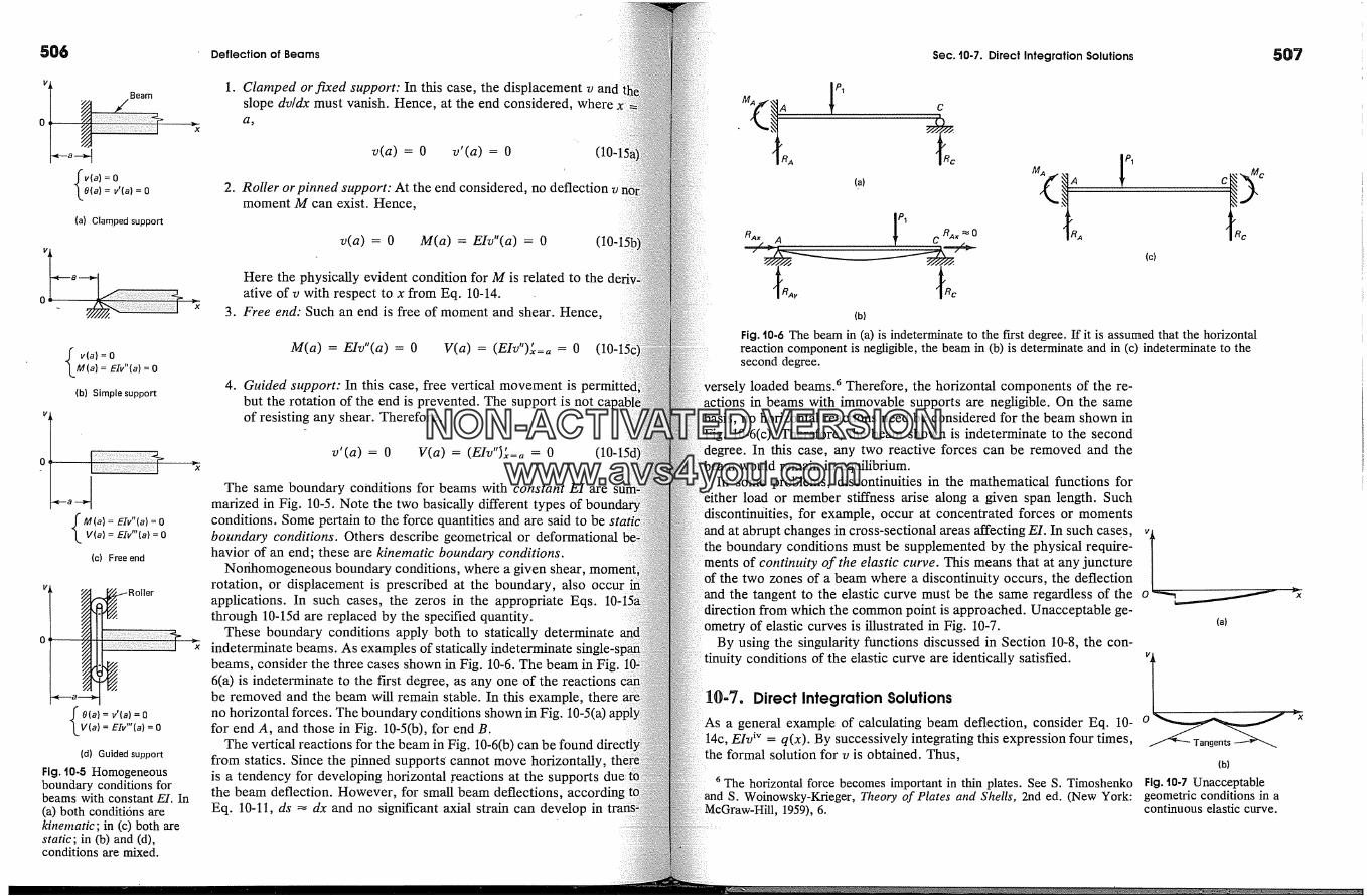
506
Beam
v(a) = 08(a): v'(a) = 0
(a) Clam�ped support
v(a) = 0M(a) = EIv"(a) = 0(b) Simple support
M (a) = EIv"(a) = 0V(a) = EIv'"(a) = 0
(c) Free end
/�. Roller
0(a) v'(a) = 0V(a) : EIv"'(a) : 0
(d) Guided support
Fig. t0-5 Homogeneousboundary conditions forbeams with constant EI. In(a) both conditi6ns arekinematic; in (c) both arestatic; in (b) and (d),conditions are mixed.
Deflection of Beams
1. Clamped orfixed support: In this case, the displacement v andslope dv/dx must vanish. Hence, at the end considered,a,
v(a) = 0 v'(a) = 0
2. Roller orpinned support: At the end considered, no deflectionmoment M can exist. Hence,
v(a) = 0 M(a) = EIv"(a) = 0
Here the physically evident condition for M is related to theative of v with respect to x from Eq. 10-14.
3. Free end: Such an end is free of moment and shear. Hence,
it iM(a) = EIv"(a) = 0 V(a) =(EIv )x=, = 0 (10-1:
4. Guided support: In this case, free vertical movement is [but the rotation of the end is prevented. The support is notof resisting any shear. Therefore,
tttv'(a) = 0 V(a) =(EIv )�=� = 0
The same boundary conditions for beams with constant EI aremarized in Fig. 10-5. Note the two basically different typesconditions. Some pertain to the force quantities and are said to beboundary conditions. Others describe geometrical or deformationalhavior of an end; these are kinematic boundary conditions.
Nonhomogeneous boundary conditions, where a given shear,rotation, or displacement is prescribed at the boundary, also occurapplications. In such cases, the zeros in the appropriate Eqs.through 10-15d are replaced by the specified quantity.
These boundary conditions apply both to statically determinateindeterminate beams. As examples of statically indeterminate sinbeams, consider the three cases shown in Fig. 10-6. The beam in Fig.6(a) is indeterminate to the first degree, as any one of the reactionsbe removed and the beam will remain stable. In this example, thereno horizontal forces. The boundary conditions shown in Fig. 10-5(a)for end A, and those in Fig. 10-5(b), for end B.
The vertical reactions for the beam in Fig. 10-6(b) can be foundfrom statics. Since the pinned supports' cannot move horizontally,is a tendency for developing horizontal .reactions at the supportsthe beam deflection. However, for small beam deflections, accordingEq. 10-11, ds � dx and no significant axial strain can develop in
Sec. t0-7. Direct Integration Solutions
M,� A '
(a) (�i r cRAx A C RAx � 0 � IRc(c)
(b)
Fig. t0-6 The beam in (a) is indeterminate to the f"u:st de�ree. If it is assumed that the horizontalreaction component is negligible, the beam in (b) is determinate and in (c) indeterminate to thesecond degree.
loaded beams. 6 Therefore, the horizontal components of the re-OhS in beams with immovable supports are negligible. On the same
no horizontal reactions need be considered for the beam shown in10-6(c). Therefore, the beam shown is indeterminate to the second
In this case, any two reactive forces can be removed and thebeam would remain in equilibrium.
In some problems, discontinuities in the mathematical functions forload or member stiffness arise along a given span length. Such
for example, occur at concentrated forces or moments
andatabruptchangesincross-sectionalareasaffectingEI.Insuchcases,vLboundary conditions must be supplemented by the physical require-ments of continuity of the elastic cur�e. This means that at any juncture
the two zones of a beam where a discontinuity occurs, the deflectionthe tangent to the elastic curve must be the same regardless of the o
from which the common point is approached. Unacceptable ge-ometry of elastic curves is illustrated in Fig. 10-7. (al
By using the singularity functions discussed in Section 10-8, the con-
tinuityconditionsoftheelasticcurveareidenticallysatisfied."1 Zang�Direct Integration SolutionsAs a general example of calculating beam deflection, consider Eq. 10- o
ivEIv = q(x). By successively integrating this expression four times,the formal solution for v is obtained. Thus,
(b)
6 The horizontal force becomes important in thin plates. See S. Timoshenko Fig. t0-7 Unacceptableand S. Woinowsky-Krieger, Theory of Plates and Shells, 2nd ed. (New York: geometric conditions in aMcGraw-Hill, 1959), 6. continuous elastic curve.
507
x
NON-ACTIVATEDVERSIONwww.avs4you.com
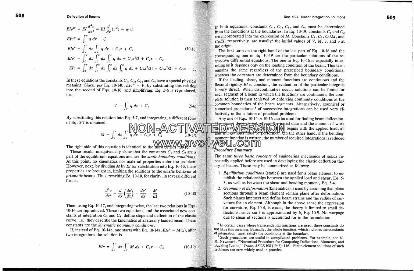
508 Deflection of Beams
In these equations the constants C�, C2, C3, and C4 have a specialmeaning. Since, per Eq. 10-14b, EIv'"= V, by substituting thisinto the second of Eqs. 10-16, and simplifying, Eq: 5-6 is
V = fo�' q dx + C�By substituting this relation into Eq. 5-7, and integrating, a differen'of Eq. 5-7 is obtained.
M= fff:dXfo":qdx + Cix + C 2The right side of this equation is identical to the third of Eqs. 10-16.
These results unequivocally show that the constants C� and C2part of the equilibrium equations and are the static boundaryAt this point, no kinematics nor material properties enter theHowever, next, by dividing M by E1 for substitution into Eq. 10-10,properties are brought in, limiting the solutions to the elastic behavior �prismatic beams. Thus, rewriting Eq. 10-10, for clarity, in severalforms,
dx 2 dx dx E1
Then, using Eq. 10-17, and integrating twice, the last two relations10-16 are reproduced. These two equations, and the associated newstants of integration C3 and C4, define slope and deflection of thecurve, i.e., they describe the kinematics of a laterally loaded beam.constants are the kinematic boundary conditions.
If, instead of Eq. 10-14c, one starts with Eq. 10-14a, EIv"= M(x),two integrations the solution is
EIv= fo�dXfo�Mdx+ C3x + C4
Sec. 10-7. Direct Integration Solutions
both equations, constants C�, C2, C3, and C4 must be determinedthe conditions at the boundaries. In Eq. 10-19, constants C� and C2
xre incorporated into the expression of M. Constants C�, C2, C3/EI, and/E�r, respectively, are usually 7 the initial values of V, M, 0, and v at
origin.The first term on the fight hand of the last part of Eq. 10-16 and the
one in Eq. 10-19 are the particular solutions of the re-Spective differential equations. The one in Eq. 10-16 is especially inter-
as it depends only on the loading condition of the beam. This termremains the same regardless of the prescribed boundary conditions,
the constants are determined from the boundary conditions.If the loading, shear, and moment functions are continuous and the
t rigidity EI is constant, the evaluation of the particular integralsvery direct. When discontinuities occur, solutions can be found for
segment of a beam in which the functions are continuous; the com-solution is then achieved by enforcing continuity conditions at the
boundaries of the beam segments. Alternatively, graphical orprocedures, 8 of successive integrations can be used very ef-
in the solution of practical problems.Any one of Eqs. 10-14 or 10-16 can be used for finding beam deflection.
Fhe choice depends entirely on the initial data and the amount of worknecessary for solving a problem. If one begins with the applied load, all
integrations must be performed. On the other hand, if the bending-moment function is written, the number of required integrations is reduced
two.
Summarysame three basic concepts of engineering mechanics of solids re-
applied before are used in developing the elastic deflection the-of beams. These may be summarized as follows:
1. Equilibrium conditions (statics) are used for a beam element to es-tablish the relationships between the applied load and shear, Eq. 5-3, as well as between the shear and bending moment, Eq. 5-4.
2. Geometry of deformation (kinematics) is used by assuming that planesections through a beam element remain plane after deformation.Such planes intersect and define beam strains and the radius of cur-vature for an element. Although in the above sense the expressionfor curvature, Eq. 10-4, is exact, the theory is limited to small de-flections, since sin 0 is approximated by 0, Eq. 10-9. No warpagedue to shear of sections is accounted for in the formulation.
7 In certain cases where transcendental functions are used, these constants donot have this meaning. Basically, the whole function, which includes the constants
must satisfy the conditions at the boundary.8 Such procedures are useful in complicated problems. For example, see N.
M. Newmark, "Numerical Procedure for Computing Deflections, Moments, andBuckling Loads," Trans. ASCE 108 (1943): 1161. Finite element solutions of such
are now widely used in practice.
509
NON-ACTIVATEDVERSIONwww.avs4you.com

Deflection of Beams
3. Properties of materials (constitutive relations) in theHooke's law, Eq. 2-3, are assumed to apply only tonormal stresses and strains. Poisson's effect is neglected.
A solution of any one of Eqs. 10-14a, 10-14b, or 10-14c, 9 subjectprescribed boundary conditions, constitutes a solution of a givenversely loaded elastic beam problem. These equations are equallycable to statically determinate and statically indeterminate beamlems. m However, the solutions are simpler if the functions q(x)are continuous across a span. When discontinuities in either q(x)occur, continuity of the elastic curve at such points must beIf I is constant, singularity functions for describing the loads canfectively used.
It is to be noted that although at load and cross-sectionlarge local perturbations in strain and stresses develop, beamare less sensitive to these effects. Deflections are determined ustegration, a process tending to smooth out the function.
Several illustrative examples of statically determinate andindeterminate beam problems follow. The applications of sintions for elastic beam deflections is given in the next section.
EXAMPLE '10-2
A bending moment M� is applied at the free end of a cantilever of lengthof constant flexural rigidity EI, Fig. 10-8(a). Find the equation of the,
Solution
The boundary conditions are recorded near the figure from inspection of the iditions at the ends. At x = L, M(L) = +M�, a nonhomogeneous
From a free-body diagram of Fig. 10-8Co), it can be observed that themoment is +M� throughout the beam. By applying Eq. 10-14a, integratingcessively, and making use of the boundary conditions, one obtains thefor v:
d2uEI �5 = M = M�
EI-� = M�x + C3But 0(0) = 0; hence, at x = 0, one has EIv'(O) = C3 = 0 and
9 The adopted sign convention for applied loads and shear results in10-13 and 10-14 having positive signs, an advantage in hand calculations.
�o This is analogous to the axially loaded bar problems discussed in19.
(b)
(c)
y,v I
v(O) = 00(0): 0
11/I 1
f M(L) = +M 1V(L) = 0
M 1 M1
M
+Mi
EI-� = Mix1
EIv= � Mix 2 + C4
(d)
0
(e)
v[(f) .
ol
+M 1 L/EI
"'"'"� +M1L2/2EIx
Fig. t0-8
But v(0) = 0; hence, EIv(O) = C4 = 0 and
Mix 2v - (10-20)
2EI
The positive sign of the result indicates that the deflection due to M� is upward.rhe largest value of v occurs at x = L. The slope of the elastic curve at the free
is +M�L/EI radians.Equation 10-20 shows that the elastic curve is a parabola. However, every
element of the beam experiences equal moments and deforms alike. Therefore,elastic curve should be a part of a circle. The inconsistency results from theof an approximate relation for the curvature 1/9. It can be shown that the
error committed is in the ratio of (9 - v) 3 to 93. As the deflection v is muchthan 9, the error is very small.
is important to associate the above successive integration procedure with asolution or interpretation. This is shown in the sequence of Figs. 10-
through (f). First, the conventional moment diagram is shown. Then using10-9 and 10-10, 1/p � d2v/dx 2 = M/EI, the curvature diagram is plotted in
10-8(d). For the elastic case, this is simply a plot of M/EI. By integrating thediagram, one obtains the 0 diagram. In the next integration, the elastic
is obtained. In this example, since the beam is fixed at the origin, the0(0) = 0 and v(0) = 0 are used in constructing the diagrams. This
approach or its numerical equivalents are very useful in the solution ofwith variable EI.
NON-ACTIVATEDVERSIONwww.avs4you.com

Fig. 10-9
Deflection of Beams
EXAMPLE '10-3
A simple beam supports a uniformly distributed downward load Wo. Therigidity EI is constant. Find the elastic curve by the following three me�tho,Use the second-order differential equation to obtain the deflection of the(b) Use the fourth-order equation instead of the one in part (a). (c)graphical solution of the problem.
Solution
(a) A diagram of the beam together with the given boundary conditions isin Fig. 10-9(a). The expression for M for use in the second-orderequation has been found in Example 5-8. From Fig. 5-24,
y, v 0
q =-w o lb/in
.J viol =o .f vlt. I =o(M(O) = o LM(L) = o
o
woL 324 EI
(b)
woe
x
v
(f)o
I V Imax
(c)
M
Wo L2+--
8 (g)
WO La+--
24EI
(d)
woL 2+--
�EI
v
(h)
o
I v Imax
0 o
Sec. t0-7. Direct Integration Solutions
M = woL�x _ WoX 22 2
this relation into Eq. 10-14a, integrating it twice, and using the bound-conditions, one finds the equation of the elastic curve:
d2v woLx Wo x2= M 2
dv . worx 2 wox 3EI �xx = 4 � + C3
worx 3 WoX 4EIv= 1-�-- 2�- q- C3X q- C4
V(0) = 0; hence, EIv(O) = 0 = C4; and, since v(L) = 0,
EIv(L) 0 w�L4 w�L3= =� + C3L and C3 = ---24 24
WoX 3v = 2-�-I (L - 2Lx 2 + x 3) (10-21)
Because of symmetry, the largest deflection occurs at x = L/2. On substitutingvalue ofx into Eq. 10-21, one obtains
I v Jmax 5w�L4= 384EI (10-22)
condition of symmetry could also have been used to determine constant C3.it is known that v'(L/2) = 0, one has
EIv'(L/2) = w�L(L/2)2 w�(L/2)34 6 + C3 =.0
as before, C3 = - woL3/24.
Application of Eq. 10-14c to the solution of this problem is direct. The con-are found from the boundary conditions.
d4vEl �x 4 = q(x) = -WoEI d3 vdx 3 -WoX + C�
d2v WoX 2El dx 2 = - � + C�x + C2
5'f3
NON-ACTIVATEDVERSIONwww.avs4you.com
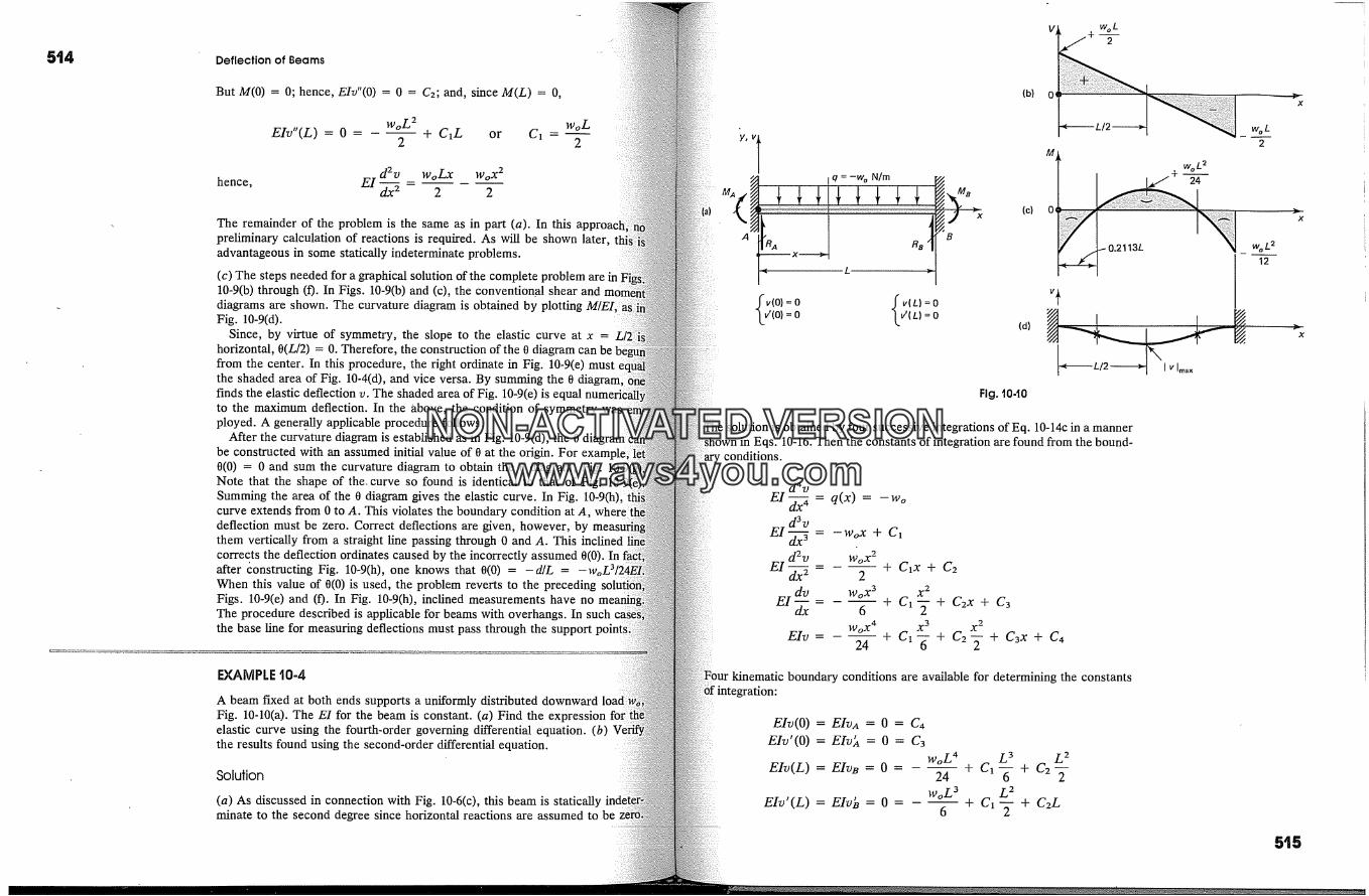
v WoL2
Deflection of Beams
But M(O) = O; hence, EIv"(O) = 0 = C2; and, since M(L) = O,
woL 2 woLEIv"(L) = 0 = - -- + C]L or C1 = --
2 2
hence, EI-- dev woLx WoX 2dx 2 2 2
The remainder of the problem is the same as in part (a). In thispreliminary calculation of reactions is required. As will be shown later,advantageous in some statically indeterminate problems.
(c) The steps needed for a graphical solution of the complete problem are in10-9(b) through (0. In Figs. 10-9(b) and (c), the convention.al shear and ]diagrams are shown. The curvature diagram is obtained by plotting M/E1,Fig. 10-9(d).
Since, by virtue of symmetry, the slope to the elastic curve at x =horizontal, 0(L/2) = 0. Therefore, the construction of the 0 diagram can befrom the center. In this procedure, the right ordinate in Fig. 10-9(e) mustthe shaded area of Fig. 10-4(d), and vice versa. By summing the 0finds the elastic deflection v. The shaded area of Fig. 10-9(e) is equalto the maximum deflection. In the above, the condition of symmetry wasployed. A gener.ally applicable procedure follows.
After the curvature diagram is established as in Fig. 10-9(d), the 0be constructed with an assumed initial value of 0 at the origin. For0(0) = 0 and sum the curvature diagram to obtain the 0 diagram, Fig.Note that the shape of the. curve so found is identical to that of Fig.Summing the area of the 0 diagram gives the elastic curve. In Fig.curve extends from 0 to A. This violates the boundary condition at A,deflection must be zero. Correct deflections are given, however, bythem vertically from a straight line passing through 0 and A. Thiscorrects the deflection ordinates caused by the incorrectly assumed 0(0). Inafter �onstructing Fig. 10-9(h), one knows that 0(0) = -d/L = -wWhen this value of 0(0) is used, the problem reverts to the precedingFigs. 10-9(e) and (f). In Fig. 10-9(h), inclined measurements have noThe procedure described is applicable for beams with overhangs. Inthe base line for measuring deflections must pass through the support
EXAMPLE 'i0-4
A beam fixed at both ends supports a uniformly distributed downwardFig. 10-10(a). The EI for the beam is constant. (a) Find the expressionelastic curve using the fourth-order governing differential equation. (b)the results found using the second-order differential equation.
Solution
(a) As discussed in connection with Fig. 10-6(c), this beam is staticallyminate to the second degree since horizontal reactions are assumed to be
(b) 0
,,vT
v(O) = 0 f v(L) = 0v'(O) = 0 L�'(L) = 0
(c)
(d)
Fig. t0-10
M
13L
woL 224
rhe solution is obtained by four successive integrations of Eq. 10-14c in a mannerts. 10-16. Then the constants of integration are found from the bound-
conditions.
d4uEl � = q(x) = -Wo
d3uEI �' i = -WoX + C]
d2v WoX 2EI--=
dx 2 2
E1 dv = WoX 3dx 6
Wo x4EIv=
24
- -- + C]x + C2
x 2--- + C] � + C2x + C3
X 3 ,X 2__ -- q- C 1 -� q- C2- �- q- C3x q- C 4
kinematic boundary conditions are available for determining the constants
2
woL 212
EIv(O) = EIvA = 0 = CaEIv'(O) = EIv.� = 0 = C3
woL 4EIv(L) = EIva = 0 =
24
woL 3EIv'(L) = EIv� = 0 =
6
L 3 L 2- + G'g- +
L 2-- � + C�'�- + C2L
x
x
x
5t5
NON-ACTIVATEDVERSIONwww.avs4you.com
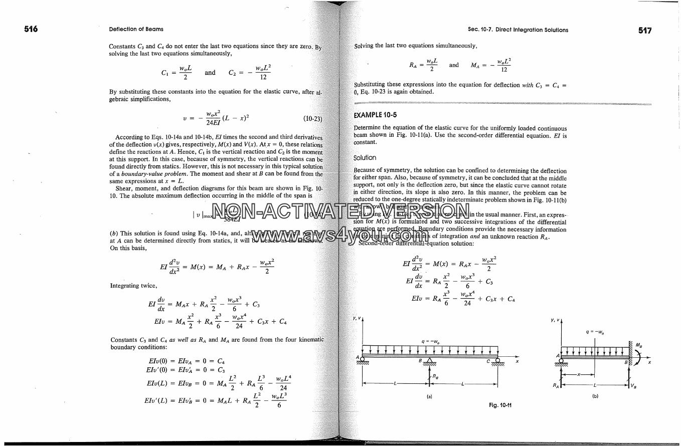
5i6 Deflection of Beams
Constants C3 and C4 do not enter the last two equations since they aresolving the last two equations simultaneously,
woL woL 2C� - and C2 =
2 12
By substituting these constants into the equation for the elastic curve,gebraic simplifications,
WoX2 (�2-� .z. - x) 2According to Eqs. 10-14a and 10-14b, EI times the second and third
of the deflection v(x) gives, respectively, M(x) and V(x). At x = 0,define the reactions at A. Hence, C� is the vertical reaction and C2 is theat this support. In this case, because of symmetry, the vertical reactions canifound directly from statics. However, this is not necessary in this typicalof a boundary-value problem. The moment and shear at B can be found fromsame expressions at x = L.
Shear, moment, and deflection diagrams for this beam are shown in Fig. 110. The absolute maximum deflection occurring in the middle of the span is
[ V [max -- w�L4384EI
(b) This solution is found using Eq. 10-14a, and, although the verticalat A can be determined directly from statics, it will be treated as anOn this basis,
der Wo x2EI �5 = M(x) = MA + RAx -- �
Integrating twice,
did X 2 �t] o x3EI �x = MAx + RA 2 6 + C3
2 2 2 3 Wo x4EIv= MA� + RA 6 24 + C3x + C4
Constants C3 and C4 as well as RA and MA are found from the fourboundary conditions:
EIv(O) = EIVA = 0 = C4EIv'(O) = EIv� = 0 = C3
L 2 L 3 woL 4EIid(L) = EIvB = 0 = MA_� + RA 6 24L 2 woL 3
EIv'(L) = Elvb = 0 = MAL + RA2 6
Sec. 10-7. Direct Integration Solutions
1olving the last two equations simultaneously,
woZ w oZ 2RA = 2 and M,a = 12
Substituting these expressions into the equation for deflection with C3 = C4 =Eq. 10-23 is again obtained.
PLE t0-5
the equation of the elastic curve for the uniformly loaded continuousshown in Fig. 10-11(a). Use the second-order differential equation. E1 is
SOlution
:cause of symmetry, the solution can be confined to determining the deflection!or either span. Also, because of symmetry, it can be concluded that at the middle
)ort, not only is the deflection zero, but since the elastic curve cannot rotatein either direction, its slope is also zero. In this manner, the problem can be
to the one-degree statically indeterminate problem shown in Fig. 10-1 l(b)With known boundary conditions.
By using Eq. 10-14a, the solution proceeds in the usual manner. First, an expres-.for M(x) is formulated and two successive integrations of the differential
are performed. Boundary conditions provide the necessary informationfor determining the constants of integration and an unknown reaction RA.
Second-order differential-equation solution:
dev Wo x2EI �5 = M(x) = RAx - �
dv ' x 2 WoX 3EI � RA 2 6 + C3
2 3 Wo x4EIv= RA + C3x + C4
6 24
Fig.
y,vj q=-w�
(b)
5'i7
NON-ACTIVATEDVERSIONwww.avs4you.com

Deflection of Beams
Boundary conditions:
EIv(O) = EIvA = 0 = C4
EIv' (L ) = Elvb = 0 = Ra
EIv(L) = EIvB = 0 = RA
L 2 woL 3+c3
2 6
L 3 Wo L4+ C3L
6 24
By solving the last two equations simultaneously,
3woL woL 3RA -- and C3 =
8 48
which, upon substitution into the equation for the elastic curve, leads to
WoXV = -- --(L 3 - 3Lx 2 + 2x 3)
48EI
From symmetry, the reactions at A and C are equal, and, by using staticsreaction at B is
5woLRB--
4
This reaction is also numeric. ally equal to 2VB.
EXAMPLE 'i0-6
A simple beam supports a concentrated downward force P at a distance athe left support, Fig. 10-12(a). The flexural rigidity EI is constant. Find the e�tion of the elastic curve by successive integration.
Solution
The solution will be obtained using the second-order differential equation.reactions and boundary conditions are noted in Fig. 10-12(a). The momentplotted in Fig. 10-12(b) clearly shows a discontinuity in M(x) at x = a, re�two different functions. At first, the solution proceeds independently forsegment of the beam.
For segment AD For segment DBd2v M Pb d2v M Pa Pa�Ix 2 E1 EIL x dx 2 EI E1 EIL x
dv Pb x 2 dv Pa Pax 2dx-EIL 2 + A� dx- EI x EIL 2 + B]
Pb x 3 Pax 2 Pax �v - -- + A�x + A2 v - + Bix
ElL 6 EI 2 EIL 6
O) = 0�10) = 0
Sec. '10-7. Direct Integration Solutions
M
v(L) =0M(L) = 0
-Z- (L -x)
(b)
Dv'(a)
(c)
x
Fig. t042
. determine the four constants A�, A2, B�, and B2, two boundary and two con-tinuity conditions must be used.
For segment AD:
v(O) = 0 = A2
segment DB:
PaL 2v(L) = 0 -
3EI= -- + B�L + B2
deflections for both segments at x = a:
pa3b pa 3 pa 4vz> = v(a) - + A�a -
6EIL 2EI 6EIL+ Bia + B2
slopes for both segments at x = a:
pa2b pa 2 pa 3Oz> = v(a) = 2EIL + Ai = E1 2EIL--+B�
solving the four equations simultaneously, one finds
PbA1 = -- (L 2 - b 2) A2 = 0
6EILPa Pa 3
B1 = -- (2L 2 + a 2) B2 =6EIL 6EI
NON-ACTIVATEDVERSIONwww.avs4you.com
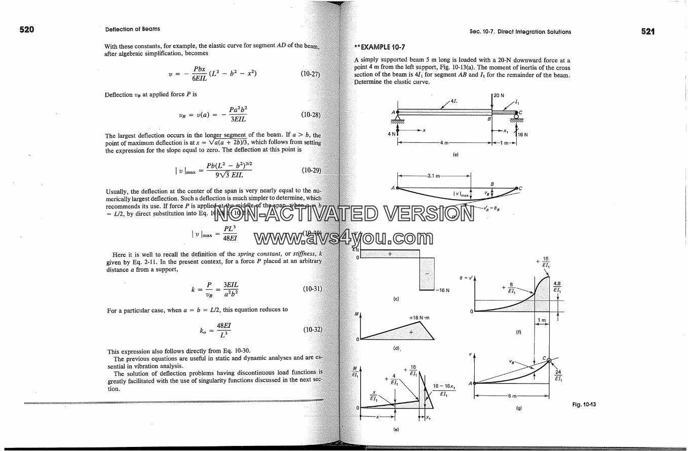
520 Deflection of Beams
With these constants, for example, the elastic curve for segment AD of theafter algebraic simplification, becomes
Pbxv = -- --(Z 2 -- b 2 - x 2)
6EIL
Deflection vB at applied force P is
vB = v(a) =pa2b 2
3EIL
The largest deflection occurs in the longer segment of the beam. If a > bpoint of maximum deflection is at x = X/a(a + 2b)/3, which follows fromthe expression for the slope equal to zero. The deflection at-this point is
Pb(L 2 - b2)3/2[max = 9X/g ElL
Usually, the deflection at the center of the span is very nearly equal to th emerically largest deflection. Such a deflection is much simpler to determine.recommends its use. If force P is applied at the middle of the span, when= L/2, by direct _substitution into Eq. 10-28 or 10-29,
pL 3I 7-1 Imax -- 48E1T
Here it is well to recall the definition of the spring constant, or stgiven by Eq. 2-11. In the present context, for a force P placed at andistance a from a support,
P 3EIL
vB a2b 2
For a particular case, when a = b = L/2, this equation reduces to
48EI
ko- L3
This expression also follows directly from Eq. 10-30.The previous equations are useful in static and dynamic analyses and
sential in vibration analysis.The solution of deflection problems having discontinuous load
greatly facilitated with the use of singularity functions discussed i�tion.
(1(
Sec. 10-7. Direct Integration Solutions
B(AMPLE 'i0-7
simply supported beam 5 m long is loaded with a 20-N downward force at a4 m from the left support, Fig. 10-13(a). The moment of inertia of the cross
section of the beam is 413 for segment AB and I� for the remainder of the beam.Determine the elastic curve.
� 12o N
4N� �x �--x, �'16Nk 4m
(a)
[ v Irna x
(b)'
' -0B� V B --
(c)
+16 N .m
(d),
4 EI�EI 1
16 - 16x�
X 1
re)
(f)
Fig. t043
52t
NON-ACTIVATEDVERSIONwww.avs4you.com
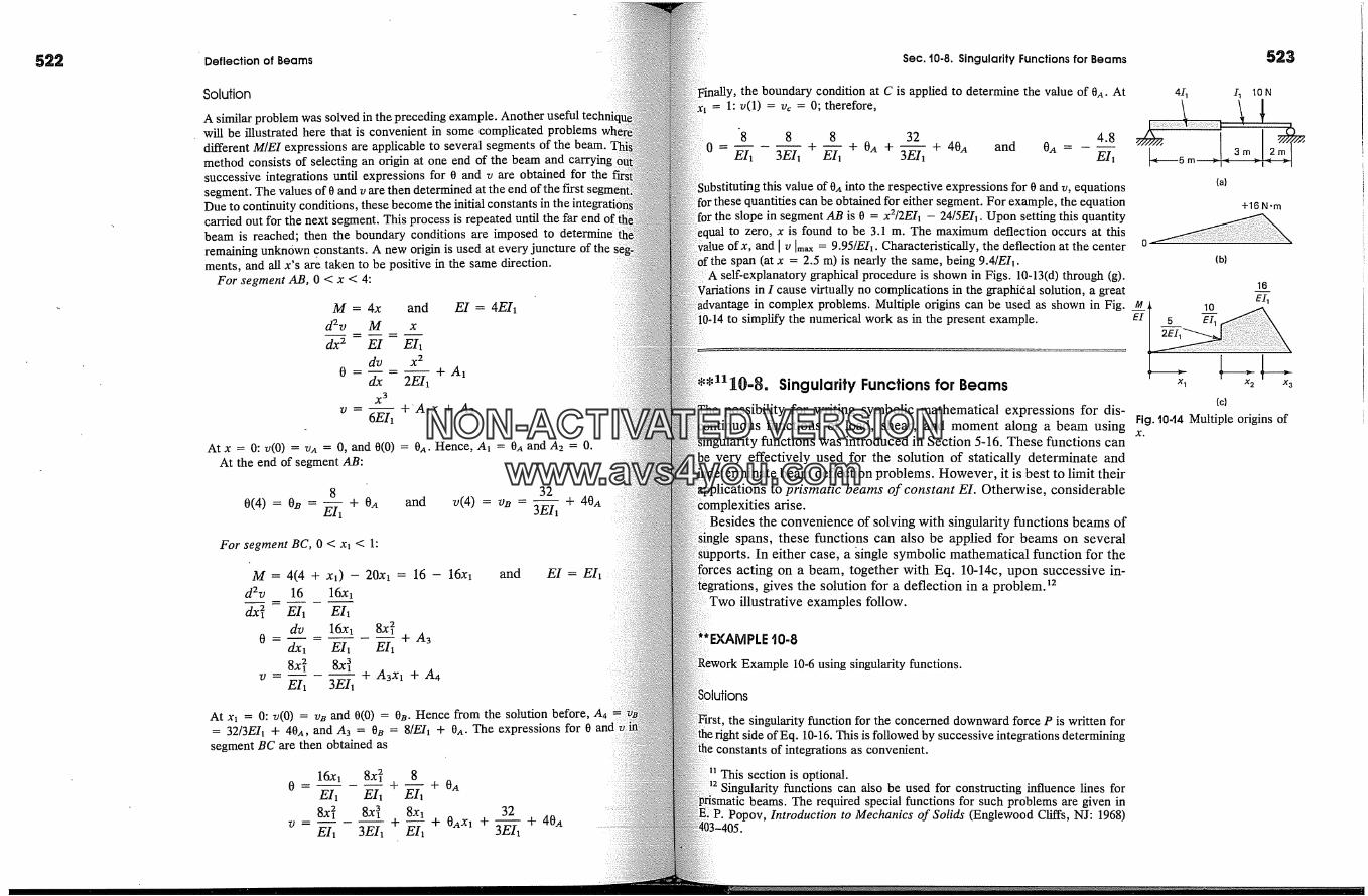
522 Deflection of Beams
Solution
A similar problem was solved in the preceding example.will be illustrated here that is convenient in some complicated problemsdifferent M/E1 expressions are applicable to several segments of the beam.method consists of selecting an origin at one end of the beam and carrying(successive integrations until expressions for 0 and v are obtained for thesegment. The values of 0 and v are then determined at the end of the first seDue to continuity conditions, these become the initial constants in the intecarded out for the next segment. This process is repeated until the far end ofbeam is reached; then the boundary conditions are imposed to determineremaining unknown constants. A new origin is used at every juncture of thements, and all x's are taken to be positive in the same direction.
For segment AB, 0 < x < 4:
M = 4x andd2v M x
dx 2 E1 Elldv x 2
0 .... +A�dx 2EI�
x 3- -- +'Atx + A2
6EI�
At x = 0: v(0) = vA = 0, and 0(0) = 0A. Hence, A� = 0� and A2 = 0.At the end of segment AB:
8 32
0(4) = OB = � + OA and v(4) = vB = 3EI� + 40AFor segment BC, 0 < x� < 1:
M = 4(4 + x�) - 20x� = 16 - 16x� andd2v 16 16x�dx� Ell Ell
dv 16xt 8x� 20 = - -- + A3
dx� EI� EI�
v -- -- + A3Xl + A4EI1 3EI�
At x� = 0: v(0) = vB and O(0) = 0B. Hence from the solution before, A4= 32/3EI� + 40,t, and A3 = 0� = 8/EI� + O,t. The expressions for 0segment BC are then obtained as
16x� 8x2� 80 - Ell EI--� + � + OA
8X� 8X] 8Xl 32v - EI, 3EI'�-'� + � + OAx, + 3-� + 40.
Sec. t0-8. Singularity Functions for Beams
the boundary condition at C is applied to determine the value of 0�. At= 1: v(1) = vc = 0; therefore,
8 8 8 32 4.8
EIt 3EI� + � + 0A + 3--� + 40A and 0A = EI�
523
this value of 0A into the respective expressions for 0 and v, equationsuantities can be obtained for either segment. For example, the equation
the slope in segment AB is 0 = x2/2EI� - 24/5EI�. Upon setting this quantityto zero, x is found to be 3.1 m. The maximum deflection occurs at thisof x, and I v Im� - 9.95/EI�. Characteristically, the deflection at the center 0
span (at x = 2.5 m) is nearly the same, being 9.4/EI�.self-explanatory graphical procedure is shown in Figs. 10-13(d) through (g).
in I cause virtually no complications in the graphical solution, a greatin complex problems. Multiple origins can be used as shown in Fig. �
�-14 to simplify the numerical work as in the present example. �I
Singularity Functions for Beamspossibility for writing symbolic mathematical expressions for dis-
functions of lead, shear, and moment along a beam using� functions was introduced in Section 5-16. These functions can
very effectively used for the solution of statically determinate andbeam deflection problems. However, it is best to limit their
to prismatic beams of constant EI. Otherwise, considerablearise.
Besides the convenience of solving with singularity functions beams ofspans, these functions can also be applied for beams on several
In either case, a �ingle symbolic mathematical function for theacting on a beam, together with Eq. 10-14c, upon successive in-
gives the solution for a deflection in a problem. �2illustrative examples follow.
(a)
'EXAMPLE t0-8
Rework Example 10-6 using singularity functions.
�olutions
the singularity function for the concerned downward force P is written forof Eq. 10-16. This is followed by successive integrations determining
of integrations as convenient.
This section is optional.Singularity functions can also be used for constructing influence lines for
beams. The required special functions for such problems are given inPopov, Introduction to Mechanics of Solids (Englewood Cliffs, NJ: 1968)
+16 N.m
(b)
lO
5 EI�
16
Xl T X3(c)
Fig. 10-14 Multiple origins ofX.NON-ACTIVATEDVERSION
www.avs4you.com

524 Deflection of Beams Sec. t0-9. Deflections by Superposition 525
d4v
d2v
= q(x) = -P(x - a)� -�
= -P(x- a) � + C�
= -P(x- a) � + C�x + C2
But M(L) = 0; hence, EIv"(O) = 0 = C2; and also since M(L) = 0,
EIv"(L) = -Pb + C�L = 0 or C� = Pb/L
Pb x2dv P (x -- a) 2 + + C3EI.�= --� �-�Pb x�EIv= P (x- a) � + + C�x + C4
But v(0) = 0; hence, EIv(O) = 0 = C4. Similarly, from v(L) = 0,
' 2Pb 3 PbL 2 PbEIv(L)=O- �-+�+C3L or C3=-6-� (L2- b2)
v = 6-� x3 - (L2 - b2)x - -�(x - a) 3
This equation applies to the entire span. For 0 < x < a, theomitted. This reduced expression agrees with Eq. 10-27 found earlier.
**EXAMPLE 'i0-9
Rework Example 10-5 using a singularity function.
Solution
In applying Eq. 10-14c using a singularity function, the whole continuousfor this beam is considered. The unknown reaction RB is treated asupward force. Here, besides the four boundary conditions, it should bethat the deflection at B is zero. This is a general approach as symmetryproblem is not utilized.
d4vEI �x 4 = q(x) = -Wo + Re (x - L)� -s
d3vE1 = -WoX +Re(x-L) � + C�dx 3
d2vdx 2
Ei dv = _ __dx
Ely -
Wo x2+Re(x- L) s + Csx + C2
2
WoX 3 (X -- L) 2 .2+Re + Cs + C2x + C3
6 2
Wo x4 (X -- L) 3 X 3 X 224 +Re 6 + C�- + C2� + C3x +�
: and kinematic conditions at A, B, and C provide information fo� determiningconstants of integration.
EIv"O) = 0:EIv(O) = 0:
EIv(L) = 0:
EIv(2L) = 0:
EIv"(2L) = 0:
2woL 4
C2=0C4=0
woL 4 3--- + Cs + C3L = 0
24L 3 4L 3
-- + Re-�- + Ci � + 2C3L = 0-2woL 2 + ReL + 2C�L = 0
the last three equations simultaneously,
3 woL 3 5Cs = � woL C3 = 48 and Re = � woL
these constants into the equation for beam deflection,
Wo
48E/-- -- (2X 4 -- 3Lx 3 + L3x - 10L (x - L) 3)
first three terms in the parentheses agree with those found in Example 10-The last term in this equation applies only for x > L when it becomes 10L(xL) 3.
Deflections by Superpositionintegration procedure� discussed before for obtaining the elastic de-
of loaded beams are generally applicable. The reader must re-however, that numerous problems with different loadings have been
and are readily available.�3 Nearly all the tabulated solutions aresimple loading conditions. Therefore, in practice, the deflections
beams subjected to several or complicated loading conditions are usu-synthesized from the simpler loadings, using the principle of super-
For example, the problem in Fig. 10-15 can be separated intodifferent cases as shown. The algebraic sum of the three separate
gives the total deflection.
�3 See any civil or mechanical engineering handbook.wP1 P2 }
/
Fig. t0-t5 Resolution of a complex problem into several simpler problems.
NON-ACTIVATEDVERSIONwww.avs4you.com
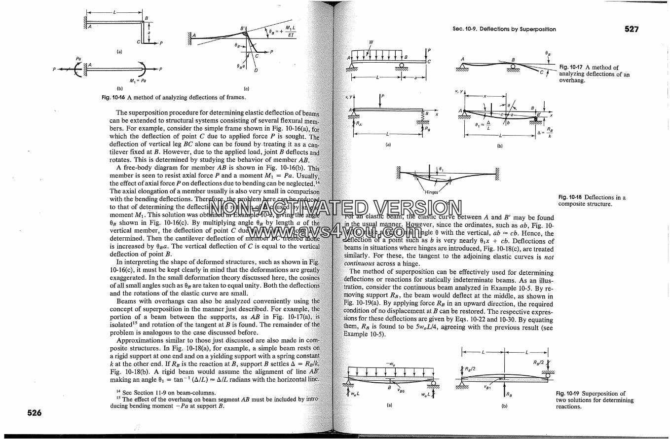
526
MI= Pa(b)
B�J ���M� L
C P��PD
(c)
Fig. 1046 A method of analyzing deflections of frames.
The superposition procedure for determining elastic deflection of bcan be extended to structural systems consisting of several flexural:bers. For example, consider the simple flame shown in Fig. 10-16(which the deflection of point C due to applied force P is sought.deflection of vertical leg BC alone can be found by.treating it astilever fixed at B. However, due to the applied load, joint B deflect:rotates. This is determined by studying the behavior of member
A flee-body diagram for member AB is shown in Fig. 10-16(b).member is seen to resist axial force P and a moment M� = Pa.the effect of axial force P on deflections due to bending can beThe axial elongation of a member usually is also very small inwith the bending deflections. Therefore, the problem here can beto that of det.ermining the deflection and rotation of B caused bymoment M�. This solution was obtained in Example 10-2, giving0B shown in Fig. 10-16(c). By multiplying angle 0B by length a oftvertical member, the deflection of point C due to rotation ofdetermined. Then the cantilever deflection of member BC treated
is increased by 0�a. The vertical deflection of C is equal to the vedeflection of point B.
In interpreting the shape of deformed structures, such as shown10-16(c), it must be kept clearly in mind that the deformations areexaggerated. In the small deformation theory discussed here, theof all small angles such as 0� are taken to equal unity.and the rotations of the elastic curve are small.
Beams with overhangs can also be analyzed convenientlyconcept of superposition in the manner just described. Forportion of a beam between the supports, as AB in Fig.isolated �5 and rotation of the tangent at B is found. The remainderproblem is analogous to the case discussed before.
Approximations similar to those just discussed are also madeposite structures. In Fig. 10-18(a), for example, a simple beama rigid support at one end and on a yielding support with a springk at the other end. If Rs is the reaction at B, support B settles A =Fig. 10-18(b). A rigid beam would assume the alignment ofmaking an angle 0� = tan-� (A/L) � A/L radians with the
�4 See Section 11-9 on beam-columns.�5 The effect of the overhang on beam segment AB must be.
ducing bending moment -Pa at support B.
w
Sec. t0-9. Deflections by Superposition
A
v, y
527
P!R�
(a)
OB
�B,, � Fig. 10-t7 A method of?//9///.�� analyzing deflections of anoverhang.
� x �
'� - L :�1A k(b)
(c)
an elastic beam, the elastic curve between A and B' may be foundthe usual manner. However, since the ordinates, such as ab, Fig. 10-
make a very small angle 0 with the vertical, ab � cb. Hence, theof a point such as b is very nearly O�x + cb. Deflections of
in situations where hinges are introduced, Fig. 10-18(c), are treated,. For these, the tangent to the adjoining elastic curves is not
across a hinge.method of superposition can be effectively used for determining
or reactions for statically indeterminate beams. As an illus-consider the continuous beam analyzed in Example 10-5. By re-support R�, the beam would deflect at the middle, as shown in
10-19(a). By applying force RB in an upward direction, the requireddisplacement at B can be restored. The respective expres-
:se deflections are given by Eqs. 10-22 and 10-30. By equatingR� is found to be 5woL/4, agreeing with the previous result (see
10-5).
B
>%L vB� wolf(a)
VB 1
R=/2
(b)
Fig. t0.18 Deflections in acomposite structure.
Fig. 10-19 Superposition oftwo solutions for determiningreactions.
NON-ACTIVATEDVERSIONwww.avs4you.com
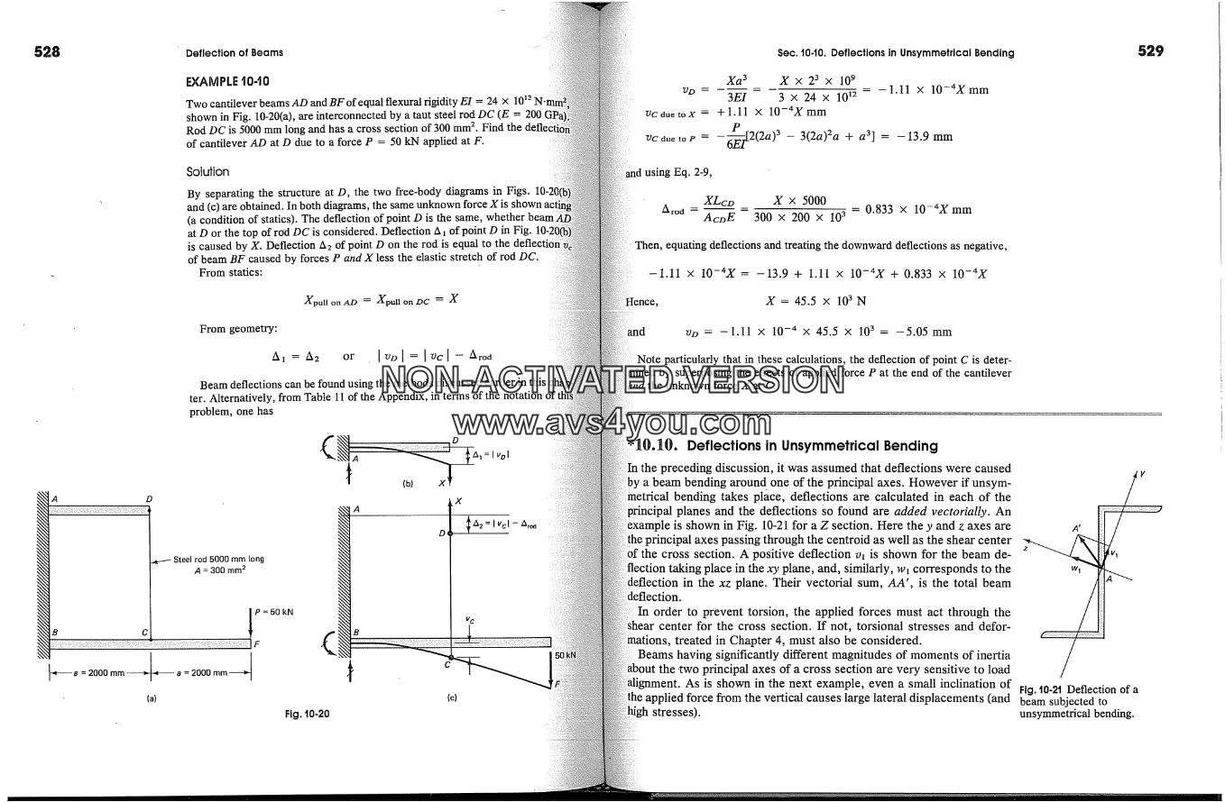
528 Deflection of Beams Sec. 1040. Deflections in Unsymmetrical Bending
EXAMPLE t0-t0
Two cantilever beams AD and BF of equal flexural rigidity E1 = 24 -x 1012 N-shown in Fig. 10-20(a), are interconnected by a taut steel rod DC (E = 200Rod DC is 5000 mm long and has a cross section of 300 mm 2. Find theof cantilever AD at D due to a force P = 50 kN applied at F.
Solution
By separating the structure at D, the two free-body diagrams in Figs.and (c) are obtained. In both diagrams, the same unknown force X is(a condition of statics). The deflection of point D is the same, whetherat D or the top of rod DC is considered. Deflection A � of point D in Fig.is caused by X. Deflection A2 of point D on the rod is equal to theof beam BF caused by forces P and X less the elastic stretch of rod DC.
From statics:
XpullonAD = XpullonDC �--- X
From geometry:
Beam deflections can be found using the methods discussed earlier in thister. Alternatively, from Table 11 of the Appendix, in terms of theproblem, one has
D
� Steel rod 5000 mm longA = 300 mm 2
C ti =50kN2000mm �-�. a =2000mm �,-
(a)
Fig. 10-20
A
� (b)x
De
(c)
v c
7J D -�-
7JCduetoX --
7JCduetoP �
using Eq. 2-9,
A rod --
Xa s X x 2 s x 109..... 1.11 x 10⁻⁴Xmm
3EI 3 x 24 x 1012+ 1.11 x 10⁻⁴X mm
-6�i[2(2a)S - 3(2a)2a + a s] = -13.9 mm
XLcz> X x 5000Acz>E 300 x 200 x l0 s
= 0.833 x 10⁻⁴X mm
equating deflections and treating the downward deflections as negative,
-1.11 x 10⁻⁴X = -13.9 + 1.11 x 10⁻⁴X + 0.833 x 10⁻⁴X
X = 45.5 x 10³N
vz> = -1.11 x 10 -4 X 45.5 x 10 3 = --5.05 mm
Note particularly that in these calculations, the deflection of point C is deter-by superposing the effects of applied force P at the end of the cantilever
and the unknown force X at C.
Deflections in Unsymmetrical Bendingn the preceding discussion, it was assumed that deflections were caused
by a beam bending around one of the principal axes. However if unsym-metrical bending takes place, deflections are calculated in each of the
planes and the deflections so found are added vectorially. Anis shown in Fig. 10-21 for a Z section. Here the y and z axes are
principal axes passing through the centreid as well as the shear centerthe cross section. A positive deflection vl is shown for the beam de-
taking place in the xy plane, and, similarly, Wl corresponds to thein the xz plane. Their vectorial sum, AA', is the total beam
order to prevent torsion, the applied forces must act through thecenter for the cross section. If not, torsional stresses and defer-
treated in Chapter 4, must also be considered.Beams having significantly different magnitudes of moments of inertia
the-two principal axes of a cross section are very sensitive to leadAs is shown in the next example, even a small inclination of
applied force from the vertical causes large lateral displacements (andstresses).
y
/Fig. t0.21 Deflection of abeam subjected tounsymmetrical bending.
NON-ACTIVATEDVERSIONwww.avs4you.com
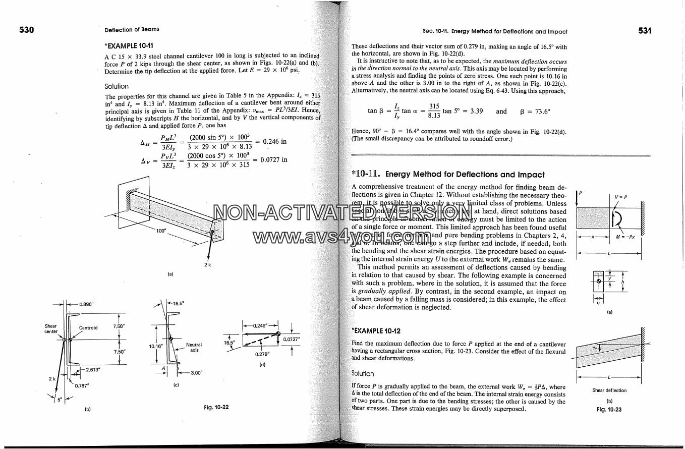
530
Shear>'1'center% I
Deflection of Beams
*EXAMPLE to.tt
A C 15 x 33.9 steel channel cantilever 100 in long is subjected toforce P of 2 kips through the shear center, as shown in Figs. 10-22(a) andDetermine the tip deflection at the applied force. Let E = 29 x 106 psi:
Solution
The properties for this channel are given in Table 5 in the Appendix: It =in n and Iy = 8.13 in 4. Maximum deflection of a cantilever bent aroundprincipal axis is given in Table 11 of the Appendix: Vm� = PL3/3EI.identifying by subscripts H the horizontal, and by V the vertical coral;tip deflection A and. applied force P, one has
PHL_� 3 _ (2000 sin 5 �) x 1003 = 0.246 inAH- 3EIy 3 X 29 X 106 X 8.13PvL� 3 _ (2000 cos 5 �) X 1003 = 0.0727 inAv- 3EIz 3 x 29 x 106 x 315
100"
2k
(a)
0.896"
Centreid 7.50"
7.50"
--2.613"0.787"
(b)
axis(c)
--0.246" > J,
(d)
Fig. t0-22
Sec. t0-11. Energy Method for Deflections and Impact
These deflections and their vector sum of 0.279 in, making an angle of 16.5 � withthe horizontal, are shown in Fig. 10-22(d).
It is instructive to note that, as to be expected, the maximum deflection occurs'n the c�irection normal to the neutral axis. This axis may be located by performing
a stress analysis and finding the points of zero stress. One such point is 10.16 inabove A and the other is 3.00 in to the right of A, as shown in Fig. 10-22(c).Alternatively, the neutral axis can be located using Eq. 6-43. Using this approach,
Iz 315 50tan [3 = � tan a = 8'�-i� tan = 3.39 and [3 = 73.6 �
90 � - 13 = 16.4 � compares well with the angle shown in Fig. 10-22(d).(The small discrepancy can be attributed to roundoff error.)
Energy Method for Deflections and Impactcomprehensive treatment of the energy method for finding beam de-
ections is given in Chapter 12. Without establishing the necessary theo-rem, it is possible to solve only a very limited class of problems. Unless
special conditions such as symmetry are at hand, direct solutions basedthe principle of conservation of energy must be limited to the action
force or moment. This limited approach has been found usefulin the axial force, torsion, and pure bending problems in Chapters 2, 4,
and 6. In beams, one can go a step further and include, if needed, boththe bending and the shear strain energies. The procedure based on equat-ing the internal strain energy U to the external work We remains the same.
This method permits an assessment of deflections caused by bendingrelation to that caused by shear. The following example is concerned
such a problem, where in the solution, it is assumed that the forcegradually applied. By contrast, in the second example, an impact on
caused by a falling mass is considered; in this example, the effectdeformation is neglected.
10-t2
the maximum deflection due to force P applied at the end of a cantilevera rectangular cross section, Fig. 10~23. Consider the effect of the flexural
shear deformations.
is gradually applied to the beam, the external work We = �PA, wherethe total deflection of the end of the beam. The internal strain energy consists
two parts. One part is due to the bending stresses; the other is caused by theThese strain energies may be directly superposed.
Pv=P
(a)
LShear deflection
(b)
Fig. t0-23
NON-ACTIVATEDVERSIONwww.avs4you.com
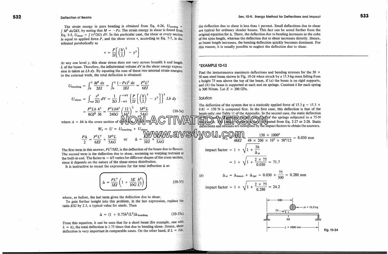
532 Deflection of Beams
The strain energy in pure bending is obtained from Eq. 6-24,f M 2 dx/2EI, by noting that M = -Px. The strain energy in shear is foundEq. 3-5, Ush� = f (x2/2G) dV. In this particular case, the shear at everyis equal to applied force P, and the shear stress �, according to Eq. 7-7,tributed parabolically as
: P[(hh 2 -
At any one level y, this shear stress does not vary across breadth h andL of the beam. Therefore, the infinitesimal volume dV in thesion is taken as Lbdy. By equating the sum of these two 'to the external work, the total deflection is obtained:
= fo(_ex)2x e2L3Sheriding J0 2EI = 2EI - 6�-
Ushear = el �'� dg = �'� hi2 � _ y2 Lbp2Lb h s _ P2LbhS (12� 5 3p2L
- 8GF 30 240G [,bh �] 5AGwhere A = bh is the cross section of the beam. Then
We = S = Sheriding + Sshear
pA p2L3 . 3P2L PL 3 6PL---+-- or A=--+--
2 6EI 5AG 3EI 5AG
The first term in this answer, PL3/3EI, is the deflection of the beanThe second term is the deflection due to shear, assuming no warpingthe built-in end. The factor at = 6/5 varies for different shapes of the crosssince it depends on the nature of the shear-stress distribution.
It is instructive to recast the expression for the total deflection a as
3Eh2)l-- 1+--�- 5lOG
where, as before, the last term gives the deflection due to shear.To gain further insight into this problem, in the last expression,
ratio E/G by 2.5, a typical value for steels. Then
A = (1 + 0.75h2/L2)Abending
From this equation, it can be seen that for a short beam (for example,L = h), the total deflection is 1.75 times that due to bending alone. Hencedeflection is very important in comparable cases. On the other hand, if L
Sec..t0-1t. Energy Method for Deflections and Impact
the deflection due to shear is less than 1 percent. Small deflections due to sheartypical for ordinary slender beams. This fact can be noted further from the
uation for A. There, the deflection due to bending increases as the cubeof the s�pan length, whereas the deflection due to shear increases directly. Hence,
s beam length increases, the bending deflection quickly becomes dominant. Forthis reason, it is usually possible to neglect the deflection due to shear.
*EXAMPLE t0-t3
the instantaneous maximum deflections and bending stresses for the 50 xmm steel beam shown in Fig. 10-24 when struck by a 15.3-kg mass falling from
a height 75 mm above the top of the beam, if (a) the beam is on rigid supports,(b) the beam is supported at each end on springs. Constant k for each spring
300 N/min. Let E = 200 GPa.
Solution
deflection of the system due to a statically applied force of 15.3 g = 15.3 x}.81 = 150 N is computed first. In the first case, this deflection is that of the
see Table 11 of the Appendix. In the second case, the static deflectionthe beam is augmented by the deflection of the springs subjected to a 75-N
force each. The impact factors are then computed from Eq. 2-27 or 2-28. Staticdeflections and stresses are multiplied by the impact factors to obtain the answers.
PL 3 150 x 1000348E1 48 x 200 x 103 x 504/12
:himpact factor = 1 + + A st
� 2x75= 1 + 1 + 0.030 = 71.7
= 0.030 mm
(b)75
Ast = Ab� + A�p� = 0.030 + 30---�
�/ 2 x 75 = 24.2impact factor = 1 + 1 + 0.28-----�
= 0.280 mm
50075 ---,_.�..�'"'�' rn =5O
k = 1000 mm
15.3 kg
Fig. 10-24
533
NON-ACTIVATEDVERSIONwww.avs4you.com

534 Deflection of Beams 535
For either case, the maximum bending stress in the beam due to a static iplication of P is
O-max)st --M PL 150 x 1000
S 4S 4 x 503/6- 1.800 �MPa
Multiplying the static deflections and stress by the respective impactgives the required results.
Static Dynamic
With Springs No Springs With Springs No SAmax, mm 0.280 0.030 6.78
Crmax, MPa 1.80 1.80 43.6. 129
It is apparent from this table that large deflections and stresses are causeda dynamically applied lead. The stress for the condition with no springsticularly large; however, owing to the flexibility of the beam, it is not exces:
*�610-12. Inelastic Deflection of BeamsAll the preceding solutions for beam deflections apply only if thebehaves elastically. This limitation is the result of introducinglaw into the strain-curvature relation, Eq. 10-5, to yield thecurvature equation, Eq. 10-6. The subsequent procedures formating the curvature as cFv/dx 2 and the integration schemes do noton the material properties.
Superposition does not apply to inelastic problems, sinceare not linearly related to the applie d forces. As a consequence,cases piecewise linear solutions for small lead orare made until the desired level of lead or displacement is reached.stepwise linear calculations are made with the aid of a computer.natively, time-consuming trial-and-error solutions are used todeflections in indeterminate beams. However, it is possible tosimple solutions for ultimate strengths of statically determinatedeterminate beams and frames assuming ideal plastic behaviorterial. For such a method, a relationship between theand curvature at a section of a beam must be developed. Andefining such a relationship is given in the next example.is this approach that is relied upon in Chapter 13 for plasticanalyses of statically determinate and indeterminate beams andframes.
The second example that follows discusses the deflection
�6 This section is optional.
Sec. 10-12. Inelastic Deflection of Beams
statically determinate elastic-plastic beam. The solution demonstratesas long as at least a part of a beam's cross section remains elastic,
he deflections remain bounded, i.e., finite, and can be calculated.
�LE t0-t4
and plot the moment-curvature relationship for an elastic-ideally plas-rectangular beam.
�olution
a rectangular elastic-plastic beam at Yo, where the juncture of the elastic andzones occurs, the linear strain e;� = +gyp; see Fig. 6-30. There_fore, ac-
to Eq. 10-5, with the curvature 1/p = K,
1 gyp gyp- = K = --- and Kyp =p yo h/2
the last expression gives the curvature of the member at impending yieldingWhen yo = hi2. From these relations,
yo Kyph/2 K
By substituting this expression into Eq. 6-40, one obtains the required mome..n.t-.relationship:
[ 1 (yoh2] 3 [ 1 (�) 2]M = M v 1 - 5 �,�-�/ J = �Myp 1 - 5 (10-36)function is plotted in Fig. 10-25. Note how rapidly it approaches the asymp-At curvature just double that of the impending yielding, eleven-twelfths, or
M
Asymptote
/
/
//
Residual curvature
gYP 2gyp 4gyp l/p= �Fig. 10-25 Moment-curvaturerelation for an elastic-plasticrectangular beam.
NON-ACTIVATEDVERSIONwww.avs4you.com
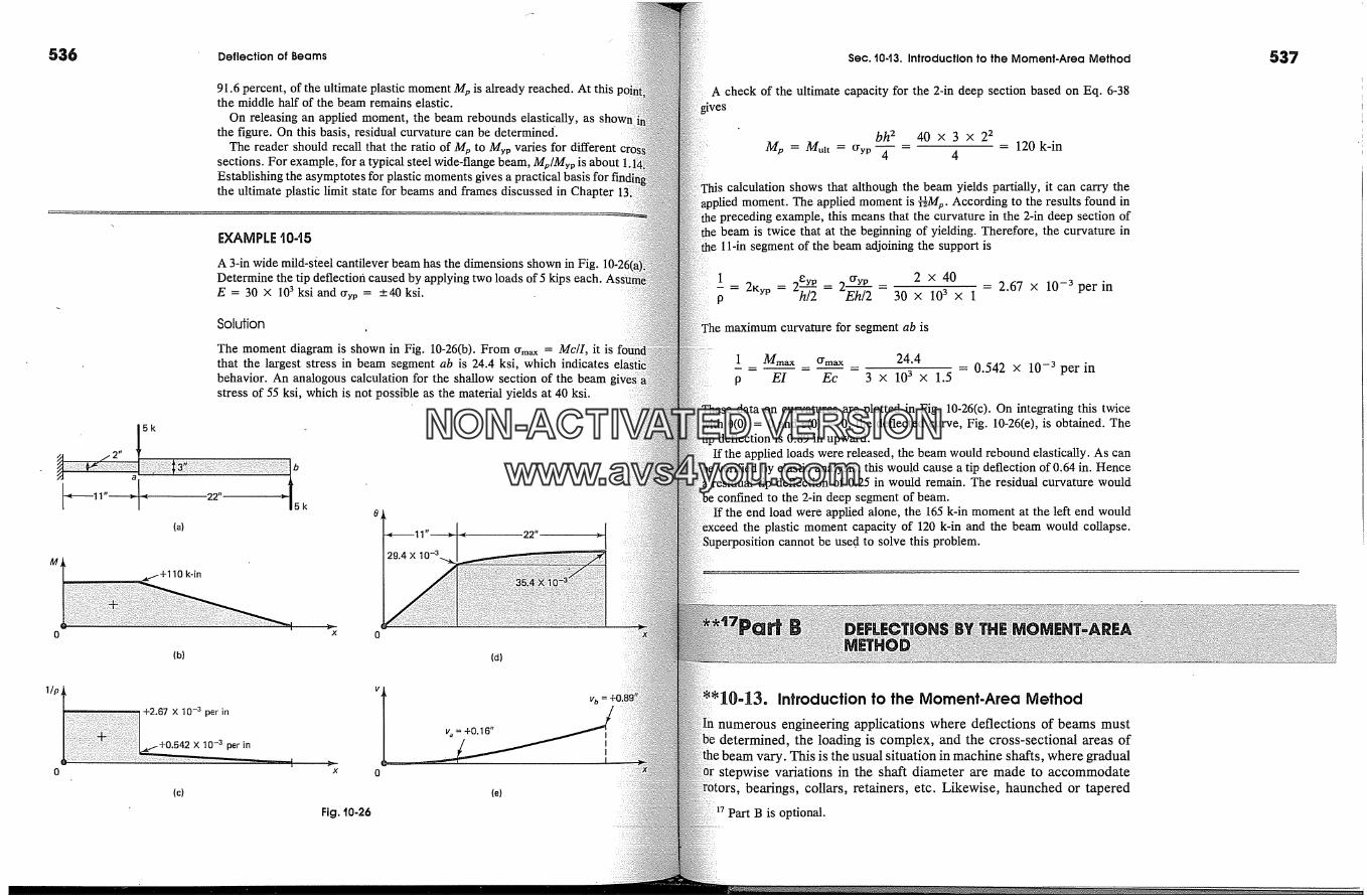
536 Deflection of Beams
91.6 percent, of the ultimate plastic moment Mp is already reached. At thisthe middle half of the beam remains elastic.
On releasing an applied moment, the beam rebounds elastically, asthe figure. On this basis, residual curvature can be determined.
The reader should recall that the ratio of Mp to Myp varies for differentsections. For example, for a typical steel wide-flange beam, M�/Myp is aboutEstablishing the asymptotes for plastic moments gives a practical basis for tthe ultimate plastic limit state for beams and frames discussed in Chapter
5k
EXAMPLE t0-t5
A 3-in wide mild-s�eel cantilever beam has the dimensions shown in Fig.Determine the tip deflection caused by applying two loads of 5 kips each.E = 30 x 103 ksi and %� = +40 ksi.
Solution
The moment diagram is shown in Fig. 10-26(b). From Crm� = Mc/I, it isthat the largest stress in beam segment ab is 24.4 ksi, which indicatesbehavior. An analogous calculation for the shallow section of the beamstress of 55 ksi, which is not possible as the material yields at 40 ksi.
(a)
k-in
29.4 X
(b)
+2.67 X 10 -3 per in
X 10 -3 per in
(c)
x o
Fig. 10-26
(d)
v�= +0.16"
(e)
Sec. t0-t3. Introduction to the Moment-Area Method
A check of the ultimate capacity for the 2-in deep section based on Eq. 6-38
Mp = Muir = O'yp-bh 2 40 x 3 x 2 2
4 4- 120 k-in
calculation shows that although the beam yields partially, it can carry theapplied moment. The applied moment is I�M�. According to the results found in
preceding example, this means that the curvature in the 2-in deep section ofthe beam is twice that at the beginning of yielding. Therefore, the curvature in
11-in segment of the beam adjoining the support is
1 2Kyp 2 �yp 2 tryp 2 x 40 2.67 x 10 -3 per inp -h/2 -Eh/2 30 x 103 x 1
maximum curvature for segment ab is
1 _ Mmax O'max _ 24.4 = 0.542 X 10 -3 per inp E1 Ec 3 x 103 x 1.5
data on curvatures are plotted in Fig. 10-26(c). On integrating this twice0(0) = 0 and v(0) = 0, the deflected curve, Fig. 10-26(e), is obtained. The
deflection is 0.89 in upward.If the applied loads were released, the beam would rebound elastically. As can
be verified by elastic analysis, this would cause a tip deflection of 0.64 in. Henceresidual tip deflection of 0.25 in would remain. The residual curvature would
be confined to the 2-in deep segment of beam.If the end load were applied alone, the 165 k-in moment at the left end would
the plastic moment capacity of 120 k-in and the beam would collapse.cannot be use.d to solve this problem.
Introduction to the Moment-Area Method
numerous engineering applications where deflections of beams mustdetermined, the loading is complex, and the cross-sectional areas of
vary. This is the usual situation in machine shafts, where gradualstepwise variations in the shaft diameter are made to accommodate
beatings, collars, retainers, etc. Likewise, haunched or tapered
Part B is optional.
537
NON-ACTIVATEDVERSIONwww.avs4you.com

538 Deflection of Beams
beams are frequently employed in aircraft as well as in bridg etion. By interpreting semigraphically the mathematical operations ofing the governing differential equation, an effective proceduretaining deflections in complicated situations has been developed.this alternative procedure, one finds that problems with load dis�uities and arbitrary variations of inertia of the cross-sectionalbeam cause no complications and require only a little morework for this solution. The solution of such problems is thethe following sections on the moment-area method?
The method to be developed is generally used to obtain onlyplacement and rotation at a single point on a beam. It may bedetermine the equation of the elastic curve, but no advantage isin comparison with the direct solution of the differential equation.however, it is the deflection and/or the angular rotation of thecurve, or both, at a particular point of a beam that are of greatestin the solution of practical problems.
The method of moment areas is just an alternative method forthe deflection problem. It possesses the same approximations andtations discussed earlier in connection with the solution of theequation of the elastic curve. By applying it, one determinesdeflection due to the flexure of the beam; deflection due to shearglected. Application of the method will be developed for staticalitterminate and indeterminate beams.
*'10-14. Moment-Area Theorems
The necessary theorems are based on the geometry of the elasticand the associated M/EI diagram. Boundary conditions do notthe derivation of the theorems since the theorems are based onlyinterpretation of definite integrals. As will be shown later, furthe:metrical considerations are necessary to solve a complete
For deriving the theorems, Eq. 10-10, c[2v/dx 2 = M/EI, canin the following alternative forms:
dx 2 = �x = �x � EI or dO = �dxFrom Fig. 10-27(a), quantity (M/E1) dx corresponds to
area of the M/EI diagram. According to Eq. 10-37, this area isthe change in angle between two adjoining tangents. Thean angle change in one element to the deformation of the elasticshown in Fig. 10-27(b).
�8 The development of the moment-area method for finding deflectionsis due to Charles E. Greene, of the University of Michigan, who taughtclasses in 1873. Somewhat earlier, in 1868, Otto Mohr, of Dresden,developed a similar method that appears to have been unknown toGreene.
(1C
x (b)
(a)
If the small angle change dO for an element is multiplied by a distancefrom an arbitrary origin to the same element, a vertical distance dt is
see Fig. 10-27(b). As only small deflections are considered, notinction between arc AA' and vertical distance dt need be made. Basedthis geometrical reasoning, one has
M
dt = x dO = �x dx (10-38)integrating Eqs. 10-37 and 10-38 between any two points such
A and B on a beam (see Fig. 10-28), yields the two moment-area theo-The first moment-area theroem is
dO = OB- OA = zXOmA = � dx (10-39)
A 0m� is the angle change between B and A. This change in anglein radians between any two tangents at points A and B on the
i +A0mA
C D
curve
Fig. i0-27 Interpretation of asmall angle change in anelement.
Fig. t0-28 Relationshipbetween the M/E1 diagramand the elastic curve.
539
NON-ACTIVATEDVERSIONwww.avs4you.com
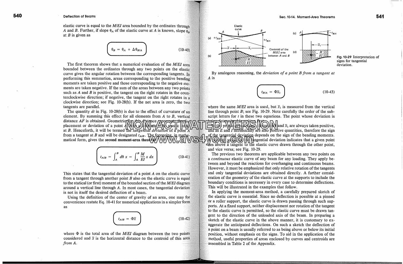
Deflection of Beams Sec. t044. Moment-Area Theorems
elastic curve is equal to the M/E1 area bounded by the. ordinatesA and B. Further, if slope 0A of the elastic curve at'A is known,at B is given as -
0B �-0A q-AOBIA)The first theorem shows that a numerical evaluation of the M/E1
bounded between the ordinates through any two points on thecurve gives the angular rotation between the corresponding tangents� ]performing this summation, areas corresponding to the positivemoments are taken positive and those corresponding to the negativements are taken negative. If the sum of the areas between any twosuch as A and B is positive, the tangent on the right rotates in theterclockwise direction; if negative, the tangent on the right rotatesclockwise direction; see Fig. 10-28(b). If the net area is zero, thetangents are parallel.
The quantity dt in Fig. 10-28(b) is due to the effect of curvature �element. By summing this effect for all elements from A to B,distance AF is obtained. Geometrically, this distance represents theplacement or deviation of a point A from a tangent to the elasticat B. Henceforth, it will be termed the tangential deviation of afrom a tangent at B and will be designated tA/B. The foregoing, inmatical form, gives the second moment-area theorem:
dO x = � x (10-41
This states that the tangential deviation of a point A on the elasticfrom a tangent through another point B also on the elastic curve isto the statical (or first) moment of the bounded section of thearound a vertical line through A. In most cases, the tangentialis not in itself the desired deflection of a beam.
Using the definition of the center of gravity of an area, one mayconvenience restate Eq. 10-41 for numerical applications in a s'as
tA/�where cI) is the total area of the M/E1 diagram between the twoconsidered and � is the horizontal distance to the centroid of this
from A.
(b)
Elastic
curve B
+t�l�� � (c) A�+ tBi A
.�I� Centroidofthe�_- M/EI area {d}between A and B
By analogous reasoning, the deviation of a point B from a tangent atA is
--tB/A=��i (10-43)
where the same M/E1 area is used, but � is measured from the verticalthrough point B; see Fig. 10-29. Note carefully the order of the sub-
letters for t in these two equations. The point whose deviation isbeing determined is written first.
In the previous equations, distances � and � are always taken positive,as E and I intrinsically are also positive quantities, therefore the sign
of the tangential deviation depends on the sign of the bending moments.A positive value for the tangential deviation indicates that a given point
above a tangent to the elastic curve drawn through the other point,vice versa; see Fig. 10-29.
The previous two theorems are applicable between any two points oncontinuous elastic curve of any beam for any loading. They apply be-
tween and beyond the reactions for overhanging and continuous beams.it must be emphasized that only relative rotation of the tangents
only tangential deviations are obtained directly. A further consid-the geometry of the elastic curve at the supports to include the
boundary conditions is necessary in every case to determine deflections.will be illustrated in the examples that follow.
In applying the moment-area method, a carefully prepared sketch ofelastic curve is essential. Since no deflection is possible at a pinned
a roller support, the elastic curve is drawn passing through such sup-ports. At a f'Lxed support, neither displacement nor rotation of the tangent
the elastic curve is permitted, so the elastic curve must be drawn tan-gent to the direction of the unloaded axis of the beam. In preparing asketch of the elastic curve in the above manner, it is customary to ex-
the anticipated deflections. On such a sketch the deflection ofa point on a beam is usually referred to as being above or below its initial
position, without emphasis on the signs. To aid in the application of theuseful properties of areas enclosed by curves and centroids are
in Table 2 of the Appendix.
Fig. t0-29 Interpretation ofsigns for tangentialdeviation.
NON-ACTIVATEDVERSIONwww.avs4you.com
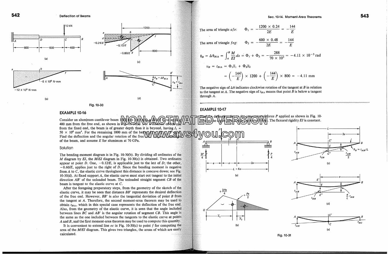
Deflection of Beams Sec. t0-14. Moment-Area Theorems
A
600 �
-12 X 106 N.mm
800 �
10 kN
a b
C __�B d-0.24/E e -0.12/E�---400
-0.60/E g
(.)
-6 X 10⁶ N-mm
-1200
(c)
�B = A�BIA
B t
B
(b) (d)
Fig. t0-30
EXAMPLE t0-t6
Consider an aluminum cantilever beam 1600 mm long with a 10-kN force400 mm from the free end, as shown in Fig. 10-30(a). For a distance of 600from the fixed end, the beam is of greater depth than it is beyond, having50 x 106 mm 4. For the remaining 1000 mm of the beam, 12 = 10 x 106Find the deflection and the angular rotation of the free end. Neglect theof the beam, and assume E for aluminum at 70 GPa.
Solution
The bending-moment diagram is in Fig. 10-30(b). By dividing all ordinatesM diagram by El, the M/E1 diagram in Fig. 10-30(c) is obtained. Twoappear at point D. One, -0.12/E, is applicable just to the lett of D; the-0.60/E, applies just to the right of D. Since the bending moment is
from A to C, the elastic curve thrdughout this distance is concave down; see10-30(d). At fixed support A, the elastic curve must start outdirection AB' of the unloaded beam. The unloaded straight segment CBbeam is tangent to the elastic curve at C.
After the foregoing preparatory steps, from the geometry of the sketchelastic curve, it may be seen that distance BB' represents the desiredof the free end. However, BB' is also the tangential deviation of point Bthe tangent at A. Therefore, the second moment-area theorem may beobtain tmA, which in this special case represents the deflection of theAlso, from the geometry of the elastic curve, it is seen that the anglebetween lines BC and AB' is the angular rotation of segment CB. Thisthe same as the one included between the tangents to the elastic curve at'A and B, and the first moment-area theorem may be used to compute this
It is convenient to extend line ec in Fig. 10-30(c) to point farea of the M/E1 diagram. This gives two triangles, the areas of which are easicalculated.
area of triangle are: � =1200 x 0.24 144
2E E
The area of triangle leg: �2 -600 x 0.48 144
2E E
= AOB/A = dx = �'+ �2 =288
70 x 103-4.11 x 10⁻³rad
vB = t�/4 = � +
x 800 = -4.11 mm
sign of A0 indicates clockwise rotation of the tangent at B in relationthe tangent at A. The negative sign of tB/A means that point B is below a tangent
A.
EXAMPLE t0-t7
the deflection due to the concentrated force P applied as shown in Fig. 10-at the center of a simply supported beam. The flexural rigidity E1 is constant.
x�--a -�� a.----.�4 2aL = 4a
(a)
+ 3Pa4 +P�
(b)
(c)
A E' < e �BE
tAIBJ n e
(d)
tAlC(e)
Fig. 10-31
NON-ACTIVATEDVERSIONwww.avs4you.com
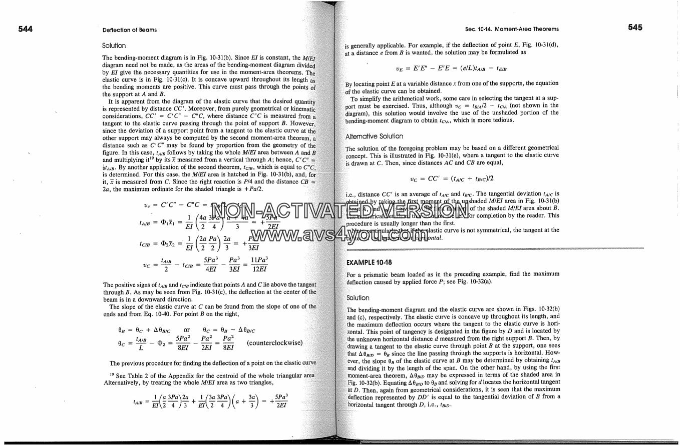
Deflection of Beams Sec. t044. Moment-Area Theorems
Solution
The bending-moment diagram is in Fig. 10-31(b). Since E1 is constant, thediagram need not be made, as the areas of the bending-moment diagramby E1 give the necessary quantities for use in the moment-area theorems.elastic curve is in Fig. 10-31(c). It is concave upward throughout itsthe bending moments are positive. This curve must pass through thethe support at A and B.
It is apparent from the diagram of the elastic curve that the desiredis represented by distance CC'. Moreover, from purely geometrical orconsiderations, CC' = C'C" - C"C, where distance C" is measuredtangent to the elastic curve passing through the point of support B.since the deviation Of a support point from a tangent to the elastic curve atother support may always be computed by the second moment-areadistance such as C'C" may be found by proportion from the geometryfigure. In this case, tA/B follows by taking the whole M/E1 area between A andand multiplying it �9 by its � measured from a vertical through A; hence,�tA/B. By another application of the second theorem, tc�, which is equal tois determined. For this case, the M/E1 area is hatched in Fig. 10-31(b),it, � is measured from C. Since the right reaction is P/4 and the distance CB2a, the maximum ordinate for the shaded triangle is +Pa/2.
The positive signs of tam and tc/� indicate that points A and C lie above tthrough B. As may be seen from Fig. 10-31(c), the deflection at the centerbeam is in a downward direction.
The slope of the elastic curve at C can be found from the slopeends and from Eq. 10-40. For point B on the right,
Oa = 0c + A0mc or 0c = Oa - A OmctA/� 5Pa 2 Pa 2 Pa 2
Oc = -- - �2 - -L 8EI 2EI 8EI
The previous procedure for finding the deflection of a point on the
�9 See Table 2 of the Appendix for the centreid of the whole triangularAlternatively, by treating the whole M/E1 area as two triangles,
tAm=� � 4 J3 +�[,T-�-)[, a+ = +2--�-
generally applicable. For example, if the deflection of point E, Fig. 10-31(d),at a distance e from B is wanted, the solution may be formulated as
v�r = E'E' - E'E = (e/L)tA/a -- tE/B
' locating point E at a variable distance x from one of the supports, the equation'the elastic curve can be obtained.To simplify the arithmetical work, some care in selecting the tangent at a sup-
must be exercised. Thus, although vc = tmA/2 -- tC/A (not shown in thethis solution would involve the use of the unshaded portion of the
-moment diagram to obtain tC/A, which is more tedious.
Solution
solution of the foregoing problem may be based on a different geometricalThis is illustrated in Fig. 10-31(e), where a tangent to the elastic curve
is drawn at C. Then, since distances AC and CB are equal,
Vc = CC' = (tAlC + tmc)12
Le., distance CC' is an average of tAlC and true The tangential deviation tmc isby taking the first moment of the unshaded M/E1 area in Fig. 10-31(b)
about A, and tmc is given by the first moment of the shaded M/E1 area about B.The numerical details of this solution are left for completion by the reader. This
�rocedure is usually longer than the first.Note particularly that if the elastic curve is not symmetrical, the tangent at the
center of the beam is not horizontal.
t048
a prismatic beam loaded' as in the preceding example, find the maximumcaused by applied force P; see Fig. 10-32(a).
Solution
bending-moment diagram and the elastic curve are shown in Figs. 10-32(b)respectively. The elastic curve is concave up throughout its length, and
the maximum deflection occurs where the tangent to the elastic curve is hori-This point of tangency is designated in the figure by D and is located by
horizontal distance d measured from the right support B. Then, bya tangent to the elastic curve thro�ugh point B at the support, one sees
that A0mz� = 0� since the line passing through the supports is horizontal. How-the slope 0� of the elastic curve at B may be determined by obtaining tA/B
and dividing it by the length of the span. On the other hand, by using the firsttheorem, A0mo may be expressed in terms of the shaded area in
10-32(b). Equating A0mo to 0a and solving for d locates the horizontal tangentThen, again from geometrical considerations, it is seen that the maximum
represented by DD' is equal to the tangential deviation of B from atangent through D, i.e., true.
NON-ACTIVATEDVERSIONwww.avs4you.com

546 Deflection of Beams
A
P
---a >, ,< 3a >-Ii- L =4a >
(a)
tA/8
O t0 e � tA/e/L
(c)
+ 3Pa4 .+Pd
0
(b)
A
Fig. t0-32
SPa 3q� = .+--
2EI
tam tam SPa 2L 4a 8EI
� �2 4 ] = 8EI
O t
Horizontal
(d)
(see Example 10-17)
(area between D and B)
Since 0B = 0z� + A0mo and it is required that 0o = 0,
pd2 SPa2 hence, d = X/�aAOmz� = 011 8EI - 8EIVmax �--- VD �--- DD' = tmz> =
1EI 12EI 12EI
After distance d is found, the maximum deflection may also be obtained as= two, or Vm�x = (d/L)tw, - tom (not shown). Also note that using the
two = tmo, Fig. 10-32(d), an equation may be set up for d.It should be apparent from this solution that it is easier to calculate
flection at the center of the beam, which was illustrated in Example 10-17,to determine the maximum deflections. Yet, by examining the end results�sees that, numerically, the two deflections differ little: v,�t� =
Sec. t0-14. Moment-Area Theorems
Vmax = 11.2Pa3/12EI. For this reason, in many practical problems ofsupported beams, where all the applied forces act in the same direction,
t is often sufficiently accurate to calcuate the deflection at the center instead ofto obtain the true maximum.
PLE t0-t9
In a simply supported beam, find the maximum deflection and rotation of thecurve at the ends caused by the application of a uniformly distributed load
wo lb/ft; see Fig. 10-33(a). Flexural rigidity E1 is constant.
bending-moment diagram is in Fig. 10-33(b). As established in Example 5-8,is a second-degree parabola with a maximum value at the vertex of woL2/8.
elastic curve passing through the points of supports A and B is shown in Fig.10-33(c).
this case, the M/E1 diagram is symmetrical about a vertical line passingthrough the center. Therefore, the elastic curve must be symmetrical, and the
tangent to this curve at the center of the beam is horizontal. From the figure, itseen that A0mc is equal to 0B, and the rotation of B is equal to one-half the
of the whole M/E1 diagram. Distance CC' is the desired deflection, andthe geometry of the figure, it is seen to be equal to tmc (or twc, not shown).
I�.)�__. (�Zw�.Z2)�.� �VOz32 24EI
011 = A0111C = � = +w�L324EI
woL 3 5LVc = Vm� = tmc = q� =
24EI 165woL 4384EI
20 See Table 2 of the Appendix for a formula giving an area enclosed by a3arabola as well as for �.
Ib/ft
BC
�--L/2 � < L/2 �(a)
+W o/2/8
I� T
OBIC' AO, a/c B � -'�
(c)
{b) Fig. t0-33
547
NON-ACTIVATEDVERSIONwww.avs4you.com
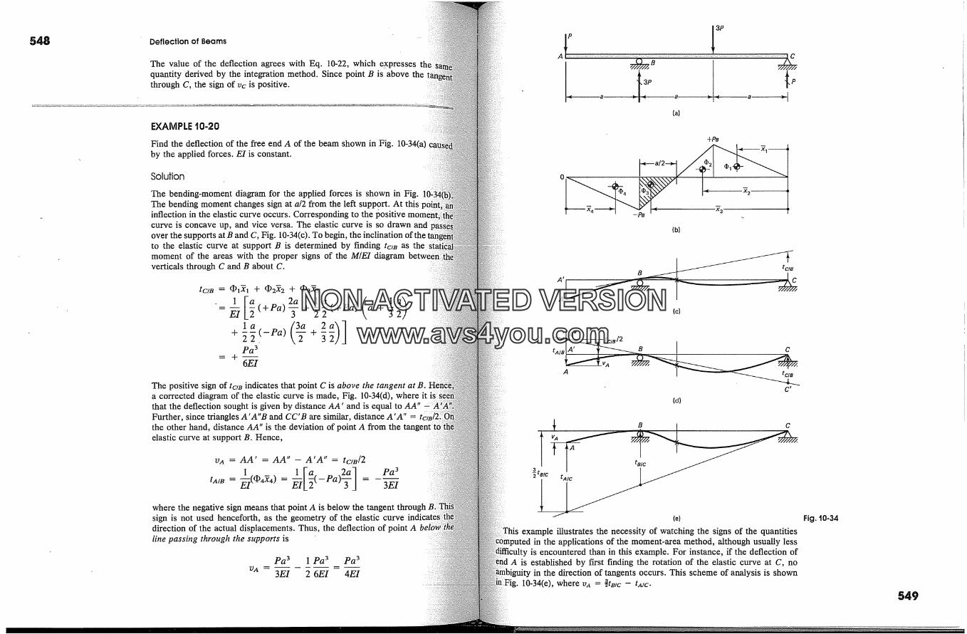
3PP
548 Deflection of Beams
The value of the deflection agrees with Eq. 10-22, which expressesquantity derived by the integration method. Since point B is above thethrough C, the sign of vc is positive.
EXAMPLE l 0-20
Find the deflection of the free end A of the beam shown in Fig. 10-34(a)by the applied forces. E1 is constant.
Solution
The bending-moment diagram for the applied forces is shown in Fig.The bending moment changes sign at a/2 from the left support. At thisinflection in the elastic curve occurs. Corresponding to the positivecurve is concave up, and vice versa. The elastic curve is so drawnover the supports at B and C, Fig. 10-34(c). To begin, the inclination ofth{to the elastic curve at support B is determined by finding tc/B asmoment of the areas with the proper signs of the M/E1 diagramverticals through C and B about C.
tc/a = cb�X'l + C1�2�' 2 q- CI)3.� 3
_ 1 [�(+pa) 2a l a ( l a)= � -�- + �(+Pa) a + �
la (3_� 2�)]+ � (-aa) + 5pa 36EI
The positive sign of tc/B indicates that point C is above the tangent at B.a corrected diagram of the elastic curve is made, Fig. 10-34(d), where itthat the deflection sought is given by distance AA' and is equal to AA"Further, since triangles A'A"B and CC'B are similar, distance A'A" =the other hand, distance AA" is the deviation of point A from the tangentelastic curve at support B. Hence,
VA = AA' = AA" - A'A" = tc/a/2
1 l[a 2aI Pa 3tA/a = �(C�4X--4) = � �(-Pa)-�' = 3EIwhere the negative sign means that point A is below the tangentsign is not used henceforth, as the geometry of the elastic curve indicatesdirection of the actual displacements. Thus, the deflection of point Aline passing through the supports is
Pa 3 1 Pa 3 Pa 33� 26� 4�
A
(a)
c
+P�
(b)
(c)
tClB
C'
(d)
�- (e)example illustrates the necessity of watching the signs of the quantifies
in the applications of the moment-area method, although usually lessis encountered than in this example. For instance, if the deflection of
is established by ftrst finding the rotation of the elastic curve at C, noin the direction of tangents occurs. This scheme of analysis is shown
a t --Fig. 10-34(e), where VA = � �/C tA/O
Fig. t0-34
549
NON-ACTIVATEDVERSIONwww.avs4you.com

550 Deflection of Beams Sec. t0-t5. Statically Indeterminate Beams 55�
(a)
A �P C l P .....iB(b)
(c)A
tAl�Fig. '10-35
EXAMPLE 'i0-2'1
A simple beam supports two equal and opposite forces P at the quartersee Fig. 10-35(a). Find the deflection of the beam at the middle of theis constant.
Solution
The bending-mo _ment diagram and elastic curve with a tangent at C areFigs. 10-35(b) and (c), respectively. Then, since the statical moments of the-itive and negative areas of the bending-moment diagram around A andspectively, are numerically equal, i.e., [ tAlC I = I tB/C I, theat the center of the span is zero. The elastic curve in this caseNoting this, much work may be avoided in obtaining the deflections atof the span. The deflection of any other point on the elastic curve canin the usual manner.
The foregoing examples illustrate the manner in which thearea method can be used to obtain the deflection of any staticallyminate beam. No matter how complex the M/EI diagrams maythe previous procedures are applicable. In practice, any M/EIwhatsoever may be approximated by a number of rectanglesIt is also possible to introduce concentrated angle changes ataccount for discontinuities in the directions of the tangents at suchThe magnitudes of the concentrations can be found fromquirements. 2�
For complicated loading conditions, deflections of elastictermined by the moment-area method are often best found bysition. In this manner, the areas of the separate M/EI diagrams
21 For a systematic treatment of more complex problems see, forC. Scordelis and C. M. Smith, "An Analytical Procedure for CalculatingDisplacements," Proc. ASCE 732 (July 1955): 732-1 to 732-17.
simple geometrical shapes. In the next section, superposition is usedsolving statically indeterminate problems.
The .method described here can be used very effectively in determining., inelastic deflection of beams, provided the M/EI diagrams are replaced
by the curvature diagrams such as in Fig. 10-26(c).
�0-15. Statically Indeterminate Beamsindeterminate beams can readily be solved for unknown re-
t�ons using the moment-area method by employing superposition. Afterredundant reactions are determined, the beam deflections and rota-
can be found in the usual manner, again, often employing super-,sition. Two different procedures for finding the redundant reactions are
in this section. In the more widely used procedure, it is rec-that restrained 22 and continuous beams differ from simply sup-
beams mainly by the presence of redundant moments at the sup-Therefore, bending-moment diagrams for these beams may be
sidered to consist of two independent parts--one part for the momentby all of the applied loading on a beam assumed to be simply
the other part for the redundant end moments. Thus, the effect,redundant end moments is superposed on a beam assumed to be simply
Physically, this notion can be clarified by imagining an in-cut through at the supports while the vertical reactions
are maintained. The continuity of the elastic curve of the beam is pre-Served by the redundant moments.
Although the critical ordinates of the bending-moment diagrams causedthe redundant moments are not known, their shape is known. Appli-
of a redundant moment at an end of a simple beam results in aled moment diagram, with a maximum at the applied mo-
and a zero ordinate at the other end. Likewise, when end momentsare present at both ends of a simple beam, two triangular moment dia-
superpose into a trapezoidal-shaped diagram.The known and the unknown parts of the bending-moment diagram
a complete bending-moment diagram. This whole diagramused in applying the moment-area theorems to the continuous
curve of a beam. The geometrical conditions of a problem, suchthe continuity of the elastic curve at the support or the tangents at
built-in ends that cannot rotate, permit a rapid formulation of equationsthe unknown values of the redundant moments at the supports.
An alternative method for determining the redundant reactions employsprocedure of plotting the bending-moment diagrams by parts. In apply-
this method, only one of the existing fixed supports is left in place,a cantilever. Then separate bending-moment diagrams for each
of the applied forces as well as for the unknown reactions at the
22 Indeterminate beams with one or more fixed ends are called restrained
NON-ACTIVATEDVERSIONwww.avs4you.com
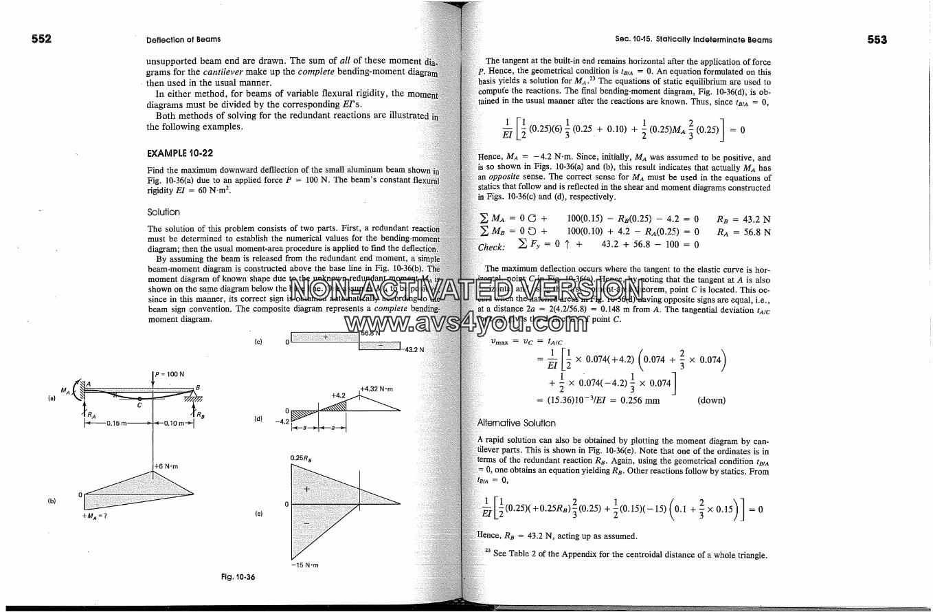
552
(a)
(b)
Deflection of Beams
unsupported beam end are drawn. The sum of all of thesegrams for the cantilever make up the complete bending-momentthen used in the usual manner.
In either method, for beams of variable flexural rigidity, thediagrams must be divided by the corresponding EI's.
Both methods of solving for the redundant reactions are illinthe following examples.
EXAMPLE t0-22
Find the maximum downward defllection of the small aluminum beamFig. 10-36(a) due to an applied force P = 100 N. The beam's constantrigidity E1 = 60 N.m 2.
Solution
The solution of this problem consists of two parts. First, a redundantmust be determined to establish the numerical values for thediagram; then the usual moment-area procedure is applied to find the
By assuming the beam is released from the redundant end moment,beam-moment diagram is constructed above the base line in Fig. 10-36(b)imoment diagram of known shape due to the unknown redundant momentshown on the sa.me diagram below the base line. One assumes MA to besince in this manner, its correct sign is obtained automatically accordingbeam sign convention. The composite diagram represents a completemoment diagram.
(c)
P= lOON
0.15m � � 0.10m-�
+6 N.m
(d)
+4.2 �'m
0.25R�
o
+MA=? (e)
Fig. t0-36
-15 N.m
Sec. 10-t5. Statically Indeterminate Beams
The' tangent at the built-in end remains horizontal after the application of forceHence, the geometrical condition is tB/A = 0. An equation formulated on this
yields a solution for Mi.23 The equations of static equilibrium are used tothe reactions. The final bending-moment diagram, Fig. 10-36(d), is ob-
tained in the usual manner after the reactions are known. Thus, since tB/A = 0,
(0.25)(6) � (0.25 + 0.10) + � (0.25)MA (0.25) = 0MA = -4.2 N-m. Since, initially, MA was assumed to be positive, and
so shown in Figs. 10-36(a) and (b), this result indicates that actually MA hasan opposite sense. The correct sense for MA must be used in the equations of
that follow and is reflected in the shear and moment diagrams constructedFigs. 10-36(c) and (d), respectively.
MA = 0 � + 100(0.15) -- RB(0.25) -- 4.2 = 0MB = 0 � + 100(0.10) + 4.2 -- RA(0.25) = 0;ck: �Fy = 0 �' + 43.2 + 56.8 - 100 = 0
Ra = 43.2 NRA = 56.8 N
The maximum deflection occurs where the tangent to the elastic curve is her-point C in Fig. 10-36(a). Hence, by noting that the tangent at A is also
and using the first moment-area theorem, point C is located. This oc-the hatched areas in Fig. 10-36(d) having opposite signs are equal, i.e.,
a distance 2a = 2(4.2/56.8) = 0.148 m from A. The tangential deviation tAlCtC/A) gives the deflection of point C.
7dmax = 7Jc = tAlC
= -- x 0.074(+4.2) 0.074 + � x 0.074EI
+ � x 0'.074(-4.2)5 x 0.074= (15.36)10-3/EI = 0.256 mm (down)
Solution
solution can also be obtained by plotting the moment diagram by can-parts. This is shown in Fig. 10-36(e). Note that one of the ordinates is in
terms of the redundant reaction R�. Again, using the geometrical condition t�/A0, one obtains an equation yielding R�. Other reactions follow by statics. From
= 0,
(0.25)(+0.25Ra) 32-(0.25) + �(0.15)(-15) 0.1 + � x 0.15 = 0R� = 43.2 N, acting up as assumed.
See Table 2 of the Appendix for the centroidal distance of a whole triangle.
553
NON-ACTIVATEDVERSIONwww.avs4you.com

Deflection of Beams Sec. t0.t5. Statically Indeterminate Beams
� MA = O� + MA + 43.2(0.25) -- 100(0.15) = 0 MA =
Here MA, within the equation of statics for the summation ofconsidered positive since it is assumed to act in a counterclocloviseHowever, in the beam sign convention, such an end moment at A is
After the combined moment diagram is constructed, Fig. 10-36(d), theder of the work is the same as in the preceding solution.
EXAMPLE t0-23
Find the moments at the supports for a fixed-end beam loaded with adistributed lead of we N/m; see Fig. 10-37(a).
Solution
The moments at the supports are called fixed-end moments, and theirnation is of great importance in structural theory. Due to symmetry in thislem, the fixed-end moments are equal, as are the vertical reactions,well2 each. The moment diagram for this beam, considered to beported, is a parabola, as shown in Fig. 10-37(b), while the assumed'end moments give the rectangular diagram shown in the same figure.
Although this beam is statically indeterminate to the second degree,of symmetry, a single equation based on a geometrical condition isyield the redundant moments. From the geometry of the elastic curve,of the following conditions may be used: AOA/B = 0, TM tB/A = 0, or tA/� =the first condition, AOAm = 0,
EI
24 Also since the tangent at the center of the span is horizontal, AOA/c =A 0c/�' = O.
4 t"v'� ....x�.� ,� R A L = + wo L 2/2
(a)
(b)
Fig. t0-37
(d)
-w� L2/2
woL 2:hen MA = MB = 12 (10-44)
negative sign for these moments indicates that their sense is opposite fromassumed in Figs. 10-37(a) and (b).
The composite moment diagram is shown in Fig. 10-37(c). In comparison withmaximum bending momen. t o,f a simple beam, a considerable reduction in the
of the critical moments occurs.
Solution
moment diagram by cantilever parts is shown in Fig. 10-37(d). Noting that= R� = well2, and using the same geometrical condition as above, AOA/� =
0, one can verify the former solution as follows:
1
EI +
woL 2MA =
12
=0
t0-24
beam fixed at both ends carries a concentrated force P, as shown in Fig. 10-Find the fixed-end moments. E1 is constant.
treating beam AB as a simple beam, the moment diagram due to P is shownthe base line in Fig. 10-38(b). The assumed positive frxed-end moments
equal and result in the trapezoidal diagram. Three geometrical conditionselastic curve are available to solve this problem, which is indeterminate
second degree:
AOA/B = 0, since the change in angle between the tangents at A and B iszero.
tB/A = 0, since support B does not deviate from a fixed tangent at A.(c) Similarly, tA/� = O.
�" � A '� B [� '"�
(a)
Fig. 10-38
o
+MA=?
Pab
(b)
+Ma = ?
NON-ACTIVATEDVERSIONwww.avs4you.com

556 Deflection of Beams Sec. t0-t5. Statically Indeterminate Beams 55�
Any two of these conditions may be used; arithmetical simplicity of the res�equations governs the choice. Thus, by using condition (a), which issimplest, and condition (b), the two equations are 25
l(�Pabl 1 )IOA,B = � L X- + � LMA + � � = 0Pab
or M� + M�-L
t�,� = � -g-5 (� + b) + �4� � + � �4� 5 � =Pab
or 2MA + M� = ---� (L + b)Solving the two reduced equations simultaneously gives
Pab 2 pa2bMA = L2 and MB = L2
These negative moments have an opposite sense from that initiallyand shown in Figs. 10-38(a) and (b)�
EXAMPLE t0-25
Plot moment an'd shear:diagrams for a continuous beam loaded as shown10-39(a). E1 is constant for'the whole beam.
Solution
This beam is staiically indeterminate to the second degree. By treating ea chas a timpie beam with the redundant moments assumed positive, thediagram of Fig. 10-39(c) is obtained. For each span, these areto the ones shown earlier in Figs. 10-36(b) and 10-38(b). No etat A as this end is on a roller. The clue to the solution is contained inmetrical conditions for the elastic curve for the whole beam, Fig. 10-39(d):
(a) 0B = 0b. Since the beam is physically continuous, there is a lineB that is tangent to the elastic curve in either span.
(b) tB/c = 0, since support B does not deviate from a f�xed tangent at
To apply condition (a), t,�/� and tc/� are determined, and, byquantities by the respective span lengths, the two angles 0� and 0b areThese angles are equal. However, although tc/� is algebraicallypositive quantity, the tangent through point B is above point C.deviation must be considered negative. Hence, by using condition (a), onetion with the redundant moments is obtained.
See Table 2 of the Appendix for the centroidal distance of a whole
(c)
MB=? Mc=?
tAiB �
o
o
4 t 0'B
+9.96 k
+3.17k.
-14.04 k.<-4.15' � �---4.15'---*- -.*---6.43'-----�
+20.7 k/ft +17.7 k/ft
-gn 4 �.ler ......-23.3 k/ft
= � 10(+30) � 10 + � 10(+M�) � 10
1 (1000+ 100M�)E1
= � 18(+40) � (18 + 6) + � 18(+M�)1
= � (2880 + 108M� + 54Mc)
1
18 + � 18(+Mc)
Fig. t0-39
NON-ACTIVATEDVERSIONwww.avs4you.com
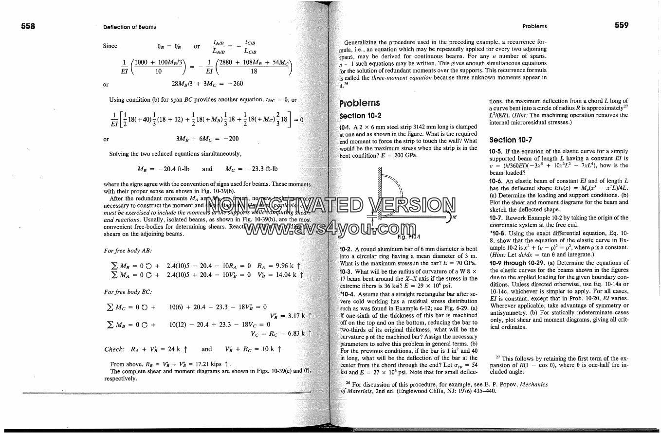
558 Problems 559Deflection of Beams
Since
or
Os = O; ortam tC/B
Lam Lcm
� (1000 +EI 10 1 (2880+ 108M�+54Mc)E1 18
28M�/3 + 3Mc = - 260
Using condition (b) for span BC provides another equation, tmc = 0, or
or
� �18(+40)�( +12)+�18(+M�)518+�18(+Mc) 18 =3M� + 6Mc = -200
Solving the two reduced equations simultaneously,
MB = -20.4 if-lb and Mc = -23.3 if-lb
where the signs agree with the convention of signs used for beams. Thesewith their proper sense are shown in Fig. 10-39(b).
After the redundant moments MA'and MB are found, no new tecnecessary to construct the moment and shear diagrams. However,must be exercised to include the moments at the supports while computing shtand reactions. Usually, isolated beams, as shown in Fig. 10-39(b), areconvenient free-bodies for determining shears. Reactions follow by addingshears on the adjoining beams.
For free body AB:
�M�=O�+�Ma=O�+
2.4(10)5 - 20.4 - 10Rn = 02.4(10)5 + 20.4 - 10Vb = 0
RA = 9.96 kVb = 14.04 k'
For free body BC:
�Mc=O� +
�M�=0G+
10(6) + 20.4 - 23.3 - 18V'3 = 0v'3=
10(12) - 20.4 + 23.3 - 18Vc = 0Vc = Rc =
Check: RA + V� = 24k �' and 1� +Rc = 10k ?
From above, R� = Vj� + V'3 = 17.21 kips J'.The complete shear and moment diagrams are shown in Figs. 10-39(e)
respectively.
Generalizing the procedure used in the preceding example, a recurrence for-i.e., an equation which may be repeatedly applied for every two adjoining
may be derived for continuous beams. For any n number of spans,- 1 guch equations may be written. This gives enough simultaneous equations� the solution of redundant moments over the supports. This recurrence formula
called the three-moment equation because three unknown moments appear int. 26
roblernsection 0-2
04, A 2 x 6 mm steel strip 3142 mm long is clampedone end as shown in the figure. What is the required
to touch the wall? What
the maximum stress when the strip is in thecondition? E = 200 GPa.
2 mm
Fig. Pt0-1
A round aluminum bar of 6 mm diameter is benta circular ring having a mean diameter of 3 m.
is the maximum stress.in the bar? E = 70 GPa.What will be the radius of curvature of a W 8 x
beam bent around the X-X axis if the stress in thefibers is 36 ksi? E = 29 x 10 � psi.
Assume that a straight rectangular bar after so-cold working has a residual stress distributionas was found in Example 6-12; see Fig. 6-29. (a)
one-sixth of the thickness of this bar is machinedthe top and on the bottom, reducing the bar to
of its original thickness, what will be thep of the machined bar? Assign the necessary
to solve this problem in general terms. (b)the previous conditions, if the bar is 1 in 2 and 40
n long, what will be the deflection of the bar at thethe chord through the end? Let tyyp = 54
= 27 x 106 psi. Note that for small deflec-
tions, the maximum deflection from a chord L long ofa curve bent into a circle of radius R is approximately 27L2/(8R). (Hint: The machining operation removes theinternal microresidual stresses.)
Section t0-7
t0-5. If the equation of the elastic curve for a simplysupported beam of length L having a constant E1 isv = (k/360EI)(-3x � + 10x3L 2 - 7xL4), how is thebeam loaded?
t0-6. An elastic beam of constant E1 and of length Lhas the deflected shape EIv(x) = Mo(x 3 - x2L)/4L.(a) Determine the loading and support conditions. (b)Plot the shear and moment diagrams for the beam andsketch the deflected shape.10-?. Rework Example 10-2 by taking the origin of thecoordinate system at the free end.'t0-8. Using the exact differential equation, Eq. 10-8, show that the equation of the elastic curve in Ex-ample 10-2 is x 2 + (v - p)2 = p2, where p is a constant.(Hint: Let dv/dx = tan 0 and integrate.)t0-9 lhrough t0-29. (a) Determine the equations ofthe elastic curves for the beams shown in the figuresdue to the applied loading for the given boundary con-ditions. Unless directed otherwise, use Eq. 10-14a or10-14c, whichever is simpler to apply. For all cases,
E1 is constant, except that in Prob. 10-20, E1 varies.Wherever applicable, take advantage of symmetry orantisymmetry. (b) For statically indeterminate casesonly, plot shear and moment diagrams, giving all crit-ical ordinates.
27 This follows by retaining the first term of the ex-pansion of R(1 - cos 0), where 0 is one-half the in-cluded angle.
26 For discussion of this procedure, for example, see E. P. Popov, Mechanics2nd ed. (Englewood Cliffs, NJ: 1976) 435-440.
NON-ACTIVATEDVERSIONwww.avs4you.com
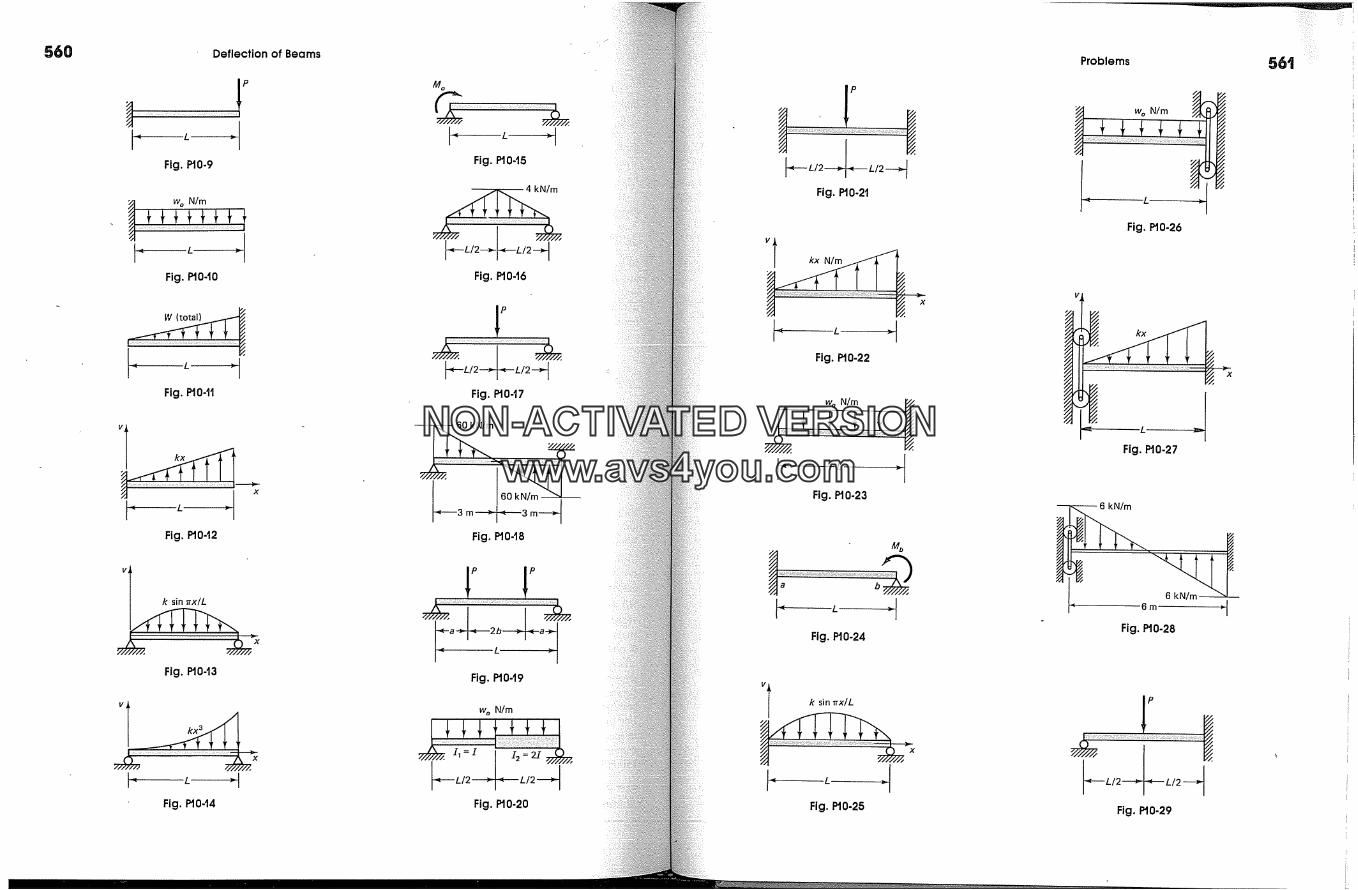
560 Deflection of Beams
Fig. P'10*9
i w o N/m
Fig. P'I 0-'10
W (total)
L �Fig. P'I 0-tt
Fig. 1�10-t2
vI ksin�'x/Lx
Fig. P'10-'13
vT kx3Fig. 1�10-�4
Fig. P'I 0-'15
Fig. P'I 0-'16
Fig. P'10-'I 7
Fig. P'10-'I 8
I p
Fig. P'I 0-'19
w o N/m
L/2---�L/2 ).Fig. 1�10-20
-- L/2"---� "'�.----L/2--�Fig. P'10-2�
Fig. P"10-22
Fig. P'10-23
Fig. P'10-24
vI k sin�x/L
Fig. 1�10-25
Problems
� w. N/m ,�
l L �Fig. P'10-26
Fig. P"10-27
N/m
�rn 'tFig. P'10-28
Fig. P"10-29
56'i
NON-ACTIVATEDVERSIONwww.avs4you.com

562 Deflection of Beams
10-30 through t0-32. (a) Determine equations for theelastic curves due to an imposed small vertical dis-placement/x of the end for the beams of length L andof constant E1 shown in the figures. (b) Plot shear andmoment diagrams.
Fig. PIO-30
Fig. PIO-3t
Fig. P10-32
10-33. If in Prob. 10-17, the cross-sectional area of thebeam is constant, and the left half of the span is madeof steel (E = 30 x 106 psi) and the right half is madeof aluminum (E = 10 x 106 psi), determine the equa-tion of the elastic curve.
t0-34. What is the equation of the elastic curve forthe cantilever of constant width and flexural strengthloaded at the end by a concentrated f6rce P? See Figs.9-17(a) and (d). Neglect the effect of the required in-crease in beam depth at the end for shear.t0-35. An overhanging beam of constant flexuralgidity E1 is loaded as shown in the figure. For portionAB of the beam, (a) find the equation of the elasticcurve due to the applied load of 2Wo N/m, and (b) de-termine the maximum deflection between the supportsand the deflection midway between the supports.
2wo N/m
Fig. P10-35
t0-36. A beam with an overhang of constantrigidity El is loaded as shown in the figure.mine length a of the overhang such that thecurve would be horizontal over support B.mine the maximum deflection between the
120 kN/m
Fig. P10-36
t0-37. Using a semigraphical 'procedure,shown in Figs. 10-9 and 10-13, find thethe beam at the point of the applied load; see theLet Ii = 400 in 4, 12 = 300 in 4, and E = 30 x 106
2O k
Fig. P10-37
10-38. Using a semigraphical procedure,shown in Figs. 10-9 and 10-13, find thethe center of the span for the beam loaded asin the figure. Neglect the effect of the axial forcedeflection. E1 for the beam is constant.
25 lb 25 lb
Fig. P10-38
t0-39. A steel beam is to span 30 ft andk/ft uniformly' distributed load, including itsweight. Select the required W section ofweight, using the abridged Table 4 in thefor bending around its strong axis. The allowable
stress is 24 ksi and that for shear is 14.4 ksi. It isrequired that the maximum deflection does not
1 in. This requirement corresponds to 1/360-th�pan length and is often used to limit deflection
to the applied load in building design. E = 29 x103 ksi.
-40. A wooden beam is to span 24 ft and to support1 k/ft uniformly distributed' load, including its own
Select the size required from Table 10 in theThe allowable bending stress is 2000 psi and
in shear is 100 psi. The deflection is limited to/360-th of the span length.
[0-4t. The maximum deflection for a simple beam24 ft and carrying a uniformly distributed
oad of 40 k total, including its own weight, is limited0.5 in. (a) Specify the required steel I beam. Let E
= 30 x 106 psi. (b) What size aluminum-alloy beambe needed for the same requirements? Let E =
x 106 psi, and use Table 3 in the Appendix forproperties. (c) Determine the maximum
in both cases.
I0-42. A uniformly loaded 6 x 12 in (nominal size)beam spans 10 ft and is considered to have
�/ deflection characteristics. Select an alu-,y I beam, a steel I beam, and a polyester-
I beam having the same deflection character-In making the beam selections, neglect the dif-
in their own weights. Let E = 1.5 x 10⁶ psifor wood and polyester plastic, E = 10 x 10 6 psi for
and E = 30 x 10 6 psi for steel. For sectionof all I beams, use Table 4 in the Appendix.
Section 10-8
10-43. Using singularity functions, rework Prob. 10-19.
Using singularity functions, rework Prob. 10-
ht0-50. Using singularity functions, ob-equations for the elastic curves for the beams
loaded as shown in the figures. E1 is constant for allbeams.
w o N/m
�a>�a>�2a__� 'Fig. P10-45
Problems 563
Fig.
Fig. 1>10.47
Fig. 1>10-48
kalb/inFig. 1>10-49
Fig. 1>10-50
Section '10.9. Use the deflection equa-tions in Examples '10.2 through '10-6 andTable '1'1 in the Appendix.
10-5t. (a) From the solution given in Table ll in theAppendix for a cantilever loaded by a concentrated
NON-ACTIVATEDVERSIONwww.avs4you.com
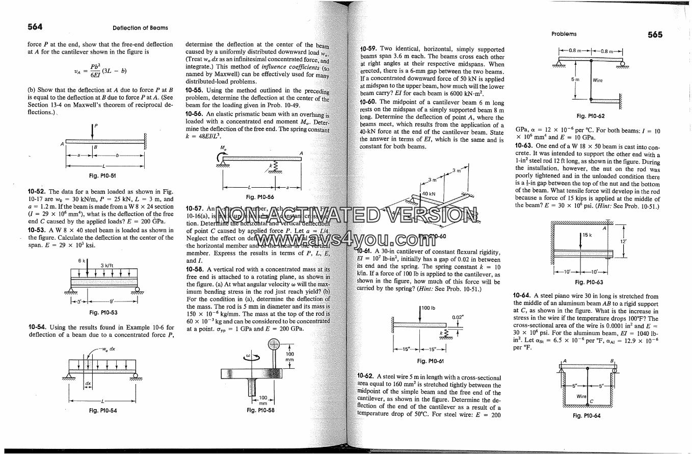
Deflection of Beams
force P at the end, show that the free-end deflectionat A for the cantilever shown in the figure is
pb �v,� = �(3L- b)
(b) Show that the deflection at A due to force P at Bis equal to the deflection at B due to force P atA. (SeeSection 13-4 on Maxwell's theorem of reciprocal de-flections.).
-L
Fig. Pt0-5t
10-52. The data for a beam loaded as shown in Fig.10-17 are Wo = 30 kN/m, P = 25 kN, L = 3 m, anda = 1.2 m. If the beam is made from a W 8 x 24 section(I = 29 x 106 mm4), what is the deflection of the freeend C caused by the applied loads? E = 200 �Pa.t0-55. A W 8 x 40 steel beam is loaded as shown inthe figure. Calculate the deflection at the center of thespan. E = 29 x 103 ksi.
Fig. Pt0-53
t0-54. Using the results found in Example 10-6 fordeflection of a beam due to a concentrated force P,
Fig. Pt0-54
determine the deflection at the center of thecaused by a uniformly distributed downward(Treat wo dx as an infinitesimal concentrated fcintegrate.) This method of influencenamed by Maxwell) can be effectively used fordistributed-load problems.t0-55. Using the method outlined in theproblem, determine the deflection at the centerbeam for the loading given in Prob. 10-49.10-56. An elastic prismatic beam with anloaded with a concentrated end moment Mo.mine the deflection of the free end. The:k = 48EI/L 3.
A
-�-----iL �- � a �Fig. Pt0-56
t0-57. An L-shaped member, such as shown10-16(a), is made up from a bar of constant
lion. Determine the horizontal and vertical
of point C caused by applied force P. Let aNeglect the effect on deflection of the axial
�the horizontal member and of the shear in the
member. Express the results in terms ofand I.
t0-58. A vertical rod with a concentrated mas:
free end is attached to a rotating plane, asthe figure. (a) At what angular velocity toimum bending stress in the rod just reachFor the condition in (a), determine thethe mass. The rod is 5 mm in diameter and150 X 10 -6 kgJmm. The mass at the top of60 x 10 -3 kg and can be considered to beat a point. cryp = 1 GPa and E = 200 GPa.
lOOmm
Fig. Pt0-58
�-59. Two identical, horizontal, simply supportedspan 3.6 m each. The beams cross each other
right angles at their respective midspans. Whenthere is a 6-mm gap between the two beams.
concentrated downward force of 50 kN is appliedupper beam, how much will the lower
beam carry? EI for each beam is 6000 kN.m 2.0-60. The midpoint of a cantilever beam 6 m long
on the midspan of a simply supported beam 8 mDetermine the deflection of point A, where the
meet, which results from the application of aforce at the end of the cantilever beam. State
answer in terms of El, which is the same and isnstant for both beams.
_�.3m'� 3m'�Fig. PtO-60
A 30-in cantilever of constant flexural rigidity,= 10 7 lb~in 2, initially has a gap of 0.02 in betweenend and the spring. The spring constant k = 10
If a force of 100 lb is applied to the cantilever, asin the figure, how much of this force will beby the spring? (Hint: See Prob. 10-51.)
100 lb ,,� 0.02
Fig.
A steel wire 5 m in length with a cross-sectionalequal to 160 mm 2 is stretched tightly between the
of the simple beam and the free end of theas shown in the figure. Determine the de-
of the end of the cantilever as a result of adrop of 50�C. For steel wire: E = 200
Problems 565
-�--0.8 m---�[
5 m Wire
Fig. Pt0.62
GPa, ct = 12 x 10 -6 per �C. For both beams: I = 10X 106 mm 4 and E = 10 GPa.
t0-63. One end ofa W 18 x 50 beam is cast into con-crete. It was intended to support the other end with a1-in 2 steel rod 12 ft long, as shown in the figure. Duringthe installation, however, the nut on the rod waspoorly tightened and in the unloaded condition thereis a �-in gap between the top of the nut and the bottomof the beam. What tensile force will develop in the rodbecause a force of 15 kips is applied at the middle ofthe beam? E = 30 x 106 psi. (Hint: See Prob. 10-51.)
//'/////////////////////////�.A
15k
Fig. Pt0.63
t0-64. A steel piano wire 30 in long is stretched fromthe middle of an aluminum beam AB to a rigid supportat C, as shown in the figure. What is the increase instress in the wire if the temperature drops 100�F? Thecross-sectional area of the wire is 0.0001 in 2 and E =30 x 106 psi. For the aluminum beam, E1 = 1040 lb-in 2. Let Ctst = 6.5 x 10 -6 per �F, ct^� = 12.9 x 10 -6per �F.
A B
Wire
Fig. Pt0-64
NON-ACTIVATEDVERSIONwww.avs4you.com
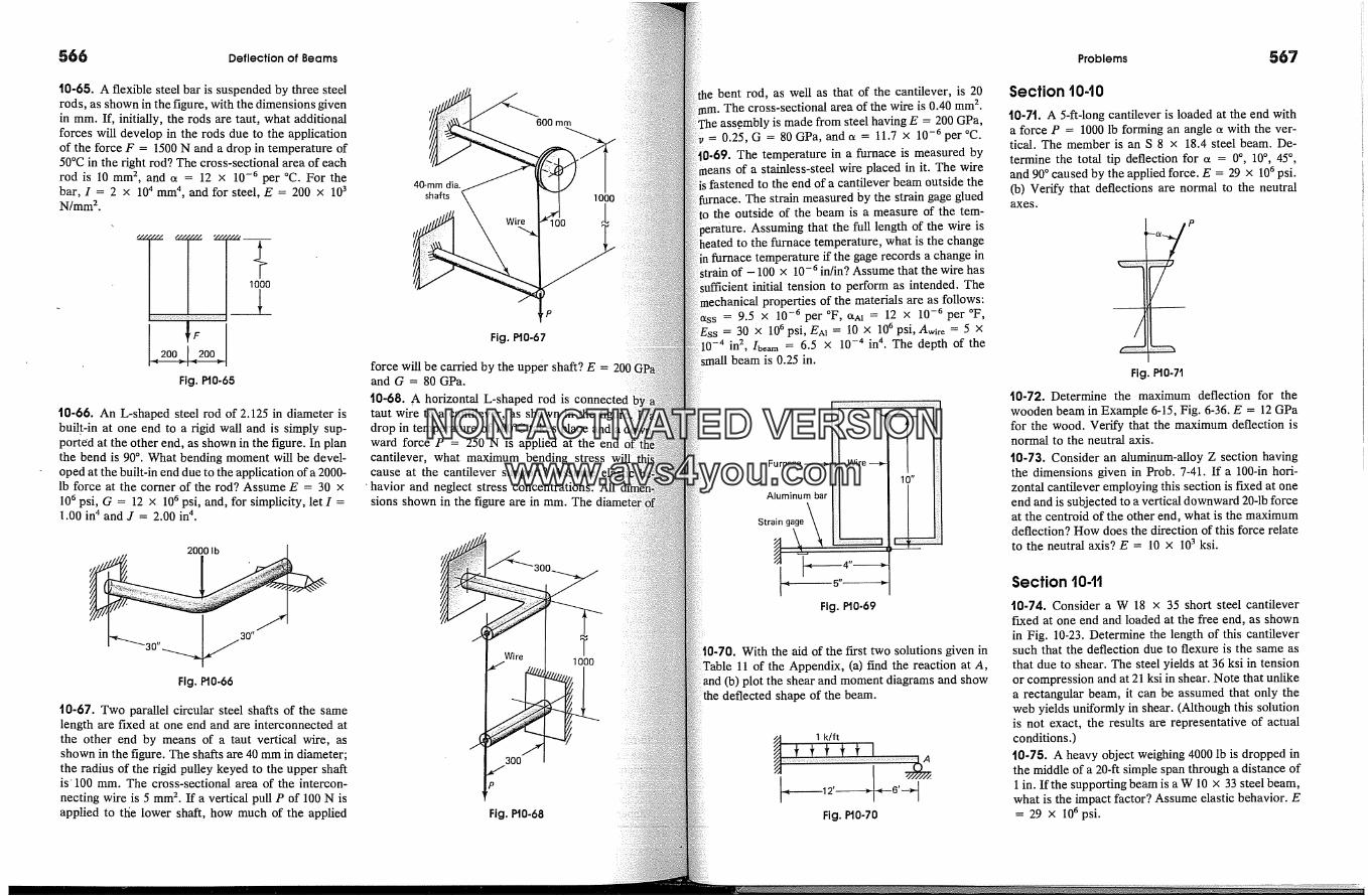
Deflection of Beams Problems
10-65. A flexible steel bar is suspended by three steelrods, as shown in the figure, with the dimensions givenin mm. If, initially, the rods are taut, what additionalforces will develop in the rods due to the applicationof the force F = 1500 N and a drop in temperature of50�C in the right rod? The cross-sectional area of eachrod is 10 mm 2, and ct = 12 x 10 -6 per �C. For thebar, I = 2 x 10 4 mm 4, and for steel, E = 200 x 103N/mm 2.
200 [ 200
Fig. P10-65
1000
10-66. An L-shaped steel rod of 2.125 in diameter isbuilt-in at one end to a rigid wall and is simply sup-ported at the other end, as shown in the figure. In planthe bend is 90 � . What bending moment will be devel-oped at the built-in end due to the application of a 2000-lb force at the corner of the rod? Assume E = 30 x10 6 psi, G = 12 x 10 6 psi, and, for simplicity, let I =1.00 in n and J = 2.00 in n.
2000 lb [
'
Fig. P10-66
10-67. Two parallel circular steel shafts of the samelength are fixed at one end and are interconnected atthe other end by means of a taut vertical wire, asshown in the figure. The shafts are 40 mm in diameter;the radius of the rigid pulley keyed to the upper shaftis' 100 mm. The cross-sectional area of the intercon-necting wire is 5 mm 2. If a vertical pull P of 100 N isapplied to the lower shaft, how much of the applied
�C�'�'��600mm
Fig. P10-67
force will be carried by the upper shaft? E = 200 (and G = 80 GPa.
t0-68. A horizontal L-shaped rod is connectedtaut wire to a cantilever, as shown in thedrop in temperature of 100�C takes place andward force P = 250 N is applied at the endcantilever, what maximum bending stress willcause at the cantilever support? Assume
' havior and neglect stress concentrations. Allsions shown in the figure are in mm. The diame
"' '�Wire 10To0
300
Fig. P10-68
bent rod, as well as that of the cantilever, is 20The cross-sectional area of the wire is 0.40 mm 2.
ass0mbly is made from steel having E = 200 GPa,-- 0.25, G = 80 GPa, and ct = 11.7 x 10 -6 per �C.1-69. The temperature in a furnace is measured by
of a stainless-steel wire placed in it. The wirefastened to the end of a cantilever beam outside the
ace. The strain measured by the strain gage gluedthe outside of the beam is a measure of the tem-
Assuming that the full length of the wire isheated to the furnace temperature, what is the change
� furnace temperature if the gage records a change inof - 100 x 10 -6 in/in? Assume that the wire has
initial tension to perform as intended. Theproperties of the materials are as follows:
= 9.5 x 10 -6 per �F, am = 12 x 10 -6 per�F,= 30 x 106 psi, E�a = 10 x 106 psi, Awire = 5 x
10 -4 in 2, lbeam = 6.5 X 10 -4 in 4. The depth of themall beam is 0.25 in.
Fig. P10-69
With the aid of the first two solutions given inTable 11 of the Appendix, (a) find the reaction at A,
the shear and moment diagrams and showthe deflected shape of the beam.
1 k/ft
Fig. P10-70
Section t040
t0-7t. A 5-ft-long cantilever is loaded at the end witha force P = 1000 lb forming an angle ct with the ver-tical. The member is an S 8 x 18.4 steel beam. De-termine the total tip deflection for ct = 0% 10% 45 �,and 90 � caused by the applied force. E = 29 x 10 6 psi.(b) Verify that deflections are normal to the neutralaxes.
P
Fig. Pt0-71
10-72. Determine the maximum deflection for thewooden beam in Example 6-15, Fig. 6-36. E = 12 GPafor the wood. Verify that the maximum deflection isnormal to the neutral axis.
10-73. Consider an aluminum-alloy Z section havingthe dimensions given in Prob. 7-41. If a 100-in hori-zontal cantilever employing this section is fixed at oneend and is subjected to a vertical downward 20-1b forceat the centreid of the other end, what is the maximumdeflection? How does the direction of this force relateto the neutral axis? E = 10 x 103 ksi.
Section t04t
t0-74. Consider a W 18 x 35 short steel cantileverfixed at one end and loaded at the free end, as shownin Fig. 10-23. Determine the length of this cantileversuch that the deflection due to flexure is the same asthat due to shear. The steel yields at 36 ksi in tensionor compression and at 21 ksi in shear. Note that unlikea rectangular beam, it can be assumed that only theweb yields uniformly in shear. (Although this solutionis not exact, the results are representative of actualconditions.)10-75. A heavy object weighing 4000 lb is dropped inthe middle of a 20-ft simple span through a distance of1 in. If the supporting beam is a W 10 x 33 steel beam,what is the impact factor? Assume elastic behavior. E= 29 x 106 psi.
NON-ACTIVATEDVERSIONwww.avs4you.com
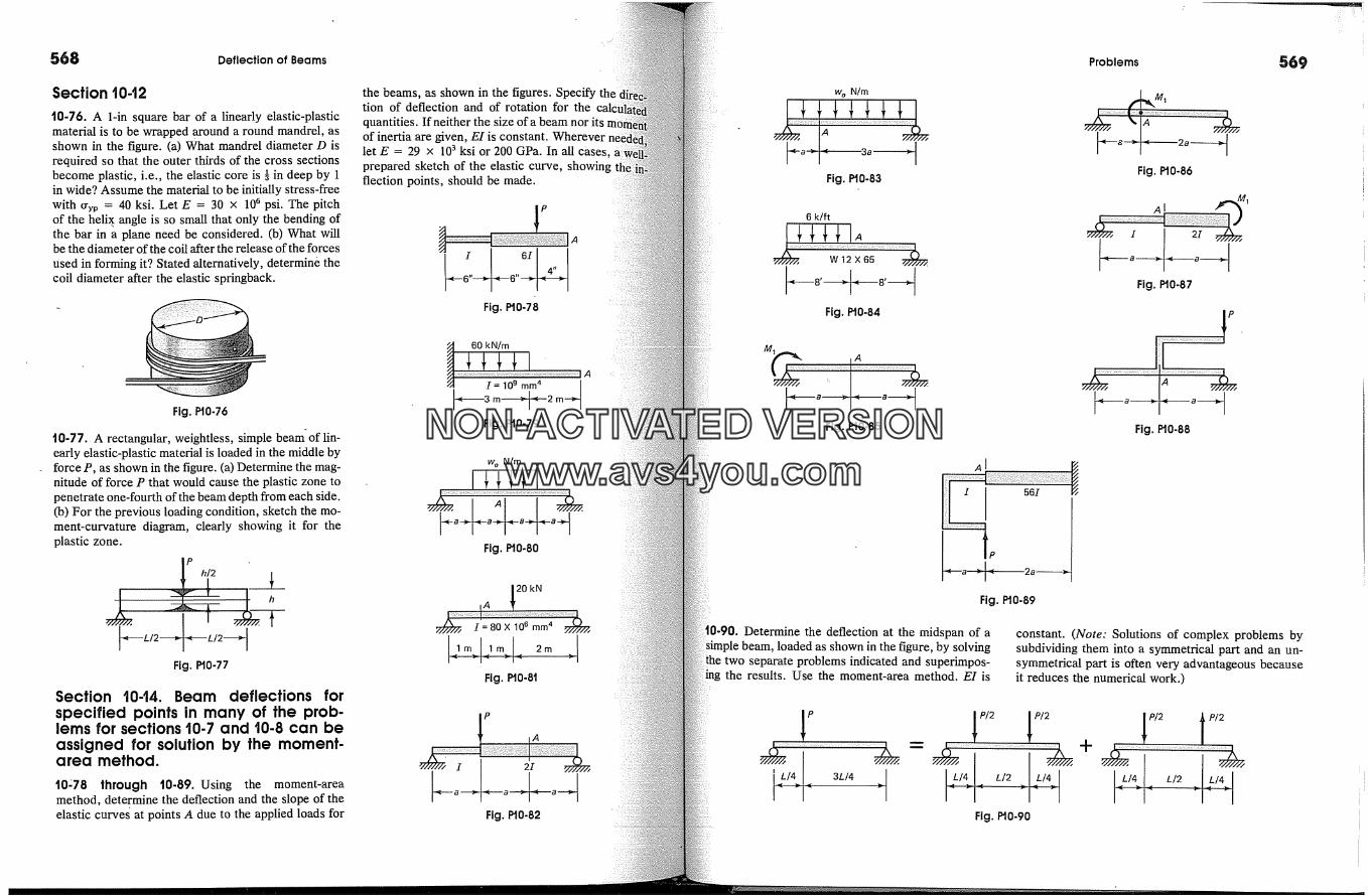
568 Deflection of Beams
Section '10-'12
t0-76. A 1-in square bar of a linearly elastic-plasticmaterial is to be wrapped around a round mandrel, asshown in the figure. (a) What mandrel diameter D isrequired so that the outer thirds of the cross sectionsbecome plastic, i.e., the elastic core is � in deep by 1in wide? Assume the material to be initially stress-freewith gyp = 40 ksi. Let E = 30 x 106 psi. The pitchof the hells. angle is so small that only the bending ofthe bar in a plane need be considered. (b) What willbe the diameter of the coil after the release of the forcesused in forming it? Stated alternatively, determin& thecoil diameter after the elastic springback.
Fig. Pt0-76
t0-77. A rectangular, weightless, simple beam-of lin-early elastic-plastic material is loaded in the middle byforce P, as shown in the figure. (a) Determine the mag-nitude of force P that would cause the plastic zone topenetrate one-fourth of the beam depth from each side.(b) For the previous loading condition, sketch the mo-ment-curvature diagram, clearly showing it for theplastic zone.
Ph/2
�---L/2---� "�'--L/2�Fig. P10-77
Section '10-'14. Beam deflections forspecified points in many of the prob-lems for sections '10-7 and '10-8 can beassigned for solution by the moment.area method.
t0�78 through t0-89. Using the moment-areamethod, determine the deflection and the slope of theelastic curves � at points A due to the applied loads for
the beams, as shown in the figures. Specifytion of deflection and of rotation for the
quantities. If neither the size of a beam nor itsof inertia are given, EI is constant. Whereverlet E = 29 x 103 ksi or 200 GPa. In all cases,prepared sketch of the elastic curve, showingflection points, should be made.
P
Fig. Pt0-78
Fig. P10-79
w o N/m
Fig. Pt0-80
20 kN
I=80Xl 0 mm �
Fig. PI0-8t
I I
Fig. P'10-82
Problems 569
wo N/m
Fig. Pt0-83Fig. Pt0-86
6 k/ft
Fig. PI0-84
Fig. Pt0-85
AI
I 21
Fig. Pt0-87
Fig. Pt0-88
AI
� 561P
Fig. Pt0-89
Determine the deflection at the midspan of aloaded as shown in the figure, by solving
separate problems indicated and superimpos-the results. Use the moment-area method. E1 is
constant. (Note: Solutions of complex problems bysubdividing them into a symmetrical part and an un-symmetrical part is often very advantageous becauseit reduces the numerical work.)
P �P/2 [ P/2
Fig. Pt0-90
�P/2 I P/2
�L/5 � J/2 �L/4�
NON-ACTIVATEDVERSIONwww.avs4you.com
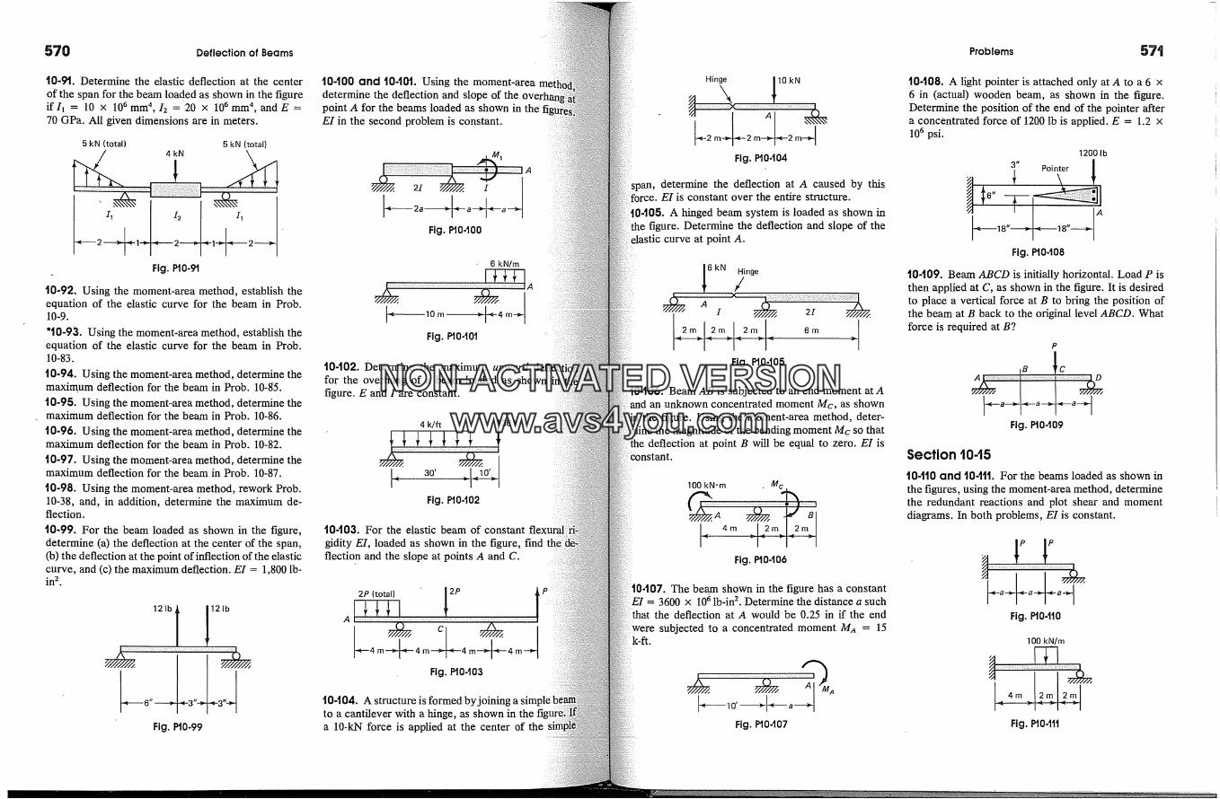
570 Deflection of Beams
10-9t. Determine the elastic deflection at the centerof the span for the beam loaded as shown in the figureif l� = 10 x 106 mm 4, 12 = 20 x 106 mm 4, and E =70 GPa. All given dimensions are in meters.
5 kN (total) 5 kN (total)
Fig. PIO-91
t0-92. Using the moment-area method, establish theequation of the elastic curve for the beam in Prob.10-9.
't0-93. Using the moment-area method, establish theequation of the elastic curve for the beam in Prob.10-83.
t0-94. Using the moment-area method, determine themaximum deflection for the beam in Prob. 10-85.t0-95. Using the moment-area method, determine themaximum deflection for the beam in Prob. 10-86.
t0-96. Using the moment-area method, determine themaximum deflection for the beam in Prob. 10-82.
t0-97. Using the moment-area method, determine themaximum deflection for the beam in Prob. 10-87.
t0-98. Using the moment-area method, rework Prob.10-38, and, in addition, determine the maximum de-flection.
t0-99. For the beam loaded as shown in the figure,determine (a) the deflection at the center of the span,(b) the deflection at the point of inflection of the elasticcurve, and (c) the maximum deflection. E1 = 1,800 lb-in 2 .
121bl 12lb.� 6"43"-*- �-3"-�
Fig. P10-99
t0-100 and 10401. Using the moment-areadetermine the deflection and slope of thepoint A for the beams loaded as shown in theEI in the second problem is constant.
Fig. PI0400
Fig. PlOdfit
t0-102. Determine the maximum upwardfor the overhang of a beam loaded as shownfigure. E and I are constant.
30'Fig. PI0402
t0-t03. For the elastic beam of constantgidity El, loaded as shown in the figure, findflection and the slope at points A and C.
A
Fig. P'10403
10404. A structure is formed by joining a simpleto a cantilever with a hinge, as shown in thea 10-kN force is applied at the center of the
Hinge 110 kN
m4+Fig. PI0-t04
determine the deflection at A caused by thisforce. E1 is constant over the entire structure.
405. A hinged beam system is loaded as shown inDetermine the deflection and slope of the
stic curve at point A.
6 kN )�inge
Fig. P'10405
10406. Beam AB is subjected to an end moment atAan unknown concentrated moment Mc, as shown
in the figure. Using the moment-area method, deter-magnitude of the bending moment Mc so that
the deflection at point B will be equal to zero. E1 isstant.
100 kN-m . Mc
Fig. PI0406
The beam shown in the figure has a constant= 3600 x 106 lb-in 2. Determine the distance a such
that the deflection at A would be 0.25 in if the endsubjected to a concentrated moment M,� = 15
['"� 10'Fig.
Problems
10408. A fight pointer is attached only atA to a 6 x6 in (actual) wooden beam, as shown in the figure.Determine the position of the end of the pointer aftera concentrated force of 1200 lb is applied. E = 1.2 x10⁶ psi.
1200 lb
Fig. PI0408
t0-t09. Beam ABCD is initially horizontal. Load P isthen applied at C, as shown in the figure. It is desiredto place a vertical force at B to bring the position ofthe beam at B back to the original level ABCD. Whatforce is required at B?
P
I
Fig. P10-109
Section t045
t0-1t0 and t0-ttt. For the beams loaded as shown in
the figures, using the moment-area method, determinethe redundant reactions and plot shear and momentdiagrams. In both problems, EI is constant.
Fig. Pt04tO
100 kN/m
Fig. PI041I
NON-ACTIVATEDVERSIONwww.avs4you.com
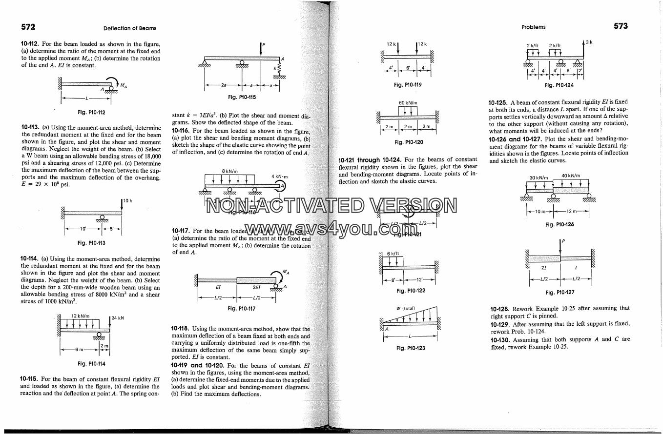
572 Deflection of Beams Problems
t0-tt2. For the beam loaded as shown in the figure,(a) determine the ratio of the moment at the fixed endto the applied moment MA; (b) determine the rotationof the end A. E1 is constant.
Fig. P10-1t2
10413. (a) Using the moment-area method, determinethe redundant moment at the fixed end for the beamshown in the figure, and plot the shear and momentdiagrams. Neglect the weight of the beam. (b) Selecta W beam using an allowable bending stress of 18,000psi and a shearing stress of 12,000 psi. (c) Determinethe maximum deflection of the beam between the sup-ports and the maximum deflection of the overhang.E= 29 x 106psi.
10k
Fig. P10-113
10414. (a) Using the moment-area method, determinethe redundant moment at the fixed end for the beamshown in the figure and plot the shear and momentdiagrams. Neglect the weight of the beam. (b) Selectthe depth for a 200-mm~wide wooden beam using anallowable bending stress of 8000 kN/m 2 and a shearstress of 1000 kN/m 2.
Fig. P10-tt4
10-1t5. For the beam of constant flexural rigidity Eland loaded as shown in the figure, (a) determine thereaction and the'deflection at point A. The spring con-
Fig, P10-1t5
stant k = 3El/a 3. (b) Plot the shear and moment �grams. Show the deflected shape of the beam.t0-t16. For the beam loaded as shown in the(a) plot the shear and bending moment diagrams,sketch the shape of the elastic curve showing theof inflection, and (c) determine the rotation of end
Fig. P10-t16
t0-1t?. For the beam loaded as shown in the(a} determine the ratio of the moment at the fixedto the applied moment M,�; (b) determine theof end A.
EI 2EI __ AI�L/2 �'i � L/2 �,Fig. P10-tt7
10-tt8. Using the moment-area method,maximum deflection of a beam fixed at both endscarrying a uniformly distributed load is one-fifthmaximum deflection of the same beam simplyported. E1 is constant.t0-tt9 and 10-t20. For the beams of constantshown in the figures, using the moment-area method(a) determine the fixed-end moments due to theloads and plot shear and bending-moment(b) Find the maximum deflections
�2k / /�2k
Fig. P10-tt9
60 kN/m
Fig. P10-120
t0-t2t through 10424. For the beams of constantflexural rigidity shown in the figures, plot the shearand bending-moment diagrams. Locate points of in-flection and sketch the elastic curves.
/1/I 1
Fig, P10-12t
-4 6 k/ft
Fig. P10-122
Fig. P10-123
2k/ft 2{_� 13Fig. Pt 0-124
10425. A beam of constant flexural rigidity El is fixedat both its ends, a distance L apart. If one of the sup-ports settles vertically downward an amount A relativeto the other support (without causing any rotation),what moments will be induced at the ends?t0-126 and 10-t27. Plot the shear and bending-mo-ment diagrams for the beams of variable flexural rig-idities shown in the figures. Locate points of inflectionand sketch the elastic curves.
30 kN/m 40 kN/m.....
k10 m-� 12m �Fig. Pt0-126
P
LI2---�-�----L/2Fig. P10-t27
10428. Rework Example 10-25 after assuming thatright support C is pinned.t0-129. After assuming that the left support is fixed,rework Prob. 10-124.
10-t30. Assuming that both supports A and C arefixed, rework Example 10-25.
NON-ACTIVATEDVERSIONwww.avs4you.com

_ chapter
574
11ol. Introduction
The selection of structural and machine elements is based on threeacteristics: strength, stiffness, and stability. The procedures of stress'deformation analyses in a state of stable equilibrium were discussedsome detail in-the preceding chapters. But not all structural systemsnecessarily stable. For example, consider a square-ended metal rodsay 10 mm in diameter. If such a rod were made 20 mm long to act asaxially compressed member, no question of instability would enter,a considerable force could be applied. On the other hand,of the same material were made 1000 mm long to act inthen, at a much smaller load than the short piece could carry, therod would buckle laterally and could collapse. A slender measuringif subjected to an axial compression, could fail in the same manner.consideration of material strength alone is not sufficient to predictbehavior of such members. Stability considerations are primary instructural systems.
The phenomenon of structural instability occurs in numerouswhere compressive stresses are present. Thin sheets, although fullypable of sustaining tensile loadings, are very poor in transmittinsion. Narrow beams, unbraced laterally, can turn sidewise andunder an applied load. Vacuum tanks, as well as submarine hulls, unle:properly designed, can severely distort under external pressure andassume shapes that differ drastically from their original geometry. Awalled tube can wrinkle like tissue paper when subjected either tocompression or a torque; see Fig. 11-1.. � During some stages of firing,
� Figures are adapted from L. A. Harris, H. W. Suer, and W. T. Skene,Investigations of Unstiflened and Stiflened Circular Shells," Exlchanics (July 1961): 3 and 5.
Sec. tt-t. Introduction
casings of rockets are critically loaded in compression. These areimportant problems for engineering design. Moreover, often the
buckling or wrinkling phenomena observed in loaded members occurrather suddenly. For this reason, many structural instability failures arespectacular and very dangerous.
A vast number of the structural instability problems suggested by thepreceding listing of problems are beyond the scope of this text. 2 Essen-tially, only the column problem will be considered here.
For convenience, this chapter is divided into two parts. Part A is de-voted to the theory of column buckling, and Part B deals with design
First, however, examples of possible instabilities that mayoccur in straight prismatic members with different cross sections will be
This will be followed by establishing the stability criteria forstatic equilibrium. The purpose of the next two introductory sections is
2 F. Bleich, Buckling Strength of Metal Structures (New York: McGraw-Hill,1952). D. O. Brush, and B. O. Almroth, Buckling of Bars, Plates, and Shells
York: McGraw-Hill, 1975). A. Chajes, Principles of Structural StabilityCliffs, NJ: Prentice-Hall, 1974). G. Gerard et al., Handbook of Struc-
Stability, Parts I-VI, NACA TN, 3781-3786, (Washington, D.C.: NASA1957-1958). B. G. Johnston (ed.), Design Criteria for Metal Compression Mem-
ed. (New York: Wiley, 1988). S. P. Timoshenko, and J. M. Gere, Theory'�Elastic Stability, 2nd ed. (New York: McGraw-Hill, 1961). A. S. Volmir, Flex-
ible Plates and Shells, Air Force Flight Dynamics Laboratory (trans.), Technical66-216, Wright-Patterson Air Force Base, 1967.
Fig. tt4 Typical bucklingpatterns for thin-walledcylinders (a) in compressionand (b) in torsion for apressurized cylinder.(Courtesy L. A. Harris ofNorth American Aviation,Inc.)NON-ACTIVATEDVERSION
www.avs4you.com
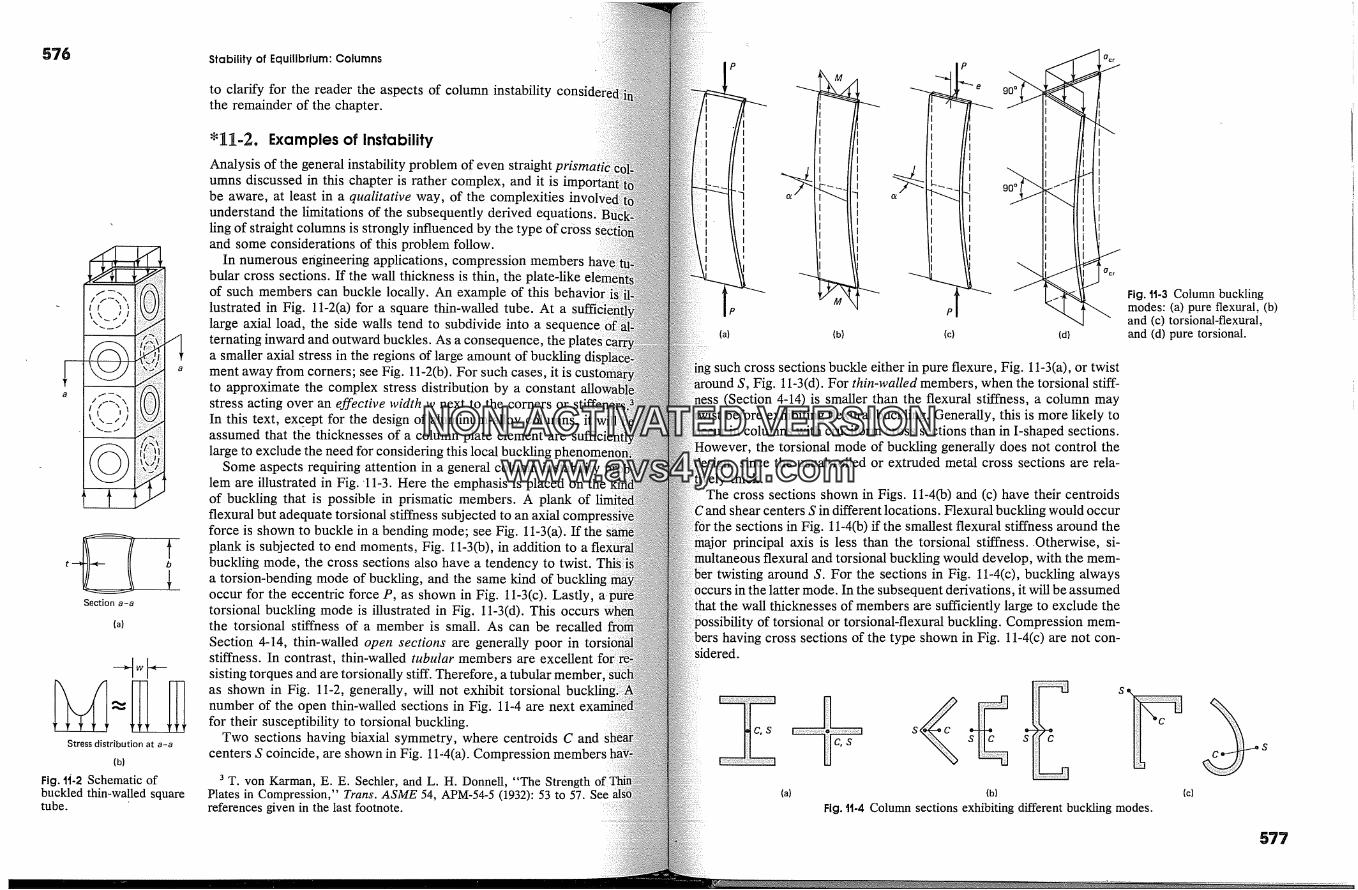
576
Section a-a
(a)
Stress distribution at a-a
(b)
Fig. �-2 Schematic ofbuckled thin-walled squaretube.
Stability of Equilibrium: Columns
to clarify for the reader the aspects of column instabilitythe remainder of the chapter.
*]1.�.=2. Examples of InstabilityAnalysis of the general instability problem of even straightumns discussed in this chapter is rather complex, and it is 'be aware, at least in a qualitative way, of the complexities invounderstand the limitations of the subsequently derivedling of straight columns is strongly influenced by the type of crossand some considerations of this problem follow.
In numerous engineering applications, compression membersbular cross sections. If the wall thickness is thin, the plate-likeof such members can buckle locally. An example of this behaviOilustrated in Fig. 11-2(a) for a square thin-walled tube. At alarge axial load, the side walls tend to subdivide into a seqternating inward and outward buckles. As a consequence, thea smaller axial stress in the regions of large amount of buckling disment away from corners; see Fig. 11-2(b). For such cases, it isto approximate the complex stress distribution by a constantstress acting over an effective width w next to the comers orIn this text, exc_ept for the design of aluminum-alloy columns,assumed that the thicknesses of a column plate element arelarge to exclude the need for considering this local buckling [
Some aspects requiring attention in a general column instabilitylem are illustrated in Fig. '11-3. Here the emphasis is placed on theof buckling that is possible in prismatic members. A plank offlexural but adequate torsional stiffness subjected to an axial,force is shown to buckle in a bending mode; see Fig. 11-3(a). If theplank is subjected to end moments, Fig. 11-3(b), in addition tobuckling mode, the cross sections also have a tendency to twist.a torsion-bending mode of buckling, and the same kind ofoccur for the eccentric force P, as shown in Fig. 11-3(c). Lastly,torsional buckling mode is illustrated in Fig. 11-3(d). This occursthe torsional stiffness of a member is small. As can be recalledSection 4-14, thin-walled open sections are generally poor instiffness. In contrast, thin-walled tubular members are excellentsisting torques and are torsionally stiff. Therefore, a tubular memberas shown in Fig. 11-2, generally, will not exhibit torsionalnumber of the open thin-walled sections in Fig. 11-4 are nextfor their susceptibility to torsional buckling.
Two sections having biaxial symmetry, where centroids C andcenters S coincide, are shown in Fig. 1 l�4(a).
3 T. von Karman, E. E. Sechler, and L. H. Donnell, "The StrengthPlates in Compression," Trans. ASME 54, APM-54-5 (1932): 53 to 57.references given in the last footnote.
P
(a)
� Pi� 9���(b) (c) (d)
: s cross sections buckle either in pure flexure, Fig. 11-3(a), or twistFig. 1 l-3(d). For thin-walled members, when the torsional stiff-
(Section 4-14) is smaller than the flexural stiffness, a column maybefore exhibiting flexural buckling. Generally, this is more likely to
,ccur in columns with cruciform cross sections than in I-shaped sections.the torsional mode of buckling generally does not control the
since the usual rolled or extruded metal cross sections are rela-thick.
The cross sections shown in Figs. 11-4(b) and (c) have their centroidscenters S in different locations. Flexural buckling would occur
sections in Fig. 11-4(b) if the smallest flexural stiffness around theprincipal axis is less than the torsional stiffness..Otherwise, si-
flexural and torsional buckling would develop, with the mem-ber twisting around S. For the sections in Fig. 11-4(c), buckling always
occurs in the latter mode. In the subsequent derivations, it will be assumedwall thicknesses of members are sufficiently large to exclude the
of torsional or torsional-flexural buckling. Compression mem-having cross sections of the type shown in Fig. 11-4(c) are not con-
Fig. 1t-3 Column bucklingmodes: (a) pure flexural, (b)and (c) torsional-flexural,and (d) pure torsional.
c,s �ic, s,(a) (b) (c)
Fig. tt-4 Column sections exhibiting different buckling modes.
577
NON-ACTIVATEDVERSIONwww.avs4you.com
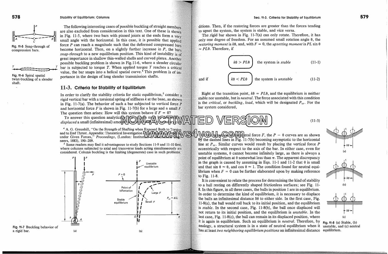
578
Fig. tt-5 Snap-through ofcompression bars.
Fig. tt-6 Spiral spatialtwist-buckling of a slendershaft.
Fig. tt-7 Buckling behavior ofa rigid bar.
Stability of Equilibrium: Columns
The following interesting cases of posare also excluded from consideration in this text. One of these isin Fig. 11-5, where two bars with pinned joints at the ends formsmall angle with the horizontal. In this case, it is possible thatforce P can reach a magnitude such that the deformedbecome horizontal. Then, on a slightly further increase in P,snap-through to a new equilibrium position. This kindgreat importance in shallow thin-walled shells and curved plates.possible buckling problem is shown in Fig. 11-6, where a slenderbar is subjected to torque T. When applied torque T reaches avalue, the bar snaps into a helical spatial curve. 4 This problem isportance in the design of long slender transmission shafts.
11-3, Criteria for Stability of EquilibriumIn order to clarify the stability criteria for static equilibrium, 5rigid vertical bar with a torsional spring of stiffness k at th e base, asin Fig. 11-7(a). The behavior of such a bar subjected to verticaland horizontal force F is shown in Fig. 11-7(b) for a large and aThe question then arises: How will this system behave if F = 07
To answer this question analytically, the system must be deliberadisplaced a small (infinitesimal) amount consistent with the boundary
4 A. G. Greenhill, "On the Strength of Shafting when Exposed Both toand to End Thrust. Appendix: Theoretical Investigation of the Stabilityunder Given Forces," Proceedings, (London: Institution of Mechanicalneers, 1883), 190-209.
5 Some readers may find it advantageous to study Sections 11-9 and 11-lfiwhere columns subjected to axial and transverse loads actingconsidered. Column buckling is the limiting (degenerate) case in such
PUnstable
equilibriumF=O I
bifurcation / Large F
Stable Pcr=equilibrium Small FI
o
gl
(a) (b)
Sec. tt-3. Criteria for Stability of Equilibrium
Then, if the restoring forces are greater than the forces tendingto upset the system, the system is stable, and vice versa.
The .rigid bar shown in Fig. 11-7(a) can only rotate. Therefore, it hasOnly one degree of freedom. For an assumed small rotation angle 0, the
' moment is k0, and, with F = 0, the upsetting moment is PL sin 0PLO. Therefore, if
k0� thesystemis stable (11-1)
if �0 < PLO) thesystemis tinstable (11-2)Right at the transition point, k0 = PLO, and the equilibrium is neither
r unstable, but is neutral. The force associated with this conditionthe critical, or buckling, load, which will be designated Per. For the
system considered,
( Pcr= k/L) (11-3)
In the presence of horizontal force F, the P - 0 curves are as shownby the dashed lines in Fig. 11-7(b) becoming asymptotic to the horizontal
line at P�r. Similar curves would result by placing the vertical force Pwith respect to the axis of the bar. In either case, even for
systems, 0 cannot become infinitely large, as there is always aPoint of equilibrium at 0 somewhat less than x. The apparent discrepancy
the graph is caused by assuming in Eqs. 11-1 and 11-2 that 0 is smallthat sin 0 � 0, and cos 0 � 1. The condition found for neutral equi-
when F = 0 can be further elaborated upon by making referenceto Fig. 11-8.
It is convenient to relate the process for determining the kind of stabilityto a ball resting on differently shaped frictionless surfaces; see Fig. 11-
In this figure, in all three cases, the balls in position 1 are in equilibrium.order to determine the kind of equilibrium, it is necessary to displace
the balls an infinitesimal distance �0 to either side. In the first case, Fig.the ball would roll back to its initial position, and the equilibrium
stable. In the second case, Fig. 11-8(b), the ball once displaced willreturn to its initial position, and the equilibrium is unstable. In thecase, Fig. 11-8(c), the ball can remain in its displaced position, where
is again in equilibrium. Such an equilibrium is neutral. Therefore, bya structural system is in a state of neutral equilibrium when it
neighboring equilibrium positions an infinitesimal distance
579
(a)
(b)
(c)
Fig. 11-8 (a) Stable, (b)unstable, and (c) neutralequilibrium.
NON-ACTIVATEDVERSIONwww.avs4you.com
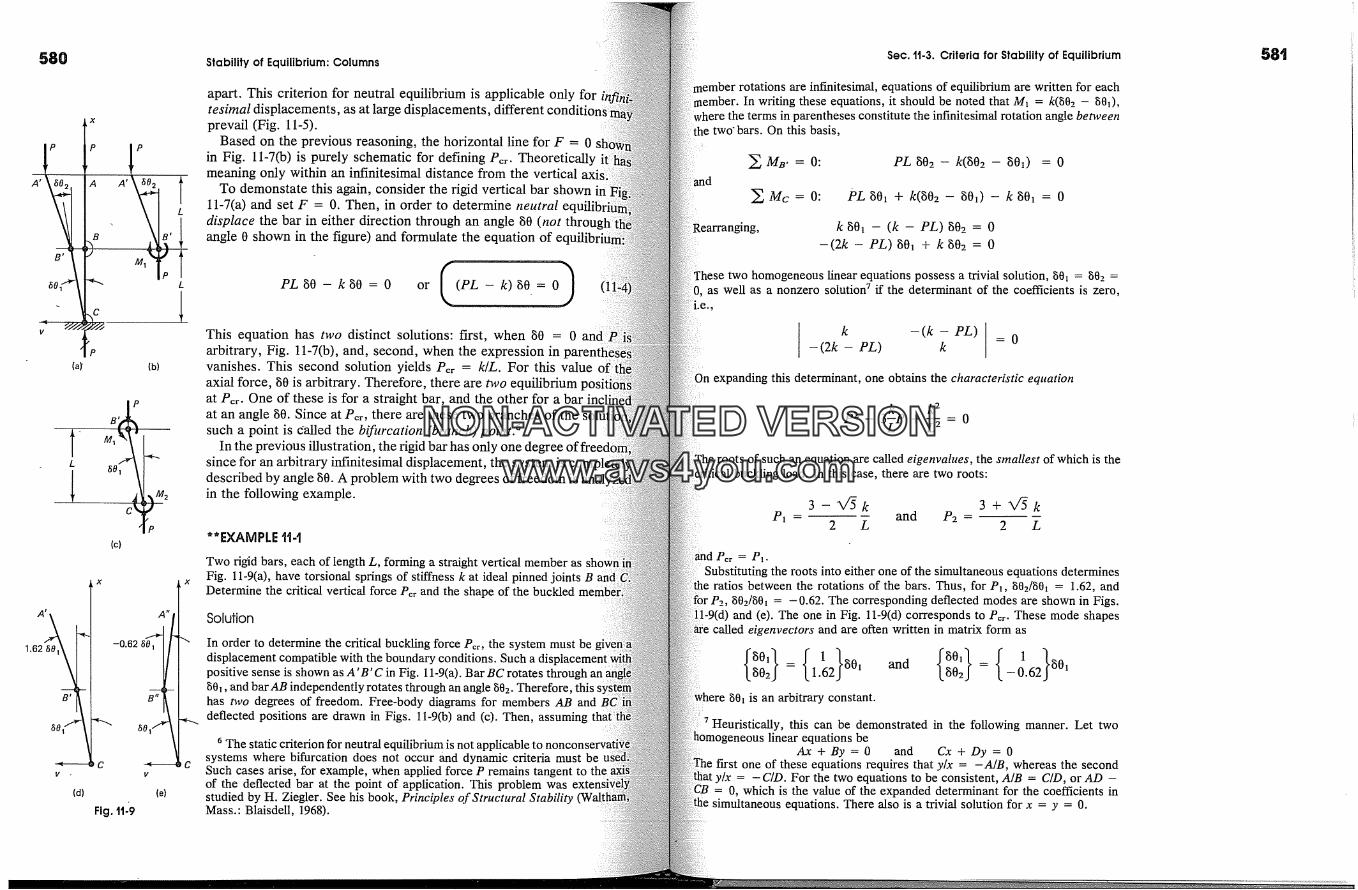
580
A' �02. A A'
(a)' (b)
(c)
x
A'
1.62 -0.62/i
C CV - V
(d) (e)
Fig. '1'1-'9
Stability of Equilibrium: Columns
apart. This criterion for neutral equilibrium is applicable only fortesimal displacements, as at large displacements, differentprevail (Fig. 11-5).
Based on the previous reasoning, the horizontal line for F = 0in Fig. 11-7(b) is purely schematic for defining Pcr. Theoreticallymeaning only within an infinitesimal distance from the vertical
To demonstate this again, consider the rigid vertical bar shown in ]11-7(a) and set F = 0. Then, in order to determine neutraldisplace the bar in either direction through an angle g0 (not throuangle 0 shown in the figure) and formulate the equation of ec
PL gO - k gO = 0 or ((PL - k) gO.= O)This equation has two distinct solutions: first, when g0 = 0 andarbitrary, Fig. 11-7(b), and, second, when the expression invanishes. This second solution yields Per = k/L. For thisaxial force, g0 is arbitrary. Therefore, there are two equilibriumat Per. One of these is for a straight bar, and the other for a barat an angle g0. Since at Per, there are these two branches of thesuch a point is Called the bifurcation (branch) point. 6
In the previous illustration, the rigid bar has only one degree of freedsince for an arbitrary infinitesimal displacement, the sydescribed by angle g0. A problem with twoin the following example.
**EXAMPLE '1'1-'1
Two rigid bars, each of length L, forming a straight vertical member asFig. 11-9(a), have torsional springs of stiffness k at ideal pinned joints BDetermine the critical vertical force Pcr and the shape of the buckled
Solution
In order to determine the critical buckling force Pcr, the system must bedisplacement compatible with the boundary conditions. Such a dispositive sense is shown as A'B'C in Fig. 11-9(a). Bar BC rotates through an80�, and bar AB independently rotates through an angle 802. Therefore, thishas two degrees of freedom. Free-body diagrams for members AB anddeflected positions are drawn in Figs. 11-9(b) and (c). Then, assuming
6 The static criterion for neutral equilibrium issystems where bifurcation does not occur and dynamic criteria must beSuch cases arise, for example, when applied force P remains tangent toof the deflected bar at the point of application. This problem wasstudied by H. Ziegler. See his book, Principles of Structural StabilityMass.: Blaisdell, 1968).
Sec. tt-3. Criteria for Stability of Equilibrium
rotations are infinitesimal, equations of equilibrium are written for each:mber. In writing these equations, it should be noted that M� = k(802 -
where the terms in parentheses constitute the infinitesimal rotation angle betweenthe two' bars. On this basis,
aid
� Me, = 0:
� Mc = O:
PL g02 - k(�02 - �0�) = 0
PL �0� + k(g02 - g0�) - k g0� = 0
k gOi - (k - PL) g02 = 0-(2k - PL) �0� + k g02 = 0
These two homogeneous linear equations possess a trivial solution, 80� = 802 =as well as a nonzero solution ? if the determinant of the coefficients is zero,
k -(k- PL) ] = 0-(2k - PL) k
expanding this determinant, one obtains the characteristic equation
k 2p2 _ 3�P + �-5 = 0The roots of such an equation are called eigenvalues, the smallest of which is the
buckling load. In this case, there are two roots:
3-X/�k 3 +X/�kP1 - and P2 =
2 L 2 L
Substituting the roots into either one of the simultaneous equations determinesratios between the rotations of the bars. Thus, for P�, 802/80� = 1.62, and
for P2,802/80� = -0.62. The corresponding deflected modes are shown in Figs.!l-9(d) and (e). The one in Fig. 11-9(d) corresponds to Pc�. These mode shapes
called eigenvectors and are often written in matrix form as
s02j= {1.162}s0� and Lg02j = {_0.62}�0,80� is an arbitrary constant.
7 Heuristically, this can be demonstrated in the following manner. Let twolinear equations be
Ax +By =0 and Cx + Dy = 0first one of these equations requires that y/x = -A/B, whereas the secondy/x = - C/D. For the two equations to be consistent, A/B = C/D, or AD -= 0, which is the value of the expanded determinant for the coefficients in
simultaneous equations. There also is a trivial solution for x = y = 0.
NON-ACTIVATEDVERSIONwww.avs4you.com
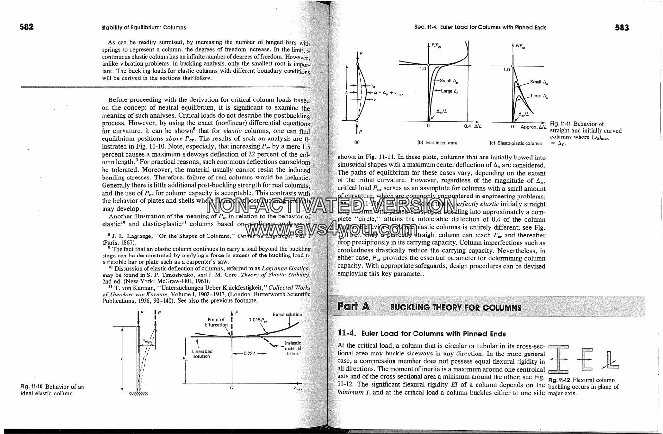
582
Fig. tt-t0 Behavior of anideal elastic col/tmn.
Stability of Equilibrium: Columns
As can be readily surmised, by increasing the number of hinged barssprings to represent a column, the degrees of freedom increase. In thecontinuous elastic column has an infinite number of degrees of freedom.unlike vibration problems, in buckling analysis, only the smallest root istant. The buckling loads for elastic columns with different boundarywill be derived in the sections that<follow.
Before proceeding with the derivation for critical column loadson the concept of neutral equilibrium, it is significant to examinemeaning of such analyses. Critical loads do not describe theprocess. However, by using the exact (nonlinear) differentialfor curvature, it can be shown s that for elastic columns, one canequilibrium positions above Per. The results of such an analysislustrated in Fig. 11-10. Note, especially, that increasing Per by a merepercent causes a maximum sideways deflection of 22 percent of theumn length. 9 For practical reasons, such enormous deflections canbe tolerated. Moreover, the material usually cannot resist thebending stresses. Therefore, failure of real columns would beGenerally there is little additional post-buckling strength for realand the use of P�r for column capacity is acceptable. This contraststhe behavior of plates and shells where significant post-bucklinmay develop.
Another illustration of the meaning of P�r in relation to theelastic �� and elastic-plastic � columns based on nonlinear analyses
8 j. L. Lagrange, "On the' Shapes of Columns," Oevres de Lagrange,(Paris, 1867).
9 The fact that an elastic column continues to carry a load beyond thestage can be demonstrated by applying a force in excess of the bucklinga flexible bar or plate such as a carpenter's saw.
�0 Discussion of elastic deflection of columns, referred to as Lagrangemay be found in S. P. Timoshenko, and J. M. Gere, Theory of Elastic2nd ed. (New York: McGraw-Hill, 1961).
u T. von Karman, "Untersuchungen Ueber Knickfestigkeit,"of Theodore yon Karman, Volume I, 1902-1913, (London: ButterworthPublications, 1956, 90-140). See also the previous footnote.
�PPoint of [ 1.015Per
bifurcation [ x�
Linearizedsolution
failur e
Sec. tt-4. Euler Load for Columns with Pinned Ends 583
all A oVo
L A=dOq-Vmax !/�Largedov
�g/A o/L0 0.4 A/L
1.0
(a) (b) Elastic columns (c) Elasto-plastic columns
all d o
rgedoApprox. z�L Fig. tl-ll Behavior of
straight and initially curvedcolumns where (V0)max= A 0.
in Fig. 11-11. In these plots, columns that are initially bowed intoshapes with a maximum center deflection of Ao are considered.
paths of equilibrium for these cases vary, depending on the extentthe initial curvature. However, regardless of the magnitude of Ao,
load P,r serves as an asymptote for columns with a small amountwhich are commonly encountered in engineering problems;
see Fig. 11-1 l(b). It is to be noted that a perfectly elastic initially straightlong column with pinned ends, upon buckling into approximately a com-plete "circle," attains the intolerable deflection of 0.4 of the columnlength. Behavior of elastic-plastic columns is entirely different; see Fig.
11-11(c). Only a perfectly straight colunto can reach P� and thereafterprecipitously in its carrying capacity. Column imperfections such as
drastically reduce the carrying capacity. Nevertheless, incase, P� provides the essential parameter for determining column
With appropriate 'safeguards, design procedures can be devisedthis key parameter.
11-4. Euler Load for Columns with Pinned Ends
thecriticalload,acolumnthatiscircularortubularinitscross-sec-� � �area may buckle sideways in any direction. In the more generala compression member does not possess equal flexural rigidity in
directions. The moment of inertia is a maximum around one centroidal
and of the cross-sectional area a minimum around the other; see Fig. Fig. 1t-12 Flexural columnThe significant flexural rigidity E1 of a column depends on the buckling occurs in plane of
minimum I, and at the critical load a column buckles either to one side major axxs.
NON-ACTIVATEDVERSIONwww.avs4you.com

584 Stability of Equilibrium: Columns Sec. 11-5. Euler Loads for Columns with Different End Restraints 585
pl pl
M = -Pv
(a)
P
(b)
Fig. 1t-13 Column pinned atboth ends.
or the other in the plane of the major axis. The use of a ' 'the derivation that follows is understood.
Consider the ideal perfectly straight column with pinnedboth ends; see Fig. 11-13(a). The least force at which a buckledpossible is the critical or Euler buckling load.
In order to determine the critical load for this column, the compreSScolumn is displaced as shown in Fig. 11-13(b). In this position,moment according to the beam sign convention �2 is -Pv. Bythis value of moment into Eq. 10-10, the differential equation for the�curve for the initially straight column becomes
d2v M Pdx 2 E1 E1 v
by letting k 2 = P/EI, and transposing, gives
j-� + X2v = 0
This is an equation of the same form as the one for simplemotion, and its solution is
v =AsinXx + BcosXx (1;
where A and B are arbitrary constants that must be determinedboundary conditions. These conditions are
v(0) = 0 and v(L) = 0
Hence, v(0) = 0 = A sin 0 + B cos 0 or B = 0
and v(L) = 0 = A sin kL
This equation can be satisfied by taking A = 0. However, with Aeach equal to zero, as can be seen from Eq. 11-7, this is a solutionstraight column, and is usually referred to as a trivial solution. Annative solution is obtained by requiring the sine term in Eq. 1This occurs when kn equals n'rr, where n is an integer. Therefore,k was defined as �, the nth critical force Pn that makes theshape of the column possible follows from solving X/P/E1 L =
�2 For the positive direction of the deflection v shown, the bendirnegative. If the column were deflected in the opposite direction, thewould be positive. However, v would be negative. Hence, to make Pvit must likewise be treated as a negative quantity.
n2�r2EI P.,Pn = L------5� (11-9)
are the eigenvalues for this problem. However, since in sta-bility problems only the least value of Pn is of importance, n must be
as unity, and the critical or Euler load �3 Per for an initially perfectlyelastic column wit h pinned ends becomes
I �r2EilPcr= L--i-- (11-10)
E is the elastic modulus of the material, I is the least moment ofinertia of the constant cross-sectional area of a column, and L is itg length.
4Pcr 9Per
�/,n = 2
n=3 '/�
(a) (b) (c)
case of a column pinned at both ends is often referred to as the Fig. tt-t4 First three bucklingcase. modes for a column pinned
According to Eq. 11-7, at the critical load, since B = 0, the equation at both ends.�the buckled elastic curve is
v = A sin Xx (11-11)
is the characteristic, or eigenfunction, of this problem, and, since Xn�r/L, n can assume any integer value. There is an infinite number of
functions. In this linearized solution, amplitude A of the bucklingremains indeterminate. For the fundamental case n = 1, the elasticis a half-wave sine curve. This shape and the modes corresponding
n = 2 and 3 are shown in Fig. 11-14. The higher modes have no physicalignificance in buckling problems, since the least critical buckling load
atn = 1.
Euler Loads for Columns with Different EndRestraints
same procedure as that discussed before can be used to determinecritical axial loads for columns with different boundary conditions.
solutions of these problems are very sensitive to the end restraints.for example, a column with one end fixed and the other pinned,
shown in Fig. 11-15, where the buckled column is drawn in a deflectedHere the effect of unknown end moment Mo and the reactions
be considered in setting up the differential equation for the elasticcurve at the critical load:
d2v M -Pv + Mo(1 - x/L)dx 2 � E1 - EI (11-12)
This formula was derived by the great mathematician Leonhard Euler in 1757.
Fio. 11-15 Column fixed atone end and pinned at theother.
NON-ACTIVATEDVERSIONwww.avs4you.com
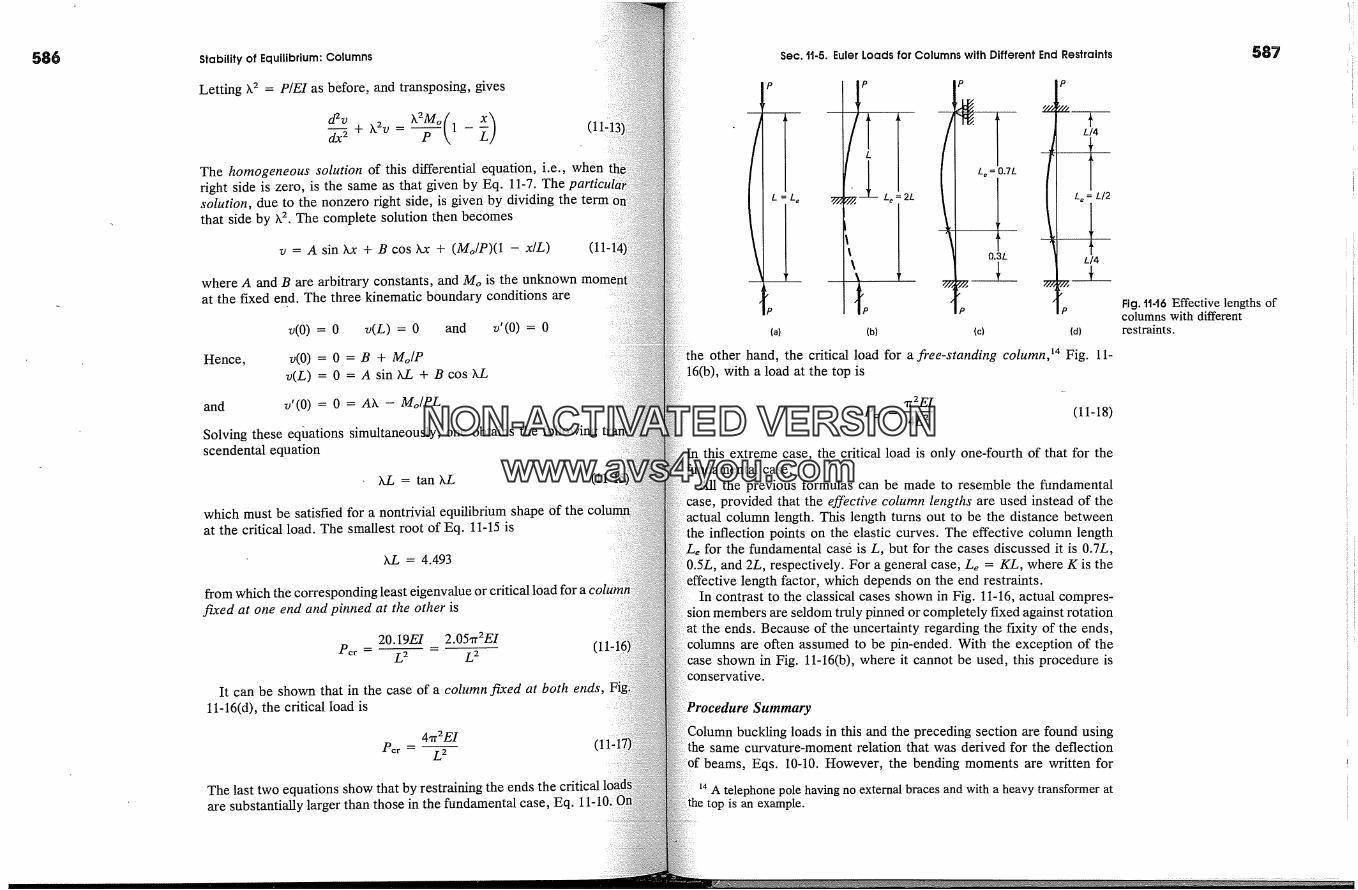
586 Stability of Equilibrium: Columns
Letting k 2 = P/EI as before, and transposing, gives
d2v X2M�(1- �) (11,dx 2 + X2v = PThe homogeneous solution of this differential equation, i.e., whenright side is zero, is the same as that given by Eq. 11-7. Thesolution, due to the nonzero right side, is given by dividing the termthat side by k 2. The complete solution then becomes
v = A sin Xx + B cos Xx + (Mo/P)(1 - x/L) (11-1
where A and B are arbitrary constants, and Mo is the unknownat the fixed end. The three kinematic boundary conditions are
v(O) = 0 v(L) = 0 and v'(O) = 0
Hence, v(O) = 0 = B + Mo/Pv(L) = 0 = A sin kL + BcoskL
and v'(O) = 0 = Ak - Mo/PL
Solving these eqhations simultaneously, one obtains the followingscendental equation
XL = tan XL (11-1
which must be satisfied for a nontrivial equilibrium shape of theat the critical load. The smallest root of Eq. 11-15 is
KL = 4.493
from which the corresponding least eigenvalue or critical load forfixed at one end and pinned at the other is
20.19EI 2.05'rr2EI (114Per - L 2 L 2
It can be shown that in the case of a column fixed at both ends,11-16(d), the critical load is
4,tr2EI(11:Pcr- L 2
The last two equations show that by restraining the ends the criticalare substantially larger than those in the fundamental case, Eq.
Sec. tl-5. Euler Loads for Columns with Different End Restraints
p I p
iL. Le2LL. = 0.7L
0.3L
P
L/4
L� = L/2
L/4
P
(a) (b) (c) (d)
the other hand, the critical load for a fi'ee-standing column, TM Fig. 11-16(b), with a load at the top is
�T2 EIPer - 4L 2 (11-18)
In this extreme case, the critical load is only one-fourth of that for thecase.
All the previous formulas can be made to resemble the fundamentalcase, provided that the effective column lengths are used instead of the
actual column length. This length tums out to be the distance betweenthe inflection points on the elastic curves. The effective column length
for the fundamental casd is L, but for the cases discussed it is 0.7L,0.5L, and 2L, respectively. For a general case, Le = KL, where K is the
length factor, which depends on the end restraints.In to the classical cases shown in Fig. 11-16, actual compres-
are seldom truly pinned or completely fixed against rotationthe ends. Because of the uncertainty regarding the fixity of the ends,
are often assumed to be pin-ended. With the exception of theshown in Fig. 11-16(b), where it cannot be used, this procedure is
Summary
buckling loads in this and the preceding section are found usingsame curvature-moment relation that was derived for the deflection
beams, Eqs. 10-10. However, the bending moments are written for
�4 A telephone pole having no external braces and with a heavy transformer attop is an example.
587
Fig. tt46 Effective lengths ofcolumns with differentrestraints.
NON-ACTIVATEDVERSIONwww.avs4you.com

588 Stability of Equilibrium: Columns Sec. H-6. Limitations of the Euler Formulas 589
axially loaded columns in slightly deflected positions. Mathematicallyresults in an entirely different kind of second order differentialthan that for beam flexure. The solution of this equation shows thatthe same load, two neighboring equilibrium configurations arefor a column. One of these configurations corresponds to a straightumn, the other to a slightly bent column. The axial force associatedmultaneously with the bent and the straight shape of the column iscritical buckling load. This occurs at the bifurcation (branching) pointthe solution.
In the developed formulation, the columns are assumed to beelastic, and to have the same cross section throughout theOnly the flexural deformations of a column are considered.
For the second order differential equations considered in thisthe same kinematic boundary conditions are applicable as for beamsflexure, Fig. 10-5.
Elastic buckling load formulas are truly remarkable. Although theynot depend on the strength of a material, they determine thecapacity of columns. The only material property involved is the elas!modulus E, which physically represents the stiffness characteristicmaterial.
Ocr , ksi
3C
20
10
Aluminumalloy
Fir-�
limit
� \ Long column� � range
0 100 120 200 LB
general. The ratio L/r of the column length to the least radius of gyrationis called the column slenderness ratio. No factor of safety is included inthe last equation.
A graphical interpretation of Eq. 11-19 is shown in Fig. 11-17, wherethe critical column stress is plotted versus the slenderness ratio for threedifferent'materials. For each material, E is constant, and the resultingThe previous equations do not apply if the axial column stress ex -
t�: i curve is a hyperbola. However, since Eq. 11-19 is based on the elasticthe proportional limit of the material. This problem is discussed in ne:: ....- behavior of a material, Crcr determined by this equation cannot exceed thenext section. proportional limit of a material. Therefore, the hyperbolas shown in Fig.11-17 are drawn dashed beyond the individual matehal's proportional
][�-6. Limitations of-the Euler FormulasThe elastic modulus E was used in the derivation of the Euler
for columns; therefore, all the reasoning presented earlier iswhile the material behavior remains linearly elastic. To bring outsignificant limitation, Eq. 11-10 is rewritten in a different form. Byniti0n, I = Ar 2, where A is the cross-sectional area, and r is itsof gyration. Substitution of this relation into Eq. 11-10 gives
�r2 EI �r2 EAr 2'Pcr -- L2 - L-�---
and these portions of the curves cannot be used. The necessaryof Eq. 11-19 to include inelastic material response will be
in the next section.
: The useful portions of the hyperbolas do not represent the behavior ofOne column, but rather the behavior of an infinite number of ideal col-
For example, a particular steel column, say, with an L/r = 120,at the most carry a load of o'�A. Not e that crc; always decreases with
� g ratios of L/r. Moreover, note th� TM PreCiSe definiti�n 6f � 16figCOlumn is now possible with the aid of these diagrams. Thus, a column
said to be long if the elastic Euler formula applies. The beginning oflong-column range is shown for three matehals in Fig. 11-17.
Fig. 1t-t7 Variation of criticalcolumn stress withslenderness ratio for threedifferent materials.
i Pcr *r2E1or crcr - A - (L/r) 2
where the critical stress crcr for a column is defined as Pcr/A, i.e.,average stress over the cross-sectional area A of a column at theload P�r. The length of the column is L, and r is the least radius ofof the cross-sectional area, since the original Euler formula is inthe minimum t: By using the effective length Le, the
the shortest length L for a steel column with pinned ends having a cross-area of 60 by 100 mm, for which the elastic Euler formula applies. Let
= 200 GPa and assume the proportional limit to be 250 MPa.
minimum moment of inertia of the cross-sectional area I.�n = 100 x 603/121.8 x 106 mm 4. Hence,
NON-ACTIVATEDVERSIONwww.avs4you.com

Sec. 1t-7. Generalized Euler Buckling. Load Formulas590 Stability of Equilibrium: Columns
and �/-�'ff x 106 V� X 10mmrmin = X 100
Then, using Eq. 11-19, O'cr= 'rr2E[(L/r) 2. Solving for the L/r ratio at thetional limit,
_�)2 ,rr2E 'rr2'x 200 x 10� 800,rr2O'cr 250
orL- = 88.9 and
FL = 88.9�/� x 10 = 1540mm
Therefore, if this column is 1.54 m or more in length, it will buckleas, for such dimensions of the column, the critical stress at bucklingexceed the proportional limit for the material.
11-7. Generalized Euler Buckling-Load FormulasA typical compression strdss-strain diagram for a specimen that isvented from buckling is shown in Fig. 11-18(a). In the stress rangeO to A, the material behaves elastically. If the stress in abuckling does not exceed this range, the column buckles elastically.hyperbola expressed by Eq. 11-19, O'er = q'r2E/(L/r2), is applicable ina case.'This portion of the curve is shown as ST in Fig. 11-18(b).important to recall that this curve does not represent thecolumn, but rather the behavior of an infinite number of idealof different lengths. The hyperbola beyond the useful range isthe figure by dashed lines.
A column with an L/r ratio corresponding to point S in Fig.the shortest column of a given material and size that wilA shorter column, having a still smaller L/r ratio, will not buckle atproportional limit of the material. On the compression stress-straingram, Fig. 11-18(a), this means that the stress level in thepassed point A and has reached some point B perhaps. At thisstress level, it may be said that a column of different material hascreated, since the stiffness of the material is no longer represented byelastic modulus. At this point, the material stiffness is givenneously by the tangent to the stress-strain curve, i.e., by themodulus E,; see Fig. 11-18(a). The column remains stable if its new
rigidity E,I at B is sufficiently large, and it can carry a higher load.the load is increased, the stress level rises, whereas the tangent mod-
decreases. A column of ever "less stiff material" is acting under anincreaging load. Substitution of the tangent modulus E, for the elasticmodulus E is then the only modification necessary to make the elastic
formulas applicable in the inelastic range. Hence, the generalizedEuler buckling-load formula, or the tangent modulus formula,iS becomes
I 'rr2Et1Crcr -- (L/r)2 (11-20)
Since stresses corresponding to the tangent moduli can be obtained fromcompression stress-strain diagram, the L/r ratio at which a column
buckle with these values can be obtained from Eq. 11-20. A plotthis behavior for low and intermediate ratios of L/r is shown
�5 The tangent modulus formula gives the carrying capacity of a columnat the instant it tends to buckle. As a column deforms further, the stiffness
of the fibers on the concave side continue to approximately exhibit thetangent modulus Et. The fibers on the convex side, however, on being
of some stress, rebound with the original elastic modulus E, as.hown in Fig. 11-A at point C. Inasmuch as two moduli, Et and E, are
used in developing this theory (see F. Bleich, Buckling Strength of MetalStructures [New York: McGraw-Hill, 1952]), it is referred to either as the
is or the reduced-modtdus theory of column buckling. Forthe same column slenderness ratio, this theory always gives a slightly
column buckling capacity than the tangent-modulus theory. Thebetween the two solutions is not very large. The reason for
was explained by F. R. Shanley (see his paper, "InelasticColumn Theory," J. Aero: Sci. 14/5 (May 1947):261-267). According to
concept, buckling proceeds simultaneously with the increasing axialload. The applied load given by the tangent-modulus theory increasesaSymptotically to that given by the double-modulus theory; see Fig. 11-
B. However. prior to reaching the load given by the double-modulus the-one can anticipate a material yield or failure, making the tangent
It is convenient that in the tangent-modulusthe mechanical properties for the whole cross section are the same,
they vary differently for different cross-sections in the double-modulus theory.
The maximum load lying between the tangent-modulus load and they time-independent elastic-plastic material and
section was accurately determined by T. H. Lin (see his paper on"Inelastic Column Buckling," J. Aeron. Sci., Vol. 17, No. 3, 1950, 159-
J. E. Duberg and T. W. Wilder (see their paper on "Column Behaviorthe Plastic Stress Range," J. Aeron. Sci., Vol. 17, No. 6, 1950, 323-
have further concluded that for materials whose stress-strain curvesgradually in the inelastic range, the maximum column load can
y above the tangent-modulus load. If, however, the materialthe inelastic range tends to rapidly exhibit plastic behavior, the max-
irnum load is only slightly higher than the tangent-modulus load.
59i
o Et
1�.0 E
Fig. 11-A Stress-strainbehavior in buckled column.
Double-modulus
nleyctual
Tangent-modulus
Cross-section rotation
Fig. tt*B Inelasticbuckling loads bydifferent theories.
NON-ACTIVATEDVERSIONwww.avs4you.com
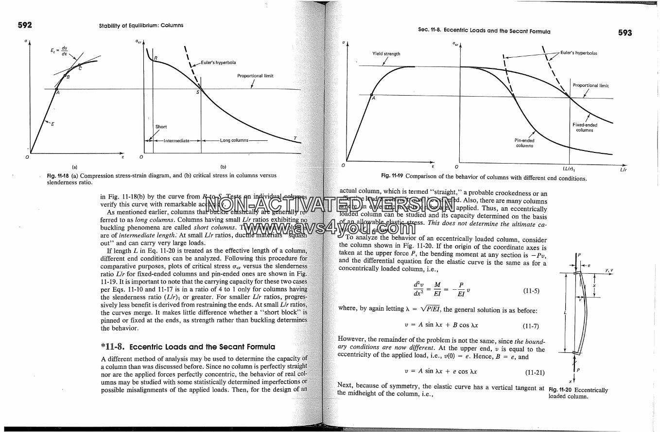
592 Stability of Equilibrium: Columns
(a)
�cr
�....Euler's hyperbolaProportional limit
/
Short
columns--
(b)
Fig. tt48 (a) Compression stress-strain diagram, and (b) critical stress in columns versusslenderness ratio.
in Fig. 11-18(b) by the curve from R to S. Tests on individualverify this curve_ with remarkable accuracy.
As mentioned earlier, columns that buckle elastically areferred to as long columns. Columns having small L/r ratiosbuckling phenomena are called short columns. The remainingare of intermediate length.' At small L/r ratios, ductile materials "s(out" and can carry very large loads.
If length L in Eq. 11-20 is treated as the effective length of adifferent end conditions can be analyzed. Following thiscomparative purposes, plots of critical stress O'cr versus theratio L/r for fixed-ended columns and pin-ended ones are shown in11-19. It is important to note that the carrying capacity for these twoper Eqs. 11-10 and 11-17 is in a ratio of 4 to 1 only for columnsthe slenderness ratio (L/r)� or greater. For smaller L/r ratiossively less benefit is derived from restraining the ends.the curves merge. It makes little difference whether a "shortpinned or fixed at the ends, as strength rather than bucklingthe behavior.
Eccentric Loads and the Secant Formula
A different method of analysis may be used to determine thea column than was discussed before. Since no column is perfectlynor are the applied forces perfectly concentric, the behaviorumns may be studied with some statistically determinedpossible misalignments of the applied loads. Then, for the design
Sec. tt-8. Eccentric Loads and the Secant Formula
Yield strength
/
Ocr
Fig. 1149 Comparison of the behavior of columns with different
� Euler'shyperbolas
Pin-ended � J
columns �( L/r h
actual column, which is termed "straight," a probable crookedness or an�.load eccentricity may be assigned. Also, there are many columns
where an eccentric load is deliberately applied. Thus, an eccentricallyloaded column can be studied and its capacity determined on the basisof an allowable elastic stress. This does not determine the ultimate ca-
of a column.To analyze the behavior of an eccentrically loaded column, consider
the column shown in Fig. 11-20. If the origin of the coordinate axes istaken at the upper force P, the bending moment at any section is -Pv,and the differential equation for the elastic curve is the same as for aconcentrically loaded column, i.e.,
d2v M Pdx 2 � � = -� v (11-5)
where, by again letting X = X/�, the general solution is as before:
(11-7)v =AsinXx + BcosXx
However, the remainder of the problem is not the same, since the bound-ary conditions are now different. At the upper end, v is equal to theeccentricity of the applied load, i.e., v(0) = e. Hence, B = e, and
(11-21)v = AsinXx + ecosXx
end conditions.
P
y� V
x
Next, because of symmetry, the elastic curve has a vertical tangent at Fig. tt-20 Eccentricallymidheight of the column, i.e., loaded column.
593
L/r
NON-ACTIVATEDVERSIONwww.avs4you.com
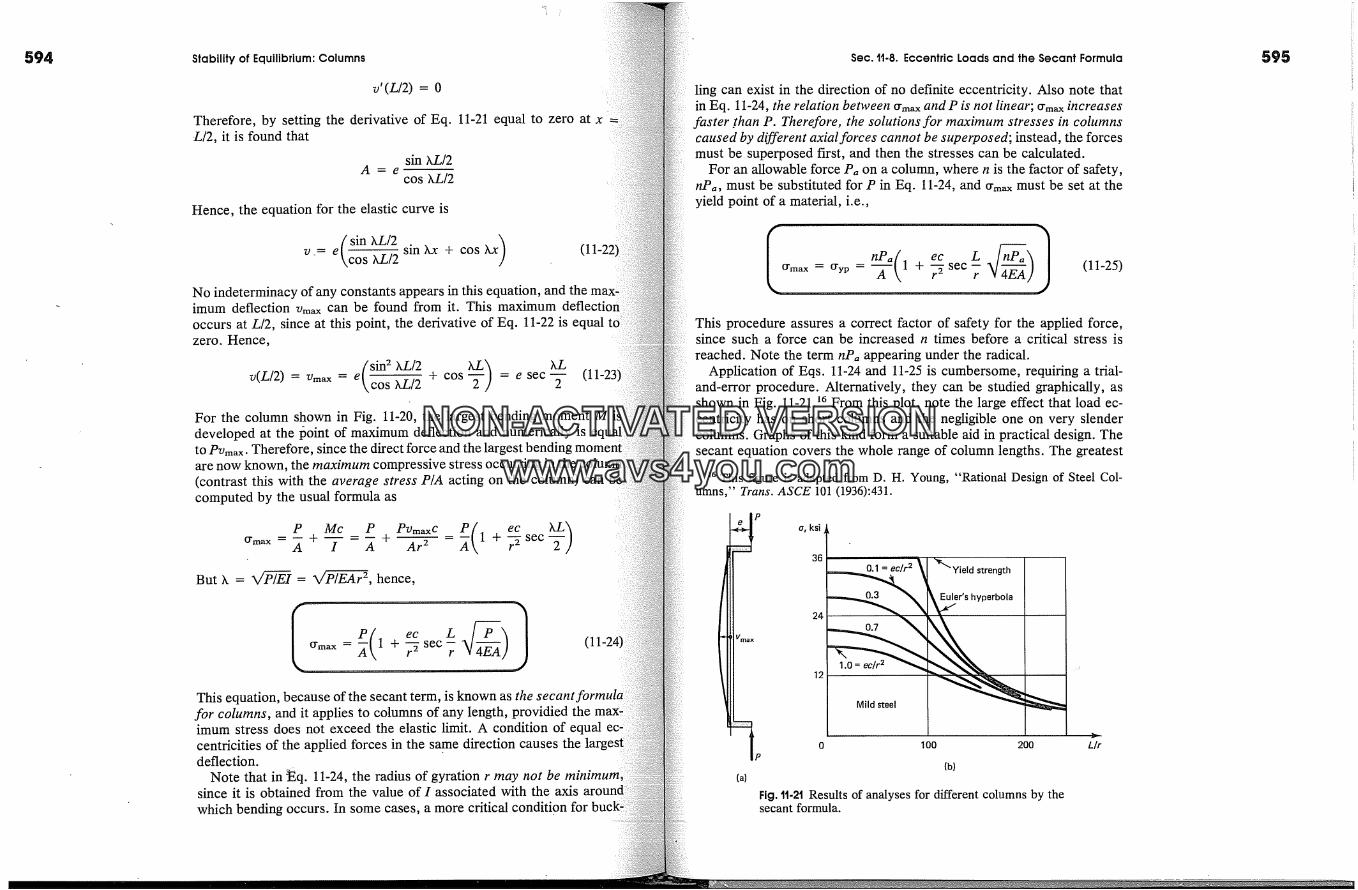
Stability of Equilibrium: Columns Sec. tt.8. Eccentric Loads and the Secant Formula
v'(L/2) = 0
Therefore, by setting the derivative of Eq. 11-21 equal to zero at x,L/2, it is found that
sin kL/2cos kL/2
Hence, the equation for the elastic curve is
e( sin xL/2v�= \co� sin Xx + cos Xx (1XL/2
No indeterminacy of any constants appears in this equation, and the max-imum deflection Vm�x can be found from it. This maximum defle,occurs at L/2, since at this point, the derivative of Eq. 11-22 is equalzero. Hence,
7J(Z/2) = Umax �- e�os �'� q- cos �- e sec-�- (11-23)For the column shown in Fig. 11-20, the largest bending moment Mdeveloped at the/)oint of maximum deflection and numerically isto Pvm�x. Therefore, since the direct force and the largest bendingare now known, the maximum compressive stress occurring in the(contrast this with the average stress P/A acting on the column) cancomputed by the usual formula as
P
ling can exist in the direction of no definite eccentricity. Also note thatin Eq. 11-24, the relation between Crm�x and P is not linear; Crm�x increases
faster .than P. Therefore, the solutions for maximum stresses in columnscaused by different axial forces cannot be superposed; instead, the forcesmust be superposed first, and then the stresses can be calculated.
For an allowable force Pa on a column, where n is the factor of safety,nPa, must be substituted for P in Eq. 11-24, and Crm�x must be set at theyield point of a material, i.e.,
But k = � = P�, hence,
AP_( ec L 4�E�)O'max �- 1 + �'� sec 7
This equation, because of the secant term, is known as the secantfor columns, and it applies to columns of any length, providied theimum stress does not exceed the elastic limit. A condition of equalcentricities of the applied forces in the same direction causes thedeflection.
Note that in 'Eq. 11-24, the radius of gyration r may not be minimumsince it is obtained from the value of I associated with the axiswhich bending occurs. In some cases, a more critical condition
I O'max�O'yp-- ec"1 + � sec 7 4EA,/ (11-25)
This procedure assures a correct factor of safety for the applied force,since such a force can be increased n times before a critical stress isreached. Note the term nP� appearing under the radical.
Application of Eqs. 11-24 and 11-25 is cumbersome, requiring a trial-and-error procedure. Alternatively, they can be studied graphically, asshown in Fig. 11-21. �6 From this plot, note the large effect that load ec-centricity has on short columns and the negligible one on very slendercolumns. Graphs of this kind form a suitable aid in practical design. Thesecant equation covers the whole range of column lengths. The greatest
�6 This figure is adapted from D. H. Young, "Rational Design of Steel Col-umns," Trans. ASCE 101 (1936):431.
e P
ecMc P PvmaxC 1 + �'� secI = A + Ar 2 -
,1P
o, ksi
36
0.1= ec/r2 \� �"Yield strength
� �er'shyperbola24
Mild steel �
0 1 O0 200 L/r
(b)
Fig. tt-2t Results of analyses for different columns by thesecant formula.
NON-ACTIVATEDVERSIONwww.avs4you.com
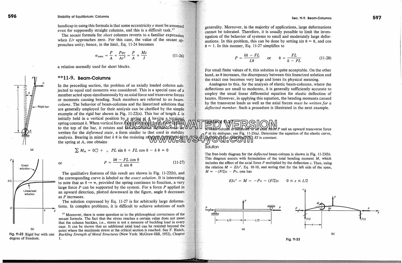
596
L bar
(a)
Exact /
Linearizedsolution
(b)
Fig. tt-22 Rigid bar with onedegree of freedom.
Stability of Equilibrium: Columns
handicap in using this formula is that some eccentricity e must be as.,even for supposedly straight columns, and this is a difficult task?
The secant formula for short columns reverts to a familiarwhen L/r approaches zero. For this case, the value of the secantproaches unity; hence, in the limit, Eq. 11-24 becomes
P Pec P Mc
Crm�x A + Ar 2 A + I
a relation normally used for short blocks.
*'11-9. Beam-Columns
In the preceding section, the problem of an axially load_ed columnjected to equal end moments was considered. This is a special case ofmember acted upon simultaneously by an axial force andor moments causing bending. Such members are referred to as becolurns. The behavior of beam-columns and the linearized solutionsare generally employed for their analysis can be clarified by theexample of the rigid bar shown in Fig. 11-22(a). This bar of length Liinitially held in a vertical position by a spring at A having aspring constant k. When vertical force P and horizontalto the top of the-bar, it rotates and the equilibrium equation mustwrriten for the deformed state, a form similar to that used inanalysis. Bearing in mind that k 0 is the resisting moment developedthe spring at A, one obtains.
� MA = O0 + �'� PL sin O + FL cos 0 - k0 = 0
or P=kO - FL cos 0
L sin 0
The qualitative features of this result are shown in Fig. 11-22(b),the corresponding curve is labeled as the exact solution. It isto note that as 0 --> �r, provided the spring continues to function, alarge force P can be supported by the system. For a force P appliedan upward direction, plotted downward in the figure, angle 0as P increases.
The solution expressed by Eq. 11-27 is for arbitrarily largetions. In complex problems, it is difficult to achieve solutions of
�7 Moreover, there is some question as to the philosophical correctness ofsecant formula. The fact that the stress reaches a certain value does notthat the column buckles, i.e., stress is not a measure of buckling load incase. It can be shown that an additional axial load can be resisted beyondpoint where the maximum stress at the critical section is reached. See F.Buckling Strength of Metal Structures (New York: McGraw-Hill, 1952), Cha1.
Sec. '1t-9. Beam-Columns
Moreover, in the majority of applications, large deformationscannot be tolerated. Therefore, it is usually possible to limit the inves-tigation of the behavior of systems to small and moderately large defor-mations. In this problem, this can be done by setting sin 0 � 0, and cos0 � 1. In this manner, Eq. 11-27 simplifies to
kO - FL FLP - or 0 = -- (11-28)
LO k - PL
For small finite values of 0, this solution is quite acceptable. On the otherhand, as 0 increases, the discrepancy between this linearized solution andthe exact one becomes very large and loses its physical meaning.
Analogous to this, for the analysis of elastic beam-columns, where thedeflections are small to moderate, it is generally sufficiently accurate toemploy the usual linear differential equation for elastic deflection ofbeams. However, in applying this equation, the bending moments causedby the transverse loads as well as the axial forces must be written for adeflected member. Such a procedure is illustrated in the next example.
EXAMPLE tt-3
A beam-column is subjected to an axial force P and an upward transverse forceF at its midspan; see Fig. 11-23(a). Determine the equation of the elastic curve,and the critical axial force Pcr- E1 is constant.
Solution
The free-body diagram for the deflected beam-column is shown in Fig. 11-23(b).This diagram assists with formulation of the total bending moment M, whichincludes the effect of the axiai force P multiplied by the deflection v. Thus, usingthe relation M =EIv", Eq. 10-10, and noting that for the left side of the span,M = -(F/2)x - Pv, one has
EIv"= M = -Pv - (F/2)x 0 --< x --< L/2
F-�L/2
(a)
Fig. tt-23
(b)
597
P
NON-ACTIVATEDVERSIONwww.avs4you.com
598 Stability of Equilibrium: Columns
or EIv" q- Pv = - (F/2)x
By dividing through by E1 and letting h 2 = P/E1, after some simplification�governing differential equation becomes
d2v k2Fdx 2 q- �.2v = 2p'X 0 <-- x --< L/2
The homogeneous solution of this differential equation is the same as thatlEq. 11-6, and the particular solution equals the right-hand term divided byTherefore, the complete solution is
v = Ci sin Xx + C2 cos IX - (F/2P)x
Constants C� and C2 follow from the boundary condition, v(0) = 0, andcondition of symmetry, v'(L/2) = 0. The first condition gives
v(0) = C2 = 0
Since
v' = C�k cos Ix - C2k sin Ix - F/2P
with C2 already known to be zero, the second condition gives
v'(L/2) = .C�k cos XL/2 - F/2P = 0
or Ci = F/[2Pk cos (XL/2)]
On substituting this constant into Eq. 11-30,
F sinIx F F (sin .k�c_ )v - 2Pk cos XL/2 2P x = 2-� \ cos � Ix (11-3where the last relationship is obtained by setting
XL/2 = � (11-32)
Since the maximum deflection occurs at x = L/2, after some simplifications
FVm�x - (tan � - �)
2Pk
and the absolute maximum bending moment occurring at midspan is
Mmax = FL Pvm�x[ F--�- - = �-� tan �
Sec. tt-9. Beam-Columns
Equations 11-31, 11-33, and 11-34 become infinite when � is a multiple of �r/2,since then cos � is equal to zero and tan � is infinite. In conformity with thisrequire. ment, for an nth mode, where n is an integer,
kL � L�=�- = �- 2 (11-35)
Solving the last two expressions for P�, and setting n = 1, the critical bucklingload is obtained.
n2,rr2EI ,r2EIPn- L2 --� Per = L2 (11-36)
This procedure shows that a solution of the linearized differential equation yieldsthe Euler buckling load causing infinite deflections and moments. For tensileforces, on the other hand, the deflections are reduced. These trends are similarto those shown in Fig. 11-22(b).
Next it is of considerable practical importance to obtain an approximate solutionto this problem that can then be generalized for a great many beam-column prob-lems for finding deflections and maximum moments. For this purpose, expandtan � into the Maclaurin (Taylor) series and subtitute the result into Eq. 11-33,making note of Eq. 11-35.
3�5 62 -9ran� = �+ �3 +�5 + �7 + 2_�u + ... (11-37)F 1(-�)3( 2 2 17-4 96_�5--Vm�x = 2P� � 1 + � + �u + u 6 + '" (11-38)
However, in view of Eqs. 11-35 and 11-36,
�.2L2 pL 2 P�2 .... 2.4674- (11-39)
4 4EI Pcr
By substituting the last equation into Eq. 11-38 and simplifying,
48EI 0.9870 + 0.9857(p�r) 2+ 0'9855(p�rr) 3+ '"1 (11-40)
By approximating the coefficients �8 in the bracketed expression by unity and
�s A. Chajes, Principles of Structural Stability (Englewood Cliffs, NJ: Prentice-Hall, 1974). For discussion of elastic-plastic beam columns, see K. Jezek, "DieTragfaehigkeit axial gedrueckter und auf Biegung beanspruchter Stahistaebe,"Der Stahlbau 9 (1936):!2, 22, and 39.
599
NON-ACTIVATEDVERSIONwww.avs4you.com
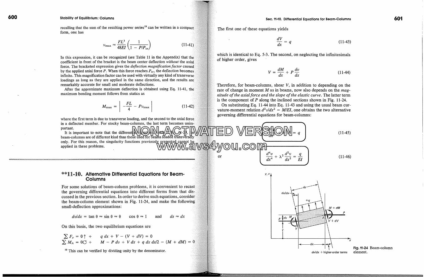
600 Stability of Equilibrium: Columns
recalling that the sum of the resulting power series �9 can be written inform, one has
FL3 1 - (11-417)max � 48---� �/Pcr
In this expression, it can be recognized (see Table 11 in the Appendix)coefficient in front of the bracket is the beam center deflection without theforce. The bracketed expression gives the deflection magnification factorby the applied axial force P. When this force reaches Per, the deflection bec�infinite. This magnification factor can be used with virtually any kindloadings as long as they are applied in the same direction, and the results areremarkably accurate for small and moderate deflections.
After the approximate maximum deflection is obtained using Eq. 11-41,maximum bending moment follows from statics as
I FL Pvmax I (1Mmax = - �- -
where the first term is due to transverse loading, and the second to the axialin a deflected member. For stocky beam-columns, the last term becomesportant.
It is important to-note that the differential equations, such as Eq. 11-29,beam-columns are of different kind than those used for beamsonly. For this reason, the singularity functions previously presented cannotapplied in these problems.
Alternative Differential Equations for Beam-Columns
For some solutions of beam-column problems, it is convenient tothe governing differential equations into different forms from that discussed in the previous section. In order to derive such equations,the beam-column element shown in Fig. 11-24, and make the followinsmall-deflection approximations:
dv/dx = tan 0 � sin 0 � 0 cos 0 � 1 and ds � dx
On this basis, the two equilibrium equations are
�MA = 0� +q dx + V- (V + dv) = 0M- P dv + V dx + q dx dx/2 - (M + dM) =
This can be verified by dividing unity by the denominator.
Sec. tt-t0. Differential Equations for Beam-Columns
The first one of these equations yields
dV
dx q (11-43)
which is identical to Eq. 5-3. The second, on neglecting the infinitesimalsof higher order, gives
dM dvV = -- + P-- (11-44)
dx dx
Therefore, for beam-columns, shear V, in addition to depending on therate of change in moment M as in beams, now also depends on the mag-nitude of the axial force and the slope of the elastic curve. The latter termis the component of P along the inclined sections shown in Fig. 11-24.
On substituting Eq. 11-44 into Eq. 11-43 and using the usual beam cur-vature-moment relation d2v/dx 2 = M/E1, one obtains the two alternativegoverning differential equations for beam-columns:
d2M 2 h (11-45)
I d4v K2d2v q i (11-46)or �-/ + dx 2 - E1
Yt V
M +dM
V+dV
x
dv/dx + higher-order termsFig. tt-24 Beam-columnelement.
60'1
NON-ACTIVATEDVERSIONwww.avs4you.com

Stability of Equilibrium: Columns Sec. 1t40. Differential Equations for Beam-Columns
where, for simplicity, EI is assumed to be constant, and, as before,P/E1. The boundary conditions for these equations are the same asbeams in flexure (see Fig. 10-5), except for shear where Eq. 11-44By again making use of the beam curvature-moment relation, Eq.in more appropriate alternative form can be written as
I. V d3v dvI (1
If P = 0, Eqs. 11-44a, 11-45, and 11-46 revert, respectively, to E{14b, 5-5, and 10-14c for transversely loaded beams.
For future reference, the homogeneous solution of Eq. 11-46 and sevof its derivatives are
v= C�sinXx+ C2cosXx+ C3x+ C4v' = C�X cos Xx - C2X sin Xx + C3v" = -C�X � sin Xx - C2X 2 cos Xx
v"' = -C�X 3 cos Xx + C2X3 sin Xx
(1
These relations are useful for expressing the boundary conditions inuating constants C�, C2, C3, and C4. The use of Eq. 11-44a ratherEq. 10-14b is essential when shear at a boundary must be considered.
Solutions of homogeneous Eqs. 11-45 or 11-46 for 1;conditions lead to critical buckling loads for elastic prismaticThese solutions have the same meaning as discussed earlier inwith the equivalent solutions of the second order differentialin Sections 11-4 and 11-5.
EXAMPLE tt-4
A slender bar of constant EI is simultaneously subjected to end moments Moaxial force P, as shown in Fig. 11-25(a). Determine the maximum deflectionthe largest bending moment.
v Total deflection
� L � Deflection due toMo only
(a) (b)
Fig. 11-25
Solution
Within the span, there is no transverse load. Therefore, the right-hand term ofEq. 11'-46 is zero, and the homogeneous solution of this equation given by Eq.11-47a is the complete solution. The boundary conditions are
v(O) = 0 v(L) = 0 M(O) = -Mo and M(L) = -Mo
Since M =EIv", with the aid of Eqs. 11-47a and 11-47c, these conditions yield:
v(0) = + c2v(L) = +C� sin kL + C2 cos kL + C3L
M(O) = - C2EIPA 2M(L) = -C1EI'A 2 sin kL - C2EI'A 2 cos
+C4=0+C4=0
Solving these four equations simultaneously,
Mo 1 - cos 205 MoC� = C2 = -C4 = and
P sin 205 P
Therefore, the equation of the elastic curve is
v =-�- �,- sinXx + cosXx- 1 (11-48)
The maximum deflection occurs at x = L/2. After some simplifications, it isfound to be
Mo (sin 2 + cos - 1 = sec-�- 1 (11-49)Vmax- P \cos kL/2 '�- � -
The largest bending moment also occurs at x = L/2. Its absolute maximum is
Mmax = I -Mo - Pvmax I = Mo sec XL/2 (11-50)
This solution is directly comparable to that given in Section 11-8 for an ec-centrically loaded column. Two differences in the details of the solutions, how-ever, should be noted. The end moments Mo = Pe of the earlier solution and thex axis of the eccentrically loaded column is at a distance e away from the columnaxis. Then, with the use of some trigonometric identities, it can be shown thatEqs. 11-22 and 11-48 lead to the same results.
The results again show that in slender members, bending moments can be sub-stantially increased in the presence of axial compressive forces. Similar to thecondition encountered in Example 11-3, when kL/2 = �r/2, axial force P = Per,and Vma x and Mmax become infinite.
If the applied axial forces are tensile instead of compresslye, the sign of Pand so does the character of Eqs. 11-45 and 11-46. For such cases, the
are reduced with increasing axial force P.
NON-ACTIVATEDVERSIONwww.avs4you.com
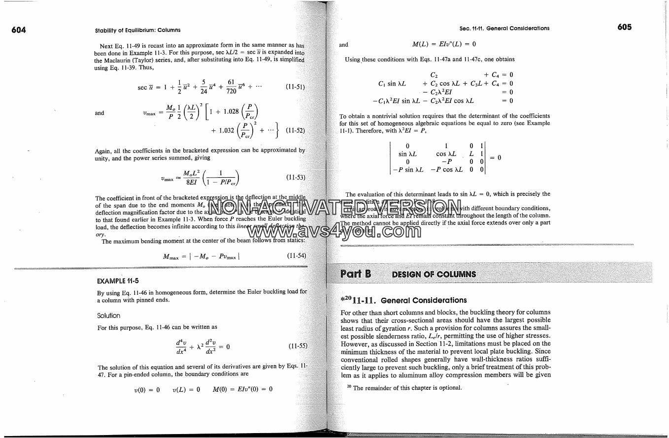
Stability of Equilibrium: Columns Sec. 11-1t. General ConsiderationsNext Eq. 11-49 is recast into an approximate form in the same manner as
been done in Example 11-3. For this purpose, sec kL/2 = sec � is expandedthe Maclaurin (Taylor) series, and, after substituting into Eq. 11-49, isusing Eq. 11-39. Thus,
1 , 5 �4 61 �6sec=1+5-+7/ +7-76 +'" (11-5[
and Vmax =-�-� 1 + 1.028+ 1.032 + --- (1
Again, all the coefficients in the bracketed expression can be approximatedunity, and the power series summed, giving
The coefficient in front of the bracketed expression is theof the span due to the end moments Me (see Table 11 in the Appendix).deflection magnification factor due to the axial force P in the brackets isto that found earlier in Example 11-3. When force P reaches the Eulerlead, the deflection becomes infinite according to this linear s�nall deflectionory.
The maximum bending momeht at the center of the beam follows from
mmax = I -me - P�dmax I
EXAMPLE tt-5
By using Eq. l 1-46 in homogeneous form, determine the Euler buckling leada column with pinned ends.
Solution
For this purpose, Eq. 11-46 can be written as
d4v d2v+ k 2
dx 4 dx 2=0
The solution of this equation and several of its derivatives are given by47. For a pin-ended column, the boundary conditions are
v(O) = 0 v(L) = 0 M(O) = EIv"(O) = 0
and lttM(L) =EIr (L) = 0
Using.these conditions with Eqs. 11-47a and 11-47c, one obtains
C2 + C4= 0C� sin kL + C2 cos KL + C3L + C4 = 0
� - C2�.2EI = 0-C�k2EI sin kL - C2�.2EI cos KL = 0
To obtain a nontrivial solution requires that the determinant of the coefficientsfor this set of homogeneous algebraic equations be equal to zero (see Example11-1). Therefore, with X2EI = P,
0 , 0 isin kL cos kL L0 -P 0
-PsinkL -PcoskL 0
=0
The evaluation of this determinant leads to sin kL = 0, which is precisely thesame condition as given by Eq. 11~8.
This approach is advantageous in problems with different boundary conditions,the axial force and E1 remain constant throughout the length of the column.
The method cannot be applied directly if the axial force extends over only a parta member.
'2�11.11. General ConsiderationsFor other than short columns and blocks, the buckling theory for columns
that their cross-sectional areas should have the largest possibleleast radius of gyration r. Such a provision for columns assures the small-est possible slenderness ratio, Le/r, permitting the use of higher stresses.
as discussed in Section 11-2, limitations must be placed on theof the material to prevent local plate buckling. Since
rolled shapes generally have wall-thickness ratios suffi-ciently large to prevent such buckling, only a brief treatment of this prob-
lem as it applies to aluminum alloy compression members will be given2o The remainder of this chapter is optional.
NON-ACTIVATEDVERSIONwww.avs4you.com

606
Lacing
Lacing(a)
Lacing
]E(b)
(e) (f)
Fig. tt-26 Typical built-upcolumn 'cross sections.
LacingLacing
Fig. tt-27 Latticeinstability.
Fig. tt-28 Schematic residualstress pattern.
Stability of Equilibrium: Columns
here. Torsional buckling modes that may control the capacitymade from thin plate elements and open unsymmetrical cross secare excluded from consideration (see Section 11-2).
Since tubular members have a large radius of gyration in relation toamount of material in a cross section, they are excellent for use asumns. Wide flange sections (sometimes referred to as H sections) arevery suitable for use as columns, and are superior to I sections,have narrow flanges, resulting in larger ratios of Le/r. In order toa large radius of gyration, columns are often built up from rolled ortruded shapes, and the individual pieces are spread out to obtaindesired effect. Cross sections for typical bridge compressionare shown in Figs. 11-26(a) and (b), for a derrick boom or a radioin Fig. 11-26(c), and for an ordinary truss in Fig. 11-26(d). The anglesthe latter case are separated by spacers. The main longitudinal shapesthe other members are separated by plates, or are lacedby light bars as shown in Figs. 11-26(e) and (f). Local instabilitycarefully guarded against to prevent failures in lacing bars, as shownFig. 11-27. Such topics are beyond the scope of this text. 2�
Unavoidable imperfections must be recognized in the practical desiof columns. Therefore, specifications usually stipulate not only the cof material, but also fabrication tolerances for permissibleness. The residual stresses caused by the manufacturing process mualso be considered. For example, steel wide-flange sections,uneven cooling during a hot rolling operation, develop residualpatterns of the type shown in Fig. 11-28. The maximum residualpressive stresses may be on the order of 0.3Cryp in such members.in aluminum alloy members reduce the mechanical properties of the:terial in the heat affected zone. For these reasons, experimentalon column buckling have a large scatter.
After initially accepting the Euler buckling-load formularange of applicability, a chaotic situation existed for many years
2� B. G. Johnson (ed.), Stability Design Criteria for Metal Structures,(New York: Wiley, 1988).
ocr � Vertex ofOypl j parabola
[ Point of� �\ \ tangency
a, \N�J/ Euler's
0 (L/r) 1
(a)
Oc r
(b)
Fig. tt-29 Typical column-buckling curves for design.
regard to column-design formulas. Now that the column-buckling phe-nomenon is more clearly understood, only a few column formula typeswe in common use. For steel, it is now customary to specify two formulas.One of these is for use for short and intermediate-length columns; theother, for slender columns, Fig. 11-29(a). For the lower range of columnlength, usually a parabola, and, in a few instances, an inclined straightline, is specified. In this manner, the basic compressive strength of thematerial, residual stresses, and fabrication tolerances are accounted for.For slender (long) columns, the Euler elastic buckling load provides thebasis for the critical stress. In this range of column lengths, the residualstresses play a relatively minor role. The dominant parameters are thematerial stiffness, E, and geometric fabrication imperfections. Often thetwo specified complementary equations have a common tangent'at a se-lected value of L/r. Such a condition cannot be full"fled if a straight lineis used instead of a parabola. In a few specifications, the more conser-
approach of using the elastic formula and an allowable stress is,y assuming an accidental eccentricity based on manufacturing tol-
erances.For some materials, a sequence of three different equations is specified
for the design of columns, Fig. 11-29(b). One of these equations for shortcolumns defines the basic compressive strength of a material. Anotherequation, specifically applicable for the long column range, is based onthe Euler buckling load. An empirical relation, such as an inclined straightline shown in the figure, or a parabola, is specified for columns of inter-mediate lengths. Such a type of formula is generally given for aluminumalloys and wood.
In applying the design formulas, it is important to observe the followingitems:
1. The material and fabrication tolerances for which the formula iswritten.
2. Whether the formula gives the working load (or stress) or whether
607
NON-ACTIVATEDVERSIONwww.avs4you.com
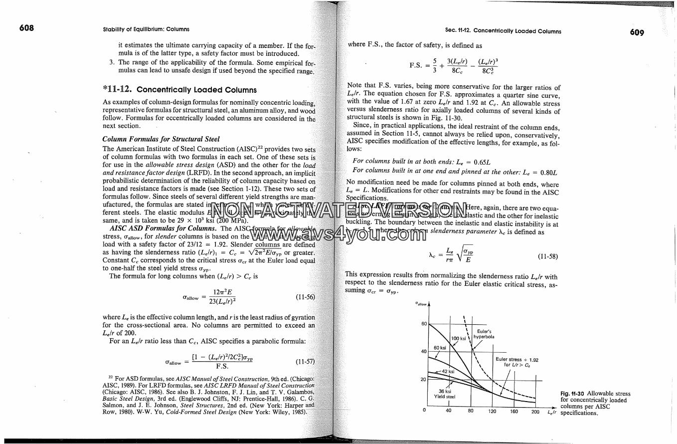
6O8 Stability of Equilibrium: Columns
it estimates the ultimate carrying capacity of a member. If themula is of the latter type, a safety factor must be introduced.The range of the applicability of the formula. Some empiricalmulas can lead to unsafe design if used beyond the specified ran:
*]]42. Concentrically Loaded ColumnsAs examples of column-design formulas for nominallyrepresentative formulas for structtural steel, an aluminum alloy,follow. Formulas for eccentrically loaded columns are considered innext section.
Column Formulas for Structural SteelThe American Institute of Steel Construction (AISC) 22 provides two setof column formulas with two formulas in each set. One of these setsfor use in the allowable stress design (ASD) and the other for theand resistance factor design (LRFD). In the second approach, anprobabilistic determination of the reliability of column capacity basedload and resistance factors is made (see Section 1-12). These two setsformulas follow. Since steels of several different yield strengthsufactured, the formulas are stated in terms of ffyp, which varies forferent steels. The elastic modulus E for all steels is approximatelysame, and is taken to be 29 x 103 ksi (200 MPa).
AISC ASD Formulas for Columns. The AISC formula for allowabstress, t�al�ow, for slender columns is based on the Euler elasticload with a safety factor of 23/12 = 1.92. Slender columns areas having the slenderness ratio (Le/r)� = Cc = X/2�2E/tyyp orConstant Cc corresponds to the critical stress trcr at the Euler loadto one-half the steel yield stress ffyp.
The formula for long columns when (L�/r) > C� is
12x2E
tral�ow - 23(Le/r) 2
where Le is the effective column length, and r is the least radius offor the cross-sectional area. No columns are permitted to exceedLe/r of 200.
For an Ldr ratio less than C�, AISC specifies a parabolic formula:
O'allow[1 -- (Le/r)2/2Cc2]tyyp
F.S.
22 For ASD formulas, see AISC Manual of Steel Construction, 9th ed.AISC, 1989). For LRFD formulas, see AISC LRFD Manual of Steel(Chicago: AISC, 1986). See also B. J. Johnston, F. J. Lin, and T. V.Basic Steel Design, 3rd ed. (Englewood Cliffs, NJ: Prentice-Hall, 1986). CSalmon, and J. E. Johnson, Steel Structures, 2nd ed. (New York:Row, 1980). W-W. Yu, Cold-Formed Steel Design (New York: Wiley,
Sec. tt-12. Concentrically Loaded Columns
F.S., the factor of safety, is defined as
609
5 3(Le/r) (Le/r) �F.S. = 5 +
Note that F.S. varies, being more conservative for the larger ratios ofLe/r. The equation chosen for F.S. approximates a quarter sine curve,
the value of 1.67 at zero Leh' and 1.92 at C�. An allowable stressslenderness ratio for axially loaded columns of several kinds of
structural steels is shown in Fig. 11-30.Since, in practical applications, the ideal restraint of the column ends,
in Section 11-5, cannot always be relied upon, conservatively,specifies modification of the effective lengths, for example, as fol-
For columns built in at both ends: Le = 0.65LFor columns built in at one end and pinned at the other: Le = 0.80L
modification need be made for columns pinned at both ends, where= L. Modifications for other end restraints may be found in the AISC
Specifications.AISC LRFD Formulas for Columns. Here, again, there are two equa-
tions governing column strength, one for elastic and the other for inelasticbuckling. The boundary between the inelastic and elastic instability is at
kc = 1.5, where the column slenderness parameter k� is defined as
X� L� tr� (11-58)r,lT
expression results from normalizing the slenderness ratio Le/r withto the slenderness ratio for the Euler elastic critical stress, as-
suming trcr = tryp.Oallow
Euler'shyperbola
40 80 120 160 200
Fig. 1t-30 Allowable stressfor concentrically loaded
v. columns per AISCLe/r specifications.
NON-ACTIVATEDVERSIONwww.avs4you.com

610 Stability of Equilibrium: Columns
For Xc > 1.5, the critical buckling stress Crcr is based on the Eulerand is given as
where the factor 0.877 is introduced to account for the initial out-istraightness of the column, see Fig. 11-11(c), and the effects of resstresses.
For h� = 1.5, an empirical relationship based on extensiveand probabilistic studies is given as
Crcr = (0.658Xc2)Cryp
This equation includes the effects of residual stresses and initialstraightness.
Both of the previous formulasof columns and must be used in conjunction with factored loadsresistance factor (b� of 0.85 (see Example 1-7). The effectiveratios Le/r are determined as for the ASD.
Column Formulas for Aluminum Alloys
A large number of aluminum alloys are available for engi�neeringcations. The yield and the ultimate strengths of such alloys varywide range. The elastic modulus for the alloys, however, isconstant. The Aluminum Association (AA) 23 provides a largecolumn design formulas for different aluminum alloys. In allmulas, the allowable stress varies with the column slenderness ratio,shown in Fig. 11-29(b). A representative set of three equations ishere fof6061-T6 alloy. As identified by the first numberelements in this aluminum alloy are magnesium and silicon. T6 desithat this alloy has been thermally treated to produce stable temper.alloy finds its greatest use for heavy-duty structures requitingrosion resistance as in trucks, pipelines, buildings, etc. Alloys2024 and 7075 in their various tempers are used in aircraft, whereformulas are employed.
The three basic column formulas for 6061-T6 alloy are
cr�uow = 19 ksi 0 < L/r < 9.5cr�uow = 20.2 - O.126L/r ksi 9.5 < L/r < 66
51,000� ksi 66 -< L/rCranow = (L/r)2
23 Aluminum Construction Manual, Section 1, "Specifications forStructures," 5th ed., April 1982; Section 2, "Illustrative Examples ofApril 1978; and "Engineering Data for Aluminum Structures," 5th ed.,1981 (Washington, DC: The Aluminum Association, Inc.).
(11-61(11-61
(11-6
Sec. tt42. Concentrically Loaded Columns 61'i
For aluminum alloy compression 'members, the effective lengths arein the same manner as recommended by the AISC.
These. stresses in Eqs. 11-61a and 11-6lb are reduced to 12 ksi within1 in of a weld.
In designing aluminum alloy columns, it is also recommended to checklocal buckling of the column components. Therefore, formulas are also
by the Aluminum Association for the allowable stresses for out-flanges or legs and column webs, i.e., flat plates with supported
legs..These formulas, in groups of three, are similar to Eqs. 11-61, exceptin place of the slenderness ratios L/r, the ratios b/t are used, where
is the width of a plate, and t is its thickness. The allowable stressesby such formulas may govern the design if such stresses are smaller
than those required in Eqs. 11-61. Two basic groups of formulas for de-termining local buckling for 6061-T6 alloy are
For outstanding legs or fianges:
cracow = 19 ksi 0 -< b/t -< 5.2 (11-62a)cracow = 23.1 - 0.79b/t ksi 5.2 -< b/t -< 12 (11-62b)cracow = 1970/(b/t) 2 ksi 12 -< b/t (11-62c)
For edge-supported plates24:
craiow = 19 ksi 0 < b/t < 16 (11-63a)cranow = 23.1 - 0.25b/t ksi 16 -< b/t -< 33 (11-63b)craiow = 490/(b/t) ksi 33 -< b/t (11-63c)
Since all three groups of these formulas are given for the allowablestresses on gross sections, they include factors of safety for the intendedusage.
Column Formulas for WoodThe National Forest Products Association (NFPA) �5 provides the nec-essary information for the design of wood columns. Here attention willbe limited to solid rectangular columns. In treating such columns, it isconvenient to recast the design formulas in terms of the slenderness ratioLe/d, where Le is the effective column length, and d is the least dimensionof the cross section; see Fig. 11-31. On this basis,
rmin = = V 12 bd x/T� (11-64)24 Such as column webs.zs See National Design Specifications for Wood Construction and Design Val-
ues for Wood Construction, NDS Supplement, National Forest Products Asso-ciation DC. Table compiled by National Forest Products Association. See alsoD. E. Breyer, Design of Wood Structures, 2nd ed (New York: McGraw-Hill, Fig. t1-$t Cross section of a
wooden column.
NON-ACTIVATEDVERSIONwww.avs4you.com
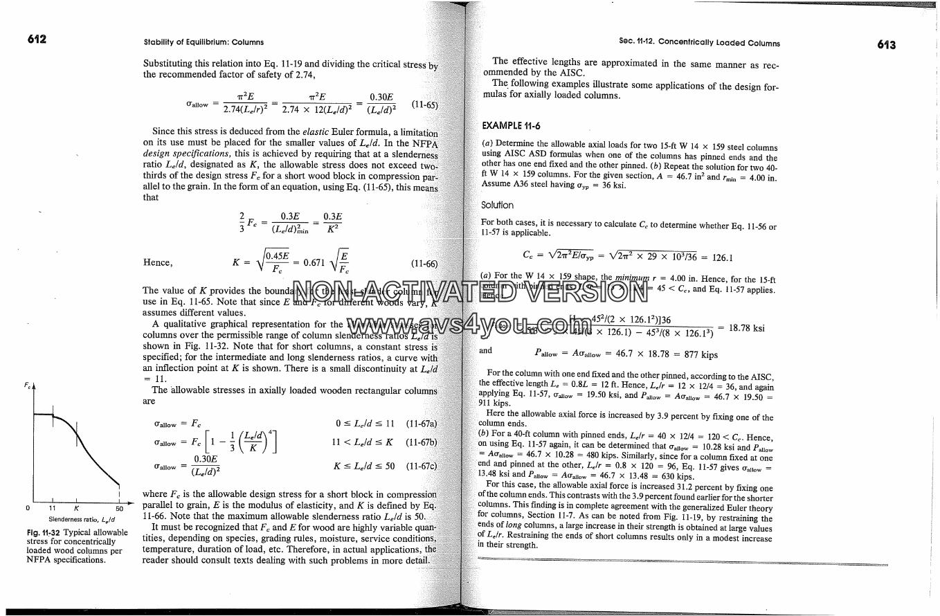
t
0 11 K 50
Slenderness ratio, Le/d
Fig. tt.-32 Typical allowablestress for concentricallyloaded wood columns perNFPA specifications.
Stability of Equilibrium: Columns
Substituting this relation into Eq. 11-19 and dividing the critical stressthe recommended factor of safety of 2.74,
'rr2E 'rr2E 0.30E(r�ow = 2.74(Le/r) 2 = 2.74 x 12(Le/d) 2 - (Le/d) 2
Since this stress is deduced from the elastic Euler formula,on its use must be placed for the smaller values of Le/d. In thedesign specifications, this is achieved by requiring that at a slenratio Le/d, designated as K, the allowable stress does not exceedthirds of the design stress F� for a short wood block in compressionallel to the grain. In the form of an equation, using Eq. (11-65),that
2 0.3E 0.3E
� F� = (Le/d)2min -- K2
Hence,
The value of K provides the boundary for the least slender columnuse in Eq. 11-65. Note that since E and F� for different woods vary,assumes different values.
A qualitative graphical representation for the allowable stressescolumns over the permissible range of column slenderness ratiosshown in Fig. 11-32. Note that for short columns, a constant stressspecified; for the intermediate and long slenderness ratios, a curvean inflection point at K is shown. There is a small discontinuity=11.
The allowable stresses in axially loaded wooden rectangularare
ITallow �' Fc
�r�ow = F� 1- 50.30E
(rm�ow - (Le/d) 2
0 --< L�/d --< 11
11 < Ldd -< K
K --< L,/d -< 50
where F, is the allowable design stress for a short block inparallel to grain, E is the modulus of elasticity, and K is defined by11-66. Note that the maximum allowable slenderness ratio Le/d is
It must be recognized that F, and E for wood are highly variabletitles, depending on species, grading rules, moisture, servicetemperature, duration of load, etc. Therefore, in actual applications, ireader should consult texts dealing with such problems in more
Sec. 1t-12. Concentrically Loaded Columns
The effective lengths are approximated in the same manner as rec-)nunended by the AISC.
The. following examples illustrate some applications of the design for-mulas for axially loaded columns.
EXAMPLE tt-6
(a) Determine the allowable axial loads for two 15-ft W 14 x 159 steel columnsusing AISC ASD formulas when one of the columns has pinned ends and theother has one end fixed and the other pinned. (b) Repeat the solution for two 40-ft W 14 x 159 columns. For the given section, A = 46.7 in 2 and rmi, = 4.00 in.Assume A36 steel having try v = 36 ksi.
Solution
For both cases, it is necessary to calculate Cc to determine whether Eq. 11-56 or11-57 is applicable.
C c = 'V/�'�/O-yp _w. X,/2.rr 2 X 29 X 103/36 = 126.1
(a) For the W 14 x 159 shape, the minimum r = 4.00 in. Hence, for the 15-ftcolumn with pinned ends, Le/r = 15 x 12/4 = 45 < Co, and Eq. 11-57 applies.
[1 - 452/(2 X 126.12)]365/3 + 3 x 45/(8 x 126.1) - 453/(8 x 126.13) 18.78 ksi
P�xow = A�r�ow = 46.7 x 18.78 = 877 kips
For the column with one end fixed and the other pinned, according to the AISC,the effective length Le = 0.8L = 12 ft. Hence, Le/r = 12 x 12/4 = 36, and againapplying Eq. 11-57, cr�o�, = 19.50 ksi, and P�ow = Atropos, = 46.7 x 19.50 =
kips.
Here the alJowable axial force is increased by 3.9 percent by firdng one of theends.
(b) For a 40-ft column with pinned ends, Ldr = 40 x 12/4 = 120 < Co. Hence,�n using Eq. 11-57 again, it can be determined that cr�o,� = 10.28 ksi and P�ow
Acr�o,� = 46.7 x 10.28 = 480 kips. Similarly, since for a column fixed at oneand pinned at the other, Ldr = 0.8 x 120 = 96, Eq. 11-57 gives cr�o,� =
13.48 ksi and P�o,� = Acr�uo�, = 46.7 x 13.48 = 630 kips.For this case, the allowable axial force is increased 31.2 percent by fixing one
of the column ends. This contrasts with the 3.9 percent found earlier for the shorterThis finding is in complete agreement with the generalized Euler theory
for columns, Section 11-7. As can be noted from Fig. 11-19, by restraining thea large increase in their strength is obtained at large values
Restraining the ends of short columns results only in a modest increasetheir strength.
NON-ACTIVATEDVERSIONwww.avs4you.com

Stability of Equilibrium: Columns Sec. t1-12. Concentrically Loaded Columns
EXAMPLE tt-7
Using the AISC ASD column formulas, select a 15-ft long pin-ended columncarry a concentric lead of 200 kips. The structural steel is to be A572, having �= 50 ksi.
Solution
The required size of the column can be found directly from the tables in theSteel Construction Manual. However, this example provides andemonstrate the trial-and-error procedure that is so often necessary inand the solution presented follows from using this method.
First try: Let L/r --' 0 (a poor assumption for a column 15 ft long).Eq. 11-57, since F.S. = 5/3, cr�o,� = 50/F.S. = 30 ksi and A = P/cracow == 6.67 in 2. From Table 4 in the Appendix, this requires a W 8 x 24
whose rmi, = 1.61 in. Hence, L/r = 15(12)/1.61 = 112. With th�sL/r,stress is found using Eq. 11-56 or 11-57, whichever is applicable dependingCc:
Cc = �/2'iT2E/O'Yp = X,/2'rr 2 X 29 x 103/50 = 107 < L/r = 112
Hence, using Eq. 11-56, cr�mow =12,r 2 X 29 x 103
23 x 1122= 11.9 ksi
This is much smaller than the initially assumed stress of 30 ksi,must be selected.
Second try: Let cr�o,� = 11.9 ksi as found before. Then A = 200/11.9 =in 2, requiring a W 8 x 58 section having rmin = 2.10 in. NOW L/r = 15(= 85.7, which is less than Cc found before. Therefore, Eq. 11-57 applies,
F.S. = 5/3 + 3(85.7)/(8 x 107) - (85.7)3/(8 X 1073) = 1.90
and (r�,ow = [1 - (85.7)2/(2 x 1072)]50/1.90 = 17.9 ksi
This stress requires A = 200/17.9 = 11.2 in 2, which is met by a W 8 x 40with rmi� = 2.04 in. A calculation of the capacity for this section showsallowable axial load for it is 204 kips, which meets the requirements of thelem.
*EXAMPLE tt-8
Determine the design compressive strength Pu for a 15-ft W 14 x 159pinned at both ends based on the AISC LRFD provisions. For this46.7 in 2 and rmin = 4.00 in. Assume A36 steel having cr�,o,� = 36 ksi.
Solutioncolumn slenderness parameter as defined by Eq. 11-58 is
15 x 12 �/� 36 '4'rr 9 x 10³ - 0.5047
Since Xc is less than 1.5, Eq. 11-60 applies for determining the critical stress and
IYcr = (0.658�'s�472)36 = 32.36 ksi
for this column, the nominal compressive strength
Pn = After = 46.7 x 32.36 = 1510 kips
and since the resistance factor Oc = 0.85, the column-design compressive strength
P,, = qb�P,� = 0.85 x 1510 = 1289 kips.
dividing P, by P�ow = 877 kips for a comparable column analyzed in theExample 11-6, one obtains 1.46. This load factor gives an indication
the relationship between the ASD and the LRFD for this case.
tt-9
the allowable axial loads for two compression members made fromaluminum alloy having 5 in x 5 in x 5.366 lb/ft wide-flange section with
dimensions shown in Fig.' 11-33. One of the members is 20 in long and theAssume each strut to be pinned at both ends. For the given section,
= 4.563 in 2, and the minimum radius of gyration rmi� = 1.188 in.
Regardless of the column length, for aluminum alloys, it is necessary to investigateFor the given section, two calculations must be made, one for the
legs of the flanges, and the other for the web. In both instances,values determine the allowable compressive stress. For the flanges,
bi 5 - 0.312 = 7.51t 2 x 0.312
ratio requires the use of Eq. 11-62b; hence,
((r�now)n�ng� = 23.1 - 0.79 x 7.51 = 17.2 ksi
Outstandingleg
X
"*---5.00'Y' - �
0.312"
X 5.00"
-�--0.312"
Fig. 11-33
NON-ACTIVATEDVERSIONwww.avs4you.com

6i6 Stability of Equilibrium: Columns
The web width-thickness ratio is
bw 5- 2 x 0.312--= = 14.0t 0.312
Since this ratio is less than 16, according to Eq. 11-63a,
(traUow)web = 19 ksi
Overall buckling is investigated using Eqs. 11-47, which depend on L/r.for a 20-in strut is _
L 20-- = 16.8
r 1.188
Hence, using Eq. 11-61b,
� cr�a�ow = 20.2 - 0.126 x 16.8 = 18.1 ksi
For this case of a well-balanced design, the allowable stress for localbuckling controls. Therefore,
P�now = 4.563 x 17.2 = 78.5 kips
The slenderness ratio for the 60-in strut is
L 60- = 50.5
r 1.188
Hence, again using Eq. 11-61b,
iranow = 20.2 - 0.126 x 50.5 = 13.8 ksi
This stress is smaller than those for local buckling; hence,
P�now = 4.563 x 13.8 = 63.0 kips
*ll-13. Eccentrically Loaded ColumnsIn the past, the secant-type formulas discussed in Section 11-8 wereas a rational method for the design of eccentrically loaded columns.other methods that have found a wide-use follow.
Allowable Stress Method
A procedure for designing eccentrically loaded columns isadapting the elastic solution for short blocks subjected to bending
Sec. '11-t3. Eccentrically Loaded Columns
axial loads, Eq. 6-45, and setting the maximum compressive stress equalto or less than for an axially loaded column. For a planar case, this be-comes
P Mc
trx = � + -�- < trynow (11-68)
The compressive stresses in the last equation are treated as positive quan-tities. If only an eccentric force P is applied, the bending moment M =Pc, where e is the load eccentricity; see Fig. 11-34. The allowable stress*�ow is determined from an appropriate formula, such as given in thepreceding section for axially loaded columns of different materials. Usu-ally, the solution of Eq. 11-68 requires a trial-and-error procedure.
For short and intermediate length columns, the previous procedure isusually conservative, since *�ow for compressive stresses is generallyless than the allowable bending stress. On the other hand, this proceduremay become unconservative for slender columns, where the deflectionsare magnified due to the axial force. For such cases, it is appropriate todetermine the extent of bending moment magnification caused by columndeflection using the approximate deflection magnification factor derivedin Example 11-3 or 11-4.
Interaction Method
In an eccentrically loaded column, much of the total stress may resultfrom the applied moment. However, the allowable stress in flexure isusually higher than the allowable axial stress. Hence, for a particularcolumn, it is desirable to accomplish some balance between the twostresses, depending on the relative magnitudes of the bending momentand the axial force. Thus, since in bending,, = Mc/I = Mc/Ar� 2, wherer� is the radius of gyrati6n in the plane of bending, in effect, area Abrequired by bending moment M is
mc
(�abF12
where crab is the allowable maximum stress in bending. (See also Section11-14.) Similarly, area Aa required for axial force P is
P
where traa is the allowable axial stress for the member acting as a column,and which depends on the L/r ratio. Therefore, the total area A requiredfor a column subjected to an axial force and a bending moment is
P McA =Aa +Ao =-- +� (11-69)O'aa O'abrl 2
Fig. tt-34 Eccentricallyloaded column.
6'7
NON-ACTIVATEDVERSIONwww.avs4you.com

6�8 Stability of Equilibrium: Columns Sec. tt-13. Eccentrically Loaded Columns 6�9
By dividing by A,
P/A Mc/Ar� 2 cra--+---1 or
O'aa O'ab O'aa O'ab
where (ra is the axial stress caused by the applied vertical loads, andis the bending stress caused by the applied moment.only an axial load and the applied moment is zero, the formulathat the column is designed for the stress (r�. On the other hand,allowable stress becomes the flexural stress cr�b ff there is no directpressive force acting on the column. Between these two extreme casEq. 11-70 measure� the relative importance of the two kinds of actionspecifies the nature of their interaction. Hence, it is often referred toan interaction formula and serves as the basis for the. specificationsthe AISC ASD manual, where it is stated that the sumratios must not exceed unity. The same philosophy has found favorapplications other than those pertaining to structural steel.Association suggests a similar relation. The National ForestAssociation developed a series of formulas to serve the same
In terms of the notations used by the AISC, Eq. 11-70 is rewritten
In practice, the eccentricity of the load on a column may be such ascause bending moments about both axes of the cross section. E�11-71 is then modified to
Subscripts x and y combined with subscript b indicate the axisabout which a particular stress applies, and
Fa = allowable axial stress ff the axial force alone existedF� = allowable compressive bending stress ff the bending
existed
�� = computed axial stress�b = computed bending stress
At points that are braced in the plane of bending, F� is equal to 60of Fy, the yield stress of the material, and
f� + f�x roy <0.6-�y �-� + �y - 1.0 (11-
At intermediate points in the length of a compression member, the sec-ondary bending moments due to deflection (see Fig. 11-34) can contributesignificantly to the combined stress. Following the AISC specifications,this c6ntribution is neglected in cases where ��/Fa is less than 0.15, i.e.,the axial stress is small in relation to the allowable axial stress, and Eq.11-73 can still be used. When ��/F� is greater than 0.15, the effect of theadditional secondary bending moments may be approximated by multi-plying both fox and roy by an amplification factor, C,,/(1 - f�/Fe'), whichtakes into account the slenderness ratio in the plane of bending and alsothe nature of the end moments. The term in the denominator of the am-plification factor brings in the effect of the slenderness ratio through theuse of F;, the Euler buckling stress (using Le/r in the plane of bending)divided by 23/12, or 1.92, which is the AISC factor of safety for a verylong column with Le/r greater than Co. (See Section 11-12 for a definitionof Co.) It can be noted that the amplification factor increases as f� in-creases and blows up as fa approaches F;. The term C,, in the numeratoris a correction factor that takes into account the ratio of the end momentsas well as their relative sense of direction. The term C,, is larger ff theend moments are such that they cause a single curvature of the member,and smaller ff they cause a reverse curvature. The formula for f�/F� >0.15 then becomes
f a Cmxf �,x Cmyf l�y� + (1 - f, IF;x)Fox + (1 - f,/Fe'y)Foy -< 1.0 (11-74)
According to the AISC specifications, 26 the value of C,, shall be takenas follows:
1. For compression members in frames subject to joint translation(sidesway), C,, = 0.85.
2. For restrained compression members in frames braced against jointtranslation and not subject to transverse loading between their sup-ports in the plane of bending,
0.6 - 0.4MJM2
(but not less than 0.4), where MJM2 is the ratio of the smaller tolarger moments at the ends of that portion of the member unbracedin the plane of bending under consideration. Mi/M2 is positive whenthe member is bent in reverse curvature and negative when it is bentin single curvature.
3. For compression members in frames braced against joint translationin the plane of loading and subjected to transverse loading betweentheir supports, the value of C,, can be determined by rational anal-
26 AISC Steel Construction Manual, 9th ed. (Chicago: AISC, 1989), 5-27.
NON-ACTIVATEDVERSIONwww.avs4you.com
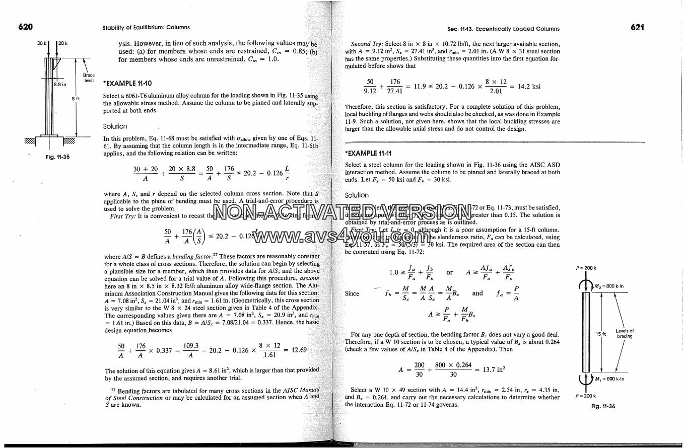
620
Fig. tt-35
Stability of Equilibrium: Columns
ysis. However, in lieu of such analysis, the followingused: (a) for members whose ends are restrained, C,,= 0.85;for members whose ends are unrestrained, C,,= 1.0.
*EXAMPLE tt-t0
Select a 6061-T6 aluminum alloy column for the loading shown in Fig.the allowable stress method. Assume the column to be. pinned and laterallyported at both ends.
Solution
In this problem, Eq. 11-68 must be satisfied with �r�uow given by one of Eqs� !l61. By assuming that the column length is in the intermediat.e range, Eq.applies, and the following relation can be written:
30 + 20 20 x 8.8 50 176 LA + S A + � - 20.2 - 0.126 -F
where A, S, and r depend on the selected column cross section. Noteapplicable to the plane of bending must be used. A trial-and-error procedure iused to solve the problem.
First Try: It is convenient to recast the last equation into the following
50 176(h 0.12&�' + .A �,S] < 20.2 - rwhere A/S = B defines a bending factor. 27 These factors are reasonablyfor a whole class of cross sections. Therefore, the solution can begin bya plausible size for a member, which then provides data for A/S, and theequation can be solved for a trial value of A. Following this procedure,here an 8 in x 8.5 in x 8.32 lb/ft aluminum alloy wide-flange section. Theminum Association Construction Manual gives the following data for this secti0h�A = 7.08 in 2, Sx = 21.04 in 3, and rmi, = 1.61 in. (Geometrically, this crossis very similar to the W 8 x 24 steel section given in Table 4 of theThe corresponding values given there are A = 7.08 in 2, Sx = 20.9 in 3, and= 1.61 in.) Based on this data, B = A/S� = 7.08/21.04 = 0.337. Hence,
design equation.becomes
50 176 109.3 8 x 12�- + �- x 0.337 - A - 20.2 - 0.126 x !.6----i-- = 12.69
The solution of this equation gives A = 8.61 in 2, which is larger than thatby the assumed section, and requires another trial.
27 Bending factors are tabulated for many cross sections in the AISCof Steel Construction or may be calculated for an assumed section whenS are known.
Sec. 1t-13. Eccentrically Loaded Columns
Second Try: Select 8 in x 8 in x 10.72 lb/ft, the next larger available section,with A = 9.12 in 2, S� = 27.41 in 3, and rmin = 2.01 in. (A W 8 x 31 steel sectionhas the same properties.) Substituting these quantities into the first equation for-mulated before shows that
50 176 8 x 12-- + - 11.9 --< 20.2 - 0.126 x -- - 14.2 ksi9.12 27.41 2.01
Therefore, this section is satisfactory. For a complete solution of this problem,local buckling of flanges and webs should also be checked, as was done in Example11-9. Such a solution, not given here, shows that the local buckling stresses arelarger than the allowable axial stress and do not control the design.
*EXAMPLE tt-tt
Select a steel column for the loading shown in Fig. 11-36 using the AISC ASDinteraction method. Assume the column to be pinned and laterally braced at bothends. Let Fy = 50 ksi and Fb = 30 ksi.
Solution
In this problem, the interaction formulas, Eq. 11-72 or Eq. 11-73, must be satisfied,depending upon whether f,/Fa is less than or greater than 0.15. The solution isobtained by trial-and-error process as is outlined.
First Try: Let Le/r = 0, although it is a'poor assumption for a 15-ft column.Corresponding to this value of the slenderness ratio, F, can be calculated, usingEq. 11-57, as F, = 50/(5/3) = 30 ksi. The required area of the section can thenbe computed using Eq. 11-72:
Since
1.0 >--f�, Af,� Afb
+ or A->-?-7 +
-- M M A AM�B�, and fa Pfb &, A S:, AP M
+ ?fiFor any one depth of section, the bending factor B� does not vary a good deal.
Therefore, if a W 10 section is to be chosen, a typical value of B� is about 0.264a few values of A/S� in Table 4 of the Appendix). Then
200 800 x 0.264A = + - 13.7 in 2
30 30
Select a W 10 x 49 section with A = 14.4 in 2, rm�, = 2.54 in, r� = 4.35 in,and Bx = 0.264, and carry out the necessary calculations to determine whether
the interaction Eq. 11-72 or 11-74 governs.
P = 200 k
�M� =800k-in
Levels of1 bracing
/r M� = 600 k-in
P=200k
Fig. tt-36
NON-ACTIVATEDVERSIONwww.avs4you.com

622 Stability of Equilibrium: Columns
P 200 MB:, 800 x 0.264�a = A 14.4 13.9 ksi �o A 14.4
Le 15 x 12- -- = 70.9 < Ce Ce = X/2'rr2E/Fy = 107r�n 2.54
= 14.7 ksi
Using Eq. 11-57, Fa = 19.3 ksi, f,dF,� = 13.9/19.3 = 0.72 > 0.15; hence,interaction formula of Eq. 11-74 must be checked. For this purpose, usingin the plane of bending, one determines
12,rr2E 149 x 103 149 x 103F� - 23(Ldr�,)2 - (15 x 12/4.35) 2 = (41.4) 2
= 86.9 ksi
Then, since the end moments subject the column to a single curvature, M= - 600/800 = - 0.75, and
C,� = 0.6 - 0.4M�/M2 = 0.6 - (0.4)(-0.75) = 0.9
With bending taking place in one plane only, Eq. 11-74 reduces to
f,� C.�foF� (1 - f�/F�)F�
---- 1.0
On substituting the appropriate quantities into this relation,
13.9 0.9 x 14.7--+19.3 (1 - 13.9/86.9)30
= 0.72 + 0.52 = 1.24 > 1.0
Since Eq. 11-74 is violated, a larger section must be used.
Second Try: As an aid in choosing a larger section, assume Fa = 19.3 ksi.is the value computed for the section in the previous trial. Also, using B� =for W 10 sections,
P MB�, 200 800 x 0.264 17.4 in 2A >�-� + �-o - 19.� + 30 =Now select a W 10 x 60 section with A = 17.6 in 2, rm�n = 2.57 in, rx = 4.39and B� = 0.264, and proceed as in the first trial to check the
MBx 800 x 0.264200 = 11.4 ksi fo- = 12.017.6 A 17.6Le 15 x 12
.... 70.0 < Cermin 2.57
Using Eq. 11-57, Fa = 19.4 ksi, f,dF,� = 11�4/19.4 = 0.59 > 0.15; hence,11-74 must be checked.
Problems 623
149 x 10 3 149 X 10 3(Le/t:�) 2 (15 X 12/4.39) 2 88.6 ksi
Again, using Eq. 11-74 for bending in one plane and substituting into it the ap-propriate quantities, one has
11.4 0.9-x 12.0
19.4 (1 - 11.4/88.6)30= 0.59 + 0.41 = 1.00
Since this relation satisfies Eq. 11-74, the W 10 x 60 section is satisfactory.
� 11-14. Lateral Stability of BeamsThe strength and deflection theory of beams developed in this text appliesonly if such beams are in stable equilibrium. Narrow or slender beamsthat do not have occasional lateral supports may buckle sideways andthus become unstable; see Fig. 11-37. Theoretical and experimental stud-ies of this problem show that, within limits, reduced bending stresses canbe used to maintain the stability of such beams. The nature of the reducedstresses resembles the curves displayed for columns in Figs. 11-29 and11-32. The key parameter for stress reduction depends on the material
properties, geometry of the cross section, and moment gradient. Severalof the references cited in this chapter discuss this topic. In this section,only a simple criterion for avoiding the problem of lateral torsional buck-ling for compact steel beams is given.
According to the AISC ASD specifications, in order for a compact beamto qualify for the maximum allowable bending stress, intermittent lateralsupports shall be provided.at intervals not exceeding the value
Fig. tl-37 Lateral-torsionalbuckling of a narrowbeam.
76b� 20,000� nor (d/A�)Fy (11-75)
where A� is the area of a compression flange, b� is the flange width, d isthe depth of a beam, and Fy is the yield stress for the material.
ProblemsSection
A rigid bar hinged at the base is held in a verticalposition by two springs: one has a stiffness k N/mmand the other, 2k N/mm, as shown in the figure. De-termine the critical force P=� for this system.
throughll-4. Rigid-bar segments ofequallengthsare connected at the joints and at the bottoms by
frictionless hinges and are maintained in straight po- Fig. Plt-1
NON-ACTIVATEDVERSIONwww.avs4you.com
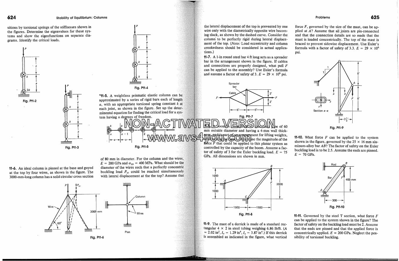
624 Stability of Equilibrium: Columns Problems 625
sitions by torsional springs of the stiffnesses shown inthe figures. Determine the eigenvalues for these sys-tems and show the eigenfunctions on separate dia-grams. Identify the critical loads.
Fig. Plt-2
Fig. Pll-3
P
Fig. Ptt-4
'tt-5. A weightless prismatic elastic column canapproximated by a series of rigid bars each ofa, with an appropriate torsional spring constanteach joint, as shown in the figure. Set up theminental equation for finding the critical load for a:tem having n. degrees of freedom.
Fig. PIt-5
tt-6. An ideal column is pinned at the base and guyedat the top by four wires, as shown in the figure. The3000-mm-long column has a solid circular cross section
P
of 80 mm in diameter. For the column and the wiresE = 200 GPa and cryp = 400 MPa. What shodiameter of the wires such that a perfectlybuckling load Per could be reachedwith lateral displacement at the the top? Assume
I Pcr
Fig. Plt-6
�,�Column
Wires"�xPlan
the lateral displacement of the top is prevented by onewire only with the diametrically opposite wire becom-ing slack, as shown by the dashed curve. Consider thecolumff to be perfectly rigid during lateral displace-ment of the top. (Note: Load eccentricity and columncrookedness should be considered in actual applica-tions.)
tt-?. A 1-in round steel bar 4 �t long acts as a spreaderbar in the arrangement shown in the figure. If cablesand connections are properly designed, what pull Fcan be applied to the assembly? Use Euler's formulaand assume a factor of safety of 3. E = 29 x 106 psi.
Spreaderbar
Cable�'�dFig. Pll-7
tl-8. A boom is made from an aluminum pipe of 60mm outside diameter and having a 4-mm wall thick-ness, and is part of an arrangement for lifting weights,as shown in the figure. Determine the magnitude of theforce F that could be applied to this planar system ascontrolled by the capacity of the boom. Assume a fac-tor of safety of 3 for the Euler buckling load. E = 75GPa. All dimensions are shown in mm.
1000
B
C F2CLO-*ii-1500 � �- 1500 4
1000
Fig. Pll-8
tt-9. The mast of a derrick is made of a standard rec-x 2 in steel tubing weighing 6.86 lb/ft. (A
= 2.02 in 2, Ix = 1.29 in 4, Iz = 3.87 in4.) If this derrick�s assembled as indicated in the figure, what vertical
force F, governed by the size of the mast, can be ap-plied at A? Assume that all joints are pin-connectedand that the connection details are so made that themast is loaded concentrically. The top of the mast isbraced to prevent sidewise displacement. Use Euler'sformula with a factor of safety of 3.3. E = 29 x 106psi.
Fig. Plt-9
t140. VV�nat force F can be applied to the systemshown in the figure, governed by the 25 x 16 mm alu-minum-alloy bar AB? The factor of safety on the Eulerbuckling load is to be 2.5. Assume the ends are pinned.E = 70 GPa.
Rod BBar
400 mm
Fig. P11-10
tt4t. Governed by the steel T section, what force Fcan be applied to the system shown in the figure? Thefactor of safety on the buckling load must be 2. Assumethat the ends are pinned and that the applied force isconcentrically applied. E = 200 GPa. Neglect the pos-sibility of torsional buckling.
NON-ACTIVATEDVERSIONwww.avs4you.com

626 Stability of Equilibrium: Columns Problems 627
0mfflFig. Pt1-tt
1142. A thin bar of stainless steel is axially procom-pressed 100 N between two plates that are fixed at aconstant distance of 150 mm apart; see the figure. Thisassembly is made at 20�C. How high can the temper-ature of the bar rise, so as to have a factor of safetyof 2 with respect to buckling? Assume E = 200 GPaand ct =. 15 x 10 -6 per �C.
3--'�- � 150
1Fig. PI'M2
1143. What size standard steel pipe should be used forthe horizontal member of the jib crane shown in thefigure for supporting the maximum force of 4 k, whichincludes an impact factor? Use the Euler buckling for-
Fig. Ptt-13
--� J,� 10mm
Section a-a
mula for columns with pinned ends and a factorsafety of 2.5. Neglect the weight of construction.29 x 10 6 psi.11-t4. Select a W steel section for member AB fo:system shown in the figure to resist a vertical force150 k. The system is laterally braced at B and C.lect the weight of the members. Assume pinnedand a factor of safety of 2. E = 29 x 103 ksi.
� 16' "� 12' �Fig. Ptt-14
tt-15. Select standard steel pipes for the tripodin the figure to support a vertical lead F =
F
Fig. Plt-15
a factor of safety of 3 on the Euler buckling lead. Neg-lect the weight of the members. E = 29 x 103 ksi.tt-t6. A tripod is to be made up from 3 x 3 in steelangles, each 10 ft long, to support a vertical lead F =8 k at the center, as shown in the figure. Using theEuler buckling formula with a factor of safety of 3 toaccount for impact, determine the required thicknessof the angles. Neglect the weight of the angles, assumethat they are loaded concentrically, and that the endsare pinned. E = 30 x 106 psi.
Fig. Pl1.t6
'tt-t7. A simple beam of flexural rigidity EIb ispropped up at the middle by a slender rod of flexuralrigidity EIc. Estimate the deflection of the beam at thecenter if a force F double the Euler lead for the columnis applied to this system.
F
L/2
Fig. Plt47
Section 11-5
11-18. Derive Eq. 11-17 using Eq. l 1-5 in the form EIv"+ Pv = Me, where Me is the moment at the end.
1t-t9. Derive Eq. 11-18 using Eq. 11-5 in the form EIv"= P(g - v), where g is the end deflection.
'tl-20. Determine the critical buckling lead for thecolumn shown in the figure. (Hint: See the precedingproblem; enforce continuity conditions at a change inEl.)
EI L/2
2E/ L/2
Fig. Plt-20
'1t-21. Determine the transcendental equation forfinding the critical buckling lead for bar AB of constantE1 due to the application of axial force P through rigidlink BC. (Hint: In a deflected position, note the pres-ence of a shear force at B.)
� EI L� Hinge P
Fig. Plt-21
1t-22. An allowable axial lead for a 4-m-long pin-ended column of a certain linearly elastic material is20 kN. Five different columns made of the same ma-terial and having the same cross section have the sup-porting conditions shown in the figure. Using the col-umn capacity for the 4-m column as the criterion, whatare the allowable loads for the five columns shown?
NON-ACTIVATEDVERSIONwww.avs4you.com
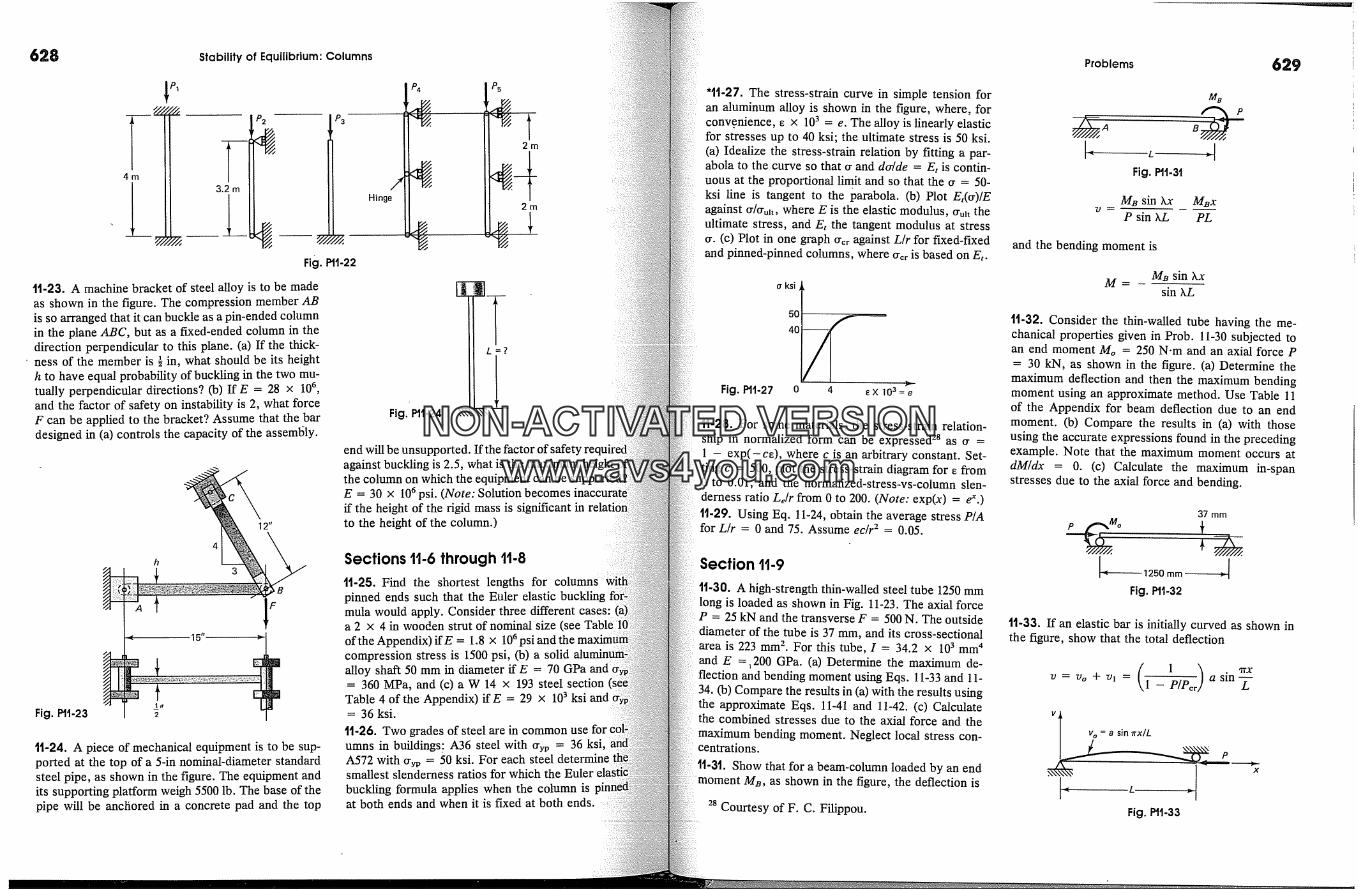
628 Stability' of Equilibrium: Columns
Fig.
tt-23. A machine bracket of steel alloy is to be madeas shown in the figure. The compression member ABis so arranged that it can buckle as a pin-ended columnin the plane ABC, but as a frxed-ended column in thedirection perpendicular to this plane. (a) If the thick-ness of the member is � in, what should be its heighth to have equal probability of buckling in the two mu-tually perpendicular directions? (b) If E = 28 x 10%and the factor of safety on instability is 2, what forceF can be applied to the bracket? Assume that the bardesigned in (a) controls the capacity of the assemlily.
12"
Fig. Pll-23
tl-24. A piece of mechanical equipment is to be sup-ported at the top of a 5-in nominal-diameter standardsteel pipe, as shown in the figure. The equipment andits supporting platform weigh 5500 lb. The base of thepipe will be anchored in a concrete pad and the top
P4
Hinge
PI1-22
Fig. PIt-24 ,�
end will be unsuppcagainst buckling is 2.5, what is the maximumthe column on which the equipmeni can beE = 30 x 106 psi. (Note: Solution becomes inaccurateif the height of the rigid mass is significant in relatito the height of the column.)
Sections 11-6 through 11-8tt-25. Find the shortest lengths forpinned ends such that the Euler elasticmula would apply. Consider three different cases:a 2 x 4 in wooden strut of nominal size (of the Appendix) ifE = 1.8 x 10⁶ psi and thecompression stress is 1500 psi, (b) a solidalloy shaft 50 mm in diameter if E = 70 GPa= 360 MPa, and (c) a W 14 x 193 steel section
Table 4 of the Appendix) if E = 29 x 103 ksi= 36 ksi.
11-26. Two grades of steel are in commonumns in buildings[ A36 steel with o-yp = 36 ksi,A572 with O-yp = 50 ksi. For each steel determinesmallest slenderness ratios for which thebuckling formula applies when the column isat both ends and when it is fixed at both ends.
'tt-27. The stress-strain curve in simple tension foran aluminum alloy is shown in the figure, where, forconv.enience, e x 103 = e. The alloy is linearly elasticfor stresses up to 40 ksi; the ultimate stress is 50 ksi.(a) Idealize the stress-strain relation by fitting a par-abola to the curve so that �r and do/de = Et is contin-uous at the proportional limit and so that the �r = 50-ksi line is tangent to the parabola. (b) Plot Et(�r)/Eagainst �r/{rutt, where E is the elastic modulus, �ru�t theultimate stress, and E, the tangent modulus at stress�r. (c) Plot in one graph O'cr against L/r for fixed-fixedand pinned-pinned columns, where �rcr is based on E,.
a ksi
50
40
Fig. PI1.27 o 4 �X 103=e
tl-28. For some materials, the stress-strain relation-ship in normalized form can be expressed 28 as �r =1 - exp(-ce), where c is an arbitrary constant. Set-ting c = 500, plot the stress-strain diagram for e from0 to 0.01, and the normalized-stress-vs-column slen-derness ratio Ldr from 0 to 200. (Note: exp(x) =tt-29. Using Eq. 11-24, obtain the average stress P/Afor L/r = 0 and 75. Assume ec[r 2 = 0.05.
Section 11-9
11-30. A high-strength thin-walled steel tube 1250 mmlong is loaded as shown in Fig. 11-23. The axial forceP = 25 kN and the transverse F = 500 N. The outsidediameter of the tube is 37 mm, and its cross-sectionalarea is 223 mm 2. For this tube, I = 34.2 x 10 3 mm 4and E =, 200 GPa. (a) Determine the maximum de-flection and bending moment using Eqs. 11-33 and 11-34. (b) Compare the results in (a) with the results usingthe approximate Eqs. 11-41 and 11-42. (c) Calculatethe combined stresses due to the axial force and themaximum bending moment. Neglect local stress con-centrations.
tt-31. Show that for a beam-column loaded by an endmoment MB, as shown in the figure, the deflection is
28 Courtesy of F. C. Filippou.
Problems 629
A
Fig. Pll-3'1
MB sin Xx M�xP sin LL PL
and the bending moment is
M= - M�sinXxsin LL
tt-32. Consider the thin-walled tube having the me-chanical properties given in Prob. 11-30 subjected toan end moment Mo = 250 N-m and an axial force P= 30 kN, as shown in the figure. (a) Determine the
maximum deflection and then the maximum bendingmoment using an approximate method. Use Table 11of the Appendix for beam deflection due to an endmoment. (b) Compare the results in (a) with thoseusing the accurate expressions found in the precedingexample. Note that the maximum moment occurs atdM/dx = 0. (c) Calculate the maximum in-spanstresses due to the axial force and bending.
37 mm
Fig. Pll-32
1t-33. If an elastic bar is initially curved as shown inthe figure, show that the total deflection
1 )1-}/Por a sin -�-
Fig. Pll-33
P
NON-ACTIVATEDVERSIONwww.avs4you.com
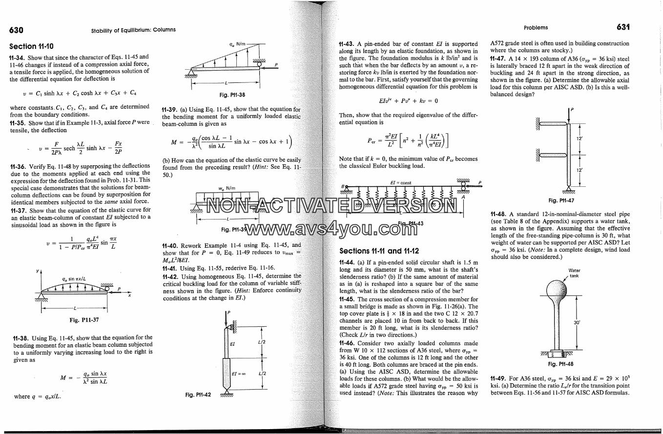
630 Stability of Equilibrium: Columns
Section 1140
tl-34. Show that since the character of Eqs. 11-45 and11-46 changes if instead of a compression axial force,a tensile force is applied, the homogeneous solution ofthe differential equation for deflection is
v = C� sinh Xx + C2 cosh Xx + C3x + C4
where constants. C,, C2, C3, and C4 are determinedfrom the boundary conditions.tt-35. Show that if in Example 11-3, axial force P weretensile, the deflection
v = 2-� sech sinh hx - 2-�
tt-36. Verify Eq. 11-48 by superposing the deflectionsdue to the moments applied at each end using theexpression �:or the deflection found in Prob. 11-31. Thisspecial case demonstrates that the solutions for beam-column deflections can be found by superposition foridentical members subjected to the same axial force.11-37. Show that the equation of the elastic curve fdran elastic beam-column of constant E� subjected to asinusoidal lead as shown in the figure is
1 L 4qo : sin --v - 1 - P/Per �r 4El L
Yl qo sin �rx/L '
Fig. Pll-37
Fig. Ptl-38
1t-39. (a) Using Eq. 11-45, show that thethe bending moment for a uniformly loadedbeam-column is given as
qof COSXL - 1 )M = -�[,' �n �, sin hx - .cos Xx + 1(b) How can the equation of the elastic curve befound from the preceding result? (Hint: See Eq. 1]50.)
w o N/m
Fig. Pll-39
tl-40. Rework Example 11-4 using Eq. 11-45,show that for P = 0, Eq. 11-49 reduces toMoL2/SEI.tl-41. Using Eq. 11-55, rederive Eq. 11-16.tt-42. Using homogeneous Eq. 11-45, determinecritical buckling lead for the column of variableness shown in the figure. (Hint: Enforceconditions at the change in EI.)
11-38. Using Eq. 11-45, show that the equation for thebending moment for an elastic beam column subjectedto a uniformly varying increasing lead to the right isgiven as
qo sin XxM = X 2 sin XL
where q = qox/L. Fig. Pll-42 �
EI L/2
EI = oo L/2
tt-43. A pin-ended bar of constant EI is supportedaJong its length by an elastic foundation, as shown inthe figure. The foundation modulus is k lb/in 2 and issuch that when the bar deflects by an amount v, a re-storing force kv lb/in is exerted by the foundation nor-mal to the bar. First, satisfy yourself that the governinghomogeneous differential equation for this problem is
EIv i'� + Pv" + /iv = 0
Then, show that the required eigenvalue of the differ-ential equation is
nr2EI [ I ( kL4X�lPer - L2 n2 + � �,rraEiJ jNote that if k = 0, the minimum value of Per becomesthe classical Euler buckling lead.
EI = const � P
Fig, Plt-43
Sections 11-11 and 11.12
tt-44. (a) If a pin-ended solid circular shaft is 1.5 mlong and its diameter is 50 mm, what is the shaft'sslenderness ratio? (b) If the same amount of materialas in (a) is reshaped into a square bar of the samelength, what is the slenderness ratio of the bar?tt-45. The cross section era compression member fora small bridge is made as shown in Fig. 11-26(a). Thetop cover plate is � x 18 in and the two C 12 x 20.7channels are placed 10 in from back to back. If thismember is 20 ft long, what is its slenderness ratio?(Check L/r in two directions.)1t-46. Consider two axially loaded columns madefrom W 10 x 112 sections of A36 steel, where cryp =36 ksi. One of the columns is 12 ft long and the otheris 40 ft long. Both columns are braced at the pin ends.(a) Using the AISC ASD, determine the allowableloads for these columns. (b) What would be the allow-able loads if A572 grade steel having Cry v = 50 ksi is
instead? (Note: This illustrates the reason why
Problems 63'i
A572 grade steel is often used in building constructionwhere the columns are stocky.)tt-47. A 14 x 193 column of A36 (%, = 36 ksi) steelis laterally braced 12 ft apart in the weak direction ofbuckling and 24 ft apart in the strong direction, asshown in the figure. (a) Determine the allowable axiallead for this column per AISC ASD. (b) Is this a well-balanced design?
P
Fig. Plt-47
1t-48. A standard 12-in-nominal-diameter steel pipe(see Table 8 of the Appendix) supports a water tank,as shown in the figure. Assuming that the effectivelength of the free-standing pipe-column is 30 ft, whatweight of water can be supported per AISC ASD? LetGyp = 36 ksi. (Note: In a complete design, wind leadshould also be considered.)
Watertank
30'
Fig. Plt-48
1t-49. For A36 steel, %0 = 36 ksi and E = 29 x 10 3ksi. (a) Determine the ratio Le/r for the transition pointbetween Eqs. 11-56 and 11-57 for AISC ASD formulas.
NON-ACTIVATEDVERSIONwww.avs4you.com
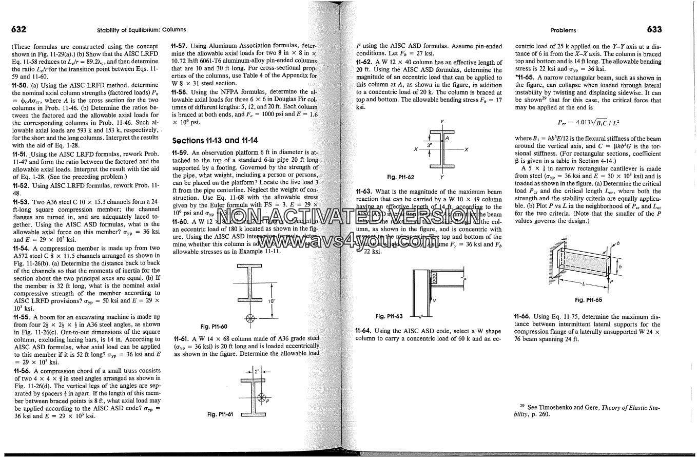
632 Stability of Equilibrium: Columns Problems 633
(These formulas are constructed using the conceptshown in Fig. 11-29(a).) (b) Show that the AISC LRFDEq. 11-58 reduces to Le/r = 89.2Xc, and then determinethe ratio Le/r for the transition point between Eqs. 11-59 and 11-60.
tt-50. (a) Using the AISC LRFD method, determinethe nominal axial column strengths (factored loads) Pn= qbcAtrcr, where A is the cross section for the two
columns in Prob. 11-46. (b) Determine the ratios be-tween the factored and the allowable axial loads forthe corresponding columns in Prob. 11-46. Such al-lowable axial loads are 593 k and 153 k, respectively,.for the short and the long columns. Interpret the resultswith the aid of Eq. 1-28.1t-5t. _Using the AISC LRFD formulas, rework Prob.11-47 and form the ratio between the factored and theallowable axial loads. Interpret the result with the aidof Eq. 1-28. (See the preceding problem.)tt-52. Using AISC LRFD formulas, rework Prob. 11-48.
tt-53. Two A36 steel C 10 x 15.3 channels form a 24-ft-long square compression member; the channelflanges are turned in, and are adequately laced to-gether. Using the AISC ASD formulas, what is theallowable axial force on this member? tryp = 36 ksiand E = 29 x 103 ksi.
11-54. A compression member is made up from twoA572 steel C 8 x 11.5 channels arranged as shown inFig. 11-26(b). (a) Determine the distance back to backof the channels so that the moments of inertia for thesection about the two principal axes are equal. (b) Ifthe member is 32 ft long, what is the nominal axialcompressive strength of the member according toAISC LRFD provisions? try" = 50 ksi and E = 29 x103 ksi.
tt-55. A boom for an excavating machine is made upfrom four 2� x 2� x � in A36 steel angles, as shownin Fig. 11-26(c). Out-to-out dimensions of the squarecolumn, excluding lacing bars, is 14 in. According toAISC ASD formulas, what axial load can be appliedto this member if it is 52 ft long? tryp = 36 ksi and E= 29 x 103ksi.
tl-56. A compression chord of a small truss consistsof two 4 x 4 x � in steel angles arranged as shown inFig. 11-26(d). The vertical legs of the angles are sep-arated by spacers � in apart. If the length of this mem-ber between braced points is 8 ft, what axial load maybe applied according to the AISC ASD code? try" =36 ksi and E = 29 x 103 ksi.
11-57. Using Aluminum Association formulas,mine the allowable axial loads for two 8 in x 810.72 lb/ft 6061-T6 aluminum-alloy pin-ended coluthat are 10 and 30 ft long. For cross-sectionalerties of the columns, use Table 4 of the AppendixW 8 x 31 steel section.
tt-58. Using the NFPA formulas, determine thelowable axial loads for three 6 x 6 in Douglasumns of different lengths: 5, 12, and 20 ft.is braced at both ends, and F� = 1000 psi and E =x 106 psi.
Sections 1143 and 1144
11-59. An observation platform 6 ft in diameter istached to the top of a standard 6-in pipe 20 ftsupported by a footing. Governed by thethe pipe, what weight, including a person orcan be placed on the platform? Locate the live loadft from the pipe centerline. Neglect the weightstruction. Use Eq. 11-68 with the allowablegiven by the Euler formula with FS = 3. E =10 6 psi and try" = 36 ksi.
11-60. A W 12 x 85 column 20 ft long is subjected tan eccentric load of 180 k located as shown in theure. Using the AISC ASD interaction formula,mine. whether this column is adequate. Use theallowable stresses as in Example 11-11.
I I l 0"
Fig. Pll-60
1t-61. A W 14 x 68 column made of A36 grade(tryp = 36 ksi) is 20 ft long and is loadedas shown in the figure. Determine the allowable
Fig. Pll-61 � -"--n
P using the AISC ASD formulas. Assume pin-endedconditions. Let F0 = 27 ksi.tt-62. A W 12 x 40 column has an effective length of20 ft. lOsing the AISC ASD formulas, determine themagnitude of an eccentric load that can be applied tothis column at A, as shown in the figure, in addition
a concentric load of 20 k. The column is braced attop and bottom. The allowabl� bending stress F0 = 17ksi.
Y
Fig. Pll-62 Y
tl-63. What is the magnitude of the maximum beamreaction that can be carded by a W 10 x 49 columnhaving an effective length of 14 ft, according to theAISC ASD interaction formula? Assume that the beamdelivers the reaction at the outside flange of the col-umn, as shown in the figure, and is concentric withrespect to the minor axis. The top and bottom of thecolumn are held laterally. Assume Fy = 36 ksi and Fb= 22 ksi.
Fig. Ptt-63
tt-64. Using the AISC ASD code, select a W shapecolumn to carry a concentric load of 60 k and an ec-
centtic load of 25 k applied on the Y-Y axis at a dis-tance of 6 in from the X-X axis. The column is bracedtop and bottom and is 14 ft long. The allowable bendingstress is 22 ksi and try. = 36 ksi.'1t-65. A narrow rectangular beam, such as shown inthe figure, can collapse when loaded through lateralinstability by twisting and displacing sidewise. It canbe shown 29 that for this case, the critical force thatmay be applied at the end is
Per = 4.013V'BiC / L 2
where B� = hb3E/12 is the flexural stiffness of the beamaround the vertical axis, and C = [3hb3G is the tor-sional stiffness. (For rectangular sections, coefficient[3 is given in a table in Section 4-14.)
A 5 x � in narrow rectangular cantilever is madefrom steel (try" = 36 ksi and E = 30 x 103 ksi) and isloaded as shown in the figure. (a) Determine the criticalload P�r and the critical length L�r, where both thestrength and the stability criteria are equally applica-ble. (b) Plot P vs L in the neighborhood of P�r and L�for the two criteria. (Note that the smaller of the Pvalues governs the design.)
Fig. Plt-65
tt-66. Using Eq. 11-75, determine the maximum dis-tance between intermittent lateral supports for thecompression flange of a laterally unsupported W 24 x76 beam spanning 24 ft.
29 See Timoshenko and Gere, Theory of Elastic Sta-bility, p. 260.
NON-ACTIVATEDVERSIONwww.avs4you.com

chapter
634
]2-]. Introduction
In a few instances in the preceding chapters, the deflection ofwas obtained by invoking the law of Conservation of energy andthe internal strain energy to the external work. This Lagrangianof employing scalarfimctions can be greatly extended, resulting inof the most effective procedures for the analysis of deformable bodies.In Part A, the previously encountered concept of elastic strain energydiscussed from a somewhat more general point of view. This is followedby a specialized statement of the law of conservation of energy forformable bodies, and the reason for the need to develop additional meth�ods based on work and energy concepts to solve deflection problems.
Part B serves as an introduction to the two virtual work methodsdeformable bodies. One of these, the method of virtual forces, isuseful for determining deflections caused by any kind of deformation andis not limited at all to elastic behavior. This method is one of theavailable for calculating deflections of members. The conjugateof virtual displacetnents, of great importance in the matrix analysisstructures and in finite elements, is also discussed. The duality of thes etwo methods is illustrated by considering discrete structural systems.
In Part C of this chapter, the classical energy methods forsimilar problems to those susceptible to analysis by virtual workare discussed. These methods are based on considering the internalenergy or the complementary strain energy and the correspondingnal work. The derived equations are specialized for linearly elastic stems and are known as Castigliano's theorems. Illustrative examplesgiven for both statically determinate and indeterminate cases. Adiscussion on an application of the elastic energy concepcolumn buckling loads concludes the chapter.
Sec. t2-2. Elastic Strain Energy
12-2. Elastic Strain EnergyThe elastic strain-energy density Uo, i.e., the strain energy per unit vol-ume, for a three-dimensional body was given by Eq. 8-49 in terms ofprincipal stresses and strains. For a cartesian element in a general stateof stress, the main energy density is
1
Uo = �(crxex + %% + o-�e� + 'rxy�xy + -ry�y� + -r�) (12-1)
Therefore, the general expression for the total internal strain energy in alinearly elastic body is
U = � (o-�,e�, + %e�, + cr�e�+ 'r�'� + 'ry:�y� + 'r,.x'�,.x)dx dy dz (12-2)
Integration extends over the volume of a body. Such a general expressionis used in elasticity. In engineering mechanics of solid, a less general classof problems is considered and Eq. 12-2 simplifies. An expression
u = � (c�,,e:, + ,�y�xy) dx dy dz (12-3)
is sufficient for determining the strain energy in axially loaded bars aswell as in bent and sheared beams. Moreover, the last term of Eq. 12-3written in the appropriate coordinates is all that is needed in the torsionproblem of a circular shaft and for thin-walled tubes. These cases includethe major types of problems treated in this text.
For linearly elastic material, for uniaxial stress, e� = ,x/E, and for pureshear, '/xy = 'rxy/G. Thus, Eq. 12-3 can be recast in the following form:
or
U = dddv �-� dx dy dz + if iv dx dy dz (12-4)for axi�loading and for shear in beams
bending ofbeams
u= -5-dxdydz+ dxdydz (12-5)
635
NON-ACTIVATEDVERSIONwww.avs4you.com
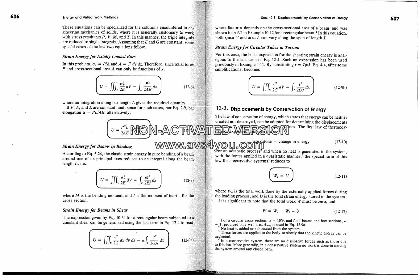
636 Energy and Virtual Work Methods
These equations can be specialized for the solutions encountered ingineering mechanics of solids, where it is generally customary towith stress resultants P, V, M, and T. In this manner, theare reduced to single integrals. Assuming that E and G are constant,special cases of the last two equations follow.
Strain Energy for Axially Loaded Bars
In this problem, �rx = P/A and A = ff dy dz. Therefore, since axialP and cross-sectional area A can only be functions of x,
where an integration along bar length L gives the required quantity.If P, A, and E are constant, and, since for such cases, per Eq. 2-9,
elongation A = PL/AE, alternatively,
I _ P2L=AEA2)U 2AE 2L JStrain Energy for Beams in BendingAccording to Eq. 6-24, the elastic strain energy in pure bendingaround one of its principal axes reduces to an integral along thelength L, i.e.,
where M is the bending moment, and I is the moment of inertia forcross section.
Strain Energy for Beams in Shear
The expression given by Eq. 10-34 for a rectangular beam subjconstant shear can be generalized using the last term in Eq. 12-4 to
= 5-&dy& =
(12-
Sec. '12-3. Displacements by Conservation of Energy
where factor ct depends on the cross-sectional area of a beam, and wasshown to be 6/5 in Example 10-12 for a rectangular beam. � In this equation,both s. hear V and area A can vary along the span of length L.
Strain Energy for Circular Tubes in Torsion
For this case, the basic expression for the shearing strain energy is anal-ogous to the last term of'Eq. 12-4. Such an expression has been usedpreviously in Example 4-11. By substituting -r = TO/J, Eq. 4-4, after somesimplifications, becomes
= dV fi. T2 (12-9b)
12-3. Displacements by Conservation of EnergyThe law of conservation of energy, which states that energy can be neithercreated nor destroyed, can be adopted for determining the displacementsof elastic systems due to the applied forces. The first law of thermody-namics expresses this principle as
work done = change in energy (12-10)
For an adiabatic process 2 and when no heat is generated in the system,with the forces applied in a quasistatic manner, 3 the special form of thislaw for conservative systems 4 reduces to
(12-11)
where We is the total work done by the externally applied forces duringthe loading process, and U is the total strain energy stored in the system.
It is significant to note that the total work W must be zero, and
W = We + Wi = 0 (12-12)
� For a circular cross section, ct = 10/9, and for I beams and box sections, ct= 1, provided only web area A,�eb is used in Eq. 12-9a.
2 No heat is added or subtracted from the system.3 These forces are applied to the body so slowly that the kinetic energy can be
neglected.4 In a conservative system, there are no dissipative forces such as those due
to friction. More generally, in a conservative system no work is done in movingthe system around any closed path.
637
NON-ACTIVATEDVERSIONwww.avs4you.com
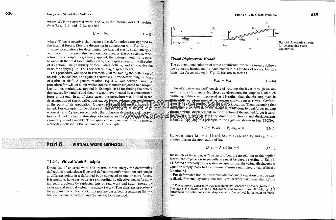
638 Energy and Virtual Work Methods
where We is the external work, and W� is the internal work.from Eqs. 12-11 and 12-12, one has
u = - w� (12-13
where Wi has a negative sign because the deformations are opposedthe internal forces. (See the discussion in connection with Fig. 12-2.
Some formulations for determining the internal elastic strainwere given in the preceding section. For linearly elastic systems,a force, or a couple, is gradually applied, the external work We isto one-half the total force multiplied by the displacement in theof its action. The possibility of formulating both We and U providesbasis for applying Eq. 12-11 for determining displacements.
This procedure was used in Example 2-10 for finding the deflectionan axially loaded bar, and again in Example 4-11 for determiningof a circular shaft. A general relation, Eq. 4-37, was derived usingprocedure for twist of a thin-walled hollow member subjected to a toreLastly, this method was applied in Example 10-12 for finding thetion caused by bending and shear in a cantilever loaded byforce at the end. In all of these cases, the procedure was limited todetermination of elastic deflections caused by a single concentratedat the point of its application. Otherwise, intractable equations aretained. For example, for two forces P� and P2, P� A�/2 + P2 A2/2 =where A� and A2 are, respectively, the unknown deflections of theforces. An additional relationship between A� and A2, except in casessymmetry, is not available. This requires development of the moremethods discussed in the remainder of the chapter.
� 12-4. Virtual Work PrincipleDirect use of 'external work and internal strain energy fordeflections breaks down if several deflections and/or rotations areat different points in a deformed body subjected to one or moreIt is possible, however, to devise extraordinarily effective means foring such problems by replacing true or real work and strain energyexternal and internal virtual (imaginary) work. Two differentfor applying the virtual work principle are described, resulting in thetual displacement method and the virtual force method.
Sec. 12-4. Virtual Work Principle
(a) (b)
Virtual Displacement Method
The conventional solution of static equilibrium problems usually followsthe concepts introduced by Archimedes in his studies of levers. On thisbasis, the forces shown in Fig. 12-1(a) are related as
P�ai = P2a2 (12-14)
An alternative method s consists of rotating the lever through an bn-agina�:y or v#'tual angle 80. Here, as elsewhere, for emphasis, all suchvirtual quantities are expressed as 80 rather than the dqb employed inusual differential notation. The rotation shown causes virtual displace-ments 8A� and 8A2 at the points of load application. Then, assuming thatthe system is conservative, the v#'tual work 8W done by real forces movingthrough virtual displacements in the direction of the applied forces is zero.Such work is positive when the direction of forces and displacementscoincide. Applying this principle to the rigid bar shown in Fig. 12-2(b),
8W = P� 8A� - P2 8A2 = 0 (12-15)
However, since 8A� = a� 80 and 8A2 = a2 8qb, and P� and P2 do notchange during the application of 80,
(P�ai - P2a2) 80 = 0 (12-16)
Inasmuch as 80 is perfectly arbitrary, bearing no relation to the appliedforces, the expression in parentheses must be zero, reverting to Eq. 12-14. Stated differently, for a system in equilibrium, the virtual displacement
equation simply leads to an equation of statics multiplied by an arbitrary
For deformable bodies, the virtual-displacement equation must be gen-eralized. For such systems, the total virtual work 8W, consisting of the
s This approach apparently was considered by Leonardo da Vinci (1452-1519),Stevinus (1548-1620), Galileo (1564-1642), and Johann Bernoulli, who in 1717introduced the notion of virtual displacements (velocities) in his letter to Varig-non.
639
Fig. '12-'1 Alternative meansfor determining staticequilibrium.
NON-ACTIVATEDVERSIONwww.avs4you.com
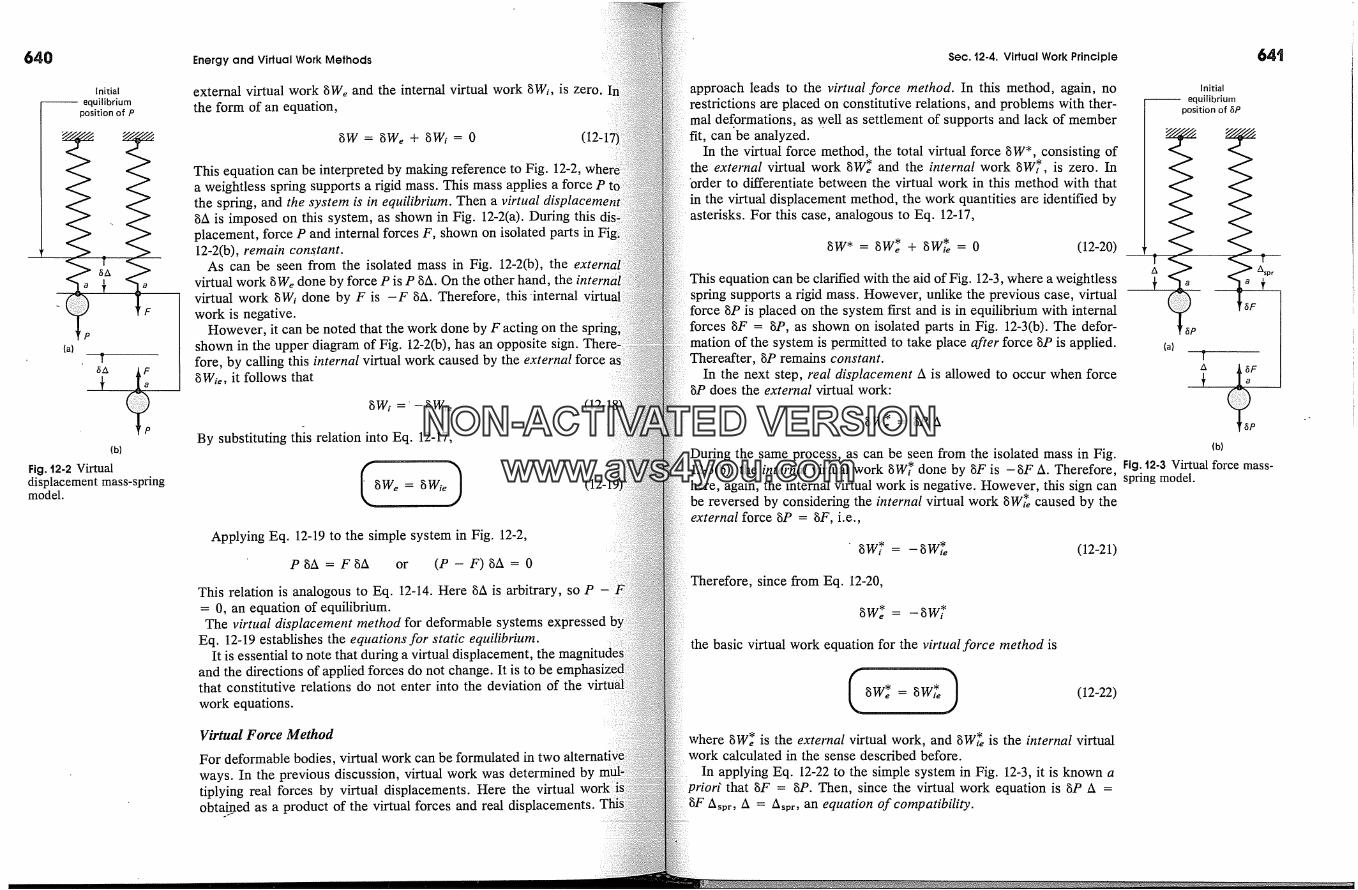
Initial
-- equilibriumposition of P
{a)T
(b)
Fig. '12-2 Virtualdisplacement mass-springmodel.
Energy and Virtual Work Methods
external virtual work gWe and the internal virtual work gW�, is zero.the form of an equation,
gW= gWe + gWi= 0
This equation can be interpreted by making reference to Fig. 12-2,a weightless spring supports a rigid mass. This mass applies a force Pthe spring, and the system is in equilibrium. Then a virtual dis�gA is imposed on this system, as shown in Fig. 12-2(a). During thisplacement, force P and internal forces F, shown on isolated parts in Fi12-2(b), remain constant.
As can be seen from the isolated mass in Fig. 12-2(b), the externvirtual work gWe done by force P is P gA. On the other hand, the internvirtual work gWi done by F is -F g/x. Therefore, this-internalwork is negative.
However, it can be noted that the work done by F acting on theshown in the upper diagram of Fig. 12-2(b), has an opposite sign.fore, by calling this internal virtual work caused by the external forcegW�,, it follows that
gWi =' -gWi� (12-18
By substituting this relation into Eq. 12-17,
' gWe�Applying Eq. 12-19 to the simple system in Fig. 12-2,
pgA = FgA or (P- F) gA = 0
This relation is analogous to Eq. 12-14. Here gA is arbitrary, so P= 0, an equation of equilibrium.
The virtual displacement method for deformable systems expressedEq. 12-19 establishes the equations for static equilibrium.
It is essential to note that during a virtual displacement,and the directions of applied forces do not change. It is to bethat constitutive relations do not enter into the deviation of thework equations.
Virtual Force Method
For deformable bodies, virtual work can be formulated in twoways. In the previous discussion, virtual work was determinedtiplying real forces by virtual displacements. Here the virtualobtained as a product of the virtual forces and real displacements.
Sec. t2-4. Virtual Work Principle 64'i
approach leads to the virtual force method. In this method, again, norestrictions are placed on constitutive relations, and problems with ther-mal deformations, as well as settlement of supports and lack of memberfit, can be analyzed.
In the virtual force method, the total virtual force gW*, consisting ofthe external virtual work gW� and the internal work gW�, is zero. In'order to differentiate between the virtual work in this method with thatin the virtual displacement method, the work quantities are identified byasterisks. For this case, analogous to Eq. 12-17,
gW* = gW� + gW�*e = 0 (12-20)
This equation can be clarified with the aid of Fig. 12-3, where a weightlessspring supports a rigid mass. However, unlike the previous case, virtualforce gP is placed on the system first and is in equilibrium with internalforces gF = gP, as shown on isolated parts in Fig. 12-3(b). The defor-mation of the system is permitted to take place after force gP is applied.Thereafter, gP remains constant.
In the next step, real displacement A is allowed to occur when forcegP does the external virtual work:
Initial
-- equilibriumposition of bP
(a}
During the same process, as can be seen from the isolated mass in Fig.12-3(b), the internal virtual work gW� done by gF is - gF A. Therefore, Fig. t2-3 Virtual force mass-here, again, the internal virtual work is negative. However, this sign can spring model.be reversed by considering the internal virtual work gW�*� caused by theexternal force gP = gF, i.e.,
gW? = -gW�e (12-21)
Therefore, since from Eq. 12-20,
the basic virtual work equation for the virtual force method is
(12-22)
where gW� is the external virtual work, and gW**e is the internal virtualwork calculated in the sense described before.
In applying Eq. 12-22 to the simple system in Fig. 12-3, it is known athat gF = gP. Then, since the virtual work equation is gP A =
Aspr, A ---� Aspr, an equation of compatibility.
NON-ACTIVATEDVERSIONwww.avs4you.com
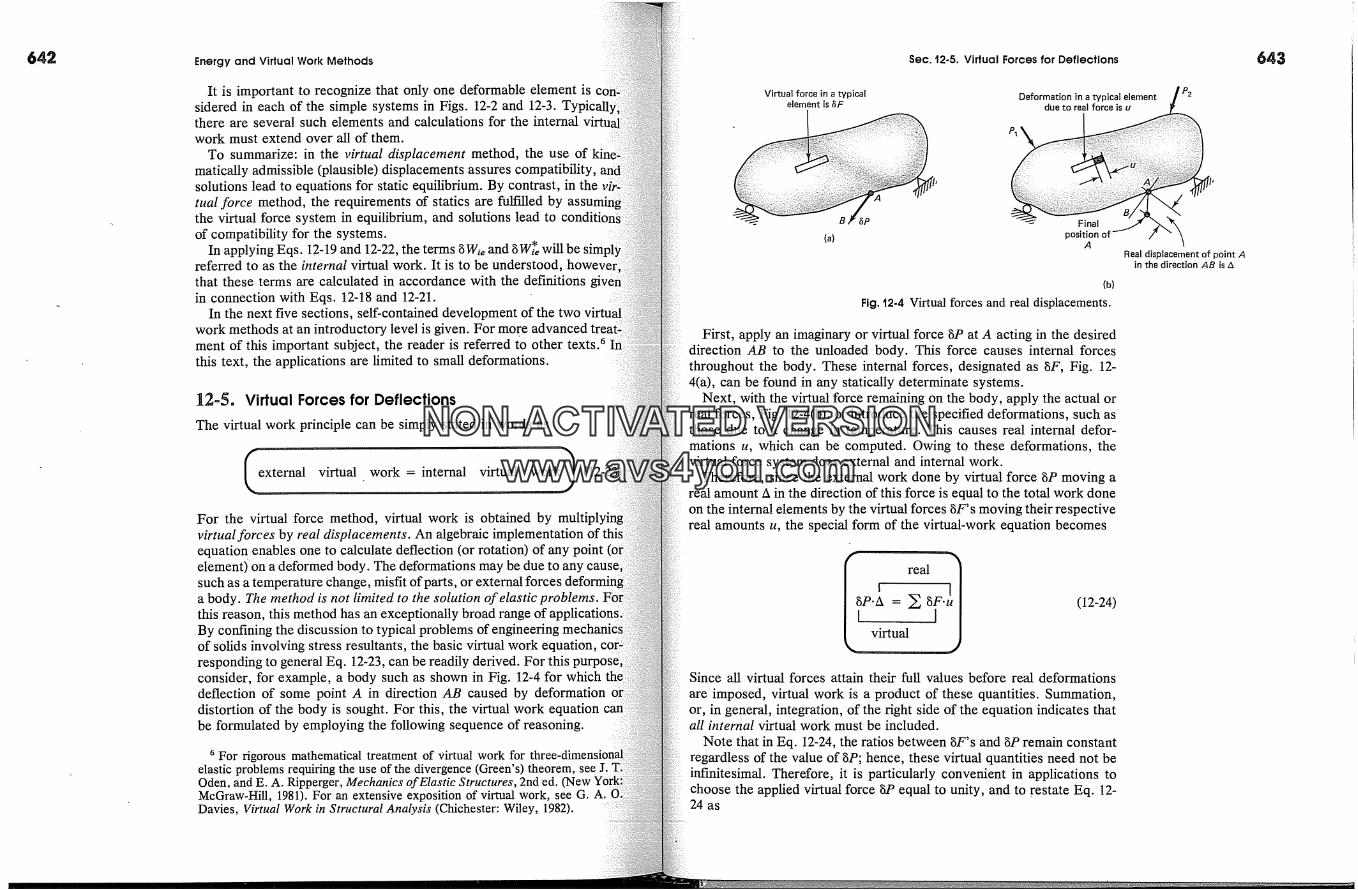
642 Energy and Virtual Work Methods Sec. t2.5. Virtual Forces for Deflections 643
It is important to recognize that only one deformable element issidered in each of the simple systems in Figs. 12-2 and 12-3.there are several such elements and calculations for the internalwork must extend over all of them.
To summarize: in the virtual displacement method, the use ofmatically admissible (plausible) displacements assures compatibility,solutions lead to equations for static equilibrium. By contrast, in thetual force method, the requirements of statics are fulfilled bythe virtual force system in equilibrium, and solutions lead toof compatibility for the systems.
In applying Eqs. 12-19 and 12-22, the terms �Wie and �W�e will be sireferred to as the internal virtual work. It is to be understood, howeverthat these terms are calculated in accordance with the definitionsin connection with Eqs. 12-18 and 12-21.
In the next five sections, self-contained development of the two virtuiwork methods at an introductory level is given. For more advancedment of this important subject, the reader is referred to other texts. 6this text, the applications are limited to small deformations.
12-5. Virtual Forces for Deflections
The virtual work principle can be simply stated in words as
external virtual work = internal virtual work�For the virtual force method, virtual work is obtained byvirtual forces by real displacements. An algebraic implementation ofequatio n enables one to calculate deflection (or rotation) of anyelement) on a deformed body. The deformations may be due to an3such as a temperature change, misfit of parts, or external forcesa body. The method is not limited to the solution of elastic problems.this reason, this method has an exceptionally broad rangeBy confining the discussion to typical problems of engineeringof solids involving stress resultants, the basic virtual work equation,responding to general Eq. 12-23, can be readily derived. For this purposeconsider, for example, a body such as shown in Fig. 12-4 for whichdeflection of some point A in direction AB caused by deformationdistortion of the body is sought. For this, the virtual work equationbe formulated by employing the following sequence of reasoning.
6 For rigorous mathematical treatment of virtual work forelastic problems requiring the use of the divergence (Green's) theorem,Oden, and E. A. Ripperger, Mechanics of Elastic Structures, 2nd ed.McGraw-Hill, 1981). For an extensive exposition of virtual work, see G. A.Davies, Virtual Work in Structural Analysis (Chichester: Wiley, 1982).
Virtual force in a typicalelement is/�F
B
(a)
�P
Deformation in a typical elementdue to real force is u
A
(b)
Fig. t2-4 Virtual forces and real displacements.
P2
Real displacement of point Ain the direction AB is A
First, apply an imaginary or virtual force gP at A acting in the desireddirection AB to the unloaded body. This force causes internal forcesthroughout the body. These internal forces, designated as gF, Fig. 12-4(a), can be found in any statically determinate systems.
Next, with the virtual force remaining on the body, apply the actual orreal forces, Fig. 12-4(b), or introduce the specified deformations, such asthose due to a change in temperature. This causes real internal defor-mations u, which can be computed. Owing to these deformations, thevirtual force system does external and internal work.
Therefore, since the external work done by virtual force gP moving areal amount A in the direction of this force is equal to the total work doneon the internal elements by the virtual forces gF's moving their respectivereal amounts u, the special form of the virtual-work equation becomes
real
virtu�__��J
(12-24)
Since all virtual forces attain their full values before real deformationsare imposed, virtual work is a product of these quantities. Summation,or, in general, integration, of the right side of the equation indicates thatall internal virtual work must be included.
Note that in Eq. 12-24, the ratios between gF's and gP remain constantregardless of the value of gP; hence, these virtual quantities need not beinfinitesimal. Therefore, it is particularly convenient in applications tochoose the applied virtual force gP equal to unity, and to restate Eq. 12-24 as
NON-ACTIVATEDVERSIONwww.avs4you.com
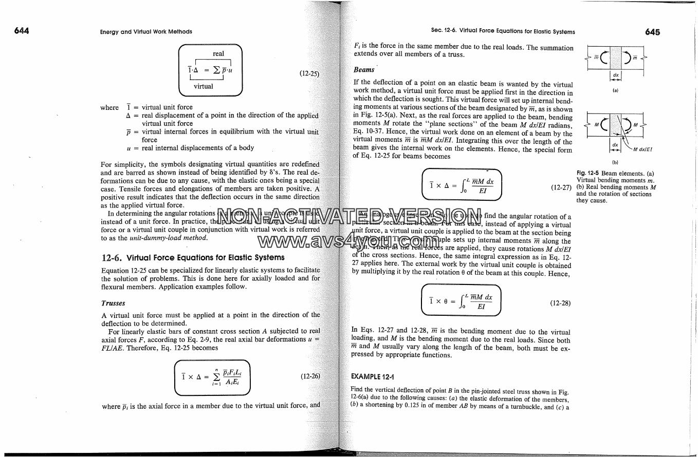
644 Energy and Virtual Work Methods
where
I ivirtual
virtual unit forcereal displacement of a point in the direction of thevirtual unit forcevirtual' internal forces in equilibrium with the virtualforce
real internal displacements of a body
For simplicity, the symbols designating virtual quantities areand are barred as shown instead of being identified by- 8's. The reallformations can be due to any cause, with the elastic ones being acase. Tensile forces and elongations of members are takenpositive result indicates that the deflection occurs in the sameas the applied virtual force.
In determining the angular rotations of a member, a unit couple isinstead of a unit force. In practice, the procedure of using a virtualforce or a virtual unit couple in conjunction with virtual work isto as the unit-dummy-load method.
12-6. Virtual Force Equations for Elastic Systems
Equation 12-25 can be specialized for linearly elastic systems tothe solution of problems. This is done here for axially loadedflexural members. Application examples follow.
Trusses
A virtual unit force must be applied at a point in the direction ofdeflection to be determined.
For linearly elastic bars of constant cross section A subjected toaxial forces F, according to Eq. 2-9, the real axial bar deformationsFL/AE. Therefore, Eq. 12-25 becomes
�x A= .= AiEi
where �i is the axial force in a member due to the virtual unit force
Sec. 12-6. Virtual Force Equations for Elastic Systems
Fi is the force in the same member due to the real loads. The summationextends over all members of a truss.
Peams
If the deflection of a point on an elastic beam is wanted by the virtualwork method, a virtual unit force must be applied first in the direction inwhich the deflection is sought. This virtual force will set up internal bend-ing moments at various sections of the beam designated by �, as is shownin Fig. 12-5(a). Next, as the real forces are applied to the beam, bendingmoments M rotate the "plane sections" of the beam M dx/EI radians,Eq. 10-37. Hence, the virtual work done on an element of a beam by thevirtual moments � is �M dx/EI. Integrating this over the length of thebeam gives the internal work on the elements. Hence, the special form
Eq. 12-25 for beams becomes
Z �M dxxA= EI (12-27)
An analogous expression may be used to find the angular rotation of aparticular section in a beam. For this case, instead of applying a virtualunit force, a virtual unit couple is applied to the beam at the section beinginvestigated. This virtual couple sets up internal moments � along thebeam. Then, as the real forces are applied, they cause rotations M dx/EIof the cross sections. Hence, the same integral expression as in Eq. 12-27 applies here. The external work by the virtual unit couple is obtainedby multiplying it by the real rotation 0 of the beam at this couple. Hence,
Yxo= E1 (12-28)
In Eqs. 12-27 and 12-28, � is the bending moment due to the virtualloading, and M is the bending moment due to the real loads. Since both
and M usually vary along the length of the beam, both must be ex-pressed by appropriate functions.
EXAMPLE t24
Find the vertical deflection of point B in the pin-jointed steel truss shown in Fig.12-6(a) due to the following causes: (a) the elastic deformation of the members,
a shortening by 0.125 in of member AB by means of a turnbuckle, and (c) a
645
d� M dx/EI(b)
Fig. t2-5 Beam elements. (a)Virtual bending moments m.(b) Real bending moments Mand the rotation of sectionsthey cause.
NON-ACTIVATEDVERSIONwww.avs4you.com

646
AA'-/� A = 0.15in2I �L =60in
3' / 3000 lb
.� L = 60 inC�.,i
(a)
* '"�833 lb
. /+0.833 lb
(b) Virtual loading
_A�. 1500lb2000 lb �
3000 lb
2000Ib� �'�-2500lbC 11500 lb
(c) Real loading
Fig. t2-6
Energy and Vidual Work Methods
drop in temperature of 120 �F occurring in member BC. The coefficient of theexpansion of steel is 6.5 x 10 -6 inch per inch per degree Fahrenheit. Nethe possibility of lateral buckling of the compression member. Let E = 30 x
.psi.
Solution
(a) A virtual unit force is applied in the upward vertical direction, as shownFig. 12-6(b), and the resulting forces � are determined and recorded on thediagram. Then the forces in each member due to the real force are alsoand recorded, Fig. 12-5(c). The solution follows by means of Eq. 12-26. The'is carded out in the table.
Member �, lb F, lb L, in A, in 2 �FL/AAB -0.833 +2500 60 0.15 -833,000BC + 0.833 - 2500 60 0.25 - 500,000
From this table, � �FL/A = - 1,333,000. Hence,
7 x A = wz� �FL -1,333,000 _AE 30 x 106
and A = -0.0444 in
- 0.0444 lb-in
The negative sign means that point B deflects down. In this case, "negative workis done by the virtual force acting upward when it is displaced in 'adirection. Note particularly the'units and the signs of all quantities. Tensilein members are taken positive, and vice versa.
(b) Equation 12-25 is used to find the vertical deflection of point B due toshortening of member AB by 0.125 in. The forces set up in the bars byforce acting in the direction of the deflection sought are shown in Fig.Then, since u is -0.125 in (shortening) for member AB and is zero forBC,
T x /t = (-0.833)(-0.125) + (+0.833)(0) = +0.1042 lb-in
and /t = + 0.1042 in up
(c) Again, using Eq. 12-25, and noting that due to the drop in temperature,2-18, Ar = -6.5 x 10 -6 X 120 X 60 = --0.0468 in in member BC,
� x /t = (+0.833)(-0.0468) = -0.0390 lb-in
and A = -0.0390 in down
By superposition, the net deflection of point B due to all three causes is
Sec. 12-6. Virtual Force Equations for Elastic Systems
+ 0.1042 - 0.0390 = +0.0208 in up. To find this quantity, all three effects couldhave been considered simultaneously in the virtual work equation.
EXAMPLE '2-2
Find the deflection and rotation at the middle of the cantilever beam loaded asshown in Fig. 12-7. EI for the beam is constant.
Solution
The downward virtual force is applied at point A, whose deflection is sought, Fig.12-7(b). The � diagram and the M diagram are shown in Figs. 12-7(c) and (d),respectively. For these functions, the same origin ofx is taken at the free end ofthe cantilever. After these moments are determined, Eq. 12-27 is applied to findthe deflection.
X HJoX X Wo X3M= - O<x<L
2 L 3 6L� = 0 0 <x<L/2� = -l(x-L/2) L/2<x<L
EI - EJ (0) �, 6L / dx1 L ( WoX3+ fL,_ -x + $]
49woL 4-- N.m3840EI
wox/L
W�o~� Realloading-'� I M diagram
(a) (d)
'L/2
diagram due to '�' N
(c)
TN.mdiagram
(f) Fig. t2-7
647
NON-ACTIVATEDVERSIONwww.avs4you.com
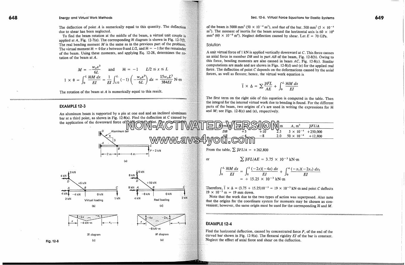
648 Energy and Virtual Work Methods Sec. 12-6. Virtual Force Equations for Elastic Systems 649
The deflection of point A is numerically equal to this quantity. Thedue to shear has been neglected.
To find the beam rotation at the middle of the beam, a virtual unitapplied at A, Fig. 12-7(e). The corresponding � diagram is shown in Fig. 12-7iThe real bending moment M is the same as in the previous part of theThe virtual moment � = 0 for x between 0 and L/2, and � = - 1 for theof the beam. Using these moments, and applying Eq. 12-28, determines thetation of the beam at A.
WoX 36L
l: mM dxIx0= E1
and � = -1 L/2<x<L
EI ,2 (-1) �, 6L ] dx =--15woL 3
384EI
The rotation of the beam at A is numerically equal to this result.
EXAMPLE '12-3
An aluminum beam is supported by a pin at one end and an inclinedbar at a third point, as shown in Fig. 12-8(a). Find the deflection at C causedthe application of the downward force of 2 kN at that point. The cross
, D 4AIiminumbar4m� =2kN
(a)
D '�5kN
2 kN Virtual loading
D �10 kNC 8.kN A 'N�B
1 kN 4 kN Real loading(b) (d)
Fig. 12-8
diagram
(c)
-8 kN.m
M diagram
(e)
of the beam is 5000 mm 2 (50 x 10 -4 m2), and that of the bar, 500 mm 2 (5 x 10 -4m2). The moment of inertia for the beam around the horizontal axis is 60 x 10 6mm 4 (60 x 10 -6 m4). Neglect deflection caused by shear. Let E = 70 GPa.
Solution
A unit virtual force of 1 kN is applied vertically downward at C. This force causesan axial force in member DB and in part AB of the beam, Fig. 12-8(b). Owing tothis force, bending moments are also caused in beam AC, Fig. 12-8(c). Similarcomputations are made and are shown in Figs. 12-8(d) and (e) for the applied realforce. The deflection of point C depends on the deformations caused by the axialforces, as well as flexure; hence, the virtual work equation is
The �rrst term on the right side of this equation is computed in the table. Thenthe integral for the internal virtual work due to bending is found. For the differentparts of the beam, two origins of x's are used in writing the expressions for �and M; see Figs. 12-8(c) and (e), respectively.
Member �, kN F, kN L, m A, m 2 �FL/ADB +5 +10 2.5 5 X 10 -4 +250,000AB -4 -8 2.0 50 X 10 -4 +12,800
From the table, � �FL/A = + 262,800
or � pFL/.AE = 3.75 x 10 -3 kN.m
fo L �M dx fo 2 (-2x)(-4x)dx /04 (-x0(-2x�)dx�EI - EI + EI= + 15.25 x 10 -3 kN.m
Therefore, T x A = 0.75 + 15.25)10 -3 = 19 x 10 -3 kN.m and point C deflects19 x 10 -3 m = 19 mm down.
Note that the work due to the two types of action was superposed. Also notethat the origins for the coordinate system for moments may be chosen as con-venient; however, the same origin must be used for the corresponding � and M.
EXAMPLE t2-4
Find the horizontal deflection, caused by concentrated force P, of the end of thecurved bar shown in Fig. 12-9(a). The flexural rigidity EI of the bar is constant.Neglect the effect of axial force and shear on the deflection.
NON-ACTIVATEDVERSIONwww.avs4you.com
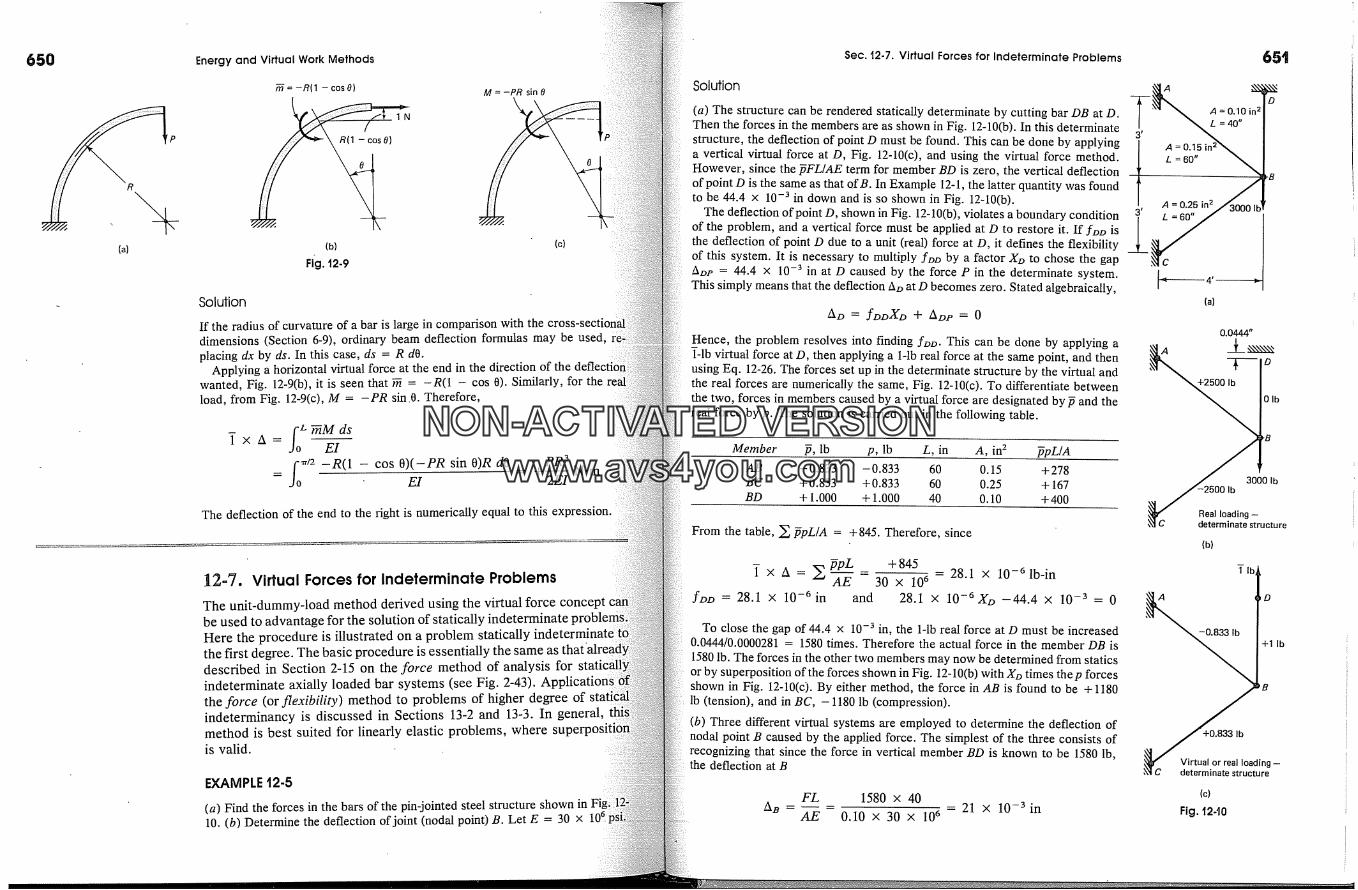
650 Energy and Virtual Work Methods Sec. '12-7. Virtual Forces for Indeterminate Problems
R P(a)
-R(1 - cos O)
(b)
Fig. '12-9
M = -PR sin 8
Solution
If the radius of curvature of a bar is large in comparison with thedimensions (Section 6-9), ordinary beam deflection formulas may be used,placing dx by ds. In this case, ds = R dO.
Applying a horizontal virtual force at the end in the direction of the deflecti0hwanted, Fig. 12-9(b), it is seen that 7fi = -R(1 - cos 0). Similarly, for theload, from Fig. 12-9(c), M = -PR sin.0. Therefore,
f ) �M dsA= EI
= fo �/2 -R(1 - cos O)(-PR sin O)R dOEI
pR 3
The deflection of the end to the right is numerically equal to this expression.
12-7. Virtual Forces for Indeterminate ProblemsThe unit-dummy-load method derived using the virtual force conceptbe used to advantage for the solution of statically indeterminate tHere the procedure is illustrated on a problem statically indethe first degree. The basic procedure is essentially the same as thatdescribed in Section 2-15 on the force method of analysis forindeterminate axially loaded bar systems (see Fig. 2-43).the force (or flexibility) method to problems of higher degree ofindeterminancy is discussed in Sections 13-2 and 13-3. In general,method is best suited for linearly elastic problems, whereis valid.
EXAMPLE t2-5
(a) Find the forces in the bars of the pin-jointed steel structure shown in10. (b) Determine the deflection of joint (nodal point) B. Let E = 30 x 10�
Solution
(a) The structure can be rendered statically determinate by cutting bar DB at D.Then the forces in the members are as shown in Fig. 12-10(b). In this determinatestructure, the deflection of point D must be found. This can be done by applyinga vertical virtual force at D, Fig. 12-10(c), and using the virtual force method.However, since the �FL/AE term for member BD is zero, the vertical deflectionof point D is the same as that of B. In Example 12-1, the latter quantity was foundto be 44.4 x 10 -3 in down and is so shown in Fig. 12-10(b).
The deflection of point D, shown in Fig. 12-10(b), violates a boundary conditionof the problem, and a vertical force must be applied at D to restore it. If �z>z> isthe deflection of point D due to a unit (real) force at D, it defines the flexibilityof this system. It is necessary to multiply fz>z> by a factor Xz> to chose the gapAz>p = 44.4 x 10 -3 in at D caused by the force P in the determinate system.This simply means that the deflection Az> at D becomes zero. Stated algebraically,
Hence, the problem resolves into finding fz>z>. This can be done by applying aT-lb virtual force at D, then applying a l-lb real force at the same point, and thenusing Eq. 12-26. The forces set up in the determinate structure by the virtual andthe real forces are numerically the same, Fig. 12-10(c). To differentiate betweenthe two, forces in members caused by a virtual force are designated by � and thereal force by p. The solution is carried out in the following table.
Member �, lb p, lb L, in A, in 2 ,�pL/AAB -0.833 -0.833 60 0.15 +278BC +0.833 +0.833 60 0.25 + 167BD + 1.000 + 1.000 40 0.10 + 400
From the table, � ,�pL/A = + 845. Therefore, since
� x A = �'. �SpL _ +845� AE 30 X 10 6 -- 28.1 x 10 -6 lb-infz�z� = 28.1 x 10 -6 in and 28.1 x 10⁻⁶Xz� -44.4 x 10 -3 = 0
To close the gap of 44.4 x 10 -3 in, the l-lb real force at D must be increased0.0444/0.0000281 = 1580 times. Therefore the actual force in the member DB is1580 lb. The forces in the other two members may now be determined from staticsor by superposition of the forces shown in Fig. 12-10(b) with Xz> times the p forcesshown in Fig. 12-10(c). By either method, the force in AB is found to be + 1180lb (tension), and in BC, -1180 lb (compression).(b) Three different virtual systems are employed to determine the deflection ofnodal point B caused by the applied force. The simplest of the three consists ofrecognizing that since the force in vertical member BD is known to be 1580 lb,the deflection at B
FL 1580 x 40Aa .... 21 x 10 -3 in
AE 0.10 X 30 X 106
-�4 �(a)
-B
�5001b 3000lbReal loading-determinate structure
(b)
lb,
+1 lb
ding --ture
(c)
Fig. '12-t0
NON-ACTIVATEDVERSIONwww.avs4you.com

652 Energy and Virtual Work Methods
This solution from the point of view of a virtual force system means that;virtual force in member DB is unity and is zero in the other members.
Alternatively, the virtual force system may consist of active members ABBC, with a zero virtual force in member BD. Then, by assuming that theunit force acts upwards at B, the virtual forces in members AB and BC areshown in Fig. 12-10(c) (or Fig. 12-6(b)). (Remember that the force in memberis assumed to be zero.) From the solution for (a), the real forces in members )BC, and BD are known to be, respectively, + 1180 lb, -1180 lb, and + 1580The solution of Eq. 12-26 to obtain the deflection atB is carriedtable.
Member �, lb F, lb L, in A, in 2 �FL/AAB -0.833 +1180 60 0.15 -393,000BC +0.833 -1180 60 0.25 ' -236,000BD 0 + 1580 40 0.10 0
� �FL/A 629,000- = -21 x 10 -3 inHence, AB = E 30 X 10 a
The negative sign shows that the deflection is downward.Lastly, let the v'ff'tual force system consist of all three bars. The virtual
in the bars due to a unit downward force can be found by dividing the bardue to the applied forces by 3000; for example, for member AB, such aforce is 1180/3000 = 0.393 lb..Again, the solution is carried out in
Member �, lb F, lb L, in A, in 2 ,�FL/AAB +0.393 + 1180 60 0.15 + 185,000BC - 0.393 - 1180 60 0.25 + 111,000BD + 0.527 + 1580 40 0.10 + 333,000
Hence, AB = .� �FL/A 629,000 = 21 x 10 -3 inE 30 X 10 a
The results are the same by three entirely different virtual force syare in static equilibrium. This is true in general. Any self-equilibratingsystem can be used provided its displacements go through the prescribeddisplacements.
In any given case, to make certain that the elastic analysis is applicable,imum stresses must be determined. For the solution to be correct, these mustlin the linearly elastic range for the material used.
Sec. 12-8. Virtual Displacements for Equilibrium
*'12-8. Virtual Displacements for EquilibriumThe virtual work principle can be adapted for developing the virtual dis-placement method of structural analysis. The delivation of this methodcan begin by restating the virtual work principle in words:
external virtual work = internal virtual work (12-23)
Virtual work for the virtual displacement method is determined by mul-tiplying the virtual displacements by real forces. This is to be contrastedwith the virtual force method, where virtual work is found by multiplyingthe virtual forces by real displacements...Because of this, a number ofdifferences arise in the virtual work equations.
In the virtual displacement method, both the virtual and the real dis-placements must be compatible with the special requirements of a prob-lem. This means that the member displacements must conform to theboundary conditions and the displacements of the load points. Since theboundary conditions are simplest to satisfy at pin-ended axially loadedbars, only such problems are considered here. Moreover, the discussionis limited to bar assemblies meeting at a single pinned joint where anexternal force is applied. Such a joint is referred to as a nodal point.Although the discussion is limited to the simplest class of problems, thedescribed procedure provides an introduction to the most widely usedmethod in the matrix analysis of structures and finite elements, where itis indispensable.
In the virtual displacement method, besides an-accurate definition ofthe real and the virtual displacements, member forces must be defined asfunctions of the nodal displacements. This is achieved with the aid ofconstitutive relationships. Here such relationships are strictly limited tolinearly elastic behavior.
As with Archimedes' lever, the virtual work equations provide the equa-tiofi s of equilibrium. In this manner, the three basic requirements of equi-librium, compatibility, and constitt!tive relations are satisfied.
In order to construct the basic virtual work equation, by analogy toEq. 12-25, one can formulate it by going directly to the unit-dummy-displacement method. Here the real external force at its full value movesthrough a virtual unit displacement in the direction of the force. Simul-taneously, the real internal forces at their full values move through thevirtual displacements caused by the unit virtual displacement. This yieldsthe following virtual work equation:
real
Z
virtual
(12-29)
653
NON-ACTIVATEDVERSIONwww.avs4you.com
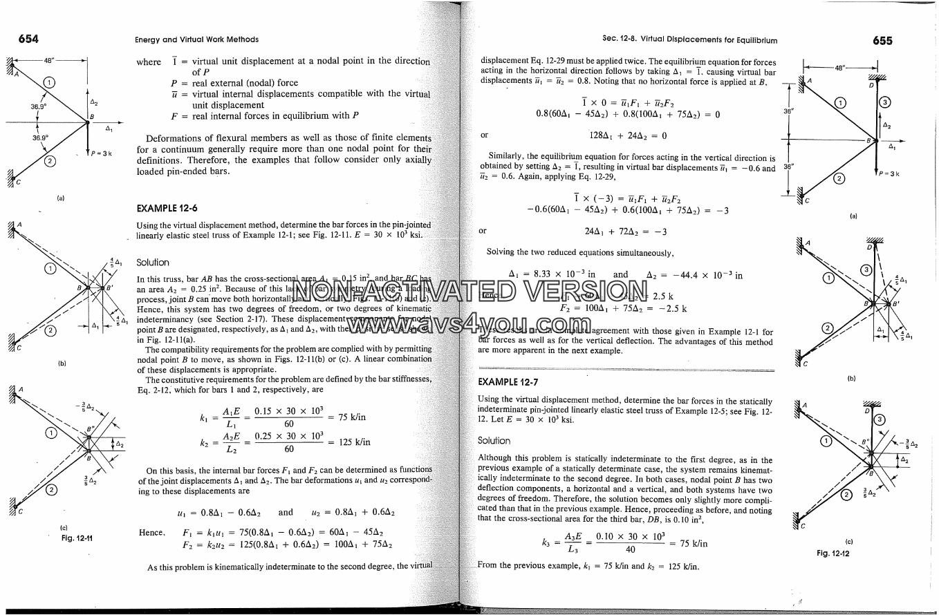
654
%/ 1
.z� . TP=3k(�)
(b)
Fig. '12-'H
Energy and Virtual Work Methods
where virtual unit displacement at a nodal point in the dire,of Preal external (nodal) forcevirtual internal displacements compatible with theunit displacementreal internal forces in equilibrium with P
Deformations of flexural members as well as those of finite elemefor a continuum generally require more than one nodal point fordefinitions. Therefore, the examples that follow consider onlyloaded pin-ended bars.
EXAMPLE t2-6
Using the virtual displacement method, determine the bar forces in thelinearly elastic steel truss of Example 12-1; see Fig. 12-11. E = 30 x 103 ksi
SolutionIn this truss, bar AB has the cross-sectional area A� = 0.15 in 2, and bar BCan area A2 = 0.25 in 2. Because of this lack of bar symmetry, during aprocess, joint B can move both horizontally and vertically, Figs. 12-1 l(b) and lHence, this system has two degrees of freedom, or two degrees ofindeterminancy (see Section 2-17). These displacement components forpoint B are designated, respectiyely, as A� and A2, with their positive sense:in Fig. 12-11(a).
The compatibility requirements for the problem are complied with bynodal point B to move, as shown in Figs. 12-11(b) or (c). A linearof these displacements is appropriate.
The constitutive requirements for the problem are defined by theEq. 2-12� which for bars 1 and 2, respectively, are
A�E 0.15 x 30 x 103k� - - = 75 k/in
Li 60A2E 0.25 x 30 x 103
k2 - - = 125 k/inL2 60
On this basis, the internal bar forces F� and F2 can be determined asof the joint displacements � and �2. The bar deformations th and ll2 COlTeSing to these displacements are
th = 0.8At -- 0.6A2 and u2 = 0.8A� + 0.6A2
Hence, F1 = klltl = 75(0.8A� - 0.6A2) = 60A1 -- 45A2F2 = k2u2 = 125(0.8At + 0.6A2) = 100A� + 75A2
As this problem is kinematically indeterminate to the second degree, the
Sec. 12-8. Virtual Displacements for Equilibrium
displacement Eq. 12-29 must be applied twice. The equilibrium equation for forcesacting in the horizontal direction follows by taking � = T. causing virtual bardisplacements 7/� = 7/2 = 0.8. Noting that no horizontal force is applied at B,
T X 0 = �F� + �2F20.8(60A� - 45A2) + 0.8(100A� + 75A2) = 0
or '128A� + 24A 2 = 0
Similarly, the equilibrium equation for forces acting in the vertical direction isobtained by setting A2 = T, resulting in virtual bar displacements 7/� = -0.6 and7/2 = 0.6. Again, applying Eq. 12-29,
T x (-3) = �1FI q- �2F2-0.6(60A� - 45A2) q- 0.6(100A� + 75A2) = --3
or 24A1 + 72A 2 = --3
Solving the two reduced equations simultaneously,
A� = 8.33 X 10 -3 in and A2 = --44.4 x 10 -3 in
Hence, F1 = 60Ai - 45A 2 = 2.5 kF2 = 100A� + 75A 2 = --2.5 k
These results are in complete agreement with those given in Example 12-1 forbar forces as well as for the vertical deflection. The advantages of this methodare more apparent in the next example.
EXAMPLE t2-7
Using the virtual displacement method, determine the bar forces in the staticallyindeterminate pin-jointed linearly elastic steel truss of Example 12-5; see Fig. 12-12. Let E = 30 x 103 ksi.
Solution
Although this problem is statically indeterminate to the first degree, as in theprevious example of a statically determinate case, the system remains kinemat-ically indeterminate to the second degree. In both cases, nodal point B has twodeflection components, a horizontal and a vertical, and both systems have twodegrees of freedom. Therefore, the solution becomes only slightly more compli-cated than that in the previous example. Hence, proceeding as before, and notingthat the cross-sectional area for the third bar, DB, is 0.10 in 2,
A3E 0.10 x 30 x 103k3 --- - = 75 k/in
L3 40
the previous example, k� = 75 k/in and k2 = 125 k/in.
655
(a)
(b)
% %
///
,xhlC
Fig. '12-'12
NON-ACTIVATEDVERSIONwww.avs4you.com
656 Energy and Virtual Work Methods
The displacements of the system in the horizontal and vertical directionsshown in Figs. 12-12(b) and (c). It is to be noted that the length of bar DBconsidered not to change because A � is very small (see Fig 2-24). Bar deformatiu� and u2 due to A� and A2, respectively, remain the same as in theexample, whereas u3 is equal to A2. Summarizing these results,
Ill = 0.8AI -- 0-6A2 tt2 = 0.8A1 + 0.6A2 and u3 = A2
Hence, recalling the earlier results, and adding only a new term for bar DB,
F� = 60A� - 45�2 F2 = 100A1 + 75A2 F3 = k3u3 = 75A
By noting that for the virtual displacement A� = T, 7/� = �2 = 0.8 and �3 =the equilibrium equation for the forces acting in the horizontal-direction,on Eq. 12-29, becomes
� x 0 = �7�F� + �2F2 q- �3F3
However, since u3 = 0, this equation reduces to the one given before,
128A� + 24A 2 = 0
Since for A2 = T, � = -0.6, �2 = 0.6, and �3 = 1, the equilibrium e�for the forces acting in the vertical direction, using Eq. 12-29, becomes
� x (-3� = �F� + �2F2 q- �3F30.6(60A� - 45A2) + 0.6(100A� + 75A2) + 75A2 = --3
or 24A� + 147A2 = --3
Solving the reduced equations simultaneously,
A� = 3.947 x 10 -3 in and A2 = -21.05 x 10 -3 in
Hence, F� = 60A� - 45A2 = 1.18 kF2 = 100A� + 75A2 = 1.18 kF3 = 75A2 = 1.58 k
These results are in complete agreement with those found earlier in12-5.
The kinematic indeterminacy of this problem would remain theof the number of bars meeting at joint B.
Problems of higher degree of statical indeterminacy are discussed in13-6 in connection with the displacement method of analysis.
Sec. t2-9. Virtual Work for Discrete Systems
*'12-9. Virtual Work for Discrete SystemsThe virtual displacement and virtual force methods both stem from thesame ;virtual work principle. It is instructive, therefore, to show the in-terrelationship between the two methods using discrete structural sys-tems, i.e., on structural systems with a finite number of applied forces,members, and nodal displacements. This is done here by employing ma-trix notation. The required matrix definitions and operations required forthis purpose follow.
A matrix is an ordered array of numbers, such as encountered earlierin Eqs. 1-1a, l-lb, and 3-12. The special matrix in Eq. 1-1a is commonlyreferred to as a column vector. The matrices in Eqs. l-lb and 3-12 areknown as square tnatrices. Here matrices are identified by braces forcolumn vectors and by brackets for square matrices, or are shown inboldface type.
A matrix product of a 2 x 2 square matrix by a 2 x 1 column vectorresults in a 2 x 1 column vector:
a2� a22_[ b2 La,_�b� + a22b2.]
A product of a 4 x 4 symmetric square matrix by a 4 x 1 columnvector is displayed in Eq. 2-42.
The transpose of a column vector such as P is denoted by pr and isobtained by interchanging the rows and columns of P. Therefore, if
then
p = P2 and �x = A2
pr = [p� P2 P3 '" P, and �X r = [A� A 2 A 3 ... A,The following products of these two functions lead to the same scalar
fitnction:
prix = p�A� + P2A2 + P3A3 + ... + p,,�Xrp = A�p� + A2P 2 + A3P 3 + ... +
These scalar functions are associated with the work term in the discussionthat follows.
The transpose of the product of the two matrices needed in the sub-sequent development is defined* as the product of the transposed matricestaken in the reverse order, i.e., if F = bP,
7 For proof, see any text on linear algebra such as B. Noble, Applied LinearAlgebra (Englewood Cliffs, NJ: Prentice-Hall, 1969).
657
NON-ACTIVATEDVERSIONwww.avs4you.com
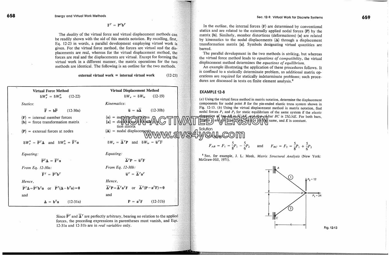
658 Energy and Virtual Work Methods Sec. 12-9. Virtual Work for Discrete SystemsFr= prbr
The duality of the virtual force and virtual displacement methodsbe readily shown with the aid of this matrix notation. By recalling,Eq. 12-23 in words, a parallel development employing virtual workgiven. For the virtual force method, the forces are virtual and theplacements are real, whereas for the virtual displacement methodforces are real and the displacements are virtual. Except for forming thlvirtual work in a different manner, the matrix operations for themethods are identical. The following is an outline for the two
external virtual work = internal virtual work (12-23
Virtual Force Method
�W�* = �W,'� (12-22)Statics:
� = b� (12-30a)
{F} = internal member forces[b] = force transformation matrix
{P} = external forces at nodes
�W� = �rA and �W; =�ru
Equating:
prA = �ru
From Eq. 12-30a:
�r = �rbr
Hence,
�rA=�rbru or �r(A-bru)=0and
A = bru (12-31a)
Virtual Displacement Method�We = �Wie (12-19)
Kinematics:
fi = aA
{u} = member distortions[a] = displacement transforma-
tion matrix
{A} = nodal displacements
(12-30b)
�We = �rp and gWie = �TF
Equating:XTp = aTF
From Eq. 12-30b:�r = �rar
Hence,
�rP=�rarF or �r(P-arF)=0and
P = arF (12-31b)
Since �r and �r are perfectly arbitrary, bearing no relation toforces, the preceding expressions in parentheses must vanish, and12-31a and 12-31b are in real variables only.
In the outline, the internal forces {F} are determined by conventionalstatics and are related to the externally applied nodal forces {P} by thematrix. [b]. Similarly, member distortions (deformations) {u} are relatedby kinematics to the nodal displacements {A} through a displacementtransformation matrix [a]. Symbols designating virtual quantities arebarred.
'The parallel development in the two methods is striking, but whereasthe virtual force method leads to equations of compatibility, the virtualdisplacement method determines the equations ofequilibriutn.
An example illustrating the application of these procedures follows. Itis confined to a statically determinate problem, as additional matrix op-erations are required for statically indeterminate problems; such proce-dures are discussed in texts on finite element analysis. 8
EXAMPLE t2-8
(a) Using the virtual force method in matrix notation, determine the displacementcomponents for nodal point B for the pin-ended elastic truss system shown inFig. 12-13. (b) Using the virtual displacement method in matrix notation, findnodal forces P, and P2 for static equilibrium of the same system if the elasticelongation of bar AB is 5L/AE, and that of bar BC is 25L/AE. For both bars,lengths L and cross-sectional areas A are the same, and E is constant.
Solution
(a) From statics,
6 - and Fac = F2 = �P� + 28 See, for example, J. L: Meek, Matrix Structural Analysis (New York:
McGraw-Hill, 1971).
Fig.
NON-ACTIVATEDVERSIONwww.avs4you.com
660 Energy and Virtual Work Methods Sec. 12-11. Strain Energy Theorems
Hence, {F�} = bP =F = F2P�P2
By using Eq. 2-9, the constitutive relations for the bars are
Hence,
III= --
ll 2 = --
By using Eq. 12-31a, for the compatibility of the system,
� = {�A;} = bru = A�= J'18'75'[ L�_ �. 16.67J AE
(b) Compatible bar deformations as functions of nodal displacements, withaid of Figs. 12-12(b) and (c), are determined to be
4 3 4 33th = �A, - �A 2 and u2 = �/x� + A 2
Hence, u = Lu2jA�A2
From constitutive relations for linearly elastic bars, since th = 5L/AE and= 25L/AE,
AE AE
F� = �th = 5 and F2 =-�-u2 = 25
Hence, using Eq. 12-31b, for static equilibrium, the joint forces are
P = P2 = 12
This result corresponds to the joint forces given for part (a). This means that thetwo processes are completely reversible for elastic systems.
In the matrix analyses of structures and especially in finite element applications,equations similar to the previous ones contain a large number of unknowns. Theuse of computers is essential for the solution of such systems of equations.
'912-10. General RemarksElastic strain-energy equations for applications in engineering mechanicsof solids are summarized in Section 12-2. The direct use of these equationsin determining deflections in conjunction with the law of conservation ofenergy in equating the total elastic energy of the system to the total workdone by the externally applied forces is very limited. This was pointedout in Section 12-3. An effective approach to enlarging the scope of pos-sible applications was discussed in Part B. Here an alternative classicalapproach based on elastic strain energy and complementary strain energyis considered. This requires the derivation of appropriate theorems forsolving problems similar to those treated in Part B describing the virtualwork methods. The derived equations will be found useful in the nextchapter in considering problems with a high degree of indeterminancy.An example of the use of the potential energy approach for determiningbuckling loads is given at the end of this part.
'12-11. Strain Energy and Complementary Strain EnergyTheorems
In Section 2-5, it was indicated that some materials during loading andunloading respond in a nonlinear manner along the same stress-straincurve, Fig. 2-11(b). Such materials are elastic although they do not obeyHooke's law. It is advantageous to consider such nonlinearly elastic ma-terials in deriving the two theorems based on strain energy concepts. Inthis manner, the distinction between elastic strain energy and comple-mentary strain energy is clearly evident. The derivation of the two basictheorems for nonlinear and linear elastic systems is essentially the same.These theorems are specialized in the next section for the solution of thelinearly elastic problems considered in this text.
As a rudimentary example for deriving the theorems, consider the ax-ially loaded bar shown in Fig. 12-14(a). The nonlinear elastic stress-straindiagram for the material of this bar is shown in Fig. 12-14(b). By multi-plying the normal stress cr in the bar by the cross-sectional area A of the
9 The remainder of this chapter is optional.
NON-ACTIVATEDVERSIONwww.avs4you.com
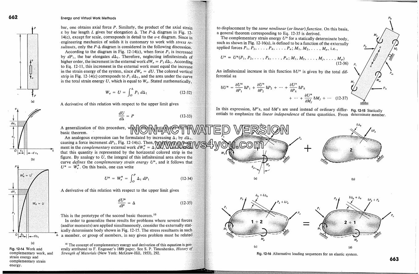
662
t
(b)
dP�
(c)
Fig. t2-14 Work andcomplementary work, andstrain energy andcomplementary strainenergy.
Energy and Virtual Work Methods
bar, one obtains axial force P. Similarly, the product of the axiale by bar length L gives bar elongation A. The p-A diagram in Fig.14(c), except for scale, corresponds in detail to the cr-e diagram. Since
� engineering mechanics of solids it is customary to work with stresssuitants, only the p-A diagram is considered in the following
According to the diagram in Fig. 12-14(c), when force P� is increas{by dP�, the bar elongates dA�. Therefore, neglecting infinitesim�shigher order, the increment in the external work dWe = P� dA �to Eq. 12-11, this increment in the external work must equal the increain the strain energy of the system, since dWe = dU. The coloredstrip in Fig. 12-14(c) corresponds to P� dA�, and the area under the curvis the total strain energy U, which is equal to We. Stated mathematic
We = U= f�P�d6,�A derivative of this relation with respect to the upper limit gives
dU- P (12-33
d6,
A generalization of this procedure, which follows, establishes the firibasic theorem.
An analogous expression can be formulated by increasing A� bycausing a force increment dP�, Fig. 12-14(c). Then, by defining an 'ment in the comple/nentaty external work dW�* = A� dP�, it can be noted)that this quantity is represented by the horizontal colored strip infigure. By analogy to U, the integral of this infinitesimal area abovecurve defines the cotnplementary strain energy U*, and it followsU* = W�*. On this basis, one can write
U* = W** = f� A i dPiA derivative of this relation with respect to the upper limit gives
dU*_ A (12-3�
dP
This is the prototype of the second basic theorem. ]�In order to generalize these results for problems where several
(and/or moments) are applied simultaneously, consider the externally staically determinate body shown in Fig. 12-15. The stress resultants ina member, or group of members, in any given problem must be
�o The concept of complementary energy and derivation of this equationerally attributed to F. Engesser's 1889 paper. See S. P. Timoshenko, HistoOStrength of Materials (New York: McGraw-Hill, 1953), 292.
to displacement by the same nonlinear (or linear)fitnction. On this basis,a general theorem corresponding to Eq. 12-35 is derived.
The complementary strain energy U* for a statically determinate body,such as shown in Fig. 12-16(a), is defined to be a function of the externallyapplied forces P�, P2 ..... Pk ..... P,,; M�, M2 ..... M v, i.e.,
U* = U*(P�, P2 .... ', Pk ..... P,; M1, M2 ..... M i ..... My)(12-36)
An infinitesimal increase in this function �U* is given by the total dif-ferential as
M 2
P1
OU* OU* OU*
�U* = OP� 8P� + '�2 �P2 + '" + �-�kOU*
+ ... + �8Mi+ --- (12-37)In this expression, 8P's, and 8M's are used instead of ordinary differ- Fig. t2.15 Staticallyentials to emphasize the linear' independence of these quantities. From determinate member.
P2
P1
Mq-
Op...�
(a) (b)
M1
A k + �SA k
,Pk + �;',
M 1
7� A k + A k
(c) (d)
Fig. t2-t6 Alternative loading sequences for an elastic system.
�P� + P�
663
NON-ACTIVATEDVERSIONwww.avs4you.com
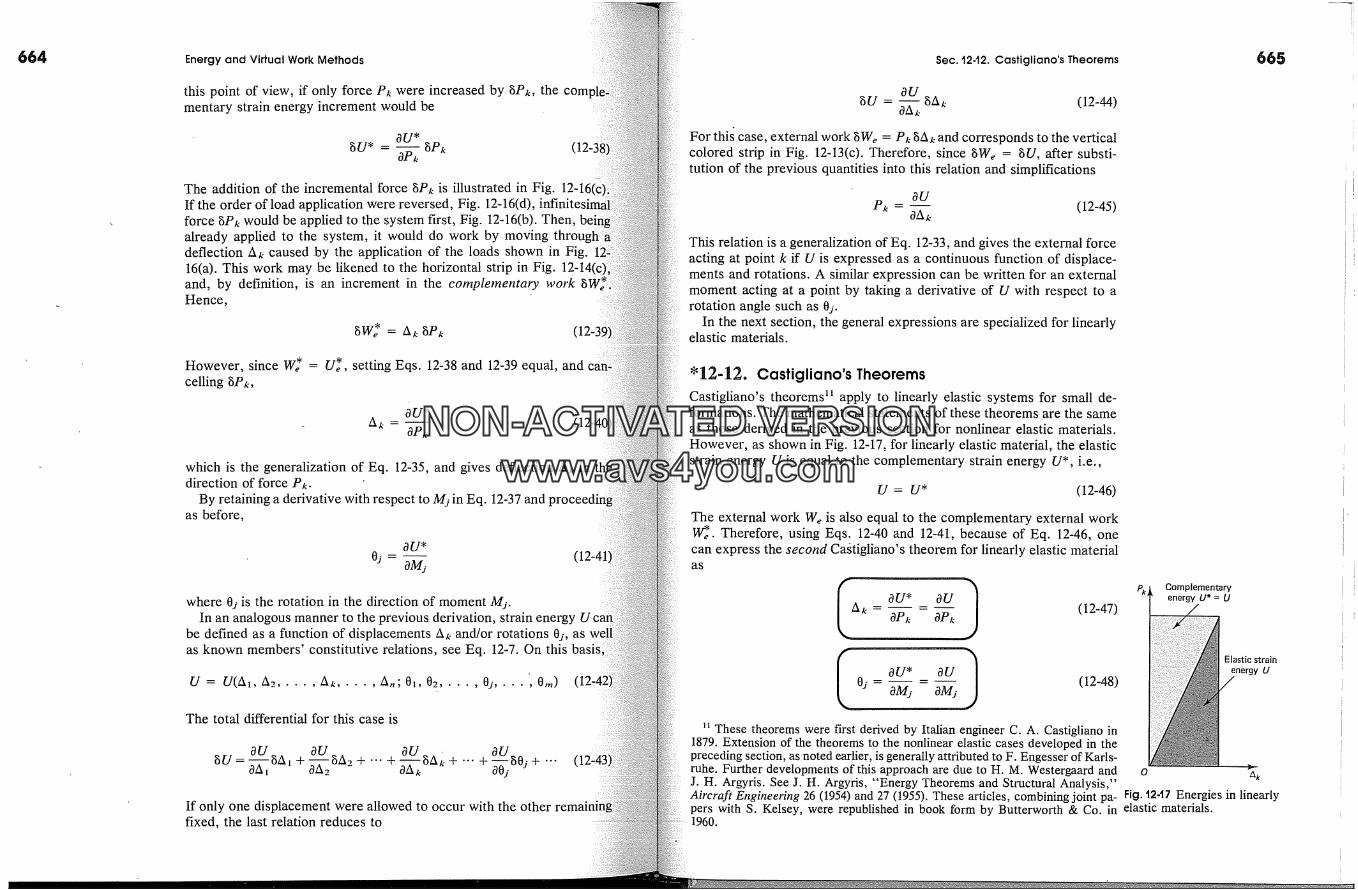
664 Energy and Virtual Work Methods Sec. 12-t2. Castigliano's Theorems
this point of view, if only force Pk were increased by 8Pk, thementary strain energy increment would be
OU*8U* = gP� (12-38
OP,
The addition of the incremental force gP� is illustrated in Fig.If the order of load application were reversed, Fig. 12-16(d),force gP�, would be applied to the system first, Fig. 12-16(b). Then,already applied to the system, it would do work by moving throudeflection Ak caused by the application of the loads shown in Fig216(a). This work may be likened to the horizontal strip in Fig.and, by definition, is an increment in the compIe�nenta�y workHence,
However, since W�* = U�*, setting Eqs. 12-38 and 12-39 equal, andcelling gPe,
OU*
OP�
which is the generalization of Eq. 12-35, and gives deflection A� indirection of force P�.
By retaining a derivative with respect to M s in Eq. 12-37 and tas before,
OU*
O�- OM s (12-41where 0s is the rotation in the direction of moment M�.
In an analogous manner to the previous derivation, strain energybe defined as a function of displacements Ak and/or rotations 0s, asas known members' constitutive relations, see Eq. 12-7. On this basis
U = U(fi�, h2 ..... �k ..... A.; 0�, 02 ..... 0s ..... Or.)
The total differential for this case is
0Us0.tv= �vtx + �v tx, + ... + _�-:V_vtx; + ... + +...0A 1 1 0A 2 _ OAk 00 s j
If only one displacement were allowed to occur with the otherfixed, the last relation reduces to
OU
8U = � 8A, (12-44)For thi� case, external work 8We = P� 8A�, and corresponds to the verticalcolored strip in Fig. 12-13(c). Therefore, since 8We = 8U, after substi-tution of the previous quantities into this relation and simplifications
OUPe - (12-45)
0A�,
This relation is a generalization of Eq. 12-33, and gives the external forceacting at point k if U is expressed as a continuous function of displace-ments and rotations. A similar expression can be written for an externalmoment acting at a point by taking a derivative of U with respect to arotation angle such as 0s.
In the next section, the general expressions are specialized for linearlyelastic materials.
� 12-12. Castigliano's TheoremsCastigliano's theorems � apply to linearly elastic systems for small de-formations. The mathematical statements of these theorems are the sameas those derived in the previous section for nonlinear elastic materials.However, as shown in Fig. 12-17, for linearly elastic material, the elasticstrain energy U is equal to the complementary strain energy U*, i.e.,
U = U* (12-46)
The external work We is also equal to the complementary external workW�. Therefore, using Eqs. 12-40 and 12-41, because of Eq. 12-46, onecan express the second Ca�tigliano's theorem for linearly elastic materialas
A k - OS* -- OS Pkj ComplementaryOP, OP� (12-47)
0 OS* OS energy U( ./-�'�- � j (12-48,
� These theorems were Errst derived by Italian engineer C. A. Castigllano in1879. Extension of the theorems to the nonlinear elastic cases developed in the
preceding section, as noted earlier, is generally attributed to F. Engesser of Karls-ruhe. Further developments of this approach are due to H. M. Westergaard and o a�J. H. Argyris. See J. H. Argyris, "Energy Theorems and Structural Analysis,"Aircraft Engineering 26 (1954) and 27 (1955). These articles, combining joint pa- Fig. t2-t7 Energies in linearlypers with S. Kelsey, were republished in book form by Butterworth & Co. in elastic materials.1960.
NON-ACTIVATEDVERSIONwww.avs4you.com
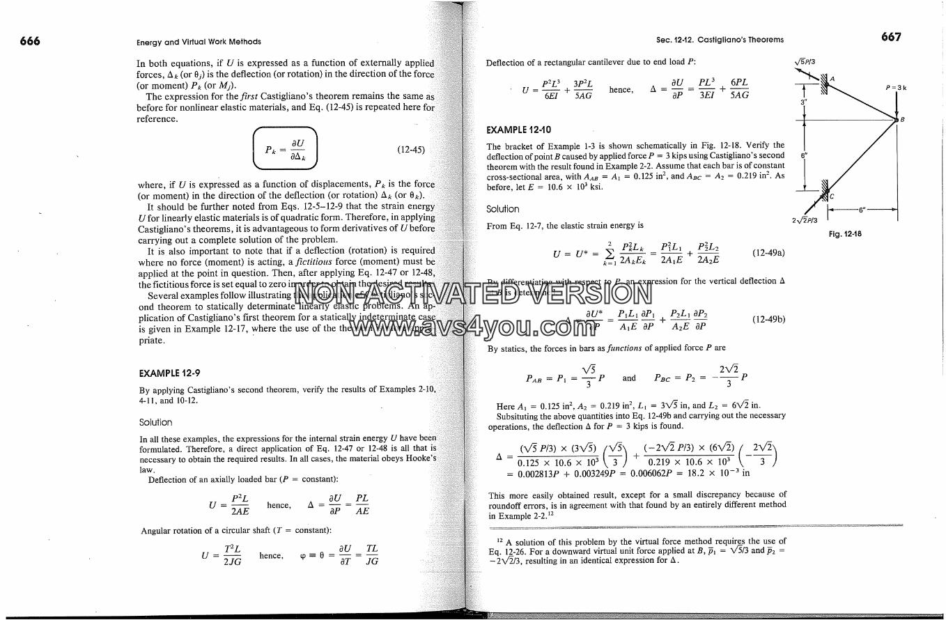
666 Energy and Virtual Work Methods
In both equations, ff U is expressed as a function of externallyforces, Ak (or 0�) is the deflection (or rotation) in the direction of the(or moment) Pk (or M�).
The expression for the first Castigliano's theorem remains the samebefore for nonlinear elastic materials, and Eq. (12-45) is repeated herereference.
(12-45)
where, ff U is expressed as a function of displacements, Pk is the forci(or moment) in the direction of the deflection (or rotation) Ak (or
It should be further noted from Eqs. 12-5-12-9 that the strain enerU for linearly elastic materials is of quadratic form. Therefore 'Castigliano's theorems, it is advantageous to form derivatives ofcarrying out a complete solution of the problem.
It is also important to note that ff a deflection (rotation) is recwhere no force (moment) is acting, a fictitious force (moment) must beapplied at the point in question. Then, after applying Eq. 12-47 orthe fictitious force is set equal to zero in order to obtain the desired result�
Several examples follow illustrating the application of Castigliano'sond theorem to statically determinate linearly elastic problems. An ap:plication of Castigliano's first theorem for a statically indeterminateis given in Example 12-17, where the use of the theorem is morepriate.
EXAMPLE '12-9
By applying Castigliano's second theorem, verify the results of Examples4-11, and 10-12.
Solution
In all these examples, the expressions for the internal strain energyformulated. Therefore, a direct application of Eq. 12-47 or 12-48 is all thatnecessary to obtain the required results. In all cases, the material obeyslaw.
Deflection of an axially loaded bar (P = constant):
P2L OU PLU = hence, A --
2AE OP AE
Angular rotation of a circular shaft (T = constant):
T2LU - hence,
2JG
OU TLcp=O = -
OT JG
Sec. t2-t2. Castigliano's Theorems
Deflection of a rectangular cantilever due to end load P:
p2L3 3p2L OU PL 3U - +-- hence, � - - --
6El 5AG OP 3EI
6PL+--
5AG
EXAMPLE t2-t0
The bracket of Example 1-3 is shown schematically in Fig. 12-18. Verify thedeflection of point B caused by applied force P = 3 kips using Castigliano's secondtheorem with the result found in Example 2-2. Assume that each bar is of constantcross-sectional area, with A�t� = A� = 0.125 in 2, and ABe = A2 = 0.219 in 2. Asbefore, let E = 10.6 x 10³ ksi.
Solution
From Eq. 12-7, the elastic strain energy is
u=u*= k=� 2AkEk 2A�E + 2A2-� (12-49a)By differentiating with respect to P, an expression for the vertical deflection Aat B is determined.
OU* P�Lx OP� P2L� OP2A = - -- + -- (12-49b)
OP AlE OP A2E OP
By statics, the forces in bars as fitnctions of applied force P are
2x/5P�a� = P� = -� P and PBc = P2 = 3 P
Here A� = 0.125 in 2, A2 = 0.219 in 2, L� = 3�/� in, and L2 = 6�/� in.Subsituting the above quantities into Eq. 12-49b and carrying out the necessary
operations, the deflection � for P = 3 kips is found.
(X/�P/3) x (3X/�)(__�) (-2X/�P/3) x (6X/�)(2__�)A = 0.125 X 10.6 X 103 + �.2-� � '�.� X 10 3 --= 0.002813P + 0.003249P = 0.006062P = 18.2 x 10 -3 in
This more easily obtained result, except for a small discrepancy because ofroundoff errors, is in agreement with that found by an entirely different methodin Example 2-2. �2
667
M'�P/3
�""�A P
Fig.
12 A solution of this problem by the virtual force method requires the use ofEq. 12-26. For a downward virtual unit force applied at B, � = �/5/3 and �2 =-2X/�/3, resulting in an identical expression for A.
NON-ACTIVATEDVERSIONwww.avs4you.com
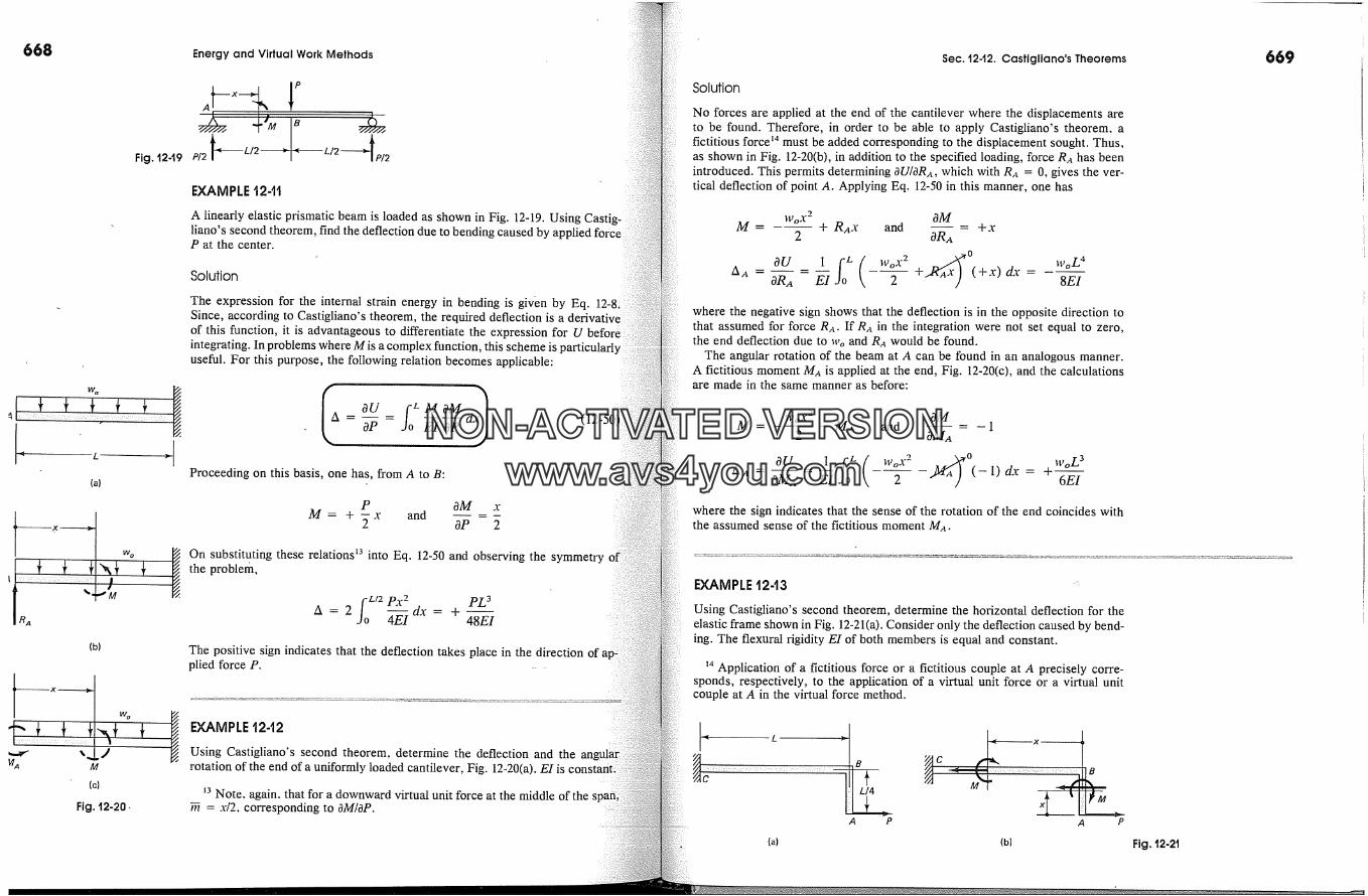
668
Fig. t2-t9
(a)
{b)
Fig. 12-20,
Energy and Virtual Work Methods
EXAMPLE t2-tt
A linearly elastic prismatic beam is loaded as shown in Fig. 12-19. Usingliano's second theorem, find the deflection due to bending caused by appliedP at the center.
Solution
The expression for the internal strain energy in bending is given by Eq.Since, according to Castigliano's theorem, the required deflection is a derivativeof this function, it is advantageous to differentiate the expression for U beforeintegrating. In problems where M is a complex function, this scheme isuseful. For this purpose, the following relation becomes applicable:
OP EI OP
Proceeding on this basis, one has, from A to B:
P OM xM = + � x and OP 2
On substituting these relations �3 into Eq. 12-50 and observing the symmetrythe problem,
fo L/2 Px 2 pL 3A = 2 �-�dx= +48---�The positive sign indicates that the deflection takes place in the direction ofplied force P.
EXAMPLE '12-t2
Using Castigliano's second theorem, determine the deflection and therotation of the end of a uniformly loaded cantilever, Fig. 12-20(a). E1 is
t3 Note. again. that for a downward virtual unit force at the middle of the� = x/2. corresponding to OM/OP.
Sec. �2-'12. Castigliano's Theorems
Solution
No forces are applied at the end of the cantilever where the displacements areto be found. Therefore, in order to be able to apply Castigliano's theorem, afictitious force TM must be added corresponding to the displacement sought, Thus,as shown in Fig. 12-20(b), in addition to the specified loading, force Ra has beenintroduced. This permits determining OU/ORa, which with R� = 0, gives the ver-tical deflection of point A. Applying Eq. 12-50 in this manner, one has
A A --
WoX- OM--- + RAX and = +x
2 ORA
oU 1 fo( WoX2 �OR.4 - E1 2 + ( + x) dx =Wo L4
8EI
where the negative sign shows that the deflection is in the opposite direction tothat assumed for force Ra. If R� in the integration were not set equal to zero,the end deflection due to Wo and Ra would be found.
The angular rotation of the beam at A can be found in an analogous manner.A fictitious moment Ma is applied at the end, Fig. 12-20(c), and the calculationsare made in the same manner as before:
where the sign indicates that the sense of the rotation of the end coincides withthe assumed sense of the fictitious moment M�.
EXAMPLE t243 :
Using Castigliano's second theorem, determine the horizontal deflection for theelastic frame shown in Fig. 12-21(a). Consider only the deflection caused by bend-ing. The flexural rigidity E1 of both members is equal and constant.
14 Application of a fictitious force or a fictitious couple at A precisely corre-sponds, respectively, to the application of a virtual unit force or a virtual unitcouple at A in the virtual force method.
A P
669
(a) (b) Fig. 12-2t
NON-ACTIVATEDVERSIONwww.avs4you.com
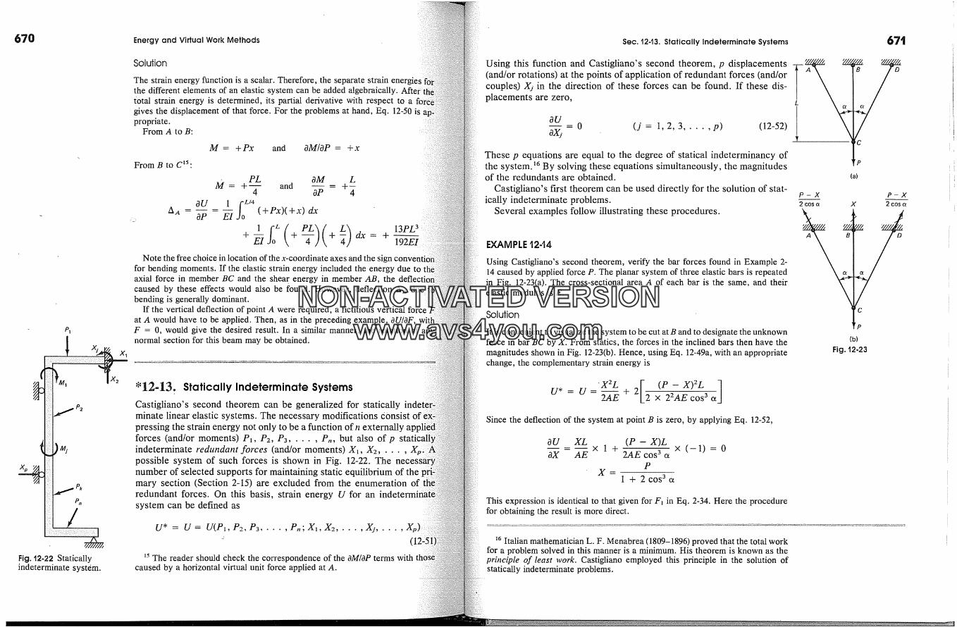
670
P1
FiG. �2-22 Staticallyindeterminate system.
Energy and Virtual Work Methods
Solution
The strain energy function is a scalar. Therefore, the separate strainthe different elements of an elastic system can be added algebraically.total strain energy is determined, its partial derivative with respect to agives the displacement of that force. For the problems at hand, Eq. 12-50 ispropriate.
From A to B:
From B to C�5:
A A --
M = +Px and OM/OP = +x
M = + � and OM LOP - 44
OU 1OP - E1 ( + Px)( + x) dx
+ �] fo L �) dx= + 192---�Note the free choice in location of the x-coordinate axes and the sign
for bending moments. If the elastic strain energy included the energy due toaxial force in member BC and the sheax7 energy in member AB, the defleccaused by these effects would also be found. However, deflection AA duebending is generally dominant.
If the vertical deflection of point A were required, a fictitious vertical forceat A would have to be applied. Then, as in the preceding example, OU/OF,F = 0, would give the desired result. In a similar manner, the rotation ofnormal section for this beam may be obtained.
� 12,-13. Statically Indeterminate SystemsCastigliano's second theorem can be generalized for staticallyminate linear elastic systems. The necessary modifications d0nsistpressing the strain energy not only to be a function of n externallyforces (and/or moments) P�, P2, Pa ..... P,, but also of pindeterminate redundant forces (and/or moments) X�, X2 .....possible system of such forces is shown in Fig. 12-22. Thenumber of selected supports for maintaining static equilibrium of themary section (Section 2-15) are excluded from the enumeration ofredundant forces. On this basis, strain energy U for ansystem can be defined as
U* = U = U(Pi, P2, P3 ..... P,; Xi, X2 ..... X� .....
�5 The reader should check the correspondence of the OM/OP terms withcaused by a horizontal virtual unit force applied at A.
Sec. 12-13. Statically Indeterminate Systems 67t
Using this function and Castigliano's second theorem, p displacements
(and/orrotations)atthepointsofapplicationofredundantforces(and/orA� la/couples.) X� in the direction of these forces can be found. If these dis-placements are zero,
.�U= 0 (j = 1,2,3..... p) (12-52)ox:
Thesep equationsareequalto the degreeof staticalindeterminancyofthe system.�6 By solving these equations simultaneously, the magnitudesof the redundants are obtained.
Castigliano's first theorem can be used directly for the solution of stat-ically indeterminate problems.
Several examples follow illustrating these procedures.
EXAMPLE t244
Using Castigliano's second theorem, verify the bar forces found in Example 2-14 caused by applied force P. The planar system of three elastic bars is repeatedin Fig. 12-23(a). The cross-sectional area A of each bar is the same, and theirelastic modulus is E.
Solution
It is convenient to visualize the system to be cut atB and to designate the unknownforce in bar BC by X. From statics, the forces in the inclined bars then have themagnitudes shown in Fig. 12-23(b). Hence, using Eq. 12-49a, with an appropriatechange, the complementary strain energy is
(a)
P-X P-X2 cos a X 2 cos a
(b)
Fig. 12-23
.X2LU* = U=
2AE + 2[2 (P-X)2L a]Since the deflection of the system at point B is zero, by applying Eq. 12-52,
OU XL (P - X)L- xl+ x
OX AE 2AE cos 3 aP
X-1 + 2 cos 3 a
(-1) = o
This expression is identical to that given for Fx in Eq. 2-34. Here the procedurefor obtaining the result is more direct.
�6 Italian mathematician L. F. Menabrea (1809-1896) proved that the total workfor a problem solved in this manner is a minimum. His theorem is known as theprinciple of least work. Castigliano employed this principle in the solution ofstatically indeterminate problems.
NON-ACTIVATEDVERSIONwww.avs4you.com
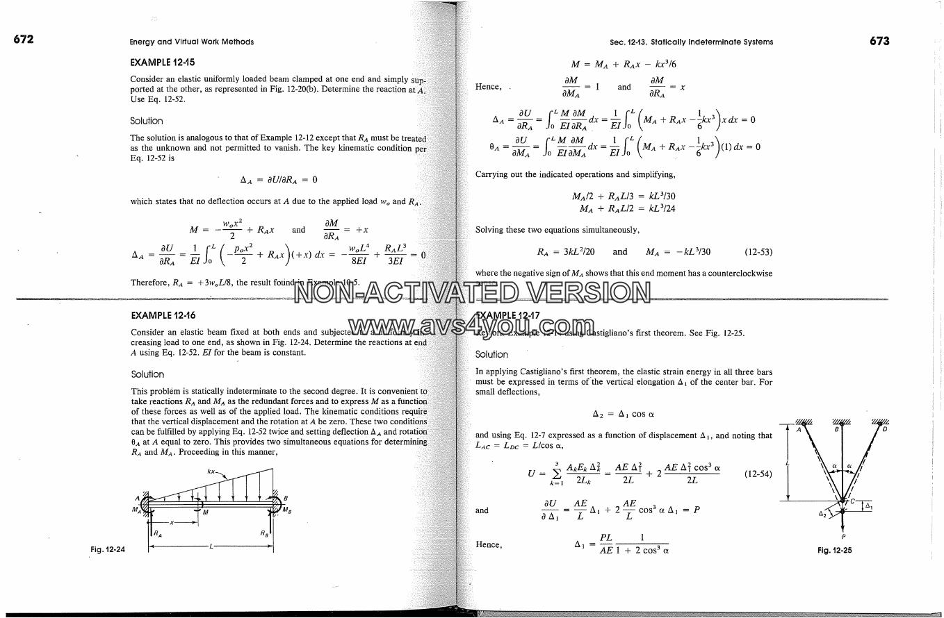
672 Energy and Virtual Work Methods
EXAMPLE t2-15
Consider an elastic uniformly loaded beam clamped at one end and simplyported at the other, as represented in Fig. 12-20(b). Determine the reactionUse Eq. 12-52.
Solution
The solution is analogous to that of Example 12-12 except that RI must be treas the unknown and not permitted to vanish. The key kinematic conditionEq. 12-52 is
A A = OU/ORA = 0
which states that no deflection occurs at A due to the applied load Wo and R21
WoX 2 aMM - + RAX and = +x
2 ORA
AA -- OS 1;oL(__poX2 ) $VoL4 RAL3ORA EI 2 + RAX ( + x) dx = - 8E---[ + 3EI -Therefore, Rt = +3woL/8, the result found in Example 10-5.
Fig. t2-24
EXAMPLE 12-t6
Consider an elastic beam fixed at both ends and subjected to a uniformlycreasing load to one end, as shown in Fig. 12-24. Determine the reactions at endA using Eq. 12-52. E1 for the beam is constant.
Solution
This prob16m is statically indeterminate to the second degree. It istake reactions RI and MI as the redundant forces and to express M as aof these forces as well as of the applied load. The kinematic conditions recthat the vertical displacement and the rotation at A be zero.can be fulfilled by applying Eq. 12-52 twice and setting deflection AI0t at A equal to zero. This provides two simultaneous equationsRt and MI. Proceeding in this manner,
BMB
Sec. 12-t3. Statically Indeterminate Systems
Hence,
M = MA + RAx - kx3/6aM aM
- 1 and - x
Carrying out the indicated operations and simplifying,
MA/2 + RAL/3 = kL�/30MA q- RAL/2 = kL�/24
Solving these two equations simultaneously,
RA = 3kL2/20 and MA = -kL3/30 (12-53)
where the negative sign of Mt shows that this end moment has a counterclockwisesense.
EXAMPLE t2-t7
Rework Example 12-14 using Castigliano's first theorem. See Fig. 12-25.
Solution
In applying Castigliano's f'Lrst theorem, the elastic strain energy in all three barsmust be expressed in terms of'the vertical elongation A � of the center bar. Forsmall deflections,
A2 = A� COS a
and using Eq. 12-7 expressed as a function of displacement A �, and noting thatLAC = LDC = L/cos o�,
� A,E� A�. AE A�2 AE A�2 cos 3 ctU= - 2Lk= � 2Lk 2L + 2 (12-54)
andOU AE
OA� L A� + 2�COS3 aAl = PPL 1
Hence, A � AE1 + 2cos 3ct
673
Fig. t2-25
NON-ACTIVATEDVERSIONwww.avs4you.com

674 Energy and Virtual Work Methods
Then the force in the vertical bar using Eq. 2-10 is
px = kA� = --A� = 1 + 2 COS3 ctThis result is in agreement with that found in Example 12-14.
This type of solution is easily extended to any number of s,bars with A� remaining as the only unknown, regardless of the degree ofterminacy.
If the inclined bars lack symmetry or the applied force forms an angle withvertical, the problem is more complex. In such cases, the elongation in eachis determined from two separate displacements at the load point. Thisis analogous to that shown in Example 12-7 and illustrated in Fig. 12-12.discussion of this approach can be found in Section 13-5, where l�hemethod of analysis is considered.
*'1244. Elastic Energy for Buckling LoadsStability problems can be treated in a very general manner usingenergy or the virtual work methods. As an introduction to suchthe basic �riteria for determining the stability of equilibrium arein this article for conservative linearly elastic systems using an energmethod.
To establish the stability criteria, a function II, called the totalof the system, must be formulated. This function is expressed as theof the internal energy U (strain energy) and the potentialof the external forces that act on a system, i.e.,
ll= U+fl
Disregarding a possible additive constant, fl = -We, i.e., the losspotential energy during the application of the forces is equal todone on the system by the external forces. Hence, Eq. 12-55rewritten as
As is known from classical mechanics, for equilibrium, total tII must be stationary; �7 therefore, its variation 8ll must equal zero, i.
Sll = 8u- 8we= o)�7 In terms of the ordinary functions, this simply means that a condition
where the derivative of a function with respect to an independent variable isand the function itself has a maximum, a minimum, a minimax, or avalue.
Sec. 12-t4. Elastic Energy for Buckling Loads
For conservative, elastic systems, this relation is in agreement with Eq.12-11. This condition can be used to determine the position of equilibrium.However, Eq. 12-57 cannot discern the type of equilibrium and therebyestablish the condition for the stability of equilibrium. Only by examiningthe higher order terms in the expression for the change Alii in the totalpotential II can this be determined. Therefore, the more complete expres-sion for the increment in II .as given by Taylor's expansion must be ex-amined. Such an expression is
Alii = $lii + �.� $2lii + 8�lii + "' (12-58)
Since for any type of equilibrium, 8lii = 0, it is the first nonvanishingterm of this expansion that determines the type of equilibrium. For linearelastic systems, the second term suffices. Thus, from Eq. 12-58, the sta-bility criteria are
I S2lii>0821-I < 0821-I = 0 l forstableequilibriumfor unstable equilibrium
for neutral equilibrium associated withthe critical load
(12-59)
The meaning of these expressions may be clarified by making referenceto Fig. 12-26, where the curve represents the potential function II. Theorigin of this function is shown below the curve, since the absolute valueof II is arbitrary. Three different possible positions of equilibrium for theball are shown in this figure? The first derivative of II at points of equi-librium is zero for all three cases; it is the second derivative that deter-mines the type of equilibrium.
For simple functions of II, the procedures for forming the derivatives,differentials, and variations are alike. If, however, the function of II isexpressed by integrals, the problem becomes mathematically much morecomplicated, requiring the use of the calculus of variations or finite ele-ments. The treatment of such problems is beyond the scope of this text. �9
EXAMPLE t2-t8
Using the energy method, verify the critical load found before for a rigid bar witha torsional spring at the base, Fig. 11-7(a).
�8 A point on a curve resulting from a combination, for example, of the curveto the left of position 1 with that of the curve to the right of position 2 defines aminimax. In stability analysis, such a point corresponds to the condition of un-stable equilibrium.
�9 H. L. Langhaar, Energy Methods in Applied Mechanics (New York: Wiley,1962). K. Washizu, Variational Methods in Elasticity and Plasticity, 2nd ed. (New
York: Pergamon, 1975). J. S. Przemieniecki, "Discrete-Element Methods for Sta-bility Analysis of Complex Structures," Aeron. J. 72(1968): 1077.
675
Fig. t2-26 Differentequilibrium conditions.
NON-ACTIVATEDVERSIONwww.avs4you.com
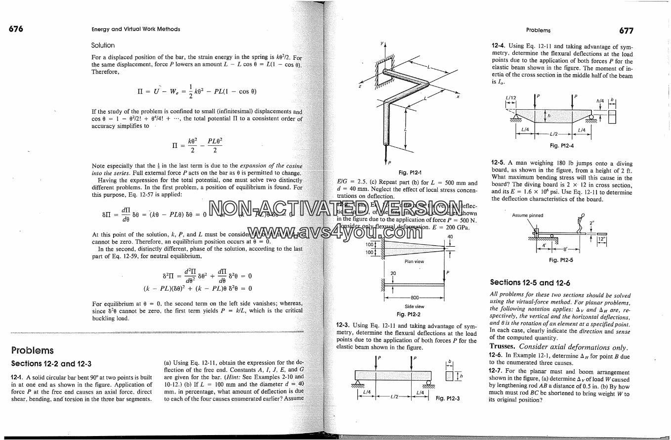
Energy and Virtual Work Methods Problems 677
Solution
For a displaced position of the bar, the strain energy in the spring is k02/2.the same displacement, force P lowers an amount L - L cos 0 = L(1 - cosTherefore,
Yl = U- W, = k02- PL(1 - cos0)
If the study of the problem is confined to small (infinitesimal) displacementscos 0 = 1 - 02/2! + 04/4! + "., the total potential 12 to a consistent order iaccuracy simplifies to
k02 PLO 22 2
Note especially that the � in the last term is due to the expansion of theinto the series. Full external force P acts on the bar as 0 is permitted to
Having the expression for the total potential, one must solve two dis!different problems. In the first problem, a position of equilibrium is found.this purpose, Eq. 12-57 is applied:
an = ao = - P�0) ao = o or (k - PL)O �0 = 0
At this point of the solution, k, p, and L must be considered constant, andcannot be zero. Therefore, an equilibrium position occurs at 0 = 0.
In the second, distinctly different, phase of the solution, according to thepart of Eq. 12-59, for neutral equilibrium,
d2yl dHa2yl =�a02 +�a20 ='0
(k - PL)(g0) 2 + (k - PL)O g20 = 0
For equilibrium at 0 = 0, the second term on the left side vanishes; whereassince g20 cannot be zero, the first term yields P = k/L, which is thebuckling load.
Problems
Sections t2.2 and t2-3
12-t. A solid circular bar bent 90 � at two points is builtin at one end as shown in the figure. Application offorce P at the free end causes an axial force. directshear, bending, andtorsion in the three bar segments.
(a) Using Eq. 12-11, obtain the expression forflection of the free end. Constants A, I, J, E,are given for the bar. (Hint: See Examples10-12.) (b) IlL = 100 mm and the diameter dmm. in percentage, what amount of deflection isto each of the four causes enumerated earlier?
L
P
Fig. DI24
E/G = 2.5. (c) Repeat part (b) for L = 500 mm andd = 40 mm. Neglect the effect of local stress concen-trations on deflection.
t2-:5. Using Eq. 12-11, determine the vertical deflec-tion, in mm, of the free end of the cantilever shownin the figure due to the application of force P = 500 N.Consider only flexural deformation. E = 200 GPa.
�oo I100 1
Plan view
4O
10 P{'� 800 �
Side view
Fig. PI2-2
t2-3. Using Eq. 12-11 and taking advantage of sym-metry, determine the flexural deflections at the loadpoints due to the application of both forces P for theelastic beam shown in the figure.
12-4. Using Eq. 12-11 and taking advantage of sym-metry, determine the flexural deflections at the loadpoints due to the application of both forces P for theelastic beam shown in the figure. The moment of in-ertia of the cross section in the middle half of the beamis Io.
LI12 P P hi4 I_b.I
Fig. PI2-4
t2-5. A man weighing 180 lb jumps onto a divingboard, as shown in the figure, from a height of 2 ft.What maximum bending stress will this cause in theboard? The diving board is 2 x- 12 in cross section,and its E = 1.6 x 10⁶ psi. Use Eq. 12-11 to determinethe deflection characteristics of the board.
Assume pinned �:)
4�-�-� 8' � �Fig. PI2-5
Sections �2-5 and �2-6
All problems for these two sections should be soh,edusing the virtual-force method. For planar problems,the following notation applies: �v and �n are, re-spectively, the vertical and the horizontal deflections,and 0 is the rotation of an element at a specified point.In each case, clearly indicate the direction and senseof the computed quantity.Trusses. Consider axial deformations only.12-6. In Example 12-1, determine A n for point B dueto the enumerated three causes.
12-7. For the planar mast and boom arrangementshown in the figure, (a) determine A v of load W causedby lengthening rod AB a distance of 0.5 in. (b) By howmuch must rod BC be shortened to bring weight W toits original position?
NON-ACTIVATEDVERSIONwww.avs4you.com
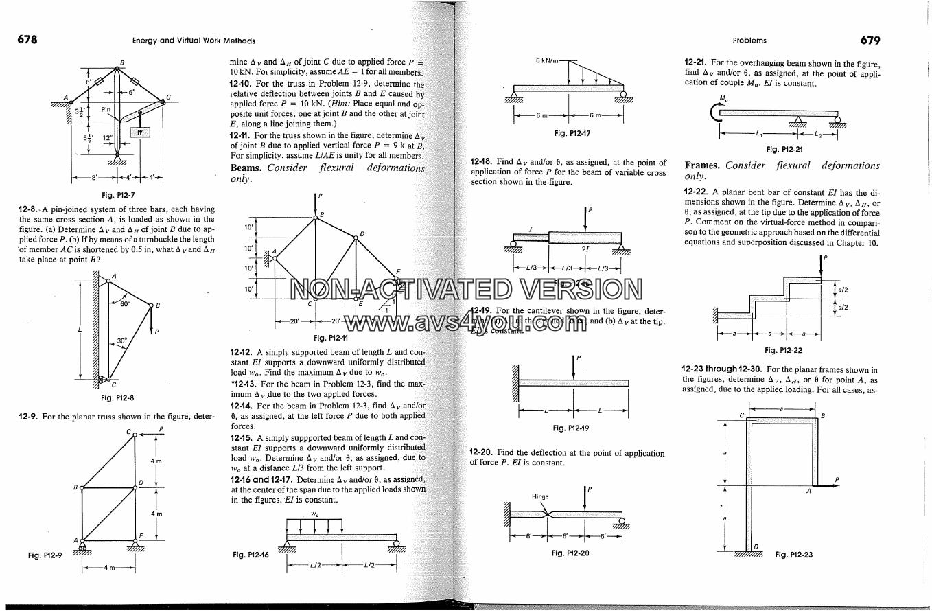
678 Energy and Virtual Work Methods Problems 679
B
Fig. Pt2-7
12-8.-A pin-joined system of three bars, each havingthe same cross section A, is loaded as shown in thefigure. (a) Determine A v and Au of joint B due to ap-plied force P. (b) If by means of a turnbuckle the length
'of member AC is shortened by 0.5 in, what A v and Autake place at point B?
Fig. PI2-8
12-9. For the planar truss shown in the figure, deter-
Fig. P12-9
A� E
�',-----4 m �
mine �x v and An of joint C due to applied force10 kN. For simplicity, assumeAE = 1 for all m,
12-t0. For the truss in Problem 12-9, determinerelative deflection between joints B and E causedapplied force P = 10 kN. (Hint: Place equalposite unit forces, one at joint B and the other atE, along a line joining them.)12-tl. For the truss shown in the figure, determiniof joint B due to applied vertical force P = 9 k atFor simplicity, assume L/AE is unity for all membBeams. Conside;' flexuralonly.
lo, t10'
10' IC E
Fig. PI24t
1242. A simply supported beam of length L andstant E1 supports a downward uniformlyload Wo. Find the maximum A v due to Wo.'1243. For the beam in Problem 12-3, find theimum A v.due to the two applied forces.t2-14. For the beam in Problem 12-3, find Av0, as assigned, at the left force P due to bothforces.
t2-t5. A simply suppported beam of length L andstant EI supports a downward uniformlyload Wo. Determine A v and/or 0, as assigned, dueWo at a distance L/3 from the left support.12-16 and 12-17. Determine �xv and/or 0, asat the center of the span due to the applied loadsin the figures. 'EI is constant.
Fig. Pt2-16 14- L/2 �' ""ei---L/2
-6m > � 6mFig. Pt2-� 7
t248. Find A v and/or 0, as assigned, at the point ofai3plication of force P for the beam of variable cross
.section shown in the figure.
Fig. P12-18
t2-19. For the cantilever shown in the figure, deter-mine (a) A v at the applied force, and (b) A v at the tip.
EI is constant.
"� L � < L -Fig. PI2-19
12-20. Find the deflection at the point of applicationof force P. E1 is constant.
z Hinge ! P
Fig. PI2-20
t2-2t. For the overhanging beam shown in the figure,find A v and/or 0, as assigned, at the point of appli-cation of couple Mo. E1 is constant.
Mo
Fig. PI2-21
Frames. Conside;' flexural deformationsonly.t2-22. A planar bent bar of constant EI has the di-mensions shown in the figure. Determine A v, Au, or0, as assigned, at the tip due to the application of forceP. Comment on the virtual-force method in compari-son to the geometric approach based on the differentialequations and superposition discussed in Chapter 10.
Fig. PI2-22
P
� a/2
12-23 through 12-30. For the planar frames shown inthe figures, determine A v, Au, or 0 for point A, asassigned, due to the applied loading. For all cases, as-
-.e----ii-- a �.
�. Fig. PI2-23
P
NON-ACTIVATEDVERSIONwww.avs4you.com
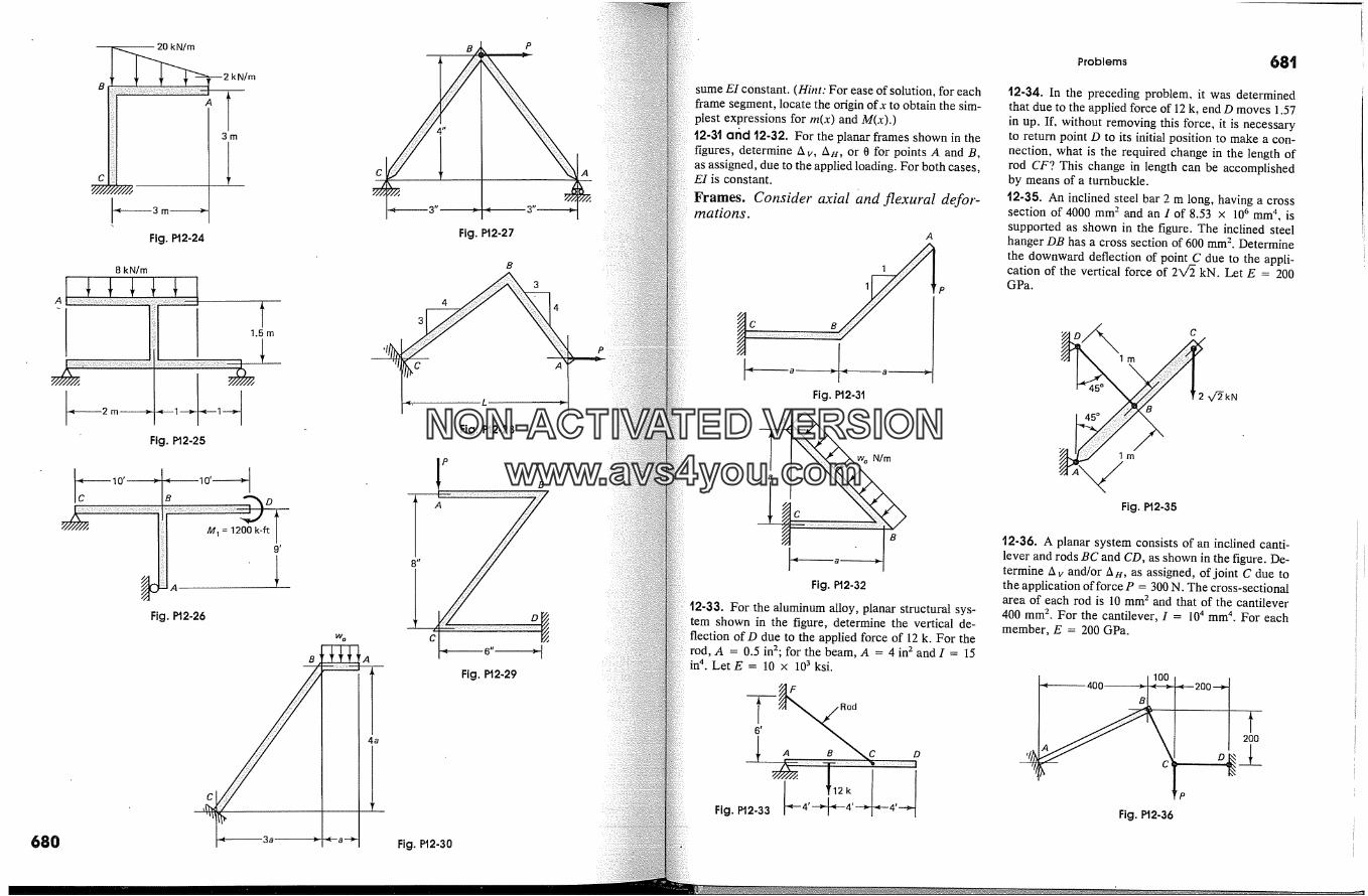
/m
A
k N/m
3m
Fig. PI2.24
8 kN/m
1,5 m
Fig, PI2-25
680
B D9'Fig. PI2-26
Wo
B A
P
Fig. PI2-27
B
3
4
Fig. PI2-28
P B/
Fig. PI2-29
Fig. PI2-30
sume EI constant. (Hint: For ease of solution, for eachframe segment, locate the origin ofx to obtain the sim-plest expressions for m(x) and M(x).)t2-;5t oriel t2-32. For the planar frames shown in thefigures, determine Av, Au, or 0 for points A and B,as assigned, due to the applied loading. For both cases,EI is constant.
Frames. Consider axial and flexural defor-mations.
A
Fig. PI2-3t
'� a ' ;-IBFig. P'12-32
t2-33. For the aluminum alloy, planar structural sys-tem shown in the figure, determine the vertical de-flection of D due to the applied force of 12 k. For therod, A = 0.5 in2; for the beam, A = 4 in 2 and I = 15in 4. Let E = 10 x 103 ksi.
6,--� Rod
Problems 68�
12-34. In the preceding problem, it was determinedthat due to the applied force of 12 k, end D moves 1.57in up. If, without removing this force, it is necessaryto return point D to its initial position to make a con-nection, what is the required change in the length ofrod CF? This change in length can be accomplishedby means of a turnbuckle.
t2-35. An inclined steel bar 2 m long, having a crosssection of 4000 mm 2 and an I of 8.53 x 10 a mm 4, issupported as shown in the figure. The inclined steelhanger DB has a cross section of 600 mm 2. Determinethe downward deflection of point C due to the appli-cation of the vertical force of 2X/� kN. Let E = 200GPa.
2x,/�kN
Fig. PI2-35
t2-36. A planar system consists of an inclined canti-lever and rods BC and CD, as shown in the figure. De-termine � v and/or flu, as assigned, of joint C due tothe application of force P = 300 N. The cross-sectionalarea of each rod is 10 mm 2 and that of the cantilever400 mm 2. For the cantilever, I = 10 4 mm 4. For eachmember, E = 200 GPa.
/ 400 I 100 t 200--*,-
Fig. PI2-36
NON-ACTIVATEDVERSIONwww.avs4you.com
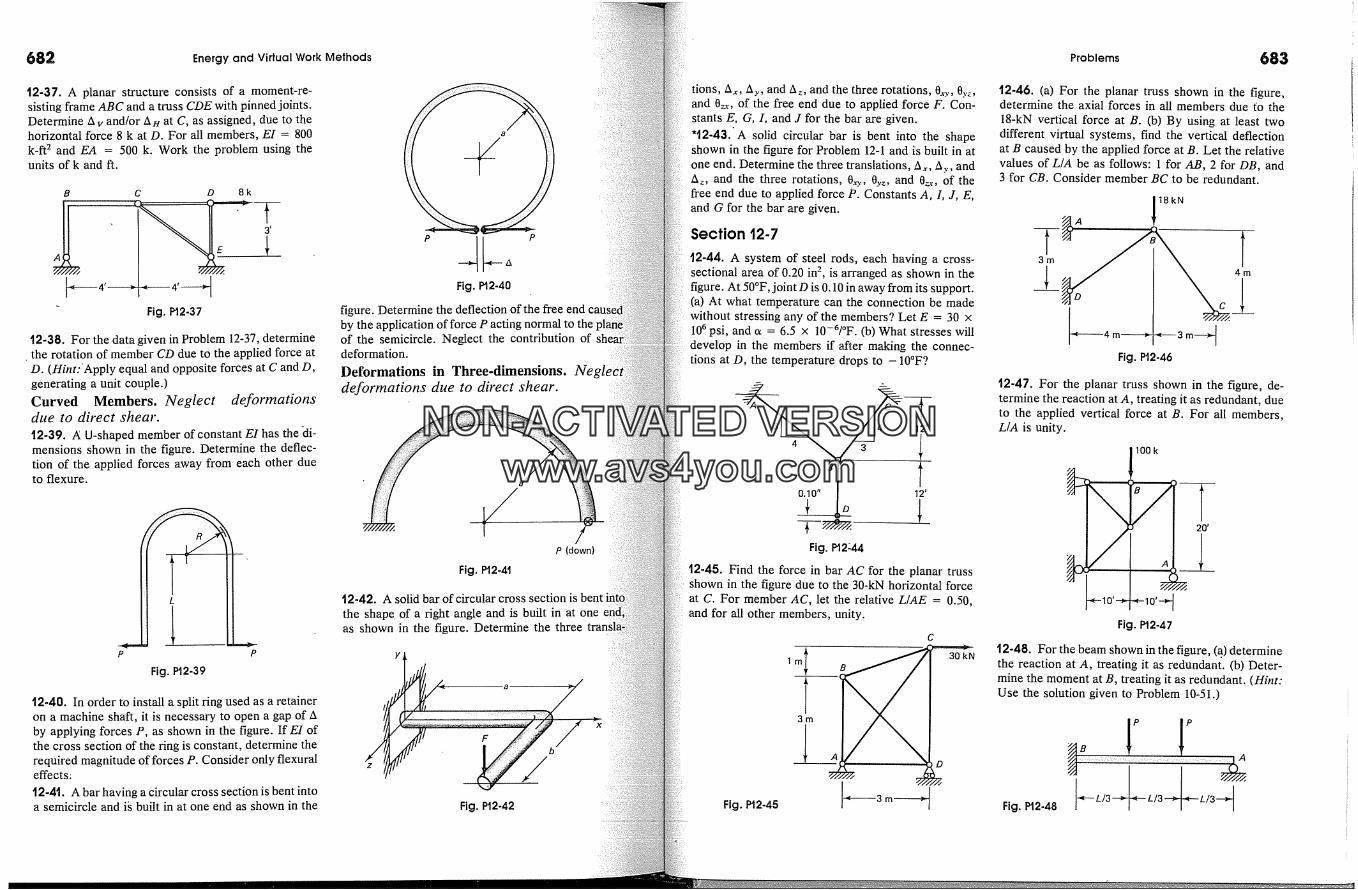
682 Energy and Virtual Work Methods Problems 683
t2-37. A planar structure consists of a moment-re-sisting frame ABC and a truss CDE with pinned joints.Determine Av and/or Au at C, as assigned, due to thehorizontal force 8 k at D. For all members, EI = 800k-ft 2 and EA = 500 k. Work the problem using theunits of k and ft.
B c D 8k
3'
E �
Fig. PI2-37
12-38. For the data given in Problem 12-37, determinethe rotation of member CD due to the applied force atD. (Hint:'Apply equal and opposite forces at C and D,generating a unit couple.)Curved Members. Neglect deformationsdue to direct shear.12-39. A U-shaped member of constant EI has the �li-mensions shown in the figure. Determine the deflec-tion of the applied forces away from each other dueto flexure.
Fig. PI2-39
t2-40. In order to install a split ring used as a retaineron a machine shaft, it is necessary to open a gap of Aby applying forces P, as shown in the figure. If EI ofthe cross section of the ring is constant, determine therequired magnitude of forces P. Consider only flexuraleffects:
12-41. A bar having a circular cross section is bent intoa semicircle and i� built in at one end as shown in the
a
Fig. PI2.40
figure. Determine the deflection of the free endby the application of force P acting normal to theof the semicircle. Neglect the contribution ofdeformation.
Deformations in Three-dimensions. Negleidefortnations due to direct shear.
a
P (down)
Fig. PI2-4t
t2-42. A solid bar of circular cross section isthe shape of a right angle and is built in at oneas shown in the figure. Determine the three
a
F
Fig. P12-42
tions, ,%, A.,., and ,x�., and the three rotations, 0�., 0y�,and 0,�, of the free end due to applied force F. Con-stants E, G, I, and J for the bar are given.'t2-43.'A solid circular bar is bent into the shapeshown in the figure for Problem 12-1 and is built in atone end. Determine the three translations, Ax, A.,., andA�, and the three rotations, 0:o., 0y�, and 09, of thefree end due to applied force P. Constants A, I, J, E,and G for the bar are given.
Section 12-7
t2-44. A system of steel rods, each having a cross-sectional area of 0.20 in 2, is arranged as shown in thefigure. At 50�F, joint D is 0.10 in away from its support.(a) At what temperature can the connection be madewithout stressing any of the members? Let E = 30 x10 6 psi, and c� = 6.5 x 10⁻⁶/�F. (b) What stresses will
develop in the members if after making the connec-tions at D, the temperature drops to - 10�F?
Fig. PI2:44
t2-45. Find the force in bar AC for the planar trussshown in the figure due to the 30-kN horizontal forceat C. For member AC, let the relative L/AE = 0.50,and for all other members, unity.
c
Fig. PI2-45
1m!m 30kN< 3m �
'12-46. (a) For the planar truss shown in the figure,determine the axial forces in all members due fo the18-kN vertical force at B. (b) By using at least twodifferent virtual systems, find the vertical deflectionat B caused by the applied force at B. Let the relativevalues of L/A be as follows: 1 for AB, 2 for DB, and3 for CB. Consider member BC to be redundant.
18kN
-"<---3 mFig. PI2-46
'12-47. For the planar truss shown in the figure, de-termine the reaction at A, treating it as redundant, dueto the applied vertical force at B. For all members,L/A is unity.
100k
10' -� �'-10'-�Fig. PI2-47
12-48. For the beam shown in the figure, (a.) determinethe reaction at A, treating it as redundant. (b) Deter-mine the moment at B, treating it as redundant. (Hint:Use the solution given to Problem 10-51.)
�B 1P 1P A
NON-ACTIVATEDVERSIONwww.avs4you.com
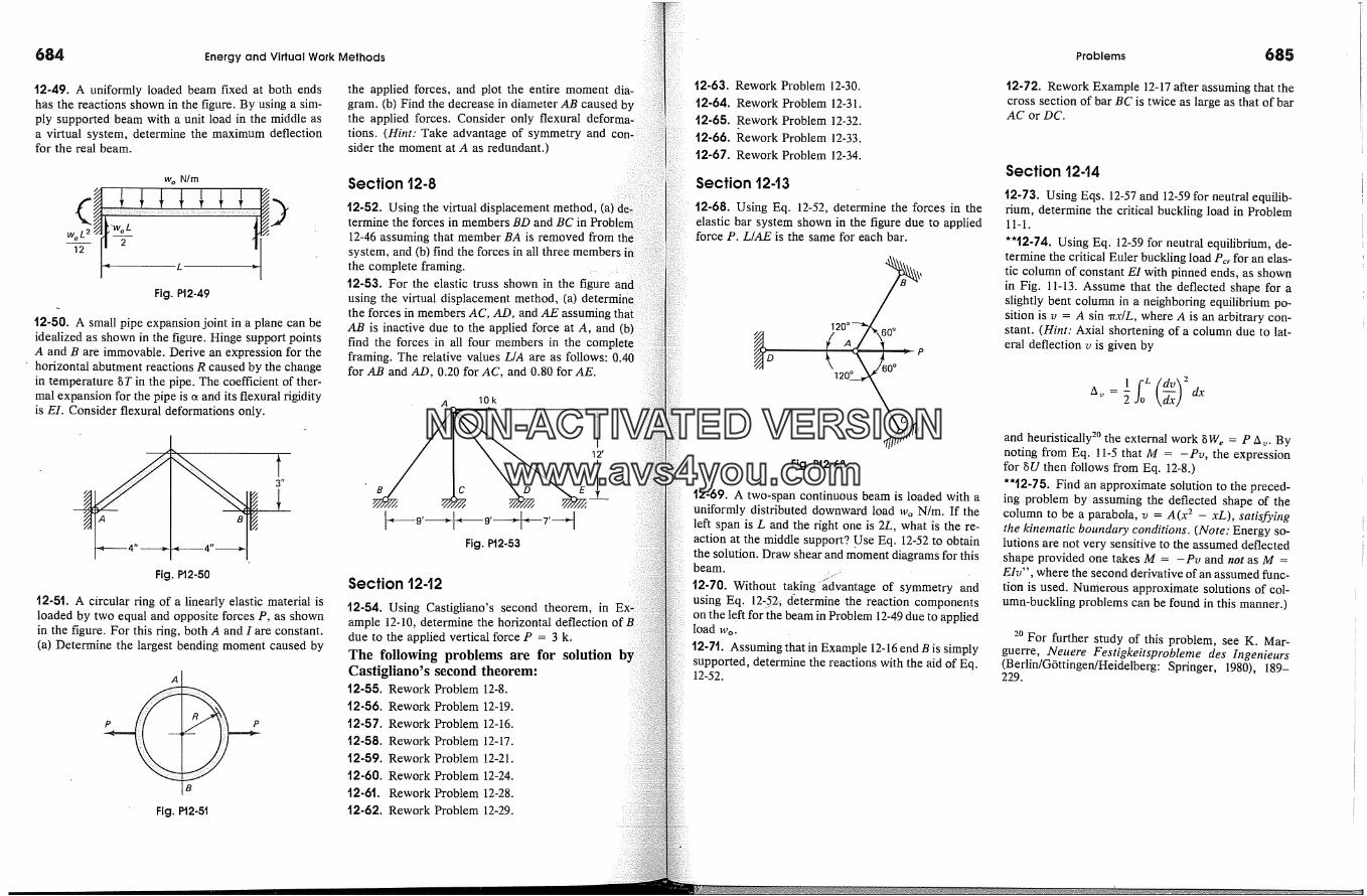
684 Energy and Virtual Work Methods
t2-49. A uniformly loaded beam fixed at both endshas the reactions shown in the figure. By using a sim-ply supported beam with a unit lead in the middle asa virtual system, determine the maximum deflectionfor the real beam.
the applied forces, and plot the entire moment dia-gram. (b) Find the decrease in diameter AB caused bythe applied forces. Consider only flexural deforma-tions. (Hint: Take advantage of symmetry and con�sider the moment at A as redundant.)
w o N/m
Fig. P12-49
12-50. A small pipe expansion joint in a plane can beidealized as shown in the figure. Hinge support pointsA and B are immovable. Derive an expression for the
' horizontal abutment reactions R caused by the changein temperature gT in the pipe. The coefficient of ther-mal expansion for the pipe is ct and its flexural rigidityis EI. Consider flexural deformations only.
Fig. Pt2-50
12-5t. A circular ring of a linearly elastic material isloaded by two equal and opposite forces P, as shownin the figure. For this ring, both A and I are constant.(a) Determine the largest bending moment caused by
A
Fig. Pt2-5t
12-63. Rework Problem 12-30.12-64. Rework Problem 12-31.
t2-65. Rework Problem 12-32.12-66. Rework Problem 12-33.12-67. Rework Problem 12-34.
Section 12-8
12-52. Using the virtual displacement method,termine the forces in members BD and BC in Prob
12-46 assuming that member BA is removed fromsystem, and (b) find the forces in all three membersthe complete framing.12-53. For the elastic truss shown in the figureusing the virtual displacement method, (a)the forces in members AC, AD, and AE assuming thatAB is inactive due to the applied force at A, and (b) [find the forces in all four members in the complete[framing. The relative values L/A are as follows: 0.40 Ifor AB and AD, 0.20 for AC, and 0.80 for AE.
1Ok
C E
Fig. P12-53
Section t2-12
t2-54. Using Castigliano's second theorem, inample 12-10, determine the horizontal deflectiondue to the applied vertical force P = 3 k.
The following problems are for solution bCastigliano's second theorem:12-55. Rework Problem 12-8.
12-56. Rework Problem 12-19.
12-57. Rework Problem 12-16.
12-58. Rework Problem 12-17.
t2-59. Rework Problem 12-21.
t2-60. Rework Problem 12-24.
t2-6t. Rework Problem 12-28.
t2-62. Rework Problem 12-29.
Section 1243
12-68. Using Eq. 12-52, determine the forces in theelastic bar system shown in the figure due to appliedforce P. L/AE is the same for each bar.
120 � 60 �
D
12
Fig. Pt2-68
t2-69. A two-span continuous beam is loaded with auniformly distributed downward lead we N/m. If theleft span is L and the right one is 2L, what is the re-action at the middle support? .Use Eq. 12-52 to obtainthe solution. Draw shear and moment diagrams for thisbeam.
t2-70. Without taking "�dx�antage of symmetry andusing Eq. 12�52; determine the reaction componentson the left for the beam in Problem 12-49 due to appliedlead We.
t2-71. Assuming that in Example 12-16 end B is simplysupported, determine the reactions with the aid of Eq.12-52.
Problems 685
12-72. Rework Example 12-17 after assuming that thecross section of bar BC is twice as large as that of bar
AC or DC.
Section t244
12-73. Using Eqs. 12-57 and 12-59 for neutral equilib-rium, determine the critical buckling lead in Problem11-1.
*'t2-74. Using Eq. 12-59 for neutral equilibrium, de-termine the critical Euler buckling lead Per for an elas-tic column of constant EI with pinned ends, as shownin Fig. 11-13. Assume that the deflected shape for aslightly bent column in a neighboring equilibrium po-sition is v = A sin �rx/L, where A is an arbitrary con-stant. (Hint: Axial shortening of a column due to lat-eral deflection v is given by
,x,, = 5 fo L axand heuristically 2� the external work gW� = P A,. Bynoting from Eq. 11-5 that M = -Pv, the expressionfor gU then follows from Eq. 12-8.)*'t2-75. Find an approximate solution to the preced-ing problem by assuming the deflected shape of thecolumn to be a parabola, v = A(x 2 - xL), satisJ�,ingthe kinematic boundary conditions. (Note: Energy so-lutions are not very sensitive to the assumed deflectedshape provided one takes M = -Pv and not as M =EIv", where the second derivative of an assumed func-tion is used. Numerous approximate solutions of col-umn-buckling problems can be found in this manner.)
20 For further study of this problem, see K. Mar-guerre, Neuere Festigkeitsprobleme des Ingenieurs(Berlin/G6ttingen/Heidelberg: Springer, 1980), 189-229.
NON-ACTIVATEDVERSIONwww.avs4you.com

=chapter
686
*x13-1. IntroductionThe force and displacement methods for solving linearly elastic staticall'indeterminate problems previously encountered in this text are exterin Part A of this chapter to more complex cases. These two methodsparticularly important in the matrix analysis of structures and inelement formulations. They are directly applicable in satisfyingdesign criteria often based on the maximum allowable stress. Such ateflon is referred to as the limit state for the maximum stress. Incases, the limit state may be the maximum allowable deflection, oreffect of system stiffness on vibrations. Such criteria arelimit states.
If the �trength of a member or members for emergency ovethe only controlling parameter, the elastic maximum stress limit statelead to an unduly conservative design. For ductile materials, wherefatigue problem does not arise, merely reaching the maximuma point or a few points of a member does not necessarily exhauststrength capacity of a system. The ultimate strength of such systemsbe reasonably well approximated by considering theplastic. A few such cases were encountered earlier. This approachdiscussed in Part B of this chapter for beams and frames. 2 Thelimit state is of considerable importance in understanding thebehavior of ductile structures, especially as it applies to seismic desiand other emergency overload situations.
� This chapter is optional.2 For further discussion of beams, frames, as well as plates and shells, see
G. Hodge. Jr., Plastic Analysis of Structures (New York: McGraw-Hill,
Sec. 13-3. Force Method
� 13-2. Two Basic Methods for Elastic AnalysisStructural systems that experience only small deformations and are com-posed of linearly elastic materials are linear structural systems. The prin-ciple ofsuperposition is applicable for such structures and forms the basisfor two of the most effective methods for the analysis of indeterminatesystems.
In the first of these methods, a statically indeterminate system is re-duced initially to one that is determinate by removing redundant (super-fluous) reactions or internal forces for maintaining static equilibrium; seeFig. 2-42. Then these redundant forces are considered as externally ap-plied, and their magnitudes are so adjusted as to satisfy the prescribeddeformation conditions at their points of application. Once the redundantreactions are determined, the system is statically determinate and can beanalyzed for strength or stiffness characteristics by the methods intro-duced earlier. This widely used method is commonly referred to as the
force �nethod, or the flexibility method; see Section 2-15.In the second method, referred to as the displacement method, or the
stiffness method, the joint displacements of a structure are treated as theunknowns; see Sections 2-16 and 2-17. The system is first reduced to aseries of members whose joints are imagined to be completely restrainedfron any movement. The joints are then released to an extent sufficientto satisfy the force equilibrium conditions at each joint. This method isextremely well-suited for computer coding and, hence, is even morewidely used in practice than the force method, especially for the analysisof large-scale structures.
While some of the older classical methods continue to have some utility,the force and displacement methods are the two modern approaches tothe solution of indeterminate structural systems.
'13-3. Force Method
The first step in the analysis of structural systems using the force methodis the determination of the degree of statical indeterminacy, which is thesame as the number of redundant reactions, as discussed in Sections 1-9 and 2-15. The redundant reactions 3 are temporarily removed to obtaina statically determinate structure, which is referred to as the released or
3 In the analysis of beams and flames, the bending moments at the supportsare often treated as redundants. In such cases, rotations of tangents at the supportsare considered instead of deflections.
687
NON-ACTIVATEDVERSIONwww.avs4you.com

688
Fig. 13-1 Superposition forthe force method.
Statically Indeterminate Problems
primary structure. Then, since this structure is artificially reduced toical determinacy, it is possible to find any desired displacement bymethods previously discussed. For example, the beam shown in Fig.l(a) is indeterminate to the first degree. For this beam to remain in st:static equilibrium, only one of the vertical reactions can be removRemoving the vertical reactions at b, Fig. 13-1(b), deflectioncaused by applied forces P can be calculated. By reapplying the removelredundant reaction Rb to the unloaded member, Fig. 13-1(c),A � at b due to Ro can be found. Since the deflection at b of thebeam must be zero, by superposing the deflections and requiring that+ A ob = 0, the magnitude of Ro = Xo can be determined.
This procedure can be generalized to any number of redundanttions. However, it is essential in such cases to recognize that theplacement of evet�y point on the pritna�y structure is affected by ea,reapplied redundant force. This also holds true for the rotation ofments. As an example, consider the beam in Fig. 13-2(a).
By removing any two of the redundant reactions such as Ro andthe beam becomes determinate and the deflections at b and c cancomputed, Fig. 13-2(b). These deflections are designated Ao,, and Arespectively, where the first letter of the subscript indicates thewhere the deflection occurs, and the second, the cause of the deflectioBy reapplying Rb to the same beam, the deflections at b and c due toat b can be found, Fig. 13-2(c). These deflections are designatedA,.o, respectively. Similarly, Aoc and Ac�, due to R�, can beFig. 13-2(d). Superposing the deflections at each support and settinsum equal to zero, since points b and c actually do not deflect,two equations:
Ab = AoJ o + Aoo + AOc = 0 (13dA� = A�., + Aco + A� = 0
These can be rewritten in a more meaningful form using flexibilityticlents �oo, �o�., �cO, and ��, which are defined as the deflectionsin Figs. 13-1(e) and (f) due to unit forces applied in the direction
[P� b [P2a b c (b)
(a)
�bb
R�, = X�
(c)
w I & P2 JP�
(a)
w / P,
9'////// � b P
(b)
P2 JP3
Sec. 13-3. Force Method
�/. b ctR, =xc(d)
ll N
(e)
Rb = Xb 1(c) (f)
redundants. Then, since a linear structural system is being considered,the deflection at point b due to the redundants can be expressed as
and Abe = �o�X� (13-2)
and, similarly, at point c as
and Ac� = f�X� (13-3)
where Xb and Xc are the redundant quantities. Using this notation, Eq.13-1 becomes
A o = fooXo + fb�X� + A oio = 0A� = f�oXo + fc�X� + A�io = 0
(13-4)
where the only unknown quantities are Xo and X�; simultaneous solutionof these equations constitutes the solution of the problem.
Generalizing the above results for' determining the unknown forces forsystems with n redundants, using superposition, the following compati-bility equations 4 can be formed:
A a = f,�,�X,� + f,�bXb + '" + f,�.X. +A b = fbaXa + fbbXb + '" + fbnXn + Abe (13-5)
:
A,, = f,,,�Xb + f,,bXb + '" + f,,,,X,, +
4 Sometimes these expressions are referred to as the Maxwell-Mohr equations.
689
Fig. 13-2 Superposition for acontinuous beam.
NON-ACTIVATEDVERSIONwww.avs4you.com

690 Statically Indeterminate Problems Sec. 13-4. Flexibility Coefficients Reciprocity
When the redundant supports are immovable, the left column of thiequation is zero. Alternatively, such deflections can be prescribed. sterms for deflections in the right column can be calculated for thestructure. The flexibility coefficients 6 �u are for the whole primary sy.,tem. All quantities in these equations represent either deflections orgular rotations, depending on whether they are associated with forcescouples.
For the force method, it is customary to express Eq. 13-5 inform as
Xb
Because the square matrix is made up of the flexibility coefficients,method is often called the flexibility method of structural analysis.
It should be clearly understood that the previous equations arecable only to linearly elastic systems that undergo smallIt should be noted further that the matrix exhibited by Eq. 13-6 is aor global flexibility matrix. Such matrices can be readily constructedrectly only for the simpler problems. For treatment of moreproblems, the reader is referred to previously cited texts on finite elemeniior structural matrix analysis in Sections 2-10 and 12-9.
Before proceeding with examples, it is shown next that the matrixthe flexibility coefficients �u is symmetric, i.e., �u = �Ji.
� 13-4. Flexibility Coefficients ReciprocityAccording to the definition for flexibility coefficients, for linearlysystems, the displacement A� at i due to forces P� at i and Pj atjafter Eq. 13-5 can be expressed as
A� = f�P� + fuP.�
Similarly, the deflection at j is
Ai = f�Pi + f�P�
where f�i, fu, ��i, and �� are the flexibility coefficients of a givenIf the strain energy of the system due to the application of tk
is U, according to Castigliano's second theorem, Eq. 12-47, thequalities are also given as
5 If an elastic support is provided at an ith point, the flexibilitythe support is increased by adding the flexibility of such a support.
a The flexibility coefficients are also called the deflection influence co�
<- a ;11 N
(a) (b)
au au
zx� = oP--5- and zXs = �By taking partial derivatives of Az with respect to Pi in Eq. 13-5a and
the preceding equation, the following equality is obtained:
OAi O2UoP: oP:
and, similarly, aAj = a2UaPi fJi - aPi OPjHowever, since the order of differentiation is immaterial,
..f�i= f�, ) (13-7)As illustrated in Fig. 13-3, this relation states that the displacement at anypoint i due to a unit force at any point j is equal to the displacement of
j due to a unit force at i, provided the directions of the forces and de-flections in each of the two cases coincide. It can be noted that this re-lationship holds true for several cases considered earlier in applicationsof virtual force equations in Section 12-6. For example, in calculatingflexibility coefficients, using Eq. 12-26, by setting Fi equal to unit forcep�, its role with 2' is interchangable. This is also true in the use of Eqs.
12-27 and 12-28.
The derived relationship is often called Maxwell's theorem of reciprocaldisplacements. 7
EXAMPLE '13-'1
For the simply supported elastic beam shown in Fig. 13-4, show that the rotationof the tangent to the elastic curve at the support i, caused by applying a unit forceat j, is equal to the deflection atj caused by applying a unit couple at i.
7 This relationship was discovered by James Clerk Maxwell in 1864. The moregeneral case was demonstrated by E. Betti in 1872.
Fig. t3-3 Reciprocaldeflections fij = fji.
NON-ACTIVATEDVERSIONwww.avs4you.com
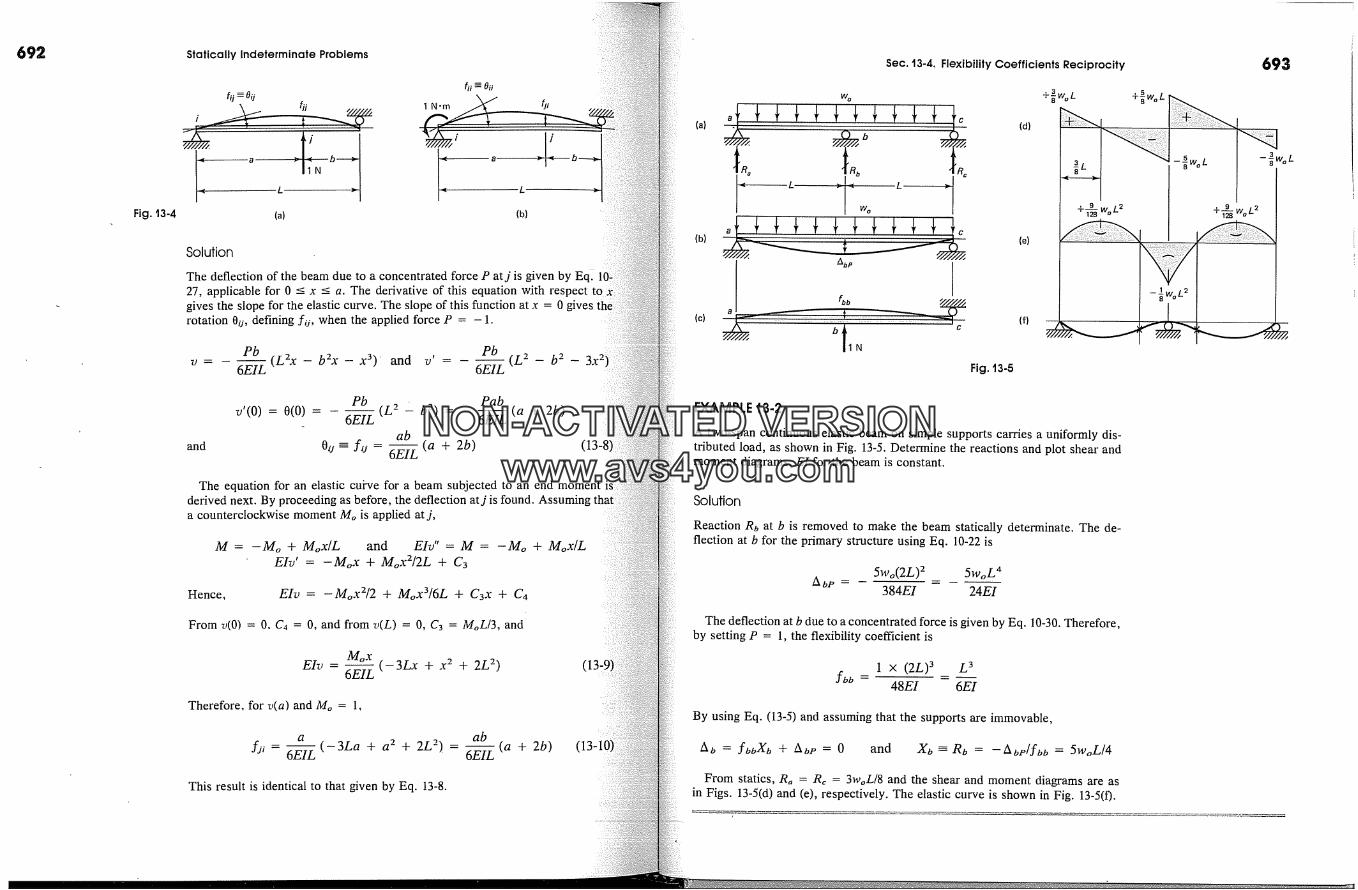
692 Statically Indeterminate ProblemsSec. 13-4. Flexibility Coefficients Reciprocity 693
Fig. 13-4
�------0 U
(a)
1 N'm
L
(b)
Solution
The deflection of the beam due to a concentrated force P atj is given by Eql 10�27, applicable for 0 < x < a. The derivative of this equation with respect togives the slope for the elastic curve. The slope of this function at x = 0rotation 0ij, defining fo, when the applied force P = - 1.
Pb Pbv = - --(L2x - b2x - x3) ' and v' = -- --(L 2 - b 2 - 3x 2
6EIL 6EIL
Pb Pabv'(O) = 0(0) = -- --(L 2 -- b 2) = i I ( a + 2b)
6EIL 6EILab
and 0o -- fu = 6--� (a + 2b) (13-8The equation for an elastic cui-ve for a beam subjected to an end moment
derived next. By proceeding as before, the deflection atj is found. Assumira counterclockwise moment Mo is applied at j,
M = -Mo + Mox/.L and EIv"= M = -Mo + Mox/LEIv'= -Mox + Mox2/2L + C3
Hence, EIv= -Mox2/2 + MoX3/6L + C3x + C4
From v(0) = 0. C4 = 0, and from v(L) = 0, C3 = MoL/3, and
moxEIv -
6EIL- -- (- 3Lx + )5 2 q- 2L 2)
Therefore, for v(a) and Mo = 1,
a
f �i - 6EIL- --(-3La + a 2 + 2L 2) -ab
6EIL- --(a + 2b)
This result is identical to that given by Eq. 13-8.
< L �L �
f� .�(c) t �b
1N
(b) (e)
+�%L
�L � -�woL
9 woL 2+T� , e woL 2
_1 2�WoL
Fig. t3-5
EXAMPLE t3-2
A two-span continuous elastic beam on simple supports carries a uniformly dis-tributed load, as shown in Fig. 13-5. Determine the reactions and plot shear andmoment diagrams. EI for the beam is constant.
Solution
Reaction R0 at b is removed to make the beam statically determinate. The de-flection at b for the primary structure using Eq. 10-22 is
A bP i5Wo(2L) 2 5woL 4
384EI 24EI
The deflection at b due to a concentrated force is given by Eq. 10-30. Therefore,by setting P = 1, the flexibility coefficient is
fbb =1 x (2L) 3 L 3
48EI 6EI
By using Eq. (13-5) and assuming that the supports are immovable,
Ab = fbbXb + Abe = 0 and Xb = Rb = --Abv/fbb = 5woL/4
From statics, R� = Rc = 3woL/8 and the shear and moment diagrams are asin Figs. 13-5(d) and (e), respectively. The elastic curve is shown in Fig. 13-5(0.
NON-ACTIVATEDVERSIONwww.avs4you.com
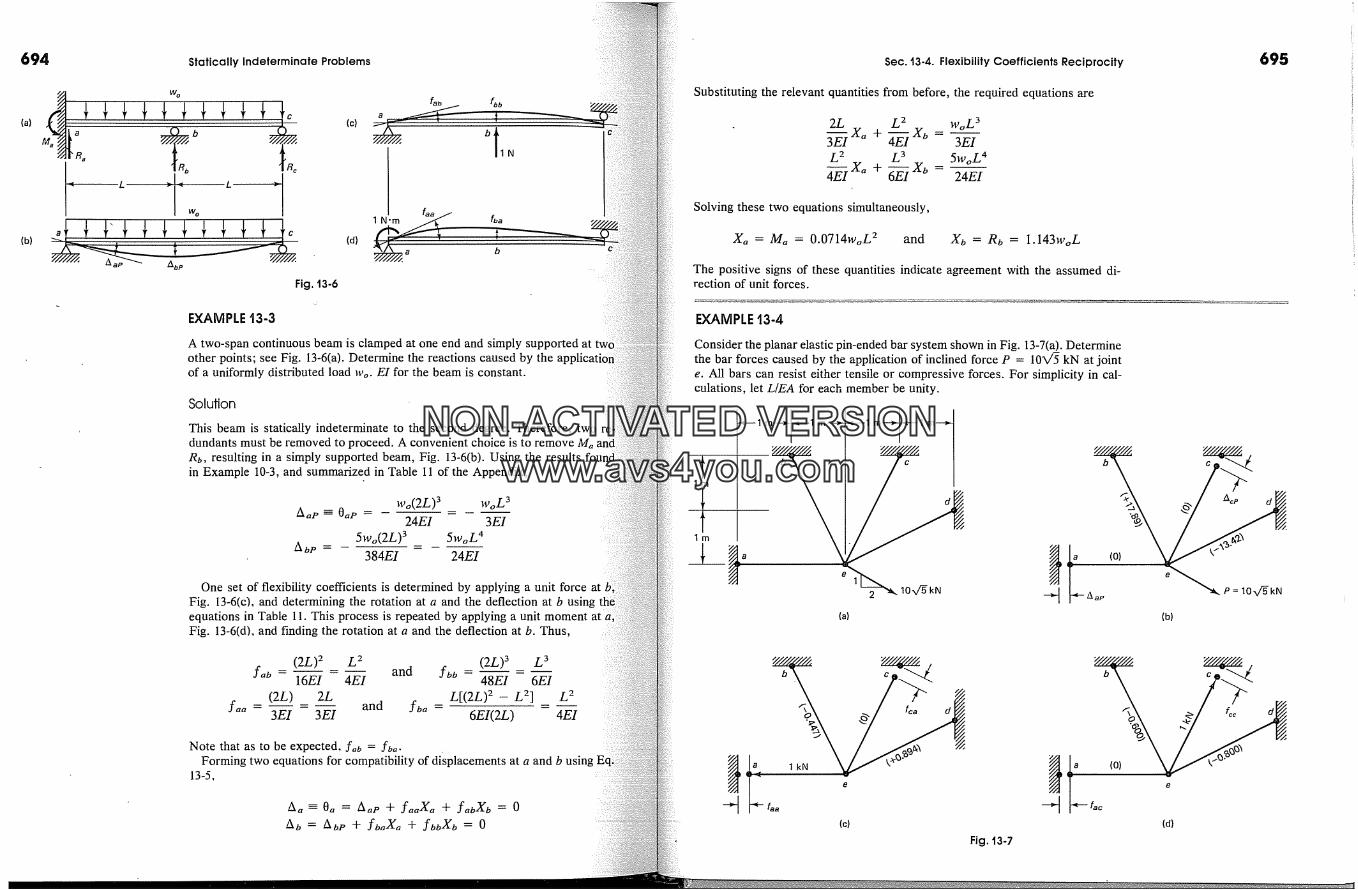
694 Statically Indeterminate Problems Sec. t3-4. Flexibility Coefficients Reciprocity
(a)
(b)
Abp
(c)
fa� fbb
Fig, t3-6
fba
EXAMPLE t3-3
A two-span continuous beam is clamped at one end and simply supported atother points; see Fig. 13-6(a). Determine the reactions caused by theof a uniformly distributed load wo. EI for the beam is constant.
Solution
This beam is statically indeterminate to the second degree. Therefore, twodundants must be removed to proceed. A convenient choice is to removeRb, resulting in a simply supported beam, Fig. 13-6(b). Using the results fouin Example 10-3, and summarized in Table 11 of the Appendix,
wo(2L) 3 woL �24EI 3EI
5wo(2L) 3 5woL 4A bP -- --
384EI 24EI
One set of flexibility coefficients is determined by applying a unit force atFig. 13-6(c), and determining the rotation at a and the deflection at b usingequations in Table 11. This process is repeated by applying a unit moment atFig. 13-6(d), and finding the rotation at a and the deflection at b. Thus,
(2L) 2 L 2 (2L) 3 L 3f�b .... and fbb -- -- --
16EI 4EI 48EI 6EI
(2L) 2L L[(2L) 2 - L 2] L 2f.. - - and lb. = =
3EI 3EI 6EI(2L) 4EI
Note that as to be expected, fab = fba.Forming two equations for compatibility of displacements at a and b
13-5,
A o = A or + fb�X� + fooXo = 0
Substituting the relevant quantities from before, the required equations are
Solving these two equations simultaneously,
X, = M, = O.0714woL 2 and Xb = Rb = 1.143woL
The positive signs of these quantities indicate agreement with the assumed di-rection of unit forces.
EXAMPLE t3-4
Consider the planar elastic pin-ended bar system shown in Fig. 13-7(a_). Determinethe bar forces caused by the application of inclined force P = 10X/5 kN at jointe. All bars can resist either tensile or compressive forces. For simplicity in cal-culations, let L/EA for each member be unity.
' 2 '""'&. 10x/�kN(a)
� P = 10x/�kN(b)
lkN �
f�
Fig. 13-7
b\
1� (o)(d)
NON-ACTIVATEDVERSIONwww.avs4you.com
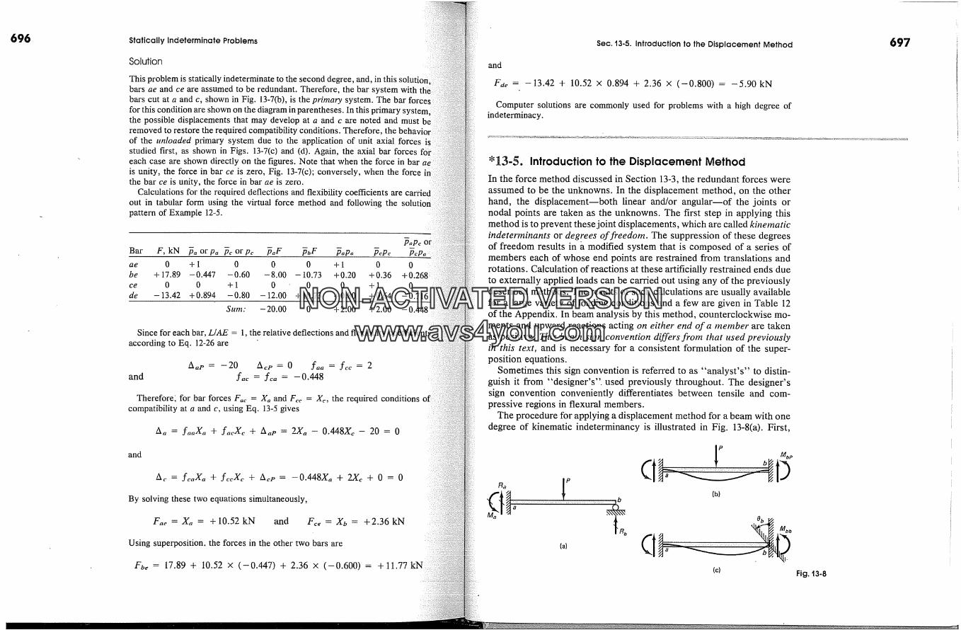
696 Statically Indeterminate Problems
Solution
This problem is statically indeterminate to the second degree, and, in this soluti �nbars ae and ce are assumed to be redundant. Therefore, the bar system withbars cut at a and c, shown in Fig. 13-7(b), is the primary system. The bar force sfor this condition are shown on the diagram in parentheses. In this primary systemthe possible displacements that may develop at a and c are noted and must b eremoved to restore the required compatibility conditions. Therefore, the behavof the unloaded primary system due to the application of unit axial forcesstudied first, as shown in Figs. 13-7(c) and (d). Again, the axial bar forces foreach case are shown directly on the figures. Note that when the force in bar,is unity, the force in bar ce is zero, Fig. 13-7(c); conversely, when the force inthe bar ce is unity, the force in bar ae is zero.
Calculations for the required deflections and flexibility coefficients areout in tabular form using the virtual force method and following thepattern of Example 12-5.
�aPcBar F, kN �a or pa � or p� fi�F fibF �,�p� �p� -ae 0 +1 0 0 0 +1 0 0be + 17.89 -0.447 -0.60 -8.00 -10.73 +0.20 +0.36ce 0 0 +1 0 0 0 +1 0de -13.42 +0.894 -0.80 -t2.00 +10.73 +0.80 +0.64 -0.7
Sum: - 20.00 0 + 2.00 + 2.00 - 0.�
Since for each bar, L/AE = 1, the relative deflections and flexibility coefficientsaccording to Eq. 12-26 are
andA a�, = --20 A c�, = 0 faa = fc� = 2
f� = f� = --0.448
Therefore; for bar forces Fac = Xa and Fcc = Xc, the required conditionscompatibility at a and c, using Eq. 13-5 gives
and
A� = f, aX, + fa�c + A�, = 2X� - 0.448X� - 20 = 0
A,. = f�Xa + f��Xc + A cj, = -0.448X� + 2X� + 0 = 0
By solving these two equations simultaneously,
F�e = X� = + 10.52 kN and F�e = Xo = +2.36 kN
Using superposition. the forces in the other two bars are
Foe = 17.89 + 10.52 x (-0.447) + 2.36 x (-0.600) = +11.77kN
Sec. 13-5. Introduction to the Displacement Method
and
Fae = -13.42 + 10.52 x 0.894 + 2.36 x (-0.800) = -5.90 kN
Computer solutions are commonly used for problems with a high degree ofindeterminacy.
� 13-5. Introduction to the Displacement MethodIn the force method discussed in Section 13-3, the redundant forces wereassumed to be the unknowns. In the displacement method, on the otherhand, the displacement--both linear and/or angular�of the joints ornodal points are taken as the unknowns. The first step in applying thismethod is to prevent these joint displacements, which are called kinetnaticindeterminants or degrees offi'eedom. The suppression of these degreesof freedom results in a modified system that is composed of a series ofmembers each of whose end points are restrained from translations androtations. Calculation of reactions at these artificially restrained ends dueto externally applied loads can be carried out using any of the previouslydescribed methods. The results of such calculations are usually availablefor a large variety of loading conditions and a few are given in Table 12of the Appendix. In beam analysis by this method, counterclockwise mo-ments and upward reactions acting on either end of a member are takenas positive. This beatn sign convention differs from that used previouslyin this text, and is necessary for a consistent formulation of the super-position equations.
Sometimes this sign convention is referred to as "analyst's" to distin-guish it from "designer's". used previously throughout. The designer'ssign convention conveniently differentiates between tensile and com-pressive regions in flexural members.
The procedure for applying a displacement method for a beam with onedegree of kinematic indeterminancy is illustrated in Fig. 13-8(a). First,
(c) Fig. �3-8
697
NON-ACTIVATEDVERSIONwww.avs4you.com

698 Statically Indeterminate Problems
' Fig. t3-9
the support at b is restrained, Fig. 13-8(b), reducing the problem toof a fixed-end beam. Both the vertical reactions and end moments ina beam can be found by methods discussed previously. Moment Mt,v isan example of such a reactive force at an end, where the first letterthe subscript designates the location and the second identifies the causeSuch end moments and reactions are referred to as fixed-end actionsbeam ends. For general use, fixed-end actions are identified here bletter A with two subscripts. For the above case, At,v --- Mt,v.P refers to any kind of applied lateral load.
Next, moment Mt,t, at b, Fig. 13-8(c), is determined as a function of:applied rotation 0t,. In this notation, the first letter of the subscripttitles the location of the fixed-end force (moment) and the second idetitles the location of the applied displacement. Two basic cases formoments and reactions caused either by applied end rotation orment are given in Table 12 in the Appendix.
Finally, an equation for static equilibrium is written. In this case,the beam is simply supported at b, total moment Mt, must be zero. FOigeneral use, such force quantities are identified as Pt,, i.e., Mt, --Therefore, assuming that the system is linearly elastic andsmall dislacements, for equilibrium a[ joint b,
Mt, = Mt,v + Mt,t, = 0
or in generalized notation,
(13-1
Pt, ' At,v + At,t, = 0
EXAMPLE t3-5
Using a displacement method, determine the reactions for a uniformly loadecbeam fixed' at one end and simply supported at the other, Fig. 13-9(a).constant.
(a)
(b)
o b
Rbb
(c)
Sec. t3-5. Introduction to the Displacement Method
Solution
Since joint rotation at b is the only kinematic unknown at the supports, Fig. 13-9(a), this beam is kinematically indeterminate to the first degree. Using Table 12in the Appendix, the fixed-end actions due to the applied load, Fig. 13-9(b), andthe end moments and reactions due to 0b, Fig. 13-9(c), are
Mav= Aaj, = woL2/12 andMat, --- Aat, = 2EIOt,/m andRat, = 6EIOt,[m 2 and
= - woL-/12Mbp m AbP '�Mbb = Abb = 4EIOb/L
Rbb = -- 6EIOb/L 2
For moment equilibrium at the end b, using Eq. 13-11a,
woL 2 4EIMt,---Pt, = Mt,v+Mt,t, = 12 + �0t, = 0
Hence, 0t, = woL2/48EI
Using this 0b in the superposition equations,
woL 2 2EI woL 2Ma = May + Mat, -- 12 + � 0b - 8
woL 6EI 5woLRa =Rav +Rat, - 2 + ~ Ot, - 8
woL 6EI 3woLRb = Rbv + Rt,t, - 2 � Ob -- 8
The sign of Ma is opposite from that of the designer's beam sign convention.
EXAMPLE t3-6
Three elastic pin-jointed bars are symmetrically arranged in a plane to form thesystem shown in Fig. 13-10(a). The cross-sectional area A of each bar is the same,and the elastic modulus is E. Verify the bar forces found in Examples 2-14, 12-23, and 12-17 caused by applied force P.
Solution
Because of symmetry, this system has only one degree of kinematic freedom andjoint c can only displace in the vertical direction. In this solution, first, the jointis restrained from displacement, Fig. 13-10(b). Here all of the fixed-end actionsare zero, and Ac�, --- Pc�, = 0. s
Force Pcc for the system is determined next as a function of deflection A � forbar bc. As in Example 12-17, for geometric compatibility at joint c, A2 =
8 If an axial force were applied somewhere between b and c, P�, would not bezero. For example, if a downward force P� were applied at a distance L�d4 abovec, per Eq. 2-39, the fixed-end downward force at c would be Roe = 3P�/4.
(a)
(b)
(c)
Fig. t3-10
NON-ACTIVATEDVERSIONwww.avs4you.com

700 Statically Indeterminate Problems
Fig. t3-tt
b
Fig. 13-12
A � cOS a. Hence, using Eq. 2-12, the bar forces F� and F2 in members bc and ac(or dc), respectively, are
� _� AE A �cosF� = k� A ] = A � and F2 = k2 A 1 COS Ct L/cos ctThen for vertical force equilibrium at joint c,
Pc = Pc�' + F� + 2F2cosct = P
Substituting the values of PeP, F�, and F2 into the above equation, and solvingfor An, one finds
PL
AE(1 + 2 cos 3
By substituting this value of A � into the relations for the bar forces, the resultsic in Example 2-23 are verified.
If in this example there were no symmetry about the vertical axis (either dueto lack of symmetry in the structure itself or due to application of force P at anangle), a horizontal displacement would' also have developed at the joint.force equilibrium equations, one in the horizontal direction and the other in thevertical direction, mr/st then be set up and solved simultaneous13and vertical displacements. Such cases are illustrated in Figs. 12-11 and 12-12and are also considered in the next section.
It should be noted that by ad�ting additional bars to the system, as shownFig. 13-11, does not increase the kinematic indeterminacy, and it remains at two.In the force method, on the other hand, the number of statical redundantscreases, as does the number of simultaneous equations for determiningdants. However, this does not imply that the displacement method alwaysvolves the solution of fewer equations compared to the force method. Considerfor example, the case of a propped cantilever with an overhang; see Fig.This beam is statically indeterminate only to the first degree, but kinemindeterminate to the third degree (rotations at b and c, and a verticalat c); hence, only one equation is needed for solution by the force method,three simultaneous equations are required using the displacement method.
'13-6. Further Remarks on the Displacement MethodThe displacement method is extended to problems with several deof kinematic indeterminancy in this section. For this purpose,the beam shown in Fig. 13-13(a), where the guided support at c allowsfor vertical displacement but no rotation Of the beam. The other degreeof freedom of this beam is the rotation of its tangent at support b.beam is thus kinematically indeterminate to the second degree.restraining these two degrees of freedom, one obtains a system
Sec. t3.6. Further Remarks on the Displacement Method
. a b c �a
(a) .
gbp
(b)
(d)
0b=lrt�
(f)
(c)
� Fig. t3-13
of two fixed-end beams, ab and bc, Fig. 12-13(b). The effect of the ex-ternally applied loads on these two fixed-end beams is to produce a setof reactive forces at the supports. The fixed-end action (moment) Abe, atb is the sum of the fixed-end moments in beams ba and bc at b causedby the applied loads. Similarly, the fixed-end action Ac�, is the verticalreaction at c restraining vertical displacement. Since the support is ca-pable of developing a moment at c, it does not enter the problem at thislevel.
Next the support at b is rotated through an angle 0b, giving rise to thefixed-end actions (moments) Aoo and Aco at points b and c, respectively,as shown in Fig. 13-13(c). Similarly, Aoc and Act are caused by the verticaldisplacement Ac at c, Fig. 13-13(d).
Since no external moment Mb is applied at b, nor a vertical reactionPc at c, the resultant forces Mo = Po and Pc at these points are equal tozero. These two forces may be found by superposing three separate anal-yses, shown in Figs. 13-13(b)-(d), leading to two simultaneous equilibriumequations:
Pb = Abp q- Abb q- Abc= 0Pc = Ac� o + Aco + Act = 0
(13-12)
These equations can be rewritten in more meaningful form using stiffnesscoefficients kob, koc, and kcc, defined as the fixed-end actions shown in
70t
NON-ACTIVATEDVERSIONwww.avs4you.com
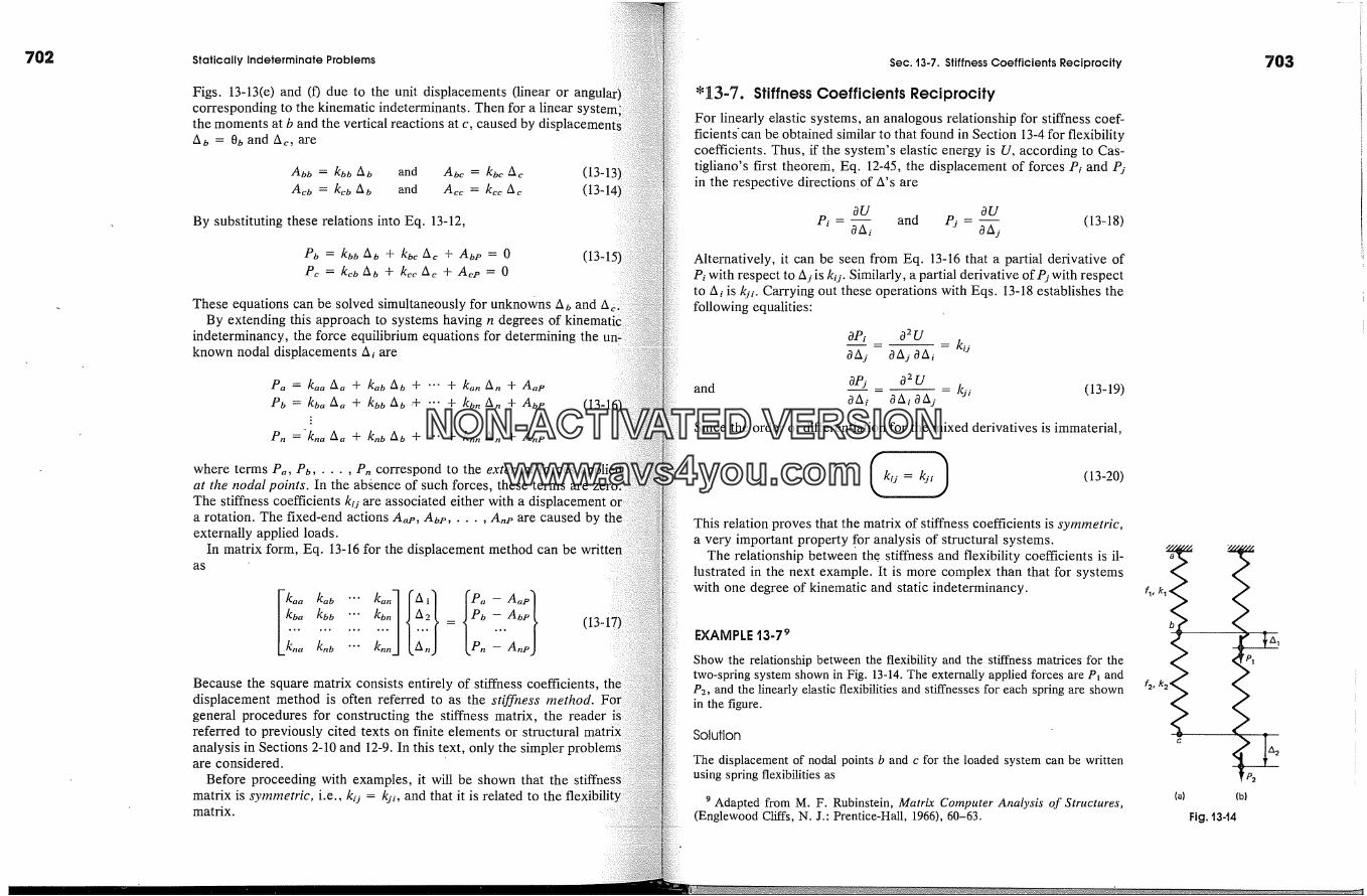
702 Statically Indeterminate Problems
Figs. 13-13(e) and (f) due to the unit displacements (linear or ancorresponding to the kinematic indeterminants. Then for a linearthe moments at b and the vertical reactions at c, caused by displacementsAb = 0bandAc, are
By substituting these relations into Eq. 13-12,
Pa = kaa &a + kac zXc + Aa�, = 0Pc = kcbAb + kccAc + Ac�, = 0
These equations can be solved simultaneously for unknowns Ao and ABy extending this approach to systems having n degrees
indeterminancy, the force equilibrium equations for determining theknown nodal displacements Ai are
Pb -- kba Aa q- kbb Ab .q- "' q- kbn An q- AbP
where terms Pa, Po ..... P,correspond to the external forces applieat the nodal points. In the absence of such forces, these terms areThe stiffness coefficients k u are associated either with a displacementa rotation. The fixed-end actions A�,, Abe, ..... A,, are caused byexternally applied loads.
In matrix form, Eq. 13-16 for the displacement method can beas
(13-1'
Because the square matrix consists entirely of stiffness coefficients,displacement method is often referred to as the stiffness method.general procedures for constructing the stiffness matrix, the readerreferred to previously cited texts on finite elements or structuralanalysis in Sections 2-10 and 12-9. In this text, only theare considered.
Before proceeding with examples, it will be shown that thematrix is symmetric, i.e., k o = k�, and that it is related to thematrix.
Sec. 13-7. Stiffness Coefficients Reciprocity
'13-7. Stiffness Coefficients ReciprocityFor linearly elastic systems, an analogous relationship for stiffness coef-ficients'can be obtained similar to that found in Section 13-4 for flexibilitycoefficients. Thus, if the system's elastic energy is U, according to Cas-tigliano's first theorem, Eq. 12-45, the displacement of forces P� and Pjin the respective directions of A's are
au auPi = and Pj = (13-18)
aA�
Alternatively, it can be seen from Eq. 13-16 that a partial derivative ofPt with respect to As is ku. Similarly, a partial derivative of Pj with respectto At is kit. Carrying out these operations with Eqs. 13-18 establishes thefollowing equalities:
aPi a 2 U- ku
and aPs a 2 U - k�, (13-19)aAi aAiaA s
Since the order of differentiation for the mixed derivatives is immaterial,
(13-20)
This relation proves that the matrix of stiffness coefficients is symmetric,a very important property for analysis of structural systems.
The relationship between the. stiffness and flexibility coefficients is il-lustrated in the next example. It is more complex than that for systemswith one degree of kinematic and static indeterminancy.
EXAMPLE t3-7 9
Show the relationship between the flexibility and the stiffness matrices for thetwo-spring system shown in Fig. 13-14. The externally applied forces are P� andP2, and the linearly elastic flexibilities and stiffnesses for each spring are shownin the figure.
Solution
The displacement of nodal points b and c for the loaded system can be writtenusing spring flexibilities as
9 Adapted from M. F. Rubinstein, Matrix Computer Analysis of Structures,(Englewood Cliffs, N.J.: Prentice-Hall, 1966), 60-63.
703
(b)
Fig. t344
NON-ACTIVATEDVERSIONwww.avs4you.com

704 Statically Indeterminate Problems
A� = (p� + p�)�� and A2 = (P� + P2)f� + P2f2
where force P� + P2 acts on spring ab.. Similarly, the equilibrium equations for each nodal point b and c, using
stiffnesses, are
P� = kl A� - k2(A2 - A1) and P2 = k2(A2 - Ai)
where the stretch of spring bc is A2 -- A�.Recasting these equations into matrix form gives
and
Next it can be noted that the individual spring flexibilities can be replaced bythe reciprocals of the spring constants. Then the flexibility matrix, expressedterms of spring constants, is multiplied by the stiffness matrix using the rulesmatrix multiplication, giving
k� + k 2 -k* =� 1 - k2 k2-This shows that a product of a flexibility matrix by a stiffness matrix leads toidentity matrix. All diagonal elements of this unit matrix are unity, and allare zero.
This result means that a flexibility matrix is an inverse of a stiffness matrix orvice versa. For these symmetric matrices, this can be symbolically written a�,
[fi = [k] or [k] = [fi-
For problems with single degrees of static and kinematic indeterminacy,expressions degenerate into simple reciprocals of these quantities.
EXAMPLE t3-8
Using the displacement method, calculate the rotations at b and c for thetinuous beam of constant EI loaded as shown in Fig. 13-15(a),moments at a and b.
Solution
At supports b and c, the beam is free to rotate, making the systemindeterminate to the second degree. By temporarily restraining these
Sec. 13.7. Stiffness Coefficients Reciprocity
(a)
kcb
kbb
(c)
(b) (d)
against rotations, a system of two fixed-end beams is obtained, Fig. 13-15(b). Thefixed-end actions for these beams can be obtained with the aid of Table 12 in theAppendix. In the following, the first letter of the subscript outside the bracketsidentifying a beam designates the end where the fixed-end action applies.For beam ab:
[Aaa]ab = + PL/8 and [Ab�,]�a = -- PL/8
For beam bc:
[A�,]�c = + Wo(2L)2/12 = + woL2/3 and [Ac�,]� = - woL3/3
For joint b:
Abt� = [Ab�']ba + [Abt�]bc = --PL/8 + woL2/3
The stiffness coefficients can be calculated by subjecting the temporarily fixedends b and c, to unit rotations one at a time, Figs. 13-15(c) and (d). Again, usingformulas in Table 12 of the Appendix and by noting that the two adjoining spanscontribute to the stiffness of the joint at b, one has
Similarly, for the member ab, due to a unit rotation at b,
= F4E!] and kab == L L J,,b L
Fig. t3-t5
705
NON-ACTIVATEDVERSIONwww.avs4you.com

706 Statically Indeterminate Problems
Since there are no externally applied forces (moments) at b and c, forrium at these joints, Eqs. 13-15 become
6E/ E/
= --ab + zXc - --2EI
PL woL 28 3
woZ 2-0
3
-0
By solving these two equations simultaneously,
L2 (-�' ) L2 ( P 7A�=O� - 11EI -*vol and Ac--Oc-- 11� 8 + �By substituting these displacement values into the member superposition e�tions, the end moments in all members are found.
15 2
M,,� = [Aa�']a� + kab0� = �-� PL - �'� woL 23 4
M� = [A�,]�, + kb�0� = -. 8-� PL - 'i� w�L23 4
Mbc = [At;�,]bc + kbcOb + kcboc = + �'� PL + �-� woZ 2M�b = [Ac�,]cb + kcbOb + k�cOc = 0
Note that with the analyst's beam sign convention employed in this solution,+ Mbc = 0, since they are of opposite sign.
EXAMPLE t3-9
Rework Example 13-4 using the displacement method of analysis; see Fig. 1!16(a).
Solution
In this problem, since nodal point e can move horizontally andsystem has two degrees of freedom. As noted in Example 13-4, this system ialso statically indeterminate to the second degree. Each additional bar
from e would increase the statical indeterminancy by one, however, thedegree of indeterminacy would remain at two.
The horizontal and vertical positive displacements, A� and A2, shown13-16(b) and (c), respectively, are the unknowns. For displacement A�,of bar ie is constrained to move only horizontally, as in the upper diagram13-16(d), the bar elongates by A� sin ai. This'would develop a bar axial
p� = k i A� sin ai, where the bar spring constant k i = A�EdL�. ThisP'i, can be resolved, respectively, into horizontal and vertical components= P� sin ai and P�2 = Pt cos el. Therefore,
Sec. 13-7. Stiffness Coefficients Reciprocity 707
(a)
Fig. t3-t6
�, L� sin2rz� A� = k�A�P�= �,L� sinrz�cosrz� zX� = k�zX�
(13-22a)
where k� and k�2 are bar stiffnesses for a horizontal displacement A �.By the same reasoning, if end e of bar ie is constrained to move A2 in the
vertical direction only, as shown in the lower diagram of Fig. 13-16(d), the re-spective horizontal and vertical force components for the bar are
AiEiP�2 = � Li COS20�i A2 = k/92 A2P}l �,-�/cos c� sin c�i A2 = k� A2
(13-22b)
where k�2 and k�2 are bar vertical and horizontal stiffnesses, respectively, forvertical displacement A2.
NON-ACTIVATEDVERSIONwww.avs4you.com
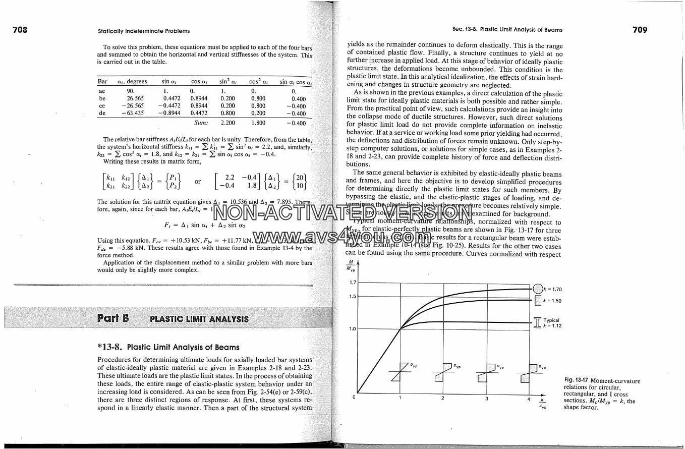
708 Statically Indeterminate Problems
To solve this problem, these equations must be applied to each of the four barsand summed to obtain the horizontal and vertical stiffnesses of the system.is carried out in the table.
Bar at, degrees sin al cos ai sin 2 al cos 2 at sin at cosae 90. 1. 0. 1. 0. 0.be 26.565 0.4472 0.8944 0.200 0.800 0.400ce -26.565 -0.4472 0.8944 0.200 0.800 -0.400de -63.435 -0.8944 0.4472 0.800 0.200 -0.400
Sum: 2.200 1.800 - 0.400
The relative bar stiffness AiEdLi for each bar is unity. Therefore, from the tabthe system's horizontal stiffness kn = � k� = � sin 2 at = 2.2, and,k22 = � cos 2 ai = 1.8, and k12 = k21 = � sin ai cos ai = -0.4.
Writing these results in matrix form,
[k,, kn- 1 A, 2.2Lk2� k22J A2 = or --0.4 1.8 A2 = 10
The solution for this matrix equation gives/x� = 10.536 and A2 = 7.895. Thefore, again, since for each bar, AiEi/Li = 1,
F� = A� sin cti + A2 sin ct2
Using this equation, F,e = + 10.53 kN, Fbe = + 11.77 kN, Fee = +2.35 kN, andFae = -5.88 kN. These results agree with those found in Example 13-4 byforce method.
Application of the displacement method to a similar problem with morewould only be slightly more complex.
� 13-8. Plastic Limit Analysis of BeamsProcedures for determining ultimate loads for axially loaded bar s]of elastic-ideally plastic material are given in Examples 2-18 and 2-23:These ultimate loads are the plastic limit states. In the process of obtaininthese loads, the entire range of elastic-plastic system behavior underincreasing load is considered. As can be seen from Fig. 2-54(e)there are three distinct regions of response. At first, these systemsspond in a linearly elastic manner. Then a part of the structural s
Sec. t3.8. Plastic Limit Analysis of Beams
yields as the remainder continues to deform elastically. This is the rangeof contained plastic flow. Finally, a structure continues to yield at nofurther increase in applied load. At this stage of behavior of ideally plasticstructures, the deformations become unbounded. This condition is theplastic limit state. In this analytical idealization, the effects of strain hard-ening and changes in structure geometry are neglected.
As is shown in the previous examples, a direct calculation of the plasticlimit state for ideally plastic materials is both possible and rather simple.From the practical point of view, such calculations provide an insight intothe collapse mode of ductile structures. However, such direct solutionsfor plastic limit load do not provide complete information on inelasticbehavior. If at a service or working load some prior yielding had occurred,the deflections and distribution of forces remain unknown. Only step-by-step computer solutions, or solutions for simple cases, as in Examples 2-18 and 2-23, can provide complete history of force and deflection distri-
butions.
The same general behavior is exhibited by elastic-ideally plastic beamsand frames, and here the objective is to develop simplified proceduresfor determining directly the plastic limit states for such members. Bybypassing the elastic, and the elastic-plastic stages of loading, and de-termining the plastic limit loads, the procedure becomes relatively simple.Some previously established results are reexamined for background.
Typical moment-curvature relationships, normalized with respect toMyp, for elastic-perfectly plastic beams are shown in Fig.-13-17 for threedifferent cross sections. Basic results for a rectangular beam were estab-lished in Example 10-14 (see Fig. 10-25). Results for the other two casescan be found using the same procedure. Curves normalized with respect
Myp
1.7
1.5
1.0 -� Typical= 1.12
70yp �OVp �Oyp
0 2 4
709
Fig. t347 Moment-curvaturerelations for cimular,rectangular, and I crosssections. Mp/Myp = k, theshape factor.
NON-ACTIVATEDVERSIONwww.avs4you.com

710
Fig. t348 Moment-curvatureidealizations for plastica. nalyses of beams ofdifferent cross sections.
Statically Indeterminate Problems
to M e are shown in Fig. 13-18. The behavior of an ideaiized cross sectiowith large flanges and a negligibly thin web is added in this diagram.
In both diagramg, as the cross sections plastify, a rapid ascentcurves toward their respective asymptotes occurs. This means that shafter reaching the elastic capacity of a beam, a rather constant moment,very near to Me, is both achieved and maintained. This istrue for the important case of an I beam. As can be noted from Fig.18, for this cross section, the elastic-plastic behavior is essentially
fined to the range between B' and C; for the remainder, the momentessentially Me. The influence of the elastic core next to theaxis is more pronounced for members with rectangular or roundsections, whose shape factors, k, are larger than those for an I beam,13-17. Nevertheless, in the plastic limit analysis of members subjectedb. ending, it is generally assumed that an abrupt transition from elasticideally plastic behavior occurs at Me. Therefore, member behaviortween Myp and Me is considered to be elastic. It is further assumedwhen Me is reached, a plastic hinge is formed in the member. Into a frictionless hinge permitting free rotation, the plastic hingelarge rotations to occur at a constant plastic moment Me.
In a plastic limit analysis of beams, the elastic displacementsto the plastic ones are small and can be neglected. Detailed analysesshown m that it is sufficiently accurate to consider beams nwith plasticity confined to plastic hinges at points. In reality,extend along short lengths of beams and depend on loading
�o See, for example, L. S. Beedle, Plastic Design of Steel FramesWiley, 1966) or S. J. Moy, Plastic Methods for Steel and Concrete(New York: Wiley, 1981).
Sec. 13-8. Plastic Limit Analysis of Beams
The approximate theory discussed here is applicable to beams as wellas columns subjected to moderate axial forces. When a cross section lacksbiaxial .symmetry, the positive and negative moments differ in their mag-nitudes and should be accounted for in the analysis. A method for de-termining the reduced plastic capacity of members in the presence of axialforces is discussed in Section 6-13.
By inserting a plastic hinge at a plastic limit load into a statically de-terminate beam, a kinematic mechanism permitting an unbounded dis-placement of the system can be formed. This is commonly referred to asthe collapse mechanism. � For each degree of static indeterminancy of abeam, an additional plastic hinge must be added to form a collapse mech-anism. The insertion of plastic hinges must be such as to obtain a kine-matically admissible (plausible) collapse mechanism. The use of kine-matically admissible collapse mechanisms is illustrated in the examplesto follow.
In plastic limit design, it is necessary to multiply working loads by aload factor larger than unity to obtain design factored loads. This is anal-ogous to the use of a factor of safety in elastic analyses. This issue isdiscussed in Section 1-11.
There are two common methods of plastic limit analysis. One is basedon conventional statics and the other on virtual work. In either methodthe bending moments anywhere along a member cannot exceed the plasticmoment Me, and the conditions of equilibrium must always be satisfied.The procedure for forming kinematically admissible mechanisms, some-what similar to continuity conditions in elastic analysis, is illustrated inthe following examples.
EXAMPLE t3-t0
A concentrated force P is applied at the middle of a simply supported prismaticbeam, as shown in Fig. 13-19(a). If the beam is of a ductile material, what is theplastic fir/fit load Pu�t? Obtain the solution using (a) the equilibrium method and(b) the virtual work method. Consider only flexural behavior, i.e., neglect theeffect of shear forces. Neglect beam weight.
Solution
(a) The shape of the moment diagram is the same regardless of the load magnitude.For any value of P, the maximum moment M = PL/4, and ifM < Myp, the beambehaves elastically. When the moment is at myp, the force at yield
Pyp = 4myp/Z
When My v is exceeded, contained yielding of the beam commences and con-tinues until the plastic moment Mp is reached, Fig. 13-19(c).
n In seismic analyses, the plastic hinges dissipate energy. Therefore, it is pref-erable to call such mechanisms energy dissipating mechanisms.
NON-ACTIVATEDVERSIONwww.avs4you.com
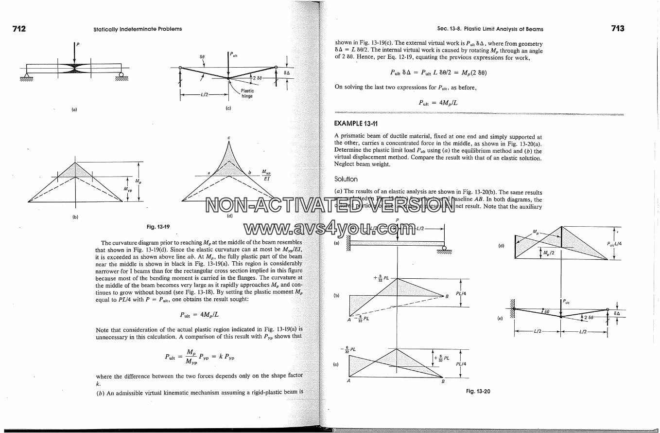
Statically Indeterminate Problems Sec. t3-8. Plastic Limit Analysis of Beams 7'!3
(a)
�o
(c)
Pult
Plastichinge
shown in Fig. 13-19(c). The external virtual work is Pu�t 8A, where from geometry8A = L 80/2. The internal virtual work is caused by rotating M e through an angleof 2 80. Hence, per Eq. 12-19, equating the previous expressions for work,
P,lt B A = P,tt L B0/2 = My(2 g0)
On solving the last two expressions for Pult, as before,
Pu�t = 4M�,/L
b MvpE1
(b) (d)
Fig. t3-19
The curvature diagram prior to reaching Me at the middle of thethat shown in Fig. 13-19(d). Since the elastic curvature can at most beit is exceeded as shown above line ab. At Mp, the fully plastic partnear the middle is shown in black in Fig. 13-19(a). This region isnarrower.for I beams than for the rectangular cross section implied in this fibecause most of the bending moment is carried' in the flanges. Thethe middle of the beam becomes very large as it rapidly approaches M e andtinues to grow without bound (see Fig. 13-18). By setting theequal to PL/4 with P = Pult, one obtains the result sought:
Pu�t = 4Mp/L
Note that consideration of the actual plastic region indicated in Fig.unnecessary in this calculation. A comparison of this result with Pyp shows
mp pyp = k PypPult = mypwhere the difference between the two forces depends only on the shapek.
(b) An admissible virtual kinematic mechanism assuming a
EXAMPLE '13-tt
A prismatic beam of ductile material, fixed at one end and simply supported atthe other, carries a concentrated force in the middle, as shown in Fig. 13~20(a).Determine the plastic limit load Pult using (a) the equilibrium method and (b) thevirtual displacement method. Compare the result with that of an elastic solution.Neglect beam weight.
Solution
(a) The results of an elastic analysis are shown in Fig. 13-20(b). The same resultsare replotted in Fig. 13-20(c) from horizontal baseline AB. In both diagrams, thecolored portions of the diagrams represent the net result. Note that the auxiliary
(a)
P
� L/2 �]� L/2 �(d)
(b)
A
(c)
PL
PL/4
PL/4
(e)
< L/2 >
A
Fig. 13-20
Pult L/4
Pult
'< L/2 q
NON-ACTIVATEDVERSIONwww.avs4you.com
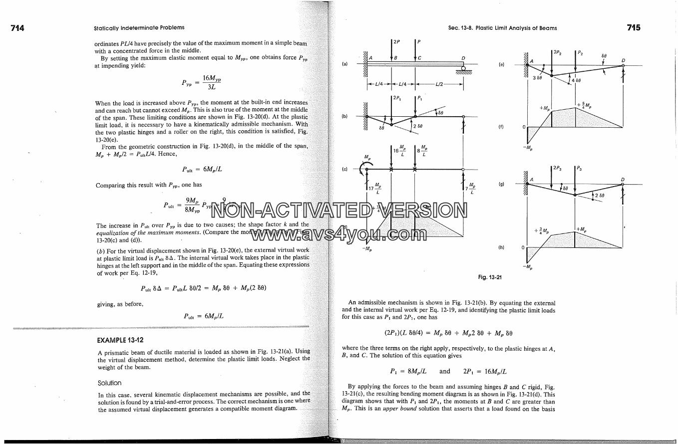
714 Statically Indeterminate Problems
ordinates PL/4 have precisely the value of the maximum moment in a simplewith a concentrated force in the middle.
By setting the maximum elastic moment equal to Mvp, one obtains forceat impending yield:
16MypPYP -- 3L
When the load is increased above Pyp, the moment at the built-in end increaseand can reach but cannot exceed M v. This is also true of the moment at theof the span. These limiting conditions are shown in Fig. 13-20(d). At thelimit load, it is necessa. ry to have a kinematically admissible mechanism.the two plastic hinges and a roller on the right, this condition is satisfied, Fi13-20(e).
From the geometric construction in Fig. 13-20(d), in the middle of theMy + My/2 = PultL/4. Hence,
Pu�t = 6Me/L
Comparing this result with Pyp, one has
9Me pyp 9Pult = 8Myp = � kPypThe increase in Pult over Pyp is due to two causes; the shape factor k andequalization of the maximum moments. (Compare the moment diagrams in Figs�13-20(c) and (d)).
(b) For the virtual displacement shown in Fig. 13-20(e), the external virtual woat plastic limit load is Pu�t gA. The internal virtual work takes place in the'hinges at the left support and in the middle of the span. Equating theseof work per Eq. 12-19,
P,�t BA = Pu�tL g0/2 = M e g0 + Me(2
giving, as before,
Pu�t = 6Me/L
EXAMPLE t342
A prismatic beam of ductile material is loaded as shown in Fig. 13-21(a).the virtual displacement method, determine the plastic limit loads. Neglectweight of the beam.
Solution
In this case, several kinematic displacement mechanisms are possible, andsolution is found by a trial-and-error process. The correct mechanism isthe assumed virtual displacement generates a compatible moment diagram.
(a)
(b)
(c)
(d)
Sec. 13.8. Plastic Limit Analysis of Beams 715
D
(e)
(f}
P2D
(g) � 2P3 IPa Dq- � M,o I+M.o
-M� (h) 0
Fig. 13-2t
An admissible mechanism is shown in Fig. 13-21(b). By equating the externaland the internal virtual work per Eq. 12-19, and identifying the plastic limit loadsfor this case as P� and 2P�, one has
(2P0(L g0/4) = M e g0 + Me2 g0 + Me g0
where the three terms on the right apply, respectively, to the plastic hinges at A,B, and C. The solution of this equation gives
P� = 8Me/L and 2P� = 16Me/L
By applying the forces to the beam and assuming hinges B and C rigid, Fig.13-21(c), the resulting bending moment diagram is as shown in Fig. 13-21(d). Thisdiagram shows that with P� and 2P�, the moments at B and C are greater thanM e. This is an upper bound solution that asserts that a load found on the basis
NON-ACTIVATEDVERSIONwww.avs4you.com
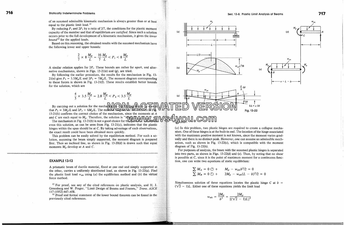
7t6 Statically Indeterminate Problems
of an assumed admissible kinematic mechanism is always greater than or at bes tequal to the plastic limit lead. �2
By reducing P� and 2P� by a ratio of 2/7, the conditions for the plastic momen tcapacity of the member and that of equilibrium are satisfied. Since such a sotutio�Occurs prior to the full development of a kinematic mechanism, it gives the lowerbound �3 for the applied loads.
Based on this reasoning, the obtained results with the assumed mechanism havethe following lower and upper bounds:
2 My 16My Me-x 8--- -<P�<8--7 L 7 L L
A similar relation applies for 2Pi. These bounds are rather far apart, and alter-native mechanisms, shown in Figs. 13-21(e) and (g), are tried.
. By following the earlier procedure, the results for the mechanism in Fig. 13-21(e) give P2 = 3.5Me/Z and 2P2 = 7Mp/Z. The moment diagram correspondingto these forces is shown in Fig. 13-21(f). These results establish better boundsfor the solution, which are
4- x 3.5 = 2.8 < P, < 3.5
By carrying out a solution for the mechanism in Fig. 13-2(g), it can be shownthat P3 = 3Me/L and 2P3 = 6Me/L. The moment diagram for these forces in Fig.13-21(h) confirms the correct choice of the mechanism, since the moments at Aand C are each equal to M e. Therefore, the solution is "exact."
The mechanism in Fig. 13-21(b) is not a good choice for this problem. However,even this solution, as can be seen from Fig. 13-21(c), indicates that the plastichinges within the span should be at C. By taking advantage of such observations,the exact result could have been obtained more quickly.
This problem can be easily solved by the equilibrium method. For such a so-:lution, as.suming the beam simply supported, the moment diagram is preparedfirst. Then an inclined line, as shown in Fig. 13-20(d) is drawn such that e�moments M e develop at A and C.
EXAMPLE t3-t3
A prismatic beam of ductile material, fixed at one end and simply supportedthe other, carries a uniformly distributed ioad� as shown in Fig. 13�22(a).the plastic limit lead Wu�t using (a) the equilibrium method and (b) theforce method.
�2 For proof, see any of the cited references On plastic analysis, and H.Greenberg and W. Prager, "Limit Design of Beams and Frames," Trans.117 (1952):447-458.
�3 Proof and formal statement of the lower bound theorem can be found inpreviously cited references.
(a)
(b)
(c)
Sec. t3-8. Plastic Limit Analysis of Beams 717
� a t,L�� b---L/2 tw.tiL2/8
� b8
(e)
f
(d)
Wult
� a=L -b �"'
Fig. t3-22
Solution
(a) In thi�-problem, two plastic hinges are required to create a collapse mecha-nism. One of these hinges is at the built-in end. The location of the hinge associatedwith the maximum positive moment is not known, since the moment varies grad-ually and there is no distinct p�ak. However, one can assume an admissible mech-anism, such as shown in Fig. 13-22(c), which is compatible with the momentdiagram of Fig. 13-22(b).
For purposes of analysis, the beam with the assumed plastic hinges is separatedinto two parts, as shown in Figs. 13-22(d) and (e). Then, by noting that no shearis possible at C, since it is the point of maximum moment for a continuous func-tion, one can write two equations of static equilibrium:
�Ma=00+�Ma=0�+
Mp - wultb2/2 = 02Mp - Wult(Z - b)2/2 = 0
Simultaneous solution of these equations locates the plastic hinge C at b =(X/� - 1)L. Either one of these equations yields the limit lead
Wult --2M. 2M.
b 2 [(V�- 1)L] 2
NON-ACTIVATEDVERSIONwww.avs4you.com
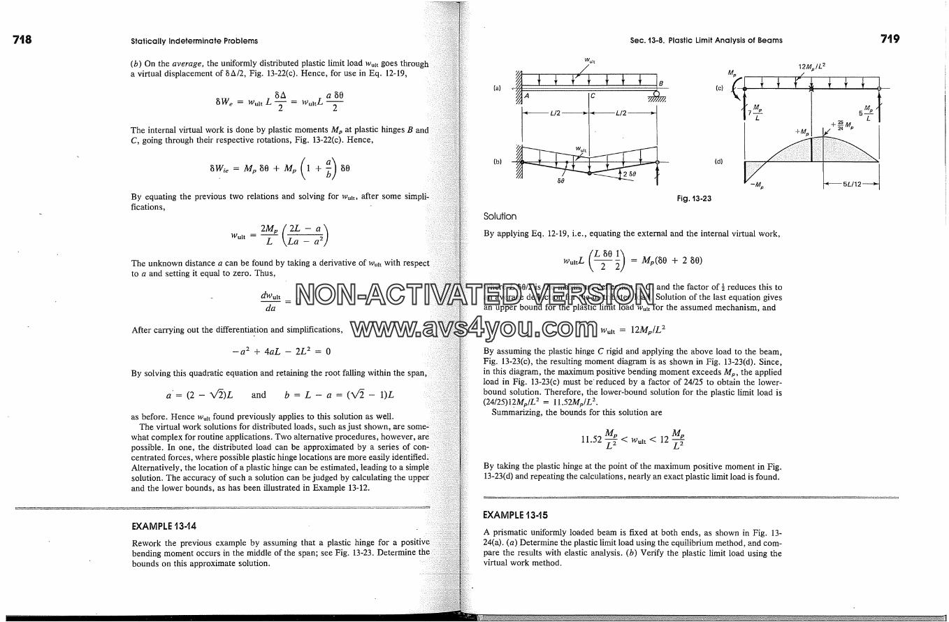
718 Statically Indeterminate Problems
(b) On the average, the uniformly distributed plastic limit load �vul t goes througha virtual displacement of �A/2, Fig. 13-22(c). Hence, for use in Eq. 12-19,
gWe = w,�t L ? = WultL a g02
The internal virtual work is done by plastic moments Me at plastic hinges BC, going through their respective rotations, Fig. 13-22(c). Hence,
By equating the previous two relations and solving for Wu�t, after some simfications,
H"ult -- L
The unknown distance a can be found by taking a derivative of Wutt with respectto a and setting it equal to zero. Thus,
dWult-0
da
After carrying out the differentiation and simplifications,
-a 2 + 4aL - 2L 2 = 0
By solving this quadratic equation and retaining the root falling within the span,
a'= (2 - X/�)L and b = L - a = (X/� - 1)L
as before. Hence wu�t found previously applies to this solution as well.The virtual work solutions for distributed loads, such as just shown, are
what complex for routine applications. Two alternative procedures, however,possible. In one, the distributed load can be approximated by a series of con-centrated forces, where possible plastic hinge locations are more easily identified;Alternatively, the location of a plastic hinge can be estimated, leading to a simpsolution. The accuracy of such a solution can be judged by calculatinand the lower bounds, as has been illustrated in Example 13-12.
EXAMPLE t3-t4
Rework the previous example by assuming that a plastic hinge for abending moment occurs in the middle of the span; see Fig. 13-23. Determinebounds on this approximate solution.
Sec. t3-8. Plastic Limit Analysis of Beams 719
(a)
(b)
Solution
A
� L/2
Wu R
c
< L/2
Fig. 13-23
(c)
(d)
12Mp/L �
+%
By applying Eq. 12-19, i.e., equating the external and the internal virtual work,
where L 80/2 is the maximum deflection at C, and the factor of � reduces this toan average deflection for the distributed load. Solution of the last equation givesan upper bound for the plastic limit load wu�t for the assumed mechanism, and
],Vul t = 12Mp/L 2
By assuming the plastic hinge C rigid and applying the above load to the beam,Fig. 13-23(c), the resulting moment diagram is as shown in Fig. 13-23(d). Since,in this diagram, the maximum positive bending moment exceeds My, the appliedload in Fig. 13-23(c) must be'reduced by a factor of 24/25 to obtain the lower-bound solution. Therefore, the lower-bound solution for the plastic limit load is(24/25)l�2Mv/L 2 = 11.52Mv/L 2.
Summarizing, the bounds for this solution are
11.52 < Wul t < 12 L2By taking the plastic hinge at the point of the maximum positive moment in Fig.13-23(d) and repeating the calculations, nearly an exact plastic limit load is found.
EXAMPLE t3-t5
A prismatic uniformly loaded beam is fixed at both ends, as shown in Fig. 13-24(a). (a) Determine the plastic limit load using the equilibrium method, and com-pare the results with elastic analysis. (b) Verify the plastic limit load using thevirtual work method.
NON-ACTIVATEDVERSIONwww.avs4you.com

720
(�)
(b)
Statically Indeterminate Problems
Fig. t3-24
(c)
Solution
According to the analysis in Example 10-23, Fig. 10-37(c), the maximum bendingmoments occur at the built-in ends and are equal to woL2/12. The maximumitive moment develops at the middle of the span and is woL2/24. Therefore,yield, based on the maximum moment,
Myp = wypL2/12 or Wyp ---= 12Myp/Z 2
By increasing the load, plastic hinges deveiop at the supports.anism is not formed, however, until a plastic hinge also develops in theof the span, Fig. 13-24(c).
The maximum moment for a simply supported uniformly loaded beamwoL2/8. Therefore, as can be seen from Fig. 13-24(b), to obtain the limitin a clamped beam, this quantity must be equated to 2M v, with wo = w,�t. Hence
, = = 16Mv/L 2w,�tL-/8 2My or
Comparing this result with wyp, one has
4My 4.As in Example 13-11, the increase of Wutt over wyp depends on shape factor k andthe equalization of the maximum moments.
(b) Because of symmetry, the precise location of the plastic hinges is as sho TMin Fig. 13-24(c). By writing a virtual work equation, Eq. 12-19, one has
WuttL -- = M�(g0 + 2 gO + gO)
and w.� = 16Mv/L 2 as before.
Sec. t3.9. Continuous Beams and Frames
(a)
P
(c)
(d)
[ P� I P2 Ps w�
Fig. 13-25 Collapse mechanisms for continuous beams.
'13-9. Continuous Beams and Frames
The procedures discussed in the Preceding section, and illustrated byexamples, can be extended to the simpler cases for plastic limit analysisof continuous beams and frames. Usually, the kinematic mechanisms incontinuous beams, associated with a collapse mode, occur locally in onlyone beam. For the two-span continuous beam shown in Fig. 13-25(a), theplastic moment at the middle support is limited to (Mv)m� of the smallerbeam. Then, whether the kinematic mechanism would develop in the rightor the left span depends on the relative beam sizes as well as the mag-nitudes of the applied loads. The solution in either case follows the pro-cedure discussed in Example 13-11, 13-12, or 13-13.
The beams, restrained at both ends, usually develop the kinematicmechanisms shown in Fig. 13-25(d) for the two left spans in Fig. 13-25(c).The solution of such problems resembles that of Example 13-15, exceptthat the end moments for each span are not necessarily equal. For ex-ample, for the left span of Fig. 13-25(c), the plastic moment on the left isdetermined by the large beam, whereas that on the right depends on theplastic moment of the confer span beam.
Plastic limit analysis of frames may become rather complex as the num-ber of members, joints, and different loading conditions increases. Foranalysis of such problems, the reader is referred to the previously citedtexts. As a reasonably simple illustration of the plastic limit state frameanalysis, an example follows.
EXAMPLE t3-t6
Consider a rigid jointed planar frame of ductile material fixed at A and pinned atE, and loaded as shown in Fig. 13-26(a). All members are of the same size andcan develop full My, i.e., the effect of the axial forces on My can be neglected.Determine the plastic limit loads.
Solution
The solution to this problem is obtained by asstiming different kinematically ad-missible mechanisms and searching for the one that satisfies both equilibrium andplastic member capacity.
NON-ACTIVATEDVERSIONwww.avs4you.com
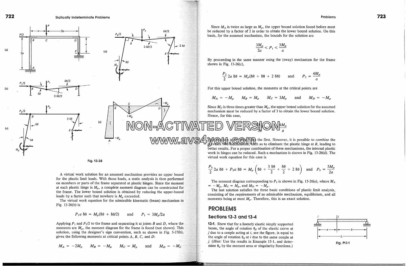
722 Statically Indeterminate Problems Problems
{a)
(b)
(c)
-�----a 2_a �,,
?/2
2a E (d)
�/2
_P�/2B �S8� 3 �8/2
P2
Fig. '13-26
J Pa �8/2
P3/2 2
C -%
A virtual work solution for an assumed mechanism provides an upper boundfor the plastic limit loads. With these loads, a static analysis is then [on members or parts of the frame separated at plastic hinges. Since theat each plastic hinge is Me, a complete moment diagram can be constructedthe frame. The lower bound solution is obtained by reducing the up[loads by a factor such that nowhere is M e exceeded.
The virtual work equation for the admissible kinematic (beam) mechanismFig. 13-26(b) is
Pia 80 = My(g0 + 80/2) and Pl = 3Mv/2a
Applying P� and P2/2 to the frame and separating it at joints B and D, wheremoments are M v, the moment diagram for the frame is found (not shown).solution, using the designer's sign convention, such as shown in Fig.gives the following moments at critical points A, B, C, and D:
Ma = - 2M�, M� = - M�, Mc = M�, and Mo =
Since MA is twice as large as My, the upper bound solution found before mustbe reduced by a factor of 2 in order to obtain the lower bound solution. On thisbasis, for the assumed mechanism, the bounds for the solution are
3My 3My2a a
By proceeding in the same manner using the (sway) mechanism for the frameshown in Fig. 13-26(c),
P2 4My-�-2a 80 = My(80 + 80 + 2 80) and P2 - a
For this upper bound solution, the moments at the critical points are
MA = - M�, Ma = Mp Mc = 3Mp and Mo = - Mp
Since Mc is three times greater than My, the upper bound solution for the assumedmechanism must be reduced by a factor of 3 to obtain the lower bound solution.Hence, for this case,
4My < P2 < 4Mp3a a
This solution is no better than the first. However, it is possible to combine theprevious two mechanisms, such as to eliminate the plastic hinge at B, leading tobetter results. For a proper combination of these mechanisms, the internal plasticwork in hinges can be reduced. Such a mechanism is shown in Fig. 13-26(d). Thevirtual work equation for this case is
P3 (38080T 2a so + a,a so = so + --5- + T + 2 so and P3 -2a
The moment diagram corresponding to P3 is shown in Fig. 13-26(e), where MA= -M v, Mc = Mv, and Mo = -Mv.
The last solution satisfies the three basic conditions of plastic limit analysis,consisting of the requirements of an admissible mechanism, equilibrium, and allmoments being at most My. Therefore, this is an exact solution.
PROBLEMS
Sections 13.3 and 13.4
t3-1. Show that for a linearly elastic simply supportedbeam, the angle of rotation 0si of the elastic curve at
j due to a couple acting at i, see the figure, is equal tothe angle of rotation 0u at i due to the same couple at
j. (Hint: Use the results in Example 13-1, and deter-mine 0u by the moment area or singularity functions.)
Fig. P13-t
NON-ACTIVATEDVERSIONwww.avs4you.com
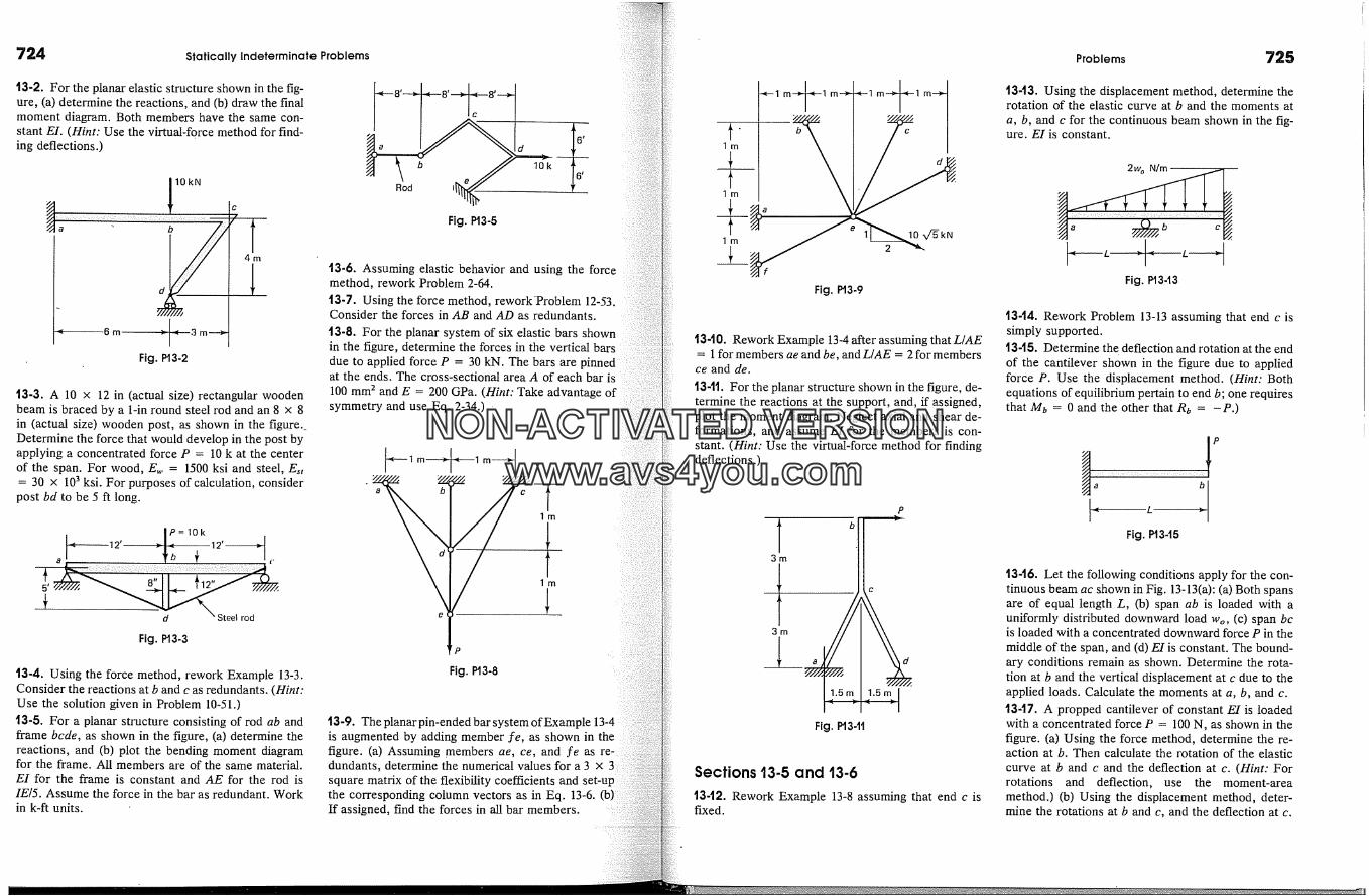
724 Statically Indeterminate Problems
t3-2. For the planar elastic structure shown in the fig-ure, (a) determine the reactions, and (b) draw the finalmoment diagram. Both members have the same con-stant El. (Hint: Use the virtual-force method for find-ing deflections.)
. 110kN
8m -� � 3m--->.
Fig. P13-2
c
t3-3. A 10 x 12 in (actual size) rectangular woodenbeam is braced by a 1-in round steel rod and an 8 x 8in (actual size) wooden post, as shown in the figure._Determine the force that would develop in the post byapplying a concentrated force P = 10 k at the centerof the span. For wood, E,. = 1500 ksi and steel, Est= 30 x 103 ksi. For purposes of calculation, consider
post bd to be 5 ft long.
P=10k
S t
d
Fig. P13-3
t3-4. Using the force method, rework Example 13-3.Consider the reactions at b and c as redundants. (Hint:Use the solution given in Problem 10-51.)t3-5. For a planar structure consisting of rod ab andframe bcde, as shown in the figure, (a) determine thereactions, and (b) plot the bending moment diagramfor the frame. All members are of the same material.E1 for the frame is constant and AE for the rod isIE/5. Assume the force in the bar as redundant. Workin k-ft units.
8' �!�*--8'�.. 8'--*-J
Fig. P13-5
t3-6. Assuming elastic behavior and using the forcemethod, rework Problem 2-64.13-7. Using the force method, rework'Problem 12-53.Consider the forces in AB and AD as redundants.
13-8. For the planar system of six elastic bars shownin the figure, determine the forces in the vertical barsdue to applied force P = 30 kN. The bars areat the ends. The cross-sectional area A of each bar is100 mm 2 and E = 200 GPa. (Hint: Take advantage ofsymmetry and use Eq. 2-34.) -
Fig. PI3-8
t3-9. Theplanarpin-endedbarsystemofExample 13-4is augmented by adding member �e, as shown in thefigure. (a) Assuming members ae, ce, and �e asdundants, determine the numerical values for a 3 xsquare matrix of the flexibility coefficients andthe corresponding column vectors as in Eq. 13-6.If assigned, find the forces in all bar members.
-,e--1m-�l m-�l m-�l mt
Fig. P13-9
t340. Rework Example 13-4 after assuming that L/AE= 1 for members ae and be, and L/AE = 2 for members
ce and de.
13-11. For the planar structure shown in the figure, de-termine the reactions at the support, and, if assigned,plot the moment diagram. Neglect axial and shear de-formations, and assume E1 for the members is con-stant. (Hint: Use the virtual-force method for findingdeflections.)
P
b
� . 1.5m JFig. P13-1t
Sections 13-5 and 13-6
t3-12. Rework Example 13-8 assuming that end c isfixed.
Problems 725
13-13. Using the displacement method, determine therotation of the elastic curve at b and the moments ata, b, and c for the continuous beam shown in the fig-ure. EI is constant.
2woN/� �
Fig. P13-13
t344. Rework Problem 13-13 assuming that end c issimply supported.13-t5. Determine the deflection and rotation at the endof the cantilever shown in the figure due to appliedforce P. Use the displacement method. (Hint: Bothequations of equilibrium pertain to end b; one requiresthat Mb = 0 and the other that Rb = -P.)
PL }-
Fig. P1345
1346. Let the following conditions apply for the con-tinuous beam ac shown in Fig. 13-13(a): (a) Both spansare of equal length L, (b) span ab is loaded with auniformly distributed downward load wo, (c) span bcis loaded with a concentrated downward force P in themiddle of the span, and (d)E1 is constant. The bound-ary conditions remain as shown. Determine the rota-tion at b and the vertical displacement at c due to theapplied loads. Calculate the moments at a, b, and c.t3-11. A propped cantilever of constant E1 is loadedwith a concentrated force P = 100 N, as shown in thefigure. (a) Using the force method, determine the re-action at b. Then calculate the rotation of the elasticcurve at b and c and the deflection at c. (Hint: Forrotations and deflection, use the moment-areamethod.) (b) Using the displacement method, deter-mine the rotations at b and c, and the deflection at c.
NON-ACTIVATEDVERSIONwww.avs4you.com
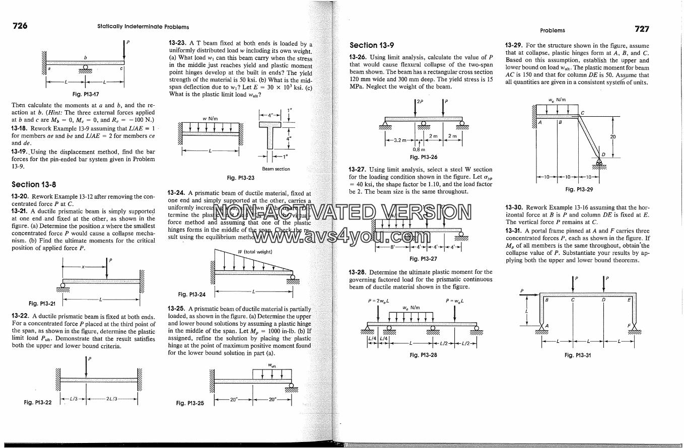
726 Statlcally Indeterminate Problems
Fig. PI347
Then calculate the moments at a and b, and the re-action at b. (Hint: The three external forces appliedatbandcareMb = 0, Me= 0, andRe = -100N.)t5-t8. Rework Example 13-9 assuming that L/AE = 1for members ae and be and L/AE = 2 for members ceand de.
t$-t9._Using the displacement method, find the barforces for the pin-ended bar system given in Problem13-9.
Section '13-8
t3-20. Rework Example 13-12 after removing the con-centrated force P at C.
t5-2t. A ductile prismatic beam is simply supporte_dat one end. and fixed at the other, as shown in thefigure. (a) Determine the position x where the smallestconcentrated force P would cause a collapse mecha-nism. (b) Find the ultimate moments for the criticalposition of applied force P.
13-22. A ductile prismatic beam is fixed at both ends.For a concentrated force P placed at the third point ofthe span, as shown in the figure, determine the plasticlimit load Pult. Demonstrate that the result satisfiesboth the upper and lower bound criteria.
Fig. P13-22 --, LI3 >j�- 2L/3 �
t3-23. A T beam fixed at both ends is loaded byuniformly distributed load w including its own weight,(a) What load w� can this beam carry when the stressin the middle just reaches yield and plastic mom,point hinges develop at the built in ends? The yieldstrength of the material is 50 ksi. (b) What is the mid-span deflection due to w�? Let E = 30 x 103 ksi.What is the plastic limit load
w N/m
Fig. P13-23
Beam section
t3-24. A prismatic beam of ductile material, fixedone end and simply supported at the other, carries auniformly increasing load, as shown in the figure.termine the plastic limit load Wu�t using theforce method and assuming that one of the plastichinges forms in the middle of the span. Check thesult using the equilibrium method.
Fig. PI3-24
W(tot�
t3-25. A prismatic beam of ductile material isloaded, as shown in the figure. (a) Determine the uand lower bound solutions by assuming a plasticin the middle of the span. Let Mp = 1000 in-lb. (b)assigned, refine the solution by placing the'hinge at the point of maximum positive momentfor the lower bound solution in part (a).
Fig. P13-25
Wult
Section 13-9
t3-26. Using limit analysis, calculate the value of Pthat would cause flexural collapse of the two-spanbeam shown. The beam has a rectangular cross section120 mm wide and 300 mm deep. The yield stress is 15MPa. Neglect the weight of the beam.
2PI'-3'2m ;I-);I ;I-' ;I
0.8 m
Fig. P13-26
t3-27. Using limit analysis, select a steel W sectionfor the loading condition shown in the figure. Let %.p= 40 ksi, the shape factor be 1.10, and the load factor
be 2. The beam size is the same throughout.
12k 27k
Fig. PI3-27
13-28. Determine the ultimate plastic moment for thegoverning factored load for the prismatic continuousbeam of ductile material shown in the figure.
P=2woL P=woLN/m
IL/4[L/41 [ I 1l�>l< �j� L ,�l < L/2-�-�-L/2-� t
Fig. P13-28
Problems 727
t3-29. For the structure shown in the figure, assumethat at collapse, plastic hinges form at A, B, and C.Based on this assumption, establish the upper andlower bound on load w,�t. The plastic moment for beamAC is 150 and that for column DE is 50. Assume thatall quantities are given in a consistent syste�m of units.
w o N/m
A B
-�-10 10 >
C
Fig. P13-29
13-30. Rework Example 13-16 assuming that the hor-izontal force at B is P and column DE is fixed at E.The vertical force P remains at C.
t3-31. A portal frame pinned at A and F carries threeconcentrated forces P, each as shown in the figure. IfMy of all members is the same throughout, obtain'thecollapse value of P. Substantiate your results by ap-plying both the upper and lower bound theorems.
Fig. P13-31
NON-ACTIVATEDVERSIONwww.avs4you.com
Tables
1A. Typical Physical Properties of and Allowable Stresses for SomeCommon Materials (in U.S. Customary System of Units)
lB. Typical Physical Properties of and Allowable Stresses for SomeCommon Materials (in SI System of Units)
2. Useful Properties of Areas
3. American Standard Steel Beams, S Shapes, Properties for Designing
4. American Wide-Flange Steel Beams, W Shapes, Properties for De-signing
5. American Standard Steel Channels, Properties for Designing
6. Steel Angles with Equal Legs, Properties for Designing
7. Steel Angles with Unequal Legs, Properties for Designing
8. Standard Steel Pipe
9. Plastic Section Moduli Around the X-X Axis
10. American Standard Timber Sizes, Properties for Designing
11. Deflections and Slopes of Elastic Curves for Variously LoadedBeams
12. Fixed-End Actions for Prismatic Beams
Acknowledgement: Data for Tables 3 through 9 are taken from the AISCManual of Steel Construction and are reproduced by permission of theAmerican Institute of Steel Construction, Inc. The tables are compiledfor use with this text. Original sources should be consulted for actualdesign.
NON-ACTIVATEDVERSIONwww.avs4you.com
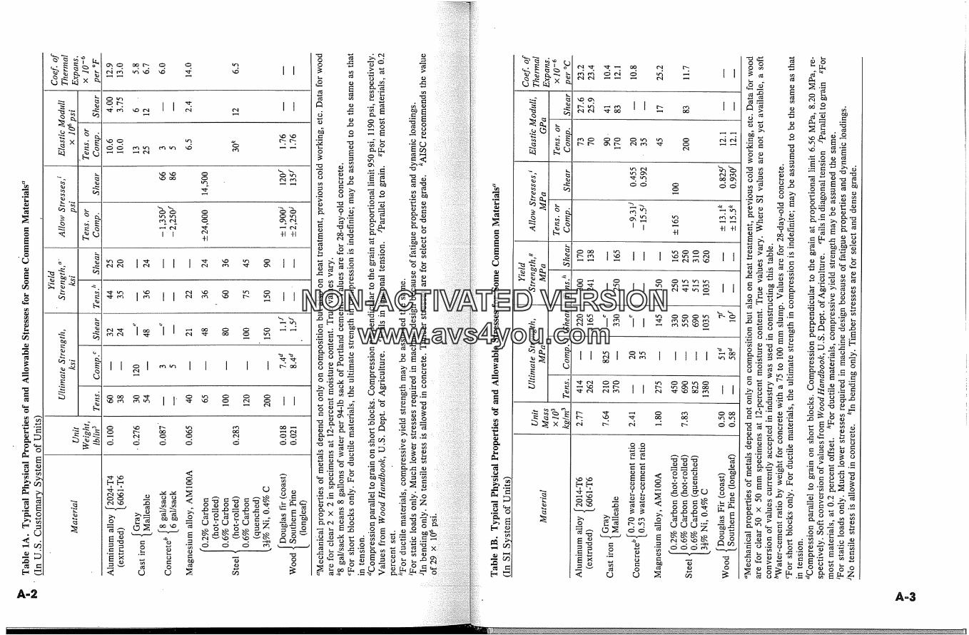
A-2 A-3
NON-ACTIVATEDVERSIONwww.avs4you.com
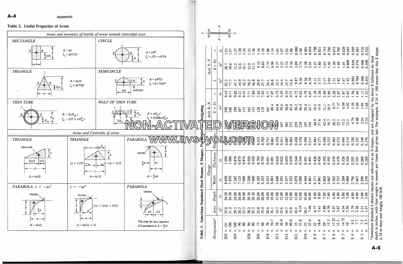
�[�=g� Appendix
Table 2. Useful Properties of Areas
Areas and moments of inertia of areas aroand centroidal axes
RECTANGLE
oleohi2
TRIANGLE
THIN TUBE
0
A = bh
! o = bh3/12
A = bh/2
I o = bh3/36
A = 2�Rav tIo = J/2 � �R�3v t
CIRCLE
t
SEMICIRCLE
0�0� �R
,� 2R �[ 4R/(3�r)HALF OF THIN TUBE
-�K2Z_� (2hr) Ray
A = 'n'R 2
I� = J/2 = �rR4/4
�rR2/2
0.110R 4
A = lrRavtI o � 0.095�rRaavt
Areas and Centroids of areas
' TRIANGLE
Centroid
A = bh/2
PARABOLA: y = - ax 2
TRIANGLE
(a+L)13�A = hL/2
y = _ ax n
+ L)/3
PARABOLA
Vertex�� I__�A = -�bh
PARABOLA
VertexVertex
h
A = bh/3
Vertex
A = bh/(n + 1)The area for any segment
of a parabola is A = �hl
dd ddd dd d d-d�'5�d d dd dd dd dd dd dd dd dd dd
.� X X X X X X X X X X X X X X X X X X X X X X X X X X X X X X X
NON-ACTIVATEDVERSIONwww.avs4you.com

XXXXX XXX XXXX XXX
A-6 A-7
NON-ACTIVATEDVERSIONwww.avs4you.com
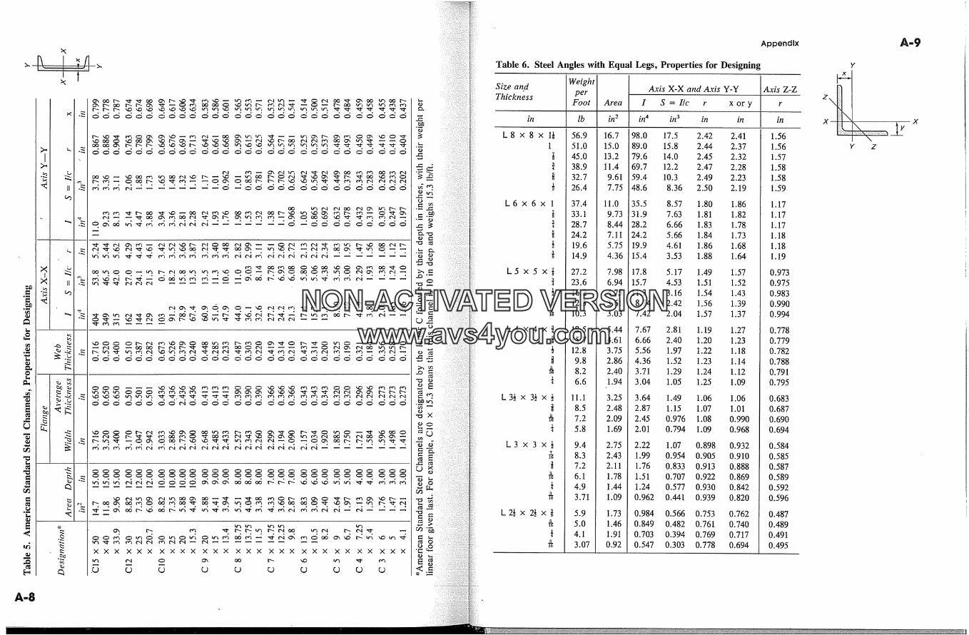
A-8
Appendix
Table 6. Steel Angles with Equal Legs, Properties for Designing
Size and Weight Axis X-X and Aris Y-Y Axis Z-ZThickness per
Foot Area I S = I/c r x or y r
in lb #l 2 #l 4 in 3 in in in
L 8 x 8 x 1� 56.9 16.7 98.0 17.5 2.42 2.41 1.561 51.0 15.0 89.0 15.8 2.44 2.37 1.56
� 45.0 13.2 79.6 14.0 2.45 2.32 1.57�a 38.9 11.4 69.7 12.2 2.47 2.28 1.58fl 32.7 9.61 59.4 10.3 2.49 2.23 1.58� 26.4 7.75 48.6 8.36 2.50 2.19 1.59
L 6 x 6 x 1 37.4 11.0 35.5 8.57 1.80 1.86 1.17� 33.1 9.73 31.9 7.63 1.81 1.82 1.17�a 28.7 8.44 28.2 6.66 1.83 1.78 1.17� 24.2 7.11 24.2 5.66 1.84 1.73 1.18� 19.6 5.75 19.9 4.61 1.86 1.68 1.18� 14.9 4.36 15.4 3.53 1.88 1.64 1.19
L 5 x 5 x � 27.2 7.98 17.8 5.17 1.49 1.57 0.973�a 23.6 6.94 15.7 4.53 1.51 1.52 0.975� 16.2 4.75 11.3 3.16 1.54 1.43 0.983� 12.3 3.61 8.74 2.42 1.56 1.39 0.990
� 10.3 3.03 7.42 2.04 1.57 1.37 0.994
L 4 x 4 x �a 18.5 5.44 7.67 2.81 1.19 1.27 0.778� 15.7 4.61 6.66 2.40 1.20 1.23 0.779� 12.8 3.75 5.56 1.97 1.22 1.18 0.782� 9.8 2.86 4.36 1.52 1.23 1.14 0.788
� 8.2 2.40 3.71 1.29 1.24 1.12 0.791� 6.6 1.94 3.04 1.05 1.25 1.09 0.795
L 3� x 3� x � 11.1 3.25 3.64 1.49 1.06 1.06 0.683� 8.5 2.48 2.87 1.15 1.07 1.01 0.687
� 7.2 2.09 2.45 0.976 1.08 0.990 0.690� 5.8 1.69 2.01 0.794 1.09 0.968 0.694
L 3 x 3 x � 9.4 2.75 2.22 1.07 0.898 0.932 0.584� 8.3 2.43 1.99 0.954 0.905 0.910 0.585
� 7.2 2.11 1.76 0.833 0.913 0.888 0.587� 6.1 1.78 1.51 0.707 0.922 0.869 0.589
� 4.9 1.44 1.24 0.577 0.930 0.842 0.592� 3.71 1.09 0.962 0.441 0.939 0.820 0.596
L 2� x 2� x � 5.9 1.73 0.984 0.566 0.753 0.762 0.487� 5.0 1.46 0.849 0.482 0.761 0.740 0.489
� 4. t 1.91 0.703 0.394 0.769 0.717 0.491� 3.07 0.92 0.547 0.303 0.778 0.694 0.495
Y
A-9
NON-ACTIVATEDVERSIONwww.avs4you.com

� ,-� � X X X X X X X X� .� � .� x x x x x x x x
-oo oo -J -J -J -J ('q -J -J -J-J
Table 8. Standard Steel Pipe
Appendix
Dimensions Properties
Nora. Outside Inside Thick- WeightDiam. Diam. Diam. hess per Foot I A r
b� h� in h� lb in 4 in 2 in
� 0.405 0.269 0.0688
� 0.540 0.364 0.088� 0'.675 0.493 0.091� 0.840 0.622 0.109a 1.050 O. 824 O. 1134
I 1.315 1.049 0.13315 1.660 1.380 0.1401� 1.900 1.610 O. 145
2 2.375 2.067 O. 1542� 2.875 2.469 0.2033 3.500 3.068 0.2163� 4.000 3.548 0.226
4 4.500 4.026 0.2375 5.563 5.047 0.2586 6.625 6.065 0.2808 8.625 7.981 0.322
10 10.750 10.020 0.36512 12.750 12.000 0.375
0.240.420.570.85
1.131.68
2.272.723.655.797.589.11
10.7914.6218.97
28.5540.4849.56
0.001 0.072 O. 120.003 0.125 0.160.007 O. 167 0.210.017 0.250 0.260.037 0.333 0.330.087 0.494 0.42O. 195 O. 669 0.540.310 0.799 0.620.666 1.07 0.79
1.53 1.70 0.953.02 2.23 1.164.79 2.68 1.347.23 3.17 1.51
15.2 4.30 1.8828.1 5.58 2.2572.5 8.40 2.94
161. 11.9 3.67279. 14.6 4.38
Table 9. Plastic Section Moduli Around the X-X Axis; 'i'yp ---- 36 ksi
Plastic Modulus Z,Shape in 3
W 36 x 230 943W 33 x 221 855W 36 x 194 767W 36 x 182 718W 36 x 170 668W 36 x 160 624W 36 x 150 581W 33 x 141 514W 36 x 135 509W 33 x 130 467W 33 x 118 415W 30 x 116 378W 30 x 108 346W 30 x 99 312W 27 x 94 278W 24 x 94 254W 27 x 84 244
Plastic Modulus Z,Shape in 3
W 24 x 84 224W 24 x 76 200W 24 x 68 177W 21 x 68 160W 24 x 62 153W 24 x 55 134W 21 x 57 129W 18 x 55 112W 21 x 44 95.4W 18 x 40 78.4W 16 x 40 72.9W 18 x 35 66.5W 16 x 31 54.0W 14 x 26 40.2W 14 x 22 33.2W 8 x 24 23.2W 8 x 18 17.0
A-11
A-'O
NON-ACTIVATEDVERSIONwww.avs4you.com
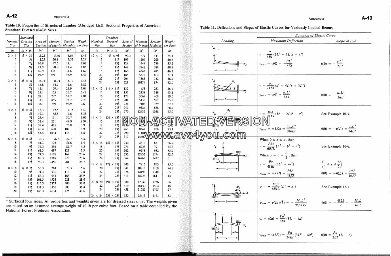
A=�2 Appendix
Table 10. Properties of Structural Lumber (Abridged List). Sectional Properties of AmericanStandard Dressed (S4S)* Sizes.
Standard Standard
Nominal Dressed Area of Motnent Section Weight Nominal Dressed Area of Moment Section WeightSize Size Section of Inertia Modtdus �er Foot Size Size Section of Inertia Modnlus per Foot
in in x in #l 2 in 4 in 3 lb in in x in in 2 in 4 in 3 lb
2 x 4 I.X_, x 3.x_, 5.25 5.36 3.06 1.46 lO x lO 9-' 9�._, x 90.3 679 143 25. l6 5� 8.25 20.8 7.56 2.29 12 I l� 109 1204 209 30.38 7�, 10.9 47.6 13. I 3.02 14 13� 128 1948 289 35.6
10 9� 13.9 98.9 21.4 3.85 16 15� 147 2948 380 40.912 11� 16.9 178 31.6 4.69 18 17� 166 4243 485 46.114 13� 19.9 291 43.9 5.52 20 19� 185 5870 602 51.4
22 21� 204 7868 732 56.73 x 4 2� x 3� 8.75 8.93 5.10 2.43 24 23� 223 10274 874 62.0
6 5-' 13.8 34.7 12.6 3.828- 7{ 18.1 79.4 21.9 5.04 12 x 12 ll.� x II-' 132 1458 253 36.7
IO 9{ 23. l 165 35.7 6.42 14 13� 155 2358 349 43. l12 I 1{ 28. I 297 52.7 7.81 16 15� 178 3569 460 49.514 13{ 33.1 485 73.2 9.20 18 17� 201 5136 587 55.916 15{ 38. I 739 96.9 10.6 20 19� 224 7106 729 62.3
22 21� 247 9524 886 68.74 x 4 3� x 3� 12.3 12.5 7.15 3.40 24 23� 270 12437 1058 75.0
6 5 -� 19.3 48.5 17.6 5.352
8 7� 25.4 Ill 30.7 7.05 14 x 14 13� x 13� 182 2768 410 50.610 9� 32.4 231 49.9 8.94_ 16 15� 209 4189 541 58.112 III 39.4 415 73.8 10.9 18 17� 236 6029 689 65.614 13� 46.4 678 102 12.9 20 19� 263 8342 856 73.116 15� 53.4 1034 136 14.8 22 21� 290 11181 1040 80.6
24 23� 317 14600 1243 88.16 x 6 5-' 5��_, x 30.3 76.3 27.7 8.40
8 7-' 41.3 193 51.6 11.4 16 x 16 15� x 15� 240 4810 621 66.7l0 9� 52.3 393 82.7 14.5 18 17� 271 6923 791 75.312 I I� 63.3 697 121 17.5 20 19� 302 9578 982 83.914 13� 74.3 1128 167 20.6 22 21� 333 12837 1194 92.516 15� 85.3 1707 220 23.6 24 23� 364 16763 1427 10118 17� 96.3 2456 281 ' 26.7
18 x 18 17� x 17� 306 7816 893 85.08 x 8 7-' 7�._, x 56.3 264 70.3 15.6 20 19� 341 10813 1109 94.8
l0 9� 71.3 536 113 i9.8 22 21� 376 14493 1348 10512 I l� 86.3 951 165 23.9 24 23� 411 18926 1611 11414 13� 101.3 1538 228 28.016 15� 116.3 2327 300 32.0 20 x 20 19� x 19� 380 12049 1236 106
22 21� 419 16150 1502 11618 17� 131.3 3350 383 36.420 19� 146.3 4634 475 40.6 24 23� 458 21089 1795 127
24 x 24 23� x 23� 552 25415 2163 153
* Surfaced four sides. All properties and weights given are for dressed sizes only. The weights givenare based on an assumed average weight of 40 lb per cubic foot. Based on a table compiled by theNational Forest Products Association.
Appendix
Table 11, Deflections and Slopes of Elastic Curves for Variously Loaded Beams
Loading
qo
P
P P
Equation of Elastic CurveMaximum Deflection Slope at End
P (9L 3 3L�r + .r �)pL 3
Vm� = v(O) = --3El
pL 2o(0) -
2El
qo
v = 2--� (x4 - 4L3x + 3L4)Urea x = u(O) : q"L4
8Elo(o) -
6EI
q,,x tL 3 _ 2Lx2 +v = 24E1 '-
5q,,L 4Vm�,, = v( L/2) -
384E1
See Example 10-3.
0(0) = -0(L) - q"L324EI
When 0 -< x -< a, then
Pbx b2v = 6-� (L2 -- -- 3'2)When a = b = , then
PJ
4--� (3L' 2v= --4x)
pL 3Vma� = v(L/2)
48.EI
See Example 10-6.
o(0) = -O(L) -pL 216E/
M,,x (L 2 _ x2 )6EIL See Example 13-1.
MoL 27Jmax � v(L/�/�) = 9�/3 E1 o(o)
pa 2v� = v(a) = �-� (3L - 4a)
Pa
Vmax = v(L/2) = 2-�--� (3L2 - 4a2)
0(L)
Pa
0(0) = �(L - a)
A43
Mo L6E/
NON-ACTIVATEDVERSIONwww.avs4you.com

Appendix
Table 12. Fixed-End Actions of Prismatic Beams'*
Loading Moments* Reactions*
P
< L �
q,,L 2 qoLMao = -Moa = R,, = Ro =
12 2
pb �Pab 2 R,* � - --� (3� + b)M,.a = L2
P ba 2 pgl 2mdc- L2 R,I = L3 (a + 3b)
qoL 2 3qoLM,,o = --- R,, = ---30 20
M�,, = q"L2 Ru = - 7qoL20 20
M,a, = � Or, R,, =-4El 6El
Mr,,, = � Or, Rt, = - �_
6El 12ElM,,� = - L-- T zk R,, L_ � iX
6El 12ElMi,. = - -�5-_,A R� = ~ A
Mb,.=M,,(-I + 4�- 3a2'�L 2 ] Rb = --6M,,a
6M,,a (1 -M"a (2 - 3�) R,. L2 �)M;. =
* For all the cases tabulated, the positive senses of the end moments and reactions are the sameas those shown in the first diagram for uniformly distributed loading. The special sign conventionused hgre Lv that adopted for the displacement method in Section 13-5.
Chapter �1-3. �/re at 0 � and 180�: 1/0;
at 45�: 0.5/0.5; at 90�: 0/0.1-5. +m at 0 � and 180�; +�/2
at 45 � and 135 � .1-7. 17.7 ksi, 2.34 ksi, 6.43 ksi.1-9. 12.1 ksi, 18.2 ksi.1-11. 21.3 MPa; 30 mm, 35 mm.1-13. �max = 25 MPa, ffmin =
10 MPa.1-15. 2.11-kPa.
1-17. - 109 psi, - 198 psi, - 119psi.
1-19. (a) 30 MPa, (b) 40.9 MPa,(c) 71.6 MPa, (d) 113MPa.
1-21. 6.5 in.1-23. 2.83 ksi.1-25. 4.81 ksi, 5.97 ksi.1-27. cr.�m = cr�c = 100.3 MPa1-29. 73.6 psi, 111 psi, 902.1
psi, 184 psi.1-31. 10 k, 4.08 ksi.1-33. (a) 2.22 MPa, (b) 0.707 m.1-35. 10.7 in.1-37. 16.4 mm.1-39. 13.2 kg.1-41. A^� = 5300mm 2, A�c =
7950 mm 2, A�e = 3640mm 2.
1-43. 0.123 in.1-45. 27 mm.1-47. &max = 14.5 MPa.1-49. 0.909 in 2 vs 0.864 in 2.
1-51. 38.9 k.1-53. 8.57 in, 18.2 in.
Chapter 2
2-1. 29.3 X 10 6 psi.2-3. (a) 10 mm, (b) 1.67
kN/mm.2-5. 50 kN/mm.2-7. 18.75 kN/mm.2-9. (a) 0.0289 in, (b) 8.57 in
from left.2-11. 9.20 mm.2-13. 0.0363 in.2-15. zk� = 3.7 mm.2-17. 597 ft.2-19. (a) 0.122 in, (b) 0.028 in.2-21. 7.64 x 10³ '�g/E.2.23. 10�'y/E mm.2-25. - 4Pa/9AE.2-27. 0.00375 in, 0.100 in. Try a
graphic solotion as in Fig.2-24(c). Use large scale.
2-29. (a) 4 kN/mm, (b) 4 mm.2-31. 2 mm2-33. 0.165 in, 0.0714 in. Try a
graphic solution as in Fig.2-29(b).
2-35. 29.3 kiN.2-37. 9.9 kiN.2-39. (a) 28.7 ksi, (b) 0.0367 in,
(c) 0.565 in, (d) 0.448 in.2-41. 0.04 in.2-43. 4 mm.
2-45. 194 MPa, 129 MPa, 228MPa (lower rod).
2-47. RL = 1.2P.2-49. (a) - 120 kN, -70 kN.2-51. (a) 5 k, -25 k.2-53. (a) 1250 N (middle wire)2-55. 0.2274P, 0.6062P.2-59. 1/3 k.2-61. Ru = 0.65P.2-63. 4.8 kN.2-65. Ru =-4P.2-67. P/[(a/b) � + 11.2-69. (a) 480 k, (b) 1100 k.2-71. 83.3 N, 333 N, 583 N.2-73. 37.8 � C.
2-75. Pyp = 376 kN, P� = 518kN at 5 mm.
2-77. 2'yw2L3/3gE.
Chapter 33-1. 51.2 N/mm.3-3. (a) - 3.50 txm, (b) 147 kN.3-5. 0.325, 0.25.3-7. 444 psi.3-9. (a) 0.20 in, use 0.25 plate,
(b) 0.212 in.3-11. 14.3-13. 0.080 in, 0.025 in.3-15. 70.7 MPa.3-17. 25.9 MPa.3-23. (a) cr� = 20(1 - 0.05/r2),
(b) 180 MPa, (c) 91.7 txm,41.0 txm.
NON-ACTIVATEDVERSIONwww.avs4you.com
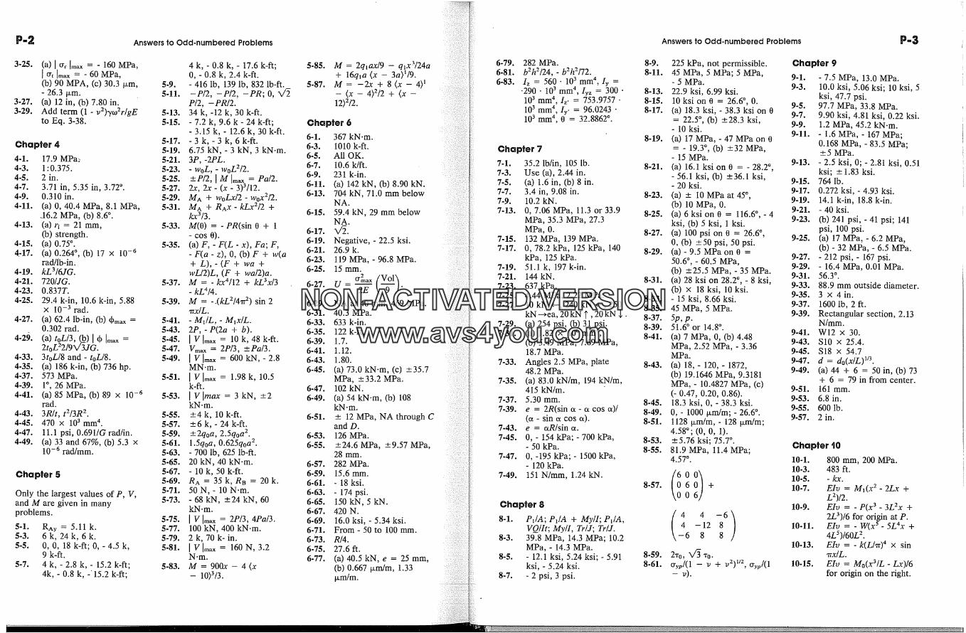
P-2 Answers to Odd-numbered Problems
3-25. (a) [ crr Im� = - 160 MPa,[ Pt [m� = - 60 MPa,(b) 90 MPA, (c) 30.3 �m,- 26.3 tzm.
3-27. (a) 12 in, (b) 7.80 in.3-29. Add term (1 - v2)�to2r/gE
to Eq. 3-38.
Chapter 44-1. 17.9 MPa:4-3. 1:0.375.4-5. 2 in.4-7. 3.71 in, 5.35 in, 3.72 � .4-9. 0.310 in.4-11. (a) 0, 40.4 MPa, 8.1 MPa,
_16.2 MPa, (b) 8.6 �.4-13. (a) ri = 21 mm,
(b) strength.4-15. (a) 0.75 �.4-17. (a) 0.264 �, (b) 17 x 10 -6
rad/ib-in.4-19. kL3/6JG.4-21. 720/JG.4-23. 0.837T.4-25. 29.4 k-in, 10.6 k-in, 5.88
X 1'0 -3 rad.4-27. (a) 62.4 lb-in, (b) 4�,� =
0.302 rad.4-2�J. (a) toL/3, 0) 10)Im� =
2toL22/9X/3JG.4-33. 3toL/8 and - toL/8.4-35. (a) 186 k-in, (b) 736 hp.4-37. 573 MPa.4-39. 1 �, 26 MPa.4-41. (a) 85 MPa, (b) 89 x 10 -6
rad.4-43. 3R/t, t2/3R 2.4-45. 470 X ][0 3 mm 4.4-47. 11.1 psi, 0.691/G rad/in.4-49. (a) 33 and 67%, (b) 5.3 x
10 -6 rad/mm.
Chapter 5
Only the largest values of P, V,and M are given in manyproblems.
5-1. RAy = 5.11 k.5-3. 6k, 24k, 6k.5-5. 0, 0, 18 k-ft; 0, - 4.5 k,
9 k-ft.5-7. 4 k, - 2.8 k, - 15.2 k-ft;
4k, - 0.8 k, -' 15.2 k-ft;
4 k, - 0.8 k, - 17.6 k-ft;0, - 0.8 k, 2.4 k-ft.
5-9. - 416 lb, 139 lb, 832 lb-ft.5-11. -P/2, -P/2, -PR; O,
P/2, - PR/2.5-13. 34 k, -12 k, 30 k-ft.5-15. - 7.2 k, 9.6 k - 24 k-ft;
- 3.15 k, - 12.6 k, 30 k-ft.5-17. -3k,-3k, 6k-ft.5-19. 6.75 kN, - 3 kN, 3 kN.m.5-21. 3P, -2PL.5-23. - woL, - woL2/2.5-25. + P/2, I m I m� = Pa/2.5-27. 2x, 2x - (x - 3)3/12.5-29. M^ + woLx/2- WoX2/2.5-31. M^ + R^x-kLx2/2 +
kx3/3.5-33. M(0) =-PR(sin0 + 1
- cos 0).5-35. (a) F, - F(L - x), Fa; F,
- F(a- z), O, (b) F + w(a+ L),-(F + wa +
wL/2)L, (F + wa/2)a.5-37. M = -kx4/12 + kL3x/3
- kL414.5-39. M = --(kZ2/4� 2) sin 2
�rx/L.5-41. - M�/L, - M�x/L.5-43. 2P,-P(2a + b).5-45. IVIm� = 10k, 48k-ft.5-47. V�,� = 2P/3, +Pa/3.5-49. [Vlm� = 600kN,-2.8
MN.m.
5-51. ]Vlm� = 1.98k, 10.5k-ft.
5-53. [ V Imax = 3 kN, +2
5-55. -+4 k, 10 k-ft.5-57. + 6 k, - 24 k-ft.5-59. +2qoa, 2.5qoa 2.5-61. 1.5qoa, 0.625qoa 2.5-63. - 700 lb, 625 lb-ft.5-65. 20 kN, 40 kN-m.5-67. - 10 k, 50 k-ft.5-69. R^ = 35k, RB = 20k.5-71. 50 N,- 10 N.m.5-73. - 68 kN, ---24 kN, 60
kN.m.
5-75. I V Imax = 2P/3, 4Pa/3.5-77. 100 kN, 400 kN-m.5-79. 2k, 70k-in.5-81. Iglm�- 160N, 3.2
N.m.5-83. M= 900x- 4
- 10)3/3.
5-85. M = 2qtax/9 - q�x3/24a+ 16q�a (x - 3a)�/9.
5-87. M = -2x + 8(x- 4) �-- {x -- 4)2/2 + (x --12)2/2.
Chapter 66-1. 367 kN.m.6-3. 1010 k-ft.6.5. All OK.6-7. 10.6 k/ft.6.9. 231 k-in.6-11. (a) 142 kN, (b) 8.90 kN.6-13. 704 kN, 71.0 mm below
NA.6-15. 59.4 kN, 29 mm below
NA.6-17. �.6-19. Negative, - 22.5 ksi.6-21. 26.9 k.6-23. 119 MPa, - 96.8 MPa.6-25. 15 mm.
tY/nax
6-27. U = � .6-29. NA at 40 mm, 469 MPa.6-31. 40.3 MPa.6-33. 633 k-in.6-35. 122 k-ft.6-39. 1.7.6-41. 1.12.6-43. 1.80.6-45. (a) 73.0 kN.m, (c) +35.7
MPa, -+ 33.2 MPa.6-47. 102 kN.6-49. (a) 54 kN.m, (b) 108
6-51. m 12 MPa, NA through Cand D.
6-53. 126 MPa.6-55. +24.6 MPa, +9.57 MPa,
28 mm.6-57. 282 MPa.6-59. 15.6 mm.6-61. - 18 ksi.6-63. - 174 psi.6-65. 150 kN, 5 kN.6-67. 420 N.6-69. 16.0 ksi, - 5.34 ksi.6-71. From - 50 to 100 mm.6-73. R/4.6-75. 27.6 ft.6-77. (a) 40.5 kN, e = 25 mm,
(b) 0.667 txm/m, 1.33txm/m.
6-79.6-81.6-83.
282 MPa.b2h2/24, - b2h2/72.I� = 560 � 103 mm 4, Iy =
-290 � 10 3 mm 4, Iy� = 300 �103 mm 4, I�, = 753.9757 �103 mm 4, Iv, = 96.0243 �103 mm 4, 0 = 32.8862 �.
Chapter 77-1. 35.2 lb/in, 105 lb.7-3. Use (a), 2.44 in.7-5. (a) 1.6 in, (b) 8 in.7-7. 3.4 in, 9.08 in.7-9. 10.2 kN.%13. 0, 7.06 MPa, 11.3 or 33.9
MPa, 35.3 MPa, 27.3MPa, 0.
7-15. 132 MPa, 139 MPa.7-17. 0, 78.2 kPa, 125 kPa, 140
kPa, 125 kPa.7-19. 51.1 k, 197 k-in.7-21. 144 kN.7-23. 637 kPa.7-25. 4.44 MPa, 2.22 MPa.7-27. 10 kN <--, 240 kN <--, 250
kN-->ea, 20kN �', 20kN $.7-29. (a) 254 psi, (b) 31 psi.7-31. (a) 1.82 x 106 mm 4,
(b) 5.49 MPa, 7.69 MPa,18.7 MPa.
7-33. Angles 2.5 MPa, plate48.2 MPa.
7-35. (a) 83.0 kN/m, 194 kN/m,415 kN/m.
7-37. 5.30 mm.7-39. e = 2R(sina-acosa)/
(a - sin a cos a).7-43. e = aR/sin a.7-45. 0, - 154 kPa; - 700 kPa,
- 50 kPa.7-47. 0, -195 kPa; - 1500 kPa,
- 120 kPa.7-49. t51 N/mm, 1.24 kN.
Chapter 88-1. P�/A; PJA + My/I; P�/A,
VQ/It; My/I, Tr/J; Tr/J.8-3. 39.8 MPa, 14.3 MPa; 10.2
MPa, - 14.3 MPa.8-5. - 12.1 ksi, 5.24 ksi; - 5.91
ksi, - 5.24 ksi.8-7. - 2 psi, 3 psi.
Answers to Odd.numbered Problems P-3
8-9. 225 kPa, not permissible.8-11. 45 MPa, 5 MPa; 5 MPa, 9-1.
- 5 MPa.9-3.
8-13. 22.9 ksi, 6.99 ksi.8-15. 10ksion0 = 26.6 � ,0. 9-5.8-17. (a) 18.3 ksi, - 38.3 ksi on 0 9-7.
= 22.5 �, (b) +28.3 ksi, 9-9.- 10 ksi.
9-11.8-19. (a) 17 MPa, - 47 MPa on 0
= - 19.3 �, (b) +32 MPa,- 15 MPa.
9-13.8-21. (a) 16.1 ksi on 0 = - 28.2 �,
- 56.1 ksi, (b) +36.1 ksi, 9-15.- 20 ksi.
9-17.8-23. (a) + 10 MPa at 45 �, 9-19.
(b) 10 MPa, 0. 9-21.8-25. (a) 6ksion0 = 116.6 � ,-4
ksi, (b) 5 ksi, t ksi. 9-23.8-27. (a) 100 psi on 0 = 26.6 �, 9-25.
0, (b) +50 psi, 50 psi.8-29. (a)-9.5MPaon0 =
50.6 �, - 60.5 MPa, 9-27.9-29.(b) +25.5 MPa, - 35 MPa. 9-31.
8-31. (a) 28 ksi on 28.2 �, - 8 ksi, 9-33.(b) x 18 ksi, 10 ksi. 9-35.
8-33. - 15 ksi, 8.66 ksi.8-35. 45 MPa, 5 MPa. 9-37.9-39.8-37. 5p, p.8-39. 51.6 � or 14.8 � .
9-41.8-41. (a) 7 MPa, 0, (b) 4.48 9-43.
MPa, 2.52 MPa, - 3.36MPa. 9-45.
9-47.8-43. (a) 18, - 120, - 1872, 9-49.
(b) 19.1646 MPa, 9.3181MPa, - 10.4827 MPa, (c) 9-51.(- 0.47, 0.20, 0.86). 9-53.
8-45. 18.3 ksi, 0, - 38.3 ksi. 9-55.8-49. 0, - 1000 txm/m; - 26.6 �. 9-57.8-51. 1128 txm/m, - 128 txm/m;
4.58�; (0, 0, 1).8-53. +5.76 ksi; 75.7 �.8-55. 81.9 MPa, 11.4 MPa;
4.57 � .
8-57. 6 +0
(_:4 _6)-12 86 8 8
8-59. 2Vo, X/� 7o.'�xl/98-61. Cryv/(1 - v + v-j ~, %.�/(1
--
Chapter 9- 7.5 MPa, 13.0 MPa.10.0 ksi, 5.06 ksi; 10 ksi, 5ksi, 47.7 psi.97.7 MPa, 33.8 MPa.9.90 ksi, 4.81 ksi, 0.22 ksi.1.2 MPa, 45.2 kN.m.
- 1.6 MPa, - 167 MPa;0.168 MPa, - 83.5 MPa;
+ 5 MPa.
- 2.5 ksi, 0; - 2.81 ksi, 0.51ksi; + 1.83 ksi.764 lb.0.272 ksi, - 4.93 ksi.14.1 k-in, 18.8 k-in.- 40 ksi.
(b) 241 psi, - 41 psi; 141psi, 100 psi.(a) 17 MPa, - 6.2 MPa,(b) - 32 MPa, - 6.5 MPa.- 212 psi, - 167 psi.- 16.4 MPa, 0.01 MPa.56.3 � .88.9 mm outside diameter.3 x4in.1600 lb, 2 ft.
Rectangular section, 2.13N/mm.W12 x 30.S10 x 25.4.S18 x 54.7d = do(x/L) v3.(a) 44 + 6 = 50 in, (b) 73+ 6 = 79 in from center.
161 mm.6.8 in.600 lb.2 in.
Chapter �iO10-1. 800 mm, 200 MPa.10-3. 483 ft.10-5. - kx.10-7. EIv= M�(x 2- 2Lx +
L2)/2.10-9. EIv= - P(x 3 - 3L2x +
2L3)/6 for origin at P.10-11. EIv= - W(x 5 - 5L4x +
4LS)/60L 2.10-13. EIv= -k(Lhr) 4 x sin
�rx/L.10-15. EIv= Mo(x3/L - Lx)/6
for origin on the fight.
NON-ACTIVATEDVERSIONwww.avs4you.com
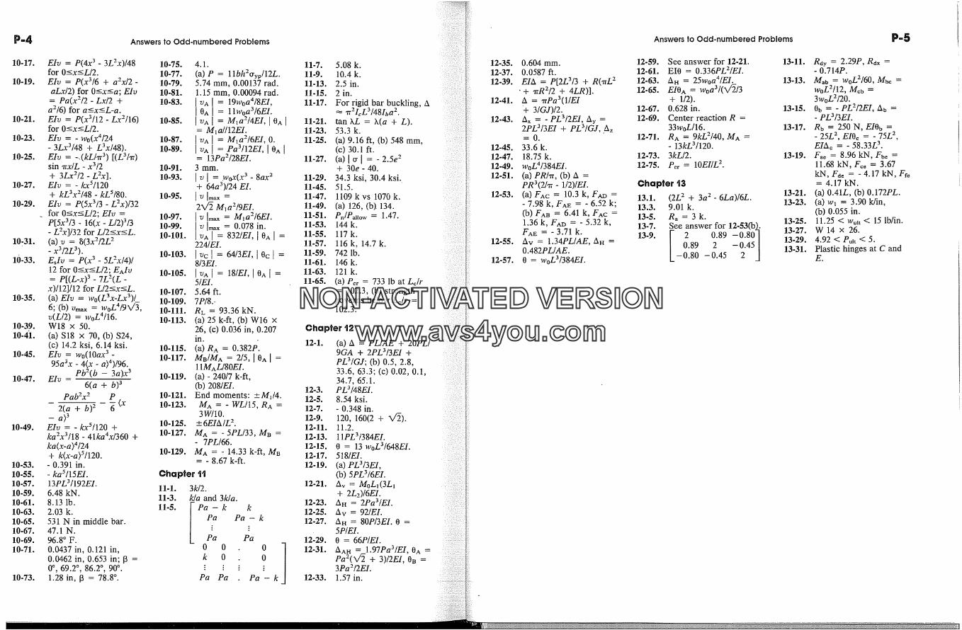
10-17.
10-19.
10-21.
10-23.
10-25.
10-27.
10-29.
10-31.
10-33.
10-35.
10-39.10-4'1.
10-45.
10-47.
10-49.
10-53.10-55.10-57.10-59.10-61.10-63.10-65.10-67.10-69.10-71.
10-73.
Answers to Odd-numbered Problems
EIv= P(4x 3 - 3L2x)[48for O-<x-< L/2.EIv= P(x3/6 + a2x/2
aLx/2) for O-<x-<a;= Pa(x2/2 - Lx'/2 +
a2/6) for a-<x-<L-a.EIv= p(x3/12 - Lx2/16)for O-<x-<L/2.EIv= - Wo(X4/24-3Lx3/48 + L3x/48).EIv= -, ( kL/'rr �) [(L3/�r)sin xx/L - x�/2+ 3Lx2/2 - L�,c].
EIv= - �r5/120+ klex2/48 - kLS/80.
EIv= P(5x3/3 - L2x)/32for O-<x--<L/2; EIv=P[5x�/3 - 16(x - L/2)�/3- L�r]/32 for(a) v = �(3x2/2L 2- x3/2L3).Eslv = P(x 3 - 5L2x/4)/12 for O-<x-<L/2; E^Iv= p[(L-x) 3 - 7L2(L -
x)/12]/12 for L/2-<x-<L.(a) EIv= wo(L3x-Lx3)/_6;'(b) Vm� = woL419X/3,v(L/2) = woL4/16.W18 x 50.(a) S18 x 70, (b) S24,(c) 14.2 ksi, 6.14 ksi.EIv= Wo(10ax �-
95a�x - 4{x - a}4)/96.pb2(b - 3a)x
EIv=6(a + b) 3
Pab2x 2 P
2(a + b) 2 6-- a} 3
EIv= - kx'5/120 +ka2x3/18 - 41ka4x/360ka(x-a}4/24+ k(x-a)S/120.
- 0.391 in.- kaS/15EI.13PL�/192EI.
6.48 kN.8.13 lb.2.03 k.531 N in middle bar.47.1 N.96.8 � F.0.0437 in, 0.121 in,0.0462 in, 0.653 in; 130 �, 69.2% 86.2 �, 90 �.1.28 in, t3 = 78.8 �.
10-75. 4.1.
10-77. (a) P = 11bh2ctyp/12L.10-79. 5.74 mm, 0.00137 rad.10-81. 1.15 mm, 0.00094 rad.10-83. I v^l = 19Wo an/8EI,
[ 0A[ = 11woaa/6EL10-85. Iv^ I = M, a2/4EI, 10^
= M�a//12EI.10-87. [ v^[ = M�a2/6EI, O.10-89. Iv^ 1 - Pa/12m, Io^
= 13Pa2/28EL10-91. 3 mm.
10-93. [ v] = 3VoX(X 3 - 8ax 2+ 64a3)/24 EI.
10-95. Iv Imx -2x/2 M�a2/9EI.
10-97. ] v Im� = Mla2/6EI.10-99. ] v ]m� = 0.078 in.10-101. Iv^[ = 832/EI,]OA[
224/EL
10-103. I Vc ! = 64/3EI, I Oc [8/3EI.
10-105. Iv^ I = 18/EI, 10^ i =5/EI.
10-107. 5.64 ft.10-109. 7P/8.-10-111. RL = 93.36 kN.10-113. (a) 25 k-ft, (b) W16 x
26, (c) 0.036 in, 0.207in.
10-115. (a) R^ = 0.382P.10-117. M�/M^ = 2/5, [ 0^ I =
11M^L/80EI.10-119. (a) - 240/7 k-ft,
(b) 208/EI.10-121. End moments: _+M,/4.10-123. M^ = - WL/15, R^ =
3W/10.10-125. + 6EI/� /L 2.10-127. M^ = - 5PL/33, M� =
- 7PL/66.10-129. M^ = - 14.33 k-ft, M�
= - 8.67 k-ft.
Chapter q�ll-l. 3k/2.11-3. k/a and 3k/a.11-5. Pa - k k
Pa Pa - k
Pa Pa0 0 0k 0 0
Pa Pa Pa - k
11-7. 5.08 k.11-9. 10.4 k.11-13. 2.5 in.11-15. 2 in.11-17. For rigid bar buckling,
� ,rr2I�L3/48I�a 2.11-21. tan kL = k(a + L).11-23. 53.3 k.11-25. (a) 9.16 ft, (b) 548 mm,
(c) 30.1 ft.11-27. (a)] cr] = - 2.5e 2
+ 30e - 40.11-29. 34.3 ksi, 30.4 ksi.11-45. 51.5.11-47. 1109 k vs 1070 k.11-49. (a) 126, (b). 134.11-51. P./P�,o,,, = 1.47.11-53. 144 k.11-55. 117 k.11-57. 116 k, 14.7 k.11-59. 742 lb.11-61. 146 k.11-63. 121 k.11-65. (a) P� = 733 lb at L�h'
= 102.3, (b) strengthgoverns below L�h' =102.3.
Chapter q2
12-1. (a) /� = PL/AE + 20PL/9GA + 2PL3/3EI +PL�/GJ; (b) 0.5, 2.8,33.6, 63.3; (c) 0.02, 0.1,34.7, 65.1.
12-3. PL�/48EL12-5. 8.54 ksi.12-7. - 0.348 in.12-9. 120, 160(2 + X/�).12-11. 11.2.12-13. 11PL�/384EI.12-15. 0 = 13 woL�/648EI.12-17. 518/EL12-19. (a) PL3/3EI,
Co) 5PL�/6EI.12-21. A� = MoL,(3L�
+ 2L2)/6EI.12-23. A� = 2Pa3/EL12-25. Av = 92/EI.12-27. � = 80P/3EI. 0 =
5P/EI.12-29. 0 = 66P/EI.12-31. A^� =_l.97Pa3/EI, O^ -
pa2(X/2 + 3)/2EI, O� =3Pa2/2EL
12-33. 1.57 in.
12-35.12-37.12-39.
12-41.
12-43.
12-45.12-47.12-49.12-51.
12-53.
12-55.
12-57.
0.604 mm.0.0587 ft.EI/� = P[2L3/3 + R(�rL 2
'+ 'trR2/2 q- 4LR)].A = �rPa3(1/EI+ 3/G J)/2.Ax = - pL3/2EI, Ay =2PL3/3EI + PL3/GJ, .�z
----- O.33.6 k.18.75 k.woL4/384EI.(a) PR/'rr, (b) A =PR3(2/'rr- 1/2)/EI.(a) F^c = 10.3 k, FAr� =- 7.98 k, F^� = - 6.52 k;(b) F^� = 6.41 k, F^c =1.36 k, F�D = - 5.32 k,
F^� = - 3.71 k.Av = 1.34PL/AE, A, =0.482PL/AE.0 = woL3/384EI.
Answers to Odd-numbered Problems
12-59. See answer for 12-21. 13-11.12-61. EI0 = 0.336PL2/EI.12-63. A, = 25woa4/EI._. 13-13.12-65. EIO^ = woa3/(X/2/3
+ 1/2).12-67. 0.628 in. 13-15.12-69. Center reaction R =
33woL/16. 13-17.12-71. R^ = 9kL2/40, M^ =
- 13kL3/120.12-73. 3kL/2. 13-19.12-75. Pc� = 10EI/L 2.
Chapter q313.1. (2L 2 + 3a 2- 6La)/6L. 13-21.13-23.13.3. 9.01 k.13-5. R� = 3 k. 13-25.13-7. See answer for 12-53(b),.
13-9. [ 2 0.89-0�180j 13-27.13-29.0.89 2 - 45 13-31.
-0.80 - 0.45
Rdy = 2.29P, Rdx =- 0.714P.Mab = woL2/60, Mb� =woL2/12, Mcb=3woL2/20.0b = - pL2/2EI, Ab =- pL3/3EI.Rb = 250 N, EIOb =- 25L 2, EIO� = - 75L 2,EI/% = - 58.33L 3.F� = 8.96 kN, F� =11.68 kN, F� = 3.67kN, Fd� = - 4.17 kN, Ff�= 4.17 kN.
(a) 0.41L, (b) 0.172PL.(a) w� = 3.90 k/in,CO) 0.055 in.11.25 < Wul� < 15 lb/in.
W 14 x 26.4.92 < P�l� < 5.Plastic hinges at C andE.
NON-ACTIVATEDVERSIONwww.avs4you.com
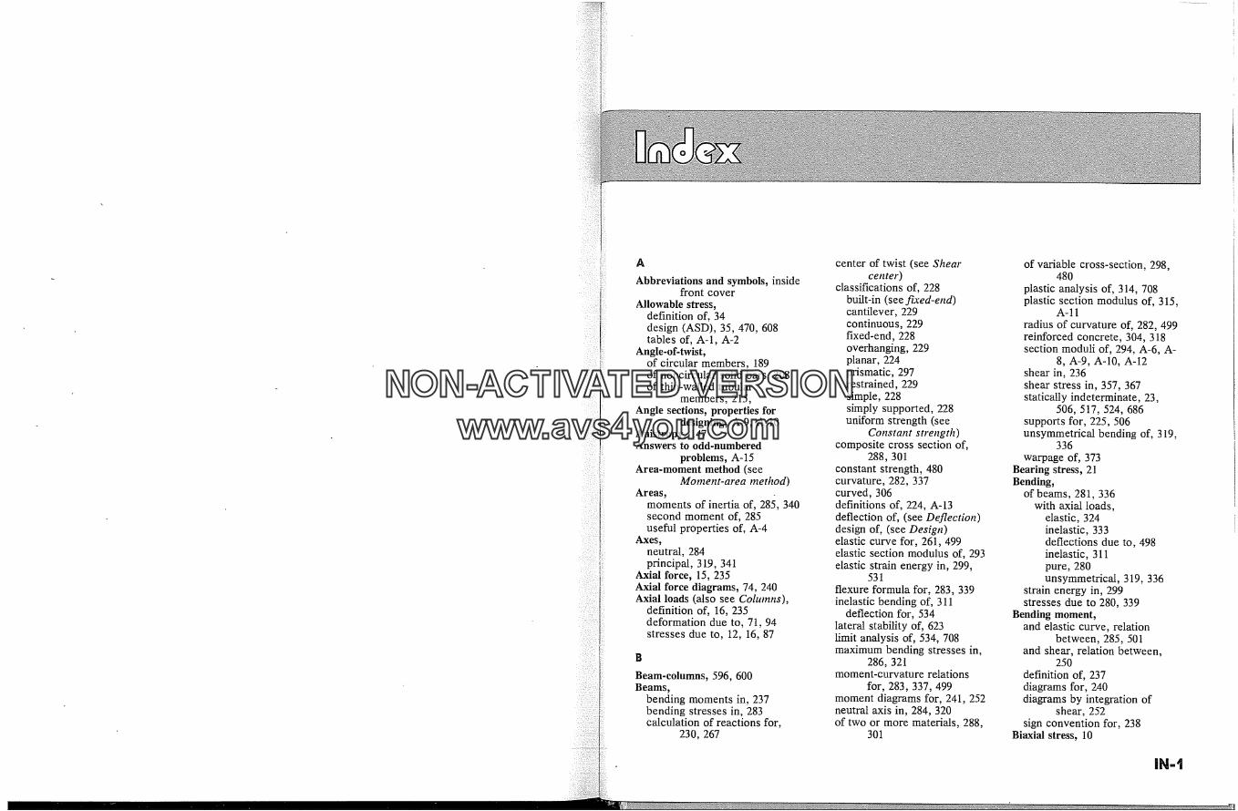
A
Abbreviations and symbols, insidefront cover
Allowable stress,definition of, 34design (ASD), 35, 470, 608tables of, A-I, A-2
Angle-of-twist,of circular members, 189of noncircular solid bars, 208of thin-walled tubular
members, 215,Angle sections, properties for
designing, A-9, A-10Anistropy, 147Answers to odd-numbered
problems, A-15Area-moment method (see
Moment-area method)Areas,
moments of inertia of, 285, 340second moment of, 285useful properties of, A-4
Axes,neutral, 284principal, 319,341
Axial force, 15, 235Axial force diagrams, 74, 240Axial loads (also see Columns),
definition of, 16, 235deformation due to, 71, 94stresses due to, 12, 16, 87
Beam-columns, 596, 600Beams,
bending moments in, 237bending stresses in, 283calculation of reactions for,
230, 267
center of twist (see Shearcenter)
classifications of, 228built-in (see fixed-end)cantilever, 229continuous, 229fixed-end, 228overhanging, 229planar, 224prismatic, 297restrained, 229simple, 228simply supported, 228uniform strength (see
Constant strength)composite cross section of,
288, 301constant strength, 480curvature, 282, 337curved, 306definitions of, 224, A-13deflection of, (see Deflection)design of, (see Design)elastic curve for, 261,499elastic section modulus of, 293elastic strain energy in, 299,
531
flexure formula for, 283,339inelastic bending of, 311
deflection for, 534lateral stability of, 623limit analysis of, 534, 708maximum bending stresses in,
286, 321moment-curvature relations
for, 283,337, 499moment diagrams for, 241,252neutral axis in, 284, 320of two or more materials, 288,
301
of variable cross-section, 298,480
plastic analysis of, 314, 708plastic section modulus of, 315,
A-11
radius of curvature of, 282,499reinforced concrete, 304, 318section moduli of, 294, A-6, A-
8, A-9, A-10, A-12shear in, 236shear stress in, 357, 367statically indeterminate, 23,
506, 517, 524, 686supports for, 225, 506unsymmetrical bending of, 319,
336warpage of, 373
Bearing stress, 21Bending,
of beams, 281,336with axial loads,
elastic, 324inelastic, 333deflections due to, 498inelastic, 311pure, 280unsymmetrical, 319, 336
strain energy in, 299stresses due to 280, 339
Bending moment,and elastic curve, relation
between, 285, 501and shear, relation between,
250definition of, 237diagrams for, 240diagrams by integration of
shear, 252sign convention for, 238
Biaxial stress, 10
NON-ACTIVATEDVERSIONwww.avs4you.com
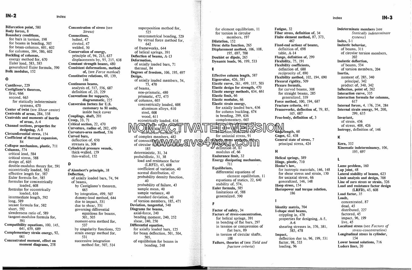
IN-2 Index
Bifurcation point, 580� Body forces, 8
Boundary conditions,for bars in torsion, 198for beams in bending, 505for beam-columns, 601,602for columns, 584, 586, 602
Buckling of columns,energy method for, 670Euler load, 583,585generalized Euler formula, 590
Bulk modulus, 152
Cantilever, 229Castigliano's theorem,
first, -666second, 665
for statically indeterminatesystems, 670
Center of twist (see Shear centet9Centroids of areas, 284, 338Centroids and moments of inertia
of areas, A-4Channel sections, properties for
designing, A-8Circumferential stress, 154Coefficient of thermal expansion,
84
Collapse mechanism, plastic, 711Columns, 574
critical load, 584critical stress, 588design of, 605double-modulus theory for, 591eccentrically loaded, 582effective length for, 587Euler formula for, 585formulas for concentrically
loaded, 608formulas for eccentrically
loaded, 616intermediate length, 592long, 589secant formula for, 582short, 592slenderness ratio of, 589tangent-modulus formula for,
591
Compatibility equations, 100, 145,641,659, 689
Complementary strain energy, 92,661
Concentrated moment, effect onmoment diagrams, 258
Concentration of stress (seeStress)
Connections,bolted, 47riveted, 47welded, 50
Conservation of energy,principle of, 94, 215, 637displacements by, 95, 215, 638
Constant strength beams, 480Consistent deformations, method
of, (see Force method)Constitutive relations, 68, 139,
146Continuous beams,
analysis of, 517, 556, 687definition of, 23,229
Conventions for supports,diagrammatic, 225
Conversion factors for U.S.customary to SI units,inside back cover
Couplings, shaft, 201Creep, 33, 71Critical section, 22, 470Curvature, radius of, 282,499Curvature-area method, 536Curved bars,
deflection of, 650stresses in, 308
Cylindrical pressure vessels,thick-walled, 159thin-walled, 152
d'Alembert's principle, 38Deflection,
of axially loaded bars, 74, 94of beams,
by Castigliano's theorem,665
by integration, 499, 507dummy-load method, 644due to impact, 531due to shear, 531governing differential
equations for beams,501,505
moment-area method for,537
by singularity functions, 523strain energy method for,
531successive integration
method for, 507, 514
superposition method for,525
unsymmetrical bending, 529by virtual force method for,
642of frameworks, 644of helical springs, 391
Deflection of beams, A-13Deformation,
of axially loaded bars, 71thermal, 84
Degrees of freedom, 106, 195, 697Design,
of axially loaded members, 34,73,470
of beams,non-prismatic, 480prismatic, 472, 475
of columns, 605concentrically loaded, 608
aluminum alloys, 610steel, 608wood, 611
eccentrically loaded, 616allowable stress methbd,
616interaction method, 617
of complex members, 482of connections, 47of circular torsional members,
185deterministic, 31, 34probabilistic, 31, 38
load and resistance factor(LRFD), 45, 608
coefficient of variation, 40normal distribution, 42probability density function,
40
probability of failure, 43sample mean, 40sample variance, 40standard deviation, 40
of torsion members, 185,471Deviation, tangential, 540Diagrams for beams,
axial-force, 240bending moment, 240, 252shear, 240, 250
Differential equation,for axially loaded bars, 125for beam deflection, 501,504,
505,of equilibrium for beams in
bending, 248
for element equilibrium, 11for torsion in circular
members, 197Dilata{ion, 152Dirac delta function, 265Displacement method, 106, 108,
195,697, 700Doublet or dipole, 265Dynamic loads, 96, 199, 533
Effective column length, 587Eigenvalue, 426, 581Elastic curve, 261,499, 337, 503Elastic design for strength, 470Elastic energy methods, 634, 661Elastic limit, 66Elastic modulus, 66Elastic strain energy,
for axially loaded bars, 636for column buckling, 674in bending, 299, 636complementary, 665for multiaxial stress, 635for shear, 141,636in torsion, 200, 215,637for uniaxial stress, 91
Elastic stress analysis, 461Elasticity,
definition of, 67modulus of, 66
Endurance limit, 32Energy dissipating mechanism,
711
Equilibrium,differential equations of
element equilibrium, 11equations of statics, 22, 640stability of, 574,
Euler formula, 585limitations of, 588generalized, 590
Factor of safety, 34Factors of stress-concentration,
for helical springs, 391in bending of flat bars, 297in tension or compression of
flat bars, 89in torsion of circular shafts,
188Failure, theories of (see YieM and
fi'acture criteria)
Fatigue, 32Fiber stress, definition of, 34Finite element method, 87, 373,
467Fixed-end actions of beams,
definition of, 698table, A-14
Flange, definition of, 299Flexibility, 75, 191Flexibility coefficients,
definition of, 688reciprocity of, 690
Flexibility method, 102, 194, 690Flexural rigidity, 509Flexure formula,
for curved beams, 308for straight beams, 285
generalized, 339Force method, 100, 194, 687Fracture criteria, 441Frameworks, deflection of, 79, 85,
105,687Free-body, definition of, 3
Gage length, 60Gages, 62, 438General state of stress, 7
principal stress, 424
Helical springs, 389Hinge, plastic, 710Hooke's law,
for isotropic materials, 146, 148for shear stress and strain, 130for uniaxial stress, 66generalized, 146, 148
Hoop stress, 154Horsepower and torque relation,
186
I
Identity matrix, 7041-shape steel beams,
crippling in, 478properties for designing, A-5,
A-6shearing stresses in, 376, 381,
385,478Impact,
deflection due to, 96, 199, 531factor, 98, 533loading, 96
Indeterminate members (seeStatical�, indeterminatesystems)
Index, I-1Inelastic behavior,
of beams, 311of circular torsion members,
202Inelastic deflection,
of beams, 534of torsion members, 204
Inertia,moment of, 285,340
principal, 342product of, 340, 342
Inflection, point of, 262Interaction curve, 335Interaction formula for columns,
617Internal forces, 4, 176, 234, 284Internal strain energy, 94, 200,
299, 635Invariant,
of strain, 436of stress, 408, 426
Isotropy, definition of, 146
Kern, 332Kinematic indeterminancy, 106,
195,697
Lame problem, 160Lap joint, 48Lateral stability of beams, 623Limit analysis and design, 708Line of zero stress or strain, 326Load and resistance factor design
(LRFD), 45, 608Load factor, 35Loads,
concentrated, 87dead, 45distributed, 227factored, 45impact, 96, 199live, 45
Localized stress (see Factors ofstress-concentration)
Longitudinal stress in cylinder,154
Lower bound solutions, 716Luders lines, 20
NON-ACTIVATEDVERSIONwww.avs4you.com

Index
Lumber, sizes, properties fordesigning, A-13
Margin of safety, 35Materials,
anisotropic, 66, 147,brittle, 65ductile, 65, 67homogeneous, 67isotropic, 146'mechanical properties, A-2, A-
3orthotropic, 147
Matrix structural analysis, 36,657, 661,703
Maximum distortion energytheory, 444
Maximum normal stress theory,449
Maximum shear stress theory, 442Maxwell's theorem of reciprocal
displacements, 691Members of composite materials,
288, 301Membrane, analogy for torsion,
209Method of sections,
definition of, 3for axially loaded members, 14,
16for beams, 234for torsion members, 175
Middle-third rule, 329Mises' yield condition, 448Modulus,
bulk, 152of elasticity, 66of resilience, 93of rigidity, 141of rupture in bending, 314of rupture in torsion, 204shear, 141tangent, 70
Mohr's circle,for strain, 435for stress, 414, 417,426
Moment (see Bending tnoment)Moment diagrams for beams, 240,
252
Moment-area method,generaI, 537for indeterminate beams, 551theorems, 538
Moment-curvature relation forbeams, 499
Moment of inertia of areas,definition, 285, 289parallel-axis theorem for, 291,
340polar, 179principal axes for, 341table of, A-4 through A-12
Moving bodies, forces caused by,90, 199, 531
Natural strain, 61Necking, 65Neutral axis, 284Neutral surface, 284Normal stress,
combined with shear stress,403
definition of, 5in axially loaded members, 14,
17in bending, 286, 336
O
Octohedral shear stress theory,448
P
Parallel-axis theorem, 291,340Pipe, standard steel, A-11Plane strain, 149Plane stress, 149, 467Plagtic hinge, 710Plastic limit analysis,
of beams, 315, 534collapse mechanisms in, 711of continuous beams and
frames, 721of torsional members, 206
Plastic moment, 315, 535, 710Photoelastic method of stress
analysis, 469Point of inflection, 262Poisson's ratio, 82Polar moment of inertia, 179Potential, total, 674Pressure vessels, thin-walled, 152Principal axes, of inertia, 319, 341Principal shear stress, 410Principal stress circles, 428Primary system, 101,688, 696
Principal strain, 436Principal stress, 409,424Probabilistic basis for structural
design, 38Properties, for designing,
of angles, A-9, A-10of channels (C), A-8of standard (S) steel beams, A-
5of pipe, standard, A-11plastic section modulii for
wide-flange steel beams,A-11
of rectangular lumber, A-12of wide-flange (WF) steel
beams, A-6Proportional limit, 66
Radius,of curvature, 282,499of gyration, 590
Ramberg-Osgood formula, 69Reactions, calculation of, 230,
514, 687Reciprocity of flexibility
coefficients, 690Redundant reactions, 23,551,672Reinforced concrete beams, 304,
318
Relation among E, G, and v, 150Relation between shear and
bending moment, 250Relation between curvature and
bending moment, 285,336, 501
Relaxation, 71Repeated loading, 32Residual stress, 19, 205,316Resilience, modulus of, 93Restrained beams, 551Rigidity, flexural, 509Rigidity, modulus of, 141Rosettes, strain, 438Rupture, modulus of, 204, 314
$
Safety index, 44Sandheap analogy for torsion, 210St. Venant's principle, 15, 74, 86,
181,467St. Venant torsion, 207Secant formula for columns, 592
Section modulus,elastic, 294plastic, 315tables, A-5 through A-12
Shaft coupling, 201Shape factor, 709Shear center, 382Shear deflection of beams,Shear diagrams (see Shear' forces
in beatns)Shear flow, 361Shear forces in beams,
definition of, 236diagrams for, 240diagrams by integration of
load, 250sign convention for, 237
Shear modulus of elasticity, 141Shear strain, 140, 144Shear stress,
definition of, 6due to axial force, 14, 20in beam flanges, 380in beams, 357, 367in circular shafts, 179in non-circular shafts, 207in rivets and bolts, 21, 48in thin-walled tubular
members, 213maximum, 410on perpendicular planes, 9, 16,
369, 410principal, 410superposition of, 386
SI units, facing inside back coverSign convention,
for moment in beams, 238for shear in beams, 237for stress, 7, 405
Simple beams, definition of, 228Singularity functions, 263,523Skew bending (see
Unsymmetrical bending)Slenderness ratio, 589S-N diagrams, 32Spherical pressure vessels, 155Spring constant, 75
torsional, 191,209, 215Springs, helical, 389Stability of equilibrium,
columns, 574, 674criteria for, 578Euler load, 583,585
Statical moment of area, 362
Statically indeterminate beams,analysis by,
Castigliano's method, 670displacement method, 697force method, 687flexibility method, 687integration of differential
equations, 507, 514moment-area, 551.singularity function
solutions, 523stiffness method, 702superposition, 527three-moment equation, 559
definition of, 23Statically indeterminate systems,
analysis by,displacement method, 106,
697energy methods, 670force method, 100, 687flexibility method, 102, 690stiffness method, 108, 702virtual work methods, 650,
653
axially loaded, 99in frames, 99, 105, 651,653nonlinear problems, 112,708,
713,721in torsion, 194
Steel shapes, properties fordesigning, A-5 throughA-11
Stiffness,definition of, 75
torsional, 191,209, 215coefficients, 702
reciprocity of, 703Stiffness matrix, 110, 702Strain,
definition of, 61, 143extensional, 61h-rotational, 145maximum, 436Mohr's circle for, 435natural, 61plane, 146, 149principal, 433,436pure, 145shear, 140, 144tensor, 145thermal, 84transformations of, 430true, 61
Index IN-5
Strain energy (see Elastic strainenergy)
Strain hardening, 69Strain rosettes, 438Strength, ultimate, 32Stress,
allowable, 1, 32, 608, 610, 612,A-2, A-3
bearing, 21biaxial, 10circumferential, 154concentration factor,
definition of, 86for axially loaded members,
89in bending, 297in springs, 391in torsion for circular bars,
187definition of, 4engineering, 65fiber, 34flexure, 283,286hoop, 154impact, 96in curved bars, 306maximum and minimum
normal, 15, 16Mohr's circle of, 414normal, 5, 22plane, 9, 149principal, 409,424residual, t9, 205,316shear, 19, 22state of, 7, 405tangential, 160tensile, 5tensor, 7, 446three-dimensional, 10, 424torsional, 179,208, 214transformation of, 403,407,
424triaxial, 10, 424true, 65two-dimensional, 407uniaxial, 10
Stress-strain,diagram, 62idealization, 67, 69relationships, 62for shear, 139
Stress trajectories, 470Stretching, 143Suddenly applied loads, 98, 199,
531
NON-ACTIVATEDVERSIONwww.avs4you.com
IN-6 Index
Superposition,of deflection, 113,525of strain, 333of stress, 113,319, 324of shear stresses, 386principle of, 102statically indeterminate
problems solved by,101, 195, 319, 325, 386,
525Supports
diagrammatic conventions for,225
fixed, 226simple, 226
Tables, index of, A-1Tangential deviation, 540Tangent modulus, 70, 59Temperatur6 or thermal strain, 84Tensile test, 31Tensor,
deviatoric stress, 446dllatational stress, 446distortion� stress, 446spherical stress, 446strain, 145stress, 7, 446zero-rank (order), 8
Theories of failure, 441Thermal stresses, 120Thick-walled cylinders, 159Thin-walled cylinders, 152Thrust, 235Torque, internal, 176Torsion,
circular members:angle-of-twist due to, 189,
205
assumptions of theory, 177elastic energy in, 200elastic torsion formula, 179inelastic, 202
statically indeterminateproblems, 194
noncircircular solid bars, 207thin-walled tubular members,
213Torsional spring constant, 191,
209, 215Torsional stiffness, 191Toughness, 93Trajectories, stress, 470Transformation,
of moments of inertia, 341of strain, 430 '
in two dimensions, 430of stress, 403
for general state of stress,424, 426
in two dimensions, 407Transformed cross-sectional area,
302Tresca yield condition, 444Triaxial stress, 10True strain, 61True stress, 65
Ultimate strength, 31Uniaxial stress, 10Uniform strength beams (see
Constant strengthbeams)
Uniform stress, conditions for,(see St. Venant's
principle)Unit, dummy load, 644Unit impulse (or step function),
265
Unsymmetrical bending of beams,319
Upper bound solution, 715
Variable cross-section, beams of,480
Vertical shear (see Shear)Virtual displacement method, 640,
658
for static equilibrium, 642,653,659
Virtual force method, 641,658for deflections, 642
for conditions of compatibility,642, 659for elastic systems, 644
for trusses, 644for beams and frames, 645
for indeterminate systems, 650Virtual work,
for discrete systems, 657external, 640, 641internal, 640, 641,642principle, 638
von Mises yield condition, 448WWarpage of beams, 373Warpage of thin-walled open
sections, 211Web, definition of, 299Welded joints (connections), 50Wide flange (WF) steel beams,
properties for designing,A-6
Wood, (see Lumber)Work, (also see Virtual work)
external, 637internal, 638principle of least, 671
Working stress, 36, 607
�
Yield and fracture criteria, 441Yield condition,
Tresca, 444von Mises, 444
Yield strength and point, 67Young's modulus, 66
NON-ACTIVATEDVERSIONwww.avs4you.com

ENGINEERING MECHANICS OF SOLIDS by
Noted Errata in 1st Printing April 23, 1990
Page
vi
x
15
16
39
42
61
67
7O
75,
79
85
98
103
107
110
112
361
433
641
A-4
A-13
Line
18
28
4
11
Fig. 1-2633
- 14
Fig: 2-10
Fig. 2-i422
Should read or be
y' (prime missing)y' (prime missing)
caption: replace * by 21, and ** by 22.Fig. 1-3flremove bar over epsilon
missing curve (see fig.)missing curve (sec fig.)
2 replace fOX.� with �Fig. 2-29Co) add sub T to deltaFig. 2-40 change 6 mm to 16 �
13 add fi3g. gl after An � �12 remove i after at
Last paragraph Add for clarity: In � _2-42� to
of the "�leltas� must be zero and its P fXe, g.,Fig. 2-53 Add R2 to bottom arrowFig. 7 .�d� reverse arrow direction for Fa17 remove more after approach
18 add at end: for a - iL�L�eXl,�i� casco10 remove last subscript e on WHALF OF THIN R,� is to middle of t
TUBE
5 X=,, = v(0) is positive: remove -.
Egor P. Popov
rim2
NON-ACTIVATEDVERSIONwww.avs4you.com
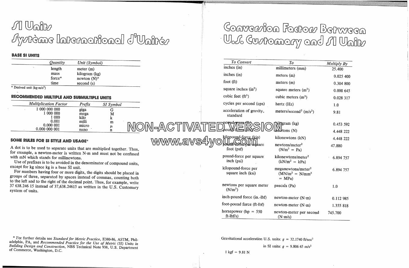
BASE SI UNITS
Quantity Unit (Symbol)length meter (m)mass kilogram (kg)force* newton (N)*time second (s)
* Derived unit (ks.naYs 2)
R�COMMENDED MUL'riPLE AND SUBMUL'r!PLE UNiI'SMultiplication Factor Prefix SI Symbol
1 000 000 000 giga G1 000 000 mega M
1 000 kilo k0.001 milli m
0.000 001 micro ix0.000 000 001 nano n
A dot is to be used to separate units that are multiplied together. Thus,for example, a newton-meter is written N.m and must not be confusedwith mN which stands for millinewtons.
Use of prefixes is to be avoided in the denominator of compound units,except for kg since kg is a base SI unit.
For numbers having four or more digits, the digits should be placed ingroups of three, separated by spaces instead of commas, counting bothto the left and to the right of the decimal point. Thus, for example, write37 638.246 15 instead of 37,638.24615 as written in the U.S. Customarysystem of units.
* For further details see Standard for Metric Practice, E380-86, ASTM, Phil-adelphia, PA, and Recommended Practice for the Use of Metric (SI) Units inBuilding Design and Construction, NBS Technical Note 938, U.S. Departmentof Commerce, Washington, D.C.
To Convert To Multiply Byinches (in) millimeters (mm) 25.400inches (in) meters (m) 0.025 400foot (ft) meters (m) 0.304 800square inches (in 2) square meters (m 2) 0.000 645cubic feet (ft 3) cubic meters (m 3) 0.028 317cycles per second (cps) hertz (Hz) 1.0acceleration of gravity, meters/second 2 (m/s 2) 9.81
standard
pound-mass (lb) kilogram (kg) 0.453 592pound-force (lbf) newtons (N) 4.448 222kilopound-force (kip) kilonewtons (kN) 4.448 222pound-force per square newtons/meter a 47.880
foot (psf) (N/m 2 = Pa)pound-force per square kilonewtons/meter a 6.894 757
inch (psi) (kN/m 2 = kPa)kilopound-force per meganewtons/meter 2 6.894 757
square inch (ksi) (MN/m 2 = N/mm 2-- MPa)
pascals (Pa)newtons per square meter(N/m 2 )
inch-pound force (in.-lbf)foot-pound force (ft-lbf)
horsepower (hp = 550ft-lbf/s)
newton-meter (N.m)
newton-meter (N.m)
newton-meter per second(N.m/s)
1.0
0.112 985
1.355 818
745.700
Gravitational acceleration U.S. units: g = 32.1740 ft/sec"-in SI units: g = 9.806 65 m/s 2
lkgf= 9.81N
NON-ACTIVATEDVERSIONwww.avs4you.com

NON-ACTIVATEDVERSIONwww.avs4you.com
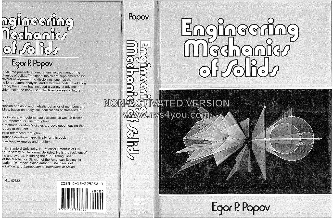
NON-ACTIVATEDVERSIONwww.avs4you.com
Related Documents