ECSS-E-ST-10-04C 15 November 2008 Space engineering Space environment ECSS Secretariat ESA-ESTEC Requirements & Standards Division Noordwijk, The Netherlands

Welcome message from author
This document is posted to help you gain knowledge. Please leave a comment to let me know what you think about it! Share it to your friends and learn new things together.
Transcript

ECSS-E-ST-10-04C15 November 2008
Space engineeringSpace environment
ECSS SecretariatESA-ESTEC
Requirements & Standards DivisionNoordwijk, The Netherlands

ECSS-E-ST-10-04C15 November 2008
ForewordThis Standard is one of the series of ECSS Standards intended to be applied together for the management, engineering and product assurance in space projects and applications. ECSS is a cooperative effort of the European Space Agency, national space agencies and European industry associations for the purpose of developing and maintaining common standards. Requirements in this Standard are defined in terms of what shall be accomplished, rather than in terms of how to organize and perform the necessary work. This allows existing organizational structures and methods to be applied where they are effective, and for the structures and methods to evolve as necessary without rewriting the standards.This Standard has been prepared by the ECSS-E-ST-10-04 Working Group, reviewed by the ECSS Executive Secretariat and approved by the ECSS Technical Authority.
DisclaimerECSS does not provide any warranty whatsoever, whether expressed, implied, or statutory, including, but not limited to, any warranty of merchantability or fitness for a particular purpose or any warranty that the contents of the item are error-free. In no respect shall ECSS incur any liability for any damages, including, but not limited to, direct, indirect, special, or consequential damages arising out of, resulting from, or in any way connected to the use of this Standard, whether or not based upon warranty, business agreement, tort, or otherwise; whether or not injury was sustained by persons or property or otherwise; and whether or not loss was sustained from, or arose out of, the results of, the item, or any services that may be provided by ECSS.
Published by: ESA Requirements and Standards DivisionESTEC, P.O. Box 299,2200 AG NoordwijkThe Netherlands
Copyright: 2008 © by the European Space Agency for the members of ECSS
2
ECSS-E-ST-10-04C15 November 2008
Change log
ECSS-E-ST-10-04A21 January 2000
First issue
ECSS-E-ST-10-04B Never issuedECSS-E-ST-10-04C15 November 2008
Second issue General
The whole document was re-written. The number of clauses and the space environment components addressed in the individual clauses were kept unchanged. The core of the document was newly structured into a main part, followed by normative and informative annexes. Descriptions, specifications of reference models and requirements, reference data and additional information are now clearly separated.Where possible, model uncertainties are given.
Main changes of standard models and requirementso Gravity
The Joint Gravity Model 2 (JGM-2) for Earth was replaced by the EIGEN-GL04C gravity model.
o Geomagnetic fieldThe Internal Geomagnetic Field Model, IGRF-95, was replaced by IGRF-10. For the external field model no standard was defined previously. Now 2 options are given as standard: the model from Alexeev et al. from 2001 or the Tsyganenko model from 1996.
o Natural electromagnetic radiation and indicesThe solar constant was updated to a value of 1 366,1 Wm-
2 at 1 AU. New indices S10.7, M10.7 and IG12 were introduced. Reference values for the indices were changed or newly provided. Reference values for short term variations of ap are newly provided.
o Neutral atmosphereThe standard model MSISE-90 was replaced by 2 different models: NRLMSISE-00 for temperatures and composition and JB-2006 for total atmospheric densities. A standard model for the Martian atmosphere was introduced.
o PlasmasThe International Reference Ionosphere model IRI 1995 was replaced by IRI 2007. For the plasma sphere of Earth the model from Carpenter and Anderson was replaced by the Global Core Plasma Model (GCPM).
3

ECSS-E-ST-10-04C15 November 2008
o Energetic particle radiationFor trapped radiation the AE8 and AP8 models remain the standard with 2 newly introduced exceptions: new standards for electron fluxes near GEO and near GPS orbits are the IGE-2006 and the ONERA MEOv2 models, respectively. The new standard for solar event proton fluences is the ESP model (replacing JPL-91). CREME96, which was the standard model for solar particle event ions and Galactic Cosmic Rays (GCR), is now the standard for solar particle peak fluxes only. For GCR ISO 15390 is the new standard. The FLUMIC model is introduced as worst case for trapped electrons for internal charging analyses. A standard radiation model for Jupiter was introduced.
o Space debris and meteoroidsMASTER 2005 is the new standard model for Space Debris (previously no standard space debris model was defined). A new standard velocity distribution (HRMP) for the meteoroid model from Grün et al. was specified. The material density for meteoroids was changed from 2,0 g/cm3 to 2,5 g/cm3. For meteoroid stream fluxes the model from Cour-Palais was replaced by the model from Jenniskens and McBride.
o ContaminationClear top level requirements for contamination assessments were introduced. The description of analysis methods and tools was streamlined and reduced.
4
ECSS-E-ST-10-04C15 November 2008
Table of contents
Change log.........................................................................................................3
Introduction......................................................................................................16
1 Scope.............................................................................................................17
2 Normative references...................................................................................18
3 Terms, definitions and abbreviated terms.................................................203.1 Terms defined in other standards....................................................................20
3.2 Terms specific to the present standard............................................................20
3.3 Abbreviated terms............................................................................................29
4 Gravity...........................................................................................................324.1 Introduction and description.............................................................................32
4.1.1 Introduction........................................................................................32
4.1.2 Gravity model formulation..................................................................32
4.1.3 Third body gravitation........................................................................34
4.1.4 Tidal effects........................................................................................34
4.2 Requirements for model selection and application..........................................34
4.2.1 General requirements for gravity models...........................................34
4.2.2 Selection and application of gravity models.......................................35
5 Geomagnetic fields......................................................................................365.1 Introduction and description.............................................................................36
5.1.1 The geomagnetic field and its sources..............................................36
5.1.2 The internal field................................................................................36
5.1.3 External field: ionospheric components.............................................37
5.1.4 External magnetic field: magnetospheric components......................37
5.1.5 Models of the internal and external geomagnetic fields.....................37
5.2 Requirements for model selection and application..........................................39
5.2.1 The internal field................................................................................39
5.2.2 The external field...............................................................................39
5.3 Tailoring guidelines..........................................................................................40
5

ECSS-E-ST-10-04C15 November 2008
6 Natural electromagnetic radiation and indices..........................................416.1 Introduction and description.............................................................................41
6.1.1 Introduction........................................................................................41
6.1.2 Electromagnetic radiation and indices...............................................41
6.2 Requirements..................................................................................................44
6.2.1 Electromagnetic radiation..................................................................44
6.2.2 Reference index values.....................................................................45
6.2.3 Tailoring guidelines............................................................................45
6.3 Tables..............................................................................................................46
7 Neutral atmospheres....................................................................................487.1 Introduction and description.............................................................................48
7.1.1 Introduction........................................................................................48
7.1.2 Structure of the Earth’s atmosphere..................................................48
7.1.3 Models of the Earth’s atmosphere.....................................................48
7.1.4 Wind model of the Earth’s homosphere and heterosphere...............49
7.2 Requirements for atmosphere and wind model selection................................50
7.2.1 Earth atmosphere..............................................................................50
7.2.2 Earth wind model...............................................................................51
7.2.3 Models of the atmospheres of the planets and their satellites...........51
8 Plasmas.........................................................................................................528.1 Introduction and description.............................................................................52
8.1.1 Introduction........................................................................................52
8.1.2 Ionosphere.........................................................................................52
8.1.3 Plasmasphere....................................................................................53
8.1.4 Outer magnetosphere........................................................................53
8.1.5 Solar wind..........................................................................................54
8.1.6 Magnetosheath..................................................................................54
8.1.7 Magnetotail........................................................................................54
8.1.8 Planetary environments.....................................................................55
8.1.9 Induced environments........................................................................55
8.2 Requirements for model selection and application..........................................55
8.2.1 General..............................................................................................55
8.2.2 Ionosphere.........................................................................................56
8.2.3 Auroral charging environment............................................................56
8.2.4 Plasmasphere....................................................................................57
8.2.5 Outer magnetosphere........................................................................57
8.2.6 The solar wind (interplanetary environment).....................................58
6
ECSS-E-ST-10-04C15 November 2008
8.2.7 Other plasma environments...............................................................58
8.2.8 Tables................................................................................................59
9 Energetic particle radiation.........................................................................609.1 Introduction and description.............................................................................60
9.1.1 Introduction........................................................................................60
9.1.2 Overview of energetic particle radiation environment and effects.....60
9.2 Requirements for energetic particle radiation environments...........................63
9.2.1 Trapped radiation belt fluxes.............................................................63
9.2.2 Solar particle event models...............................................................65
9.2.3 Cosmic ray models............................................................................66
9.2.4 Geomagnetic shielding......................................................................66
9.2.5 Neutrons............................................................................................66
9.2.6 Planetary radiation environments......................................................67
9.3 Preparation of a radiation environment specification.......................................67
9.4 Tables..............................................................................................................68
10 Space debris and meteoroids...................................................................6910.1 Introduction and description.............................................................................69
10.1.1 The particulate environment in near Earth space..............................69
10.1.2 Space debris......................................................................................69
10.1.3 Meteoroids.........................................................................................70
10.2 Requirements for impact risk assessment and model selection......................70
10.2.1 General requirements for meteoroids and space debris....................70
10.2.2 Model selection and application.........................................................71
10.2.3 The MASTER space debris and meteoroid model............................72
10.2.4 The meteoroid model.........................................................................72
10.2.5 Impact risk assessment.....................................................................73
10.2.6 Margins and worst case fluxes..........................................................74
11 Contamination............................................................................................7511.1 Introduction and description.............................................................................75
11.1.1 Introduction........................................................................................75
11.1.2 Description of molecular contamination.............................................75
11.1.3 Transport mechanisms......................................................................76
11.1.4 Description of particulate contamination............................................76
11.1.5 Transport mechanisms......................................................................77
11.2 Requirements for contamination assessment..................................................77
7
ECSS-E-ST-10-04C15 November 2008
Annex A (normative) Natural electromagnetic radiation and indices.........78A.1 Solar activity values for complete solar cycle..................................................78
A.2 Tables..............................................................................................................79
Annex B (normative) Energetic particle radiation........................................83B.1 Historical dates of solar maximum and minimum............................................83
B.2 GEO model (IGE-2006)...................................................................................83
B.3 ONERA MEOv2 model....................................................................................83
B.4 FLUMIC model.................................................................................................84
B.4.1 Overview............................................................................................84
B.4.2 Outer belt (L>2,5 Re).........................................................................84
B.4.3 Inner belt (L<2,5 Re)..........................................................................85
B.5 NASA worst case GEO spectrum....................................................................86
B.6 ESP solar proton model specification..............................................................86
B.7 Solar ions model..............................................................................................87
B.8 Geomagnetic shielding (Størmer theory).........................................................87
B.9 Tables..............................................................................................................88
Annex C (normative) Space debris and meteoroids..................................100C.1 Flux models...................................................................................................100
C.1.1 Meteoroid velocity distribution.........................................................100
C.1.2 Flux enhancement and altitude dependent velocity distribution......100
C.1.3 Earth shielding and flux enhancement from spacecraft motion.......102
C.1.4 Meteoroid streams...........................................................................103
C.2 Tables............................................................................................................105
Annex D (informative) Gravitation..............................................................108D.1 Gravity models: background..........................................................................108
D.2 Guidelines for use..........................................................................................109
D.3 Availability of models.....................................................................................111
D.4 Tables............................................................................................................111
D.5 Figures...........................................................................................................112
Annex E (informative) Geomagnetic fields.................................................113E.1 Overview of the effects of the geomagnetic field...........................................113
E.2 Models of the internal geomagnetic field.......................................................113
E.3 Models of the external geomagnetic field......................................................114
E.4 Magnetopause boundary...............................................................................115
E.5 Geomagnetic coordinate system – B and L...................................................115
E.6 Tables............................................................................................................118
8
ECSS-E-ST-10-04C15 November 2008
E.7 Figures...........................................................................................................120
Annex F (informative) Natural electromagnetic radiation and indices.....122F.1 Solar spectrum...............................................................................................122
F.2 Solar and geomagnetic indices – additional information...............................122
F.2.1 E10.7................................................................................................122
F.2.2 F10.7................................................................................................122
F.2.3 S10.7................................................................................................123
F.2.4 M10.7...............................................................................................123
F.3 Additional information on short-term variation...............................................123
F.4 Useful internet references for indices............................................................124
F.5 Earth electromagnetic radiation.....................................................................124
F.5.1 Earth albedo.....................................................................................124
F.5.2 Earth infrared...................................................................................125
F.6 Electromagnetic radiation from other planets................................................126
F.6.1 Planetary albedo..............................................................................126
F.6.2 Planetary infrared.............................................................................126
F.7 Activity indices information............................................................................126
F.8 Tables............................................................................................................126
F.9 Figures...........................................................................................................127
Annex G (informative) Neutral atmospheres..............................................130G.1 Structure of the Earth’s atmosphere..............................................................130
G.2 Development of models of the Earth’s atmosphere.......................................130
G.3 NRLMSISE-00 and JB-2006 - additional information....................................131
G.4 The GRAM series of atmosphere models......................................................132
G.5 Atmosphere model uncertainties and limitations...........................................132
G.6 HWM93 additional information.......................................................................132
G.7 Planetary atmospheres models.....................................................................133
G.7.1 Jupiter..............................................................................................133
G.7.2 Venus...............................................................................................133
G.7.3 Mars.................................................................................................134
G.7.4 Saturn..............................................................................................134
G.7.5 Titan.................................................................................................134
G.7.6 Neptune...........................................................................................134
G.7.7 Mercury............................................................................................134
G.8 Reference data..............................................................................................135
G.9 Tables............................................................................................................136
G.10 Figures...........................................................................................................141
9
ECSS-E-ST-10-04C15 November 2008
Annex H (informative) Plasmas....................................................................145H.1 Identification of plasma regions.....................................................................145
H.2 Plasma effects on spacecraft.........................................................................145
H.3 Reference data..............................................................................................146
H.3.1 Introduction......................................................................................146
H.3.2 Ionosphere.......................................................................................146
H.3.3 Plasmasphere..................................................................................146
H.3.4 Outer magnetosphere......................................................................147
H.3.5 Magnetosheath................................................................................147
H.3.6 Magnetotail and distant magnetosheath..........................................147
H.3.7 Planetary environments...................................................................148
H.3.8 Induced environments......................................................................148
H.4 Tables............................................................................................................149
H.5 Figures...........................................................................................................152
Annex I (informative) Energetic particle radiation......................................153I.1 Trapped radiation belts..................................................................................153
I.1.1 Basic data........................................................................................153
I.1.2 Tailoring guidelines: orbital and mission regimes............................153
I.1.3 Existing trapped radiation models....................................................154
I.1.4 The South Atlantic Anomaly............................................................156
I.1.5 Dynamics of the outer radiation belt................................................157
I.1.6 Internal charging..............................................................................157
I.2 Solar particle event models...........................................................................157
I.2.1 Overview..........................................................................................157
I.2.2 ESP model.......................................................................................158
I.2.3 JPL models......................................................................................158
I.2.4 Spectrum of individual events..........................................................159
I.2.5 Event probabilities............................................................................160
I.2.6 Other SEP models...........................................................................160
I.3 Cosmic ray environment and effects models.................................................161
I.4 Geomagnetic shielding..................................................................................161
I.5 Atmospheric albedo neutron model...............................................................161
I.6 Planetary environments.................................................................................162
I.6.1 Overview..........................................................................................162
I.6.2 Existing models................................................................................162
I.7 Interplanetary environments..........................................................................163
I.8 Tables............................................................................................................163
10
ECSS-E-ST-10-04C15 November 2008
I.9 Figures...........................................................................................................165
Annex J (informative) Space debris and meteoroids.................................171J.1 Reference data..............................................................................................171
J.1.1 Trackable space debris....................................................................171
J.1.2 Reference flux data for space debris and meteoroids.....................171
J.2 Additional information on flux models............................................................172
J.2.1 Meteoroids.......................................................................................172
J.2.2 Space debris flux models.................................................................173
J.2.3 Model uncertainties..........................................................................175
J.3 Impact risk assessment.................................................................................175
J.3.1 Impact risk analysis procedure........................................................175
J.3.2 Analysis complexity..........................................................................176
J.3.3 Damage assessment.......................................................................176
J.4 Analysis tools.................................................................................................177
J.4.1 General............................................................................................177
J.4.2 Deterministic analysis......................................................................177
J.4.3 Statistical analysis............................................................................177
J.5 Tables............................................................................................................178
J.6 Figures...........................................................................................................182
Annex K (informative) Contamination modelling and tools......................185K.1 Models...........................................................................................................185
K.1.1 Overview..........................................................................................185
K.1.2 Sources............................................................................................185
K.1.3 Transport of molecular contaminants..............................................187
K.2 Contamination tools.......................................................................................189
K.2.1 Overview..........................................................................................189
K.2.2 COMOVA: COntamination MOdelling and Vent Analysis................189
K.2.3 ESABASE: OUTGASSING, PLUME-PLUMFLOW and CONTAMINE modules...........................................................................................189
K.2.4 TRICONTAM....................................................................................190
Figures
Figure D-1 : Graphical representation of the EIGEN-GLO4C geoid (note: geoid heights are exaggerated by a factor 10 000).........................................................112
Figure E-1 : The IGRF-10 field strength (nT, contour level = 4 000nT, at 2005) and secular variation (nT yr-1, contour level = 20 nT yr-1, valid for 2005), at geodetic altitude 400 km with respect to the WGS-84 reference ellipsoid).120
11

ECSS-E-ST-10-04C15 November 2008
Figure E-2 : The general morphology of model magnetospheric field lines, according to the Tsyganenko 1989 model, showing the seasonal variation, dependent on rotation axis tilt.....................................................................................121
Figure F-1 : Solar spectral irradiance (in red, AM0 (Air Mass 0) is the radiation level outside of the Earth's atmosphere (extraterrestrial), in blue, AM1,5 is the radiation level after passing through the atmosphere 1,5 times, which is about the level at solar zenith angle 48,19°s, an average level at the Earth's surface (terrestrial))...................................................................................127
Figure F-2 : Daily solar and geomagnetic activity indices over the last two solar cycles128
Figure F-3 : Monthly mean solar and geomagnetic activity indices over the last two solar cycles...............................................................................................129
Figure G-1 : Temperature profile of the Earth’s atmosphere.......................................141
Figure G-2 : Variation of the JB-2006 mean air density with altitude for low, moderate, high long and high short term solar and geomagnetic activities...............142
Figure G-3 : Variation of the NRLMSISE00 mean atomic oxygen with altitude for low, moderate and high long solar and geomagnetic activities........................143
Figure G-4 : Variation of the NRLMSISE00 mean concentration profile of the atmosphere constituents N2, O, O2, He, Ar, H, N and anomalous O with altitude for moderate solar and geomagnetic activities (F10.7 = F10.7avg = 140, Ap = 15).............................................................................................144
Figure H-1 : Profile of electron density for solar magnetic local time = 18hr, solar magnetic latitude=0, Kp =0 and 9 from the GCPM for 1/1/1999...............152
Figure I-1 : Contour plots of the proton and electron radiation belts...........................165
Figure I-2 : Electron (a) and proton (b) omnidirectional fluxes, integral in energy, on the geomagnetic equator for various energy thresholds.................................166
Figure I-3 : Integral omnidirectional fluxes of protons (>10 MeV) and electrons (>10 MeV) at 400 km altitude showing the inner radiation belt’s “South Atlantic anomaly” and, in the case of electrons, the outer radiation belt encountered at high latitudes....................................................................167
Figure I-4 : Comparison of POLE with AE8 (flux vs. Energy) for 15 year mission (with worst case and best case included)..........................................................168
Figure I-5 : Comparison of ONERA/GNSS model from 0,28 MeV up to 1,12 MeV (best case, mean case and worst case) with AE8 (flux vs. Energy) for 15 yr mission (with worst case & best case)......................................................168
Figure I-6 : Albedo neutron spectra at 100 km altitude at solar maximum..................169
Figure I-7 : Albedo neutron spectra at 100 km altitude at solar minimum...................169
Figure I-8 : Jupiter environment model (proton & electron versions)...........................170
Figure J-1 : Time evolution of the number of trackable objects in orbit (as of September 2008).........................................................................................................182
Figure J-2 : Semi-major axis distribution of trackable objects in LEO orbits (as of September 2008)......................................................................................183
Figure J-3 : Distribution of trackable objects as function of their inclination (as of September 2008)......................................................................................183
Figure J-4 : The HRMP velocity distribution for different altitudes from the Earth surface. ....................................................................................................184
12
ECSS-E-ST-10-04C15 November 2008
Tables
Table 6-1: Conversion from Kp to ap..............................................................................46
Table 6-2: Electromagnetic radiation values..................................................................46
Table 6-3: Reference fixed index values.......................................................................46
Table 6-4: Reference index values for variations of ap..................................................46
Table 8-1: Worstcase biMaxwellian environment..........................................................59
Table 8-2: Solar wind parameters..................................................................................59
Table 9-1: Standard field models to be used with AE8 and AP8...................................68
Table A-1 : Solar cycle 23 solar activity indices averaged over 30-day (1 month) intervals.......................................................................................................78
Table B-1 : Minima and maxima of sunspot number cycles..........................................87
Table B-2 : IGE 2006 GEO average model – electron flux (kev-1cm-2s-1sr-1) according to year in the solar cycle (referred to solar min: 0) and for different energies for a mission duration of 1 year...................................................................88
Table B-3 IGE 2006 GEO upper case model - maximum electron flux (kev-1cm-2s-1sr-1) according to year in the solar cycle (referred to solar min: 0) and for different energies for a mission duration of 1 year......................................89
Table B-4 : MEOv2 average case model - average electron flux (Mev-1cm-2s-1sr-1) according to year in the solar cycle (referred to solar min: 0) and for different energies for a mission duration of 1 year......................................91
Table B-5 : MEOv2 upper case model - maximum electron flux (Mev-1cm-2s-1sr-1) according to year in the solar cycle (referred to solar min: 0) and for different energies for a mission duration of 1 year......................................91
Table B-6 : Worst case spectrum for geostationary orbits.............................................92
Table B-7 : Values of the parameters for the ESP model..............................................92
Table B-8 : Values to scale fluence from >100 MeV to >300 MeV................................93
Table B-9 : CREME-96 solar ion worst 5-minute fluxes in an interplanetary environment93
Table B-10 : CREME-96 solar ion worst day fluxes in an interplanetary environment. .95
Table B-11 : CREME-96 solar ion worst week fluxes in an interplanetary environment97
Table C-1 : Normalized meteoroid velocity distribution...............................................104
Table C-2 : The annual meteor streams......................................................................105
Table D-1 : Degree power attenuation for an orbit at 25 000 km altitude....................110
Table D-2 : Coefficients of the EIGEN-GL04C model up to degree and order 8 × 8...111
Table E-1 : IGRF-10 data for epoch 1960-2010..........................................................117
Table E-2 : Sibeck et al. Magnetopause model...........................................................118
Table F-1 : Reference values for average planetary albedo and infra-red radiation.. .125
Table G-1 : Altitude profiles of the atmosphere constituents N2, O, O2, He, Ar, H, N and anomalous O for low solar and geomagnetic activities (NRLMSISE-00 model - F10.7 = F10.7avg = 65, Ap = 0)......................................................135
13

ECSS-E-ST-10-04C15 November 2008
Table G-2 : Altitude profiles of the atmosphere constituents N2, O, O2, He, Ar, H, N and anomalous O for mean solar and geomagnetic activities (NRLMSISE-00 model - F10.7 = F10.7avg = 140, Ap = 15)..................................................136
Table G-3 : Altitude profiles of the atmosphere constituents N2, O, O2, He, Ar, H, N and anomalous O for high long term solar and geomagnetic activities (NRLMSISE-00 model - F10.7 = F10.7avg = 250, Ap = 45)........................137
Table G-4 : Altitude profiles of total density kg m-3for low, moderate, high long and high short term solar and geomagnetic activities (JB-2006 model)..........138
Table H-1 : Regions encountered by different mission types......................................148
Table H-2 : Main engineering concerns due to space plasmas...................................149
Table H-3 : Ionospheric electron density profiles derived from IRI-2007 for date 01/01/2000, lat=0, long=0.........................................................................149
Table H-4 : Profile of densities for solar magnetic local time = 18hr, solar magnetic latitude=0, Kp = 5,0 from the GCPM for 1/1/1999.....................................150
Table H-5 : Typical plasma parameters at geostationary orbit....................................150
Table H-6 : Typical magnetosheath plasma parameters.............................................150
Table H-7 : Typical plasma parameters around L2......................................................150
Table H-8 : Worst-case environments for eclipse charging near Jupiter and Saturn. .151
Table H-9 : Photoelectron sheath parameters.............................................................151
Table H-10 : Some solar UV photoionization rates at 1 AU........................................151
Table I-1 : Characteristics of typical radiation belt particles........................................162
Table I-2 : Recommended updated values of the parameters of the JPL model........162
Table I-3 : Proton fluence levels for energy, mission duration and confidence levels from the ESP model with the NASA parameters from Table B-7..............163
Table I-4 : Parameters for the fit to the peak fluxes from the October 1989 events....163
Table J-1 : Approximate flux ratios for meteoroids for 400 km and 800 km altitudes..177
Table J-2 : Cumulative number of impacts, N, to a randomly oriented plate for a range of minimum particle sizes using the MASTER-2005 model......................177
Table J-3 : Cumulative number of impacts, N, to a randomly oriented plate for a range of minimum particle sizes using the MASTER-2005 model......................178
Table J-4 : Cumulative number of impacts, N, to a randomly oriented plate for a range of minimum particle sizes using the MASTER-2005 model......................179
Table J-5 : Cumulative number of impacts, N, to a randomly oriented plate for a range of minimum particle masses......................................................................180
Table J-6 : Parameters (appearing in Eq. (C-15) to account for modified meteoroid fluxes encountered by spacecraft in circular Earth orbits at various altitudes181
14

ECSS-E-ST-10-04C15 November 2008
Introduction
This standard forms part of the System Engineering branch (ECSS-E-10) of the Engineering area of the ECSS system. As such it is intended to assist in the consistent application of space environment engineering to space products through specification of required or recommended methods, data and models to the problem of ensuring best performance, problem avoidance or survivability of a product in the space environment.The space environment can cause severe problems for space systems. Proper assessment of the potential effects is part of the system engineering process as defined in ECSS-E-ST-10. This is performed in the early phases of a mission when consideration is given to e.g. orbit selection, mass budget, thermal protection, and component selection policy. As the design of a space system is developed, further engineering iteration is normally necessary with more detailed analysis.In this Standard, each component of the space environment is treated separately, although synergies and cross-linking of models are specified. Informative annexes are provided as explanatory background information associated with each clause.
15
ECSS-E-ST-10-04C15 November 2008
1Scope
This standard applies to all product types which exist or operate in space and defines the natural environment for all space regimes. It also defines general models and rules for determining the local induced environment.Project-specific or project-class-specific acceptance criteria, analysis methods or procedures are not defined.The natural space environment of a given item is that set of environmental conditions defined by the external physical world for the given mission (e.g. atmosphere, meteoroids and energetic particle radiation). The induced space environment is that set of environmental conditions created or modified by the presence or operation of the item and its mission (e.g. contamination, secondary radiations and spacecraft charging). The space environment also contains elements which are induced by the execution of other space activities (e.g. debris and contamination).This standard may be tailored for the specific characteristic and constrains of a space project in conformance with ECSS-S-ST-00.
16

ECSS-E-ST-10-04C15 November 2008
2Normative references
The following normative documents contain provisions which, through reference in this text, constitute provisions of this ECSS Standard. For dated references, subsequent amendments to, or revision of any of these publications do not apply, However, parties to agreements based on this ECSS Standard are encouraged to investigate the possibility of applying the more recent editions of the normative documents indicated below. For undated references, the latest edition of the publication referred to applies.ECSS-S-ST-00-01
ECSS system – Glossary of terms
[RN.1] C. Förste, F. Flechtner, R. Schmidt, R. König, U. Meyer, R. Stubenvoll, M. Rothacher, F. Barthelmes, H. Neumayer, R. Biancale, S. Bruinsma, J.-M. Lemoine, and S. Loyer, A Mean Global Gravity Field Model from the Combination of Satellite Mission and Altimetry/Gravimetry Surface Data – EIGEN-GL04C, Geophysical Research Abstracts, Vol.8, 03462, 2006
[RN.2] D.D. McCarthy and Gerard Petit (editors), IERS Conventions (2003), IERS Technical Note 32, Verlag des Bundesamtes für Kartographie und Geodäsie, Frankfurt am Main, 2004
[RN.3] E.M. Standish, JPL Planetary and Lunar Ephemerides DE405/LE405, JPL Inter-Office Memorandum IOM 312F-98-048, Aug.25, 1998
[RN.4] Picone, J. M., A. E. Hedin, D. P. Drob and Aikin, A. C., “NRLMSISE-00 Empirical Model of the Atmosphere: Statistical Comparisons and Scientific Issues”, J. Geophys. Res., 107(A12), doi 10.1029/2002JA009430. 2002, p. 1468.
[RN.5] Bowman, B. R., Tobiska, W. K., Marcos, F. A., Valladares, “The JB2006 Empirical Thermospheric Density Model”, Journal of Atmospheric and Solar-Terrestrial Physics, Vol. 70, Issue 5, pp. 774-793, 2008, doi:10.1016/j.jastp.2007.10.002.
[RN.6] Hedin, A.E., E.L. Fleming, A.H. Manson, F.J. Scmidlin, S.K. Avery, R.R. Clark, S.J. Franke, G.J. Fraser, T. Tsunda, F. Vial and R.A. Vincent, Empirical Wind Model for the Upper, Middle, and Lower Atmosphere, J. Atmos. Terr. Phys., 58, 1421-1447, 1996.
[RN.7] Lewis S. R., Collins M., Read P.L., Forget F., Hourdin F., Fournier R., Hourdin C., Talagrand O., Huot, J.-P.,, “A Climate Database for Mars”, J. Geophys. Res. Vol. 104, No. E10, p. 24,177-24,194, 1999.
[RN.8] Gallagher D.L., P.D. Craven, and R.H. Comfort. Global Core Plasma model. J. Geophys. Res., 105, A8, 18819-18833, 2000.
[RN.9] Bilitza, D. and B. Reinisch, International Reference Ionosphere 2007: Improvements and New Parameters, Advances in Space Research,, 42, Issue 4, pp. 599-609, 2008.
[RN.10] Vette J.I., “The AE-8 Trapped Electron Model Environment”, NSSDC/WDC-A-R&S Report 91-24, NASA-GSFC, 1991.
17
ECSS-E-ST-10-04C15 November 2008
[RN.11] Sawyer D.M. and J.I. Vette, “AP8 Trapped Proton Environment For Solar Maximum and Solar Minimum”, NSSDC WDC-A-R&S 76-06, NASA-GSFC, 1976.
[RN.12] A Sicard-Piet, S. A.Bourdarie, D. M. Boscher, R. H. W. Friedel, M. Thomsen, T. Goka, H.Matsumoto, H. Koshiishi, “A new international geostationary electron model: IGE-2006, from 1 keV to 5.2 MeV”, Space Weather, 6, S07003, doi:10.1029/2007SW000368, 2008.
[RN.13] Sicard-Piet A., S. Bourdarie, D. Boscher, R. Friedel, T. Cayton, Solar Cycle Electron Radiation Environement at GNSS Like Altitude, session D5.5-04, Proceedings 57th International Astronautical Congress, Valencia, Sept 2006
[RN.14] Rodgers D.J, Hunter K.A and Wrenn G.L, The Flumic Electron Environment Model, Proceedings 8th Spacecraft Charging Technology Conference, Huntsville Alabama, 2003
[RN.15] Xapsos, M. A., G.P. Summers, J.L. Barth, E. G. Stassinopoulos and E.A. Burke, “Probability Model for Cumulative Solar Proton Event Fluences”, IEEE Trans. Nucl. Sci., vol. 47, no. 3, June 2000, pp 486-490
[RN.16] Lario et al., Radial and Longitudinal Dependence of solar 4-13 MeV and 27-37 MeV Proton Peak Intensities and Fluences: HELIOS and IMP8 Observations, Astrophys Journal, 653:1531-1544, Dec 20, 2006.
[RN.17] Bourdarie, S., A. Sicard-Piet, “Jupiter environment modelling”, ONERA Technical note 120 Issue 1.2, ESA contract 19735/NL/HB, FR 1/11189 DESP, October 2006
[RN.18] CREME96: https://creme96.nrl.navy.mil/[RN.19] ISO Model 15390[RN.20] Adams J.H., R. Silberberg and C.H. Tsao, “Cosmic Ray Effects on
Microelectronics, Part I: The NearEarth Particle Environment”, NRL Memorandum Report 4506, Naval Research Laboratory, Washington DC 20375-5000, USA, 1981.
[RN.21] Desorgher, L., MAGNETOCOSMICS User Manual 2003, http://reat.space.qinetiq.com/septimess/magcos/
[RN.22] Smart, D. F., Shea, M.A., Calculated cosmic ray cut-off rigidities at 450 km for epoch 1990, Proc. 25th ICRC, 2, 397-400, 1997.
[RN.23] Stassinopoulos E.G. and J.H. King, “Empirical Solar Proton Model For Orbiting Spacecraft Applications”, IEEE Trans. on Aerosp. and Elect. Systems AES-10, 442, 1973
[RN.24] D. C. Jensen and J. C. Cain, An Interim Geomagnetic Field, J. Geophys.Res. 67, 3568, 1962.
[RN.25] J. C. Cain, S. J. Hendricks, R. A. Langel, and W. V. Hudson, A Proposed Model for the International Geomagnetic Reference Field, 1965, J. Geomag. Geoelectr. 19, 335, 1967.
[RN.26] MASTER-2005 CD, Release 1.0, April 2006[RN.27] NOAA/SEC source of dates for solar maxima and minima:
ftp://ftp.ngdc.noaa.gov/STP/SOLAR_DATA/SUNSPOT_NUMBERS/maxmin.new
[RN.28] Roberts C.S., “Coordinates for the Study of Particles Trapped in the Earth’s Magnetic Field: A Method of Converting from B,L to R,λ Co-ordinates”, J. Geophys. Res. 69, 5 089, 1964.
[RN.29] IGRF-10, the list of coefficients is given at the IGRF web page on the IAGA web site: http://www.ngdc.noaa.gov/IAGA/vmod/igrf.html
[RN.30] Alexeev I.I., Kalegaev V.V., Belenkaya E.S., Bobrovnikov S.Yu., Feldstein Ya.I., Gromova L.I. (2001), J. Geophys. Res., V.106, No A11, P. 25,683-25,694
[RN.31] Tsyganenko, N.A., and D.P. Stern, Modeling the global magnetic field of the large-scale Birkeland current sustems, J. Geophys. Res., V. 101, 27187-27198, 1996.
18

ECSS-E-ST-10-04C15 November 2008
3Terms, definitions and abbreviated terms
3.1 Terms defined in other standardsFor the purpose of this Standard, the terms and definitions from ECSS-S-ST-00-01 apply, in particular for the following terms:
contaminationenvironmentmissionspace debris
3.2 Terms specific to the present standard3.2.1 Ap, Kp indicesgeomagnetic activity indices to describe fluctuations of the geomagnetic field
NOTE Values of Ap range from 0 to 400 and they are expressed in units of nT (nanotesla). Kp is essentially the logarithm of Ap.
3.2.2 absorbed doseenergy absorbed locally per unit mass as a result of radiation exposure which is transferred through ionization and excitation
NOTE A portion of the energy absorption can result in damage to the lattice structure of solids through displacement of atoms, and this is now commonly referred to as Non-Ionizing Energy Loss (NIEL).
3.2.3 accommodation coefficientmeasure for the amount of energy transfer between a molecule and a surface
3.2.4 albedofraction of sunlight which is reflected off a planet
3.2.5 atmospheric albedo neutronsneutrons escaping from the earth’s atmosphere following generation by the interaction of cosmic rays and solar particles
NOTE Atmospheric albedo neutrons can also be produced by other planetary atmospheres and surfaces.
19

ECSS-E-ST-10-04C15 November 2008
3.2.6 bremsstrahlunghigh-energy electromagnetic radiation in the X-γ energy range emitted by charged particles slowing down by scattering of atomic nuclei
NOTE The primary particle is ultimately absorbed while the bremsstrahlung can be highly penetrating. In space, the most common source of bremsstrahlung is electron scattering.
3.2.7 contaminantmolecular and particulate matter that can affect or degrade the performance of any component when being in line of sight with that component or when residing onto that component
3.2.8 contaminant environmentmolecular and particulate environment in the vicinity of and created by the presence of a spacecraft
3.2.9 currentthe rate of transport of particles through a boundary
NOTE In contrast to flux, current is dependent on the direction in which the particle crosses the boundary (it is a vector integral). An isotropic omnidirectional flux, f, incident on a plane gives rise to a current of ¼ f normally in each direction across the plane. Current is often used in the discussion of radiation transport.
3.2.10 direct fluxfree stream or outgassing molecules that directly impinge onto a critical surface, i.e. without prior collisions with other gas species or any other surface
3.2.11 distribution function f(x,v)function describing the particle density of a plasma in 6-D space made up of the three spatial vectors and the three velocity vectors, with units s3 m-6
NOTE For distributions that are spatially uniform and isotropic, it is often quoted as f(v), a function of scalar velocity, with units s m-
4, or f(E) a function of energy, with units J-1m-3. This can be converted to flux as follows:
(3-1)
or(3-2)
wherev is the scalar velocity;E is the energy;m is the particle mass.
3.2.12 dosequantity of radiation delivered at a position
20
ECSS-E-ST-10-04C15 November 2008
NOTE In its broadest sense this can include the flux of particles, but in the context of space energetic particle radiation effects, it usually refers to the energy absorbed locally per unit mass as a result of radiation exposure.
3.2.13 dose equivalentradiation quantity normally applied to biological effects and includes scaling factors to account for the more severe effects of certain kinds of radiation
3.2.14 dustparticulates which have a direct relation to a specific solar system body and which are usually found close to the surface of this body (e.g. Lunar, Martian or Cometary dust)
3.2.15 Earth infraredthermal radiation emitted by the Earth
NOTE It is also called outgoing long wave radiation.
3.2.16 energetic particleparticles which, in the context of space systems radiation effects, can penetrate outer surfaces of spacecraft
NOTE For electrons, this is typically above 100 keV, while for protons and other ions this is above 1 MeV. Neutrons, gamma rays and X-rays are also considered energetic particles in this context.
3.2.17 equivalent fluencequantity which attempts to represent the damage at different energies and from different species
NOTE 1 For example: For solar cell degradation it is often taken that one 10 MeV protons is “equivalent” to 3 000 electrons of 1 MeV. This concept also occurs in consideration of Non-ionizing Energy Loss effects (NIEL).NOTE 2 Damage coefficients are used to scale the effect caused by particles to the damage caused by a standard particle and energy.
3.2.18 exospherepart of the Earth’s atmosphere above the thermosphere for which the mean free path exceeds the scale height, and within which there are very few collisions between atoms and molecules
NOTE 1 Near the base of the exosphere atomic oxygen is normally the dominant constituent.NOTE 2 With increasing altitude, the proportion of atomic hydrogen increases, and hydrogen normally becomes the dominant constituent above about 1 000 km. Under rather special conditions (i.e. winter polar region) He
21

ECSS-E-ST-10-04C15 November 2008
atoms can become the major constituent over a limited altitude range.NOTE 3 A small fraction of H and He atoms can attain escape velocities within the exosphere.
3.2.19 external fieldpart of the measured geomagnetic field produced by sources external to the solid Earth
NOTE the external sources are mainly: electrical currents in the ionosphere, the magnetosphere and coupling currents between these regions.
3.2.20 F10.7 fluxsolar flux at a wavelength of 10.7 cm in units of 104 Jansky (one Jansky equals 10-26 Wm-2Hz-1)
3.2.21 fluencetime-integration of the flux
3.2.22 fluxamount of radiation crossing a surface per unit of time, often expressed in “integral form” as particles per unit area per unit time (e.g. electrons cm-2s-1) above a certain threshold energy
NOTE The directional flux is the differential with respect to solid angle (e.g. particles cm-2 steradian-1s-1) while the “differential” flux is differential with respect to energy (e.g. particles cm-2 MeV-1s-1). In some cases fluxes are also treated as a differential with respect to Linear Energy Transfer (see 3.2.32).
3.2.23 free molecular flow regime condition where the mean free path of a molecule is greater than the dimensions of the volume of interest (characteristic length)
3.2.24 geocentric solar magnetospheric coordinates (GSM)elements of a right-handed Cartesian coordinate system (X,Y,Z) with the origin at the centre of the Earth
NOTE X points towards the Sun; Z is perpendicular to X, lying in the plane containing the X and geomagnetic dipole axes; Y points perpendicular to X and Z and points approximately towards dusk magnetic local time (MLT).
3.2.25 heterosphereEarth’s atmosphere above 105 km altitude where the neutral concentration profiles are established due to diffusive equilibrium between the species
NOTE N2 is normally dominant below approximately 200 km, O is normally dominant from approx 200 km to approx. 600 km, He is dominant above 600 km altitude, and H dominant at very high altitudes. These conditions depend on solar and geomagnetic activity, and the situation may be quite variable at high altitudes during major geomagnetic disturbances.
22

ECSS-E-ST-10-04C15 November 2008
3.2.26 homosphereEarth’s atmosphere below 105 km altitude where complete vertical mixing yields a near-homogeneous composition of about 78,1% N2, 20,9% O2, 0,9% Ar, and 0,1% CO2 and trace constituents
NOTE The homopause (or turbopause) marks the ceiling of the homosphere.
3.2.27 indirect fluxmolecules impinging on a critical surface, after collision with, or collision and sojourn on other surfaces
3.2.28 internal fieldpart of the measured geomagnetic field produced by sources internal to the solid Earth, primarily due to the time-varying dynamo operating in the outer core of the Earth
3.2.29 interplanetary magnetic fieldsolar coronal magnetic field carried outward by the solar wind, pervading the solar system
3.2.30 isotropicproperty of a distribution of particles where the flux is constant over all directions
3.2.31 L or L shellparameter of the geomagnetic field, often used to describe positions in near-Earth space
NOTE L or L shell has a complicated derivation based on an invariant of the motion of charged particles in the terrestrial magnetic field (see Annex E). However, it is useful in defining plasma regimes within the magnetosphere because, for a dipole magnetic field, it is equal to the geocentric altitude in Earth-radii of the local magnetic field line where it crosses the equator.
3.2.32 linear energy transfer (LET)rate of energy deposit from a slowing energetic particle with distance travelled in matter, the energy being imparted to the material
NOTE Normally used to describe the ionization track caused by passage of an ion. LET is material-dependent and is also a function of particle energy. For ions involved in space radiation effects, it increases with decreasing energy (it also increases at high energies, beyond the minimum ionizing energy). LET allows different ions to be considered together by simply representing the ion environment as the summation of the fluxes of all ions as functions of their LETs. This simplifies single-event upset calculation. The rate of energy loss of a particle, which also includes emitted secondary radiations, is the stopping power.
3.2.33 magnetic local time (MLT)parameter analogous to longitude, often used to describe positions in near-Earth space
NOTE Pressure from the solar wind distorts the Earth magnetic field into a comet-like shape. This structure remains fixed with its nose towards the Sun and the tail away from it as the Earth spins within it. Hence
23

ECSS-E-ST-10-04C15 November 2008
longitude, which rotates with the Earth, is not a useful way of describing position in the magnetosphere. Instead, magnetic local time is used. This has value 0 (midnight) in the anti-sunward direction, 12 (noon) in the sunward direction and 6 (dawn) and 18 (dusk) perpendicular to the sunward/anti-sunward line. This is basically an extension of the local solar time on Earth, projected vertically upwards into space although allowance is made for the tilt of the dipole.
3.2.34 mass flow ratemass (g) of molecular species crossing a specified plane per unit time and unit area (g cm-2s-1)
3.2.35 Maxwellian distributionplasma distribution functions described in terms of scalar velocity, v, by the Maxwellian distribution below:
(3-3)
wheren is the density;k is the Boltzmann constant;T is the temperature.
NOTE The complete distribution is therefore described by a pair of numbers for density and temperature. This distribution is valid in thermal equilibrium. Even non-equilibrium distributions can often be usefully described by a combination of two Maxwellians.
3.2.36 meteoroidsparticles in space which are of natural origin
NOTE nearly all meteoroids originate from asteroids or comets.
3.2.37 meteoroid streammeteoroids that retain the orbit of their parent body and that can create periods of high flux
3.2.38 molecular column density (MCD)integral of the number density (number of molecules of a particular species per unit volume) along a specified line of sight originating from a (target, critical, measuring, reference) surface
3.2.39 molecular contaminantcontaminant without observable dimensions
3.2.40 nano-Tesla standard unit of Geomagnetism
NOTE An older unit, not widely used now, is the Gauss, which is 105 nT.
3.2.41 omnidirectional fluxscalar integral of the flux over all directions
24
ECSS-E-ST-10-04C15 November 2008
NOTE This implies that no consideration is taken of the directional distribution of the particles which can be non-isotropic. The flux at a point is the number of particles crossing a sphere of unit cross-sectional surface area (i.e. of radius 1/√π). An omnidirectional flux is not to be confused with an isotropic flux.
3.2.42 outgassing ratemass of molecular species evolving from material per unit time and unit surface area (g cm-2s-1)
NOTE Outgassing rates can also be given in other units, such as in relative mass unit per time unit: (g s-1), (% s-1) or (% s-1cm-2).
3.2.43 particulate contaminantsolid or liquid contaminant particles
3.2.44 permanent molecular deposition (PMD)molecular matter that permanently sticks onto a surface (non-volatile under the given circumstances) as a result of reaction with surface material, UV-irradiation or residual atmosphere induced reactions (e.g. polymerization, formation of inorganic oxides)
3.2.45 plasmapartly or wholly ionized gas whose particles exhibit collective response to magnetic and electric fields
NOTE The collective motion is brought about by the electrostatic Coulomb force between charged particles. This causes the particles to rearrange themselves to counteract electric fields within a distance of the order of the Debye length. On spatial scales larger than the Debye length plasmas are electrically neutral.
3.2.46 radiationtransfer of energy by means of a particle (including photons)
3.2.47 return fluxmolecules returning to the source or a surface which is not in direct view of the incoming flux
NOTE The cause can be: collisions with other residual natural atmospheric species (ambient scatter) or with other identical or different contaminant species (self scatter) before reaching the critical surface; ionization or dissociative ionization of the molecules under radiation (e.g. UV or particles) and subsequent attraction to a charged surface
25
ECSS-E-ST-10-04C15 November 2008
3.2.48 single-event upset (SEU), single-event effect (SEE), single-event latch-up (SEL)
effects resulting from the highly localized deposition of energy by single particles or their reaction products and where the energy deposition is sufficient to cause observable effects
3.2.49 sporadic fluxrandom flux with no apparent pattern
3.2.50 solar constantelectromagnetic radiation from the Sun that falls on a unit area of surface normal to the line from the Sun, per unit time, outside the atmosphere, at one astronomical unit
NOTE 1 AU = average Earth-Sun distance
3.2.51 solar flareemission of optical, UV and X-radiation from an energetic event on the Sun
NOTE There is some controversy about the causal relationship between solar flares and the arrival of large fluxes of energetic particles at Earth. Therefore, it is more consistent to refer to the latter as Solar Energetic Particle Events (SEPEs).
3.2.52 sticking coefficientparameter defining the probability that a molecule, colliding with a surface, stays onto that surface for a time long compared to the phenomena under investigation
NOTE It is a function of parameters such as contamination/surface material pairing, temperature, photo-polymerization, and reactive interaction with atomic oxygen.
3.2.53 surface accommodationsituation which occurs when a molecule becomes attached to a surface long enough to come into a thermal equilibrium with that surface
3.2.54 thermosphereEarth’s atmosphere between 120 km and 250 km to approximately 400 km (depending on the activity level), where temperature has an exponential increase up to a limiting value T∞ at the thermopause (where T∞ is the exospheric temperature)
3.2.55 trackable objectsobjects regularly observed and catalogued by ground-based sensors of a space surveillance network (typically objects larger than about 10 cm in LEO and larger than about 1 m in GEO)
3.2.56 VCM-testscreening thermal vacuum test to determine the outgassing properties of materials
NOTE The test is described in ECSS-Q-ST-70-02 [RD.23] and ASTM-E595 [RD.24]. The test results are:
26

ECSS-E-ST-10-04C15 November 2008
TML - Total Mass Loss, measured ex-situ as a difference of mass before and after exposure to a vacuum under the conditions specified in the outgassing test, normally expressed in % of initial mass of material. CVCM - Collected Volatile Condensable Material, measured ex-situ on a collector plate after exposure (to a vacuum) under the conditions specified in the outgassing test, normally expressed in % of initial mass of material.
3.2.57 world magnetic modelrevised every five years by a US-UK geomagnetic consortium, primarily for military use
3.3 Abbreviated termsFor the purpose of this Standard, the abbreviated terms from ECSS-S-ST-00-01 and the following apply:
Abbreviation MeaningASTM American Society for Testing and MaterialsAE auroral electrojetAO atomic oxygenBIRA Belgisch Instituut voor Ruimte-AeronomieCIRA COSPAR International Reference AtmosphereCOSPAR Committee on Space ResearchCVCM collected volatile condensable materialDISCOS ESA’s database and information system
characterizing objects in spaceDTM density and temperature modelemfESP Model
electro-motive forceEmission of Solar Protons Model
GCR galactic cosmic rayGEO GNSS
geostationary Earth orbitglobal navigation satellite system
GRAM global reference atmosphere modelGSM geocentric solar magnetospheric co-ordinatesHEO highly eccentric orbitHWM horizontal wind modelIAGA International Association for Geomagnetism and
AeronomyIASB Institute d’Aeronomie Spatiale de BelgiqueECM in-flight experiment for contamination monitoringIERS international earth rotation service
27

ECSS-E-ST-10-04C15 November 2008
IGRF international geomagnetic reference fieldIMF interplanetary magnetic fieldJB-2006 Jacchia-Bowman semi-empirical model (2006)LDEF long duration exposure facilityLEO low Earth orbitLET linear energy transferMAH model of the high atmosphereMASTER meteoroid and space debris terrestrial
environment reference modelMCD molecular column densityMEO medium (altitude) Earth orbitMET Marshall engineering thermosphere modelMLT magnetic local timeMSIS mass spectrometer and incoherent scatterNIEL non-ionizing energy lossnT nano-TeslaPMD permanent molecular depositionR sunspot numberRC rigidity Cut-off for geomagnetic shieldingRE Earth radiusRHU radiosisotope heater unitRJ jovian radiusr.m.s. root-mean-squareRTG radioisotope thermo-electric generatorSEU single-event upsetSEE single-event effectSEL single-event latch-upSEPs solar energetic particlesSEPE solar energetic particle eventssfu solar flux unitSPE solar particle eventsSRP solar radiation pressureSPIDR Space Physics Interactive Data ResourceSW solar windTML total mass lossTD total density modelURSI Union Radio Science InternationaleUSSA US standard atmosphereVBQC vacuum balance quartz contaminationVCM volatile condensable materialVUV vacuum ultra violetWMM world magnetic model
28

ECSS-E-ST-10-04C15 November 2008
4Gravity
4.1 Introduction and description
4.1.1 IntroductionAny two bodies attract each other with a force that is proportional to the product of their masses, and inversely proportional to the square of the distance between them (Newton’s law):
(4-4)
whereF is the gravitational forceG = (6,6726 ± 0,0009)×10-11m3kg-1s-2 is the universal gravitational constantm1, m2 are the two point massesr is the distance between the masses
The simplest case of gravitational attraction occurs between bodies that can be considered as point masses. These are bodies at a relative distance r that is sufficiently large in comparison to the sizes of the bodies to ignore the shape of the bodies. For two spherical bodies with a homogeneous mass distribution Newton’s law is correct also at all locations above their surface (“2-body problem”).Also third body perturbations and tidal effects are important for an accurate analysis of the gravitational interaction.
4.1.2 Gravity model formulationWithout compromising the general validity of underlying theories, all subsequent gravity model discussions are focused on the Earth. The gravity acceleration acting on a point mass, which is external to the central body, is the gradient of the potential function U of that body. The corresponding geopotential surface satisfies the so called Laplace equation:
29
ECSS-E-ST-10-04C15 November 2008
(4-5)
The corresponding perturbing acceleration can be determined from equation (4-6) by means of computationally efficient recursion algorithms (e.g. as in [RD.1]).
(4-6)
where
is the 2nd time derivative of the position vector.
The solution U of the partial differential equation (4-5) is typically written in the form of a series expansion, in terms of so-called surface spherical harmonic functions, for a location defined in spherical coordinates r, λ, ϕ.
(4-7)
whereGM = μ is the gravity constant of the Earth (M being its mass);μ = 3,98604415×10¹⁴ m3s-2 for the EIGEN-GL04C modelae is the mean equatorial radius of the Earth; ae = 6 378 136,460 m for the EIGEN-GL04C modelr is the radial distance from centre of the Earth to satelliteN is the maximum degree of the expansionl is the degree of a certain harmonic functionm is the order of a certain harmonic functionClm, Slm are coefficients that determine amplitude and phase of a certain harmonic functionλ is the geodetic longitude of the sub-satellite pointϕ is the geodetic latitude of the sub-satellite pointPlm are associated Legendre functions of the first kind, of degree l and order m; recurrance relations for these functions are available in the literature (e.g. [RD.1]).
A gravity model consists of adopted values for GM, ae, and a set of model coefficients Clm, Slm. Practical implementations of gravity models, e.g. for numerical integration of a satellite orbit, are typically interested in the gravity acceleration resulting from the potential function U in (4-7). Corresponding partial derivatives of (4-7) in Cartesian coordinates of an Earth-fixed system x, y, z can be computed recursively (see [RD.1]).
30

ECSS-E-ST-10-04C15 November 2008
The model coefficients Clm, Slm are typically provided in their normalized versions, according to (4-8) in order to limit their numerical range for higher degrees and orders.
(4-8)
The Legendre functions Plm (sin ϕ) in this case are normalized by the inverse of the square root in equation (4-8).
4.1.3 Third body gravitationWhen acting as a third-body perturbation, the gravitational attraction by the Sun and its planets can be modelled by means of point mass attractions. This requires knowledge on the masses and positions of the bodies, as well as some guidelines on which effects are important. In general, for orbit computations of Earth-orbiting satellites it is sufficient to include the planetary gravity due to Venus, Mars, Jupiter and Saturn; the other planets are either too small, or too far away to have any significant impact on a satellite orbit around the Earth.
4.1.4 Tidal effectsThe gravity potential of a central body only represents the static part of the gravitational acceleration acting on a satellite. There are, however, additional gravity-related effects due to tides that can be important for precise applications. Several tidal effects can be distinguished (see [RD.1]): Solid Earth tides associated with the deformations of the
Earth’s body under the gravitational effects of Sun and Moon and leading to complicated variations in the geopotential coefficients.
Ocean tides, associated with the displacements of the ocean water masses under the effect of solar and lunar tides. The water displacements in turn modify the geopotential in complicated variational patterns.
The permanent tide, which is a non-zero constant component of the above tides which nonetheless is not considered part of the static geopotential.
Pole tides, which are due to the centrifugal effects of polar motion, which in turn is the movement of the Earth’s body axis relative to the instantaneous axis of rotation.
4.2 Requirements for model selection and application
4.2.1 General requirements for gravity modelsa. Gravity effects shall be included in all orbit determination and
orbit prediction processes, and in attitude determination and prediction processes for Earth and planetary orbiters.
31

ECSS-E-ST-10-04C15 November 2008
b. The inclusion of different gravity sources, their associated model details, and corresponding model truncation errors shall be compliant with the requirements on orbit and/or attitude determination accuracy, and they shall be at least of the same perturbation order as considered perturbing accelerations due to non-gravitational effects.
c. The retained accuracy level of a gravity model shall be compliant with the accuracy of the position and orientation of the central body.
NOTE Harmonic coefficients can lead to resonance effects, if they have a degree or order close to some integer multiple of the ground track repeat cycle. For orbits that are known to be repetitive, it is then recommendable to include discrete resonant harmonics of degrees that normally fall outside the truncated expansion series.
4.2.2 Selection and application of gravity modelsd. For Earth orbits the gravity model EIGEN-GLO4C given in
[RN.1] shall be used. NOTE The EIGEN-GLO4C model has a spatial resolution in latitude and longitude of 1 1 (corresponding to degree order = 360 360).
e. Data on gravitational effects from tides and on Earth orientation parameters shall be obtained from the International Earth Rotation Service IERS given in [RN.2].
f. For third body gravitational perturbations the Development Ephemerides data on planets (DE-405) and the Lunar Ephemerides data (LE-405), both given in [RN.3], shall be used.
g. For planetary mass values the 2003 standards of the International Earth Rotation Services IERS, as described in IERS Technical Note 32 [RN.2], shall be used.
32
ECSS-E-ST-10-04C15 November 2008
5Geomagnetic fields
5.1 Introduction and description
5.1.1 The geomagnetic field and its sources Within the magnetopause, the boundary between the influence of the solar wind and embedded IMF of solar origin, the near-Earth environment is strongly influenced by the geomagnetic field. The geomagnetic field is due to a variety of sources, those within the Earth, those within the ionosphere, and those within the magnetosphere.
The Earth’s magnetic field is responsible for organizing the flow of ionized plasmas within most regions of the near-Earth environment .
Hence, it determines the boundaries of distinct plasma regimes. The magnetic field is also used widely for attitude measurement and for important spacecraft sub-systems such as magneto-torquers.
5.1.2 The internal fieldUnder quiet solar and geomagnetic activity conditions, the magnetic field measured at the Earth’s surface is primarily (>90%) due to a magneto-hydrodynamic dynamo, operating in the liquid outer core of the Earth. The secular (or time) variation of this field operates on a scale of months to centuries, or more, with position dependent amplitude of anywhere between zero and up to a few hundred nT year-1
. The core field morphology is closely dipolar, at least far from the Earth, and is inclined to the Earth’s rotation axis by around 11 degrees at the present time (see Figure E-1).Superimposed on this core field is the static magnetic field of geological sources in the lithosphere and upper mantle. Typically the field from these crustal rocks decays rapidly away from the source. For example, in low Earth orbit, the crustal signature is probably no more than about 20 nT, decaying rapidly with altitude.Traditionally the combination of the core and crustal field is referred to as the ‘main field’. The mean “main field” as measured at the Earth’s surface is depicted in Figure E-1.
5.1.3 External field: ionospheric componentsCurrents flowing in the ionosphere induce an external magnetic field component. Sources of these currents include wind-driven motion of ionospheric plasma that produces a daily variation field known as Sq
33

ECSS-E-ST-10-04C15 November 2008
(‘solar quiet’). This takes the form of two vortices, fixed north and south of the Sun-Earth line, on the dayside of the Earth, as the Earth rotates beneath. Along the geomagnetic equator an equatorial electrojet is formed, due to a high conductivity channel related to the near-horizontal field morphology. Below (or above) this electrojet the field amplitude can be enhanced by several hundred nT, within about five degrees i.e. a few hundred km of the magnetic equator.At auroral latitudes (approximately 55-65 magnetic degrees), the auroral electrojet is formed at the open/closed field line boundary .
This electrojet is fed by field-aligned currents that connect the ionosphere to the magnetospheric flanks and to the night-side tail and partial ring current sheet. The magnitude of the resulting induced fields is very dynamic and can be many hundreds of nT as observed at ground level or in low Earth orbit during periods of disturbed geomagnetic activity.In the lower magnetosphere there are inter-hemispheric (field-aligned) currents of several nT at around 400 km altitude. Plasma ‘bubbles’ can also cause localised magnetic variations of a few nT to be measured by low-Earth orbit satellite altitudes. At high and polar latitudes the Earth’s field is also open to the solar wind and cusp currents, also known as Region 0 currents flow.
5.1.4 External magnetic field: magnetospheric components
In the magnetosphere, there are several major current systems controlled by the interaction of the Earth’s field with the solar wind .
The strength of the total magnetospheric field is closely tied to solar and solar wind variations and to plasma outflow from the ionosphere. The major magnetospheric magnetic fields are a result of: magnetopause currents; cross-tail currents, and the symmetric and partial ring currents.Magnetopause currents flow to shield the internal field from the IMF. And connect to a cross-tail current sheet that separates lobes of opposite magnetic polarity, extending hundreds of Earth radii down-wind from the Earth. An azimuthal drift of plasma (westward for ions, eastwards for electrons) around the Earth produces the symmetric ring current. The partial, or asymmetric, ring current is found on the dusk-side of the Earth and is closed via ionospheric currents. provides the general morphology of model magnetospheric field lines, according to the Tsyganenko 1989 model [RD.111] showing the seasonal variation, dependent on rotation axis tilt . This figure shows a cut in the noon-midnight plane.
5.1.5 Models of the internal and external geomagnetic fields
The magnetic field is commonly modelled by expressing the field as a series of spherical harmonic terms. At the present time (2000-2010) there is much scientific activity in the field modelling community and in source field reconstruction. This is due to several successful satellite magnetometer surveys, such as those of Ørsted and Champ.
34
ECSS-E-ST-10-04C15 November 2008
5.1.5.1 Models of the internal fieldScientific models of the internal field now extend to around spherical harmonic degree 100, equivalent to a minimum wavelength of 400 km at the Earth’s surface. However the effective amplitudes of these high degree terms decrease rapidly with increasing altitude above the Earth’s surface. The core field, which dominates for degrees less than about 14 at the Earth’s surface, can be readily simplified to that of a simple inclined and offset dipole or a low-degree model for spacecraft operation above a few hundred km altitude. Although they are by no means the only recognised high quality models, the IGRF models are products of the international community of geomagnetic scientists, updated on a five-year basis, assuming a linear secular variation between updates. The descriptive annex to this Chapter (Annex E) describes in more detail the current revision of the IGRF, and further information on other internal field models.
5.1.5.2 Models of the external fieldThere are a number of dynamic models of the external field. These are typically either empirical (in the sense of a simplified mathematical model fit to measured data), analytic (based on physical models of the various external current systems), or magneto-hydrodynamic (or ‘general circulation models’). Of the latter type, the science is rapidly evolving and whilst, in principle, they should fully capture the details of magnetospheric processes, such models are judged not yet mature enough to serve as a reliable standard. Of those models that are currently maintained and updated in the light of new data and new field parameterisations, the model of Tsyganenko (revised repeatedly between 1987 and 2006 [RN.31] [RD.98] [RD.99] [RD.111] [RD.112]) is well used and is empirical in nature. The model of Alexeev et al (2001) [RN.30] is described as an analytic model. This model is at the core of a proposed International Standards Organisation (ISO) standard external field model [RD.113].
The availability of suitable inputs to external models is a factor that affects whether they can be useful in common applications. Alexeev et al (2001) [RN.30] has inputs of date, time, solar wind density and velocity, and Tsyganenko 1996 [RN.31]has inputs of solar wind pressure, Dst and IMF By and Bz components. Tsyganenko 2002 to 2005 [RD.98] [RD.99] models require a more complex set of inputs.Further discussion of these models and of their applications are dealt with in Annex E.
5.2 Requirements for model selection and application
5.2.1 The internal field h. IGRF 10 [RN.29] shall be used as the Internal Geomagnetic
Field Model.
35
ECSS-E-ST-10-04C15 November 2008
NOTE As a stand-alone model, the inputs required of the IGRF-10 are either position in geodetic coordinates, according to the reference ‘World Geodetic Service 84’ standard ellipsoid, or position in a geocentric system, with respect to the centre of the Earth and for which the reference Earth radius is 6 371,2 km. The coordinates are therefore geodetic or geocentric latitude in decimal degrees, longitude (same in both coordinate systems), altitude in km above the reference ellipsoid, or distance in km from the centre of the Earth. Time is input in decimal years, e.g. 2 007,5. It is recommended that geocentric data are used, to avoid errors or confusion in respect of the reference ellipsoid.
i. If a different model is an inherent part of a specific space environment model, then that specific geomagnetic field model shall be used.
NOTE An example is the AE8 and AP8 radiation flux / belt models (see Clause 9)
5.2.1.1 Applicationj. For times in the past and in the future, IGRF-10 shall be used,
in association with its secular variations.NOTE 1 IGRF-10 and future versions contain revisions of models of earlier epochs.NOTE 2 Beyond 5 years from the assumed epoch, the precision of the model is considerably reduced. IGRF-11 is expected to be issued for the epoch 2010, and can be used post 2010.
5.2.2 The external fieldk. For modelling the average characteristics of the terrestrial
magnetic field and its variation according to geomagnetic and solar activity, one of the following two external magnetic field models shall be used: Alexeev et al 2001, [RN.30] Tsyganenko 1996 [RN.31]
NOTE 1 These models are suitable for assessment of the mean and range of magnetic field strength; for estimation of B and L coordinates (but not for input to radiation belt models created with different field models); and in calculation of geomagnetic shielding of cosmic rays and solar particles.NOTE 2 Recently, external field models have been created (e.g. Tsyganenko 2001 [RD.98], 2004 [RD.99]) that are used in research environments for dynamic modelling of field variations, e.g. substorm development. These have the capacity to represent more accurately the instantaneous magnetic field, but are not given here as standards because the definition of inputs to the
36

ECSS-E-ST-10-04C15 November 2008
models is not reasonably achievable in an engineering environment.
5.3 Tailoring guidelines l. While the IGRF 10 model should normally be used for internal
fields, a lowfidelity dipole model (using aligned, eccentric or tilted dipoles as appropriate) may suffice for some engineering applications.
m. For the external field, the recent Tsyganenko 2001 [RD.98] and 2004 [RD.99] models may be used instead of the reference models defined in clause 5.2.2.
NOTE Most engineering applications do not need the externalsource model augmentation of these later Tsyganenko models. These are only useful for certain scientific magnetospheric missions, for instance if data on high latitude or high altitude variability of the fields with respect to local time and solargeomagnetic activity was important.
37

ECSS-E-ST-10-04C15 November 2008
6Natural electromagnetic radiation and
indices
6.1 Introduction and description
6.1.1 IntroductionA spacecraft in LEO receives electromagnetic radiation from three primary external sources. The largest source is the direct solar flux. The mean value of this solar flux at the mean SunEarth distance is called the “solar constant”. It is not really a constant but varies by about 3,4 % during each year because of the slightly elliptical orbit of the Earth about the Sun. The two others radiation sources are the fraction of the incident sunlight reflected off the planet, termed albedo, and the Earth infrared radiation.Solar and geomagnetic activities are often described by indices. The UV radiation of the Sun, which strongly affects the Earth atmosphere, cannot be directly measured from the ground. But it was found to be strongly correlated with e.g. the sunspot number and the cm wavelength Sun radiation. For example, the widely used 10,7 cm radio flux index (F10.7) gives an indication of the solar UV radiation output which is highly variable over a solar cycle.Geomagnetic indices typically describe the variation of the geomagnetic field over a certain time period. They provide a measure of the disturbance of the magnetosphere which has direct consequences for the charged particle space environment, or the external component of the geomagnetic field.Solar and geomagnetic indices are used as input for upper atmosphere and other models of the near Earth space environment. They are provided for short durations or as long time averages. Predictions for future index values are usually provided at different confidence levels and they are available for complete solar cycles. The given data are mainly average values. For detailed thermal analyses or certain special applications, more detailed data and models are required. These are outside the scope of this Standard.
6.1.2 Electromagnetic radiation and indices
6.1.2.1 Solar constantThe solar constant is defined as the radiation that falls on a unit area of surface normal to the line from the Sun, per unit time, outside the
38

ECSS-E-ST-10-04C15 November 2008
atmosphere, at one astronomical unit (1 AU = average EarthSun distance). The currently measured 1-sigma standard deviation in the composite dataset is approximately 0,6 Wm-2 and there is a long-term (yearly) smoothed solar cycle minimum to maximum relative variation about the mean value of approximately 1,4 Wm -2 [RD.2] (largest during the period of maximum solar activity).
6.1.2.2 Solar spectrum
6.1.2.2.1 Soft X-rays or XUV (0,1 nm to 10 nm)
Usually associated with solar coronal phenomena, flares, million-degree temperatures, and atomic dissociation. The corona extends from about 21 000 km to 1 400 000 km above the photosphere. X-ray flares are responsible for enhancements in the D and E regions of the Earth's ionosphere.
6.1.2.2.2 Extreme ultraviolet or EUV (10 nm to 121 nm)
EUV has emission lines that come from the upper chromosphere (near-coronal temperatures), transition region, and lower corona. This spectral band is responsible for ionization and heating in the E and F regions of the ionosphere.
6.1.2.2.3 Ultraviolet or UV (100 nm to 400 nm)UV solar flux is emitted primarily from the base of the sun's chromosphere layer, and has components due to active and quiet solar conditions. This band is responsible for only 1% of the total solar irradiance, but it is important because below 300 nm, it is completely absorbed by ozone and diatomic oxygen atoms in the earth's upper atmosphere.
6.1.2.2.4 Visible, optical or VIS (380 nm to 760 nm)
Visible light comes from the solar photosphere, which is only about 400 km thick, has a temperature of approximately 5 000 to 6 000 degrees Kelvin, and yet is responsible for the greatest percentage of the total solar radiation.
6.1.2.2.5 Infrared or IR (0,70 m to 1 mm)Solar infrared in this range is responsible for the direct heating of the Earth's lower atmosphere, through absorption by H2O, and has an effect on minor species constituents in the Earth's mesosphere and thermosphere.
NOTE The ISO 21348 Standard on determining solar irradiances provides more details on the solar spectrum [RD.3].
6.1.2.3 Indices
6.1.2.3.1 General
Solar and geomagnetic indices are used to describe the activity levels of the Sun and the disturbance of the geomagnetic field. Most activity indices are given for short periods and as long duration averages. They are also used for long range predictions of solar activities. Many space environment models require activity index values as input parameters.
39

ECSS-E-ST-10-04C15 November 2008
6.1.2.3.2 Solar activity indices
Sunspot number (R)The sunspot number (R, alternatively called Ri or Rz) is a daily index of sunspot activity, defined as
(6-9)
wheres is the number of individual spots, g the number of sunspot groups, andk is an observatory factor.
NOTE R12 (Rz12) is the 12-month running mean of the sunspot number R.
F10.7F10.7 (abbreviated F10) is the traditional solar energy proxy that is used both for NRLMSISE-00 [RN.4] and JB-2006 [RN.5] atmosphere models. It corresponds to the solar radio flux emitted by the sun at 2 800 megaHertz (10,7 cm wavelength).
NOTE The physical units of F10.7 are 10-22 Wm-
2Hz-1; the numerical value is used without the multiplier as is customarily done and expressed as solar flux units (sfu). In other words, a 10,7 cm radio emission of 150x10-22 W m-2Hz-1 is simply referred to as F10.7 = 150 sfu.
F10.7 and the sunspot number, R, are correlated. Averaged (over one month or longer) values can be converted by the following expression:
(6-10)
S10.7S10.7 (abbreviated S10) [RD.122] is a solar energy proxy that is used for the JB-2006 atmosphere model [RN.5] It is measured by SOHO with the Solar Extreme-ultraviolet Monitor (SEM) in the 26–34 nm solar EUV range, and normalized using a mean value of 1,9955x10¹⁰ photons cm-2s-1. It is expressed in sfu, as F10.7.
M10.7M10.7 (abbreviated M10) [RD.122] is a solar energy proxy that is used for JB-2006 atmosphere model. It is measured by NOAA 16 and NOAA 17 operational satellites with the Solar Backscatter Ultraviolet (SBUV) spectrometer. It is a measure of chromospheric and some photospheric solar active region activity and is expressed in sfu, as F10.7 and S10.7.
IG12IG12 [RD.147] is a solar activity index derived from the monthly mean noon f0F2 data available from thirteen ionospheric observations. The IG index has been confirmed as an alternative to sunspot number when predictions of f0F2 are being prepared with the aid of the CCIR atlas of ionospheric characteristics. IG12 is used for the IRI-2007 ionospheric model.
Solar wind speed
40
ECSS-E-ST-10-04C15 November 2008
The solar wind speed is used in external magnetic field model computation. It is the outward flux of solar particles and magnetic fields from the sun. Typically, solar wind velocities are near 350 km s-1.
6.1.2.3.3 Geomagnetic activity indices
Geomagnetic activity indices are used to describe fluctuations of the geomagnetic field. Kp and ap
Most widely used planetary indices are Kp and ap. They are based on 3hour measurements from 13 ground stations. Values of ap range from 0 to 400 and are expressed in units of 2 nT. Kp
is essentially the logarithm of ap, its scale is 0 to 9 expressed in thirds of a unit, e.g. 5- is 4 2/3, 5o is 5 and 5+ is 5 1/3.The conversion from Kp to ap is given in Table 6-1 (taken from [RD.100]. A daily index, Ap, is obtained by averaging the eight values of ap for each day. The index Ap can have values intermediate to those of ap.
DstDst (Disturbance Storm Time) is a geomagnetic index used in external magnetic field model computation. It describes variations in the equatorial ring current and is derived from hourly scalings of low-latitude horizontal magnetic variation. It is expressed in nT.
IMFIMF (Interplanetary Magnetic Field) is a geomagnetic index used in external magnetic field model computation. It corresponds to the part of the Sun's magnetic field that is carried into interplanetary space by the solar wind. The three orthogonal components of the IMF are Bx, By and Bz. Bx and By are oriented parallel to the ecliptic.The IMF is a weak field, varying in strength near the Earth from 1 to 37 nT, with an average value of about 6 nT.
6.2 Requirements
6.2.1 Electromagnetic radiationn. The values in Table 6-2 shall be used for the electromagnetic
radiation. o. The solar spectrum shall be approximated by a black body
curve with a characteristic temperature of 5 762 K. p. A space sink temperature of 3 K shall be used.
6.2.2 Reference index valuesq. For daily and 81 day averaged values of F10.7, S10.7 and
M10.7 the values given in Table A-1 shall be used.NOTE 1 Ap is only weakly correlated with the solar activity indices.
41
ECSS-E-ST-10-04C15 November 2008
It has a seasonal variation and is higher at the equinoxes.NOTE 2 81 days corresponds to 3 solar rotations and 81 day averaged values are used as input for atmosphere models.
r. For fixed index values, the numbers given in Table 6-3 for low, moderate and high solar and geomagnetic activities shall be used: 1. The longterm values are averaged values for periods
longer than 27 days.2. The long-term values apply as well for periods of 1 week
or longer.3. The short-term values are daily values.
s. The temporal evolution in ap shown in Table 6-4 shall be used to describe the worst case fluctuations during successive three-hour intervals for a total duration of 24 hours.
t. The ap values of Table 6-4 shall be used together with the relevant (low, moderate or high) long term averaged values of F10.7, S10.7 and M10.7 given in Table 6-3.
6.2.3 Tailoring guidelinesu. For design purposes the “worst-case” activity values given in
Table 6-3 shall be used. NOTE These can be the high or low values, depending on the effect to be studied.
v. All worst-case values shall be used without any additional margin.
w. The values given in Table A-1 for a full solar cycle shall be used:1. for applications that require a realistic sequence of index
values for future predictions, for example orbital calculations using index-driven atmospheric models;
2. for a given specific phase of the solar activity cycle.x. The solar cycle activity in Table A-1 of the normative annex
shall be extended by repetition of the 11year cycle.NOTE August 2008 can be assumed as start of cycle 24 unless another estimate with a higher confidence level is released from the Solar Cycle 24 Prediction Panel (at NOAA Space Environment Center (SEC) [RD.4]).
6.3 Tables
Table 6-1: Conversion from Kp to ap
Kp 0 0+
1- 1o
1+
2- 2o 2+ 3 3o 3+ 4- 4o 4+
ap 0 2 3 4 5 6 7 9 12 15 18 22 27 32
42
ECSS-E-ST-10-04C15 November 2008
Kp 5- 5o
5+
6- 6o
6+
7- 7o 7+ 8- 8o 8+ 9- 9o
ap 39
48
56
67
80
94
111
132
154
179
207
236
300
400
Table 6-2: Electromagnetic radiation valuesSolar constant at 1 AU 1 366,1 W m-2
Solar energy flux at aphelion 1 321,6 W m-2
Solar energy flux at perihelion 1 412,9 W m-2
NOTE The solar constant, a historical term, is not constant. It varies geometrically with the Earth’s distance from the sun and physically with the sun’s magnetic field activity on short to long timescales, as well as with the observer’s heliocentric latitude. The value of 1 366,1 W m-2 is the measurement community’s current agreement. The currently measured 1-sigma variation of the composite dataset of space based measurements is approximately 0,6 W m-2 and there is a long-term (yearly) smoothed solar cycle minimum to maximum relative variation about the mean value of approximately 1,4 W m-2 [RD.2].
NOTE
Table 6-3: Reference fixed index valuesLong-term (27+ days) Short-term (daily)
Low Moderate High Low Moderate HighF10.7 65 140 250 65 140 300
S10.7 60 125 220 60 125 235
M10.7 60 125 220 60 125 240
Ap 0 15 45 0 15 240NOTE 1 The reference index values are rounded numbers from the last solar cycle 23.NOTE 2 Low, moderate or high values for Ap can occur at any time in the solar cycle.NOTE 3 For short terms, higher values than those given in this table have been measured (e.g. F10.7 = 380
over a day and ap= 400 for 3 hours). However, present atmosphere models are not developed for such high index values and its use leads to large and unknown errors.
Table 6-4: Reference index values for variations of ap
Time [hrs] ap
0 153 156 3009 130
12 5015 1518 1521 1524 15
43

ECSS-E-ST-10-04C15 November 2008
7Neutral atmospheres
7.1 Introduction and description
7.1.1 IntroductionA good knowledge of temperature, total density, concentrations of gas constituents and pressure is important for many space missions exploiting the low-earth orbit regime (LEO), below approx. 1 000 km altitude. Aerodynamic forces on the spacecraft, due to the orbital motion of a satellite through a rarefied gas which itself can have variable high velocity winds, are important for the combination of planning satellite lifetime, for the maintenance of orbits, for sizing the necessary propulsion system, for the design of attitude control system, and for estimating the peak accelerations and torques imposed on sensitive payloads.Surface corrosion effects due to the impact of large fluxes of atomic oxygen are assessed to predict the degradation of a wide range of sensitive coatings of spacecraft and instruments. The reactions of atomic oxygen around a spacecraft can also lead to intense “vehicle glow”.
7.1.2 Structure of the Earth’s atmosphereThe Earth atmosphere can be broadly divided into three distinct regimes: The homosphere which comprises the regions of the
troposphere (surface up to ~ 10 - 12 km altitude), the stratosphere (~ 10 - 12 km up to 50 km), and the mesosphere (~50 km up to about 90 km);
The thermosphere which extends from about 90 km altitude to approx. 400 km (depending on solar and geomagnetic activity levels);
The exosphere which extends from the top of the thermosphere and extends into space.
More information on these three regions can be found in Annex G.
7.1.3 Models of the Earth’s atmosphere
7.1.3.1 NRLMSISE-00 modelThe NRL Mass Spectrometer, Incoherent Scatter Radar Extended Model (NRLMSISE-00) model [RN.4] describes the neutral temperature and species densities in Earth's atmosphere.
44
ECSS-E-ST-10-04C15 November 2008
It is based on a very large underlying set of supporting data from satellites, rockets and radars, with extensive temporal and spatial distribution. It has been extensively tested by the global scientific community against experimental data. The model has a flexible mathematical formulation.It is valid for use from ground level to the exosphere.Two indices are used in this model: F10.7 (both the daily value of the previous day and the 81-day
average centred on the input day), Ap (daily value).
7.1.3.2 JB-2006 modelThe Jacchia-Bowman 2006 (JB-2006) model [RN.5] also describes the neutral temperature and the total density in Earth’s thermosphere and exosphere. Its new features, described in Annex G, lead to a better and more accurate model representation of the mean total density, compared with previous models, including the NRLMSISE-00.It is valid for use from an altitude of 120 km to the exosphere.Four indices are used in this model: F10.7 (both tabular value one day earlier and the 81-day
average centred on the input time), S10.7 (both tabular value one day earlier and the 81-day
average centred on the input time), M10.7 (both tabular value five days earlier and the 81-day
average centred on the input time), Ap (tabular value 6,7 hours earlier).
7.1.4 Wind model of the Earth’s homosphere and heterosphere
The Horizontal Wind Model (HWM) is a comprehensive empirical global model of horizontal winds in the mesosphere and thermosphere (middle and upper atmosphere). The HWM-93 model [RN.6] is based on accumulated measurements made using a variety of observational techniques, including satellite, radar, and ground-based optical remote sensing. The model is used to provide the necessary winds, accounting for time, space and geophysical variations, for many ionospheric, dynamical, and aeronomical calculations It provides meridional (+ northward) and zonal (+ eastward) speed and covers all altitude regions.Two indices are used in this model: F10.7 (both the daily value of the previous day and the 81-day
average centred on the input day), Ap (daily value).
45
ECSS-E-ST-10-04C15 November 2008
7.2 Requirements for atmosphere and wind model selection
7.2.1 Earth atmosphere
7.2.1.1 Generaly. The NRLMSISE-00 model [RN.4] shall be used for calculating
both the neutral temperature, and the detailed composition of the atmosphere.
z. The JB-2006 model [RN.5] shall be used for calculating the total atmospheric density above an altitude of 120 km.
aa. For altitudes below 120 km, NRLMSISE-00 shall be used for calculating the total air density.
NOTE This recommendation follows the advice of the CIRA Working Group, sponsored by COSPAR and URSI.
7.2.1.2 Application guidelinesbb. The NRLMSISE-00 model for species densities shall not be
mixed with the JB-2006 model for total density.cc. For worst case high results and analysis periods not exceeding
1 week high daily short-term values given in Table 6-3 shall be used as input for daily activity together with the high long-term values for the 81-day average activity.
dd. For analysis periods longer than 1 week the long term activities given in Table 6-3 shall be used as input for both, the daily and the 81-day averaged values.
ee. For analysis periods longer than 1 week and conditions specified in 1.1.1w, the daily and 81-day averaged solar activities given in Table A-1 shall be used.
ff. Short-term daily high solar activity values shall not be used together with low or moderate long-term solar activity values.
NOTE 1 Both models can only predict large scale and slow variations, on the order of 1 000 km (given by the highest harmonic component) and 3 hours. Spacecraft can encounter density variations with smaller temporal and spatial scales partly since they are in motion (for example, +100% or -50% in 30 s), and partly because smaller-scale disturbances certainly occur during periods of disturbed geomagnetic activity.NOTE 2 Reference values for the key indices needed as inputs for the atmosphere models are given in Clause 6.
NOTE 3 The F10.7 81-day average activity can also be estimated by averaging three successive monthly predicted values.
46
ECSS-E-ST-10-04C15 November 2008
NOTE 4 Information on density model uncertainties can be found in G.5 and in [RN.4] and [RN.5].NOTE 5 For high activities the atmosphere models only give realistic results if high short term values are combined with high 81-day averaged values.NOTE 6 High Ap values can be used with low, moderate or high solar activities.
7.2.2 Earth wind modelgg. The HWM-93 model [RN.6] shall be used.hh. High daily short-term values shall be used as worst-case for the
daily activity but the 81-day average activity shall not exceed the high long-term value.
NOTE 1 Reference values for the key Indices needed as inputs for the wind model are given in Clause 6.NOTE 2 The F10.7 81-day average activity can also be estimated by averaging three successive monthly predicted values as given in Clause 6.NOTE 3 The use of the HWM-93 model at high geomagnetic latitudes and for disturbed geomagnetic periods necessitates caution.
7.2.3 Models of the atmospheres of the planets and their satellites
ii. For the Martian Atmosphere, the European Martian Climate Data Base [RN.7] shall be used.
NOTE 1 No specific models are imposed for the other planets and their satellites.NOTE 2 International Reference Atmospheres have been adopted for Mars (MIRA) and Venus (VIRA). There have also been major advances in the case of the atmospheres of Jupiter, Saturn, Neptune and Titan. This is a matter of ongoing work. Considerable work has also been performed for the atmosphere of Mercury.
NOTE 3 Additional information on Planetary Atmospheres is provided in Annex G.
47

ECSS-E-ST-10-04C15 November 2008
8Plasmas
8.1 Introduction and description
8.1.1 IntroductionAll spacecraft, once they exceed about 60 km in altitude during the day or around 80 km at night, are exposed to the charged particles of the space plasma environment. These particles interact with and are collected by the surface materials of a spacecraft and change the electric fields on and around it. Of the continuum of charged particles of all energies, those below 50 keV are generally regarded as plasma and are covered in this clause. Higher energy particles are covered in the radiation environment clause (clause 9).Within the magnetosphere, plasma flows almost freely up and down magnetic field lines but only slowly across it. Hence, two spacecraft observe similar plasmas if they are on the same field line, even if far apart. These spacecraft share the same Lshell and magnetic local time.A brief overview of the effects of the plasma environment is given in Annex H.2. Requirements for design, analysis and testing of spacecraft, concerning the effects of plasma on spacecraft systems are described in a parallel standard ECSS-E-ST-20-06 (Spacecraft Charging).
8.1.2 IonosphereThe ionosphere is the ionized plasma in the upper atmosphere, produced by the dissociation of atmospheric atoms. It is generally divided into layers D, E and F1 at low altitudes and F2 at higher altitude. The low altitude layers are significant only during daylight hours. F2 is permanent and the densest, peaking at around 300 km altitude. For most space applications, it is the electron density which is the most important characteristic. Immediately above the F2 peak, density falls off nearly exponentially with height. At mid to low latitudes, the density falloff slows down at higher altitudes as the magnetic field traps plasma to form the plasmasphere.Intense auroral charging environments are associated with discrete aurorae which are generally found between 60 and 77 degrees magnetic latitude. However, at times of enhanced geomagnetic activity, the auroral zone is moved southwards. In this region, ionospheric density can become irregular on the scale of metres to kilometres vertically and metres to hundreds of kilometres horizontally. The energetic electrons have energies of 10s of keV.
48
ECSS-E-ST-10-04C15 November 2008
Plasma density in this region can suddenly increase by a factor of up to 100 during magnetically active periods.In the Polar Cap, typically above 70latitude, there is a strong wintersummer asymmetry because of the tilt of the Earth,. Strong drift motion occurs due to electric fields. In winter, density is maintained by this drift and by “polar rain”, a weak electron flux from the solar wind with energy around 100eV. When both these processes are depressed, ionospheric density in this region can become very low.Ionospheric plasma characteristics are expressed in the International Reference Ionosphere (IRI) [RN.9]. IRI is an empirical model based on a large volume of ground and space data. IRI describes monthly average conditions but can be updated to time-specific conditions using measured characteristic parameters, e.g., F-peak density and height, if these are available. This model calculates densities, temperatures and composition in the altitude range 50 to 1 500 km in the non-auroral ionosphere. The model describes the densities of O+, H+, He+, NO+, O2
+, N+, and Cluster ions. External drivers for the IRI model are the sunspot number and the ionospheric index IG; in both cases the 12-month running mean of the index is used.
8.1.3 PlasmasphereThe plasmasphere is a region of cold dense plasma originating in the ionosphere and trapped by the Earth’s magnetic field. At low Lshells, the particles drift around the Earth on closed drift paths. This allows ions, escaping from the ionosphere, to accumulate to form this dense region. The boundary between closed and open drift paths is highly variable and the outer regions of the plasmasphere are continually being lost and refilled over a period of days. Typically, the plasmapause, the outer edge of the plasmasphere, lies at an Lshell (3.2.31) of 3 to 6, with a bulge in the dusk region of magnetic local time. The Global Core Plasma Model (GCPM) [RN.8] is a widely used and well tested plasmasphere model and is recommended by the authors of IRI. It provides empirically derived plasma density as a function of geomagnetic conditions throughout the inner magnetosphere.
8.1.4 Outer magnetosphereBeyond the plasmapause, the magnetospheric plasma environment is characterized by high temperatures and low densities. This region usually encompasses the geostationary orbit. The location of the outer boundary of this region, the magnetopause, is controlled by the balance between the ram pressure of the flowing solar wind and the magnetic pressure of the terrestrial magnetic field. See Annex H.3.4 for further discussion of the magnetopause position. During active periods, large amounts of magnetic energy are injected into the plasma in this region. These are called magnetic storms and substorms and are detectable on the ground as magnetic disturbances at certain latitudes. Hence there is a strong link between hot plasma and high values of the magnetic index Kp.
49
ECSS-E-ST-10-04C15 November 2008
8.1.5 Solar wind The solar wind is part of the Sun’s outer atmosphere, expanding outwards and carrying the solar magnetic field with it. Solar wind velocity near the Earth is commonly around 400 km s-1 but with frequent highspeed streams with velocities around 700 km s-1 and sometimes beyond 1 000 km s-1. Earthorbiting satellites and those in L1 and L2 see solar wind fluctuations at different times but otherwise do not observe noticeable differences in solar wind characteristics. On average, the solar wind is made up mostly of protons (95%), with 4% alpha particles and around 1% minor ions, of which carbon, nitrogen, oxygen, neon, magnesium, silicon and iron are the most abundant [RD.5].In interplanetary space, solar wind average density varies, to a good approximation with r-2 (where r is radial distance from the Sun) in the range ±40 degrees solar latitude. The average electron temperature has been seen to vary as r-0,64 for r between 1,52 to 2,31 AU. Ion velocity does not show a significant radial variation.
8.1.6 MagnetosheathNear the magnetopause the solar wind is slowed, compressed, heated and deflected by the ‘bow shock’. This typically lies 3 RE
upstream of the magnetopause on the EarthSun line. The diameter of the bow shock perpendicular to the Earth-Sun axis increases in the anti-sunward direction so that around L2 (236 RE downstream) it is around 100 RE in radius. The region between the bow shock and the magnetopause is called the ‘magnetosheath’.
8.1.7 MagnetotailAlthough the Earth’s magnetosphere extends typically out to 10 RE in the sunward direction, it extends to at least 500RE in the anti-sunward direction. This downstream region of the magnetosphere is called the magnetotail. Beyond about 30 RE, the magnetotail becomes cylindrical with radius virtually independent of distance from the Earth (around 15 to 30 RE
in radius depending on solar wind pressure). It does not point directly anti-sunwards but swings according to solar wind velocity components up to about 10 degrees from the Earth-Sun line in both the ecliptic plane and perpendicular to it. The mean deflection with respect to the Earth-Sun line is about 4 degrees. Within the magnetotail, there are somewhat different plasmas, with hotter plasma (the plasma sheet) around the ecliptic plane and the cooler plasma (the lobes/mantle) north and south of it [RD.117]. Although these are magnetically linked to regions near the Earth, populated with ions of ionospheric and solar wind origin respectively, in this region virtually all ions are of solar wind origin [RD.6] and the differences in density and temperature are not as strong as near the Earth.
50

ECSS-E-ST-10-04C15 November 2008
8.1.8 Planetary environmentsWhenever planets have strong magnetic fields that exclude the solar wind from around the planet, there is the possibility of plasma being trapped in a similar way to the plasma in the Earth’s magnetosphere.
Jupiter and Saturn, in particular, have large magnetic fields and larger magnetospheres than that of the Earth.
8.1.9 Induced environmentsThe natural plasma environment can be augmented by a number of sources inside or on the satellite surface, such as photo-emission, outgassing and electric propulsion systems.
8.2 Requirements for model selection and application
8.2.1 Generaljj. Applicable plasma regions that can be encountered shall be
identified according to the spacecraft location or orbit as follows:1. The ionosphere for altitudes between 60 km and 2 000
km.2. The auroral charging environment for orbital inclinations
above 50 degrees for altitudes above 80 km and below 2 000 km.
3. The plasmasphere for altitudes above 2 000 km (approximately L=1,3 at the equator) and below L=7.
4. The outer magnetosphere for all L values above L=3 and within the magnetopause as defined in clause 5, (including the geostationary regime).
5. The magnetosheath for locations outside of the magnetopause as defined in clause 5 and within the bow shock.
6. The solar wind for locations outside of the magnetopause and bow shock.
7. The magnetotail and distant mgnetosheath for locations within the bow shock but more than 30 RE from the Earth in the anti-Sunward direction.
8. Planetary plasma environments for regions within the planetary bow shock, or planetary magnetopause, or planetary ionopause, whichever of these are present.
NOTE 1 See Annex E.5 for definition of L (L-shell).NOTE 2 Some typical orbits and regions encountered are described in Annex H
kk. Applicable environments for each region shall be characterised according to the models specified in 8.2.2 to 8.2.6.
51
ECSS-E-ST-10-04C15 November 2008
8.2.2 Ionospherell. For the ionospheric environment, the International Reference
Ionosphere 2007 (IRI-2007) [RN.9], shall be used. mm. Inputs to the IRI-2007 model, shall be:
1. choice of geographic or geomagnetic coordinates; 2. latitude; 3. longitude; 4. date; 5. local or universal time; 6. altitude (start and end of range and step size).
nn. Other inputs shall be the default values for dates up to June 2008 or later periods if available in the input files that are provided with the model.
NOTE This means that Sunspot number Rz12, IG12 (see 6.1.2.3.2), F10.7 and ap data are taken from default files.
oo. For future dates not covered by the defaults files, for F10.7 and ap the activity indices defined in clause 6 and corresponding values for IG12 and Rz12 shall be used.
NOTE Information on the accuracy of the IRI-2007 model and typical ionospheric density profiles are given in Annex H.3.1
8.2.3 Auroral charging environmentpp. For auroral charging assessment, the following worstcase
electron distribution function shall be used. For E 17,44 keV:
f(v) = 3,9 × 10⁻¹⁸ s3m-6 (8-11)
For E > 17,44:
(8-12)
wheref(v) is the distribution function in sec3 m-6
N0 is the density in m-3 me is the electron mass in kgkT0 is the thermal energy in J E0 is in J E is energy in Jand parameters of the worst case environment are:N0 = 1,13E6 m-3
kT0 = 3,96 keVE0 = 17,44 keV
52
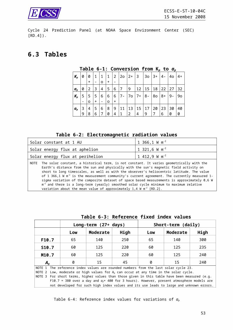
ECSS-E-ST-10-04C15 November 2008
NOTE This comes from [RD.7] and is based on work described in [RD.8]. Unfortunately, it is printed in [RD.7] with a typographical error.
qq. For worst case auroral charging assessments, a thermal ion density of 125 cm-3 and temperature 0,2 eV shall be used.
NOTE This low ion density comes from a severe charging case seen on the DMSP spacecraft by [RD.9]. Measuring ionospheric thermal ion density during a strong charging event is potentially prone to errors because of the way the charged satellite alters ion trajectories, so there is a degree of uncertainty in this measurement.
8.2.4 Plasmasphererr. The plasma parameters representing the terrestrial
plasmasphere shall be taken from the Global Core Plasma Model (GCPM) [RN.8].
NOTE 1 Profiles of typical plasmasphere densities versus altitude are given in Annex H.3.3. NOTE 2 Outputs are densities of electrons, protons, helium ions and oxygen ions. Input parameters are: time, geocentric radial distance, solar magnetic local time, solar magnetic latitude and Kp index.
ss. For spacecraft charging assessments, Kp=9 shall be used in the GCPM model to represent a worst case situation.
NOTE This is because the plasmasphere is a moderating influence on spacecraft charging, and so the worst case is considered to be when the plasmasphere is small which occurs when geomagnetic activity is high.
8.2.5 Outer magnetospherett. For assessment of surface charging, the worstcase environment
listed in Table 8-5 shall be used as input to a spacecraft charging simulation or calculation, applicable to the outer magnetosphere environment.
NOTE This is a dynamic region in terms of plasma density and temperature and for most engineering purposes, worstcase environments are the most important consideration. See Annex H.3.4 for typical plasma parameters in this region.
8.2.6 The solar wind (interplanetary environment)uu. For calculation of engineering effects due to the solar wind, a
flowing Maxwellian distribution shall be used, with density and temperature given in Table 8-6.
vv. Spacecraft in L1 and L2 shall be considered to experience the same mean and range of plasma parameters in the solar wind as at the Earth.
NOTE Because the solar wind flows through the near-Earth interplanetary medium with negligible modification (unless it
53
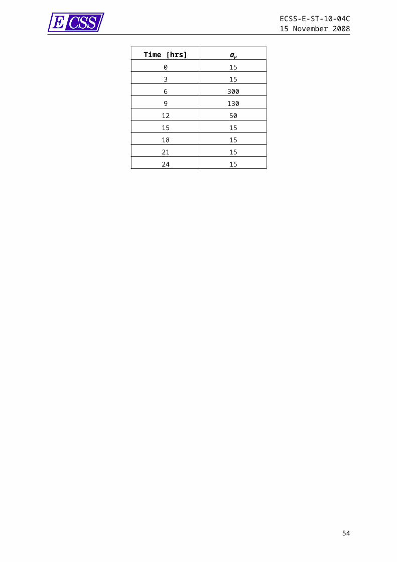
ECSS-E-ST-10-04C15 November 2008
encounters the bow shock), the mean and range of plasma density and temperature can be considered spatially uniform in the vicinity of 1AU. However, variations in plasma at the Earth are seen at L1 and L2 between approximately 30 and 90 minutes earlier or later, respectively.
ww. A r-2 variation shall be used to map the mean and range of solar wind density to other locations in the heliosphere in the ecliptic plane, where r is heliocentric distance.
xx. A r-0,64 variation shall be used to map the mean and range of the electron temperature to other locations in the heliosphere in the ecliptic plane.
yy. The ion temperature and composition shall be assumed to be the same as near the Earth.
8.2.7 Other plasma environments
8.2.7.1 MagnetosheathMagnetosheath plasma parameters differ according to the latitude and local time of the observation. No standard models for magnetosheath plasma characteristics are defined but typical values can be found in Annex H.3.5.
8.2.7.2 Magnetotail and distant magnetosheath No standard model for the magnetotail and distant magnetosheath are defined. Typical plasma parameters that can be encountered in the magnetotail and distant magnetosheath around the L2 point are given in Annex H.3.6.
8.2.7.3 Planetary environments No standard models are defined for planetary environments because information in these regions is still quite limited. Information relevant to worst case charging environments around Jupiter and Saturn are described in Annex H.3.7.
8.2.7.4 Induced environments There are no standard models related to plasma created by spacecraft surface interactions but information on the calculation of induced environment parameters is given in Annex H.3.8.
8.2.8 TablesThe values in Table 8-5 is a doubleMaxwellian fit to an extremely severe event observed by the SCATHA spacecraft on 24 April 1979 [RD.114], when the spacecraft charged to -8 kV in sunlight. The values in Table 8-6 are taken from [RD.10]. Note that although the listed ion and electron densities are not equal, electrical neutrality is maintained by less energetic plasma which is not involved in the charging process and so not stated.
54
ECSS-E-ST-10-04C15 November 2008
Table 8-5: Worstcase biMaxwellian environmentElectron density (cm-3)
Electron temperature (keV)
Ion density (cm-3)
Ion temperatur
e (keV)Population 1 0,2 0,4 0,6 0,2Population 2 1,2 27,5 1,3 28,0
Table 8-6: Solar wind parameters Parameter Mean 5-95 % RangeSpeed (km s-1) 468 320 - 710Density (cm-3) 8,7 3,2 - 20Tp (K) 1,2 x10⁵ 1 x10⁴ - 3 x 10⁵
Te (K) 1,0x10⁵ 9 x 10⁴ - 2 x 10⁵
Nalpha/Nproton 0,047 0,017 - 0,078
55

ECSS-E-ST-10-04C15 November 2008
9Energetic particle radiation
9.1 Introduction and description
9.1.1 Introduction Energetic charged particles with energies in the MeV range and above are encountered throughout the Earth magnetosphere, in interplanetary space, and in the magnetospheres of other planets [RD.12].At prephase A, radiation environments are an element in tradeoffs for orbit selection. Effects on both the payload and on the spacecraft carrier are considered.A radiation environment specification for a mission is established wherein all types of radiation are considered, reflecting general and missionspecific radiation susceptibilities; this specification is then used for component selection, material effects and shielding optimisation.For radiation analysis, there are general models and models more specific to particular orbits, such as geostationary orbits.
9.1.2 Overview of energetic particle radiation environment and effects
9.1.2.1 Radiation beltsEnergetic electrons and ions are magnetically trapped around the Earth forming the radiation belts, also known as the Van Allen belts. The radiation belts extend from 100 km to 65 000 km and consist principally of electrons of up to a few MeV energy and protons of up to several hundred MeV energy. The high energy particle flux in the radiation belts is dependent on the solar activity. The socalled South Atlantic anomaly is the inner edge of the inner radiation belt encountered in low altitude orbits. The offset, tilted geomagnetic field brings the inner belt to its lowest altitudes in the South Atlantic region. More information can be found in references [RN.10] and [RN.11].
9.1.2.2 Solar energetic particlesSolar Energetic Particles (SEP) are high-energy particles that are encountered in interplanetary space and close to the Earth. These
56

ECSS-E-ST-10-04C15 November 2008
particles are seen in short duration bursts associated with other solar activity. Solar Energetic Particle Events, as detected in Earth orbit, can last from a few hours to several days. The Earth’s magnetic field provides a varying degree of geomagnetic shielding of nearEarth locations from these particles. They consist of protons, electrons and heavy ions with energies from a few tens of keV to GeV ranges (the fastest particles can reach relativistic speeds) and can originate from two processes: energisation in association with activity seen on the solar disk e.g. flaring, or by shock waves associated with Coronal Mass Ejection (CMEs) as they propagate through the heliosphere. They are of particular interest and importance because they can endanger life and electronics in outer space (especially particles exceeding some tens of MeV).
9.1.2.3 Galactic cosmic raysGalactic cosmic rays (GCR) are high-energy charged particles that enter the solar system from the outside, the flux of which becomes modulated in anti-correlation with solar activity due to the solar wind. They are composed of protons, electrons, and fully ionized nuclei. There is a continuous and isotropic flux of Galactic Cosmic Ray (GCR) ions. Although the flux is low, a few particles cm-2s-1, GCRs include energetic heavy ions which can deposit significant amounts of energy in sensitive volumes and so cause problems to spacecrafts' electronics and humans in space. As for Solar particles, the Earth’s magnetic field provides a varying degree of geomagnetic shielding of nearEarth locations from these particles.
9.1.2.4 Geomagnetic shieldingThe Earth’s magnetic field partially shields nearEarth space from solar energetic particles and cosmic rays, an effect known as geomagnetic shielding. However, these particles can easily reach polar regions and high altitudes such as the geostationary orbit. Geomagnetic shielding of protons is computed on the basis of their trajectories in geomagnetic B, L space.
9.1.2.5 Other planetsThe above environments are common to planets other than the Earth. Jupiter, Saturn, Uranus and Neptune have strong magnetic fields inducing severe radiation environments in their radiation belts. Mercury has a small magnetosphere which may lead to transient radiation belts. The other planets (Mars, Venus) have no trapped radiation. Missions to them are only exposed to GCR and SEP.
9.1.2.6 NeutronsNeutrons are ejected by the Sun. They decay rapidly in the interplanetary medium, and only a few can reach the Earth. They are important for missions close to the Sun. When highly energetic charged particles strike the earth’s upper atmosphere they create secondary particles throughout the atmosphere including very significant fluxes of neutrons. Of these, some are emitted back into space as atmospheric albedo neutrons of between 0,1 and 2,2 cm-2s-1, depending on the geomagnetic latitude and the phase of the solar cycle, and these are significant for LEO
57

ECSS-E-ST-10-04C15 November 2008
spacecraft including ISS. Model results for albedo neutron spectra are given in Annex I.For some planetary environments, such as Mars, the secondary neutrons from cosmic ray and solar proton interactions with the atmosphere and regolith become the dominant radiation, in particular for manned missions.
9.1.2.7 Secondary radiationSecondary radiation is generated by the interaction of the above environmental components with materials of the spacecraft. A wide variety of secondary radiations are possible, of varying importance. The ECSS-E-ST-10-12 standard deals with these sources of radiation. Secondary neutrons are important for manned missions and also play a role in generating background in sensitive detector systems.
9.1.2.8 Other radiation sourcesOther sources of radiation include emissions from onboard radioactive sources such as in instrument calibration units, Radioisotope Thermoelectric Generator (RTG) electrical power systems and Radioisotope Heating Units (RHU). Any use of reactor power sources provide intense fluxes of neutrons and gamma rays.
9.1.2.9 Effects surveyThe above radiation environments represent important hazards to space missions. Energetic particles, particularly from the radiation belts and from solar particle events cause radiation damage to electronic components, solar cells and materials. They can easily penetrate typical spacecraft walls and deposit doses of hundreds of kilorads (1 rad = 1 cGy) during missions in certain orbits. Radiation is a concern for manned missions. The limits of acceptable radiological dose for astronauts, determined to ensure as low as reasonably achievable longterm risk, is indicated in ECSS-E-ST-10-12. There are many possible radiation effects to humans, beyond the scope of this document. These are described in . Heavy ions and neutrons are known to cause severe biological damage, and therefore these contributions receive a heavier weighting than gamma radiation. The “quality factors”, as they are called, are established by the International Commission on Radiological Protection [RD.13].Energetic ions, primarily from cosmic rays and solar particle events, lose energy rapidly in materials, mainly through ionization. This energy transfer can disrupt or damage targets such as a living cell, or a memory element, leading to Singleevent Effect (SEE) in a component, or an element of a detector (radiation background). These effects can also arise from nuclear interactions between very energetic trapped protons and materials (sensitive parts of components, biological experiments, detectors). Here, the proton breaks the nucleus apart and the fragments cause highlylocalized ionization.Energetic particles also interfere with payloads, most notably with detectors on astronomy and observation missions where they produce a “background” signal which is not distinguishable from the photon signal being counted, or which can overload the detector system.
58
ECSS-E-ST-10-04C15 November 2008
Energetic electrons can penetrate thin shields and build up static charge in internal dielectric materials such as cable and other insulation, circuit boards, and on ungrounded metallic parts. These can subsequently discharge, generating electromagnetic interference.Apart from ionizing dose, particles can lose energy through non-ionizing interactions with materials, particularly through “displacement damage”, or “bulk damage”, where atoms are displaced from their original sites. This can alter the electrical, mechanical or optical properties of materials and is an important damage mechanism for electrooptical components (e.g. solar cells and optocouplers) and for detectors, such as CCDs.For a more complete description of these effects refer to ECSS-E-ST-10-12.
9.2 Requirements for energetic particle radiation environments
9.2.1 Trapped radiation belt fluxes
9.2.1.1 Long term average fluxes for Earth orbitszz. For Earth orbits other than those addressed in 9.2.1.2, the
standard models of the radiation belt energetic particle fluxes shall be the AE-8 and AP-8 models for electrons [RN.10] and protons [RN.11].
NOTE 1 These models are based on long term dataset averages and are most appropriate for long term cumulative effects on missions of more than 6 months duration. Statistical variation and uncertainties can be significant and are presented in Annex I.
aaa. They shall be used together with the geomagnetic field models shown in Table 9-7.
bbb. The version of the model, i.e. solar maximum/minimum that is commensurate with the solar activity levels (MIN or MAX), of the mission phase shall be used.
ccc. The dates of Minima and Maxima that shall be used for solar cycles 1 to 23 and the algorithm for forecasting future Minima and Maxima are presented in Annex B.1 and Table B-1.
NOTE 1 As it is difficult to define the % of solar MIN and MAX to apply for missions not scheduled in Max or Min periods, a more conservative analysis can be obtained for all periods using AE8MAX for electron fluxes and AP8MIN for proton fluxes.
ddd. For analysis of the South Atlantic Anomaly (SAA), the drift of the SAA due to geomagnetic field evolution shall be included.
59

ECSS-E-ST-10-04C15 November 2008
NOTE The translation of the orbit locations eastward in longitude 0,3° per year since 1960 prior to accessing the models provides a first approximation to this drift. [RD.14].
9.2.1.2 Long term Flux models for specific orbits1
9.2.1.2.1 Long term average fluxes in geostationary orbitseee. For electron fluxes in geostationary orbits (± 500 km altitude)
the standard model for Earth radiation belt energetic electrons shall be the IGE 2006 average model (previously called POLE [RN.12] and Annex B.2).
fff. For conservative analysis, the upper case model shall be used.ggg. The mission duration parameter used with the IGE2006 model
shall be rounded up to the nearest integral year.hhh. For trapped proton fluxes in geostationary orbit, the trapped
proton models (AP-8) specified in 9.2.1.1 shall be used.
9.2.1.2.2 Long term fluxes in GNSS/Navigation orbitsiii. For electron fluxes in GPS orbits (circular, 20 000 km ± 500 km
altitude; 55° Inclination) the standard model for Earth radiation belt energetic electrons shall be the ONERA MEOv2 average model (Annex B.3, [RN.13]).
jjj. For conservative analysis, the upper case MEOv2 model shall be used.
kkk. The mission duration parameter used with the MEOv2 model shall be rounded up to the nearest integral year.
lll. Extrapolation of the flux spectrum from the MEOv2 model to higher energies shall use the orbit averaged spectral form provided by AE-8 MAX.
mmm. For trapped proton fluxes, the trapped proton models (AP-8) specified in 9.2.1.1 shall be used.
nnn. For orbits of altitudes between 20 500 km and 24 000 km and the Inclination range of 55° ± 5°, either the AE-8 or the MEOv2 model may be used.
NOTE If used above 20 500 km altitude the MEOv2 model can provide conservative results. More information on this model is given in Annex I.
9.2.1.3 Worst case trapped electron fluxes for internal charging analyses
ooo. For internal charging analyses, the FLUMIC V3 model [RN.14] as described in Annex B.4 or, for geostationary orbits, the NASA worst case model (Annex B.5) shall be used throughout the mission and the highest fluxes reported by the model used.
NOTE These electron belt models are also appropriate for short-term (from 1 day to 1 month) worst-case cumulative radiation effect analyses.
1 Models for other orbits are available; more information on these models is given in Annex I.
60

ECSS-E-ST-10-04C15 November 2008
9.2.1.4 Worst case trapped proton fluxesThere is no provision in this standard related to peak or worst case trapped proton fluxes. These particles can be significant for certain applications and effects, such as sensor interference.
9.2.2 Solar particle event modelsStandard solar particle event models do not include electrons. These electrons can be significant for certain applications and effects like internal charging. Information on typical electron fluxes during solar particle events is given in [RD.15], [RD.16].
9.2.2.1 Directionalityppp. Fluxes and fluences of solar energetic particles shall be
assumed to be isotropic.NOTE Anisotropic distributions do exist in near-Earth space due to geomagnetic shielding (see clause 9.2.4) and in the early stages of a SPE, where particles arrive along interplanetary field lines. The direction of the interplanetary magnetic field can be variable and not along the Earth-Sun direction. An isotropic distribution is assumed due to a lack of knowledge for specific events.
9.2.2.2 Solar Particle Fluence Modelsqqq. Proton fluence from Solar Partic Events integrated over
mission durations (of 1 year or more) shall be derived using the ESP model [RN.15] described in Annex B.6.
rrr. For mission durations shorter than 1 year, the fluences for one year shall be used [RN.15].
NOTE For mission durations shorter than 1 year, this results in a conservative fluence estimate.
sss. When using the model to calculate fluences for mission durations longer than 1 solar cycle (11 years), the model shall be used with the total number of years of high solar activity during the mission.
ttt. For interplanetary missions, the results of the solar particle models shall be scaled by a factor calculated as the mean value over the mission of: r-2 for r<1AU [RN.16] and 1 for r>1AU, where r is in units of AU.
NOTE Beyond 1 AU using a factor of 1 corresponds to a conservative estimate of the maximum coefficient recommended in [RN.16].
9.2.2.3 Solar Particle Peak Flux Modelsuuu. For solar particle fluxes (protons and other ions), either the
CREME96 model [RN.18] (only available online) or Table B-9, Table B-10, and Table B-11 shall be used.
vvv. In Table B-9, Table B-10, and Table B-11 all ions shall be treated as fully ionised for geomagnetic shielding calculations.
61

ECSS-E-ST-10-04C15 November 2008
NOTE In cases where the instantaneous solar proton flux is required or as a function of time during an event, there are several large events that have been measured, their spectral fits are provided in Annex I.2.4.
9.2.3 Cosmic ray models www. The ISO 15390 Model [RN.19] of galactic cosmic rays shall
be used for GCR flux calculations. NOTE Although cosmic ray fluxes increase gradually with heliocentric distance, it is a reasonable engineering approximation for current missions to assume uniformity throughout the heliosphere.
9.2.4 Geomagnetic shielding xxx. The minimum energies, i.e. cut-off energies, necessary for ions
to penetrate to a geographic location shall be calculated with one of the following methods: Størmer’s theory [RN.20] MAGNETOCOSMICS [RN.21] The method given by Smart and Shea in [RN.22] Stassinopoulos & King: no geomagnetic shielding for
McIlwain L-shells greater than 5 RE [RN.23] No geomagnetic shielding for a conservative estimate.
9.2.5 NeutronsThere is presently no model for atmospheric albedo neutron fluxes considered mature enough to be used as a standard.
NOTE Values for the Earth albedo neutrons are available from the QinetiQ Atmospheric Radiation Model (QARM) [RD.17] and [RD.18], some results are given in Annex I.5.
9.2.6 Planetary radiation environmentsyyy. For Jupiter the model described in [RN.17] shall be used.
NOTE No standard is defined for the radiation environment at other planets but some information is available in Annex I.6.
zzz. For internal charging, potential enhancements in planetary radiation belts shall be included in the assessment.
NOTE Evidence from Galileo [RD.19] suggests that enhancements of fluxes in jovian orbit of between a factor 2 and 3 times that expected from the mean Divine and Garrett model, which is included in [RN.17] can take place [RD.20].
9.3 Preparation of a radiation environment specificationaaaa.A specification of the expected radiation environment of a
space system shall be established.
62
ECSS-E-ST-10-04C15 November 2008
bbbb. The specification of a mission environment shall include:1. Missionaverage proton and electron energy spectra from
trapped radiation issued from the chosen models (according to mission orbit and time).
2. The fluence spectrum of solar protons for the complete mission with geomagnetic shielding applied.
3. Maximum instantaneous energy spectra of trapped electrons, trapped protons and solar energetic protons (geomagnetically shielded) for the mission, for internal charging and sensor interference analysis.
4. The ion LET flux spectrum derived from the GCR flux spectra for the appropriate solar cycle phase, together with the worst 5 minute solar energetic particle LET spectrum, including:(a) Contributions from all ions from Z = 1 to Z = 92. (b) Geomagnetic shielding. (c) Material shielding. If no justification is available for
another value, 1 g cm-2 of aluminium shielding is used.
5. The ion LET fluence spectrum derived from the GCR fluence spectra for the appropriate solar cycle phase, together with the fluence spectra from a number of events at worst day CREME96 solar energetic particle LET spectrum, including:(a) Contributions from all ions from Z = 1 to Z = 92. (b) Geomagnetic shielding. (c) Material shielding. If no justification is available for
another value, 1 g cm-2 of aluminium shielding is used.
NOTE For solar cycle 23 the number of CREME96 worst days was 5-7.
6. Orbital timebehaviour of radiationbelt (if any), cosmic ray and solar energetic particle fluxes if the mission has a susceptibility to radiation background in sensors.
7. Additional contributions from onboard nuclear/radioactive sources.
8. Uncertainties of the radiation models as applied for the given mission.
cccc. The uncertainties in results from the models shall be included in the risk assessment.
NOTE For all the models, it is of the responsibility of the mission manager to specify the margins for the project.
dddd. The specification shall include the evolution of the mission orbit whether caused naturally or by deliberate orbit manoeuvres.
NOTE This can have significant effects on radiationbelt exposure (e.g. due to natural perigee rise and apogee fall).
eeee.The effects of operations that result in geosynchronization of the orbit shall be included in the assessment
63
ECSS-E-ST-10-04C15 November 2008
NOTE 1 For example: geostationary, apogee longitude maintenance of nearsynchronous HEO orbits. NOTE 2 In such missions radiation belt exposures are not averaged out.
9.4 Tables
Table 9-7: Standard field models to be used with AE8 and AP8
Radiationbelt model
Geomagnetic field model
AE-8-MIN JensenCain 1960 [RN.24]AE-8-MAX JensenCain 1960AP-8-MIN JensenCain 1960AP-8-MAX GSFC 12/66 extrapolated to 1970
[RN.25]
64
ECSS-E-ST-10-04C15 November 2008
10Space debris and meteoroids
10.1 Introduction and description
10.1.1 The particulate environment in near Earth space
Every spacecraft in Earth orbit is exposed to a certain flux of natural micrometeoroids and manmade space debris. Collisions with these particles take place with hypervelocity speed. The damage caused by collisions with meteoroids and space debris depends on the size, density, speed and direction of the impacting particle and on the characteristics of the impacted structure.Impact analysis techniques fall naturally into two different categories: larger, trackable pieces and smaller, nontrackable particles. Trackable orbiting objects, whose orbital elements are known, can be propagated along their orbit and their chance of a future collision with another spacecraft or fragment can be assessed. This deterministic approach provides at the same time all relevant parameters of such a potential collision, like impact velocity and direction.For meteoroids and the abundant smaller space debris particles which cannot be tracked, the risk assessment is supported by statistical flux models as described in the subsequent chapters.
10.1.2 Space debrisSpace debris are man-made objects that are remainders of human spaceflight activities. In early 2008 only 7% of the catalogued orbit population are operational spacecraft, while 41% can be attributed to decommissioned satellites, spent upper stages, and mission related objects (launch adapters, lens covers, etc.). The remainder of 52% is originating from more than 200 on-orbit fragmentations which have been recorded since 1961. These events are collisions (in three cases) and explosions of spacecraft and upper stages. The total population of objects larger than 1 cm is on the order of 500 000 to 700 000. The major source of space debris, fragmentations of space objects, originates from spare fuel that mostly remains inside pressurized tanks once the rocket stage is discarded into Earth orbit. Over time, and in the harsh environment of space, the mechanical integrity of
65
ECSS-E-ST-10-04C15 November 2008
the booster's internal components breaks down and tanks start to leak. The resulting sudden releases of pressure or even high energetic explosions expel numerous fragments into orbit. The most important non-fragmentation source is solid rocket motor firings during which aluminium oxide (Al2O3) in the form μm-sized dust and mm to cm-sized slag particles is exhausted. A second important source was the ejection of reactor cores during the end of operation of the Russian RORSATs (Radar Ocean Reconnaissance Satellites) in the 1980’s, which released droplets of the reactor coolant (sodium potassium alloy (NaK)) into space. Another historic source was the release of thin copper wires as part of a radio communication experiment during the MIDAS missions in the 1960’s. Finally, under the influence of the harsh space environment (extreme ultra violet radiation, impinging atomic oxygen and micro particle impacts), surfaces of space objects start to erode. This leads to mass losses of surface coatings and to the detachment of flakes of the surface paint, both with μm and mm sizes.
10.1.3 MeteoroidsMeteoroids are particles of natural origin. Nearly all meteoroids originate from asteroids or comets. The natural meteoroid flux represents, at any instant, a total of about 200 kg of mass within 2 000 km of the Earth surface [RD.21]. Meteoroid streams are accumulations of meteoroids with nearly identical heliocentric orbits. Relative to Earth all particles of a given meteoroid stream have nearly identical impact directions and velocities. Encounters with meteoroid streams typically last from a few hours to several days.Meteoroids which do not form part of identified streams are called sporadics. Their flux is fairly constant over the year and they do not follow any apparent pattern with respect to incident direction or velocity. The annual integrated flux of meteoroid streams amounts to about 10% of the sporadic meteoroid flux.
10.2 Requirements for impact risk assessment and model selection
10.2.1 General requirements for meteoroids and space debris
ffff. Impact risk assessments shall be performed for space debris and meteoroids.
gggg. The statistical flux models specified in 10.2.2, 10.2.3 and 10.2.4 shall be used tailored for the specific mission parameters.
hhhh. The directional and velocity distributions of the space debris and meteoroid fluxes shall be included in the impact risk assessment.
66
ECSS-E-ST-10-04C15 November 2008
10.2.2 Model selection and application
10.2.2.1 Space debrisiiii. The space debris part of the MASTER-2005 model specified in
clause 10.2.3 shall be used for Earth altitudes below 36 786,0 km.
jjjj. The model shall be used for all mission durations. kkkk.The model shall be used for particle diameters from 1 micron to
100 m.llll. For conversion between mass and diameter and for impact
damage assessments the following shall be used:1. An average density of 2,8 g cm-3.2. A spherical shape.
NOTE 1 For altitudes above 36 786,0 km and for all other interplanetary or planetary orbits space debris does not need to be considered. NOTE 2 The density of 2,8 g cm-3
represents the average density of space debris objects > 1mm. Additional information is given in Annex J.2.2.1.4.
10.2.2.2 Meteoroidsmmmm. The meteoroid model shall be selected according to the
mission altitude as follows: 1. For the analysis of meteoroid fluxes in Earth altitudes
below 36 786,0 km, use either the meteoroid part of the MASTER-2005 model specified in clause 10.2.3 or the model specified in clause 10.2.4.
NOTE The meteoroid model in 10.2.3 is defined for particle masses from 10-12g to 100g. The meteoroid model defined in 10.2.4 is defined for particle masses from 10-18g to 100g.
2. For the analysis of meteoroid fluxes in orbits not covered by 1.1.1.11 and between the mean Venus and Mars heliocentric orbits, use the model specified in clause 10.2.4.
NOTE 1 This includes the moon distance and the Lagrange points of the Sun-Earth system. NOTE 2 Contributions from the meteoroid stream model specified in clause 10.2.4.5 can be neglected for orbits between Venus and Mars and not covered by 1.1.1.11.NOTE 3 For interplanetary orbits outside of the range defined in 1.1.1.11 and 1.1.1.12 no reference model is specified. Available interplanetary meteoroid flux models are given in Annex J.2.1.5.
67

ECSS-E-ST-10-04C15 November 2008
nnnn. The models specified in 1.1.1mmmm shall be used for all mission durations.
oooo.For missions of less than 3 weeks duration the flux from the meteoroid stream model specified in 10.2.4.5 shall be added for the given mission period.
pppp. For conversion between mass and diameter and for impact damage assessments the following shall be used:1. A density of 2,5 g cm-3.
2. A spherical shape.
10.2.3 The MASTER space debris and meteoroid model
qqqq. The MASTER-2005 flux model [RN.26] shall be used together with the following input parameters: 1. MASTER-2005’s latest reference epoch of May 2005 for
mission periods after May 2005.2. The size interval given in terms of diameter.3. All sources included.
NOTE Access points for the ESA Master model and its patches are defined in Annex J. Model characteristics, uncertainties, some general aspects and other space debris flux models are discussed in Annex J as well.
10.2.4 The meteoroid model
10.2.4.1 Meteoroid flux modelrrrr. The total average meteoroid flux (sporadic + stream average)
given in terms of the integral flux Fmet,0 shall be used:
(10-13)
whereFmet,0 is the unshielded isotropic interplanetary flux at 1 AU
distance from the Sun. It gives the number of particles with mass m or larger per m2 per year impacting a single-sided randomlyoriented flat plate.
andF1(m) = (2,2 103 m0,306 + 15) -4,38;F2(m) = 1,3 10-9 (m + 1011 m2 + 1027m4) -0,36;F3(m) = 1,3 10-16 (m + 106 m2) -0,85;with m in g
NOTE The meteoroid flux model specified in 10.2.4.1 is taken from [RD.22].
68

ECSS-E-ST-10-04C15 November 2008
10.2.4.2 Velocity distributionssss. The meteoroid model given in 10.2.4.1 shall be used together
with the normalised velocity distribution of meteoroids at 1 AU given in Table C-1 in Annex C.
10.2.4.3 Flux enhancement and altitude dependent velocity distribution
tttt. The velocity distribution in Table C-1 shall be adjusted according to the procedure given in Annex C.1.2 to reflect its altitude dependence.
NOTE The velocity correction which is used to increase the flux with decreasing distance from the Earth is used to adjust the velocity distribution which is then re-binned accordingly.
10.2.4.4 Earth attraction and shieldinguuuu. For Earth orbits, the unshielded flux Fmet,0 specified in
10.2.4.1 shall be modified as specified in Annex C.1.3 to account for the gravitational attraction (which enhances the meteoroid flux in the Earth proximity) and the geometrical shielding of the Earth (which reduces the flux).
vvvv. If applied near the Moon, Venus or Mars the corresponding attraction and shielding factors of Annex C.1.2 and C.1.3 shall be modified by exchanging the parameters for Earth by the corresponding ones for Moon, Venus and Mars.
10.2.4.5 Meteoroid streams fluxeswwww. For the calculation of meteoroid stream fluxes, the meteor
stream parameters given in Table C-2 shall be used together with the flux calculation procedure given in Annex C.1.4.2 and C.1.4.3.
xxxx. For each meteoroid stream the specific particle velocity shall be considered.
yyyy. For meteoroid stream particles a mass density of 1,0 g cm-3
shall be used.NOTE This meteoroid stream model is also implemented in MASTER-2005
10.2.5 Impact risk assessmentzzzz. For the translation of flux into number of impacts N, a linear
increase of N with exposed area and with exposure time shall be used, as follows:
(10-14)
Where:F is the number of impacts per unit area;A is the total exposed area;T is the exposure time.
69

ECSS-E-ST-10-04C15 November 2008
aaaaa. Impact risk analyses based on the number of impacts N shall be conducted through the application of Poisson statistics.
bbbbb. The probability of exactly n impacts occurring in the corresponding time interval shall be determined according to the expression:
(10-15)
10.2.6 Margins and worst case fluxes ccccc. For a nominal assessment the space debris and meteoroid
flux models shall be applied without additional margin factors.NOTE 1 The flux models given in 10.2.3 and 10.2.4 were developed as best estimates rather than as conservative ones. Information on the model uncertainties is given in Annex J.2.3.NOTE 2 The uncertainty of the impact fluxes of both space debris and meteoroids is estimated to be a factor 3 for all sizes.
70

ECSS-E-ST-10-04C15 November 2008
11Contamination
11.1 Introduction and description
11.1.1 Introduction This clause deals with the induced molecular and particulate environment in the vicinity of and created by the presence of a spacecraft in space. It is meant mainly to aid in the definition of the contamination environment of a satellite. Possible physical models and computer tools are in Annex K.The quantitative modelling of this contamination environment is very complex. This is due to the high number of materials involved, with a variability of outgassing characteristics. Furthermore, there are interactions of the outgassing products with surfaces, residual gas and with other environmental parameters such as solar radiation and atomic oxygen.The contamination analysis, which necessarily is very much dependent on a specific project/application, cannot be more detailed in this standard. ECSS-Q-ST-70-01 defines amongst others the requirements to be followed and guidelines to be taken into account in order to control the particulate and molecular contamination within the specified limits during mission. It also includes a list of potential contamination effects on space hardware.
11.1.2 Description of molecular contamination
11.1.2.1 Primary sources of molecular contamination
11.1.2.1.1 Outgassing of organic materials
Outgassing of organic materials can be approached as a surface evaporation combined with diffusion for bulk contaminant species. These species can be either initially present components, or decomposition products.Initially present outgassing species can be: water, solvents, additives, uncured monomeric material, lubricants, ground contamination species, due to e.g. processes, test, storage, handling, prelaunch and launch.The decomposition products are due to exposure of molecular materials to other environments, such as: thermal, solar radiation,
71

ECSS-E-ST-10-04C15 November 2008
electromagnetic and charged particles, atomic oxygen, impacts by micrometeoroids or debris, electrical discharges and arcingThese products consist of lower molecular weight (higher volatility) species than the original species.
11.1.2.1.2 Plumes
Plume species can result from combustion, unburned propellant vapours, incomplete combustion products, sputtered material and other degradation products from a propulsion or attitude control system and its surroundings swept along with the jet.Plumes can also be produced by dumps of gaseous and liquid waste materials of the environment control and life support systems in manned spacecraft or by leaks in systems or internal payloads. Return flux or back flow is possible due to ambient scattering, self scattering or diffusion processes.
11.1.2.1.3 Pyrotechnics and release mechanisms
During operation of pyrotechnics or other release mechanisms gases can evolve.
11.1.2.2 Secondary sources of molecular contaminationA surface can act as a secondary source if an incoming contaminant molecule reflects (i.e. does not accommodate, stick or condense on the surface) or if it has a limited residence time on that surface. Secondary sources can for example be solar panels having a higher temperature than the surrounding surfaces.
11.1.3 Transport mechanismsMain transport mechanisms are: reflection on surfaces, re-evaporation from surfaces, migration on surfaces, collisions with the residual (natural) atmosphere, collisions with other outgassed molecules, ionization by other environmental parameters.
11.1.4 Description of particulate contamination
11.1.4.1 Sources of particulate contaminationSources inherent to materials are: particles originating from manufacturing (machining, sawing), handling (e.g. for brittle materials such as certain paints) or wear (friction); degradation of binder under different environments (e.g. AO, UV) resulting in loose filler; crack formation and subsequent flaking as a result of thermal cycling; formation of particles due to oxidation in an atomic oxygen environment.Sources external to materials are: Dust particles caused by atmospheric fallout (dust) during assembly, integration and storage or by human sources during such activities (e.g. hair, skin flakes, lints or fibres from garments); particles produced during spacecraft propulsion or attitude control operations, the functioning of moving parts (such as shutters), and water dumps; particles resulting from micrometeoroid or debris impacts on materials.
72
ECSS-E-ST-10-04C15 November 2008
11.1.5 Transport mechanismsParticles can be transported by vibrations due to launch, (attitude control) manoeuvring and docking. Pyrotechnic shocks can cause particles to migrate from one surface to another.Particles can be charged due to their interaction with ambient plasma or photo emission, and subsequently attracted by electrically charged surfaces.For specific missions other mechanisms can have an effect on the particles, such as: drag, due to the residual atmosphere in the lowest Earth orbits; radiation pressure due to solar radiation; gravitational tide, e.g. reattraction to spacecraft.
11.2 Requirements for contamination assessmentddddd. The user shall perform an assessment of the system or
equipment contamination sensitivity;eeeee. The user shall identify the contamination sources onboard;fffff. The user shall evaluate, in accordance with ECSS-Q-70-01, the
expected contamination levels or quantities present in critical areas, assessing the mechanisms of transport and fixation of contaminants.
ggggg. The user shall define the modelling requirements and where quantitative levels are required use a physical outgassing and contamination transport model.
NOTE 1 No specific outgassing and contamination transport model is defined as requirement. The physical model, given in Annex K can be used for the analyses in all cases.NOTE 2 When the spacecraft is not sensitive, outgassing modelling can be based on VCMtest results [RD.23], [RD.24], differentiating between CVCM (low vapour pressure, condensable material) for room temperature range and TML (sum of condensable and non-condensable material) for cryogenic applications. NOTE 3 For information, tools with different level of complexity, which treat outgassing and contamination are given in Annex K.
73

ECSS-E-ST-10-04C15 November 2008
Annex A (normative)Natural electromagnetic radiation and
indices
A.1 Solar activity values for complete solar cycleA.2.1.1.Table A-1 lists the minimum, mean and maximum daily and 81day averaged values for F10.7, S10.7 and M10.7 for each month of solar cycle 23. The values are averaged over 30-day (1 month) intervals. This table is referred to in 6.2.2, 6.2.3 and 7.2.1.
74

ECSS-E-ST-10-04C15 November 2008
A.2 TablesTable A-1: Solar cycle 23 solar activity indices averaged over 30-day (1 month) intervals.
(Part 1 of 4)Month F10min F10mean F10max F81min F81mean F81max S10min S10mean S10max S81min S81mean S81max M10min M10mean M10max M81min M81mean M81max
0 72 74 77 74 76 78 74 78 82 78 79 79 65 72 76 72 73 741 71 74 81 74 74 74 74 77 82 78 78 78 62 71 75 72 72 732 70 74 76 74 74 74 73 79 83 78 79 79 66 73 80 73 73 743 69 74 81 74 74 74 74 80 86 79 80 81 67 75 86 74 75 764 71 75 85 72 73 74 78 83 91 81 81 81 72 78 87 76 76 775 68 72 77 72 72 73 78 81 87 81 81 82 70 76 86 76 76 776 67 71 80 73 73 77 75 80 87 82 83 86 68 75 85 76 77 807 70 78 92 77 82 85 80 88 95 86 89 93 73 81 92 80 83 878 85 96 119 85 87 90 95 100 103 93 96 98 81 94 101 87 89 929 79 85 90 90 92 93 92 98 103 98 100 102 85 91 98 92 93 9510 86 97 118 93 94 96 97 103 119 102 102 103 84 95 118 95 95 9711 85 100 117 96 97 97 95 105 120 103 104 105 84 100 121 97 98 9912 81 95 108 94 95 97 92 104 110 103 104 105 85 100 114 97 98 9913 83 94 107 94 97 101 93 104 110 103 105 108 85 98 114 97 99 10114 90 108 133 101 105 108 97 109 123 108 110 113 83 103 117 101 105 10815 88 109 141 108 109 110 101 118 131 113 115 116 94 114 147 108 110 11216 87 107 133 106 107 109 101 114 125 116 116 117 90 111 129 112 113 11317 93 104 117 106 108 109 103 117 128 116 117 117 90 110 124 113 116 11818 99 114 129 108 116 123 118 118 118 117 118 119 101 125 150 118 123 12819 109 130 154 123 128 131 118 118 118 118 118 118 120 132 144 128 131 13320 117 141 179 130 132 133 118 118 118 118 118 119 121 139 151 132 134 13521 112 123 143 128 130 132 118 118 118 119 123 127 117 132 147 131 133 13422 103 128 162 129 133 139 118 133 150 127 133 138 109 129 156 133 135 13723 126 147 168 139 142 147 127 146 159 138 141 142 116 141 175 137 139 14024 110 147 184 143 145 147 134 141 148 139 140 140 109 140 170 137 139 14025 99 146 205 137 141 144 115 135 159 137 138 139 102 140 172 134 136 13826 110 133 157 130 132 137 129 143 154 137 138 138 117 137 159 130 133 13427 100 117 141 127 128 131 118 135 151 138 139 142 101 125 157 130 131 13328 98 135 178 131 138 148 111 142 168 142 147 154 97 131 175 133 138 14529 137 157 176 148 156 162 140 162 179 154 161 166 121 151 175 145 152 15730 130 166 210 162 165 168 156 174 200 166 169 170 132 163 197 157 159 16131 123 164 216 157 164 169 146 165 190 162 168 171 129 156 187 154 159 16232 107 161 248 153 155 157 136 162 194 158 161 162 121 155 202 150 153 15433 122 149 200 154 160 167 148 157 168 158 160 162 130 152 167 150 153 156
75

ECSS-E-ST-10-04C15 November 2008
Table A-1: Solar cycle 23 solar activity indices averaged over 30-day (1 month) intervals.(Part 2 of 4)
Month F10min F10mean F10max F81min F81mean F81max S10min S10mean S10max S81min S81mean S81max M10min M10mean M10max M81min M81mean M81max
34 143 184 249 167 172 181 151 166 187 162 166 170 134 161 195 156 159 16435 143 175 221 175 177 181 153 176 193 168 171 173 139 165 186 161 164 16736 130 172 217 163 167 177 143 170 200 170 171 173 125 165 209 163 164 16737 126 159 208 165 172 181 142 173 196 171 174 179 129 166 209 163 166 17138 141 193 233 181 186 191 157 182 201 179 184 189 131 171 196 171 175 18139 164 199 234 189 192 195 173 198 214 187 189 191 156 189 213 178 180 18340 127 174 244 182 187 194 165 181 206 186 188 191 146 171 199 177 179 18241 146 193 262 181 185 194 165 185 212 184 186 192 141 175 210 173 176 18342 156 188 245 186 190 196 176 193 222 192 194 197 152 183 224 181 184 18743 148 191 262 178 181 186 185 208 234 193 195 197 162 196 236 182 184 18744 131 159 194 170 177 184 162 184 212 184 189 193 131 175 220 174 179 18345 133 184 232 171 172 174 166 179 197 181 182 184 150 173 196 173 174 17446 150 172 204 171 175 179 171 185 197 181 182 183 137 177 211 173 174 17647 135 168 205 171 174 176 156 178 224 183 184 184 126 165 211 174 175 17648 144 180 201 166 171 174 158 186 209 179 182 183 139 177 203 170 174 17649 148 163 184 155 161 166 174 179 185 171 176 179 154 176 188 159 166 17050 130 145 177 155 163 168 158 164 179 171 174 176 127 147 179 158 162 16451 134 193 274 165 169 170 155 185 218 173 174 174 141 170 216 157 158 15952 123 163 196 166 170 172 152 170 186 173 174 174 116 157 188 158 161 16353 130 147 180 155 161 166 151 163 173 168 170 173 125 153 173 161 161 16354 116 165 221 150 151 155 151 174 190 165 166 168 142 170 194 159 160 16155 115 137 167 151 156 163 142 156 168 166 167 168 133 149 172 159 160 16256 143 177 226 163 180 193 167 175 195 168 177 185 145 166 188 162 169 17757 173 230 285 193 209 222 189 204 230 185 195 203 173 197 223 177 189 19758 171 215 248 216 219 222 192 208 232 203 205 206 176 201 234 197 199 20159 170 215 271 214 221 226 182 201 232 204 206 209 168 197 225 200 203 20660 206 234 275 223 224 226 197 213 232 207 210 213 196 214 233 203 209 21261 189 229 261 213 221 227 197 218 235 210 212 213 195 220 243 210 213 21462 172 197 235 200 204 213 191 202 213 200 205 210 192 203 228 200 204 21063 166 184 217 185 190 200 181 189 195 190 194 200 176 186 202 189 193 20064 147 185 226 179 182 185 171 189 203 181 185 190 167 188 212 183 186 18965 157 178 191 159 169 179 161 179 194 168 176 181 157 185 210 171 178 18366 131 146 170 159 163 165 150 161 174 163 166 168 143 164 188 165 168 17167 129 177 242 163 169 177 144 162 181 163 165 168 139 165 201 165 167 17068 135 183 241 177 182 183 149 172 202 168 171 172 134 173 214 170 173 17669 136 173 221 174 177 182 150 173 198 169 172 173 144 175 207 173 175 17670 136 168 183 164 170 174 150 165 180 163 166 169 146 169 190 165 169 17371 137 168 199 162 165 169 149 161 176 160 163 166 140 162 185 161 165 16972 114 157 213 148 157 162 135 164 177 154 158 161 130 164 193 153 159 16373 115 144 189 137 143 148 133 149 172 144 150 154 128 149 182 143 149 154
76

ECSS-E-ST-10-04C15 November 2008
Table A-1: Solar cycle 23 solar activity indices averaged over 30-day (1 month) intervals.(Part 3 of 4)
Month F10min F10mean F10max F81min F81mean F81max S10min S10mean S10max S81min S81mean S81max M10min M10mean M10max M81min M81mean M81max
74 102 125 150 129 133 137 111 135 151 133 139 144 109 130 163 132 137 14375 89 132 160 126 127 129 102 131 153 126 130 133 94 131 172 126 129 13276 99 127 160 121 123 126 109 128 149 123 125 126 106 131 158 123 125 12677 92 117 154 122 124 126 104 123 142 124 125 126 94 122 147 123 125 12878 106 128 193 125 126 127 107 125 139 125 126 127 103 126 151 127 128 13179 100 129 157 123 126 128 110 128 134 125 126 127 113 134 150 129 130 13180 99 121 137 118 120 123 108 122 136 123 124 126 118 127 140 127 128 13081 94 110 134 115 121 132 106 121 136 122 123 126 106 123 144 125 127 13082 92 134 257 129 134 141 110 124 161 123 125 127 102 128 163 126 129 13383 91 158 279 137 138 141 100 132 185 124 125 127 92 136 187 128 130 13384 86 123 175 122 129 140 92 122 150 117 120 124 84 128 173 122 124 12985 102 119 137 111 115 122 97 114 136 112 114 117 96 119 156 113 116 12286 87 102 118 109 110 113 96 109 120 109 111 113 88 107 127 109 111 11487 90 110 127 106 107 110 101 110 122 110 111 112 90 107 123 108 109 11288 88 108 129 104 105 106 101 113 125 109 110 110 99 112 126 107 108 10989 85 99 118 99 101 104 99 105 111 104 106 109 95 104 115 103 105 10890 83 99 119 97 102 108 97 101 107 102 103 104 87 102 116 101 103 10591 78 114 175 106 109 112 89 106 125 103 104 105 81 108 142 102 104 10692 83 117 165 111 113 115 88 105 118 105 105 106 79 107 135 105 107 10893 86 105 131 102 107 114 97 105 112 102 104 106 85 108 131 103 106 10894 87 92 112 106 107 108 92 97 111 104 104 105 86 98 109 106 107 10995 95 122 141 106 106 107 103 111 122 104 104 105 99 113 131 107 107 10996 85 99 113 101 105 107 92 101 113 101 102 104 87 105 129 103 106 10897 83 103 145 98 100 101 89 99 119 96 98 101 83 101 117 98 101 10398 82 101 133 97 98 99 85 99 119 93 95 96 79 102 121 95 97 9899 74 92 114 91 93 97 76 89 101 89 91 93 72 92 113 92 93 95100 77 84 90 90 91 93 81 87 92 88 89 90 75 89 101 91 92 94101 77 99 126 92 93 95 81 90 100 89 89 90 75 93 109 93 93 94102 82 96 116 94 97 99 84 90 98 89 91 92 79 96 107 94 95 97103 72 95 130 93 94 95 77 91 107 89 90 91 72 94 123 92 94 95104 71 87 111 91 92 95 72 85 103 89 89 90 71 89 118 92 93 94105 74 95 119 85 89 91 74 90 101 84 86 89 72 93 110 88 90 92106 72 82 112 84 85 85 73 83 98 82 83 84 71 88 105 85 87 88107 72 78 100 83 84 85 70 78 83 80 81 82 71 81 91 84 85 86108 80 92 106 85 86 88 78 83 89 81 82 83 79 88 102 85 86 87109 77 85 93 83 86 88 76 84 93 82 83 83 75 88 107 85 86 87110 74 81 94 78 81 83 72 79 88 77 80 82 72 81 96 80 83 85111 72 76 79 78 79 80 71 75 79 77 77 77 70 78 86 79 80 80112 72 83 100 79 81 82 71 79 88 77 79 80 72 82 91 80 82 83113 72 85 101 82 83 83 74 84 89 80 81 82 77 90 108 83 85 86
77

ECSS-E-ST-10-04C15 November 2008
Table A-1: Solar cycle 23 solar activity indices averaged over 30-day (1 month) intervals.(Part 4 of 4)
Month F10min F10mean F10max F81min F81mean F81max S10min S10mean S10max S81min S81mean S81max M10min M10mean M10max M81min M81mean M81max
114 72 78 85 78 80 82 72 79 88 78 80 81 69 83 97 81 84 85115 70 77 87 76 77 78 70 76 82 75 76 78 70 79 91 78 80 81116 70 73 85 77 78 79 69 72 76 74 74 75 67 75 82 78 78 79117 73 82 89 77 78 78 70 75 82 74 74 74 67 80 92 76 77 78118 70 76 85 78 78 79 67 75 81 74 74 75 66 77 92 75 76 76119 70 78 91 79 80 83 66 72 81 74 74 75 63 71 81 74 75 76120 77 89 103 82 83 85 73 78 90 74 74 75 63 78 86 74 76 77121 72 83 94 83 84 85 68 74 80 74 75 75 62 77 89 76 77 77122 76 83 92 79 80 83 72 74 77 72 73 74 67 76 84 73 75 76123 71 74 78 74 76 79 67 70 75 70 71 72 65 70 74 70 72 73124 69 72 75 73 73 74 64 68 73 68 69 70 64 68 74 69 69 70125 68 75 87 73 74 75 63 67 71 68 68 69 62 69 80 69 70 71126 67 75 87 74 74 75 66 70 79 68 68 69 64 72 89 70 71 72127 65 71 84 72 73 74 61 68 79 67 68 69 62 72 89 70 71 72128 66 71 79 70 70 72 62 66 70 65 66 67 61 69 76 68 69 70129 67 69 72 68 69 70 61 64 66 63 64 65 60 65 69 66 66 68130 65 67 69 68 68 68 60 61 62 61 62 63 61 64 67 65 65 66131 67 68 69 68 69 71 59 61 66 61 61 62 61 64 67 65 66 69132 67 70 75 71 73 74 59 61 64 62 62 64 62 68 80 69 71 72133 71 79 94 74 75 75 60 65 71 64 64 65 62 79 94 72 72 72134 70 74 80 72 74 75 61 67 76 64 64 65 61 67 77 67 70 72135 68 71 73 72 72 72 59 62 66 63 63 64 64 67 74 67 67 67136 68 74 89 71 71 72 60 64 70 63 63 64 64 67 71 66 67 67137 67 70 76 70 71 71 60 64 70 63 64 64 62 65 70 66 66 66138 66 68 72 67 68 70 58 63 68 60 61 63 62 65 70 65 65 66139 65 66 67 66 67 67 57 58 60 58 59 60 62 63 65 63 64 65NOTE 1 F10 (F10.7), S10 (S10.7) and M10 (M10.7) are the daily activity indices, F81, S81 and M81 are the corresponding 81-day averaged values. NOTE 2 The subscripts min, mean and max, denote the minimum, mean and maximum values for the given month of the solar cycle.
78

ECSS-E-ST-10-04C15 November 2008
Annex B (normative)Energetic particle radiation
B.1 Historical dates of solar maximum and minimumThe dates of the commencement of solar minimum and solar maximum are provided in Table B-1 based on data from NOAA/SEC [RN.27]:For use with the trapped radiation belt models specified in 9.2.1.1 and for solar particle models, a period of solar maximum activity is considered to be starting 2,5 years before the year of maximum sunspot number and ending 4,5 years after the period of solar maximum. For solar cycles beyond cycle 23, the year of solar maximum for cycle i is estimated by the following formula:
(B-16)
B.2 GEO model (IGE-2006)IGE-2006 (International GEO electrons) (referred to in 9.2.1.2.1) is an international model based on two and a half solar cycles of in-orbit data coming from different space environment monitors which have been inter-calibrated. It provides the average and upper case electron flux at geostationary orbit for different energies (from 0,9 keV to 5,2 MeV) and for the eleven years around Solar Min (see Table B-2 and ). The upper case model includes uncertainties in the models and underlying data.
B.3 ONERA MEOv2 modelThe ONERA MEOv2 (referred to in 9.2.1.2.2) model is based on data from intercalibrated space environment monitors on board LANL-GPS satellites in the period 1990 to 2006. It provides the average and upper case electron flux at GNSS orbits for different energies (from 280 keV to 2,24 MeV) and for the eleven years around Solar Min (see Table B-4 and TableB-5). The upper case model includes uncertainties in the models and underlying data.
79

ECSS-E-ST-10-04C15 November 2008
B.4 FLUMIC model
B.4.1 OverviewFLUMIC (Flux Model for Internal Charging) model (referred to in 9.2.1.3) is for evaluating severe internal charging environment in the Earth’s magnetosphere. The model is a fit to the upper boundary envelope of daily-averaged fluxes. The algorithms used by FLUMIC version 3 [RN.14] are shown below.
B.4.2 Outer belt (L>2,5 Re)
B.4.2.1. >2MeV flux at L=6,6 ReThe peak integral flux above 2 MeV at L= 6,6 is taken to be 8x10⁸m-2s-1sr-1.
B.4.2.2. Solar cycle
(B-17)
wherefsc is the solar cycle phase starting at solar minimum
B.4.2.3. Season
(B-18)
wherefoy is the fraction of year starting from 1st January.
B.4.2.4. Spectrum
(B-19)
where
for m-2s-1sr-1
for m-2s-1sr-1
B.4.2.5. Flux versus L profile
m-2s-
1sr-1(B-20)
80

ECSS-E-ST-10-04C15 November 2008
where
B.4.3 Inner belt (L<2,5 Re)
B.4.3.1. >1MeV flux versus L profile
m-2s-1sr-1 (B-21)
B.4.3.2. Spectrum
(B-22)
where
B.4.3.3. B/B0
B.4.3.3.1 For L < 3
(B-23)
where
for
for
B.4.3.3.2 For L ≥ 3
The formula of Vette [RD.26] is used, as in AE8, i.e.
(B-24)
81

ECSS-E-ST-10-04C15 November 2008
where
for
for
B.5 NASA worst case GEO spectrumThe model given in Table B-6 (referred to in 9.2.1.3) is a worst case spectrum for geostationary orbits.This model is provided by NASA-HDBK-4002 and is based on data from the LANL SOPA and ESP instruments for an approximately 99,9 % worst day for GOES >2MeV fluxes.
B.6 ESP solar proton model specification The ESP model [RN.15], (first published in [RD.146]; referred to in 9.2.2) provides a technique to compute the percentile of the distribution of cumulated solar proton fluence. It is based on an explicit formula for the probability of exceeding a given fluence ϕ of protons with energy above E, over a duration T:
(B-25)
with
(B-26)
and
(B-27)
where
ФRV and Фmean are respectively the relative variance and the mean of 1 year averaged proton fluence at 1 AU from the sun in the corresponding energy range.
The values for ФRV and Фmean for different energy ranges during solar maximum are given in Table B-7 and Table B-8.The parameter values given in Table B-7 and Table B-8 have been calculated at NASA for periods during solar active years. The latest update of these parameters, which are used for these tables, dates from 14 Nov. 2002.The extension to higher energy (up to > 300 MeV) is done through using the probability parameters for the > 100 MeV fluence, ϕ (>100 MeV), and scaling the fluence according to Table B-8.
82
ECSS-E-ST-10-04C15 November 2008
Tabulated values of the proton fluence as obtained from the ESP model for different confidence levels are given in Table I-3.
B.7 Solar ions modelTable B-9, Table B-10, and Table B-11 are derived from the CREME-96 solar proton worst 5-minute, worst day and worst week fluxes in an interplanetary environment. These tables are referred to in 9.2.2.
B.8 Geomagnetic shielding (Størmer theory)At a given location in the field there are minimum cutoff energies necessary for ions to penetrate to that point. Størmer’s theory gives a cut-off rigidity, Pc, for particle arrival at a point, depending on the point’s geomagnetic R, λ coordinates and the angle of ion arrival from east, γ [RN.20].
(B-28)
M is the normalized dipole moment of the Earth. From this equation, it can be seen that cosmic rays penetrate the geomagnetic field more easily from the west (γ = 180) than from the east (γ = 0). The R, λ coordinates can be computed from B and L according to the method of Roberts [RN.28]. For vertical arrival, the expression simplifies to:
(B-29)
since γ =90 and R = L cos2 ()An approximate value of 16 for the constant M/4 is used to fit with observed effective cutoffs. Magnetospheric disturbances, which often follow solarflares or CMEs, can result in a lowering of cutoff; this has been described by Adams et al. [RN.20] as:
(B-30)
with Pc in units of GV.
83

ECSS-E-ST-10-04C15 November 2008
B.9 TablesTable B-1: Minima and maxima of sunspot number cycles
Sunspot
cycle cumbe
r
Year of
min
Smallest smoothed monthly
meanYear
of max
Largest smoothed monthly
mean
Rise to
max (years
)
Fall to
min (year
s)
Cycle length (years)
11755,
2 8,4 1761,5 86,5 6,3 5 11,3
21766,
5 11,2 1769,7 115,8 3,2 5,8 9
31775,
5 7,2 1778,4 158,5 2,9 6,3 9,2
41784,
7 9,5 1788,1 141,2 3,4 10,2 13,6
51798,
3 3,2 1805,2 49,2 6,9 5,4 12,3
61810,
6 0 1816,4 48,7 5,8 6,9 12,7
71823,
3 0,1 1829,9 71,7 6,6 4 10,6
81833,
9 7,3 1837,2 146,9 3,3 6,3 9,6
91843,
5 10,5 1848,1 131,6 4,6 7,9 12,510 1856 3,2 1860,1 97,9 4,1 7,1 11,2
111867,
2 5,2 1870,6 140,5 3,4 8,3 11,7
121878,
9 2,2 1883,9 74,6 5 5,7 10,7
131889,
6 5 1894,1 87,9 4,5 7,6 12,1
141901,
7 2,6 1907 64,2 5,3 6,6 11,9
151913,
6 1,5 1917,6 105,4 4 6 10
161923,
6 5,6 1928,4 78,1 4,8 5,4 10,2
171933,
8 3,4 1937,4 119,2 3,6 6,8 10,4
181944,
2 7,7 1947,5 151,8 3,3 6,8 10,1
191954,
3 3,4 1957,9 201,3 3,6 7 10,6
201964,
9 9,6 1968,9 110,6 4 7,6 11,6
211976,
5 12,2 1979,9 164,5 3,4 6,9 10,3
84

ECSS-E-ST-10-04C15 November 2008
Sunspot
cycle cumbe
r
Year of
min
Smallest smoothed monthly
meanYear
of max
Largest smoothed monthly
mean
Rise to
max (years
)
Fall to
min (year
s)
Cycle length (years)
221986,
8 12,3 1989,6 158,5 2,8 6,8 9,7
231996,
4 a 8,0 2000,3 a 120,8 4a. May 1996 marks the mathematical minimum of cycle 23. October 1996 marks the consensus minimum
determined by an international group of solar physicists. April 2000 marks the mathematical maximum of cycle 23. However, several other solar indices recorded a higher secondary maximum in late 2001.
85

ECSS-E-ST-10-04C15 November 2008
Table B-2: IGE 2006 GEO average model – electron flux (kev-1cm-2s-1sr-1) according to year in the solar cycle (referred to solar min: 0) and for different energies for a mission duration of 1 year.
(Part 1 of 2)Energy (keV)
-6 -5 -4 -3 -2 -1 0 (solar min)
1 2 3 4
9,17E-01 1,35E+07
1,43E+07
1,25E+07
9,80E+06
8,57E+06
6,93E+06
7,13E+06 7,87E+06
8,99E+06
9,98E+06
1,39E+07
1,20E+00 1,15E+07
1,21E+07
1,06E+07
8,41E+06
7,29E+06
6,01E+06
6,22E+06 6,86E+06
7,80E+06
8,58E+06
1,19E+07
1,57E+00 9,85E+06
1,04E+07
9,13E+06
7,32E+06
6,34E+06
5,28E+06
5,47E+06 6,02E+06
6,85E+06
7,47E+06
1,02E+07
2,05E+00 8,39E+06
8,84E+06
7,80E+06
6,32E+06
5,52E+06
4,63E+06
4,53E+06 4,71E+06
5,70E+06
6,27E+06
8,53E+06
2,67E+00 7,07E+06
7,42E+06
6,62E+06
5,42E+06
4,78E+06
4,01E+06
3,91E+06 4,02E+06
4,93E+06
5,36E+06
7,21E+06
3,47E+00 5,85E+06
6,06E+06
5,52E+06
4,59E+06
4,08E+06
3,40E+06
3,54E+06 3,85E+06
4,45E+06
4,70E+06
6,15E+06
4,53E+00 4,67E+06
4,76E+06
4,45E+06
3,77E+06
3,38E+06
2,79E+06
2,96E+06 3,21E+06
3,69E+06
3,85E+06
4,94E+06
5,90E+00 3,57E+06
3,58E+06
3,47E+06
2,99E+06
2,70E+06
2,19E+06
2,35E+06 2,52E+06
2,88E+06
3,00E+06
3,80E+06
7,73E+00 2,57E+06
2,54E+06
2,56E+06
2,24E+06
2,04E+06
1,61E+06
1,75E+06 1,84E+06
2,10E+06
2,20E+06
2,76E+06
1,02E+01 1,73E+06
1,68E+06
1,77E+06
1,57E+06
1,45E+06
1,10E+06
1,19E+06 1,24E+06
1,41E+06
1,51E+06
1,87E+06
1,33E+01 1,08E+06
1,05E+06
1,15E+06
1,01E+06
9,56E+05
7,09E+05
7,50E+05 7,72E+05
8,79E+05
9,68E+05
1,18E+06
1,74E+01 6,28E+05
6,10E+05
6,99E+05
6,06E+05
5,85E+05
4,28E+05
4,35E+05 4,39E+05
5,09E+05
6,17E+05
7,05E+05
3,00E+01 1,92E+05
1,89E+05
2,39E+05
2,13E+05
2,42E+05
2,14E+05
1,74E+05 1,61E+05
1,92E+05
2,14E+05
1,59E+05
6,12E+01 6,66E+04
6,42E+04
8,20E+04
7,54E+04
8,92E+04
7,76E+04
6,39E+04 5,87E+04
6,82E+04
7,30E+04
5,52E+04
86
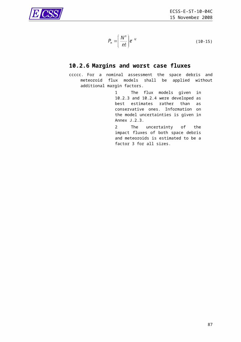
ECSS-E-ST-10-04C15 November 2008
8,87E+01 2,62E+04
2,48E+04
3,19E+04
3,02E+04
3,70E+04
3,18E+04
2,64E+04 2,41E+04
2,74E+04
2,83E+04
2,18E+04
1,26E+02 9,18E+03
8,52E+03
1,11E+04
1,08E+04
1,35E+04
1,17E+04
9,86E+03 9,02E+03
1,00E+04
9,90E+03
7,83E+03
1,84E+02 3,45E+03
3,15E+03
4,13E+03
4,22E+03
5,37E+03
4,71E+03
4,02E+03 3,66E+03
3,91E+03
3,65E+03
2,99E+03
2,66E+02 1,23E+03
1,10E+03
1,48E+03
1,58E+03
2,07E+03
1,79E+03
1,53E+03 1,36E+03
1,43E+03
1,27E+03
1,07E+03
3,97E+02 3,83E+02
3,23E+02
4,77E+02
5,41E+02
7,31E+02
6,22E+02
5,24E+02 4,53E+02
4,64E+02
3,87E+02
3,33E+02
6,12E+02 7,56E+01
6,33E+01
9,96E+01
1,22E+02
1,71E+02
1,45E+02
1,17E+02 9,93E+01
9,87E+01
7,70E+01
6,57E+01
9,08E+02 1,81E+01
1,57E+01
2,80E+01
3,51E+01
5,39E+01
4,28E+01
3,26E+01 2,73E+01
2,66E+01
1,97E+01
1,60E+01
87
ECSS-E-ST-10-04C15 November 2008
Table B-2: IGE 2006 GEO average model – electron flux (kev-1cm-2s-1sr-1) according toyear in the solar cycle (referred to solar min: 0) and for different energies for a mission
duration of 1 year.(Part 2 of 2)
1,29E+03 4,63E+00
4,56E+00
8,68E+00
1,11E+01
1,86E+01
1,37E+01
9,84E+00 8,07E+00
7,78E+00
5,52E+00
4,25E+00
1,99E+03 5,79E-01
6,73E-01
1,39E+00
1,81E+00
3,41E+00
2,28E+00
1,52E+00 1,22E+00
1,15E+00
7,74E-01
5,56E-01
2,44E+03 1,96E-01
2,45E-01
5,26E-01
6,92E-01
1,37E+00
8,79E-01
5,65E-01 4,48E-01
4,21E-01
2,76E-01
1,92E-01
3,07E+03 5,29E-02
7,23E-02
1,62E-01
2,15E-01
4,54E-01
2,76E-01
1,71E-01 1,34E-01
1,24E-01
7,93E-02
5,30E-02
3,97E+03 9,09E-03
1,37E-02
3,21E-02
4,32E-02
9,74E-02
5,60E-02
3,31E-02 2,56E-02
2,36E-02
1,46E-02
9,36E-03
5,20E+03 1,27E-03
2,12E-03
5,23E-03
7,12E-03
1,72E-02
9,33E-03
5,27E-03 4,01E-03
3,67E-03
2,19E-03
1,35E-03
:
Table B-3IGE 2006 GEO upper case model - maximum electron flux (kev-1cm-2s-1sr-1) according to year in the solar cycle (referred to solar min: 0) and for different energies for a mission duration of 1 year.
(Part 1 of 2)Energy (keV)
-6 -5 -4 -3 -2 -1 0 (solar min)
1 2 3 4
9,17E-01 1,89E+07
2,00E+07
1,75E+07
1,37E+07
1,20E+07
9,71E+06
9,99E+06 1,10E+07
1,26E+07
1,40E+07
1,95E+07
1,20E+00 1,61E+07
1,69E+07
1,48E+07
1,18E+07
1,02E+07
8,42E+06
8,71E+06 9,61E+06
1,09E+07
1,20E+07
1,67E+07
1,57E+00 1,38E+07
1,46E+07
1,28E+07
1,03E+07
8,88E+06
7,40E+06
7,66E+06 8,43E+06
9,60E+06
1,05E+07
1,43E+07
2,05E+00 1,18E+07
1,24E+07
1,09E+07
8,86E+06
7,73E+06
6,49E+06
6,35E+06 6,60E+06
7,99E+06
8,79E+06
1,20E+07
88

ECSS-E-ST-10-04C15 November 2008
2,67E+00 9,91E+06
1,04E+07
9,28E+06
7,60E+06
6,70E+06
5,62E+06
5,48E+06 5,63E+06
6,91E+06
7,51E+06
1,01E+07
3,47E+00 8,20E+06
8,50E+06
7,74E+06
6,44E+06
5,72E+06
4,77E+06
4,96E+06 5,40E+06
6,24E+06
6,59E+06
8,62E+06
4,53E+00 6,55E+06
6,68E+06
6,24E+06
5,29E+06
4,74E+06
3,91E+06
4,15E+06 4,50E+06
5,18E+06
5,40E+06
6,93E+06
5,90E+00 5,01E+06
5,02E+06
4,87E+06
4,20E+06
3,79E+06
3,07E+06
3,30E+06 3,54E+06
4,04E+06
4,21E+06
5,33E+06
7,73E+00 3,61E+06
3,57E+06
3,60E+06
3,15E+06
2,87E+06
2,26E+06
2,46E+06 2,58E+06
2,95E+06
3,09E+06
3,88E+06
89

ECSS-E-ST-10-04C15 November 2008
: (Part 2 of 2)
1,02E+01
2,43E+06
2,36E+06
2,49E+06
2,21E+06
2,04E+06
1,55E+06
1,67E+06
1,74E+06
1,98E+06
2,12E+06
2,63E+06
1,33E+01
1,52E+06
1,48E+06
1,62E+06
1,42E+06
1,35E+06
9,98E+05
1,06E+06
1,09E+06
1,24E+06
1,36E+06
1,66E+06
1,74E+01
8,86E+05
8,60E+05
9,86E+05
8,55E+05
8,25E+05
6,04E+05
6,14E+05
6,19E+05
7,18E+05
8,70E+05
9,94E+05
3,00E+01
2,72E+05
2,68E+05
3,39E+05
3,02E+05
3,43E+05
3,03E+05
2,47E+05
2,28E+05
2,72E+05
3,03E+05
2,25E+05
6,12E+01
9,57E+04
9,22E+04
1,18E+05
1,08E+05
1,28E+05
1,11E+05
9,18E+04
8,43E+04
9,80E+04
1,05E+05
7,93E+04
8,87E+01
3,81E+04
3,60E+04
4,64E+04
4,39E+04
5,38E+04
4,62E+04
3,84E+04
3,50E+04
3,98E+04
4,11E+04
3,17E+04
1,26E+02
1,35E+04
1,26E+04
1,64E+04
1,59E+04
1,99E+04
1,73E+04
1,45E+04
1,33E+04
1,48E+04
1,46E+04
1,16E+04
1,84E+02
5,21E+03
4,76E+03
6,24E+03
6,37E+03
8,11E+03
7,11E+03
6,07E+03
5,53E+03
5,91E+03
5,51E+03
4,52E+03
2,66E+02
1,92E+03
1,72E+03
2,31E+03
2,46E+03
3,23E+03
2,79E+03
2,39E+03
2,12E+03
2,23E+03
1,98E+03
1,67E+03
3,97E+02
6,27E+02
5,29E+02
7,81E+02
8,86E+02
1,20E+03
1,02E+03
8,58E+02
7,42E+02
7,60E+02
6,34E+02
5,46E+02
6,12E+02
1,34E+02
1,12E+02
1,76E+02
2,16E+02
3,02E+02
2,56E+02
2,07E+02
1,75E+02
1,74E+02
1,36E+02
1,16E+02
9,08E+02
3,52E+01
3,05E+01
5,45E+01
6,83E+01
1,05E+02
8,32E+01
6,34E+01
5,31E+01
5,17E+01
3,83E+01
3,11E+01
1,29E+03
1,01E+01
9,91E+00
1,89E+01
2,41E+01
4,04E+01
2,98E+01
2,14E+01
1,75E+01
1,69E+01
1,20E+01
9,24E+00
1,99E+03
1,50E+00
1,75E+00
3,61E+00
4,70E+00
8,85E+00
5,91E+00
3,94E+00
3,16E+00
2,98E+00
2,01E+00
1,44E+00
2,44E+03
5,61E-01
7,02E-01
1,51E+00
1,98E+00
3,92E+00
2,52E+00
1,62E+00
1,28E+00
1,21E+00
7,90E-01
5,50E-01
90

ECSS-E-ST-10-04C15 November 2008
3,07E+03
1,72E-01
2,34E-01
5,25E-01
6,97E-01
1,47E+00
8,95E-01
5,54E-01
4,34E-01
4,02E-01
2,57E-01
1,72E-01
3,97E+03
3,44E-02
5,18E-02
1,21E-01
1,63E-01
3,68E-01
2,12E-01
1,25E-01
9,68E-02
8,93E-02
5,52E-02
3,54E-02
5,20E+03
5,74E-03
9,58E-03
2,36E-02
3,22E-02
7,77E-02
4,22E-02
2,38E-02
1,81E-02
1,66E-02
9,90E-03
6,10E-03
91
ECSS-E-ST-10-04C15 November 2008
Table B-4: MEOv2 average case model - average electron flux (Mev-1cm-2s-1sr-1) according to year in the solar cycle
(referred to solar min: 0) and for different energies for a mission duration of 1 year.Energy (MeV)
-6 -5 -4 -3 -2 -1 0 (solar min)
1 2 3 4
0,282,90E+
062,89E+
063,79E+
063,95E+
064,93E+
064,31E+
06 3,88E+063,46E+
063,69E+
063,36E+
062,90E+
06
0,41,61E+
061,57E+
062,25E+
062,53E+
063,35E+
062,89E+
06 2,47E+062,15E+
062,22E+
061,87E+
061,61E+
06
0,566,75E+
056,48E+
051,01E+
061,22E+
061,70E+
061,44E+
06 1,17E+061,00E+
069,98E+
057,91E+
056,75E+
05
0,82,00E+
051,94E+
053,33E+
054,14E+
056,19E+
055,03E+
05 3,89E+053,28E+
053,21E+
052,42E+
052,00E+
05
1,125,80E+
045,99E+
041,11E+
051,40E+
052,27E+
051,72E+
05 1,27E+051,05E+
051,02E+
057,35E+
045,80E+
04
1,61,21E+
041,37E+
042,70E+
043,48E+
046,14E+
044,34E+
04 3,01E+042,44E+
042,33E+
041,61E+
041,21E+
04
2,242,15E+
032,62E+
035,45E+
037,12E+
031,35E+
048,98E+
03 5,94E+034,75E+
034,49E+
033,01E+
032,15E+
03
Table B-5: MEOv2 upper case model - maximum electron flux (Mev-1cm-2s-1sr-1) according to year in the solar cycle
(referred to solar min: 0) and for different energies for a mission duration of 1 year.Energy (MeV)
-6 -5 -4 -3 -2 -1 0 (solar min)
1 2 3 4
0,287,39E+
067,40E+
069,54E+
069,79E+
061,20E+
071,06E+
07 9,65E+068,65E+
069,27E+
068,55E+
067,39E+
06
0,44,38E+
064,27E+
066,03E+
066,73E+
068,78E+
067,61E+
06 6,58E+065,74E+
065,94E+
065,05E+
064,38E+
06
0,561,99E+
061,91E+
062,95E+
063,53E+
064,86E+
064,16E+
06 3,41E+062,92E+
062,92E+
062,32E+
061,99E+
060,8 6,48E+ 6,24E+ 1,06E+ 1,32E+ 1,94E+ 1,60E+ 1,25E+06 1,05E+ 1,03E+ 7,82E+ 6,48E+
92
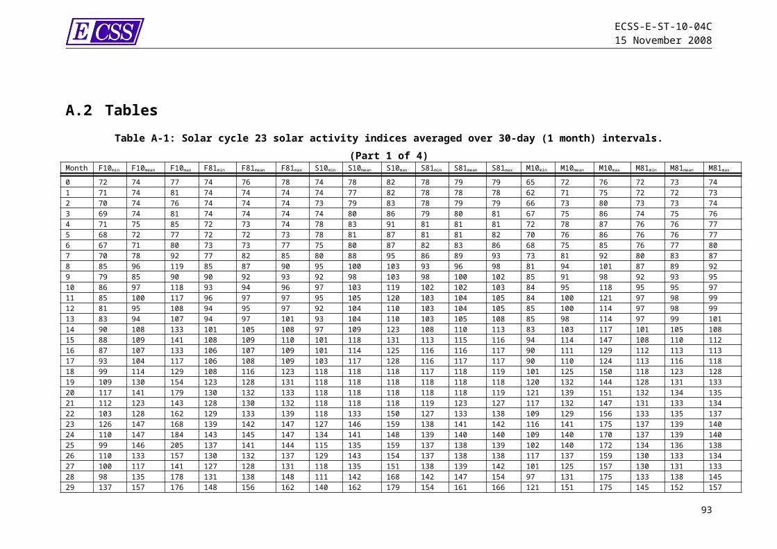
ECSS-E-ST-10-04C15 November 2008
05 05 06 06 06 06 06 06 05 05
1,122,13E+
052,18E+
054,01E+
055,06E+
058,09E+
056,22E+
05 4,61E+053,82E+
053,71E+
052,69E+
052,13E+
05
1,65,24E+
045,88E+
041,15E+
051,48E+
052,60E+
051,85E+
05 1,29E+051,05E+
051,00E+
056,96E+
045,24E+
04
2,241,11E+
041,34E+
042,77E+
043,61E+
046,78E+
044,55E+
04 3,03E+042,43E+
042,30E+
041,54E+
041,11E+
04
93

ECSS-E-ST-10-04C15 November 2008
Table B-6: Worst case spectrum for geostationary orbitsElectron Energy, MeV Flux, cm-2s-1sr-1
0,225 6,5E60,315 4,2E60,5 2,2E60,75 1,0E61,1 4,4E51,5 2,0E51,8 1,05E53,5 6,4E3
Table B-7: Values of the parameters for the ESP modelEnergy range
Фmean (cm-2)
ФRV
> 1 MeV 8,877E+10 0,940> 3 MeV 3,297E+10 3,038> 5 MeV 1,973E+10 5,250> 7 MeV 1,371E+10 7,575> 10 MeV 9,089E+09 11,239> 15 MeV 5,476E+09 17,675> 20 MeV 3,707E+09 24,351> 25 MeV 2,687E+09 31,126> 30 MeV 2,034E+09 37,889> 35 MeV 1,589E+09 44,572> 40 MeV 1,273E+09 51,130> 45 MeV 1,038E+09 57,504> 50 MeV 8,602E+08 63,674> 55 MeV 7,215E+08 69,642> 60 MeV 6,117E+08 75,368> 70 MeV 4,518E+08 86,122> 80 MeV 3,431E+08 95,852> 90 MeV 2,665E+08 104,635> 100 MeV 2,109E+08 112,465
Table B-8: Values to scale fluence from >100 MeV to >300 MeVEnergy Range: Fluence (p cm-2):
> 125 MeV 0,603 x ϕ(>100 MeV)> 150 MeV 0,390 x ϕ(>100 MeV)> 175 MeV 0,267 x ϕ(>100 MeV)> 200 MeV 0,191 x ϕ(>100 MeV)> 225 MeV 0,141 x ϕ(>100 MeV)
94
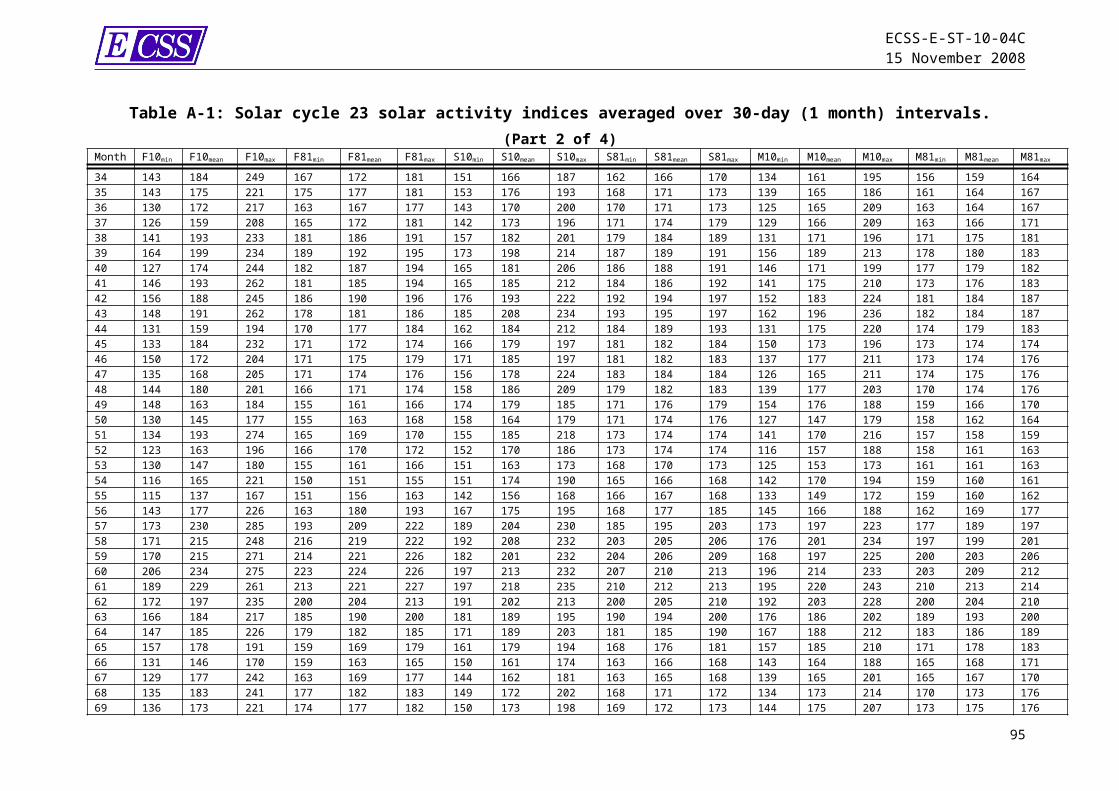
ECSS-E-ST-10-04C15 November 2008
> 250 MeV 0,107 x ϕ(>100 MeV)> 275 MeV 0,0823 x ϕ(>100 MeV)> 300 MeV 0,0647 x ϕ(>100 MeV)
Table B-9: CREME-96 solar ion worst 5-minute fluxes in an interplanetary environment(Part 1 of 2)
Ion Flux [# m-2s-1sr-1(MeV/nucl)-1]Energy
[MeV/nucl] H He C N O Fe
1,0E+001,36E+0
95,25E+0
75,05E+0
51,29E+0
51,07E+0
64,11E+0
5
2,0E+006,36E+0
82,09E+0
72,01E+0
55,15E+0
44,27E+0
51,64E+0
5
3,0E+003,81E+0
81,11E+0
71,07E+0
52,74E+0
42,27E+0
58,70E+0
4
4,0E+002,56E+0
86,76E+0
66,50E+0
41,66E+0
41,38E+0
55,30E+0
4
5,0E+001,83E+0
84,47E+0
64,29E+0
41,10E+0
49,12E+0
43,50E+0
4
6,0E+001,37E+0
83,12E+0
63,00E+0
47,69E+0
36,38E+0
42,45E+0
4
7,0E+001,06E+0
82,27E+0
62,18E+0
45,59E+0
34,64E+0
41,78E+0
4
8,0E+008,44E+0
71,71E+0
61,64E+0
44,20E+0
33,48E+0
41,34E+0
4
9,0E+006,83E+0
71,31E+0
61,26E+0
43,23E+0
32,68E+0
41,03E+0
4
1,0E+015,61E+0
71,03E+0
69,91E+0
32,54E+0
32,11E+0
48,08E+0
3
2,0E+011,32E+0
71,25E+0
51,20E+0
33,09E+0
22,56E+0
31,37E+0
3
3,0E+014,89E+0
62,30E+0
42,21E+0
25,66E+0
14,69E+0
22,96E+0
2
4,0E+012,26E+0
66,90E+0
36,62E+0
11,70E+0
11,41E+0
27,94E+0
1
5,0E+011,20E+0
62,71E+0
32,61E+0
16,68E+0
05,54E+0
12,87E+0
1
6,0E+016,95E+0
51,27E+0
31,22E+0
13,12E+0
02,59E+0
11,25E+0
1
7,0E+014,31E+0
56,67E+0
26,40E+0
01,64E+0
01,36E+0
16,18E+0
0
8,0E+012,81E+0
53,83E+0
23,67E+0
0 9,42E-017,81E+0
03,37E+0
0
9,0E+011,91E+0
52,35E+0
22,25E+0
0 5,77E-014,79E+0
01,97E+0
0
1,0E+021,35E+0
51,52E+0
21,46E+0
0 3,73E-013,09E+0
01,22E+0
0
95
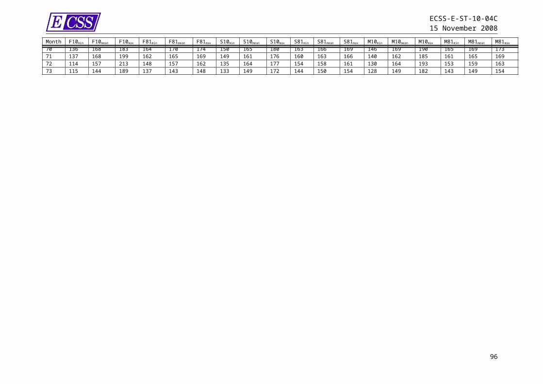
ECSS-E-ST-10-04C15 November 2008
Ion Flux [# m-2s-1sr-1(MeV/nucl)-1]Energy
[MeV/nucl] H He C N O Fe
2,0E+021,18E+0
48,78E+0
0 8,43E-02 2,16E-02 1,79E-01 5,41E-02
3,0E+022,70E+0
31,72E+0
0 1,65E-02 4,23E-03 3,50E-02 9,03E-03
4,0E+029,45E+0
2 5,53E-01 5,31E-03 1,36E-03 1,13E-02 2,60E-03
96
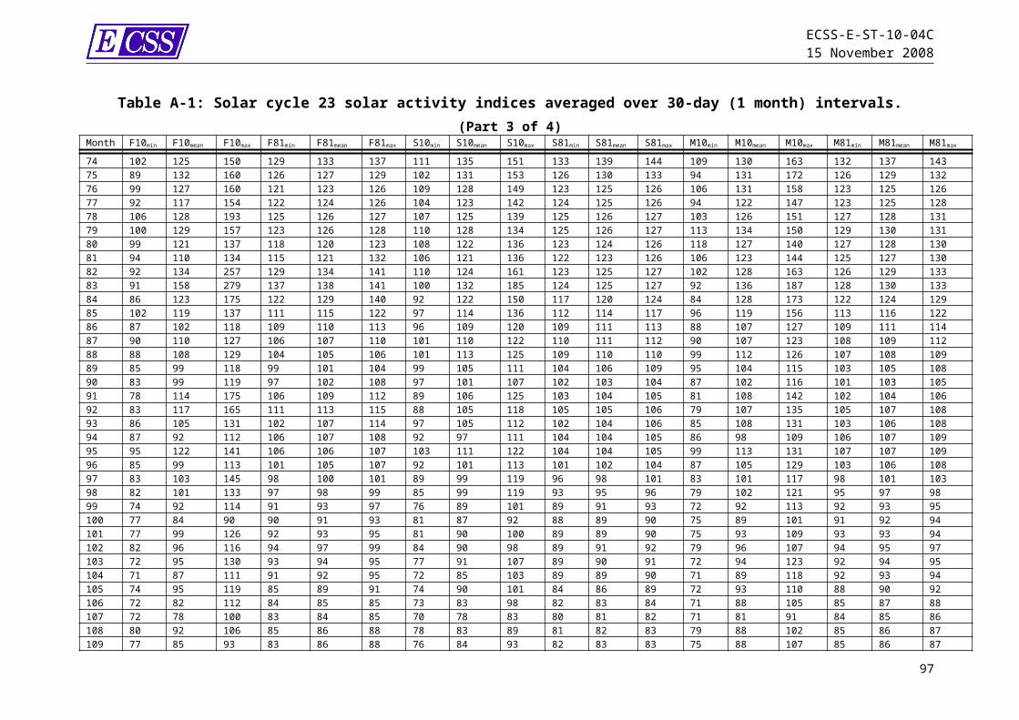
ECSS-E-ST-10-04C15 November 2008
Table B-9: CREME-96 solar ion worst 5-minute fluxes in aninterplanetary environment
(Part 2 of 2)Ion Flux [# m-2s-1sr-1(MeV/nucl)-1]
Energy [MeV/nucl] H He C N O Fe
5,0E+024,00E+0
2 2,20E-01 2,11E-03 5,40E-04 4,48E-03 9,47E-04
6,0E+021,74E+0
2 1,03E-01 9,91E-04 2,54E-04 2,11E-03 4,14E-04
7,0E+029,16E+0
1 5,45E-02 5,24E-04 1,34E-04 1,11E-03 2,06E-04
8,0E+025,27E+0
1 3,14E-02 3,01E-04 7,72E-05 6,40E-04 1,13E-04
9,0E+023,24E+0
1 1,93E-02 1,85E-04 4,74E-05 3,93E-04 6,60E-05
1,0E+032,09E+0
1 1,24E-02 1,20E-04 3,06E-05 2,54E-04 4,10E-05
2,0E+031,19E+0
0 7,06E-04 6,78E-06 1,74E-06 1,44E-05 1,77E-063,0E+03 2,21E-01 1,32E-04 1,26E-06 3,24E-07 2,69E-06 2,83E-074,0E+03 6,72E-02 4,00E-05 3,84E-07 9,85E-08 8,17E-07 7,68E-085,0E+03 2,67E-02 1,59E-05 1,53E-07 3,91E-08 3,24E-07 2,80E-086,0E+03 1,25E-02 7,47E-06 7,17E-08 1,84E-08 1,52E-07 1,22E-087,0E+03 6,63E-03 3,94E-06 3,79E-08 9,71E-09 8,05E-08 6,09E-098,0E+03 3,81E-03 2,27E-06 2,18E-08 5,58E-09 4,63E-08 3,33E-099,0E+03 2,34E-03 1,39E-06 1,34E-08 3,43E-09 2,84E-08 1,95E-091,0E+04 1,51E-03 9,01E-07 8,65E-09 2,22E-09 1,84E-08 1,21E-092,0E+04 8,58E-05 5,11E-08 4,90E-10 1,26E-10 1,04E-09 5,24E-113,0E+04 1,60E-05 9,53E-09 9,15E-11 2,34E-11 1,94E-10 8,35E-124,0E+04 4,86E-06 2,89E-09 2,78E-11 7,13E-12 5,91E-11 2,27E-125,0E+04 1,93E-06 1,15E-09 1,10E-11 2,83E-12 2,35E-11 8,25E-136,0E+04 9,08E-07 5,40E-10 5,19E-12 1,33E-12 1,10E-11 3,61E-137,0E+04 4,79E-07 2,85E-10 2,74E-12 7,02E-13 5,82E-12 1,80E-138,0E+04 2,76E-07 1,64E-10 1,58E-12 4,04E-13 3,35E-12 9,82E-149,0E+04 1,69E-07 1,01E-10 9,68E-13 2,48E-13 2,06E-12 5,76E-141,0E+05 1,09E-07 6,52E-11 6,26E-13 1,60E-13 1,33E-12 3,57E-14
97
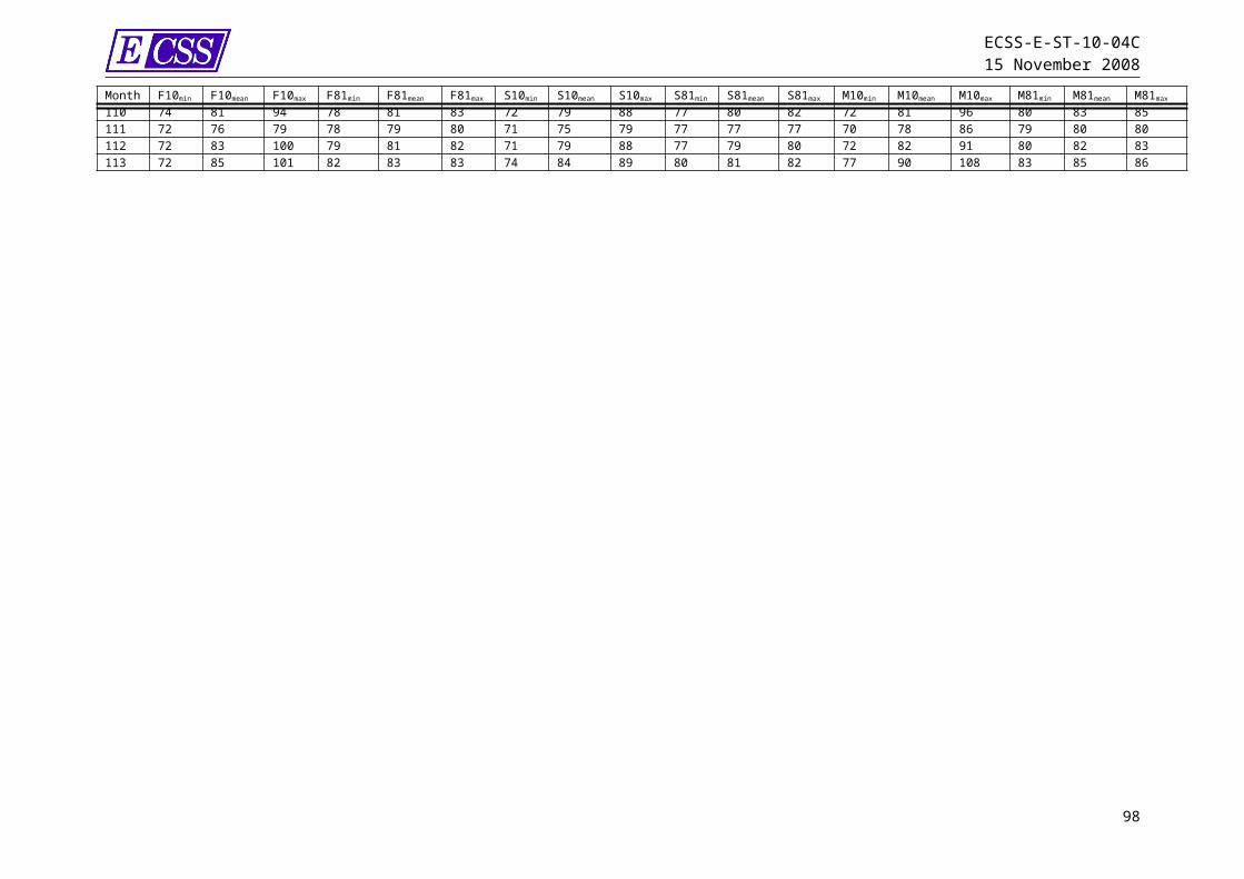
ECSS-E-ST-10-04C15 November 2008
Table B-10: CREME-96 solar ion worst day fluxes in an interplanetary environment(Part 1 of 2)
Ion Flux [# m-2s-1sr-1(MeV/nucl)-1]Energy
[MeV/nucl] H He C N O Fe
1,0E+003,24E+
081,25E+
071,20E+
053,08E+
042,56E+
059,81E+
04
2,0E+001,54E+
085,07E+
064,87E+
041,25E+
041,03E+
053,97E+
04
3,0E+009,34E+
072,72E+
062,61E+
046,70E+
035,55E+
042,13E+
04
4,0E+006,32E+
071,67E+
061,60E+
044,11E+
033,41E+
041,31E+
04
5,0E+004,57E+
071,11E+
061,07E+
042,74E+
032,27E+
048,71E+
03
6,0E+003,44E+
077,82E+
057,51E+
031,93E+
031,60E+
046,13E+
03
7,0E+002,68E+
075,73E+
055,50E+
031,41E+
031,17E+
044,48E+
03
8,0E+002,14E+
074,32E+
054,15E+
031,06E+
038,82E+
033,38E+
03
9,0E+001,74E+
073,34E+
053,21E+
038,23E+
026,82E+
032,62E+
03
1,0E+011,44E+
072,64E+
052,53E+
036,49E+
025,38E+
032,06E+
03
2,0E+013,47E+
063,31E+
043,18E+
028,14E+
016,75E+
023,61E+
02
3,0E+011,31E+
066,17E+
035,93E+
011,52E+
011,26E+
027,95E+
01
4,0E+016,16E+
051,88E+
031,80E+
014,62E+
003,83E+
012,16E+
01
5,0E+013,29E+
057,45E+
027,15E+
001,83E+
001,52E+
017,86E+
00
6,0E+011,92E+
053,50E+
023,36E+
008,62E-
017,14E+
003,44E+
00
7,0E+011,19E+
051,85E+
021,78E+
004,55E-
013,77E+
001,71E+
00
8,0E+017,82E+
041,06E+
021,02E+
002,62E-
012,17E+
009,35E-
01
9,0E+015,33E+
046,53E+
016,27E-
011,61E-
011,33E+
005,49E-
01
1,0E+023,75E+
044,22E+
014,05E-
011,04E-
018,62E-
013,40E-
01
2,0E+023,22E+
032,39E+
002,30E-
025,89E-
034,89E-
021,47E-
02
3,0E+027,02E+
024,47E-
014,29E-
031,10E-
039,12E-
032,35E-
034,0E+02 2,32E+ 1,36E- 1,30E- 3,34E- 2,77E- 6,38E-
98

ECSS-E-ST-10-04C15 November 2008
Ion Flux [# m-2s-1sr-1(MeV/nucl)-1]Energy
[MeV/nucl] H He C N O Fe02 01 03 04 03 04
5,0E+029,29E+
015,39E-
025,17E-
041,33E-
041,10E-
032,32E-
04
6,0E+023,91E+
012,53E-
022,43E-
046,23E-
055,17E-
041,02E-
04
7,0E+022,06E+
011,34E-
021,28E-
043,29E-
052,73E-
045,06E-
05
8,0E+021,18E+
017,69E-
037,39E-
051,89E-
051,57E-
042,76E-
05
9,0E+027,27E+
004,72E-
034,54E-
051,16E-
059,64E-
051,62E-
05
1,0E+034,70E+
003,05E-
032,93E-
057,52E-
066,23E-
051,01E-
05
2,0E+032,66E-
011,73E-
041,66E-
064,26E-
073,53E-
064,35E-
07
3,0E+034,97E-
023,23E-
053,10E-
077,95E-
086,59E-
076,94E-
08
4,0E+031,51E-
029,82E-
069,43E-
082,42E-
082,00E-
071,88E-
08
5,0E+036,00E-
033,90E-
063,74E-
089,59E-
097,95E-
086,86E-
09
6,0E+032,82E-
031,83E-
061,76E-
084,51E-
093,74E-
083,00E-
09
99
ECSS-E-ST-10-04C15 November 2008
Table B-10: CREME-96 solar ion worst day fluxes in an interplanetaryenvironment(Part 2 of 2)
Ion Flux [# m-2s-1sr-1(MeV/nucl)-1]Energy
[MeV/nucl] H He C N O Fe
7,0E+031,49E-
039,68E-
079,29E-
092,38E-
091,97E-
081,49E-
09
8,0E+038,57E-
045,57E-
075,35E-
091,37E-
091,14E-
088,16E-
10
9,0E+035,26E-
043,42E-
073,28E-
098,41E-
106,98E-
094,79E-
10
1,0E+043,40E-
042,21E-
072,12E-
095,44E-
104,51E-
092,97E-
10
2,0E+041,93E-
051,25E-
081,20E-
103,08E-
112,56E-
101,29E-
11
3,0E+043,60E-
062,34E-
092,24E-
115,75E-
124,77E-
112,05E-
12
4,0E+041,09E-
067,10E-
106,82E-
121,75E-
121,45E-
115,56E-
13
5,0E+044,34E-
072,82E-
102,71E-
126,94E-
135,75E-
122,03E-
13
6,0E+042,04E-
071,33E-
101,27E-
123,26E-
132,70E-
128,87E-
14
7,0E+041,08E-
077,00E-
116,72E-
131,72E-
131,43E-
124,41E-
14
8,0E+046,20E-
084,03E-
113,87E-
139,91E-
148,22E-
132,41E-
14
9,0E+043,81E-
082,47E-
112,37E-
136,09E-
145,05E-
131,41E-
14
1,0E+052,46E-
081,60E-
111,54E-
133,93E-
143,26E-
138,77E-
15
100

ECSS-E-ST-10-04C15 November 2008
Table B-11: CREME-96 solar ion worst week fluxes in an interplanetary environment(Part 1 of 2)
Ion Flux [# m-2s-1sr-1(MeV/nucl)-1]Energy
[MeV/nucl] H He C N O Fe
1,0E+004,64E+
072,36E+
062,75E+
047,04E+
035,84E+
041,57E+
04
2,0E+002,28E+
079,53E+
051,11E+
042,85E+
032,36E+
046,34E+
03
3,0E+001,41E+
075,12E+
055,97E+
031,53E+
031,27E+
043,41E+
03
4,0E+009,77E+
063,14E+
053,66E+
039,39E+
027,79E+
032,09E+
03
5,0E+007,19E+
062,09E+
052,44E+
036,25E+
025,19E+
031,39E+
03
6,0E+005,51E+
061,47E+
051,72E+
034,40E+
023,65E+
039,80E+
02
7,0E+004,36E+
061,08E+
051,26E+
033,22E+
022,67E+
037,17E+
02
8,0E+003,53E+
068,13E+
049,48E+
022,43E+
022,02E+
035,41E+
02
9,0E+002,91E+
066,29E+
047,33E+
021,88E+
021,56E+
034,19E+
02
1,0E+012,44E+
064,96E+
045,78E+
021,48E+
021,23E+
033,30E+
02
2,0E+016,61E+
055,20E+
036,06E+
011,55E+
011,29E+
024,93E+
01
3,0E+012,74E+
051,13E+
031,32E+
013,37E+
002,80E+
011,07E+
01
4,0E+011,38E+
053,81E+
024,45E+
001,14E+
009,45E+
003,63E+
00
5,0E+017,90E+
041,64E+
021,92E+
004,92E-
014,08E+
001,57E+
00
6,0E+014,88E+
048,27E+
019,65E-
012,47E-
012,05E+
007,91E-
01
7,0E+013,20E+
044,63E+
015,40E-
011,38E-
011,15E+
004,43E-
01
8,0E+012,20E+
042,80E+
013,26E-
018,36E-
026,94E-
012,68E-
01
9,0E+011,56E+
041,80E+
012,09E-
015,37E-
024,45E-
011,72E-
01
1,0E+021,14E+
041,21E+
011,41E-
013,61E-
022,99E-
011,16E-
01
2,0E+021,27E+
038,86E-
011,03E-
022,65E-
032,20E-
021,28E-
02
3,0E+023,16E+
021,92E-
012,24E-
035,74E-
044,76E-
034,00E-
034,0E+02 1,13E+ 6,50E- 7,58E- 1,94E- 1,61E- 1,76E-
101
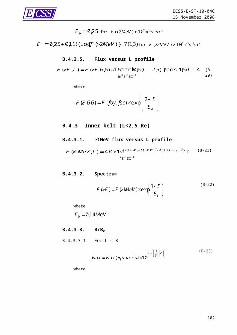
ECSS-E-ST-10-04C15 November 2008
Ion Flux [# m-2s-1sr-1(MeV/nucl)-1]Energy
[MeV/nucl] H He C N O Fe02 02 04 04 03 03
5,0E+024,79E+
012,80E-
023,27E-
048,38E-
056,95E-
049,28E-
04
6,0E+022,13E+
011,41E-
021,64E-
044,21E-
053,50E-
045,51E-
04
7,0E+021,19E+
017,89E-
039,20E-
052,36E-
051,96E-
043,54E-
04
8,0E+027,20E+
004,77E-
035,56E-
051,43E-
051,18E-
042,42E-
04
9,0E+024,62E+
003,06E-
033,57E-
059,14E-
067,58E-
051,73E-
04
1,0E+033,11E+
002,06E-
032,40E-
056,15E-
065,10E-
051,28E-
04
2,0E+032,30E-
011,51E-
041,76E-
064,51E-
073,74E-
061,76E-
05
3,0E+035,00E-
023,27E-
053,82E-
079,79E-
088,12E-
075,51E-
06
4,0E+031,69E-
021,11E-
051,29E-
073,31E-
082,75E-
072,42E-
06
5,0E+037,31E-
034,78E-
065,57E-
081,43E-
081,18E-
071,28E-
06
6,0E+033,68E-
032,40E-
062,80E-
087,18E-
095,96E-
087,58E-
07
102

ECSS-E-ST-10-04C15 November 2008
Table B-11: CREME-96 solar ion worst week fluxes in an interplanetaryenvironment(Part 2 of 2)
Ion Flux [# m-2s-1sr-1(MeV/nucl)-1]Energy
[MeV/nucl] H He C N O Fe
7,0E+032,06E-
031,34E-
061,57E-
084,02E-
093,33E-
084,88E-
07
8,0E+031,25E-
038,13E-
079,48E-
092,43E-
092,01E-
083,33E-
07
9,0E+038,02E-
045,21E-
076,08E-
091,56E-
091,29E-
082,38E-
07
1,0E+045,40E-
043,51E-
074,09E-
091,05E-
098,69E-
091,76E-
07
2,0E+043,98E-
052,57E-
083,00E-
107,69E-
116,38E-
102,42E-
08
3,0E+048,66E-
065,58E-
096,51E-
111,67E-
111,38E-
107,59E-
09
4,0E+042,94E-
061,89E-
092,20E-
115,64E-
124,68E-
113,33E-
09
5,0E+041,27E-
068,14E-
109,49E-
122,43E-
122,02E-
111,76E-
09
6,0E+046,39E-
074,09E-
104,78E-
121,22E-
121,02E-
111,04E-
09
7,0E+043,58E-
072,29E-
102,67E-
126,85E-
135,68E-
126,72E-
10
8,0E+042,17E-
071,38E-
101,62E-
124,14E-
133,43E-
124,59E-
10
9,0E+041,39E-
078,88E-
111,04E-
122,66E-
132,20E-
123,27E-
10
1,0E+059,35E-
085,97E-
116,97E-
131,79E-
131,48E-
122,42E-
10
103
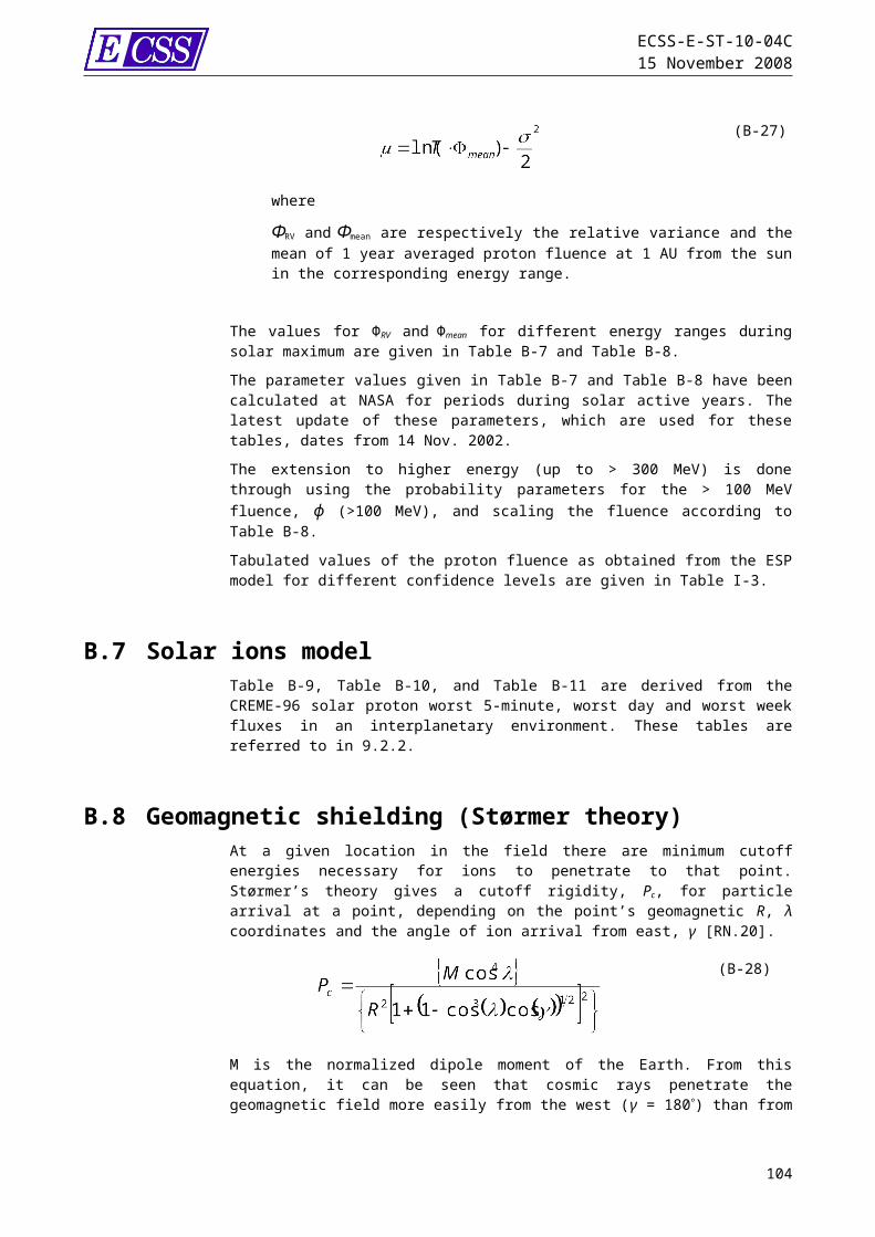
ECSS-E-ST-10-04C15 November 2008
Annex C (normative)Space debris and meteoroids
C.1 Flux models
C.1.1 Meteoroid velocity distributionTable C-1 gives the velocity distribution for the sporadic meteoroid flux model specified in 10.2.4.
NOTE The velocity distribution in Table C-1 is based on data from the Harvard Radio Meteor Project (HRMP) where about 20 000 meteor observations which were re-evaluated and corrected by Taylor [RD.27].
C.1.2 Flux enhancement and altitude dependent velocity distribution
The velocity distribution given in Table C-1 is modified by the gravitational attraction of Earth.In case of a single velocity value the flux increase due to Earth gravity at a given distance r of the centre of the Earth is described by the factor G which is given by
Gv
vesc
12
2
(C-1)
or(C-2)
with
v v vesc2 2 2
(C-3)
G describes the factor by which a particle flux a large distance from Earth, is enhanced when measured near to Earth, due to the gravitational bending of trajectories (causing an increase in particle spatial density) and increase of particle velocity [RD.121].Using the product of the constant of gravitation with Earth’s mass ( = 3,986 105 km3s-2), the escape velocity at distance r can be written as
104

ECSS-E-ST-10-04C15 November 2008
(C-4)
and v∞ is the velocity in free space, i.e. in the absence of Earth’s gravity which is tabulated in Table C-1, and v is the ‘enhanced’ meteoroid velocity at distance r. To obtain the correct flux enhancement in case a velocity distribution is given we realise that G is a function of v∞. Thus the enhanced flux FE is obtained from the flux Fmet,0 by
(C-5)
with (C-6)
is the weighted mean G factor for a given velocity distribution. This assumes that the velocity distribution n(v∞) has been normalised:
(C-7)
The above formulas contain the necessary information to calculate the altitude dependence of the velocity distribution, since we can write
(C-8)
With nk = n(v∞,k) and n’k = n’(v,k) representing the tabulated values for the original distribution function and for the distribution function at distance r respectively. N gives the number of bins used for the velocity distribution. Given the escape velocity at distance r, vesc and the tabulated values of n(v∞) in 1 km s-1 bins nk, we calculate the values n’k for the distribution n’(v) at distance r by
(C-9)
with
(C-10)
and
(C-11)
If we now tabulate the values of n’k we need to change the bin limits by inserting the values of v at the places of the given values of v which is done by using again the formula
(C-12)
As a result the bin widths are now no longer equidistant in v, which is the independent variable of the new distribution function n’(v). The new
105

ECSS-E-ST-10-04C15 November 2008
distribution function is re-normalized and re-binning is required by interpolating the values of n’(v) to obtain equidistant bins in v. This completes the calculation procedure of the new table for the velocity distribution n’(v) at the given distance r.
The gravitational enhancement, expressed by the factor , increases the flux due to a real increase in spatial density of meteoroids due to Earth’s attraction and also due to the increase in the meteoroids’ velocity. Expression (C-5) accounts for both effects.Additional information and examples of modified velocity distributions for various Earth altitudes are given in Annex J.
C.1.3 Earth shielding and flux enhancement from spacecraft motion
C.1.3.1. Earth ShieldingThe Earth shielding factor, sf, for a given surface depends on the spacecraft altitude above the Earth surface and on the relative orientation of the surface normal with respect to the Earth direction.The average Earth shielding factor is given by:
(C-13)
with:
(C-14)
whereRe is the Earth radius = 6 378 km;h is the spacecraft altitude in km; 100 km accounts for the atmaosphere
The corrections for Earth shielding are taken from [RD.21]]
C.1.3.2. Flux enhancement from spacecraft motionIn addition to the Earth attraction and shielding, the spacecraft velocity causes the encountered flux to increase. The flux increase is given by vrel/v where v is the (gravitational enhanced) meteoroid velocity and v rel is the relative velocity of the meteoroid with respect to the spacecraft. When calculating fluxes using codes one generally considers each meteoroid velocity vk bin separately. However, the outcome, which depends on the velocity distribution, is a single enhancement factor K. The meteoroid flux to an Earth orbiting spacecraft is then given by:
(C-15)
Values of , sf and K for typical Earth orbits are given in Table J-6.
106
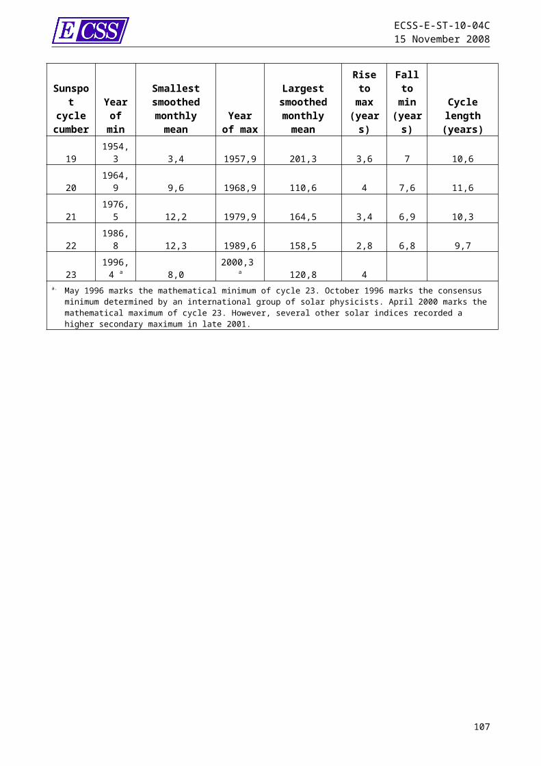
ECSS-E-ST-10-04C15 November 2008
C.1.4 Meteoroid streams
C.1.4.1. Meteor streamsTable C-2 gives the parameters for the main annual meteor streams. From these stream parameters fluxes are derived according to the method given in C.1.4.2.
The meteoroid streams model is based on a method by N. McBride [RD.28] to derive meteoroid fluxes from meteor data. The present reference model uses data for 50 annual meteor streams as given by P. Jenniskens [RD.29]. These data were collected by a large number of observers over a 10 year period from observation sites in both the northern and southern hemispheres. The meteoroid streams model given in C.1.4.2. is implemented in MASTER 2005 [RN.26] and in ESABASE2/DEBRIS [RD.30].
C.1.4.2. Meteor stream fluxesThe meteor stream geometry and activity at shower maximum is defined by: The solar longitude at shower maximum max. The maximum zenithal hourly rate ZHRmax , which is the number of
‘visible’ meteors seen after various observer and location related corrections have been applied.
Apparent radiant position in RA (right ascension of the radiant) and Dec (declination of the radiant) . These values are tabulated in TableC-2 at an epoch defined by the solar longitude 0.
The geocentric meteoroid speeds, defined as the final geocentric velocity V (in km s-1) as the meteoroids reach the top of the atmosphere.
The right ascension of the radiant and for the declination for an instantaneous value of the solar longitude are obtained by
(C-16)
(C-17)
The shower activity as a function of time around its maximum is described by
(C-18)
where B is given in Table C-2 and describes the slopes of the activity profiles. Since most streams are found to have symmetrical profiles a single value of B is sufficient. The Geminids are the exception; this stream needs a different value of B for the inward and outward slope. Six of the streams do not have a strong enough ZHR to produce a slope, here a ‘typical’ value of B = 0,2 is used. Six other streams are best represented by the sum of 2 activity profiles, defined by a peak profile ZHRp
max and Bp
and a background profile ZHRbmax with separate inward and outward slope
values Bb+ and Bb- respectively. This results in the following expression:
107
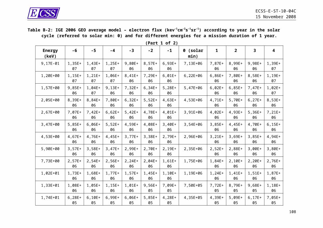
ECSS-E-ST-10-04C15 November 2008
(C-19)
The cumulative flux at solar longitude can now be expressed as:
(C-20)
with
(C-21)
The total particle flux FTOT is obtained by summation over all streams
(C-22)
NOTE If the stream model is used in combination with the reference model of 10.2.3 it is considered that the model in 10.2.3 already includes the average yearly stream contribution.
C.1.4.3. Calculation of meteoroid stream fluxesThe following algorithm applies to determine the individual streams’ fluxes:a. Given , choose the closest value of max in Table C-2 and determine
the stream number.b. From = 2/B determine if is within the range (max - ) < <
(max+ ) ( determined by 1% of ZHRmax), if not, skip this stream (max to be taken from Table C-2).
c. Calculate ZHR within the profile
(C-23)
d. For the six streams in Table C-2 which have two activity profiles (non vanishing Bb+ / Bb- values), calculate ZHR(λ) according to equation (C-19).
e. Form the ratio
(C-24)
f. The cumulative flux is now given by
(C-25)
with
(C-26)
or
108

ECSS-E-ST-10-04C15 November 2008
(C-27)
k and are obtained from Table C-2 according to the relevant stream number.The arrival velocity V includes the gravitational corrections due to the Earth gravity.
C.2 Tables
Table C-1: Normalized meteoroid velocity distributionv∞ n(v∞) v∞ n(v∞) v∞ n(v∞) v∞ n(v∞)
0,5 7,22E-04 18,5 4,47E-02 36,5 4,91E-03 54,5 3,45E-041,5 2,27E-03 19,5 4,22E-02 37,5 4,03E-03 55,5 3,26E-042,5 5,15E-03 20,5 3,94E-02 38,5 3,30E-03 56,5 2,98E-043,5 9,44E-03 21,5 3,63E-02 39,5 2,67E-03 57,5 2,66E-044,5 1,49E-02 22,5 3,29E-02 40,5 2,14E-03 58,5 2,38E-045,5 2,09E-02 23,5 2,97E-02 41,5 1,68E-03 59,5 2,15E-046,5 2,68E-02 24,5 2,66E-02 42,5 1,31E-03 60,5 1,93E-047,5 3,22E-02 25,5 2,39E-02 43,5 1,03E-03 61,5 1,68E-048,5 3,68E-02 26,5 2,15E-02 44,5 8,17E-04 62,5 1,42E-049,5 4,05E-02 27,5 1,94E-02 45,5 6,53E-04 63,5 1,18E-0410,5 4,34E-02 28,5 1,73E-02 46,5 5,35E-04 64,5 9,54E-0511,5 4,56E-02 29,5 1,53E-02 47,5 4,65E-04 65,5 7,47E-0512,5 4,72E-02 30,5 1,33E-02 48,5 4,33E-04 66,5 5,57E-0513,5 4,83E-02 31,5 1,15E-02 49,5 4,19E-04 67,5 3,98E-0514,5 4,88E-02 32,5 9,87E-03 50,5 4,05E-04 68,5 2,81E-0515,5 4,87E-02 33,5 8,42E-03 51,5 3,86E-04 69,5 1,93E-0516,5 4,79E-02 34,5 7,12E-03 52,5 3,68E-04 70,5 1,18E-0517,5 4,66E-02 35,5 5,94E-03 53,5 3,56E-04 71,5 4,86E-06NOTE The velocity is in km s-1 and describes the middle of the 1 km s-1 wide bin. Each value of n(v∞)
describes the relative flux of particles within the corresponding bin of 1 km s-1 width.
109
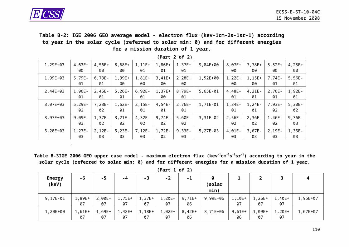
ECSS-E-ST-10-04C15 November 2008
Table C-2: The annual meteor streams(Part 1 of 2)
λmax
RAma
x
ΔRA
Decm
ax
ΔDec
ZRHpm
ax Bp+ Bp-ZHRb
m
ax Bb+ Bb- α kv∞
Bootids283,
3 232 0,6 45-
0,31 10 2,5 2,5 200,37 0,45
0,92
8,4E-17
43
γVelids285,
7 124 0,5 -47 -0,2 2,4 0,12 0,12 0 0 0 1,15,8E-
1935
αCrucids294,
5 193 1,1 -63 -0,4 3 0,11 0,11 0 0 01,06
1,9E-19
50
αHydrusids 300 138 0,7 -13 -0,3 2 0,2 0,2 0 0 01,03
3,4E-19
44
αCarinids311,
2 99 0,4 -54 0 2,3 0,16 0,16 0 0 00,92
1,3E-17
25
δVelids 318 127 0,5 -50 -0,3 1,3 0,2 0,2 0 0 0 1,13,1E-
1935
αCentaurids
319,4 210 1,3 -58 -0,3 7,3 0,18 0,18 0 0 0
0,83
3,7E-18
57
οcentaurids323,
4 176 0,9 -55 -0,4 2,2 0,15 0,15 0 0 01,03
1,9E-19
51
θCentaurids 334 220 1,1 -44 -0,4 4,5 0,2 0,2 0 0 0
0,95
4,4E-19
60
δLeonids 335 169 1 17 -0,3 1,10,04
90,04
9 0 0 0 1,11,9E-
1823
Virginids 340 165 0,9 9 -0,2 1,5 0,2 0,2 0 0 0 1,11,5E-
1826
γNormids 353 285 1,3 -56 -0,2 5,8 0,19 0,19 0 0 00,87
1,9E-18
56
δPavonids 11,1 311 1,6 -63 -0,2 5,30,07
50,07
5 0 0 00,95
5,1E-19
60
Lyrids 32,4 274 1,2 33 0,2 12,8 0,22 0,22 0 0 00,99 2E-18
49
μVirginids 40 230 0,5 -8 -0,3 2,20,04
50,04
5 0 0 0 1,11,1E-
1830
ηAquarids 46,5 340 0,9 -1 0,3 36,7 0,08 0,08 0 0 00,99
1,5E-18
66
βCorona Aust. 56 284 1,3 -40 0,1 3 0,2 0,2 0 0 0
1,13
1,5E-19
45
αScorpiids 55,9 252 1,1 -27 -0,2 3,2 0,13 0,13 0 0 00,92
4,7E-17
21
Da.Arietids 77 47 0,7 24 0,6 54 0,1 0,1 0 0 00,99
2,6E-17
38
γSagitarids 89,2 286 1,1 -25 0,1 2,40,03
70,03
7 0 0 01,06
1,9E-18
29
τCetids 95,7 24 0,9 -12 0,4 3,6 0,18 0,18 0 0 00,92
3,7E-19
66
θOphiuchids 98 292 1,1 -11 0,1 2,3
0,037
0,037 0 0 0
1,03
3,5E-18
27
τAquarids 98 342 1 -12 0,4 7,1 0,24 0,24 0 0 00,92
8,9E-19
63
νPhoenicids
111,2 28 1 -40 0,5 5 0,25 0,25 0 0 0 1,1
2,6E-19
48
οCygnids116,
7 305 0,6 47 0,2 2,5 0,13 0,13 0 0 00,99
1,4E-18
37
Capricornid
122,4 302 0,9 -10 0,3 2,2
0,041
0,041 0 0 0
0,69
8,3E-17
25
τAquarids N
124,1 324 1 -8 0,2 1
0,063
0,063 0 0 0
1,19
3,6E-20
42
Pisces Aust.
124,4 339 1 -33 0,4 2 0,4 0,4 0,9
0,03 0,1
1,16
1,5E-19
42
δAquarids S.
125,6 340 0,8 -17 0,2 11,4
0,091
0,091 0 0 0
1,19
3,6E-19
43
τAquarids S.
131,7 335 1 -15 0,3 1,5 0,07 0,07 0 0 0
1,19
1,2E-19
36
Perseids140,
2 47 1,3 58 0,1 70 0,35 0,35 230,05
0,092
0,92
1,2E-17
61
κCygnids146,
7 290 0,6 52 0,3 2,30,06
90,06
9 0 0 00,79 3E-17
27
πEridanids 153 51 0,8 -16 0,3 40 0,2 0,2 0 0 01,03
1,7E-18
59
γDoradids155,
7 60 0,5 -50 0,2 4,8 0,18 0,18 0 0 01,03
1,1E-18
41
110
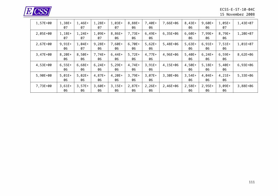
ECSS-E-ST-10-04C15 November 2008
λmax
RAma
x
ΔRA
Decm
ax
ΔDec
ZRHpm
ax Bp+ Bp-ZHRb
m
ax Bb+ Bb- α kv∞
Aurigids158,
2 73 1 43 0,2 9 0,19 0,19 0 0 00,99
2,9E-19
69
κAquarids177,
2 339 0,9 -5 0,4 2,7 0,11 0,11 0 0 01,03
1,9E-17
19
εGeminids206,
7 104 0,7 28 0,1 2,90,08
20,08
2 0 0 0 1,12,1E-
2071
Orionids208,
6 96 0,7 16 0,1 25 0,12 0,12 0 0 01,13
1,6E-19
67
Leo Minorids
209,7 161 1 38 -0,4 1,9 0,14 0,14 0 0 0
0,99
1,1E-19
61
Taurids223,
6 50 0,3 18 0,1 7,30,02
60,02
6 0 0 00,83
4,3E-17
30
δEridanids 229 54 0,9 -2 0,2 0,9 0,2 0,2 0 0 01,03
7,5E-19
31
Table C-2: The annual meteor streams(Part 2 of 2)
λmax
RAma
x
ΔRA
Decm
ax
ΔDec
ZRHpm
ax Bp+ Bp-ZHRb
m
ax Bb+ Bb- α kv∞
ζPuppids232,
2 117 0,7 -42 -0,2 3,2 0,13 0,13 0 0 01,22
9,5E-20
41
Leonids235,
1 154 1 22 0,4 19 0,55 0,55 40,02
50,15
1,22
3,4E-20
71
Puppids/Vel 252 128 0,8 -42 -0,4 4,5
0,034
0,034 0 0 0
1,06
8,2E-19
40
Phoenicids252,
4 19 0,8 -58 0,4 2,8 0,3 0,3 0 0 01,03
2,5E-17
18
Monoceroti.
260,9 100 1 14 -0,1 2 0,25 0,25 0 0 0
1,25
3,3E-20
43
Geminids262,
1 113 1 32 0,1 74 0,59 0,81 18 0,090,31
0,95
7,8E-17
36
σHydrusids265,
5 133 0,9 0 -0,3 2,5 0,1 0,1 0 0 0 1,14,7E-
2059
Ursids 271 224 -0,2 78 -0,3 10 0,9 0,9 2 0,08 0,21,22
8,1E-19
35
111

ECSS-E-ST-10-04C15 November 2008
Annex D (informative) Gravitation
D.1 Gravity models: backgroundEquation (4-7) can be rewritten in terms of amplitude Jlm and phase angle λlm of individual contributions of the spherical harmonic functions to the geopotential.
(D-1)
The equivalence of and is governed by the following equations.
(D-2)
(D-3)
(D-4)
(D-5)
For m l, the terms are called tesseral harmonics. These components divide the Earth’s surface in a checkerboard pattern of hills and valleys, the amplitude and phase of which are determined by the associated coefficients .
For l = m, the functions = 1,0. These terms are called sectorial harmonics. They divide the spherical surface into longitude-dependent sectors, similar to the segments of a basket ball.
For m = 0, the only remaining terms (where is mostly abbreviated as ) are called zonal harmonics. They divide the spherical surface into purely latitude-dependent bands of toroidal hills and valleys, with Earth oblateness ( ) as the dominating contribution. reflects the equilibrium response of a rotating, elastic Earth under the influence of centrifugal and gravitational forces. For the model EIGEN-GL04C the resulting Earth ellipsoid has an equatorial radius of (may slightly vary with the selected geopotential model), a polar radius of
112

ECSS-E-ST-10-04C15 November 2008
(may slightly vary with the selected geopotential model), and an oblateness of .
By convention, the central attraction term of a spherical body of uniform mass distribution is . If the centre of mass coincides with the origin of the body-centred coordinate system, then . If the body-fixed coordinate axes furthermore coincide with the axes of the main moments of inertia, then .
In order to develop a geopotential model it is necessary to measure the gravitational acceleration directly or indirectly, and estimate the set of model coefficients (GM, , ) in a least squares sense on the basis of an adequately large number of such measurements. Direct measurements of the gravity potential are difficult, and typically involve highly sensitive gradiometers that measure the acceleration gradient. Indirect measurements of the gravity potential are obtained from precise tracking data for Earth orbiting satellites. Because of the difficulties of collecting global gravity measurements on land or sea, relevant global geopotential models did not exist before the days of artificial Earth orbiting satellites, and only the first few degree and order terms were known with some accuracy. However, a revolution in gravity model development has occurred after the year 2000, in the form of the three dedicated gravity field missions: CHAMP, GRACE and GOCE (expected to be launched in 2008). All three satellites employ precise global tracking via GPS, allowing continuous high quality orbit determination, and measure the gravity acceleration directly. The arrival of these dedicated gravity missions has essentially rendered any earlier gravity model obsolete. GRACE-only models of 360×360 resolution in degree and order (about 1×1 patches, with ~100 km resolution on the Earth’s surface) have demonstrated to be superior to any of the earlier combined models, even if these were based on the accumulated satellite data sets from three preceding decades. The GRACE models are accurate enough to investigate the temporal variability of the gravity field, for instance due to seasonal displacements of water masses.
D.2 Guidelines for useThe evaluation of a complete 360 × 360 geopotential model at every satellite location of interest represents a substantial computational effort that is usually both undesirable and unnecessary. This section explains how an adequate truncation level of the expansion series may be selected for a satellite orbit of interest, based on two elementary observations.
The first observation is that the term in equations (D-1) and (4-7) leads to a rapid attenuation of the gravity potential with orbit radius r, so that the details of the geopotential become less and less notable at increasing height (in other words, the Earth rapidly turns into a point mass with increasing distance). The second observation is that the expansion series may always be safely truncated at a degree l that provides contributions of lower order of magnitude than the inherent noise level of the model itself.Considering these observations, an adequate truncation degree can be determined on the basis of Kaula’s rule ([RD.31] and equation D.6). This is briefly illustrated via an example that selects a suitable truncation degree l
113

ECSS-E-ST-10-04C15 November 2008
for the orbit height of GNSS constellations, which have a radius r of about 4 times the equatorial radius (i.e. an altitude of H≈25 000 km).
In theory, the degree N of the expansion should be infinite to model the exact variability of the geopotential surface. In practice the maximum degree remains finite. This leads to truncation errors in the expansion series, and thus in a quantification error of the gravity acceleration. In order to get an impression of the truncation effect, Kaula (see [RD.31]) formulated a rule-of-thumb that provides the order of magnitude of normalized expansion coefficients as a function of the degree l:
(D-6)
This estimate has turned out to be remarkably accurate, even for modern day models that expand up to degree and order 360 or higher.Table D-1 shows for increasing degree l the signal power in the harmonic components for that degree according to the Kaula rule, the attenuation factor for that degree, and the product of these two, which represents the remaining signal power at the orbit height of interest.The inherent noise level of a 360 × 360 degree model can be approximated by the signal power for l = 360, which is 7,7x10⁻¹¹. Looking in the last column of Table D-1, it appears that the attenuating effect of the 25 000 km orbit height already reduces the degree 8 terms of the model to an order of magnitude that is below the noise level of the model. In practice, one should account for the fact that Kaula’s rule is just an approximation, albeit an accurate one. Instead of applying the estimated 8 × 8 resolution, one can choose to apply e.g. a 12 × 12 resolution for GPS orbits, especially because the effort of evaluating a 12 × 12 field is still trivial in comparison to the evaluation of the full 360 × 360 model. The above selection process for a suitable truncation degree does not account for cases where the orbital motion of the satellite, in combination with the rotation of the Earth, leads to a resonance situation where certain harmonic components are continuously sensed by the satellite in exactly the same way. This is particularly likely to happen for so called repeat orbits, where the ground track of the spacecraft returns to the same point on the Earth surface after M orbital revolutions, which take exactly the same amount of time as N revolutions of the Earth (= days). This is, for instance, the case for geosynchronous, GNSS, and Earth observation satellites. Even very small harmonic components that are in exact phase with orbital motion may then result in significant orbital perturbations after sufficient propagation time intervals. For Earth-orbiting satellites, the only tide generating bodies of interest are the Sun and the Moon. This leads to the following main conclusions: The tidal effects of the Moon are more pronounced than those due to
the Sun, because the effect of distance is stronger than that of mass.
The main gravity harmonic perturbation is the zonal harmonic which is of order 10-3, while further gravity harmonics are of order 10-6 or smaller. Consequently, tidal effects can only be ignored in cases where the gravity field is truncated at degree 2 (Earth oblateness only) or 1 (central body gravity only).
114

ECSS-E-ST-10-04C15 November 2008
Hence, luni-solar tide effects become non negligible when modelling harmonic perturbations of the gravity field for degrees 3 or higher. Table D-2 gives the coefficients of the EIGEN-GLO4C model up to degree and order 8x8.Figure D-1 shows a graphical representation of the EIGEN-GLO4C Geoid (greatly exaggerated).
D.3 Availability of models The EIGEN-GLO4C model data and implementation details can be
downloaded from the International Centre for Global Earth Models http://icgem.gfz-potsdam.de/ICGEM/ICGEM.html
The IERS report 32 can be downloaded from http://www.iers.org/
DE-405/LE-405 ephemerides data & implementation details can be downloaded from ftp://ssd.jpl.nasa.gov/pub/eph/export/
D.4 TablesTable D-1: Degree power attenuation for an orbit at 25 000 km
altitudedegre
e lKaula signal
power for this degree
attenuation factor at
H=25 000 km
remaining signal power at H=25 000 km
2 2,500E-06 6,250E-02 1,563E-073 1,111E-06 1,563E-02 1,736E-084 6,250E-07 3,906E-03 2,441E-095 4,000E-07 9,766E-04 3,906E-106 2,778E-07 2,441E-04 6,782E-117 2,041E-07 6,104E-05 1,246E-118 1,563E-07 1,526E-05 2,384E-129 1,235E-07 3,815E-06 4,710E-13
10 1,000E-07 9,537E-07 9,537E-1412 6,944E-08 5,960E-08 4,139E-1515 4,444E-08 9,313E-10 4,139E-1720 2,500E-08 9,095E-13 2,274E-2050 4,000E-09 7,889E-31 3,155E-39
100 1,000E-09 6,223E-61 6,223E-70360 7,716E-11 1,813E-217 1,399E-227
Table D-2: Coefficients of the EIGEN-GL04C model up to degree and order 8 × 8
m = 0 1 2 3 4 5 6 7 8l = 0
1,00E+00
0,00E+00
115

ECSS-E-ST-10-04C15 November 2008
m = 0 1 2 3 4 5 6 7 81 0,00E+00 0,00E+00
0,00E+00 0,00E+00
2 -4,84E-04 -2,55E-10 2,44E-06 C-coefficient
0,00E+00 1,44E-09 -1,40E-06 S-coefficient
3 9,57E-07 2,03E-06 9,05E-07 7,21E-070,00E+00 2,48E-07 -6,19E-07 1,41E-06
4 5,40E-07 -5,36E-07 3,51E-07 9,91E-07 -1,88E-070,00E+00 -4,74E-07 6,62E-07 -2,01E-07 3,09E-07
5 6,87E-08 -6,29E-08 6,52E-07 -4,52E-07 -2,95E-07 1,75E-070,00E+00 -9,44E-08 -3,23E-07 -2,15E-07 4,98E-08 -6,69E-07
6 -1,50E-07 -7,59E-08 4,87E-08 5,72E-08 -8,60E-08 -2,67E-07 9,46E-090,00E+00 2,65E-08 -3,74E-07 8,94E-09 -4,71E-07 -5,37E-07 -2,37E-07
7 9,05E-08 2,81E-07 3,30E-07 2,50E-07 -2,75E-07 1,65E-09 -3,59E-07 1,52E-090,00E+00 9,51E-08 9,30E-08 -2,17E-07 -1,24E-07 1,79E-08 1,52E-07 2,41E-08
8 4,95E-08 2,32E-08 8,00E-08 -1,94E-08 -2,44E-07 -2,57E-08 -6,60E-08 6,73E-08 -1,24E-070,00E+00 5,89E-08 6,53E-08 -8,60E-08 6,98E-08 8,92E-08 3,09E-07 7,49E-08 1,21E-07
D.5 Figures
Figure D-1: Graphical representation of the EIGEN-GLO4C geoid (note: geoid heights are exaggerated by a factor 10 000).
116
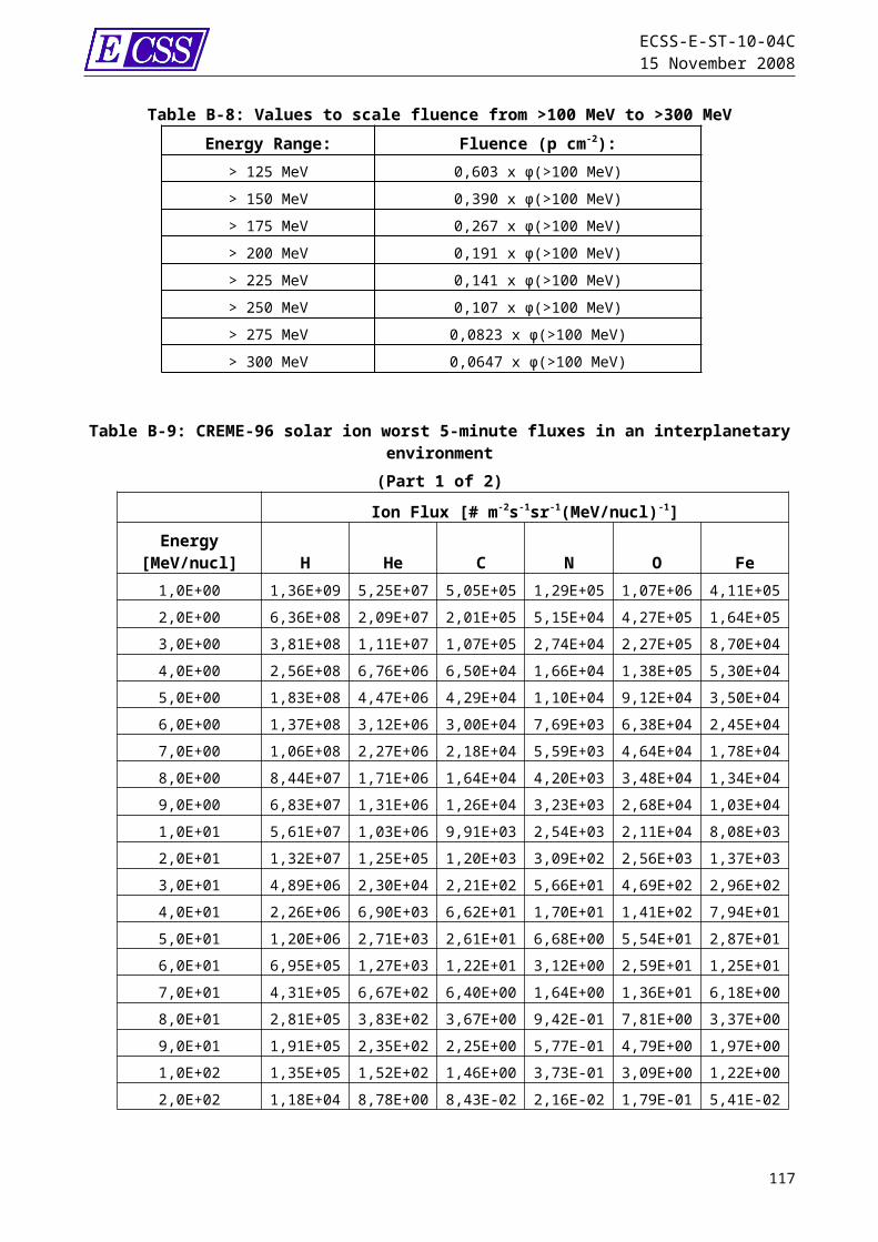
ECSS-E-ST-10-04C15 November 2008
Annex E (informative)Geomagnetic fields
E.1 Overview of the effects of the geomagnetic fieldSpacecraft motion across the geomagnetic field results in a motionally-induced e.m.f. given by in the spacecraft. If a current path can be completed, a current flows through the spacecraft and the surrounding plasma. These phenomena can lead to generation of a few volts potential differences on large spacecraft in LEO. The effect is also used or studied in tethered satellite missions where the length of the tether perpendicular to B can lead to large currents and potentials.Interaction between the magnetic field and an onboard magnetic moment m gives rise to a force:
(E-1)
which can be used for attitude control where an onboard magnetic torquer provides m. Dynamic fluctuations in plasma populations, electric fields and geomagnetic fields are intimatly connected and plasma disturbances can be monitored via observations of the geomagnetic field. These are quantified by the familiar Kp, Ap, Dst and other geomagnetic indices (see clause 6 for more detail on geomagnetic activity indices.
E.2 Models of the internal geomagnetic fieldExamples of recognised, high-degree, models of the internal field are those due to Olsen et al. [RD.138] and Maus et al. [RD.139]. These models currently cover the period (approximately) of 2000 to 2005. Another is the ‘Comprehensive Model’ of Sabaka et al (2004) [RD.140]. This model seeks to represent all field sources under magnetically quiet conditions and models the time variation of sources by cubic splines. The Comprehensive Model is widely used in the scientific community: it has a long history and is regarded as being amongst the most accurate and flexible for scientific purposes. It can be expected that this model, now at revision four (CM4), continues to be occasionally updated, in the light of new scientific advances. However the set of input parameters is relatively complex and it is not applicable under all solar and geomagnetic activity conditions.
Moreover the external field component is not as flexible as the purely internal field models such as the IGRF even though it does include a representation of the dayside Sq ionospheric magnetic field.Models such as the International Geomagnetic Reference Field (IGRF) and World Magnetic Model (WMM) represent the internal fields of the Earth only.
117

ECSS-E-ST-10-04C15 November 2008
See Figure E-1 and Table E-1 for more information on the current revision of the IGRF. These models are updated on a five-year basis, assuming a linear secular variation between updates. The IGRF currently extends to spherical harmonic degree 13 (equivalent to a wavelength of 3 077 km on the ground) and is produced by a collaboration of IAGA scientists. IAGA also define a definitive reference field (DGRF) for a given epoch (most recently DGRF2000), where it is agreed that no new data is likely to be forthcoming to revise and improve the existing IGRF for that epoch or earlier. Prior to 2000, the IGRF is truncated at degree 10, the increased resolution after that date being due to the improved quality of recent global satellite surveys of the main field. The World Magnetic Model (WMM), produced jointly with the US National Geophysical Data Centre (NGDC), is the standard model in UK Ministry of Defence and US Department of Defence navigation and attitude reference systems. It is also used widely in civilian navigation systems. The model is used on marine charts. Like the IGRF the WMM is revised according to fixed procedures every five years. The current model, WMM2005, extends to spherical harmonic degree 13 and is valid till 2010.
E.3 Models of the external geomagnetic fieldSpherical harmonic models of external fields, e.g. CM4, are typically no higher than degree two (i.e. quadrupolar) and capture only the quasi-static elements of the external field. There is usually some dependence on the Dst (or similar) geomagnetic index, which parameterises variations in the symmetric ring current intensity. Neither the IGRF nor WMM have an external field component.For satellite operations closer to the Earth, the spherical harmonic models of Olsen et al [RD.138] or Sabaka et al [RD.140] can be useful. However, these models are inaccurate on the dayside of the Earth (approximately 0700-1700 local solar time), at geomagnetic latitudes above about 55 degrees, or during more active geomagnetic conditions (approximately Kp>3). They are also likely to be degraded in accuracy beyond low-Earth orbit (>800km altitude), where the magnetic survey satellites that measure the base data for these models are flown.Non-spherical harmonic models use a variety of geomagnetic and solar wind data to parameterise the various external current systems. Dynamic models are widely used and combined with internal models such as IGRF. The models of Tsyganenko and of Alexeev and co-workers both use the IGRF as the core field. They therefore both provide a consistent model of the total field measured by any in-situ spacecraft, from approximately 2-70 Earth radii.
Older dynamic models also exist, dating back to the 1960s, and these are occasionally used in the space science and engineering community, e.g. when using radiation belt models of that era. These include models due to Mead and Fairfield (1975) [RD.141], Olsen and Pfitzer (1977) [RD.142], Hilmer (1989) [RD.143] and Voight (1981) [RD.144]. For further information on these older models see the review of Jordan (1994) [RD.145].
118
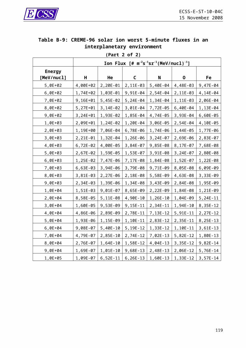
ECSS-E-ST-10-04C15 November 2008
E.4 Magnetopause boundaryThe location and field strength of the magnetopause is integral to most external field models. However, it is sometimes useful to be able to estimate the magnetopause location explicitly. Some simple expressions can be used to estimate basic locations of magnetospheric boundaries for mission planning. The standoff radial distance of the magnetopause in the sunward direction is given approximately by:
(E-2)
where Lmp is in units of Earthradii, nsw, the solar wind proton number density is in units of cm-3
and usw the solar wind bulk velocity is in units of km s-1
.
Typical values for nsw and usw are 8 cm-3 and 450 km s-1 respectively, leading to a standoff distance of about 10 RE. The model of Sibeck et al. [RD.32] represents the complete magnetopause position, not just at the sub-solar point, as the function:
(E-3)
whereR2 = y2 + z2;x, y, and z are GSM coordinates, in Earthradii;A, B and C are fit parameters dependent on the solar wind pressure as given in E.6.1.1.Table E-2.
E.5 Geomagnetic coordinate system – B and L Geomagnetic coordinates are useful or necessary for a number of applications where charged particle morphology or behaviour needs to be described in the magnetosphere. The most important application is in models of the Earth’s radiationbelt environment (see clause 9). These particle models give fluxes of trapped energetic particles as functions of particle energy and of McIlwain’s geomagnetic coordinates L and B/B0
[RD.102].The kinetic energy of a charged particle trapped in a geomagnetic field model is conserved (a constant of motion) provided the B-field is stationary (independent of time), and provided that the acceleration by magnetospheric electric fields can be neglected. This is a satisfactory approximation for particles whose kinetic energy is larger than 500 keV.When the kinetic energy of the particles is smaller than 500 MeV their motion can be described as the superposition of a gyration about the magnetic field lines, a latitudinal oscillation between two conjugate mirror points and an azimuthal drift around the Earth. Three adiabatic invariants (μ, I and Ф) can be associated respectively with these three periodic motions provided certain conditions are satisfied. The approximate conservation of the adiabatic invariants, contributes to the definition of invariant coordinates for mapping directional and omni-directional fluxes of particles trapped in the Earth’s Radiation Belts.
119

ECSS-E-ST-10-04C15 November 2008
Two invariant coordinates, e.g. mirror point magnetic field (Bm) and I (E-4), are required to define a drift shell, i.e. the surface formed by the segments of geomagnetic field lines between conjugate mirror points of particles.
(E-4)
Bm is the magnetic field strength at the mirror points (the low altitude edge of a drift shell); since the magnetic moment μ of trapped particles is the first adiabatic invariant of motion of trapped particles, Bm is also an invariant coordinate characterizing a drift shell;I is the second invariant coordinate required to identify uniquely the drift shell. The integral in (E-4) is evaluated along the field line between both conjugate mirror points l1 and l2 .Since I is not a visually suggestive coordinate, McIwain [RD.101], [RD.102], [RD.118] introduced his L parameter which is approximately (but not exactly) equal to the equatorial distance of the magnetic field line passing across the point of an observational measurement. When Bm is determined by using a geomagnetic field model (e.g. IGRF) the value of L is uniquely determined by the mathematical transformation (E-5):
(E-5)
In this equation I is computed by numerical integration of (E-4) ausing the same magnetic field model (IGRF).Md = 31 165,3 nT RE
3 is the fixed value of the magnetic moment of the reference dipole adopted in 1961 by McIwain to map the measured fluxes of trapped of radiation belt particles [RD.102], [RD.118].
L is the second invariant coordinate used (instead of I) to label drift shells.
The pair of invariant coordinates (Bm, L) uniquely defines a drift shell. It should be emphasized that different points along the same geomagnetic field lines may be characterized by different values L and by different drift shells.The function f (E-5) was calculated by McIlwain [RD.102] and a simple approximation for f was found by Hilton [RD.103].Note that a drift shell can also be characterized by Ф the third invariant of motion (the flux invariant), and an associated L* parameter. In general L and L* are not equal, except for a dipole geomagnetic field. However, the invariance of Ф or L* requires that the geomagnetic field distribution does not change significantly over a time period longer than the azimuthal drift period (> 10 minutes), while the adiabatic invariance of I or L requires that the B-field distribution is independent of time over only several bounce periods (> 1 second).Other pairs of invariant coordinates derived from Bm and L have been proposed and happen to be more appropriate in certain cases: e.g. the invariant latitude (Λ), the invariant radius (R), or the invariant altitude
120
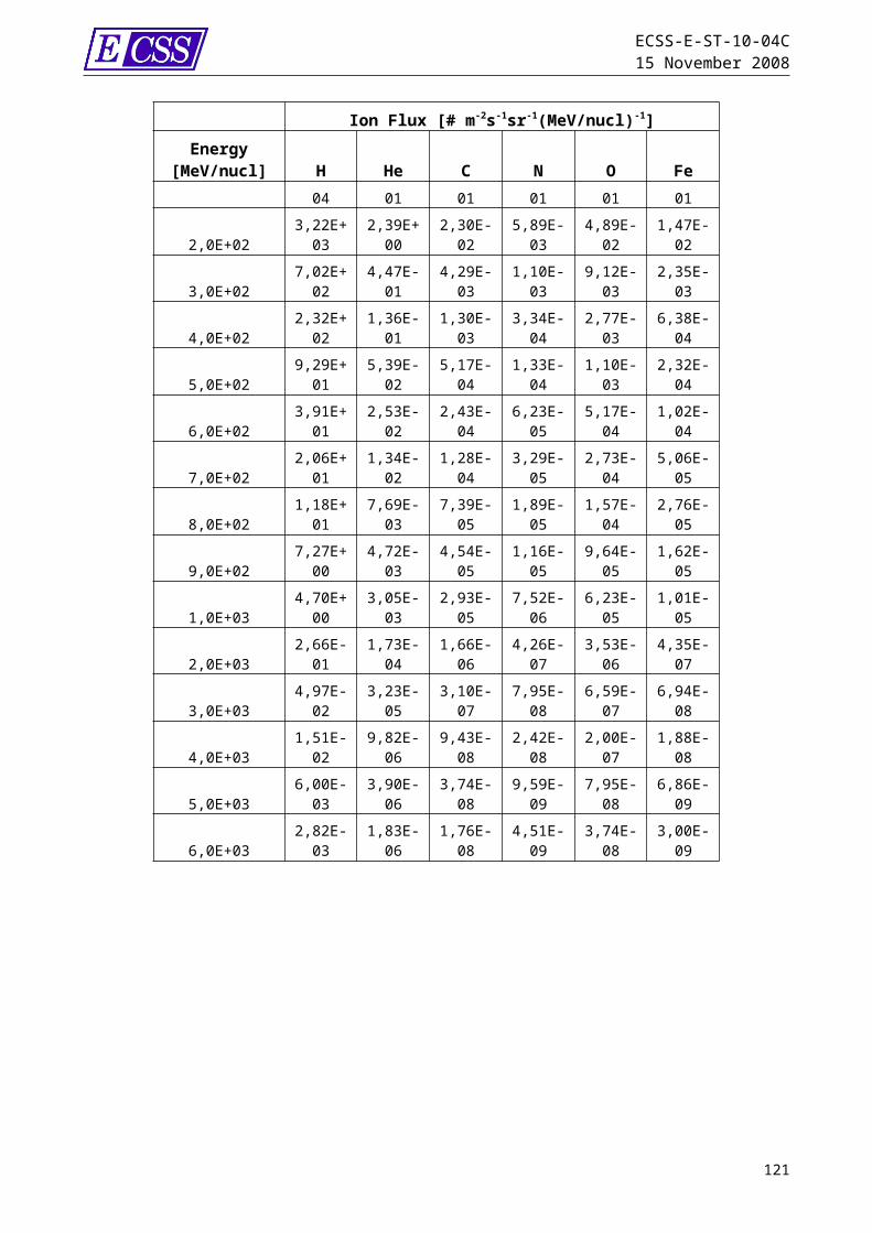
ECSS-E-ST-10-04C15 November 2008
(h_inv) [RD.120] which is quite convenient to bin/map fluxes measurements at low-altitudes in the Radiations Belts .
121

ECSS-E-ST-10-04C15 November 2008
E.6 TablesTable E-1: IGRF-10 data for epoch 1960-2010
(Part 1 of 2)
Epoch
M(nT RE3)
M(1030 nT
cm3)
DIPOLE Tilt (Deg)
Lat Nort
h (Deg
)
Lon Nort
h (Deg
)
Lat Sout
h (Deg
)
Lon Sout
h (Deg
)
ECCENTRIC Centre
(km)
Lat North (Deg)
Lon North (Deg)
Lat South (Deg)
Lon South (Deg)
190032 176,2
6 8,32146 11,3861 78,61291,2
1 -78,61111,2
1 330,5 80,22 277,53 -76,54 121,14
190532 096,4
2 8,30081 11,3928 78,61291,2
5 -78,61111,2
5 337,2 80,25 277,28 -76,48 121,32
1910 31 986,5 8,27238 11,413 78,59291,2
8 -78,59111,2
8 344,43 80,27 277,03 -76,4 121,46
191531 843,7
1 8,23545 11,4316 78,57291,4
3 -78,57111,4
3 351,78 80,33 276,97 -76,3 121,63
1920 31 690 8,1957 11,4438 78,56291,6
2 -78,56111,6
2 359,4 80,4 276,98 -76,2 121,8
192531 553,5
7 8,16042 11,4464 78,55291,7
3 -78,55111,7
3 368,47 80,5 276,86 -76,09 121,87
193031 433,1
8 8,12928 11,4739 78,53291,7
4 -78,53111,7
4 378,01 80,58 276,7 -75,94 121,8
193531 344,9
9 8,10647 11,5067 78,49291,6
4 -78,49111,6
4 386,6 80,67 276,53 -75,8 121,56
194031 285,8
6 8,09118 11,5347 78,47291,4
9 -78,47111,4
9 395,1 80,76 276,34 -75,65 121,25
194531 224,5
1 8,07531 11,5337 78,47291,4
7 -78,47111,4
7 406,83 80,9 276,14 -75,52 121,09
195031 183,7
1 8,06476 11,5339 78,47291,1
5 -78,47111,1
5 418,95 81,04 275,61 -75,38 120,671955 31 129,2 8,05067 11,5396 78,46 290,8 -78,46 110,8 430,3 81,15 275,06 -75,25 120,29
122

ECSS-E-ST-10-04C15 November 2008
Epoch
M(nT RE3)
M(1030 nT
cm3)
DIPOLE Tilt (Deg)
Lat Nort
h (Deg
)
Lon Nort
h (Deg
)
Lat Sout
h (Deg
)
Lon Sout
h (Deg
)
ECCENTRIC Centre
(km)
Lat North (Deg)
Lon North (Deg)
Lat South (Deg)
Lon South (Deg)
2 4 4
196031 043,1
6 8,02841 11,4903 78,51290,5
3 -78,51110,5
3 441,58 81,3 274,43 -75,19 119,98
196530 951,6
4 8,00474 11,4654 78,53290,1
5 -78,53110,1
5 451,57 81,4 273,73 -75,13 119,62
197030 829,1
8 7,97307 11,409 78,59289,8
2 -78,59109,8
2 462,6 81,53 272,94 -75,1 119,4
197530 696,3
8 7,93873 11,3126 78,69289,5
3 -78,69109,5
3 474,38 81,68 272,01 -75,11 119,29
1980 30 573,7 7,907 11,1944 78,81289,2
4 -78,81109,2
4 488,63 81,88 270,95 -75,11 119,17
123

ECSS-E-ST-10-04C15 November 2008
Table E-1: IGRF-10 data for epoch 1960-2010(Part 2 of 2)
Epoch
M(nT RE3)
M(1030 nT
cm3)
DIPOLE Tilt (Deg)
Lat Nort
h (Deg
)
Lon Nort
h (Deg
)
Lat Sout
h (Deg
)
Lon Sout
h (Deg
)
ECCENTRIC Centre
(km)
Lat North (Deg)
Lon North (Deg)
Lat South (Deg)
Lon South (Deg)
198530 434,7
7 7,87107 11,0256 78,97 289,1 -78,97 109,1 502,26 82,15 269,95 -75,15 119,18
199030 318,1
6 7,84091 10,8617 79,14288,8
7 -79,14108,8
7 514,67 82,4 268,92 -75,2 119,04
199530 215,0
8 7,81425 10,6768 79,32288,5
8 -79,32108,5
8 526,93 82,68 267,77 -75,27 118,83
200030 119,6
2 7,78956 10,4567 79,54288,4
3 -79,54108,4
3 540,14 83,03 266,73 -75,34 118,64
200530 036,7
4 7,76813 10,2562 79,74288,2
2 -79,74108,2
2 552,09 83,36 265,75 -75,41 118,32
201029 972,6
3 7,75155 10,0556 79,95288,0
2 -79,95108,0
2 563,43 83,7 264,8 -75,49 117,97NOTE For each date the following are listed (in order): magnetic dipole moment (nT RE
3); magnetic dipole moment (nT cm3); dipole tilt angle (degrees); North dipole pole in latitude and longitude (degrees); South dipole pole in latitude and longitude (degrees); the eccentric dipole centre offset from the Earth’s centre (km); North eccentric dipole pole in latitude and longitude (degrees); South eccentric dipole pole in latitude and longitude (degrees).
Table E-2: Sibeck et al. Magnetopause modelSolar wind pressure
range (nPa) A B C
Subsolar point(RE)
Dawn meridian
(RE)0,54-0,87 0,19 19,3 -272,4 12,6 16,50,87-1,47 0,19 19,7 -243,9 11,7 15,61,47-2,60 0,14 18,2 -217,2 11,0 14,7
124

ECSS-E-ST-10-04C15 November 2008
2,60-4,90 0,15 17,3 -187,4 10,0 13,74,90-9,90 0,18 14,2 -139,2 8,8 11,8Sibeck et al. [RD.32]
125

ECSS-E-ST-10-04C15 November 2008
E.7 Figures
Figure E-1: The IGRF-10 field strength (nT, contour level = 4 000nT, at 2005) and secular variation (nT yr-1, contour level = 20 nT yr-1, valid for 2005), at geodetic altitude 400 km with respect to the WGS-84 reference ellipsoid).
126

ECSS-E-ST-10-04C15 November 2008
The Figure shows a cut in the noon-midnight plane, with the Sun to the left and with distance Re in GSM coordinates.
Figure E-2: The general morphology of model magnetospheric field lines, according to the Tsyganenko 1989 model, showing the seasonal variation,
dependent on rotation axis tilt
127

ECSS-E-ST-10-04C15 November 2008
Annex F (informative)Natural electromagnetic radiation and indices
F.1 Solar spectrumIn 2000, the American Society for Testing and Materials developed an AM0 reference spectrum (ASTM E-490) for use by the aerospace community [RD.33]. That ASTM E490 Air Mass Zero solar spectral irradiance is based on data from satellites, space shuttle missions, high-altitude aircraft, rocket soundings, ground-based solar telescopes, and modelled spectral irradiance. The integrated spectral irradiance has been made to conform to the value of the solar constant accepted by the space community; which is 1 366,1 W m-2. Figure F-1 shows the solar irradiation spectrum at AM0 and AM1.5.
F.2 Solar and geomagnetic indices – additional information
F.2.1 E10.7Although not used in atmosphere models described in clause 7, E10.7 is the integration in the range from 1 to 105 nm of the energy flux of solar irradiance, reported in solar flux units (sfu) or x10-22 Watts per meter squared per Hertz.
F.2.2 F10.7The sun emits radio energy with a slowly varying intensity. This radio flux, which originates from atmospheric layers high in the sun's chromosphere and low in its corona, changes gradually from day-to-day in response to the number of spot groups on the disk. Solar flux density at 10,7 cm wavelength has been recorded routinely by radio telescope near Ottawa since February 14, 1947.Each day, levels are determined at local noon (1700 GMT). Beginning in June 1991, the solar flux density measurement source is Penticton, B.C., Canada. Its observations are available through the DRAO website and all values are also archived at the Space Physics Interactive Data Resource (SPIDR).Three sets of fluxes - the observed, the adjusted, and the absolute - are summarized. Of the three, the observed numbers are the least refined, since they contain fluctuations as large as 7% that arise from the changing sun-earth distance. In contrast, adjusted fluxes have this variation removed; the numbers in these tables equal the energy flux received by a detector located at the mean distance between sun and earth. Finally, the absolute levels carry the error reduction one step further; here each adjusted value is multiplied by 0,90 to compensate for uncertainties in antenna gain and in waves reflected from the ground.
128

ECSS-E-ST-10-04C15 November 2008
F.2.3 S10.7The NASA/ESA Solar and Heliospheric Observatory (SOHO) research satellite operates in a halo orbit at the Lagrange Point 1 (L1) on the Earth-Sun line and has an uninterrupted view of the Sun. One of the instruments on SOHO is the Solar Extreme-ultraviolet Monitor (SEM) that measures the 26–34 nm solar EUV emission with 15-second time resolution in its first order broadband wavelength range. The integrated 26–34 nm emission is normalized. The normalized value is converted to sfu through linear regression with F10.7 (for historical data) over the common time frame and the resulting index is called S10.7.The broadband (wavelength integrated) SEM 26-34 nm irradiances, represented by the S10.7 index, are EUV line emissions dominated by the chromospheric He II line at 30,4 nm with contributions from other chromospheric and coronal lines. This energy principally comes from solar active regions, plage, and network. Once the photons reach the Earth, they are deposited (absorbed) in the terrestrial thermosphere mostly by atomic oxygen above 200 km.
F.2.4 M10.7NOAA 16 and NOAA 17 operational satellites host the Solar Backscatter Ultraviolet (SBUV) spectrometer that has the objective of monitoring ozone in the Earth’s lower atmosphere. In its discrete operating mode, a diffuser screen is placed in front of the instrument’s aperture in order to scatter solar MUV radiation near 280 nm into the instrument. This solar spectral region contains both photospheric continuum and chromospheric line emissions. The chromospheric Mg II h and k lines at 279,56 and 280,27 nm, respectively, and the weakly varying photospheric wings or continuum longward and shortward of the core line emission, are operationally observed by the instrument.On the ground, the Mg II core-to-wing ratio is calculated between the variable lines and nearly non-varying wings. The result is a measure of chromospheric and some photospheric solar active region activity is referred to as the Mg II core-to-wing ratio (cwr), and is provided daily by NOAA Space Environment Center (SEC). The ratio is an especially good proxy for some solar FUV and EUV emissions and it can represent very well the photospheric and lower chromospheric solar FUV Schumann-Runge Continuum emission. The daily Mg II cwr is used in a linear regression with F10.7 to derive the M10.7 index for reporting in F10.7 units and with a 5-day lag.
F.3 Additional information on short-term variationThe profile given in Table 6-4 starts from medium activity levels. Then an x-ray / gamma-ray flare occurs. On the sun-surface this goes together with the ejection of highly energetic charged particles. The flare can push up the F10.7 index near Earth almost instantaneously. The ap is still at its normal value for medium activity between 7 and 15. The F10.7 then fades within about 9 hours to pre-flare values. After a little less than a day the fastest solar wind particles arrive at Earth, disturb the magnetic field, and thus the ap index increases. The disturbance lasts only about 6 hours. Thereafter it settles at its pre-event levels between 7-15 hours. The F10.7 stays at its average value.The profile covers 1 day. It can be recurring as a disturbance event can easily last about a week. During such an event, flares occur repeatedly within the same active region on the sun. Extreme values of F10.7 and ap do not usually
129

ECSS-E-ST-10-04C15 November 2008
occur simultaneously. Such a situation only occurs at the Earth if a second flare, essentially unrelated to the first, occurred on the sun at the same time that the charged particles from the first flare arrived at Earth. That situation is possible but happens rarely and seems not to have occurred within the historical data set.The activity profile given in Table 6-4 describes a “worst case” event but is neither unrealistic nor overly conservative. The x-rays (high F10.7) can lead to enhanced intensities and heating at equatorial and low latitude regions where the solar radiation intensity is highest. The high ap values lead mainly to an increase of atmospheric density in the high latitude and polar regions where the effect of dissipation of energy and momentum from the magnetosphere is largest.The short term variation profile in Table 6-4 addresses ap only. Short term variations of the geomagnetic field have larger effects on the atmosphere than short term variations of the solar activity. The atmospheric effects of solar activity variations on time scales of hours are still uncertain. Large short term variations of ap can occur during all phases of a solar cycle.
F.4 Useful internet references for indices Indices glossary: http://www.sec.noaa.gov/info/glossary.html F10.7 daily values at DRAO website: http://hia-iha.nrc-
cnrc.gc.ca/drao/icarus_e.html F10.7, Kp, Ap, Dst, Solar Wind Speed, IMF archive values at Space
Physics Interactive Data Resource (SPIDR): http://spidr.ngdc.noaa.gov/spidr/index.jsp
S10.7 and M10.7 at JB-2006 website: http://sol.spacenvironment.net/~JB2006/indices.html
F10.7 predictions at Marshall Space Flight Center’s: http://sail.msfc.nasa.gov/
F.5 Earth electromagnetic radiation
F.5.1 Earth albedoThe fraction of incident sunlight that is reflected off a planet is termed albedo. For an orbiting spacecraft the albedo value depends mainly on the sunlit part of the Earth which it can see. Albedo radiation has approximately the same spectral distribution as the Sun and in this Standard albedo refers to the total solar spectrum albedo. Albedo is highly variable across the globe and depends on surface properties and cloud cover. It also depends on the solar zenith angle. Average albedo values have sometimes to be used with care, e.g. for short duration analyses or for Sunsynchronous orbits where albedo is from specific local times.The average albedo of the Earth is 0,3. For an orbiting spacecraft, the albedo can vary between 0,05 (open ocean) and 0,6 (high cloud/icecap).A model has been constructed for estimating the influence of latitude and longitude on albedo variability (seasonal effect) [RD.34]. The albedo, a, is given by:
130
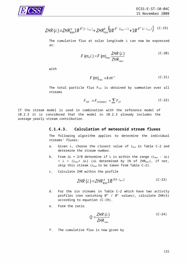
ECSS-E-ST-10-04C15 November 2008
(F-1)
where
t0 is the dateω is the orbital pulsation (=2π/365,25) ϕ is the equatorial latitudeJD is the Julian date of interestPn is the nth degree Legendre polynomial
anda0=0,34a1 [c0=0, c1=0,10, c2=0]a2=0,29
F.5.2 Earth infraredThe Earthemitted thermal radiation has a spectrum of a black body with a characteristic average temperature of 288 K. The Earth infrared radiation also varies across the globe but less than the albedo. It also shows a diurnal variation which is small over the ocean but can amount to 20 % for desert areas.The average infrared radiation emitted by Earth is 230 W m-2. For an orbiting spacecraft, it can vary from 150 W m-2 to 350 W m-2. The diurnal variations can amount to about 20 % over desert areas while being smaller over the oceans. A model has been constructed for estimating the influence of latitude and longitude on Earth infrared variability (seasonal effect) [RD.34], given by:
(F-2)
where
t0 is the dateω is the orbital pulsation (=2π/365,25) ϕ is the equatorial latitudeJD is the Julian date of interestPn is the nth degree Legendre polynomialand the following values are proposed: e0= 0,68e1 [k0=0, k1=-0,07, k2=0]e2= -0,18
131

ECSS-E-ST-10-04C15 November 2008
F.6 Electromagnetic radiation from other planets
F.6.1 Planetary albedo Albedo is the fraction of sunlight, which is reflected off a planet. The reflection is assumed to be diffuse. For the albedo the same spectral shape as for sunlight is assumed. The actual albedo spectrum can change, depending on properties of the surface (different materials can lead to absorption in certain wavelength bands and result in a highly variable spectrum). Albedo values are only applicable when the portion of the planet that is seen by the spacecraft is sunlit.
F.6.2 Planetary infrared A large portion of the incident solar radiation being absorbed as heat by the planet is re-emitted in the infrared range of the spectrum. Reference values for average planetary albedo and infra-red radiation are given in Table F-1.
F.7 Activity indices informationFigure F-2 and Figure F-3 show the F10.7, Sunspot Number R and Ap indices over the last two solar cycles. Figure F-2 gives the daily and Figure F-3 the monthly mean values. The large fluctuations in the daily values are averaged out in the monthly mean values (please note the different scale of the figures). The short term Ap spikes are important for density variations and this is not well reflected in the long term high values.
F.8 TablesTable F-1: Reference values for average planetary albedo and infra-red
radiationPlanet Average
AlbedoAlbedo Range
Average IR [K]
IR Range [K]
Mercury 0,106 0,09 – 0,45 442 100 – 725Venus 0,65 231,7 737 (surface)Mars 0,15 210,1 184 - 242Jupiter 0,52 110,0 112 @ 0,1 barSaturn 0,47 81,1 1 – 143 @ 1 barUranus 0,51 58,2 76 @ 1 bar 53@ 0,1
barNeptune 0,41 46,6 72@1 bar, 44 @ 0,1
barTitan 0,22
132

ECSS-E-ST-10-04C15 November 2008
F.9 Figures
Figure F-1: Solar spectral irradiance (in red, AM0 (Air Mass 0) is the radiation level outside of the Earth's atmosphere (extraterrestrial), in blue, AM1,5 is the radiation level after passing through the atmosphere 1,5 times, which is about the level at solar zenith angle 48,19°s, an average level at the Earth's surface
(terrestrial)).
133
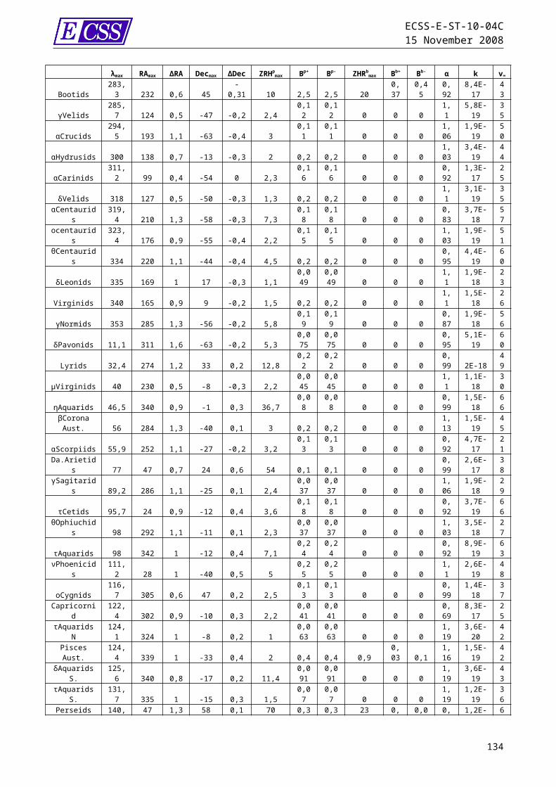
ECSS-E-ST-10-04C15 November 2008
F10.7 cm solar radio flux
0
50
100
150
200
250
300
350
400
Jan-86 Jan-89 Jan-92 Jan-95 Jan-98 Jan-01 Jan-04
Sunspot Number R
0
50
100
150
200
250
300
350
Jan-86 Jan-89 Jan-92 Jan-95 Jan-98 Jan-01 Jan-04
Daily Average Ap
0
50
100
150
200
250
Jan-86 Jan-89 Jan-92 Jan-95 Jan-98 Jan-01 Jan-04
Figure F-2: Daily solar and geomagnetic activity indices over the last two solar cycles
134
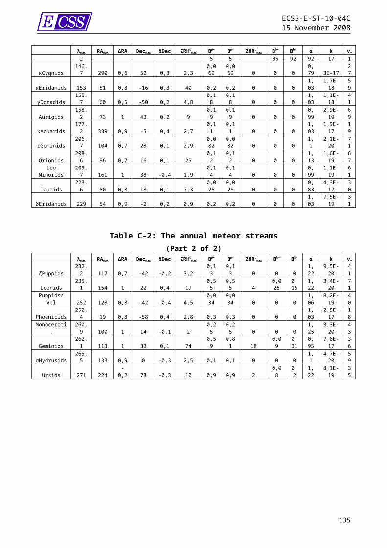
ECSS-E-ST-10-04C15 November 2008
F10.7 cm solar radio flux
0
50
100
150
200
250
Jan-86 Jan-89 Jan-92 Jan-95 Jan-98 Jan-01 Jan-04 Sunspot Number R
0
50
100
150
200
Jan-86 Jan-89 Jan-92 Jan-95 Jan-98 Jan-01 Jan-04 Monthly Average Ap
0
10
20
30
40
50
Jan-86 Jan-89 Jan-92 Jan-95 Jan-98 Jan-01 Jan-04
Figure F-3: Monthly mean solar and geomagnetic activity indices over the last two solar cycles
135
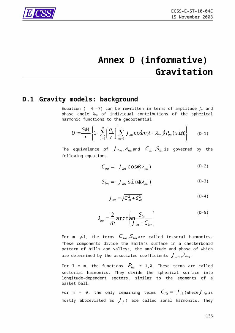
ECSS-E-ST-10-04C15 November 2008
Annex G (informative)Neutral atmospheres
G.1 Structure of the Earth’s atmosphereThe Earth atmosphere can be broadly divided into three distinct regimes, as shown in Figure G-1: the homosphere comprises the regions of the troposphere (surface up
to ~ 10 - 12 km altitude), the stratosphere (~ 10 - 12 km up to 50 km), and the mesosphere (~50 km up to 90 km),
the thermosphere extends from about 90 km altitude to approx 400 km, depending on solar and geomagnetic activity,
the exosphere extends from the top of the thermosphere and extends into space.
The boundaries between these regions are classically defined by relatively sharp and consistent changes in the temperature profile as a function of altitude, with the exception of the base of the exosphere . The exosphere base is defined by that altitude where the mean free path equals the scale height. In practice, all of these boundaries, whether determined in altitude or in a pressure co-ordinate system, vary with solar, seasonal, latitudinal and other conditions.Due to vertical winds and turbulent mixing the homosphere has a nearly uniform composition of about 78,1% N2, 20,9% O2, and 0,9% Ar. The temperature profile of the heterosphere shows alternating gradients with (normally) the maximum temperature at the surface (global average ~288K), a local minimum at the tropopause (global average ~218K), a local maximum at the stratopause (global average ~280K), and another local minimum at the mesopause (150K – 250K).
G.2 Development of models of the Earth’s atmosphereA “Standard Atmosphere” is defined as a vertical distribution of atmospheric temperature, pressure, and density, which by international agreement is taken to be representative of the Earth’s atmosphere. The first “Standard Atmospheres” established by international agreement were developed in the 1920’s primarily for purposes of pressure altimeter calibrations, aircraft performance calculations, aircraft and rocket design, ballistic tables, etc. Later some countries, notably the United States, also developed and published “Standard Atmospheres”. The term “Reference Atmosphere” is used to identify vertical descriptions of the atmosphere for specific geographical locations or globally. These were developed by organizations for specific applications, especially as the aerospace industry began to mature after World War II. The term “Standard Atmosphere” has in recent years also been used by national and international organizations to describe vertical descriptions of atmospheric trace constituents, the ionosphere,
136
ECSS-E-ST-10-04C15 November 2008
atomic oxygen, aerosols, ozone, winds, water vapour, planetary atmospheres, etc. Currently some of the most commonly used Standard and Reference Atmospheres include the ISO Standard Atmosphere, 1975 [RD.126], 1982 [RD.127] the U. S. Standard Atmosphere Supplements, 1962 [RD.123], 1966 [RD.124]] 1976 [RD.125], the COSPAR International Reference Atmosphere (CIRA), 1986 [RD.128] (previously issued as CIRA 1961 [RD.129], CIRA 1965 [RD.130] and CIRA 1972 [RD.131]), the NASA/MSFC Global Reference Atmosphere Model (GRAM), 1999 [RD.136] (previously issued as GRAM-86 [RD.132]], GRAM-88 [RD.133], GRAM-90 [RD.134] and GRAM-95 [RD.135]), the NRLMSISE-00 Thermospheric Model, 2000 [RN.4] (previously issued as MSIS-77 [RD.35], -83 [RD.37], -86 [RD.38]] and MSISE-90 [RD.137]) and most recently the JB-2006 density Model [RN.5].
G.3 NRLMSISE-00 and JB-2006 - additional informationThe Mass Spectrometer and Incoherent Scatter (MSIS) series of models developed between 1977 and 1990 are used extensively by the scientific community for their superior description of neutral composition. The models utilized atmospheric composition data from instrumented satellites and temperatures from ground-based radars. The initial MSIS 1977 model [RD.35] was based on the Jacchia temperature profile framework, but the density at 120 km varied with local time and other geophysical parameters to fit the measurements. Exospheric temperature and density variations were represented by spherical harmonics resulting in requiring fewer parameters for a given level of accuracy. Subsequent versions of the model include the longitude variations [RD.36], a refined geomagnetic storm effect [RD.37], improved high latitude, high solar flux data [RD.38] and a boundary lowered to sea level [RD.39].The NRLMSISE-00 model [RN.4] of atmospheric composition, temperature, and total mass density from ground to exobase includes the following: drag data based on orbit determination, more recent accelerometer data sets, new temperature data derived from Millstone Hill and Arecibo
incoherent scatter radar observations, observations of O2 by the Solar Maximum Mission (SMM), based on
solar ultraviolet occultation.A new species, “anomalous oxygen,” primarily for drag estimation, allows for appreciable O+ and hot atomic oxygen contributions to the total mass density at high altitudes.The new Jacchia-Bowman density (JB-2006) model [RN.5] is based on the Jacchia model heritage. It includes two key novel features. Firstly, there is a new formulation concerning the semi-annual density variation observed in the thermosphere, but not previously included in any of the semi-empirical atmospheric models. Secondly, there is a new formulation of solar indices, relating more realistically to the dependence of heat and energy inputs from the solar radiation to specific altitude regions and heating processes within the upper atmosphere. JB-2006 inserts the improved J70 temperature formulations into the CIRA 1972 model to permit integrating the diffusion equation at every point rather than relying on look-up tables.
137

ECSS-E-ST-10-04C15 November 2008
G.4 The GRAM series of atmosphere models.The GLOBAL Reference Atmosphere Models have been produced on behalf of NASA to describe the terrestrial atmosphere from ground level upward for operational purposes. These models are available via license to qualified users, and provide usability and information quality similar to that of the NRLMSISE-00 Model [RD.40].
G.5 Atmosphere model uncertainties and limitationsFor mean activity conditions, the estimated uncertainty of the NRLMSISE-00 species density is 15%. For short term and local-scale variations, the estimated uncertainty of the NRLMSISE-00 species density is 100%. Within the homosphere (below 90 km), the uncertainty is below 5% [RD.40].
For mean activity conditions, the estimated uncertainty of the JB-2006 total density within the thermosphere is 10-15% (depending on altitude). For extreme conditions (very high solar or geomagnetic activities), this uncertainty can considerably increase due to the lack of corresponding measurement data. The total density can have +/- 100% variation at 400-500 km for some activities and locations.It should be noted that the NRLMSISE-00 model’s accuracy of prediction of atmospheric density and other parameters is limited by the complex behaviour of the atmosphere, and the causes of variability. While certain aspects of atmospheric variability are more or less deterministic, meteorological variations of the homosphere are difficult to predict more than 3 – 5 days in advance, and yet have effects on higher regions of the atmosphere (thermosphere). In the thermosphere, the response to varying solar and geomagnetic activity is complex, particularly in respect of the latter. Upper atmosphere density models can be used for prediction of future orbital lifetime, either to determine the orbital altitude insertions to ensure a given lifetime, or to estimate energy requirements for maintaining a particular orbit, for a particular spacecraft/satellite. The primary influence on accuracy of the model’s density output is the accuracy of the future predictions of solar and geomagnetic activity used as inputs, rather than the accuracy of the specific model in representing the density as a function of solar and geomagnetic activity.
G.6 HWM93 additional informationThe HWM is an empirical model of the horizontal neutral wind in the upper thermosphere. It is based on wind data obtained from the AE-E and DE 2 satellites. A limited set of vector spherical harmonics is used to describe the zonal and meridional wind components. The first edition of the model released in 1987 (HWM87) [RD.42] was intended for winds above 220 km. With the inclusion of wind data from ground-based incoherent scatter radar and Fabry-Perot optical interferometers, HWM90 was extended down to 100 km and using MF/Meteor data HWM93 was extended down to the ground [RN.6]. Solar cycle variations are included (since HWM90), but they are found to be small and not always very clearly delineated be the current data. Variations with magnetic activity (Ap) are included. Mid- and low-latitude data are reproduced quite well by the model. The polar vortices are present, but not in full detail. The model describes the transition from predominately diurnal variations in the upper thermosphere to semidiurnal variations in the lower thermosphere and a transition from summer to winter flow above 140 km to winter to summer flow below. Significant altitude gradients in the wind
138

ECSS-E-ST-10-04C15 November 2008
extend up to 300 km at some local times. The model software provides zonal and meridional winds for specified latitude, longitude, time, and Ap index. A comparison of the HWM values with winds derived from IRI parameters and from ionosonde measurements have shown in general good agreement.
G.7 Planetary atmospheres models
G.7.1 JupiterBecause Jupiter is a large planet that rotates fast, the equatorial tangential velocity of the atmosphere is 12,7 km s-1, and decreases like the cosine of latitude. In the reference frame rotating with the planet the acceleration of gravity is 22,88 N kg-1 at the equator and 25 N kg-1 at the poles.The structure of the upper atmosphere of Jupiter is reasonably well-known between 60 degrees north and south down to a pressure of 1 bar, thanks to the measurements of the Composite Infrared Spectrometer, during the swing-by of the Cassini spacecraft past Jupiter in late 2000 and early 2001 [RD.43]. In addition the equatorial atmosphere has been explored down to a pressure of 21 bars during the entry and descent of the Galileo probe [RD.44].These measurements reveal that the structure of the atmosphere of Jupiter is relatively simple: a troposphere in convective equilibrium with a constant adiabatic lapse rate, topped by a well-defined tropopause at a minimum temperature of about 100 K above which the temperature increases to a temperature of 160 K and remains practically constant in the region of maximum deceleration and heat fluxes during entry. Above that constant temperature region, roughly above 300 km the temperature increases again.The composition of the atmosphere of Jupiter has been measured by the Galileo probe between pressure levels of 0,51 bars and 21,1 bars [RD.44]. This composition is as follows (volume mixing ratio): H2 (86%), He (13,6%), CH4 (0,18%), N2 (0,07%). The above composition is valid for the troposphere and most of the stratosphere. The corresponding molar mass is 2,31x10⁻³ kg mol-1.The atmosphere of Jupiter is subject to a small seasonal cycle and the equatorial stratosphere experiences cyclic temperature variations of about 10 K with a quasi-quadrennial cycle. This cycle seems to be related to wave activity [RD.45], and large-scale gravity waves have been observed by the Galileo Atmosphere Structure Instrument (ASI) during the Galileo entry [RD.46].
G.7.2 VenusA Venus International Reference Atmosphere (VIRA), from 0 to 100 km, has been compiled by COSPAR [RD.47] It consists of a deep atmosphere, extending from 0 to 32 km (altitudes are referenced to a planetary radius of 6 052 km) whose vertical structure is independent of latitude and characterized by a surface pressure of 92,1 bars, surface temperature of 753,3 K and surface density of 64,8 kg m-3 and a lapse rate increasing from 8 to 9 K km-1. Above 32 km, the atmosphere shows some latitude dependence, and is tabulated by bands of latitude.
139
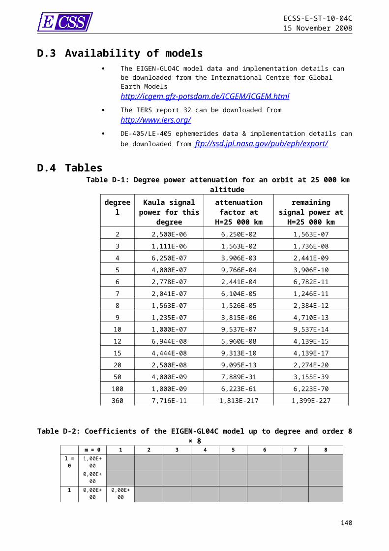
ECSS-E-ST-10-04C15 November 2008
G.7.3 MarsBasic knowledge of the Martian atmospheric environment can be found in [RD.48]].For Mars two reference models exist: the MarsGRAM-2005 [RD.49], [RD.50] developed by NASA MSFC and the Martian Climate Database (EMCD) developed jointly by Laboratoire de Météorologie Dynamique (France), Oxford University (UK) and the Institute of Astrophysics of Andalusia (Spain) [RN.7]These models, which cover the altitude range 0–250 km, have been derived with the help of a combination of geophysical measurements and simulations using general circulation models of the Martian atmosphere.[RD.41], [RD.51].The models agree broadly with each other but differ in many details. Ultimately the use of one or the other model for mission design gives equivalent results if appropriate margins have been taken into account.
G.7.4 SaturnThere is currently no adopted Reference Atmosphere Model for Saturn. Saturn's atmosphere is about 96 percent hydrogen and 3 percent helium by volume, a proportion similar to that found in the sun and Jupiter. Small amounts of methane, ammonia, and water also are present. A layer of clouds composed of ammonia ice compose what is seen in photographs and through the telescope. Deeper in the atmosphere, the clouds can be formed of water ice.
G.7.5 TitanAn engineering-level atmospheric model for Titan (Titan-GRAM) has been developed [RD.52] for use in NASA’s systems analysis studies of aerocapture applications in missions to outer planets.
G.7.6 NeptuneAn engineering-level atmospheric models for Neptune (Neptune-GRAM) has been developed [RD.52] for use in NASA’s systems analysis studies of aerocapture applications in missions to outer planets.
G.7.7 MercuryThere is currently no adopted Reference Atmosphere Model for Mercury. The atmosphere is more accurately described as an exosphere, where individual atoms and molecules reside mainly on the surface, until released into ballistic orbits by a combination of excitation by solar photons and energetic particles (again, primarily of solar origin). The composition is not precisely known, but O, H, He, Na, Ca and K have been detected . The temperature reflects the Mercury surface temperature, the surface pressure is of order 10-12 bar, with a number density of order 1011 m-3
140

ECSS-E-ST-10-04C15 November 2008
G.8 Reference dataNRLMSISE00 altitude profiles at equatorial latitude of temperature, and number densities (concentrations) are listed in Table G-1, Table G-2, and Table G-3 for low solar and geomagnetic activities (F10.7 = F10.7avg = 65, Ap
= 0), moderate solar and geomagnetic activities (F10.7 = F10.7avg = 140, Ap
= 15), and high long term solar and geomagnetic activities (F10.7 = F10.7avg
= 250, Ap = 45), respectively. The tables cover both homospheric and heterospheric altitudes from ground level up to 900 km, averaged over diurnal and seasonal variations. Figure G-1, illustrates the altitude profile of the temperature. Figure G-3 shows the atomic oxygen number densities at low, moderate and high long term activity conditions. For moderate activity levels, Figure G-4 shows the logarithmic number concentration profiles of the main atmospheric constituents.A JB-2006 altitude profile of total density at equatorial latitude is listed in Table G-4 and plotted again in Figure G-2 for low solar and geomagnetic activities
(F10.7 = F10.7avg = 65, S10.7 = S10.7avg = 60, M10.7 = M10.7avg = 60, Ap = 0)
moderate solar and geomagnetic activities(F10.7 = F10.7avg = 140, S10.7 = S10.7avg = 125, M10.7 = M10.7avg = 125, Ap = 15)
high long term (27 days or longer) solar and geomagnetic activities
(F10.7 = F10.7avg = 250, S10.7 = S10.7avg = 220, M10.7 = M10.7avg = 220, Ap = 45)
and high short term (daily) solar and geomagnetic activities (F10.7 = 300, F10.7avg = 250, S10.7 = 235, S10.7avg = 220, M10.7 = 240, M10.7avg = 220, Ap = 240)
The subscript ‘avg’denotes the 81-day average.These values have been averaged over diurnal and seasonal variations.
141

ECSS-E-ST-10-04C15 November 2008
G.9 TablesTable G-1: Altitude profiles of the atmosphere constituents N2, O, O2, He, Ar, H, N and
anomalous O for low solar and geomagnetic activities (NRLMSISE-00 model - F10.7 = F10.7avg = 65, Ap = 0)
H (km)
nHE (m-
3)nO (m-
3)nN2 (m-
3)nO2 (m-
3)nAR (m-
3)nH (m-
3)nN (m-
3)nAnomal O(m-3) T(K)
ρ(kg.m-
3)
01,17E+
200,00E+
001,74E+
254,67E+
242,08E+2
30,00E+
000,00E+
000,00E+
003,00E+
021,07E+
00
209,46E+
180,00E+
001,41E+
243,78E+
231,69E+2
20,00E+
000,00E+
000,00E+
002,06E+
028,68E-
02
404,05E+
170,00E+
006,04E+
221,62E+
227,23E+2
00,00E+
000,00E+
000,00E+
002,57E+
023,72E-
03
603,29E+
160,00E+
004,90E+
211,31E+
215,86E+1
90,00E+
000,00E+
000,00E+
002,45E+
023,01E-
04
801,89E+
153,01E+
152,73E+
207,27E+
193,25E+1
82,65E+
136,64E+
102,28E-
512,06E+
021,68E-
05
1001,17E+
144,78E+
171,02E+
192,38E+
181,04E+1
72,70E+
133,10E+
112,24E-
371,71E+
026,18E-
07
1202,50E+
137,23E+
163,11E+
174,36E+
161,36E+1
56,07E+
121,19E+
121,41E-
273,53E+
021,88E-
08
1401,50E+
132,12E+
164,89E+
164,45E+
151,09E+1
42,17E+
126,16E+
122,44E-
195,21E+
023,08E-
09
1601,16E+
139,37E+
151,38E+
161,06E+
151,88E+1
31,09E+
121,61E+
131,12E-
126,05E+
029,49E-
10
1809,61E+
124,88E+
154,76E+
153,34E+
144,23E+1
27,31E+
112,20E+
131,45E-
076,48E+
023,70E-
10
2008,21E+
122,73E+
151,80E+
151,15E+
141,08E+1
25,94E+
112,02E+
131,20E-
036,70E+
021,63E-
10
2207,12E+
121,59E+
157,14E+
144,11E+
132,98E+1
15,32E+
111,51E+
131,22E+
006,82E+
027,80E-
11
2406,21E+
129,42E+
142,93E+
141,51E+
138,62E+1
04,98E+
111,04E+
132,43E+
026,88E+
023,97E-
11
2605,45E+
125,66E+
141,23E+
145,66E+
122,59E+1
04,75E+
116,85E+
121,40E+
046,92E+
022,13E-
11
2804,78E+
123,44E+
145,27E+
132,16E+
128,02E+0
94,57E+
114,50E+
123,08E+
056,94E+
021,18E-
11
3004,21E+
122,10E+
142,30E+
138,42E+
112,54E+0
94,41E+
112,96E+
123,26E+
066,95E+
026,80E-
12
3203,71E+
121,30E+
141,01E+
133,33E+
118,22E+0
84,27E+
111,96E+
121,96E+
076,96E+
024,01E-
12
3403,28E+
128,05E+
134,54E+
121,33E+
112,71E+0
84,13E+
111,30E+
127,64E+
076,96E+
022,41E-
12
3602,90E+
125,02E+
132,06E+
125,42E+
109,06E+0
74,00E+
118,74E+
112,13E+
086,96E+
021,47E-
12
3802,56E+
123,15E+
139,43E+
112,23E+
103,07E+0
73,87E+
115,88E+
114,60E+
086,96E+
029,14E-
13
4002,27E+
121,99E+
134,37E+
119,29E+
091,06E+0
73,75E+
113,98E+
118,15E+
086,96E+
025,75E-
13
4202,01E+
121,26E+
132,04E+
113,91E+
093,66E+0
63,64E+
112,70E+
111,24E+
096,96E+
023,66E-
13
4401,78E+
128,06E+
129,61E+
101,66E+
091,29E+0
63,53E+
111,85E+
111,69E+
096,96E+
022,35E-
13
4601,58E+
125,17E+
124,56E+
107,13E+
084,55E+0
53,42E+
111,26E+
112,09E+
096,96E+
021,53E-
13
4801,41E+
123,33E+
122,18E+
103,09E+
081,63E+0
53,32E+
118,68E+
102,42E+
096,96E+
021,01E-
13
5001,25E+
122,15E+
121,05E+
101,35E+
085,87E+0
43,22E+
115,99E+
102,66E+
096,96E+
026,79E-
14
5201,11E+
121,40E+
125,11E+
095,92E+
072,13E+0
43,12E+
114,15E+
102,81E+
096,96E+
024,63E-
14
5409,91E+
119,14E+
112,50E+
092,62E+
077,81E+0
33,03E+
112,88E+
102,88E+
096,96E+
023,21E-
14
142

ECSS-E-ST-10-04C15 November 2008
H (km)
nHE (m-
3)nO (m-
3)nN2 (m-
3)nO2 (m-
3)nAR (m-
3)nH (m-
3)nN (m-
3)nAnomal O(m-3) T(K)
ρ(kg.m-
3)
5608,83E+
115,99E+
111,23E+
091,17E+
072,88E+0
32,94E+
112,00E+
102,88E+
096,96E+
022,28E-
14
5807,88E+
113,94E+
116,07E+
085,24E+
061,07E+0
32,85E+
111,40E+
102,83E+
096,96E+
021,65E-
14
6007,04E+
112,60E+
113,02E+
082,36E+
064,01E+0
22,77E+
119,79E+
092,74E+
096,96E+
021,23E-
14
6206,29E+
111,73E+
111,51E+
081,07E+
061,51E+0
22,69E+
116,88E+
092,63E+
096,96E+
029,37E-
15
6405,63E+
111,15E+
117,59E+
074,90E+
055,74E+0
12,61E+
114,84E+
092,50E+
096,96E+
027,33E-
15
6605,04E+
117,67E+
103,84E+
072,25E+
052,19E+0
12,54E+
113,42E+
092,37E+
096,96E+
025,88E-
15
6804,51E+
115,14E+
101,95E+
071,04E+
058,42E+0
02,46E+
112,42E+
092,23E+
096,96E+
024,83E-
15
7004,04E+
113,45E+
109,94E+
064,84E+
043,26E+0
02,39E+
111,72E+
092,09E+
096,96E+
024,04E-
15
7203,63E+
112,33E+
105,10E+
062,26E+
041,27E+0
02,33E+
111,22E+
091,96E+
096,96E+
023,44E-
15
7403,26E+
111,58E+
102,63E+
061,06E+
044,97E-
012,26E+
118,70E+
081,83E+
096,96E+
022,98E-
15
7602,93E+
111,07E+
101,36E+
065,00E+
031,96E-
012,20E+
116,21E+
081,70E+
096,96E+
022,61E-
15
7802,63E+
117,28E+
097,06E+
052,37E+
037,75E-
022,14E+
114,45E+
081,59E+
096,96E+
022,31E-
15
8002,37E+
114,97E+
093,68E+
051,13E+
033,09E-
022,08E+
113,20E+
081,48E+
096,96E+
022,06E-
15
8202,13E+
113,40E+
091,93E+
055,41E+
021,24E-
022,02E+
112,30E+
081,38E+
096,96E+
021,85E-
15
8401,92E+
112,33E+
091,02E+
052,60E+
024,99E-
031,97E+
111,66E+
081,28E+
096,96E+
021,67E-
15
8601,73E+
111,61E+
095,36E+
041,26E+
022,02E-
031,91E+
111,20E+
081,19E+
096,96E+
021,51E-
15
8801,57E+
111,11E+
092,85E+
046,09E+
018,25E-
041,86E+
118,68E+
071,11E+
096,96E+
021,38E-
15
9001,41E+
117,67E+
081,52E+
042,97E+
013,38E-
041,81E+
116,30E+
071,03E+
096,96E+
021,26E-
15
Table G-2: Altitude profiles of the atmosphere constituents N2, O, O2, He, Ar, H, N and anomalous O for mean solar and geomagnetic activities (NRLMSISE-00 model -
F10.7 = F10.7avg = 140, Ap = 15)H
(km)nHE (m-
3)nO (m-
3)nN2 (m-
3)nO2 (m-
3)nAR (m-
3) nH (m-3)nN (m-
3)nAnomal O(m-3) T(K)
ρ (kg.m-3)
01,26E+
200,00E+
001,88E+
255,04E+
242,25E+2
30,00E+
000,00E+
000,00E+
003,00E+0
21,16E+0
0
201,02E+
190,00E+
001,52E+
244,09E+
231,82E+2
20,00E+
000,00E+
000,00E+
002,06E+0
2 9,37E-02
404,38E+
170,00E+
006,53E+
221,75E+
227,81E+2
00,00E+
000,00E+
000,00E+
002,57E+0
2 4,02E-03
603,55E+
160,00E+
005,29E+
211,42E+
216,33E+1
90,00E+
000,00E+
000,00E+
002,45E+0
2 3,26E-04
802,07E+
153,71E+
153,00E+
207,66E+
193,56E+1
82,53E+
138,61E+
108,53E-
511,98E+0
2 1,83E-05
1001,16E+
145,22E+
179,60E+
182,00E+
189,71E+1
61,89E+
133,76E+
117,28E-
371,88E+0
2 5,73E-07
1203,08E+
139,27E+
163,36E+
173,95E+
161,49E+1
53,47E+
121,77E+
125,52E-
273,65E+0
2 2,03E-08
1401,83E+
132,73E+
165,38E+
163,84E+
151,26E+1
48,82E+
119,45E+
128,98E-
196,10E+0
2 3,44E-09
1601,39E+
131,31E+
161,72E+
169,29E+
142,64E+1
33,46E+
112,73E+
134,12E-
127,59E+0
2 1,20E-09
143

ECSS-E-ST-10-04C15 November 2008
H (km)
nHE (m-
3)nO (m-
3)nN2 (m-
3)nO2 (m-
3)nAR (m-
3) nH (m-3)nN (m-
3)nAnomal O(m-3) T(K)
ρ (kg.m-3)
1801,16E+
137,47E+
157,08E+
153,22E+
147,67E+1
22,01E+
114,18E+
135,33E-
078,53E+0
2 5,46E-10
2001,00E+
134,67E+
153,27E+
151,31E+
142,61E+1
21,53E+
114,31E+
134,43E-
039,11E+0
2 2,84E-10
2208,91E+
123,06E+
151,62E+
155,81E+
139,73E+1
11,33E+
113,64E+
134,48E+
009,49E+0
2 1,61E-10
2408,00E+
122,07E+
158,36E+
142,71E+
133,84E+1
11,23E+
112,82E+
138,94E+
029,73E+0
2 9,60E-11
2607,24E+
121,43E+
154,44E+
141,31E+
131,58E+1
11,17E+
112,10E+
135,14E+
049,88E+0
2 5,97E-11
2806,59E+
129,94E+
142,40E+
146,48E+
126,69E+1
01,13E+
111,56E+
131,14E+
069,98E+0
2 3,83E-11
3006,01E+
127,00E+
141,32E+
143,27E+
122,90E+1
01,10E+
111,15E+
131,20E+
071,00E+0
3 2,52E-11
3205,50E+
124,96E+
147,35E+
131,67E+
121,28E+1
01,07E+
118,60E+
127,22E+
071,01E+0
3 1,69E-11
3405,04E+
123,54E+
144,13E+
138,66E+
115,75E+0
91,05E+
116,45E+
122,81E+
081,01E+0
3 1,16E-11
3604,62E+
122,54E+
142,35E+
134,54E+
112,61E+0
91,02E+
114,86E+
127,85E+
081,01E+0
3 7,99E-12
3804,24E+
121,83E+
141,34E+
132,40E+
111,20E+0
91,00E+
113,68E+
121,69E+
091,01E+0
3 5,60E-12
4003,90E+
121,32E+
147,74E+
121,28E+
115,61E+0
89,79E+
102,79E+
123,00E+
091,02E+0
3 3,96E-12
4203,59E+
129,56E+
134,50E+
126,90E+
102,64E+0
89,59E+
102,13E+
124,57E+
091,02E+0
3 2,83E-12
4403,30E+
126,96E+
132,63E+
123,74E+
101,25E+0
89,38E+
101,63E+
126,21E+
091,02E+0
3 2,03E-12
4603,04E+
125,08E+
131,55E+
122,05E+
106,00E+0
79,19E+
101,25E+
127,70E+
091,02E+0
3 1,47E-12
4802,80E+
123,72E+
139,15E+
111,13E+
102,90E+0
79,00E+
109,59E+
118,92E+
091,02E+0
3 1,07E-12
5002,58E+
122,73E+
135,44E+
116,24E+
091,41E+0
78,81E+
107,39E+
119,81E+
091,02E+0
3 7,85E-13
5202,38E+
122,01E+
133,26E+
113,48E+
096,90E+0
68,64E+
105,71E+
111,04E+
101,02E+0
3 5,78E-13
5402,20E+
121,48E+
131,96E+
111,95E+
093,40E+0
68,46E+
104,42E+
111,06E+
101,02E+0
3 4,29E-13
5602,03E+
121,10E+
131,18E+
111,10E+
091,69E+0
68,29E+
103,43E+
111,06E+
101,02E+0
3 3,19E-13
5801,88E+
128,17E+
127,19E+
106,24E+
088,42E+0
58,12E+
102,67E+
111,04E+
101,02E+0
3 2,39E-13
6001,74E+
126,08E+
124,38E+
103,55E+
084,23E+0
57,96E+
102,08E+
111,01E+
101,02E+0
3 1,80E-13
6201,61E+
124,54E+
122,68E+
102,04E+
082,13E+0
57,81E+
101,62E+
119,69E+
091,02E+0
3 1,36E-13
6401,49E+
123,40E+
121,65E+
101,17E+
081,08E+0
57,65E+
101,27E+
119,22E+
091,02E+0
3 1,04E-13
6601,38E+
122,55E+
121,02E+
106,78E+
075,52E+0
47,50E+
109,91E+
108,72E+
091,02E+0
3 7,98E-14
6801,28E+
121,92E+
126,33E+
093,94E+
072,83E+0
47,36E+
107,78E+
108,20E+
091,02E+0
3 6,16E-14
7001,18E+
121,45E+
123,94E+
092,30E+
071,46E+0
47,22E+
106,11E+
107,70E+
091,02E+0
3 4,80E-14
7201,10E+
121,09E+
122,46E+
091,34E+
077,54E+0
37,08E+
104,81E+
107,20E+
091,02E+0
3 3,76E-14
7401,02E+
128,27E+
111,54E+
097,91E+
063,92E+0
36,94E+
103,80E+
106,73E+
091,02E+0
3 2,98E-14
7609,45E+
116,28E+
119,72E+
084,67E+
062,05E+0
36,81E+
103,00E+
106,28E+
091,02E+0
3 2,38E-14
7808,78E+
114,78E+
116,14E+
082,77E+
061,07E+0
36,68E+
102,37E+
105,85E+
091,02E+0
3 1,92E-14
144

ECSS-E-ST-10-04C15 November 2008
H (km)
nHE (m-
3)nO (m-
3)nN2 (m-
3)nO2 (m-
3)nAR (m-
3) nH (m-3)nN (m-
3)nAnomal O(m-3) T(K)
ρ (kg.m-3)
8008,16E+
113,64E+
113,89E+
081,65E+
065,65E+0
26,56E+
101,88E+
105,45E+
091,02E+0
3 1,57E-14
8207,58E+
112,78E+
112,47E+
089,83E+
052,99E+0
26,44E+
101,49E+
105,07E+
091,02E+0
3 1,29E-14
8407,05E+
112,13E+
111,58E+
085,89E+
051,59E+0
26,32E+
101,19E+
104,72E+
091,02E+0
3 1,07E-14
8606,56E+
111,63E+
111,01E+
083,54E+
058,47E+0
16,20E+
109,45E+
094,40E+
091,02E+0
3 9,03E-15
8806,11E+
111,26E+
116,47E+
072,14E+
054,53E+0
16,09E+
107,54E+
094,09E+
091,02E+0
3 7,67E-15
9005,69E+
119,68E+
104,16E+
071,29E+
052,44E+0
15,98E+
106,02E+
093,81E+
091,02E+0
3 6,59E-15
145
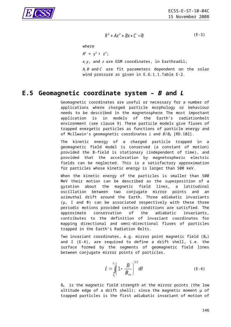
ECSS-E-ST-10-04C15 November 2008
Table G-3: Altitude profiles of the atmosphere constituents N2, O, O2, He, Ar, H, N and anomalous O for high long term solar and geomagnetic activities (NRLMSISE-00
model - F10.7 = F10.7avg = 250, Ap = 45)H (km)
nHE (m-
3)nO (m-
3)nN2 (m-
3)nO2 (m-
3) nAR (m-3) nH (m-3)nN (m-
3)nAnomal O(m-3) T(K)
ρ (kg.m-
3)
01,41E+
200,00E+
002,10E+
255,65E+
242,52E+2
30,00E+0
00,00E+
000,00E+
003,00E+
021,29E+
00
201,14E+
190,00E+
001,71E+
244,57E+
232,04E+2
20,00E+0
00,00E+
000,00E+
002,06E+
021,05E-
01
404,90E+
170,00E+
007,31E+
221,96E+
228,74E+2
00,00E+0
00,00E+
000,00E+
002,57E+
024,49E-
03
603,98E+
160,00E+
005,92E+
211,59E+
217,09E+1
90,00E+0
00,00E+
000,00E+
002,45E+
023,64E-
4
802,34E+
154,36E+
153,39E+
208,15E+
194,02E+1
82,51E+1
31,23E+
112,04E-
501,93E+
022,03E-
05
1001,21E+
145,70E+
179,71E+
181,72E+
189,73E+1
61,43E+1
35,38E+
111,57E-
362,02E+
025,64E-
07
1203,61E+
131,15E+
173,72E+
173,37E+
161,62E+1
52,13E+1
23,08E+
121,36E-
263,80E+
022,22E-
08
1402,09E+
133,51E+
166,07E+
163,02E+
151,43E+1
43,93E+1
11,76E+
132,12E-
187,10E+
023,93E-
09
1601,59E+
131,86E+
162,17E+
166,80E+
143,51E+1
31,24E+1
15,84E+
139,74E-
129,16E+
021,54E-
09
1801,34E+
131,15E+
161,00E+
162,29E+
141,21E+1
36,34E+1
01,02E+
141,26E-
061,05E+
037,87E-
10
2001,17E+
137,72E+
155,24E+
159,68E+
134,91E+1
24,52E+1
01,18E+
141,05E-
021,14E+
034,57E-
10
2201,05E+
135,42E+
152,93E+
154,65E+
132,18E+1
23,83E+1
01,09E+
141,06E+
011,19E+
032,86E-
10
2409,62E+
123,93E+
151,71E+
152,42E+
131,03E+1
23,51E+1
09,18E+
132,11E+
031,23E+
031,87E-
10
2608,85E+
122,90E+
151,03E+
151,32E+
135,02E+1
13,34E+1
07,39E+
131,22E+
051,25E+
031,27E-
10
2808,19E+
122,17E+
156,30E+
147,43E+
122,52E+1
13,23E+1
05,87E+
132,68E+
061,27E+
038,87E-
11
3007,60E+
121,64E+
153,91E+
144,28E+
121,30E+1
13,15E+1
04,65E+
132,84E+
071,28E+
036,31E-
11
3207,07E+
121,25E+
152,46E+
142,51E+
126,77E+1
03,08E+1
03,70E+
131,71E+
081,29E+
034,56E-
11
3406,59E+
129,53E+
141,56E+
141,49E+
123,59E+1
03,02E+1
02,95E+
136,65E+
081,30E+
033,34E-
11
3606,16E+
127,32E+
141,00E+
148,94E+
111,93E+1
02,97E+1
02,36E+
131,85E+
091,30E+
032,47E-
11
3805,75E+
125,65E+
146,44E+
135,41E+
111,05E+1
02,91E+1
01,90E+
134,00E+
091,30E+
031,85E-
11
4005,38E+
124,37E+
144,18E+
133,30E+
115,75E+0
92,86E+1
01,54E+
137,10E+
091,30E+
031,40E-
11
4205,04E+
123,39E+
142,73E+
132,03E+
113,18E+0
92,82E+1
01,24E+
131,08E+
101,30E+
031,06E-
11
4404,72E+
122,64E+
141,79E+
131,26E+
111,78E+0
92,77E+1
01,01E+
131,47E+
101,31E+
038,13E-
12
4604,42E+
122,06E+
141,18E+
137,84E+
101,00E+0
92,72E+1
08,21E+
121,82E+
101,31E+
036,26E-
12
4804,14E+
121,62E+
147,85E+
124,91E+
105,66E+0
82,68E+1
06,69E+
122,11E+
101,31E+
034,84E-
12
5003,89E+
121,27E+
145,23E+
123,10E+
103,23E+0
82,64E+1
05,47E+
122,32E+
101,31E+
033,76E-
12
5203,65E+
129,97E+
133,50E+
121,96E+
101,85E+0
82,60E+1
04,48E+
122,45E+
101,31E+
032,94E-
12
5403,43E+
127,86E+
132,36E+
121,25E+
101,07E+0
82,55E+1
03,67E+
122,51E+
101,31E+
032,31E-
12
146
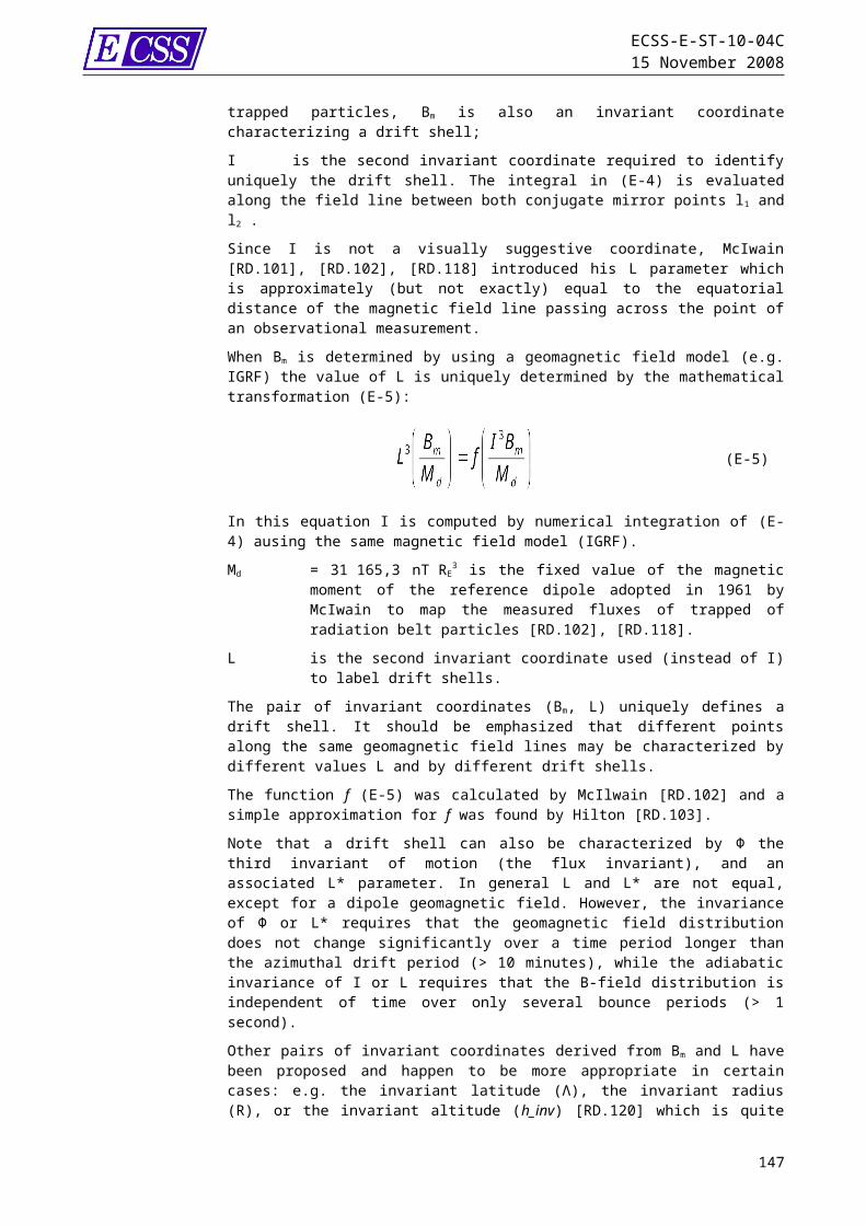
ECSS-E-ST-10-04C15 November 2008
H (km)
nHE (m-
3)nO (m-
3)nN2 (m-
3)nO2 (m-
3) nAR (m-3) nH (m-3)nN (m-
3)nAnomal O(m-3) T(K)
ρ (kg.m-
3)
5603,22E+
126,21E+
131,59E+
128,01E+
096,21E+0
72,51E+1
03,02E+
122,51E+
101,31E+
031,82E-
12
5803,02E+
124,92E+
131,08E+
125,15E+
093,62E+0
72,48E+1
02,48E+
122,47E+
101,31E+
031,43E-
12
6002,84E+
123,91E+
137,34E+
113,33E+
092,13E+0
72,44E+1
02,04E+
122,39E+
101,31E+
031,14E-
12
6202,67E+
123,11E+
135,02E+
112,16E+
091,25E+0
72,40E+1
01,69E+
122,29E+
101,31E+
039,06E-
13
6402,52E+
122,48E+
133,44E+
111,41E+
097,41E+0
62,36E+1
01,39E+
122,18E+
101,31E+
037,23E-
13
6602,37E+
121,98E+
132,37E+
119,19E+
084,41E+0
62,33E+1
01,15E+
122,06E+
101,31E+
035,79E-
13
6802,23E+
121,58E+
131,63E+
116,03E+
082,63E+0
62,29E+1
09,57E+
111,94E+
101,31E+
034,65E-
13
7002,10E+
121,27E+
131,13E+
113,97E+
081,58E+0
62,26E+1
07,94E+
111,82E+
101,31E+
033,75E-
13
7201,98E+
121,02E+
137,86E+
102,63E+
089,50E+0
52,22E+1
06,60E+
111,70E+
101,31E+
033,03E-
13
7401,87E+
128,21E+
125,48E+
101,74E+
085,74E+0
52,19E+1
05,50E+
111,59E+
101,31E+
032,46E-
13
7601,76E+
126,62E+
123,83E+
101,16E+
083,48E+0
52,16E+1
04,58E+
111,48E+
101,31E+
032,00E-
13
7801,66E+
125,35E+
122,68E+
107,74E+
072,12E+0
52,13E+1
03,82E+
111,38E+
101,31E+
031,63E-
13
8001,57E+
124,33E+
121,88E+
105,19E+
071,29E+0
52,10E+1
03,20E+
111,29E+
101,31E+
031,34E-
13
8201,48E+
123,51E+
121,33E+
103,48E+
077,93E+0
42,07E+1
02,67E+
111,20E+
101,31E+
031,10E-
13
8401,40E+
122,85E+
129,39E+
092,35E+
074,87E+0
42,04E+1
02,24E+
111,12E+
101,31E+
039,06E-
14
8601,32E+
122,32E+
126,65E+
091,59E+
073,01E+0
42,01E+1
01,88E+
111,04E+
101,31E+
037,50E-
14
8801,25E+
121,89E+
124,72E+
091,07E+
071,86E+0
41,98E+1
01,58E+
119,67E+
091,31E+
036,23E-
14
9001,18E+
121,54E+
123,36E+
097,30E+
061,16E+0
41,95E+1
01,33E+
119,01E+
091,31E+
036,00E-
14
Table G-4: Altitude profiles of total density kg m-3for low, moderate, high long and high short term solar and geomagnetic
activities (JB-2006 model)(Part 1 of 2)
H (km)Low
activityModerate activity
High activity(long term)
High activity(short term)
100 5,31E-07 5,47E-07 5,44E-07 5,43E-07120 2,18E-08 2,40E-08 2,45E-08 2,46E-08140 3,12E-09 3,98E-09 4,32E-09 4,45E-09160 9,17E-10 1,36E-09 1,54E-09 1,60E-09180 3,45E-10 6,15E-10 7,40E-10 7,77E-10200 1,47E-10 3,17E-10 4,10E-10 4,38E-10220 6,96E-11 1,77E-10 2,46E-10 2,70E-10240 3,54E-11 1,05E-10 1,56E-10 1,77E-10260 1,88E-11 6,47E-11 1,04E-10 1,21E-10
147
ECSS-E-ST-10-04C15 November 2008
H (km)Low
activityModerate activity
High activity(long term)
High activity(short term)
280 1,03E-11 4,12E-11 7,12E-11 8,57E-11300 5,86E-12 2,69E-11 5,00E-11 6,22E-11320 3,40E-12 1,80E-11 3,59E-11 4,60E-11340 2,02E-12 1,23E-11 2,61E-11 3,45E-11360 1,22E-12 8,48E-12 1,93E-11 2,63E-11380 7,46E-13 5,95E-12 1,44E-11 2,02E-11400 4,63E-13 4,22E-12 1,09E-11 1,57E-11420 2,92E-13 3,02E-12 8,32E-12 1,23E-11440 1,87E-13 2,18E-12 6,40E-12 9,69E-12460 1,21E-13 1,59E-12 4,96E-12 7,70E-12480 8,04E-14 1,17E-12 3,87E-12 6,16E-12500 5,44E-14 8,60E-13 3,04E-12 4,95E-12520 3,77E-14 6,39E-13 2,40E-12 4,01E-12540 2,68E-14 4,77E-13 1,91E-12 3,25E-12560 1,96E-14 3,58E-13 1,52E-12 2,66E-12580 1,47E-14 2,71E-13 1,22E-12 2,18E-12600 1,14E-14 2,06E-13 9,82E-13 1,79E-12620 9,10E-15 1,57E-13 7,93E-13 1,48E-12640 7,41E-15 1,20E-13 6,43E-13 1,23E-12660 6,16E-15 9,28E-14 5,22E-13 1,02E-12680 5,22E-15 7,19E-14 4,25E-13 8,49E-13700 4,50E-15 5,60E-14 3,47E-13 7,09E-13720 3,93E-15 4,40E-14 2,84E-13 5,94E-13
148

ECSS-E-ST-10-04C15 November 2008
Table G-4: Altitude profiles of total density kg m-3for low,moderate, high long and high short term solar and
geomagnetic activities (JB-2006 model)(Part 2 of 2)
740 3,48E-15 3,48E-14 2,34E-13 4,98E-13760 3,10E-15 2,79E-14 1,92E-13 4,19E-13780 2,79E-15 2,26E-14 1,59E-13 3,54E-13800 2,53E-15 1,85E-14 1,32E-13 2,99E-13820 2,30E-15 1,53E-14 1,10E-13 2,54E-13840 2,11E-15 1,28E-14 9,21E-14 2,16E-13860 1,94E-15 1,08E-14 7,72E-14 1,84E-13880 1,78E-15 9,27E-15 6,50E-14 1,57E-13900 1,65E-15 8,01E-15 5,49E-14 1,35E-13
NOTE: Low, moderate, high long term and high short term solar and geomagenetic activities have the following meanings:low (F10.7 = F10.7avg = 65, S10.7 = S10.7avg = 60, M10.7 = M10.7avg = 60, Ap = 0)moderate (F10.7 = F10.7avg = 140, S10.7 = S10.7avg = 125, M10.7 = M10.7avg = 125, Ap = 15), high long term (F10.7 = F10.7avg = 250, S10.7 = S10.7avg = 220, M10.7 = M10.7avg = 220, Ap = 45) high short term (F10.7 = 300, F10.7avg = 250, S10.7 = 235, S10.7avg = 220, M10.7 = 240, M10.7avg = 220, Ap = 240)
149
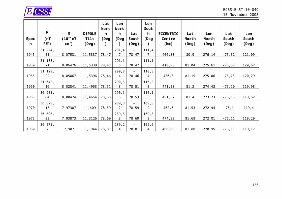
ECSS-E-ST-10-04C15 November 2008
G.10 Figures
Figure G-1: Temperature profile of the Earth’s atmosphere
150
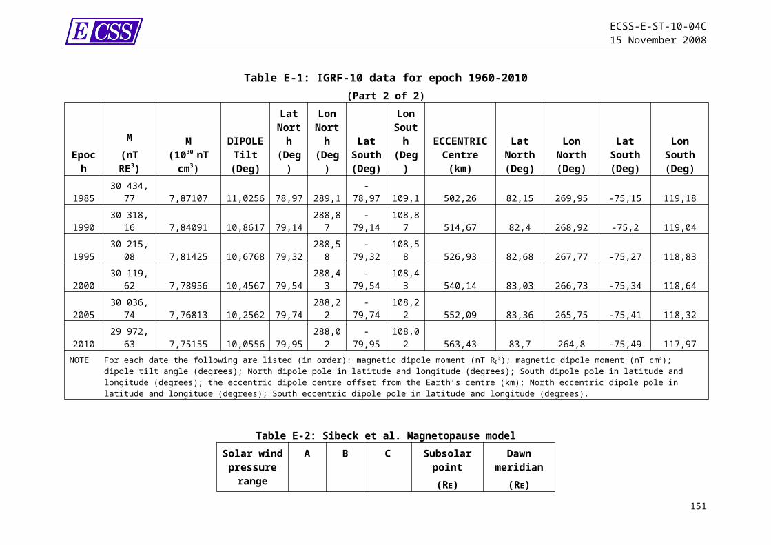
ECSS-E-ST-10-04C15 November 2008
Low, moderate, high long term and high short term solar and geomagenetic activities have the following meanings:low (F10.7 = F10.7avg = 65, S10.7 = S10.7avg = 60, M10.7 = M10.7avg = 60, Ap = 0)moderate (F10.7 = F10.7avg = 140, S10.7 = S10.7avg = 125, M10.7 = M10.7avg = 125, Ap = 15)high long term (F10.7 = F10.7avg = 250, S10.7 = S10.7avg = 220, M10.7 = M10.7avg = 220, Ap = 45)high short term (F10.7 = 300, F10.7avg = 250, S10.7 = 235, S10.7avg = 220, M10.7 = 240, M10.7avg = 220, Ap = 240)
Figure G-2: Variation of the JB-2006 mean air density with altitude for low, moderate, high long and high short term solar and geomagnetic activities
151

ECSS-E-ST-10-04C15 November 2008
1.00E+08
1.00E+09
1.00E+10
1.00E+11
1.00E+12
1.00E+13
1.00E+14
1.00E+15
1.00E+16
1.00E+17
1.00E+18
0 100 200 300 400 500 600 700 800 900
Altitude (km)
O d
ensi
ty (m
-3)
High Activity
Moderate ActivityLow Activity
Low, moderate, and high long term solar and geomagenetic activities have the following meanings:low (F10.7 = F10.7avg = 65, Ap = 0) moderate (F10.7 = F10.7avg = 140, Ap = 15) high long term (F10.7 = F10.7avg = 250, Ap = 45)
Figure G-3: Variation of the NRLMSISE00 mean atomic oxygen with altitude for low, moderate and high long solar and geomagnetic activities
152

ECSS-E-ST-10-04C15 November 2008
1E+04
1E+05
1E+06
1E+07
1E+08
1E+09
1E+10
1E+11
1E+12
1E+13
1E+14
1E+15
1E+16
1E+17
1E+18
0 100 200 300 400 500 600 700 800 900Altitude (km)
1E+04
1E+05
1E+06
1E+07
1E+08
1E+09
1E+10
1E+11
1E+12
1E+13
1E+14
1E+15
1E+16
1E+17
1E+18nHe (/m3) nAr (/m3)
nN2 (/m3) nH (/m3)
nN (/m3) nAnomalous O (/m3)
nO (/m3) nO2 (/m3)N2
Ar
H
NO2
He
Anomalous O
O
Figure G-4: Variation of the NRLMSISE00 mean concentration profile of the atmosphere constituents N2, O, O2, He, Ar, H, N and anomalous O with altitude for moderate solar and geomagnetic activities (F10.7 = F10.7avg = 140, Ap = 15)
153

ECSS-E-ST-10-04C15 November 2008
Annex H (informative)Plasmas
H.1 Identification of plasma regionsSome typical examples of plasma regimes to be considered are given in TableH-1.
H.2 Plasma effects on spacecraftThe principal spacecraft engineering concerns caused by space plasmas in different regions are outlined in Table H-2. Some of the most significant effects are listed below.Because of their higher mobility, electrons preferentially accumulate on exposed spacecraft surfaces, causing them to charge negatively. In hot plasmas in the 10keV range charging can reach hundreds or thousands of volts. Charging is however greatly mitigated by secondary electron emission and photoemission. In cold plasma (e.g. ionosphere) charging levels are generally very low, however, the high velocity of an orbiting spacecraft relative to ion velocity in this region leads to a plasma void in its wake. This can permit high-voltage surface charging to occur on wake surfaces during auroral crossings. High plasma densities (such as found in the ionosphere) cause reflection of radio beams below a critical frequency, as well as refraction and scintillation. Hence this acts as a barrier to satelliteground communications and complicates satellite radar altimetry, satellite navigation systems and the radio tracking of satellites.For high potential surfaces, in dense plasmas, ions and electrons are drawn to negative and positive regions respectively, allowing a current to flow through the plasma. This acts as a current drain on high voltage systems, such as solar arrays and can affects the spacecraft floating potential. Ion impacts due to flowing plasma (such as the solar wind) can result in sputtering from surface materials. Although solar wind plasma is cold, the ions carry considerable kinetic energy, typically ~1 keV for protons and ~4 keV for He++. Neutral spacecraft-generated atoms can be ionized by sunlight or charge-exchange with other ions, to create a lowenergy (<10 eV) ion population. These ions can be drawn to negatively charged surfaces and can cause surface contamination. Further details on spacecraft-plasma interactions can be found in the ECSS-E-ST-20-06 (Spacecraft Charging) standard.
154

ECSS-E-ST-10-04C15 November 2008
H.3 Reference data
H.3.1 IntroductionThis section provides further information about the different space plasma regimes. This does not form part of the requirements but may help the user by describing typical data derived from the standard models or models that have not yet been defined as standards.
H.3.2 Ionosphere
H.3.2.1. IRI 2007IRI-2007 contains a number of options suitable for different applications. Recommended choices are indicated when the code is run. The accuracy of the IRI electron density model is typically 50-80 % at heights from 65 km to 95 km 5-15 % at heights from 100 km to 200 km during daytime 15-30 % at heights from 100 km to 200 km during night-time 15-25 % at heights from 200 km to 1 000 km at low and middle dip
latitudes (< 60) 50-80 % at heights from 200 km to 1 000 km at high dip latitudes (>
60)Table H-3 shows a typical altitude profile of electron density. This has been calculated from IRI-2007, at 0 longitude and latitude, on 1st January, for a nearaverage sunspot number of 100, at 0 h and 12 h local time, using otherwise default options.
The IRI-2007 ([RN.9]) homepage is at http://IRI.gsfc.nasa.gov which provides information and references about the IRI project, lets users download the IRI Fortran source code, and lets them also compute and plot IRI parameters.
H.3.2.2. Auroral charging environmentThe auroral charging environment in section 8.2.3 is expressed in terms of distribution function but charging simulations often require input spectra in terms of flux. Flux in cm-2s-1sr-1keV-1 can be found from the distribution function as follows:
(H-1)
whereEkeV is energy in keV
H.3.3 PlasmasphereTypical ion and electron temperatures, throughout the plasmasphere are of the order of 0,5 eV. The electron temperature is thus far too low to produce hazardous charging effects.
155
ECSS-E-ST-10-04C15 November 2008
The CGPM code [RN.8] has been widely distributed by the Marshall Space Flight Center and can generally be obtained directly from them.A representative profile though the ionosphere and plasmasphere is shown in Table A-1. The density profile is dependent on geomagnetic activity as indicated in Figure H-1.
H.3.4 Outer magnetosphereNASA has defined a severe charging environment [RD.53] based on the 90th
percentile of severe environments. However, this is not the one adopted as the ECSS Standard.Table H-5 gives typical plasma parameters for the geostationary environment for quiet and substorm periods.The outer boundary of the magnetosphere, the magnetopause, is controlled by the balance between the pressure of the magnetic field and that of the solar wind. Along the EarthSun line, the magnetopause is closest to the Earth and its position can be expressed approximately [RD.54] as:
(H-2)
whereLm is the distance from the centre of the Earth to the magnetopause, at the subsolar point, in Earthradii;B0 is the strength of the terrestrial internal magnetic field, at surface of the Earth, on the equator = 3 104 nT;o is the permeability of free space;n is the density of the solar wind;m is the mass of the proton;V is the velocity of the solar wind.
Lm is typically 10 Earthradii away from the subsolar point. The magnetopause flares out on the flanks and is effectively infinite in length in the antisolar direction. This boundary is described in more detail in clause 5.
H.3.5 MagnetosheathMagnetosheath plasma parameters differ according to the latitude and local time of the observation. The highest density and temperature and the steepest velocity drop are observed at the subsolar point i.e. zero degrees latitude at local noon. Typical values for this region are given in Table H-6.
H.3.6 Magnetotail and distant magnetosheathTypical plasma parameters that may be encountered in the magnetotail and distant magnetosheath around the L2 point are given in Table H-7.
156
ECSS-E-ST-10-04C15 November 2008
H.3.7 Planetary environmentsFor charging investigations around Jupiter and Saturn, a description of the plasma environment has been described by Garrett and Hoffman [RD.11]. This describes the environments as either a Maxwellian distribution or a Kappa distribution or a sum of the two, as followsMaxwellian:
m-6s3 (H-3)
Kappa:
m-6s3 (H-4)
where is the Gamma Function.
[RD.11] lists appropriate parameters for various regions in the magnetospheres of Jupiter and Saturn.Worst-case plasma parameters, i.e. corresponding to the highest calculated charging level in eclipse in [RD.11], are given in Table H-8.
H.3.8 Induced environments
H.3.8.1. Photo and secondary electronsThe electron flux at the spacecraft surface can be determined from the incident UV and primary electron fluxes, multiplied by the yield for the surface in question. Away from the emitting surface the density can be calculated from the following [RD.115]:
(H-5)
whereN is the density (cm-3);N0 is the density at emitter (cm-3);z is the distance from surface;0 is the shielding distance, calculated as the Debye length due to the emitted electrons.
Table H-9 gives typical photoelectron sheath parameters [RD.55].
H.3.8.2. Ionization of contaminant gassesOnce neutral gas is released into space by whatever mechanism, it becomes subject to photoionization and dissociation by solar UV and ionization by charge exchange with solar wind ions. Production of new ions can be
157
ECSS-E-ST-10-04C15 November 2008
calculated from the appropriate photoionization rates and charge exchange crosssections (from [RD.57]).
(H-6)
whereQ is the production rate, ions s-1;Ni is the ion density; is the photoionization rate coefficient;nsw is the solar wind density;vsw is the solar wind velocity; is the charge exchange coefficient.
Photoionization rates depend on the atom or molecule concerned, and UV intensity and spectrum. Huebner and Giguere [RD.56] have tabulated a number of rate coefficients for different species, for sunlight at 1 AU. As an example, some photoionization rates for common gasses are listed in TableH-10. For H2O, where the charge exchange coefficient is around 2,1 10-19 m-2
[RD.57], photoionization and charge exchange are comparable processes. However, all species and dissociation products need to be considered to calculate the total production of emitted ions.
H.4 TablesTable H-1: Regions encountered by different mission types
Orbit Regions encounteredLow inclination LEO (<50) Ionosphere High-inclination LEO e.g. Polar orbit
Ionosphere, Auroral zone
Geostationary orbit Outer magnetosphere, Plasmasphere, Magnetosheath (occasionally)
MEO circular orbit e.g. Galileo Outer magnetosphere, Plasmasphere, Magnetosheath (possibly at high latitude)
Geostationary transfer orbit Ionosphere, Plasmasphere, Outer magnetosphere, Magnetosheath (occasionally)
High apogee elliptical orbit All regions can be encountered, depending on orbit.
L1, L4, L5 Lagrangian points Solar windL2 Solar wind, magnetotail and distant
magnetosheathInterplanetary cruise Solar windPlanetary orbit / encounter Planetary environment
Table H-2: Main engineering concerns due to space plasmasScenario ProblemOuter magnetosphere Surface charging - possibly harmful electrostatic discharges.
158
ECSS-E-ST-10-04C15 November 2008
Scenario ProblemHighvoltage systems in the ionosphere
Power leakage, possible discharges, high spacecraft ground potential, sputtering.
Large spacecraft in the ionosphere
Spacecraft wake creation.
Auroral zone crossings Surface charging - sputtering and possible electrostatic discharges.
All spacecraft Ionospheric barrier to groundspace communications below a threshold frequency.Perturbation of signals at higher frequencies.
Radar/navigation Ionospheric propagation delays to beams.Electric propulsion Interactions between generated plasma, ambient plasma, and
the spacecraft.Scientific spacecraft Low level charging and photoelectrons which interfere with
plasma measurements.Plasma entry into sensitive detectors.
Table H-3: Ionospheric electron density profiles derived from IRI-2007 for date 01/01/2000, lat=0, long=0.
Height(km)
Midnight electron density(cm-3)
Noon electron density(cm-3)
100 3 082 163 327200 16 432 231 395300 688 694 512 842400 978 126 1 394 750500 513 528 1 197 828600 254 377 554 483700 140 005 268 714800 85 766 148 940900 57 255 92 547
1000 40 847 62 7311100 30 679 45 4011200 23 989 34 5451300 19 369 27 3271400 16 047 22 2911500 13 579 18 6371600 11 693 15 8981700 10 217 13 7881800 9 038 12 1231900 8 080 10 7852000 7 288 9 689
NOTE: Sunspot number Rz12=112,1 for this date
Table H-4: Profile of densities for solar magnetic local time = 18hr, solar magnetic latitude=0, Kp = 5,0 from the GCPM for 1/1/1999
RE Electron Density(cm-3 )
Proton Density(cm-3 )
Helium Ion Density(cm-3 )
Oxygen Ion Density(cm-3 )
1,3 5,31E+03 4,73E+03 5,46E+02 3,24E+011,35 4,98E+03 4,44E+03 5,22E+02 2,69E+011,4 4,68E+03 4,16E+03 4,91E+02 2,42E+01
159
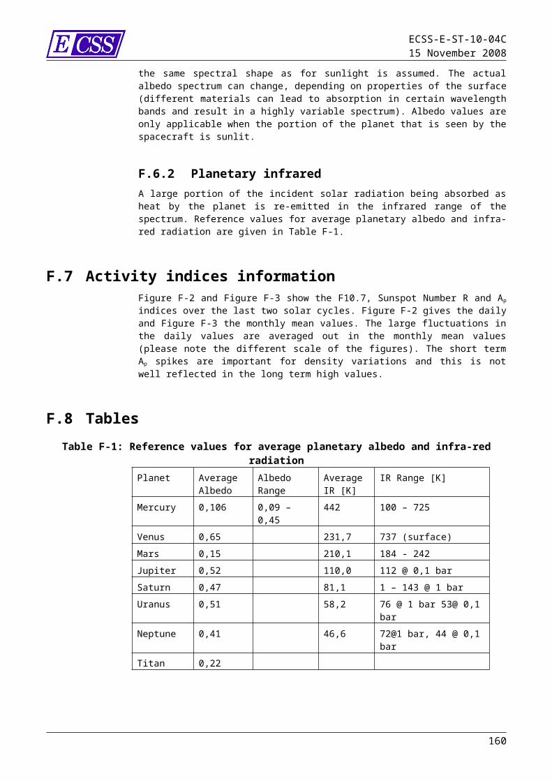
ECSS-E-ST-10-04C15 November 2008
1,5 4,12E+03 3,68E+03 4,25E+02 2,08E+011,75 3,00E+03 2,70E+03 2,85E+02 1,50E+012,0 2,19E+03 1,99E+03 1,90E+02 1,09E+012,5 1,16E+03 1,07E+03 8,35E+01 5,81E+003,0 6,17E+02 5,77E+02 3,67E+01 3,08E+003,5 3,27E+02 3,10E+02 1,61E+01 1,64E+004,0 1,74E+02 1,66E+02 7,04E+00 8,69E-01 NOTE: Distance in Earth radii (RE) is measured from the centre of the Earth.
Table H-5: Typical plasma parameters at geostationary orbit
Density(cm-3)
Ion temperatur
e
Electron temperatur
e D(m)Quiet 10 1 eV-1 keV 1 eV-1 keV 50Substorm 1 10 keV 10 keV 500
Table H-6: Typical magnetosheath plasma parametersLocal time Speed (km s-
1)Tp (K) Te (K) Density
(cm-3)12 noon 50 2 106 2 106 3506 hours 350 1106 1 106 20NOTE From [RD.116]
Table H-7: Typical plasma parameters around L2 n cm-3 Ti eV Te eV V km s-1
Magnetosheath 1,0 80 26 312Lobe 0,1 540 180 60Plasma sheet 0,15 610 145 72NOTE: Ttaken from 50% cumulative probability measurement from
Geotail [RD.6])
Table H-8: Worst-case environments for eclipse charging near Jupiter and Saturn
Jupiter SaturnElectrons
Protons
Electrons
Protons
- 104 7,2105
7,4105
- 1,0 0,028 0,026104 - 1,11
1053,0103
1,0 - 0,458 30,82,0 - 1,7 8,5Co-rotation velocity - 250 - 80
160

ECSS-E-ST-10-04C15 November 2008
km s-1
Table H-9: Photoelectron sheath parametersTemperature
(eV)Photoelectroncurrent (A m-2)
Surface electron density (m-3)
3 1 10-5 1 108
Table H-10: Some solar UV photoionization rates at 1 AUSpecies Photoionization rate
(s-1)H2O 3,34 10-7
O2 5,13 10-7
N2 3,52 10-7
NOTE: From [RD.56]
H.5 Figures
Electron density CGPM
1,0E+00
1,0E+01
1,0E+02
1,0E+03
1,0E+04
1 2 3 4 5 6 7 8
Earth Radii
Den
sity
cm
-3
KP=9KP=0
Figure H-1: Profile of electron density for solar magnetic local time = 18hr, solar magnetic latitude=0, Kp =0 and 9 from the GCPM for 1/1/1999.
161
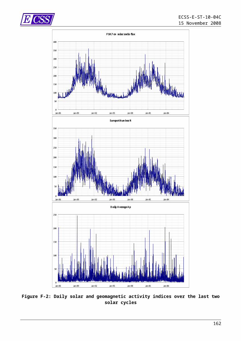
ECSS-E-ST-10-04C15 November 2008
Annex I (informative)Energetic particle radiation
I.1 Trapped radiation belts
I.1.1 Basic dataTrapped radiation belt charged energetic particles gyrate in the geomagnetic field with a gyration period:
(I-1)
and a radius of gyration of :
(I-2)
Table I-1 gives typical characteristics of energetic particles.
I.1.2 Tailoring guidelines: orbital and mission regimesIn the following sections, attention is drawn to special considerations for various orbit types.
I.1.2.1. Geostationary orbitGeostationary orbit is a circular orbit usually encountering an environment dominated by energetic electrons. This environment is characterized by strong time variations with many extended quiet periods of low radiation levels and many episodes of intense injections of energetic electrons which increase e.g. dose, sensor interference and electrostatic charging. Solar protons and cosmic rays have unrestricted access to this orbit. Solar particles make shortlived but important contributions to the total dose, interference and single event effects. They do not directly participate in charging processes. Cosmic rays provide a continuous source of singleevent effects and sensor interference.
I.1.2.2. MEO, HEOThese orbits encounter the electrondominated environment mentioned above, but in addition HEO encounters the inner, proton radiation belt. In HEO orbits, singleevent effects from protons and proton nonionizing damage need to be considered. These orbits often encounter more severe electron environments, near the peak of the electron belt (the location of which is also
162

ECSS-E-ST-10-04C15 November 2008
variable) than geostationary orbit and so electrostatic charging can be a more serious threat.
I.1.2.3. LEOCurrently manned activities are limited to low (< 550 km) and medium-inclination (<57.1) orbits, however, this is going to change in the future. We refer to these orbital regimes as LEO. Missions in these orbits encounter the inner edge of the radiation belt. This region is dominated by the South Atlantic anomaly. Also important is the asymmetry in energetic proton fluxes from East and West. The lowaltitude environment is characterized by high-energy radiationbelt trapped protons. The deflection of charged particles from outside the magnetosphere by the Earth magnetic field (geomagnetic shielding) reduces the fluxes of cosmic rays and solar energetic particles, but the shielding is not total. Like polar orbits, LEO orbits also encounter outer-belt trapped electrons at highlatitudes.
I.1.2.4. PolarPolar orbits are generally of less than 1 500 km altitude with inclinations above 80. They encounter the inner proton and electron belts in the form of the South Atlantic anomaly and also the outer electron belt where the geomagnetic field lines bring it to low altitudes at “auroral” latitudes above about 50. On the highlatitude parts of the orbit a spacecraft is exposed to almost unattenuated fluxes of cosmic rays and solar energetic particles. At low latitudes, geomagnetic shielding considerably reduces these fluxes.
I.1.3 Existing trapped radiation models
I.1.3.1. OverviewFor trapped radiation and all earth orbits, the best known and most widely used models of radiation belt energetic particles are the AE-8 and AP-8 models for electrons [RN.10] and protons [RN.11], respectively. They were developed at Aerospace Corporation for the NSSDC at NASA/GSFC based on data from satellites flown in the 1960s and early 1970s. The models give omnidirectional fluxes as functions of idealized geomagnetic dipole coordinates B/B0 and L. The user defines an orbit, generates a trajectory, transforms it to geomagnetic coordinates and access the radiation belt models to compute flux spectra, using the same geomagnetic field as used to develop the model. Apart from separate versions for solar maximum and solar minimum, there is no description of the temporal behaviour of fluxes. At high altitudes in particular (e.g. around geostationary orbit) fluxes vary by orders of magnitude over short times and exhibit significant diurnal variations; the models do not describe these. In addition, the models do not contain any explicit flux directionality. At low altitudes, on the inner edge of the radiation belts, particle fluxes rise very steeply with altitude and small errors in computing locations can give rise to large errors in particle fluxes. This is a problem since the geomagnetic field is shifting and decaying so that the situation is no longer the same as when the model data were acquired. Use of a geomagnetic field model other than the one used in generating the model can result in large flux errors at low altitude. Although use of an old field model and epoch can reduce errors in the magnitudes of fluxes, it does not model the spatial locations of radiationbelt
163
ECSS-E-ST-10-04C15 November 2008
features (e.g. the position of the South Atlantic anomaly), or particle fluxes, as they are today.The AP-8 model for protons gives proton fluxes from 0,1 to 400 MeV while the AE-8 model for electrons covers electrons from 0,04 to 7 MeV. Figure I-1 shows contour plots of AE-8 and AP-8 model omnidirectional, integral fluxes for energies above 1 MeV and 10 MeV, respectively, in idealized dipole space. Figure I-2 shows values of energetic electron and proton particle fluxes as stored in these models, for positions on the geomagnetic equator (B=B0), as functions of L for both solar maximum and solar minimum. This shows that as far as the models are concerned, the solar activity only affects electron fluxes in the midL range and protons at low altitude where the higher neutral atmospheric density at solar maximum leads to reduced proton fluxes because of enhanced loss. Solar cycle effects on electrons appear to differ from this behaviour in reality [RD.58].
I.1.3.2. Uncertainties in trapped particle modelsThe accuracy of the predicted fluxes is within a factor of 2 for AP8 and within a factor depending on the location and incident electron energy for AE8. In [RN.10], a reasonable limit of the error on AE8 is a factor of 2, however, in some regions (L=3) this can increase to a factor of 4.5 and is energy dependent, the error is higher for the higher energies. In other regions, such as geostationary orbits, the AE8 models are pessimistic.For short term estimates the models can underpredict by a considerable amount – instantaneous fluxes measured at specific locations in the electron belts have been measured to be several orders of magnitude higher than the long term model fluxes.
I.1.3.3. Specific orbitsFor electron fluxes in geostationary orbit a great number of measurements exist. The standard model IGE 2006 (International GEO Electron model version 2006) developed by ONERA & LANL [RN.12], is a statistical model based on more than 2 solar cycles of electron flux data from radiation monitors on-board different international GEO satellites (mainly US and Japan) see Figure I-4. This model is available in the SPENVIS [RD.59] or OMERE [RD.60] space environment tools.The accuracy of IGE 2006 is included in the model as the upper case takes into account uncertainties in the measurements, in the duration and strength of the solar cycle. For MEO altitude, the electron environment is very hard, intense and dynamic. The model developed at ONERA [RN.13] and given in Table B-4 and Table B-5, is based on GPS data acquired from Los Alamos, covering from the early nineties to 2007. Data have been analysed in terms of saturation, contamination and global coherence to ensure high fidelity. This MEO model provides energetic electrons fluxes in the energy spectral range 0,28 MeV–2,24 MeV and gives three spectra: an average case, a lower case and an upper case. The accuracy of MEO-V2 is included in the model as the upper case takes into account uncertainties in the measurements, in the duration and the strength of the solar cycle.The electron fluxes obtained in the mean case of MEO model are very close to electron fluxes deduced from NASA/AE8 model over a full solar cycle (7 years MAX and 4 years MIN for AE8), see Figure I-5. Similarly, the electron fluxes from the MEO mean model propagated to near geostationary orbit are in agreement with electron fluxes deduced from IGE06 model.
164

ECSS-E-ST-10-04C15 November 2008
I.1.3.4. Other trapped radiation modelsOther trapped radiation models exist. Amongst them, the main known are:Those based on CRRES data : CRRESELE: The Combined Radiation and Release Effects Satellite (CRRES) electron flux model specifies the location and intensity of electron omni-directional flux over the energy range 0,5-6,6 MeV for a range of geomagnetic activity levels [RD.61].CRRESPRO: The Combined Radiation and Release Effects Satellite (CRRES) proton flux model specifies the location and intensity of proton omni-directional flux over the energy range 1-100 MeV for quiet, average, or active geophysical conditions [RD.62].TPM1 (Trapped Proton model) [RD.25] which provides a solar-cycle dependent low-altitude extension to the CRRESPRO trapped energetic proton model based on NOAA/TIROS data from 1,5 to 81 MeV (but it is ITAR restricted).These models are available in the AF-GEOSPACE tool, see: http://www.kirtland.af.mil/library/factsheets/factsheet.asp?id=7899Other models are also listed and available in http://modelweb.gsfc.nasa.gov/
I.1.4 The South Atlantic Anomaly
I.1.4.1. OverviewThe South Atlantic Anomaly (see clause 9.2.1) produces an “island” of radiation and provides the only significant radiation encountered on low Earth orbits with altitudes below about 800 km and inclinations below about 40. Figure I-3 shows the South Atlantic Anomaly at 400 km.
I.1.4.2. Anisotropy (the “EastWest effect”)Because of the inclination of geomagnetic fieldlines with respect to the atmosphere here, particles reaching a point from the West have gyrated from higher altitude while those arriving from the East have gyrated from lower altitude. There are fewer coming from below because of atmospheric absorption and therefore an asymmetry in the fluxes results. This can be important in certain cases, including the International Space Station. The current standard AP-8 model does not treat this effect but models have been developed by NASA [RD.63] and BIRA [RD.64]. The ratio of the East and West peak fluxes is about 4,6 for 100 MeV protons in an ISS type orbit. Measurements from MIR are also available which are consistent with this ratio [RD.65].
I.1.4.3. Location of the South Atlantic AnomalyThe slow movement of the South Atlantic Anomaly as a result of shifts in the geomagnetic field has been clearly observed. This shift is essentially westward at a rate of 0,3yr-1 (~10 since the models were created) and account is taken of this figure for low Earth orbits when planning operations which involve a sensitivity to radiation (payload radiation background, astronaut EVA). Models including this shift capability are available [RD.14].
165

ECSS-E-ST-10-04C15 November 2008
I.1.5 Dynamics of the outer radiation belt The dynamic nature of the outer electron radiation belt, together with its diurnal variations mean that unless one is interested in longterm averages (such as provided by AE-8), some statistical description is desirable. This is especially true when deep dielectric charging and radiation background are of concern. No standard models for the variability are yet available, but for engineering purposes the CRRESELE model has been developed [RD.61]. An older version of the AE-8 electron model, AE-4 [RD.26], included a statistical model giving standard deviations of the logarithm of electron fluxes (assumed to be normallydistributed). It also included a model for local time flux modulation. This was a sinusoidal model providing amplitudes of the variation, with a fixed maximum at 11:00 hours local time. These have been extended and applied to the AE-8 model [RD.66], although this extension is unvalidated.
I.1.6 Internal chargingThe FLUMIC (Flux Model for Internal Charging) model used for internal charging assessments is integral to the DICTAT internal charging tool but can be applied separately. FLUMIC describes the electron flux, which has an exponential dependence on energy E and varies with L, time of year and phase of the solar cycle. FLUMIC version 1 and 2 covered L-shells above 2,8, i.e. the outer belt only. The exponential spectrum can a priori be extrapolated down to lower energy (say a few 100 keV), although for more dynamics in the lower energy environment more sophisticated models are available. Version 3 of FLUMIC is broadly similar to FLUMIC version 2 in the outer belt because here it is based on the same data. However, it also models electron fluxes in the inner belt (see Annex B.4). The FLUMIC v3 model, presented in Annex B.4, has been evaluated with in-flight data and shown to provide electron fluxes between 0,8 MeV and 2,8 MeV that exceed 95-98% of the data for L-Shells above 4 Earth Radii. For the Geostationary orbit, the models provided electron fluences that exceeded 95% of the data points [RD.67].
I.2 Solar particle event models
I.2.1 OverviewDuring energetic events on the Sun, large fluxes of energetic protons are produced which can reach the Earth. Solar particle events, because of their unpredictability and large variability in magnitude, duration and spectral characteristics, are treated statistically. Current models make the assumption that large events are confined to a 7year period defined as solar maximum. Although large events are absent during the remaining 4 solar minimum years of the 11year solar cycle (see clause 6) the occasional small event can still occur.An inherent input to probablistic models is the use of a “confidence level”. As a result: the risks of encountering environments can be more severe than the
one predicted, and margins are implicitly assumed by applying high confidence levels.
166

ECSS-E-ST-10-04C15 November 2008
Two main approaches are currently described in the literature to specify the mission integrated fluence: the ESP model approach and the JPL model approach.
I.2.2 ESP modelThe ESP model approach is based on the observation that a good fit to the distribution of the yearly accumulated fluence from the solar maximum periods of the solar cycles 20, 21 and 22 is obtained with a log-normal distribution. It is deduced from this observation that the distribution of the logarithm of the n-year accumulated fluence should also have a gaussian distribution with a mean and a relative variance that can be expressed as a function of the 1-year distribution mean and variance as follows:
(I-3)
and(I-4)
I.2.3 JPL modelsThe approach used in JPL models, JPL85 and JPL91 [RD.68] [RD.69], is based on a combined consideration of: the distribution of fluences seen in SEP events and the probability of occurrence of an event (irrespective of magnitude)
over a given period. A normal probability distribution function, f, is employed to describe the log10
of individual event fluences, F,(I-5)
where μ is the mean of the distribution of the log10 of fluence valuesσ is the standard deviation
The probability p of n events occurring in time τ is given by a Poisson distribution such that
(I-6)
where w is the average number of events occurring per active year
The probability, P, of exceeding a selected fluence level, F, during a mission lifetime, τ can be expressed analytically as,
(I-7)
where Q(F, n) is the probability that the sum of all fluences due to n
(n = [1, ∞]) events will exceed 10F
167
ECSS-E-ST-10-04C15 November 2008
The derivation of P requires an estimate of the parameters w, μ and σ to perform computer based Monte Carlo simulations to derive Q(F, n).JPL-91 has been a de-facto standard for many years. However, it was recently shown that the values of the parameters μ, σ and w derived from the data for JPL-91 lead to an underestimation of the fluence [RD.70]. Updated values of these parameters have been proposed for the fluence specification in the energy ranges >10 MeV and >30 MeV [RD.70], [RD.71]. The values of the parameters μ, σ and w of the model that are recommended to be used are given in Table I-2.
The complete calculation of has been coded in IDLTM and the source code can be found in [RD.70].
I.2.4 Spectrum of individual events
I.2.4.1. OverviewSolar proton event spectra are variable, the worstcase event at one energy is not necessarily worstcase at another. The August 1972 event yield worstcase doses at most typical spacecraft shielding (1-10 mm) where particles of energy 10-70 MeV are most important. The October 1989 flare is apparently more severe at lower and higher energies. Lower energies are important for surface material and solar cell effects and the higher energies more important for deep shielding (e.g. for heavy spacecraft, manned missions and planetary atmospheres) and for nuclear interactions giving rise to certain types of background and SEUs. Hence the term “worstcase” is application dependent.
I.2.4.2. August 1972 eventThe August 1972 event produced a peak flux near the Earth in excess of 106
protons cm-2s-1 above 10 MeV energy. A fluence spectrum which is often used to represent a worst case flare, classified as “anomalously large” is based on the very large August 1972 event [RD.72]:
(I-8)
with energy E in MeV and fluence J in protons cm-2.
I.2.4.3. October 1989 eventThe October 1989 event was the largest seen since August 1972 but had lower fluences at the medium energies. The events of 19, 22 and 24 October 1989 have been fitted to Weibull spectral forms as suggested by Xapsos et al [RD.73]. Account has been taken of ground level neutron monitors in addition to spacecraft data as suggested by Dyer et al [RD.74] in order to get the correct spectra at higher energies. The differential flux spectrum is given by the form:
(I-9)
With energy E in MeV and the flux J in protons cm-2 s-1 sr-1 MeV-1. The parameters for the peak fluxes during these events are given in Table I-4.
168

ECSS-E-ST-10-04C15 November 2008
I.2.4.4. Worst caseIt has been proposed that a truncated power law can provide a good fit to the distribution of the log of the intensity of the solar proton events [RD.12]. Such a model predicts therefore a worst case event which is found to be 1,3E+10 cm-2 for proton with energy above 30 MeV. Consideration on the statistical uncertainty leads to estimate that an actual worst case is about 3E+10 cm-2.The JPL approach is based on a good fit of the distribution of the log of the intensity of events through a Gaussian function. With the parameters given in Table I-2 above for the range > 30 MeV, a fluence of 3E+10 cm-2 is likely to not be exceeded by 99,5% of the events.
I.2.5 Event probabilitiesThe probability p of n events occurring in time τ is given by a Poisson distribution such that
(I-10)
where w is the average number of events occurring per active year
The value of w depends of the definition of an event. Values of w given in Table I-2 can be used for the relevant energy range.
I.2.6 Other SEP modelsOther model are under development. These developments relate to alternative statistical approaches and models for peak fluxes.The Nymmik proton model ([RD.75] and [RD.76]) is in the process to be considered as an ISO standard (ISO TS 15391).The PSYCHIC solar particle model [RD.105] includes heavy ions and extends the energy range of solar protons to 300 MeV.
I.3 Cosmic ray environment and effects models Cosmic ray environment and effects models were originally created by Adams and coworkers at the U.S. Naval Research Laboratory [RD.77], under the name CREME. They provided a comprehensive set of cosmic ray and flare ion LET and energy spectra, including treatment of geomagnetic shielding and material shielding. CREME has been superseded by CREME96 [RD.78]. The major differences to the environment specification are in the inclusion of a model of the cosmic ray environment and its solarcycle modulation due to Nymmik et al. [RD.79], improved geomagnetic shielding calculation, and more realistic Solar Energetic Particle event (SEP) ion environments (see clause 9.2.3). The cosmic ray fluxes are anticorrelated with solar activity so the highest cosmic ray fluxes occur at solar minimum.
169
ECSS-E-ST-10-04C15 November 2008
I.4 Geomagnetic shielding The Earth’s magnetic field partially shields nearEarth space from solar energetic particles and cosmic rays, an effect known as geomagnetic shielding. However, these particles can easily reach polar regions and high altitudes such as the geostationary orbit. Geomagnetic shielding of protons is computed on the basis of the trajectory in geomagnetic B, L space (see Clause 5).Stassinopoulos and King [RD.80] developed a model which has total cutoff at L = 5. It assumes that no protons can penetrate to lower values. It can be shown that this model corresponds to a quiet magnetosphere vertical cutoff model excluding protons of E < 200 MeV from L < 5 Earthradii. This model is adequate for most cases. However, in reality protons of lower energy can penetrate below L = 5 with nonvertical arrival directions, especially in a disturbed magnetosphere where the geomagnetic shielding is weakened. For westward arrival at the L = 5 geomagnetic equator in a disturbed magnetosphere, the energy cutoff can be as low 30 MeV. For engineering purposes, geomagnetic cutoff is usually not applied to orbits spending more than 50 % of the orbit period above L = 5. Geomagnetic cutoff is usually applied to orbits spending more than 75 % of their time below L = 5.
I.5 Atmospheric albedo neutron modelThe QinetiQ Atmospheric Radiation Model (QARM) uses a response function approach based on Monte Carlo radiation transport codes to generate directional fluxes of atmospheric secondary radiation. The model has been widely validated against a range of measurements [RD.17], [RD.18]. It can be applied to give the upward (albedo) neutron flux at 100 km altitude and this can then be scaled to any spacecraft altitude using the inverse square law:
(I-11)
where ϕ is the particle flux, h is the altitude in km and Re is the earth’s radius in km
This method compares favourably with the limited experimental measurements [RD.81], [RD.82].Results for three cut-off rigidities are given for solar minimum and maximum respectively in Figure I-6 and Figure I-7.
I.6 Planetary environments
I.6.1 OverviewAs giant planets (Neptune, Jupiter, Saturn) have large magnetospheres, spacecrafts orbiting close to them encounter intense trapped radiation environments inducing direct radiation effects and internal charging.
170
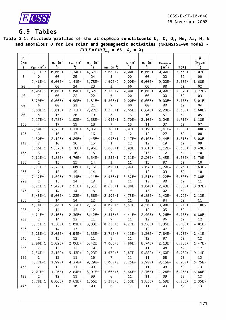
ECSS-E-ST-10-04C15 November 2008
I.6.2 Existing models
I.6.2.1. JupiterThree models are currently available, see Figure I-8: The Divine and Garett model which is constructed using data from
Pioneer 10 and 11 and which extends to 10 jovian radii RJ for protons and more than 100 RJ for electrons [RD.20].
GIRE (Galileo Interim Electron Environment) based on Galileo and Pioneer electron data between 8 to 16 RJ [RD.83] and developed at ONERA [RN.17] using a physical model. This model has been validated by comparing calculated synchroton radiation with that measured from the ground by the VLA telescope and extends to 10 RJ.
I.6.2.2. Internal chargingFor internal charging see [RD.19].
I.6.2.3. MarsFor Mars the orbital environment is very similar to an interplanetary environment – as the planet has no significant magnetic field that can neither support trapped radiation, nor provide adequate geomagnetic shielding. The only significant deviation from the interplanetary environment is the solid angle subtended by the planet that can provide some shielding - particularly for low altitude orbits. The radiation environment on the surface of Mars largely derives from the secondary particles produced by cosmic rays and solar protons in the atmosphere and regolith. For manned missions to the planet the dominant particle species of concern is the neutron. Several software packages have been developed to calculate the ambient environment at Mars due to atmospheric interactions [RD.84],[RD.85],[RD.86]. Residual crustal magnetic fields do exists that may provide some form of magnetic shielding, the effectiveness of which can be evaluated using the PLANETOCOSMICS software [RD.86].
I.7 Interplanetary environmentsThe interplanetary environment is characterized by cosmic rays and occasional solar energetic particle events. For mission analysis, it is important to take into account the variations in particle intensities with heliocentric radius and solar cycle modulation as specified in 9.2.2.Science missions also take place at the Lagrangian points of the SunEarth system or EarthMoon system, locations which are usually considered interplanetary from the point of view of the radiation environment.
171

ECSS-E-ST-10-04C15 November 2008
I.8 TablesTable I-1: Characteristics of typical radiation belt particles
Particle1 MeV
Electron10 MeV Proton
Range in aluminium (mm) 2 0,4
Peak equatorial omnidirectional flux (cm-2s-
1)*4 × 106 3,4 × 10⁵
Radial location (L) of peak flux (Earth-radii)*
4,4 1,7
Radius of gyration (km)@ 500 km@ 20 000 km
0,610
50880
Gyration period (s)@ 500 km@ 20 000 km
10-5
2 × 10⁻⁴
7 × 10⁻³
0,13Bounce period (s)
@ 500 km@ 20 000 km
0,10,3
0,651,7
Longitudinal drift period (min)@ 500 km@ 20 000 km
103,5
31,1
* derived from the models of clause 9.3.1
Table I-2: Recommended updated values of the parameters of the JPL model
Parameter >10MeV >30MeV 8,07 7,42Σ 1,10 1,2W 6,15 5,40
NOTE: Taken from [RD.70] (>10MeV) and [RD.71] (>30MeV)
Table I-3: Proton fluence levels for energy, mission duration and confidence levels from the ESP model with the NASA parameters from Table B-7.
Energy
(MeV)
Probability
(confidence)
level (%)
1 year(cm2)
2 years(cm2)
3 years(cm2)
5 years(cm2)
7 years(cm2)
>1 50 6,37E+10
1,46E+11
2,32E+11
4,07E+11
5,83E+11
>1 75 1,10E+11
2,23E+11
3,30E+11
5,39E+11
7,41E+11
172

ECSS-E-ST-10-04C15 November 2008
Energy
(MeV)
Probability
(confidence)
level (%)
1 year(cm2)
2 years(cm2)
3 years(cm2)
5 years(cm2)
7 years(cm2)
>1 90 1,81E+11
3,24E+11
4,54E+11
6,93E+11
9,20E+11
>1 95 2,43E+11
4,06E+11
5,48E+11
8,06E+11
1,05E+12
>1 99 4,23E+11
6,20E+11
7,83E+11
1,07E+12
1,33E+12
>10 50 2,60E+09
7,07E+09
1,25E+10
2,52E+10
3,94E+10
>10 75 7,55E+09
1,79E+10
2,90E+10
5,24E+10
7,63E+10
>10 90 1,97E+10
4,11E+10
6,19E+10
1,01E+11
1,38E+11
>10 95 3,51E+10
6,78E+10
9,75E+10
1,50E+11
1,97E+11
>10 99 1,03E+11
1,73E+11
2,28E+11
3,15E+11
3,84E+11
>30 50 3,26E+08
9,11E+08
1,65E+09
3,47E+09
5,62E+09
>30 75 1,19E+09
2,93E+09
4,92E+09
9,33E+09
1,41E+10
>30 90 3,79E+09
8,36E+09
1,31E+10
2,27E+10
3,23E+10
>30 95 7,59E+09
1,57E+10
2,36E+10
3,87E+10
5,29E+10
>30 99 2,80E+10
5,10E+10
7,10E+10
1,05E+11
1,34E+11
>100 50 1,98E+07
5,58E+07
1,02E+08
2,18E+08
3,57E+08
>100 75 8,59E+07
2,17E+08
3,70E+08
7,21E+08
1,11E+09
>100 90 3,22E+08
7,34E+08
1,18E+09
2,12E+09
3,09E+09
>100 95 7,09E+08
1,53E+09
2,36E+09
4,04E+09
5,71E+09
>100 99 3,12E+09
6,01E+09
8,69E+09
1,36E+10
1,80E+10
Table I-4: Parameters for the fit to the peak fluxes from the October 1989 events.
Event A[cm-2s-1sr-1MeV-1]
Κ α
173
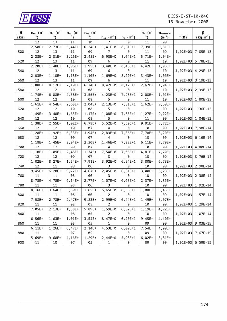
ECSS-E-ST-10-04C15 November 2008
19 Oct. 1989 214 0,526 0,36622 Oct 1989 429 0,458 0,390824 Oct 1989 54 900 2,38 0,23NOTE Some of the parameters in the reference [RD.74] Table I are incorrect and
the verified values are presented in Table I-4.
I.9 Figures
NOTE: Omnidirectional fluxes are for particles >10 MeV and >1 MeV respectively for protons and electrons. The data are derived from the AP-8 and AE-8 models, respectively, and are shown in an idealised dipole representation of the Earth’s magnetic field.
Figure I-1: Contour plots of the proton and electron radiation belts
174

ECSS-E-ST-10-04C15 November 2008
1,E+00
1,E+01
1,E+02
1,E+03
1,E+04
1,E+05
1,E+06
1,E+07
1,E+08
1 2 3 4 5 6 7 8 9 10 11 12 Geomagnetic L value (Earth radii)
Omnidirectional flux > E (/cm2/s)
0,5 MeV 1 MeV 2 MeV 3 MeV 4 MeV 5 MeV
(a) Electron
(b) Proton
1,E+00
1,E+01
1,E+02
1,E+03
1,E+04
1,E+05
1,E+06
1,E+07
1,E+08
1 2 3 4 5 6 Geomagnetic L value (Earth radii)
Omnidirectional flux > E (/cm2/s)
> Energy: 1. MeV > Energy: 10 MeV > Energy: 30 MeV > Energy: 100 MeV
Figure I-2: Electron (a) and proton (b) omnidirectional fluxes, integral in energy, on the geomagnetic equator for various energy thresholds
175

ECSS-E-ST-10-04C15 November 2008
Figure I-3: Integral omnidirectional fluxes of protons (>10 MeV) and electrons (>10 MeV) at 400 km altitude showing the inner radiation belt’s “South Atlantic anomaly” and, in the case of electrons, the outer radiation belt
encountered at high latitudes
176

ECSS-E-ST-10-04C15 November 2008
Figure I-4: Comparison of POLE with AE8 (flux vs. Energy) for 15 year mission (with worst case and best case included)
1,0E+00
1,0E+01
1,0E+02
1,0E+03
1,0E+04
1,0E+05
1,0E+06
1,0E+07
0,1 1 10Energie (MeV)
Flux
(cm-2
.s-1.
sr-1)
1,0E+00
1,0E+01
1,0E+02
1,0E+03
1,0E+04
1,0E+05
1,0E+06
1,0E+07
0,1 1 10Energie (MeV)
Flux
(cm-2
.s-1.
sr-1)
Flux d'électrons sur un cycle solaire (11 ans)
1,0E+00
1,0E+01
1,0E+02
1,0E+03
1,0E+04
1,0E+05
1,0E+06
1,0E+07
0,1 1 10Energie (MeV)
Flux
(cm
-2.s
-1.s
r-1)
XX
MEO: mean case
MEO: best case
MEO: worth case
AE8 (7 years MAX, 4 years MIN)
Energy (MeV)
Figure I-5: Comparison of ONERA/GNSS model from 0,28 MeV up to 1,12 MeV (best case, mean case and worst case) with AE8 (flux vs. Energy) for 15 yr
mission (with worst case & best case)
177

ECSS-E-ST-10-04C15 November 2008
1,0E-10
1,0E-09
1,0E-08
1,0E-07
1,0E-06
1,0E-05
1,0E-04
1,0E-03
1,0E-02
1,0E-01
1,0E+00
1,0E+01
1,0E+02
1,0E+03
1,0E+04
1,E-06 1,E-05 1,E-04 1,E-03 1,E-02 1,E-01 1,E+00 1,E+01 1,E+02 1,E+03 1,E+04
Neutron Energy (MeV)
Diff
eren
tial F
lux
(neu
tron
s/cm
2 /MeV
/s)
0,00
0,20
0,40
0,60
0,80
1,00
1,20
1,40
1,60
Inte
gral
Flu
x (n
eutr
ons/
cm2 /s
)
RC = 0 GV, Dif
RC = 5 GV, Dif
RC = 16,6 GV, Dif
RC= 0 GV, Int
RC = 5GV, Int
RC = 16,6 GV, Int
Figure I-6: Albedo neutron spectra at 100 km altitude at solar maximum
1,0E-10
1,0E-09
1,0E-08
1,0E-07
1,0E-06
1,0E-05
1,0E-04
1,0E-03
1,0E-02
1,0E-01
1,0E+00
1,0E+01
1,0E+02
1,0E+03
1,0E+04
1,E-06 1,E-05 1,E-04 1,E-03 1,E-02 1,E-01 1,E+00 1,E+01 1,E+02 1,E+03 1,E+04
Neutron Energy (MeV)
Diff
eren
tial F
lux
(neu
tron
s/cm
2 /MeV
/s)
0,00
0,50
1,00
1,50
2,00
2,50
Inte
gral
Flu
x (n
eutr
ons/
cm2 /s
)RC = 0 GV, Dif
RC = 5 GV, Dif
RC = 16,6 GV, Dif
RC= 0 GV, Int
RC = 5GV, Int
RC = 16,6 GV, Int
Figure I-7: Albedo neutron spectra at 100 km altitude at solar minimum
178

ECSS-E-ST-10-04C15 November 2008
Figure I-8: Jupiter environment model (proton & electron versions)
179
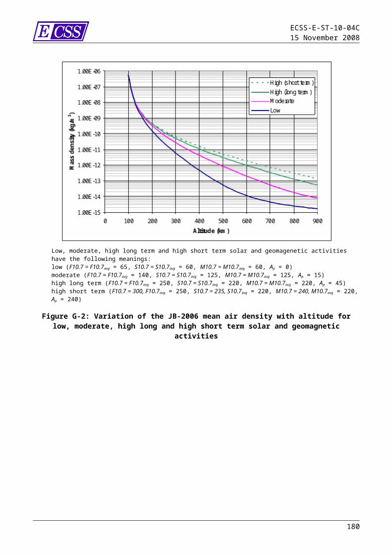
ECSS-E-ST-10-04C15 November 2008
Annex J (informative)Space debris and meteoroids
J.1 Reference data
J.1.1 Trackable space debrisThe given information on the catalogued space debris population was obtained from the DISCOS [RD.87] database. The figures show the situation in September 2008. The time evolution of the number of trackable objects in orbit is shown in Figure J-1.The altitude dependence for the lower altitudes is given in Figure J-2.The object distribution as function of their inclination is plotted in Figure J-3. A concentration at certain inclinations is clearly visible.
J.1.2 Reference flux data for space debris and meteoroids Cumulative meteoroid and space debris fluxes (i.e. fluxes of particles of given size or larger) can be obtained directly from the flux models. Figure J-2 to Table J-5 give results from the models specified in the normative part of the document for specific orbits.Figure J-2 gives the number of impacts m-2 yr-1 to a randomly oriented plate for a range of minimum particle sizes. The MASTER-2005 model was used for the debris and meteoroid fluxes. The results are for an altitude h = 400 km, inclination i = 51,6, and the epoch May 1st, 2005. Table J-3 gives the same results for a polar reference orbit (h = 800 km, i = 98, all other parameters are as for Table J-2).Table J-4 gives the number of impacts at the geostationary altitude (h = 36 000 km). Table J-5 gives the number of impacts m-2 yr-1 to a randomly oriented plate for a range of minimum particle sizes/masses. The meteoroid model from 10.2.4.1 was used. A position outside the Earth’s influence on the meteoroid flux was selected (i.e. no shielding and no gravitational focusing was considered), e.g. the Earth Lagrange points.Table J-6 gives flux enhancement and shielding factors for sporadic meteoroid fluxes encountered by spacecraft in typical Earth orbits. The procedure described in C.1 was used.For various distances from Earth, Figure J-4 gives the meteoroid velocity distributions and average velocities as modified by the gravitational attraction of Earth according to the procedure described in C.1.2.
180
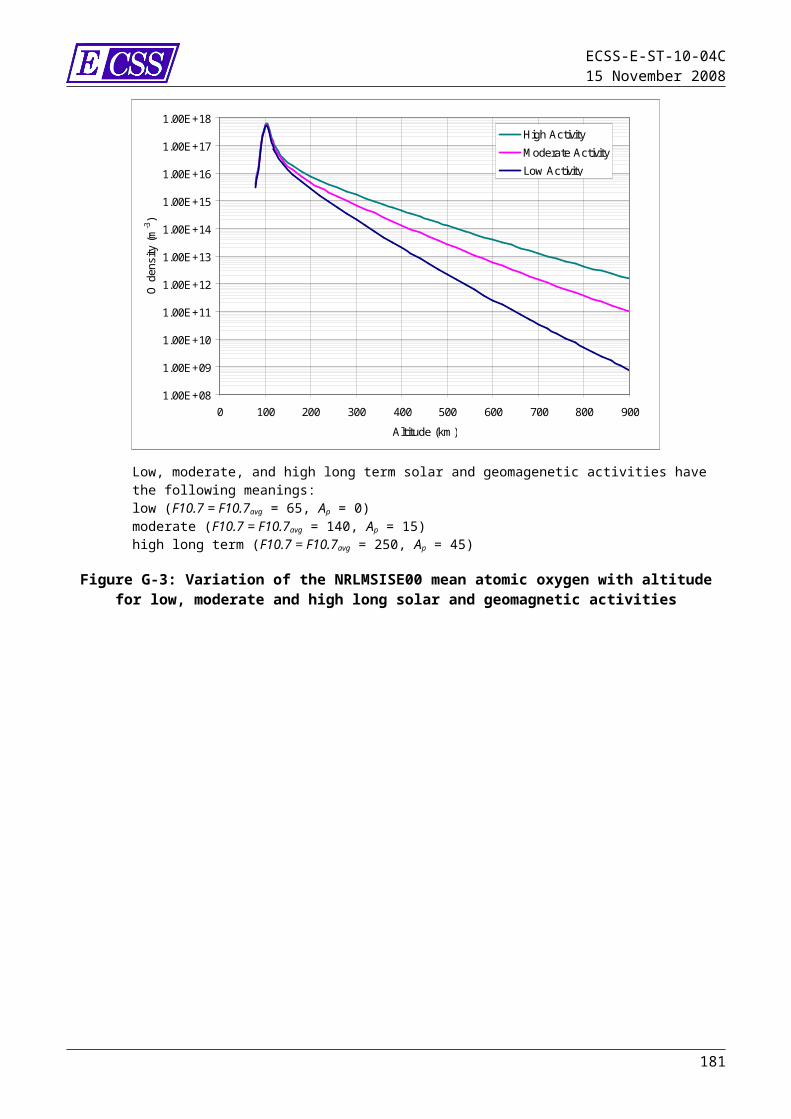
ECSS-E-ST-10-04C15 November 2008
J.2 Additional information on flux models
J.2.1 Meteoroids
J.2.1.1. Meteoroids directionalityThe meteoroid flux model given in 10.2.4 assumes an isotropic flux with respect to the Earth surface. For an orbiting spacecraft the Earth shielding and the spacecraft motion both introduce a directional dependence.The directionality caused by the spacecraft motion leads to increased fluxes on forward facing surfaces and to reduced fluxes on trailing surfaces. Combining the two factors approximate flux ratios for meteoroids are found for 400 km and 800 km altitudes, given in Table J-1.As resulting effects such as penetration depth or impact plasma generation also depend on parameters such as impact velocity and angle, the directional ratios for these effects can be considerably different from those given in Table J-1.
J.2.1.2. Mass density of meteoroidsThe mass density of meteoroids varies widely from about 0,15 g cm -3 to 8 g cm-3.According to reference [RD.21] the average density of micrometeoroids larger than 0,01 g is assumed to be 0,5 g cm-3. Meteoroids smaller than 10-6 g are thought to have a higher mean density of 2 g cm -3. The recommended value for masses between 10-6 g and 0,01 g is 1 g cm-3. The reference meteoroid models given in 10.2.3 and 10.2.4 are based on a mass density of 2,5 g cm-3.
However, there is still a considerable uncertainty about these densities.
J.2.1.3. Flux enhancement from gravitational attractionThe method described in C.1.2 to account for a modified velocity distribution and enhanced fluxes due to Earth’s gravitational attraction modifies the range and width of each velocity bin given in Table C-1. It is acceptable to account for this re-binning by simply oversampling the original velocity distribution, e.g. using 0,1 km s-1 steps in velocity instead of 1 km s-1 steps, and ignoring the changes in bin width but simply adding the contribution to the appropriate velocity bin. This gives approximately the same result. For example, the n(v∞) velocity distribution at 13,5 km s-1 is 4,83E-02 (from TableC-1) where this value represents the contribution from 13 to 14 km s-1. We can oversample n(v∞) by a factor of 10 such that we can assign 4,83E-03 to 10 bins between 13 and 14 km s-1. (alternatively, interpolate the n(v∞) values to produce a new 0.1 km s-1 step distribution, and renormalize it). So for example, a value of n(v∞) (or rather, nk) at 13,95 km s-1 (i.e. representing values between 13,90 to 14,00 km s-1) is 4,83E-03. Using expression (C-3), a value of v∞ = 13,95 km s-1 becomes v = 17,64 km s-1 (assuming vesc = 10,8 km s-1 which is true for LEO). Thus our n(v∞) value of 4,83E-03 gets added to the 17,6 to 17,7 km s-1 bin. Once all values of n(v∞) have been considered, the 0,1 step distribution can be converted to the final 1 km s-1 step distribution (i.e. this is then n'k).
181

ECSS-E-ST-10-04C15 November 2008
J.2.1.4. Meteoroid streamsAt peak activity stream fluxes can exceed the sporadic background fluxes by a factor five or more. Occasionally, very high fluxes (meteoroid storms, the visible meteor background flux can be exceeded by a factor 10 000 or more) can be encountered for short periods (1-2 hours). Examples of such storms are the Leonid streams in 1998, 1999 and 2001.Meteoroid streams consist of relative large particles only (mass > 10-8 g) with low density (0,5-1,0 g cm-3).
J.2.1.5. Interplanetary meteoroid modelNew interplanetary meteoroid flux models were presented in [RD.106], [RD.110] and [RD.108]. These models are based on different types of meteoroid populations whose relative contributions depend on the particle size range and the distance from the Sun. The models include directional distributions of the populations.For Earth orbits the meteoroid models predict similar total fluxes as the reference model in clause 10.2.4. In addition they include directional effects. The interplanetary meteoroid models are still in the development stage. At present no specific reference model is defined as standard.
J.2.2 Space debris flux models
J.2.2.1. MASTER-2005 space debris model
J.2.2.1.1 Overview
MASTER-2005 uses a semideterministic approach which represents the debris environment by modelling its history from the beginning of spaceflight to present [RD.88]. It considers all known source terms (launch and mission related objects, break-ups, solid rocket motor firings, release of reactor coolant during reactor core ejection by RORSAT satellites, paint flakes, ejecta and Westford needles) for the debris population and follows the orbital evolutions of the resulting particles. MASTER-2005 implements the Divine-Staubach meteoroid model [RD.108] and the seasonal meteoroid stream models from Jenniskens-McBride (see Annex C) and Cour-Palais. The space debris population at the reference epoch (May 1st, 2005) is derived from 203 on-orbit break-ups, 16 RORSAT reactor core ejections and 1 076 solid rocket motor firings.MASTER-2005 covers impactor sizes larger than 1μm for Earth-bound target orbits up to geostationary altitudes. An analysis application allows interrogating the spatial debris distribution to determine collision fluxes for an arbitrary target orbit passing through the control volume. Flux results can be analysed with respect to collision velocity magnitude, its direction (azimuth and elevation), the orbit location, and the 3D position where the flux was encountered. MASTER-2005 is provided on a DVD containing the flux database together with the analysis software and runs on all Windows and Unix as well as Linux operating systems.
182

ECSS-E-ST-10-04C15 November 2008
J.2.2.1.2 Access points
The MASTER-2005 DVD can be obtained through:ESA Space Debris Office, ESA/ESOCRobert-Bosch-Str. 5, D-64293 DarmstadtPatches can be obtained through http://www.master-2005.de/
J.2.2.1.3 Impact velocity for space debrisImpact velocities can range from 0 to about 15,5 km s-1 with an average velocity of 10 km s-1 for low inclination and of 13 km s -1 for high inclination orbits.
J.2.2.1.4 Mass density of space debris objectsThe mass density of space debris objects is a function of the object diameter and the space debris sources considered. Different sources release particles of different materials the density of which can vary between 0,01 – 4,7 g cm-3. Since different source terms dominate in different size regimes, the cumulative density averaged over all objects varies significantly with the limiting diameter. For example, objects larger than 1cm are mainly explosion fragments so that the average density of debris is close to that of aluminium (2,7 g cm-3). Objects larger than 1 μm are dominated by solid rocket motor dust (aluminium oxide, 3,5 g cm-3).
J.2.2.2. Other space debris models
J.2.2.2.1 OverviewSeveral additional space debris models exist for various ranges of applicability and different purpose. Only a subset of these is publicly available and thus of interest for this standard.For some international space programmes specific models, other than MASTER-2005, have been defined as applicable. For the International Space Station the space debris models NASA-90 [RD.21] or ORDEM-2000 [RD.107] are applicable, even for European contributions.
J.2.2.2.2 ORDEM-2000ORDEM 2000 was developed by the NASA Orbital Debris Program Office at JSC [RD.107]. It uses careful empirical estimates of the orbit populations derived from measurements, incorporating a large set of observational data with the US Space Command Catalog, the Haystack Radar, and the Long Duration Exposure Facility spacecraft returned surfaces being the three primary sources. By this, the model covers an object size range from 10 µm to 10 m and employs a new analytical technique utilizing a maximum likelihood estimator to convert observations into debris population probability distribution functions. The model describes the orbital debris environment in the low Earth orbit region between 200 and 2,000 km altitude.
J.2.2.2.3 NASA-90 modelFrom about 1990 until 1996 the NASA space debris engineering model defined in [RD.21] has been most widely used for design applications. This model is given in terms of simple analytical expressions. It is relatively easy to use and widely distributed. However, it has some known shortcomings of which the assumption of spherical orbits for all debris particles is probably the most severe. The user should be aware of its shortcomings.
183
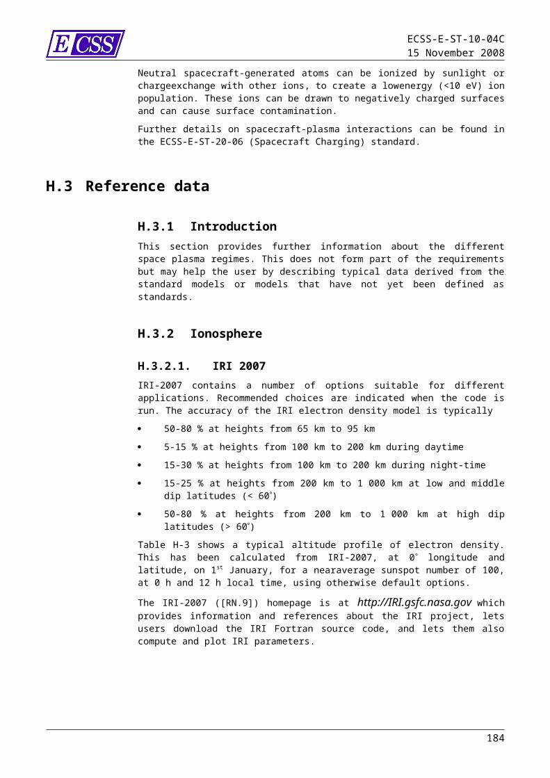
ECSS-E-ST-10-04C15 November 2008
J.2.3 Model uncertainties
J.2.3.1. GeneralThe meteoroid and space debris environment flux models given in 10 and Annex C contain several known approximations and other uncertainties.
J.2.3.2. MeteoroidsAccording to [RD.21] uncertainties in the meteoroid models mainly result from uncertainties in particle densities and masses. Fluxes for meteoroids larger than 10-6 g are well defined, but the associated masses are quite uncertain. The mass density of meteoroids spans a wide range, from about 0,15 g cm-3 to values as large as 8 g cm-3. For meteoroids flux uncertainties at a given mass are estimated to be at least a factor of 0,33 to 3.
J.2.3.3. Space debrisThe space debris flux models were developed as a best estimate rather than a conservative one. In [RD.89] the spatial density distributions as predicted by various space debris models are compared. Model predictions are not always consistent, in particular in terms of quantity and for lower debris sizes. Significant modelling related deviations can also occur between model versions.
Fluxes of sub-mm size objects in orbits below 1 000 km have short lifetimes of weeks or months. Their population depends heavily on individual generation events and can vary by an order of magnitude. Other uncertainties of debris models are the debris density and shape. A more detailed discussion of model uncertainties is given in [RD.21] and [RD.90].Considering all these factors, flux uncertainties for space debris at a given diameter are estimated to be on average at least a factor of 0,33 to 3 (as for meteoroids), and in certain size ranges even larger.
J.3 Impact risk assessment
J.3.1 Impact risk analysis procedure For a given surface area and exposure duration the total number of impacts N is obtained from the impact flux by multiplication with the total exposed surface area and exposure duration. From the number of impacts, N, the probability of exactly n impacts occurring in the corresponding time interval is determined by Poisson statistics:
(J-1)
184

ECSS-E-ST-10-04C15 November 2008
The probability for no impacts, P0 is given by:
(J-2)
For values of N << 1, the probability Q for at least one impact (Q = 1 - P0) is nearly equal to N:
(J-3)
J.3.2 Analysis complexity Typically, surface orientations and the spacecraft velocity vector as well as velocity distributions of space debris and meteoroids are considered for the calculation of fluxes.A preliminary analysis conducted on a lower level of complexity can be useful in particular when several design iterations steps are expected. In this case, a constant impact velocity of 10 km s-1 for space debris and of 20 km s-1 for meteoroids as well as a constant impact angle of 45 degrees from the surface normal are useful assumptions. These simplified assessments usually agree with a fully 3-D analysis to within a factor 2 for impact fluxes and a factor 5 for the number of impact damages.
J.3.3 Damage assessmentHere a brief general overview of damage assessment criteria and procedures is given. A more detailed and extensive description can be found in [RD.91]For each individual project the damage assessment is tailored according to the specific conditions and requirements (e.g. orbit, shielding, damage criteria, and required reliability).Any damage assessment depends to a large extend on the relevant failure criteria. Possible failure criteria include: cratering (sensor degradation, window blinding, surface erosion); larger craters (sealing problems, short circuits on solar arrays); impact generated plasma (interference, discharge triggering); impulse transfer (attitude problems); spallation from inner wall (equipment damage, crew injury); wall penetration (damage, injury, loss of liquid or air); burst, rupture (pressurized parts); structural damage.For a quantitative damage and risk assessment so called damage or design equations for the given shielding configuration are needed. They give shielding thresholds or hole sizes for given impacting particle parameters and failure mode.Sometimes scaled effective thicknesses in combination with known damage equations can be used for a first assessment.For impact damage and risk assessments secondary ejecta can be important as well. The total mass of the ejected particles can exceed the mass of the primary impactor by orders of magnitude. Secondary particles are typically ejected within a cone around the impact direction. Their velocities are typically below 2 km s-1.
185
ECSS-E-ST-10-04C15 November 2008
J.4 Analysis tools
J.4.1 GeneralSeveral numerical tools have been developed to perform impact and impact risk analyses. The following tools are mentioned for information only.
J.4.2 Deterministic analysisFor information and analysis of the deterministic, trackable space objects, the DISCOS database was developed [RD.87]. DISCOS (ESA’s Database and Information System Characterising Objects in Space) is a catalogue on Earth orbiting space objects and debris.DISCOS can be used to extract detailed data on all the tracked objects. DISCOS is implemented at and maintained by ESA/ESOC. It is accessible for registered users only.
J.4.3 Statistical analysisA statistical tool, ESABASE2/DEBRIS, was developed for a detailed impact risk assessment of smaller, nontrackable particles [RD.30]. ESABASE2/DEBRIS is a fully three dimensional numerical analysis tool including directional and geometrical effects and spacecraft shielding considerations. It is based on environment and particle/wall interaction models and includes several meteoroid and space debris flux models.The user specifies the mission, spacecraft geometry, attitude and shielding as well as the particle type, size and velocity range to be analysed. The computed output includes: the number of impacts; the resulting number of damaging impacts taking into account the
spacecraft shielding and damage assessment equations; the mean particle impact velocity (amplitude and direction); the numbers of craters of specified size; the probability of no failure.ESABASE2/DEBRIS is applicable for earth orbits and allows the optional use of several meteoroid and debris flux models. The tool includes the MASTER-2005 model and the sporadic and stream meteoroid models given in 10.2.4, including the altitude dependent velocity distribution.
J.5 TablesTable J-1: Approximate flux ratios for meteoroids
for 400 km and 800 km altitudes400 km
800 km
Front/random
2,1 2,1
Front/rear 7,7 7,2Space face / 12,0 5,5
186

ECSS-E-ST-10-04C15 November 2008
Earth face
Table J-2: Cumulative number of impacts, N, to a randomly oriented plate for a range of minimum particle sizes using the MASTER-2005 model
Diameter (cm) Ndeb (m-2yr-1) Nmet (m-2yr-1) Ntot (m-2yr-1)0,0001 1,26E+2 9,33E+2 1,06E+30,0002 5,68E+1 5,54E+2 6,11E+20,0003 4,68E+1 4,73E+2 5,19E+20,0005 2,67E+1 4,06E+2 4,33E+20,0007 1,89E+1 2,87E+2 3,06E+20,001 1,26E+1 1,85E+2 1,98E+20,002 1,09E+1 7,21E+1 8,30E+10,003 9,77E+0 3,29E+1 4,27E+10,005 6,68E+0 1,04E+1 1,70E+10,007 4,46E+0 4,63E+0 9,08E+00,01 3,29E+0 1,99E+0 5,28E+00,02 3,72E-1 3,35E-1 7,07E-10,03 2,19E-2 8,70E-2 1,09E-10,05 1,95E-3 1,68E-2 1,88E-20,07 5,04E-4 5,06E-3 5,57E-30,1 2,44E-4 1,33E-3 1,58E-30,2 6,78E-5 1,08E-4 1,75E-40,3 2,77E-5 1,72E-5 4,49E-50,5 8,48E-6 2,86E-6 1,13E-50,7 3,80E-6 7,46E-7 4,55E-61,0 1,42E-6 1,57E-7 1,58E-62,0 3,89E-7 - 3,89E-73,0 1,79E-7 - 1,79E-75,0 1,34E-7 - 1,34E-710,0 1,29E-7 - 1,29E-7NOTE: The results are for an altitude h = 400 km, inclination i = 51,6, and the epoch
May 1st, 2005. For meteoroids a density of = 2,5 g cm-3 was used to convert masses to diameters.
187

ECSS-E-ST-10-04C15 November 2008
Table J-3: Cumulative number of impacts, N, to a randomly oriented plate for a range of minimum particle sizes using the MASTER-2005 model
Diameter (cm) Ndeb (m-2yr-1) Nmet (m-2yr-1) Ntot (m-2yr-1)0,0001 3,41E+3 9,97E+2 4,41E+30,0002 2,09E+3 6,01E+2 2,69E+30,0003 1,81E+3 5,16E+2 2,33E+30,0005 1,48E+3 4,44E+2 1,93E+30,0007 1,31E+3 3,14E+2 1,63E+30,001 9,25E+2 2,03E+2 1,13E+30,002 4,22E+2 7,88E+1 5,01E+20,003 2,34E+2 3,60E+1 2,70E+20,005 1,24E+2 1,13E+1 1,35E+20,007 7,67E+1 4,98E+0 8,17E+10,01 3,88E+1 2,15E+0 4,10E+10,02 4,87E+0 3,61E-1 5,23E+00,03 6,10E-1 9,28E-2 7,03E-10,05 2,76E-2 1,75E-2 4,50E-20,07 4,52E-3 5,24E-3 9,76E-30,1 1,51E-3 1,37E-3 2,89E-30,2 4,79E-4 1,14E-4 5,93E-40,3 2,78E-4 1,82E-5 2,96E-40,5 1,06E-4 2,88E-6 1,09E-40,7 6,81E-5 7,50E-7 6,89E-51,0 3,53E-5 1,60E-7 3,55E-52,0 1,11E-5 - 1,15E-53,0 7,80E-6 - 7,80E-65,0 4,60E-6 - 4,60E-610,0 3,19E-6 - 3,19E-6NOTE:The results are for an altitude h = 800 km, inclination i = 98, and the epoch
May 1st, 2005. For meteoroids a density of = 2,5 g cm-3 was used to convert masses to diameters.
Table J-4: Cumulative number of impacts, N, to a randomly oriented plate for a range of minimum particle sizes using the MASTER-2005 model
Diameter (cm) Ndeb (m-2yr-1) Nmet (m-2yr-1) Ntot (m-2yr-1)0,0001 1,37E+2 7,39E+2 8,76E+20,0002 3,99E+1 4,34E+2 4,74E+20,0003 3,59E+1 3,68E+2 4,04E+20,0005 1,26E+1 3,16E+2 3,28E+20,0007 6,64E+0 2,23E+2 2,30E+20,001 3,31E+0 1,44E+2 1,47E+20,002 2,02E+0 5,59E+1 5,79E+10,003 1,38E+0 2,56E+1 2,70E+10,005 1,00E+0 7,97E+0 8,98E+0
188

ECSS-E-ST-10-04C15 November 2008
Diameter (cm) Ndeb (m-2yr-1) Nmet (m-2yr-1) Ntot (m-2yr-1)0,007 7,59E-1 3,52E+0 4,27E+00,01 4,98E-1 1,48E+0 1,98E+00,02 1,17E-1 2,46E-1 3,63E-10,03 2,55E-2 6,21E-2 8,76E-20,05 1,38E-3 1,12E-2 1,26E-20,07 1,36E-4 3,39E-3 3,52E-30,1 2,40E-5 8,86E-4 9,10E-40,2 2,60E-6 7,53E-5 7,79E-50,3 1,02E-6 1,07E-5 1,17E-50,5 2,22E-7 1,74E-6 1,96E-60,7 1,23E-7 4,53E-7 5,76E-71,0 5,86E-8 9,64E-8 1,55E-72,0 1,75E-8 - 1,75E-83,0 1,08E-8 - 1,08E-85,0 6,48E-9 - 6,48E-910,0 5,38E-9 - 5,38E-9NOTE: The results are for an altitude h = 35 786 km, inclination i = 0,5, and the epoch
May 1st, 2005. For meteoroids a density of = 2,5 g cm-3 was used to convert masses to diameters
Table J-5: Cumulative number of impacts, N, to a randomly oriented plate for a range of minimum particle masses
Mass (g) Diameter (cm)
Nmet (m-2yr-1)
1,00E-12 9,14E-5 1,09E+35,00E-12 1,56E-4 6,11E+21,00E-11 1,97E-4 4,71E+25,00E-11 3,37E-4 2,57E+21,00E-10 4,24E-4 2,02E+25,00E-10 7,26E-4 1,20E+21,00E-9 9,14E-4 9,51E+15,00E-9 1,56E-3 5,15E+11,00E-8 1,97E-3 3,74E+15,00E-8 3,37E-3 1,51E+11,00E-7 4,24E-3 9,54E+05,00E-7 7,26E-3 2,75E+01,00E-6 9,14E-3 1,49E+05,00E-6 1,56E-2 3,07E-11,00E-5 1,97E-2 1,47E-15,00E-5 3,37E-2 2,36E-21,00E-4 4,24E-2 1,04E-25,00E-4 7,26E-2 1,43E-31,00E-3 9,14E-2 5,97E-4
189
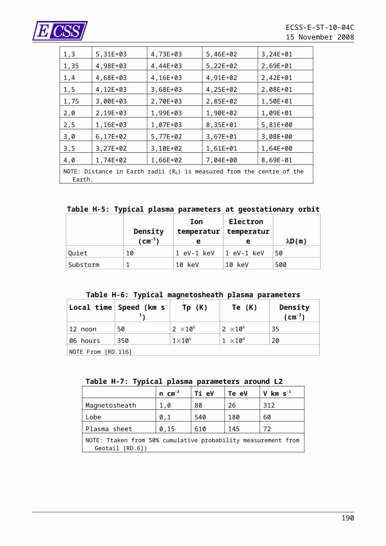
ECSS-E-ST-10-04C15 November 2008
Mass (g) Diameter (cm)
Nmet (m-2yr-1)
5,00E-3 1,56E-1 7,57E-51,00E-2 1,97E-1 3,07E-55,00E-2 3,37E-1 3,72E-61,00E-1 4,24E-1 1,49E-65,00E-1 7,26E-1 1,77E-71,00E+0 9,14E-1 7,02E-85,00E+0 1,56E+0 8,22E-91,00E+1 1,97E+0 3,26E-95,00E+1 3,37E+0 3,79E-101,00E+2 4,24E+0 1,50E-105,00E+2 7,26E+0 1,74E-11NOTE 1: The meteoroid model specified in 10.2.4.1 was
used.NOTE 2: The results are for an object located outside the
Earth’s influence (no gravitational focusing and no shielding, e.g. Earth Lagrange Points).
NOTE 3: A density of = 2,5 g cm-3 was used to convert masses to diameters
190

ECSS-E-ST-10-04C15 November 2008
Table J-6: Parameters (appearing in Eq. (C-15) to account for modified meteoroid fluxes encountered by spacecraft in circular Earth orbits at various
altitudesAltitude [km] sf K
100 2,04 0,50 1,09200 2,03 0,58 1,09400 2,00 0,63 1,09800 1,94 0,70 1,08
1 000 1,92 0,72 1,082 000 1,81 0,79 1,084 000 1,65 0,87 1,07
10 000 1,41 0,95 1,0520 000 1,26 0,98 1,04
35 790 (GEO) 1,16 0,99 1,03100 000 1,06 1,00 1,01At 1 AU 1,00 1,00 1,00
NOTE: is the weighted mean gravitational enhancement factor for the velocity distribution of Table C-1. The factor sf accounts for the geometrical shielding of Earth. K gives the flux enhancement for a randomly tumbling plate that result from the spacecraft motion itself.
J.6 Figures
0
2000
4000
6000
8000
10000
12000
14000
1958 1964 1970 1976 1982 1988 1994 2000 2006
NU
MB
ER
YEAR
Catalogued Objects in Orbit as of September 2008
OTHER OBJECTSESA OBJECTSUSA OBJECTS
USSR/CIS OBJECTS
Figure J-1: Time evolution of the number of trackable objects in orbit (as of September 2008)
191

ECSS-E-ST-10-04C15 November 2008
Figure J-2: Semi-major axis distribution of trackable objects in LEO orbits (as of September 2008)
Figure J-3: Distribution of trackable objects as function of their inclination (as of September 2008)
192
ECSS-E-ST-10-04C15 November 2008
Taylor/HRMP velocity distributions
0
0.01
0.02
0.03
0.04
0.05
0.06
0.07
0 10 20 30 40 50 60 70 80
Impact velocity [km/s]
Nor
mal
ised
vel
ocity
dis
tribu
tion
[--] ISS
Sun Synchronous
Geostationay
L 2
NOTE: ‘ISS’ corresponds to: 400 km, ‘Sun-Synchronous’: 1 500 km, ‘Geostationary’: 36 000. ‘L2’ corresponds to the distribution at 1 AU without Earth attraction. The gravitational attraction of Earth shifts the distribution to higher velocities. Average velocities are: 22,7 km/s at 400 km, 21,7 km/s at 1 500 km, 18,8 km/s at 36 000 km and 17,2 km/s outside of the influence of Earth
Figure J-4: The HRMP velocity distribution for different altitudes from the Earth surface. .
193

ECSS-E-ST-10-04C15 November 2008
Annex K (informative)Contamination modelling and tools
K.1 Models
K.1.1 OverviewGenerally, outgassing/condensation models take into account the data of outgassing or mass flow rates, surface accommodation and sticking coefficients as obtained by e.g. the VBQCtest [RD.92] or the ASTM E1559 test [RD.109].
K.1.2 Sources
K.1.2.1. OutgassingFor a material that outgassses at a constant rate, independently of the quantity present, such as e.g. during evaporation or sublimation from a bulk, the process is described as a zero order reaction.
(K-1)
where
is the outgassing rate (g cm-2s-1);
k is the reaction constant.
The weightloss through evaporation, at a temperature T is given by [RD.93]
(K-2)
where
is the weight loss per unit area in g cm-2s-1;
Ps is the vapour pressure in hPa;M is the molecular mass;T is the temperature in K.
194

ECSS-E-ST-10-04C15 November 2008
The outgassing is often described as a first order reaction [RD.93], i.e. the material outgasses at a rate that is proportional to the mass available, and using Arrhenius law temperature dependency. Important parameters for the outgassing rate are temperature, exposed surface area (or the surface available for evaporation), surface morphology, dimensions of the material (characteristic dimension, thickness).
(K-3)
The factor k can be seen as a measure for the temperature dependent time constant () of the outgassing phenomenon.
(K-4)
Integration of
(K-5)
gives
(K-6)
Assuming the Arrhenius relation to be valid
(K-7)
it is possible to determine the outgassing as function of temperature.The mass loss can be expressed as
(K-8)
K.1.2.2. PlumesEvaluation of plumes of thrusters or vents is often described by specific application related models. Parametric descriptions of plumes constitute an interesting alternative to spacecraft designers.The mass flux of a plume can be expressed in the most generic form
(K-9)
where(r, ) is the flux at a given position from the vent;r is the radial distance from the vent; is the angle from the centerline of the vent;
is the mass flow from the vent;
where, moreover, the function f depends on the plume type. However this formula can in general be reduced in a good approximation to the product
195
ECSS-E-ST-10-04C15 November 2008
(K-10)
whereA is a normalization coefficient.
For a thruster, the function f1 is peaked around = 0 and can be expressed as a sum of decreasing exponentials [RD.94] or as a (high) power law of cos() or both [RD.95]. It is in some extent specific of each thruster.Plumes from vents are more standard and the f1 function can consequently be fixed: the mass flux is approximated by the following engineering model:
(K-11)
where 1 n 2 is used for space station design. Their divergence is larger than that of thrusters.
K.1.3 Transport of molecular contaminants
K.1.3.1. Transport between surfaces
K.1.3.1.1 GeneralThe following clauses only deal with the methods and models for transport of neutral molecules. There is no available model of ion transport devoted to contamination. Three levels of complexity and accuracy in modelling the transport of neutral molecular contaminants can be distinguished.
K.1.3.1.2 Simplest view factorsThis model simulates collisionless transport. In such a case the fraction of contaminants coming from surface j to surface i is given by the view factor Vij
of surface i seen from surface j (including the cosine factor coming from the Lambertian emission law). These view factors are similar to the ones of radiative thermal analysis. They can be computed geometrically or by Monte Carlo ray tracing. The incident mass rate on a surface i is then given by
(K-12)
whereSj sticking coefficient on surface jj runs over all surfaces and
denotes the outgassing mass rate of surface j.
K.1.3.1.3 Simplified Monte CarloCollisions of contaminants are simulated in a simplified way; the density and speed of possible partners for molecular collisions are given a priori:
196
ECSS-E-ST-10-04C15 November 2008
for ambient scatter, the ambient density and speed are easily known, but wakes (or “shades”) are usually not treated;
for selfscatter, the contaminant density is very simplified and usually taken proportional to r-2 and with spherical symmetry.
This method is usually limited to one collision per molecule because the uncertainties due to the densities given a priori increase with collision number. This effective view factors can conveniently be computed by Monte Carlo raytracing method.Both methods (K.1.3.1.2 and K.1.3.1.3) can include other contaminant sources such as vents and plumes. The view factors are then replaced by interception factors.
K.1.3.1.4 True Monte Carlo (Direct Simulation Monte Carlo, DSMC)This computes multiple collisions in a realistic way. The collision probabilities are computed autocoherently from the densities given by the simulation. This method is more time consuming and requires more work for programming (in particular, it requires a meshing of volume and not only of spacecraft surfaces).Either method can be better suited, depending on the spacecraft configuration. A potential contamination of a sensitive protected surface through multiple collisions requires a precise DSMC simulation. In simpler cases, when contamination essentially happens in lineofsight, it is more appropriate to use the less timeconsuming and more widespread methods of K.1.2.1.2 and K.1.2.1.3.
K.1.3.2. Surface transportReflections on surfaces and reevaporation are easy to implement and are usually included in models, the latter (reevaporation) often as part of the outgassing process. Migrations on surfaces on the contrary are complex processes and there is no commercial available model.
K.1.3.3. Transport of particlesAs mentioned in 11.1.5 particulate transport is governed by several phenomena: a. atmospheric dragb. solar radiation pressurec. differential gravitational effects (with respect to spacecraft) which
result in tide effectsd. particulate charging and subsequent electrostatic effectsAmong which the first three can be computed by methods similar to spacecraft orbit computing, whereas point d. requires specific modelling to access particulate charging in a plasma and potential map around spacecraft. The dominant phenomena are most commonly modelled: point a. atmospheric drag, first, and also point d. that gets important in GEO. Points b. and c. can become dominant in cases when points a. and d. become small (high altitude and no charging).A last aspect of particulate transport is their interaction with walls. Sticking and accommodation coefficients are, however, very difficult to assess.Most particulate contamination models remain in the field of research. Very few of them seem to be transferable to other users.
197

ECSS-E-ST-10-04C15 November 2008
K.2 Contamination tools
K.2.1 OverviewThe computer codes dedicated to spacecraft contamination are presented here. COMOVA and ESABASE were developed in Europe and are available to Europeans. COMOVA is more recent and has extra modelling capabilities concerning transport, while ESABASE also embeds plume models. TRICONTAM is specifically dedicated to plume modelling.
K.2.2 COMOVA: COntamination MOdelling and Vent Analysis
COMOVA was developed by ONERA (physics) and HTS AG (interfaces) under ESA sponsorship. It is now distributed since the year 2002 by ONERA (see http://www-mip.onera.fr/comova). It covers the physical modelling of the following sources: Outgassing: it follows the European physical approach of residence
time (same model and database as OUTGASSING) Venting: vents can be modelled either similarly to an outgassing source
(hence representative of the efflux from an outgassing cavity) or as commanded (then more representative of purging)
Molecular transport is especially sophisticated. It takes into account: Deposition and reemission (the latter being modelled through
"reemission residence time") Reflections on surfaces Gas phase reflections (self and ambient scattering) with a BGK model
using realistic densities for ambient and outgassed speciesPre and post processing for COMOVA are done in external tools with which COMOVA is interfaced (FEMAP and I-DEAS). One hierarchy level of kinematics modelling, i.e. modelling of moving parts is also enabled, as the relative motion or pointing of sub models with respect to the main model along the orbit
K.2.3 ESABASE: OUTGASSING, PLUME-PLUMFLOW and CONTAMINE modules
ESABASE is a general spacecraft modelling tool including several modules developed by several parties under ESA sponsorship. ESABASE essentially deals with contamination through its OUTGASSING module, developed by Matra Marconi Space (MMS). It allows computation of contaminant deposit on spacecraft by numerical integration:The PLUME module currently implemented in ESABASE simulates thruster plume expansion. It was derived from CONTAM code and does not correctly model plume backflow. It is thus essentially used for forces and torques, and thermal analysis.The module called CONTAMINE computes surface interactions (adsorption, diffuse reflection, specular reflection) and, above all, surface effects: modification of thermooptical, electrical and mechanical properties, or global output power reduction for solar cells. These property changes are either
198

ECSS-E-ST-10-04C15 November 2008
taken from data gathered in a data base included in CONTAMINE (with interpolation between available data, which are not always very numerous), or complex index computed. It can also be interfaced with the older OUTGASSING module to compute deposit thickness including reemission.
K.2.4 TRICONTAM TRICONTAM is a global contamination model developed at Technical University Hamburg Harburg (TUHH), Germany [RD.96]. It seems to be essentially devoted to computing contamination from thruster plume exhausts. The plume flowfield is computed by an improved version of CONTAM III (CONTAM III is an older code essentially concerning transient combustion processes and chemistry), and the contaminant transport to spacecraft surfaces is assumed to be collisionless. An important part of the software is dedicated to forces, torques and thermal analysis.The major interest of that code is that its results were compared to the numerous experimental measurements realized at TUHH [RD.97].
199
ECSS-E-ST-10-04C15 November 2008
Bibliography
ECSS-S-ST-00 ECSS system – Description, implementation and general requirements
ECSS-E-ST-10 Space engineering – System engineering general requirements
ECSS-E-ST-10-12
Space engineering – Methods for the calculation of radiation received and its effects and a policy for design margins
ECSS-Q-ST-70-01
Space product assurance – Contamination and cleanliness control
ECSS-E-ST-20-06
Spacecraft engineering – Spacecraft charging
[RD.1] Montenbruck, O., Gill, E.; Satellite Orbits Models, Methods, Applications; Springer, Berlin-Heidelberg-New York, 2000
[RD.2] ASTM E 490 – 00a, Standard Solar Constant and Zero Air Mass Solar Spectral Irradiance Tables, © ASTM, 100 Barr Harbor Drive, West Conshohocken, PA 19428-2959 (2000).
[RD.3] ISO 21348 “Space System - Space environment – Solar irradiance determinations,” 2007.
[RD.4] Solar Cycle 24 Prediction Panel (at NOAA Space Environment Center (SEC) http://www.swpc.noaa.gov/SolarCycle/SC24/
[RD.5] K.W. Ogilvie and M.A. Coplan , Solar wind composition, U.S. National Report to IUGG, 1991-1994, Rev. Geophys. Vol. 33 Suppl., AGU, 1995, http://www.agu.org/revgeophys/ogilvi00/ogilvi00.html
[RD.6] S.W.Evans (editor), Natural Environment near the Sun/Earth-Moon L2 libration point, MSFC http://snap.lbl.gov/pub/nj_bscw.cgi/d84104/SNAP-TECH-03009.pdf
[RD.7] “Space Environment for USAF Space Vehicles”, MIL-STD-1809 (USAF), 15 Feb 1991.
[RD.8] Yeh H.C. and M.S. Gussenhoven, “The statistical Electron Environment for Defense Meteorological Satellite Program Eclipse Charging”, J. Geophys. Res., pp.7705-7715, 1987.
[RD.9] Gussenhoven M.S, D.A. Hardy, F. Rich, W.J. Burke and H.C. Yeh, “HighLevel Spacecraft Charging in the LowAltitude Polar Auroral Environment”, J. Geophys. Res., pp.11009-11023, 1985.
[RD.10] Solar Wind Radial and Latitudinal Variations From Pole-to-Pole Ulysses Radio measurements, K. Issautier, N. Meyer-Vernet, S. Hoang, M. Moncuquet
[RD.11] H.B. Garrett and A .R. Hoffman , ‘Comparison of Spacecraft Charging Environments at the Earth, Jupiter, and Saturn’, IEEE Trans. Plasma Science, Vol.28, No.6, p.2048, 2000
[RD.12] Hess W.N., “The Radiation Belt and Magnetosphere”, Blaisdell Publ. Co.,1968.[RD.13] ICRP, “1990 Recommendations of the International Commission on
Radiological Protection”, ICRP Publication 60, Annals of the ICRP 21, 1-3 ISBN: 0-08-041144-4, Pergamon Press, NY and Oxford, 1991.
200
ECSS-E-ST-10-04C15 November 2008
[RD.14] Lemaire J., A.D. Johnstone, D. Heynderickx, D.J. Rodgers, S. Szita and V. Pierrard, “Trapped Radiation Environment Model Development (TREND2)” Final Report of ESA Contr. 9828, Aeronomica Acta 393-1995, Institut d’Aeronomie Spatiale de Belgique/Belgisch Institut voor RuimteAeornomie, ISSN 0065-3713, 1995.
[RD.15] P. Nieminen, “On the energy spectra and occurrence rate of solar electron events”, Proc. of Space Radiation workshop, DERA, Nov. 1999.
[RD.16] J.I. Minow, L. N.Parker, R.L. Altstatt, W.C. Blackwell, Jr, A. Diekmann, “Radiation and internal charging environments for thin dielectrics in interplanetary space”, Proc. of 9th Spacecraft Charging Technology Conf., Tsukuba, 2005.
[RD.17] F Lei, S Clucas, C Dyer, P Truscott, An atmospheric radiation model based on response matrices generated by detailed Monte Carlo simulations of cosmic ray interactions, IEEE Transactions in Nuclear Science, Vol 51, No 6, pp 3442-3451, Dec 2004.
[RD.18] F Lei, A Hands, C Dyer, P Truscott, Improvements to and Validations of the QinetiQ Atmospheric Radiation Model (QARM), IEEE Transactions on Nuclear Science Vol. 53, No. 4, pp 1851-1858, Aug. 2006.
[RD.19] Evans R.W, and H.B.Garrett, Modeling Jupiter’s Internal Electrostatic Discharge Environment, J.Spacecraft&Rockets, Vol.39, No.6, p.926, 2002
[RD.20] Divine, N. and H. Garrett, Charged particle distribution in Jupiter's magnetosphere. J. Geophys. Res. 88, 6889-6903 (1983)
[RD.21] Anderson B.J., “Natural Orbital Environment Guidelines for Use in Aerospace Vehicle Development”, by:, editor and R.E. Smith, compiler; NASA TM 4527, chapter 7, June 1994.
[RD.22] Grün E., H.A. Zook, H. Fechtig and R.H. Giese, “Collisional Balance of the Meteoritic Complex”, Icarus, Vol. 62, p.244, 1985.
[RD.23] ECSS-Q-ST-70-02, Space product assurance: Thermal vacuum outgassing test for the screening of space materials.
[RD.24] ASTM E-595, Method for Total Mass Loss and Collected Volatile Condensable Materials from outgassing in a vacuum environment.
[RD.25] S.L. Huston*, Space Environments and Effects: Trapped Proton Model, NASA/CR-2002-211784, 2002
[RD.26] Singley G.W. and I. Vette J.I., “The AE-4 Model of the Outer Radiation Zone Electron Environment”, NSSDC/WDC-A-R&S 72-06, NASA-GSFC, 1972.
[RD.27] Taylor, A.D. The Harvard Radio Meteor Project meteor velocity distribution reappraised, Icarus, 116: 154-158, 1995
[RD.28] McBride, N., “The importance of the annual meteoroid streams to spacecraft and their detectors”, Adv. In Space Research, Vol. 20, pp 1513 –1516, 1997.
[RD.29] Jenniskens P., “Meteor Stream Activity”, Astron. Astrophys. Vol. 287, pp 990-1013, 1994.
[RD.30] Eta_max space, “ESABASE2/DEBRIS, Technical Description”, ref. r040_rep025_02_00_01, July 2006.
[RD.31] Kaula, W.M.; 1966 Theory of Satellite Geodesy, Waltham & Blaisdell[RD.32] Sibeck, D. G., R. E. Lopez, and E. C. Roelof (1991), Solar wind control of the
magnetopause shape, location and motion, J. Geophys. Res, 96, 5489.[RD.33] E 490 – 00a, Standard Solar Constant and Zero Air Mass Solar Spectral
Irradiance Tables, © ASTM, 100 Barr Harbor Drive, West Conshohocken, PA 19428-2959 (2000).
201

ECSS-E-ST-10-04C15 November 2008
[RD.34] Knocke, P.C.; Ries, J.C.; Tapley, B.D., Earth Radiation Pressure Effects on Satellites, AIAA-1988-4292, AIAA/AAS Astrodynamics Conference, Minneapolis/MN, Aug 15-17, 1988
[RD.35] a) Hedin, A. E., Salah, J.E.., Evans, J.V., Reber, C. A., Newton, G. P., Spencer, N. W., Kayser, D.C., Alcayde, D., Bauer, P., Cogger, L., and McClure, J.P., “A Global Thermospheric Model Based on Mass Spectrometer and Incoherent Scatter Data: MSIS 1. N2 density and temperature. ”, J. Geophys. Res., Vol. 82, pp. 2139-2147, 1977. b)Hedin, A. E., Reber, C. A., Newton, G. P., Spencer, N. W., Brinton, H. C., Mayr, H. G., and Potter, W. E., “A Global Thermospheric Model Based on Mass Spectrometer and Incoherent Scatter Data: MSIS 2. Composition”, J. Geophys. Res., Vol. 82, pp. 2148-2156, 1977.
[RD.36] Hedin, H.E., Reber, C. A., Spencer, N. W., Brinton, H. C. and Kayser, D. C., "Global Model of Longitude/UT Variations in Thermospheric Composition and Temperature Based on Mass Spectrometer Data”, J. Geophys. Res., Vol. 84, 1979 p.1.
[RD.37] Hedin, A. E., “A Revised Thermospheric Model Based on Mass Spectrometer and Incoherent Scatter Data: MSIS-83,” J. Geophys. Res., Vol. 88, 1983, p., 10170.
[RD.38] Hedin, A. E., “MSIS-86 Thermospheric Model,” J. Geophys. Res., Vol. 92, 1987, p. 4649.
[RD.39] Hedin, A. E., “Extension of the MSIS Thermosphere Model into the Middle and Lower Atmosphere,” J. Geophys. Res., Vol. 96, 1991, p. 1159.
[RD.40] Bowman, B. R., Marcos, F. A. and Kendra, M. J., “A Method for Computing Accurate Daily Atmospheric Density Values from Satellite Drag Data”, AAS-04-173, AAS/AIAA Flight Mechanics Meeting, Maui, HI, 2004.
[RD.41] Angelatsi Coll, M., et al., The first Mars thermospheric general circulation model: The Martian atmosphere from the ground to 240 km, Geophysical Research Letters, Volume 32, Issue 4, CiteID L04201, 2005.
[RD.42] Hedin, A. E., N. W. Spencer, and T. L. Killeen, Empirical Global Model of Upper Thermosphere Winds Based on Atmosphere and Dynamics Explorer Satellite Data, J. Geophys. Res., 93, 9959- 9978, 1988.
[RD.43] Flasar, F.M. et al, An intense stratospheric jet on Jupiter, Nature, 427,132-135, 2004.
[RD.44] Bagenal F., T. Dowling and W. McKinnon Ed., Jupiter, Cambridge University Press, Cambridge, 2004.
[RD.45] Friedson A.J., New observations and modelling of a QBO-like oscillation in Jupiter’s stratosphere, Icarus, 137, 34-55, 1999.
[RD.46] Young L., et al., Gravity waves in Jupiter’s stratosphere, as measured by the Galileo ASI experiment, Icarus, 173,185-199,2005.
[RD.47] Kliore A.J., V.I Moroz and G.M. Keating Ed., The Venus International Reference atmosphere, Advances in Space Research, 5, 11, 1985.
[RD.48] Mars transportation environment définition document, M. Alexander Ed., NASA/TM-2001-210935.
[RD.49] Justus, C.G. and Johnson, D.L., Mars Global Reference Atmospheric Model 2001 Version (Mars-GRAM 2001) Users Guide, NASA/TM-2001-210961, April, 2001.
[RD.50] Justus, C.G., et al. Mars-GRAM 2000: A Mars Atmospheric Model for Engineering Applications, Advances in Space Research, Vol. 29, 193-202, 2002.
[RD.51] Forget, F., F. Hourdin, R. Fournier, C. Hourdin, O. Talagrand, M. Collins, S. R. Lewis, P.L. Read, J-P Huot, Improved General Circulation Models of the
202

ECSS-E-ST-10-04C15 November 2008
Martian Atmosphere from the Surface to Above 80 km, J. Geophys. Res. Vol. 104, No. E10, p. 24,155-24,176, 1999.
[RD.52] Justus, C.G., Duvall, A.L., and Johnson, D.L., Engineering-Level Model Atmospheres for Titan and Neptune, AIAA-2003-4803, 39th AIAA/ASME/ SAE/ASEE Joint Propulsion Conference, Huntsville, Alabama, July 20-23, 2003.
[RD.53] Purvis C.K, H.B. Garrett, A.C. Whittlesey and N.J. Stevens, “Design Guidelines for Assessing and Controlling Spacecraft Charging Effects”, NASA TP-2361, 1984.
[RD.54] Burke W.J., D.A. Hardy and R.P. Vancour, “Magnetospheric and High Latitude Ionospheric Electrodynamics”, Chapter 8 of “Handbook of Geophysics and the Space Environment”, Ed. A. Uram, USAF, 1985.
[RD.55] Scialdone J.J., “An Estimate of the Outgassing of Space Payloads and Its Gaseous Influence on the Environment”, J. Spacecraft and Rockets, 23, p.373, 1986.
[RD.56] Huebner W.F. and P.T. Giguere, “A Model of Comet Comae II. Effects of Solar Photodissociative Ionization”, Astrophys. J., 238, p.753, 1980.
[RD.57] Huddleston D.E., A.D. Johnstone and A.J. Coates, “Determination of Comet Halley Gas Emission Characteristics from Mass Loading of the Solar Wind”, J. Geophys. Res., 95, p.21, 1990.
[RD.58] Belian, R.D., T.E. Cayton, R.A. Christensen, J.C. Ingraham, M.M. Meier, G.D. Reeves and A.J. Lazarus, “Relativistic electrons in the outerzone: An 11year cycle; their relation to the solar wind”, Proceedings of the Taos Workshop on the Earth’s Trapped Particle Environment, Ed, G.D. Reeves, AIP Conference Proceedings 383, 13-18, ISBN 1-56396-540-2, 1986.
[RD.59] SPENVIS: http://www.spenvis.oma.be/spenvis/[RD.60] OMERE: http://www.trad.fr/[RD.61] Brautigam, D. H., and J. T. Bell, CRRESELE Documentation, PL-TR-95-2128,
Environmental Research Papers, 1178, Phillips Laboratory, 1995.[RD.62] Meffert, J. D., and M. S. Gussenhoven, CRRESPRO Documentation, PL-TR-
94-2218, Environmental Research Papers, 1158, Phillips Laboratory, 1994.[RD.63] Watts J.W., T.A. Parnell and H.H. Heckman, “Approximate Angular
Distribution and Spectra for Geomagnetically Trapped Protons in LowEarth Orbit”, in “HighEnergy Radiation Background in Space”, AIP Conference Proceedings 186, AIP, NewYork, 1989.
[RD.64] Kruglanski M. and J. Lemaire, “Trapped Proton Anisotropy at Low Altitude”, Technical Note 6, ESA/ESTEC/WMA Contr. 10725, Institut d’Aeronomie Spatiale de Belgique, 1996.
[RD.65] Bühler P., A. Zehnder, E. Daly and L. Adams, “REM Measurements onBoard MIR in 1995”, Advances in Space Research 21, 1645 (1998)
[RD.66] Tranquille C, “Extension to AE-4 Local Time and Statistical Models for Application to AE-8”, ESTEC/WMA Internal Memorandum, 1986.
[RD.67] Evans, H.D.R., D.J Rodgers, E.J. Daly, P. Nieminen, A. Mohammadzadeh, P. Buehler, W. Hajdas, “Energetic electron results from the ESA Monitors and Comparison with Existing Radiation Belt Internal Charging Models”, Spacecraft Charging Technology Conference 2007 proceedings.
[RD.68] Feynman J., T. Armstrong, L. Dao- Givner, S. Silverman, “New Interplanetary Proton Fluence Model”, J. Spacecraft, Vol 27, No. 4, July-Aug. 1990.
[RD.69] Feynman J., G. Spitale, J. Wang and S. Gabriel, “Interplanetary Proton Fluence Model: JPL 1991”, J. Geophys. Res. 98, A8, 13 281-13 294, 1993.
[RD.70] Rosenqvist, L., A. Hilgers, H. Evans, E. Daly, M. Hapgood, R. Stamper, R. Zwickl, S. Bourdarie and D. Bosher, A toolkit for updating interplanetary
203

ECSS-E-ST-10-04C15 November 2008
proton cumulated fluence models, J. Spacecraft and Rockets, Vol. 42, Number 6, Nov-Dec 2005.
[RD.71] Glover, A., A. Hilgers, L. Rosenqvist, S. Bourdarie, Interplanetary Proton Cumulated Fluence Model Update, Advances in Space Research, 2007
[RD.72] King, J.H., “Solar Proton Fluences for 1977-1983 Space Missions”, J. Spacecrafts and Rockets, 11, 401, 1974.
[RD.73] Xapsos, M.A., R J Walters, G P Summers, J L Barth, E G Stassinopoulos, S R Messenger, E A Burke,"Characterizing solar proton energy spectra for radiation effects applications," IEEE Trans. on Nucl. Sci , vol. 47, no. 6, pp 2218-2223, Dec. 2000.
[RD.74] C. S Dyer, F.Lei, S.N. Clucas, D. F. Smart, M.A. Shea, “Solar particle enhancements of single event effect rates at aircraft altitudes,” IEEE Trans. Nucl. Sci. , vol.50, no. 6, pp. 2038-2045, Dec. 2003.
[RD.75] Nymmik, R.A. Probabilistic model for fluences and peak fluxes of solar particles. Ra-diat. Meas. 30, 287-296, 1999
[RD.76] Nymmik R., Initial conditions for radiation analysis : Models of galactic cosmic rays and solar particle events, Advances in Space Research, 38 issue 6, pp 1182-1190, 2006
[RD.77] Adams, J.H., “Cosmic Ray Effects on MicroElectronics, Part IV”, NRL Memorandum Report 5901, Naval Research Laboratory, Washington DC 20375-5000, USA, 1986.
[RD.78] Tylka, A.J., et al., “CREME96: A Revision of the Cosmic Ray Effects on Micro-Electronics Code”, IEEE Trans. Nucl. Sci. NS-44, 2 150-2 160, 1997.
[RD.79] Nymmik, R.A., M.I. Panasyuk, T. I. Pervaja, and A.A. Suslov, “A Model of Galactic Cosmic Ray Fluxes”, by, Nucl. Tracks & Radiat. Meas, 20, 427-429, 1992.
[RD.80] Stassinopoulos E.G. and J.H. King, “Empirical Solar Proton Model For Orbiting Spacecraft Applications”, IEEE Trans. on Aerosp. and Elect. Systems AES-10, 442, 1973.
[RD.81] F Ait-Ouamer, A D Zych, R S White, “Atmospheric neutrons at 8.5 GV Cutoff in the Southern hemisphere,” J. Geophys. Res., Vol. 93, No. A4, pp. 2499-2510, April 1988.
[RD.82] D J Morris, H Aarts, K Bennett, J A Lockwood, M L McConnell, J M Ryan, V sconfelder, H Steinle, X Peng,” Neutron measurements in near-earth orbit with COMPTEL,” J. Geophys. Res., Vol. 100, No. A7, pp. 12243-12249, July 1995.
[RD.83] I. Jun, H.B. Garrett and R. W. Evans, High-energy trapped particle environments at Jupiter: an update IEEE Trans. Nuc. Science, V52, 2281, December 2005
[RD.84] G. De Angelis , M. S. Clowdsley, R. C. Singleterry and J. W. Wilson, A new Mars radiation environment model with visualization, Advances in Space Research, 34 Issue 6, pp 1328-1332, 2004
[RD.85] Keating, A, A. Mohammadzadeh, P. Nieminen, D. Maia, S. Coutinho, H. Evans, M. Pimenta, J-P. Huot, E. Daly, “A Model for Mars Radiation Environment Characterisation”, IEEE Trans. Nucl Sci, Vol 52, No 6. Dec 2005.
[RD.86] Desorgher, L, E. O. Flückiger, M. Gurtner, “The PLANETOCOSMICS Geant4 application”, 36th COSPAR Scientific Assembly. Held 16 - 23 July 2006, in Beijing, China. Meeting abstract from the CDROM, #2361
[RD.87] Hernandez de la Torre C., F. P. Caballero, N. Sanchez Ortiz, H. Sdunnus, H. Klinkrad, “DISCOS Database and Web Interface, Proceedings of the Third European Conference on Space Debris, ESOC, Darmstadt, ESA SP-473, 19-21 March 2001.
204
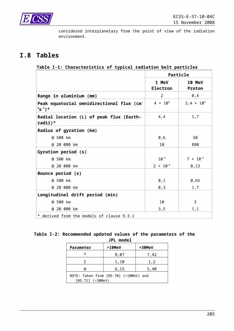
ECSS-E-ST-10-04C15 November 2008
[RD.88] Oswald, M., Stabroth, S., Wiedemann, C., Klinkrad, H., Vörsmann, P, MASTER-2005 - The Debris Risk Assessment Tool for the Space Industry, paper AIAA-2006-7219, AIAA Space 2006 Conference, San Jose, CA, USA, 2006.
[RD.89] Fukushige S., Akahoshi Y., Kitzawa Y., “Comparison of Debris Environment Models; ORDEM2000, MASTER2001 and MASTER2005”, IHI Engineering Review, Vol. 40 No.1 February 2007
[RD.90] Kessler D.J., J. Zhang, M.J. Matney, P. Eichler, R.C. Reynolds, P.D. Anz-Meador and E.G. Stansbery, “A Computer Based Orbital Debris Environment Model for Spacecraft Design and Observations in Low Earth Orbit”; NASA TM 104825, November 1996.
[RD.91] Inter-Agency Space Debris Coordination Committee, ‘Protection Manual’, IADC-WD-00-03, Version 3.3, April 2004.
[RD.92] Van Eesbeek M. and A. Zwaal, “Outgassing and contamination model based on residence time”, ESA SP232, Proc. of the 3rd European Symp. on spacecraft materials in a space environment, Noordwijk, The Netherlands, 1-4 Oct 1985.
[RD.93] Scialdone J., “Characterisation of the outgassing of spacecraft materials”, SPIE Vol. 287 Shuttle Optical Environment, 1981.
[RD.94] Trinks H., “Exhaust Plume Databook Update Version No. 3 / ESA/ESTEC Contract 7590/87/NL/TP”.
[RD.95] Simons G.A., “Effect of Nozzle Boundary Layers on Rocket Exhaust Plumes”, AIAA Journal, Tech. Notes, vol. 10, No. 11, pp. 1534-1535, 1972.
[RD.96] Trinks H., Exhaust Plume Data Handbook (EPDH IV), Progress Report IV, ESA Contract No 7510/87/NL/PP, Sept. 1991a.
[RD.97] Guernsey C. S., McGregor R. D., Bipropellant rocket exhaust plume analysis on the Galileo spacecraft, AIAA paper No 861488, AIAA/ASME/SAE/ASEE 22nd Joint Propulsion Conference, Huntsville, AL, June 1618, 1986.b.
[RD.98] Tsyganenko, N. A. (2002), A model of the near magnetosphere with a dawn-dusk asymmetry 1. Mathematical structure J. Geophys. Res., v.107(A8), doi:10.1029/2001JA000219
[RD.99] Tsyganenko, N. A., and M. I. Sitnov (2005), Modeling the dynamics of the inner magnetosphere during strong geomagnetic storms, J. Geophys. Res., v. 110 (A3), A03208, doi: 10.1029/2004JA010798.
[RD.100] Menvielle M. and A. Berthelier, “The Kderived Planetary Indices: Description and Availability”, Rev. Geophys., 29, 3, pp 415-432, August 1991.
[RD.101] Hess W.N., The Radiation Belt and the Magnetosphere, Blaisdell Publ. Co., New York, 1968.
[RD.102] McIlwain C.E., Co-ordinates for Mapping the Distribution of Geomagnetically Trapped Particles, J. Geophys. Res., 66, 3681, 1961.
[RD.103] Hilton H.H., L Parameter – A New Approximation, J. Geophys. Res., 76, 6952, 1971. (Note that this paper contains a typographical error in its expression for a3 of Eq. 5.3).
[RD.104] Xapsos M.A., Summers G.P., Barth J.L., et al.. Probability model for worst case solar proton event fluences, IEEE Trans. on Nuclear Science, 46 (6), 1481-1485, 1999
[RD.105] Xapsos M.A., Stauffer C., Jordan T., Barth J.L. and Mewaldt A., Model for Cumulative Solar Heavy Ion Energy and Linear Energy Transfer Spectra, IEEE Transactionson Nucl Science, Vol. 54, No. 6, 2007.
[RD.106] Dikarev V., E. Grün, M. Landgraf and R. Jehn, “Update of the ESA Meteoroid Model”, Proc. of 4th European Conf. on Space Debris, ESOC, 18-20 April 2005, ESA-SP-587, pp 271—276, 2005.
205
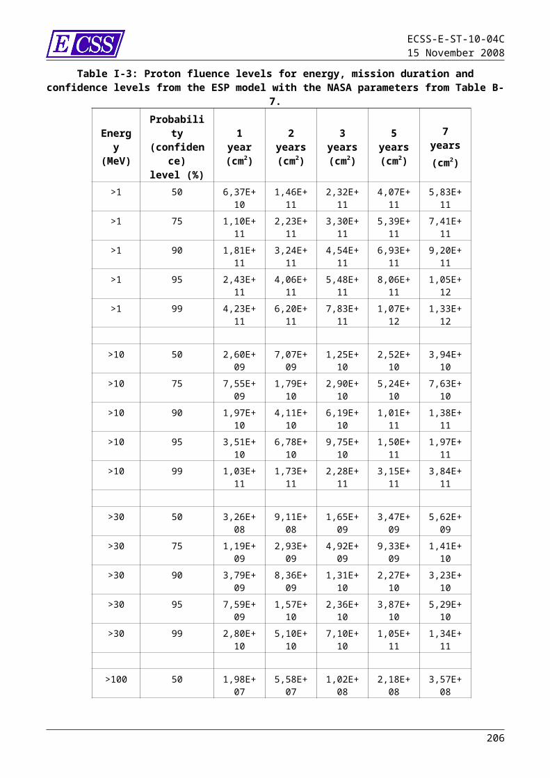
ECSS-E-ST-10-04C15 November 2008
[RD.107] Liou J.-C., M. J. Matney, P. D. Anz-Meador, D. Kessler, M. Jansen, J. R. Theall “The New NASA Orbital Debris Engineering Model ORDEM2000”, NASA/TP-2002-210780, May 2002.
[RD.108] Staubach P., E. Grün and R. Jehn, “The meteoroid environment of the Earth”, 31th COSPAR Sci. Assembly, Birmingham/UK, July, 1996.
[RD.109] ASTM E-1559, Method for contamination outgassing characteristics of space materials.
[RD.110] Jones J. “Meteoroid Engineering Model – Final Report”, SEE/CR-2004-400, NASA/MSFC, June 2004.
[RD.111] Tsyganenko, N.N., “A Magnetospheric Magnetic Field Model with a Warped Tail Current Sheet”, Planet. Space Sci. 37, 5-20, 1989.
[RD.112] Tsyganenko, N.A. (1995), Modeling the Earth's magnetospheric magnetic field confined within a realistic magnetopause, J.Geophys.Res., v.100, pp.5599-5612
[RD.113] ISO Standard “Space Systems- Model of Earth’s magnetospheric magnetic field, ISO DIS 22009, 2007.
[RD.114] Gussenhoven, M.S. and E.G. Mullen, “Geosynchronuos environment for severe spacecraft charging”, J. Spacecraft and Rockets 20, p. 26, 1988.
[RD.115] Grard R.J.L. and J.K.E. Tunaley, “Photo Electron Sheath Near a planar Probe in Interplanetary Space”, J. Geophys. Res., 76, p.2498, 1971.
[RD.116] Feynman, J., “Solar Wind”, Chapter 3 of “Handbook of Geophysics and the Space Environment”, Ed. A. Juram, USAF, 1985.
[RD.117] Christon, S.P., T.E. Eastman, T. Doke, L.A. Frank, G. Gloeckler, H. Kojima, S. Kokubun, A.T.Y. Lui, H. Matsumoto, R.W. McEntire, T. Mukai, S.R. Nylund, W.R. Paterson, E.C. Roelof, Y. Saito, T. Sotirelis, K. Tsuruda, D.J. Williams, and T. Yamamoto, "Magnetospheric Plasma Regimes Identified Using Geotail Measurements 2. Statistics, Spatial Distribution, and GeomagneticDependence,"J. Geophys. Res., 103, 23521 – 23542, 1998.
[RD.118] Heynderickx, D., J. Lemaire, and E. J. Daly, “Historical Review of the Different Procedures Used to Compute the L-Parameter”, Radiat. Meas. 26, 325-331, 1996
[RD.119] Roederer J.G, “Dynamics of Geomagnetically Trapped Radiation”, Springer, Berlin, 1970
[RD.120] Cabrera and Lemaire, Space Weather, Vol. 5 S04007, doi: 10.1029/2006SW000263, 2007.
[RD.121] Öpik, E.J., “Collision probabilities with the planets and the distribution of interplanetary matter”, Proc. R.I.A., 54, pp. 165-199, 1951.
[RD.122] Tobiska, W.K., S.D. Bouwer, and B.R. Bowman, “The development of new solar indices for use in thermospheric density modelling”, J. Atm. Solar Terr. Phys., 70, pp803-819, 2008
[RD.123] National Aeronautics and Space Administration, U.S. Air Force, and U.S. Weather Bureau, “U.S. Standard Atmosphere 1962”, U.S. Government Printing Office, Washington, DC, 1962.
[RD.124] U.S. Standard Atmosphere Supplements 1966, ESSA, NASA and U.S. Air Force, Dec. 1966.
[RD.125] National Oceanic and Atmospheric Administration, National Aeronautics and Space Administration, U.S. Air Force, “U.S. Standard Atmosphere 1976”, U.S. Government Printing Office, Washington, DC, 1976.
[RD.126] ISO International Standard 2533-1975, “Standard Atmosphere First Edition”, Corrigendum 1 1978, ISO, Geneva, Switzerland.
206
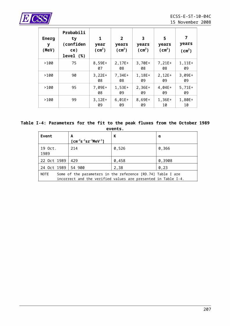
ECSS-E-ST-10-04C15 November 2008
[RD.127] ISO International Standard 5878-1982, Reference Atmospheres for Aerospace Use, First Edition-1982-04-14, Technical Committee ISO/TC 20, Aircraft and Space Vehicles.
[RD.128] a) Rees, D., Editor, (1988): "COSPAR International Reference Atmosphere 1986, Part l. Thermospheric Models", Advances in Space Research, Vol. 8, No. 5/6Pergamon Press, Oxford and NY. b) Rees, D., J. J. Barnett, and K. Labitzke, editors (1990): "CIRA 1986, COSPAR International Reference Atmosphere, Part II: Middle Atmosphere Models," Advances in Space Research, Vol. 10, No. 12, Pergamon Press, Oxford and NY. c) Keating, G. M., editor (1996): “COSPAR International Reference Atmosphere (CIRA), Part III: Trace Constituent Reference Models," Advances in Space Research, Vol. 18, No. 9/10, Pergamon Press, Oxford and NY.
[RD.129] CIRA 1961, H. Kallmann-Bijl, R.L.F. Boyd, H. Lagow, S.M. Poloskov, and W. Priester (eds.), North-Holland Publishing Company, Amsterdam, 1961.
[RD.130] CIRA 1965, North-Holland Publishing Company, Amsterdam, 1965.[RD.131] COSPAR International Reference Atmosphere 1972, Compiled by the members
of COSPAR Working Group 4, Akademie-Verlag, Berlin, 1972.[RD.132] Justus C.G., F.N. Alyea, D.M. Cunnold, and D.L. Johnson (1986), GRAM-86,
“Improvements in the Global Atmospheric Model”, NASA MSFC Report ED-5-15-86.
[RD.133] Justus C.G., F.N. Alyea, D.M. Cunnold, R.S. Blocker, and D.L. Johnson (1988), GRAM-88, “Improvements to the Perturbation Simulation of the Global Reference Atmospheric Model”, NASA MSFC Memorandum ES-44-11-9-88.
[RD.134] Justus C.G., F.N. Alyea, D.M. Cunnold, W.R. Jefferies III, and D.L. Johnson (1991), “The NASA/MSFC Global Reference Atmospheric Model – 1990 Version (GRAM-90), Part 1: Technical/Users Manual”. NASA TM-4268, Grant NAG8-078.
[RD.135] Justus C.G., W.R. Jefferies III, S.P. Yung, and D.L. Johnson (1995), “The NASA/MSFC Global Reference Atmospheric Model – 1995 Version (GRAM-95)”, NASA TM-4715.
[RD.136] Justus C.G., and D.L. Johnson (1999), “The NASA/MSFC Global Reference Atmospheric Model – 1999 Version (GRAM-99)”, NASA TM-1999-209630.
[RD.137] Picone, J. M., A. E. Hedin, K. P. Drob, and J. Lean, NRLMSISE-00 Empirical Atmospheric Model: Comparisons to Data and Standard Models. Advances in the Astronautical Sciences, Vol. 109 II//Pages 1385-1387, AAS/AIAA Astrodynamics Conference, July 30-August 2, 2001, Quebec City, Que., ISSN 0065-3438.
[RD.138] Olsen N., H.Lühr,T.J.Sabaka, M.Mandea, M.Rother, L.Tøffner-Clausen and S.Choi , CHAOS—a model of the Earth’s magnetic field derived from CHAMP, Ørsted, and SAC-C magnetic satellite data, Geophys. J. Int. 166, 67–75 (2006)
[RD.139] Maus S., H.Lühr2, G.Balasis, M.Rother and M.Mandea, Third generation of the Potsdam Magnetic Model of the Earth (POMME), Geochemistry Geophysics Geosystems, 7, Q07008, 2006
[RD.140] Sabaka T.J., Olsen, N., and M.E. Purucker, Extending comprehensive models of the Earth's magnetic field with Oersted and Champ data, Geophys. J. Int.,159,521-547, (2004)
[RD.141] Mead, G. D. and Fairfield, D. H., A quantitative magnetospheric model derived from spacecraft magnetometer data, J.Geophys. Res., 80, 523-534, (1975)
[RD.142] Olsen, W.P. and Pfitzer, K.A., A dynamic model of the magnetospheric magnetic and electric fields for July 29, 1977, J. Geophys. Res., 87, 5943-5948, (1977)
207

ECSS-E-ST-10-04C15 November 2008
[RD.143] Hilmer, R. V. (1989), A magnetospheric magnetic field model with flexible internal current systems, PhD thesis, 156pp., Rice Univ., Houston, Texas.
[RD.144] Voight, G.-H. (1981), A mathematical magnetospheric field model with independent physical parameters, Planet. Space Sci., 29(10), 1-20.
[RD.145] Jordan, C. E., Empirical Models of the Magnetospheric Magnetic Field, Rev. Geophys., 32, 2, 139-157, (1994)
[RD.146] Xapsos M. A., J.L. Barth, E.G. Stassinopoulos, E.A. Burke, and G.B. Gee, Space Environment Effects: Model for Emission of Solar Protons (ESP) – Cumulative and Worst-Case Event Fluences, NASA/TP-1999-209763, 1999..
[RD.147] Liu RY, Smith PA and King JW, ‘A new solar index which leads to improved foF2 predictions using the CCIR ATLAS’,Telecommunication Journal, 1983, Volume 50 (8), pages 408-414.
208
Related Documents