Dr. Naser Abu-Zaid; Lecture notes on Electromagnetic Theory(1); Ref:Engineering Electromagnetics; William Hayt& John Buck, 7th & 8th editions; 2012 Page 1 Preliminary material (mathematical requirements) Vector:A quantity with both magnitude and direction. (Force N 10 F to the east). Scalar:A quantity that does not posses direction, Real or complex. (Temperature o T 20 . Vector addition: 1) Parallelogram: 2) Head to Tail: A B A B B A A B A B B A Vector Analysis Vector algebra: Addition; Subtraction; Multiplication Vector Calculus: Differentiation; Integration

Welcome message from author
This document is posted to help you gain knowledge. Please leave a comment to let me know what you think about it! Share it to your friends and learn new things together.
Transcript

Dr. Naser Abu-Zaid; Lecture notes on Electromagnetic Theory(1); Ref:Engineering
Electromagnetics; William Hayt& John Buck, 7th & 8th editions; 2012
Page 1
Preliminary material
(mathematical
requirements)
Vector:A quantity with both magnitude and direction. (Force N10F to the
east).
Scalar:A quantity that does not posses direction, Real or complex. (Temperature oT 20 .
Vector addition:
1) Parallelogram:
2) Head to Tail:
A
B
A
B
BA
A
B
A
B
BA
Vector Analysis
Vector algebra:
Addition; Subtraction;
Multiplication
Vector Calculus:
Differentiation; Integration

Dr. Naser Abu-Zaid; Lecture notes on Electromagnetic Theory(1); Ref:Engineering
Electromagnetics; William Hayt& John Buck, 7th & 8th editions; 2012
Page 2
Vector Subtraction:
Multiplication by scalar: AB k
AB 2
AB 50.
AB 3
Commulative law: ABBA
Associative law: CBACBA
Equal vectors: BA if 0BA (Both have same length and direction) Add or subtract vector fields which are defined at the same point. If non vector fields are considered then vectors are added or subtracted
which are not defined at same point (By shifting them)
A
A3
A50.
A
A A2
A
B
A
B
B
A
B
B
BA

Dr. Naser Abu-Zaid; Lecture notes on Electromagnetic Theory(1); Ref:Engineering
Electromagnetics; William Hayt& John Buck, 7th & 8th editions; 2012
Page 3
THE RECTANGULAR COORDINATE SYSTEM
z,y,x are coordinate
variables (axis) which are
mutually perpendicular.
A point is located by its y,x
and z coordinates, or as the
intersection of three constant
surfaces (planes in this case)
x
y
z
321 ,,P
1x
2y
3z
x
y
z
Right Handed System
Out of page

Dr. Naser Abu-Zaid; Lecture notes on Electromagnetic Theory(1); Ref:Engineering
Electromagnetics; William Hayt& John Buck, 7th & 8th editions; 2012
Page 4
x
y
z
321 ,,P
1x
Surface
(plane)
2y
surface
(plane)
3z
surface
(plane)
Three mutually perpendicular surfaces intersect at a common point
Dr. Naser Abu-Zaid; Lecture notes on Electromagnetic Theory(1); Ref:Engineering
Electromagnetics; William Hayt& John Buck, 7th & 8th editions; 2012
Page 5
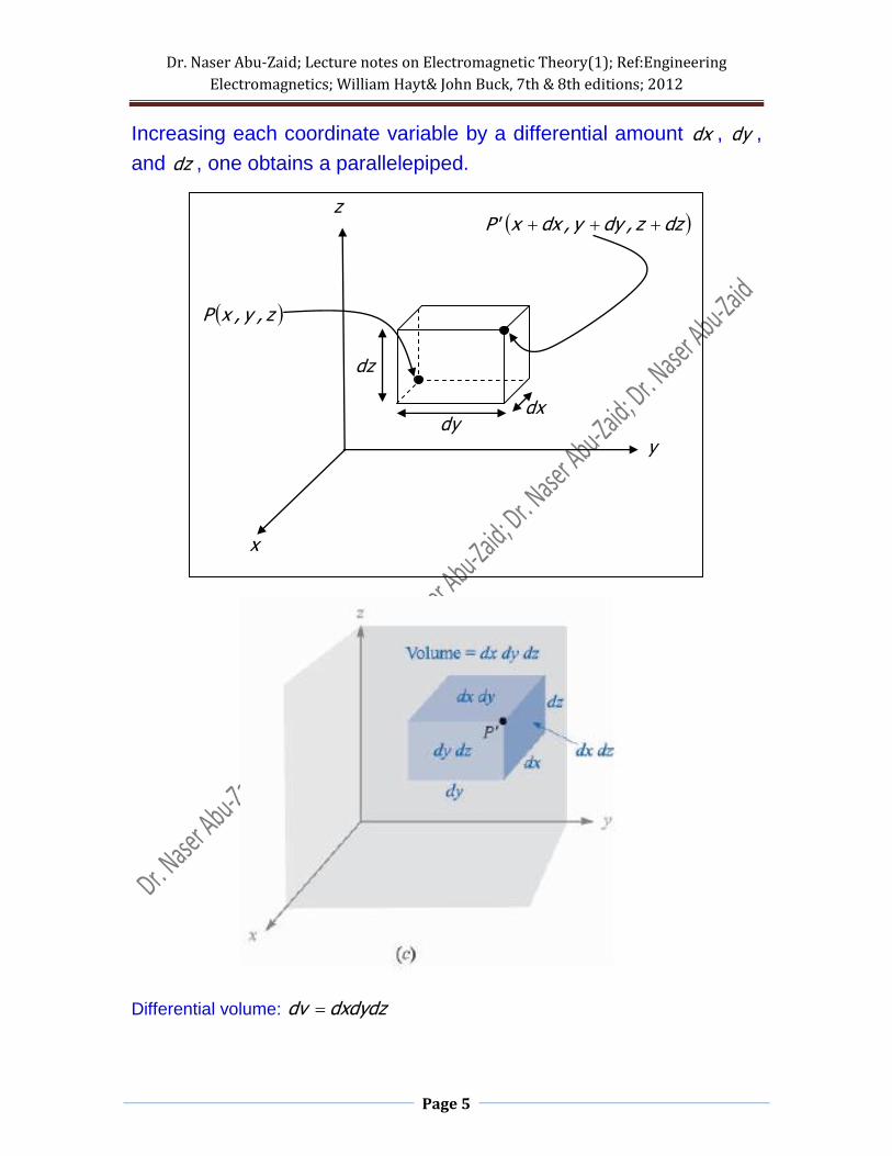
Increasing each coordinate variable by a differential amount dx , dy ,
and dz , one obtains a parallelepiped.
Differential volume: dxdydzdv
x
y
z
z,y,xP
dz
dx dy
dzz,dyy,dxx'P

Dr. Naser Abu-Zaid; Lecture notes on Electromagnetic Theory(1); Ref:Engineering
Electromagnetics; William Hayt& John Buck, 7th & 8th editions; 2012
Page 6
Differential Surfaces: Six planes with dierential areas dxdyds ; dzdyds ;
dxdzds
Differential length: from P to P’ 222dzdydxdl
VECTOR COMPONENTS AND UNIT VECTORS
A general vector r may be written as the sum of three vectors;
,,BA and C arevector components with constant directions.
Unit vectors xa , ya , and za directed along x, y, and z respectively with unity
length and no dimensions.
x
y
z
321 ,,P
1x
2y
3z
r
A B
C
Projection of
r into x-axis
Projection of
r into z-axis
Projection of
r into y-axis
CBAr
Dr. Naser Abu-Zaid; Lecture notes on Electromagnetic Theory(1); Ref:Engineering
Electromagnetics; William Hayt& John Buck, 7th & 8th editions; 2012
Page 7
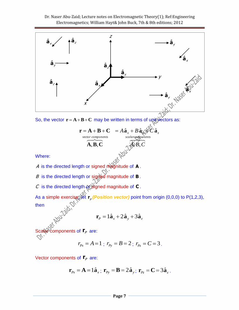
So, the vector CBAr may be written in terms of unit vectors as:
componentsscalarcomponentsvector
zyx
CBA
CBA
,,,,
ˆˆˆ
CBA
aaaCBAr
Where:
A is the directed length or signed magnitude of A .
B is the directed length or signed magnitude of B .
C is the directed length or signed magnitude of C .
As a simple exercise, let pr (Position vector) point from origin (0,0,0) to P(1,2,3),
then
zyxP aaar ˆ3ˆ2ˆ1
Scalar components of Pr are:
1 ArPx ; 2 BrPy ; 3CrPz .
Vector components of Pr are:
xPx aAr ˆ1 ; yPy aBr ˆ2 ; zPz aCr ˆ3 .
x
y
z
xa
xa
xa
xa
ya
ya
ya
ya za
za
za

Dr. Naser Abu-Zaid; Lecture notes on Electromagnetic Theory(1); Ref:Engineering
Electromagnetics; William Hayt& John Buck, 7th & 8th editions; 2012
Page 8
If Q(2,-2,1) then
zyxQ aaar ˆˆ2ˆ2
And the vector directed from P to Q, PQPQ rrr (displacement vector)
which is given by
zyxzyxPQ ˆˆˆˆˆˆ aaaaaar 24312212
The vector Pr is termed position vector which is directed from the origin toward
the point in quesion.
Other types of vectors (vector fields such as Force vector) are denoted:
x
y
z
Qr
Pr
POr
Pr

Dr. Naser Abu-Zaid; Lecture notes on Electromagnetic Theory(1); Ref:Engineering
Electromagnetics; William Hayt& John Buck, 7th & 8th editions; 2012
Page 9
zzyyxx ˆFˆFˆF aaaF
Where ,F,F yx zF are scalar components, and zzyyxx ˆF,ˆF,ˆF aaa are the
vector components.
The magnitude of a vector zzyyxx ˆBˆBˆB aaaB is;
222
zyx BBBB B
A unit vector in the direction of B is;
222
zyx
zzyyxxB
BBB
ˆBˆBˆBˆ
aaa
B
Ba
Let zzyyxx ˆBˆBˆB aaaB and zzyyxx ˆAˆAˆA aaaA , then
zzzyyyxxx ˆBAˆBAˆBA aaaBA
zzzyyyxxx ˆBAˆBAˆBA aaaBA
Ex:Specify the unit vector extending from the origin toward the point G(2,-2,-1).
Ex: Given M(-1,2,1), N(3,-3,0) and P(-2,-3,-4) Find:
(a) MNR
(b) MPMN RR
(c) Mr
(d) MPa
(e) NP rr 32
B
Ba

Dr. Naser Abu-Zaid; Lecture notes on Electromagnetic Theory(1); Ref:Engineering
Electromagnetics; William Hayt& John Buck, 7th & 8th editions; 2012
Page 10
THE VECTOR FIELD AND SCALAR FIELD
Vector Field: vector function of a position vector r . It has a magnitude and
direction at each point in space.
zzyyxx
zzyyxx
ˆz,y,xvˆz,y,xvˆz,y,xv
ˆvˆvˆv
aaa
arararrv
Scalar field: A scalar function of a position vector r . Temperature is an
example z,y,xTT r which has a scalar value at each point in space.
Velocity or air flow in a pipe

Dr. Naser Abu-Zaid; Lecture notes on Electromagnetic Theory(1); Ref:Engineering
Electromagnetics; William Hayt& John Buck, 7th & 8th editions; 2012
Page 11
Ex:A vector field is expressed as
zyx ˆzˆyˆx
zyxaaaS 121
121
125222
(a) Is this a scalar or vector field?
(b) Evaluate S @ 342 ,,P .
(c) Determine a unit vector that gives the direction of S @ 342 ,,P .
(d) Specify the surface z,y,xf on which 1S .
1T
2T
3T

Dr. Naser Abu-Zaid; Lecture notes on Electromagnetic Theory(1); Ref:Engineering
Electromagnetics; William Hayt& John Buck, 7th & 8th editions; 2012
Page 12
THE DOT PRODUCT
ABcos BABA
Which results in a scalar value, and AB is the smaller angle between A and B .
ABBA since ABAB coscos ABBA
11110cosˆˆˆˆ xxxx aaaa
11110cosˆˆˆˆ yyyy aaaa
11110cosˆˆˆˆ zzzz aaaa
xy
o
yxyx aaaaaa ˆˆ001190cosˆˆˆˆ
xz
o
zxzx aaaaaa ˆˆ001190cosˆˆˆˆ
yz
o
zyzy aaaaaa ˆˆ001190cosˆˆˆˆ
A
B
Projection of A into B
ABcos A
Projection of B into A
ABcos B
AB

Dr. Naser Abu-Zaid; Lecture notes on Electromagnetic Theory(1); Ref:Engineering
Electromagnetics; William Hayt& John Buck, 7th & 8th editions; 2012
Page 13
Let zzyyxx BBB aaaB ˆˆˆ and zzyyxx AAA aaaA ˆˆˆ , then
zzyyxx BABABA BA
AAAAA AAAAA zyx22222
The scalar component of B in the direction of an arbitrary unit vector a is given
by aB ˆ
The vector component of B in the direction of an arbitrary unit vector a is given
by aaB ˆˆ .
B
Scalar Projection of B into a
cosB aB ˆ
cos
cosˆˆ
B
aBaB
a

Dr. Naser Abu-Zaid; Lecture notes on Electromagnetic Theory(1); Ref:Engineering
Electromagnetics; William Hayt& John Buck, 7th & 8th editions; 2012
Page 14
Distributive property: CABACBA
Ex: Given zyx ˆˆx.ˆy aaaE 352 and Q(4,5,2) Find:
(a) E @ Q.
(b) The scalar component of E @ Q in the direction of
zyxnˆˆˆˆ aaaa 22
3
1 .
(c) The vector component of E @ Q in the direction of
zyxnˆˆˆˆ aaaa 22
3
1 .
(d) The angle Ea between QrE and na .
B
Vector Projection of B into a
aaB ˆˆ
a

Dr. Naser Abu-Zaid; Lecture notes on Electromagnetic Theory(1); Ref:Engineering
Electromagnetics; William Hayt& John Buck, 7th & 8th editions; 2012
Page 15
THE CROSS PRODUCT
nAB aBABA ˆsin results in a vector
ABsinBABA
nofDirection aBA ˆ
na is a unit vector normal to the plane containing A and B . Since there are two
possible s'ˆ na , we use the Right Hand Rule (RHR) to determine the direction of
BA .
Cross product clearly results in a vector, and AB is the smaller angle between A
and B .
Properties:
ABBA
CABACBA
A
B
ABsin B
which is the height
Of the parallelogram
AB
BA
ABBA
ABsin BA
Is the area of the
parallelogram
na

Dr. Naser Abu-Zaid; Lecture notes on Electromagnetic Theory(1); Ref:Engineering
Electromagnetics; William Hayt& John Buck, 7th & 8th editions; 2012
Page 16
CBACBA
00 nxxxx ˆsinˆˆˆˆ aaaaa
00 nyyyy ˆsinˆˆˆˆ aaaaa
00 nzzzz ˆsinˆˆˆˆ aaaaa
znno
yxyx ˆˆˆsinˆˆˆˆ aaaaaaa 11190
ynno
zxzx ˆˆˆsinˆˆˆˆ aaaaaaa 11190
znno
xyxy ˆˆˆsinˆˆˆˆ aaaaaaa 11190
xnno
zyzy ˆˆˆsinˆˆˆˆ aaaaaaa 11190
ynno
xzxz ˆˆˆsinˆˆˆˆ aaaaaaa 11190
xnno
yzyz ˆˆˆsinˆˆˆˆ aaaaaaa 11190
Let zzyyxx ˆBˆBˆB aaaB and zzyyxx ˆAˆAˆA aaaA , then
zxyyxyxzzxxyzzy
zyx
zyx
zyx
nAB
ˆBABAˆBABAˆBABA
BBB
AAA
ˆˆˆ
ˆsin
aaa
aaa
aBABA
x
y
z
RHR
Out of page
Dr. Naser Abu-Zaid; Lecture notes on Electromagnetic Theory(1); Ref:Engineering
Electromagnetics; William Hayt& John Buck, 7th & 8th editions; 2012
Page 17
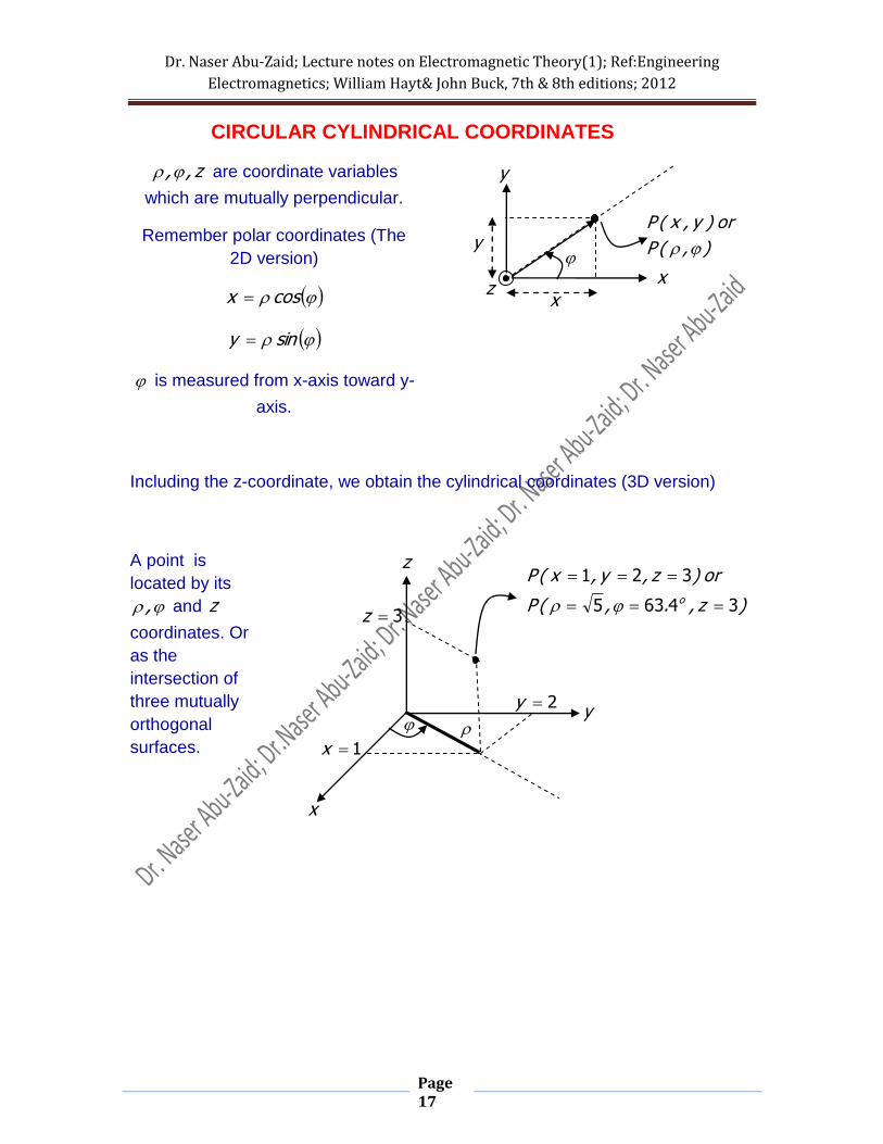
CIRCULAR CYLINDRICAL COORDINATES
z,, are coordinate variables
which are mutually perpendicular.
Remember polar coordinates (The
2D version)
cosx
siny
is measured from x-axis toward y-
axis.
Including the z-coordinate, we obtain the cylindrical coordinates (3D version)
A point is
located by its
, and z
coordinates. Or
as the
intersection of
three mutually
orthogonal
surfaces.
x
y
z
1x
2y
3z )z,.,(P
or)z,y,x(Po 34635
321
x
y
z x
y ),(P
or)y,x(P
Dr. Naser Abu-Zaid; Lecture notes on Electromagnetic Theory(1); Ref:Engineering
Electromagnetics; William Hayt& John Buck, 7th & 8th editions; 2012
Page 18
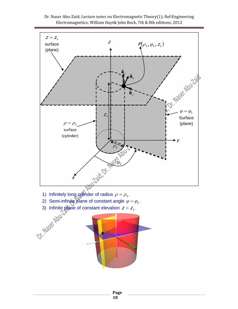
1) Infinitely long cylinder of radius 1 .
2) Semi-infinite plane of constant angle 1 .
3) Infinite plane of constant elevation 1zz .
x
y
z
111 z,,P
1
Surface
(plane) 1
surface
(cylinder)
1zz
surface
(plane)
1
1
1z
a
a
za

Dr. Naser Abu-Zaid; Lecture notes on Electromagnetic Theory(1); Ref:Engineering
Electromagnetics; William Hayt& John Buck, 7th & 8th editions; 2012
Page 19
The three unit vectors za , a , and
a are in the direction of increasing variables
and are perpendicular to the surface at which the coordinate variable is
constant.
x
y
z x
y
a
a
za

Dr. Naser Abu-Zaid; Lecture notes on Electromagnetic Theory(1); Ref:Engineering
Electromagnetics; William Hayt& John Buck, 7th & 8th editions; 2012
Page 20
Note that in Cartesian coordinates, unit vectors are not functions of coordinate
variables. But in cylindrical coordinates a , and
a are functions of .
The cylindrical coordinate system is Right Handed: zˆˆˆ aaa .
Increasing each coordinate variable by a differential amount d , d , and dz ,
one obtains:
x
y
z
1
1 2
2 xa
ya ya
xa
x
y
z
1
1
1a
1a
2 2
2a
2a
Dr. Naser Abu-Zaid; Lecture notes on Electromagnetic Theory(1); Ref:Engineering
Electromagnetics; William Hayt& John Buck, 7th & 8th editions; 2012
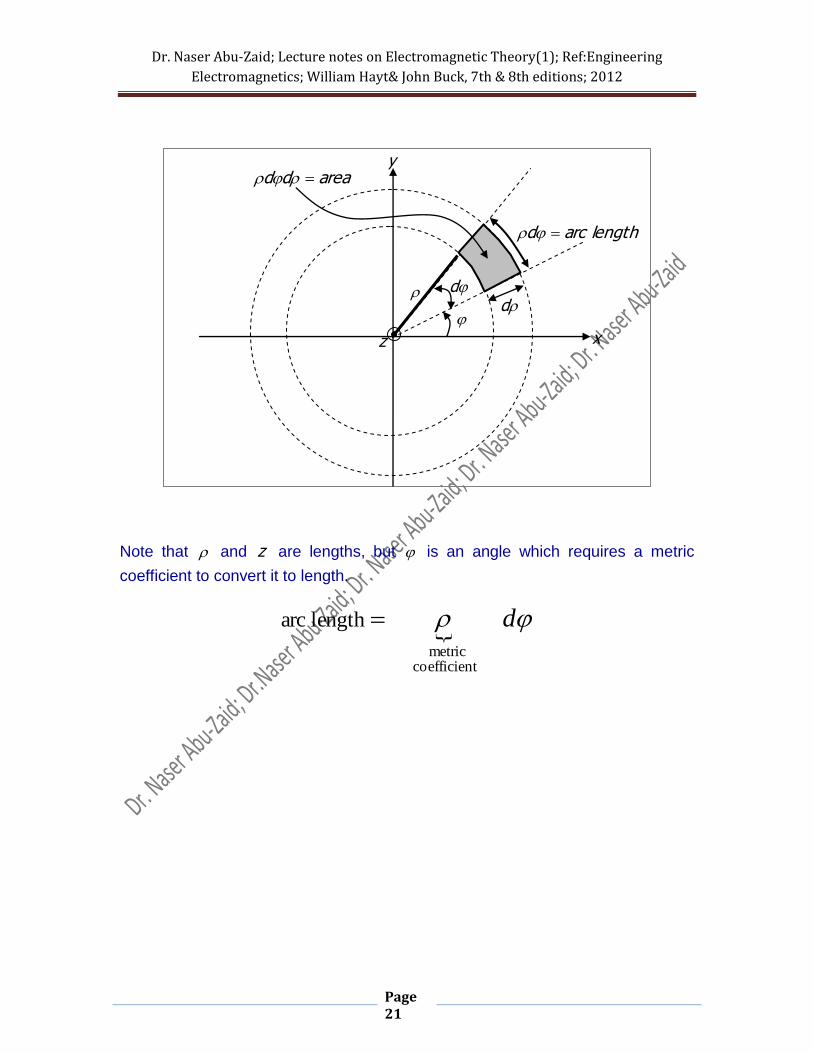
Page 21
Note that and z are lengths, but is an angle which requires a metric
coefficient to convert it to length.
d
tcoefficienmetric
lengtharc
x
y
z
d
d
lengtharcd
areadd

Dr. Naser Abu-Zaid; Lecture notes on Electromagnetic Theory(1); Ref:Engineering
Electromagnetics; William Hayt& John Buck, 7th & 8th editions; 2012
Page 22
Differential volume: dzdddv
Differential Surfaces: Six planes with differential areas shown in the figure above.
(Try it!)
x
y
z
d d
dz
d
dzdds
dzdds
ddds

Dr. Naser Abu-Zaid; Lecture notes on Electromagnetic Theory(1); Ref:Engineering
Electromagnetics; William Hayt& John Buck, 7th & 8th editions; 2012
Page 23
Transformations between Cylindrical and Cartesian Coordinates
From cylindrical to cart:
cosx
siny
zz
From cart. To cyl.:
22 yx
x
ytan 1
zz
x
y
z
1xx
1yy
1zz
1 1

Dr. Naser Abu-Zaid; Lecture notes on Electromagnetic Theory(1); Ref:Engineering
Electromagnetics; William Hayt& John Buck, 7th & 8th editions; 2012
Page 24
Consider a vector in rectangular coordinates;
zzyyxx EEE aaaE ˆˆˆ
Wishing to write E in cylindrical coordinates:
zzEEE aaaE ˆˆˆ
From the dot product:
aE ˆE aE ˆE zzE aE ˆ
aaaa ˆˆˆˆ zzyyxx EEEE
?
ˆˆ
?
ˆˆ
?
ˆˆ aaaaaa zzyyxx EEE
aaaa ˆˆˆˆ zzyyxx EEEE
?
ˆˆ
?
ˆˆ
?
ˆˆ aaaaaa zzyyxx EEE
zzzyyxxz EEEE aaaa ˆˆˆˆ
?
ˆˆ
?
ˆˆ
?
ˆˆzzzzyyzxx EEE aaaaaa
Dr. Naser Abu-Zaid; Lecture notes on Electromagnetic Theory(1); Ref:Engineering
Electromagnetics; William Hayt& John Buck, 7th & 8th editions; 2012
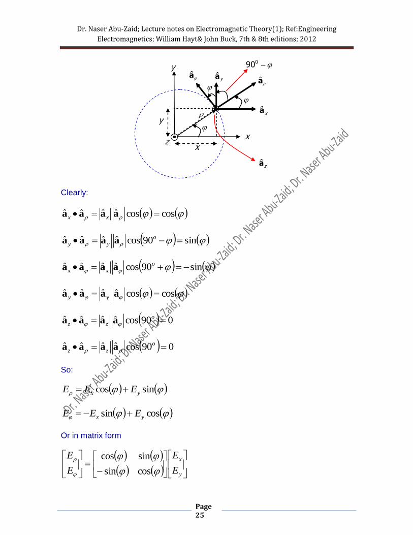
Page 25
Clearly:
coscosˆˆˆˆ aaaa xx
sin90cosˆˆˆˆ o
yy aaaa
sin90cosˆˆˆˆ o
xx aaaa
coscosˆˆˆˆ aaaa yy
090cosˆˆˆˆ o
zz aaaa
090cosˆˆˆˆ o
zz aaaa
So:
sincos yx EEE
cossin yx EEE
Or in matrix form
y
x
E
E
E
E
cossin
sincos
x
y
z x
y
a
a
za
xa
ya
090

Dr. Naser Abu-Zaid; Lecture notes on Electromagnetic Theory(1); Ref:Engineering
Electromagnetics; William Hayt& John Buck, 7th & 8th editions; 2012
Page 26
And, the inverse relation is:
E
E
E
E
y
x
cossin
sincos
Note that the story is not finished here, after transforming the components; you
should also transform the coordinate variables.
Dr. Naser Abu-Zaid; Lecture notes on Electromagnetic Theory(1); Ref:Engineering
Electromagnetics; William Hayt& John Buck, 7th & 8th editions; 2012
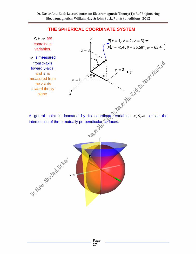
Page 27
THE SPHERICAL COORDINATE SYSTEM
,,r are
coordinate
variables.
is measured
from x-axis
toward y-axis,
and is
measured from
the z-axis
toward the xy
plane.
A genral point is loacated by its coordinate variables ,,r , or as the
intersection of three mutually perpendicular surfaces.
x
y
z
1x
2y
3z
oo .,.,rP
orz,y,xP
463693514
321
r

Dr. Naser Abu-Zaid; Lecture notes on Electromagnetic Theory(1); Ref:Engineering
Electromagnetics; William Hayt& John Buck, 7th & 8th editions; 2012
Page 28
1) Sphere of radius 1rr , centered at the origin.
2) Semi-infinite plane of constant angle 1 with it’s axis aligned with z-
axis. 3) Right angular cone with its apex centered at the origin, and it axis aligned
with z-axis, and a cone angle 1 .
The three unit vectors ra , a , and a are in the direction of increasing
variables and are perpendicular to the surface at which the coordinate variable
is constant.
x
y
z
111 ,, rP
1
Surface
(plane)
1rr
surface
(sphere)
1
surface
(cone)
ra
a
a

Dr. Naser Abu-Zaid; Lecture notes on Electromagnetic Theory(1); Ref:Engineering
Electromagnetics; William Hayt& John Buck, 7th & 8th editions; 2012
Page 29
x
y
z 111 ,,rP
1
ra
a
1
1r
a
Dr. Naser Abu-Zaid; Lecture notes on Electromagnetic Theory(1); Ref:Engineering
Electromagnetics; William Hayt& John Buck, 7th & 8th editions; 2012
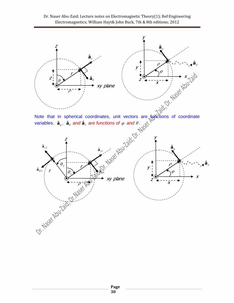
Page 30
Note that in spherical coordinates, unit vectors are functions of coordinate
variables. a , a and ra are functions of and .
x
y
z x
y
a
za
planexy
z
1
r
1ˆa
1ˆ
ra 2
ˆra
2ˆa r
2
x
y
z x
y
a
za
planexy
z
z
r
a
ra

Dr. Naser Abu-Zaid; Lecture notes on Electromagnetic Theory(1); Ref:Engineering
Electromagnetics; William Hayt& John Buck, 7th & 8th editions; 2012
Page 31
The spherical coordinate system is Right Handed:
aaa ˆˆˆ r .
Increasing each coordinate variable by a differential amount dr , d , and d ,
one obtains:
x
y
z
1
1 2
2 xa
ya ya
xa
x
y
z
1
1
1a
1a
2 2
2a
2a
Dr. Naser Abu-Zaid; Lecture notes on Electromagnetic Theory(1); Ref:Engineering
Electromagnetics; William Hayt& John Buck, 7th & 8th editions; 2012
Page 32
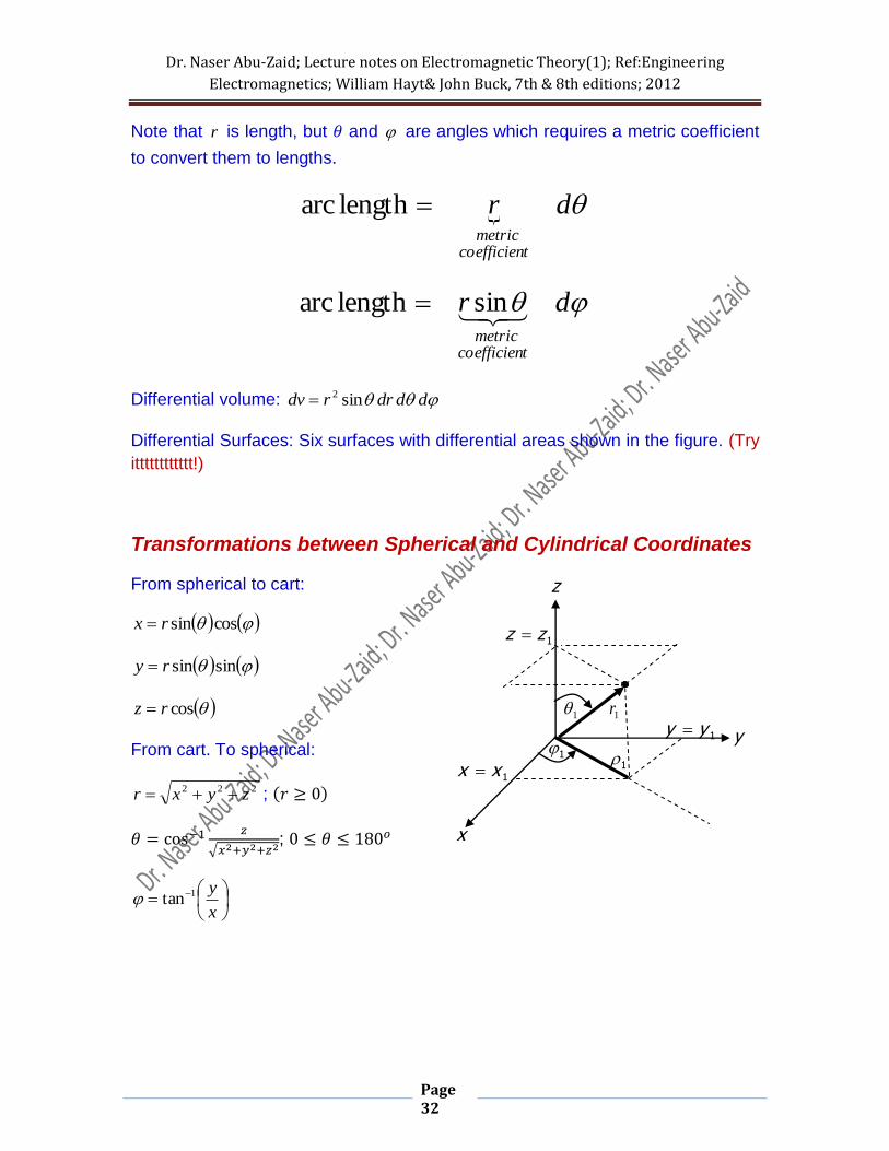
Note that r is length, but and are angles which requires a metric coefficient
to convert them to lengths.
dr
tcoefficienmetric
lengtharc
dr
tcoefficienmetric
sinlengtharc
Differential volume: dddrrdv sin2
Differential Surfaces: Six surfaces with differential areas shown in the figure. (Try
itttttttttttt!)
Transformations between Spherical and Cylindrical Coordinates
From spherical to cart:
cossinrx
sinsinry
cosrz
From cart. To spherical:
222 zyxr ;
;
x
y1tan
x
y
z
1xx
1yy
1zz
1
1
1
1r
Dr. Naser Abu-Zaid; Lecture notes on Electromagnetic Theory(1); Ref:Engineering
Electromagnetics; William Hayt& John Buck, 7th & 8th editions; 2012
Page 33
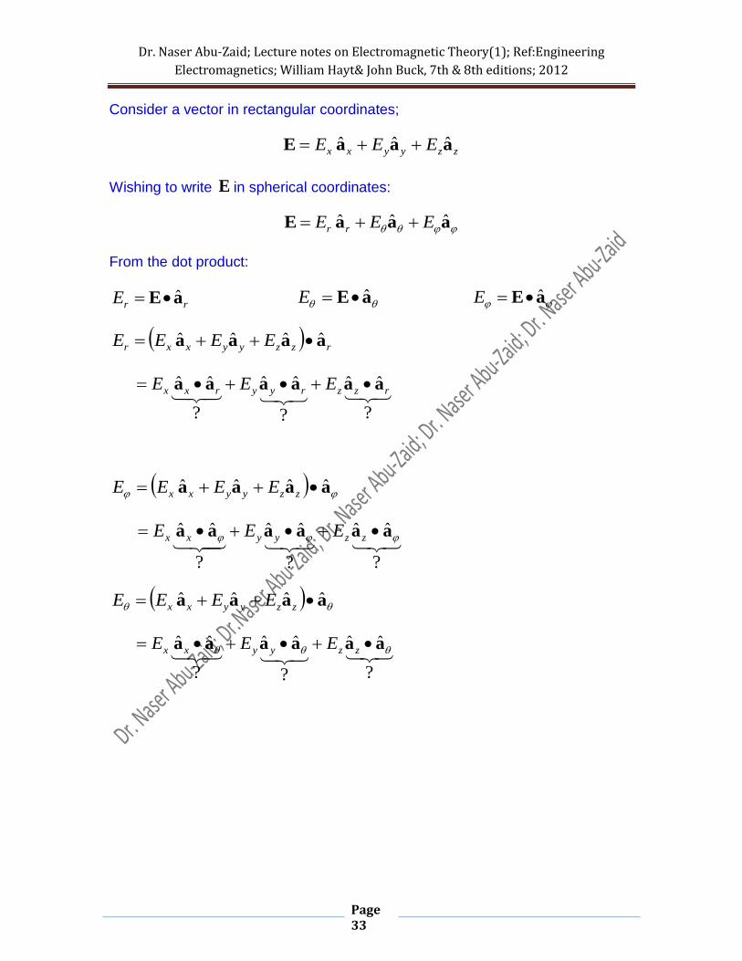
Consider a vector in rectangular coordinates;
zzyyxx EEE aaaE ˆˆˆ
Wishing to write E in spherical coordinates:
aaaE ˆˆˆ EEE rr
From the dot product:
rrE aE ˆ aE ˆE aE ˆE
rzzyyxxr EEEE aaaa ˆˆˆˆ
?
ˆˆ
?
ˆˆ
?
ˆˆrzzryyrxx EEE aaaaaa
aaaa ˆˆˆˆ zzyyxx EEEE
?
ˆˆ
?
ˆˆ
?
ˆˆ aaaaaa zzyyxx EEE
aaaa ˆˆˆˆ zzyyxx EEEE
?
ˆˆ
?
ˆˆ
?
ˆˆ aaaaaa zzyyxx EEE

Dr. Naser Abu-Zaid; Lecture notes on Electromagnetic Theory(1); Ref:Engineering
Electromagnetics; William Hayt& John Buck, 7th & 8th editions; 2012
Page 34
From figure
coscosˆˆˆˆ rzrz aaaa
sin90cosˆˆˆˆ o
rr aaaa
sin90cosˆˆˆˆ o
zz aaaa
And the rest is left to you as an exercise!
So:
cossinsincossin zyxr EEEE
Note that, after transforming the components; you should also transform the
coordinate variables.
planexy
z
z r
a
ra za
a
090

Dr. Naser Abu-Zaid; Lecture notes on Electromagnetic Theory(1); Ref:Engineering
Electromagnetics; William Hayt& John Buck, 7th & 8th editions; 2012
Page 35
Dr. Naser Abu-Zaid; Lecture notes on Electromagnetic Theory(1); Ref:Engineering
Electromagnetics; William Hayt& John Buck, 7th & 8th editions; 2012
Page 36
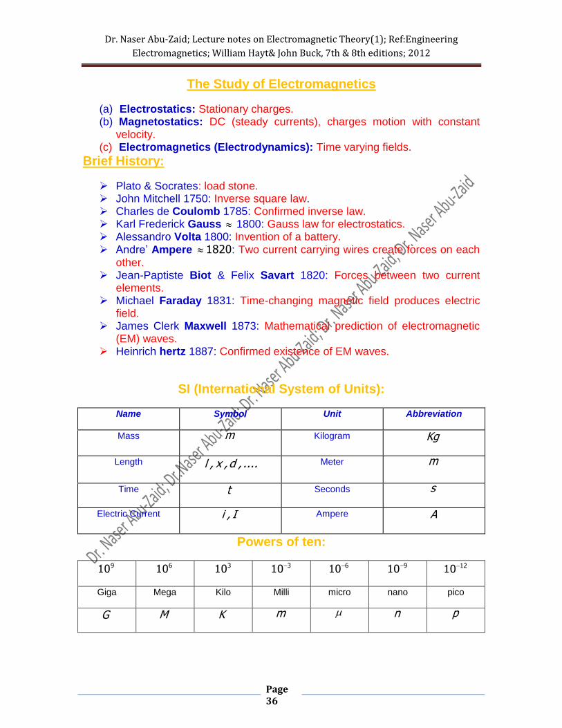
The Study of Electromagnetics
(a) Electrostatics: Stationary charges. (b) Magnetostatics: DC (steady currents), charges motion with constant
velocity. (c) Electromagnetics (Electrodynamics): Time varying fields.
Brief History:
Plato & Socrates: load stone. John Mitchell 1750: Inverse square law. Charles de Coulomb 1785: Confirmed inverse law. Karl Frederick Gauss 1800: Gauss law for electrostatics. Alessandro Volta 1800: Invention of a battery. Andre’ Ampere 1820 : Two current carrying wires create forces on each
other. Jean-Paptiste Biot & Felix Savart 1820: Forces between two current
elements. Michael Faraday 1831: Time-changing magnetic field produces electric
field. James Clerk Maxwell 1873: Mathematical prediction of electromagnetic
(EM) waves. Heinrich hertz 1887: Confirmed existence of EM waves.
SI (International System of Units):
Name Symbol Unit Abbreviation
Mass m Kilogram Kg
Length ....,d,x,l Meter m
Time t Seconds s
Electric Current I,i Ampere A
Powers of ten:
910 610
310 310
610
910
1210
Giga Mega Kilo Milli micro nano pico
G M K m n p

Dr. Naser Abu-Zaid; Lecture notes on Electromagnetic Theory(1); Ref:Engineering
Electromagnetics; William Hayt& John Buck, 7th & 8th editions; 2012
Page 37
Charge Distributions
Electric Charge is a fundamental property of matter, and the charge on an
electron is e , where: C.e 191061 , and C is the unit of charge
(Coulomb).
Point charge distributionQ : assumed to
exist (concentrated) at isolated points in
space.
Line charge distribution is the distribution
of charge over a line. The line charge
density is the amount of electric charge
per unit length in a line of vanishingly
small radius.
Surface charge distribution is the
distribution of charge over a surface.
The surface charge density is the
amount of electric charge per unit area
in a surface of vanishingly small
thickness.
x
y
z
+ +
+ +
+ + +
- - -
- - -
2m
Cz,y,xs
x
y
z
+ +
+ + + + +
- - - -
- -
m
Cz,y,xl
x
y
z
1Q
2Q 3Q
4Q

Dr. Naser Abu-Zaid; Lecture notes on Electromagnetic Theory(1); Ref:Engineering
Electromagnetics; William Hayt& John Buck, 7th & 8th editions; 2012
Page 38
Volume charge distribution is the
distribution of charge over a volume.
The volume charge density is the
amount of electric charge per unit
volume in a volume.
Charge density in general may depend on position (nonuniform). But if it is
constant over the respective region (independent of x, y, and z), it is said to be
uniform charge density.
Perhaps the most frequently used method for solving electrostatic field
problems is the differential element of charge, with this method, the charge
distribution is reduced to a differential element of charge, dQ , which is treated as
point charges.
Let v be the volume charge density measured in 3mC , then:
3
3m
m
CC
vQ v
As 0v (differential volume dv ) then dQQ (a point charge), so:
dvdQ v
v
v
v
v dvdvQ
Infinitely large number of
vanishingly small
charges spaced by
differentialy small
distances.
Volume v containing
total charge Q
Considering a volume element
v containing elemental
amount of charge Q
x
y
z
+ +
+ + +
+ +
- - - -
- -
3m
Cz,y,xv

Dr. Naser Abu-Zaid; Lecture notes on Electromagnetic Theory(1); Ref:Engineering
Electromagnetics; William Hayt& John Buck, 7th & 8th editions; 2012
Page 39

Dr. Naser Abu-Zaid; Lecture notes on Electromagnetic Theory(1); Ref:Engineering
Electromagnetics; William Hayt& John Buck, 7th & 8th editions; 2012
Page 40
zv e
5106105
20
10
42
cmcm
cmzcm
A charge distribution of vanishingly small thickness is referred to as
surface charge. Like the charge on the surface of a perfect conductor.
Let s be the surface charge density measured in 2mC , then:
x
y
3m
Cz,y,xv
z
Dr. Naser Abu-Zaid; Lecture notes on Electromagnetic Theory(1); Ref:Engineering
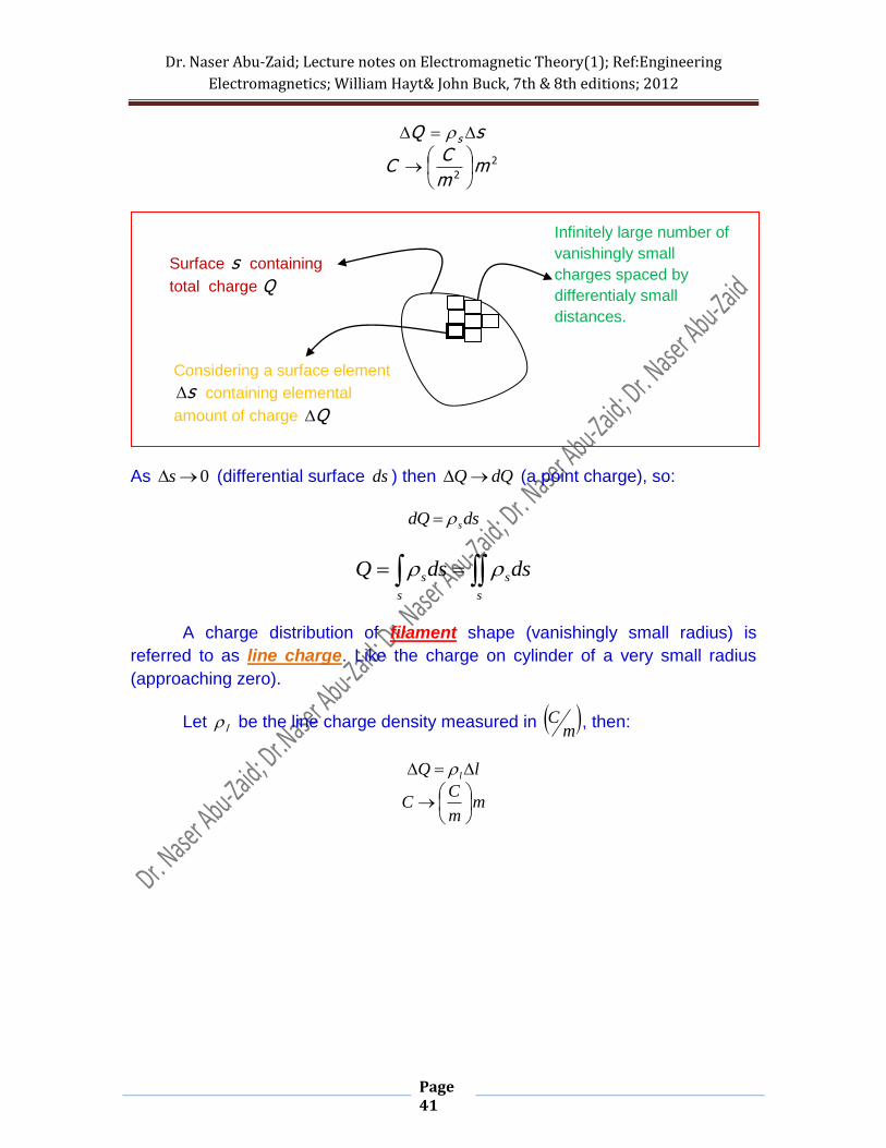
Electromagnetics; William Hayt& John Buck, 7th & 8th editions; 2012
Page 41
2
2m
m
CC
sQ s
As 0s (differential surface ds ) then dQQ (a point charge), so:
dsdQ s
s
s
s
s dsdsQ
A charge distribution of filament shape (vanishingly small radius) is
referred to as line charge. Like the charge on cylinder of a very small radius
(approaching zero).
Let l be the line charge density measured in m
C , then:
mm
CC
lQ l
Infinitely large number of
vanishingly small
charges spaced by
differentialy small
distances.
Surface s containing
total charge Q
Considering a surface element
s containing elemental
amount of charge Q

Dr. Naser Abu-Zaid; Lecture notes on Electromagnetic Theory(1); Ref:Engineering
Electromagnetics; William Hayt& John Buck, 7th & 8th editions; 2012
Page 42
As 0l (differential line dl ) then dQQ (a point charge), so:
dldQ l
l
l dlQ
Note that
Coulomb’ Law
The force between two very small objects separated in a vacuum or free
space by a distance which is large compared to their size is proportional to the
charge on each and inversely proportional to the square of the distance between
them.
x
y
z
1r
2r
21R 1Q 2Q
1F
2F 21a
21a
Assuming both charges have
the same polarity
Infinitely large number of
vanishingly small
charges spaced by
differentialy small
distances.
Line l containing total
charge Q
Considering a line element l
containing elemental amount
of charge Q
Dr. Naser Abu-Zaid; Lecture notes on Electromagnetic Theory(1); Ref:Engineering
Electromagnetics; William Hayt& John Buck, 7th & 8th editions; 2012
Page 43
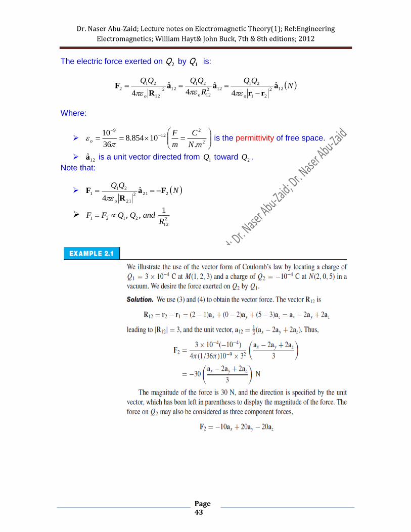
The electric force exerted on 2Q by 1Q is:
NQQ
R
QQQQ
ooo
122
21
21122
12
21122
12
212
ˆ4
ˆ4
ˆ4
arr
aaR
F
Where:
2
212
9
.10854.8
36
10
mN
C
m
Fo
is the permittivity of free space.
12a is a unit vector directed from 1Q toward 2Q .
Note that:
NQQ
o
2212
21
211
ˆ4
FaR
F
2
12
2121
1,,
RandQQFF

Dr. Naser Abu-Zaid; Lecture notes on Electromagnetic Theory(1); Ref:Engineering
Electromagnetics; William Hayt& John Buck, 7th & 8th editions; 2012
Page 44
The Electric Field Intensity E
Assume a test charge tQ is moving around (still stationary) a fixed charge
Q as shown:
The Electric field intensity E is the vector electric force on a unit positive test
charge. Since
NQQ
Qt
Qto
tt a
RF ˆ
42
So;
m
V
C
NQ
QQt
Qtot
t aR
FE ˆ
42
Q
FE
x
y
z
r tr
QtR Q
tQ tF
Qta
tQ
QtR
Qta
tr
tF
tF
tr
tQ
QtR

Dr. Naser Abu-Zaid; Lecture notes on Electromagnetic Theory(1); Ref:Engineering
Electromagnetics; William Hayt& John Buck, 7th & 8th editions; 2012
Page 45
Note that E exists regardless tQ exists or not, so E is measured at any
point in space called the observation point (field point or test point) which is a
distance R from the source point Q . To remove all the subscripts, we use
primed coordinates to indicate source point(s) and unprimed coordinates to
indicate observation point as illustrated in the following figure.
m
V
C
NQQQ
o
R
o
R
o
322'4
ˆ'4
ˆ4 rr
Ra
rra
RE
Where:
'rrR ; R
Ra Rˆ
r : Position vector locating the observation point zyx zyx aaar ˆˆˆ
'r : Position vector locating the source point zyx zyx aaar ˆ'ˆ'ˆ''
zyx zzyyxx aaaR ˆ'ˆ'ˆ'
x
y
'r
r
R Q
z,y,xP
Ra
Assuming Q is positive
E
'z,'y,'xP
z

Dr. Naser Abu-Zaid; Lecture notes on Electromagnetic Theory(1); Ref:Engineering
Electromagnetics; William Hayt& John Buck, 7th & 8th editions; 2012
Page 46
E Due to n discrete point charges
In this case superposition applies.
n
i
Ri
io
i
Rn
no
nR
o
R
o
n
Q
QQQ
12
222
2
212
1
1
321
ˆ4
ˆ4
...ˆ4
ˆ4
...
aR
aR
aR
aR
EEEEE
Where;
'
ii rrR and i
iRi
R
Ra ˆ
x
y
z
'2r
'3r
2R
2Q 3Q
1Q 1R
'1r
'nr
nQ
nR
r
3R
x,y,xP

Dr. Naser Abu-Zaid; Lecture notes on Electromagnetic Theory(1); Ref:Engineering
Electromagnetics; William Hayt& John Buck, 7th & 8th editions; 2012
Page 47
Dr. Naser Abu-Zaid; Lecture notes on Electromagnetic Theory(1); Ref:Engineering
Electromagnetics; William Hayt& John Buck, 7th & 8th editions; 2012
Page 48
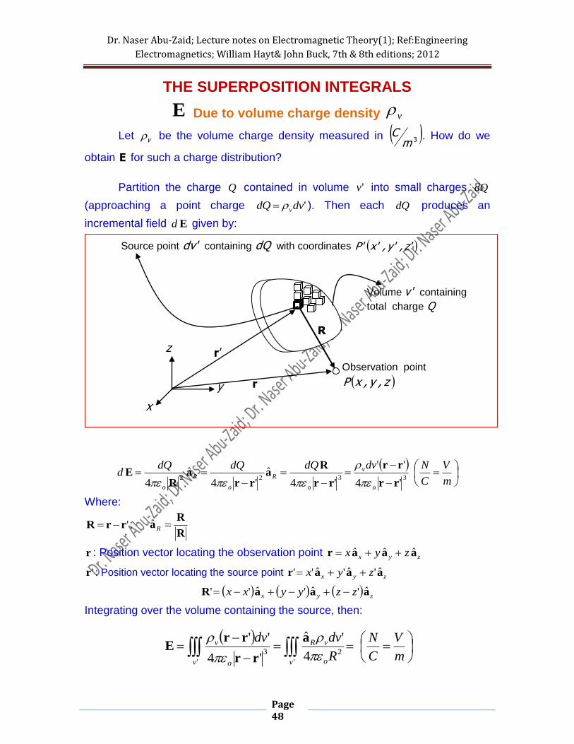
THE SUPERPOSITION INTEGRALS
E Due to volume charge density v
Let v be the volume charge density measured in 3mC . How do we
obtain E for such a charge distribution?
Partition the charge Q contained in volume 'v into small charges dQ
(approaching a point charge 'dvdQ v ). Then each dQ produces an
incremental field Ed given by:
m
V
C
NdvdQdQdQd
o
v
o
R
o
R
o
3322'4
''
'4ˆ
'4ˆ
4 rr
rr
rr
Ra
rra
RE
Where:
'rrR ; R
Ra Rˆ
r : Position vector locating the observation point zyx zyx aaar ˆˆˆ
'r : Position vector locating the source point zyx zyx aaar ˆ'ˆ'ˆ''
zyx zzyyxx aaaR ˆ'ˆ'ˆ''
Integrating over the volume containing the source, then:
m
V
C
N
R
dvdv
v o
vR
v o
v
'
2
'
34
'ˆ
'4
''
a
rr
rrE
x
y
z
'r
R
Observation point
z,y,xP
Source point 'dv containing dQ with coordinates 'z,'y,'x'P
Volume 'v containing
total charge Q
r
Dr. Naser Abu-Zaid; Lecture notes on Electromagnetic Theory(1); Ref:Engineering
Electromagnetics; William Hayt& John Buck, 7th & 8th editions; 2012
Page 49
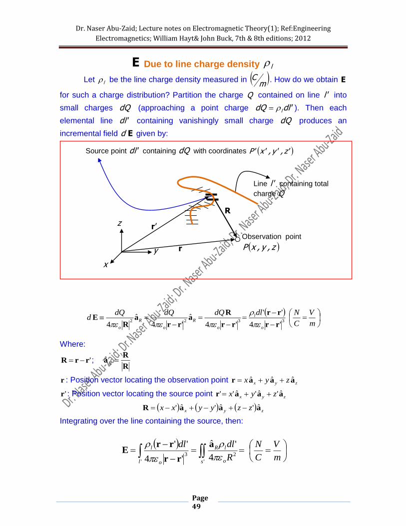
E Due to line charge density l
Let l be the line charge density measured in m
C . How do we obtain E
for such a charge distribution? Partition the charge Q contained on line 'l into
small charges dQ (approaching a point charge 'dldQ l ). Then each
elemental line 'dl containing vanishingly small charge dQ produces an
incremental field Ed given by:
m
V
C
NdldQdQdQd
o
l
o
R
o
R
o
3322'4
''
'4ˆ
'4ˆ
4 rr
rr
rr
Ra
rra
RE
Where:
'rrR ; R
Ra Rˆ
r : Position vector locating the observation point zyx zyx aaar ˆˆˆ
'r : Position vector locating the source point zyx zyx aaar ˆ'ˆ'ˆ''
zyx zzyyxx aaaR ˆ'ˆ'ˆ'
Integrating over the line containing the source, then:
m
V
C
N
R
dldl
s o
lR
l o
l
'
2
'
34
'ˆ
'4
''
a
rr
rrE
x
y
z
'r
R
Observation point
z,y,xP
Source point 'dl containing dQ with coordinates 'z,'y,'x'P
Line 'l containing total
charge Q
r

Dr. Naser Abu-Zaid; Lecture notes on Electromagnetic Theory(1); Ref:Engineering
Electromagnetics; William Hayt& John Buck, 7th & 8th editions; 2012
Page 50
Example: An infinite filament of uniform charge density

Dr. Naser Abu-Zaid; Lecture notes on Electromagnetic Theory(1); Ref:Engineering
Electromagnetics; William Hayt& John Buck, 7th & 8th editions; 2012
Page 51
What if the filament is not aligned with the z-axis?

Dr. Naser Abu-Zaid; Lecture notes on Electromagnetic Theory(1); Ref:Engineering
Electromagnetics; William Hayt& John Buck, 7th & 8th editions; 2012
Page 52
Observations:
aE ˆ
2 o
l For an infinite length line.
E is perpendicular to the line charge, aE ˆ?E .
E does not vary with or z , aE ˆE .
R
o
l
RaE ˆ
2
For an infinite length line, that is arbitrarily aligned.
E Due to surface charge density s
Let s be the surface charge density measured in 2mC . How do we
obtain E for such a charge distribution? Partition the charge Q contained on
surface 's into small charges dQ (approaching a point charge 'dsdQ s ).
Then each elemental surface 'ds containing vanishingly small charge dQ
produces an incremental field Ed given by:
x
y
z
'r
R
Observation point
z,y,xP
Source point 'ds containing dQ with coordinates 'z,'y,'x'P
Surface 's containing
total charge Q
r

Dr. Naser Abu-Zaid; Lecture notes on Electromagnetic Theory(1); Ref:Engineering
Electromagnetics; William Hayt& John Buck, 7th & 8th editions; 2012
Page 53
m
V
C
NdsdQdQdQd
o
s
o
R
o
R
o
3322'4
''
'4ˆ
'4ˆ
4 rr
rr
rr
Ra
rra
RE
Where:
'rrR ; R
Ra Rˆ
r : Position vector locating the observation point zyx zyx aaar ˆˆˆ
'r : Position vector locating the source point zyx zyx aaar ˆ'ˆ'ˆ''
zyx zzyyxx aaaR ˆ'ˆ'ˆ''
Integrating over the surface containing the source, then:
m
V
C
N
R
dsds
s o
sR
s o
s
'
2
'
34
'ˆ
'4
''
a
rr
rrE
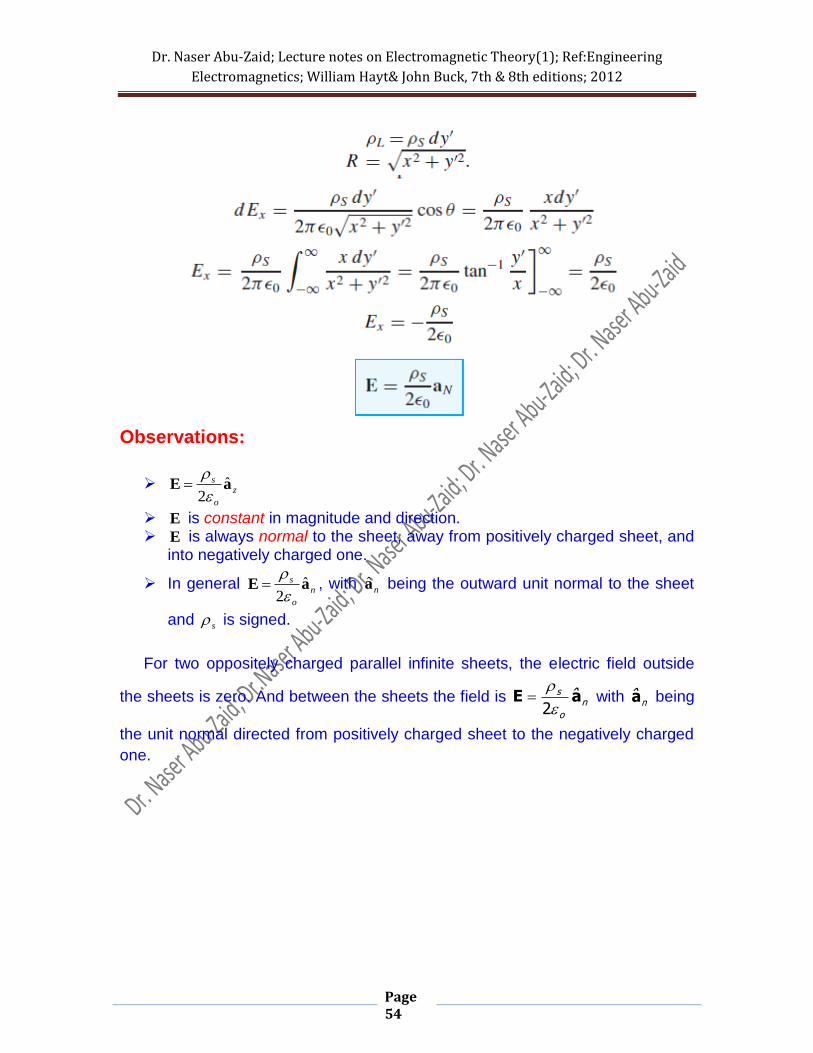
Example: Consider an infinite sheet lying in the yz-plane, having a uniform
charge distribution of
2m
Cs . Determine an expression for E at an arbitrary
point lying on the x-axis.
Dr. Naser Abu-Zaid; Lecture notes on Electromagnetic Theory(1); Ref:Engineering
Electromagnetics; William Hayt& John Buck, 7th & 8th editions; 2012
Page 54
Observations:
z
o
s aE ˆ2
E is constant in magnitude and direction. E is always normal to the sheet, away from positively charged sheet, and
into negatively charged one.
In general n
o
s aE ˆ2
, with na being the outward unit normal to the sheet
and s is signed.
For two oppositely charged parallel infinite sheets, the electric field outside
the sheets is zero. And between the sheets the field is n
o
s aE
2 with na being
the unit normal directed from positively charged sheet to the negatively charged
one.

Dr. Naser Abu-Zaid; Lecture notes on Electromagnetic Theory(1); Ref:Engineering
Electromagnetics; William Hayt& John Buck, 7th & 8th editions; 2012
Page 55
1) :x 0 x
o
s aE
2
and x
o
s aE
2 0 EEE .
2) :x 0 x
o
s aE
2 and x
o
s aE
2
0 EEE .
3) :ax 0 x
o
s aE
2 and x
o
s aE
2 x
o
s aEEE
.
x
+ +
+
+
+
- -
-
-
-
E E
E E
E
E
+ - 0x ax
E
Dr. Naser Abu-Zaid; Lecture notes on Electromagnetic Theory(1); Ref:Engineering
Electromagnetics; William Hayt& John Buck, 7th & 8th editions; 2012
Page 56
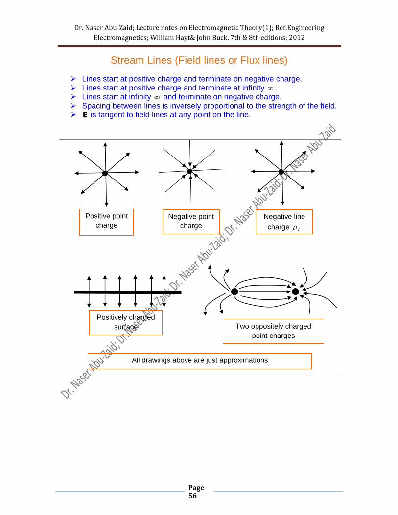
Stream Lines (Field lines or Flux lines)
Lines start at positive charge and terminate on negative charge. Lines start at positive charge and terminate at infinity . Lines start at infinity and terminate on negative charge. Spacing between lines is inversely proportional to the strength of the field. E is tangent to field lines at any point on the line.
Positive point
charge
Negative point
charge
Negative line
charge l
Positively charged
surface Two oppositely charged
point charges
All drawings above are just approximations
Related Documents


![Restricted Dzogchen Teachings, Part 2: Buddhahood Without … · 2018. 10. 2. · [Zab chos zhi khro dgoºs pa raº grol las rdzogs rim bar do drug gi khrid yig. English] Natural](https://static.cupdf.com/doc/110x72/60c4576c97047869ae4cc298/restricted-dzogchen-teachings-part-2-buddhahood-without-2018-10-2-zab-chos.jpg)

![Rakow TB210808 Endversion Layout · durch Meditation über die friedvollen und zornvollen [Gottheiten] (zab chos zhi khro dgongs pa rang grol las/ bar do thos grol chen mo). 6 Zur](https://static.cupdf.com/doc/110x72/5e9807f2037c937108713ff5/rakow-tb210808-endversion-layout-durch-meditation-ber-die-friedvollen-und-zornvollen.jpg)


