Engineering Conference 1981 - Federal Railroad Administration

REPORT NO. FRA/TTC-82/01

PROCEEDINGS

Facility for Rccelerated Service Te/tlng“ US US“ \

Engineering Conference 1981DENVER, COLORADO

NOVEMBER 4 & 5, 1981

Th i s d o c u m e n t is a v a i l a b l e to the publ ic t h r o u g h The N a t i o n a l T e c h n i c a l I n for ma t i on Se r v i ce

S p r i n g f i e l d , V i r g i n i a 22161

AN I N T E R N A T I O N A L G O V E R N M E N T - I N D U S T R Y RESEARCH P R O G R A M

U.S. D E P A R T M E N T OF T R A N S P O R T A T I O N A S S O C I A T I O N OF A M E R I C A N RAI LROA DSFEDERAL R A I LR O A D A D M I N I S T R A T I O N 1 9 2 0 L S t r e e t , N . W .

W a s h i ng t on , D . C . 2 0 5 9 0 W a s h i n g t o n . D.C. 2 0 0 3 6

RAI LWAY PR O G R E S S I N S T I T U T E 801 Nor th Fa i r f a x S t r e e t

A l e x a n d r i a . V i r g i n i a 2 2 3 1 4

FRA

R R IR A IL W A Y |

P R O G R E S S ■ IN S T IT U T E

RPI55A A R

a in Dynamics

)Technical Report Documentation Page

1 . R eport N o .

FRA/TTC-82/012. G overnm ent A c c e s s io n No. 3. R e c ip ie n t's C a ta lo g No.

4 . T i t le and S u b title

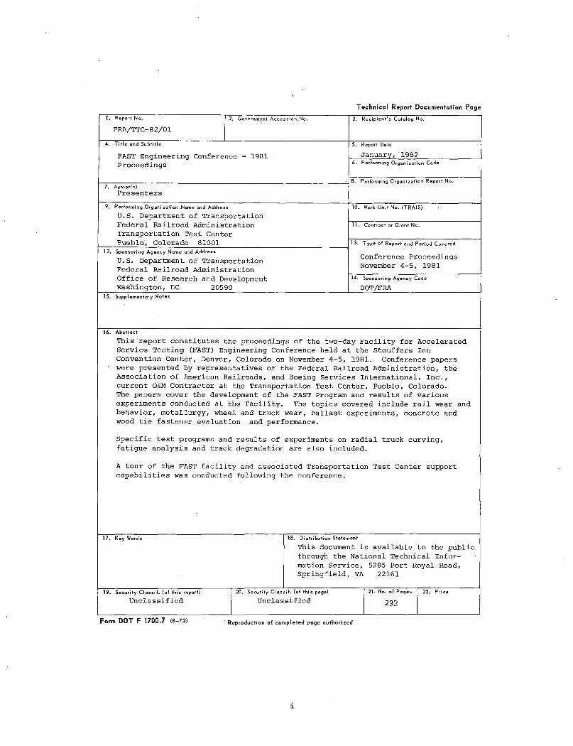
FAST Engineering Conference - 1981 Proceedings

5 . Report D ate

January, 19826 . Perform ing O rg an iza tio n Code

8 . Perform ing O rg a n iza tio n R eport No.7. A u th o rs )Presenters9. P erfo rm in g O rg a n iza tio n Nam e ond Address

U.S. Department of Transportation Federal Railroad Administration Transportation Test Center Pueblo, Colorado 81001

10. Work U n it No. (T R A IS )

11. C o n trac t or G rant N o .

13 . T y p e o f R eport and P e rio d C overed

Conference Proceedings November 4-5, 1981

12 . Sponsoring A g en cy N am e and A ddress

U.S. Department of Transportation Federal Railroad Administration Office of Research and Development Washington, DC 20590

14. Sponsoring A g en cy Code

DOT/FRA15. S upp lem entary N o tes

1 6 . A b s tra c t

This report constitutes the proceedings of the two-day Facility for Accelerated Service Testing (FAST) Engineering Conference held at the Stouffers Inn Convention Center, Denver, Colorado on November 4-5, 1981. Conference papers were presented by representatives of the Federal Railroad Administration, the Association of American Railroads, and Boeing Services International, Inc., current O&M Contractor at the Transportation Test Center, Pueblo, Colorado.The papers cover the development of the FAST Program and results of various experiments conducted at the facility. The topics covered include rail wear and behavior, metallurgy, wheel and truck wear, ballast experiments, concrete and wood tie fastener evaluation and performance.

Specific test programs and results of experiments on radial truck curving, fatigue analysis and track degradation are also included.

A tour of the FAST facility and associated Transportation Test Center support capabilities was conducted following the conference.

1 7 . K e y w o rd s 18 . D is trib u tio n S tatem ent

This document is available to the public through the National Technical Infor­mation Service, 5285 Port Royal Road, Springfield, VA 22161

1 9 . S e c u rity C la s s if . (o f th is report)

Unclassified20. Security C la s s if . (o f th is page)

Unclassified21* No. of P ages

23222. P ric e

Form DOT F 1700.7 ( 8 - 7 2 ) Repro duction of c o mple te d page aut h o ri ze d

ACKNOWLEDGEMENT

The Federal Railroad Administration, Transportation Test Center, wishes to express their appreciation in behalf of all the responsible FAST committees and participants for the efforts expended to make the 1981 FAST Engineering Conference and Proceedings a success.

o To the authors for their dedication in presenting data and information which will be useful to the Railroad Industry.

o To Boeing Services International, Inc. for the manpower and efforts in preparing the presentations, organizing the conference, and preparing these proceedings.

o To the attendees who so intently listened.

i i

TABLE OF CONTENTS

a) Conference Welcome (November 4, 1981)............................................1Walter W. Simpson

b) Conference Welcome (November 5, 1981) ............................................ 5Peter J. Detmold

c) FAST Overview................................... 7Gregory P. McIntosh

d) Introduction.................................................................. 11James R. Lundgren

e) Evolution of Measurement Techniques at F A S T ..................................... 19Thomas P. Larkin

TRACK

1) Ballast Experiments at F A S T ............... 45Bruce N. Bosserman

Introduction to Tie & Fastener Performance................................. 55

2) Results of Standard Wood Tie and Manufactured Ties Experiments at FAST . . 57Lauress C. Collister

3) Evaluation of Various Wood Tie Fasteners Under Heavy Freight RailroadService Loading ............................................................ 63

Larry Daniels

4) Concrete Tie & Fastener Performance................................... ,. 75John W. Weber

5) Concrete Tie & Track Systems Engineering Considerations ................. 83Jack. E. Heiss

6) Tie/Ballast Interaction Comparisons for Wood and Concrete Ties .......... 91Bruce N. Bosserman

7) Aspects of Concrete Tie Performance on FAST and Revenue Service ........ 97Howard G. Moody

8) Correlations of FAST and Laboratory Tests with Concrete and Wood TieFastener Results ...........................................................103

Howard G. Moody

9) Rail: It's Behavior and Relationships to Total System W e a r .....................115Roger K. Steele, Ph.D.

Note: This paper is composite of 4 papers presented at Conference: o Rail Wear and Metal Flow o Welded Rail End Batter o Rail Failure Behavior o Wheel/Rail System Wear

i i i

10) Rail Corrugation Investigations at F A S T ............ .........................165Timothy J. Devine

MECHANICAL

11) Major Variables that Affect Wheel Wear ..................... .......... .. . .175Donald E. Gray

12) Wear Rates of Freight Car Wheels as a Function of Chemistry ..................199V. E. Kahle

13) Radial Truck Wheel W e a r .......................................................205Roy A. Allen

14) The Mechanical Aspects of Wheel/Rail W e a r .................... 217Roy A. Allen

15) Fatigue Analysis Tests at F A S T .............................................. 229S. K. Punwani

FUTURES

16) Track Degradation Experiment................................................ 237James W. Brent

17) Defective Growth Rate Pilot T e s t ............................................ 241Oscar Orringer

18) Radial Truck Curving Performance Evaluation ................................ .247Roy A. Allen

A P P E N D I X .....................................................................251

iv

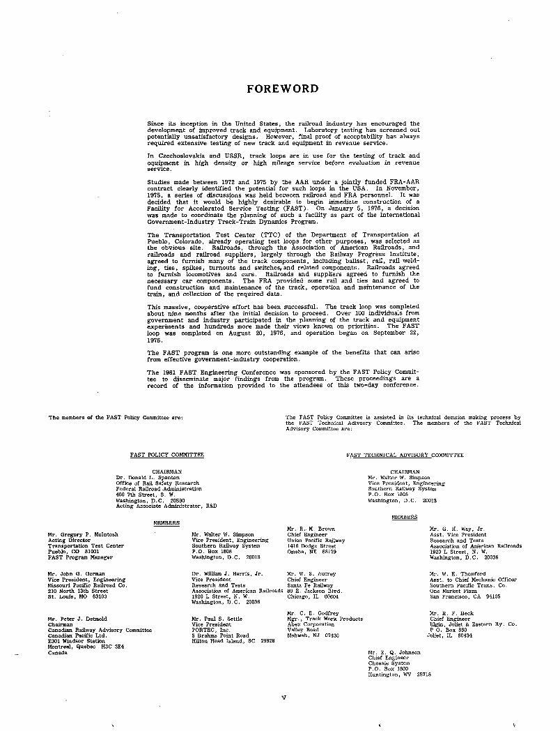
FOREWORD

Since its inception in the United States, the railroad industry has encouraged the development of unproved track and equipment. Laboratory testing has screened out potentially unsatisfactory designs. However, final proof of acceptability has always required extensive testing of new track and equipment in revenue service.

In Czechoslovakia and USSR, track loops are in use for the testing of track and equipment in high density or high mileage service before evaluation in revenue service.

Studies made between 1972 and 1975 by the AAR under a jointly funded FRA-AAR contract clearly identified the potential for such loops in the USA. In November,1975, a series of discussions was held between railroad and FRA personnel. It was decided that it would be highly desirable to begin immediate construction of a Facility for Accelerated Service Testing (FAST). On January 5, 1976, a decision was made to coordinate the planning of such a facility as part of the International Government-Industry Track-Train Dynamics Program.

The Transportation Test Center (TTC) of the Department of Transportation at Pueblo, Colorado, already operating test loops for other purposes, was selected as the obvious site. Railroads, through the Association of American Railroads, and railroads and railroad suppliers, largely through the Railway Progress Institute, agreed to furnish many of the track components, including ballast, rail, rail weld­ing, ties, spikes, turnouts and switches,and related components. Railroads agreed to furnish locomotives and cars. Railroads and suppliers agreed to furnish the necessary car components. The FRA provided some rail and ties and agreed to fund construction and maintenance of die track, operation and maintenance of the train, and collection of the required data.

This massive, cooperative effort has been successful. The track loop was completed about nine months after the initial decision to proceed. Over 100 individuals from government and industry participated in the planning of the track and equipment experiments and hundreds more made their views known on priorities. The FAST loop was completed on August 20, 1976, and operation began on September 22,1976.

The FAST program is one more outstanding example of the benefits that can arise from effective government-industry cooperation.

The 1981 FAST Engineering Conference was sponsored by the FAST Policy Commit­tee to disseminate major findings from the program. These proceedings are a record o f the information provided to the attendees of this two-day conference.

The members o f the FAST Policy Committee are: The FAST Policy Committee is assisted in its technical decision making process bythe FAST Technical Adivsory Committee. The members of the FAST Technical Advisory Committee are:

FAST POLICY COMMITTEE FAST TECHNICAL ADVISORY COMMITTEE

CHAIRMAN Dr. Donald L. Span ton Office of Rail Safety Research Federal Railroad Administration 400 7th Street, S. W.Washington, D . C . 20590Acting Associate Administrator, R&D

CHAIRMANMr. Walter W. Simpson Vice President, Engineering Southern Railway System P.O. Box 1808 Washington, D .C . 20013

Mr. Gregory P. McIntosh Acting Director Transportation Test Center Pueblo, CO 81001 FAST Program Manager

MEMBERS

Mr. Walter W. Simpson Vice President, Engineering Southern Railway System P.O. Box 1808 Washington, D .C . 20013

Mr. R.- M. Brown Chief Engineer Union Pacific Railway 1416 Dodge Street Omaha, NE 68179

MEMBERS

Mr. G. H. Way, Jr.Asst. Vice President Research and Tests Association o f American Railroads 1920 L Street, N. W.Washington, D .C . 20036

Mr. John G. German Vice President, Engineering Missouri Pacific Railroad Co. 210 North 13th Street St. Louis, MO 63103

Mr. Peter J. Detmold ChairmanCanadian Railway Advisory Committee Canadian Pacific Ltd.E301 Windsor Station Montreal, Quebec H3C 3E4 Canada

Dr. William J. Harris, Jr. Mr. W. S. AutreyVice President Chief EngineerResearch and Tests Santa Fe RailwayAssociation of American Railroads 80 E. Jackson Blvd. 1920 L Street, N. W. Chicago, IL 60604Washington, D .C . 20036

Mr. W. E. ThomfordAsst, to Chief Mechanic OfficerSouthern Pacific Trans. Co.One Market PlazaSan Francisco, CA 94105

Mr. Paul S. Settle Vice President PORTEC, Inc.5 Brahms Point Road Hilton Head Island, SC 29928

Mr. C. E. GodfreyMgr., Track Work ProductsAbex CorporationValley RoadMahwah, NJ 07430

Mr. R. F. Beck Chief EngineerElgin, Joliet & Eastern Ry. Co. P.O. Box 880

Joliet, IL 60434

Mr. E. Q. Johnson Chief Engineer Chessie System P.O. Box 1800 Huntington, WV 25718

V

WALTER W. S I M P S O N VI CE P R E S I D E N T . E N G I N E E R I NG

SOUTHERN RAI LWAY S Y S TE M

CONFERENCE WELCOMENOV. 4, 1981

C H A I R M A N FAST T E C H N I C A L C O M M I T T E E M E M B E R FAST POLI CY C O M M I T T E E

Good morning, ladies and gentlemen. Welcome to Denver and to the first full report of what we have learned at FAST.

I would like this morning, in addition to saying, "I'm glad you're here," to provide you with a brief history of FAST and the reason for its existence—to talk a little bit about its future, and also some of its failures. A clear understanding of past problems of FAST, together with knowledge as to how the problems were overcome can aid in decisions relative to the future value of FAST to the industry.

The Transportation Test Center in Pueblo resulted from an act of Congress—"The High Speed Ground Transportation Act of 1965." The Test Center opened in 1971 and, as you might imagine from the title of the legislation, started researching the movement of people at high ground speeds in unusual looking vehicles.

In the mid 1970's under a program of track research jointly funded by AAR and FRA, we recognized the need for improved facilities to study the interaction of trains and track. This new facility was to be designed to help us learn to run freight trains in a more normal speed range with complete reliability and maximum efficiency.

The FAST track, located at the Transportation Center, was opened on November 8, 1976, and will celebrate its fifth year in existence some four days from now.

Back in 1975, a test track was considered of great potential value to the industry. Basic research in track and equipment areas was badly needed. This new test facility would provide the means to take new developments from testing to practical use ten times faster than could be accomplished in ordinary service. The informa­tion available from the accelerated testing mode was particularly important in view of the increasing cost of fuel, rail, cross ties, and rolling stock and the deterio­rating financial condition of the railroads. After all, our future success requires that we obtain the maximum return for all of our resources.

The need for FAST, or a similar facility, is probably more important today than it was in 1975. Competition in the deregulated environment is going to become more aggressive, the reliability of our service more important, and control of costs mandatory for our survival.

If we accept the premise that the industry needs such a test facility, what does the future hold? Under the Reagan Administration's budget cutting, the federal fund­ing level is uncertain. In fact, the FRA would prefer private sector operation--and funding—of the Test Center. Because of the budget cutting efforts of the new adminstration, the Department of Transportation, the Association of American Rail­roads, the supply industry, and some individual railroads have in recent months examined the value of FAST to the industry and, most particularly, what has been achieved during this five-year period since opening day.

1

V V

I have been personally involved with FAST for the last two years and other South­ern Railway people have worked with the FAST program since its birth. We know the problems FAST has encountered over the years, and the delays that often marked their handling. I'm sure there are some here today who think the reports on the agenda at this Engineering Conference should have been available two or three years ago.

Nevertheless, because of the uncertain future and the need to determine the value of FAST to the industry, I think it desirable that we review some of FAST's fail­ures and consider the corrective actions that were taken. My purpose is to demon­strate that the problems that resulted in delays and sometimes less than satisfactory reports have been addressed. What is coming out of FAST is a quality product.

If you ask some of the statisticians involved in the FAST operation what went wrong, they will say there were too many initial experiments and that they were poorly designed.

If you ask a management expert, he'll tell you that the definition of responsibility between on-site managers, including AAR, FRA, and the contractor, was not properly established.

If you ask a research type, he might say that measurement techniques were not perfected prior to use and maintenance practices interfered with accurate test results.

Finally, if you ask railroad and supply industry engineers, they might say that too much effort went into data gathering and too little effort to analysis and reporting of results.

All of these people would be correct to some extent.

FAST got off to a good start. In September, 1975, the report recommending the proposed facility was submitted; one ■ year later a test was in operation. That accomplishment may have been our first mistake. It produced some hastily designed experiments—along with some good ones—and caused a lack of synchronization that plagued FAST for several years. Considerable data was being gathered very quick-, ly, but there wasn't even a computer at the test site when the test trains started running. This resulted in massive problems in data quality and access. Measure­ment techniques and instruments commonly used by the railroad industry were adopted on FAST, but many were not accurate enough or required an unusual amount of expertise and time to maintain consistent accuracy.

These measurement tools often had to be modified, and when no tools were avail­able, new instruments were developed. Rail and wheel profilometers as well as tools for hardness tests, longitudinal rail stress measurements and truck wear measure­ments are just a few examples.

Follow-on experiments were being designed before data from the first experiment in the series could be analyzed or' even accessed. Data quality problems, were dis­covered after the fact. Inventory confusion—what types of wheels were under what cars, and what kind of rail steel was at what location—resulted in delays in data analysis. Far too much effort was required to correct errors and verify operating conditions.

This clogging of the system with massive amounts of incoming data and too little information coming out caused severe communication problems among the three organizations involved in FAST—the FRA, the Contractor, and the AAR. It was months before these data processing problems were resolved and the experiment managers could obtain their data in a reasonably timely fashion. The slow infor­mation feedback contributed to delays in the publication of technical reports on findings. And often, as the reports neared completion, new problems developed. There were even problems of report approval, with the approval process itself going through numerous revisions. The objectives—to assure high quality reports and to portray the performance of vendor products fairly and accurately—were admirable, but the delays were discouraging.

2

Operating problems and unexpectedly high failure and wear rates forced redesign of experiments and resulted in major material and component supply problems. Ex­amples include the high failure rate of wheels in the unlubricated environment and high failure rates of welded rail. Each of these situations had serious repercus­sions . They forced changes in experiment designs on the fly . Wheels and rail were wearing out so rapidly that the accurate documentation of what was failing and what it was being replaced by caused additional delay.

There were other totally different problems, too. The quality of the design of the experiments, their statistical validity, and their contribution to knowledge varied widely depending on the qualifications of the experiment designer and the avail­ability of data from recently completed experiments. Added to this was substantial variation in the quality of the analysis of various experiments. Again, this was dependent upon the skills and the experience of the analyst.

Looking back over the first few years of FAST operations, I believe our difficulties really stemmed from a confusion of priorities. For a long time the priority was accumulating tonnage, the accelerated service part of FAST. The worst thing that could happen was a train standing idle. But the raw product of FAST was data, not tonnage, and accurate and accessible data was not assigned a top priority until we were well down stream.

What is the situation today? I think it is vastly improved. The problems I have mentioned have been addressed directly and effectively. Organizational problems have been solved by establishing clear lines of authority and clear separation of responsiblilities.

Experiments now are carefully designed from the ground up. Ad hoc committees, drawing from the industry those individuals with particular expertise in the area of the experiment, now assist the design process. Statistical validity is assured by making certain that one or more members of the committee is skilled in the field of experiment design.

Data quality has been tackled on a broad front, ranging from improved instrumen­tation and measurement techniques to a variety of controls to assure high quality data input. Experiment managers can now access the data in a timely fashion. The quality of the analysis of the experiment is steadily improving. Some of the exper­iments being reported on today and tomorrow, I believe you will agree, are truly at the cutting edge of knowledge in the railroad environment. Each of you, as partic­ipants in this engineering conference must in the next two days draw your own conclusions as to the value of FAST to the industry. In its five years of existence it has not been as productive as those of us familiar with the program would have liked. A lot of mistakes have been made, most of them due to the complexity of the problems being dealt with and the organizational problems associated with the coop­erative nature of the program. But the past is gone, and we have learned some­thing from it. Today FAST is being managed properly and, as far as I am con­cerned, has come of age.

As to the future, I would hope that it includes the FAST facility or one somewhat like it, for our industry will need this important range of research activities even more than today.

3

CONFERENCE WELCOMENOV. 5. 1981

PETER J. DETMOLD SPECIAL CONSULTANT

CANADIAN PACIFIC LIMITED

CHAIRMAN FAST POLICY COMMITTEE

HAPPINESS IS JUST A THING CALLED CHANGE*

It is both a pleasure and an honour to welcome you to the second day of the con­ference on behalf of the Canadian railway community, our public servants as well as our railroaders.

But just before I sit down, my two bits worth will be to tell you why today is going to be so important for all of us.

Railroading is the only sector of the transport industry in which the power, the vehicles and the fixed plant are purchased directly by the operator from more than 350 manufacturers. If you buy a ship or a plane it arrives (all being well) in one piece. Trucks and trailers may be a problem. With railroads, research is made much more complicated by this basic fact of life concerning supply.

In view of its heterogenous nature and the broad variety of operating conditions, although each manufacturer issues a warranty for the successful performance of his product, there is no warranty for the train, no warranty on the track and none, of course, on the train and the track together. Little or no central research effort into the railroad as a system had been made until the advent of programs such as track-train dynamics, and full scale physical experiments such as FAST. There has, therefore, been no assurance that, as technological railroad developments essential to the economies of our two countries took place, new combinations of the component parts of a railroad would be wholly compatible or that the overall oper­ation of the system might not be adversely affected if they were not wholly compat­ible.

This was probably not too serious a disadvantage during long periods in the past in which technological development was comparatively static and equipment specifica­tions could remain substantially unchanged. But we have entered a new phase in our history in which intensive technical change is not only possible, but in some cases, highly desirable. We have entered a phase in which the cost of capital and energy fluctuate sharply, creating the need to be able to respond rapidly with new technical solutions to problems of an economic as well as of a technical nature.

Many of the large railways in your country and in ours have excellent research departments. But what can any single research department do to ensure that the combinations of track, power, and cars are ideally suited to the specific conditions of their property when maybe more than a quarter of the cars at one time carry someone else's logo--most of them modern cars but just a few with graffiti on the side assuring us that Thomas Dewey will make a very good President.

*A "one-liner" from NEWSWEEK Magazine.

So let me say to FAST, to TTD, to TTC, and to TSC—"we need you!" We need cooperative research in both our countries. We cannot develop further as a thriving modern industry unless we maintain effective means of carrying out the kinds of research we cannot do as individual roads—research that regards railroads as integrated systems, and research that is not too overly respectful of the status quo.

Most of you are well aware that the future of this cooperative research work is currently in some doubt. It would not be my wish to come here from Canada and offer you advice on solutions to the problems of administering programs of this kind. But it is very much my wish to come here and to assure you that the Canadian railway industry will do all we can to cooperate with you in ways that will facilitate the keeping in place of the cooperative research effort that is so essential to us all.

One final thought. To do this research alone is not enough; we also need to apply the conclusions to our operations. Anyone who was here yesterday must already be convinced that a large number of ideas for improving the design of track and vehicles have already emerged and many more will follow. What is the first need in applying research? My goodness, I believe it's cash flow! In our different ways we need to ensure that return on investment in railroading no longer lags behind the average for other industries as it has for so many years in both our countries. Hopefully, the recent tax changes in the U.S. will go some way to improving the situation. In Canada, pious talk about improved safety on the railways, if it is to be effective, must be accompanied by a solution to the Crow grain rate problem. Only then will the cash flow make possible investment on the large scale that will be required. But cash is not the only requirement. We also need to develop a more adventuresome, a more innovative attitude to technical change. We need to increase the pace at which we can alter the nature of our operations. To achieve this, railroaders and manufacturers alike need to regard the component with which they are concerned as a component of an overall system with the implication that it may sometimes be necessary to alter the specification of an individual component to improve safety and efficiency overall.

Conferences such as this one not only indicate directions for change but also chal­lenge the assumption that we should learn to live with problems that are within ou,r collective capability to eradicate.

Thank you.

6

1 i

f i\ 3 Ii m a m in

(Facility for Accelerated Service Testing)

G. McIntosh FAST Program Manager

To set the stage for the technical papers which are presented in these proceedings, this paper will present an overview of the FAST facility, the operations and.the organizations, which are responsible for the administration, implementation and direction of the FAST Program. Mr. McIntosh is the FAST Program Manager and also is Acting Director of the Transportation Test Center.

BACKGROUND

FAST (Facility for Accelerated Service Testing) is a joint industry and government program composed of members from the Federal Railroad Administration (FRA), Association of American Railroads (AAR), and the Railway Progress Institute (RPI). FAST has had international participation from the Canadian and Mexican Railroads as well as a large number of hard­ware suppliers and manufacturers from various coun­tries throughout the world.

The FAST Program was conceived by a joint industry and Government committee in the spring of 1976. By modifying existing facilities and utilizing a small number of existing staff, the FAST train started operations at the Transportation Test Center, Pueblo, Colorado in September 1976.

The list of participants is found in the appendix of these proceedings.

OBJECTIVE

The primary objective of the FAST Program is to provide a facility and test capability to maintain

and improve the safety and efficiency of the rail­road industry. This is achieved by providing the capability to obtain accelerated and closely con­trolled engineering data. This data base can be utilized by the railroad community to make technical and management decisions relative to track and mechanical components, track structures, mechanical systems and auxiliary equipment, i.e., hot box detectors, grade crossing and fault detection sys­tems.

SCOPE OF CAPABILITY

FAST is a unique Facility. It provides the ability to perform extremely complex experiments, requiring large quantities of highly accurate parametric data under controlled conditions. FAST has the ability to perform experiments of long duration such as wear, life, fatigue, and track degradation. Tests of short duration commonly referred to as "Mini Tests" are also conducted. Examples are; carbody and track accelerations, wheel/rail-loads, instru­mented wheels, and angle of attack tests in support of curving performance evaluations.

FAST also provides the capability to develop and improve measurement and instrumentation techniques

7

and to develop the hardware necessary to obtain repeatable and highly accurate data.

To summarize, FAST provides the capability to con­duct the most complex to simple tests under con­trolled environments and conditions not otherwise available in normal service.

MANAGEMENT

The original management structure was established under the control of the Track-Train Dynamics Program. However, the program was so large and complex that a decision was made to form an in­dependent management organization. The present organization has been in effect since 1979.

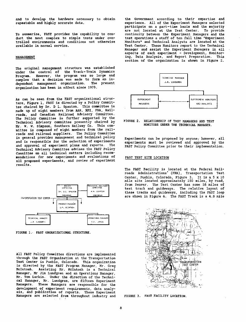
As can be seen from the FAST organizational struc­ture, Figure 1, FAST is directed by a Policy Commit­tee chaired by Dr. D L. Spanton. This committee is made up of eight members from AAR, RPI, FRA, Rail­roads, and Canadian Railroad Advisory Committee. The Policy Committee is further supported by the Technical Advisory committee presently chaired by Mr. W. W. Simpson, Southern Railway Co. This com­mittee is composed of eight members from the rail­roads and railroad suppliers. The Policy Committee in general provides management and technical policy and is responsible for the selection of experiments and approval of experiment plans and reports. The Technical Advisory Committee advises the FAST Policy Committee on all technical matters including recom­mendations for new experiments and evaluations of all proposed experiments, and review of experiment results.

FIGURE 1. FAST ORGANIZATIONAL STRUCTURE.

All FAST Policy Committee directions are implemented through the FAST Organization at the Transportation Test Center in Pueblo, Colorado. This organization is directed by the FAST Program Manager, Mr. Greg McIntosh. Assisting Mr. McIntosh is a Technical Manager, Mr Jim Lundgren and an Operations Manager, Mr. Tom Larkin. Under the direction of the Techni­cal Manager, Mr. Lundgren, are fifteen Experiment Managers. These Managers are responsible for the development of experiment requirements, data analy­sis, and publication of reports. These Experiment Managers are selected from throughout industry and

the Government according to their expertise and experience. All of the Experiment Managers selected participate on a part-time basis and the majority are not located at the Test Center. To provide continuity between the Experiment Managers and the test operations a staff of ten full time "Experiment Monitors" and Technical Analysts are located at the Test Center. These Monitors report to the Technical Manager and assist the Experiment Managers in all aspects of each experiment - Development, Monitor­ing, Data Analysis, and Report Preparation. This section of the organization is shown in Figure 2.

FIGURE 2. RELATIONSHIP OF TEST MANAGERS AND TEST MONITORS UNDER THE TECHNICAL MANAGER.

Experiments can be proposed by anyone; however, all experiments must be reviewed and approved by the FAST Policy Committee prior to their implementation.

FAST TEST SITE LOCATION

The FAST Facility is located at the Federal Rail­roads Administrations* (FRA), Transportation Test Center, Pueblo, Colorado, Figure 3. It is a 5 x 10 mile site located approximately 150 miles, by road, from Denver. The Test Center has some 58 miles of test track and guideways. The relative layout of these tracks and guideways, including the FAST loop are shown in Figure 4. The FAST Track is a 4.8 mile

FIGURE 3. FAST FACILITY LOCATION.

8

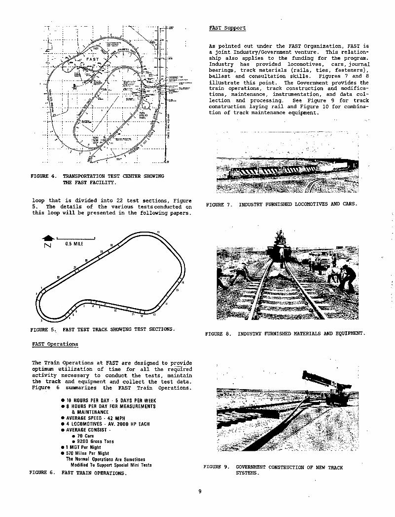
FAST Support

FIGURE 4. TRANSPORTATION TEST CENTER SHOWING THE FAST FACILITY.

As pointed out under the FAST Organization, FAST is a joint, Industry/Government venture. This relation­ship also applies to the funding for the program. Industry has provided locomotives, cars, journal bearings, track materials (rails, ties, fasteners), ballast and consultation skills. Figures 7 and 8 illustrate this point. The Government provides the train operations, track construction and modifica­tions, maintenance, instrumentation, and data col­lection and processing. See Figure 9 for track construction laying rail and Figure 10 for combina­tion of track maintenance equipment.

loop that is divided into 22 test sections. Figure 5. The details of the various tests conducted on this loop will be presented in the following papers.

FAST Operations

The Train Operations at FAST are designed to provide optimum utilization of time for all the required activity necessary to conduct the tests, maintain the track and equipment and collect the test data. Figure 6 summarizes the FAST Train Operations. •

• 16 HOURS PER DAY - 5 DAYS PER WEEK• 8 HOURS PER DAY FOR MEASUREMENTS

& MAINTENANCE• AVERAGE SPEED - 42 MPH• 4 LOCOMOTIVES - AV. 2000 HP EACH• AVERAGE CONSIST -

• 70 Cars• 9200 Gross Tons

• 1 MGT Per Night• 570 Miles Per Night

The Normal Operations Are SometimesModified To Support Special Mini Tests

FIGURE 6. FAST TRAIN OPERATIONS.

FIGURE 7. INDUSTRY FURNISHED LOCOMOTIVES AND CARS.

FIGURE 8. INDUSTRY FURNISHED MATERIALS AND EQUIPMENT.

FIGURE 9. GOVERNMENT CONSTRUCTION OF NEW TRACK SYSTEMS.

9

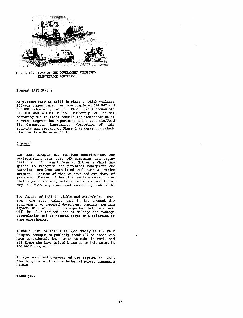
FIGURE 10. SOME OF THE GOVERNMENT FURNISHED MAINTENANCE EQUIPMENT.

Present FAST Status

At present FAST is still in Phase 1, which utilizes 100-ton hopper cars. We have completed 614 MGT and 353,000 miles of operation. Phase 1 will accumulate 818 MGT and 480,000 miles. Currently FAST is not operating due to track rebuild for incorporation of a Track Degradation Experiment and a Concrete/Wood Tie Comparison Experiment. Completion of this activity and restart of Phase 1 is currently sched­uled for late November 1981.

Summary

The FAST Program has received contributions and participation from over 160 companies and organ­izations. It doesn't take an MBA or a Chief En­gineer to recognize the potential management and technical problems associated with such a complex program. Because of this we have had our share of problems. However, I feel that we have demonstrated that a joint venture, between Government and Indus­try of this magnitude and complexity can work.

The future of FAST is viable and worthwhile. How­ever, one must realize that in the present day environment of reduced Government funding, certain impacts will occur. It is expected that the effect will be 1) a reduced rate of mileage and tonnage accumulation and 2) reduced scope or elimination of some experiments.

I would like to take this opportunity as the FAST Program Manager to publicly thank all of those who have contributed, have tried to make it work, and all those who have helped bring us to this point in the FAST Program.

I hope each and everyone of you acquire or learn something useful from the Technical Papers presented herein.

Thank you.

10

INTRODUCTION TO TECHNICAL SESSIONS

J. R. LUNDGREN FAST, Technical Manager

Association of American Railroads

G C I E T p* facility for f * p n J -Accelerated I " I— * 1 Service Te/ting I i fC fre SIS UT"\ Engineering Conference 1981

On behalf of the FAST Technical Group, I, too, would like to welcome each of you to our FAST Engineering Conference. We appreciate your attendance. We are pleased that all of you have elected to come.

As each of our presenters stands before you today and tomorrow, we recognize that he has been supported by hundreds of individuals and organizations who have enabled us to arrive at the point where we can sponsor this technical conference. FAST is the collective achievement of thousands of people working together toward common goals. These individuals include those who work directly on the program at Pueblo; the Transportation~Test Center support staff; Railroad, Railroad Supply, and Government people who have given generously of their time, money, materials, and services; and those who serve on our governing bodies; the FAST Policy Committee and the FAST Technical Advisory Committee. To each of you we express our gratitude.

INTRODUCTORY REMARKS

During the course of the next two days, we have a number of exciting and fascinating technical ac­complishments to share with you. We have selected results from many of the FAST experiments to high­light five years of technical progress at FAST.

Although we will be unable to cover all of the topics in depth due to our limited time, we intend to convey the essential features and appropriate conclusions to you. We are confident you will find the two days well spent.

The purpose of my introduction is to set the stage for the experiment results you will hear about in the upcoming 5 technical sessions. This background information will cover those general conditions, the test characteristics, and the common technical elements which define the environment for all of the

experiments. Many of these conditions will be referred to by the presenters as we proceed through the various topics. Let us begin!

Those of us working on the program sincerely believe FAST to be a unique opportunity for the advancement of railroad technology.

FASTA UNIQUE OPPORTUNITY

FOR THE ADVANCEMENT OF RAILROAD TECHNOLOGY

11

We are hopeful that the results that you will be given during this conference will substantiate our claim.

OBJECTIVE OF FAST

We have set as our general technical objective the development of improved track and equipment compo­nents and subsystems for railroad freight transpor­tation.

TECHNICAL OBJECTIVE

TO FURTHER THE DEVELOPMENT OF

IMPROVED TRACK AND EQUIPMENT COMPONENTS

AND SUBSYSTEMS

FOR RAILROAD FREIGHT TRANSPORTATION

As we have all come to know, the "A" in FAST stands for accelerated. The essential features of the accelerated simulated service testing at Pueblo consist of the items in the following list:

ACCELERATED TESTING AT FAST:

• Full scale

• High levels of tonnage accumulation on track

• High rates of mileage accumulation on equipment

• Uniform test environment

• Controlled axle loadings

• Controlled train speed

• Controlled maintenance effort

• Extensive measurement systems available

• Complete data collection and reduction capability

• High inspection frequency

• Secure site, low accident risk

FAST'S emphasis is on hardware testing. To that end, our measurements concentrate on the wear, force, and deflection measurements of components under test as shown below:

PRIMARY THRUST OF FAST INVESTIGATIONS:

• Wear and fatigue of track and mechanical components under accelerated life testing

• Force and deflection measurements of test components under simulated revenue service operation

• Comparative evaluations of components and systems

To further reduce the influence of both controlled and uncontrolled factors on test results, FAST has concentrated on using absolute measurements in the comparative evaluation of components and systems.

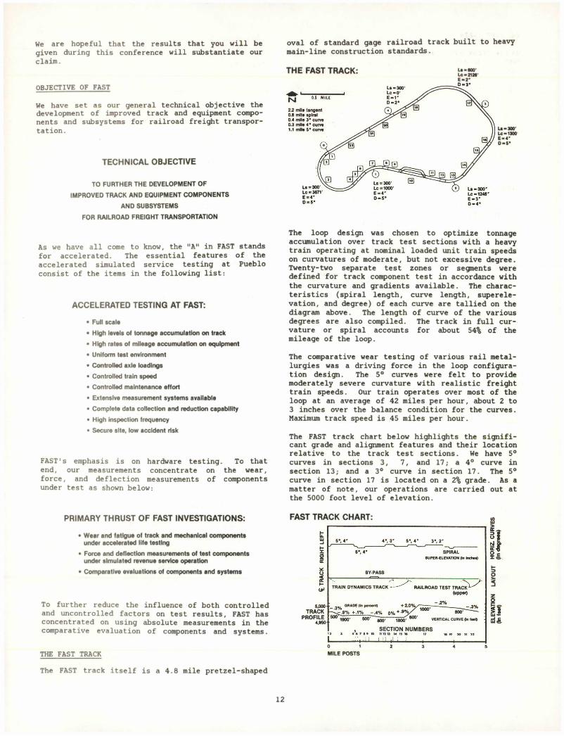
THE FAST TRACKThe FAST track itself is a 4.8 mile pretzel-shaped

oval of standard gage railroad track built to heavy main-line construction standards.

THE FAST TRACK:

The loop design was chosen to optimize tonnage accumulation over track test sections with a heavy train operating at nominal loaded unit train speeds on curvatures of moderate, but not excessive degree. Twenty-two separate test zones or segments were defined for track component test in accordance with the curvature and gradients available. The charac­teristics (spiral length, curve length, superele­vation, and degree) of each curve are tallied on the diagram above. The length of curve of the various degrees are also compiled. The track in full cur­vature or spiral accounts for about 54% of the mileage of the loop.

The comparative wear testing of various rail metal­lurgies was a driving force in the loop configura­tion design. The 5° curves were felt to provide moderately severe curvature with realistic freight train speeds. Our train operates over most of the loop at an average of 42 miles per hour, about 2 to 3 inches over the balance condition for the curves. Maximum track speed is 45 miles per hour.

The FAST track chart below highlights the signifi­cant grade and alignment features and their location relative to the track test sections. We have 5° curves in sections 3, 7, and 17; a 4° curve in section 13; and a 3° curve in section 17. The 5° curve in section 17 is located on a 2% grade. As a matter of note, our operations are carried out at the 5000 foot level of elevation.

FAST TRACK CHART:

MILE POSTS

X <=. »-

§

12

THE FAST TRAIN

We now focus our attention on the FAST consist. The FAST train represents traffic similar to that on heavy haul lines. While we do not have a true unit train condition because of some differences in car construction within our fleet, we do apply severe loaded 100-ton car train service to the test com­ponents. One important difference is in our prac­tice of running all of our cars in the train fully loaded all of the time. FAST has no empty back­hauls .

The characteristics of the FAST consist are summa­rized below:

THE FAST TRAIN:

Motive Power: Four 4-axle, 2000hp locomotives.

Car Equipment Ninety-nine cars In FAST pool;Ninety-two 100-ton open-top hopper; Six 100-ton tank;One 70-ton TTX

i Lading: Hoppers— expanded shale(simulated coal lading);

Tanks—water; ,100-ton design cars— loaded to gross weight

on rail of 263,000lbs ±2,000lbs.

Nominal Consist Four units plus 70 cars;9200 trailing tons;

0.8 7.lhp per trailing ton.

We have restricted ourselves to four-axle power to eliminate the influence of varied motive power characteristics on test results. The expanded shale material used, for lading in the hopper cars was chosen for its simulation of the correct center of gravity for loaded coal hoppers and for its. non- corrosive properties.

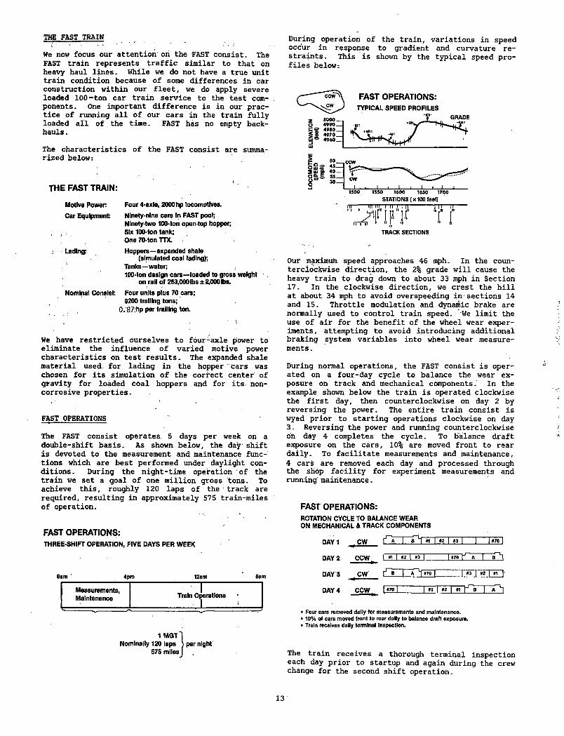
FAST OPERATIONS

The FAST consist operates 5 days per week on a double-shift basis. As shown below, the day" shift is devoted to the measurement and maintenance func­tions which are best performed under daylight con­ditions. During the night-time operation of the train we set a goal of one million gross tons. To achieve this, roughly 120 laps of the ■ track are required, resulting in approximately 575 train-miles of operation.

FAST OPERATIONS:THREE-SHIFT OPERATION, FIVE DAYS PER WEEK

Sam 4pm 12am Sam

Measurements,Maintenance Train Operations

__ J ______ L

1 MGT Nominally 120 laps

575 milesper night'

During operation of the train, variations in speed occur in response to gradient and curvature re­straints. This is shown by the typical speed pro­files below:

TRACK SECTIONS

Our maximum speed approaches 46 mph. In the coun­terclockwise direction, the 2% grade will cause the heavy train to drag down to about 33 mph in Section 17. In the clockwise direction, we crest the hill at about 34 mph to avoid overspeeding in sections 14 and 15. Throttle modulation and dynamic brake are normally used to control train speed. ‘We limit the use of air for the benefit of the wheel wear exper­iments, attempting to avoid introducing additional braking system variables into wheel wear measure­ments.

During normal operations, the FAST consist is oper­ated on a four-day cycle to balance the wear ex­posure on track and mechanical components. In the example shown below the train is operated clockwise the first day, then counterclockwise on day 2 by reversing the power. The entire train consist is wyed prior to starting operations clockwise on day 3. Reversing the power and running counterclockwise on day 4 completes the cycle. To balance draft exposure on the cars, 10% are moved front to rear daily. To facilitate measurements and maintenance, 4 cars are removed each day and processed through the shop facility for experiment measurements and running maintenance.

FAST OPERATIONS:ROTATION CYCLE TO BALANCE WEAR ON MECHANICAL & TRACK COMPONENTS

DAY 1 C W n " l 42 | 43 | | ~ [ E □

DAY 2 C C W l m J #2 1 13 1 1 470 ^ A |

DAY 3 C W f '- B 1 470 | | 43 | 42 1 « 1'

DAY 4 C C W r » 7 o i _____ l_ !L 1 4 2 1 *i rr V T * ! ]

• Four cars removed dally for measurements and maintenance.• 10% of cars moved front to rear dally to balance draft exposure.• Train receives daily terminal Inspection.

13

The train receives a thorough terminal inspection each day prior to startup and again during the crew change for the second shift operation.

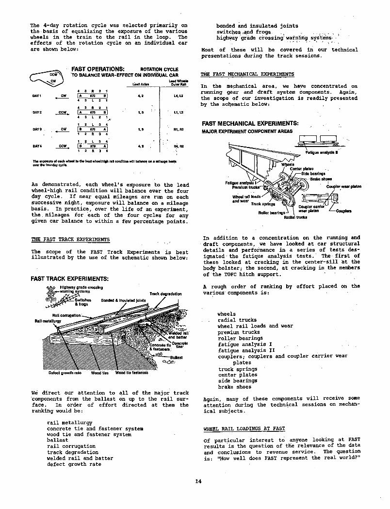
The 4-day rotation cycle was selected primarily on the basis of equalizing the exposure of the various wheels in the train to the rail in the loop. The effects of the rotation cycle on an individual car are shown below:

Tit* exposure of each whool to the lead wheal/hlgh rati condition will balance on a mileage basis over the four-day cycle.

As demonstrated, each wheel's exposure to the lead wheel-high rail condition will balance over the four day cycle. If near equal mileages are run on each successive night, exposure will balance on a mileage basis. In practice, over the life of an experiment, the mileages for each of the four cycles for any given car balance to within a few percentage points.

bonded and insulated jointsswitches ,and frogs ., - , .... ,highway grade crossing warning systems-

Host of these will be covered in our technical presentations during the track sessions.

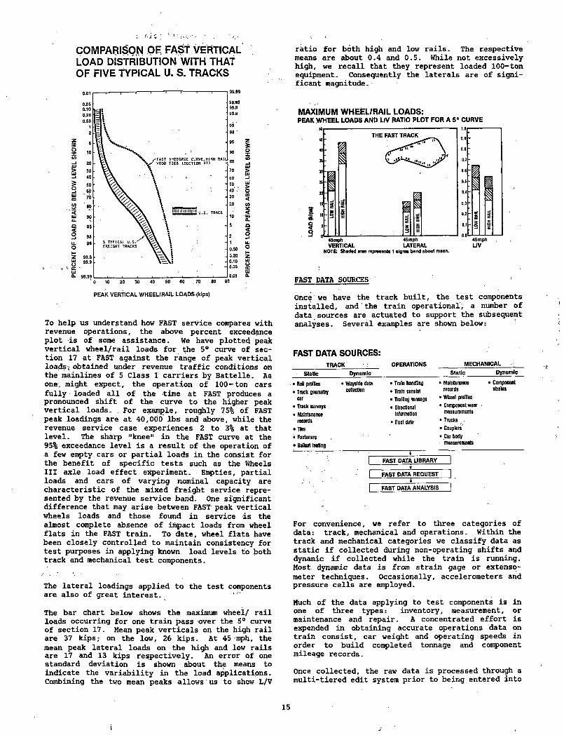
THE FAST MECHANICAL EXPERIMENTS

In the mechanical area, we have concentrated on running gear and draft system components. Again, the scope of our investigation is readily presented by the schematic below:

FAST MECHANICAL EXPERIMENTS:MAJOR EXPERIMENT COMPONENT AREAS

THE FAST TRACK EXPERIMENTS

The scope of the FAST Track Experiments is best illustrated by the use of the schematic shown below:

FAST TRACK EXPERIMENTS:

We direct our attention to all of the major track components from the ballast on up to the rail sur­face. In order of effort directed at them the ranking would be:

rail metallurgyconcrete tie and fastener system wood tie and fastener system ballastrail corrugation track degradation welded rail and batter defect growth rate

In addition to a concentration on the running and draft components, we have looked at car structural details and performance in a series of tests des­ignated * the fatique analysis tests. The first of these looked at cracking in the center-sill at the body bolster; the second, at cracking in the members of the TOFC hitch support.

A rough order of ranking by effort placed on the various components is:

wheelsradial truckswheel rail loads and wearpremium trucksroller bearingsfatigue analysis Ifatigue analysis IIcouplers; couplers and coupler carrier wear

platestruck springs center plates side bearings brake shoes

Again, many of these components will receive some attention during the technical sessions on mechan­ical subjects.

WHEEL RAIL LOADINGS AT FAST

Of particular interest to anyone looking at FAST results is the question of the relevance of the data and conclusions to revenue service. The question is: “How well does FAST represent the real world?"

14

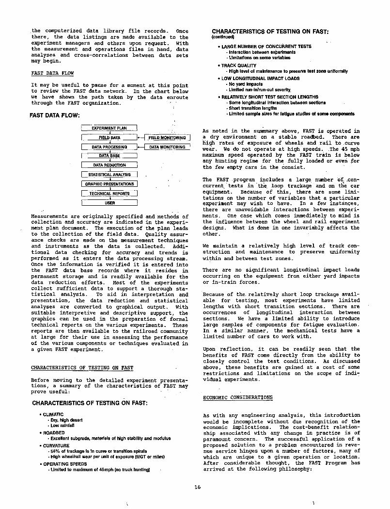
COMPARISON OF FAST VERTICAL LOAD DISTRIBUTION WITH THAT OF FIVE TYPICAL U. S. TRACKS

To help us understand how FAST service compares with revenue operations, the above percent exceedance plot is of some assistance. We have plotted peak vertical wheel/rail loads for the 5° curve of sec­tion 17 at FAST against the range of peak vertical loads; obtained under revenue traffic conditions on the mainlines of 5 Class 1 carriers by Battelle. As one: might expect, the operation of 100-ton cars fully loaded all of the time at FAST produces a pronounced shift of the curve to the higher peak vertical loads. For example, roughly 75% of FAST peak loadings are at 40,000 lbs and above, while the revenue service case experiences 2 to 3% at that level. The sharp "knee" in the FAST curve at the 95% exceedance level is a result of the operation of a few empty cars or partial loads in the consist for the benefit of specific tests such as the Wheels III axle load effect experiment. Empties, partial loads and cars of varying nominal capacity are characteristic of the mixed freight service repre­sented by the revenue service band. One significant difference that may arise between FAST peak vertical wheels loads and those found in service is the almost complete absence of impact loads from wheel flats in the FAST train. To date, wheel flats have been closely controlled to maintain consistency for test purposes in applying known load levels to both track and mechanical test components.

The lateral loadings applied to the test components are also of great interest.

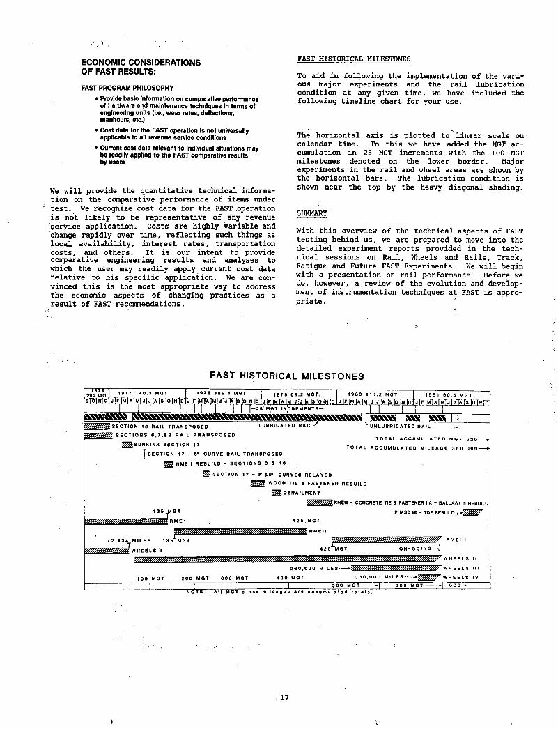
The bar chart below shows the maximum wheel/ rail loads occurring for one train pass over the 5° curve of section 17. Mean peak verticals on the high rail are 37 kips; on the low, 26 kips. At 4 5 -mph, the mean peak lateral loads on the high and low rails are 17 and 13 kips respectively. An error of one standard deviation is shown about the means to indicate the variability in the load applications. Combining the two mean peaks allows us to show L/V

ratio for both high and low rails. The respective means are about 0.4 and 0.5. While not excessively high, we recall that they represent loaded 100-ton equipment. Consequently the laterals are of signi­ficant magnitude.

MAXIMUM WHEEL/RAIL LOADS:PEAK WHEEL LOADS AND LfV RATIO PLOT FOR A 5° CURVE

VERTICAL LATERAL

mI

1

45 mphL/V

NOTE: Shaded area represent# 1 algma band about mean.

FAST DATA SOURCES

Once we have the track built, the test components installed, and the train operational; a number of data sources are actuated to support the subsequent analyses. Several examples are shown below:

FAST DATA SOURCES:TRACK :___ OPERATIONS _______MECHANICAL

Static Dynamic Static Dynamic

• Rat profiles • Wayside data • Train handling • Maintenance • Component• Track geometry collection • Train consist records strains

car • Trailing tonnage • Wheel profiles• Track surveys • Directional • Component wear >• Maintenance Information measurements

records • Fuel data • Trucks .• Ties • Couplers• Fasteners • Car body• BaDast testing • measurements

♦ ~ I FAST DATA LIBRARY I

I FAST DATA REQUEST I

I FAST DATA ANALYSIS I

For convenience, we refer to three categories of data: track, mechanical and operations. Within the track and mechanical categories we classify data as static if collected during non-operating shifts and dynamic if collected while the train is running. Most dynamic data is from strain gage or extenso- meter techniques. Occasionally, accelerometers and pressure cells are employed.

Much of the data applying to test components is in one of three types: inventory, measurement, or maintenance and repair. A concentrated effort is expended in obtaining accurate operations data on train consist, car weight and operating speeds in order to build completed tonnage and component mileage records.

Once c o l le c t e d , th e raw d a ta i s p ro c e s s e d th ro u g h a m u l t i - t i e r e d e d i t sys te m p r i o r t o b e in g e n te re d i n t o

15

the computerized data library file records. Once there, the data listings are made available to the experiment managers and others upon request. With the measurement and operations files in hand, data analyses and cross-correlations between data sets may begin.

FAST DATA FLOW

It may be useful to pause for a moment at this point to review the FAST data network. In the chart below we have shown the path taken by the data enroute through the FAST organization.

FAST DATA FLOW:

EXPERIMENT PLAN 1lFIELD DATA J - l FIELD MONITORING

_______ 1___DATA PROCESSING T -r DATA MONITORING

DATA BASE i4DATA REDUCTION ii

STATISTICAL ANALYSIS i .iGRAPHIC PRESENTATIONS ii

TECHNICAL REPORTS i*USER i

Measurements are originally specified and methods of collection and accuracy are indicated in the experi­ment plan document. The execution of the plan leads to the collection of the field data. Quality assur­ance checks are made on the measurement techniques and instruments as the data is collected. Addi­tional data checking for accuracy and trends is performed as it enters the data processing stream. Once the information is verified it is entered into the FAST data base records where it resides in permanent storage and is readily available for the data reduction efforts. Most of the experiments collect sufficient data to support a thorough sta­tistical analysis. To aid in interpretation and presentation, the data reduction and statistical analyses are converted to graphical output. With suitable interpretive and descriptive support, the graphics can be used in the preparation of formal technical reports on the various experiments. These reports are then available to the railroad community at large for their use in assessing the performance of the various components or techniques evaluated in a given FAST experiment.

CHARACTERISTICS OF TESTING ON FAST

Before moving to the detailed experiment presenta­tions, a summary of the characteristics of FAST may prove useful:

CHARACTERISTICS OF TESTING ON FAST:

• CLIMATIC• Dry, h ig h dese rt ■ L o w ra in fa ll

• R O AD BED- E xce lle n t subg rade , m a te ria ls o f h ig h s ta b il ity a nd m o d u lu s

• CURVATURE- 5 4 % o f tra c k a g e Is In cu rve o r tra n s it io n sp ira ls- H ig h w h e e l/ra il w e a r p e r u n it o f e xposu re (M G T o r m iles)

• O PER ATIN G SPEEDS- L im ite d to m a x im u m o f 4 5 m p h (no tru c k h un tin g )

CHARACTERISTICS OF TESTING ON FAST:(continued)

• LARGE NUMBER OF CONCURRENT TESTS- Interaction between experiments■ Limitations on some variables

• TRACK QUALITY- High level of maintenance to preserve test zone uniformity

• LOW LONGITUDINAL IMPACT LOADS• No yard Impacts- Limited run-in/run-out severity.

• RELATIVELY SHORT TEST SECTION LENGTHS• Some longitudinal Interaction between sections■ Short transition lengths- Limited sample sizes for fatigue studies of some components

As noted in the summmary above, FAST is operated in a dry environment on a stable roadbed. There are high rates of exposure of wheels and rail to .curve wear. We do not operate at high speeds. The 45 mph maximum speed operated by the FAST train is below any hunting regime for the fully loaded or even for the few empty cars in the consist.

The FAST program includes a large number of con­current tests in the loop trackage and on the car equipment. Because of this, there are some limi­tations on the number of variables that a particular experiment may wish to have. In a few instances, there are unavoidable interactions between experi­ments. One case which comes immediately to mind is the influence between the wheel and rail experiment designs. What is done in one invariably affects the other.

We maintain a relatively high level of track con­struction and maintenance to preserve uniformity within and between test zones.

There are no significant longitudinal impact loads occurring on the equipment from either yard impacts or in-train forces.

Because of the relatively short loop trackage avail­able for testing, most experiments have limited lengths with short transition sections. There are occurrences of longitudinal interaction between sections. We have a limited ability to introduce large samples of components for fatigue evaluation. In a similar manner, the mechanical tests have a limited number of cars to work with.

Upon reflection, it can be readily seen that the benefits of FAST come directly from the ability to closely control the test conditions. As discussed above, these benefits are gained at a cost of some restrictions and limitations on the scope of indi­vidual experiments.

ECONOMIC CONSIDERATIONS

As with any engineering analysis, this introduction would be incomplete without due recognition of the economic implications. The cost-benefit relation­ship associated with any change in practice is of paramount concern. The successful application of a proposed solution to a problem encountered in reve­nue service hinges upon a number of factors, many of which are unique to a given operation or location. After considerable thought, the FAST Program has arrived at the following philosophy:

16

ECONOMIC CONSIDERATIONS OF FAST RESULTS:

FAST PROGRAM PHILOSOPHY

• Provide basic Information on comparative performance of hardware and maintenance techniques In terms of engineering units (i.e., wear rates, deflections, manhours, etc.)

• Cost data for the FAST operation Is not universally applicable to all revenue service conditions

• Current cost data relevant to individual situations may be readily applied to the FAST comparative resultsby users

We will provide the quantitative technical informa­tion on the comparative performance of items under test. We recognize cost data for the FAST operation is not likely to be representative of any revenue service application. Costs are highly variable and change rapidly over time, reflecting such things as local availability, interest rates, transportation costs, and others. It is our intent to provide comparative engineering results and analyses to which the user may readily apply current cost data relative to his specific application. We are con­vinced this is the most appropriate way to address the economic aspects of changing practices as a result of FAST recommendations.

FAST HISTORICAL MILESTONES

To aid in following the implementation of the vari­ous major experiments and the rail lubrication condition at any given time, we have included the following timeline chart for your use.

The horizontal axis is plotted to linear scale on calendar time. To this we have added the MGT ac­cumulation in 25 MGT increments with the 100 MGT milestones denoted on the lower border. Major experiments in the rail and wheel areas are shown by the horizontal bars. The lubrication condition is shown near the top by the heavy diagonal shading.

SUMMARY

With this overview of the technical aspects of FAST testing behind us, we are prepared to move into the detailed experiment reports provided in the tech­nical sessions on Rail, Wheels and Rails, Track, Fatigue and Future FAST Experiments. We will begin with a presentation on rail performance. Before we do, however, a review of the evolution and develop­ment of instrumentation techniques at FAST is appro­priate .

F A S T H IS T O R IC A L M IL E S T O N E S< 9 7 6

29 2 MGT.s T o j n| p

BBBBgeaSBB SBCBSK 8BK S8S

1 9 7 7 1 4 0 . 3 M G T I 1 9 7 8 1 8 9 . 1 MGT I 1 g 7

D liIf |M I*M jJ J M s IoJnJd] j |f MJa JmJ j to Jn |d }j 1f Jm [aJ___ L _ J __I__I____l I I I___I I I I >«»•»»•

9 6 9 . 2 MGT.I a 1m H O T Is 16 In Jd

MGT I N C R E M E N T S - ^

1 9 8 0 1 1 1 . 2 MGTj J l l M [ A [ m' [j Ij |a j s [p i n [p

1 9 8 1 8 0 . 5 M G Tj In a TMf j f j Ta [s Io TnTd'

L U B R I C A T E D RAI L 7 ' U N L U B R I C A T E D RAI L

T O T A L A C C U M U L A T E D M G T 6 2 0 -

T O T A L A C C U M U L A T E D M I L E A G E 3 6 0 . 0 0 0 -

S E C T I O N 1 9 RAI L T R A N S P O S E D

S E C T I O N S 6 . 7 , 8 8 R A I L T R A N S P O S E D

^ g S U N K I N K S E C T I O N 17

J S E C T I O N 1 7 - 5* C U R V E RAI L T R A N S P O S E D

^ R M E I I R E B U I L D - S E C T I O N S 3 8 1 3

^ S E C T I O N 1 7 - 3 * 8 5 * C U R V E S R E L A Y E D

W O O D TIE 8 F A S T E N E R R E B UI L D

D E R A I L M E N T

RMEIII - CONCRETE TIE 8 FASTENER IIA - BALLAST II REBUILO

PHASE MB - TDE R E B U I L D ' Z ^ ' ^ ^ ^ '

* fiME1

7 2 , 4 3 4 M I L E S

/ w h e e l s I

1 3 5 M G T

4 2 5 M G T

J RME I I

R ME I I I

> " M G T O N - G O I N G

3 0 0 MG T

W H E E L S II

2 6 0 , 0 0 0 M I L E S ------ W H E E L S III

i M G T 3 3 0 . 0 0 0 M I L E S —

5 0 0 M G T ---------- 6 0 0 MGT- —N O T E - A l l M G T ' s a n d m i l e a g e s a r e a c c u m u l a t e d t o t a l s .

W H E E L S IV *| 6 0 0 .

17

I

EVOLUTION OF MEASUREMENT TECHNIQUES AT FAST

Thomas P. Larkin FAST Operations Manager

Federal Railroad Administration

Approximately twenty percent of the total FAST labor budget is expended on the acquisition of data. This equates to 750,000 static measurements and 150 dynamic tapes per year in addition to 205 Train Operations Recording System (TORS) cas­settes, and 50 Plasser track geometry tapes. When added to the effort required to process, reduce, analyze and report, it is clearly evident that data acquisition instrumentation occupies a keystone position in establishing the success of the FAST Program. Measurement techniques and instrumentation have evolved as a direct result of increased understanding by experimenters of minimum accuracies and samples re­quired to statistically meet experiment objectives and the necessity to upgrade commercially available measurement devices or design new instruments to meet these requirements. Most of the measurements were developed to satisfy experiment re­quirements; however, others evolved from efforts to resolve frequent operation problems. Regardless of the source of requirements, instruments and procedures have been developed for which accuracy is well established.

BACKGROUND

FAST proceeded from concept approval to operation in what many regard record time. While the massive efforts by the railroads, railroad supply indus­tries, and the Federal Government resulted in an operational program in less than six months after go ahead, this haste was not without cost. The primary objective of FAST was to expose a track to as much tonnage and consist mileage as possible in the shortest period of time. FAST accomplished this objective. Numerous measurements were defined which were considered secondary to tonnage accumulation and, lacking the necessary time, final use of the measurements to support specific test objectives was not defined; hence, required tolerances and sound sampling densities were lacking.

Approximately one year after start of consist oper­ations, Experiment Managers were selected for the recognized areas of interest. Upon attempts by the Experiment Managers to formulate experiment objec­tives compatible with data being acquired on FAST, it was immediately apparent that measurements being taken were not necessarily those required to satisfy experiment objectives. Where measurements had been adequately specified, it was found that much data was not usable due to inaccuracy of instruments, errors in recording, or both.

In early 1978, an extensive program to upgrade the quality of FAST data was undertaken, which involved reassessment of all effort from the recording of the data through loading of the data into the data base. Included in this activity was an audit of all exist­ing measurement techniques, both hardware and pro­cedures, in order to define the inherent accuracy that could be expected by using a specific instru­ment to approved procedures. A policy was estab­

lished which has become standard for implementing new measurements on FAST and which resulted in redesign of many then-existing measurement devices. This standard requires development of a step-by-step procedure for taking the data! and rigorous enforce­ment of the procedure during data collection from a known standard by several different technicians on different days. Finally, the data is reviewed for scatter by the Experiment Manager or Monitor who provides ultimate approval of the instrument and procedure. This approval authority or responsi­bility has led to early identification of procedure and instrument problems and allowed correction prior to initial use on a test.

Numerous displays of FAST measurement instruments and data collecting hardware and vehicles are pre­sented in Appendix A. These displays are not all- inclusive; however, they do provide an indication of the extensive data collection capabilities of FAST. It is not my intent to discuss each of the instru­ments or vehicles displayed, but to provide brief examples of measurement developments in the mech­anical, track, and operations areas.

MECHANICAL

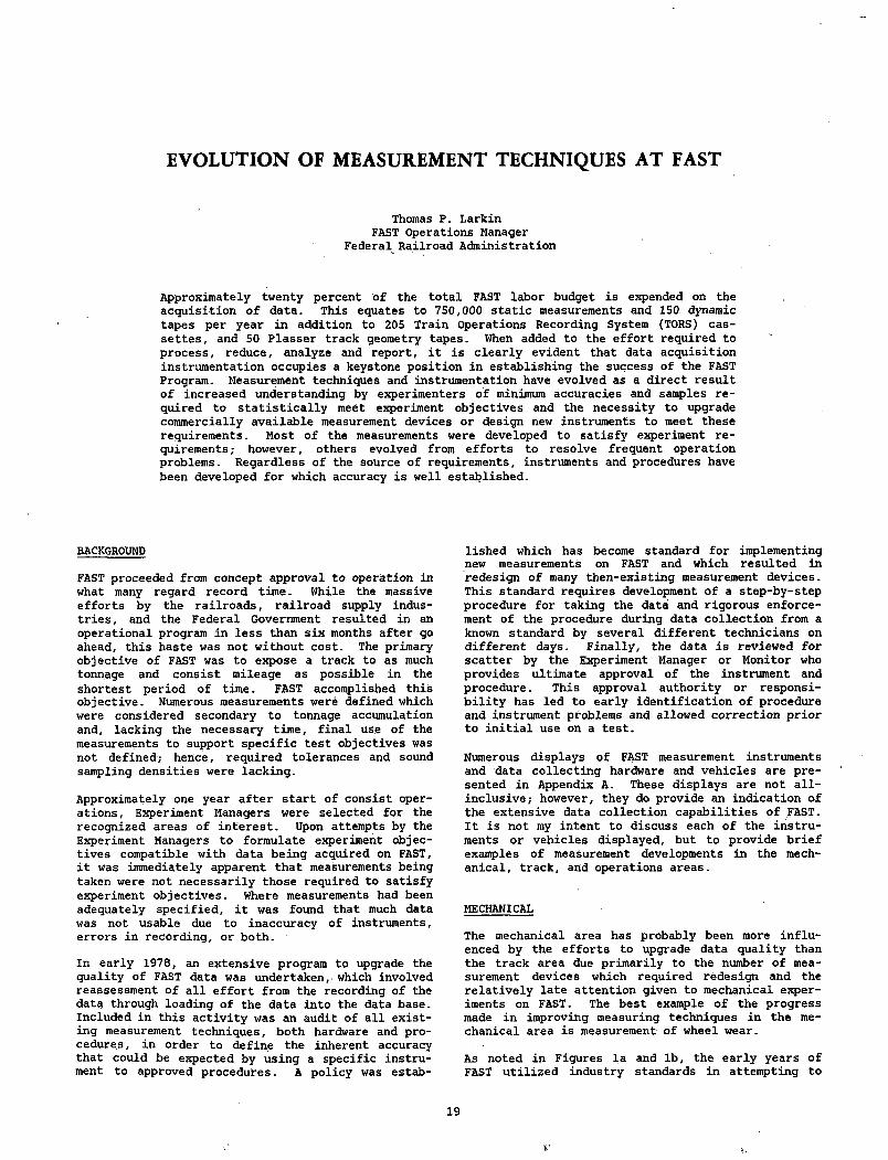
The mechanical area has probably been more influ­enced by the efforts to upgrade data quality than the track area due primarily to the number of mea­surement devices which required redesign and the relatively late attention given to mechanical exper­iments on FAST. The best example of the progress made in improving measuring techniques in the me­chanical area is measurement of wheel wear.

As noted in Figures la and lb, the early years of FAST utilized industry standards in attempting to

19

obtain wheel measurements. Figure lb shows the •development chronology associated with attempts to improve measurement accuracy ultimately leading to almost exclusive use of the modified Canadian Na­tional profilometer and related computer software to accomplish, in a superior manner, data acquisition from previously used measurement devices.

FIGURE la. WHEEL WEAR SURFACE MEASUREMENTS.

FIGURE lb. INSTRUMENT MEASUREMENT PROGRESSION.

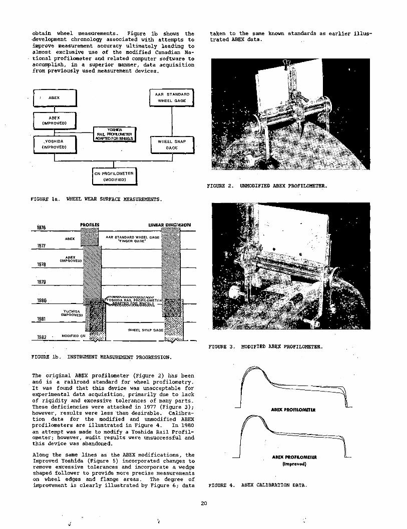
The original ABEX profilometer (Figure 2) has been and is a railroad standard for wheel profilometry. It was found that this device was unacceptable for experimental data acquisition, primarily due to lack of rigidity and excessive tolerances of many parts. These deficiencies were attacked in 1977 (Figure 3); however, results were less than desirable. Calibra­tion data for the modified and unmodified ABEX profilometers are illustrated in Figure 4. In 1980 an attempt was made to modify a Yoshida Rail Profil­ometer; however, audit results were unsuccessful and this device was abandoned.

Along the same lines as the ABEX modifications, the Improved Yoshida (Figure 5) incorporated changes to remove excessive tolerances and incorporate a wedge shaped follower to provide more precise measurements on wheel edges and flange areas. The degree of improvement is clearly illustrated by Figure 6; data

taken to the same known standards as earlier illus­trated ABEX data.

FIGURE 2. UNMODIFIED ABEX PROFILOMETER.

FIGURE 3. MODIFIED ABEX PROFILOMETER.

ABEX PROFILOMETER

FIGURE 4. ABEX CALIBRATION DATA.

20

4 1

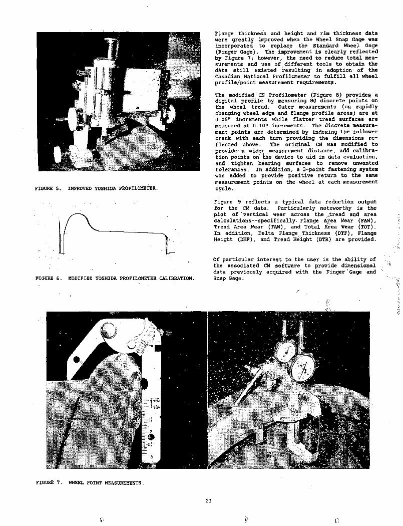
FIGURE 5. IMPROVED YOSHIDA PROFILOMETER.

FIGURE 6. MODIFIED YOSHIDA PROFILOMETER CALIBRATION.

Flange thickness and height and rim thickness data were greatly improved when the Wheel Snap Gage was incorporated to replace the Standard Wheel Gage (Finger Gage). The improvement is clearly reflected by Figure 7; however, the need to reduce total mea­surements and use of different tools to obtain the data still existed resulting in adoption; of the Canadian National Profilometer to fulfill all wheel profile/point measurement requirements.

The modified CN Profilometer (Figure 8) provides, a digital profile by measuring 80 discrete points on the wheel tread. Outer measurements (on rapidly changing wheel edge and flange profile areas) are at 0.05" increments while flatter tread surfaces are measured at 0.10" increments. The discrete measure­ment points are determined by indexing the follower crank with each turn providing the dimensions re­flected above. The original CN was modified to provide a wider measurement distance, add calibra­tion points on the device to aid in data evaluation, and tighten bearing surfaces to remove unwanted tolerances. In addition, a 3-point fastening system was added to provide positive return to the same measurement points on the wheel at each measurement cycle.

Figure 9 reflects a typical data reduction output for the CN data. Particularly noteworthy is the plot of vertical wear across the jtread and area calculations--specifically• Flange Area Wear (FAW), Tread Area Wear (TAW), and Total Area Wear (TOT). In addition, Delta Flange .Thickness (DTF), Flange Height (DHF), and Tread Height (DTR) are provided.

Of particular interest to the user is the ability of the associated CN software to provide dimensional data previously acquired with the Finger' Gage and Snap Gage.

FIGURE 7. WHEEL POINT MEASUREMENTS.

21

V*

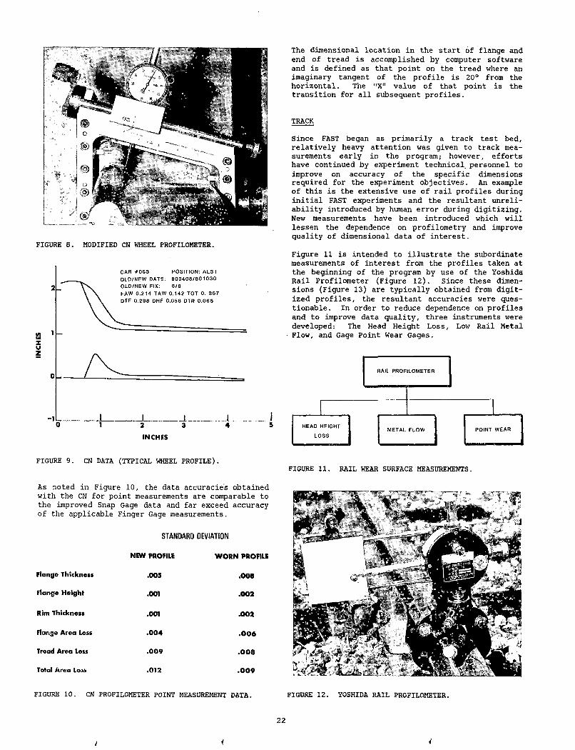
The dimensional location in the start of flange and end of tread is accomplished by computer software and is defined as that point on the tread where an imaginary tangent of the profile is 20° from the horizontal. The "X" value of that point is the transition for all subsequent profiles.

TRACK

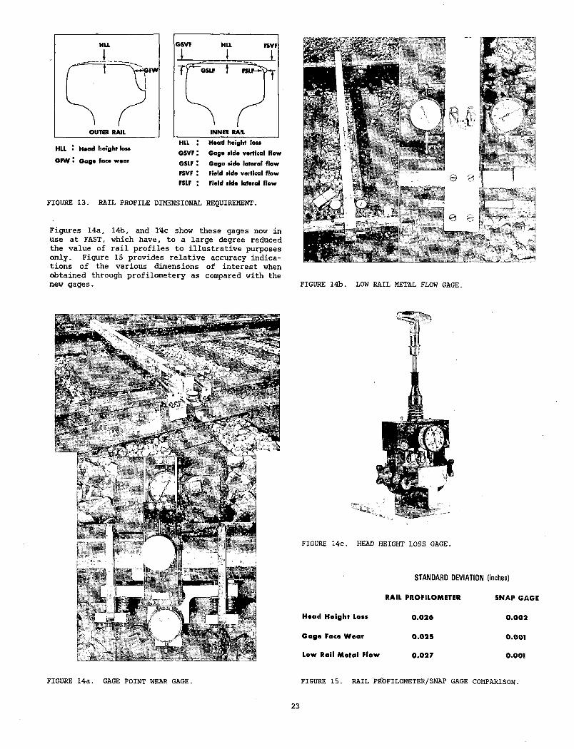
Since FAST began as primarily a track test bed, relatively heavy attention was given to track mea­surements early in the program; however, efforts have continued by experiment technical personnel to improve on accuracy of the specific dimensions required for the experiment objectives. An example of this is the extensive use of rail profiles during initial FAST experiments and the resultant unreli­ability introduced by human error during digitizing. New measurements have been introduced which will lessen the dependence on profilometry and improve quality of dimensional data of interest.

Figure 11 is intended to illustrate the subordinate measurements of interest from the profiles taken at the beginning of the program by use of the Yoshida Rail Profilometer (Figure 12). Since these dimen­sions (Figure 13) are typically obtained from digit­ized profiles, the resultant accuracies were ques­tionable. In order to reduce dependence on profiles and to improve data quality, three instruments were developed: The Head Height Loss, Low Rail Metal Flow, and Gage Point Wear Gages.

FIGURE 9. CN DATA (TYPICAL WHEEL PROFILE).FIGURE 11. RAIL WEAR SURFACE MEASUREMENTS.

As noted in Figure 10, the data accuracies obtained with the CN for point measurements are comparable to the improved Snap Gage data and far exceed accuracy of the applicable Finger Gage measurements.

STANDARD DEVIATION

NEW PROFILE W O R N PROFILE

Flange Thickness .005 .0 0 8

Flange Height .001 .0 0 2

Rim Thickness .001 .0 0 2

Flange Area Loss .0 0 4 .0 0 6

Tread Area Loss .0 0 9 .0 0 8

Total Area Loss .013 .0 0 9

FIGURE 10. CN PROFILOMETER POINT MEASUREMENT DATA. FIGURE 12. YOSHIDA RAIL PROFILOMETER.

22

i

HLL • Head height Io m

GFW • Gag# face wear GSLF ! Gage tide lateral flew FSVF • Field side vertical flow

FSLF ; Field side lateral flow

FIGURE 13. RAIL PROFILE DIMENSIONAL REQUIREMENT.

i ,* -v**' 1

& * * y ~ ' * II?:Figures 14a, 14b, and i4c show these gages now in use at FAST, which have, to a large degree reduced the value of rail profiles to illustrative purposes only. Figure 15 provides relative accuracy indica­tions of the various dimensions of interest when obtained through profilometery as compared with the new gages. FIGURE 14b. LOW RAIL METAL FLOW GAGE.

FIGURE 14a. GAGE POINT WEAR GAGE.

FIGURE 14c. HEAD HEIGHT LOSS GAGE.

STANDARD DEVIATION

RAIL PROFILOMETER

H ead H e ig h t Lo«* 0 .0 2 6

G a g e Face W e a r 0 .0 2 5

Low Rail M eta l F low 0 .0 2 7

FIGURE 15. RAIL PROFILOMETER/SNAP GAGE COMPARISON.

(inches)

SNAP GAGE

0.002

0.001

0.001

23

OPERATIONS

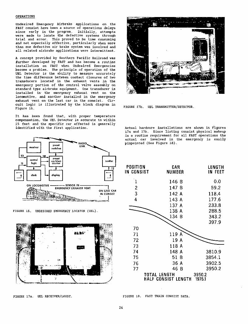
Undesired Emergency Airbrake applications on the FAST consist have been a source of operations delays since early in the program. Initially, attempts were made to locate the defective systems through trial and error. This proved to be time consuming and not especially effective, particularly when more than one defective air brake system was involved and all related airbrake applications were intermittent.

A concept provided by Southern Pacific Railroad was further developed by FAST and has become a routine installation on FAST when Undesired Emergencies become a problem. The principle of operation of the UEL Detector is the ability to measure accurately the time difference between contact closures of two transducers located in the exhaust vents in the emergency portion of the control valve assembly on standard type airbrake equipment. One transducer is installed in- the emergency exhaust vent on the locomotive, and another installed in the emergency exhaust vent on the last car in the consist. Cir­cuit logic is illustrated by the block diagram in Figure 16.

It has been found that, with proper temperature compensation, the UEL Detector is accurate to within 15 feet and the specific car affected is generally identified with the first application.

O N LOCOMOTIVE -------------------SENSOR I N --------------------------------------- ,I EMERGENCY EXHAUST VENT I■SHE S i r 'l l ,<j. ON LAST CAR

P X w p C M T h f M IN CONSIST

FIGURE 16. UNDESIRED EMERGENCY LOCATOR (UEL).

FIGURE 17a. UEL RECEIVER/LOGIC.

FIGURE 17b. UEL TRANSMITTER/DETECTOR.

Actual hardware installations are shown in Figures 17a and 17b. Since listing consist physical makeup is a routine requirement for all FAST operations the actual car involved in the emergency is easily pinpointed (See Figure 18).

PO S IT IO N CAR LENG THIN C O N S IS T N U M B E R IN FEET

1 1 4 6 B 0.02 1 4 7 B 5 9 . 2

3 1 4 2 A 1 1 8 . 4

4 1 4 3 A 1 7 7 . 6

1 3 7 A 2 3 3 . 8

^ 1 3 8 A 2 8 8 . 5

7 0

^ ^ 1 3 4 B 3 4 3 . 2

3 9 7 . 9

7 1 1 1 9 A ^ v7 2 1 9 A

7 3 1 1 8 A

7 4 1 4 8 A 3 8 1 0 . 9

7 5 5 1 B 3 8 5 4 . 1

7 6 3 6 A 3 9 0 2 . 5

7 7 4 6 B 3 9 5 0 . 2

T O T A L LENGTH 3 9 5 0 .2HALF C O N S IS T LENGTH 1975.1

FIGURE 18. FAST TRAIN CONSIST DATA.

24

SUMMARY QUESTIONS AND ANSWERS

A combination of efforts of several FAST organiza­tions has been responsible for the increase in quality of data available for analysis. It is felt, however, that success of this effort must be attri­buted to two specific activities. First, rigorous enforcement of procedures has increased consistency and, second, the on-site availability of experiment personnel has assured that errors, regardless of source, are identified and corrected prior to caus­ing irreparable damage to an experiment. The total effort for data improvement, including the upgrading of measurement devices, has resulted in accurate data being available for the user in a fraction of its previous time. FAST Static Data is generally available in the data base in less than five working days and dynamic data generally within two to three weeks.

Question 1

Is the improved CN wheel profilometer available on a commercial basis? If not, is sufficient information available on how to buy standard CN profilometer and adapt for improvements made at FAST? ’ ;

Answer

The "improved" profilometer is not available on a commercial basis; however, drawings of the modifications are available from the Transpor­tation Test Center and will be furnished by this office upon request. Information on the availability of the basic profilometer should be obtained from Canadian National. It is suggested that Mr. Nelson Caldwell of CN, (514) 343-5422 be contacted for further information.

In addition to the profilometer, software will be required for data reduction and this subject should also be explored with Mr. Caldwell if obtaining a profilometer is to be pursued.

Question 2

Since FAST wear data is destined to be incor­porated into a computer data base, why hasn't an attempt been made to provide, digitized data in machine readable form directly from the instrument.

Answer

This has been recognized as a desirable goal for several years. FAST is a particularly adaptable environment for this "activity and effort was undertaken in 1981 to incorporate a

. direct output into the CN wheel profilometer. This effort, as well as most new developments, has been abandoned due to successive reductions in FAST budgets. At this time, reinitiation of the effort in the foreseeable future does not appear likely.

25

APPENDIX A

The illustrations of this Appendix are of displays provided at the FAST Engineering Conference and, as previously noted, are not all-inclusive but are representative of the overall measurement capability developed by the program.

Each illustration is self-explanatory and is intended to show hardware involved in the measurement(s), format of data recorded and typical data printed from the stor­age files. Sizing of the illustrations affects clarity of some of the information furnished. In general, no attempt has been made to illustrate reduced data or analysis outputs.

27

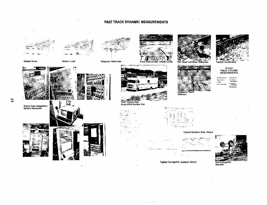
FAST TRACK DYNAMIC MEASUREMENTS

Ballast Strain Ballast Load

FAST Digital Data Acquisition System Van

':-S - ”, ■ ... ••

OTHERTRACK DYNAMIC MEASUREMENTS

Rail Raw detection Tt«i Goormvy

Conor*?* Ti* Strain

Usemi Tie Pusft R*« Vertical

Displacement

Displacement Htit Load r«t

Typical Dynamic Data Output

Analyzer

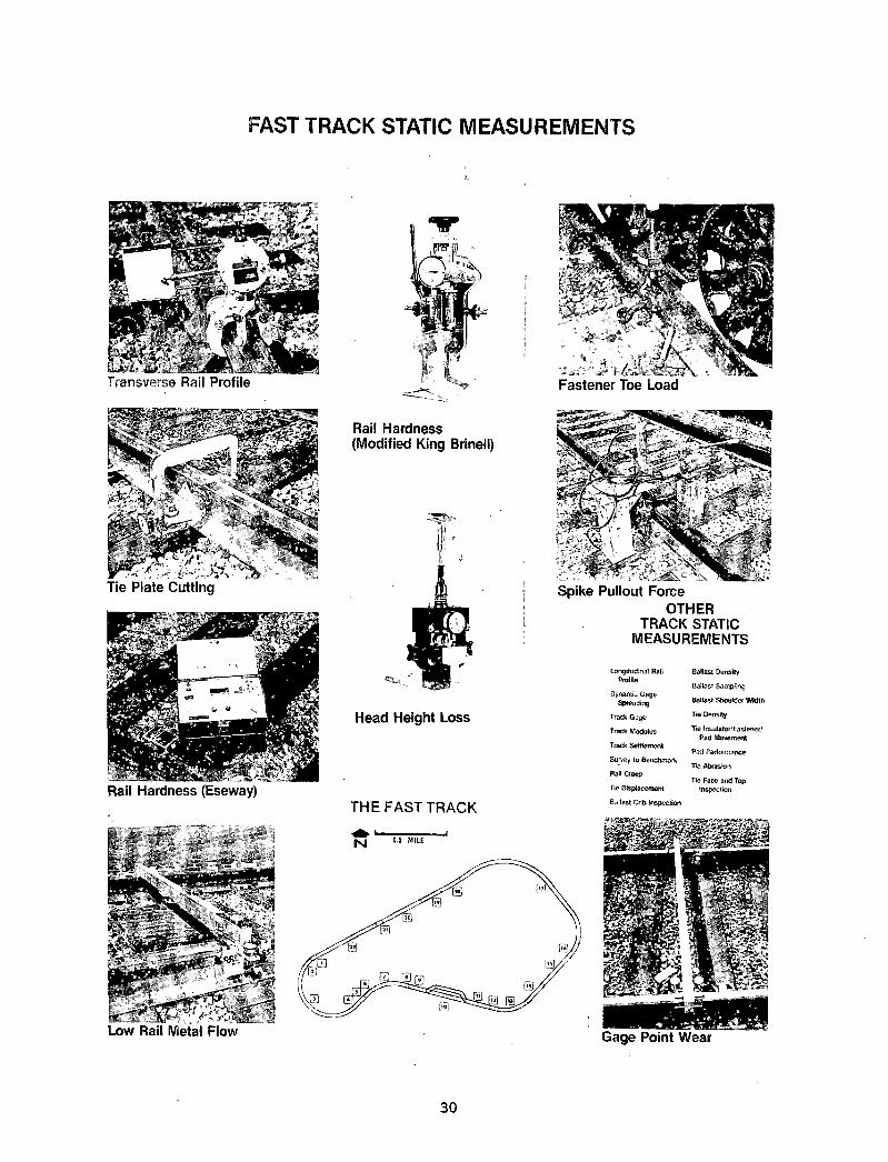
FAST TRACK STATIC MEASUREM ENTS

Rail Hardness (Eseway)T H E FA S T TR A C K

Spike Pullout ForceOTHER

TRACK STATIC MEASUREMENTS

Longitudinal Rail Profile

Dynam ic Gage Spreading

Trade Gage

Track Modulus

Track Settlement

Survey to Benchmark

Rail Creep

Tie Displacement

Ballast Crib inspection

Ballast Density

Ballast Sampling

Ballast Shoulder W idth

Tie Etensity

T ie InsulatorfFastener/ Pad Movement

Pad Performance

Tie Abrasion

Tie Face and Top Inspection

3 0

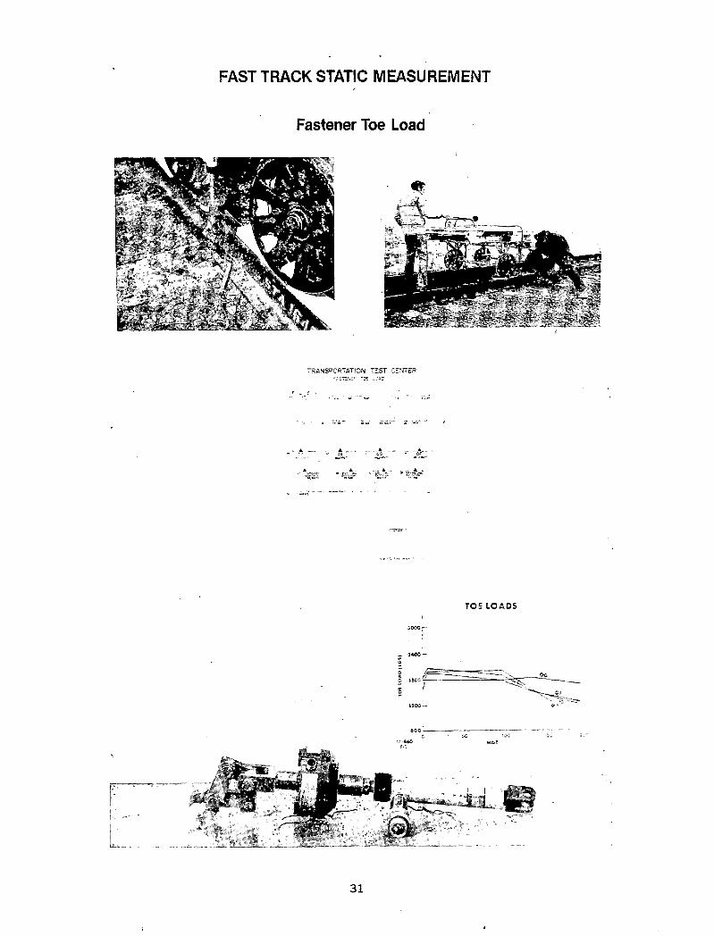
FAST TRACK STATIC MEASUREMENT

Fastener Toe Load

T O E L O A D S

50 00 —

- 2*00

\tGQ~

*03 --— —----0 - 5 0 50CS7-*«0 *»otf -5.

31

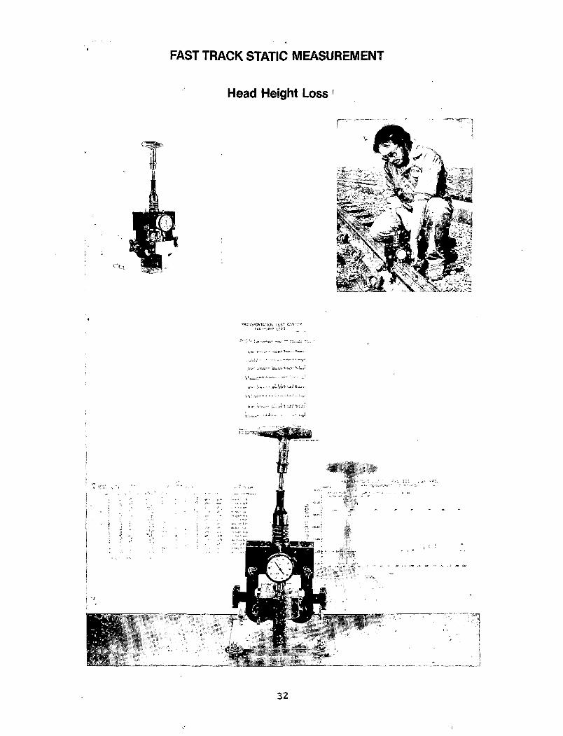
FAST TRACK STATIC MEASUREMENT

Head Height Loss'

3 2

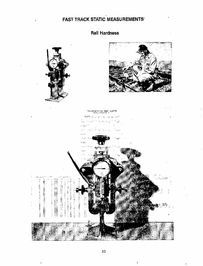
FAST TRACK STATIC MEASUREMENTS

Rail Hardness

3 3

)

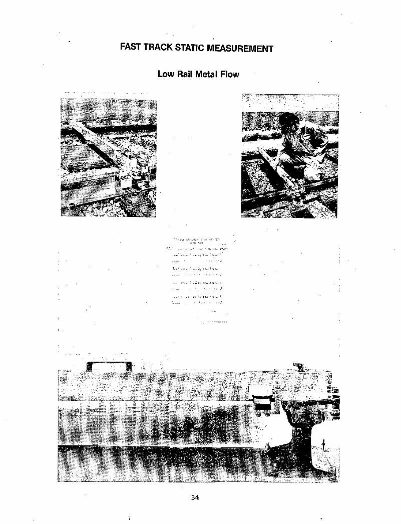
FAST TRACK STATIC MEASUREMENT

Low Rail Metal Flow

3 4

t

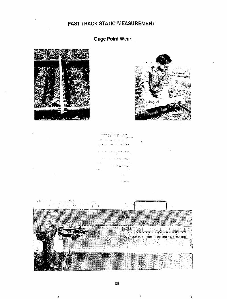
FAST TRACK STATIC MEASUREMENT

Gage Point Wear

3 5

t i

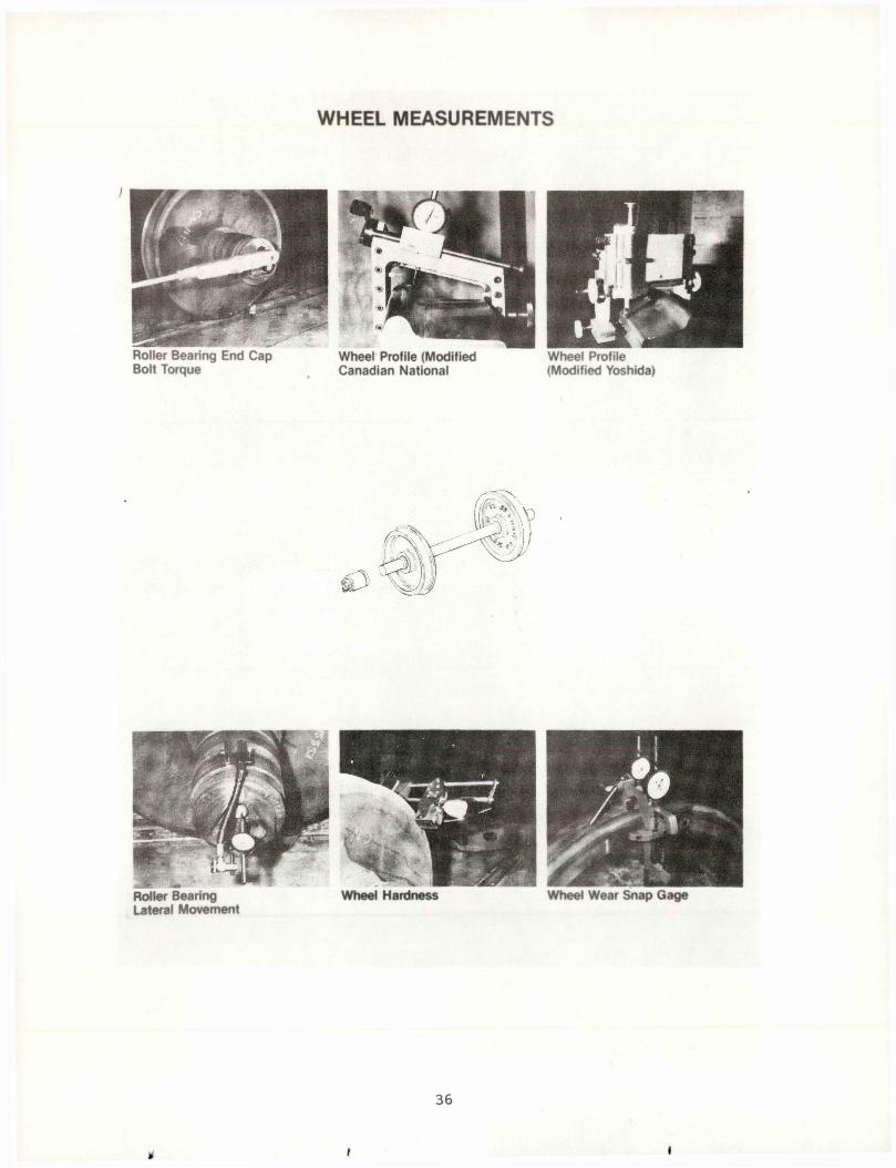
WHEEL MEASUREMENTS

Roller Rearing End Cap Wheel Profile (Modified Wheel ProfileBolt Torque # Canadian National (Modified Yoshida)

Roller Bearing Wheel Hardness Wheel Wear Snap GageLateral Movement

3 6

v l

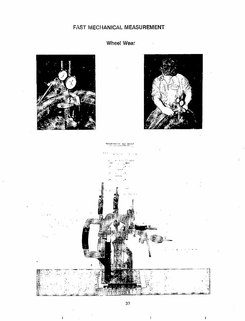
FAST MECHANICAL MEASUREMENT

Wheel Wear

TRANSPORTATION TE S T CENTER f.-x>\ vsssgwjvcvs

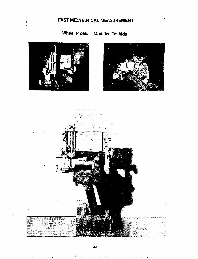
FAST MECHANICAL MEASUREMENT

Wheel Profile— Modified Yoshida

3 8

i

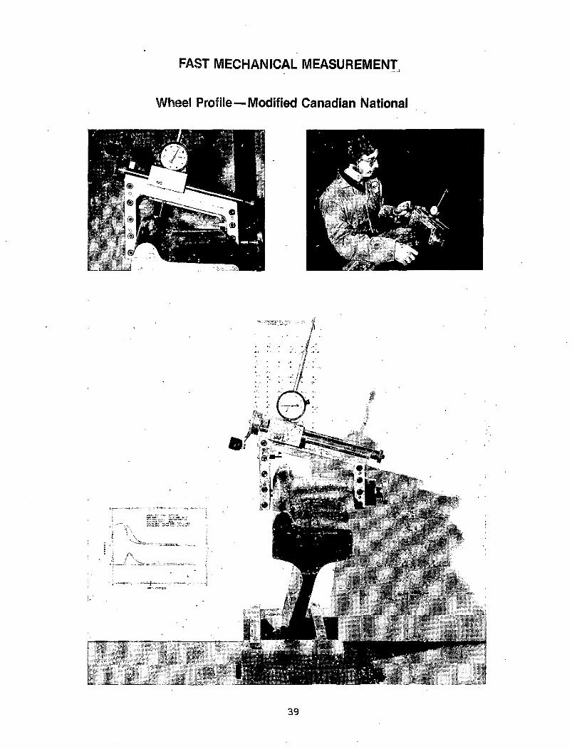
FAST MECHANICAL MEASUREMENT,

3 9

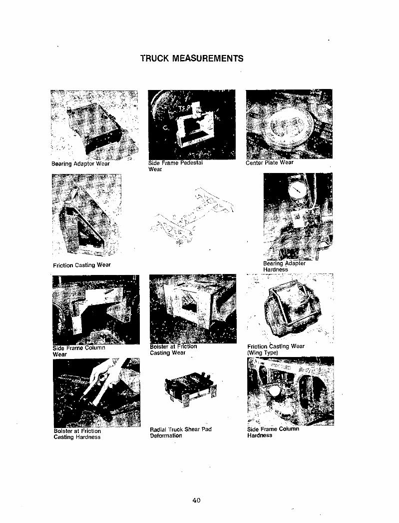
TRUCK MEASUREMENTS

Friction Casting Wear

Casting Hardness Deformation

Center Plate Wear

Friction Casting Wear (Wing Type)

Side Frame Column Hardness

4 0

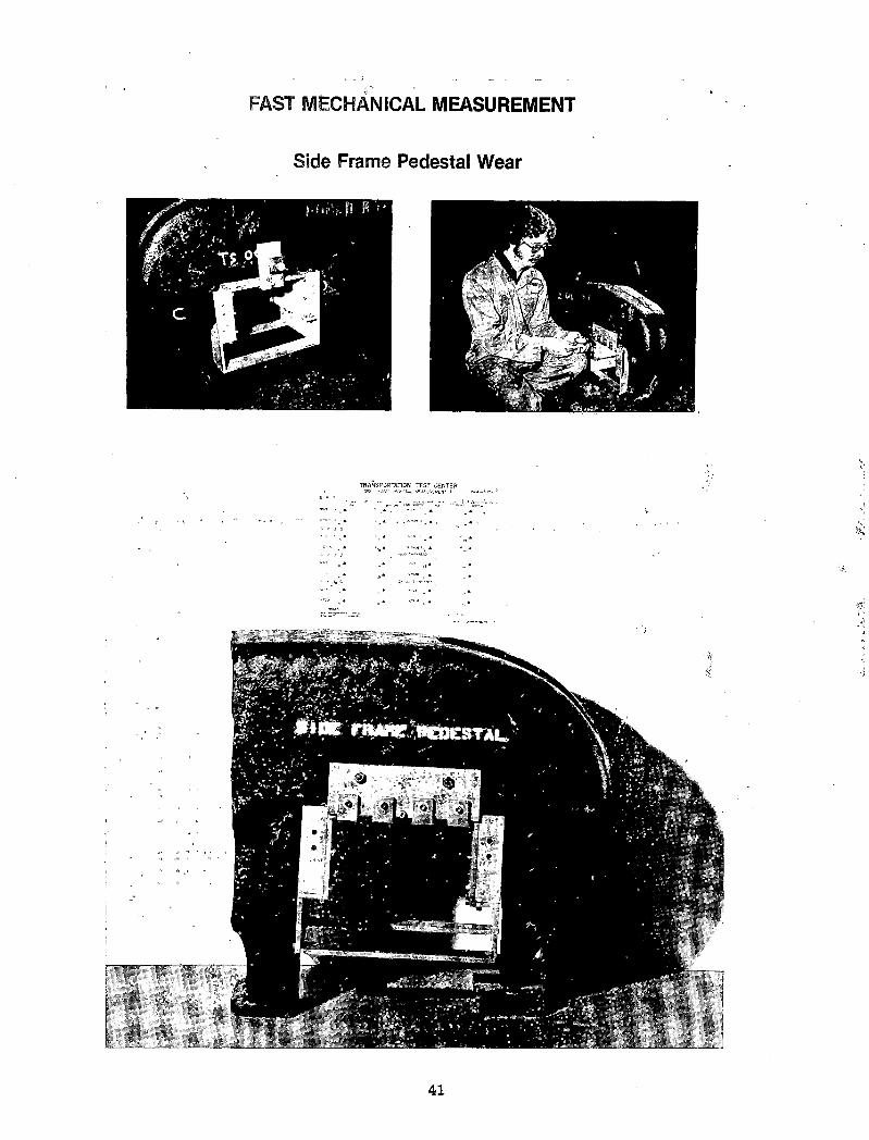
u „ •.

FAST MECHANICAL MEASUREMENT

Side Frame Pedestal Wear

TRANSPORTATION TEST CENTER

41

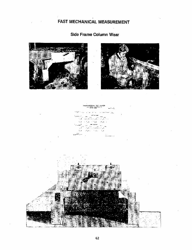
FAST MECHANICAL MEASUREMENT

Side Frame Column Wear

TRANSPORTATION T £ S T CENTERset oavl' n

ax-jus duct.

4 2

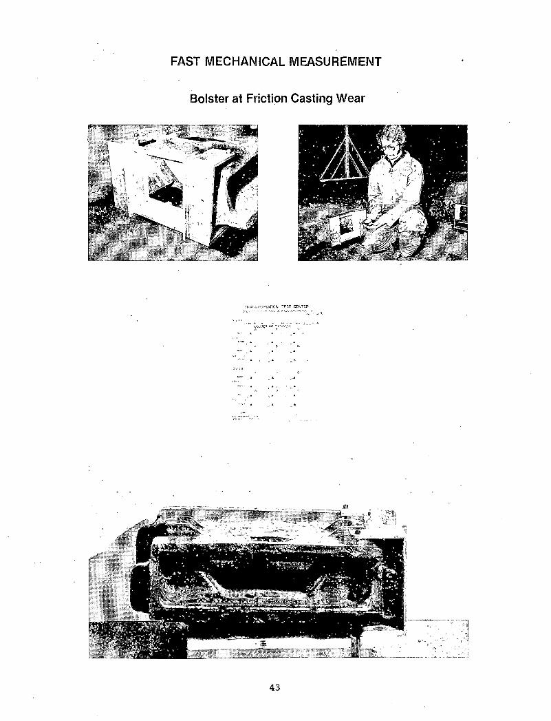
FAST MECHANICAL MEASUREMENT

Bolster at Friction Casting Wear

TRANSPORTATION TEST CENTER

4 3

TRACK1981 FAST ENGINEERING CONFERENCE

KEY TOPICS

RAIL METALLURGY

CONCRETE TIES

WOOD TIES

BALLAST

RAIL CORRUGATIONS

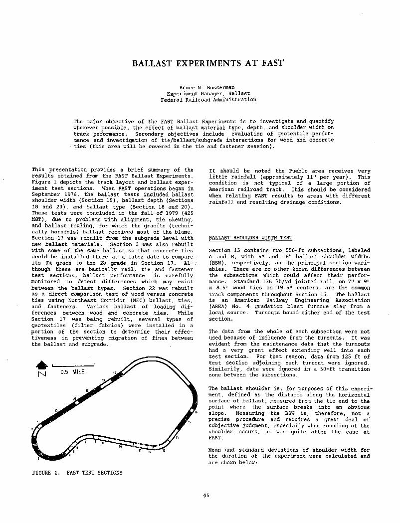
BALLAST EXPERIMENTS AT FAST

Bruce N. Bosserman Experiment Manager, Ballast

Federal Railroad Administration

The major objective of the FAST Ballast Experiments is to investigate and quantify wherever possible, the effect of ballast material type, depth, and shoulder width on track peformance. Secondary objectives include evaluation of geotextile perfor­mance and investigation of tie/ballast/subgrade interactions for wood and concrete ties (this area will be covered in the tie and fastener session).

This presentation provides a brief summary of the results obtained from the FAST Ballast Experiments. Figure 1 depicts the track layout and ballast exper­iment test sections. When FAST operations began in September 1976, the ballast tests included ballast shoulder width (Section 15), ballast depth (Sections 18 and 20), and ballast type (Section 18 and 20). These tests were concluded in the fall of 1979 (425 MGT), due to problems with alignment, tie skewing, and ballast fouling, for which the granite (techni­cally hornfels) ballast received most of the blame. Section 17 was rebuilt from the subgrade level with new ballast materials. Section 3 was also rebuilt with some of the same ballast so that concrete ties could be installed there at a later date to compare its 0% grade to the 2% grade in Section 17. Al- ; though these are basically rail, tie and fastener test sections, ballast performance is carefully monitored to detect differences which may exist between the ballast types. Section 22 was rebuilt as a direct comparison test of wood versus concrete ties using Northeast Corridor (NEC) ballast, ties, and fasteners. Various ballast of loading dif­ferences between wood and concrete ties. While Section 17 was being rebuilt, several types of geotextiles (filter fabrics) were installed in a portion of the section to determine their effec­tiveness in preventing migration of fines between the ballast and subgrade.

FIGURE 1. FAST TEST SECTIONS

It should be noted the Pueblo area receives very little rainfall (approximately 11" per year). This condition is not typical of a large portion of American railroad track. This should be considered when relating FAST results to areas with different rainfall and resulting drainage conditions.

BALLAST SHOULDER WIDTH TEST

Section 15 contains two 550-ft subsections, labeled A and B, with 6" and 18" ballast shoulder widths (BSW), respectively, as the principal section vari­ables. There are no other known differences between the subsections which could affect their perfor­mance. Standard 136 lb/yd jointed rail, on 7" x 9" x 8.5' wood ties on 19.5" centers, are the common track components throughout Section 15. The ballast is an American Railway Engineering Association (AREA) No. 4 gradation blast furnace slag from a local source. Turnouts bound either end of the test section.

The data from the whole of each subsection were not used because of influence from the turnouts. It was evident from the maintenance data that the turnouts had a very great effect extending well into each test section. For that reason, data from 125 ft of test section adjoining each turnout were ignored. Similarily, data were ignored in a 50-ft transition zone between the subsections.

The ballast shoulder is, for purposes of this experi­ment, defined as the distance along the horizontal surface of ballast, measured from the tie end to the point where the surface breaks into an obvious slope. Measuring the BSW is, therefore, not a precise procedure and requires a great deal of subjective judgment, especially when rounding of the shoulder occurs, as was quite often the case at FAST.

Mean and standard deviations of shoulder width for the duration of the experiment were calculated and are shown below:

45

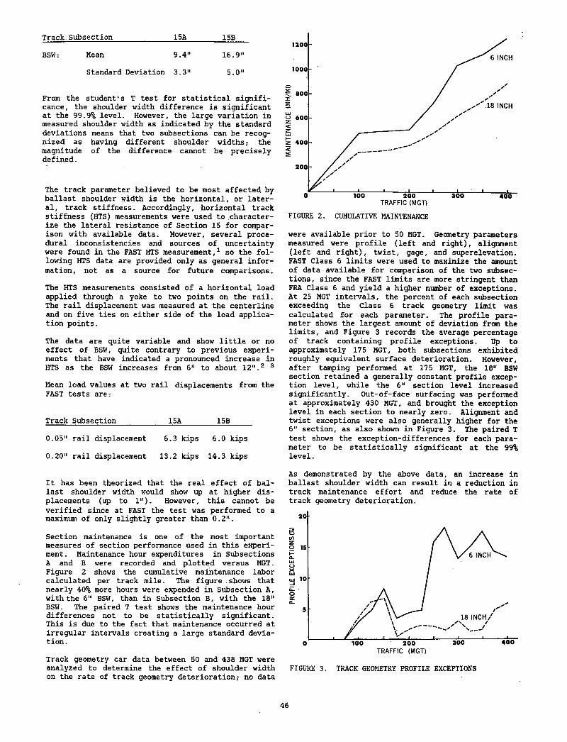
Track Subsection_______ _______15&______ 15B

BSW: Mean 9.4" 16.9

Standard Deviation 3.3" 5.0

From the student's T test for statistical signifi­cance, the shoulder width difference is significant at the 99.9% level. However, the large variation in measured shoulder width as indicated by the standard deviations means that two subsections can be recog­nized as having different shoulder widths; the magnitude of the difference cannot be precisely defined.

The track parameter believed to be most affected by ballast shoulder width is the horizontal, or later­al, track stiffness. Accordingly, horizontal track stiffness (HTS) measurements were used to character­ize the lateral resistance of Section 15 for compar­ison with available data. However, several proce­dural inconsistencies and sources of uncertainty were found in the FAST HTS measurement,1 so the fol­lowing HTS data are provided only as general infor­mation, not as a source for future comparisons.

The HTS measurements consisted of a horizontal load applied through a yoke to two points on the rail. The rail displacement was measured at the centerline and on five ties on either side of the load applica­tion points.

The data are quite variable and show little or no effect of BSW, quite contrary to previous experi­ments that have indicated a pronounced increase in HTS as the BSW increases from 6" to about 12".2 3

Mean load values at two rail displacements from the FAST tests are:

Track Subsection____________ 15A________ 15B

0.05" rail displacement 6.3 kips 6.0 kips

0.20" rail displacement 13.2 kips 14.3 kips

It has been theorized that the real effect of bal­last shoulder width would show up at higher dis­placements (up to 1"). However, this cannot be verified since at FAST the test was performed to a maximum of only slightly greater than 0.2".

Section maintenance is one of the most important measures of section performance used in this experi­ment. Maintenance hour expenditures in Subsections A and B were recorded and plotted versus MGT. Figure 2 shows the cumulative maintenance labor calculated per track mile. The figure .shows that nearly 40% more hours were expended in Subsection A, with the 6" BSW, than in Subsection B, with the IB" BSW. The paired T test shows the maintenance hour differences not to be statistically significant. This is due to the fact that maintenance occurred at irregular intervals creating a large standard devia­tion.

Track geometry car data between 50 and 438 MGT were analyzed to determine the effect of shoulder width on the rate of track geometry deterioration; no data

FIGURE 2. CUMULATIVE MAINTENANCE

were available prior to 50 MGT. Geometry parameters measured were profile (left and right), alignment (left and right), twist, gage, and superelevation. FAST Class 6 limits were used to maximize the amount of data available for comparison of the two subsec­tions, since the FAST limits are more stringent than FRA Class 6 and yield a higher number of exceptions. At 25 MGT intervals, the percent of each subsection exceeding the Class 6 track geometry limit was calculated for each parameter. The profile para­meter shows the largest amount of deviation from the limits, and Figure 3 records the average percentage of track containing profile exceptions. Up to approximately 175 MGT, both subsections exhibited roughly equivalent surface deterioration. However, after tamping performed at 175 MGT, the 18" BSW section retained a generally constant profile excep­tion level, while the 6" section level increased significantly. Out-of-face surfacing was performed at approximately 430 MGT, and brought the exception level in each section to nearly zero. Alignment and twist exceptions were also generally higher for the 6" section, as also shown in Figure 3. The paired T test shows the exception-differences for each para­meter to be statistically significant at the 99% level.

As demonstrated by the above data, an increase in ballast shoulder width can result in a reduction in track maintenance effort and reduce the rate of track geometry deterioration.

FIGURE 3. TRACK GEOMETRY PROFILE EXCEPTIONS

46

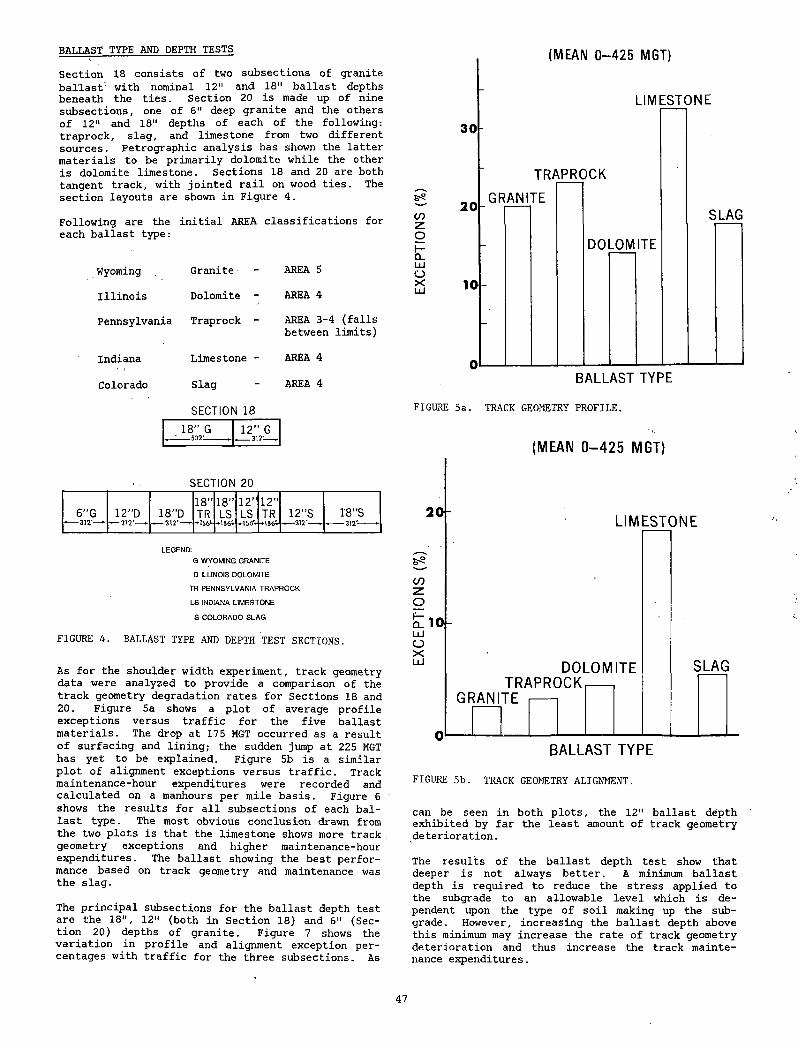
RATI.AST TYPE AND DEPTH TESTS (MEAN 0-425 MGT)Section 18 consists of two subsections of granite bal'last: with nominal 12" and 18" ballast depths beneath the ties. Section 20 is made up of nine subsections, one of 6" deep granite and the others of 12" and 18" depths of each of the following: traprock, slag, and limestone from two different sources. Petrographic analysis has shown the latter materials to be primarily dolomite while the other is dolomite limestone. Sections 18 and 20 are both tangent track, with jointed rail on wood ties. The section layouts are shown in Figure 4.

Following are the initial AREA classifications for each ballast type:

Wyoming Granite AREA 5

Illinois Dolomite - AREA 4

Pennsylvania Traprock - AREA 3-4 (falls between limits)

Indiana Limestone - AREA 4

Colorado Slag AREA 4

SECTION 1818” G 12" G

SECTION 2018” 18” 12” 12”

6”G 12”D 18”D TR LS LS TR 12”S 18”S■*— 312'— *— 312'— ►— 312' — *156 ♦156*♦156%♦156**— 312'-**--312'---*

LEGEND:

G W YOMING GRANITE

D ILLINOIS DO LOM ITE

TR PENNSYLVANIA TRAPROCK

LS INDIANA LIM ESTO NE

S COLORADO SLAG

FIGURE 4. BALLAST TYPE AND DEPTH TEST SECTIONS.

As for the shoulder width experiment, track geometry data were analyzed to provide a comparison of the track geometry degradation rates for Sections 18 and 20. Figure 5a shows a plot of average profile exceptions versus traffic for the five ballast materials. The drop at 175 MGT occurred as a result of surfacing and lining; the sudden jump at 225 MGT has yet to be explained. Figure 5b is a similar plot of alignment exceptions versus traffic. Track maintenance-hour expenditures were recorded and calculated on a manhours per mile basis. Figure 6 shows the results for all subsections of each bal­last type. The most obvious conclusion drawn from the two plots is that the limestone shows more track geometry exceptions and higher maintenance-hour expenditures. The ballast showing the best perfor­mance based on track geometry and maintenance was the slag.

The principal subsections for the ballast depth test are the 18", 12" (both in Section 18) and 6" (Sec­tion 20) depths of granite. Figure 7 shows the variation in profile and alignment exception per­centages with traffic for the three subsections. As

COzoI-CL1x1OX

LIMESTONE

FIGURE 5a. TRACK GEOMETRY PROFILE.

(M E A N 0 - 4 2 5 M G T )

BALLAST TYPE

FIGURE 5b. TRACK GEOMETRY ALIGNMENT.

can be seen in both plots, the 12" ballast depth exhibited by far the least amount of track geometry deterioration.

The results of the ballast depth test show that deeper is not always better. A minimum ballast depth is required to reduce the stress applied to the subgrade to an allowable level which is de­pendent upon the type of soil making up the sub­grade. However, increasing the ballast depth above this minimum may increase the rate of track geometry deterioration and thus increase the track mainte­nance expenditures.

47

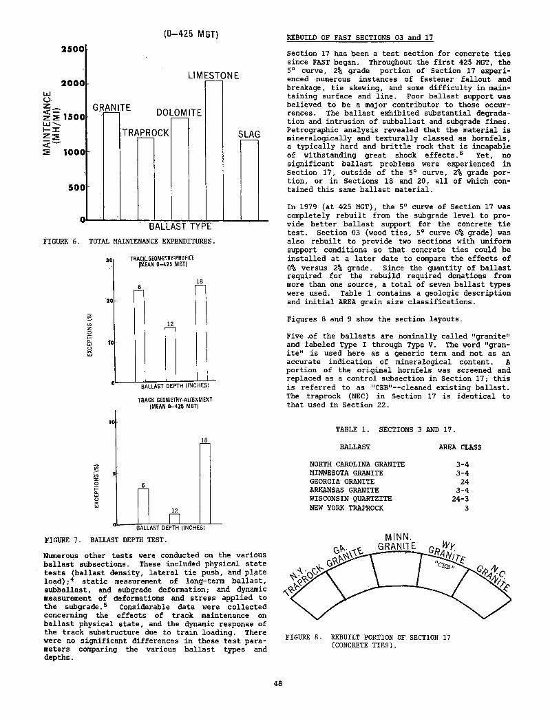
(0-425 MGT)

TRACK GEOMETRY-ALIGNMENT (MEAN 0-425 MGT)

FIGURE 7. BALLAST DEPTH TEST.

Numerous other tests were conducted on the various ballast subsections. These included physical state tests (ballast density, lateral tie push, and plate load),-4 static measurement of long-term ballast, subballast, and subgrade deformation; and dynamic measurement of deformations and stress applied to the subgrade.5 Considerable data were collected concerning the effects of track maintenance on ballast physical state, and the dynamic response of the track substructure due to train loading. There were no significant differences in these test para­meters comparing the various ballast types and depths.

REBUILD OF FAST SECTIONS 03 and 17

Section 17 has been a test section for concrete ties since FAST began. Throughout the first 425 MGT, the 5° curve, 2% grade portion of Section 17 experi­enced numerous instances of fastener fallout and breakage, tie skewing, and some difficulty in main­taining surface and line. Poor ballast support was believed to be a major contributor to those occur­rences. The ballast exhibited substantial degrada­tion and intrusion of subballast and subgrade fines. Petrographic analysis revealed that the material is mineralogically and texturally classed as hornfels, a typically hard and brittle rock that is incapable of withstanding great shock effects.6 Yet, no significant ballast problems were experienced in Section 17, outside of the 5° curve, 2% grade por­tion, or in Sections 18 and 20, all of which con­tained this same ballast material.

In 1979 (at 425 MGT), the 5° curve of Section 17 was completely rebuilt from the subgrade level to pro­vide better ballast support for the concrete tie test. Section 03 (wood ties, 5° curve 0% grade) was also rebuilt to provide two sections with uniform support conditions so that concrete ties could be installed at a later date to compare the effects of 0% versus 2% grade. Since the quantity of ballast required for the rebuild required donations from more than one source, a total of seven ballast types were used. Table 1 contains a geologic description and initial AREA grain size classifications.

Figures 8 and 9 show the section layouts.

Five xif the ballasts are nominally called "granite" and labeled Type I through Type V. The word "gran­ite" is used here as a generic term and not as an accurate indication of mineralogical content. A portion of the original hornfels was screened and replaced as a control subsection in Section 17; this is referred to as "CEB"— cleaned existing ballast. The traprock (NEC) in Section 17 is identical to that used in Section 22.

TABLE 1. SECTIONS 3 AND 17.

BALLAST AREA CLASS

NORTH CAROLINA GRANITE 3-4MINNESOTA GRANITE 3-4GEORGIA GRANITE 24ARKANSAS GRANITE 3-4WISCONSIN QUARTZITE 24-3NEW YORK TRAPROCK 3

FIGURE 8. REBUILT PORTION OF SECTION 17 (CONCRETE TIES).

48

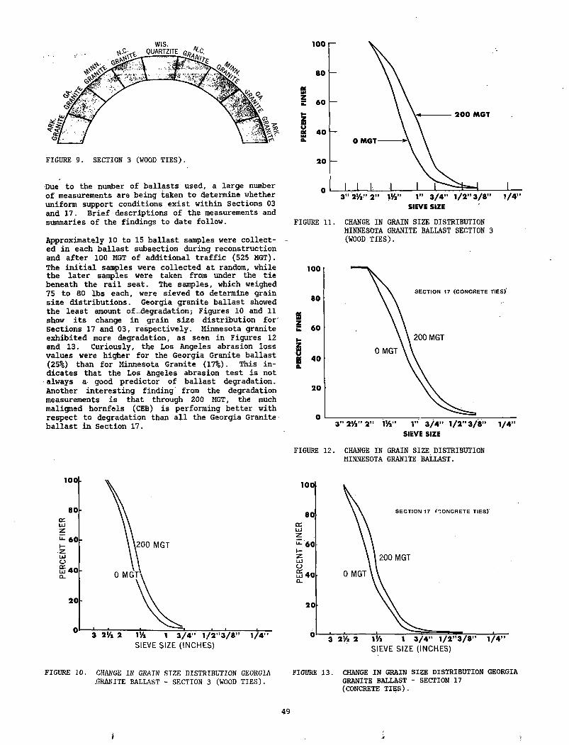
FIGURE 9. SECTION 3 (WOOD TIES).

Due to the number of ballasts used, a large number of measurements are being taken to determine whether uniform support conditions exist within Sections 03 and 17. Brief descriptions of the measurements and summaries of the findings to date follow.

Approximately 10 to 15 ballast samples were collect- - ed in each ballast subsection during reconstruction and after 100 MGT of additional traffic (525 MGT). The initial samples were collected at random, while the later samples were taken from under the tie beneath the rail seat. The samples, which weighed 75 to 80 lbs each, were sieved to determine grain size distributions. Georgia granite ballast showed the least amount of-degradation; Figures 10 and 11 show its change in grain size distribution for' Sections 17 and 03, respectively. Minnesota granite exhibited more degradation, as seen in Figures 12 and 13. Curiously, the Los Angeles abrasion loss values were higher for the Georgia Granite ballast (25%) than for Minnesota Granite (17%). This in­dicates that the Los Angeles abrasion test is not always a good predictor of ballast degradation. Another interesting finding from the degradation measurements is that through 200 MGT, the much maligned hornfels (CEB) is performing better with respect to degradation than all the Georgia Granite ballast in Section 17.

FIGURE 10. CHANGE IN GRAIN SIZE DISTRIBUTION GEORGIA .GRANITE BALLAST - SECTION 3 (WOOD TIES).

FIGURE 11. CHANGE IN GRAIN SIZE DISTRIBUTION MINNESOTA GRANITE BALLAST SECTION 3 (WOOD TIES).

FIGURE 12. CHANGE IN GRAIN SIZE DISTRIBUTION MINNESOTA GRANITE BALLAST.

FIGURE 13. CHANGE IN GRAIN SIZE DISTRIBUTION GEORGIA GRANITE BALLAST - SECTION 17 (CONCRETE TIES).

49

I

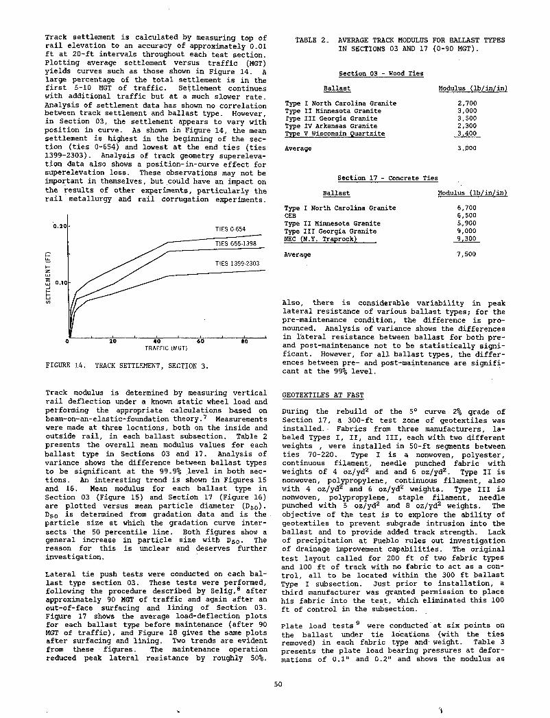
Track settlement is calculated by measuring top of rail elevation to an accuracy of approximately 0.01 ft at 20-ft intervals throughout each test section. Plotting average settlement versus traffic (MGT) yields curves such as those shown in Figure 14. A large percentage of the total settlement is in the first 5-10 MGT of traffic. Settlement continues with additional traffic but at a much slower rate. Analysis of settlement data has shown no correlation between track settlement and ballast type. However, in Section 03, the settlement appears to vary with position in curve. As shown in Figure 14, the mean settlement is highest in the beginning of the sec­tion (ties 0-654) and lowest at the end ties (ties 1399-2303). Analysis of track geometry supereleva­tion data also shows a position-in-curve effect for superelevation loss. These observations may not be important in themselves, but could have an impact on the results of other experiments, particularly the rail metallurgy and rail corrugation experiments.

FIGURE 14. TRACK SETTLEMENT, SECTION 3.

TABLE 2. AVERAGE TRACK MODULUS FOR BALLAST TYPES IN SECTIONS 03 AND 17 (0-90 MGT).

Section 03 - Wood TiesBallast Modulus (lb/in/in)

Type I North Carolina Granite 2,700 Type II Minnesota Granite 3,000 Type III Georgia Granite 3,500 Type IV Arkansas Granite 2,300 Type V Wisconsin Quartzite 3,400Average 3,000

Section 17 - Concrete TiesBallast Modulus (lb/in/in)

Type I North Carolina Granite 6,700 CEB 6,500 Type II Minnesota Granite 5,900 Type III Georgia Granite 9,000 NEC (N.Y- Traprock) 9,300

Average 7,500

Also, there is considerable variability in peak lateral resistance of various ballast types; for the pre-maintenance condition, the difference is pro­nounced. Analysis of variance shows the differences in lateral resistance between ballast for both pre- and post-maintenance not to be statistically signi­ficant. However, for all ballast types, the differ­ences between pre- and post-maintenance are signifi­cant at the 99% level.

Track modulus is determined by measuring vertical rail deflection under a known static wheel load and performing the appropriate calculations based on beam-on-an-elastic-foundation theory.7 Measurements were made at three locations, both on the inside and outside rail, in each ballast subsection. Table 2 presents the overall mean modulus values for each ballast type in Sections 03 and 17. Analysis of variance shows the difference between ballast types to be significant at the 99.9% level in both sec­tions. An interesting trend is shown in Figures 15 and 16. Mean modulus for each ballast type in Section 03 (Figure 15) and Section 17 (Figure 16) are plotted versus mean particle diameter (D50). D5o is determined from gradation data and is the particle size at which the gradation curve inter­sects the 50 percentile line. Both figures show a general increase in particle size with D50- The reason for this is unclear and deserves further investigation.

Lateral tie push tests were conducted on each bal­last type section 03. These tests were performed, following the procedure described by Selig,8 after approximately 90 MGT of traffic and again after an out-of-face surfacing and lining of Section 03. Figure 17 shows the average load-deflection plots for each ballast type before maintenance (after 90 MGT of traffic), and Figure 18 gives the same plots after surfacing and lining. Two trends are evident from these figures. The maintenance operation reduced peak lateral resistance by roughly 50%.

GEOTEXTILES AT FAST

During the rebuild of the 5° curve 2% grade of Section 17, a 300-ft test zone of geotextiles was installed.- Fabrics from three manufacturers, la­beled Types I, II, and III, each with two different weights , were installed in 50-ft segments between ties 70-220. Type I is a nonwoven, polyester, continuous filament, needle punched fabric with weights of 4 oz/yd2 and and 6 oz/yd2. Type II is nonwoven, polypropylene, continuous filament, also with 4 oz/yd2 and 6 oz/yd2 weights. Type III is nonwoven, polypropylene, staple filament, needle punched with 5 oz/yd2 and 8 oz/yd2 weights. The objective of the test is to explore the ability of geotextiles to prevent subgrade intrusion into the ballast and to provide added track strength. Lack of precipitation at Pueblo rules out investigation of drainage improvement capabilities. The original test layout called for 200 ft of two fabric types and 100 ft of track with no fabric to act as a con­trol, all to be located within the 300 ft ballast Type I subsection. Just prior to installation, a third manufacturer was granted permission to place his fabric into the test, which eliminated this 100 ft of control in the subsection.

Plate load tests 9 were conducted' at six points on the ballast under tie locations (with the ties removed) in each fabric type and weight. Table 3 presents the plate load bearing pressures at defor­mations of 0.1" and 0.2" and shows the modulus as

50

'1

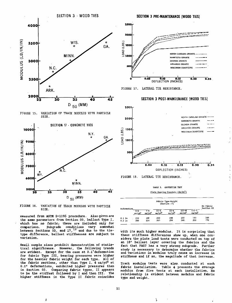
SECTION 3 - WOOD TIES SECTION 3 PRE-MAINTENANCE (WOOD TIES]

z

CO

inZ3_lrjQO

4000

2000ARK.

25 30 35 40 45D 5 0 (M M )

FIGURE 15. VARIATION OF TRACK MODULUS WITH PARTICLE SIZE.

FIGURE 16. VARIATION OF TRACK MODULUS WITH PARTICLE SIZE.

measured from ASTM D-1195 procedure. Also given are the same parameters from Section 03, ballast Type I, which has no fabric; these are included only for comparison. Subgrade conditions vary somewhat between Sections 03, and 17,10 and due to the tie- type difference, ballast stiffnesses are subject to variation.

Small sample sizes prohibit demonstration of statis­tical significance. However, the following trends are evident. Except for the case at 0.1udeformation for fabric Type III, bearing pressures, were higher for the heavier fabric weight for each type. All of the fabric sections, other than Type I, 4 oz/yd2 at 0.1" deformations, exhibited higher pressures than in Section 03. Comparing fabric types, II appears to be the stiffest followed by I and then III. The higher stiffness in the Type II fabric coincides

DEFLECTION (INCHES)

FIGURE 17. LATERAL TIE RESISTANCE.

SECTION 3 POST-MAINTENANCE (WOOD TIES]

FIGURE 18. LATERAL TIE RESISTANCE.

TABLE 3. GEOTEXTILE TEST

Plate Bearing Pressure (lb/in2)

Fabric Type-Weight (Section 17)

No FabricDeformation___________________________________________________________ Section 03

1-6 1-4 II-6 II-4 III-8 III-5oz/yd2 oz/yd2 oz/yd2_____oz/yd2 oz/yd2 oz/yd2______________

0.1 in 230 140 230 190 160 160 1400.2 in 260 210 360 250 240. 200 190

with its much higher modulus. It is surprising that these stiffness differences show up, when one con­siders the plate load tests were conducted on top of an 18" ballast layer covering the fabrics and the fact that FAST has a very strong subgrade. Further study is necessary to determine whether the fabrics and variations in modulus truly cause an increase in stiffness and if so, the magnitude of that increase.

Track modulus tests were also, conducted at each fabric installation. Table 4 presents the average modulus from five tests at each installation. No relationship is evident between modulus and fabric type and weight.

51

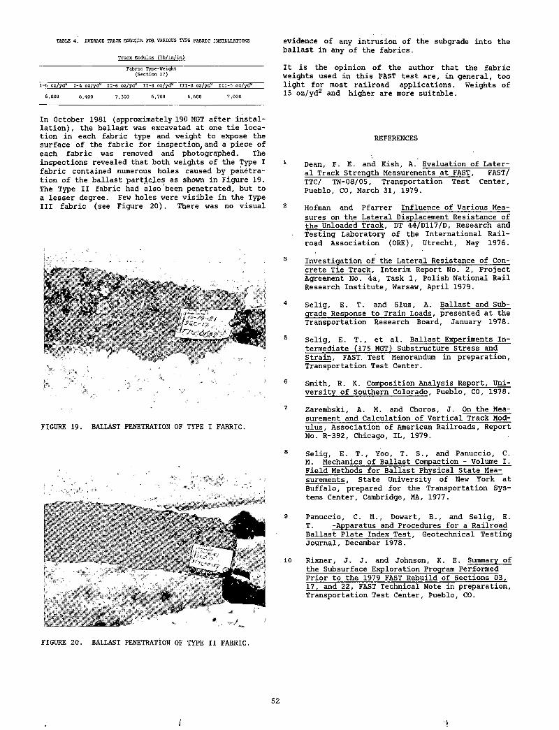
TABLE 4. AVERAGE TRACK MODULUS FOR VARIOUS TYPE FABRIC INSTALLATIONS

Track Modulus (Ib/in/in)

Fabric Type-Weight (Section 17)

1-6 oz/yd^ 1-4 oz/ydz II-6 oz/yd* II-4 oz/yd* III-8 02/yd^ III-5 oz/yd*'

6,800 6,400 7,300 6,700 6,600 7,000

evidence of any intrusion of the subgrade into the ballast in any of the fabrics.

It is the opinion of the author that the fabric weights used in this FAST test are, in general, too light for most railroad applications. Weights of 15 oz/yd2 and higher are more suitable.

In October 1981 (approximately 190 MGT after instal­lation) , the ballast was excavated at one tie loca­tion in each fabric type and weight to expose the surface of the fabric for inspection, and a piece of each fabric was removed and photographed. The inspections revealed that both weights of the Type I 1 fabric contained numerous holes caused by penetra­tion of the ballast particles as shown in Figure 19.The Type II fabric had also been penetrated, but to a lesser degree. Few holes were visible in the Type III fabric (see Figure 20). There was no visual 2

REFERENCES

Dean, F. E. and Kish, A. Evaluation of Later­al Track Strength Measurements at FAST, FAST/ TTC/ TN-08/05, Transportation Test Center, Pueblo, CO, March 31, 1979.

Hofman and Pfarrer Influence of Various Mea­sures on the Lateral Displacement Resistance of the Unloaded Track, DT 44/D117/D, Research and Testing Laboratory of the International Rail­road Association (ORE), Utrecht, May 1976.

Investigation of the Lateral Resistance of Con­crete Tie Track, Interim Report No. 2, Project Agreement No. 4a, Task 1, Polish National Rail Research Institute, Warsaw, April 1979.

Selig, E. T. and Sluz, A. Ballast and Sub­grade Response to Train Loads, presented at the Transportation Research Board, January 1978.

Selig, E. T., et al. Ballast Experiments In­termediate (175 MGT) Substructure Stress and Strain, FAST Test Memorandum in preparation. Transportation Test Center.

Smith, R. K. Composition Analysis Report, Uni­versity of Southern Colorado, Pueblo, CO, 1978.

FIGURE 19. BALLAST PENETRATION OF TYPE I FABRIC.

Zarembski, A. M. and Choros, J. On the Mea­surement and Calculation of Vertical Track Mod­ulus, Association of American Railroads, Report No. R-392, Chicago, IL, 1979.

8 Selig, E. T., Yoo, T. S., and Panuccio, C. M. Mechanics of Ballast Compaction - Volume I. Field Methods for Ballast Physical State Mea­surements, State University of New York at Buffalo, prepared for the Transportation Sys­tems Center, Cambridge, MA, 1977.

9 Panuccio, C. M., Dowart, B., and Selig, E. T. -Apparatus and Procedures for a Railroad Ballast Plate Index Test, Geotechnical Testing Journal, December 1978. 10

10 Rixner, J. J. and Johnson, K. E. Summary of the Subsurface Exploration Program Performed Prior to the 1979 FAST Rebuild of Sections 03, 17, and 22, FAST Technical Note in preparation. Transportation Test Center, Pueblo, CO.

FIGURE 20. BALLAST PENETRATION OF TYPE II FABRIC.

QUESTIONS AND ANSWERS

Question 1

Will there be future test at FAST on heavier fabrics, i.e., 14-18 oz. and if so when?

Answer

There are currently no plans for future testing due to limitations described in the presenta­tion.

Question 2

All the ballast material types supplied for the project are of high quality and used by a variety of railroads. Isn't it fair .to say that all of these can do a suitable job and that a potential user should take the economics of a particular material into consideration when looking for a ballast source?

Answer

Only performance comparisons were provided. FAST does not attempt to provide these economic data. The user certainly must trade off per­formance and economic considerations when choosing a ballast material.

Limestones in strength, L.A. Abrasion test results and other physical properties. Only one Limestone has been tested. Will different Limestones with different propreties be tested in the future? Why was Limestone eliminated when Sections 17 and 03 were rebuilt?

Answer

1) There are currently no plans testing of limestone in the future.

2) It was the conscientious opinion of the planners of the rebuild that granite/granite like materials would be used to create as nearly uniform performance as possible so as not to adversely affect the tie/fastener and metallurgy tests.

Question 6

Slide shows installation of geotextile looks like textile is being spread out over the track. Where is the textile actually placed, and how is it placed?

Answer

Geotextile was not spread over the track. Fabric was placed on the subgrade surface. Approximately 6" of ballast was hand placed on top before placement of ties to avoid damaging fabric while placing ties.

Question 3Question 7

Was a ballast compactor used after tamping to determine the effect this would have on lateral stability?

Answer

No.

Question 4

What is your opinion of the ability of the wet attrition test (developed by British Railways) to predict ballast performance?

Answer

I have seen no data comparing predictions to performance. A test program doing this is beneficial.

Question 5

There are wide d iffe ren ces in the properties o f

Have you considered a section containing a simulated situation involving poor drainage in which ballast could bis evaluated in respect to mud seepage up over the ties (or the avoidance of such seepage) accompanied by moderate to servere tie pumping? -

Answer

It has been considered but never implemented due mostly to cost factors and logistics of moving the water.

Question 8

In soil mechanics, molding in foundries and ceramics manufacturing average grain size is not sufficient for evaluations and grain size distribution is used. Have you looked into this for ballast evaluation?

Answer

The only time average grain s ize was used in

53

i'

correlating track modulus to ballast pro­perties. Correlation with grain size was much better than with grain size distribution.

Question 9

Would you please explain why the deflection of subgrade still increases significantly after 200 MGT traffic loading? How to define the good subgrade what are the major parameters and characteristics?

Answer

1) Subgrade deflection still increases after 200 MGT but much slower than at the initial rate. I would guess that in the next 200 MGT the deflection rate will be reduced to near zero. This is consistent with previous data.

2) A good subgrade has sufficient shear strength to support loads supplied by the ballast, has minimum compressibility and is not affected by variations in moisture content temperature, etc.

54

k; v

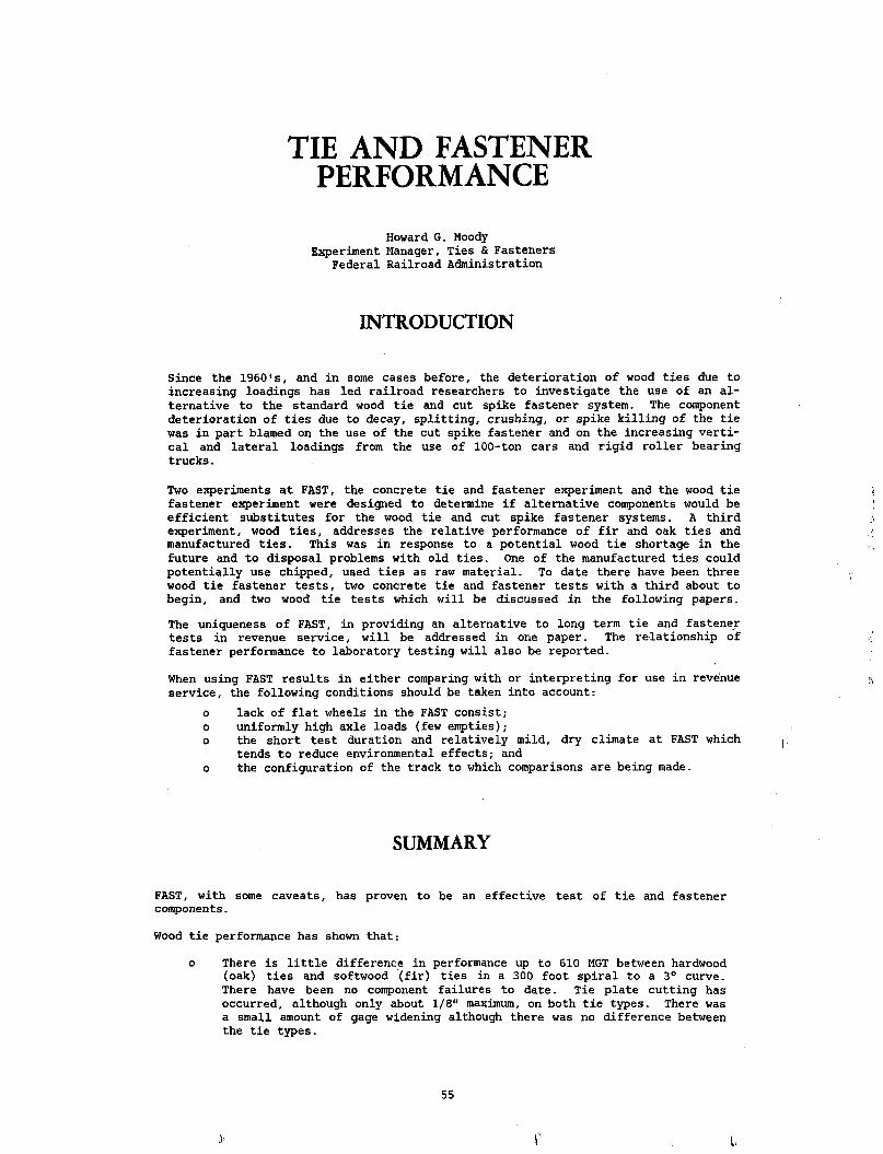
TIE AND FASTENER PERFORMANCEHoward G. Moody

Experiment Manager, Ties & Fasteners Federal Railroad Administration

INTRODUCTION

Since the 1960‘s, and in some cases before, the deterioration of wood ties due to increasing loadings has led railroad researchers to investigate the use of an al­ternative to the standard wood tie and cut spike fastener system. The component deterioration of ties due to decay, splitting, crushing, or spike killing of the tie was in part blamed on the use of the cut spike fastener and on the increasing verti­cal and lateral loadings from the use of 100-ton cars and rigid roller bearing trucks.

Two experiments at FAST, the concrete tie and fastener experiment and the wood tie fastener experiment were designed to determine if alternative components would be efficient substitutes for the wood tie and cut spike fastener systems. A third experiment, wood ties, .addresses the relative performance of fir and oak ties and manufactured ties. This was in response to a potential wood tie shortage in the future and to disposal problems with old ties. One of the manufactured ties could potentially use chipped, used ties as raw material. To date there have been three wood tie fastener tests, two concrete tie and fastener tests with a third about to begin, and two wood tie tests which will be discussed in the following papers.

The uniqueness of FAST, in providing an alternative to long term tie and fastener tests in revenue service, will be addressed in one paper. The relationship of fastener performance to laboratory testing will also be reported.

When using FAST results in either comparing with or interpreting for use in revenue service, the following conditions should be taken into account:

o lack of flat wheels in the FAST consist; o uniformly high axle loads (few empties);o the short test duration and relatively mild, dry climate at FAST which

tends to reduce environmental effects,- and o the configuration of the track to which comparisons are being made.

SUMMARY

FAST, with some caveats, has proven to be an effective test of tie and fastener components.

Wood tie performance has shown that:

o There is little difference in performance up to 610 MGT between hardwood (oak) ties and softwood (fir) ties in a 300 foot spiral to a 3° curve. There have been no component failures to date. Tie plate cutting has occurred, although only about 1/8" maximum, on both tie types. There was a small amount of gage widening although there was no difference between the tie types.

55

r

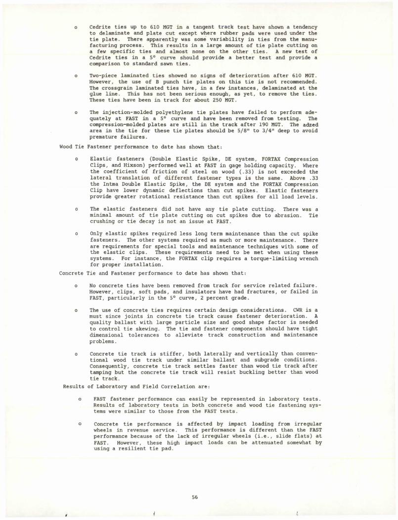
o Cedrite ties up to 610 MGT in a tangent track test have shown a tendency to delaminate and plate cut except where rubber pads were used under the tie plate. There apparently was some variability in ties from the manu­facturing process. This results in a large amount of tie plate cutting on a few specific ties and almost none on the other ties. A new test of Cedrite ties in a 5° curve should provide a better test and provide a comparison to standard sawn ties.

o Two-piece laminated ties showed no signs of deterioration after 610 MGT. However, the use of B punch tie plates on this tie is not recommended. The crossgrain laminated ties have, in a few instances, delaminated at the glue line. This has not been serious enough, as yet, to remove the ties. These ties have been in track for about 250 MGT.

o The injection-molded polyethylene tie plates have failed to perform ade­quately at FAST in a 5° curve and have been removed from testing. The compression-molded plates are still in the track after 190 MGT. The adzed area in the tie for these tie plates should be 5/8" to 3/4" deep to avoid premature failures.

Wood Tie Fastener performance to date has shown that:

o Elastic fasteners (Double Elastic Spike, DE system, FORTAX Compression Clips, and Hixson) performed well at FAST in gage holding capacity. Where the coefficient of friction of steel on wood (.33) is not exceeded the lateral translation of different fastener types is the same. Above .33 the Intma Double Elastic Spike, the DE system and the FORTAX Compression Clip have lower dynamic deflections than cut spikes. Elastic fasteners provide greater rotational resistance than cut spikes for all load levels.

o The elastic fasteners did not have any tie plate cutting. There was a minimal amount of tie plate cutting on cut spikes due to abrasion. Tie crushing or tie decay is not an issue at FAST.

o Only elastic spikes required less long term maintenance than the cut spike fasteners. The other systems required as much or more maintenance. There are requirements for special tools and maintenance techniques with some of the elastic clips. These requirements need to be met when using these systems. For instance, the FORTAX clip requires a torque-limiting wrench for proper installation.

Concrete Tie and Fastener performance to date has shown that:

o No concrete ties have been removed from track for service related failure. However, clips, soft pads, and insulators have had fractures, or failed in FAST, particularly in the 5° curve, 2 percent grade.

o The use of concrete ties requires certain design considerations. CWR is a must since joints in concrete tie track cause fastener deterioration. A quality ballast with large particle size and good shape factor is needed to control tie skewing. The tie and fastener components should have tight dimensional tolerances to alleviate track construction and maintenance problems.

o Concrete tie track is stiffer, both laterally and vertically than conven­tional wood tie track under similar ballast and subgrade conditions. Consequently, concrete tie track settles faster than wood tie track after tamping but the concrete tie track will resist buckling better than wood tie track.

Results of Laboratory and Field Correlation are:

o FAST fastener performance can easily be represented in laboratory tests. Results of laboratory tests in both concrete and wood tie fastening sys­tems were similar to those from the FAST tests.

o Concrete tie performance is affected by impact loading from irregular wheels in revenue service. This performance is different than the FAST performance because of the lack of irregular wheels (i.e., slide flats) at FAST. However, these high impact loads can be attenuated somewhat by using a resilient tie pad.

56

i l

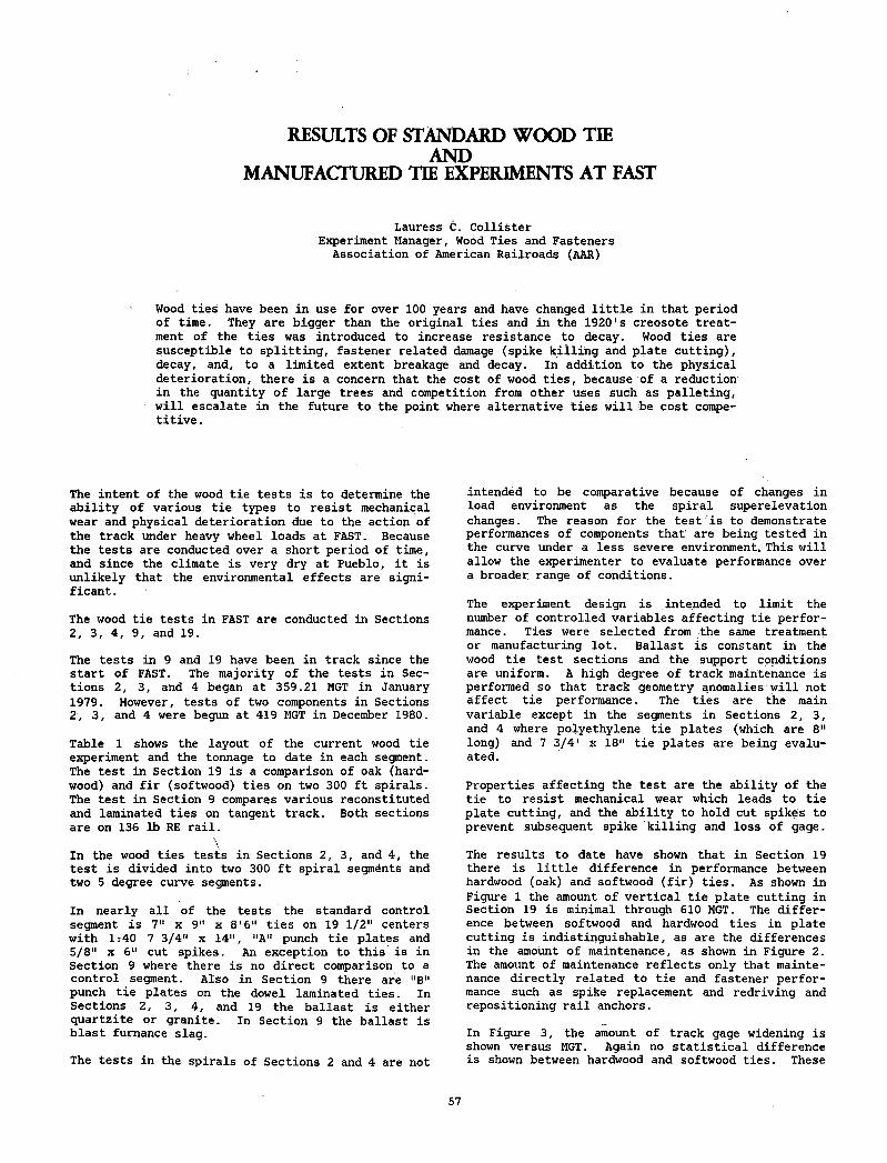
RESULTS OF STANDARD WOOD TIE AND

MANUFACTURED TIE EXPERIMENTS AT FAST

Lauress C. CollisterExperiment Manager, Wood Ties and Fasteners

Association of American Railroads (AAR)

Wood ties have been in use for over 100 years and have changed little in that period of time. They are bigger than the original ties and in the 19201 s creosote treat­ment of the ties was introduced to increase resistance to decay. Wood ties are susceptible to splitting, fastener related damage (spike killing and plate cutting), decay, and, to a limited extent breakage and decay. In addition to the physical deterioration, there is a concern that the cost of wood ties, because of a reduction in the quantity of large trees and competition from other uses such as palleting, will escalate in the future to the point where alternative ties will be cost compe­titive .

The intent of the wood tie tests is to determine the ability of various tie types to resist mechanical wear and physical deterioration due to the action of the track under heavy wheel loads at FAST. Because the tests are conducted over a short period of time, and since the climate is very dry at Pueblo, it is unlikely that the environmental effects are signi­ficant.

The wood tie tests in FAST are conducted in Sections 2, 3, 4, 9, and 19.

The tests in 9 and 19 have been in track since the start of FAST. The majority of the tests in Sec­tions 2, 3, and 4 began at 359.21 MGT in January 1979. However, tests of two components in Sections 2, 3, and 4 were begun at 419 MGT in December 1980.

Table 1 shows the layout of the current wood tie experiment and the tonnage to date in each segment. The test in Section 19 is a comparison of oak (hard­wood) and fir (softwood) ties on two 300 ft spirals. The test in Section 9 compares various reconstituted and laminated ties on tangent track. Both sections are on 136 lb RE rail.

\In the wood ties tests in Sections 2, 3, and 4, the test is divided into two 300 ft spiral segments and two 5 degree curve segments.

In nearly all of the tests the standard control segment is 7" x 9" x 8'6“ ties on 19 1/2" centers with 1.-40 7 3/4" x 14", "A" punch tie plates and 5/8" x 6" cut spikes. An exception to this is in Section 9 where there is no direct comparison to a control segment. Also in Section 9 there are "B" punch tie plates on the dowel laminated ties. In Sections 2, 3, 4, and 19 the ballast is eitherquartzite or granite. In Section 9 the ballast is blast furnance slag.

The tests in the spirals of Sections 2 and 4 are not

intended to be comparative because of changes in load environment as the spiral superelevation changes. The reason for the test‘is to demonstrate performances of components that' are being tested in the curve under a less severe environment. This will allow the experimenter to evaluate performance over a broader range of conditions.

The experiment design is intended to limit the number of controlled variables affecting tie perfor­mance. Ties were selected from the same treatment or manufacturing lot. Ballast is constant in the wood tie test sections and the support conditions are uniform. A high degree of track maintenance is performed so that track geometry anomalies1will not affect tie performance. The ties are the main variable except in the segments in Sections 2, 3, and 4 where polyethylene tie plates (which are 8" long) and 7 3/41 x 18" tie plates are being evalu­ated.

Properties affecting the test are the ability of the tie to resist mechanical wear which leads to tie plate cutting, and the ability to hold cut spikes to prevent subsequent spike killing and loss of gage.

The results to date have shown that in Section 19 there is little difference in performance between hardwood (oak) and softwood (fir) ties. As shown in Figure 1 the amount of vertical tie plate cutting in Section 19 is minimal through 610 MGT. The differ­ence between softwood and hardwood ties in plate cutting is indistinguishable, as are the differences in the amount of maintenance, as shown in Figure 2. The amount of maintenance reflects only that mainte­nance directly related to tie and fastener perfor­mance such as spike replacement and redriving and repositioning rail anchors.

In Figure 3, the amount of track gage widening is shown versus MGT. Again no statistical difference is shown between hardwood and softwood ties. These

57

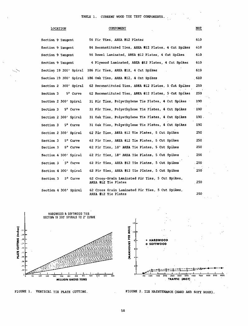
TABLE 1. CURRENT WOOD TIE TEST COMPONENTS.

LOCATION COMPONENT MGT

Section 9 Tangent 56

Section 9 Tangent 84

Section 9 Tangent 95

Section 9 Tangent 4

Section IS1 300' Spiral 186

Section 19 300' Spiral 186

Section 2 300' Spiral 62

Section 3 5C’ Curve 62

Section 2 300' Spiral 31

Section 3 5° Curve 31

Section 2 300' Spiral 31

Section 3 5° Curve 31

Section 2 300' Spiral 62

Section 3 5° Curve 62

Section 3 5° Curve 62

Section 4 300' Spiral 62

Section 3 5° Curve 62

Section 4 300' Spiral 62

Section 3 5° Curve 62AR1

Section 4 300' Spiral 62AREA #12 Tie Plates

610

610

610

610

610

610

250

250

190

190

190

.190

250

250

250

250

.250

250

250

250

FIGURE 1. VERTICAL TIE PLATE CUTTING. FIGURE 2. TIE MAINTENANCE (HARD AND SOFT WOOD)

58

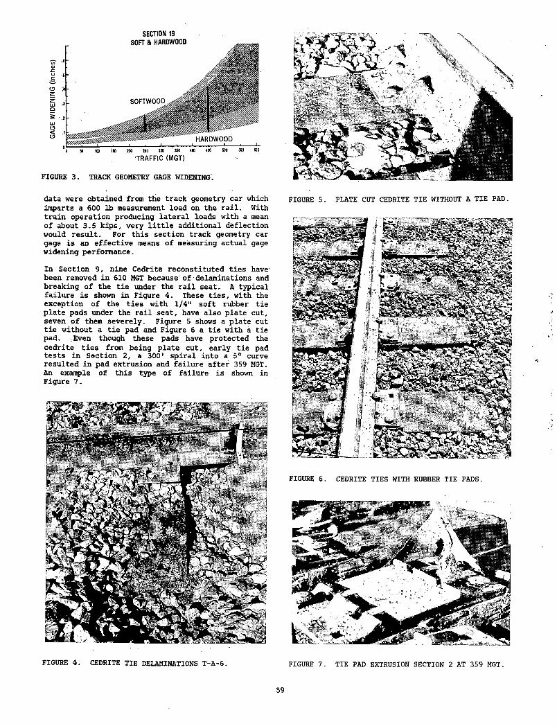
SECTION 19

FIGURE 3. TRACK GEOMETRY GAGE WIDENING:

data were obtained from the track geometry car which imparts a 600 lb measurement load on the rail. With train operation producing lateral loads with a mean of about 3.5 kips, very little additional deflection would result. For this section track geometry car gage is an effective means of measuring actual gage widening performance.

In Section 9, nine Cedrite reconstituted ties have’ been removed in 610 MGT because of delaminations and breaking of the tie under the rail seat. A typical failure is shown in Figure 4. These ties, with the exception of the ties with 1/4“ soft rubber tie plate pads under the rail seat, have also plate cut, seven of them severely. Figure 5 shows a plate cut tie without a tie pad and Figure 6 a tie with a tie pad. (Even though these pads have protected the cedrite ties from being plate cut, early tie pad tests in Section 2, a 300' spiral into a 5° curve resulted in pad extrusion and failure after 359 MGT. An example of this type of failure is shown in Figure 7.

FIGURE 4 . CEDRITE TIE DELAMINATIONS T-A-6.

FIGURE 5. PLATE CUT CEDRITE TIE WITHOUT A TIE PAD.

FIGURE 6. CEDRITE TIES WITH RUBBER TIE PADS.

FIGURE 7. TIE PAD EXTRUSION SECTION 2 AT 359 MGT.

59

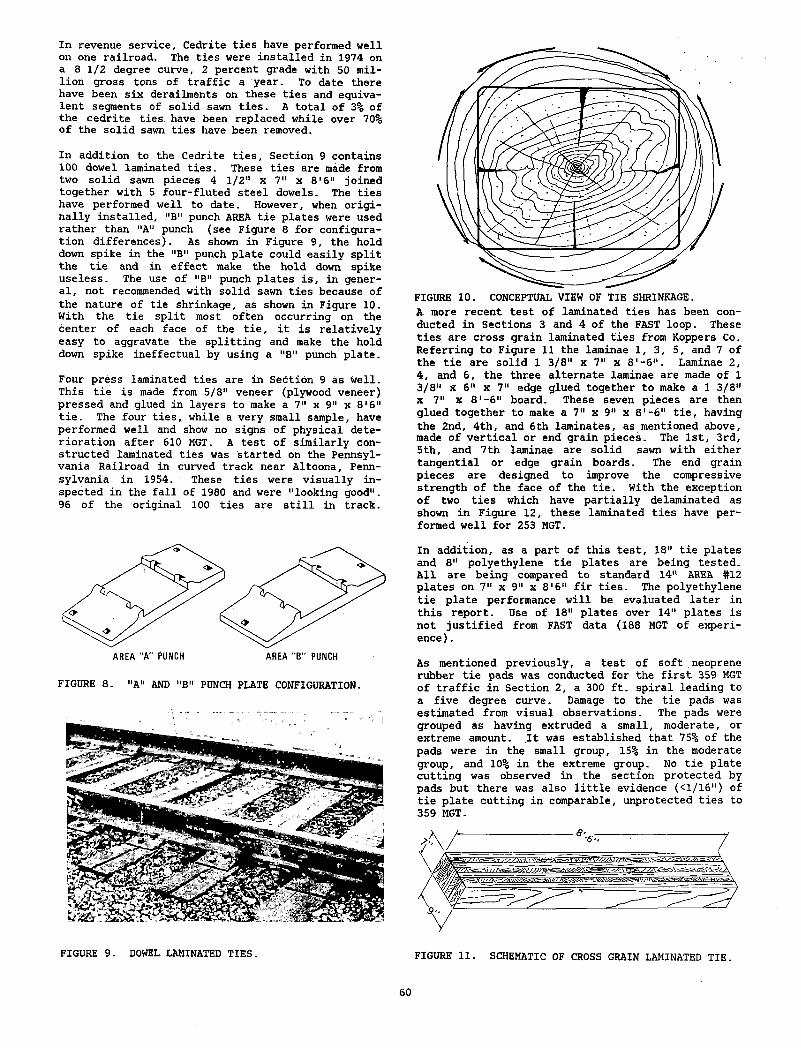
In revenue service, Cedrite ties have performed well on one railroad. The ties were installed in 1974 on a 8 1/2 degree curve, 2 percent grade with 50 mil­lion gross tons of traffic a year. To date there have been six derailments on these ties and equiva­lent segments of solid sawn ties. A total of 3% of the cedrite ties, have been replaced while over 70% of the solid sawn ties have been removed.

In addition to the Cedrite ties. Section 9 contains 100 dowel laminated ties. These ties are made from two solid sawn pieces 4 1/2“ x 7" x 8 16" joined together with 5 four-fluted steel dowels. The ties have performed well to date. However, when origi­nally installed, "B" punch AREA tie plates were used rather than "A" punch (see Figure 8 for configura­tion differences). As shown in Figure 9, the hold down spike in the "B" punch plate could easily split the tie and in effect make the hold down spike useless. The use of "B" punch plates is, in gener­al, not recommended with solid sawn ties because of the nature of tie shrinkage, as shown in Figure 10. With the tie split most often occurring on the center of each face of the tie, it is relatively easy to aggravate the splitting and make the hold down spike ineffectual by using a "B" punch plate.

Four press laminated ties are in Section 9 as Well. This tie is made from 5/8" veneer (plywood veneer) pressed and glued in layers to make a 7" x 9" x 8‘6" tie. The four ties, while a very small sample, have performed well and show no signs of physical dete­rioration after 610 MGT. A test of similarly con­structed laminated ties was started on the Pennsyl­vania Railroad in curved track near Altoona, Penn­sylvania in 1954. These ties were visually in­spected in the fall of 1980 and were "looking good". 96 of the original 100 ties are still in track.

FIGURE 8. "A" AND "B" PUNCH PLATE CONFIGURATION.

FIGURE 9. DOWEL LAMINATED TIES.

FIGURE 10. CONCEPTUAL VIEW OF TIE SHRINKAGE.A more recent test of laminated ties has been con­ducted in Sections 3 and 4 of the FAST loop. These ties are cross grain laminated ties from Hoppers Co. Referring to Figure 11 the laminae 1, 3, 5, and 7 of the tie are solid 1 3/8" x 7" x 8'-6". Laminae 2, 4, and 6, the three alternate laminae are made of 1 3/8" x 6" x 7" edge glued together to make a 1 3/8" x 7" x 8'-6" board. These seven pieces are then glued together to make a 7" x 9" x 8'-6" tie, having the 2nd, 4th, and 6th laminates, as mentioned above, made of vertical or end grain pieces. The 1st, 3rd, 5th, and 7th laminae are solid sawn with either tangential or edge grain boards. The end grain pieces are designed to improve the compressive strength of the face of the tie. With the exception of two ties which have partially delaminated as shown in Figure 12, these laminated ties have per­formed well for 253 MGT.

In addition, as a part of this test, 18" tie plates and 8" polyethylene tie plates are being tested. All are being compared to standard 14" AREA #12 plates on 7“ x 9" x 8 ’6" fir ties. The polyethylene tie plate performance will be evaluated later in this report. Use of 18" plates over 14" plates is not justified from FAST data (188 MGT of experi­ence) .

As mentioned previously, a test of soft neoprene rubber tie pads was conducted for the first 359 MGT of traffic in Section 2, a 300 ft. spiral leading to a five degree curve. Damage to the tie pads was estimated from visual observations. The pads were grouped as having extruded a small, moderate, or extreme amount. It was established that 75% of the pads were in the small group, 15% in the moderate group, and 10% in the extreme group. No tie plate cutting was observed in the section protected by pads but there was also little evidence (<1/16") of tie plate cutting in comparable, unprotected ties to 359 MGT.

FIGURE 11. SCHEMATIC OF CROSS GRAIN LAMINATED TIE.

60

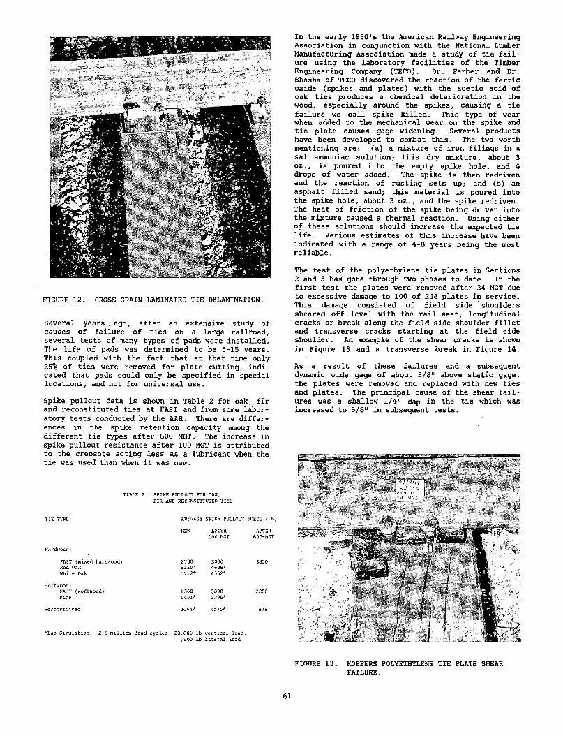
FIGURE 12. CROSS GRAIN LAMINATED TIE DELAMINATION.

Several years ago, after an extensive study of causes of failure of ties on a large railroad, several tests of many types of pads were installed. The life of pads was determined to be 5-15 years. This coupled with the fact that at that time only 25% of ties were removed for plate cutting, indi­cated that pads could only be specified in special locations, and not for universal use.

Spike pullout data is shown in Table 2 for oak, fir and reconstituted ties at FAST and from some labor­atory tests conducted by the AAR. There are differ­ences in the spike retention capacity among the different tie types after 600 MGT. The increase in spike pullout resistance after 100 MGT is attributed to the creosote acting less as a lubricant when the tie was used than when it was new.

TABLE 2. SPIKE PULLOUT FOR OAK,FIR AND RECONSTITUTED TIES.

TIE TYPE AVERAGE SPIKE PULLOUT FORCE (LB)

NEW AFTER 100 MGT

AFTER600+MGT

Hardwood:

FAST (mixed hardwood) 2760 3030 3850Red Oak 5130* 4688*White Oak 5712* 4552*

Softwood:FAST (softwood) 1300 3800 2250Pine 1481* 2296*

Reconstitued: 4094* 4575* 878

*Lab Simulation: 2.5 million load cycles, 20,000 lb vertical load,7,500 lb lateral load

In the early 1950's the American Railway Engineering Association in conjunction with the National Lumber Manufacturing Association made a study of tie fail­ure using the laboratory facilities of the Timber Engineering Company (TECO). Dr. Farber and Dr. Shasha of TECO discovered the reaction of the ferric oxide (spikes and plates) with the acetic acid of oak ties produces a chemical deterioration in the wood, especially around the spikes, causing a tie failure we call spike killed. This type of wear when added to the mechanical wear on the spike and tie plate causes gage widening. Several products have been developed to combat this. The two worth mentioning are: (a) a mixture of iron filings in a sal ammoniac solution; this dry mixture, about 3 oz., is poured into the empty spike hole, and 4 drops of water added. The spike is then redriven and the reaction of rusting sets up; and (b) an asphalt filled sand; this material is poured into the spike hole, about 3 oz., and the spike redriven. The heat of friction of the spike being driven into the mixture caused a thermal reaction. Using either of these solutions should increase the expected tie life. Various estimates of this increase have been indicated with a range of 4-8 years being the most reliable.

The test of the polyethylene tie plates in Sections 2 and 3 has gone through two phases to date. In the first test the plates were removed after 34 MGT due to excessive damage to 100 of 248 plates in service. This damage consisted of field side shoulders sheared off level with the rail seat, longitudinal cracks or break along the field side shoulder fillet and transverse cracks starting at the field side shoulder. An example of the shear cracks is shown in Figure 13 and a transverse break in Figure 14.

As a result of these failures and a subsequent dynamic wide gage of about 3/8" above static gage, the plates were removed and replaced with new ties and plates. The principal cause of the shear fail­ures was a shallow 1/4" dap in the tie which was increased to 5/8" in subsequent tests.

FIGURE 13. HOPPERS POLYETHYLENE TIE PLATE SHEAR FAILURE.

61

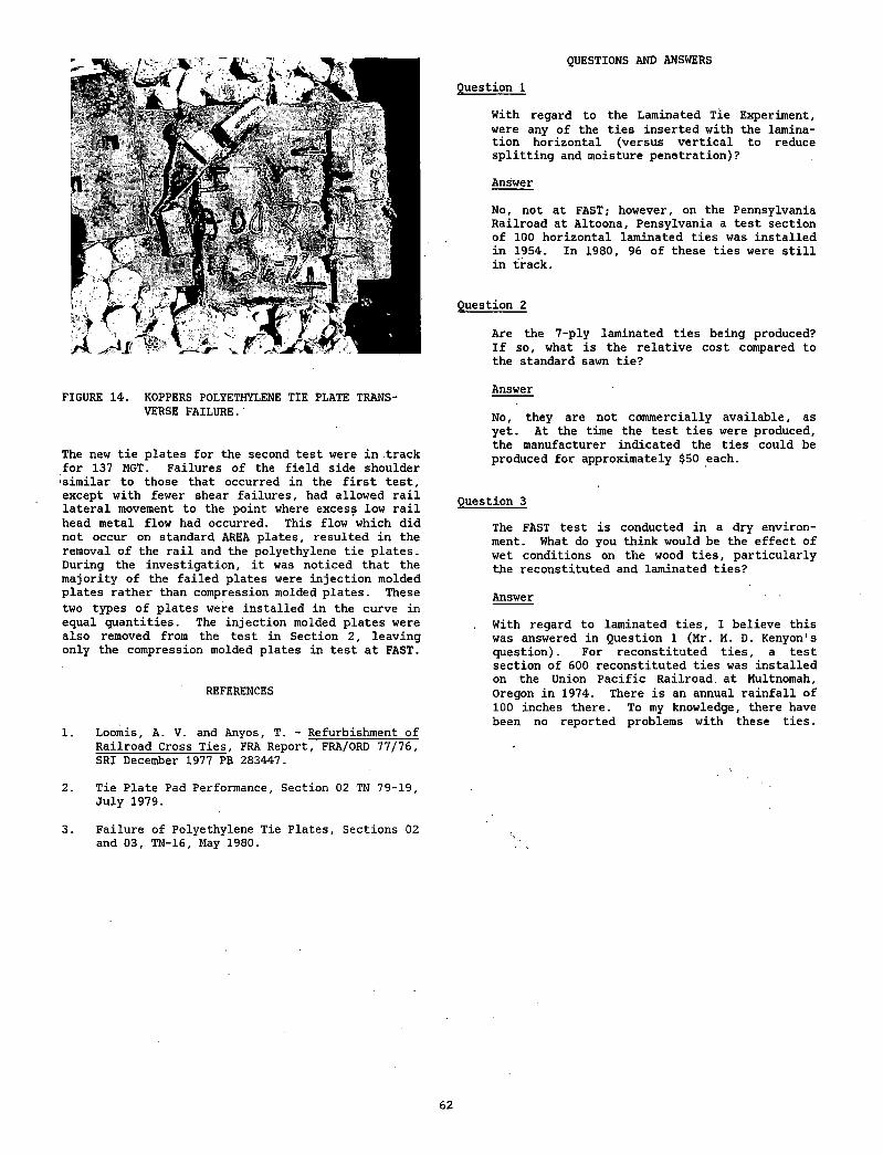
QUESTIONS AND ANSWERS

FIGURE 14. KOPPERS POLYETHYLENE TIE PLATE TRANS­VERSE FAILURE.

The new tie plates for the second test were in track for 137 MGT. Failures of the field side shoulder 'similar to those that occurred in the first test, except with fewer shear failures, had allowed rail lateral movement to the point where excess low rail head metal flow had occurred. This flow which did not occur on standard AREA plates, resulted in the removal of the rail and the polyethylene tie plates. During the investigation, it was noticed that the majority of the failed plates were injection molded plates rather than compression molded plates. These two types of plates were installed in the curve in equal quantities. The injection molded plates were also removed from the test in Section 2, leaving only the compression molded plates in test at FAST.

REFERENCES

1. Loomis, A. V. and Anyos, T. - Refurbishment of Railroad Cross Ties, FRA Report, FRA/ORD 77/76, SRI December 1977 PB 283447.

2. Tie Plate Pad Performance, Section 02 TN 79-19, July 1979. 3

3. Failure of Polyethylene Tie Plates, Sections 02 and 03, TN-16, May 1980.

Question 1

With regard to the Laminated Tie Experiment, were any of the ties inserted with the lamina­tion horizontal (versus vertical to reduce splitting and moisture penetration)?

Answer

No, not at FAST; however, on the Pennsylvania Railroad at Altoona, Pensylvania a test section of 100 horizontal laminated ties was installed in 1954. In 1980, 96 of these ties were still in track.

Question 2

Are the 7-ply laminated ties being produced? If so, what is the relative cost compared to the standard sawn tie?

Answer

No, they are not commercially available, as yet. At the time the test ties were produced, the manufacturer indicated the ties could be produced for approximately $50 each.

Question 3

The FAST test is conducted in a dry environ­ment. What do you think would be the effect of wet conditions on the wood ties, particularly the reconstituted and laminated ties?

Answer

With regard to laminated ties, I believe this was answered in Question 1 (Mr. M. D. Kenyon's question). For reconstituted ties, a test section of 600 reconstituted ties was installed on the Union Pacific Railroad, at Multnomah, Oregon in 1974. There is an annual rainfall of 100 inches there. To my knowledge, there have been no reported problems with these ties.

62

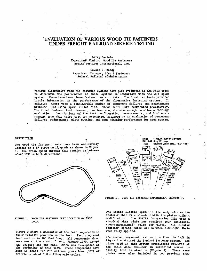
EVALUATION OF VARIOUS WOOD TIE FASTENERS UNDER FREIGHT RAILROAD SERVICE TESTING

Larry Daniels Experiment Monitor, Wood Tie Fasteners

Boeing Services International, Inc.

Howard G. MoodyExperiment Manager, Ties & Fasteners

Federal Railroad Administration

Various alternative wood tie fastener systems have been evaluated at the FAST track to determine the performance of these systems in comparison with the cut spike system. There have been three fastener tests to date. The first two tests provided little information on the performance of the alternative fastening systems. In addition, there were a considerable number of component failures and maintenance problems, including spike killed ties. These tests were terminated prematurely. The third fastener test, however, has been comprehensive enough to allow a thorough evaluation. Descriptions of the test configuration, measurements, and load envi­ronment from this third test are presented, followed by an evaluation of component'failures, maintenance, plate cutting, and

DESCRIPTION

The wood tie fastener tests have been exclusively located in a 5° curve on J.% grade as shown in Figure 1. The train speed through this section is between 40-45 MPH in both directions.

FIGURE 1. WOOD TIE FASTENER TEST LOCATION ON FAST LOOP.

Figure 2 shows a schematic of the test components in their relative position in the test. Each component test section is 100 feet long. All components shown were new at the start of test, January 1979, except the ballast and the rail, which was transposed at the beginning of this test. These components have been in track for 257 million gross tons (MGT) of traffic or about 7.8 million axle cycles.

gage widening performance for each system.

RAIL: 140 Ib lyd., fu lly heat treatedBALLAST: S la g ,15? deepTIES: Southern ye llow pine, 7 " x 9 " x 8 '6 "

FIGURE 2. WOOD TIE FASTENER EXPERIMENT, SECTION 7.

The Double Elastic Spike is the only alternative fastener that fits standard AREA tie plates without modification. The FORTAX Compression Clip uses a standard AREA plate but requires four additional (non-conventional) holes per plate. All elastic fastener spring rates are between 4500-5000 lb/in when fully applied.

The second component test section from the left in Figure 2 contained the Pandrol Fastener System. The plate used in this system ■ experienced failures at the field side shoulder in sufficient number to justify test termination (Figure 3). These same plates were also included in two previous FAST

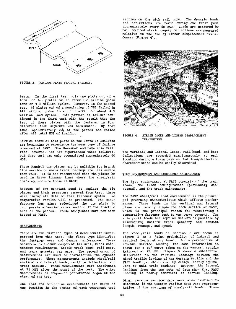
FIGURE 3. PANDROL PLATE TYPICAL FAILURE.

tests. In the first test only one plate out of a total of 496 plates failed after 135 million gross tons or 4.3 million cycles. However, in the second test, 65 plates out of a population of 752 failed in 141 million gross tons of traffic or about 4.5 million load cycles. This pattern of failure con­tinued in the third test with the result that the test of these plates with the fastener in four different test segments was terminated. By that time, approximately 75% of the plates had failed after 465 total MGT of traffic.

Service tests of this plate on the Santa Fe Railroad are beginning to, experience the same type of failure observed at FAST. The Bessemer and Lake Erie Rail­road, however, has not experienced these failures, but that test has only accumulated approximately 60 MGT.

These Pandrol tie plates may be suitable for branch line service or where track loadings are less severe than FAST. It is not recommended that the plates be used in heavy tonnage lines where the wheel/rail loads approximate those at FAST.

Because of the constant need to replace the tie plates and their premature removal from test, there were incomplete data on this fastener system. No comparative results will be presented. The manu­facturer has since redesigned the tie plate to incorporate a heavier cross section in the fracture area of the plates. These new plates have not been tested at FAST.

MEASUREMENTS

section on the high rail only. The dynamic loads and deflections are taken during one train pass approximately every 50 MGT. Loads are measured by rail mounted strain gages; deflections are measured relative to the tie by linear displacement trans­ducers (Figure 4).,

FIGURE 4. STRAIN GAGES AND LINEAR DISPLACEMENT TRANSDUCERS.

The vertical and lateral loads, rail head, and base deflections are recorded simultaneously at each location during a train pass so that load/deflection characteristics can be easily determined.

TEST ENVIRONMENT AND COMPONENT MAINTENANCE

The test environment at FAST consists of the train loads^ the track configuration (previously dis­cussed), and the track maintenance.

The FAST wheel/rail load environment is the princi­pal governing characteristic which affects perfor­mance. These loads in the vertical and lateral plane are usually unique for each section at FAST, which is the principal reason for restricting a comparative fastener test to one curve segment. The wheel/rail loads are kept as uniform as possible by maintaining uniform track geometry and consist length, tonnage, and speed.

There are two distinct types of measurements incor­porated into this test. The first type identifies the fastener wear and damage performance. These measurements include component failures, track main­tenance requirements, static track gage, rail wear, and track geometry car gage. The second group of measurements are used to characterize the dynamic performance. These measurements include wheel/rail vertical and lateral loads, rail/tie deflection, and track modulus. These measurements were instituted at 75 MGT after the start of the test. The other measurements of component performance began at the start of the test.

The load and deflection measurements are taken at one location in the center of each component test

The wheel/rail loads in Section 7 are shown in Figure 5 as a joint probability of lateral and vertical loads at any level. For a perspective of revenue service loading, the same information is shown for a 10° curve taken on the Western Pacific Railroad at 25 MPH. Figure 5 shows a substantial difference in the vertical loadings between the mixed traffic loading of the Western Pacific and the FAST loadings, which are, by design, nearly equiva­lent to unit train loadings. However, the lateral loadings from the two sets of data show that FAST loading is nearly identical to service loading.

Other revenue service data were also examined to determine if the Western Pacific data were represen­tative of the spectrum of wheel/rail loads. These

64

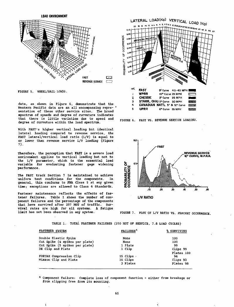
LOAD ENVIRONM ENT

FASTREVENUE SERVICE

I

FIGURE 5. WHEEL/RAIL LOADS.

data, as shown in Figure 6, demonstrate that the Western Pacific data are an all encompassing repre- -* sentation of these other service sites. The broad spectrum of speeds and degree of curvature indicates that there is little variation due to speed and degree of curvature within the load spectrum.

With FAST1s higher vertical loading but identical lateral loading compared to revenue service, the FAST lateral/vertical load ratio (L/V) is equal to or lower than revenue service L/V loading (Figure 7).

Therefore, the perception that FAST is a severe load environment applies to vertical loading but not to the L/V parameter, which is the essential load variable for evaluating fastener gage widening performance.

The FAST track Section 7 is maintained to achieve uniform test conditions for the components. In general, this conforms to FRA Class 5 at any given time; exceptions are allowed to Class 4 Standards.

Fastener maintenance reflects the effects of fas­tener failures. Table 1 shows the number of com­ponent failures and the percentage of the components that have survived after 257 MGT of traffic. Sur­vival rates are high for all systems. A fatigue limit has not been observed in any system.

ref.

Iz345

FAST 5° Curve 4 0 -4 5 MPH IWPRR 10° Curve 25 MPH ICHESSIE 3° Curve 25 MPH ISTARR, OHIO 5 °Curve 20 MPH ICANADIAN NAT'L 5° a 12° Curve I UPRR 6° Curve 35 MPH I

FIGURE 6. FAST VS. REVENUE SERVICE LOADING.

L/V RATIO

FIGURE 7. PLOT OF L/V RATIO VS. PERCENT OCCURRENCE.

TABLE 1. TOTAL FASTENER FAILURES (250 MGT OF SERVICE, 7.8 LOAD CYCLES)

FASTENER SYSTEM FAILURES* % SURVIVING

Double Elastic Spike None 100Cut Spike (4 spikes per plate) None 100Cut Spike (5 spikes per plate) 1 Plate 99DE Clip and Plate 1 Clip Clips 99

Plates 100FORTAX Compression Clip 15 Clips 94Hixson Clip and Plate 16 Clips Clips 93

3 Plates Plates 98

* Component Failure: Complete loss of component function - either from breakage orfrom slipping free from its mounting.

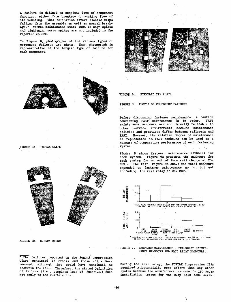
A failure is defined as complete loss of component function, either from breakage or working free of its mounting. This definition covers elastic clips falling from the assembly as well as normal break­age.* Normal maintenance items such as high spikes and tightening screw spikes are not included in the reported counts.

In Figure 8, photographs of the various types, of component failures are shown. Each photograph is representative of the largest type of failure for each component.

FIGURE. 8a. FORTAX CLIPS

FIGURE 8b. HIXSON WEDGE

FIGURE 8c. STANDARD TIE PLATE

FIGURE 8. PHOTOS OF COMPONENT FAILURES.

Before discussing fastener maintenance, a caution concerning FAST maintenance is in order. FAST maintenance manhours are not directly relatable to other service environments because maintenance policies and practices differ between railroads and FAST. However, the relative degree of maintenance as represented in FAST manhours can be used as a measure of comparative performance of.each fastening system.

Figure 9 shows fastener maintenance manhours for each system. Figure 9a presents the manhours' for each system, for an out of face rail change at 257 MGT of the' test; Figure 9b shows the total manhours expended on fastener maintenance up to, but not including, the rail relay at 257 MGT.

LlI Xoc z<S

6.0- j ----------------

3.0-

J H i r h i ia)RAIL RELAY MANHOURS SHOWN INCLUDE ONLY THE EFFORT REMOVING AND RE­APPLYING THE FASTENERS DURING A RAIL CHANGE AT 257MGT OF TEST,

<!6.On

tr o , x 3.0-

cut INTMA FORTAX CUT HIXSON, SPIKE x DOUBLE COMPRESSION SPIKE SYSTEM DE SYSTEM(5 PER PLATE) ELASTIC CLIP (4 PER PLATE)

SPIKE b)PRE-RELAY MAINTENANCE IS TOTAL FASTENER MAINTENANCE THRU 2S7 MGT, EXCLUSIVE OF INITIAL INSTALLATION AND FASTENER WORK DUE TO RAIL FAILURES.

FIGURE 9. FASTENER MAINTENANCE - PRE-RELAY MAINTE­NANCE MANHOURS AND RAIL RELAY MANHOURS.

* The failures reported on the FORTAX Compression Clips consisted of cracks and these clips were removed, although they could have continued to restrain the rail. Therefore, the stated definition of failure (i.e., complete loss of function) does not apply to the FORTAX clips.

During the rail relay, the FORTAX Compression Clip required substantially more effort than any other system because the manufacturer recommends 150 ft/lb installation torque for the clip hold down screw.

66

Si i

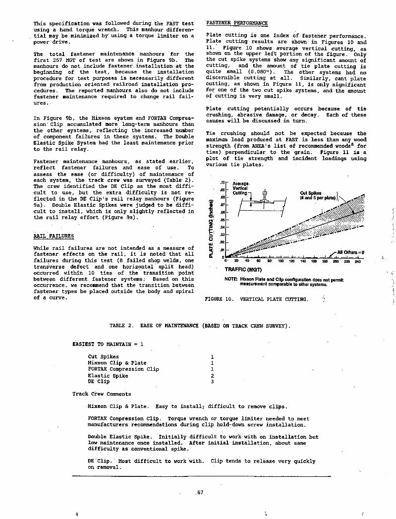
This specification was followed during the FAST test using a hand torque wrench. This manhour differen­tial may be minimized by using a torque limiter on a power drive.

The total fastener maintenance manhours for the first 257 MGT of test are shown in Figure 9b. The manhours do not include fastener installation at the beginning of the test, because the installation procedure for test purposes is necessarily different from production oriented railroad installation pro­cedures. The reported manhours also do not include fastener maintenance required to change rail fail­ures .

In Figure 9b, the Hixson system and FORTAX Compres­sion Clip accumulated more long-term manhours than the other systems, reflecting the increased number of component failures in these systems. The Double Elastic Spike System had the least maintenance prior to the rail relay.

Fastener maintenance manhours, as stated earlier, reflect fastener failures and ease of use. To assess the ease (or difficulty) of maintenance of each system, the track crew was surveyed (Table 2). The crew identified the DE Clip as the most diffi­cult to use, but the extra difficulty is not re­flected in the DE Clip's rail relay manhours (Figure 9a). Double Elastic Spikes were judged to be diffi­cult to install, which is only slightly reflected in the rail relay effort (Figure 9a).

RAIL FAILURES

While rail failures are not intended as a measure of fastener effects on the rail, it is noted that all failures during this test (8 failed shop welds, one transverse defect and one horizontal split head) occurred within 10 ties of the transition point between different fastener systems: Based on this occurrence, we recommend that the transition between fastener types be placed outside the body and spiral of a curve.

Plate cutting is one index of fastener performance. Plate cutting results are shown in Figures 10 and 11. Figure 10 shows average vertical cutting, as shown on the upper left portion of the figure. Only the cut spike systems show any significant amount of cutting, and the amount of tie plate cutting is quite small (0.080"). The other systems had no discernible cutting at all. Similarly, cant plate cutting, as shown in Figure 11, is only significant for one of the two cut spike systems, and the amount of cutting is very small.

Plate cutting . potentially occurs because of tie crushing, abrasive damage, or decay. Each of these causes will be discussed in turn.

Tie crushing should not be expected because the maximum load produced at FAST is less than any wood strength (from AREA'S list of recommended woods6 for ties) perpendicular to the grain. Figure 11 is a plot of tie strength and incident loadings using various tie plates.

FASTENER PERFORMANCE

NOTE: Hixson Plate and Clip configuration does not permit measurement comparable to other systems.

FIGURE 10. VERTICAL PLATE CUTTING.

TABLE 2. EASE OF MAINTENANCE (BASED ON TRACK CREW SURVEY).

EASIEST TO MAINTAIN = 1

Cut Spikes 1 Hixson Clip & Plate 1 FORTAX Compression Clip 1 Elastic Spike 2 DE Clip 3

Track Crew Comments

Hixson Clip & Plate. Easy to install; difficult to remove clips.

FORTAX Compression Clip. Torque wrench or torque limiter needed to meet manufacturers recommendations during clip hold-down screw installation.

Double Elastic Spike. Initially difficult to work with on installation but low maintenance once installed. After initial installation, about same difficulty as conventional spike.

DE Clip. : Most difficult to work with. Clip tends to release very quickly on removal.

,67

V vJr

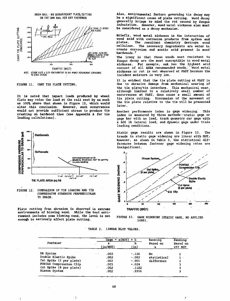
(HIGH RAIL - NO SIGNIFICANT PLATE, CUTTING ON THE LOW RAIL FOR ANY FASTENER)

TRAFFIC (MGT)NO TE: HIXSON PLATE S C L IP CONTI GURATION DO NOT PERMIT MEASUREMENT COMPARABLE

" TO OTHER SYSTEMS

FIGURE 11. CANT TIE PLATE CUTTING.

It is noted that impact loads produced by wheel flats may raise the load at the rail seat by as much as 100% above that shown in Figure 12, which would alter this conclusion. However, such occurrences would not provide sufficient stress to produce tie crushing on hardwood ties (see Appendix A for tie loading calculations).

FIGURE 12. COMPARISON OF TIE LOADING AND TIE COMPRESSIVE STRENGTH PERPENDICULAR TO GRAIN.

Plate cutting from abrasion is observed in extreme environments of blowing sand. While the test envi­ronment includes some blowing sand, the level is not enough to seriously affect plate cutting.

Also, environmental factors governing tie decay may be a significant cause of plate cutting. Wood decay generally brings to mind the rot caused by fungus infestation. However, wood metal sickness also must be considered as a.decay mechanism.

Briefly, wood metal sickness is the interaction of wood acid with corrosion products from spikes and plates. The resultant chemistry destroys wood cellulose. The necessary ingredients are water to, create corrosion and acetic acid present in most4 hardwoods.7The irony is that those woods most resistant to fungus decay are the most susceptible to wood metal sickness. For example, oak has the highest acid content of all AREA recommended woods. Wood metal sickness-or rot is not observed at FAST because the incident moisture is very low.It is evident that the tie plate cutting at FAST is due to abrasive damage from mechanical wearing of the tie plate/tie interface. This mechanical wear, although limited to a relatively small number of occurrences at FAST, does cause a small amount of tie plate cutting. Discussion of the movement of the tie plate relative to the tie will be presented later.Another performance index is gage widening. This index is measured by three methods— static gage or gage bar with no load, track geometry car gage with a 600 lb lateral load, and dynamic gage under train loading conditions.

Static gage results are shown in Figure 13. The trends in static gage widening are linear with MGT; however, as shown in Table 3, the statistical dif­ferences between fastener gage widening rates are insignificant.

FIGURE 13. GAGE WIDENING (STATIC GAGE, NO APPLIED LOAD).

TABLE 3. LINEAR PLOT VALUES.

FastenerGaqe = a

(in/MGT)

a(MGT) + b b

(in)

Ranking Based on

a

Ranking Based on 257 MGT

DE System .002 -.126 No 1Double Elastic Spike .002 -.082 statistical' 1Cut Spike (5 per plate) .002 -.001 difference 2FORTAX Compression Clip .003 -.024 3Cut Spike (4 per plate) .002 .1182 3Hixson System .002 .2356 3

68

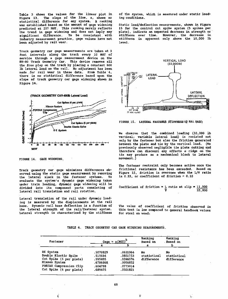
Table 3 shows the values for the linear plot in Figure 13. The slope of the line, a, shows no statistical, difference for any system, a ranking was established based on the amount of gage widening predicted at 257 MGT. This ranking merely reflects the trend in gage widening and does not imply any significant difference. To be consistent. with industry measurement practice, gage values have not been adjusted by rail wear.

Track geometry car gage measurements are taken at 1 foot intervals along the track every 10 MGT of service through a gage measurement device on the EM-80 Track Geometry Car. This device removes all the free play on the track by placing a constant 600 lb lateral load on the rail. No adjustment has been made for rail wear in these data. From Table 4, there is no statistical difference based upon the slope of track geometry car gage widening shown in Figure 14.

(TRACK GEOMETRY CAR-600lb Lateral Load)

FIGURE 14. GAGE WIDENING.

Track geometry car gage minimizes differences ob­served using the static gage measurement by removing the lateral slack in the fastener systems. To evaluate the system's dynamic gage widening taken under train loading, dynamic gage widening will be divided into its component parts consisting of lateral rail translation and rail rotation.

Lateral translation of the rail under dynamic load­ing is measured by the displacements at the rail base. Dynamic rail base deflection is a function of the lateral strength of the rail/fastener system. Lateral strength is characterized by the stiffness

of the system, which is measured under static load­ing conditions.

Static load/deflection measurements, shown in Figure 15 for the control cut spike system (5 spikes per plate), indicate ah expected decrease in strength or stiffness over time. However, the decrease in stiffness is apparent only above the 10,000 lb level.

V E R T IC A L LOAD (33,0001b)

FIGURE 15. LATERAL FASTENER STIFFNESS (@ RAIL BASE)

He observe that the combined loading (33,000 lb vertical; variable lateral load) is resisted not only by the fastener but also the friction generated between the plate and tie by the vertical load. (We previously observed negligible tie plate cutting and therefore can discount any effects a ridge on the tie may produce as a mechanical block to lateral movement.)

The fastener restraint only becomes active once the frictional resistance has been exceeded. Based on Figure 15, friction is overcome when the L/V ratio is 0.33, or coefficient of friction = 0.33

Coefficient of friction = L ratio at slip = 11,000V 33,000

The value of coefficient of friction observed in this test is low compared to general handbook values for steel on wood:

TABLE 4. TRACK GEOMETRY CAR GAGE WIDENING MEASUREMENTS.

Fastener Gaqe = a(MGT)bRanking Based on

Ranking . Based on

a b a b

DE SystemDouble Elastic Spike Cut Spike (5 per plate) Hixson System FORTAX Compression Clip Cut Spike (4 per plate)

.5070829

.515034

.595495

.6786868

.604798

.689475

.0631064

.0851753

.0246576

.0056832

.0773014

.0501821

Nostatisticaldifference

Nostatisticaldifference

69

i

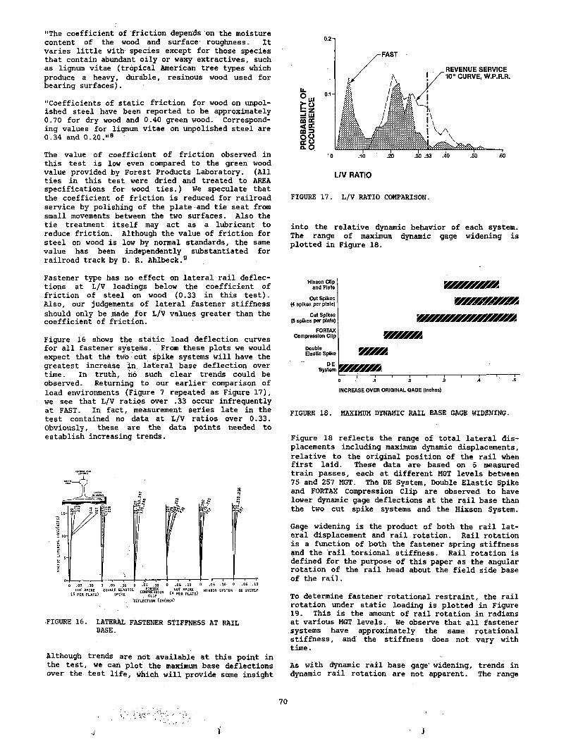
"The coefficient of friction depends on the moisture content of the wood and surface roughness. It varies little with species except for those species that contain abundant oily or waxy extractives, such as lignum vitae (tropical American tree types which produce a heavy, durable, resinous wood used for bearing surfaces).

"Coefficients of static friction for wood on unpol­ished steel have been reported to be approximately 0.70 for dry wood and 0.40 green wood. Correspond­ing values for lignum vitae on unpolished steel are 0.34 and 0.20.1,8

The value of coefficient of friction observed in this test is low even compared to the green wood value provided by Forest Products Laboratory. (All ties in this test were dried and treated to AREA specifications for wood ties.) We speculate that the coefficient of friction is reduced for railroad service by polishing of the plate and tie seat from small movements between the two surfaces. Also the tie treatment itself may act as a lubricant to reduce friction. Although the value of friction for steel on wood is low by normal standards, the same value has been independently substantiated for railroad track by D. R. Ahlbeck.9

Fastener type has no effect on lateral rail deflec­tions at L/V loadings below the coefficient of friction of steel on wood (0.33 in this test). Also, our judgements of lateral fastener stiffness should only be made fbr L/V values greater than the coefficient of friction.

Figure 16 shows the static load deflection curves for all fastener systems. From these plots we would expect that the two cut spike systems Will have the greatest increase in lateral base deflection over time. In truth, ho such clear trends could be observed. Returning to our earlier comparison of load environments (Figure 7 repeated as Figure 17), we see that L/V ratios over .33 occur infrequently at FAST. In fact, measurement series late in the test contained no data at L/V ratios over 0.33. Obviously, these are the data points needed to establish increasing trends.

•FIGURE 16. LATERAL FASTENER STIFFNESS AT RAIL BASE.

Although trends are not available at this point in the test, we can plot the maximum base deflections over the test life, which will provide some insight

L/V RATIO

FIGURE 17. L/V RATIO COMPARISON.

into the relative dynamic behavior of each system. The range of maximum dynamic gage widening is plotted in Figure 18.

FIGURE 18. MAXIMUM DYNAMIC RAIL BASE GAGE WIDENING.

Figure 18 reflects the range of total lateral dis­placements including maximum dynamic displacements, relative to the original position of the rail when first laid. These data are based on 5 measured train passes, each at different MGT levels between 75 and 257 MGT. The DE System, Double Elastic Spike and FORTAX Compression Clip are observed to have lower dynamic gage deflections at the rail base than the two cut spike systems and the Hixson System.

Gage widening is the product of both the rail lat­eral displacement and rail rotation. Rail rotation is a function of both the fastener spring stiffness and the rail torsional stiffness. Rail rotation is defined for the purpose of this paper as the angular rotation of the rail head about the field side base of the rail.

To determine fastener rotational restraint, the rail rotation under static loading is plotted in Figure 19. This is the amount of rail rotation in radians at various MGT levels. We observe that all fastener systems have approximately the same rotational stiffness, and the stiffness does not vary with time.

As with dynamic rail base gage' widening, trends in dynamic rail rotation are not apparent. The range

70

J l )

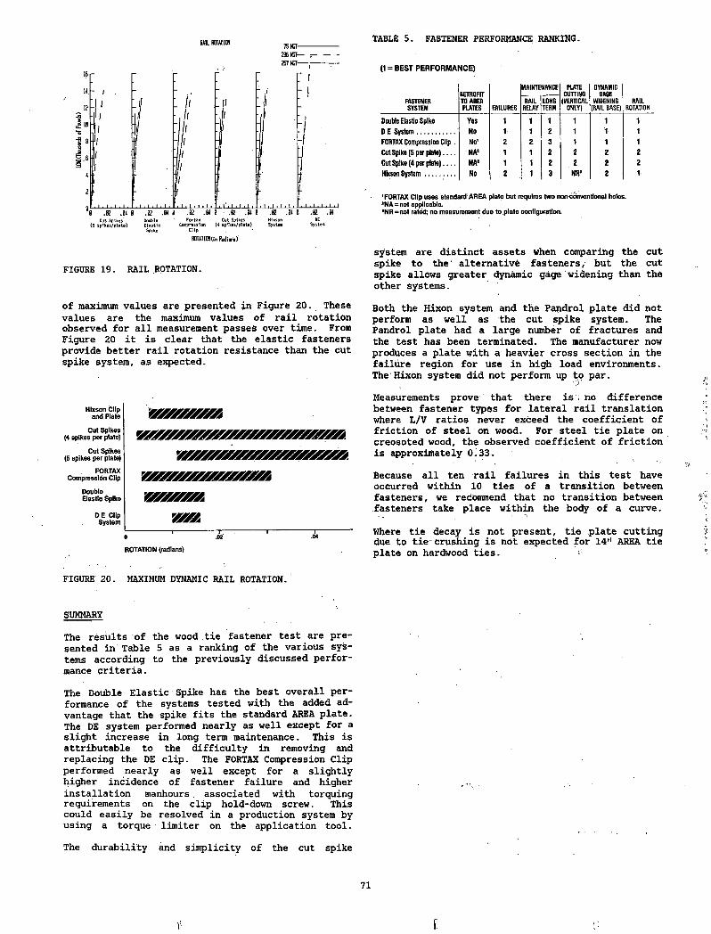
TABLE 5. FASTENER PERFORMANCE RANKING.RAIL ROTATION236 ROT— r - ' — -

FIGURE 19. RAIL ROTATION.

of maximum values are presented in Figure 20. These values are the maximum values of rail rotation observed for all measurement passes over time. From Figure 20 it is clear that the elastic fasteners provide better rail rotation resistance than the cut spike system, as expected.

(1 = BEST PERFORMANCE)

FASTENERSYSTEM

RETROFIT TO AREA PLATES FAILURES

MAINTENANCE PLATECUTTING(VERTICAL

ONLY)

DYNAMIC GAGE

WIDENING (RAIL RASE)

RAILROTATION

RAILRELAY

LONGTERM

Double Elastic Spike Yes 1 1 1 1 1 1D E System................. No 1 1 2 1 1 1FORTAX Compression Clip . No1 2 2 3 1 1 1Cut Spike (5 per plate)__ NA' 1 1 2 2 2 2Cut Spike (4 per plate)...... NA' 1 2 2 2 2Hixson System.............. No 2 3 NR' 2 1

' FORTAX Clip uses standard AREA plate but requires two non-conventional holes. fNA= not applicable. .’NR= not rated; no measurement due to plate configuration.

system are distinct assets when comparing the cut spike to the alternative fasteners, but the cut spike allows greater dynamic gage widening than the other systems.

Both the Hixon system and the Pandrol plate did not perform as well as the cut spike system. The Pandrol plate had a large number of fractures and the test has been terminated. The manufacturer now produces a plate with a heavier cross section in the failure region for use in high load environments. The Hixon system did not perform up to par.

Hixson Clip and Plate

Cut Spikes (4 spikes per plate)

Cut Spikes (5 spikes per plate)

FORTAX Compression Clip

Double Elastic Spike

DE Clip System

Y/rsssssssssjrj/mmwyssssssss/ysssssssarsssssss*

YSSA--------------------------1-----------------------r — :------------------1----------------------------1-------------------0 .02 .04

ROTATION (radians)

Measurements prove that there is ; no difference between fastener types for lateral rail translation where L/V ratios never exceed the coefficient of friction of steel on wood. For steel tie plate on creosoted wood, the observed coefficient of friction is approximately 0.33.

Because all ten rail failures in this test have occurred within 10 ties of a transition between fasteners, we recommend that no transition between fasteners take place within the body of a curve.

Where tie decay is not present, tie plate cutting due to tie-crushing is not expected for 14" AREA tie plate on hardwood ties.

FIGURE 20. MAXIMUM DYNAMIC RAIL ROTATION.

SUMMARY

The results of the wood tie fastener test are pre­sented in Table 5 as a ranking of the various sys­tems according to the previously discussed perfor­mance criteria.

The Double Elastic•Spike has the best overall per­formance of the systems tested with the added ad­vantage that the spike fits the standard AREA plate. The DE system performed nearly as well except for a slight increase in long term maintenance. This is attributable to the difficulty in removing and replacing the DE clip. The FORTAX Compression Clip performed nearly as well except for a slightly higher incidence of fastener failure and higher installation manhours . associated with torquing requirements on the clip hold-down screw. This could easily be resolved in a production system by using a torque ■ limiter on the application tool.

The durability and simplicity of the cut spike

71

V

REFERENCES QUESTIONS AND ANSWERS

1 Unpublished data, Courtesy of the Western Pacific R.R., C. A. Gerstner, Engineer - Con­struction.

2 Unpublished data, courtesy of Battelle - Columbus Laboratories.

3 Ahlbeck, D . R. and Battelle - Columbus Labora­tories - Summary Report, Vehicle/Track Inter­action Tests - Wayside Test Data Summary,July 27, 1981.

4 Telephone Conversation, J. R. Lundgren, AAR, and N. Caldwell, Canadian National R.R.

5 Ahlbeck, D. R., Harrison, H. D., Tuten, J. M., and Johnson, Dr. M. R. - Measurements of Wheel/ Rail Loads on Class 5 Track, Interim Report under contract to DOT/FRA, June 1979.

6 ' Handbook of Recommended Practice, AREA, Ch.3.1.1, Specification for Wood Ties.

7 Degradation of Wood By Products of Metal Corro­sion, Forest Service Research Paper FPL 229,U.S. Department of Agriculture, Forest Products Laboratory, Madison, Wisconsin.

8 Wood Handbook: Wood as an Engineering Material,Agriculture Handbook #12, U.S. Department of Agriculture, Forest Products Laboratory,Madison, Wisconsin.

9 Ahlbeck, D. R. and Battelle - Columus Labora­tories - "The Effects of Track Modulus on Vehi­cle-Track Dynamic Interaction," to be published, ASME/IEEE Joint Railroad Conference, April/ 1982.

10 Timoshenko & Langer - "Stresses in Track," APM- ASME, Applies Mechanics, 1929.

Question 1

Would the use of the INTMA (Double Elastic Fastener) inhibit rail changing operation?

Answer

Not appreciably. The track crew was surveyedto assess the difficulty of use of each fas­tener system. The results of that survey are stated in the body of the proceeding paper. The Double Elastic Fastener is said to be roughly equivalent to the standard cut spike in terms of ease of use. However, this spike is difficult to install on first application.

Question 2

Is it reasonable to attempt to draw conclusions (Static or Dynamic) based on geometry devia­tions limited to approximately \ those allow­able by current FRA Safety Standards and rail­road practices?

Answer

FRA Safety Standards and railroad operating limits are not appropriate judgement criteria for performance testing. Such safety limits do not reflect the relationship between MGT, applied load, fastener strength and resulting wear or deterioration.

The trends in deterioration with the appropri­ate engineering information provides a basis for engineering and economic judgement of performance, irrespective of the safety limits chosen by a railroad.

72

i !

Ap p endix aTie Pressure Under Rail Seat

Train loading at the tie surface is a function of the applied wheel load, the beam strength of the rail, and the structural integrity of the, track.

The estimated loading at the rail seat for a static loading condition is given by Timoshenko & Langer10:

Load delivered to individual tie plate: load = §a P

where p = f k

K = Track Modulus lb/in/in E = Young's Modulus for steel =

= 30 x 106 psiI = Moment of inertia of rail

= 96.8 in4 (140 lb rail) a = tie spacing = 19.5 in P = applied wheel load.

The relationship offered by Timoshenko is based on the beam-on-elastic-foundation theory which, in this form, is solved only for static loading cases.

However, field measurements (unpublished) by Battelle Institute, under dynamic conditions, indi­cate that this relationship provides a very reason­able estimate of the load supported by an individual tie.

The maximum FAST load is approximately 55,000 lb. The Track Modulus is measured in this experiment and

averages 1,680 lb/in/in.

No plate bending is included in this estimate. That is, the tie plate load is assumed to be distributed across the full tie plate area (width x length) to the tie.

As a matter for discussion for those interested, the maximum loading at the tie surface should also consider the effects of impact loading, such as that caused by wheel flats or rail joints. The FAST consist contains no significant wheel flats and thus impacts are not pertinent to discussion of why no plate cutting occurs at FAST. However, such impacts do occur in revenue service.

Field measurements of impact loads in revenue ser­vice shows that loads at the tie seat are 2 to 5 times greater than the nominal (i.e., static) wheel load.

Theory consideration of structures such as track suggest that a higher rate of loading abbreviates the shape of the wave made by the loaded rail. This decreases the number of ties supporting the load, increasing the load on each tie.

While no field measurements have been made to vali­date theory, it is intuitively realistic to expect that minimizing the occurrence of wheel flats and rail joints (or battered welds) will also minimize damage to other elements of the track such as the ties.

73

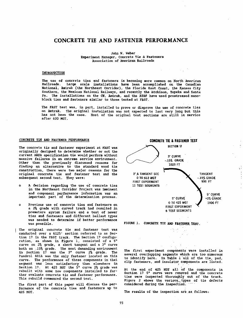
CONCRETE TIE AND FASTENER PERFORMANCE

John W. WeberExperiment Manager, Concrete Tie & Fasteners

Association of American Railroads

INTRODUCTION

The use of concrete ties and fasteners is becoming more common on North American Railroads. Large scale installations have been accomplished on the Canadian National, Amtrak (the Northeast Corridor), the Florida East.Coast, the Kansas City Southern, the Mexican National Railways, and recently the Atchison, Topeka and Santa Fe. The installations on the CN, Amtrak, and the ATSF have used prestressed mono­block ties and fasteners similar to those tested at FAST.

The FAST test was, in part, installed to prove or disprove the use of concrete ties on Amtrak. The original installation was not expected to last very long but this has not been the case. Most of the original test sections are still in service after 600 MGT.

CONCRETE TIE AND FASTENER PERFORMANCE CONCRETE TIE & FASTENER TESTThe concrete tie and fastener experiment at FAST was originally designed to determine whether or not the current AREA specification tie would perform without massive failures in an extreme service environment. Other than the previously discussed reasons for finding an alternative to the standard wood tie construction, there were two major reasons for the original concrete tie and fastener test and the subsequent second test. They were:

o A decision regarding the use of concrete ties in the Northeast Corridor Project was imminent and component performance information was an important part of the determination process.

o Previous use of concrete ties and fasteners on a 2% grade with curved track had resulted in premature system failure and a test of newer ties and fasteners and different ballast types was needed to determine if better performance was possible.

The original concrete tie and fastener test was. conducted over a 6125' section referred to as Sec­tion 17 in the FAST track. The Section 17 configu­ration, as shown in Figure 1, consisted of a 5° curve on 2% grade, a short tangent and a 3° curve both on .15% grade. The most demanding environment in Section 17 was the 5° curve 2% grade. The Pandrol 601A was the only fastener located on this curve. The performance of these components in that segment was less satisfactory than elsewhere in Section 17. At 425 MGT the 5° curve 2% grade was rebuilt with some new components installed to fur­ther evaluate concrete tie and fastener performance. This rebuild commenced the second test.The first part of this paper will discuss the per­formance of the concrete ties and fasteners up to 425 MGT.

3° & TANGENT SEC 0 TO 612 MGT

FIRST EXPERIMENT 11 TEST SEGMENTS

SECTION 17

3° CURVE .15% GRADE

3325 FT

TANGENT 15% GRADE

900 FT

5° CURVE

0 TO 425 MGT FIRST EXPERIMENT 6 TES T SEGMENTS

FIGURE 1. CONCRETE TIE AND FASTENER, TEST.

The first experiment components were installed in several overlapping segments which are too numerous to identify here. In Table 1 all of the tie, pad, clip fasteners, and insulator components are listed.VAt the end of 425 MGT all of the components in Section 17 5° curve were removed and the concrete ties were inspected thoroughly out of the track. Figure 2 shows the variou^. types of tie defects considered during the inspection.

The results of the inspection are as follows:

75

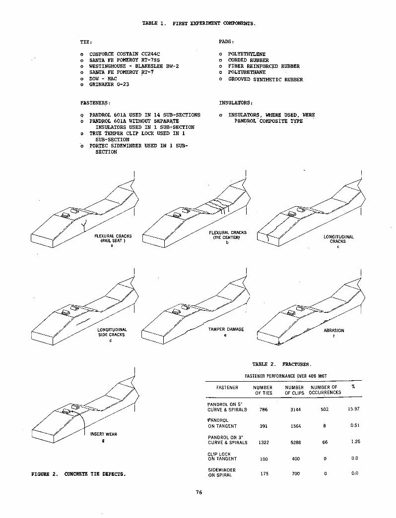
TABLE 1. FIRST EXPERIMENT COMPONENTS.

TIE: PADS:

0 CONFORCE COSTAIN CC244C o POLYETHYLENEo SANTA FE POMEROY RT-7SS o CORDED RUBBER0 WESTINGHOUSE - BLAKESLEE BW-2 o FIBER REINFORCED RUBBER0 SANTA FE POMEROY RT-7 o POLYURETHANE0 DOW - MAC 0 GROOVED SYNTHETIC RUBBER0 GRINAKER G-23

FASTENERS: INSULATORS:

o PANDROL 601A USED IN 14 SUB-SECTIONS o INSULATORS, WHERE USED, WEREo PANDROL 601A WITHOUT SEPARATE PWIDROL COMPOSITE TYPE

INSULATORS USED IN 1 SUB-SECTION o TRUE TEMPER CLIP LOCK USED IN 1

SUB-SECTIONO PORTEC SIDEWINDER USED IN 1 SUB­

SECTION

FIGURE 2. CONCRETE TIE DEFECTS.

TABLE 2. FRACTURES.

FASTENER PERFORMANCE OVER 400 MGT

FASTENER NUMBER OF TIES

NUMBER OF CLIPS

NUMBER OF OCCURRENCES

%

PANDROL ON 5" CURVE & SPIRALS 786 3144 502 15.97

'PANDROL ON TANGENT 391 1564 8 0.51

PANDROL ON 3' CURVE & SPIRALS 1322 5288 66 1.25

CLIP LOCK ON TANGENT 100 400 0 0.0

SIDEWINDER ON SPIRAL 175 700 0 0.0

76

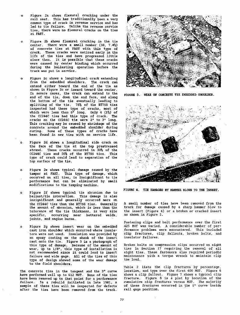
o Figure 2a shows flexural cracking under the rail seat. This has traditionally been a very common type of crack in revenue service and has led to tie failure. Unlike the revenue service ties, there were no flexural cracks on the ties at FAST.

o Figure 2b shows flexural cracking in the tie center. There were a small number (38, 7.4%) of concrete ties at FAST with this type of crack. These cracks were noticed early in the life of the ties and have progressed little since then. It is possible that these cracks were caused by center binding which occurred during the ballasting operation before the track was put in service.

o Figure 2c shows a longitudinal crack extending from the embedded shoulders. The crack can extend either toward the end of the tie as shown in Figure 2c or inward toward the center. In severe cases, the crack can extend to the end of the tie, down the end face, and along the bottom of the tie eventually leading to splitting of the tie. 78% of the RT7SS ties inspected had these type of cracks, most of which were less than 6" long. Only 4 (1%) of the CC244C ties had this type of crack. The cracks on the CC244C tie were 2" to 3" long. This cracking may be caused by shrinkage of the concrete around the embedded shoulder during curing. Some of these types of cracks have been found in new ties with no service life.

o Figure 2d shows a longitudinal side crack on the face of the tie at the top prestressed strand. These cracks occurred in 30% of the CC244C ties and 50% of the RT7SS ties. This type of crack could lead to separation of the top surface of the tie.

o Figure 2e shows typical damage caused by the tamper at FAST. This type of damage, which occurred on all ties, is insignificant to tie performance but can be eliminated by small modifications to the tamping machine.

o Figure 2f shows typical tie abrasion due toballast/tie interaction. This damage is also insignificant and generally occurred more on the CC244C ties than the RT7SS ties. Generally the amount of abrasion, which is less than the tolerance of the tie thickness, is very site specific, occurring near battered welds, joints, and engine burns.

o Figure 2g shows insert wear on the embeddedcast iron shoulder which occurred where insula­tors were not used. Insulation was provided by an epoxy coating on the shank of the insert cast onto the tie. Figure 3 is a photograph of this type of damage. Because of the amount of wear, up to 1/8", this type of installation is not recommended since it could lead to insert failure and wide gage. All of the ties of this type of design showed some of the wear damage to the field shoulders.

The concrete ties in the tangent and the 3° curve have performed well up to 612 MGT. None of the ties have been removed up to that point for a performance failure. In a rebuild initiated in late 1981, a sample of these ties will be inspected for defects after the ties have been removed from the track.

FIGURE 3. HEAR ON CONCRETE TIE EMBEDDED SHOULDER.

FIGURE 4. TIE DAMAGED BY HAMMER BLOWS TO THE INSERT.

A small number of ties have been removed from the track for damage caused by a sharp hammer blow to the insert (Figure 4) or a broken or cracked insert as shown in Figure 5.

Fastening clips and bolt performance over the first 425 MGT was varied. A considerable number of per­formance problems were encountered. This included clip fractures, clip fallouts, broken bolts, and insulator failures.

Broken bolts on compression clips occurred on eight ties in Section 17 requiring the removal of all eight ties. These fasteners also required periodic maintenance with a torque wrench to maintain clip toe load.

Table 2 lists the clip fractures by percentage, location, and type over the first 400 MGT. Figure 6 shows a clip fallout. Figure 7 shows a typical clip fracture. Figure 8 is a plot by location of the cumulative clip fractures versus MGT. The majority of these fractures occurred in the 5° curve inside rail gage position.

77

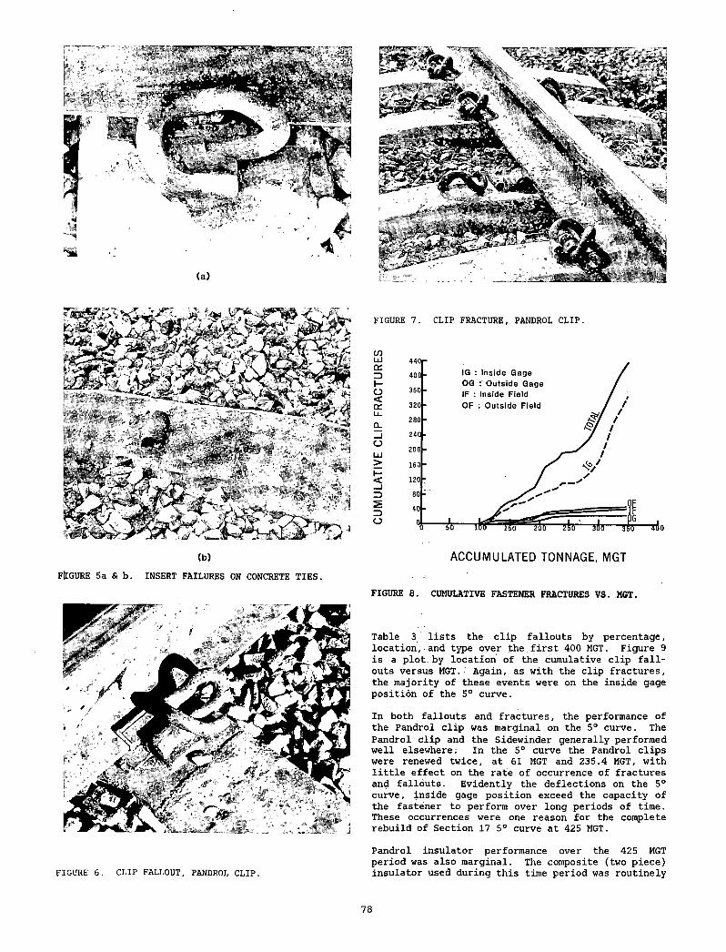
(a)

(b)

FIGURE 5a & b. INSERT FAILURES ON CONCRETE TIES.A C C U M U L A T E D T O N N A G E , M G T

FIGURE 8. CUMULATIVE FASTENER FRACTURES VS. MGT.

Table 3 lists the clip fallouts by percentage, location, and type over the first 400 MGT. Figure 9 is a plot, by location of the cumulative clip fall­outs versus MGT.' Again, as with the clip fractures, the majority of these events were on the inside gage position of the 5° curve.

In both fallouts and fractures, the performance of the Pandrol clip was marginal on the 5° curve. The Pandrol clip and the Sidewinder generally performed well elsewhere: In the 5° curve the Pandrol clips were renewed twice, at 61 MGT and 235.4 MGT, with little effect on the rate of occurrence of fractures and fallouts. Evidently the deflections on the 5° curve, inside gage position exceed the capacity of the fastener to perform over long periods of time. These occurrences were one reason for the complete rebuild of Section 17 5° curve at 425 MGT.

FIGURE 6. CLIP FALLOUT, PANDROL CLIP.

Pandrol insulator performance over the 425 MGT period was also marginal. The composite (two piece) insulator used during this time period was routinely

78

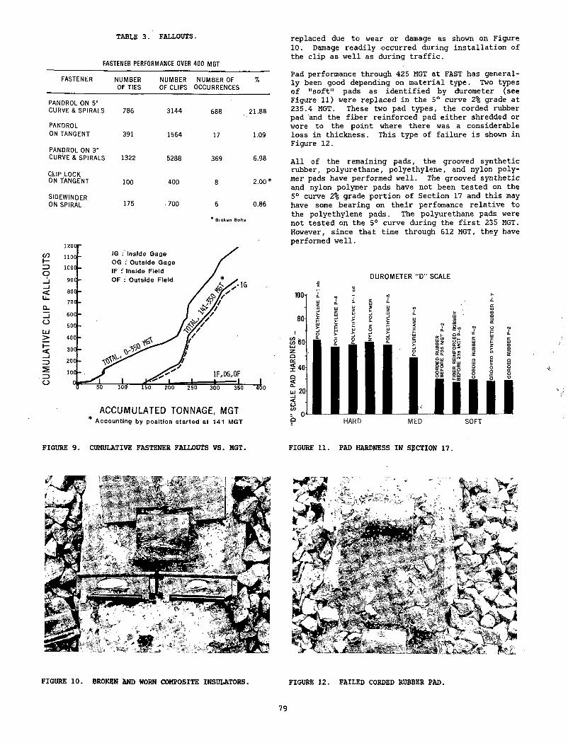
TABLE 3. FALLOUTS.

FASTENER PERFORMANCE OVER 400 MGT

FASTENER NUMBER OF TIES

NUMBER OF CLIPS

NUMBER OF OCCURRENCES

%

PANDROL ON 5° CURVE & SPIRALS 786 3144 688 21.88

PANDROL ON TANGENT 391 1564 17 1.09

PANDROL ON 3° CURVE & SPIRALS 1322 5288 369 6.98

CLIP LOCK ON TANGENT 100 400 8 2.00

SIDEWINDER ON SPIRAL 175 700 6 0.86

* Broken Bolts

A C C U M U L A T E D T O N N A G E , M G T* Accounting by position started at 141 MGT

FIGURE 9. CUMULATIVE FASTENER FALLOUTS VS. MGT.

FIGURE 10. BROKEN AND WORN COMPOSITE INSULATORS.

replaced due to wear or damage as shown on Figure 10. Damage readily occurred during installation of the clip as well as during traffic.

Pad performance through 425 MGT at FAST has general­ly been good depending on material type. Two types of "soft" pads as identified by durometer (see Figure 11) were replaced in the 5° curve 2% grade at 235.4 MGT. These two pad types, the corded rubber pad and the fiber reinforced pad either shredded or wore to the point where there was a considerable loss in thickness. This type of failure is shown in Figure 12.

All of the remaining pads, the grooved synthetic rubber, polyurethane, polyethylene, and nylon poly­mer pads have performed well. The grooved synthetic and nylon polymer pads have not been tested on the 5° curve 2% grade portion of Section 17 and this may have some bearing on their perfomance relative to the polyethylene pads. The polyurethane pads were not tested on the 5° curve during the first 235 MGT. However, since that time through 612 MGT, they have performed well.

DUROM ETER “ D” SCALE

HARD MED SOFT

FIGURE 11. PAD HARDNESS IN SECTION 17.

FIGURE 12. FAILED CORDED RUBBER PAD.

79

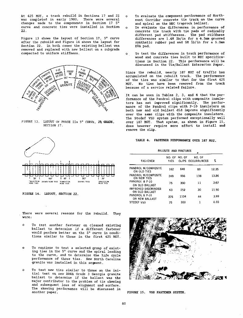
At 425 MGT, a track rebuild in Sections 17 and 22 was completed in early 1980. There were several changes made to the components in Section 17 5° curve and concrete ties were installed in Section 22.

Figure 13 shows the layout of Section 17, 5° curve after the rebuild and Figure 14 shows the layout for Section 22. In both cases the existing ballast was removed and replaced with new ballast on a subgrade compacted to uniform stiffness.

FIGURE 13. LAYOUT OF PHASE H a 5° CURVE, 2% GRADE, SECTION 17.

o To evaluate the component performance of North­east Corridor concrete tie track on the curve and spiral on the NEC traprock ballast,

o To evaluate the differences in performance of concrete tie track with tie pads of radically different pad stiffnesses. The pad stiffness differences are 1.4M lb/in for a 4.5mm grooved synthetic rubber pad and 5M lb/in for a 5.0mm EVA pad.

o To test the differences in track performance of wood and concrete ties built to NEC specifica­tions in Section 22. This performance will be discussed in the Tie/Ballast Interacton Paper.

Since the rebuild, nearly 187 MGT of traffic has accumulated on the rebuilt track. The performance of the ties was similar to that for the first 425 MGT. No ties have been removed from the track because of a service related failure.

It can be seen in Tables 2, 3, and 4 that the per­formance of the Pandrol clips with composite insula­tors has not improved significantly. The perfor­mance of the Pandrol clips with P-10 insulators on both new and old ballast did improve significantly over the same clips with the composite insulators. The Stedef VSD system performed exceptionally well over 187 MGT. That system, as shown in Figure 15, does however require more effort to install and remove the clip.

FIGURE 14. LAYOUT, SECTION 22.

TABLE 4. FASTENER PERFORMANCE OVER 187 MGT.

FALLOUTS AND FRACTURES

FASTENERNO. OF

TIESNO. OF CLIPS

NO. OFOCCURRENCES %

PANDROL W/COMPOSITE ON OLD TIES

162 648 80 12.35

PANDROL W/COMPOSITE ON NEW TIES

249 996 138 13.86

PANDROL & P-10 ON OLD BALLAST

75 300 11 3.67

IMPROVED SIDEWINDER ON OLD BALLAST

63 252 30 11.90

PANDROL & P-10 ON NEW BALLAST

276 1104 44 3.99

STEDEF VSD 75 300 1 0.33

There were several reasons for the rebuild. They were:

o To test another fastener on cleaned existing ballast to determine if a different fastener would perform better on the 5° curve in condi­tions similar to those in the first 425 MGT.

o To continue to test a selected group of exist­ing ties in the 5° curve and the spiral leading to the curve, and to determine the life cycle performance of those ties. New North Carolina granite was installed in this segment.

o To test new ties similar to those on the ini­tial test on new AREA Grade 3 Georgia granite ballast to determine if the ballast was the major contributor to the problem of tie skewing and subsequent loss of alignment and surface. The skewing performance will be discussed in another paper. FIGURE 15. VSD FASTENER SYSTEM.

80

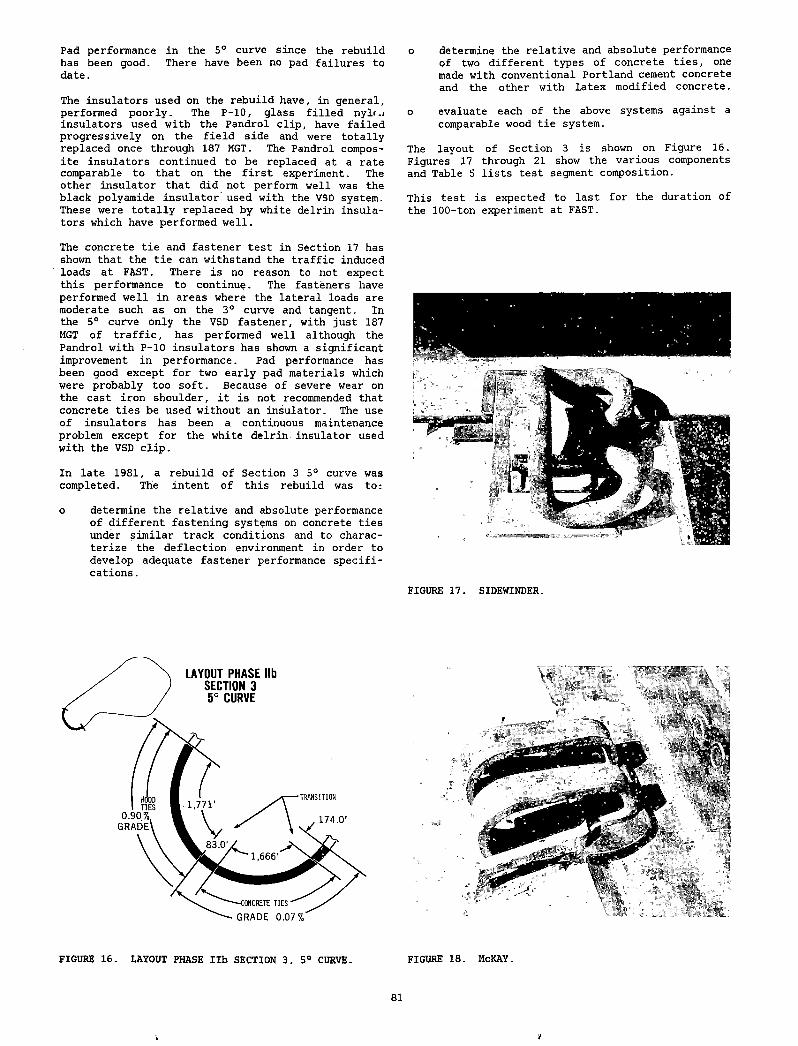
Pad performance in the 5° curve since the rebuild has been good. There have been no pad failures to date.

The insulators used on the rebuild have, in general, performed poorly. The P-10, glass filled nyl',i insulators used with the Pandrol clip, have failed progressively on the field side and were totally replaced once through 187 MGT. The Pandrol compos­ite insulators continued to be replaced at a rate comparable to that on the first experiment. The other insulator that did not perform well was the black polyamide insulator used with the VSD system. These were totally replaced by white delrin insula­tors which have performed well.

The concrete tie and fastener test in Section 17 has shown that the tie can withstand the traffic induced loads at FAST. There is no reason to not expect this performance to continue. The fasteners have performed well in areas where the lateral loads are moderate such as on the 3° curve and tangent. In the 5° curve only the VSD fastener, with just 187 MGT of traffic, has performed well although the Pandrol with P-10 insulators has shown a significant improvement in performance. Pad performance has been good except for two early pad materials which were probably too soft. Because of severe wear on the cast iron shoulder, it is not recommended that concrete ties be used without an insulator. The use of insulators has been a continuous maintenance problem except for the white delrin insulator used with the VSD clip.

In late 1981, a rebuild of Section 3 5° curve was completed. The intent of this rebuild was to:

o determine the relative and absolute performance of different fastening systems on concrete ties under similar track conditions and to charac­terize the deflection environment in order to develop adequate fastener performance specifi­cations .

FIGURE 16. LAYOUT PHASE l ib SECTION 3, 5° CURVE.

o determine the relative and absolute performance of two different types of concrete ties, one made with conventional Portland cement concrete and the other with latex modified concrete.

o evaluate each of the above systems against a comparable wood tie system.

The layout of Section 3 is shown on Figure 16. Figures 17 through 21 show the various components and Table 5 lists test segment composition.

This test is expected to last for the duration of the 100-ton experiment at FAST.

FIGURE, 17. SIDEWINDER.

FIGURE 18. McKAY.

81

i

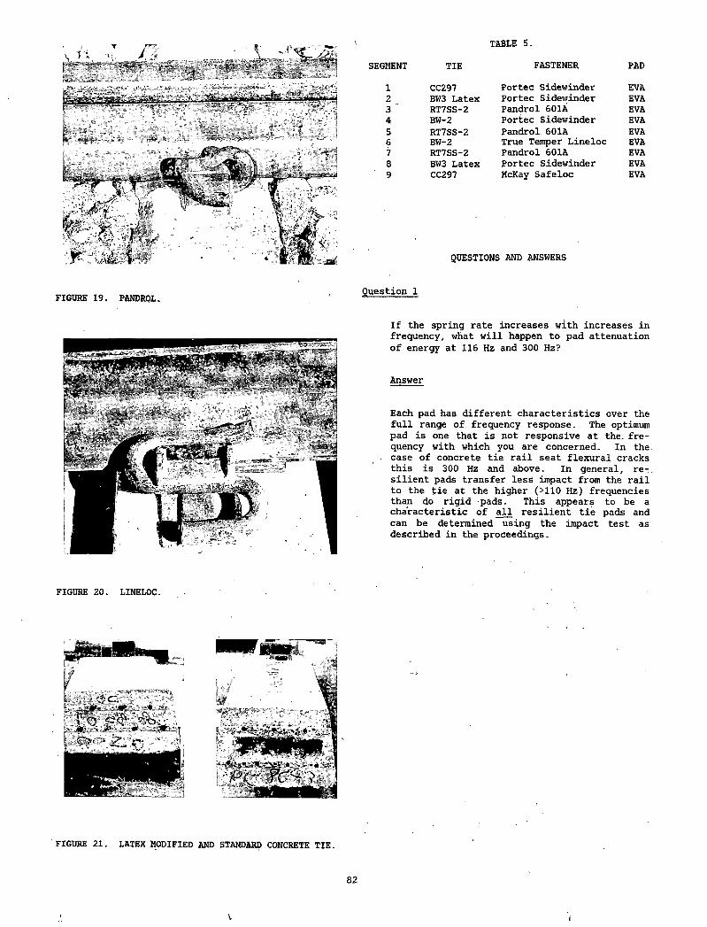
/TABLE 5.

SEGMENT TIE FASTENER PAD

1 CC297 Portec Sidewinder EVA2 BW3 Latex Portec Sidewinder EVA3 ' RT7SS-2 Pandrol 601A EVA4 BW-2 Portec Sidewinder EVA5 RT7SS-2 Pandrol. 601A EVA6 BW-2 True Temper Lineloc EVA7 RT7SS-2 Pandrol 601A EVA8 BW3 Latex Portec Sidewinder EVA9 CC297 McKay Safeloc EVA

QUESTIONS AND ANSWERS

FIGURE 19. PANDROL. Question 1

FIGURE 20. LINELOC.

If the spring rate increases with increases in frequency, what will happen to pad attenuation of energy at 116 Hz and 300 Hz?

Answer

Each pad has different characteristics over the full range of frequency response. The optimum pad is one that is not responsive at the. fre­quency with which you are concerned. In the: case of concrete tie rail seat flexural cracks this is 300 Hz and above. In general, re­silient pads transfer less impact from the rail to the tie at the higher (>110 Hz) frequencies than do rigid -pads. This appears to be a characteristic of all resilient tie pads and can be determined using the impact test as described in the proceedings.

FIGURE 21. LATEX MODIFIED AND STANDARD CONCRETE TIE.

82

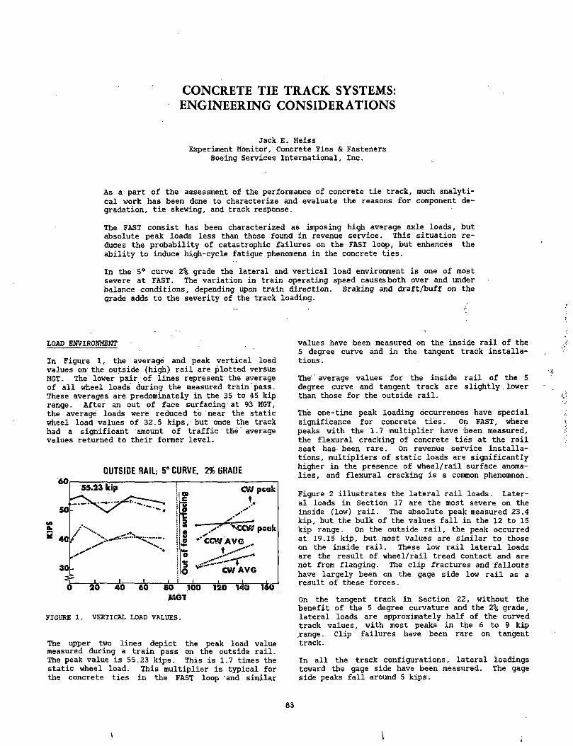
CONCRETE TIE TRACK SYSTEMS: ENGINEERING CONSIDERATIONS

Jack E. HeissExperiment Monitor, Concrete Ties & Fasteners

Boeing Services International, Inc.

As a part of the assessment of the performance of concrete tie track, much analyti­cal work has been done to characterize and evaluate the reasons for component de­gradation, tie skewing, and track response.

The FAST consist has been characterized as imposing high average axle loads, but absolute peak loads less than those found in revenue service. This situation re­duces the probability of catastrophic failures on the FAST loop, but enhances the ability to induce high-cycle fatigue phenomena in the concrete ties.

In the 5° curve 2% grade the lateral and vertical load environment is one of most severe at FAST. The variation in train operating speed causes both over and under balance conditions, depending upon train direction. Braking and draft/buff on the grade adds to the severity of the track loading.

LOAD ENVIRONMENT

In Figure 1, the average and peak vertical load values on the outside (high) rail are plotted versus MGT. The lower pair of lines represent the average of all wheel loads during the measured train pass. These averages are predominately in the 35 to 45 kip range. After an out of face surfacing'at 93 MGT, the average loads were reduced to near the static wheel load values of 32.5 kips, but once the track had a significant amount of traffic the average values returned to their former level.

i»GT

FIGURE 1. VERTICAL LOAD VALUES.

The upper two lines depict the peak load value measured during a train pass on the outside rail. The peak value is 55.23 kips. This is 1.7 times the static wheel load. This multiplier is typical for the concrete ties in the FAST loop and similar

values have been measured on the inside rail of the 5 degree curve and in the tangent track installa­tions .

The'' average values for the inside rail of the 5 degree curve and tangent track are slightly, lower than those for the outside rail.

The one-time peak loading occurrences have special significance for concrete ties. On FAST, where peaks with the 1.7 multiplier have been measured, the flexural cracking of concrete ties at the rail seat has- been rare. On revenue service installa­tions, multipliers of static loads are significantly higher in the presence of wheel/rail surface anoma­lies, and flexural cracking is a common phenomnoii.

Figure 2 illustrates the lateral rail loads. Later­al loads in Section 17 are the most severe on the inside (low) rail. The absolute peak measured 23.4 kip, but the bulk of the values fall in the 12 to 15 kip range. On the outside rail, the peak occurred at 19.15 kip, but most values are similar to those on the inside rail. These low rail lateral loads are the result of wheel/rail tread contact and are not from flanging. The clip fractures and fallouts have largely been on the gage side low rail as a result of these forces.

On the tangent track in Section 22, without the benefit of the 5 degree curvature and the 2% grade, lateral loads are approximately half of the curved track values, with most peaks in the 6 to 9 kip ,range. Clip failures have been rare on tangent track.

In all the track configurations, lateral loadings toward the gage side have been measured. The gage side peaks fall around 5 kips.

83

i

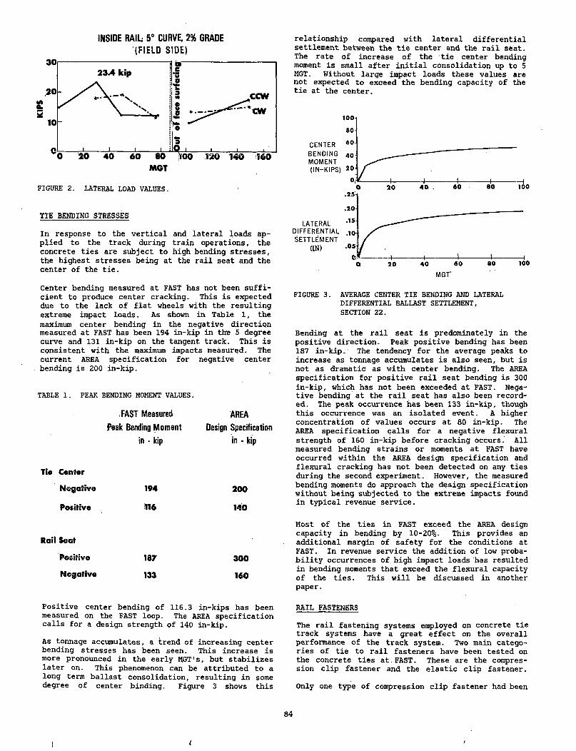
INSIDE RAIL; 5° CURVE. 2% GRADE (FIELD SIDE)

FIGURE 2. LATERAL LOAD VALUES.

TIE BENDING STRESSES

In response to the vertical and lateral loads ap­plied to the track during train operations, the concrete ties are subject to high bending stresses, the highest stresses being at the rail seat and the center of the tie.

Center bending measured at FAST has not been suffi­cient to produce center cracking. This is expected due to the lack of flat wheels with the resulting extreme impact loads. As shown in Table 1, the maximum center bending in the negative direction measured at FAST has been 194 in-kip in the 5 degree curve and 131 in-kip on the tangent track. This is consistent with the maximum impacts measured. The current AREA specification for negative center bending is 200 in-kip.

TABLE 1. PEAK BENDING MOMENT VALUES.

FAST Measured AREAPeak Bending Moment Design Specification

in - kip in - kip

Tie Center

N e g a tive 194 200

Positive 116 140

Rail Seat

Positive 187 300

N e g a tive 133 160

relationship compared with lateral differential settlement between the tie center and the rail seat. The rate of increase of the tie center bending moment is small after initial consolidation up to 5 MGT. Without large impact loads these values are not expected to exceed the bending capacity of the tie at the center.

FIGURE 3. AVERAGE CENTER TIE BENDING AND LATERAL DIFFERENTIAL BALLAST SETTLEMENT, SECTION 22.

Bending at the rail seat is predominately in the positive direction. Peak positive bending has been 187 in-kip. The tendency for the average peaks to increase as tonnage accumulates is also seen, but is not as dramatic as with center bending. The AREA specification for positive rail seat bending is 300 in-kip, which has not been exceeded at FAST. Nega­tive bending at the rail seat has also been record­ed. The peak occurrence has been 133 in-kip, though this occurrence was an isolated event. A higher concentration of values occurs at 80 in-kip. The AREA specification calls for a negative flexural strength of 160 in-kip before cracking occurs. All measured bending strains or moments at FAST have occurred within the AREA design specification and flexural cracking has not been detected on any ties during the second experiment. However, the measured bending moments do approach the design specification without being subjected to the extreme impacts found in typical revenue service.

Most of the ties in FAST exceed the AREA design capacity in bending by 10-20%. This provides an additional margin of safety for the conditions at FAST. In revenue service the addition of low proba­bility occurrences of high impact loads has resulted in bending moments that exceed the flexural capacity of the ties. This will be discussed in another paper.

Positive center bending of 116.3 in-kips has been measured on the FAST loop. The AREA specification calls for a design strength of 140 in-kip.

As tonnage accumulates, a trend of increasing center bending stresses has been seen. This increase is more pronounced in the early MGT's, but stabilizes later on. This phenomenon can be attributed to a long term ballast consolidation, resulting in some degree of center binding. Figure 3 shows this

RAIL FASTENERS

The rail fastening systems employed on concrete tie track systems have a great effect on the overall performance of the track system. Two main catego­ries of tie to rail fasteners have been tested on the concrete ties at, FAST. These are the compres­sion clip fastener and the elastic clip fastener.

Only one type of compression clip fastener had been

84

i

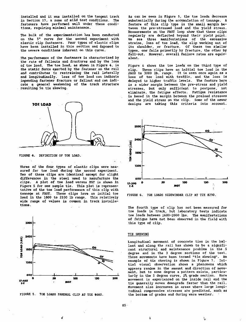
installed and it was installed on the tangent track in Section 17, a zone of mild test conditions. The fasteners have performed well under these condi­tions, requiring minimal maintenance.

The hulk of the experimentation has been conducted on the 5° curve for the second experiment with elastic clip fasteners. Four types of elastic clips have been installed in this section and exposed to the severe conditions inherent on this curve.

The performance of the fasteners is characterized by the rate of fallouts and fractures and by the loss of toe load. The toe load, as shown in Figure 4, is the static force exerted by the fastener on the rail and contributes to restraining the rail laterally and longitudinally. Loss of toe load can indicate impending fastener fracture or fallout and can indi­cate a general weakening of the track structure resulting In tie skewing.

Three of the four, types of elastic clips were mea­sured for toe load during the second experiment. Two of these clips are identical except for slight differences in the steel used to manufacture the clips. A plot of toe load versus MGT is shown in Figure 5 for one sample tie. This plot is represen­tative of the toe load performance of this clip with tonnage at FAST. These clips have an initial toe load in the 1800 to 2100 lb range. This relatively wide range of values is common in track installa­tions .

FIGURE 5. TOE LOADS PANDROL CLIP AT TIE #460.

As can be seen in Figure 5, the toe loads decrease substantially during the accumulation of tonnage. A feature of this clip type is the small margin be­tween the pre-stressed load and the yield stress. Measurements on the FAST loop show that these clips regularly are deflected beyond their yield point. We see three manifestations of the excessive strains, loss of toe load, the clip working out of its shoulder, or fracture. Of these two similar types, one fails primarily by fracture, the other by fall-out. However, overall failure rates are equiv­alent .

Figure 6 shows the toe loads on the third type of clip. These clips have an initial toe load in the 2600 to 3000 lb. range. It is seen once again as a loss of toe load with traffic, and the loss is delayed to higher traffic levels. The feature here is a wider margin between the pre-stress and yield stresses, but only sufficient to postpone, not eliminate, the fatigue effects. Fatigue resistance is based in the margin between the preload stresses and the yield stress on the clip. Some of the newer designs are taking this criteria into account.

FIGURE 6. TOE LOADS SIDEWINDER CLIP AT TIE #290.

The fourth type of clip has not been measured for toe loads in track, but laboratory tests indicate toe loads between 1600-2000 lbs. The manifestations of fatigue have not been observed in the field with this type of clip.

TIE SKEWING

Longitudinal movement of concrete ties in the bal­last and along the rail has shown to be a signifi­cant structural and maintenance problem in the 5 degree and in the 3 degree sections of the test. These movements have been termed "tie skewing". An example of tie skewing is shown in Figure 7. Ini­tial visual observation shows a phenomena which appears random in the amount and direction of move­ment, but to some degree a pattern exists, particu­larly in the 5 degree curve, 2% grade section. More movement is experienced on the inside rail and the tie generally moves downgrade faster than the rail. Movement also increases in areas where large longi­tudinal compressive,stresses are predicted, such as the bottom of grades and during warm weather.

85

v

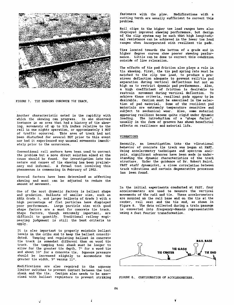
FIGURE 7. TIE SKEWING CONCRETE TIE TRACK.

Another characteristic noted is the rapidity with which the skewing can progress. In one observed instance in an area that had a history of tie skew­ing, movements of up to 11-j inches relative to the rail in one nights operation, or approximately 1 MGT of traffic occurred. This area of track had not been disturbed for several MGT prior to this event nor had it experienced any unusual movements immedi­ately prior to the occurrence.

Conventional rail anchors have been used to correct the problem but a more direct solution aimed at the cause should be found. Our investigation into the nature and causes of tie skewing has been prelimi­nary and informal. A formal test involving this phenomenon is commencing in February of 1982.

Several factors have been determined as affecting skewing and most can be adjusted to reduce the amount of movement.

One of the most dramatic factors is ballast shape and gradation. Ballasts of smaller size, such as AREA Grade 5, and larger ballasts of Grade 3 with a high percentage of flat particles have displayed poor performance. Large particle size with good shape factors are a must for concrete tie track. Shape factors, though extremely important, are difficult to quantify. Traditional railway engi­neering judgement is still the best criteria to apply.

It is also important to properly maintain ballast levels in the cribs and to keep the ballast consoli­dated. Tamping and regulating ballast in concrete tie track is somewhat different than on wood tie track. The tamping tool shank must be longer to allow for the greater tie depth, 7" for a wood tie and about 10" for a concrete tie. Squeeze pressure should be increased slightly to accomodate the greater tie width, 9" versus 11".

Modifications are also required to the squeeze limiter switches to prevent contact between the tool shank and the tie. Caution also needs to be exer­cised with ballast regulators to prevent striking

fasteners with the plow. Modifications with a cutting torch are usually sufficient to correct this problem.

Rail clips in the higher toe load ranges have also displayed improved skewing performance, but design of the clip system may be such that high longitudi­nal resistance can be achieved in the lower toe load ranges when incorporated with resilient tie pads.

Ties located towards the bottom of a grade and in higher degree curves show poorer skewing perfor­mance. Little can be done to correct this condition outside of line relocation.

The effects of tie pad friction also plays a role in tie skewing. First, the tie pad spring rate must be matched to the clip toe load, to produce a pre­stress deflection adequate to prevent rail/tie pad separation during vertical deflections but not so high as to restrict dynamic pad performance. Also, a high coefficient of friction is desirable to restrain movement during vertical deflection. To achieve these criteria, resilient pads appear to be desirable. Caution must be exercised in the selec­tion of pad material. Some of the resilient pad materials are extremely temperature sensitive and subject to mechanical wear. Also, some material appearing resilient became quite rigid under dynamic loading. The introduction of a "shape factor", usually in the form of grooves has shown beneficial effects on resilience and material life.

VIBRATIONS

Recently, an investigation into the vibrational behavior of concrete tie track was begun at FAST. Using accelerometry techniques and spectrum anal­ysis, significant advances have been made in under­standing the dynamic characteristics of the track structure. Under the guidance of Dr. Robert Baird, FAST staff dynamicist, a close correlation between track vibrations and certain degenerative processes has been found.

In the initial experiments conducted at FAST, four accelerometers are used to measure the vertical movements of the rail and tie. These accelerometers are mounted on the rail base and on the tie at the center, rail seat and the tie end, as shown in Figure 8. The data collected during a train passage is converted into frequency-domain representation using a fast Fourier transformation.

RAIL BASE

FIGURE 8., CONFIGURATION OF ACCELEROMETERS.

86

i V

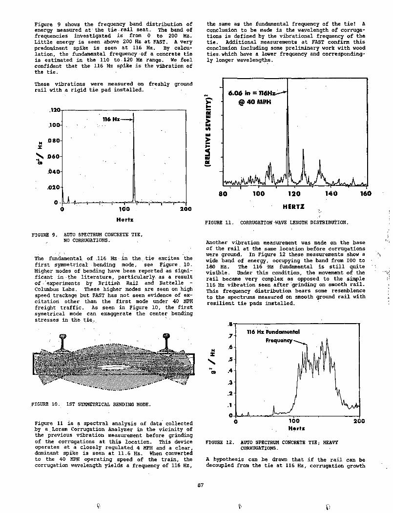
Figure 9 shows the frequency band distribution of energy measured at the tie rail seat. The band of frequencies investigated is from 0 to 200 Hz. Little energy is seen above 200 Hz at FAST. A very predominant spike is seen at 116 Hz. By calcu­lation, the fundamental frequency of a concrete tie is estimated in the 110 to 120 Hz range. We feel confident that the 116 Hz spike is the vibration of the tie.

These vibrations were measured on freshly ground rail with a rigid tie pad installed.

FIGURE 9. AUTO SPECTRUM CONCRETE TIE, NO CORRUGATIONS.

The fundamental of .116 Hz in the tie excites the first symmetrical bending mode, see Figure. 10. Higher modes of bending have been reported as signi­ficant in; the literature, particularly as a result o f . experiments by British Rail and Battelle - Columbus Labs. These higher modes are seen on high speed trackage but FAST has not seen evidence of ex­citation other than the first mode under 40 MPH freight traffic. As seen in Figure 10, the first symetrical mode can exaggerate the center bending stresses in the tie.

FIGURE 10. 1ST SYMMETRICAL BENDING MODE.

Figure 11 is a spectral analysis of data collected by a Loram Corrugation Analyzer in the vicinity of the previous vibration measurement before grinding of the corrugations at this location. This device operates at a closely regulated 4 MPH and a clear, dominant spike is seen at 11.6 Hz. When converted to the 40 MPH operating speed of the train, the corrugation wavelength yields a frequency of 116 Hz,

the same as the fundamental frequency of the tie! A conclusion to be made is the wavelength of corruga­tions is defined by the vibrational frequency of the tie. Additional measurements at FAST confirm this conclusion including some preliminary work with wood ties, which have a lower frequency and corresponding­ly longer wavelengths.

FIGURE 11. CORRUGATION WAVE LENGTH DISTRIBUTION.

Another vibration measurement was made on the base of the rail at the same location before corrugations were ground. In Figure 12 these measurements show a wide band of energy, occupying the band from 100 to 180 Hz. The 116 Hz fundamental is still quite visible. Under this condition, the movement of the rail became very complex as opposed to the simple 116 Hz vibration seen after grinding on smooth rail. This frequency distribution bears some resemblence to the spectrums measured on smooth ground rail with resilient tie pads installed.

FIGURE 12. AUTO SPECTRUM CONCRETE TIE; HEAVY CORRUGATIONS.

A hypothesis can be drawn that if the rail can be decoupled from the tie at 116 Hz, corrugation growth

87

Cl

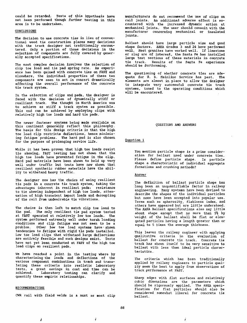
could be retarded. Tests of this hypothesis have not been performed though further testing in this area is to be undertaken.

CONCLUSIONS

The decision to use concrete ties in lieu of conven­tional wood tie construction places many decisions with the track designer not traditionally encoun­tered. Only a portion of those decisions in the selection of components are fully covered by gener­ally accepted specifications.

The most complex decision involves the selection of clip toe load and tie pad spring rate. As experi­ence has been gained with concrete ties on FAST and elsewhere, the individual properties of these two components are seen to act in concert dramatically affecting the overall performance of the concrete tie track system.

In the selection of clips and pads, the designer is faced with the decision of dynamically stiff or resilient track. The thought in North America was to achieve as stiff a track system as possible. This end can be achieved by employing clips with relatively high toe loads and hard tie pads.

The newer fastener systems being made available on this continent generally reflect this philosophy. The basis for this design criteria is that the high toe load clip restricts deflections, hence minimiz­ing fatigue problems. The hard pad is also chosen for the purpose of prolonging service life.

While it has been proven that high toe loads resist tie skewing, FAST testing has not shown that the high toe loads have prevented fatigue in the clip. Hard pad materials have been shown to hold up very well under traffic but tests have now shown that resilient synthetic rubber materials have the abil­ity to withstand heavy traffic.

The designer now has the choice of using resilient tie pads in a concrete tie track system, taking the advantages inherent in resilient pads: resistance to tie skewing independent of high toe loads, atten­uation of high transient impact loads and decoupling of the rail from undesirable tie vibrations.

The choice is then left to match clip toe load to the pad. The only resilient tie pad system tested at FAST operated at relatively low toe loads. The system performed extremely well under harsh loading conditions and clip fatigue was not seen to be a problem. Other low toe load systems have'shown tendencies to fatigue with rigid tie pads installed. Low toe load clips that withstand large deflections are entirely feasible and such designs exist. Tests have not yet been conducted at FAST of the high toe load clips on resilient pads.

We have reached a point in the testing where by characterizing the loads and deflections of the various component combinations in track and trans­lating these criteria into realistic laboratory tests, a great savings in cost and time can be achieved. Laboratory testing can clarify and quantify these empiric relationships.

RECOMMENDATIONS

CWR r a i l with f i e ld welds is a must as most c l ip

manufacturers do not recommend the use of clips on rail joints. An additional adverse effect is en­countered with the increased dynamic action at mechanical joints. The user should consult with the manufacturer concerning mechanical or insulated joints.

Ballast should have large particle size and good shape factors. AREA Grades 3 and 24 have performed well. Most granites have worked well. If limestone or slag are of interest, the Santa Fe has installed large test sections of these materials in concrete tie track. Results of the Santa Fe experience should be forthcoming.

The questioning of whether concrete ties are ade­quate for U. S. Mainline Service has past. The elements are almost in place to allow the designer to integrate very successful concrete tie track systems, tuned to the operating conditions which will be encountered.

QUESTIONS AND ANSWERS

Question 1

You mention particle shape is a prime consider­ation for ballast used under concrete ties. Please define particle shape. Is particle shape a characteristic of individual aggregate formations and crushing methods?

Answer

The definition of ballast particle shape has 'long been an unquantifiable factor in railway engineering. Many systems have been devised to describe the shapes of the individual particles but none have been accepted into popular use. Terms such as spherosity, flakiness index, and others have appeared but are little understood. The AREA Ballast specifications also say little about shape except that no more than 5% by weight of the ballast shall be flat or elon­gated particles having a length greater than or equal to 5 times the average thickness.

This leaves the railway engineer with applying qualitative criteria in the evaluation of ballast for concrete tie track. Concrete tie track has shown itself to be very sensitive to ballast with less than ideal particle charac­teristics .

The criteria which has been traditionally applied by railway engineers to particle qual­ity seem the best to apply from observations of track performance at FAST.

Sharp edges with flat surfaces and relatively cubic dimensions are the parameters which should be rigorously applied. The AREA speci­fication for flat particles should also be considered somewhat liberal for concrete tie ballast.

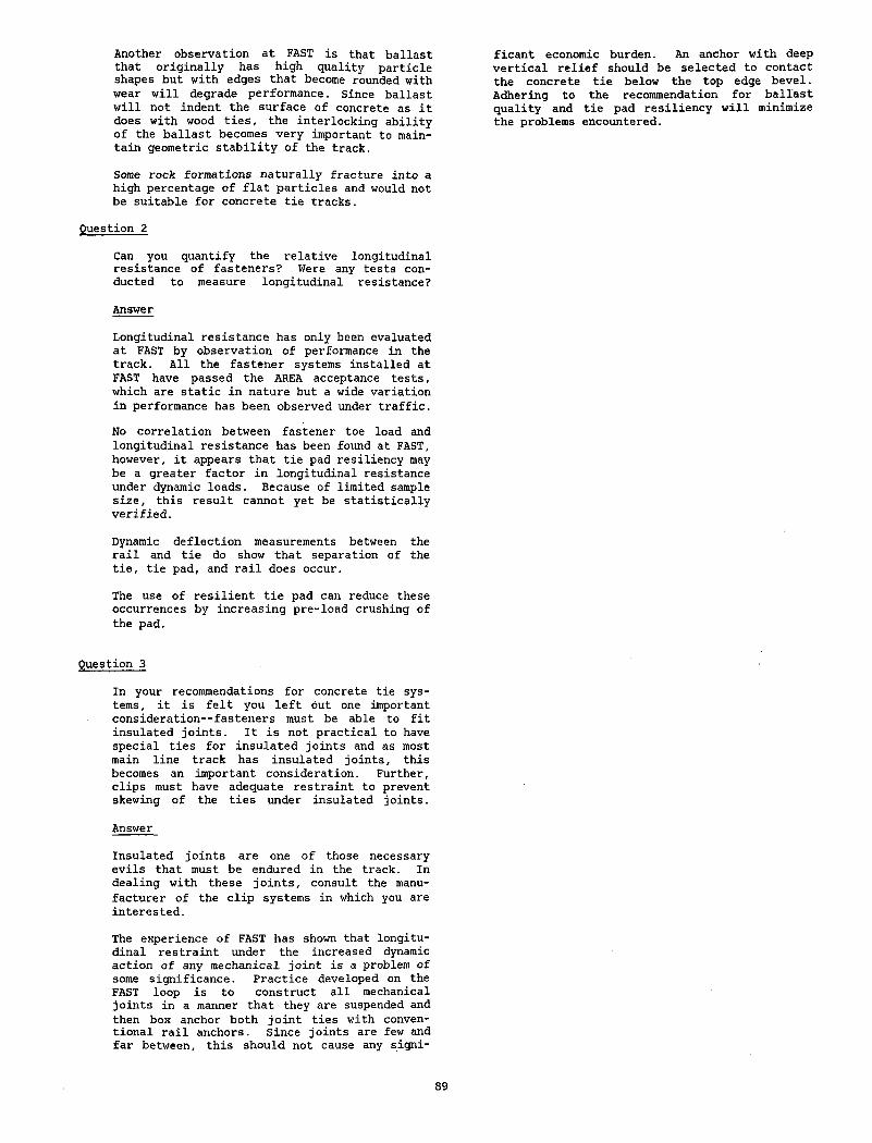
Another observation at FAST is that ballast that originally has high quality particle shapes but with edges that become rounded with wear will degrade performance. Since ballast will not indent the surface of concrete as it does with wood ties, the interlocking ability of the ballast becomes very important to main­tain geometric stability of the track.

Some rock formations naturally fracture into a high percentage of flat particles and would not be suitable for concrete tie tracks.

Question 2

Can you quantify the relative longitudinal resistance of fasteners? Were any tests con­ducted to measure longitudinal resistance?

Answer

ficant economic burden. An anchor with deep vertical relief should be selected to contact the concrete tie below the top edge bevel. Adhering to the recommendation for ballast quality and tie pad resiliency will minimize the problems encountered.

Longitudinal resistance has only been evaluated at FAST by observation of performance in the track. All the fastener systems installed at FAST have passed the AREA acceptance tests, which are static in nature but a wide variation in performance has been observed under traffic.

No correlation between fastener toe load and longitudinal resistance has been found at FAST, however, it appears that tie pad resiliency may be a greater factor in longitudinal resistance under dynamic loads. Because of limited sample size, this result cannot yet be statistically verified.

Dynamic deflection measurements between the rail and tie do show that separation of the tie, tie pad, and rail does occur.

The use of resilient tie pad can reduce these occurrences by increasing pre-load crushing of the pad.

Question 3

In your recommendations for concrete tie sys­tems, it is felt you left out one important consideration— fasteners must be able to fit insulated joints. It is not practical to have special ties for insulated joints and as most main line track has insulated joints, this becomes an important consideration. Further, clips must have adequate restraint to prevent skewing of the ties under insulated joints.

Answer

Insulated joints are one of those necessary evils that must be endured in the track. In dealing with these joints, consult the manu­facturer of the clip systems in which you are interested.

The experience of FAST has shown that longitu­dinal restraint under the increased dynamic action of any mechanical joint is a problem of some significance. Practice developed on the FAST loop is to construct all mechanical joints in a manner that they are suspended and then box anchor both joint ties with conven­tional rail anchors. Since joints are few and far between, this should not cause any signi-

89

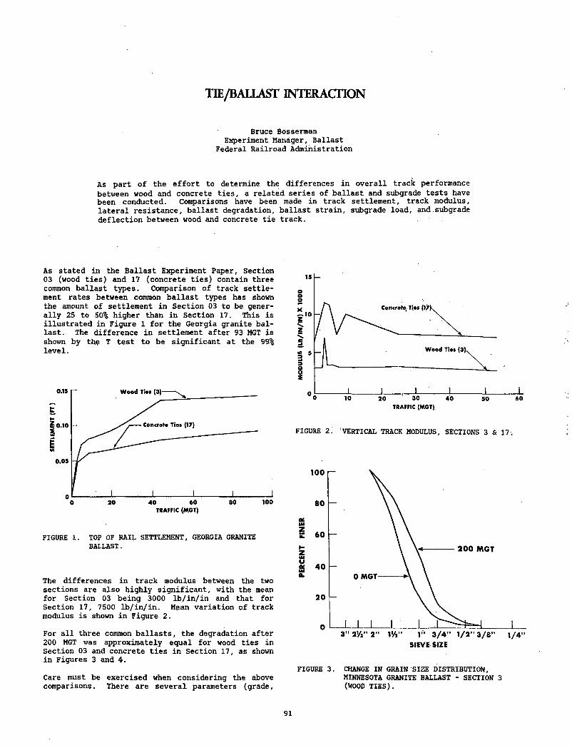
TIE/BALLAST INTERACTION

Bruce Bosserman Experiment Manager, Ballast

Federal Railroad Administration

As part of the effort to determine the differences in overall track performance between wood and concrete ties, a related series of ballast and subgrade tests have been conducted. Comparisons have been made in track settlement, track modulus, lateral resistance, ballast degradation, ballast strain, subgrade load, and subgrade deflection between wood and concrete tie track.

As stated in the Ballast Experiment Paper, Section 03 (wood ties) and 17 (concrete ties) contain three common ballast types. Comparison of track settle­ment rates between common ballast types has shown the amount of settlement in Section 03 to be gener­ally 25 to 50% higher than in Section 17. This is illustrated in Figure 1 for the Georgia granite bal­last. The difference in settlement after 93 MGT is shown by the T test to be significant at the 99% level.

FIGURE 1. TOP OF RAIL SETTLEMENT, GEORGIA GRANITE BALLAST.

The differences in track modulus between the two sections are also highly significant, with the mean for Section 03 being 3000 lb/in/in and that for Section 17, 7500 lb/in/in. Mean variation of track modulus is shown in Figure 2.

For all three common ballasts, the degradation after 200 MGT was approximately equal for wood ties in Section 03 and concrete ties in Section 17, as shown in Figures 3 and 4.

Care must be exercised when considering the above comparisons. There are several parameters (grade,

FIGURE 2. VERTICAL TRACK MODULUS, SECTIONS 3 &

inzzUluotCL

SIEVE SIZE

FIGURE 3. CHANGE IN GRAIN SIZE DISTRIBUTION, MINNESOTA GRANITE BALLAST - SECTION (WOOD TIES).

_L60

17.

1 / 4 ”

3

91

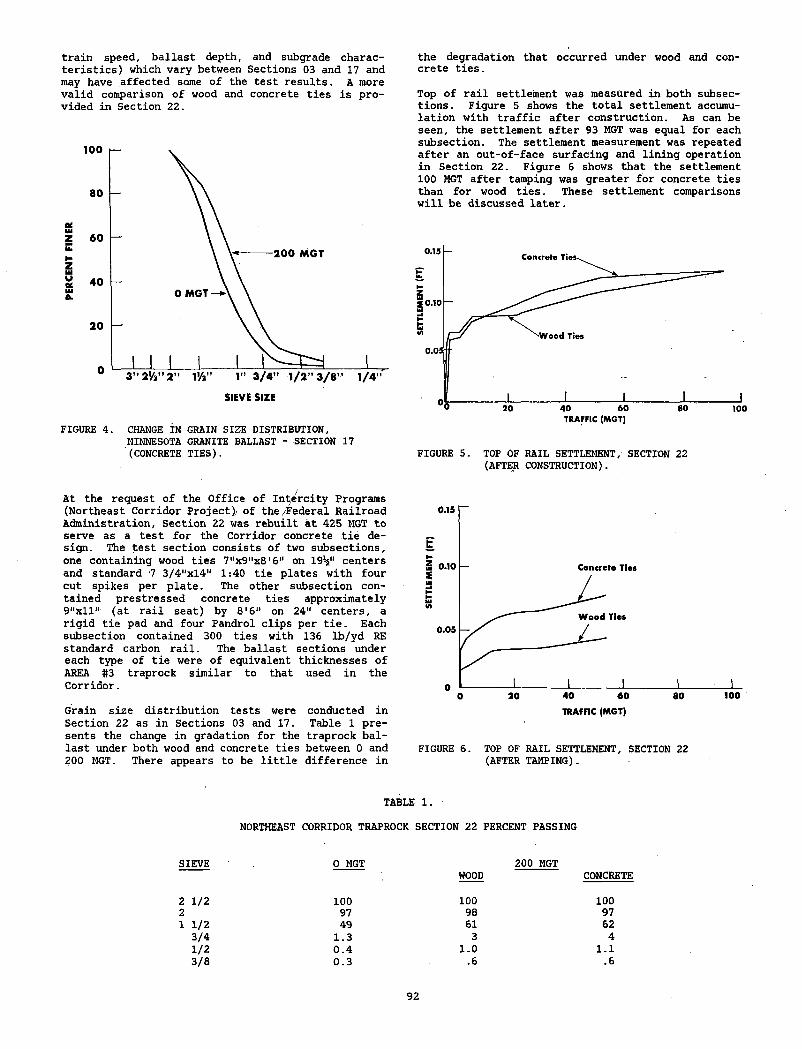
train speed, ballast depth, and subgrade charac­teristics) which vary between Sections 03 and 17 and may have affected some of the test results. A more valid comparison of wood and concrete ties is pro­vided in Section 22.

FIGURE 4. CHANGE IN GRAIN SIZE DISTRIBUTION,MINNESOTA GRANITE BALLAST - SECTION 17 (CONCRETE TIES).

At the request of the Office of Intercity Programs (Northeast Corridor Project)/ of the/Federal Railroad Administration, Section 22 was rebuilt at 425 MGT to serve as a test for the Corridor concrete tie de­sign. The test section consists of two subsections, one containing wood ties 7"x9"x8'6" on 19V1 centers and standard '7 3/4"xl4,‘ 1:40 tie plates with four cut spikes per plate. The other subsection con­tained prestressed concrete ties approximately 9"xll" (at rail seat) by 8 16" on 24" centers, a rigid tie pad and four Pandrol clips per tie. Each subsection contained 300 ties with 136 lb/yd RE standard carbon rail. The ballast sections under each type of tie were of equivalent thicknesses of AREA #3 traprock similar to that used in the Corridor.

Grain size distribution tests were conducted in Section 22 as in Sections 03 and 17. Table 1 pre­sents the change in gradation for the traprock bal­last under both wood and concrete ties between 0 and 200 MGT. There appears to be little difference in

the degradation that occurred under wood and con­crete ties.

Top of rail settlement was measured in both subsec­tions. Figure 5 shows the total settlement accumu­lation with traffic after construction. As can be seen, the settlement after 93 MGT was equal for each subsection. The settlement measurement was repeated after an out-of-face surfacing and lining operation in Section 22. Figure 6 shows that the settlement 100 MGT after tamping was greater for concrete ties than for wood ties. These settlement comparisons will be discussed later.

FIGURE 5. TOP OF RAIL SETTLEMENT, SECTION 22 (AFTER CONSTRUCTION).

FIGURE 6. TOP OF RAIL SETTLEMENT, SECTION 22 (AFTER TAMPING).

TABLE 1.

NORTHEAST CORRIDOR TRAPROCK SECTION 22 PERCENT PASSING

SIEVE O MGT

2 1/2 1002 971 1/2 49

3/4 1.31/2 0.43/8 0.3

200 MGTWOOD CONCRETE

100 10098 9761 623 4

1.0 1.1.6 .6

92

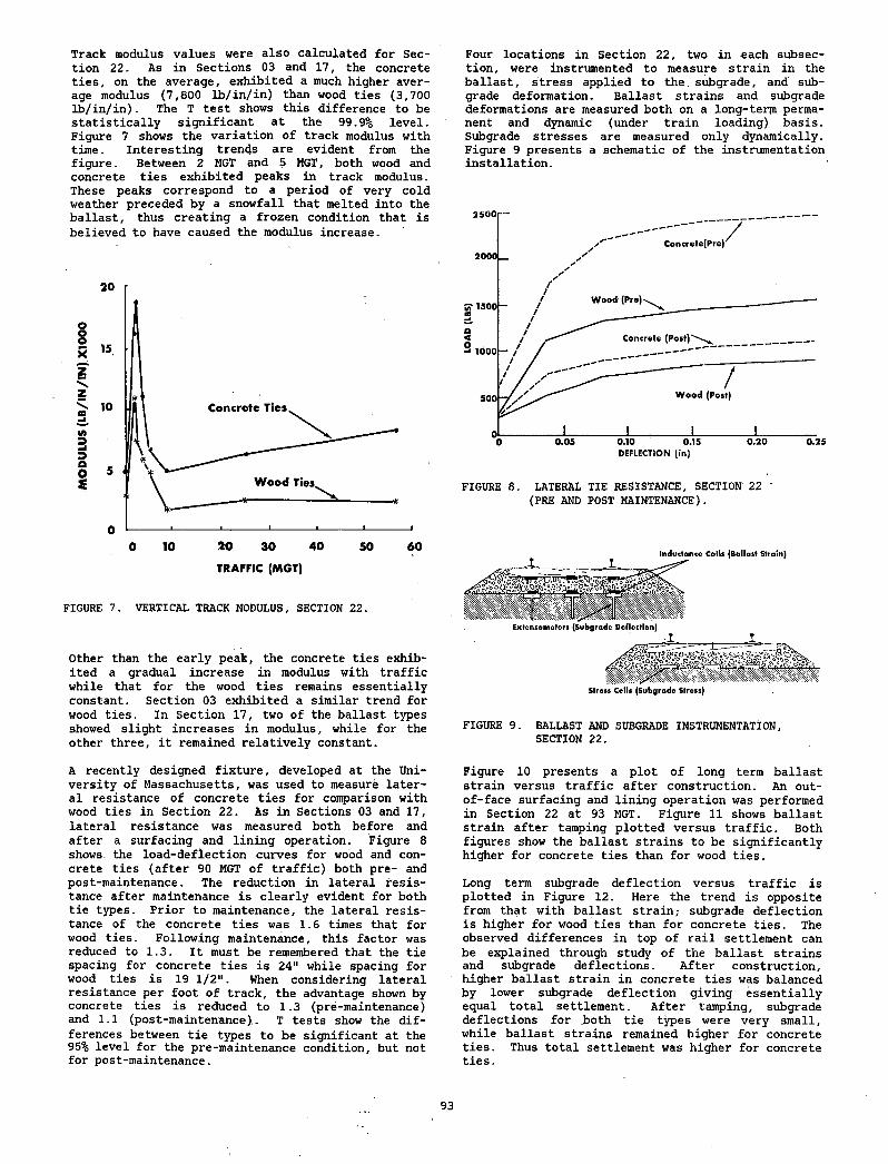
Track modulus values were also calculated for Sec­tion 22. As in Sections 03 and 17, the concrete ties, on the average, exhibited a much higher aver­age modulus (7,800 lb/in/in) than wood ties (3,700 lb/in/in). The T test shows this difference to be statistically significant at the 99.9% level. Figure 7 shows the variation of track modulus with time. Interesting trends are evident from the figure. Between 2 MGT and 5 MGT, both wood and concrete ties exhibited peaks in track modulus. These peaks correspond to a period of very cold weather preceded by a snowfall that melted into the ballast, thus creating a frozen condition that is believed to have caused the modulus increase.

FIGURE 7. VERTICAL TRACK MODULUS, SECTION 22.

Other than the early peak, the concrete ties exhib­ited a gradual increase in modulus with traffic while that for the wood ties remains essentially constant. Section 03 exhibited a similar trend for wood ties. In Section 17, two of the ballast types showed slight increases in modulus, while for the other three, it remained relatively constant.

Four locations in Section 22, two in each subsec­tion, were instrumented to measure strain in the ballast, stress applied to the. subgrade, and sub­grade deformation. Ballast strains and subgrade deformations are measured both on a long-term perma­nent and dynamic (under train loading) basis. Subgrade stresses are measured only dynamically. Figure 9 presents a schematic of the instrumentation installation.

FIGURE 8. LATERAL TIE RESISTANCE, SECTION 22 (PRE AND POST MAINTENANCE).

FIGURE 9. BALLAST AND SUBGRADE INSTRUMENTATION, SECTION 22.

A recently designed fixture, developed at the Uni­versity of Massachusetts, was used to measure later­al resistance of concrete ties for comparison with wood ties in Section 22. As in Sections 03 and 17, lateral resistance was measured both before and after a surfacing and lining operation. Figure 8 shows, the load-defiection curves for wood and con­crete ties (after 90 MGT of traffic) both pre- and post-maintenance. The reduction in lateral resis­tance after maintenance is clearly evident for both tie types. Prior to maintenance, the lateral resis­tance of the concrete ties was 1.6 times that for wood ties. Following maintenance, this factor was reduced to 1.3. It must be remembered that the tie spacing for concrete ties is 24" while spacing for wood ties is 19 1/2". When considering lateral resistance per foot of track, the advantage shown by concrete ties is reduced to 1.3 (pre-maintenance) and 1.1 (post-maintenance). T tests show the dif­ferences between tie types to be significant at the 95% level for the pre-maintenance condition, but not for post-maintenance.

Figure 10 presents a plot of long term ballast strain versus traffic after construction. An out- of-face surfacing and lining operation was performed in Section 22 at 93 MGT. Figure 11 shows ballast strain after tamping plotted versus traffic. Both figures show the ballast strains to be significantly higher for concrete ties than for wood ties.

Long term subgrade deflection versus traffic is plotted in Figure 12. Here the trend is opposite from that with ballast strain,- subgrade deflection is higher for wood ties than for concrete ties. The observed differences in top of rail settlement can be explained through study of the ballast strains and subgrade deflections. After construction, higher ballast strain in concrete ties was balanced by lower subgrade deflection giving essentially equal total settlement. After tamping, subgrade deflections for .both tie types were very small, while ballast strains remained higher for concrete ties. Thus total settlement was higher for concrete ties.

93

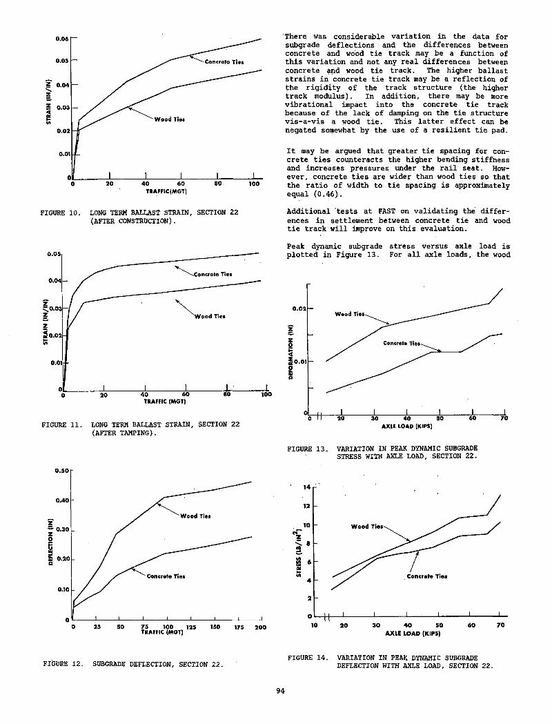
There was considerable variation in the data for subgrade deflections and the differences between concrete and wood tie track may be a function of this variation and not any real differences between concrete and wood tie track. The higher ballast strains in concrete tie track may be a reflection of the rigidity of the track structure (the higher track modulus). In addition, there may be more vibrational impact into the concrete tie track because of the lack of damping on the tie structure vis-a-vis a wood tie. This latter effect can be negated somewhat by the use of a resilient tie pad.

It may be argued that greater tie spacing for con­crete ties counteracts the higher bending stiffness and increases pressures under the rail seat. How­ever, concrete ties are wider than v/ood ties so that the ratio of width to tie spacing is approximately equal (0.46).

FIGURE 10. LONG TERM BALLAST STRAIN, SECTION 22 (AFTER CONSTRUCTION).

Additional tests at FAST on validating the differ­ences in settlement between concrete tie and wood tie track will improve on this evaluation.

FIGURE 11. LONG TERM BALLAST STRAIN, SECTION 22 (AFTER TAMPING).

Peak dynamic subgrade stress versus axle load is plotted in Figure 13. For all axle loads, the wood

o_0 ao 30 4 0 50 6 0 7 0AXLE LOAD (KIPS)

FIGURE 13. VARIATION IN PEAK DYNAMIC SUBGRADE STRESS WITH AXLE LOAD, SECTION 22.

FIGURE 12. SUBGRADE DEFLECTION, SECTION 22.FIGURE 14. VARIATION IN PEAK DYNAMIC SUBGRADE

DEFLECTION WITH AXLE LOAD, SECTION 22.

ties stressed the subgrade higher although the difference is not statistically significant due to' large variability in the data. Peak dynamic sub­grade deflections are similarily plotted in Figure 14. Again, wood ties cause higher deflections in the subgrade. Here, the differences are'statisti­cally significant. Dynamic ballast strain data is currently being evaluated.

The results of the comparison of concrete and wood tie track have shown that in Sections 03 and 17 there was more settlement after construction on wood tie track and an approximately equal amount of ballast degradation. The differences in performance in these two sections can probably be attributed more to varying test site conditions than to any­thing else.

In Section 22, a more valid test where the sections were back to back on the same track configuration, the substantive differences in performance between concrete and wood tie track were higher settlement and greater lateral resistance for concrete tie track. Whether the increased settlement indicates greater differential settlement has not been evalu­ated. However, it is apparent that there is no detrimental effect on the ballast degradation or subgrade stresses as a result.

QUESTIONS AND ANSWERS

Question 1

You showed relative average settlement under concrete ties and wood ties. Was there any variation in variability of this settlement, for example in standard deviation of settle­ment .

Answer

Actually it is the differential settlement which controls the maintenance cycle. So far there has been insufficient traffic to show difference in differential settlement.

95

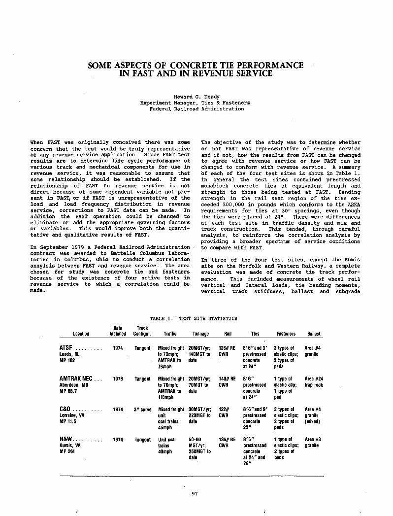
SOME ASPECTS OF CONCRETE TIE PERFORMANCE IN FAST AND IN REVENUE SERVICE

Howard G. MoodyExperiment Manager, Ties & Fasteners

Federal Railroad Administration

When FAST was originally conceived there was some concern that the test would be truly representative of any revenue service application. Since FAST test results are to determine life cycle performance of various track and mechanical components for use in revenue service, it was reasonable to assume that some relationship should be established. If the relationship of FAST to revenue service is not direct because of some dependent variable not pre­sent in FAST, or if FAST is unrepresentative of the load and load frequency distribution in revenue service, corrections to FAST data can be made. In addition the FAST operation could be changed to eliminate or add the appropriate governing factors or variables. This would improve both the quanti­tative and qualitative results of FAST.

In September 1979 a Federal Railroad Administration contract was awarded to Battelle Columbus Labora­tories in Columbus, Ohio to conduct a correlation anaylsis between FAST and revenue service. The area chosen for study was concrete tie and fasteners because of the existence of four active tests in revenue service to which a correlation could be made.

The objective of the study was to determine whether or not FAST was representative of revenue service and if not, how the results from FAST can be changed to- agree with revenue service or how FAST can be changed to conform with revenue service. A summary of each of the four test sites is shown in Table 1. In general the test sites contained prestressed monoblock concrete ties of equivalent length and strength to those being tested at FAST. Bending strength in the rail seat region of the ties ex­ceeded 300,000 in pounds which conforms to the AREA requirements for ties at 30" spacings, even though the ties were placed at 24". There were differences at each test site in traffic density and mix and track construction. This tended, through careful analysis, to' reinforce the correlation analysis by providing a broader spectrum of service conditions to compare with FAST.

In three of the four test sites, except the Kumis site on the Norfolk and Western Railway, a complete evaluation was made of concrete tie track perfor­mance. This included measurements of wheel rail vertical and lateral loads, tie bending moments, vertical track stiffness, ballast and subgrade

TABLE,!. TEST SITE STATISTICSDate Track

Location Installed Configur. Traffic Tonnage Rail Ties Fasteners Ballast

ATSF .................Leeds, III.MP 102

1974 Tangent Mixed freight to 70mph; AMTRAK to 79mph

20MGT/yr; 140MGT to date

136# RE CWR

8'6"and9' prestressed concrete at 24"

3 types of elastic clips; 2 types of pads

Area #4 granite

AMTRAK NEC .. Aberdeen, MD MP 68.7

1978 Tangent Mixed freight to 70mph; AMTRAK to 110mph

20MGT/yr; 70MGT to date

140# RE CWR

8'6"prestressed concrete at 24"

1 type of elastic clip; 1 type of pad

Area #24 trap rock

C & 0 ................... 1974 3° curve Mixed freight 30MGT/yr; 122# 8'6"and9' 2 types of Area #4Lorraine, VA MP 11.6

unitcoal trains 45mph

220MGT to date

CWR prestressedconcrete25"

elastic clips; 2 types of pads

granite(mixed)

N&W..................Kumis, VA MP 261

1974 Tangent Unit coaltrains40mph

50-60 MGT/yr; 260MGT to date

136# RE CWR

8 '6"prestressed concrete at 24" and 26"

1 type of elastic clips;2 types of pads

Area #3 granite

97

f

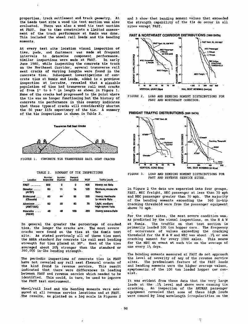
properties, track settlement and track geometry. At the Leeds test site a wood tie test' section was also evaluated. There was also a wood tie test section at FAST. Due to time constraints a limited assess­ment of the track performance at Kumis was done. This included the wheel rail loads and tie bending moments.

At every test site location visual inspection of ties, pads, and fasteners was made at frequent intervals to determine component performance. Similar inspections were made at FAST. In early June 1980, while inspecting the concrete tie track on the Northeast Corridor, several transverse rail seat cracks of varying lengths were found in the concrete ties. Subsequent investigations of con­crete ties at Kumis and Leeds, added to a previous inspection at Lorraine, revealed that a sizeable population of ties had transverse rail seat cracks of from 1" to 6 11 in length as shown in Figure 1. None of the cracks had progressed to tKe point where the tie was no longer functioning but the history of concrete tie performance in this country indicates that these types of cracks will considerably shorten the 50 year life expectancy of the tie. A summary of the tie inspections is shown in Table 2.

Transverse Rail Seal Cracks

TABLE 2. SUMMARY OF TIE INSPECTIONS

LocationNumber

InspectedNumberCracked

PercentCracked MGT Traffic Loads

F A S T .............. 600 0 0 425 Heavy; no fla ts

S tre a to r ..........(ATSF)

80 11 14 125 M edium ; m oderate fla ts

R ichm ond . . . (Chassis)

80 44 55 220 Heavy; m oderate to severe fla ts

A b e rd e e n___(AMTRAK)

60 56 93 70 Light, m edium ; h igh speed fla ts

Roanoke ___(N&W )

48 48 100 260 Heavy; severe fla ts

In general the greater the percentage of cracked ties, the longer the cracks are. The most severe cracks were found on the ties at the Kumis test site. As stated previously all of these ties meet the AREA standard for concrete tie rail seat bending strength for ties placed at 30". Most of the ties averaged about 20% stronger than the standard or 360,000 in-lbs bending strength.

The periodic inspections of concrete ties in FAST have not revealed any rail seat flexural cracks of the kind found in revenue service. This result indicated that there were differences in loading between FAST and revenue service which needed to be identified. This could, in turn, be used to improve the FAST test environment.

Wheel/rail load and tie bending moments were mea­sured at all revenue service locations and at FAST. .The results, as plotted on a log scale in Figures 2

and 3 show•that bending moment values that exceeded the strength capability of the tie do occur in all sites except FAST.

FAST & NORTHEAST CORRIDOR DISTRIBUTIONS (1980 DATA)

FIGURE 2. LOAD AND BENDING MOMENT DISTRIBUTIONS FOR FAST AND NORTHEAST CORRIDOR.

FREIGHT TRAFFIC DISTRIBUTIONS (isai d a t a )

FIGURE 3. LOAD AND BENDING MOMENT DISTRIBUTIONS FOR FAST AND REVENUE SERVICE SITES.

In Figure 2 the data are separated into four groups, FAST, NEC freight, NEC passenger at less than 70 mph and NEC passenger greater than 70 mph. The majority of the bending moments exceeding the 360 in-kip cracking threshold were from the passenger equipment above 70 mph.

For.the other sites, the most severe condition was, as predicted by the visual inspections, on the N & W at Kumis. The traffic on that test section is primarily loaded 100 ton hopper cars. The frequency of occurrence of values exceeding the cracking threshold for the N & W and NEC was about .1% or one cracking moment for every 1000 axles. This means for the NEC an event at each tie on the average of one every 1% days.

The bending moments measured at FAST do not approach the level of severity of any of the revenue service sites. The predominant feature of the FAST loads and bending moments were the higher average values, symptomatic, of the 100 ton loaded hopper car con­sist.

It was evident from these data that the very large loads at the .1% level and above were causing tie cracking. Ah inspection of the AMTRAK passenger equipment ’ revealed that some of these high loads were caused by long wavelength irregularities on the

98

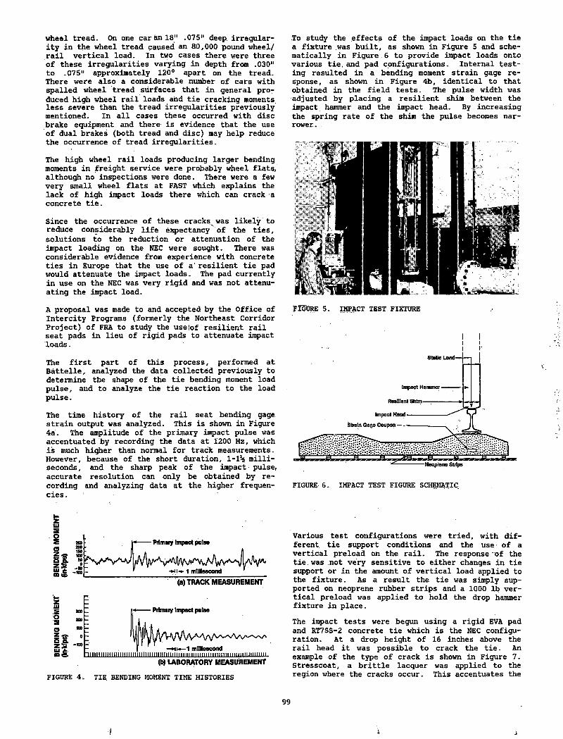
wheel tread. On one car an 18" .075" deep, irregular­ity in the wheel tread caused an 80,000 pound wheel/ rail vertical load. In two cases there were three of these irregularities varying in depth from .030" to .075" approximately 120° apart on the tread. There were also a considerable number of cars with spalled wheel tread surfaces that in general pro­duced high wheel rail loads and tie cracking moments less severe than the tread irregularities previously mentioned. In all cases these occurred with disc brake equipment and there- is evidence that the use of dual brakes (both tread and disc) may help reduce the occurrence of tread irregularities.

The high wheel rail loads producing larger bending moments in freight service were probably wheel flats, although no inspections were done. There were a few very small wheel flats at FAST which explains the lack of high impact loads there which can crack a concrete tie.

Since the occurrence of these cracks was likely to reduce considerably life expectancy of the ties, solutions to the reduction or attenuation of the impact loading on the NEC were sought. There was considerable evidence from experience with concrete ties in Europe that the use of a' resilient tie pad would attenuate the impact loads. The pad currently in use on the NEC was very rigid and was not attenu­ating the impact load.

To study the effects of the impact loads on the tie a fixture was built, as shown in Figure 5 and sche­matically in Figure 6 to provide impact loads onto various tie. and pad configurations. Internal test­ing resulted in a bending moment strain gage re­sponse, as shown in Figure 4b, identical to that obtained in the field tests. The pulse width was adjusted by placing a resilient shim between the impact hammer and the impact head. By increasing the spring rate of the shim the pulse becomes nar­rower.,

A proposal was made to and accepted by the Office of Intercity Programs (formerly the Northeast Corridor Project) of FRA to study the use {of resilient rail seat pads in lieu of rigid pads to attenuate impact loads.

The first part of this process, performed at Battelle, analyzed the data collected previously to determine the shape of the tie bending moment load pulse, and to analyze the tie reaction to the load pulse.

The time history of the rail seat bending gage strain output was analyzed. This is shown in Figure 4a. The amplitude of the primary impact pulse was accentuated by recording the data at 1200 Hz, which is much higher than normal for track measurements. However, because of the short duration, 1-1% milli­seconds, and the sharp peak of the impact pulse, accurate resolution can only be obtained by re­cording and analyzing data at the higher frequen­cies.

FIGURE 5. IMPACT TEST FIXTURE

1 II i

FIGURE 6. IMPACT TEST FIGURE SCHEMATIC

(a) TRACK MEASUREMENT

OSo

si■ A

- Pibniiy Impact pulse

I —h h —1 millisecondh l l l l l l l lH I H I I I I I I I I I I I I I I I I I I l l l l l l l l i l l i i i l i i i i i i i m i i i i i i i i i i i i i iM i i i i i i i l i i i i .

I LABORATORY MEASUREMENT

FIGURE 4. TIE BENDING MOMENT TIME HISTORIES

Various test configurations were tried, with dif­ferent tie support conditions and the use of a vertical preload on the rail. The response "of the tie, was not very sensitive to either changes in tie support or in the amount of vertical load applied to the fixture. As a result the tie was simply sup­ported on neoprene rubber strips and a 1000 lb ver­tical preload was applied to hold the drop hammer fixture in place.

The impact tests were begun using a rigid EVA pad and RT7SS-2 concrete tie which is the NEC configu­ration. At a drop height of 16 inches above the rail head it was possible to crack the tie. An example of the type of crack is shown in Figure 7. Stresscoat, a brittle lacquer was applied to the region where the cracks occur. This accentuates the

99

■1 j

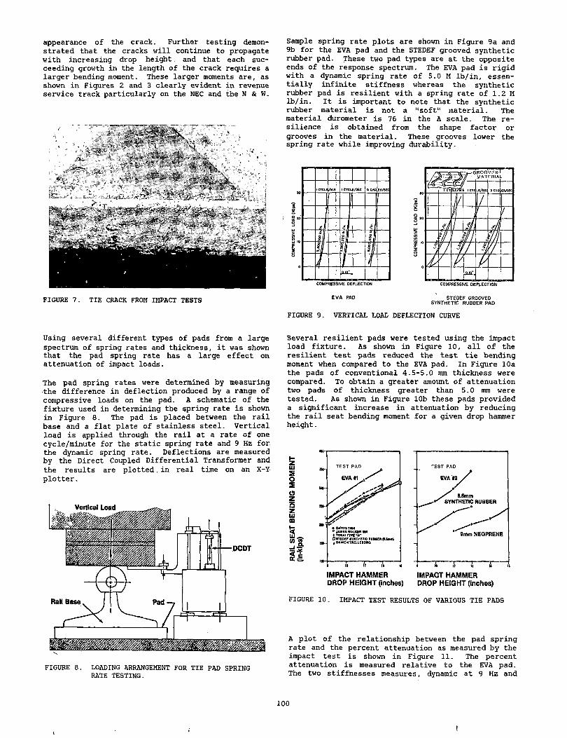
appearance of the crack. Further testing demon­strated that the cracks will continue to propagate with increasing drop height. and that each suc­ceeding growth in the length of the crack requires a larger bending moment. These larger moments are, as shown in Figures 2 and 3 clearly evident in revenue service track particularly on the NEC and the N & W.

FIGURE 7. TIE CRACK FROM IMPACT TESTS

Sample spring rate plots are shown in Figure 9a and 9b for the EVA pad and the STEDEF grooved synthetic rubber pad. These two pad types are at the opposite ends of the response spectrum. The EVA pad is rigid with a dynamic spring rate of 5.0 M lb/in, essen­tially infinite stiffness whereas the synthetic rubber pad is resilient with a spring rate of 1.2 M lb/in. It is important to note that the synthetic rubber material is not a "soft" material. The material durometer is 76 in the A scale. The re­silience is obtained from the shape factor or grooves in the material. These grooves lower the spring rate while improving durability.

COMPRESSIVE DEFLECTION

E V A PAD STEDEF GROOVED SYNTHETIC RUBBER PAD

FIGURE 9. VERTICAL LOAL DEFLECTION CURVE

Using several different types of pads from a large spectrum of spring rates and thickness, it was shown that the pad spring rate has a large effect on attenuation of impact loads.

The pad spring rates were determined by measuring the difference in deflection produced by a range of compressive loads on the pad. A schematic of the fixture used in determining the spring rate is shown in Figure 8. The pad is placed between the rail base and a flat plate of stainless steel. Vertical load is applied through the rail at a rate of one cycle/minute for the static spring rate and 9 Hz for. the dynamic spring rate. Deflections are measured by the Direct Coupled Differential Transformer and the results are plotted. in real time on an X-Y- plotter.

FIGURE 8. LOADING ARRANGEMENT FOR TIE PAD SPRING RATE TESTING.

Several resilient pads were tested using the impact load fixture. As shown in Figure 10, all of the resilient test pads reduced the test tie bending moment when compared to the EVA pad. In Figure 10a the pads of conventional 4.5-5.0 mm thickness were compared. To obtain a greater amount of attenuation two pads of thickness greater than 5.0 mm were tested. As shown in Figure 10b these pads provided a significant increase in attenuation by reducing the rail seat bending moment for a given drop hammer height.

ui£osaz5uiso

IMPACT HAMMER IMPACT HAMMERDROP HEIGHT (inches) DROP HEIGHT (inches)

FIGURE 10. IMPACT TEST RESULTS OF VARIOUS TIE PADS

A plot of the relationship between the pad spring rate and the percent attenuation as measured by the impact test is shown in Figure 11. The percent attenuation is measured relative to the EVA pad. The two stiffnesses measures, dynamic at 9 Hz and

100

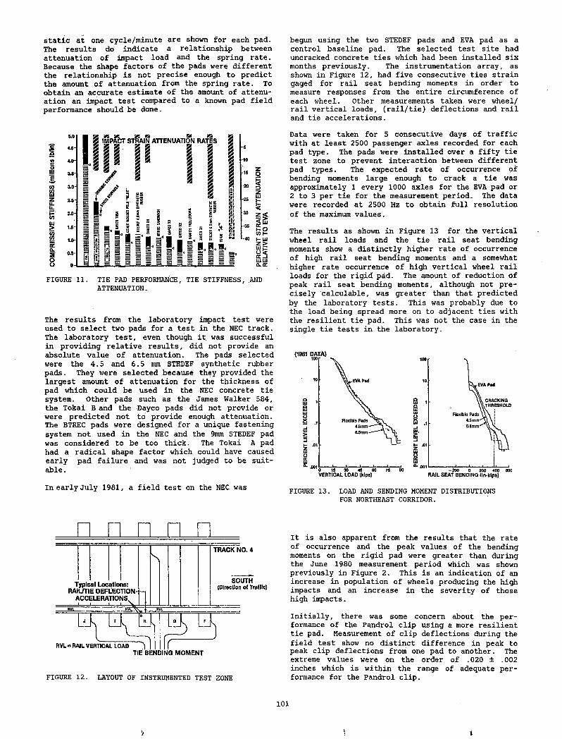
static at one cycle/minute are shown for each pad. The results do indicate a relationship between attenuation of impact load and the spring rate. Because the shape factors of the pads were different the relationship is not precise enough to predict the amount of attenuation from the spring rate. To obtain an accurate estimate of the amount of attenu­ation an impact test compared to a known pad field performance should be done.

begun using the two STEDEF pads and EVA pad as a control baseline pad. The selected test site had uncracked concrete ties which had been installed six months previously. The instrumentation array, as shown in Figure 12, had five consecutive ties strain gaged for rail seat bending moments in order to measure responses from the entire circumference of each wheel. Other measurements taken were wheel/ rail vertical loads, (rail/tie) deflections and rail and tie accelerations.

FIGURE 11. TIE PAD PERFORMANCE, TIE STIFFNESS, AND ATTENUATION.

The results from the laboratory impact test were used to select two pads for a test in the NEC track. The laboratory test, even though it was successful in providing relative results, did not provide an absolute value of attenuation. The pads selected were the 4.5 and 6.5 mm STEDEF synthetic rubber pads. They were selected because they provided the largest amount of attenuation for the thickness of pad which could be used in the NEC concrete tie system. Other pads such as the James Walker 584, the Tokai B and the Dayco pads did not provide or were predicted not to provide enough attenuation. The BTREC pads were designed for a unique fastening system not used in the NEC and the 9mm STEDEF pad was considered to be too thick. The Tokai A pad had a radical shape factor which could have caused early pad failure and was not judged to be suit­able .

Data were taken for 5 consecutive days of traffic with at least 2500 passenger axles recorded for each pad type. The pads were installed over a fifty tie test zone to prevent interaction between different pad types. The expected rate of occurrence of bending moments large enough to crack a tie was approximately 1 every 1000 axles for the EVA pad or 2 to 3 per tie for the measurement period. The data were recorded at 2500 Hz to obtain full resolution of the maximum values.

The results as shown in Figure 13 for the vertical wheel rail loads and the tie rail seat bending moments show a distinctly higher rate of occurrence of high rail seat bending moments and a somewhat higher rate occurrence of high vertical wheel rail loads for the rigid pad. The amount of reduction of peak rail seat bending moments, although not pre­cisely calculable, was greater than that predicted by the laboratory tests. This was probably due to the load being spread more on to adjacent ties with the resilient tie pad. This was not the case in the single tie tests in the laboratory.

In early July 1981, a field test on the NEC was FIGURE 13. LOAD AND SENDING MOMENT DISTRIBUTIONS FOR NORTHEAST CORRIDOR.

D

FIGURE 12. LAYOUT OF INSTRUMENTED TEST ZONE

It is also apparent from the results that the rate of occurrence and the peak values of the bending moments on the rigid pad were greater than during the June 1980 measurement period which was shown previously in Figure 2. This is an indication of an increase in population of wheels producing the high impacts and an increase in the severity of those high impacts.

Initially, there was some concern about the per­formance of the Pandrol clip using a more resilient tie pad. Measurement of clip deflections during the field test show no distinct difference in peak to peak clip deflections from one pad to another. The extreme values were on the order of .020 ± .002 inches which is within the range of adequate per­formance for the Pandrol clip.

101

1V 1

There is no doubt that the use of a more resilient tie pad will improve the performance of concrete ties by reducing the incidence of transverse rail seat cracks and preventing the crack from growing to the point where the tie fails.

Even so, when considering the use of resilient pads several pad performance criteria must be considered. The pad spring rate should be relatively uniform over the entire temperature range for the expected track conditions. ; For .the NEC this would be from -20°F to +130°F. Also the spring rate will change over the life time of the pad, depending upon the material, its shape factor, and the environment. The Japanese National Railways found that the Shinkansen pad increased in stiffness by about two thirds over the 10 year life span of the pad. The pad must also be durable enough to withstand the track environment for the expected life. In order to be sure that the durability will be adequate a reasonable life cycle test should be performed.

The results of this part of the concrete tie cor­relation analysis demonstrate that FAST is not representative of revenue service in one aspect of tie performance. FAST does demonstrate that without high impact loads, concrete ties, in the current AREA design, should last for the expected life of 50 years. To be able to evaluate the degree of impact loading that would affect concrete tie performance and to evaluate the benefits of the use of a resil­ient tie pad with impact loading, wheel irregular­ities would need to be introduced into FAST.

With the acceptance and use of a resilient tie pad in concrete tie_’ track in the U.S., there is no reason not to expect concrete ties as presently designed to last, ‘on the average for the full fifty year expected life.

REFERENCES

1 . American Railway E n gin eerin g A s s o c ia t io n , Manual For Railway E n gin eerin g ; Chapter 10, 1980-81.

2 . "D e s c r ip t io n o f FAST Track and M echanical E xperim en ts," February 1979, TN79-02.

3 . F. E. Dean - "Measurement and C o r r e la t io n A n a ly s is P lan f o r C oncrete T ie and F astener Perform ance A n a ly s is ," t o be p u b lish e d , 1982.

4 . F. E. Dean - "The E f f e c t o f T ie Pad S t i f f n e s s oh the A tten u a tion o f Impact S tra in in C oncrete T i e s ," to be p u b lish ed , 1982.'

QUESTIONS AND ANSWERS

Question 1

Was there any evidence that high speed pass­enger trains caused greater degradation of concrete tie(s) rail seat (cracks) and if so what can be done to allow high speed passenger traffic to operate in mixed traffic concrete ties?

Answer

Yes, there is an abundance of analytical evi­dence that the passenger equipment was the primary cause of the large impact loads and the subsequent large concrete tie bending moments.

Things can be done with immediate benefits. They are:

o Use a resilient tie pad. On the Northeast Corridor a pad of spring rate between 800,000 to 1.1 million lbs/in was recom­mended. Fastener deflections have not proven to be an issue with a resilient pad but pad durability has been. It is ex­pected that the resilient tie pad will last a minimum of 10 years with normal traffic of 20 MGT/year.

o Use of a wheel detector to determine which axles are producing the high impact loads. This can be done with a rail load or bending moment circuit, a real time data analyzer that can identify each axle and each peak above a specified threshold, and a means of transmitting that data to a location where the car(s) can be in­spected.

102

»

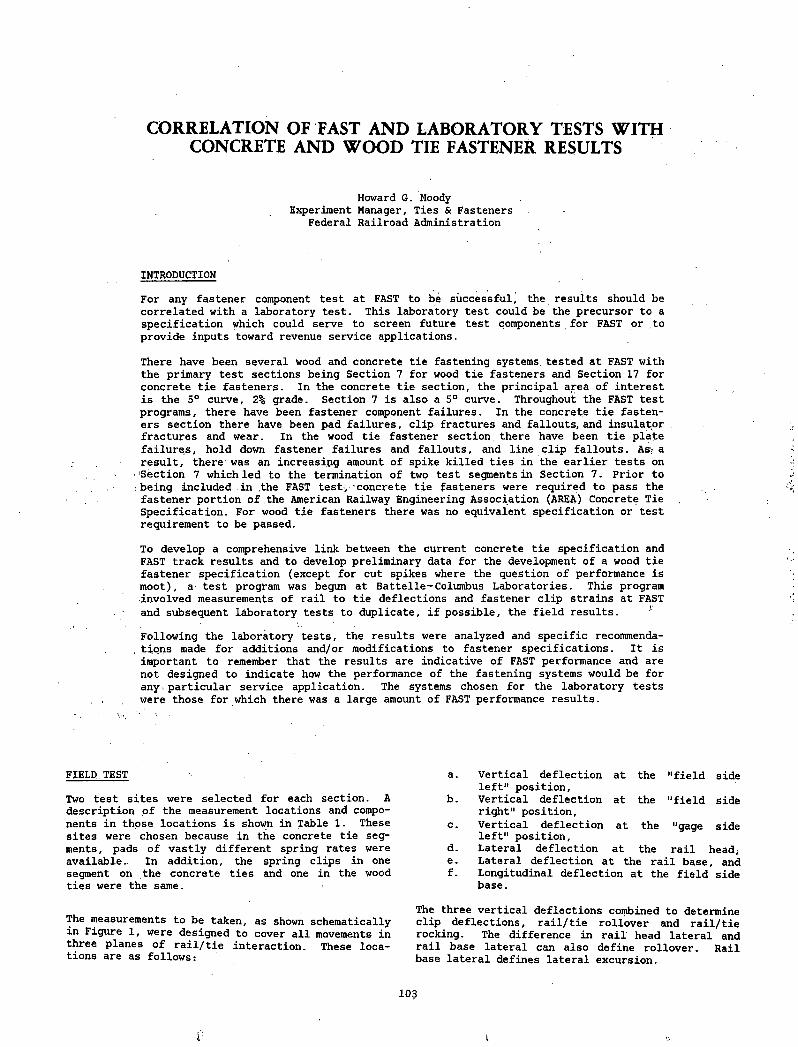
CORRELATION OF FAST AND LABORATORY TESTS WITH CONCRETE AND W OOD TIE FASTENER RESULTS

Howard G. Moody Experiment Manager, Ties & Fasteners

Federal Railroad Administration

INTRODUCTION

For any fastener component test at FAST to be successful, the results should be correlated with a laboratory test. This laboratory test could be the precursor to a specification which could serve to screen future test components for FAST or to provide inputs toward revenue service applications.

There have been several wood and concrete tie fastening systems, tested at FAST with the primary test sections being Section 7 for wood tie fasteners and Section 17 for concrete tie fasteners. In the concrete tie section, the principal area of interest is the 5° curve, 2% grade. Section 7 is also a 5° curve. Throughout the FAST test programs, there have been fastener component failures. In the concrete tie fasten­ers section there have been pad failures, clip fractures and fallouts, and insulator fractures and wear. In the wood tie fastener section, there have been tie plate failures, hold down fastener failures and fallouts, and line clip fallouts. Asy a result, there was an increasing amount of spike killed ties in the earlier tests on 'Section 7 which led to the termination of two test segments in Section 7. Prior to being included in the FAST test, concrete tie fasteners were required to pass, the fastener portion of the American Railway Engineering Association (AREA) Concrete Tie Specification. For wood tie fasteners there was no equivalent specification or test requirement to be passed.

To develop a comprehensive link between the current concrete tie specification and FAST track results and to develop preliminary data for the development of a wood tie fastener specification (except for cut spikes where the question of performance is moot), a test program was begun at Battelle-Columbus Laboratories. This program involved measurements of rail to tie deflections and fastener clip strains at FAST and subsequent laboratory tests to duplicate, if possible, the field results.

Following the laboratory tests, the results were analyzed and specific recommenda­tions made for additions and/or modifications to fastener specifications. It is important to remember that the results are indicative of FAST performance and are not designed to indicate how the performance of the fastening systems would be for any. particular service application. The systems chosen for the laboratory tests were those for which there was a large amount of FAST performance results.

FIELD TEST

Two test sites were selected for each section. A description of the measurement locations and compo­nents in those locations is shown in Table 1. These sites were chosen because in the concrete tie seg­ments, pads of vastly different spring rates were available. In addition, the spring clips in one segment on the concrete ties and one in the wood ties were the same.

The measurements to be taken, as shown schematically in Figure 1, were designed to cover all movements in three planes of rail/tie interaction. These loca­tions are as follows:

a. Vertical deflection left" position.

at the "field side

b. Vertical deflection right" position,

at the "field side

c. Vertical deflection left" position.

at the "gage side

d. Lateral deflection at the rail head,e. Lateral deflection at the rail base, andf. Longitudinal deflection at the field side

base.

The three vertical deflections combined to determine clip deflections, rail/tie rollover and rail/tie rocking. The difference in rail head lateral and rail base lateral can also define rollover. Rail base lateral defines lateral excursion.

103

l t

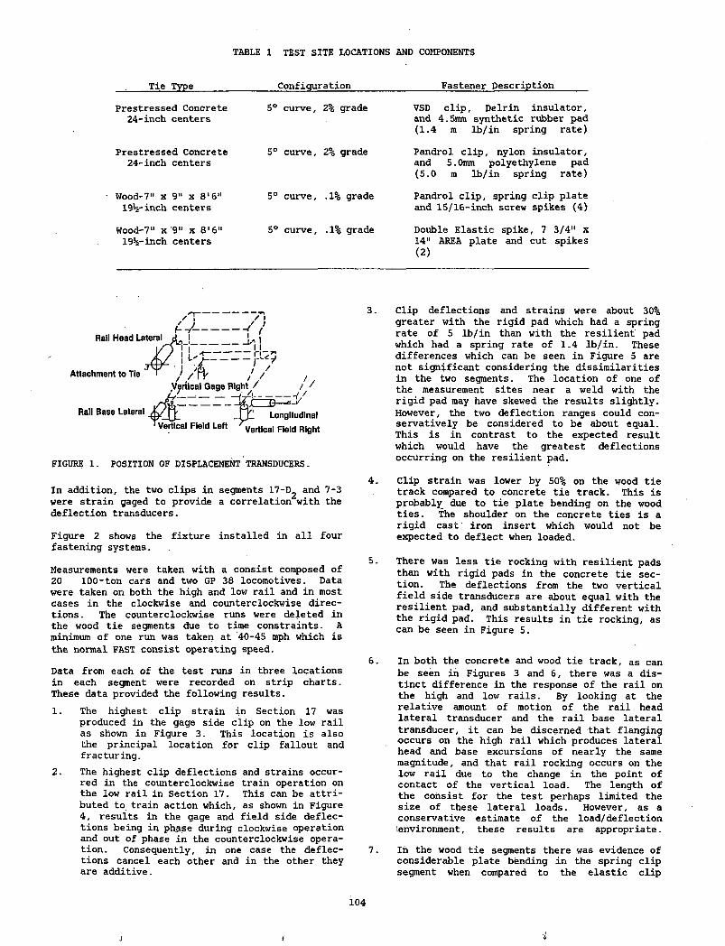
TABLE 1 TEST SITE LOCATIONS AND COMPONENTS

Tie Type Configuration Fastener Description

Prestressed Concrete 24-inch centers

5° curve, 2% grade VSD clip, Delrin insulator, and 4.5mm synthetic rubber pad (1.4 m lb/in spring rate)

Prestressed Concrete 24-inch centers

5° curve, 2% grade Pandrol clip, nylon insulator, and 5.0mm polyethylene pad (5.0 m lb/in spring rate)

Wood-7" x 9" x 8'6" 19%-inch centers

5° curve, .1% grade Pandrol clip, spring clip plate and 15/16-inch screw spikes (4)

Wood-7" x 9" x 8'6" 19Vinch centers

5° curve, .1% grade Double Elastic spike, 7 3/4" x 14" AREA plate and cut spikes (2)

FIGURE 1. POSITION OF DISPLACEMENT TRANSDUCERS.

In addition, the two clips in segments 17-D2 and 7-3 were strain gaged to provide a correlation with the deflection transducers.

Figure 2 shows the fixture installed in all four fastening systems.

Measurements were taken with a consist composed of 20 100-ton cars and two GP 38 locomotives. Datawere taken on both the high and low rail and in most cases in the clockwise and counterclockwise direc­tions. The counterclockwise runs were deleted in the wood tie segments due to time constraints. A minimum of one run was taken at 40-45 mph which is the normal FAST consist operating speed.

Data from each of the test runs in three locations in each segment were recorded on strip charts. These data provided the following results. 1 2 * 41. The highest clip strain in Section 17 was

produced in the gage side clip on the low rail as shown in Figure 3. This location is also the principal location for clip fallout and fracturing.

2. The highest clip deflections and strains occur­red in the counterclockwise train operation on the low rail in Section 17. This can be attri­buted to train action which, as shown in Figure4, results in the gage and field side deflec­tions being in phase during clockwise operation and out of phase in the counterclockwise opera­tion. Consequently, in one case the deflec­tions cancel each other and in the other they are additive.

3. Clip deflections and strains were about 30% greater with the rigid pad which had a spring rate of 5 lb/in than with the resilient pad which had a spring rate of 1.4 lb/in. These differences which can be seen in Figure 5 are not significant considering the dissimilarities in the two segments. The location of one of the measurement sites near a weld with the rigid pad may have skewed the results slightly. However, the two deflection ranges could con­servatively be considered to be about equal. This is in contrast to the expected result which would have the greatest deflections occurring on the resilient pad.

4. Clip strain was lower by 50% on the wood tie track compared to concrete tie track. This is probably due to tie plate bending on the wood ties. The shoulder on the concrete ties is a rigid cast iron insert which would not be expected to deflect when loaded.

5. There was less tie rocking with resilient pads than with rigid pads in the concrete tie sec­tion. The deflections from the two vertical field side transducers are about equal with the resilient pad, and substantially different with the rigid pad. This results in tie rocking, as can be seen in Figure 5.

6. In both the concrete and wood tie track, as can be seen in Figures 3 and 6, there was a dis­tinct difference in the response of the rail on the high and low rails. By looking at the relative amount of motion of the rail head lateral transducer and the rail base lateral transducer, it can be discerned that flanging occurs on the high rail which produces lateral head and base excursions of nearly the same magnitude, and that rail rocking occurs on the low rail due to the change in the point of contact of the vertical load. The length of the consist for the test perhaps limited the size of these lateral loads. However, as a conservative estimate of the load/deflection lenvironment, these results are appropriate.

7. In the wood tie segments there was evidence of considerable plate bending in the spring clip segment when compared to the elastic clip

104

1 i

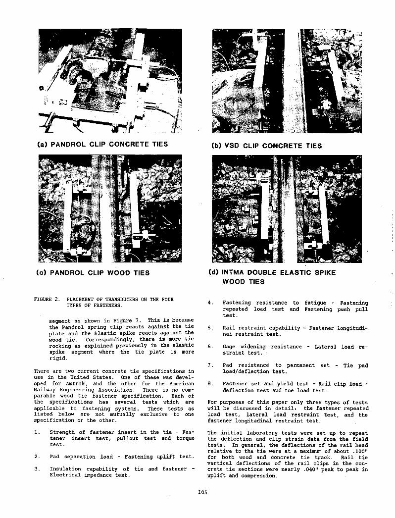
(a ) PANDROL CLIP CONCRETE TIES

(c ) PANDROL CLIP WOOD TIES

FIGURE 2. PLACEMENT OF TRANSDUCERS ON THE FOUR TYPES OF FASTENERS.

segment as shown in Figure 7. This is because the Pandrol spring clip reacts against the tie plate and the Elastic spike reacts against the wood tie. Correspondingly, there is more tie rocking as explained previously in the elastic spike segment where the tie plate is more rigid.

There are two current concrete tie specifications in use in the United States. One of these was devel­oped for Amtrak, and the other for the American Railway Engineering Association. There is no com­parable wood tie fastener specification. Each of the specifications has several tests which are applicable to fastening systems. These tests as listed below are not mutually exclusive to one specification or the other.

1. Strength of fastener insert in the tie - Fas­tener insert test, pullout test and torque test.

2. Pad separation load - Fastening uplift test.

Insulation capability of tie and fastener - Electrical impedance test.

(b ) VSD CLIP CONCRETE TIES

(d) INTMA DOUBLE ELASTIC SPIKE WOOD TIES

4. Fastening resistance to fatigue - Fastening repeated load test and Fastening push pull test.

5. Rail restraint capability - Fastener longitudi-. nal restraint test.

6. Gage widening resistance - Lateral load re­straint test.

7. Pad resistance to permanent set - Tie pad load/deflection test.

8. Fastener set and yield test - Rail clip load - deflection test and toe load test.

For purposes of this paper only three types of tests will be discussed in detail: the fastener repeatedload test, lateral load restraint test, and the fastener longitudinal restraint test.

The initial laboratory tests were set up to repeat the deflection and clip strain data from the field tests. In general, the deflections of the rail head relative to the tie were at a maximum of about .100" for both wood and concrete tie track. Rail tie vertical deflections of the rail clips in the con­crete tie sections were nearly .040" peak to peak in uplift and compression.

3.

105

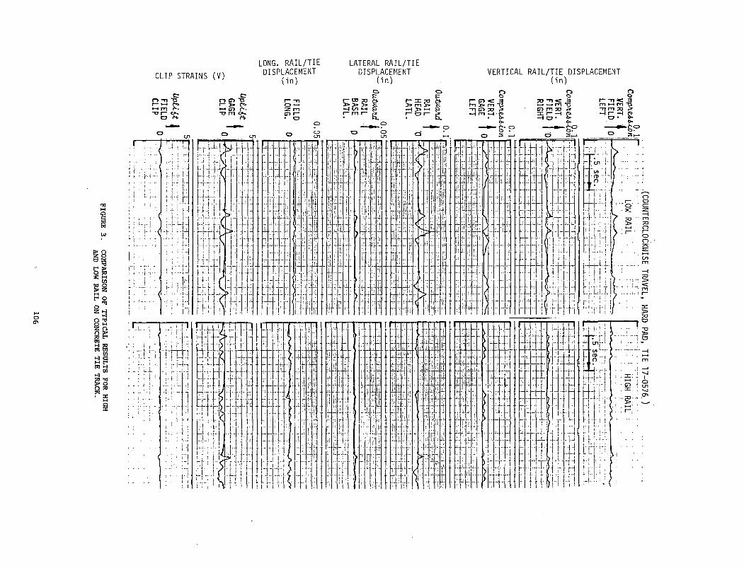
FIGURE 3. COMPARISON OF TYPICAL RESULTS FOR HIGH AND LOW RAIL ON CONCRETE TIE TRACK.

CLIP STRAINS (V)

LONG. RAIL/TIE DISPLACEMENT

(in)

LATERAL RAIL/TIEDISPLACEMENT

(in)VERTICAL RAIL/TIE DISPLACEMENT

(in)

.(COUNTERCLOCKWISE TRAVEL, HARD PAD,

TIE 17-0576.)

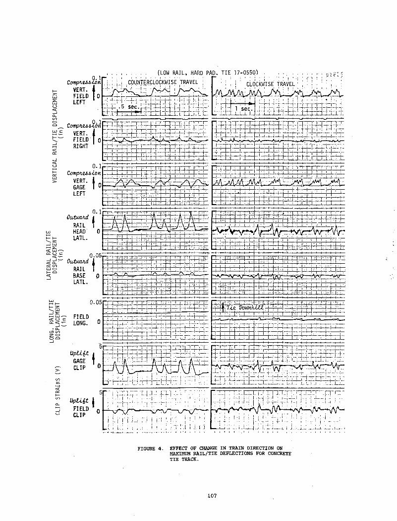
FIGURE 4. EFFECT OF CHANGE IN TRAIN DIRECTION ONMAXIMUM RAIL/TIE DEFLECTIONS FOR CONCRETE TIE TRACK.

107

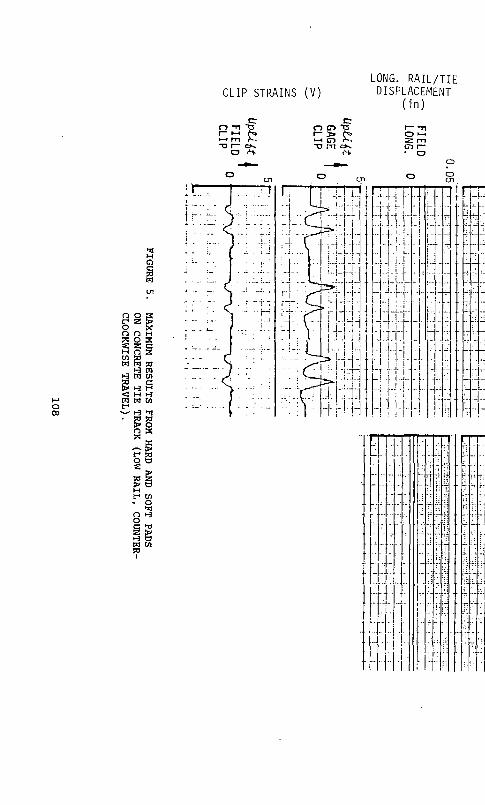
ON CONCRETE T

IE TRACK

(LOW R

AIL

, COU

NTER­

CLOCKWISE

TRA

VE

L).

HC§PItn

M3

50towClr*

50O2

JOo

t)wo»oH>0gw

LONG. RAIL/TIECLIP STRAINS (V) DISPLACEMENT

(in)

cn r- • o

Ooocn

i r

i ii\

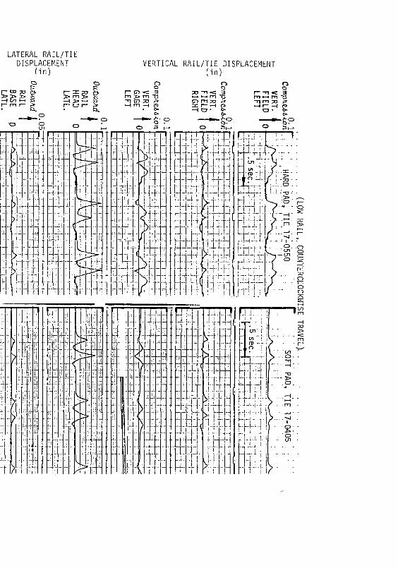
LATERAL RAIL/TIE DISPLACEMENT

(in)VERTICAL RAIL/TIE DISPLACEMENT

(in)

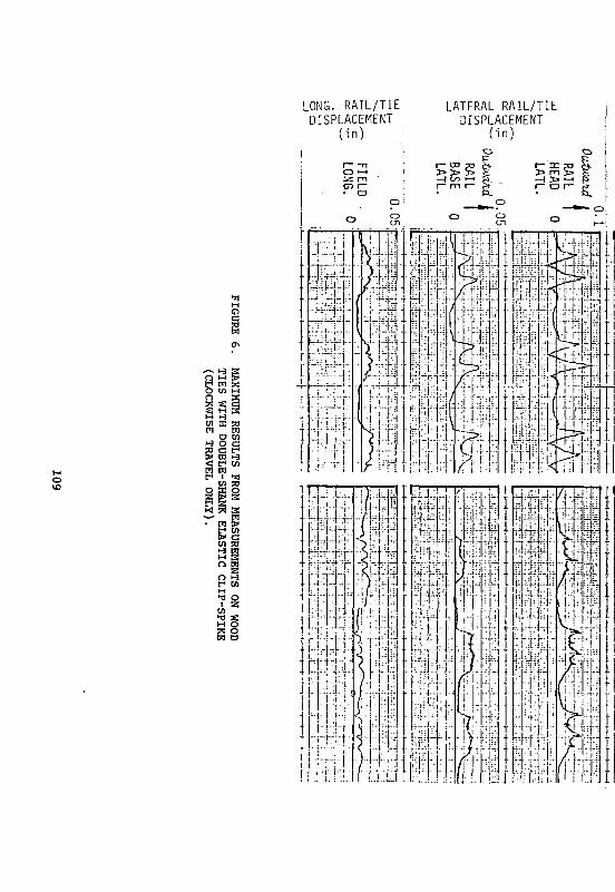
109

oG50M

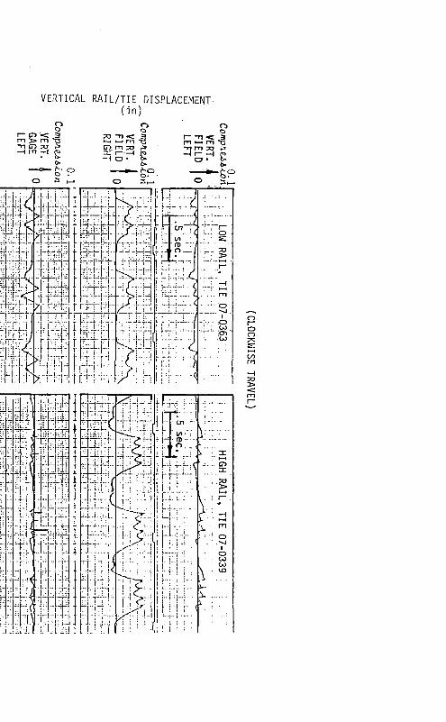
VERTICAL RAIL/TIE DISPLACEMENT-(in)

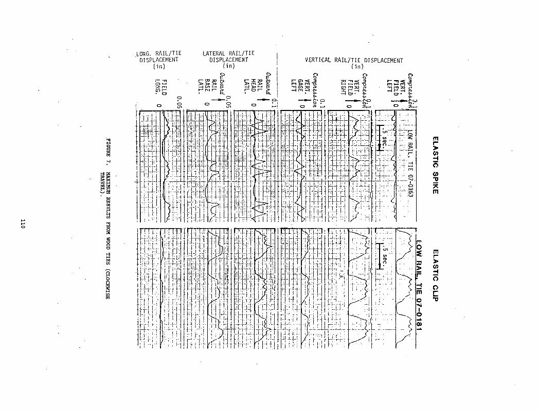
FIGURE 7. MAXIMUM RESULTS FROM WOOD TIES (CLOCKWISE TRAVEL).

ELA

STIC

SP

IKE

E

LAS

TIC C

LIP

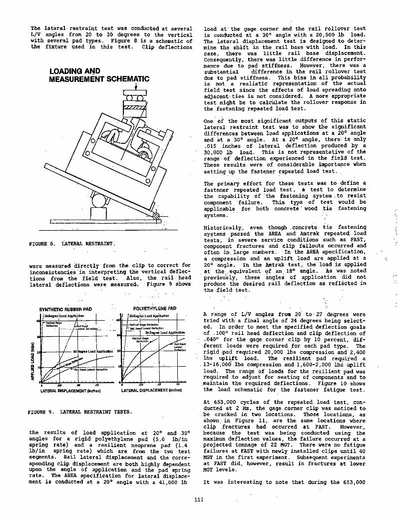
The lateral restraint test was conducted at several L/V angles from 20 to 30 degrees to the vertical with several pad types. Figure 8 is a schematic of the fixture used in this test. Clip deflections

LOADING AND MEASUREMENT SCHEMATIC

FIGURE 8. LATERAL RESTRAINT.

were measured directly from the clip to correct for inconsistencies in interpreting the vertical deflect tions from the field test. Also, the rail head lateral deflections were measured. Figure 9 shows

SYNTHETIC RUBBER PAD POLYETHYLENE PAD

FIGURE 9. LATERAL RESTRAINT TESTS.

the results of load application at 20° and 30° angles for a rigid polyethylene pad (5.0 lb/in spring rate) and a resilient neoprene pad (1.4 lb/in spring rate) which are from the two testsegments. Sail lateral displacement and the corre­sponding clip displacement are both highly dependent upon the angle of application and the pad spring rate. The AREA specification for lateral displace­ment is conducted at a 20° angle with a 41,000 lb

load at the gage corner and the rail rollover test is conducted at a 30° angle with a 20,500 lb load. The lateral displacement test is designed to deter­mine the shift in the rail base with load. In this case, there was little rail base displacement. Consequently, there was little difference in perform mance due to pad stiffness. However, there was a substantial difference in the rail rollover test due to pad stiffness. This bias in all probability is not a realistic representation of the actual field test since the effects of load spreading onto adjacent-ties is not considered. A more appropriate test might be to calculate the rollover response in the fastening repeated load test.

One of the most significant outputs of this static lateral restraint test was to show the significant differences between load applications at a 20° angle and at a 30° angle. At a 20° angle, there is only .015 inches of lateral deflection produced by a 30,000 lb load. This is not representative of the range of deflection experienced in the field test. These results were of considerable importance when setting up the fastener repeated load test. ,

The primary effort for these tests was to define a fastener repeated load test, a test to determine- the capability of the fastening system , to resist component failure. This type of test would be applicable for both concrete wood tie fastening systems.

Historically, even though concrete tie fastening systems passed the AREA and' Amtrak repeated load tests, in severe service conditions such as FAST, component fractures and clip fallouts occurred and often in large numbers. In the AREA specification, a compression and an uplift load are applied at a 20° angle. In the Amtrak test, the load is applied at the equivalent of an 18° angle. As was noted previously, these angles of application did not produce the desired rail deflection as reflected in the field test.

A range of L/V angles from 20 to ■ 27 degrees were tried with a final angle of 24 degrees being select­ed. In order to meet the specified deflection goals of .100" rail head deflection and clip deflection of .040" for the gage corner clip by 10 percent, dif­ferent loads were required for each pad type. The rigid-pad required 20,000 lbs compression and 2,400 lbs uplift load. The resilient pad required a 13-16,000 lbs compression and 1,600-2,000 lbs uplift load. The range of loads for the resilient pad was required to adjust for seating of components and to .maintain the required deflections. Figure 10 shows the load schematic for the fastener fatigue test.

At 653,000 cycles of the repeated load test, con­ducted at 2 Hz, the gage corner clip was noticed to be -cracked in two locations. Those locations, as shown in Figure 11, are the same locations where clip fractures had occurred at FAST. However, because the test was being conducted using the maximum deflection values, the failure occurred at a projected tonnage of 22 MGT. There were no fatigue failures at FAST with newly installed clips until 40 MGT in the first experiment. Subsequent experiments at FAST did, however, result in fractures at lower MGT levels.

It was interesting to note that during the 653,000

111

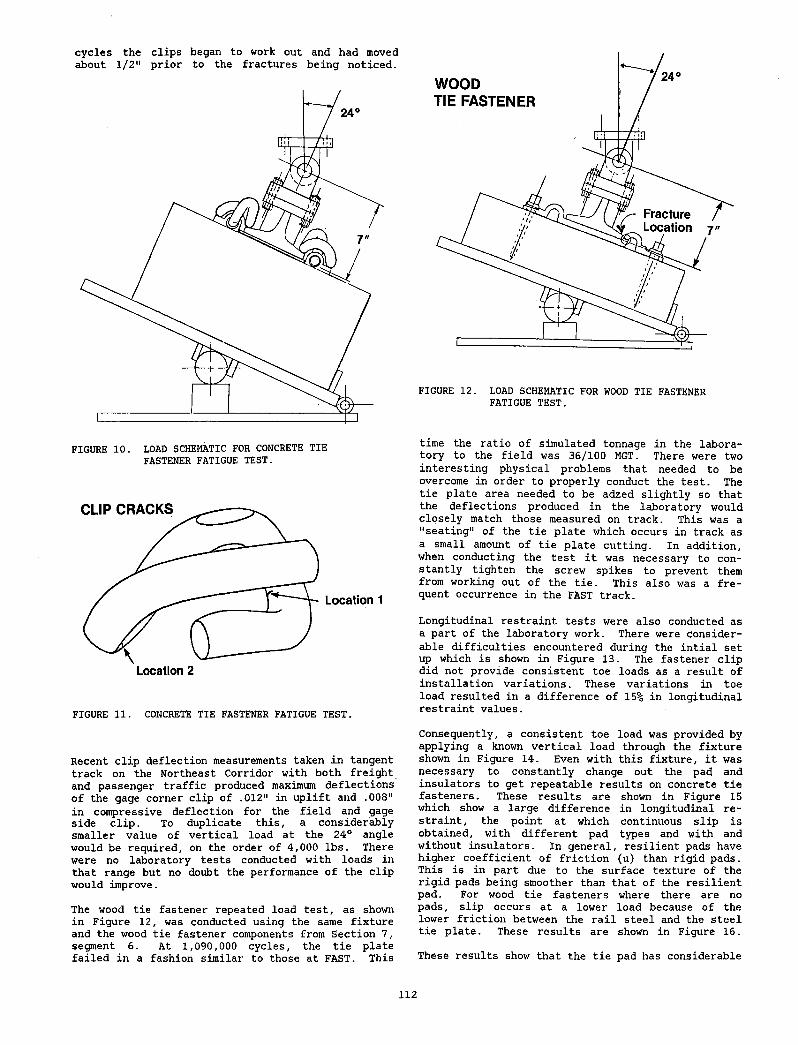
cycles the clips began to work out and had moved about 1/2" prior to the fractures being noticed.

FIGURE 12. LOAD SCHEMATIC FOR WOOD TIE FASTENER FATIGUE TEST.

FIGURE 10. LOAD SCHEMATIC FOR CONCRETE TIE FASTENER FATIGUE TEST.

FIGURE 11. CONCRETE TIE FASTENER FATIGUE TEST.

Recent clip deflection measurements taken in tangent track on the Northeast Corridor with both freight and passenger traffic produced maximum deflections of the gage corner clip of .012" in uplift and .008" in compressive deflection for the field and gage side clip. To duplicate this, a considerably smaller value of vertical load at the 24° angle would be required, on the order of 4,000 lbs. There were no laboratory tests conducted with loads in that range but no doubt the performance of the clip would improve.

The wood tie fastener repeated load test, as shown in Figure 12, was conducted using the same fixture and the wood tie fastener components from Section 7, segment 6. At 1,090,000 cycles, the tie plate failed in a fashion similar to those at FAST. This

time the ratio of simulated tonnage in the labora­tory to the field was 36/100 MGT. There were two interesting physical problems that needed to be overcome in order to properly conduct the test. The tie plate area needed to be adzed slightly so that the deflections produced in the laboratory would closely match those measured on track. This was a "seating" of the tie plate which occurs in track as a small amount of tie plate cutting. In addition, when conducting the test it was necessary to con­stantly tighten the screw spikes to prevent them from working out of the tie. This also was a fre­quent occurrence in the FAST track.

Longitudinal restraint tests were also conducted as a part of the laboratory work. There were consider­able difficulties encountered during the intial set up which is shown in Figure 13. The fastener clip did not provide consistent toe loads as a result of installation variations. These variations in toe load resulted in a difference of 15% in longitudinal restraint values.

Consequently, a consistent toe load was provided by applying a known vertical load through the fixture shown in Figure 14. Even with this fixture, it was necessary to constantly change out the pad and insulators to get repeatable results on concrete tie fasteners. These results are shown in Figure 15 which show a large difference in longitudinal re­straint, the point at which continuous slip is obtained, with different pad types and with and without insulators. In general, resilient pads have higher coefficient of friction (u) than rigid pads. This is in part due to the surface texture of the rigid pads being smoother than that of the resilient pad. For wood tie fasteners where there are no pads, slip occurs at a lower load because of the lower friction between the rail steel and the steel tie plate. These results are shown in Figure 16.

These results show that the tie pad has considerable

112

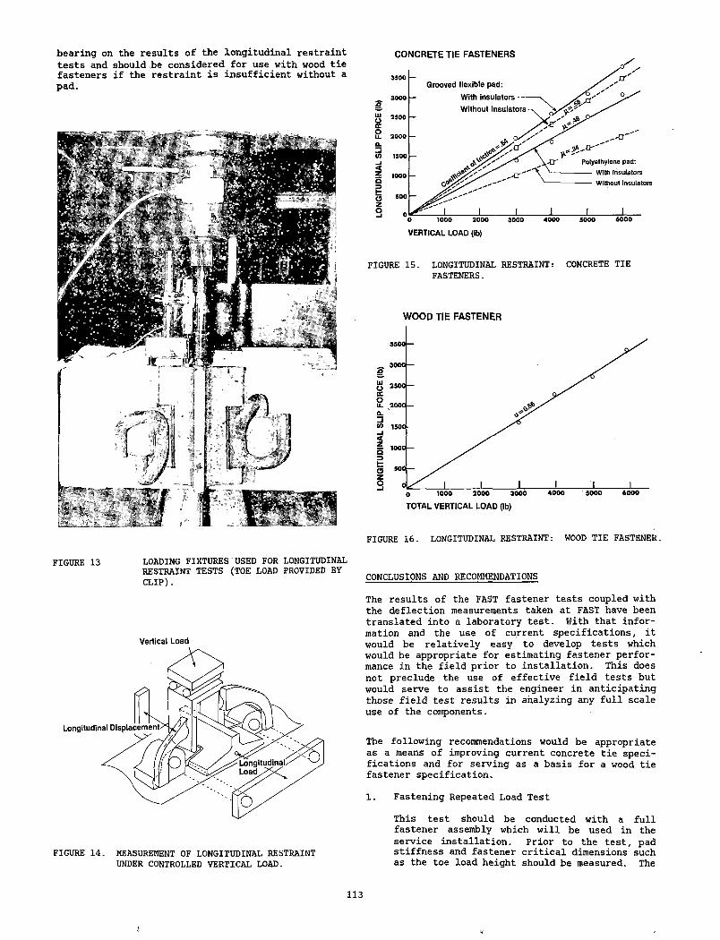
bearing on the results of the longitudinal restraint tests and should ibe considered for use with wood tie fasteners if the restraint is insufficient without a pad.

CONCRETE TIE FASTENERS

FIGURE 15. LONGITUDINAL RESTRAINT: CONCRETE TIEFASTENERS.

W OOD TIE FASTENER

FIGURE 16. LONGITUDINAL RESTRAINT: WOOD TIE FASTENER.

FIGURE 13 LOADING FIXTURES USED FOR LONGITUDINALRESTRAINT TESTS (TOE LOAD PROVIDED BY CLIP).

Vertical Load

FIGURE 14. MEASUREMENT OF LONGITUDINAL RESTRAINT UNDER CONTROLLED VERTICAL LOAD.

CONCLUSIONS AND RECOMMENDATIONS * 1

The results of the FAST fastener tests coupled with the deflection measurements taken at FAST have been translated into a laboratory test. With that infor­mation and the use of current specifications, it would be relatively easy to develop tests which would be appropriate for estimating fastener perfor­mance in the field prior to installation. This does not preclude the use of effective field tests but would serve to assist the engineer in anticipating those field test results in analyzing any full scale use of the components.

The following recommendations would be appropriate as a means of improving current concrete tie speci­fications and for serving as a basis for a wood tie fastener specification.

1. Fastening Repeated Load Test

This test should be conducted with a full fastener assembly which will be used in the service installation. Prior to the test, pad stiffness and fastener critical dimensions such as the toe load height should be measured. The

113

fastener assembly set up at 24-27° angle to the vertical, apply an uplift load and a compres­sion load large enough to produce a deflection equivalent to the maximum expected lateral rail head deflection in track. For FAST this would mean -.010" to +.100".

This test should be conducted for 3,000,000 cycles at a maximum rate of 2 Hz. Following the test an evaluation of pad stiffness, clip critical dimension and component integrity (i.e., no fracturing of any component) should be made.

2. Fastening Lateral Load Restraint

The existing test as defined in Chapter 10 of the AREA Manual is sufficient but the rollover test should be deleted. The fastening repeated load test can serve as a substitute for that test.

3. Fastening Longitudinal Restraint Test

This test should be conducted under dynamic load conditions of 15,000 lbs vertical com­pression and 2,000 lbs vertical uplift at 2 Hz using the current static restraint test as outlined in the AREA Specification. The static test should be done on at least four new fas­tener assemblies, followed by a dynamic test on each assembly. Value of longitudinal force applied should be recorded up to the point of continuous slippage. Acceptance of a fastening system is predicated upon the specific in-track conditions.

REFERENCES

1 . F. E. Dean - "Measurements o f R a i l /T ie D e f le c ­t io n s and F astener C lip S tra in s a t FAST," O cto ­b e r 1981, FRA/TTC-81/03.

2 . F. E. Dean - In v e s t ig a t io n o f R a il F a sten er Perform ance Requirem ents, t o be p u b lis h e d ,

. 1982.

3 . American Railway' E n gin eering A s s o c ia t io n Manual f o r Recommended P r a c t ic e s , -Volume I , Chapter 10.

114

v1

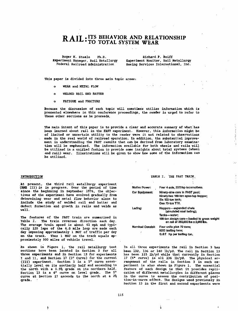
f t A T T - ITS BEHAVIOR a n d r e l a t i o n s h i p xv.rn.La • TO TOTAL SYSTEM WEAR

Roger K. Steele Ph.D. Experiment Manager, Rail Metallurgy

Federal Railroad Administration

Richard.P. ReiffExperiment Monitor, Rail Metallurgy Boeing Services International, Inc.

This paper is divided into three main topic areas:

o WEAR and METAL FLOW

O WELDED RAIL END BATTER

o FATIGUE and FRACTURE

Because the discussion of each topic will sometimes utilize information which is presented elsewhere in this conference proceedings, the reader is urged to refer to these other sections as he proceeds.

The main intent of this paper is to provide a clear and accurate summary of what'has been learned about rail in the FAST experiment. However, this information might be of limited or uncertain utility to the reader were it not related to observations made in the real world of railroad operation. In addition, the substantial improve­ment in understanding the FAST results that can be derived from laboratory examina­tion will be emphasized. The information available for both wheels and rails will be utilized in a unified fashion to provide some insights about total systems (wheel and rail) wear. Illustrations will be given to show how some of the information can be utilized.

INTRODUCTION TABLE I. THE FAST TRAIN.

At present, the third rail metallurgy experiment (RME III) is in progress. Over the period of time since the beginning in September 1976, the objec­tives of the experiment have evolved gradually from determining wear and metal flow behavior alone to include the study of welded rail end batter and defect formation and growth in rails and welds as well.

The features of the FAST train are summarized in Table I. The train reverses direction each day. The average train speed is about 41 mph and typi­cally 120 laps of the 4.8 mile loop are made each day imposing approximately 1 MGT of traffic per day on the track. Thus 1 MGT on the track equals ap­proximately 500 miles of vehicle travel.

As shown in Figure 1, the rail metallurgy test sections have been located in Section 3 for all three experiments and in Section 13 for experiments I and II, and Section 17 (5° Curve) for the current (III) experiment. Section 3 is a 5° curve essen­tially level on its southerly half and ascending to the north with a 0.9% grade on its northern half. Section 13 is a 4° curve on level grade. The 5° curve a t , Section 17 ascends to the north at a 2% grade.

Motive Power:

Car Equipment:

Lading:

Nominal Consist:

Four 4-axle, 2000hp locomotives.

Ninety-nine cars in FAST pool;Ninety-two 100-ton open-top hopper;Six 100-ton tank;One 70-ton TTX.

Hoppers— expanded shale (simulated coal lading);

Tanks— water;100-ton design cars— loaded to gross weight

on rail of 263,000lbs ±2,000lbs.

Four units plus 70 cars;9200 trailing tons;0 .8 7 hp per trailing ton.

In all three experiments the rail in Section 3 has been 132, 136 or 140 lb/yd. The rail in Section 13 has been 115 lb/yd while that currently in Section 17 (5° curve) is all 136 lb/yd. The physical ar­rangement of the rails in Section 3 in each ex­periment is also shown in Figure 1. The essential feature of each design is that it provides repli­cation of different metallurgies in different places in the curve to assess the contribution of posi- tion-in-curve effect. The designs used previously in Section 13 in the first and second experiments were

115

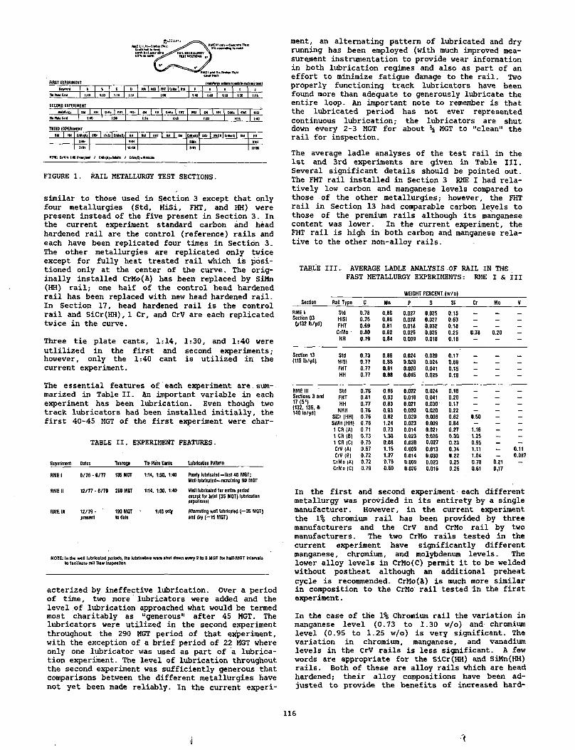
NlUdurgt ltd [ KH Cl Hi | FHT HiSI I ltd I KH C>K« | FHT HOI l ltd 1 KH ClKI | (HI WStTunmCiN t :40 1:M 1:14 !:ll tjn 1:14 1:40

THUD EXPEIIIMiHTSI4 1 HH CittMA) SJCr | IKCi I &M«C) HH Std | FHT 1 HH | til W **) Sib 1 1KCH 1 CrHMCI 1 Sid KH

SiMn NHH M i NHH2/11 11/M 1/11 12/10

KOn: Cl« H 1:40 IhMlKMl / &H«(4)-bU!lc / CtlU(C)-WMlM

FIGURE 1. RAIL METALLURGY TEST SECTIONS.

similar to those used in Section 3 except that only four metallurgies (Std, HiSi, FHT, and HH) were present instead of the five present in Section 3. In the current experiment standard carbon and head hardened rail are the control (reference) rails and each have been replicated four times in Section 3. The other metallurgies are replicated only twice except for fully heat treated rail which is posi­tioned only at the center of the curve. The orig­inally installed CrMo(A) has been replaced by SiMn (HH) rail; one half of the control head hardened rail has been replaced with new head hardened rail. In Section 17, head hardened rail is the control rail and SiCr(HH), 1 Cr, and CrV are each replicated twice in the curve.

Three tie plate cants, 1:14, 1:30, and 1:40 were utlilized in the first and second experiments; however, only the 1:40 cant is utilized in the current experiment.

The essential features of each experiment are. sum­marized in Table II. An important variable in each experiment has been lubrication. Even though two track lubricators had been installed initially, the first 40-45 MGT of the first experiment were char-

TABLE II. EXPERIMENT FEATURES.

Experiment Dates Tonnage Tie Plate Cants Lubrication Pattern

RME 1 8/76 * B/77 135 MGT 1:14, 1:30, 1:40 Poorly lubricated—first 45 MGT; Wen lubricated—remaining 90 MGT

RME II 12/77 - 6/79 2S0 MGT 1:14, 1:30, 1:40 Well lubricated for entire period except lor brief (35 MGT) lubrication experiment

RME III 12/79 • . present

190 MQT to date

1:40 only Alternating well lubricated (~3S MGT) and dry (-15 MGT)

NOTE: In the w e ll lubrica ted periods, the lubricators ware shut down svary 2 to 3 MOT lo r ha lf-M G T Intervals to fe e ilita le rati Daw Inspection

acterized by ineffective lubrication. Over a period of time, two more lubricators were added and the level of lubrication approached what would be termed most charitably as “generous" after 45 MGT. The lubricators were utilized in the second experiment throughout the 290 MGT period of that experiment, with the exception of a brief period of 22 MGT where only one lubricator was used as part of a lubrica­tion experiment. The level of lubrication throughout the second experiment was sufficiently generous that comparisons between the different metallurgies have not yet been made reliably. In the current experi­

ment, an alternating pattern of lubricated and dry running has been employed (with much improved mea­surement instrumentation to provide wear information in both lubrication regimes and also as part of an effort to minimize fatigue damage to the rail. Two properly functioning track lubricators have been found more than adequate to generously lubricate the entire loop. An important note to remember is that the lubricated period has not ever represented continuous lubrication; the lubricators are shut down every 2-3 MGT for about h MGT to "clean" the rail for inspection.

The average ladle analyses of the test rail in the 1st and 3rd experiments are given in Table III. Several significant details should be pointed out. The FHT rail installed in Section 3 RME I had rela­tively low carbon and manganese levels compared to those of the other metallurgies; however, the FHT rail in Section 13 had comparable carbon levels to those of the premium rails although its manganese content was lower. In the current experiment, the FHT rail is high in both carbon and manganese rela­tive to the other non-alloy rails.

TABLE III. AVERAGE LADLE ANALYSIS OF RAIL IN THEFAST METALLURGY EXPERIMENTS: RME I & III

WEIGHT‘ PERCENT(w/o)Section Rail Type C Mn P S SI Cr Mo V

RME I Std 0.78 0.86 0.027 0.025 0.15 _ _Section 03 HiSi 0.76 0.86 0.028 0.027 0.63 _ _fe132 Ib/yd) FHT 0.69 0.81 0.018 0.032 0.16 — — —

CrMo ' 0.80 0.82 0.026 0.025 0.25 0.78 0.20 —HH 0.79 0.84 0.009 0.018 0.16 - - -

Section 13 Std 0.73 0.86 0.024 0.020 0.17(115 (b/yd) HiSi 0.77 0.88 0.029 0.024 0.68 _ _

FHT 0.77 0.81 0.020 0.041 0.15 _ _ —HH 0.77 0.88 0.015 0.025 0.18 ~ —

RME III Std 0.76 0.86 0.022 0.024 0.18 _ _ _Sections 3 and FHT 0.B1 0.93 0.018 0.041 0.20 — _ —1 / (b w) HH 0.77 0.83 0.021 0.030 0.17 — — —

NHH 0.76 0.93 0.020 0.020 0.22 _ — —

SiCr (HH) . 0.76 0.82 0.020 0.006 0*62 0.50 — —

SiMn(HH) 0.76 1.24 0.023 0.009 0.84 — — —1 CR (A) 0.71 0.73 0.014 0.021 0.27 1.16 — —1 CR (B) 0.73 1.30 0.023 0.026 0.30 1.25 — —1 CR (C) 0.75 0.8B 0.030 0.027 0.23 0.95 — —

CrV (A) 0.67 1.15 0.009 0.013 0.34 1.11 — 0.11CrV (8) 0.72 1.27 0.014 0.030 0.22 1.04 — 0.087

CrMo (A) 0.72 0.79 0.009 0.023 0.25 0.78 0.21 —

CrMo (C) 0.79 0.60 0.026 0.016 0.26 0.61 Q.,17

In the first and second experiment each different metallurgy was provided in its entirety by a single manufacturer. However, in the current experiment the 1% chromium rail has been provided by three manufacturers and the CrV and CrMo rail by two manufacturers. The two CrMo rails tested in the current experiment have significantly different manganese, chromium, and molybdenum levels. The lower alloy levels in CrMo(C) permit it to be welded without postheat although an additional preheat cycle is recommended. CrMo (A) is much more similar in composition to the CrMo’ rail tested In the first experiment.

In the case of the 1% Chromium rail the variation in manganese level (0.73 to 1.30 w/o) and chromium level (0.95 to 1.25 w/o) is very significant. The variation in chromium, manganese, and vanadium levels in the CrV rails is less significant. A few words are appropriate for the SiCr(HH) and SiMn(HH) rails. Both of these are alloy rails which are head hardened; their alloy compositions have been ad­justed to provide the benefits of increased hard-

1 1 6

4 't

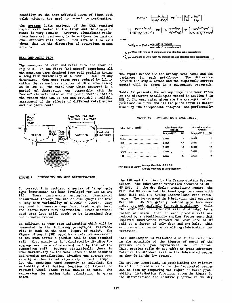
enability at the heat affected zones of flash butt welds without the need to resort to postheating.

The average ladle analyses of the AREA standard carbon rail tested in the first and third experi­ments is very similar. However, significant varia­tions have occurred among ladle analyses for indivi­dual standard rail heats. Much more, will be said about this in the discussion of equivalent carbon effects.

WEAR AMD METAL FLOW

The measures of wear and metal flow are shown in Figure 2. In the first {and second) experiment all the measures were obtained from rail profiles having a long term variability of ±0.020" - 0.030" on any dimension. When wear rates were reduced by lubri­cation (by as much as a factor of 10 in some cases) as in RME II, the total wear which occurred in a period of. observation was comparable with the "noise" characteristic of the profilometer; This is the reason that RME II has not provided a reliable assessment of the effects of different metallurgies and tie plate cants.

To correct this problem, a series of "snap" gage type instruments has been developed for use in RME III. These instruments accomplish dimensional measurement through the use of dial guages and have a long term variability of ±0.002" - 0.003". They are used to generate gage face, head heigth loss, and lateral metal flow information. Cross sectional head area loss still needs to be determined from profilometer traces.

In addition to wear rate information which will be presented in the following paragraphs, reference will be made to the term "figure of merit". The figure of merit (FM) provides a relative assessment of how much better a premium rail is than standard rail. Most simply is is calculated by dividing-the average wear rate of standard rail by that of the comparison rail. Because statistically there is some variability in the wear rates of both standard and premium metallurgies, dividing one average wear rate by another is not rigorously correct. Proper­ly, the technique used commonly to calculate the probability distribution function of lateral to vertical wheel loads ratio whould be used. The expression for making this calculation is given below.

PDF (Z) = f--------5<_5lJ exp { - ' / . [ ( * * Y + / « * ) ’ljT (O yJ- Z ’<V)J I 1 \axl l<Jy/

+ r exp ( - V 4 | er( [ Mx<V + ZMy(fxJ_ 1

( \ [2 ti (Gy>+ Z aax2)*'I J ' (ay’ + Z ‘ax,)> (<rxOy \J(2<ryi + Z !tfx i)J

where:

wear rate o l Std railZ = Figure of Merit =• .wear rate of comparison rail

P x , y = W ear rate means of comparison and standard rails, respectively

y = Variances of wear rates for comparison and standard rails, respectively

The inputs needed are the average wear rates and the variances for each metallurgy. The difference between the simple method and the rigorously correct method will be shown in a subsequent paragraph.

Table IV presents the average gage face wear rates of the different metallurgies tested in Section 3 in RME I. The wear rates given are the averages for all positions-in-curve and all tie plate cants as deter­mined by two independent analyses, one performed by

TABLE IV. AVERAGE GAGE FACE LOSS.

SECTION 3: RM E I Below Lubrication Above LubricationTransition Transition

___________________________________ Rate, (n/MGT FM Rate, In/MGT FM

Std................................................... 0.0086 1 0.0012 1

HlSi.................................................. 0.0061 1.4 0.0012 1

FHT................................................. 0.0059 1.5 0.0011 1.1

CrMo................................................ 0.0041 . 2.1 0.0011 1.1

HH................................................... 0.0032 2.7 0.0007 1.5

FM = Figure of Merit = Average Wear Rate of Std Rail Average Wear Rate of Comparison Rail

the AAR and the other by the Transportation Systems Center. The lubrication transition occurred at 40 - 45 MGT. In the dry (below transition) regime, the CrMo and HH exhibited the least gage face wear with both HiSi and FHT having intermediate wear resis­tance. The improvement in lubrication that occurred near 40 - 45 MGT greatly reduced gage face wear rates but not uniformly for each metallurgy. While the wear rate of standard rail diminished by a factor of seven, that of each premium rail was reduced by a significantly smaller factor such that improved lubrication reduced the wear rate of HH rail by a factor of only four and one half. This occurrence is termed a metallurgy:lubrication in­teraction.

This interaction is reflected also in the reduction in the magnitude of the figures of merit of the premium rails upon improvement in lubrication. Thus, premium rails do not offer as great advantage relative to standard rail in the lubricated regime as they do in the dry regime.

The greater uncertainty in establishing the relative benefit of premium rails in the lubricated regime can be seen by comparing the figure of merit prob­ability distribution functions shown in Figure 3. The distributions are relatively narrow in the dry

117

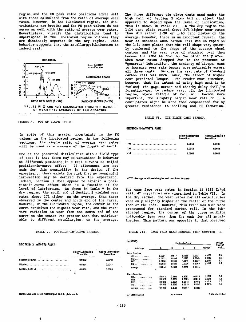
regime and the FM peak value positions agree well with those calculated from the ratio of average wear rates. However, in the lubricated regime, the dis­tributions are broader and the FM peak values do not agree as well with the ratio of average wear rates. Nevertheless, clearly the distributions tend to superimpose in the lubricated regime whereas they are distinctly separate in the dry regime. This behavior suggests that the metallurgy:lubrication is indeed real.

DRY.TRACK

V A L U E S IN ( ) A R E F M 's C A L C U L A T E D F R O M T H E R A T IO O F W E A R R A T E A V E R A G E S O F T S C A N A L Y S IS

FIGURE 3. PDF OF-SLOPE RATIOS.

In spite of this greater uncertainty in the FM values in the lubricated regime, in the following sections, the simple ratio of average wear rates will be used as a measure of the figure of merit.

One of the potential difficulties with a field type of test is that there may be variations in behavior at different positions.in a test curve-a so called position-in-curve effect. If allowances are not made for this possibility in the design of the experiment, there exists the risk that no meaningful information may be derived from the experiment. Indeed, Section 3 does appear to exhibit a posi- tion-in-curve effect which is a function of the level of lubrication. As shown in Table V in the dry regime, the south end of Section 3 yielded wear rates about 20% higher, on the average, than those observed in the center and north end of the curve. However, in the lubricated regime, the center of the curve exhibited the highest wear rate, and the rela­tive variation in wear from the south end of the curve to the center was greater than that attribut­able to different metallurgies, on the average.

TABLE V. POSITION-IN-CURVE EFFECT.

SECTION 3 (In/MGT): RME 1

Below Lubrication . Above Lubrication' .____________________________________________Transition____________ Transition

Section 02 E n d .............................................................. 0.0052 0.0012M iddle.............................................................................. 0.0054 0.0017

Section 04 E n d ........ ...................................................... 0.0064 0.0006

NOTE: Average of all metallurgies and tie plate cants

The three different tie plate cants used under the high rail of Section 3 also had an effect that appeared to depend upon the level of lubrication; this is shown in Table Vi. In the dry regime the 1:14 cant plate caused about 20% higher wear rates than did either 1:30 or 1:40 cant plates on the average. However, there is an important caveat: thewear of standard AREA carbon rail was so rapid on the 1:14 cant plates that the rail shape very quick­ly conformed to the shape of the average wheel contour and the wear rate of standard rail then became the same as that on the other tie plates. When wear rates dropped due to the presence of "generous" lubrication, the tendency of steeper cant to increase wear rate became more noticeable across all three cants. Because the wear rate of standard carbon rail was much lower, the effect of higher cant persisted longer. The reader must remember, however, that the intent of using high cant is to "unload" the gage corner and thereby delay shell/TD formation— not to reduce wear. In the lubricated regime, where fatigue of rail will become more important, the slightly higher wear rate on 1:14 cant plates might be more than compensated for by greater resistance to shelling and TD formation.

TABLE VI. TIE PLATE CANT EFFECT.

SECTION 3 (In/MGT): RME I

Below Lubrication Above Lubricatlc 1 _______ ______ Transition Transition

1:40 .......................................................................... 0.0053 0.0008

1:30 .......................................................................... 0.0053 0.0011

1:14 .......................................................................... 0.0062 .0.0013

NOTE: Average of all metallurgies and positions in curve

The gage face wear rates in Section 13 (115 lb/yd rail, 4° curvature) are summerized in Table VII. In the dry regime, the wear rates for all metallurgies were only slightly higher at the center of the curve than at the ends. However, this trend was much more pronounced for standard carbon rail. In the lub-ricated regime. the center of the curve exhibitsnoticeably less wear than the ends for all metal-lurgies. This pattern was opposite to that observed

TABLE VII. GAGE FACE WEAR RESULTS FROM SECTION 13.

(in/MGT) Position-ln-Curve Average

Metallurgy A B c D Average Merit

Below TransitionHH....................... 0.0021 0.0017 0.0025 0.0021 0.0022 3.5HiSi.............. 0.0052 0.0049 0.0045 0.0043 0.0047 1.6FHT..................... 0.0038 0.0038 0.0034 0.0037 0.0037 2.1Std...... ............ 0.0063 0.0092 0.0094 0.0060 0.0077 1.0Average................. 0.0044 0.0049 0.0050 0.0046

Above TransitionHH....................... 0.0014 0.0012 0.0003 0.0010 0.0010 1.3HiSi..................... 0.0025 0.0001 0.0006 0.0014 0.0012 1.1FHT..................... 0.0020 -0.0001 0.0010 0.0012 0.0010 1.3Std ..................... 0.0016 ' 0.0010 0.0010 0.0016 0.0013 1.0Average................. 0.0019 0.0006 0.0007 0:00131

A = S ection 02 End B,C = M id d le D = S e c t io n 04 End

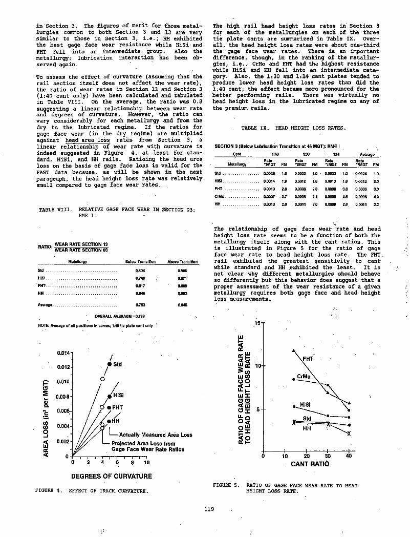
in Section 3. The figures of merit for those metal­lurgies common to both Section 3 and 13 are very similar to those in Section 3, i.e.; HH exhibited the best gage face wear resistance while HiSi and FHT fell into an intermediate group. Also the metallurgy: lubrication interaction has been ob­served again.

To assess the effect of curvature (assuming that the rail section itself does not affect the wear rate), the ratio of wear rates in Section 13 and Section 3 (1:40 cant only) have been calculated and tabulated in Table VIII. On the average, the ratio was 0.8 suggesting a linear relationship between wear rate and degrees of curvature. However, the ratio can vary considerably for each metallurgy and from the dry to the lubricated regime. If the ratios for gage face wear (in the dry regime) are multiplied against head area loss rates from Section 3, a linear relationship of wear rate with curvature is indeed suggested in Figure 4, at least for stan­dard, HiSi, and HH rails. Ratioing the head area loss on the basis of gage face loss is valid for the FAST data because, as will be shown in the next paragraph, the head height loss rate was relatively small compared to gage face wear rates.

TABLE VIII. RELATIVE GAGE FACE WEAR IN SECTION 03: RME: I.

WEAR RATE SECTION 13 ' WEAR RATE SECTION 03

Metallurgy Below Transition Above Transition

Std ....................................................................... 0,804HiSi....................................................................... 0.746FHT........... ........................................................ 0.617HH ......................................... 0.846

Average................................................................. 0.753

OVERALL AVERAGE=0.799

NOTE: Average of all positions In curves; 1:40 tie plate cant only

0.9060.6710.8090.993

0.645

FIGURE 4. EFFECT OF TRACK CURVATURE.

The high rail head height loss rates in Section 3 for each of the metallurgies on each pf the three tie plate cants are summarized in Table IX. Over­all, the head height loss rates were about one-third the gage face wear rates. There is an important difference, though, in the ranking of the metallur­gies, i.e., CrMo and FHT had the highest resistance while HiSi and HH fell into an intermediate cate­gory. Also, the 1:30 and 1:14 cant plates tended to produce lower head height loss rates than did the 1:40 cant; the effect became more pronounced for the better performing rails. There was virtually no head height loss in the lubricated regime on any of the premium rails.

TABLE IX. HEAD HEIGHT LOSS RATES.

SECTION 3 (Below Lubrication Transition at 45 MGT): RME I_________Cant _________ L40____________L30___________ 1d4_________ Average

Rate Rate Rate RateMetallurgy________ "/MGT FM "/MGT FM "/MGT FM "/MGT FM

S td .................................... 0.0026 1.0 0.0022 1.0 0.0023 1.0 0.0024 1.0HISI..................... 0.0014 1.9 0.0012 1.8 0.0013 1.8 0.0012 2.0

F H T .................................. 0.0010 2.6 0.0008 2.8 0.0006 3.8 0.0008 3.0CrMo.................................. 0.0007 3.7 0.0005 4.4 0.0005 4 6 0.0006 4.0H H .................................... 0.0013 2.0 . 0.0011 2.0 0.0009 2.6 0.0011 2.2

The relationship of gage face wear Irate and head height loss rate seems to be a function of both the metallurgy itself along with the cant ratios. This is illustrated in Figure 5 for the ratio of gage face wear rate to head height loss rate. The FHT, rail exhibited the greatest sensitivity to cant while standard and HH .exhibited the least. It is not clear why different metallurgies should behave so differently but this behavior does suggest that a proper assessment of the wear resistance of a given metallurgy requires both gage face and head height loss measurements.

FIGURE 5. RATIO OF GAGE FACE WEAR RATE TO HEAD HEIGHT LOSS RATE.

119

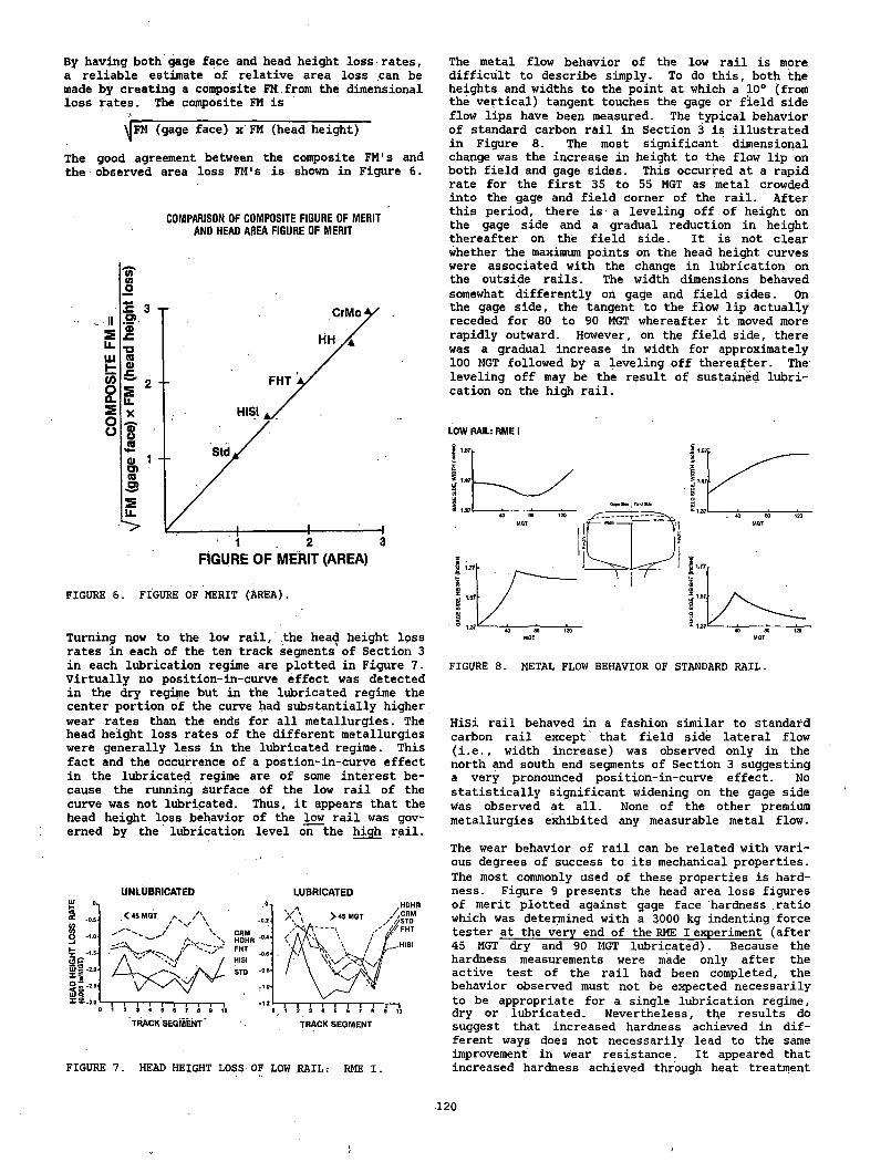
By having both gage face and head height loss rates, a reliable estimate of relative area loss can be made by creating a composite FM.from the dimensional loss rates. The composite FM is

\JFM (gage face) x FM (head height)

The good agreement between the composite FM1 s and the observed area loss FM's is shown in Figure 6.

COMPARISON OF COMPOSITE FIGURE OF MERIT AND HEAD AREA FIGURE OF MERIT

FIGURE 6. FIGURE OF MERIT (AREA).

Turning now to the low rail, the head height loss rates in each of the ten track segments of Section 3 in each lubrication regime are plotted in Figure 7. Virtually no position-in-curve effect was detected in the dry regime but in the lubricated regime the center portion of the curve had substantially higher wear rates than the ends for all metallurgies. The head height loss rates of the different metallurgies were generally less in the lubricated regime. This fact and the occurrence of a postion-in-Curve effect in the lubricated regime are of some interest be­cause the running surface Of the low rail of the curve was not lubricated. Thus, it appears that the head height loss behavior of the low rail was gov­erned by the lubrication level on the high rail.

UNLUBRICATED LUBRICATED

FIGURE 7. HEAD HEIGHT LOSS OF LOW RAIL: RME I.

The metal flow behavior of the low rail is more difficult to describe simply. To do this, both the heights and widths to the point at which a 10° (from the vertical) tangent touches the gage or field side flow lips have been measured. The typical behavior of standard carbon rail in Section 3 is illustrated in Figure 8. The most significant dimensional change was the increase in height to the flow lip on both field and gage sides. This occurred at a rapid rate for the first 35 to 55 MGT as metal crowded into the gage and field corner of the rail. After this period, there is a leveling off of height on the gage side and a gradual reduction in height thereafter on the field side. It is not clear whether the maximum points on the head height curves were associated with the change in lubrication on the outside rails. The width dimensions behaved somewhat differently on gage and field sides. On the gage side, the tangent to the flow lip actually receded for 80 to 90 MGT whereafter it moved more rapidly outward. However, on the field side, there was a gradual increase in width for approximately 100 MGT followed by a leveling off thereafter. The leveling off may be the result of sustained lubri­cation on the high rail.

LOW RAIL: RME I

FIGURE 8. METAL FLOW BEHAVIOR OF STANDARD RAIL.

HiSi rail behaved in a fashion similar to standard carbon rail except that field side lateral flow (i.e., width increase) was observed only in the north and south end segments of Section 3 suggesting a very pronounced position-in-curve effect. No statistically significant widening on the gage side was observed at all. None of the other premium metallurgies exhibited any measurable metal flow.

The wear behavior of rail can be related with vari­ous degrees of success to its mechanical properties. The most commonly used of these properties is hard­ness. Figure 9 presents the head area loss figures of merit plotted against gage face hardness ratio which was determined with a 3000 kg indenting force tester at the very end of the RME I experiment (after 45 MGT dry and 90 MGT lubricated). Because the hardness measurements were made only after the active test of the rail had been completed, the behavior observed must not be expected necessarily to be appropriate for a single lubrication regime, dry or lubricated. Nevertheless, the results do suggest that increased hardness achieved in dif­ferent ways does not necessarily lead to the same improvement in wear resistance. It appeared that increased hardness achieved through heat treatment

120

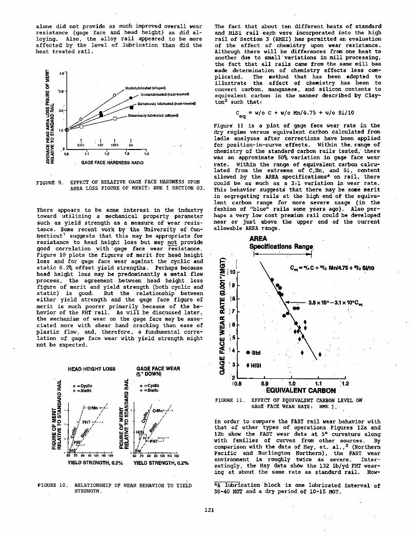
alone did not provide as much improved overall wear resistance (gage face and head height) as did al­loying. Also, the alloy rail appeared to be more affected by the level of lubrication than did the heat treated rail.

FIGURE 9. EFFECT OF RELATIVE GAGE FACE HARDNESS UPON AREA LOSS FIGURE OF MERIT: RME I SECTION 03.

There appears to be some interest in the industry toward utilizing a mechanical property parameter such as yield strength as a measure of wear resis­tance. Some recent work by the University of Con­necticut1 suggests that this may be appropriate for resistance to head height loss but may not provide good correlation with gage face wear resistance. Figure 10 plots the figures of merit for head height loss and for gage face wear against the cyclic and static 0.2% offset yield strengths. Perhaps because head height loss may be predominantly a metal flow process, the agreement between head height loss figure of merit and yield strength (both cyclic and static) is good. But the relationship between either yield strength and the gage face figure of merit is much poorer primarily because of the be­havior of the FHT rail. As will be discussed later, the mechanism of wear on the gage face may be asso­ciated more with shear band cracking than ease of plastic flow, and, therefore, a fundamental corre­lation of gage face wear with yield strength might not be expected.

HEAD HEIGHT LOSS GAGE FACE WEAR (S ' DOWN)

2QCC<Q

HiLil (/)

s £U- HO lUUl^ccb0 Eu U. QC

x = Cyclic + b Static 2

O:a2

L < | z

£ V)S PU.HO u ,LU ^

3 ^ Offi LU QC

x = Cyclic + = Static

■ ^ C r M o *f?/ /

■ Sf /

P£.ht3 ../ // /

Std . . .

YIELD STRENGTH, 0.2%60 70 00 00 100 110 120

YIELD STRENGTH, 0.2%

FIGURE 10. RELATIONSHIP OF WEAR BEHAVIOR TO YIELD STRENGTH.

The fact that about ten different heats of standard and HiSi rail each were incorporated into the high rail of Section 3 (RMEI) has permitted an evaluation of the effect of chemistry upon wear resistance. Although there will be differences from one heat to another due to small variations in mill processing, the fact that all rails came from the same mill has made determination of chemistry effects less com­plicated. The method that has been adopted to illustrate the effect of chemistry has been to convert carbon, manganese, and silicon contents to equivalent carbon in the manner described by Clay­ton2 such that:

C = w/o C + w/o Mn/4.75 + w/o Si/10

Figure 11 is a plot of gage face wear rate in the dry regime versus equivalent carbon calculated from ladle analyses after corrections have been applied for position-in-curve effects. Within the. range of chemistry of the standard carbon rails' tested, there was an approximate 50% variation in gage face wear rate. Within the range of equivalent carbon calcu­lated from the extremes of C,Mn, and Si, content allowed by the AREA specifications* on rail, there could be as much as a 3:1 variation in wear rate. This behavior suggests that there may be some merit in segregating rails at the high end of the equiva­lent carbon range for more severe usage (in the fashion of "blue" rails some years ago). Also per­haps a very low cost premium rail could be developed near or just above the upper end of the current allowable AREA range.

AREASpecifications Range

FIGURE 11. EFFECT OF EQUIVALENT CARBON LEVEL ON GAGE FACE WEAR RATE: RME I.

In order to compare the FAST rail wear behavior with that of other types of operations Figures 12a and 12b show the FAST wear data at 5° curvature along with families of curves from other sources. By comparison with the data of Hay, et. al.,3 (Northern Pacific and Burlington Northern), the FAST wear environment is roughly twice as severe. Inter­estingly, the Hay data sh6w the 132 lb/yd FHT wear­ing at about the same rate as standard rail. How-

*A lubrication block is one lubricated interval of 30-40 MGT and a dry period of 10-15 MGT.

121

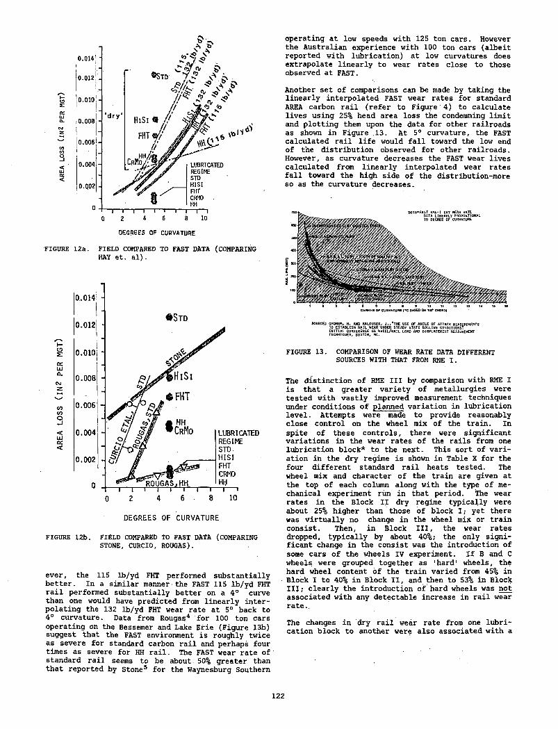
FIGURE 12a. FIELD COMPARED TO FAST DATA (COMPARING HAY et. al).

DEGREES OF CURVATURE

FIGURE 12b. FIELD COMPARED TO FAST DATA (COMPARING STONE, CURCIO, ROUGAS).

ever, the 115 lb/yd FHT performed substantially better. In a similar manner the FAST 115 lb/yd FHT rail performed substantially better on a 4° curve than one would have predicted from linearly inter­polating the 132 lb/yd FHT wear rate at 5° back to 4° curvature. Data from Rougas4 for 100 ton cars operating on the Bessemer and Lake Erie (Figure 13b) suggest that the FAST environment is roughly twice as severe for standard carbon rail and perhaps four times as severe for HH rail. The FAST wear rate of standard rail seems to be about 50% greater than that reported by Stone5 for the Waynesburg Southern

operating at low speeds with 125 ton cars. However the Australian experience with 100 ton cars (albeit reported with lubrication) at low curvatures does extrapolate linearly to wear rates close to those observed at FAST.

Another set of comparisons can be made by taking the linearly interpolated FAST wear rates for standard AREA carbon rail (refer to Figure 4) to calculate lives using 25% head area loss the condemning limit and plotting them upon the data for other railroads as shown in Figure .13. At 5° curvature, the FAST calculated rail life would fall toward the low end of the distribution observed for other railroads. However, as curvature decreases the FAST wear lives calculated from linearly interpolated wear rates fall toward the high side of the distribution-more so as the curvature decreases.

DOTS-FAST RME-1 DRY WEAR RATEDATA LINEARLY PROPORTIONAL TO DEGREE OF CURVATURE

DEGREE OF CURVATURE (‘ C EASED ON HO* CHORD)

SOURCE: GHONEM, H. AND KALOUSEK, J ,,"THE USE OF AN6LE OF ATTACK MEASUREMENTS TO ESTABLISH RAIL HEAR UNDER STEADY STATE ROLLING CONDITIONS?INITIAL CONFERENCE ON HHEELZrAIL LOAD AND DISPLACEMENT MEASUREMENT TECHNIQUES, BOSTON, MA.

FIGURE 13. COMPARISON OF WEAR RATE DATS DIFFERENT SOURCES WITH THAT FROM RME I.

The distinction of RME III by comparison with RME I is that a greater variety of metallurgies were tested with vastly improved measurement techniques under conditions of planned variation in lubrication level. Attempts were made to provide reasonably close control on the wheel mix of the train. In spite of these controls, there were significant variations in the wear rates of the rails from one lubrication block* to the next. This sort of vari­ation in the dry regime is shown in Table X for the four different standard rail heats tested. The wheel mix and character of the train are given at the top of each column along with the type of me­chanical experiment run in that period. The wear rates in the Block II dry regime typically were about 25% higher than those of block I; yet there was virtually no change in the wheel mix or train consist. Then, in Block III, the wear rates dropped, typically by about 40%; the only signi­ficant change in the consist was the introduction of some cars of the wheels IV experiment. If B and C wheels were grouped together as 'hard' wheels, the hard wheel content of the train varied from 45% in Block I to 40% in Block II, and then to 53% in.Block III; clearly the introduction of hard wheels was not associated with any detectable increase in rail wear rate..

The changes in dry rail wear rate from one lubri­cation block to another were also associated with a

122

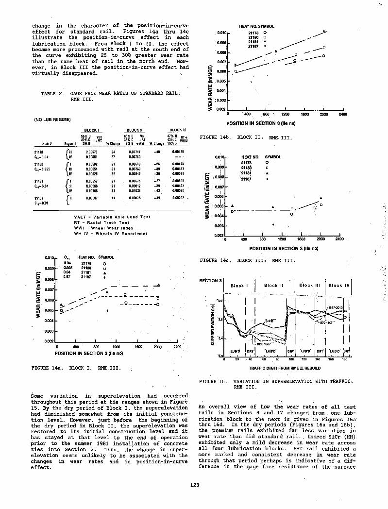
Vv

change in the character of the position-in-curve effect for standard rail. Figures 14a thru 14c illustrate the position-in-curve effect in each lubrication block. From Block X to II, the effect became more pronounced with rail at the south end of the curve exhibiting 25 to 30% greater wear rate than the same heat of rail in the north end. How­ever, in Block III the position-in-curve effect had virtually disappeared.

TABLE X. GAGE FACE WEAR RATES OF STANDARD RAIL:RME

(NO LUB REGIME)

I I I .

BLOCK I BLOCK tl BLOCK III

Heat 8 Segment55% U valt«%!• +rt3%B % Change

60% U Valt 38% C +RT 2% B +WWI % Change

47% U RT+ 43% C iiiuiu 10% B WHIV

21178 0.00578 24 0.00717 -40 0.00430C„=0.94 0.00561 37 0.00769

21180 r i 0.00502 21 0.00609 -26 0.00448Ciq =0.995 V" 0.00654 21 0.00789 -39 0.00463

u» 0.00626 35 0.00847 -39 0.00514

21181 f t 0.00557 21 0.00676 -27 0.00506C,g=0.94 < ii 0.00668 21 0.00812 -39 0.00492 .

I 'V 0.00765 33 0.01021 -42 0.00590.

21187c lq=o:97 ( "

0.00507 14 0.00576 -49 0.00292 <

V A L T - V a r ia b le A x le L o a d T e s t R T - R a d ia l T ru c k T e s t W W I W h e e l W e a r In d e x W H IV - W h e e ls IV E x p e r im e n t

POSITION IN SECTION 3 (tie no)

FIGURE 14a. BLOCK I: RME III.

Some variation in superelevation had occurred throughout this period at tie ranges shown in Figure 15. By the dry period of Block I, the superelevation had diminished somewhat from its initial construc­tion level. However, just before the beginning of the dry period in Block II, the superelevation was restored to its initial construction level and it has stayed at that level to the end of operation prior to the summer 1981 installation of concrete ties into Section 3. Thus, the change in supers elevation seems unlikely to be associated with the changes in wear rates and in position-in-curve effect.

HEAT NO. SYMBOL

FIGURE 14b. BLOCK II: RME: H I .

FIGURE 14c. BLOCK III: RME III.

FIGURE 15. VARIATION IN SUPERELEVATION WITH TRAFFIC: RME III.

An overall view of how the wear rates of all test rails in Sections 3 and 17 changed from . one- lub­rication block to the next is given in Figures 16a thru 16d. In the dry periods (Figures 16a and 16b), the premium rails exhibited far less variation in wear rate than did standard rail. . Indeed SiCr (HH) exhibited only . a mild decrease in wear rate across all four lubrication blocks. FHT rail exhibited a more marked and consistent decrease in wear rate through that period perhaps is indicative■of a dif­ference in the gage face resistance of the surface

123

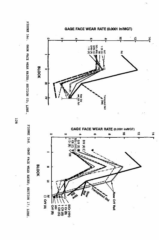
FIGURE 16c. GAGE FACE WEAR RATES; SECTION 03; LUBE.,

FIGURE 16d. GAGE FACE WEAR RATES; SECTION 17; LUBE.

GAGE FACE WEAR RATE (0.0001 in/MGT)

o ro A 0> CD10 12 14

V »o o S 2 _k

FHT CR (C)

HH :r (HH) 'Mo (C) 'Mo (A) I Cr (B) eg

S

GAGE FACE WEAR RATE (0.0001 in/MGT)

•s o i 52~ 3 = g g o o

3 o > S =

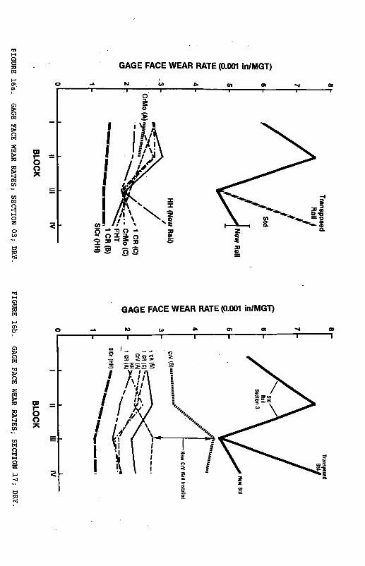
FIGURE 16a. GAGE FACE WEAR RATES; SECTION 03; DRY.

FIGURE 16b. GAGE FACE WEAR RATES; SECTION 11; DRY.

GAGE FACE WEAR RATE (0.001 in/MGT)

0 lo co * <n a> «m os1 'I I I i i i -------1--------- r0

1o>

GAGE FACE WEAR RATE (0.001 in/MGT)

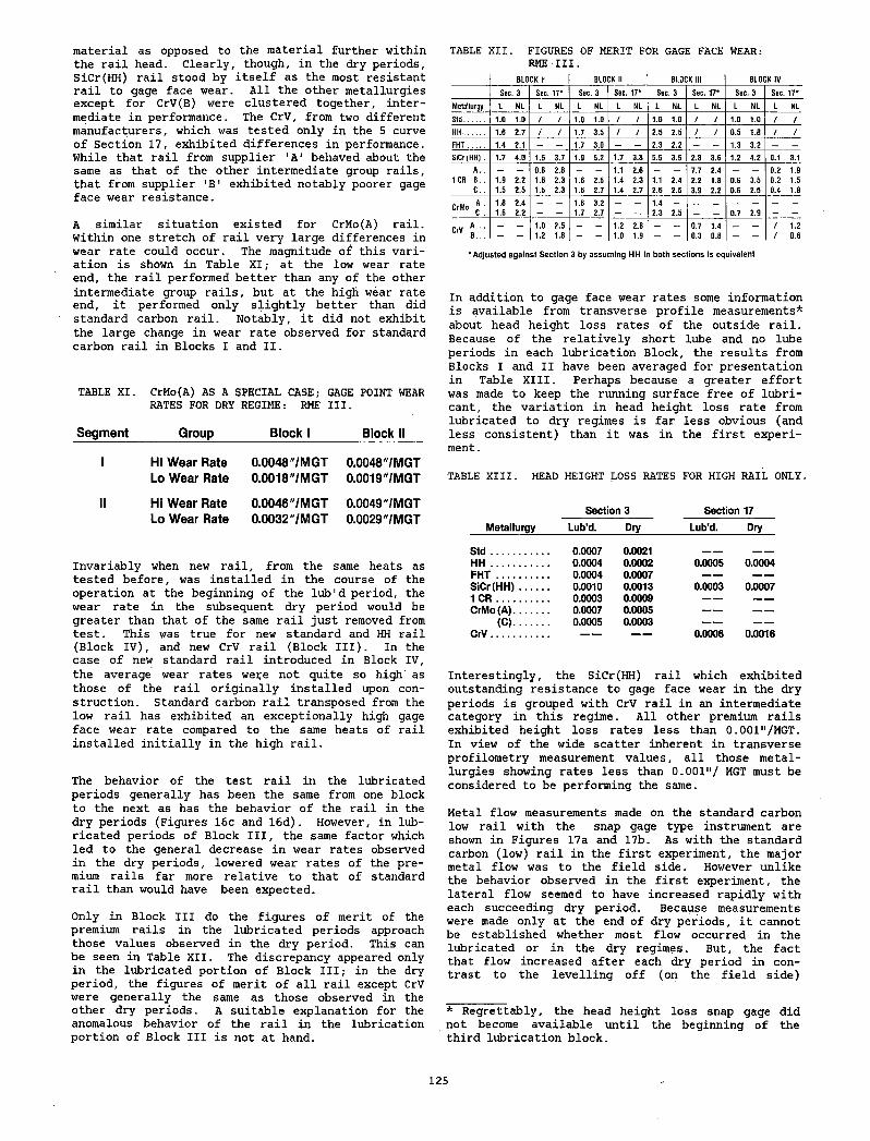
material as opposed to the material further within the rail head. Clearly, though, in the dry periods, SiCr(HH) rail stood by itself as the most resistant rail to gage face wear. All the other metallurgies except for CrV(B) were clustered together, inter­mediate in performance. The CrV, from two different manufacturers, which was tested only in the 5 curve of Section 17, exhibited differences in performance. While that rail from supplier 'A' behaved about the same as that of the other intermediate group rails, that from supplier 1B 1 exhibited notably poorer gage face wear resistance.

A similar situation existed for CrMo(A) rail. Within one stretch of rail very large differences in wear rate could occur. The magnitude of this vari­ation is shown in Table XI; at the low wear rate end, the rail performed better than any of the other intermediate group rails, but at the high wear rate end, it performed only slightly better than did standard carbon rail. Notably, it did not exhibit the large change in wear rate observed for standard carbon rail in Blocks I and II.

CrMo(A) AS A SPECIAL CASE; GAGE POINT WEAR RATES FOR DRY REGIME: RME III.

Group________ Block I________ Block II

TABLE XI.

Segment

I

II

Hi Wear Rate Lo Wear Rate

Hi Wear Rate Lo Wear Rate

0.0048 "/MGT 0.0018"/MGT

0.0046 "/MGT 0.0032 "/MGT

0.0048"/MGT 0.0019 "/MGT

0.0049"/MGT 0.0029 "/MGT

Invariably when new rail, from the same heats as tested before, was installed in the course of the operation at the beginning of the lub'd period, the wear rate in the subsequent dry period would be greater than that of the same rail just removed from test. This was true for new standard and HH rail (Block IV), and new CrV rail (Block III). In the case of new standard rail introduced in Block IV, the average wear rates wece not quite so high as those of the rail originally installed upon con­struction. Standard carbon rail transposed from the low rail has exhibited an exceptionally high gage face wear rate compared to the same heats of rail installed initially in the high rail.

The behavior of the test rail in the lubricated periods generally has been the same from one block to the next as has the behavior of the rail in the dry periods (Figures 16c and 16d). However, in lub­ricated periods of Block III, the same factor which led to the general decrease in wear rates observed in the dry periods, lowered wear rates of the pre­mium rails far more relative to that of standard rail than would have been expected.

Only in Block III do the figures of merit of the premium rails in the lubricated periods approach those values observed in the dry period. This can be seen in Table XII. The discrepancy appeared only in the lubricated portion of Block III; in the dry period, the figures of merit of all rail except CrV were generally the same as those observed in the other dry periods. A suitable explanation for the anomalous behavior of the rail in the lubrication portion of Block III is not at hand.

TABLE XII. FIGURES OF MERIT FOR GAGE FACE WEAR: RME III.

B L O C K I* B L O C K II B L O C K III B L O C K IV

Sec 3 S e c. 1 7 * S e c . 3 S e c . 1 7 * S e c . 3 S e c . 1 7 * S e c . 3 S e c . 1 7 *

M e ta llu rg y L N L N L L N L L N L L N L L N L N L L N L

S t d ............... 1 .0 1 .0 1 .0 1 .0 / 1 .0 1 .0 / 1 .0 1 .0 /

H H .............. 1 .6 2 .7 / 1 .7 3 .5 / 2 .5 2 .5 / 0 .5 1 .8 /

F H T ............ 1 .4 2 .1 _ _ 1 .7 3 .0 _ _ 2 .3 2 .2 — _ 1 .3 3 .2 — —S iC r ( H H ) . 1 .7 4 .0 1 .5 3 .7 1 .9 5 .2 1 .7 3 .8 5 .5 3 .5 2 .8 3 .6 1 .2 4 .2 0 .1 3 .1

A . . _ _ 0 .8 2 .8 _ _ 1 .1 2 .6 _ _ 7 .7 2 .4 _ _ 0 .2 1 .9

1 CR B . . 1 .9 2 .2 1 .6 2 .3 1 .6 2 .5 1 .4 2 .3 1.1 2 .4 2 .2 1 .8 0 .6 3 .5 0 .2 1 .5

C . . 1 .5 2 .5 1 .5 2 .3 1 .6 2 .7 1 .4 2 .7 2 .6 2 .5 3 .9 2 .2 0 .6 2 .5 0 .4 1 .8

C rM o J ’1 .8 2 .4 _ _ 1 .6 3 .2 _ _ 1 .4 _ _ _ _ _ _ _

1 .6 2 .2 - — 1 .7 2 .7 — - 2 .3 2 .5 — — 0 .7 2 .9 — —

Crv S::: - _ 1 .0 2 .5 _ _ 1 .2 2 .8 _ _ 0 .7 1 .4 _ _ 1 .2

- - 1 .2 1 .8 - - 1 .0 1 .9 - - 0 .3 0 .8 - - 0 .6

*Adjusted against Section 3 by assuming HH in both sections is equivalent

In addition to gage face wear rates some information is available from transverse profile measurements* about head height loss rates of the outside rail. Because of the relatively short lube and no lube periods in each lubrication Block, the results from Blocks I and II have been averaged for presentation in Table XIII. Perhaps because a greater effort was made to keep the running surface free of lubri­cant, the variation in head height loss rate from lubricated to dry regimes is far less obvious (and less consistent) than it was in the first experi­ment.

TABLE XIII. HEAD HEIGHT LOSS RATES FOR HIGH RAIL ONLY.

Section 3 Section 17

Metallurgy______Lub’d. Dry_________ Lub’d._____ Dry

S td ................... 0.0007 0.0021 — —

H H ................... 0.0004 0.0002 0.0005 0.0004F H T ....... 0.0004 0.0007 — —

S iC r(H H )......... 0.0010 0.0013 0.0003 0.00071 CR............... 0.0003 0.0009 — —CrMo ( A ) ............. 0.0007 0.0005 — —

(C j........... 0.0005 0.0003 — —

CrV................. — — 0.0006 0.0016

Interestingly, the SiCr(HH) rail which exhibited outstanding resistance to gage face wear in the dry periods is grouped with CrV rail in an intermediate category in this regime. All other premium rails exhibited height loss rates less than 0.001"/MGT. In view of the wide scatter inherent in transverse profilometry measurement values, all those metal­lurgies showing rates less than 0.001"/ MGT must be considered to be performing the same.

Metal flow measurements made on the standard carbon low rail with the snap gage type instrument are shown in Figures 17a and 17b. As with the standard carbon (low) rail in the first experiment, the major metal flow was to the field side. However unlike the behavior observed in the first experiment, the lateral flow seemed to have increased rapidly with each succeeding dry period. Because measurements were made only at the end of dry periods, it cannot be established whether most flow occurred in the lubricated or in the dry regimes. But, the fact that flow increased after each dry period in con­trast to the levelling off (on the field side)

* Regrettably, the head height loss snap gage did not become available until the beginning of the third lubrication block.

125

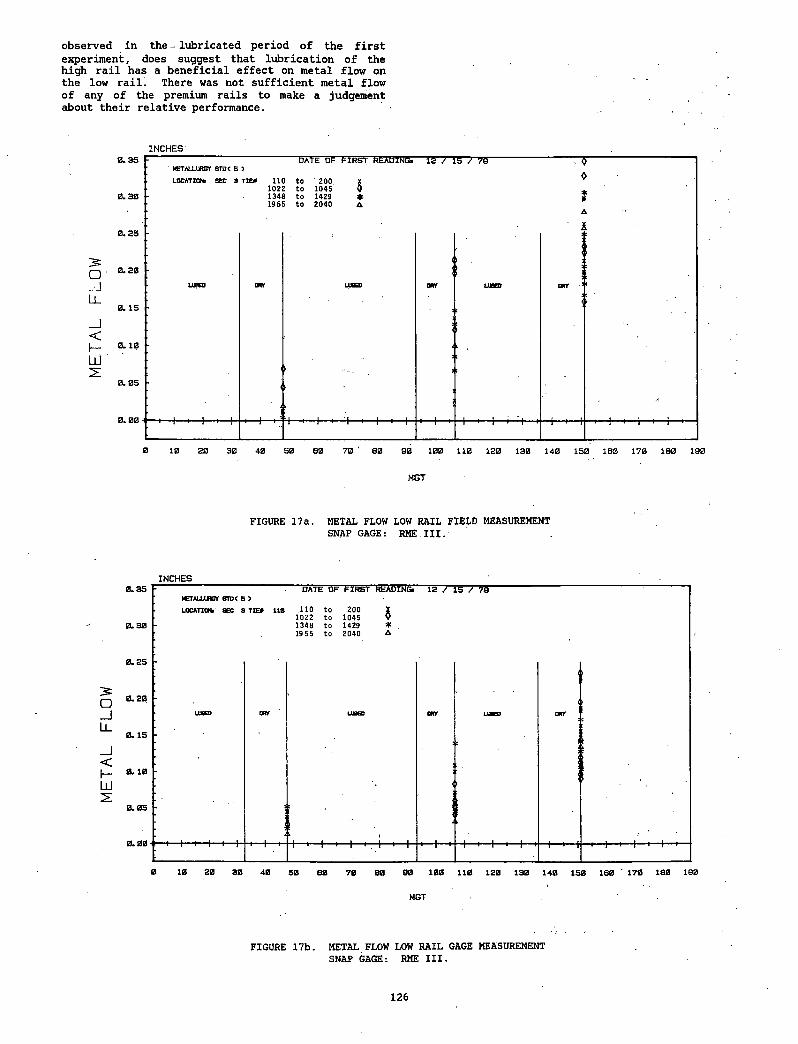
observed in the - lubricated period of the first experiment, does suggest that lubrication of the high rail has a beneficial effect on metal flow on the low rail. There was not sufficient metal flow of any of the premium rails to make a judgement about their relative performance.

INCHES

MGT

FIGURE 17a. METAL FLOW LOW RAIL FIELD MEASUREMENT SNAP GAGE: RME III.

INCHES

FIGURE 17b. METAL FLOW LOW RAIL GAGE MEASUREMENT SNAP GAGE: RME III.

126

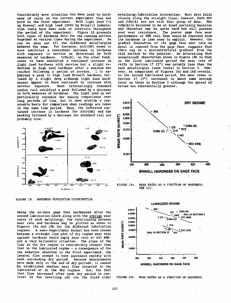
Considerably more attention has been paid to hard­ness of rails in the current experiment than was paid in the first experiment. Both light load (~1 kg Eseway) and high load.(3000 kg Brinell) indenta­tion tests have been made at intervals throughout the period of the experiment. Figure 18 presents both types of hardness data for the running surface together at various times during the experiment. As can be seen not all the different metallurgies behaved the same.' For instance, SiCr(HH) seems to have exhibited a consistent increase in hardness with exposure to service as determined by both measures of hardness. CrMo(A), on the other hand, seems to have exhibited a continued increase in light load hardness with service but a slight re­duction in high load hardness after a maximum was reached following a period of service. 1 Cr ex­hibited a peak in high load Brinell hardness fol­lowed by a slight drop although light load hard­nesses appear to have continued to increase with service exposure. Most interestingly standard carbon rail exhibited a peak followed by a decrease in both measures of hardness. The light load'is not particularly suitable for making comparisons over long periods of time, but it does provide a rea­sonable basis for comparison when readings are taken in the same time period. Thus, the indicated con­tinued increase in hardness for SiCr(HH) and the peaking followed by a decrease for standard rail are probably true.

4?5r

42 5 •

375 •

325 -

27 5 -

475

425

375

325

275

225

CrMo (A )

Std

40 0 42 5 250

B1 (B n iN F l.O

SiCr

f- 6/8 1

1/80

1% Cr

30 0 350 400 . 425

metallurgy:lubrication interaction. Most data falls closely along the straight lines; however, both FHT and CrMo (A) are not with that group of data. The CrMo(A)is believed to be at least partially bainitic and therefore may be quite hard but will possess poor wear resistance.' The poorer gage face wear performance of FHT rail than would be expected from its hardness is less easy to explain. However, the gradual diminution of its gage face wear rate as metal is removed from the gage face, suggests that there may be a microstructural gradient from the rail surface to the interior. An interesting (but unexplained) observation shown in Figure 19b is that in the first lubricated period the wear rate of rails in Section 17 (5°) was notably less than the same metallurgies (same heats) in Section 3. How­ever, as comparison of Figures 16c and 16d reveals, in the second lubricated period, the wear rates in Section 17 (5°) increased to about same average level as those in Section 3 although the spread of values was substantially greater.

FIGURE 19a. WEAR RATES AS A FUNCTION OF HARDNESS: RME III.

FIGURE 18. HARDNESS POPULATION DISTRIBUTION.

Using the as-worn gage face hardnesses after the second lubrication block-along with the average wear rates of each metallurgy, the relationship between wear rate and hardness may be plotted as shown in Figures 19a and 19b for the different lubrication regimes. A semi-logarithmic format has been chosen because a straight line plot of dry regime wear rate against hardness would imply zero rate at 430 BHN- not a very believable situation. The slope of the line in the dry regime is considerably steeper than that in the lubricated regime - a consequence of the the behavior observed in the first experiment, the lateral flow seemed to have increased rapidly with each succeeding dry period. Because measurements were made only at the end of dry periods, it cannot be established whether most flow occurred in the lubricated or in the dry regimes. But, the fact that flow increased after each dry period in con­trast to the levelling off (on the field side)

LUBRICATED REGIME

BRINELL HARDNESS ON GAGE FACE

FIGURE 19b. WEAR RATES AS A FUNCTION OF HARDNESS.

127

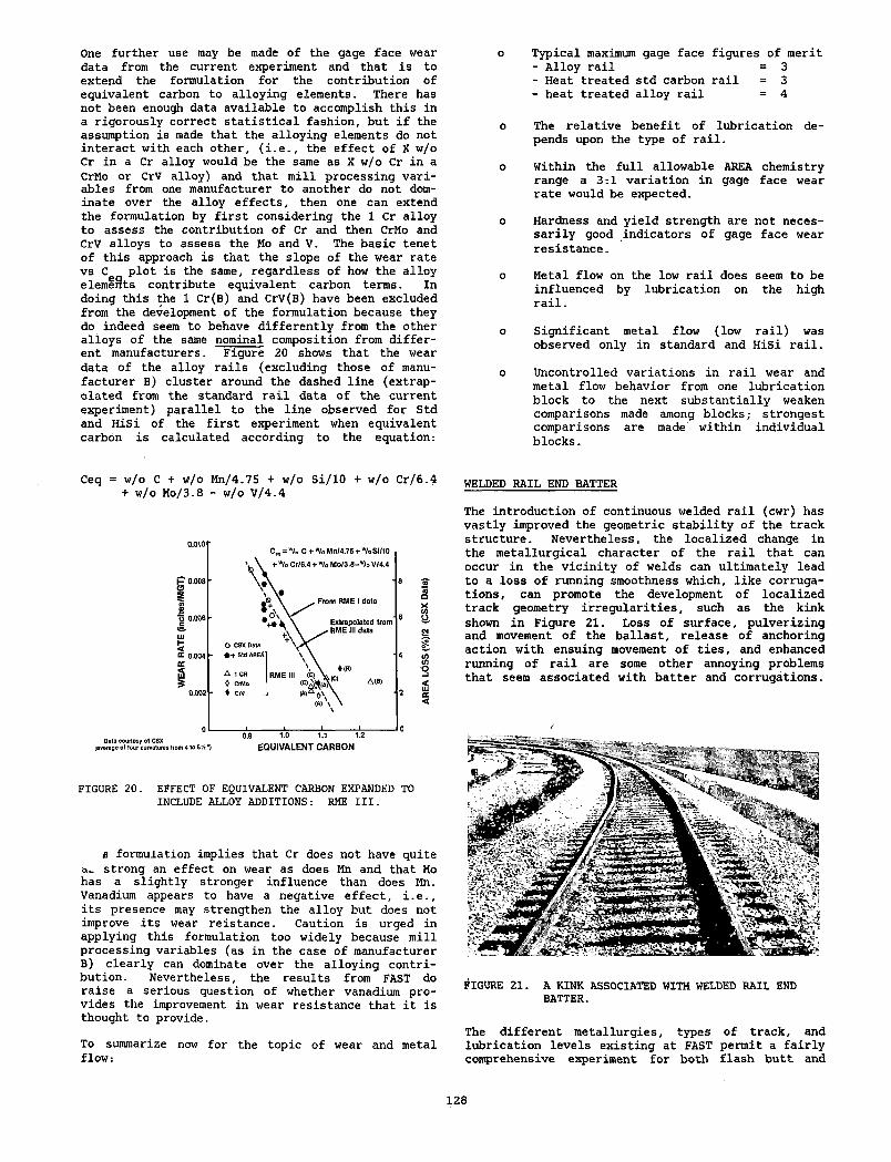
One further use may be made of the gage face wear data from the current experiment and that is to extend the formulation for the contribution of equivalent carbon to alloying elements. There has not been enough data available to accomplish this in a rigorously correct statistical fashion, but if the assumption is made that the alloying elements do not interact with each other, (i.e., the effect of X w/o Cr in a Cr alloy would be the same as X w/o Cr in a CrMo or CrV alloy) and that mill processing vari­ables from one manufacturer to another do not dom­inate over the alloy effects, then one can extend the formulation by first considering the 1 Cr alloy to assess the contribution of Cr and then CrMo and CrV alloys to assess the Mo and V. The basic tenet of this approach is that the slope of the wear rate vs C plot is the same, regardless of how the alloy elemlrlts contribute equivalent carbon terms. In doing this the 1 Cr(B) and CrV(B) have been excluded from the development of the formulation because they do indeed seem to behave differently from the other alloys of the same nominal composition from differ­ent manufacturers. Figure 20 shows that the wear data of the alloy rails (excluding those of manu­facturer B) cluster around the dashed line (extrap­olated from the standard rail data of the current experiment) parallel to the line observed for Std and HiSi of the first experiment when equivalent carbon is calculated according to the equation:

Ceq = w/o C + w/o Mn/4.75 + w/o Si/10 + w/o Cr/6.4 + w/o Mo/3.8 - w/o V/4.4

FIGURE 2 0 . EFFECT OF EQUIVALENT CARBON EXPANDED TO INCLUDE ALLOY ADDITIONS: RME I I I .

£ formulation implies that Cr does not have quite a- strong an effect on wear as does Mn and that Mo has a slightly stronger influence than does Mn. Vanadium appears to have a negative effect, i.e., its presence may strengthen the alloy but does not improve its wear reistance. Caution is urged in applying this formulation too widely because mill processing variables (as in the case of manufacturer B) clearly can dominate over the alloying contri­bution. Nevertheless, the results from FAST do raise a serious question of whether vanadium pro­vides the improvement in wear resistance that it is thought to provide.

To summarize now for the topic of wear and metal flow:

o Typical maximum gage face figures of merit- Alloy rail = 3- Heat treated std carbon rail = 3- heat treated alloy rail = 4

o The relative benefit of lubrication de­pends upon the type of rail.

o Within the full allowable AREA chemistry range a 3:1 variation in gage face wear rate would be expected.

o Hardness and yield strength are not neces­sarily good indicators of gage face wear resistance.

o Metal flow on the low rail does seem to be influenced by lubrication on the high rail.

o Significant metal flow (low rail) was observed only in standard and HiSi rail.

o Uncontrolled variations in rail wear and metal flow behavior from one lubrication block to the next substantially weaken comparisons made among blocks; strongest comparisons are made within individual blocks.

WELDED RAIL END BATTER

The introduction of continuous welded rail (cwr) has vastly improved the geometric stability of the track structure. Nevertheless, the localized change in the metallurgical character of the rail that can occur in the vicinity of welds can ultimately lead to a loss of running smoothness which, like corruga­tions, can promote the development of localized track geometry irregularities, such as the kink shown in Figure 21. Loss of surface, pulverizing and movement of the ballast, release of anchoring action with ensuing movement of ties, and enhanced running of rail are some other annoying problems that seem associated with batter and corrugations.

Figure 2 1. a ki n k associated wi t h welded rail endBATTER.

The different metallurgies, types of track, and lubrication levels existing at FAST permit a fairly comprehensive experiment for both flash butt and

128

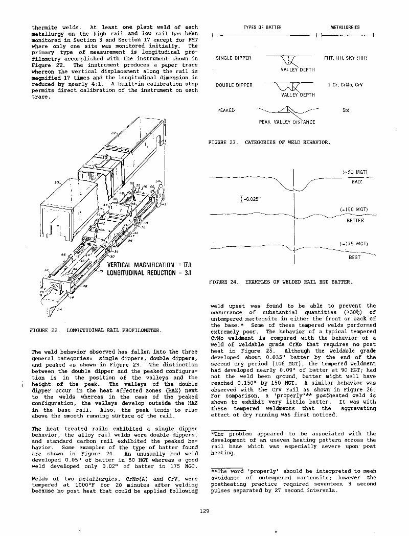
TYP ES OF BATTER METALLURGIESthermite welds. At least one plant weld of each metallurgy on the high rail and low rail has been monitored in Section 3 and Section 17 except for FHT where only one site was monitored initially. The primary type of measurement is longitudinal pro- filometry accomplished with the instrument shown in SIN G LE D IPPERFigure 2'2. The instrument produces a paper trace whereon the vertical displacement along the rail is magnified 17 times and the longitudinal dimension is reduced by nearly 4:1. A built-in calibration step DOUBLE D IPPERpermits direct calibration of the instrument on each trace.

------------1

X R —VALLEY DEPTH

FHT, HH, SiCr (H H )

1 Cr, CrM o, CrV

VALLEY DEPTH

FIGURE 22. LONGITUDINAL RAIL PROFILOMETER.

The weld behavior observed has fallen into the three general categories: single dippers, double dippers, and peaked as shown in Figure 23. The distinction between the double dipper and the peaked configura­tion is in the position of the valleys and the height of the peak. The valleys of the double dipper occur in the heat affected zones (HAZ) next to the welds whereas in the case of the peaked configuration, the valleys develop outside the HAZ in the base rail. Also, the peak tends to rise above the smooth running surface of the rail.

PEAKED Std

PEAK VALLEY D ISTA N C E

FIGURE 23. CATEGORIES OF WELD BEHAVIOR.

FIGURE 24. EXAMPLES OF WELDED RAIL END BATTER.

weld upset was found to be able to prevent the occurrance of substantial quantities (>30%) of untempered martensite in either the front or back of the base.* Some of these tempered welds performed extremely poor. The behavior of a typical tempered CrMo weldment is compared with the behavior of a weld of weldable grade CrMo that requires no post heat in Figure 25. Although the weldable grade developed about 0.035" batter by the end of the second dry period (106 MGT), the tempered weldment had developed nearly 0.09" of batter at 90 MGT; had not the weld been ground, batter might well have reached 0.150" by 150 MGT. A similar behavior was observed with the CrV rail as shown in Figure 26. For comparison, a 'properly1** postheated weld is shown to exhibit very little batter. It was with these tempered weldments that the aggravating effect of dry running was first noticed.

The heat treated rails exhibited a single dipper behavior, the alloy rail welds were double dippers, and standard carbon rail exhibited the peaked be­havior. Some examples of the type of batter found are shown in Figure 24. An unusually bad weld developed 0.05" of batter in 50 MGT whereas a good weld developed only 0.02" of batter in 175 MGT.

Welds of two metallurgies, CrMo(A) and CrV, were tempered at 1000°F for 20 minutes after welding because no post heat that could be applied following

*The problem appeared to be associated with the development of an uneven heating pattern across the rail base which was especially severe upon post heating.

**The word 'properly' should be interpreted to mean avoidance of untempered martensite; however the postheating practice required seventeen 3 second pulses separated by 27 second intervals.

129

V

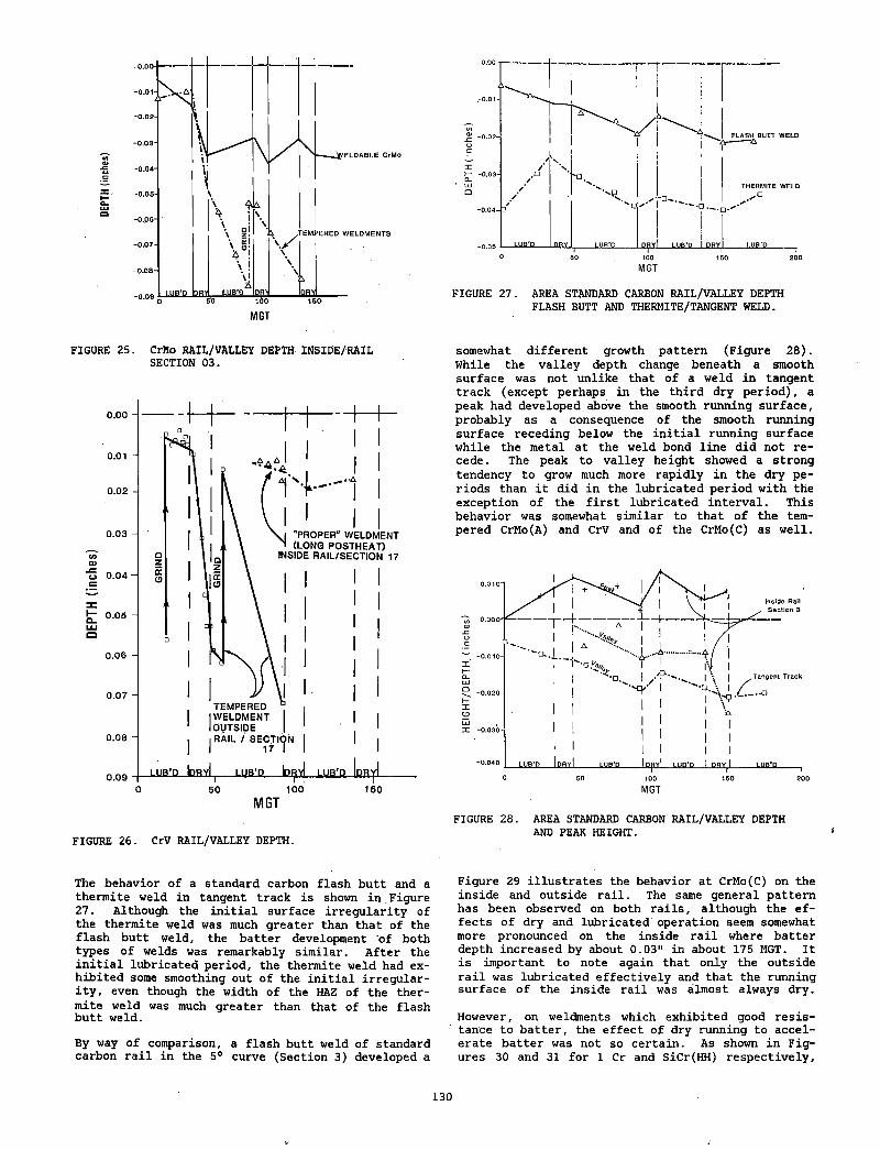
FIGURE 27. AREA STANDARD CARBON RAIL/VALLEY DEPTH FLASH BUTT AND THERMITE/TANGENT WELD.

FIGURE 25. CrMo RAIL/VALLEY DEPTH INSIDE/RAIL SECTION 03.

MGT

FIGURE 26. CrV RAIL/VALLEY DEPTH.

The behavior of a standard carbon flash butt and a thermite weld in tangent track is shown in Figure 27. Although the initial surface irregularity of the thermite weld was much greater than that of the flash butt weld, the batter development of both types of welds was remarkably similar. After the initial lubricated period, the thermite weld had ex­hibited some smoothing out of the initial irregular­ity, even though the width of the HAZ of the ther­mite weld was much greater than that of the flash butt weld.

By way of comparison, a flash butt weld of standard carbon rail in the 5° curve (Section 3) developed a

somewhat different growth pattern (Figure 28). While the valley depth change beneath a smooth surface was not unlike that of a weld in tangent track (except perhaps in the third dry period), a peak had developed above the smooth running surface, probably as a consequence of the smooth running surface receding below the initial running surface while the metal at the weld bond line did not re­cede. The peak to valley height showed a strong tendency to grow much more rapidly in the dry pe­riods than it did in the lubricated period with the exception of the first lubricated interval. This behavior was somewhat similar to that of the tem­pered CrMo(A) and CrV and of the CrMo(C) as well.

FIGURE 28. AREA STANDARD CARBON RAIL/VALLEY DEPTH AND PEAK HEIGHT.

Figure 29 illustrates the behavior at CrMo(C) on the inside and outside rail. The same general pattern has been observed on both rails, although the ef­fects of dry and lubricated operation seem somewhat more pronounced on the inside rail where batter depth increased by about 0.03" in about 175 MGT. It is important to note again that only the outside rail was lubricated effectively and that the running surface of the inside rail was almost always dry.

However, on weldments which exhibited good resis- ; tance to batter, the effect of dry running to accel­erate batter was not so certain. As shown in Fig­ures 30 and 31 for 1 Cr and SiCr(HH) respectively.

130

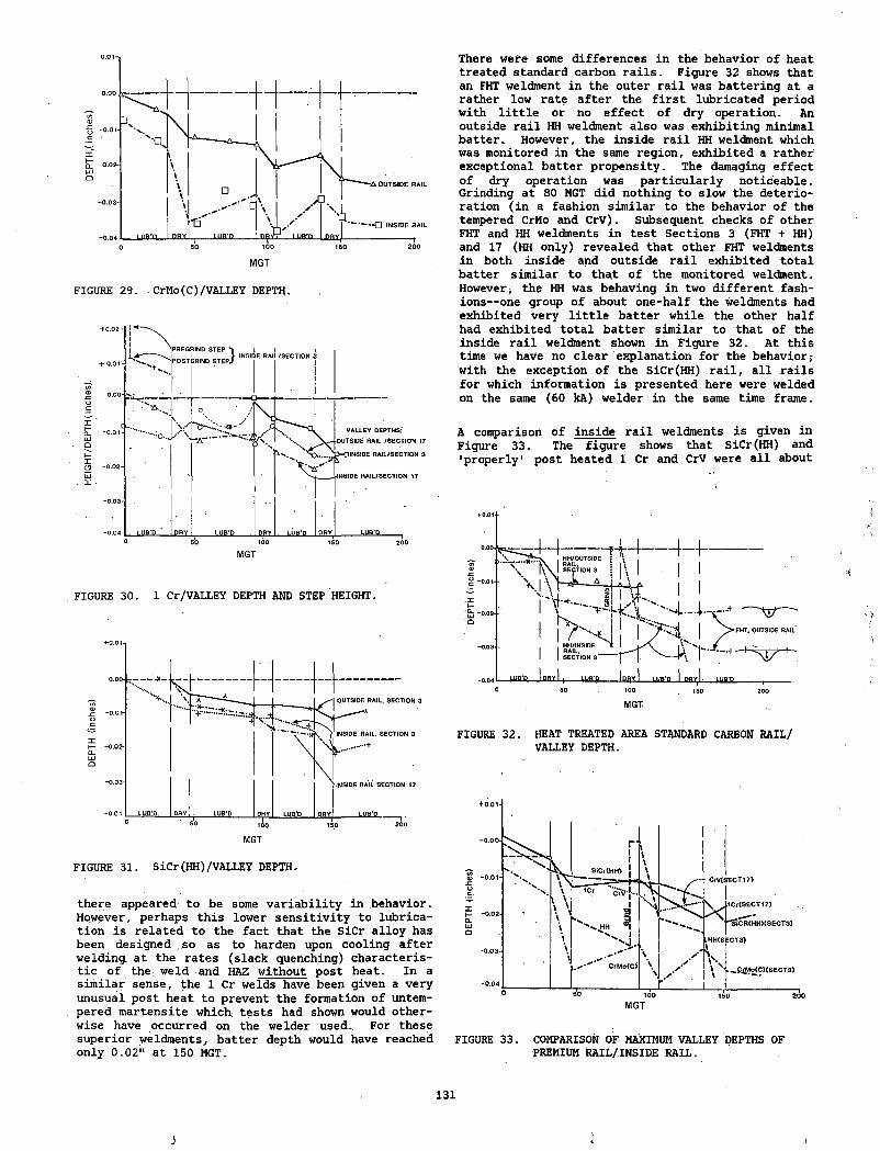
FIGURE 29. .CrMo(C)/VALLEY DEPTH.

FIGURE 30. 1 Cr/VALLEY DEPTH AND STEP HEIGHT.

FIGURE 31. SiCr(HH)/VALLEY DEPTH.

there appeared to be some variability in behavior. However, perhaps this lower sensitivity to lubrica­tion is related to the fact that the SiCr alloy has been designed .so as to harden upon cooling after welding at the rates (slack quenching) characteris­tic of the; weld and HAZ without post heat. In a similar sense, the 1 Cr welds have been given a very unusual post heat to prevent the formation of untem­pered martensite which; tests had shown would other­wise have occurred on the welder used. For these superior weldments, batter depth would have reached only 0.02" at 150 MGT.

There were some differences in the behavior of heat treated standard carbon rails. Figure 32 shows that an FHT weldment in the outer rail was battering at a rather low rate after the first lubricated period with little or no effect of dry operation. An outside rail HH weldment also was exhibiting minimal batter. However, the inside rail HH weldment which was monitored in the same region, exhibited a rather exceptional batter propensity. The damaging effect of dry operation was particularly noticeable. Grinding at 80 MGT did nothing to slow the deterio­ration (in a fashion similar to the behavior of the tempered CrMo and CrV). Subsequent checks of other FHT and HH weldments in test Sections 3 (FHT + HH) and 17 (HH only) revealed that other FHT weldments in both inside and outside rail exhibited total batter similar to that of the monitored weldment. However, the HH was behaving in two different fash­ions— one group of about one-half the weldments had exhibited very little batter while the other half had exhibited total batter similar to that of the inside rail weldment shown in Figure 32. At this time we have no clear explanation for the behavior,- with the exception of the SiCr(HH) rail, all rails for which information is presented here were welded on the same (60 kA) welder in the same time frame.

A comparison of inside rail weldments is given in Figure 33. The figure shows that SiCr(HH) and 'properly' post heated I Cr and CrV were all about

FIGURE 32. HEAT TREATED AREA STANDARD CARBON RAIL/ VALLEY DEPTH.

FIGURE 33. COMPARISON OF MAXIMUM VALLEY DEPTHS OF PREMIUM RAIL/INSIDE RAIL.

131

J 1

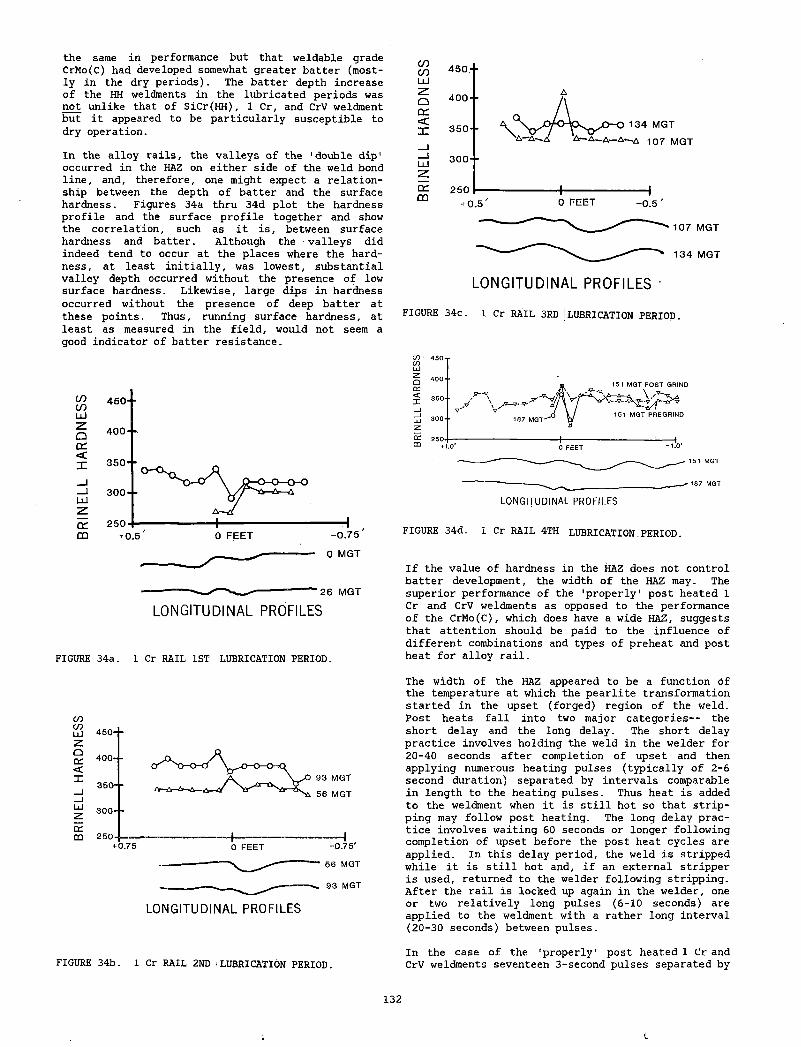
the same in performance but that weldable grade CrMo(C) had developed somewhat greater batter (most­ly in the dry periods). The batter depth increase of the HH weldments in the lubricated periods was not unlike that of SiCr(HH), 1 Cr, and CrV weldment but it appeared to be particularly susceptible to dry operation.

In the alloy rails, the valleys of the 1 double dip1 occurred in the HAZ on either side of the weld bond line, and, therefore, one might expect a relation­ship between the depth of batter and the surface hardness. Figures 34a thru 34d plot the hardness profile and the surface profile together and show the correlation, such as it is, between surface hardness and batter. Although the valleys did indeed tend to occur at the places where the hard­ness, at least initially, was lowest, substantial valley depth occurred without the presence of low surface hardness. Likewise, large dips in hardness occurred without the presence of deep batter at these points. Thus, running surface hardness, at least as measured in the field, would not seem a good indicator of batter resistance.

----— ■>— ----- ---- 26 MGTLONGITUDINAL PROFILES

FIGURE 34a. 1 Cr RAIL 1ST LUBRICATION PERIOD.

to

LONGITUDINAL PROFILES

FIGURE 34b. 1 Cr RAIL 2ND i LUBRICATION PERIOD.

134 MGT

LONGITUDINAL PROFILES •

FIGURE 34c. 1 Cr RAIL 3RD I LUBRICATION PERIOD.

FIGURE 34d. 1 Cr RAIL 4TH LUBRICATION PERIOD

If the value of hardness in the HAZ does not control batter development, the width of the HAZ may. The superior performance of the 'properly1 post heated 1 Cr and CrV weldments as opposed to the performance of the CrMo(C), which does have a wide HAZ, suggests that attention should be paid to the influence of different combinations and types of preheat and post heat for alloy rail.

The width of the HAZ appeared to be a function of the temperature at which the pearlite transformation started in the upset (forged) region of the weld. Post heats fall into two major categories— the short delay and the long delay. The short delay practice involves holding the weld in the welder for 20-40 seconds after completion of upset and then applying numerous heating pulses (typically of 2-6 second duration) separated by intervals comparable in length to the heating pulses. Thus heat is added to the weldment when it is still hot so that strip­ping may follow post heating. The long delay prac­tice involves waiting 60 seconds or longer following completion of upset before the post heat cycles are applied. In this delay period, the weld is stripped while it is still hot and, if an external stripper is used, returned to the welder following stripping. After the rail is locked up again in the welder, one or two relatively long pulses (6-10 seconds) are applied to the weldment with a rather long interval (20-30 seconds) between pulses.

In the case of the 'properly' post heated 1 Cr and CrV weldments seventeen 3-second pulses separated by

132

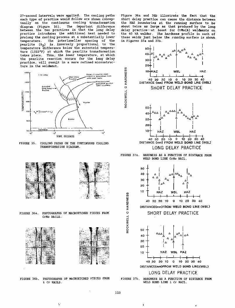
27-second intervals were applied. The cooling paths each type of practice would follow are shown concep­tually on the continuous cooling transformation diagram (Figure 35). The important difference between the two practices is that the long delay practice introduces the additional heat needed to prolong the cooling process at a substantially lower temperature. The interlamellar spacing of the pearlite (Sp) is . inversely proportional to the temperature difference below the eutectoid tempera­ture (1333°F) at which the pearlite transformation takes place. Thus, the lower temperature, at which the pearlite reaction occurs for the long delay practice, will result in a more refined microstruc­ture in the weldment.

FIGURE 35. COOLING PATHS ON THE CONTINUOUS COOLING TRANSFORMATION DIAGRAM.

FIGtJRE 36a. PHOTOGRAPHS OF MACROETCHED PIECES FROM CrMo RAILS.

FIGURE 36b. PHOTOGRAPHS OF MACROETCHED PIECES FROM 1 Cr RAILS.

Figure 36a and 36b illustrate the fact that the short delay practice can cause the distance between the HAZ boundaries at the running surface to be about twice as large as that produced by the long delay practice— at least for CrMo(A) weldments on the 60 kA welder. The hardness profile in each of these welds just below the running surface is shown in Figures 37a and 37b.

cocohizoCE<Xo SHORT DELAY PRACTICE_iin&

DISTANCE (mm)' FROM WELD BOND LINE (WBL)

LONG DELAY PRACTICEFIGURE 37a. HARDNESS AS A FUNCTION OF DISTANCE FROM

WELD BOND LINE CrMo RAIL.

« SHORT DELAY PRACTICE_iUJ5

DISTANCE(mm)FROM WELD BOND LINE (W BL)

LONG DELAY PRACTICEFIGURE 37b. HARDNESS AS A FUNCTION OF DISTANCE FROM

WELD BOND LINE 1 Cr RAIL.

133

V k

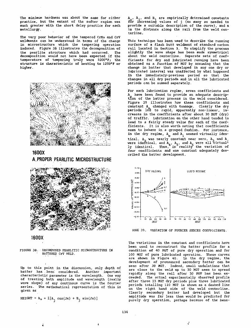
The minimum hardness was about the same for either practice, but the extent of the softer region was much greater with the short delay practice for each metallurgy.

The very poor behavior of the tempered CrMo and CrV weldments can be understood in terms of the change in microstructure which the tempering operation induced. Figure 38 illustrates the decomposition of the pearlite structure which had occurred. The decomposition would not have been expected if the temperature of tempering truly were 1000°F; the structure is characteristic of heating to 1250°F or higher.

1600XA,PROPER PEARLITIC MICROSTRUCTURE

1600X

FIGURE 38. DECOMPOSED PEARLITIC MICROSTRUCTURE IN ' BATTERED CrV WELD.

Up to this point in the discussion, only depth of batter has . been considered. Another important characteristic parameter is the wavelength. One way of treating both amplitude and wavelength (really wave shape) of any continous curve is the Fourier series. The mathematical representation of this is given as

HEIGHT = A0 + I[Aj cos(Jx) + sin(Jx)]

Aq, A., and B. are empirically determined constants for increasing values of j (as many as needed to provide a suitable description of the curve), and x is the distance along the rail from the weld cen­terline .

This technique has been used to describe the running surface of a flash butt weldment of standard carbon rail located in Section 3. To simplify the process slightly the wave shape has been made symmetrical about the weld centerline. Separate sets of coef­ficients for dry and lubricated running have been obtained as a function of MGT by assuming that the change in batter that developed in any one dry or lubricated interval was unaffected by what happened in the immediately-previous period so that the changes in all dry periods and in all the lubricated periods can be summed separately.

For each lubrication regime, seven coefficients and A have been found to provide an adequate descrip­tion of the batter process in the weld considered. Figure 39 illustrates how these coefficients and constant Aq changed with tonnage. Clearly the dry periods lea to rapid, apparently non-linear, in­creases in the coefficients after about 30 MGT (dry) of traffic. Lubrication on the other hand tended to lead to a fairly steady value for each of the coef­ficients. It is also worth noting that coefficients seem to behave in a grouped fashion. For instance, in the dry regime, Aq and A^ seemed virtually iden­tical, A_ was nearly constant near zero, A3 and A.. were identical, and A^, A,., and A^ were all virtual­ly identical. Thus, in reality the variation of four coefficients and one constant adequately des­cribed the batter development.

SURE 39. VARIATION OF FOURIER SERIES COEFFICIENTS.

The variations in the constant and coefficients have been used to reconstruct the batter profile for a condition of 40 MGT of pure dry operation and for 100 MGT of pure lubricated operation. These curves are shown in Figure 40. In the dry regime, the development of pronounced secondary batter can be seen after 30 MGT. Indeed, small undulations that are close to the weld up to 30 MGT seem to spread rapidly along the rail after 30 MGT has been ex­ceeded. The actual experimentally observed profile after three 15 MGT dry periods plus three lubricated periods totalling 110 MGT is shown as a dashed line on the right hand side of the weld centerline. Clearly secondary batter had developed but the amplitude was far less than would be predicted for purely dry operation, perhaps because of the bene-

134

i

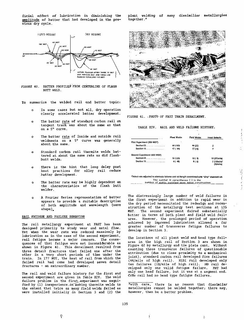
ficial effect of lubrication in diminishing the plant welding of many dissimiliar metallurgies amplitude of batter that had developed in the pre- together.* vious dry cycle.

FIGURE 40. BATTER PROFILES' FROM CENTERLINE OF FLASH BUTT WELD.

To summarize the welded rail end batter topic:

o In some cases but not all, dry operation clearly accelerated batter development.

o The batter rate of standard carbon rail on tangent track was about the same as that on a 5° curve.

FIGURE 41. -PHOTO OF FAST TRAIN DERAILMENT.

TABLE XIV. RAIL AND WELD FAILURE HISTORY.

o The batter rate of inside and outside rail weldments on a 5° curve was generally about the same.

o Standard carbon rail thermite welds bat­tered at about the same rate as did flash- butt welds.

o There is the hint that long delay post heat practices for alloy rail reduce batter development.

o The batter rate may be highly dependent on the characteristics of the flash butt welder.

o A Fourier Series representation of batter appears to provide a suitable description of both amplitude and wavelength (wave shape),

RAIL FATIGUE AND FAILURE BEHAVIOR

The rail metallurgy experiment at FAST has been designed primarily to study wear and metal flow. Yet when the wear rate was reduced massively by lubrication as in the case of the second experiment, rail fatigue became a major concern. The conse­quences of that fatigue were not inconsiderable as shown in Figure 41. This derailment resulted from three detail fractures that failed one after the other in a very short periods of time under the train. In 177 MGT, the heat of rail from which the failed rail had come had developed seven detail fractures - an extraordinary number.

The rail and weld failure history for the first and second experiment are given in Table XIV. The weld failure problem in the firsjt^experiment was magni­fied by (1) inexperience iif'making thermite welds to the extent that twice as many field welds failed as were installed initially in Section 3 and (2) the

Plant Welds______Field Welds Head Defects

First Experiment (135 MGT)Section 03............................. 44(180) 44(22) 2Section 13.............................. 17(64) 17(10) 7

Second Experiment (250 MGT)Section 03.............................. 10(120) 12( 0) 15 (27/miie)Section 13.............................. 4 (48) 8 (0 ) 7(10/mile)’

(30/mile)

1 Defect rate adjusted to eliminate failures and rail length associated with “dirty" standard rail.The number in parentheses ( ) is the

___________ number of welds installed upon initial construction__________

The distressingly large number of weld failures in the first experiment in addition to rapid wear in the dry period necessitated the redesign and recon­struction of the metallurgy test sections at 135 MGT. The second experiment faired substantially better in terms of both plant and field weld fail­ures. However, the prolonged period of operation achieved by improved lubrication allowed a far greater number of transverse fatigue failures to develop in Section 3.

The locations of all plant weld and head type fail­ures in the high rail of Section 3 are shown in Figure 42 by metallurgy and tie plate cant. Without counting those transverse failures of questionable attribution (due to close proximity to a mechanical joint), standard carbon rail developed five failures (44/mile of high rail). HiSi rail developed only two failures (18/mile of high rail). HH rail de­veloped only one valid fatigue failure. FHT had only one head failure, but it was at a segment end. CrMo rail had no head type fatigue failures.

*with care, there is no reason that dissimilar metallurgies cannot be welded together; there may, however, then be a batter problem.

135

S'

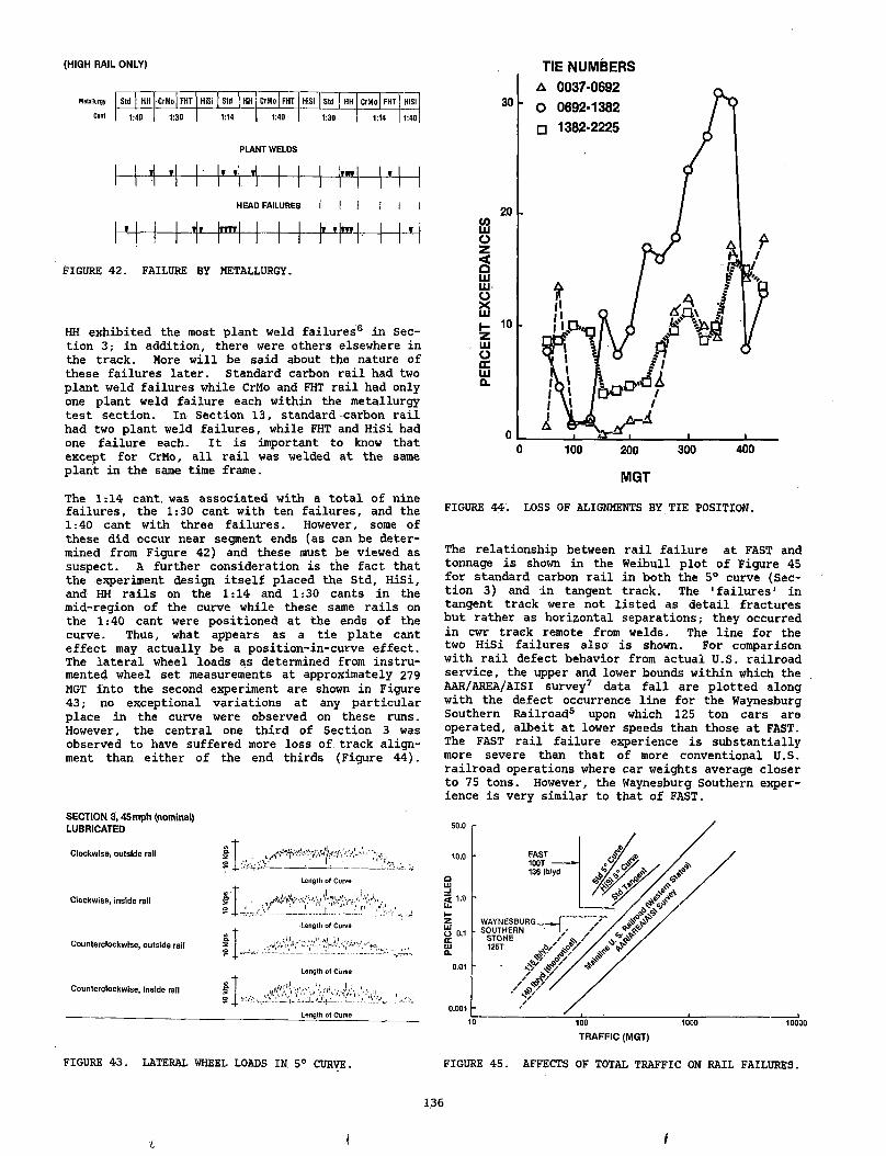
(H I G H R A IL O N L Y )

Metallurgy S td H H ■ C rM o ]F H T H IS i J S id | HH C rM o | FH T H IS I | S td | HH C rM o | F H T H iS i

Cant 1 :4 0 1 :3 0 1 :1 4 1 :4 0 1 :3 0 1 :1 4 1 :4 0

i

PLANT WELDS

T .Tj tj--------j____ |____ j____jDBLj____ |_f_|____ j

HEAD FAILURES I I I I I I

FIGURE 42. FAILURE BY METALLURGY.

HH exhibited the most plant weld failures6 in Sec­tion 3; in addition, there were others elsewhere in the track. More will be said about the nature of these failures later. Standard carbon rail had two plant weld failures while CrMo and FHT rail had only one plant weld failure each within the metallurgy test section. In Section 13, standard-carbon rail had two plant weld failures, while FHT and HiSi had one failure each. It is important to know that except for CrMo, all rail was welded at the same plant in the same time frame.

The 1:14 cant, was associated with a total of nine failures, the 1:30 cant with ten failures, and the 1:40 cant with three failures. However, some of these did occur near segment ends (as can be deter­mined from Figure 42) and these must be viewed as suspect. A further consideration is the fact that the experiment design itself placed the Std, HiSi, and HH rails on the 1:14 and 1:30 cants in the mid-region of the curve while these same rails on the 1:40 cant were positioned at the ends of the curve. Thus, what appears as a tie plate cant effect may actually be a position-in-curve effect. The lateral wheel loads as determined from instru­mented wheel set measurements at approximately 279 MGT into the second experiment are shown in Figure 43; no exceptional variations at any particular place in the curve were observed on these runs. However, the central one third of Section 3 was observed to have suffered more loss of track align­ment than either of the end thirds (Figure 44).

SECTION 3 ,45mph (nominal)LUBRICATED

Clockwise, outside rail £ ; v .

Clockwise, inside rail

Counterclockwise, outside rail

12

Length of Curve

FIGURE 43. LATERAL WHEEL LOADS IN 5° CURVE.

TIE NUMBERS

FIGURE 44. LOSS OF ALIGNMENTS BY TIE POSITION.

The relationship between rail failure at FAST and tonnage is shown in the Weibull plot of Figure 45 for standard carbon rail in both the 5° curve (Sec­tion 3) and in tangent track. The 'failures' in tangent track were not listed as detail fractures but rather as horizontal separations; they occurred in cwr track remote from welds. The line for the two HiSi failures also is shown. For comparison with rail defect behavior from actual U.S. railroad service, the upper and lower bounds within which the AAR/AREA/AISI survey7 data fall are plotted along with the defect occurrence line for the Waynesburg Southern Railroad5 upon which 125 ton cars are operated, albeit at lower speeds than those at FAST. The FAST rail failure experience is substantially more severe than that of more conventional U.S. railroad operations where car weights average closer to 75 tons. However, the Waynesburg Southern exper­ience is very similar to that of FAST.

FIGURE 45. AFFECTS OF TOTAL TRAFFIC ON RAIL FAILURES.

1.36

i i

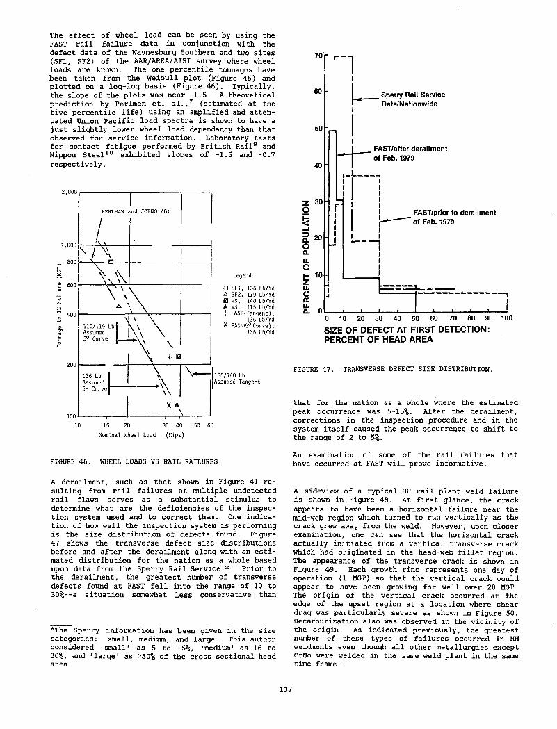
The effect of wheel load can be seen by using the FAST rail failure data in conjunction with the defect data of the Waynesburg Southern and two sites (SF1, SF2) of the AAR/AREA/AISI survey where wheel loads are known. The one percentile tonnages have been taken from the Weibull plot (Figure 45) and plotted on a log-log basis (Figure 46). Typically, the slope of the plots was near -1.5. A theoretical prediction by Perlman et. al.,7 (estimated at the five percentile life) using an amplified and atten­uated Union Pacific load spectra is shown to have a just slightly lower wheel load dependancy than that observed for service information. Laboratory tests for contact fatigue performed by British Rail9 and Nippon Steel10 exhibited slopes of -1.5 and -0.7 respectively.

Nominal Wheel Load (Kips)

70

60

50

40

30o

_i3Q.oa.u.O

20 -

10 -

LUoCCLU

HU - Sperry Rail Service

Data/Nationwide

, FAST/after derailm ent of Feb. 1979

r 1- —l l-I

iFAST/prior to derailm ent

' of Feb. 1979

"1II

0 10 20 30 40 50 60 70 80 90 100

SIZE OF DEFECT AT FIRST DETECTION: PERCENT OF HEAD AREA

FIGURE 47. TRANSVERSE DEFECT SIZE DISTRIBUTION.

that for the nation as a whole where the estimated peak occurrence was 5-15%. After the derailment, corrections in the inspection procedure and in the system itself caused the peak occurrence to shift to the range of 2 to 5%.

FIGURE 46. WHEEL LOADS VS RAIL FAILURES.An examination of some of the rail failures that have occurred at FAST will prove informative.

A derailment, such as that shown in Figure 41 re­sulting from rail failures at multiple undetected rail flaws serves as a substantial stimulus to determine what are the deficiencies of the inspec­tion system used and to correct them. One indica­tion of how well the inspection system is performing is the size distribution of defects found. Figure 47 shows the transverse defect size distributions before and after the derailment along with an esti­mated distribution for the nation as a whole based upon data from the Sperry Rail Service.* Prior to the derailment, the greatest number of transverse defects found at FAST fell into the range of 10 to 30%— a situation somewhat less conservative than

*The Sperry information has been given in the size categories: small, medium, and large. This author considered 'small' as 5 to 15%, 'medium' as 16 to 30%, and 'large' as >30% of the cross sectional head area.

A sideview of a typical HH rail plant weld failure is shown in Figure 48. At first glance, the crack appears to have been a horizontal failure near the mid-web region which turned to run vertically as the crack grew away from the weld. However, upon closer examination, one can see that the horizontal crack actually initiated from a vertical transverse crack which had originated in the head-web fillet region. The appearance of the transverse crack is shown in Figure 49. Each growth ring represents one day of operation (1 MGT) so that the vertical crack would appear to have been growing for well over 20 MGT. The origin of the vertical crack occurred at the edge of the upset region at a location where shear drag was particularly severe as shown in Figure 50. Decarburization also was observed in the vicinity of the origin. As indicated previously, the greatest number of these types of failures occurred in HH weldments even though all other metallurgies except CrMo were welded in the same weld plant in the same time frame.

137

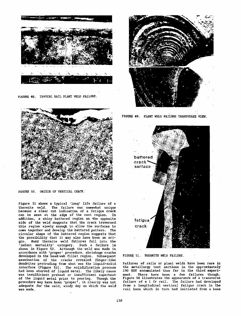
re:> Ct y

FIGURE 48. TYPICAL RAIL PLANT WELD FAILURE.

FIGURE 50. ORIGIN OF VERTICAL CRACK.

Figure 51 shows a typical 'long1 life failure of a thermite weld. The failure was somewhat unique because a clear cut indication of a fatigue crack can be seen at the edge of the cast region. In addition, a shiny battered region on the opposite side of the weld suggests that the crack traversed this region slowly enough to allow the surfaces to come together and develop the battered pattern. The circular shape of the battered region suggests that the possibility that it may also have been an ori­gin. Many thermite weld failures fall into the 'infant mortality1 category. Such a failure is shown in Figure 52. Although the weld was made in accordance with 'proper' procedure, shrinkage cracks developed in the head-web fillet region. Subsequent examination of the cracks revealed finger-like dendrites protruding from what was the liquid-solid interface (Figure 53). The solidification process had been starved of liquid metal. The likely cause was insufficient preheat or insufficient superheat of the liquid metal prior to pouring. Though the procedure may have been 'proper', it clearly was not adequate for the cold, windy day on which the weld was made.

battered c r a c k ^ surface

fatigue'crack

FIGURE 51. THERMITE WELD FAILURE.

Failures of rails or plant welds have been rare in the metallurgy test sections in the approximately 190 MGT accumulated thus far in the third experi­ment. There have been a few failures though. Figure 54 illustrates the appearance of a transverse failure of a 1 Cr rail. The failure had developed from a longitudinal vertical fatigue crack in the rail base which in turn had initiated from a base

138

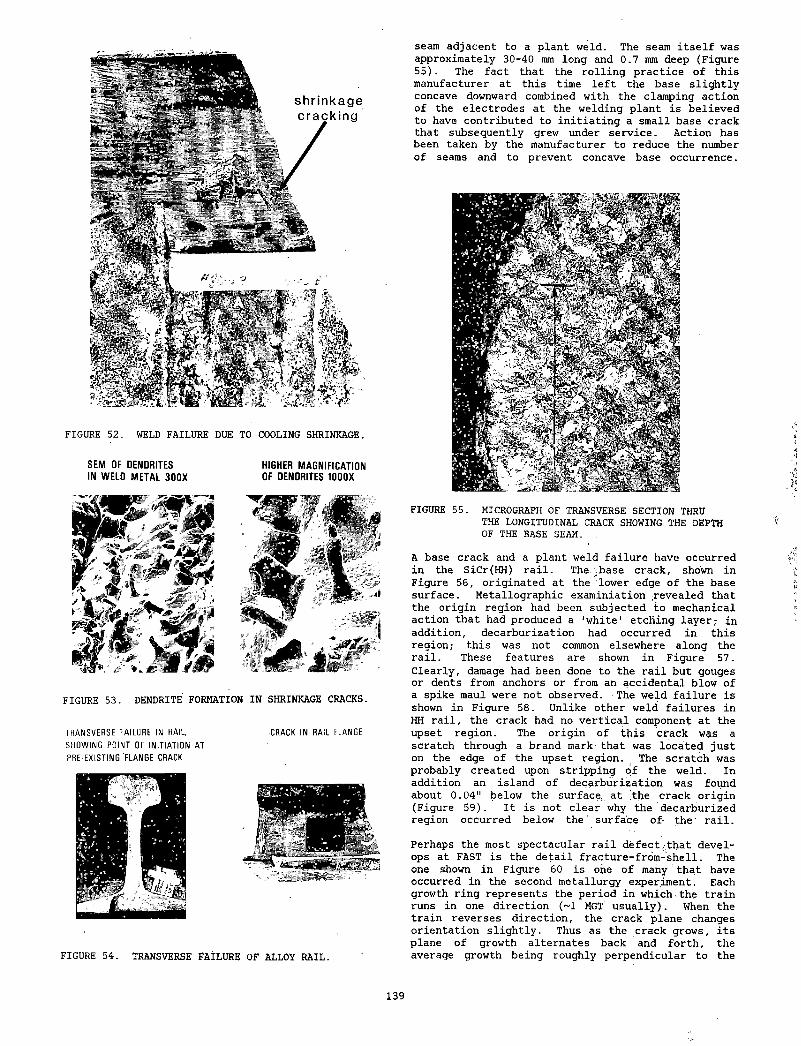
FIGURE 52. WELD FAILURE DUE TO COOLING SHRINKAGE.

SEM OF DENDRITES HIGHER MAGNIFICATIONIN WELD METAL 300X OF DENDRITES 1000X

FIGURE 53. DENDRITE FORMATION IN SHRINKAGE CRACKS.

TRANSVERSE FAILURE IN RAIL. CRACK IN RAIL FLANGESHOWING POINT OF INITIATION AT PRE-EXISTING FLANGE CRACK

FIGURE 54. TRANSVERSE FAILURE OF ALLOY RAIL.

seam adjacent to a plant weld. The seam itself was approximately 30-40 mm long and 0.7 mm deep (Figure 55). The fact that the rolling practice of this manufacturer at this time left the base slightly concave downward combined with the clamping action of the electrodes at the welding plant is believed to have contributed to initiating a small base crack that subsequently grew under service. Action has been taken by the manufacturer to reduce the number of seams and to prevent concave base occurrence.

FIGURE 55. MICROGRAPH OF TRANSVERSE SECTION THRUTHE LONGITUDINAL CRACK SHOWING THE DEPTH OF THE BASE SEAM.

A base crack and a plant weld failure have occurred in the SiCr(HH) rail. The.;,base crack, shown in Figure 56, originated at the lower edge of the base surface. Metallographic examiniation revealed that the origin region had been subjected to mechanical action that had produced a 'white' etching layer,- in addition, decarburization had occurred in this region; this was not common elsewhere along the rail. These features are shown in Figure 57. Clearly, damage had been done to the rail but gouges or dents from anchors or from an accidental blow of a spike maul were not observed. The weld failure is shown in Figure 58. Unlike other weld failures in HH rail, the crack had no vertical component at the upset region. The origin of this crack was a scratch through a brand mark; that was located just on the edge of the upset region. The scratch was probably created upon stripping of the weld. In addition an island of decarburization was found about 0.04" below the surface at the crack origin (Figure 59). It is not clear why the decarburized region occurred below the' surface of the' rail.

Perhaps the most spectacular rail defect,that devel­ops at FAST is the detail fracture-from-shell. The one shown in Figure 60 is one of many that have occurred in the second metallurgy experiment. Each growth ring represents the period in which-the train runs in one direction (~1 MGT usually). When the train reverses direction, the crack plane changes orientation slightly. Thus as the crack grows, its plane of growth alternates back and forth, the average growth being roughly perpendicular to the

139

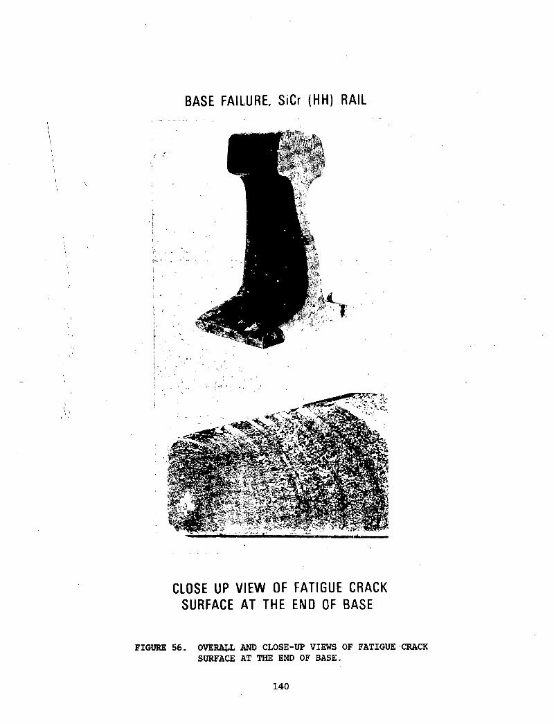
BASE FAILURE, SiCr (HH) RAIL

CLOSE UP VIEW OF FATIGUE CRACK SURFACE AT THE END OF BASE

F I G U R E 5 6 . O V E R A L L A N D C L O S E - U P V I E W S O F F A T I G U E C R A C K

S U R F A C E A T T H E E N D O F B A S E .

140

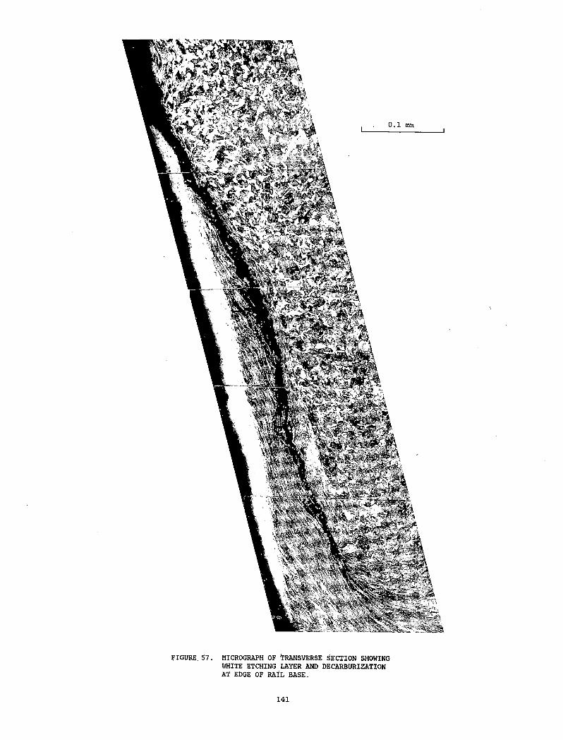
FIGURE. 57. MICROGRAPH OF 'TRANSVERSE SECTION SHOWING WHITE ETCHING LAYER AND DECARBURIZATION AT EDGE OF RAIL BASE.

141

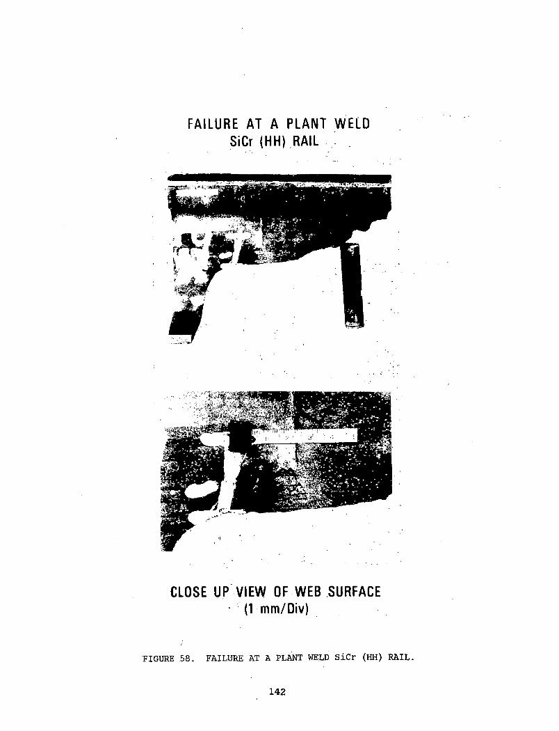
FAILURE AT A PLANT WELD SiCr (HH) RAIL

CLOSE UP VIEW OF WEB SURFACE (1 mm/Div)

FIGURE 58. FAILURE AT A PLANT WELD SiCr (HH) RAIL

1 4 2

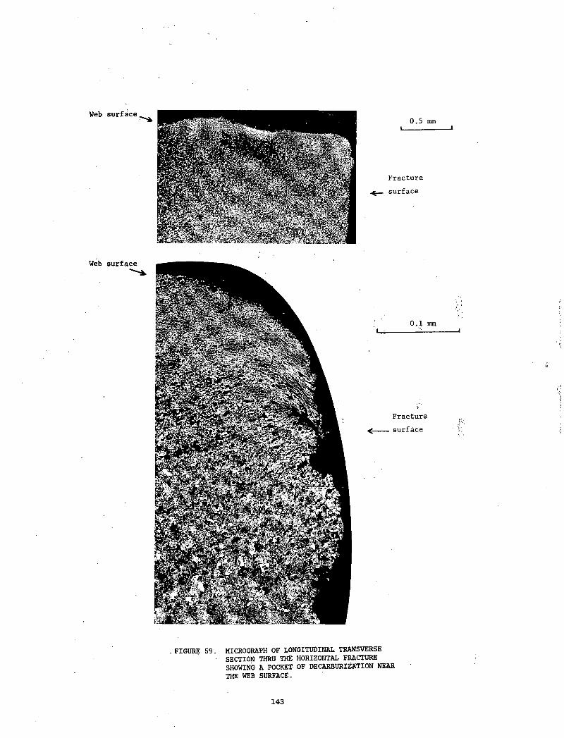
- FIGURE 59. MICROGRAPH OF LONGITUDINAL TRANSVERSE - SECTION THRU THE HORIZONTAL FRACTURE

SHOWING A POCKET OF DECARBURIZATION NEAR THE WEB SURFACE.

143

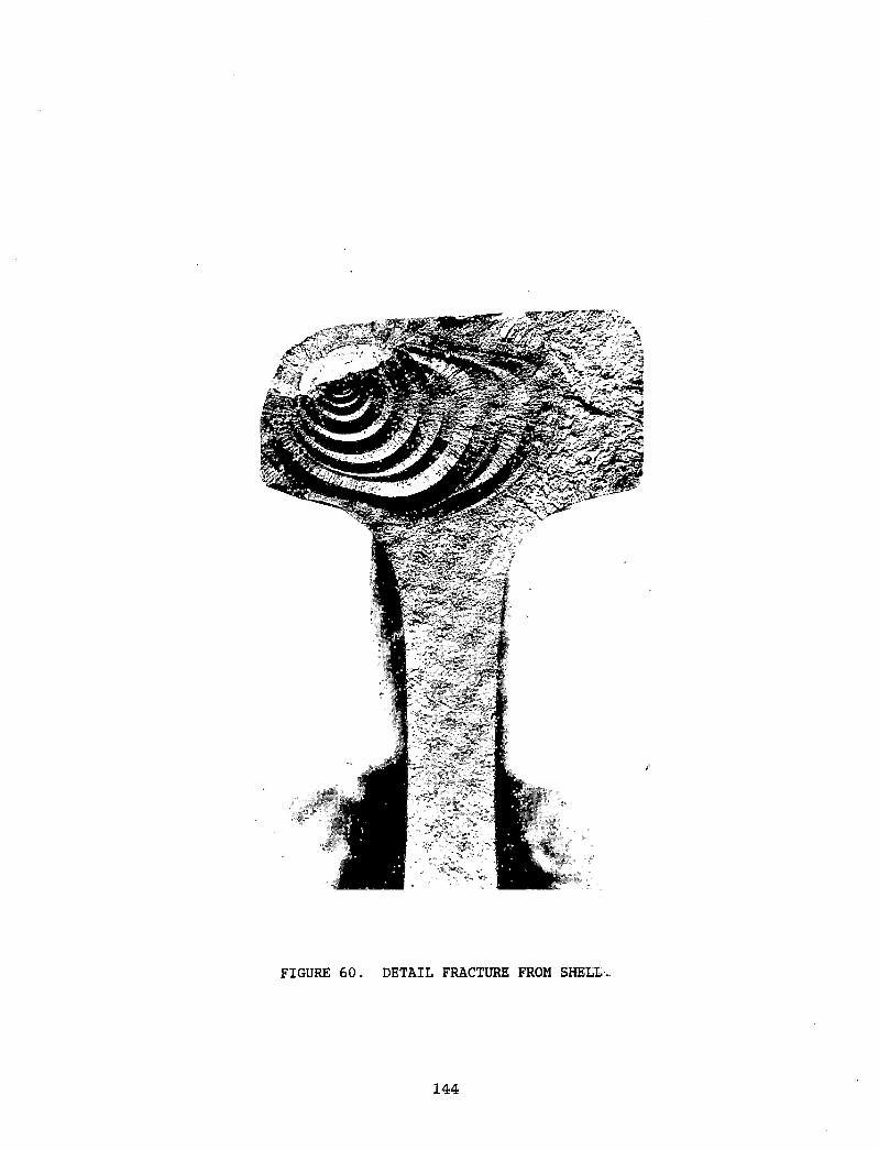
FIGURE 60. DETAIL FRACTURE FROM SHELL

144

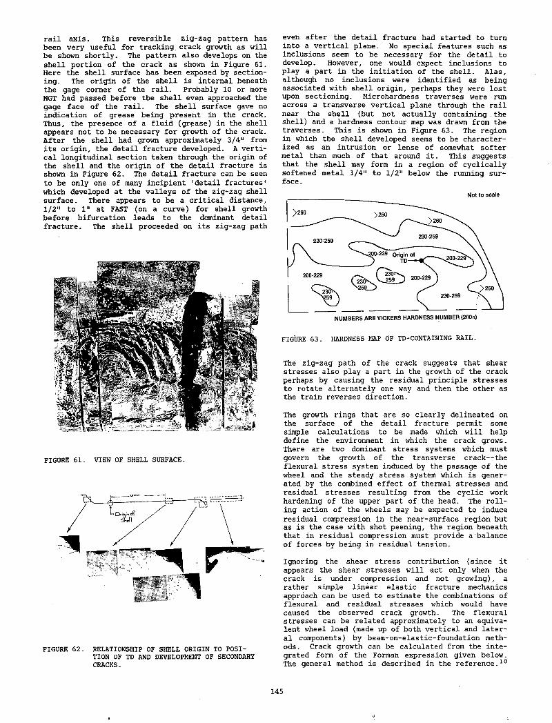
rail axis. This reversible zig-zag pattern has been very useful for tracking crack growth as will be shown shortly. The pattern also develops on the shell portion of the crack as shown in Figure 61. Here the shell surface has been exposed by section­ing. The origin of the shell is internal beneath the gage corner of the rail. Probably 10 or more MGT had passed before the shell even approached the gage face of the rail. The shell surface gave no indication of grease being present in the crack. Thus, the presence of a fluid (grease) in the shell appears not to be necessary for growth of the crack. After the shell had grown approximately 3/4" from its origin, the detail fracture developed. A verti­cal longitudinal section taken through the origin of the shell and the origin of the detail fracture is shown in Figure 62. The detail fracture can be seen to be only one of many incipient 'detail fractures' which developed at the valleys of the zig-zag shell surface. There appears to be a critical distance, 1/2" to 1" at FAST (on a curve) for shell growth before bifurcation leads to the dominant detail fracture. The shell proceeded on its zig-zag path

FIGURE 61. VIEW OF SHELL SURFACE.

FIGURE 62. RELATIONSHIP OF SHELL ORIGIN TO POSI­TION OF TD AND DEVELOPMENT OF SECONDARY CRACKS.

even after the detail fracture had started to turn into a vertical plane. No special features such as inclusions seem to be necessary for the detail to develop. However, one would expect inclusions to play a part in the initiation of the shell. Alas, although no inclusions were identified as being associated with shell origin, perhaps they were lost upon sectioning. Microhardness traverses were run across a transverse vertical plane through the rail near the shell (but not actually containing . the shell) and a hardness contour map was drawn from the traverses. This is shown in Figure 63. The region in which the shell developed seems to be character­ized as an intrusion or lense of somewhat softer metal than much of that around it. This suggests that the shell may form in a region of cyclically softened metal 1/4" to 1/2" below the running sur­face .

Not to scale

FIGURE 63. HARDNESS MAP OF TD-CONTAINING RAIL.

The zig-zag path of the crack suggests that shear stresses also play a part in the growth of the crack perhaps by causing the residual principle stresses to rotate alternately one way and then the other as the train reverses direction.

The growth rings that are so clearly delineated on the surface of the detail fracture permit some simple calculations to be made which will help define the environment in which the crack grows. There are two dominant stress systems which must govern the growth of the transverse crack--the flexural stress system induced by the passage of the wheel and the steady stress system which is gener­ated by the combined effect of thermal stresses and residual stresses resulting from the cyclic work hardening of the upper part of the head. The roll­ing action of the wheels may be expected to induce residual compression in the near-surface region but as is the case with shot peening, the region beneath that in residual compression must provide a balance of forces by being in residual tension.

Ignoring the shear stress contribution (since it appears the shear stresses will act only when the crack is under compression and not growing), a rather simple linear elastic fracture mechanics approach can be used to estimate the combinations of flexural and residual stresses which would have caused the observed crack growth. The flexural stresses can be related approximately to an equiva­lent wheel load (made up of both vertical and later­al components) by beam-on-elastic-foundation meth­ods. Crack growth can be calculated from the inte­grated form of the Forman expression given below. The general method is described in the reference.10

145

■l

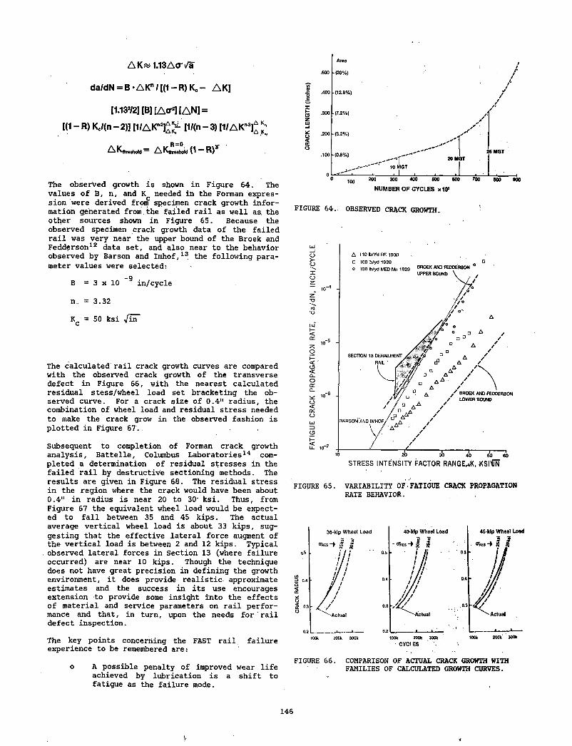
A K fV 1.13A<T\/aArea

.500 -(20% )

da/dN = B • A K " / [( 1 - R) Ko - A K ] (Aa>fO

.400 •(12.8%)

[1.132/2] [B] [Acr2] IA N ] = X<3 .300 •(7.2%)

- R) KJ(n - 2)] [ 1 / A K ^ ^ [1/(n - 3) [1 /A K *3£ LU_l* .200-(3 .2% )

^ threshold ^ threshold (1 R)<cco

.100-(0 .8% )

010 MGT, I

The observed growth is shown in Figure 64. The values of B, n, and K needed in the Forman expres­sion were derived from specimen crack growth infor­mation generated from the failed rail as well as, the other sources shown in Figure 65. Because the observed specimen crack growth data of the failed rail was very near the upper bound of the Broek and Fedderson12 data set, and also near to the behavior observed by Barson and Imhof,13 the following para­meter values were selected:

-9B = 3 x 10 in/cycle

n_ = 3.32

K = 50 ksi Jin c ’

The calculated rail crack growth curves are compared with the observed crack growth of the transverse defect in Figure 66, with the nearest calculated residual stess/wheel load set bracketing the ob­served curve. For a crack size of 0.4" radius, the combination of wheel load and residual stress needed to make the crack grow in the observed fashion is plotted in Figure 67..

Subsequent to completion of Forman crack growth analysis, Battelle, Columbus Laboratories14 com­pleted a determination of residual stresses in the failed rail by destructive sectioning methods. The results are given in Figure 68. The residual stress in the region where the crack would have been about 0.4" in radius is near 20 to 30' ksi. Thus, from Figure 67 the equivalent wheel load would be expect­ed to fall between 35 and 45 kips. The actual average vertical wheel load is about 33 kips, sug­gesting that the effective lateral force augment of the vertical load is between 2 and 12 kips. Typical observed lateral forces in Section 13 (where failure occurred) are near 10 kips. Though the technique does not have great precision in defining the growth environment, it does provide realistic- approximate estimates and the success in its use encourages extension to provide some insight into the effects of material and service parameters on rail perfor­mance and that, in turn, upon the needs for 1 rail defect inspection.

The key points concerning the FAST rail failure experience to be remembered are:

o A possible penalty of improved wear life achieved by lubrication is a shift to fatigue as the failure mode.

1 0 0 2 0 0 300 400 500 600 700 000 900NUMBER OF CYCLES x 1 P

FIGURE 64. OBSERVED CRACK GROWTH.

FIGURE 65. VARIABILITY OF FATIGUE CRACK PROPAGATION RATE BEHAVIOR.

FIGURE 66. COMPARISON OF ACTUAL CRACK GROWTH WITH FAMILIES OF CALCULATED GROWTH CURVES.

146

V

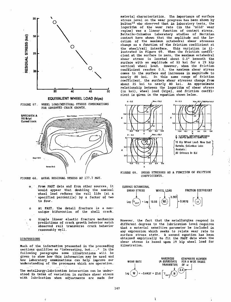
EQUIVALENT WHEEL LOAD (kips)

FIGURE 67. WHEEL LOAD/RESIDUAL STRESS COMBINATIONS FOR OBSERVED CRACK GROWTH.

material characteristics. The importance of surface stress level on the wear progress has been shown by Bolton15 who observed that in laboratory tests, the logarithm of the wear rate (in the 'mild1 wear regime) was a linear function of contact stress. Battelle-Columbus Laboratory studies of Hertzian contact have shown that the amplitude and the lo­cation of the maximum octahedral shear stresses change as a function of the friction coefficient at the wheel/rail interface. This variation is il­lustrated in Figure 69. When the friction coeffi­cient at the surface is zero, the maximum octahedral shear stress is located about 0.1" beneath the surface with an amplitude of 53 ksi for a 19 kip vertical wheel load. However, when the friction coefficient reaches 0.5, the maximum shear stress comes to the surface and increases in magnitude to nearly 80 ksi. In this same range of friction coefficient, the surface shear stresses change from about 25 ksi to nearly 80 ksi. An approximate relationship between the logarithm of shear stress (in ksi), wheel load (kips), and friction coeffi­cient is given in the equation shown below.

I = ^ eReath s)

19 Kip Wheel Load: New Rail Battelle, Columbus Labs Analysis !All Stresses In Ksi

FIGURE 69. SHEAR STRESSES AS A FUNCTION OF FRICTION COEFFICIENTS.

o. From FAST data and from other sources, it would appear that doubling the nominal wheel load reduces the rail life (at a

• specified percentile) by a factor of two to four.

o At FAST, the detail fracture is a non- uniqUe bifurcation of the shell crack.

SURFACE OCTAHEDRALSHEAR STRESS WHEEL TOAD FRICTION COEFFICIENT

o Simple linear elastic fracture mechanics \ predictions of crack growth behavior match

observed rail transverse crack behavior reasonably well.

DISCUSSIONS

Much of the information presented in the preceedingsections qualifies as "interesting, but.__" In thefollowing paragraphs some illustrations will be given to show how this information may be used and how laboratory examinations can help improve our understanding of the processes which are operative.

The metallurgy:lubrication interaction can be under­stood in terms of variation in surface shear stress with lubrication when adjustments are made for

However, the fact that the metallurgies respond in different degrees to the lubrication level requires that a material sensitive parameter be included in any expression which seeks to relate wear rate to surface stress state. A second equation has been obtained empirically to fit the FAST data when the shear stress is based upon 19 kip wheel load for illustration.

WEAR RATEHARDNESS

(A SURROGATE PARAMETER)

Log = -3 .4 4 3 7 + 27.41

COMPOSITE NUMBER FOR A WIDE RANGEOF u

2^)*—

147

v \

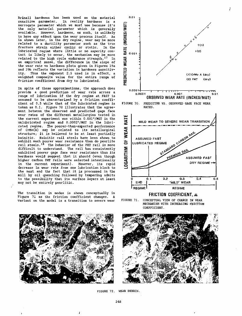
Brinell hardness has been used as the material sensitive parameter. In reality hardness is a surrogate parameter which we must use because it's the only material parameter which is generally available. However, hardness, as such, is unlikely to have any effect upon the wear process itself. As is shown later, in the dry regime, wear may be more related to a ductility parameter such as the true fracture strain either cyclic or static. In the lubricated regime where little or no asperity con­tact is likely to occur, the mechanism may be more related to the high cycle endurance strength.17 In an empirical sense, the difference in the slope of the wear rate vs hardness plots given in Figures 19a and 19b reflects the variation in hardness sensitiv­ity. Thus the exponent 2.5 used is in effect, a weighted composite value for the entire range of friction coefficient from dry to lubricated.

In spite of these approximations, the approach does provide a good prediction of wear rate across a range of lubrication if the dry regime at FAST is assumed to be characterized by a friction coeffi­cient of 0.5 while that of the lubricated regime is taken as 0.1. Figure 70 illustrates that the agree­ment between the observed and predicted gage face wear rates of the different metallurgies tested in the current experiment was within 0.001"/MGT in the unlubricated regime and 0.0002"/MGT in the lubri­cated regime. The poorer-than-expected performance of CrMo(A) may be related to its metallurgical structure; it is believed to be at least partially bainitic. Bainitic rail steels have been shown to exhibit much poorer wear resistance than do pearlite rail steels.18 The behavior of the FHT rail is more difficult to understand. The rail has consistently exhibited poorer gage face wear resistance than its hardness would suggest that it should (even though higher carbon FHT rails were selected intentionally in the current experiment). However, its rapid decrease in wear rate from one lubrication block to the next and the fact that it is processed in the mill by oil quenching followed by tempering admits to the possibility that its surface layers at least may not be entirely pearlitic.

The transition in modes is shown conceptually in Figure 71 as the friction coefficient changes. A variant on the model is a transition to severe wear

FIGURE 70. PREDICTED VS. OBSERVED GAGE FACE WEAR RATES.

FR ICTIO N COEFFIC IENT, x iFIGURE 71. CONCEPTUAL VIEW OF CHANGE IN WEAR

MECHANISM WITH INCREASING FRICTION COEFFICIENT.

148

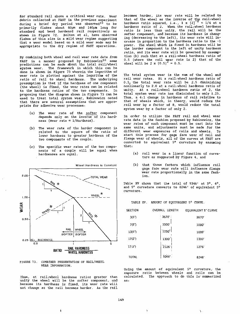
for standard rail above a critical wear rate. Wear debris collected at FAST in the previous experiment during a brief dry period was observed19 to be primarily flakes about 80|jm and 140pm long for standard and head hardened rail respectively as shown in Figure 72. Bolton et al, have observed flakes of this size in a mild wear regime suggesting that a wear model based on a mild wear mode may be appropriate to the dry regime of FAST operations.

By combining both wheel and rail wear rate data from FAST in a manner proposed by Rabinowicz20 some predictions can be made about the total rail/wheel system wear. The framework in which this can be done is shown in Figure 73 wherein the logarithm of wear rate is plotted against the logarithm of the ratio of rail to wheel hardness. The underlying presumption is that if the hardness of one component (the wheel) is fixed, the wear rates can be related to the hardness ratios of the two components. In proposing that the diagram shown in Figure 73 can be used to treat total system wear, Rabinowicz noted that there are several assumptions that are appro­priate for adhesive wear processes:

(a) The wear rate of the softer component depends only on the inverse of its hard­ness (wear rate a 1/Hardness).

(b) The wear rate of the harder component is related to the square of the ratio of lower hardness to greater hardness of the two components of the couple.

(c) The specific wear rates of the two compo­nents of a couple will be equal when hardnesses are equal.

Wheel Hardness is Constant

RAIL HARDNESS WHEEL HARDNESS

FIGURE 73. COMBINED PRESENTATION OF RAIL/WHEEL WEAR INFORMATION.

Thus, at rail:wheel hardness ratios greater than unity the wheel will be the softer component, and because its hardness is fixed, its wear rate will not change as the rail becomes harder. As the rail

becomes harder, its wear rate will be related to that of the wheel as the inverse of th,e railrwheel hardness ratio squared, i.e., 1 x [2] = 1/4 at a hardness ratio of 2. When the rail:wheel hardness ratio is less than unity, the rail will be the softer component, and because its hardness is chang­ing (decreasing to the left), its wear rate will in­crease in proportion to the hardness ratio to the -1 power. The wheel which is fixed in hardness will be the harder component to the left of unity hardness ratio, and its wear rate will be governed by assump­tion (b) such that at a rail:wheel hardness ratio of 0.5 (where the rail vrear rate is 2) that of the wheel will be 2 x [0.5] =0.5.

The total system wear is the sum of the wheel and rail wear rates. At a rail .-wheel hardness ratio of 0.5, the total wear rate will be 2.5 diminishing nonlinearly to 2.0 at a rail:wheel hardness ratio of unity. At a rail:wheel hardness ratio of 2, the total system wear rate has diminished to only 1.25. Thus, a 4:1 change in hardness of rail relative to that of wheels which, in theory, would reduce the rail wear by a factor of 8, would reduce the total system wear by a factor of only 2.

In order to utilize the FAST rail and wheel wear rate data in the fashion proposed by Rabinowicz, the wear rates of each component must be cast into thesame units, and adjustments must be made for thedifferent wear exposures of rails and wheels. To start this process for gage face wear of rail andflange wear of wheels, all of the curves at FAST areconverted to equivalent 5° curvature by assuming that:

(a) rail wear is a linear function of curva­ture as suggested by Figure 4, and

(b) that those factors which influence rail gage face wear rate will influence flange wear rate proportionally in the same fash­ion.

Table XV shows that the total of 9346' at 3°, 4°, and 5° curvature converts to 82461 of equivalent 5° curvature.

TABLE XV. AMOUNT OF EQUIVALENT 5° CURVE.

SECTION OVERALL LENGTH EQUIVALENT 5” CURVE

3(5") 3670’ 3670’

7(5") 1000’ 1000’

13(4") “12507 1000’

17(5") 1300’' 1300’

17(3") ~2i26’ 1276’

TOTAL 9346’ 8246’

Using the amount of equivalent 5° curvature, the exposure ratio between wheels and rails can be calculated. The approach to do this is' summarized as:

149

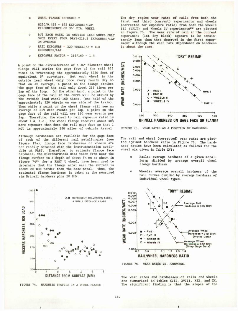
o WHEEL FLANGE EXPOSURE =

8250/9.425 = 875 EXPOSURES/LAP CIRCUMFERENCE OF 36" DIA. WHEEL

o BUT EACH WHEEL IS OUTSIDE LEAD WHEEL ONLY ONCE EVERY FOUR DAYS+218.8 EXPOSURES/LAP ON AVERAGE

o RAIL EXPOSURE = 320 WHEELS/2 = 160 EXPOSURES/LAP

o EXPOSURE FACTOR = 219/160 =1.4

A point on the circumference of a 36" diameter wheel flange will strike the gage face of the rail 875 times in traversing the approximately 8250 feet of equivalent 5° curvature. But each wheel is the outside lead wheel only once every fourth day so that on an average, a point on the flange strikes the gage face of the rail only about 219 times per lap of the loop. On the other hand, a point on the gage face of the rail in the curve will be struck by the outside lead wheel 160 times, (one half of the approximately 320 wheels on one side of the train). Thus while a point on the wheel flange will see an average of 219 wear events per lap, a point on the gage face of the rail will see 160 wear events per lap. Therefore, the wheel to rail exposure ratio is about 1.4, i.e., the wheel flange receives about 40% more exposure than does the rail gage face so that 1 MGT is approximately 350 miles of vehicle travel.

The dry regime wear rates of rails from both the first and third (current) experiments and wheels (corrected for exposure ratio) from both the Wheels III (VALT) and Wheels IV experiments22 are plotted in Figure 75. The wear rate of rail in the current experiment (1st dry block) appears to be consis­tently less than that observed in the first exper­iment although the wear rate dependance on hardness is about the same.

CD2ECOL UXo

<ocQC<

FIGURE 75. WEAR RATES AS A FUNCTION OF HARDNESS.

Although hardnesses are available for the gage face of each of the different rail metallurgies (see Figure 19a), flange face hardnesses of wheels are not readily obtained with the instrumentation avail­able at FAST. Therefore, to estimate flange face hardness, the microhardness data taken from near the flange surface to a depth of about 5% mm as shown in Figure 7427 for a FAST U wheel, have been used to determine that the flange metal near the surface is about 20 BHN harder than the base metal. Thus, the estimated flange hardness is taken as the measured rim Brinell hardness plus 20 BHN.

The rail and wheel (corrected) wear rates are plot­ted against hardness ratio in Figure 76. The hard­ness ratios have been calculated as follows for the wheel mix given in Table XVI:

o Rails: average hardness of a given metal­lurgy divided by average overall wheel flange hardness

o Wheels: average overall hardness of therail curves divided by average hardness of individual wheel types.

320-

o<o_ J

CD300-

00 290CO

ooc<00QCO

270-

0,0 R E P R E S E N T T R A V E R S E S T A K E N

A S M A L L D IS T A N C E A P A R T

• ••

• •

oooo

O ^ O ® 1. . 0

° ° °t>oS! <V * V * 8 °

1 2 3 4 5

DISTANCE FROM SURFACE (M M )

FIGURE 74. HARDNESS PROFILE IN A WHEEL FLANGE.

0.010 0.009- 0.008- 0.007

2E o.ooe-oq 0.005-

CD

O

0.003-

0 .002-

35s

0.001

DRY" REGIME

□

o

Average Rail Hardness = 365 BHN

Average Wheel Hardness =312 BHN

(Profile Data)

Average Wheel HaiUriesa-. 322 BHN

(Snap Gage Data)

0.8 ” CL9 1 TTl ^ 1.3 1.4

RAIL/WHEEL HARDNESS RATIO

FIGURE 76. WEAR RATES VS. HARDNESS.

The wear rates and hardnesses of rails and wheels are summarized in Tables XVII, XVIII, XIX, and XX. The significant finding is that the slopes of the

t

150

♦

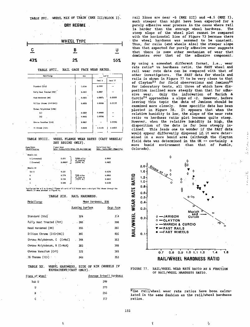
TABLE XVI. WHEEL MIX OF TRAIN'(RME

DRY REGIME

WHEEL TYPE

III/BLOCK I).

c B u" —

43% 2% 55%

TABLE XVII. RAIL GAGE FACE WEAR RATES.Metallurgy Dry tub'd

Sect 3 Sect 17

Standard (Std) 0.0066 0.0010 -

Fully Heat Treated (FHT) 0.0031 0.0007 -

Heat Hardened (HH) 0.0023 0.00075 0.00028

Silicon Chrome (CrSI(HH)) 0.0016 0.0006S 0.00030

Chrome Molybdenum (CrMo)

(C)

(A)

0.0029

, . 0.0036

0.00065

0.00090-

Chrome Vanadium (CrV) 0.0027 - 0.00040

IS Chrome (lCr) 0.0030 0.00065 0.00034

TABLE XVIII. WHEEL FLANGE WEAR RATES (CAST WHEELS/ DRY REGIME ONLY).Flange WearRate. Inches/1000 Miles (1S.8mn/1000 tan)

Normalized WearRate, Inches/MGT (28mn/HGMg)

rail lines are hear -6 (RME III) and -4.5 (RME I), much steeper than might have been expected for a purely adhesive wear process in the cases where rail is harder than the average wheel hardness. The steep slope of the wheel plot cannot be compared with the horizontal line of Figure 73 because there the wheel hardness was assumed to be constant. Thus, for rails (and wheels also) the steeper slope than that expected for purely adhesive wear suggests that there is some other mechanism of wear that dominates over that of the adhesive component.

By using a somewhat different format, i.e., wear rate ratio* vs hardness ratio, the FAST wheel and rail wear rate data can be compared with that of other investigators. The FAST data for wheels and rails is shown in Figure 77 to be very close to that of Clayton23 for field observations and Jamison24 for laboratory tests, all three of which have dis­position inclined more steeply than that for adhe­sive wear. Only the information of Marich & Curcio24 approaches a slope of -2. However, before leaving this topic the data of Jamison should be examined more closely. Some specific data has been plotted in Figure 78. It appears that when the relative humidity is low, the slope of the wear rate ratio vs hardness ratio' plot becomes quite steep. However, when the relative humidity is high, the disposition of the data is far less steeply in­clined. This leads one to wonder if the FAST data would appear differently disposed if it were deter­mined in a more humid area (although the Clayton field data was determined in the UK — certainly a more humid environment than that of Pueblo, Colorado).

' Wheels III

U (untreated)

C (treated)

Wheels IV

Sub U

0.014

0.00634

0.221

0.174

0.135

0.090

}14000 miles of running (22540 km)

7000 miles of running (11270 km)

0.0049

0.0022

0.0070

0.0063

0.0049

0.0028

"estimated for a C vs U wheel figure of merit of 2.2 based upon a straight line drawn through the Wheels IV data plotted in Figure 4a.

TABLE XIX. RAIL HARDNESS.Metallurgy Mean Hardness, BHN

Running Surface Gage Face

Standard (Std) 324 314

Fully Heat Treated (FHT) . • 366' 386

Head Hardened (HH) 355 381

Silicon Chrome (SiCr(HH)) 391 405

Chrome Molybdenum, C (CrMoC) . 344 353

Chrome Molybdenum, A (CrMoA) 383 398

Chrome Vanadium (CrV) 372 365

\% Chrome (lCr) i 348 353R A IL /W H E E L H A R D N E S S RA TIO

TABLE XX. WHEEL HARDNESS, SIDE OF RIM (WHEELS IV EXPERIMENT/CAST ONLY).

Class of Wheel

Sub U

U B C

Average Brinell Hardness

249

273

295

317

FIGURE 77. RAIL/WHEEL WEAR RATE RATIO AS A FUNCTION OF RAIL/WHEEL HARDNESS RATIO.

*the rail/wheel wear rate ratios have been calcu­lated in the same fashion as the rail/wheel hardness ratios.

151

\\

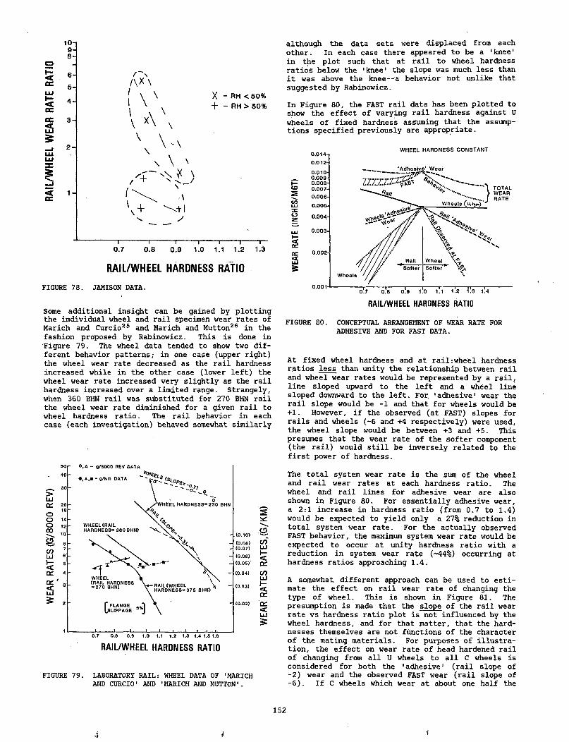
R A IL /W H E E L HARDNESS RATIO

FIGURE 78. JAMISON DATA.

Some additional insight can be gained by plotting the individual wheel and rail specimen wear rates of Marich and Curcio25 and Marich and Mutton26 in the fashion proposed by Rabinowicz. This is done in Figure 79. The wheel data tended to show two dif­ferent behavior patterns; in one case (upper right) the wheel wear rate decreased as the rail hardness increased while in the other case (lower left) the wheel wear rate increased very slightly as the rail hardness increased over a limited range. Strangely, when 360 BHN rail was substituted for 270 BHN rail the wheel wear rate diminished for a given rail to wheel hardness ratio. The rail behavior in each case (each investigation) behaved somewhat similarly

( 0 . 10)

(o.oa)(0.07)(0.06)(0.05)(0.04)

(0.03)

idUtri

<C d

ir>LUi-<C d

C d<

RAIL/WHEEL HARDNESS RATIO

FIGURE 79. LABORATORY RAIL: WHEEL DATA OF 'MARICH AND CURCIO1 AND 'MARICH AND MUTTON'.

although the data sets were displaced from each other. In each case there appeared to be a 'knee' in the plot such that at rail to wheel hardness ratios below the 'knee' the slope was much less than it was above the knee--a behavior not unlike that suggested by Rabinowicz.

In Figure 80, the FAST rail data has been plotted to show the effect of varying rail hardness against U wheels of fixed hardness assuming that the assump­tions specified previously are appropriate.

W H E E L H A R D N E S S C O N S T A N T

FIGURE 80. CONCEPTUAL ARRANGEMENT OF WEAR RATE FOR ADHESIVE AND FOR FAST DATA.

At fixed wheel hardness and at rail:wheel hardness ratios less than unity the relationship between rail and wheel wear rates would be represented by a rail, line sloped upward to the left and a wheel line sloped downward to the left. For 'adhesive' wear the rail slope would be -1 and that for wheels would be +1. However, if the observed (at FAST) slopes for rails and wheels (-6 and +4 respectively) were used, the wheel slope would be between +3 and +5. This presumes that the wear rate of the softer component (the rail) would still be inversely related to the first power of hardness.

The total system wear rate is the sum of the wheel and rail wear rates at each hardness ratio. The wheel and rail lines for adhesive wear are also shown in Figure 80. For essentially adhesive wear, a 2:1 increase in hardness ratio (from 0.7 to 1.4) would be expected to yield only a 27% reduction in total system wear rate. For the actually observed FAST behavior, the maximum system wear rate would be expected to occur at unity hardness ratio with a reduction in system wear rate (~44%) occurring at hardness ratios approaching 1.4.

A somewhat different approach can be used to esti­mate the effect on rail wear rate of changing the type of wheel. This is shown in Figure 81. The presumption is made that the slope of the rail wear rate vs hardness ratio plot is not influenced by the wheel hardness, and for that matter, that the hard­nesses themselves are not functions of the character of the mating materials. For purposes of illustra­tion, the effect on wear rate of head hardened rail of changing from all U wheels to all C wheels is considered for both the 'adhesive' (rail slope of -2) wear and the observed FAST wear (rail slope of -6). If C wheels which wear at about one half the

152

<S> •I

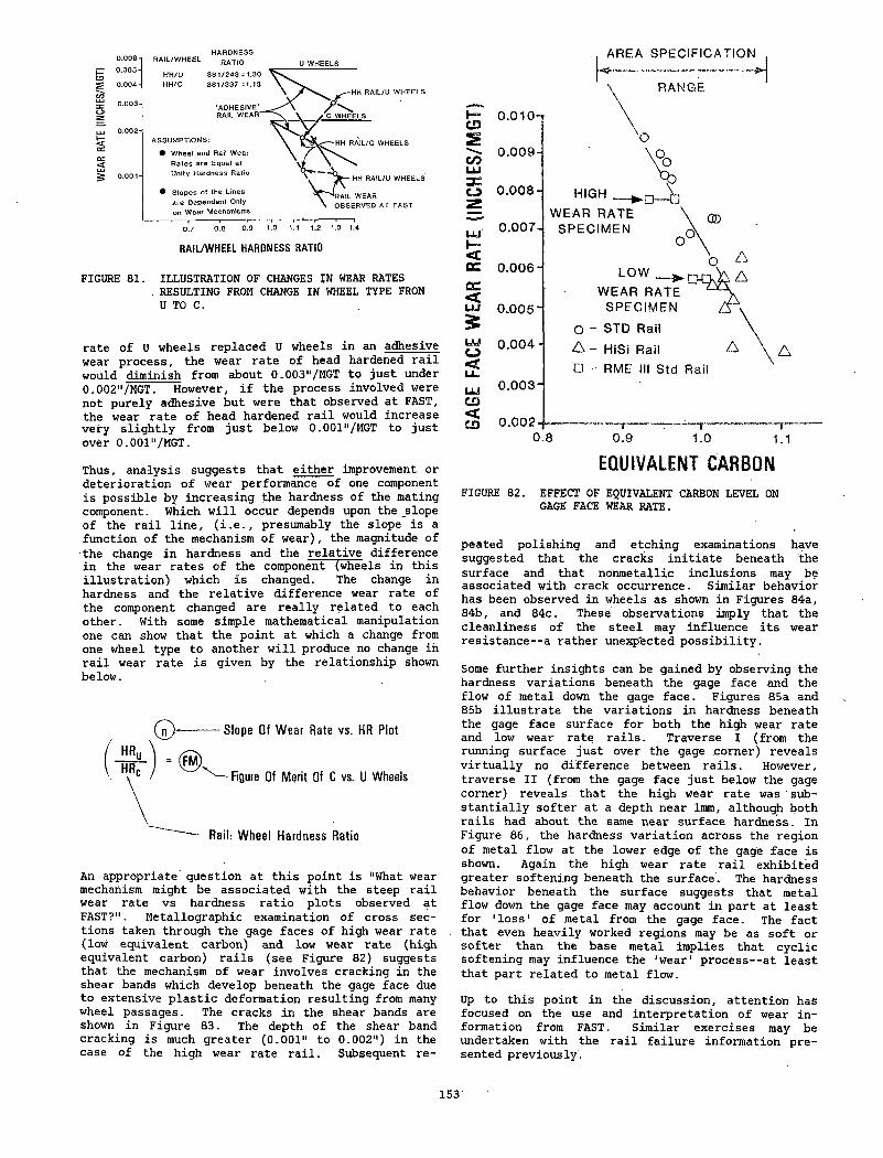
FIGURE 81. ILLUSTRATION OF CHANGES IN WEAR RATES. RESULTING FROM CHANGE IN WHEEL TYPE FROM U TO C.

rate of U wheels replaced U wheels in an adhesive wear process, the wear rate of head hardened rail would diminish from about 0.003"/MGT to just under 0.002"/MGT. However, if the process involved were not purely adhesive but were that observed at FAST, the wear rate of head hardened rail would increase very slightly from just below 0.001"/MGT to just over 0.001"/MGT.

Thus, analysis suggests that either improvement or deterioration of wear performance of one component is possible by increasing the hardness of the mating component. Which will occur depends upon the slope of the rail line, (i.e., presumably the slope is a function of the mechanism of wear), the magnitude of the change in hardness and the relative difference in the wear rates of the component (wheels in this illustration) which is changed. The change in hardness and the relative difference wear rate of the component changed are really related to each other. With some simple mathematical manipulation one can show that the point at which a change from one wheel type to another will produce no change in rail wear rate is given by the relationship shown below.

Slope Of W ear Rate vs. HR P lot

Figure Of M erit Of C vs. U Wheels

Rail: W heel Hardness Ratio

An appropriate question at this point is "What wear mechanism might be associated with the steep rail wear rate vs hardness ratio plots observed at FAST?". Metallographic examination of cross sec­tions taken through the gage faces of high wear rate (low equivalent carbon) and low wear rate (high equivalent carbon) rails (see Figure 82) suggests that the mechanism of wear involves cracking in the shear bands which develop beneath the gage face due to extensive plastic deformation resulting from many wheel passages. The cracks in the shear bands are shown in Figure 83. The depth of the shear band cracking is much greater (0.001" to 0.002") in the case of the high wear rate rail. Subsequent re-

EQUIVALENT CARBONFIGURE 82. EFFECT OF EQUIVALENT CARBON LEVEL ON

GAGE FACE WEAR RATE.

peated polishing and etching examinations have suggested that the cracks initiate beneath the surface and that nonmetallic inclusions may be associated with crack occurrence. Similar behavior has been observed in wheels as shown in Figures 84a, 84b, and 84c. These observations imply that the cleanliness of the steel may influence its wear resistance--a rather unexpected possibility.

Some further insights can be gained by observing the hardness variations beneath the gage face and the flow of metal down the gage face. Figures 85a and 85b illustrate the variations in hardness beneath the gage face surface for both the high wear rate and low wear rate rails. Traverse I (from the running surface just over the gage corner) reveals virtually no difference between rails. However, traverse II (from the gage face just below the gage corner) reveals that the high wear rate was sub­stantially softer at a depth near 1mm, although both rails had about the same near surface hardness. In Figure 86, the hardness variation across the region of metal flow at the lower edge of the gage face is shown. Again the high wear rate rail exhibited greater softening beneath the surface. The hardness behavior beneath the surface suggests that metal flow down the gage face may account in part at least for 'loss' of metal from the gage face. The fact that even heavily worked regions may be as soft or softer than the base metal implies that cyclic softening may influence the 'wear' process— at least that part related to metal flow.

Up to this point in the discussion, attention has focused on the use and interpretation of wear in­formation from FAST. Similar exercises may be undertaken with the rail failure information pre­sented previously.

153

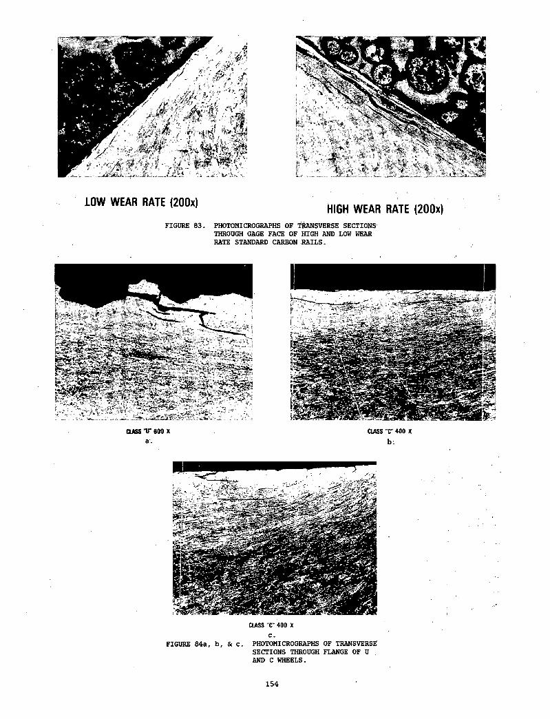
LOW WEAR RATE (200x) HIGH WEAR RATE (200x)FIGURE 83. PHOTOMICROGRAPHS OF TRANSVERSE SECTIONS

THROUGH GAGE FACE OF HIGH AND LOW WEAR RATE STANDARD CARBON RAILS.

CLASS "C" 400 XC .

FIGURE 84a, b, St c. PHOTOMICROGRAPHS OF TRANSVERSE SECTIONS THROUGH FLANGE OF U AND C WHEELS.

154

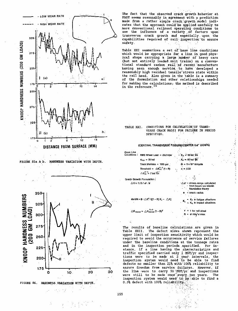
KNOO

P HA

RDNE

SS N

UMBE

RS (

200

GM L

OADS

)

DISTANCE FROM SURFACE (MM)

FIGURE 85a & b. HARDNESS VARIATION WITH DEPTH.

FIGURE 86. HARDNESS VARIATION WITH DEPTH..

The fact that the observed crack growth behavior at FAST seems reasonably in agreement, with a prediction made from a rather simple crack, growth model indi­cates that the approach could be applied usefully to more conventional railroad operating•conditions to see the influence of a variety of factors upon' transverse crack growth and especially. upon the capabilities required of rail- inspection’to assure safety. -

Table XXI summarizes a set of base line conditions which would be appropriate for a line in good phys­ical shape carrying a large number of heavy cars (but not entirely loaded .unit trains) bn a conven­tional standard carbon raili’of recent manufacture having seen enough service to have developed a reasonably high residual tensile’’stress state within the rail head. Also given in the table is a summary of the formulation and other relationships needed for making the calculations; the method is described in the reference.10 , * .

TABLE XXI. CONDITIONS FOR CALCULATION OF TRANS­VERSE CRACK RADII FOR FAILURE IN PERIOD SPECIFIED.

(C E N T R A L TR A N S V E R S E R S S U R E /C E N TE R 0 .4 ” D O W N )

Base LineConditions : RMS Wheel Load = 23.2 kips* - K0 = 30 ksl'fin

dREs = 30 ksi ; Kf = 50 ksi \firT

Track Modulus = 1500 psi B = 3 x 1 0 ® in/cycleThreshold = A K ^ O - R ) .... n. = .3.32

A K „ = 7 ksi VTiT

Crac.k Growth Formulation: A 1.13 A c / a A ct = stress .range calculated

v 11 from beam-on-elastic - foundation theory

a = crack radiu&

da/dN = B • A K n / [(1 — R) Ke— A K ] „ = KF in fatigue situations= Kd in impact situations

A K threshold AK'hreshoId 0 R) * = 1 for rail steel R = a min / d max

The results of baseline calculations , are given in Table XXII. The defect sizes shown represent the upper limit of inspection sensitivity which would be required to avoid the occurrence of service failures under the baseline conditions at the tonnage rates and in the inspection periods .specified. For in­stance, if a line having the characteristics and traffic specified carried only i MGT/yr and inspec­tions were to be made' at 2 year, intervals, the inspection system would need to be able to find defects no smaller than 21% with‘lQQ% reliability to assure freedom from service failures. However, if the line were to carry 50 MGT/yr and inspections were still to be made onge" every two years. The inspection system would need to be able to find a 0.3% defect with 100% reliability..

155

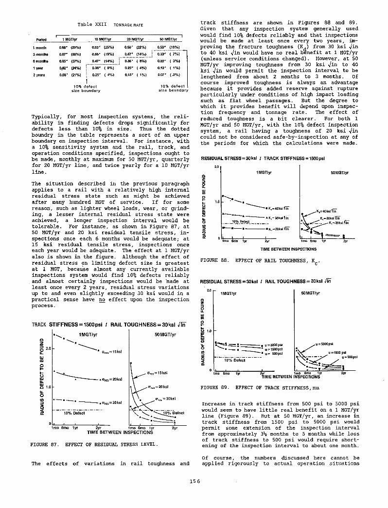
T ab le XXII tonnage rate

Period 1 MGT/yr 10 MGT/yr 20 MGT/yr 50 MGT/yr

1 month 0.68' (29%) 0.63" (25%) 0.59" (22%) 0.50" (16%)

3 months 0.67' (28%) 0.55" (19%) 0.47" (14%) 0.33" ( 7%)

6 months 0.65' (27%) 047" (14%) 0.36" ( 8%) 0.22" ( 3%)

1 year 0.62' (24%) 0.36" ( 8%) 0.25" ( 4%) 0.13" ( 1%)

2 years 0.58" (21%) 0.25" ( 4%) 0.15" ( 1%) 0.07" (.3%)

10%T

d e fe c t 10% d e fe c tsize bou nda ry s ize b o u n d a ry

Typically, for most inspection systems, the reli­ability in finding defects drops significantly for defects less than 10% in size. Thus the dotted boundry in the table represents a sort of an upper boundary on inspection interval. For instance, with a 10% sensitivity system and the rail, track, and operation conditions specified, inspections ought to be made, monthly at maximum for 50 MGT/yr, quarterly for 20 MGT/yr line, and twice yearly for a 10 MGT/yr line.

The situation described in the previous paragraph applies to a rail with a relatively high internal residual stress state such as might be achieved after many hundred MGT of service. If for some reason, such as lighter wheel loads, wear, or grind­ing, ^ lesser internal residual stress state were achieved, a longer inspection interval would be tolerable. For instance, as shown in Figure 87, at 50 MGT/yr and 20 ksi residual tensile stress, in­spections once each 6 months would be adequate; at 15 ksi residual tensile stress, inspections once each year would be adequate. The effect at 1 MGT/yr also is shown in the figure. Although the effect of residual stress on limiting defect size is greatest at 1 MGT, because almost any currently available inspections system would find 10% defects reliably and almost certainly inspections would be made at least once every 2 years, residual stress variations up to and even slightly exceeding 30 ksi would in a practical sense have no effect upon the inspection process.

TRACK STIFFNESS = 1500psi / RAIL TOUGHNESS = 30ksi /in '

FIGURE 87. EFFECT OF RESIDUAL STRESS LEVEL.

track stiffness are shown in Figures 88 and 89. Given that any inspection system generally used would find 10% defects reliably and that inspections would be made at least once every two years, im­proving the fracture toughness (K^) from 30 ksi /in to 40 ksi /in would have no real benefit at 1 MGT/yr (unless service conditions changed). However, at 50 MGT/yr improving toughness from 30 ksi /in to 40 ksi /in would permit the inspection interval to be lengthened from about 2 months to 3 months. Of course improved toughness is always an advantage because it provides added reserve against rupture particularly under conditions of high impact loading such as flat wheel passages. But the degree to which it provides benefit will depend upon inspec­tion frequency and tonnage rate. The effect of reduced toughness is a bit clearer. For both 1 MGT/yr and 50 MGT/yr, with the 10% defect inspection system, a rail having a toughness of 20 ksi /in could not be considered safe-by-inspection at any of the periods for which the calculations were made.

RESIDUAL STRESS = 30ksi / TRACK STIFFNESS = 1500psi

TIME BETWEEN INSPECTIONS

FIGURE 88. EFFECT OF RAIL TOUGHNESS, K .c

RESIDUAL STRESS = 30ksi / RAIL TOUGHNESS = 30ksl /in

TIM E BETWEEN INSPECTIONS

FIGURE 89. EFFECT OF TRACK STIFFNESS, na

Increase in track stiffness from 500 psi to 5000 psi would seem to have little real benefit on a 1 MGT/yr line (Figure 89). But at 50 MGT/yr, an increase in track stiffness from 1500 psi to 5000 psi would permit some extension of the inspection interval from approximately 3% months to 5 months while loss of track stiffness to 500 psi would require short­ening of the inspection interval to about one month.

Of course, the numbers discussed here cannot be applied rigorously to actual operation situationsThe e f fe c t s o f varia tion s in r a i l toughness and

15 6

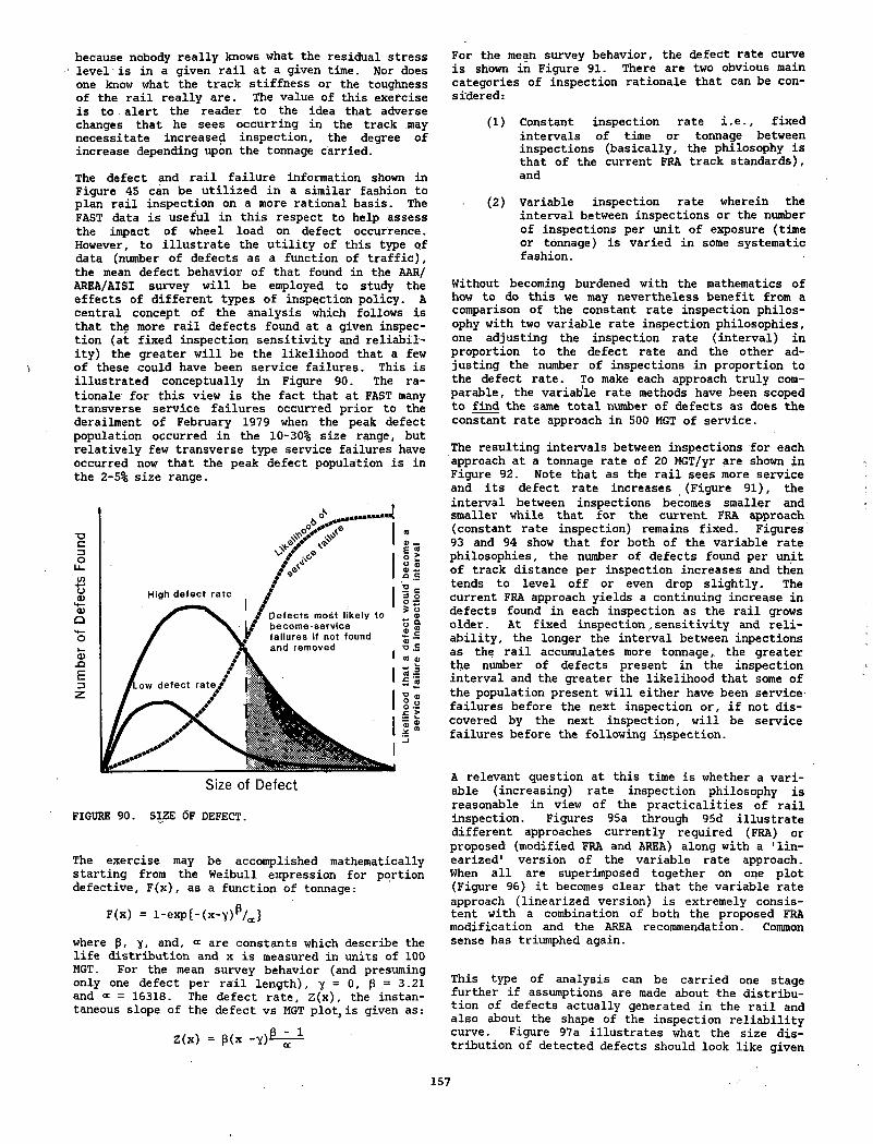
because nobody really knows what the residual stress level is in a given rail at a given time. Nor does one know what the track stiffness or the toughness of the rail really are. The value of this exercise is to alert the reader to the idea that adverse changes that he sees occurring in the track may necessitate increased inspection, the degree of increase depending upon the tonnage carried.

The defect and rail failure information shown in Figure 45 can be utilized in a similar fashion to plan rail inspection on a more rational basis. The FAST data is useful in this respect to help assess the impact of wheel load on defect occurrence. However, to illustrate the utility of this type of data (number of defects as a function of traffic), the mean defect behavior of that found in the AAR/ AREA/AISI survey will be employed to study the effects of different types of inspection policy. A central concept of the analysis which follows is that the more rail defects found at a given inspec­tion (at fixed inspection sensitivity and reliabil­ity) the greater will be the likelihood that a few of these could have been service failures. This is illustrated conceptually in Figure 90. The ra­tionale for this view is the fact that at FAST many transverse service failures occurred prior to the derailment of February 1979 when the peak defect population occurred in the 10-30% size range, but relatively few transverse type service failures have occurred now that the peak defect population is in the 2-5% size range.

s o

■a .E

FIGURE 90. SIZE OF DEFECT.

The exercise may be accomplished mathematically starting from the Weibull expression for portion defective, F(x), as a function of tonnage:

F(x) = l-exp{-(x-y)P/a }

where p, y, and, are constants which describe the life distribution and x is measured in units of 100 MGT. For the mean survey behavior (and presuming only one defect per rail length), y = 0, p = 3.21 and « = 16318. The defect rate, Z(x), the instan­taneous slope of the defect vs MGT plot,is given as:

Z(x) = P(x -y)^ ~ X-

For the mean survey behavior, the defect rate curve is shown in Figure 91. There are two obvious main categories of inspection rationale that can be con­sidered:

(1) Constant inspection rate i.e., fixed intervals of time or tonnage between inspections (basically, the philosophy is that of the current FRA track standards), and

(2) Variable inspection rate wherein the interval between inspections or the number of inspections per unit of exposure (time or tonnage) is varied in some systematic fashion.

Without becoming burdened with the mathematics of how to do this we may nevertheless benefit from a comparison of the constant rate inspection philos­ophy with two variable rate inspection philosophies, one adjusting the inspection rate (interval) in proportion to the defect rate and the other ad­justing the number of inspections in proportion to the defect rate. To make each approach truly com­parable, the variable rate methods have been scoped to find the same total number of defects as does the constant rate approach in 500 MGT of service.

The resulting intervals between inspections for each approach at a tonnage rate of 20 MGT/yr are shown in Figure 92. Note that as the rail sees more service and its defect rate increases (Figure 91), the interval between inspections becomes smaller and smaller while that for the current FRA approach (constant rate inspection) remains fixed. Figures 93 and 94 show that for both of the variable rate philosophies, the number of defects found per unit of track distance per inspection increases and then tends to level off or even drop slightly. The current FRA approach yields a continuing increase in defects found in each inspection as the rail grows older. At fixed inspection,sensitivity and reli­ability, the longer the interval between inpections as the rail accumulates more tonnage, the greater the number of defects present in the inspection interval and the greater the likelihood that some of the population present will either have been service failures before the next inspection or, if not dis­covered by the next inspection, will be service failures before the following inspection.

A relevant question at this time is whether a vari­able (increasing) rate inspection philosophy is reasonable in view of the practicalities of rail inspection. Figures 95a through 95d illustrate different approaches currently required (FRA) or proposed (modified FRA and AREA) along with a 'lin­earized1 version of the variable rate approach. When all are superimposed together on one plot (Figure 96) it becomes clear that the variable rate approach (linearized version) is extremely consis­tent with a combination of both the proposed FRA modification and the AREA recommendation. Common sense has triumphed again.

This type of analysis can be carried one stage further if assumptions are made about the distribu­tion of defects actually generated in the rail and also about the shape of the inspection reliability curve. Figure 97a illustrates what the size dis­tribution of detected defects should look like given

157

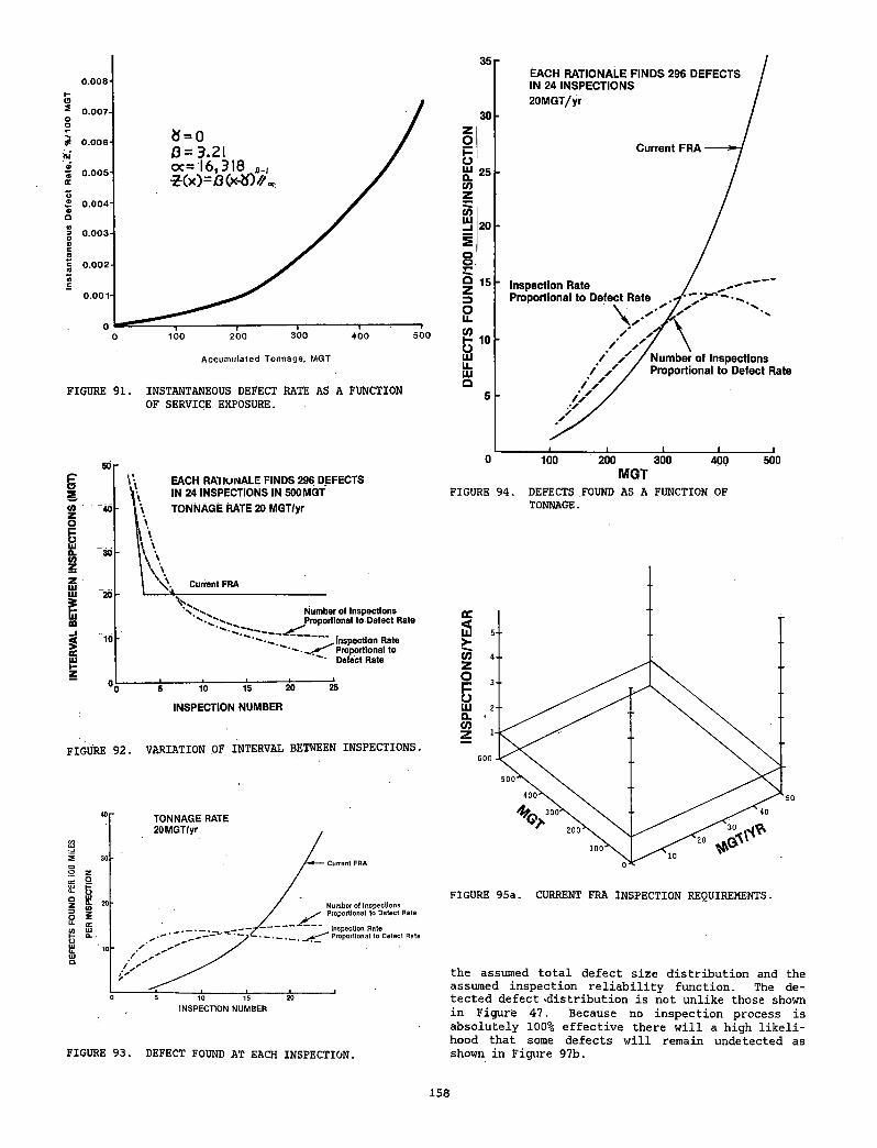
FIGURE 91. INSTANTANEOUS DEFECT RATE AS A FUNCTION OF SERVICE EXPOSURE.

5 0 r

§£

UlQ.</>zUlUl

1111

EACH RATIUNALE FINDS 296 DEFECTS IN 24 INSPECTIONS IN 500 MGT TONNAGE RATE 20 MGT/yr

Current FRA

V v Number of Inspections Proportional to Defect Rate

’“ V Inspection Rate Proportional to

***■ Defect Rate 5

5 10 15 20

INSPECTION NUMBER

FIGURE 92. VARIATION OF INTERVAL BETWEEN INSPECTIONS.

FIGURE 93. DEFECT FOUND AT EACH INSPECTION.

FIGURE 94. DEFECTS FOUND AS A FUNCTION OF TONNAGE.

FIGURE 95a. CURRENT FRA INSPECTION REQUIREMENTS.

the assumed total defect size distribution and the assumed inspection reliability function. The de­tected defect 'distribution is not unlike those shown in Figure 47. Because no inspection process is absolutely 100% effective there will a high likeli­hood that some defects will remain undetected as shown in Figure 97b.

158

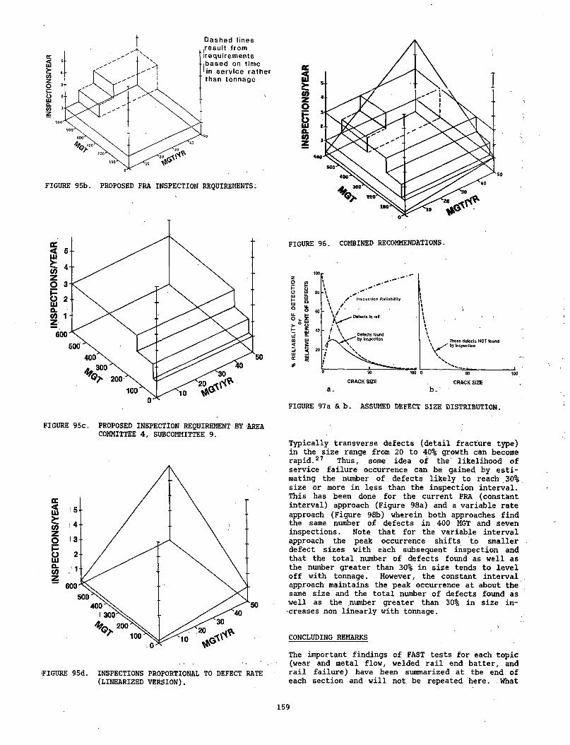
FIGURE 96. COMBINED RECOMMENDATIONS.

O </)d as Sir qMl u

° &

o z> ° sL_ OC£ ui

FIGURE 97 a & b. ASSUMED DEFECT SIZE DISTRIBUTION.

FIGURE 95c. PROPOSED INSPECTION REQUIREMENT BY AREA COMMITTEE 4, SUBCOMMITTEE 9.

IFIGURE 95d. INSPECTIONS PROPORTIONAL TO DEFECT RATE (LINEARIZED VERSION).

Typically transverse defects (detail fracture type) in the size range from 20 to 40% growth can become rapid.27 Thus, some idea of the likelihood of service failure occurrence can be gained by esti­mating the number of defects likely to reach 30% size or more in less than the inspection interval. This has been done for the current FRA (constant interval) approach (Figure 98a) and a variable rate approach (Figure 98b) wherein both approaches find the same number of defects in 400 MGT and seven inspections. Note that for the variable interval approach the peak occurrence shifts to smaller defect sizes with each subsequent inspection and that the total number of defects found as well as the number greater than 30% in size tends to level off with tonnage. However, the constant interval approach maintains the peak occurrence at about the same size and the total number of defects found as well as the number greater than 30% in size in­creases non linearly with tonnage.

CONCLUDING REMARKS

The important findings of FAST tests for each topic (wear and metal flow, welded rail end batter, and rail failure) have been summarized at the end of each section and will not. be repeated here. . What

159

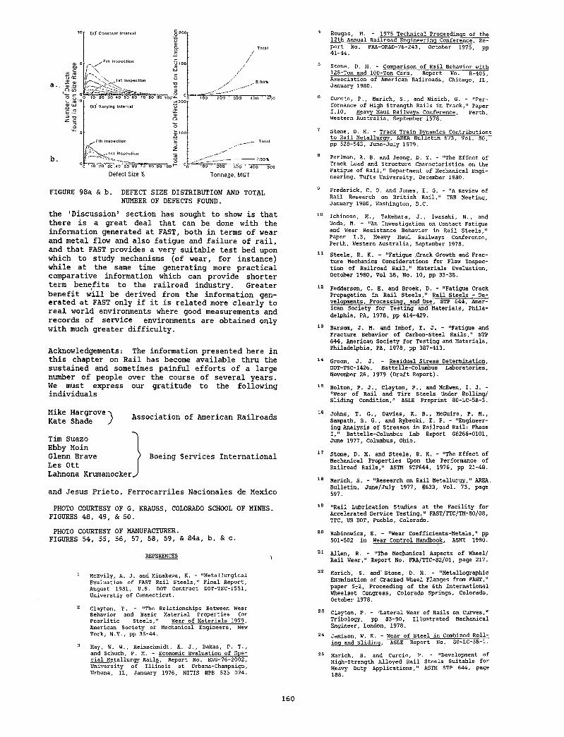
(a ) C on s tan t in te rva l10 §2 0 0

Va.4 Rougas, M. - 1975 T e ch n ica l P roceed in gs o f the

12th Annual R a ilr o a d E n gin eerin g C on feren ce . Re- T o ta i Po r t No. FRA-0R&D-76-243, O ctober 1975, pp

4 1 -4 4 .

a..

b.‘ ■ ^ ^ ^ I s t insp ec tio n

° 0 10 20 3 0 .4 0 50 6'0~70T 80 90 li)0

Defect Size %

2 30%

T5o 20 0 ' 3 0 0 ' 4t)0 ■ 5&0

_____ To ta l

10O ‘ 2 b o ” ' 30O 4 0 0 ' 5 b 0

Tonnage, MGT

S tone, D. H. - Comparison o f R a il B ehavior w ith 125-Ton and 100-Ton C a rs , R eport No. R -405, A s s o c ia t io n o f Am erican R a ilr o a d s , C h icago, IL , January 1980.

6 C u rc io , P . , M arich , S . , and N is ic h , G. - "P er­form ance o f High S tren gth R a ils in T ra ck ," Paper I . 10, Heavy Haul R ailw ays C on feren ce , P erth , W estern A u s tr a l ia , September 1978.

7 Stone, D. H. - Track T ra in Dynamics C on tr ib u tion s to R a il M e ta llu rg y , AREA B u lle t in 673, V o l. 80. pp 528 -543 , Ju n e-Ju ly 1979.

8 Perlman, A. B. and Jeong, D. Y. - "The E f f e c t o f Track Load and S tru ctu re C h a r a c te r is t ic s on the F atigue o f R a i l , " Department o f M echanical Engi­n e e r in g , T u fts U n iv e rs ity , December 1980.

FIGURE 98a & b. DEFECT SIZE DISTRIBUTION AND TOTAL NUMBER OF DEFECTS FOUND.

F red er ick , C. 0 . and Jon es , E. G. - "A Review o f R a il Research on B r i t is h R a i l , " TRB M eeting , January 1980, W ashington, D.C.

the ‘Discussion1 section has sought to show is that there is a great deal that can be done with the information generated at FAST, both in terms of wear and metal flow and also fatigue and failure of rail, and that FAST provides a very suitable test bed upon which to study mechanisms (of wear, for instance) while at the same time generating more practical comparative information which can provide shorter term benefits to the railroad industry. Greater benefit will be derived from the information gen­erated at FAST only if it is related more clearly to real world environments where good measurements and records of service environments are obtained only with much greater difficulty.

Acknowledgements: The information presented here in this chapter on Rail has become available thru the sustained and sometimes painful efforts of a large number of people over the course of several years. We must express our gratitude to the following individuals

10 Ic h in o s e , H ., Takehara, J . , Iw asaki, N ., and Ueda, M. - "An I n v e s t ig a t io n on C ontact F atigue and Wear R e s is ta n ce B eh avior in R a il S t e e l s , " Paper 1 .3 , Heavy Haul Railw ays C on feren ce , P erth , W estern A u s tr a l ia , September 1978.

11 S te e le , R. K . - "F a tig u e .Crack Growth and F rac­tu re M echanics C o n s id e ra tio n s f o r Flaw In sp ec ­t io n o f R a ilr o a d R a i l , " M a ter ia ls E v a lu a tion , O ctober 1980, V o l 38 , No. 10, pp 33 -38 .

12 Fedderson , C. E. and B roek, D. - "F a tigu e Crack P ropa gation in R a il S t e e l s , " R a il S te e ls - De­velopm en ts, P r o c e s s in g , and U se, STP 644 , Amer­ica n S o c ie ty f o r T e s t in g and M a te r ia ls , P h ila ­d e lp h ia , PA, 1978, pp 414 -42 9 .

13 Barsom, J . M. and Im hof, E. J . - "F atigu e and F ractu re B eh avior o f C a rb on -S tee l R a i l s , " STP 644 , Am erican S o c ie t y f o r T e s t in g and M a te r ia ls , P h ila d e lp h ia , PA, 1978, pp 387 -413 .

14 Groom, J . J . - R es id u a l S tre ss D eterm in ation , DOT-TSC-1426, B a tte lle -C o lu m bu s L a b o r a to r ie s , November 26 , 1979 (D ra ft R e p o rt ) .

15 B o lton , P . J . , C la y ton , P . , and McEwen, I . J . - "Wear o f R a il and T ire S t e e ls Under R o l l in g / S l id in g C o n d it io n ," ASLE P re p r in t 80-LC -5B -3.

Mike Hargrove Kate Shade Association of American Railroads

Tim Suazo Ebby Moin Glenn Brave Les OttLahnona Krumanocker.

Boeing Services International

and Jesus Prieto, Ferrocarriles Nacionales de Mexico

16 Johns, T. G ., D a v ies , K. B . , M cGuire, P . M ., Sampath, S . G ., and R y b eck i, E. F. - "E n g in eer­in g A n a ly s is o f S tre s s e s in R a ilro a d R a il : Phase I , " B atte lle -C o lu m bu s Lab R eport G 6266-0101, June 1977, Columbus, O hio.

17 S ton e, D. H. and S t e e le , R. K. - "The E f fe c t o f M echanical P r o p e r t ie s Upon the Perform ance o f R a ilro a d R a i l s , " ASTM STP644, 1976, pp 21 -48 .

18 M arich, S . - "R esearch on R a il M e ta llu rg y ," AREA. B u lle t in , J u n e /J u ly 1977, #633, V o l. 73 , page 597.

PHOTO COURTESY OF G. KRAUSS, COLORADO SCHOOL OF MINES. FIGURES 48, 49, & 50.

19 "R a il L u b r ica t io n S tu d ies a t the F a c i l i t y f o r A cce le ra te d S e rv ice T e s t in g ," FAST/TTC/TM-80/08, TTC, US DOT, P u eb lo , C o lora d o .

PHOTO COURTESY OF MANUFACTURER.FIGURES 54, 55, 56, 57, 58, 59, & 84a, b, & c.

REFERENCES

1 M cEvily , A. J . and Minakawa, K. - "M e ta llu r g ica l E v a lu ation o f FAST R a il S t e e l s , " F in a l R ep ort, August 1981, U .S. DOT C on tract DOT-TSC-1551, U n iv e rs t iy o f C on n ecticu t.

2 C layton , P. - "The R e la tion sh ip s Between Wear B eh avior and B a sic M ateria l P ro p e r t ie s f o r P e a r l i t i c S t e e l s ," Wear o f M a ter ia ls 1979 , American S o c ie ty o f M echanical E n gin eers, New Y ork , N .Y ., pp 35 -44 . 3

3 Hay, W. W., R einschm idt, A. J . , Bakas, P. T . , and Schuch, P. M. - Economic E v a lu ation o f Spe­c i a l M eta llu rgy R a i l s , Report No. ENG-76-2002, U n iv e rs ity o f I l l i n o i s a t Urbana-Champaign, Urbana, IL , January 1976, NITIS #PB 525 024.

20 R abin ow icz, E. - "Wear C o e f f ic ie n t s -M e t a ls ," pp 501-502 in Wear C on tro l Handbook, ASME 1980.

21 A lle n , R. - "The M echanica l A sp ects o f W heel/ R a il W ear," R ep ort No. FRA/TTC-82/01, page 217.

22 M arich, S. and- S ton e , D. H. - "M eta llog ra p h ic EHamination o f Cracked Wheel F langes from FAST," paper 5r2 , P roceed in g o f the 6th In te rn a t io n a l W heelset C on gress, C olorado S p rin g s , C o lorad o , O ctober 1978.

23 C layton , P. - "L a te ra l Wear o f R a ils on C u rv es," T r ib o lo g y , pp 8 3 -9 0 , I l lu s t r a t e d M echanical E n gin eer, London, 1978.

24 Jam ison, W. E. - Wear o f S te e l in Combined R o l l ­in g and S l id in g , ASLE R eport No. 80-LC -5B-1.

25 M arich, S. and C u rc io , P. - "Development o f H igh -S tren gth A llo y e d R a il S te e ls S u ita b le fo r Heavy Duty A p p lic a t io n s ," ASTM STP 644, page 188.

160

26 M arich , S. and M utton, P. J . - "An In v e s t ig a t io n o f Severe Wear Under R o l l in g /S l id in g C ontact C on d ition s E x is t in g in Heavy Haul R a ilw a y s ," ' Seventh In te r n a t io n a l W heelset C on gress, Vienna, O ctober 1981.

27 R a il D e fe c t Manual, S perry R a il S e r v ic e , 4th P r in t in g 4 /6 8 , page 39.

QUESTIONS AND ANSWERS

Question 1

If hardness and yield strength are. not good indicators of gage face wear, what do we strive for to obtain better performance?

Answer

In most cases as-worn surface hardness, and by inference, initial hardness as well, will provide a good correlation with wear resis­tance. However, some notable exceptions have been pointed out. Likewise, both static and cyclic yield strength seem well related to head height loss rate, but not to gage face wear rate in all cases. Because gage face wear rate (under FAST conditions) appears to involve a shear band cracking process, cyclic ductility (cyclic true fracture strain) may prove to be a better predictor of gage face wear resistance. Work by Paul Clayton at British Rail does suggest that there is a good correlation be­tween wear rate and the total plastic strain at a fixed stress level. Really, though, at this time we don11 know enough about the nature of the wear process itself to suggest that any mechanical test parameter will be a truly reliable predictor of wear resistance. How­ever, Were I responsible for attempting to find, and control the quality of, a better rail, I'd watch hardness, equivalent carbon level, and microstructure.

Question 2

What, if any, is the effect of lubrication on failures?

Answer

Effective lubrication clearly prolongs the life of rail long enough to allow fatigue to become an important concern. We have not seen any indication that lubricant acts as a hydraulic 'wedge' to propagate a crack. However, the reduction of the friction coefficient at the wheel/rail interface that is achieved by effec­tive lubrication would be expected to move the point at which the maximum shear stresses occur to greater depths beneath the running surface and to reduce the amplitude of these stresses. These changes could well alter the rate and location at which fatigue cracks develop. The FAST results suggest that modest wear may actually serve to prolong rail life by defer­ring fatigue as a competitive mode of failure.

Where are lubricators located?

1. On curve where flange first contacts high rail, or

2. Tangent, if tangent is gage tightened? If so how much?

Answer

In the past, lubricators have been located in tangent track just prior to the entry to the spirals. Most recently lubricators have been located in tangent track, in some cases thou­sands of feet from the curves which they must lubricate. Track gage has not been tightened in such cases. Perhaps, because FAST is a closed loop and our lubricators in these tan­gent track installation 'geyser' so much even on the lowest output setting, we are able to get effective lubrication of a high rail (in­side loop rail in Section 7) up to two or more miles from the lubricator (in Section 20). FAST does not represent a challenge to achieve a lubricated state but rather to prevent it from overwhelming us.

Question 3

Question 4

Is there any relationship between change in wear rates vs. work softening and/or work hardening of the rail with traffic?

Is there any evidence of work hardening or work softening behavior at FAST?

Answer

Probably yes. We see that a high wear rate standard carbon rail (low equivalent carbon) does exhibit a layer of what appears to be softened material beneath the surface deformed region and that metal pushed down the gage face is far softer than we'd expect to observe for metal so heavily deformed. Likewise, the region in which a shell has developed in one of our failed rails appears to be softer than much of the metai around it. We suspect that the work softened material may be more prone to fatigue damage. However, the region (0.001- 0.002" beneath the gage face) in which wear debris is generated does not seem softer than nearby regions. Thus, at this time we are unable to estimate the effect of work softening on wear itself.

Question 5

Have you (or anyone) looked at these rail samples under transmission electron microscopy? Does this shed any light on the origins of wear in the different rail samples as well as the influence of lubrication?

Answer

No, we have not yet used the transmission electron microscope to examine the character of the metal in the vicinity of the wear inter-

161

•i

face. To do so would be an extremely useful exercise in that such examination would help define the nature of the deformation processes occurring in the region of debris generation. Thus we could anticipate more accurately what characteristics should be sought for an im­proved rail— even an improved standard carbon rail. Use of preferred orientation determina­tion techniques (X-ray diffraction) also would provide valuable insights into the processes which occur at the rail/wheel interface.

Question 6

Is the rate of metal flow on rail uniform through age? If not, how does it vary?

Answer

Apparently not! Although data from the first rail metallurgy experiment does show a steady rise and then a levelling off of low rail lateral flow to the field side (in the lubri­cated regime), information from the third experiment (not available at the time of the Conference presentation) suggests that lateral flow on both field and gage side of the low rail occurs at an increasing rate after each lubrication interval.

Question 7

Have you analyzed the economic cost of differ­ent rails based on your data (not including transportation)?

What is the difference between type B, C, & U wheels you showed on graph in Phase III?

Answer

No, but Mike Hargrove at AAR in Washington has been using the FAST rail wear data to calibrate a rail life model prepared by the Canadian Institute of Guided Ground Transport. This model would then be exercised to provide eco­nomic cost analysis. Although w e 1ve not per­formed an economic analysis, an improved stan-

. dard carbon which might have 50% better wear resistance at less than 10% additional cost would appear to be highly attractive and, based upon the FAST rail wear results, would appear to be easily within reach.

With regard to wheel designations, U and C class wheels have the same carbon content, but

. the C wheel is rim hardened (somewhat akin to , head hardened rail). A B class wheel is rim hardened but has a lower carbon content than the C wheel.

Question 8

You infer that there is a substantial improve­ment in .wear due to lubrication, but you did not mention any specific comparison in quanti­tative terms. What would be, the FM (figure of merit) comparing dry standard rail vs lubri­cated standard rail, dry CrMo, lubed CrMo, dry HH and lubed HH, etc?

Answer

The generous lubrication which we've encoun­tered at FAST improves the wear resistance of standard rail by about a factor of 8 to 10. However, the wear resistance of the better premium rails will improve by a factor of 4 to 5 only. Thus, the figure of merit of premium rails relative to standard rail diminishes significantly as the level of lubrication improves as with SiCr(HH) where the figure of merit exceeds 4 when dry, but is less than 2 when well lubricated. Similar changes occur for the other premium metallurgies.

Question 9

Is gage face wear, head loss, and total wear rate measurement compared to initial no service conditions of each rail metallurgy or compared to a nominal rail section? If the latter comparison, how are the wear rates of different rail sections reconciled?

Answer

The FAST wear measurements have been made by comparing the profiles after service exposure at each meaurement site to the initial "actual profiles at that site.

Question 10

Is there any information available why a bain- itic structure does not fit into the hardness wear characteristic? Why is a bainitic micro­structure wearing different than a pearlitic one of approximately the same hardness— test heats with 4.3% Cr, ~400 HBN, structure fully bainitic, done in Germany about six years ago, showed higher wear rate than 1% Cr pearlictic rail steel with ~320 HBN?

Answer

We don't know enough about the mechanism of wear and the relationship of wear to mechanical behavior to explain why bainite and martensite exhibit poorer wear resistance than pearlite of the same hardness. However, it is interesting to note that both bainite and , martensite are the products of shear transformations while the pearlite transformation is a two phase nuclea- tion and growth process. As a consequence of the shear transformation,- the morphology of the iron carbides in bainite and martensite (tem­pered) is very different from that of pearlite. Although we can say these differences exist, alas it is not clear why they should imbue bainite and martensite with inferior wear characteristics.

Question 11

You mentioned in your.jtalk that two (or more) types of head hardened rail has been tested and that the second type tested seems to wear somewhat more rapidly than the first.

162

r l

Do you think this is due to something the manufacturer is doing in the heat treating process, or is it due to chemistry? Is it statistically significant? Are you allowed to name names if it is? Does it have anything to do with rail cleanliness?

This question is asked because we are buying two different types of HH rail at the moment (Nippon and NKK). About 15 years ago we bought some Curvemaster and it failed, mainly.with the shell.

Answer

Both conventional standard carbon head hardened and silicon chrome head hardened rail have been tested thoroughly. The silicon chrome rail is an alloy specially designed to benefit from slack quenching (as in the flash butt welding operation). The gage face wear resistance of the silicon chrome head hardened rail is about one-third better than that of conventional head hardened rail when running dry. However, its head height loss resistance (running dry) may not be so good as that of conventional head hardened rail. Both rails are approximately comparable when running in the lubricated state. The difference in chemistry probably is chiefly responsible for the difference in gage face wear resistance.

We try to avoid naming manufacturers. But we do see differences in behavior for rails of nominally the same chemistry which are likely due to differences in processing from one manufacturer to another.

With regard to cleanliness, yes, much to our surprise we think there may be a relationship between gage face wear (not just fatigue fail­ure, i.e., shelling) and the inclusion content of the steel. But this ’ is not yet well estab­lished.

Question 12

Does rail design, specifically the slope of gage face side, affect gage face wear? (Slopes of 140 RE and 136 RE rails are different.)

Also, has corrective head grinding affected gage face wear?

Answer

Wear at FAST is rapid enough in the dry regime so that all rails will quickly adopt the same profile after a short period of service. Thus, the original slope of the side of the rail is quickly lost and is replaced by a slope charac­teristic of the average wheel tread/throat/ flange configuration. However, the rate at which this new contour progresses down the side of the rail head may indeed be a function of the head design (as well as of metallurgy). We really don't know. However, once the new contour has extended to the 5/8" gage point, the wear measurements now are all taken at the same representative geometry and the wear rate is governed by the inherent wear resistance of the metallurgy.

We have been able to detect experimentally any effect of corrective head grinding upon gage face wear but this lack of relationship may be attributed to the fact that the experiment has not.been designed to study the effect of grind­ing on gage face wear.

Question 13

You will be interested in the grain refinement being found in hot rolled (not controlled rolled) steel if V&N are present. This obser­vation needs more investigation to be sure. Do you have nitrogen contents -of the V rails?

Answer

No, unfortunately, we don't know the nitrogen content of the vanadium containing rails. It

. would be appropriate for us to find out.. We're not sure what structural features other than pearlite interlamellar spacing need be con­trolled to assure good wear resistance. The relationship between vanadium and nitrogen levels and microstructural refinement is in­triguing and this relationship may offer-, some aid in understanding why chrome vanadium compo­sitions have not done better than we have observed.

Question 14 ' /

Has the mechanism of rail wear been investi­gated from the standpoint of nucleus of ori­gin, i.e., what effects have metallurgical grain size and steel cleanliness been upon wear initiation and progression? If not, is there any plan to investigate these factors?

Answer

We believe the gage face wear process itself is a shear band failure process which may well depend on steel cleanliness. Of course the formation of shells (and TD's) by a- fatigue process has long been felt to be related to steel cleanliness. The question at hand is "how much cleanliness is worth paying for?". We have just started to attempt to develop the correlations which might answer that question.

Question 15

Were climatic changes or differences correlated with wear rates, i.e'., seasons of high or low humidity which varied from block to block or snow quantities or temperatures?

Answer

We have not been able to detect any relation­ship between wear rate and the season of the year and the temperature or humidity. Admit­tedly, we've not gone at this in a rigorous fashion. • Though we've not seen a clear corre-

- lation’ (would that we could use this explana­tion to rationalize our block to block varia­tions), we have an open mind on the subject.

163

Would the introduction of anomolies in the wheel bearing area cause greater metal flow or a more rapid loss of head height?

If so, would there be a difference in rate between dry and lube?

Answer

I interpret this question to mean "will fea­tures such as welded rail end batter, engine burns, and corrugations act to accelerate the wear process?". In theory, the higher dynamic forces occurring under such conditions might be expected to accelerate wear. Our measurement techniques have not been sensitive enough yet to shed light on this question.

Question 16

Question 17

How can my railroad measure the amount of (or effectiveness of) lubricant film on gage face at a specific 'distance from a lubricator?

Answer

There appears to be no simple, reliable method of measuring the amount of lubricant film in the field. The best approach is to determine the wear rate (preferably with an instrument having a 0.001" measuring sensitivity) in both the dry and lubricated states at the same place in track. If the lubricated wear rate is one-fifth to one-tenth that of the dry state, you are obtaining effective lubrication.

Question 18

Why didn1t you use equivalent carbon content of wheels and rail vs. wear rate instead of wheel and rail hardness vs. wear rate as a predicter of overall wear?

Answer

If wear rate were only a function of equivalent carbon, conceivably this would be possible. But heat treatment also influences wear rate at a given equivalent carbon level. Therefore, some parameter such as hardness is used which is responsive both to chemistry and heat treat­ment. From a practical point of view, hardness is a good parameter because it can be measured so easily.

Question 19

In the derailment of the FAST train traced to detail fracture, why was it not possible to detect the initiation of the fracture or the fracture itself during growth with the detector cars which, it is assumed, are used to greater extent at FAST?

Answer

There were three TD's within one 20' piece of rail. On one inspection, the detection system

picked up two of the three defects but the operator noted neither of the two which ap­peared on the strip chart record. A few days later on the next inspection, the vehicle had reversed direction and only one of the defects was detected. The defect was detected again on the next inspection (vehicle travelling in the same direction as on the day that the strip chart record indicated two defects); the second defect was not observed. The one which was observed was indicated as a 8% TD— smaller than the size requiring joint bar installation.

This unfortunate series of events resulted from two major causes which have been corrected subsequently. The first of these was that the strip chart record was not examined at the end of the day's run to determine whether defects were found but not entered on the log. The second was the fact that the twelve 70° trans­ducers (six in each rail wheel) were not all functioning at equal sensitivity and that no periodic test of sensitivity of each transducer was required. The fact that three 70° trans­ducers within a group are wired in parallel means that the loss of sensitivity of one or two of these cannot be detected without using a procedure designed to check each transducer individually. Rail inspection at FAST is made every 2-3 MGT which is an appropriate interval. But, inspection at any interval will be in­effective if all parts of the inspection system are not known to be functioning properly.

Question 20

Has there been any consideration of steel metallurgy (for rails) as related to failure rate and impact properties?

Might not the variable hardness zones found in (some) rail fractures be associated with steel solidification dendritic patterns (i.e., higher % C segregation at dendritics)?

Answer

Fracture toughness (both static and dynamic) which can be a function of the type of metal­lurgy can, as shown in the text, have a large effect on the performance of the rail and upon the inspection sensitivity and intervals re­quired. However, FAST has not been able to provide an effective assessment of how differ­ent metallurgies behave because so few premium rails have failed due to fatigue of the rail (as opposed to the weld) itself. Although FAST wheel loads are high, there are virtually no flat wheels which could provide the impact loading needed to increase the rail failure rate. Basically, FAST has not been designed as a fatigue test.

With regard to the second question, the 'soft­ened' zone is only about 3/8" below the run- ning/gage surface and is not found on the field side of the rail. It's hard to imagine that the effects of dendritic segregation would occur only at this depth on the gage side of the rail head while they have been destroyed (by prior hot rolling) on the field side of the head.

164

)i

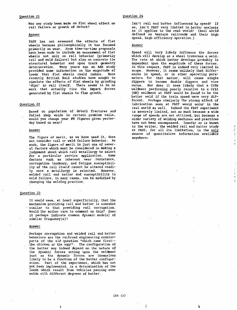
Has any study been made on flat wheel effect on rail failure or growth of defect?

Answer

FAST has not assessed the effects of flat wheels because philosophically it has focused primarily on wear. From time-to-time proposals have been made to include an assessment of flat wheels not only on rail behavior (primarily rail and weld failure) but also on concrete tie structural behavior and upon track geometry deterioration. Many years ago an AAR study provided some information on the magnitude of loads that flat wheels could induce. More recently British Rail studies have sought to simulate the effects of flat wheels by grinding 'dips' in rail itself. There seems to be no work that actually ties the impact forces generated by flat wheels to flaw growth.

Question 21

Question 22

Based on population of detail fractures and failed shop welds in certain premium rails, would you change your FM figures given yester­day based on wear?

Answer

The figure of merit, as we have used it, does not consider rail or weld failure behavior. As such, the figure of merit is just one of sever­al factors which must be considered in making a judgement about which rail metallurgy to select for a particular service application. Some factors such as inherent wear resistance, corrugation tendency, and fatigue susceptibil­ity of the rail itself cannot be altered readi­ly once a metallurgy is selected. However, welded rail end batter and susceptibility to weld failure, in many cases, can be modified by changing the welding practice.

Isn't rail end batter influenced by -speed? If so, isn't FAST very limited in batter analysis as it applies to the real world? (Real world defined as Western railroads and their high speed, high efficiency operation.)

Answer

Speed will very likely influence the forces which will develop as a wheel traverses a weld. The rate at which batter develops probably is dependent upon the magnitude of these forces. In this respect, FAST is indeed very limited in scope. However, it seems unlikely that differ­ences in speed, or in other operating para­meters for that matter, will cause single dippers to become double dippers and vice versa. Nor does it seem likely that a CrMo weldment performing poorly relative to a CrSi (HH) weldment at FAST would be found to be the better weld if the train speed were very dif­ferent. Perhaps similarly the strong effect of lubrication seen at FAST would occur in the real world as well. Indeed the FAST experiment is severely limited, not so much because a wide range of speeds are not utilized, but because a wider variety of welding machines and practices have not been encompassed. Insofar as is known to the writer, the welded rail end batter study at FAST, for all its limitation,' is the only source of quantitative information available anywhere:

Question 24

Question 23

It would seem, at least superficially, that the mechanism providing rail end batter is somewhat similar to that providing rail corrugation. Would the author care to comment on this? Does it perhaps indicate common dynamic mode(s) of similar frequency(s)?

Answer

Perhaps corrugation and welded rail end batter behaviors are the railroad engineering counter­parts of the old question "which came first— the chicken or the egg?". The configuration of the batter may indeed depend on the nature of the dynamic forces acting upon the weldment just as the dynamic forces are themselves likely to be a function of the batter configur­ation. Part of the experiment, which has not yet been implemented, is a determination of the loads which result from vehicles passing over welds with different degrees of batter. i

164 (a)

» y i

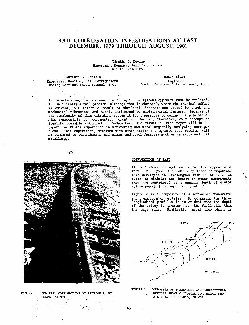
RAIL C O R R U G A T IO N IN VESTIG ATIO N S A T FAST: DECEMBER, 1979 T H R O U G H A U G U ST, 1981

Timothy J. DevineExperiment Manager, Rail Corrugation

Griffin Wheel Co.

Lawrence E. Daniels Experiment Monitor, Rail Corrugations Boeing Services International, Inc.

Nancy Blume Engineer

Boeing Services International, Inc.

In investigating corrugations the concept of a systems approach must be utilized. It isn't merely a rail problem, although that is obviously where the physical effect is evident, but rather a result of wheel/rail interactions caused by track and mechanical vibrations and highly influenced by environmental factors. Because of the complexity of this vibrating system it isn't possible to define one sole mecha­nism responsible for corrugation formation. We can, therefore, only attempt to identify possible contributing mechanisms. The thrust of this paper will be to report on FAST's experience in monitoring and metallurgically analyzing corruga­tions. This experience, combined with other static and dynamic test results, will be compared to contributing mechanisms and track features such as geometry and rail metallurgy.

-0"

FIGURE 1.. LOW RAIL CORRUGATIONS AT SECTION 3, 5° CURVE, 73 MGT.

CORRUGATIONS AT FAST

Figure 1 shows corrugations as they have appeared at FAST. Throughout the FAST loop these corrugations have developed in wavelengths from 5" to 13": In order to minimize the impact on other experiments they are restricted to a maximum depth of 0.050" before remedial action is required.

Figure 2 is a composite of a series of transverse and longitudinal profiles. By comparing the three longitudinal profiles it is evident that the depth of the valley is greater near the field side than the gage side. Similarily, metal flow which is

.FIGURE 2. COMPOSITE OF TRANSVERSE AND LONGITUDINAL . PROFILES SHOWING TYPICAL CORRUGATED LOW

RAIL NEAR TIE 03-814, 50 MGT.

165

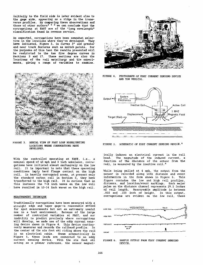
initially to the field side is later evident also to the gage side, appearing as a ridge in the trans­verse profiles. By comparing these Observations and those of other authors1 2 3 we can conclude that the corrugations at FAST are of the "long wavelength" classification found in revenue service.

As expected, corrugations have been somewhat selec­tive in the locations where they've developed. They have initiated. Figure 3, in curves 3° and greater and near track features such as switch points. For the purposes of this test the results presented will be restricted to the two five degree curves in Sections 3 and 17. These sections are also the locations of the rail metallurgy and tie experi­ments, giving a range of variables to examine.

FIGURE 3. AERIAL VIEW OF FAST LOOP HIGHLIGHTING LOCATIONS WHERE CORRUGATIONS HAVE DEVELOPED.

With the controlled operating at FAST, i.e., a nominal speed of 45 mph and 3 inch unbalance, corru­gations have initiated almost exclusively on the low rail. It is important to note that these operating conditions imply hard flange contact on the high rail. In heavily corrugated areas, at present only the standard carbon rail in Section 3, they have transferred to the high rail. It is curious that in this instance the 7-8 inch waves on the low rail have resulted in 13-14 inch waves on the high rail.

MEASUREMENT TECHNIQUE

Traditionally corrugations have been measured with a straight edge and taper gage--a reasonable method for spot measurements but not an extremely useful one in a test environment. Because of the large number of controlled variables at FAST, and our inability to predict precisely where corrugations will develop, we made use of the eddy current sens­ing device shown in Figure 4. This device continu­ously measures and records the railhead profile. In the center of the six foot ski riding above the rail is an electrical cable. Shown schematically in Figure 5, these leads are connected to an eddy current sensing device. With the six foot ski acting as a planar reference, the sensor magnet-

FIGURE 4. PHOTOGRAPH OF EDDY CURRENT SENSING DEVICE AND TOW VEHICLE.

FIGURE 5. SCHEMATIC OF EDDY CURRENT SENSING DEVICE.4

ically induces an electrical current in the rail head. The magnitude of the induced current, a function of the distance of the sensor from the rail, is measured by the inactive coil.4

While being pulled at 4 mph, the output from the sensor is recorded along with distance and event information in the form shown in Figure 6. This figure contains the low and high rail profiles, distance, and location/event markings. Each major pulse on the distance channel represents 29.5 inches of rail length. Measureable amplitude is between .005 and .100 inch of height. In this output, corrugations are evident on the low rail, these

29.5*

EVENT ----- --------------------------------------------------- *----------- ----------------------------- -

FIGURE 6. SAMPLE OUTPUT FROM EDDY CURRENT SENSING DEVICE.

166

/ /

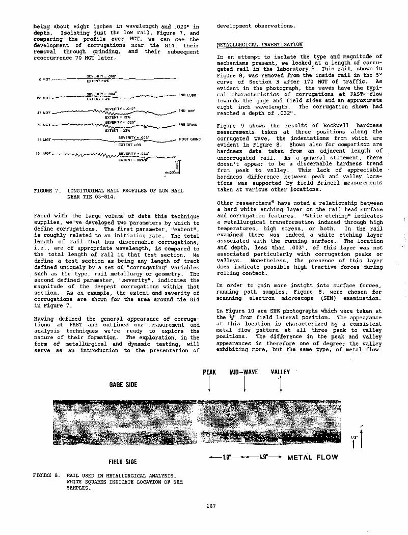
being about eight inches in wavelength and .020" in depth. Isolating just the low rail, Figure 7, and comparing the profile over MGT, we can see the development of corrugations near tie 814, their removal through grinding, and their subsequent reoccurrence 70 MGT later.

SEVERITY = ,0 0 0 ' EXTENt = 0 *

SEVERITY - ,0 0 4 EXTENT = 4 *

e p v p n i T Y = n 1 7 '

POST GRIND

FIGURE 7. LONGITUDINAL RAIL PROFILES OF LOW RAIL NEAR TIE 03-814.

Faced with the large volume of data this technique supplies, we've developed two parameters by which to define corrugations. The first parameter, "extent", is roughly related to an initiation rate. The total length of rail that has discernable corrugations, i.e., are of appropriate wavelength, is compared to the total length of rail in that test section. We define a test section as being any length of track defined uniquely by a set of "corrugating" variables such as tie type, rail metallurgy or geometry. The second defined parameter, "severity", indicates the magnitude of the deepest corrugations within that section. As an example, the extent and severity of corrugations are shown for the area around tie 814 in Figure 7.

Having defined the general appearance of corruga­tions at FAST and outlined our measurement and analysis techniques we're ready to explore the nature of their formation. The exploration, in the form of metallurgical and dynamic testing, will serve as an introduction to the presentation of

development observations.

METALLURGICAL INVESTIGATION

In an attempt to isolate the type and magnitude of mechanisms present, we looked at a length of corru­gated rail in the laboratory.5 This rail, shown in Figure 8, was removed from the inside rail in the 5° curve of Section 3 after 170 MGT of traffic. As evident in the photograph, the waves have the typi­cal characteristics of corrugations at FAST— flow towards the gage and field sides and an approximate eight inch wavelength. The corrugation shown had reached a depth of .032".

Figure 9 shows the results of Rockwell hardness measurements taken at three positions along the corrugated wave, the indentations from which are evident in Figure 8. Shown also for comparison are hardness data taken from an adjacent length of uncorrugated rail. As a general statement, there doesn't appear to be a discernable hardness trend from peak to valley. This lack of appreciable hardness difference between peak and valley loca­tions was supported by field Brinell measurements taken at various other locations.

Other researchers6 have noted a relationship between a hard white etching layer on the rail head surface and corrugation features. "White etching" indicates a metallurgical transformation induced through high temperatures, high stress, or both. In the rail examined there was indeed a white etching layer associated with the running surface. The location and depth, less than .003", of this layer was not associated particularly with corrugation peaks or valleys. Nonetheless, the presence of this layer does indicate possible high tractive forces during rolling contact.

In order to gain more insight into surface forces, running path samples. Figure 8, were chosen for scanning electron microscope (SEM) examination.

In Figure 10 are SEM photographs which were taken at the V from field lateral position. The appearance at this location is characterized by a consistent metal flow pattern at all three peak to valley positions. The difference in the peak and valley appearances is therefore one of degree,- the valley exhibiting more, but the same type, of metal flow.

GAGE SIDE

.............. ... . B

FIGURE 8. RAIL USED IN METALLURGICAL ANALYSIS.WHITE SQUARES INDICATE LOCATION OF SEM SAMPLES.

PEAK MID-WAVE VALLEY

1.9"— —— 1.9”---- ► METAL FLOW

167

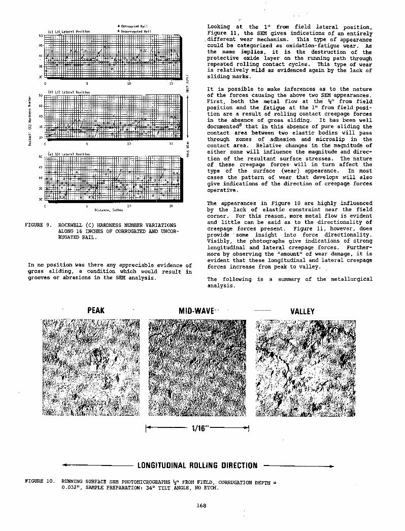
* Corrugated "Rail

o Uncorrugated Rail(c) 1/4 Lateral Position

(d) 1/2 Lateral Position

FIGURE 9. ROCKWELL (C) HARDNESS NUMBER VARIATIONS ALONG 16 INCHES OF CORRUGATED AND UNCOR­RUGATED RAIL.

In no position was there any appreciable evidence of gross sliding, a condition which would result in grooves or abrasions in the SEM analysis.

Looking at the 1" from field lateral position. Figure 11, the SEM gives indications of an entirely different wear mechanism. This type of appearance could be categorized as oxidation-fatigue wear. As the name implies, it is the destruction of the protective oxide layer on the running path through repeated rolling contact cycles.' This type of wear is relatively mild as evidenced again by the lack of sliding marks.

It is possible to make inferences as to the nature of the forces causing the above two SEM appearances. First, both the metal flow at the- V from field position and the fatigue at the 1" from field posi­tion are a result of rolling contact creepage forces in the absence of gross sliding. It has been well documented8 that in this absence of pure sliding the contact area between two elastic bodies will pass through zones of adhesion and microslip in the contact area. Relative changes in the magnitude of either zone will influence the magnitude and direc­tion of the resultant surface stresses. The nature of these creepage forces will in turn affect the type of the surface (wear) appearance. In most cases the pattern of wear that develops will also give indications of the direction.of creepage.forces operative.

The appearances in Figure 10 are highly influenced by the lack of elastic constraint near the field corner. For this reason, more metal flow is evident and little can be said as to the directionality of creepage forces present. Figure 11, however, does provide ' some insight into force directionality. Visibly, the photographs give indications of strong longitudinal and lateral creepage forces. Further­more by observing the "amount11 of wear damage, it is evident that these longitudinal and lateral creepage forces increase from peak to valley.

The following is a summary of the metallurgical analysis.

PEAK MID-WAVE ----------- VALLEY

1/ 16"

---------------------------------- LONGITUDINAL ROLLING DIRECTION ------

FIGURE 10. RUNNING SURFACE SEM PHOTOMICROGRAPHS i V FROM FIELD, CORRUGATION DEPTH = 0.032", SAMPLE PREPARATION: 34° TILT I ANGLE, NO ETCH.

168

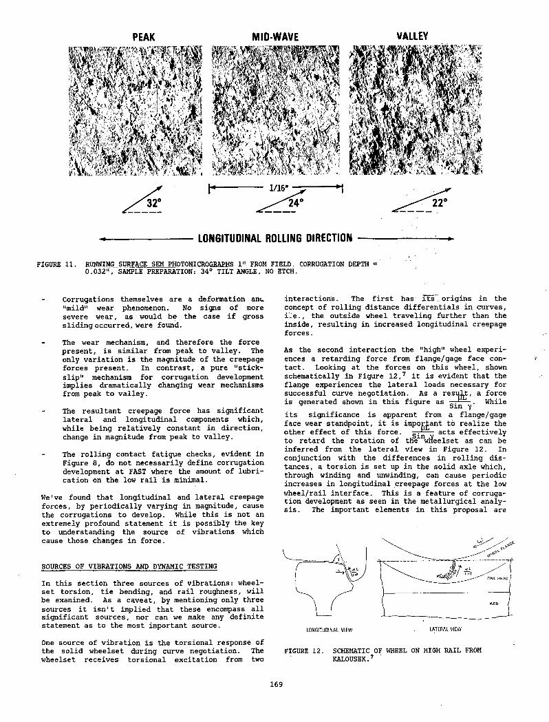
PEAK MID-WAVE VALLEY

LONGITUDINAL ROLLING DIRECTION

FIGURE 11. RUNNING SURFACE SEM PHOTOMICROGRAPHS 1" FROM FIELD. CORRUGATION DEPTH = 0.032", SAMPLE PREPARATION: 34° TILT ANGLE, NO ETCH.

Corrugations themselves are a deformation ant. "mild" wear phenomenon. No signs of more severe wear, as would be the case if gross sliding occurred, were found.

The wear mechanism, and therefore the force present, is similar from peak to valley. The only variation is the magnitude of the creepage forces present. In contrast, a pure "stick- slip" mechanism for corrugation development implies dramatically changing wear mechanisms from peak to valley.

The resultant creepage force has significant lateral and longitudinal components which, while being relatively constant in direction, change in magnitude from peak to valley.

The rolling contact fatigue checks, evident in Figure 8, do not necessarily define corrugation development at FAST where the amount of lubri­cation on the low rail is minimal.

We've found that longitudinal and lateral creepage forces, by periodically varying in magnitude, cause the corrugations to develop. While this is not an extremely profound statement it is possibly the key to understanding the source of vibrations which cause those changes in force.

SOURCES OF VIBRATIONS AND DYNAMIC TESTING

In this section three sources of vibrations: wheel- set torsion, tie bending, and rail roughness, will be examined. As a caveat, by mentioning only three sources it isn't implied that these encompass all significant sources, nor can we make any definite statement as to the most important source.

interactions. The first has Its origins in the concept of rolling distance differentials in curves, i.e., the outside wheel traveling further than the inside, resulting in increased longitudinal creepage forces.

As the second interaction the "high" wheel experi­ences a retarding force from flange/gage face con­tact. Looking at the forces on this wheel, shown schematically in Figure 12,7 it is evident that the flange experiences the lateral loads necessary for successful curve negotiation. As a resul^t, a force is generated shown in this figure as — . Whileits significance is apparent from a flange/gage face wear standpoint, it is important to realize the other effect of this force, — acts effectively to retard the rotation of theinw$eelset as can be inferred from the lateral view in Figure 12. In conjunction with the differences in rolling dis­tances, a torsion is set up in the solid axle which, through winding and unwinding, can cause periodic increases in longitudinal creepage forces at the low wheel/rail interface. This is a feature of corruga­tion development as seen in the metallurgical analy­sis. The important elements in this proposal are

One source of vibration is the torsional response of the solid wheelset during curve negotiation. The wheelset receives torsional excitation from two

FIGURE 12. SCHEMATIC OF WHEEL ON HIGH RAIL FROM KALOUSEK.7

169

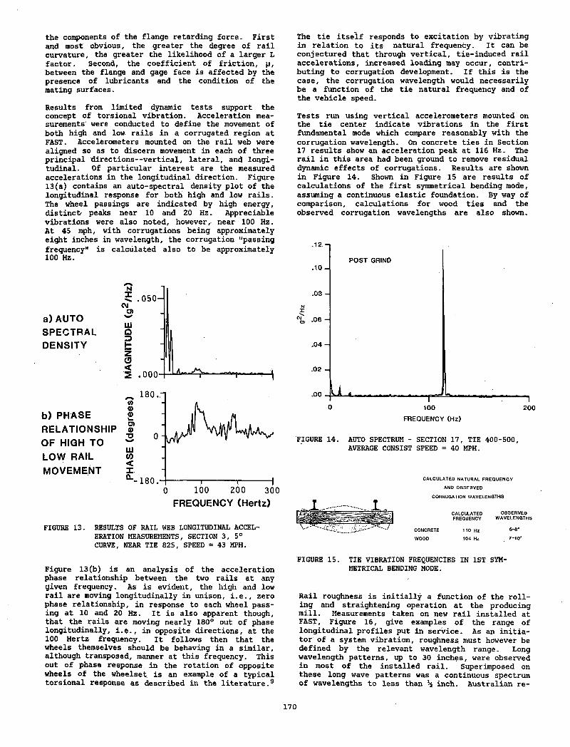
the components of the flange retarding force. First and most obvious, the greater the degree of rail curvature, the greater the likelihood of a larger L factor. Second, the coefficient of friction, p, between the flange and gage face is affected by the presence of lubricants and the condition of the mating surfaces.

Results from limited dynamic tests support the concept of torsional vibration. Acceleration mea­surements' were conducted to define the movement of both high and low rails in a corrugated region at FAST. Accelerometers mounted on the rail web were aligned so as to discern movement in each of three principal directions— vertical, lateral, and longi­tudinal. Of particular interest are the measured accelerations in the longitudinal direction. Figure 13(a) contains an auto-spectral density plot of the longitudinal response for both high and low rails. The wheel passings are indicated by high energy, distinct- peaks near 10 and 20 Hz. Appreciable vibrations were also noted, however, near 100 Hz. At 45 mph, with corrugations being approximately eight inches in wavelength, the corrugation "passing frequency" is calculated also to be approximately 100 Hz.

The tie itself responds to excitation by vibrating in relation to its natural frequency. It can be conjectured that through vertical, tie-induced rail accelerations, increased loading may occur, contri­buting to corrugation development. If this is the case, the corrugation wavelength would necessarily be a function of the tie natural frequency and of the vehicle speed.

Tests run using vertical accelerometers mounted on the tie center indicate vibrations in the first fundamental mode which compare reasonably with the corrugation wavelength. On concrete ties in Section 17 results show an acceleration peak at 116 Hz. The rail in this area had been ground to remove residual dynamic effects of corrugations. Results are shown in Figure 14. Shown in Figure 15 are results of calculations of the first symmetrical bending mode, assuming a continuous elastic foundation. By way of comparison, calculations for wood ties and the observed corrugation wavelengths are also shown.

.12

.10 -

POST GRIND

a ) A U T O

SPECTRALDENSITY

b) PHASE RELATIONSHIP OF HIGH TO LOW RAIL MOVEMENT

FIGURE 13. RESULTS OF RAIL WEB LONGITUDINAL ACCEL­ERATION MEASUREMENTS, SECTION 3, 5° CURVE, NEAR TIE 825, SPEED = 43 MPH.

.08 -

.06 -

.04 -

.02 -

.00 ■h100

FREQUENCY (Hz)

200

FIGURE 14. AUTO SPECTRUM - SECTION 17, TIE 400-500, AVERAGE CONSIST SPEED = 40 MPH.

CALCULATED NATURAL FREQUENCY

AND OBSERVED

CORRUGATION WAVELENGTHS

CALCULATED OBSERVEDFREQUENCY WAVELENGTHS

CONCRETE 110 Hz 6 -8 "

WOOD 104 Hz 7 -1 0 '

Figure 13(b) is an analysis of the acceleration phase relationship between the two rails at any given frequency. As is evident, the high and low rail are moving longitudinally in unison, i.e., zero phase relationship, in response to each wheel pass­ing at 10 and 20 Hz. It is also apparent though, that the rails are moving nearly 180° out of phase longitudinally, i.e., in opposite directions, at the 100 Hertz frequency. It follows then that the wheels themselves should be behaving in a similar, although transposed, manner at this frequency. This out of phase response in the rotation of opposite wheels of the wheelset. is an example of a typical torsional response as described in the literature.9

FIGURE 15. TIE VIBRATION FREQUENCIES IN 1ST SYM­METRICAL BENDING MODE.

Rail roughness is initially a function of the roll­ing and straightening operation at the producing mill. Measurements taken on new rail installed at FAST, Figure 16, give examples of the range of longitudinal profiles put in service. As an initia­tor of a system vibration, roughness must however be defined by the relevant wavelength range. Long wavelength patterns, up to 30 inches, were observed in most of the installed rail. Superimposed on these long wave patterns was a continuous spectrum of wavelengths to less than \ inch. Australian re­

170

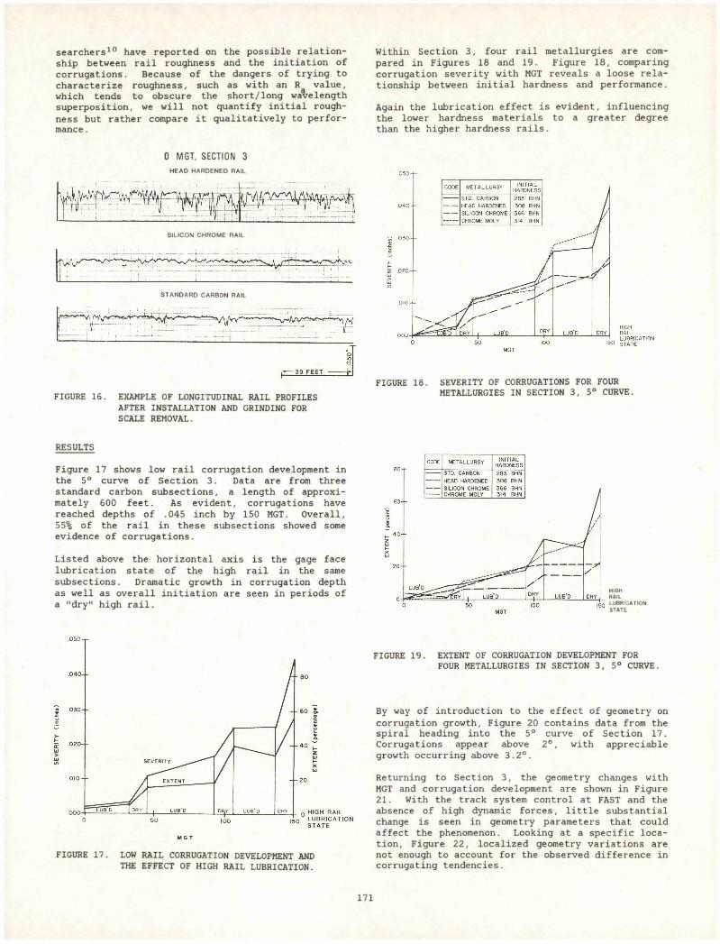
searchers10 have reported on the possible relation­ship between rail roughness and the initiation of corrugations. Because of the dangers of trying to characterize roughness, such as with an Rq value, which tends to obscure the short/long wavelength superposition, we will not quantify initial rough­ness but rather compare it qualitatively to perfor­mance .

Within Section 3, four rail metallurgies are com­pared in Figures 18 and 19. Figure 18, comparing corrugation severity with MGT reveals a loose rela­tionship between initial hardness and performance.

Again the lubrication effect is evident, influencing the lower hardness materials to a greater degree than the higher hardness rails.

0 MGT, SECTION 3

H E A D H A R D E N E D R A IL

S I L I C O N C H R O M E R A IL

S T A N D A R D C A R B O N R A IL

FIGURE 16. EXAMPLE OF LONGITUDINAL RAIL PROFILES AFTER INSTALLATION AND GRINDING FOR SCALE REMOVAL.

FIGURE 18. SEVERITY OF CORRUGATIONS FOR FOURMETALLURGIES IN SECTION 3, 5° CURVE.

RESULTS

Figure 17 shows low rail corrugation development in the 5° curve of Section 3. Data are from three standard carbon subsections, a length of approxi­mately 600 feet. As evident, corrugations have reached depths of .045 inch by 150 MGT. Overall, 55% of the rail in these subsections showed some evidence of corrugations.

Listed above the horizontal axis is the gage face lubrication state of the high rail in the same subsections. Dramatic growth in corrugation depth as well as overall initiation are seen in periods of a "dry" high rail.

HIGHRAILL U B R IC A TIO NS TA T E

FIGURE 17. LOW RAIL CORRUGATION DEVELOPMENT AND THE EFFECT OF HIGH RAIL LUBRICATION.

FIGURE 19. EXTENT OF CORRUGATION DEVELOPMENT FORFOUR METALLURGIES IN SECTION 3, 5° CURVE.

By way of introduction to the effect of geometry on corrugation growth, Figure 20 contains data from the spiral heading into the 5° curve of Section 17. Corrugations appear above 2°, with appreciable growth occurring above 3.2°.

Returning to Section 3, the geometry changes with MGT and corrugation development are shown in Figure 21. With the track system control at FAST and the absence of high dynamic forces, little substantial change is seen in geometry parameters that could affect the phenomenon. Looking at a specific loca­tion, Figure 22, localized geometry variations are not enough to account for the observed difference in corrugating tendencies.

171

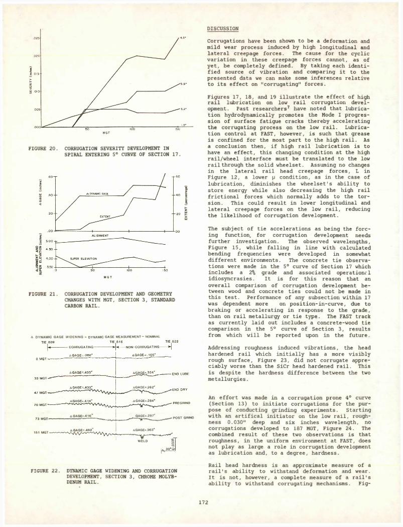
DISCUSSION

FIGURE 20. CORRUGATION SEVERITY DEVELOPMENT INSPIRAL ENTERING 5° CURVE OF SECTION 17.

FIGURE 21. CORRUGATION DEVELOPMENT AND GEOMETRY CHANGES WITH MGT, SECTION 3, STANDARD CARBON RAIL.

A DYNAMIC GAGE WIDENING = DYNAMIC GAGE MEASUREMENT-NOMINAL

73 MGTa GAGE=.416‘

151 MGTA GAGE=.462~ a GAGE=.363*

“VWELD

FIGURE 22. DYNAMIC GAGE WIDENING AND CORRUGATION DEVELOPMENT, SECTION 3, CHROME MOLYB­DENUM RAIL.

Corrugations have been shown to be a deformation and mild wear process induced by high longitudinal and lateral creepage forces. The cause for the cyclic variation in these creepage forces cannot, as of yet, be completely defined. By taking each identi­fied source of vibration and comparing it to the presented data we can make some inferences relative to its effect on "corrugating" forces.

Figures 17, 18, and 19 illustrate the effect of high rail lubrication on low rail corrugation devel­opment. Past researchers7 have noted that lubrica­tion hydrodynamically promotes the Mode I progres­sion of surface fatigue cracks thereby accelerating the corrugating process on the low rail. Lubrica­tion control at FAST, however, is such that grease is confined for the most part to the high rail. As a conclusion then, if high rail lubrication is to have an effect, this changing condition at the high rail/wheel interface must be translated to the low rail through the solid wheelset. Assuming no changes in the lateral rail head creepage forces, L in Figure 12, a lower p condition, as in the case of lubrication, diminishes the wheelset's ability to store energy while also decreasing the high rail frictional forces which normally adds to the tor­sion. This could result in lower longitudinal and lateral creepage forces on the low rail, reducing the likelihood of corrugation development.

The subject of tie accelerations as being the forc­ing function, for corrugation development needs further investigation. The observed wavelengths, Figure 15, while falling in line with calculated bending frequencies were developed in somewhat different environments. The concrete tie observa­tions were made in the 5° curve of Section 17 which includes a 2% grade and associated operationcl idiosyncrasies. It is for this reason that an overall comparison of corrugation development be­tween wood and concrete ties could not be made in this test. Performance of any subsection within 17 was dependent more on position-in-curve, due to braking or accelerating in response to the grade, than on rail metallurgy or tie type. The FAST track as currently laid out includes a concrete-wood tie comparison in the 5° curve of Section 3, results from which will be reported upon in the future.

Addressing roughness induced vibrations, the head hardened rail which initially has a more visibly rough surface, Figure 23, did not corrugate appre­ciably worse than the SiCr head hardened rail. This is despite the hardness difference between the two metallurgies.

An effort was made in a corrugation prone 4° curve (Section 13) to initiate corrugations for the pur­pose of conducting grinding experiments. Starting with an artifical initiator on the low rail, rough­ness 0.030" deep and six inches wavelength, no corrugations developed to 187 MGT, Figure 24. The combined result of these two observations is that roughness, in the uniform environment at FAST, does not play as large a role in corrugation development as lubrication and, to a degree, hardness.

Rail head hardness is an approximate measure of a rail's ability to withstand deformation and wear. It is not, however, a complete measure of a rail's ability to withstand corrugating mechanisms. Fig-

172

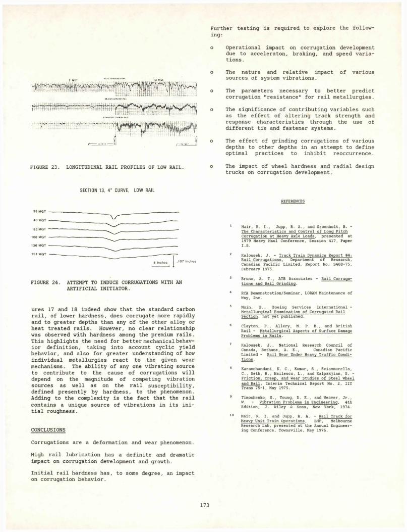
Further testing is required to explore the follow­ing:

o Operational impact on corrugation development due to acceleraton, braking, and speed varia­tions .

o The nature and relative impact of varioussources of system vibrations.

o The parameters necessary to better predictcorrugation "resistance" for rail metallurgies.

o The significance of contributing variables such as the effect of altering track strength and response characteristics through the use of different tie and fastener systems.

o The effect of grinding corrugations of various depths to other depths in an attempt to define optimal practices to inhibit reoccurrence.

FIGURE 23. LONGITUDINAL RAIL PROFILES OF LOW RAIL. o The impact of wheel hardness and radial design trucks on corrugation development.

SECTION 13. 4° CURVE. L O W RAIL

REFERENCES

33 MGT

46 MGT

93 MGT

108 MGT

136 MGT

151 MGT

.107 Inches

FIGURE 24. ATTEMPT TO INDUCE CORRUGATIONS WITH AN ARTIFICIAL INITIATOR.

ures 17 and 18 indeed show that the standard carbon rail, of lower hardness, does corrugate more rapidly and to greater depths than any of the other alloy or heat treated rails. However, no clear relationship was observed with hardness among the premium rails. This highlights the need for better mechanical behav­ior definition, taking into account cyclic yield behavior, and also for greater understanding of how individual metallurgies react to the given wear mechanisms. The ability of any one vibrating source to contribute to the cause of corrugations will depend on the magnitude of competing vibration sources as well as on the rail susceptibility, defined presently by hardness, to the phenomenon. Adding to the complexity is the fact that the rail contains a unique source of vibrations in its ini­tial roughness.

CONCLUSIONS

1 Mair, R. I., Jupp, R. A., and Groenholt, R. - The Characteristics and Control of Long Pitch Corrugation at Heavy Axle Loads, presented at 1979 Heavy Haul Conference. Session 417, Paper 1.8.

2 Kalousek, J. - Track Train Dynamics Report #4: Rail Corrugations, Department of Research, Canadian Pacific Limited, Report No. S488-75, February 1975.

3 Bruno, A. T., ATB Associates - Rail Corruga­tions and Rail Grinding.

4 RCA Demonstration/Seminar, LORAM Maintenance of Way, Inc.

5 Moin, E., Boeing Services International -Metallurgical Examination of Corrugated Rail Section, not yet published.

6 Clayton, P., Allery, M. P. B., and British Rail - Metallurgical Aspects of Surface Damage Problems in Rails.

7 Kalousek, J., National Research Council ofCanada, Bethune, A. E., Canadian PacificLimited - Rail Wear Under Heavy Traffic Condi­tions .

8 Karamchandani, K. C., Kumar, S., Sciammarella, C., Seth, B., Nailescu, L., and Kalpakjian, S. - Friction, Creep, and Wear Studies of Steel Wheel and Rail, Interim Technical Report No. 2, IIT Trans 75-1, May 1975.

9 Timoshenko, S., Young, D. E., and Weaver, Jr., W. - Vibration Problems in Engineering, 4th Edition, J. Wiley & Sons, New York, 1974.

10 Mair, R. I. and Jupp, R. A. - Rail Track for Heavy Unit Train Operations, BHP, Melbourne Research Lab, presented at the Annual Engineer­ing Conference, Townsville, May 1976.

Corrugations are a deformation and wear phenomenon.

High rail lubrication has a definite and dramatic impact on corrugation development and growth.Initial rail hardness has, to some degree, an impact on corrugation behavior.

173

QUESTIONS AND ANSWERS

Question 1

What recommendations do you make with your cur­rent knowledge of when to grind and how much for maximum economy of grinding expense, rail expense, and train delay expense?

Answer

Until recently, the FAST Program has not been able to address the grinding issue as we would have liked. The experiment itself must be careful to avoid impact on other experiments (tie, ballast, etc.). However, we have two programs which will, in the near future, pro­duce results. In the 5° Curve of Section 7, we have alternately ground segments of new stan­dard rail. Results from this test should give us more insight into the grinding of new rail controversy.

Question 2

As stated by the author, the effect is a cycl­ical dynamic one involving longitudinal creep- age (as well as lateral) vertical motion, etc. Since modeling knowledge exists sufficient to simulate wheelset motion in such a regime, has any thought been given to employing these in search of a fuller explanation?

Answer

Part of the original objective of this' exper­iment included only laying the ground work for future testing and the formation mechanisms. Our overall concept was to observe corruga­tions, trying to isolate where and under what conditions they develop, as well as documenting growth rate and reoccurrence. Using this as a base, we are now in a position to look into formation mechanisms. Our anticipated next phase is just as you suggested. While con­tinuing observational testing, we will address the mechanism issue with coordinated dynamic testing and modelling.

Question 4

1) What causes corrugations to develop?

2) What can be done to avoid it? Please give answers in a plain manner - bare facts - which can be easily understood by our everyday track people.

Answer

Corrugations of this type are a direct result of the wheelset negotiating the curve. In doing this, it encounters differences in rolling distances (i.e., the low rail is shorter than the high rail) and also, dif­ferences in load because of the forces required to guide a car through a curve. Vibrations are, as a result, initiated within the wheelset itself and, also, within the track and mechan­ical systems. These vibrations cause periodic, every 8" for example, increases in load which result in increased wear and metal flow.

The method to avoid corrugations can be ad­dressed from two view points. First, is to get rid of the source of vibrations. Disconnecting the wheels from one another or alternating the track design are some suggestions, although neither are very partical. We, therefore, must look at how to reduce the forces present and live for the time being with the vibration. High rail lubrication seems to be an effect at FAST in reducing the forces due to axle re­sponse. Also, as documented on the Canadian Pacific, see Reference 2, gage control is important in minimizing contact stresses. High contact stresses can develop and cause metal flow when the wheelset is allowed to run near its front rim face, i.e., areas of excessively wide gage. As a last result, if we don't control the vibrations, and it's not practical to control the forces, it is best to use a type of rail that is able to withstand both. They have found at FAST that harder rails generally resist corrugations better. This is by no means a "hard" and "fast" rule, more work needs to be done to understand why some premium rails perform well and others don't.

Question 3

I missed magnification, etching, and other particulars for S.E.M. micros. Please supply.

Answer

I hope sufficient documentation is provided in the text of the proceedings. For more refer­ences on the use of the technique itself as well as general comments, please contact me directly.

174

MECHANICAL1981 FAST ENGINEERING CONFERENCE

KEY TOPICS

WHEELS

RADIAL TRUCKS

FATIGUE ANALYSIS

WEAR INDEX TESTING

WHEEL/RAIL LOADS

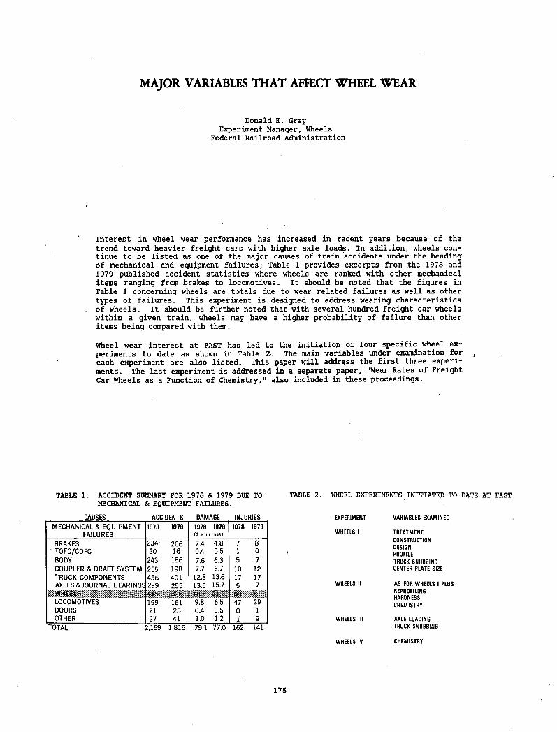
MAJOR VARIABLES TH AT AFFECT WHEEL WEAR

Donald E. Gray Experiment Manager, Wheels

Federal Railroad Administration

Interest in wheel wear performance has increased in recent years because of the trend toward heavier freight cars with higher axle loads. In addition, wheels con­tinue to be listed as one of the major causes of train accidents under the heading of mechanical and equipment failures; Table 1 provides excerpts from the 1978 and 1979 published accident statistics where wheels are ranked with other mechanical items ranging from brakes to locomotives. It should be noted that the figures in Table 1 concerning wheels are totals due to wear related failures as well as other types of failures. This experiment is designed to address wearing characteristics of wheels. It should be further noted that with several hundred freight car wheels within a given train, wheels may have a higher probability of failure than other items being compared with them.

Wheel wear interest at FAST has led to the initiation of four specific wheel ex­periments to date as shown in Table 2. The main variables under examination for , each experiment are also listed. This paper will address the first three experi­ments. The last experiment is addressed in a separate paper, "Wear Rates of Freight Car Wheels as a Function of Chemistry," also included in these proceedings.

TABLE I. ACCIDENT SUMMARY FOR 1978 & 1979 DUE TO MECHANICAL & EQUIPMENT FAILURES.

CAUSES_______________ ACCIDENTS DAMAGE INJURIESMECHANICAL & EQUIPM ENT

FAILURES1978 1979 1978 1979

($ m illio n s )1978 1979

BRAKES 234' 206 7.4 4.8 7 8TOFC/COFC 20 16 0.4 0.5 1 0BODY 243 186 7.6 6.3 5 7COUPLER & DRAFT SYSTEM 255 198 7.7 6.7 10 12TRUCK COMPONENTS 456 401 12.8 13.6 17 17AXLES & JOURNAL BEARINGS 299 255 13.5 15.7 5 7

415 326 21.2 69 51LOCOMOTIVES 199 161 9.8 6.5 47 29DOORS 21 25 0.4 0.5 0 1OTHER 27 41 1.0 1.2 1 9

TOTAL 2,169 1,815 79.1 77.0 162 141

TABLE 2. WHEEL EXPERIMENTS INITIATED TO DATE AT FAST

EXPERIMENT VARIABLES EXAMINED

WHEELS 1 TREATMENTCONSTRUCTIONDESIGNPROFILETRUCK SNUBBING CENTER PLATE SIZE

WHEELS II AS FOR WHEELS 1 PLUS REPROFILING HARDNESS CHEMISTRY

WHEELS III AXLE LOADING TRUCK SNUBBING

WHEELS IV CHEMISTRY

175

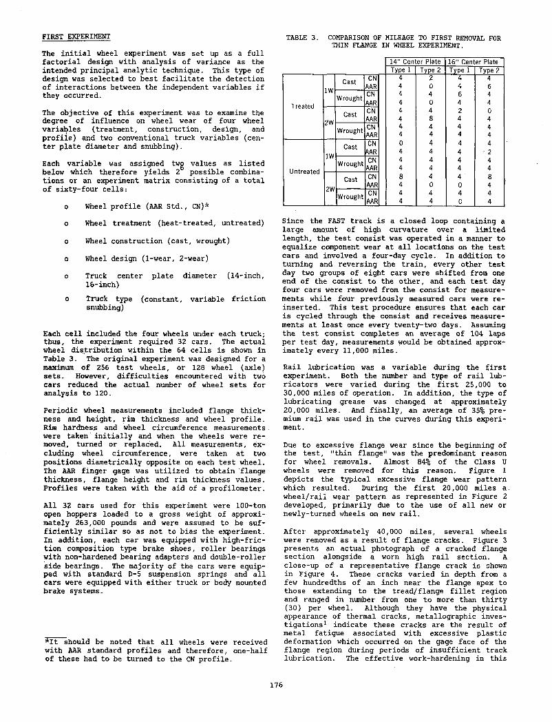
FIRST EXPERIMENT

The initial wheel experiment was set up as a full factorial design with analysis of variance as the intended principal analytic technique. This type of design was selected to best facilitate the detection of interactions between the independent variables if they occurred.

The objective of this experiment was to examine the degree of influence on wheel wear of four wheel variables (treatment, construction, design, and profile) and two conventional truck variables (cen­ter plate diameter and snubbing).

Each variable was assigned twg values as listed below which therefore yields 2 possible combina­tions or an experiment matrix consisting of a total of sixty-four cells:

o Wheel profile (AAR Std., CN)*

o Wheel treatment (heat-treated, untreated)

o Wheel construction (cast, wrought)

o Wheel design (1-wear, 2-wear)

o Truck center plate diameter (14-inch,16-inch)

o Truck type (constant, variable friction snubbing)

Each cell included the four wheels under each truck; thus, the experiment required 32 cars. The actual wheel distribution within the 64 cells is shown in Table 3. The original experiment was designed for a maximum of 256 test wheels, or 128 wheel (axle) sets. However, difficulties encountered with two cars reduced the actual number of wheel sets for analysis to 120.

Periodic wheel measurements included flange thick­ness and height, rim thickness and wheel profile. Rim hardness and wheel circumference measurements were taken initially and when the wheels were re­moved, turned or replaced. All measurements, ex­cluding wheel circumference, were taken at two positions diametrically opposite on each test wheel. The AAR finger gage was utilized to obtain flange thickness, flange height and rim thickness values. Profiles were taken with the aid of a profilometer.

All 32 cars used for this experiment were 100-^ton open hoppers loaded to a gross weight of approxi­mately 263,000 pounds and were assumed to be suf­ficiently similar so as not to bias the experiment. In addition, each car was equipped with high-fric­tion composition type brake shoes, roller bearings with non-hardened bearing adapters and double-roller side bearings. The majority of the cars were equip­ped with standard D-5 suspension springs and all cars were equipped with either truck or body mounted brake systems.

*It should be noted that all wheels were received with AAR standard profiles and therefore, one-half of these had to be turned to the CN profile.

TABLE 3. COMPARISON OF MILEAGE TO FIRST REMOVAL FOR THIN FLANGE IN WHEEL EXPERIMENT.

1 4 ” C e n te r P la te 1 6 ” C en te r P lateTyp e 1 T yp e 2 T y p e 1 T yp e 2

1WC as t CN

AAR44

20

44

46

T re a te dW ro u g h t CN

AAR44

40

64

44

2WC ast CN

AAR44

48

24

04

W ro u g h t CNAAR

44

44

44

44

1WC as t CN

AAR04

44

44

4• 2

U n tre a te dW ro u g h t CN

AAR44

44

44

44

2WC ast CN

AAR84

40

40

84

W ro u g h t CNAAR

44

44

40

44

Since the FAST track is a closed loop containing a large amount of high curvature over a limited length, the test consist was operated in a manner to equalize component wear at all locations on the test cars and involved a four-day cycle. In addition to turning and reversing the train, every other test day two groups of eight cars were shifted from one end of the consist to the other, and each test day four cars were removed from the consist for measure­ments while four previously measured cars were re­inserted. This test procedure ensures that each car is cycled through the consist and receives measure­ments at least once every twenty-two days. Assuming the test consist completes an average of 104 laps per test day, measurements would be obtained approx­imately every 11,000 miles.

Rail lubrication was a variable during the first experiment. Both the number and type of rail lub­ricators were varied during the first 25,000 to30.000 miles of operation. In addition, the type of lubricating grease was changed at approximately20.000 miles. And finally, an average of 35% pre­mium rail was used in the curves during this experi­ment.

Due to excessive flange wear since the beginning of the test, "thin flange" was the predominant reason for wheel removals. Almost 84% of the Class U wheels were removed for this reason. Figure 1 depicts the typical excessive flange wear pattern which resulted. During the first 20,000 miles a. wheel/rail wear pattern as represented in Figure 2 developed, primarily due to the use of all new or newly-turned wheels on new rail.

After approximately 40,000 miles, several wheels were removed as a result of flange cracks. Figure 3 presents an actual photograph of a cracked flange section alongside a worn high rail section. A close-up of a representative flange crack is shown in Figure 4. These cracks varied in depth from a few hundredths of an inch near the flange apex to those extending to the tread/flange fillet region and ranged in number from one to more than thirty (30) per wheel. Although they have the physical appearance of thermal cracks, metallographic inves­tigations1 indicate these cracks are the result of metal fatigue associated with excessive plastic deformation which occurred on the gage face of the flange region during periods of insufficient track lubrication. The effective work-hardening in this

176

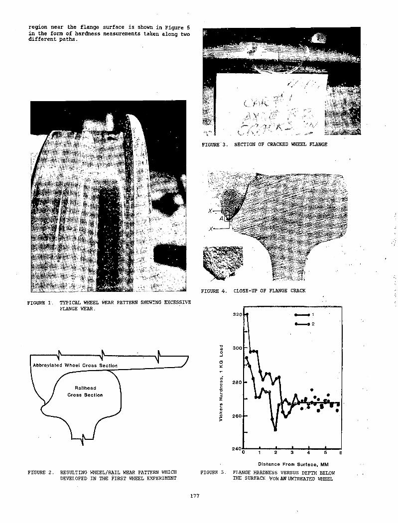
region near the flange surface is shown in Figure 5 in the form of hardness measurements taken along two different paths.

FIGURE 3. SECTION OF CRACKED WHEEL FLANGE

FIGURE 4. CLOSE-UP OF FLANGE CRACK

FIGURE 1. TYPICAL WHEEL WEAR PATTERN SHOWING EXCESSIVE FLANGE WEAR.

FIGURE 2. RESULTING WHEEL/RAIL WEAR PATTERN WHICH DEVELOPED IN THE FIRST WHEEL EXPERIMENT

D i s t a n c e F r o m S u r f a c e , M M

FIGURE 5. FLANGE HARDNESS VERSUS DEPTH BELOW THE SURFACE IFOR AN UNTREATED WHEEL

177

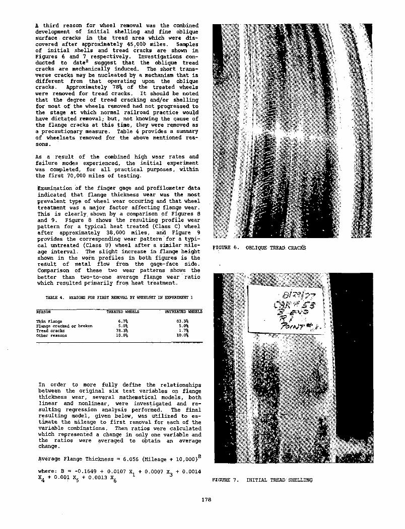
A third reason for wheel removal was the combined development of initial shelling and fine oblique surface cracks in the tread area which were dis­covered after approximately 45,000 miles. Samples of initial shells and tread cracks are shown in Figures 6 and 7 respectively. Investigations con­ducted to date2 suggest that the oblique tread cracks are mechanically induced. The short trans­verse cracks may be nucleated by a mechanism that is different from that operating upon the oblique cracks. Approximately 78% of the treated wheels were removed for tread cracks. It should be noted that the degree of tread cracking and/or shelling for most of the wheels removed had not progressed to the stage at which normal railroad practice would have dictated removal; but, not knowing the cause of the flange cracks at this time, they were removed as a precautionary measure. Table 4 provides a summary of wheelsets removed for the above mentioned rea­sons.

As a result of the combined high wear rates and failure modes experienced, the initial experiment was completed, for all practical purposes, within the first 70,000 miles of testing.

Examination of the finger gage and profilometer data indicated that flange thickness wear was the most prevalent type of wheel wear occuring and that wheel treatment was a major factor affecting flange wear. This is clearly, shown by a comparison of Figures 8 and 9. Figure 8 shows the resulting profile wear pattern for a typical heat treated (Class C) wheel after approximately 38,000 miles, and Figure 9 provides the corresponding wear pattern for a typi­cal untreated (Class U) wheel after a similar mile­age interval. The slight increase in flange height shown in the worn profiles in both figures is the result of metal flow from the gage-face side. Comparison of these two wear patterns shows the better than two-to-one average flange wear ratio which resulted primarily from heat treatment.

TABLE 4. REASONS FOR FIRST REMOVAL BY WHEELSET IN EXPERIMENT 1

REASON TREATED WHEELS UNTREATED WHEELS

Thin Flange 6.7% 83.3%Flange cracked or broken 5.0% 5.0%Tread cracks 78.3% 1.7%Other reasons 10-0% 10.0%

In order to more fully define the relationships between the original six test variables on flange thickness wear, several mathematical models, both linear and nonlinear, were investigated and re­sulting regression analysis performed. The final resulting model, given below, was utilized to es­timate the mileage to first removal for each of the variable combinations. Then ratios were calculated which represented a change in only one variable and the ratios were averaged to obtain an average change.

Average Flange Thickness = 6.056 (Mileage + 10,000)B

where: B = -0.1649 + 0.0107 X + 0.0007 X + 0.0014X4 + °-°01 x5 + 0-0013 X6 FIGURE 7. INITIAL TREAD SHELLTNtj

178

BA

'V'i

r' i

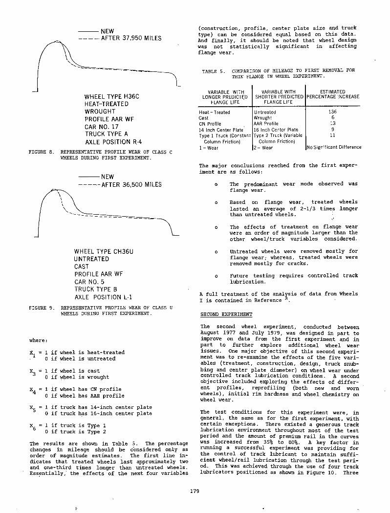
NEW

W R O U G H T PRO FILE AAR W F CAR NO. 17 T R U C K TY P E A AXLE P O S IT IO N R,4

FIGURE 8. REPRESENTATIVE PROFILE WEAR OF CLASS C WHEELS DURING FIRST EXPERIMENT.

--------------NEW-------------- AFTER 3 6 , 5 0 0 MILES

W HEEL TY P E C H 3 6 UU N T R E A T E DCASTPROFILE AAR W F CAR NO. 5 TR U C K TYPE B AXLE P O S IT IO N L - l

FIGURE 9. REPRESENTATIVE PROFILE WEAR OF CLASS U WHEELS DURING FIRST EXPERIMENT.

where:

Xj = 1 if wheel is heat-treated 0 if wheel is untreated

X3 = 1 if wheel is cast0 if wheel is wrought

X^ = 1 if wheel has CN profile 0 if wheel has AAR profile

Xg = 1 if truck has 14-inch center plate 0 if truck has 16-inch center plate

X& = 1 if truck is Type 1 0 if truck is Type 2

The results are shown in Table 5. The percentage changes in mileage should be considered only as order of magnitude estimates. The first line in­dicates that treated wheels last approximately two and one-third times longer than untreated wheels. Essentially, the effects of the next four variables

(construction, profile, center plate size and truck type) can be considered equal based on this data. And finally, it should be noted that wheel design was not statistically significant in affecting flange wear.

TABLE 5. COMPARISON OF MILEAGE TO FIRST REMOVAL FOR THIN FLANGE IN WHEEL EXPERIMENT.

V A R IA BLE W ITH LO N G E R P R E D IC TE D

FLA N G E LIFE

VARIABLE W ITH S H O R TE R P R E D IC TE D

FLA N G E LIFE

E S T IM A TE DPER C E N TA G E IN C R E A S E

H e a t -T r e a te d U n tre a te d 1 3 6C as t W ro u g h t 6CN P ro file AAR P ro file 1314 Inch C e n te r P late 16 Inch C en ter P la te 9T y p e 1 T ru c k (C o n s ta n t T y p e 2 T ru ck (V ariab le 11

C o lu m n F ric tio n ) C o lu m n F ric tio n )1 - W ear 2 - W ear No S ig n if ic a n t D iffe re n c e

The major conclusions reached from the first exper­iment are as follows:

o The predominant wear mode observed was flange wear.

o Based on flange wear, treated wheels lasted an average of 2-1/3 times longer than untreated wheels.

o The effects of treatment on flange wear were an order of magnitude larger than the other wheel/truck variables considered.

o Untreated wheels were removed mostly for flange wear; whereas, treated wheels were removed mostly for cracks.

o Future testing requires controlled track lubrication.

A full treatment of the analysis of data from Wheels I is contained in Reference 3.

SECOND EXPERIMENT

The second wheel experiment, conducted between August 1977 and July 1979, was designed in part to improve on data from the first experiment and in part to further explore additional wheel wear issues. One major objective of this second experi­ment was to re-examine the effects of the five vari­ables (treatment, construction, design, truck snub­bing and center plate diameter) on wheel wear under controlled track lubrication conditions. A second objective included exploring the effects of differ­ent profiles, reprofiling (both new and worn wheels), initial rim hardness and wheel chemistry on wheel wear.

The test conditions for this experiment were, in general, the same as for the first experiment, with certain exceptions. There existed a generous track lubrication environment throughout most of the test period and the amount of premium rail in the curves was increased from 35% to 80%. A key factor in running a successful experiment was providing for the control of track lubricant to maintain suffi­cient wheel/rail lubrication through the test peri­od. This was achieved through the use of four track lubricators positioned as shown in Figure 10. Three

179

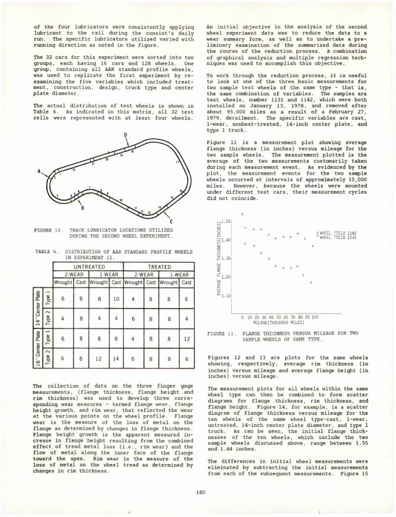
of the four lubricators were consistently applying lubricant to the rail during the consist's daily run. The specific lubricators utilized varied with running direction as noted in the figure.

The 32 cars for this experiment were sorted into two groups, each having 16 cars and 128 wheels. One group, containing all AAR standard profile wheels, was used to replicate the first experiment by re­examining the five variables which included treat­ment, construction, design, truck type and center plate diameter.

The actual distribution of test wheels is shown in Table 6. As indicated in this matrix, all 32 test cells were represented with at least four wheels.

0

FIGURE 10. TRACK LUBRICATOR LOCATIONS UTILIZED DURING THE SECOND WHEEL EXPERIMENT.

TABLE 6. DISTRIBUTION OF AAR STANDARD PROFILE WHEELS IN EXPERIMENT II.

UNTREATED TREATED2-WEAR 1-WEAR 2-WEAR 1-WEAR

Wrought Cast Wrought Cast Wrought Cast Wrought Cast

14”Center Plate

Type 1

6 8 8 10 4 8 8 6

Type 2

4 8 4 4 6 8 8 4

16” Center Plate

Type 1

6 8 8 8 4 8 8 12

Type 2

6 8 12 14 6 8 8 6

The collection of data on the three finger gage measurements, (flange thickness, flange height and rim thickness) was used to develop three corre­sponding wear measures - termed flange wear, flange height growth, and rim wear, that reflected the wear at the various points on the wheel profile. Flange wear is the measure of the loss of metal on the flange as determined by changes in flange thickness. Flange height growth is the apparent measured in­crease in flange height resulting from the combined effect of tread metal loss (i.e., rim wear) and the flow of metal along the inner face of the flange toward the apex. Rim wear is the measure of the loss of metal on the wheel tread as determined by changes in rim thickness.

An initial objective in the analysis of the second wheel experiment data was to reduce the data to a wear summary form, as well as to undertake a pre­liminary examination of the summarized data during the course of the reduction process. A combination of graphical analysis and multiple regression tech­niques was used to accomplish this objective.

To work through the reduction process, it is useful to look at one of the three basic measurements for two sample test wheels of the same type - that is, the same combination of variables. The samples are test wheels, number 1131 and 1142, which were both installed on January 13, 1978, and removed after about 95,000 miles as a result of a February 27, 1979, derailment. The specific variables are cast, 1-wear, nonheat-treated, 14-inch center plate, and type 1 truck.

Figure 11 is a measurement plot showing average flange thickness (in inches) versus mileage for the two sample wheels. The measurement plotted is the average of the two measurements customarily taken during each measurement event. As evidenced by the plot, the measurement events for the two sample wheels occurred at intervals of approximately 10,000 miles. However, because the wheels were mounted under different test cars, their measurement cycles did not coincide.

a.so

ri .40

E 1.30

-1.20

* WHEEL TTCID 1142 WHEEL TTCID 1131

: 1. 10-

0 10 20 30 40 50 60 70 80 90 100 MILAGE(THOUSAND MILES)

FIGURE 11. FLANGE THICHNESS VERSUS MILEAGE FOR TWO SAMPLE WHEELS OF SAME TYPE.

Figures 12 and 13 are plots for the same wheels showing, respectively, average rim thickness (in inches) versus mileage and average flange height (in inches) versus mileage.

The measurement plots for all wheels within the same wheel type can then be combined to form scatter diagrams for flange thickness, rim thickness, and flange height. Figure 14, for example, is a scatter diagram of flange thickness versus mileage for the ten wheels of the same wheel type-cast, 1-wear, untreated, 14-inch center plate diameter, and type 1 truck. As can be seen, the initial flange thick­nesses of the ten wheels, which include the two sample wheels discussed above, range between 1.55 and 1.44 inches.

The differences in initial wheel measurements were eliminated by subtracting the initial measurements from each of the subsequent measurements. Figure 15

180

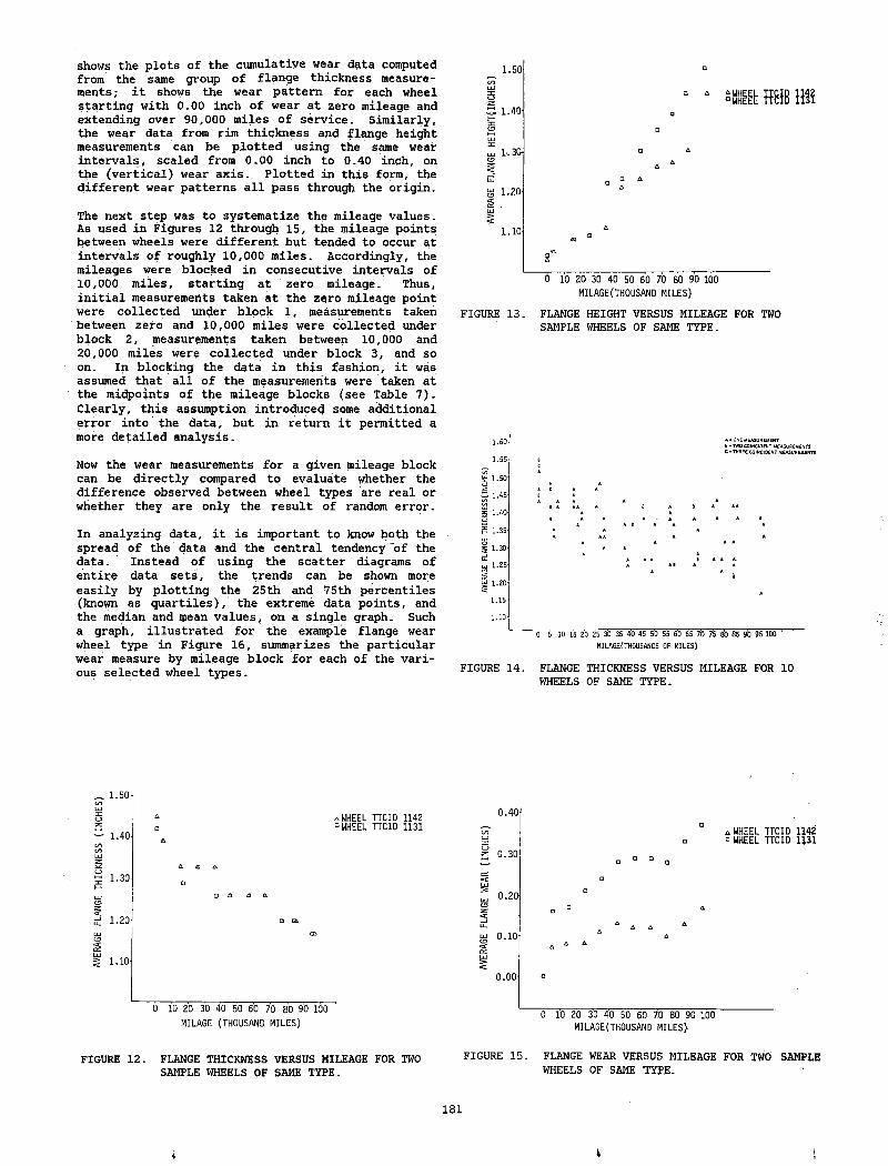
shows the plots of the cumulative wear data computed from the same group of flange thickness measure­ments; it shows the wear pattern for each wheel starting with 0.00 inch of wear at zero mileage and extending over 90,000 miles of service. Similarly, the wear data from rim thickness and flange height measurements can be plotted using the same wear intervals, scaled from 0.00 inch to 0.40 inch, on the (vertical) wear axis. Plqtted in this form, the different wear patterns all pass through the origin.

The next step was to systematize the mileage values. As used in Figures 12 through 15, the mileage points between wheels were different but tended to occur at intervals of roughly 10,000 miles. Accordingly, the mileages were blocked in consecutive intervals of10.000 miles, starting at zero mileage. Thus, initial measurements taken at the zero mileage point were collected under block 1, measurements taken between zero and 10,000 miles were collected under block 2, measurements taken between 10,000 and20.000 miles were collected under block 3, and so on. In blocking the data in this fashion, it was assumed that all of the measurements were taken at the midpoints of the mileage blocks (see Table 7). Clearly, this assumption introduced some additional error into the data, but in return it permitted a more detailed analysis.

Now the wear measurements for a given mileage block can be directly compared to evaluate whether the difference observed between wheel types are real or whether they are only the result of random error.

In analyzing data, it is important to know both the spread of the data and the central tendency of the data. Instead of using the scatter diagrams of entire data sets, the trends can be shown more easily by plotting the 25th and 75th percentiles (known as quartiles), the extreme data points, and the median and mean values, on a single graph. Such a graph, illustrated for the example flange wear wheel type in Figure 16, summarizes the particular wear measure by mileage block for each of the vari­ous selected wheel types.

1.50

1.40mt Ti&iB m

1'. 30-

1.20s .

1.10

0 10 20 30 40 50 60 70 80 90 100 MILAGE(THOUSAND MILES)

FIGURE 13. FLANGE HEIGHT VERSUS MILEAGE FOR TWO SAMPLE WHEELS OF SAME TYPE.

1.60

1.55

§ 1.50

§ 1'45 | 1.40

5 1.35

5 1.30

S 1'25'ig 1.20- <

1.15-

1 . 10-

A . ONE MEASUREMENT B - TWO COINCIDENT MEASUREMENTS C* THREE COINOOENT MEASUREMENTS

0 5 10 15 20 25 30 35 40 45 50 55 60 65 70 75 I

MILAGEITHOUSANDS OF MILES)

) 35 90 9 5 ltlO

FIGURE 14. FLANGE THICKNESS VERSUS MILEAGE FOR 10 WHEELS OF SAME TYPE.

1.50

1.40

« 1.30

1.20

1.10

a WHEEL TTCID 1142 a WHEEL TTCID 1131

a a a a

0 10 20 30 40 50 60 70 80 90 100 MILAGE (THOUSAND. MILES)

0.40-

0.30

0.20

0.10

0.00

a WHEEL TTCID 1142 oWHEEL TTCID 1131

0 10 20 30 40 50 60 70 80 90 100 MILAGE(TH0USAND MILES)

FIGURE 12. FLANGE THICKNESS VERSUS MILEAGE FOR TWO SAMPLE WHEELS OF SAME TYPE.

FIGURE 15. FLANGE WEAR VERSUS MILEAGE FOR TWO SAMPLE WHEELS OF SAME TYPE.

181

1- (

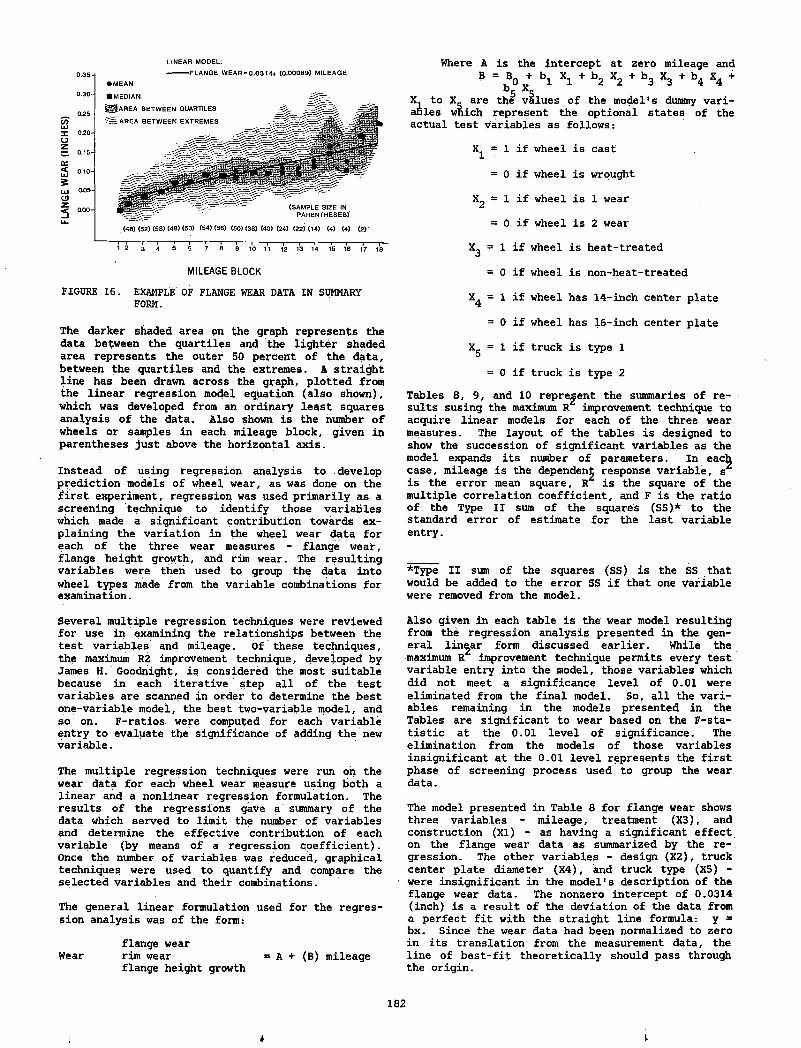
LINEAR MODEL:

MILEAGE BLOCKFIGURE 16. EXAMPLE OF FLANGE WEAR DATA IN SUMMARY

FORM.

The darker shaded area on the graph represents the data between the quartiles and the lighter shaded area represents the outer 50 percent of the data, between the quartiles and the extremes. A straight line has been drawn across the graph, plotted from the linear regression model equation (also shown), which was developed from an ordinary least squares analysis of the data. Also shown is the number of wheels or samples in each mileage block, given in parentheses just above the horizontal axis.

Instead of using regression analysis to develop prediction models of wheel wear, as was done on the first experiment, regression was used primarily as a screening technique to identify those variables which made a significant contribution towards ex­plaining the variation in the wheel wear data for each of the three wear measures - flange wear, flange height growth, and rim wear. The resulting variables were then used to group the data into wheel types made from the variable combinations for examination.

Several multiple regression techniques were reviewed for use in examining the relationships between the test variables and mileage. Of these techniques, the maximum R2 improvement technique, developed by James H. Goodnight, is considered the most suitable because in each iterative step all of the test variables are scanned in order to determine the best one-variable model, the best two-variable model, and so on. F-ratios were computed for each variable entry to evaluate the significance of adding the new variable.

The multiple regression techniques were run on the wear data for each wheel wear measure using both a linear and a nonlinear regression formulation. The results of the regressions gave a summary of the data which served to limit the number of variables and determine the effective contribution of each variable (by means of a regression coefficient). Once the number of variables was reduced, graphical techniques were used to quantify and compare the selected variables and their combinations.

The general linear formulation used for the regres­sion analysis was of the form:

flange wearWear rim wear = A + (B) mileage

flange height growth

? = V bl Xl +b2 X2 +b3 X3 +b4 X4 + b5 X5X. to Xs are the values of the model's dummy vari­

ables which represent the optional states of the actual test variables as follows:

X^ = 1 if wheel is cast

= 0 if wheel is wrought

X2 = 1 if wheel is 1 wear

= 0 if wheel is 2 wear

Xg = 1 if wheel is heat-treated

= 0 if wheel is non-heat-treated

X^ = 1 if wheel has 14-inch center plate

= 0 if wheel has 16-inch center plate

Xg = 1 if truck is type 1

= 0 if truck is type 2

Tables 8, 9, and 10 represent the summaries of re­sults susing the maximum R£ improvement technique to acquire linear models for each of the three wear measures. The layout of the tables is designed to show the succession of significant variables as the model expands its number of parameters. In each case, mileage is the dependent response variable, sZ is the error mean square, Rz is the square of the multiple correlation coefficient, and F is the ratio of the Type II sum of the squares (SS)* to the standard error of estimate for the last variable entry.

Where A is the in te rcep t at zero mileage and

*Type II sum of the squares (SS) is the SS that would be added to the error SS if that one variable were removed from the model.

Also given in each table is the wear model resulting from the regression analysis presented in the gen­eral linear form discussed earlier. While the maximum R^ improvement technique permits every test variable entry into the model, those variables which did not meet a significance level of 0.01 were eliminated from the final model. So, all the vari­ables remaining in the models presented in the Tables are significant to wear based on the F-sta- tistic at the 0.01 level of significance. The elimination from the models of those variables insignificant at the 0.01 level represents the first phase of screening process used to group the wear data.

The model presented in Table 8 for flange wear shows three variables - mileage, treatment (X3), and construction (XI) - as having a significant effect on the flange wear data as summarized by the re-, gression. The other variables - design (X2), truck center plate diameter (X4), and truck type (X5) - were insignificant in the model's description of the flange wear data. The nonzero intercept of 0.0314 (inch) is a result of the deviation of the data from a perfect fit with the straight line formula: y = bx. Since the wear data had been normalized to zero in its translation from the measurement data, the line of best-fit theoretically should pass through the origin.

182

ii

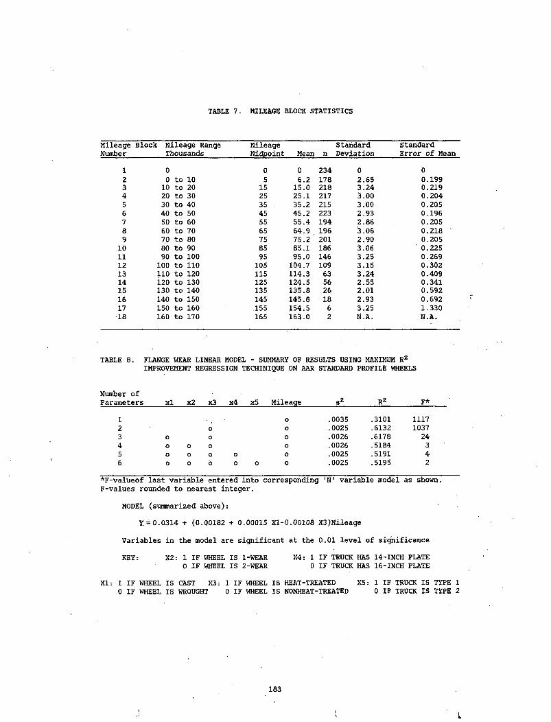
TABLE 7. MILEAGE BLOCK STATISTICS

Mileage Block Mileage Range Mileage Standard StandardNumber Thousands Midpoint Mean n Deviation Error of Mean

1 0 0 0 234 0 02 0 to 10 5 6.2 178 2.65 0.1993 10 to 20 15 15.0 218 3.24 0.2194 20 to 30 25 25.1 217 3.00 0.2045 30 to 40 35 35.2 215 3.00 0.2056 40 to 50 45 45.2 223 2.93 0.1967 50 to 60 55 55.4 194 2.86 0.2058 60 to 70 65 64.9 196 3.06 0.218 '9 70 to 80 75 75.2 201 2.90 0.205

10 80 to 90 85 85.1 186 3.06 ’ 0.22511 90 to 100 95 95.0 146 3.25 0.26912 100 to 110 105 104.7 109 3.15 0.30213 110 to 120 115 114.3 63 3.24 0.40914 120 to 130 125 124.5 56 2.55 0.34115 130 to 140 135 135.8 26 2.01 0.59216 140 to 150 145 145.8 18 2.93 0.69217 150 to 160 ,155 154.5 6 3.25 1.330•18 160 to 170 165 163.0 2 N.A. N.A.

TABLE 8. FLANGE WEAR LINEAR MODEL - SUMMARY OF RESULTS USING MAXIMUM R2IMPROVEMENT REGRESSION TECHINIQUE ON AAR STANDARD PROFILE WHEELS

Number ofParameters xl x2 x3 x4 x5 Mileaqe s2 R2 F*

1 o .0035 .3101 11172 0 0 .0025 .6132 10373 0 0 0 .0026 .6178 244 0 O 0 0 .0026 .5184 35 o O 0 0 0 .0025 .5191 46 0 o 6 0 0 0 .0025 .5195 2

*F-valueof last variable entered into corresponding 1N 1 variable model as shown. F-values rounded to nearest integer.

MODEL (summarized above):

Y. = 0.0314 + (0.00182 + 0.00015 Xl-0.00108 X3)Mileage

Variables in the model are significant at the 0.01 level of significance

KEY: X2: 1 IF WHEEL IS 1-WEAR X4: 1 IF TRUCK HAS 14-INCH PLATEO IF WHEEL IS 2-WEAR 0 IF TRUCK HAS 16-INCH PLATE

XI: 1 IF WHEEL IS CAST X3: 1 IF WHEEL IS HEAT-TREATED X5: 1 IF TRUCK IS TYPE 1 0 IF WHEEL IS WROUGHT 0 IF WHEEL IS NONHEAT-TREATED 0 IF TRUCK IS TYPE 2

183

L

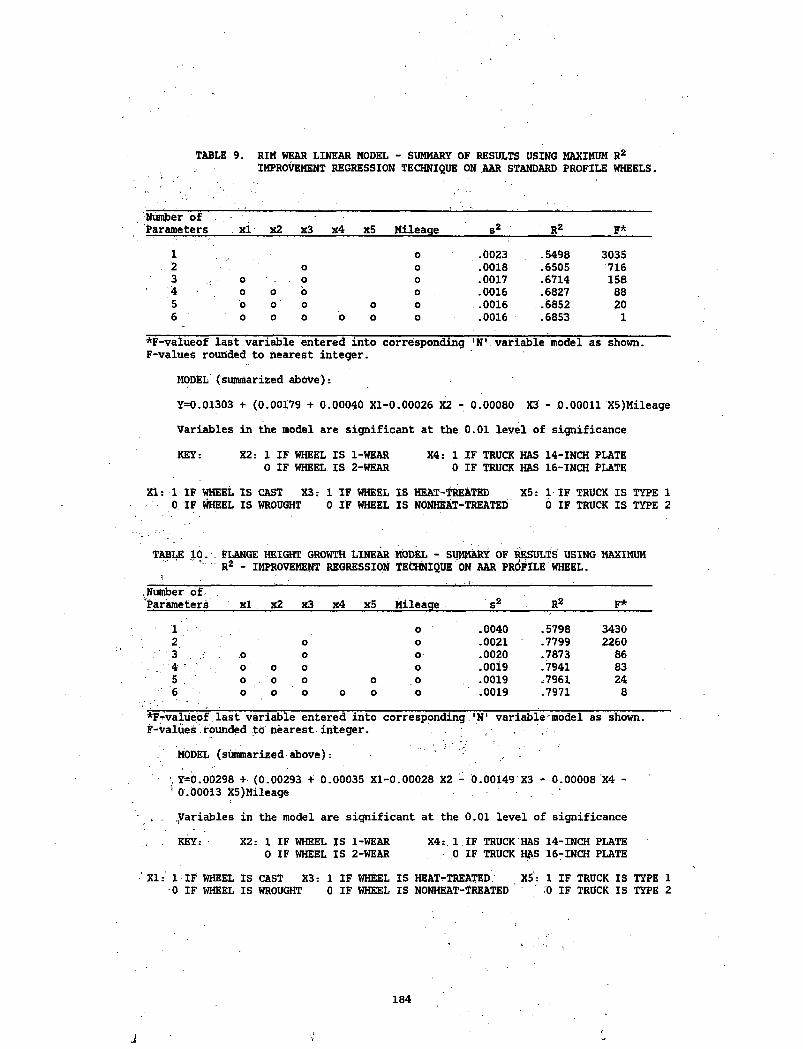
TABLE 9. RIM HEAR LINEAR MODEL - SUMMARY OF RESULTS USING MAXIMUM R2IMPROVEMENT REGRESSION TECHNIQUE ON AAR STANDARD PROFILE WHEELS.

Number of Parameters xi x2 x3 x4 x5 Mileaqe s2 R2 F*

1 0 .0023 .5498 30352 0 0 .0018 .6505 7163 0 0 0 .0017 .6714 1584 0 0 6 0 .0016 .6827 885 0 0 0 0 0 .0016 .6852 206 0 0 0 0 0 0 .0016 .6853 1

*F-valueof last variable entered into corresponding 'N* 1. variable model as shown. F-values rounded to nearest integer.

MODEL (summarized above):

Y=0.01303 + (0.00179 + 0.00040 Xl-0.00026 X2 - 0.00080 X3 - 0.00011 X5)Mileage

Variables in the model are significant at the 0.01 level of significance

KEY: X2: 1 IF WHEEL IS 1-WEAR X4: 1 IF TRUCK HAS 14-INCH PLATE0 IF WHEEL IS 2-WEAR 0 IF TRUCK HAS 16-INCH PLATE

XI: 1 IF WHEEL IS CAST X3: 1 IF WHEEL IS HEAT-TREATED X5: 1 IF TRUCK IS TYPE 1 0 IF WHEEL IS WROUGHT 0 IF WHEEL IS NONHEAT-TREATED 6 IF TRUCK IS TYPE 2

TABLE 10. FLANGE HEIGHT GROWTH LINEAR MODEL - SUMMARY OF RESULTS USING MAXIMUM R2 - IMPROVEMENT REGRESSION TECHNIQUE ON AAR PROFILE WHEEL.

Number of. 'Parameters xl x2 x3 x4 x5 Mileaqe s2 R2 F*

1 0 .0040 .5798 34302 o 0 .0021 .7799 22603 .0 o 0 .0020 .7873 864 ' 0 0 0 0 .ooi9 .7941 835 . ' 0 0 o o 0 .0019 .7961 246 o 0 0 o 0 o .0019 .7971 8

*F-rvaluebf last variable entered into corresponding 'N1 variable'model as shown. F-Values founded to'nearest integer.

MODEL (summarized above):

Y*0.00298 + (0.00293 + 0.00035 Xl-0.00028 X2 - 0.00149 X3 - 0.00008 X4 -1 0.00013 X5)Mileage

, , Variables in the model are significant at the 0.01 level of significance

. . KEY: X2: 1 IF WHEEL IS 1-WEAR X4:. 1. IF TRUCK HAS 14-INCH PLATEO IF WHEEL IS 2-WEAR 0 IF TRUCK HAS 16-INCH PLATE

‘ XI:' 1 IF WHEEL IS CAST X3: 1 IF WHEEL IS HEAT-TREATED/ X5 : 1 IF TRUCK IS TYPE 1 0 IF WHEEL IS WROUGHT 0 IF WHEEL IS NONHEAT-TREATED 0 IF TRUCK IS TYPE 2

184

J

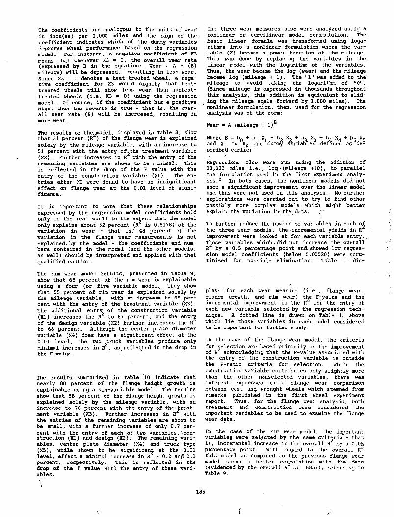
The coefficients are analogous to the units of wear in inch(es) per 1,000 miles and the sign of the coefficient indicates which of the dummy variables improves wheel performance based on the regression model. For instance, a negative coefficient of X3 means that whenever X3 = 1, the overall wear rate (expressed by B in the equation: Wear = A + (B)mileage) will be depressed, resulting in less wear. Since X3 = 1 denotes a heat-treated wheel, a nega­tive coefficient for X3 would signify that heat- treated wheels will show less wear than nonheat- treated wheels (i.e. X3 = 0) using the regression model. Of course, if the coefficient has a positive sign, then the reverse is true - that is, the over­all wear rate (B) will be increased, resulting in more wear.

The results of the_model, displayed in Table 8, show that 31 percent (k ) of the flange wear is explained solely by the mileage variable, with an increase to 51 percent with the entry of2the treatment variable (X3). Further increases in R with the entry of the remaining variables are shown to be minimal. This is reflected in the drop of the F value with the entry of the construction variable (XI). The en­tries after XI were found to have an insignificant effect on flange wear at the 0.01 level of signi­ficance.

It is important to note that these relationships expressed by the regression model coefficients hold only in the real world to the extent that the model only explains about 52 percent (R^ is 0.5178) of the variation in wear - that is, ' 48 percent of the variation in the flange wear measurements is not explained by the model - the coefficients and num­bers contained in the model (and the other models, as well) should be interpreted and applied with that qualified caution.

The rim wear model results, presented, in Table 9, show that 68 percent of the rim wear is explainable using a four (or five variable model. They show that 55 percent of rim wear is explained solely by the mileage variable, with an increase to 65 per­cent with the entry of the treatment variable (X3). The additional entry, of the construction variable (XI) increases the k to 67 percent, and the entrg of the design variable (X2) further increases the R to 68 percent. Although the center plate diameter variable (X4) does have a significant effect at the 0.01 level, the two £ruck variables produce only minimal increases in R , as reflected in the drop in the F value.

The results summarized in Table 10 indicate that nearly 80 percent of the flange height growth . is explainable using a six-variable model. The results show that 58 percent of the flange height growth is explained solely by the mileage variable, with an increase to 78 percent with the entry of the treat­ment variable (X3). Further increases in R£ with the entries of the remaining variables are shown to be small, with a further increase of only 0.7 per­cent with the entry of each of two variables, con­struction (XI) and design (X2). The remaining vari­ables, center plate diameter (X4) and truck type (X5), while shown to be significant at the 0.01 level, effect a minimal increase in R - 0.2 and 0.1 percent, respectively. This is reflected in the drop of the F value with the entry of these vari­ables.\

The three wear measures also were analyzed using a nonlinear or curvilinear model forumulation. The basic linear formula was transformed using loga­rithms into a nonlinear formulation where the var­iable (X) became a power function of the mileage. This was done by replacing the variables in the linear model with the logarithm of the variables. Thus, the wear became the log (wear) and the mileage became log (mileage + 1); The "l" was added to the mileage to avoid taking the logarithm of "0", (Since mileage is expressed in thousands throughout this analysis, this addition is equivalent to slid­ing the mileage scale forward by 1,000 miles). The nonlinear formulation, then, used for the regression analysis was of the form:

Wear = A (mileage +1 )

Where B = bQ .+ b, Xx + b2 X2 + b , X 3 + b . X- + b5 Xg and X^ to UX^ are 1dummy variables defined as de­scribed earlier.

Regressions also were run using the addition of 10,000 miles i.e., log ■(mileage +10), to parallel the formulation used in the first experiment analy­sis.2 In both cases, the nonlinear models did not show a significant improvement over the linear model and thus were not used in this analysis. No further explorations were carried out to try to find other possibly more complex models which might better explain the variation in the data.

To further reduce the number of variables in each o| the three wear models, the incremental yields in R improvement were looked at for each variable entry. Ttjose variables which • did not increase the overall R by a 0.5 percentage point and showed low regres­sion model coefficients (below 0.00020) were scru­tinized for possible elimination. Table 11 dis­

plays for each wear measure (i.e., flange wear, flange growth, and rim wear) thp Frvalue and the incremental improvement in the R^ for the entry of each new variable selected by the regression tech­nique. A dotted line is drawn on Table 11 above which lie those variables in each model considered to be important for further study.

In the case of the flange wear model, the criteria for selection are based primarily on the improvement of Rz acknowledging that the F-value associated with the entry of the construction variable is outside the F-ratio criteria for selection. While the construction variable contributes only slightly more than the other nonselected variables, there was interest expressed, in a flange wear comparison between cast and wrought wheels which stemmed from remarks published in the first wheel experiment report. Thus, for the flange wear analysis, both treatment and construction were considered the important variables to be used to examine the flange wear data.

In . the case of the rim wear model, the important variables were selected by the same criteria - that is, incremental increase in the overall by a 0.05 percentage point. With regard to the overall R^ this model as compared to the previous flange wear model shows a better coo-elation with the data (evidenced by the overall R of .6853), referring to Table 9.

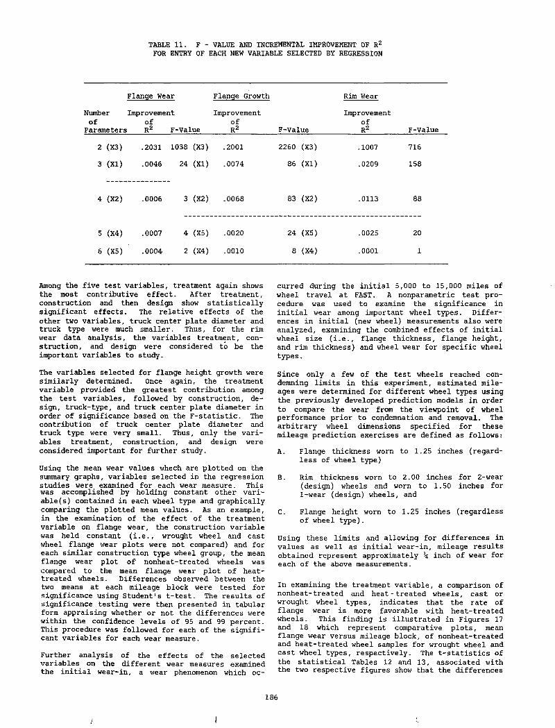
TABLE 11. F - VALUE AND INCREMENTAL IMPROVEMENT OF R2 FOR ENTRY OF EACH NEW VARIABLE SELECTED BY REGRESSION

Flanqe Wear Flanqe Growth

Number Improvement Improvement of of of

Parameters R2 F-Value R2 F-Value

Rim Wear

ImprovementofR2 F-Value

2 (X3) .2031 1038 (X3) .2001 2260 (X3) .1007 716

3 (XI) .0046 24 (XI) .0074 86 (XI) .0209 158

4 (X2) .0006 3 (X2) .0068 83 (X2) .0113 88

5 (X4) .0007 4 (X5) .0020 24 (X5) .0025 20

6 (X5) .0004 2 (X4) .0010 8 (X4) .0001 1

five test variables, treatment again shows curred during the initial 5,000 to 15,the most contributive effect. After treatment, construction and then design show statistically significant effects. The relative effects of the other two variables, truck center plate diameter and truck type were much smaller. Thus, for the rim wear data analysis, the variables treatment, con­struction, and design were considered to be the important variables to study.

wheel travel at FAST. A nonparametric test pro­cedure was used to examine the significance in initial wear among important wheel types. Differ­ences in initial (new wheel) measurements also were analyzed, examining the combined effects of initial wheel size (i.e., flange thickness, flange height, and rim thickness) and wheel wear for specific wheel types.

The variables selected for flange height growth were similarly determined. Once again, the treatment variable provided the greatest contribution among the test variables, followed by construction, de­sign, truck-type, and truck center plate diameter in order of significance based on the F-statistic. The contribution of truck center plate diameter and truck type were very small. Thus, only the vari­ables treatment, construction, and design were considered important for further study.

Using the mean wear values whech are plotted on the summary graphs, variables selected in the regression studies were examined for each wear measure. This was accomplished by holding constant other vari­able (s) contained in each wheel type and graphically comparing the plotted mean values. As an example, in the examination of the effect of the treatment variable on flange wear, the construction variable was held constant (i.e., wrought wheel and cast wheel flange wear plots were not compared) and for each similar construction type wheel group, the mean flange wear plot of nonheat-treated wheels was compared to the mean flange wear plot of heat- treated wheels. Differences observed between the two means at each mileage block were tested for significance using Student's t-test. The results of significance testing were then presented in tabular form appraising whether or not the differences were within the confidence levels of 95 and 99 percent. This procedure was followed for each of the signifi­cant variables for each wear measure.

Since only a few of the test wheels reached con­demning limits in this experiment, estimated mile­ages were determined for different wheel types using the previously developed prediction models in order to compare the wear from the viewpoint of wheel performance prior to condemnation and removal. The arbitrary wheel dimensions specified for these mileage prediction exercises are defined as follows:

A. Flange thickness worn to 1.25 inches (regard­less of wheel type)

B. Rim thickness worn to 2.00 inches for 2-wear (design) wheels and worn to 1.50 inches for 1-wear (design) wheels, and

C. Flange height worn to 1.25 inches (regardless of wheel type).

Using these limits and allowing for differences in values as well as initial wear-in, mileage results obtained represent approximately \ inch of wear for each of the above measurements.

In examining the treatment variable, a comparison of nonheat-treated and heat-treated wheels, cast or wrought wheel types, indicates that the rate of flange wear is more favorable with heat-treated wheels. This finding is illustrated in Figures 17 and 18 which represent comparative plots, mean flange wear versus mileage block, of nonheat-treated and heat-treated wheel samples for wrought wheel and cast wheel types, respectively. The t-statistics of the statistical Tables 12 and 13, associated with the two respective figures show that the differences

Further analysis of the effects of the selected variables on the different wear measures examined the initial wear-in, a wear phenomenon which oc-

186

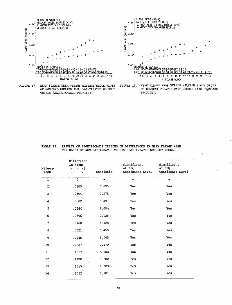
FLAN

GE W

EARf

INCH

ES)

0.40-FLANGE WEAR(MEAN)WROUGHT WHEEL SAMPLES(X1=0) □=UNTREATED WHEELS(X3=0) A=TREATED WHEELS(X3=1)

0.30-

FLANGE WEAR (MEAN)CAST WHEEL SAMPLES(X1=1)□ =NON HEAT TREATED WHEELS(X3=0) A =HEAT TREATED WHEELS(X3=1)

O □0 . 20-

0 . 10-

(NUMBER OF SAMPLES)X3=0 $ 4 ) (18) (48) 4) (47) (48) ft8) (43 (40) (IE) (13) (10)X3=l (38) m m SO) ft8) (45) S8) (42) 64) ftO) (391 (261 (241 (13 (14) (3

i 2 3 4 5 6 7 8 9 10 11 12 13 14 15 16 17 18MILEAGE BLOCK

0 . 20-

o.io-

0.00-(NUMBER OF SAMPLES)X3=0 (50) (70) (63 69) (63 63fc3(55)(4d) (2363X3=l (43 63 (53 63 33 60) (54) 66) 63 (33 do) (24 (23 0.4) (4) (4 H 2 )

1 2 3 4 5 6 7 8 9 10 11 12 13 14 15 16 17 18- MILAGE BLOCK

FIGURE 17. MEAN FLANGE WEAR VERSUS MILEAGE BLOCK PLOTS OF NONHEAT-TREATED AND HEAT-TREATED WROUGHT WHEELS (AAR STANDARD PROFILE).

FIGURE 18. MEAN FLANGE WEAR VERSUS MILEAGE BLOCK PLOTS OF NONHEAT-TREATED CAST WHEELS (AAR STANDARD PROFILE).

TABLE 12. RESULTS OF SIGNIFICANCE TESTING ON DIFFERENCES IN MEAN FLANGE WEAR PER BLOCK ON NONHEAT-TREATED VERSUS HEAT-TREATED WROUGHT WHEELS

MileageBlock

Difference in Means (x - x)1 2

tStatistic

Significant at 95%Confidence Level

Significant at 99%Confidence Level

1 0 - -

2 .0285 3.695 Yes Yes

3 .0504 7.273 Yes Yes

4 .0502 6.491 Yes Yes

5 .0444 6.094 Yes Yes

6 .0605 7.135 Yes Yes

7 .0488 5.428 Yes Yes

8 .0621 6.450 Yes Yes

9 .0646 6.148 Yes Yes

10 .0837 7.470 Yes Yes

11 .1027 8.682 Yes Yes

12 .1178 9.202 Yes Yes

13 .1315 6.289 Yes Yes

14 .1082 5.281 Yes Yes

187

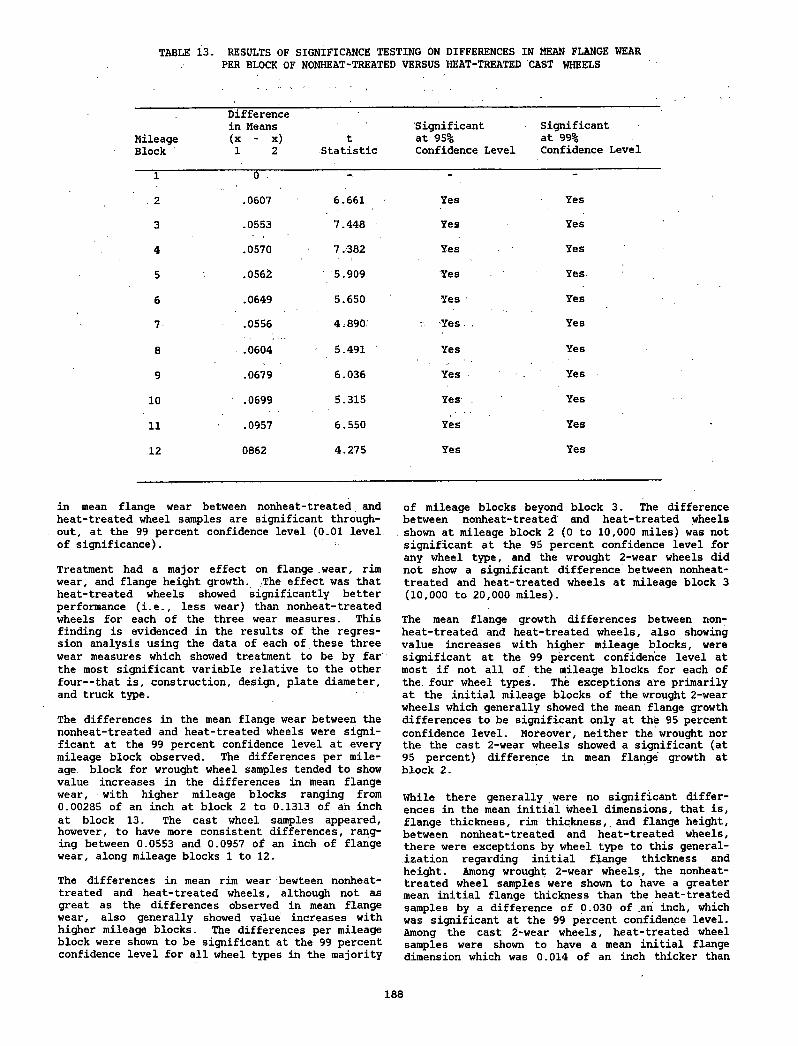
TABLE 13. RESULTS OF SIGNIFICANCE TESTING ON DIFFERENCES IN MEAN FLANGE WEAR PER BLOCK OF NONHEAT-TREATED VERSUS HEAT-TREATED CAST WHEELS

MileageBlock

Difference in Means (x - x)1 2

tStatistic

Significant at 95%Confidence Level

Significant at 99%Confidence Level

1 0 . - “

2 .0607 6.661 Yes Yes

3 .0553 7.448 Yes Yes

4 .0570 7 . 382 Yes Yes

5 .0562 5.909 Yes Yes

6 .0649 5.650 Yes Yes

7 .0556 4.890 Yes . . Yes

8 .0604 5.491 Yes Yes

9 .0679 6.036 Yes . Yes

10 .0699 5.315 Yes . Yes

11 .0957 6.550 Yes Yes

12 0862 4.275 Yes Yes

in mean flange wear between nonheat-treated and heat-treated wheel samples are significant through­out, at the 99 percent confidence level (0.01 level of significance).

Treatment had a major effect on flange .wear, rim wear, and flange height growth. The effect was that heat-treated wheels showed significantly better performance (i.e., less wear) than nonheat-treated wheels for each of the three wear measures. This finding is evidenced in the results of the regres­sion analysis using the data of each of these three wear measures which showed treatment to be by far' the most significant variable relative to the other four— that is, construction, design, plate diameter, and truck type.

The differences in the mean flange wear between the nonheat-treated and heat-treated wheels were signi­ficant at the 99 percent confidence level at every mileage block observed. The differences per mile­age block for wrought wheel samples tended to show value increases in the differences in mean flange wear, with higher mileage blocks ranging from 0.00285 of an inch at block 2 to 0.1313 of an inch at block 13. The cast wheel samples appeared, however, to have more consistent differences, rang­ing between 0.0553 and 0.0957 of an inch of flange wear, along mileage blocks 1 to 12.

The differences in mean rim wear bewteen nonheat- treated and heat-treated wheels, although not as great as the differences observed in mean flange wear, also generally showed value increases with higher mileage blocks. The differences per mileage block were shown to be significant at the 99 percent confidence level for all wheel types in the majority

of mileage blocks beyond block 3. The difference between nonheat-treated and heat-treated wheels shown at mileage block 2 (0 to 10,000 miles) was not significant at the 95 percent confidence level for any wheel type, and the wrought 2-wear wheels did not show a significant difference between nonheat- treated and heat-treated wheels at mileage block 3 (10,000 to 20,000 miles).

The mean flange growth differences between non­heat-treated and heat-treated wheels, also showing value increases with higher mileage blocks, were significant at the 99 percent confidence level at most if not all of the mileage blocks for each of the. four wheel types. The exceptions are primarily at the initial mileage blocks of the wrought 2-wear wheels which generally showed the mean flange growth differences to be significant only at the 95 percent confidence level. Moreover, neither the wrought nor the the cast 2-wear wheels showed a significant (at 95 percent) difference in mean flange growth at block 2.

While there generally were no significant differ­ences in the mean initial wheel dimensions, that is, flange thickness, rim thickness,, and flange height, between nonheat-treated and heat-treated wheels, there were exceptions by wheel type to this general­ization regarding initial flange thickness and height. Among wrought 2-wear wheels, the nonheat- treated wheel samples were shown to have a greater mean initial flange thickness than the heat-treated samples by a difference of 0.030 of an inch, which was significant at the 99 percent confidence level. Among the cast 2-wear wheels, heat-treated wheel samples were shown to have a mean initial flange dimension which was 0.014 of an inch thicker than

188

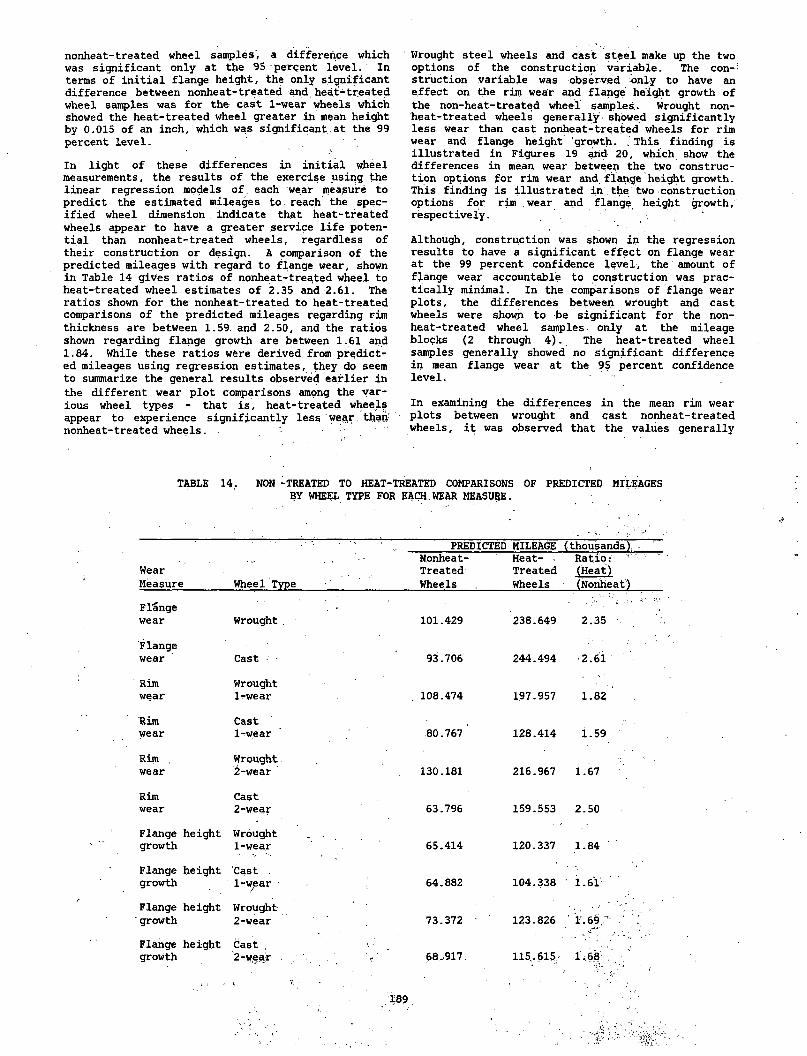
nonheat-treated wheel samples’, a difference which was significant only at the 95 percent level. In terms of initial flange height, the only significant difference between nonheat-treated and heat-treated wheel samples was for the cast 1-wear wheels which showed the heat-treated wheel greater in mean height by 0.015 of an inch, which was significant at the 99 percent level.

In light of these differences in initial wheel measurements, the results of the exercise using the linear regression models of each wear measure to predict the estimated mileages to reach the spec­ified wheel dimension indicate that heat-treated wheels appear to have a greater service life poten­tial than nonheat-^ treated wheels, regardless of their construction or design. A comparison of the predicted mileages with regard to flange wear, shown in Table 14 gives ratios of nonheat-treated wheel to heat-treated wheel estimates of 2.35 and 2.61. The ratios shown for the nonheat-treated to heat-treated comparisons of the predicted mileages regarding rim thickness are between 1.59 and 2.50, and the ratios shown regarding flange growth are between 1.61 and 1.84. While these ratios were derived from predict­ed mileages using regression estimates, they do seem to summarize the general results observed earlier in the different wear plot comparisons among the var­ious wheel types - that is, heat-treated wheels appear to experience significantly less wear than nonheat-treated wheels.

Wrought steel wheels and cast steel make up the two options of the construction variable. The con-; struction variable was observed only to have an effect on the rim wear and flange height growth of the non-heat-treated wheel samples.. Wrought non­heat-treated wheels generally showed significantly less wear than cast nonheat-treated wheels for rim wear and flange height growth. . This finding is illustrated in Figures 19 and 20, which show the differences in mean wear between the two construc­tion options for rim wear and flange height growth. This finding is illustrated in the two construction options for rim wear and flange height growth, respectively.

Although, construction was shown in the regression results to have a significant effect on flange wear at the 99 percent confidence level, the amount of flange wear accountable to construction was prac­tically minimal. In the comparisons of flange wear plots, the differences between wrought and cast wheels were shown to be significant for the non- heat-treated wheel samples only at the mileage blocks (2 through 4). The heat-treated wheel samples generally showed no significant difference in mean flange wear at the 95 percent confidence level.

In examining the differences in the mean rim wear plots between wrought and cast nonheat-treated wheels, it was observed that the values generally

TABLE 14. NON -TREATED TO HEAT-TREATED COMPARISONS OF PREDICTED MILEAGES BY WHEEL TYPE FOR EACH WEAR MEASUBE.

WearMeasure Wheel Type

PREDICTEDNonheat-TreatedWheels

MILEAGEHeat-TreatedWheels

(thousands).Ratio:(Heat)(Noriheat)

F l'ange ' . V V ’':.'. *•wear Wrought . 101.429 238.649 2.35

Flangewear Cast 93.706 244.494 2.61

Rim Wroughtwear l^wear 108.474 197.957 1.82

Rim Castwear 1-wear .80.767 128.414 1.59

Rim . Wroughtwear 2-wear 130.181 216.967 1.67

Rim Castwear 2-wear 63.796 159.553 2.50

Flange height Wrought . .growth 1-wear 65.414 120.337 1.84

Flange height Castgrowth 1-wpar 64.882 104.338 1.61

Flange height Wroughtgrowth 2-wear 73.372 123.826 ' 1.69 /

Flange height Cast ,growth 2-wear 68.917 115.615 1.68

189

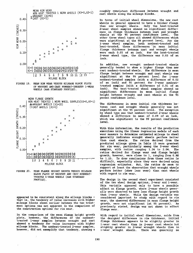
MILAGE BLOCK

FIGURE 19. MEAN RIM WEAR VERSUS MILEAGE BLOCK PLOTSOF WROUGHT AND CAST NONHEAT-TREATED 1-WEAR WHEELS (AAR STANDARD PROFILE).

MEAN FLANGE GROWTHNON HEAT TREATED 1 WEAR WHEEL SAMPLES(X3=0,X2=1)

„ A WROUGHT WHEELS (Xl=10)_ 0-40' □ CAST WHEELS (Xl=l)m □o~ 0.30-

S 0.20-

0 . 10-

CDZ<0 . 00 - 6

X1=0 &2) £30) (32) (325 (36) (32) (30) (24) (IE)Xl =l GO) G2) (36) (33 (33) (34) (24) (23) (20) (8 )-----------r =r i— i------1 ■ r ~ ^---------1------- 1------- :------- i------- 1—

12 3 4 5 6 7 8 9 10 11T

MILEAGE BLOCK

FIGURE 20. MEAN FLANGE HEIGHT GROWTH VERSUS MILEAGE BLOCK PLOTS OF WROUGHT AND CAST NONHEAT- TREATED 1-WEAR WHEELS (AAR STANDARD PROFILE).

appeared to be consistent along the mileage blocks - that is, the tendency of value increases with higher mileage blocks shown earlier between the two treat­ment options was not apparent in the comparison of the construction options for rim wear.

roughly consistent difference between wrought and cast wheels along the mileage blocks.

In terms of initial wheel dimensions, the new cast wheels in general appeared to have a thicker flange than new wrought wheels. Only the heat-treated 2-wear wheel samples showed no significant differ­ence in flange thickness between cast and wrought wheels at the 95 percent confidence level. The other three wheel types all showed differences which were significant at the 99 percent level. For the1- wear wheel samples, both nonheat-treated and heat-treated, these differences in mean initial flange thickness between cast and wrought wheels were each 0.05 of an inch. For the heat-treated2- wear wheel type, the difference was 0.03 of an inch.

In addition, new wrought nonheat-treated wheels generally tended to show a higher flange than new cast nonheat-treated wheels. The difference in mean flange height between wrought and cast wheels was significant at the 99 percent level for 1-wear nonheat-treated samples (with a difference of 0.02 of an inch) and 95 percent for 2-wear nonheat- treated samples (with a difference of 0.01 of an inch). The heat-treated wheel samples showed no significant differences in mean initial flange height between wrought and cast wheels at the 95 pecent confidence level.

The differences in mean initial rim thickness be­tween cast and wrought wheels generally was not significant at the 95 percent level. The exception by wheel type was that nonheat-treated 2-wear wheels showed a difference in mean of 0.09 of an inch, which was significant to the 99 percent confidence level.

With this information, the results of the prediction exercises using the linear regression models of each wear measure to determine estimated mileage to wheel generally indicates wrought wheels perform better than cast wheels. The ratios derived from the predicted mileage given in Table 15 were greatest for rim wear, particularly among the 2-wear wheel samples, with ratios ranging 1.34 to 2.04. The ratios derived for flange wear and flange height growth, however, were close to 1, ranging from 0.98 to 1.15. To draw conclusions from these ratios is difficult, especially since they were derived using regression estimates. But, the ratios do seem to support at least the observation that wrought wheels perform better (show less wear) than cast wheels with regard to rim wear.

The design in the second wheel experiment consisted of the two wheel design options, 2-wear and 1-wear. This variable appeared only to have a possible effect on flange growth, where 2-wear wheels gener­ally were observed to have less flange height growth than 1-wear wheels. While the design variable was considered important to study with regard to rim wear, the observed differences in mean flange height growth, were not significant (at 95 percent). As previously stated, design was not shown to effect flange wear.

In the comparison of the mean flange height growth plots, however, the differences of the nonheat- treated 1-wear samples between wrought and cast showed a tendency for value increases with higher mileage blocks. The nonheat-treated 2-wear samples, however, did not exemplify that tendency, showing a

With regard to initial wheel dimensions, aside from the designed difference in rim thickness, initial flange thickness•appears to be slightly greater in 1-wear cast wheels than in 2-wear cast wheels but slightly greater in 2-wear wrought wheels than in 1-wear wrought wheels. There was generally no

190

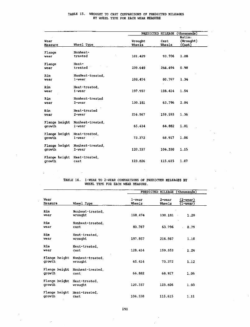
TABLE 15. WROUGHT TO CAST COMPARISONS OF PREDICTED MILEAGES BY WHEEL TYPE FOR EACH WEAR MEASURE

PREDICTED MILEAGE (thousands)

WearMeasure Wheel Type

WroughtWheels

CastWheels

Ratio:(Wrought)(Cast)

Flangewear

Nonheat-treated 101.429 93.706 1.08

Flangewear

Heat-treated 239.649 244.494 0.98

Rimwear

NonHeat-treated, 1-wear 108.474 80.767 1.34

Rimwear

Heat-treated,1-wear 197.957 128.414 1.54

Rimwear

Nonheat-treated2-wear 130.181 63.796 2.04

Rimwear

Heat-treated2-wear 216.967 159.553 1.36

Flange height growth

Nonheat-treated, 1-wear 65.414 64.882 1.01

Flange height growth

Heat-treated,1-wear 73.372 68.917 1.06

Flange height growth

Nonheat-treated, 2-wear 120.337 104.338 1.15

Flange height growth

Heat-treated,cast 123.826 115.615 1.07

TABLE 16. 1-WEAR TO WHEEL TYPE

2-WEAR COMPARISONS OF PREDICTED MILEAGES BY FOR EACH WEAR MEASURE.

PREDICTED MILEAGE (thousands)

WearMeasure Wheel Type

1-wearWheels

2-wearWheels

(2-wear)(1-wear)

Rimwear

Nonheat-treated, wrought 108.474 130.181 1.20

Rimwear

Nonheat-treated, cast 80.767 63.796 0.79

Rimwear

Heat-treated,wrought 197.957 216.967 1.10

Rimwear

Heat-treated,cast 128.414 159.553 1.24

Flange height growth

Nonheat-treated, wrought 65.414 73.372 1.12

Flange height growth

Nonheat-treated, cast 64.882 68.917 1.06

Flange height growth

Heat-treated,wrought 120.337 123.826 1.03

Flange height growth

Heat-treated,cast 104.338 115.615 1.11

191

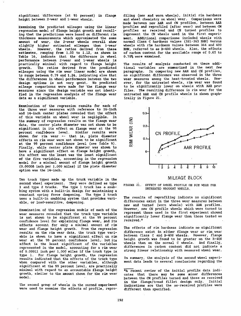
significant "difference (at 95 percent) in flange height between 2-wear and 1-wear wheels.

Examining the predicted mileages using the linear regression model of flange height growth and recall­ing that the predictions were based on different rim thickness measurements which approximated the same amount of wear, the 2-wear wheels overall show slightly higher estimated mileages than 1-wear wheels. However, the ratios derived from theseestimates, ranging from 1.03 to 1.12, as shown in Table 16, indicate that the difference in wheel performance between 2-wear and 1-wear wheels is practically minimal with regard to flange height growth. The ratios derived from the predictedmileages using the rim wear linear model are shown to range between 0.79 and 1.24, indicating also that the differences in wheel performance between the two design options is not very great. No predicted mileage comparisons were made for the flange wear measures since the design variable was not identi­fied in the regression analysis of the flange wear data as a significant variable.

Examination of the regression results for each of the three wear measures with reference to 16-inch and 14-inch center plates revealed that the effect of this variable on wheel wear is negligible. In the summary of regression results on the flange wear data, the center plate diameter Was not shown to be significant in its effect on flange wear at the 99 percent confidence level. Similar results were shown for rim wear — that is, plate diameter effects on rim wear were not shown to be significant at the 99 percent confidence level (see Table 9). Finally, while center plate diameter was shown to have a significant effect on flange height growth, its effect was the least was the least significant of the five variables, accounting in the regression model for a minimal amount of flange height growth (0.00008 inch per 1,000 miles) if the plate diameter option was the 14-inch.

Two truck types made up the truck variable in the second wheel experiment. They were defined as type 1 and type 2 trucks. The type 1 truck has a snub­bing system with a built-in design for maintaining a constant spring force dampening. The type 2 truck uses a built-in snubbing system that provides vari­able, or load-sensitive, dampening.

Examination of the regression models of each of the wear measures revealed that the truck type variable is not shown to be significant at the 99 percent confidence level for explaining flange wear, and its effects account for only a minimal amount of rim wear and flange height growth. From the regression results on the rim wear data, the truck type vari­able is shown to have a significant effect on rim wear at the 99 percent confidence level,, but its effect is the least significant of the variables represented in the model, accounting for a rim wear of 0.00011 inch per 1,000 miles if the truck type is type 1. For flange height growth, the regression results indicated that the effects of the truck type when compared with the other variables, although significant at the 99 percent level, are practically minimal with regard to an accountable flange height growth, similar to the amount shown for the rim wear model.

The second group of wheels in the second experiment were used to examine the effects of profile, repro­

filing (new and worn wheels), initial rim hardness and wheel chemistry on wheel wear. Comparisons were made between new AAR and CN profiles., between AAR ^profiles and reprofiled (after wear) and between CN profiles as received and CN turned profiles to represent the CN wheels used in the first experi­ment. Additional comparisons included wheels with normal Class C hardness values (321-363 BHN) versus wheels with rim hardness values between 364 and 400 BHN, referred to as B-400 wheels. Also, the effects of carbon content for the available range of 0.65 to 0.78% were examined.

The results of analysis conducted on these addi­tional variables are summarized in the next few paragraphs. In comparing new AAR and CN profiles, no significant difference- was observed in the three wear measures among the heat-treated wheels. How­ever, for the untreated wheels, rim wear was found to be significantly lower on wheels with AAR pro­files. The resulting difference in rim wear for the untreated AAR and CN profile wheels is shown graph­ically in Figure 21.

FIGURE 21. EFFECT OF WHEEL PROFILE ON RIM WEAR FOR UNTREATED WROUGHT WHEELS.

The results of reprofiling indicate no significant differences exist in the three wear measures between new and turned (worn wheels) with AAR profiles. However, new CN profile wheels which were turned to represent those used in the first experiment showed significantly lower flange wear than those tested as received.*

The effects of rim hardness indicate no significant difference exist in either flange wear or rim wear between Class C and B-400 wheels. However, flange height growth was found to be greater on the B-400 wheels than on the normal C wheels. And finally, differences in carbon content did not indicate a strong linear relationship with measured wheel wear.

In summary, the analysis of the second wheel experi­ment data leads to several conclusions regarding the

*A recent review of the initial profile data indi­cates that there may be some minor differences between the CN profiles turned and those as received in the flange/tread fillet design only. Initial indications are that the as-received profiles were different than specified.

192

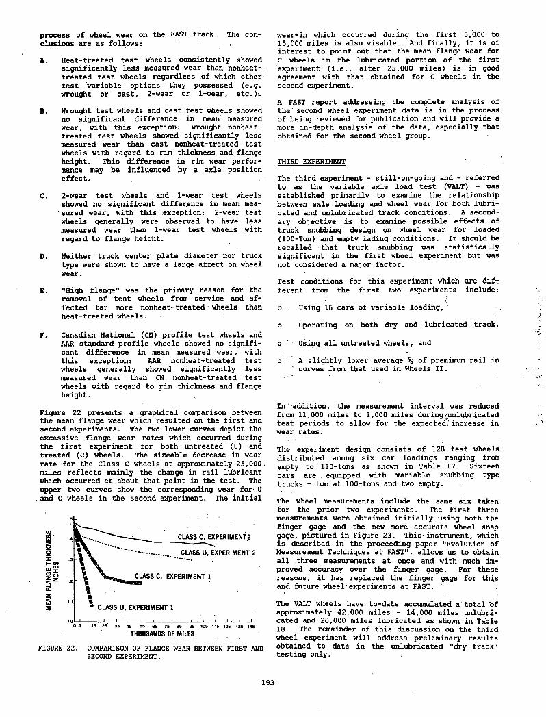
process of wheel wear on the FAST track. The con­clusions are as follows:

A. Heat-treated test wheels consistently showed significantly less measured wear than nonheat- treated test wheels regardless of which other- test "variable options they possessed (e.g. wrought or cast, 2-wear or 1-wear, etc.).

B. Wrought test wheels and cast test wheels showedno significant difference in mean measured wear, with this exception: wrought nonheat-treated test wheels showed significantly less measured wear than cast nonheat-treated test wheels with regard to rim thickness and flange height. This difference in rim wear perfor­mance may be influenced by a axle position effect.

C. 2-wear test wheels and 1-wear test wheelsshowed no significant difference in-mean mea­sured wear, with this exception: 2-wear testwheels generally were observed to have less measured wear than 1-wear test wheels with regard to flange height.

D. Neither truck center plate diameter nor truck type were shown to have a large affect on wheel wear.

E. "High flange" was the primary reason for.the removal of test wheels from service and af­fected far more nonheat-treated wheels than heat-treated wheels.

F. Canadian National (CN) profile test wheels andAAR standard profile wheels showed no signifi­cant difference in mean measured wear, with this exception: AAR nonheat-treated testwheels generally showed significantly less measured wear than CN nonheat-treated test wheels with regard to rim thickness and flange height.

Figure 22 presents a graphical comparison between the mean flange wear which resulted on the first and second experiments. The two lower curves depict the excessive flange wear rates which occurred during the first experiment for both untreated (U) and treated (C) wheels. The sizeable decrease in wear rate for the Class C wheels at approximately 25,000. miles reflects mainly the change in rail lubricant which occurred at about that point in the test. The upper two curves show the corresponding wear for' U and C wheels in the second experiment. The initial

FIGURE 22. COMPARISON OF FLANGE WEAR BETWEEN FIRST AND SECOND EXPERIMENT.

wear-in which occurred during the first 5,000 to 15,000 miles is also visable. And finally, it is of interest to point out that the mean flange wear for C wheels in the lubricated portion of the first experiment, (i.e., after 25,000 miles) is in good agreement- with that obtained for C wheels in the second experiment.

A FAST report addressing the complete analysis of the second wheel experiment data is in the process, of being reviewed for publication and will provide a more in-depth analysis of the data, especially that obtained for the second wheel group.

THIRD EXPERIMENT

The third experiment - still-on-going and - referred to as the variable axle load test (VALT) - was established primarily to examine the relationship between axle loading and wheel wear for both lubri­cated and . unlubricated track conditions. A second­ary objective is to examine possible effects of truck snubbing design on wheel wear for loaded (100-Ton) and empty lading conditions. It should be recalled that truck snubbing was statistically significant in the first wheel experiment but was not considered a major factor.

Test conditions for this experiment which are dif­ferent from the first two experiments include:

o - Using 16 cars of variable loading,'

o Operating ■ on both dry and lubricated track,

o ’ Using all untreated wheels, and

o A slightly lower average % of premimum rail in curves from that used in Wheels II.

I n ' addition, the measurement interval- was reduced from 11,000 miles to 1,000 miles duringjunlubricated test periods to allow for the expected,'increase in wear rates.

The experiment design consists of 128 test wheels distributed among six car loadings ranging from empty to 110-tons as shown in Table 17. Sixteen cars are . equipped with variable snubbing type trucks - two at 100-tons and two empty.

The wheel measurements include the same six taken for the prior two experiments. The first three measurements were obtained initially using both the finger gage and the new more accurate wheel snap gage, pictured in Figure 23. This-instrument, which is described in the proceeding paper "Evolution of Measurement Techniques at FAST", allows.us to obtain all three measurements at once and with much im­proved accuracy over the finger gage. For these reasons, it has replaced the finger gage for this and future wheel experiments at FAST.

The VALT wheels have to-date accumulated a total of approximately 42,000 miles - 14,000 miles unlubri­cated and 28,000 miles lubricated as shown in Table 18. The remainder of this discussion on the third wheel experiment will address preliminary results obtained to date in the unlubricated "dry track" testing only.

193

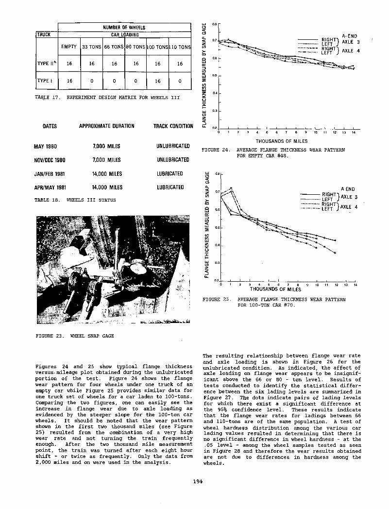
NUMBER OF WHEELS

TRUCK CAR LOADING

TYPE II*

EMPTY 33 TONS 66 TONS 80 TONS LOO TONS 110 TON S

16 16 16 16 16 16

TYPE 1 16 0 0 0 16 0

TABLE 17. EXPERIMENT DESIGN MATRIX FOR WHEELS III

DATES APPROXIMATE DURATION TRACK CONDITION

MAY 1980 7 .000 MILES

NOV/DEC 1980 7 .000 MILES

UNLUBRICATED

UNLUBRICATED

T H O U S A N D S OF MILES

FIGURE 24. AVERAGE FLANGE THICKNESS WEAR PATTERN FOR EMPTY CAR #48.

JAN/FEB 1981 14.000 MILES

APR/MAY 1981 14 .000 MILES

TABLE 18. WHEELS III STATUS

LUBRICATED

LUBRICATED

FIGURE 25. AVERAGE FLANGE THICKNESS WEAR PATTERN FOR lOO-TON CAR #70.

FIGURE 23. WHEEL SNAP GAGE

Figures 24 and 25 show typical flange thickness Versus, mileage plot obtained during the unlubricated portion of the test. Figure 24 shows the flange wear pattern for four wheels under one truck of an empty car while Figure 25 provides similar data for one truck set of wheels for a car laden to 100-tons. Comparing the two figures, one can easily see the increase in flange wear due to axle loading as evidenced by the steeper slope for the 100-ton car wheels. It should be noted that the wear pattern shown in the first two thousand miles (see Figure 25) resulted from the combination of a very high wear rate and not turning the train frequently enough. After the two thousand mile measurement point, the train was turned after each eight hour shift - or twice as frequently. Only the data from 2,000 miles and on were used in the analysis.

The resulting relationship between flange wear rate and axle loading is shown in Figure 26 for the unlubricated condition. As indicated, the affect of axle loading on flange wear appears to be insignif­icant above the 66 or 80 - ton level. Results of tests conducted to identify the statistical differ­ence between the six lading levels are summarized in Figure 27. The dots indicate pairs of lading levels for which there exist a significant difference at the 95% confidence level. These results indicate that the flange wear rates for ladings between 66 and 110-tons are of the same population. A test of wheel hardness distribution among the various car lading values resulted in determining that there is no significant difference in wheel hardness - at the .05 level - among the wheel samples tested as seen in Figure 28 and therefore the wear results obtained are not due to differences in hardness among the wheels.

194

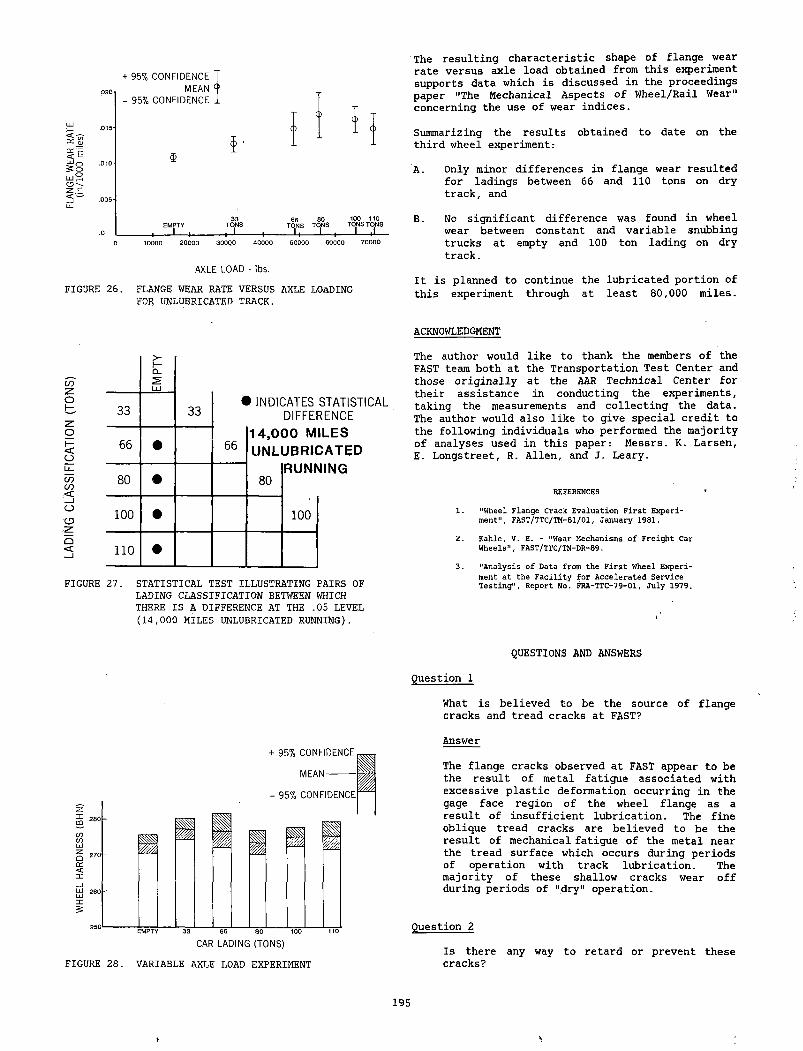
.020'

+ 95% C O N FID E N C E M EAN °

- 95% C O N FID E N C E . .

z.E < —

.015-

.0 1 0

.0 0 5 '

$

The resulting characteristic shape of flange wear rate versus axle load obtained from this experiment supports data which is discussed in the proceedings paper "The Mechanical Aspects of Wheel/Rail Wear" concerning the use of wear indices.

Summarizing the results obtained to date on the third wheel experiment:

A. Only minor differences in flange wear resulted for ladings between 66 and 110 tons on dry track, and

3 3 66 8 0 100 110EMPTY TONS TONS TONS TONS TONS

.0 ____________, I |____________, _ l _________ ,__________ I | I____ I______ I____ J ___

0 1 0 00 0 2 0 0 0 0 3 0 0 0 0 4 0 0 0 0 5 0 0 0 0 6 0 0 0 0 7 0 0 0 0

AXLE LOAD ■ lbs.

FIGURE 26. FLANGE WEAR RATE VERSUS AXLE LOADING FOR UNLUBRICATED TRACK.

B. No significant difference was found in wheel wear between constant and variable snubbing trucks at empty and 100 ton lading on dry track.

It is planned to continue the lubricated portion of this experiment through at least 80,000 miles.

cnz ----------ot 33

EMPT

Y

3 3• INDICATES STATISTICAL

DIFFERENCEo£ 66 o

• 6614 ,0 00 MILES UNLUBRICATED

1 so«rT• 80

RUNNING

o 100 • 100

Q< 110 •

FIGURE 27. STATISTICAL TEST ILLUSTRATING PAIRS OF LADING CLASSIFICATION BETWEEN WHICH THERE IS A DIFFERENCE AT THE .05 LEVEL (14,000 MILES UNLUBRICATED RUNNING).

ACKNOWLEDGMENT

The author would like to thank the members of the FAST team both at the Transportation Test Center and those originally at the AAR Technical Center for their assistance in conducting the experiments, taking the measurements and collecting the data. The author would also like to give special credit to the following individuals who performed the majority of analyses used in this paper: Messrs. K. Larsen,E. Longstreet, R. Allen, and J. Leary.

REFERENCES

1 . "Wheel Flange Crack E v a lu ation F ir s t E x p eri­m ent", FAST/TTC/TM-81/01, January 1981.

2 . K ahle, V. E. - "Wear Mechanisms o f F re ig h t Car W heels", FAST/TTC/TN-DR-89.

3 . "A n a ly s is o f Data from the F ir s t Wheel E x p eri­ment a t the F a c i l i t y f o r A cce le ra te d S erv ice T e s t in g " , Report No. FRA-TTC-79-01, J u ly 1979.

+ 95% CONFIDENCE

M E A N ------------

- 95% CO NFIDENCE

FIGURE 28. VARIABLE AXLE LOAD EXPERIMENT

QUESTIONS AND ANSWERS

Question 1

What is believed to be the source of flange cracks and tread cracks at FAST?

Answer

The flange cracks observed at FAST appear to be the result of metal fatigue associated with excessive plastic deformation occurring in the gage face region of the wheel flange as a result of insufficient lubrication. The fine oblique tread cracks are believed to be the result of mechanical fatigue of the metal near the tread surface which occurs during periods of operation with track lubrication. The majority of these shallow cracks wear off during periods of "dry" operation.

Question 2

Is there any way to retard or prevent these cracks?

195

v

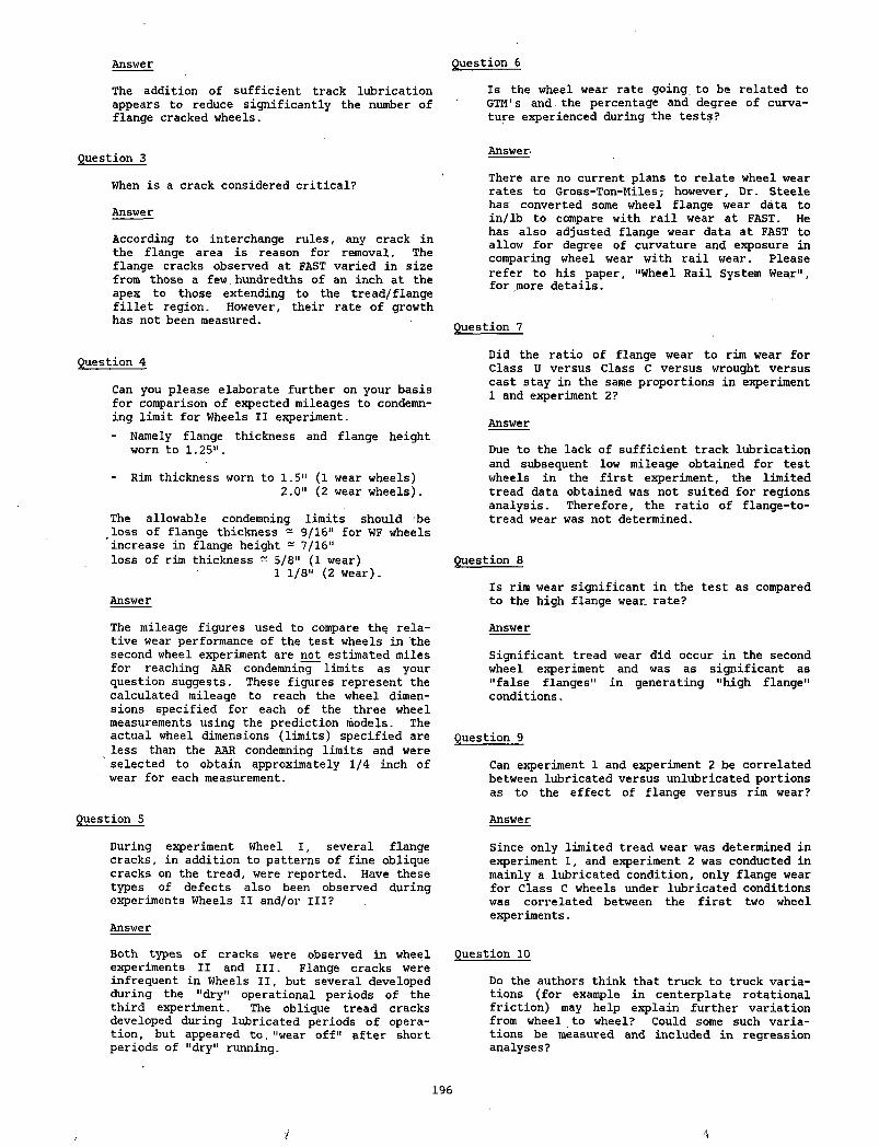
The addition of sufficient track lubrication appears to reduce significantly the number of flange cracked wheels.

Question 3

When is a crack considered critical?

Answer

According to interchange rules, any crack in the flange area is reason for removal. The flange cracks observed at FAST varied in size from those a few. hundredths of an inch at the apex to those extending to the tread/flange fillet region. However, their rate of growth has not been measured.

Answer

Question 4

Can you please elaborate further on your basis for comparison of expected mileages to condemn­ing limit for Wheels II experiment.- Namely flange thickness and flange height

worn to 1.25“.

- Rim thickness worn to 1.5" (1 wear wheels)2.0" (2 wear wheels).

The allowable condemning limits should be loss of flange thickness - 9/16" for WF wheels increase in flange height - 7/16" loss of rim thickness - 5/8" (1 wear)

1 1/8" (2 wear).

Answer

The mileage figures used to compare the rela­tive wear performance of the test wheels in the second wheel experiment are not estimated miles for reaching AAR condemning limits as your question suggests. These figures represent the calculated mileage to reach the wheel dimen­sions specified for each of the three wheel measurements using the prediction models. The actual wheel dimensions (limits) specified are less than the AAR condemning limits and were selected to obtain approximately 1/4 inch of wear for each measurement.

Question 5

During experiment Wheel I, several flange cracks, in addition to patterns of fine oblique cracks on the tread, were reported. Have these types of defects also been observed during experiments Wheels II and/or III?

Answer

Both types of cracks were observed in wheel experiments II and III. Flange cracks were infrequent in Wheels II, but several developed during the "dry" operational periods of the third experiment. The oblique tread cracksdeveloped during lubricated periods of opera­tion, but appeared to, "wear off" after short periods of "dry" running.

Is the wheel wear rate going to be related to GTM's and. the percentage and degree of curva­ture experienced during the tests?

Answer-

There are no current plans to relate wheel wear rates to Gross-Ton-Miles; however. Dr. Steele has converted some wheel flange wear data to in/lb to compare with rail wear at FAST. He has also adjusted flange wear data at FAST to allow for degree of curvature and exposure in comparing wheel wear with rail wear. Please refer to his paper, "Wheel Rail System Wear", for more details.

Question 6

Question 7

Did the ratio of flange wear to rim wear for Class U versus Class C versus wrought versus cast stay in the same proportions in experiment 1 and experiment 2?

Answer

Due to the lack of sufficient track lubrication and subsequent low mileage obtained for test wheels in the first experiment, the limited tread data obtained was not suited for regions analysis. Therefore, the ratio of flange-to- tread wear was not determined.

Question 8

Is rim wear significant in the test as compared to the high flange wear, rate?

Answer

Significant tread wear did occur in the second wheel experiment and was as significant as "false flanges" in generating "high flange" conditions.

Question 9

Can experiment 1 and experiment 2 be correlated between lubricated versus unlubricated portions as to the effect of flange versus rim wear?

Answer

Since only limited tread wear was determined in experiment 1, and experiment 2 was conducted in mainly a lubricated condition, only flange wear for Class C wheels under lubricated conditions was correlated between the first two wheel experiments.

Question 10

Do the authors think that truck to truck varia­tions (for example in centerplate rotational friction) may help explain further variation from wheel to wheel? Could some such varia­tions be measured and included in regression analyses?

196

/

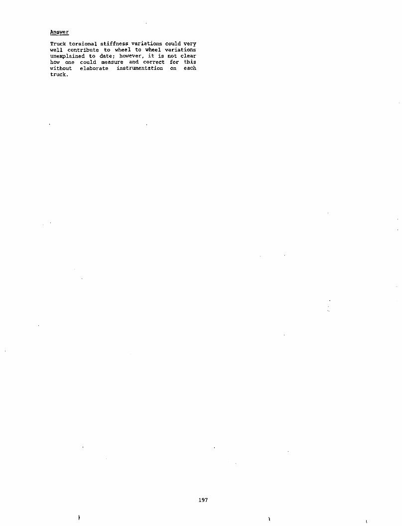
AnswerTruck torsional stiffness variations could very well contribute to wheel to wheel variations unexplained to date; however, it is not clear how one could measure and correct for this without elaborate instrumentation on each truck.

197

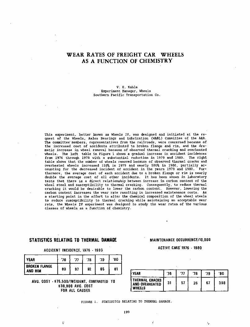
WEAR RATES OF FREIGHT CAR WHEELS AS A FUNCTION OF CHEMISTRY

V. E. KahleExperiment Manager, Wheels

Southern Pacific Transportation Co.

This experiment, better known as Wheels IV, was designed and initiated at the re­quest of the Wheels, Axles Bearings and Lubrication (WABL) Committee of the AAR. The committee members, representatives from the railroads, were concerned because of the increased cost of accidents attributed to broken flange and rim, and the dra­matic increase in wheel removal because of observed thermal cracking and overheated wheels. The left table in Figure 1 shows a gradual increase in accident incidences from 1976 through 1978 with a substantial reduction in 1979 and 1980. The right table shows that the number of wheels removed because of observed thermal cracks and overheated wheels increased 158% in 1979 and nearly 500% in 1980, partially ac­counting for the decreased incident of accident in the years 1979 and 1980. Fur­thermore, the average cost of each accident due to a broken flange or rim is nearly double the average cost of all other incidents. It has been shown in laboratory tests that there is a direct relationship between increase in carbon content of the wheel steel and susceptibility to thermal cracking. Consequently, to reduce thermal cracking it would be desirable to lower the carbon content. However, lowering the carbon content increases the wear rate resulting in increased maintenance costs. As a starting point in the effort to alter the chemical composition of the wheel steels to reduce susceptibility to thermal cracking while maintaining an acceptable wear rate, the Wheels IV experiment was designed to study the wear rates of the various classes of wheels as a function of chemistry.

STATISTICS RELATING TO THERMAL DAMAGE

ACCIDENT INCIDENCE. 1976 - 1980

YEAR '76 77 78 79 ’80BROKEN FLANGE AND RIM 80 97 92 65 61

AVG. COST - $75.500/INCIDENT, CONTRASTED TO $38,900 AVG. COST

FOR ALL CAUSES

MAINTENANCE 0CCURRENCE/10.000

ACTIVE CARS' 1976 - 1980

YEAR 7 6 77 7 8 79 '80THERMAL CRACKS AND OVERHEATED WHEELS

31 57 26 67 398

FIGURE 1. STATISTICS RELATING TO THERMAL DAMAGE.

199

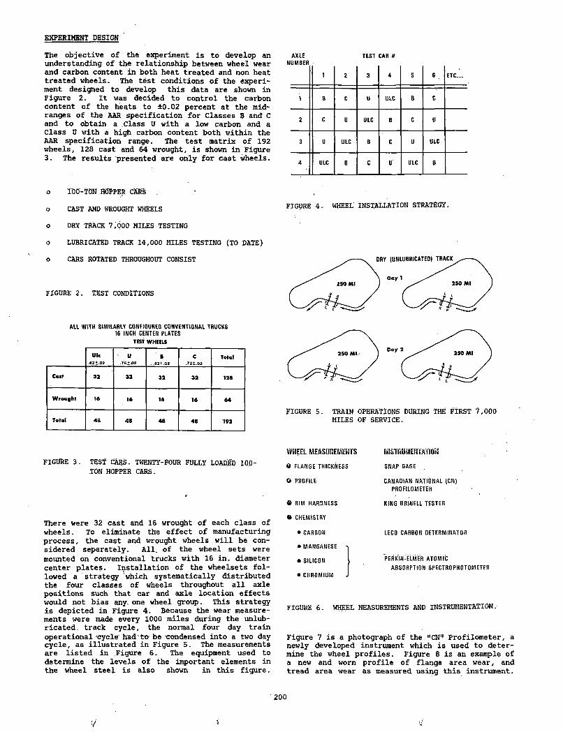
EXPERIMENT DESIGN

TEST CAR #The objective of the experiment is to develop an understanding of the relationship between wheel wear and carbon content in both heat treated and non heat treated wheels. The test conditions of the experi­ment designed to develop this data are shown in Figure 2. It was decided to control the carbon content of the heats to 10.02 percent at the mid­ranges of the AAR specification for Classes B and C and to obtain a Class U with a low carbon and a Class 0 with a high carbon content both within the AAR specification range. The test matrix of 192 wheels, 128 cast and 64 wrought, is shown in Figure3. The results presented are only for cast wheels.

AXLENUMBER

i 2 3 4 5 6 E TC ...,

1 B c U ULC B C

2 C U ULC B C U

3 u ULC B c U ULC

4 ULC B c u ULC B

o 100-TON HOPPER CARS

o CAST AND WROUGHT WHEELS

o DRY TRACK 7,000 MILES TESTING

o LUBRICATED TRACK 14,000 MILES TESTING (TO DATE)

o CARS ROTATED THROUGHOUT CONSIST

FIGURE 2. TEST CONDITIONS

ALL WITH SIMILARLY CONFIGURED CONVENTIONAL TRUCKS 16 INCH CENTER PLATES

TEST WHEELS

Ulc.621.02

U.751.02

B. .621.02

C.721.02

Total

Cast 32 32 32 32 128

W ro ugh t 16 16 16 16 64

Total 48 48 48 48 192

FIGURE 4. WHEEL INSTALLATION STRATEGY.

FIGURE 5. TRAIN OPERATIONS DURING THE' FIRST 7,000 MILES OF SERVICE.

FIGURE 3. TEST CARS. TWENTY-FOUR FULLY LOADED 100- TON HOPPER CARS.

WHEEL MEASUREMENTS

O FLANGE THICKNESS

O PROFILE

© RIM HARDNESS

iN STRU K TATiO N

SNAP GAGE

CANADIAN NATIONAL |CN) PROFILOMETER

KING BRINELL TESTER

There were 32 cast and 16 wrought of each class of wheels. To eliminate the effect of manufacturing process, the cast and wrought wheels will be con­sidered separately. All. of the wheel sets were mounted on conventional trucks with 16 in. diameter center plates. Installation of the wheelsets fol­lowed a strategy which systematically distributed the four classes of wheels throughout all axle positions such that car and axle location effects would not bias any. one wheel group. This strategy is depicted in Figure 4. Because the wear measure­ments were made every 1000 miles during the unlub­ricated. track cycle, the normal four day train operational-cycle had^to-be-«>ndensed into a two day cycle, as illustrated in Figure 5. The measurements are listed in Figure 6. The equipment used to determine the levels of the important elements in the wheel steel is also shown. in this figure.

• CHEM ISTRY

• CARBON

• MANGANESE

• SILICON

• CHROMIUM

LECO CARBON DETERMINATOR

PERKIN ELMER ATOMIC

ABSORPTION SPECTROPHOTOMETER

FIGURE 6, WHEEL MEASUREMENTS AND INSTRUMENTATION.

Figure 7 is a photograph of the "CN" Profilometer, a newly developed instrument which is used to deter­mine the wheel profiles. Figure 8 is an example of a new and worn profile of flange area wear, and tread area wear as measured using this instrument.

200

* t/

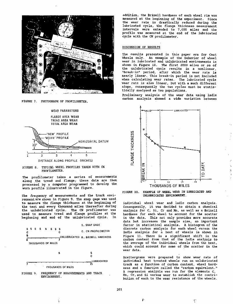
FIGURE 7. PHOTOGRAPH OF PROFILOMETER.

addition, the Brinell hardness of each wheel rim was measured at the beginning of the experiment. Since the wear rate is drastically reduced during the lubricated cycle, the flange thickness- measurement intervals were extended to 7,000 miles and the profile was measured at the end of the lubricated cycle with the CN profilometer.

DISCUSSION OF RESULTS

The results presented in this paper are for Cast Wheels only. An example of the behavior of wheel wear in lubricated and unlubricated environments is shown in Figure 10. The first 2000 miles or so of the unlubricated cycle results in a nonlinear, "break-in" period, after which the wear rate is nearly linear. This break-in period is not included when calculating wear rates. The lubricated cycle wear rate is also linear, but with a much different slope, consequently the. two cycles must be statis­tically analyzed as two populations.Preliminary analysis of the wear data using ladle carbon analysis showed a wide variation between

WEAR PARAMETERS

FLANGE AREA WEAR TREAD AREA WEAR TOTAL AREA WEAR

D ISTA N C E ALONG P RO FILE (INCHES)

FIGURE 8. TYPICAL WHEEL PROFILES TAKEN WITH CN PROFILOMETER.

The profilometer takes a series of measurements along the tread and flange; these data are then processed by a computer programmed to develop the worn profile illustrated in the figure.

The frequency of measurements and the track envi­ronment are shown in Figure 9. The snap gage was used to measure the flange thickness at the beginning of the test and every thousand miles thereafter during the unlubricated cycle. The CN profilometer was used to measure tread and flange profiles at the beginning and end of the unlubricated cycle. In

S S S S cB

0 ' ' r

S S S S C

S.. SNAP GAGE

C.. CN PROFILOMETER

UNLUBRICATED B.. BRINELL HARDNESS

THOUSANDS OF MILES

7

FIGURE 9.

S Sc

, ................................................................... I I I R R I C A T E D21

1 THOUSANDS OF MILES

FREQUENCY OF MEASUREMENTS AND TRACK ENVIRONMENT.

FIGURE 10. EXAMPLE OF WHEEL WEAR IN LUBRICATED AND UNLUBRICATED ENVIRONMENT.

individual wheel wear and ladle carbon analysis. Consequently, it was decided to obtain a chemical analysis for C, Si, Cr and Mn, as well as a Brinell hardness for each wheel to account for the scatter in the data. This not only provides more accurate data but increases the sample size, an important factor in statistical analysis. A histogram of the discrete carbon analysis for each wheel versus the ladle analysis for a heat of wheels is shown in Figure 11. There is a significant shift in the carbon content from that of the ladle analysis to the average of the individual wheels from the heat, which could account for some of the scatter in the wear data.

Scattergrams were prepared to show wear rate of individual heat treated wheels run on unlubricated track as a function of carbon content, wheel hard­ness and a function called the "carbon equivalent." A regression analysis was run for the elements C, Mn, Cr, and Si versus wear to establish the contri­bution of each to the wear resistance of the wheels.

201

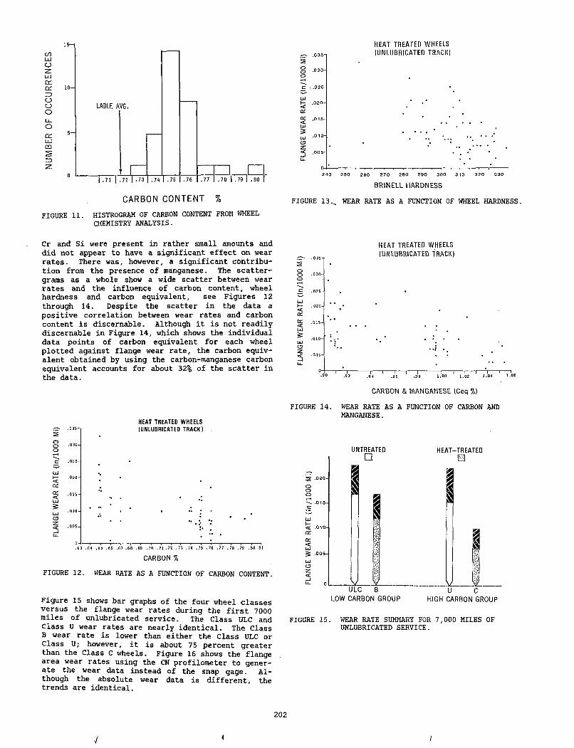
15—COL U

O

cnCdZDOoooCdL iJCD

ZD

CARBON CONTENT %

FIGURE 11. HISTROGRAM OF CARBON CONTENT FROM WHEEL CHEMISTRY ANALYSIS.

^ .0 3 5 "sg .0 3 0 -or-Hc • .0 2 5 -

<Cor

LU<3

. 0 2 0 -

.0 1 5 -

.010-

.0 0 5 -

HEAT TREATED W HEELS (U N LU B R IC A TE D TRACK)

o-l— .— .— .— ,— ,— ,— ,— ,— ,— ,— ,— .— .— i— .— i— ,— ,— 2 4 0 2 5 0 2 6 0 2 7 0 2 8 0 2 0 0 3 0 0 3 1 0 3 2 0 3 30

BRINELL HARDNESS

FIGURE 13., WEAR RATE AS A FUNCTION OF WHEEL HARDNESS.

Cr and Si were present in rather small amounts and did not appear to have a significant effect on wear rates. There was, however, a significant contribu­tion from the presence of manganese. The scatter- grams as a whole show a wide scatter between wear rates and the influence of carbon content, wheel hardness and carbon equivalent, see Figures 12 through 14. Despite the scatter in the data a positive correlation between wear rates and carbon content is discernable. Although it is not readily discernable in Figure 14, which shows the individual data points of carbon equivalent for each wheel plotted against flange wear rate, the carbon equiv­alent obtained by using the carbon-manganese carbon equivalent accounts for about 32% of the scatter in the data.

0 - -.90

HEAT TREATED W HEELS 1UNLUBRICATED TRACK)

1------ 1------ 1------ 1------1------1------ 1------ ! 1------1 1------1—94 .96 .98 1.00 1.02 1 .04 1.06

CARBON & MANGANESE (Ceq %)

O ' .035-is§ -030-o

c .025-

LU

<o:cd<

. 0 2 0 -

.01 5-

C3< .oos-

HEAT TREATED WHEELS (UNLUBRICATED TRACK)

U —I— ■[ | I I I ■■ [ ■ - I —1— I1 — 1 ■ 1— ].63 .64 .65 .66 .67 .68 .69 .70 .7 1 .7 2 .73 .74 .75 .76 .77 .78 .79 .80.81

CARBON %

FIGURE 12. WEAR RATE AS A FUNCTION OF CARBON CONTENT.

Figure 15 shows bar graphs of the four wheel classes versus the flange wear rates during the first 7000 miles of unlubricated service. The Class ULC and Class U wear rates are nearly identical. The Class B wear rate is lower than either the Class ULC or Class U; however, it is about 75 percent greater than the Class C wheels. Figure 16 shows the flange area wear rates using the CN profilometer to gener­ate the wear data instead of the snap gage. Al­though the absolute wear data is different, the trends are identical.

FIGURE 14. WEAR RATE AS A FUNCTION OF CARBON AND MANGANESE.

< .010- a• o:<LU5 .0 0 5 - LU

z<

UNTREATED□

v

1I

SLULC B

LOW CARBON GROUP

HEAT-TREATEDm

...vu c

HIGH CARBON GROUP

FIGURE 15. WEAR RATE SUMMARY FOR 7,000 MILES OF UNLUBRICATED SERVICE.

202

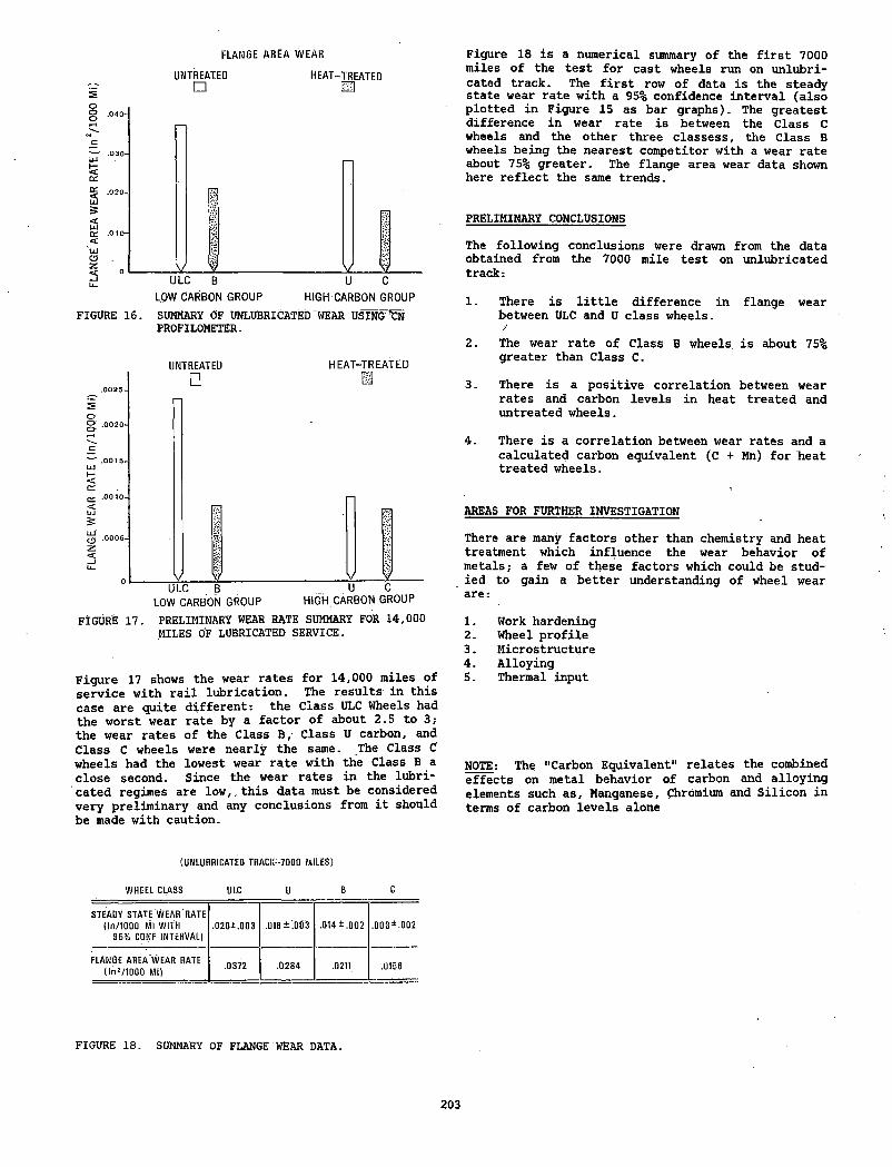
FLANGE A R E A W EAR

UNTREATED HEAT-TREATED

FIGURE 16. SUMMARY OF UNLUBRICATED WEAR USING ’CN PROFILOMETER.

UNTREATED H EA T-TR EATED

FIGURE 17. PRELIMINARY WEAR RATE SUMMARY FOR 14,000 MILES OF LUBRICATED SERVICE.

Figure 17 shows the wear rates for 14,000 miles of service with rail lubrication. The results in this case are quite different: the Class ULC Wheels had the worst wear rate by a factor of about 2.5 to 3; the wear rates of the Class B,' Class U carbon, and Class C wheels were nearly the same. The Class C wheels had the lowest wear rate with the Class B a close second. Since the wear rates in the lubri­cated regimes are low,,this data must be considered very preliminary and any conclusions from it should be made with caution.

Figure 18 is a numerical summary of the first 7000 miles of the test for cast wheels run on unlubri­cated track. The first row of data is the steady state wear rate with a 95% confidence interval (also plotted in Figure 15 as bar graphs). The greatest difference in wear rate is between the Class C wheels and the other three classess, the Class B wheels being the nearest competitor with a wear rate about 75% greater. The flange area wear data shown here reflect the same trends.

PRELIMINARY CONCLUSIONS

The following conclusions were drawn from the dataobtained from the 7000 mile test on unlubricatedtrack:

1. There is little difference in flange wear between ULC and U class wheels./

2. The wear rate of Class B wheels is about 75% greater than Class C.

3. There is a positive correlation between wear rates and carbon levels in heat treated and untreated wheels.

4. There is a correlation between wear rates and a calculated carbon equivalent (C + Mn) for heat treated wheels.

AREAS FOR FURTHER INVESTIGATION

There are many factors other than chemistry and heat treatment which influence the wear behavior of metals; a few of these factors which could be stud­ied to gain a better understanding of wheel wear are:

1. Work hardening2. Wheel profile3. Microstructure4. Alloying5. Thermal input

NOTE: The "Carbon Equivalent" relates the combined effects on metal behavior of carbon and alloying elements such as. Manganese, Chromium and Silicon in terms of carbon levels alone

(UNLUBRICATED TRACK-7000 MILES)

WHEEL CLASS ULC u B c

STEADY STATE WEAR RATE (ln /1000 Mi WITH

95% CONF INTERVAL)-020±.003 .018 ± .003 .014 ± .002 .0034 .002

FLANGE AREA WEAR RATE ( ln z/1000 Mi) .0372 .0284 .0211 .0156

FIGURE 18. SUMMARY OF FLANGE WEAR DATA.

203

QUESTIONS AND ANSWERS

Question 1

Your data for accidents shows an increase for the number of incidents from 80 to 92 during the period 1976-1978, an increase of 15%. Was the increase truly significant when considering the increase in tonnage or train movements during that period?

The basis for this question is that Santa Fe statistics show a decrease in the accident rate (accidents per billion gross ton miles). For that period primarily this effect is due to efforts to hold the line on the accident fre­quency while handling increased tonnages over previous years.

Answer

The increase in the number of incidents was insignificant but the increase in cost per incident and the increase in axle set removal to prevent wheel failure due to thermal damage was very significant. The railroads have done a magnificent job of reducing accidents but the reduction was accomplished at a high mainte­nance cost.

Question 2

In railroad service tests of Class U, B, and C wheels, we have generally found the Class B and U wheels to have similar wear rates and in some cases, the Class U wheels have a better (lower) wear rate than Class B wheels. Would the author care to comment on these differences in service compared to FAST.

Answer

Since the service conditions and carbon and manganese content of the wheels in question are not known to me, it would be difficult to make an intelligent response to the question. It appears that we have much to learn about wear mechanisms of metallic components in unlubri­cated environments.

204

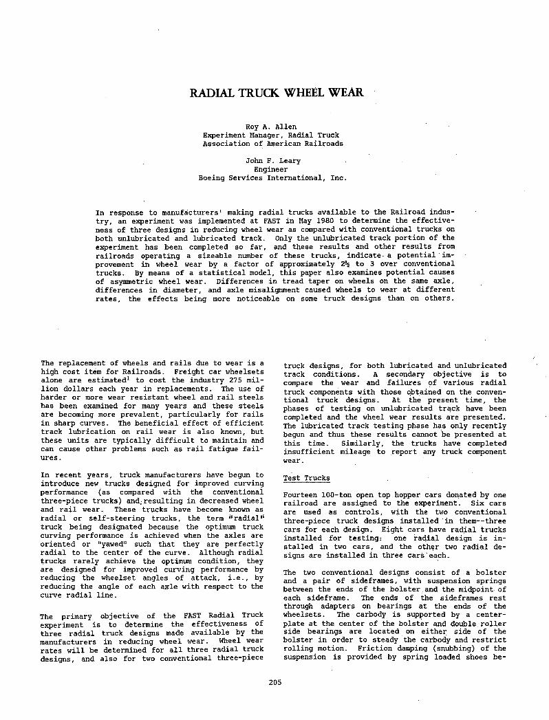
RADIAL TRUCK WHEEL WEAR

Roy A. AllenExperiment Manager, Radial Truck Association of American Railroads

John F. Leary Engineer

Boeing Services International, Inc.

In response to manufacturers1 making radial trucks available to the Railroad indus­try, an experiment was implemented at FAST in May 1980 to determine the effective­ness of three designs in reducing wheel wear as compared with conventional trucks on both unlubricated and lubricated track. Only the unlubricated track portion of the experiment has been completed so far, and these results and other results from railroads operating a sizeable number of these trucks, indicate- a potential im­provement in wheel wear by a factor of approximately 2\ to 3 over conventional trucks. By means of a statistical model, this paper also examines potential causes of asymmetric wheel wear. Differences in tread taper on wheels on the same axle, differences in diameter, and axle misalignment caused wheels to wear at different rates, the effects being more noticeable on some truck designs than on others.

The replacement of wheels and rails due to wear is a high cost item for Railroads. Freight car wheelsets alone are estimated1 to cost the industry 275 mil­lion dollars each year in replacements. The use of harder or more wear resistant wheel and rail steels has been examined for many years and these steels are becoming more prevalent, particularly for rails in sharp curves. The beneficial effect of efficient track lubrication on rail wear is also known, but these units are typically difficult to maintain and can cause other problems such as rail fatigue fail­ures.

In recent years, truck manufacturers have begun to introduce new trucks designed for improved curving performance (as compared with the conventional three-piece trucks) and. resulting in decreased wheel and rail wear. These trucks have become known as radial or self-steering trucks, the term ‘‘radial11 truck being designated because the optimum truck curving performance is achieved when the axles are oriented or "yawed" such that they are perfectly radial to the center of the curve. Although radial trucks rarely achieve the optimum condition, they are designed for improved curving performance by reducing the wheelset angles of attack, i.e., by reducing the angle of each axle with respect to the curve radial line.

The primary objective of the FAST Radial Truck experiment is to determine the effectiveness of three radial truck designs made available by the manufacturers in reducing wheel wear. Wheel wear rates will be determined for all three radial truck designs, and also for two conventional three-piece

truck designs, for both lubricated and unlubricated track conditions. A secondary objective is to compare the wear and failures of various radial truck components with those obtained on the conven­tional truck designs. At the present time, the phases of testing on unlubricated track have been completed and the wheel wear results are presented. The lubricated track testing phase has only recently begun and thus these results cannot be presented at this time. Similarly, the trucks have completed insufficient mileage to report any truck component wear.

Test Trucks

Fourteen 100-ton open top hopper cars donated by one railroad are assigned to the experiment. Six cars are used as controls, with the two conventional three-piece truck designs installed in them— three cars for each design. Eight cars have radial trucks installed for testing: one radial design is in­stalled in two cars, and the other two radial de­signs are installed in three cars each.

The two conventional designs consist of a bolster and a pair of sideframes, with suspension springs between the ends of the bolster and the midpoint of each sideframe. The ends of the sideframes rest through adapters on bearings at the ends of the wheelsets. The carbody is supported by a center- plate at the center of the bolster and double roller side bearings are located on either side of the bolster in order to steady the carbody and restrict rolling motion. Friction damping (snubbing) of the suspension is provided by spring loaded shoes be-

205

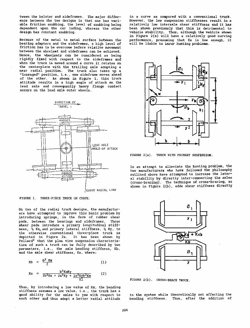
tween the bolster and sideframes. The major differ­ence between the two designs is that one has vari­able friction snubbing, the level of snubbing being dependent upon the car lading, whereas the other design has constant snubbing.

Because of the metal to metal surface between the bearing adapters and the sideframes, a high level of friction has to be overcome before relative movement between the wheelset and sideframes can be achieved. Hence, the wheelsets can be considered as being rigidly fixed with respect to the sideframes and when the truck is moved around a curve it rotates on the centerplate with the trailing axle adopting a near radial position. The truck also takes up a "lozenged" position, i.e., one sideframe moves ahead of the other. As shown in Figure 1, this truck attitude results in a high angle of attack on the lead axle and consequently heavy flange contact occurs on the lead axle outer wheels.

DIRECTION OF TRAVEL I *"

On two of the radial truck designs, the manufactur­ers have attempted to improve this basic problem by introducing springs, in the form of rubber shear pads, between the bearings and sideframes. These shear pads introduce a primary longitudinal stiff­ness, \ Kx, and primary lateral stiffness, \ Ky, to the otherwise conventional three-piece truck as depicted in Figure 2a. It has been shown by Pollard2 that the plan view suspension characteris­tics of such a truck can be fully described by two parameters, i.e., the axle bending stiffness, Kb, and the axle shear stiffness, Ks, where:

Kb b2 Kx 2 (1)

Ks ______b2KxKy2b2Kx + 2azKy + 2a2Kyb2Kx

K1( 2 )

in a curve as compared with a conventional truck. However, the low suspension stiffnesses result in a relatively low interaxle shear stiffness and it has been shown previously that this is detrimental to vehicle stability. Thus, although the vehicle shown in Figure 2(a) will have a relatively good curving performance, presuming that Kx is low enough, it will be liable to incur hunting problems.

FIGURE 2(a). TRUCK WITH PRIMARY SUSPENSION.

In an attempt to alleviate the hunting problem, the two manufacturers who have followed the philosophy outlined above have attempted to increase the later­al stability by directly inter-connecting the axles (cross-bracing). The technique of cross-bracing, as shown in Figure 2(b), adds shear stiffness directly

FIGURE 2(b). CROSS-BRACE TRUCK.

Thus, by introducing a low value of Kx, the bending stiffness assumes a low value, i.e., the truck has a good ability for the axles to yaw with respect to each other and thus adopt a better radial attitude

to the system while theoretically not affecting the bending stiffness. Thus, after the addition of

206

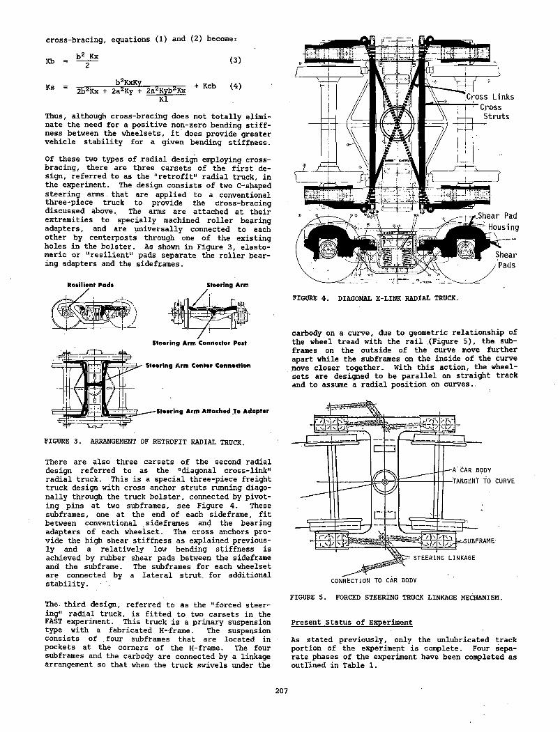
cross-bracing, equations (1) and (2) become:

Kb b2 Kx 2 ( 3 )

Ks _________b2KxKy2b2Kx + 2a2Ky + 2a2Kyb:iKx

Kl+ Kcb ( 4 )

Thus, although cross-bracing does not totally elimi­nate the need for a positive non-zero bending stiff­ness between the wheelsets, it does provide greater vehicle stability for a given bending stiffness.

Of these two types of radial design employing cross­bracing, there are three carsets of the first de­sign, referred to as the "retrofit11 radial truck, in the experiment. The design consists of two C-shaped steering arms that are applied to a conventional three-piece truck to provide the cross-bracing discussed above. The arms are attached at their extremities to specially machined roller bearing adapters, and are universally connected to each other by centerposts through one of the existing holes in the bolster. As shown in Figure 3, elasto­meric of "resilient11 pads separate the roller bear­ing adapters and the sideframes.

Roiilient Pads Steering Arm

Steering Arm Connector Post

Steering Arm Center Connection

Steering Arm Attached To Adapter

FIGURE 3. ARRANGEMENT OF RETROFIT RADIAL TRUCK.

There are also three carsets of the second radial design referred to as the "diagonal cross-link" radial truck. This is a special three-piece freight truck design with cross anchor struts running diago­nally through the truck bolster, connected by pivot­ing pins at two subframes, see Figure 4. These subframes, one at the end of each sideframe, fit between conventional sideframes and the bearing adapters of each wheelset. The cross anchors pro­vide the high shear stiffness as explained previous­ly and a relatively low bending stiffness is achieved by rubber shear pads between the sideframe and the subframe. The subframes for each wheelset are connected by a lateral strut, for additional stability.

FIGURE 4. DIAGONAL X-LINK RADIAL. TRUCK.

carbody on a curve, due to geometric relationship of the wheel tread with the rail .(Figure 5), the sub- frames on the outside of the curve move further apart while the subframes on the inside of the curve move closer together. With this action, the wheel- sets are designed to be parallel on straight track and to assume a radial position on curves..

The. third design, referred to as the "forced steer­ing" radial truck, is fitted to two carsets in the FAST experiment. This truck is a primary suspension type with a fabricated H-frame. The suspension consists of .four subframes that are located in pockets at the corners of the H-frame. The four subframes and the carbody are connected by a linkage arrangement so that when the truck swivels under the

FIGURE 5. FORCED STEERING TRUCK LINKAGE MECHANISM.

Present Status of Experiment

As stated previously, only the unlubricated track portion of the experiment is complete. Four sepa­rate phases of the experiment have been completed as outlined in Table 1.

207

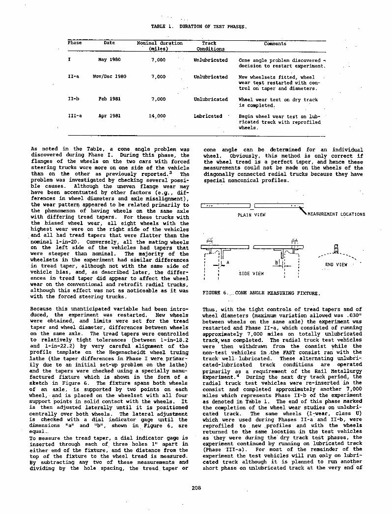
TABLE 1. DURATION OF TEST PHASES.

Phase Date Nominal duration (miles)

TrackConditions

Comments

I May 1980 7,000 Unlubricated Cone angle problem discovered - decision to restart experiment.

Il-a Nov/Dec 1980 7,000 Unlubricated New wheelsets fitted, wheel wear test restarted with con­trol on taper and diameters.

Il-b Feb 1981 7,000 Unlubricated Wheel wear test on dry track is completed.

Ill-a Apr 1981 14,000 Lubricated 1 Begin wheel wear test on lub­ricated track with reprofiledwheels.

As noted in the Table, a cone angle problem was discovered during Phase I. During this phase, the flanges of the wheels on the two cars with forced steering trucks wore more on one side of the vehicle than on the other as previously reported.3 The problem was investigated by checking several possi­ble causes. Although the uneven flange wear may have been accentuated by other factors (e.g., dif­ferences in wheel diameters and axle misalignment), the wear pattern appeared to be related primarily to the phenomenon of having wheels on the same axle with differing tread tapers. For these trucks with the biased wheel wear, all eight wheels with the highest wear were on the right side of the vehicles and all had tread tapers that were flatter than the nominal l-in-20. Conversely, all the mating wheels on the left side of the vehicles had tapers that were steeper than nominal. The majority of the wheelsets in the experiment had similar differences in tread taper, although not with the same side of vehicle bias, and, as described later, the differ­ences in tread taper did appear to affect the wheel wear on the conventional and retrofit radial trucks, although this effect was not as noticeable as it was with the forced steering trucks.

Because this unanticipated variable had been intro­duced, the experiment was restarted. New wheels were obtained, and limits were set for the tread taper and wheel diameter, differences between wheels on the same axle. The tread tapers were controlled to relatively tight tolerances (between l-in-18.2 and l-in-22.2) by very careful alignment of the profile template on the Hegenscheidt wheel truing lathe (the taper differences in Phase I were primar­ily due to an initial set-up problem on the lathe) and the tapers were checked using a specially manu­factured fixture which is shown in the form of a sketch in Figure 6. The fixture spans both wheels of an axle, is supported by two points on each wheel, and is placed on the wheelset with all four support points in solid contact with the wheels. It is then adjusted laterally until it is positioned centrally over both wheels. The lateral adjustment is checked with a dial indicator gage until the dimensions "a" and "b", shown in Figure 6, are equal.To measure the tread taper, a dial indicator gage is inserted through each of three holes 1" apart in either end of the fixture, and the distance from the top of the fixture to the wheel tread is measured. By subtracting any two of these measurements and dividing by the hole spacing, the tread taper or

cone angle can be determined for an individual wheel. Obviously, this method is only correct if the Wheel tread is a perfect taper, and hence these measurements could not be made on the wheels of the diagonally connected radial trucks because they have special nonconical profiles.

* 1 l > «

PLAIN VIEW > MEASUREMENT LOCATIONS

tri• - __ i L i 1 '- 1 U

p c y r 1J| 1

_ A b | | ! END VIEW ' ^ 11 1 | 1 1 1

SIDE VIEW 11

FIGURE 6...CONE ANGLE MEASURING FIXTURE.

Thus, with the tight controls of tread tapers and of wheel diameters (maximum variation allowed was .030" between wheels on the same axle) the experiment was restarted and Phase Il-a, which consisted of running approximately 7,000 miles on totally unlubricated track, was completed. The radial truck test vehicles were then withdrawn from the consist while the non-test vehicles in the FAST consist ran with the track well • lubricated. These alternating unlubri­cated-lubricated track conditions are operatedprimarily as a requirement of the Rail Metallurgy Experiment.4 During the next dry track period, the radial truck test vehicles were re-inserted in the consist and completed approximately another 7,000 miles which represents Phase Il-b of the experiment as denoted in Table 1. The end of this phase marked the completion of the wheel wear studies on unlubri­cated track. The same wheels (1-wear, class U) which were used during Phases Il-a and Il-b, were reprofiled to , new profiles and with the wheels returned to the same location in the test vehicles as they were during the' dry track test phases, the experiment continued by running on lubricated track (Phase Ill-a). For most of the remainder of the experiment the test vehicles will run only on lubri­cated track although it is planned to run another short phase on unlubricated track at the very end of

208

the experiment in order to gather data of"the'ef­fects on wheel wear of changing rail metallurgies as a result of the introduction of the Track Degrada­tion Experiment.5

It should be noted that in order to leave adequate metal to reprofile the existing wheels for Phase III of the experiment, the wheels were not allowed to' incur more than 0.3" of flange wear during PhaseII- a and Il-b. Some of the test wheels did achieve this limit prior to completion of Phase Il-b and were temporarily removed fom the experiment. These wheelsets were replaced by non-test wheelsets for the remainder of Phase II testing, but the original test wheels were then reprofiled and reassembled under the test vehicles at the beginning of PhaseIII- a.

Phases Il-a and Il-b contain the main bulk of the data which are reported herein from which one of the experiment objectives, i.e., to determine wheel wear rates on totally unlubricated track, was achieve^- As noted previously. Phase I data are confounded by the tread taper problem and these data are not used in comparing wheel wear performance of different truck designs. However, as reported later, the Phase I data did enable an analytical study, which was unplanned at the beginning of the experiment, to be carried out to highlight some causes of asym­metric wheel wear.

WHEEL WEAR MEASUREMENT METHODS

At the beginning of the unlubricated test phases, linear measurements of flange thickness, flange height, and rim thickness were taken using both the AAR finger gage and a previously unused fixture called the wheel snap gage. ' The snap gage. Figure 7, essentially measures the same parameters as the finger gage and does so by means of dial gage indi­cators as opposed to the graduated scales used on the finger gage. As reported by Larkin,6 the accu­racy of the snap gage is superior to that of the finger gage and during this experiment the reliabil­ity of the fixture was proved. Hence, part way through the experiment, it was decided to cease use of' the finger gage and only the snap gage results are discussed.

FIGURE 7. WHEEL SNAP GAGE.

Typical snap gage data are presented in Figure 8 which shows the flange thickness readings over a period of 14,000 miles comprising Phase Il-a and Il-b data. The data represents the flange wear on two wheels (wheels R1 and LI on car 136) with mea­surements being taken at two radial positions, 180° apart, on each wheel. As can be seen, the flanges were exposed to initial rapid wear during the first1,000 - 2,000 miles and thereafter wore at a reason­ably linear rate. This phenomena is typical of wheel wear data collected on FAST unlubricated track,7 8 and most of the data analysis presented in this paper deals only with data obtained from 2,000 miles onwards.

CAR 136 14.000 MILES ON UNLUBRICATED TRACK

DISTANCE TRAVELLED (MILES)

FIGURE 8; .RADIAL TRUCK EXPERIMENT SNAP GAGE DATA.

The other wheel wear measurement fixture‘-is the modified CN profilometer which has been described by Larkin6 ■ and Kahle.8 The profilometer,' Figure 9, takes a series of dial indicator readings across the wearing surface of the wheel. These data form the input to a computer program which calculates flange area wear, tread area wear, and total profile area wear by comparing the profile of a worn wheel with the new, original profile of- that- same wheel.

EflGURE 9. MODIFIED CN PROFILOMETER.

209

Snap gage readings were taken every 1,000 miles (approximately) during the unlubricated track phases with profilometer data taken at the beginning and end of each of the phases outlined in Table 1. Additional measurements taken are as follows:

wheel hardness, using the King Brinell tester, prior to Phase I and Phase Il-a,

wheel diameter, using the digital read-out on the Hegenscheidt wheel truing lathe, prior to Phase I and Phase Il-a,

tread taper, using the special fixture shown in Figure 6, part-way through Phase I and prior to Phase Il-a, and

axle misalignment, reported previously9 and to be discussed later, taken between Phases I and Il-a.

WHEEL WEAR RESULTS - TRUCK COMPARISON

In comparing the flange and tread wear of the radial trucks with the conventional trucks, the Phase I data were not used because the differences in tread taper introduced unforeseen noise. This made it difficult to pursue the objective of the experiment. Thus, the data which are reported in this portion of the paper are those obtained from Phases Il-a and Il-b, i.e., for 14,000 miles of operation on totally unlubricated track.

Before presenting the data, a discussion of the test conditions prevailing during Phases Il-a and Il-b is necessary in order that the results can be viewed in the correct context. First, the FAST track has a high curve to tangent ratio— approximately 54% of the track is curves or spirals— with all curves being of 3°, 4°, or 5°. In addition to the unlubri­cated track conditions described above, it should be noted that at FAST the relative humidity is typical­ly very low, and thus high values of the limiting coefficient of friction between wheel and rail are

present. All the test vehicles were fully loaded 100-ton, open top hopper cars supplied by one rail­road, and, throughout the experiment, they formed the first fourteen cars at the head end of the consist in order that they always be subjected to the highest drawbar forces. In order to minimize the effects of tread braking on the tread wear data, dynamic braking was used except when slowing the consist to a complete stop, or if, in the opinion of the locomotive engineer, a hazardous situation would have resulted.

As for the wheel chemistry experiment (Wheels IV), reported by Kahle,8 the normal FAST end-for-end consist turning operation was modified slightly, such that for each 1,000 mile period of operation during this experiment, each wheel on all trucks received an approximately equal exposure to the high wear condition of running on the lead axle on the high rail. All wheels were untreated class U cast, and all had standard AAR l-in-20 coned profiles except for those on the diagonal cross-link truck, which had high conicity profiles specially designed based on the work of Scheffel.10 11 Because wheels could not be obtained with the special profile, the cast wheels were turned to this profile on the Hegenscheidt wheel truing lathe at the Transporta­tion Test Center. Thus, these wheels could not be tested with the original cast running surface intact and, in order to eliminate a variable which might potentially have affected wheel wear, the remaining wheels in the experiment received a minimal turning cut, typically between .050" and .100" removed from the diameter, on the same lathe.

Finally, as stated before for Phases Il-a and Il-b, tread tapers and wheel diameters were strictly controlled with tapers being between l-in-18.2 and l-in-22.2 and the diameter tolerance allowing a maximum variation of .030" between wheels on the same axle.

The wheel wear results are summarized in Table 2 and 3 for flange and tread wear, respectively.

TABLE 2. FLANGE WEAR IN PHASE II.

Truck type

Flange linear wear rate (in/1000 mi) Flangeafter

area loss 14,000 mi(in2)

allmean

wheels ±95% conf

worst wheel per axle mean ±95% conf

allmean

wheels ±95% conf

Conventional, variable snubbing 0.0160 0.0023 0.0180 0.0039 .292 .026Conventional, constant snubbing 0.0147 0.0020 0.0165 0.0032 .247 .020Radial, retrofit 0.0115 0.0013 0.0134 0.0018 .194 .017Radial, forced steering 0.0121 0.0029 0.0143 0.0059 .207 .048Radial, diagonal X-link 0.0067 0.0012 0.0084 0.0013 .117 .011

TABLE 3. TREAD WEAR IN PHASE II.

Truck type

Tread linear wear rate (in/1000 mi) Treadafter

area loss 14,000 mi(in2)

allmean

wheels ±95% conf

worst wheel per axle mean ±95% conf

allmean

wheels ±95% conf

Conventional, variable snubbing 0.0061 0.0007 0.0069 0.0008 .110 .017Conventional, constant snubbing 0.0056 0.0010 0.0063 0.0014 ■ 111 .014Radial, retrofit 0.0030 0.0010 0.0036 0.0016 .056 .010Radial, forced steering 0.0013 0.0013 0.0025 0.0015 .052 .016Radial, diagonal X-link 0.0028 0.0006 0.0034 0.0010 .042 .010

210

The linear wear rates were obtained by linear re­gression of the snap gage readings between 2,000 and14,000 miles. The two columns of data under the linear wear rate heading are calculated using (a) all wheels for each truck type in the regression analysis, and (b) only the highest wearing wheel (worst wheel) on each axle for each truck type. The worst wheel per axle data are presented because, of course, in practice it is the worst wearing wheel which determines when both wheels of that axle are condemned. The third column in each table repre­sents the area of metal lost after 14,000 miles of operation and is simply determined by comparing the wheel profiles at 14,000 miles, as measured by the modified CN profilometer, with the original unworn profiles measured prior to Phase II. It should be noted that some of the wheels, particularly on the conventional trucks, were withdrawn from the consist before the end of Phase Il-b because they had reached the artificial condemning limit of 0.3" of flange wear as described previously. In these cases, the area lost at the time of removal was calculated and these values prorated, assuming the wheels wore linearly with mileage, to obtain an estimate of what the wear would have been at 14,000 miles.

Having made this assumption, it is interesting to note that the mean values agree well with the mean linear wear rates obtained from the snap gage data in that all the results indicate that, in general, the wheels on the radial trucks wore less than on the conventional trucks and that all results place the trucks in the same general ranking order. Thus, despite the fact that the profilometer is regarded as a prototype in the respect that FAST has to resolve some operational and computing problems resulting mainly from the fact that the fixture is used on a “mass-production" type basis, the results are very encouraging.

The flange linear wear rate results for all wheels (presented in Table 2) show that the mean wear rates of the conventional trucks are higher than those for all radial trucks and as much as 2% times higher than the best performing diagonal X-link radial truck. The scatter of the data, as denoted by the values of the ±95% confidence interval values, is large for the forced steering truck and is even larger still when only the worst wheel per axle is used in the regression analysis. The large confi­dence interval is caused partly by the smaller sample size--two test vehicles as opposed to three for the other truck designs— but is probably due more to axle/truck misalignment. This notion is supported somewhat by data obtained in the FAST wear index experiment12 where one of the forced steering trucks tested showed a large angle of attack (3 mrads) on tangent track. Large angles of attack on tangent track are indicative of poor axle align­ment.13 Additionally, the axle alignment results9 indicate that one truck (car 141, truck B) was particularly poorly aligned and it is the wheels on this truck which suffered the highest wear, with both wheelsets being withdrawn from the consist, because of the artificial wear limit, after only6,000 miles. With the exception of one other wheel- set, which was withdrawn after 13,000 miles, none of the other wheels on the forced steering trucks had reached the 0.3" flange wear limit after 14,000 miles of operation. Therefore, the large data scatter is primarily attributable to the high wear rates on one truck.

Apart from the large scatter, the worst wheel per axle results in Table 2 are generally in good agree­ment with those for all wheels except that, natural­ly, the mean flange wear rates are slightly higher for all truck types.

The tread wear rates in Table 3, although consid­erably lower than the flange wear rates, show simi­lar general trends with all radial trucks performing better than the conventional trucks, typically by factors of 2 or 2.5 to 1.

Thus, summarizing the results obtained from Phase II— 14,000 miles of operation on unlubricated track— the primary conclusion is that the tread wear on all radial trucks and the flange wear on the best performing radial truck were typically approximately 2% times better than that on conventional trucks. This conclusion is in reasonable agreement with preliminary results obtained by three Railroads operating a reasonable number of radial trucks. For instance. Union Pacific has 100 carsets of radial trucks in iron-ore service and has monitored wheel wear on these trucks and on 150 carsets of conven­tional trucks operating in the same service. After145,000 miles of operation, the data indicates that wheel life' on the radial trucks will be at least twice (and probably more) than on the conventional trucks.

Southern Railway has a total of 134 .100-ton coal cars in service equipped with self-steering, radial trucks; one unit train of 97 cars is completely equipped with self-steering trucks. Preliminary test results after approximately 150,000 miles indicate flange wear life is at least three times greater than conventional trucks in the same service.

Finally, Canadian National has 75 carsets of radial trucks in service of which 15 carsets are being regularly monitored for wheel wear. Seven carsets of conventional trucks in the same service are also monitored for comparison purposes. Many of the trucks have accumulated 160,000 miles of operation and preliminary results indicate that flange wear on the radial trucks, as determined by monitoring both flange area and flange thickness, is on average approximately 1/3 of that on the conventional trucks.

Asymmetric Wheelwear-Parametric Study

Recognizing that the flange on cars fitted with the forced steering design truck wore more on one side of the vehicle than the other during Phase I, a study was carried out to find the source of this anomaly. As previously mentioned, this was thought to be the result of the systematic installation of wheelsets possessing asymmetric wheel tapers. That is, on a given wheelset, one wheel may have had a l-in-16 taper and its mate a l-in-23. In fact, a wheelset difference as great as l-in-14.7 and 1-in- 26.3 was discovered.

Consideration was also given to differences in diameter. This difference, which is not solely attributable to taper difference, may also have independently influenced wheel wear since differ­ences in taper were not highly correlated with differences in diameter. Therefore, these two effects were considered separately in this study.

Axle alignment of two radial design trucks was also

211

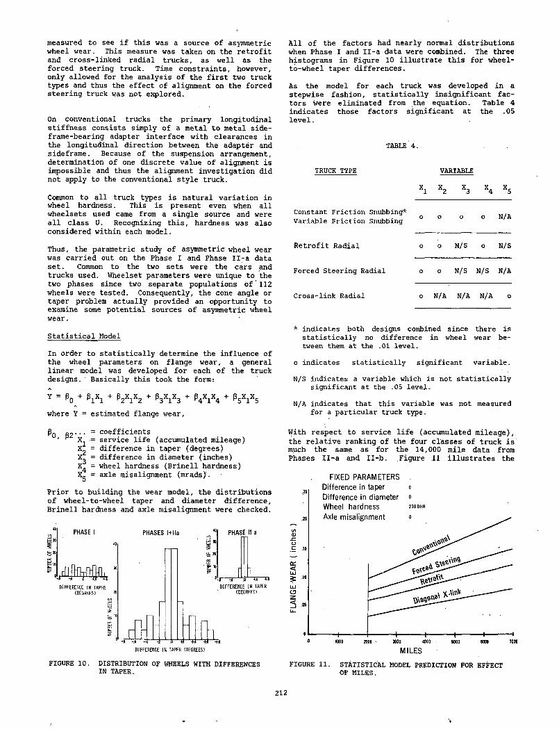
measured to see if this was a source of asymmetric wheel wear. This measure was taken on the retrofit and cross-linked radial . trucks, as well as the forced steering truck. Time constraints, however, only allowed for the analysis of the first two truck types and thus the effect of alignment on the forced steering truck was not explored.

On conventional trucks the primary longitudinal stiffness consists simply of a metal to metal side- frame-bearing adapter interface with clearances in the longitudinal direction between the adapter and sideframe. Because of the suspension arrangement, determination of one discrete value of alignment is impossible and thus the alignment investigation did not apply to the conventional style truck.

Common to all truck types is natural variation in wheel hardness. This is present even when allwheelsets used came from a single source and were all class U. Recognizing this, hardness was also considered within each model.

Thus, the parametric study of asymmetric wheel wear was carried out on the Phase I and Phase Il-a data set. Common to the two sets were the cars andtrucks used. Wheelset parameters were unique to the two phases since two separate populations o f '112 wheels were tested. Consequently, the cone angle or taper problem actually provided an opportunity to examine some potential sources of asymmetric wheel wear.

Statistical Model

In order to statistically determine the influence of the wheel parameters on flange wear, a general linear model was developed for each of the truck designs. Basically this took the form:

i = P0 + h*l + P2X1X2 + P3X1X3 + P4X1X4 + h h h where Y = estimated flange wear,

All of the factors had nearly normal distributions when Phase I and Il-a data were combined. The three histograms in Figure 10 illustrate this for wheel- to-wheel taper differences.

As the model for each truck was developed in a stepwise fashion, statistically insignificant fac­tors were eliminated from the equation. Table 4 indicates those factors significant at the .05 level.

TABLE 4.

TRUCK TYPE VARIABLE

X1 X2 X3 X4 X5

Constant Friction Snubbing* Variable Friction Snubbing 0 o o 0 N/A

Retrofit Radial 0 o N/S o N/S

Forced Steering Radial 0 0 N/S N/S N/A

Cross-link Radial 0 N/A N/A N/A o

* indicates both designs combined since there is statistically no difference in wheel wear be­tween them at the .01 level.

o indicates statistically significant variable.

N/S indicates a variable which is not statistically significant at the .05 level.

N/A indicates that this variable was not measured for a particular truck type.

B2‘‘‘ = coefficients' p = service life (accumulated mileage)X^ = difference in taper (degrees)X^ = difference in diameter (inches)X^ = wheel hardness (Brinell hardness)Xc = axle misalignment (mrads).5

Prior to building the wear model, the distributions of wheel-to-wheel taper and diameter difference, Brinell hardness and axle misalignment were checked.

FIGURE 10. DISTRIBUTION OF WHEELS WITH DIFFERENCES IN TAPER.

With respect to service life (accumulated mileage), the relative ranking of the four classes of truck is much the same as for the 14,000 mile data from Phases Il-a and Il-b. Figure 11 illustrates the

FIXED PARAMETERS

FIGURE 11. STATISTICAL MODEL PREDICTION FOR EFFECT OF MILES.

212

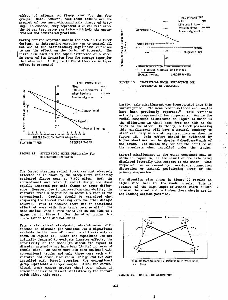
effect of mileage on flange wear for the four groups. Note, however, that these results are the product of two seven-thousand mile phases of test­ing. In essence, they represent a 28 car test since the 14 car test group ran twice with both the uncon­trolled and controlled profiles.

Having derived separate models for each of the truck designs, an interesting exercise was to control all but one of the statistically significant variables to see the effect on the factor of interest. The first discussed is the taper difference of a wheel in terms of its deviation from the average taper for that wheelset. In Figure 12 the difference in taper effect is presented.

FIXED PARAMETERS

DIFFERENCE IN TAPER (degrees)

FLATTER TAPER STEEPER TAPER

FIGURE 12. STATISTICAL MODEL PREDICTION FOR DIFFERENCE IN TAPER.

The forced steering radial truck was most adversely affected as is shown by the steep curve reflecting estimated flange wear at 7,000 miles. Both the conventional and retrofit radial design are about equally impacted per unit change in taper differ­ence. However, due to improved curving ability, the retrofit truck's magnitude is about 60% that of the conventional. Caution should be exercised when comparing the forced steering with the other designs however. This is because there was an additional effect at work with this truck because all of the more conical wheels were installed on one side of a given car in Phase I. For the other trucks this installation bias did not exist.

From a statistical standpoint, wheel-to-wheel dif­ference in diameter per wheelset was a significant variable in the case of conventional trucks only as shown in Figure 13. Since the experiment was not initially designed to evaluate diameter effects, the sensitivity., of the model to detect the impact of diameter asymmetry may have'-been limited in terms of sample size. As there were six cars equipped with conventional trucks and only three cars each with retrofit and cross-link radial design and two cars installed with forced steering, the conventional group represents a larger -sample.• Also, the conven­tional truck causes greater wheel wear making it somewhat easier to dissect statistically the factors which affect this wear.

cn Conventional

FIXED PARAMETERS Miles 7000

Difference in taper o Wheel hardness o r o b h n

Axle m isalignm ent o

Retrofit - » Diagonal X—Link

“ .0X- .0 0 - .05- . 04- .03- .00--.01 +.01 +.0 2 +.031.04 405406407

D IFFE R E N C E IN D IA M ETER ( in ch es )

S M A LLE R W HEEL LARGER WHEEL

FIGURE 13. STATISTICAL MODEL PREDICTION FOR DIFFERENCE IN DIAMETER.

Lastly, axle misalignment was incorporated into this investigation. The measurement methods and results have been previously reported.9 This variable actually is comprised of two components. One is the radial component illustrated in Figure 14 which is the difference in wheel base from one side of the truck to the other. In theory, a truck possessing this misalignment will have a natural tendency to steer well only in one of two directions as shown in Figure 15. This effect should be evidenced by higher wheel wear on the shorter "wheelbase" side of the truck. Its source may reflect the attitude of the wheelsets when installed under the. trucks.

Lateral misalignment is the other component and, as shown in Figure 16, is the result of one axle being displaced laterally with respect to the other. This component can be caused by icross-brace connection distortion or lateral positioning error of the primary Suspension.

The direction bias shown in Figure 17 results in higher wheel wear for the shaded wheels. This is because of. the high angle of attack which exists between the wheel and rail when these wheels are in the leading outside position.

i.e., B> A

FIGURE. 14. RADIAL MISALIGNMENT.

213

\ 1

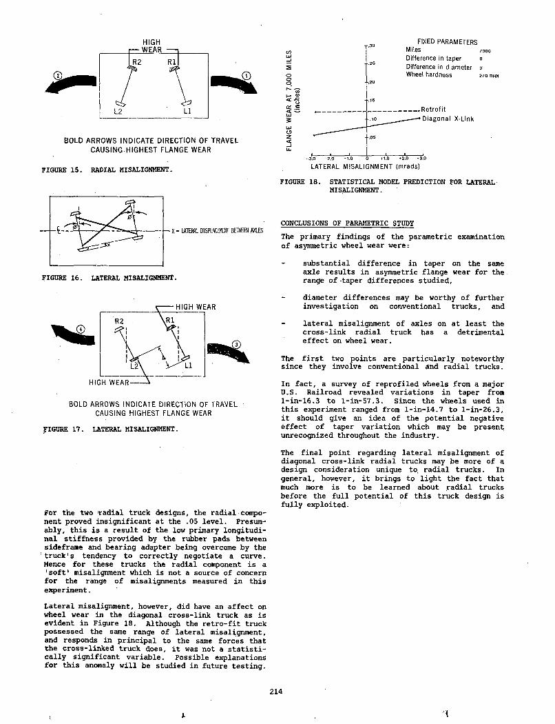
HIGH

B O L D A R R O W S INDICATE DIRECTION O F T R A V E L C A U S I N G H I G H E S T F L A N G E W E A R

FIGURE 15. RADIAL MISALIGNMENT.

B O L D A R R O W S INDICATE DIRECTION OF T R A V E L C A U S I N G H I GHEST F L A N G E W E A R

FIGURE 17. LATERAL MISALIGNMENT.

FIGURE 18. STATISTICAL MODEL PREDICTION FOR LATERAL MISALIGNMENT.

CONCLUSIONS OF PARAMETRIC STUDYThe primary findings of the parametric examination of asymmetric wheel wear were:

substantial difference in taper on the same axle results in asymmetric flange wear for the , range of taper differences studied,

diameter differences may be worthy of further investigation on conventional trucks, and

lateral misalignment of axles on at least the cross-link radial truck has a detrimental effect on wheel wear.

The first two points are particularly noteworthy since they involve conventional and radial trucks.

In fact, a survey of reprofiled wheels from a major U.S. Railroad revealed variations in taper from l-in-16.3 to l-in-57.3. Since the wheels used in this experiment ranged from l-in-14.7 to l-in-26.3, it should give an idea of the potential negative effect of taper variation which may be present unrecognized throughout the industry.

For the two ‘radial truck designs, the radial compo­nent proved insignificant at the .05 level. Presum­ably, this is a result of the low primary longitudi­nal stiffness provided by the rubber pads between sideframe and bearing adapter being overcome by the truck's tendency to correctly negotiate a curve. Hence for these trucks the radial component is a 'soft' misalignment which is not a source of concern for the range of misalignments measured in this experiment.

The final point regarding lateral misalignment of diagonal cross-link radial trucks may be more of a design consideration unique to radial trucks. In general, however, it brings to light the fact that much more is to be learned about radial trucks before the full potential of this truck design is fully exploited.

Lateral misalignment, however, did have an affect on wheel wear in the diagonal cross-link truck as is evident in Figure 18. Although the retro-fit truck possessed the same range of lateral misalignment, and responds in principal to the same forces that the cross-linked truck does, it was not a statisti­cally significant variable. Possible explanations for this anomaly will be studied in future testing.

214

1 l

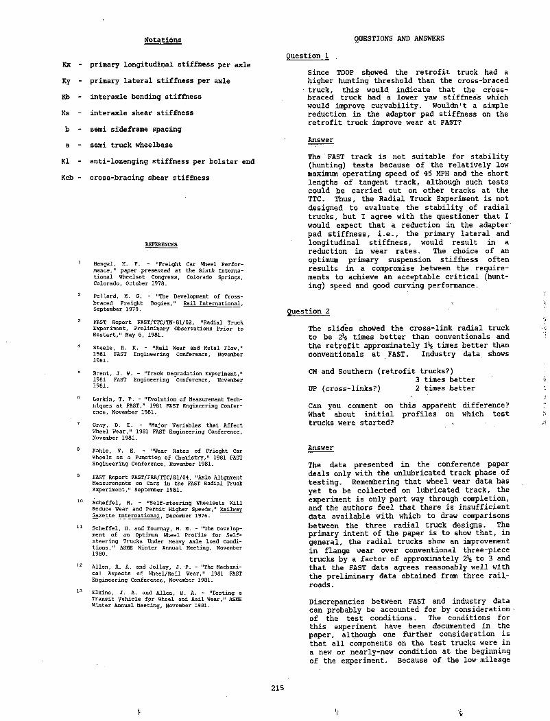
Notations QUESTIONS AND ANSWERS

Kx - primary longitudinal stiffness per axle

Ky - primary lateral stiffness per axle

Kb - interaxle bending stiffness

Ks - interaxle shear stiffness

b - semi sideframe spacing

a - semi truck wheelbase

K1 - anti-lozenging stiffness per bolster end

Kcb - cross-bracing shear stiffness

Question 1

REFERENCES

1 H engal, M. F. - “ F re ig h t Car Wheel P e r fo r ­m ance," paper presented a t the S ix th In tern a ­t io n a l W heelset C on gress, C olorado S prin gs, C o lo ra d o , O ctober 1978.

2 P o l la r d , M. G. - "The Development o f C ross- b ra ced F re ig h t B o g ie s ," R a il I n te r n a t io n a l , September 1979.

3 FAST R ep ort FAST/TTC/TN-61/02, "R a d ia l Truck E xperim ent, P re lim in a ry O bservation s P r io r to R e s t a r t , " May 6 , 1981.

4 S t e e le , R. K. - "R a il Wear and Metal F low ," 1981 FAST E n gin eering C on feren ce , November 1981.

5 B ren t, J . W. - "T rack D egradation Experim ent," 1981 FAST E n gin eerin g C on ference, November 1981.

6 L a rk in , T . P. - "E v o lu t io n o f Measurement Tech­n iq u es a t FAST," 1981 FAST E n gin eering C on fer­e n ce , November 1981.

7 G ray, D. E. - "M ajor V a ria b le s th at A f fe c t Wheel W ear," 1981 FAST E n gin eerin g C on ference, November 1981.

8 K ahle, V . E. - "Wear R ates o f F riegh t Car Wheels as a F u nction o f C h em istry ," 1981 FAST E n g in eerin g C on feren ce , November 1981.

9 FAST R ep ort FAST/FRA/TTC/81/04, "A xle Alignment Measurements on Cars in the FAST R adia l Truck E xperim en t," September 1981.

10 S c h e f f e l , H. - " S e l f - s t e e r in g W heelsets W ill Reduce Wear and Perm it H igher Speeds>" Railway G azette I n t e r n a t io n a l , December 1976.

S c h e f f e l , H. and Tournay, H. M. - "The D evelop­ment o f an Optimum Wheel P r o f i l e f o r S e l f ­s t e e r in g Trucks Under Heavy A xle Load Condi­t i o n s , " ASME W inter Annual M eeting, November 1980.

A lle n , R. A. and J o l la y , J . P. - "The Mechani­c a l A sp ects o f W h eel/R a il W ear," 1981 FAST E n g in eerin g C on feren ce , November 1981.

E lk in s , J . A . and A lle n , R. A. - "T e s tin g a T ra n s it V e h ic le f o r Wheel and R a il W ear," ASME W inter Annual M eeting , November 1981.

Since TDOP showed the retrofit truck had a higher hunting threshold than the cross-braced truck, this would indicate that the cross- braced truck had a lower yaw stiffness which would improve curvability. Wouldn't a simple reduction in the adaptor pad stiffness on the retrofit truck improve wear at FAST?

Answer

The FAST track is not suitable for stability (hunting) tests because of the relatively low maximum operating speed of 45 MPH and the short lengths of tangent track, although such tests could be carried out on other tracks at the TTC. Thus, the Radial Truck Experiment is not designed to evaluate the stability of radial trucks, but I agree with the questioner that I would expect that a reduction in the adapter pad stiffness, i.e., the primary lateral and longitudinal stiffness, would result in a reduction in wear rates. The choice of an optimum primary suspension stiffness often results in a compromise between the require­ments to achieve an acceptable critical (hunt­ing) speed and good curving performance.

Question 2

The slides showed the cross-link radial truck to be 2h times better than conventional and the retrofit approximately lh times better than conventionals at FAST. Industry data shows

CN and Southern (retrofit trucks?)3 times better

UP (cross-links?) 2 times better

Can you comment on this apparent difference? What about initial profiles on which test trucks were started?

Answer

The data presented in the conference paper deals only with the unlubricated track phase of testing. Remembering that wheel wear data has yet to be collected on lubricated track, the experiment is only part way through completion, and the authors feel that there is insufficient data available with which to draw comparisons between the three radial truck designs. The primary intent of the paper is to show that, in general, the radial trucks show an improvement in flange wear over conventional three-piece trucks by a factor of approximately 2% to 3 and that the FAST data agrees reasonably well with the preliminary data obtained from three rail­roads .

Discrepancies between FAST and industry data can probably be accounted for by consideration of the test conditions. The conditions for this experiment have been documented in, the paper, although one further consideration is that all components on the test trucks were in a new or nearly-new condition at the beginning of the experiment. Because of the low mileage

215

V t

accrued during this portion of the experiment, truck component wear was minimal. For a given amount of wheel wear, truck component wear in normal service would be considerably greater than that experienced during this experiment. Thus, the effect of increased truck clearances due to component wear, particularly those components which control truck squaring on conventional trucks, have not been accounted for in this experiment.

The questioner's assumption that CN has re­trofit radial trucks in their test consist is correct, but Southern Railway has a mixture of both retrofit and diagonal cross-link radial trucks. The UP data, for diagonal cross-links, indicates an improvement of at least two times, and probably more, over conventional trucks.

As described in the text, the wheels on the diagonal cross-link trucks were turned to a special high conicity profile whereas those on all other test trucks had the standard AAR 1 in 20 profile. These profiles were the result of decisions made by the manufacturers prior to the test, and the effects of wheel profiles on the curving performance of radial trucks is of considerable interest to the industry. A new "mini-test" experiment, described in the paper entitled "Radial Truck Curving Performance Evaluation," will be carried out at FAST in early 1982 which should provide data with which to assess this effect.

216

■1 i

THE MECHANICAL ASPECTS OF WHEEL/RAIL WEAR

Roy A. AllenExperiment Manager, Radial Trucks Association of American Railroads

James P. Jollay Engineer

Boeing Services International, Inc.

Wheel/rail lateral load and angle of attack data obtained from two "short-term" experiments on FAST are used to examine their applicability to predict wheel flange wear measured bn two long-term wheel wear experiments. The data suggests that the product of lateral load and angle of attack, while not being directly proportional to wheel wear, is a reasonable predictor of the flange wear data examined. The data presented should provide for further detailed examination of wear indices which have been proposed in the past. The data also indicates that neither the presence of rail gage-face lubrication, nor varying axle load, has much effect on the magnitude of the axle angles of attack and only the latter has a definite effect of the magni­tude of the lateral loads for conventional three-piece trucks.

INTRODUCTION

The wear of wheels and rails, in particular wheel flange and rail gage face wear, represents a sub­stantial portion of expenditure to railroads, par­ticularly with the fairly recent introduction of unit trains and increases in car capacity and motive power output. On a world-wide basis, many research organizations associated with railroads, their suppliers, and government agencies have sought a better understanding of the wheel/rail interface phenomena, all with common goals to increase rail­roads' safety and efficiency and to reduce wheel and rail wear.

There are many kinds of wear mechanisms and the interaction and influence of many different factors creates a very complex problem to those researchers studying the1 phenomenon. The list of factors af­fecting wheel and rail wear is exhaustive but can be divided into three major categories,- i.e., mechani­cal, metallurgical, and the external environment. Within the mechanical group, such factors as oper­ating conditions (traffic density, speed, braking characteristics, etc.), wheel/rail contact area geometry, creepage, and contact stresses exist. The metallurgical group contains such effects as wheel and rail hardness and chemistry content, heat treat­ment and microstructure, and within the external environment the effects of track lubrication and relative humidity exist.

Much work has been, and continues to be, carried out in this field although most literature on the sub­ject results from laboratory testing. Relatively little field work has been carried out partly be­cause of the high cost associated with this type of testing but also because of the difficulty in achieving a controlled wear environment in the "real

world". For instance, when studying rail wear in service, the data can be very difficult to analyze because of the wide variety of vehicles, axle load­ings, etc. and also because the external environment is rarely constant. Similarly, wheel wear data is confounded by changes in the external environment, varying rail metallurgies and the fact that vehicles typically encounter a wide range of track curva­tures. Although it is not perfect for this type of research, FAST provides a more controlled environ­ment than most real world situations and thus lends itself better to this type of investigation. Conse­quently, the FAST program has begun to investigate the wheel/rail wear phenomenon. Steele1 has inves­tigated some of the metallurgical and external environment factors, particularly the effects of wheel/rail hardness and track lubrication, and this paper examines some of the mechanical factors.

Thus the metallurgical and external environment factors play an important role in the wheel and rail wear, and the phenomenon is complex. However, it would be extremely important, particularly to truck designers, to be able to relate wheel and rail wear, for a given set of metallurgical and external envi­ronment conditions, to the mechanical parameters associated with the wheel/rail interaction. With this in mind, a number of "wear index" formulae have been proposed and, in some cases, used as predictors of wheel and/or rail wear but with little full-size experimental data to determine their validity. This paper describes some data obtained from FAST which can be used to determine the applicability of these wear indices to the prediction of flange wear. Data from two short-term experiments, the Wheel/Rail Loads Test and the Wear Index experiment are com­pared with flange wear data from the long-term Variable Axle Load and Radial Truck experiments.

217

V

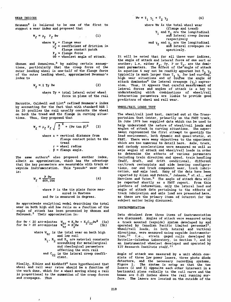
WEAR INDICES

Heumann2 is believed to be one of the first to suggest a wear index and proposed that

Wf « |Jf Ff 0w (1)

where W_ = flange wearp = coefficient of friction in

flange contact patch = flange force

0w = wheelset angle of attack.

Ghonem and Gonsalves,3 by making certain assump­tions, particularly that the creep force of the outer leading wheel is one-half of the flange force of the outer leading wheel, approximated Heumman's index to

W f «. 2 Ty 0w (2)

where Ty = total lateral outer wheel force in plane of the rail

Marcotte, Caldwell and List4 refined Heumann1s index by accounting for the fact that with standard AAR 1 in 20 profiles the rail usually contacts the wheel on both the tread and the flange in curving situa­tions. Thus, they proposed that

w f “ Mf Ff / f 2 + (0wtanp)2 (3)where a = vertical distance from

flange contact point to the tread

r = wheel radius P = flange angle.

The same authors4 also proposed another index, albeit an approximation, which has the advantage that the key parameters are measurable with track or wayside instrumentation. This "pseudo" wear index is:

Wfa _ P _ 0 w _

809,350 (4)

where P is the tie plate force mea­sured in Newtons

and 0w is measured in degrees.

An approximate analytical model describing the total wear on both high and low rails as a function of the angle of attack has been presented by Ghonem and Kalousek.5 Their approximation is:

for 0w < 20 arc-minutes W. « K,0w + K_C_„0w2 (5a)for 0w > 20 arc-minutes « K^Ow ^ (5b)

where is the total wear on both high and low rail

K1 ' K2 an0 K3 are n,ateriai constants accounting for metallurgical and rheological parameters affecting the worn rail

and C22 is the lateral creep coeffi­cient .

Finally, Elkins and Eickhoff6 have hypothesised that wheel and rail wear rates should be a function of the work done, which for a wheel moving along a rail is proportional to the summation of the creep forces and creepages. Thus

where Ww is the total wheel wear (flange and tread)

T^ and T2 are the longitudinal ana lateral creep forces respectively

and y2 and y2 are the longitudinal ana lateral creepages re­spectively.

It will be noted that for all these wear indices, the angle of attack and lateral force of one sort or another,- i.e, either F_, Ty, P or T2 , are the domi­nant parameters. The effect of the angle of attack in equation 6 may not be readily apparent but T2 typically is much larger than T1 for bad curvingf high wear situations and of course the angle of attack dominates6 the lateral creepage (y„) expres­sion. Thus, it appears that careful measurement of lateral forces and angles of attack is a key to understanding which combinations of wheel/rail interaction parameters are liable to provide good predictors of wheel and rail wear.

WHEEL/RAIL LOADS TEST

Ww « Ti Yl + T2 y2 (6)

The wheel/rail load test, carried out at the Trans­portation Test Center, primarily on the FAST track, in June 1979 has supplied data which can be used to help understand the nature of wheel/rail loads and angles of attack in curving situations. The exper­iment represented the first attempt to quantify the load environment, both dynamic and quasi-static, at FAST. There were many objectives to the experiment which are too numerous to detail here. Axle, truck, and carbody accelerations were measured as well as axle angles of attack and wheel/rail loads in order to determine the effects of various parameters including train direction and speed, train handling (buff, draft, and drift conditions), different car/truck centerplate and side bearing configura­tions, car and truck component wear, track lubri­cation, and axle load. Many of the data have been reported by Allen and Peters,7 Johnson,8 et.al., and Harrison and Tuten.9 The angle of attack data will be reported shortly as a FAST report. From this plethora of information, only the lateral load and angle of attack data pertaining to the effects of track lubrication and axle load are presented here, as these are the primary items of interest for the subject matter being discussed.

INSTRUMENTATION

Data obtained from three items of instrumentation are discussed. Angles of attack were measured using a track mounted (wayside) system developed by and operated by Canadian Pacific Limited personnel5 . Wheel/rail loads, in both lateral and vertical directions, were measured using wayside instrumenta­tion,-10 i.e., strain gaged rails developed by Battelle— Columbus Laboratory, in Section 7, and by an instrumented wheelset developed and operated by IIT Research Institute staff.11

Angle of attack was measured by a unit which con­sists of three low power lasers, three photo diode detectors, and the necessary recording systems. Figure 1. The system is setup so that the two lasers (2 and 3) opposite each other intersect in a horizontal plane radially to the rail curve and the beams are 0.25 inches above the rail running sur­face. The lasers are located on the outside of the

218

I

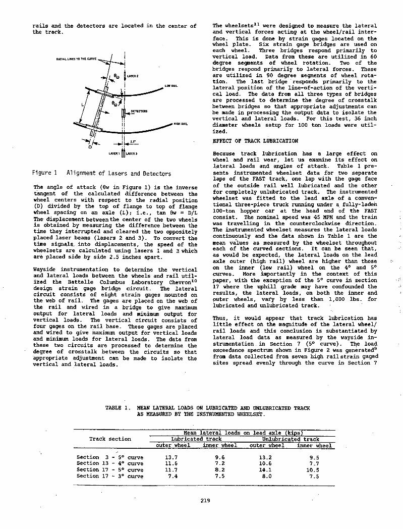
rails and the detectors are located in the center of the track.

F ig u re 1 A lig n m e n t o f Lasers and D e te c to rs

The angle of attack (0w in Figure 1) is the inverse tangent of the calculated difference between the wheel centers with respect to the radial position (D) divided by the top of flange to top of flange wheel spacing on an axle (L); i.e.( tan 0w = D/L The displacement between the center of the two wheels is obtained by measuring the difference between the time they interrupted and cleared the two oppositely placed laser beams (lasers 2 and 3). To convert the time signals...into displacements, the speed of the wheelsets are calculated using lasers 1 and 3 which are placed side by side 2.5 inches apart.

Wayside instrumentation to determine the vertical and lateral loads between the wheels and rail util­ized the Battelle Columbus Laboratory Chevron10 design strain gage bridge circuit. The lateral circuit consists of eight strain gages mounted on the web of rail. The gages are placed on the web of the rail and wired in a bridge to give maximum output for lateral loads and minimum output for vertical loads. The vertical circuit consists of four gages on the rail base. These gages are placed and wired to give maximum output for vertical loads and minimum loads for lateral loads. The data from these two circuits are processed to determine the degree of crosstalk between the circuits so that appropriate adjustment can be made to isolate the vertical and lateral loads.

The wheelsets11 were designed to measure the lateral and vertical forces acting at the wheel/rail inter­face. This is done by strain gages located on the wheel plate. Six strain gage bridges are used on each wheel. Three bridges respond primarily to vertical load. Data from these are utilized in 60 degree segments of wheel rotation. Two of the bridges respond primarily to lateral forces. These are utilized in 90 degree segments of wheel rota­tion. The last bridge responds primarily to the lateral position of the line-of-action of the verti­cal load. The data from all three types of bridges are processed to determine the degree of crosstalk between bridges so that appropriate adjustments can be made in processing the output data to isolate the vertical and lateral loads. For this test, 36 inch diameter wheels setup for 100 ton loads were util­ized.EFFECT OF TRACK LUBRICATION

Because track lubrication has a large effect on wheel and rail wear, let us examine its effect on lateral loads and angles of attack. Table 1 pre­sents instrumented wheelset data for two separate laps of the FAST track, one lap with the gage face of the outside rail well lubricated and the other for completely unlubricated track. The instrumented wheelset was fitted to the lead axle of a conven­tional three-piece truck running under a fully-laden 100-ton hopper car at the head end of the FAST consist. The nominal speed was 45 MPH and the train was travelling in the counterclockwise direction. The instrumented wheelset measures the lateral loads continuously and the data shown in Table 1 are the mean values as measured by the wheelset throughout each of the curved sections. It can be seen that, as would be expected, the lateral loads on the lead axle outer (high rail) wheel are higher than those on the inner (low rail) wheel on the 4° and 5° curves. More importantly in the context of this paper, with the exception of the 5° curve in section 17 where the uphill grade may have confounded the results, the lateral loads, on both the inner and outer wheels, vary by less than 1,000 lbs. for lubricated and unlubricated track.

Thus, it would appear that track lubrication has little effect on the magnitude of the lateral wheel/ rail loads and this conclusion is substantiated by lateral load data as measured by the wayside in­strumentation in Section 7 (5° curve). The load exceedance spectrum shown in Figure 2 was generated9 from data collected from seven high rail strain gaged sites spread evenly through the curve in Section 7

TABLE 1. MEAN LATERAL LOADS ON LUBRICATED AND UNLUBRICATED TRACK AS MEASURED BY THE INSTRUMENTED WHEELSET.

Track sectionMean lateral loads on lead axle (kips)________

Lubricated track Unlubricated trackouter wheel inner wheel outer wheel inner wheel

Section 3 - 5 ° curve 13.7 9.6 13.2 9.5Section 13 - 4° curve 11.6 7.2 10.6 7.7Section 17 - 5° curve 11.7 8.2 14.1 10.5Section 17 - 3° curve 7.4 7.5 8.0 7.5

219

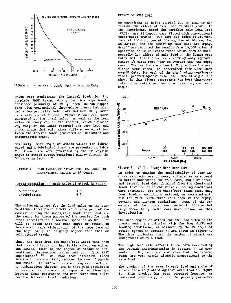
HIGH RAIL LATERAL LOAD

F ig u re 2 W h e e l/R a il Loads T e s t - W ayside Data

EFFECT OF AXLE LOAD

An experiment is being carried out on FAST to de­termine the effect of axle load on wheel wear. In the experiment, named the Variable Axle Load Test (VALT), are 16 hopper cars fitted with conventional three-piece trucks. Two cars are laden at 110-ton, four at 100-ton, two at 80-ton, two at 66-ton, two at 33-ton, and the remaining four cars are empty. Gray13 has reported the results from 14,000 miles of operation on unlubricated track which show an unex­pectedly low effect of axle load on the flange wear rates with the 100-ton cars showing only approxi­mately lh times more wear on average than the empty cars. The results are shown in Figure 3 as the mean flange wear rates, as determined from wheel snap gage12 data, for each of the six loading configura­tions, plotted against axle load. The straight line shown in this Figure represents the best character­istic line determined using a least square tech­nique .

which were monitoring the lateral loads for the complete FAST train, which, for this experiment, consisted primarily of fully laden 100-ton hopper cars with conventional three-piece trucks but also had a few partially laden cars and some fully laden cars with radial trucks. Figure 2 includes loads generated by the trail axles, as well as the lead axles on every car in the consist, which explains why many of the loads recorded are very low, and shows again that only minor differences exist be­tween the lateral loads generated on lubricated and unlubricated track.

Similarly, mean angle of attack values for lubri­cated and unlubricated track are presented in Table 2. These data were generated by the CP wayside angle of attack system positioned midway through the 5° curve in Section 7.

TABLE 2. MEAN ANGLES OF ATTACK FOR LEAD AXLES OF CONVENTIONAL TRUCKS ON 5° CURVE.

Track condition Mean anqle of attack (:m rads)

Lubricated 4.9Unlubricated 4.3

The values shown are for the lead axles on the con-ventional three-piece trucks which were part of the consist during the wheel/rail loads test, and are the means for three passes of the consist for each track condition at a nominal speed of 45 MPH. It will be noted that the mean angle of attack on lubricated track (lubrication of the gage face of the high rail) is slightly higher than that on unlubricated track.

Thus, the data from the wheel/rail loads test show that track lubrication has little effect on either the lateral loads or the angles of attack on con­ventional three-piece trucks and yet, from FAST experiments1 12, we know that effective track lubrication substantially reduces the wear of wheels and rails. If lateral loads and angles of attack, or combinations thereof are in fact good predictors of wear, it is obvious that separate relationships between these parameters and wear rates must exist for the different track conditions.

.020 -

oLo

DRY TRACK

X

X

X __X

Empty

20,000

33 66 80 100 110Ion

J ______ l

ton

_______1__

Ion

1 i

IonI

Ion

_ 1 _40.000 60.000

AXLE LOAD (Ib i)

F ig u re 3 VALT - F lan ge Wear R ate Data In order to examine the applicability of wear in­dices as predictors of wear, and also as an attempt to better understand the VALT data, angle of attack and lateral load data obtained from the wheel/rail loads test for different vehicle loading conditions were examined. For the wheel/rail loads test, only four loading conditions existed, as compared with six for VALT, with three cars each in the empty, 66-ton, and 110-ton conditions. Most of the re­mainder of the consist was loaded to 100-ton but only three fully laden cars were chosen for this investigation.

The mean angles of attack for the lead axles of the trucks under the vehicles with the four different loading conditions, as measured by the CP angle of attack system in Section 7, are shown in Figure 4. The data indicates that the angles of attack are independent of axle load.

The high lead axle lateral force data measured by the wayside instrumentation in Section 7, is pre­sented in Figure 5 and indicates that the lateral loads are very nearly directly proportional to the., axle load. ■ .' 1

The product of the mean lateral load and angle of attack is also plotted against axle load in Figure 6. This product has been computed because, as discussed previously, it is the primary parameter

220

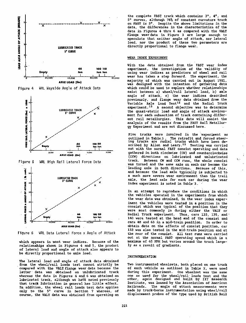
I-z<

a3

EmptyI i

LUBRICATED TRACK 5° CURVE

66ten

j ______L

100 110 Ion IonI— L

A X U LOAD (lbs)

F ig u re 4 WRL W ayside A n g le o f A tta c k Data

xs’ •

23SIfi

/ (LUBRICATED TRACK ^

5° CURVE xX . /

X

/ / / Empty66ten

100 noten ton

20,000 4 0.000 60,000 60,000AXLE LOAD (Ibt)

F ig u re 5 WRL H igh R a il L a te r a l Force Data

bA

! "

LUBRICATED TRACK 5° CURVE

Im p ly__L

66tenI

100 110 ten ten

_ |__ L_20,000 40,000 60^000

AXU LOAD (lbs)

F ig u re 6 WRL D ata L a te r a l F orce x A ngle o f A tta c k

which appears in most wear indices. Because of the relationships shown in Figures 4 and 5, the product of lateral load and angle of attack also appears to be directly proportional to axle load.

The lateral load and angle of attack data obtained from the wheel/rail loads test cannot strictly be compared with the VALT flange wear data because the latter data was obtained on unlubricated track whereas the data in Figures 4 and^ 6 was obtained on lubricated track, although we have noted previously that track lubrication in general has little effect. In addition, the wheel rail loads test data applies only to the 5° curve in Section 7 whereas, of course, the VALT data was obtained from operating on

the complete FAST track which contains 3°, 4°, and 5° curves, although 76% of constant curvature track on FAST is 5°. Despite the above limitations in the data, the differences in the characteristics of the data in Figures 4 thru 6 as compared with the VALT flange wear data in Figure 3 are large enough to speculate that neither angle of attack, nor lateral load, nor the product of these two parameters are directly proportional to flange wear.

WEAR INDEX EXPERIMENT

With the data obtained from the FAST wear index experiment, the investigation of the validity of using wear indices as predictors of wheel and rail wear has taken a step forward. The experiment, the majority of which was carried out in August 1981, was designed with the intention of gathering data which could be used to explore whether relationships exist between a) wheel/rail lateral load, b) axle angle of attack, c) the wear indices described previously, and flange wear data obtained from the Variable Axle Load Test12 and the Radial Truck experiment.13 A second objective was to determine the quasi-static load and angle of attack environ­ment for each subsection of track containing differ­ent rail metallurgies. This data will assist the analysis of the results from the FAST Rail Metallur­gy Experiment and are not discussed here.

Five trucks were involved in the experiment as outlined in Table,3 . The retrofit and forced steer­ing trucks are radial trucks which have been de­scribed by Allen and Leary.13 Testing was carried out with the normal FAST consist operating and data gathered in both clockwise (CW) and counterclockwise (CCW) directions on lubricated and unlubricated track. Between CW and CCW runs, the whole consist was turned and the same axle on each car became the leading axle in both directions. Because of this, and because the lead axle typically is subjected to a much more severe wear environment than the trail axle, the lead axle for each car during the wear index experiment is noted in Table'3. '

In an attempt to reproduce the conditions in which the vehicles operated in the experiments from which the wear data was obtained, in the wear index exper­iment the vehicles were tested in a position in the consist which was typical of the position that they were most commonly in during either the VALT or Radial Truck experiment. Thus, cars 133, 139, and" 140 were tested at the head end of the consist and cars 48 and 63 in a mid-train position. In order to obtain data on the effects of consist position, car 133 was also tested in the mid-train position and at the rear of the consist. All test runs were carried out at the normal FAST operating speed which is a maximum of 45 MPH but varies around the track large­ly as a result of gradients.

INSTRUMENTATION

Two instrumented wheelsets, both placed on one truck of each vehicle as outlined in Table .3 , were used during this experiment. One wheelset was the same one as used for the wheel/rail loads test and the other, again designed and built by IIT Research Institute, was loaned by the Association of American Railroads. The angle of attack measurements were made by truck-borne instrumentation using wheel/rail displacement probes of the type used by British Rail

221

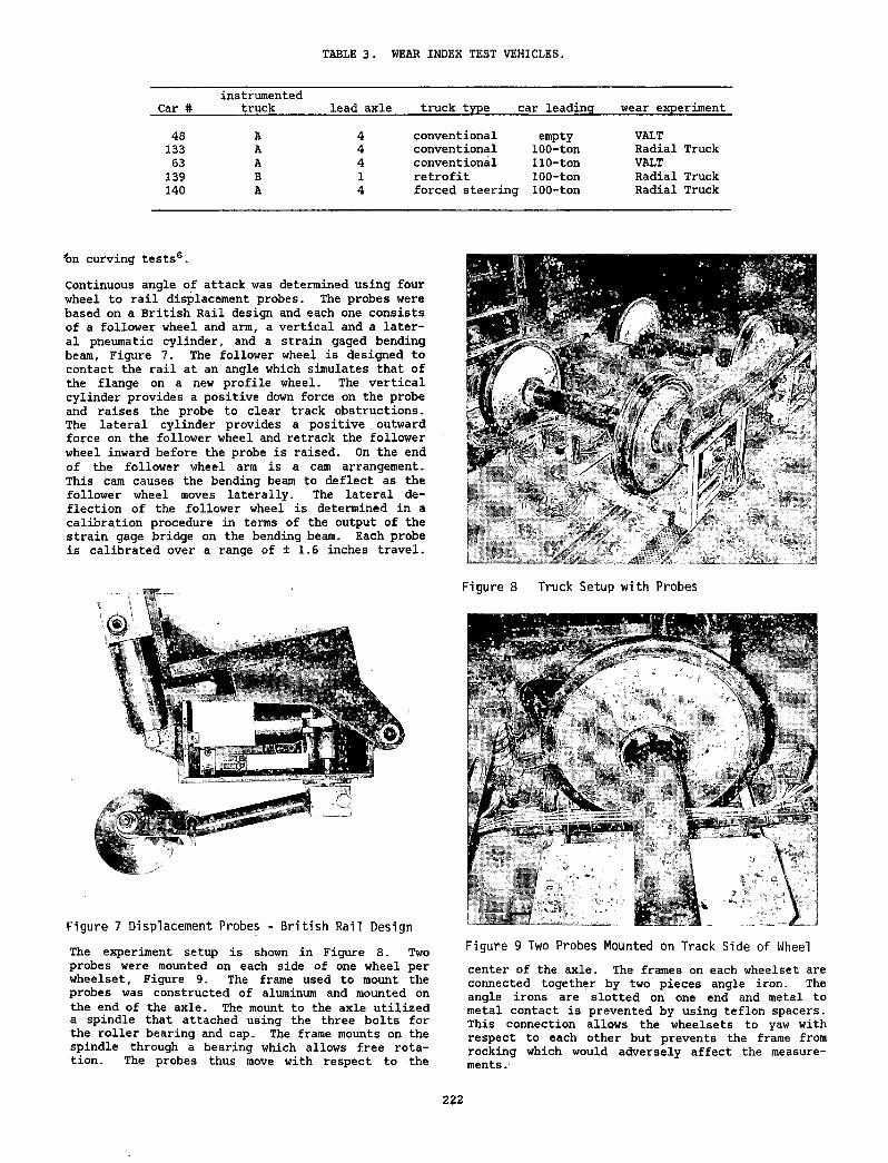
TABLE 3. WEAR INDEX TEST VEHICLES.

Car #instrumented

truck lead axle truck type car leading wear experiment

48 A 4 conventional empty VALT133 A 4 conventional 100-ton Radial Truck63 A 4 conventional 110-ton VALT

139 B 1 retrofit 100-ton Radial Truck140 A 4 forced steering 100-ton Radial Truck

’bn curving tests6 .

Continuous angle of attack was determined using four wheel to rail displacement probes. The probes were based on a British Rail design and each one consists of a follower wheel and arm, a vertical and a later­al pneumatic cylinder, and a strain gaged bending beam, Figure 7. The follower wheel is designed to contact the rail at an angle which simulates that of the flange on a new profile wheel. The vertical cylinder provides a positive down force on the probe and raises the probe to clear track obstructions. The lateral cylinder provides a positive outward force on the follower wheel and retrack the follower wheel inward before the probe is raised. On the end of the follower wheel arm is a cam arrangement. This cam causes the bending beam to deflect as the follower wheel moves laterally. The lateral de­flection of the follower wheel is determined in a calibration procedure in terms of the output of the strain gage bridge on the bending beam. Each probe is calibrated over a range of ± 1.6 inches travel.

F ig u re 7 D is p lac em e n t Probes - B r i t is h R a il D esign

The experiment setup is shown in Figure 8. Two probes were mounted on each side of one wheel per wheelset. Figure 9. The frame used to mount the probes was constructed of aluminum and mounted on the end of the axle. The mount to the axle utilized a spindle that attached using the three bolts for the roller bearing and cap. The frame mounts on the spindle through a bearing which allows free rota­tion. The probes thus move with respect to the

F ig u re 8 T ru ck Setup w ith Probes

F ig u re 9 Two Probes Mounted on T ra ck S id e o f Wheel

center of the axle. The frames on each wheelset are connected together by two pieces angle iron. The angle irons are slotted on one end and metal to metal contact is prevented by using teflon spacers. This connection allows the wheelsets to yaw with respect to each other but prevents the frame from rocking which would adversely affect the measure­ments.

222

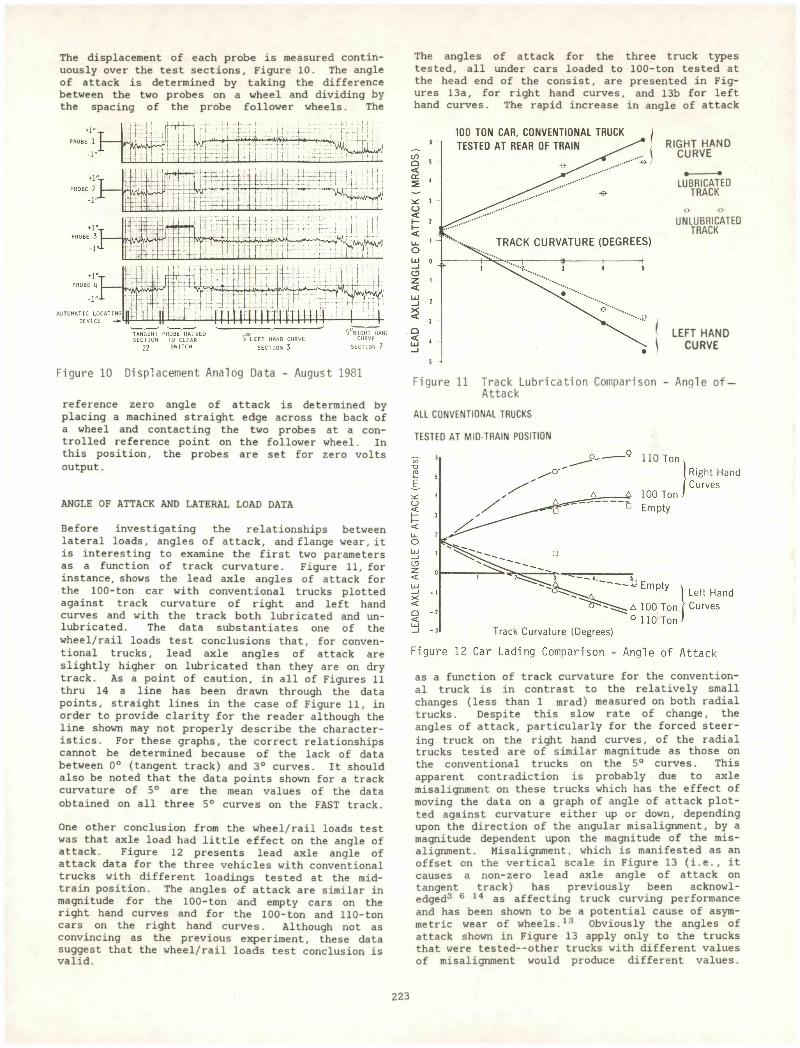
The displacement of each probe is measured contin­uously over the test sections, Figure 10. The angle of attack is determined by taking the difference between the two probes on a wheel and dividing by the spacing of the probe follower wheels. The

The angles of attack for the three truck types tested, all under cars loaded to 100-ton tested at the head end of the consist, are presented in Fig­ures 13a, for right hand curves, and 13b for left hand curves. The rapid increase in angle of attack

RIGHT H A N D C U R V E

Figure 10 Displacement Analog Data - August 1981Figure 11 Track Lubrication Comparison

Attack

LUBRICATEDTRACK

UNLUBRICATEDTRACK

LEFT H A N D C U R V E

Angle of —

reference zero angle of attack is determined by placing a machined straight edge across the back of a wheel and contacting the two probes at a con­trolled reference point on the follower wheel. In this position, the probes are set for zero volts output.

ANGLE OF ATTACK AND LATERAL LOAD DATA

Before investigating the relationships between lateral loads, angles of attack, and flange wear, it is interesting to examine the first two parameters as a function of track curvature. Figure 11, for instance, shows the lead axle angles of attack for the 100-ton car with conventional trucks plotted against track curvature of right and left hand curves and with the track both lubricated and un­lubricated. The data substantiates one of the wheel/rail loads test conclusions that, for conven­tional trucks, lead axle angles of attack are slightly higher on lubricated than they are on dry track. As a point of caution, in all of Figures 11 thru 14 a line has been drawn through the data points, straight lines in the case of Figure 11, in order to provide clarity for the reader although the line shown may not properly describe the character­istics. For these graphs, the correct relationships cannot be determined because of the lack of data between 0° (tangent track) and 3° curves. It should also be noted that the data points shown for a track curvature of 5° are the mean values of the data obtained on all three 5° curves on the FAST track.

One other conclusion from the wheel/rail loads test was that axle load had little effect on the angle of attack. Figure 12 presents lead axle angle of attack data for the three vehicles with conventional trucks with different loadings tested at the mid­train position. The angles of attack are similar in magnitude for the 100-ton and empty cars on the right hand curves and for the 100-ton and 110-ton cars on the right hand curves. Although not as convincing as the previous experiment, these data suggest that the wheel/rail loads test conclusion is valid.

ALL CONVENTIONAL TRUCKS

TESTED AT MID-TRAIN POSITION

as a function of track curvature for the convention­al truck is in contrast to the relatively small changes (less than 1 mrad) measured on both radial trucks. Despite this slow rate of change, the angles of attack, particularly for the forced steer­ing truck on the right hand curves, of the radial trucks tested are of similar magnitude as those on the conventional trucks on the 5° curves. This apparent contradiction is probably due to axle misalignment on these trucks which has the effect of moving the data on a graph of angle of attack plot­ted against curvature either up or down, depending upon the direction of the angular misalignment, by a magnitude dependent upon the magnitude of the mis­alignment. Misalignment, which is manifested as an offset on the vertical scale in Figure 13 (i.e., it causes a non-zero lead axle angle of attack on tangent track) has previously been acknowl­edged3 6 14 as affecting truck curving performance and has been shown to be a potential cause of asym­metric wear of wheels.13 Obviously the angles of attack shown in Figure 13 apply only to the trucks that were tested--other trucks with different values of misalignment would produce different values.

223

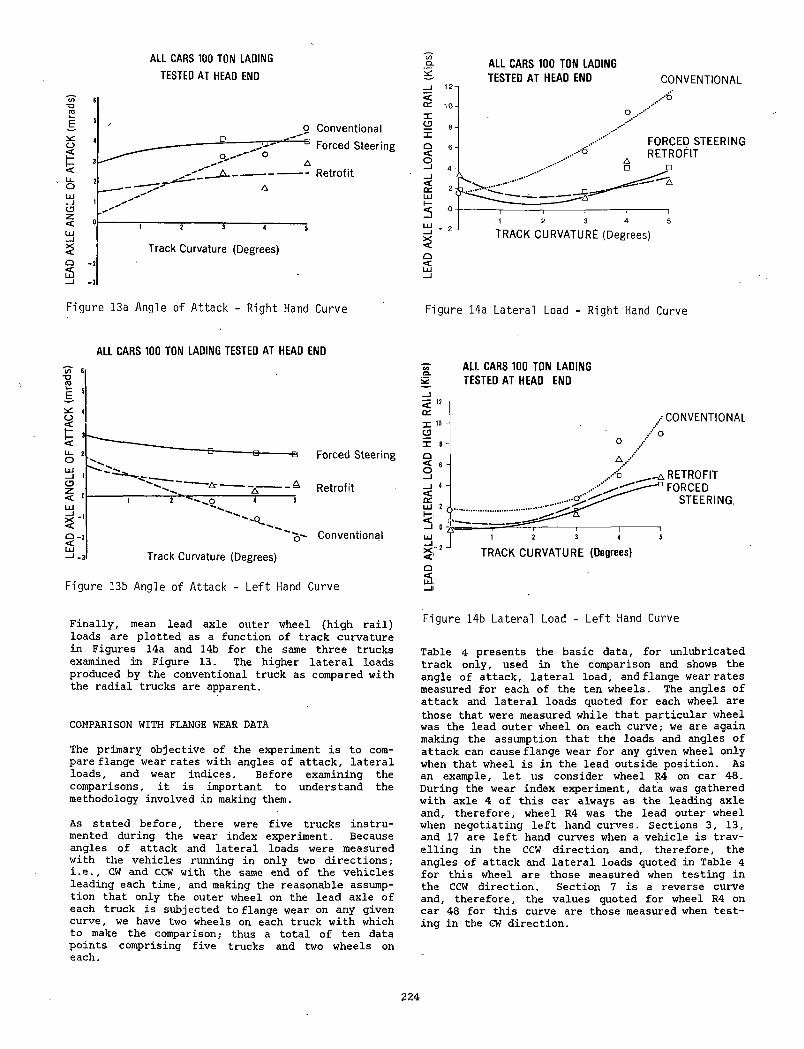
LEAD

AXL

E AN

GLE

OF

ATTA

CK (

mra

ds)

-n

LEAD

AXL

E AN

GLE

OF

ATTA

CK (

mra

ds)

ALL CARS 100 TON LADING TESTED AT HEAD END

.9- ALL CARS 100 JON LADING— TESTED AT HEAD END CONVENTIONAL

Q<

F ig u re 14a L a te ra l Load - R ig h t Hand Curve

ALL CARS 100 TON LADING TESTED AT HEAD END

Forced Steering

Retrofit

Ty- Conventional

F ig u re 13b A ngle o f A tta c k - L e f t Hand Curve

ALL CARS 100 TON LADING 2 TESTED AT HEAD END

Finally, mean lead axle outer wheel (high rail) loads are plotted as a function of track curvature in Figures 14a and 14b for the same three trucks examined in Figure 13. The higher lateral loads produced by the conventional truck as compared with the radial trucks are apparent.

COMPARISON WITH FLANGE WEAR DATA

The primary objective of the experiment is to com­pare flange wear rates with angles of attack, lateral loads, and wear indices. Before examining the comparisons, it is important to understand the methodology involved in making them.

As stated before, there were five trucks instru­mented during the wear index experiment. Because angles of attack and lateral loads were measured with the vehicles running in only two directions ; i.e., CW and CCW with the same end of the vehicles leading each time, and making the reasonable assump­tion that only the outer wheel on the lead axle of each truck is subjected to flange wear on any given curve, we have two wheels on each truck with which to make the comparison; thus a total of ten data points comprising five trucks and two wheels on each.

F ig u re 14b L a te ra l Load - L e f t Hand Curve

Table 4 presents the basic data, for unlubricated track only, used in the comparison and shows the angle of attack, lateral load, and flange wear rates measured for each of the ten wheels. The angles of attack and lateral loads quoted for each wheel are those that were measured while that particular wheel was the lead outer wheel on each curve; we are again making the assumption that the loads and angles of attack can cause flange wear for any given wheel only when that wheel is in the lead outside position. As an example, let us consider wheel R4 on car 48. During the wear index experiment, data was gathered with axle 4 of this car always as the leading axle and, therefore, wheel R4 was the lead outer wheel when negotiating left hand curves. Sections 3, 13, and 17 are left hand curves when a vehicle is trav­elling in the CCW direction and, therefore, the angles of attack and lateral loads quoted in Table 4 for this wheel are those measured when testing in the CCW direction. Section 7 is a reverse curve and, therefore, the values quoted for wheel R4 on car 48 for this curve are those measured when test­ing in the CW direction.

224

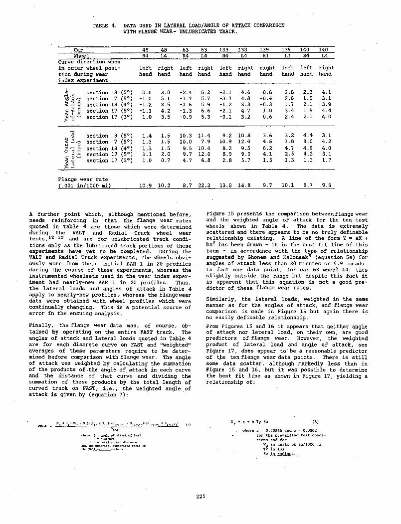
TABLE 4. DATA USED IN LATERAL LOAD/ANGLE OF ATTACK COMPARISON WITH FLANGE WEAR- UNLUBRICATED TRACK.

Car 48 48 63 63 133 133 139 139 140 140Wheel R4 L4 R4 L4 R4 L4 R1 ,L1 R4 L4

Curve direction whenin outer wheel posi­tion during wear index experiment

lefthand

righthand

lefthand

righthand

lefthand

righthand

righthand

lefthand

lefthand

righthand

<D section 3 (5°) 0.0 3.0 -2.4 6.2 -2.1 4.6 0.6 2.8 2.3 4.1

Mean

Ang

l of

-Att

ac!

(mra

ds) section 7 (5°) -1.0 5.1 -1.7 5.7 -3.7 4.8 -0.4 2.6 1.5 3.1

section 13 (4°) -1.2 3.5 -1.6 5.9 -1.2 3.3 -0.3 1.7 2.1 3.9section 17 (5°) -1.1 4.2 -1.3 6.6 -2.1 4.7 1.0 3.4 1.9 4.4section 17 (3°) 1.0 3.5 -0.9 5.3 -0.1 3.2 0.6 2.4 2.1 4.0

T3cdM O (1) i-J /—■* + J CO 3 H P.

O CO *H

C3 <D cO 4->CD cO ^

section 3 (5°) 1.4 1.5 10.3 11.4 9.2 10.8 3.6 3.2 4.4 3.1section 7 (5°) 1.3 1.5 10.0 7.9 10.9 12.0 4.5 1.8 3.0 4.2section 13 (4°) 1.3 1.5 9.5 10.4 8.2 9.5 6.2 4.7 4.9 4.0section 17 (5°) 1.1 2.0 9.7 12.0 8.9 9.0 4.1 2.5 4.2 3.1section 17 (3°) 1.0 0.7 4.7 6.8 2.8 5.7 1.5 1.3 1.3 1.7

sar rate a000 mi) 10.9 10.2 8.7 22.3 13.8 14.8 9.7 10.1 8.7 9.6

A further point which, although mentioned before, needs reinforcing in that the flange wear rates quoted in Table 4 are those which were determined during the VALT and Radial Truck wheel wear tests,12 13 and are for unlubricated track condi­tions only as the lubricated track portions of these experiments have yet to be completed. During the VALT and Radial Truck experiments, the wheels obvi­ously wore from their initial AAR 1 in 20 profiles during the course of these experiments, whereas the instrumented wheelsets used in the wear index exper­iment had nearly-new AAR 1 in 20 profiles. Thus, the lateral loads and angles of attack in Table 4 apply to nearly-new profiles, whereas the flangewear data were obtained with wheel profiles which were continually changing. This is a potential source of error in the ensuing analysis.

Finally, the flange wear data was, of course, ob­tained by operating on the entire FAST track. The angles of attack and lateral loads quoted in Table 4 are for each discrete curve on FAST and "weighted" averages of these parameters require to be deter­mined before comparison with flange wear. The angle of attack was weighted by calculating the summation of the products of the angle of attack in each curve and the distance of that curve and dividing the summation of these products by the total length of curved track on FAST; i.e., the weighted angle of attack is given by (equation 7):

Figure 15 presents the comparison between flange wear and the weighted angle of attack for the ten test wheels shown in Table 4. The data is extremely scattered and there appears to be no truly definable relationship existing. A line of the form Y = aX + bXz has been drawn - it is the best fit line of this form - in accordance with the type of relationship suggested by Ghonem and Kalousek5 (equation 5a) for angles of attack less than 20 minutes or 5.9 mrads. In fact one data point, for car 63 wheel L4, lies slightly outside the range but despite this fact it is apparent that this equation is not a good pre­dictor of these flange wear rates.Similarly, the lateral loads, weighted in the same manner as for the angles of attack, and flange wear comparison is made in Figure 16 but again there is no easily definable relationship.From Figures 15 and 16 it appears that neither angle of attack nor lateral load, on their own, are good predictors of flange wear. However, . the weighted product of lateral load and angle of attack, see Figure 17, does appear to be a reasonable predictor of the ten flange wear data points. There is still some data scatter, although markedly less than in Figure 15 and 16, but it was possible to determine the best fit line as shown in Figure 17, yielding a relationship of.-

WWAoA (03 x S3)+(e? x S?)+(613 x S13)+(617(5<a) x s17(5o))*(917(3o) x Si7(3°)) (7)Stcd

where 0 = angle of attack of lead ‘S -= distance

ted = total curved distance and the numerical subscripts refer to the FAST section numbers.

= a + b Ty 0w (8 )

where a = 0 .00865 and b = 0.0002f o r the p r e v a i l in g t e s t co n d i­t io n s and f o r

W_ in u n its o f in /1 0 0 0 mi Ty in lb s 0w in ra d ia n s .

225

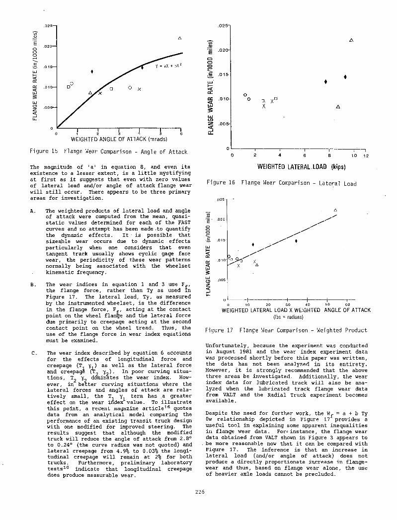
F ig u re 15 F lange Wear Comparison - A ngle o f A tta c k

.025-

oCO C D

!e .015-

<DC

DC .0 1 0 -<

.005 -

□. X

~ 1--- 110 12

The magnitude of 'a' in equation 8, and even its existence to a lesser extent, is a little mystifying at first as it suggests that even with zero values of lateral load and/or angle of attack flange wear will still occur. There appears to be three primary areas for investigation.

WEIGHTED LATERAL LOAD (kips)

F ig u re 16 F lan g e Wear Comparison - L a te r a l Load

.025 -1 "

A. The weighted products of lateral load and angle of attack were computed from the mean, quasi­static values determined for each of the FAST curves and no attempt has been made -to quantify the dynamic effects. It is possible that sizeable wear occurs due to dynamic effects particularly when one considers that even tangent track usually shows cyclic gage face wear, the periodicity of these wear patterns normally being associated with the wheelset kinematic frequency.

B. The wear indices in equation 1 and 3 use F^, the flange force, rather than Ty as used in Figure 17. The lateral load, Ty, as measured by the instrumented wheelset, is the difference in the flange force, Ff , acting at the contact point on the wheel flange and the lateral force due primarily to creepage acting at the second contact point on the wheel tread. Thus, the use of the flange force in wear index equations must be examined.

C. The wear index described by equation 6 accounts for the effects of longitudinal force and creepage (T y ) as well as the lateral force and creepage (r2 y2). In poor curving situa­tions, T2 y dominates the wear index. How­ever, in better curving situations where the lateral forces and angles of attack are rela­tively small, the T^ y^ term has a greater effect on the wear index value. To illustrate this point, a recent magazine article16 quotes data from an analytical model comparing the performance of an existing transit truck design with one modified for improved steering. The results suggest that although the modified truck will reduce the angle of attack from 2.8° to 0.24° (the curve radius was not quoted) and lateral creepage from 4.9% to 0.03% the longi­tudinal creepage will remain at 2% for both trucks. Furthermore, preliminary laboratory tests16 indicate that longitudinal creepage does produce measurable wear.

0 10 20 30 40 50 60

W E I G H T E D LATERAL L O A D X W E I G H T E D A N G L E O F A T T A C K(lbs x radians)

F ig u re 17 F lan ge Wear Comparison - W eighted P ro d u ct

Unfortunately, because the experiment was conducted in August 1981 and the wear index experiment data was processed shortly before this paper was written, the data has not been analyzed in its entirety. However, it is strongly recommended that the above three areas be investigated. Additionally, the wear index data for lubricated track will also be ana­lyzed when the lubricated track flange wear data from VALT and the Radial Truck experiment becomes available.

Despite the need for further work, the W, = a + b Ty 8w relationship depicted in Figure 17r provides a useful tool in explaining some apparent inequalities in flange wear data. For«-instance, the flange wear data obtained from VALT shown in Figure 3 appears to be more reasonable now that it can be compared with Figure 17. The inference is that an increase in lateral load (and/or angle of attack) does not produce a directly proportionate increase in flange- wear and thus, based on flange wear alone, the use of heavier axle loads cannot be precluded.

226

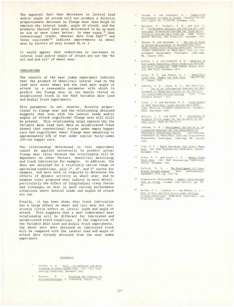
The apparent fact that decreases in lateral load and/or angle of attack will not produce a directly proportionate decrease in flange wear also helps to explain why lateral loads, angle of attack, and the products thereof have been determined to be as much as six or more times better, in some cases,3 than conventional trucks, whereas data from FAST13 and three railroads13 indicate improvements in wheel wear by factors of only around 2X1 or 3.

It would appear that reductions or increases in lateral load and/or angle of attack are not the "be all and end all" of wheel wear.

CONCLUSIONS

Ghonem, H. and Gonsalves, R. - Comparative Performance of Type II Trucks, Canadian Pacific Ltd. report No. S 576-78, November 1978.

Marcotte, P., Caldwell, W. M. , and List, H. A. - Performance Analysis and Testing of a Con­ventional Three-Piece Freight Car Truck Retro­fitted to Provide Axle Steering, ASME Winter Annual Meeting, San Francisco, December 1978.

Ghonem, H. and Kalousek, J. - The Use of Angle of Attack Measurements to Estimate Rail Wear Under Steady State Rolling Conditions, Interna­tional Conference on Wheel/Rail Load and Dis­placement Measurement Techniques, Cambridge, MA, January 1981.

Elkins, J. A. and Eickhoff, B. M. - Advances in Non-Linear Wheel/Rail Force Prediction Methods and their Validation, ASME Winter Annual Meet­ing, New York, December 1979.

The results of the wear index experiment indicate that the product of wheel/rail lateral load on the lead axle outer wheel and the lead axle angle of attack is a reasonable parameter with which to predict the flange wear on ten wheels tested on unlubricated track in the FAST Variable Axle Load and Radial Truck experiments.

This parameter is not, however, directly propor­tional to flange wear and the relationship obtained suggests that even with low lateral loads and/or angles of attack significant flange wear will still be present. This relationship helps explain why the Variable Axle Load test data on unlubricated track showed that conventional trucks under empty hopper cars had significant wheel flange wear amounting to approximately 60% of that under similar fully-laden 100-ton hopper cars.

7 Allen, R. A. and Peters, A. J. - Wheel/Rail Loads Test, Hopper Car Ride Data, FRA/TTC-80/ 07, August 1980.

8 Johnson, M. R., Joyce, R. P., and Mancillas,C . - Use of an Instrumented Wheelset for Mea­surement of Wheel/Rail Forces at the Facility for Accelerated Service Testing, Track Train Dynamics Report - 471.

9 Tuten, J. M. and Harrison, H. D. - Final Report on FAST Wheel/Rail Loads Wayside Data Reduc­tion, Battelle Columbus Laboratories, Columbus, Ohio, September 1980.

10 Me Irvin, L. L. and Graff, R. - Evaluation of Weldable Strain Gages for Use on Rails in the FAST Track, FAST/TTC/TN-80/03.

11 Johnson, M. R. - Development and Use of an In­strumented Wheelset for the Measurement of Wheel/Rail Interaction Forces, International Conference on Wheel/Rail Load and Displacement Measurement Techniques, Cambridge, MA, January 1981.

The relationship determined in this experiment cannot be applied universally to predict actual flange wear rates because the relationship will be dependent on other factors, wheel/rail metallurgy and track lubrication for example. In addition, the data was obtained for a relatively narrow range of operating conditions, only 3°, 4°, and 5° curves for example, and more work is required to determine the effects of dynamic activity on wheel wear, and to examine other proposed wear indices in more detail, particularly the effect of longitudinal creep forces and creepages on wear in good curving performance situations where lateral loads and angles of attack are low.

Finally, it has been shown that track lubrication has a large effect on wheel and rail wear but rel­atively little effect on lateral loads and angle of attack. This suggests that a wear index/wheel wear relationship will be different for lubricated and unlubricated track conditions. At the completion of the Variable Axle Load and Radial Truck experiments, the wheel wear data obtained on lubricated track will be compared with the lateral load and angle of attack data already obtained from the wear index experiment.

12 Gray, D. E. - Major Variables that Affect Wheel Wear, 1981 FAST Engineexing Conference, Denver, November 1981.

13 Allen, R. A. and Leary, J. F. - Radial Truck Wheel Wear, 1981 FAST Engineering Conference, Denver, November 1981.

14 Pollard, M. G. - The Development of Cross- Braced Freight Bogies, Rail International, September 1979, pp. 735-758.

15 Progressive Railroading - Radial Truck Designs Come on Strong, October 1981 edition, pp. 58, 60.

16 Bolton, P. J., Clayton, P., and McEwan, I. J. - Wear of Rail and Tyre Steels under Rolling/ Sliding Conditions, ASME/ASLE Conference, San Francisco, August 1980.

REFERENCES

Steele, R. K. - Rail: Its Behavior and Rela­tionship to Total System Wear, 1981 FAST Engi­neering Conference, November 1981.Heumann. H. - Grundzuqe der Fuhrunq der Schienenfahrzeuge, R. Oldenburg, Munich, .954.

22 7

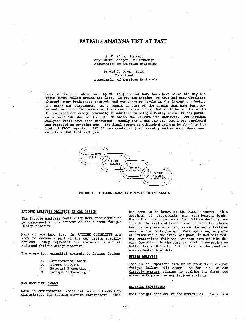
FATIGUE ANALYSIS TEST AT FAST

S. K. (John) Punwani Experiment Manager, Car Dynamics Association of American Railroads

Gerald J. Moyar, Ph.D. Consultant

Association of American Railroads

Many of the cars which make up the FAST consist have been here since the day the train first rolled around the loop. As you can imagine, we have had many wheelsets changed, many brakeshoes changed, and our share of cracks in the freight car bodies and other car components. As a result of some of the cracks that have been ob­served, we felt that some mini-tests could be conducted that would be beneficial to the railroad car design community in addition to being directly useful to the parti­cular owner/builder of the car on which the failure was observed. Two Fatigue Analysis Tests have been conducted - namely FAT I and FAT II. FAT I was completed and reported on sometime ago. The final report is published and can be found in the list of FAST reports. FAT II was conducted just recently and we will share some data from that test with you.

FIGURE 1. FATIGUE ANALYSIS PRACTICE IN CAR DESIGN

FATIGUE ANALYSIS PRACTICE IN CAR DESIGNThe fatigue analysis tests which were conducted must be discussed in the context of the current fatigue design practice.

Many of you know that the FATIGUE GUIDELINES are soon to become a part of the car design specifi­cations. They represent the state-of-the art ofrailroad fatigue design practice.

There are four essential elements to fatigue design

a. Environmental Loadsb. Stress Analysisc. Material Propertiesd. Fatigue Methodology

ENVIRONMENTAL LOADS

Data on environmental loads are being collected to characterize the revenue service environment. This

has come to be known as the FEEST program. This consists of centerplate and side bearing loads. Some of you veterans know that fatigue design prac­tice in the railroad freight car industry has always been centerplate oriented, since the early failures were in the centerplates. Cars operating in parts of Mexico where the track was poor,, it was observed, had centerplate failures, whereas cars of like de­sign (sometimes in the same car series) operating on better track did not. This points to the need for environmental load data.STRESS ANALYSIS

This is an important element in predicting whether fatigue failure will occur. As for FAST, we can directly measure strains to combine the first two elements required in any fatigue analysis.

MATERIAL PROPERTIES

Most freight cars are welded structures. There is a

229

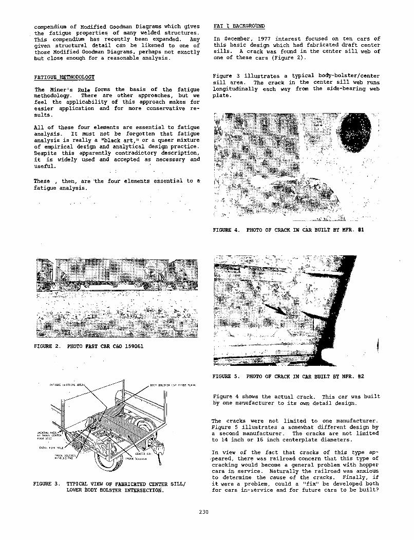
compendium of Modified Goodman Diagrams which gives the fatigue properties of many welded structures. This compendium has recently been expanded. Any given structural detail can be likened to one of those Modified Goodman Diagrams, perhaps not exactly but close enough for a reasonable analysis.

FATIGUE METHODOLOGY

The Miner's Rule forms the basis of the fatigue methodology. There are other approaches, but we feel the applicability of this approach makes for easier application and for more conservative re­sults.

All of these four elements are essential to fatigue analysis. It must not be forgotten that fatigue analysis is really a "black art," or a queer mixture of empirical design and analytical design practice. Despite this apparently contradictory description, it is widely used and accepted as necessary and useful.

These , then, are the four elements essential to a fatigue analysis.

In December, 1977 interest focused on ten cars of this basic design which had fabricated draft center sills. A crack was found in the center sill web of one of these cars (Figure 2)-

Figure 3 illustrates a typical body-bolster/center sill area. The crack in the center sill web runs longitudinally each way from the side-bearing web plate.

FAT I BACKGROUND

FIGURE 4. PHOTO OF CRACK IN CAR BUILT BY MFR. #1

FIGURE 2. PHOTO FAST CAR C&O 159061

FIGURE 3. TYPICAL VIEW OF FABRICATED CENTER SILL/ LOWER BODY BOLSTER INTERSECTION.

FIGURE 5. PHOTO OF CRACK IN CAR BUILT BY MFR. #2

Figure 4 shows the actual crack. This car was built by one manufacturer to its own detail design.

The cracks were not limited to one manufacturer. Figure 5 illustrates a somewhat different design by a second manufacturer. The cracks are not limited to 14 inch or 16 inch centerplate diameters.

In view of the fact that cracks of this type ap­peared, there was railroad concern that this type of cracking would become a general problem with hopper cars in service. Naturally the railroad was anxious to determine the cause of the cracks. Finally, if it were a problem, could a "fix" be developed both for cars in-service and for future cars to be built?

230

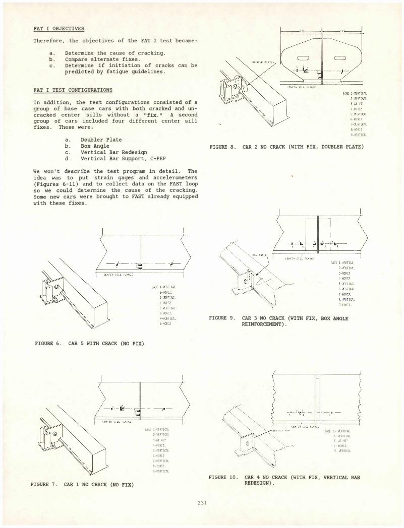
FAT I OBJECTIVES

Therefore, the objectives of the FAT I test became:

a. Determine the cause of cracking.b. Compare alternate fixes.c. Determine if initiation of cracks can be

predicted by fatigue guidelines.

FAT I TEST CONFIGURATIONS

In addition, the test configurations consisted of a group of base case cars with both cracked and un­cracked center sills without a “fix." A second group of cars included four different center sill fixes. These were:

a. Doubler Plateb . Box Anglec. Vertical Bar Redesignd. Vertical Bar Support, C-PEP

8 - H 0 R IZ

9 - VERTICAL

FIGURE 8. CAR 2 NO CRACK (WITH FIX, DOUBLER PLATE)

We won't describe the test program in detail. The idea was to put strain gages and accelerometers (Figures 6-11) and to collect data on the FAST loop so we could determine the cause of the cracking. Some new cars were brought to FAST already equipped with these fixes.

FIGURE 9. CAR 3 NO CRACK (WITH FIX, REINFORCEMENT).

BOX ANGLE

FIGURE 6. CAR 5 WITH CRACK (NO FIX)

GAGE 1-V E R TIC A L

2-V E R TIC A L

VAT 45’4 - H O R IZ .

5 - VERTICAL

6 - HORIZ

7 - VERTICAL

8 - H O R IZ .

9 - VERTICAL

FIGURE 7. CAR 1 NO CRACK (NO FIX)

GAGE 1 - VERTICAL

2 - VERTICAL3 - AT 45 °

4 - HO R IZ.

5 - VERTICAL

FIGURE 10. CAR 4 NO CRACK (WITH FIX, VERTICAL BAR REDESIGN).

231

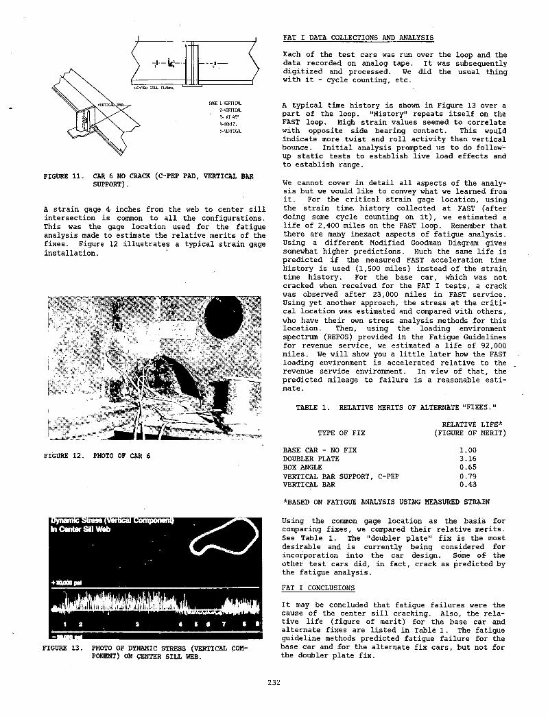
FAT I DATA COLLECTIONS AND ANALYSIS

FIGURE 11. CAR 6 NO CRACK (C-PEP PAD, VERTICAL BAR SUPPORT).

A strain gage 4 inches from the web to center sill intersection is common to all the configurations. This was the gage location used for the fatigue analysis made to estimate the relative merits of the fixes. Figure 12 illustrates a typical strain gage installation.

FIGURE 12. PHOTO OF CAR 6

FIGURE 13. PHOTO OF DYNAMIC STRESS (VERTICAL COM­PONENT) ON CENTER SILL WEB.

Each of the test cars was run over the loop and the data recorded on analog tape. It was subsequently digitized and processed. We did the usual thing with it - cycle counting, etc.

A typical time history is shown in Figure 13 over a part of the loop. "History" repeats itself on the FAST loop. High strain values seemed to correlate with opposite side bearing contact. This would indicate more twist and roll activity than vertical bounce. Initial analysis prompted us to do follow­up static tests to establish live load effects and to establish range.

We cannot cover in detail all aspects of the analy­sis but we would like to convey what we learned from it. For the critical strain gage location, using the strain time, history collected at FAST (after doing some cycle counting on it), we estimated a life of 2,400 miles on the FAST loop. Remember that there are many inexact aspects of fatigue analysis. Using a different Modified Goodman Diagram gives somewhat higher predictions. Much the same life is predicted if the measured FAST acceleration time history is used (1,500 miles) instead of the strain time history. For the base car, which was not cracked when received for the FAT I tests, a crack was observed after 23,000 miles in FAST service. Using yet another approach, the stress at the criti­cal location was estimated and compared with others, who have their own stress analysis methods for this location. Then, using the loading environment spectrum (REPOS) provided in the Fatigue Guidelines for revenue service, we estimated a life of 92,000 miles. We will show you a little later how the FAST loading environment is accelerated relative to the revenue service environment. In view of that, the predicted mileage to failure is a reasonable esti­mate.

TABLE 1. RELATIVE MERITS OF ALTERNATE "FIXES."

RELATIVE LIFE*TYPE OF FIX (FIGURE OF MERIT)

BASE CAR - NO FIX 1.00DOUBLER PLATE 3.16BOX ANGLE 0.65VERTICAL BAR SUPPORT, C-PEP 0.79VERTICAL BAR 0.43

*BASED ON FATIGUE ANALYSIS USING MEASURED STRAIN

Using the common gage location as the basis for comparing fixes, we compared their relative merits. See Table 1. The "doubler plate" fix is the most desirable and is currently being considered for incorporation into the car design. Some of the other test cars did, in fact, crack as predicted by the fatigue analysis.

FAT I CONCLUSIONS

It may be concluded that fatigue failures were the cause of the center sill cracking. Also, the rela­tive life (figure of merit)' for the base car and alternate fixes are listed in Table 1. The fatigue guideline methods predicted fatigue failure for the base car and for the alternate fix cars, but not for the doubler plate fix.

232

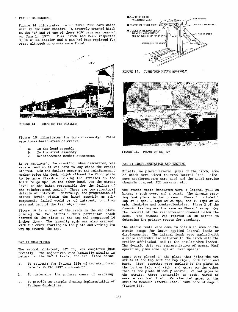
FAT II BACKGROUND

Figure 14 illustrates one of three TOFC cars which were in the FAST consist. A severely cracked hitch on the 1B 1 end of one of these TOFC cars was removed on June 1, 1979. This hitch had teen inspected 3,000 miles earlier and a pin had been replaced for wear, although no cracks were found.

FIGURE 14. PHOTO OF TTX TRAILER

Figure 15 illustrates the hitch assembly. There were three basic areas of cracks:

a. In the head assemblyb. In the strut assemblyc. Reinforcement member attachment

As we mentioned, the cracking, when discovered, was severe, and so it was hard to say where the cracks started. Did the failure occur at the reinforcement member below the deck, which allowed the floor plate to be more flexible causing the stresses in the hitch to go up? On the other hand, was the stress level on the hitch responsible for the failure of the reinforcement member? These are two structural details of interest. Naturally, the progression of stress levels within the hitch assembly as sub­components failed would be of interest, but they were not part of the test objectives.Figure 16 is a view of the crack in the web plate joining the two struts.' This particular crack started in the plate at the top and progressed 14 inches down.- The opposite side was also cracked, with the crack starting in the plate and working its way up towards the top.

FAT II OBJECTIVES

The second mini-test, FAT II, was completed just recently. The objectives were basically similar in nature to the FAT I tests, and are listed below.

a. To estimate the fatigue life of two structural details in the FAST environment.

b. To determine the primary cause of cracking.

c. To provide an example showing implementation of Fatigue Guidelines.

) CRACKS IN HEAD

FIGURE 15. CUSHIONED HITCH ASSEMBLY

FIGURE 16. PHOTO OF CAR 67

FAT II INSTRUMENTATION AND TESTING

Briefly, we placed several gages on the hitch, some of which were wired to read lateral load. Also, some accelerometers were used and the usual service channels... speed, ALD markers, etc.

The static tests conducted were a lateral pull on hitch, a rock over, and a twist. The dynamic test­ing took place in two phases. Phase 1 included 1 lap at 5 mph, 2 laps at 25 mph, and 10 laps at 45 mph, clockwise and counterclockwise. Phase 2 of the dynamic testing was the same as Phase 1 except for the removal of the reinforcement channel below the deck. The channel was removed in an effort to determine the primary reason for cracking.

The static tests were done to obtain an idea of the strain range for known applied lateral loads or displacements. The lateral loads were applied with a cable and hydraulic actuator to the hitch with the trailer off-loaded, and to the trailer when loaded. The dynamic data was representative of normal FAST operation, plus some laps at lower speeds.

Gages were placed on the plate that joins the two struts at the top left and top right, both front and back. Also, rosettes were applied to the plate at the bottom left and right and gages on the other face of the plate directly behind. • We had gages on the struts, three vertically on each, wired to measure vertical load. We also had gages on the strut to measure lateral load. Take note of Gage 5 (Figure 17).

233

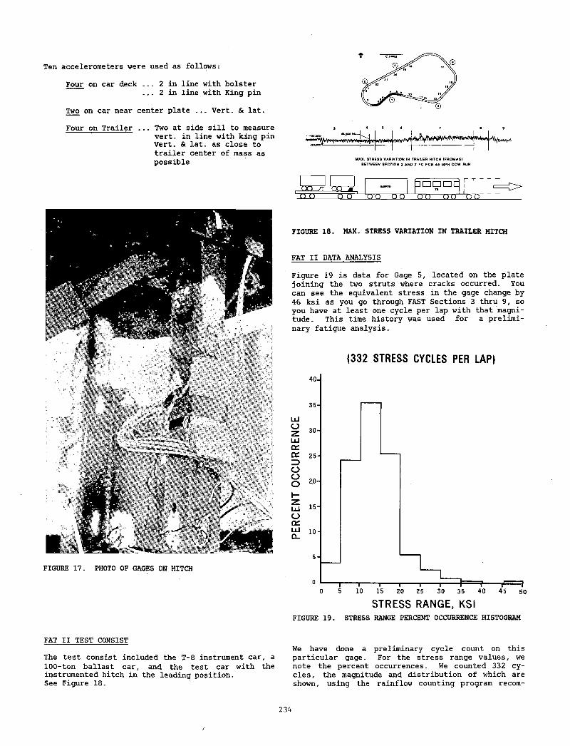
Ten accelerometers were used as follows:

Four on car deck ... 2 in line with bolster __ 2 in line with King pin

Two on car near center plate ... Vert. & lat.

Four on Trailer ... Two at side sill to measure vert, in line with king pin Vert. & lat. as close to trailer center of mass as possible

FIGURE 17. PHOTO OF GAGES ON HITCH

iw j*4 5 8 7 8 B

MAX. STRESS VARIATION IN TRAILER HITCH (FROMMS) BETWEEN SECTION 3 ANO 7 FO FOR 45 MPH CCW RUN

uo /t nn~T T C T oo oo ono o

FIGURE 18. MAX. STRESS VARIATION IN TRAILER HITCH

FAT II DATA ANALYSIS

Figure 19 is data for Gage 5, located on the plate joining the two struts where cracks occurred. You can see the equivalent stress in the gage change by 46 ksi as you go through FAST Sections 3 thru 9, so you have at least one cycle per lap with that magni­tude. This time history was used for a prelimi­nary fatigue analysis.

( 3 3 2 STRES S CYCLES PER LAP)

STRESS RANGE, KSIFIGURE 19. STRESS RANGE PERCENT OCCURRENCE HISTOGRAM

FAT II TEST CONSIST

The test consist included the T-8 instrument car, a 100-ton ballast car, and the test car with the instrumented hitch in the leading position.See Figure 18.

We have done a preliminary cycle count on this particular gage. For the stress range values, we note the percent occurrences. We counted 332 cy­cles, the magnitude and distribution of which are shown, using the rainflow counting program recom­

234

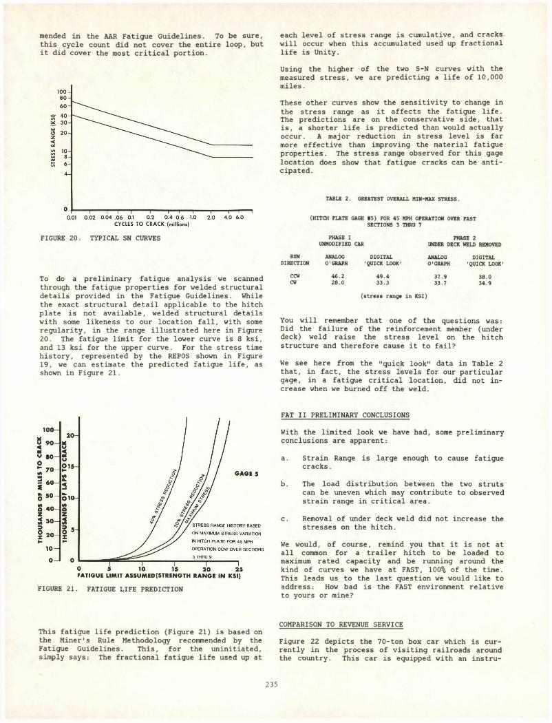
mended in the AAR Fatigue Guidelines. To be sure, this cycle count did not cover the entire loop, but it did cover the most critical portion.

FIGURE 20. TYPICAL SN CURVES

To do a preliminary fatigue analysis we scanned through the fatigue properties for welded structural details provided in the Fatigue Guidelines. While the exact structural detail applicable to the hitch plate is not available, welded structural details with some likeness to our location fall, with some regularity, in the range illustrated here in Figure 20. The fatigue limit for the lower curve is 8 ksi, and 13 ksi for the upper curve. For the stress time history, represented by the REPOS shown in Figure 19, we can estimate the predicted fatigue life, as shown in Figure 21.

FIGURE 21. FATIGUE LIFE PREDICTION

This fatigue life prediction (Figure 21) is based on the Miner's Rule Methodology recommended by the Fatigue Guidelines. This, for the uninitiated, simply says: The fractional fatigue life used up at

each level of stress range is cumulative, and cracks will occur when this accumulated used up fractional life is Unity.

Using the higher of the two S-N curves with the measured stress, we are predicting a life of 10,000 miles.

These other curves show the sensitivity to change in the stress range as it affects the fatigue life. The predictions are on the conservative side, that is, a shorter life is predicted than would actually occur. A major reduction in stress level is far more effective than improving the material fatigue properties. The stress range observed for this gage location does show that fatigue cracks can be anti­cipated.

TABLE 2 . GREATEST OVERALL MIN-MAX STRESS.

(HITCH PLATE GAGE #5) FOR 45 MPH OPERATION OVER FAST SECTIONS 3 THRU 7

PHASE I PHASE 2UNMODIFIED CAR UNDER DECK WELD REMOVED

RUN ANALOG DIGITAL ANALOG DIGITALDIRECTION O'GRAPH •QUICK LOOK' O'GRAPH 'QUICK LOOK

CCW 4 6 .2 4 9 .4 37 .9 3 8 .0CW 2 8 .0 33 .3 33.7 34 .9

( s t r e s s range in KSI)

You will remember that one of the questions was: Did the failure of the reinforcement member (under deck) weld raise the stress level on the hitch structure and therefore cause it to fail?

We see here from the "quick look" data in Table 2 that, in fact, the stress levels for our particular gage, in a fatigue critical location, did not in­crease when we burned off the weld.

FAT II PRELIMINARY CONCLUSIONS

With the limited look we have had, some preliminary conclusions are apparent:

a. Strain Range is large enough to cause fatigue cracks.

b. The load distribution between the two struts can be uneven which may contribute to observed strain range in critical area.

c. Removal of under deck weld did not increase the stresses on the hitch.

We would, of course, remind you that it is not at all common for a trailer hitch to be loaded to maximum rated capacity and be running around the kind of curves we have at FAST, 100% of the time. This leads us to the last question we would like to address: How bad is the FAST environment relativeto yours or mine?

COMPARISON TO REVENUE SERVICE

Figure 22 depicts the 70-ton box car which is cur­rently in the process of visiting railroads around the country. This car is equipped with an instru-

235

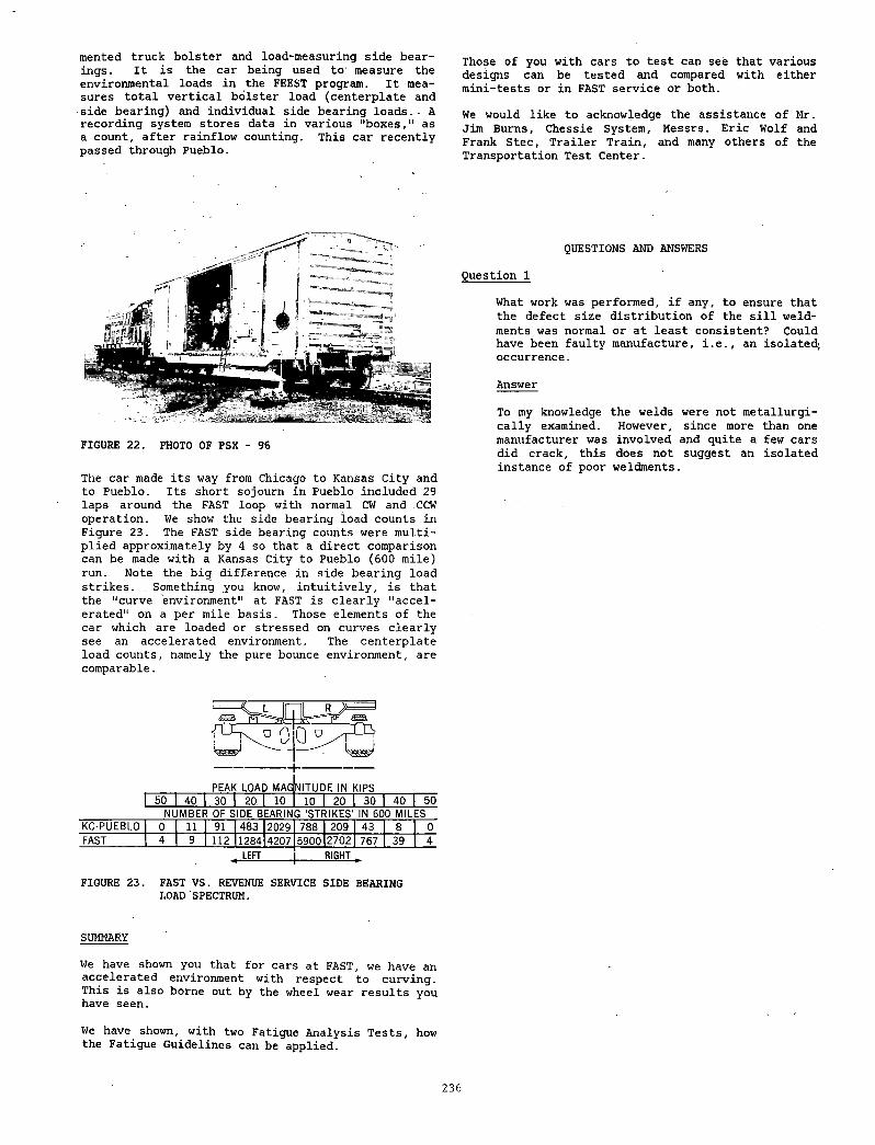
merited truck bolster and load-measuring side bear­ings. It is the car being used to measure the environmental loads in the FEEST program. It mea­sures total vertical bolster load (centerplate and side bearing) and individual side bearing loads. A recording system stores data in various "boxes," as a count, after rainflow counting. This car recently passed through Pueblo.

FIGURE 22. PHOTO OF PSX - 96

The car made its way from Chicago to Kansas City and to Pueblo. Its short sojourn in Pueblo included 29 laps around the FAST loop with normal CW and CCW operation. We show the side bearing ioad counts in Figure 23. The FAST side bearing counts were multi­plied approximately by 4 so that a direct comparison can be made with a Kansas City to Pueblo (600 mile) run. Note the big difference in side bearing load strikes. . Something you know, intuitively, is that the "curve environment" at FAST is clearly "accel­erated" on a per mile basis. Those elements of the car which are loaded or stressed on curves clearly see an accelerated environment. The centerplate load counts, namely the pure bounce environment, are comparable.

Those of you with cars to test can see that various designs can be tested and compared with either mini-tests or in FAST service or both.

We would like to acknowledge the assistance of Mr. Jim Burns, Chessie System, Messrs. Eric Wolf and Frank Stec, Trailer Train, and many others of the Transportation Test Center.

QUESTIONS AND ANSWERS

Question 1

What work was performed, if any, to ensure that the defect size distribution of the sill weld­ments was normal or at least consistent? Could have been faulty manufacture, i.e., an isolated; occurrence.

Answer

To my knowledge the welds were not metallurgi- cally examined. However, since more than one manufacturer was involved and quite a few cars did crack, this does not suggest an isolated instance of poor weldments.

PEAK LOAD MAG NITUDE IN KIPSr 50~ 40 30 __20. 10 10 20 30 1 4 0 50

NUMBER OF SIDE BEARING ‘STRIKES’ IN 600 MILESKC-PUEBLO 0 11 91 483 2029 788 209 43 8 0FAST 4 9 112 1284 4207 5900 2702 767 39 4

, LEFT RIGHT .

FIGURE 23. FAST VS. REVENUE SERVICE SIDE BEARING LOAD SPECTRUM.

SUMMARY

We have shown you that for cars at FAST, we have an accelerated environment with respect to curving. This is also borne out by the wheel wear results you have seen.

We have shown, with two Fatigue Analysis Tests, how the Fatigue Guidelines can be applied.

236

FUTURES1981 FAST ENGINEERING CONFERENCE

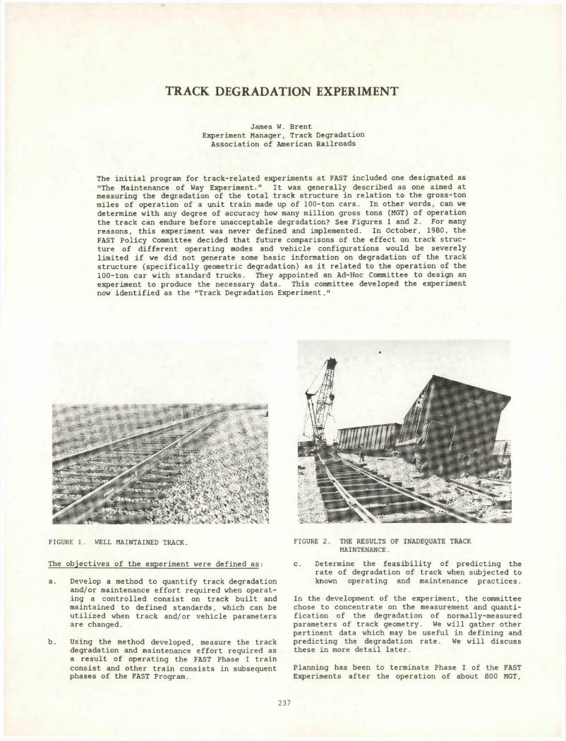
TRACK DEGRADATION EXPERIMENT

James W. BrentExperiment Manager, Track Degradation

Association of American Railroads

The initial program for track-related experiments at FAST included one designated as "The Maintenance of Way Experiment." It was generally described as one aimed at measuring the degradation of the total track structure in relation to the gross-ton miles of operation of a unit train made up of 100-ton cars. In other words, can we determine with any degree of accuracy how many million gross tons (MGT) of operation the track can endure before unacceptable degradation? See Figures 1 and 2. For many reasons, this experiment was never defined and implemented. In October, 1980, the FAST Policy Committee decided that future comparisons of the effect on track struc­ture of different operating modes and vehicle configurations would be severely limited if we did not generate some basic information on degradation of the track structure (specifically geometric degradation) as it related to the operation of the 100-ton car with standard trucks. They appointed an Ad-Hoc Committee to design an experiment to produce the necessary data. This committee developed the experiment now identified as the "Track Degradation Experiment."

FIGURE 1. WELL MAINTAINED TRACK.

The objectives of the experiment were defined as:

a. Develop a method to quantify track degradation and/or maintenance effort required when operat­ing a controlled consist on track built and maintained to defined standards, which can be utilized when track and/or vehicle parameters are changed.

b. Using the method developed, measure the track degradation and maintenance effort required as a result of operating the FAST Phase I train consist and other train consists in subsequent phases of the FAST Program.

FIGURE 2. THE RESULTS OF INADEQUATE TRACK MAINTENANCE.

c. Determine the feasibility of predicting the rate of degradation of track when subjected to known operating and maintenance practices.

In the development of the experiment, the committee chose to concentrate on the measurement and quanti­fication of the degradation of normally-measured parameters of track geometry. We will gather other pertinent data which may be useful in defining and predicting the degradation rate. We will discuss these in more detail later.

Planning has been to terminate Phase I of the FAST Experiments after the operation of about 800 MGT,

237

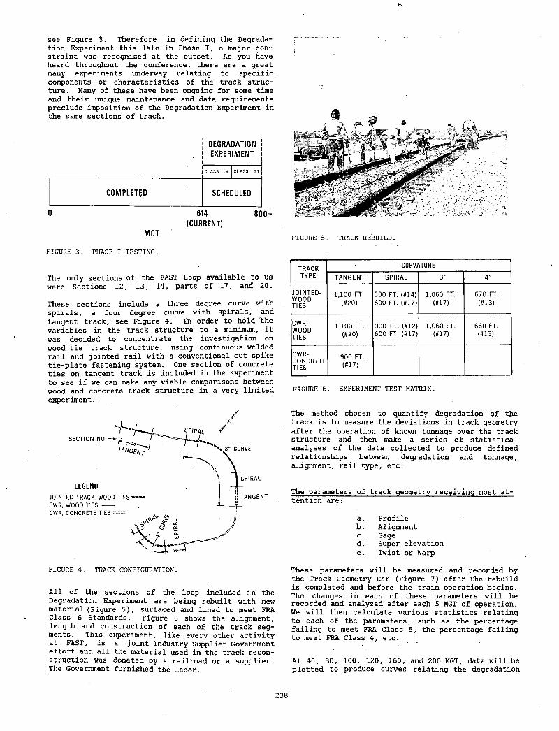
ha,

see Figure 3. Therefore, in defining the Degrada­tion Experiment this late in Phase I, a major con­straint was recognized at the outset. As you have heard throughout the conference, there are a great many experiments underway relating to specific, components or characteristics of the track struc­ture, Many of these have been ongoing for some time and their unique maintenance and data requirements preclude imposition of the Degradation Experiment in the same sections of track.

DEGRADATIONEXPERIMENT

C L A S S IV C L A S S III

COMPLETED SCHEDULED

0 614 800+(CURRENT)

MGT

FIGURE 3. PHASE I TESTING.

The only sections of the FAST Loop available to us were Sections 12, 13, 14, parts of 17, and 20.

These sections include a three degree curve with spirals, a four degree curve with spirals, and tangent track, see Figure 4. In order to hold the variables in the track structure to a minimum, it was decided to concentrate the investigation on wood tie track structure, using continuous welded rail and jointed rail with a conventional cut spike tie-plate fastening system. One section of concrete ties on tangent track is included in the experiment to see if we can make any viable comparisons between wood and concrete track structure in a very limited experiment.

FIGURE 4. TRACK CONFIGURATION.

All of the sections of the loop included in the Degradation Experiment are being rebuilt with new material (Figure 5), surfaced and lined to meet FRA Class 6 Standards. Figure 6 shows the alignment, length and construction of each of the track seg­ments. This experiment, like every other activity at FAST, is a joint Industry-Supplier-Government effort and all the material used in the track recon­struction was donated by a railroad or a supplier. The Government furnished the labor.

FIGURE 5. TRACK REBUILD.

TRACKTYPE

CURVATURE

TANGENT SPIRAL 3° 4°

JOINTED-WOODTIES

1,100 FT. (#20)

300 FT. (#14) 600 F T . (#17)

1,060 FT. (#17)

670 FT. (#13)

CWR-WOODTIES

1,100 FT. (#20)

300 FT. (#12) 600 FT. (#17)

1,060 FT. (#17)

660 FT. (#13)

CWR-CONCRETETIES

900 FT. (#17)

FIGURE 6. EXPERIMENT TEST MATRIX.

The method chosen to quantify degradation of the track is to measure the deviations in track geometry after the operation of known tonnage over the track structure and then make a series of statistical analyses of the data collected to produce defined relationships between degradation and tonnage, alignment, rail type, etc.

The parameters of track geometry receiving most at­tention are:

a. Profileb. Alignmentc. Gaged. Super elevatione. Twist or Warp

These parameters will be measured and recorded by the Track Geometry Car (Figure 7) after the rebuild is completed and before the train operation begins. The changes in each of these parameters will be recorded and analyzed after each 5 MGT of operation. We will then calculate various statistics relating to each of the parameters, such as the percentage failing to meet FRA Class .5, the percentage failing to meet FRA Class 4, etc.

At 40, 80, 100, 120, 160, and 200 MGT, data will be plotted to produce curves relating the degradation

238

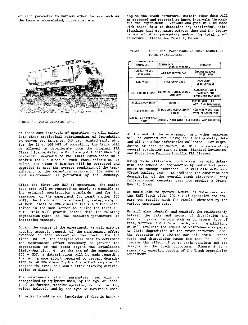
of each parameter to various other factors such as the tonnage accumulated, curvature, etc.

FIGURE 7. TRACK GEOMETRY CAR.

At these same intervals of operation, we will calcu­late other statistical relationships of degradation on curves vs. tangents, CWR vs. jointed rail, etc. For the first 100 MGT of operation, the track will be allowed to deteriorate from the original FRA Class 6 Standard (Figure 8), to a point that when any parameter degrades to the limit established as a minimum for FRA Class 4 Track, those defects at, or below, the Class 4 Minimum will be corrected and upgraded to meet the average condition of the track adjacent to the defective area— much the same as spot maintenance is performed by the Industry.

After the first 100 MGT of operation, the entire test area will be restored as nearly as possible to the original construction standards, and for the remainder of the experiment (at least another 100 MGT), the track will be allowed to deteriorate to minimum limits of FRA Class 3 Track and then main­tained in the same manner as during the first 100 MGT. This will provide better data for relating degradation rates of the measured parameters to increasing tonnage.

During the course of the experiment, we will also be keeping accurate records of the maintenance effort expended on each segment of the track. For the first 100 MGT, the analysis will seek to determine the maintenance effort necessary to prevent the degradation of the track beyond the established limit— FRA Class 4. At the end of the experiment, 200 + MGT, a determination will be made regarding the maintenance effort required to prevent degrada­tion below FRA Class 3 plus the effort required to restore the track to Class 4 after allowing deterio­ration to Class 3.

The maintenance effort parameters used will be catagorized by equipment used, by the type of labor (such as foremen, machine operator, laborer, welder, welder helper), and by the type of materials used.

In order to add to our knowledge of what is happen­

ing to the track structure, certain other data will be measured and recorded at known intervals through­out the experiment. Various analyses will be made with these data to determine any statistical rela­tionships that may exist between them and the degra­dation of other parameters and/or the total track structure. Please see Table 1, below.

TABLE 1. ADDITIONAL PARAMETERS OF TRACK STRUCTURE TO BE INVESTIGATED.

PARAMETER EQUIPMENT/INSTRUMENTATION

REMARKS

LATERAL TRACK STRENGTH AAR DECAROTOR CAR

CHANGE IN GAGE DNDER LOAD '

RAIL WEAR FAST SNAP GAGE MEASURED AT LUBE CHANGES

RAIL CORRUGATIONS LORAM RAIL CORRUGATION ANALYZER

COORDINATE WITH CORROGATION

EXPERIMENT MANAGER

TRACK .DISPLACEMENT TRANSITRECORD VERT. LAT'L,

AND LONG. MOVEMENT

TRACK MODULUSSTRAIN AND DISPLACEMENT

GAGESCOMPARE WOOD TIES WITH CONCRETE TIES

LATERAL AND VERTICAL LOADS INSTRUMENTED WHEEL SET RECORD APPLIED LOADS

At the end of the experiment, many other analyses will be carried out, using the track-geometry data and all the other information collected. For degra­dation of each parameter, we will be calculating several statistics such as Mean, Standard Deviation, and Percentage Failing Specific FRA Classes.

Using these statistical indicators, we will deter­mine the amount of degradation by individual para­meter as tonnage -increases. We will also develop a "Track Quality Index" to indicate the condition and degradation of the overall track structure. Many railroad-owned geometry cars now produce a Track Quality Index.

We would like to operate several of those cars over the FAST Track after 100 MGT of operation and com­pare our results with the results obtained by the various operating cars.

We will also identify and quantify the relationship between the rate and amount of degradation and various physical factors such as curvature, type of rail, vertical and lateral loads, etc. In addition, we will evaluate the amount of maintenance required to limit degradation of the track structure under the operation of a 100-ton car unit train. These costs and degradation rates can then be used to compare the effect of other train consists and car designs on the track structure. Figure 8 is a summary of expected results of the Track Degradation Experiment.

239

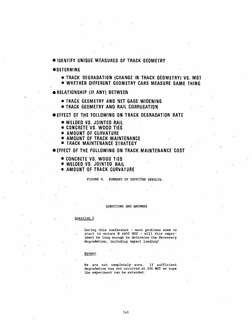
• ID E N T IF Y U N IQ U E M E A S U R E S OF T R A C K G E O M E T R Y

• D E T E R M IN E

• TR A C K D E G R A D A T IO N (C H A N G E IN TR A C K G E O M E T R Y ) VS . M G T

• W H E T H E R D IF F E R E N T G E O M E T R Y CARS M E A S U R E S A M E T H IN G

• R E L A T IO N S H IP ( IF A N Y ) B E T W E E N

• TR A C K G E O M E T R Y A N D NET GAGE W ID E N IN G

• TR A C K G E O M E T R Y A N D R A IL C O R R U G A TIO N

• EFFECT OF T H E F O L L O W IN G ON T R A C K D E G R A D A T IO N RATE

• W E L D E D V S , J O IN T E D RAIL• CO N C RE TE V S . W O O D T IE S

• A M O U N T OF C U R V A T U R E• A M O U N T OF T R A C K M A IN T E N A N C E• T R A C K M A IN T E N A N C E S T R A T E G Y

• EFFECT OF T H E F O L L O W IN G ON T R A C K M A I N T E N A N C E COST

• CONCRETE V S . W O O D T IE S• W E L D E D V S . J O IN T E D RAIL• A M O U N T OF T R A C K C U R V A T U R E

FIGURE 8. SUMMARY OF EXPECTED RESULTS.

QUESTIONS AND ANSWERS

Question 1

During this conference - most problems seem to start; to occure @ ±200 MGT - will this exper­iment be long enough to determine the Necessary degradation, including impact loading?

Answer

We are not completely sure. If sufficient degradation has not occurred at 200 MGT we hope the experiment can be extended.

240

DEFECT GROW TH RATE PILOT TEST

Oscar Orringer Experiment Manager

DOT Transportation Systems Center

INTRODUCTION

The FAST Defect Growth Rate Pilot Test (DGRPT), scheduled to get underway in early 1982, applies FAST testing to railroad technology improvement in a much more sophis­ticated way than the usual FAST experiment. The purpose of this paper is to explain how the DGRPT will help to guide railroad technology toward safer operations, why sophistication is necessary, and what is expected from the experiment.

The American Railway Engineering Association Ad Hoc Committee on Track Performance Standards is sponsoring the DGRPT to provide part of the data on which to base a realistic performance specification for controlling populations of rail defects in track. The DOT Transportation Systems Center, under the auspices of the Improved Track Structures Division of the FRA Office of Safety Research, is functioning as experiment design and technical management staff for the DGRPT and related activi­ties. The total effort combines the DGRPT with the post-test metallurgical analysis to establish the tonnage required to grow rail defects in track, and with studies' of railroad data to identify rail defect occurrence patterns.

BACKGROUND

Recent studies of rail defect occurrence patterns have indicated that it may be possible to control rail defect populations by adjusting t o . more fre­quent inspection as the rate of defect occurrence rises, provided that the inspection method is able to find the defects before breakout is imminent. Defect growth is also an important factor in deter­mining the time available to remove flawed rails prior to breakout. Finally, the ability to modify growth rates by means of an interim remedial action, as permitted under the current Track Safety Stan­dards, Part 213.113, may have an important bearing on the length of time over which a defect can be safely protected in the track.

The Ad Hoc Committee has evaluated the technical and practical feasibility of several alternative ap­proaches to economically improving rail integrity. The Committee has concluded that an approach based on relating inspection frequency to defect occur­rence rate offers the most promise, provided that the rate of occurrence of the defect population father than growth rate of detectable flaws deter­mines the time available for detection. The impact of search time in a performance-based rail integrity specification has a strong influence on railroad operations. Therefore, it is essential that the content of the specification be based on a highly reliable assessment of search time under service conditions.

In order to complete the development of a perfor­mance specification based on this' approach, two major studies to characterize rail flaw behavior must be completed. These studies are:

(1) defect population behavior analysis, and

(2) defect growth rate characterization.

The behavior of the defect population as a function of track usage, and population-size/derailment-inci- dence correlations is currently being investigated by analysis of the detection histories of four Class 1 railroads. This study will establish the critical population for control of inspection scheduling.

The- idea of controlling defect populations by in­spection interval adjustment is developed in Figure 1. The studies of railroad defects have indicated that most defects tend to occur in clusters associ­ated with relatively short lengths of track (5 to 10 miles), and that the cluster locations tend to persist for several years. The proposed performance specification would take advantage of this behavior pattern by focusing frequent supplemental inspection on identified clusters, while, using continuous search methods less frequently to give early warning about the appearance of new.clusters.

A parallel effort is required to quantify defect growth rates to support the approach of control by population level. Both supplemental and continuous search inspections must be performed often enough to avoid the likelihood of defect breakouts between inspections. An appropriate upper limit on inspec­tion interval for this purpose can be defined from the curve of defect size versus tonnage. Figure 2 presents a schematic illustration of the definition for continuous search inspection. Supplemental inspections would probably focus on the larger defect sizes, thus having a larger detectable size and a shorter upper limit on inspection interval.

Despite the potentially critical role of defect growth rates in controlling rail integrity, there

241

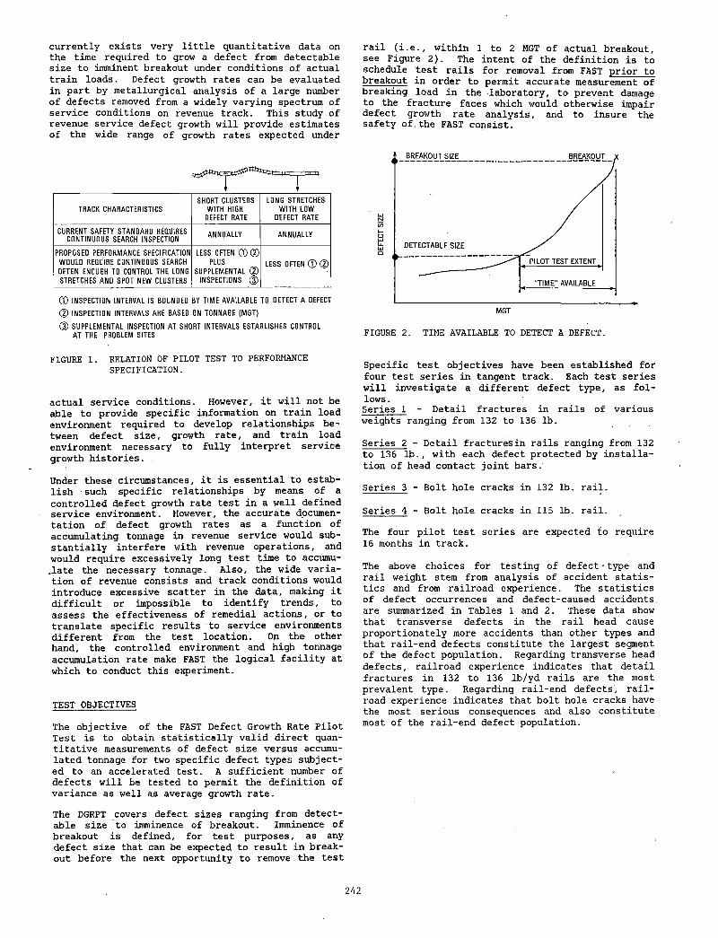
currently exists very little quantitative data on the time required to grow a defect from detectable size to imminent breakout under conditions of actual train loads. Defect growth rates can be evaluated in part by metallurgical analysis of a large number of defects removed from a widely varying spectrum of service conditions on revenue track. This study of revenue service defect growth will provide estimates of the wide range of growth rates expected under

TRACK CHARACTERISTICSSHORT CLUSTERS

WITH HIGH DEFECT RATE

LONG STRETCHES WITH LOW

DEFECT RATE

CURRENT SAFETY STANDARD REQUIRES CONTINUOUS SEARCH INSPECTION

ANNUALLY ANNUALLY

PROPOSED PERFORMANCE SPECIFICATION WOULD REQUIRE CONTINUOUS SEARCH OFTEN ENOUGH TO CONTROL THE LONG STRETCHES AND SPOT NEW CLUSTERS

LESS OFTEN © @ PLUS

SUPPLEMENTAL © INSPECTIONS ©

LESS OFTEN © ©

© INSPECTION INTERVAL IS BOUNDED BY TIME AVAILABLE TO DETECT A DEFECT

© INSPECTION INTERVALS ARE BASED ON TONNAGE (MOT)

© SUPPLEMENTAL INSPECTION AT SHORT INTERVALS ESTABLISHES CONTROL AT THE PROBLEM SITES

FIGURE 1. RELATION OF PILOT TEST TO PERFORMANCE SPECIFICATION.

actual service conditions. However, it will not be able to provide specific information on train load environment required to develop relationships be­tween defect size, growth rate, and train load environment necessary to fully interpret service growth histories.

Under these circumstances, it is essential to estab­lish - such specific relationships by means of a controlled defect growth rate test in a well defined service environment. However, the accurate documen­tation of defect growth rates as a function of accumulating tonnage in revenue service would sub­stantially interfere with revenue operations, and would require excessively long test time to accumu- .late the necessary tonnage. Also, the wide varia­tion of revenue consists and track conditions would introduce excessive scatter in the data, making it difficult or impossible to identify trends, to assess the effectiveness of remedial actions, or to translate specific results to service environments different from the test location. On the other hand, the controlled environment and high tonnage accumulation rate make FAST the logical facility at which to conduct this experiment.

TEST OBJECTIVES

The objective of the FAST Defect Growth Rate Pilot Test is to obtain statistically valid direct quan­titative measurements of defect size versus accumu­lated tonnage for two specific defect types subject­ed to an accelerated test. A sufficient number of defects will be tested to permit the definition of variance as well as average growth rate.

The DGRPT covers defect sizes ranging from detect­able size to imminence of breakout. Imminence of breakout is defined, for test purposes, as any defect size that can be expected to result in break­out before the next opportunity to remove the test

rail (i.e., within 1 to 2 MGT of actual breakout, see Figure 2). The intent of the definition is to schedule test rails for removal from FAST prior to breakout in order to permit accurate measurement of breaking load in the laboratory, to prevent damage to the fracture faces which would otherwise impair defect growth rate analysis, and to insure the safety of.the FAST consist.

FIGURE 2. TIME AVAILABLE TO DETECT A DEFECT.

Specific test objectives have been established for four test series in tangent track. Each test series will investigate a different defect type, as fol­lows .Series 1 - Detail fractures in rails of variousweights ranging from 132 to 136 lb.

Series 2 - Detail fractures in rails ranging from 132 to 136 lb., with each defect protected by installa­tion of head contact joint bars.

Series 3 - Bolt hole cracks in 132 lb. rail.

Series 4 - Bolt hole cracks in 115 lb. rail.

The four pilot test series are expected to require 16 months in track.

The above choices for testing of defect • type and rail weight stem from analysis of accident statis­tics and from railroad experience. The statistics of defect occurrences and defect-caused accidents are summarized in Tables 1 and 2. These data show that transverse defects in the rail head cause proportionately more accidents than other types and that rail-end defects constitute the largest segment of the defect population. Regarding transverse head defects, railroad experience indicates that detail fractures in 132 to 136 lb/yd rails are the most prevalent type. Regarding rail-end defects, rail­road experience indicates that bolt hole cracks have the most serious consequences and also constitute most of the rail-end defect population.

242

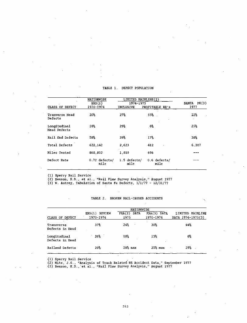
TABLE 1. DEFECT POPULATION

NATIONWIDE LIMITED MAINLINE( 2 )

CLASS OF DEFECTSRS(l)

1970-19741974-1975

INCLUSIVE PROFITABLE RR'sSANTA FE(3)

1977

Tranverse Head Defects

20% 27% 55% . 22%

Longitudinal Head Defects

18% 29% .8% 25%

Rail End Defects 58% 39% 17% 38%

Total Defects 622,142 2,623 412 6,307

Miles Tested 868,802 1,810 696 —

Defect Rate 0.72 defects/ mile

1.5 defects/ mile

0.6 defects/ mile

—

(1) Sperry Rail Service(2) Benson, K.D., et al., “Rail Flaw Survey Analysis," August 1977(3) W. Autrey, Tabulation of Santa Fe Defects, 1/1/77 - 12/31/77

TABLE 2. BROKEN RAIL-CAUSED ACCIDENTS \

NATIONWIDE

CLASS OF DEFECTSRS(l) REVIEW

1970-1974FRA(2) DATA

1975FRA(3) DATA 1970-1974

LIMITED MAINLINE DATA 1974-1975(3)

Transverse Defects in Head

37% 24% 30% 44%

Longitudinal Defects in Head

26% 18% 13% 8%

Railend Defects 20% 28% max 25% max 29% .

(1) Sperry Rail Service(2) Hitz, J.S., "Analysis of Track Related RR Accident Data," September 1977(3) Benson, K.D.,'et al., "Rail Flaw Survey Analysis," August 1977

243

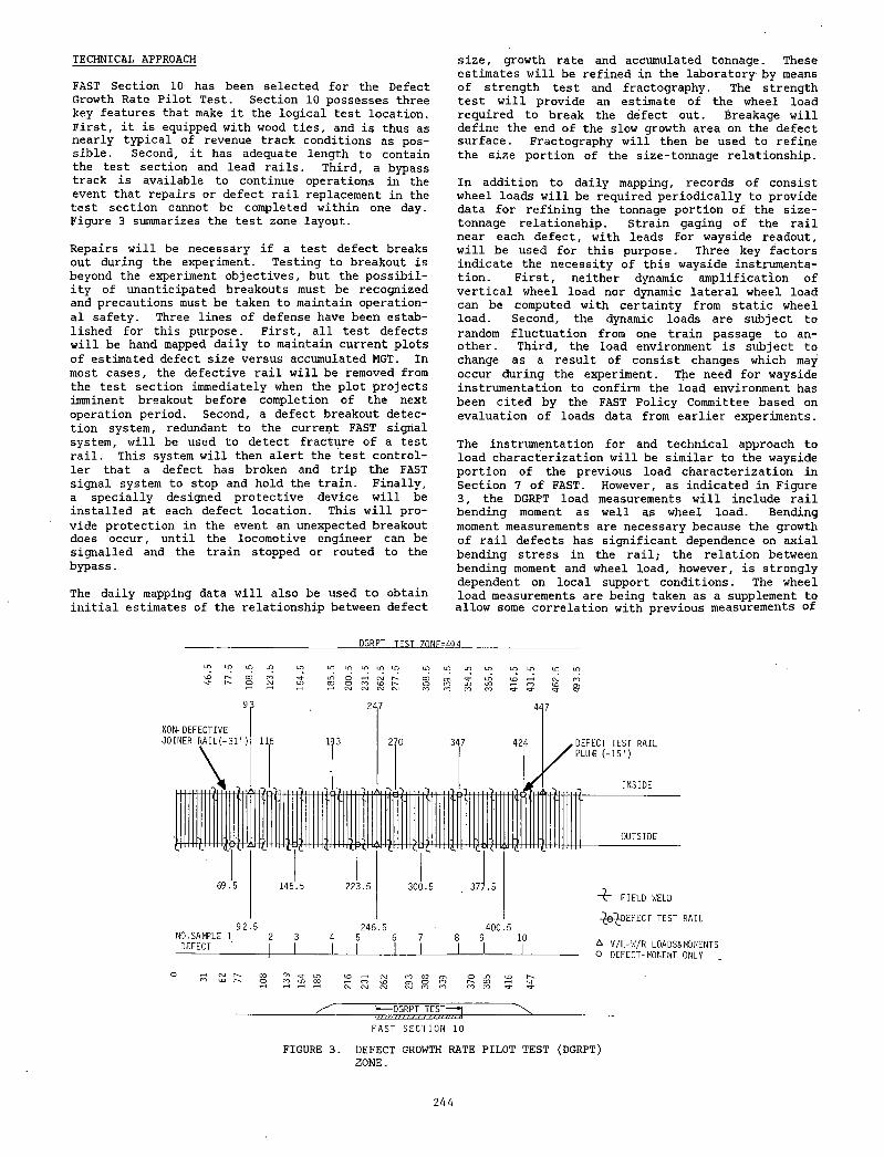
FAST Section 10 has been selected for the Defect Growth Rate Pilot Test. Section 10 possesses three key features that make it the logical test location. First, it is equipped with wood ties, and is thus as nearly typical of revenue track conditions as pos­sible. Second, it has adequate length to contain the test section and lead rails. Third, a bypass track is available to continue operations in the event that repairs or defect rail replacement in the test section cannot be completed within one day. Figure 3 summarizes the test zone layout.

Repairs will be necessary if a test defect breaks out during the experiment. Testing to breakout is beyond the experiment objectives, but the possibil­ity of unanticipated breakouts must be recognized and precautions must be taken to maintain operation­al safety. Three lines of defense have been estab­lished for this purpose. First, all test defects will be hand mapped daily to maintain current plots of estimated defect size versus accumulated MGT. In most cases, the defective rail will be removed from the test section immediately when the plot projects imminent breakout before completion of the next operation period. Second, a defect breakout detec­tion system, redundant to the current FAST signal system, will be used to detect fracture of a test rail. This system will then alert the test control­ler that a defect has broken and trip the FAST signal system to stop and hold the train. Finally, a specially designed protective device will be installed at each defect location. This will pro­vide protection in the event an unexpected breakout does occur, until the locomotive engineer can be signalled and the train stopped or routed to the bypass.

The daily mapping data will also be used to obtain initial estimates of the relationship between defect

TECHNICAL APPROACH size, growth rate and accumulated tonnage. These estimates will be refined in the laboratory by means of strength test and fractography. The strength test will provide an estimate of the wheel load required to break the defect out. Breakage will define the end of the slow growth area on the defect surface. Fractography will then be used to refine the size portion of the size-tonnage relationship.

In addition to daily mapping, records of consist wheel loads will be required periodically to provide data for refining the tonnage portion of the size- tonnage relationship. Strain gaging of the rail near each defect, with leads for wayside readout, will be used for this purpose. Three key factors indicate the necessity of this wayside instrumenta­tion. First, neither dynamic amplification of vertical wheel load nor dynamic lateral wheel load can be computed with certainty from static wheel load. Second, the dynamic loads are subject to random fluctuation from one train passage to an­other. Third, the load environment is subject to change as a result of consist changes which may occur during the experiment. The need for wayside instrumentation to confirm the load environment has been cited by the FAST Policy Committee based on evaluation of loads data from earlier experiments.

The instrumentation for and technical approach to load characterization will be similar to the wayside portion of the previous load characterization in Section 7 of FAST. However, as indicated in Figure 3, the DGRPT load measurements will include rail bending moment as well as wheel load. Bending moment measurements are necessary because the growth of rail defects has significant dependence on axial bending stress in the rail; the relation between bending moment and wheel load, however, is strongly dependent on local support conditions. The wheel load measurements are being taken as a supplement to allow some correlation with previous measurements of

DGRPT TEST Z0NE=494

LO

to'CLO

r-.t o r n LD LO LO LO LO LD

c o c o L o o i - H C \ j r - *O CM LD co o co to r-.« - ! * - < *— I I—I CSJ CM CNJ CSJ

LO

COoCO

lo LO

't rLOCO

LO

COCO

LO

toLO

CO«=3-

lO LO

CsJ CO£ §!

h— DGRPT TEST— *|

F A S T S E C T I O N 10

FIGURE 3. DEFECT GROWTH RATE PILOT TEST (DGRPT) ZONE.

244

revenue service dynamic environment, where only wheel loads were recorded.

Other measurements to be taken during the DGRPT or the post-test phase include track geometry and modulus, static longitudinal stress in the rail, rail residual stress, and lab fatigue performance. The track geometry/modulus data will further assist in the process of correlation between FAST and revenue track. The static longitudinal stress measurements are intended to capture the history of thermal and track adjustment stresses in each test rail during the course of the experiment. In the post-test phase, selected test rails will be de­structively sampled to determine the pattern of residual stresses in the rail head. Previous re­search has shown that plastic flow in the wheel/rail contact zone tends to build up tensile residual stresses inside the rail head, where they may accel­erate the growth of detail fractures. Other post­test rails will be subjected to simplified lab-rig fatigue testing in an attempt to determine if a correlation can be established between defect growth rates in the laboratory and in track.

Cooperating railroads have supplied about 75 sample rails containing detail fractures. These samples are currently (November 1981) undergoing receiving inspection, sorting, and instrumentation at the TTC Component Test Laboratory. One partially instru­mented sample will be placed in Section 10 during November 1981 - January 1982 for the purpose of shaking down the DGRPT data collection procedures prior to the scheduled February 1982 start of Series 1. DGRPT Series 1 and 2 will consume 20 samples; the remainder will be placed directly in the post­test phase to gather data related to revenue track. The bolt hole crack evaluation associated with Series 3 and 4 will deal with similar numbers of samples.

The interpretation of test results is a complex task because the many factors which affect rail defect growth rates interact with each other and may vary significantly from FAST to revenue track. Detailed history and metallurgy work-ups will, therefore, be prepared for each sample to provide the basis for synthesizing the fundamental characteristics of defect growth rate behavior. These detailed reports will be reviewed by the DGRPT Experiment Technical Assessment Committee, which includes technical specialists from the Transportation Test Center and the Association of American Railroads Technical Center.

EXPECTED RESULTS AND BENEFITS

The FAST Defect Growth Rate Pilot Test and post-test phase are expected to produce curves of defect size versus tonnage for detail fractures and bolt hole cracks in standard control-cooled rail in tangent track, adjusted to account for differences between FAST and revenue track. The curve for bolt hole cracks should be directly applicable to the perfor­mance specification for control of rail defects. Detail fractures are sensitive, however, to lateral load effects and will probably require additional testing in a curved section of FAST. Proper adjust­ment of the FAST results for revenue track may also require limited monitoring of one or two defects in a field test.

Although premium-alloy rails are not a part of the

DGRPT, the performance specification must eventually address this category. Of particular concern in this respect is the use of premium-alloy rail in curves to increase wear life. Such increase may introduce additional head defect occurrences which are not seen on standard-rail curves only because the standard rails are removed from service much earlier. It is hoped, however, that the DGRPT will indirectly support the performance specifications for premium alloy rail by producing a reliable interpretation of laboratory fatigue tests of rail sections, in terms of the performance implied in track. Differences between the lab and track per­formances with respect to defect growth depend on the mechanics (loads and support conditions) but are independent of the rail material properties. Thus, it may be possible in the light of the DGRPT to cover the premium alloys more quickly and cheaply by means of well calibrated laboratory test procedures.

Finally, it is expected that the DGRPT post-test phase will provide long-term benefits in the form of guidelines for improved mill practice. Recent developments in premium alloy rail have emphasized surface hardness for longer wear life, with little attention paid to the ability of the interior of the rail head to resist the formation and breakout of defects. It is hoped that the post-test metallurgi­cal analysis will provide useful clues to improved processing of rail in the mill for combined long wear life and high resistance to defects.

245

RADIAL TRUCK CURVING PERFORMANCE EVALUATION

Roy A. AllenExperiment Manager, Radial Truck Association of American Railroads

James P. Jollay Engineer

Boeing Services International, Inc.

A short-term "mini" test is to be carried out at FAST in the near future to evaluate the curving performance of radial trucks over a range of curves varying from lh to lh° • The experiment should enable the differences in energy consumption between radial and conventional trucks to be quantified and will lead to a better under­standing of the mechanics of radial trucks. By combining the experimental results with a computer model, the effects of axle misalignment, yaw stiffness, and wheel profiles will be predicted. The data will form inputs for economic analyses of the benefits of radial trucks and will aid FAST management to decide whether to test a complete consist of vehicles with radial trucks in the next phase of FAST.

INTRODUCTION

The concept of radial, or self-steering, truck designs offers many potential benefits to the rail­road industry as a result of lower lateral forces, lower angle of attack, and higher critical hunting speeds as compared with conventional three-piece trucks. Potential benefits certainly include re­duced wheel and rail wear and lower fuel costs, and may also include improved track component life. The effect of radial trucks on wheel wear has been, and is being, studied within the industry, including FAST1 and a few tests have been carried out to ascertain potential fuel savings. Little or no data exists to determine reduction in rail wear, except by using wheel wear results to estimate rail wear and track component life. To this end the FAST program, and the FAST Policy Committee in parti­cular, is considering implementing a new phase of FAST testing which would examine all potential benefits with a complete consist of radial trucks. If adopted, this test would begin after a further 200-250 MGT of traffic has been accumulated with the existing consist of primarily conventional three- piece trucks.

Prior to making a decision, data are required in order to further understand the basic mechanism of radial trucks in curves, to estimate potential fuel savings on FAST, and to determine the effects of such variables as axle misalignment, primary yaw suspension stiffnesses, and wheel profiles. A number of railroads are also interested in determin­ing truck curving performance with the cross-bracing links inoperative, and this variable will also be investigated with a short-term, or "mini", test to be carried out at the Transportation Test Center in the near future (scheduled for January, 1982).

Thus, the radial truck mini-test is designed to

provide a set of base line data on the curving performance and energy consumption of radial trucks. Because it is impractical to test all the variables of interest from a budgetary standpoint, the tests are to be supplemented by the use of a mathematical computer model2 which predicts the quasi-static performance of vehicles on curves. The model has been used previously to supplement test data3 4 and is used- as a truck design tool at British Rail.5 After validation with the test data, the model will be used to predict the effect of variables which will not be tested on the track.

Specifically, the objectives of the mini-test are:

To obtain curving performance data, particular­ly angles of attack and wheel/rail lateral loads, over curves of lh°, 3°, 4°, 5°, and 7h° for five different speeds (one at balance speed and two each above and below balance) on each curve. Three truck designs will be tested: conventional and the retrofit and diagonal cross-link radial designs (see reference 1 for a description of these designs).

To obtain curving performance data as above on the two radial designs with the cross-bracing members disconnected.

Using the above curving performance data and truck parameter stiffness data, validate the mathematical curving model and then use the model to predict the effects of other vari­ables.

To determine the curving resistance of cars equipped with radial trucks when operating on FAST, thus establishing base line data to determine energy consumption differences be­tween conventional and radial trucks.

247

ENERGY CONSUMPTION TEST CURVING PERFORMANCE TESTS

Actual locomotive fuel consumption data requires sophisticated instrumentation and is extremely difficult to use in a meaningful way unless the fuel data is gathered over a long period of time in which case statistical techniques can be used to analyze the data. However, in a short-term test such as this, many uncontrolled variables affect the useful­ness of the data. Train handling will have a signi­ficant impact on such measurements particularly due to the fact that the motive power and train consist may be different on successive test days. Likewise the crew may also be different. Thus, rather than measure fuel usage, this experiment will obtain train resistance data through the use of an instru­mented coupler, which will be used to calculate energy consumption.

The tests will be carried out on three test tracks at the TTC - the Transit Test Track (TTT) for the 1 h° curve, FAST for th 3°, 4°, and 5° curves, and the Balloon track for the 1\° curve. The latter curve is normally used only for turning trains at the TTC but has previously been successfully used for experiments.4 Runs will be made on FAST with the track both unlubricated and lubricated. The Balloon and TTT runs will be made on unlubricated track only.

For this portion of the experiment, the instru­mentation will include a dynamometer coupler (range: ±30,000 lb, accuracy ±30 lb), coupler angularity transducers, and accelerometers measuring carbody longitudinal accelerations to determine grade forces.

For the curving performance tests, one truck of each of the three designs will be instrumented with two instrumented wheelsets to measure vertical and lateral forces at all four wheels, and four wheel/ rail displacement probes to measure lead and trail axle angles of attack as described by Allen and Jollay.7 In addition, the primary longitudinal displacements (roller bearing to sideframe) dis­placements will be measured at each wheel as well as the truck swivel rotation. The latter sets of measurements will enable the mechanism of the ex­pected reduction in angle of attack of the radial trucks, as compared to the conventional truck, to be better understood. The measured data will enable the effects of track curvature and train speed on angles of attack and lateral load to be determined for a wide range of track curvatures. The typical format of the analyzed data will be similar to that shown symbolically in Figure 1.

SYMBOLIC DATA SYMBOLIC DATA

TRACK C U R VA TU R E (DEGREES)

The three truck designs will be tested in groups of three cars of each truck design. Each group of three cars will in turn be placed at the rear of a consist containing locomotive power, an instrumenta­tion recording car, and a buffer car. The instru­mented coupler will be situated between the buffer car and the three test cars as shown below.

The data will determine the effect of train speed and track curvature on the curving resistance for the conventional and radial trucks. Similar data has previously been obtained on the Truck Design Optimization Program (TDOP)6 but was obtained using a single car. The degree of confidence in the data will be increased by use of a three-car test consist in this expei imeiiL. It is also proposed to compare curving resistance between the concrete tie section (stiff track) and the equivalent wood tie section on FAST, and the applicability of proposed formulae for calculating rolling resistance will be examined. Two formulae, the traditional Davis formulae repre­sentation and the TDOP representation, are shown in Appendix 1. Successful validation of one or the other of these formulae would enable the results of this experiment to be used to estimate the reduction in rolling resistance, and hence potential fuel savings, of radial trucks on other routes.

FIGURE 1. SAMPLE DATA FORMAT FOR TRUCK COMPARISON.

There are many variables which affect truck curving performance; e.g., axle misalignment, wheel profile and primary longitudinal stiffness; which, because of the number of variables, cannot be examined directly in this experiment. However, the use of a well-proven mathematical curving model will allow predictions of the effects of these variables to be made with confidence. Before it is used to make predictions, however, it is essential to validate the model using the test data obtained above. The model has shown good agreement with data obtained in a previous experiment4 on a transit vehicle carried out at the Transportation Test Center. An example of this is shown in Figure 2 which presents data from this test in the form of graphs of lead axle angle of attack plotted against track curvature. The top two graphs are for a left hand curve, the bottom two for a right hand curve, and the four sets of data represent four different sets of conditions (Cl being the normal suspension, both empty and laden, with AAR 1 in 20 wheel profiles, C2 being with reduced primary longitudinal stiffness and AAR 1 in 20 wheel profiles, and C3 being the softer suspension with CN wheel profiles). The data points represent data obtained experimentally whereas the lines represent the computer model predictions.

In order to obtain this type of empirical/analytical agreement, it is essential to measure certain para­meters which are critical to truck curving perfor­mance . These data are being used as input data to the model. These parameters include truck rotational

248

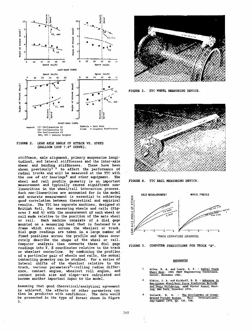
LEFT-HAND CURVE

Speed (ni/h) Speed (mi/h)0 xo 20 30 40- 50 0 10 20 30 40

Legend: Cl- Configuration Ci Symbols - Test DataC2= Configuration C2 Lines ' Computer PredictionsC3a Configuration C3AW0, AW3 ■= vehicle Weights

FIGURE 2. LEAD AXLE ANGLE OF ATTACK VS. SPEED (BALLOON LOOP 7.4° CURVE).

stiffness, axle alignment, primary suspension longi­tudinal, and lateral stiffnesses and the inter-axle shear . and bending stiffnesses. These have been shown previously1 3 to affect the performance of radial trucks and will be measured at the TTC with the use of air bearings8 and other equipment. The wheel and rail profile geometry is an important measurement and typically causes significant non- linearities in the wheel/rail interaction process. Such non-linearities are accounted for in the model and accurate measurement is essential to achieving good correlation between theoretical and empirical results. The TTC has separate machines, designed at British Rail, for measuring wheels and rails (Fig­ures 3 and 4) with the measurement of each wheel or rail made relative to the position of the mate wheel or rail. Each machine consists of a dial gage mounted on a measuring head that is fastened to a frame which rests across the wheelset or track. Dial gage readings are taken in a large number of fixed positions across the profile and these accu­rately describe the shape of the wheel or rail. Computer analysis then converts these dial gage readings into Y, Z coordinates relative to the track or wheelset centerline. By combining the profiles of a particular pair of wheels and rails, the mutual contacting geometry can be studied. For a series of lateral shifts of the wheelset relative to the track, various parameters9— rolling radius differ­ence, contact angles, wheelset roll angles, and contact patch size and slope— are calculated and become another important input to the model.

Assuming that good theoretical/analytical agreement is achieved, the effects of other parameters can then be predicted with confidence. The data would be presented in the type of format shown in Figure 5.

FIGURE 3. TTC WHEEL MEASURING DEVICE.

FIGURE 4. TTC RAIL MEASURING DEVICE.

AXLE MISALIGNMENT WHEEL PROFILE

FIGURE 5. COMPUTER PREDICTIONS FOR TRUCK "A".

REFERENCES

A lle n , R. A . and L eary, J . F . - R a d ia l Truck Wheel Wear. 1981 FAST E n gin eerin g C on feren ce , D enver, November 1981.

El-kins, J . A . and E ic k h o f f , B. M. - Advances in N on-L inear W h ee l/R a il F orce P r e d ic t io n Methods and T h e ir V a lid a t io n , ASME W inter Annual Meet­in g , New Y ork , December 1970.

P o l la r d , M. 6 . - The Development o f C ro ss -B raced F re ig h t B o g ie s , R a il In te r n a t io n a l, Sep-tem ber 1979, p p . 735 , 758.

249

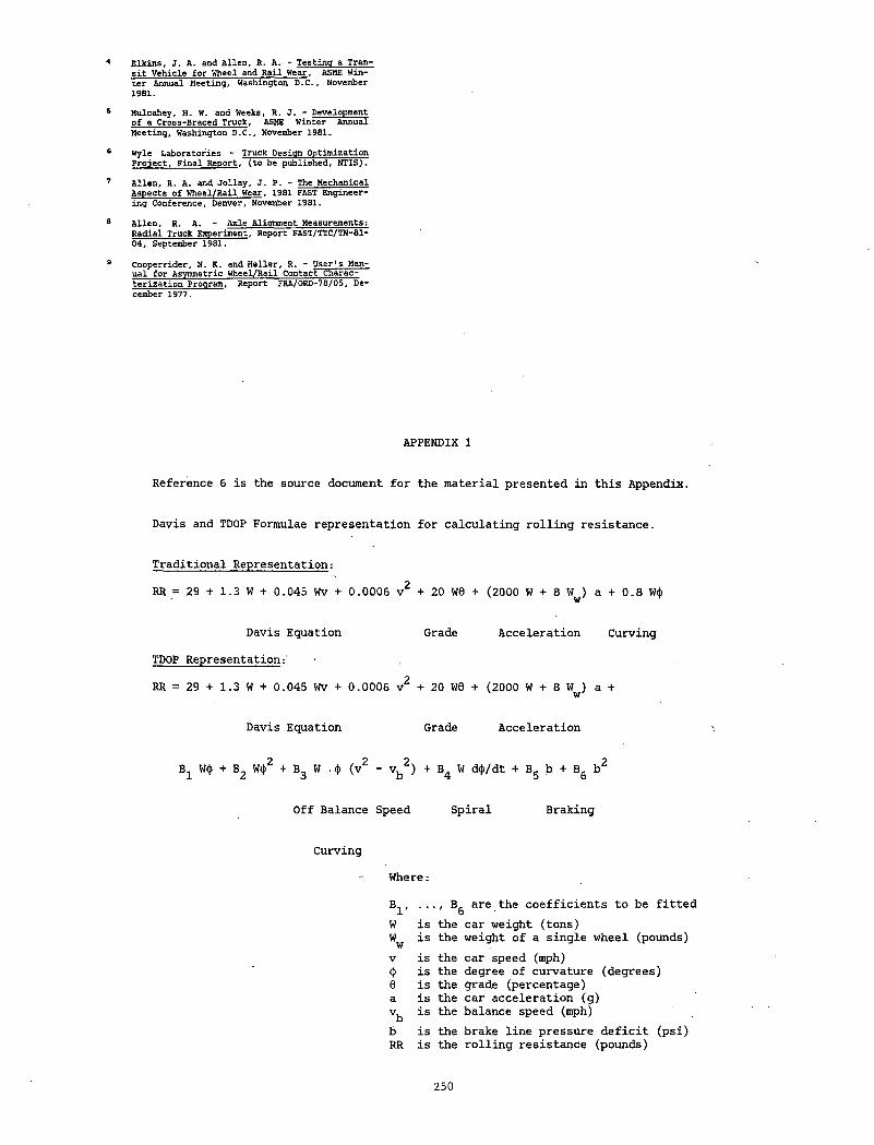
E lk in s , J . A. and A lle n , R. A. - T e s t in g a Tran­s i t V e h ic le f o r Wheel and R a il Wear, ASME Win­t e r Annual M eeting, Washington D .C ., November 1981.

M ulcahey, H. W. and Weeks, R. J . - Development o f a C ross-B raced Truck, ASME W inter Annual M eeting, Washington D .C ., November 1981.

Wyle L a b ora tories - Truck D esign O ptim ization P r o je c t , F in a l R ep ort , ( t o be p u b lish e d , N TIS).

A l le n , R. A. and J o l la y , J . P . - The M echanical A sp ects o f W h eel/R a il Wear, 1981 FAST E n gin eer­in g C on feren ce , Denver, November 1981.

A lle n , R. A. - A xle Alignm ent Measurements: R a d ia l Truck Experim ent, R eport FAST/TTC/TN-81- 04 , September 1981.

C oop err id er , N. K. and H e lle r , R. - U s e r 's Man­u a l f o r Asymmetric W h eel/R ail C on tact C harac- t e r iz a t io n Program, Report FRA/ORD-78/OS, De­cember 1977.

APPENDIX 1

Reference 6 is the source document for the material presented in this Appendix.

Davis and TDOP Formulae representation for calculating rolling resistance.

Traditional Representation:

RR = 29 + 1.3 W + 0.045 Wv + 0.0006 v2 + 20 W0 + (2000 W + 8 Ww > a + 0.8 W(J>

Davis Equation Grade Acceleration

TDOP Representation:

RR = 29 + 1.3 W + 0.045 Wv + 0.0006 v2 + 20 W6 + (2000 W + 8 »# )

Davis Equation Grade Acceleration

B, W<j> + B_ W<|>2 + B W .<)> (v2 - v, 2) + B. W d<)>/dt + B- b + B, b2 1 c J D 4 d o

Off Balance Speed Spiral Braking

Curving

a +

Curving

Where:

V Bw is theww is theV is thef is thee is thea is thevb is theb is theRR is the

are the coefficients to be fitted>car weight (tons)weight of a single wheel (pounds)car speed (mph)degree of curvature (degrees)grade (percentage)car acceleration (g)balance speed (mph)brake line pressure deficit (psi) rolling resistance (pounds)

250

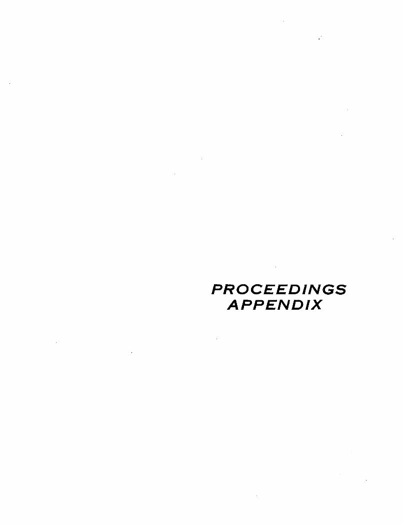
P R O C E E D I N G SA P P E N D I X

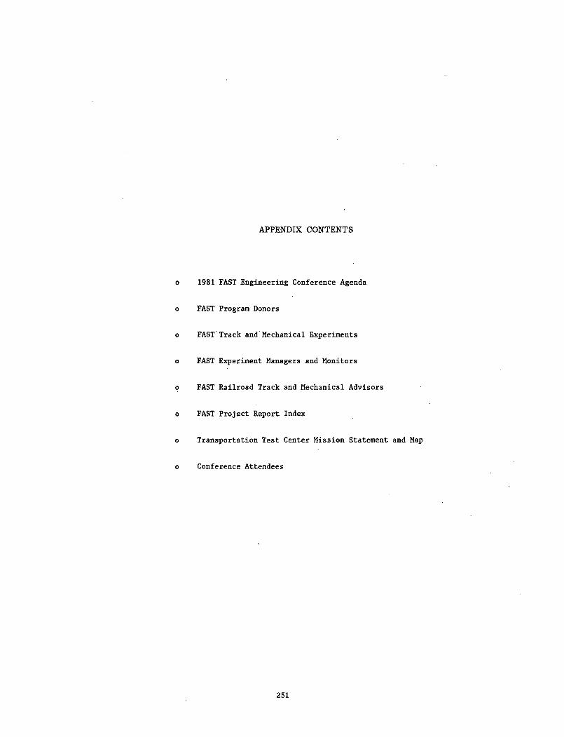
APPENDIX CONTENTS

1981 FAST Engineering Conference Agenda

FAST Program Donors

FAST Track and Mechanical Experiments

FAST Experiment Managers and Monitors

FAST Railroad Track and Mechanical Advisors

FAST Project Report Index

Transportation Test Center Mission Statement and Map

Conference Attendees

251

1 9 8 1

FAST TUESDAYNOVEMBER 3, 19811:00 5:30 p.mRegistration Stouffers Inn Convention Center Foyer

Wednesday NOVEMBER 4, 19817:00 • 8:00 p.m.Registration Stouffers Inn Convention Center Foyer

8:00 a m.Conference Welcome ............Centennial Square C &. D

Walter W. SimpsonChairman, FAST Technical Advisory Committee Member, FAST Policy Committee

8:15 a m.FAST Overview

Gregory P. McIntosh, FAST Program Manager Acting Director, Transportation Test Center

8:30 a.m.Session Introduction

James R. Lundgren, FAST Technical Manager Director, AAR Research &, Test Operation, Pueblo, CO

Session 1: RAILS8:45 a.m.Evolution o f Measurement Techniques at FAST

Thomas P. Larkin, FAST Operations Manager

9:15 a.m.Rail Wear and Metal Flow

Roger K. Steele, Ph.D., Rail Metallurgy Experiment Manager

10:30 a.m.Rail Corrugation Investigations at FAST: December 1979 through August 1981

Timothy J. Devine, Rail Corrugation Experiment Manager

11:00 a.m.Welded Rail-End Batter

Roger K. Steele, Ph D., Rail Metallurgy Experiment Manager

11:20 a.m.Questions and Discussions

James R. Lundgren, FAST Technical Manager

11:45 a.m.Luncheon Centennial Square A &, B

Session 2: WHEELS AND RAIL1:00 p.m.Major Variables that Affect Wheel Wear

Donald E. Gray, Wheels Experiment Manager

1:50 p.m.Wear Rates o f Freight Car Wheels as aFunction o f Chemistry

V. E. Kahle, Wheels Experiment Manager

2:10 p.m. •Radial Truck Wheel Wear

Roy A. Allen, Radial Truck Experiment Manager

2:40 p.m.The Mechanical Aspects o f Wheel/Rail Wear

Roy A. Allen, Radial Truck Experiment Manager

3:30 p.m.Wheel/Rail System Wear

Roger K. Steele, Ph.D., Rail Metallurgy Experiment Manager

4:4* p.m.Questions and Discussions

James R. Lundgren, FAST Technical Manager

5:00 p.m.Adjourn

7:00 p.m.FAST Banquet......................... Centennial Square A A, B

Banquet Host: The Railway Supply Association L. D. Gaeth, Senior Marketing Manager, Griffin

Wheel—RSA Representative Banquet Chairman: Donald Spanton, FAST Policy

Committee ChairmanKeynote Speaker: J. W. Gessner, President and Chief

Executive Officer, Missouri Pacific Railroad Co.

ThursdayNOVEMBER S, 1981

6:45 • 7:45 a.m.Buffet Breakfast..................... Centennial Square A &. B

Breakfast Host: Dresser Industries, Inc.

8:00 a.m.Introductory Remarks............Centennial Square C &, D

Paul Settle and Peter Detmold FAST Policy Committee Members

8:10 a.m.Session Introduction

James R. Lundgren, FAST Technical Manager

Session 3: TRACK8:15 a.m.Ballast Experiments at FAST

Bruce N. Bosserman, Ballast Experiment Manager

9:00 a.m.Results o f Standard Wood Tie and Manufactured Tie Experiments at FAST

Lauress C. Collister, Wood Ties and Fasteners Experiment Manager

9:25 a.m.Evaluation o f Various Wood Tie Fasteners Under Freight Railroad Service Loading

Larry Daniels, Wood Ties and Fasteners Experiment Monitor

9:50 a.m.Concrete Tie and Fastener Performance

John W. Weber, Concrete Ties and Fasteners Experiment Manager

10:15 a.m.Concrete Tie lYack Systems: Engineering Considerations

Jack E. Heiss, Concrete I ies and Fasteners Experiment Manager

10:40 a.m.Tie/Ballast Interaction Comparisons fo r Wood and Concrete Ties

Bruce \ Bosserman. Ballast Experiment Manager

11:05 a m.Some Aspects o f Concrete Tie Performance on FAST and Revenue Service

Howard G. Moody. lies and Fasteners Experiment Manager

Correlation o f FAST and Laboratory Tests with Concrete and Wood Tie Fastener Results

Howard G. Moody, Ties and Fasteners Experiment Manager

11:30 a.m.Track Degradation Experiment

James W. Brent, Track Degradation Experiment Manager

11:40 a.m.Questions and DiscussionsJames R. Lundgren, FAST Technical Manager

12:00 noonLuncheon................................Centennial Square A & B

1:15 p.m.Session Introduction

James R Lundgren. FAST Technical Manager

Session 4. FATIGUE1:30 p.m.Fatigue Analysis Tests at FAST

S. K. Punwani, Car Dynamics Experiment Manager

2:00 p.m.Rail Failure Behavior

Roger K. Steele, Ph D., r«u;l Metallurgy Experiment Manager

Session 5: FUTURES2:20 p.m.Defective Growth Rate Pilot Test

Oscar Orringer, DGRPT Experiment Manager

2:30 p.m.Radial Truck Curving Performance Evaluation

Roy A. Allen, Radial Truck Ex|)eriment Manager

2:40 p.m.Questions and Discussions

James R. Lundgren, FAST Technical Manager

3:00 p.m.FAST Tour Presentation

Gregory P. McIntosh, FAST Program Manager Acting Director, Transportation Test Center

3:05 p.m.Closing Remarks

Walter W. SimpsonChairman, FAST Technical Advisory Committee

Member, FAST Policy Committee

3:20 p.m.Adjourn

FridayNOVEMBER 0, 1981

FAST TOUR6:00 a.m.Buses depart Stouffers Denver Inn, front entrance

9:00 a.m.Arrive Transportation Test Center Tour of FAST

3:00 p.m.Return to Denver, Stapleton Airport

3:30 p.m.Return to Stouffers Denver Inn

2 5 2

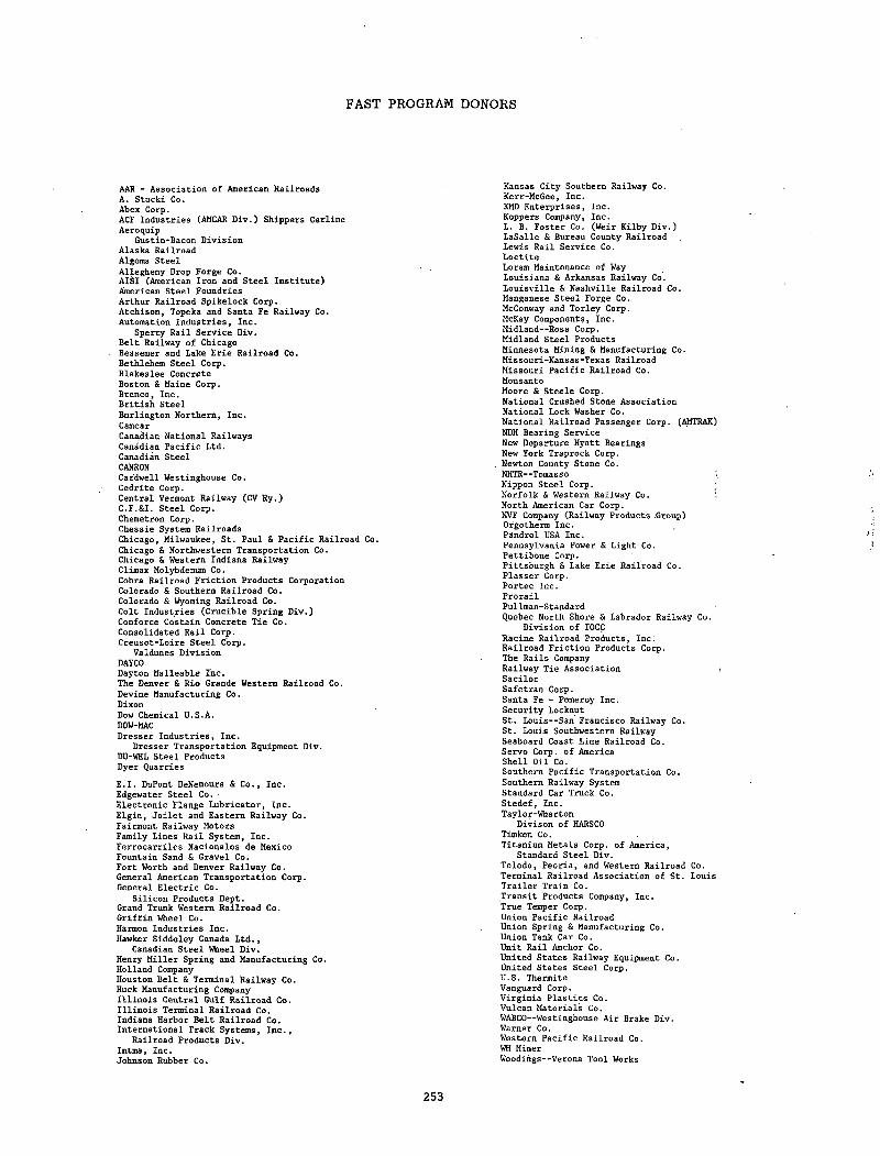
FAST PROGRAM DONORS

AAR - Association of American Railroads A. Stucki Co.Abex Corp.ACF Industries (AMCAR Div.) Shippers Carline Aeroquip

Gustin-Bacon Division Alaska Railroad Algoma Steel Allegheny Drop Forge Co.AISI (American Iron and Steel Institute)American Steel Foundries Arthur Railroad Spikelock Corp.Atchison, Topeka and Santa Fe Railway Co. Automation Industries, Inc.

Sperry Rail Service Div.Belt Railway of ChicagoBessemer and Lake Erie Railroad Co.Bethlehem Steel Corp.Blakeslee Concrete Boston & Maine Corp.Brenco, Inc.British Steel Burlington Northern, Inc.CamcarCanadian National Railways Canadian Pacific Ltd.Canadian Steel CANRONCardwell Vestinghouse Co.Cedrite Corp.Central Vermont Railway (CV Ry.)C.F.&I. Steel Corp.Chemetron Corp.Chessie System RailroadsChicago, Milwaukee, St. Paul & Pacific Railroad Co. Chicago & Northwestern Transportation Co.Chicago & Western Indiana Railway Climax Molybdenum Co.Cobra Railroad Friction Products Corporation Colorado & Southern Railroad Co.Colorado & Wyoming Railroad Co.Colt Industries (Crucible Spring Div.)Conforce Costain Concrete Tie Co.Consolidated Rail Corp.Creusot-Loire Steel Corp.

Valdunes Division DAYCODayton Malleable Inc.The Denver & Rio Grande Western Railroad Co.Devine Manufacturing Co.DixonDow Chemical U.S.A.DOW-MACDresser Industries, Inc.

Dresser Transportation Equipment Div.DU-WEL Steel Products Dyer QuarriesE I. DuPont DeNemours & Co., Inc.Edgewater Steel Co. -Electronic Flange Lubricator, Inc.Elgin, Joilet and Eastern Railway Co.Fairmont Railway Motors Family Lines Rail System, Inc.Ferrocarriles Nacionales de Mexico Fountain Sand & Gravel Co.Fort Worth and Denver Railway Co.General American Transportation Corp.General Electric Co.

Silicon Products Dept.Grand Trunk Western Railroad Co.Griffin Wheel Co.Harmon Industries Inc.Hawker Siddeley Canada Ltd.,

Canadian Steel Wheel Div.Henry Miller Spring and Manufacturing Co.Holland CompanyHouston Belt & Terminal Railway Co.Huck Manufacturing Company Illinois Central Gulf Railroad Co.Illinois Terminal Railroad Co.Indiana Harbor Belt Railroad Co.International Track Systems, Inc.,

Railroad Products Div.Intma, Inc.Johnson Rubber Co.

Kansas City Southern Railway Co. Kerr-McGee, Inc.KMD Enterprises, Inc.Koppers Company, Inc.L. B. Foster Co. (Weir Kilby Div.)LaSalle & Bureau County Railroad Lewis Rail Service Co.LoctiteLoram Maintenance of Way Louisiana & Arkansas Railway Co.Louisville & Nashville Railroad Co. Manganese Steel Forge Co.McConway and Torley Corp.McKay Components, Inc.Midland— Ross Corp.Midland Steel Products Minnesota Mining & Manufacturing Co. Missouri-Kansas-Texas Railroad Missouri Pacific Railroad Co.MonsantoMoore & Steele Corp.National Crushed Stone Association National Lock Washer Co.National Railroad Passenger Corp. (AMTRAK)NDH Bearing ServiceNew Departure Hyatt BearingsNew York Traprock Corp.Newton County Stone Co.NHTR— Tomasso Nippon Steel Corp.Norfolk & Western Railway Co.North American Car Corp.NVF Company (Railway Products .Group) Orgotherm Inc.Pdndrol USA Inc.Pennsylvania Power & Light Co.Pettibone Corp.Pittsburgh & Lake Erie Railroad Co.Plasser Corp.Portec Inc.ProrailPullman-StandardQuebec North Shore & Labrador Railway Co.

Division of IOCC Racine Railroad Products, Inc.'Railroad Friction Products Corp.The Rails Company Railway Tie Association Sacilor Safetran Corp.Santa Fe - Pomeroy Inc.Security LocknutSt. Louis— San Francisco Railway Co.St. Louis Southwestern Railway Seaboard Coast Line Railroad Co.Servo Corp. of America Shell Oil Co.Southern Pacific Transportation Co. Southern Railway System Standard Car Truck Co.Stedef, Inc.Taylo r-Wharton

Divison of HARSCO Timken Co.Titanium Metals Corp. of America,

Standard Steel Div.Toledo, Peoria, and Western Railroad Co. Terminal Railroad Association of St. Louis Trailer Train Co.Transit Products Company, Inc.True Temper Corp.Union Pacific RailroadUnion Spring & Manufacturing Co.Union Tank Car Co.Unit Rail Anchor Co.United States Railway Equipment Co.United States Steel Corp.U.S. Thermite Vanguard Corp.Virginia Plastics Co.Vulcan Materials Co.WABCO— Westinghouse Air Brake Div.Warner Co.Western Pacific Railroad Co.WH MinerWoodings— Verona Tool Works

253

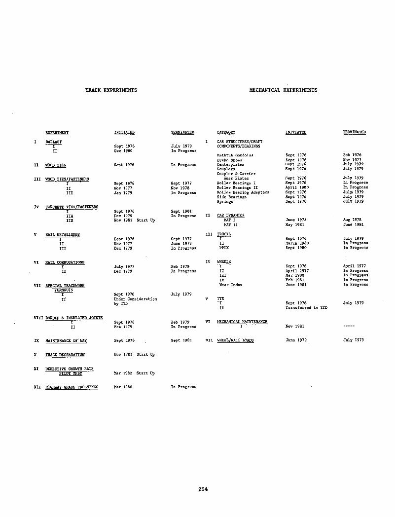
TRACK EXPERIMENTS MECHANICAL EXPERIMENTS.

EXPERIMENT INITIATED TERMINATED CATEGORY INITIATED TERMINATED

I BALLAST I CAR STRUCTURES/DRAFTI Sept 1976 July 1979 COMPONENTS/BEARINGSII Dec 1980 In Progress

Bathtub Gondolas Sept 1976 Feb 1976Brake Shoes Sept 1976 Nov 1977

II WOOD TIES Sept 1976 In Progress Centerplates Sept 1976 July 1979Couplers Sept 1976 July 1979Coupler & Carrier

III WOOD TIES/FASTENERS Wear Plates Sept 1976 July 1979I Sept 1976 Sept 1977 Roller Bearings I Sept 1976 In ProgressII Nov 1977 Nov 1978 Roller Bearings II April 1980 In Progress:III Jan 1979 In Progress Roller Bearing Adapters Sept 1976 July. 1979

Side Bearings Sept 1976 July 1979Springs Sept 1976 July 1979

IV CONCRETE TIES/FASTENERSI Sept 1976 Sept 198iIIA Dec 1979 In Progress II CAR DYNAMICSIIB Nov 1981 Start Up FAT I June 1978 Aug 1978

FAT II May 1981 June 1981

V RAIL METALLURGY III TRUCKSI Sept 1976 Sept 1977 I Sept 1976 July 1979II Nov 1977 June 1979 II March 1980 In ProgressIII Dec 1979 In Progress PPLX Sept 1980 In Progress

VI RAIL CORRUGATIONS IV WHEELSI July 1977 Feb 1979 I Sept 1976 April 1977II Dec 1979 In Progress II April 1977 In Progress

III Mar 1980 In ProgressIV Feb 1981 In Progress

VII SPECIAL TRACKWORK Wear Index June 1981 In ProgressTURNOUTS

I Sept 1976 July 1979II Under Consideration V TTX

by TTD I Sept 1976 July 1979II Transferred to TTD

VIII BONDED & INSULATED JOINTSI Sept 1976 Feb 1979 VI MECHANICAL MAINTENANCEII Feb 1979 In Progress I Nov 1981

IX MAINTENANCE OF’WAY Sept 1976 Sept 1981 VII WHEEL/RAIL LOADS June 1979 July 1979

X TRACK DEGRADATION Nov 1981 Start Up

XI DEFECTIVE GROWTH RATEPILOT TEST Mar 1982 Start Up

XII HIGHWAY GRADE CROSSINGS Mar 1980 In Progress

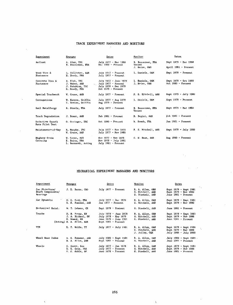
TRACK EXPERIMENT MANAGERS AND MONITORS

Experiment Manager Dates Monitor Dates

Ballast A. Sluz, TSCB. Bosserman, FRA

July 1977 Mar 1980 -

- Mar 1980 Present

B. Bosserman, FRA VacantJ. Heiss, OStM

Sept 1979 April 1981

- Mar 1980 - Present

Wood Ties & Fasteners

L. Collister, AAR H. Moody, FRA

July 1977 July 1977

- Present- Present

L. Daniels, O&M Sept 1979 - Present

Concrete Ties & Fasteners

A. Kish, TSC J. Weber, AAR J. Putukian, TSC H. Moody, FRA

July 1977 July 1977 July 1979 Oct 1979 -

- June 1979- Present- Dec 1979 Present

L. Daniels, 0&M J. Heiss, O&M

Sept 1979 Oct 1980 -

- Oct 1980 Present

Special Trackwork W. Cruse, AAR July 1977 - Present F. S. Mitchell, AAR Sept 1979 - July 1980

Corrugations W. Kucera, Griffin T. Devine, Griffin

July 1977 Aug 1979 -

- Aug 1979 Present

L. Daniels, 0&M Sept 1979 - Present

Rail Metallurgy R. Steele, FRA July 1977 - Present B. Bosserman, FRA Vacant

Sept 1979 - Mar 1980

Track Degradation J. Brent, AAR Feb 1981 - Present R. Begier, AAR Feb 1981 - PresentDefective Growth Rate Pilot Test

0. Orringer, TSC Oct 1980 - Present R. Brush, FRA Jan 1981 - Present

Maintenance-of-Way R. Murphy, TSC W. Cruse, AAR

July 1977 July 1977

- Nov 1979- Nov 1980

F. S. Mitchell, AAR Sept 1979 - July 1980

Highway Grade Crossing

W. Cruse, AAR E. Baicy, FRA L. Bernardi, Acting

Nov 1977 - Nov 1978 - July 1981

Nov 1978 July 1981 - Present

C. W. Bean, AAR Aug 1980 - Present

MECHANICAL EXPERIMENT1 MANAGERS AND MONITORS

Experiment Manager Dates Monitor DatesCar Structure/ J. E. Burns, C&0 July 1977 - Present R. A. Allen, O&M Sept 1979 - Sept 1981Draft Components/ G. Mitchell, AAR Sept 1979 - Nov 1980Bearings G. Staeheli, AAR June 1981 - PresentCar Dynamics D. E. Gray, FRA July 1977 - Dec 1978 R. A. Allen, O&M Sept 1979 - Sept 1961

S. K. Punwani, AAR Jan 1977 - Present G. Mitchell, AAR Sept 1979 - Nov 1980Mechanical Maint. W. T. Lehman, CR Sept 1979 - Present G. Staeheli, AAR June 1981 - PresentTrucks D. H. Propp, BN July 1979 - June 1978 R. A. Allen, 0&M Sept 197,9 - Sept 1981

J. A. Bichsel, BN July 1978 - May 1979 G. Mitchell, AAR Sept 1979 - Nov 1980K. Rownd, BN June 1979 - June 1981 G. Staeheli, AAR June 1981 - Present

(Acting) R. A. Allen, AAR Sept 1981 - PresentTTX E. T. Wolfe, TT July 1977 - July 1981 R. A. Allen, O&M Sept 1979 - Sept 1981

G. Mitchell, AAR Sept 1979 - Nov 1980J. Jollay, 0&M July 1980 - July 1981

Wheel Wear Index S. K. Punwani, AAR July 1980 - Sept 1981 R. A. Allen, 0&M July 1980 - Sept 1981R. A. Allen, AAR Sept 1981 - Present G. Staeheli, AAR June 1981 - Present

Wheels C. Scott, Sou July 1977 - Jan 1978 R. A. Allen, 0&M Sept 1979 - Sept 1981D. E. Gray, FRA July 1977 - Present G. Mitchell, AAR Sept 1979 - Nov 1980V. E. Kahle, SP June 1978 - Present G. Staeheli, AAR June 1981 - Present

255

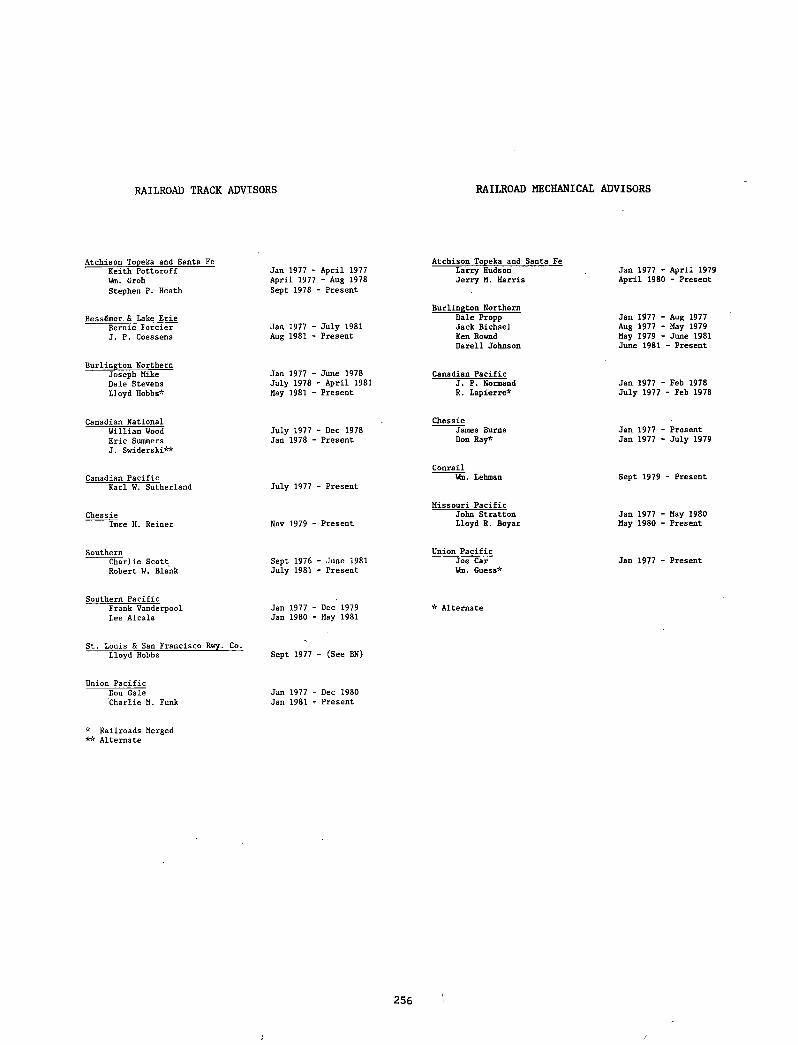
RAILROAD TRACK ADVISORS RAILROAD MECHANICAL ADVISORS

Atchison Topeka and Santa Fe Atchison Topeka and Santa FeKeith Pottoroff Wm. Groh Stephen P. Heath

Jan 1977 - April 1977 April 1977 - Aug 1978 Sept 1978 - Present

Larry Hudson Jerry M. Harris

Jan 1977 - April 1979 April 1980 - Present

Bessemer & Lake Erie Bernie Forcier J. P. Coessens

Jan 1977 - July 1981 Aug 1981 - Present

Burlington Northern Dale Propp Jack Bichsel Ken Rovmd Darell Johnson

Jan 1977 - Aug 1977 Aug 1977 - May 1979 May 1979 - June 1981 June 1981 - Present

Burlington Northern Joseph Mike Dale Stevens Lloyd Hobbs*

Jan 1977 - June 1978 July 1978 - April 1981 May 1981 - Present

Canadian Pacific J. P. Normand R. Lapierre*

Jan 1977 - Feb 1978 July 1977 - Feb 1978

Canadian National William Wood Eric Summers J. Swiderski**

July 1977 - Dec 1978 Jan 1978 - Present

ChessieJames Burns Don Ray*

Jan 1977 - Present Jan 1977 - July 1979

Canadian PacificKarl W. Sutherland July 1977 - Present

ConrailWm. Lehman Sept 1979 - Present

ChessieImre H. Reiner Nov 1979 - Present

Missouri PacificJohn Stratton Lloyd R. Boyar

Jan 1977 - May 1980 May 1980 - Present

SouthernCharlie Scott Robert W. Blank

Sept 1976 - June 1981 July 1981 - Present

Union Pacific Joe Car Win. Guess*

Jan 1977 - Present

Southern PacificFrank Vanderpool Lee Alcala

Jan 1977 - Dec 1979 Jan 1980 - May 1981

* Alternate

St. Louis & San Francisco Rwy. Co. Lloyd Hobbs Sept 1977 - (See BN)

Union Pacific Don Gale Charlie M. Funk

Jan 1977 - Dec 1980 Jan 1981 - Present

* Railroads Merged** Alternate

256

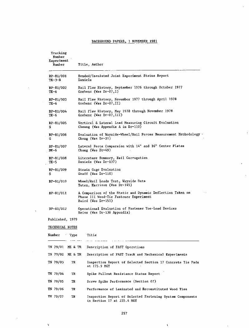
BACKGROUND PAPERS, 1 NOVEMBER 1981

TrackingNumber

ExperimentNumber Title, Author

BP-81/001TE-3-B

Bonded/Insulated Joint Experiment Status Report Daniels

BP-81/002TE-6

Rail Flaw History, September 1976 through October 1977 Grebenc (Was Dr-07,1)

BP-81/003TE-6

Rail Flaw History, November 1977 through April 1978 Grebenc (Was Dr-07,II)

BP-81/004TE-6

Rail Flaw History, May 1978 through November 1978 Grebenc (Was Dr-07,III)

BP-81/005S

Vertical & Lateral Load Measuring Circuit Evaluation Cheung (Was Appendix A in Dr-110)

BP-81/006G

Evaluation of Wayside-Wheel/Rail Forces Measurement Methodology Chang (Was Dr-31)

BP-81/007ME-6

Lateral Force Comparsion with 14" and 16" Center Plates Chang (Was Dr-49)

BP-81/008TE-5

Literature Summary, Rail Corrugation Daniels (Was Dr-137)

BP-81/009S

Strain Gage Evaluation Graff (Was Dr-110)

BP-81/010 Wheel/Rail Loads Test, Wayside Data Tuten, Harrison (Was Dr-145)

BP-81/011 A Comparison of the Static and Dynamic Deflection Taken on Phase III Wood-Tie Fastener Experiment Baird (Was Dr-151)

BP-81/012 Operational Evaluation of Fastener Toe-Load Devices Heiss (Was Dr-136 Appendix)

Published, 1979

TECHNICAL NOTES

Number Type Title

TN 79/01 ME & TR Description of FAST Operations

TN 79/02 ME & TR Description of FAST Track and Mechanical Experiments

TN 79/03 TR Inspection Report of Selected Section 17 Concrete Tie Pads at 175.9 MGT

TN 79/04 TR Spike Pullout Resistance Status Report

TN 79/05 TR Screw Spike Performance (Section 07)

TN 79/06 TR Performance of Laminated and Reconstituted Wood Ties

TN 79/07 TR Inspection Report of Selected Fastening System Components in Section 17 at 235.4 MGT

257

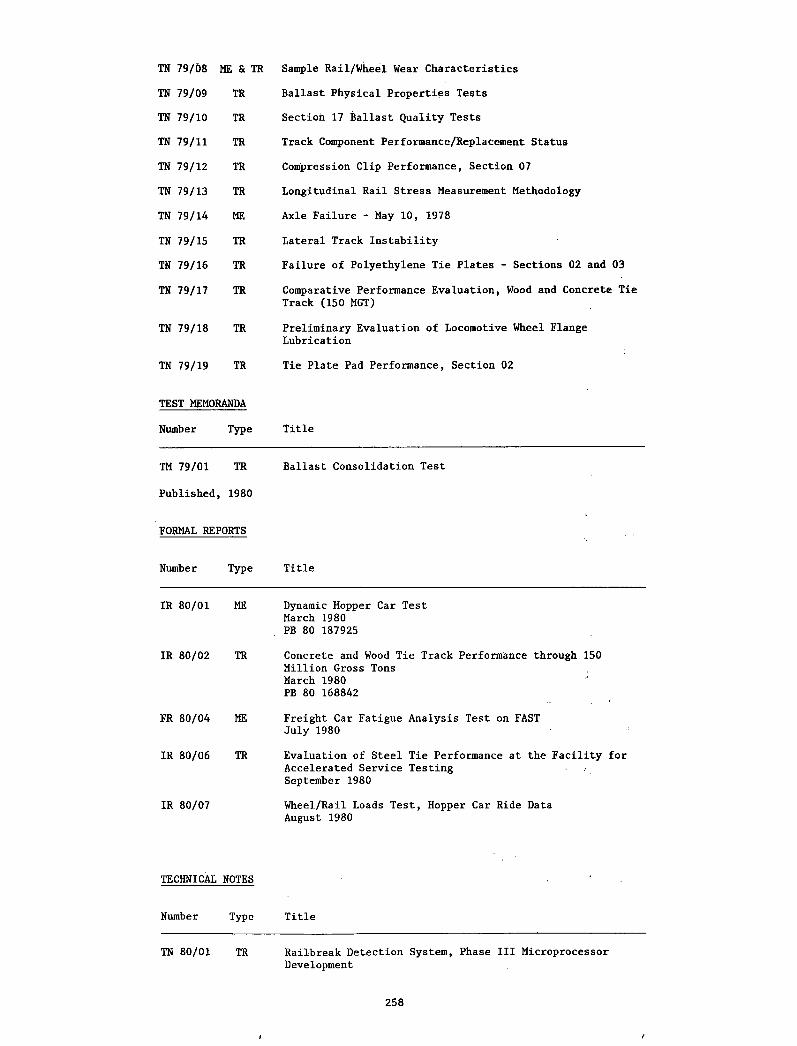
TN 79/08 ME & TR Sample Rail/Wheel Wear Characteristics

TN 79/09 TR Ballast Physical Properties Tests

TN 79/10 TR Section 17 Ballast Quality Tests

TN 79/11 TR Track Component Performance/Replacement Status

TN 79/12 TR Compression Clip Performance, Section 07

TN 79/13 TR Longitudinal Rail Stress Measurement Methodology

TN 79/14 ME Axle Failure - May 10, 1978

TN 79/15 TR Lateral Track Instability

TN 79/16 TR Failure of Polyethylene Tie Plates - Sections 02 and 03

TN 79/17 TR Comparative Performance Evaluation, Wood and Concrete Tie Track (150 MGT)

TN 79/18 TR Preliminary Evaluation of Locomotive Wheel Flange Lubrication

TN 79/19 TR Tie Plate Pad Performance, Section 02

TEST MEMORANDA

Number Type Title

TM 79/01 TR Ballast Consolidation Test

Published , 1980

FORMAL REPORTS

Number Type Title

IR 80/01 ME Dynamic Hopper Car Test March 1980PB 80 187925

IR 80/02 TR Concrete and Wood Tie Track Performance through 150 Million Gross Tons March 1980 PB 80 168842

FR 80/04 ME Freight Car Fatigue Analysis Test on FAST July 1980

IR 80/06 TR Evaluation of Steel Tie Performance at the Facility for Accelerated Service Testing September 1980

IR 80/07 Wheel/Rail Loads Test, Hopper Car Ride Data August 1980

TECHNICAL NOTES

Number Type Title

TN 80/01 TR Railbreak Detection System, Phase III MicroprocessorDevelopment

258

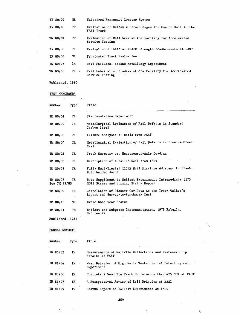
TN 80/02 ME Undesired- Emergency Locator System

TN 80/03 TR Evaluation of Weldable Strain Gages For Use on Rail in the FAST Track

TN 80/04 TR Evaluation of Rail Wear at the Facility for Accelerated Service Testing

TN 80/05 TR Evaluation of Lateral Track Strength Measurements at FAST

TN 80/06 ME Fabricated Truck Evaluation

TN 80/07 TR Rail Failures, Second Metallurgy Experiment

TN 80/08 TR Rail Lubrication Studies at the Facility for Accelerated Service Testing

Published, 1980

TEST MEMORANDA

Number Type Title

TM 80/01 TR Tie Insulation Experiment

TM 80/02 TR Metallurgical Evaluation of Rail Defects in Standard Carbon Steel

TM 80/03 TR Failure Analysis of Rails from FAST

TM 80/04 TR Metallurgical Evaluation of Rail Defects in Premium Steel Rail

TM 80/05 TR Track Geometry vs. Measurement-Axle Loading

TM 80/06 TR Description of a Failed Rail from FAST

TM 80/07 TR Fully Heat-Treated 115RE Rail Fracture Adjacent to Flash- Butt Welded Joint

TM 80/08 TR See TM 81/03

Data Supplement to Ballast Experiments Intermediate (175 MGT) Stress and Strain, Status Report

TM 80/09 TR Correlation of Plasser Car Data to the Track Walker's Report and Survey-to-Benchmark Test

TM 80/10 ME Brake Shoe Wear Status

TM 80/11 TR Ballast and Subgrade Instrumentation, 1979 Rebuild, Section 22

Published, 1981

FORMAL REPORTS

Number Type Title

IR 81/03 TR Measurements of Rail/Tie Deflections and Fastener Clip Strains at FAST

IR 81/04 TR Wear Behavior of High Rails Tested in 1st Metallurgical, Experiment

IR 81/06 TR Concrete & Wood Tie Track Performance thru 425 MGT at FAST

IR 81/07 TR A Perspectival Review of Rail Behavior at FAST

IR 81/09 TR Status Report on Ballast Experiments at FAST

\

259

V

FR 81/10 ME Hopper vs. Tank Car Truck Loads

IR 81/11 TR The Effect of Service Loading on the Bending Strength of Concrete Ties

TECHNICAL NOTES

Number Type Title

TN 81/01 ME Description of Selected FAST Truck Measurements, First Truck Experiment

TN 81/02 ME Radial Truck Experiment - Restart at FAST

TN 81/03 TE Ballast Shoulder Width Experiment

TN 81/04 ME Axle Alignment Measurements on Cars in the FAST Radial Truck Experiment

TN 81/05 Alternate Method for Separable Body Center Plate Replacement

Publishedj, 1981

TEST MEMORANDA

Number Type Title

TM 81/01 ME Wheel Flange Cracks Evaluation, First Experiment

TM 81/02 TR Concrete Tie Instrumentation for the Phase II Tie/Fastener Experiment at FAST

TM 81/03 TR Ballast Experiments Intermediate (175 MGT) Stress & Strain Status Report

TM 81/04 TR Summary of the Subsurface Exploration Program Performed Prior to the 1979 FAST Rebuild, Sections 03, 17 and 22

TM 81/05 TR Operational Evaluation of Fastener Tie Load Devices, October 20, 21, and 22, 1980

TM 81/06 TR Documentation of Ballast and Subgrade Aspects of 1979 Rebuild of FAST, Sections 03, 17 and 22

TM 81/07 TR Track Settlement Predictions at FAST

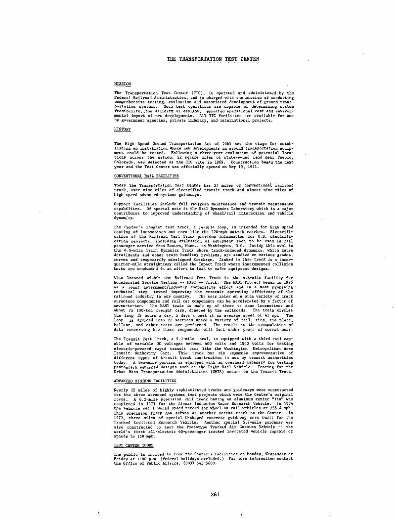
THE TRANSPORTATION TEST CENTER

MISSIONThe Transportation Test Center (TTC), is operated and administered by the Federal Railroad Administration, and is charged with the mission of conducting comprehensive testing, evaluation and associated development of ground trans­portation systems. Such test operations are capable of determining system feasibility, .the validity of designs, expected operational cost and environ­mental impact of new developments. All TTC facilities are available for use by government agencies, private industry, and international projects.HISTORY

The High Speed Ground Transportation Act of 1965 set the stage for estab­lishing an installation where new developments in ground transportation equip­ment could be tested. Following a three-year evaluation of potential loca­tions across the nation, 52 square miles of state-owned land near Pueblo, Colorado, was selected as the TTC site in 1969. Construction began the next year and the Test Center was officially opened on May 19, 1971.CONVENTIONAL RAIL FACILITIESToday the Transportation Test Center has 37 miles of conventional railroad track, over nine miles of electrified transit track and almost nine miles of high speed advanced systems guideways.Support facilities include full railroad maintenance and transit maintenance capabilites. Of special note is the Rail Dynamics Laboratory which is a major contributor to improved understanding of wheel/rail interaction and vehicle dynamics.The Center's longest test track, a 14-mile loop, is intended for high speed testing of locomotives and cars like the 120-mph Amtrak coaches.' Electrifi­cation of the Railroad Test Track provides information for U.S. electrifi­cation projects, including evaluation of equipment soon to be used in rail passenger service from Boston, Mass., to Washington, D.C. Inside this oval is the 4.5-mile Train Dynamics Track where track-induced dynamics, which cause derailments and other train handling problems, are studied on various grades, curves and temporarily misaligned trackage. Linked to this track is a three- quarter-mile straightaway called the Impact Track where instrumented collision tests are conducted in an effort to lead to safer equipment designs.Also located within the Railroad Test Track is the 4.8-mile Facility for Accelerated Service Testing — FAST — Track. The FAST Project began in 1976 as a joint government/industry cooperative effort and is a most promising technical step toward improving the economic operating efficiency of the railroad industry in our country. The wear rates on a wide variety of track structure components and rail car components can be accelerated by a factor of seven-to-ten. The FAST train is made up of three to four locomotives and about 75 100-ton freight cars, donated by the railroads. The train circles the loop 15 hours a day, 5 days a week at an average speed of 41 mph. The loop is divided into 22 sections where a variety of rail, ties, tie plate, ballast, and other tests are performed. The result is the accumulation of data concerning how these components will last under years of normal wear.The Transit Test Track, a 9.1-mile oval, is equipped with a third rail cap­able of variable DC voltages between 400 volts and 1500 volts for testing electric-powered rapid transit cars like the Washington Metropolitan Area Transit Authority Cars. This track has six segments representative of different types of transit track construction in use by transit authorities today. A two-mile portion is equipped with an overhead catenary for testing pantograph-equipped designs such as the Light Rail Vehicle. Testing for the Urban Mass Transportation Administration (UMTA) occurs on the Transit Track.ADVANCED SYSTEMS FACILITIESNearly 15 miles of highly sophisticated tracks and guideways were constructed for the three advanced systems test projects which were the Center's original focus. A 6.2-mile precision rail track having an aluminum center "fin" was completed in 1971 for the Linear Induction Motor Research Vehicle. In 1974 the vehicle set a world speed record for wheel-on-rail vehicles at 255.4 mph. This precision track now serves as another access track to the Center. In 1973, three, miles of special U-shaped concrete guideway were built for the Tracked Levitated Research Vehicle. Another special 5.7-mile guideway was also constructed to test the Prototype Tracked Air Cushion Vehicle -- the world’s first all-electric 60-passenger tracked levitated vehicle capable of speeds to 150 mph.TEST CENTER TOURSThe public is invited to tour the Center's facilities on Monday, Wednesday or Friday at 1:00 p.m. (federal holidays excluded.) For more information contact the Office of Public Affairs, (303) 545-5660.

261

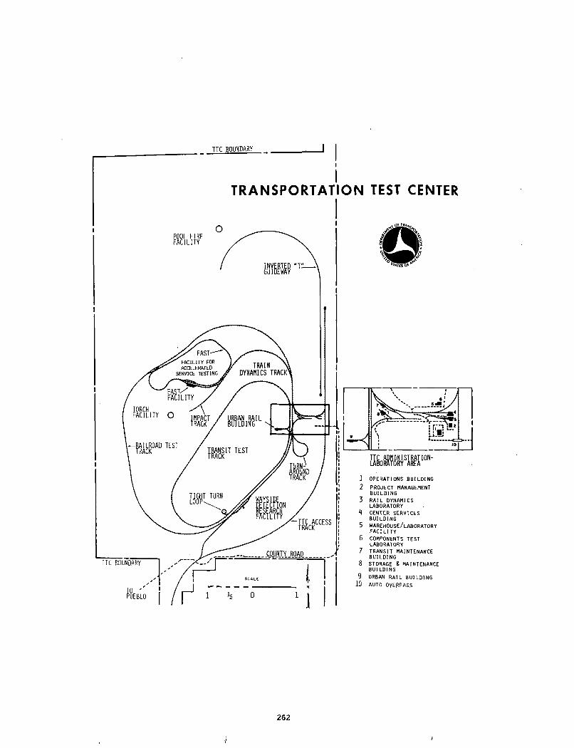
TTC BOUNDARY

i

TRANSPORTATION TEST CENTER

POOL FIRE FACILITY

INVERTED "Ti- GUIDEWAY

I QLIMa,

IU ' 1PUEBLO

I

] OPERATIONS BUILDING

2 PROJECT MANAGEMENT BUILDING

3 RAIL DYNAMICS LABORATORY

A CENTER SERVICES BUILDING

5 w a r e h o u s e / l a b o r a t o r y FACIL ITY

6 COMPONENTS TEST LABORATORY

7 TRANSIT MAINTENANCE BUILDING

8 STORAGE 8 MAINTENANCE BUILDING

9 URBAN RAIL BUILDING 10 AUTO OYERPASS

262

FEDERAL RAILROAD ADMINISTRATION ATTENDEES

Richard D. AndersonFacility Eng. & Construction Coordinator Transportation Test Center P.O. Box 11330 Pueblo, CO 81001

R. M. McCaffertyChief, Systems Engineering Division Transportation Test Center P.O. Box 11330 Pueblo, CO 81001

Trevor R. Chapman Program Analyst Transportation Test Center P.O. Box 11330 Pueblo, CO 81001

J. J. ReimersFAST Project Test Mechanical Manager Transportation Test Center P.O. Box 11330 Pueblo, CO 81001

Eldon L. EkbergChief, Facilities Management Division Transportation Test Center P.O. Box 11330 Pueblo, CO 81001

BOEING SERVICES INTERNATIONAL ATTENDEES

Thomas E. O'Brien Site Manager

Don MillerSupervisor, Operations & Data Production

C. E. Maddox Deputy Site Manager

Jodi TorpeyPublic Communications Coordinator

C. R. PerryManager, FAST Engineering Conference

Nancy Blume Associate Engineer

Harry MutterManager, Test Design & Analysis

Dick GraffSupervisor, Test Instrumentation System

John LearyIndustrial Engineer Statistician

Ernie SmithEngineering Test Support Planner

Jan Parlett Cost Accountant

J. A. Gardner Engineering Aide

Tom CookManager, FAST Operations

Jim Jollay Engineer

Randy Jackson Senior Engineer

Glenn SanduskySupervisor, System Software & Configuration Management

Gloria Ornelas Clerk

Tom GuentherEngineering Test Support Planner

Jeff Champine Engineer

Tom Roderick Carman Lead

Rich Reiff Senior Engineer

Dave ReadSupervisor Track Management

263

Rich Crader Engineering Aide

Ted BerrianEngineering Test Support Planner

Curt UrbanMeasurement Tech Lead

Bill Rhodes Electronic Tech Lead

Jack SeyfferSupervisor, Test Data Production & FAST Sotware

Troy BomarManager, Test Operations Department

Leon SappSupervisor, Equipment Maintenance & Vehicle Operations

Don DuransoSupervisor, Quality Assurance

Tim SuazoResource Controller

John St. Vrain Engineering Specialist

Scott Livingston Programmer

Britto RajkumarSenior Specialist Engineer

Luis MieraQuality Assurance Specialist

Mike Strah Programmer

Larry BenedictRail Safety Supervisor

Bev WheelerMaintenance Data Evaluation Analyst

Doug TaylorSupervisor, Application Software Development

Navin Parikh Senior System Analyst

Ramesh DigheSupervisor, Test Support

Tom Sanchez Programmer

Leroy KuennenSupervisor, Rail Equipment Maintenance

Rick HerndonSupervisor, Motor/Heavy Equipment & Track Equipment

Ravi Margasahayam Senior, Specialist Engineer

Gerry O'KeefeSupervisor, Vehicle Operations

Jeff HahneQuality Assurance Specialist

Steve Singsass Engineering Specialist

James Morrissey Programmer

Ernie ShoafSupervisor, Computer Operations/Data Entry & I/O Control

Lahnona Krumanocker Programmer

Carl AckerMeasurements/Video Systems Specialist

MAGAZINE ATTENDEES

D. B. Mabry William J. SemioliEditor EditorCrossties' Magazine Railway Track & Structures

29 East Madison StreetChicago, IL 60602

F. Stewart Mitchell Modern Railroads Magazine 5 South Wabash Avenue Chicago, IL 60603

Carl H. Wesselmann EditorProgressive Railroading 20 North Wacker Drive Chicago, IL 60606

264

ASSOCIATION OF AMERICAN RAILROAD ATTENDEES

John A. Angold AAR Consultant 13527 Hyacinta Sun City West, AZ 85375

Charlie Bean AARTransportation Test Center P.0. Box 11130 Pueblo, CO 81001

Ronald J. BegierFAST Technical SupportAARTransportation Test Center P.O. Box 11130 Pueblo, CO 81001

John Choros Research Engineer AAR Technical Center 3140 S. Federal St. Chicago, IL 60616

Bill Cruse Track Consultant AARP.O. Box 1464 404 N. Abrego Dr.Green Valley, AZ 85614

Wayne K. MingerDirector of AdministrationAAR1920 "L" Street Washington, D.C. 20036

Jesus Prieto AARTransportation Test Center P.O. Box 11130 Pueblo, CO 81001

Alex Rodriquez AARTransportation Test Center P.O. Box 11130 Pueblo, CO 81001

Glen StaeheliExperiment Monitor - Mechanical AARTransportation Test Center P.O. Box 11130 Pueblo, CO 81001

G. W. Walker AARTransportation Test Center P.O. Box 11130 Pueblo, CO 81001

Keith L. Hawthorne Director TTD R&T - AARAmerican Railroads Building Washington, D.C. 20036

Leslie WoodallOperations & Safety Consultant AAR2614 W. Regency Drive Tucker, GA 30084

Thomas B. Hutcheson Transportation Consultant AAR1825 Elizabeth Place Jacksonville, FL 32205

Can-Wen Yang EngineerResearch & Test Association of American Railroads Technical Center 3140 S. Federal St.Chicago, IL 60616

William Frederick Lewis Economics & Finance Dept. AARAmerican Railroads Building Washington, D.C. 20036

265

PRESENTERS

Roy A. AllenAssociation of American Railroads AAR Technical Center 3140 S. Federal St.Chicago, 1L 60616

V. E. KahleSr. Assistant Chief Chemist Southern Pacific Transportation Co. 401 "I" Street Sacramento, CA 95814

Bruce N. BossermanProject ManagerTest Design & AnalysisFederal Railroad AdministrationTransportation Test CenterPueblo, CO 81001

James W. Brent ConsultantAssociation of American Railroads 6303 Mandeville Road Louisville, KY 40228

Lauress C. Collister ConsultantAssociation of American Railroads 1914 Sims Street Topeka, KS 66604

Larry E. Daniels Boeing Services International Transportation Test Center P.0. Box 11449 Pueblo, CO 81001

Thomas P. Larkin Chief, Test Operations Division Federal Railroad Administration Transportation Test Center Pueblo, CO 81001

James R. Lundgren FAST Technical Manager Association of American Railroads Transportation Test Center Pueblo, CO 81001

✓Gregory P. McIntosh FAST Program Manager Federal Railroad Administration Transportation Test Center Pueblo, CO 81001

Howard G. Moody Office of Rail Safety Research Federal Railroad Administration 400 Seventh Street, S.W. Washington, D.C. 20590

Timothy J. Devine Sr. Project Engineer Griffin Wheel Company 200 West Monroe Street Chicago, IL 60606

J. W. GessnerPresident & Chief Executive Officer Missouri Pacific Railroad Co.210 N. 13th St.St. Louis, M0 63103

Donald E. GrayAnalysis & Evaluation Division Office of Rail Safety Research Federal Railroad Administration 400 Seventh Street, S.W. Washington, D.C. 20590

Oscar Orringer Department of Transportation Transportation System Center Kendall Square Cambridge, MA 02142

S. K. Punwani Senior Research Engineer AAR Technical Center 3140 S. Federal St. Chicago, IL 60616

Roger K. Steele - Manager, Metallurgy Federal Railroad Administration Transportation Test Center Pueblo, CO 81001

Jack E. HeissBoeing Services International Transportation Test Center P.0. Box 11449 Pueblo, CO 81001

John W-. Weber 2727 Black Hawk Road Wilmette, IL 60091

266

1981 FAST CONFERENCE ATTENDANCE ROSTER

Robert AckertSr. Research. AssociateAlgoma SteelQueen St. West ,Sault Ste. Marie, Ontario Canada

G. G. Albin ’Director - Track Quality & Tests Engineering Department Burlington Northern 176 East Fifth Street St. Paul, MN 55101

Rex Alexander Sales Engineer Concrete Crossties Blakeslee Prestress, Inc.P.0. Box 510 Branford, CT 06405

Eugene C. Allen Supervising Engineer Parsons, Brinkerhoff, CENTEC Inc. 8200 Greensboro Drive, Suite 100 McLean, VA 22102

Paul B. Armstrong Engineer of Track Union Pacific 400 West Street Salt Lake City, UT 84101

William W. AtkinsonChief of Equipment EngineeringSouth Pacific Transportation Co.#1 Market PlazaSan Francisco, CA 94105

' ! .1

W. S. Autrey ;Chief EngineerThe Atchison, Topeka & Santa Fe Railway Co. 80 East Jackson Blvd., Room 201 Chicago, IL 60604

E. C. Bailey "Director of Engineering Dresser, Inc.2 Main St.Depew, NY 14043

Benj amin F . Baker Sales ManagerInternational Track Systems, Inc. 620 West 32nd St.Ashtabula, OH 44004

John D. BakerEngineering Special ProjectThe Atchison, Topeka & Santa Fe Railway Co.80 East Jackson Blvd.Chicago, IL 60604

Cliff BaldwinPublic Service Co. of Colorado P.0. Box 840 Denver, CO 80201

C . D . Barton Chief EngineerMissouri Pacific Railroad Co. 210 N. 13th St.St. Louis, MO 63103

John R. Baxter General Manager Btrec, Inc.1581 Stone Ridge Rd.Stone Mountain, GA 30083

D. K. BeachySpeciality Sales Administrator Treated Wood Products Division Koppers Company, Inc. Pittsburgh, PA 15219

John Beal-Preston Pandrol, Inc.P.0. Box 44 Bridgeport, NJ 08014

R. F. Beck Chief EngineerElgin, Joilet & Eastern Railway Co. Joliet, IL 60434

267

1981 FAST CONFERENCE ATTENDANCE ROSTER

Roger E. Belau Manager, Product Planning Fairmont Railway Motors Fairmont, MN 56031

Steven R. Benton Research City Manager Research Center Portec, Inc., R.P.P.300 Windsor Drive Oak Brook, IL 60521

Harry B. Berkshire Assistant Vice-President Maintenance of Way & Engineering Southern Pacific Transportation Co. #1 Market Plaza San Francisco, CA 94105

Mario Bertolini PresidentBlakeslee Prestress, Inc.P.0. Box 510 Branford, CT 06405

Allen C. BieberManager - Mechanical Design Engineer Locomotive Engineering Dept.General Electric Co.2901 East Lake Road Erie, PA 16531

Alan J. BingConsultant & Senior Staff Arthur D. Little, Inc.Acorn Park Cambridge, MA 02140

Fred B. BladerDirector, Railroad SystemsTASCOne Jacob Way Reading, MA 01867

R. W. BlankChief Materials Engineer Research & Tests Southern Railway Co.409 S. Henry St. Alexandria, VA 22314

Bernard E. BloodChief Intercity Systems Division U.S. DOT/TSC Kendall Square Cambridge, MA 02140

D. L. BogerAssistant Chief Engineer C&NW Transport Co.500 W. Madison Chicago, IL 60606

George BonnerAssistant Chief Engineering Engineering & MOW Dept.The Family Lines Rail System 500 Water Street Jacksonville, FL 32202

J. Eloy Yanez Bordier General Superintendent F.C. Chihuahua A1 Pacifico Chihuahua, Chih., Mexico

R. J. BourqueChief, Rail Crossing & Construction Canadian Transport Commission Terminal Plaza Building 1222 Main St.Moncton, N.B. E1C 1H6

K. W. BradleyAssistant Chief Engineer Planning Denver & Rio Grande Western Railroad Co. P.0. Box 5482 Denver, CO 80217

Chuck Branstrom Vice President True TemperChemetron, Div. of Allegheny Int. Ill East Wacker Drive Chicago, IL 60601

Alan BriggsSales ManagerRail & Track ProductsBritish Steel Corp.Dresser Tower, 601 Jefferson Houston, TX 77002

268

1981 FAST CONFERENCE ATTENDANCE ROSTER.

R. G. BrohaughAssistant Vice President - Engineering Burlington Northern 176 East Fifth Street St. Paul, MN 55101

Charles M. Brown Product Development Manager Market Development Department Union Carbide Corporation 4625 Royal Avenue, P.O. Box 579 Niagra Falls, NY 14302

James T. Brown Assistant Chief Engineer Bethlehem Steel Corp. F Johnstown, PA 15907

R. M. Brown Chief Engineer Engineering Dept.Union Pacific Railroad 1416 Dodge St.Omaha, NE 68179

Trevor Brown Technical Director Pandrol, Inc. -9 HolbornLondon, ECIN 2NE *

R. G. BuffalowSuperintendent Air Brakes 1Denver & Rio Grande Western Railroad' P.O. Box 5482 * ■'Denver, CO 80217 '' *

R. L. BullockManager, Research and Development- Standard Car Truck Company 332 South Michigan Ave. - Chicago, IL 60604 c

E. B. Burwell, E.V.P. Southern Railway Washington, D.C. 20013.

R. F. ButterEngineer - Maintenance of Way Pittsburgh & Lake Erie Railroad Co. P. & L.E. Terminal Bldg.Pittsburgh, PA 15219

W. Nelson Caldwell Senior Research Engineer C&N Rail Research 3950 Hickmore Ave.St. Laurent, Quebec, Canada H4T1K2

Ross G. CarleVice President of Engineering Railroad Dynamics 10 East Athens Ardmore, PA 19003

Sherry L. Carpenter DirectorKansas City Southern Railway Co. Louisiana & Arkansas Railway Co. 114 W. Eleventh St.Kansas City, MO 64105

C. Chambers Senior Estimator Railco Multi Construction Sherwood, OR 97140

J. G. Chandler Project Engineer Engineering & MOW Dept.The Family Lines Rail System 500 Water Street Jacksonville, FL 32202

Joseph ChisholmAsst. Dir. Rail Safety & Service Rail TransportCanadian Transport Commission Government of Canada

Anthony T . BrunoManager Railgrinding ServicesFairmont Railways Motors'"ATB Associates 472 South Salina St.Syracuse, NY 13202

269

1981 FAST CONFERENCE ATTENDANCE ROSTER

H. B. ChristiansonDirector - Train Accident Prevention Casualty Prevention Department Chessie System Railroads Baltimore, MD 21201

M. J. Crespo Transportation Engineer Bethel Civil & Minerals, Inc. P.0. Box 3965 San Francisco, CA 94119

Donald E. Cleveland, P.E. Professor - Civil Engineering University of Michigan Ann Arbor, MI 48103

J. 0. Crook, P.E.Chief Engineer Pounding Mill Quarry Corp. P.0. Box 13527 Roanoke, VA 24010

Bryan Clough Pandrol Incorporated P.0. Box 44 Bridgeport, NJ 08014

Marino Curati Chief Engineer Railway Appliances, Inc. Ill East Wacker Drive Chicago, IL 60601

R. J. CochenourPittsburgh & Lake Erie Railroad P. & L.E. Terminal Building Pittsburgh, PA 15219

P. J. CurleyAssistant Manager, Product SalesTransit Products846 South Central Ave.Hapeville, GA 30354

George R. Collier Project Engineer Retired Santa Fe Railroad 1311 Chipper Lane Wichita, KS 67212

David CurrentTrack Maintenance Supervisor Navajo ProjectBlack Mesa Lake Powell Railroad Box WPage, AZ 86040

Steve Conquergood Development Engineer Con-Force Costain Concrete Tie Co., Ltd.Box 3618, Station D Edmonton, Alberta TSL4J6

Robert H. Curtin General Manager Deleuw Cather Parsons 1201 Connecticut Ave., N.W. Washington, D.C. 20036

J. C. Cosgrove PresidentUnit Rail Anchor Co.2 North Riverside Plaza, Suite 2336 Chicago, IL 60606

Calvin C. Custer Chief Metallurgist , , Bethlehem Steel Corp. Steelton, PA 17113

Carl L. Crawley Section ChiefPower Division, Civil DepartmentBurn & McDonnellP.0. Box 173Kansas City, MO 64141

Angelo M. D'Attoma Manager, Omark Track-Lok . Omark Industries, Unit No. 9 2091 Springdale Road Cherry Hill, NJ 08003

.270

1981 FAST CONFERENCE ATTENDANCE ROSTER

C. P. DavisMaintenance Operations Engineer Illinois Central Gulf Railroad Two Illinois Center 233 N. Michigan' Ave. J Chicago, IL 60601

Dennis Dobson Managing Director Pandrol, Inc.P.0. Box 44 Bridgeport, NJ 08014

Francis DeanPrincipal Research Engineer Battelle Columbus Laboratories 505 King Ave.Columbus, OH 43201 0

Ronald H. Dunn Vice PresidentParsons, Brinckerhoff, Centec Inc. 8200 Greensboro Drive, Suite 100 McLean, VA 22102

Doug G. DeBergEngineer - Maintenance of Way Toledo, Peoria & Western Railroad Co. 2000 E . Washington St.East Peoria, IL 61611 !

J. B. Dupere SupervisorQuebec North Shore & Labrador Railway Dock OfficeSept lies, Quebec Canada

R. B. DehlsV.P. & Mgr. - Trans. Sales & Planning Treated Wood Products Division Koopers Company, Inc.Pittsburgh, PA 152i9

H. B. Durrant Assistant Chief Engineer Engineering Department Union Pacific Railroad 1416 Dodge St.Omaha, NE 68179

C. S. DeSar ProfessorDepartment of Civil Eng. & Eng. Mechanics The University of Arizona Tucson, AZ 85721

Dennis J. DwyerGovernment Affairs Representative Railway Progress Institute 700 N. Fairfax St.Alexandria, VA 22314

Douglas W. Dibble ‘ Development Officer Transportation Development Center 1000 Sherbrooke St. W.P.0. Box 549Montreal, Quebec H3A 2R3

B. J. EckDirector - Product Engineering Griffin Wheel Company 200 West Monroe Chicago, IL 60606

Gary G. DillDirector, New Product Sales Frame Division Midland Steel Products1 Co. P.0. Box 6386 Cleveland, OH 44101

John A. ElkinsMember of Technical StaffTASCOne Jacob Way Reading, MA 01867

S. R. DitmeyerDirector, Research & Development Burlington Northern Railroad 176 E. Fifth Street, Room 230 St. Paul, MN 55101

H. L. Ellis Regional Engineer Chessie SystemOperating Headquarters Building P.0. Box 1800 Huntington, WV 25718

1981 FAST CONFERENCE ATTENDANCE ROSTER

C. J. Engelhardt, P.E.Senior Director Equipment Engineering AMTRAK400 North Capitol St., N.W. Washington, D.C. 20001

J. T. Evans Acting Associate Dean Michigan Technology University Houghton, MI 49931

Robert A. Evans Mechanical Consultant 3329 Flyntwood Dr. Santa Rosa, CA 95404

John T. FergusonManager, Rail Welding & Track Test Union Pacific Railroad Laramie, WY

William H. Ferryman Chief Engineer Region Engineering Division Burlington Northern 1405 Curtis St.Denver, CO 80202

W. L. FinnManager of Car Repair Engineering Shippers Car Line Division ACF Industries, Inc.620 N. 2nd St.St. Charles, MO 63301

D. FirthRegional General Manager Con-Force Costain 12707 - 170 Street Edmonton, Alberta Canada

Carl S. Fletcher General Manager Newton County Stone Co., Inc. Kentland, IN 47951

Dr. Hans D. FrickePresidentU.S. Thermit, Inc.Ridgeway Boulevard Lakehurst, NJ 08733

Robert A. Frigstad Manager Product Development Technical Services 3M Co.St. Paul, MN 55144

Ralph Frost Technical Director Chemetron Railway Products 111 E. Wacker Dr.Chicago, IL 60601

Charles M. Funk Engineer Track - ED Union Pacific Railroad Co. 1416 Dooge St.Omaha, NE 68179

Iwad Furuya Manager, R&D Nippon Steel, USA, Inc. 345 Park Ave., 41st Floor New York City, NY 10154

D. J. Gale Engineer of Track Union Pacific Railroad 400 West St.Salt Lake City, UT 84101

Erich Gehrke Director Btrec, Inc.1581 Stone Ridge Rd.Stone Mountain, GA 30083

Howard Gilbertson ConsultantNorth Eastern Railroad Products, Inc. P.0. Box 320 55 Russell St.Woburn, MA 01801

272

i

1981 FAST CONFERENCE ATTENDANCE ROSTER

Charles Godfrey Consultant ABEX Corp.P.0. Box 369Green Valley, AZ 856i4

Ben GordonChief Engineering Office ConrailPhiladelphia, PA

Pedro Juarez Gracias Asst. Chief Mech. Officer Ferrocarriles Nacionales De Mexico Ave. Centeral 140 Piso 60 Ala "A" Mexico City, Mexico 3, D.F.

R. L. GrayDirector Standards & Development R.T.C. Canadian Transport Commission Government of Canada

Bill Greenwood Dresser, Inc.2 Main Street Depew, NY 14043

Harvey HaldenbySenior Metallurgist - 'Shape ProductsAlgoma SteelQueen St. WestSault Ste. Marie,•OntarioCanada

William R. Hamilton Director of R&D Portec, Inc.Railway Products Division 300 Windsor Dr.Oak Brook, IL 60521

Edward G. Hansen Principal Engineer T&D DepartmentE .I . DuPont De Nemours & Co. Wilmington, DE 19898

J. G. HarrisAsst. Engineer - Mechanical Denver & Rio Grande Western Railroad P.0. Box 5482 Denver, CO 80217

Dale A. Harrison Special Products Engineer Santa Fe Railway Co.9th & Jackson Ave.Topeka, KS 66605

Harley H. Hartman CF&ICanal & Abriendo Ave. Pueblo, CO 81004

William G. HarveyExecutive V.P. & General ManagerChicago & Illinois Midland Railway Co.P.0. Box 189Springfield, II 62705

H. T. HastingsManager of Car Design & Construction Mechanical Department Family Lines Rail System 500 Water St.Jacksonville, FL 32202

E. F. HeatonSupervisor Locomotive Equipment Missouri Pacific Railroad Co.210 N. 13th St.St. Louis, M0 63103

Robert J. HenryEngineerResearchBethlehem Steep Corp. Bethlehem, PA 18016

L. M. HeplerProduct Manager - Brake Shoes Griffin Wheel Company 200 West Monroe Chicago, IL 60606

273

V

1981 FAST CONFERENCE ATTENDANCE ROSTER

J. D. Hines Manager of Sales Unit Rail Anchor Co.2 North Riverside Plaza, Suite 2336 Chicago, IE 60606

George A. HommelGroup Vice President - CastingsMidland Ross700 S. Dock St.Sharon, PA 16146

Charles N. Hood Director Market Development Marketing Division American Steel Foundries 3600 Prudential Plaza Chicago, IL 60601

Eugene Y. HuangActing Associate Dean of Graduate Michigan Technology University Houghton, MI 49931

Bob Hudson Pandrol, Inc.P.0. Box 44 Bridgeport, NJ 08014

David J. Hughes President Pandrol, Inc.P.0. Box 44 Bridgeport, NJ 08014

J. H. Hughes Vice PresidentKansas City Southern Railway Co. Louisiana & Arkansas Railway Co. 114 W. Eleventh St.Kansas City, MO 64105

Larry R. Jacobson Project Manager Dalton, Dalton & Newport 3605 Warrensville Center Rd, Cleveland, OH 44122

D. L. JermanSenior EngineerM/W Standards & TestingNational Railroad Passenger^Corp.400 North Capitol St., N.W.Washington, D.C. 20001

Darrell L. Johnson Mechanical Inspector Mechanical Burlington Northern 176 E. Fifth St.St. Paul, MN 55119

S. R. JohnsonAssistant Vice PresidentOperations PlanningThe Family Lines Rail System500 Water StreetJacksonville, FL 32202

W. A. JohnsonDirector - Maintenance Planning Engineering Department Burlington Northern Railroad 176 E. Fifth St. . -St. Paul, MN 55101

C. R. KaelinDirector - ,uTechnical Research & Development AT&SF Railway Co.Topeka, KS 66628

Joseph C. KahrManager, Cobra Shoe Engineering Engineering Department i!WABCOAmerican Standard,:'Inc. Wilmerding, PA 15148

Kazuo (Jim) Kato &1Assistant General Manager Mitsui & Co. n<200 Park Ave.New York, NY 10017 x’

Robert A. Kendall !Senior Manager, Field Operations (DCP) Deleuw Cather Parsons - 1201 Connecticut Ave., N.W.1!' Washington, D.C. 20036 J

274

1981 FAST CONFERENCE ATTENDANCE ROSTER

Marty Kennedy Pandrol, Inc.P.0. Box 44Bridgeport, NJ 08014 ;

M. D. Kenyon rAssistant Chief Engineer Denver & Rio Grande Western Railroad P.0. Box 5482 Denver, CO 80217 ,

G. F. LazarProduct Manager - Wheels Griffin Wheel Company 200 West Monroe Chicago, IL 60606

Geoffry Leeves Pandrol, Inc.

Co. P.0. Box 44Bridgeport, NJ 08014

Glen KesterRailroad Superintendent Navajo ProjectBlack Mesa Lake Powell!, Railroad Box WPage, AZ 86040

Michael J. Klima Rail Marketing Engineer Stedef, Inc.Tysons Office Park, #14 7657 Leesburg Pike Falls Church, VA 22043

Dr. Sudhir KumarProfessor & Director R.R. Eng. Lab. Illinois Institute of Technology 11T Center Chicago, IL 60616

Robert L. LantzRegional Manager - Trans. Sales West Forest Products Group,,Koppers Company, Inc.122 South Michigan Ave.Chicago, IL 60603 r

Kenneth W. Larsen Program Manager ;Dynamic Science, Inc.Washington Operations 8326 Professional Hill Drive Fairfax, VA 22031

R. F. LawsonVice President - Chief Engineer National Railroad Passenger Corp.400 North Capitol St., N.W. Washington, D.C. 20001

Kenneth Lenzen AREA Committee #24 Engineering Division of AAR University of Kansas Lawrence, KS

Jack R. LongDirector, Eng. Research & Development Midland Ross 700 S. Dock St.Sharon, PA 16146

Robert B. Love Regional Sales Manager Marketing Division American Steel Foundries 3600 Prudential Plaza Chicago, IL 60601

J. K. LynchManager, Transp., Sales & Rail Car Vulcan Materials Co.P.0. Box 7497 Birmingham, AL 35253

Joseph F. LynchSuperintendent, Metallurgy & Q.C. Wheel, Pittsburgh Steel Monessen Plant Monessen, PA 15062

Robert N. Madderom Pandrol, Inc.P.0. Box 44 Bridgeport, NJ 08014

1981 FAST CONFERENCE ATTENDANCE ROSTER

Dan Mahoney SalesmanFabreeka Products Co.7100 Broadway P.0. Box 21346 Denver, CO 80221-0346

Gene D. Mall Manager - Eastern Sales Kerr-McGee Chemical Corp. Kerr-McGee Center Oklahoma City, OK 73125

N. C. MarshAssistant Manager, Reliability Engineering Technical Research & Development AT&SF Railway Co.Topeka, KS 66628

John H. Martens Senior Metallurgical Engineer Bethlehem Steel Corp. Bethlehem, PA 18016

Donald H. McDonell Engineer, Structural Division Stone & Webster Engineering Corp. P.O. Box 5406 Denver, CO 80217

Tom McElroySupervisor, Maintenance of Way Quebec North Shore & Labrador Railway Dock OfficeSept lies, Quebec, Canada

Robert D. Mclntire Vice President & General Manager Midland Ross 700 S. Dock St.Sharon, PA 16146

C. W. McKee Director R&D Teleweld, Inc.1555 Hawthorne Lane West Chicago, 1L 60185

J. R. MastersChief Engineer - Maintenance PlanningEngineering DepartmentBurlington Northern176 East Fifth StreetSt. Paul, MN 55101

Hiroshi Matsumoto ManagerEngineering & Steel Products NKK America, Inc.450 Park Ave.New York, NY 10022

Robert A. Matthews Vice President Railway Progress Institute 700 N. Fairfax St.Alexandria, VA 22314

Ron MayvilleConsultant & Senior Staff Arthur D. Little, Inc. Cambridge, MA 02140

Philip J. McQueen, P.E. Consulting Engineer 30 Fairway Drive Ignacio, CA 94947

Hubert V. Meek Gen. RoadmasterThe Denver & Rio Grande Western Railroad P.O. Box 5482 Denver, CO 80217

Kenneth D. MelsChief Locomotive Development Engineer Electro-Motive Division General Motors Corp.LaGrange, IL 60525

Scott D. Miller Sales Representative Plasser American Corp. 2001 Myers Rd. Chesapeake, VA 23324

276

>J

1981 FAST CONFERENCE ATTENDANCE ROSTER

John R. Mitoraj Manager, Railroad Sales J. P. Ruklic Screw Co'; 13550 S. Chatham a Blue Island, IA 60406

Chas. Moehling Manager, Track Engineering American Steel Foundries 3600 Prudential Plaza ' Chicago, II 60601

P. I. Montgomery Manager, Engineering Systems Norfolk & Western Railway Co. 8 North Jefferson St.Roanoke, VA 240427 C

Jim E. Morenz CF&ICanal & Abriendo Ave.Pueblo, CO 81004

Jeff MorrowManager, HSLA Development Climax Molybdenum Co.'3072 One Oliver Plaza.Pittsburgh, PA 15222'

Jerry Munro Regional Manager True TemperCheinetron, Div. of Allegheny Int. Ill East Wacker Drive Chicago, II 60601

Miguel leal Murguia Chief Track Machinery DepartmentF .C .. Chihuahua AL Pacifico Chihuahua, Chih., Mexico

Graham Murray DirectorBtrec, Inc. r s1581 Stone Ridge Rd.aC Stone Mountain, GA 30083

G. A. Musolf Manager, Engineering Standard Car Truck Company 332 South Michigan Ave. Chicago, II 60604

Walter Muzychenko ManagerRailway Division Engineering American Koyo Corp.29570 Clemens Rd., P.0. Box 45028 Westlake, OH 44145

Georg Nadorff Representative HRS Germany 561 Beech Drive Kent, OH 44240

Brad Nelson Track Engineer AMAX - Henderson Mine Box 68Empire, CO 80438

O. T. Nephew Director of Engineering Teleweld, Inc.1555 Hawthorne lane West Chicago, II 60185

Ronald R. NewmanManager, Track Train DynamicsOperations DepartmentBurlington Northern176 East Fifth StreetSt. Paul, MN 55101

Harry S. Nichols PresidentThe Nichols CompanyP. 0. Box 157 Troy, MI 48099

Yasuhide Nishimoto Department General Manager Mitsui & Co.200 Park Ave.New York, NY 10017

277

Vi’

1981 FAST CONFERENCE ATTENDANCE ROSTER

Mrs. J. J. O'Dea Mechanical Engineer Research & Tests Southern Railway Co.409 S. Henry St.Alexandria, VA 22314

Keisuke Ogawa Assistant Manager Steel Department Mitsui & Co.17117 W. Nine Mile Road, Suite 1440 Southfield, MI 48075

James L. Ozment Division EngineerDenver & Rio Grande Western Railroad Co. 650 Davis Rd.Salt Lake City, UT 84119

Romolo Panetti Pandrol, Inc.P.O. Box 44 Bridgeport, NJ 08014

Stewart P. Park, Jr.Chief Mechanical Officer Maine Central Railroad Company 242 St. John St.Portland, ME 04102

Robert E. Parsons U.S. Department of Commerce National Bureau of Standards 109 McLaughlin Hall Berkeley, CA 94720

Lynn Patterson Sales Manager Fabreeka Products Co.7100 Broadway P.O. Box 21346 Denver, CO 80221-0346

R. K. Pattison PresidentParsons, Brinkerhoff, Centec Inc. 8301 Greensboro Dr., Suite 220 McLean, VA 22102

Warren B. Peterson Chief Engineer jSoo Line Rail road. Company • Box 530Minneapolis, MN 55440

Vincent Petrucelly Research EngineerPort Authority of New York & New Jersey 1 Path Plaza, 3rd Floor Jersey City, NJ 07306

A. E. Pew, III Director, Administration RED Division i jBurlington Northern Railroad 176 E. Fifth Street St. Paul, MN 55101

David A. Pittinger National Sales Manager Railroad Products Lone Star Industries, Inc. .6416 Halsey Drive . >Woodridge, IL 60517

C. T. Popma , -tAssistant Vice-President Quality Control & Mechanical Eng. Dept. C0NRAIL1802, 1528 Walnut St.Philadelphia, PA 19102

A. K. Pottorff vDistrict EngineerAT&SF Railway Co. .P.O. Box 1738 gTopeka, KS 66628

Don Powell, P.E.Construction Materials Engineer Vulcan Materials Co.P.O. Box 7497 ; .JBirmingham, AL 35223

Robert H. Prause ,,, uSection Manager 0Battelle Columbus Laboratories 505 King Ave. 1Columbus, OH 43201. ,;

278

1981 FAST CONFERENCE ATTENDANCE ROSTERA

A. E. Price Shaun RichmondTechnical Director n Manager, Design AnalysisSales/Marketing Thrall Car Manufacturing Co.General American Transportation Corp. - GATX 26th & State St.120 South Riverside Plaza Chicago, IL 60606

Julia Prudhoe Pandrol, Inc. ' iP.0. Box 44 Bridgeport, NJ 08014'

, 0

C. 1. PuriRegional EngineerCanadian Transport Commission60 Adelaide St. East, 4th FloorToronto, OntarioCanada LAT 3P9 -

j (

Esteban QuinteroChief Inspector Carbozulia Project Railroad Department t;IE CO180 Howard St. ^San Francisco, CA 94105

Leonard U. RastrelliDirector, Department of Special Studies Instrumentation Research Division Southwest Research Institute P.0. Drawer 28510 San Antonio, TX 78284

IA. J. ReinschmidtAsst. Prof, of Railway EngineeringPennsylvania State UniversityAccounting Operations302 Shields BuildingUniversity Park, PA 16802

Ernest J. RewuckiEng. of Track CP RailWindsor Station, Room^401430 Montrose Dr. cMontreal, Quebec, Canada H3C 3E4

H. E. Richardson Assistant Chief Engineer Engineering & MOW Dept.The Family Lines Rail-System 500 Water Street Jacksonville, FL 32202

Chicago Heights, IL 60411

Armin RichterSupervisor Systems Shop Programming Burlington Northern 1675 Old Hudson Rd.St. Paul, MN 55106

S . RishovdL0RAM Maintenance of Way, Inc. 3900 Arrowhead Drive Hamel, MN 55340

A1 Rivoire Pandrol, Inc.P.0. Box 14 Bridgeport, NJ 08014

Stuart M. RobertsonChief Railroad Design Dept.IECO180 Howard St.San Francisco, CA 94105

H. L. RoseAssistant Vice President MW&S of Southern Railway Co. 99 Spring St.Atlanta, GA

Dean J. RougasAssistant Manager, RailroadCF&I SteelP.0. Box 1830Pueblo, CO 81002

R. RoughtChief Product Engineer Engineering Department Midland Steel Products Co. P.0. Box 6386 Cleveland, OH 44101

279

1981 FAST CONFERENCE ATTENDANCE ROSTER

W. T. RousisSupervisor, Material Control, MW Material Management Department NW Railway8 N. Jefferson St. - 60 B East Roanoke, VA 24042

C. N. ScottDirector, Research & Test Southern Railway 409 S. Henry St. Alexandria, VA 22313

Kenneth C. Rownd Project Engineer Proform, Inc.7901 Xerxes Avenue So. Minneapolis, MN 55431

Frank Scott Research EngineerNelson Caldwell Service Research Eng. Canadian Nation Rail, CN Research Center 3950 Hiekmore Ave.St. Laurent, Quebec H4T 1K2

J. E. RussellManager, Transportation Equipment Industrial Chemical Division PPG Industries, Inc.One Gateway Center Pittsburgh, PA 15222

David R. Seeley Pandrol, Inc.P.0. Box 44 Bridgeport, NJ 08014

Brian T. Scales Railway Consultant Devine Mfe. Co. Pittsburgh, PA 15219

William W. Sellers PresidentStandard Car Truck Company 332 South Michigan Ave. Chicago, IL 60604

H. L. Schaaf Marketing El DuPont Co.1414 Lark Dr. Evansville, IN 47715

A. E. Shaw, Jr., P.E.Director - Engineering Department AMTRAK1617 J. F. Kennedy Blvd. Philadelphia, PA 19103

K. R. Schaeffer General Car Inspector Denver & Rio Grand Railroad P.0. Box 5482 Denver, CO 80217

Nathan E. SmithAssistant V.P., Chief Engineer The Milwaukee Road 516 West Jackson Blvd.Chicago, IL 60606

Thomas G. Schultz 1931 Rosebud Court San Jose, CA 95128

R. E. Snyder Director, MTC OPR C.& N.W. Transport Co. 500 W. Madison St. Chicago, IL 60606

Jon Schumaker Executive Vice President Pandrol, Inc.P.0. Box 44 Bridgeport, NJ 08014

Bill SpencerDirector of Maintenance Planning Union & Pacific Railroad 1416 Dodge St.Omaha, NE 68179

280

3 1981 FAST CONFERENCE ATTENDANCE ROSTER

Harry C. Steelman Assistant Division Engineer Union Pacific Railroad *J 1745 Massachusetts Ct.Green River, NY 82935.

Max Stephens Manager Sales Vulcan Materials Co.P.0. Box 80730 15Atlanta, GA 30366 “

£ ' it

Lars C. Strom Project ManagerStone & Webster Engineering Co.P.0. Box 5406Denver, CO 80217 J'

Eric J. Summers System Supervisor, MOW 1 Engineering Department CN Rail ' ;Montreal, Quebec Canada 1

J. E. Sunderland Regional Engineer Chessie System y"Operating Headquarters Building 100 N. Charles St. /Baltimore, MD 21201 1

F. W. B. Taylor Highway Engineer U.S. Army Forces Command Hdqrs., U.S. Army Forces Command Fort McPherson, GA 30330

Takao TeradaManager - Plate & Shape Dept., Yawata WorksNippon Steel Corporation6-3, Otemachi 2-ChomeChiyoda-KuTokyo 100, Japan

Gerhard A. Thelen DirectorMechanical Engineering*.C0NRA1L x225 30th Street Station Philadelphia, PA 19104

J. W. Thomas Quality Control Manager Sperry Rail Service Division Automotive Industries, Inc. Shelter Rock Road Danbury, CT 06810

Robert Tobias Track Foreman AMAX - Henderson Mine Box 68Empire, CO 80438

Y. H. TseAssistant Manager - Analytical SupportMechanical EngineeringC0NRAIL225 30th Street Station Philadelphia, PA 19104

William S. Tuinstra Special Assistant Engineer Staff Studies & Planning Santa Fe Railroad Co.80 E. Jackson Chicago, IL 60604

D. M. TutkoChief Mechanical Officer Missouri Pacific Railroad Co.210 N. 13th St.St. Louis, M0 63103

Robert F. TuveManager, Quality Control Engineering Engineering and Research Department Southern Railway System 99 Spring St., S.W.Atlanta, GA 30303

Hugo ValladaresAsst. Chief Inspector Cairbozulia ProjectRailroad DepartmentIEC0180 Howard St.San Francisco, CA 94105

Wayne Vanderleest Pandrol Incorporated P.0. Box 44 Bridgeport, NJ 08014

281

1981 FAST CONFERENCE ATTENDANCE ROSTER

Nick VentiChief Mechanical Engineer Servo Corp. of America 111 New South Road Hicksville, NY 11802

Hans Von Lange PresidentElastic Spike Corp. of America 115 East Joppa Road Baltimore, MD 21204

R. P. Wallace Director Quality Control Chessie SystemOperating Headquarters Building P.0. Box 1800 Huntington, WV 25718

James W. WalshDirector Freight Car Maintenance Mechanical Department Boston & Maine Corp.High StreetNorth Billerica, MA 01882

R. H. Walsh General Sales Manager Holland Company 1020 Washington Ave.Chicago Heights, IL 60411

E. H. Waring Chief Engineer D&RGW Railroad P.0. Box 5482 Denver, CO 80217

John G. WhiteVice President & General Manager Con-Force Costain 1000-1520 - 4th St. SW Calgary, Alberta Canada T2R 1H5

D. B. Whitehurst Vice-President - Marketing Griffin Wheel Company 200 West Monroe Chicago, IL 60606 *

Eric Wolf Manager, Research Trailer Train Co.101 North Wacker Drive Chicago, IL 60606

Gary P. WolfSr. Operations Research Analyst Operations Research Southern Railway System 125 Spring St. S.W., Room 815 Atlanta, GA 30303

L. F. WoodlockChief Engineer - Maintenance of Way Engineering Department Burlington Northern 176 East Fifth Street St. Paul, MN 55101

Arthur W. Worth Engineer Standards CN Rail935 de La Gauchetiere St. West Montreal, Quebec Canada

Bruce E. Wylie PresidentRobert J. Wylie Co.295 E. Marie Ave.West St. Paul, MN 55118

Ken YatesRail Tech. Manager, Track Products British Steel Corp., Inc. Workington, United Kingdom

William Zacharkiw Pandrol, Inc.P.0. Box 44 Bridgeport, NJ 08014

Alan Zarembski Pandrol, Ind.P.0. Box 44 Bridgeport, NJ 08014

* U. S. GOVERNMENT PRINTING OFFICE 1982 - 578-00^/170 Reg. 8

282

ASSOCIATION OF

R E S E A R C H A N D T E S T D E P A R T M E N T — O P E R A T I O N S . P U E B L O

1 1 3 8 B L U E S T E M , P . O . B O X 1 1 1 3 0 , P U E B L O , C O L O R A D O 8 1 0 0 1

J . R . L U N D G R E N

D i r e c t o r - A A R O p e r a t i o n s , P u e b l o

E x t . 3 1 7 / 2 8 1

C . W . B E A N

A s s i s t a n t t o D i r e c t o r , P u e b l o

E x t . 2 9 2 / 3 1 7

R . J . B E G I E R

M anager, FAST Technical S u p p o r t E x t . 2 8 9 1 2 8 1

G . W . W A L K E R

M a n a g e r , F A S T I n d u s t r y

S u p p o r t E x t . 2 0 8 1 2 1 5

March 4, 1982

To: AREA Committee MembersAAR Mechanical Committee Members Track-Train Dynamics Committee Members FAST Donors

Gentlemen:

We are pleased to enclose a copy of the Proceedings of our November, 1981 FAST Engineering Conference.

These proceedings represent a selection of the more impor­tant findings from the major FAST Experiments after five years of operation.

Your continued inter is sincerely appreciated.

JRL:lbb

'est m and support of the FAST Program

JjyR. Lundgren, Director Operations, Pueblo

Attach.

cc: W. J. Harris, Jr.

!

\

1981 FAST ENGINEERING CONFERENCE PROCEEDINGS

ERRATA SHEET

Page 48 - Figure 8 - "Wyoming Granite", is also known as "CEB".

Page 49 - Figure 13 - Caption should read: "Change in grain sizedistribution, Georgia Granite Ballast - Section 17 (concrete ties)".

Page 50, Table 2 - "Section 18" should be "Section 17".

Page 51, Table 3 - "III-6" should be "III-8".

Page 52, First paragraph - "90 MGT" should be "190 MGT".

Page 53, Question No. 2 - Change "Shoule" to "Should".

Page 53, Question No. 5, Answer No. 2 - "granite" should be"granite/granite like".

Page 63, First paragraph - Change "1% grade" to ".1% grade".

Page 63 - Figure 2 - Change "BALLAST: Slag, 14" deep" to"BALLAST: Slag, 15" deep".

Page 65, Table 1 - Delete asterisk next to "Clips 99".Add asterisk next to heading, "FAILURES*"..

Page 68 - Delete bracket in Table 3.

Page 69 - Delete brackets in Table 4.

Page 69 - Delete: "(@RAIL BASE)" at the top of Figure 15.Add: "at rail base" to caption of Figure 15.

Page 71, Column 2, Paragraph 2 - Delete: "clip and".

Page 87 - Figure 12 - Caption should read: "Auto Spectrum Concrete Tie;Heavy Corrugations".

Page 99 - Column 2, Paragraph 2 - Change "studs" to "strips".D elete "to s tr ip s " .

Page 115, Column 1, Paragraph 3 - Change "assending" to "ascending".

Page 117, Column 2 - Under equation, change "y = variance. . ."tox 9~y

"a = variance".x >y

Page 136, Column 1, Paragraph 2 - Change "affects" to "effects".

Page 178 - Figures 6 and 7 are reversed.

- f '/

Continued . .

V A

V'*

)

Errata Sheet (Continued)

Page 181 - Figure 12 - Caption should read "Flange Thickness..."

Page 182 , Column 2, Paragraph 2 - "S2" should be "S^"

Page 184, Table 9 - Model equation should be:"Y = 0.01303 + (0.00179 + 0.00040X1 - 0.00026X2 - 0.00080X3

- 0.00011X5) mileage"Corrections are underlined.

Page 184, Table 10 - Model equation should be:"Y = 0.00298 + (0.00293 + 0.00035X1 + 0.00028X2 - 0.00149X3 - 0.00008X4 - 0.00013X5) mileage"Corrections are underlined.

Page 188, Table 13 - Change caption from "Wrought" to "Cast".

Page 193, Column 2, Paragraph 6 - "Table 16" should be "Table 17".

Page 220, Column 1, Paragraph 1 - "+0.02 percent" should be " t 0.02 percent".

Page 203, Column 2 - Note change "metal behavior or carbon . . . " to"metal behavior of carbon . . . "

Page 218 - Equation 3 is w£ - yf F£ + (e* tan 8)2 "

/ r~2 : 2a + (0w tan B) " r

Page 218, Column 2, Paragraph 4 - "lasers " should be "lasers (2 and 3)"

Page 219, Column 1, Paragraph 1 - "lasers 1 and 2" should be "lasers 1 and 3"

Page 221 - Figure 6 - Data point missing for empty - should be 13 (lb rads)

Page 232, Column 2, Paragraph 5 - "Table 2" should read "Table 1".

Page 234, Figure 17 - Photo is upside down.

Page 249, Figure 3 - Caption should read "TTC Wheel Measuring Device".Figure 4 - Caption should read "TTC Rail Measuring Device".

Page 250, Reference 6 is the source document for the material presented in the Appendix.

Continued . . .

-2-

A

/

Errata Sheet (Continued)

Page 250, Appendix 1 - MR" in the two equations should be "RR"

From TDOP representation:

" b = B, b2 " 5 o

Should be: " Bc b + B, b2 " 5 0

\

FAST Engineering Confernce -1981 Proceedings, 1982 US DOT FRA/TTC-82/01

__PROPERTY OF FRARESEARCH & DEVELOPMENT

LIBRARY ....... .

NOTICE

This document is disseminated under the sponsorship of the Department of Transportation in the interest of information exchange. The United States Govern­ment assumes no liability for its contents or use.

NOTICE

The United States Government does not endorse pro­ducts or manufacturers. Trade or manufacturers’ names appear herein solely because they are con­sidered essential to the object of this report.