Engineering Applications of Adaptive Kalman Filtering Based ...

applied sciences

Article

Engineering Applications of Adaptive KalmanFiltering Based on Singular Value Decomposition(SVD)

Juan Carlos Bermúdez Ordoñez * , Rosa María Arnaldo Valdés andVictor Fernando Gómez Comendador *

School of Aeronautical and Space Engineering, Universidad Politécnica de Madrid, Plaza Cardenal Cisneros 3,28040 Madrid, Spain; [email protected]* Correspondence: [email protected] (J.C.B.O.); [email protected] (V.F.G.C.)

Received: 11 May 2020; Accepted: 21 July 2020; Published: 27 July 2020

Abstract: This paper presents the results of applying the new mechanization of the Kalman filter (KF)algorithm using singular value decomposition (SVD). The proposed algorithm is useful in applicationswhere the influence of round-off errors reduces the accuracy of the numerical solution of the associatedRiccati equation. When the Riccati equation does not remain symmetric and positive definite, thefidelity of the solution can degrade to the point where it corrupts the Kalman gain, and it can corruptthe estimate. In this research, we design an adaptive KF implementation based on SVD, provide itsderivation, and discuss the stability issues numerically. The filter is derived by substituting the SVDof the covariance matrix into the conventional discrete KF equations after its initial propagation, andan adaptive estimation of the covariance measurement matrix Rk is introduced. The results showthat the algorithm is equivalent to current methods in terms of robustness, and it outperforms theestimation accuracy of the conventional Kalman filter, square root, and unit triangular matrix diagonal(UD) factorization methods under ill-conditioned and dynamic applications, and is applicable tomost nonlinear systems. Four sample problems from different areas are presented for comparativestudy from an ill-conditioned sensitivity matrix, navigation with a dual-frequency Global PositioningSystem (GPS) receiver, host vehicle dynamic models, and distance measuring equipment (DME)using simultaneous slant range measurements, performed with a conventional KF and SVD-based(K-SVD) filter.

Keywords: adaptive Kalman filter applications; singular value decomposition filtering; computerround-off errors; control systems; navigation; GNSS; DME

1. Introduction

By defining what robustness means in the context of this research, we can focus on the engineeringapplications of the proposed method. We refer to robustness as the “relative insensitivity of the solutionto errors of some sort” [1]; also, we refer to numerical stability to denote robustness against round-off

errors [2].The design of the Kalman filter (KF) usually aims to “ensure that the covariance matrix of

estimation uncertainty (the dependent variable of the matrix Riccati equation) remains symmetric andpositive definite” [1,3]. The main problem to be solved in this research is the numerical robustness ofKF. The proposed algorithm is useful in applications where the influence of round-off errors reducesthe accuracy of the numerical solution of the associated Riccati equation. The fidelity of the solutionmay degrade to the point that it corrupts the Kalman gain when the Riccati equation does not staysymmetric and positive definite, and it can corrupt the estimate [1]. Verhaegen and Van Dooren have

Appl. Sci. 2020, 10, 5168; doi:10.3390/app10155168 www.mdpi.com/journal/applsci

Appl. Sci. 2020, 10, 5168 2 of 26

shown that the asymmetry of P is one of the factors contributing to the numerical instability of theRiccati equation [4].

The problem was circumvented by Bierman [5] using unit triangular matrix diagonal (UD)factorization, which was one of several alternatives available to those in need of computationallyefficient and stable algorithms. This decomposition of the covariance matrix is of the form:

P = UDUT, (1)

where D denotes the diagonal matrix and U is the upper triangular matrix with ones along its maindiagonal. One of the individual characteristics of UD factorization and the Cholesky method is thatthere is no need to solve simultaneous Equations [6]. Additionally, UD factorization does not use asquare root numerical operation [6], but more recently square root filtering using standard matrixdecomposition has found greater acceptance [7]. In this matrix,

S = P12 such that P = SST. (2)

S is obtained in a triangular matrix from the well-known Cholesky decomposition [8,9], a drawbackof which is that it cannot be used if the covariance matrix is singular [6]. Both the square root andBierman methods can be used only if one has single-dimensional measurements with uncorrelatedmeasurement noise. Generally, one does not have this in practice [8,9]. To overcome the limitation,another method can be used—which is one of the topics of this research—that will facilitate the solutionof this type of problem, as the computation can be performed in parallel because it is formulated inthe form of matrix and matrix-vector operations without the need for additional transformations [10],where the solution also is able to deal with ill-conditioned matrices. This method is singular valuedecomposition (SVD).

The singular values (which are positive by definition) or principal standard deviation σi are thesquare roots of the diagonal elements. For the discrete time linear problem, which is evaluated in thisresearch, the first KF based on SVD was researched by Wang, Libert, and Manneback [8,9]. In thispaper, the algorithm is further improved by making the filter adaptable to changes in sensor quality.

The Riccati equation of the Kalman filter is an important tool for designing navigation systems,particularly those that incorporate sensors with diverse error characteristics, such as the GlobalNavigation Satellite System (GNSS) and the inertial navigation system (INS). The Riccati equationpermits us to predict the performance of a given system design as a function of the subsystem andcomponent error characteristics [2]. Designers can then search for the mixture of components thatwill reach a predefined set of performance endpoints at the lowest framework cost. The design ofthe Kalman filter is aimed at making sure the estimation uncertainty of the covariance matrix (thedependent variable of the matrix Riccati equation) remains symmetric and positive definite [1]. In thisresearch, we design an adaptive Kalman filter implementation based on SVD, provide its derivation,and discuss the stability issues numerically. The filter is derived by substituting the SVD of thecovariance matrix into the conventional discrete Kalman filter equations after its initial propagationand adaptive estimation of the covariance measurement matrix Rk.

One application of SVD in navigation is to apply it in calculating position errors to decomposethe geometric matrix G, where error analysis with SVD is used to construct the pseudo inverse of G,making the solution numerically stable. While the linear least squares (LLS) is somewhat susceptibleto round-up errors, where the normal equation is sometimes close to singular, SVD fixes the round-upproblem and produces a solution that is the best approximation in the least-squares sense [11].

Different applications in the area of ionospheric tomography, as the problem to be solved, encounterthe same ill-conditioned issue for the design matrix, which is composed of contributions of unknownparameters containing the ionospheric electron density (IED) in the total electron content (STEC)measurements, which is often not square, ill-posed, and ill-conditioned. Many methods have beenemployed to circumvent the problem of ill-posedness in the GNSS tomographic equation [12]. Those

Appl. Sci. 2020, 10, 5168 3 of 26

algorithms are iterative and include the Kalman filter, singular value decomposition, and algebraicreconstruction [7,9].

In the field of industrial electronic applications where numerical stability is necessary, an exampleis sensorless motor control, where the advantages of estimating the speed/position of the rotor includereduced hardware complexity, lower cost, reduced machine drive size, the elimination of the sensorcable, noise immunity, and increased reliability [13]; for example, a motor without a position sensor issuitable for harsh environments (such as submerged pumps). Other applications include diagnostics,the fault-tolerant control of AC drives, distributed generation and storage systems, robotics, visionand sensor fusion technologies, signal processing and instrumentation applications, and the real-timeimplementation of the Kalman filter for industrial control systems [13]. We briefly discuss the numericalstability of the Kalman filter related to industrial control systems and sensor fusion for cardiorespiratorysignal extraction, but focus on numerical examples in aerospace applications like GNSS navigation.

The safe and efficient operation of control systems requires computer-based failure detectionalgorithms [13], where diagnosis may be used to provide fault-tolerant control. Several failures canoccur in electrical systems, and redundant design is one of the solutions to assure the continuity and,therefore, the reliability of operations. Kalman filters can be used in fault-tolerant controls, for example,in aircraft control, home and municipal appliances (gas turbines, cooling systems, and heat pumps),and electric vehicles.

A challenge in the real-time implementation of Kalman filters is the high computational complexity,and among the main difficulties is numerical stability when computing the covariance matrices as wellthe computational load and execution time. There are three possible solutions to circumvent theseissues, and one solution is to modify the algorithm, which is the scope of this paper. In addition, anefficient digital architecture to implement the estimator [13], and parallel computing can be used. Theobservability problem physically means that one or more state variables (or linear combinations) arehidden from the view of the observer (i.e., the measurements) [6]. This is a challenge in the sensorlesscontrol of AC drives, which can be accentuated when the stator frequency is close to zero and therotor voltage carries small values. In addition, under continuous excitation conditions, when the statorfrequency is close to zero and when the inductor rotor voltage carries small values, an estimationof the speed of an induction motor (IM) is not likely to be obtainable. In practice, compared withextended Luenberger observers and slipping modes, the Kalman filter appears to function well in theseconditions with no divergence [13]. With this trade-off, the complexity of the Kalman filter is higher.

Other important applications of the KF are in the signal extraction and fusion of sensors, self-drivingcars, GNSS/INS integration, and biomedical sensors; for example, when extracting cardiorespiratorysignals from noninvasive and noncontacting sensor arrangements, such as magnetic induction sensors.In those applications, the signals are separated for monitoring purposes; by using the KF, it is possibleto measure the heart and breathing rates in real time [14], improving the estimation of results, whereasother filtering techniques fail to extract relevant information due to the mixing of respiratory andcardiac signals and disturbance by measurement noise [14].

The second objective of this paper is to promote the use of continuous adaptation changes inthe measurement error covariance matrix Rk. The Kalman gain Kk weights the innovation for themeasurement error covariance matrix Rk (the estimation error covariance matrix P−k+1 is influenced byQk), where higher values of Rk make the measurement update step differ a little from the predictedvalue when the Kalman gain Kk becomes very small [15]. On the contrary, high values of Qk engendermore trust in the estimation of the state; Zhang et al. [16] showed that inappropriate tuning parametersmay lead to low convergence by introducing adaptive technology consisting of adjustments to thenoise covariance matrices to improve the estimation accuracy. Muñoz-Bañon et al. [17] showed thatthe Kalman filter can be used to integrate high-level localization subsystems, where the covarianceinformation plays an essential role as new observations become available. This approach will be usedin this research.

Appl. Sci. 2020, 10, 5168 4 of 26

The proper selection of Rk and Qk is vital for optimal filter performance, as the system modelshould describe as closely as possible the time evolution of the measured data, and the choices shouldreflect the system model error and measurement noise [15]. This research only explores changes inthe measurement error covariance matrix Rk. Zhang et al. [18] showed that when the system beingconsidered has a stronger nonlinear action, the accuracy of the mode estimation will be poor. In order toaddress the shortcomings of the KF-based algorithm (K-SVD) and enhance the estimation precision, theadaptive filtering algorithm (K-SVD adaptive) was investigated, consisting of the adaptive estimationof Rk, which is a function of the standard deviation.

2. Conventional Kalman Filter

The filter estimates, at each time, the a priori state of the system based on the a posteriori estimatefor the previous moment and its dynamic equation. With this a priori estimate of the state, thecorresponding predicted measurement (Hkx−) that corresponds to that state is obtained. Then, it iscompared with the actual measurement (z) made at the same moment, then it corrects the a priori

estimation as a function of its discrepancy and weight between the trust in the a priori estimates andthe measurements represented by the gain K of the filter. The process performed by the filter can beseparated into two phases: prediction and correction [19].

Consider a discrete time model for a linear stochastic system:

xk+1 = Φk+1,kXk + Gkwk, (3)

Zk = Hkxk + vk, (4)

where xk ∈ Rnx1 is the state vector; Zk ∈ Rmx1 is the measurement vector; wk ∈ Rnx1 is the disturbanceinput vector; vk ∈ Rmx1 is the measurement noise vector; and Φk+1,k ∈ Rnxn, Gk ∈ Rnxn, and Hk ∈ Rmxn

are the system matrices. The covariance of wk is Qk, known as the process covariance matrix, and thatof Vk is Rk, known as the measurement covariance matrix, and they are presumed to be zero-meanGaussian white noise with the symmetric positive definite covariance matrices Qk and Rk, respectively.Then, w ∼ N(0, Q) and v ∼ N(0, R) at time tk, where a superscript (−) indicates the a priori valuesof the variables and a superscript (+) denotes values after the measurement update. The Kalman filteris described by following the recursive equations under the assumption that the system matrices arewell known:

Time extrapolation:x−k+1 = Φk−1,kx+k−1, (5)

P−k+1 = Φk−1P+k−1ΦT

k−1,k + Ψk−1Qk−1ΨTk−1. (6)

Measurement update:x+k = x−k + Kk

(zk −Hkx−k

), (7)

Kk = P−k HTk

(HkP−k HT

k + Rk)−1

, (8)

P+k = (I −KkH)P−k , (9)

where Pk is the covariance of estimation uncertainty, Kk is the Kalman gain matrix, and zk −Hkx−k arethe innovations of the discrete Kalman filter.

3. Singular Value Decomposition

Here, we consider singular value decomposition, which is a way of decomposing a matrix, A, inthe product of three other matrices: A = USVT.

Appl. Sci. 2020, 10, 5168 5 of 26

Remark 1. Let A be an n×d matrix with the right singular vectors v1 , v2, . . . , vk; left singular vectors u1, u2 ,. . . , uk ; and corresponding singular values σ1, σ2, . . . , σk . Then, A can be decomposed into a sum of rank-onematrices as follows:

A =k∑

i=1

σiuivTi ≈ σ1u1vT

1 + σ2u2vT2 + . . .+ σkukvT

k = UΣVT. (10)

Here, U ∈ Rmxm and V ∈ Rnxn , such that:

A = UΣVT, (11)

where:

Σ =

(S 00 0

). (12)

Here, Σ ∈ Rmxn and S = diag( σ2, . . . , σr) , with:

σ1 ≥ · · · ≥ σr ≥ 0,

σr+1 = 0 · · · σn = 0.,

The numbers σ1 . . . σr along with σr+1 = 0, . . . σn = 0 are known as the singular values of A, and they arethe positive square roots of the eigenvalues of ATA.

Columns U of A are the orthonormal eigenvectors of AAT, whereas columns V of A are theorthonormal eigenvectors of ATA. It is understood that the singular values and singular vectors ofa matrix are relatively insensitive to disturbance from the entries of the matrix and finite precisionerrors [8,20].

Given a non-square matrix A = U ΣVT, two matrices and their factorizations are of specialinterest:

AT A = VΣ2VT, (13)

AAT = U Σ2UT. (14)

The algorithm is developed by comparing both sides of the obtained matrix equations.

4. SVD of Kalman Filter

In practical terms, if AT A is positive definite, then Equation (13) can be compacted to:

A = U(

S0

)VT, (15)

where S is an n × n diagonal matrix. Specifically, if A is itself positive definite, then it will have anasymmetric singular decomposition (which is also an eigendecomposition):

A = UΣUT = UD2UT, (16)

where the principal standard deviations σi are the square roots of the diagonal elements of A. Assumingthat the covariance of the Kalman filter has been propagated and updated for everything from thefilter algorithm, the singular value decomposition of the equation of P. is:

P+k = U+

k D+2k U+T

k , (17)

Appl. Sci. 2020, 10, 5168 6 of 26

Equation (6) can then be written as:

P−k+1 = Φk+1U+k D+2

k U+Tk ΦT

k+1,k + ΨkQk ΨTk . (18)

The idea is to find the factors Uk+1 and Dk+1 from Equation (18), such that:

Pk+1 = Uk+1D2k+1UT

k+1. (19)

We define the following (s + n) × n matrix: D+2U+TΦTk+1,k(

Q112)T

ΨT

︸ ︷︷ ︸Pre−array

. (20)

Then, we compute its singular value decomposition: D+2U+TΦTk+1,k(

Q112)T

ΨT

︸ ︷︷ ︸Pre−array

= U′k

(D′k0

)V′k︸ ︷︷ ︸

Post−array SVD f actos

. (21)

Multiplying each term on the left by its transpose, we get:

Φk+1,kU+k D+T

k D+k U+T

k Φk+1,kT +ψk(Qk)

12

(Q

12k

)TψT

k = V′k[D′Tk

∣∣∣ 0]UTU

[D′k0

]V′Tk . (22)

We obtain:Φk+1,kU+

k D+2k Φk+1,k

T +ψkQkψTk = V′kD

′2k V

′Tk . (23)

Comparing the result of Equation (23) with Equations (18) and (19), it is easy to associate V′k andD′k with Uk+1 and Dk+1. In the orthodox Kalman measurement update, substituting Equation (8) into(9) yields:

P+k = P−k − P−k HT

k

(HkP−k HT

k + Rk)−1

HkP−k . (24)

Lemma 1. Using the matrix inversion lemma in the case where the inverse of a positive definite matrix A adds arank-one matrix bbT yields: (

A + bbT)−1

= A−1−A−1b

(1 + bTA−1

)−1btA−1, (25)

where the superscript T denotes the complex conjugate transpose (or Hermitian) operation. It is well known in theliterature that this formula is handy to develop a recursive least-squares algorithm for the recursive identificationor design of an adaptive filter [21].

The lemma on Equations (24) and (25) yields:(P+

k

)−1= P−1

k + HTk R−1

k Hk. (26)

Implementing the singular value decomposition of a symmetric positive definite matrix into P+k+1

and Pk yields: (U+

k D+2k U+T

k

)−1=

(UkD2

kUTk

)−1+ HT

k R−1k Hk, (27)(

U+k D+2

k U+Tk

)−1=

(UT

k

)−1(D+2

k + UTk HT

k R−1k HkUk

)U−1

k . (28)

Appl. Sci. 2020, 10, 5168 7 of 26

To make the system adaptable to changes in sensor quality, the measurement noise is alsoestimated, which leads to a time-variant matrix. When the signal comes from different sensors, at eachdiscrete time step k the noise covariance matrix is updated by appraising the standard deviation (std)of an arithmetically differentiated (diff) small-signal segment [14]:

Rk =

1 . . . 0...

. . . 00 0 1

∗ σ2noise,,k, (29)

σinoise,k =

std(di f f (Si))√

2. (30)

The adaptive computation of the KF and SVD-based (K-SVD) algorithm can be added independentof the SVD portion, as for some applications the measurement covariance matrix is known and can bepre-computed at the algorithm initiation.

After computing Equations (29) and (30), let

R−1k = LkLT

k (31)

be the Cholesky decomposition of the inverse of the covariance matrix. If covariance matrix R isknown, but not the inverse, then the reverse Cholesky decomposition R1/2R1/2T = R0, , R1/2 [8]

upper triangular can be identified. It then follows that Lk =(R1/2T

k

)−1is the necessary Cholesky

decomposition [20] in Equation (31).Now, we consider the (m + n) × n matrix:[

LTk HkUk

D−1k

], (32)

and compute its singular value decomposition:(LT

k HkUk

D−1k

)︸ ︷︷ ︸

Pre=array

= U∗k

(D∗k0

)V∗Tk︸ ︷︷ ︸

Post−array SVD f actors

. (33)

Multiplying each term on the left by its transpose produces:

D−2k + UT

k HTk LkLT

k HkUk = V∗kD∗2k V∗Tk . (34)

Then, Equation (28) can be written as follows:(UT

k

)−1(D+

k

)−2(U+

k

)−1=

(UT

k

)−1V∗kD∗2k V∗Tk U−1

k , (35)

(UT

k

)−1(D+

k

)−2(U+

k

)−1=

[(UkV∗k

)T]−1

D∗2k

[UkV∗k

]−1. (36)

Comparing both sides of Equation (36):

U+k = UkV∗k, (37)

D+k =

(D∗k

)−1. (38)

Appl. Sci. 2020, 10, 5168 8 of 26

The update measurement formulation is obtained, which requires calculating the singular valuedecomposition of the nonsymmetrical matrix without specifically defining its left orthogonal componentthat has a larger dimension. The Kalman gain term can be derived as:

Kk = PkHTk

(HkPkHT

k + Rk)−1

. (39)

Inserting P+k

(P+

k

)−1and (Rk)

−1Rk will not alter the gain. Thus, the Kalman filter gain can bewritten as:

Kk = P+k

(P+

k

)−1PkHT

k R−1k Rk

(HkPkHT

k + Rk)−1

, (40)

Kk = P+k

(P+

k

)−1PkHT

k R−1k

(HkPkHT

k R−1k + I

)−1, (41)

where I denotes the identity matrix. Next, from Equation (26), for(P+

k

)−1we get:

Kk = P+k HT

k R−1k , (42)

Kk = U+k D+2

k U+Tk HT

k LkLTk . (43)

The Kalman gain Kk is fully defined, and the state vector measurement is given by:

X+k = Xk + Kk

(Zk −HkXk

). (44)

Algorithm 1. Singular value decomposition-based Kalman filtering:

Input:Initialization (k = 0). Perform SVD on P0 to determine the initial U0 and D0. The initial P0 ∈ Rnxn, where U0

and D0 are orthogonal and diagonal matrices, respectively. Matrix U0 contains the singular values of P0.Steps (k = 1 to n):

1. Update U+k and D+

k by constructing the (m + n) × n matrix using a pre-array (32). Use only the rightSVD factor V.

2. Compute the Kalman gain Kk from Equation (43).

3. Update the estimate^x+

k from Equation (44). Notice that LTk is triangular, and the computation of

HTkLk =

(LT

kHk)T

can be obtained from step 2.

4. Compute the extrapolation^x−

k+1; from Equation (3), Uk+1 and Dk+1 can be obtained by the SVD from theEquation (21) pre-array matrix without forming the left orthogonal factor (the one associated withEquation (13) of the SVD).

5. Compute the measured noise time-variant matrix using Equations (29) and (30).

Return: Compute Lk using Equation (31) as Lk =(R1/2T

k

)−1.

The Algorithm 1 requires the Cholesky decomposition of noise covariance matrices R; fortime-invariant matrices, the Cholesky decomposition is performed once during the initial step—i.e.,before the KF recursion. Note that the algorithm also requires the m ×m matrix inversion for the termsR

12 and R

12 T in Equation (31). Again, if the process noise covariance is constant over time, the matrix

calculation is pre-computed while the filter is initialized.

5. Numerical Experiments: Applications in Navigation

The computer round-off for floating-point arithmetic is always demarcated by a single parameterεroundo f f , called the unit round-off error, which is demarcated as 1 + εroundo f f≡ 1 in machine precision.

In MATLAB, the parameter “eps” satisfies the definition above [2].

Appl. Sci. 2020, 10, 5168 9 of 26

Round-off errors are a side effect of computer arithmetic using fixed or floating-point data wordswith a fixed number of bits [2]. The next example demonstrates that round-off can still be a problemwhen implementing KF in MATLAB environments and how a problem that is well-conditioned can bemade ill-conditioned by the filter implementation [2]. The problem is taken from Grewal and Andrews,and it is significant, as it shows the filter’s observational behavior. The example does not make use ofthe Algorithm 1 adaptive computation from Equations (29) and (30), and the resulting algorithm iscalled K-SVD.Example 1. Let In denote the n × n identity matrix. Considering the filtering problem with the measurementsensitivity matrix:

H =

[1 1 11 1 1 + δ

],

and covariance matrices.P0 = I3 and R = δ2I2; to simulate round-off, it is assumed that:δ2 < εroundo f f but δ > εroundo f f .In this case, although H has rank = 2 in machine precision, the product HkP−0 HT

k with round-off

will equal: [3 3 + δ

3 + δ 3 + 2δ

],

which is singular, and the results remain unchanged when R is added to HkP−0 HTk .

All the KF tests were carried out with the same precision (64-bit floating-point) in MATLABrunning on a standard personal computer with an Intel(R) Core(TM) processor, i5-4200U CPU @ 1.60GHz 2.30 GHz, 8.0 GB RAM, where the unit round-off error is 2−53

∼ 1.11.10−16. The MATLAB epsfunction is twice the unit round-off error [2,22]. Hereafter, the set of numerical experiments is repeatedfor various values of the ill-conditioned parameter δ; as such, delta tends toward the machine precisionlimit δ→ εroundo f f . This example does not prove the robustness of the solution of the UD, square rootKalman (SQRK), and K-SVD methods. Full implementation would require temporal updates; however,observational updates have created difficulties with traditional implementation [2].

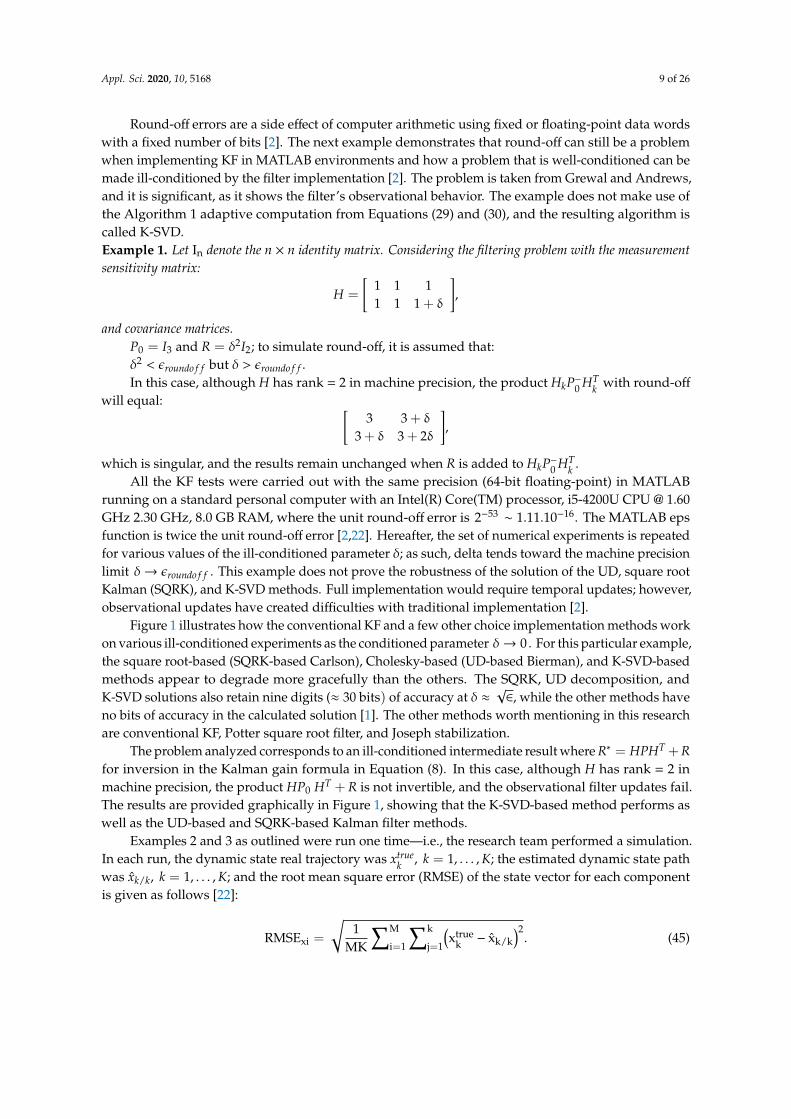
Figure 1 illustrates how the conventional KF and a few other choice implementation methods workon various ill-conditioned experiments as the conditioned parameter δ→ 0 . For this particular example,the square root-based (SQRK-based Carlson), Cholesky-based (UD-based Bierman), and K-SVD-basedmethods appear to degrade more gracefully than the others. The SQRK, UD decomposition, andK-SVD solutions also retain nine digits (≈ 30 bits) of accuracy at δ ≈

√∈, while the other methods have

no bits of accuracy in the calculated solution [1]. The other methods worth mentioning in this researchare conventional KF, Potter square root filter, and Joseph stabilization.

The problem analyzed corresponds to an ill-conditioned intermediate result where R∗ = HPHT +Rfor inversion in the Kalman gain formula in Equation (8). In this case, although H has rank = 2 inmachine precision, the product HP0 HT + R is not invertible, and the observational filter updates fail.The results are provided graphically in Figure 1, showing that the K-SVD-based method performs aswell as the UD-based and SQRK-based Kalman filter methods.

Examples 2 and 3 as outlined were run one time—i.e., the research team performed a simulation.In each run, the dynamic state real trajectory was xtrue

k , k = 1, . . . , K; the estimated dynamic state pathwas xk/k, k = 1, . . . , K; and the root mean square error (RMSE) of the state vector for each componentis given as follows [22]:

RMSExi =

√1

MK

∑M

i=1

∑k

j=1

(xtrue

k − xk/k

)2. (45)

Appl. Sci. 2020, 10, 5168 10 of 26

Figure 1. Degradation of observational updates with the problem conditioning of the Riccati equation.

Examples 2 and 3 use a GPS configuration loaded as Yuma ephemeris data from a GPS satellitefrom March 2014, downloaded from the US Coast Guard site YUMA Almanac [2].

Example 2. The following example shows a navigation simulation with a dual-frequency GPS receiver on a 100km-long figure-8 track for 1 h with signal outages of 1 min each. The problem is taken from Grewal and Andrews,and it is significant as it shows the filter’s observational behavior [2]. The state vector corresponds to nine hostvehicle model dynamic variables and two receiver clock error variables. The nine host vehicle variables are: easterror (m), north error (m), altitude error (m), east velocity error (m/s), north velocity error (m/s), altitude rateerror (m/s), east acceleration error (m), north acceleration error (m), and upward acceleration error (m). TheMATLAB m-file solves the Riccati equation with a dynamic coefficient matrix structure [2], where the 9 × 9matrix corresponds to the host vehicle dynamics and the 2 × 2 to the clock error.

9× 9 · · · 0...

. . ....

0 · · · 2× 2

(46)

Table 1 summarizes the outcome for a simulation using real ephemeris GPS data and anill-conditioned intermediate result where R−1 = HPHT +R for inversion in the Kalman gain formula inEquation (8). The example does not make use of the Algorithm 1 adaptive computation from Equations(29) and (30), and the resulting algorithm is called K-SVD.

The results in Table 1 show that the conventional KF is not suitable to gracefully handle round-off

errors, and other filter methods can be used to better handle the round-off issue. A large δ correspondsto a well-conditioned state. Once degradation happens, some of the filters decay faster than the K-SVD.The filter robustness can then be obtained by comparing the outcomes shown in Table 1 against thosewith the worst performance. The threshold where the filter can handle the error is reached when thealgorithm produces “NaN,” or not a number, and this happens when the conventional KF is at δ = 10−10.A comparison of the K-SVD with SQR-KF and UD-KF shows that the K-SVD algorithm is superior inhandling round-off errors. UD-KF is slightly better than SQR-KF, and the conventional KF performs aswell as the other two. Regarding the execution time, K-SVD and conventional KF are slower than SQRTand UD, and this is because SVD is computationally more costly than Cholesky decomposition [22].However, SVD is suitable for parallel computing and has a better numerical stability.

Appl. Sci. 2020, 10, 5168 11 of 26

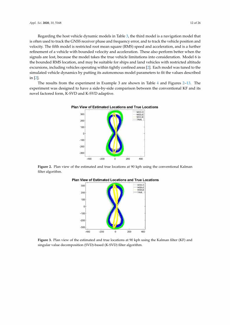
Table 1. Vector norm of absolute errors for each component of the dynamic state—i.e., ‖ RMSExj ‖2

(example 2). RMSE, root mean square error; KF, Kalman filter; SVD, singular value decomposition;SQRK, square root; UD, unit triangular matrix diagonal; NaN, not a number.

Algorithm ‖RMSExj‖2, i=1,. . . ,19 while Growing Ill-Conditioned δ→ε Round-OffExecutionTime (ms)

10−1 10−2 10−3 10−4 10−5 10−6 10−7 10−8 10−9 10−10 10−11 10−12 10−13 10−14 10−15 10−16

Kalmanfilter (KF) 0.318 0.32 3.2 3.185 3.186 3.186 3.186 3.186 3.846 NaN NaN NaN NaN NaN NaN NaN 1.75

K-SVD 0.318 0.32 3.2 3.186 3.186 3.186 3.186 3.186 3.186 3.186 3.186 3.186 3.186 3.186 3.186 1.2095 1.87

SQR-KF 0.317 0.32 3.2 3.185 3.186 3.186 3.186 3.198 3.380 NaN NaN NaN NaN NaN NaN NaN 0.123

UD-KF 0.318 0.32 3.2 3.185 3.186 3.186 3.186 3.201 2.607 NaN NaN NaN NaN NaN NaN NaN 0.06

Example 3. To compare and evaluate the performance of the new algorithm with conventional KF implementations,we include example 3, which is taken from [2]. The example is a comparison of the GNSS navigation performancewith four vehicle tracking models, using a simulated racetrack with a 1.5 km figure-8 track at 90, 140, 240, and360 kph average speed and a nominal low-cost clock, with a relative stability of 1× 10−9 part/part over 1 s. Thenumber of states in the KF model varies as satellites come into and fall from view. The vehicle states (position,velocity, and acceleration) are as follows: position north, position east, position up (vertical), velocity north,velocity east, velocity vertical, acceleration north, acceleration east, acceleration vertical. Models 3 and 5 do notinclude the three acceleration states (north, east, vertical).

Table 2 lists the number of state variables and the minimum and maximum number of visiblesatellites. Table 3 lists the parametric models used in this research to model a single componentof the motion of a host vehicle. The model parameters mentioned in Table 3 include the standarddeviation σ and the correlation time constant τ of position, velocity, acceleration, and jerk (derivative ofacceleration) [2]. The example 3 makes use of the Algorithm 1 adaptive computation from Equations(29) and (30), and the resulting algorithm is called K-SVD adaptive.

Table 2. State variables of the host vehicle dynamic models and the min/max number of visible satellites.

Name State Variables Min Satellites Max Satellites

MODL3 6 17 19MODL5 6 17 19MODL6 9 20 22

Table 3. Host vehicle dynamic models for example 3.

Model No.Model Parameters (Each Axis) Independent

ParametersDependentParametersF Q

3[

0 10 0

] [0 00 σ2

acc∆t2

]σ2

acc σ2pos →∞

5

0 1 00 −1

τvel

τacc

0 0 00 0 00 0 σ2

jerk∆t2

σ2

velσ2

accσ2

accτacc

σ2pos →∞

τvelρvel,accσ2

jerkτpos

6

−1τpos

−1τvel

−1τacc

0 0 00 0 00 0 σ2

jerk∆t2

σ2

pos

σ2pos

σ2accτacc

τvelρpos,velρpos,accρvel,accσ2

jerk

Appl. Sci. 2020, 10, 5168 12 of 26

Regarding the host vehicle dynamic models in Table 3, the third model is a navigation model thatis often used to track the GNSS receiver phase and frequency error, and to track the vehicle position andvelocity. The fifth model is restricted root mean square (RMS) speed and acceleration, and is a furtherrefinement of a vehicle with bounded velocity and acceleration. These also perform better when thesignals are lost, because the model takes the true vehicle limitations into consideration. Model 6 isthe bounded RMS location, and may be suitable for ships and land vehicles with restricted altitudeexcursions, including vehicles operating within tightly confined areas [2]. Each model was tuned to thesimulated vehicle dynamics by putting its autonomous model parameters to fit the values describedin [2].

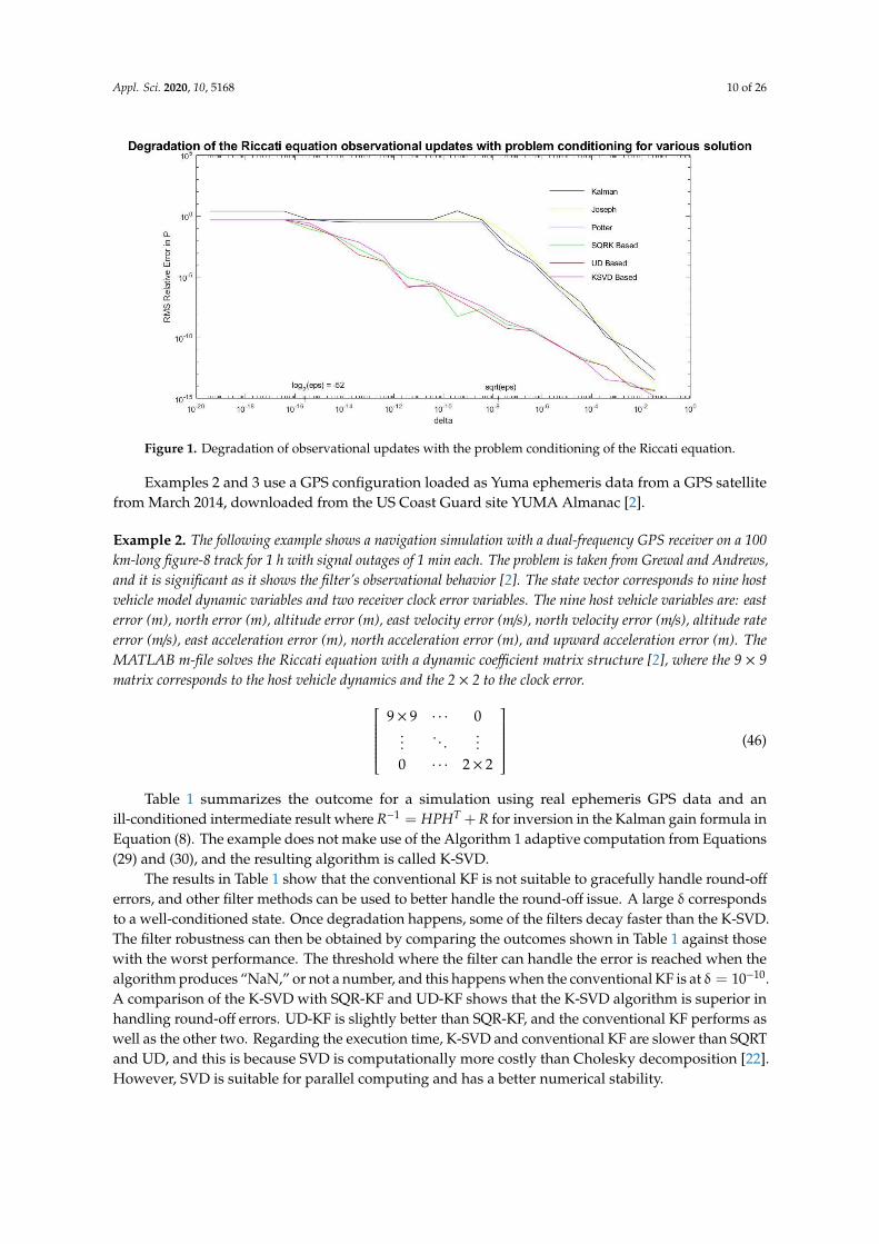
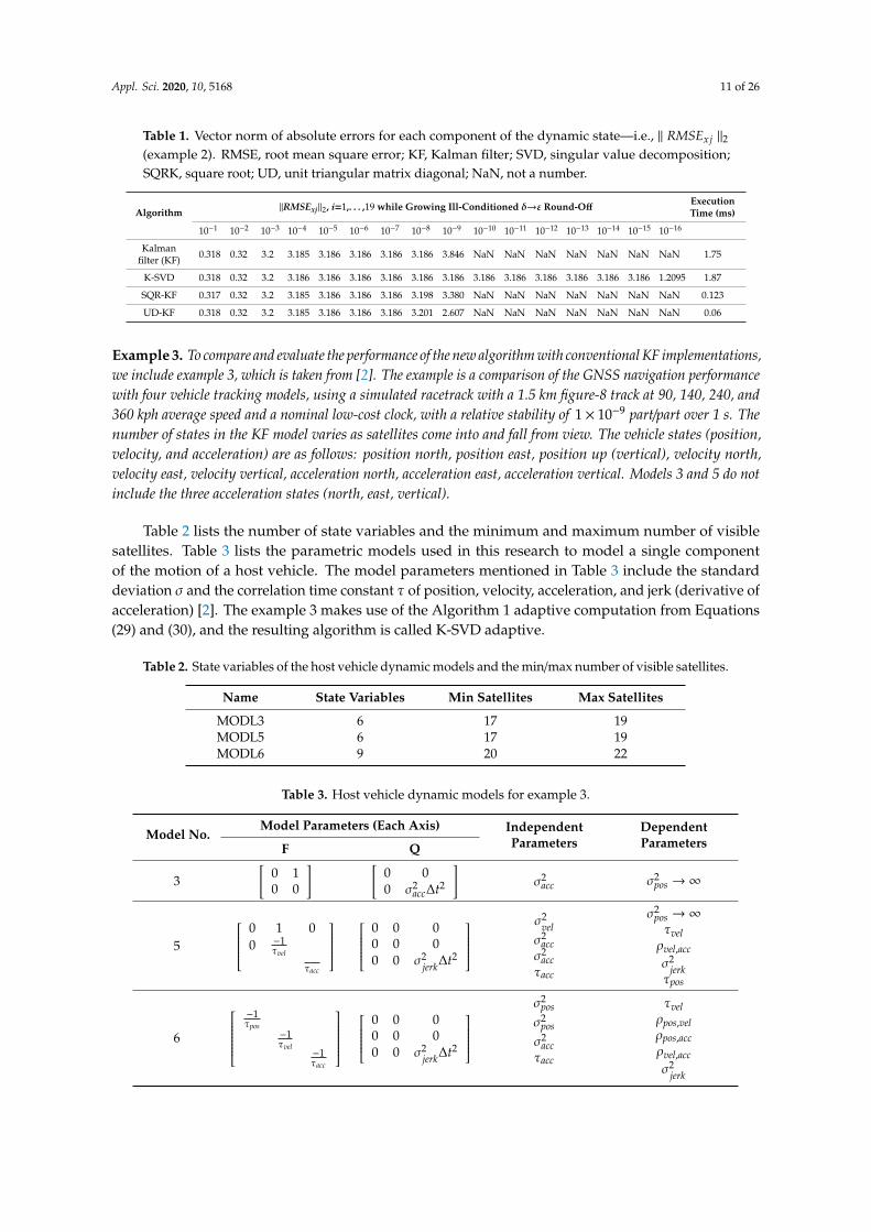
The results from the experiment in Example 3 are shown in Table 4 and Figures 2–13. Theexperiment was designed to have a side-by-side comparison between the conventional KF and itsnovel factored form, K-SVD and K-SVD adaptive.

Figure 2. Plan view of the estimated and true locations at 90 kph using the conventional Kalmanfilter algorithm.

Figure 3. Plan view of the estimated and true locations at 90 kph using the Kalman filter (KF) andsingular value decomposition (SVD)-based (K-SVD) filter algorithm.

Appl. Sci. 2020, 10, 5168 13 of 26

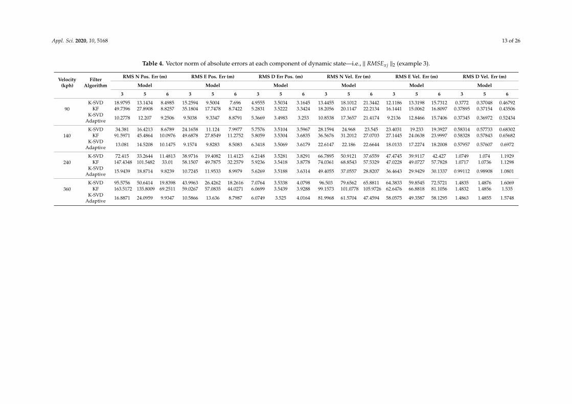
Table 4. Vector norm of absolute errors at each component of dynamic state—i.e., ‖ RMSExj ‖2 (example 3).

Velocity(kph)

FilterAlgorithm

RMS N Pos. Err (m) RMS E Pos. Err (m) RMS D Err Pos. (m) RMS N Vel. Err (m) RMS E Vel. Err (m) RMS D Vel. Err (m)

Model Model Model Model Model Model

3 5 6 3 5 6 3 5 6 3 5 6 3 5 6 3 5 6

90K-SVD 18.9795 13.1434 8.4985 15.2594 9.5004 7.696 4.9555 3.5034 3.1645 13.4455 18.1012 21.3442 12.1186 13.3198 15.7312 0.3772 0.37048 0.46792

KF 49.7396 27.8908 8.8257 35.1804 17.7478 8.7422 5.2831 3.5222 3.3424 18.2056 20.1147 22.2134 16.1441 15.0062 16.8097 0.37895 0.37154 0.43506K-SVD

Adaptive 10.2778 12.207 9.2506 9.5038 9.3347 8.8791 5.3669 3.4983 3.253 10.8538 17.3657 21.4174 9.2136 12.8466 15.7406 0.37345 0.36972 0.52434

140K-SVD 34.381 16.4213 8.6789 24.1658 11.124 7.9977 5.7576 3.5104 3.5967 28.1594 24.968 23.545 23.4031 19.233 19.3927 0.58314 0.57733 0.68302

KF 91.5971 45.4864 10.0976 49.6878 27.8549 11.2752 5.8059 3.5304 3.6835 36.5676 31.2012 27.0703 27.1445 24.0638 23.9997 0.58328 0.57843 0.65682K-SVD

Adaptive 13.081 14.5208 10.1475 9.1574 9.8283 8.5083 6.3418 3.5069 3.6179 22.6147 22.186 22.6644 18.0133 17.2274 18.2008 0.57957 0.57607 0.6972

240K-SVD 72.415 33.2644 11.4813 38.9716 19.4082 11.4123 6.2148 3.5281 3.8291 66.7895 50.9121 37.6559 47.4745 39.9117 42.427 1.0749 1.074 1.1929

KF 147.4348 101.5482 33.01 58.1507 49.7875 32.2579 5.9236 3.5418 3.8778 74.0361 68.8543 57.5329 47.0228 49.0727 57.7828 1.0717 1.0736 1.1298K-SVD

Adaptive 15.9439 18.8714 9.8239 10.7245 11.9533 8.9979 5.6269 3.5188 3.6314 49.4055 37.0557 28.8207 36.4643 29.9429 30.1337 0.99112 0.98908 1.0801

360K-SVD 95.5756 50.6414 19.8398 43.9963 26.4262 18.2616 7.0764 3.5338 4.0798 96.503 79.6562 65.8811 64.3833 59.8545 72.5721 1.4835 1.4876 1.6069

KF 163.5172 135.8009 69.2511 59.0267 57.0835 44.0271 6.0699 3.5439 3.9288 99.1573 101.0778 105.9726 62.6476 66.8818 81.1056 1.4832 1.4856 1.535K-SVD

Adaptive 16.8871 24.0959 9.9347 10.5866 13.636 8.7987 6.0749 3.525 4.0164 81.9968 61.5704 47.4594 58.0575 49.3587 58.1295 1.4863 1.4855 1.5748

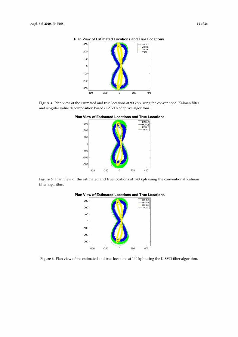
Appl. Sci. 2020, 10, 5168 14 of 26

Figure 4. Plan view of the estimated and true locations at 90 kph using the conventional Kalman filterand singular value decomposition based (K-SVD) adaptive algorithm.

Figure 5. Plan view of the estimated and true locations at 140 kph using the conventional Kalmanfilter algorithm.

Figure 6. Plan view of the estimated and true locations at 140 kph using the K-SVD filter algorithm.

Appl. Sci. 2020, 10, 5168 15 of 26

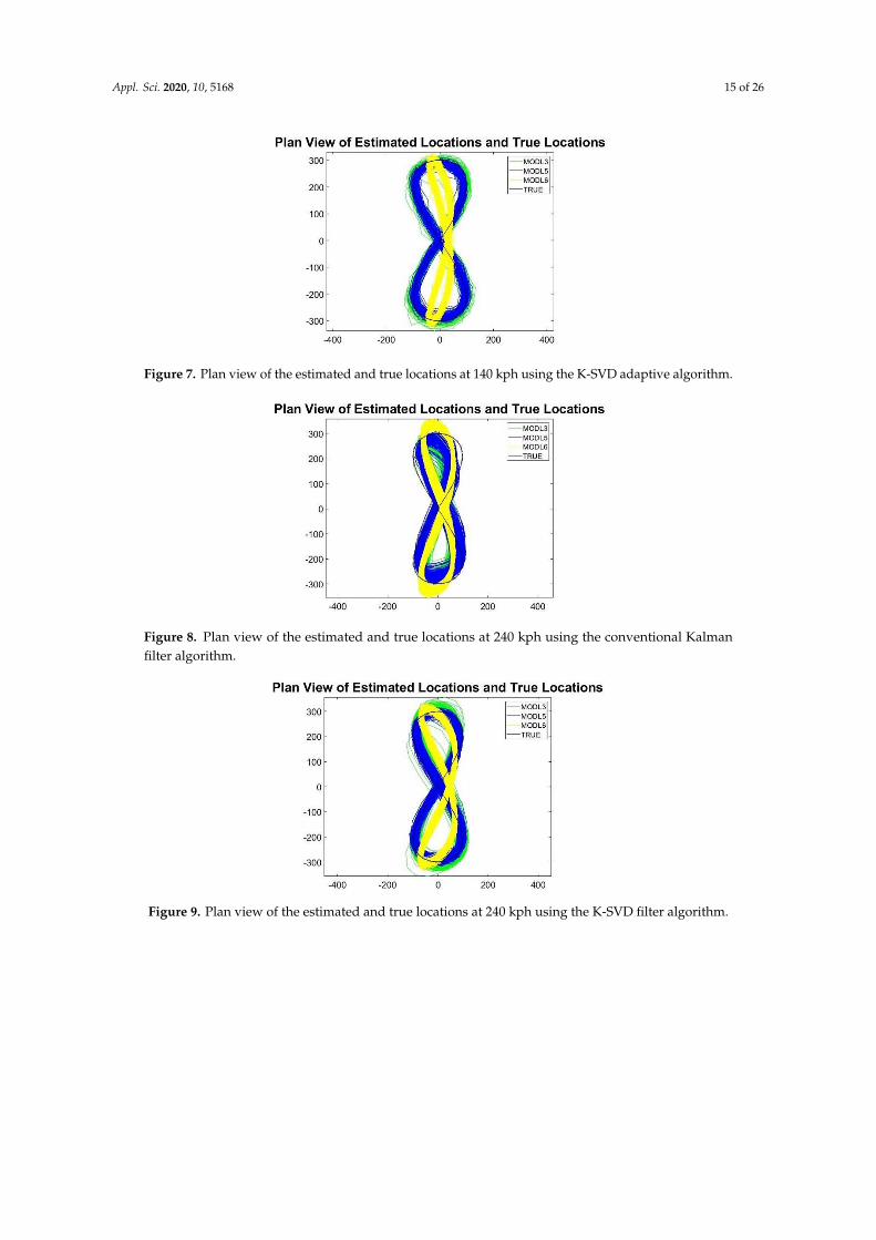
Figure 7. Plan view of the estimated and true locations at 140 kph using the K-SVD adaptive algorithm.

Figure 8. Plan view of the estimated and true locations at 240 kph using the conventional Kalmanfilter algorithm.

Figure 9. Plan view of the estimated and true locations at 240 kph using the K-SVD filter algorithm.

Appl. Sci. 2020, 10, 5168 16 of 26

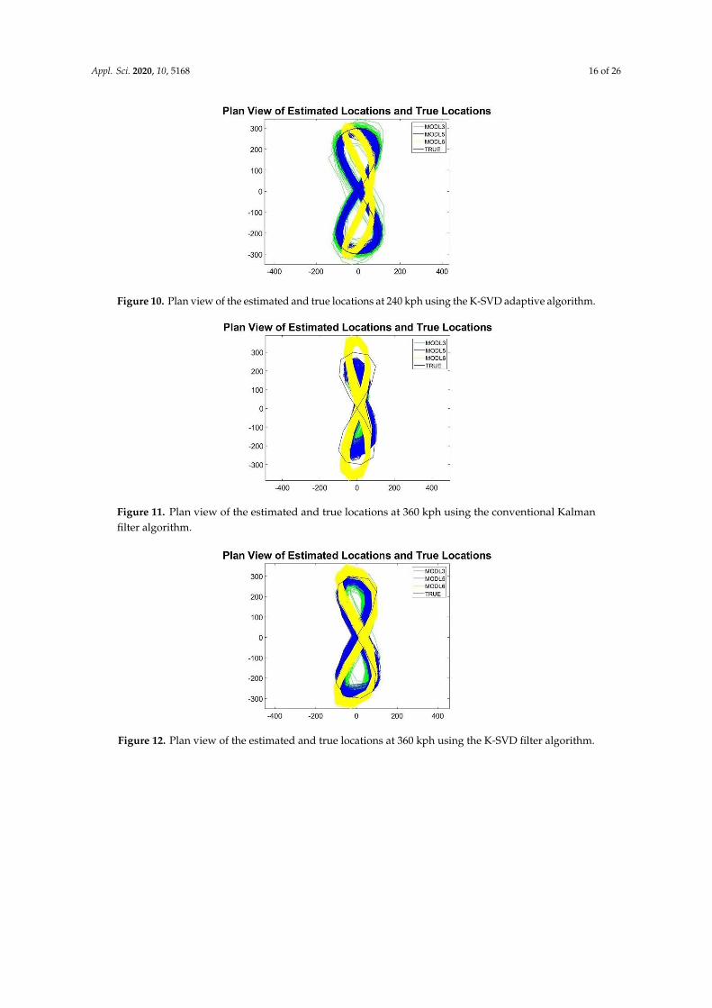
Figure 10. Plan view of the estimated and true locations at 240 kph using the K-SVD adaptive algorithm.

Figure 11. Plan view of the estimated and true locations at 360 kph using the conventional Kalmanfilter algorithm.

Figure 12. Plan view of the estimated and true locations at 360 kph using the K-SVD filter algorithm.

Appl. Sci. 2020, 10, 5168 17 of 26

Figure 13. Plan view of the estimated and true locations at 360 kph using the K-SVD adaptive algorithm.

Comparing the values for each model in Table 4 at different velocities, it is clear that when thevelocity is increased (e.g., from 90 to 360 kph), the conventional KF always increases the RMS errorabsolute value well above the K-SVD by about 172%. At the model level, the best performer in allcases is model 5. From the figures above, it can be inferred that with all things being equal (the onlydifference in the MATLAB source code is the algorithm to compute the Kalman filter), K-SVD adaptivehas a better prediction accuracy than the conventional KF and traditional factored KFs. This meansthat K-SVD adaptive is more robust than the current known factor-based algorithms, at the same timeproviding a better filtering capability when it performs the same operations. The algorithm capturesthe information that matters, which is the N-dimensional subspace of RN spanned by the first columnsof V or the right orthogonal factor [8,9]. By performing a matrix multiplication, the algorithm realizes alow dimensionality reduction that captures much of the variability and corresponds with the selectionof the eigenvectors with the largest eigenvalues (since SVD orders them from the largest to smallest).Additionally, by adapting to variations in the covariance measurement error, the algorithm has ahigher accuracy.

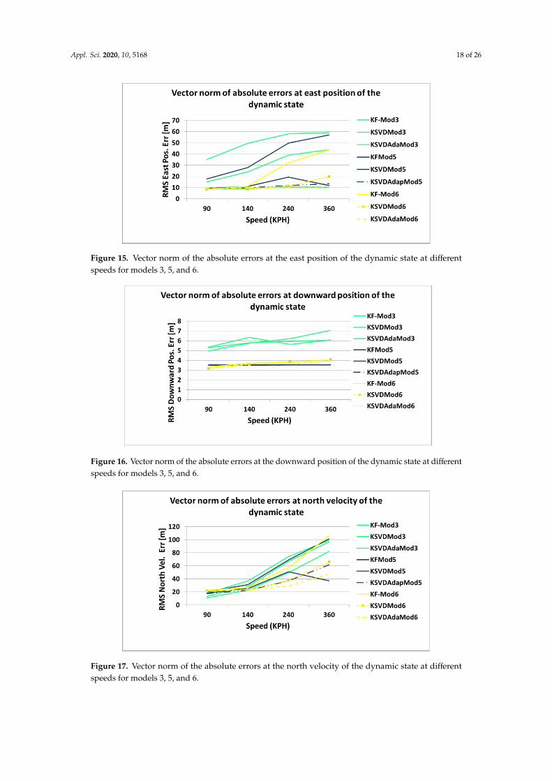
Figures 14–19 represent the results of Table 4. By observing Figure 14, it is easy to see that K-SVDadaptive model 6 performs better for the north position. K-SVD model 5 also performs relatively wellcompared with the conventional KF. Similar results can be inferred from Figure 15; K-SVD adaptivemodel 6 is the best performer, followed by K-SVD adaptive models 3 and 5. Conclusive results canalso be seen for the downward position RMS error in Figure 16. Model 5 performs better, independentof the filter type. Model 6 is also a good performer for downward velocity, and the worst is model 3.

Figure 14. Vector norm of the absolute errors at the north position of the dynamic state at differentspeeds for models 3, 5, and 6.

Appl. Sci. 2020, 10, 5168 18 of 26

Figure 15. Vector norm of the absolute errors at the east position of the dynamic state at differentspeeds for models 3, 5, and 6.

Figure 16. Vector norm of the absolute errors at the downward position of the dynamic state at differentspeeds for models 3, 5, and 6.

Figure 17. Vector norm of the absolute errors at the north velocity of the dynamic state at differentspeeds for models 3, 5, and 6.

Appl. Sci. 2020, 10, 5168 19 of 26

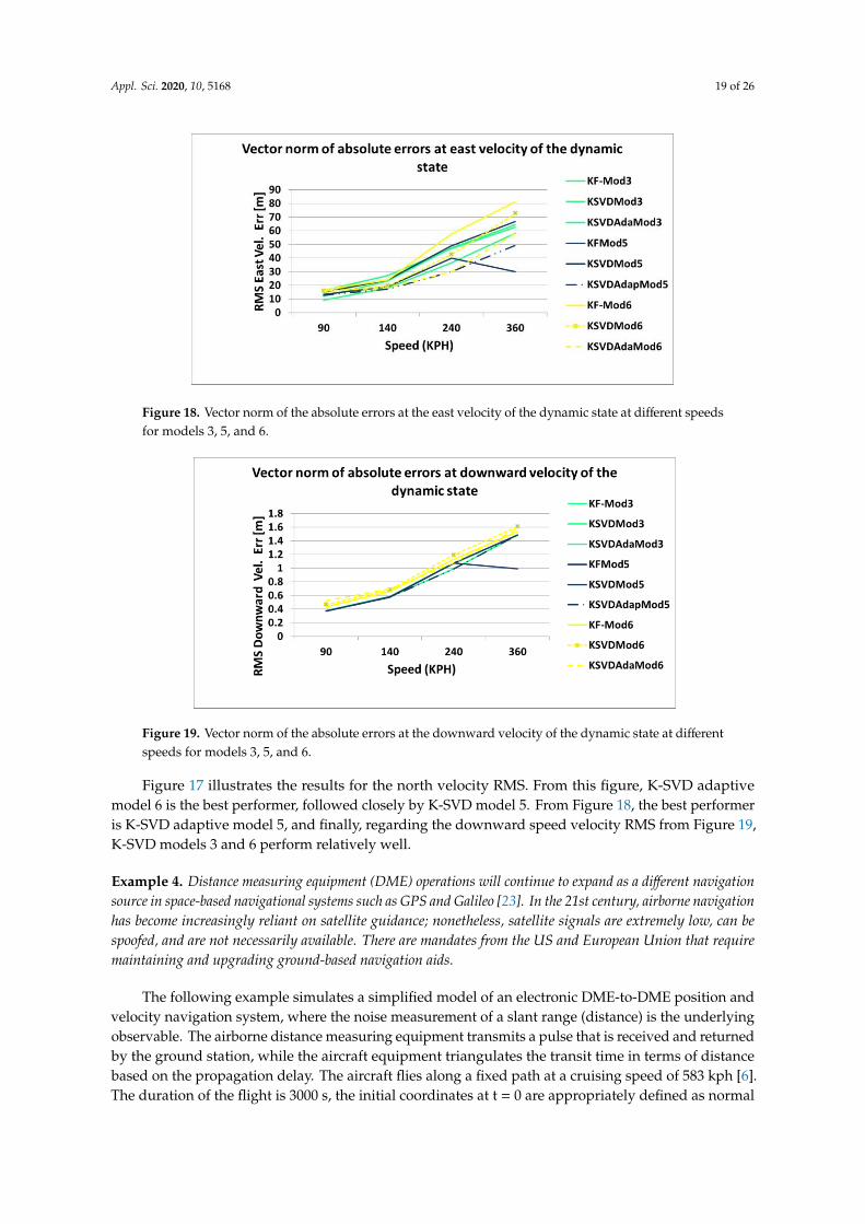
Figure 18. Vector norm of the absolute errors at the east velocity of the dynamic state at different speedsfor models 3, 5, and 6.

Figure 19. Vector norm of the absolute errors at the downward velocity of the dynamic state at differentspeeds for models 3, 5, and 6.

Figure 17 illustrates the results for the north velocity RMS. From this figure, K-SVD adaptivemodel 6 is the best performer, followed closely by K-SVD model 5. From Figure 18, the best performeris K-SVD adaptive model 5, and finally, regarding the downward speed velocity RMS from Figure 19,K-SVD models 3 and 6 perform relatively well.

Example 4. Distance measuring equipment (DME) operations will continue to expand as a different navigationsource in space-based navigational systems such as GPS and Galileo [23]. In the 21st century, airborne navigationhas become increasingly reliant on satellite guidance; nonetheless, satellite signals are extremely low, can bespoofed, and are not necessarily available. There are mandates from the US and European Union that requiremaintaining and upgrading ground-based navigation aids.

The following example simulates a simplified model of an electronic DME-to-DME position andvelocity navigation system, where the noise measurement of a slant range (distance) is the underlyingobservable. The airborne distance measuring equipment transmits a pulse that is received and returnedby the ground station, while the aircraft equipment triangulates the transit time in terms of distancebased on the propagation delay. The aircraft flies along a fixed path at a cruising speed of 583 kph [6].The duration of the flight is 3000 s, the initial coordinates at t = 0 are appropriately defined as normal

Appl. Sci. 2020, 10, 5168 20 of 26

random variables, x0 ∼ N(60, 10 km2

), y0 ∼ N

(210, 10 km2

), sample time T = 2 s, g = 10 m/s, and the

maximum deviation in the acceleration for the aircraft is σa max= 0.001 msec2 .

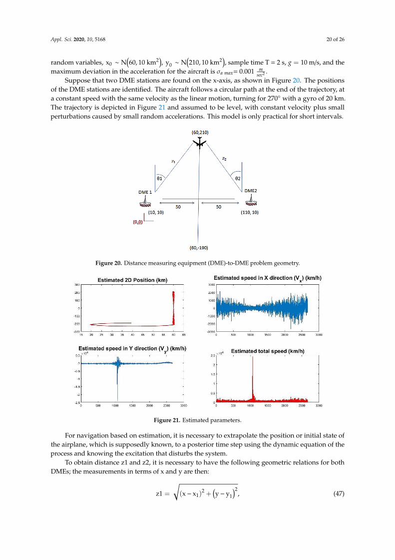
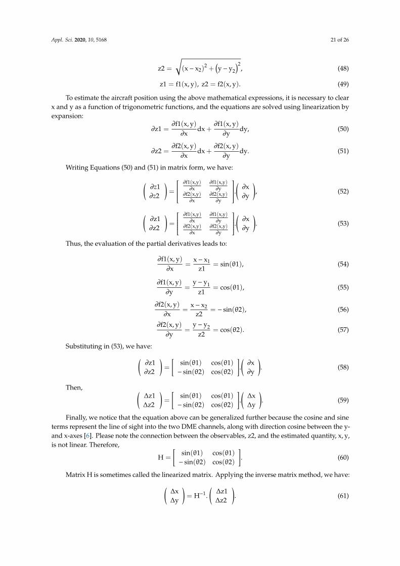
Suppose that two DME stations are found on the x-axis, as shown in Figure 20. The positionsof the DME stations are identified. The aircraft follows a circular path at the end of the trajectory, ata constant speed with the same velocity as the linear motion, turning for 270 with a gyro of 20 km.The trajectory is depicted in Figure 21 and assumed to be level, with constant velocity plus smallperturbations caused by small random accelerations. This model is only practical for short intervals.

Figure 20. Distance measuring equipment (DME)-to-DME problem geometry.

Figure 21. Estimated parameters.

For navigation based on estimation, it is necessary to extrapolate the position or initial state ofthe airplane, which is supposedly known, to a posterior time step using the dynamic equation of theprocess and knowing the excitation that disturbs the system.

To obtain distance z1 and z2, it is necessary to have the following geometric relations for bothDMEs; the measurements in terms of x and y are then:

z1 =

√(x− x1)

2 +(y− y1

)2, (47)

Appl. Sci. 2020, 10, 5168 21 of 26

z2 =

√(x− x2)

2 +(y− y2

)2, (48)

z1 = f1(x, y), z2 = f2(x, y). (49)

To estimate the aircraft position using the above mathematical expressions, it is necessary to clearx and y as a function of trigonometric functions, and the equations are solved using linearization byexpansion:

∂z1 =∂f1(x, y)∂x

dx +∂f1(x, y)∂y

dy, (50)

∂z2 =∂f2(x, y)∂x

dx +∂f2(x, y)∂y

dy. (51)

Writing Equations (50) and (51) in matrix form, we have:

(∂z1∂z2

)=

∂f1(x,y)∂x

∂f1(x,y)∂y

∂f2(x,y)∂x

∂f2(x,y)∂y

.(∂x∂y

), (52)

(∂z1∂z2

)=

∂f1(x,y)∂x

∂f1(x,y)∂y

∂f2(x,y)∂x

∂f2(x,y)∂y

.(∂x∂y

). (53)

Thus, the evaluation of the partial derivatives leads to:

∂f1(x, y)∂x

=x− x1

z1= sin(θ1), (54)

∂f1(x, y)∂y

=y− y1

z1= cos(θ1), (55)

∂f2(x, y)∂x

=x− x2

z2= − sin(θ2), (56)

∂f2(x, y)∂y

=y− y2

z2= cos(θ2). (57)

Substituting in (53), we have:(∂z1∂z2

)=

[sin(θ1) cos(θ1)− sin(θ2) cos(θ2)

].(∂x∂y

). (58)

Then, (∆z1∆z2

)=

[sin(θ1) cos(θ1)− sin(θ2) cos(θ2)

].(

∆x∆y

). (59)

Finally, we notice that the equation above can be generalized further because the cosine and sineterms represent the line of sight into the two DME channels, along with direction cosine between the y-and x-axes [6]. Please note the connection between the observables, z2, and the estimated quantity, x, y,is not linear. Therefore,

H =

[sin(θ1) cos(θ1)− sin(θ2) cos(θ2)

]. (60)

Matrix H is sometimes called the linearized matrix. Applying the inverse matrix method, we have:(∆x∆y

)= H−1.

(∆z1∆z2

). (61)

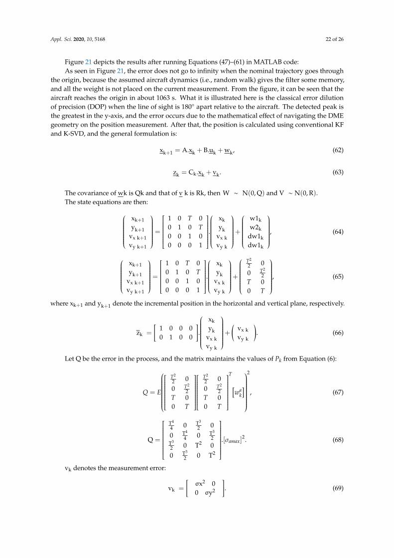
Appl. Sci. 2020, 10, 5168 22 of 26

Figure 21 depicts the results after running Equations (47)–(61) in MATLAB code:As seen in Figure 21, the error does not go to infinity when the nominal trajectory goes through

the origin, because the assumed aircraft dynamics (i.e., random walk) gives the filter some memory,and all the weight is not placed on the current measurement. From the figure, it can be seen that theaircraft reaches the origin in about 1063 s. What it is illustrated here is the classical error dilutionof precision (DOP) when the line of sight is 180 apart relative to the aircraft. The detected peak isthe greatest in the y-axis, and the error occurs due to the mathematical effect of navigating the DMEgeometry on the position measurement. After that, the position is calculated using conventional KFand K-SVD, and the general formulation is:

xk+1 = A.xk + B.uk + wk, (62)

zk = Ck.xk + vk. (63)

The covariance of wk is Qk and that of v k is Rk, then W ∼ N(0, Q) and V ∼ N(0, R).The state equations are then:

xk+1

yk+1vx k+1

vy k+1

=

1 0 T 00 1 0 T0 0 1 00 0 0 1

.

xk

ykvx k

vy k

+

w1k

w2k

dw1k

dw1k

, (64)

xk+1

yk+1vx k+1

vy k+1

=

1 0 T 00 1 0 T0 0 1 00 0 0 1

.

xk

ykvx k

vy k

+

T2

2 00 T2

2T 00 T

, (65)

where xk+1 and yk+1 denote the incremental position in the horizontal and vertical plane, respectively.

zk =

[1 0 0 00 1 0 0

].

xk

ykvx k

vy k

+(

vx k

vy k

). (66)

Let Q be the error in the process, and the matrix maintains the values of Pk from Equation (6):

Q = E

T2

2 00 T2

2T 00 T

T2

2 00 T2

2T 00 T

T[

wak

]

2

, (67)

Q =

T4

4 0 T3

2 00 T4

4 0 T3

2T3

2 0 T2 00 T3

2 0 T2

.[σamax]2. (68)

vk denotes the measurement error:

vk =

[σx2 00 σy2

]. (69)

Appl. Sci. 2020, 10, 5168 23 of 26

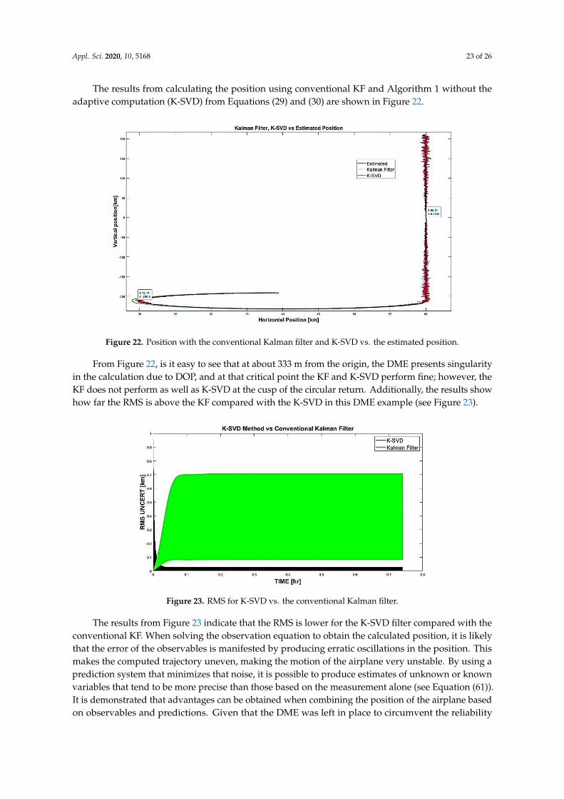
The results from calculating the position using conventional KF and Algorithm 1 without theadaptive computation (K-SVD) from Equations (29) and (30) are shown in Figure 22.

Figure 22. Position with the conventional Kalman filter and K-SVD vs. the estimated position.

From Figure 22, is it easy to see that at about 333 m from the origin, the DME presents singularityin the calculation due to DOP, and at that critical point the KF and K-SVD perform fine; however, theKF does not perform as well as K-SVD at the cusp of the circular return. Additionally, the results showhow far the RMS is above the KF compared with the K-SVD in this DME example (see Figure 23).

Figure 23. RMS for K-SVD vs. the conventional Kalman filter.

The results from Figure 23 indicate that the RMS is lower for the K-SVD filter compared with theconventional KF. When solving the observation equation to obtain the calculated position, it is likelythat the error of the observables is manifested by producing erratic oscillations in the position. Thismakes the computed trajectory uneven, making the motion of the airplane very unstable. By using aprediction system that minimizes that noise, it is possible to produce estimates of unknown or knownvariables that tend to be more precise than those based on the measurement alone (see Equation (61)).It is demonstrated that advantages can be obtained when combining the position of the airplane basedon observables and predictions. Given that the DME was left in place to circumvent the reliability

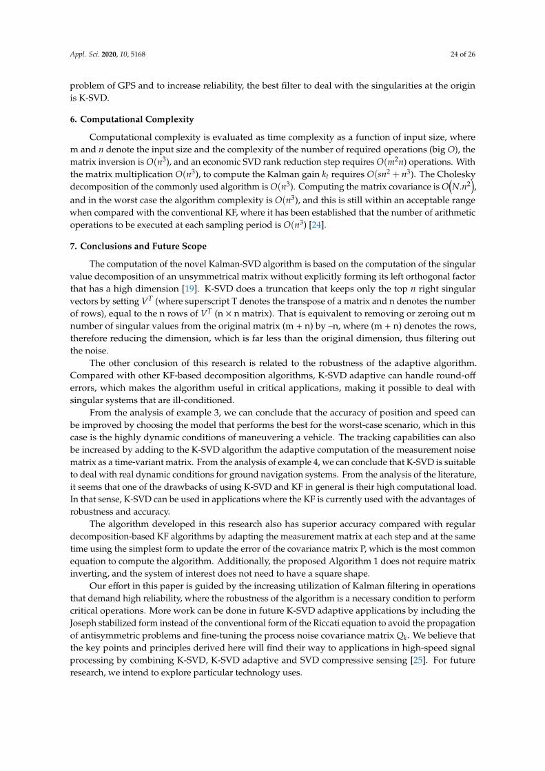
Appl. Sci. 2020, 10, 5168 24 of 26

problem of GPS and to increase reliability, the best filter to deal with the singularities at the originis K-SVD.

6. Computational Complexity

Computational complexity is evaluated as time complexity as a function of input size, wherem and n denote the input size and the complexity of the number of required operations (big O), thematrix inversion is O(n3), and an economic SVD rank reduction step requires O(m2n) operations. Withthe matrix multiplication O(n3), to compute the Kalman gain kt requires O(sn2 + n3). The Choleskydecomposition of the commonly used algorithm is O(n3). Computing the matrix covariance is O

(N.n2

),

and in the worst case the algorithm complexity is O(n3), and this is still within an acceptable rangewhen compared with the conventional KF, where it has been established that the number of arithmeticoperations to be executed at each sampling period is O(n3) [24].

7. Conclusions and Future Scope

The computation of the novel Kalman-SVD algorithm is based on the computation of the singularvalue decomposition of an unsymmetrical matrix without explicitly forming its left orthogonal factorthat has a high dimension [19]. K-SVD does a truncation that keeps only the top n right singularvectors by setting VT (where superscript T denotes the transpose of a matrix and n denotes the numberof rows), equal to the n rows of VT (n × n matrix). That is equivalent to removing or zeroing out mnumber of singular values from the original matrix (m + n) by –n, where (m + n) denotes the rows,therefore reducing the dimension, which is far less than the original dimension, thus filtering outthe noise.

The other conclusion of this research is related to the robustness of the adaptive algorithm.Compared with other KF-based decomposition algorithms, K-SVD adaptive can handle round-off

errors, which makes the algorithm useful in critical applications, making it possible to deal withsingular systems that are ill-conditioned.

From the analysis of example 3, we can conclude that the accuracy of position and speed canbe improved by choosing the model that performs the best for the worst-case scenario, which in thiscase is the highly dynamic conditions of maneuvering a vehicle. The tracking capabilities can alsobe increased by adding to the K-SVD algorithm the adaptive computation of the measurement noisematrix as a time-variant matrix. From the analysis of example 4, we can conclude that K-SVD is suitableto deal with real dynamic conditions for ground navigation systems. From the analysis of the literature,it seems that one of the drawbacks of using K-SVD and KF in general is their high computational load.In that sense, K-SVD can be used in applications where the KF is currently used with the advantages ofrobustness and accuracy.

The algorithm developed in this research also has superior accuracy compared with regulardecomposition-based KF algorithms by adapting the measurement matrix at each step and at the sametime using the simplest form to update the error of the covariance matrix P, which is the most commonequation to compute the algorithm. Additionally, the proposed Algorithm 1 does not require matrixinverting, and the system of interest does not need to have a square shape.

Our effort in this paper is guided by the increasing utilization of Kalman filtering in operationsthat demand high reliability, where the robustness of the algorithm is a necessary condition to performcritical operations. More work can be done in future K-SVD adaptive applications by including theJoseph stabilized form instead of the conventional form of the Riccati equation to avoid the propagationof antisymmetric problems and fine-tuning the process noise covariance matrix Qk. We believe thatthe key points and principles derived here will find their way to applications in high-speed signalprocessing by combining K-SVD, K-SVD adaptive and SVD compressive sensing [25]. For futureresearch, we intend to explore particular technology uses.

Appl. Sci. 2020, 10, 5168 25 of 26

Author Contributions: J.C.B.O. designed the mathematical model of the proposed algorithm and wrote the paper,R.M.A.V. performed the experiments, and V.F.G.C. analyzed the data. All authors have read and agreed to thepublished version of the manuscript.

Funding: This research received no external funding.

Conflicts of Interest: The authors declare no conflict of interest.

References

1. Grewal, M.S.; Andrews, A.P.; Bartone, C.G. Global Navigation Satellite Systems, Inertial Navigation, andIntegration; John Wiley & Sons: Hoboken, NJ, USA, 2013.

2. Grewal, M.S.; Andrews, A.P. Kalman Filtering: Theory and Practice Using MATLAB; John Wiley & Sons:Hoboken, NJ, USA, 2014.

3. Grewal, M.S.; Weill, L.R.; Andrews, A.P. Global Positioning Systems, Inertial Navigation, and Integration; JohnWiley & Sons: Hoboken, NJ, USA, 2001.

4. Verhaegen, M.; Van Dooren, P. Numerical aspects of different Kalman filter implementations. IEEE Trans.Autom. Control 1986, 31, 907–917. [CrossRef]

5. Bierman, G.J. Factorization Methods for Discrete Sequential Estimation; Academic Press: New York, NY, USA,1977.

6. Brown, R.G.; Hwang, P.G. Introduction to Random Signals and Applied Kalman Filtering with MATLAB Exercises,4th ed.; John Wiley & Sons: Hoboken, NJ, USA, 2012.

7. Prvan, T.; Osborne, M.R. A square-root fixed-interval discrete-time smoother. J. Aust. Math. Soc. Ser. B. Appl.Math. 1988, 30, 57–68. [CrossRef]

8. Wang, L.; Libert, G.; Manneback, P. Kalman Filter Algorithm Based on Singular Value Decomposition. InProceedings of the 31st IEEE Conference on Decision and Control, Tucson, AZ, USA, 16–18 December 1992.

9. Wang, L.; Libert, G.; Manneback, P. A Singular Value Decomposition Based Kalman Filter Algorithm. InProceedings of the 1992 International Conference on Industrial Electronics, Control, Instrumentation, andAutomation, San Diego, CA, USA, 13 November 1992.

10. Zhang, Y.; Dai, G.; Zhang, H.; Li, Q. A SVD-based extended Kalman filter and applications to aircraftflight state and parameter estimation. In Proceedings of the 1994 American Control Conference—ACC ’94,Baltimore, MD, USA, 29 June–1 July 1994.

11. Fan, J.; Ma, G. Characteristics of GPS positioning error with non-uniform pseudorange error. GPS Solut.2014, 18, 615–623. [CrossRef]

12. Chen, B.; Wu, L.; Dai, W.; Luo, X.; Xu, Y. A new parameterized approach for ionospheric tomography. GPSSolut. 2019, 23. [CrossRef]

13. Auger, F.; Hilairet, M.; Guerrero, J.M.; Monmasson, E.; Orlowska-Kowalska, T.; Katsura, S. IndustrialApplications of the Kalman Filter: A Review. IEEE Trans. Ind. Electron. 2013, 60, 5458–5471. [CrossRef]

14. Foussier, J.; Teichmann, D.; Jia, J.; Misgeld, B.J.; Leonhardt, S. An adaptive Kalman filter approach forcardiorespiratory signal extraction and fusion of non-contacting sensors. BMC Med. Inform. Decis. Making2014, 14, 37. [CrossRef] [PubMed]

15. Spincemaille, P.; Nguyen, T.D.; Prince, M.R.; Wang, Y. Kalman filtering for real-time navigator processing.Magn. Reson. Med. 2008, 60, 158–168. [CrossRef] [PubMed]

16. Zhang, C.; Yan, F.; Du, C.; Rizzoni, G. An Improved Model-Based Self-Adaptive Filter for OnlineState-of-Charge Estimation of Li-Ion Batteries. Appl. Sci. 2018, 8, 2084. [CrossRef]

17. Muñoz-Bañón, M.Á.; Del Pino, I.; Candelas-Herías, F.A.; Torres, F. Framework for Fast Experimental Testingof Autonomous Navigation Algorithms. Appl. Sci. 2019, 9, 1997.

18. Zhang, C.; Guo, C.; Zhang, D. Data Fusion Based on Adaptive Interacting Multiple Model for GPS/INSIntegrated Navigation System. Appl. Sci. 2018, 8, 1682. [CrossRef]

19. Nieto, F.J.S. Navegacion Aerea; Garceta Grupo Editorial: Madrid, Spain, 2012.20. Durdu, O.F. Estimation of state variables for controlled irrigation canals via a singular value based Kalman

filter. Fresenius Environ. Bull. 2004, 13, 1139–1150.21. Kohno, K.; Inouye, Y.; Kawamoto, M. A Matrix Pseudo-Inversion Lemma for Positive Semidefinite Hermitian

Matrices and Its Application to Adaptive Blind Deconvolution of MIMO Systems. IEEE Trans. Circuits Syst.I: Regul. Pap. 2008, 55, 424–435. [CrossRef]

Appl. Sci. 2020, 10, 5168 26 of 26

22. Kulikova, M.V.; Tsyganova, J.V. Improved Discrete-Time Kalman Filtering within Singular ValueDecomposition. Available online: https://www.groundai.com/project/improved-discrete-time-kalman-filtering-within-singular-value-decomposition/3 (accessed on 25 March 2020).

23. Department of Defense; U.S. Department of Transportation. Available online: https://www.transportation.gov/pnt/radionavigation-systems-planning#:~:text=The%20Federal%20Radionavigation%20Plan%20(accessed on 2 July 2020).

24. Mendel, J. Computational requirements for a discrete Kalman filter. IEEE Trans. Autom. Control. 1971, 16,748–758. [CrossRef]

25. Ordoñez, J.C.B.; Valdés, R.M.A.; Comendador, F.G. Energy Efficient GNSS Signal Acquisition Using SingularValue Decomposition (SVD). Sensors 2018, 18, 1586. [CrossRef] [PubMed]

© 2020 by the authors. Licensee MDPI, Basel, Switzerland. This article is an open accessarticle distributed under the terms and conditions of the Creative Commons Attribution(CC BY) license (http://creativecommons.org/licenses/by/4.0/).