Engine Validation of Noise and Emission Reduction ...

Don Weir, editorHoneywell Aerospace, Phoenix, Arizona

Engine Validation of Noise and Emission ReductionTechnology Phase I

NASA/CR—2008-215225

May 2008

Honeywell Report No. 21–13843A

NASA STI Program . . . in Profi le

Since its founding, NASA has been dedicated to the advancement of aeronautics and space science. The NASA Scientifi c and Technical Information (STI) program plays a key part in helping NASA maintain this important role.

The NASA STI Program operates under the auspices of the Agency Chief Information Offi cer. It collects, organizes, provides for archiving, and disseminates NASA’s STI. The NASA STI program provides access to the NASA Aeronautics and Space Database and its public interface, the NASA Technical Reports Server, thus providing one of the largest collections of aeronautical and space science STI in the world. Results are published in both non-NASA channels and by NASA in the NASA STI Report Series, which includes the following report types: • TECHNICAL PUBLICATION. Reports of

completed research or a major signifi cant phase of research that present the results of NASA programs and include extensive data or theoretical analysis. Includes compilations of signifi cant scientifi c and technical data and information deemed to be of continuing reference value. NASA counterpart of peer-reviewed formal professional papers but has less stringent limitations on manuscript length and extent of graphic presentations.

• TECHNICAL MEMORANDUM. Scientifi c

and technical fi ndings that are preliminary or of specialized interest, e.g., quick release reports, working papers, and bibliographies that contain minimal annotation. Does not contain extensive analysis.

• CONTRACTOR REPORT. Scientifi c and

technical fi ndings by NASA-sponsored contractors and grantees.

• CONFERENCE PUBLICATION. Collected

papers from scientifi c and technical conferences, symposia, seminars, or other meetings sponsored or cosponsored by NASA.

• SPECIAL PUBLICATION. Scientifi c,

technical, or historical information from NASA programs, projects, and missions, often concerned with subjects having substantial public interest.

• TECHNICAL TRANSLATION. English-

language translations of foreign scientifi c and technical material pertinent to NASA’s mission.

Specialized services also include creating custom thesauri, building customized databases, organizing and publishing research results.

For more information about the NASA STI program, see the following:

• Access the NASA STI program home page at http://www.sti.nasa.gov

• E-mail your question via the Internet to help@

sti.nasa.gov • Fax your question to the NASA STI Help Desk

at 301–621–0134 • Telephone the NASA STI Help Desk at 301–621–0390 • Write to:

NASA Center for AeroSpace Information (CASI) 7115 Standard Drive Hanover, MD 21076–1320

Don Weir, editorHoneywell Aerospace, Phoenix, Arizona

Engine Validation of Noise and Emission ReductionTechnology Phase I

NASA/CR—2008-215225

May 2008

Honeywell Report No. 21–13843A

National Aeronautics andSpace Administration

Glenn Research CenterCleveland, Ohio 44135

Prepared under Contract NAS3–01136

Acknowledgments

The Engine Validation of Noise and Emissions Reduction Technology Program was sponsored by the NASA Glenn Research Center Revolutionary Aero-Space Engine Research (RASER) Program, Contract No. NAS3-01136, Task Order No. 8. The

NASA Task Manager was Dr. Joe Grady, NASA Glenn Research Center. The author would like to thank the staffs of the NASA Glenn Research Center and the NASA Langley Research Center, for their support and technical insight.

Available from

NASA Center for Aerospace Information7115 Standard DriveHanover, MD 21076–1320

National Technical Information Service5285 Port Royal RoadSpringfi eld, VA 22161

Available electronically at http://gltrs.grc.nasa.gov

Trade names and trademarks are used in this report for identifi cation only. Their usage does not constitute an offi cial endorsement, either expressed or implied, by the National Aeronautics and

Space Administration.

This work was sponsored by the Fundamental Aeronautics Program at the NASA Glenn Research Center.

Level of Review: This material has been technically reviewed by expert reviewer(s).

TABLE OF CONTENTS Page

i

1. INTRODUCTION 1 1.1 Abstract 2 1.2 Objectives 2

2. STATEMENT OF WORK 3 2.1 Work Element 1: Project Management 3 2.2 Work Element 2: Systems Engineering and Integration 3 2.3 Work Element 3: Technology Maturation 4

2.3.1 HQ Tube/Optimum Liner - Aft Duct HQ Tubes 4 2.3.2 Modeling and Validation of Inlet Liner Impedance Discontinuities 4

2.4 Work Element 4: Engine Tests 5 2.4.1 Engine Build Up 6 2.4.2 Baseline Noise Measurements 6 2.4.3 Separate Flow Nozzle 6 2.4.4 3/5/7 Microphone 6 2.4.5 In-Situ Impedance Measurements 6 2.4.6 Run Without Fan 7 2.4.7 Phased Array 7 2.4.8 Internal Flow Measurements 8 2.4.9 Fan Modal Measurements 8 2.4.10 Signal Conditioning Acquisition 8 2.4.11 Combustor Noise Diagnostic Measurements 8 2.4.12 Start of Take-off Roll Simulation 9

3. ENGINE PRELIMINARY DESIGN 10 4. TECHNOLOGY MATURATION 15

4.1 HQ Tube/Optimum Liner - Aft Duct HQ Tubes 15 4.1.1 Liner Design 15 4.1.2 Calculation of HQ-Tube Mode Shapes 25 4.1.3 Hardware Fabrication 41 4.1.4 HQ-Tube Design Validation 46 4.1.5 Engine Testing 47 4.1.6 Data Reduction and Analysis 56 4.1.7 Noise Attenuation Impact 72

4.2 Modeling and Validation of Inlet Liner Impedance Discontinuities 73 4.2.1 Overview 73 4.2.2 Model Development 74 4.2.3 Initial Software Validation 97 4.2.4 Experimental Data 109

NASA/CR—2008-215225

TABLE OF CONTENTS (CONT.) Page

ii

4.2.5 Liner Discontinuity Model Validation 140 4.2.6 Parametric Studies 158

5. ENGINE DIAGNOSTIC TESTING TECHNICAL APPROACH 170 5.1 Overall Approach 170 5.2 Baseline Noise Testing 172

5.2.1 Standard Operating Points 172 5.2.2 Quiet High Speed Fan 172 5.2.3 Pretest Predictions 174

5.3 Separate Flow Nozzle 178 5.3.1 Aerodynamic Design 178 5.3.2 Mechanical Design 179

5.4 3/5/7 Microphone 180 5.4.1 Analysis Methods 181 5.4.2 Model-Scale GTRI Measurements and Analysis 189 5.4.3 Selection of Baseline Analysis Methods 205 5.4.4 Internal Sensor Design 206 5.4.5 Measurements During Engine Tests 210 5.4.6 Five Microphone Method Solution 211

5.5 In-Situ Impedance Measurements 216 5.5.1 Introduction 216 5.5.2 Preliminary Impedance Experiments 219 5.5.3 Grazing Flow Experiments 231

5.6 Run Without Fan 259 5.6.1 Overall Configuration 259 5.6.2 CFD Analysis 260 5.6.3 Interface to the Water Brake 261

5.7 Phased Array Measurements 262 5.7.1 Tarmac Arrays 262 5.7.2 Inlet Phased Array 262 5.7.3 Aft Fan Duct Array 269 5.7.4 Cage Array 271 5.7.5 Sensor Selection and Validation 279 5.7.6 Data Acquisition System 283

5.8 Internal Flow Measurements 283 5.8.1 Hot Film Probes 283 5.8.2 Unsteady Pressure Measurement 290

5.9 Fan Modal Measurements 299 5.9.1 Basic Design 299 5.9.2 Measurement Rakes 304

NASA/CR—2008-215225


iii

5.9.3 Electronics 314 5.9.4 Fabrication 315

5.10 Combustor Noise Diagnostic Measurements 320 6. MEASUREMENT RESULTS 323

6.1 Baseline Testing 330 6.1.1 Results 330 6.1.2 Comparison With Pretest Predictions 383 6.1.3 Engine Noise Component Separation 392

6.2 Separate Flow Nozzle 404 6.2.1 Baseline Engine Performance Verification 404 6.2.2 Separate Flow Nozzle Performance 405 6.2.3 Separate Flow Nozzle Acoustic Test 407 6.2.4 Jet Noise Predictions 416 6.2.5 Application of Multiple Microphone Technique 419

6.3 3/5/7 Microphone 420 6.3.1 Initial (2005) Data Processing 420 6.3.2 3-microphone Method for a Single Coherent Noise Source 421 6.3.3 Internal Engine Measurements 430

6.4 In-Situ Impedance 436 6.4.1 Engine Test 437 6.4.2 Adjustments to Impedance Measurements 439 6.4.3 Impedance Results 439 6.4.4 Engine Rotating Rake Measurements 454 6.4.5 Rotating Rake Validation With ANCF Rig Data 454

6.5 Run Without Fan 454 6.5.1 Test Cell Installation 454 6.5.2 Test Description 459 6.5.3 Evaluation of Run Without Fan Far Field Narrowband Data. 460 6.5.4 Evaluation of Run Without Fan Far Field 1/3 Octave Band Data. 462 6.5.5 Noise Predictions 466

6.6 Phased Array 472 6.6.1 Low Frequency Tarmac Array 472 6.6.2 High Frequency Tarmac Array 476 6.6.3 Inlet In-duct Phased Array 485 6.6.4 Internal Exhaust (C-Duct) Phased Array 510 6.6.5 Effect of Baseline vs. QHSF II on Internal Inlet and Exhaust Array Levels523 6.6.6 Exhaust Cage Array 525

6.7 Internal Flow Measurements 535 6.7.1 Unsteady Pressure Measurements 535

NASA/CR—2008-215225


iv

6.7.2 Hot Film Measurements 550 6.8 Fan Modal Measurements 557

6.8.1 Initial Testing Attempt 557 6.8.2 Further Rake Design Validation 562 6.8.3 Inlet Rake Data Acquisition 578 6.8.4 Inlet Modal Data Processing 585 6.8.5 Aft Rake Data Acquisition 593 6.8.6 Aft Modal Data Processing 598

6.9 Combustor Noise Diagnostic Measurements 602 6.9.1 Test Configuration 602 6.9.2 Internal Combustor Noise Analysis 603 6.9.3 3-Microphone Method Analysis 608

6.10 Start of Take-off Roll Simulation 619 6.10.1 Mixed Flow Nozzle 619 6.10.2 Separate Flow Nozzle 625

6.11 Identification of Noise Sources 638 7. RISK ASSESSMENT 643 8. CONCLUSIONS 644

8.1 Engine Preliminary Design 644 8.2 HQ Tube/Optimum Liner - Aft Duct HQ Tubes 644 8.3 Modeling of Liner With Discontinuities 644

8.3.1 Experimental results 645 8.3.2 Model Validation 645 8.3.3 Parametric Analysis 646

8.4 Baseline Testing 646 8.5 Separate Flow Nozzle 647 8.6 3/5/7 Microphone 647 8.7 In Situ Impedance 648 8.8 Run Without Fan 649 8.9 Phased Array 649

8.9.1 Low Frequency Tarmac Array 649 8.9.2 High Frequency Tarmac Array 649 8.9.3 Inlet In-duct Phased Array 650 8.9.4 Aft Fan Duct Array 650 8.9.5 Cage Array 651

8.10 Internal Flow Measurements 652 8.10.1 Unsteady Pressure Measurements 652

NASA/CR—2008-215225


v

8.10.2 Hot Film Measurements 652 8.11 Fan Modal Measurements 652

8.11.1 Inlet Rake 652 8.11.2 Aft Rake 652

8.12 Combustor Noise Diagnostic Measurements 653 9. REFERENCES 654

NASA/CR—2008-215225

LIST OF FIGURES Page

vi

Figure 1. Modifications To The HTF7000 Performance Model Were Made To Predict The HTF8000 Performance. 11

Figure 2. Fan And Booster Flowpath. 13 Figure 3. Diagram Of The TECH8000 Low Pressure Turbine. 14 Figure 4. A Photograph Of The Existing TECH977 C-Duct Shows The Zone Where The

HQ-Tubes Will Be Installed. 15 Figure 5. A 3-D Model Shows The Location Of The HQ-Tubes In The C-Ducts Of The

TECH977 Engine. 15 Figure 6. Evaluation Of The Baseline Noise Data For The TECH977 C-Duct Liner

Attenuation Identifies Power Settings That Require Improved Liner Performance. 16

Figure 7. Comparison Of Broadband Power Reduction For Different Liners With A Resistance Level Of 1.0. 18

Figure 8. Predicted Mode Attenuation At 48 Percent RPM Using 1 ρc Liners (Interaction Modes). 18

Figure 9. Attenuation Of Mode (22,0) At 71 Percent RPM For Different Liners – 2650 Hz. 19 Figure 10. The Construction Of The Existing C-Ducts Limits The Axial And

Circumferential Extent Of The Acoustic Treatment. 20 Figure 11. Attenuation Of Mode (22,0) Using Two Arrays OF 19 HQ Tubes For A Hard

Wall Duct. 20 Figure 12. Summary Of The Preliminary Design Of The HQ-Tubes. 21 Figure 13. The Final Design Of The Adaptive HQ-Tube System With Optimized Passive

Liner Has Been Completed. 22 Figure 14. An Actuation System Translates The Ball In Each HQ-Tube To Adapt To A

Specific Tuning Frequency. 23 Figure 15. The Change In HQ-Tube Diameter From 1.5 Inches To 1.6 Inches Increased

The Attenuation Of The Least Attenuated Mode (2,0). 23 Figure 16. The Change In HQ-Tube Diameter From 1.5 Inches To 1.6 Inches Increased

The Broadband Noise Attenuation In The Higher Frequency Values. 24 Figure 17. The Revised Layout Of The HQ-Tubes Shows The Increased Area Occupied

By The Tubes. 24 Figure 18. Analytical Model Of Adaptive (Ball-In) HQ Tube. 25 Figure 19. FEM Models For (a) Straight Waveguide And (b) HQ Tube. 26 Figure 20. Pressure And Particle Velocity Mode Shapes For The 2nd, 3rd, And 4th

Resonances Using Analytical Model – Ball At Center. 29 Figure 21. Pressure And Particle Velocity Mode Shapes For The 2nd, 3rd, And 4th

Resonances Using Analytical Model – Ball At 0.75 Inches From Center. 30 Figure 22. Pressure And Particle Velocity Mode Shapes For The 2nd, 3rd, And 4th

Resonances Using Analytical Model – Ball At 1.575 Inches From Center. 31 Figure 23. Pressure And Particle Velocity Mode Shapes For The 2nd, 3rd, And 4th

Resonances Using FEM Model – Ball At Center. 32 Figure 24. Pressure And Particle Velocity Mode Shapes For The 2nd, 3rd, And 4th

Resonances Using FEM Model – Ball At 0.75 Inches From Center. 33

NASA/CR—2008-215225

LIST OF FIGURES (CONT.) Page

vii

Figure 25. Pressure And Particle Velocity Mode Shapes For The 2nd, 3rd, And 4th Resonances Using FEM Model – Ball At 1.575 Inches From Center. 34

Figure 26. Slice Plane Inside Straight Waveguide For Mapping The Pressure And Particle Velocity Distributions At The Resonance Frequencies. 35

Figure 27. Slice Plane Mode Shapes For The 2nd, 3rd, And 4th Resonances Using FEM Model – Ball At Center. 36

Figure 28. Slice Plane Mode Shapes For The 2nd, 3rd, And 4th Resonances Using FEM Model – Ball At 1.575 Inches From Center. 37

Figure 29. Slice Plane Inside HQ Tube For Mapping The Pressure And Particle Velocity Distributions At The Resonance Frequencies. 38

Figure 30. HQ Tube Slice Plane Mode Shapes For The 2nd, 3rd, And 4th Resonances Using FEM Model – Ball At Center. 39

Figure 31. HQ Tube Slice Plane Mode Shapes For The 2nd, 3rd, And 4th Resonances. 40 Figure 32. A Bond Tool Has Been Designed For Fabricating The Adaptive HQ-

Tube/Optimum Passive Liner For The TECH977 Engine. 41 Figure 33. Goodrich Has Successfully Bonded A Passive Liner With Cutouts To

Accommodate The Adaptive HQ-Tubes. 41 Figure 34. The Bond Tool Allows Assembly Of The Face Sheet, Honeycomb, And

Backing Sheet For Bonding. 42 Figure 35. The Backing Skin Is Installed On The Bonding Tool With The Holes To Allow

Sound Into The Adaptive HQ-Tubes. 43 Figure 36. This Close-Up View Of The Backing Skin Shows The Honeycomb Core And

The Porous Facesheet Of The Passive Liner. 43 Figure 37. This External View Of The C-Ducts Shows Where The Adaptive HQ-Tubes

Are Installed. 44 Figure 38. This External View Of The C-Ducts Shows The Flow Path Of The C-Ducts

And The Passive Liner With The Cut-Outs For The Sound To Enter The HQ-Tubes. 44

Figure 39. Four HQ-Tubes Have Been Successfully Fit To The Exterior Of The C-Ducts. 45 Figure 40. The Sample HQ-Tubes Are Shown On The C-Ducts In A Simulated Closed

Position. 45 Figure 41. Lord Has Completed An Adaptive HQ Assembly For Evaluation By The

EVNERT Team. 46 Figure 42. Comparison Of Predicted And Measured Frequencies For The Adaptive

Herschel-Quincke Tube. 47 Figure 43. A Portion Of The Acoustic Liner Of The Customer C-Ducts Was Taped To

Match The Treated Area Of The HQ-Tube/Liner In The Laboratory C-Ducts. 50 Figure 44. TECH977 Engine With HQ Tubes Installed. Four actuators Were Used To

Position Balls Within The HQ Tubes. 52 Figure 45. TECH977 Engine With HQ Tubes Installed. The HQ Tubes Opened To The

Outer Bypass Duct. 52 Figure 46. C-Duct With HQ Tubes Installed. Kulites Were Located In 4 Of The HQ

Tubes. 53

NASA/CR—2008-215225


viii

Figure 47. Liner Taping. The Liner Was Taped Over With Aluminum Tape, Leaving The HQ Tube Holes Exposed. 53

Figure 48. HQ Tube Assembly. The Tube Base And Outer Cover Plate Are Replaced By The Blockoff Plate. 54

Figure 49. HQ Tube Ball. The Actuators Position The Balls Within The HQ Tubes. 54 Figure 50. HQ Tube With Pressure Probes. Total And Static Pressure Are Measured

Within 2 Of The HQ Tubes. 55 Figure 51. HQ Tube Pressure Probe Locations. Total And Static Pressure Are Measured

Within 2 Of The HQ Tubes. 55 Figure 52. The HQ-Tube Baseline Treated Area Measurement Has A Slightly Higher

PNLT In The Aft Arc For The 87 Percent Fan Corrected Speed (Sideline) Case. 56 Figure 53. A Comparison Of The Corrected Narrow Band Spectra Of The HQ-Tube

Baseline With The Hard Wall And Fully Treated Customer C-Ducts At 120 Degrees Shows A Small Impact Of The Area Reduction For The 87 Percent Fan Corrected Speed (Sideline) Case. 57

Figure 54. The HQ-Tube Baseline Treated Area Measurement Has A Slightly Higher PNLT In The Aft Arc For The 71 Percent Fan Corrected Speed (Cutback) Case. 58

Figure 55. A Comparison Of The Corrected Narrow Band Spectra Of The HQ-Tube Baseline With The Hard Wall And Fully Treated Customer C-Ducts At 120 Degrees Shows A Small Impact Of The Area Reduction For The 71 Percent Fan Corrected Speed (Cutback) Case. 58

Figure 56. The HQ-Tube Baseline Treated Area Measurement Has A Slightly Higher PNLT In The Aft Arc For The 60 Percent Fan Corrected Speed (Cutback) Case. 59

Figure 57. A Comparison Of The Corrected Narrow Band Spectra Of The HQ-Tube Baseline With The Hard Wall And Fully Treated Customer C-Ducts At 120 Degrees Shows A Small Impact Of The Area Reduction For The 60 Percent Fan Corrected Speed (Approach) Case. 59

Figure 58. Initial Review Of The HQ-Tube Narrow Band Data Showed Significant Differences At Higher Frequencies At 120 Degrees From The Inlet At The Sideline Condition (87 Percent Corrected Fan Speed). Engine Order 1 Is An Average Frequency Of 145 Hz. 60

Figure 59. Correcting The HQ-Tube Data For Atmospheric Absorption Using The ANSI Method Reduces The Amount Of Variability In The Data At Higher Frequencies At 120 Degrees From The Inlet At The Sideline Condition (87 Percent Corrected Fan Speed). Engine Order 1 Is An Average Frequency Of 145 Hz. 61

Figure 60. The HQ-Tube Corrected Narrowband Data Show That The Optimum Linear Liner Provides About 2 dB Of Broadband Noise Attenuation From Engine Order 15 To 35 At 120 Degrees From The Inlet At The Cutback Condition (71 Percent Corrected Fan Speed). Engine Order 1 Is An Average Frequency Of 119 Hz. 62

NASA/CR—2008-215225


ix

Figure 61. Comparing Configurations 57 And 59 Shows That The HQ-Tubes Reduce The Corrected BPF Tone Levels From 80-110 Degrees (Higher Order Modes) At The Expense Of Lower Order Modes At The Cutback Condition (71 Percent Corrected Fan Speed). 62

Figure 62. Comparing Configurations 57 And 59 Shows That The HQ-Tubes Reduce The 2BPF Corrected Tone Levels From 80-110 Degrees (Higher Order Modes) At The Expense Of Lower Order Modes At The Cutback Condition (71 Percent Corrected Fan Speed). 63

Figure 63. Comparing Configurations 59 And 61 Shows That The HQ-Tubes Ball Position Does Not Appear To Have A Consistent Effect At The Cutback Condition (71 Percent Corrected Fan Speed). 64

Figure 64. Comparing Configurations 59 And 61 Shows That The HQ-Tubes Ball Position Does Have A Consistent Effect At The Approach Condition (60 Percent Corrected Fan Speed). 64

Figure 65. 1/3 Octave Band Data Comparison Of The HQ-Tube Liner With The Hardwall Liner Shows Little Attenuation Of The Liner As Well As Significant Differences In High Frequency Noise (71 Percent Fan Corrected Speed, 120 Degrees From Inlet, ARP866A Absorption Correction). 65

Figure 66. 1/3 Octave Band Data Comparison Of The HQ-Tube Liner With The Hardwall Liner Shows Little Attenuation Of The Liner And Differences In High Frequency Noise (71 Percent Fan Corrected Speed, 120 Degrees From Inlet, Volpe Absorption Correction). 66

Figure 67. 1/3 Octave Band Data Comparison Of The HQ-Tube Liner With The Hardwall Liner Shows That The Liner Performance Is Improved At Lower Power Settings (60 Percent Fan Corrected Speed, 120 Degrees From Inlet, Volpe Absorption Correction). 66



Figure 70. The Test Results Show That The HQ-Tubes Reduce The Corrected BPF Tone Levels From 70-110 Degrees At The Sideline Condition (87 Percent Corrected Fan Speed). 69

Figure 71. The Test Results Show That The HQ-Tubes Reduce The Corrected BPF Tone Levels From 70-110 Degrees At The Cutback Condition (71 Percent Corrected Fan Speed). 70

Figure 72. The Test Results Show That The HQ-Tubes Reduce The Corrected BPF Tone Levels From 70-110 Degrees At The Approach Condition (60 Percent Corrected Fan Speed). 71

NASA/CR—2008-215225


x

Figure 73. Flyover Estimates For A Typical Business Aviation Aircraft Show The Potential Benefit Of Herschel-Quincke Tube Technology. 72

Figure 74. The Basic Model Is Designed To Model A Typical Turbofan Engine Liner. 74 Figure 75: The Modeling Approach For The Liner Discontinuity Is A Two Step Process. 75 Figure 76. Schematic Of A Piston Source. 78 Figure 77: Particle And Piston Velocity For A Piston Source Located On The Outer And

Inner Walls. 79 Figure 78: (a) CASE 1: Observation Source “o” Is Downstream Of The Source “s”, (b)

CASE 2: Observation Source “o” Is Upstream Of The Source “s” And (c) CASE 3: Observation Source “o” And Source “s” At Same Axial Location. 82

Figure 79: Sound Intensity Through A Cross Section At z = L Of A Lined Duct With Discontinuities. 87

Figure 80: Schematic Of Transmitted And Reflected Waves Due To Wall Impedance Discontinuity At The Hard Wall/Liner Interface Located A z = 0. 87

Figure 81: Spherical Coordinate System Located At Inlet Open End. 94 Figure 82. Schematics Of Two Splices Of 3in Discretized With 6 Rows (Circumferential

Direction) And 72 Columns (Axial Direction). 98 Figure 83. Amplitude And Phase Of Piston Velicities Along Each Row Of Splice 1(2

Splices 3 Inches Wide – Configuration C). 100 Figure 84. Close-Up View Of Phase Of Piston Velocities Along Each Row Of Splice 1(2

Splices 3 Inches Wide – Configuration C). 101 Figure 85. Sound Power Scattered Into Different Circumferential Modes (2 Splices 3

Inches Wide – Configuration C). 101 Figure 86. Sound Power Scattered Into Different Circumferential Modes (2 Splices 3

Inches Wide Configuration C). 102 Figure 87. Sound Power Scattered Into Different Circumferential Modes (2 Splices 3

Inches Wide – Configuration C). 102 Figure 88. (a) Amplitude And (b) Phase Of Piston Velicities Along Each Row Of Splice 1

(3 Splices 2 Inches wide – Configuration D) 103 Figure 89. Close-Up View Of Phase Of Piston Velocities Along Each Row Of Splice 1(3

Splices 2 Inches Wide – Configuration D). 104 Figure 90. Phase Of Piston Velocities Along The First Rows Of Each One Of The Three

Splices (3 Splices 2 Inches Wide – Configuration D). 104 Figure 91. Total Sound Power vs. Position Along The Liner. 105 Figure 92. Spherical Coordinate System Located At Inlet Open End. 106 Figure 93. Radiation Directivity For Configuration C (Two Splices Of 3 Inches Width) At

87 Percent Corrected Fan Speed - Baffled Circular Duct Method. 106 Figure 94. Radiation Directivity For Configuration C (Two Splices Of 3 Inches Width) At

87 Percent Corrected Fan Speed - Semi-Infinite Unflanged Circular Duct Method. 107

Figure 95. Radiation Directivity For Configuration D (Three Splices Of 2 Inches Width) At 87 Percent Corrected Fan Speed - Baffled Circular Duct Method. 107

NASA/CR—2008-215225


xi

Figure 96. Radiation Directivity For Configuration D (Three Splices Of 2 Inches Width) At 87 Percent Corrected Fan Speed - Semi-Infinite Unflanged Circular Duct Method. 108

Figure 97. Radiation Directivity Predicted Using The Baffled Circular Duct And Semi-Infinite Unflanged Circular Duct Models For Configuration C (Two Splices Of 3 Inch Width) At 87 Percent Corrected Fan Speed. 108

Figure 98. Radiation Directivity Predicted Using The Baffled Circular Duct And Semi-Infinite Unflanged Circular Duct Models For Configuration D (Three Splices Of 2 Inch Width) At 87 Percent Corrected Fan Speed. 109

Figure 99. Validation Data For The Liner Discontinuity Code Were Obtained At The NASA ANCF Facility. 110

Figure 100. SDOF Linear Liner Used In The ANCF Rig. 111 Figure 101. Liner Normalized Impedance – Measured Without Grazing Flow And

Predicted With Grazing Flow M=0.115. 112 Figure 102. Measured Normalized Impedance Liner-PU Film Combination Without

Grazing Flow. 113 Figure 103. ANCF Rig Liner With 2 Rigid Splices Of 4.2 Inch Width Separated At 180º

(Configuration 4). 114 Figure 104. ANCF Rig Liner With 3 Splices Of 2.8 Inch Width Separated 120º

(Configuration 5). 115 Figure 105. Segmented Liner: 15 Segments With PU Film Equally Spaced, i.e.

Configuration 7. 115 Figure 106. Checkered Liner: 15 Segments With PU Film Equally Spaced, i.e.

Configuration 8. 116 Figure 107. Sound Power Attenuation Of The 1, 2 And 3 BPF Tones At 1800 rpm. 118 Figure 108. Power Radiation Directivity Of The 1BPF Tone At 1800 rpm. 119 Figure 109. Power Radiation Directivity Of The 2BPF Tone At 1800 rpm. 120 Figure 110. Power Radiation Directivity Of The 3BPF Tone At 1800 rpm. 121 Figure 111. Sound Power Attenuation Of The Broadband Components At 1800 rpm. 122 Figure 112. Sound Power Attenuation Of Broadband Component For The 1.5 To 5.5BPF

Range At 1800 rpm. 123 Figure 113. Power Radiation Directivity Of The 1BB Tone At 1800 rpm. 124 Figure 114. Power Radiation Directivity Of The 2BB Tone At 1800 rpm. 125 Figure 115. Power Radiation Directivity Of The 3BB Tone At 1800 rpm. 126 Figure 116. Modal Sound Power For The 2BPF Tone At 1800 rpm For Configuration 1

(Hard Wall). 127 Figure 117. Modal Sound Power For The 2BPF Tone At 1800 RPM For Configuration 2

(Seamless 1.0ρc Liner). 128 Figure 118. Modal Sound Power For The 2BPF Tone At 1800 RPM For Configuration 3

(2 Splices Of 2.8 Inch Width). 128 Figure 119. Measured Sound Power Attenuation For The (4,0) And (4,1) Modes And The

Sum Of The Two At The 2BPF At 1800 rpm. 129

NASA/CR—2008-215225


xii

Figure 120. The Standard Far Field Engine And Microphone Configuration Was Used For The Liner Discontinuity Testing. 131

Figure 121. Normalized Impedance Of Liner Used In Honeywell TECH977 Experiments. 132 Figure 122. Four Liner Splice Configurations Were Tested In The Far Field Noise

Experiments. 133 Figure 123. BPF Directivity Pattern At 48 Percent Power Setting. 134 Figure 124. BPF Directivity Pattern At 54 Percent Power Setting. 134 Figure 125. BPF Directivity Pattern At 60 Percent Power Setting. 135 Figure 126. BPF Directivity Pattern At 71 Percent Power Setting. 135 Figure 127. BPF Directivity Pattern At 87 Percent Power Setting. 136 Figure 128. BPF Directivity Pattern At 91 Percent Power Setting. 136 Figure 129. Directivity Pattern At 1680 Hz Or Shaft Order 12 At 91 Percent Power

Setting. 137 Figure 130. Broadband Directivity Patterns At 48 Percent Power Setting At 1/3 Octave

Bands. 138 Figure 131. Broadband Directivity Patterns At 60 Percent Power Setting At 1/3 Octave

Bands. 139 Figure 132. Comparison Between Predictions And Experiments Of The Attenuation Of

The (4,0) And (4,1) Modes And The Sum Of The Two At The 2BPF At 1800 rpm For Four Configurations. 142

Figure 133. Radiation Directivity Of 2BPF Tone For Splices Configurations At 1800 rpm. 143 Figure 134. Comparison Between Predictions And Experiments Of The Attenuation Of

The (4,0) And (4,1) Modes And The Sum Of The Two At The 2BPF At 1800 rpm. 144

Figure 135. Radiation Directivity Of 2BPF Tone For Liner Configurations At 1800 rpm. 145 Figure 136. Comparison Between Predictions And Experiments For The 2BB Broadband

Sound Power Attenuation At 1800 rpm. 146 Figure 137. Radiation Directivity Of 2BB Broadband Component For Splices

Configurations At 1800 rpm. 147 Figure 138. Comparison Between Predictions And Experiments Of The 2BB Sound Power

Attenuation At 1800 rpm. 148 Figure 139. Comparison Of Measured And Predicted Sound Power level Radiation

Directivity Of The 2BB At 1800 rpm. 149 Figure 140. Comparison Of Predictions And Experiments Of The Sound Power

Attenuation Of The Broadband Component (1.5-5.5 BPF Range) At 1800 rpm – Splice Configurations. 150

Figure 141. Comparison Of Predictions And Experiments Of The Sound Power Attenuation Of The Broadband Component (1.5-5.5 BPF Range) At 1800 rpm – Checkered/Segmented Liner Configurations. 150

Figure 142. Radiation Directivity Comparison Of Engine Order 17 At 87 Percent Power At 2512 Hz. 153

Figure 143. Radiation Directivity Comparison Of Engine Order 12 At 91 Percent Power At 1680 Hz. 154

NASA/CR—2008-215225


xiii

Figure 144. Radiation Directivity Comparison For 2000 Hz 1/3 Octave Band At 54 Percent Power Setting. 156

Figure 145. Radiation Directivity Comparison For 3150 Hz 1/3 Octave Band At 54 Percent Power Setting. 157

Figure 146. Axial WaveNumber ( )zk +

For (10,0) Mode For Both Hard Wall And 1.5ρc Liner. 159

Figure 147. Liner Sound Power Attenuation As A Function Of The Numbers Of Rigid Splices (Total Splice Surface Keep Constant). 160

Figure 148. Power Attenuation Due To Two Different Liners As A Function Of The Normalized Parameter Sw/λm ( Wavelength In The Circumferential Direction/Splice Width). 161

Figure 149. Schematics Of A 3D Radiation Directivity Plot. 161 Figure 150. 3-D Radiation Directivity For 1.5ρc Liner With 3 Splices Of 2 Inches Width. 163 Figure 151. 3-D Radiation Directivity For The 1.5ρc Liner With 4 Splices Of 1.5 Inches

Width And A (10,0) Incident Mode. 164 Figure 152. Liner Power Attenuation With A Single 36 in2 Rigid Square Patch As A

Function Of Axial Location From The Beginning Of The Liner. 165 Figure 153. Liner Power Attenuation Of A Single Patch As A Function Of The Patch Size

For The 1.5ρc Liner. 166 Figure 154. Liner Power Attenuation Of The (10,0) Mode Due A Single Patch For The

1.5ρc Liner. 167 Figure 155. Liner Power Attenuation Of The (15,0) Mode Due A Single Patch For The

1.5ρc Liner. 167 Figure 156. Liner Power Attenuation Of The (20,0) Mode Due A Single Patch For The

1.5ρc Liner. 168 Figure 157. Liner Power Attenuation Of A Single Patch As A Function Of The Patch Size

For The 1.0ρc Liner. 168 Figure 158. Liner Power Attenuation Of A Single Patch As A Function Of The Patch Size

– 1.8ρc Liner. 169 Figure 159. The Engine On The Left Is The TECH7000 And The Engine To The Right Is

The TECH977. 170 Figure 160. The TECH977 Engine Installed In The Honeywell Acoustic Stand. 171 Figure 161. The Engine Scale Quiet High Speed Fan II Has Been Installed On The

TECH7000 For A Fit Check. 173 Figure 162. Close-Up View Of The Fan Tip Casing Treatment For The Engine Scale Quiet

High Speed Fan II Installed On The TECH7000 Engine. 173 Figure 163. Close-Up View Of The Stator-Strut Alignment OB The Quiet High Speed Fan

II Installed In The TECH7000 Engine. 174 Figure 164. Typical 1/3 Octave Band Noise Spectrum Showing Estimated Component

Noise Breakdown At 5400 RPM And 60 Degrees Angle From Inlet. 175 Figure 165. Typical 1/3 Octave Band Noise Spectrum Showing Estimated Component

Noise Breakdown At 8800 RPM And 60 Degrees Angle From Inlet. 176

NASA/CR—2008-215225


xiv

Figure 166. Typical 1/3 Octave Band Noise Spectrum Showing Estimated Component Noise Breakdown At 5400 RPM And 90 Degrees Angle From Inlet. 176




Figure 170. Separate Flow Nozzle Design For TECH977 Test. 179 Figure 171. Separate Flow Nozzle Design For TECH977 Test (Shown In The Run Without

Fan Configuration). 180 Figure 172. Separate Flow Nozzle Design has Adjustable Core And Bypass Areas. 180 Figure 173. Schematic Diagram Of Coherent Output Power Spectrum Application. 182 Figure 174. Schematic Diagram For The Application Of The Three-Microphone Method. 183 Figure 175. Schematic Diagram For Applying Partial Coherence Based Conditional

Spectral Analysis To Signal Enhancement Technique. 185 Figure 176. Range Of Error Of Auto-Spectrum When The Three-Microphone Technique is

Applied To A System That Contains Two Correlated Sources (From Minami And Ahuja (Reference 38). 187

Figure 177. Schematic Diagram For Applying The Five-Microphone Technique. 188 Figure 178. The “External-Source” Configuration With Foam Removed. 190 Figure 179. The “Internal-Source” Configuration With Foam Removed. 191 Figure 180. Reduction In Coherence Of Jet Noise Between Two Far-Field Microphones

With Increasing Separation Between Them (Reference Microphone Positioned At 90° Relative To The Jet Exit). 192

Figure 181. Effect Of Number Of Averages On Coherence Values. 193 Figure 182. Changes In Measured Jet Noise Coherence With Varying Polar Arc Radius

With Angular Separation Fixed At 10°. 195 Figure 183. Reduction In Measured Jet Noise Coherence As The Microphone Pair is

Moved Closer To The Nozzle Axis With Fixed Linear Separation, S/D = 22.5. 196 Figure 184. Measured Jet Noise Coherence At R/D = 22.5 For Varying Microphone

Separation. 196 Figure 185. Measured Jet Noise Coherence At Polar Arc Radius Of 75 Diameters With

Adjacent Microphones Spaced 10° Apart (Reference Microphone At 30°). 197 Figure 186. Measured Jet Noise Coherence At Polar arc Radius Of 75 Diameters With

Adjacent Microphones Spaced 10° Apart (Reference Microphone At 90°). 197 Figure 187. Measured Jet Noise Coherence At Polar Arc Radius Of 75 Diameters With

Adjacent Microphones Spaced 10° And 20° Apart (Reference Microphone Indicated By The First Angle In The Brackets). 198

Figure 188. Percent Of Measured Coherence Values Between Two Completely Independent Signals Across All Frequencies Below A Given Coherence Level (nd = 1024). 199

NASA/CR—2008-215225


xv

Figure 189. Three-Microphone Method Results For Tests Where Drivers Were Operational Individually And Collectively. 201

Figure 190. Three-Microphone Method Results For Tests Where Drivers Were Operational Individually And Collectively. 202

Figure 191. Coherent Output Power Results For A Test Where Two Drivers And A Jet (Mj = 0.7) Were Operated Collectively (External-Source Configuration). 203

Figure 192. Coherent Output Power Results For A Test Where Two Drivers And A Jet (Mj = 0.55) Were Operated Collectively (Internal-Source Configuration). 204

Figure 193. Partial Coherence Method Results For A Test Where Two Drivers And A Jet (Mj = 0.55) Were Operated Collectively (External-Source Configuration). 205

Figure 194. Schematic Diagram Of Instrumentation And Waveguide For Infinite Tube Testing at NASA LaRC. 206

Figure 195. The Infinite Tube Kulite Configuration (6 Inch Probe Length) Was Measured In The NASA Langley Vertical Impedance Tube. 207

Figure 196. The Infinite Line Kulite Configuration (6 Inch Probe Length) Shows Errors In SPL Of Less Than 1 dB Below 1000 Hz. 208

Figure 197. The Infinite Line Kulite Configuration (6 Inch Probe Length) Shows A Linear Phase Variation With Frequency. 208

Figure 198. The Infinite Line Kulite Configuration (6 Inch Probe Length) Shows Good Response To Tone Noise Levels Typical Of A Turbofan Engine. 209

Figure 199. The Infinite Line Kulite Does Not Show Any Unusual Nonlinear Behavior As Compared To The B&K Microphone And The Flush-Mounted Kulite. 209

Figure 200. Minami And Ahuja Simulation. 211 Figure 201. Dean’s Two Microphone In-Situ Method For Impedance Determination For A

Single Degree-Of-Freedom Resonant Liner. 218 Figure 202. Linear Acoustic Lining System In The Inlet Of The TECH7000 Inlet. 219 Figure 203. Normalized Impedance Of Linear TECH7000 Liner; Measurements By

Honeywell With TMM Impedance Tube. 220 Figure 204. Face Sheet Used For EVNERT Liner Tests. 221 Figure 205. GTRI Normal Incidence Impedance Tube; 1.12-Inch Diameter. 222 Figure 206. Endevco Calibration Set-Up: B&K ¼-Inch Reference. 223 Figure 207. Phase Relationship Between The Endevco Microphones Referenced To A

B&K Microphone. 223 Figure 208. Measured Phase Differences Between The Endevco Microphones. 224 Figure 209. Measured Amplitude Differences Between Endevco Microphones Referenced

To A B&K Microphone. 224 Figure 210. Liner Perforate Testing In GTRI Normal Incidence Impedance Tube. 225 Figure 211. In Situ Microphone Installation For Impedance Tube Measurements. 226 Figure 212. Measured In Situ Impedance Using Kulite Transducers With Comparison To

TMM. 227 Figure 213. Measured In Situ Impedance Using Endevco Transducers With Comparison

To TMM. 228

NASA/CR—2008-215225


xvi

Figure 214. Measured In Situ Impedance Using Endevco Transducers With Comparison To TMM; Additional Filtering With Terminal Blocks. 228

Figure 215. Measured In Situ Impedance; Broadband Excitation And Single Tone Excitation. 229

Figure 216. Measured Phase Between Face Sheet Microphone And Back Wall Microphone; Broadband Excitation And Single Tone Excitation. 230

Figure 217. Effect Of Face Sheet Microphone Location; Note Increased Resistance With Face Sheet Microphone Replacing Perforate Hole. 231

Figure 218. NASA’s Grazing Incidence Tube. 232 Figure 219. Schematic Of In-Situ Impedance Measurement Designed To Minimize

Hydrodynamic Pressure Effects On Transducers. 233 Figure 220. NASA GIT Entry 1 Test Liner; Back Side Looking Forward. 234 Figure 221. Test Liner Back Wall Retaining Block. 235 Figure 222. Back Wall Of Honeycomb Cell Showing Microphone And Wire Pass

Through. 235 Figure 223. Typical Face Sheet Microphone Installation. 236 Figure 224. Installation Of Face Sheet Microphones In Test Liner. 236 Figure 225. Test Liner Installed In NASA’s GIT. 237 Figure 226. In-Situ Impedance Results For The TE Microphones As A Function Of

Grazing Mach Number. 239 Figure 227. In Situ Impedance For Three Different Source Characteristics As A Function

Of Grazing Mach Number From The NASA GIT Facility. 240 Figure 228. Effect Of Source Amplitude On The In-Situ Impedance. 241 Figure 229. Comparison Of In-Situ Measurement With Educed Impedance; Mgr = 0.00. 242 Figure 230. Comparison Of In Situ Measurement With Educed Impedance; Mgr = 0.30. 243 Figure 231. Comparison Of In Situ Measurement With Educed Impedance; Mgr = 0.475. 244 Figure 232. Correlated (G11-corr) And Uncorrelated (G11) SPL Spectra Of The LE Face

Sheet Microphone. 245 Figure 233. Coherence Between The LE Face Sheet Microphone And The Reference Face

Sheet Microphone. 246 Figure 234. Comparison Of In Situ Impedance Computed With And Without 3-

Microphone Correlation, Mgr = 0.475. 247 Figure 235. Face Sheet Sensor Installed In The Refurbished Test Liner. 248 Figure 236. Face Sheet Sensor As seen From The Back Wall. 248 Figure 237. Back Wall Sensor Placement Hole And Face Sheet Sensor Exit Location. 249 Figure 238. Refurbished Test Liner Installed On The GTRI Small Impedance Tube. 249 Figure 239. Comparison Of Normal Incidence Impedance Of Refurbished Test Liner:

NASA 2 Inches X 2 Inches NIT vs. GTRI 1.13 Inches Dia NIT. 250 Figure 240. Comparison Of Normal Incidence Impedance Of The Refurbished Test Liner:

NASA 2 Inches X 2 Inches NIT vs. GTRI 2 Inches X 2 Inches NIT. 252 Figure 241. Correlated (G11-corr) And Uncorrelated (G11) SPL Spectra Of The LE Face

Sheet Microphone. 253

NASA/CR—2008-215225


xvii

Figure 242. Coherence Between The LE Face Sheet Microphone And The Reference Face Sheet Microphone. 253

Figure 243. Comparison Of In Situ Impedance Computed With and Without 3-Microphone Correlation, Mgr = 0.3. 254

Figure 244. Comparison Of In-Situ and Educed Data From NASA GIT, Mgr = 0.00; 140 dB Tone Source. 255

Figure 245. Comparison Of In Situ and Educed Data From NASA GIT, Mgr = 0.30; 140 dB Tone Source. 256

Figure 246. TECH977 With Water Brake Instead Of Fan. 259 Figure 247. Predicted Contours Of Static Temperature For The TECH977 Operated

Without A Fan at A Core Inlet Corrected Flow Of 26.2 lbm/s. Surge Bleed = 5 Percent Of Core Flow, Surge Bleed Temperature = 649 °F, Core Exhaust Temperature = 1120 °F. 260

Figure 248. CFD Mach contours Indicate That The Splitter Should Be Modified To Prevent Separation In The Core Flowpath. Core Corrected Flow = 26.2 lbm/s. Surge Bleed = 5 Percent Of Core Flow, Surge Bleed TT = 649 °F, Core Exhaust TT = 1120 °F. 261

Figure 249. Go-Forward Tarmac Array Designs. 263 Figure 250. Point Spread Functions For Polar Arc Used As Phased Array To Examine Jet

Noise Having Different Source Lengths. 264 Figure 251. Microphone Arrangement For The Inlet Phased Array For The

NASA/Honeywell EVNRC Test. 264 Figure 252. Typical Point Spread Function Of The EVNRC Array For an (10,4) Incident

Mode. 265 Figure 253. Schematic Diagram Of A Typical Inlet Cross Array Evaluated For The

EVNERT Program. 266 Figure 254. Typical Point Spread Function For A Cross Array For an (10,4) Incident

Mode. 266 Figure 255. Design 9 Was Selected For The Axial Arm Of The Inlet Cross Array Due to

It’s Better Sidelobe Performance. 267 Figure 256. Final Configuration Of the Inlet Internal Phased Array. 268 Figure 257. Preliminary Drawing Of Spool Piece For Inlet Internal Phased Array. 268 Figure 258. TECH977 C-Duct For Aft Internal Phased Array. 269 Figure 259. Rectangular Duct Model. 270 Figure 260. C-Duct Array Results At 4 kHz. 270 Figure 261. Final Exhaust Array Design. 271 Figure 262. The Calibration Setup For The 1999 NASA/Honeywell/Boeing Cage Array

For The Engine Validation Of Noise Reduction Concepts (EVNRC) Contract. 272 Figure 263. Results Of The EVNRC Cage Array Measurements Show Significant Side

Lobes For Downstream Source Locations. 273 Figure 264. Cage Array Used In The 2003 Nasa Glenn Test. 273 Figure 265. A 180 Degree Cage Phased Array Was Implemented In A 2004 Rayleigh

Scattering Test At NASA Glenn. 274

NASA/CR—2008-215225


xviii

Figure 266. Four Cage Array Configurations Were Selected For Detailed Evaluation For The EVNERT Program (1 kHz, x = 7.5 Feet Results For The Point Spread Function Are Shown). 275

Figure 267. Example Point Spread Function Of The Final Cage Array Design. 276 Figure 268. EVNERT Cage Array Design And Positions Relative To TECH7000 Exhaust. 277 Figure 269. The Structure To Support The Cage Array Is Designed To Be Self Supporting

And Can Be Axially Translated To Survey The Engine Plume. 278 Figure 270. Setup For Sensor Validation Test. 280 Figure 271. Photos Of Sensor Validation Test Setups. 281 Figure 272. Results From Sensor Validation Test Showing All Sensors Are Acceptable For

EVNERT Testing. 282 Figure 273. The Rotor Exit Hot Film Measurements Were Made With A Radial Traverse.

The Stator Exit Hot Film Measurements Were Made With An Inclined X-Y Traverse. 284

Figure 274. Existing And Proposed Performance Survey Boss Hardware Was Reviewed For Suitability For The Hot Film Measurements. 285

Figure 275. The Rotor Exit Radial Traverse Interfaces With The Fan Case Via Two Adapter Pads That Will Enable Insertion And Removal Of The Probes External To The Engine. 286

Figure 276. The Insert Adapter Pad Has A Recessed Cavity That Helps To Protect The Hot Film Probe From Damage During Installation And Removal. 287

Figure 277. Detailed Drawings For The Housing Adapter Pad [Left] And Insert Adapter Pad [Right] Were Completed And The Parts Were Ordered. 287

Figure 278. The Hot Film Survey Probe Is Retracted Into A Cavity In The Insert Adapter Pad To Protect It During Installation And Removal. 288

Figure 279. The Rotor Exit Hot Film Survey Bosses Were Installed On The Fan Inlet Housing. 288

Figure 280. View Of The Stator Exit Survey Hardware Mounted On The Front Frame. 289 Figure 281. View Of The Stator Exit Survey Slot On The Front Frame. 290 Figure 282. Five Kulites Were Flush-Mounted Along The Leading Edge Of The Front

Frame, Positioned In Between The Total Pressure Probes. 291 Figure 283. Phase In Radians Of The TFaNS-Predicted Unsteady Gust Response At Twice

The Blade Passage Frequency At Approach Power. 291 Figure 284. The Composite QHSFII Vane Is Thick Enough To Embed Flush-Mounted

Kulite LQ/LE-062 Pressure Transducers. 292 Figure 285. Flush-Mounted Vane Sensor Layouts Were Investigated. 293 Figure 286. Options For Routing The Kulite Transducer Leads In The Vane Were

Considered. A Potential Option Is Shown In This Schematic. 293 Figure 287. Twenty-Five LE-062-25A Kulites Were Received For The Dynamic Pressure

Measurements On The Vane And Strut. 294 Figure 288. Twenty-Five 0.062″ Diameter LE-062-25A Kulites Will Be Used For The

Dynamic Pressure Measurements On The Vane And Strut. 295

NASA/CR—2008-215225


xix

Figure 289. Locations Of The 20 Absolute Pressure Transducers For The Vane Dynamic Pressure Measurements Were Finalized. 296

Figure 290. View Of The Vane Fabricated By Using A Rotary Hand Drill To Create Recesses For The Instrumentation And Wires. 297

Figure 291. Rectangular Standoffs Were Glued To The Two Halves Of The Vane Mold To Create Recesses In A New Vane. 297

Figure 292. View Of The Vane Fabricated By Using A Modified Mold To Create Recesses For The Instrumentation And Wires. 298

Figure 293. Close-up Of The Vane In Figure 292, Showing The Pockets For The LE-062-25A Kulite Pressure Transducers. 298

Figure 294. Ten Kulites Were Installed Near The Leading Edge On Both The Pressure Side And Suction Side [Left] Of A QHSFII Vane, With The Transducers Flush-Mounted To The Surface [Right]. 299

Figure 295. Relative Sizes Of EVNRC Rotating Rake And TECH7000 Engine. 300 Figure 296. The Larger Rotating Rake Integrates With The Test Hardware For Both The

TECH7000 And TECH8000 Engines. 301 Figure 297. The Design And Drawing Of The Rotating Rake Support Frame Was

Completed. 301 Figure 298. Slots Were Added To The Mounting Pads Of The Support Frame [Left] And

Stationary Ring [Right] To Enable Lateral And Vertical Adjustment Of The Rake Relative To The Engine Centerline. 303

Figure 299. The Rotating And Stationary Rings Are Connected Together Using Bearings And Guide Rails. 304

Figure 300. A Modified Support Frame, Spacer Brackets, And Upper Bracket Were Designed To Enable Mounting Of The Rotating Rake To The TECH977 Engine Sled. 304

Figure 301. The Original Inlet Rake Design (Center) Was Revised (Left) To Reduce Weight And Reduce The Aerodynamic Footprint, Resulting In A Design That Is Similar To The Rake Previously Used On The TFE731-60 EVNRC test (Right). 306

Figure 302. The EVNERT Rotating Inlet Measurement Rake Uses 16 Pressure Transducers And Incorporates Many Design Features Of The EVNRC Rake. 307

Figure 303. The EVNERT Inlet Rake Air Diffuser Is Designed To Slide Over The Inlet Measurement Rake In A Manner Similar To The EVNRC Inlet Rake Diffuser. 308

Figure 304. The Test Setup Drawing For The Inlet Rotating Rake Measurement Summarizes The Integration And Clearances Between Major Facility Hardware. 309

Figure 305. The Assembly Drawing Summarizes The Rake Hardware Components Used In The Three Test Configurations. 310

Figure 306. A Preliminary Design Of The Exhaust Rake Arm Was Completed For The Customer C-Duct Separate Flow Nozzle Configuration. 311

Figure 307. Drawings For The Exhaust Rake Arm, Diffuser, And Vortical Wave Screens Were Completed. 312

NASA/CR—2008-215225


xx

Figure 308. A Test Setup Drawing Shows The Installation Of The Aft Rotating Rake In The Laboratory C-Duct Configuration. 313

Figure 309. Drawings For The Aft Support Frame, Modified Engine Support, And Frame-To-Sled Bracket, Required For The Aft Measurements, Were Completed. 313

Figure 310. A Rotating Ring Hoisting Fixture [Left] And Vertical/Lateral Adjustment Bracket Assemblies [Center/Right] Were Designed To Simplify Installation And Alignment Of The Rotating Rake System. 314

Figure 311. A Bracing Strut And Associated Brackets Is Used To Provide Additional Bracing Of The Rotating Rake To Minimize Vibration. 314

Figure 312. Fabrication Of The Rotating Rake Support Frame Was Nearly Completed. 315 Figure 313. Fabrication Of The Rotating Rake Support Frame Was Completed. 316 Figure 314. The Drive Chain Was Installed On The Rotating Ring, With The Majority Of

Pads Being Welded. 316 Figure 315. Major Mechanical Assembly Of The Stationary Ring And Rotating Ring Was

Completed, As Shown In This Assembled View. 317 Figure 316. Transducer Tubes Were Brazed Into The Rotating Inlet Rake Arm. 318 Figure 317. The Remote Control Panel Enables Operation Of The Rotating Rake Motor

System From The Test Cell. 319 Figure 318. Fabrication Was Completed For The Modified Support Frame, The Spacer

Brackets, And Mounting Brackets. 319 Figure 319. Electrical Installation Of The DC Power Converters, Signal Amplifier Cards,

And Wireless Transmitters Into The Rotating Rake Was Completed. 320 Figure 320. Electrical Assembly Of The Gemini Controller Box And The Remote

Controller Panel Were Completed. 320 Figure 321. Semi-Infinite Probes Use High-Response Pressure Transducers To Measure

Combustor Noise. 321 Figure 322. Bosses Designed To Position Semi-Infinite Probes Using High-Response

Pressure Transducers To Measure Combustor Noise. 322 Figure 323. The Photographs Show The TECH977 In The Baseline Configuration With

And Without The Inflow Control Device (ICD). 330 Figure 324. The Photographs Show The Baseline TECH977 Engine Configuration With

The Barriers In The Forward Position. 331 Figure 325. The Photographs Show The Baseline TECH977 Engine Configuration With

The Barriers In The Aft Position. 331 Figure 326. Effect Of Barriers On TECH977 Measured Far Field Noise Levels. 332 Figure 327. The Change In Inlet Acoustic Liner Resistance Had Little Effect On The Inlet

Radiated Noise At The Sideline Operating Condition (87 Percent Fan Corrected Speed). 333

Figure 328. The 1/3 Octave Band Spectra Comparison Shows That the Liner Impedance Mainly Affects The Fan Tone Attenuation At 3150 Hz And 6000 Hz For A Directivity Angle Of 40 Degrees At The Sideline Power Condition (87 Percent Corrected Fan Speed). 334

NASA/CR—2008-215225


xxi

Figure 329. The Change In Inlet Acoustic Liner Resistance Had Observable Effect On The Inlet Radiated Noise At The Sideline Operating Condition (71 Percent Fan Corrected Speed). 334

Figure 330. The 1/3 Octave Band Spectra Comparison Shows That The Liner Impedance Mainly Affects The Fan Tone Attenuation At 2500 Hz For A Directivity Angle Of 40 Degrees At The Cutback Power Condition (71 Percent Corrected Fan Speed). 335

Figure 331. The 1/3 Octave Band Spectra Comparison Shows That The Liner Impedance Mainly Affects The Fan Tone Attenuation At 2500 Hz For A Directivity Angle Of 65 Degrees At The Cutback Power Condition (71 Percent Corrected Fan Speed). 335

Figure 332. The Corrected Narrow Band Spectra Comparison Confirms That The Liner Impedance Mainly Affects The Fan Tone Attenuation At 2500 Hz For A Directivity Angle Of 65 Degrees At The Cutback Power Condition (71 Percent Corrected Fan Speed). 336

Figure 333. The Change In Inlet Acoustic Liner Resistance Had Little Effect On The Inlet Radiated Noise At The Approach Operating Condition (60 Percent Fan Corrected Speed). 336

Figure 334. Effect Of Inlet Acoustic Treatment On TECH977 Measured Far Field Noise Levels. 338

Figure 335. Effect Of Inlet Acoustic Treatment On TECH977 Measured Noise Levels At An Angle Of 60° From The Inlet Centerline. 339

Figure 336. Calculated Attenuation Of The Inlet Acoustic Treatment On TECH977 At An Angle Of 60° From The Inlet Centerline. 340

Figure 337. Effect Of Exhaust Acoustic Treatment On TECH977 Measured Far Field Noise Levels. 341

Figure 338. Effect Of Exhaust Acoustic Treatment On TECH977 Measured Noise Levels At An Angle Of 120° From The Inlet Centerline. 342

Figure 339. Corrected Narrowband Spectra Of The Sound Pressure Level At 120 Degrees From The Inlet For The Sideline (87 Percent Fan Corrected Speed) Condition. 343

Figure 340. Corrected Narrowband Spectra Of The Sound Pressure Level At 120 Degrees From The Inlet For The Cutback (71 Percent Fan Corrected Speed) Condition. 344

Figure 341. Corrected Narrowband Spectra Of The Sound Pressure Level At 120 Degrees From The Inlet For The Approach (60 Percent Corrected Speed) Condition. 344

Figure 342. Comparison Of The Recent TECH977 Data To The Data Taken Last Year Show Little Change In Engine Characteristics (Sideline, 87 Percent Fan Corrected Speed). 345

Figure 343. Comparison Of The Recent TECH977 Data To The Data Taken Last Year Show Little Change In Engine Characteristics (Approach, 60 Percent Fan Corrected Speed). 346

Figure 344. The Pre-Production Fan For The TECH977 Shows Higher Noise Than The Production TECH7000 Fan At The Sideline Operating Condition (87 Percent Corrected Fan Speed). 347

NASA/CR—2008-215225


xxii

Figure 345. The Pre-Production Fan For The TECH977 Shows Higher Noise Than The Production TECH7000 Fan At The Approach Operating Condition (60 Percent Corrected Fan Speed). 347

Figure 346. The Pre-Production Fan For The TECH977 Shows Similar Characteristics Of The Aft-Radiated Fan Noise Than The Production TECH7000 Fan At The Sideline Operating Condition (87 Percent Corrected Fan Speed, 120 Degrees From The Inlet). 348

Figure 347. The Pre-Production Fan For The TECH977 Shows Similar Characteristics Of The Aft-Radiated Fan Noise Than The Production TECH7000 Fan At The Approach Operating Condition (60 Percent Corrected Fan Speed, 120 Degrees From the Inlet). 348

Figure 348. The Pre-Production Fan For The TECH977 Shows Higher Inlet Radiated Noise Than The Production TECH7000 Fan At The Approach Operating Condition (60 Percent Corrected Fan Speed). 349

Figure 349. The Pre-Production Fan For The TECH977 Shows Similar Inlet Radiated Noise Levels Than The Production TECH7000 Fan At The Approach Operating Condition (60 Percent Corrected Fan Speed, Aft Barrier In Place). 350

Figure 350. The Pre-Production Fan For The TECH977 Shows Higher Inlet Fan Blade Pass Tone Than The Production TECH7000 Fan At The Sideline Operating Condition (87 Percent Corrected Fan Speed, 70 Degrees From The Inlet, Aft Barrier In Place). 350

Figure 351. The Pre-Production Fan For The TECH977 Shows Higher Inlet Fan Blade Pass Tone Than The Production TECH7000 Fan At The Approach Operating Condition (60 Percent Corrected Fan Speed, 70 Degrees From The Inlet, Aft Barrier In Place). 351

Figure 352. The Seamless TECH7000 Inlet Installed On TECH977 Clearly Shows Improved Sound Attenuation Than The Baseline Production TECH7000 Inlet At The Sideline Operating Condition (87 Percent Corrected Fan Speed). 352

Figure 353. The Seamless TECH7000 Inlet Installed On TECH977 Shows Little Difference In Sound Attenuation From The Baseline Production TECH7000 Inlet At The Approach Operating Condition (60 Percent Corrected Fan Speed). 352

Figure 354. The Seamless Inlet Installed On TECH977 Clearly Shows Improved Attenuation Of The Blade Pass Tone Than The Baseline Production Inlet At The Sideline Operating Condition (87 Percent Corrected Fan Speed) At 60 Deg. From The Inlet. 353

Figure 355. The Seamless Inlet Installed On TECH977 Shows Little Difference In Attenuation For All Frequencies From The Baseline Production Inlet At The Approach Operating Condition (60 Percent Corrected Fan Speed) At 60 Deg. From The Inlet. 353

Figure 356. QHSF II Noise Measurements With A Hard Wall Nacelle Show High Noise Levels From 20 To 50 Degrees From The Inlet At The Sideline (87 Percent Fan Corrected Speed) Condition. 355

NASA/CR—2008-215225


xxiii

Figure 357. The 1/3 Octave Spectra QHSF II Data At 30 Degrees From The Inlet Show Fan Noise Levels Typical Of MPT Noise At The Sideline (87 Percent Fan Corrected Speed) Condition. 355

Figure 358. The 1/3 Octave Spectra QHSF II Data At 60 Degrees From The Inlet Show Higher Fan Noise Levels Typical Of MPT Noise At The Sideline (87 Percent Fan Corrected Speed) Condition. 356

Figure 359. The Corrected Narrowband Spectra QHSF II Data At 30 Degrees From The Inlet Confirm MPT Fan Noise Levels At The Sideline (87 Percent Fan Corrected Speed) Condition. 356

Figure 360. The Corrected Narrowband Spectra QHSF II Data At 60 Degrees From The Inlet Confirm MPT Fan Noise Levels At The Sideline (87 Percent Fan Corrected Speed) Condition. 357

Figure 361. QHSF II Noise Measurements With A Hard Wall Nacelle Show Lower Noise Levels From 100 To 160 Degrees From The Inlet At The Cutback (71 Percent Fan Corrected Speed) Condition. 357

Figure 362. The 1/3 Octave Spectra QHSF II Data Show the Lower Noise Levels At 120 Degrees From The Inlet At The Cutback (71 Percent Fan Corrected Speed) Condition. 358

Figure 363. The Corrected Narrowband Spectra QHSF II Data Confirm The Lower Broadband Noise Levels At 120 Degrees From The Inlet At The Cutback (71 Percent Fan Corrected Speed) Condition. 358

Figure 364. QHSF II Noise Measurements With A Hard Wall Nacelle Show Lower Noise Levels From 80 To 160 Degrees From The Inlet At The Approach (60 Percent Corrected Fan Speed) Condition. 359

Figure 365. The 1/3 Octave Band Spectra QHSF II Data Show The Lower Noise Levels At 120 Degrees From The Inlet At The Approach (60 Percent Fan Corrected Speed) Condition. 359

Figure 366. The Corrected Narrowband Spectra QHSF II Data Confirm The Lower Tonal And Broadband Noise Levels At 120 Degrees From The Inlet At The Approach (60 Percent Fan Corrected Speed) Condition. 360

Figure 367. QHSF II Noise Measurements With A Hard Wall Nacelle And The Aft Barrier Show High Noise Levels From 20 To 50 Degrees From The Inlet At The Sideline (87 Percent Fan Corrected Speed) Condition As Compared To The TECH7000 Block II+ Fan. 361

Figure 368. The 1/3 Octave Spectra QHSF II Data At 60 Degrees From The Inlet With The Aft Barrier Show MPT Noise At The Sideline (87 Percent Fan Corrected Speed) Condition. 361

Figure 369. The Corrected Narrowband Spectra QHSF II Data At 60 Degrees From the Inlet With The Aft Barrier Confirm MPT Fan Noise Levels At The Sideline (87 Percent Fan Corrected Speed) Condition. 362

Figure 370. The 1/3 Octave Spectra With The Aft Barrier At 45 Degrees From The Inlet Show An Increase In The Baseline Fan Tone Level At The Sideline (87 Percent Fan Corrected Speed) Condition. 363

NASA/CR—2008-215225


xxiv

Figure 371. The Corrected Narrowband Spectra With The Aft Barrier At 45 Degrees From The Inlet Confirms The Increase In The Baseline Fan Tone Level At The Sideline (87 Percent Fan Corrected Speed) Condition. 363

Figure 372. QHSF II Noise Measurements With A Hard Wall Nacelle And Aft Barrier Show Lower Noise Levels From 45 To 65 Degrees From The Inlet At The Cutback (71 Percent Fan Corrected Speed) Condition. 364

Figure 373. The 1/3 Octave Spectra With The Aft Barrier At 60 Degrees From The Inlet Show A Lower QHSF II Fan Tone Level At The Cutback (71 Percent Fan Corrected Speed) Condition. 364

Figure 374. QHSF II Noise Measurements With A Hard Wall Nacelle And Aft Barrier Show Higher Noise Levels At The Approach (60 Percent Fan Corrected Speed) Condition. 365

Figure 375. The Corrected Narrowband Spectra With The Aft Barrier At 60 Degrees From The Inlet Confirms The Higher QHSF II Noise Levels At The Approach (60 Percent Fan Corrected Speed) Condition. 365

Figure 376. QHSF II Noise Measurements With A Treated Nacelle Only Shows Higher Noise Levels At 35 Degrees From The Inlet At The Sideline (87 Percent Fan Corrected Speed) Condition. 366

Figure 377. The Corrected Narrowband Spectra At 35 Degrees From The Inlet Shows The Higher QHSF II Blade Pass Tone (3200 Hz) at The Sideline (87 Percent Fan Corrected Speed) Condition. 367

Figure 378. The Corrected Narrowband Spectra At 45 Degrees From The Inlet Shows The Higher Baseline Fan Blade Pass Tone (3200 Hz) At The Sideline (87 Percent Fan Corrected Speed) Condition. 367

Figure 379. The Corrected Narrowband Spectra At 120 Degrees From The Inlet Shows There Is Little Noise Difference Between The Two Fans At The Sideline (87 Percent Fan Corrected Speed) Condition. 368

Figure 380. QHSF II Noise Measurements With A Treated Nacelle Shows Lower Noise Levels At The Cutback (71 Percent Fan Corrected Speed) Condition. 368

Figure 381. The Corrected Narrowband Spectra At 60 Degrees From The Inlet Shows The Higher Broadband Noise Above 6000 Hz At The Cutback (71 Percent Fan Corrected Speed) Condition. 369

Figure 382. The Corrected Narrowband Spectra At 120 Degrees From The Inlet Shows The Lower QHSF II Blade Pass Tone (2600 Hz) At The Cutback (71 Percent Fan Corrected Speed) Condition. 369

Figure 383. QHSF II Noise Measurements With A Treated Nacelle Shows Lower Noise Levels At The Approach (60 Percent Fan Corrected Speed) Condition. 370

Figure 384. The Estimated EPNLs From The Simplified Source Separation Process Agree Reasonably Well With The Results From The 22 Inches Rig Testing At NASA Glenn. 372

Figure 385. The Quiet High Speed Fan Shows A Reduction In EPNL For The Approach Certification Condition. 373

NASA/CR—2008-215225


xxv

Figure 386. The Quiet High Speed Fan Shows A Reduction In EPNL For The Flyover (Cutback) Certification Condition. 373

Figure 387. The Quiet High Speed Fan Shows A Small Reduction in EPNL For The Lateral (Sideline) Certification Condition. 374

Figure 388. Noise Testing Was Conducted On The TECH977 With The Cowl Doors Installed. 375

Figure 389. The TECH977 With Cowl Doors Installed Shows Similar Overall Noise Levels Than Without Cowl Doors At The Sideline Condition (87 Percent Corrected Fan Speed). Forward Arc Noise Difference Is Due To Fan And Inlet Changes. 376

Figure 390. The TECH977 With Cowl Doors Installed Shows Similar Overall Noise Levels Than Without Cowl Doors At The Approach Condition (60 Percent Corrected Fan Speed). Forward Arc Noise Difference Is Due To Fan And Inlet Changes. 376

Figure 391. Examination Of The 1/3 Octave Spectra At 90 Deg. Clearly Shows That The Cowl Doors Attenuate The Noise In The Frequency Range Observed In The Tarmac Phased Array Data At The Sideline Operating Condition (87 Percent Corrected Fan Speed). 377

Figure 392. Examination Of The 1/3 Octave Spectra Clearly Shows That The Cowl Doors Attenuate The Noise In The Frequency Range Observed In The Tarmac Phased Array Data At The Approach Operating Condition (60 Percent Corrected Fan Speed). 377

Figure 393. The TECH977 With Cowl Doors Installed Shows Similar Aft Radiated Overall Noise Levels Than Without Cowl Doors At The Sideline Operating Condition (87 Percent Corrected Fan Speed, Inlet Barrier Installed). 378

Figure 394. The TECH977 With Cowl Doors Installed Shows Similar Aft Radiated Overall Noise Levels Than Without Cowl Doors At The Approach Operating Condition (60 Percent Corrected Fan Speed, Inlet Barrier Installed). 379

Figure 395. Examination Of The 1/3 Octave Spectra Clearly Shows That The Cowl Doors Have No Effect On The Aft-Radiated Noise Data At The Sideline Operating Condition (87 Percent Corrected Fan Speed) Since The Barriers Are Already Blocking The Noise. 379

Figure 396. Examination Of The 1/3 Octave Spectra Clearly Shows That The Cowl Doors Have No Effect On The Aft-Radiated Noise Data At The Approach Operating Condition (60 Percent Corrected Fan Speed) Since The Barriers Are Already Blocking The Noise. 380

Figure 397. The Intensity Scan Shows The Likely Location Of The Reduced Case Radiated Noise (Color Scale In W/m2) For Frequencies Up To The Blade Passage Tone At The Maximum Power Condition (91 Percent Fan Corrected Speed). 381

Figure 398. The Intensity Scan Shows The Likely Location Of The Reduced Case Radiated Noise (Color Scale In W/m2) For Frequencies Below 700 Hz At The Maximum Power Condition (91 Percent Fan Corrected Speed). 382

NASA/CR—2008-215225


xxvi

Figure 399. The Intensity Scan Shows Minimal Case Radiated Noise (Color Scale In W/m2) for Frequencies Below 3500 Hz At The Approach Power Condition (60 Percent Fan Corrected Speed). 383

Figure 400. Predicted Liner Attenuations Were Used For The Baseline Noise Predictions. 384 Figure 401. The Pretest Prediction Methods Are Compared With The Baseline Regional

Nacelle (Configuration 13) Measurements For The Maximum Fan Corrected Speed Condition. 386

Figure 402. The Pretest Prediction Methods Are Compared With The Baseline Regional Nacelle (Configuration 13) Measurements For The 87 Percent Fan Corrected Speed (Sideline) Condition. 387

Figure 403. The Pretest Prediction Methods Are Compared With The Baseline Regional Nacelle (Configuration 13) Measurements For The 71 Percent Fan Corrected Speed (Cutback) Condition. 388

Figure 404. The Pretest Prediction Methods Are Compared With The Baseline Regional Nacelle (Configuration 13) Measurements For The 60 Percent Fan Corrected Speed (Approach) Condition. 389

Figure 405. The Pretest Prediction Methods Are Compared With The Baseline Regional Nacelle (Configuration 13) Measurements For The 54 Percent Fan Corrected Speed Condition. 390

Figure 406. The Pretest Prediction Methods Are Compared With The Baseline Regional Nacelle (Configuration 13) Measurements For The 48 Percent Fan Corrected Speed Condition. 391

Figure 407. A Comparison Of Predictions The Baseline Data Show An Over Prediction Of The Jet Noise At The Sideline (87 Percent Corrected Speed Condition) (From Figure 402). 393

Figure 408. Comparison Of The Data From The Barrier Configurations Confirms That The Noise Below 200 Hz Is Unaffected By The Barrier At The 87 Percent Corrected Fan Speed Case. 394

Figure 409. Comparison Of The Data From The Treatment Sensitivity Configurations Confirms The Frequency Range That Fan Noise Dominates At The 87 Corrected Fan Speed Case. 395

Figure 410. Comparison Of The Data From The Mixed And Separate Flow Nozzle Configurations Confirms The Frequency Range Of The Extra Mixing Noise At The 87 Percent Corrected Fan Speed Case. 396

Figure 411. A Comparison Of Predictions The Baseline Data Show Good Prediction Of The Jet And Broadband Fan Noise At The Cutback (71 Percent Corrected Speed Condition) (From Figure 403). 397



NASA/CR—2008-215225


xxvii


Figure 415. A Comparison Of Predictions The Baseline Data Show Good Prediction Of The Jet And Broadband Fan Noise At The Cutback (60 Percent Corrected Speed Condition) (From Figure 404). 401




Figure 419. Separate Flow Nozzle Installed On TECH977. 406 Figure 420. TECH977 Configured For Separate Flow Nozzle Area Sizing. 406 Figure 421. Customer C-Duct Tape Peeling Noticed After Hardwall Test. 408 Figure 422. The Separate Flow Nozzle Results In Increased Noise Levels From 65-90 And

120-160 Degrees From The Inlet For The Sideline Operating Condition (87 Percent Fan Corrected Speed). 408

Figure 423. The 1/3 Octave Data At 70 Degrees From The Inlet Show That The Separate Flow Nozzle Has Significantly Higher Noise Levels In The 3150 Hz Band For The Sideline Operating Condition (87 Percent Fan Corrected Speed). 409

Figure 424. The 1/3 Octave Data at 120 Degrees From The Inlet Show That The Separate Flow Nozzle Has Significantly Higher Noise Levels For Frequencies From 50 To 1000 Hz For The Sideline Operating Condition (87 Percent Fan Corrected Speed). 409

Figure 425. The Difference In Operating Temperatures For Configurations 31 And 84 Makes Comparison Of The Corrected Narrow Band Spectra Difficult Due To rpm Differences At The Same Corrected Fan Speed (87 Percent Fan Corrected Speed, 120 Degrees From Inlet). 410

Figure 426. Plotting The Corrected Narrow Band Data As A Function Of Engine Order Makes Direct Comparison Of The Two Configurations Easier. 411

Figure 427. The Corrected Narrow Band Data At 70 Degrees From The Inlet Show That The Separate Flow Nozzle Has Significantly Higher Noise Levels In Engine Orders 22 And 44 For The Sideline Operating Condition (87 Percent Fan Corrected Speed). 411

Figure 428. The Separate Flow Nozzle Results In Slightly Increased Noise Levels From 120-140 Degrees From The Inlet For The Cutback Operating Condition (71 Percent Fan Corrected Speed). 412

NASA/CR—2008-215225


xxviii

Figure 429. The 1/3 Octave Data At 120 Degrees From The Inlet Show That The Separate Flow Nozzle Has Significantly Higher Noise Levels For Frequencies From 50 To 800 Hz For The Cutback Operating Condition (71 Percent Fan Corrected Speed). 413

Figure 430. The Corrected Narrow Band Data At 120 Degrees From The Inlet Show That The Mixed Flow Nozzle Has A Higher Noise Levels In Engine Orders 22 For The Cutback Operating Condition (71 Percent Fan Corrected Speed). 413

Figure 431. The Separate Flow Nozzle Results In Increased Noise Levels From 80 To 100 And 110 To 160 Degrees From The Inlet For The Approach Operating Condition (60 Percent Fan Corrected Speed). 414

Figure 432. The 1/3 Octave Data At 120 Degrees From The Inlet Show That The Separate Flow Nozzle Has Higher Noise Levels For Frequencies From 50 To 500 Hz And Above 2500 Hz For The Approach Condition (60 Percent Fan Corrected Speed). 414

Figure 433. The Corrected Narrow Band Data At 120 Degrees From The Inlet Show That The Mixed Flow Nozzle Has A Higher Noise Levels Above Engine Order 22 For The Approach Operating Condition (60 Percent Fan Corrected Speed). 415

Figure 434. The Corrected Narrow Band Data At 120 Degrees From The Inlet Show The Effectiveness Of The Customer Acoustic Treatment For The Cutback Operating Condition (71 Percent Fan Corrected Speed). 415

Figure 435. The Corrected Narrow Band Data At 120 Degrees From The Inlet Show The Effectiveness Of The Customer Acoustic Treatment For The Approach Operating Condition (60 Percent Fan Corrected Speed). 416

Figure 436. The New Stone Jet Noise Method Accurately Predicts The Separate Flow Nozzle Data At The 87 Percent Fan Corrected Speed (Sideline) Condition. 417

Figure 437. The New Stone Jet Noise Method Accurately Predicts The Separate Flow Nozzle Data At The 71 Percent Fan Corrected Speed (Cutback) Condition. 418

Figure 438. 3-Microphone Processed Results At The 120° Far Field Microphone Location For The Separate Flow Nozzle At An Operating Condition Of 54 Percent Corrected Fan Speed. 419

Figure 439. 3-Microphone Processed Results At The 120° Far Field Microphone Location For The Baseline Mixer Nozzle At An Operating Condition Of 54 Percent Corrected Fan Speed. 420

Figure 440. Microphone At 110° Relative To The Engine Inlet (Configuration 21, Max Power, Mics 110°, 130°, And 160°). 421



Figure 443. Microphone At 110° Relative To The Engine Inlet (Configuration 21, 60 Percent Power, Mics 110°, 130°, And 160°). 423


NASA/CR—2008-215225


xxix


Figure 446. Microphone At 130° Relative To The Engine Inlet, ∆F = 4 Hz (Configuration 21, Max Power, Microphones At 110°, 130°, And 160°). 425




Figure 450. Microphone At 130° Relative To The Engine Inlet, ∆f = 4 Hz, 0 Percent Overlap, (Configuration 21, Max Power, Microphones At 110°, 130°, And 160°). 427

Figure 451. Microphone At 130° Relative To The Engine Inlet, ∆f =4 Hz, 75 Percent Overlap, (Configuration 21, Max Power, Microphones At 110°, 130°, And 160°). 427

Figure 452. Aligned Coherence (Ref Mic: 90° Relative To Engine Inlet, Configuration 21, Max Power, 50 Percent Overlap, 552 Avgs). 428

Figure 453. Unaligned Coherence (Ref Mic: 90° Relative To Engine Inlet, Configuration 21, Max Power, 50 Percent Overlap, 552 Avgs). 429

Figure 454. Aligned Coherence (Ref Mic: 90° Relative To Engine Inlet, Configuration 21, 60 Percent Power, 50 Percent Overlap, 552 Avgs). 429

Figure 455. Unaligned Coherence (Ref Mic: 90° Relative To Engine Inlet, Configuration 21, 60 Percent Power, 50 Percent Overlap, 552 Avgs). 430

Figure 456. Five Internal Sensors Were Installed In The TECH977 Engine For Verification Of The 3/5 Microphone Source Separation Techniques. 431

Figure 457. Data From The Igniter Plug Kulite Clearly Shows The ¼ Wave Resonance Of Cavity For The Semi-Infinite Tube Probe. 432

Figure 458. Further Examination Of The Igniter Plug Kulite Identifies Spectral Peaks Of Candidate Combustor Resonances. 432

Figure 459. A Comparison Of The Two Turbine Sensors Show Good Agreement At The Two Clocking Angles (Aft Looking Forward). 433

Figure 460. The Preliminary Data Show A Potential Problem With The Starboard Sensor In The Aft Fan Duct. 433

Figure 461. Educed Results Using The Three-Microphone And Coherent Output Power Methods At The 130° Far-Field Microphone. (60 Percent Fan Corrected Speed, Δf = 8 Hz). 435

Figure 462. Educed Results Using The Three-Microphone And Partial Coherence Methods At The 130° Far-Field Microphone. (60 Percent Fan Corrected Speed, Δf = 8 Hz). 435

Figure 463. In-Situ Impedance Microphones Were Installed In The Inner Barrel Of A TECH7000 Inlet. 437

NASA/CR—2008-215225


xxx

Figure 464. Locations Were Selected For The In-Situ Impedance Measurements To Quantify The Variation Within The Inlet. 438

Figure 465. Schematic Of Sensor Locations In The Inlet For In-Situ Impedance Engine Testing. 438

Figure 466. Typical Autospectra Of Instrumented TECH977 Liner With Face Sheet And Back Wall Microphones Shown At 54 Percent Engine Power. 440

Figure 467. Measured Phase Between Face Sheet And Back Wall Microphones For Three Liner Locations At The Fan Face At 54 Percent Fan Corrected Speed. 441

Figure 468. Calculated Impedance Using Data From 5 O’clock Fan Face Location. No Signal Enhancement Or Face Sheet Correction Is Applied And The Fan Corrected Speed Is 54 Percent. 442

Figure 469. Calculated Impedance Using Data From 2 And 10 O’clock Fan Face Location. No Signal Enhancement Or Face Sheet Correction Is Applied, Engine Power Is 54 Percent. 443

Figure 470. Impedance Comparison Of Engine Inlet Impedance At 48 Percent Power With GTRI Normal Incidence Tube Results Using The In-Situ Method And The Standard 2-Microphone Method. 444

Figure 471. Resistance And Reactance At Low And High Engine Power Settings Using The In-Situ Impedance Method. 445

Figure 472. Comparison Of Engine Test Configuration On Computed In-Situ Impedance. Engine Power: 48 Percent, Fan Face Location, 2 O’clock Location; No Flow Noise Rejection. 446

Figure 473. Comparison Of Engine Test Configuration On Computed In-Situ Impedance. Engine Power: 48 Percent, Fan Face Location, 10 O’clock Location; No Flow Noise Rejection. 446

Figure 474. Comparison Of Engine Test Configuration On Computed In-Situ Impedance. Fan Corrected Speed: 48 Percent, Fan Face Location, 2 And 10 O’clock Location; With 3-Microphone Flow Rejection. 447

Figure 475. Comparison Of Engine Test Configuration On Computed In-Situ Impedance. Fan Corrected Speed: 48 Percent, Inlet Entrance Location, 2 And 5 O’clock Location; With 3-Microphone Flow Rejection. 447

Figure 476. Comparison Of Engine Test Configuration On Computed In-Situ Impedance. Engine Power Settings: 75 Percent, 82 Percent, And 91 Percent; Fan Face Location, 2 O’clock Location; With 3-Microphone Flow Rejection. 449

Figure 477. In-Situ Impedance Comparison With And Without Flow Noise Rejection. Engine Power: 91 Percent, Fan Face Location, 2 O’clock Location; Configuration 31. 450

Figure 478. Autospectra Measured At 2 O’clock Fan Face Inlet Location With Face Sheet And Back Wall Mics Shown At 91 Percent Engine Power. Note That Primary BPF Is At 3320 Hz With Many Harmonics And Rotor-Stator Interactions Prominent. 450

Figure 479. Effect Of In-Situ Instrumentation: Acoustic Impedance With And Without The Face Sheet Microphone In Place Of A Perforate Hole. 452

NASA/CR—2008-215225


xxxi

Figure 480. Effect Of SPL On Acoustic Resistance. 452 Figure 481. DC Normalized Flow Resistance For Liner Face Sheet. 453 Figure 482. Comparison Of Face Sheet Resistance: Engine Data vs. Impedance Tube Data. 454 Figure 483. Run Without Fan Water Cooling Scheme. 455 Figure 484. Large Water Reservoir And Second Cooling Loop Extend Test Time. 455 Figure 485. Run Without Fan Water Cooling Layout. 456 Figure 486. System Components Located Off East End Of Acoustic Test Pad. 457 Figure 487. Run Without Fan Test Setup. 457 Figure 488. Water Brake Supported By Engine. 458 Figure 489. Water Brake Joined To Engine Through Torque Element. 458 Figure 490. Engine Hardware Eliminates Hot Gas Reingestion And Minimizes Distortion. 459 Figure 491. Corrected Narrowband Data Comparison Of The No Fan Data With The

Separate Flow Baseline Shows The Reduction In Broadband Noise Over The Entire Spectra (60 Percent Corrected Fan Speed, 120 Degree From The Inlet). 460

Figure 492. Corrected Narrowband Data Comparison Of The No Fan Data With The Separate Flow Baseline Shows The Reduction In Broadband Noise Over The Entire Spectra (54 Percent Corrected Fan Speed, 120 Degree From The Inlet). 461

Figure 493. Corrected Narrowband Data Comparison Of The No Fan Data With The Separate Flow Baseline Shows The Reduction In Broadband Noise Over The Entire Spectra (48 Percent Corrected Fan Speed, 120 Degree From The Inlet). 461

Figure 494. Corrected Narrowband Data Comparison Of The No Fan Data With And Without The Barrier Shows Little Noise Contamination From The Inlet Except For The Compressor Blade Pass Tone (60 Percent Corrected Fan Speed, 120 Degree From The Inlet). 462

Figure 495. PNLT Data Comparison Of The No Fan Data With The Separate Flow Baseline Shows The Reduction In Noise Over All Angles Except For 120 Degrees From The Inlet (60 Percent Corrected Fan Speed). 463

Figure 496. 1/3 Octave Band Data Comparison Of The No Fan Data With The Separate Flow Baseline Shows The Reduction In Jet And Fan Noise (60 Percent Corrected Fan Speed). 463

Figure 497. PNLT Data Comparison Of The No Fan Data With The Separate Flow Baseline Shows The Reduction In Noise Over All Angles (54 Percent Corrected Fan Speed). 464


Figure 499. PNLT Data Comparison Of The No Fan Data With The Separate Flow Baseline Shows The Reduction In Noise Over All Angles Up To 150 Degrees (48 Percent Corrected Fan Speed). 465


NASA/CR—2008-215225


xxxii

Figure 501. ANOPP Predictions Identify Jet, Combustion, And Turbine Noise In The No Fan Engine Configuration At 90 Degrees From The Inlet (60 Percent Corrected Fan Speed). 466




Figure 505. The Corrected Narrowband Data Shows A Decrease In Broadband Noise Throughout The High Frequency Range (120 Degrees From The Inlet, 60 Percent Corrected Fan Speed, 1 EO = 100 Hz). 469






Figure 511. Baseline Configuration As Seen By The Polar Phased Array. 473 Figure 512. Effect Of Engine Installation (2005 vs. 2006) As Seen By Beamforming With

The 32 5° Microphones, 87 Percent Power. Cfg 13 Is From 2005 And Cfg. 83 Is From 2006. Neither Configuration Has Cowl Doors Installed. 474

Figure 513. Step 2 In The Beamforming Process For Tarmac Array Data: Creating The Beamform Map. 475

Figure 514. Step 3 in the Tarmac Array Beamforming Process: DAMAS. 476 Figure 515. High Frequency Tarmac Array Beamforming Results. 477 Figure 516. Baseline Configuration As Seen By The HF Phased Array. 478 Figure 517. Aft Barrier Results From The High Frequency (HF) Phased Array. 478 Figure 518. Sound Pressure Levels From The 75 Degree Microphone For The Same

Conditions As Figure 517. 479 Figure 519. HF Phased Array Results Using The Inlet Barrier. 479

NASA/CR—2008-215225


xxxiii

Figure 520. Sound Pressure Levels From The 75 Degree Microphone. 480 Figure 521. 1D DAMAS Results From The HF Tarmac Array Before Additional Sidelobe

Removal. 481 Figure 522. 1D DAMAS Results After Removing Sidelobes With

Cleanup_1D_Sidelobes.java. 482 Figure 523. Configuration For HF Tarmac And Forward 5° Polar Array Validation. 483 Figure 524. DAMAS Beamforming And Median Array Microphone Spectra For Phased

Array Validation. 485 Figure 525. NASA Personnel (Carl Gerhold) Instrumental In Assuring A Successful

Engine Test Run For Inlet Mode Measurements From Wall Mounted Kulites. 486 Figure 526. Instrumented Inlet Spool Piece With 119 Total Kulites, 90 Around The

Circumference And 29 Along An Axial Line Near Top Dead Center. 486 Figure 527. The Instrumented Spool Piece For The Inlet Phase Array Extends The Inlet 36

Inches Forward Of The Baseline Position. 487 Figure 528. The Spool Piece With The Phased Array Has A Significant Influence In The

Far Field Noise Levels For The Baseline Fan At The Sideline (87 Percent Fan Corrected Speed) Condition. 488

Figure 529. The 1/3 Octave Spectra At 60 Deg From The Inlet Shows A Significantly Higher Blade Pass Tone Level With The Spool Piece For The Baseline Fan At The Sideline (87 Percent Fan Corrected Speed) Condition. 488

Figure 530. The Corrected Narrowband Spectra At 60 Deg From The Inlet Confirms The Significantly Higher Blade Pass Tone Level With The Spool Piece For The Baseline Fan At The Sideline (87 Percent Fan Corrected Speed) Condition. 489

Figure 531. The Spool Piece With The Phased Array Has A Reduced Influence In The Far Field Noise Levels For The Baseline Fan At The Cutback (71 Percent Fan Corrected Speed) Condition. 489

Figure 532. The Spool Piece With The Phased Array Has A Minimal Influence In The Far Field Noise Levels For The Baseline Fan At The Approach (60 Percent Fan Corrected Speed) Condition. 490

Figure 533. The Spool Piece With The Phased Array Has A Significant Influence In The Far Field Noise Levels For The QHSF II At The Sideline (87 Percent Fan Corrected Speed) Condition. 491

Figure 534. The 1/3 Octave Spectra At 35 Deg From The Inlet Shows A Significantly Higher Blade Pass Tone Level With The Spool Piece For The QHSF II At The Sideline (87 Percent Fan Corrected Speed) Condition. 491

Figure 535. The Corrected Narrowband Spectra At 35 Deg From The Inlet Confirms The Significantly Higher Blade Pass Tone Level With The Spool Piece For The QHSF II At The Sideline (87 Percent Corrected Speed) Condition. 492

Figure 536. The Spool Piece With The Phased Array Has A Reduced Influence In The Far Field Noise Levels For The QHSF II at The Cutback (71 Percent Fan Corrected Speed) Condition. 492

NASA/CR—2008-215225


xxxiv

Figure 537. The Spool Piece With The Phased Array Has A Minimal Influence In The Far Field Noise Levels For The QHSF II At The Approach (60 Percent Fan Corrected Speed) Condition. 493

Figure 538. Duct array data As An Imagej Image For Input To Duct_Beamform.java. One Slice From A Stack Is Shown. The 256 Rows Represent Samples At A Decimated Rate Of 16,667 Samples Per Second. 494

Figure 539. The input Parameters For Duct_Beamform_Modal.java. 495 Figure 540. Inlet Array Data Filtered To The Blade Passage Frequency (Intermediate

Output From Duct_Beamform_Modal.java). 496 Figure 541. Modal Beamform Map From Duct_Beamform_Modal.java. The Cuton

Region Is Shown In Blue. Radial Orders N- Refer To Modes Propagating In The –X Direction, Or Toward The Inlet From The Fan. Radial Orders n+ Are Modes Propagation Toward The Fan. The Only Significant Mode Is Outward Propagating, n = 0, m = 22. 497

Figure 542. Dialog For Duct_Beamform_Twelth_OB.java. This Run Produces 64 1/12 Octave Bands From 1250 Hz Through 5946 Hz. 498

Figure 543. Output Of Duct_Beamform_Twelth_OB.java at Two Frequencies For 82 Percent Fan Corrected Speed. Selected Frequencies Are a) 2115 Hz And b) 4000 Hz. The Notation n+ And n- Refers To Modes Propagation The In The +x And –x Direction. 499

Figure 544. Output From Output of Duct_Beamform_Twelth_OB.java At Two Frequencies For 48 Percent Fan Corrected Speed. Selected Frequencies Are a) 3550 Hz, And b) 4472 Hz. The Notation n+ And n- Refers To Modes Propagation The In The +x And –x Direction. The 3550 Hz 1/12 Octave Band Contains The 2BPF Frequency Of 3526 Hz, So Part a) Is A Tone Case. The Mode At m = -9 Is An Interaction Between The 22 Fan Blades And The 53 Fan Exit Guide Vanes: 2*22-53 = -9. 500

Figure 545. New Dialog For Duct_Beamform_Twelth_OB.java. 502 Figure 546. Inlet Array Spinning Mode Results For 48 Percent Fan Corrected Speed. 503 Figure 547. Inlet Array 2D Mode Results For 48 Percent Fan Corrected Speed, 2BPF. 504 Figure 548. Inlet Array Spinning Mode Results For 82 Percent Fan Corrected Speed. 505 Figure 549. Inlet Array 2D Mode Results For 82 Percent Fan Corrected Speed, BPF. 506 Figure 550. Inlet Array 2D Mode Results For 82 Percent Fan Corrected Speed At A

Broadband 1/12 Octave Band Centered At 2364 Hz. The Single Mode m = 17, n = 0, (Outgoing) Dominates The Power. 507

Figure 551. Inlet Array 2D Mode Results For 75 Percent Fan Corrected Speed, 2BPF. 508 Figure 552. Inlet spinning Mode (Joppa) Plots For The Baseline And QHSF

Configurations. 60 Percent Power. Beamforming With Diagonal Deletion Was Applied. 509

Figure 553. Instrumented Exhaust By-Pass Duct On The TECH977. 510 Figure 554. The C-Ducts With The Phased Array Has A Small Influence In The Far Field

Noise Levels For The Baseline Fan At The Sideline (87 Percent Fan Corrected Speed) Condition. 511

NASA/CR—2008-215225


xxxv

Figure 555. The 1/3 Octave Spectra At 120 Deg From The Inlet Shows A Higher Blade Pass Tone Level With The C-Duct Phased Array For The Baseline Fan At The Sideline (87 Percent Fan Corrected Speed) Condition. 511

Figure 556. The Corrected Narrow Band Spectra At 120 Deg From The Inlet Confirms The Higher Blade Pass Tone Level With The C-Duct Phased Array For The Baseline Fan At The Sideline (87 Percent Fan Corrected Speed) Condition. 512

Figure 557. The C-Duct With The Phased Array Has A Comparable Influence In The Far Field Noise Levels For The Baseline Fan At The Cutback (71 Percent Fan Corrected Speed) Condition. 512

Figure 558. The C-Ducts With The Phased Array Has A Comparable Influence In The Far Field Noise Levels For The Baseline Fan At The Approach (60 Percent Fan Corrected Speed) Condition. 513

Figure 559. The C-Duct With The Phased Array Has A Little Influence In The Far Field Noise Levels For The QHSF II At The Sideline (87 Percent Fan Corrected Speed) Condition. 514

Figure 560. The 1/3 Octave Spectra At 120 Deg From The Inlet Shows Higher High Frequency Noise With C-Duct Array For The QHSF II At The Sideline (87 Percent Fan Corrected Speed) Condition. 514

Figure 561. The Corrected Narrowband Spectra At 120 Deg From The Inlet Confirms The Higher High Frequency Noise With The C-Duct Array For The QHSF II At The Sideline (87 Percent Fan Corrected Speed) Condition. 515

Figure 562. The C-Ducts With The Phased Array Has A Small Influence In The Far Field Noise Levels For The QHSF II At The Cutback (71 Percent Fan Corrected Speed) Condition. 515

Figure 563. The C-Ducts With The Phased Array Has A Small Influence In The Far Field Noise Levels For The QHSF II At The Approach (60 Percent Fan Corrected Speed) Condition. 516

Figure 564. Speaker Calibration Test Of The Exhaust Array. Speaker Located At The Exit Of The Aft By-Pass Duct On The Instrumented Kulite Side And Driven By A Broadband And A 3 KHz Tone Source. 517

Figure 565. C-Duct Array Identification Of Speaker Source At 3 Khz At The Exhaust Exit. Left: Individual Time Traces For All 112 Channels; Middle: FFT Results (With Several Bad Channels); Right: Beamform Map. 518

Figure 566. Median Narrowband C-Duct Array Spectra For Baseline Fan. 519 Figure 567. Median Narrowband C-Duct Array Spectra For QHSF II Fan. 519 Figure 568. Delta (QHSF - Baseline) Median Narrowband C-Duct Array Spectra. 520 Figure 569. C-Duct Array Spinning Mode Plots At 54 Percent Corrected Fan Speed. 521 Figure 570. C-Duct Array Spinning Mode Plots At 87 Percent Corrected Fan Speed. 522 Figure 571. Median Array Results For The Inlet And Aft Internal Arrays And The

Baseline And QHSF Configurations. 1/12 o.b. Spectra. 60 Percent Power. 524 Figure 572. Narrowband Median Array Results For The Inlet And Aft Internal Arrays And

The Baseline And QHSF Configurations. 60 Percent Power. 524

NASA/CR—2008-215225


xxxvi

Figure 573. Narrowband Median Cross Spectral Levels For Adjacent Microphones In The Inlet And Aft Internal Arrays For The Baseline And QHSF Configurations. 60 Percent Power. 525

Figure 574. The Cage Array Structure At The San Tan Test Facility. 526 Figure 575. One Of The Seven Photos Used To Establish The Cage Array Kulite

Locations By Photogrammetry. 527 Figure 576. Results Of The Cage Array Validation Test Using An Impulsive (Nail Gun)

Source Located Near The Top Surface Of The Ladder. The Photo Is Reversed To Better Align With The Beamforming Grid. The Grid Indicates The Locations For The Separate-Flow And Mixed-Flow Nozzles In The Engine Testing. 528

Figure 577. The Locations Of The Kulite Transducers In Relation To The Sagittal Beamforming Plane And The Nozzles For The Forward, Middle, And Aft Cage Positions. 529

Figure 578. Kulite Autospectra vs. Channel Number For The Separate-Flow Nozzle At 60 Percent Power. 530

Figure 579. Kulite Autospectra vs. Channel Number For The Separate-Flow Nozzle At 87 Percent Power. 531

Figure 580. Cage Array Beamforming Results For The Core Noise Frequency (415 Hz, With An Analysis Bandwidth Of 24.4 Hz) And An Upper Jet Noise Frequency (891 Hz With A Bandwidth Of 195 Hz.) 532

Figure 581. Low Frequency, Narrowband Kulite Autospectra Vs. Channel Number For The Separate-Flow Nozzle At 87 Percent Power. 533

Figure 582. Low Frequency, Narrowband Kulite Autospectra Vs. Channel Number For The Mixed-Flow Nozzle At 87 Percent Power. 533

Figure 583. Low Frequency, Narrowband Cage Array Beamforming Plots At 109 Hz For 87 Percent Power. vs. Channel Number For The Mixed-Flow Nozzle At 87 Percent Power. 534



Figure 586. The TECH7000 Engine Was Installed In San Tan Indoor Test Cell 968 In Preparation For The Vane/Strut Dynamic Pressure And Hot Film Measurements. 536

Figure 587. Vane And Strut Kulites Were Terminated At A WK5 Connector Pad [Left] And Connected To The Sonoran Microsystems Signal Conditioning And B&K Pulse Recording Equipment [Right]. 537

Figure 588. Measurements Were Acquired On The Pressure And Suction Sides Of A Stator Vane [Left] And Along The Leading Edge Of A Strut [Right]. 538

NASA/CR—2008-215225


xxxvii

Figure 589. Raw Time Histories For The Stator Vane Kulites On The Suction Side [Left] And Pressure Side [Right] During One Shaft Revolution At 71 Percent NFC. 540

Figure 590. Raw Time Histories For The Strut Kulites [Left] And The Aero Vane Kulites [Right] During One Shaft Revolution At 71 Percent NFC. 540

Figure 591. Time Domain Averaged Time Histories For The Stator Vane Kulites On The Suction Side [Left] And Pressure Side [Right] During One Shaft Revolution At 71 Percent NFC. 541

Figure 592. Time Domain Averaged Time Histories For The Strut Kulites [Left] And The Aero Vane Kulites [Right] Recorded During One Shaft Revolution At 71 Percent. 541

Figure 593. Narrowband Spectra For The Suction Side Stator Vane Kulite #7 [Left] And Leading Edge Strut Kulite #3 [Right] Reveal The Presence Of A Strong Rotor Wake Response. 542

Figure 594. Standard Deviation Of The Unsteady Time Histories For The Stator Kulites On The Suction Side [Left] And Pressure Side [Right] Show The Increase In Dynamic Response Amplitudes With Increasing Engine Speed. 542

Figure 595. Standard Deviation Of The Unsteady Time Histories For The Kulites On The Strut Leading Edge [Left] And Along The Chord Of The Aero Vane [Right] Show The Increase In Dynamic Response Amplitudes With Increasing Engine Speed. 543

Figure 596. Time Domain Averaged �p Time Histories For The Stator Vane Kulites Over One Shaft Revolution [Left] And The Narrowband Spectra For Location #7 [Right] At 71 Percent Corrected Fan Speed. 543

Figure 597. Magnitude And Phase Of The Vane Unsteady Loading As A Function Of Spanwise Position At The Blade Passing Frequency At 71 Percent Corrected Fan Speed. 544

Figure 598. Magnitude And Phase Of The Vane Unsteady Loading As A Function Of Spanwise Position At Twice Blade Passing Frequency At 71 Percent Corrected Fan Speed. 544

Figure 599. Time Domain Averaged �p Time Histories For The Stator Vane Kulites Over One Shaft Revolution [Left] And The Narrowband Spectra For Location #7 [Right] At 54 Percent, 75 Percent, And 87 Percent Corrected Fan Speed. 546

Figure 600. Magnitude [Left] And Phase [Right] Of The Vane Unsteady Loading As A Function Of Spanwise Position At The Blade Passing Frequency At 48 Percent, 54 Percent, And 60 Percent Corrected Fan Speed. 547



Figure 603. Hot Film Surveys Were Acquired Behind The Quiet High Speed Fan Rotor And Stator At A Fixed Circumferential Location. 550

NASA/CR—2008-215225


xxxviii

Figure 604. The Hot Film Probe Survey Behind The Rotor Of The Quiet High Speed Fan Shows A Separation Region At The Outer Span Of The Blade At The Approach Condition (60 Percent Fan Corrected Speed). Data Processed At NASA Glenn. 551

Figure 605. The Hot Film Probe Survey Behind The Rotor Of The Quiet High Speed Fan Shows A Smaller Separation Region At The Outer Span Of The Blade At The Cutback Condition (71 Percent Fan Corrected Speed). Data Processed At NASA Glenn. 552

Figure 606. The Hot Film Probe Survey Behind The Rotor Of The Quiet High Speed Fan Shows No Separation At The Outer Span Of The Blade At The Sideline Condition (87 Percent Fan Corrected Speed). Data Processed At NASA Glenn. 553

Figure 607. The Rotor Wake Structure Is Partially Preserved, But Modified, After It Transits Through The Stator Vanes At 87 Percent Corrected Fan Speed. 554


Figure 609. At 71 Percent Corrected Fan Speed, The Strut Leading Edge Kulite Clearly Shows The Blade Pass And Twice Blade Pass Tone Frequencies Due To The Residual Rotor Wakes Downstream Of The Stator. 556


Figure 611. A Forklift Positions The Rotating Rake On The Inlet Of The TECH977 Engine. 558

Figure 612. The Rotating Rake Was Installed On The TECH977 Engine. 558 Figure 613. A Sailcloth Was Cannibalized And Used To Prevent Flow Between The

Rotating Rake And The Engine. 560 Figure 614. Pistonphones With Tubing Were Used For Calibration Of The Rake Arm

Transducers. 561 Figure 615. A Preliminary Engine Test Was Conducted Using The Rotating Rake With

The Inflow Control Device Installed. 562 Figure 616. An Adapter Was Fabricated To Enable Calibration Of The Rake Arm

Transducers (Two At A Time) Using The Honeywell Impedance Tube. 563 Figure 617. The Functionality Of The Transducers In The Inlet Rake Arm Were

Evaluated. 564 Figure 618. The Rake Arm Transducers Were Evaluated With The Honeywell Impedance

Tube. 565 Figure 619. A Special Adapter Was Used To Evaluate Two Mounted Endevco

Transducers Along With A Reference Microphone. 566 Figure 620. The Sensitivities Computed By The Impedance Tube Calibration Agree Well

With The Factory Sensitivities. 567 Figure 621. The Autospectra Of The Microphone And All 16 Endevcos Are Overlayed In

This Plot Showing That All Transducers Provide Similar Frequency Response. 568

NASA/CR—2008-215225


xxxix

Figure 622. Differences Between The Endevco Autospectra And The Microphone Autospectra Are Rather Small Are Likely Better Than Can Be Evaluated In The Impedance Tube. 569

Figure 623. The Difference In Phase Response Of The Transducers Relative To One Another Are Less Than 0.5 Up To 5 kHz. 570

Figure 624. Telemetry Amplitude Responses Relative To The Input Signal. 571 Figure 625. Normalized Amplitude Response Differences Relative To Channel 1. 571 Figure 626. Telemetry Phase Responses Relative To The Input Signal. 572 Figure 627. Telemetry Phase Response Differences Relative To Channel 1. 573 Figure 628. An Impedance Tube Was Used To Excite Two Transducers At A Time To A

Sound Pressure Level Established By A Reference Microphone. 574 Figure 629. The Transducer Frequency Responses Show Good Agreement With One

Another And With The Reference Microphone. 575 Figure 630. The Transducers Phase Responses Are Within ±2 Degrees Up To 5 kHz. 575 Figure 631. Gain Response Of Each Data Channel As A Function Of Sound Pressure

Level, For A Transmitter Gain Setting Of -6 dB. 577 Figure 632. Gain Response Of Each Data Channel As A Function Of Sound Pressure

Level, For A Transmitter Gain Setting Of -6 dB. 577 Figure 633. Gain Response Of Each Data Channel As A Function Of Sound Pressure

Level, For A Transmitter Gain Setting Of +10 dB. 578 Figure 634. Inlet Rotating Rake Installed On The TECH977 Engine. 579 Figure 635. Transmitter Cables Were Originally Wired According To The Schematic

Using Pin 3 As The Signal Input, But Were Altered To Use Pin 4 As The Signal Input. 580

Figure 636. Configurations 38: Fully Hardwall Inlet With The Rake Transducers Positioned At The Throat Location. 581

Figure 637. Configuration 40: Fully Treated Liner [Left] And Configuration 41: Two 2 Inches Splices [Right]. 582

Figure 638. Configuration 42: Two 3 Inches Splices [Left] And Configuration 43: Three 2 Inches Splices [Right]. 582

Figure 639. Configuration 44: Square Patch, Close To Fan, At Current Inlet Repair Limits. 583 Figure 640. Configuration 45: Irregular Patch, Close To Fan, At Current Inlet Repair

Limits. 583 Figure 641. Configuration 46: Square Patch, Close To Fan, At Twice Current Inlet Repair

Limits. 583 Figure 642. Configuration 47: Square Patch, Away From Fan, At Current Inlet Repair

Limits. 584 Figure 643. Configuration 39: Fully Treated Inlet With The Rake Transducers Positioned

25 Percent Aft Of The Treated Leading Edge. 584 Figure 644. Inlet Rotating Rake Test Configuration 48, QHSFII Fan And Stator With

Hardwall Inlet, Was Completed On 3/16/07. 585 Figure 645. The m=22 Mode Is Dominant At The Blade Passage Frequency At High

Power Conditions. 586

NASA/CR—2008-215225


xl

Figure 646. An Example Of The Rake-To-Engine Synchronization Error, Where An Oscillatory Speed-Mismatch Is Superimposed Onto An Overall Speed Drift. 587

Figure 647. An Enlarged View Of A Portion Of The Tracking For Configuration 40 At 65 Percent Speed, Shows Four Oscillations Within Each Rake Revolution. 588

Figure 648. The Inlet Acoustic Treatment Provides Substantial Attenuation Of All Modes At The Blade Passing Frequency, As Shown In This Modal Decomposition At 87 Percent Speed. 589

Figure 649. Modal Decomposition Of The Hardwall Seam Configurations At The Blade Passing Frequency At 60 Percent Speed. 589

Figure 650. Modal Decomposition Of The Hardwall Seam Configurations At The Blade Passing Frequency At 87 Percent Speed. 590

Figure 651. Modal Decomposition Of The Treatment Patch Configurations At The Blade Passing Frequency At 60 Percent Speed. 590

Figure 652. Modal Decomposition Of The Treatment Patch Configurations At The Blade Passing Frequency At 87 Percent Speed. 591

Figure 653. Modal Decomposition At 2BPF At 48 Percent Speed Shows The Presence Of A Rotor-Stator Interaction Mode (m = -9) For The TECH7000 Fan. 592

Figure 654. Modal Decomposition At BPF At 60 Percent Speed Shows The Presence Of A Rotor-Strut Interaction Mode (m = -14) For The QHSFII And TECH7000 Fans. 592

Figure 655. Modal Decomposition At 2BPF At 79 Percent Speed Shows The Presence Of The Rotor-Locked 1st Harmonic Mode (m = 44) For The QHSFII And TECH7000 Fans. 593

Figure 656. Modal Decomposition At BPF At 87 Percent Speed Shows The Presence Of A Rotor-Locked Mode (m = 22) For The QHSFII And TECH7000 Fans. 593

Figure 657. The Rotating Exhaust Rake System Was Installed In The Aft Position [Left] And The Exhaust Rake Was Aligned Inside The Bypass Flowpath [Right]. 594

Figure 658. After An Initial Failure Of The Epoxy Bond On A Vortical Windscreen [Left], And A Second Failure After An Interim Repair Was Applied [Middle], Data For Configuration 74 Was Acquired Using Only The Center Windscreen [Right]. 594

Figure 659. Testing Of The Hq-Tube C-Ducts Required Re-Staging Of The Engine And Re-Installation Of The Rotating Rake Using A Different Support Frame. 595

Figure 660. Testing Of Exhaust Rotating Rake Configuration 72 [Left], With The Liner And The HQ Tubes Taped Over [Right], Was Completed On March 6, 2007. 596

Figure 661. Exhaust Rotating Rake Test Configuration 76, Acoustically Treated Duct With HQ Tube Blankoff Plates, Was Completed On March 7, 2007. 596

Figure 662. Exhaust Rotating Rake Test Configuration 73, Acoustically Treated Duct With HQ Tube Balls In Forward Position, Was Completed On March 8, 2007. 597

Figure 663. Exhaust Rotating Rake Test Configuration 75, QHSFII Fan And Stator With Hardwall Lab C-Ducts, Was Completed On March 15, 2007. 597

Figure 664. Modal Decomposition At 1BPF At 48 Percent Shows The Benefits Of Acoustic Treatment, But The Modal Content Is Not Definitive. 599

NASA/CR—2008-215225


xli




Figure 668. Modal Decomposition At 1BPF At 87 Percent Shows The Benefits Of Acoustic Treatment, But Very Erratic Modal Content. 601

Figure 669. Modal Decomposition At 2BPF At 87 Percent Shows The Benefits Of Acoustic Treatment And Appears To Show A Strong M=-10 Mode. 601

Figure 670. Bosses Designed To Position Semi-Infinite Probes Using High-Response Pressure Transducers To Measure Combustor Noise. 602

Figure 671. Semi-Infinite Probes Installed Beneath Engine Bypass Ducts. 603 Figure 672. The Semi-Infinite Probe Kulites Installed In The Combustor Measured

Consistent Resonant Peaks In The Spectra At 71 Percent Corrected Fan Speed. 604 Figure 673. Modal Analysis Of The Measured Data Shows Distinct And Symmetric Modal

Content Up To 3000 Hz At 71 Percent Corrected Fan Speed. 605 Figure 674. The Spectral Shape In Figure 672 Is Reconstructed By Summing The

Amplitude Of The Sound Pressure Level In Each Mode Order At 71 Percent Corrected Fan Speed. 605

Figure 675. Little Evidence Of The Combustor Resonance Frequencies Are Seen In The Far Field Noise Data At 71 Percent Corrected Fan Speed. 606

Figure 676. The Semi-Infinite Probe Kulites Installed In The Combustor Measured Consistent Resonant Peaks In The Spectra At 48 Percent Corrected Fan Speed. 607

Figure 677. Modal Analysis Of The Measured Data Shows Distinct And Symmetric Modal Content Up To 3000 Hz At 48 Percent Corrected Fan Speed. 607

Figure 678. The Spectral Shape In Figure 676 Is Reconstructed By Summing The Amplitude Of The Sound Pressure Level In Each Mode Order At 48 Percent Corrected Fan Speed. 608

Figure 679. Evidence Of The Combustor Resonance Frequencies At 900 And 2100 Hz Are Seen In The Far Field Noise Data At 48 Percent Corrected Fan Speed. 608

Figure 680. Kulite Sensors In The Combustor And Turbine Axial Stations. [Note: X Indicates Sensors That Failed] 609

Figure 681. Far Field Microphones At Specified Polar Directivity Angles. 610 Figure 682. Comparison Of Correlated Noise Spectrum At Kulite Location 1 Using

Kulites 1, 5, And 8 At 54 Percent Fan Corrected Speed. 611 Figure 683. Coherence Between Internal Combustor Kulites 1, 5, And 8 At 54 Percent Fan

Corrected Speed. 611 Figure 684. Comparison Of Correlated Noise Spectrum At Kulite Location 2 Using

Kulites 2, 5, And 8 At 54 Percent Fan Corrected Speed. 612 Figure 685. Coherent Output Power Spectrum At Kulite Location 7 Using Kulites 7 And 8

At 54 Percent Fan Corrected Speed. 612

NASA/CR—2008-215225


xlii

Figure 686. Coherent Output Power Spectrum At The Turbine Kulite Using Combustor Kulite 1 And Turbine Kulite 7 At 54 Percent Fan Corrected Speed. 613

Figure 687. 3-Microphone Processed Results At The 120° Far Field Microphone Location Using Microphones At 100°, 120°, 140° At 54 Percent Fan Corrected Speed. 614







Figure 694. An Extended Microphone Layout Is Used To Provide Data To Model Start-Of-Roll Noise Levels Behind An Aircraft. 619

Figure 695. The Start-Of-Roll Takeoff Measurements Were Made With A Combination Of The Honeywell 32-Microphone Tarmac Array And 9 Additional Microphones From NASA Langley. 620

Figure 696. The Summary Of The Measured Dba Noise Levels Shows Wind Noise Contamination On The 175 To 185 Degree Microphones. 621

Figure 697. The Measured Single Engine Data Directivity From The Highest Thrust Level Reasonably Matches The Results Of The Fuselage Mounted, Two Engine Data From The Dulles Noise Measurement Study. 622

Figure 698. The Narrowband Spectra Shows The Frequency Range Where The Wind Noise From The Plume Contaminates The Measured Spectra At The Maximum Thrust (90 Percent Fan Corrected Speed) Condition. 623

Figure 699. The Narrowband Spectra Shows The Frequency Range Where The Wind Noise From The Plume Contaminates The Measured Spectra At A Reduced Thrust (60 Percent Fan Corrected Speed) Condition. 623

Figure 700. Time Traces Show The Intermittent Nature Of The Noise From The Plume Wind At The Maximum Power (90 Percent Fan Corrected Speed) Condition. 624

Figure 701. Time Traces Show The Intermittent Nature Of The Noise From The Plume Wind At A Reduced Power (60 Percent Fan Corrected Speed) Condition. 625

Figure 702. Directivity Pattern For Separate Flow Nozzle. 626 Figure 703. Directivity Pattern For Mixed Flow Nozzle. 627 Figure 704. Directivity Pattern For The Start Of Takeoff Roll Measurement At The At

Maximum Power Condition. 628 Figure 705. Directivity Pattern For The Start Of Takeoff Roll Measurement At The At

Sideline Power Condition (87 Percent Fan Corrected Speed). 628

NASA/CR—2008-215225


xliii

Figure 706. Directivity Pattern For The Start Of Takeoff Roll Measurement At The At Cutback Power Condition (71 Percent Fan Corrected Speed). 629

Figure 707. Directivity Pattern For The Start Of Takeoff Roll Measurement At The At Approach Power Condition (60 Percent Fan Corrected Speed). 629

Figure 708. Narrow Band Data Comparison For The 160° Microphone At Maximum Power (90 Percent Fan Corrected Speed). 630

Figure 709. Narrow Band Data Comparison For The 160° Microphone At Sideline Power (87 Percent Fan Corrected Speed). 630

Figure 710. Narrow Band Data Comparison For The 160° Microphone At Cutback Power (71Percent Fan Corrected Speed). 631

Figure 711. Narrow Band Data Comparison For The 160° Microphone At Approach Power (60 Percent Fan Corrected Speed). 631

Figure 712. Narrow Band Data Comparison Of The Mixed Flow Nozzle At 160°, 175°, And 180° At Maximum Power (90 Percent Fan Corrected Speed). 632

Figure 713. Narrow Band Data Comparison Of The Mixed Flow Nozzle At 160°, 175°, And 180° At The Cutback Operating Condition (71 Percent Fan Corrected Speed). 633

Figure 714. Narrow Band Data Comparison Of The Separate Flow Nozzle At 160°, 175°, And 180° At Maximum Power (90 Percent Fan Corrected Speed). 633

Figure 715. Narrow Band Data Comparison Of The Separate Flow Nozzle At 160°, 175°, And 180° At The Cutback Operating Condition (71 Percent Fan Corrected Speed). 634

Figure 716. Predicted Sea Level Static, ISA, Take-Off Plume Velocity And Temperature Profile For The TECH977. 634

Figure 717. Narrow Band Data Comparison Of The Two Nozzles At The 180° Pole Microphone At Maximum Power (90 Percent Fan Corrected Speed). 635

Figure 718. Narrow Band Data Comparison Of The Two Nozzles At The 180° Pole Microphone At Sideline Condition (87 Percent Fan Corrected Speed). 636

Figure 719. Narrow Band Data Comparison Of The Two Nozzles At The 180° Pole Microphone At Cutback Power (71 Percent Fan Corrected Speed). 636

Figure 720. Narrow Band Data Comparison Of The Two Nozzles At The 180° Pole Microphone At Approach Power (60 Percent Fan Corrected Speed). 637

Figure 721. 1/3-Octave Wind Induced Noise Levels At 0° Incidence For A ½ Inch Microphone Fitted With Nose Cone UA0386. 638

Figure 722. The Diagnostic Tests in the EVNERT Program Can Identify the Noise Sources for the Baseline Engine at Approach Power in the Aft Arc (60% Fan Corrected Speed and 110 Degrees From the Inlet). 639

Figure 723. Results From the 3-Microphone Method Show Correlated Peaks in the Measurements That May be Attributed to Combustion Noise (60% Fan Corrected Speed and 110 Degrees From the Inlet). 640

Figure 724. Measurements of the Engine Noise With and Without the Exhaust Mixer Verifies that the Jet Noise is the Dominant Source from 50 to 500 Hz (60% Fan Corrected Speed and 110 Degrees From the Inlet). 640

NASA/CR—2008-215225


xliv

Figure 725. Tones that Occur in the Spectra Were Identified Using the Measured Engine Rotational Speeds and the Physical Blade Counts of Each Rotating Stage (60% Fan Corrected Speed and 110 Degrees From the Inlet). 641

Figure 726. Data from the Run Without Fan Test Shows that Fan Broadband Noise Likely Extends Beyond 12,000 Hz (Engine Order of 120) (60% Fan Corrected Speed and 110 Degrees From the Inlet). 641

Figure 727. The Acoustic Treatment Sensitivity Testing Confirms that the Broadband Noise From 1800 to 5000 Hz was Produced by the Fan and was Attenuated by the Aft Bypass Duct Acoustic Treatment (60% Fan Corrected Speed and 110 Degrees From the Inlet). 642

Figure 728. Major Routines Of The Liner Discontinuity Code. I-2 Figure 729. File Lbatchnames.inp” Is Used By The Liner Discontinuity Code. I-5 Figure 730. Example Of The File Containing A Liner Nondimensional Admittance. I-6 Figure 731. Major Routines Included In The Far-Field Radiation Code. I-7 Figure 732. “Lbatchnames.inp” File Used By The Far-Field Radiation Code. I-9 Figure 733. Schematic Of a Circular Duct and the Reference System used in Derivations. II-1 Figure 734. Schematic Of Particle Velocity Affected By The Presence Of Shear Flow. II-3 Figure 735. Modal Information For The Of The 2BPF Tone At 1800 rpm for

Configuration 4 (2 Splices Of 4.2 Inches Width). IV-1 Figure 736. Modal Information for the 2BPF Tone at 1800 rpm for Configuration 5 (3

Splices Of 2.8 Inches Width). IV-2 Figure 737. Modal Information For The Of The 2BPF Tone At 1800 rpm for

Configuration 7 (Segmented Liner). IV-2 Figure 738. Modal Information For The Of The 2BPF Tone At 1800 rpm For

Configuration 8 (Checkered Liner). IV-3 Figure 739. Broadband Directivity Patterns At 48 Percent Power Setting At 1/3 Octave

Bands. IV-4 Figure 740. Broadband Directivity Patterns At 48 Percent Power Setting At 1/3 Octave



Bands IV-7 Figure 743. Broadband Directivity Patterns At 54 Percent Power Setting At 1/3 Octave

Bands, IV-8 Figure 744. Broadband Directivity Patterns At 60 Percent Power Setting At 1/3 Octave




Bands. IV-12

NASA/CR—2008-215225


xlv

Figure 748. Broadband Directivity Patterns At 71 Percent Power Setting At 1/3 Octave Bands. IV-13

Figure 749. The Fan 1/Rev Signal Was Processed To Allow Ensemble Averaging Of The Data. V-3

Figure 750. BPF Tone Sound Power As A Function Of The Corrected Engine Speed For Configuration 29. V-4

Figure 751. Sound Power For The Circumferential Order m = 0 Modes As A Function Of The Axial Position In The Liner. VI-2


Figure 753. Sound Power For The Circumferential Order m = -12 Modes As A Function Of The Axial Position In The Liner. VI-3


Figure 755. Sound Power For The Circumferential Order m = -22 Modes As A Function Of The Axial Position In The Liner VI-4

NASA/CR—2008-215225

LIST OF TABLES Page

xlvi

Table 1. Personnel Contributions To Report Preparation. 1 Table 2. The TECH8000 Will Be A Demonstrator For A Future Honeywell HTF8000

Engine. 10 Table 3. Results Of Noise Predictions For The TECH8000. 11 Table 4. Projected TECH8000 LTO Emissions. 12 Table 5. Key Spinning Modes Were Identified For The HQ-Tube Design Point Of 71 Fan

Speed. 17 Table 6. Resonance Frequencies For A Straight Waveguide Configuration Using An

Analytical Model And FEM Predictions. 27 Table 7. A Test Matrix Is Proposed For The Adaptive HQ-Tube/Optimum Passive Liner Far

Field Testing. 48 Table 8. A Test Matrix Is Proposed For The Adaptive HQ-Tube/Optimum Passive Liner

Rotating Rake Testing. 49 Table 9. The HQ-Tubes Are Instrumented To Assist In Evaluating Their Performance. 50 Table 10. Tabulated EPNL Benefit Of HQ-Tube Acoustic Liner. 73 Table 11. ANCF Rig Far-Field Microphone Location. 111 Table 12. Configurations Tested In The NASA Glenn ANCF Rig. 113 Table 13. Liner Discontinuity Configurations For The TECH977 Tests. 130 Table 14. Incident Acoustic Field Definition For The NASA Glenn ANCF Rig at1800 rpm. 141 Table 15. Case Definitions For The Honeywell TECH977 Turbofan Engine. 152 Table 16. Splice Configurations. 158 Table 17. Cut-On Frequencies Of The Different Modes Used In The Analysis. 159 Table 18. Cases Investigated For The Repair Patches Parametric Analysis. 165 Table 19. The Engine Performance Calibration For The TECH977 Shows That The Engine

is Suitable For Acoustic Testing. 171 Table 20. Engine Operating Conditions, Conditions 3, 4, And 6 Run Only For Subset Of

TECH7000 Hardware Configurations Related To Fan Noise Comparisons. 172 Table 21. Observations On The Noise Sources Of The TECH7000 Engine With No Acoustic

Treatment. 175 Table 22. Combinations Of Microphones Recommended For The Static Engine Tests 210 Table 23. Summary Of Five-Microphone Solution Routines Attempted. 215 Table 24. Axial Array Configurations Evaluated For Inlet Phased Array Design. 267 Table 25. Baseline Configurations Tested In 2005. 324 Table 26. Configurations Tested In 2006. 325 Table 27. Configurations Tested In 2007. 327 Table 28. The Estimated EPNLs From the Simplified Source Separation Process Show the

Noise Benefit Of the Quiet High Speed Fan II. 371 Table 29. The Quiet High Speed Fan Increases The TECH977 Cumulative Noise Margin By

4.0 EPNdB at Typical Certification Conditions. 372 Table 30. A Repeat Of The TECH977 Engine Performance Calibration Served As A

Baseline For The Separate Flow Nozzle Sizing. 405 Table 31. The Separate Flow Nozzle Calibration Established That the Nozzle Areas Were

Set Properly In The Design Process. 407

NASA/CR—2008-215225

LIST OF TABLES (CONT.) Page

xlvii

Table 32. Analyzed Engine Data From 2005 Testing Using The Three-Microphone Method. 420 Table 33. Effect Of 3-Microphone Coherence Technique On Impedance Calculation For

Low Signal-To-Noise Ratio (S/N) 448 Table 34. Different Hard-Wall Configurations Analyzed. Data Collected In The Far-Field. V-1 Table 35. Discretization Cases For Two Splice Configuration. VI-1 Table 36. Incidence Field, Flow, And Liner Properties Used In The Convergence Analysis. VI-1

NASA/CR—2008-215225

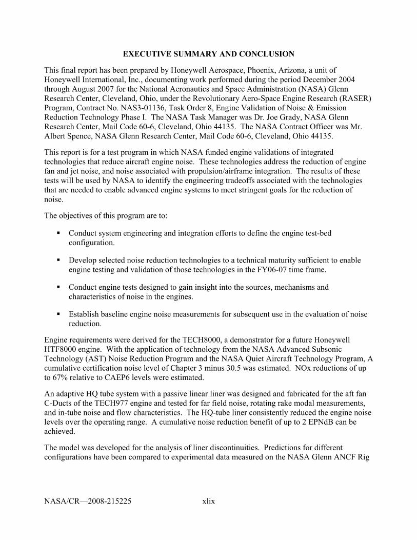
xlix

EXECUTIVE SUMMARY AND CONCLUSION

This final report has been prepared by Honeywell Aerospace, Phoenix, Arizona, a unit of Honeywell International, Inc., documenting work performed during the period December 2004 through August 2007 for the National Aeronautics and Space Administration (NASA) Glenn Research Center, Cleveland, Ohio, under the Revolutionary Aero-Space Engine Research (RASER) Program, Contract No. NAS3-01136, Task Order 8, Engine Validation of Noise & Emission Reduction Technology Phase I. The NASA Task Manager was Dr. Joe Grady, NASA Glenn Research Center, Mail Code 60-6, Cleveland, Ohio 44135. The NASA Contract Officer was Mr. Albert Spence, NASA Glenn Research Center, Mail Code 60-6, Cleveland, Ohio 44135.

This report is for a test program in which NASA funded engine validations of integrated technologies that reduce aircraft engine noise. These technologies address the reduction of engine fan and jet noise, and noise associated with propulsion/airframe integration. The results of these tests will be used by NASA to identify the engineering tradeoffs associated with the technologies that are needed to enable advanced engine systems to meet stringent goals for the reduction of noise.

The objectives of this program are to:

Conduct system engineering and integration efforts to define the engine test-bed configuration.

Develop selected noise reduction technologies to a technical maturity sufficient to enable engine testing and validation of those technologies in the FY06-07 time frame.

Conduct engine tests designed to gain insight into the sources, mechanisms and characteristics of noise in the engines.

Establish baseline engine noise measurements for subsequent use in the evaluation of noise reduction.

Engine requirements were derived for the TECH8000, a demonstrator for a future Honeywell HTF8000 engine. With the application of technology from the NASA Advanced Subsonic Technology (AST) Noise Reduction Program and the NASA Quiet Aircraft Technology Program, A cumulative certification noise level of Chapter 3 minus 30.5 was estimated. NOx reductions of up to 67% relative to CAEP6 levels were estimated.

An adaptive HQ tube system with a passive linear liner was designed and fabricated for the aft fan C-Ducts of the TECH977 engine and tested for far field noise, rotating rake modal measurements, and in-tube noise and flow characteristics. The HQ-tube liner consistently reduced the engine noise levels over the operating range. A cumulative noise reduction benefit of up to 2 EPNdB can be achieved.

The model was developed for the analysis of liner discontinuities. Predictions for different configurations have been compared to experimental data measured on the NASA Glenn ANCF Rig

NASA/CR—2008-215225

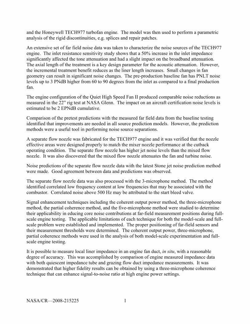
l

and the Honeywell TECH977 turbofan engine. The model was then used to perform a parametric analysis of the rigid discontinuities, e.g. splices and repair patches.

An extensive set of far field noise data was taken to characterize the noise sources of the TECH977 engine. The inlet resistance sensitivity study shows that a 50% increase in the inlet impedance significantly affected the tone attenuation and had a slight impact on the broadband attenuation. The axial length of the treatment is a key design parameter for the acoustic attenuation. However, the incremental treatment benefit reduces as the liner length increases. Small changes in fan geometry can result in significant noise changes. The pre-production baseline fan has PNLT noise levels up to 3 PNdB higher from 60 to 90 degrees from the inlet as compared to a final production fan.

The engine configuration of the Quiet High Speed Fan II produced comparable noise reductions as measured in the 22” rig test at NASA Glenn. The impact on an aircraft certification noise levels is estimated to be 2 EPNdB cumulative.

Comparison of the pretest predictions with the measured far field data from the baseline testing identified that improvements are needed in all source prediction models. However, the prediction methods were a useful tool in performing noise source separations.

A separate flow nozzle was fabricated for the TECH977 engine and it was verified that the nozzle effective areas were designed properly to match the mixer nozzle performance at the cutback operating condition. The separate flow nozzle has higher jet noise levels than the mixed flow nozzle. It was also discovered that the mixed flow nozzle attenuates the fan and turbine noise.

Noise predictions of the separate flow nozzle data with the latest Stone jet noise prediction method were made. Good agreement between data and predictions was observed.

The separate flow nozzle data was also processed with the 3-microphone method. The method identified correlated low frequency content at low frequencies that may be associated with the combustor. Correlated noise above 500 Hz may be attributed to the start bleed valve.

Signal enhancement techniques including the coherent output power method, the three-microphone method, the partial coherence method, and the five-microphone method were studied to determine their applicability in educing core noise contributions at far-field measurement positions during full-scale engine testing. The applicable limitations of each technique for both the model-scale and full-scale problem were established and implemented. The proper positioning of far-field sensors and their measurement thresholds were determined. The coherent output power, three-microphone, partial coherence methods were used in the analysis of both model-scale experimentation and full-scale engine testing.

It is possible to measure local liner impedance in an engine fan duct, in situ, with a reasonable degree of accuracy. This was accomplished by comparison of engine measured impedance data with both quiescent impedance tube and grazing flow duct impedance measurements. It was demonstrated that higher fidelity results can be obtained by using a three-microphone coherence technique that can enhance signal-to-noise ratio at high engine power settings.

NASA/CR—2008-215225

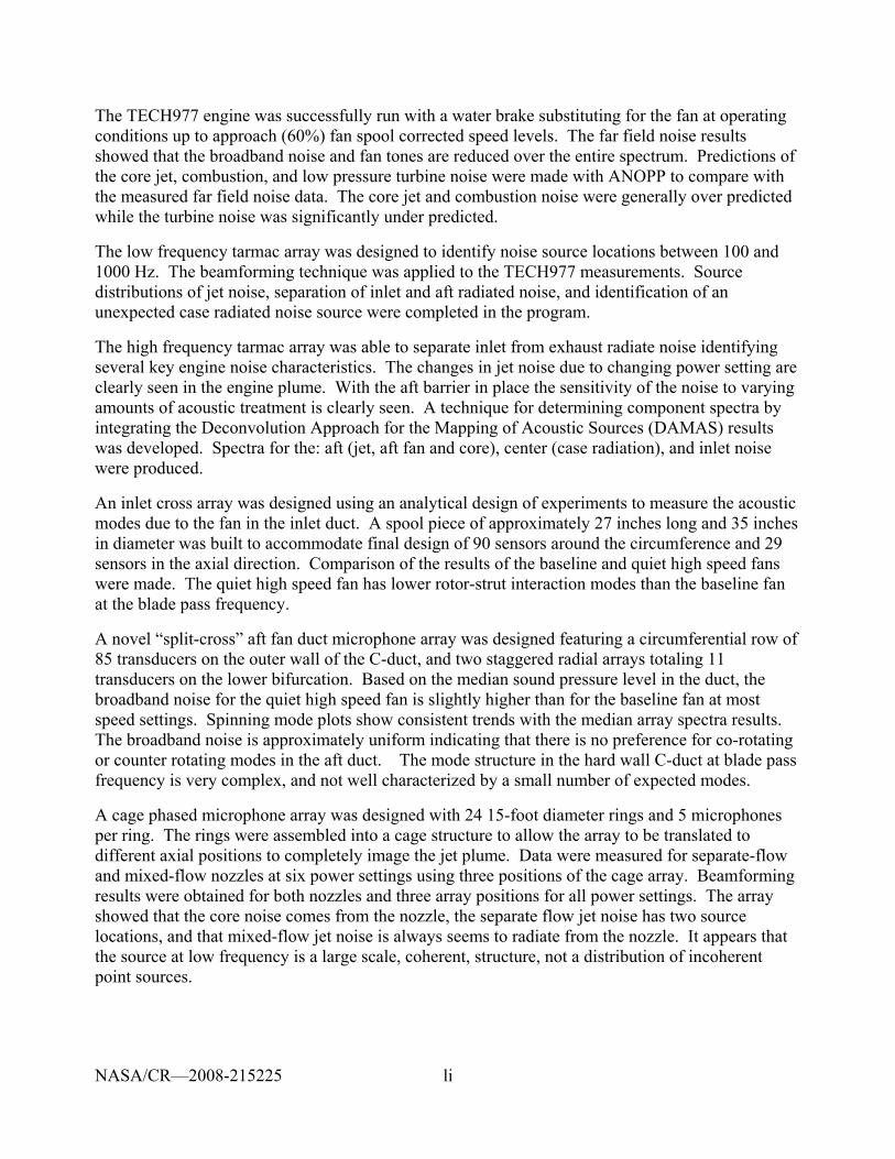
li

The TECH977 engine was successfully run with a water brake substituting for the fan at operating conditions up to approach (60%) fan spool corrected speed levels. The far field noise results showed that the broadband noise and fan tones are reduced over the entire spectrum. Predictions of the core jet, combustion, and low pressure turbine noise were made with ANOPP to compare with the measured far field noise data. The core jet and combustion noise were generally over predicted while the turbine noise was significantly under predicted.

The low frequency tarmac array was designed to identify noise source locations between 100 and 1000 Hz. The beamforming technique was applied to the TECH977 measurements. Source distributions of jet noise, separation of inlet and aft radiated noise, and identification of an unexpected case radiated noise source were completed in the program.

The high frequency tarmac array was able to separate inlet from exhaust radiate noise identifying several key engine noise characteristics. The changes in jet noise due to changing power setting are clearly seen in the engine plume. With the aft barrier in place the sensitivity of the noise to varying amounts of acoustic treatment is clearly seen. A technique for determining component spectra by integrating the Deconvolution Approach for the Mapping of Acoustic Sources (DAMAS) results was developed. Spectra for the: aft (jet, aft fan and core), center (case radiation), and inlet noise were produced.

An inlet cross array was designed using an analytical design of experiments to measure the acoustic modes due to the fan in the inlet duct. A spool piece of approximately 27 inches long and 35 inches in diameter was built to accommodate final design of 90 sensors around the circumference and 29 sensors in the axial direction. Comparison of the results of the baseline and quiet high speed fans were made. The quiet high speed fan has lower rotor-strut interaction modes than the baseline fan at the blade pass frequency.

A novel “split-cross” aft fan duct microphone array was designed featuring a circumferential row of 85 transducers on the outer wall of the C-duct, and two staggered radial arrays totaling 11 transducers on the lower bifurcation. Based on the median sound pressure level in the duct, the broadband noise for the quiet high speed fan is slightly higher than for the baseline fan at most speed settings. Spinning mode plots show consistent trends with the median array spectra results. The broadband noise is approximately uniform indicating that there is no preference for co-rotating or counter rotating modes in the aft duct. The mode structure in the hard wall C-duct at blade pass frequency is very complex, and not well characterized by a small number of expected modes.

A cage phased microphone array was designed with 24 15-foot diameter rings and 5 microphones per ring. The rings were assembled into a cage structure to allow the array to be translated to different axial positions to completely image the jet plume. Data were measured for separate-flow and mixed-flow nozzles at six power settings using three positions of the cage array. Beamforming results were obtained for both nozzles and three array positions for all power settings. The array showed that the core noise comes from the nozzle, the separate flow jet noise has two source locations, and that mixed-flow jet noise is always seems to radiate from the nozzle. It appears that the source at low frequency is a large scale, coherent, structure, not a distribution of incoherent point sources.

NASA/CR—2008-215225

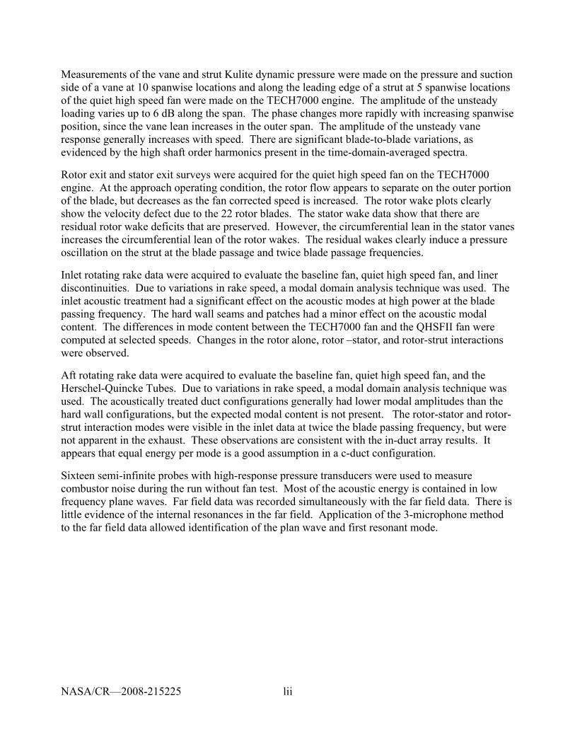
lii

Measurements of the vane and strut Kulite dynamic pressure were made on the pressure and suction side of a vane at 10 spanwise locations and along the leading edge of a strut at 5 spanwise locations of the quiet high speed fan were made on the TECH7000 engine. The amplitude of the unsteady loading varies up to 6 dB along the span. The phase changes more rapidly with increasing spanwise position, since the vane lean increases in the outer span. The amplitude of the unsteady vane response generally increases with speed. There are significant blade-to-blade variations, as evidenced by the high shaft order harmonics present in the time-domain-averaged spectra.

Rotor exit and stator exit surveys were acquired for the quiet high speed fan on the TECH7000 engine. At the approach operating condition, the rotor flow appears to separate on the outer portion of the blade, but decreases as the fan corrected speed is increased. The rotor wake plots clearly show the velocity defect due to the 22 rotor blades. The stator wake data show that there are residual rotor wake deficits that are preserved. However, the circumferential lean in the stator vanes increases the circumferential lean of the rotor wakes. The residual wakes clearly induce a pressure oscillation on the strut at the blade passage and twice blade passage frequencies.

Inlet rotating rake data were acquired to evaluate the baseline fan, quiet high speed fan, and liner discontinuities. Due to variations in rake speed, a modal domain analysis technique was used. The inlet acoustic treatment had a significant effect on the acoustic modes at high power at the blade passing frequency. The hard wall seams and patches had a minor effect on the acoustic modal content. The differences in mode content between the TECH7000 fan and the QHSFII fan were computed at selected speeds. Changes in the rotor alone, rotor –stator, and rotor-strut interactions were observed.

Aft rotating rake data were acquired to evaluate the baseline fan, quiet high speed fan, and the Herschel-Quincke Tubes. Due to variations in rake speed, a modal domain analysis technique was used. The acoustically treated duct configurations generally had lower modal amplitudes than the hard wall configurations, but the expected modal content is not present. The rotor-stator and rotor-strut interaction modes were visible in the inlet data at twice the blade passing frequency, but were not apparent in the exhaust. These observations are consistent with the in-duct array results. It appears that equal energy per mode is a good assumption in a c-duct configuration.

Sixteen semi-infinite probes with high-response pressure transducers were used to measure combustor noise during the run without fan test. Most of the acoustic energy is contained in low frequency plane waves. Far field data was recorded simultaneously with the far field data. There is little evidence of the internal resonances in the far field. Application of the 3-microphone method to the far field data allowed identification of the plan wave and first resonant mode.

NASA/CR—2008-215225

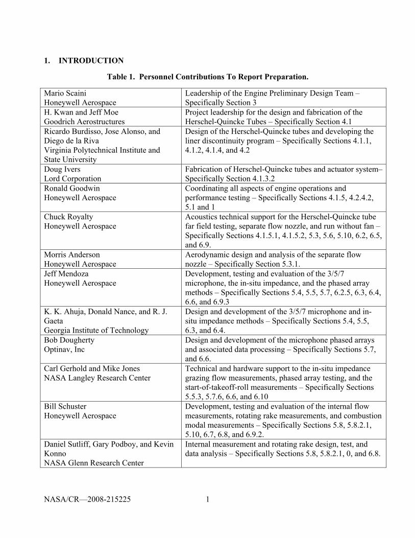
1

1. INTRODUCTION

Table 1. Personnel Contributions To Report Preparation.

Mario Scaini Honeywell Aerospace

Leadership of the Engine Preliminary Design Team – Specifically Section 3

H. Kwan and Jeff Moe Goodrich Aerostructures

Project leadership for the design and fabrication of the Herschel-Quincke Tubes – Specifically Section 4.1

Ricardo Burdisso, Jose Alonso, and Diego de la Riva Virginia Polytechnical Institute and State University

Design of the Herschel-Quincke tubes and developing the liner discontinuity program – Specifically Sections 4.1.1, 4.1.2, 4.1.4, and 4.2

Doug Ivers Lord Corporation

Fabrication of Herschel-Quincke tubes and actuator system– Specifically Section 4.1.3.2

Ronald Goodwin Honeywell Aerospace

Coordinating all aspects of engine operations and performance testing – Specifically Sections 4.1.5, 4.2.4.2, 5.1 and 1

Chuck Royalty Honeywell Aerospace

Acoustics technical support for the Herschel-Quincke tube far field testing, separate flow nozzle, and run without fan – Specifically Sections 4.1.5.1, 4.1.5.2, 5.3, 5.6, 5.10, 6.2, 6.5, and 6.9.

Morris Anderson Honeywell Aerospace

Aerodynamic design and analysis of the separate flow nozzle – Specifically Section 5.3.1.

Jeff Mendoza Honeywell Aerospace

Development, testing and evaluation of the 3/5/7 microphone, the in-situ impedance, and the phased array methods – Specifically Sections 5.4, 5.5, 5.7, 6.2.5, 6.3, 6.4, 6.6, and 6.9.3

K. K. Ahuja, Donald Nance, and R. J. Gaeta Georgia Institute of Technology

Design and development of the 3/5/7 microphone and in-situ impedance methods – Specifically Sections 5.4, 5.5, 6.3, and 6.4.

Bob Dougherty Optinav, Inc

Design and development of the microphone phased arrays and associated data processing – Specifically Sections 5.7, and 6.6.

Carl Gerhold and Mike Jones NASA Langley Research Center

Technical and hardware support to the in-situ impedance grazing flow measurements, phased array testing, and the start-of-takeoff-roll measurements – Specifically Sections 5.5.3, 5.7.6, 6.6, and 6.10

Bill Schuster Honeywell Aerospace

Development, testing and evaluation of the internal flow measurements, rotating rake measurements, and combustion modal measurements – Specifically Sections 5.8, 5.8.2.1, 5.10, 6.7, 6.8, and 6.9.2.

Daniel Sutliff, Gary Podboy, and Kevin Konno NASA Glenn Research Center

Internal measurement and rotating rake design, test, and data analysis – Specifically Sections 5.8, 5.8.2.1, 0, and 6.8.

NASA/CR—2008-215225

2

Table 1. Personnel Contributions To Report Preparation (Cont).

George Kontos Manpower, Inc.

Acquisition and analysis of the static engine acoustic data – Specifically Section 1.

1.1 Abstract

This final report has been prepared by Honeywell Aerospace, Phoenix, Arizona, a unit of Honeywell International, Inc., documenting work performed during the period December 2004 through August 2007 for the National Aeronautics and Space Administration (NASA) Glenn Research Center, Cleveland, Ohio, under the Revolutionary Aero-Space Engine Research (RASER) Program, Contract No. NAS3-01136, Task Order 8, Engine Validation of Noise & Emission Reduction Technology Phase I. The NASA Task Manager was Dr. Joe Grady, NASA Glenn Research Center, Mail Code 60-6, Cleveland, Ohio 44135. The NASA Contract Officer was Mr. Albert Spence, NASA Glenn Research Center, Mail Code 60-6, Cleveland, Ohio 44135. This report is for a test program in which NASA funded engine validations of integrated technologies that reduce aircraft engine noise. These technologies address the reduction of engine fan and jet noise, and noise associated with propulsion/airframe integration. The results of these tests will be used by NASA to identify the engineering tradeoffs associated with the technologies that are needed to enable advanced engine systems to meet stringent goals for the reduction of noise.

1.2 Objectives

The objectives of this program are to:

Conduct system engineering and integration efforts to define the engine test-bed configuration.

Develop selected noise reduction technologies to a technical maturity sufficient to enable engine testing and validation of those technologies in the FY06-07 time frame.

Conduct engine tests designed to gain insight into the sources, mechanisms and characteristics of noise in the engines.

Establish baseline engine noise measurements for subsequent use in the evaluation of noise reduction.

NASA/CR—2008-215225

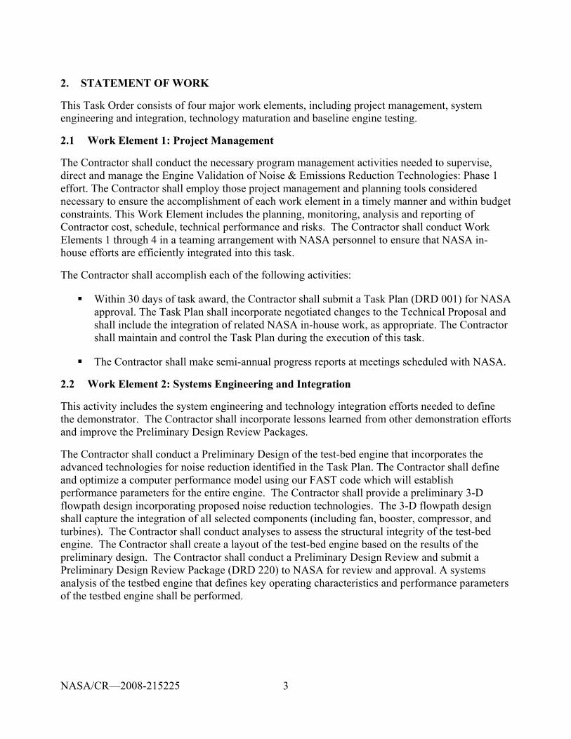
3

2. STATEMENT OF WORK

This Task Order consists of four major work elements, including project management, system engineering and integration, technology maturation and baseline engine testing.

2.1 Work Element 1: Project Management

The Contractor shall conduct the necessary program management activities needed to supervise, direct and manage the Engine Validation of Noise & Emissions Reduction Technologies: Phase 1 effort. The Contractor shall employ those project management and planning tools considered necessary to ensure the accomplishment of each work element in a timely manner and within budget constraints. This Work Element includes the planning, monitoring, analysis and reporting of Contractor cost, schedule, technical performance and risks. The Contractor shall conduct Work Elements 1 through 4 in a teaming arrangement with NASA personnel to ensure that NASA in-house efforts are efficiently integrated into this task.

The Contractor shall accomplish each of the following activities:

Within 30 days of task award, the Contractor shall submit a Task Plan (DRD 001) for NASA approval. The Task Plan shall incorporate negotiated changes to the Technical Proposal and shall include the integration of related NASA in-house work, as appropriate. The Contractor shall maintain and control the Task Plan during the execution of this task.

The Contractor shall make semi-annual progress reports at meetings scheduled with NASA.

2.2 Work Element 2: Systems Engineering and Integration

This activity includes the system engineering and technology integration efforts needed to define the demonstrator. The Contractor shall incorporate lessons learned from other demonstration efforts and improve the Preliminary Design Review Packages.

The Contractor shall conduct a Preliminary Design of the test-bed engine that incorporates the advanced technologies for noise reduction identified in the Task Plan. The Contractor shall define and optimize a computer performance model using our FAST code which will establish performance parameters for the entire engine. The Contractor shall provide a preliminary 3-D flowpath design incorporating proposed noise reduction technologies. The 3-D flowpath design shall capture the integration of all selected components (including fan, booster, compressor, and turbines). The Contractor shall conduct analyses to assess the structural integrity of the test-bed engine. The Contractor shall create a layout of the test-bed engine based on the results of the preliminary design. The Contractor shall conduct a Preliminary Design Review and submit a Preliminary Design Review Package (DRD 220) to NASA for review and approval. A systems analysis of the testbed engine that defines key operating characteristics and performance parameters of the testbed engine shall be performed.

NASA/CR—2008-215225

4

2.3 Work Element 3: Technology Maturation

2.3.1 HQ Tube/Optimum Liner - Aft Duct HQ Tubes

The Contractor shall:

• Design an adaptive HQ-tube liner system for the TECH977 exhaust duct. Different adaptive mechanisms shall be evaluated and tested at a laboratory environment. An applicable adaptive device shall be selected. Then, an adaptive HQ-tube liner system shall be designed for the TECH977 engine static test configuration. An individual functional adaptive control system also will be designed for the HQ-tubes. The aft HQ-liner duct model developed for the NASA/Goodrich ANCF rig test (Goodrich proprietary information) will be used to design the HQ system. If possible, HQ-liners will be implemented in both the inner and outer surfaces of the bypass duct.

• Fabricate adaptive HQ-tube liner system. The contractor shall design, integrate, and fabricate the adaptive HQ-tube zone liner. This system will be mounted in the aft fan duct of the contractor’s TECH977 engine.

• Evaluate an adaptive HQ-tube liner system at the Contractor test facility: The adaptive HQ-tube duct liner shall be installed on the TECH977 engine and tested at the contractor’s acoustic test facility. Measurements of the far field noise shall be performed with the tarmac array and aft duct modal measurements shall be made with the rotating rake.

• Data reduction and analysis: The contractor shall provide the acoustic data for reduction and analysis.

• Evaluate noise attenuation impact of an adaptive HQ-tube liner system on “production” turbofan engine. An assessment of the overall noise attenuation impact of the adaptive HQ-tube liner system on a turbofan engine will be performed in order to evaluate EPNdB benefits.

2.3.2 Modeling and Validation of Inlet Liner Impedance Discontinuities

The presence of non-uniformities in turbofan engine inlet liners can affect the propagation of the fan noise, especially the tonal component such as the blade passage frequency tones at high power settings. One source of impedance discontinuities are of structural splices that separate adjacent liner panels in the inlet.

The Contractor shall perform the following:

• Code development: The analytical formulation based on AIAA Paper No. 2003-3144 shall be developed and the model shall be implemented in a FORTRAN code. The formulation shall be initially be based on infinite lined duct theory, then modifications shall be introduced to account for finite liner effects such as transmissions and reflections at the hard wall liner interfaces. Reflection effects at the open end of the engine inlet shall be accounted for to allow for calculations of far-field radiation. The code shall be able to model any arbitrary liner impedance discontinuity.

NASA/CR—2008-215225

5

• Experimental Data: To validate the model and assess the influence of liner splices and other discontinuities, experimental data will be collected on a liner in the Active Noise Control Facility at NASA Glenn and a liner installed on the Honeywell TECH977 turbofan engine at the San Tan Honeywell facilities. The rotating rake method shall be used to determine the acoustic modal structure and the change in duct acoustic power due to liner splices and other discontinuities. Far field noise measurements of selected configurations shall also be made for the TECH977.

• Experimental data reduction and analysis: The in-duct modal and far-field data shall be reduced and analyzed.

• Evaluate noise attenuation impact: The impact of splices and other discontinuities shall be quantified in terms of liner sound power attenuation, effect on modal structure, and far-field radiation.

• Code validation: The experimental data shall be used to validate the code for both modal structure predictions and far-field radiation. Far-field validation shall include both power attenuation and directivity patterns.

• Parametric studies: A parametric analysis shall be performed with the validated code to fully understand the influence of liner splices, i.e. size, number and distribution around the circumference.

The Contractor shall submit the following Contract Deliverables for Technology Maturation elements 3.2 through 3.4:

• A test and instrumentation plan (DRD-010), submitted for review and approval of the NASA Task Manager one month prior to imitation of the rig-scale demonstration of TRL 5 readiness.

• An informal test report (DRD-211), submitted for review and approval of the NASA Task Manager within one month of test completion. The report shall include an updated assessment of the anticipated technology benefit, in terms of reduction in noise.

2.4 Work Element 4: Engine Tests

Engine Noise Source Diagnostic Tests. The Contractor shall conduct static engine tests to characterize the noise sources and to identify dominant source mechanisms. The Contractor shall apply existing and/or new source separation methods and appropriate diagnostic tools to identify the characteristics of noise associated with different engine components and to identify any installation associated effects. The Contractor shall establish baseline noise measurements for subsequent use in the evaluation of noise reduction concepts and shall provide detailed explanations of the spectral features of those measurements. The Contractor shall obtain far-field 1/3-octave and narrowband acoustic data for all microphones, at all engine speeds and engine operating conditions tested.

The Contractor shall perform the following activities for source noise diagnostics:

NASA/CR—2008-215225

6

2.4.1 Engine Build Up

The Contractor shall assemble the appropriate test engine with accommodations made for special hardware and instrumentation as defined below.

2.4.2 Baseline Noise Measurements

The Contractor shall make predictions of the engine far field noise signature prior to engine measurements using the NASA Aircraft Noise Prediction Program (ANOPP) or equivalent noise prediction code. Far-field acoustic data shall be acquired at an acoustic test facility with a 100-foot microphone array to determine overall engine acoustic characteristics of the TECH7000. This test shall include the evaluation of both the current production design HTF7000 fan, as well as the Quiet High Speed Fan (QHSF II). Inlet and exhaust treatment evaluation tests shall be conducted on the TECH7000 on one business jet nacelle and one regional jet nacelle as part of defining the baseline noise characteristics of the engine. These tests shall define treatment effectiveness and determine optimum treatment area of two different single degree of freedom (SDOF) inlet and aft duct liners. Treated versus untreated area studies for both the inlet and exhaust shall also be performed using noise barriers to isolate inlet and exhaust noise propagation to the far field, and hardwall inlet/exhaust components. The measured noise levels shall be compared to the pretest predictions and assess the adequacy of the prediction models. Narrowband data and existing fan/jet model test data shall be used to identify engine component spectra separating the fan, jet, compressor, combustor and turbine components.

2.4.3 Separate Flow Nozzle

The Contractor shall design and fabricate a separate flow nozzle (SFN) for the TECH7000 and tested to support source noise diagnostics. The SFN design shall accommodate different nozzle configurations, using spacers for the center body, flanges for the core nozzle, and spacers and shims for the bypass nozzle to adjust the core and fan flow area to match the required engine cycle conditions. The Contractor shall perform jet noise predictions with ANOPP and compare those predictions to test data from this task. Microphones on a 100’ polar arc in the far field of the TECH7000 engine shall provide baseline noise measurements for the SFN. Multiple microphone techniques shall be used to identify noise sources. The polar arc array shall also be used for source identification.

2.4.4 3/5/7 Microphone

Prior to engine testing, the Contractor shall conduct laboratory testing for verification of the source separation technique using a flow-duct and acoustic drivers to model correlated sources. The Contractor shall use multiple microphone techniques involving 3, 5, or 7 microphones in the far field of the TECH7000 and transducers in the internal engine for source separation of aft-radiated noise. Spectral comparisons shall be made with an existing source separation model for refinement of source noise modeling.

2.4.5 In-Situ Impedance Measurements

The Contractor shall team with NASA to make in-situ impedance measurements (conventional and rotating-rake method) during acoustic liner evaluations. The measurements shall be used to

NASA/CR—2008-215225

7

substantiate treatment design, provide understanding of flow effects on installed liner performance, and provide modeling input for fan noise propagation. Instrumentation on the TECH7000 shall consist of transducers located at axial and polar locations on the face sheet and in the backing cavity of the acoustic treatment. Thermocouples to reduce the effect of temperature (wave number) on impedance measurement inaccuracies shall be included. Validation testing in the Langley Grazing Incidence Tube shall refine the data acquisition and processing of in-situ acoustic impedance in the presence of flow using the conventional in-situ impedance eduction approach. Phase and amplitude calibrations of the sensors shall be performed to minimize measurement error. Rotating rake mechanism and data acquisition support shall also be included. Validation testing with a low speed fan in the Glenn ANCF shall refine the data acquisition and processing of in-situ impedance using the rotating-rake method.

2.4.6 Run Without Fan

The Contractor shall remove the fan of the TECH7000 and operate the engine using a water brake dynamometer. A performance analysis shall be performed to ensure that the compressor and turbine stages are operating near the desired operating line. Comprehensive rotor dynamics and structural analyses shall be performed to design coupling and support hardware. The engine shall be operated over a range of power conditions to obtain data at different fan speeds, ranging from power settings typical of approach conditions to the highest power settings possible within safe operating constraints. Noise from the water brake shall be isolated using a barrier. The Contractor shall use a barrier for separation of inlet and aft noise sources. Far field and internal engine noise measurements shall be made for source separation.

2.4.7 Phased Array

The Contractor shall team with NASA to use both recent phased array measurement advancements, as well as the results of Aeroacoustics Research Consortium (AARC) funded research to discern critical inlet and exhaust noise mechanisms. The 100-foot polar arc array of 32 far-field microphones shall be used to measure narrow band and 1/3-octave band spectra. The narrow band spectra shall be analyzed to separate the tone sources between fan, compressor, and turbine. Additional microphones shall be added to the polar arc near 90° to form a phased array to separate inlet from aft noise in this area.

Separation of jet, core, and aft fan noise shall be accomplished with a caged array of microphones surrounding the jet. NASA will provide instrumentation for a 3-D caged array and will work with the Contractor to design, instrument, and test the array. The Contractor shall use data from the caged array to validate source modeling of jet noise physics and to identify mechanisms for noise reduction.

Circumferential rings of in-duct microphones shall be used to separate rotor-alone from rotor-stator interaction noise. NASA will provide the instrumentation for the internal array processing and work with the Contractor to design and process the internal modal arrays. The internal arrays shall provide spinning mode content of fan noise, differentiate between rotor and stator sources, perform model validation, and enhance acoustic treatment design.

NASA/CR—2008-215225

8

2.4.8 Internal Flow Measurements

Baseline internal flow measurements shall be made on a TECH7000 to characterize fan noise mechanisms. Measurements of the rotor flow-field shall be made using a traversing hot wire or hot film system. The mean and turbulent properties of the rotor wake flow in front of and behind the stator shall be measured. Kulites shall be used to measure unsteady pressure on vane and strut surfaces due to the impingement of the unsteady rotor flow. Measurements of the unsteady pressure at the fan duct wall shall be made to characterize the modal content of the acoustic field.

The Contractor shall team with specialists at NASA to acquire these measurements on the TECH7000. The fan case and front frame of the TECH7000 shall be modified to accommodate the measurement systems. The Contractor and NASA shall define the desired locations for the vane, strut, and case mounted transducers, and the Contractor shall instrument the hardware and acquire the data. Measurements of the rotor wake flow and the vane/strut/wall pressure shall be acquired for a specified range of engine operating conditions. The Contractor and NASA shall jointly analyze the collected data.

2.4.9 Fan Modal Measurements

The Contractor shall design and fabricate a rotating rake system for the TECH7000, using as much hardware as possible from the system developed for the EVNRC program. The Contractor shall conduct the modal testing with support from NASA. .The engine shall have a hard wall inlet and a separate-flow exhaust nozzle. Both the baseline fan and QHSF II shall be tested. Circumferential and radial modes of the sound field in the inlet and fan nozzle shall be measured at several operating conditions for source identification, model validation, and acoustic treatment design.

2.4.10 Signal Conditioning Acquisition

The Contractor shall purchase a 128-channel signal conditioning unit using the specification provided by NASA.

2.4.11 Combustor Noise Diagnostic Measurements

The Contractor shall make modal measurements of the acoustic field in the combustor and turbine of the TECH977 engine as part of 4.8. There shall be internal measurements in the combustor to identify and quantify any modal structures. Additional acoustic instrumentation shall be installed in the turbine to identify and separate the combustion generated noise from noise due to the turbine interactions with the combustor flow field. The modal measurements shall be compared to far field noise measurements to identify potential sources of the resonances observed in the far field.

The measurements shall apply the lessons learned from the RASER Task Order 7 measurements of the combustor modes in an APU and the measurement and analysis techniques developed in 4.5.

The Contractor shall apply existing combustion noise prediction methods to the combustor and compare predictions with source separated data. The Contractor shall include recommendations for improvements in combustion noise prediction in the final report.

NASA/CR—2008-215225

9

2.4.12 Start of Take-off Roll Simulation

The contractor shall perform two test sequences, one for a mixed flow engine configuration and the other for a separate flow engine configuration, to study the radiated sound field aft of the engine during "start-of-roll". For each configuration, the need data shall be acquired at multiple power settings (the standard set) using an enhanced far-field array. The enhancement shall consist of 8 additional microphones, located at angles of 165 to 200 degrees, in increments of 5 degrees (covering the aft arc). The microphones, preamps and cables will be supplied by Langley. The data shall be acquired using the standard far-field data acquisition system. The Contractor shall process the data to provide 1/3-octave band and A-weighted data projected to a 1000 ft arc (using standard spherical spreading and atmospheric absorption).

NASA/CR—2008-215225

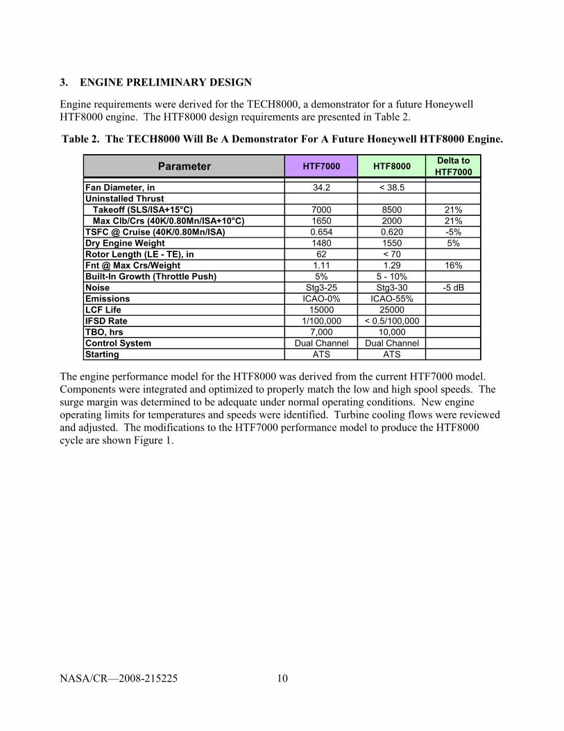
10

3. ENGINE PRELIMINARY DESIGN

Engine requirements were derived for the TECH8000, a demonstrator for a future Honeywell HTF8000 engine. The HTF8000 design requirements are presented in Table 2.

Table 2. The TECH8000 Will Be A Demonstrator For A Future Honeywell HTF8000 Engine.

Parameter HTF7000 HTF8000 Delta to HTF7000

Fan Diameter, in 34.2 < 38.5Uninstalled Thrust Takeoff (SLS/ISA+15°C) 7000 8500 21% Max Clb/Crs (40K/0.80Mn/ISA+10°C) 1650 2000 21%TSFC @ Cruise (40K/0.80Mn/ISA) 0.654 0.620 -5%Dry Engine Weight 1480 1550 5%Rotor Length (LE - TE), in 62 < 70Fnt @ Max Crs/Weight 1.11 1.29 16%Built-In Growth (Throttle Push) 5% 5 - 10%Noise Stg3-25 Stg3-30 -5 dBEmissions ICAO-0% ICAO-55%LCF Life 15000 25000IFSD Rate 1/100,000 < 0.5/100,000TBO, hrs 7,000 10,000Control System Dual Channel Dual ChannelStarting ATS ATS

The engine performance model for the HTF8000 was derived from the current HTF7000 model. Components were integrated and optimized to properly match the low and high spool speeds. The surge margin was determined to be adequate under normal operating conditions. New engine operating limits for temperatures and speeds were identified. Turbine cooling flows were reviewed and adjusted. The modifications to the HTF7000 performance model to produce the HTF8000 cycle are shown Figure 1.

NASA/CR—2008-215225

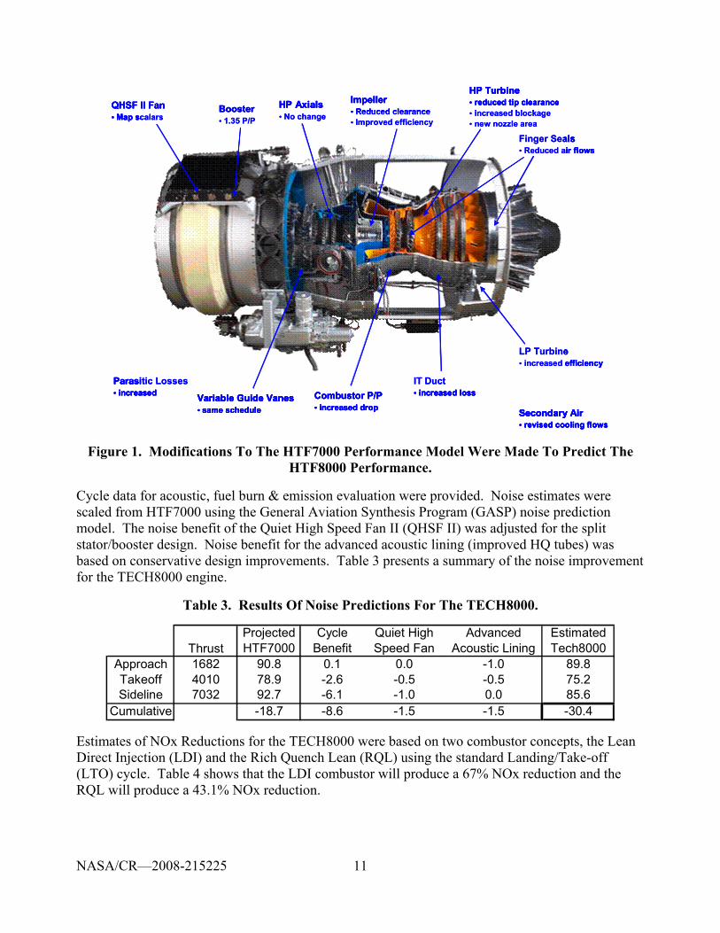
11

QHSF II Fan• Map scalars

Booster• 1.35 P/P

Impeller• Reduced clearance• Improved efficiency

HP Turbine• reduced tip clearance• increased blockage• new nozzle area

Parasitic Losses• increased

IT Duct• increased loss

LP Turbine• increased efficiency

Finger Seals• Reduced air flows

HP Axials• No change

Combustor P/P• increased drop

Variable Guide Vanes• same schedule Secondary Air

• revised cooling flows


Booster• 1.35 P/P












Booster• 1.35 P/P












Booster• 1.35 P/P











Figure 1. Modifications To The HTF7000 Performance Model Were Made To Predict The HTF8000 Performance.

Cycle data for acoustic, fuel burn & emission evaluation were provided. Noise estimates were scaled from HTF7000 using the General Aviation Synthesis Program (GASP) noise prediction model. The noise benefit of the Quiet High Speed Fan II (QHSF II) was adjusted for the split stator/booster design. Noise benefit for the advanced acoustic lining (improved HQ tubes) was based on conservative design improvements. Table 3 presents a summary of the noise improvement for the TECH8000 engine.

Table 3. Results Of Noise Predictions For The TECH8000.

ThrustProjected HTF7000

Cycle Benefit

Quiet High Speed Fan

Advanced Acoustic Lining

Estimated Tech8000

Approach 1682 90.8 0.1 0.0 -1.0 89.8Takeoff 4010 78.9 -2.6 -0.5 -0.5 75.2Sideline 7032 92.7 -6.1 -1.0 0.0 85.6

Cumulative -18.7 -8.6 -1.5 -1.5 -30.4

Estimates of NOx Reductions for the TECH8000 were based on two combustor concepts, the Lean Direct Injection (LDI) and the Rich Quench Lean (RQL) using the standard Landing/Take-off (LTO) cycle. Table 4 shows that the LDI combustor will produce a 67% NOx reduction and the RQL will produce a 43.1% NOx reduction.

NASA/CR—2008-215225

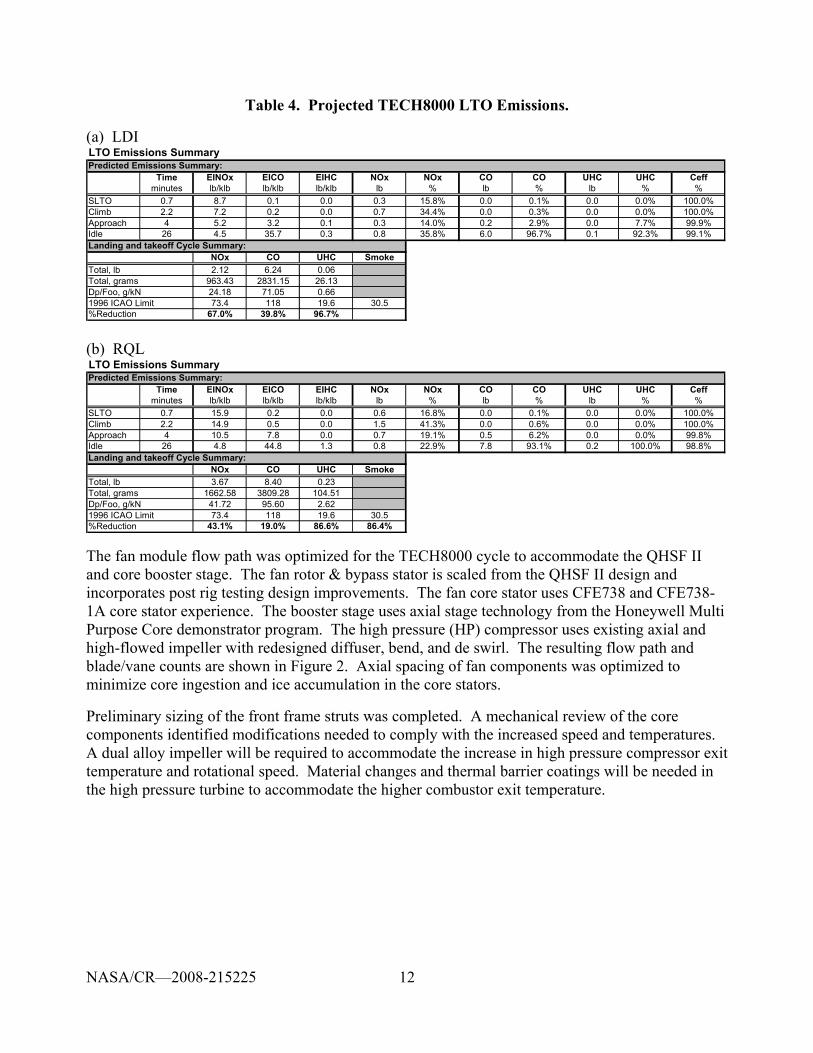
12

Table 4. Projected TECH8000 LTO Emissions.

(a) LDI LTO Emissions SummaryPredicted Emissions Summary:

Time EINOx EICO EIHC NOx NOx CO CO UHC UHC Ceffminutes lb/klb lb/klb lb/klb lb % lb % lb % %

SLTO 0.7 8.7 0.1 0.0 0.3 15.8% 0.0 0.1% 0.0 0.0% 100.0%Climb 2.2 7.2 0.2 0.0 0.7 34.4% 0.0 0.3% 0.0 0.0% 100.0%Approach 4 5.2 3.2 0.1 0.3 14.0% 0.2 2.9% 0.0 7.7% 99.9%Idle 26 4.5 35.7 0.3 0.8 35.8% 6.0 96.7% 0.1 92.3% 99.1%Landing and takeoff Cycle Summary:

NOx CO UHC SmokeTotal, lb 2.12 6.24 0.06Total, grams 963.43 2831.15 26.13Dp/Foo, g/kN 24.18 71.05 0.661996 ICAO Limit 73.4 118 19.6 30.5%Reduction 67.0% 39.8% 96.7% (b) RQL LTO Emissions SummaryPredicted Emissions Summary:

Time EINOx EICO EIHC NOx NOx CO CO UHC UHC Ceffminutes lb/klb lb/klb lb/klb lb % lb % lb % %

SLTO 0.7 15.9 0.2 0.0 0.6 16.8% 0.0 0.1% 0.0 0.0% 100.0%Climb 2.2 14.9 0.5 0.0 1.5 41.3% 0.0 0.6% 0.0 0.0% 100.0%Approach 4 10.5 7.8 0.0 0.7 19.1% 0.5 6.2% 0.0 0.0% 99.8%Idle 26 4.8 44.8 1.3 0.8 22.9% 7.8 93.1% 0.2 100.0% 98.8%Landing and takeoff Cycle Summary:

NOx CO UHC SmokeTotal, lb 3.67 8.40 0.23Total, grams 1662.58 3809.28 104.51Dp/Foo, g/kN 41.72 95.60 2.621996 ICAO Limit 73.4 118 19.6 30.5%Reduction 43.1% 19.0% 86.6% 86.4%

The fan module flow path was optimized for the TECH8000 cycle to accommodate the QHSF II and core booster stage. The fan rotor & bypass stator is scaled from the QHSF II design and incorporates post rig testing design improvements. The fan core stator uses CFE738 and CFE738-1A core stator experience. The booster stage uses axial stage technology from the Honeywell Multi Purpose Core demonstrator program. The high pressure (HP) compressor uses existing axial and high-flowed impeller with redesigned diffuser, bend, and de swirl. The resulting flow path and blade/vane counts are shown in Figure 2. Axial spacing of fan components was optimized to minimize core ingestion and ice accumulation in the core stators.

Preliminary sizing of the front frame struts was completed. A mechanical review of the core components identified modifications needed to comply with the increased speed and temperatures. A dual alloy impeller will be required to accommodate the increase in high pressure compressor exit temperature and rotational speed. Material changes and thermal barrier coatings will be needed in the high pressure turbine to accommodate the higher combustor exit temperature.

NASA/CR—2008-215225

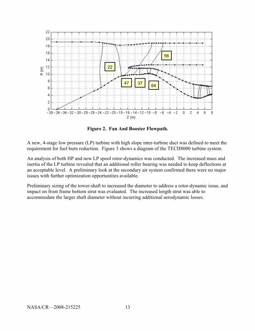
13

22

56

47 37 64

22

56

47 37 64

Figure 2. Fan And Booster Flowpath.

A new, 4-stage low pressure (LP) turbine with high slope inter-turbine duct was defined to meet the requirement for fuel burn reduction. Figure 3 shows a diagram of the TECH8000 turbine system.

An analysis of both HP and new LP spool rotor-dynamics was conducted. The increased mass and inertia of the LP turbine revealed that an additional roller bearing was needed to keep deflections at an acceptable level. A preliminary look at the secondary air system confirmed there were no major issues with further optimization opportunities available.

Preliminary sizing of the tower-shaft to increased the diameter to address a rotor-dynamic issue, and impact on front frame bottom strut was evaluated. The increased length strut was able to accommodate the larger shaft diameter without incurring additional aerodynamic losses.

NASA/CR—2008-215225

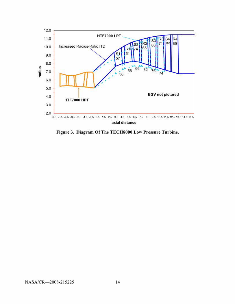
14

2.0

3.0

4.0

5.0

6.0

7.0

8.0

9.0

10.0

11.0

12.0

-6.5 -5.5 -4.5 -3.5 -2.5 -1.5 -0.5 0.5 1.5 2.5 3.5 4.5 5.5 6.5 7.5 8.5 9.5 10.5 11.5 12.5 13.5 14.5 15.5

axial distance

radi

us

HTF7000 HPT

HTF7000 LPTR469

S4100

R371

S380S2

74S157

R265R1

61

EGV not pictured

Increased Radius-Ratio ITD

5856 66 62 76

74

Figure 3. Diagram Of The TECH8000 Low Pressure Turbine.

NASA/CR—2008-215225

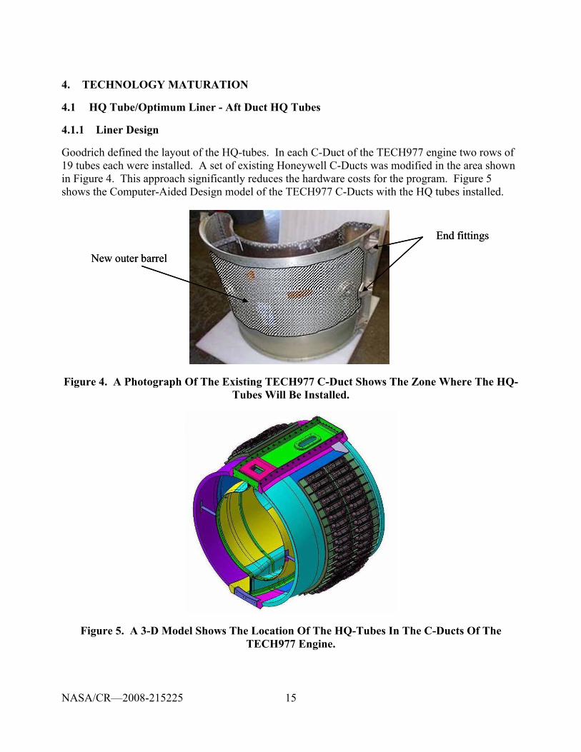
15

4. TECHNOLOGY MATURATION

4.1 HQ Tube/Optimum Liner - Aft Duct HQ Tubes

4.1.1 Liner Design

Goodrich defined the layout of the HQ-tubes. In each C-Duct of the TECH977 engine two rows of 19 tubes each were installed. A set of existing Honeywell C-Ducts was modified in the area shown in Figure 4. This approach significantly reduces the hardware costs for the program. Figure 5 shows the Computer-Aided Design model of the TECH977 C-Ducts with the HQ tubes installed.

End fittings

New outer barrel

End fittings

New outer barrel

Figure 4. A Photograph Of The Existing TECH977 C-Duct Shows The Zone Where The HQ-Tubes Will Be Installed.

Figure 5. A 3-D Model Shows The Location Of The HQ-Tubes In The C-Ducts Of The TECH977 Engine.

NASA/CR—2008-215225

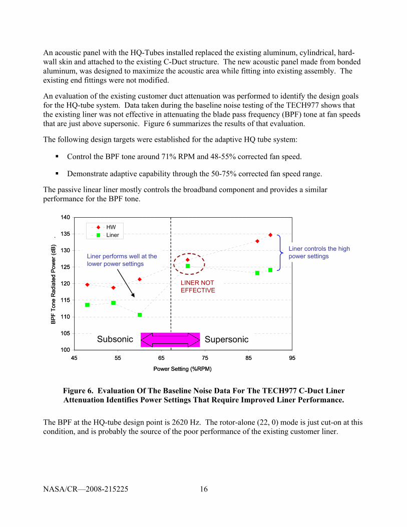
16

An acoustic panel with the HQ-Tubes installed replaced the existing aluminum, cylindrical, hard-wall skin and attached to the existing C-Duct structure. The new acoustic panel made from bonded aluminum, was designed to maximize the acoustic area while fitting into existing assembly. The existing end fittings were not modified.

An evaluation of the existing customer duct attenuation was performed to identify the design goals for the HQ-tube system. Data taken during the baseline noise testing of the TECH977 shows that the existing liner was not effective in attenuating the blade pass frequency (BPF) tone at fan speeds that are just above supersonic. Figure 6 summarizes the results of that evaluation.

The following design targets were established for the adaptive HQ tube system:

Control the BPF tone around 71% RPM and 48-55% corrected fan speed.

Demonstrate adaptive capability through the 50-75% corrected fan speed range.

The passive linear liner mostly controls the broadband component and provides a similar performance for the BPF tone.

100

105

110

115

120

125

130

135

140

45 55 65 75 85 95

Power Setting (%RPM)

BP

F To

ne R

adia

ted

Pow

er (d

B)

.

HWLiner

SupersonicSubsonic

Liner performs well at the lower power settings

Liner controls the high power settings

LINER NOT EFFECTIVE

100

105

110

115

120

125

130

135

140

45 55 65 75 85 95

Power Setting (%RPM)

BP

F To

ne R

adia

ted

Pow

er (d

B)

.

HWLiner

SupersonicSubsonic

Liner performs well at the lower power settings

Liner controls the high power settings

LINER NOT EFFECTIVE

Figure 6. Evaluation Of The Baseline Noise Data For The TECH977 C-Duct Liner Attenuation Identifies Power Settings That Require Improved Liner Performance.

The BPF at the HQ-tube design point is 2620 Hz. The rotor-alone (22, 0) mode is just cut-on at this condition, and is probably the source of the poor performance of the existing customer liner.

NASA/CR—2008-215225

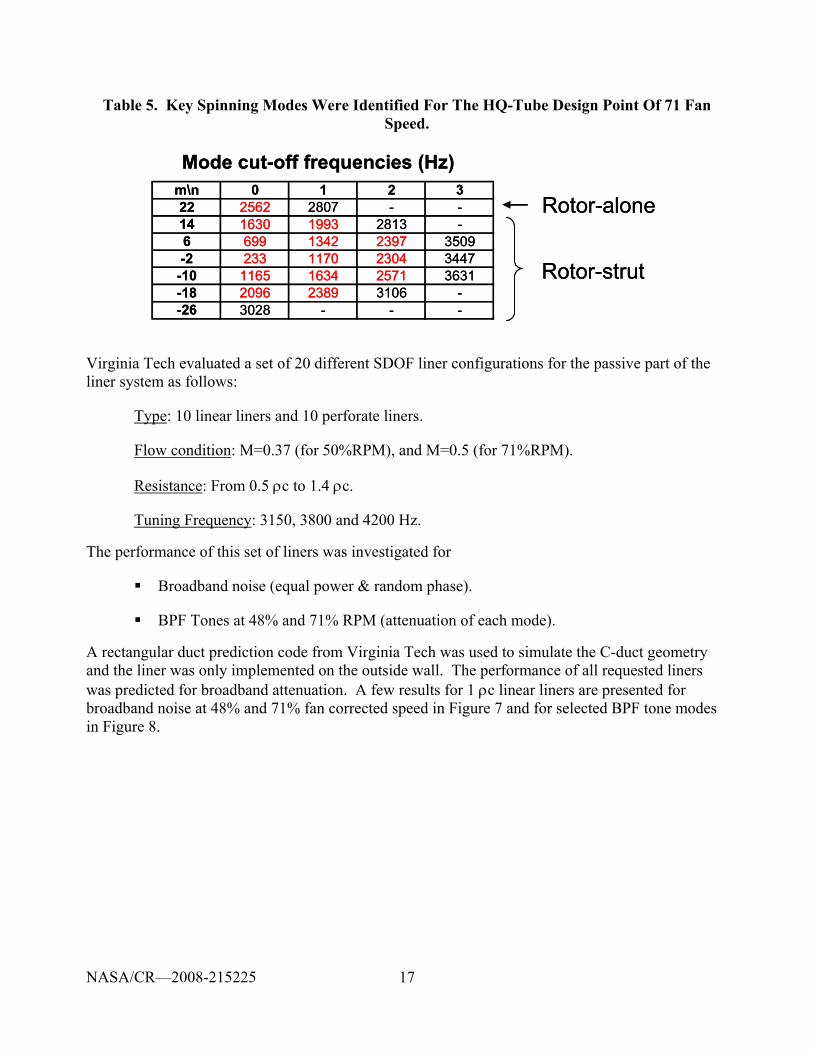
17

Table 5. Key Spinning Modes Were Identified For The HQ-Tube Design Point Of 71 Fan Speed.

m\n 0 1 2 322 2562 2807 - -14 1630 1993 2813 -6 699 1342 2397 3509-2 233 1170 2304 3447-10 1165 1634 2571 3631-18 2096 2389 3106 --26 3028 - - -

Rotor-alone

Rotor-strut

Mode cut-off frequencies (Hz)m\n 0 1 2 322 2562 2807 - -14 1630 1993 2813 -6 699 1342 2397 3509-2 233 1170 2304 3447-10 1165 1634 2571 3631-18 2096 2389 3106 --26 3028 - - -

Rotor-alone

Rotor-strut

Mode cut-off frequencies (Hz)

Virginia Tech evaluated a set of 20 different SDOF liner configurations for the passive part of the liner system as follows:

Type: 10 linear liners and 10 perforate liners.

Flow condition: M=0.37 (for 50%RPM), and M=0.5 (for 71%RPM).

Resistance: From 0.5 ρc to 1.4 ρc.

Tuning Frequency: 3150, 3800 and 4200 Hz.

The performance of this set of liners was investigated for

Broadband noise (equal power & random phase).

BPF Tones at 48% and 71% RPM (attenuation of each mode).

A rectangular duct prediction code from Virginia Tech was used to simulate the C-duct geometry and the liner was only implemented on the outside wall. The performance of all requested liners was predicted for broadband attenuation. A few results for 1 ρc linear liners are presented for broadband noise at 48% and 71% fan corrected speed in Figure 7 and for selected BPF tone modes in Figure 8.

NASA/CR—2008-215225

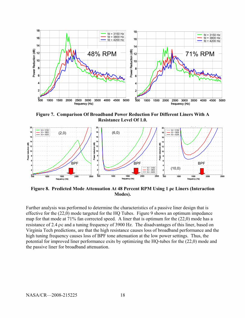
18

48% RPM 71% RPM

500 1000 1500 2000 2500 3000 3500 4000 4500 50000

2

4

6

8

10

12

14

16

18

frequency (Hz)

Pow

er R

educ

tion

(dB

)

fd = 3150 Hzfd = 3800 Hzfd = 4200 Hz

71% RPM

500 1000 1500 2000 2500 3000 3500 4000 4500 50000

2

4

6

8

10

12

14

16

18

frequency (Hz)

Pow

er R

educ

tion

(dB

)fd = 3150 Hzfd = 3800 Hzfd = 4200 Hz

48% RPM48% RPM 71% RPM

500 1000 1500 2000 2500 3000 3500 4000 4500 50000

2

4

6

8

10

12

14

16

18

frequency (Hz)

Pow

er R

educ

tion

(dB

)

fd = 3150 Hzfd = 3800 Hzfd = 4200 Hz

71% RPM

500 1000 1500 2000 2500 3000 3500 4000 4500 50000

2

4

6

8

10

12

14

16

18

frequency (Hz)

Pow

er R

educ

tion

(dB

)fd = 3150 Hzfd = 3800 Hzfd = 4200 Hz

48% RPM

Figure 7. Comparison Of Broadband Power Reduction For Different Liners With A Resistance Level Of 1.0.

500 1000 1500 2000 25000

2

4

6

8

10

12

14

16

18

20

frequency (Hz)

Pow

er re

duct

ion

(dB)

fd = 3150fd = 3800fd = 4200

500 1000 1500 2000 25000

2

4

6

8

10

12

14

16

18

20

frequency (Hz)

Pow

er re

duct

ion

(dB)

fd = 3150fd = 3800fd = 4200

500 1000 1500 2000 25000

2

4

6

8

10

12

14

16

18

20( , ) ρ %

frequency (Hz)

Pow

er re

duct

ion

(dB)

fd = 3150fd = 3800fd = 4200

BPF BPF BPF

(2,0) (6,0)

(10,0)

500 1000 1500 2000 25000

2

4

6

8

10

12

14

16

18

20

frequency (Hz)

Pow

er re

duct

ion

(dB)

fd = 3150fd = 3800fd = 4200

500 1000 1500 2000 25000

2

4

6

8

10

12

14

16

18

20

frequency (Hz)

Pow

er re

duct

ion

(dB)

fd = 3150fd = 3800fd = 4200

500 1000 1500 2000 25000

2

4

6

8

10

12

14

16

18

20( , ) ρ %

frequency (Hz)

Pow

er re

duct

ion

(dB)

fd = 3150fd = 3800fd = 4200

BPF BPF BPF

(2,0) (6,0)

(10,0)

Figure 8. Predicted Mode Attenuation At 48 Percent RPM Using 1 ρc Liners (Interaction Modes).

Further analysis was performed to determine the characteristics of a passive liner design that is effective for the (22,0) mode targeted for the HQ Tubes. Figure 9 shows an optimum impedance map for that mode at 71% fan corrected speed. A liner that is optimum for the (22,0) mode has a resistance of 2.4 ρc and a tuning frequency of 3900 Hz. The disadvantages of this liner, based on Virginia Tech predictions, are that the high resistance causes loss of broadband performance and the high tuning frequency causes loss of BPF tone attenuation at the low power settings. Thus, the potential for improved liner performance exits by optimizing the HQ-tubes for the (22,0) mode and the passive liner for broadband attenuation.

NASA/CR—2008-215225

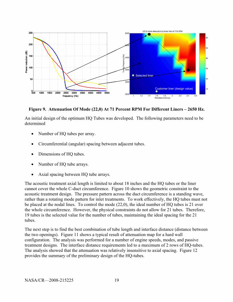
19

500 1000 1500 2000 2500 3000 3500 4000 4500 50000

50

100

150

200

250

frequency (Hz)

Pow

er r

educ

tion

(dB

)

Customer liner (design value)

Selected liner

500 1000 1500 2000 2500 3000 3500 4000 4500 50000

50

100

150

200

250

frequency (Hz)

Pow

er r

educ

tion

(dB

)

Customer liner (design value)

Selected liner

Figure 9. Attenuation Of Mode (22,0) At 71 Percent RPM For Different Liners – 2650 Hz.

An initial design of the optimum HQ Tubes was developed. The following parameters need to be determined

• Number of HQ tubes per array.

• Circumferential (angular) spacing between adjacent tubes.

• Dimensions of HQ tubes.

• Number of HQ tube arrays.

• Axial spacing between HQ tube arrays.

The acoustic treatment axial length is limited to about 18 inches and the HQ tubes or the liner cannot cover the whole C-duct circumference. Figure 10 shows the geometric constraint to the acoustic treatment design. The pressure pattern across the duct circumference is a standing wave, rather than a rotating mode pattern for inlet treatments. To work effectively, the HQ tubes must not be placed at the nodal lines. To control the mode (22,0), the ideal number of HQ tubes is 21 over the whole circumference. However, the physical constraints do not allow for 21 tubes. Therefore, 19 tubes is the selected value for the number of tubes, maintaining the ideal spacing for the 21 tubes.

The next step is to find the best combination of tube length and interface distance (distance between the two openings). Figure 11 shows a typical result of attenuation map for a hard wall configuration. The analysis was performed for a number of engine speeds, modes, and passive treatment designs. The interface distance requirements led to a maximum of 2 rows of HQ-tubes. The analysis showed that the attenuation was relatively insensitive to axial spacing. Figure 12 provides the summary of the preliminary design of the HQ-tubes.

NASA/CR—2008-215225

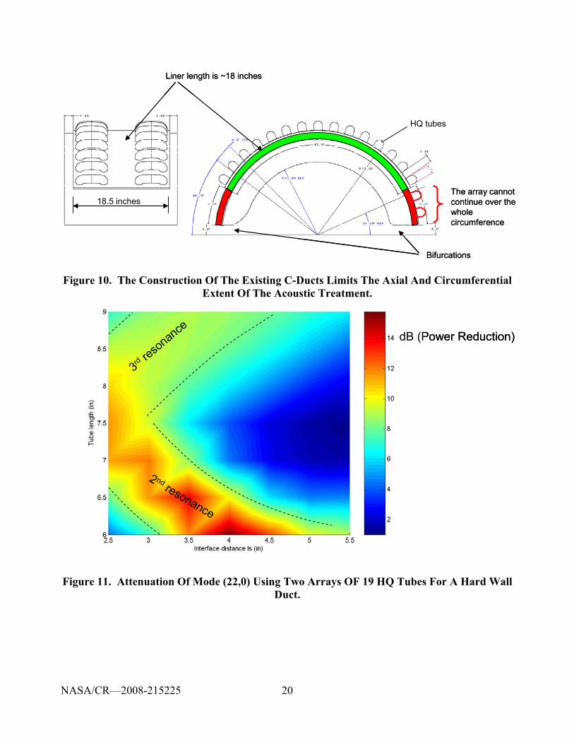
20

HQ tubes

Bifurcations

Liner length is ~18 inches

18.5 inchesThe array cannot continue over the whole circumference

HQ tubes

Bifurcations

Liner length is ~18 inches

18.5 inchesThe array cannot continue over the whole circumference

Figure 10. The Construction Of The Existing C-Ducts Limits The Axial And Circumferential Extent Of The Acoustic Treatment.

3rd reso

nance

2 ndresonance

dB (Power Reduction)

3rd reso

nance

2 ndresonance

dB (Power Reduction)

Figure 11. Attenuation Of Mode (22,0) Using Two Arrays OF 19 HQ Tubes For A Hard Wall Duct.

NASA/CR—2008-215225

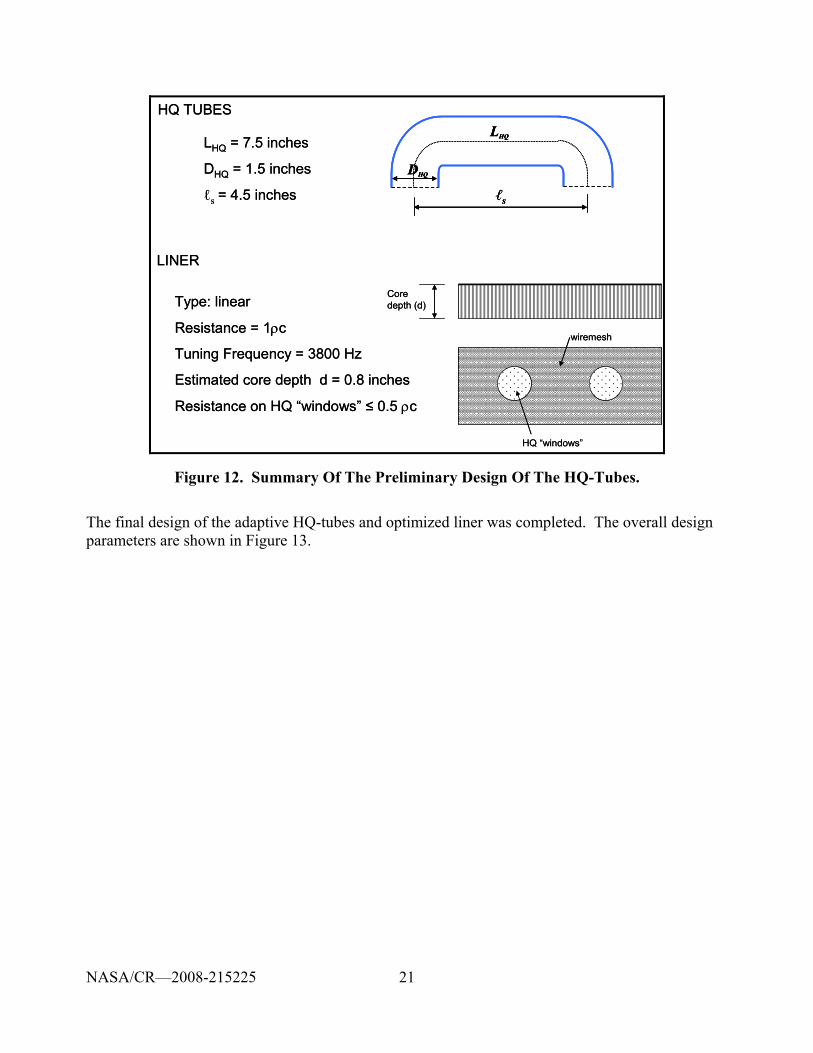
21

LHQ

ℓs

DHQ

LHQ = 7.5 inches

DHQ = 1.5 inches

ℓs = 4.5 inches

LINER

HQ TUBES

Core depth (d)Type: linear

Resistance = 1ρc

Tuning Frequency = 3800 Hz

Estimated core depth d = 0.8 inches

Resistance on HQ “windows” ≤ 0.5 ρc

wiremesh

HQ “windows”

LHQ

ℓs

DHQ

LHQ

ℓs

DHQ

LHQ = 7.5 inches

DHQ = 1.5 inches

ℓs = 4.5 inches

LINER

HQ TUBES

Core depth (d)Type: linear

Resistance = 1ρc

Tuning Frequency = 3800 Hz

Estimated core depth d = 0.8 inches

Resistance on HQ “windows” ≤ 0.5 ρc

wiremesh

HQ “windows”

Figure 12. Summary Of The Preliminary Design Of The HQ-Tubes.

The final design of the adaptive HQ-tubes and optimized liner was completed. The overall design parameters are shown in Figure 13.

NASA/CR—2008-215225

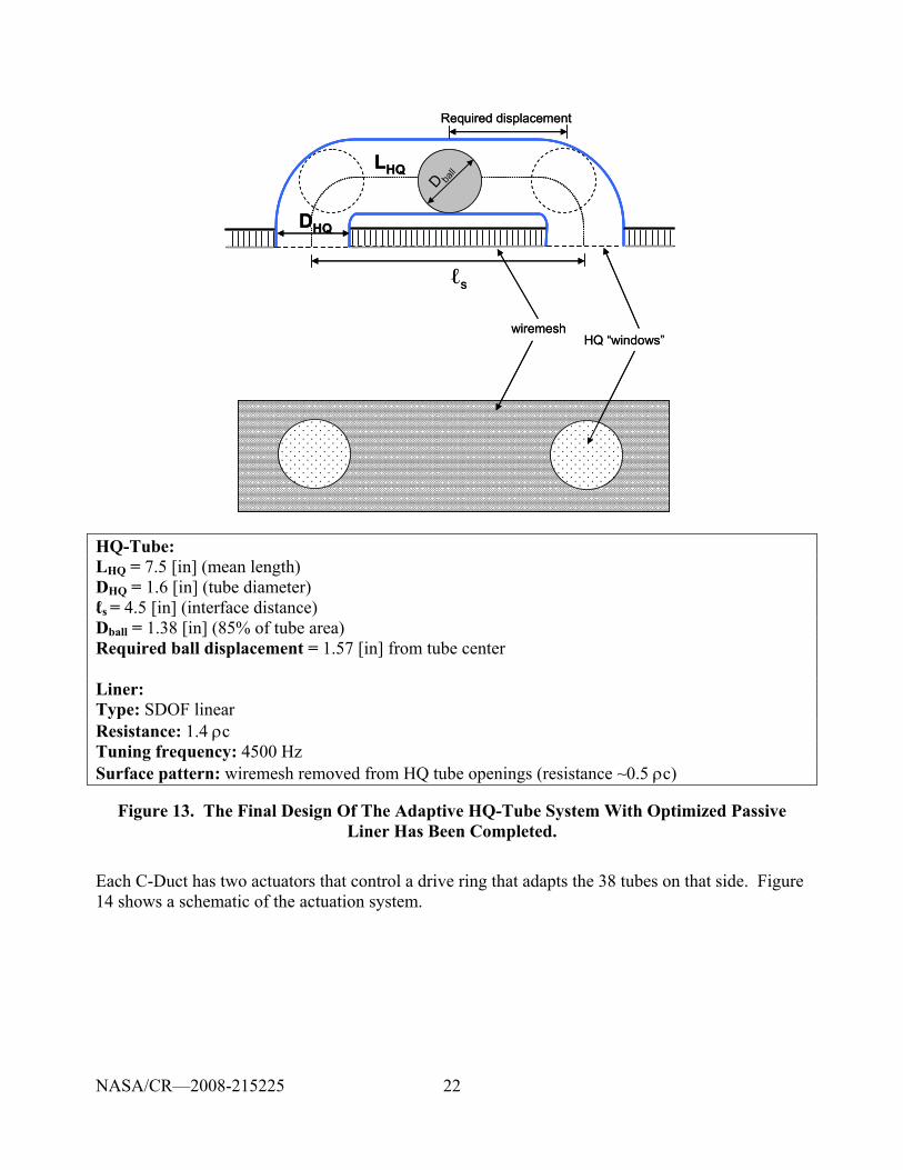
22

wiremeshHQ “windows”

ℓs

D ball

Required displacement

LHQ

DHQ

wiremeshHQ “windows”

ℓs

D ball

Required displacement

LHQ

DHQ

HQ-Tube: LHQ = 7.5 [in] (mean length) DHQ = 1.6 [in] (tube diameter) ℓs = 4.5 [in] (interface distance) Dball = 1.38 [in] (85% of tube area) Required ball displacement = 1.57 [in] from tube center Liner: Type: SDOF linear Resistance: 1.4 ρc Tuning frequency: 4500 Hz Surface pattern: wiremesh removed from HQ tube openings (resistance ~0.5 ρc)

Figure 13. The Final Design Of The Adaptive HQ-Tube System With Optimized Passive Liner Has Been Completed.

Each C-Duct has two actuators that control a drive ring that adapts the 38 tubes on that side. Figure 14 shows a schematic of the actuation system.

NASA/CR—2008-215225

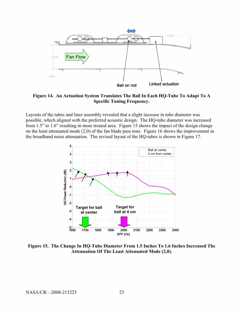
23

Linked actuationBall on rod

Fan Flow

Linked actuationBall on rod

Fan Flow

Figure 14. An Actuation System Translates The Ball In Each HQ-Tube To Adapt To A Specific Tuning Frequency.

Layouts of the tubes and liner assembly revealed that a slight increase in tube diameter was possible, which aligned with the preferred acoustic design. The HQ-tube diameter was increased from 1.5” to 1.6” resulting in more treated area. Figure 15 shows the impact of the design change on the least attenuated mode (2,0) of the fan blade pass tone. Figure 16 shows the improvement in the broadband noise attenuation. The revised layout of the HQ-tubes is shown in Figure 17.

1600 1700 1800 1900 2000 2100 2200 2300 2400-5

-4

-3

-2

-1

0

1

2

3

4

5

BPF [Hz]

HQ

Pow

er R

educ

tion

(dB

)

Ball at center4 cm from center

Target for ball at 4 cm

Target for ball at center

1600 1700 1800 1900 2000 2100 2200 2300 2400-5

-4

-3

-2

-1

0

1

2

3

4

5

BPF [Hz]

HQ

Pow

er R

educ

tion

(dB

)

Ball at center4 cm from center

Target for ball at 4 cm

Target for ball at center

Figure 15. The Change In HQ-Tube Diameter From 1.5 Inches To 1.6 Inches Increased The Attenuation Of The Least Attenuated Mode (2,0).

NASA/CR—2008-215225

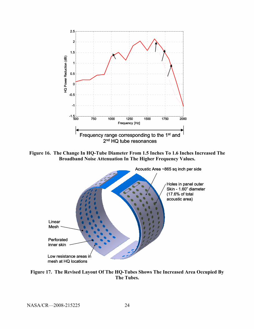
24

500 750 1000 1250 1500 1750 2000-1.5

-1

-0.5

0

0.5

1

1.5

2

2.5

Frequency [Hz]

HQ

Pow

er R

educ

tion

(dB

)

Frequency range corresponding to the 1st and 2nd HQ tube resonances

500 750 1000 1250 1500 1750 2000-1.5

-1

-0.5

0

0.5

1

1.5

2

2.5

Frequency [Hz]

HQ

Pow

er R

educ

tion

(dB

)

Frequency range corresponding to the 1st and 2nd HQ tube resonances

Figure 16. The Change In HQ-Tube Diameter From 1.5 Inches To 1.6 Inches Increased The Broadband Noise Attenuation In The Higher Frequency Values.

Acoustic Area ~865 sq inch per side

Holes in panel outer Skin - 1.60” diameter(17.6% of total acoustic area)

Low resistance areas in mesh at HQ locations

Linear Mesh

Perforated inner skin

Acoustic Area ~865 sq inch per side

Holes in panel outer Skin - 1.60” diameter(17.6% of total acoustic area)

Low resistance areas in mesh at HQ locations

Linear Mesh

Perforated inner skin

Figure 17. The Revised Layout Of The HQ-Tubes Shows The Increased Area Occupied By The Tubes.

NASA/CR—2008-215225

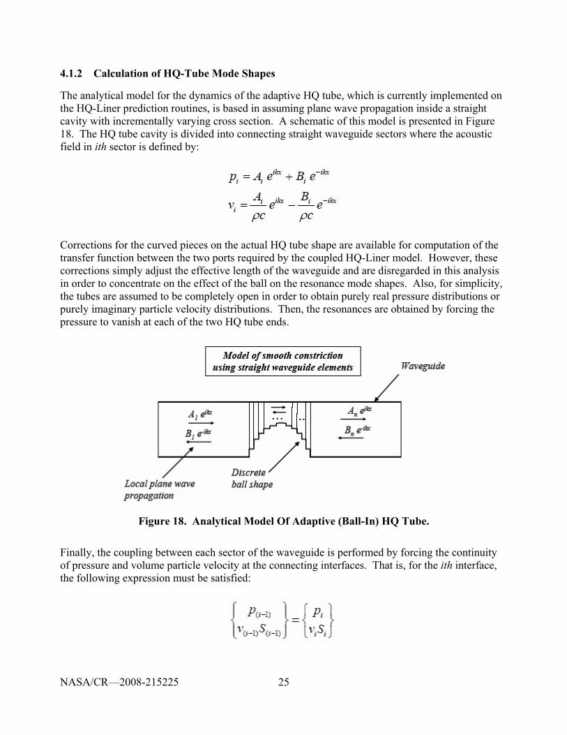
25

4.1.2 Calculation of HQ-Tube Mode Shapes

The analytical model for the dynamics of the adaptive HQ tube, which is currently implemented on the HQ-Liner prediction routines, is based in assuming plane wave propagation inside a straight cavity with incrementally varying cross section. A schematic of this model is presented in Figure 18. The HQ tube cavity is divided into connecting straight waveguide sectors where the acoustic field in ith sector is defined by:

Corrections for the curved pieces on the actual HQ tube shape are available for computation of the transfer function between the two ports required by the coupled HQ-Liner model. However, these corrections simply adjust the effective length of the waveguide and are disregarded in this analysis in order to concentrate on the effect of the ball on the resonance mode shapes. Also, for simplicity, the tubes are assumed to be completely open in order to obtain purely real pressure distributions or purely imaginary particle velocity distributions. Then, the resonances are obtained by forcing the pressure to vanish at each of the two HQ tube ends.

Figure 18. Analytical Model Of Adaptive (Ball-In) HQ Tube.

Finally, the coupling between each sector of the waveguide is performed by forcing the continuity of pressure and volume particle velocity at the connecting interfaces. That is, for the ith interface, the following expression must be satisfied:

NASA/CR—2008-215225

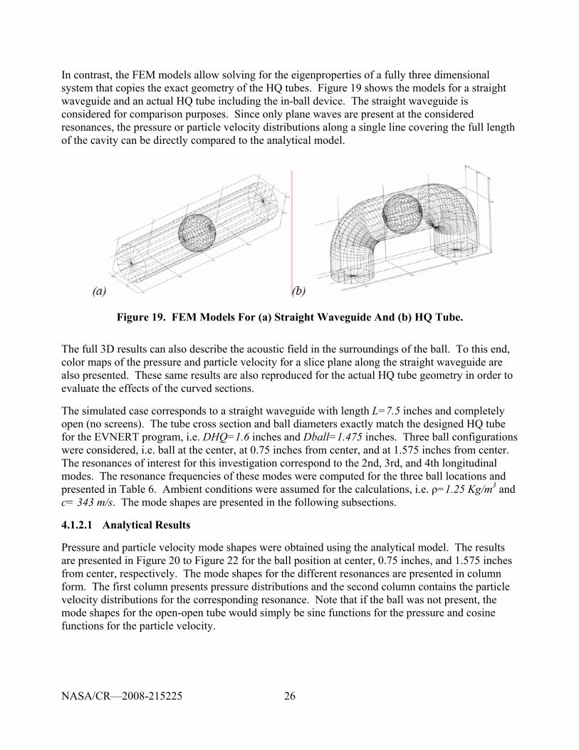
26

In contrast, the FEM models allow solving for the eigenproperties of a fully three dimensional system that copies the exact geometry of the HQ tubes. Figure 19 shows the models for a straight waveguide and an actual HQ tube including the in-ball device. The straight waveguide is considered for comparison purposes. Since only plane waves are present at the considered resonances, the pressure or particle velocity distributions along a single line covering the full length of the cavity can be directly compared to the analytical model.

Figure 19. FEM Models For (a) Straight Waveguide And (b) HQ Tube.

The full 3D results can also describe the acoustic field in the surroundings of the ball. To this end, color maps of the pressure and particle velocity for a slice plane along the straight waveguide are also presented. These same results are also reproduced for the actual HQ tube geometry in order to evaluate the effects of the curved sections.

The simulated case corresponds to a straight waveguide with length L=7.5 inches and completely open (no screens). The tube cross section and ball diameters exactly match the designed HQ tube for the EVNERT program, i.e. DHQ=1.6 inches and Dball=1.475 inches. Three ball configurations were considered, i.e. ball at the center, at 0.75 inches from center, and at 1.575 inches from center. The resonances of interest for this investigation correspond to the 2nd, 3rd, and 4th longitudinal modes. The resonance frequencies of these modes were computed for the three ball locations and presented in Table 6. Ambient conditions were assumed for the calculations, i.e. ρ=1.25 Kg/m3 and c= 343 m/s. The mode shapes are presented in the following subsections.

4.1.2.1 Analytical Results

Pressure and particle velocity mode shapes were obtained using the analytical model. The results are presented in Figure 20 to Figure 22 for the ball position at center, 0.75 inches, and 1.575 inches from center, respectively. The mode shapes for the different resonances are presented in column form. The first column presents pressure distributions and the second column contains the particle velocity distributions for the corresponding resonance. Note that if the ball was not present, the mode shapes for the open-open tube would simply be sine functions for the pressure and cosine functions for the particle velocity.

NASA/CR—2008-215225

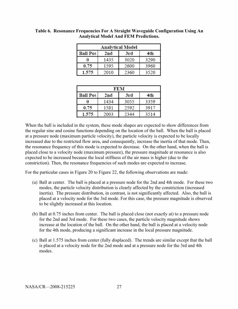
27

Table 6. Resonance Frequencies For A Straight Waveguide Configuration Using An Analytical Model And FEM Predictions.

When the ball is included in the system, these mode shapes are expected to show differences from the regular sine and cosine functions depending on the location of the ball. When the ball is placed at a pressure node (maximum particle velocity), the particle velocity is expected to be locally increased due to the restricted flow area, and consequently, increase the inertia of that mode. Then, the resonance frequency of this mode is expected to decrease. On the other hand, when the ball is placed close to a velocity node (maximum pressure), the pressure magnitude at resonance is also expected to be increased because the local stiffness of the air mass is higher (due to the constriction). Then, the resonance frequencies of such modes are expected to increase.

For the particular cases in Figure 20 to Figure 22, the following observations are made:

(a) Ball at center. The ball is placed at a pressure node for the 2nd and 4th mode. For these two modes, the particle velocity distribution is clearly affected by the constriction (increased inertia). The pressure distribution, in contrast, is not significantly affected. Also, the ball is placed at a velocity node for the 3rd mode. For this case, the pressure magnitude is observed to be slightly increased at this location.

(b) Ball at 0.75 inches from center. The ball is placed close (not exactly at) to a pressure node for the 2nd and 3rd mode. For these two cases, the particle velocity magnitude shows increase at the location of the ball. On the other hand, the ball is placed at a velocity node for the 4th mode, producing a significant increase in the local pressure magnitude.

(c) Ball at 1.575 inches from center (fully displaced). The trends are similar except that the ball is placed at a velocity node for the 2nd mode and at a pressure node for the 3rd and 4th modes.

NASA/CR—2008-215225

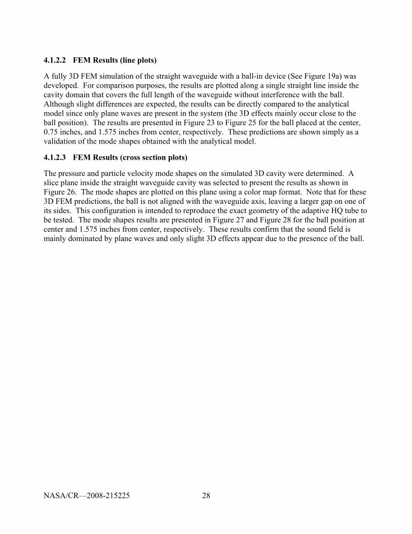
28

4.1.2.2 FEM Results (line plots)

A fully 3D FEM simulation of the straight waveguide with a ball-in device (See Figure 19a) was developed. For comparison purposes, the results are plotted along a single straight line inside the cavity domain that covers the full length of the waveguide without interference with the ball. Although slight differences are expected, the results can be directly compared to the analytical model since only plane waves are present in the system (the 3D effects mainly occur close to the ball position). The results are presented in Figure 23 to Figure 25 for the ball placed at the center, 0.75 inches, and 1.575 inches from center, respectively. These predictions are shown simply as a validation of the mode shapes obtained with the analytical model.

4.1.2.3 FEM Results (cross section plots)

The pressure and particle velocity mode shapes on the simulated 3D cavity were determined. A slice plane inside the straight waveguide cavity was selected to present the results as shown in Figure 26. The mode shapes are plotted on this plane using a color map format. Note that for these 3D FEM predictions, the ball is not aligned with the waveguide axis, leaving a larger gap on one of its sides. This configuration is intended to reproduce the exact geometry of the adaptive HQ tube to be tested. The mode shapes results are presented in Figure 27 and Figure 28 for the ball position at center and 1.575 inches from center, respectively. These results confirm that the sound field is mainly dominated by plane waves and only slight 3D effects appear due to the presence of the ball.

NASA/CR—2008-215225

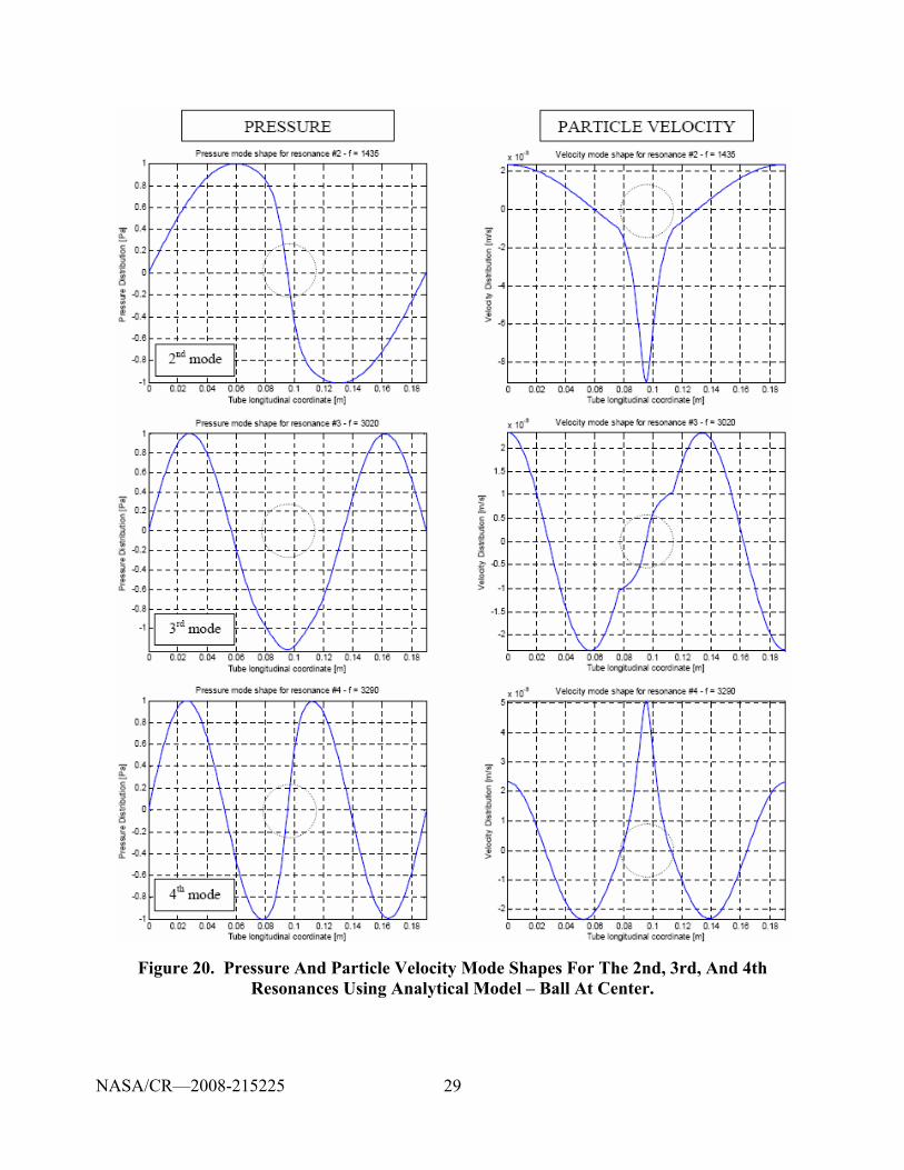
29

Figure 20. Pressure And Particle Velocity Mode Shapes For The 2nd, 3rd, And 4th Resonances Using Analytical Model – Ball At Center.

NASA/CR—2008-215225

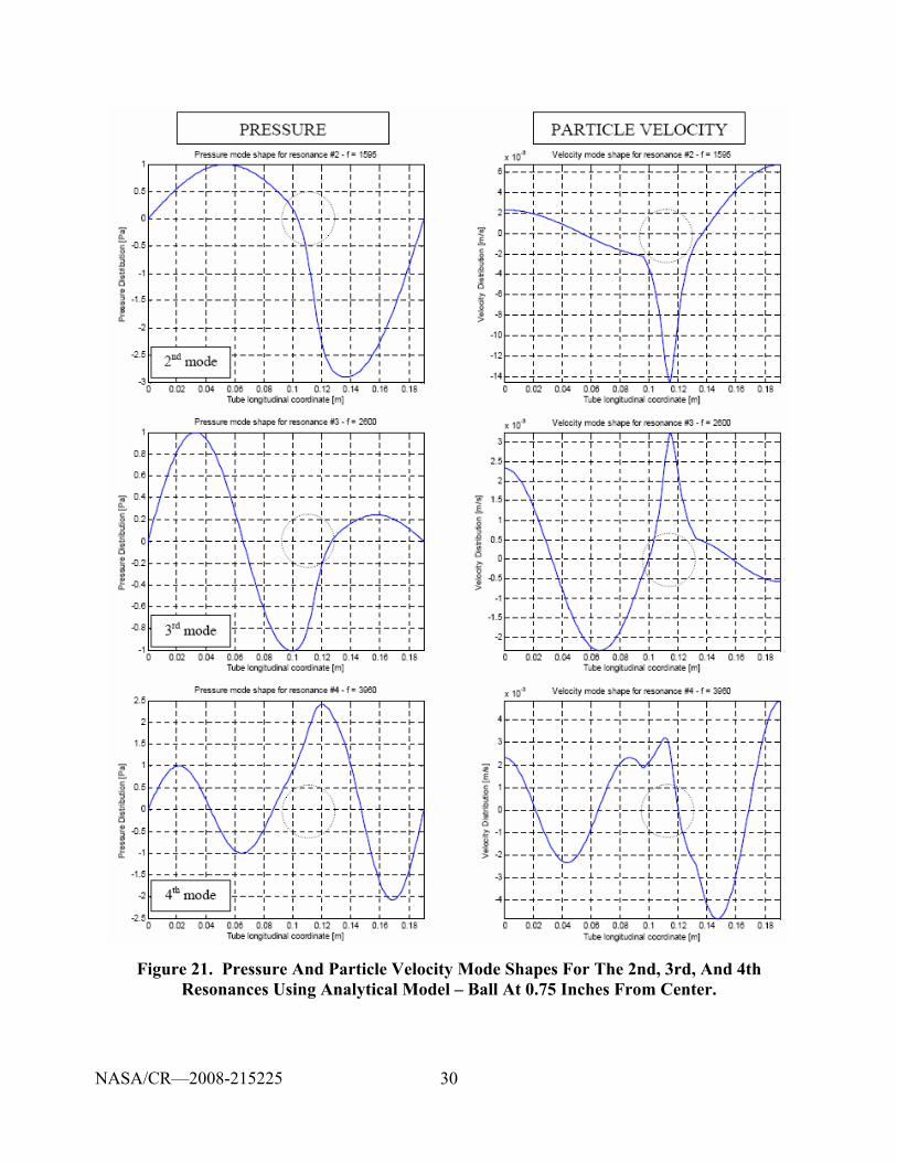
30

Figure 21. Pressure And Particle Velocity Mode Shapes For The 2nd, 3rd, And 4th Resonances Using Analytical Model – Ball At 0.75 Inches From Center.

NASA/CR—2008-215225

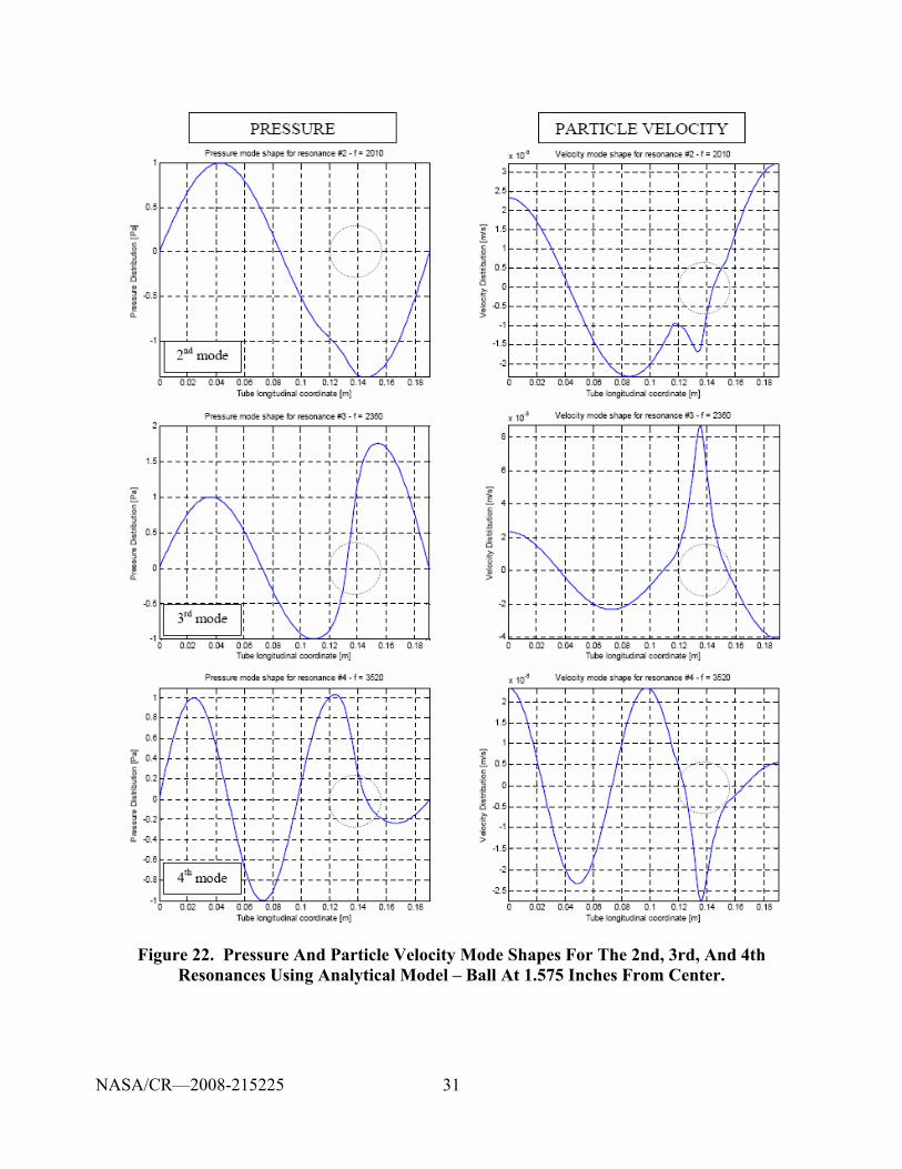
31

Figure 22. Pressure And Particle Velocity Mode Shapes For The 2nd, 3rd, And 4th Resonances Using Analytical Model – Ball At 1.575 Inches From Center.

NASA/CR—2008-215225

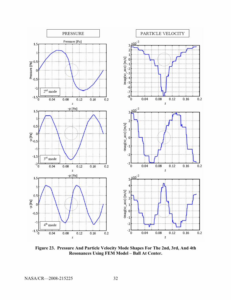
32

Figure 23. Pressure And Particle Velocity Mode Shapes For The 2nd, 3rd, And 4th Resonances Using FEM Model – Ball At Center.

NASA/CR—2008-215225

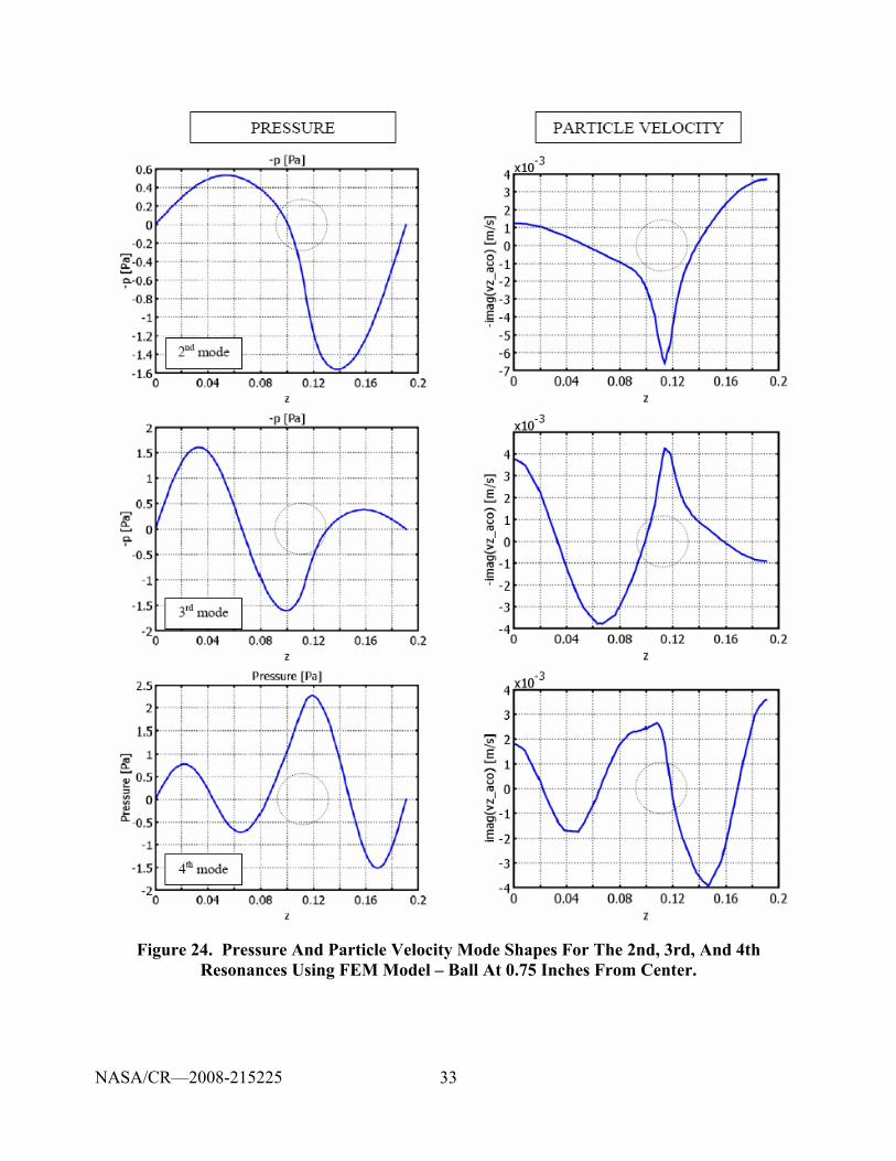
33

Figure 24. Pressure And Particle Velocity Mode Shapes For The 2nd, 3rd, And 4th Resonances Using FEM Model – Ball At 0.75 Inches From Center.

NASA/CR—2008-215225

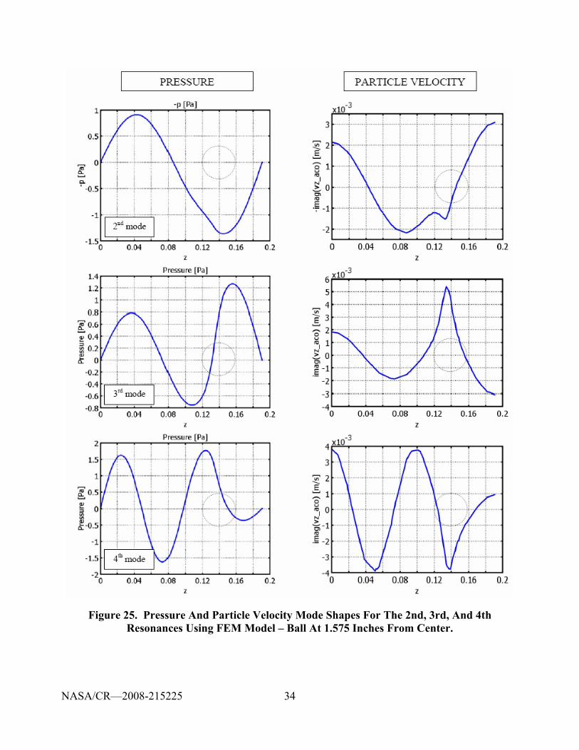
34

Figure 25. Pressure And Particle Velocity Mode Shapes For The 2nd, 3rd, And 4th Resonances Using FEM Model – Ball At 1.575 Inches From Center.

NASA/CR—2008-215225

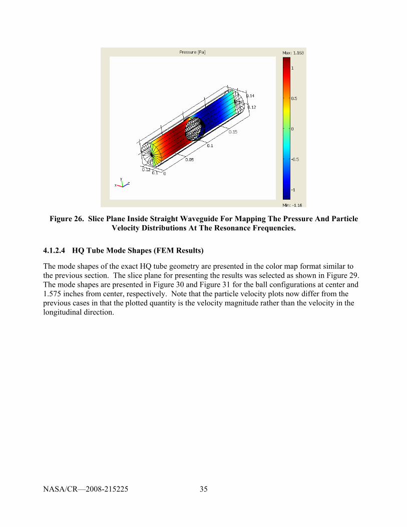
35

Figure 26. Slice Plane Inside Straight Waveguide For Mapping The Pressure And Particle Velocity Distributions At The Resonance Frequencies.

4.1.2.4 HQ Tube Mode Shapes (FEM Results)

The mode shapes of the exact HQ tube geometry are presented in the color map format similar to the previous section. The slice plane for presenting the results was selected as shown in Figure 29. The mode shapes are presented in Figure 30 and Figure 31 for the ball configurations at center and 1.575 inches from center, respectively. Note that the particle velocity plots now differ from the previous cases in that the plotted quantity is the velocity magnitude rather than the velocity in the longitudinal direction.

NASA/CR—2008-215225

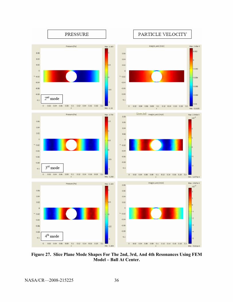
36

Figure 27. Slice Plane Mode Shapes For The 2nd, 3rd, And 4th Resonances Using FEM Model – Ball At Center.

NASA/CR—2008-215225

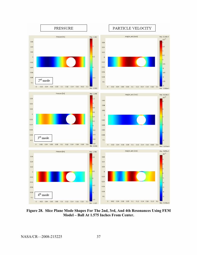
37

Figure 28. Slice Plane Mode Shapes For The 2nd, 3rd, And 4th Resonances Using FEM Model – Ball At 1.575 Inches From Center.

NASA/CR—2008-215225

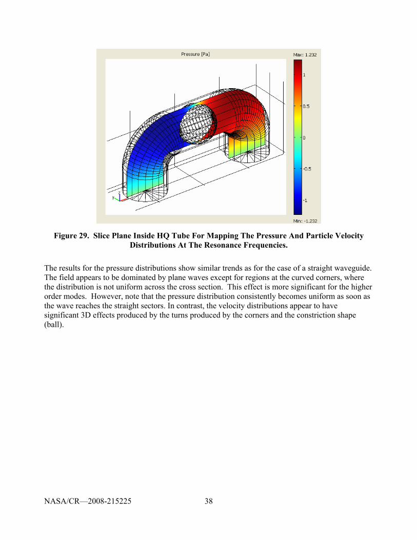
38

Figure 29. Slice Plane Inside HQ Tube For Mapping The Pressure And Particle Velocity Distributions At The Resonance Frequencies.

The results for the pressure distributions show similar trends as for the case of a straight waveguide. The field appears to be dominated by plane waves except for regions at the curved corners, where the distribution is not uniform across the cross section. This effect is more significant for the higher order modes. However, note that the pressure distribution consistently becomes uniform as soon as the wave reaches the straight sectors. In contrast, the velocity distributions appear to have significant 3D effects produced by the turns produced by the corners and the constriction shape (ball).

NASA/CR—2008-215225

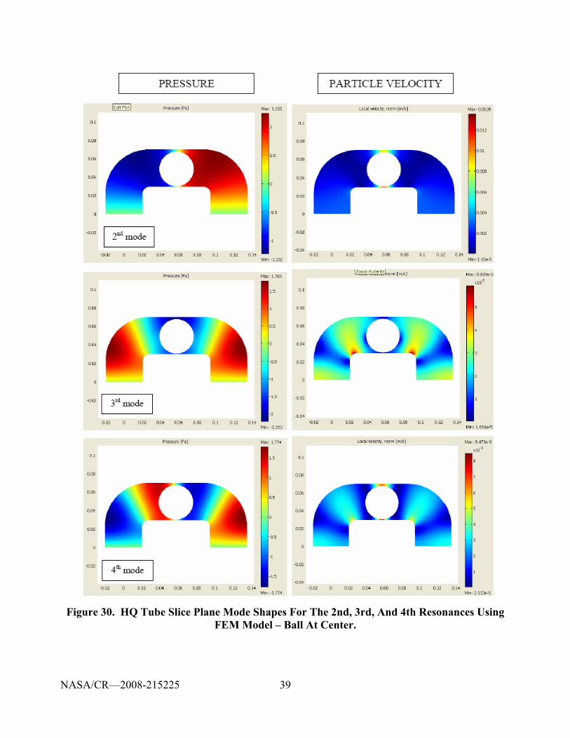
39

Figure 30. HQ Tube Slice Plane Mode Shapes For The 2nd, 3rd, And 4th Resonances Using FEM Model – Ball At Center.

NASA/CR—2008-215225

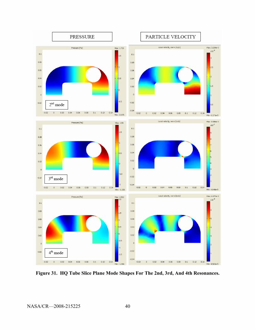
40

Figure 31. HQ Tube Slice Plane Mode Shapes For The 2nd, 3rd, And 4th Resonances.

NASA/CR—2008-215225

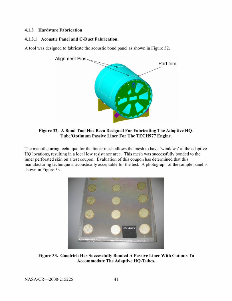
41

4.1.3 Hardware Fabrication

4.1.3.1 Acoustic Panel and C-Duct Fabrication.

A tool was designed to fabricate the acoustic bond panel as shown in Figure 32.

Figure 32. A Bond Tool Has Been Designed For Fabricating The Adaptive HQ-Tube/Optimum Passive Liner For The TECH977 Engine.

The manufacturing technique for the linear mesh allows the mesh to have ‘windows’ at the adaptive HQ locations, resulting in a local low resistance area. This mesh was successfully bonded to the inner perforated skin on a test coupon. Evaluation of this coupon has determined that this manufacturing technique is acoustically acceptable for the test. A photograph of the sample panel is shown in Figure 33.

Figure 33. Goodrich Has Successfully Bonded A Passive Liner With Cutouts To Accommodate The Adaptive HQ-Tubes.

NASA/CR—2008-215225

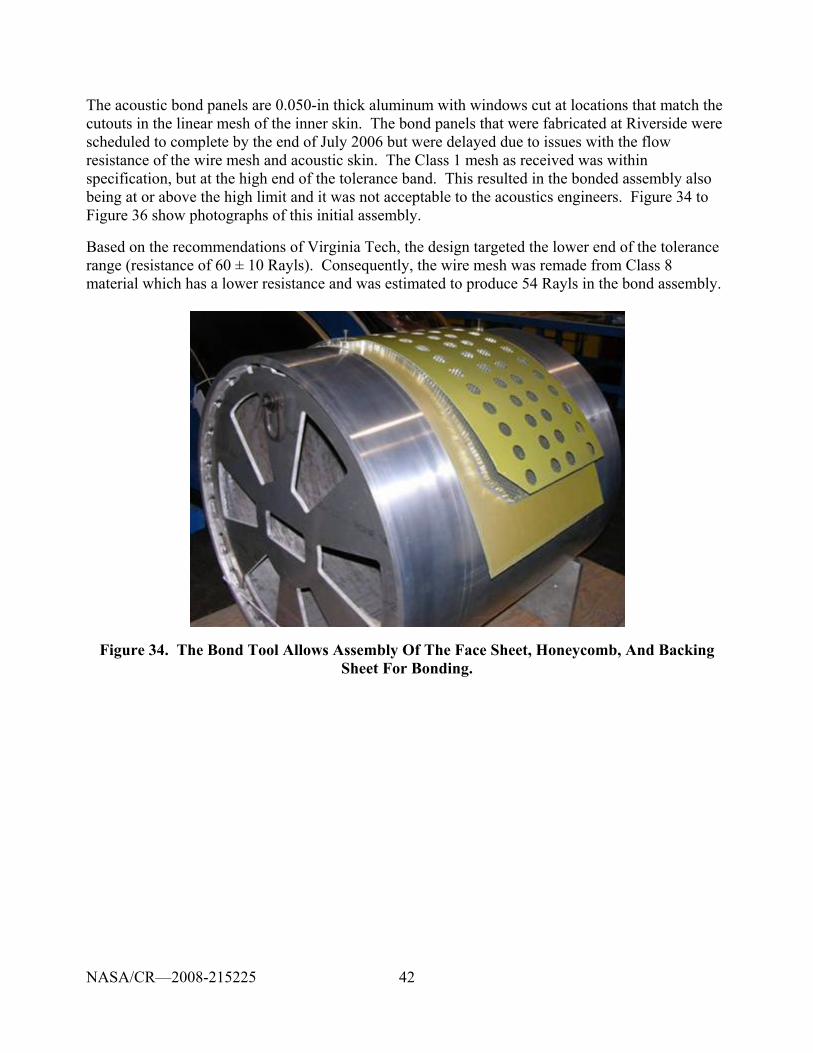
42

The acoustic bond panels are 0.050-in thick aluminum with windows cut at locations that match the cutouts in the linear mesh of the inner skin. The bond panels that were fabricated at Riverside were scheduled to complete by the end of July 2006 but were delayed due to issues with the flow resistance of the wire mesh and acoustic skin. The Class 1 mesh as received was within specification, but at the high end of the tolerance band. This resulted in the bonded assembly also being at or above the high limit and it was not acceptable to the acoustics engineers. Figure 34 to Figure 36 show photographs of this initial assembly.

Based on the recommendations of Virginia Tech, the design targeted the lower end of the tolerance range (resistance of 60 ± 10 Rayls). Consequently, the wire mesh was remade from Class 8 material which has a lower resistance and was estimated to produce 54 Rayls in the bond assembly.

Figure 34. The Bond Tool Allows Assembly Of The Face Sheet, Honeycomb, And Backing Sheet For Bonding.

NASA/CR—2008-215225

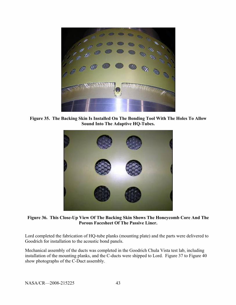
43

Figure 35. The Backing Skin Is Installed On The Bonding Tool With The Holes To Allow Sound Into The Adaptive HQ-Tubes.

Figure 36. This Close-Up View Of The Backing Skin Shows The Honeycomb Core And The Porous Facesheet Of The Passive Liner.

Lord completed the fabrication of HQ-tube planks (mounting plate) and the parts were delivered to Goodrich for installation to the acoustic bond panels.

Mechanical assembly of the ducts was completed in the Goodrich Chula Vista test lab, including installation of the mounting planks, and the C-ducts were shipped to Lord. Figure 37 to Figure 40 show photographs of the C-Duct assembly.

NASA/CR—2008-215225

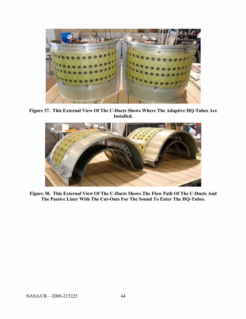
44

Figure 37. This External View Of The C-Ducts Shows Where The Adaptive HQ-Tubes Are Installed.

Figure 38. This External View Of The C-Ducts Shows The Flow Path Of The C-Ducts And The Passive Liner With The Cut-Outs For The Sound To Enter The HQ-Tubes.

NASA/CR—2008-215225

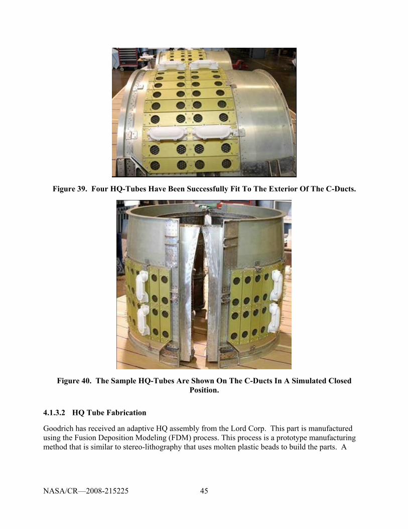
45

Figure 39. Four HQ-Tubes Have Been Successfully Fit To The Exterior Of The C-Ducts.

Figure 40. The Sample HQ-Tubes Are Shown On The C-Ducts In A Simulated Closed Position.

4.1.3.2 HQ Tube Fabrication

Goodrich has received an adaptive HQ assembly from the Lord Corp. This part is manufactured using the Fusion Deposition Modeling (FDM) process. This process is a prototype manufacturing method that is similar to stereo-lithography that uses molten plastic beads to build the parts. A

NASA/CR—2008-215225

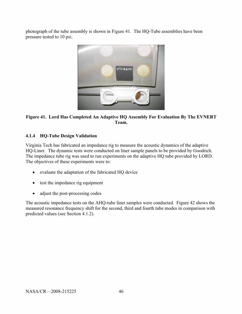
46

photograph of the tube assembly is shown in Figure 41. The HQ-Tube assemblies have been pressure tested to 10 psi.

Figure 41. Lord Has Completed An Adaptive HQ Assembly For Evaluation By The EVNERT Team.

4.1.4 HQ-Tube Design Validation

Virginia Tech has fabricated an impedance rig to measure the acoustic dynamics of the adaptive HQ-Liner. The dynamic tests were conducted on liner sample panels to be provided by Goodrich. The impedance tube rig was used to run experiments on the adaptive HQ tube provided by LORD. The objectives of these experiments were to:

• evaluate the adaptation of the fabricated HQ device

• test the impedance rig equipment

• adjust the post-processing codes

The acoustic impedance tests on the AHQ-tube liner samples were conducted. Figure 42 shows the measured resonance frequency shift for the second, third and fourth tube modes in comparison with predicted values (see Section 4.1.2).

NASA/CR—2008-215225

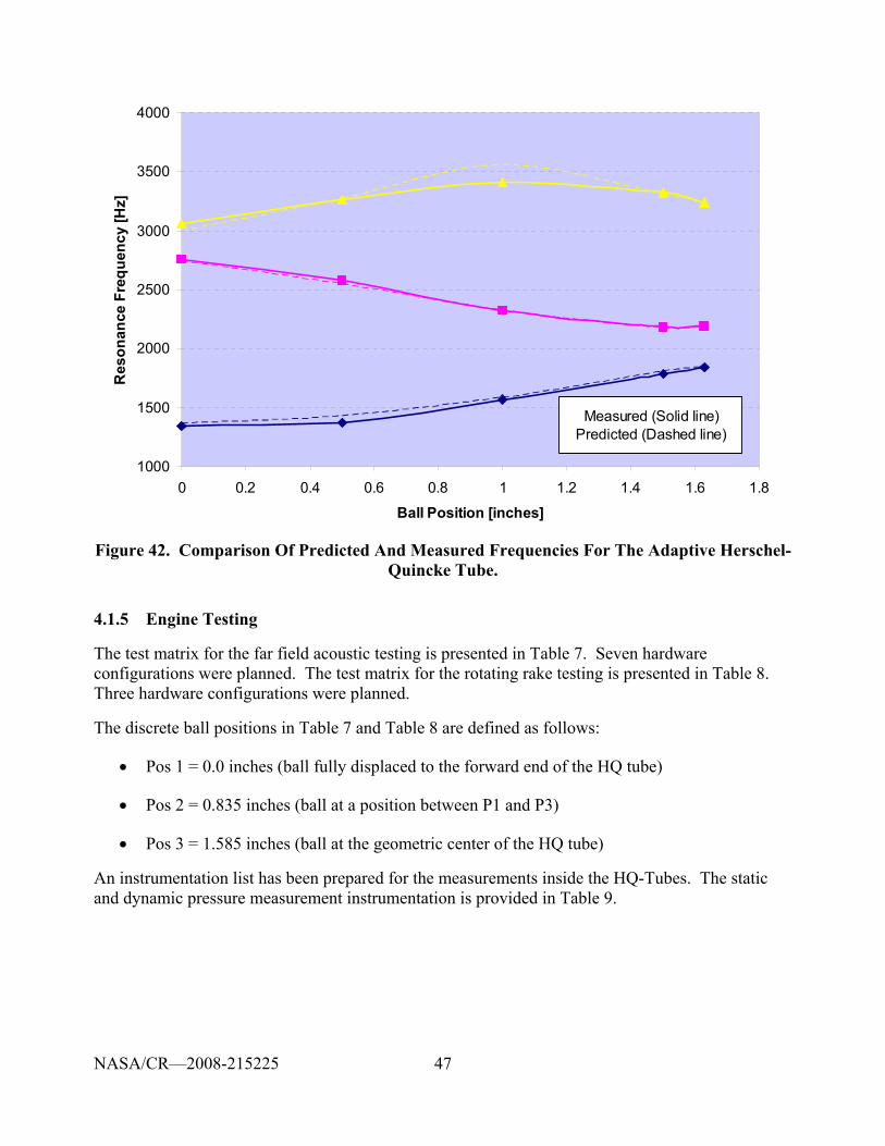
47

1000

1500

2000

2500

3000

3500

4000

0 0.2 0.4 0.6 0.8 1 1.2 1.4 1.6 1.8

Ball Position [inches]

Res

onan

ce F

requ

ency

[Hz]

Measured (Solid line)Predicted (Dashed line)

Figure 42. Comparison Of Predicted And Measured Frequencies For The Adaptive Herschel-Quincke Tube.

4.1.5 Engine Testing

The test matrix for the far field acoustic testing is presented in Table 7. Seven hardware configurations were planned. The test matrix for the rotating rake testing is presented in Table 8. Three hardware configurations were planned.

The discrete ball positions in Table 7 and Table 8 are defined as follows:

• Pos 1 = 0.0 inches (ball fully displaced to the forward end of the HQ tube)

• Pos 2 = 0.835 inches (ball at a position between P1 and P3)

• Pos 3 = 1.585 inches (ball at the geometric center of the HQ tube)

An instrumentation list has been prepared for the measurements inside the HQ-Tubes. The static and dynamic pressure measurement instrumentation is provided in Table 9.

NASA/CR—2008-215225

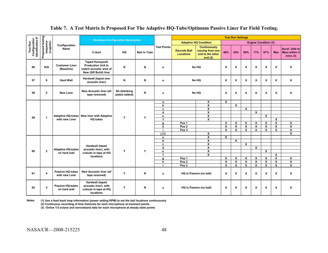
48

Table 7. A Test Matrix Is Proposed For The Adaptive HQ-Tube/Optimum Passive Liner Far Field Testing.

C-duct HQ Ball in Tube Discrete Ball Locations

Continuously moving from one end to the other

end (2)

48% 54% 60% 71% 87% MaxAccel. (Idle to Max) within 2

mins (2)

a X Xb X Xc X Xd X Xe X Xf X Xg Pos 1 X X X X X X Xh Pos 2 X X X X X X Xi Pos 3 X X X X X X X

j (1) X Xa X Xb X Xc X Xd X Xe X Xf X Xg Pos 1 X X X X X X Xh Pos 2 X X X X X X Xi Pos 3 X X X X X X X

Notes

(3) Online 1/3 octave and narrowband data for each microphone at steady state points(2) Continuous recording of time histories for each microphone at transient points

No HQ

61 4 Passive HQ tubes with new Liner

New Acoustic liner (all tape removed) Y

(1) Use a feed back loop information (power setting RPM) to set the ball locations continuously

2 Y YAdaptive HQ-tubes on hard wall

Hardwall (taped acoustic liner), with

cutouts in tape at HQ locations

80 N/A Customer Liner (Baseline)

Taped Honeywell Production Unit to

match acoustic area of New (GR Build) liner

N N

Configuration Name

Hardware Configuration Description

Test Points

Test Run Settings

Adaptive HQ Condition Engine Condition (3)

New liner with Adaptive HQ tubes

New Liner New Acoustic liner (all tape removed)

No (blanking plates added)

Y

N No HQHard Wall Hardwall (taped new acoustic liner) N

N HQ is Passive (no ball)

a

a

a

N

Y

HQ is Passive (no ball)

N No HQ

57

58

62

59

60

Hardwall (taped acoustic liner), with

cutouts in tape at HQ locations

Y

Prop

osed

test

ing

sequ

ence

(L

ogis

tic)

Passive HQ-tubes on hard wall

1 Adaptive HQ-tubes with new Liner

6

5

3

Test

Run

C

onfig

urat

ion

Iden

tific

atio

n #

a X X X X X X X

a X X X X X X X

X X X X X X X

X X X X X X X

X X X X X X X

NASA/CR—2008-215225

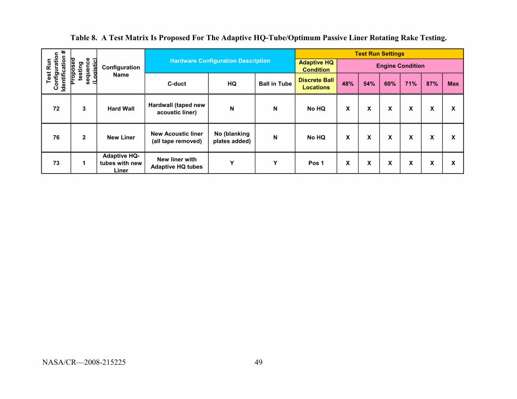
49

Table 8. A Test Matrix Is Proposed For The Adaptive HQ-Tube/Optimum Passive Liner Rotating Rake Testing.

Adaptive HQ Condition

C-duct HQ Ball in Tube Discrete Ball Locations 48% 54% 60% 71% 87% Max

73 1Adaptive HQ-

tubes with new Liner

New liner with Adaptive HQ tubes Y Y Pos 1 X X X X X X

X

X X X X2

Test

Run

C

onfig

urat

ion

Iden

tific

atio

n #

Prop

osed

te

stin

g se

quen

ce

(Log

istic

)

72

76 No HQ

N No HQ XX X X X

X XNew Liner New Acoustic liner (all tape removed)

No (blanking plates added) N

Configuration Name

Hardware Configuration Description

Hard Wall Hardwall (taped new acoustic liner) N3

Engine Condition

Test Run Settings

NASA/CR—2008-215225

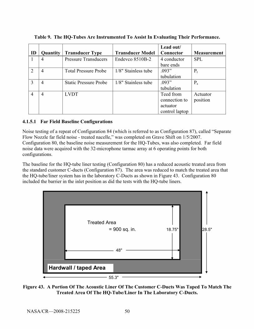
50

Table 9. The HQ-Tubes Are Instrumented To Assist In Evaluating Their Performance.

ID Quantity Transducer Type Transducer Model Lead out/ Connector Measurement

1 4 Pressure Transducers Endevco 8510B-2 4 conductor bare ends

SPL

2 4 Total Pressure Probe 1/8" Stainless tube .093” tubulation

Pt

3 4 Static Pressure Probe 1/8" Stainless tube .093” tubulation

Ps

4 4 LVDT Teed from connection to actuator control laptop

Actuator position

4.1.5.1 Far Field Baseline Configurations

Noise testing of a repeat of Configuration 84 (which is referred to as Configuration 87), called “Separate Flow Nozzle far field noise - treated nacelle,” was completed on Grave Shift on 1/5/2007. Configuration 80, the baseline noise measurement for the HQ-Tubes, was also completed. Far field noise data were acquired with the 32-microphone tarmac array at 6 operating points for both configurations.

The baseline for the HQ-tube liner testing (Configuration 80) has a reduced acoustic treated area from the standard customer C-ducts (Configuration 87). The area was reduced to match the treated area that the HQ-tube/liner system has in the laboratory C-Ducts as shown in Figure 43. Configuration 80 included the barrier in the inlet position as did the tests with the HQ-tube liners.

Treated Area = 900 sq. in. 18.75" 28.5"

48"

55.3"

Hardwall / taped Area

Figure 43. A Portion Of The Acoustic Liner Of The Customer C-Ducts Was Taped To Match The Treated Area Of The HQ-Tube/Liner In The Laboratory C-Ducts.

NASA/CR—2008-215225

51

4.1.5.2 Far Field HQ-Tube Configurations

All HQ tube far field noise testing was conducted on the TECH977 engine. The tested configurations included:

Configuration 57 Taped liner, No HQ tubes

Configuration 58 Treated liner, No HQ tubes

Configuration 59 Treated liner, Adaptive HQ tubes with balls

Configuration 60 Taped liner, Adaptive HQ tubes with balls

Configuration 61 Treated liner, Passive HQ tubes without balls

The HQ tubes and their actuators were installed on the engine by representatives from Goodrich, Virginia Tech, and Lord Corporation (Figure 44). Four actuators were used to position the balls within the HQ tubes. The actuators were controlled from a laptop computer located in the test cell control room. The tubes opened to the outer skin of the bypass duct (Figure 45).

High-response pressure transducers (Kulites) were located in 4 of the HQ tubes (Figure 46). These transducers were processed on the B&K Pulse system with the 32 microphone far-field array data. In addition, RVDT signals corresponding to the ball actuator positions were recorded on the Pulse system.

The baseline, untreated configuration (Configuration 57) was run using the hard wall laboratory C-ducts. However, the treatment was covered with aluminum-backed tape for Configuration 60 to use only the HQ tubes (Figure 47). Holes were cut from the tape to expose the HQ tube holes. This allowed evaluation of the HQ tubes without the contribution of the liner.

For Configuration 58 with the treatment exposed but the HQ tubes covered, block off plates were installed in place of the HQ tube bases (Figure 48). This configuration evaluated the liner without the contribution of the HQ tubes.

The balls were positioned axially within the tubes by the actuators (Figure 49). Three fixed-ball positions were evaluated as well as a condition where the balls were being continuously traversed throughout the measurement period. The tubes were also tested with the balls entirely removed.

Two of the HQ tubes were fitted with pressure probes that were acquired along with the basic engine performance information (Figure 50). Each of the tubes was fitted with 2 total pressure and 2 static pressure probes (Figure 51). This data was acquired at a low sample rate of approximately 10 Hz.

Time history recordings of the far-field microphones and Kulites were acquired at 48, 54, 60, 65, 71, 87, and 91 percent corrected fan speed. In addition, a slow acceleration from idle to maximum speed was conducted. Ambient measurements were also recorded prior to engine start. All time series test data files were transmitted to Virginia Tech and Goodrich. Test data analyses are currently under way.

NASA/CR—2008-215225

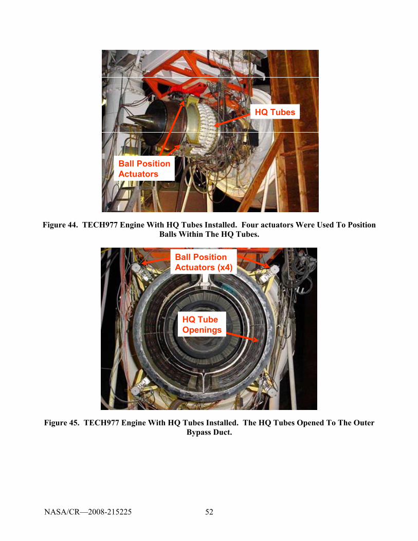
52

HQ Tubes

Ball PositionActuators

HQ Tubes

Ball PositionActuators

Figure 44. TECH977 Engine With HQ Tubes Installed. Four actuators Were Used To Position Balls Within The HQ Tubes.

Ball PositionActuators (x4)

HQ TubeOpenings

Ball PositionActuators (x4)

HQ TubeOpenings

Figure 45. TECH977 Engine With HQ Tubes Installed. The HQ Tubes Opened To The Outer Bypass Duct.

NASA/CR—2008-215225

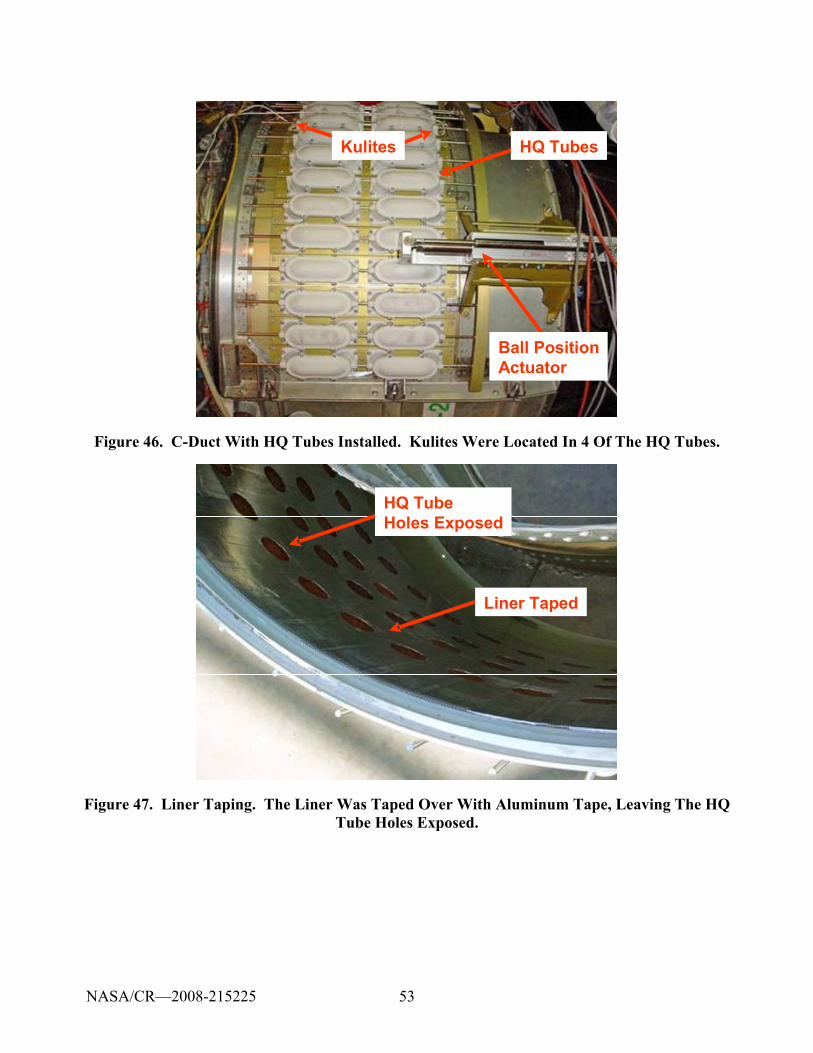
53

HQ Tubes

Ball PositionActuator

Kulites HQ Tubes

Ball PositionActuator

Kulites

Figure 46. C-Duct With HQ Tubes Installed. Kulites Were Located In 4 Of The HQ Tubes.

Liner Taped

HQ TubeHoles Exposed

Liner Taped

HQ TubeHoles Exposed

Figure 47. Liner Taping. The Liner Was Taped Over With Aluminum Tape, Leaving The HQ Tube Holes Exposed.

NASA/CR—2008-215225

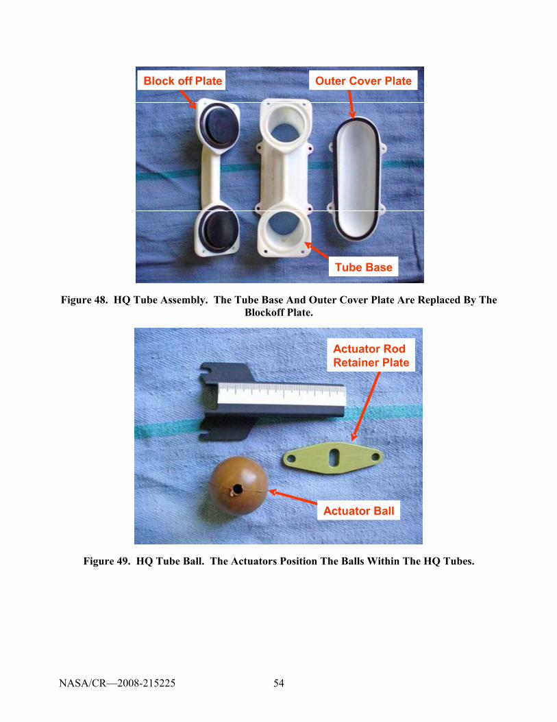
54

Outer Cover Plate

Tube Base

Block off Plate Outer Cover Plate

Tube Base

Block off Plate

Figure 48. HQ Tube Assembly. The Tube Base And Outer Cover Plate Are Replaced By The Blockoff Plate.

Actuator Ball

Actuator RodRetainer Plate

Actuator Ball

Actuator RodRetainer Plate

Figure 49. HQ Tube Ball. The Actuators Position The Balls Within The HQ Tubes.

NASA/CR—2008-215225

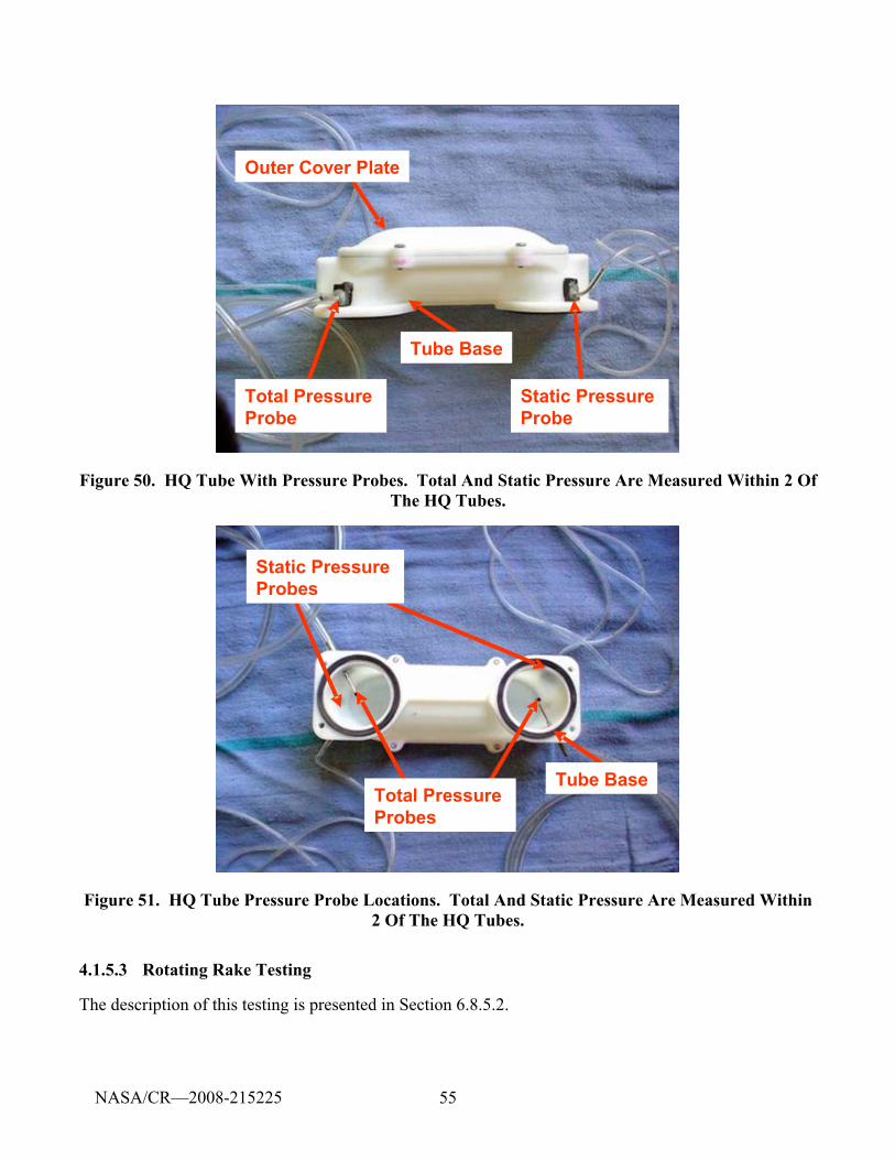
55

Outer Cover Plate

Tube Base

Static Pressure Probe

Total Pressure Probe

Outer Cover Plate

Tube Base

Static Pressure Probe

Total Pressure Probe

Figure 50. HQ Tube With Pressure Probes. Total And Static Pressure Are Measured Within 2 Of The HQ Tubes.

Tube BaseTotal Pressure Probes

Static Pressure Probes

Tube BaseTotal Pressure Probes

Static Pressure Probes

Figure 51. HQ Tube Pressure Probe Locations. Total And Static Pressure Are Measured Within 2 Of The HQ Tubes.

4.1.5.3 Rotating Rake Testing

The description of this testing is presented in Section 6.8.5.2.

NASA/CR—2008-215225

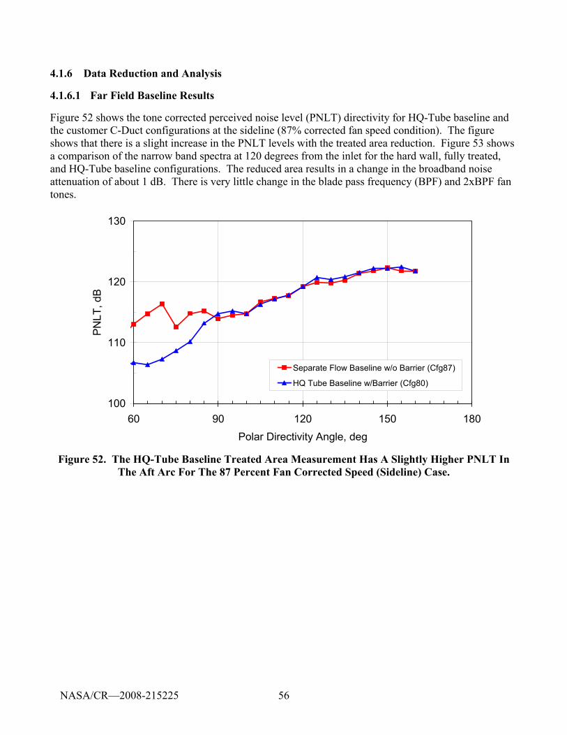
56

4.1.6 Data Reduction and Analysis

4.1.6.1 Far Field Baseline Results

Figure 52 shows the tone corrected perceived noise level (PNLT) directivity for HQ-Tube baseline and the customer C-Duct configurations at the sideline (87% corrected fan speed condition). The figure shows that there is a slight increase in the PNLT levels with the treated area reduction. Figure 53 shows a comparison of the narrow band spectra at 120 degrees from the inlet for the hard wall, fully treated, and HQ-Tube baseline configurations. The reduced area results in a change in the broadband noise attenuation of about 1 dB. There is very little change in the blade pass frequency (BPF) and 2xBPF fan tones.

100

110

120

130

60 90 120 150 180Polar Directivity Angle, deg

PNLT

, dB

Separate Flow Baseline w/o Barrier (Cfg87)

HQ Tube Baseline w/Barrier (Cfg80)

Figure 52. The HQ-Tube Baseline Treated Area Measurement Has A Slightly Higher PNLT In The Aft Arc For The 87 Percent Fan Corrected Speed (Sideline) Case.

NASA/CR—2008-215225

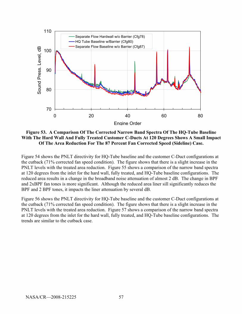
57

70

80

90

100

110

0 20 40 60 80Engine Order

Soun

d P

ress

. Lev

el, d

BSeparate Flow Hardwall w/o Barrier (Cfg78)HQ Tube Baseline w/Barrier (Cfg80)Separate Flow Baseline w/o Barrier (Cfg87)

Figure 53. A Comparison Of The Corrected Narrow Band Spectra Of The HQ-Tube Baseline With The Hard Wall And Fully Treated Customer C-Ducts At 120 Degrees Shows A Small Impact

Of The Area Reduction For The 87 Percent Fan Corrected Speed (Sideline) Case.

Figure 54 shows the PNLT directivity for HQ-Tube baseline and the customer C-Duct configurations at the cutback (71% corrected fan speed condition). The figure shows that there is a slight increase in the PNLT levels with the treated area reduction. Figure 55 shows a comparison of the narrow band spectra at 120 degrees from the inlet for the hard wall, fully treated, and HQ-Tube baseline configurations. The reduced area results in a change in the broadband noise attenuation of almost 2 dB. The change in BPF and 2xBPF fan tones is more significant. Although the reduced area liner sill significantly reduces the BPF and 2 BPF tones, it impacts the liner attenuation by several dB.

Figure 56 shows the PNLT directivity for HQ-Tube baseline and the customer C-Duct configurations at the cutback (71% corrected fan speed condition). The figure shows that there is a slight increase in the PNLT levels with the treated area reduction. Figure 57 shows a comparison of the narrow band spectra at 120 degrees from the inlet for the hard wall, fully treated, and HQ-Tube baseline configurations. The trends are similar to the cutback case.

NASA/CR—2008-215225

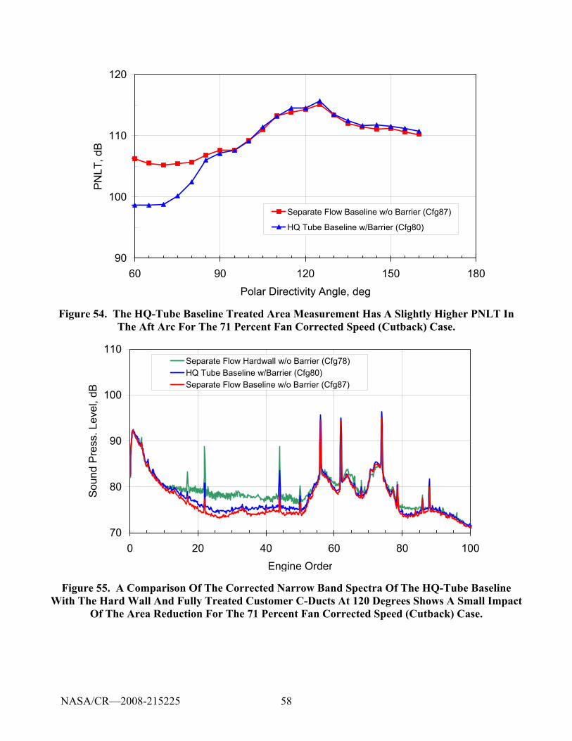
58

90

100

110

120


PN

LT, d

B



Figure 54. The HQ-Tube Baseline Treated Area Measurement Has A Slightly Higher PNLT In The Aft Arc For The 71 Percent Fan Corrected Speed (Cutback) Case.

70

80

90

100

110

0 20 40 60 80 100Engine Order

Sou

nd P

ress

. Lev

el, d

B

Separate Flow Hardwall w/o Barrier (Cfg78)HQ Tube Baseline w/Barrier (Cfg80)Separate Flow Baseline w/o Barrier (Cfg87)


Of The Area Reduction For The 71 Percent Fan Corrected Speed (Cutback) Case.

NASA/CR—2008-215225

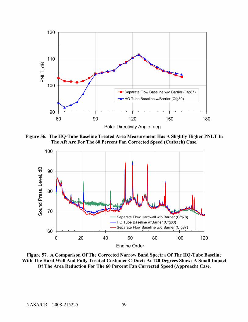
59

90

100

110

120


PN

LT, d

B



Figure 56. The HQ-Tube Baseline Treated Area Measurement Has A Slightly Higher PNLT In The Aft Arc For The 60 Percent Fan Corrected Speed (Cutback) Case.

60

70

80

90

100

0 20 40 60 80 100 120Engine Order

Soun

d P

ress

. Lev

el, d

B

Separate Flow Hardwall w/o Barrier (Cfg78)HQ Tube Baseline w/Barrier (Cfg80)Separate Flow Baseline w/o Barrier (Cfg87)


Of The Area Reduction For The 60 Percent Fan Corrected Speed (Approach) Case.

NASA/CR—2008-215225

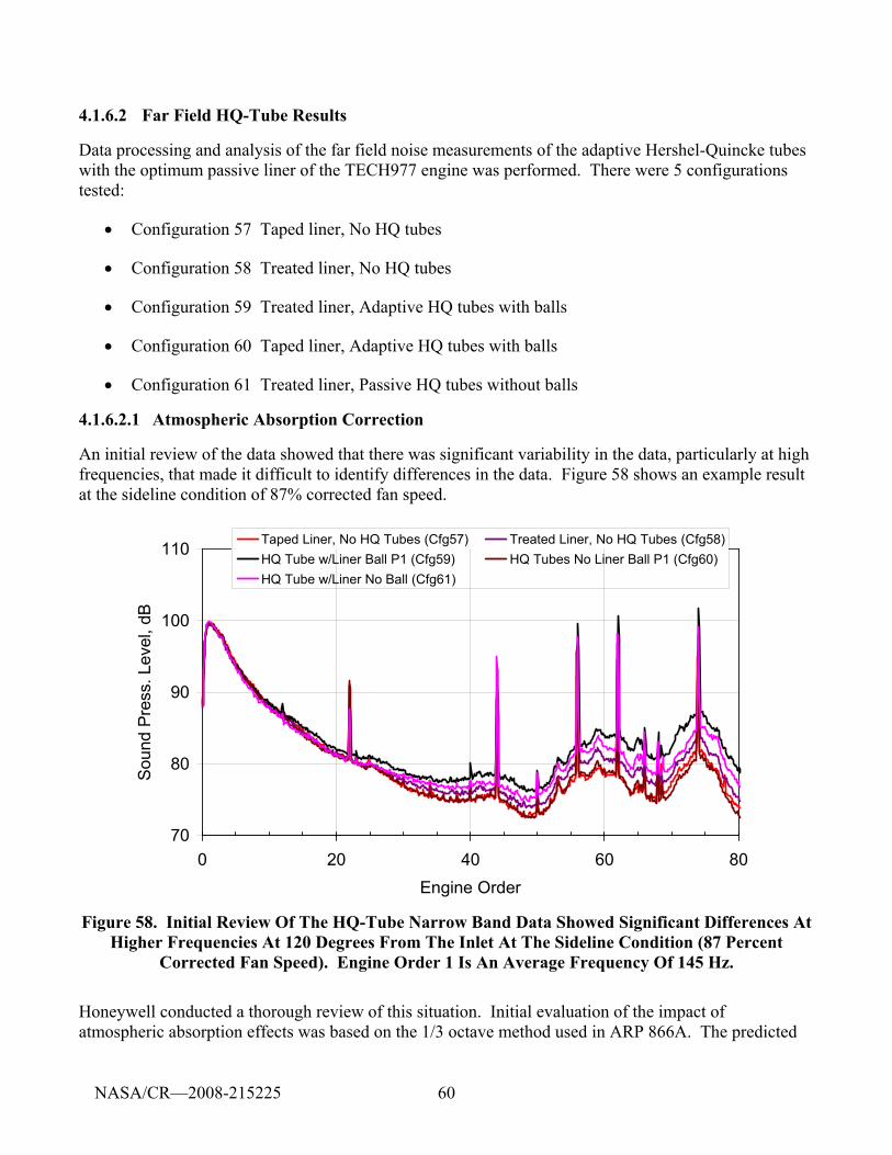
60

4.1.6.2 Far Field HQ-Tube Results

Data processing and analysis of the far field noise measurements of the adaptive Hershel-Quincke tubes with the optimum passive liner of the TECH977 engine was performed. There were 5 configurations tested:

• Configuration 57 Taped liner, No HQ tubes

• Configuration 58 Treated liner, No HQ tubes

• Configuration 59 Treated liner, Adaptive HQ tubes with balls

• Configuration 60 Taped liner, Adaptive HQ tubes with balls

• Configuration 61 Treated liner, Passive HQ tubes without balls

4.1.6.2.1 Atmospheric Absorption Correction

An initial review of the data showed that there was significant variability in the data, particularly at high frequencies, that made it difficult to identify differences in the data. Figure 58 shows an example result at the sideline condition of 87% corrected fan speed.

70

80

90

100

110


Sou

nd P

ress

. Lev

el, d

B

Taped Liner, No HQ Tubes (Cfg57) Treated Liner, No HQ Tubes (Cfg58)HQ Tube w/Liner Ball P1 (Cfg59) HQ Tubes No Liner Ball P1 (Cfg60)HQ Tube w/Liner No Ball (Cfg61)

Figure 58. Initial Review Of The HQ-Tube Narrow Band Data Showed Significant Differences At Higher Frequencies At 120 Degrees From The Inlet At The Sideline Condition (87 Percent

Corrected Fan Speed). Engine Order 1 Is An Average Frequency Of 145 Hz.

Honeywell conducted a thorough review of this situation. Initial evaluation of the impact of atmospheric absorption effects was based on the 1/3 octave method used in ARP 866A. The predicted

NASA/CR—2008-215225

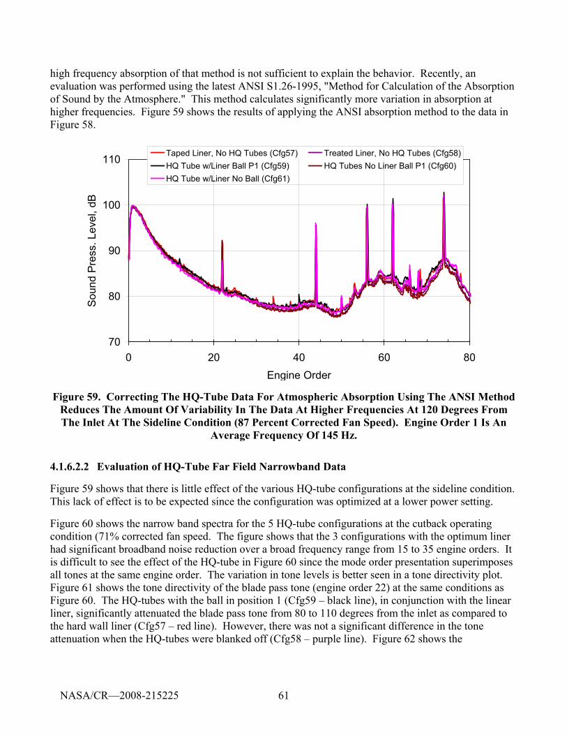
61

high frequency absorption of that method is not sufficient to explain the behavior. Recently, an evaluation was performed using the latest ANSI S1.26-1995, "Method for Calculation of the Absorption of Sound by the Atmosphere." This method calculates significantly more variation in absorption at higher frequencies. Figure 59 shows the results of applying the ANSI absorption method to the data in Figure 58.

70

80

90

100

110


Soun

d Pr

ess.

Lev

el, d

B

Taped Liner, No HQ Tubes (Cfg57) Treated Liner, No HQ Tubes (Cfg58)HQ Tube w/Liner Ball P1 (Cfg59) HQ Tubes No Liner Ball P1 (Cfg60)HQ Tube w/Liner No Ball (Cfg61)

Figure 59. Correcting The HQ-Tube Data For Atmospheric Absorption Using The ANSI Method Reduces The Amount Of Variability In The Data At Higher Frequencies At 120 Degrees From The Inlet At The Sideline Condition (87 Percent Corrected Fan Speed). Engine Order 1 Is An

Average Frequency Of 145 Hz.

4.1.6.2.2 Evaluation of HQ-Tube Far Field Narrowband Data

Figure 59 shows that there is little effect of the various HQ-tube configurations at the sideline condition. This lack of effect is to be expected since the configuration was optimized at a lower power setting.

Figure 60 shows the narrow band spectra for the 5 HQ-tube configurations at the cutback operating condition (71% corrected fan speed. The figure shows that the 3 configurations with the optimum liner had significant broadband noise reduction over a broad frequency range from 15 to 35 engine orders. It is difficult to see the effect of the HQ-tube in Figure 60 since the mode order presentation superimposes all tones at the same engine order. The variation in tone levels is better seen in a tone directivity plot. Figure 61 shows the tone directivity of the blade pass tone (engine order 22) at the same conditions as Figure 60. The HQ-tubes with the ball in position 1 (Cfg59 – black line), in conjunction with the linear liner, significantly attenuated the blade pass tone from 80 to 110 degrees from the inlet as compared to the hard wall liner (Cfg57 – red line). However, there was not a significant difference in the tone attenuation when the HQ-tubes were blanked off (Cfg58 – purple line). Figure 62 shows the

NASA/CR—2008-215225

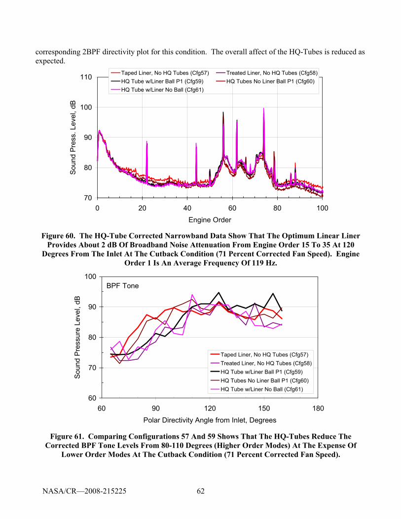
62

corresponding 2BPF directivity plot for this condition. The overall affect of the HQ-Tubes is reduced as expected.

70

80

90

100

110

0 20 40 60 80 100Engine Order

Soun

d Pr

ess.

Lev

el, d

BTaped Liner, No HQ Tubes (Cfg57) Treated Liner, No HQ Tubes (Cfg58)HQ Tube w/Liner Ball P1 (Cfg59) HQ Tubes No Liner Ball P1 (Cfg60)HQ Tube w/Liner No Ball (Cfg61)

Figure 60. The HQ-Tube Corrected Narrowband Data Show That The Optimum Linear Liner Provides About 2 dB Of Broadband Noise Attenuation From Engine Order 15 To 35 At 120

Degrees From The Inlet At The Cutback Condition (71 Percent Corrected Fan Speed). Engine Order 1 Is An Average Frequency Of 119 Hz.

BPF Tone

60

70

80

90

100

60 90 120 150 180Polar Directivity Angle from Inlet, Degrees

Sou

nd P

ress

ure

Leve

l, dB

Taped Liner, No HQ Tubes (Cfg57)Treated Liner, No HQ Tubes (Cfg58)HQ Tube w/Liner Ball P1 (Cfg59)HQ Tubes No Liner Ball P1 (Cfg60)HQ Tube w/Liner No Ball (Cfg61)

Figure 61. Comparing Configurations 57 And 59 Shows That The HQ-Tubes Reduce The Corrected BPF Tone Levels From 80-110 Degrees (Higher Order Modes) At The Expense Of

Lower Order Modes At The Cutback Condition (71 Percent Corrected Fan Speed).

NASA/CR—2008-215225

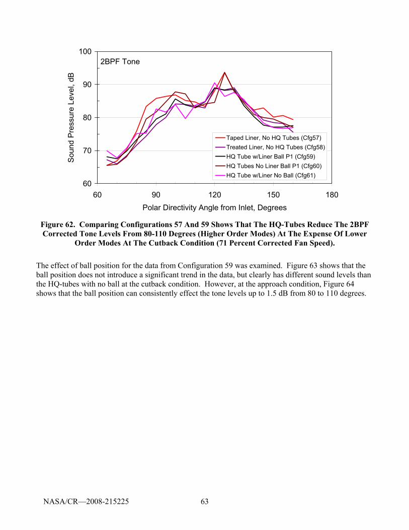
63

2BPF Tone

60

70

80

90

100


Sou

nd P

ress

ure

Leve

l, dB

Taped Liner, No HQ Tubes (Cfg57)Treated Liner, No HQ Tubes (Cfg58)HQ Tube w/Liner Ball P1 (Cfg59)HQ Tubes No Liner Ball P1 (Cfg60)HQ Tube w/Liner No Ball (Cfg61)

Figure 62. Comparing Configurations 57 And 59 Shows That The HQ-Tubes Reduce The 2BPF Corrected Tone Levels From 80-110 Degrees (Higher Order Modes) At The Expense Of Lower

Order Modes At The Cutback Condition (71 Percent Corrected Fan Speed).

The effect of ball position for the data from Configuration 59 was examined. Figure 63 shows that the ball position does not introduce a significant trend in the data, but clearly has different sound levels than the HQ-tubes with no ball at the cutback condition. However, at the approach condition, Figure 64 shows that the ball position can consistently effect the tone levels up to 1.5 dB from 80 to 110 degrees.

NASA/CR—2008-215225

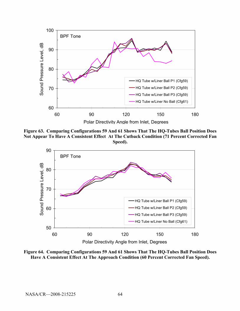
64

BPF Tone

60

70

80

90

100


Soun

d Pr

essu

re L

evel

, dB

HQ Tube w/Liner Ball P1 (Cfg59)



HQ Tube w/Liner No Ball (Cfg61)

Figure 63. Comparing Configurations 59 And 61 Shows That The HQ-Tubes Ball Position Does Not Appear To Have A Consistent Effect At The Cutback Condition (71 Percent Corrected Fan

Speed).

BPF Tone

50

60

70

80

90


Soun

d Pr

essu

re L

evel

, dB




HQ Tube w/Liner No Ball (Cfg61)

Figure 64. Comparing Configurations 59 And 61 Shows That The HQ-Tubes Ball Position Does Have A Consistent Effect At The Approach Condition (60 Percent Corrected Fan Speed).

NASA/CR—2008-215225

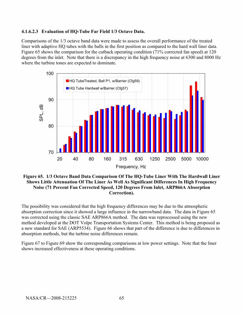
65

4.1.6.2.3 Evaluation of HQ-Tube Far Field 1/3 Octave Data.

Comparisons of the 1/3 octave band data were made to assess the overall performance of the treated liner with adaptive HQ tubes with the balls in the first position as compared to the hard wall liner data. Figure 65 shows the comparison for the cutback operating condition (71% corrected fan speed) at 120 degrees from the inlet. Note that there is a discrepancy in the high frequency noise at 6300 and 8000 Hz where the turbine tones are expected to dominate.

70

80

90

100

20 40 80 160 315 630 1250 2500 5000 10000Frequency, Hz

SPL,

dB

HQ TubeTreated, Ball P1, w/Barrier (Cfg59)

HQ Tube Hardwall w/Barrier (Cfg57)

Figure 65. 1/3 Octave Band Data Comparison Of The HQ-Tube Liner With The Hardwall Liner Shows Little Attenuation Of The Liner As Well As Significant Differences In High Frequency

Noise (71 Percent Fan Corrected Speed, 120 Degrees From Inlet, ARP866A Absorption Correction).

The possibility was considered that the high frequency differences may be due to the atmospheric absorption correction since it showed a large influence in the narrowband data. The data in Figure 65 was corrected using the classic SAE ARP866A method. The data was reprocessed using the new method developed at the DOT Volpe Transportation Systems Center. This method is being proposed as a new standard for SAE (ARP5534). Figure 66 shows that part of the difference is due to differences in absorption methods, but the turbine noise differences remain.

Figure 67 to Figure 69 show the corresponding comparisons at low power settings. Note that the liner shows increased effectiveness at these operating conditions.

NASA/CR—2008-215225

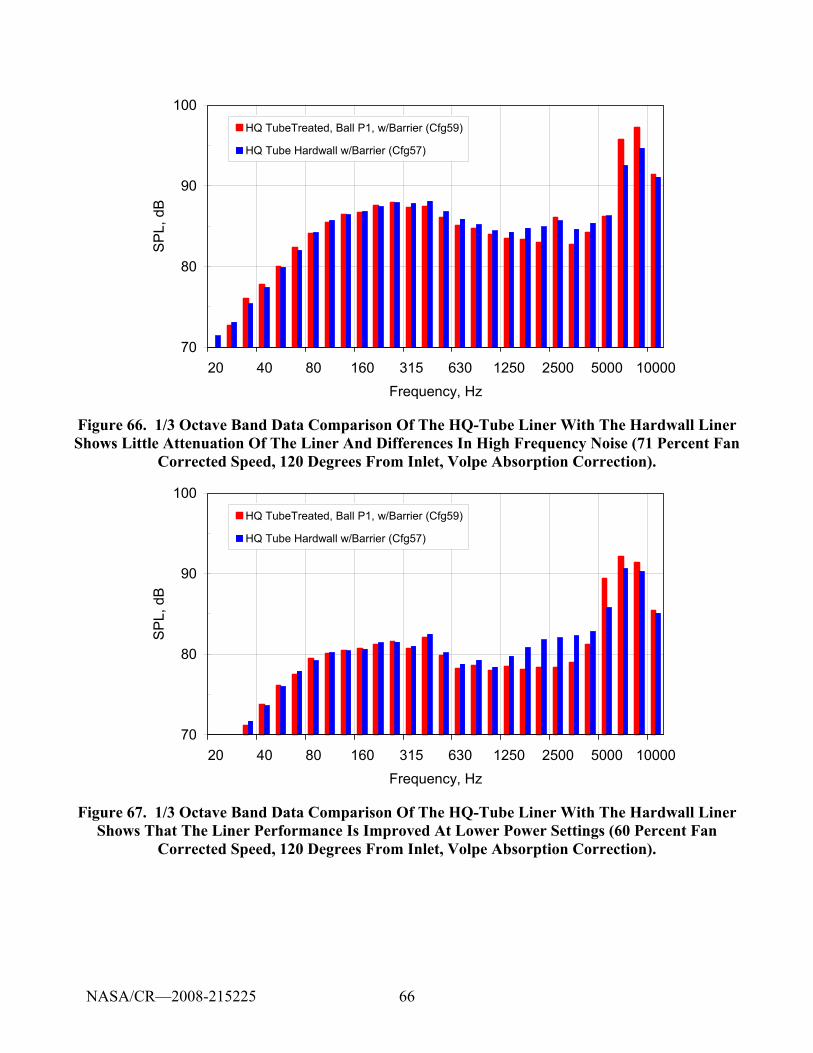
66

70

80

90

100

20 40 80 160 315 630 1250 2500 5000 10000Frequency, Hz

SPL,

dB



Figure 66. 1/3 Octave Band Data Comparison Of The HQ-Tube Liner With The Hardwall Liner Shows Little Attenuation Of The Liner And Differences In High Frequency Noise (71 Percent Fan

Corrected Speed, 120 Degrees From Inlet, Volpe Absorption Correction).

70

80

90

100

20 40 80 160 315 630 1250 2500 5000 10000Frequency, Hz

SPL,

dB



Figure 67. 1/3 Octave Band Data Comparison Of The HQ-Tube Liner With The Hardwall Liner Shows That The Liner Performance Is Improved At Lower Power Settings (60 Percent Fan


NASA/CR—2008-215225

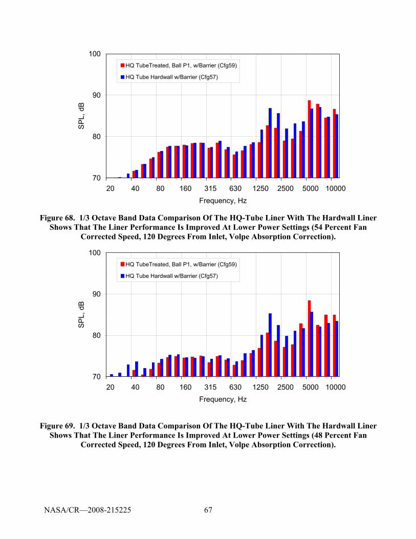
67

70

80

90

100

20 40 80 160 315 630 1250 2500 5000 10000Frequency, Hz

SP

L, d

B





70

80

90

100

20 40 80 160 315 630 1250 2500 5000 10000Frequency, Hz

SPL,

dB





NASA/CR—2008-215225

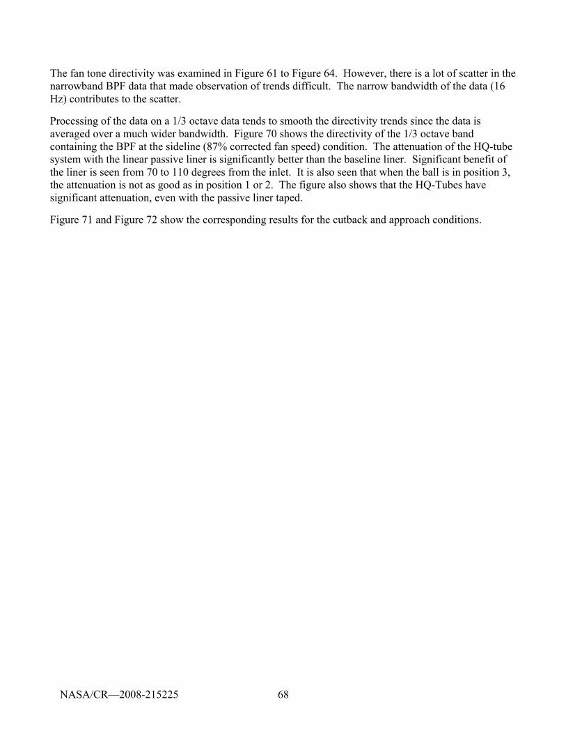
68

The fan tone directivity was examined in Figure 61 to Figure 64. However, there is a lot of scatter in the narrowband BPF data that made observation of trends difficult. The narrow bandwidth of the data (16 Hz) contributes to the scatter.

Processing of the data on a 1/3 octave data tends to smooth the directivity trends since the data is averaged over a much wider bandwidth. Figure 70 shows the directivity of the 1/3 octave band containing the BPF at the sideline (87% corrected fan speed) condition. The attenuation of the HQ-tube system with the linear passive liner is significantly better than the baseline liner. Significant benefit of the liner is seen from 70 to 110 degrees from the inlet. It is also seen that when the ball is in position 3, the attenuation is not as good as in position 1 or 2. The figure also shows that the HQ-Tubes have significant attenuation, even with the passive liner taped.

Figure 71 and Figure 72 show the corresponding results for the cutback and approach conditions.

NASA/CR—2008-215225

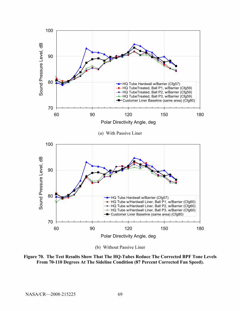
69

70

80

90

100


Sou

nd P

ress

ure

Leve

l, dB

HQ Tube Hardwall w/Barrier (Cfg57)HQ TubeTreated, Ball P1, w/Barrier (Cfg59)HQ TubeTreated, Ball P2, w/Barrier (Cfg59)HQ TubeTreated, Ball P3, w/Barrier (Cfg59)Customer Liner Baseline (same area) (Cfg80)

(a) With Passive Liner

70

80

90

100


Sou

nd P

ress

ure

Leve

l, dB

HQ Tube Hardwall w/Barrier (Cfg57)HQ Tube w/Hardwall Liner, Ball P1, w/Barrier (Cfg60)HQ Tube w/Hardwall Liner, Ball P2, w/Barrier (Cfg60)HQ Tube w/Hardwall Liner, Ball P3, w/Barrier (Cfg60)Customer Liner Baseline (same area) (Cfg80)

(b) Without Passive Liner

Figure 70. The Test Results Show That The HQ-Tubes Reduce The Corrected BPF Tone Levels From 70-110 Degrees At The Sideline Condition (87 Percent Corrected Fan Speed).

NASA/CR—2008-215225

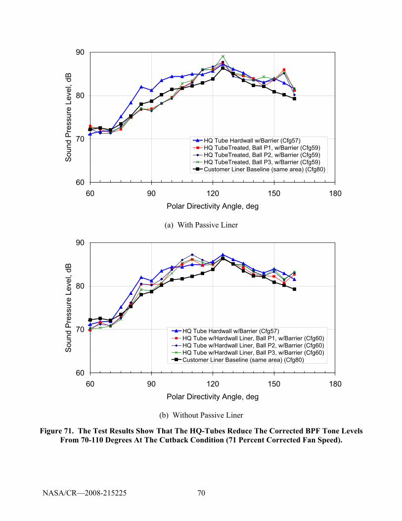
70

60

70

80

90


Soun

d Pr

essu

re L

evel

, dB



60

70

80

90


Soun

d Pr

essu

re L

evel

, dB



Figure 71. The Test Results Show That The HQ-Tubes Reduce The Corrected BPF Tone Levels From 70-110 Degrees At The Cutback Condition (71 Percent Corrected Fan Speed).

NASA/CR—2008-215225

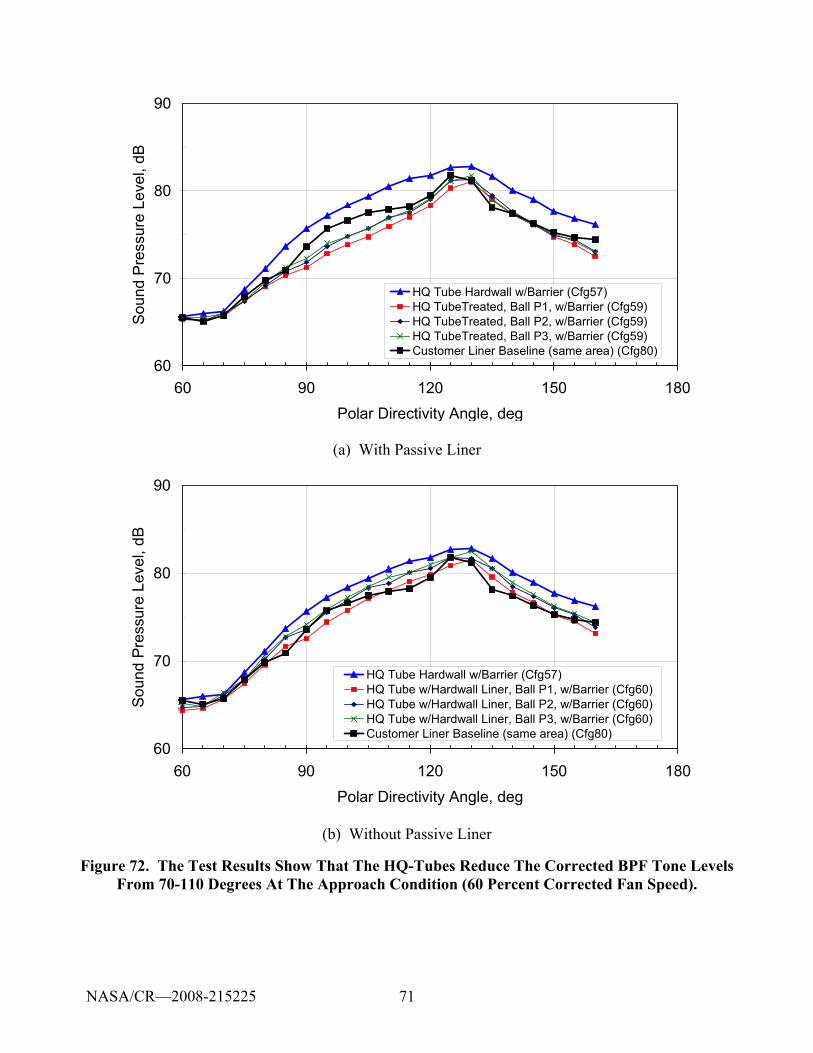
71

60

70

80

90


Soun

d Pr

essu

re L

evel

, dB



60

70

80

90


Soun

d Pr

essu

re L

evel

, dB



Figure 72. The Test Results Show That The HQ-Tubes Reduce The Corrected BPF Tone Levels From 70-110 Degrees At The Approach Condition (60 Percent Corrected Fan Speed).

NASA/CR—2008-215225

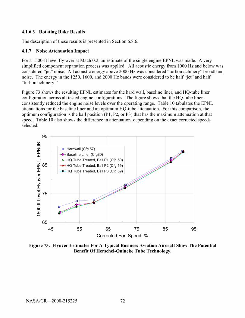
72

4.1.6.3 Rotating Rake Results

The description of these results is presented in Section 6.8.6.

4.1.7 Noise Attenuation Impact

For a 1500-ft level fly-over at Mach 0.2, an estimate of the single engine EPNL was made. A very simplified component separation process was applied. All acoustic energy from 1000 Hz and below was considered “jet” noise. All acoustic energy above 2000 Hz was considered “turbomachinery” broadband noise. The energy in the 1250, 1600, and 2000 Hz bands were considered to be half “jet” and half “turbomachinery.”

Figure 73 shows the resulting EPNL estimates for the hard wall, baseline liner, and HQ-tube liner configuration across all tested engine configurations. The figure shows that the HQ-tube liner consistently reduced the engine noise levels over the operating range. Table 10 tabulates the EPNL attenuations for the baseline liner and an optimum HQ-tube attenuation. For this comparison, the optimum configuration is the ball position (P1, P2, or P3) that has the maximum attenuation at that speed. Table 10 also shows the difference in attenuation. depending on the exact corrected speeds selected.

65

75

85

95

45 55 65 75 85 95Corrected Fan Speed, %

1500

ft L

evel

Fly

over

EP

NL,

EP

NdB

Hardwall (Cfg 57)Baseline Liner (Cfg80)HQ Tube Treated, Ball P1 (Cfg 59)HQ Tube Treated, Ball P2 (Cfg 59)HQ Tube Treated, Ball P3 (Cfg 59)

Figure 73. Flyover Estimates For A Typical Business Aviation Aircraft Show The Potential Benefit Of Herschel-Quincke Tube Technology.

NASA/CR—2008-215225

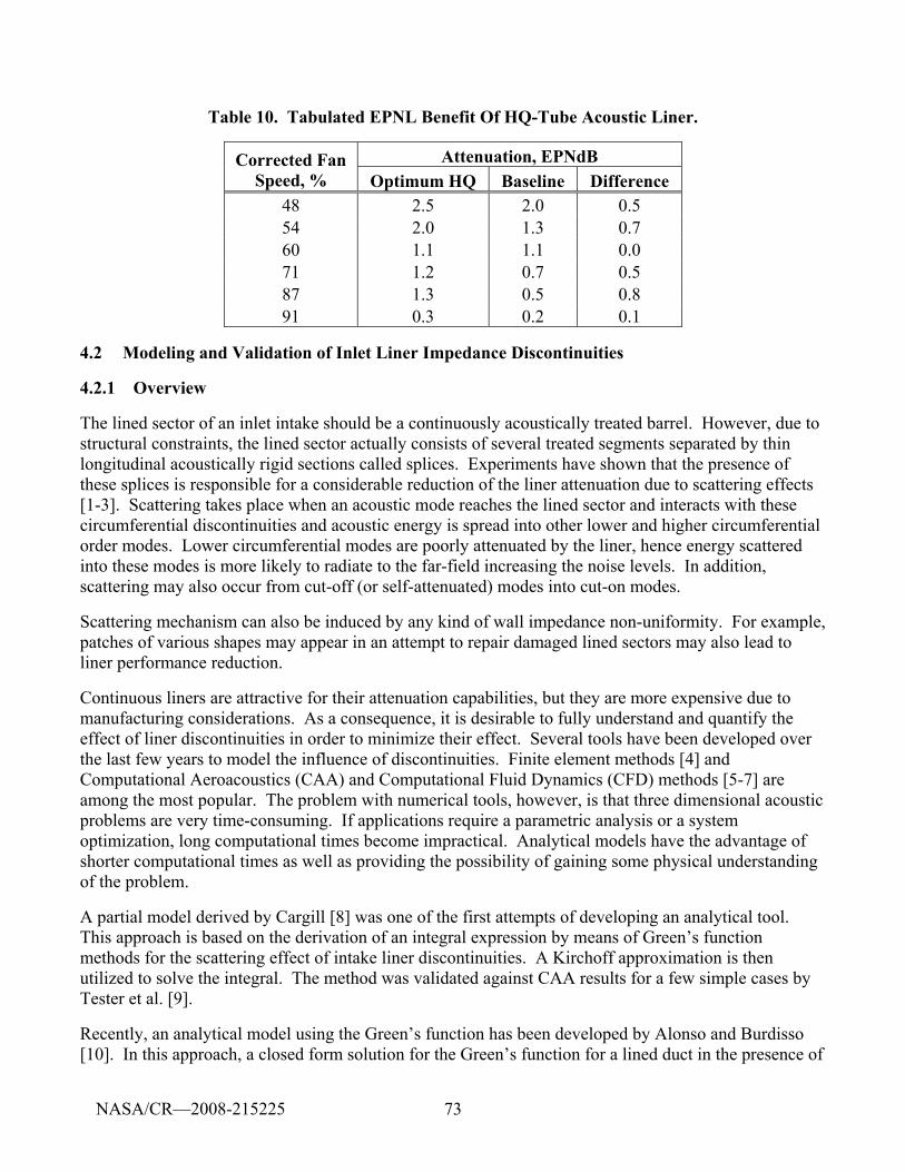
73

Table 10. Tabulated EPNL Benefit Of HQ-Tube Acoustic Liner.

Attenuation, EPNdB Corrected Fan Speed, % Optimum HQ Baseline Difference

48 2.5 2.0 0.5 54 2.0 1.3 0.7 60 1.1 1.1 0.0 71 1.2 0.7 0.5 87 1.3 0.5 0.8 91 0.3 0.2 0.1

4.2 Modeling and Validation of Inlet Liner Impedance Discontinuities

4.2.1 Overview

The lined sector of an inlet intake should be a continuously acoustically treated barrel. However, due to structural constraints, the lined sector actually consists of several treated segments separated by thin longitudinal acoustically rigid sections called splices. Experiments have shown that the presence of these splices is responsible for a considerable reduction of the liner attenuation due to scattering effects [1-3]. Scattering takes place when an acoustic mode reaches the lined sector and interacts with these circumferential discontinuities and acoustic energy is spread into other lower and higher circumferential order modes. Lower circumferential modes are poorly attenuated by the liner, hence energy scattered into these modes is more likely to radiate to the far-field increasing the noise levels. In addition, scattering may also occur from cut-off (or self-attenuated) modes into cut-on modes.

Scattering mechanism can also be induced by any kind of wall impedance non-uniformity. For example, patches of various shapes may appear in an attempt to repair damaged lined sectors may also lead to liner performance reduction.

Continuous liners are attractive for their attenuation capabilities, but they are more expensive due to manufacturing considerations. As a consequence, it is desirable to fully understand and quantify the effect of liner discontinuities in order to minimize their effect. Several tools have been developed over the last few years to model the influence of discontinuities. Finite element methods [4] and Computational Aeroacoustics (CAA) and Computational Fluid Dynamics (CFD) methods [5-7] are among the most popular. The problem with numerical tools, however, is that three dimensional acoustic problems are very time-consuming. If applications require a parametric analysis or a system optimization, long computational times become impractical. Analytical models have the advantage of shorter computational times as well as providing the possibility of gaining some physical understanding of the problem.

A partial model derived by Cargill [8] was one of the first attempts of developing an analytical tool. This approach is based on the derivation of an integral expression by means of Green’s function methods for the scattering effect of intake liner discontinuities. A Kirchoff approximation is then utilized to solve the integral. The method was validated against CAA results for a few simple cases by Tester et al. [9].

Recently, an analytical model using the Green’s function has been developed by Alonso and Burdisso [10]. In this approach, a closed form solution for the Green’s function for a lined duct in the presence of

NASA/CR—2008-215225

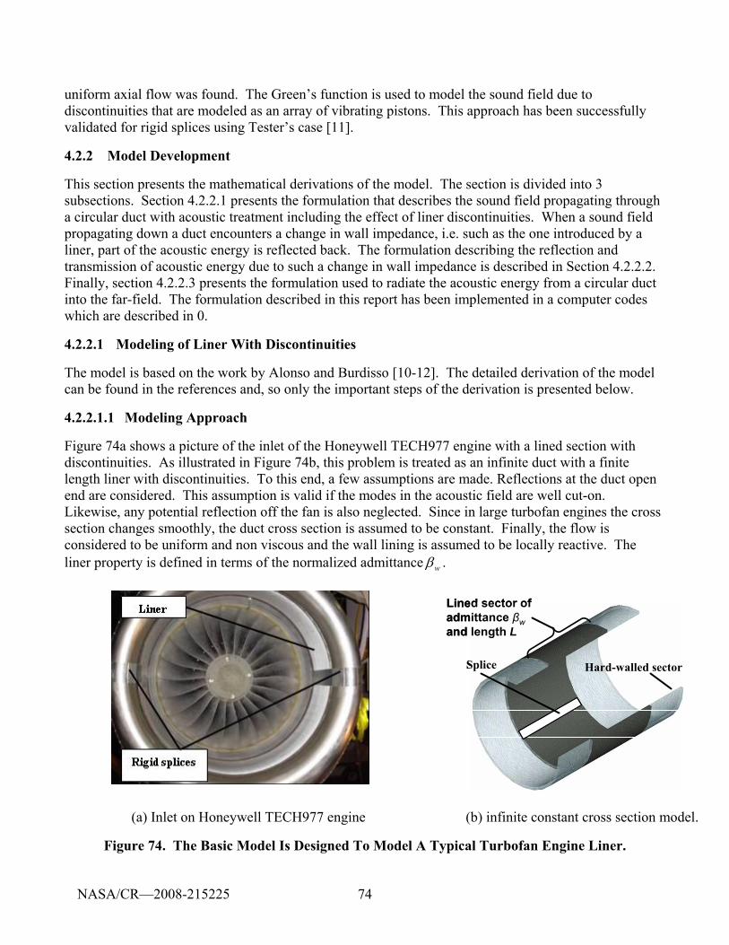
74

uniform axial flow was found. The Green’s function is used to model the sound field due to discontinuities that are modeled as an array of vibrating pistons. This approach has been successfully validated for rigid splices using Tester’s case [11].

4.2.2 Model Development

This section presents the mathematical derivations of the model. The section is divided into 3 subsections. Section 4.2.2.1 presents the formulation that describes the sound field propagating through a circular duct with acoustic treatment including the effect of liner discontinuities. When a sound field propagating down a duct encounters a change in wall impedance, i.e. such as the one introduced by a liner, part of the acoustic energy is reflected back. The formulation describing the reflection and transmission of acoustic energy due to such a change in wall impedance is described in Section 4.2.2.2. Finally, section 4.2.2.3 presents the formulation used to radiate the acoustic energy from a circular duct into the far-field. The formulation described in this report has been implemented in a computer codes which are described in 0.

4.2.2.1 Modeling of Liner With Discontinuities

The model is based on the work by Alonso and Burdisso [10-12]. The detailed derivation of the model can be found in the references and, so only the important steps of the derivation is presented below.

4.2.2.1.1 Modeling Approach

Figure 74a shows a picture of the inlet of the Honeywell TECH977 engine with a lined section with discontinuities. As illustrated in Figure 74b, this problem is treated as an infinite duct with a finite length liner with discontinuities. To this end, a few assumptions are made. Reflections at the duct open end are considered. This assumption is valid if the modes in the acoustic field are well cut-on. Likewise, any potential reflection off the fan is also neglected. Since in large turbofan engines the cross section changes smoothly, the duct cross section is assumed to be constant. Finally, the flow is considered to be uniform and non viscous and the wall lining is assumed to be locally reactive. The liner property is defined in terms of the normalized admittance wβ .

Splice Hard-walled sector

Lined sector of admittance βwand length L

Splice Hard-walled sector


(a) Inlet on Honeywell TECH977 engine (b) infinite constant cross section model.

Figure 74. The Basic Model Is Designed To Model A Typical Turbofan Engine Liner.

NASA/CR—2008-215225

75

The modeling approach is depicted in Figure 75a. The sound field generated by the fan propagates upstream through the hard-wall duct until it encounters the liner. At this first hard-wall/liner interface, a transmission/reflection analysis is performed and the incidence sound field at the beginning of the liner determined. The sound field in the lined sector can now be thought as the result of combining two acoustic fields. The first field is due to the fan while the second field is due to the liner discontinuities. These discontinuities are modeled as an array of rectangular shaped pistons/sources vibrating with a certain velocity (see Figure 75b).

Disturbance (reflections off fan neglected)

Discontinuity on liner surface modeled as

vibrating piston


Reflections at duct end neglected

Flow

Hardwall/liner interface

z = 0


z = L

Pd

Pdisc

Transmitted sound radiates in the far-

field Disturbance (reflections off fan neglected)

Discontinuity on liner surface modeled as

vibrating piston


Reflections at duct end neglected

Flow


z = 0


z = L

Pd

Pdisc

Transmitted sound radiates in the far-

field

(a) Superposition of the fan and the sound field due to vibrating pistons is applied in the lined sector

Flow

Discontinuity on liner surface discretized as an array of vibrating

pistons

DisturbancePdisc due to the

ith piston

Lined sector of admittance βw and

length L

Flow

Discontinuity on liner surface discretized as an array of vibrating

pistons

DisturbancePdisc due to the

ith piston

Lined sector of admittance βw and

length L

(b) Discretization of a rigid splice into an array of vibrating pistons

Figure 75: The Modeling Approach For The Liner Discontinuity Is A Two Step Process.

NASA/CR—2008-215225

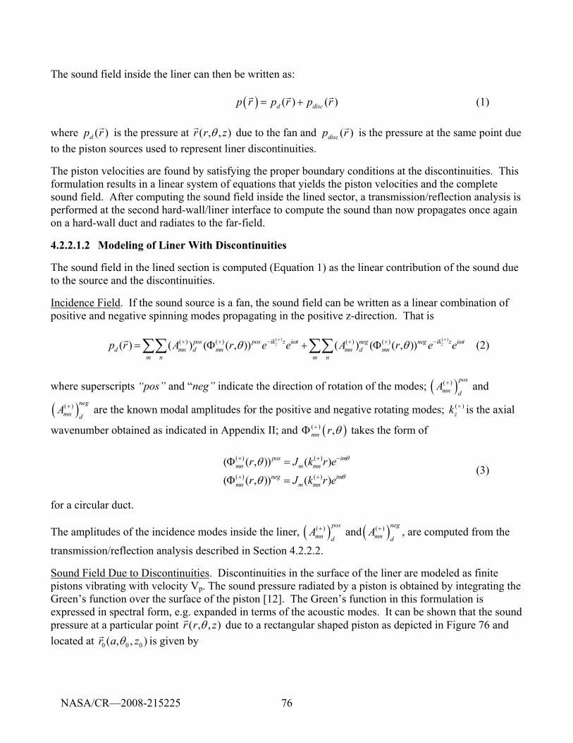
76

The sound field inside the liner can then be written as: ( ) ( ) ( )d discp r p r p r= +

r r r (1) where )(rpd

r is the pressure at ),,( zrr θr due to the fan and ( )discp rr is the pressure at the same point due to the piston sources used to represent liner discontinuities.

The piston velocities are found by satisfying the proper boundary conditions at the discontinuities. This formulation results in a linear system of equations that yields the piston velocities and the complete sound field. After computing the sound field inside the lined sector, a transmission/reflection analysis is performed at the second hard-wall/liner interface to compute the sound than now propagates once again on a hard-wall duct and radiates to the far-field.

4.2.2.1.2 Modeling of Liner With Discontinuities

The sound field in the lined section is computed (Equation 1) as the linear contribution of the sound due to the source and the discontinuities.

Incidence Field. If the sound source is a fan, the sound field can be written as a linear combination of positive and negative spinning modes propagating in the positive z-direction. That is

( ) ( )( ) ( ) ( ) ( )( ) ( ) ( ( , )) ( ) ( ( , ))z zik z ik zpos pos i t neg neg i td mn d mn mn d mn

m n m n

p r A r e e A r e eω ωθ θ+ +− −+ + + += Φ + Φ∑∑ ∑∑r (2)

where superscripts “pos” and “neg” indicate the direction of rotation of the modes; ( )( ) pos

mn dA + and

( )( ) neg

mn dA + are the known modal amplitudes for the positive and negative rotating modes; ( )

zk + is the axial

wavenumber obtained as indicated in Appendix II; and ( )( ) ,mn r θ+Φ takes the form of

( ) ( )

( ) ( )

( ( , )) ( )

( ( , )) ( )

pos immn m mn

neg immn m mn

r J k r e

r J k r e

θ

θ

θ

θ

+ + −

+ +

Φ =

Φ = (3)

for a circular duct.

The amplitudes of the incidence modes inside the liner, ( )( ) pos

mn dA + and ( )( ) neg

mn dA + , are computed from the

transmission/reflection analysis described in Section 4.2.2.2.

Sound Field Due to Discontinuities. Discontinuities in the surface of the liner are modeled as finite pistons vibrating with velocity Vp. The sound pressure radiated by a piston is obtained by integrating the Green’s function over the surface of the piston [12]. The Green’s function in this formulation is expressed in spectral form, e.g. expanded in terms of the acoustic modes. It can be shown that the sound pressure at a particular point ),,( zrr θr due to a rectangular shaped piston as depicted in Figure 76 and located at 0 0 0( , , )r a zθr is given by

NASA/CR—2008-215225

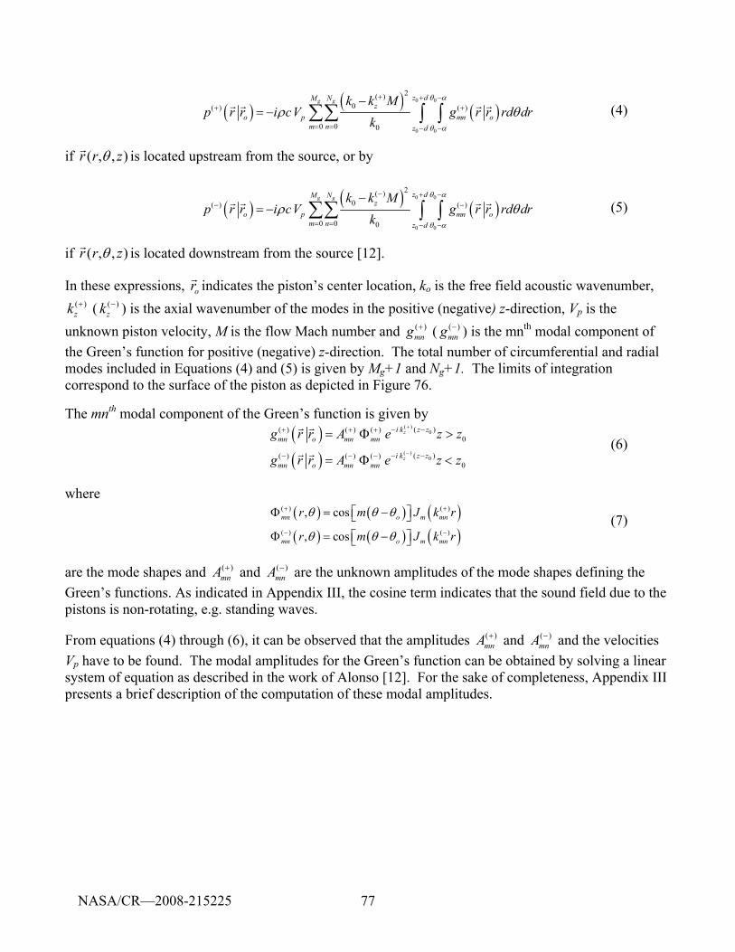
77

( ) ( ) ( )0 0

0 0

2( )0( ) ( )

0 0 0

g g z dM Nz

o p mn om n z d

k k Mp r r i cV g r r rd dr

k

θ α

θ α

ρ θ+ + −

+ +

= = − −

−= − ∑∑ ∫ ∫

r r r r (4)

if ),,( zrr θr is located upstream from the source, or by

( ) ( ) ( )0 0

0 0

2( )0( ) ( )

0 0 0

g g z dM Nz

o p mn om n z d

k k Mp r r i cV g r r rd dr

k

θ α

θ α

ρ θ− + −

− −

= = − −

−= − ∑∑ ∫ ∫

r r r r (5)

if ),,( zrr θr is located downstream from the source [12].

In these expressions, orr indicates the piston’s center location, ko is the free field acoustic wavenumber,

( )zk + ( ( )

zk − ) is the axial wavenumber of the modes in the positive (negative) z-direction, Vp is the unknown piston velocity, M is the flow Mach number and ( )

mng + ( ( )mng − ) is the mnth modal component of

the Green’s function for positive (negative) z-direction. The total number of circumferential and radial modes included in Equations (4) and (5) is given by Mg+1 and Ng+1. The limits of integration correspond to the surface of the piston as depicted in Figure 76.

The mnth modal component of the Green’s function is given by

( )( )

( )0

( )0

( )( ) ( ) ( )0

( )( ) ( ) ( )0

z

z

i k z zmn o mn mn

i k z zmn o mn mn

g r r A e z z

g r r A e z z

+

−

− −+ + +

− −− − −

= Φ >

= Φ <

r r

r r (6)

where

( ) ( ) ( )( ) ( ) ( )

( ) ( )

( ) ( )

, cos

, cos

mn o m mn

mn o m mn

r m J k r

r m J k r

θ θ θ

θ θ θ

+ +

− −

Φ = − ⎡ ⎤⎣ ⎦

Φ = −⎡ ⎤⎣ ⎦

(7)

are the mode shapes and ( )mnA + and ( )

mnA − are the unknown amplitudes of the mode shapes defining the Green’s functions. As indicated in Appendix III, the cosine term indicates that the sound field due to the pistons is non-rotating, e.g. standing waves.

From equations (4) through (6), it can be observed that the amplitudes ( )mnA + and ( )

mnA − and the velocities Vp have to be found. The modal amplitudes for the Green’s function can be obtained by solving a linear system of equation as described in the work of Alonso [12]. For the sake of completeness, Appendix III presents a brief description of the computation of these modal amplitudes.

NASA/CR—2008-215225

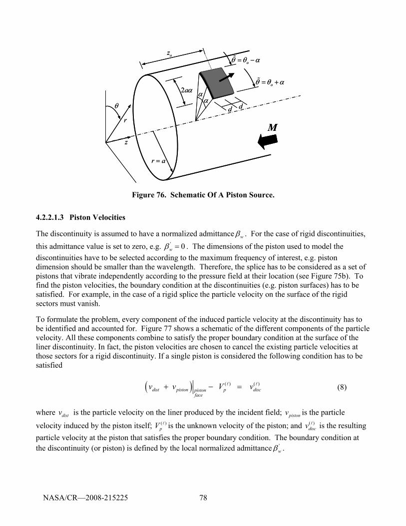
78

oθ θ α= +%

oθ θ α= −%

αα

d d

oz

2aα

r a=

Mz

r

θ

oθ θ α= +%

oθ θ α= −%

αα

d d

oz

2aα

r a=

Mz

r

θ

Figure 76. Schematic Of A Piston Source.

4.2.2.1.3 Piston Velocities

The discontinuity is assumed to have a normalized admittance wβ . For the case of rigid discontinuities, this admittance value is set to zero, e.g. ' 0wβ = . The dimensions of the piston used to model the discontinuities have to be selected according to the maximum frequency of interest, e.g. piston dimension should be smaller than the wavelength. Therefore, the splice has to be considered as a set of pistons that vibrate independently according to the pressure field at their location (see Figure 75b). To find the piston velocities, the boundary condition at the discontinuities (e.g. piston surfaces) has to be satisfied. For example, in the case of a rigid splice the particle velocity on the surface of the rigid sectors must vanish.

To formulate the problem, every component of the induced particle velocity at the discontinuity has to be identified and accounted for. Figure 77 shows a schematic of the different components of the particle velocity. All these components combine to satisfy the proper boundary condition at the surface of the liner discontinuity. In fact, the piston velocities are chosen to cancel the existing particle velocities at those sectors for a rigid discontinuity. If a single piston is considered the following condition has to be satisfied ( ) ( ) ( )

dist piston p discpistonface

v v V v + − = l l (8)

where distv is the particle velocity on the liner produced by the incident field; pistonv is the particle

velocity induced by the piston itself; ( )pV l is the unknown velocity of the piston; and ( )

discv l is the resulting particle velocity at the piston that satisfies the proper boundary condition. The boundary condition at the discontinuity (or piston) is defined by the local normalized admittance '

wβ .

NASA/CR—2008-215225

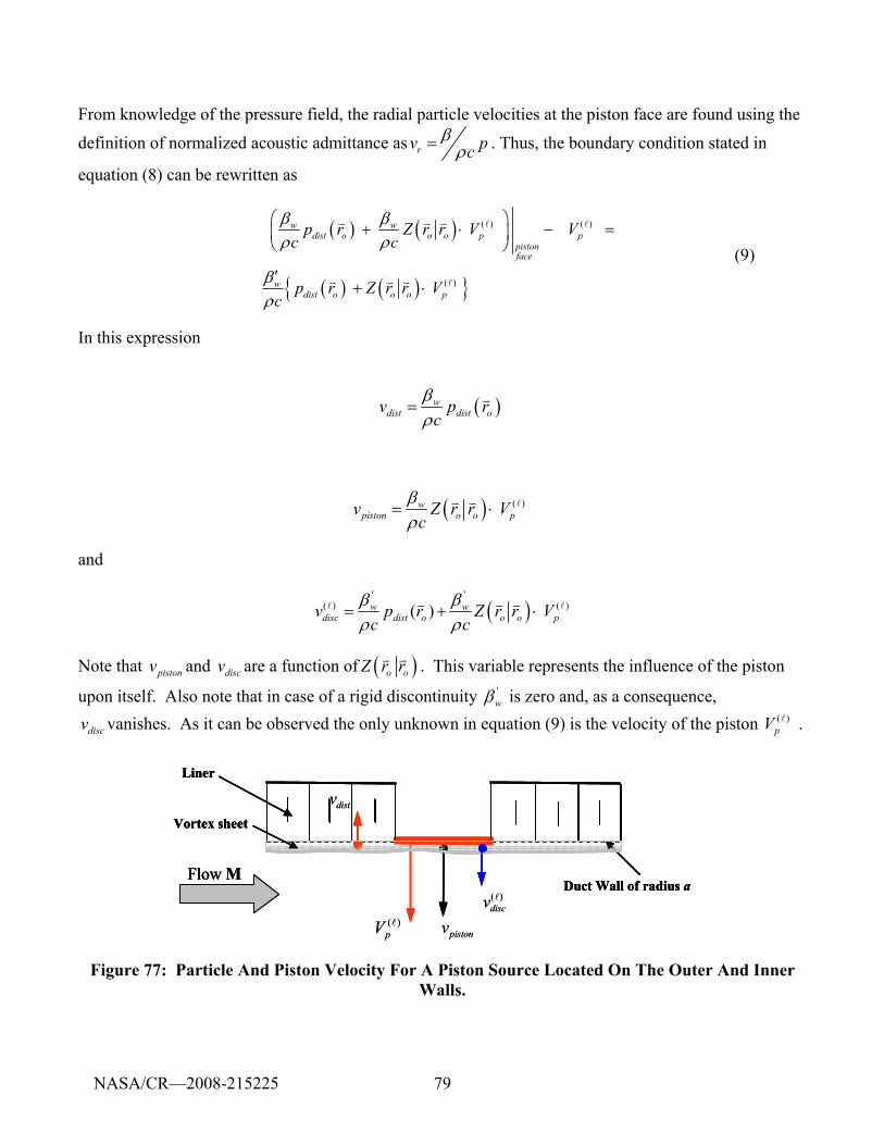
79

From knowledge of the pressure field, the radial particle velocities at the piston face are found using the

definition of normalized acoustic admittance as rv pcβ

ρ= . Thus, the boundary condition stated in

equation (8) can be rewritten as

( ) ( )

( ) ( ){ }

( ) ( )

( )

w wdist o o o p p

pistonface

wdist o o o p

p r Z r r V Vc c

p r Z r r Vc

β βρ ρ

βρ

⎛ ⎞ + ⋅ − = ⎜ ⎟

⎝ ⎠

′ + ⋅

l l

l

v v v

v v v

(9)

In this expression

( )wdist dist ov p r

cβρ

= v

( ) ( )wpiston o o pv Z r r V

cβρ

= ⋅ lv v

and

( )' '

( ) ( )( )w wdisc dist o o o pv p r Z r r V

c cβ βρ ρ

= + ⋅ l lv v v

Note that pistonv and discv are a function of ( )o oZ r rv v . This variable represents the influence of the piston

upon itself. Also note that in case of a rigid discontinuity 'wβ is zero and, as a consequence,

discv vanishes. As it can be observed the only unknown in equation (9) is the velocity of the piston ( )pV l .

Liner

Duct Wall of radius a

Vortex sheet

Flow M

( )pV l

pistonv

( )discv l

distvLiner


Vortex sheet

Flow M

Liner


Vortex sheet

Flow M

( )pV l

pistonv

( )discv l

distv

Figure 77: Particle And Piston Velocity For A Piston Source Located On The Outer And Inner Walls.

NASA/CR—2008-215225

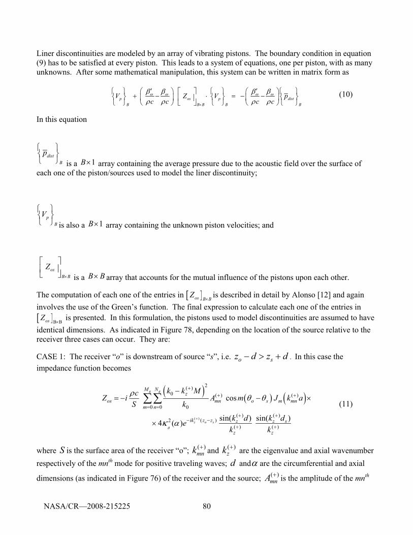
80

Liner discontinuities are modeled by an array of vibrating pistons. The boundary condition in equation (9) has to be satisfied at every piston. This leads to a system of equations, one per piston, with as many unknowns. After some mathematical manipulation, this system can be written in matrix form as

p os p distB B B B B

V Z V pc c c cω ω ω ωβ β β β

ρ ρ ρ ρ×

′ ′⎛ ⎞ ⎛ ⎞⎧ ⎫ ⎡ ⎤ ⎧ ⎫ ⎧ ⎫ + − ⋅ = − − ⎨ ⎬ ⎨ ⎬ ⎨ ⎬⎜ ⎟ ⎜ ⎟⎢ ⎥

⎩ ⎭ ⎣ ⎦ ⎩ ⎭ ⎩ ⎭⎝ ⎠ ⎝ ⎠ (10)

In this equation

distB

p⎧ ⎫⎨ ⎬⎩ ⎭ is a 1B× array containing the average pressure due to the acoustic field over the surface of each one of the piston/sources used to model the liner discontinuity;

pB

V⎧ ⎫⎨ ⎬⎩ ⎭ is also a 1B× array containing the unknown piston velocities; and

osB B

Z×

⎡ ⎤ ⎢ ⎥⎣ ⎦ is a B B× array that accounts for the mutual influence of the pistons upon each other.

The computation of each one of the entries in [ ]os B BZ

×is described in detail by Alonso [12] and again

involves the use of the Green’s function. The final expression to calculate each one of the entries in [ ]osZ

Β×Β is presented. In this formulation, the pistons used to model discontinuities are assumed to have

identical dimensions. As indicated in Figure 78, depending on the location of the source relative to the receiver three cases can occur. They are:

CASE 1: The receiver “o” is downstream of source “s”, i.e. o sz d z d− > + . In this case the impedance function becomes

( ) ( ) ( )

( )

2( )0 ( ) ( )

0 0 0( ) ( )

( )2( ) ( )

cos

sin( ) sin( ) ( )

g g

z o s

M Nz

os mn o s m mnm n

ik z z z z s

z z

k k McZ i A m J k aS k

k d k dek kθ

ρ θ θ

ακ+

++ +

= =

+ +− −

+ +

−= − − ×

× 4

∑∑ (11)

where S is the surface area of the receiver “o”; ( )mnk + and ( )

zk + are the eigenvalue and axial wavenumber respectively of the mnth mode for positive traveling waves; d andα are the circumferential and axial

dimensions (as indicated in Figure 76) of the receiver and the source; ( )mnA + is the amplitude of the mnth

NASA/CR—2008-215225

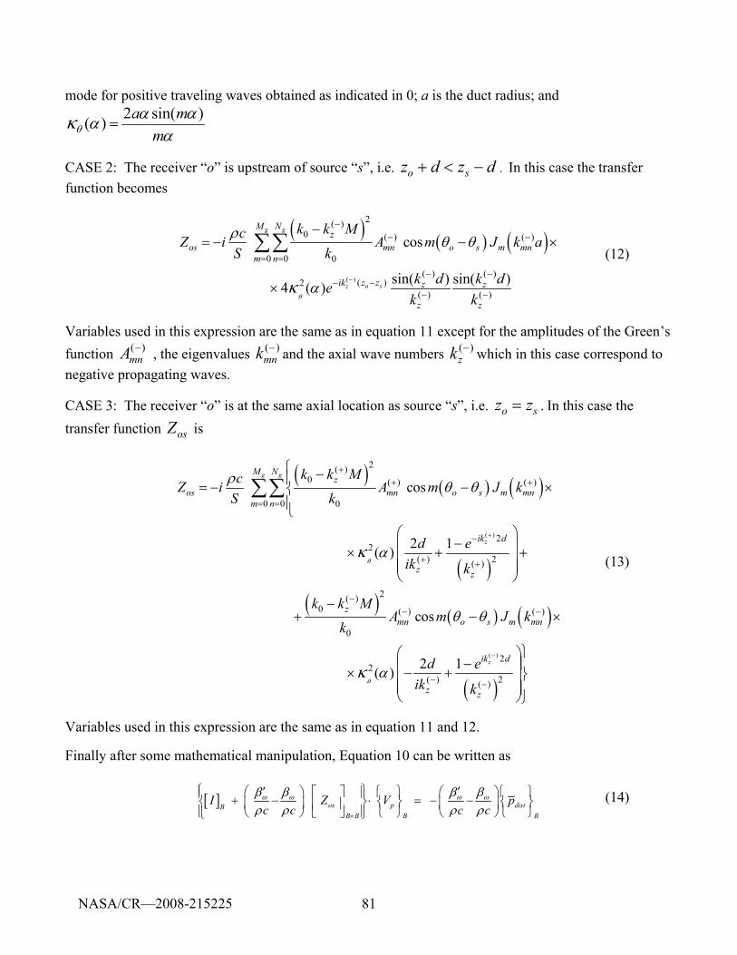
81

mode for positive traveling waves obtained as indicated in 0; a is the duct radius; and 2 sin( )( ) a m

mθα αα

ακ =

CASE 2: The receiver “o” is upstream of source “s”, i.e. o sz d z d+ < − . In this case the transfer function becomes

( ) ( ) ( )

( )

2( )0 ( ) ( )

0 0 0( ) ( )

( )2( ) ( )

cos

sin( ) sin( ) ( )

g g

z o s

M Nz

os mn o s m mnm n

ik z z z z

z z

k k McZ i A m J k aS k

k d k dek kθ

ρ θ θ

ακ−

−− −

= =

− −− −

− −

−= − − ×

× 4

∑∑ (12)

Variables used in this expression are the same as in equation 11 except for the amplitudes of the Green’s function ( )

mnA − , the eigenvalues ( )mnk − and the axial wave numbers ( )

zk − which in this case correspond to negative propagating waves.

CASE 3: The receiver “o” is at the same axial location as source “s”, i.e. o sz z= . In this case the transfer function osZ is

( ) ( ) ( )

( )

( )

2( )0 ( ) ( )

0 0 0

22

( ) 2( )

0

cos

2 1( )

g g

z

M Nz

os mn o s m mnm n

ik d

z z

z

k k McZ i A m J kS k

d eik k

k k

θ

ρ θ θ

ακ+

++ +

= =

−

+ +

⎧ −⎪= − − ×⎨⎪⎩

⎛ ⎞−⎜ ⎟ × + +⎜ ⎟⎜ ⎟

⎝ ⎠

− +

∑∑

( ) ( ) ( )

( )

( )

2( )( ) ( )

0

22

( ) 2( )

cos

2 1( )z

mn o s m mn

ik d

z z

MA m J k

k

d eik k

θ

θ θ

ακ−

−− −

− −

− ×

⎫⎛ ⎞− ⎪⎜ ⎟ × − + ⎬⎜ ⎟⎜ ⎟⎪⎝ ⎠⎭

(13)

Variables used in this expression are the same as in equation 11 and 12.

Finally after some mathematical manipulation, Equation 10 can be written as

[ ] os p distBB B B B

I Z V pc c c cω ω ω ωβ β β β

ρ ρ ρ ρ×

⎧ ⎫′ ′⎛ ⎞ ⎛ ⎞⎡ ⎤ ⎧ ⎫ ⎧ ⎫⎪ ⎪ + − ⋅ = − − ⎨ ⎬ ⎨ ⎬ ⎨ ⎬⎜ ⎟ ⎜ ⎟⎢ ⎥⎪ ⎪⎣ ⎦ ⎩ ⎭ ⎩ ⎭⎝ ⎠ ⎝ ⎠⎩ ⎭

(14)

NASA/CR—2008-215225

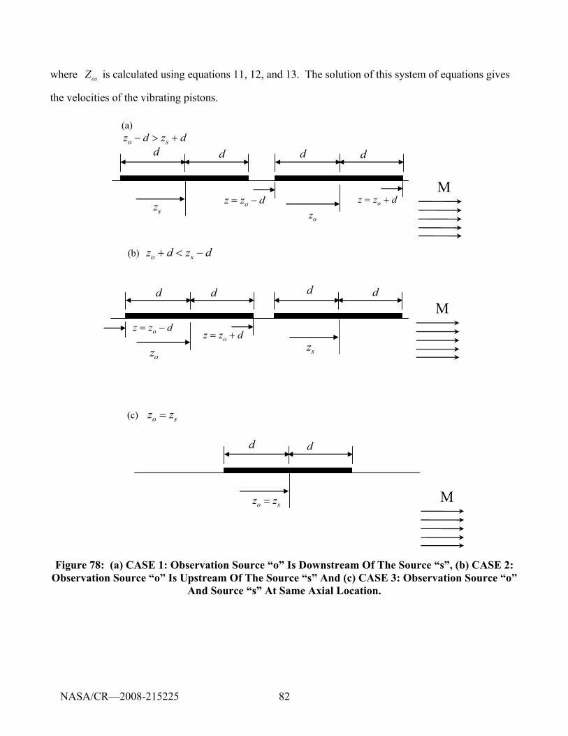
82

where osZ is calculated using equations 11, 12, and 13. The solution of this system of equations gives

the velocities of the vibrating pistons.

dd

szM

M

(a) o sz d z d− > +

(c) o sz z=

(b) o sz d z d+ < −

d d

d d d d

dd

M

oz sz

oz z d= −

oz

oz z d= − oz z d= +

o sz z=

oz z d= +

Figure 78: (a) CASE 1: Observation Source “o” Is Downstream Of The Source “s”, (b) CASE 2: Observation Source “o” Is Upstream Of The Source “s” And (c) CASE 3: Observation Source “o”

And Source “s” At Same Axial Location.

NASA/CR—2008-215225

83

4.2.2.1.4 Total Modal Amplitudes

Once the piston velocities have been calculated, the sound field due to the liner discontinuities can be calculated and combined with the . In this section, an expression for the modal amplitudes of the combined sound field is derived.

The sound pressure field at the end of the liner on the lined sector can be written in terms of positive and negative spinning modes as follows

( ) ( ) ( ) ( )( ) ( )( ) ( ) ( ) ( )

0 0 0 0

s s s sz z

M N M Npos negik z ik zim imtot mn m mn mn m mntot tot

m n m np A J k r e e A J k r e eθ θ+ +− −+ + − + +

= = = =

= +∑∑ ∑∑

(15)

where ( )( ) pos

mn totA + and ( )( ) neg

mn totA + are the modal amplitudes of the positive and negative spinning modes

(propagating in the positive z-direction), respectively. These amplitudes account for the effects of both the liner and liner discontinuities and can be expressed as

( ) ( ) ( )( ) ( ) ( ) ( )

1

s

p

Npos pos pos rmn mn mntot d r

rA A A V+ + +

=

= + ∑ (16)

( ) ( ) ( )( ) ( ) ( ) ( )

1

s

p

Nneg neg neg rmn mn mntot d r

rA A A V+ + +

=

= + ∑ (17)

The modal amplitudes ( )( ) pos


mn dA + are the known amplitudes of the spinning modes included

in the . The source velocities ( )p

rV are obtained from the solution of the system of equations in 14. The

first step to derive an expression for ( )( ) pos

mn rA + and ( )( ) neg

mn rA + is to write the expression of the sound

pressure as a linear superposition

1

( , , ) ( , , ) ( , , , , )sN

tot d r r rr

p r z p r z p r z r zθ θ θ θ=

= + ∑ (18)

The modal amplitudes of the pressure dp due to the are assumed to be known as ( )( ) pos


mn dA + .

The pressure produced by the rth piston/source with a unit velocity at the end of the liner, i.e. z = L, is obtained from the finite piston radiation formula previously derived by Alonso [12]

( ) ( ) ( )

( )

2( )0 ( ) ( )

0 0 0( )

( )( )

( , , | , , ) cos

sin( ) ( ) 2

g g

z r

M Nz

r r mn r m mnm n

ik z z z rr

z r

k k Mp r z a z i c A m J k r

k

k de dk dθ

θ θ ρ θ θ

ακ+

++ +

= =

+− −

+

−= − − ×

×

∑∑

(19)

NASA/CR—2008-215225

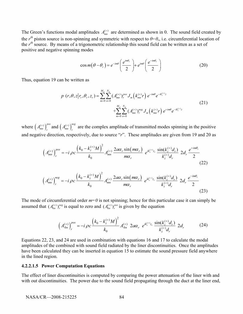
84

The Green’s functions modal amplitudes ( )mnA + are determined as shown in 0. The sound field created by

the rth piston source is non-spinning and symmetric with respect to θ=θr, i.e. circumferential location of the rth source. By means of a trigonometric relationship this sound field can be written as a set of positive and negative spinning modes

( )cos2 2

r rim imim im

re em e e

θ θθ θθ θ

−− ⎛ ⎞ ⎛ ⎞

− = + ⎜ ⎟ ⎜ ⎟⎝ ⎠ ⎝ ⎠

(20)

Thus, equation 19 can be written as

( )

( )

( )

( )

( ) ( )

0 0

( ) ( )

0 0

( , , , , ) ( )

+ ( )

g g

z

g g

z

M Nik zpos im

r r r mn r m mnm n

M Nik zneg im

mn r m mnm n

p r z r z A J k r e e

A J k r e e

θ

θ

θ θ+

+

−+ + −

= =

−+ + +

= =

=

∑∑

∑∑ (21)

where ( )( ) pos

mn rA + and ( )( ) neg

mn rA + are the complex amplitude of transmitted modes spinning in the positive

and negative direction, respectively, due to source “r”. These amplitudes are given from 19 and 20 as

( ) ( ) ( ) ( )

2( ) ( )0( ) ( )

( )0

2 sin sin( ) 22

rz r

impos z ik zr r z rmn mn rr

r z r

k k M a m k d eA i c A e dk m k d

θα αρ

α+

+ +++ +

+

−= −

(22)

( ) ( ) ( ) ( )

2( ) ( )0( ) ( )

( )0

2 sin sin( ) 22

rz r

imneg z ik zr r z rmn mn rr

r z r

k k M a m k d eA i c A e dk m k d

θα αρ

α+

+ −++ +

+

−= −

(23)

The mode of circumferential order m=0 is not spinning; hence for this particular case it can simply be assumed that ( )

0( )negn rA + is equal to zero and ( )

0( ) posn rA + is given by the equation

( ) ( ) ( )

2( ) ( )0( ) ( )

0 0 ( )0

sin( )2 2z rpos z ik z z r

n n r rrz r

k k M k dA i c A a e dk k d

ρ α+

+ ++ +

+

−= − (24)

Equations 22, 23, and 24 are used in combination with equations 16 and 17 to calculate the modal amplitudes of the combined with sound field radiated by the liner discontinuities. Once the amplitudes have been calculated they can be inserted in equation 15 to estimate the sound pressure field anywhere in the lined region.

4.2.2.1.5 Power Computation Equations

The effect of liner discontinuities is computed by comparing the power attenuation of the liner with and with out discontinuities. The power due to the sound field propagating through the duct at the liner end,

NASA/CR—2008-215225

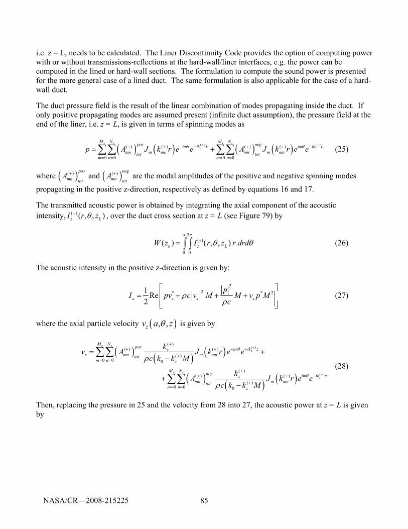
85

i.e. z = L, needs to be calculated. The Liner Discontinuity Code provides the option of computing power with or without transmissions-reflections at the hard-wall/liner interfaces, e.g. the power can be computed in the lined or hard-wall sections. The formulation to compute the sound power is presented for the more general case of a lined duct. The same formulation is also applicable for the case of a hard-wall duct.

The duct pressure field is the result of the linear combination of modes propagating inside the duct. If only positive propagating modes are assumed present (infinite duct assumption), the pressure field at the end of the liner, i.e. z = L, is given in terms of spinning modes as

( ) ( ) ( ) ( )( ) ( )( ) ( ) ( ) ( )

0 0 0 0

s s s sz z

M N M Npos negik L ik Lim immn m mn mn m mntot tot

m n m np A J k r e e A J k r e eθ θ+ +− −+ + − + +

= = = =

= +∑∑ ∑∑ (25)

where ( )( ) pos

mn totA + and ( )( ) neg

mn totA + are the modal amplitudes of the positive and negative spinning modes

propagating in the positive z-direction, respectively as defined by equations 16 and 17.

The transmitted acoustic power is obtained by integrating the axial component of the acoustic intensity, ( ) ( , , )z LI r zθ+ , over the duct cross section at z = L (see Figure 79) by

2

0 0

( ) , , )a

n z LW z I r z r drdπ

θ θ(+)= ( ∫ ∫ (26)

The acoustic intensity in the positive z-direction is given by:

2

2* * 21 Re2z z z z

pI pv c v M M v p M

cρ

ρ

⎡ ⎤= + + + ⎢ ⎥

⎢ ⎥⎣ ⎦ (27)

where the axial particle velocity ( ), ,zv a zθ is given by

( ) ( ) ( )

( ) ( ) ( )

( )

( )

( )( ) ( )

( )0 0 0

( )( ) ( )

( )0 0 0

s sz

s sz

M N pos ik zimzz mn m mntot

m n z

M N neg ik zimzmn m mntot

m n z

kv A J k r e ec k k M

kA J k r e ec k k M

θ

θ

ρ

ρ

+

+

+−+ + −

+= =

+−+ +

+= =

= +−

+−

∑∑

∑∑ (28)

Then, replacing the pressure in 25 and the velocity from 28 into 27, the acoustic power at z = L is given by

NASA/CR—2008-215225

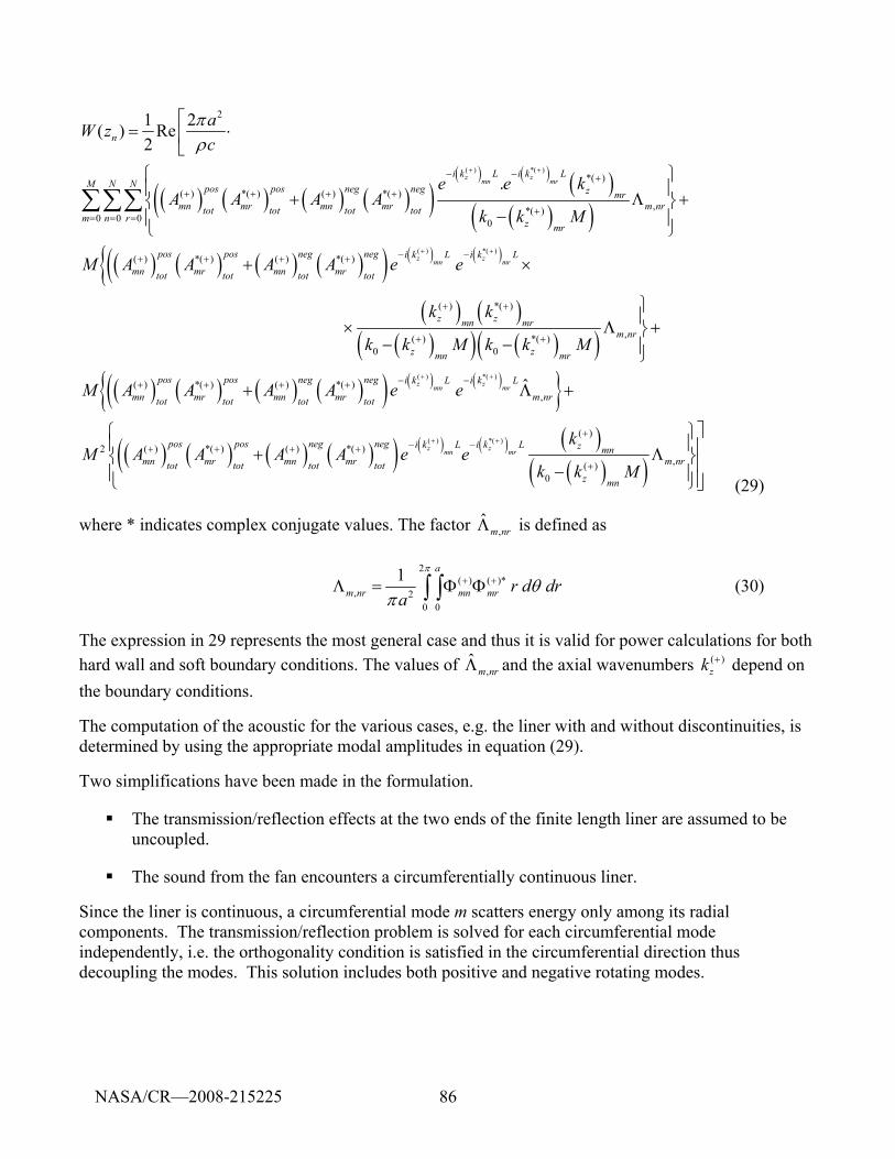
86

( ) ( ) ( ) ( )( )( ) ( ) ( )

( )( )( ) ( ) ( ) ( )( )

( ) *( )

2

*( )( ) *( ) ( ) *( )

,*( )0 0 0 0

( ) *( ) ( ) *( )

1 2( ) Re2

.z zmn mr

n

i k L i k LM N N pos pos neg neg z mr

mn mr mn mr m nrtot tot tot totm n r z mr

pos pos neg neg

mn mr mn mrtot tot tot tot

aW zc

e e kA A A A

k k M

M A A A A e

πρ

+ +− − +

+ + + +

+= = =

−+ + + +

⎡= ⋅⎢

⎣⎧ ⎫⎪ ⎪+ Λ +⎨ ⎬

−⎪ ⎪⎩ ⎭

+

∑∑∑

( ) ( ){( ) ( )

( )( ) ( )( )( ) ( )

( ) *( )

( ) *( )

,( ) *( )0 0

( ) *( ) (

z zmn mri k L i k L

z zmn mrm nr

z zmn mr

pos pos

mn mr mntot tot

e

k k

k k M k k M

M A A A

+ +−

+ +

+ +

+ + +

×

⎫⎪ × Λ +⎬

− − ⎪⎭

+ ( ) ( )( ) ( ) ( ){ }( ) ( ) ( ) ( )( ) ( ) ( ) ( )

( )( )

( ) *( )

( ) *( )

) *( ),

( )2 ( ) *( ) ( ) *( )

,( )0

ˆz zmn mr

z zmn mr

neg neg i k L i k L

mr m nrtot tot

pos pos neg neg i k L i k L z mnmn mr mn mr m nrtot tot tot tot

z mn

A e e

kM A A A A e e

k k M

+ +

+ +

− −+

+− −+ + + +

+

Λ +

⎤⎧ ⎫⎪ ⎪⎥+ Λ⎨ ⎬⎥−⎪ ⎪⎥⎩ ⎭⎦ (29)

where * indicates complex conjugate values. The factor ,ˆ

m nrΛ is defined as

2

( ) ( )*, 2

0 0

1 a

m nr mn mr r d dra

π

θπ

+ +Λ = Φ Φ ∫ ∫ (30)

The expression in 29 represents the most general case and thus it is valid for power calculations for both hard wall and soft boundary conditions. The values of ,

ˆm nrΛ and the axial wavenumbers ( )

zk + depend on the boundary conditions.

The computation of the acoustic for the various cases, e.g. the liner with and without discontinuities, is determined by using the appropriate modal amplitudes in equation (29).

Two simplifications have been made in the formulation.

The transmission/reflection effects at the two ends of the finite length liner are assumed to be uncoupled.

The sound from the fan encounters a circumferentially continuous liner.

Since the liner is continuous, a circumferential mode m scatters energy only among its radial components. The transmission/reflection problem is solved for each circumferential mode independently, i.e. the orthogonality condition is satisfied in the circumferential direction thus decoupling the modes. This solution includes both positive and negative rotating modes.

NASA/CR—2008-215225

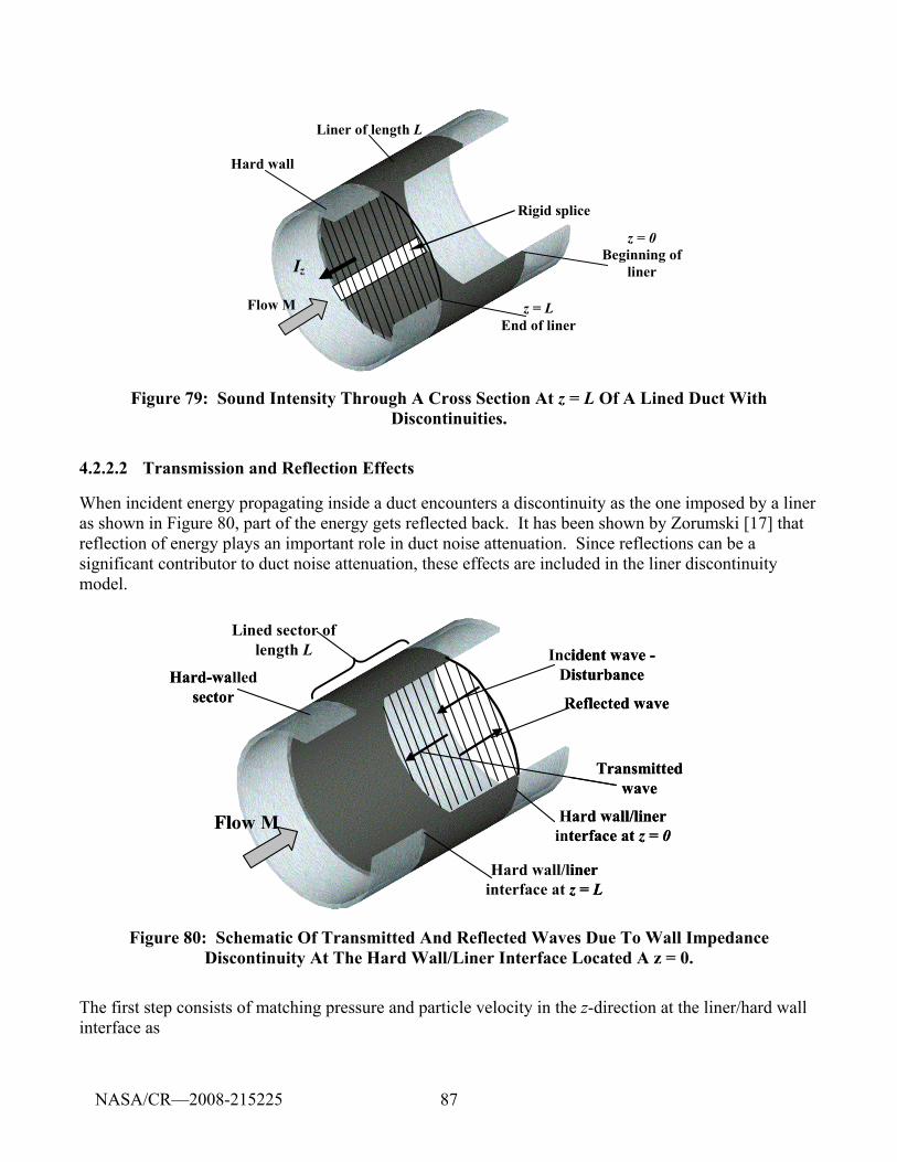
87

Liner of length L

Hard wall

Flow M

Iz

z = L End of liner

Rigid splice

z = 0 Beginning of

liner

Figure 79: Sound Intensity Through A Cross Section At z = L Of A Lined Duct With Discontinuities.

4.2.2.2 Transmission and Reflection Effects

When incident energy propagating inside a duct encounters a discontinuity as the one imposed by a liner as shown in Figure 80, part of the energy gets reflected back. It has been shown by Zorumski [17] that reflection of energy plays an important role in duct noise attenuation. Since reflections can be a significant contributor to duct noise attenuation, these effects are included in the liner discontinuity model.

Hard-walled sector

Flow M

Incident wave -Disturbance

Transmitted wave

Reflected wave

Hard wall/liner interface at z = L

Lined sector of length L

Hard wall/liner interface at z = 0

Hard-walled sector

Flow M

Incident wave -Disturbance

Transmitted wave

Reflected wave

Hard wall/liner interface at z = L

Lined sector of length L

Hard wall/liner interface at z = 0

Figure 80: Schematic Of Transmitted And Reflected Waves Due To Wall Impedance Discontinuity At The Hard Wall/Liner Interface Located A z = 0.

The first step consists of matching pressure and particle velocity in the z-direction at the liner/hard wall interface as

NASA/CR—2008-215225

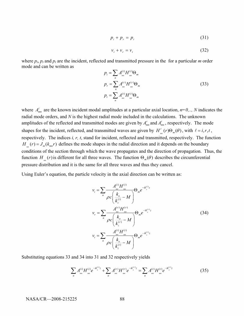
88

tri ppp =+ (31) tri vvv =+ (32)

where pi, pr and pt are the incident, reflected and transmitted pressure in the for a particular m order mode and can be written as

( ) ( )

( ) ( )

( ) ( )

mn mn

mn mn

mn mn

i ii m

nr r

r mn

t tt m

n

p A H

p A H

p A H

= Θ

= Θ

= Θ

∑

∑

∑

(33)

where imnA are the known incident modal amplitudes at a particular axial location, n=0,.., N indicates the

radial mode orders, and N is the highest radial mode included in the calculations. The unknown amplitudes of the reflected and transmitted modes are given by r

mnA and tmnA , respectively. The mode

shapes for the incident, reflected, and transmitted waves are given by ( ) ( )mn mH r θΘl , with , ,i r t=l ,

respectively. The indices i, r, t, stand for incident, reflected and transmitted, respectively. The function ( ) ( )

mn m mnH r J k r= defines the mode shapes in the radial direction and it depends on the boundary conditions of the section through which the wave propagates and the direction of propagation. Thus, the function ( )

mnH r is different for all three waves. The function ( )m θΘ describes the circumferential

pressure distribution and it is the same for all three waves and thus they cancel.

Using Euler’s equation, the particle velocity in the axial direction can be written as:

( )

( )

( )

( ) ( )

( )

( ) ( )

( )

( ) ( )

( )

imn mn z

rmn mn z

tmn mn z

i iik z

i mn o

iz

r rik z

r mn o

rz

t tik z

t mn o

tz

A Hv e

kc Mk

A Hv e

kc Mk

A Hv e

kc Mk

ρ

ρ

ρ

−

−

−

= Θ⎛ ⎞

−⎜ ⎟⎝ ⎠

= Θ⎛ ⎞

−⎜ ⎟⎝ ⎠

= Θ⎛ ⎞

−⎜ ⎟⎝ ⎠

∑

∑

∑

(34)

Substituting equations 33 and 34 into 31 and 32 respectively yields

( ) ( ) ( )

( ) ( ) ( ) ( ) ( ) ( )i r i

z z z

mn mn mn mn mn mn

ik z ik z ik zi i r r t t

n n nA H e A H e A H e− − −

+ =∑ ∑ ∑ (35)

NASA/CR—2008-215225

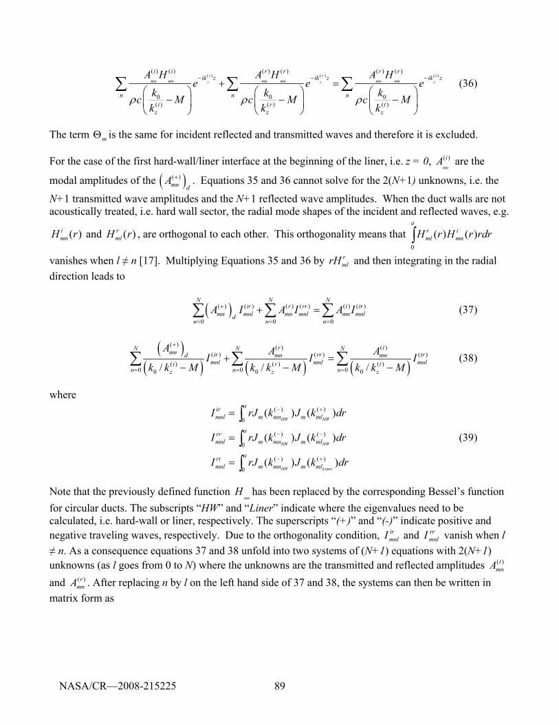
89

( ) ( ) ( )

( ) ( ) ( ) ( ) ( ) ( )

0 0 0( ) ( ) ( )

i r tmn mn mn mn mn mnz z z

i i r r r rik z ik z ik z

n n ni r t

z z z

A H A H A He e e

k k kc M c M c Mk k k

ρ ρ ρ

− − −+ =

⎛ ⎞ ⎛ ⎞ ⎛ ⎞− − −⎜ ⎟ ⎜ ⎟ ⎜ ⎟

⎝ ⎠ ⎝ ⎠ ⎝ ⎠

∑ ∑ ∑ (36)

The term mΘ is the same for incident reflected and transmitted waves and therefore it is excluded.

For the case of the first hard-wall/liner interface at the beginning of the liner, i.e. z = 0, ( )mn

iA are the

modal amplitudes of the ( )( )mn d

A + . Equations 35 and 36 cannot solve for the 2(N+1) unknowns, i.e. the

N+1 transmitted wave amplitudes and the N+1 reflected wave amplitudes. When the duct walls are not acoustically treated, i.e. hard wall sector, the radial mode shapes of the incident and reflected waves, e.g.

( )imnH r and )(rH r

ml , are orthogonal to each other. This orthogonality means that 0

( ) ( )a

r iml mnH r H r rdr∫

vanishes when l ≠ n [17]. Multiplying Equations 35 and 36 by rmlrH and then integrating in the radial

direction leads to

( )( ) ( ) ( ) ( ) ( ) ( )

0 0 0

N N Nir r rr t tr

mn mnl mn mnl mn mnldn n n

A I A I A I+

= = =

+ =∑ ∑ ∑ (37)

( )

( ) ( ) ( )( ) ( ) ( )

( ) ( ) ( )( ) ( ) ( )

0 0 00 0 0/ / /

r tN N Nmn ir rr trd mn mnmnl mnl mnli r t

n n nz z z

A A AI I Ik k M k k M k k M

+

= = =

+ =− − −

∑ ∑ ∑ (38)

where

( ) ( )

0

( ) ( )

0

( ) ( )

0

( ) ( )

( ) ( )

( ) ( )

HW HW

HW HW

HW Liner

airmnl m mn m ml

arrmnl m mn m ml

artmnl m mn m ml

I rJ k J k dr

I rJ k J k dr

I rJ k J k dr

− +

− −

− +

=

=

=

∫∫∫

(39)

Note that the previously defined function mn

H has been replaced by the corresponding Bessel’s function for circular ducts. The subscripts “HW” and “Liner” indicate where the eigenvalues need to be calculated, i.e. hard-wall or liner, respectively. The superscripts “(+)” and “(-)” indicate positive and negative traveling waves, respectively. Due to the orthogonality condition, ir

mnlI and rrmnlI vanish when l

≠ n. As a consequence equations 37 and 38 unfold into two systems of (N+1) equations with 2(N+1) unknowns (as l goes from 0 to N) where the unknowns are the transmitted and reflected amplitudes )(t

mnA and )(r

mnA . After replacing n by l on the left hand side of 37 and 38, the systems can then be written in matrix form as

NASA/CR—2008-215225

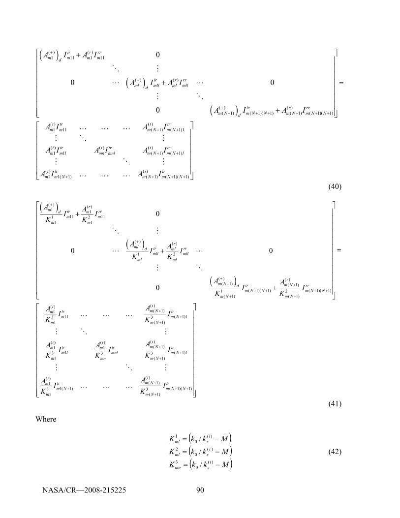
90

( )

( )

( )

( ) ( )1 11 1 11

( ) ( )

( ) ( )( 1) ( 1)( 1) ( 1) ( 1)( 1)

( ) ( )1 11 ( 1) ( 1)1

( ) ( )1 1 (

0

0 0

0

ir r rrm m m md

ir r rrml mll ml mlld

ir r rrm N m N N m N m N Nd

t tr t trm m m N m N

t tr t trm m l mn mnl m N

A I A I

A I A I

A I A I

A I A I

A I A I A

+

+

++ + + + + +

+ +

+

⎡ ⎤+⎢ ⎥⎢ ⎥⎢ ⎥

+ =⎢ ⎥⎢ ⎥⎢ ⎥⎢ ⎥+⎢ ⎥⎣ ⎦

O M

L L

M O

K K K

M O M( )

1) ( 1)

( ) ( )1 1( 1) ( 1) ( 1)( 1)

t trm N l

t tr i irm m N m N m N N

I

A I A I

+

+ + + +

⎡ ⎤⎢ ⎥⎢ ⎥⎢ ⎥⎢ ⎥⎢ ⎥⎢ ⎥⎣ ⎦

M O M

K K K

(40)

( )

( )

( )

( ) ( )1 1

11 111 21 1

( ) ( )

1 2

( ) ( )( 1) ( 1)

( 1)( 1) ( 1)( 1)1 2( 1) ( 1)

(( )( 1)1

1131

0

0 0

0

rm ir rrd m

m mm m

rml ir rrd ml

mll mllml ml

rm N m Nir rrd

m N N m N Nm N m N

tm Ntrm

mm

A AI IK K

A AI IK K

A AI I

K K

AA IK

+

+

++ +

+ + + ++ +

+

⎡ ⎤⎢ ⎥+⎢ ⎥⎢ ⎥⎢ ⎥⎢ ⎥⎢ ⎥ =+⎢ ⎥⎢ ⎥⎢ ⎥⎢ ⎥⎢ ⎥+⎢ ⎥⎣ ⎦

O M

L L

M O

K K K)

( 1)13( 1)

( )( ) ( )( 1)1 1

1 ( 1)3 3 31 ( 1)

( )( )( 1)1

1( 1) ( 1)( 1)3 31 ( 1)

ttrm N

m N

tt tm Ntr tr trm m

m l mnl m N lm mn m N

ttm Ntr trm

m N m N Nm m N

IK

AA AI I IK K K

AA I IK K

++

++

+

++ + +

+

⎡ ⎤⎢ ⎥⎢ ⎥⎢ ⎥⎢ ⎥⎢ ⎥⎢ ⎥⎢ ⎥⎢ ⎥⎢ ⎥⎢ ⎥⎢ ⎥⎢ ⎥⎣ ⎦

M O M

M O M

K K K

(41)

Where

( )( )( )MkkK

MkkK

MkkK

tzmn

rzml

izml

−=

−=

−=

)(0

3

)(0

2

)(0

1

/

/

/

(42)

NASA/CR—2008-215225

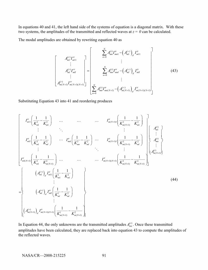
91

In equations 40 and 41, the left hand side of the systems of equation is a diagonal matrix. With these two systems, the amplitudes of the transmitted and reflected waves at z = 0 can be calculated.

The modal amplitudes are obtained by rewriting equation 40 as

( )

( )

( )

( ) ( )1 1 11

0( )1 11

( ) ( )( )

0

( )( 1) ( 1)( 1)

( ) ( )( 1) ( 1) ( 1)( 1)

0

Nt tr ir

mn mn m mdnr rr

m m

Nt tr irr rr

mn mnl ml mllml mll dn

r rrm N m N N N

t tr irmn mn N m N m N Nd

n

A I A IA I

A I A IA I

A IA I A I

+

=

+

=

+ + ++

+ + + +=

⎡ ⎤−⎢ ⎥

⎢ ⎥⎡ ⎤⎢ ⎥⎢ ⎥⎢ ⎥⎢ ⎥⎢ ⎥⎢ ⎥ = −⎢ ⎥⎢ ⎥⎢ ⎥⎢ ⎥⎢ ⎥⎢ ⎥

⎣ ⎦ ⎢−⎢

⎣ ⎦

∑

∑

∑

MM

MM

⎥⎥

(43)

Substituting Equation 43 into 41 and reordering produces

11 ( 1)13 2 3 21 1 ( 1) 1

1 ( 1)3 2 3 2 3 21 ( 1)

1( 1) ( 1)( 1)3 21 ( 1) (

1 1 1 1

1 1 1 1 1 1

1 1 1

tr trm m N

m m m N m

tr tr trm l mnl m N l

m ml mn ml m N ml

tr trm N m N N

m m N m

I IK K K K

I I IK K K K K K

I IK K K

++

++

+ + ++

⎛ ⎞⎛ ⎞− −⎜ ⎟⎜ ⎟ ⎜ ⎟⎝ ⎠ ⎝ ⎠

⎛ ⎞⎛ ⎞ ⎛ ⎞− − −⎜ ⎟⎜ ⎟ ⎜ ⎟ ⎜ ⎟⎝ ⎠ ⎝ ⎠ ⎝ ⎠

⎛ ⎞−⎜ ⎟⎜ ⎟

⎝ ⎠

K K K

M O M

L L

M O M

K K K

( )

( )

( )

( )1

( )

( )( 1)

3 21) ( 1)

( )1 11 1 2

1 1

( )1 2

( )( 1) ( 1)( 1) 1 2

( 1) ( 1)

1

1 1

1 1

1 1

tm

tmn

tm N

N m N

irm md

m m

irml mlld

ml ml

irm N m N Nd

m N m N

A

A

A

K

A IK K

A IK K

A IK K

+

+ +

+

+

++ + +

+ +

⎡ ⎤⎢ ⎥⎢ ⎥

⎧ ⎫⎢ ⎥⎪ ⎪⎢ ⎥⎪ ⎪⎢ ⎥ ⎪ ⎪⎢ ⎥ ⎨ ⎬

⎢ ⎥ ⎪ ⎪⎢ ⎥ ⎪ ⎪⎢ ⎥ ⎪ ⎪⎩ ⎭⎢ ⎥⎛ ⎞⎢ ⎥−⎜ ⎟⎜ ⎟⎢ ⎥⎝ ⎠⎣ ⎦

⎛ ⎞−⎜ ⎟

⎝ ⎠

⎛ ⎞−= ⎜ ⎟

⎝ ⎠

−

M

M

M

M

⎧ ⎫⎪ ⎪⎪ ⎪⎪ ⎪⎪ ⎪⎪ ⎪⎪ ⎪⎨ ⎬⎪ ⎪⎪ ⎪⎪ ⎪

⎛ ⎞⎪ ⎪⎜ ⎟⎪ ⎪⎜ ⎟⎪ ⎪⎝ ⎠⎩ ⎭

(44)

In Equation 44, the only unknowns are the transmitted amplitudes )(tmnA . Once these transmitted

amplitudes have been calculated, they are replaced back into equation 43 to compute the amplitudes of the reflected waves.

NASA/CR—2008-215225

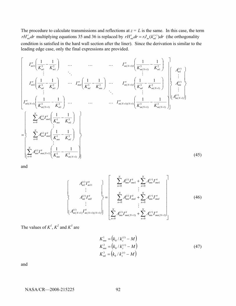
92

The procedure to calculate transmissions and reflections at z = L is the same. In this case, the term drrH r

ml multiplying equations 35 and 36 is replaced by ( )( )tml m mlrH dr rJ k dr+= (the orthogonality

condition is satisfied in the hard wall section after the liner). Since the derivation is similar to the leading edge case, only the final expressions are provided.

⎪⎪⎪⎪⎪

⎭

⎪⎪⎪⎪⎪

⎬

⎫

⎪⎪⎪⎪⎪

⎩

⎪⎪⎪⎪⎪

⎨

⎧

⎟⎟⎠

⎞⎜⎜⎝

⎛−

⎟⎟⎠

⎞⎜⎜⎝

⎛−

⎟⎟⎠

⎞⎜⎜⎝

⎛−

=

⎪⎪⎪

⎭

⎪⎪⎪

⎬

⎫

⎪⎪⎪

⎩

⎪⎪⎪

⎨

⎧

⎥⎥⎥⎥⎥⎥⎥⎥⎥⎥

⎦

⎤

⎢⎢⎢⎢⎢⎢⎢⎢⎢⎢

⎣

⎡

⎟⎟⎠

⎞⎜⎜⎝

⎛−⎟

⎟⎠

⎞⎜⎜⎝

⎛−

⎟⎟⎠

⎞⎜⎜⎝

⎛−⎟⎟

⎠

⎞⎜⎜⎝

⎛−⎟⎟

⎠

⎞⎜⎜⎝

⎛−

⎟⎟⎠

⎞⎜⎜⎝

⎛−⎟⎟

⎠

⎞⎜⎜⎝

⎛−

∑

∑

∑

= ++

=

=

+

++++

++

++

++

N

n Nmmn

itNmn

imn

N

n mlmn

itmnl

imn

N

n mmn

itmn

imn

rNm

rmn

rm

NmNm

rtNNm

mNm

rtNm

Nmml

rtlNm

mnml

rtmnl

mml

rtlm

mNm

rtNm

mm

rtm

KKIA

KKIA

KKIA

A

A

A

KKI

KKI

KKI

KKI

KKI

KKI

KKI

03

)1(1)1(

)(

031

)(

03

111

)(

)()1(

)(

)(1

2)1(

3)1(

)1)(1(21

3)1(

)1(1

2)1(

3)1(2321

31

21

3)1(

1)1(21

31

11

11

11

11

1111

111111

1111

M

M

M

M

KKK

MOM

LL

MOM

KKK

(45)

and

⎥⎥⎥⎥⎥⎥⎥⎥

⎦

⎤

⎢⎢⎢⎢⎢⎢⎢⎢

⎣

⎡

+

+

+

=

⎪⎪⎪

⎭

⎪⎪⎪

⎬

⎫

⎪⎪⎪

⎩

⎪⎪⎪

⎨

⎧

∑∑

∑∑

∑∑

=+

=+

==

==

+++N

n

rtNmn

rmn

N

n

itNmn

imn

N

n

rtmnl

rmn

N

n

itmnl

imn

N

n

rtmn

rmn

N

n

itmn

imn

ttNNm

tNm

ttmll

tml

ttm

tm

IAIA

IAIA

IAIA

IA

IA

IA

0)1(

)(

0)1(

)(

0

)(

0

)(

01

)(

01

)(

)1)(1()(

)1(

)(

11)(1

M

M

M

M

(46)

The values of K1, K2 and K3 are

( )( )( )MkkK

MkkK

MkkK

tzml

rzmn

izmn

−=

−=

−=

)(0

3

)(0

2

)(0

1

/

/

/

(47)

and

NASA/CR—2008-215225

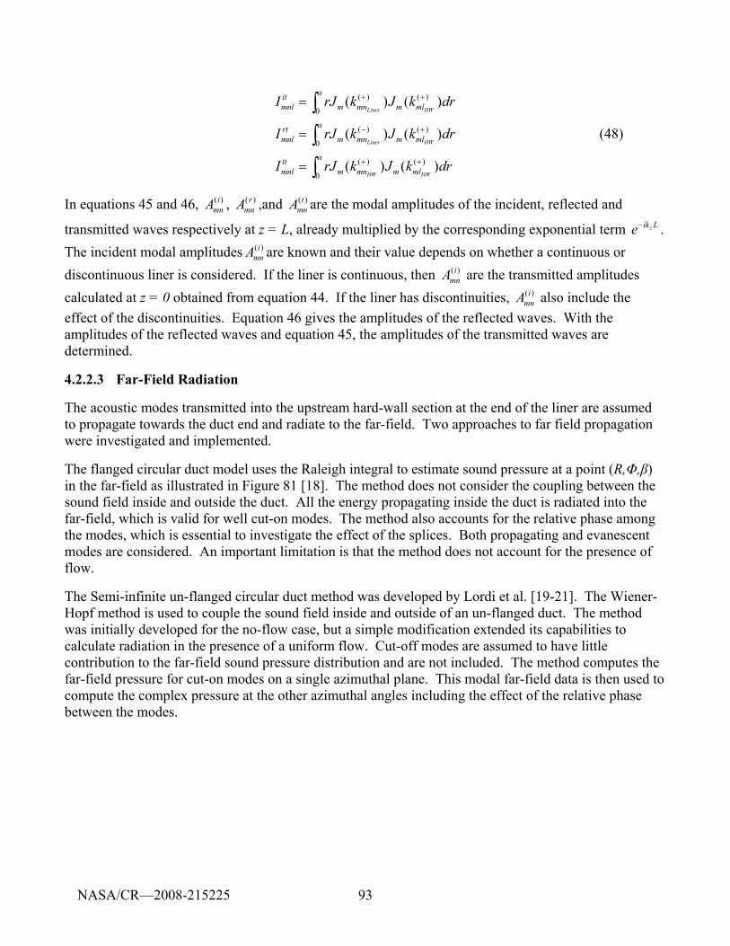
93

( ) ( )

0

( ) ( )

0

( ) ( )

0

( ) ( )

( ) ( )

( ) ( )

Liner HW

Liner HW

HW HW

aitmnl m mn m ml

artmnl m mn m ml

attmnl m mn m ml

I rJ k J k dr

I rJ k J k dr

I rJ k J k dr

+ +

− +

+ +

=

=

=

∫∫∫

(48)

In equations 45 and 46, ( )imnA , ( )r

mnA ,and ( )tmnA are the modal amplitudes of the incident, reflected and

transmitted waves respectively at z = L, already multiplied by the corresponding exponential term zik Le− . The incident modal amplitudes ( )i

mnA are known and their value depends on whether a continuous or discontinuous liner is considered. If the liner is continuous, then ( )i

mnA are the transmitted amplitudes calculated at z = 0 obtained from equation 44. If the liner has discontinuities, ( )i

mnA also include the effect of the discontinuities. Equation 46 gives the amplitudes of the reflected waves. With the amplitudes of the reflected waves and equation 45, the amplitudes of the transmitted waves are determined.

4.2.2.3 Far-Field Radiation

The acoustic modes transmitted into the upstream hard-wall section at the end of the liner are assumed to propagate towards the duct end and radiate to the far-field. Two approaches to far field propagation were investigated and implemented.

The flanged circular duct model uses the Raleigh integral to estimate sound pressure at a point (R,Φ,β) in the far-field as illustrated in Figure 81 [18]. The method does not consider the coupling between the sound field inside and outside the duct. All the energy propagating inside the duct is radiated into the far-field, which is valid for well cut-on modes. The method also accounts for the relative phase among the modes, which is essential to investigate the effect of the splices. Both propagating and evanescent modes are considered. An important limitation is that the method does not account for the presence of flow.

The Semi-infinite un-flanged circular duct method was developed by Lordi et al. [19-21]. The Wiener-Hopf method is used to couple the sound field inside and outside of an un-flanged duct. The method was initially developed for the no-flow case, but a simple modification extended its capabilities to calculate radiation in the presence of a uniform flow. Cut-off modes are assumed to have little contribution to the far-field sound pressure distribution and are not included. The method computes the far-field pressure for cut-on modes on a single azimuthal plane. This modal far-field data is then used to compute the complex pressure at the other azimuthal angles including the effect of the relative phase between the modes.

NASA/CR—2008-215225

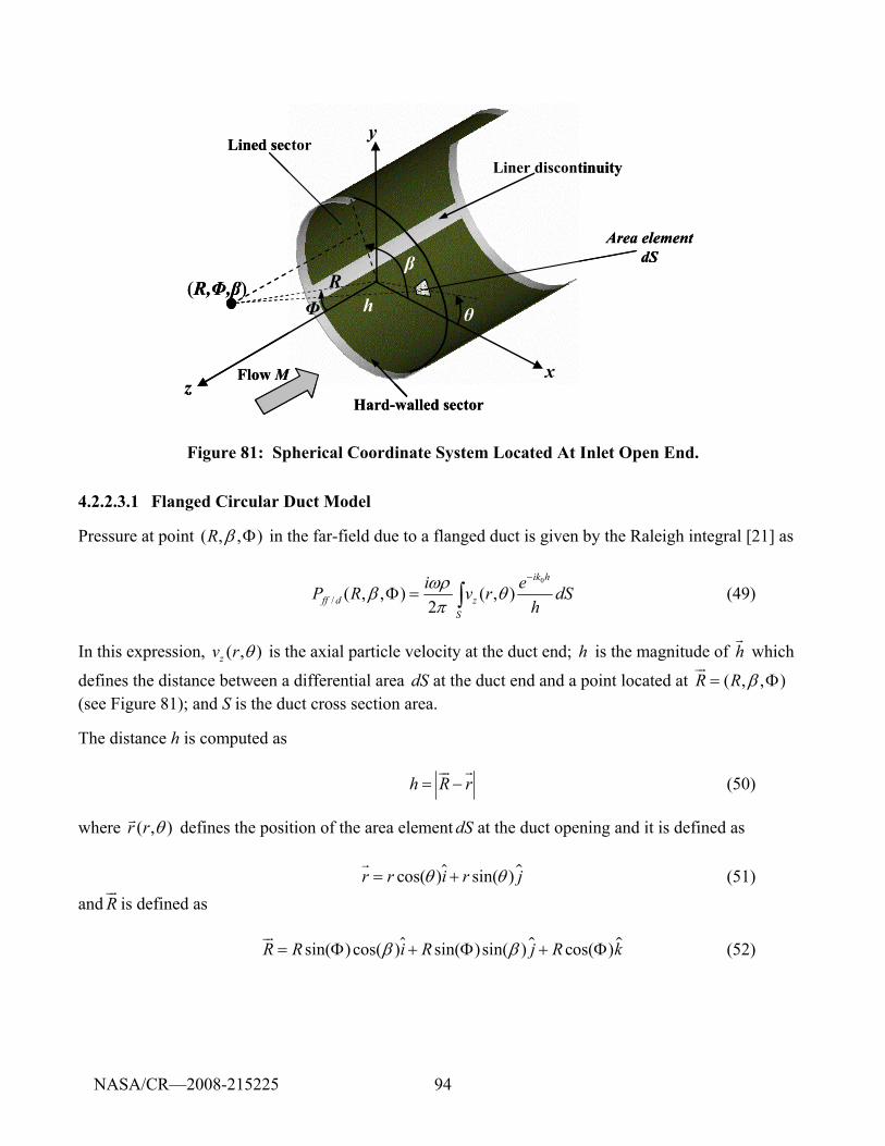
94

z

y

θΦR

Lined sector

Hard-walled sector

Liner discontinuity

Flow M x

(R,Φ,β)h

Area element dSβ

z

y

θΦR

Lined sector

Hard-walled sector

Liner discontinuity

Flow M x

(R,Φ,β)h

Area element dSβ

Figure 81: Spherical Coordinate System Located At Inlet Open End.

4.2.2.3.1 Flanged Circular Duct Model

Pressure at point ( , , )R β Φ in the far-field due to a flanged duct is given by the Raleigh integral [21] as

0

/ ( , , ) ( , )2

ik h

ff d zS

i eP R v r dSh

ωρβ θπ

−

Φ = ∫ (49)

In this expression, ( , )zv r θ is the axial particle velocity at the duct end; h is the magnitude of hr

which

defines the distance between a differential area dS at the duct end and a point located at ( , , )R R β= Φur

(see Figure 81); and S is the duct cross section area.

The distance h is computed as h R r= −

ur r (50)

where ( , )r r θr defines the position of the area element dS at the duct opening and it is defined as $cos( ) sin( )r r i r jθ θ= +

r$ (51)

and Rur

is defined as $ $sin( )cos( ) sin( )sin( ) cos( )R R i R j R kβ β= Φ + Φ + Φ

ur$ (52)

NASA/CR—2008-215225

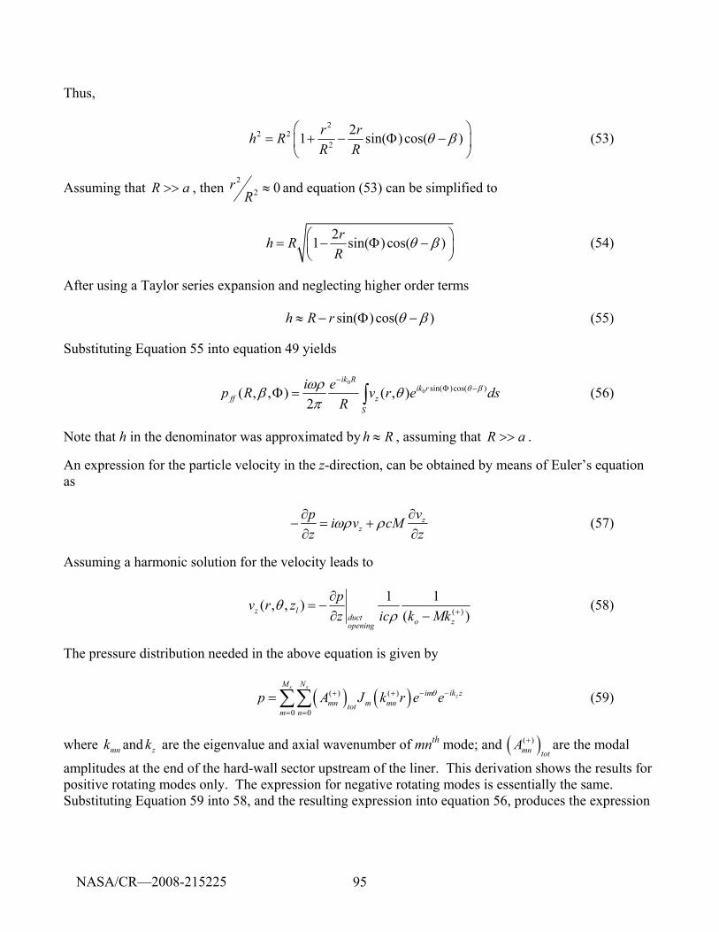
95

Thus,

2

2 22

21 sin( )cos( )r rh RR R

θ β⎛ ⎞

= + − Φ −⎜ ⎟⎝ ⎠

(53)

Assuming that R a>> , then 2

2 0rR ≈ and equation (53) can be simplified to

21 sin( ) cos( )rh RR

θ β⎛ ⎞= − Φ −⎜ ⎟⎝ ⎠

(54)

After using a Taylor series expansion and neglecting higher order terms sin( )cos( )h R r θ β≈ − Φ − (55)

Substituting Equation 55 into equation 49 yields

0

0 sin( )cos( )( , , ) ( , )2

ik Rik r

ff zS

i ep R v r e dsR

θ βωρβ θπ

−Φ −Φ = ∫ (56)

Note that h in the denominator was approximated by h R≈ , assuming that R a>> .

An expression for the particle velocity in the z-direction, can be obtained by means of Euler’s equation as

zz

vp i v cMz z

ωρ ρ ∂∂− = +

∂ ∂ (57)

Assuming a harmonic solution for the velocity leads to

( )

1 1( , , )( )z l

duct o zopening

pv r zz ic k Mk

θρ +

∂= −

∂ − (58)

The pressure distribution needed in the above equation is given by

( ) ( )( ) ( )

0 0

s sz

M Nik zim

mn m mntotm n

p A J k r e eθ −+ + −

= =

= ∑∑ (59)

where mnk and zk are the eigenvalue and axial wavenumber of mnth mode; and ( )( )mn tot

A + are the modal

amplitudes at the end of the hard-wall sector upstream of the liner. This derivation shows the results for positive rotating modes only. The expression for negative rotating modes is essentially the same. Substituting Equation 59 into 58, and the resulting expression into equation 56, produces the expression

NASA/CR—2008-215225

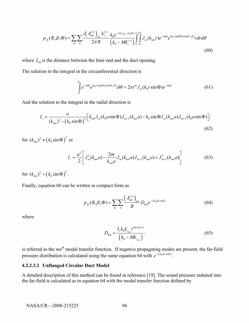
96

( )

( )0

0

( ) ( ) 2( )sin( )cos( )0

( )0 00

( , , ) ( )2

z de ai k L k Rmn z ik rimtot

ff m mnm n z

i A k k ep R J k r e e rdrdR k Mk

πθ βθβ θ

π

+ + − +Φ −−

+Φ =

−∑∑ ∫ ∫

(60)

where deL is the distance between the liner end and the duct opening.

The solution to the integral in the circumferential direction is

0

2sin( )cos( )

00

2 ( sin )ik rim m imme e d i J k r e

πθ βθ βθ πΦ −− −= Φ∫ (61)

And the solution to the integral in the radial direction is

( ) 0 1 0 1 022

0

( sin ) ( ) sin ( ) ( sin )( ) sin

r mn m m mn m mn mmn

aI k J k a J k a k J k a J k ak k

+ +⎡ ⎤= Φ − Φ Φ⎣ ⎦− Φ

(62)

for ( )220( ) sinmnk k≠ Φ or

2

2 21 1

2( ) ( ) ( ) ( )2r m mn m mn m mn m mn

mn

a mI J k a J k a J k a J k ak a + +

⎡ ⎤= − +⎢ ⎥

⎣ ⎦ (63)

for ( )220( ) sinmnk k= Φ .

Finally, equation 60 can be written in compact form as

( )

0

( )( )( , , )

mn i k R mtotff mn

m n

Ap R D e

Rββ

+

− +Φ = ∑∑ (64)

where

( )

( ) 10

0

mn

mn

abs mr z

mnz

I k k iD

k Mk

+

=−

(65)

is referred as the mnth modal transfer function. If negative propagating modes are present, the far-field pressure distribution is calculated using the same equation 64 with 0( )i k R me β− − .

4.2.2.3.2 Unflanged Circular Duct Model

A detailed description of this method can be found in reference [19]. The sound pressure radiated into the far-field is calculated as in equation 64 with the modal transfer function defined by

NASA/CR—2008-215225

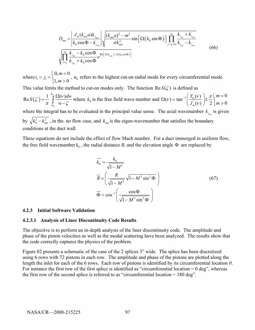
97

( )0

1

00

1

2 2

020

Re ( ) ( cos )0

0

( ) ( ) sin sincos

coscos

mj mnmn

mn mj mn

zmi mn

mi

nz zm mn z mn

mnj j nz mn z z

nS k S kz

i i z

k kJ k a k k a mD kk k k k k

k ke

k k

π = ≠

⎡ ⎤− Φ⎣ ⎦

=

+−⎡ ⎤= Ω Φ⎣ ⎦Φ − −

− Φ

+ Φ

∏

∏ (66)

where 1 1

0, 01, 0

mi j

m=⎧

= = ⎨ >⎩, 0n refers to the highest cut-on radial mode for every circumferential mode.

This value limits the method to cut-on modes only. The function Re ( )S ζ is defined as

( )0

0

1 ( )Rek

k

dwSwνζ

π ζ−

Ω=

−∫ where 0k is the free field wave number and '

1'

0( )( ) tan0( ) 2

m

m

mYmJ

ν πνν

− =⎛ ⎞ ⎧Ω = ± ⎨⎜ ⎟ >⎩⎝ ⎠

where the integral has to be evaluated in the principal value sense. The axial wavenumber mnzk is given

by 2 20 mnk k− , in the. no flow case, and mnk is the eigen-wavenumber that satisfies the boundary

conditions at the duct wall.

These equations do not include the effect of flow Mach number. For a duct immerged in uniform flow, the free field wavenumber 0k , the radial distance R, and the elevation angle Φ are replaced by

00 2

2 2

2

1

2 2

1

1 sin1

coscos1 sin

kkM

RR MM

M−

=−

⎛ ⎞= − Φ⎜ ⎟

−⎝ ⎠⎛ ⎞Φ

Φ = ⎜ ⎟− Φ⎝ ⎠

(67)

4.2.3 Initial Software Validation

4.2.3.1 Analysis of Liner Discontinuity Code Results

The objective is to perform an in-depth analysis of the liner discontinuity code. The amplitude and phase of the piston velocities as well as the modal scattering have been analyzed. The results show that the code correctly captures the physics of the problem.

Figure 82 presents a schematic of the case of the 2 splices 3” wide. The splice has been discretized using 6 rows with 72 pistons in each row. The amplitude and phase of the pistons are plotted along the length the inlet for each of the 6 rows. Each row of pistons is identified by its circumferential location θ. For instance the first row of the first splice is identified as “circumferential location = 0 deg”, whereas the first row of the second splice is referred to as “circumferential location = 180 deg”.

NASA/CR—2008-215225

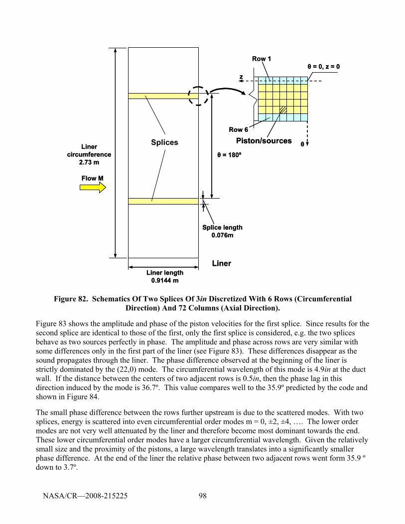
98

Liner circumference

2.73 m

Liner length 0.9144 m

θ = 180º

Splice length 0.076m

Flow M

Splices θ

z

Row 1

Row 6

θ = 0, z = 0

Piston/sources

Liner

Liner circumference

2.73 m

Liner length 0.9144 m

θ = 180º

Splice length 0.076m

Flow M

Splices θ

z

Row 1

Row 6

θ = 0, z = 0

Piston/sources

Liner

Figure 82. Schematics Of Two Splices Of 3in Discretized With 6 Rows (Circumferential Direction) And 72 Columns (Axial Direction).

Figure 83 shows the amplitude and phase of the piston velocities for the first splice. Since results for the second splice are identical to those of the first, only the first splice is considered, e.g. the two splices behave as two sources perfectly in phase. The amplitude and phase across rows are very similar with some differences only in the first part of the liner (see Figure 83). These differences disappear as the sound propagates through the liner. The phase difference observed at the beginning of the liner is strictly dominated by the (22,0) mode. The circumferential wavelength of this mode is 4.9in at the duct wall. If the distance between the centers of two adjacent rows is 0.5in, then the phase lag in this direction induced by the mode is 36.7º. This value compares well to the 35.9º predicted by the code and shown in Figure 84.

The small phase difference between the rows further upstream is due to the scattered modes. With two splices, energy is scattered into even circumferential order modes m = 0, ±2, ±4, …. The lower order modes are not very well attenuated by the liner and therefore become most dominant towards the end. These lower circumferential order modes have a larger circumferential wavelength. Given the relatively small size and the proximity of the pistons, a large wavelength translates into a significantly smaller phase difference. At the end of the liner the relative phase between two adjacent rows went form 35.9 º down to 3.7º.

NASA/CR—2008-215225

99

Figure 85 through Figure 87 show sound power scattered into several circumferential order modes as they progress through the liner. The mode (22,0) is included in Figure 87. As it can be observed, positive and negative rotating modes converge towards the same sound power level at the end of the liner. Note that higher circumferential order modes converge faster than lower circumferential modes. Also note that at the beginning of the liner, the power difference between positive and negative rotating modes is more important for the higher order modes.

The case of 3 splices of 2” width was also simulated. Figure 88 through Figure 90 present the amplitude and phase of piston velocities. The 2 in splices were represented with 4 rows of 72 piston sources. Figure 88 shows the amplitude and phase of piston velocities for every row of pistons in the first of the three splices. Like in the previous case, the same behavior or trends is observed for this case. The phase lag between sources of adjacent rows is determined by the circumferential wavelength of the . For the present case, this translates into a phase difference of 36.7º which compares very well with the 34.4º shown in Figure 89.

Finally, Figure 90 shows a phase difference between pistons along the first row of each one of the three splices. The phase difference between splices is 120º, e.g. the splices behave as three sources with a phase difference of 120º.

NASA/CR—2008-215225

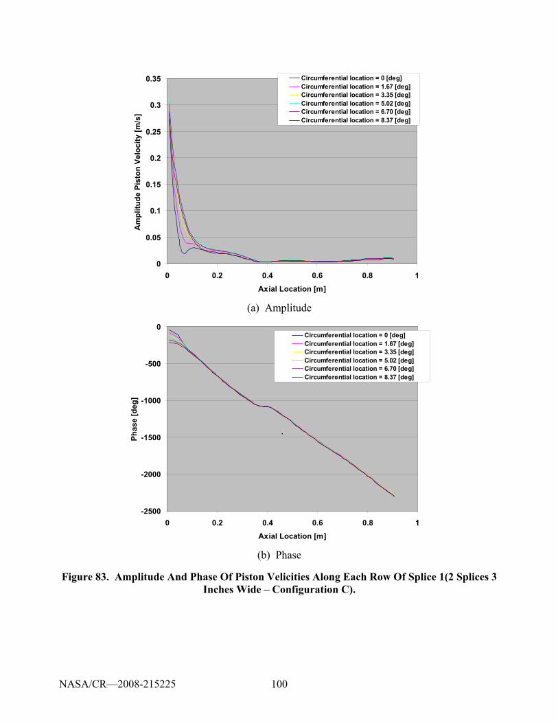
100

0

0.05

0.1

0.15

0.2

0.25

0.3

0.35

0 0.2 0.4 0.6 0.8 1Axial Location [m]

Am

plitu

de P

isto

n Ve

loci

ty [m

/s]

Circumferential location = 0 [deg]Circumferential location = 1.67 [deg]Circumferential location = 3.35 [deg]Circumferential location = 5.02 [deg]Circumferential location = 6.70 [deg]Circumferential location = 8.37 [deg]

(a) Amplitude

-2500

-2000

-1500

-1000

-500

0

0 0.2 0.4 0.6 0.8 1Axial Location [m]

Phas

e [d

eg]


`

(b) Phase

Figure 83. Amplitude And Phase Of Piston Velicities Along Each Row Of Splice 1(2 Splices 3 Inches Wide – Configuration C).

NASA/CR—2008-215225

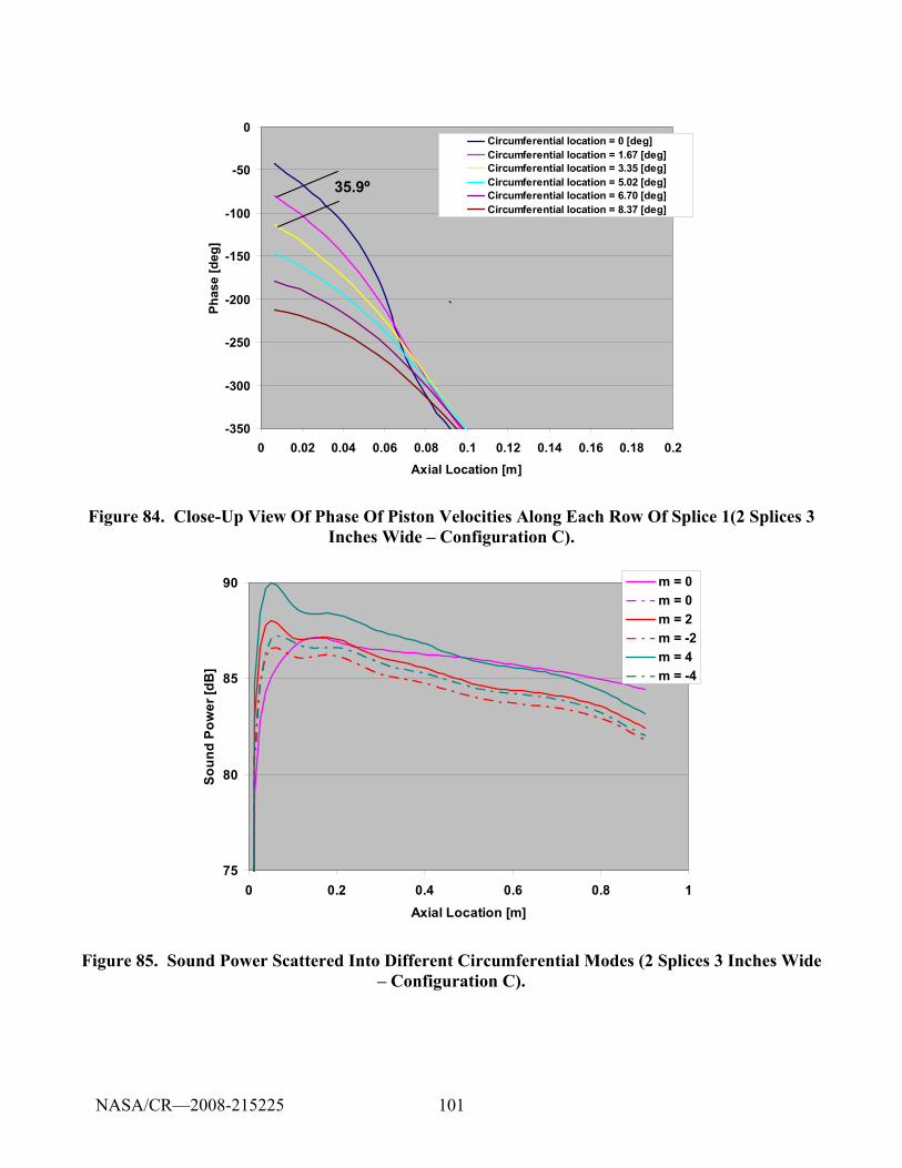
101

-350

-300

-250

-200

-150

-100

-50

0

0 0.02 0.04 0.06 0.08 0.1 0.12 0.14 0.16 0.18 0.2Axial Location [m]

Phas

e [d

eg]


`

35.9º

-350

-300

-250

-200

-150

-100

-50

0

0 0.02 0.04 0.06 0.08 0.1 0.12 0.14 0.16 0.18 0.2Axial Location [m]

Phas

e [d

eg]


`

35.9º

Figure 84. Close-Up View Of Phase Of Piston Velocities Along Each Row Of Splice 1(2 Splices 3 Inches Wide – Configuration C).

75

80

85

90

0 0.2 0.4 0.6 0.8 1Axial Location [m]

Soun

d Po

wer

[dB

]

m = 0m = 0m = 2m = -2m = 4m = -4

Figure 85. Sound Power Scattered Into Different Circumferential Modes (2 Splices 3 Inches Wide – Configuration C).

NASA/CR—2008-215225

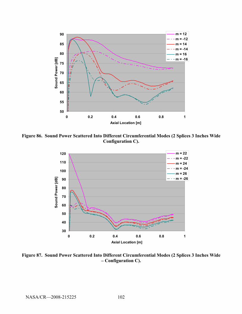
102

50

55

60

65

70

75

80

85

90

0 0.2 0.4 0.6 0.8 1Axial Location [m]

Soun

d Po

wer

[dB

]

m = 12m = -12m = 14m = -14m = 16m = -16

Figure 86. Sound Power Scattered Into Different Circumferential Modes (2 Splices 3 Inches Wide Configuration C).

30

40

50

60

70

80

90

100

110

120

0 0.2 0.4 0.6 0.8 1Axial Location [m]

Soun

d Po

wer

[dB

]

m = 22m = -22m = 24m = -24m = 26m = -26

Figure 87. Sound Power Scattered Into Different Circumferential Modes (2 Splices 3 Inches Wide – Configuration C).

NASA/CR—2008-215225

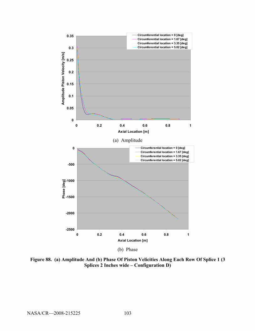
103

0

0.05

0.1

0.15

0.2

0.25

0.3

0.35

0 0.2 0.4 0.6 0.8 1Axial Location [m]

Am

plitu

de P

isto

n Ve

loci

ty [m

/s]

Circumferential location = 0 [deg]Circumferential location = 1.67 [deg]Circumferential location = 3.35 [deg]Circumferential location = 5.02 [deg]

(a) Amplitude

-2500

-2000

-1500

-1000

-500

0

0 0.2 0.4 0.6 0.8 1Axial Location [m]

Phas

e [d

eg]


(b) Phase

Figure 88. (a) Amplitude And (b) Phase Of Piston Velicities Along Each Row Of Splice 1 (3 Splices 2 Inches wide – Configuration D)

NASA/CR—2008-215225

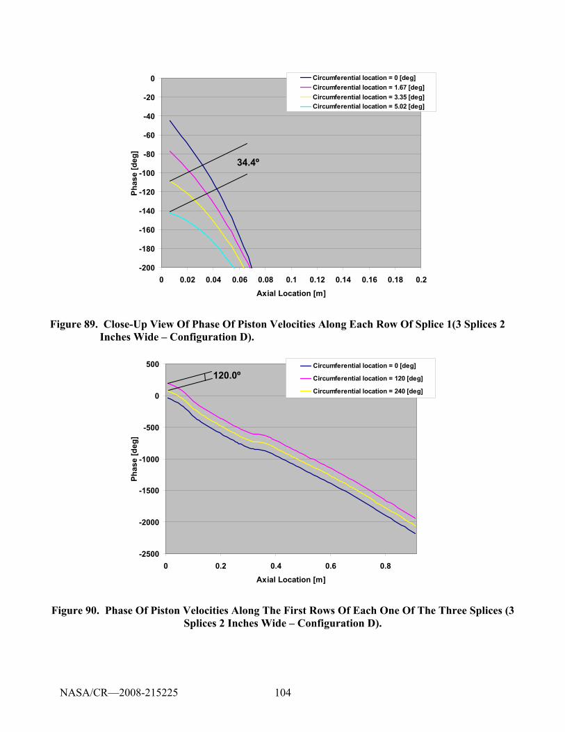
104

-200

-180

-160

-140

-120

-100

-80

-60

-40

-20

0

0 0.02 0.04 0.06 0.08 0.1 0.12 0.14 0.16 0.18 0.2Axial Location [m]

Phas

e [d

eg]


34.4º

-200

-180

-160

-140

-120

-100

-80

-60

-40

-20

0

0 0.02 0.04 0.06 0.08 0.1 0.12 0.14 0.16 0.18 0.2Axial Location [m]

Phas

e [d

eg]


34.4º

Figure 89. Close-Up View Of Phase Of Piston Velocities Along Each Row Of Splice 1(3 Splices 2 Inches Wide – Configuration D).

-2500

-2000

-1500

-1000

-500

0

500

0 0.2 0.4 0.6 0.8Axial Location [m]

Phas

e [d

eg]

Circumferential location = 0 [deg]



120.0º

-2500

-2000

-1500

-1000

-500

0

500

0 0.2 0.4 0.6 0.8Axial Location [m]

Phas

e [d

eg]




120.0º

Figure 90. Phase Of Piston Velocities Along The First Rows Of Each One Of The Three Splices (3 Splices 2 Inches Wide – Configuration D).

NASA/CR—2008-215225

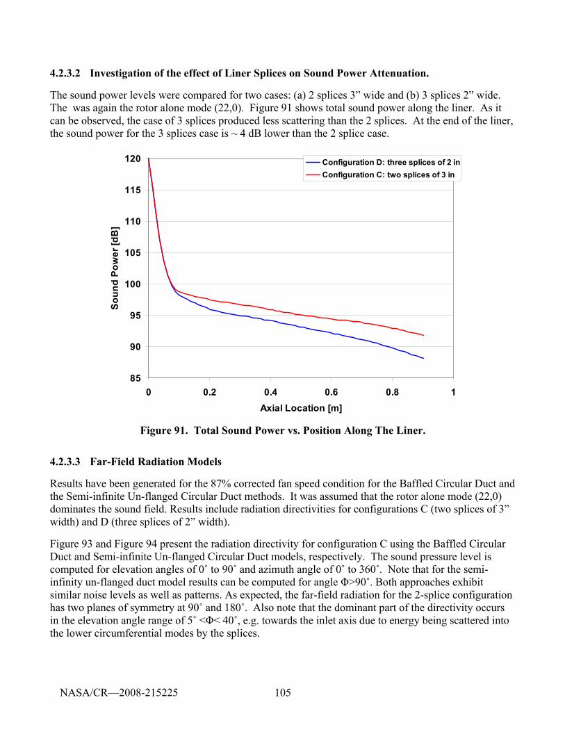
105

4.2.3.2 Investigation of the effect of Liner Splices on Sound Power Attenuation.

The sound power levels were compared for two cases: (a) 2 splices 3” wide and (b) 3 splices 2” wide. The was again the rotor alone mode (22,0). Figure 91 shows total sound power along the liner. As it can be observed, the case of 3 splices produced less scattering than the 2 splices. At the end of the liner, the sound power for the 3 splices case is ~ 4 dB lower than the 2 splice case.

85

90

95

100

105

110

115

120

0 0.2 0.4 0.6 0.8 1Axial Location [m]

Soun

d Po

wer

[dB

]

Configuration D: three splices of 2 inConfiguration C: two splices of 3 in

Figure 91. Total Sound Power vs. Position Along The Liner.

4.2.3.3 Far-Field Radiation Models

Results have been generated for the 87% corrected fan speed condition for the Baffled Circular Duct and the Semi-infinite Un-flanged Circular Duct methods. It was assumed that the rotor alone mode (22,0) dominates the sound field. Results include radiation directivities for configurations C (two splices of 3” width) and D (three splices of 2” width).

Figure 93 and Figure 94 present the radiation directivity for configuration C using the Baffled Circular Duct and Semi-infinite Un-flanged Circular Duct models, respectively. The sound pressure level is computed for elevation angles of 0˚ to 90˚ and azimuth angle of 0˚ to 360˚. Note that for the semi-infinity un-flanged duct model results can be computed for angle Φ>90˚. Both approaches exhibit similar noise levels as well as patterns. As expected, the far-field radiation for the 2-splice configuration has two planes of symmetry at 90˚ and 180˚. Also note that the dominant part of the directivity occurs in the elevation angle range of 5˚ <Φ< 40˚, e.g. towards the inlet axis due to energy being scattered into the lower circumferential modes by the splices.

NASA/CR—2008-215225

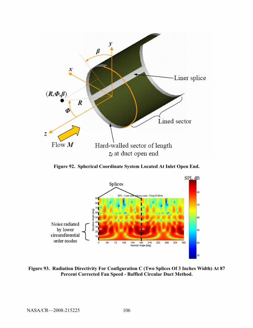
106

Figure 92. Spherical Coordinate System Located At Inlet Open End.

Figure 93. Radiation Directivity For Configuration C (Two Splices Of 3 Inches Width) At 87 Percent Corrected Fan Speed - Baffled Circular Duct Method.

NASA/CR—2008-215225

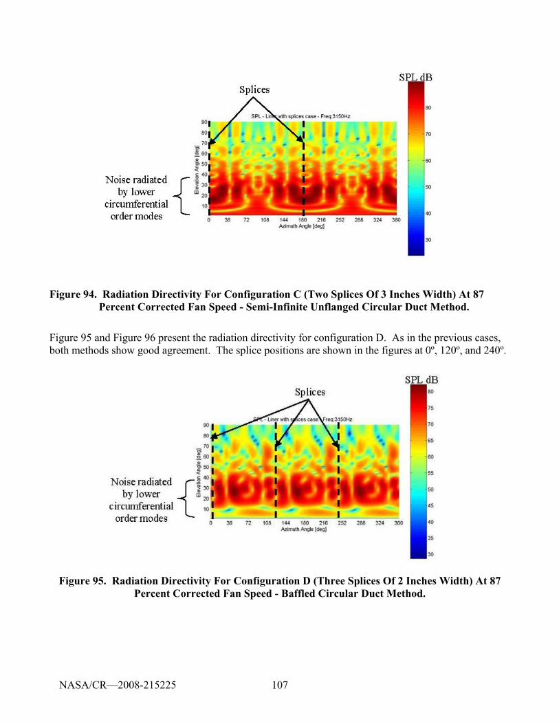
107

Figure 94. Radiation Directivity For Configuration C (Two Splices Of 3 Inches Width) At 87 Percent Corrected Fan Speed - Semi-Infinite Unflanged Circular Duct Method.

Figure 95 and Figure 96 present the radiation directivity for configuration D. As in the previous cases, both methods show good agreement. The splice positions are shown in the figures at 0º, 120º, and 240º.

Figure 95. Radiation Directivity For Configuration D (Three Splices Of 2 Inches Width) At 87 Percent Corrected Fan Speed - Baffled Circular Duct Method.

NASA/CR—2008-215225

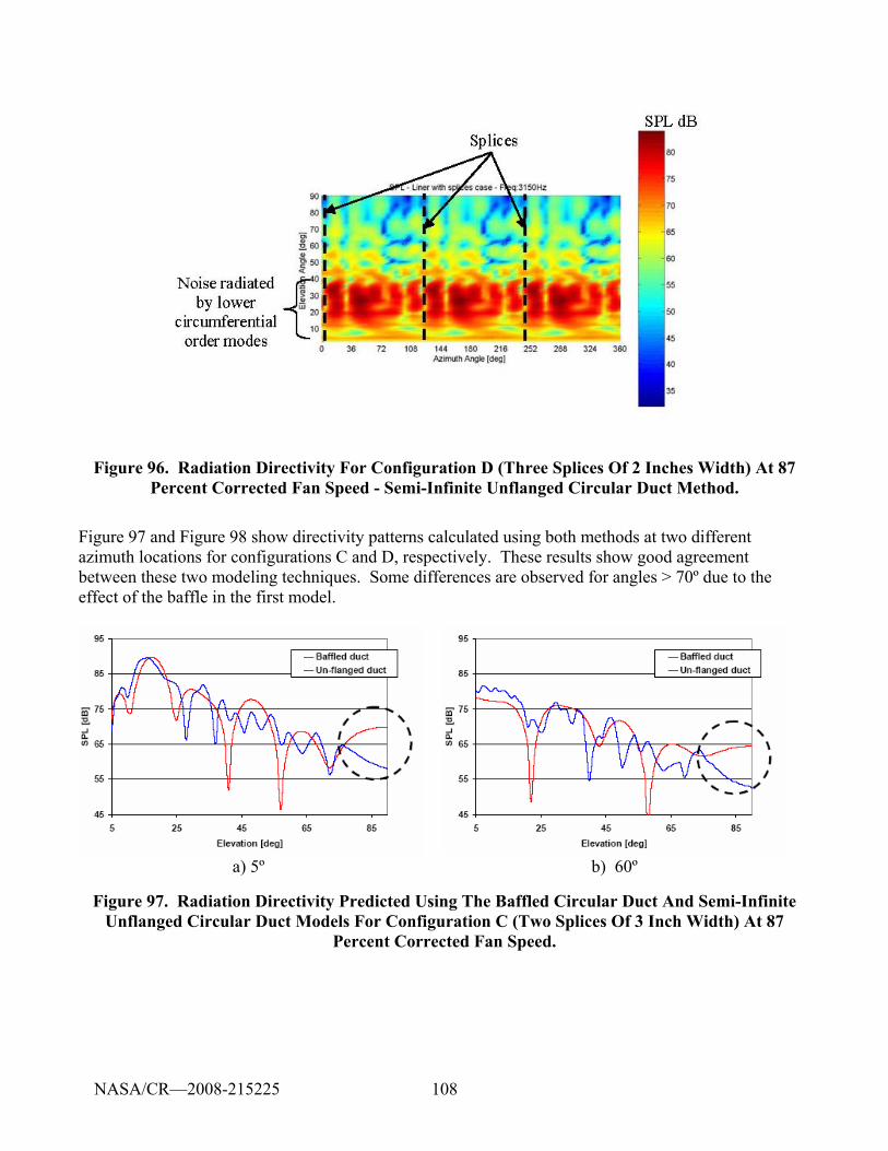
108

Figure 96. Radiation Directivity For Configuration D (Three Splices Of 2 Inches Width) At 87 Percent Corrected Fan Speed - Semi-Infinite Unflanged Circular Duct Method.

Figure 97 and Figure 98 show directivity patterns calculated using both methods at two different azimuth locations for configurations C and D, respectively. These results show good agreement between these two modeling techniques. Some differences are observed for angles > 70º due to the effect of the baffle in the first model.

a) 5º b) 60º

Figure 97. Radiation Directivity Predicted Using The Baffled Circular Duct And Semi-Infinite Unflanged Circular Duct Models For Configuration C (Two Splices Of 3 Inch Width) At 87

Percent Corrected Fan Speed.

NASA/CR—2008-215225

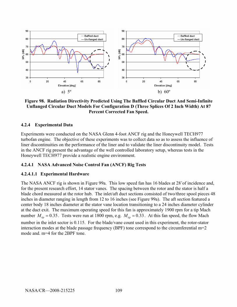
109

a) 5º b) 60º

Figure 98. Radiation Directivity Predicted Using The Baffled Circular Duct And Semi-Infinite Unflanged Circular Duct Models For Configuration D (Three Splices Of 2 Inch Width) At 87

Percent Corrected Fan Speed.

4.2.4 Experimental Data

Experiments were conducted on the NASA Glenn 4-foot ANCF rig and the Honeywell TECH977 turbofan engine. The objective of these experiments was to collect data so as to assess the influence of liner discontinuities on the performance of the liner and to validate the liner discontinuity model. Tests in the ANCF rig present the advantage of the well controlled laboratory setup, whereas tests in the Honeywell TECH977 provide a realistic engine environment.

4.2.4.1 NASA Advanced Noise Control Fan (ANCF) Rig Tests

4.2.4.1.1 Experimental Hardware

The NASA ANCF rig is shown in Figure 99a. This low speed fan has 16 blades at 28˚of incidence and, for the present research effort, 14 stator vanes. The spacing between the rotor and the stator is half a blade chord measured at the rotor hub. The inlet/aft duct sections consisted of two/three spool pieces 48 inches in diameter ranging in length from 12 to 16 inches (see Figure 99a). The aft section featured a center body 18 inches diameter at the stator vane location transitioning to a 24 inches diameter cylinder at the duct exit. The maximum operating speed for this fan is approximately 1900 rpm for a tip Mach number 0.35tipM = . Tests were run at 1800 rpm, e.g. 0.33tipM = . At this fan speed, the flow Mach number in the inlet sector is 0.115. For the blade/vane count used in this experiment, the rotor-stator interaction modes at the blade passage frequency (BPF) tone correspond to the circumferential m=2 mode and. m=4 for the 2BPF tone.

NASA/CR—2008-215225

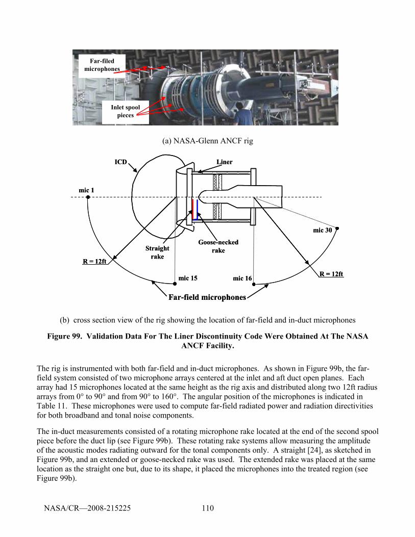
110

Inlet spool pieces

Far-filed microphones

Inlet spool pieces


Inlet spool pieces


(a) NASA-Glenn ANCF rig

R = 12ft

R = 12ft

Far-field microphones

mic 15

mic 1

mic 16

mic 30

Straight rake

ICD Liner

Goose-necked rake

R = 12ft

R = 12ft

Far-field microphones

mic 15

mic 1

mic 16

mic 30

Straight rake

ICD Liner

Goose-necked rake

(b) cross section view of the rig showing the location of far-field and in-duct microphones

Figure 99. Validation Data For The Liner Discontinuity Code Were Obtained At The NASA ANCF Facility.

The rig is instrumented with both far-field and in-duct microphones. As shown in Figure 99b, the far-field system consisted of two microphone arrays centered at the inlet and aft duct open planes. Each array had 15 microphones located at the same height as the rig axis and distributed along two 12ft radius arrays from 0° to 90° and from 90° to 160°. The angular position of the microphones is indicated in Table 11. These microphones were used to compute far-field radiated power and radiation directivities for both broadband and tonal noise components.

The in-duct measurements consisted of a rotating microphone rake located at the end of the second spool piece before the duct lip (see Figure 99b). These rotating rake systems allow measuring the amplitude of the acoustic modes radiating outward for the tonal components only. A straight [24], as sketched in Figure 99b, and an extended or goose-necked rake was used. The extended rake was placed at the same location as the straight one but, due to its shape, it placed the microphones into the treated region (see Figure 99b).

NASA/CR—2008-215225

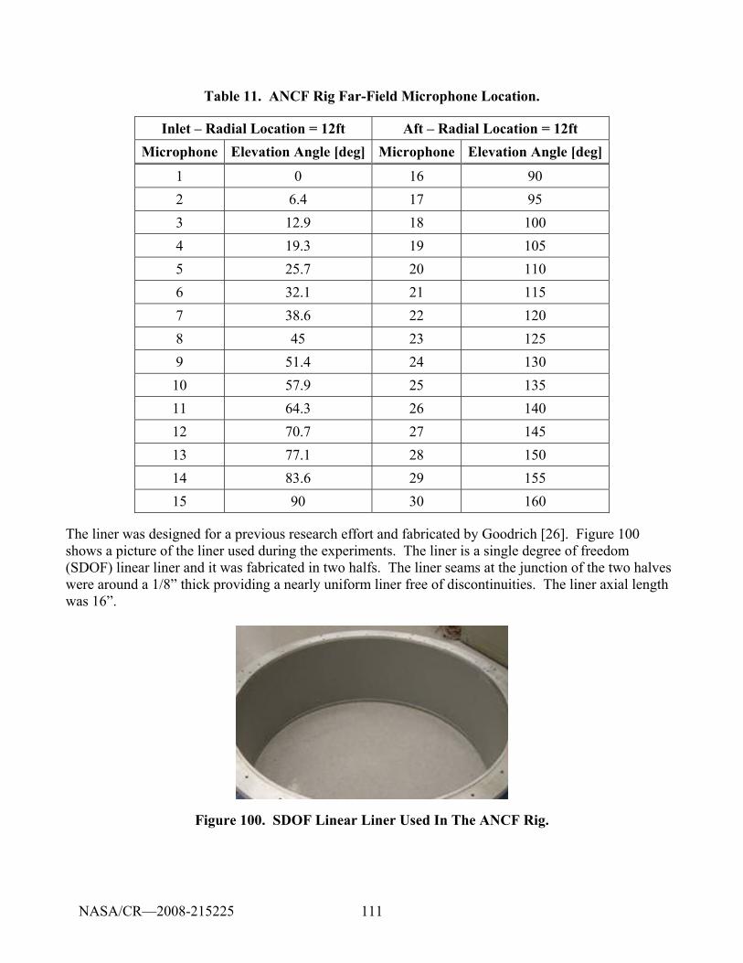
111

Table 11. ANCF Rig Far-Field Microphone Location.

Inlet – Radial Location = 12ft Aft – Radial Location = 12ft Microphone Elevation Angle [deg] Microphone Elevation Angle [deg]

1 0 16 90 2 6.4 17 95 3 12.9 18 100 4 19.3 19 105 5 25.7 20 110 6 32.1 21 115 7 38.6 22 120 8 45 23 125 9 51.4 24 130 10 57.9 25 135 11 64.3 26 140 12 70.7 27 145 13 77.1 28 150 14 83.6 29 155 15 90 30 160

The liner was designed for a previous research effort and fabricated by Goodrich [26]. Figure 100 shows a picture of the liner used during the experiments. The liner is a single degree of freedom (SDOF) linear liner and it was fabricated in two halfs. The liner seams at the junction of the two halves were around a 1/8” thick providing a nearly uniform liner free of discontinuities. The liner axial length was 16”.

Figure 100. SDOF Linear Liner Used In The ANCF Rig.

NASA/CR—2008-215225

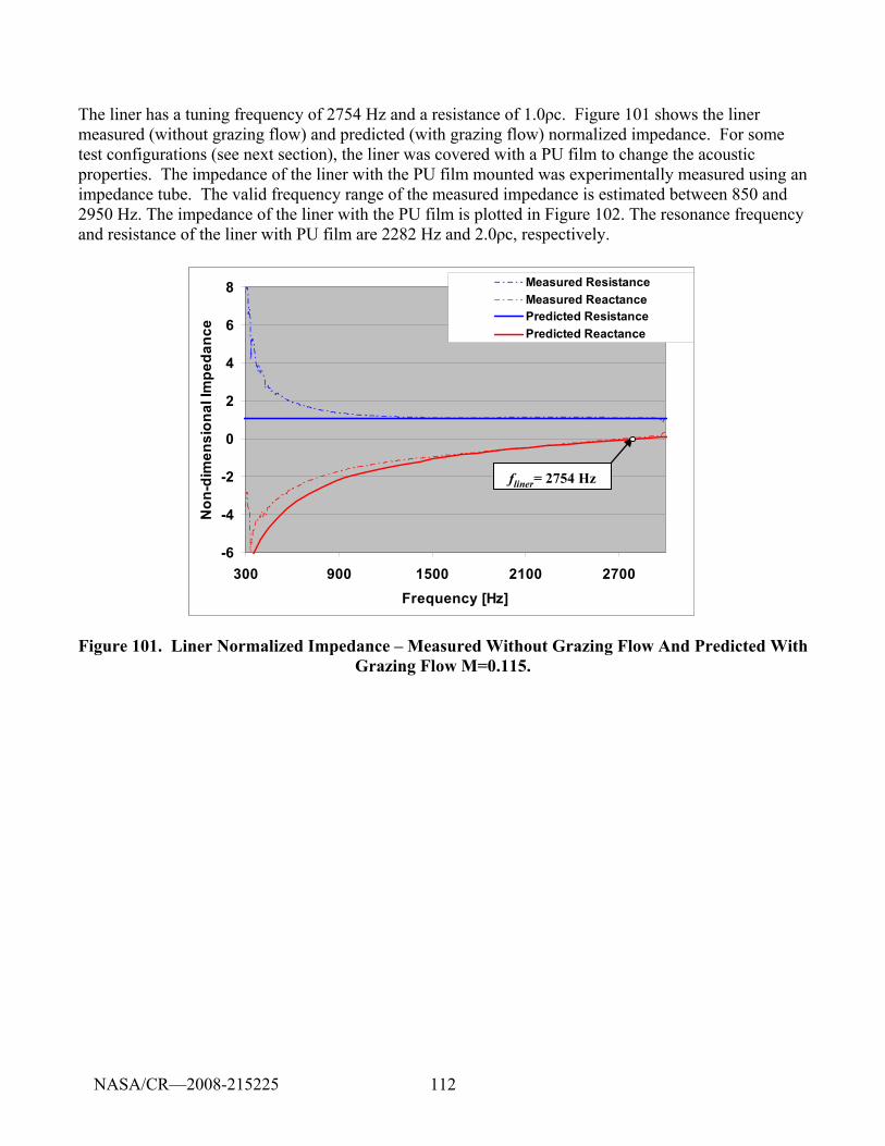
112

The liner has a tuning frequency of 2754 Hz and a resistance of 1.0ρc. Figure 101 shows the liner measured (without grazing flow) and predicted (with grazing flow) normalized impedance. For some test configurations (see next section), the liner was covered with a PU film to change the acoustic properties. The impedance of the liner with the PU film mounted was experimentally measured using an impedance tube. The valid frequency range of the measured impedance is estimated between 850 and 2950 Hz. The impedance of the liner with the PU film is plotted in Figure 102. The resonance frequency and resistance of the liner with PU film are 2282 Hz and 2.0ρc, respectively.

-6

-4

-2

0

2

4

6

8

300 900 1500 2100 2700Frequency [Hz]

Non

-dim

ensi

onal

Impe

danc

e

Measured ResistanceMeasured ReactancePredicted ResistancePredicted Reactance

fliner= 2754 Hz

-6

-4

-2

0

2

4

6

8

300 900 1500 2100 2700Frequency [Hz]

Non

-dim

ensi

onal

Impe

danc

e

Measured ResistanceMeasured ReactancePredicted ResistancePredicted Reactance

fliner= 2754 Hz

Figure 101. Liner Normalized Impedance – Measured Without Grazing Flow And Predicted With Grazing Flow M=0.115.

NASA/CR—2008-215225

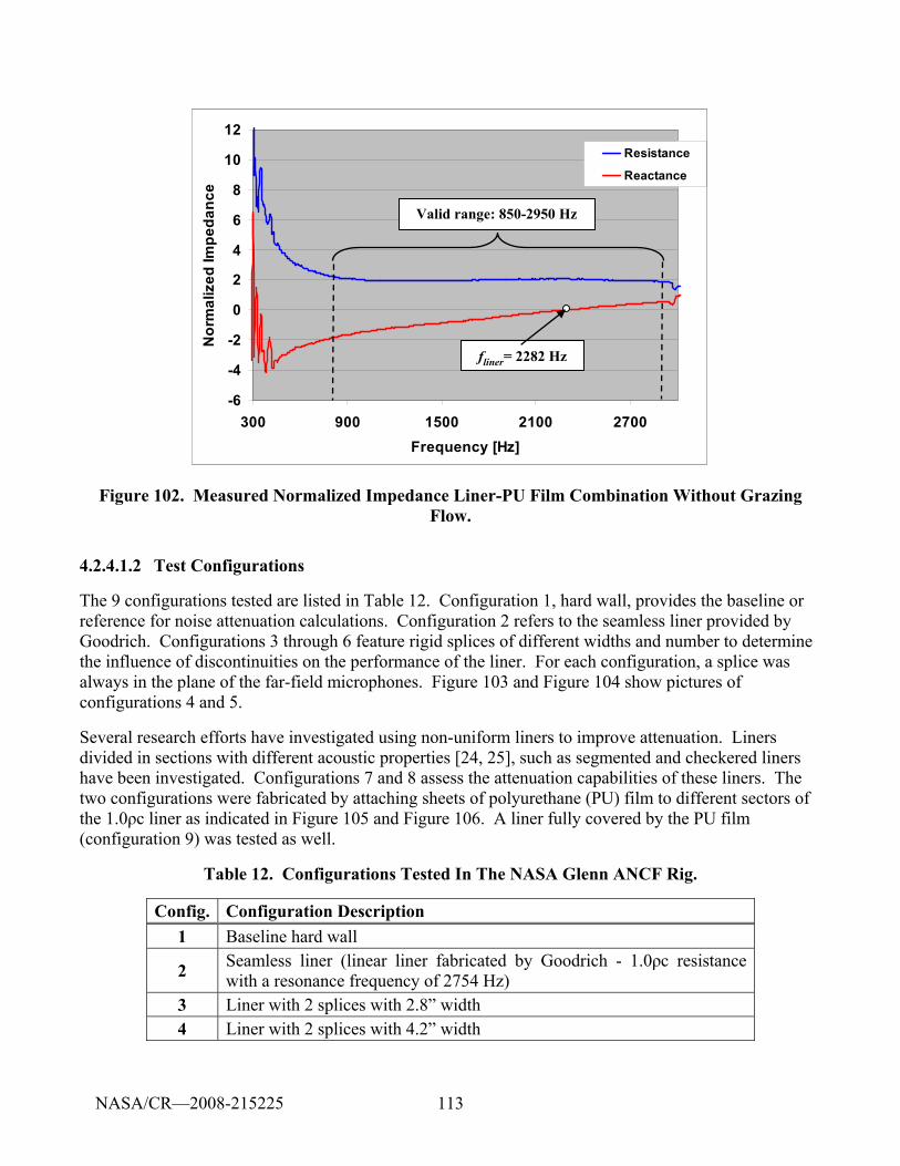
113

-6

-4

-2

0

2

4

6

8

10

12

300 900 1500 2100 2700Frequency [Hz]

Nor

mal

ized

Impe

danc

e

Resistance

Reactance

Valid range: 850-2950 Hz

fliner= 2282 Hz

-6

-4

-2

0

2

4

6

8

10

12

300 900 1500 2100 2700Frequency [Hz]

Nor

mal

ized

Impe

danc

e

Resistance

Reactance

Valid range: 850-2950 Hz

fliner= 2282 Hz

Figure 102. Measured Normalized Impedance Liner-PU Film Combination Without Grazing Flow.

4.2.4.1.2 Test Configurations

The 9 configurations tested are listed in Table 12. Configuration 1, hard wall, provides the baseline or reference for noise attenuation calculations. Configuration 2 refers to the seamless liner provided by Goodrich. Configurations 3 through 6 feature rigid splices of different widths and number to determine the influence of discontinuities on the performance of the liner. For each configuration, a splice was always in the plane of the far-field microphones. Figure 103 and Figure 104 show pictures of configurations 4 and 5.

Several research efforts have investigated using non-uniform liners to improve attenuation. Liners divided in sections with different acoustic properties [24, 25], such as segmented and checkered liners have been investigated. Configurations 7 and 8 assess the attenuation capabilities of these liners. The two configurations were fabricated by attaching sheets of polyurethane (PU) film to different sectors of the 1.0ρc liner as indicated in Figure 105 and Figure 106. A liner fully covered by the PU film (configuration 9) was tested as well.

Table 12. Configurations Tested In The NASA Glenn ANCF Rig.

Config. Configuration Description 1 Baseline hard wall

2 Seamless liner (linear liner fabricated by Goodrich - 1.0ρc resistance with a resonance frequency of 2754 Hz)

3 Liner with 2 splices with 2.8” width 4 Liner with 2 splices with 4.2” width

NASA/CR—2008-215225

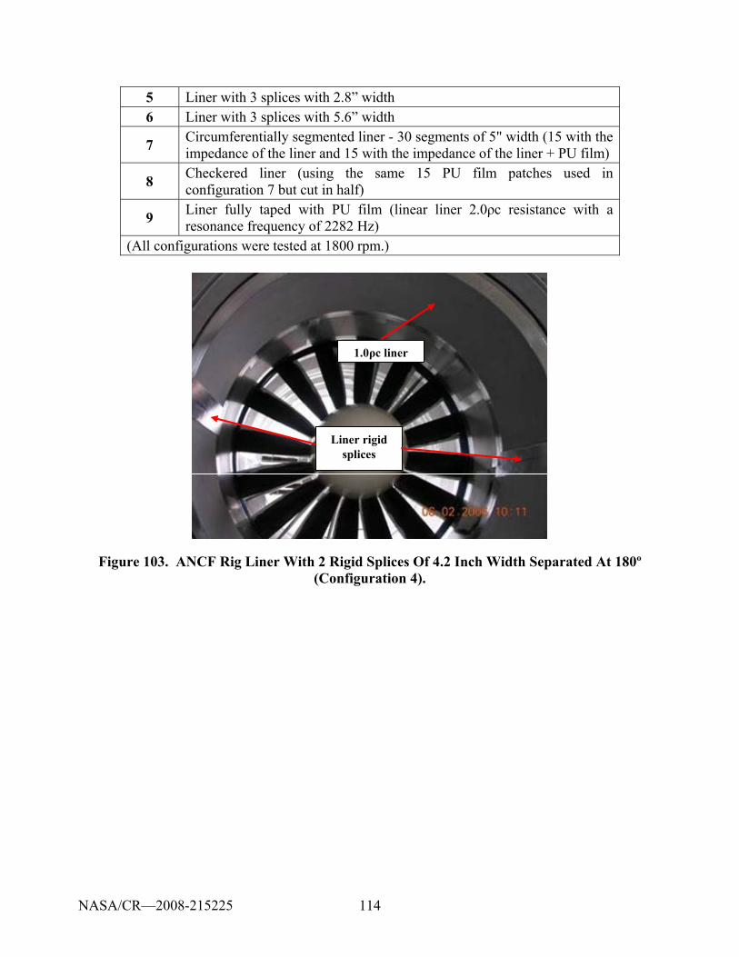
114

5 Liner with 3 splices with 2.8” width 6 Liner with 3 splices with 5.6” width

7 Circumferentially segmented liner - 30 segments of 5" width (15 with the impedance of the liner and 15 with the impedance of the liner + PU film)

8 Checkered liner (using the same 15 PU film patches used in configuration 7 but cut in half)

9 Liner fully taped with PU film (linear liner 2.0ρc resistance with a resonance frequency of 2282 Hz)

(All configurations were tested at 1800 rpm.)

1.0ρc liner

Liner rigid splices

1.0ρc liner

Liner rigid splices

Figure 103. ANCF Rig Liner With 2 Rigid Splices Of 4.2 Inch Width Separated At 180º (Configuration 4).

NASA/CR—2008-215225

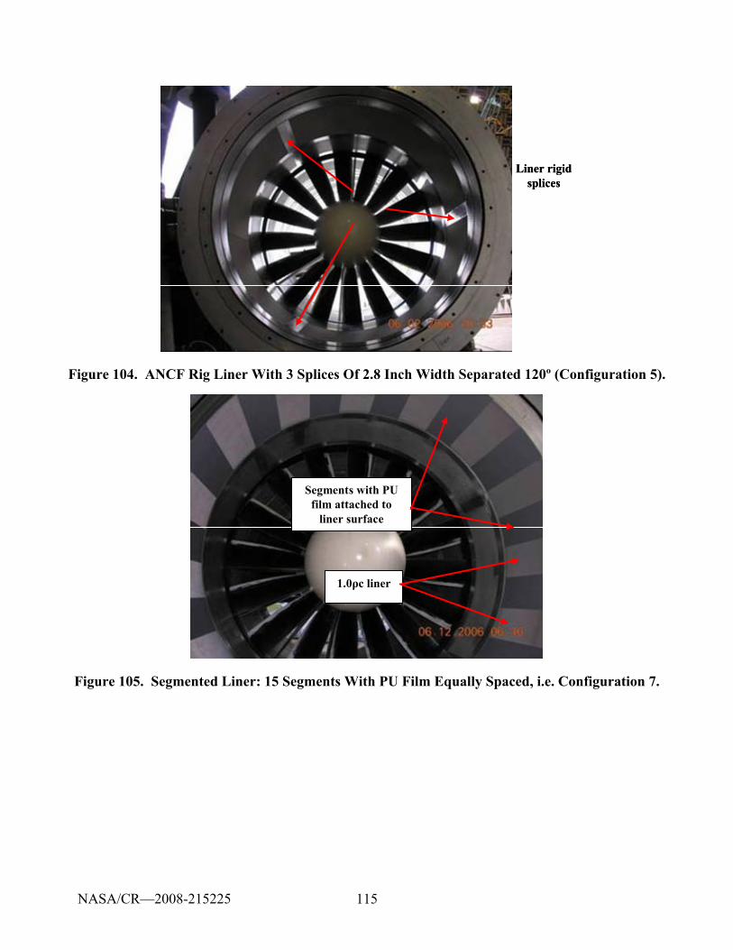
115

Liner rigid splices

Liner rigid splices

Figure 104. ANCF Rig Liner With 3 Splices Of 2.8 Inch Width Separated 120º (Configuration 5).

Segments with PU film attached to

liner surface

1.0ρc liner


liner surface

1.0ρc liner

Figure 105. Segmented Liner: 15 Segments With PU Film Equally Spaced, i.e. Configuration 7.

NASA/CR—2008-215225

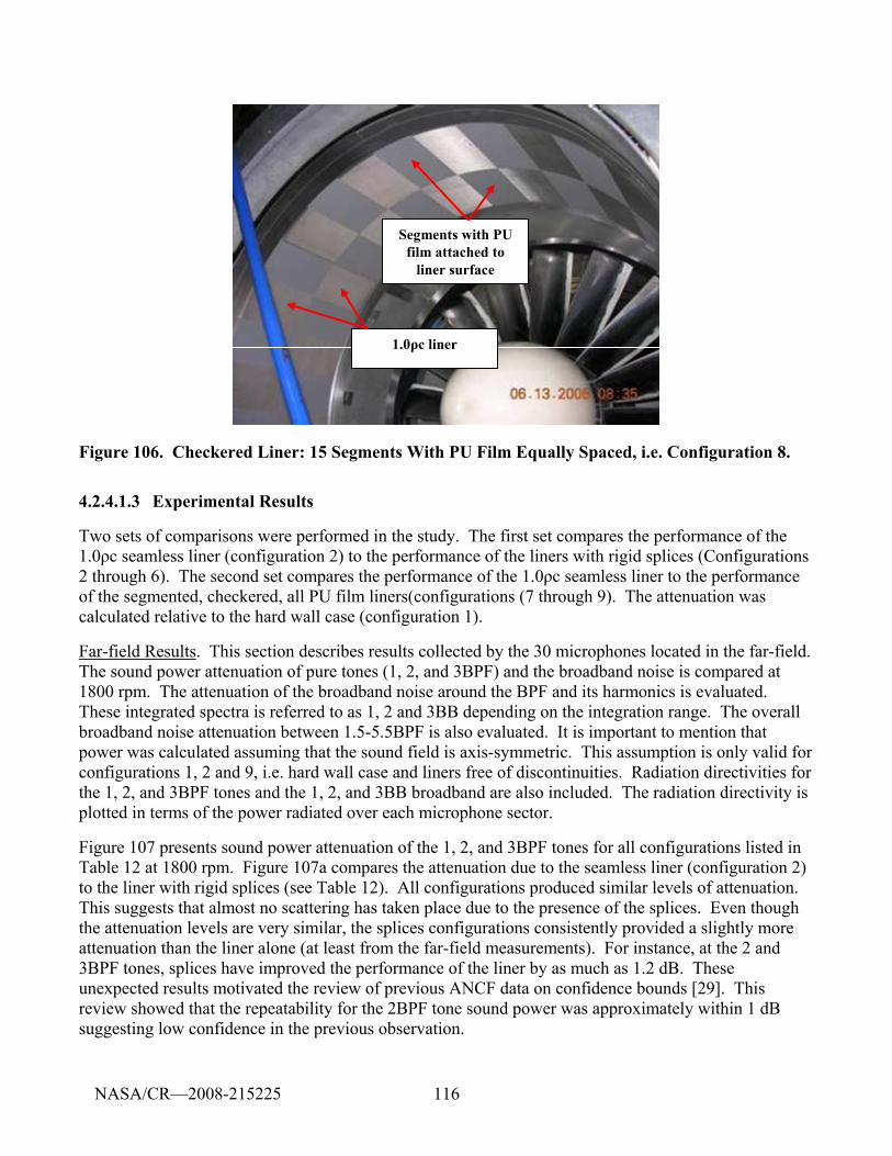
116


liner surface

1.0ρc liner


liner surface

1.0ρc liner

Figure 106. Checkered Liner: 15 Segments With PU Film Equally Spaced, i.e. Configuration 8.

4.2.4.1.3 Experimental Results

Two sets of comparisons were performed in the study. The first set compares the performance of the 1.0ρc seamless liner (configuration 2) to the performance of the liners with rigid splices (Configurations 2 through 6). The second set compares the performance of the 1.0ρc seamless liner to the performance of the segmented, checkered, all PU film liners(configurations (7 through 9). The attenuation was calculated relative to the hard wall case (configuration 1).

Far-field Results. This section describes results collected by the 30 microphones located in the far-field. The sound power attenuation of pure tones (1, 2, and 3BPF) and the broadband noise is compared at 1800 rpm. The attenuation of the broadband noise around the BPF and its harmonics is evaluated. These integrated spectra is referred to as 1, 2 and 3BB depending on the integration range. The overall broadband noise attenuation between 1.5-5.5BPF is also evaluated. It is important to mention that power was calculated assuming that the sound field is axis-symmetric. This assumption is only valid for configurations 1, 2 and 9, i.e. hard wall case and liners free of discontinuities. Radiation directivities for the 1, 2, and 3BPF tones and the 1, 2, and 3BB broadband are also included. The radiation directivity is plotted in terms of the power radiated over each microphone sector.

Figure 107 presents sound power attenuation of the 1, 2, and 3BPF tones for all configurations listed in Table 12 at 1800 rpm. Figure 107a compares the attenuation due to the seamless liner (configuration 2) to the liner with rigid splices (see Table 12). All configurations produced similar levels of attenuation. This suggests that almost no scattering has taken place due to the presence of the splices. Even though the attenuation levels are very similar, the splices configurations consistently provided a slightly more attenuation than the liner alone (at least from the far-field measurements). For instance, at the 2 and 3BPF tones, splices have improved the performance of the liner by as much as 1.2 dB. These unexpected results motivated the review of previous ANCF data on confidence bounds [29]. This review showed that the repeatability for the 2BPF tone sound power was approximately within 1 dB suggesting low confidence in the previous observation.

NASA/CR—2008-215225

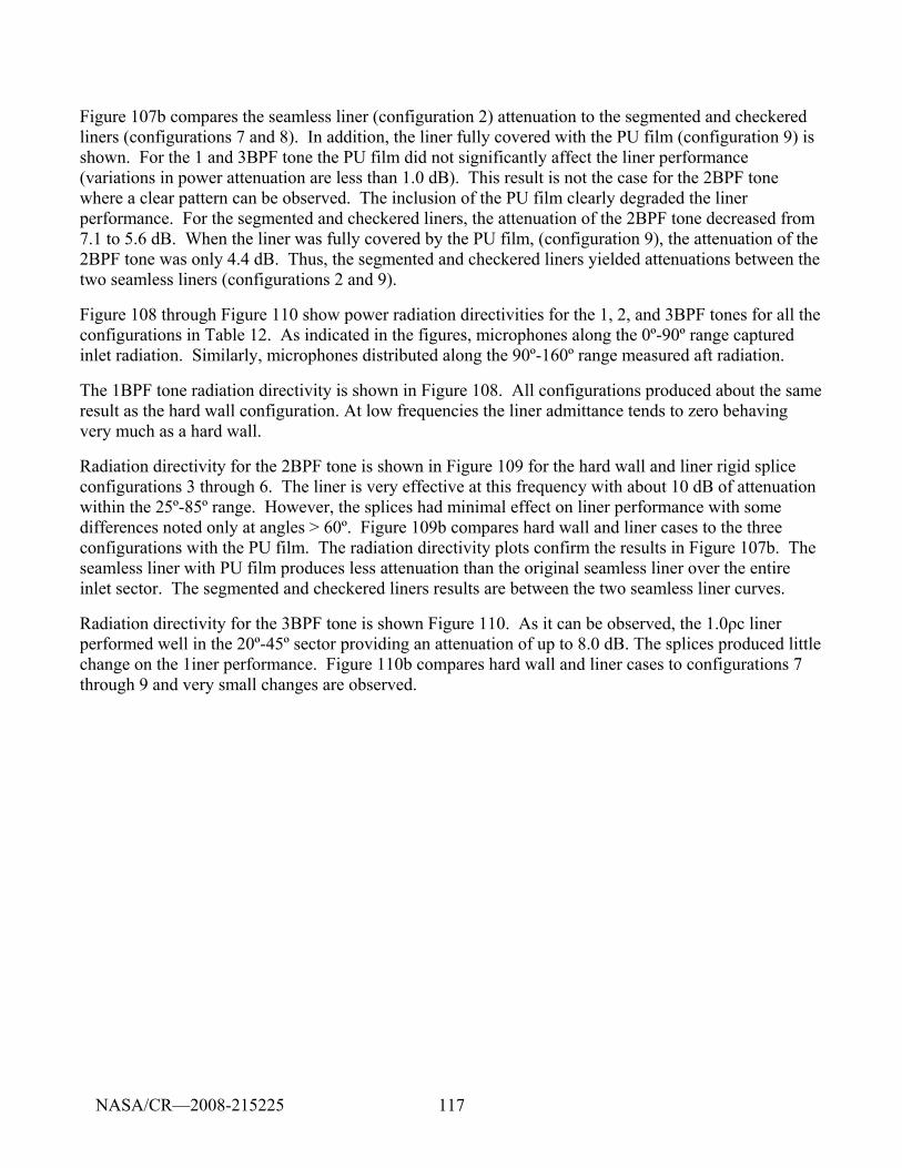
117

Figure 107b compares the seamless liner (configuration 2) attenuation to the segmented and checkered liners (configurations 7 and 8). In addition, the liner fully covered with the PU film (configuration 9) is shown. For the 1 and 3BPF tone the PU film did not significantly affect the liner performance (variations in power attenuation are less than 1.0 dB). This result is not the case for the 2BPF tone where a clear pattern can be observed. The inclusion of the PU film clearly degraded the liner performance. For the segmented and checkered liners, the attenuation of the 2BPF tone decreased from 7.1 to 5.6 dB. When the liner was fully covered by the PU film, (configuration 9), the attenuation of the 2BPF tone was only 4.4 dB. Thus, the segmented and checkered liners yielded attenuations between the two seamless liners (configurations 2 and 9).

Figure 108 through Figure 110 show power radiation directivities for the 1, 2, and 3BPF tones for all the configurations in Table 12. As indicated in the figures, microphones along the 0º-90º range captured inlet radiation. Similarly, microphones distributed along the 90º-160º range measured aft radiation.

The 1BPF tone radiation directivity is shown in Figure 108. All configurations produced about the same result as the hard wall configuration. At low frequencies the liner admittance tends to zero behaving very much as a hard wall.

Radiation directivity for the 2BPF tone is shown in Figure 109 for the hard wall and liner rigid splice configurations 3 through 6. The liner is very effective at this frequency with about 10 dB of attenuation within the 25º-85º range. However, the splices had minimal effect on liner performance with some differences noted only at angles > 60º. Figure 109b compares hard wall and liner cases to the three configurations with the PU film. The radiation directivity plots confirm the results in Figure 107b. The seamless liner with PU film produces less attenuation than the original seamless liner over the entire inlet sector. The segmented and checkered liners results are between the two seamless liner curves.

Radiation directivity for the 3BPF tone is shown Figure 110. As it can be observed, the 1.0ρc liner performed well in the 20º-45º sector providing an attenuation of up to 8.0 dB. The splices produced little change on the 1iner performance. Figure 110b compares hard wall and liner cases to configurations 7 through 9 and very small changes are observed.

NASA/CR—2008-215225

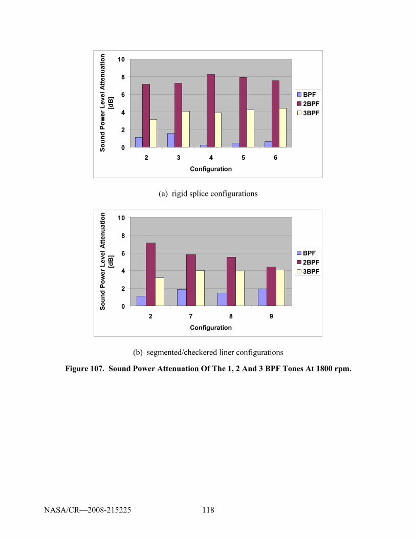
118

0

2

4

6

8

10

2 3 4 5 6

Configuration

Soun

d Po

wer

Lev

el A

ttenu

atio

n [d

B] BPF

2BPF3BPF

(a) rigid splice configurations

0

2

4

6

8

10

2 7 8 9

Configuration

Soun

d Po

wer

Lev

el A

ttenu

atio

n [d

B] BPF

2BPF3BPF

(b) segmented/checkered liner configurations

Figure 107. Sound Power Attenuation Of The 1, 2 And 3 BPF Tones At 1800 rpm.

NASA/CR—2008-215225

119

60

70

80

90

100

110

0 20 40 60 80 100 120 140 160

Microphone Angular Location [deg]

Soun

d Po

wer

Lev

el [d

B]

HWLiner2sp (2.8in)2sp (4.2in)3sp (2.8in)3sp (5.6in)

Inlet Aft

60

70

80

90

100

110

0 20 40 60 80 100 120 140 160


Soun

d Po

wer

Lev

el [d

B]


Inlet AftInlet Aft


60

70

80

90

100

110

0 20 40 60 80 100 120 140 160


Soun

d Po

wer

Lev

el [d

B]

HWLinerLiner with PU filmSegmented linerCheckered liner

Inlet Aft

60

70

80

90

100

110

0 20 40 60 80 100 120 140 160


Soun

d Po

wer

Lev

el [d

B]


Inlet AftInlet Aft


Figure 108. Power Radiation Directivity Of The 1BPF Tone At 1800 rpm.

NASA/CR—2008-215225

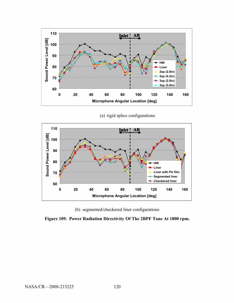
120

60

70

80

90

100

110

0 20 40 60 80 100 120 140 160Microphone Angular Location [deg]

Soun

d Po

wer

Lev

el [d

B]


60

70

80

90

100

110


Soun

d Po

wer

Lev

el [d

B]


Inlet AftInlet AftInlet Aft

60

70

80

90

100

110


Soun

d Po

wer

Lev

el [d

B]


60

70

80

90

100

110


Soun

d Po

wer

Lev

el [d

B]


Inlet AftInlet AftInlet AftInlet Aft


60

70

80

90

100

110


Soun

d Po

wer

Lev

el [d

B]


60

70

80

90

100

110


Soun

d Po

wer

Lev

el [d

B]


Inlet AftInlet AftInlet Aft

60

70

80

90

100

110


Soun

d Po

wer

Lev

el [d

B]


60

70

80

90

100

110


Soun

d Po

wer

Lev

el [d

B]


Inlet AftInlet AftInlet AftInlet Aft



NASA/CR—2008-215225

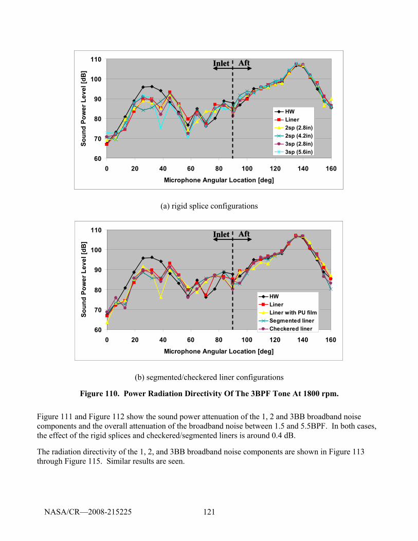
121

60

70

80

90

100

110

0 20 40 60 80 100 120 140 160


Soun

d Po

wer

Lev

el [d

B]


Inlet Aft

60

70

80

90

100

110

0 20 40 60 80 100 120 140 160


Soun

d Po

wer

Lev

el [d

B]


Inlet AftInlet Aft


60

70

80

90

100

110

0 20 40 60 80 100 120 140 160


Soun

d Po

wer

Lev

el [d

B]


Inlet Aft

60

70

80

90

100

110

0 20 40 60 80 100 120 140 160


Soun

d Po

wer

Lev

el [d

B]


Inlet AftInlet Aft



Figure 111 and Figure 112 show the sound power attenuation of the 1, 2 and 3BB broadband noise components and the overall attenuation of the broadband noise between 1.5 and 5.5BPF. In both cases, the effect of the rigid splices and checkered/segmented liners is around 0.4 dB.

The radiation directivity of the 1, 2, and 3BB broadband noise components are shown in Figure 113 through Figure 115. Similar results are seen.

NASA/CR—2008-215225

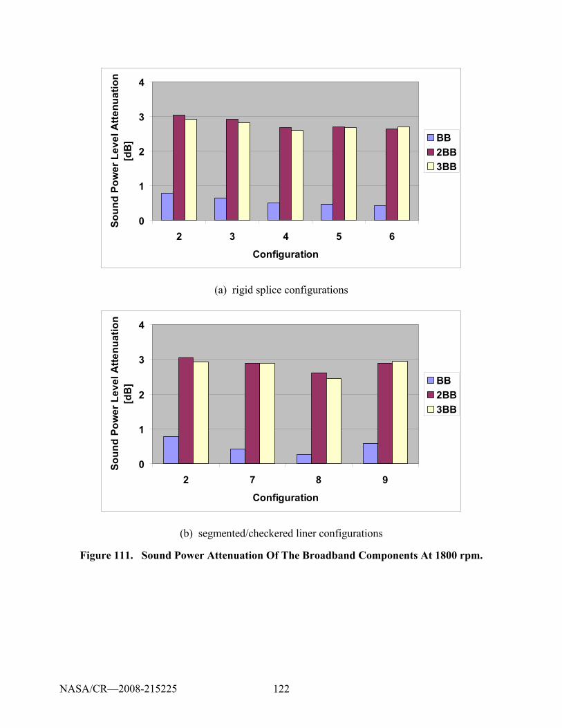
122

0

1

2

3

4

2 3 4 5 6

Configuration

Soun

d Po

wer

Lev

el A

ttenu

atio

n [d

B] BB

2BB3BB


0

1

2

3

4

2 7 8 9

Configuration

Soun

d Po

wer

Lev

el A

ttenu

atio

n [d

B] BB

2BB3BB


Figure 111. Sound Power Attenuation Of The Broadband Components At 1800 rpm.

NASA/CR—2008-215225

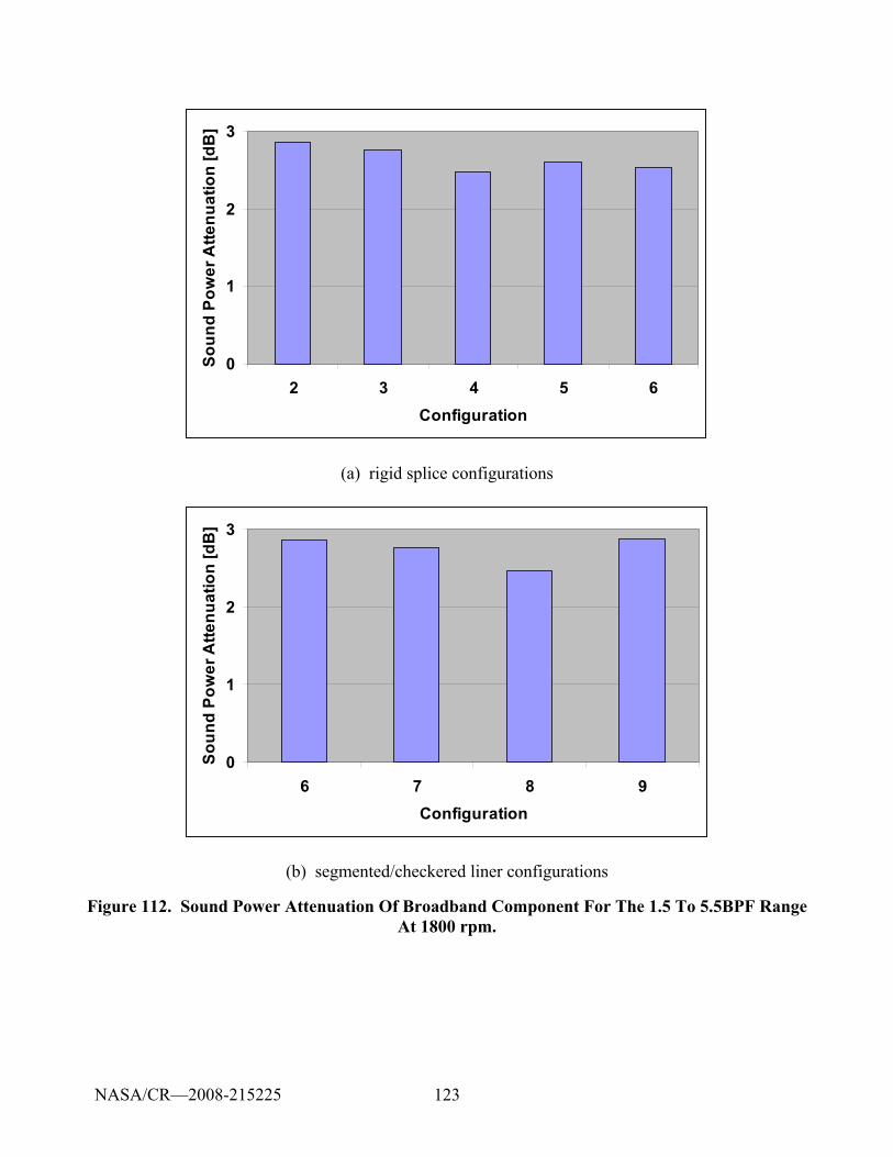
123

0

1

2

3

2 3 4 5 6Configuration

Soun

d Po

wer

Atte

nuat

ion

[dB

]


0

1

2

3

6 7 8 9Configuration

Soun

d Po

wer

Atte

nuat

ion

[dB

]


Figure 112. Sound Power Attenuation Of Broadband Component For The 1.5 To 5.5BPF Range At 1800 rpm.

NASA/CR—2008-215225

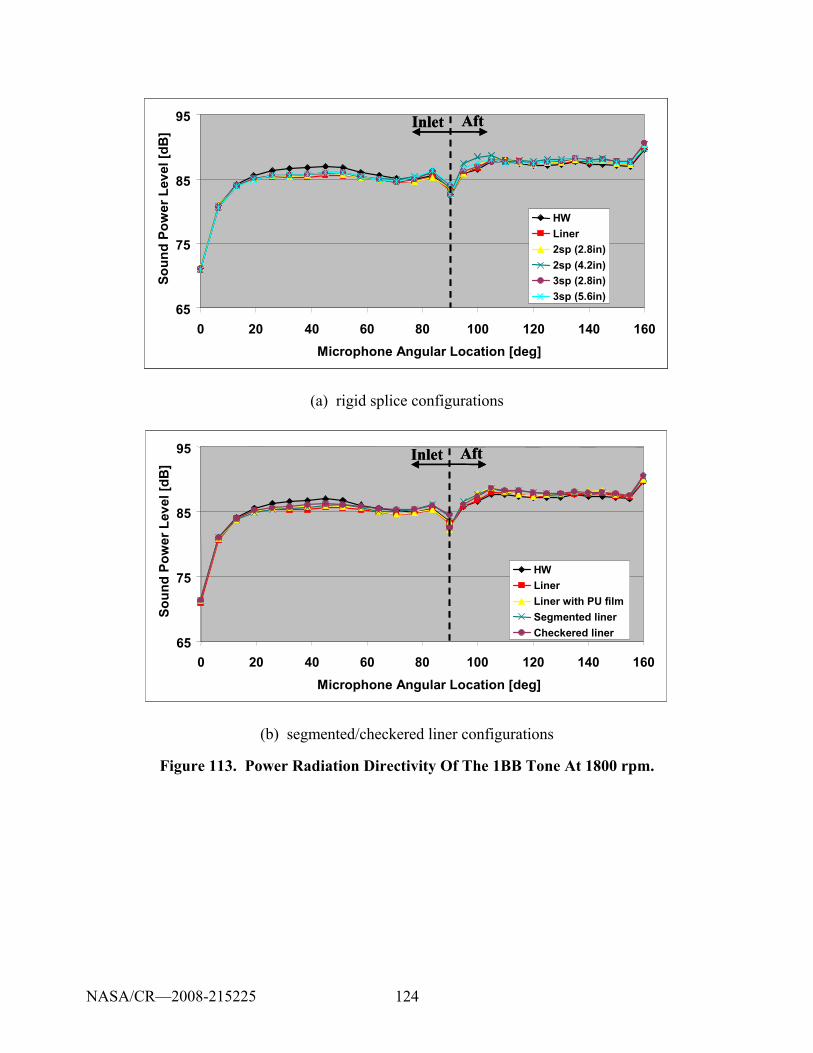
124

65

75

85

95


Soun

d Po

wer

Lev

el [d

B]


Inlet Aft

65

75

85

95


Soun

d Po

wer

Lev

el [d

B]


65

75

85

95


Soun

d Po

wer

Lev

el [d

B]


Inlet AftInlet Aft


65

75

85

95


Soun

d Po

wer

Lev

el [d

B]


Inlet Aft

65

75

85

95


Soun

d Po

wer

Lev

el [d

B]


65

75

85

95


Soun

d Po

wer

Lev

el [d

B]


Inlet AftInlet Aft


Figure 113. Power Radiation Directivity Of The 1BB Tone At 1800 rpm.

NASA/CR—2008-215225

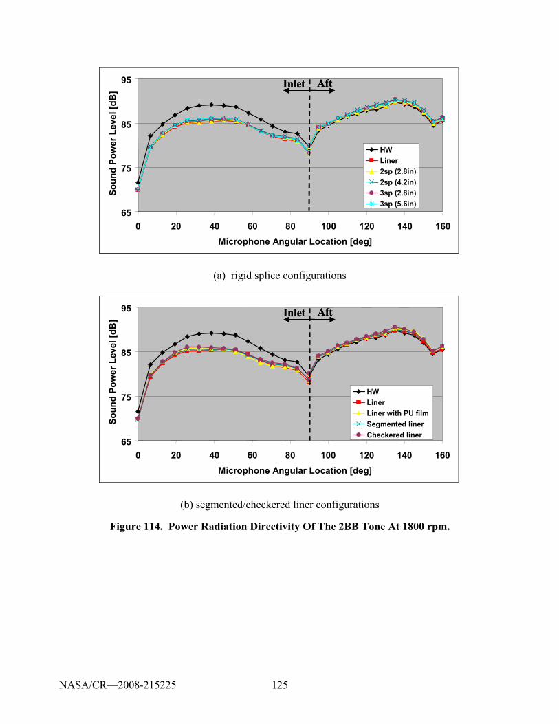
125

65

75

85

95


Soun

d Po

wer

Lev

el [d

B]


Inlet Aft

65

75

85

95


Soun

d Po

wer

Lev

el [d

B]


65

75

85

95


Soun

d Po

wer

Lev

el [d

B]


Inlet AftInlet Aft


65

75

85

95


Soun

d Po

wer

Lev

el [d

B]


Inlet Aft

65

75

85

95


Soun

d Po

wer

Lev

el [d

B]


65

75

85

95


Soun

d Po

wer

Lev

el [d

B]


Inlet AftInlet Aft



NASA/CR—2008-215225

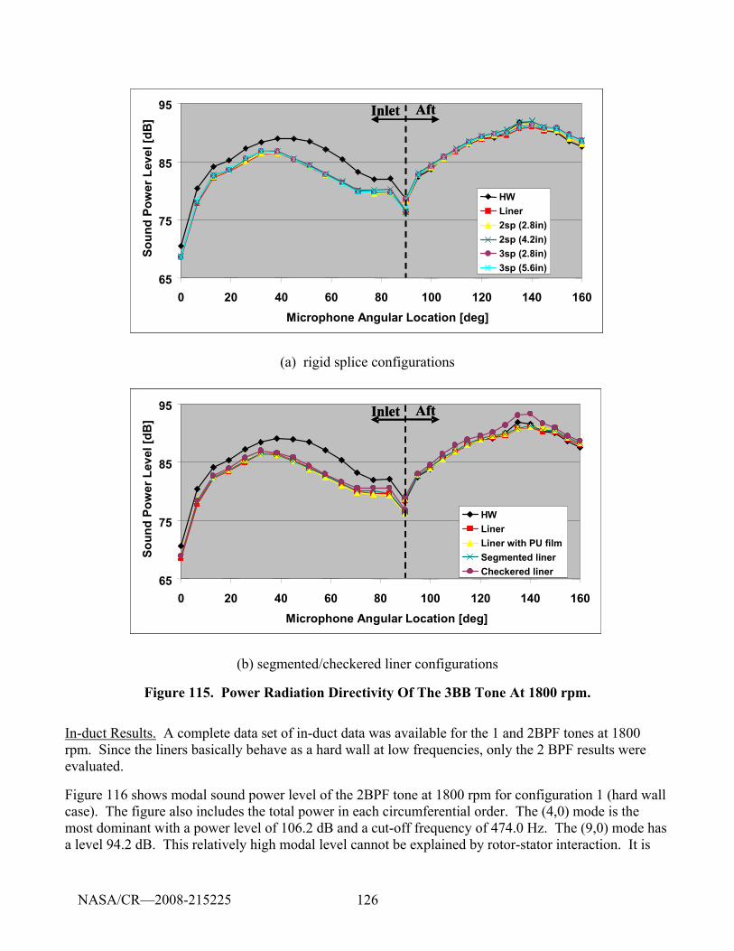
126

65

75

85

95


Soun

d Po

wer

Lev

el [d

B]


Inlet Aft

65

75

85

95


Soun

d Po

wer

Lev

el [d

B]


65

75

85

95


Soun

d Po

wer

Lev

el [d

B]


Inlet AftInlet Aft


65

75

85

95

0 20 40 60 80 100 120 140 160Microphone Anguar Location [deg]

Soun

d Po

wer

Lev

el [d

B]


Inlet Aft

65

75

85

95


Soun

d Po

wer

Lev

el [d

B]


65

75

85

95


Soun

d Po

wer

Lev

el [d

B]


Inlet AftInlet Aft

65

75

85

95


Soun

d Po

wer

Lev

el [d

B]


65

75

85

95


Soun

d Po

wer

Lev

el [d

B]


Inlet AftInlet Aft

65

75

85

95


Soun

d Po

wer

Lev

el [d

B]


65

75

85

95


Soun

d Po

wer

Lev

el [d

B]


Inlet AftInlet Aft



In-duct Results. A complete data set of in-duct data was available for the 1 and 2BPF tones at 1800 rpm. Since the liners basically behave as a hard wall at low frequencies, only the 2 BPF results were evaluated.

Figure 116 shows modal sound power level of the 2BPF tone at 1800 rpm for configuration 1 (hard wall case). The figure also includes the total power in each circumferential order. The (4,0) mode is the most dominant with a power level of 106.2 dB and a cut-off frequency of 474.0 Hz. The (9,0) mode has a level 94.2 dB. This relatively high modal level cannot be explained by rotor-stator interaction. It is

NASA/CR—2008-215225

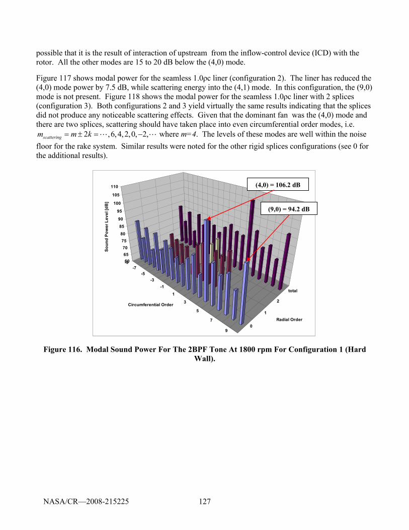
127

possible that it is the result of interaction of upstream from the inflow-control device (ICD) with the rotor. All the other modes are 15 to 20 dB below the (4,0) mode.

Figure 117 shows modal power for the seamless 1.0ρc liner (configuration 2). The liner has reduced the (4,0) mode power by 7.5 dB, while scattering energy into the (4,1) mode. In this configuration, the (9,0) mode is not present. Figure 118 shows the modal power for the seamless 1.0ρc liner with 2 splices (configuration 3). Both configurations 2 and 3 yield virtually the same results indicating that the splices did not produce any noticeable scattering effects. Given that the dominant fan was the (4,0) mode and there are two splices, scattering should have taken place into even circumferential order modes, i.e.

2 ,6,4,2,0, 2,scatteringm m k= ± = −L L where m=4. The levels of these modes are well within the noise floor for the rake system. Similar results were noted for the other rigid splices configurations (see 0 for the additional results).

-9-7

-5-3

-1

1

3

5

7

90

1

2

total

6065707580

8590

95

100

105

110

Soun

d Po

wer

Lev

el [d

B]

Circumferential Order

Radial Order

(4,0) = 106.2 dB

(9,0) = 94.2 dB

-9-7

-5-3

-1

1

3

5

7

90

1

2

total

6065707580

8590

95

100

105

110

Soun

d Po

wer

Lev

el [d

B]


Radial Order

(4,0) = 106.2 dB

(9,0) = 94.2 dB

Figure 116. Modal Sound Power For The 2BPF Tone At 1800 rpm For Configuration 1 (Hard Wall).

NASA/CR—2008-215225

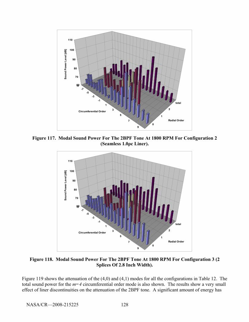
128

-9-7

-5-3

-1

1

3

5

7

90

1

2

total

60

70

80

90

100

110

Soun

d Po

wer

Lev

el [d

B]


Radial Order

Figure 117. Modal Sound Power For The 2BPF Tone At 1800 RPM For Configuration 2 (Seamless 1.0ρc Liner).

-9-7

-5-3

-1

1

3

5

7

90

1

2

total

60

70

80

90

100

110

Soun

d Po

wer

Lev

el [d

B]


Radial Order

Figure 118. Modal Sound Power For The 2BPF Tone At 1800 RPM For Configuration 3 (2 Splices Of 2.8 Inch Width).

Figure 119 shows the attenuation of the (4,0) and (4,1) modes for all the configurations in Table 12. The total sound power for the m=4 circumferential order mode is also shown. The results show a very small effect of liner discontinuities on the attenuation of the 2BPF tone. A significant amount of energy has

NASA/CR—2008-215225

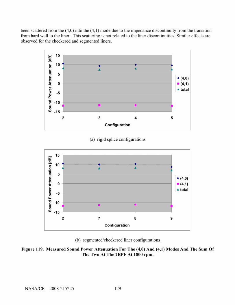
129

been scattered from the (4,0) into the (4,1) mode due to the impedance discontinuity from the transition from hard wall to the liner. This scattering is not related to the liner discontinuities. Similar effects are observed for the checkered and segmented liners.

-15

-10

-5

0

5

10

15

2 3 4 5

Configuration

Soun

d Po

wer

Atte

nuat

ion

[dB

]

(4,0)(4,1)total


-15

-10

-5

0

5

10

15

2 7 8 9

Configuration

Soun

d Po

wer

Atte

nuat

ion

[dB

]

(4,0)(4,1)total

-15

-10

-5

0

5

10

15

2 7 8 9

Configuration

Soun

d Po

wer

Atte

nuat

ion

[dB

]

(4,0)(4,1)total


Figure 119. Measured Sound Power Attenuation For The (4,0) And (4,1) Modes And The Sum Of The Two At The 2BPF At 1800 rpm.

NASA/CR—2008-215225

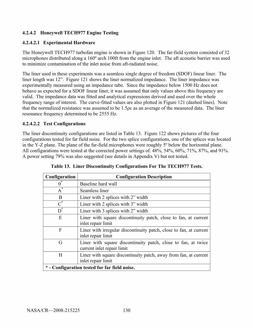
130

4.2.4.2 Honeywell TECH977 Engine Testing

4.2.4.2.1 Experimental Hardware

The Honeywell TECH977 turbofan engine is shown in Figure 120. The far-field system consisted of 32 microphones distributed along a 160º arch 100ft from the engine inlet. The aft acoustic barrier was used to minimize contamination of the inlet noise from aft-radiated noise.

The liner used in these experiments was a seamless single degree of freedom (SDOF) linear liner. The liner length was 12”. Figure 121 shows the liner normalized impedance. The liner impedance was experimentally measured using an impedance tube. Since the impedance below 1500 Hz does not behave as expected for a SDOF linear liner, it was assumed that only values above this frequency are valid. The impedance data was fitted and analytical expressions derived and used over the whole frequency range of interest. The curve-fitted values are also plotted in Figure 121 (dashed lines). Note that the normalized resistance was assumed to be 1.5ρc as an average of the measured data. The liner resonance frequency determined to be 2555 Hz.

4.2.4.2.2 Test Configurations

The liner discontinuity configurations are listed in Table 13. Figure 122 shows pictures of the four configurations tested for far field noise. For the two splice configurations, one of the splices was located in the Y-Z plane. The plane of the far-field microphones were roughly 5º below the horizontal plane. All configurations were tested at the corrected power settings of. 48%, 54%, 60%, 71%, 87%, and 91%. A power setting 79% was also suggested (see details in Appendix V) but not tested.

Table 13. Liner Discontinuity Configurations For The TECH977 Tests.

Configuration Configuration Description 0* Baseline hard wall A* Seamless liner B Liner with 2 splices with 2” width C* Liner with 2 splices with 3” width D* Liner with 3 splices with 2” width E Liner with square discontinuity patch, close to fan, at current

inlet repair limit F Liner with irregular discontinuity patch, close to fan, at current

inlet repair limit G Liner with square discontinuity patch, close to fan, at twice

current inlet repair limit H Liner with square discontinuity patch, away from fan, at current

inlet repair limit * - Configuration tested for far field noise.

NASA/CR—2008-215225

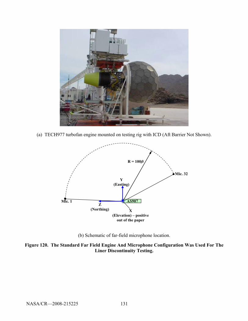
131

(a) TECH977 turbofan engine mounted on testing rig with ICD (Aft Barrier Not Shown).

Mic. 1

Mic. 32

R = 100ft

Z (Northing)

Y (Easting)

AS907

X (Elevation) – positive

out of the paper

(b) Schematic of far-field microphone location.

Figure 120. The Standard Far Field Engine And Microphone Configuration Was Used For The Liner Discontinuity Testing.

NASA/CR—2008-215225

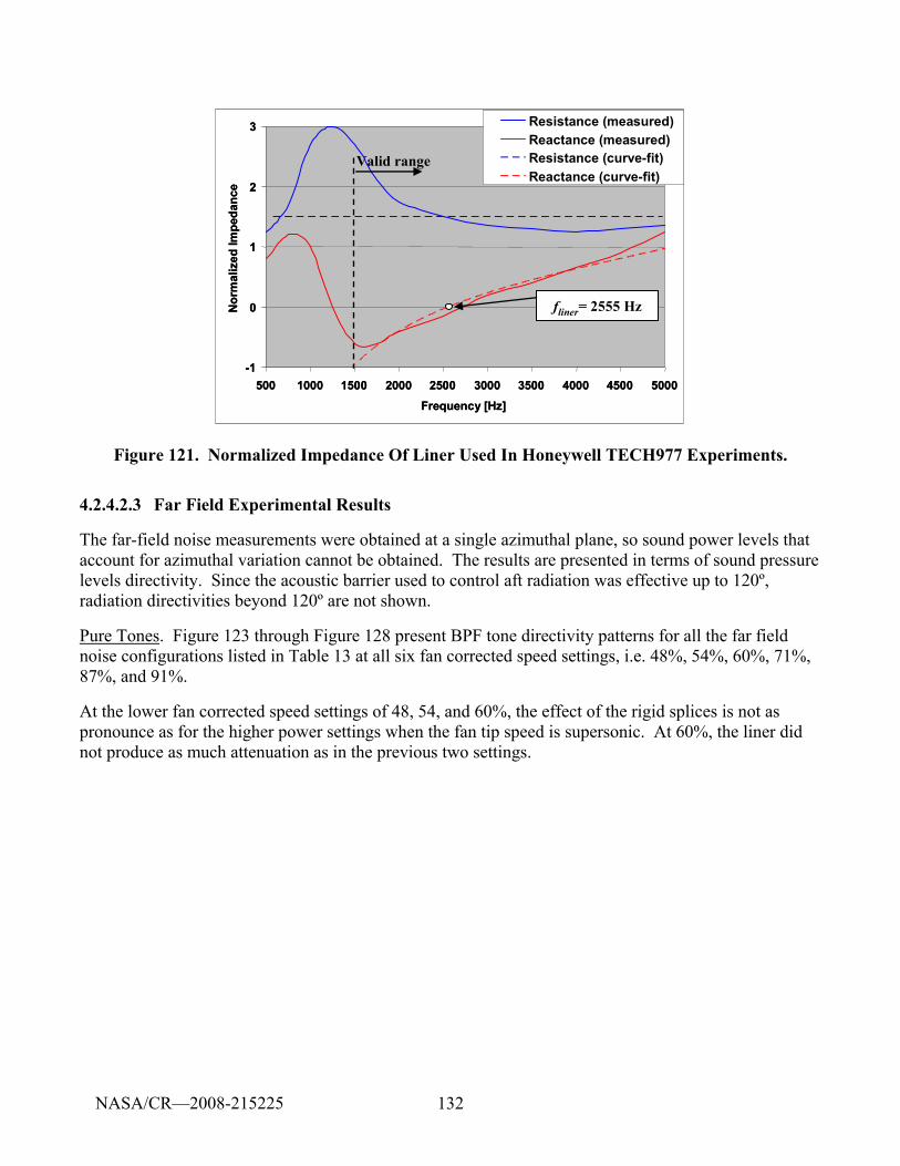
132

-1

0

1

2

3

500 1000 1500 2000 2500 3000 3500 4000 4500 5000

Frequency [Hz]

Nor

mal

ized

Impe

danc

e

Resistance (measured)Reactance (measured)Resistance (curve-fit)Reactance (curve-fit)

fliner= 2555 Hz

Valid range

-1

0

1

2

3

500 1000 1500 2000 2500 3000 3500 4000 4500 5000

Frequency [Hz]

Nor

mal

ized

Impe

danc

e

Resistance (measured)Reactance (measured)Resistance (curve-fit)Reactance (curve-fit)

fliner= 2555 Hz

Valid range

Figure 121. Normalized Impedance Of Liner Used In Honeywell TECH977 Experiments.

4.2.4.2.3 Far Field Experimental Results

The far-field noise measurements were obtained at a single azimuthal plane, so sound power levels that account for azimuthal variation cannot be obtained. The results are presented in terms of sound pressure levels directivity. Since the acoustic barrier used to control aft radiation was effective up to 120º, radiation directivities beyond 120º are not shown.

Pure Tones. Figure 123 through Figure 128 present BPF tone directivity patterns for all the far field noise configurations listed in Table 13 at all six fan corrected speed settings, i.e. 48%, 54%, 60%, 71%, 87%, and 91%.

At the lower fan corrected speed settings of 48, 54, and 60%, the effect of the rigid splices is not as pronounce as for the higher power settings when the fan tip speed is supersonic. At 60%, the liner did not produce as much attenuation as in the previous two settings.

NASA/CR—2008-215225

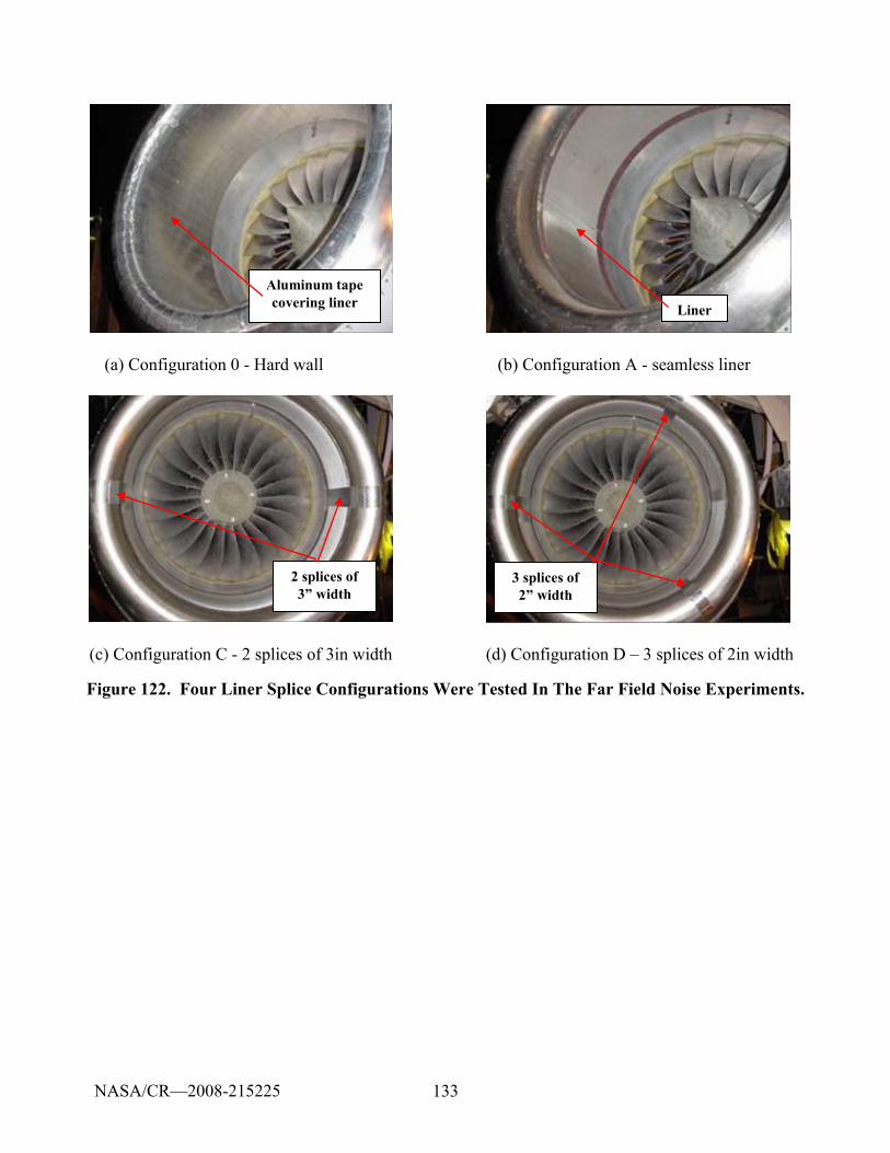
133

Aluminum tape covering liner

Aluminum tape covering liner

LinerLiner

(a) Configuration 0 - Hard wall (b) Configuration A - seamless liner

2 splices of 3” width




(c) Configuration C - 2 splices of 3in width (d) Configuration D – 3 splices of 2in width

Figure 122. Four Liner Splice Configurations Were Tested In The Far Field Noise Experiments.

NASA/CR—2008-215225

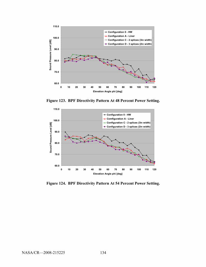
134

60.0

70.0

80.0

90.0

100.0

110.0

0 10 20 30 40 50 60 70 80 90 100 110 120

Elevation Angle phi [deg]

Soun

d Pr

essu

re L

evel

[dB

]

Configuration 0 - HWConfiguration A - LinerConfiguration C - 2 splices (3in width)Configuration D - 3 splices (2in width)

Figure 123. BPF Directivity Pattern At 48 Percent Power Setting.

60.0

70.0

80.0

90.0

100.0

110.0

0 10 20 30 40 50 60 70 80 90 100 110 120


Soun

d Pr

essu

re L

evel

[dB

]

Configuration 0 - HWComfiguration A - LinerConfiguration C - 2 splices (3in width)Configuration D - 3 splices (2in width)


NASA/CR—2008-215225

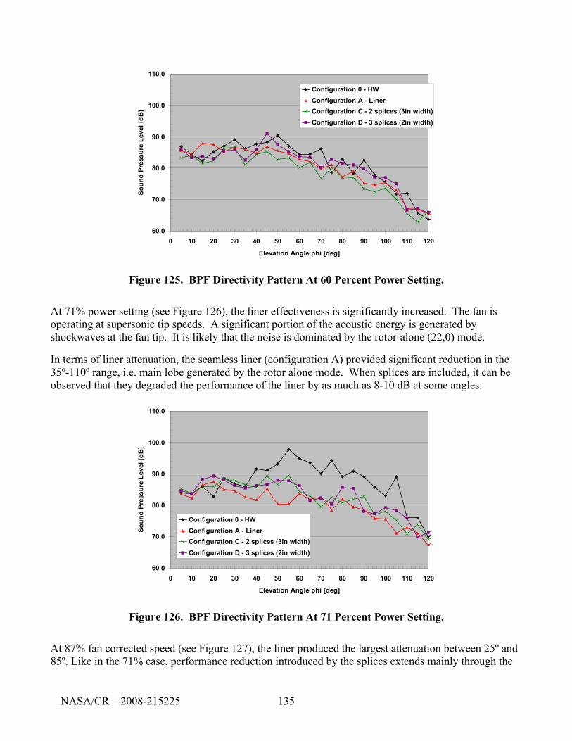
135

60.0

70.0

80.0

90.0

100.0

110.0

0 10 20 30 40 50 60 70 80 90 100 110 120


Soun

d Pr

essu

re L

evel

[dB

]



At 71% power setting (see Figure 126), the liner effectiveness is significantly increased. The fan is operating at supersonic tip speeds. A significant portion of the acoustic energy is generated by shockwaves at the fan tip. It is likely that the noise is dominated by the rotor-alone (22,0) mode.

In terms of liner attenuation, the seamless liner (configuration A) provided significant reduction in the 35º-110º range, i.e. main lobe generated by the rotor alone mode. When splices are included, it can be observed that they degraded the performance of the liner by as much as 8-10 dB at some angles.

60.0

70.0

80.0

90.0

100.0

110.0

0 10 20 30 40 50 60 70 80 90 100 110 120


Soun

d Pr

essu

re L

evel

[dB

]



At 87% fan corrected speed (see Figure 127), the liner produced the largest attenuation between 25º and 85º. Like in the 71% case, performance reduction introduced by the splices extends mainly through the

NASA/CR—2008-215225

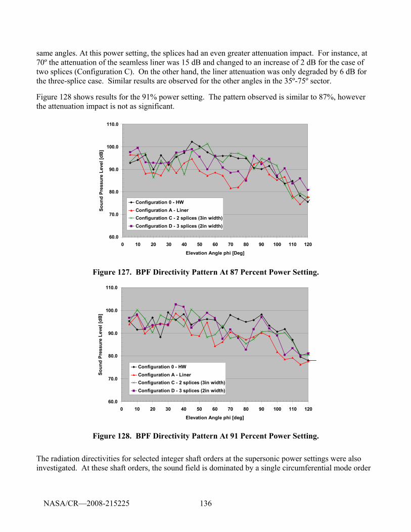
136

same angles. At this power setting, the splices had an even greater attenuation impact. For instance, at 70º the attenuation of the seamless liner was 15 dB and changed to an increase of 2 dB for the case of two splices (Configuration C). On the other hand, the liner attenuation was only degraded by 6 dB for the three-splice case. Similar results are observed for the other angles in the 35º-75º sector.

Figure 128 shows results for the 91% power setting. The pattern observed is similar to 87%, however the attenuation impact is not as significant.

60.0

70.0

80.0

90.0

100.0

110.0

0 10 20 30 40 50 60 70 80 90 100 110 120

Elevation Angle phi [Deg]

Soun

d Pr

essu

re L

evel

[dB

]



60.0

70.0

80.0

90.0

100.0

110.0

0 10 20 30 40 50 60 70 80 90 100 110 120


Soun

d Pr

essu

re L

evel

[dB

]



The radiation directivities for selected integer shaft orders at the supersonic power settings were also investigated. At these shaft orders, the sound field is dominated by a single circumferential mode order

NASA/CR—2008-215225

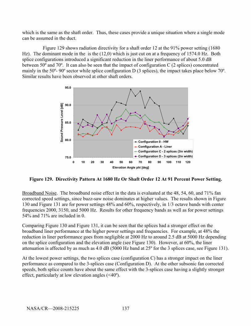
137

which is the same as the shaft order. Thus, these cases provide a unique situation where a single mode can be assumed in the duct.

Figure 129 shows radiation directivity for a shaft order 12 at the 91% power setting (1680 Hz). The dominant mode in the is the (12,0) which is just cut on at a frequency of 1574.0 Hz. Both splice configurations introduced a significant reduction in the liner performance of about 5.0 dB between 50º and 70º. It can also be seen that the impact of configuration C (2 splices) concentrated mainly in the 50º- 90º sector while splice configuration D (3 splices), the impact takes place below 70º. Similar results have been observed at other shaft orders.

75.0

80.0

85.0

90.0

95.0

0 10 20 30 40 50 60 70 80 90 100 110 120


Soun

d Pr

essu

re L

evel

[dB

]

Configuration 0 - HWComfiguration A - LinerConfiguration C - 2 splices (3in width)Configuration D - 3 splices (2in width)

Figure 129. Directivity Pattern At 1680 Hz Or Shaft Order 12 At 91 Percent Power Setting.

Broadband Noise. The broadband noise effect in the data is evaluated at the 48, 54, 60, and 71% fan corrected speed settings, since buzz-saw noise dominates at higher values. The results shown in Figure 130 and Figure 131 are for power settings 48% and 60%, respectively, in 1/3 octave bands with center frequencies 2000, 3150, and 5000 Hz. Results for other frequency bands as well as for power settings 54% and 71% are included in 0.

Comparing Figure 130 and Figure 131, it can be seen that the splices had a stronger effect on the broadband liner performance at the higher power settings and frequencies. For example, at 48% the reduction in liner performance goes from negligible at 2000 Hz to around 2.5 dB at 5000 Hz depending on the splice configuration and the elevation angle (see Figure 130). However, at 60%, the liner attenuation is affected by as much as 4.0 dB (5000 Hz band at 25º for the 3 splices case, see Figure 131).

At the lowest power settings, the two splices case (configuration C) has a stronger impact on the liner performance as compared to the 3-splices case (Configuration D). At the other subsonic fan corrected speeds, both splice counts have about the same effect with the 3-splices case having a slightly stronger effect, particularly at low elevation angles (<40º).

NASA/CR—2008-215225

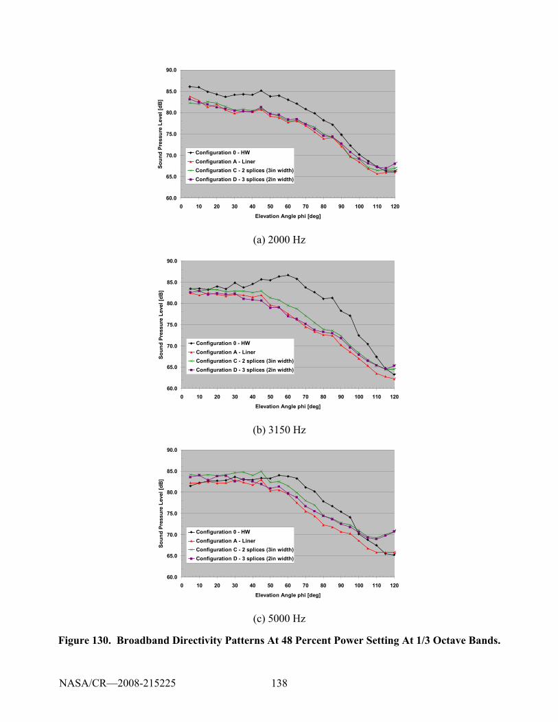
138

60.0

65.0

70.0

75.0

80.0

85.0

90.0

0 10 20 30 40 50 60 70 80 90 100 110 120


Soun

d Pr

essu

re L

evel

[dB

]Configuration 0 - HWConfiguration A - LinerConfiguration C - 2 splices (3in width)Configuration D - 3 splices (2in width)

(a) 2000 Hz

60.0

65.0

70.0

75.0

80.0

85.0

90.0

0 10 20 30 40 50 60 70 80 90 100 110 120


Soun

d Pr

essu

re L

evel

[dB

]


(b) 3150 Hz

60.0

65.0

70.0

75.0

80.0

85.0

90.0

0 10 20 30 40 50 60 70 80 90 100 110 120


Soun

d Pr

essu

re L

evel

[dB

]


(c) 5000 Hz

Figure 130. Broadband Directivity Patterns At 48 Percent Power Setting At 1/3 Octave Bands.

NASA/CR—2008-215225

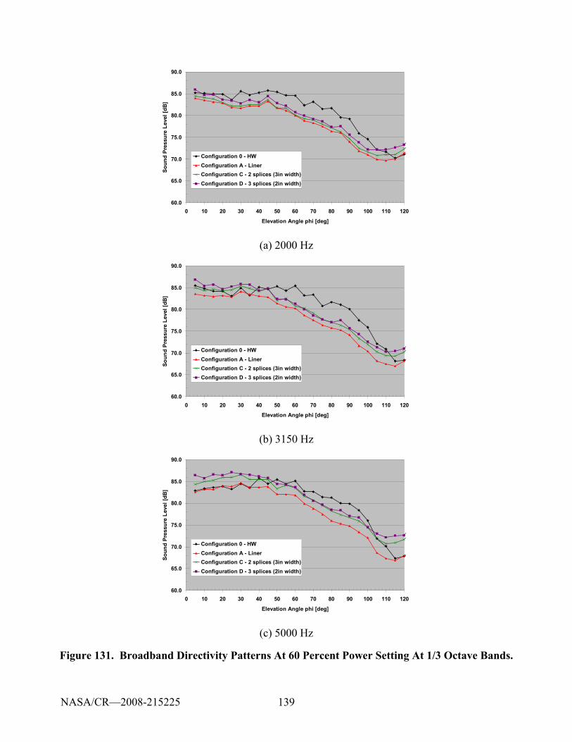
139

60.0

65.0

70.0

75.0

80.0

85.0

90.0

0 10 20 30 40 50 60 70 80 90 100 110 120


Soun

d Pr

essu

re L

evel

[dB


(a) 2000 Hz

60.0

65.0

70.0

75.0

80.0

85.0

90.0

0 10 20 30 40 50 60 70 80 90 100 110 120


Soun

d Pr

essu

re L

evel

[dB

]


(b) 3150 Hz

60.0

65.0

70.0

75.0

80.0

85.0

90.0

0 10 20 30 40 50 60 70 80 90 100 110 120


Soun

d Pr

essu

re L

evel

[dB

]


(c) 5000 Hz


NASA/CR—2008-215225

140

4.2.4.3 Modal Measurement Results

The rotating rake measurements description is presented in Section 6.8.3.2. Some analysis of the results is presented in Section 6.8.4.

4.2.5 Liner Discontinuity Model Validation

The NASA Glenn ANCF rig and Honeywell TECH977 turbofan engine data were used in the validation process. The liner discontinuities are modeled as an array of vibrating pistons, a convergence analysis was performed in order to define the proper number of pistons to use. This analysis is included in 0.

4.2.5.1 Validation Using NASA ANCF Data

The validation was performed at 1800 RPM. Precise modal information of the acoustic field incident on the liner is needed. Two different approaches were used to generate the incident field input. For pure tones, only the 2BPF tone (960 Hz at 1800 rpm) was considered. The 1BPF tone was excluded since at that frequency the liner behaves like a rigid wall producing almost no attenuation. Liner incident modal information on the 3BPF tone was not available and therefore was not considered. For broadband noise, a modified version of the equal modal power and random phase approach was used. The validation is based on sound power attenuation and sound power radiation directivity. Radiation directivities have been calculated using the flanged and un–flanged models but only the un-flanged case are presented.

4.2.5.1.1 Incident Acoustic Field

Pure tone modal information required by the model was measured in a hard-wall condition using the rotating rake described in section 4.2.4.1.1. The most dominant mode was the (4,0) with a power of 106.2 dB and a cut-on frequency of 474.0 Hz. This mode was input into the model.

The method used to provide the models with the broadband incident acoustic field is a modified version of the equal modal power and random phase approach. In the standard version, the broadband noise contains all modes that are cut-on in the hard wall condition. The modal amplitude of these cut-on modes is obtained by assigning the same power to all the modes while the relative phase is random. In the modified version, additional modes are further eliminated once they propagate into the liner. If a mode is strongly attenuated by the liner, it is eliminated from the sound field. The key reason for this technique is that the liner attenuation would be over-estimated because these strongly attenuated modes tend to hide the effect of the other more weakly attenuated ones. The criterion used to eliminate these modes is by using a parameter Γ* as proposed by Morse and Ingard [13] as follows

Γ≥⎟⎟⎠

⎞⎜⎜⎝

⎛=Γ

+

2

0

2)(* )(Re

kkmn (68)

where ( )mnk + is the mode eigen-wavenumber in the lined section; 0k is the free field wave number; and Γ

is the discriminating parameter whose value is problem dependent. If *Γ for a particular mode is larger than Γ, the mode is strongly attenuated by the liner and eliminated from the . The Γ parameter is selected by the user.

Information for both the 2BPF tone and broadband component is summarized in Table 14.

NASA/CR—2008-215225

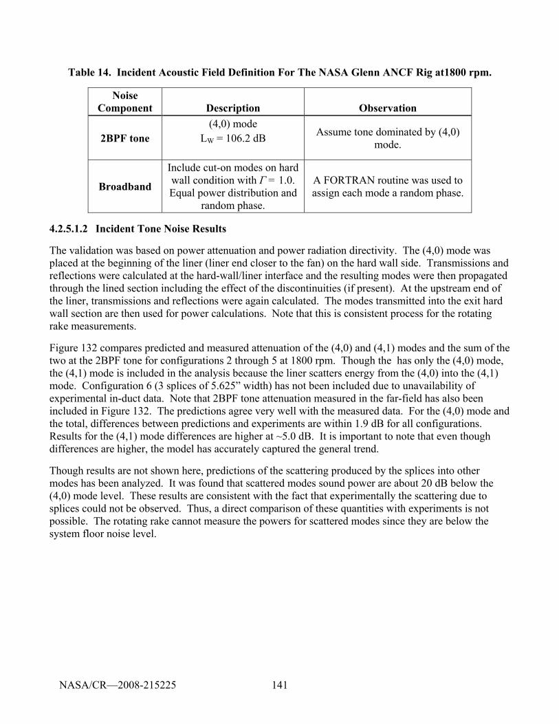
141

Table 14. Incident Acoustic Field Definition For The NASA Glenn ANCF Rig at1800 rpm.

Noise Component Description Observation

2BPF tone (4,0) mode

LW = 106.2 dB

Assume tone dominated by (4,0) mode.

Broadband

Include cut-on modes on hard wall condition with Г = 1.0. Equal power distribution and

random phase.

A FORTRAN routine was used to assign each mode a random phase.

4.2.5.1.2 Incident Tone Noise Results

The validation was based on power attenuation and power radiation directivity. The (4,0) mode was placed at the beginning of the liner (liner end closer to the fan) on the hard wall side. Transmissions and reflections were calculated at the hard-wall/liner interface and the resulting modes were then propagated through the lined section including the effect of the discontinuities (if present). At the upstream end of the liner, transmissions and reflections were again calculated. The modes transmitted into the exit hard wall section are then used for power calculations. Note that this is consistent process for the rotating rake measurements.

Figure 132 compares predicted and measured attenuation of the (4,0) and (4,1) modes and the sum of the two at the 2BPF tone for configurations 2 through 5 at 1800 rpm. Though the has only the (4,0) mode, the (4,1) mode is included in the analysis because the liner scatters energy from the (4,0) into the (4,1) mode. Configuration 6 (3 splices of 5.625” width) has not been included due to unavailability of experimental in-duct data. Note that 2BPF tone attenuation measured in the far-field has also been included in Figure 132. The predictions agree very well with the measured data. For the (4,0) mode and the total, differences between predictions and experiments are within 1.9 dB for all configurations. Results for the (4,1) mode differences are higher at ~5.0 dB. It is important to note that even though differences are higher, the model has accurately captured the general trend.

Though results are not shown here, predictions of the scattering produced by the splices into other modes has been analyzed. It was found that scattered modes sound power are about 20 dB below the (4,0) mode level. These results are consistent with the fact that experimentally the scattering due to splices could not be observed. Thus, a direct comparison of these quantities with experiments is not possible. The rotating rake cannot measure the powers for scattered modes since they are below the system floor noise level.

NASA/CR—2008-215225

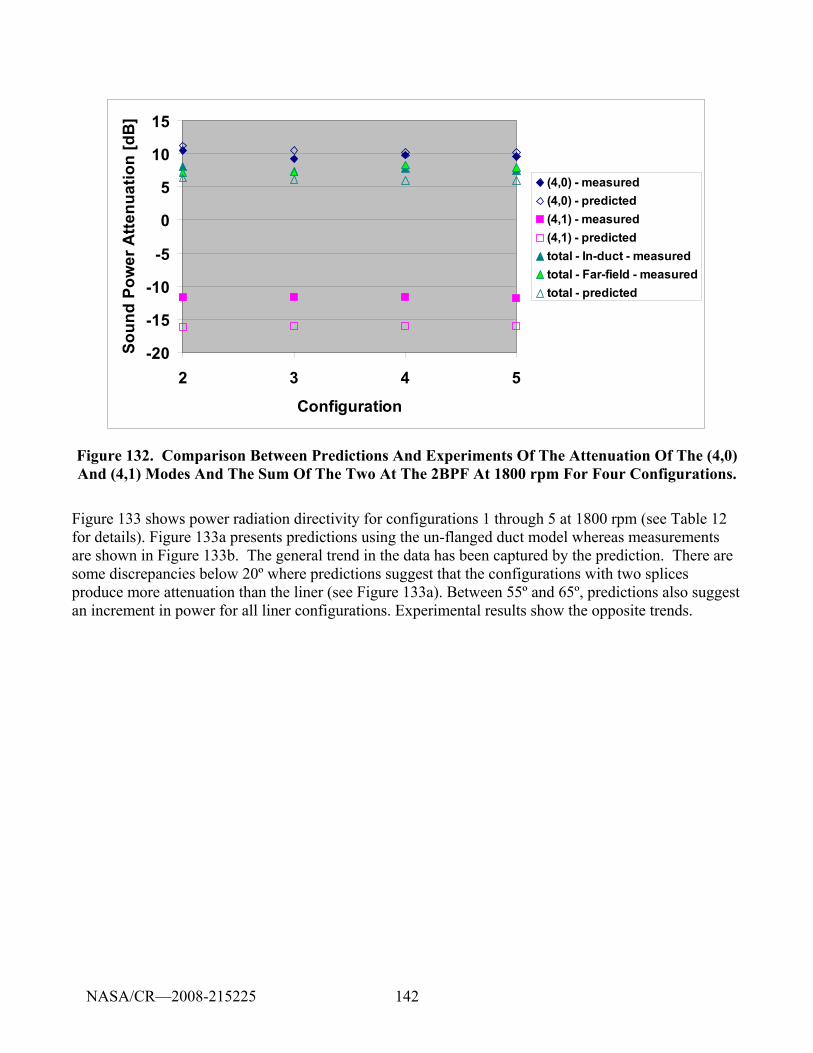
142

-20

-15

-10

-5

0

5

10

15

2 3 4 5

Configuration

Soun

d Po

wer

Atte

nuat

ion

[dB

]

(4,0) - measured(4,0) - predicted(4,1) - measured(4,1) - predictedtotal - In-duct - measured total - Far-field - measuredtotal - predicted

Figure 132. Comparison Between Predictions And Experiments Of The Attenuation Of The (4,0) And (4,1) Modes And The Sum Of The Two At The 2BPF At 1800 rpm For Four Configurations.

Figure 133 shows power radiation directivity for configurations 1 through 5 at 1800 rpm (see Table 12 for details). Figure 133a presents predictions using the un-flanged duct model whereas measurements are shown in Figure 133b. The general trend in the data has been captured by the prediction. There are some discrepancies below 20º where predictions suggest that the configurations with two splices produce more attenuation than the liner (see Figure 133a). Between 55º and 65º, predictions also suggest an increment in power for all liner configurations. Experimental results show the opposite trends.

NASA/CR—2008-215225

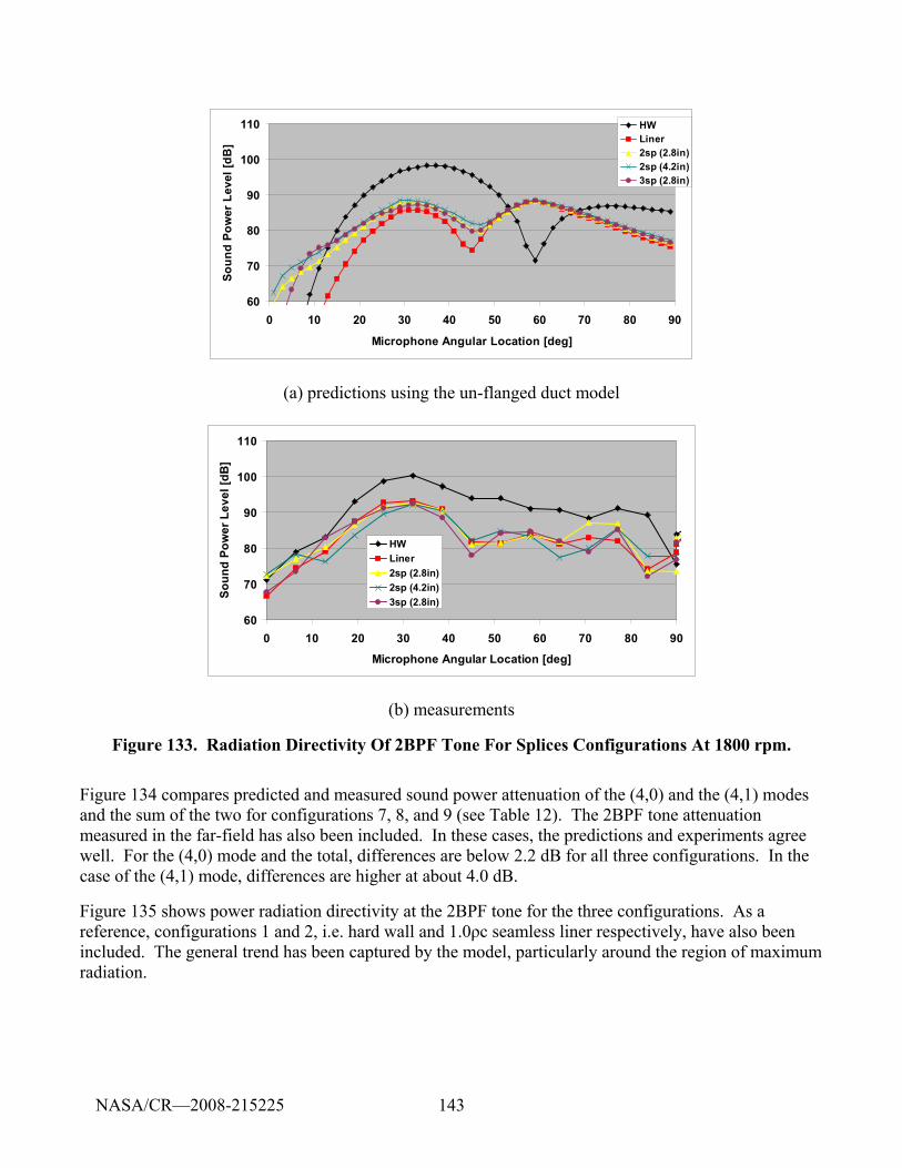
143

60

70

80

90

100

110

0 10 20 30 40 50 60 70 80 90


Soun

d Po

wer

Lev

el [d

B]

HWLiner2sp (2.8in)2sp (4.2in)3sp (2.8in)

(a) predictions using the un-flanged duct model

60

70

80

90

100

110

0 10 20 30 40 50 60 70 80 90


Soun

d Po

wer

Lev

el [d

B]

HWLiner2sp (2.8in)2sp (4.2in)3sp (2.8in)

(b) measurements

Figure 133. Radiation Directivity Of 2BPF Tone For Splices Configurations At 1800 rpm.

Figure 134 compares predicted and measured sound power attenuation of the (4,0) and the (4,1) modes and the sum of the two for configurations 7, 8, and 9 (see Table 12). The 2BPF tone attenuation measured in the far-field has also been included. In these cases, the predictions and experiments agree well. For the (4,0) mode and the total, differences are below 2.2 dB for all three configurations. In the case of the (4,1) mode, differences are higher at about 4.0 dB.

Figure 135 shows power radiation directivity at the 2BPF tone for the three configurations. As a reference, configurations 1 and 2, i.e. hard wall and 1.0ρc seamless liner respectively, have also been included. The general trend has been captured by the model, particularly around the region of maximum radiation.

NASA/CR—2008-215225

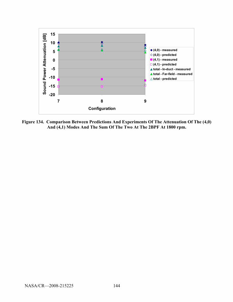
144

-20

-15

-10

-5

0

5

10

15

7 8 9

Configuration

Soun

d Po

wer

Atte

nuat

ion

[dB

](4,0) - measured(4,0) - predicted(4,1) - measured(4,1) - predictedtotal - In-duct - measured total - Far-field - measuredtotal - predicted

Figure 134. Comparison Between Predictions And Experiments Of The Attenuation Of The (4,0) And (4,1) Modes And The Sum Of The Two At The 2BPF At 1800 rpm.

NASA/CR—2008-215225

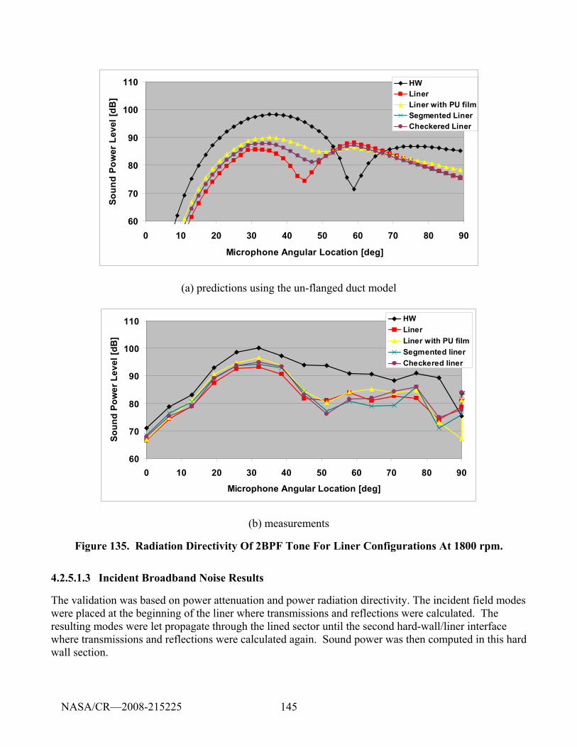
145

60

70

80

90

100

110

0 10 20 30 40 50 60 70 80 90


Soun

d Po

wer

Lev

el [d

B]

HWLinerLiner with PU filmSegmented LinerCheckered Liner


60

70

80

90

100

110

0 10 20 30 40 50 60 70 80 90


Soun

d Po

wer

Lev

el [d

B]


(b) measurements

Figure 135. Radiation Directivity Of 2BPF Tone For Liner Configurations At 1800 rpm.

4.2.5.1.3 Incident Broadband Noise Results

The validation was based on power attenuation and power radiation directivity. The incident field modes were placed at the beginning of the liner where transmissions and reflections were calculated. The resulting modes were let propagate through the lined sector until the second hard-wall/liner interface where transmissions and reflections were calculated again. Sound power was then computed in this hard wall section.

NASA/CR—2008-215225

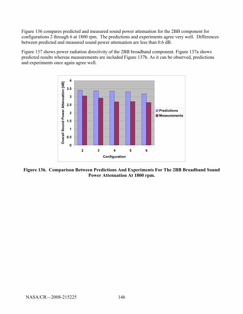
146

Figure 136 compares predicted and measured sound power attenuation for the 2BB component for configurations 2 through 6 at 1800 rpm. The predictions and experiments agree very well. Differences between predicted and measured sound power attenuation are less than 0.6 dB.

Figure 137 shows power radiation directivity of the 2BB broadband component. Figure 137a shows predicted results whereas measurements are included Figure 137b. As it can be observed, predictions and experiments once again agree well.

0

0.5

1

1.5

2

2.5

3

3.5

4

2 3 4 5 6

Configuration

Ove

rall

Soun

d Po

wer

Atte

nuat

ion

[dB

]

PredictionsMeasurements

Figure 136. Comparison Between Predictions And Experiments For The 2BB Broadband Sound Power Attenuation At 1800 rpm.

NASA/CR—2008-215225

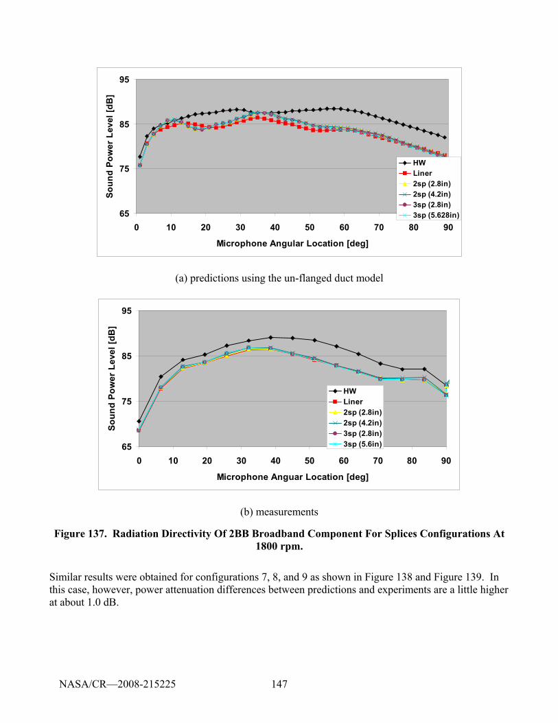
147

65

75

85

95

0 10 20 30 40 50 60 70 80 90


Soun

d Po

wer

Lev

el [d

B]



65

75

85

95

0 10 20 30 40 50 60 70 80 90

Microphone Anguar Location [deg]

Soun

d Po

wer

Lev

el [d

B]


(b) measurements

Figure 137. Radiation Directivity Of 2BB Broadband Component For Splices Configurations At 1800 rpm.

Similar results were obtained for configurations 7, 8, and 9 as shown in Figure 138 and Figure 139. In this case, however, power attenuation differences between predictions and experiments are a little higher at about 1.0 dB.

NASA/CR—2008-215225

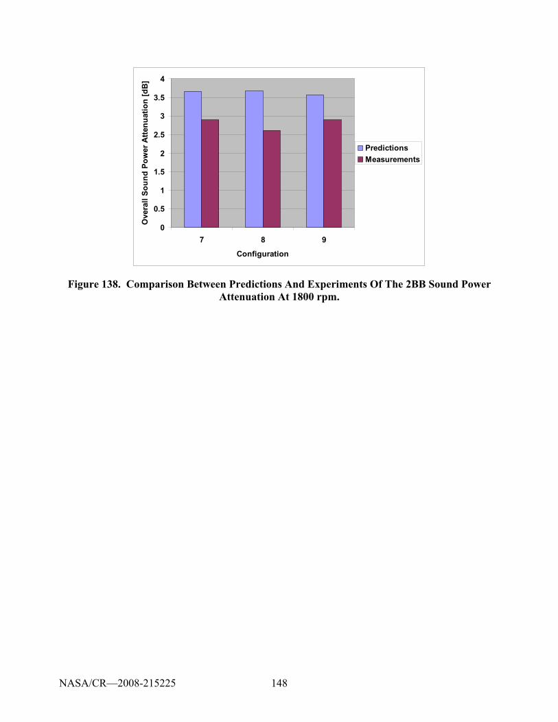
148

0

0.5

1

1.5

2

2.5

3

3.5

4

7 8 9

Configuration

Ove

rall

Soun

d Po

wer

Atte

nuat

ion

[dB

]PredictionsMeasurements

Figure 138. Comparison Between Predictions And Experiments Of The 2BB Sound Power Attenuation At 1800 rpm.

NASA/CR—2008-215225

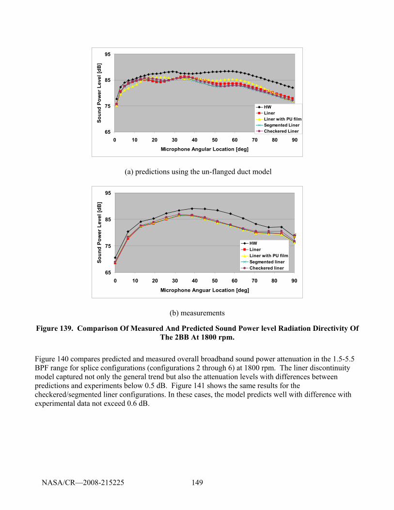
149

65

75

85

95

0 10 20 30 40 50 60 70 80 90


Soun

d Po

wer

Lev

el [d

B]

HWLinerLiner with PU filmSegmented LinerCheckered Liner


65

75

85

95

0 10 20 30 40 50 60 70 80 90

Microphone Anguar Location [deg]

Soun

d Po

wer

Lev

el [d

B]


(b) measurements

Figure 139. Comparison Of Measured And Predicted Sound Power level Radiation Directivity Of The 2BB At 1800 rpm.

Figure 140 compares predicted and measured overall broadband sound power attenuation in the 1.5-5.5 BPF range for splice configurations (configurations 2 through 6) at 1800 rpm. The liner discontinuity model captured not only the general trend but also the attenuation levels with differences between predictions and experiments below 0.5 dB. Figure 141 shows the same results for the checkered/segmented liner configurations. In these cases, the model predicts well with difference with experimental data not exceed 0.6 dB.

NASA/CR—2008-215225

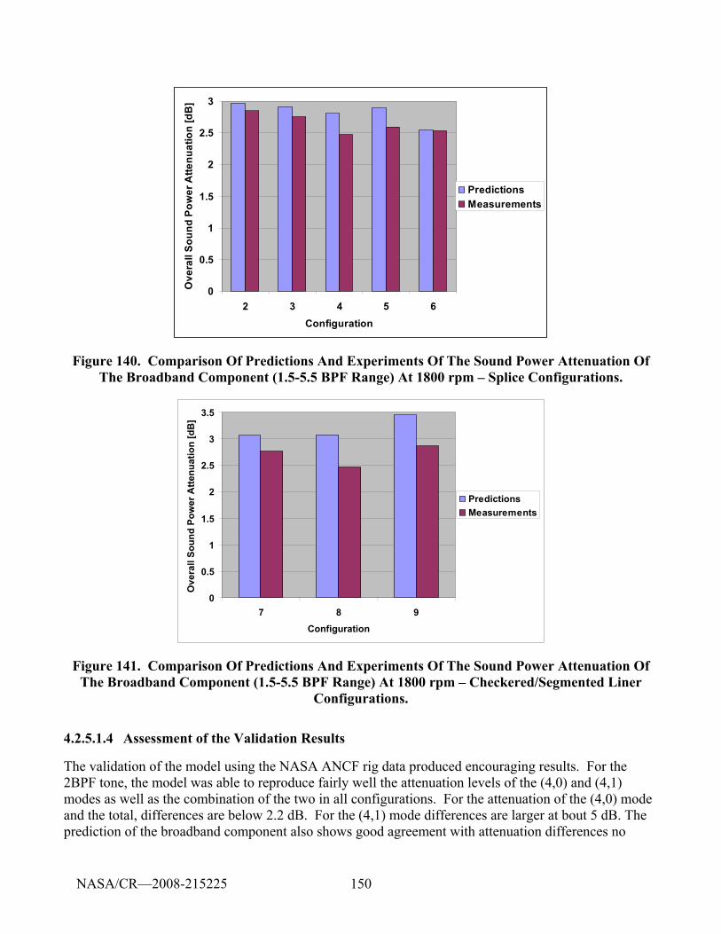
150

0

0.5

1

1.5

2

2.5

3

2 3 4 5 6Configuration

Ove

rall

Soun

d Po

wer

Atte

nuat

ion

[dB

]PredictionsMeasurements

Figure 140. Comparison Of Predictions And Experiments Of The Sound Power Attenuation Of The Broadband Component (1.5-5.5 BPF Range) At 1800 rpm – Splice Configurations.

0

0.5

1

1.5

2

2.5

3

3.5

7 8 9Configuration

Ove

rall

Soun

d Po

wer

Atte

nuat

ion

[dB

]

PredictionsMeasurements

Figure 141. Comparison Of Predictions And Experiments Of The Sound Power Attenuation Of The Broadband Component (1.5-5.5 BPF Range) At 1800 rpm – Checkered/Segmented Liner

Configurations.

4.2.5.1.4 Assessment of the Validation Results

The validation of the model using the NASA ANCF rig data produced encouraging results. For the 2BPF tone, the model was able to reproduce fairly well the attenuation levels of the (4,0) and (4,1) modes as well as the combination of the two in all configurations. For the attenuation of the (4,0) mode and the total, differences are below 2.2 dB. For the (4,1) mode differences are larger at bout 5 dB. The prediction of the broadband component also shows good agreement with attenuation differences no

NASA/CR—2008-215225

151

larger than 1.0 dB. In the case of far-field radiation, the model has captured the general trend shown by experiments.

However, the liner discontinuities had little effect on the performance of the liner. Though the model has been able of capturing this trend, further validation in an environment where the effect of discontinuities is more significant was still needed. This environment has been provided by the Honeywell TECH977 turbofan engine.

4.2.5.2 Validation Using Honeywell TECH977 Turbofan Far Field Engine Data

The process for the validation was the same as for the NASA ANCF data. For pure tones, the lack of incident acoustic modal data at the BPF resulted in the use of several buzz-saw tones at supersonic power settings. Since only far-field data were available, validation was limited to comparing the sound pressure levels in the plane of the microphones. Sound directivities were calculated using the two radiation models described in section 4.2.2.3, but only the un-flanged case is presented.

4.2.5.2.1 Incident Acoustic Field

Pure tones predictions were performed using buzz-saw tones. The modal structure of a buzz-saw tone is far simpler than that of the BPF tone, where rotor-stator interaction modes may also be a significant contribution to the sound field. In the case of a buzz-saw tone, which takes place at integer engine order, the sound field is dominated by a single mode. The circumferential order of the mode is the same as the shaft engine order. For instance, at engine order 12 the most significant mode in the is the m=12 mode. The only two power settings dominated by buzz-saw tones were 87% and 91%. Therefore, the following cases were selected for the validation:

1. Engine order 17 at 87%. The engine order 17 corresponds to a frequency of 2512 Hz and the only mode in the is the (17,0) mode with a cut-on frequency of 2187.6 Hz.

2. Engine order 12 at 91%. The engine order 12 corresponds to a frequency of 1680 Hz and the only mode in the is the (12,0) mode with a cut-on frequency of 1573.8 Hz.

The method used to provide the model with the broadband is the same modified version of the equal modal power and random phase approach used in the ANCF rig (see section 4.2.5.1.1 for details). The value for parameter Γ was set at 0.9. Results at the power setting 54% were selected for the broadband validation. Predictions were performed between 1600 and 6300 Hz. The lower limit was selected because little effect of the splices on the liner attenuation was observed below this frequency. The upper limit was given by the measured liner acoustic impedance (see section 4.2.4.2.1). Information for buzz-saw tones and broadband cases is summarized in Table 15.

NASA/CR—2008-215225

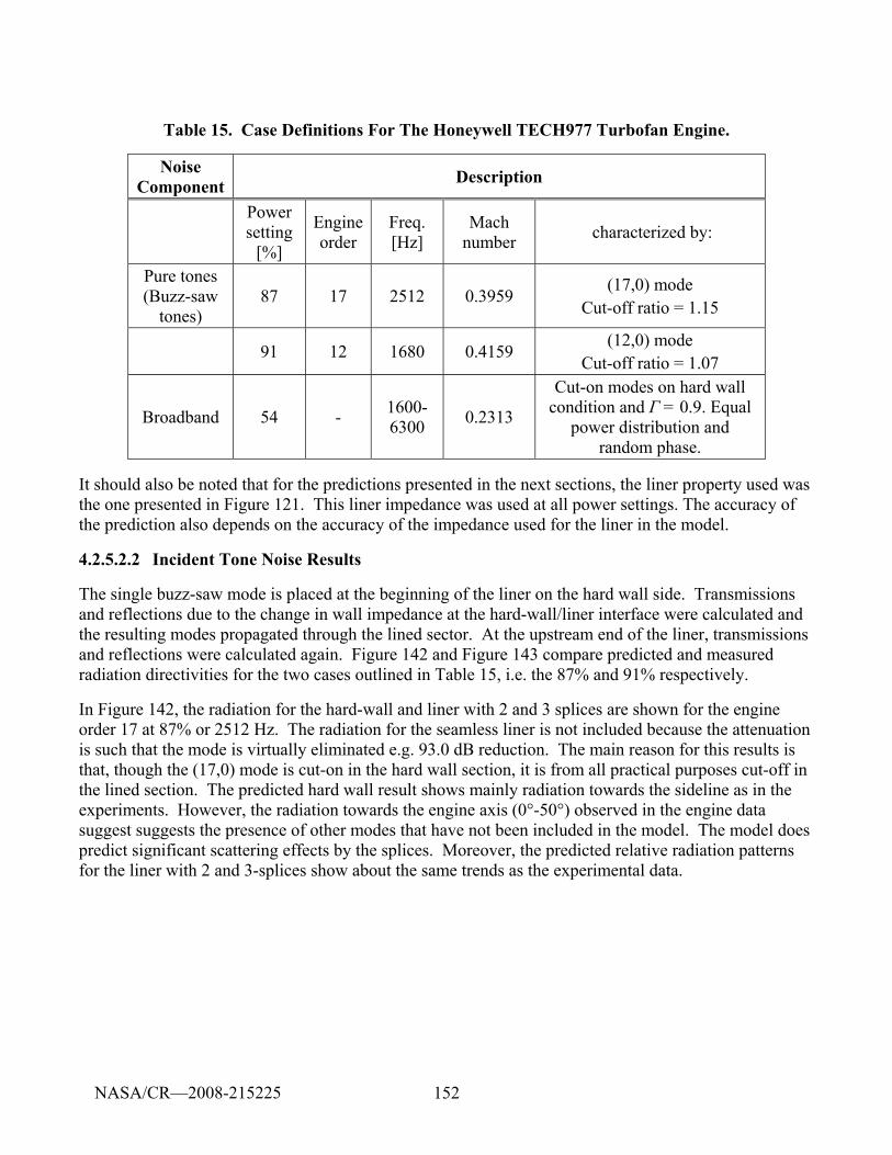
152

Table 15. Case Definitions For The Honeywell TECH977 Turbofan Engine.

Noise Component Description

Power setting

[%]

Engine order

Freq. [Hz]

Mach number characterized by:

Pure tones (Buzz-saw

tones) 87 17 2512 0.3959

(17,0) mode Cut-off ratio = 1.15

91 12 1680 0.4159 (12,0) mode

Cut-off ratio = 1.07

Broadband 54 - 1600-6300 0.2313

Cut-on modes on hard wall condition and Г = 0.9. Equal

power distribution and random phase.

It should also be noted that for the predictions presented in the next sections, the liner property used was the one presented in Figure 121. This liner impedance was used at all power settings. The accuracy of the prediction also depends on the accuracy of the impedance used for the liner in the model.

4.2.5.2.2 Incident Tone Noise Results

The single buzz-saw mode is placed at the beginning of the liner on the hard wall side. Transmissions and reflections due to the change in wall impedance at the hard-wall/liner interface were calculated and the resulting modes propagated through the lined sector. At the upstream end of the liner, transmissions and reflections were calculated again. Figure 142 and Figure 143 compare predicted and measured radiation directivities for the two cases outlined in Table 15, i.e. the 87% and 91% respectively.

In Figure 142, the radiation for the hard-wall and liner with 2 and 3 splices are shown for the engine order 17 at 87% or 2512 Hz. The radiation for the seamless liner is not included because the attenuation is such that the mode is virtually eliminated e.g. 93.0 dB reduction. The main reason for this results is that, though the (17,0) mode is cut-on in the hard wall section, it is from all practical purposes cut-off in the lined section. The predicted hard wall result shows mainly radiation towards the sideline as in the experiments. However, the radiation towards the engine axis (0°-50°) observed in the engine data suggest suggests the presence of other modes that have not been included in the model. The model does predict significant scattering effects by the splices. Moreover, the predicted relative radiation patterns for the liner with 2 and 3-splices show about the same trends as the experimental data.

NASA/CR—2008-215225

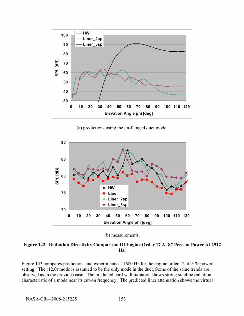
153

30

40

50

60

70

80

90

100

0 10 20 30 40 50 60 70 80 90 100 110 120Elevation Angle phi [deg]

SPL

[dB

]

HWLiner_2spLiner_3sp


70

75

80

85

90


SPL

[dB

]

HWLinerLiner_2spLiner_3sp

(b) measurements.

Figure 142. Radiation Directivity Comparison Of Engine Order 17 At 87 Percent Power At 2512 Hz.

Figure 143 compares predictions and experiments at 1680 Hz for the engine order 12 at 91% power setting. The (12,0) mode is assumed to be the only mode in the duct. Some of the same trends are observed as in the previous case. The predicted hard wall radiation shows strong sideline radiation characteristic of a mode near its cut-on frequency. The predicted liner attenuation shows the virtual

NASA/CR—2008-215225

154

elimination of the (12,0) since it is essentially an evanescent mode in the lined section. The predictions show that the 2-splices case results in more radiation or scattering effects as compared to the 3-splice case, particularly at angles greater than 40°. The experimental results also indicate similar tends although the amplitude differences are smaller. The experimental far-field radiation for the hard wall case suggests that other modes may be present in addition to the (12,0) used in the model.

30

40

50

60

70

80

90

100


SPL

[dB

]

HWLiner_2spLiner_3sp


70

75

80

85

90

95

100


SPL

[dB

]

HWLinerLiner_2spLiner_3sp

(b) measurements.

Figure 143. Radiation Directivity Comparison Of Engine Order 12 At 91 Percent Power At 1680 Hz.

NASA/CR—2008-215225

155

4.2.5.2.3 Incident Broadband Noise Results

Predictions were performed at 54% power setting for the 1/3 octave bands with 2000 and 3150 Hz center frequencies. In Figure 144, predictions and experiments are compared at the 2000 Hz 1/3 octave band. This figure shows that the predicted attenuation for the seamless liner is greater than the one observed experimentally. However, the model captures the splices behavior well. The splices have a very small effect on the liner performance as shown experimentally.

Figure 145 shows the same comparison at 3150 Hz center frequency. The 2-splices case reduced the liner attenuation by ~2.0-2.5 dB through out the entire sector. The 3-splices case also showed less attenuation reduction. The predictions support a similar conclusion with the 2-splices configuration producing more scattering. However, the predictions underestimate the scattering for the 2-splices by about 1.5 dB for the 45º-90º sector.

4.2.5.2.4 Assessment of the Validation Results

The validation of the model using the TECH977 engine data has produced reasonably good results. However, the lack of indecent sound field data means that these results should be taken qualitatively. One concern with this validation is that the comparison of predictions with experiments was restricted to the radiation in the plane of the microphones. The radiation pattern around the axis of the engine changes significantly, in particular with discontinuities. In order to improve predictions, more precise modal information should be provided to the model.

NASA/CR—2008-215225

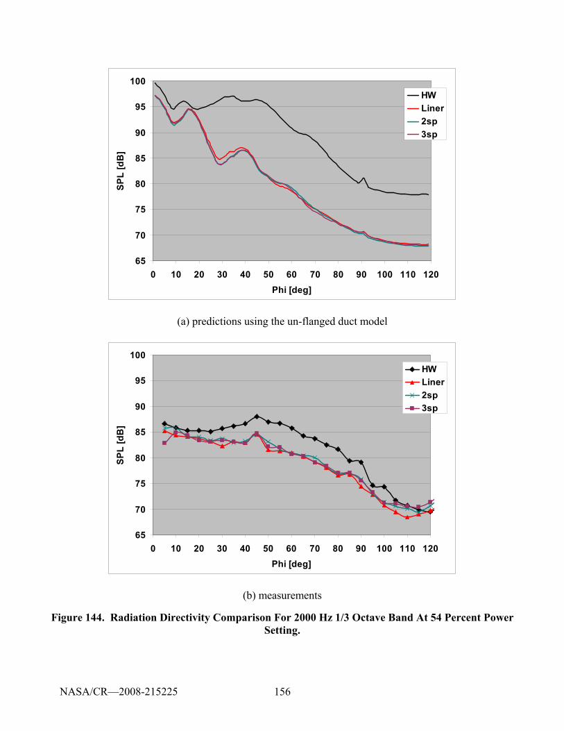
156

65

70

75

80

85

90

95

100

0 10 20 30 40 50 60 70 80 90 100 110 120Phi [deg]

SPL

[dB

]

HWLiner2sp3sp


65

70

75

80

85

90

95

100

0 10 20 30 40 50 60 70 80 90 100 110 120Phi [deg]

SPL

[dB

]

HWLiner2sp3sp

(b) measurements

Figure 144. Radiation Directivity Comparison For 2000 Hz 1/3 Octave Band At 54 Percent Power Setting.

NASA/CR—2008-215225

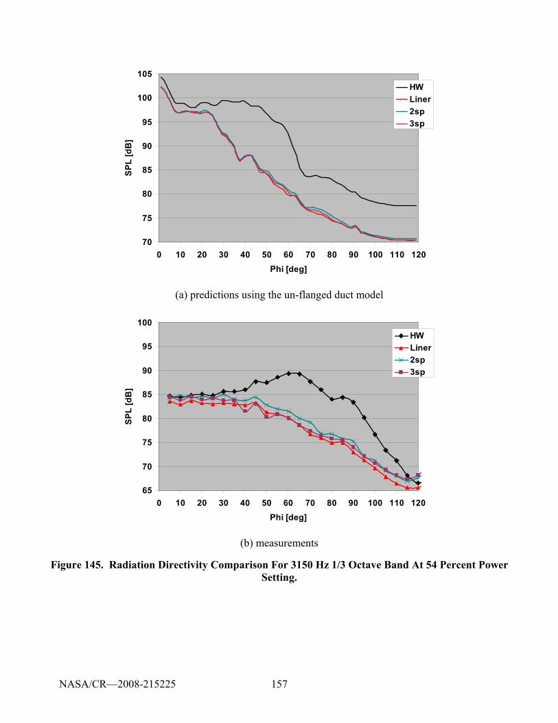
157

70

75

80

85

90

95

100

105

0 10 20 30 40 50 60 70 80 90 100 110 120Phi [deg]

SPL

[dB

]

HWLiner2sp3sp


65

70

75

80

85

90

95

100

0 10 20 30 40 50 60 70 80 90 100 110 120Phi [deg]

SPL

[dB

]

HWLiner2sp3sp

(b) measurements

Figure 145. Radiation Directivity Comparison For 3150 Hz 1/3 Octave Band At 54 Percent Power Setting.

NASA/CR—2008-215225

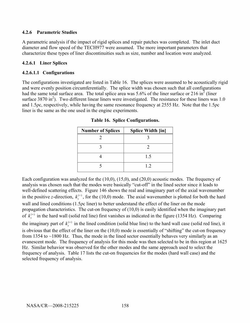
158

4.2.6 Parametric Studies

A parametric analysis if the impact of rigid splices and repair patches was completed. The inlet duct diameter and flow speed of the TECH977 were assumed. The more important parameters that characterize these types of liner discontinuities such as size, number and location were analyzed.

4.2.6.1 Liner Splices

4.2.6.1.1 Configurations

The configurations investigated are listed in Table 16. The splices were assumed to be acoustically rigid and were evenly position circumferentially. The splice width was chosen such that all configurations had the same total surface area. The total splice area was 5.6% of the liner surface or 216 in2 (liner surface 3870 in2). Two different linear liners were investigated. The resistance for these liners was 1.0 and 1.5ρc, respectively, while having the same resonance frequency at 2555 Hz. Note that the 1.5ρc liner is the same as the one used in the engine experiments.

Table 16. Splice Configurations.

Number of Splices Splice Width [in] 2 3

3 2

4 1.5

5 1.2

Each configuration was analyzed for the (10,0), (15,0), and (20,0) acoustic modes. The frequency of analysis was chosen such that the modes were basically “cut-off” in the lined sector since it leads to well-defined scattering effects. Figure 146 shows the real and imaginary part of the axial wavenumber in the positive z-direction, ( )

zk + , for the (10,0) mode. The axial wavenumber is plotted for both the hard wall and lined conditions (1.5ρc liner) to better understand the effect of the liner on the mode propagation characteristics. The cut-on frequency of (10,0) is easily identified when the imaginary part of ( )

zk + in the hard wall (solid red line) first vanishes as indicated in the figure (1354 Hz). Comparing the imaginary part of ( )

zk + in the lined condition (solid blue line) to the hard wall case (solid red line), it is obvious that the effect of the liner on the (10,0) mode is essentially of “shifting” the cut-on frequency from 1354 to ~1800 Hz. Thus, the mode in the lined sector essentially behaves very similarly as an evanescent mode. The frequency of analysis for this mode was then selected to be in this region at 1625 Hz. Similar behavior was observed for the other modes and the same approach used to select the frequency of analysis. Table 17 lists the cut-on frequencies for the modes (hard wall case) and the selected frequency of analysis.

NASA/CR—2008-215225

159

-30

0

30

60

90

120

0 500 1000 1500 2000 2500 3000 3500 4000Frequency [hz]

Axi

al W

aven

umbe

r K

z [1

/m]

Real (Kz) - HWImag (Kz) - HWReal (Kz) - LinerImag (Kz) - Liner

Mode cut-on Frequency (1354 Hz) Liner “shift” cut-on

frequency to ~ 1800Hz

Mode in the liner behaves as an evanescent wave in this

frequency region

Frequency of analysis 1625Hz

-30

0

30

60

90

120

0 500 1000 1500 2000 2500 3000 3500 4000Frequency [hz]

Axi

al W

aven

umbe

r K

z [1

/m]

Real (Kz) - HWImag (Kz) - HWReal (Kz) - LinerImag (Kz) - Liner

Mode cut-on Frequency (1354 Hz) Liner “shift” cut-on

frequency to ~ 1800Hz

Mode in the liner behaves as an evanescent wave in this

frequency region

Frequency of analysis 1625Hz

Figure 146. Axial WaveNumber ( )zk + For (10,0) Mode For Both Hard Wall And 1.5ρc Liner.

Table 17. Cut-On Frequencies Of The Different Modes Used In The Analysis.

Mode Hard-Wall Cut-

on Freq. [Hz] Cut-on RatioFreq. of Analysis

[Hz] (10,0) 1354 1.2 1625

(15,0) 1958 1.2 2350

(20,0) 2556 1.2 3067

4.2.6.1.2 Results

Figure 147 shows sound power attenuation due to the liners as a function of the number of splices for the three modes investigated. The attenuation of the seamless liner is not included because the incident mode is virtually eliminated. Two observations can be made. First, the liner power attenuation is essentially linear with the number of splices (in the decibel scale). Second, the slope seems to be approximately the same for the two liners and slightly different from mode to mode. In general, the “average” slope for the cases shown in this figure is about 2 dB/splice. Thus, as the number of splices increases (while keeping the same surface area) the sound power due to the scattering is reduce by 2dB for each splice added.

NASA/CR—2008-215225

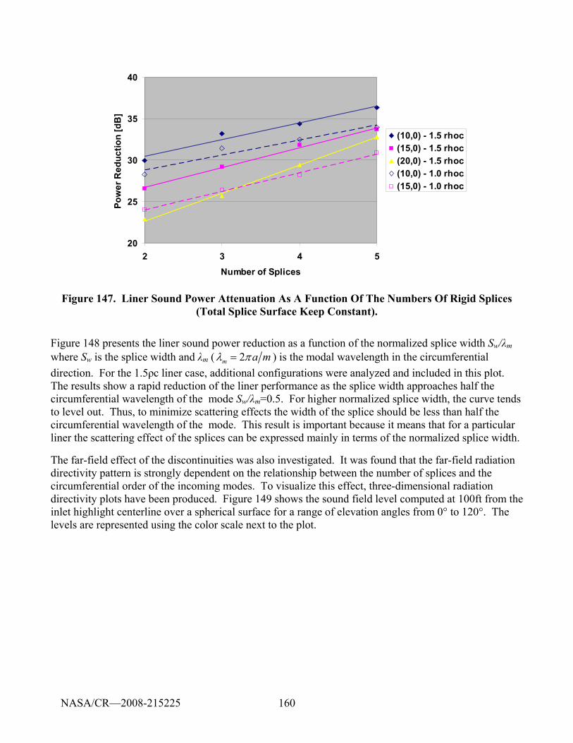
160

20

25

30

35

40

2 3 4 5Number of Splices

Pow

er R

educ

tion

[dB

]

(10,0) - 1.5 rhoc(15,0) - 1.5 rhoc(20,0) - 1.5 rhoc(10,0) - 1.0 rhoc(15,0) - 1.0 rhoc

Figure 147. Liner Sound Power Attenuation As A Function Of The Numbers Of Rigid Splices (Total Splice Surface Keep Constant).

Figure 148 presents the liner sound power reduction as a function of the normalized splice width Sw/λm where Sw is the splice width and λm ( 2m a mλ π= ) is the modal wavelength in the circumferential direction. For the 1.5ρc liner case, additional configurations were analyzed and included in this plot. The results show a rapid reduction of the liner performance as the splice width approaches half the circumferential wavelength of the mode Sw/λm=0.5. For higher normalized splice width, the curve tends to level out. Thus, to minimize scattering effects the width of the splice should be less than half the circumferential wavelength of the mode. This result is important because it means that for a particular liner the scattering effect of the splices can be expressed mainly in terms of the normalized splice width.

The far-field effect of the discontinuities was also investigated. It was found that the far-field radiation directivity pattern is strongly dependent on the relationship between the number of splices and the circumferential order of the incoming modes. To visualize this effect, three-dimensional radiation directivity plots have been produced. Figure 149 shows the sound field level computed at 100ft from the inlet highlight centerline over a spherical surface for a range of elevation angles from 0° to 120°. The levels are represented using the color scale next to the plot.

NASA/CR—2008-215225

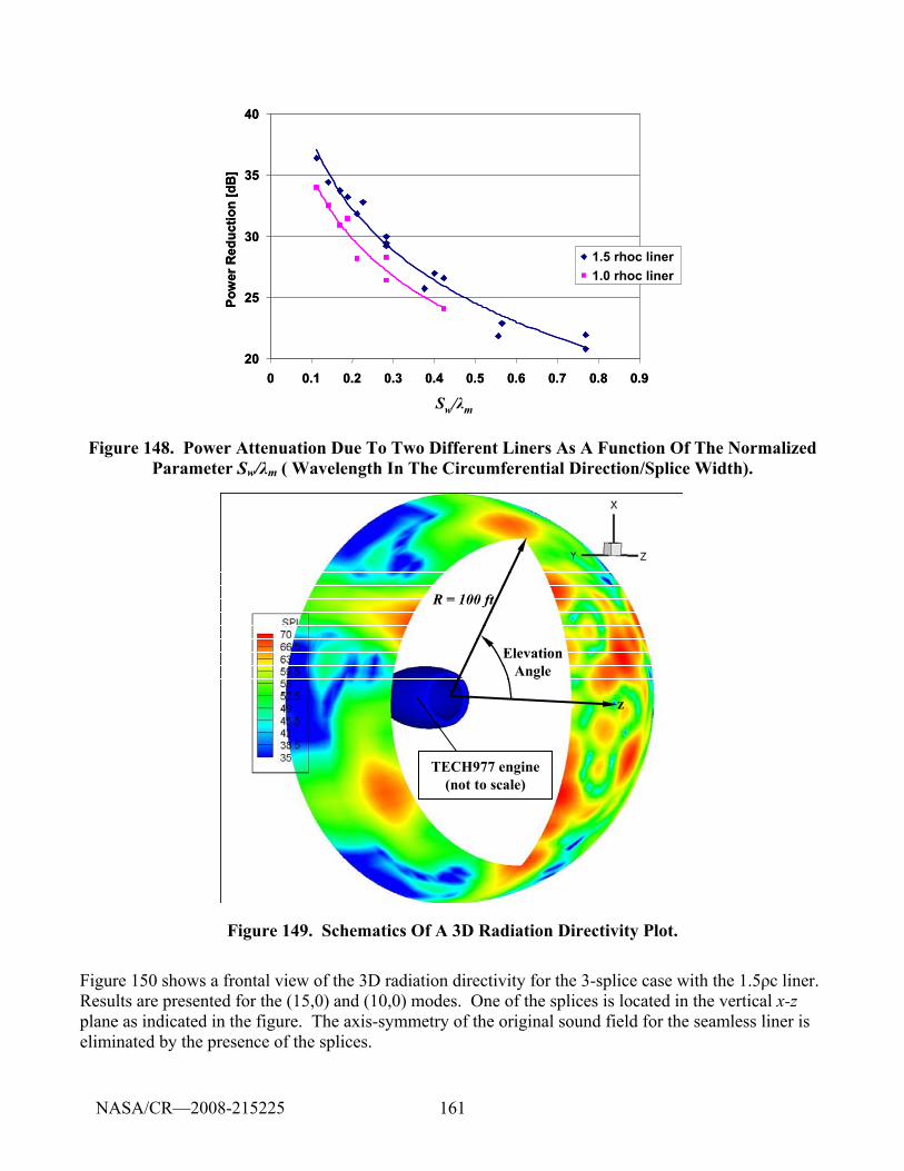
161

Sw/λm

20

25

30

35

40

0 0.1 0.2 0.3 0.4 0.5 0.6 0.7 0.8 0.9

Pow

er R

educ

tion

[dB

]

1.5 rhoc liner1.0 rhoc liner

Sw/λm

20

25

30

35

40

0 0.1 0.2 0.3 0.4 0.5 0.6 0.7 0.8 0.9

Pow

er R

educ

tion

[dB

]

1.5 rhoc liner1.0 rhoc liner

Figure 148. Power Attenuation Due To Two Different Liners As A Function Of The Normalized Parameter Sw/λm ( Wavelength In The Circumferential Direction/Splice Width).

Elevation Angle

R = 100 ft

TECH977 engine (not to scale)

z

Elevation Angle

R = 100 ft

TECH977 engine (not to scale)

z

Figure 149. Schematics Of A 3D Radiation Directivity Plot.

Figure 150 shows a frontal view of the 3D radiation directivity for the 3-splice case with the 1.5ρc liner. Results are presented for the (15,0) and (10,0) modes. One of the splices is located in the vertical x-z plane as indicated in the figure. The axis-symmetry of the original sound field for the seamless liner is eliminated by the presence of the splices.

NASA/CR—2008-215225

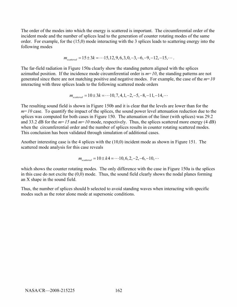
162

The order of the modes into which the energy is scattered is important. The circumferential order of the incident mode and the number of splices lead to the generation of counter rotating modes of the same order. For example, for the (15,0) mode interacting with the 3 splices leads to scattering energy into the following modes

15 3 15,12,9,6,3,0, 3, 6, 9, 12, 15,scatteredm k= ± = − − − − −L L .

The far-field radiation in Figure 150a clearly show the standing pattern aligned with the splices azimuthal position. If the incidence mode circumferential order is m=10, the standing patterns are not generated since there are not matching positive and negative modes. For example, the case of the m=10 interacting with three splices leads to the following scattered mode orders

10 3 10,7,4,1, 2, 5, 8, 11, 14,scatteredm k= ± = − − − − −L L

The resulting sound field is shown in Figure 150b and it is clear that the levels are lower than for the m=10 case. To quantify the impact of the splices, the sound power level attenuation reduction due to the splices was computed for both cases in Figure 150. The attenuation of the liner (with splices) was 29.2 and 33.2 dB for the m=15 and m=10 mode, respectively. Thus, the splices scattered more energy (4 dB) when the circumferential order and the number of splices results in counter rotating scattered modes. This conclusion has been validated through simulation of additional cases.

Another interesting case is the 4 splices with the (10,0) incident mode as shown in Figure 151. The scattered mode analysis for this case reveals

10 4 10,6,2, 2, 6, 10,scatteredm k= ± = − − −L L

which shows the counter rotating modes. The only difference with the case in Figure 150a is the splices in this case do not excite the (0,0) mode. Thus, the sound field clearly shows the nodal planes forming an X shape in the sound field.

Thus, the number of splices should b selected to avoid standing waves when interacting with specific modes such as the rotor alone mode at supersonic conditions.

NASA/CR—2008-215225

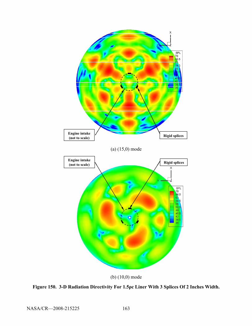
163

Engine intake (not to scale) Rigid splicesEngine intake (not to scale) Rigid splicesEngine intake (not to scale) Rigid splicesEngine intake (not to scale) Rigid splices

(a) (15,0) mode

Engine intake (not to scale) Rigid splicesEngine intake (not to scale) Rigid splices

(b) (10,0) mode

Figure 150. 3-D Radiation Directivity For 1.5ρc Liner With 3 Splices Of 2 Inches Width.

NASA/CR—2008-215225

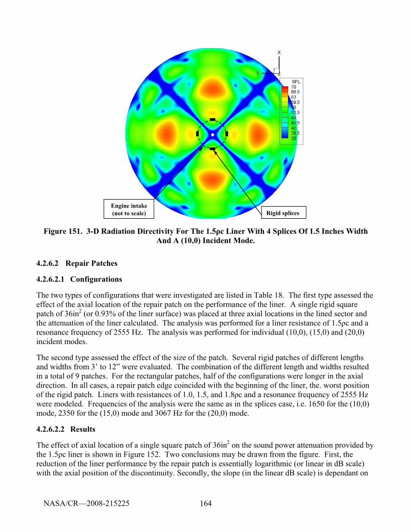
164

Engine intake (not to scale) Rigid splicesEngine intake (not to scale) Rigid splices

Figure 151. 3-D Radiation Directivity For The 1.5ρc Liner With 4 Splices Of 1.5 Inches Width And A (10,0) Incident Mode.

4.2.6.2 Repair Patches

4.2.6.2.1 Configurations

The two types of configurations that were investigated are listed in Table 18. The first type assessed the effect of the axial location of the repair patch on the performance of the liner. A single rigid square patch of 36in2 (or 0.93% of the liner surface) was placed at three axial locations in the lined sector and the attenuation of the liner calculated. The analysis was performed for a liner resistance of 1.5ρc and a resonance frequency of 2555 Hz. The analysis was performed for individual (10,0), (15,0) and (20,0) incident modes.

The second type assessed the effect of the size of the patch. Several rigid patches of different lengths and widths from 3’ to 12” were evaluated. The combination of the different length and widths resulted in a total of 9 patches. For the rectangular patches, half of the configurations were longer in the axial direction. In all cases, a repair patch edge coincided with the beginning of the liner, the. worst position of the rigid patch. Liners with resistances of 1.0, 1.5, and 1.8ρc and a resonance frequency of 2555 Hz were modeled. Frequencies of the analysis were the same as in the splices case, i.e. 1650 for the (10,0) mode, 2350 for the (15,0) mode and 3067 Hz for the (20,0) mode.

4.2.6.2.2 Results

The effect of axial location of a single square patch of 36in2 on the sound power attenuation provided by the 1.5ρc liner is shown in Figure 152. Two conclusions may be drawn from the figure. First, the reduction of the liner performance by the repair patch is essentially logarithmic (or linear in dB scale) with the axial position of the discontinuity. Secondly, the slope (in the linear dB scale) is dependant on

NASA/CR—2008-215225

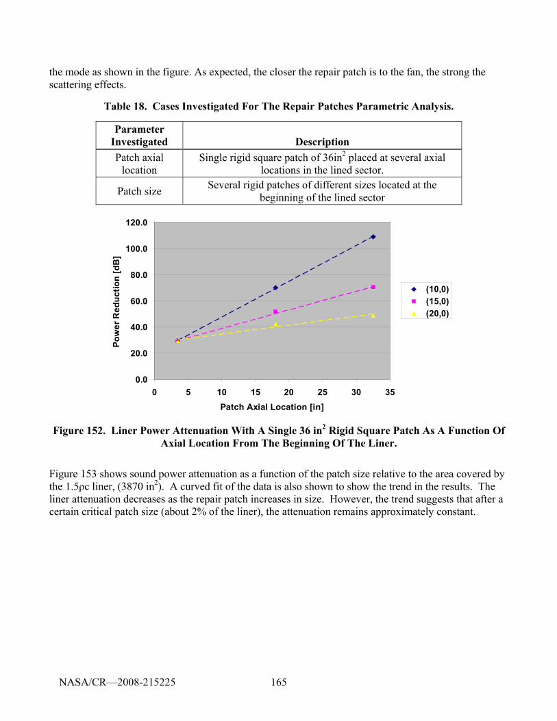
165

the mode as shown in the figure. As expected, the closer the repair patch is to the fan, the strong the scattering effects.

Table 18. Cases Investigated For The Repair Patches Parametric Analysis.

Parameter Investigated Description Patch axial

location Single rigid square patch of 36in2 placed at several axial

locations in the lined sector.

Patch size Several rigid patches of different sizes located at the beginning of the lined sector

0.0

20.0

40.0

60.0

80.0

100.0

120.0

0 5 10 15 20 25 30 35Patch Axial Location [in]

Pow

er R

educ

tion

[dB

]

(10,0)(15,0)(20,0)

Figure 152. Liner Power Attenuation With A Single 36 in2 Rigid Square Patch As A Function Of Axial Location From The Beginning Of The Liner.

Figure 153 shows sound power attenuation as a function of the patch size relative to the area covered by the 1.5ρc liner, (3870 in2). A curved fit of the data is also shown to show the trend in the results. The liner attenuation decreases as the repair patch increases in size. However, the trend suggests that after a certain critical patch size (about 2% of the liner), the attenuation remains approximately constant.

NASA/CR—2008-215225

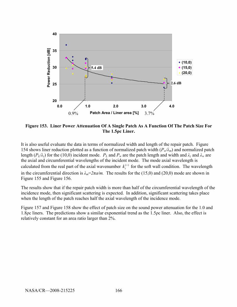
166

20

25

30

35

40

0.0 1.0 2.0 3.0 4.0Patch Area [%]

Pow

er R

educ

tion

[dB

]

(10,0)(15,0)(20,0)

0.9%

5.4 dB

3.7%

2.6 dB

Patch Area / Liner area [%]

20

25

30

35

40

0.0 1.0 2.0 3.0 4.0Patch Area [%]

Pow

er R

educ

tion

[dB

]

(10,0)(15,0)(20,0)

0.9%

5.4 dB

3.7%

2.6 dB


Figure 153. Liner Power Attenuation Of A Single Patch As A Function Of The Patch Size For The 1.5ρc Liner.

It is also useful evaluate the data in terms of normalized width and length of the repair patch. Figure 154 shows liner reduction plotted as a function of normalized patch width (Pw/λm) and normalized patch length (PL/λz) for the (10,0) incident mode. PL and Pw are the patch length and width and λz and λw are the axial and circumferential wavelengths of the incident mode. The mode axial wavelength is calculated from the real part of the axial wavenumber ( )

zk + for the soft wall condition. The wavelength in the circumferential direction is λm=2πa/m. The results for the (15,0) and (20,0) mode are shown in Figure 155 and Figure 156.

The results show that if the repair patch width is more than half of the circumferential wavelength of the incidence mode, then significant scattering is expected. In addition, significant scattering takes place when the length of the patch reaches half the axial wavelength of the incidence mode.

Figure 157 and Figure 158 show the effect of patch size on the sound power attenuation for the 1.0 and 1.8ρc liners. The predictions show a similar exponential trend as the 1.5ρc liner. Also, the effect is relatively constant for an area ratio larger than 2%.

NASA/CR—2008-215225

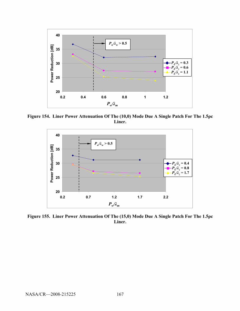
167

20

25

30

35

40

0.2 0.4 0.6 0.8 1 1.2Pw/Lm

Pow

er R

educ

tion

[dB

]

Pl/Lz 0.3Pl/Lz 0.6Pl/Lz 1.1

PL/λz = 0.3PL/λz = 0.6PL/λz = 1.1

Pw/λm

Pw/λw > 0.5

20

25

30

35

40

0.2 0.4 0.6 0.8 1 1.2Pw/Lm

Pow

er R

educ

tion

[dB

]


PL/λz = 0.3PL/λz = 0.6PL/λz = 1.1

Pw/λm

Pw/λw > 0.5

Figure 154. Liner Power Attenuation Of The (10,0) Mode Due A Single Patch For The 1.5ρc Liner.

20

25

30

35

40

0.2 0.7 1.2 1.7 2.2Pw/Lm

Pow

er R

educ

tion

[dB

]


Pw/λm

PL/λz = 0.4PL/λz = 0.8PL/λz = 1.7

Pw/λw > 0.5

20

25

30

35

40

0.2 0.7 1.2 1.7 2.2Pw/Lm

Pow

er R

educ

tion

[dB

]


Pw/λm

PL/λz = 0.4PL/λz = 0.8PL/λz = 1.7

PL/λz = 0.4PL/λz = 0.8PL/λz = 1.7

Pw/λw > 0.5


NASA/CR—2008-215225

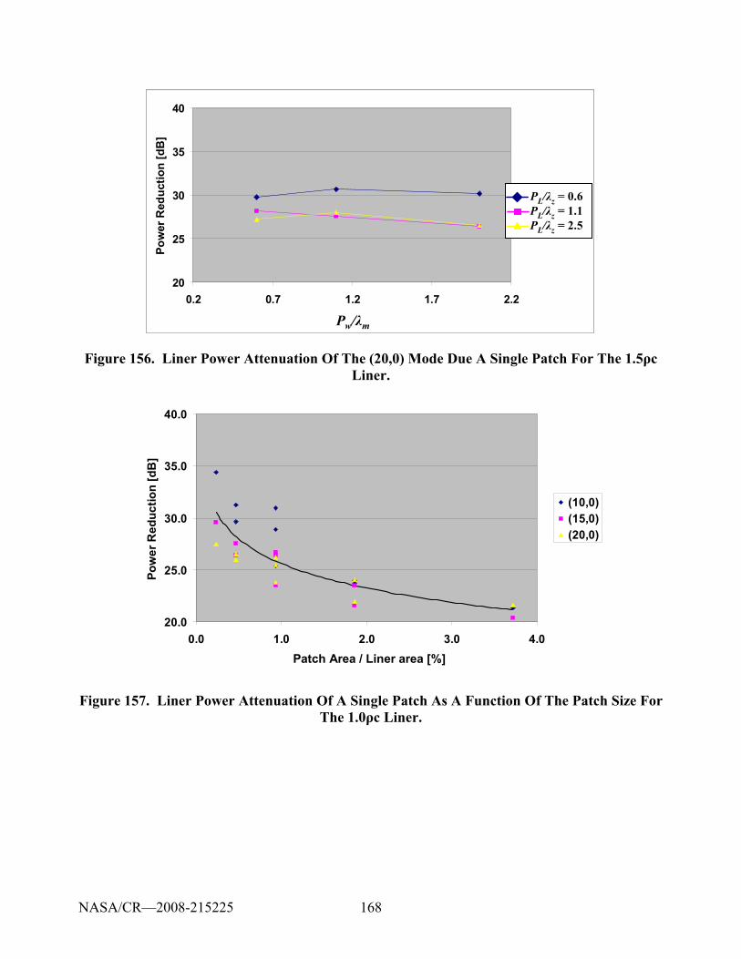
168

20

25

30

35

40

0.2 0.7 1.2 1.7 2.2Pw/Lm

Pow

er R

educ

tion

[dB

]


Pw/λm

PL/λz = 0.6PL/λz = 1.1PL/λz = 2.5

20

25

30

35

40

0.2 0.7 1.2 1.7 2.2Pw/Lm

Pow

er R

educ

tion

[dB

]


Pw/λm

PL/λz = 0.6PL/λz = 1.1PL/λz = 2.5

PL/λz = 0.6PL/λz = 1.1PL/λz = 2.5


20.0

25.0

30.0

35.0

40.0

0.0 1.0 2.0 3.0 4.0Patch Area [%]

Pow

er R

educ

tion

[dB

]

(10,0)(15,0)(20,0)


20.0

25.0

30.0

35.0

40.0

0.0 1.0 2.0 3.0 4.0Patch Area [%]

Pow

er R

educ

tion

[dB

]

(10,0)(15,0)(20,0)


Figure 157. Liner Power Attenuation Of A Single Patch As A Function Of The Patch Size For The 1.0ρc Liner.

NASA/CR—2008-215225

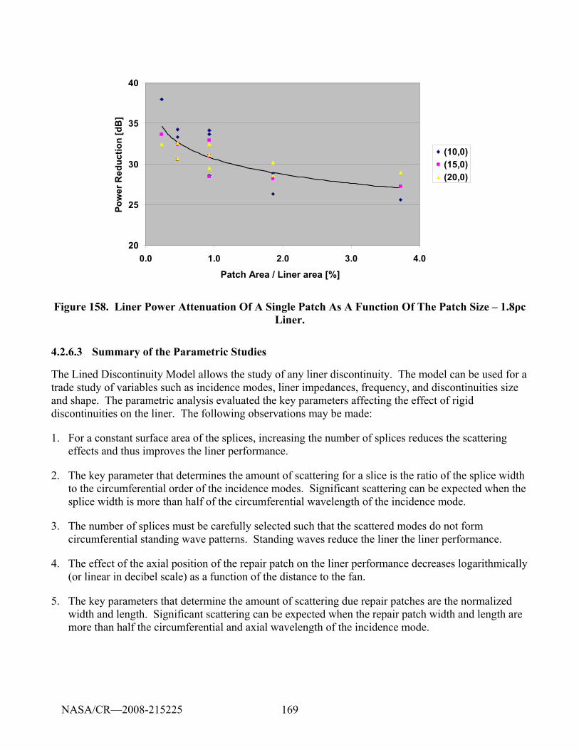
169

20

25

30

35

40

0.0 1.0 2.0 3.0 4.0Patch Area [%]

Pow

er R

educ

tion

[dB

]

(10,0)(15,0)(20,0)


20

25

30

35

40

0.0 1.0 2.0 3.0 4.0Patch Area [%]

Pow

er R

educ

tion

[dB

]

(10,0)(15,0)(20,0)


Figure 158. Liner Power Attenuation Of A Single Patch As A Function Of The Patch Size – 1.8ρc Liner.

4.2.6.3 Summary of the Parametric Studies

The Lined Discontinuity Model allows the study of any liner discontinuity. The model can be used for a trade study of variables such as incidence modes, liner impedances, frequency, and discontinuities size and shape. The parametric analysis evaluated the key parameters affecting the effect of rigid discontinuities on the liner. The following observations may be made:

1. For a constant surface area of the splices, increasing the number of splices reduces the scattering effects and thus improves the liner performance.

2. The key parameter that determines the amount of scattering for a slice is the ratio of the splice width to the circumferential order of the incidence modes. Significant scattering can be expected when the splice width is more than half of the circumferential wavelength of the incidence mode.

3. The number of splices must be carefully selected such that the scattered modes do not form circumferential standing wave patterns. Standing waves reduce the liner the liner performance.

4. The effect of the axial position of the repair patch on the liner performance decreases logarithmically (or linear in decibel scale) as a function of the distance to the fan.

5. The key parameters that determine the amount of scattering due repair patches are the normalized width and length. Significant scattering can be expected when the repair patch width and length are more than half the circumferential and axial wavelength of the incidence mode.

NASA/CR—2008-215225

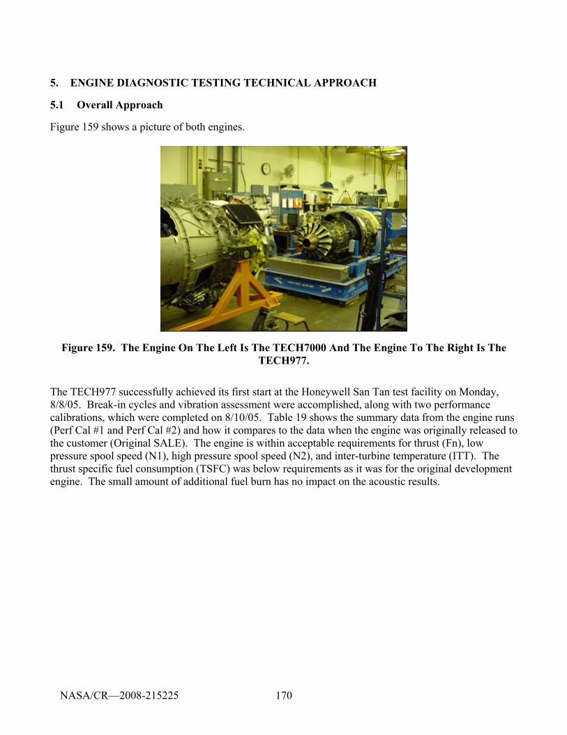
170

5. ENGINE DIAGNOSTIC TESTING TECHNICAL APPROACH

5.1 Overall Approach

Figure 159 shows a picture of both engines.

Figure 159. The Engine On The Left Is The TECH7000 And The Engine To The Right Is The TECH977.

The TECH977 successfully achieved its first start at the Honeywell San Tan test facility on Monday, 8/8/05. Break-in cycles and vibration assessment were accomplished, along with two performance calibrations, which were completed on 8/10/05. Table 19 shows the summary data from the engine runs (Perf Cal #1 and Perf Cal #2) and how it compares to the data when the engine was originally released to the customer (Original SALE). The engine is within acceptable requirements for thrust (Fn), low pressure spool speed (N1), high pressure spool speed (N2), and inter-turbine temperature (ITT). The thrust specific fuel consumption (TSFC) was below requirements as it was for the original development engine. The small amount of additional fuel burn has no impact on the acoustic results.

NASA/CR—2008-215225

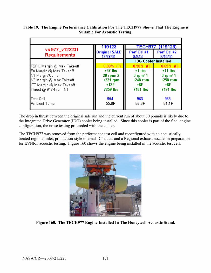
171

Table 19. The Engine Performance Calibration For The TECH977 Shows That The Engine is Suitable For Acoustic Testing.

The drop in thrust between the original sale run and the current run of about 80 pounds is likely due to the Integrated Drive Generator (IDG) cooler being installed. Since this cooler is part of the final engine configuration, the noise testing proceeded with the cooler.

The TECH977 was removed from the performance test cell and reconfigured with an acoustically treated regional inlet, production-style internal “C” ducts and a Regional exhaust nozzle, in preparation for EVNRT acoustic testing. Figure 160 shows the engine being installed in the acoustic test cell.

Figure 160. The TECH977 Engine Installed In The Honeywell Acoustic Stand.

NASA/CR—2008-215225

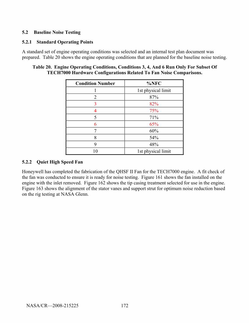
172

5.2 Baseline Noise Testing

5.2.1 Standard Operating Points

A standard set of engine operating conditions was selected and an internal test plan document was prepared. Table 20 shows the engine operating conditions that are planned for the baseline noise testing.

Table 20. Engine Operating Conditions, Conditions 3, 4, And 6 Run Only For Subset Of TECH7000 Hardware Configurations Related To Fan Noise Comparisons.

Condition Number %NFC 1 1st physical limit 2 87% 3 82% 4 75% 5 71% 6 65% 7 60% 8 54% 9 48% 10 1st physical limit

5.2.2 Quiet High Speed Fan

Honeywell has completed the fabrication of the QHSF II Fan for the TECH7000 engine. A fit check of the fan was conducted to ensure it is ready for noise testing. Figure 161 shows the fan installed on the engine with the inlet removed. Figure 162 shows the tip casing treatment selected for use in the engine. Figure 163 shows the alignment of the stator vanes and support strut for optimum noise reduction based on the rig testing at NASA Glenn.

NASA/CR—2008-215225

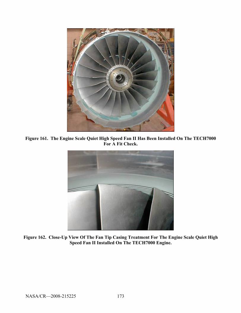
173

Figure 161. The Engine Scale Quiet High Speed Fan II Has Been Installed On The TECH7000 For A Fit Check.

Figure 162. Close-Up View Of The Fan Tip Casing Treatment For The Engine Scale Quiet High Speed Fan II Installed On The TECH7000 Engine.

NASA/CR—2008-215225

174

Figure 163. Close-Up View Of The Stator-Strut Alignment OB The Quiet High Speed Fan II Installed In The TECH7000 Engine.

5.2.3 Pretest Predictions

To assist in planning the noise diagnostic measurements, some acoustic data on an early development version of the TECH7000 in 1999 were located. The engine centerline was at 10 ft and the microphones were on a 100 ft polar arc from 5 to 160 degrees (32 microphones). An Inflow Control Device was used with flight inlet. There was no acoustic treatment in the engine. A single flow circular nozzle with no center body was installed behind the mixer.

Predictions of the component noise levels were made with the Honeywell proprietary General Aviation Synthesis Program (GASP). Originally developed by Honeywell under NASA funding, this program makes system noise predictions using component noise models similar to those in the NASA Aircraft Noise Prediction Program (ANOPP). The small engine method for fan noise developed by Honeywell for NASA from Reference 59 and the small engine methods for jet, combustion, and turbine noise developed by Honeywell for NASA from Reference 60 were used. Predictions for 8 different power settings were completed and 1/3 octave band spectra of predicted component noise levels were provided to NASA.

The results from a typical approach power setting (5400 RPM) and a typical full power take-off (sideline) power setting (8800 RPM) are presented below. Three polar directivity angles where inlet noise (60 deg), all noise (90 deg), and aft noise (120 deg) contribute were plotted. Table 21 summarizes the Honeywell observations of the noise characteristics.

NASA/CR—2008-215225

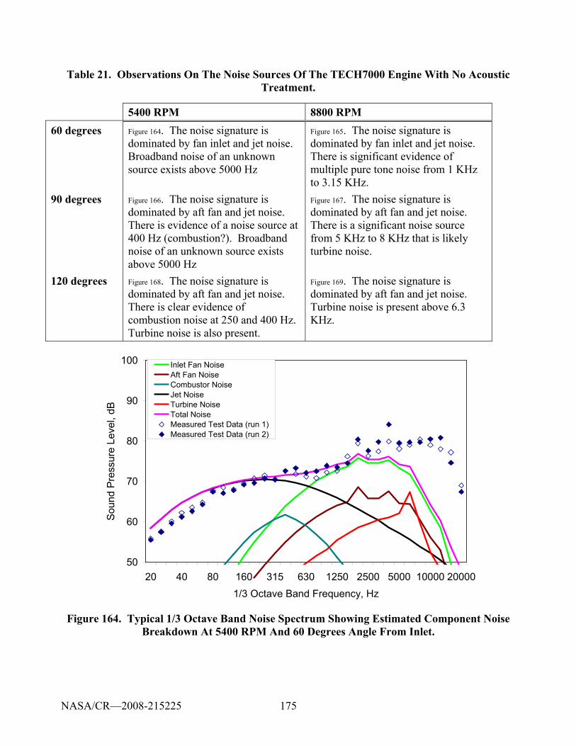
175

Table 21. Observations On The Noise Sources Of The TECH7000 Engine With No Acoustic Treatment.

5400 RPM 8800 RPM 60 degrees Figure 164. The noise signature is

dominated by fan inlet and jet noise. Broadband noise of an unknown source exists above 5000 Hz

Figure 165. The noise signature is dominated by fan inlet and jet noise. There is significant evidence of multiple pure tone noise from 1 KHz to 3.15 KHz.

90 degrees Figure 166. The noise signature is dominated by aft fan and jet noise. There is evidence of a noise source at 400 Hz (combustion?). Broadband noise of an unknown source exists above 5000 Hz

Figure 167. The noise signature is dominated by aft fan and jet noise. There is a significant noise source from 5 KHz to 8 KHz that is likely turbine noise.

120 degrees Figure 168. The noise signature is dominated by aft fan and jet noise. There is clear evidence of combustion noise at 250 and 400 Hz. Turbine noise is also present.

Figure 169. The noise signature is dominated by aft fan and jet noise. Turbine noise is present above 6.3 KHz.

50

60

70

80

90

100

20 40 80 160 315 630 1250 2500 5000 10000 200001/3 Octave Band Frequency, Hz

Soun

d Pr

essu

re L

evel

, dB

Inlet Fan NoiseAft Fan NoiseCombustor NoiseJet NoiseTurbine NoiseTotal NoiseMeasured Test Data (run 1)Measured Test Data (run 2)

Figure 164. Typical 1/3 Octave Band Noise Spectrum Showing Estimated Component Noise Breakdown At 5400 RPM And 60 Degrees Angle From Inlet.

NASA/CR—2008-215225

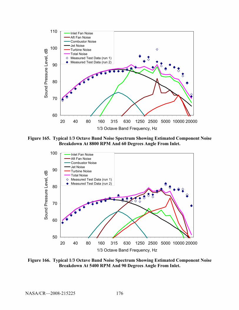
176

60

70

80

90

100

110


Soun

d P

ress

ure

Leve

l, dB



50

60

70

80

90

100


Sou

nd P

ress

ure

Leve

l, dB



NASA/CR—2008-215225

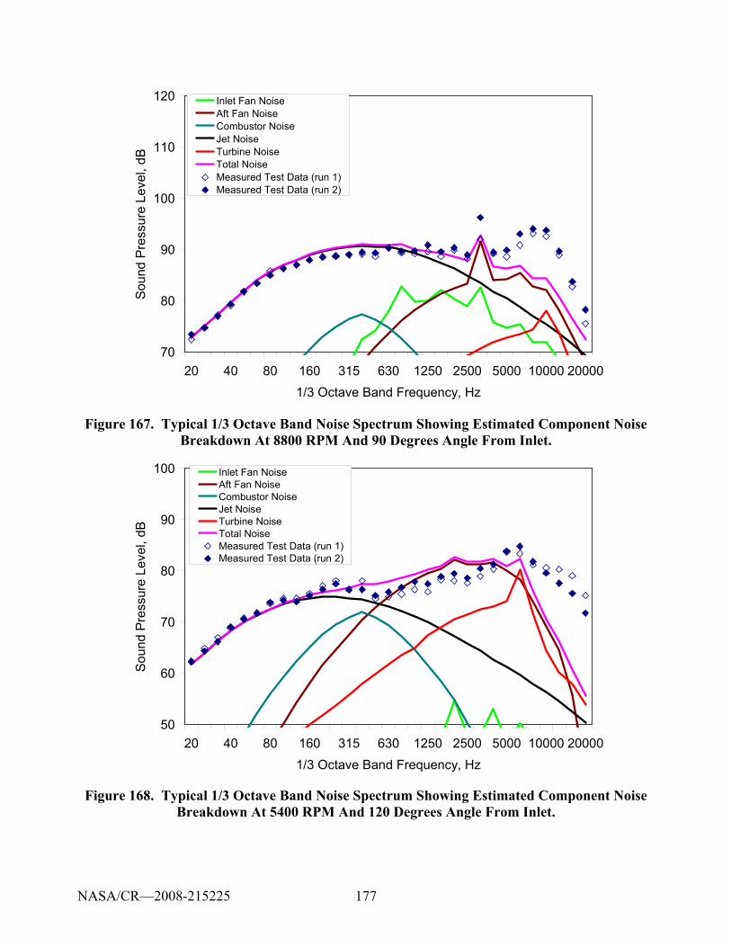
177

70

80

90

100

110

120


Sou

nd P

ress

ure

Leve

l, dB



50

60

70

80

90

100


Soun

d Pr

essu

re L

evel

, dB



NASA/CR—2008-215225

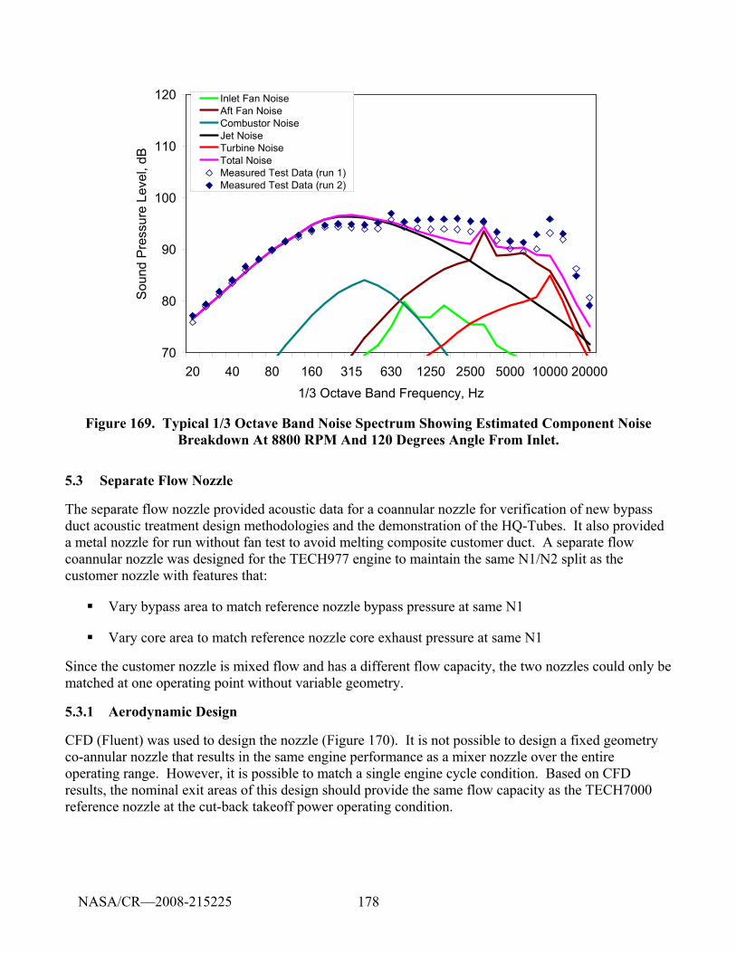
178

70

80

90

100

110

120


Sou

nd P

ress

ure

Leve

l, dB



5.3 Separate Flow Nozzle

The separate flow nozzle provided acoustic data for a coannular nozzle for verification of new bypass duct acoustic treatment design methodologies and the demonstration of the HQ-Tubes. It also provided a metal nozzle for run without fan test to avoid melting composite customer duct. A separate flow coannular nozzle was designed for the TECH977 engine to maintain the same N1/N2 split as the customer nozzle with features that:

Vary bypass area to match reference nozzle bypass pressure at same N1

Vary core area to match reference nozzle core exhaust pressure at same N1

Since the customer nozzle is mixed flow and has a different flow capacity, the two nozzles could only be matched at one operating point without variable geometry.

5.3.1 Aerodynamic Design

CFD (Fluent) was used to design the nozzle (Figure 170). It is not possible to design a fixed geometry co-annular nozzle that results in the same engine performance as a mixer nozzle over the entire operating range. However, it is possible to match a single engine cycle condition. Based on CFD results, the nominal exit areas of this design should provide the same flow capacity as the TECH7000 reference nozzle at the cut-back takeoff power operating condition.

NASA/CR—2008-215225

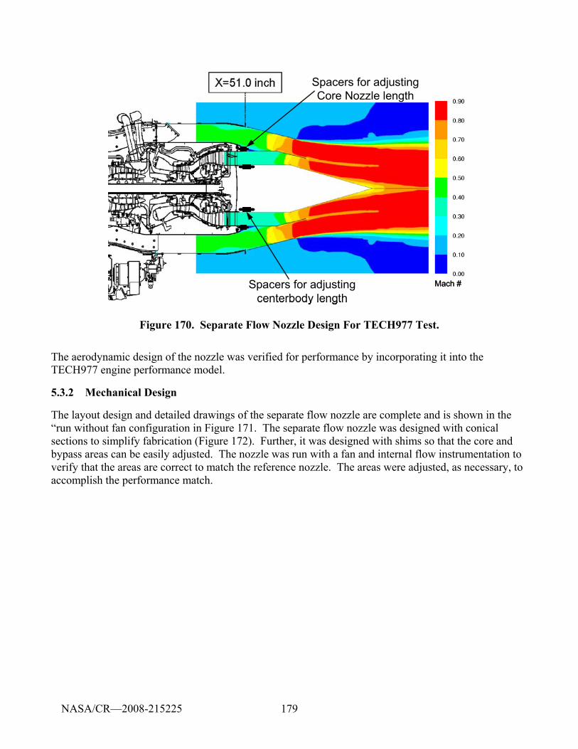
179

Spacers for adjusting centerbody length

Spacers for adjusting Core Nozzle length

Mach #Spacers for adjusting centerbody length


Spacers for adjusting centerbody length


Mach #

Figure 170. Separate Flow Nozzle Design For TECH977 Test.

The aerodynamic design of the nozzle was verified for performance by incorporating it into the TECH977 engine performance model.

5.3.2 Mechanical Design

The layout design and detailed drawings of the separate flow nozzle are complete and is shown in the “run without fan configuration in Figure 171. The separate flow nozzle was designed with conical sections to simplify fabrication (Figure 172). Further, it was designed with shims so that the core and bypass areas can be easily adjusted. The nozzle was run with a fan and internal flow instrumentation to verify that the areas are correct to match the reference nozzle. The areas were adjusted, as necessary, to accomplish the performance match.

NASA/CR—2008-215225

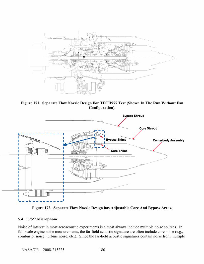
180

Figure 171. Separate Flow Nozzle Design For TECH977 Test (Shown In The Run Without Fan Configuration).

Bypass Shroud

Core Shroud

Centerbody AssemblyBypass Shims

Core Shims

Bypass Shroud

Core Shroud

Centerbody AssemblyBypass Shims

Core Shims

Figure 172. Separate Flow Nozzle Design has Adjustable Core And Bypass Areas.

5.4 3/5/7 Microphone

Noise of interest in most aeroacoustic experiments is almost always include multiple noise sources. In full-scale engine noise measurements, the far-field acoustic signature are often include core noise (e.g., combustor noise, turbine noise, etc.). Since the far-field acoustic signatures contain noise from multiple

NASA/CR—2008-215225

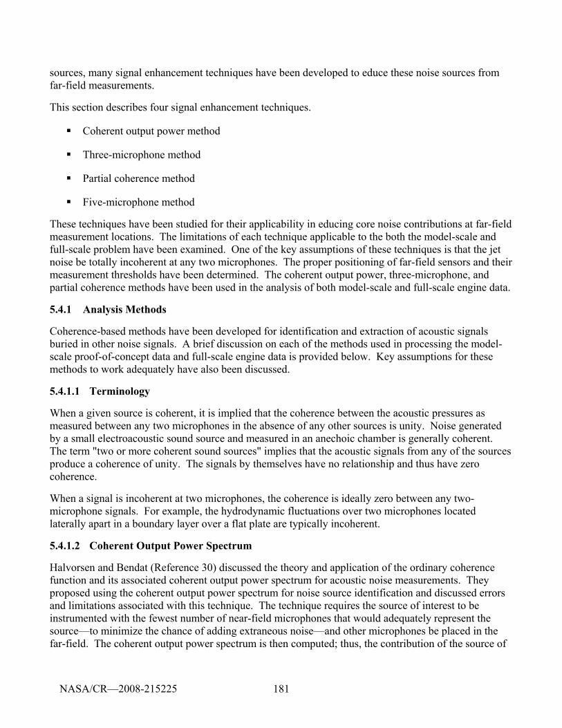
181

sources, many signal enhancement techniques have been developed to educe these noise sources from far-field measurements.

This section describes four signal enhancement techniques.

Coherent output power method

Three-microphone method

Partial coherence method

Five-microphone method

These techniques have been studied for their applicability in educing core noise contributions at far-field measurement locations. The limitations of each technique applicable to the both the model-scale and full-scale problem have been examined. One of the key assumptions of these techniques is that the jet noise be totally incoherent at any two microphones. The proper positioning of far-field sensors and their measurement thresholds have been determined. The coherent output power, three-microphone, and partial coherence methods have been used in the analysis of both model-scale and full-scale engine data.

5.4.1 Analysis Methods

Coherence-based methods have been developed for identification and extraction of acoustic signals buried in other noise signals. A brief discussion on each of the methods used in processing the model-scale proof-of-concept data and full-scale engine data is provided below. Key assumptions for these methods to work adequately have also been discussed.

5.4.1.1 Terminology

When a given source is coherent, it is implied that the coherence between the acoustic pressures as measured between any two microphones in the absence of any other sources is unity. Noise generated by a small electroacoustic sound source and measured in an anechoic chamber is generally coherent. The term "two or more coherent sound sources" implies that the acoustic signals from any of the sources produce a coherence of unity. The signals by themselves have no relationship and thus have zero coherence.

When a signal is incoherent at two microphones, the coherence is ideally zero between any two-microphone signals. For example, the hydrodynamic fluctuations over two microphones located laterally apart in a boundary layer over a flat plate are typically incoherent.

5.4.1.2 Coherent Output Power Spectrum

Halvorsen and Bendat (Reference 30) discussed the theory and application of the ordinary coherence function and its associated coherent output power spectrum for acoustic noise measurements. They proposed using the coherent output power spectrum for noise source identification and discussed errors and limitations associated with this technique. The technique requires the source of interest to be instrumented with the fewest number of near-field microphones that would adequately represent the source—to minimize the chance of adding extraneous noise—and other microphones be placed in the far-field. The coherent output power spectrum is then computed; thus, the contribution of the source of

NASA/CR—2008-215225

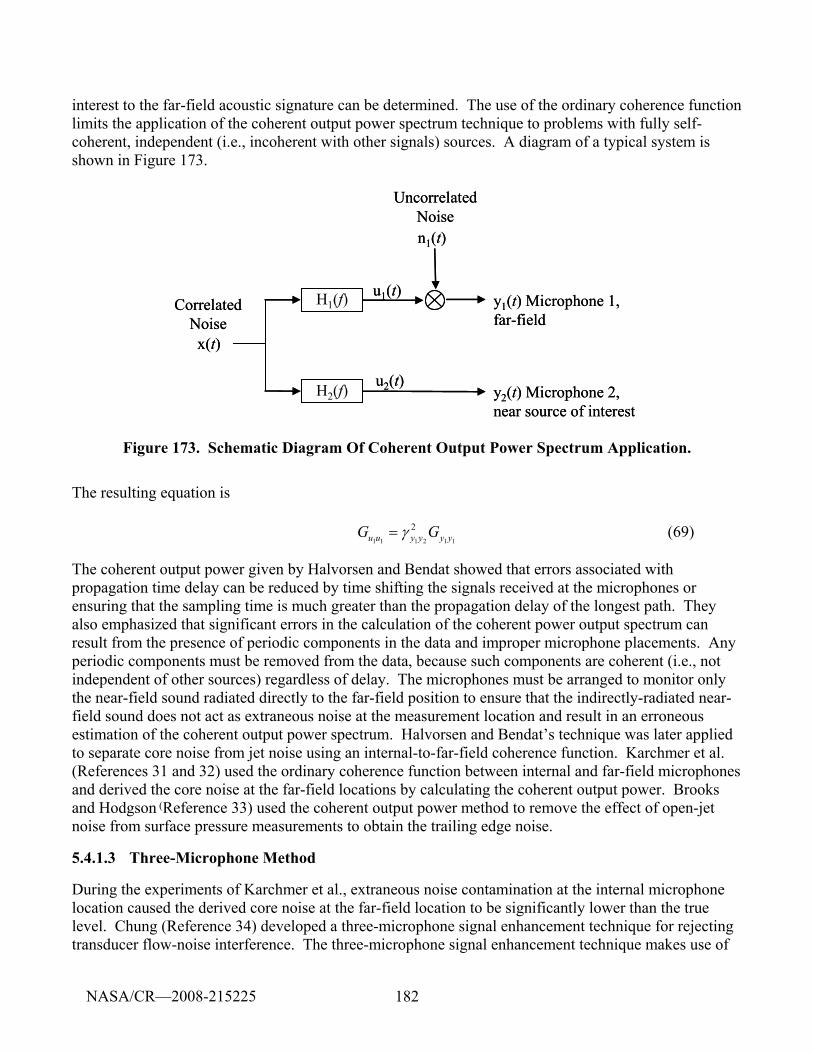
182

interest to the far-field acoustic signature can be determined. The use of the ordinary coherence function limits the application of the coherent output power spectrum technique to problems with fully self-coherent, independent (i.e., incoherent with other signals) sources. A diagram of a typical system is shown in Figure 173.

Correlated Noisex(t)

Uncorrelated Noise

y1(t) Microphone 1,far-field

u1(t)

n1(t)

y2(t) Microphone 2,near source of interest

u2(t)

H1(f)

H2(f)

Correlated Noisex(t)

Uncorrelated Noise

y1(t) Microphone 1,far-field

u1(t)

n1(t)

y2(t) Microphone 2,near source of interest

u2(t)

H1(f)

H2(f)

Figure 173. Schematic Diagram Of Coherent Output Power Spectrum Application.

The resulting equation is

112111

2yyyyuu GG γ= (69)

The coherent output power given by Halvorsen and Bendat showed that errors associated with propagation time delay can be reduced by time shifting the signals received at the microphones or ensuring that the sampling time is much greater than the propagation delay of the longest path. They also emphasized that significant errors in the calculation of the coherent power output spectrum can result from the presence of periodic components in the data and improper microphone placements. Any periodic components must be removed from the data, because such components are coherent (i.e., not independent of other sources) regardless of delay. The microphones must be arranged to monitor only the near-field sound radiated directly to the far-field position to ensure that the indirectly-radiated near-field sound does not act as extraneous noise at the measurement location and result in an erroneous estimation of the coherent output power spectrum. Halvorsen and Bendat’s technique was later applied to separate core noise from jet noise using an internal-to-far-field coherence function. Karchmer et al. (References 31 and 32) used the ordinary coherence function between internal and far-field microphones and derived the core noise at the far-field locations by calculating the coherent output power. Brooks and Hodgson (Reference 33) used the coherent output power method to remove the effect of open-jet noise from surface pressure measurements to obtain the trailing edge noise.

5.4.1.3 Three-Microphone Method

During the experiments of Karchmer et al., extraneous noise contamination at the internal microphone location caused the derived core noise at the far-field location to be significantly lower than the true level. Chung (Reference 34) developed a three-microphone signal enhancement technique for rejecting transducer flow-noise interference. The three-microphone signal enhancement technique makes use of

NASA/CR—2008-215225

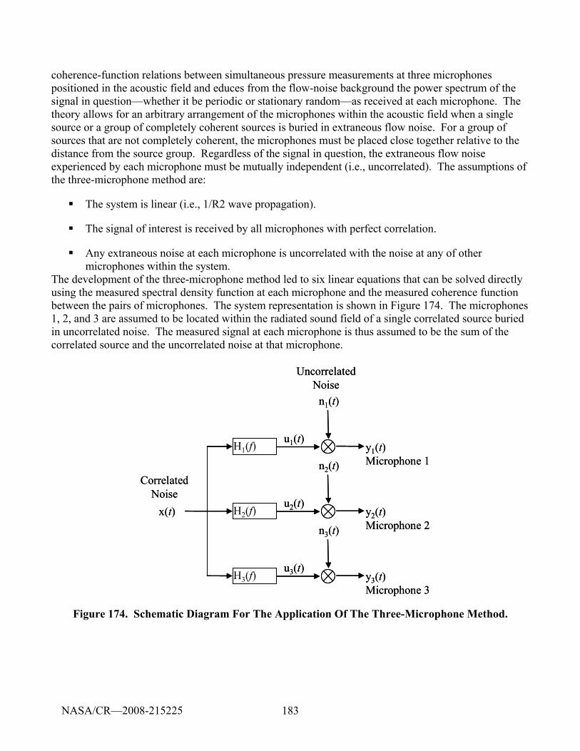
183

coherence-function relations between simultaneous pressure measurements at three microphones positioned in the acoustic field and educes from the flow-noise background the power spectrum of the signal in question—whether it be periodic or stationary random—as received at each microphone. The theory allows for an arbitrary arrangement of the microphones within the acoustic field when a single source or a group of completely coherent sources is buried in extraneous flow noise. For a group of sources that are not completely coherent, the microphones must be placed close together relative to the distance from the source group. Regardless of the signal in question, the extraneous flow noise experienced by each microphone must be mutually independent (i.e., uncorrelated). The assumptions of the three-microphone method are:

The system is linear (i.e., 1/R2 wave propagation).

The signal of interest is received by all microphones with perfect correlation.

Any extraneous noise at each microphone is uncorrelated with the noise at any of other microphones within the system.

The development of the three-microphone method led to six linear equations that can be solved directly using the measured spectral density function at each microphone and the measured coherence function between the pairs of microphones. The system representation is shown in Figure 174. The microphones 1, 2, and 3 are assumed to be located within the radiated sound field of a single correlated source buried in uncorrelated noise. The measured signal at each microphone is thus assumed to be the sum of the correlated source and the uncorrelated noise at that microphone.

Correlated Noise

x(t)

Uncorrelated Noise

y1(t) Microphone 1

u1(t)

n1(t)

y2(t) Microphone 2

u2(t)

n2(t)

y3(t) Microphone 3

u3(t)

n3(t)

H1(f)

H2(f)

H3(f)

Correlated Noise

x(t)

Uncorrelated Noise

y1(t) Microphone 1

u1(t)

n1(t)

y2(t) Microphone 2

u2(t)

n2(t)

y3(t) Microphone 3

u3(t)

n3(t)

H1(f)

H2(f)

H3(f)

Figure 174. Schematic Diagram For The Application Of The Three-Microphone Method.

NASA/CR—2008-215225

184

The spectral density functions of the correlated signal at each microphone are:

23

13121111 γ

γγyyuu GG = (70)

13

23122222 γ

γγyyuu GG = (71)

12

23133333 γ

γγyyuu GG = (72)

The spectral density functions of the uncorrelated signal at each microphone are:

111111 uuyynn GGG −= (73)

222222 uuyynn GGG −= (74)

333333 uuyynn GGG −= (75)

Chung’s signal enhancement technique has been applied in a number of research programs. A few notable studies include Shivashankara (Reference 35), Stoker et al. (Reference 36), and Hsu and Ahuja (Reference 37). Shivashankara applied Chung’s signal enhancement technique to separate aft fan, core, and jet noise components of a large high-bypass ratio engine. In applying Chung’s signal enhancement technique, Shivashankara used signals gathered from internal and far-field microphones. The use of the internal-to-far-field coherence techniques was shown useful for component separation even when in-duct microphone signals were contaminated by extraneous noise. When separating the core noise, he implemented the signal enhancement technique with two in-duct sensors positioned such that they were dominated by the core noise and one far-field sensor was assumed to measure the combined signals. Similarly, for the separation of the fan noise component, he used signals from two internal sensors that were dominated by the fan noise and one far-field sensor. The three-microphone signal enhancement technique was also used to educe the sum of the core plus fan noise from jet-mixing noise received at far-field microphone locations, and the results were compared with those from the use of the internal-to-far-field coherence function and its resulting coherent output power spectrum. Shivashankara showed that with the use of three-microphone signal enhancement technique and far-field microphones alone, it is possible to separate the sum of the core- and fan-noise components from the jet-mixing noise.

Stoker et al. used the three-microphone signal enhancement technique to separate wind-tunnel background noise and boundary layer noise in measurements made in the interior of an automobile tested in a subsonic wind tunnel. They showed that the wind-tunnel background noise consisting of motor noise and other dipole sources was mutually coherent between microphone positions and that all other noise sources were incoherent; thus, validating the assumptions needed to use the three-microphone technique. The three-microphone technique was successfully used to extract known background noise from measured interior noise using two different microphone arrangements:

two in-flow microphones and one interior microphone

two flush-mounted (on the surface of the test vehicle) microphones and one interior microphone

NASA/CR—2008-215225

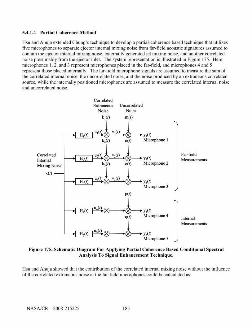
185

5.4.1.4 Partial Coherence Method

Hsu and Ahuja extended Chung’s technique to develop a partial-coherence based technique that utilizes five microphones to separate ejector internal mixing noise from far-field acoustic signatures assumed to contain the ejector internal mixing noise, externally generated jet mixing noise, and another correlated noise presumably from the ejector inlet. The system representation is illustrated in Figure 175. Here microphones 1, 2, and 3 represent microphones placed in the far-field, and microphones 4 and 5 represent those placed internally. The far-field microphone signals are assumed to measure the sum of the correlated internal noise, the uncorrelated noise, and the noise produced by an extraneous correlated source, while the internally positioned microphones are assumed to measure the correlated internal noise and uncorrelated noise.

H5(f) y5(t) Microphone 5

q(t)


k1(t) m(t)


k2(t) n(t)


k3(t) o(t)


p(t)

Far-fieldMeasurements

InternalMeasurements

Uncorrelated Noise

Correlated Extraneous

Noise

Correlated Internal Mixing Noise

u1(t)

u2(t)

u3(t)

u4(t)

u5(t)

v1(t)

v2(t)

v3(t)x(t)


q(t)


k1(t) m(t)


k2(t) n(t)


k3(t) o(t)


p(t)

Far-fieldMeasurements

InternalMeasurements

Uncorrelated Noise

Correlated Extraneous

Noise

Correlated Internal Mixing Noise

u1(t)

u2(t)

u3(t)

u4(t)

u5(t)

v1(t)

v2(t)

v3(t)x(t)

Figure 175. Schematic Diagram For Applying Partial Coherence Based Conditional Spectral Analysis To Signal Enhancement Technique.

Hsu and Ahuja showed that the contribution of the correlated internal mixing noise without the influence of the correlated extraneous noise at the far-field microphones could be calculated as:

NASA/CR—2008-215225

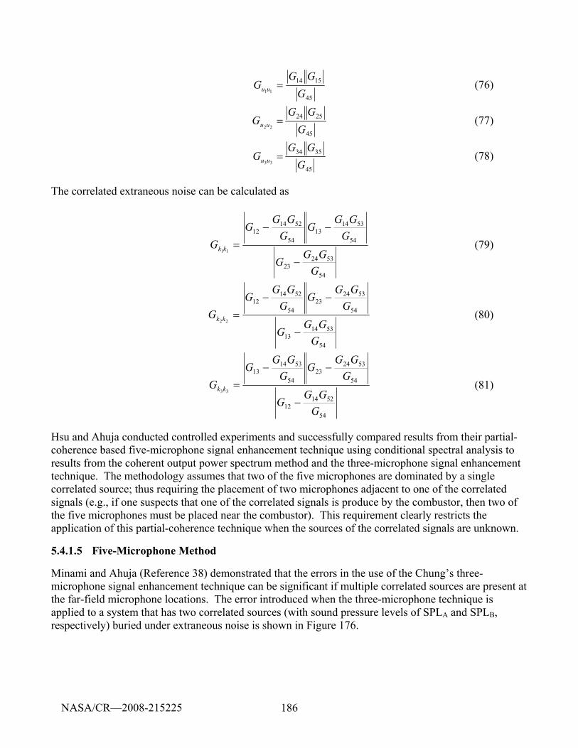
186

45

151411 G

GGG uu = (76)

45

252422 G

GGG uu = (77)

45

353433 G

GGG uu = (78)

The correlated extraneous noise can be calculated as

54

532423

54

531413

54

521412

11

GGG

G

GGG

GG

GGG

G kk

−

−−

= (79)

54

531413

54

532423

54

521412

22

GGG

G

GGG

GG

GGG

G kk

−

−−

= (80)

54

521412

54

532423

54

531413

33

GGG

G

GGG

GG

GGG

G kk

−

−−

= (81)

Hsu and Ahuja conducted controlled experiments and successfully compared results from their partial-coherence based five-microphone signal enhancement technique using conditional spectral analysis to results from the coherent output power spectrum method and the three-microphone signal enhancement technique. The methodology assumes that two of the five microphones are dominated by a single correlated source; thus requiring the placement of two microphones adjacent to one of the correlated signals (e.g., if one suspects that one of the correlated signals is produce by the combustor, then two of the five microphones must be placed near the combustor). This requirement clearly restricts the application of this partial-coherence technique when the sources of the correlated signals are unknown.

5.4.1.5 Five-Microphone Method

Minami and Ahuja (Reference 38) demonstrated that the errors in the use of the Chung’s three-microphone signal enhancement technique can be significant if multiple correlated sources are present at the far-field microphone locations. The error introduced when the three-microphone technique is applied to a system that has two correlated sources (with sound pressure levels of SPLA and SPLB, respectively) buried under extraneous noise is shown in Figure 176.

NASA/CR—2008-215225

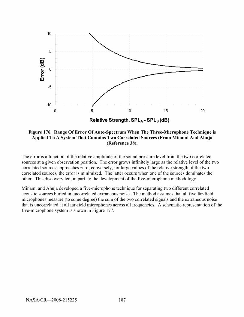
187

-10

-5

0

5

10

0 5 10 15 20

Relative Strength, SPLA - SPLB (dB)

Erro

r (dB

)

Figure 176. Range Of Error Of Auto-Spectrum When The Three-Microphone Technique is Applied To A System That Contains Two Correlated Sources (From Minami And Ahuja

(Reference 38).

The error is a function of the relative amplitude of the sound pressure level from the two correlated sources at a given observation position. The error grows infinitely large as the relative level of the two correlated sources approaches zero; conversely, for large values of the relative strength of the two correlated sources, the error is minimized. The latter occurs when one of the sources dominates the other. This discovery led, in part, to the development of the five-microphone methodology.

Minami and Ahuja developed a five-microphone technique for separating two different correlated acoustic sources buried in uncorrelated extraneous noise. The method assumes that all five far-field microphones measure (to some degree) the sum of the two correlated signals and the extraneous noise that is uncorrelated at all far-field microphones across all frequencies. A schematic representation of the five-microphone system is shown in Figure 177.

NASA/CR—2008-215225

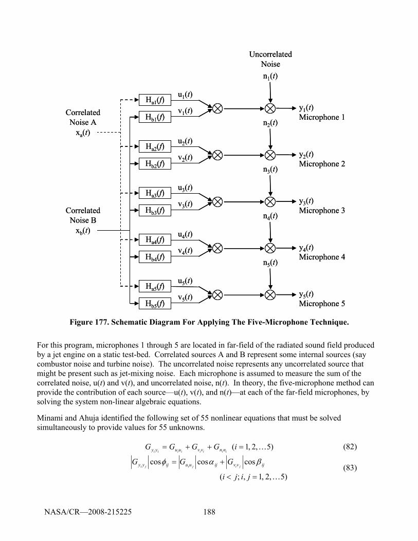
188

Correlated Noise A

xa(t)

Uncorrelated Noise

Ha1(f)y1(t) Microphone 1

u1(t)

Hb1(f)v1(t)

n1(t)

Correlated Noise B


u2(t)

Hb2(f)v2(t)

n2(t)


u3(t)

Hb3(f)v3(t)

n3(t)


u4(t)

Hb4(f)v4(t)

n4(t)


u5(t)

Hb5(f)v5(t)

n5(t)

xb(t)

Correlated Noise A

xa(t)

Uncorrelated Noise


u1(t)

Hb1(f)v1(t)

n1(t)

Correlated Noise B


u2(t)

Hb2(f)v2(t)

n2(t)


u3(t)

Hb3(f)v3(t)

n3(t)


u4(t)

Hb4(f)v4(t)

n4(t)


u5(t)

Hb5(f)v5(t)

n5(t)

xb(t)

Figure 177. Schematic Diagram For Applying The Five-Microphone Technique.

For this program, microphones 1 through 5 are located in far-field of the radiated sound field produced by a jet engine on a static test-bed. Correlated sources A and B represent some internal sources (say combustor noise and turbine noise). The uncorrelated noise represents any uncorrelated source that might be present such as jet-mixing noise. Each microphone is assumed to measure the sum of the correlated noise, u(t) and v(t), and uncorrelated noise, n(t). In theory, the five-microphone method can provide the contribution of each source—u(t), v(t), and n(t)—at each of the far-field microphones, by solving the system non-linear algebraic equations.

Minami and Ahuja identified the following set of 55 nonlinear equations that must be solved simultaneously to provide values for 55 unknowns. )5 ,2 ,1( K=++= iGGGG

iiiiiiii nnvvuuyy (82)

)5 ,2 ,1, ;(

coscoscos

K=<

+=

jiji

GGG ijvvijuuijyy jijijiβαφ

(83)

NASA/CR—2008-215225

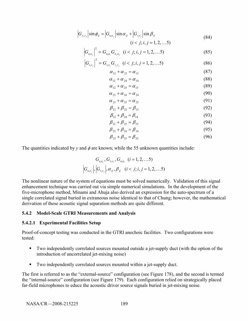
189

)5 ,2 ,1, ;(

sinsinsin

K=<

+=

jiji

GGG ijvvijuuijyy jijijiβαφ

(84)

)5 ,2 ,1, ;( 2

K=<= jijiGGGjjiiji uuuuuu (85)

)5 ,2 ,1, ;( 2

K=<= jijiGGGjjiiji vvvvvv (86)

132312 ααα =+ (87) 142412 ααα =+ (88) 152512 ααα =+ (89) 243423 ααα =+ (90) 253523 ααα =+ (91) 132312 βββ =+ (92) 142412 βββ =+ (93) 152512 βββ =+ (94) 243423 βββ =+ (95) 253523 βββ =+ (96)

The quantities indicated by y and φ are known; while the 55 unknown quantities include:

)5 ,2 ,1, ;( , , ,

)5 ,2 ,1( , ,

K

K

=<

=

jijiGG

iGGG

ijijvvuu

nnvvuu

jiji

iiiiii

βα

The nonlinear nature of the system of equations must be solved numerically. Validation of this signal enhancement technique was carried out via simple numerical simulations. In the development of the five-microphone method, Minami and Ahuja also derived an expression for the auto-spectrum of a single correlated signal buried in extraneous noise identical to that of Chung; however, the mathematical derivation of these acoustic signal separation methods are quite different.

5.4.2 Model-Scale GTRI Measurements and Analysis

5.4.2.1 Experimental Facilities Setup

Proof-of-concept testing was conducted in the GTRI anechoic facilities. Two configurations were tested:

Two independently correlated sources mounted outside a jet-supply duct (with the option of the introduction of uncorrelated jet-mixing noise)

Two independently correlated sources mounted within a jet-supply duct.

The first is referred to as the “external-source” configuration (see Figure 178), and the second is termed the “internal-source” configuration (see Figure 179). Each configuration relied on strategically placed far-field microphones to educe the acoustic driver source signals buried in jet-mixing noise.

NASA/CR—2008-215225

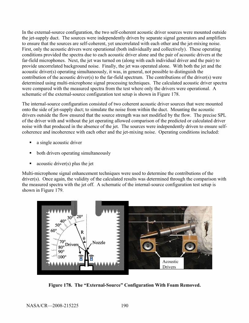
190

In the external-source configuration, the two self-coherent acoustic driver sources were mounted outside the jet-supply duct. The sources were independently driven by separate signal generators and amplifiers to ensure that the sources are self-coherent, yet uncorrelated with each other and the jet-mixing noise. First, only the acoustic drivers were operational (both individually and collectively). These operating conditions provided the spectra due to each acoustic driver alone and the pair of acoustic drivers at the far-field microphones. Next, the jet was turned on (along with each individual driver and the pair) to provide uncorrelated background noise. Finally, the jet was operated alone. With both the jet and the acoustic driver(s) operating simultaneously, it was, in general, not possible to distinguish the contribution of the acoustic driver(s) to the far-field spectrum. The contributions of the driver(s) were determined using multi-microphone signal processing techniques. The calculated acoustic driver spectra were compared with the measured spectra from the test where only the drivers were operational. A schematic of the external-source configuration test setup is shown in Figure 178.

The internal-source configuration consisted of two coherent acoustic driver sources that were mounted onto the side of jet-supply duct; to simulate the noise from within the duct. Mounting the acoustic drivers outside the flow ensured that the source strength was not modified by the flow. The precise SPL of the driver with and without the jet operating allowed comparison of the predicted or calculated driver noise with that produced in the absence of the jet. The sources were independently driven to ensure self-coherence and incoherence with each other and the jet-mixing noise. Operating conditions included:

a single acoustic driver

both drivers operating simultaneously

acoustic driver(s) plus the jet

Multi-microphone signal enhancement techniques were used to determine the contributions of the driver(s). Once again, the validity of the calculated results was determined through the comparison with the measured spectra with the jet off. A schematic of the internal-source configuration test setup is shown in Figure 179.

θ

20°

50°

70° Nozzle Drivers

30°40°

60°

80°90°100°

R

Acoustic Drivers

θ

20°

50°

70° Nozzle Drivers

30°40°

60°

80°90°100°

R

Acoustic Drivers

Figure 178. The “External-Source” Configuration With Foam Removed.

NASA/CR—2008-215225

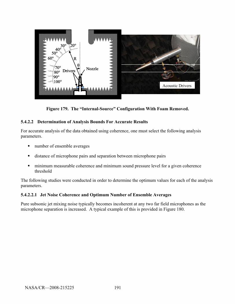
191

θ

20°

50°

70° Nozzle Drivers

30°40°

60°

80°90°100°

R

Acoustic Drivers

θ

20°

50°

70° Nozzle Drivers

30°40°

60°

80°90°100°

R

Acoustic Drivers

Figure 179. The “Internal-Source” Configuration With Foam Removed.

5.4.2.2 Determination of Analysis Bounds For Accurate Results

For accurate analysis of the data obtained using coherence, one must select the following analysis parameters.

number of ensemble averages

distance of microphone pairs and separation between microphone pairs

minimum measurable coherence and minimum sound pressure level for a given coherence threshold

The following studies were conducted in order to determine the optimum values for each of the analysis parameters.

5.4.2.2.1 Jet Noise Coherence and Optimum Number of Ensemble Averages

Pure subsonic jet mixing noise typically becomes incoherent at any two far field microphones as the microphone separation is increased. A typical example of this is provided in Figure 180.

NASA/CR—2008-215225

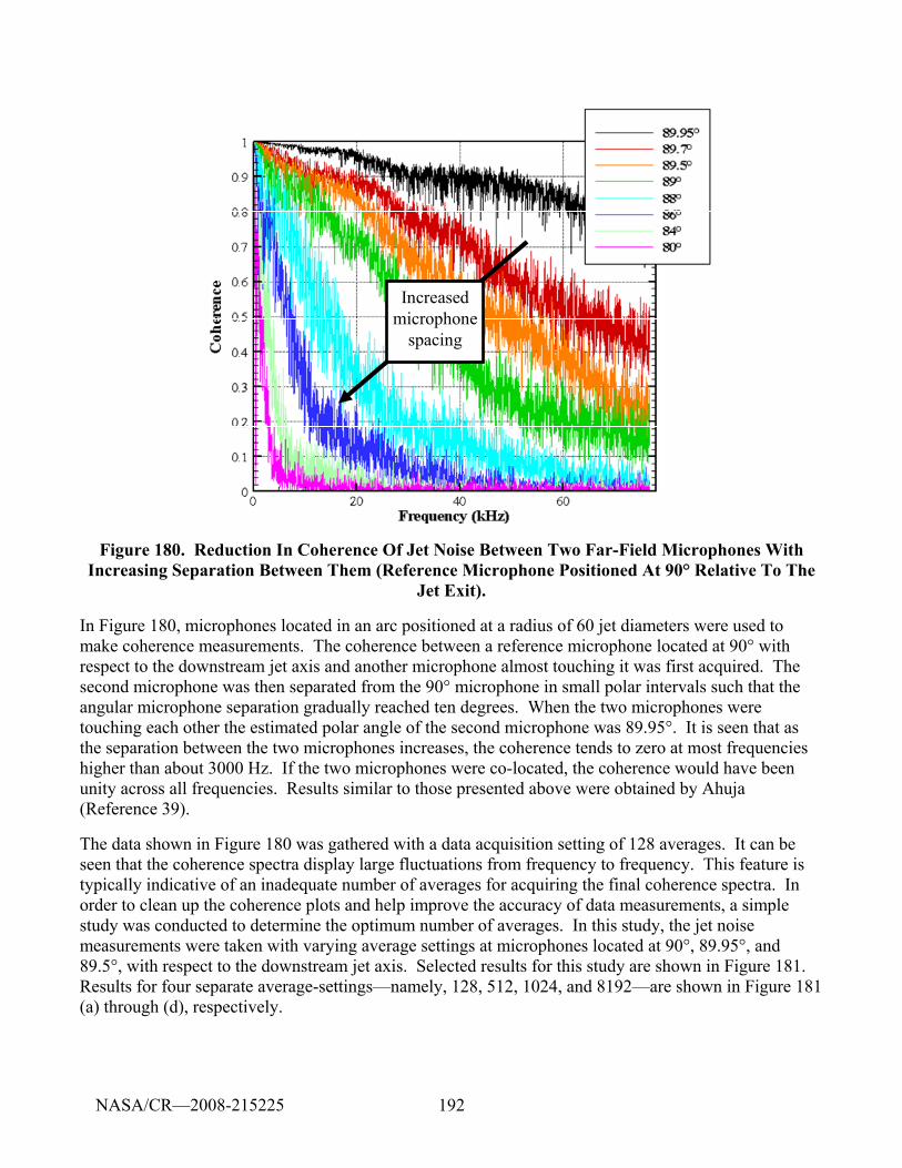
192

Increased microphone

spacing

Increased microphone

spacing

Figure 180. Reduction In Coherence Of Jet Noise Between Two Far-Field Microphones With Increasing Separation Between Them (Reference Microphone Positioned At 90° Relative To The

Jet Exit).

In Figure 180, microphones located in an arc positioned at a radius of 60 jet diameters were used to make coherence measurements. The coherence between a reference microphone located at 90° with respect to the downstream jet axis and another microphone almost touching it was first acquired. The second microphone was then separated from the 90° microphone in small polar intervals such that the angular microphone separation gradually reached ten degrees. When the two microphones were touching each other the estimated polar angle of the second microphone was 89.95°. It is seen that as the separation between the two microphones increases, the coherence tends to zero at most frequencies higher than about 3000 Hz. If the two microphones were co-located, the coherence would have been unity across all frequencies. Results similar to those presented above were obtained by Ahuja (Reference 39).

The data shown in Figure 180 was gathered with a data acquisition setting of 128 averages. It can be seen that the coherence spectra display large fluctuations from frequency to frequency. This feature is typically indicative of an inadequate number of averages for acquiring the final coherence spectra. In order to clean up the coherence plots and help improve the accuracy of data measurements, a simple study was conducted to determine the optimum number of averages. In this study, the jet noise measurements were taken with varying average settings at microphones located at 90°, 89.95°, and 89.5°, with respect to the downstream jet axis. Selected results for this study are shown in Figure 181. Results for four separate average-settings—namely, 128, 512, 1024, and 8192—are shown in Figure 181 (a) through (d), respectively.

NASA/CR—2008-215225

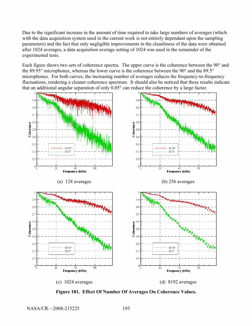
193

Due to the significant increase in the amount of time required to take large numbers of averages (which with the data acquisition system used in the current work is not entirely dependant upon the sampling parameters) and the fact that only negligible improvements in the cleanliness of the data were obtained after 1024 averages, a data acquisition average setting of 1024 was used in the remainder of the experimental tests.

Each figure shows two sets of coherence spectra. The upper curve is the coherence between the 90° and the 89.95° microphones, whereas the lower curve is the coherence between the 90° and the 89.5° microphones. For both curves, the increasing number of averages reduces the frequency-to-frequency fluctuations, rendering a cleaner coherence spectrum. It should also be noticed that these results indicate that an additional angular separation of only 0.05° can reduce the coherence by a large factor.

(a) 128 averages (b) 256 averages

(c) 1024 averages (d) 8192 averages

Figure 181. Effect Of Number Of Averages On Coherence Values.

NASA/CR—2008-215225

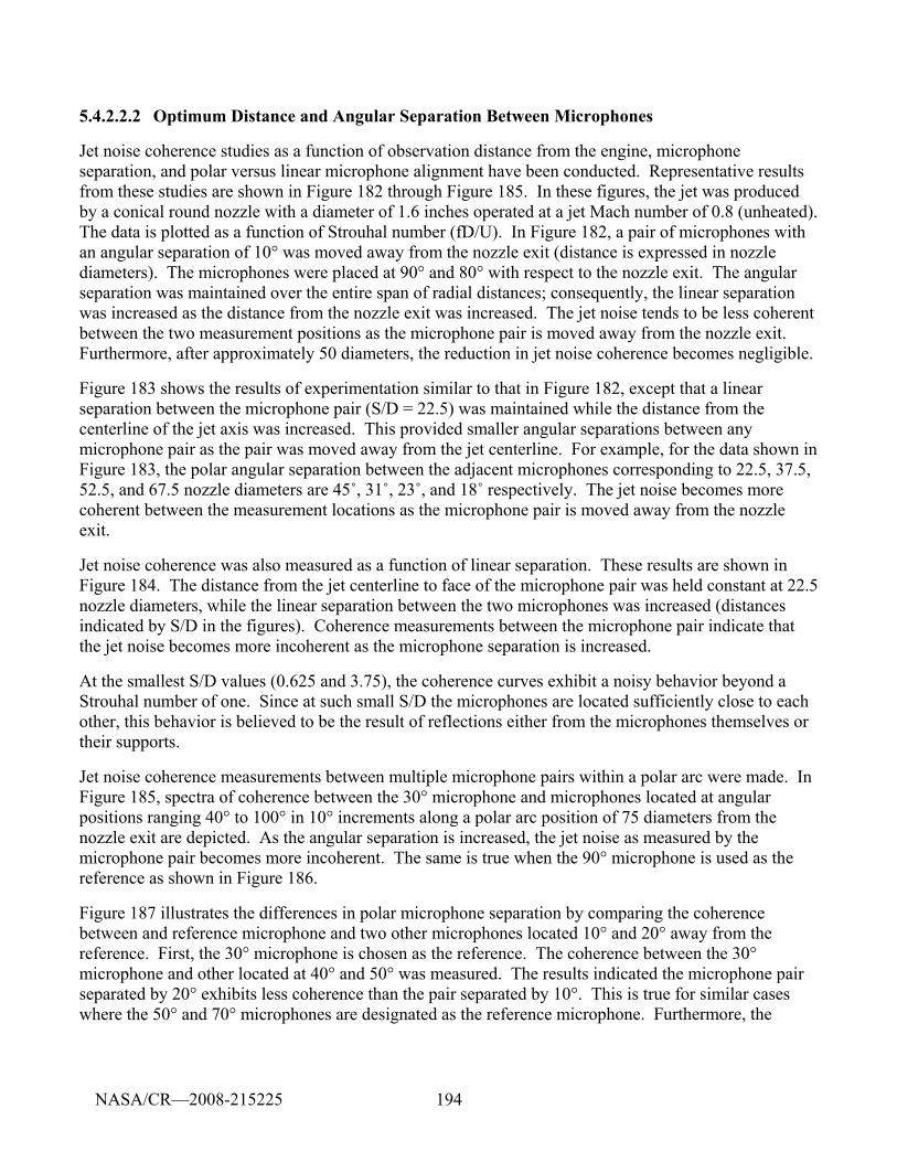
194

5.4.2.2.2 Optimum Distance and Angular Separation Between Microphones

Jet noise coherence studies as a function of observation distance from the engine, microphone separation, and polar versus linear microphone alignment have been conducted. Representative results from these studies are shown in Figure 182 through Figure 185. In these figures, the jet was produced by a conical round nozzle with a diameter of 1.6 inches operated at a jet Mach number of 0.8 (unheated). The data is plotted as a function of Strouhal number (fD/U). In Figure 182, a pair of microphones with an angular separation of 10° was moved away from the nozzle exit (distance is expressed in nozzle diameters). The microphones were placed at 90° and 80° with respect to the nozzle exit. The angular separation was maintained over the entire span of radial distances; consequently, the linear separation was increased as the distance from the nozzle exit was increased. The jet noise tends to be less coherent between the two measurement positions as the microphone pair is moved away from the nozzle exit. Furthermore, after approximately 50 diameters, the reduction in jet noise coherence becomes negligible.

Figure 183 shows the results of experimentation similar to that in Figure 182, except that a linear separation between the microphone pair (S/D = 22.5) was maintained while the distance from the centerline of the jet axis was increased. This provided smaller angular separations between any microphone pair as the pair was moved away from the jet centerline. For example, for the data shown in Figure 183, the polar angular separation between the adjacent microphones corresponding to 22.5, 37.5, 52.5, and 67.5 nozzle diameters are 45˚, 31˚, 23˚, and 18˚ respectively. The jet noise becomes more coherent between the measurement locations as the microphone pair is moved away from the nozzle exit.

Jet noise coherence was also measured as a function of linear separation. These results are shown in Figure 184. The distance from the jet centerline to face of the microphone pair was held constant at 22.5 nozzle diameters, while the linear separation between the two microphones was increased (distances indicated by S/D in the figures). Coherence measurements between the microphone pair indicate that the jet noise becomes more incoherent as the microphone separation is increased.

At the smallest S/D values (0.625 and 3.75), the coherence curves exhibit a noisy behavior beyond a Strouhal number of one. Since at such small S/D the microphones are located sufficiently close to each other, this behavior is believed to be the result of reflections either from the microphones themselves or their supports.

Jet noise coherence measurements between multiple microphone pairs within a polar arc were made. In Figure 185, spectra of coherence between the 30° microphone and microphones located at angular positions ranging 40° to 100° in 10° increments along a polar arc position of 75 diameters from the nozzle exit are depicted. As the angular separation is increased, the jet noise as measured by the microphone pair becomes more incoherent. The same is true when the 90° microphone is used as the reference as shown in Figure 186.

Figure 187 illustrates the differences in polar microphone separation by comparing the coherence between and reference microphone and two other microphones located 10° and 20° away from the reference. First, the 30° microphone is chosen as the reference. The coherence between the 30° microphone and other located at 40° and 50° was measured. The results indicated the microphone pair separated by 20° exhibits less coherence than the pair separated by 10°. This is true for similar cases where the 50° and 70° microphones are designated as the reference microphone. Furthermore, the

NASA/CR—2008-215225

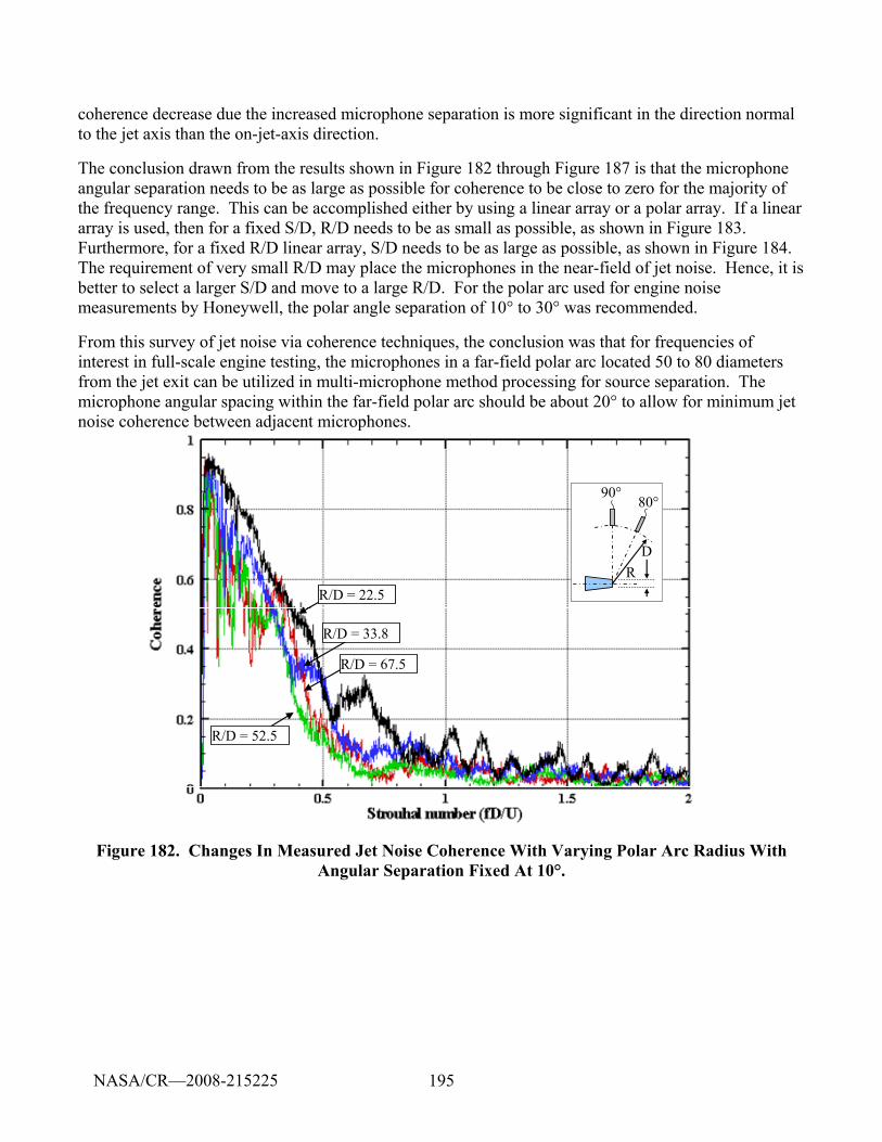
195

coherence decrease due the increased microphone separation is more significant in the direction normal to the jet axis than the on-jet-axis direction.

The conclusion drawn from the results shown in Figure 182 through Figure 187 is that the microphone angular separation needs to be as large as possible for coherence to be close to zero for the majority of the frequency range. This can be accomplished either by using a linear array or a polar array. If a linear array is used, then for a fixed S/D, R/D needs to be as small as possible, as shown in Figure 183. Furthermore, for a fixed R/D linear array, S/D needs to be as large as possible, as shown in Figure 184. The requirement of very small R/D may place the microphones in the near-field of jet noise. Hence, it is better to select a larger S/D and move to a large R/D. For the polar arc used for engine noise measurements by Honeywell, the polar angle separation of 10° to 30° was recommended.

From this survey of jet noise via coherence techniques, the conclusion was that for frequencies of interest in full-scale engine testing, the microphones in a far-field polar arc located 50 to 80 diameters from the jet exit can be utilized in multi-microphone method processing for source separation. The microphone angular spacing within the far-field polar arc should be about 20° to allow for minimum jet noise coherence between adjacent microphones.

R/D = 52.5

R/D = 22.5

R/D = 33.8

R/D = 67.5

R

80°90°

D

R/D = 52.5

R/D = 22.5

R/D = 33.8

R/D = 67.5

R/D = 52.5

R/D = 22.5

R/D = 33.8

R/D = 67.5

R

80°90°

DR

80°90°

D

Figure 182. Changes In Measured Jet Noise Coherence With Varying Polar Arc Radius With Angular Separation Fixed At 10°.

NASA/CR—2008-215225

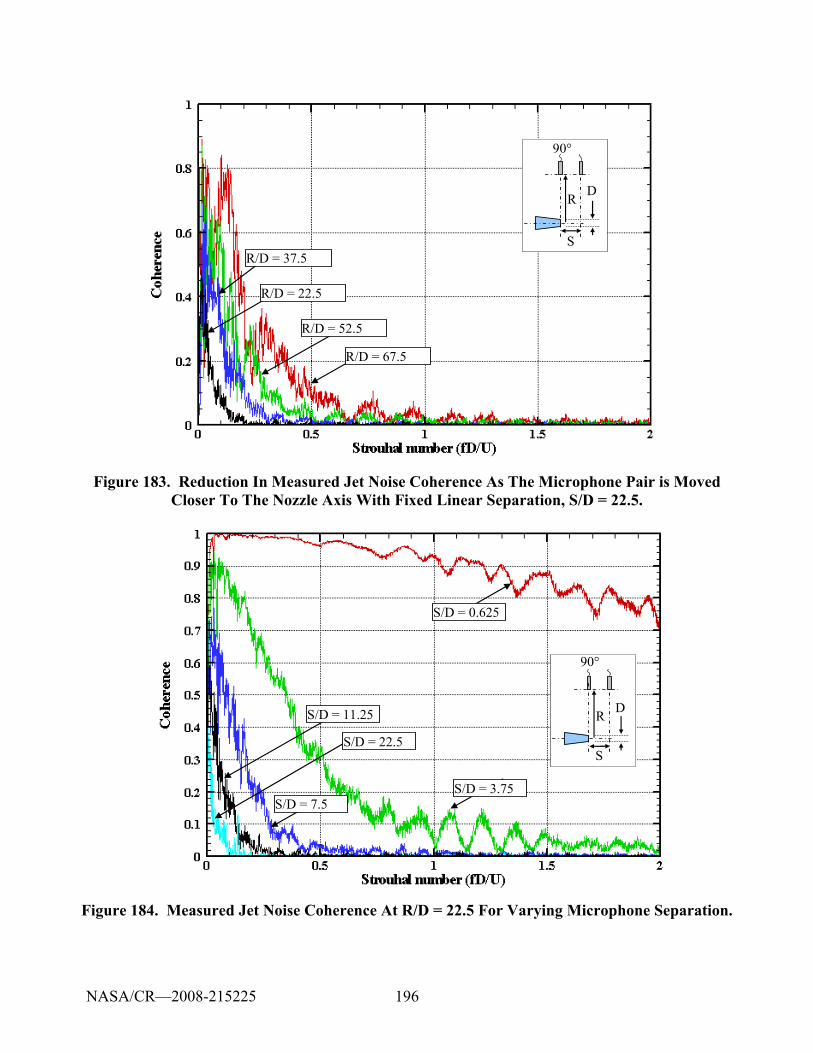
196

R/D = 37.5

R/D = 67.5

R/D = 52.5

R/D = 22.5

R

90°

D

SR/D = 37.5

R/D = 67.5

R/D = 52.5

R/D = 22.5

R

90°

D

S

R

90°

D

S

Figure 183. Reduction In Measured Jet Noise Coherence As The Microphone Pair is Moved Closer To The Nozzle Axis With Fixed Linear Separation, S/D = 22.5.

S/D = 22.5

S/D = 7.5S/D = 3.75

S/D = 11.25

S/D = 0.625

R

90°

D

SS/D = 22.5

S/D = 7.5S/D = 3.75

S/D = 11.25

S/D = 0.625

S/D = 22.5

S/D = 7.5S/D = 3.75

S/D = 11.25

S/D = 0.625

R

90°

D

S

R

90°

D

S

Figure 184. Measured Jet Noise Coherence At R/D = 22.5 For Varying Microphone Separation.

NASA/CR—2008-215225

197

Increasing microphone separation

R

D

Microphones spaced at 10° from 30° to 100°

θIncreasing microphone separation

R

D


θR

D


θ

Figure 185. Measured Jet Noise Coherence At Polar Arc Radius Of 75 Diameters With Adjacent Microphones Spaced 10° Apart (Reference Microphone At 30°).


R

D


θ


R

D


θR

D


θ

Figure 186. Measured Jet Noise Coherence At Polar arc Radius Of 75 Diameters With Adjacent Microphones Spaced 10° Apart (Reference Microphone At 90°).

NASA/CR—2008-215225

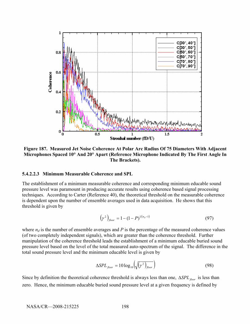
198

Figure 187. Measured Jet Noise Coherence At Polar Arc Radius Of 75 Diameters With Adjacent Microphones Spaced 10° And 20° Apart (Reference Microphone Indicated By The First Angle In

The Brackets).

5.4.2.2.3 Minimum Measurable Coherence and SPL

The establishment of a minimum measurable coherence and corresponding minimum educable sound pressure level was paramount in producing accurate results using coherence based signal processing techniques. According to Carter (Reference 40), the theoretical threshold on the measurable coherence is dependent upon the number of ensemble averages used in data acquisition. He shows that this threshold is given by ( ) ( )112 )1(1 −−−= dn

floor Pγ (97)

where nd is the number of ensemble averages and P is the percentage of the measured coherence values (of two completely independent signals), which are greater than the coherence threshold. Further manipulation of the coherence threshold leads the establishment of a minimum educable buried sound pressure level based on the level of the total measured auto-spectrum of the signal. The difference in the total sound pressure level and the minimum educable level is given by ( )( )floorfloorSPL 2

10log10 γ=Δ (98)

Since by definition the theoretical coherence threshold is always less than one, floorSPLΔ is less than zero. Hence, the minimum educable buried sound pressure level at a given frequency is defined by

NASA/CR—2008-215225

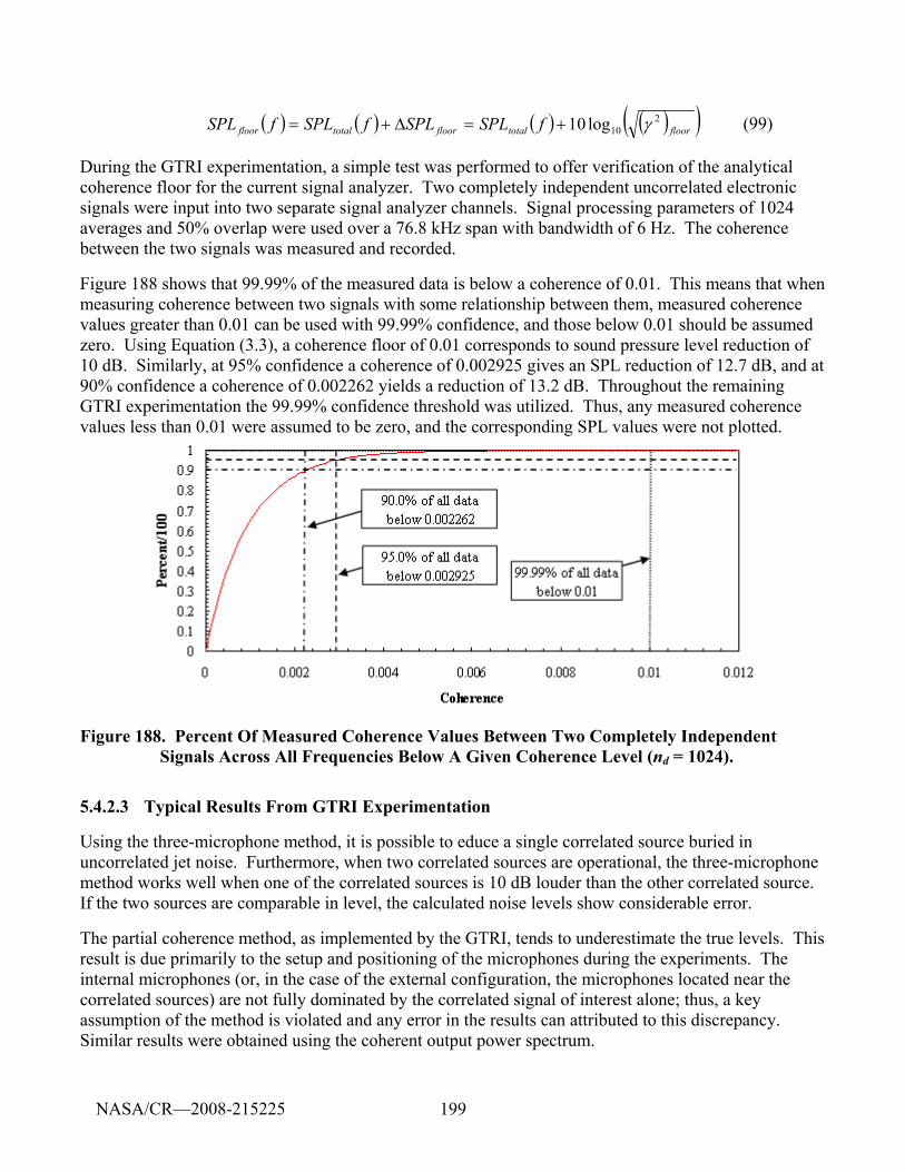
199

( ) ( ) ( ) ( )( )floortotalfloortotalfloor fSPLSPLfSPLfSPL 210log10 γ+=Δ+= (99)

During the GTRI experimentation, a simple test was performed to offer verification of the analytical coherence floor for the current signal analyzer. Two completely independent uncorrelated electronic signals were input into two separate signal analyzer channels. Signal processing parameters of 1024 averages and 50% overlap were used over a 76.8 kHz span with bandwidth of 6 Hz. The coherence between the two signals was measured and recorded.

Figure 188 shows that 99.99% of the measured data is below a coherence of 0.01. This means that when measuring coherence between two signals with some relationship between them, measured coherence values greater than 0.01 can be used with 99.99% confidence, and those below 0.01 should be assumed zero. Using Equation (3.3), a coherence floor of 0.01 corresponds to sound pressure level reduction of 10 dB. Similarly, at 95% confidence a coherence of 0.002925 gives an SPL reduction of 12.7 dB, and at 90% confidence a coherence of 0.002262 yields a reduction of 13.2 dB. Throughout the remaining GTRI experimentation the 99.99% confidence threshold was utilized. Thus, any measured coherence values less than 0.01 were assumed to be zero, and the corresponding SPL values were not plotted.

Figure 188. Percent Of Measured Coherence Values Between Two Completely Independent Signals Across All Frequencies Below A Given Coherence Level (nd = 1024).

5.4.2.3 Typical Results From GTRI Experimentation

Using the three-microphone method, it is possible to educe a single correlated source buried in uncorrelated jet noise. Furthermore, when two correlated sources are operational, the three-microphone method works well when one of the correlated sources is 10 dB louder than the other correlated source. If the two sources are comparable in level, the calculated noise levels show considerable error.

The partial coherence method, as implemented by the GTRI, tends to underestimate the true levels. This result is due primarily to the setup and positioning of the microphones during the experiments. The internal microphones (or, in the case of the external configuration, the microphones located near the correlated sources) are not fully dominated by the correlated signal of interest alone; thus, a key assumption of the method is violated and any error in the results can attributed to this discrepancy. Similar results were obtained using the coherent output power spectrum.

NASA/CR—2008-215225

200

In Figure 189, typical results from the external-source configuration are shown. The solid black line in each of the plots represents auto-spectra data as measured by the 60° microphone when either the jet and driver A, the jet and driver B, or the jet and both drivers are operational. The solid blue line represents auto-spectra data measured at the 60° microphone with only driver A operational, and the solid pink line shows auto-spectra data measured at the 60° microphone with only driver B operational. The green circles indicated calculated correlated three-microphone method values using microphones located at 20°, 60°, and 90°; while the red dashes represent calculated uncorrelated three-microphone method data using the same three microphones. In (a) and (b), only one driver—either A or B—is operational along with the jet. In these instances, the three-microphone method is able to educe the single buried correlated source. In (c), both drivers are operational along with the jet; here, the three-microphone method results are not accurate. The method is not able to educe the signals individually or collectively.

NASA/CR—2008-215225

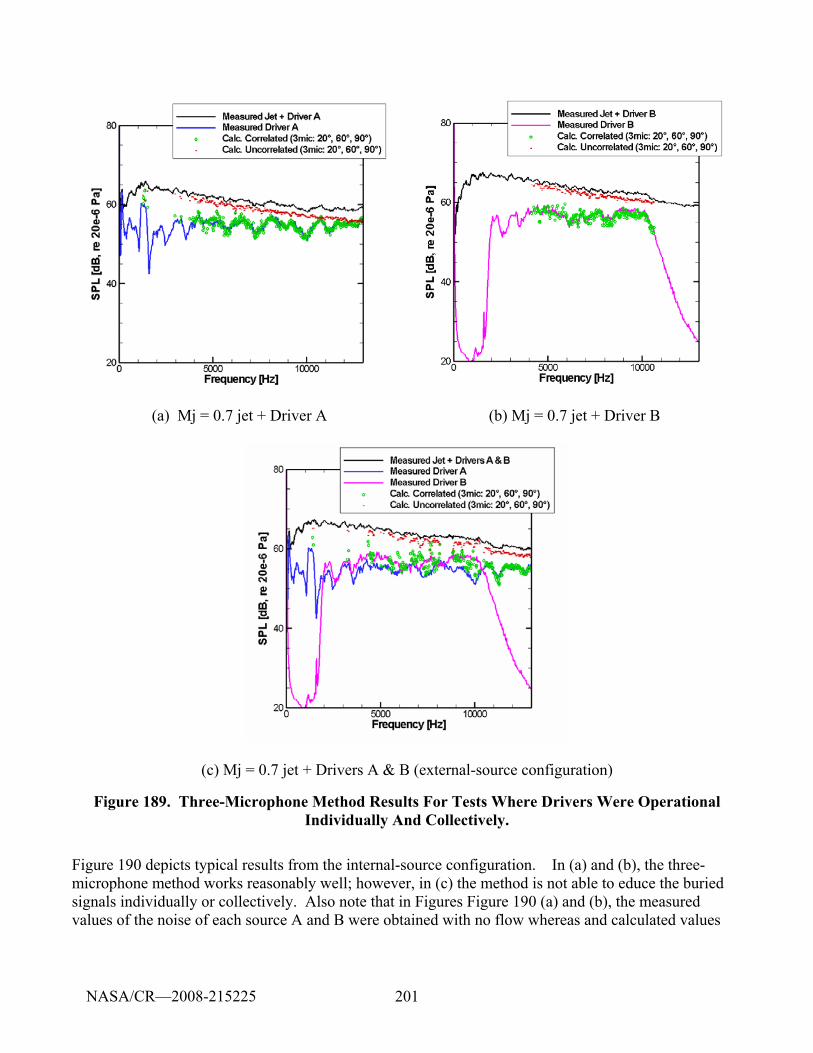
201

(a) Mj = 0.7 jet + Driver A (b) Mj = 0.7 jet + Driver B

(c) Mj = 0.7 jet + Drivers A & B (external-source configuration)

Figure 189. Three-Microphone Method Results For Tests Where Drivers Were Operational Individually And Collectively.

Figure 190 depicts typical results from the internal-source configuration. In (a) and (b), the three-microphone method works reasonably well; however, in (c) the method is not able to educe the buried signals individually or collectively. Also note that in Figures Figure 190 (a) and (b), the measured values of the noise of each source A and B were obtained with no flow whereas and calculated values

NASA/CR—2008-215225

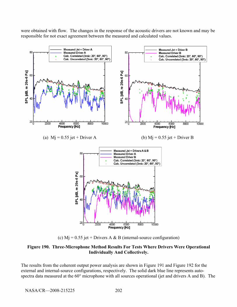
202

were obtained with flow. The changes in the response of the acoustic drivers are not known and may be responsible for not exact agreement between the measured and calculated values.

(a) Mj = 0.55 jet + Driver A (b) Mj = 0.55 jet + Driver B

(c) Mj = 0.55 jet + Drivers A & B (internal-source configuration)

Figure 190. Three-Microphone Method Results For Tests Where Drivers Were Operational Individually And Collectively.

The results from the coherent output power analysis are shown in Figure 191 and Figure 192 for the external and internal-source configurations, respectively. The solid dark blue line represents auto-spectra data measured at the 60° microphone with all sources operational (jet and drivers A and B). The

NASA/CR—2008-215225

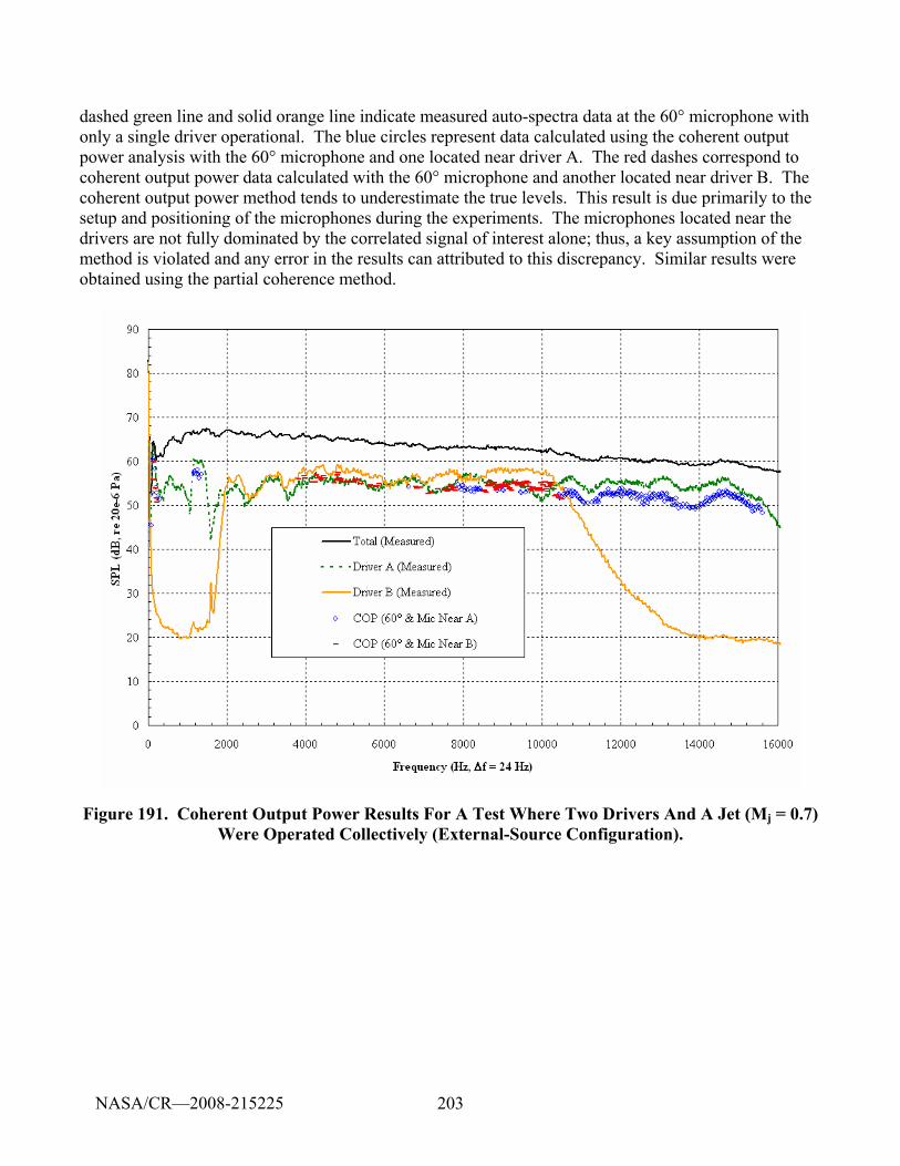
203

dashed green line and solid orange line indicate measured auto-spectra data at the 60° microphone with only a single driver operational. The blue circles represent data calculated using the coherent output power analysis with the 60° microphone and one located near driver A. The red dashes correspond to coherent output power data calculated with the 60° microphone and another located near driver B. The coherent output power method tends to underestimate the true levels. This result is due primarily to the setup and positioning of the microphones during the experiments. The microphones located near the drivers are not fully dominated by the correlated signal of interest alone; thus, a key assumption of the method is violated and any error in the results can attributed to this discrepancy. Similar results were obtained using the partial coherence method.

Figure 191. Coherent Output Power Results For A Test Where Two Drivers And A Jet (Mj = 0.7) Were Operated Collectively (External-Source Configuration).

NASA/CR—2008-215225

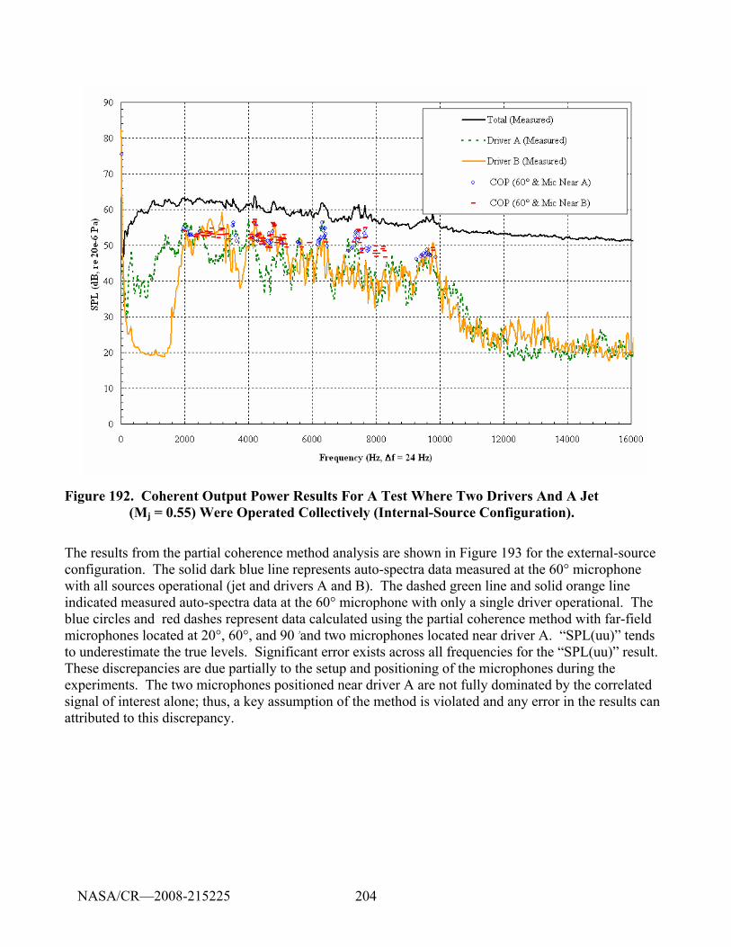
204

Figure 192. Coherent Output Power Results For A Test Where Two Drivers And A Jet (Mj = 0.55) Were Operated Collectively (Internal-Source Configuration).

The results from the partial coherence method analysis are shown in Figure 193 for the external-source configuration. The solid dark blue line represents auto-spectra data measured at the 60° microphone with all sources operational (jet and drivers A and B). The dashed green line and solid orange line indicated measured auto-spectra data at the 60° microphone with only a single driver operational. The blue circles and red dashes represent data calculated using the partial coherence method with far-field microphones located at 20°, 60°, and 90 ۥand two microphones located near driver A. “SPL(uu)” tends to underestimate the true levels. Significant error exists across all frequencies for the “SPL(uu)” result. These discrepancies are due partially to the setup and positioning of the microphones during the experiments. The two microphones positioned near driver A are not fully dominated by the correlated signal of interest alone; thus, a key assumption of the method is violated and any error in the results can attributed to this discrepancy.

NASA/CR—2008-215225

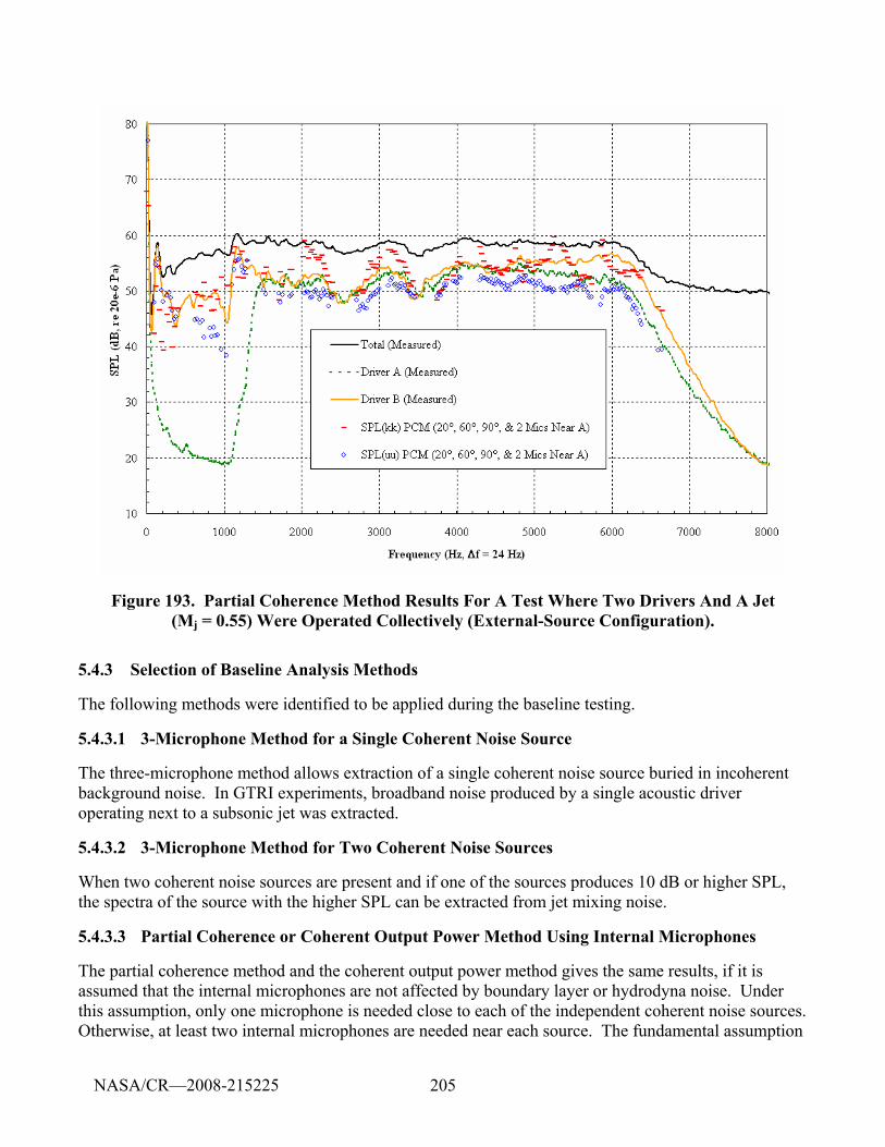
205

Figure 193. Partial Coherence Method Results For A Test Where Two Drivers And A Jet (Mj = 0.55) Were Operated Collectively (External-Source Configuration).

5.4.3 Selection of Baseline Analysis Methods

The following methods were identified to be applied during the baseline testing.

5.4.3.1 3-Microphone Method for a Single Coherent Noise Source

The three-microphone method allows extraction of a single coherent noise source buried in incoherent background noise. In GTRI experiments, broadband noise produced by a single acoustic driver operating next to a subsonic jet was extracted.

5.4.3.2 3-Microphone Method for Two Coherent Noise Sources

When two coherent noise sources are present and if one of the sources produces 10 dB or higher SPL, the spectra of the source with the higher SPL can be extracted from jet mixing noise.

5.4.3.3 Partial Coherence or Coherent Output Power Method Using Internal Microphones

The partial coherence method and the coherent output power method gives the same results, if it is assumed that the internal microphones are not affected by boundary layer or hydrodyna noise. Under this assumption, only one microphone is needed close to each of the independent coherent noise sources. Otherwise, at least two internal microphones are needed near each source. The fundamental assumption

NASA/CR—2008-215225

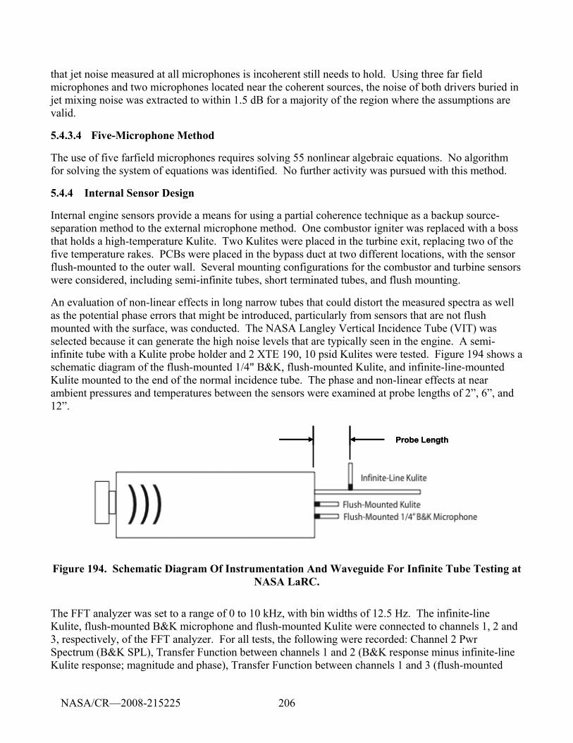
206

that jet noise measured at all microphones is incoherent still needs to hold. Using three far field microphones and two microphones located near the coherent sources, the noise of both drivers buried in jet mixing noise was extracted to within 1.5 dB for a majority of the region where the assumptions are valid.

5.4.3.4 Five-Microphone Method

The use of five farfield microphones requires solving 55 nonlinear algebraic equations. No algorithm for solving the system of equations was identified. No further activity was pursued with this method.

5.4.4 Internal Sensor Design

Internal engine sensors provide a means for using a partial coherence technique as a backup source-separation method to the external microphone method. One combustor igniter was replaced with a boss that holds a high-temperature Kulite. Two Kulites were placed in the turbine exit, replacing two of the five temperature rakes. PCBs were placed in the bypass duct at two different locations, with the sensor flush-mounted to the outer wall. Several mounting configurations for the combustor and turbine sensors were considered, including semi-infinite tubes, short terminated tubes, and flush mounting.

An evaluation of non-linear effects in long narrow tubes that could distort the measured spectra as well as the potential phase errors that might be introduced, particularly from sensors that are not flush mounted with the surface, was conducted. The NASA Langley Vertical Incidence Tube (VIT) was selected because it can generate the high noise levels that are typically seen in the engine. A semi-infinite tube with a Kulite probe holder and 2 XTE 190, 10 psid Kulites were tested. Figure 194 shows a schematic diagram of the flush-mounted 1/4" B&K, flush-mounted Kulite, and infinite-line-mounted Kulite mounted to the end of the normal incidence tube. The phase and non-linear effects at near ambient pressures and temperatures between the sensors were examined at probe lengths of 2”, 6”, and 12”.

Probe LengthProbe Length

Figure 194. Schematic Diagram Of Instrumentation And Waveguide For Infinite Tube Testing at NASA LaRC.

The FFT analyzer was set to a range of 0 to 10 kHz, with bin widths of 12.5 Hz. The infinite-line Kulite, flush-mounted B&K microphone and flush-mounted Kulite were connected to channels 1, 2 and 3, respectively, of the FFT analyzer. For all tests, the following were recorded: Channel 2 Pwr Spectrum (B&K SPL), Transfer Function between channels 1 and 2 (B&K response minus infinite-line Kulite response; magnitude and phase), Transfer Function between channels 1 and 3 (flush-mounted

NASA/CR—2008-215225

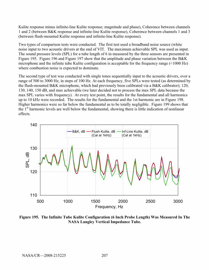
207

Kulite response minus infinite-line Kulite response; magnitude and phase), Coherence between channels 1 and 2 (between B&K response and infinite-line Kulite response), Coherence between channels 1 and 3 (between flush-mounted Kulite response and infinite-line Kulite response).

Two types of comparison tests were conducted. The first test used a broadband noise source (white noise input to two acoustic drivers at the end of VIT. The maximum achievable SPL was used as input. The sound pressure levels (SPL) for a tube length of 6 in measured by the three sensors are presented in Figure 195. Figure 196 and Figure 197 show that the amplitude and phase variation between the B&K microphone and the infinite tube Kulite configuration is acceptable for the frequency range (<1000 Hz) where combustion noise is expected to dominate.

The second type of test was conducted with single tones sequentially input to the acoustic drivers, over a range of 500 to 3000 Hz, in steps of 100 Hz. At each frequency, five SPLs were tested (as determined by the flush-mounted B&K microphone, which had previously been calibrated via a B&K calibrator); 120, 130, 140, 150 dB, and max achievable (we later decided not to process the max SPL data because the max SPL varies with frequency). At every test point, the results for the fundamental and all harmonics up to 10 kHz were recorded. The results for the fundamental and the 1st harmonic are in Figure 198. Higher harmonics were so far below the fundamental as to be totally negligible. Figure 199 shows that the 1st harmonic levels are well below the fundamental, showing there is little indication of nonlinear effects.

110

120

130

140

500 1000 1500 2000 2500 3000Frequency, Hz

SPL,

dB

B&K, dB Flush Kulite, dB(Cal at 1kHz)

Inf-Line Kulite, dB(Cal at 1kHz)

Figure 195. The Infinite Tube Kulite Configuration (6 Inch Probe Length) Was Measured In The NASA Langley Vertical Impedance Tube.

NASA/CR—2008-215225

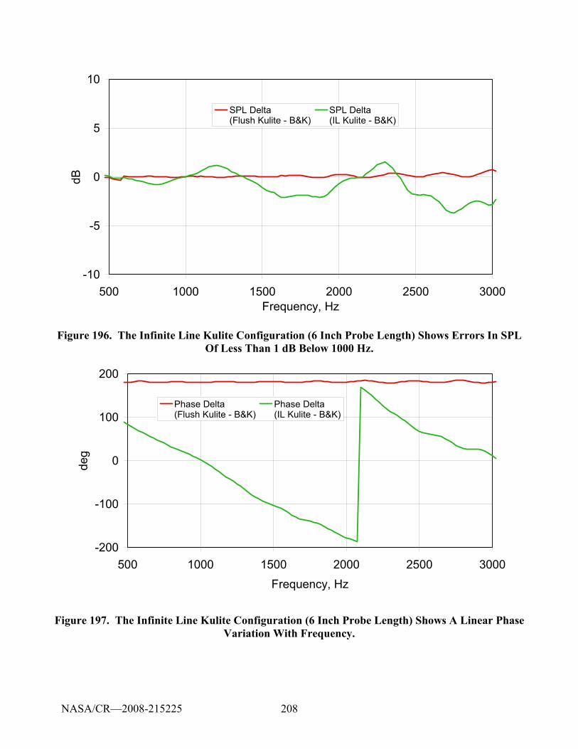
208

-10

-5

0

5

10

500 1000 1500 2000 2500 3000Frequency, Hz

dB

SPL Delta(Flush Kulite - B&K)

SPL Delta(IL Kulite - B&K)

Figure 196. The Infinite Line Kulite Configuration (6 Inch Probe Length) Shows Errors In SPL Of Less Than 1 dB Below 1000 Hz.

-200

-100

0

100

200

500 1000 1500 2000 2500 3000Frequency, Hz

deg

Phase Delta(Flush Kulite - B&K)

Phase Delta(IL Kulite - B&K)

Figure 197. The Infinite Line Kulite Configuration (6 Inch Probe Length) Shows A Linear Phase Variation With Frequency.

NASA/CR—2008-215225

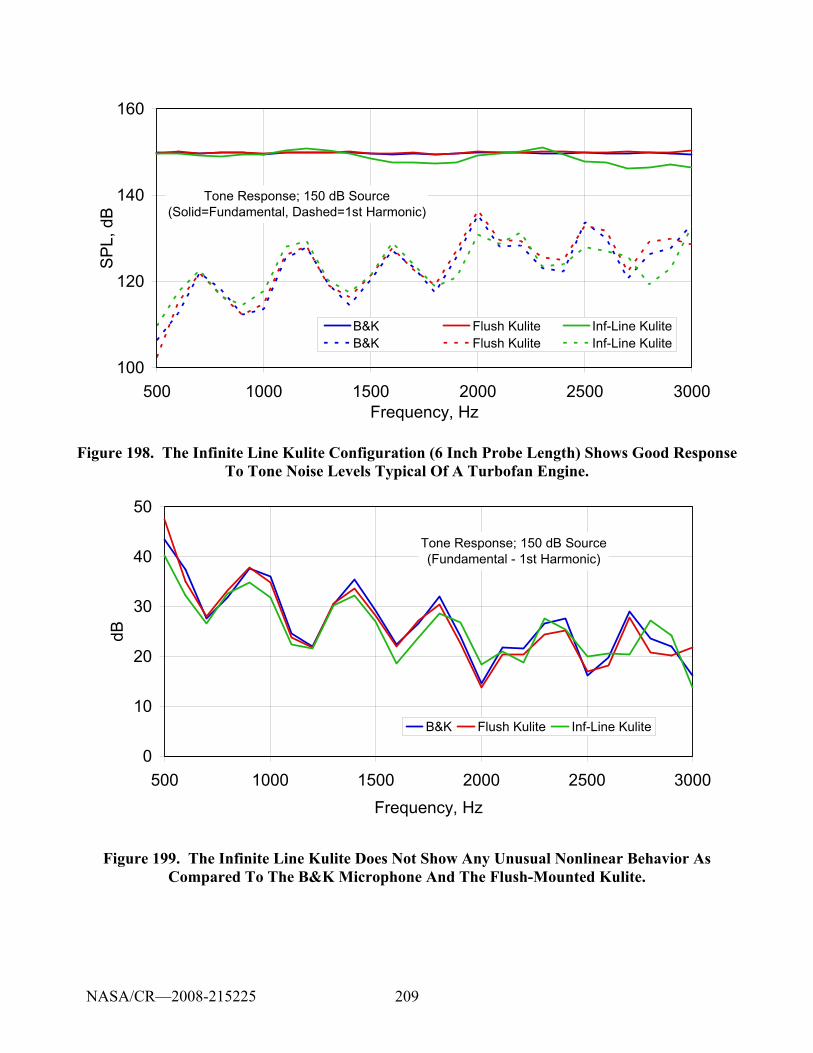
209

Tone Response; 150 dB Source(Solid=Fundamental, Dashed=1st Harmonic)

100

120

140

160

500 1000 1500 2000 2500 3000Frequency, Hz

SP

L, d

B

B&K Flush Kulite Inf-Line KuliteB&K Flush Kulite Inf-Line Kulite

Figure 198. The Infinite Line Kulite Configuration (6 Inch Probe Length) Shows Good Response To Tone Noise Levels Typical Of A Turbofan Engine.

Tone Response; 150 dB Source(Fundamental - 1st Harmonic)

0

10

20

30

40

50

500 1000 1500 2000 2500 3000Frequency, Hz

dB

B&K Flush Kulite Inf-Line Kulite

Figure 199. The Infinite Line Kulite Does Not Show Any Unusual Nonlinear Behavior As Compared To The B&K Microphone And The Flush-Mounted Kulite.

NASA/CR—2008-215225

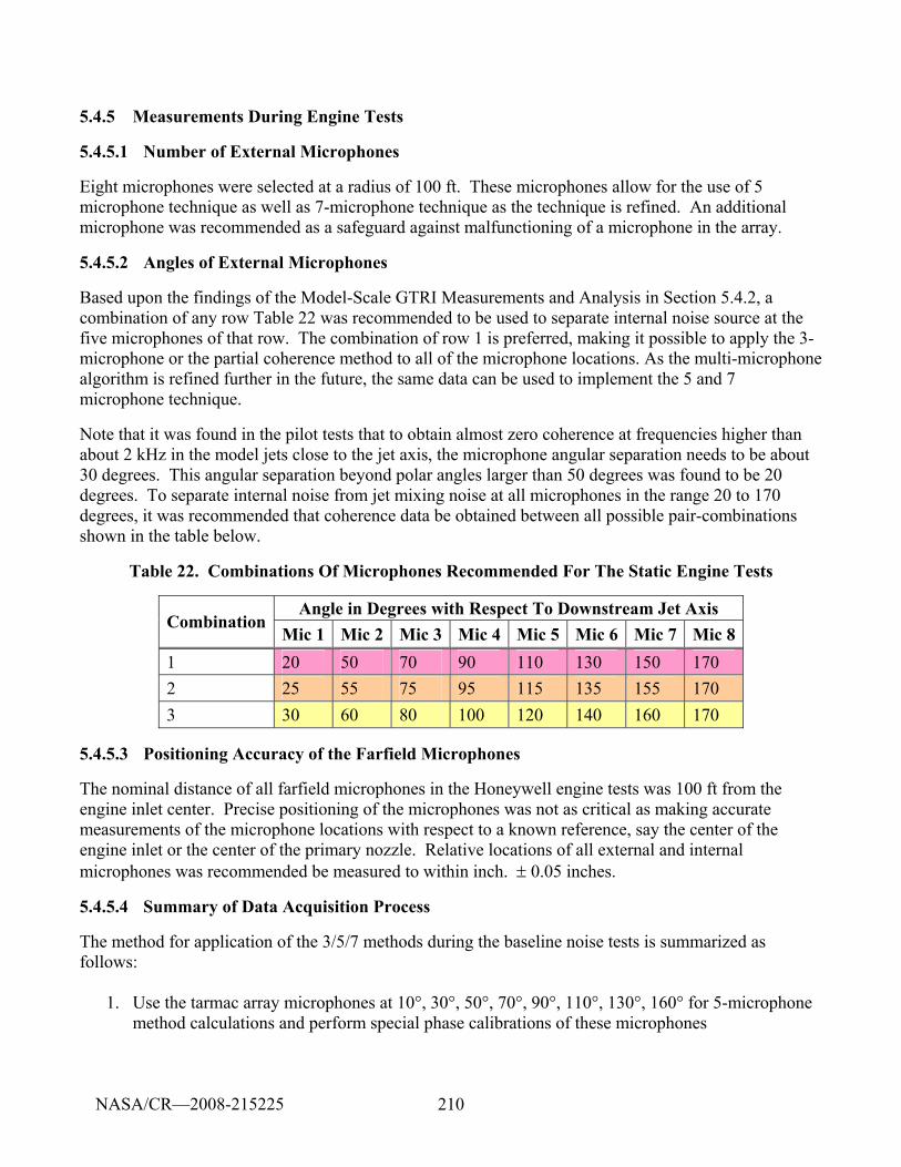
210

5.4.5 Measurements During Engine Tests

5.4.5.1 Number of External Microphones

Eight microphones were selected at a radius of 100 ft. These microphones allow for the use of 5 microphone technique as well as 7-microphone technique as the technique is refined. An additional microphone was recommended as a safeguard against malfunctioning of a microphone in the array.

5.4.5.2 Angles of External Microphones

Based upon the findings of the Model-Scale GTRI Measurements and Analysis in Section 5.4.2, a combination of any row Table 22 was recommended to be used to separate internal noise source at the five microphones of that row. The combination of row 1 is preferred, making it possible to apply the 3-microphone or the partial coherence method to all of the microphone locations. As the multi-microphone algorithm is refined further in the future, the same data can be used to implement the 5 and 7 microphone technique.

Note that it was found in the pilot tests that to obtain almost zero coherence at frequencies higher than about 2 kHz in the model jets close to the jet axis, the microphone angular separation needs to be about 30 degrees. This angular separation beyond polar angles larger than 50 degrees was found to be 20 degrees. To separate internal noise from jet mixing noise at all microphones in the range 20 to 170 degrees, it was recommended that coherence data be obtained between all possible pair-combinations shown in the table below.

Table 22. Combinations Of Microphones Recommended For The Static Engine Tests

Angle in Degrees with Respect To Downstream Jet Axis Combination

Mic 1 Mic 2 Mic 3 Mic 4 Mic 5 Mic 6 Mic 7 Mic 81 20 50 70 90 110 130 150 170 2 25 55 75 95 115 135 155 170 3 30 60 80 100 120 140 160 170

5.4.5.3 Positioning Accuracy of the Farfield Microphones

The nominal distance of all farfield microphones in the Honeywell engine tests was 100 ft from the engine inlet center. Precise positioning of the microphones was not as critical as making accurate measurements of the microphone locations with respect to a known reference, say the center of the engine inlet or the center of the primary nozzle. Relative locations of all external and internal microphones was recommended be measured to within inch. ± 0.05 inches.

5.4.5.4 Summary of Data Acquisition Process

The method for application of the 3/5/7 methods during the baseline noise tests is summarized as follows:

1. Use the tarmac array microphones at 10°, 30°, 50°, 70°, 90°, 110°, 130°, 160° for 5-microphone method calculations and perform special phase calibrations of these microphones

NASA/CR—2008-215225

211

2. Use any tarmac microphones for the 3-microphone methods since no phase calibration is required

3. Use internal sensors (1 combustor, 2 turbine exit, 2 fan bypass duct) with external sensors and partial coherence or coherent output power methods as additional source separation techniques.

4. Record 70 seconds of data for all sensors at 65,536 Hz sample rate to allow data reduction with 16 Hz bandwidth to 25600 Hz

5. Measure and record necessary ambient conditions and sensor placements

5.4.6 Five Microphone Method Solution

Attempts have been made to solve the non-linear system of equations resulting from the implementation of the five-microphone method; however, to date all have failed to give solutions of sufficient accuracy. The original solution procedure employed by Minami and Ahuja and its caveats are discussed below, along with a brief summary of the solution schemes attempted during the present work and the failures of each.

5.4.6.1 Solving the Numerical Simulation of Minami and Ahuja

5.4.6.1.1 Minami and Ahuja Solution Procedure

Minami and Ahuja algebraically reduced the system of 55 equations with 55 unknowns to a system consisting of only 8 equations with 8 unknowns to solve the five-microphone problem for the simulation outlined in their paper (see Reference 38). The reduced 8-equation system was solved using the Newton-Rhapson method. This solution procedure required an initial guess of the unknown variables. They used an initial guess that was very close to the known answer. A good guess is physically unattainable in experiments where the unknown variables are not numerically pre-defined. Thus, their solution procedure was not useful for the proof-of-concept testing in model-scale facilities. Further code development was needed to use the five-microphone methodology for the static engine measurements.

L (=20')

5 Microphones

d (= 1")

L2 (= 2')L1 (= 2‘)

CorrelatedSource A

CorrelatedSource B

Uncorrelated Noise N

L (=20')

5 Microphones

d (= 1")

L2 (= 2')L1 (= 2‘)

CorrelatedSource A

CorrelatedSource B

Uncorrelated Noise N

Figure 200. Minami And Ahuja Simulation.

NASA/CR—2008-215225

212

5.4.6.1.2 Attempted Solution Procedure Using Polymath 6.0

A third-party Newton-Rhapson based software, Polymath 6.0, was implemented. This software required an initial guess for each unknown value. When using the initial guess prescribed by Minami and Ahuja for their numerical simulation results of sufficient accuracy were reached. However, the findings resulting from these early attempts at solving both the original 55-equation system and the reduced 8-equation system were quite poor—non-physical imaginary solutions were obtained—when using physics-based initial values for the unknowns.

5.4.6.1.3 Attempted Solution Procedure Using MATLAB ‘fminsearch’

The use of the MATLAB® fminsearch function to solve the original 55-equation system was next attempted. This built-in function locally optimizes a scalar function of several variables by searching for function minima starting with an initial estimate of each variable. Specifics of the algorithm can be found in the MATLAB® Help Documentation. Since the fminsearch function requires a single scalar function for optimization, the 55-equation system was reduced to one equation by subtracting the right-hand side of each equation from both the left- and right-hand sides of that equation. For example, take ( ) ( 1, 2, 5)

i i i i i i i iy y u u v v n nG G G G i= + + = K (100)

Subtracting the RHS from both itself and the LHS gives ( ) )5 ,2 ,1( 0 K==++− iGGGG

iiiiiiii nnvvuuyy (101)

This was done for each of the 55 equations, and then equations were squared and summed. The result of this process was one scalar function of all variables that is equal to zero when minimized. Just as with the solution procedure employed by Minami and Ahuja, an initial guess of each unknown variables is required. When utilizing the fminsearch function, results within ±1 dB of the actual solution were obtained using initial values within ±2 % of the actual solution (very similar to the one used by Minami and Ahuja). However, initial guesses with that type of accuracy are unrealistic (i.e., there is no way to know the solution within ±2 % in any type of aeroacoustic testing). Thus, a physic-based arbitrary initial guess was then used. In this case, results were off by as much as 30 dB. An alternate method was then explored.

5.4.6.1.4 Attempted Solution Procedure Using MATLAB ‘ga’ and ‘fminsearch’

The use of genetic algorithms was explored. The built-in genetic algorithm within MATLAB®, ga, was utilized along with the fminsearch function. The ga function provides a means by which the single scalar function described above can be minimized globally. The specifics of the algorithm used by the ga function are available in the MATLAB® Help Documentation. By pairing the genetic algorithm with the fminsearch, the need of an initial guess is eliminated. The solution to the ga function is used as the initial guess for the fminsearch function. Thus, the scalar function is first minimized globally, and then the solution is refined locally. The ga function does allow for a set of bounds to be prescribed for the unknown variables. Doing so limits the search space and reduces the computation time. By defining these bounds based on the realistic physical constraints of the Minami and Ahuja simulated system, results within ±1 dB of the actual solution were obtained at all frequencies with the paired ga and fminsearch routine. At this point, a solution of Minami and Ahuja simulation of acceptable accuracy

NASA/CR—2008-215225

213

was attainable via the paired routine with physics-based bounds placed on the unknown variables. The attention then turned to solving the five-microphone problem for proof-of-concept experimentation.

5.4.6.2 Solving the System for Proof-of-Concept Testing

5.4.6.2.1 Establishing Physics-Based Initial Guess/Bounds

The issue of the physics-based initial guess or bounds for the unknown variables must be addressed—their origin as well as their significance to data processing. The manner in which the physics-based initial values are obtained is not so important for the numerical simulation. In such a case, the values of the simulated auto-spectra and phases were simply input as the initial guess for the unknown variables. Furthermore, the manner in which the bounds placed upon the unknown variables were chosen for the ga function is only slightly more complex. In the numerical simulation, these physics-based bounds were chosen based on the masking rule of acoustics that requires a buried signal to be within 12 dB of the loudest level in order to meaningfully contribute to the total sound pressure level. Thus, the lower bounds placed on the unknown auto-spectra and cross-spectra magnitudes were determined by simply subtracting 12 dB from simulated levels of the auto-spectrum and cross-spectrum magnitude at any given microphone or pair of microphones respectively. The upper bounds were set at the total simulated levels. The phases were allowed to vary over the entire numerical space, [-π, π]. The determination of the system’s physical bounds for proof-of-concept experimentation is based on the existence of a theoretical threshold on the lowest measurable coherence that was previously discussed. The lower bounds placed on the unknown auto-spectra and cross-spectra magnitudes were determined by simply subtracting floorSPLΔ from measured levels of the auto-spectrum and cross-spectrum magnitude at any given microphone or pair of microphones respectively. The upper bounds are set at the total measured levels. Because the five-microphone problem is so sensitive to even minor discrepancies in the measured coherence values, the proof-of-concept testing data were analyzed with a coherence threshold of 0.01, thus, leading to lower bounds of 10 dB less than the measured levels of the auto-spectrum and cross-spectrum magnitude and upper bounds equal to the total measured levels. As in the numerical simulation, the phases are allowed to vary over the entire numerical space, [-π, π].

5.4.6.2.2 Attempted Solution Procedure Using MATLAB ‘ga’ and ‘fminsearch’

Prior to the implementation of the paired ga and fminsearch routine with physics-based bounds in proof-of-concept experimentation, the paired routine with bounds of unattainable accuracy was used. These bounds were determined from the auto-spectra and cross-spectra magnitude of the buried correlated signals described in the external-source configuration testing of the previous chapter. As mentioned earlier, experiments were run with each driver operating alone, the jet operating alone, and all operating collectively. Testing in this manner allows for the solution of the five-microphone problem to be known beforehand. Thus, bounds of ±3 dB, ±5 dB, and ±10 dB of the actual solution for the auto-spectra and cross-spectra magnitudes were used. The phases were allowed to vary over the entire numerical space, [-π, π]. When using bounds of ±3 dB and ±5 dB, the accuracy of the results at selected frequencies was only slightly better than that of the bounds, ±2.6 dB and ±4.7 dB, respectively. In the case of the ±10 dB bounds, the code ran for days without reaching solution indicating that the search space was far too large.

NASA/CR—2008-215225

214

The paired routine with physics-based bounds was then attempted. Experiments, using the external-source configuration depicted in Figure 178, were examined at selected frequencies using the paired routine with the physical bounds described earlier. In this case, results within ±8 dB of the actual solution were found at selected frequencies. Thus, no improvement had been made.

5.4.6.2.3 Limiting the Solution Search Space Using the Three-Microphone Method

The use of an alternative approach to limit the search space of the ga algorithm was then investigated. This solution space limiting approach utilized the three-microphone method solution of the system at each microphone. The three-microphone method was used to find the uncorrelated portion of the total signal at each far-field microphone. Since the validity of this approach was not completely known at the time (it has since been studied and is addressed later in this report), the unknown uncorrelated portion of the auto-spectra were not set to be exactly these values. The three-microphone solution was used to provide a very limited search space for the uncorrelated portion by setting the bounds of the uncorrelated noise auto-spectra in the five-microphone problem to values only slightly less than and greater than the values obtained via the three-microphone method. The bounds of the remaining unknown auto-spectra and the unknown cross-spectra magnitudes were determined using coherence threshold approach and the unknown cross-spectra phases were once again allowed to vary over the entire numerical space. After changing the many options within the MATLAB® ga function numerous times, the best results for the experimental data were merely within ±5 dB of actual solution. Thus, a solution procedure of sufficient accuracy has not been obtained.

In summary, the paired ga and fminsearch routine with physics-based bounds placed on the unknown variables provides a solution of sufficient accuracy for the numerical simulation outlined in Minami and Ahuja. The physics-based bounds rely on the physical constraints of the radiated sound field and signal analyzer. This method along with many permutations of it has not been successful in solving the five-microphone problem in proof-of-concept testing. Table 23 is provided below as a summary of the effort.

NASA/CR—2008-215225

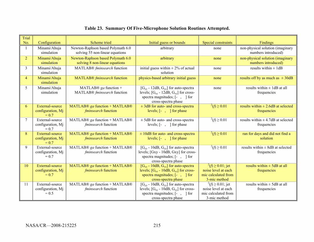
215

Table 23. Summary Of Five-Microphone Solution Routines Attempted.

Trial No. Configuration Scheme tried Initial guess or bounds Special constraints Findings 1 Minami/Ahuja

simulation Newton-Raphson based Polymath 6.0

solving 55 non-linear equations arbitrary none non-physical solution (imaginary

numbers introduced) 2 Minami/Ahuja

simulation Newton-Raphson based Polymath 6.0

solving 8 non-linear equations arbitrary none non-physical solution (imaginary

numbers introduced) 3 Minami/Ahuja

simulation MATLAB® fminsearch function initial guess within ± 2% of actual

solution none results within ± 1dB

4 Minami/Ahuja simulation

MATLAB® fminsearch function physics-based arbitrary initial guess none results off by as much as ± 30dB

5 Minami/Ahuja simulation

MATLAB® ga function + MATLAB® fminsearch function

[Gyy - 12dB, Gyy] for auto-spectra levels; [Gxy - 12dB, Gxy] for cross-

spectra magnitudes; [-�, �] for cross-spectra phase

none results within ± 1dB at all frequencies

6 External-source configuration, Mj

= 0.7


± 3dB for auto- and cross-spectra levels; [-�, �] for phase

�2(f) ≥ 0.01 results within ± 2.6dB at selected frequencies


= 0.7



�2(f) ≥ 0.01 results within ± 4.7dB at selected frequencies


= 0.7



�2(f) ≥ 0.01 ran for days and did not find a solution


= 0.7




�2(f) ≥ 0.01 results within ± 8dB at selected frequencies


= 0.7




�2(f) ≥ 0.01; jet noise level at each

mic calculated from 3-mic method

results within ± 5dB at all frequencies


= 0.5




�2(f) ≥ 0.01; jet noise level at each

mic calculated from 3-mic method

results within ± 5dB at all frequencies

NASA/CR—2008-215225

216

5.5 In-Situ Impedance Measurements

5.5.1 Introduction

Determination of acoustic liner impedance for jet engine applications remains a challenge for the designer. Although suitable models have been developed that take account of source amplitude and the local flow environment experienced by the liner (Reference 41 to 43), experimental validation of these models has been difficult.

The objective for the present work was to demonstrate the efficacy of making local, in-situ impedance measurements on an installed liner. In-situ impedance measurements substantiate the treatment design, provide understanding of flow effects on installed liner performance, and provide modeling input for fan noise propagation computations.

Honeywell, NASA Langley, and GTRI have conducted a series of acoustic liner evaluation tests for this study

in-situ and two-microphone method tests in a normal incidence impedance tube

in-situ and impedance eduction method tests in a grazing flow impedance tube

in-situ testing in a full scale engine nacelle during ground tests

The first of these tests were essentially risk mitigation steps. Lab tests were intended to provide insight and guidance for accurately measuring the impedance of the liner housed in the inlet of a Honeywell TECH7000 turbofan.

5.5.1.1 Reliable, Robust, Simple Liner Impedance Determination

The design of acoustic liners for aero-engine applications relies on optimizing specific acoustic impedance for a given fan, turbine, and inlet/nozzle configuration. Once the optimum impedance is determined, the liner is designed and fabricated and the resultant liner impedance is experimentally determined. Impedance determination can be obtained by a variety of methods. A common and simple method uses a normal incidence impedance tube to provide rapid determination of the liner impedance under normal plane wave incidence. Several impedance tube techniques exist, but the accepted method is the so-called Two-Microphone Method (TMM) that is outlined in the ASTM Standard E1090-98 (Reference 44) and follows the original work of Chung and Blaser (Reference 45)

However, the normal incidence impedance tube doesn’t account for effects of grazing incidence and grazing flow on the liner impedance. The latter effect is substantial, especially for the resonant class of liners most commonly used on aero-engines. Many studies (Reference 46 to 50) have shown the strong effects of a grazing flow field on the impedance of a resonant liner, specifically in how it affects the liner’s optimum impedance for a specific duct. To assess the performance under a velocity boundary layer, a liner is typically installed in a flow duct as part of the wall. There are two fundamental ways to experimentally determine liner impedance under grazing flow. One is to establish a controlled environment in a flow duct where fluctuating pressures can be measured and

NASA/CR—2008-215225

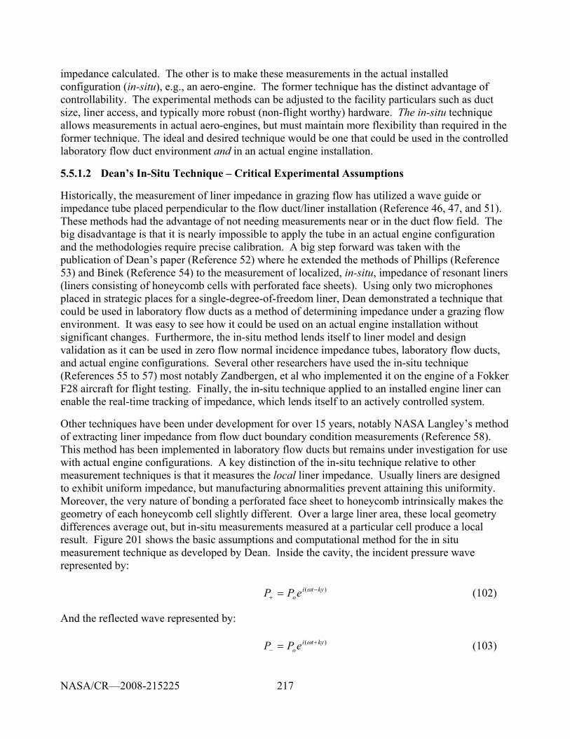
217

impedance calculated. The other is to make these measurements in the actual installed configuration (in-situ), e.g., an aero-engine. The former technique has the distinct advantage of controllability. The experimental methods can be adjusted to the facility particulars such as duct size, liner access, and typically more robust (non-flight worthy) hardware. The in-situ technique allows measurements in actual aero-engines, but must maintain more flexibility than required in the former technique. The ideal and desired technique would be one that could be used in the controlled laboratory flow duct environment and in an actual engine installation.

5.5.1.2 Dean’s In-Situ Technique – Critical Experimental Assumptions

Historically, the measurement of liner impedance in grazing flow has utilized a wave guide or impedance tube placed perpendicular to the flow duct/liner installation (Reference 46, 47, and 51). These methods had the advantage of not needing measurements near or in the duct flow field. The big disadvantage is that it is nearly impossible to apply the tube in an actual engine configuration and the methodologies require precise calibration. A big step forward was taken with the publication of Dean’s paper (Reference 52) where he extended the methods of Phillips (Reference 53) and Binek (Reference 54) to the measurement of localized, in-situ, impedance of resonant liners (liners consisting of honeycomb cells with perforated face sheets). Using only two microphones placed in strategic places for a single-degree-of-freedom liner, Dean demonstrated a technique that could be used in laboratory flow ducts as a method of determining impedance under a grazing flow environment. It was easy to see how it could be used on an actual engine installation without significant changes. Furthermore, the in-situ method lends itself to liner model and design validation as it can be used in zero flow normal incidence impedance tubes, laboratory flow ducts, and actual engine configurations. Several other researchers have used the in-situ technique (References 55 to 57) most notably Zandbergen, et al who implemented it on the engine of a Fokker F28 aircraft for flight testing. Finally, the in-situ technique applied to an installed engine liner can enable the real-time tracking of impedance, which lends itself to an actively controlled system.

Other techniques have been under development for over 15 years, notably NASA Langley’s method of extracting liner impedance from flow duct boundary condition measurements (Reference 58). This method has been implemented in laboratory flow ducts but remains under investigation for use with actual engine configurations. A key distinction of the in-situ technique relative to other measurement techniques is that it measures the local liner impedance. Usually liners are designed to exhibit uniform impedance, but manufacturing abnormalities prevent attaining this uniformity. Moreover, the very nature of bonding a perforated face sheet to honeycomb intrinsically makes the geometry of each honeycomb cell slightly different. Over a large liner area, these local geometry differences average out, but in-situ measurements measured at a particular cell produce a local result. Figure 201 shows the basic assumptions and computational method for the in situ measurement technique as developed by Dean. Inside the cavity, the incident pressure wave represented by: )( kyti

oePP −+ = ω (102)

And the reflected wave represented by: )( kyti

oePP +− = ω (103)

NASA/CR—2008-215225

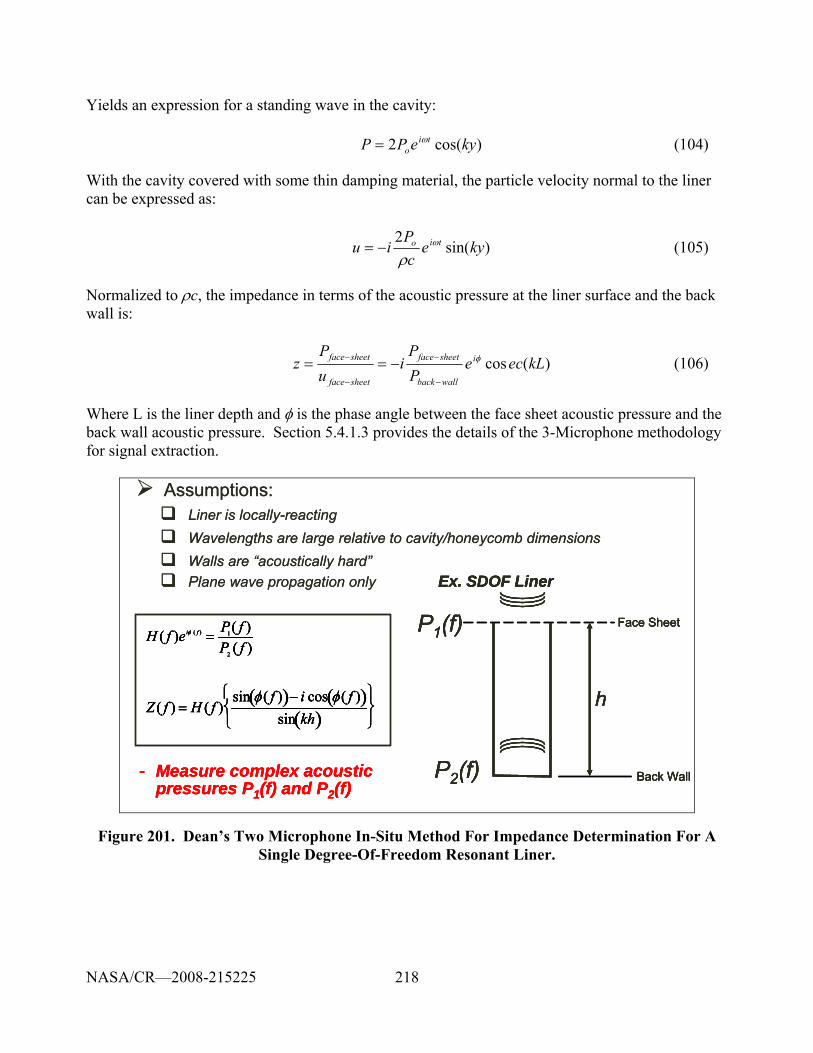
218

Yields an expression for a standing wave in the cavity: )cos(2 kyePP ti

oω= (104)

With the cavity covered with some thin damping material, the particle velocity normal to the liner can be expressed as:

)sin(2

kyecP

iu tio ω

ρ−= (105)

Normalized to ρc, the impedance in terms of the acoustic pressure at the liner surface and the back wall is:

)(cos kLecePP

iuP

z i

wallback

sheetface

sheetface

sheetface φ

−

−

−

− −== (106)

Where L is the liner depth and φ is the phase angle between the face sheet acoustic pressure and the back wall acoustic pressure. Section 5.4.1.3 provides the details of the 3-Microphone methodology for signal extraction.

Assumptions:Liner is locally-reactingWavelengths are large relative to cavity/honeycomb dimensionsWalls are “acoustically hard”Plane wave propagation only

- Measure complex acoustic pressures P1(f) and P2(f)

H ( f )eiφ ( f ) =P1( f )P2 ( f )

Z ( f ) = H ( f )sin φ ( f )( )− i cos φ ( f )( )

sin kh( )⎧ ⎨ ⎩

⎫ ⎬ ⎭

Ex. SDOF Liner

Face Sheet

Back Wall

P1(f)

P2(f)

h

Assumptions:Liner is locally-reactingWavelengths are large relative to cavity/honeycomb dimensionsWalls are “acoustically hard”Plane wave propagation only


H ( f )eiφ ( f ) =P1( f )P2 ( f )


sin kh( )⎧ ⎨ ⎩

⎫ ⎬ ⎭

Ex. SDOF Liner

Face Sheet

Back Wall

P1(f)

P2(f)

h


H ( f )eiφ ( f ) =P1( f )P2 ( f )


sin kh( )⎧ ⎨ ⎩

⎫ ⎬ ⎭

Ex. SDOF Liner

Face Sheet

Back Wall

P1(f)

P2(f)

h

H ( f )eiφ ( f ) =P1( f )P2 ( f )


sin kh( )⎧ ⎨ ⎩

⎫ ⎬ ⎭

Ex. SDOF Liner

Face Sheet

Back Wall

P1(f)

P2(f)

h

Figure 201. Dean’s Two Microphone In-Situ Method For Impedance Determination For A Single Degree-Of-Freedom Resonant Liner.

NASA/CR—2008-215225

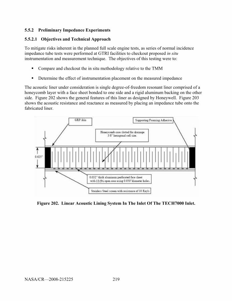
219

5.5.2 Preliminary Impedance Experiments

5.5.2.1 Objectives and Technical Approach

To mitigate risks inherent in the planned full scale engine tests, as series of normal incidence impedance tube tests were performed at GTRI facilities to checkout proposed in situ instrumentation and measurement technique. The objectives of this testing were to:

Compare and checkout the in situ methodology relative to the TMM

Determine the effect of instrumentation placement on the measured impedance

The acoustic liner under consideration is single degree-of-freedom resonant liner comprised of a honeycomb layer with a face sheet bonded to one side and a rigid aluminum backing on the other side. Figure 202 shows the general features of this liner as designed by Honeywell. Figure 203 shows the acoustic resistance and reactance as measured by placing an impedance tube onto the fabricated liner.

Figure 202. Linear Acoustic Lining System In The Inlet Of The TECH7000 Inlet.

NASA/CR—2008-215225

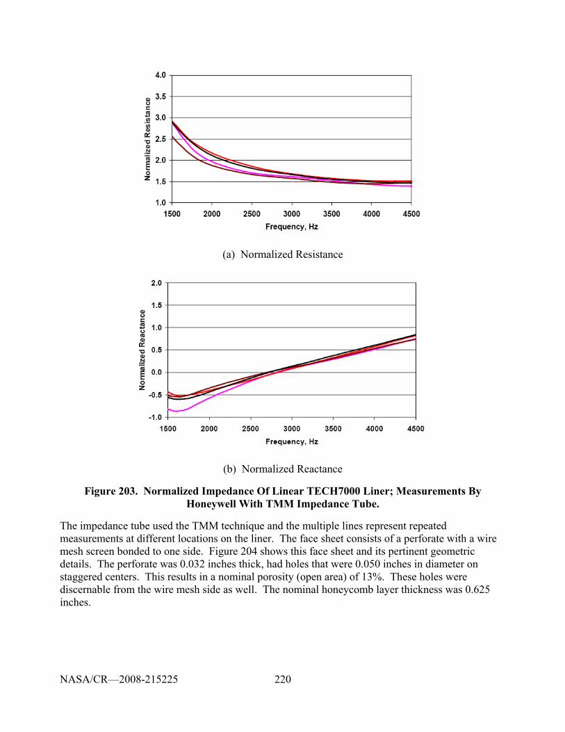
220

(a) Normalized Resistance

(b) Normalized Reactance

Figure 203. Normalized Impedance Of Linear TECH7000 Liner; Measurements By Honeywell With TMM Impedance Tube.

The impedance tube used the TMM technique and the multiple lines represent repeated measurements at different locations on the liner. The face sheet consists of a perforate with a wire mesh screen bonded to one side. Figure 204 shows this face sheet and its pertinent geometric details. The perforate was 0.032 inches thick, had holes that were 0.050 inches in diameter on staggered centers. This results in a nominal porosity (open area) of 13%. These holes were discernable from the wire mesh side as well. The nominal honeycomb layer thickness was 0.625 inches.

NASA/CR—2008-215225

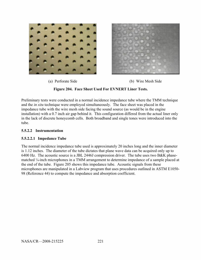
221

(a) Perforate Side (b) Wire Mesh Side

Figure 204. Face Sheet Used For EVNERT Liner Tests.

Preliminary tests were conducted in a normal incidence impedance tube where the TMM technique and the in situ technique were employed simultaneously. The face sheet was placed in the impedance tube with the wire mesh side facing the sound source (as would be in the engine installation) with a 0.7 inch air gap behind it. This configuration differed from the actual liner only in the lack of discrete honeycomb cells. Both broadband and single tones were introduced into the tube.

5.5.2.2 Instrumentation

5.5.2.2.1 Impedance Tube

The normal incidence impedance tube used is approximately 20 inches long and the inner diameter is 1.12 inches. The diameter of the tube dictates that plane wave data can be acquired only up to 6400 Hz. The acoustic source is a JBL 2446J compression driver. The tube uses two B&K phase-matched ¼-inch microphones in a TMM arrangement to determine impedance of a sample placed at the end of the tube. Figure 205 shows this impedance tube. Acoustic signals from these microphones are manipulated in a Labview program that uses procedures outlined in ASTM E1050-98 (Reference 44) to compute the impedance and absorption coefficient.

NASA/CR—2008-215225

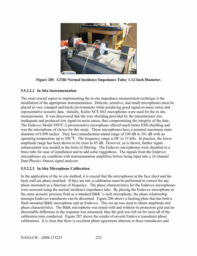
222

Figure 205. GTRI Normal Incidence Impedance Tube; 1.12-Inch Diameter.

5.5.2.2.2 In Situ Instrumentation

The most crucial aspect to implementing the in situ impedance measurement technique is the installation of the appropriate instrumentation. Delicate, sensitive, and small microphones must be placed in very cramped and harsh environments while producing good signal-to-noise ratios and representative acoustic data. Initially, Kulite XCE-062 microphones were used for the in situ measurements. It was discovered that the wire shielding provided by the manufacturer was inadequate and produced low signal-to-noise ratios, thus compromising the integrity of the data. The Endevco Model 8507C-2 piezoresistive microphone offered much better EMI shielding and was the microphone of choice for this study. These microphones have a nominal maximum outer diameter of 0.090 inches. They have manufacturer-stated range of 100 dB to 181 dB with an operating temperature up to 200 0F. The frequency range is DC to 15 kHz. In practice, the lower amplitude range has been shown to be close to 85 dB. However, as is shown, further signal enhancement was needed in the form of filtering. The Endevco microphones were sheathed in a brass tube for ease of installation and to add some ruggedness. The signals from the Endevco microphones are condition with instrumentation amplifiers before being input into a 16 channel Data Physics Abacus signal analyzer.

5.5.2.2.3 In Situ Microphone Calibration

In the application of the in situ method, it is crucial that the microphones at the face sheet and the back wall are phase matched. If they are not, a calibration must be performed to correct for any phase mismatch as a function of frequency. The phase characteristics for the Endevco microphones were assessed using the normal incidence impedance tube. By placing the Endevco microphone in the same acoustic pressure field as a standard B&K ¼-inch microphone, the phase relationship amongst Endevco transducers can be discerned. Figure 206 shows a backing plate that has both a flush-mounted B&K microphone and an Endevco. This set up was used to obtain amplitude and phase characteristics. The B&K microphone was tested with and without its protection grid and no discernable difference in the response was measured, thus the grid was left on for most all of the calibration tests conducted. Figure 207 shows the results of several Endevco transducer phase calibrations. It is clear that there is excellent phase agreement inherent in these transducers and

NASA/CR—2008-215225

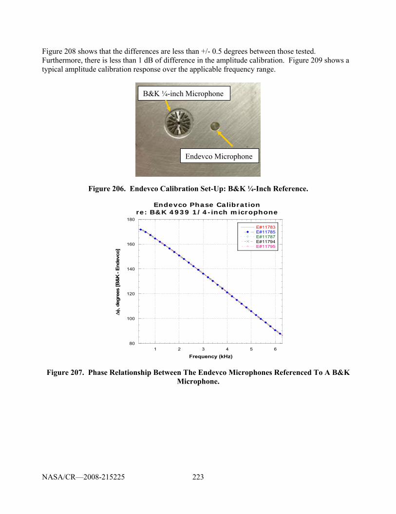
223

Figure 208 shows that the differences are less than +/- 0.5 degrees between those tested. Furthermore, there is less than 1 dB of difference in the amplitude calibration. Figure 209 shows a typical amplitude calibration response over the applicable frequency range.

B&K ¼-inch Microphone

Endevco Microphone

B&K ¼-inch Microphone

Endevco Microphone

Figure 206. Endevco Calibration Set-Up: B&K ¼-Inch Reference.

80

100

120

140

160

180

1 2 3 4 5 6

Endevco Phase Calibrationre: B&K 4939 1/4-inch microphone

E#11783E#11785E#11787E#11794E#11795

Δφ,

deg

rees

[B&

K -

Ende

vco]

Frequency (kHz)

Figure 207. Phase Relationship Between The Endevco Microphones Referenced To A B&K Microphone.

NASA/CR—2008-215225

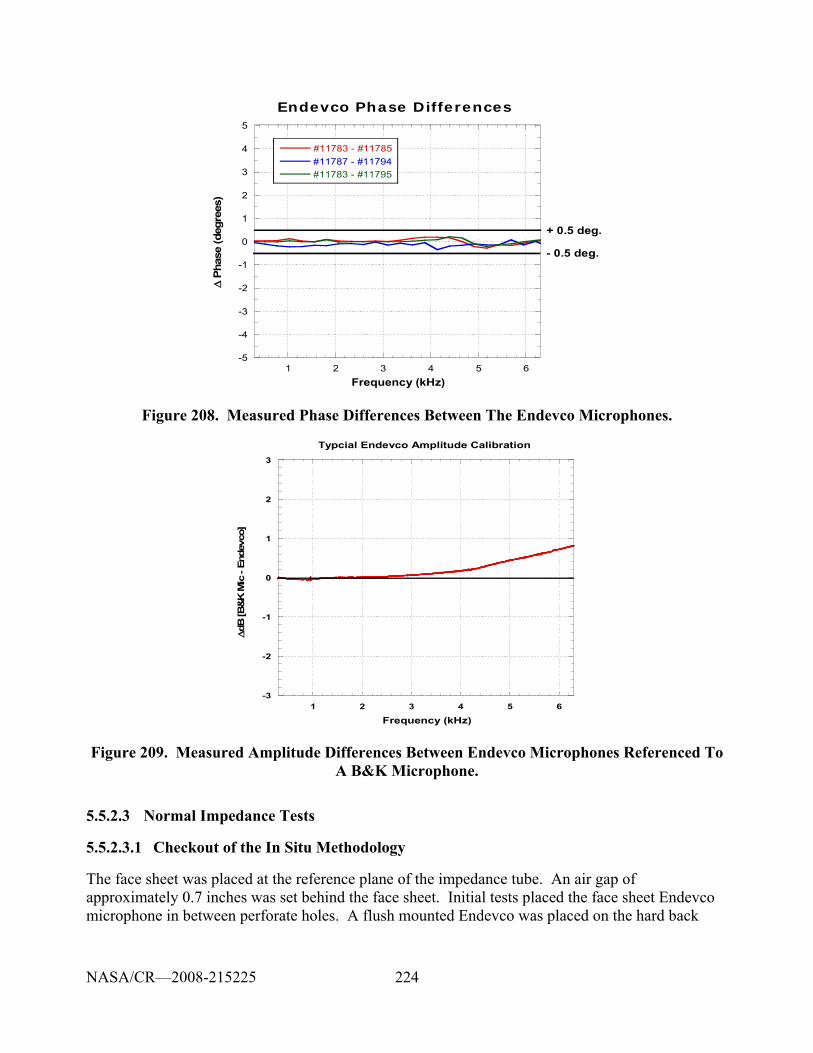
224

-5

-4

-3

-2

-1

0

1

2

3

4

5

1 2 3 4 5 6

Endevco Phase Differences

#11783 - #11785#11787 - #11794#11783 - #11795

Δ P

hase

(deg

rees

)

Frequency (kHz)

+ 0.5 deg.

- 0.5 deg.

Figure 208. Measured Phase Differences Between The Endevco Microphones.

-3

-2

-1

0

1

2

3

1 2 3 4 5 6

Typcial Endevco Amplitude Calibration

ΔdB

[B&

K M

ic -

Ende

vco]

Frequency (kHz)

Figure 209. Measured Amplitude Differences Between Endevco Microphones Referenced To A B&K Microphone.

5.5.2.3 Normal Impedance Tests

5.5.2.3.1 Checkout of the In Situ Methodology

The face sheet was placed at the reference plane of the impedance tube. An air gap of approximately 0.7 inches was set behind the face sheet. Initial tests placed the face sheet Endevco microphone in between perforate holes. A flush mounted Endevco was placed on the hard back

NASA/CR—2008-215225

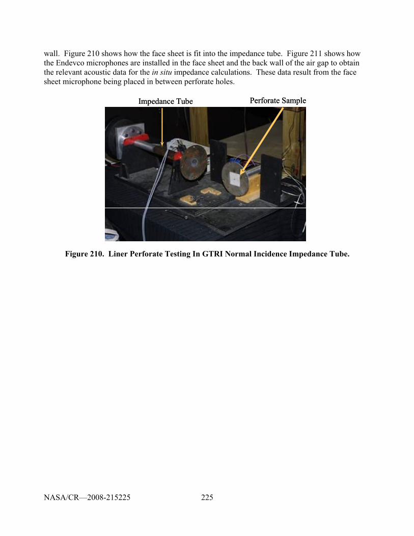
225

wall. Figure 210 shows how the face sheet is fit into the impedance tube. Figure 211 shows how the Endevco microphones are installed in the face sheet and the back wall of the air gap to obtain the relevant acoustic data for the in situ impedance calculations. These data result from the face sheet microphone being placed in between perforate holes.

Impedance Tube Perforate Sample Impedance Tube Perforate Sample

Figure 210. Liner Perforate Testing In GTRI Normal Incidence Impedance Tube.

NASA/CR—2008-215225

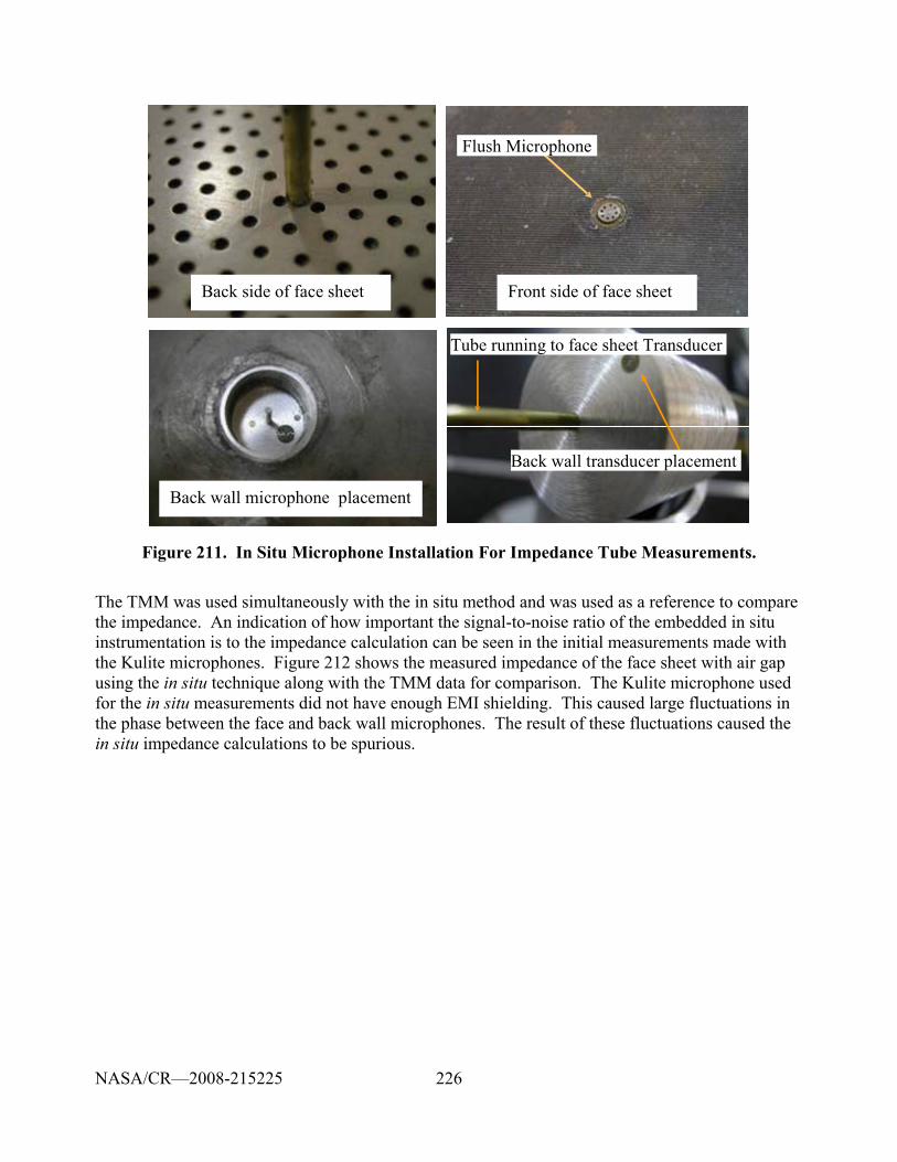
226

Flush Microphone

Back wall microphone placement

Back side of face sheet Front side of face sheet

Back wall transducer placement

Tube running to face sheet Transducer

Flush Microphone

Back wall microphone placement

Back side of face sheet Front side of face sheet

Back wall transducer placement

Tube running to face sheet Transducer

Figure 211. In Situ Microphone Installation For Impedance Tube Measurements.

The TMM was used simultaneously with the in situ method and was used as a reference to compare the impedance. An indication of how important the signal-to-noise ratio of the embedded in situ instrumentation is to the impedance calculation can be seen in the initial measurements made with the Kulite microphones. Figure 212 shows the measured impedance of the face sheet with air gap using the in situ technique along with the TMM data for comparison. The Kulite microphone used for the in situ measurements did not have enough EMI shielding. This caused large fluctuations in the phase between the face and back wall microphones. The result of these fluctuations caused the in situ impedance calculations to be spurious.

NASA/CR—2008-215225

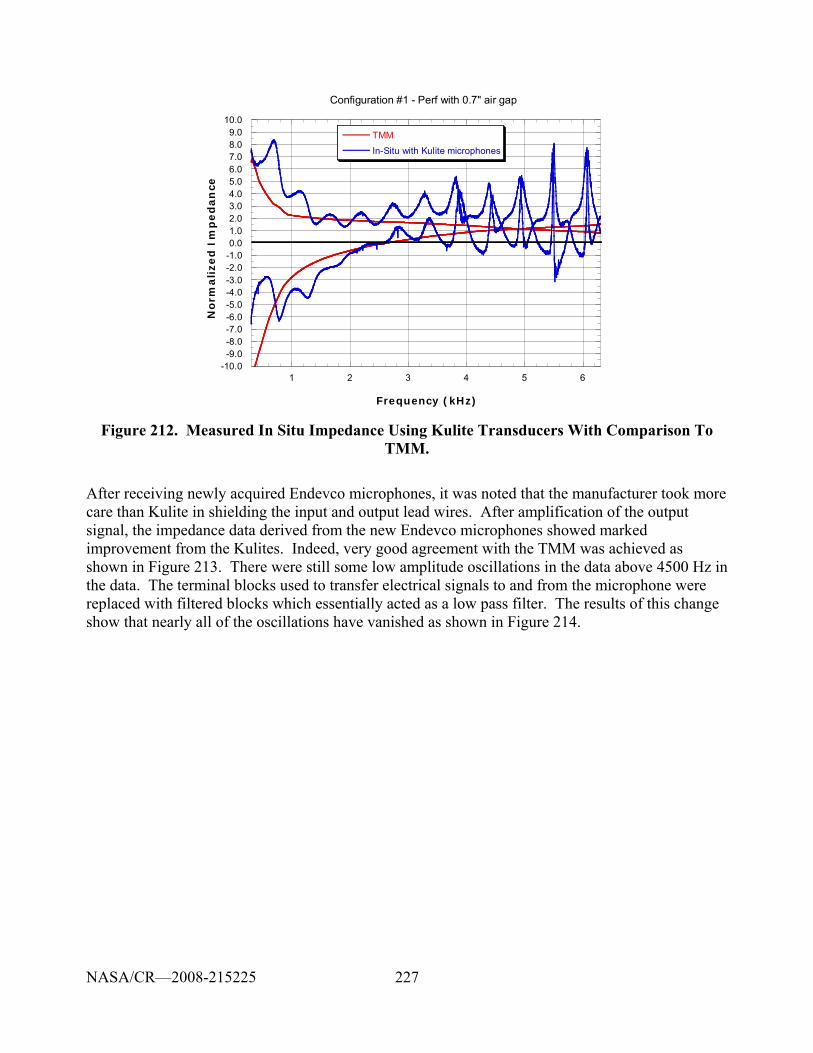
227

-10.0-9.0-8.0-7.0-6.0-5.0-4.0-3.0-2.0-1.00.01.02.03.04.05.06.07.08.09.0

10.0

1 2 3 4 5 6

TMM

In-Situ with Kulite microphones

Norm

alize

d I

mp

ed

an

ce

Frequency (kHz)

Configuration #1 - Perf with 0.7" air gap

Figure 212. Measured In Situ Impedance Using Kulite Transducers With Comparison To TMM.

After receiving newly acquired Endevco microphones, it was noted that the manufacturer took more care than Kulite in shielding the input and output lead wires. After amplification of the output signal, the impedance data derived from the new Endevco microphones showed marked improvement from the Kulites. Indeed, very good agreement with the TMM was achieved as shown in Figure 213. There were still some low amplitude oscillations in the data above 4500 Hz in the data. The terminal blocks used to transfer electrical signals to and from the microphone were replaced with filtered blocks which essentially acted as a low pass filter. The results of this change show that nearly all of the oscillations have vanished as shown in Figure 214.

NASA/CR—2008-215225

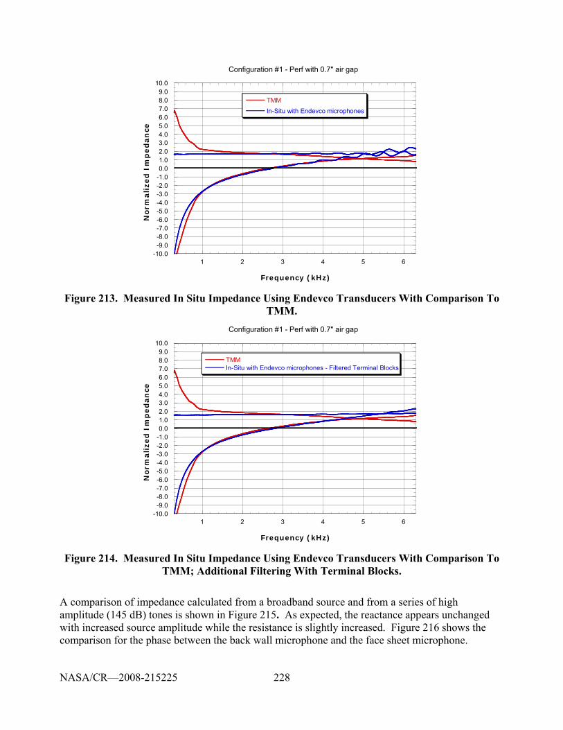
228

-10.0-9.0-8.0-7.0-6.0-5.0-4.0-3.0-2.0-1.00.01.02.03.04.05.06.07.08.09.0

10.0

1 2 3 4 5 6

TMM In-Situ with Endevco microphones

Norm

alized

Im

ped

an

ce

Frequency (kHz)


Figure 213. Measured In Situ Impedance Using Endevco Transducers With Comparison To TMM.

-10.0-9.0-8.0-7.0-6.0-5.0-4.0-3.0-2.0-1.00.01.02.03.04.05.06.07.08.09.0

10.0

1 2 3 4 5 6

TMM In-Situ with Endevco microphones - Filtered Terminal Blocks

Norm

alized

Im

ped

an

ce

Frequency (kHz)


Figure 214. Measured In Situ Impedance Using Endevco Transducers With Comparison To TMM; Additional Filtering With Terminal Blocks.

A comparison of impedance calculated from a broadband source and from a series of high amplitude (145 dB) tones is shown in Figure 215. As expected, the reactance appears unchanged with increased source amplitude while the resistance is slightly increased. Figure 216 shows the comparison for the phase between the back wall microphone and the face sheet microphone.

NASA/CR—2008-215225

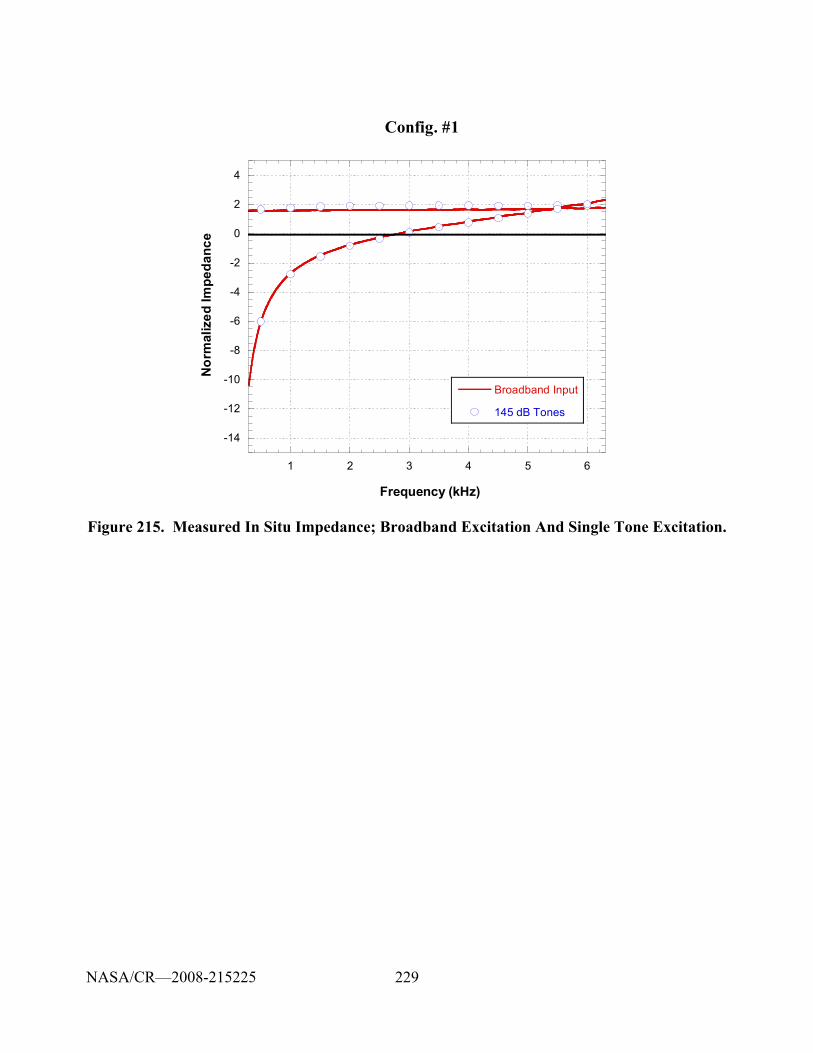
229

-14

-12

-10

-8

-6

-4

-2

0

2

4

1 2 3 4 5 6

Broadband Input

145 dB Tones

Nor

mal

ized

Impe

danc

e

Frequency (kHz)

Config. #1

Figure 215. Measured In Situ Impedance; Broadband Excitation And Single Tone Excitation.

NASA/CR—2008-215225

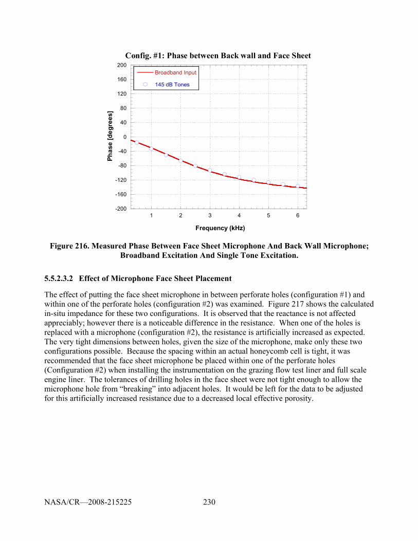
230

-200

-160

-120

-80

-40

0

40

80

120

160

200

1 2 3 4 5 6

Config. #1: Phase between Back wall and Face Sheet

Broadband Input

145 dB Tones

Phas

e [d

egre

es]

Frequency (kHz)

Figure 216. Measured Phase Between Face Sheet Microphone And Back Wall Microphone; Broadband Excitation And Single Tone Excitation.

5.5.2.3.2 Effect of Microphone Face Sheet Placement

The effect of putting the face sheet microphone in between perforate holes (configuration #1) and within one of the perforate holes (configuration #2) was examined. Figure 217 shows the calculated in-situ impedance for these two configurations. It is observed that the reactance is not affected appreciably; however there is a noticeable difference in the resistance. When one of the holes is replaced with a microphone (configuration #2), the resistance is artificially increased as expected. The very tight dimensions between holes, given the size of the microphone, make only these two configurations possible. Because the spacing within an actual honeycomb cell is tight, it was recommended that the face sheet microphone be placed within one of the perforate holes (Configuration #2) when installing the instrumentation on the grazing flow test liner and full scale engine liner. The tolerances of drilling holes in the face sheet were not tight enough to allow the microphone hole from “breaking” into adjacent holes. It would be left for the data to be adjusted for this artificially increased resistance due to a decreased local effective porosity.

NASA/CR—2008-215225

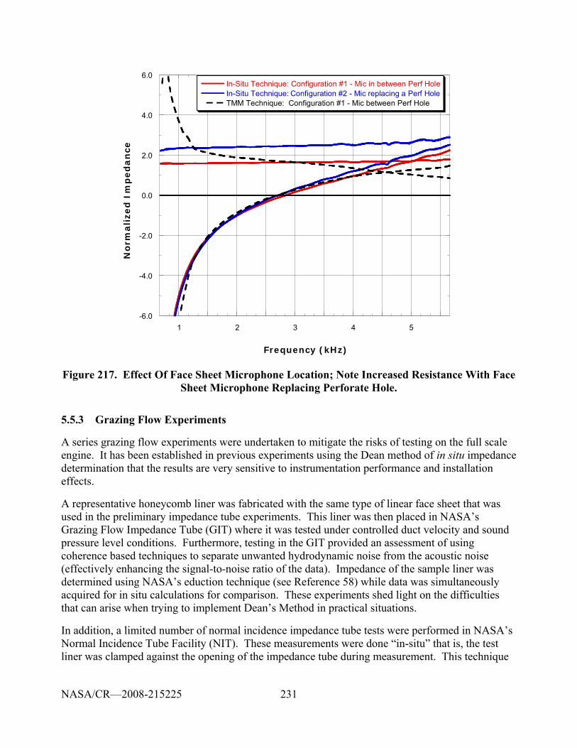
231

-6.0

-4.0

-2.0

0.0

2.0

4.0

6.0

1 2 3 4 5

In-Situ Technique: Configuration #1 - Mic in between Perf HoleIn-Situ Technique: Configuration #2 - Mic replacing a Perf HoleTMM Technique: Configuration #1 - Mic between Perf Hole

Norm

ali

zed

Im

ped

an

ce

Frequency (kHz)

Figure 217. Effect Of Face Sheet Microphone Location; Note Increased Resistance With Face Sheet Microphone Replacing Perforate Hole.

5.5.3 Grazing Flow Experiments

A series grazing flow experiments were undertaken to mitigate the risks of testing on the full scale engine. It has been established in previous experiments using the Dean method of in situ impedance determination that the results are very sensitive to instrumentation performance and installation effects.

A representative honeycomb liner was fabricated with the same type of linear face sheet that was used in the preliminary impedance tube experiments. This liner was then placed in NASA’s Grazing Flow Impedance Tube (GIT) where it was tested under controlled duct velocity and sound pressure level conditions. Furthermore, testing in the GIT provided an assessment of using coherence based techniques to separate unwanted hydrodynamic noise from the acoustic noise (effectively enhancing the signal-to-noise ratio of the data). Impedance of the sample liner was determined using NASA’s eduction technique (see Reference 58) while data was simultaneously acquired for in situ calculations for comparison. These experiments shed light on the difficulties that can arise when trying to implement Dean’s Method in practical situations.

In addition, a limited number of normal incidence impedance tube tests were performed in NASA’s Normal Incidence Tube Facility (NIT). These measurements were done “in-situ” that is, the test liner was clamped against the opening of the impedance tube during measurement. This technique

NASA/CR—2008-215225

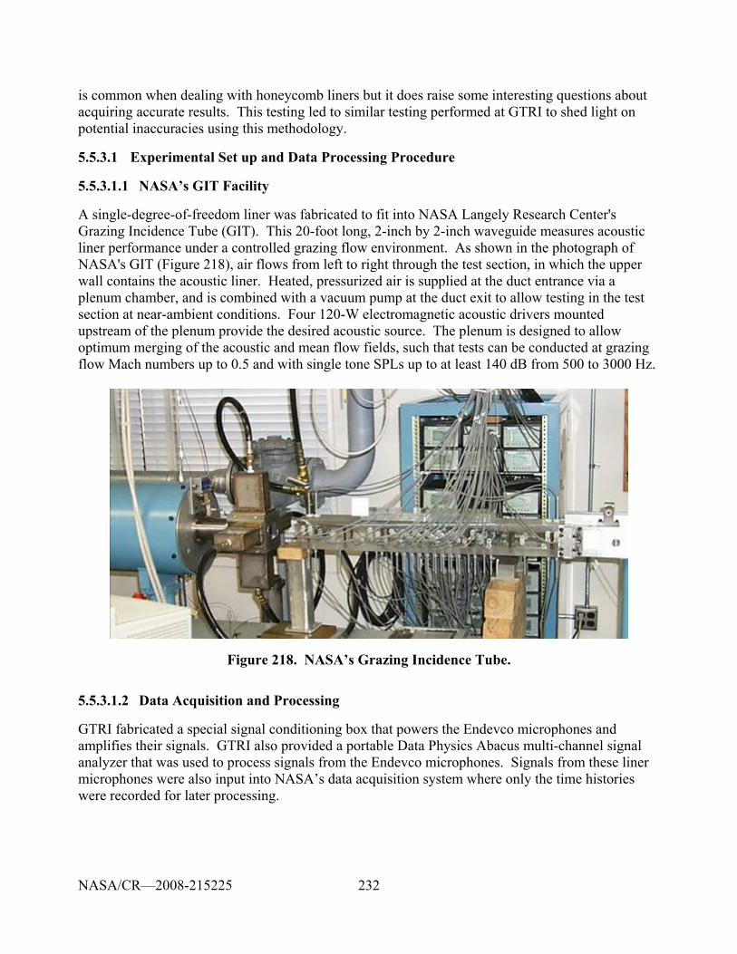
232

is common when dealing with honeycomb liners but it does raise some interesting questions about acquiring accurate results. This testing led to similar testing performed at GTRI to shed light on potential inaccuracies using this methodology.

5.5.3.1 Experimental Set up and Data Processing Procedure

5.5.3.1.1 NASA’s GIT Facility

A single-degree-of-freedom liner was fabricated to fit into NASA Langely Research Center's Grazing Incidence Tube (GIT). This 20-foot long, 2-inch by 2-inch waveguide measures acoustic liner performance under a controlled grazing flow environment. As shown in the photograph of NASA's GIT (Figure 218), air flows from left to right through the test section, in which the upper wall contains the acoustic liner. Heated, pressurized air is supplied at the duct entrance via a plenum chamber, and is combined with a vacuum pump at the duct exit to allow testing in the test section at near-ambient conditions. Four 120-W electromagnetic acoustic drivers mounted upstream of the plenum provide the desired acoustic source. The plenum is designed to allow optimum merging of the acoustic and mean flow fields, such that tests can be conducted at grazing flow Mach numbers up to 0.5 and with single tone SPLs up to at least 140 dB from 500 to 3000 Hz.

Figure 218. NASA’s Grazing Incidence Tube.

5.5.3.1.2 Data Acquisition and Processing

GTRI fabricated a special signal conditioning box that powers the Endevco microphones and amplifies their signals. GTRI also provided a portable Data Physics Abacus multi-channel signal analyzer that was used to process signals from the Endevco microphones. Signals from these liner microphones were also input into NASA’s data acquisition system where only the time histories were recorded for later processing.

NASA/CR—2008-215225

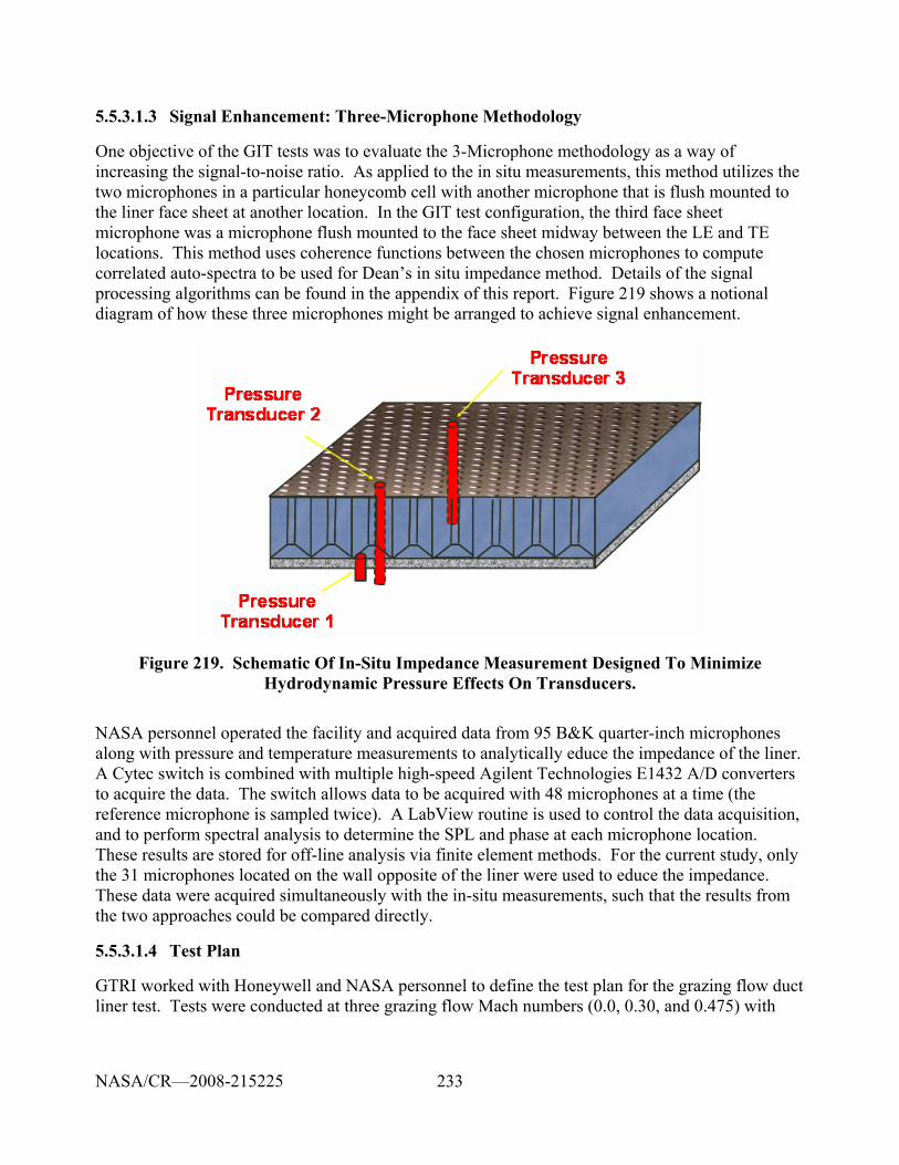
233

5.5.3.1.3 Signal Enhancement: Three-Microphone Methodology

One objective of the GIT tests was to evaluate the 3-Microphone methodology as a way of increasing the signal-to-noise ratio. As applied to the in situ measurements, this method utilizes the two microphones in a particular honeycomb cell with another microphone that is flush mounted to the liner face sheet at another location. In the GIT test configuration, the third face sheet microphone was a microphone flush mounted to the face sheet midway between the LE and TE locations. This method uses coherence functions between the chosen microphones to compute correlated auto-spectra to be used for Dean’s in situ impedance method. Details of the signal processing algorithms can be found in the appendix of this report. Figure 219 shows a notional diagram of how these three microphones might be arranged to achieve signal enhancement.

Figure 219. Schematic Of In-Situ Impedance Measurement Designed To Minimize Hydrodynamic Pressure Effects On Transducers.

NASA personnel operated the facility and acquired data from 95 B&K quarter-inch microphones along with pressure and temperature measurements to analytically educe the impedance of the liner. A Cytec switch is combined with multiple high-speed Agilent Technologies E1432 A/D converters to acquire the data. The switch allows data to be acquired with 48 microphones at a time (the reference microphone is sampled twice). A LabView routine is used to control the data acquisition, and to perform spectral analysis to determine the SPL and phase at each microphone location. These results are stored for off-line analysis via finite element methods. For the current study, only the 31 microphones located on the wall opposite of the liner were used to educe the impedance. These data were acquired simultaneously with the in-situ measurements, such that the results from the two approaches could be compared directly.

5.5.3.1.4 Test Plan

GTRI worked with Honeywell and NASA personnel to define the test plan for the grazing flow duct liner test. Tests were conducted at three grazing flow Mach numbers (0.0, 0.30, and 0.475) with

NASA/CR—2008-215225

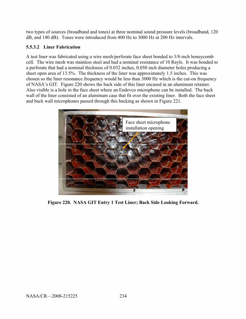
234

two types of sources (broadband and tones) at three nominal sound pressure levels (broadband, 120 dB, and 140 dB). Tones were introduced from 400 Hz to 3000 Hz at 200 Hz intervals.

5.5.3.2 Liner Fabrication

A test liner was fabricated using a wire mesh/perforate face sheet bonded to 3/8-inch honeycomb cell. The wire mesh was stainless steel and had a nominal resistance of 10 Rayls. It was bonded to a perforate that had a nominal thickness of 0.032 inches, 0.050 inch diameter holes producing a sheet open area of 13.5%. The thickness of the liner was approximately 1.5 inches. This was chosen so the liner resonance frequency would be less than 3000 Hz which is the cut-on frequency of NASA’s GIT. Figure 220 shows the back side of this liner encased in an aluminum retainer. Also visible is a hole in the face sheet where an Endevco microphone can be installed. The back wall of the liner consisted of an aluminum case that fit over the existing liner. Both the face sheet and back wall microphones passed through this backing as shown in Figure 221.

Face sheet microphone installation openingFace sheet microphone installation opening

Figure 220. NASA GIT Entry 1 Test Liner; Back Side Looking Forward.

NASA/CR—2008-215225

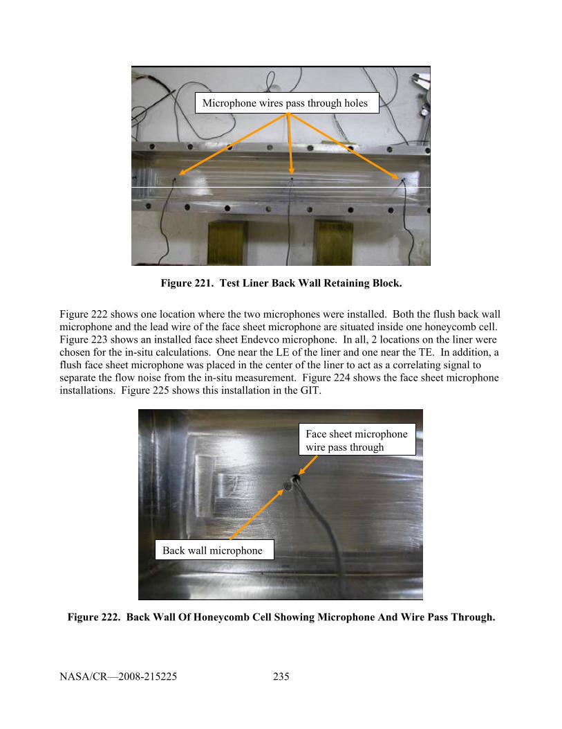
235

Microphone wires pass through holesMicrophone wires pass through holes

Figure 221. Test Liner Back Wall Retaining Block.

Figure 222 shows one location where the two microphones were installed. Both the flush back wall microphone and the lead wire of the face sheet microphone are situated inside one honeycomb cell. Figure 223 shows an installed face sheet Endevco microphone. In all, 2 locations on the liner were chosen for the in-situ calculations. One near the LE of the liner and one near the TE. In addition, a flush face sheet microphone was placed in the center of the liner to act as a correlating signal to separate the flow noise from the in-situ measurement. Figure 224 shows the face sheet microphone installations. Figure 225 shows this installation in the GIT.

Back wall microphone

Face sheet microphone wire pass through

Back wall microphone

Face sheet microphone wire pass through

Figure 222. Back Wall Of Honeycomb Cell Showing Microphone And Wire Pass Through.

NASA/CR—2008-215225

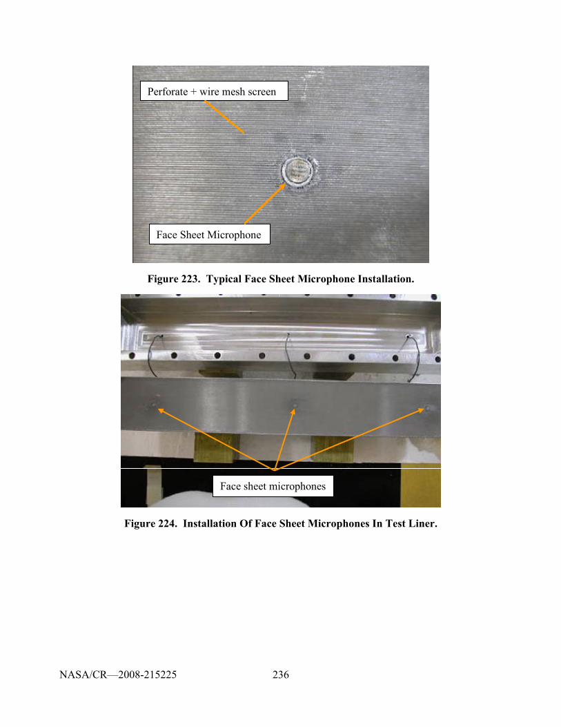
236

Perforate + wire mesh screen

Face Sheet Microphone

Perforate + wire mesh screen

Face Sheet Microphone

Figure 223. Typical Face Sheet Microphone Installation.

Face sheet microphonesFace sheet microphones

Figure 224. Installation Of Face Sheet Microphones In Test Liner.

NASA/CR—2008-215225

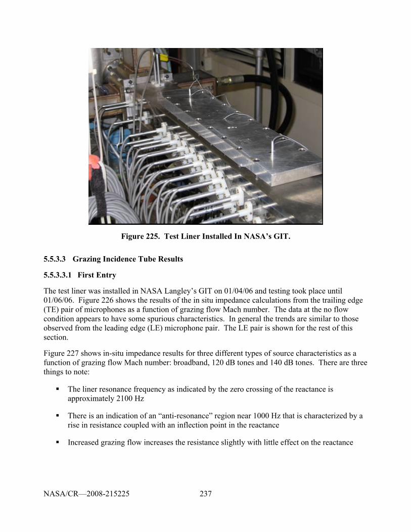
237

Figure 225. Test Liner Installed In NASA’s GIT.

5.5.3.3 Grazing Incidence Tube Results

5.5.3.3.1 First Entry

The test liner was installed in NASA Langley’s GIT on 01/04/06 and testing took place until 01/06/06. Figure 226 shows the results of the in situ impedance calculations from the trailing edge (TE) pair of microphones as a function of grazing flow Mach number. The data at the no flow condition appears to have some spurious characteristics. In general the trends are similar to those observed from the leading edge (LE) microphone pair. The LE pair is shown for the rest of this section.

Figure 227 shows in-situ impedance results for three different types of source characteristics as a function of grazing flow Mach number: broadband, 120 dB tones and 140 dB tones. There are three things to note:

The liner resonance frequency as indicated by the zero crossing of the reactance is approximately 2100 Hz

There is an indication of an “anti-resonance” region near 1000 Hz that is characterized by a rise in resistance coupled with an inflection point in the reactance

Increased grazing flow increases the resistance slightly with little effect on the reactance

NASA/CR—2008-215225

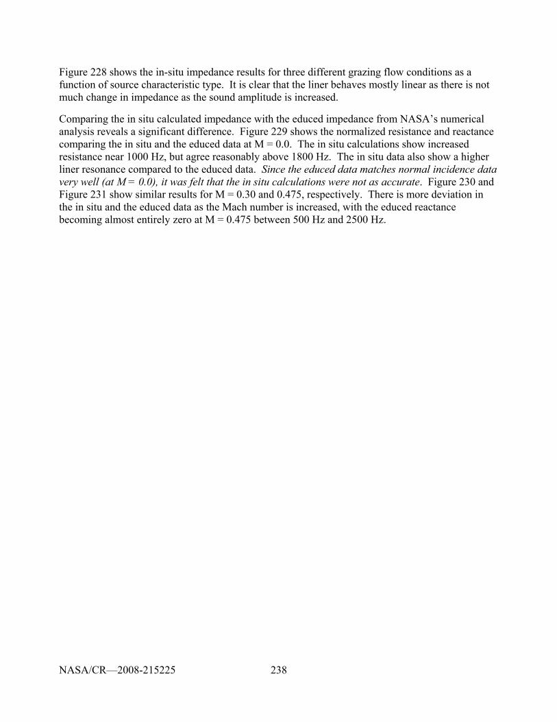
238

Figure 228 shows the in-situ impedance results for three different grazing flow conditions as a function of source characteristic type. It is clear that the liner behaves mostly linear as there is not much change in impedance as the sound amplitude is increased.

Comparing the in situ calculated impedance with the educed impedance from NASA’s numerical analysis reveals a significant difference. Figure 229 shows the normalized resistance and reactance comparing the in situ and the educed data at M = 0.0. The in situ calculations show increased resistance near 1000 Hz, but agree reasonably above 1800 Hz. The in situ data also show a higher liner resonance compared to the educed data. Since the educed data matches normal incidence data very well (at M = 0.0), it was felt that the in situ calculations were not as accurate. Figure 230 and Figure 231 show similar results for M = 0.30 and 0.475, respectively. There is more deviation in the in situ and the educed data as the Mach number is increased, with the educed reactance becoming almost entirely zero at M = 0.475 between 500 Hz and 2500 Hz.

NASA/CR—2008-215225

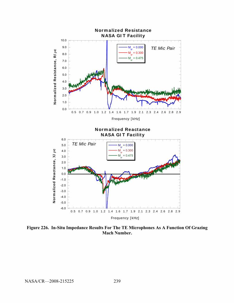
239

0.5 0.7 0.9 1.0 1.2 1.4 1.6 1.7 1.9 2.1 2.3 2.4 2.6 2.8 2.9

g pNormalized Resistance

NASA GIT Facility

Mgr

= 0.000

Mgr

= 0.300

Mgr

= 0.475

0.0

1.0

2.0

3.0

4.0

5.0

6.0

7.0

8.0

9.0

10.0

Norm

alized

Resi

sta

nce

, R

/ρc

Frequency [kHz]

TE Mic Pair

0.5 0.7 0.9 1.0 1.2 1.4 1.6 1.7 1.9 2.1 2.3 2.4 2.6 2.8 2.9

Normalized ReactanceNASA GIT Facility

Mgr

= 0.000

Mgr

= 0.300

Mgr

= 0.475

-6.0

-5.0

-4.0

-3.0

-2.0

-1.0

0.0

1.0

2.0

3.0

4.0

5.0

6.0

No

rmalized

React

an

ce,

Χ/

ρc

Frequency [kHz]

TE Mic Pair

Figure 226. In-Situ Impedance Results For The TE Microphones As A Function Of Grazing Mach Number.

NASA/CR—2008-215225

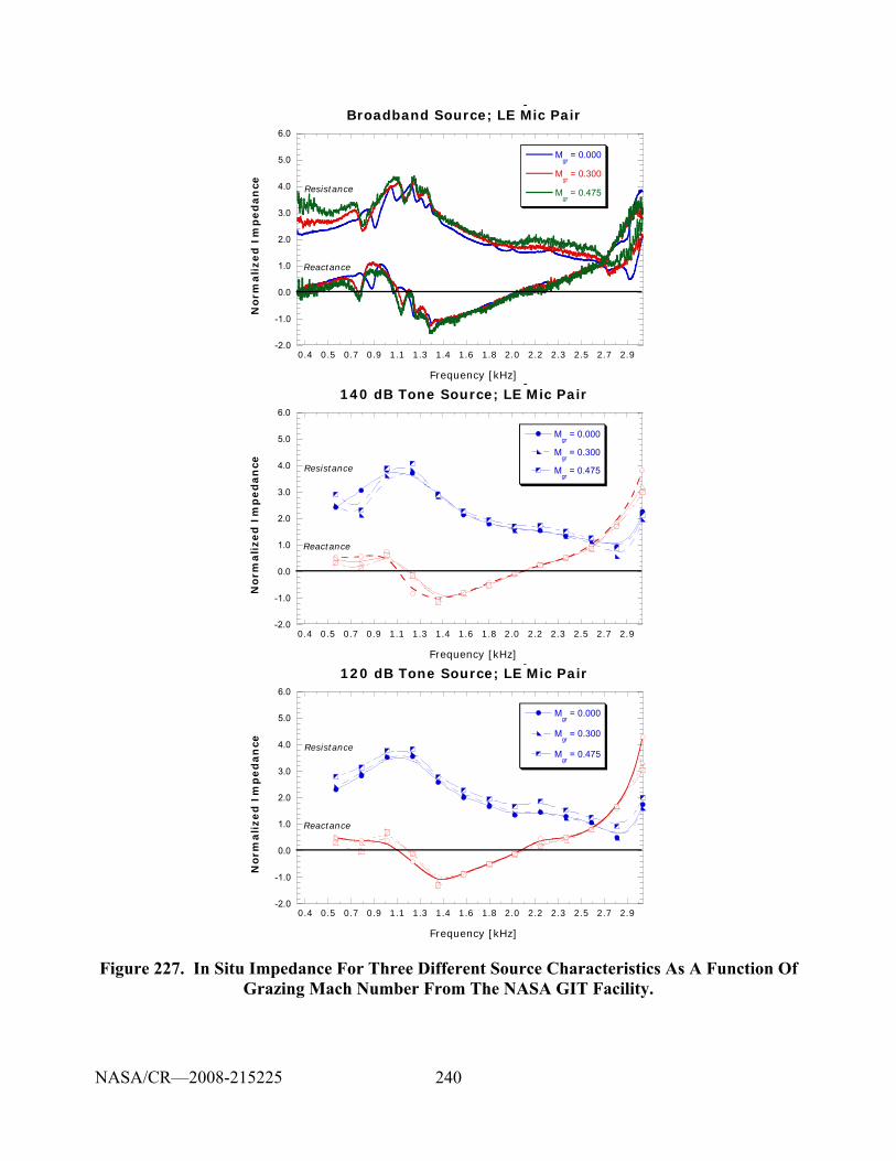
240

0.4 0.5 0.7 0.9 1.1 1.3 1.4 1.6 1.8 2.0 2.2 2.3 2.5 2.7 2.9

yBroadband Source; LE Mic Pair

Mgr

= 0.000

Mgr

= 0.300

Mgr

= 0.475

-2.0

-1.0

0.0

1.0

2.0

3.0

4.0

5.0

6.0

Norm

alized

Im

ped

an

ce

Frequency [kHz]

Resistance

Reactance

0.4 0.5 0.7 0.9 1.1 1.3 1.4 1.6 1.8 2.0 2.2 2.3 2.5 2.7 2.9

y140 dB Tone Source; LE Mic Pair

Mgr

= 0.000

Mgr

= 0.300

Mgr

= 0.475

-2.0

-1.0

0.0

1.0

2.0

3.0

4.0

5.0

6.0

Norm

alize

d I

mp

ed

an

ce

Frequency [kHz]

Resistance

Reactance

0.4 0.5 0.7 0.9 1.1 1.3 1.4 1.6 1.8 2.0 2.2 2.3 2.5 2.7 2.9

y120 dB Tone Source; LE Mic Pair

Mgr

= 0.000

Mgr

= 0.300

Mgr

= 0.475

-2.0

-1.0

0.0

1.0

2.0

3.0

4.0

5.0

6.0

Norm

alized

Im

ped

an

ce

Frequency [kHz]

Resistance

Reactance

Figure 227. In Situ Impedance For Three Different Source Characteristics As A Function Of Grazing Mach Number From The NASA GIT Facility.

NASA/CR—2008-215225

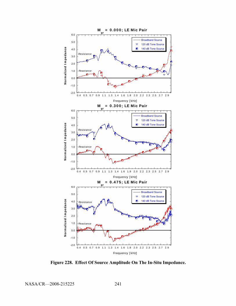
241

0.4 0.5 0.7 0.9 1.1 1.3 1.4 1.6 1.8 2.0 2.2 2.3 2.5 2.7 2.9

Mgr

= 0.000; LE Mic Pair

Broadband Source

120 dB Tone Source

140 dB Tone Source

-2.0

-1.0

0.0

1.0

2.0

3.0

4.0

5.0

6.0

No

rmali

zed

Im

ped

an

ce

Frequency [kHz]

Resistance

Reactance

0.4 0.5 0.7 0.9 1.1 1.3 1.4 1.6 1.8 2.0 2.2 2.3 2.5 2.7 2.9

Mgr


Broadband Source

120 dB Tone Source

140 dB Tone Source

-2.0

-1.0

0.0

1.0

2.0

3.0

4.0

5.0

6.0

No

rmali

zed

Im

ped

an

ce

Frequency [kHz]

Resistance

Reactance

0.4 0.5 0.7 0.9 1.1 1.3 1.4 1.6 1.8 2.0 2.2 2.3 2.5 2.7 2.9

Mgr


Broadband Source

120 dB Tone Source

140 dB Tone Source

-2.0

-1.0

0.0

1.0

2.0

3.0

4.0

5.0

6.0

No

rmali

zed

Im

ped

an

ce

Frequency [kHz]

Resistance

Reactance

Figure 228. Effect Of Source Amplitude On The In-Situ Impedance.

NASA/CR—2008-215225

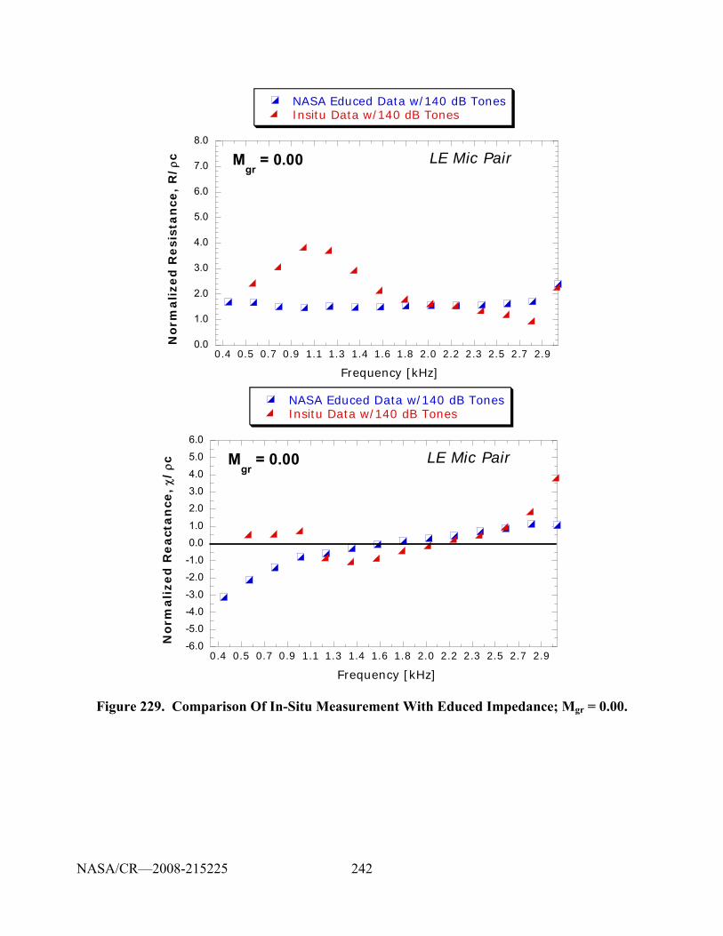
242

0.4 0.5 0.7 0.9 1.1 1.3 1.4 1.6 1.8 2.0 2.2 2.3 2.5 2.7 2.9

NASA Educed Data w/140 dB TonesInsitu Data w/140 dB Tones

0.0

1.0

2.0

3.0

4.0

5.0

6.0

7.0

8.0

Norm

alized

Resi

stan

ce,

R/

ρc

Frequency [kHz]

LE Mic PairMgr

= 0.00

0.4 0.5 0.7 0.9 1.1 1.3 1.4 1.6 1.8 2.0 2.2 2.3 2.5 2.7 2.9


-6.0

-5.0-4.0-3.0

-2.0-1.0

0.01.0

2.03.04.0

5.0

6.0

Norm

ali

zed

React

an

ce,

χ/ρc

Frequency [kHz]

LE Mic PairMgr

= 0.00

Figure 229. Comparison Of In-Situ Measurement With Educed Impedance; Mgr = 0.00.

NASA/CR—2008-215225

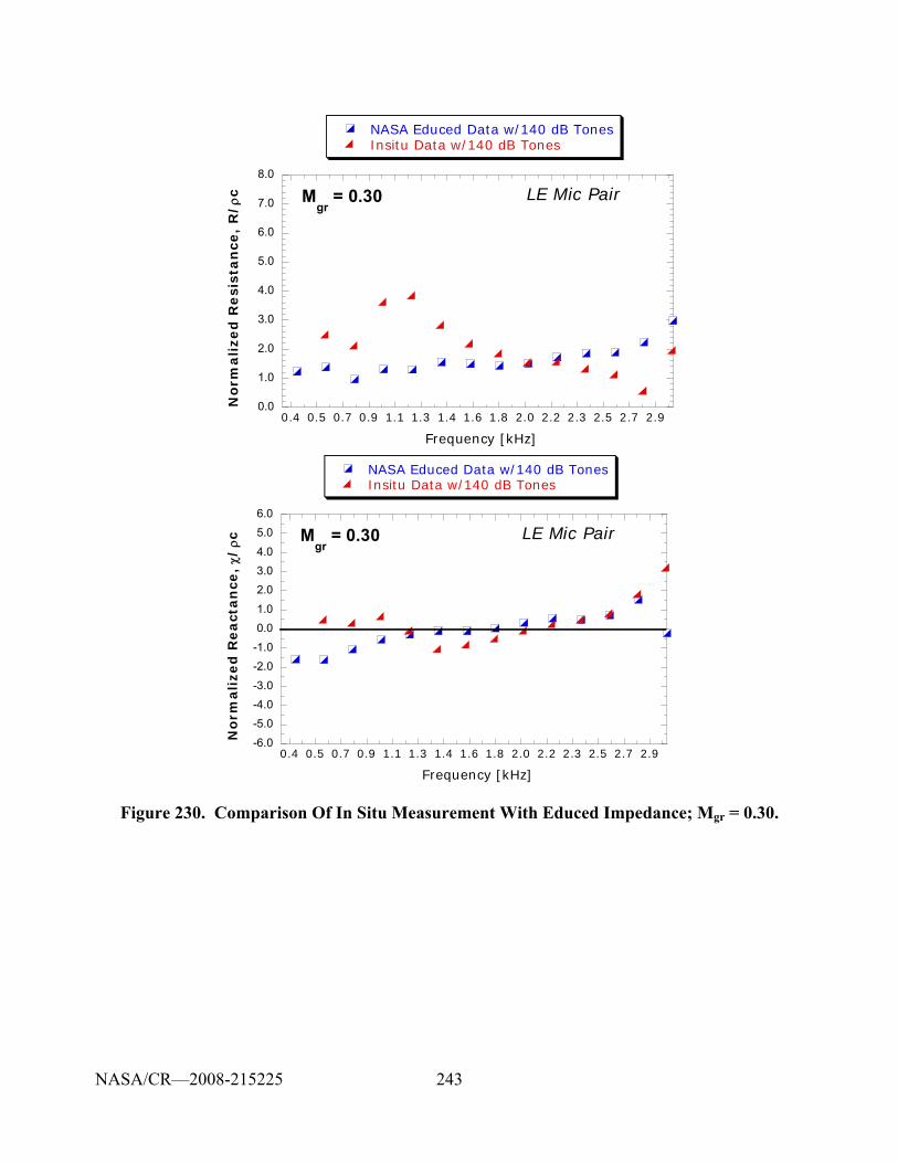
243

0.4 0.5 0.7 0.9 1.1 1.3 1.4 1.6 1.8 2.0 2.2 2.3 2.5 2.7 2.9


0.0

1.0

2.0

3.0

4.0

5.0

6.0

7.0

8.0

Norm

alize

d R

esi

sta

nce

, R

/ρc

Frequency [kHz]

LE Mic PairMgr

= 0.30

0.4 0.5 0.7 0.9 1.1 1.3 1.4 1.6 1.8 2.0 2.2 2.3 2.5 2.7 2.9


-6.0

-5.0-4.0-3.0

-2.0-1.0

0.01.0

2.03.04.0

5.06.0

Norm

ali

zed

React

an

ce,

χ/ρc

Frequency [kHz]

LE Mic PairMgr

= 0.30

Figure 230. Comparison Of In Situ Measurement With Educed Impedance; Mgr = 0.30.

NASA/CR—2008-215225

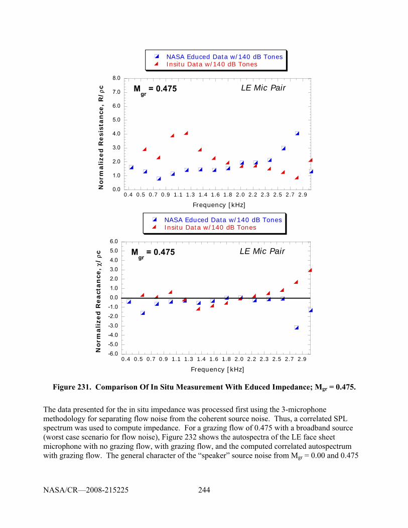
244

0.4 0.5 0.7 0.9 1.1 1.3 1.4 1.6 1.8 2.0 2.2 2.3 2.5 2.7 2.9


0.0

1.0

2.0

3.0

4.0

5.0

6.0

7.0

8.0

Norm

alized

Resis

tan

ce,

R/ρ

c

Frequency [kHz]

LE Mic PairMgr

= 0.475

0.4 0.5 0.7 0.9 1.1 1.3 1.4 1.6 1.8 2.0 2.2 2.3 2.5 2.7 2.9


-6.0

-5.0-4.0-3.0

-2.0-1.0

0.01.0

2.03.04.0

5.06.0

Norm

ali

zed

React

an

ce,

χ/ρc

Frequency [kHz]

LE Mic PairMgr

= 0.475

Figure 231. Comparison Of In Situ Measurement With Educed Impedance; Mgr = 0.475.

The data presented for the in situ impedance was processed first using the 3-microphone methodology for separating flow noise from the coherent source noise. Thus, a correlated SPL spectrum was used to compute impedance. For a grazing flow of 0.475 with a broadband source (worst case scenario for flow noise), Figure 232 shows the autospectra of the LE face sheet microphone with no grazing flow, with grazing flow, and the computed correlated autospectrum with grazing flow. The general character of the “speaker” source noise from Mgr = 0.00 and 0.475

NASA/CR—2008-215225

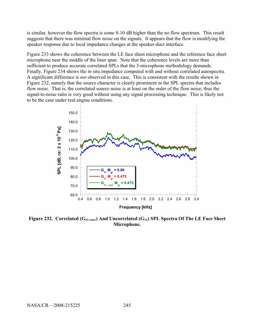
245

is similar, however the flow spectra is some 8-10 dB higher than the no flow spectrum. This result suggests that there was minimal flow noise on the signals. It appears that the flow is modifying the speaker response due to local impedance changes at the speaker-duct interface.

Figure 233 shows the coherence between the LE face sheet microphone and the reference face sheet microphone near the middle of the liner span. Note that the coherence levels are more than sufficient to produce accurate correlated SPLs that the 3-microphone methodology demands. Finally, Figure 234 shows the in situ impedance computed with and without correlated autospectra. A significant difference is not observed in this case. This is consistent with the results shown in Figure 232, namely that the source character is clearly prominent in the SPL spectra that includes flow noise. That is, the correlated source noise is at least on the order of the flow noise, thus the signal-to-noise ratio is very good without using any signal processing technique. This is likely not to be the case under real engine conditions.

60.0

70.0

80.0

90.0

100.0

110.0

120.0

130.0

140.0

150.0

0.4 0.6 0.8 1.0 1.2 1.4 1.6 1.8 2.0 2.2 2.4 2.6 2.8 3.0

G11

Mgr

= 0.00

G11

Mgr

= 0.475

G11 - corr

Mgr

= 0.475

SPL

[dB

; re:

2 x

10-5

Pa]

Frequency [kHz]

Figure 232. Correlated (G11-corr) And Uncorrelated (G11) SPL Spectra Of The LE Face Sheet Microphone.

NASA/CR—2008-215225

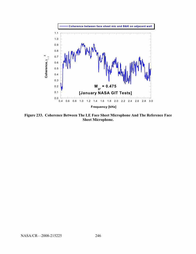
246

0.0

0.1

0.2

0.3

0.4

0.5

0.6

0.7

0.8

0.9

1.0

1.1

0.4 0.6 0.8 1.0 1.2 1.4 1.6 1.8 2.0 2.2 2.4 2.6 2.8 3.0

Coherence between face sheet mic and B&K on adjacent wall

Coh

eren

ce, γ

1−32

Frequency [kHz]

Mgr

= 0.475[January NASA GIT Tests]

Figure 233. Coherence Between The LE Face Sheet Microphone And The Reference Face Sheet Microphone.

NASA/CR—2008-215225

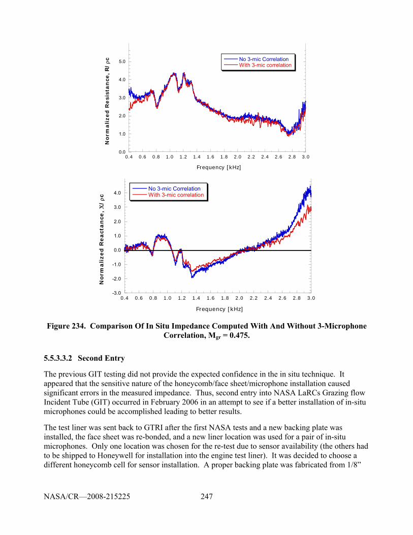
247

0.4 0.6 0.8 1.0 1.2 1.4 1.6 1.8 2.0 2.2 2.4 2.6 2.8 3.0

No 3-mic CorrelationWith 3-mic correlation

0.0

1.0

2.0

3.0

4.0

5.0

Norm

alized

Resis

tan

ce,

R/

ρc

Frequency [kHz]

0.4 0.6 0.8 1.0 1.2 1.4 1.6 1.8 2.0 2.2 2.4 2.6 2.8 3.0


-3.0

-2.0

-1.0

0.0

1.0

2.0

3.0

4.0

Norm

alized

React

an

ce,

Χ/

ρc

Frequency [kHz]

Figure 234. Comparison Of In Situ Impedance Computed With And Without 3-Microphone Correlation, Mgr = 0.475.

5.5.3.3.2 Second Entry

The previous GIT testing did not provide the expected confidence in the in situ technique. It appeared that the sensitive nature of the honeycomb/face sheet/microphone installation caused significant errors in the measured impedance. Thus, second entry into NASA LaRCs Grazing flow Incident Tube (GIT) occurred in February 2006 in an attempt to see if a better installation of in-situ microphones could be accomplished leading to better results.

The test liner was sent back to GTRI after the first NASA tests and a new backing plate was installed, the face sheet was re-bonded, and a new liner location was used for a pair of in-situ microphones. Only one location was chosen for the re-test due to sensor availability (the others had to be shipped to Honeywell for installation into the engine test liner). It was decided to choose a different honeycomb cell for sensor installation. A proper backing plate was fabricated from 1/8”

NASA/CR—2008-215225

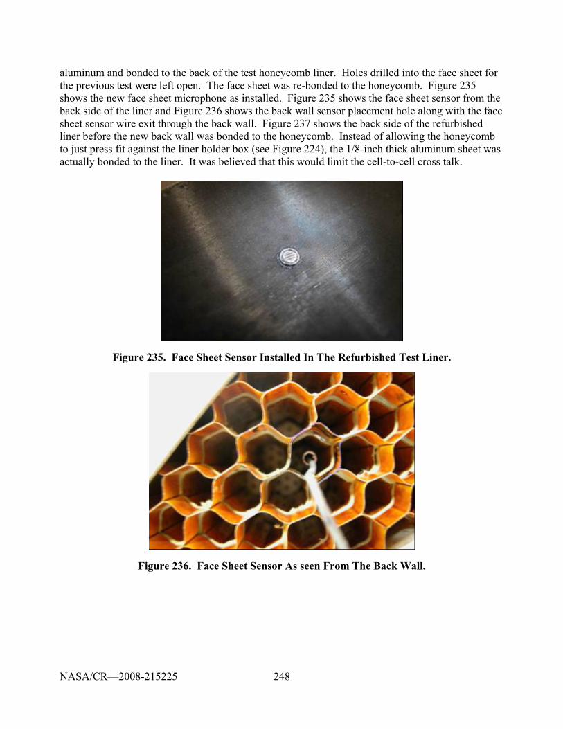
248

aluminum and bonded to the back of the test honeycomb liner. Holes drilled into the face sheet for the previous test were left open. The face sheet was re-bonded to the honeycomb. Figure 235 shows the new face sheet microphone as installed. Figure 235 shows the face sheet sensor from the back side of the liner and Figure 236 shows the back wall sensor placement hole along with the face sheet sensor wire exit through the back wall. Figure 237 shows the back side of the refurbished liner before the new back wall was bonded to the honeycomb. Instead of allowing the honeycomb to just press fit against the liner holder box (see Figure 224), the 1/8-inch thick aluminum sheet was actually bonded to the liner. It was believed that this would limit the cell-to-cell cross talk.

Figure 235. Face Sheet Sensor Installed In The Refurbished Test Liner.

Figure 236. Face Sheet Sensor As seen From The Back Wall.

NASA/CR—2008-215225

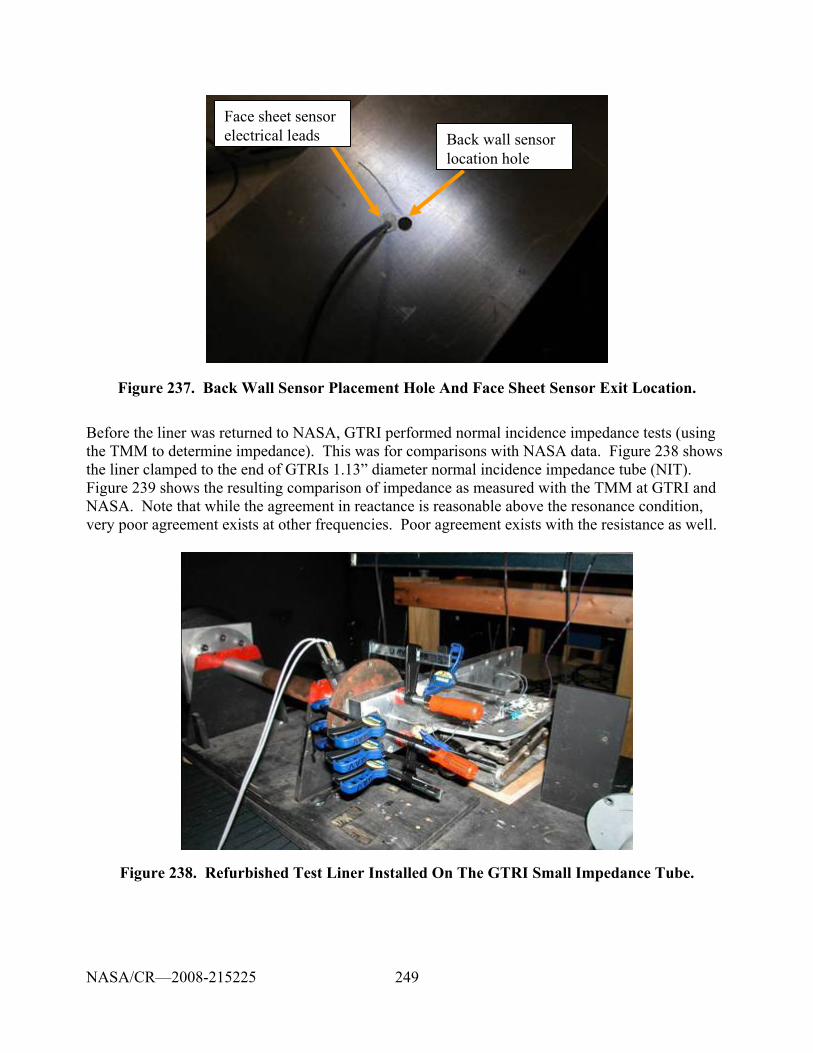
249

Face sheet sensor electrical leads Back wall sensor

location hole

Face sheet sensor electrical leads Back wall sensor

location hole

Figure 237. Back Wall Sensor Placement Hole And Face Sheet Sensor Exit Location.

Before the liner was returned to NASA, GTRI performed normal incidence impedance tests (using the TMM to determine impedance). This was for comparisons with NASA data. Figure 238 shows the liner clamped to the end of GTRIs 1.13” diameter normal incidence impedance tube (NIT). Figure 239 shows the resulting comparison of impedance as measured with the TMM at GTRI and NASA. Note that while the agreement in reactance is reasonable above the resonance condition, very poor agreement exists at other frequencies. Poor agreement exists with the resistance as well.

Figure 238. Refurbished Test Liner Installed On The GTRI Small Impedance Tube.

NASA/CR—2008-215225

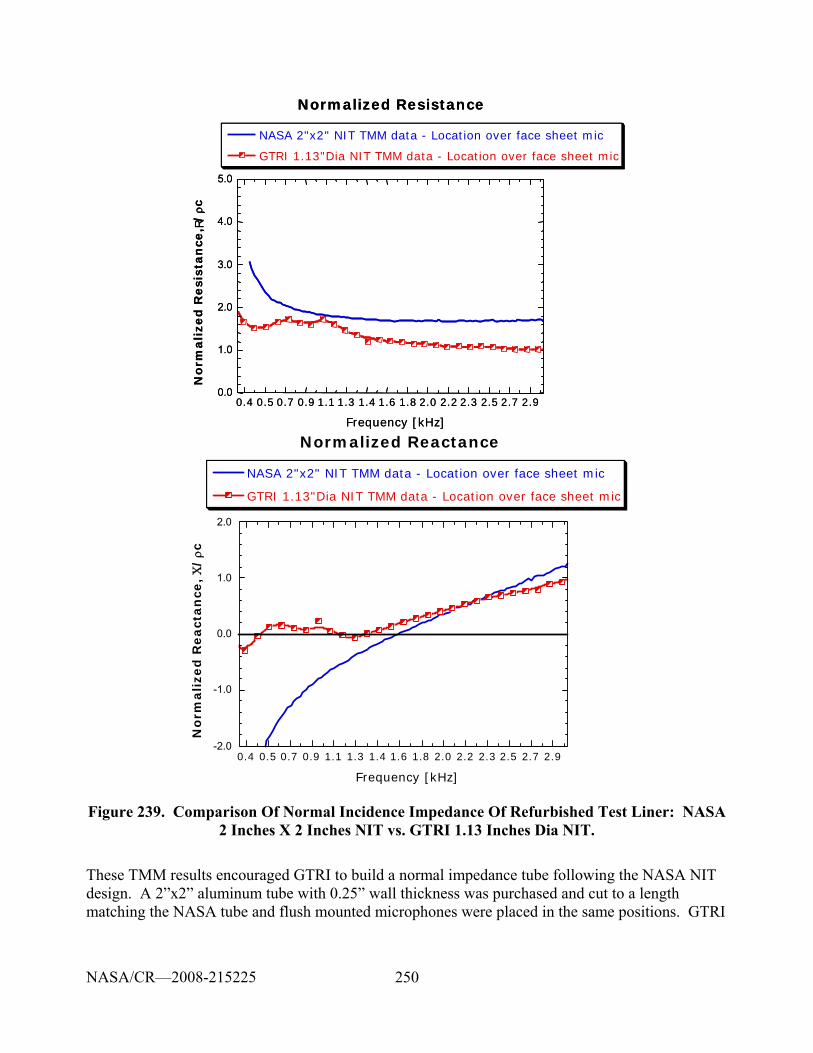
250

0.4 0.5 0.7 0.9 1.1 1.3 1.4 1.6 1.8 2.0 2.2 2.3 2.5 2.7 2.9

Normalized Resistance

NASA 2"x2" NIT TMM data - Location over face sheet mic

GTRI 1.13"Dia NIT TMM data - Location over face sheet mic

0.0

1.0

2.0

3.0

4.0

5.0

Norm

ali

zed

Resi

stan

ce, R

/ρc

Frequency [kHz]

0.4 0.5 0.7 0.9 1.1 1.3 1.4 1.6 1.8 2.0 2.2 2.3 2.5 2.7 2.9




0.0

1.0

2.0

3.0

4.0

5.0

Norm

ali

zed

Resi

stan

ce, R

/ρc

Frequency [kHz]

0.4 0.5 0.7 0.9 1.1 1.3 1.4 1.6 1.8 2.0 2.2 2.3 2.5 2.7 2.9

Normalized Reactance



-2.0

-1.0

0.0

1.0

2.0

No

rmalize

d R

eact

an

ce,

Χ/

ρc

Frequency [kHz]

Figure 239. Comparison Of Normal Incidence Impedance Of Refurbished Test Liner: NASA 2 Inches X 2 Inches NIT vs. GTRI 1.13 Inches Dia NIT.

These TMM results encouraged GTRI to build a normal impedance tube following the NASA NIT design. A 2”x2” aluminum tube with 0.25” wall thickness was purchased and cut to a length matching the NASA tube and flush mounted microphones were placed in the same positions. GTRI

NASA/CR—2008-215225

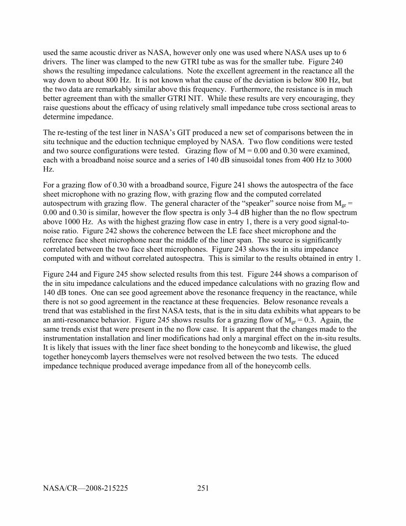
251

used the same acoustic driver as NASA, however only one was used where NASA uses up to 6 drivers. The liner was clamped to the new GTRI tube as was for the smaller tube. Figure 240 shows the resulting impedance calculations. Note the excellent agreement in the reactance all the way down to about 800 Hz. It is not known what the cause of the deviation is below 800 Hz, but the two data are remarkably similar above this frequency. Furthermore, the resistance is in much better agreement than with the smaller GTRI NIT. While these results are very encouraging, they raise questions about the efficacy of using relatively small impedance tube cross sectional areas to determine impedance.

The re-testing of the test liner in NASA’s GIT produced a new set of comparisons between the in situ technique and the eduction technique employed by NASA. Two flow conditions were tested and two source configurations were tested. Grazing flow of M = 0.00 and 0.30 were examined, each with a broadband noise source and a series of 140 dB sinusoidal tones from 400 Hz to 3000 Hz.

For a grazing flow of 0.30 with a broadband source, Figure 241 shows the autospectra of the face sheet microphone with no grazing flow, with grazing flow and the computed correlated autospectrum with grazing flow. The general character of the “speaker” source noise from Mgr = 0.00 and 0.30 is similar, however the flow spectra is only 3-4 dB higher than the no flow spectrum above 1000 Hz. As with the highest grazing flow case in entry 1, there is a very good signal-to-noise ratio. Figure 242 shows the coherence between the LE face sheet microphone and the reference face sheet microphone near the middle of the liner span. The source is significantly correlated between the two face sheet microphones. Figure 243 shows the in situ impedance computed with and without correlated autospectra. This is similar to the results obtained in entry 1.

Figure 244 and Figure 245 show selected results from this test. Figure 244 shows a comparison of the in situ impedance calculations and the educed impedance calculations with no grazing flow and 140 dB tones. One can see good agreement above the resonance frequency in the reactance, while there is not so good agreement in the reactance at these frequencies. Below resonance reveals a trend that was established in the first NASA tests, that is the in situ data exhibits what appears to be an anti-resonance behavior. Figure 245 shows results for a grazing flow of Mgr = 0.3. Again, the same trends exist that were present in the no flow case. It is apparent that the changes made to the instrumentation installation and liner modifications had only a marginal effect on the in-situ results. It is likely that issues with the liner face sheet bonding to the honeycomb and likewise, the glued together honeycomb layers themselves were not resolved between the two tests. The educed impedance technique produced average impedance from all of the honeycomb cells.

NASA/CR—2008-215225

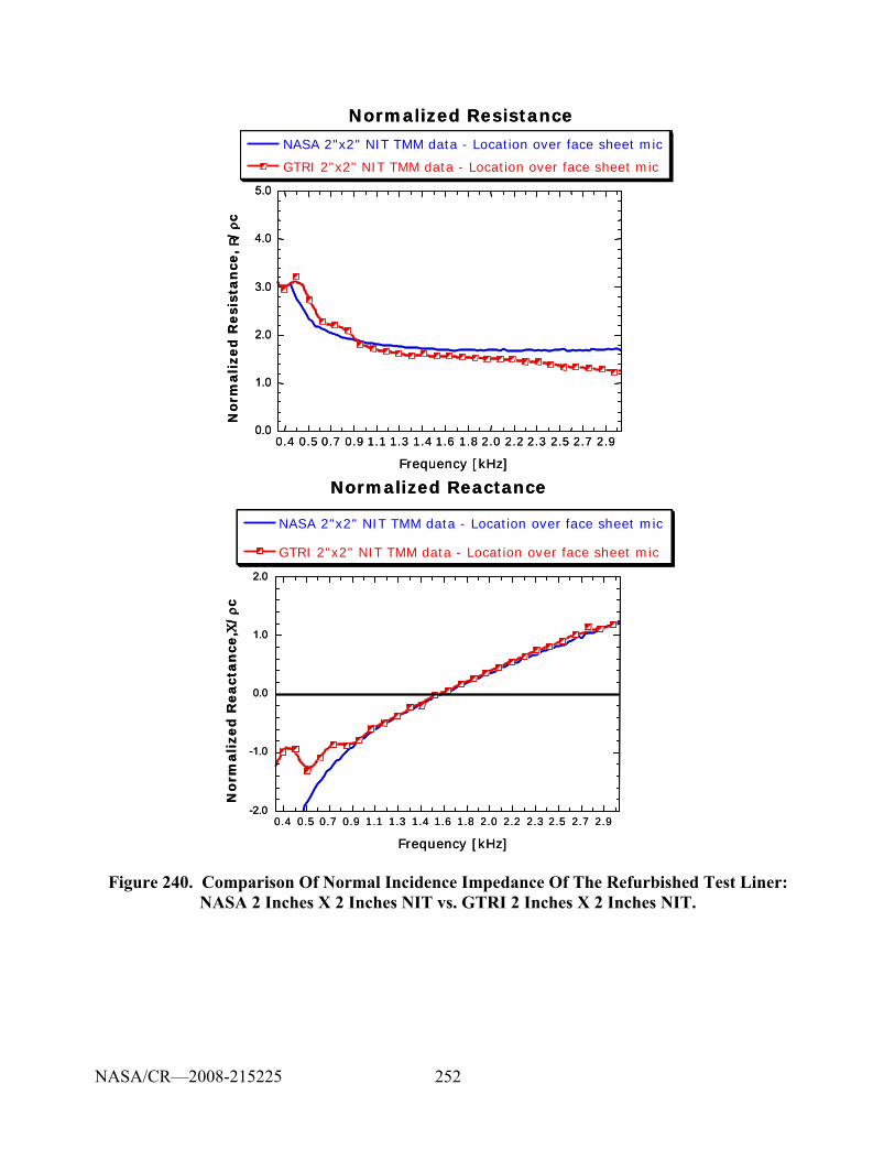
252

0.4 0.5 0.7 0.9 1.1 1.3 1.4 1.6 1.8 2.0 2.2 2.3 2.5 2.7 2.9



GTRI 2"x2" NIT TMM data - Location over face sheet mic

0.0

1.0

2.0

3.0

4.0

5.0

Norm

ali

zed

Resi

stan

ce,

R/ρ c

Frequency [kHz]

0.4 0.5 0.7 0.9 1.1 1.3 1.4 1.6 1.8 2.0 2.2 2.3 2.5 2.7 2.9




0.0

1.0

2.0

3.0

4.0

5.0

Norm

ali

zed

Resi

stan

ce,

R/ρ c

Frequency [kHz]

0.4 0.5 0.7 0.9 1.1 1.3 1.4 1.6 1.8 2.0 2.2 2.3 2.5 2.7 2.9




-2.0

-1.0

0.0

1.0

2.0

No

rmalized

React

an

ce, Χ

/ρ c

Frequency [kHz]

0.4 0.5 0.7 0.9 1.1 1.3 1.4 1.6 1.8 2.0 2.2 2.3 2.5 2.7 2.9




-2.0

-1.0

0.0

1.0

2.0

No

rmalized

React

an

ce, Χ

/ρ c

Frequency [kHz]

Figure 240. Comparison Of Normal Incidence Impedance Of The Refurbished Test Liner: NASA 2 Inches X 2 Inches NIT vs. GTRI 2 Inches X 2 Inches NIT.

NASA/CR—2008-215225

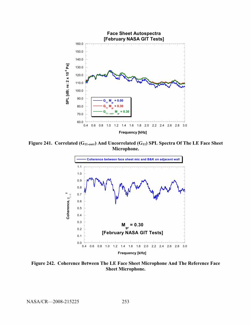
253

60.0

70.0

80.0

90.0

100.0

110.0

120.0

130.0

140.0

150.0

160.0

0.4 0.6 0.8 1.0 1.2 1.4 1.6 1.8 2.0 2.2 2.4 2.6 2.8 3.0

Face Sheet Autospectra[February NASA GIT Tests]

G11

Mgr

= 0.00

G11

Mgr

= 0.30

G11 - corr

Mgr

= 0.30

SPL

[dB

; re:

2 x

10-5

Pa]

Frequency [kHz]

Figure 241. Correlated (G11-corr) And Uncorrelated (G11) SPL Spectra Of The LE Face Sheet Microphone.

0.0

0.1

0.2

0.3

0.4

0.5

0.6

0.7

0.8

0.9

1.0

1.1

0.4 0.6 0.8 1.0 1.2 1.4 1.6 1.8 2.0 2.2 2.4 2.6 2.8 3.0

Coherence between face sheet mic and B&K on adjacent wall

Coh

eren

ce, γ

1−32

Frequency [kHz]

Mgr

= 0.30[February NASA GIT Tests]

Figure 242. Coherence Between The LE Face Sheet Microphone And The Reference Face Sheet Microphone.

NASA/CR—2008-215225

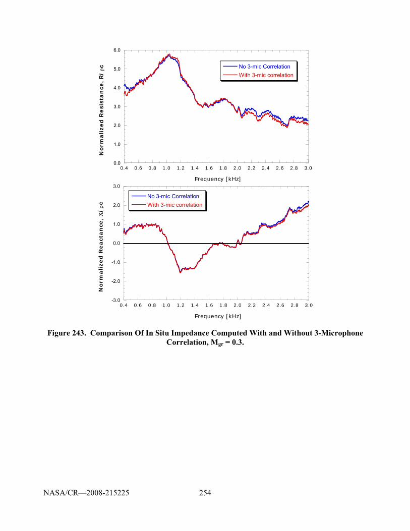
254

0.4 0.6 0.8 1.0 1.2 1.4 1.6 1.8 2.0 2.2 2.4 2.6 2.8 3.0


0.0

1.0

2.0

3.0

4.0

5.0

6.0

Norm

alized

Resis

tan

ce,

R/

ρc

Frequency [kHz]

0.4 0.6 0.8 1.0 1.2 1.4 1.6 1.8 2.0 2.2 2.4 2.6 2.8 3.0


-3.0

-2.0

-1.0

0.0

1.0

2.0

3.0

Norm

alized

React

an

ce,

Χ/

ρc

Frequency [kHz]

Figure 243. Comparison Of In Situ Impedance Computed With and Without 3-Microphone Correlation, Mgr = 0.3.

NASA/CR—2008-215225

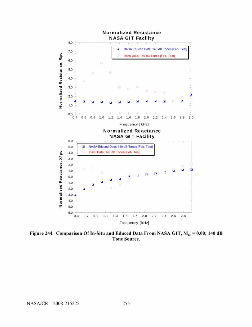
255

0.4 0.6 0.8 1.0 1.2 1.4 1.6 1.8 2.0 2.2 2.4 2.6 2.8 3.0

Normalized ResistanceNASA GIT Facility

NASA Educed Data; 140 dB Tones [Feb. Test]

Insitu Data; 140 dB Tones [Feb. Test]

0.0

1.0

2.0

3.0

4.0

5.0

6.0

7.0

8.0

No

rmali

zed

Resi

stan

ce,

R/ρ

c

Frequency [kHz]

0.4 0.7 0.9 1.1 1.3 1.5 1.7 2.0 2.2 2.4 2.6 2.8




-6.0

-5.0

-4.0

-3.0

-2.0

-1.0

0.0

1.0

2.0

3.0

4.0

5.0

6.0

Norm

ali

zed

React

an

ce,

Χ/

ρc

Frequency [kHz]

Figure 244. Comparison Of In-Situ and Educed Data From NASA GIT, Mgr = 0.00; 140 dB Tone Source.

NASA/CR—2008-215225

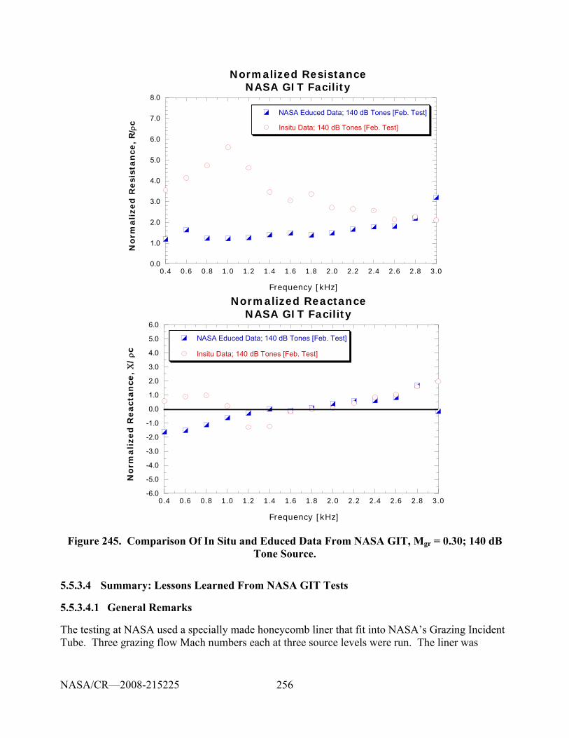
256

0.4 0.6 0.8 1.0 1.2 1.4 1.6 1.8 2.0 2.2 2.4 2.6 2.8 3.0

Normalized ResistanceNASA GIT Facility



0.0

1.0

2.0

3.0

4.0

5.0

6.0

7.0

8.0

Norm

ali

zed

Resi

stan

ce,

R/ρ

c

Frequency [kHz]

0.4 0.6 0.8 1.0 1.2 1.4 1.6 1.8 2.0 2.2 2.4 2.6 2.8 3.0




-6.0

-5.0

-4.0

-3.0

-2.0

-1.0

0.0

1.0

2.0

3.0

4.0

5.0

6.0

Norm

ali

zed

React

an

ce,

Χ/

ρc

Frequency [kHz]

Figure 245. Comparison Of In Situ and Educed Data From NASA GIT, Mgr = 0.30; 140 dB Tone Source.

5.5.3.4 Summary: Lessons Learned From NASA GIT Tests

5.5.3.4.1 General Remarks

The testing at NASA used a specially made honeycomb liner that fit into NASA’s Grazing Incident Tube. Three grazing flow Mach numbers each at three source levels were run. The liner was

NASA/CR—2008-215225

257

instrumented with 5 sensors. At a leading edge liner location, at a given honeycomb cell, one sensor was fixed flush within a hole at the face sheet while another was flush to the back wall of the cell. This was repeated at a trailing edge location. A fifth sensor was fixed flush at the face sheet at a midway point along the length of the liner. Simultaneously, NASA used their multi-microphone technique for educing the wall impedance from the duct for comparison of impedance measurements. The following “lessons” were learned from these series of risk mitigation tests:

1. It is imperative that the best possible bonding is achieved between face sheet and the honeycomb and the backing plate and the honeycomb. This bonding preserves the locally reacting assumption necessary for the in-situ technique.

The bonding of test liner provided by Honeywell had to be compromised due to complications arising from inadequate dimensions for the GIT facility. Two problems existed: a) The liner was too large in width and length by some 0.050 inches and b) the GIT retaining block doubled as the backing wall for the liner. The latter issue arose from miscommunication between all parties involved. The net effect was that the retaining block had to be milled (with sensors installed) about 2 inches in depth to allow sufficient depth of the liner to be exposed. Furthermore, the outside of the liner had to be milled (with sensors installed) to make it fit in the GIT. The result was that the face sheet became debonded from the honeycomb along a good portion of the liner. NASA was able to bond the perimeter of the face sheet, but there were no guarantees that the center honeycomb cells were bonded to the face sheet completely.

2. The sensors are differential and require proper equilibration to behave as expected. Face sheet sensor vent tube should remain in honeycomb cell. Back wall sensor vent tube should be connected to the pressure imposed on the face sheet sensor.

During the NASA testing, the static pressure in the inside of the grazing flow duct was kept constant with the outside ambient pressure. This check was made with at pressure port downstream of the liner, thus the static pressure ahead of this point (and in the location of the liner sensors) would be higher than ambient. Back wall sensor irregularities became apparent at the highest grazing flow Mach number. It was speculated and later shown that the static pressure at these conditions was more than 0.3 psig. This was enough to put the sensor out of its dynamic range. Subsequently, the internal static pressure was adjusted such that the pressure at the leading edge location sensor was balanced with the outside ambient. Recall that the back wall sensor vent tube is located outside the grazing flow duct. Once this was done, results were obtained that were similar to those acquired with no flow in the duct.

3. Extreme care must be taken in assuring face sheet sensor is flush and sealed to the face sheet and the back wall sensor is flush and midway between the center of the cell and the wall.

A critical assumption in the in situ impedance method is that the face sheet microphone measures the average acoustic pressure of the face sheet. Any leakage around the sensor periphery alters the impedance which is sought to be measured.

NASA/CR—2008-215225

258

5.5.3.4.2 Procedures For Preparing, Installing and Signal Conditioning Sensor Output

Liner Face Sheet Sensor

1. The length of the tube that equalizes pressure on both sides of sensor diaphragm (installed by manufacturer), must be sized so that it terminates within the honeycomb cell of the liner. Use a very fine cutoff wheel as the tube is very soft and small diameter.

2. A soft aluminum tube with outer diameter of 0.125 inches and wall thickness of 0.033 inches should be cut to 0.5 inches in length. Under magnification, slide the sensor into the tube (end first). When sensor head is flush, use a single horsehair applicator and apply a small amount of CyanoAcrylate (CA) super thin-type, to the perimeter of the sensor, making sure not to have the CA wick into the sensor diaphragm. Alternate methods may be used, but glue must not be allowed to wick onto sensor.

3. It is suggested that the bundled wires about 5 inches from the sensor tip be cut. On one side, male pins should be soldered and female pins should be soldered on the other side.

4. The 5 wires that make up the bundle should be separated at the end and fork terminals should be installed on each wire.

Installation of Sensors into Liner

1. At each “In situ measurement” location there is a face sheet sensor and a corresponding back wall sensor. Assuming the liner is installed in the engine nacelle, a drill should locate a perforate hole nearest to the center of the cell and enlarge the hole. Before using a drill bit, use an abrasive cone-shaped Dremel tool (tungsten).

2. The drill should pass through the honeycomb cell and through the back wall plate of the liner. It is assumed that the back of the liner can be accessed.

3. The back wall sensor is located midway between the face sheet hole and the cell wall.

4. The face sheet sensor is inserted and put in place with a very small amount of CA. The bundled wires pass through the hole in the back plate and they are sealed with epoxy.

5. The back wall sensor is then inserted and put in place with a small amount of CA.

6. The back wall sensor vent tube should be connected to the pressure imposed on the face sheet sensor.

NASA/CR—2008-215225

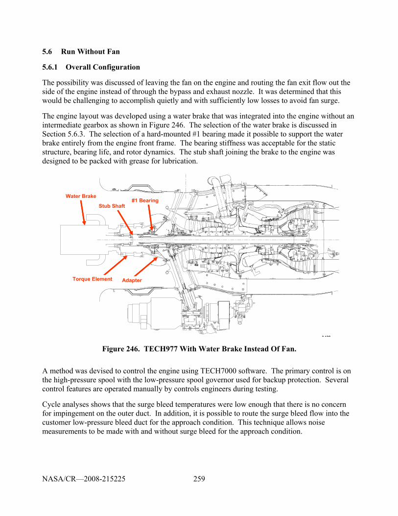
259

5.6 Run Without Fan

5.6.1 Overall Configuration

The possibility was discussed of leaving the fan on the engine and routing the fan exit flow out the side of the engine instead of through the bypass and exhaust nozzle. It was determined that this would be challenging to accomplish quietly and with sufficiently low losses to avoid fan surge.

The engine layout was developed using a water brake that was integrated into the engine without an intermediate gearbox as shown in Figure 246. The selection of the water brake is discussed in Section 5.6.3. The selection of a hard-mounted #1 bearing made it possible to support the water brake entirely from the engine front frame. The bearing stiffness was acceptable for the static structure, bearing life, and rotor dynamics. The stub shaft joining the brake to the engine was designed to be packed with grease for lubrication.

Water Brake

Torque Element

Stub Shaft

Adapter

#1 BearingWater Brake

Torque Element

Stub Shaft

Adapter

#1 Bearing

Figure 246. TECH977 With Water Brake Instead Of Fan.

A method was devised to control the engine using TECH7000 software. The primary control is on the high-pressure spool with the low-pressure spool governor used for backup protection. Several control features are operated manually by controls engineers during testing.

Cycle analyses shows that the surge bleed temperatures were low enough that there is no concern for impingement on the outer duct. In addition, it is possible to route the surge bleed flow into the customer low-pressure bleed duct for the approach condition. This technique allows noise measurements to be made with and without surge bleed for the approach condition.

NASA/CR—2008-215225

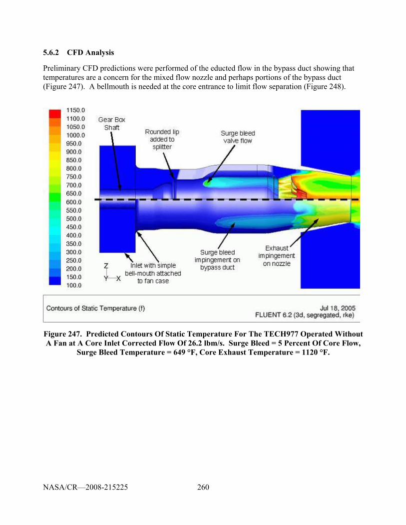
260

5.6.2 CFD Analysis

Preliminary CFD predictions were performed of the educted flow in the bypass duct showing that temperatures are a concern for the mixed flow nozzle and perhaps portions of the bypass duct (Figure 247). A bellmouth is needed at the core entrance to limit flow separation (Figure 248).

Figure 247. Predicted Contours Of Static Temperature For The TECH977 Operated Without A Fan at A Core Inlet Corrected Flow Of 26.2 lbm/s. Surge Bleed = 5 Percent Of Core Flow,

Surge Bleed Temperature = 649 °F, Core Exhaust Temperature = 1120 °F.

NASA/CR—2008-215225

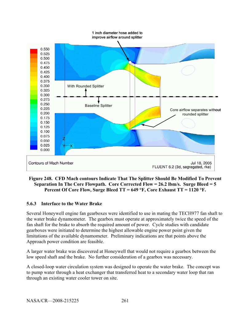
261

1 inch diameter hose added to improve airflow around splitter

Core airflow separates without rounded splitter

With Rounded Splitter

Baseline Splitter

1 inch diameter hose added to improve airflow around splitter

Core airflow separates without rounded splitter

With Rounded Splitter

Baseline Splitter

Figure 248. CFD Mach contours Indicate That The Splitter Should Be Modified To Prevent Separation In The Core Flowpath. Core Corrected Flow = 26.2 lbm/s. Surge Bleed = 5

Percent Of Core Flow, Surge Bleed TT = 649 °F, Core Exhaust TT = 1120 °F.

5.6.3 Interface to the Water Brake

Several Honeywell engine fan gearboxes were identified to use in mating the TECH977 fan shaft to the water brake dynamometer. The gearbox must operate at approximately twice the speed of the fan shaft for the brake to absorb the required amount of power. Cycle studies with candidate gearboxes were initiated to determine the highest allowable engine power point given the limitations of the available dynamometer. Preliminary indications are that points above the Approach power condition are feasible.

A larger water brake was discovered at Honeywell that would not require a gearbox between the low speed shaft and the brake. No further consideration of a gearbox was necessary.

A closed-loop water circulation system was designed to operate the water brake. The concept was to pump water through a heat exchanger that transferred heat to a secondary water loop that ran through an existing water cooler tower on site.

NASA/CR—2008-215225

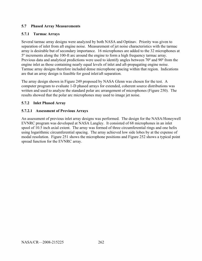
262

5.7 Phased Array Measurements

5.7.1 Tarmac Arrays

Several tarmac array designs were analyzed by both NASA and Optinav. Priority was given to separation of inlet from aft engine noise. Measurement of jet noise characteristics with the tarmac array is desirable but of secondary importance. 16 microphones are added to the 32 microphones at 5º increments along the 100-ft arc around the engine to form a high frequency tarmac array. Previous data and analytical predictions were used to identify angles between 70º and 90º from the engine inlet as those containing nearly equal levels of inlet and aft-propagating engine noise. Tarmac array designs therefore included dense microphone spacing within that region. Indications are that an array design is feasible for good inlet/aft separation.

The array design shown in Figure 249 proposed by NASA Glenn was chosen for the test. A computer program to evaluate 1-D phased arrays for extended, coherent source distributions was written and used to analyze the standard polar arc arrangement of microphones (Figure 250). The results showed that the polar arc microphones may used to image jet noise.

5.7.2 Inlet Phased Array

5.7.2.1 Assessment of Previous Arrays

An assessment of previous inlet array designs was performed. The design for the NASA/Honeywell EVNRC program was developed at NASA Langley. It consisted of 68 microphones in an inlet spool of 10.5 inch axial extent. The array was formed of three circumferential rings and one helix using logarithmic circumferential spacing. The array achieved low side lobes by at the expense of modal resolution. Figure 251 shows the microphone positions and Figure 252 shows a typical point spread function for the EVNRC array.

NASA/CR—2008-215225

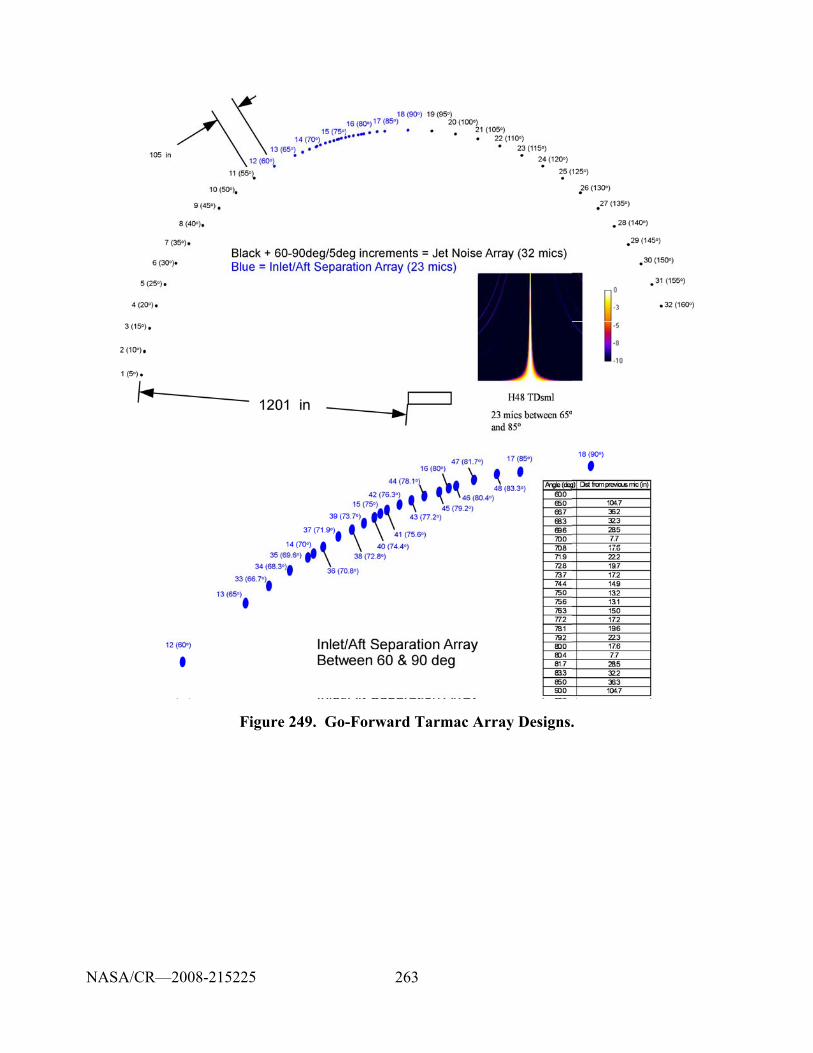
263

Figure 249. Go-Forward Tarmac Array Designs.

NASA/CR—2008-215225

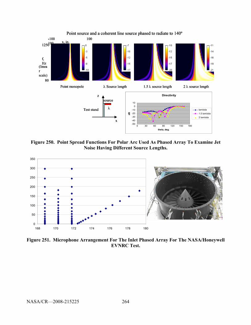
264

λ Source lengthPoint monopole 1.5 λ source length 2 λ source length

-100 100x, in.

-100

f, Hz

80

1250

(linearscale)

Point source and a coherent line source phased to radiate to 140º

Directivity

-50-40-30-20-10

010

0 30 60 90 120 150 180theta, deg.

dB

lambda

1.5 lambda

2 lambdax

Test stand

source

λ

z

λ Source lengthPoint monopole 1.5 λ source length 2 λ source length

-100 100x, in.

-100

f, Hz

80

1250

(linearscale)

Point source and a coherent line source phased to radiate to 140º

Directivity

-50-40-30-20-10

010

0 30 60 90 120 150 180theta, deg.

dB

lambda

1.5 lambda

2 lambdax

Test stand

source

λ

z

Figure 250. Point Spread Functions For Polar Arc Used As Phased Array To Examine Jet Noise Having Different Source Lengths.

0

50

100

150

200

250

300

350

168 170 172 174 176 178 180

Figure 251. Microphone Arrangement For The Inlet Phased Array For The NASA/Honeywell EVNRC Test.

NASA/CR—2008-215225

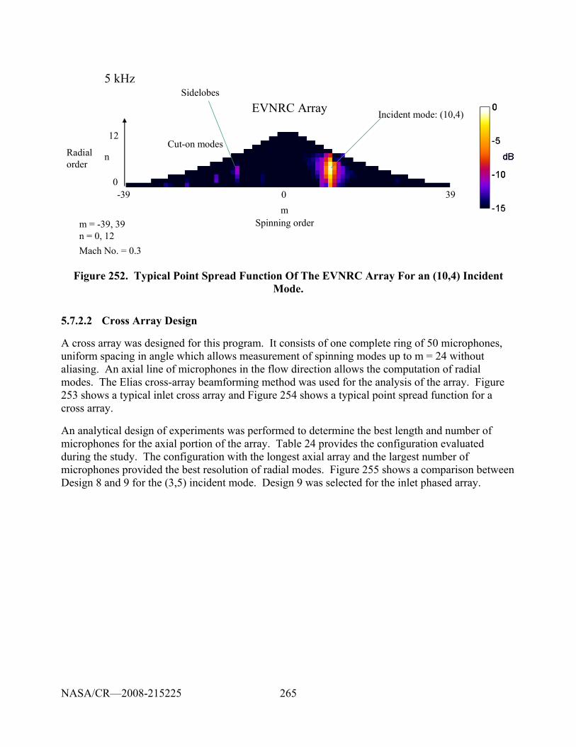
265

5 kHz

EVNRC Array Incident mode: (10,4)

-390

39

12

n

m0

Spinning order

Radialorder

Sidelobes

m = -39, 39n = 0, 12

Cut-on modes

Mach No. = 0.3

Figure 252. Typical Point Spread Function Of The EVNRC Array For an (10,4) Incident Mode.

5.7.2.2 Cross Array Design

A cross array was designed for this program. It consists of one complete ring of 50 microphones, uniform spacing in angle which allows measurement of spinning modes up to m = 24 without aliasing. An axial line of microphones in the flow direction allows the computation of radial modes. The Elias cross-array beamforming method was used for the analysis of the array. Figure 253 shows a typical inlet cross array and Figure 254 shows a typical point spread function for a cross array.

An analytical design of experiments was performed to determine the best length and number of microphones for the axial portion of the array. Table 24 provides the configuration evaluated during the study. The configuration with the longest axial array and the largest number of microphones provided the best resolution of radial modes. Figure 255 shows a comparison between Design 8 and 9 for the (3,5) incident mode. Design 9 was selected for the inlet phased array.

NASA/CR—2008-215225

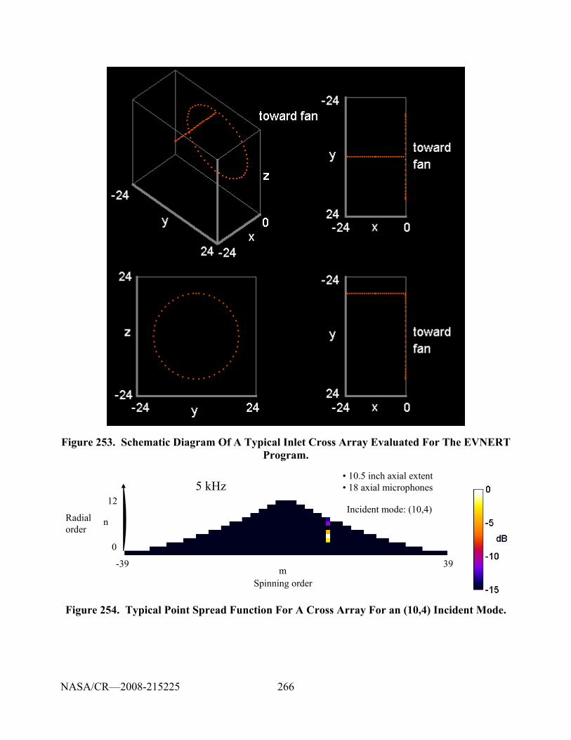
266

Figure 253. Schematic Diagram Of A Typical Inlet Cross Array Evaluated For The EVNERT Program.

5 kHz

Incident mode: (10,4)

• 10.5 inch axial extent• 18 axial microphones

0

12

nRadialorder

-39 39m

Spinning order

Figure 254. Typical Point Spread Function For A Cross Array For an (10,4) Incident Mode.

NASA/CR—2008-215225

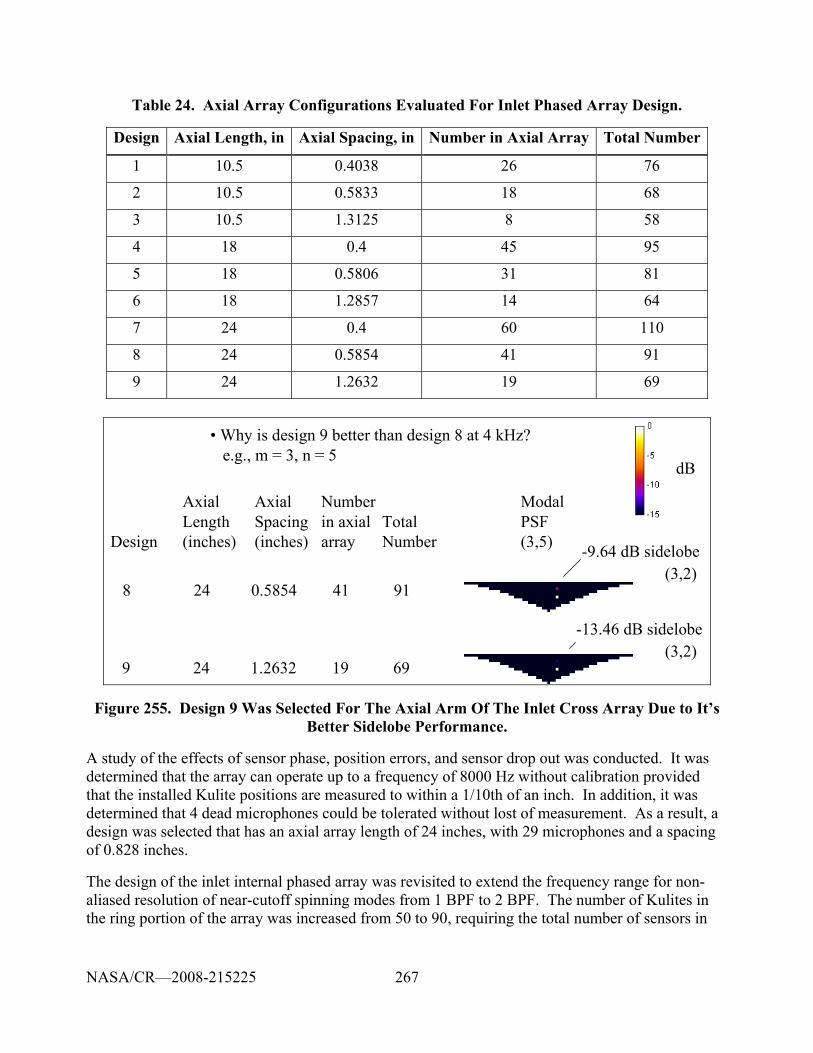
267

Table 24. Axial Array Configurations Evaluated For Inlet Phased Array Design.

Design Axial Length, in Axial Spacing, in Number in Axial Array Total Number

1 10.5 0.4038 26 76

2 10.5 0.5833 18 68

3 10.5 1.3125 8 58

4 18 0.4 45 95

5 18 0.5806 31 81

6 18 1.2857 14 64

7 24 0.4 60 110

8 24 0.5854 41 91

9 24 1.2632 19 69

• Why is design 9 better than design 8 at 4 kHz?e.g., m = 3, n = 5

Design

8

9

AxialLength(inches)

AxialSpacing(inches)

Numberin axialarray

TotalNumber

24

24

0.5854

1.2632

41

19

91

69

ModalPSF(3,5)

dB

-9.64 dB sidelobe

-13.46 dB sidelobe

(3,2)

(3,2)

Figure 255. Design 9 Was Selected For The Axial Arm Of The Inlet Cross Array Due to It’s Better Sidelobe Performance.

A study of the effects of sensor phase, position errors, and sensor drop out was conducted. It was determined that the array can operate up to a frequency of 8000 Hz without calibration provided that the installed Kulite positions are measured to within a 1/10th of an inch. In addition, it was determined that 4 dead microphones could be tolerated without lost of measurement. As a result, a design was selected that has an axial array length of 24 inches, with 29 microphones and a spacing of 0.828 inches.

The design of the inlet internal phased array was revisited to extend the frequency range for non-aliased resolution of near-cutoff spinning modes from 1 BPF to 2 BPF. The number of Kulites in the ring portion of the array was increased from 50 to 90, requiring the total number of sensors in

NASA/CR—2008-215225

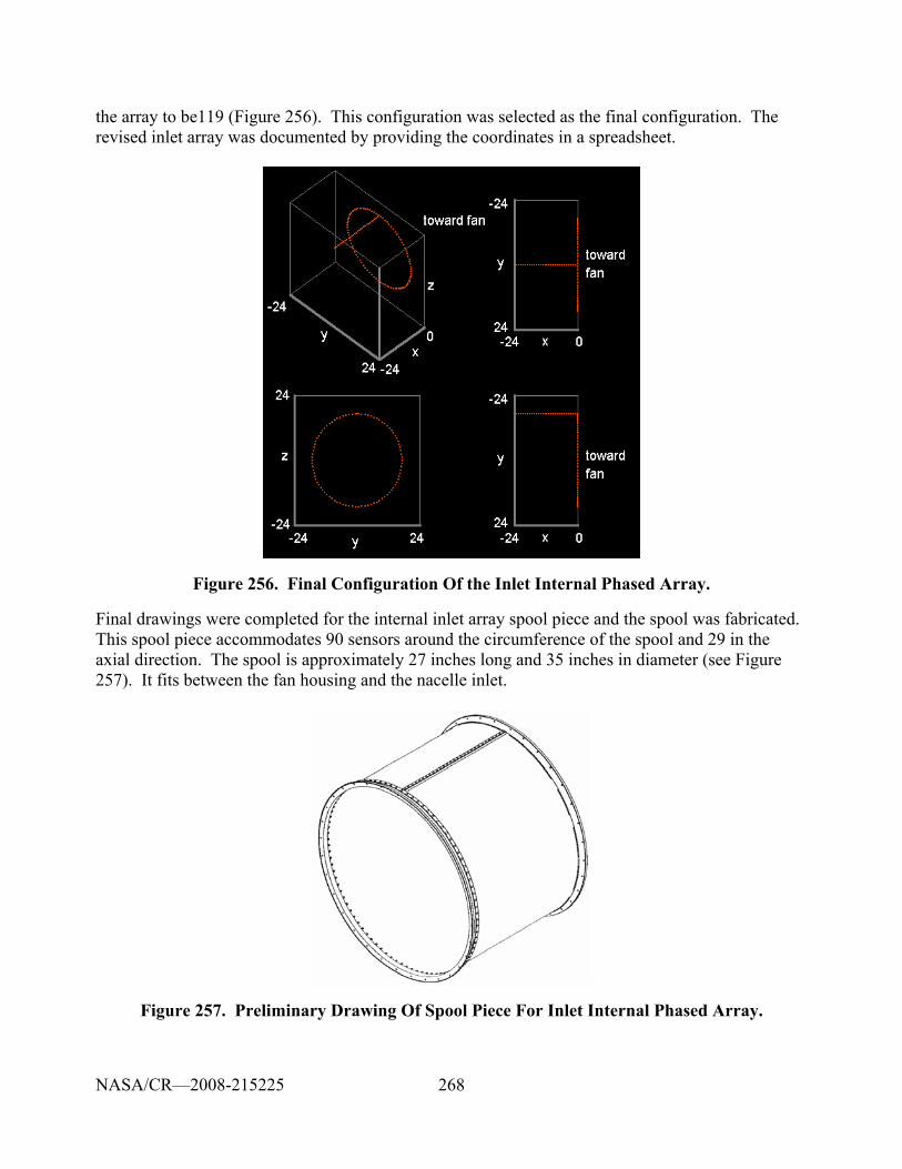
268

the array to be119 (Figure 256). This configuration was selected as the final configuration. The revised inlet array was documented by providing the coordinates in a spreadsheet.

Figure 256. Final Configuration Of the Inlet Internal Phased Array.

Final drawings were completed for the internal inlet array spool piece and the spool was fabricated. This spool piece accommodates 90 sensors around the circumference of the spool and 29 in the axial direction. The spool is approximately 27 inches long and 35 inches in diameter (see Figure 257). It fits between the fan housing and the nacelle inlet.

Figure 257. Preliminary Drawing Of Spool Piece For Inlet Internal Phased Array.

NASA/CR—2008-215225

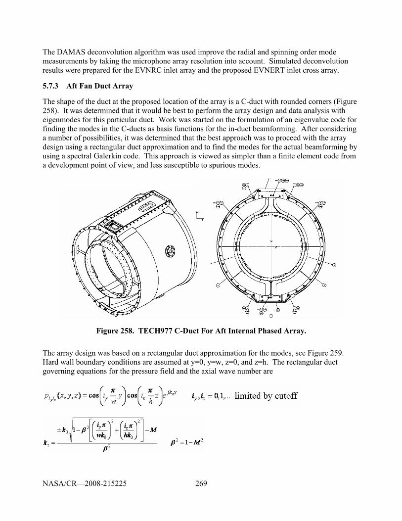
269

The DAMAS deconvolution algorithm was used improve the radial and spinning order mode measurements by taking the microphone array resolution into account. Simulated deconvolution results were prepared for the EVNRC inlet array and the proposed EVNERT inlet cross array.

5.7.3 Aft Fan Duct Array

The shape of the duct at the proposed location of the array is a C-duct with rounded corners (Figure 258). It was determined that it would be best to perform the array design and data analysis with eigenmodes for this particular duct. Work was started on the formulation of an eigenvalue code for finding the modes in the C-ducts as basis functions for the in-duct beamforming. After considering a number of possibilities, it was determined that the best approach was to proceed with the array design using a rectangular duct approximation and to find the modes for the actual beamforming by using a spectral Galerkin code. This approach is viewed as simpler than a finite element code from a development point of view, and less susceptible to spurious modes.

Figure 258. TECH977 C-Duct For Aft Internal Phased Array.

The array design was based on a rectangular duct approximation for the modes, see Figure 259. Hard wall boundary conditions are assumed at y=0, y=w, z=0, and z=h. The rectangular duct governing equations for the pressure field and the axial wave number are

NASA/CR—2008-215225

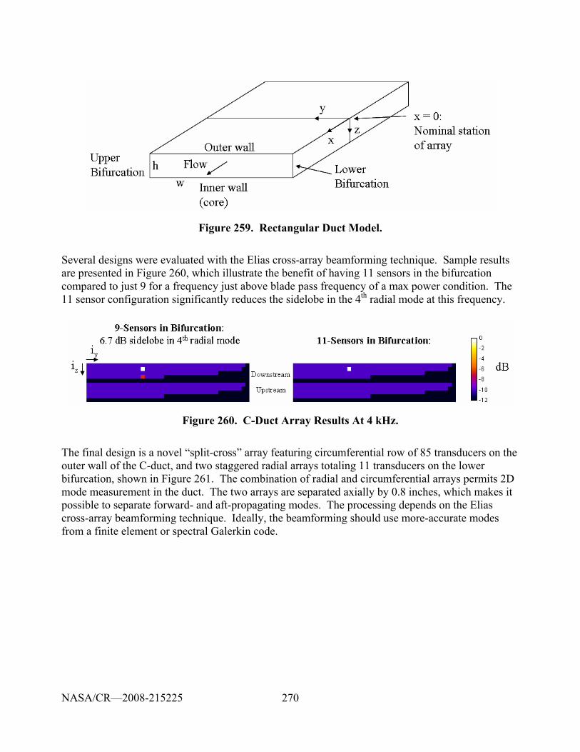
270

Figure 259. Rectangular Duct Model.

Several designs were evaluated with the Elias cross-array beamforming technique. Sample results are presented in Figure 260, which illustrate the benefit of having 11 sensors in the bifurcation compared to just 9 for a frequency just above blade pass frequency of a max power condition. The 11 sensor configuration significantly reduces the sidelobe in the 4th radial mode at this frequency.

Figure 260. C-Duct Array Results At 4 kHz.

The final design is a novel “split-cross” array featuring circumferential row of 85 transducers on the outer wall of the C-duct, and two staggered radial arrays totaling 11 transducers on the lower bifurcation, shown in Figure 261. The combination of radial and circumferential arrays permits 2D mode measurement in the duct. The two arrays are separated axially by 0.8 inches, which makes it possible to separate forward- and aft-propagating modes. The processing depends on the Elias cross-array beamforming technique. Ideally, the beamforming should use more-accurate modes from a finite element or spectral Galerkin code.

NASA/CR—2008-215225

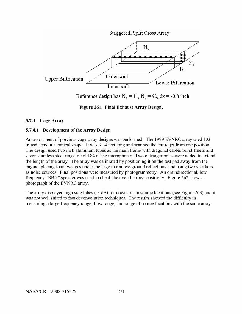
271

Figure 261. Final Exhaust Array Design.

5.7.4 Cage Array

5.7.4.1 Development of the Array Design

An assessment of previous cage array designs was performed. The 1999 EVNRC array used 103 transducers in a conical shape. It was 31.4 feet long and scanned the entire jet from one position. The design used two inch aluminum tubes as the main frame with diagonal cables for stiffness and seven stainless steel rings to hold 84 of the microphones. Two outrigger poles were added to extend the length of the array. The array was calibrated by positioning it on the test pad away from the engine, placing foam wedges under the cage to remove ground reflections, and using two speakers as noise sources. Final positions were measured by photogrammetry. An omindirectional, low frequency “BBN” speaker was used to check the overall array sensitivity. Figure 262 shows a photograph of the EVNRC array.

The array displayed high side lobes (-3 dB) for downstream source locations (see Figure 263) and it was not well suited to fast deconvolution techniques. The results showed the difficulty in measuring a large frequency range, flow range, and range of source locations with the same array.

NASA/CR—2008-215225

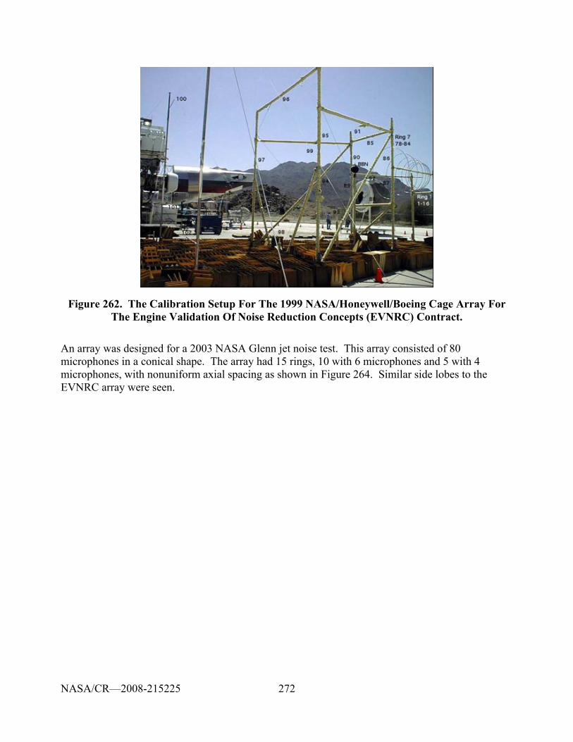
272

Figure 262. The Calibration Setup For The 1999 NASA/Honeywell/Boeing Cage Array For The Engine Validation Of Noise Reduction Concepts (EVNRC) Contract.

An array was designed for a 2003 NASA Glenn jet noise test. This array consisted of 80 microphones in a conical shape. The array had 15 rings, 10 with 6 microphones and 5 with 4 microphones, with nonuniform axial spacing as shown in Figure 264. Similar side lobes to the EVNRC array were seen.

NASA/CR—2008-215225

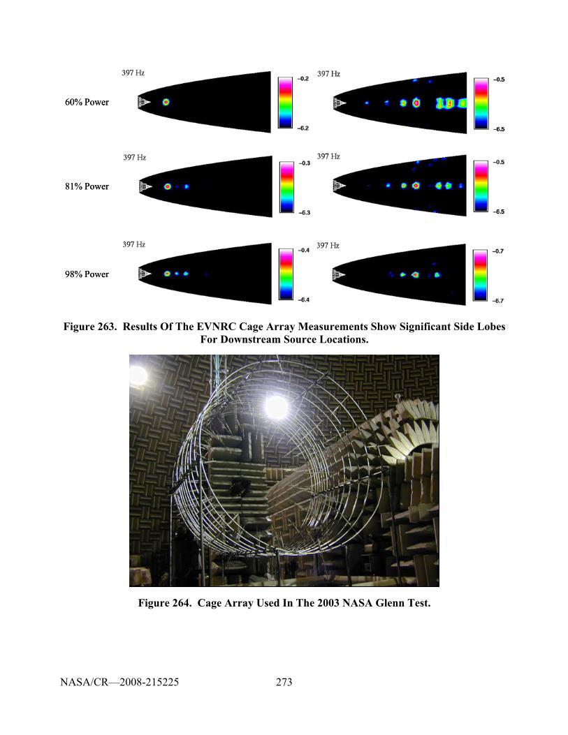
273

60% Power

81% Power

98% Power

60% Power

81% Power

98% Power

Figure 263. Results Of The EVNRC Cage Array Measurements Show Significant Side Lobes For Downstream Source Locations.

Figure 264. Cage Array Used In The 2003 NASA Glenn Test.

NASA/CR—2008-215225

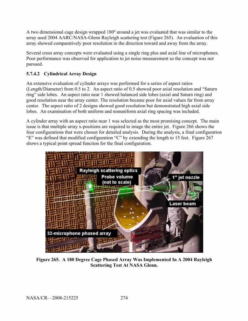
274

A two dimensional cage design wrapped 180º around a jet was evaluated that was similar to the array used 2004 AARC/NASA-Glenn Rayleigh scattering test (Figure 265). An evaluation of this array showed comparatively poor resolution in the direction toward and away from the array.

Several cross array concepts were evaluated using a single ring plus and axial line of microphones. Poor performance was observed for application to jet noise measurement so the concept was not pursued.

5.7.4.2 Cylindrical Array Design

An extensive evaluation of cylinder arrays was performed for a series of aspect ratios (Length/Diameter) from 0.5 to 2. An aspect ratio of 0.5 showed poor axial resolution and “Saturn ring” side lobes. An aspect ratio near 1 showed balanced side lobes (axial and Saturn ring) and good resolution near the array center. The resolution became poor for axial values far from array center. The aspect ratio of 2 designs showed good resolution but demonstrated high axial side lobes. An examination of both uniform and nonuniform axial ring spacing was included.

A cylinder array with an aspect ratio near 1 was selected as the most promising concept. The main issue is that multiple array x-positions are required to image the entire jet. Figure 266 shows the four configurations that were chosen for detailed analysis. During the analysis, a final configuration “E” was defined that modified configuration “C” by extending the length to 15 feet. Figure 267 shows a typical point spread function for the final configuration.

Figure 265. A 180 Degree Cage Phased Array Was Implemented In A 2004 Rayleigh Scattering Test At NASA Glenn.

NASA/CR—2008-215225

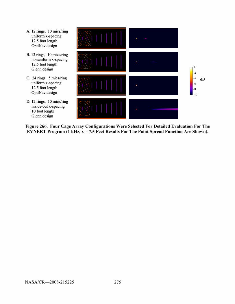
275

B. 12 rings, 10 mics/ringnonuniform x-spacing12.5 foot lengthGlenn design

A. 12 rings, 10 mics/ringuniform x-spacing12.5 foot length OptiNav design

C. 24 rings, 5 mics/ringuniform x-spacing12.5 foot lengthOptiNav design

D. 12 rings, 10 mics/ringinside-out x-spacing10 foot lengthGlenn design

dB

B. 12 rings, 10 mics/ringnonuniform x-spacing12.5 foot lengthGlenn design

A. 12 rings, 10 mics/ringuniform x-spacing12.5 foot length OptiNav design

C. 24 rings, 5 mics/ringuniform x-spacing12.5 foot lengthOptiNav design

D. 12 rings, 10 mics/ringinside-out x-spacing10 foot lengthGlenn design

dB

Figure 266. Four Cage Array Configurations Were Selected For Detailed Evaluation For The EVNERT Program (1 kHz, x = 7.5 Feet Results For The Point Spread Function Are Shown).

NASA/CR—2008-215225

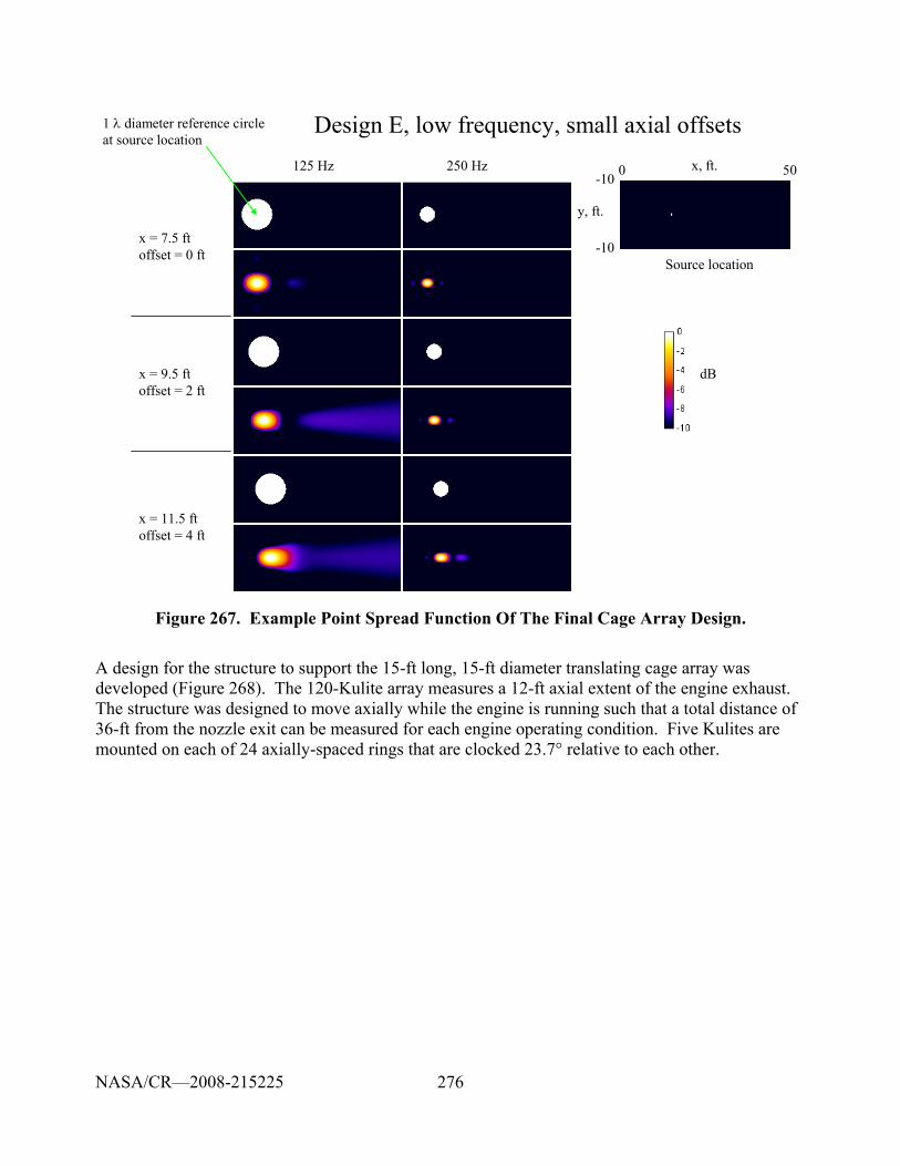
276

125 Hz 250 Hz

x = 7.5 ftoffset = 0 ft



Design E, low frequency, small axial offsets

dB

x, ft.

y, ft.

-10

-10 0 50

1 λ diameter reference circleat source location

Source location

Figure 267. Example Point Spread Function Of The Final Cage Array Design.

A design for the structure to support the 15-ft long, 15-ft diameter translating cage array was developed (Figure 268). The 120-Kulite array measures a 12-ft axial extent of the engine exhaust. The structure was designed to move axially while the engine is running such that a total distance of 36-ft from the nozzle exit can be measured for each engine operating condition. Five Kulites are mounted on each of 24 axially-spaced rings that are clocked 23.7° relative to each other.

NASA/CR—2008-215225

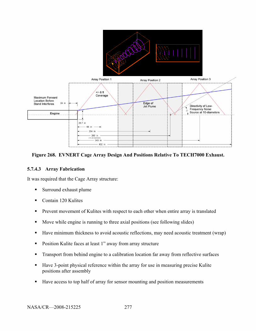
277

Figure 268. EVNERT Cage Array Design And Positions Relative To TECH7000 Exhaust.

5.7.4.3 Array Fabrication

It was required that the Cage Array structure:

Surround exhaust plume

Contain 120 Kulites

Prevent movement of Kulites with respect to each other when entire array is translated

Move while engine is running to three axial positions (see following slides)

Have minimum thickness to avoid acoustic reflections, may need acoustic treatment (wrap)

Position Kulite faces at least 1” away from array structure

Transport from behind engine to a calibration location far away from reflective surfaces

Have 3-point physical reference within the array for use in measuring precise Kulite positions after assembly

Have access to top half of array for sensor mounting and position measurements

NASA/CR—2008-215225

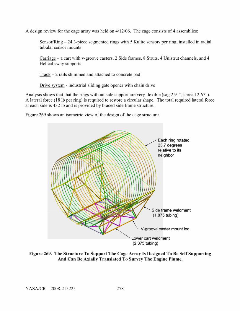
278

A design review for the cage array was held on 4/12/06. The cage consists of 4 assemblies:

Sensor/Ring – 24 3-piece segmented rings with 5 Kulite sensors per ring, installed in radial tubular sensor mounts Carriage – a cart with v-groove casters, 2 Side frames, 8 Struts, 4 Unistrut channels, and 4 Helical sway supports Track – 2 rails shimmed and attached to concrete pad Drive system - industrial sliding gate opener with chain drive

Analysis shows that that the rings without side support are very flexible (sag 2.91”, spread 2.67”). A lateral force (18 lb per ring) is required to restore a circular shape. The total required lateral force at each side is 432 lb and is provided by braced side frame structure.

Figure 269 shows an isometric view of the design of the cage structure.

V-groove caster mount loc

Lower cart weldment(2.375 tubing)

Side frame weldment(1.875 tubing)

Each ring rotated23.7 degreesrelative to itsneighbor

V-groove caster mount loc

Lower cart weldment(2.375 tubing)

Side frame weldment(1.875 tubing)

Each ring rotated23.7 degreesrelative to itsneighbor

Figure 269. The Structure To Support The Cage Array Is Designed To Be Self Supporting And Can Be Axially Translated To Survey The Engine Plume.

NASA/CR—2008-215225

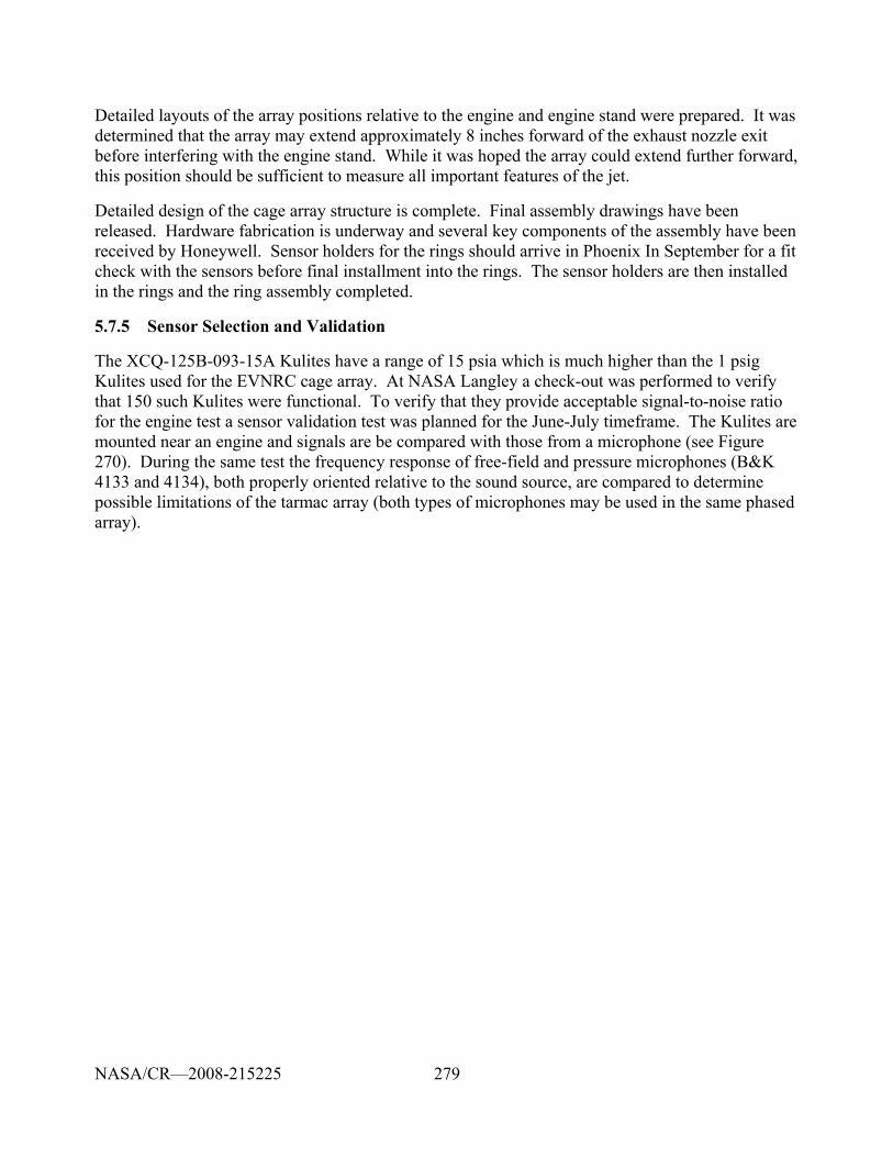
279

Detailed layouts of the array positions relative to the engine and engine stand were prepared. It was determined that the array may extend approximately 8 inches forward of the exhaust nozzle exit before interfering with the engine stand. While it was hoped the array could extend further forward, this position should be sufficient to measure all important features of the jet.

Detailed design of the cage array structure is complete. Final assembly drawings have been released. Hardware fabrication is underway and several key components of the assembly have been received by Honeywell. Sensor holders for the rings should arrive in Phoenix In September for a fit check with the sensors before final installment into the rings. The sensor holders are then installed in the rings and the ring assembly completed.

5.7.5 Sensor Selection and Validation

The XCQ-125B-093-15A Kulites have a range of 15 psia which is much higher than the 1 psig Kulites used for the EVNRC cage array. At NASA Langley a check-out was performed to verify that 150 such Kulites were functional. To verify that they provide acceptable signal-to-noise ratio for the engine test a sensor validation test was planned for the June-July timeframe. The Kulites are mounted near an engine and signals are be compared with those from a microphone (see Figure 270). During the same test the frequency response of free-field and pressure microphones (B&K 4133 and 4134), both properly oriented relative to the sound source, are compared to determine possible limitations of the tarmac array (both types of microphones may be used in the same phased array).

NASA/CR—2008-215225

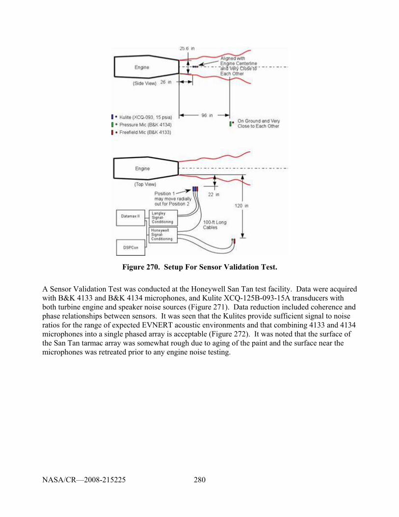
280

Figure 270. Setup For Sensor Validation Test.

A Sensor Validation Test was conducted at the Honeywell San Tan test facility. Data were acquired with B&K 4133 and B&K 4134 microphones, and Kulite XCQ-125B-093-15A transducers with both turbine engine and speaker noise sources (Figure 271). Data reduction included coherence and phase relationships between sensors. It was seen that the Kulites provide sufficient signal to noise ratios for the range of expected EVNERT acoustic environments and that combining 4133 and 4134 microphones into a single phased array is acceptable (Figure 272). It was noted that the surface of the San Tan tarmac array was somewhat rough due to aging of the paint and the surface near the microphones was retreated prior to any engine noise testing.

NASA/CR—2008-215225

281

Figure 271. Photos Of Sensor Validation Test Setups.

NASA/CR—2008-215225

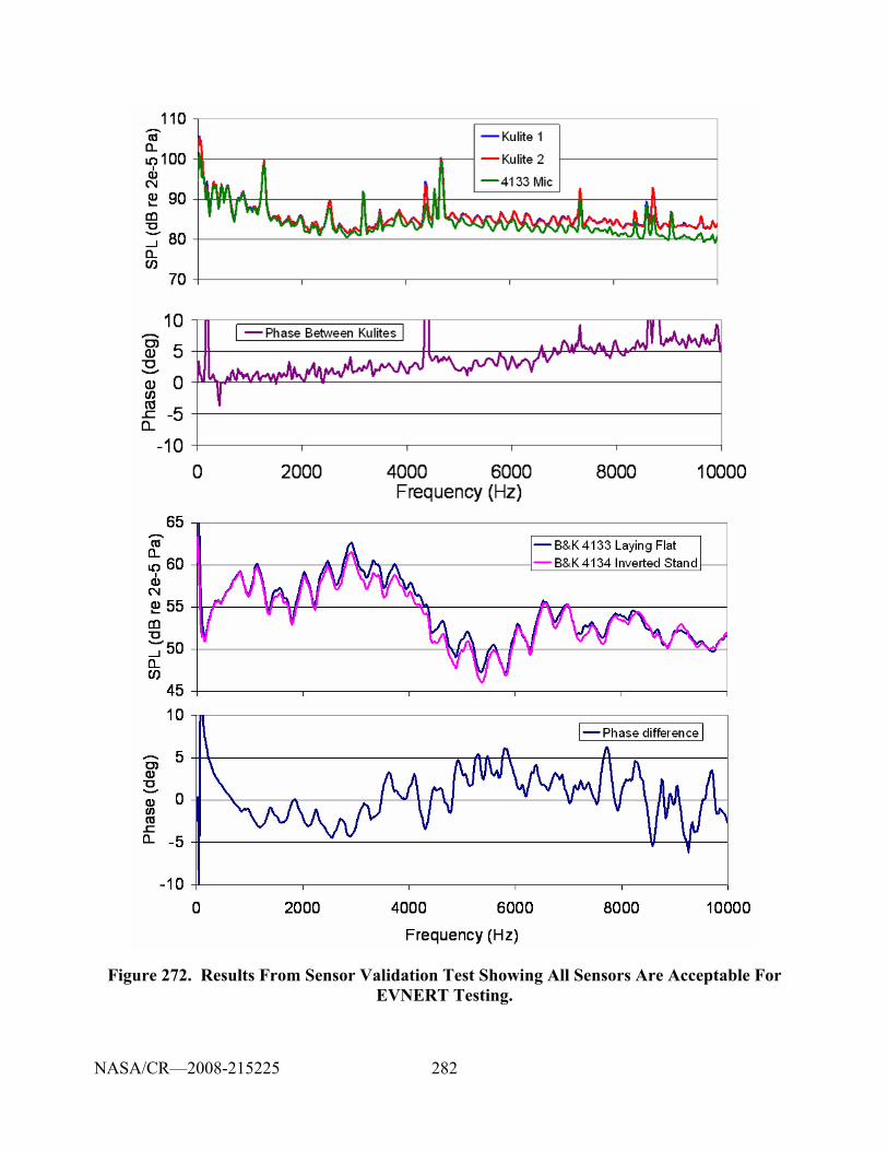
282

Figure 272. Results From Sensor Validation Test Showing All Sensors Are Acceptable For EVNERT Testing.

NASA/CR—2008-215225

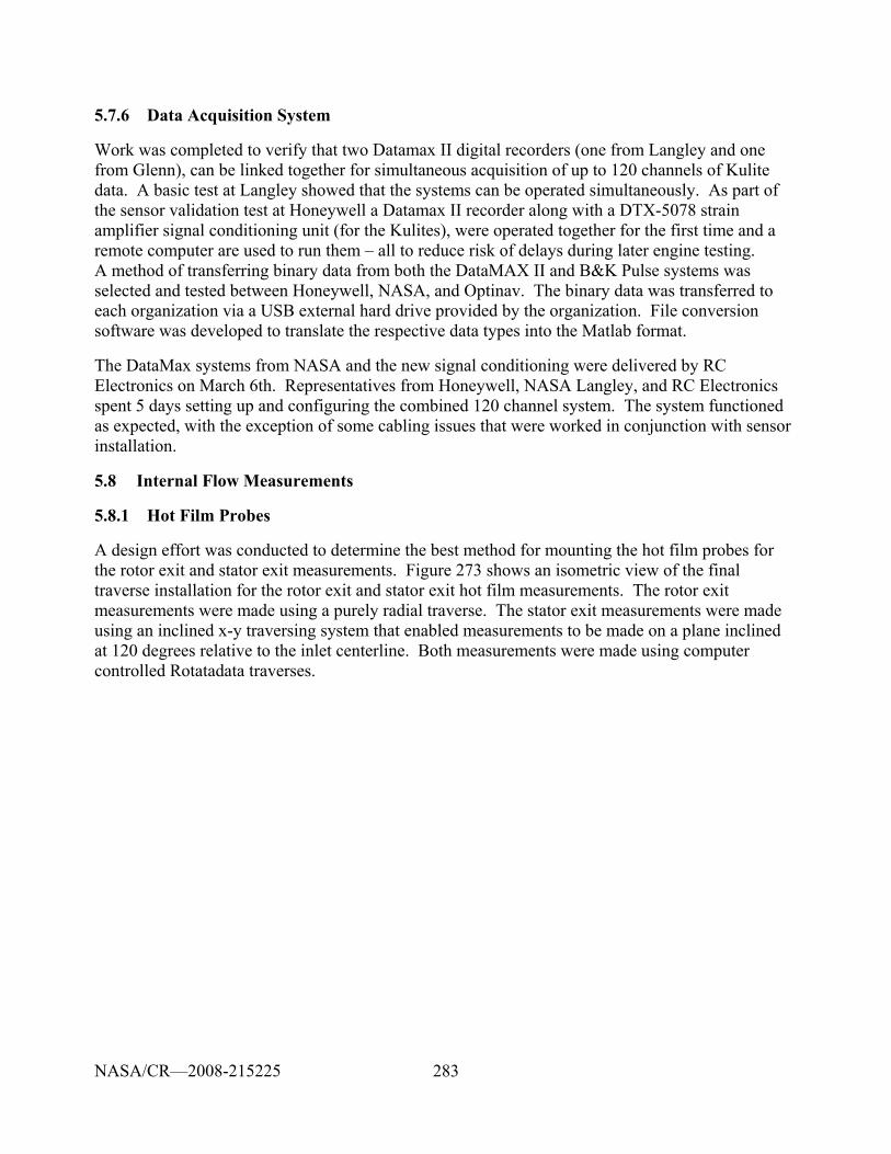
283

5.7.6 Data Acquisition System

Work was completed to verify that two Datamax II digital recorders (one from Langley and one from Glenn), can be linked together for simultaneous acquisition of up to 120 channels of Kulite data. A basic test at Langley showed that the systems can be operated simultaneously. As part of the sensor validation test at Honeywell a Datamax II recorder along with a DTX-5078 strain amplifier signal conditioning unit (for the Kulites), were operated together for the first time and a remote computer are used to run them – all to reduce risk of delays during later engine testing. A method of transferring binary data from both the DataMAX II and B&K Pulse systems was selected and tested between Honeywell, NASA, and Optinav. The binary data was transferred to each organization via a USB external hard drive provided by the organization. File conversion software was developed to translate the respective data types into the Matlab format.

The DataMax systems from NASA and the new signal conditioning were delivered by RC Electronics on March 6th. Representatives from Honeywell, NASA Langley, and RC Electronics spent 5 days setting up and configuring the combined 120 channel system. The system functioned as expected, with the exception of some cabling issues that were worked in conjunction with sensor installation.

5.8 Internal Flow Measurements

5.8.1 Hot Film Probes

A design effort was conducted to determine the best method for mounting the hot film probes for the rotor exit and stator exit measurements. Figure 273 shows an isometric view of the final traverse installation for the rotor exit and stator exit hot film measurements. The rotor exit measurements were made using a purely radial traverse. The stator exit measurements were made using an inclined x-y traversing system that enabled measurements to be made on a plane inclined at 120 degrees relative to the inlet centerline. Both measurements were made using computer controlled Rotatadata traverses.

NASA/CR—2008-215225

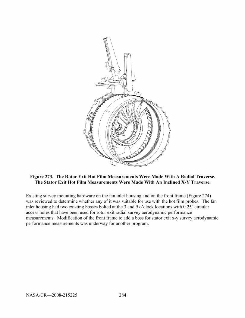
284

Figure 273. The Rotor Exit Hot Film Measurements Were Made With A Radial Traverse. The Stator Exit Hot Film Measurements Were Made With An Inclined X-Y Traverse.

Existing survey mounting hardware on the fan inlet housing and on the front frame (Figure 274) was reviewed to determine whether any of it was suitable for use with the hot film probes. The fan inlet housing had two existing bosses bolted at the 3 and 9 o’clock locations with 0.25˝ circular access holes that have been used for rotor exit radial survey aerodynamic performance measurements. Modification of the front frame to add a boss for stator exit x-y survey aerodynamic performance measurements was underway for another program.

NASA/CR—2008-215225

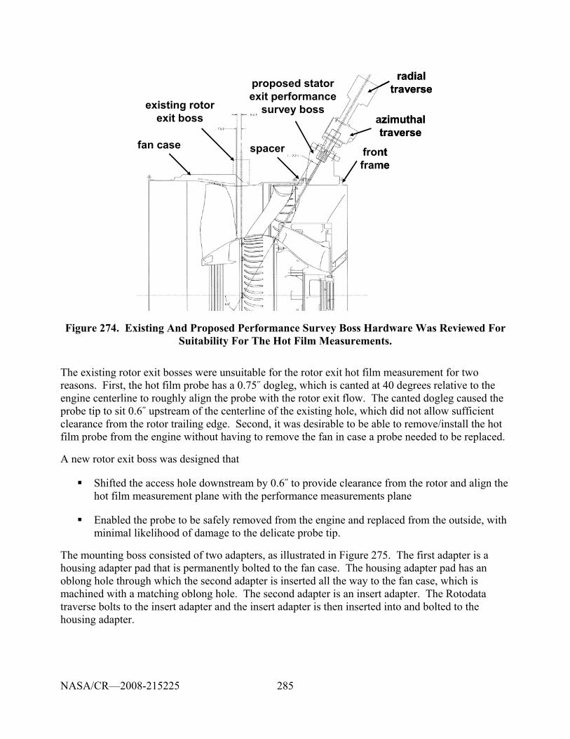
285

existing rotorexit boss

proposed statorexit performance

survey boss

fan case spacer frontframe

azimuthaltraverse

radialtraverse

existing rotorexit boss

proposed statorexit performance

survey boss

fan case spacer frontframe

azimuthaltraverse

radialtraverse

Figure 274. Existing And Proposed Performance Survey Boss Hardware Was Reviewed For Suitability For The Hot Film Measurements.

The existing rotor exit bosses were unsuitable for the rotor exit hot film measurement for two reasons. First, the hot film probe has a 0.75˝ dogleg, which is canted at 40 degrees relative to the engine centerline to roughly align the probe with the rotor exit flow. The canted dogleg caused the probe tip to sit 0.6˝ upstream of the centerline of the existing hole, which did not allow sufficient clearance from the rotor trailing edge. Second, it was desirable to be able to remove/install the hot film probe from the engine without having to remove the fan in case a probe needed to be replaced.

A new rotor exit boss was designed that

Shifted the access hole downstream by 0.6˝ to provide clearance from the rotor and align the hot film measurement plane with the performance measurements plane

Enabled the probe to be safely removed from the engine and replaced from the outside, with minimal likelihood of damage to the delicate probe tip.

The mounting boss consisted of two adapters, as illustrated in Figure 275. The first adapter is a housing adapter pad that is permanently bolted to the fan case. The housing adapter pad has an oblong hole through which the second adapter is inserted all the way to the fan case, which is machined with a matching oblong hole. The second adapter is an insert adapter. The Rotodata traverse bolts to the insert adapter and the insert adapter is then inserted into and bolted to the housing adapter.

NASA/CR—2008-215225

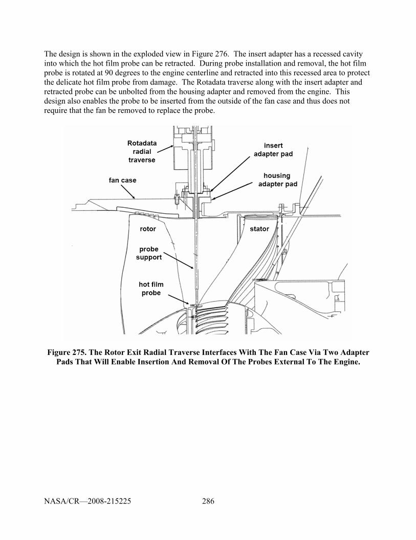
286

The design is shown in the exploded view in Figure 276. The insert adapter has a recessed cavity into which the hot film probe can be retracted. During probe installation and removal, the hot film probe is rotated at 90 degrees to the engine centerline and retracted into this recessed area to protect the delicate hot film probe from damage. The Rotadata traverse along with the insert adapter and retracted probe can be unbolted from the housing adapter and removed from the engine. This design also enables the probe to be inserted from the outside of the fan case and thus does not require that the fan be removed to replace the probe.

Figure 275. The Rotor Exit Radial Traverse Interfaces With The Fan Case Via Two Adapter Pads That Will Enable Insertion And Removal Of The Probes External To The Engine.

NASA/CR—2008-215225

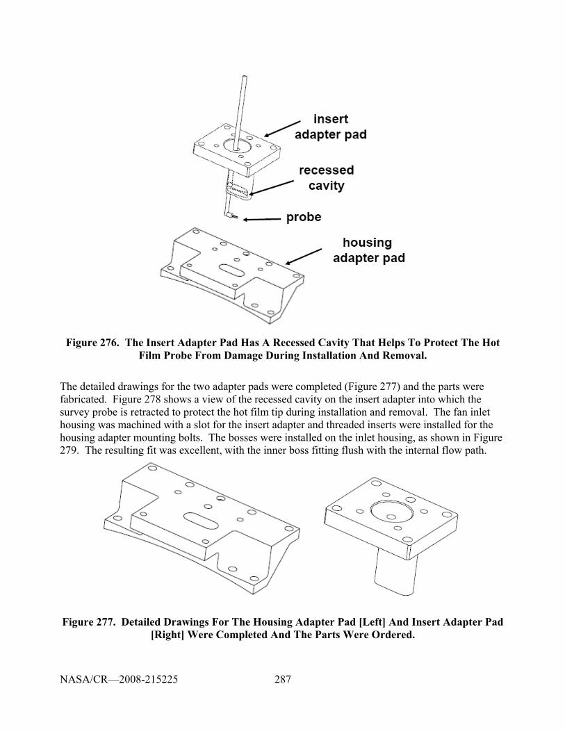
287

Figure 276. The Insert Adapter Pad Has A Recessed Cavity That Helps To Protect The Hot Film Probe From Damage During Installation And Removal.

The detailed drawings for the two adapter pads were completed (Figure 277) and the parts were fabricated. Figure 278 shows a view of the recessed cavity on the insert adapter into which the survey probe is retracted to protect the hot film tip during installation and removal. The fan inlet housing was machined with a slot for the insert adapter and threaded inserts were installed for the housing adapter mounting bolts. The bosses were installed on the inlet housing, as shown in Figure 279. The resulting fit was excellent, with the inner boss fitting flush with the internal flow path.

Figure 277. Detailed Drawings For The Housing Adapter Pad [Left] And Insert Adapter Pad [Right] Were Completed And The Parts Were Ordered.

NASA/CR—2008-215225

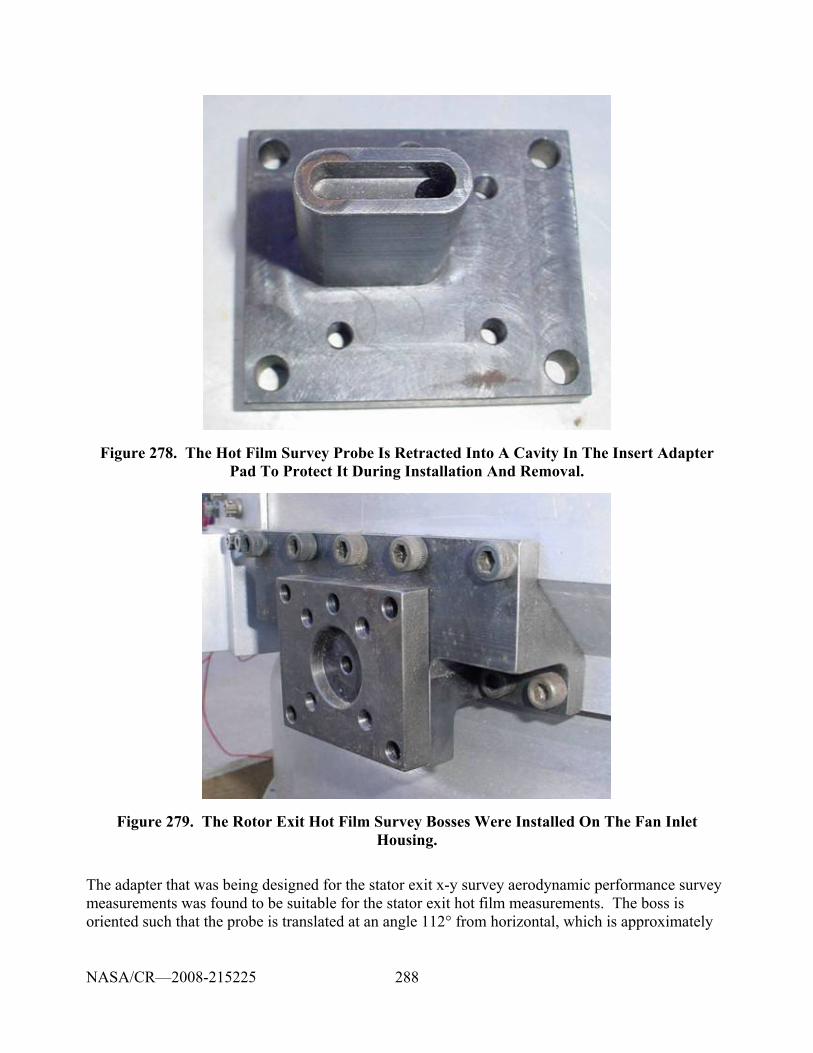
288

Figure 278. The Hot Film Survey Probe Is Retracted Into A Cavity In The Insert Adapter Pad To Protect It During Installation And Removal.

Figure 279. The Rotor Exit Hot Film Survey Bosses Were Installed On The Fan Inlet Housing.

The adapter that was being designed for the stator exit x-y survey aerodynamic performance survey measurements was found to be suitable for the stator exit hot film measurements. The boss is oriented such that the probe is translated at an angle 112° from horizontal, which is approximately

NASA/CR—2008-215225

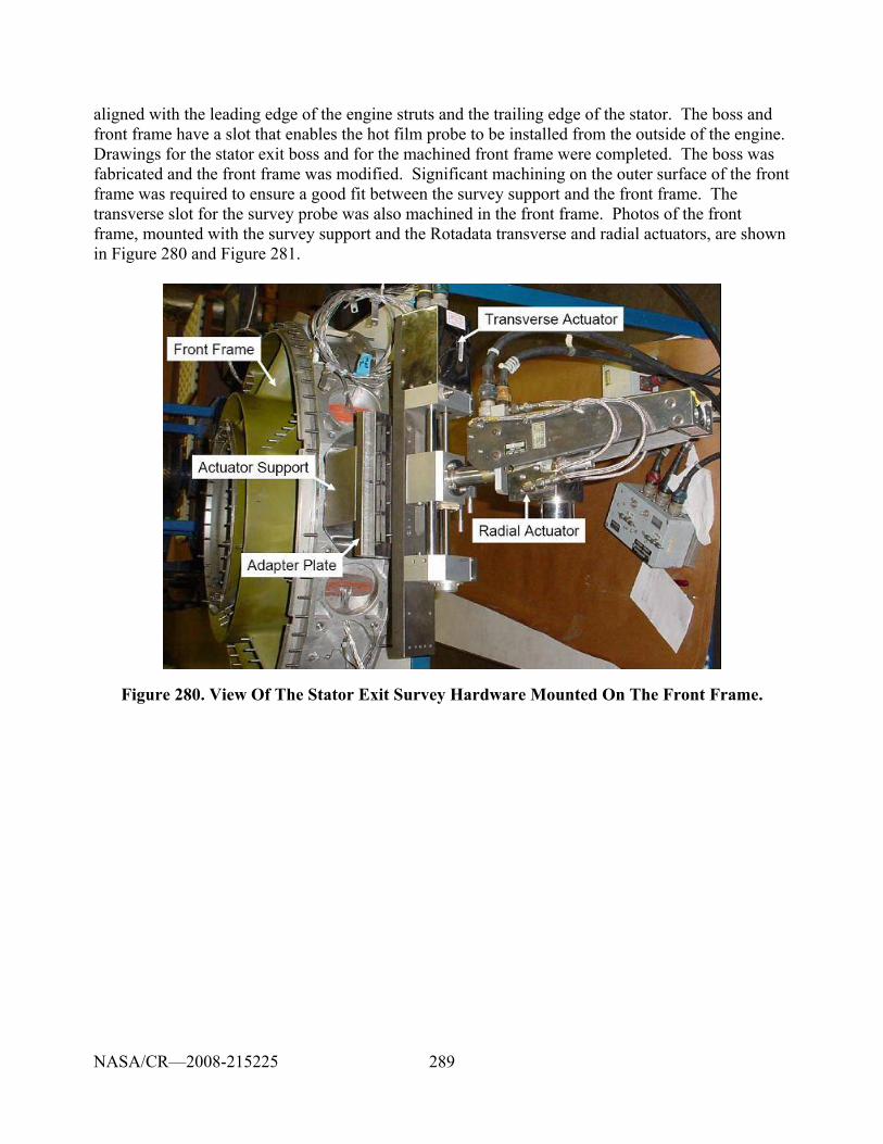
289

aligned with the leading edge of the engine struts and the trailing edge of the stator. The boss and front frame have a slot that enables the hot film probe to be installed from the outside of the engine. Drawings for the stator exit boss and for the machined front frame were completed. The boss was fabricated and the front frame was modified. Significant machining on the outer surface of the front frame was required to ensure a good fit between the survey support and the front frame. The transverse slot for the survey probe was also machined in the front frame. Photos of the front frame, mounted with the survey support and the Rotadata transverse and radial actuators, are shown in Figure 280 and Figure 281.

Figure 280. View Of The Stator Exit Survey Hardware Mounted On The Front Frame.

NASA/CR—2008-215225

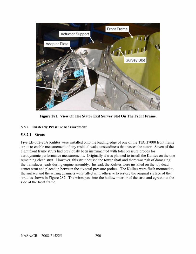
290

Figure 281. View Of The Stator Exit Survey Slot On The Front Frame.

5.8.2 Unsteady Pressure Measurement

5.8.2.1 Struts

Five LE-062-25A Kulites were installed onto the leading edge of one of the TECH7000 front frame struts to enable measurement of any residual wake unsteadiness that passes the stator. Seven of the eight front frame struts had previously been instrumented with total pressure probes for aerodynamic performance measurements. Originally it was planned to install the Kulites on the one remaining clean strut. However, this strut housed the tower shaft and there was risk of damaging the transducer leads during engine assembly. Instead, the Kulites were installed on the top dead center strut and placed in between the six total pressure probes. The Kulites were flush mounted to the surface and the wiring channels were filled with adhesive to restore the original surface of the strut, as shown in Figure 282. The wires pass into the hollow interior of the strut and egress out the side of the front frame.

NASA/CR—2008-215225

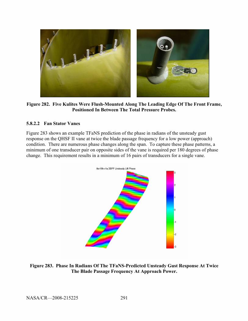
291

Figure 282. Five Kulites Were Flush-Mounted Along The Leading Edge Of The Front Frame, Positioned In Between The Total Pressure Probes.

5.8.2.2 Fan Stator Vanes

Figure 283 shows an example TFaNS prediction of the phase in radians of the unsteady gust response on the QHSF II vane at twice the blade passage frequency for a low power (approach) condition. There are numerous phase changes along the span. To capture these phase patterns, a minimum of one transducer pair on opposite sides of the vane is required per 180 degrees of phase change. This requirement results in a minimum of 16 pairs of transducers for a single vane.

Figure 283. Phase In Radians Of The TFaNS-Predicted Unsteady Gust Response At Twice The Blade Passage Frequency At Approach Power.

NASA/CR—2008-215225

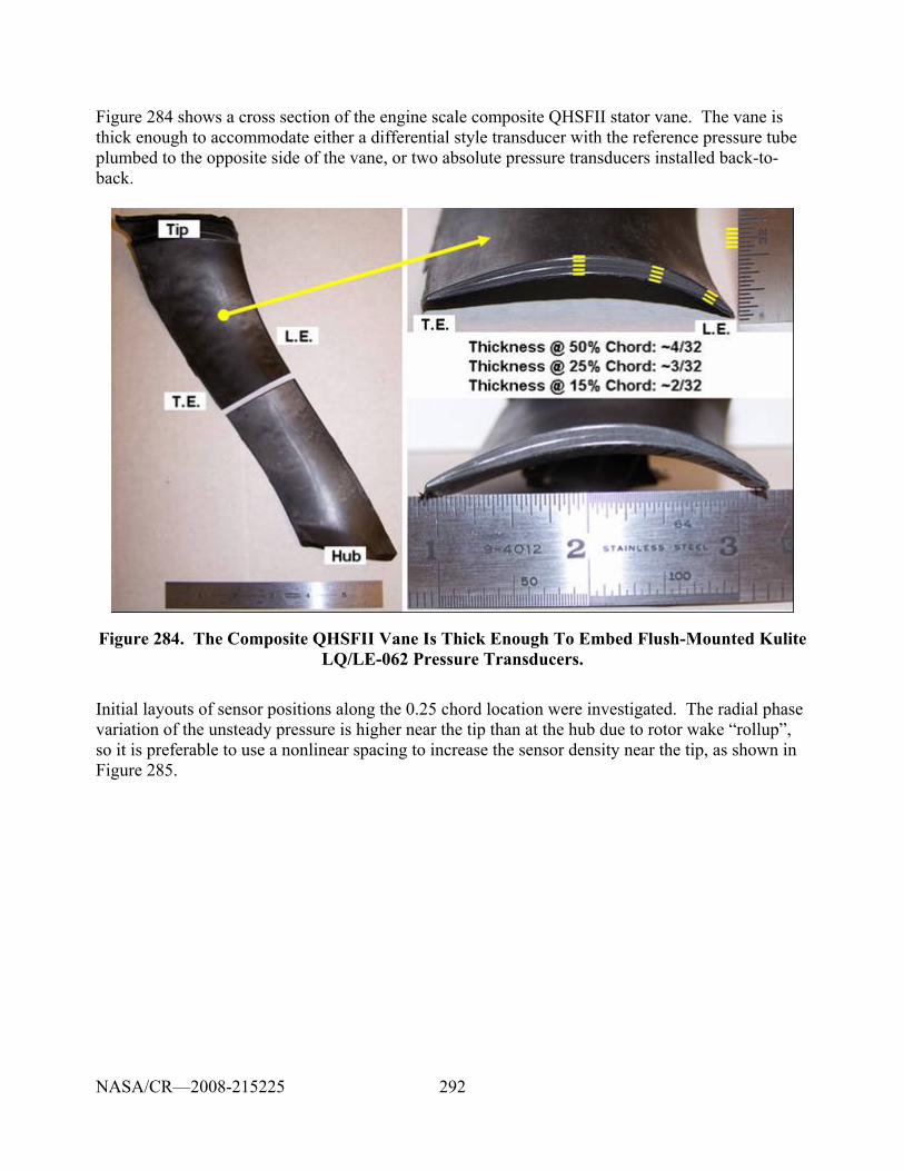
292

Figure 284 shows a cross section of the engine scale composite QHSFII stator vane. The vane is thick enough to accommodate either a differential style transducer with the reference pressure tube plumbed to the opposite side of the vane, or two absolute pressure transducers installed back-to-back.

Figure 284. The Composite QHSFII Vane Is Thick Enough To Embed Flush-Mounted Kulite LQ/LE-062 Pressure Transducers.

Initial layouts of sensor positions along the 0.25 chord location were investigated. The radial phase variation of the unsteady pressure is higher near the tip than at the hub due to rotor wake “rollup”, so it is preferable to use a nonlinear spacing to increase the sensor density near the tip, as shown in Figure 285.

NASA/CR—2008-215225

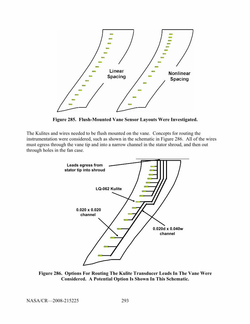
293

Figure 285. Flush-Mounted Vane Sensor Layouts Were Investigated.

The Kulites and wires needed to be flush mounted on the vane. Concepts for routing the instrumentation were considered, such as shown in the schematic in Figure 286. All of the wires must egress through the vane tip and into a narrow channel in the stator shroud, and then out through holes in the fan case.

LQ-062 Kulite

0.020 x 0.020channel

0.020d x 0.040wchannel

Leads egress fromstator tip into shroud

LQ-062 Kulite

0.020 x 0.020channel

0.020d x 0.040wchannel

Leads egress fromstator tip into shroud

Figure 286. Options For Routing The Kulite Transducer Leads In The Vane Were Considered. A Potential Option Is Shown In This Schematic.

NASA/CR—2008-215225

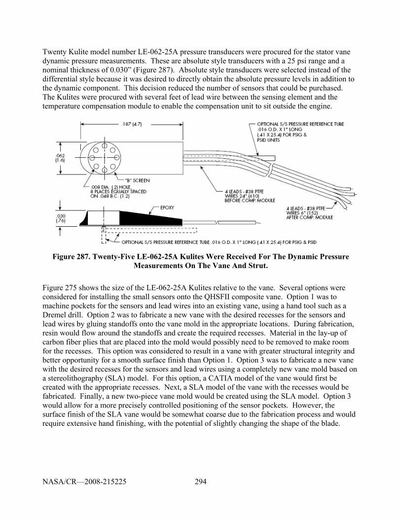
294

Twenty Kulite model number LE-062-25A pressure transducers were procured for the stator vane dynamic pressure measurements. These are absolute style transducers with a 25 psi range and a nominal thickness of 0.030” (Figure 287). Absolute style transducers were selected instead of the differential style because it was desired to directly obtain the absolute pressure levels in addition to the dynamic component. This decision reduced the number of sensors that could be purchased. The Kulites were procured with several feet of lead wire between the sensing element and the temperature compensation module to enable the compensation unit to sit outside the engine.

Figure 287. Twenty-Five LE-062-25A Kulites Were Received For The Dynamic Pressure Measurements On The Vane And Strut.

Figure 275 shows the size of the LE-062-25A Kulites relative to the vane. Several options were considered for installing the small sensors onto the QHSFII composite vane. Option 1 was to machine pockets for the sensors and lead wires into an existing vane, using a hand tool such as a Dremel drill. Option 2 was to fabricate a new vane with the desired recesses for the sensors and lead wires by gluing standoffs onto the vane mold in the appropriate locations. During fabrication, resin would flow around the standoffs and create the required recesses. Material in the lay-up of carbon fiber plies that are placed into the mold would possibly need to be removed to make room for the recesses. This option was considered to result in a vane with greater structural integrity and better opportunity for a smooth surface finish than Option 1. Option 3 was to fabricate a new vane with the desired recesses for the sensors and lead wires using a completely new vane mold based on a stereolithography (SLA) model. For this option, a CATIA model of the vane would first be created with the appropriate recesses. Next, a SLA model of the vane with the recesses would be fabricated. Finally, a new two-piece vane mold would be created using the SLA model. Option 3 would allow for a more precisely controlled positioning of the sensor pockets. However, the surface finish of the SLA vane would be somewhat coarse due to the fabrication process and would require extensive hand finishing, with the potential of slightly changing the shape of the blade.

NASA/CR—2008-215225

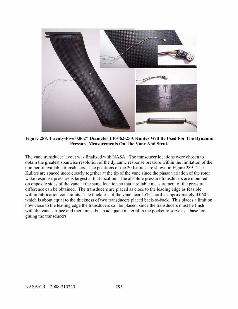
295

Figure 288. Twenty-Five 0.062″ Diameter LE-062-25A Kulites Will Be Used For The Dynamic Pressure Measurements On The Vane And Strut.

The vane transducer layout was finalized with NASA. The transducer locations were chosen to obtain the greatest spanwise resolution of the dynamic response pressure within the limitation of the number of available transducers. The positions of the 20 Kulites are shown in Figure 289. The Kulites are spaced more closely together at the tip of the vane since the phase variation of the rotor wake response pressure is largest at that location. The absolute pressure transducers are mounted on opposite sides of the vane at the same location so that a reliable measurement of the pressure difference can be obtained. The transducers are placed as close to the leading edge as feasible within fabrication constraints. The thickness of the vane near 15% chord is approximately 0.060”, which is about equal to the thickness of two transducers placed back-to-back. This places a limit on how close to the leading edge the transducers can be placed, since the transducers must be flush with the vane surface and there must be an adequate material in the pocket to serve as a base for gluing the transducers.

NASA/CR—2008-215225

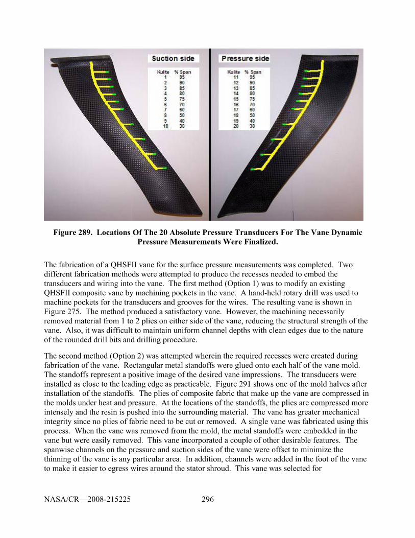
296

Figure 289. Locations Of The 20 Absolute Pressure Transducers For The Vane Dynamic Pressure Measurements Were Finalized.

The fabrication of a QHSFII vane for the surface pressure measurements was completed. Two different fabrication methods were attempted to produce the recesses needed to embed the transducers and wiring into the vane. The first method (Option 1) was to modify an existing QHSFII composite vane by machining pockets in the vane. A hand-held rotary drill was used to machine pockets for the transducers and grooves for the wires. The resulting vane is shown in Figure 275. The method produced a satisfactory vane. However, the machining necessarily removed material from 1 to 2 plies on either side of the vane, reducing the structural strength of the vane. Also, it was difficult to maintain uniform channel depths with clean edges due to the nature of the rounded drill bits and drilling procedure.

The second method (Option 2) was attempted wherein the required recesses were created during fabrication of the vane. Rectangular metal standoffs were glued onto each half of the vane mold. The standoffs represent a positive image of the desired vane impressions. The transducers were installed as close to the leading edge as practicable. Figure 291 shows one of the mold halves after installation of the standoffs. The plies of composite fabric that make up the vane are compressed in the molds under heat and pressure. At the locations of the standoffs, the plies are compressed more intensely and the resin is pushed into the surrounding material. The vane has greater mechanical integrity since no plies of fabric need to be cut or removed. A single vane was fabricated using this process. When the vane was removed from the mold, the metal standoffs were embedded in the vane but were easily removed. This vane incorporated a couple of other desirable features. The spanwise channels on the pressure and suction sides of the vane were offset to minimize the thinning of the vane is any particular area. In addition, channels were added in the foot of the vane to make it easier to egress wires around the stator shroud. This vane was selected for

NASA/CR—2008-215225

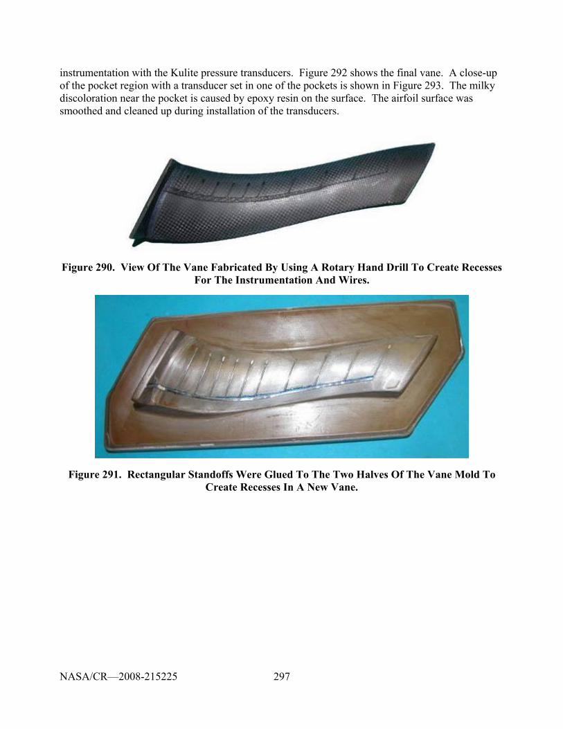
297

instrumentation with the Kulite pressure transducers. Figure 292 shows the final vane. A close-up of the pocket region with a transducer set in one of the pockets is shown in Figure 293. The milky discoloration near the pocket is caused by epoxy resin on the surface. The airfoil surface was smoothed and cleaned up during installation of the transducers.

Figure 290. View Of The Vane Fabricated By Using A Rotary Hand Drill To Create Recesses For The Instrumentation And Wires.

Figure 291. Rectangular Standoffs Were Glued To The Two Halves Of The Vane Mold To Create Recesses In A New Vane.

NASA/CR—2008-215225

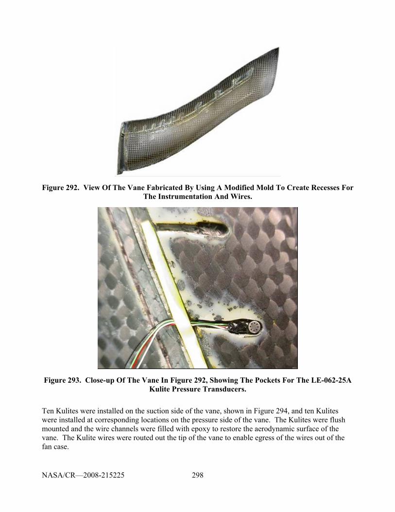
298

Figure 292. View Of The Vane Fabricated By Using A Modified Mold To Create Recesses For The Instrumentation And Wires.

Figure 293. Close-up Of The Vane In Figure 292, Showing The Pockets For The LE-062-25A Kulite Pressure Transducers.

Ten Kulites were installed on the suction side of the vane, shown in Figure 294, and ten Kulites were installed at corresponding locations on the pressure side of the vane. The Kulites were flush mounted and the wire channels were filled with epoxy to restore the aerodynamic surface of the vane. The Kulite wires were routed out the tip of the vane to enable egress of the wires out of the fan case.

NASA/CR—2008-215225

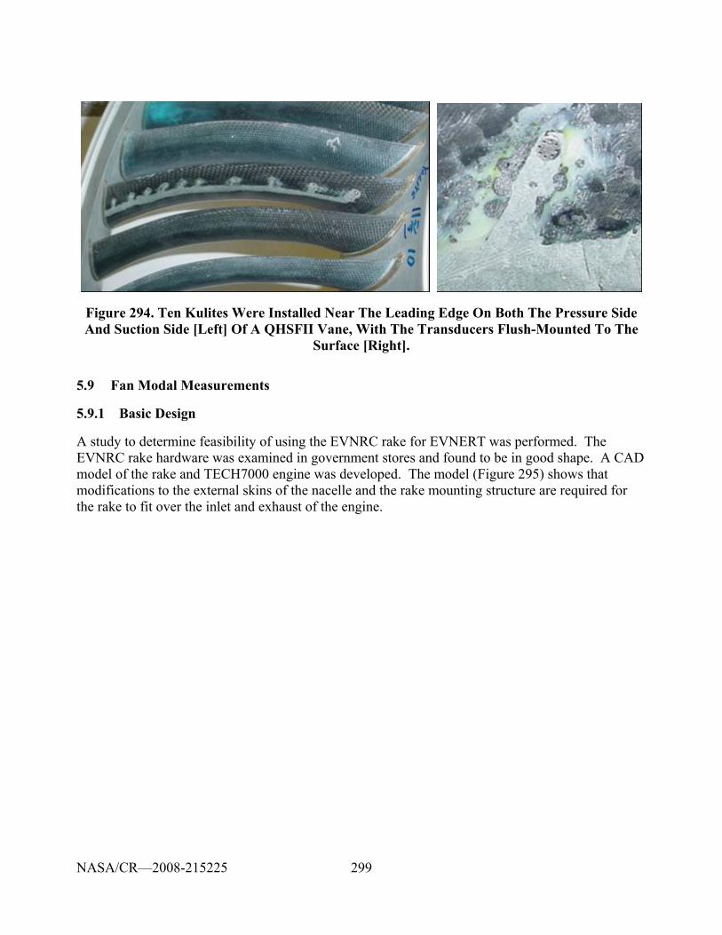
299

Figure 294. Ten Kulites Were Installed Near The Leading Edge On Both The Pressure Side And Suction Side [Left] Of A QHSFII Vane, With The Transducers Flush-Mounted To The

Surface [Right].

5.9 Fan Modal Measurements

5.9.1 Basic Design

A study to determine feasibility of using the EVNRC rake for EVNERT was performed. The EVNRC rake hardware was examined in government stores and found to be in good shape. A CAD model of the rake and TECH7000 engine was developed. The model (Figure 295) shows that modifications to the external skins of the nacelle and the rake mounting structure are required for the rake to fit over the inlet and exhaust of the engine.

NASA/CR—2008-215225

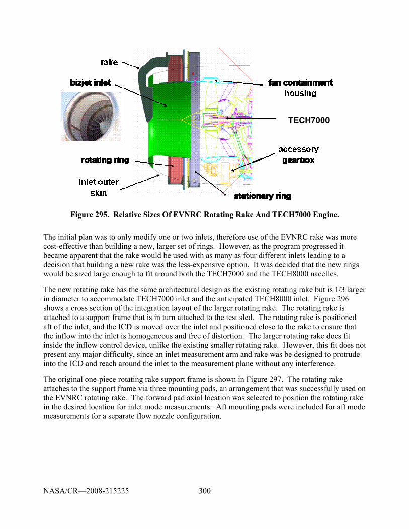
300

TECH7000TECH7000

Figure 295. Relative Sizes Of EVNRC Rotating Rake And TECH7000 Engine.

The initial plan was to only modify one or two inlets, therefore use of the EVNRC rake was more cost-effective than building a new, larger set of rings. However, as the program progressed it became apparent that the rake would be used with as many as four different inlets leading to a decision that building a new rake was the less-expensive option. It was decided that the new rings would be sized large enough to fit around both the TECH7000 and the TECH8000 nacelles.

The new rotating rake has the same architectural design as the existing rotating rake but is 1/3 larger in diameter to accommodate TECH7000 inlet and the anticipated TECH8000 inlet. Figure 296 shows a cross section of the integration layout of the larger rotating rake. The rotating rake is attached to a support frame that is in turn attached to the test sled. The rotating rake is positioned aft of the inlet, and the ICD is moved over the inlet and positioned close to the rake to ensure that the inflow into the inlet is homogeneous and free of distortion. The larger rotating rake does fit inside the inflow control device, unlike the existing smaller rotating rake. However, this fit does not present any major difficulty, since an inlet measurement arm and rake was be designed to protrude into the ICD and reach around the inlet to the measurement plane without any interference.

The original one-piece rotating rake support frame is shown in Figure 297. The rotating rake attaches to the support frame via three mounting pads, an arrangement that was successfully used on the EVNRC rotating rake. The forward pad axial location was selected to position the rotating rake in the desired location for inlet mode measurements. Aft mounting pads were included for aft mode measurements for a separate flow nozzle configuration.

NASA/CR—2008-215225

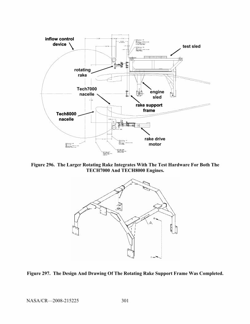
301

inflow control

device

Tech7000 nacelle

Tech8000 nacelle

rotating rake

rake support frame

rake drive motor

test sled

engine sled

inflow control device

Tech7000 nacelle

Tech8000 nacelle

rotating rake

rake support frame

rake drive motor

test sled

engine sled

Figure 296. The Larger Rotating Rake Integrates With The Test Hardware For Both The TECH7000 And TECH8000 Engines.

Figure 297. The Design And Drawing Of The Rotating Rake Support Frame Was Completed.

NASA/CR—2008-215225

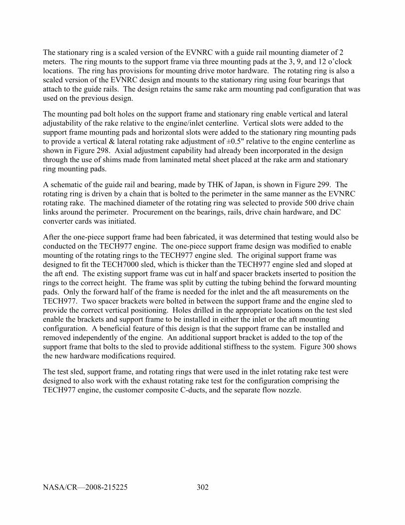
302

The stationary ring is a scaled version of the EVNRC with a guide rail mounting diameter of 2 meters. The ring mounts to the support frame via three mounting pads at the 3, 9, and 12 o’clock locations. The ring has provisions for mounting drive motor hardware. The rotating ring is also a scaled version of the EVNRC design and mounts to the stationary ring using four bearings that attach to the guide rails. The design retains the same rake arm mounting pad configuration that was used on the previous design.

The mounting pad bolt holes on the support frame and stationary ring enable vertical and lateral adjustability of the rake relative to the engine/inlet centerline. Vertical slots were added to the support frame mounting pads and horizontal slots were added to the stationary ring mounting pads to provide a vertical & lateral rotating rake adjustment of ±0.5" relative to the engine centerline as shown in Figure 298. Axial adjustment capability had already been incorporated in the design through the use of shims made from laminated metal sheet placed at the rake arm and stationary ring mounting pads.

A schematic of the guide rail and bearing, made by THK of Japan, is shown in Figure 299. The rotating ring is driven by a chain that is bolted to the perimeter in the same manner as the EVNRC rotating rake. The machined diameter of the rotating ring was selected to provide 500 drive chain links around the perimeter. Procurement on the bearings, rails, drive chain hardware, and DC converter cards was initiated.

After the one-piece support frame had been fabricated, it was determined that testing would also be conducted on the TECH977 engine. The one-piece support frame design was modified to enable mounting of the rotating rings to the TECH977 engine sled. The original support frame was designed to fit the TECH7000 sled, which is thicker than the TECH977 engine sled and sloped at the aft end. The existing support frame was cut in half and spacer brackets inserted to position the rings to the correct height. The frame was split by cutting the tubing behind the forward mounting pads. Only the forward half of the frame is needed for the inlet and the aft measurements on the TECH977. Two spacer brackets were bolted in between the support frame and the engine sled to provide the correct vertical positioning. Holes drilled in the appropriate locations on the test sled enable the brackets and support frame to be installed in either the inlet or the aft mounting configuration. A beneficial feature of this design is that the support frame can be installed and removed independently of the engine. An additional support bracket is added to the top of the support frame that bolts to the sled to provide additional stiffness to the system. Figure 300 shows the new hardware modifications required.

The test sled, support frame, and rotating rings that were used in the inlet rotating rake test were designed to also work with the exhaust rotating rake test for the configuration comprising the TECH977 engine, the customer composite C-ducts, and the separate flow nozzle.

NASA/CR—2008-215225

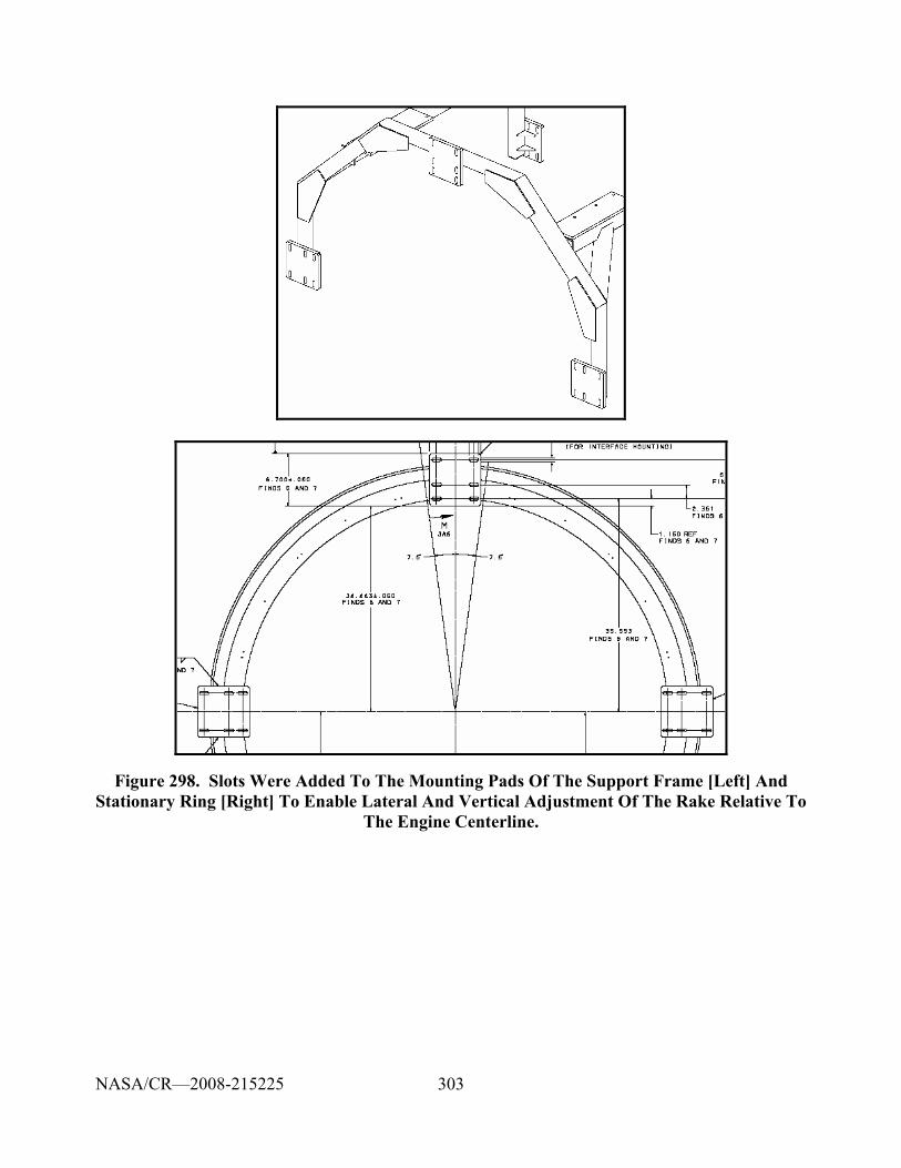
303

Figure 298. Slots Were Added To The Mounting Pads Of The Support Frame [Left] And Stationary Ring [Right] To Enable Lateral And Vertical Adjustment Of The Rake Relative To

The Engine Centerline.

NASA/CR—2008-215225

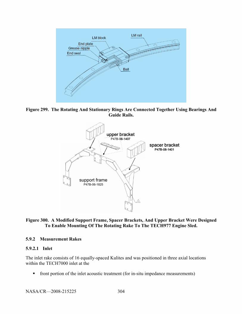
304

Figure 299. The Rotating And Stationary Rings Are Connected Together Using Bearings And Guide Rails.

support frameP47B-06-1825

spacer bracketP47B-08-1401

upper bracketP47B-08-1407

support frameP47B-06-1825

spacer bracketP47B-08-1401

upper bracketP47B-08-1407

Figure 300. A Modified Support Frame, Spacer Brackets, And Upper Bracket Were Designed To Enable Mounting Of The Rotating Rake To The TECH977 Engine Sled.

5.9.2 Measurement Rakes

5.9.2.1 Inlet

The inlet rake consists of 16 equally-spaced Kulites and was positioned in three axial locations within the TECH7000 inlet at the

front portion of the inlet acoustic treatment (for in-situ impedance measurements)

NASA/CR—2008-215225

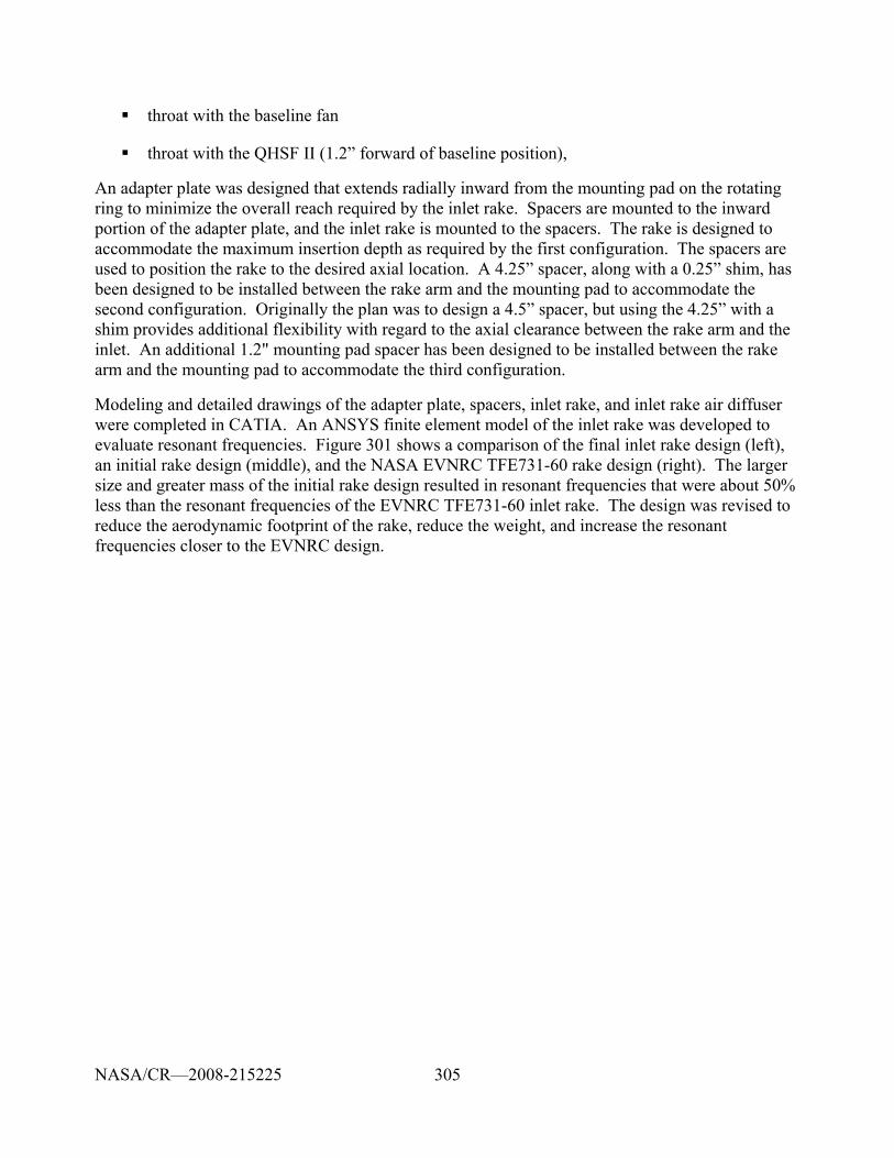
305

throat with the baseline fan

throat with the QHSF II (1.2” forward of baseline position),

An adapter plate was designed that extends radially inward from the mounting pad on the rotating ring to minimize the overall reach required by the inlet rake. Spacers are mounted to the inward portion of the adapter plate, and the inlet rake is mounted to the spacers. The rake is designed to accommodate the maximum insertion depth as required by the first configuration. The spacers are used to position the rake to the desired axial location. A 4.25” spacer, along with a 0.25” shim, has been designed to be installed between the rake arm and the mounting pad to accommodate the second configuration. Originally the plan was to design a 4.5” spacer, but using the 4.25” with a shim provides additional flexibility with regard to the axial clearance between the rake arm and the inlet. An additional 1.2" mounting pad spacer has been designed to be installed between the rake arm and the mounting pad to accommodate the third configuration.

Modeling and detailed drawings of the adapter plate, spacers, inlet rake, and inlet rake air diffuser were completed in CATIA. An ANSYS finite element model of the inlet rake was developed to evaluate resonant frequencies. Figure 301 shows a comparison of the final inlet rake design (left), an initial rake design (middle), and the NASA EVNRC TFE731-60 rake design (right). The larger size and greater mass of the initial rake design resulted in resonant frequencies that were about 50% less than the resonant frequencies of the EVNRC TFE731-60 inlet rake. The design was revised to reduce the aerodynamic footprint of the rake, reduce the weight, and increase the resonant frequencies closer to the EVNRC design.

NASA/CR—2008-215225

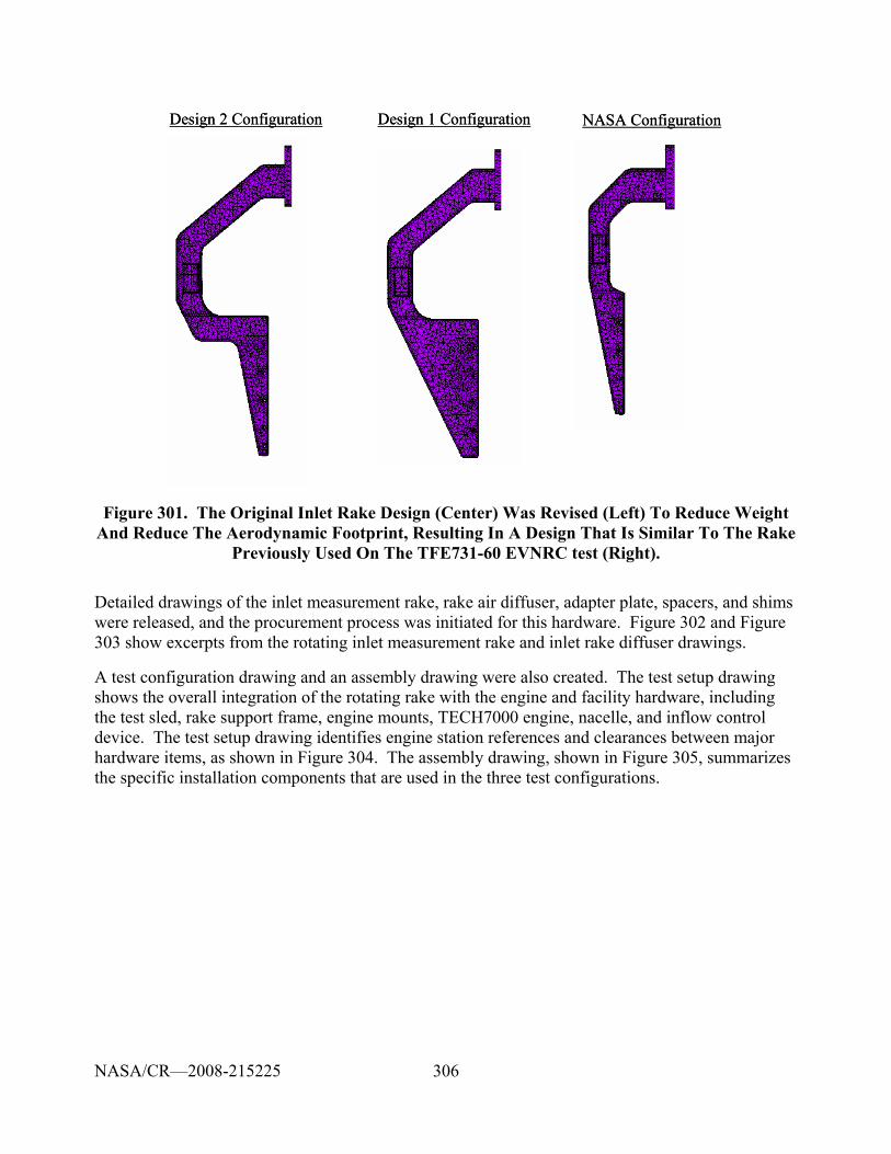
306

Design 2 Configuration NASA ConfigurationDesign 1 ConfigurationDesign 2 Configuration NASA ConfigurationDesign 1 Configuration

Figure 301. The Original Inlet Rake Design (Center) Was Revised (Left) To Reduce Weight And Reduce The Aerodynamic Footprint, Resulting In A Design That Is Similar To The Rake

Previously Used On The TFE731-60 EVNRC test (Right).

Detailed drawings of the inlet measurement rake, rake air diffuser, adapter plate, spacers, and shims were released, and the procurement process was initiated for this hardware. Figure 302 and Figure 303 show excerpts from the rotating inlet measurement rake and inlet rake diffuser drawings.

A test configuration drawing and an assembly drawing were also created. The test setup drawing shows the overall integration of the rotating rake with the engine and facility hardware, including the test sled, rake support frame, engine mounts, TECH7000 engine, nacelle, and inflow control device. The test setup drawing identifies engine station references and clearances between major hardware items, as shown in Figure 304. The assembly drawing, shown in Figure 305, summarizes the specific installation components that are used in the three test configurations.

NASA/CR—2008-215225

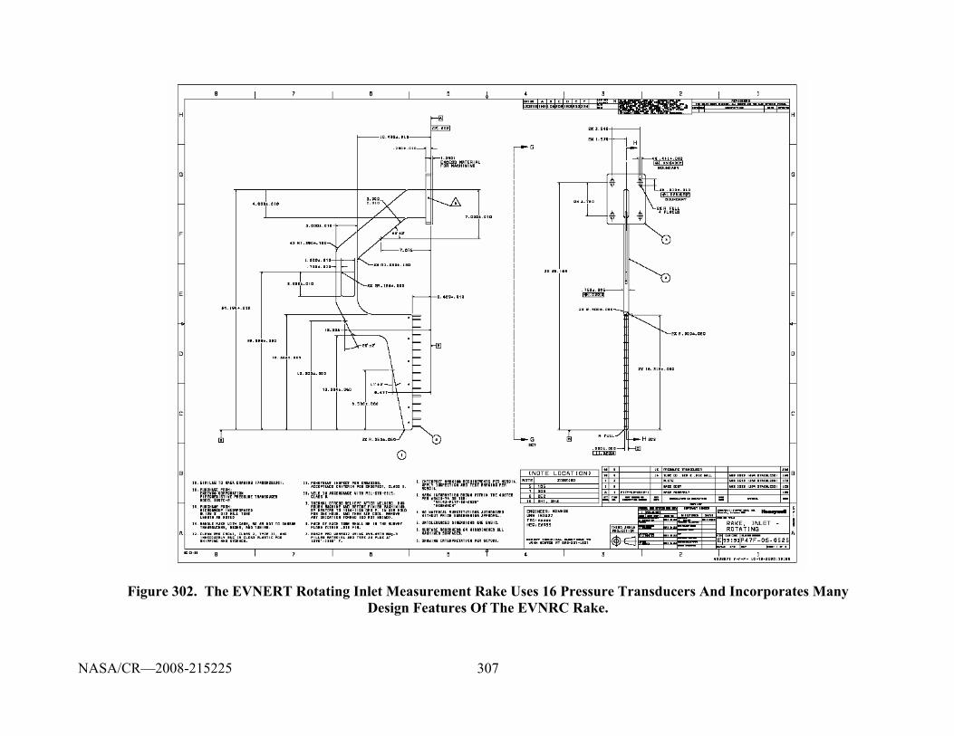
307

Figure 302. The EVNERT Rotating Inlet Measurement Rake Uses 16 Pressure Transducers And Incorporates Many Design Features Of The EVNRC Rake.

NASA/CR—2008-215225

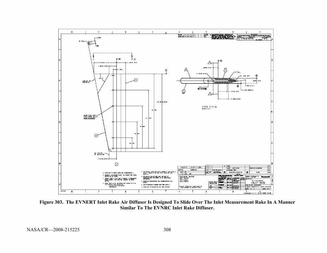
308

Figure 303. The EVNERT Inlet Rake Air Diffuser Is Designed To Slide Over The Inlet Measurement Rake In A Manner Similar To The EVNRC Inlet Rake Diffuser.

NASA/CR—2008-215225

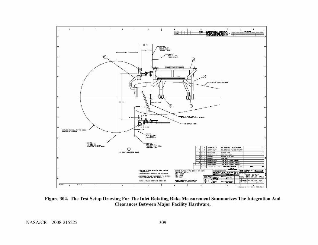
309

Figure 304. The Test Setup Drawing For The Inlet Rotating Rake Measurement Summarizes The Integration And Clearances Between Major Facility Hardware.

NASA/CR—2008-215225

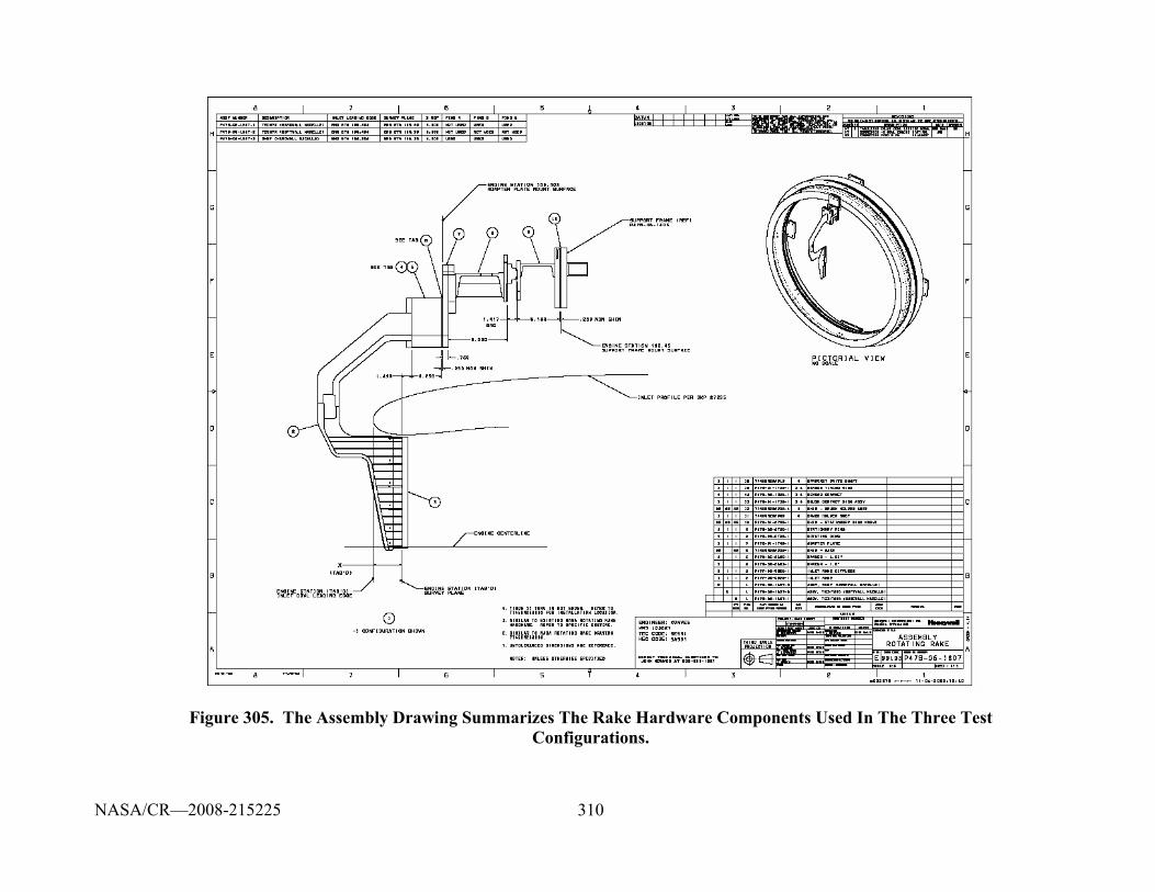
310

Figure 305. The Assembly Drawing Summarizes The Rake Hardware Components Used In The Three Test Configurations.

NASA/CR—2008-215225

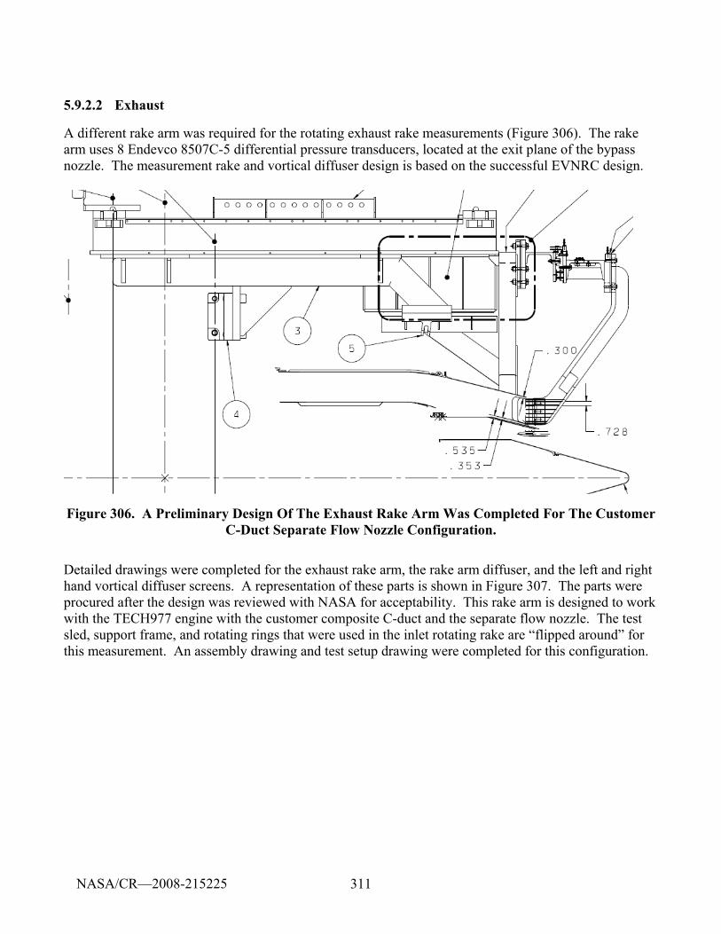
311

5.9.2.2 Exhaust

A different rake arm was required for the rotating exhaust rake measurements (Figure 306). The rake arm uses 8 Endevco 8507C-5 differential pressure transducers, located at the exit plane of the bypass nozzle. The measurement rake and vortical diffuser design is based on the successful EVNRC design.

Figure 306. A Preliminary Design Of The Exhaust Rake Arm Was Completed For The Customer C-Duct Separate Flow Nozzle Configuration.

Detailed drawings were completed for the exhaust rake arm, the rake arm diffuser, and the left and right hand vortical diffuser screens. A representation of these parts is shown in Figure 307. The parts were procured after the design was reviewed with NASA for acceptability. This rake arm is designed to work with the TECH977 engine with the customer composite C-duct and the separate flow nozzle. The test sled, support frame, and rotating rings that were used in the inlet rotating rake are “flipped around” for this measurement. An assembly drawing and test setup drawing were completed for this configuration.

NASA/CR—2008-215225

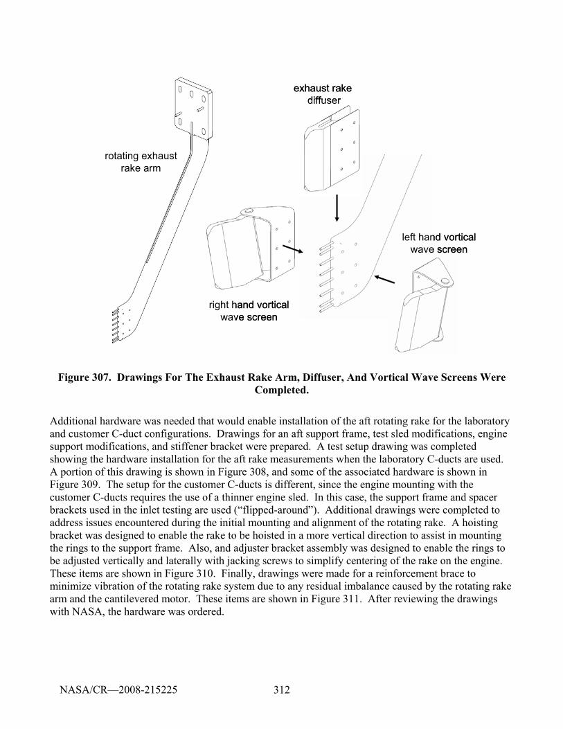
312

rotating exhaustrake arm

exhaust rake diffuser

right hand vorticalwave screen

left hand vorticalwave screen

rotating exhaustrake arm

exhaust rake diffuser

right hand vorticalwave screen

left hand vorticalwave screen

Figure 307. Drawings For The Exhaust Rake Arm, Diffuser, And Vortical Wave Screens Were Completed.

Additional hardware was needed that would enable installation of the aft rotating rake for the laboratory and customer C-duct configurations. Drawings for an aft support frame, test sled modifications, engine support modifications, and stiffener bracket were prepared. A test setup drawing was completed showing the hardware installation for the aft rake measurements when the laboratory C-ducts are used. A portion of this drawing is shown in Figure 308, and some of the associated hardware is shown in Figure 309. The setup for the customer C-ducts is different, since the engine mounting with the customer C-ducts requires the use of a thinner engine sled. In this case, the support frame and spacer brackets used in the inlet testing are used (“flipped-around”). Additional drawings were completed to address issues encountered during the initial mounting and alignment of the rotating rake. A hoisting bracket was designed to enable the rake to be hoisted in a more vertical direction to assist in mounting the rings to the support frame. Also, and adjuster bracket assembly was designed to enable the rings to be adjusted vertically and laterally with jacking screws to simplify centering of the rake on the engine. These items are shown in Figure 310. Finally, drawings were made for a reinforcement brace to minimize vibration of the rotating rake system due to any residual imbalance caused by the rotating rake arm and the cantilevered motor. These items are shown in Figure 311. After reviewing the drawings with NASA, the hardware was ordered.

NASA/CR—2008-215225

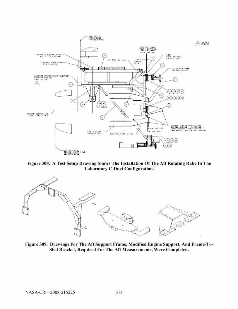
313

Figure 308. A Test Setup Drawing Shows The Installation Of The Aft Rotating Rake In The Laboratory C-Duct Configuration.

Figure 309. Drawings For The Aft Support Frame, Modified Engine Support, And Frame-To-Sled Bracket, Required For The Aft Measurements, Were Completed.

NASA/CR—2008-215225

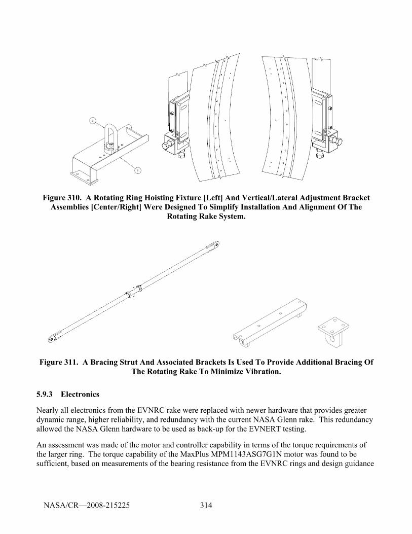
314

Figure 310. A Rotating Ring Hoisting Fixture [Left] And Vertical/Lateral Adjustment Bracket Assemblies [Center/Right] Were Designed To Simplify Installation And Alignment Of The

Rotating Rake System.

Figure 311. A Bracing Strut And Associated Brackets Is Used To Provide Additional Bracing Of The Rotating Rake To Minimize Vibration.

5.9.3 Electronics

Nearly all electronics from the EVNRC rake were replaced with newer hardware that provides greater dynamic range, higher reliability, and redundancy with the current NASA Glenn rake. This redundancy allowed the NASA Glenn hardware to be used as back-up for the EVNERT testing.

An assessment was made of the motor and controller capability in terms of the torque requirements of the larger ring. The torque capability of the MaxPlus MPM1143ASG7G1N motor was found to be sufficient, based on measurements of the bearing resistance from the EVNRC rings and design guidance

NASA/CR—2008-215225

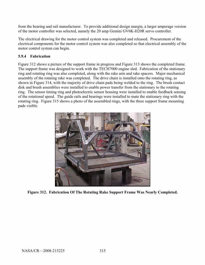
315

from the bearing and rail manufacturer. To provide additional design margin, a larger amperage version of the motor controller was selected, namely the 20 amp Gemini GV6K-H20R servo controller.

The electrical drawing for the motor control system was completed and released. Procurement of the electrical components for the motor control system was also completed so that electrical assembly of the motor control system can begin.

5.9.4 Fabrication

Figure 312 shows a picture of the support frame in progress and Figure 313 shows the completed frame. The support frame was designed to work with the TECH7000 engine sled. Fabrication of the stationary ring and rotating ring was also completed, along with the rake arm and rake spacers. Major mechanical assembly of the rotating rake was completed. The drive chain is installed onto the rotating ring, as shown in Figure 314, with the majority of drive chain pads being welded to the ring. The brush contact disk and brush assemblies were installed to enable power transfer from the stationary to the rotating ring. The sensor timing ring and photoelectric sensor housing were installed to enable feedback sensing of the rotational speed. The guide rails and bearings were installed to mate the stationary ring with the rotating ring. Figure 315 shows a photo of the assembled rings, with the three support frame mounting pads visible.

Figure 312. Fabrication Of The Rotating Rake Support Frame Was Nearly Completed.

NASA/CR—2008-215225

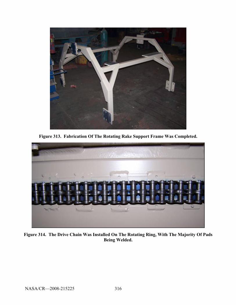
316

Figure 313. Fabrication Of The Rotating Rake Support Frame Was Completed.

Figure 314. The Drive Chain Was Installed On The Rotating Ring, With The Majority Of Pads Being Welded.

NASA/CR—2008-215225

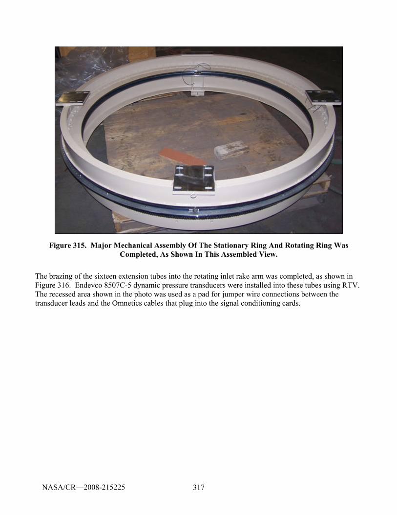
317

Figure 315. Major Mechanical Assembly Of The Stationary Ring And Rotating Ring Was Completed, As Shown In This Assembled View.

The brazing of the sixteen extension tubes into the rotating inlet rake arm was completed, as shown in Figure 316. Endevco 8507C-5 dynamic pressure transducers were installed into these tubes using RTV. The recessed area shown in the photo was used as a pad for jumper wire connections between the transducer leads and the Omnetics cables that plug into the signal conditioning cards.

NASA/CR—2008-215225

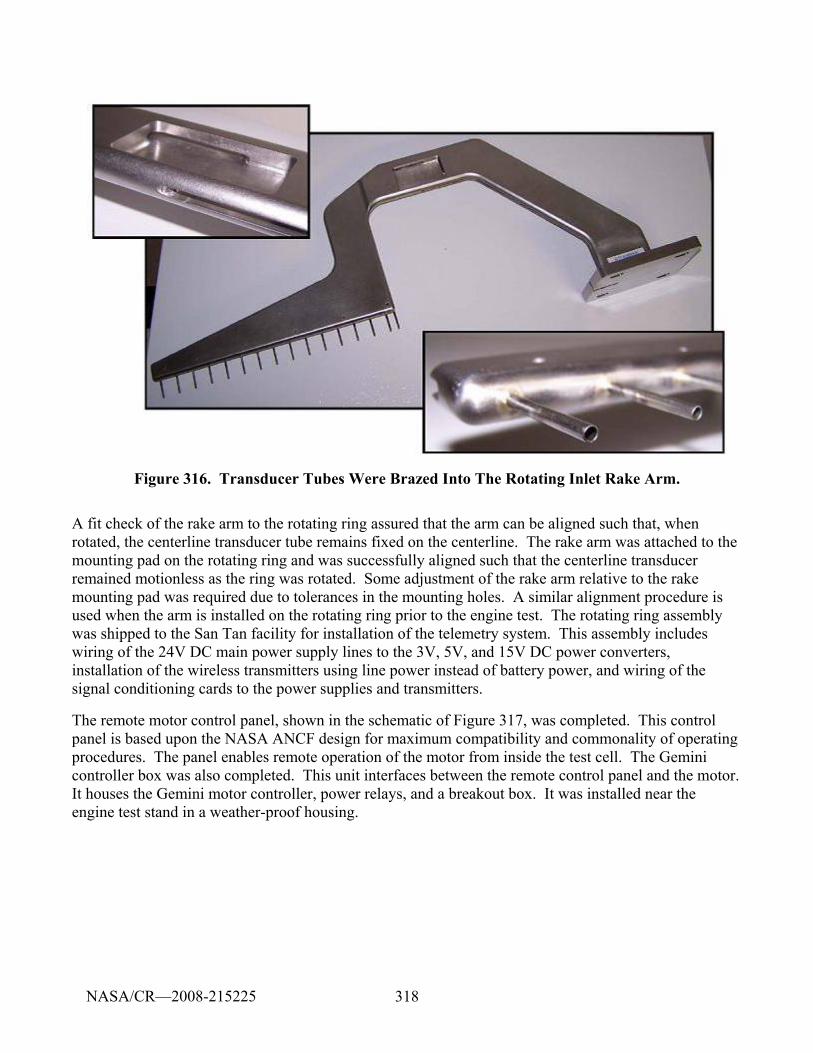
318

Figure 316. Transducer Tubes Were Brazed Into The Rotating Inlet Rake Arm.

A fit check of the rake arm to the rotating ring assured that the arm can be aligned such that, when rotated, the centerline transducer tube remains fixed on the centerline. The rake arm was attached to the mounting pad on the rotating ring and was successfully aligned such that the centerline transducer remained motionless as the ring was rotated. Some adjustment of the rake arm relative to the rake mounting pad was required due to tolerances in the mounting holes. A similar alignment procedure is used when the arm is installed on the rotating ring prior to the engine test. The rotating ring assembly was shipped to the San Tan facility for installation of the telemetry system. This assembly includes wiring of the 24V DC main power supply lines to the 3V, 5V, and 15V DC power converters, installation of the wireless transmitters using line power instead of battery power, and wiring of the signal conditioning cards to the power supplies and transmitters.

The remote motor control panel, shown in the schematic of Figure 317, was completed. This control panel is based upon the NASA ANCF design for maximum compatibility and commonality of operating procedures. The panel enables remote operation of the motor from inside the test cell. The Gemini controller box was also completed. This unit interfaces between the remote control panel and the motor. It houses the Gemini motor controller, power relays, and a breakout box. It was installed near the engine test stand in a weather-proof housing.

NASA/CR—2008-215225

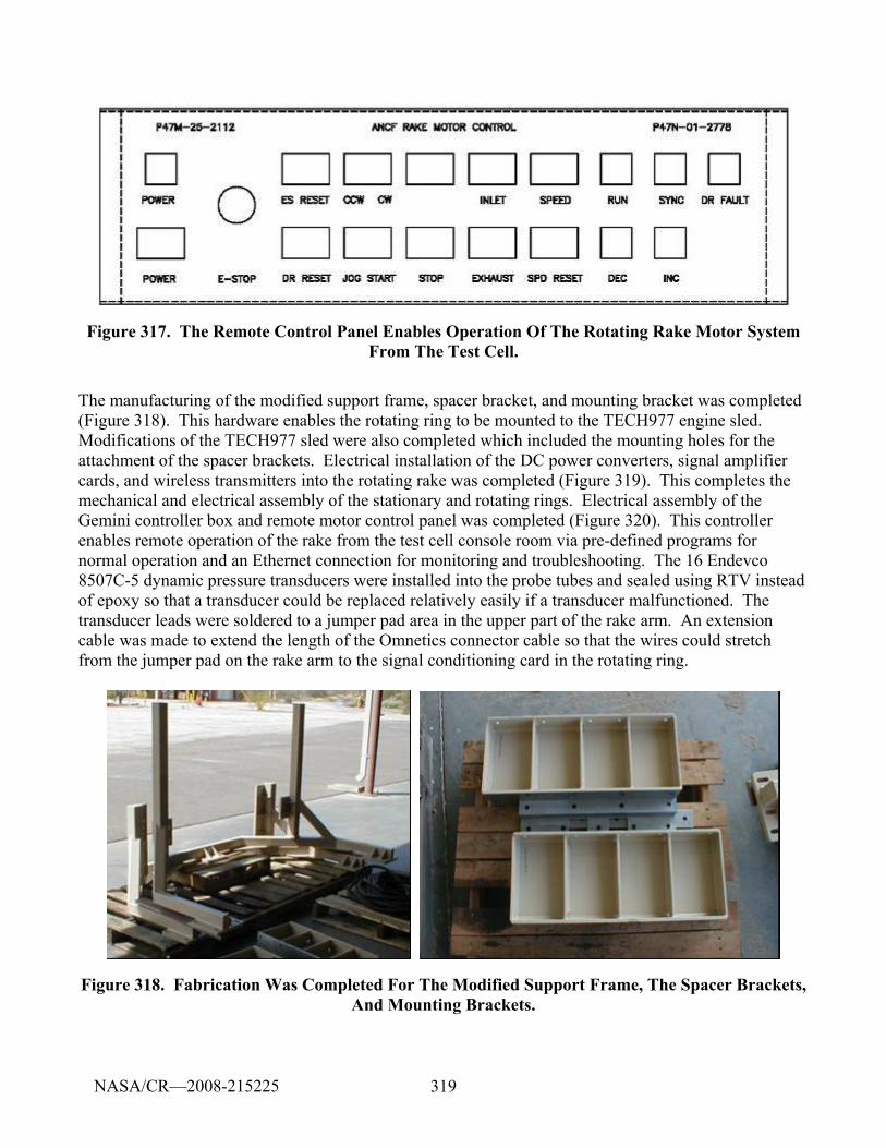
319

Figure 317. The Remote Control Panel Enables Operation Of The Rotating Rake Motor System From The Test Cell.

The manufacturing of the modified support frame, spacer bracket, and mounting bracket was completed (Figure 318). This hardware enables the rotating ring to be mounted to the TECH977 engine sled. Modifications of the TECH977 sled were also completed which included the mounting holes for the attachment of the spacer brackets. Electrical installation of the DC power converters, signal amplifier cards, and wireless transmitters into the rotating rake was completed (Figure 319). This completes the mechanical and electrical assembly of the stationary and rotating rings. Electrical assembly of the Gemini controller box and remote motor control panel was completed (Figure 320). This controller enables remote operation of the rake from the test cell console room via pre-defined programs for normal operation and an Ethernet connection for monitoring and troubleshooting. The 16 Endevco 8507C-5 dynamic pressure transducers were installed into the probe tubes and sealed using RTV instead of epoxy so that a transducer could be replaced relatively easily if a transducer malfunctioned. The transducer leads were soldered to a jumper pad area in the upper part of the rake arm. An extension cable was made to extend the length of the Omnetics connector cable so that the wires could stretch from the jumper pad on the rake arm to the signal conditioning card in the rotating ring.

Figure 318. Fabrication Was Completed For The Modified Support Frame, The Spacer Brackets, And Mounting Brackets.

NASA/CR—2008-215225

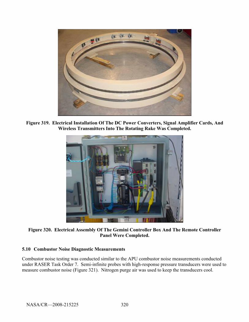
320

Figure 319. Electrical Installation Of The DC Power Converters, Signal Amplifier Cards, And Wireless Transmitters Into The Rotating Rake Was Completed.

Figure 320. Electrical Assembly Of The Gemini Controller Box And The Remote Controller Panel Were Completed.

5.10 Combustor Noise Diagnostic Measurements

Combustor noise testing was conducted similar to the APU combustor noise measurements conducted under RASER Task Order 7. Semi-infinite probes with high-response pressure transducers were used to measure combustor noise (Figure 321). Nitrogen purge air was used to keep the transducers cool.

NASA/CR—2008-215225

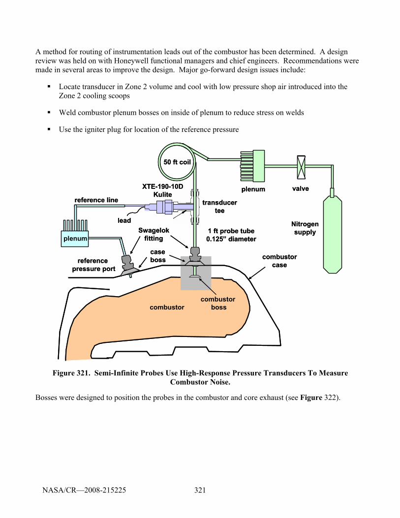
321

A method for routing of instrumentation leads out of the combustor has been determined. A design review was held on with Honeywell functional managers and chief engineers. Recommendations were made in several areas to improve the design. Major go-forward design issues include:

Locate transducer in Zone 2 volume and cool with low pressure shop air introduced into the Zone 2 cooling scoops

Weld combustor plenum bosses on inside of plenum to reduce stress on welds

Use the igniter plug for location of the reference pressure

Figure 321. Semi-Infinite Probes Use High-Response Pressure Transducers To Measure Combustor Noise.

Bosses were designed to position the probes in the combustor and core exhaust (see Figure 322).

50 ft coil

combustor

Swagelokfitting

transducertee

1 ft probe tube0.125” diameter

combustorcase

caseboss

combustorboss

reference line

XTE-190-10DKulite

plenum

reference pressure port

Nitrogensupply

valve

lead

plenum

50 ft coil

combustor

Swagelokfitting

transducertee

1 ft probe tube0.125” diameter

combustorcase

caseboss

combustorboss

reference line

XTE-190-10DKulite

plenum

reference pressure port

Nitrogensupply

valve

lead

plenum

NASA/CR—2008-215225

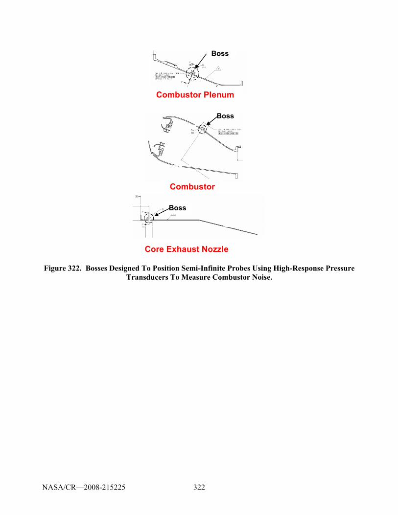
322

Combustor Plenum

Combustor

Core Exhaust Nozzle

Boss

Boss

Boss

Combustor Plenum

Combustor

Core Exhaust Nozzle

Boss

Boss

Boss

Figure 322. Bosses Designed To Position Semi-Infinite Probes Using High-Response Pressure Transducers To Measure Combustor Noise.

NASA/CR—2008-215225

323

6. MEASUREMENT RESULTS

Table 25 to Table 27 show the configurations tested during 2005, 2006, and 2007, respectively.

NASA/CR—2008-215225

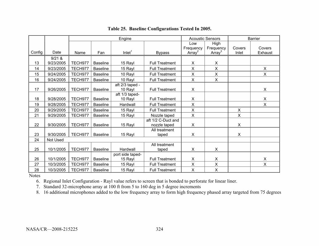
324

Table 25. Baseline Configurations Tested In 2005.

Engine Acoustic Sensors Barrier

Config Date Name Fan Inlet1 Bypass

Low Frequency

Array2

High Frequency

Array3 Covers

Inlet Covers Exhaust

13 9/21 &

9/23/2005 TECH977 Baseline 15 Rayl Full Treatment X X 14 9/23/2005 TECH977 Baseline 15 Rayl Full Treatment X X X 15 9/24/2005 TECH977 Baseline 10 Rayl Full Treatment X X X 16 9/24/2005 TECH977 Baseline 10 Rayl Full Treatment X X

17 9/26/2005 TECH977 Baselineaft 2/3 taped -

10 Rayl Full Treatment X X

18 9/28/2005 TECH977 Baselineaft 1/3 taped-

10 Rayl Full Treatment X X 19 9/28/2005 TECH977 Baseline Hardwall Full Treatment X X 20 9/29/2005 TECH977 Baseline 15 Rayl Full Treatment X X 21 9/29/2005 TECH977 Baseline 15 Rayl Nozzle taped X X

22 9/30/2005 TECH977 Baseline 15 Rayl aft 1/2 C-Duct and

nozzle taped X X

23 9/30/2005 TECH977 Baseline 15 Rayl All treatment

taped X X 24 Not Used

25 10/1/2005 TECH977 Baseline Hardwall All treatment

taped X X

26 10/1/2005 TECH977 Baselineport side taped-

15 Rayl Full Treatment X X X 27 10/3/2005 TECH977 Baseline 15 Rayl Full Treatment X X X 28 10/3/2005 TECH977 Baseline 15 Rayl Full Treatment X X

Notes 6. Regional Inlet Configuration - Rayl value refers to screen that is bonded to perforate for linear liner. 7. Standard 32-microphone array at 100 ft from 5 to 160 deg in 5 degree increments 8. 16 additional microphones added to the low frequency array to form high frequency phased array targeted from 75 degrees

NASA/CR—2008-215225

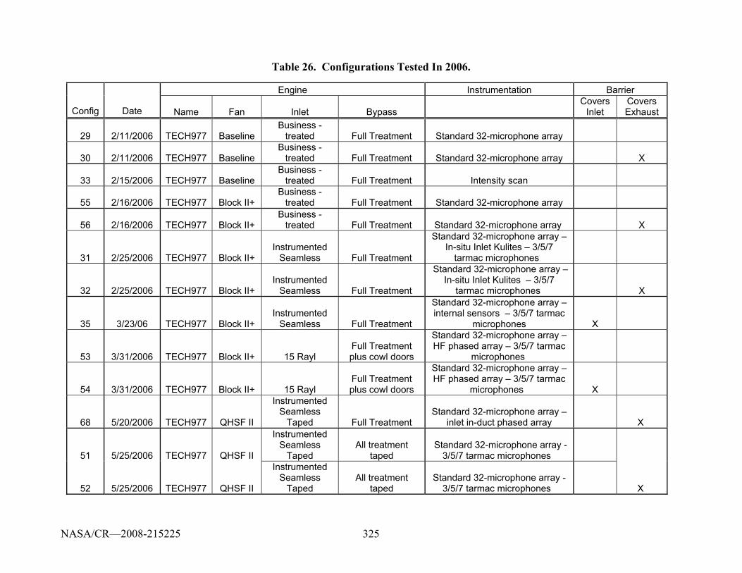
325

Table 26. Configurations Tested In 2006.

Engine Instrumentation Barrier

Config Date Name Fan Inlet Bypass Covers


29 2/11/2006 TECH977 Baseline Business -

treated Full Treatment Standard 32-microphone array


treated Full Treatment Standard 32-microphone array X


treated Full Treatment Intensity scan

55 2/16/2006 TECH977 Block II+ Business -

treated Full Treatment Standard 32-microphone array

56 2/16/2006 TECH977 Block II+ Business -

treated Full Treatment Standard 32-microphone array X

31 2/25/2006 TECH977 Block II+ Instrumented

Seamless Full Treatment

Standard 32-microphone array – In-situ Inlet Kulites – 3/5/7

tarmac microphones



Standard 32-microphone array – In-situ Inlet Kulites – 3/5/7

tarmac microphones X



Standard 32-microphone array – internal sensors – 3/5/7 tarmac

microphones X

53 3/31/2006 TECH977 Block II+ 15 Rayl Full Treatment plus cowl doors

Standard 32-microphone array – HF phased array – 3/5/7 tarmac

microphones

54 3/31/2006 TECH977 Block II+ 15 Rayl Full Treatment plus cowl doors

Standard 32-microphone array – HF phased array – 3/5/7 tarmac

microphones X

68 5/20/2006 TECH977 QHSF II

Instrumented Seamless

Taped Full Treatment Standard 32-microphone array –

inlet in-duct phased array X

51 5/25/2006 TECH977 QHSF II


Taped All treatment

taped Standard 32-microphone array -

3/5/7 tarmac microphones

52 5/25/2006 TECH977 QHSF II


Taped All treatment

taped Standard 32-microphone array -

3/5/7 tarmac microphones X

NASA/CR—2008-215225

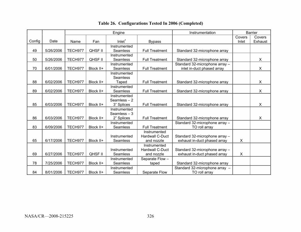
326

Table 26. Configurations Tested In 2006 (Completed)


Config Date Name Fan Inlet1 Bypass Covers


49 5/26/2006 TECH977 QHSF II Instrumented

Seamless Full Treatment Standard 32-microphone array


Seamless Full Treatment Standard 32-microphone array X


Seamless Full Treatment Standard 32-microphone array –

inlet in-duct phased array X

88 6/02/2006 TECH977 Block II+


Taped Full Treatment Standard 32-microphone array X


Seamless Full Treatment Standard 32-microphone array X

85 6/03/2006 TECH977 Block II+

Instrumented Seamless – 2

3” Splices Full Treatment Standard 32-microphone array X

86 6/03/2006 TECH977 Block II+


2” Splices Full Treatment Standard 32-microphone array X


Seamless Full Treatment Standard 32-microphone array –

TO roll array


Seamless

Instrumented Hardwall C-Duct

and nozzle Standard 32-microphone array –

exhaust in-duct phased array X


Seamless

Instrumented Hardwall C-Duct

and nozzle Standard 32-microphone array –

exhaust in-duct phased array X


Seamless Separate Flow –

taped Standard 32-microphone array


Seamless Separate Flow Standard 32-microphone array –

TO roll array

NASA/CR—2008-215225

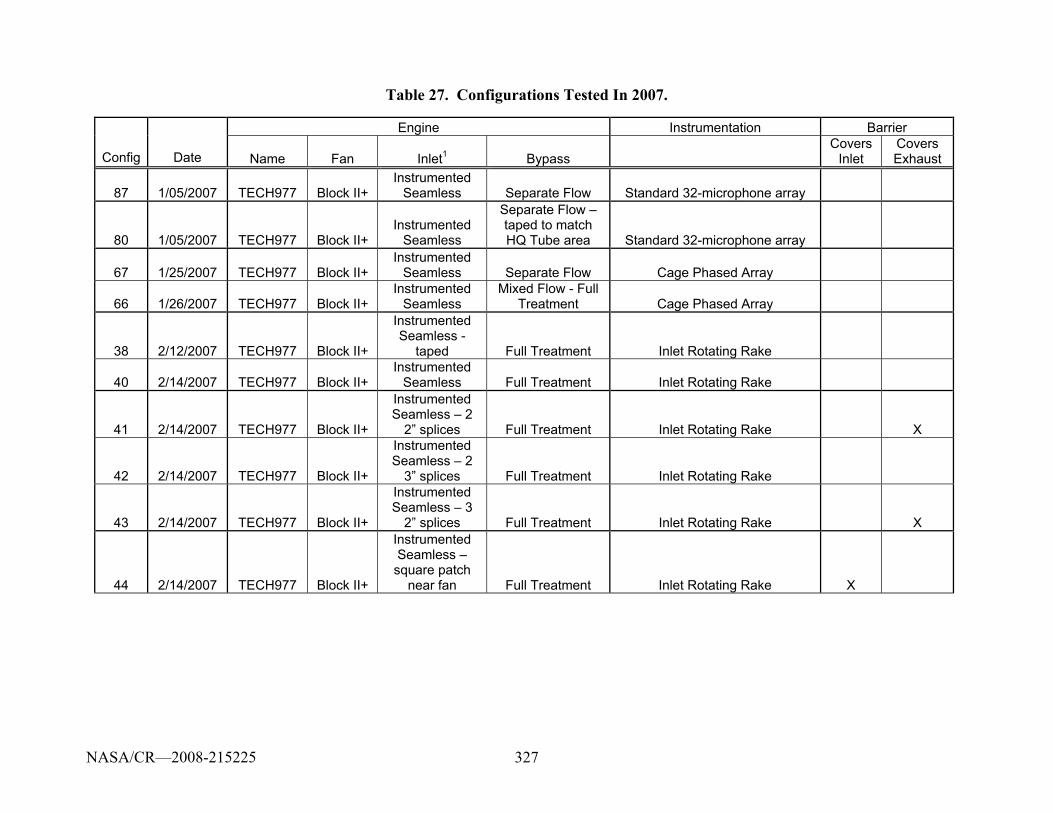
327

Table 27. Configurations Tested In 2007.





Seamless Separate Flow Standard 32-microphone array


Seamless

Separate Flow – taped to match HQ Tube area Standard 32-microphone array


Seamless Separate Flow Cage Phased Array


Seamless Mixed Flow - Full

Treatment Cage Phased Array

38 2/12/2007 TECH977 Block II+

Instrumented Seamless -

taped Full Treatment Inlet Rotating Rake


Seamless Full Treatment Inlet Rotating Rake

41 2/14/2007 TECH977 Block II+


2” splices Full Treatment Inlet Rotating Rake X

42 2/14/2007 TECH977 Block II+


3” splices Full Treatment Inlet Rotating Rake

43 2/14/2007 TECH977 Block II+


2” splices Full Treatment Inlet Rotating Rake X

44 2/14/2007 TECH977 Block II+

Instrumented Seamless – square patch

near fan Full Treatment Inlet Rotating Rake X

NASA/CR—2008-215225

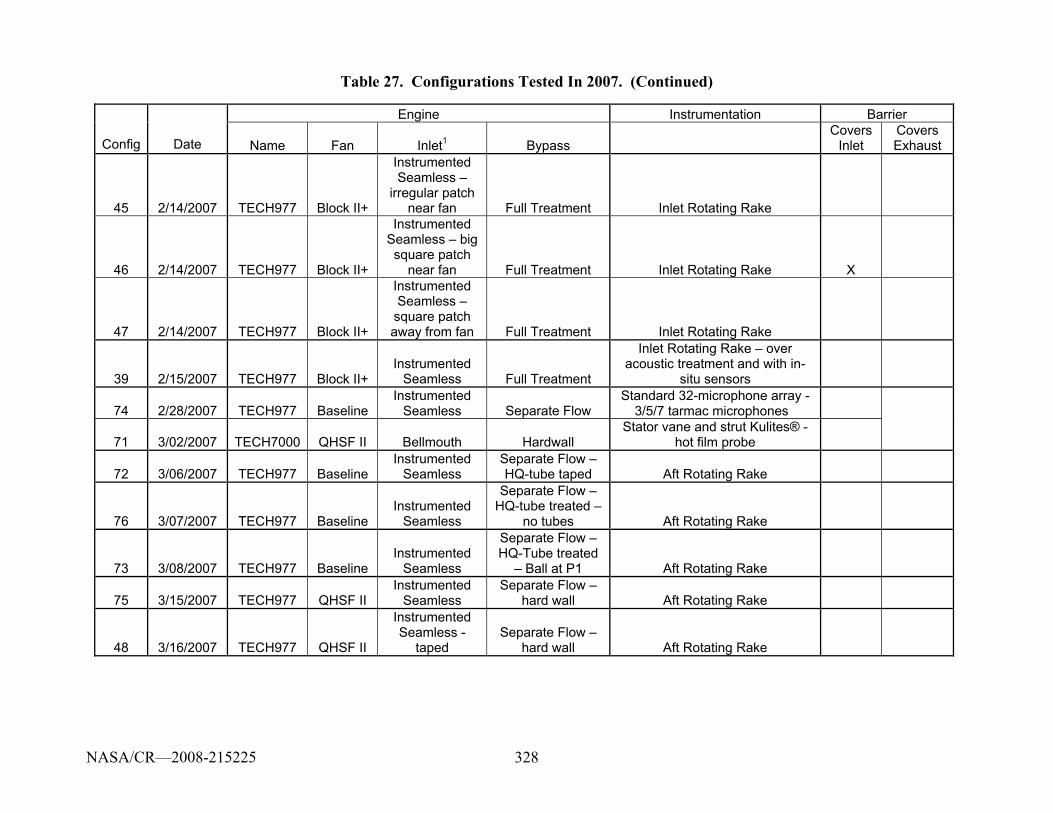
328

Table 27. Configurations Tested In 2007. (Continued)




45 2/14/2007 TECH977 Block II+

Instrumented Seamless –

irregular patch near fan Full Treatment Inlet Rotating Rake

46 2/14/2007 TECH977 Block II+

Instrumented Seamless – big square patch

near fan Full Treatment Inlet Rotating Rake X

47 2/14/2007 TECH977 Block II+

Instrumented Seamless – square patch away from fan Full Treatment Inlet Rotating Rake



Inlet Rotating Rake – over acoustic treatment and with in-

situ sensors

74 2/28/2007 TECH977 Baseline Instrumented

Seamless Separate Flow Standard 32-microphone array -

3/5/7 tarmac microphones

71 3/02/2007 TECH7000 QHSF II Bellmouth Hardwall Stator vane and strut Kulites® -

hot film probe


Seamless Separate Flow – HQ-tube taped Aft Rotating Rake


Seamless

Separate Flow – HQ-tube treated –

no tubes Aft Rotating Rake


Seamless

Separate Flow – HQ-Tube treated

– Ball at P1 Aft Rotating Rake


Seamless Separate Flow –

hard wall Aft Rotating Rake

48 3/16/2007 TECH977 QHSF II

Instrumented Seamless -

taped Separate Flow –

hard wall Aft Rotating Rake

NASA/CR—2008-215225

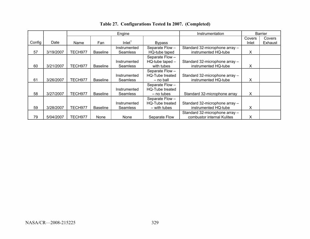
329

Table 27. Configurations Tested In 2007. (Completed)





Seamless Separate Flow – HQ-tube taped

Standard 32-microphone array – instrumented HQ-tube X


Seamless

Separate Flow – HQ-tube taped –

with tubes Standard 32-microphone array –

instrumented HQ-tube X


Seamless


– no ball Standard 32-microphone array –



Seamless


– no tubes Standard 32-microphone array X


Seamless


– with tubes Standard 32-microphone array –


79 5/04/2007 TECH977 None None Separate Flow Standard 32-microphone array –

combustor internal Kulites X

NASA/CR—2008-215225

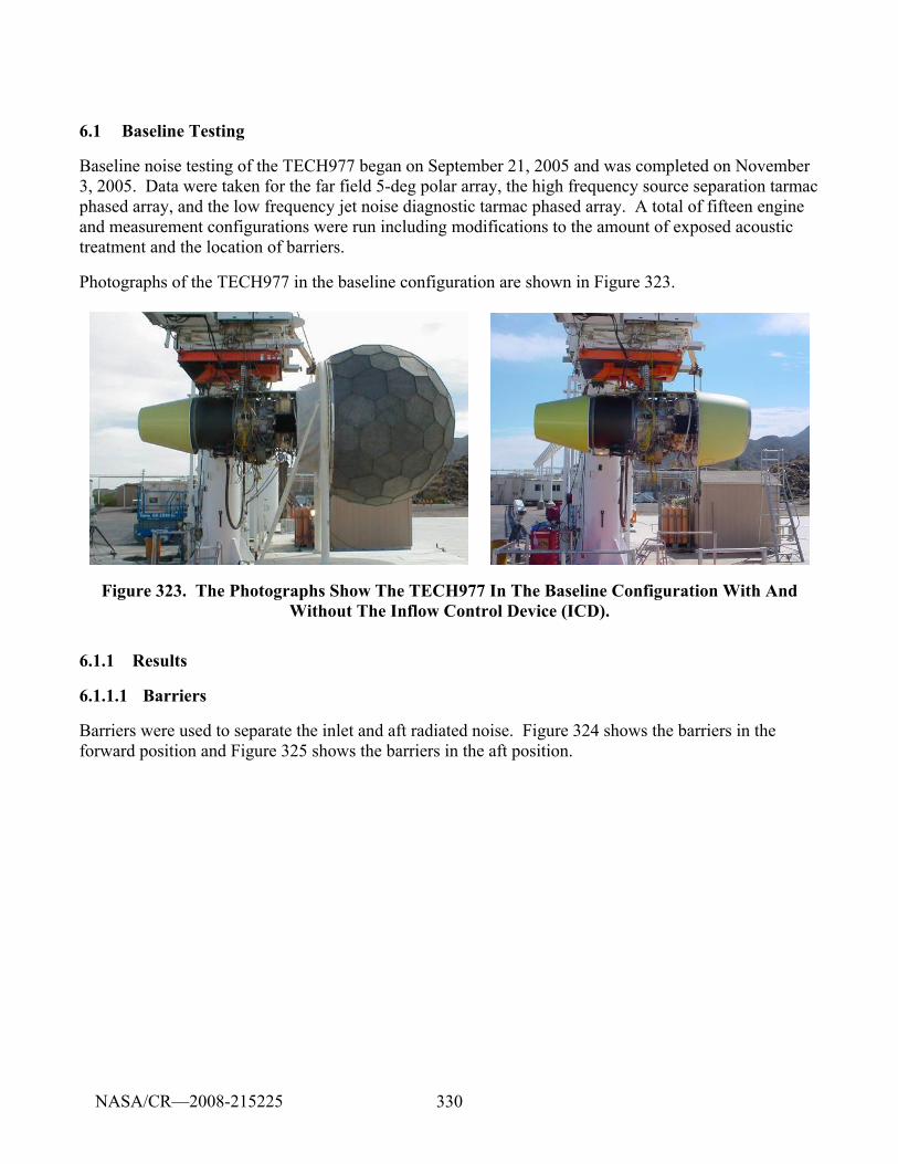
330

6.1 Baseline Testing

Baseline noise testing of the TECH977 began on September 21, 2005 and was completed on November 3, 2005. Data were taken for the far field 5-deg polar array, the high frequency source separation tarmac phased array, and the low frequency jet noise diagnostic tarmac phased array. A total of fifteen engine and measurement configurations were run including modifications to the amount of exposed acoustic treatment and the location of barriers.

Photographs of the TECH977 in the baseline configuration are shown in Figure 323.

Figure 323. The Photographs Show The TECH977 In The Baseline Configuration With And Without The Inflow Control Device (ICD).

6.1.1 Results

6.1.1.1 Barriers

Barriers were used to separate the inlet and aft radiated noise. Figure 324 shows the barriers in the forward position and Figure 325 shows the barriers in the aft position.

NASA/CR—2008-215225

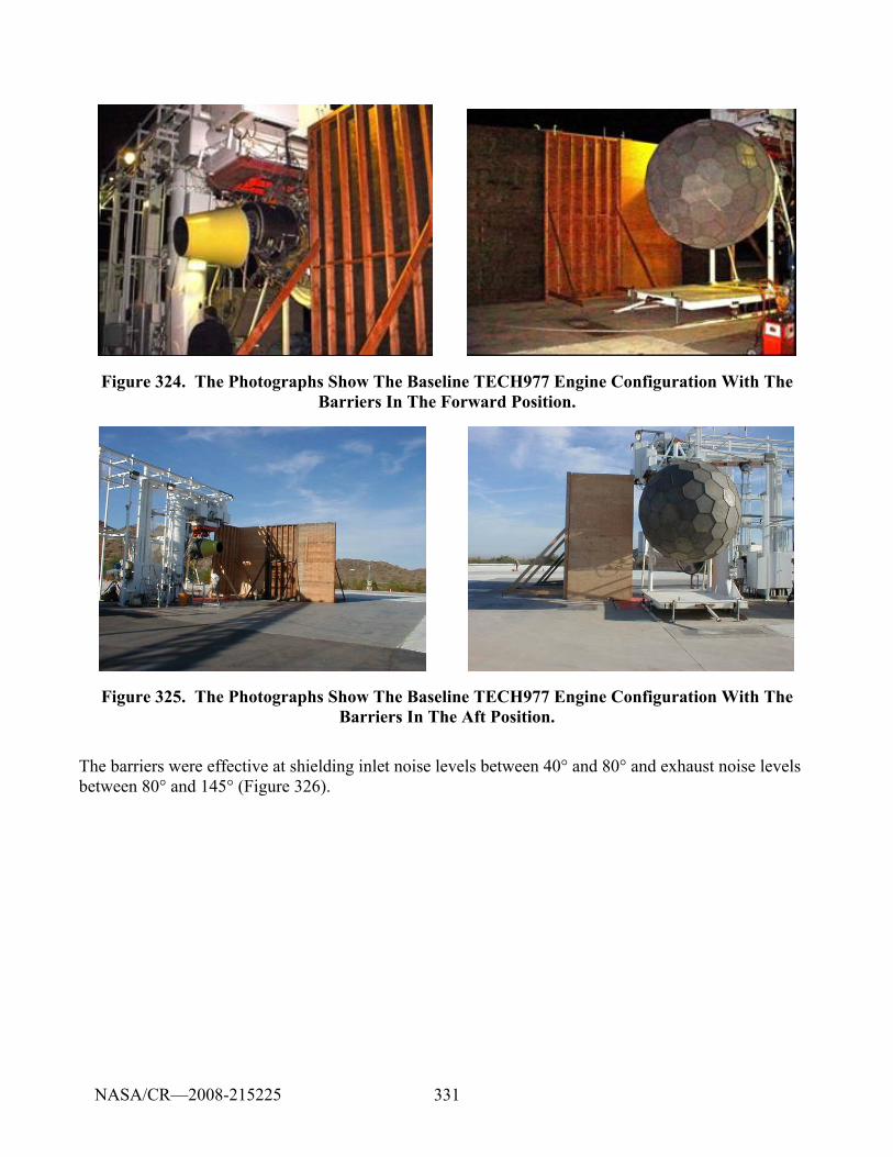
331

Figure 324. The Photographs Show The Baseline TECH977 Engine Configuration With The Barriers In The Forward Position.

Figure 325. The Photographs Show The Baseline TECH977 Engine Configuration With The Barriers In The Aft Position.

The barriers were effective at shielding inlet noise levels between 40° and 80° and exhaust noise levels between 80° and 145° (Figure 326).

NASA/CR—2008-215225

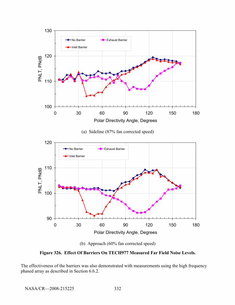
332

100

110

120

130

0 30 60 90 120 150 180Polar Directivity Angle, Degrees

PN

LT, P

NdB

No Barrier Exhaust Barrier

Inlet Barrier

(a) Sideline (87% fan corrected speed)

90

100

110

120

0 30 60 90 120 150 180Polar Directivity Angle, Degrees

PN

LT, P

NdB

No Barrier Exhaust Barrier

Inlet Barrier

(b) Approach (60% fan corrected speed)

Figure 326. Effect Of Barriers On TECH977 Measured Far Field Noise Levels.

The effectiveness of the barriers was also demonstrated with measurements using the high frequency phased array as described in Section 6.6.2.

NASA/CR—2008-215225

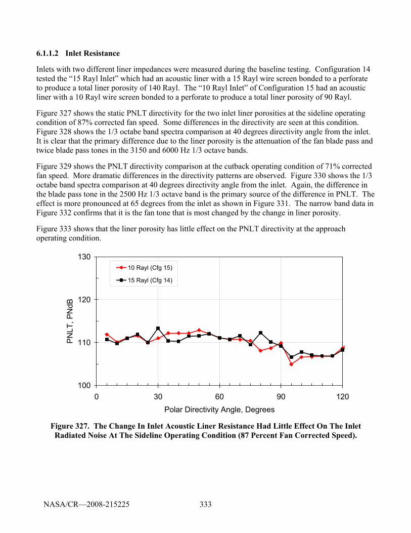
333

6.1.1.2 Inlet Resistance

Inlets with two different liner impedances were measured during the baseline testing. Configuration 14 tested the “15 Rayl Inlet” which had an acoustic liner with a 15 Rayl wire screen bonded to a perforate to produce a total liner porosity of 140 Rayl. The “10 Rayl Inlet” of Configuration 15 had an acoustic liner with a 10 Rayl wire screen bonded to a perforate to produce a total liner porosity of 90 Rayl.

Figure 327 shows the static PNLT directivity for the two inlet liner porosities at the sideline operating condition of 87% corrected fan speed. Some differences in the directivity are seen at this condition. Figure 328 shows the 1/3 octabe band spectra comparison at 40 degrees directivity angle from the inlet. It is clear that the primary difference due to the liner porosity is the attenuation of the fan blade pass and twice blade pass tones in the 3150 and 6000 Hz 1/3 octave bands.

Figure 329 shows the PNLT directivity comparison at the cutback operating condition of 71% corrected fan speed. More dramatic differences in the directivity patterns are observed. Figure 330 shows the 1/3 octabe band spectra comparison at 40 degrees directivity angle from the inlet. Again, the difference in the blade pass tone in the 2500 Hz 1/3 octave band is the primary source of the difference in PNLT. The effect is more pronounced at 65 degrees from the inlet as shown in Figure 331. The narrow band data in Figure 332 confirms that it is the fan tone that is most changed by the change in liner porosity.

Figure 333 shows that the liner porosity has little effect on the PNLT directivity at the approach operating condition.

100

110

120

130

0 30 60 90 120Polar Directivity Angle, Degrees

PNLT

, PN

dB

10 Rayl (Cfg 15)

15 Rayl (Cfg 14)

Figure 327. The Change In Inlet Acoustic Liner Resistance Had Little Effect On The Inlet Radiated Noise At The Sideline Operating Condition (87 Percent Fan Corrected Speed).

NASA/CR—2008-215225

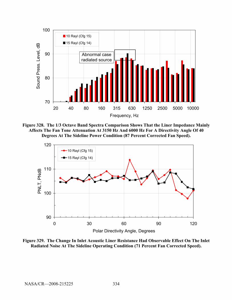
334

70

80

90

100

20 40 80 160 315 630 1250 2500 5000 10000Frequency, Hz

Soun

d Pr

ess.

Lev

el, d

B10 Rayl (Cfg 15)

15 Rayl (Cfg 14)

Abnormal case radiated source

Figure 328. The 1/3 Octave Band Spectra Comparison Shows That the Liner Impedance Mainly Affects The Fan Tone Attenuation At 3150 Hz And 6000 Hz For A Directivity Angle Of 40

Degrees At The Sideline Power Condition (87 Percent Corrected Fan Speed).

90

100

110

120


PNLT

, PN

dB

10 Rayl (Cfg 15)

15 Rayl (Cfg 14)

Figure 329. The Change In Inlet Acoustic Liner Resistance Had Observable Effect On The Inlet Radiated Noise At The Sideline Operating Condition (71 Percent Fan Corrected Speed).

NASA/CR—2008-215225

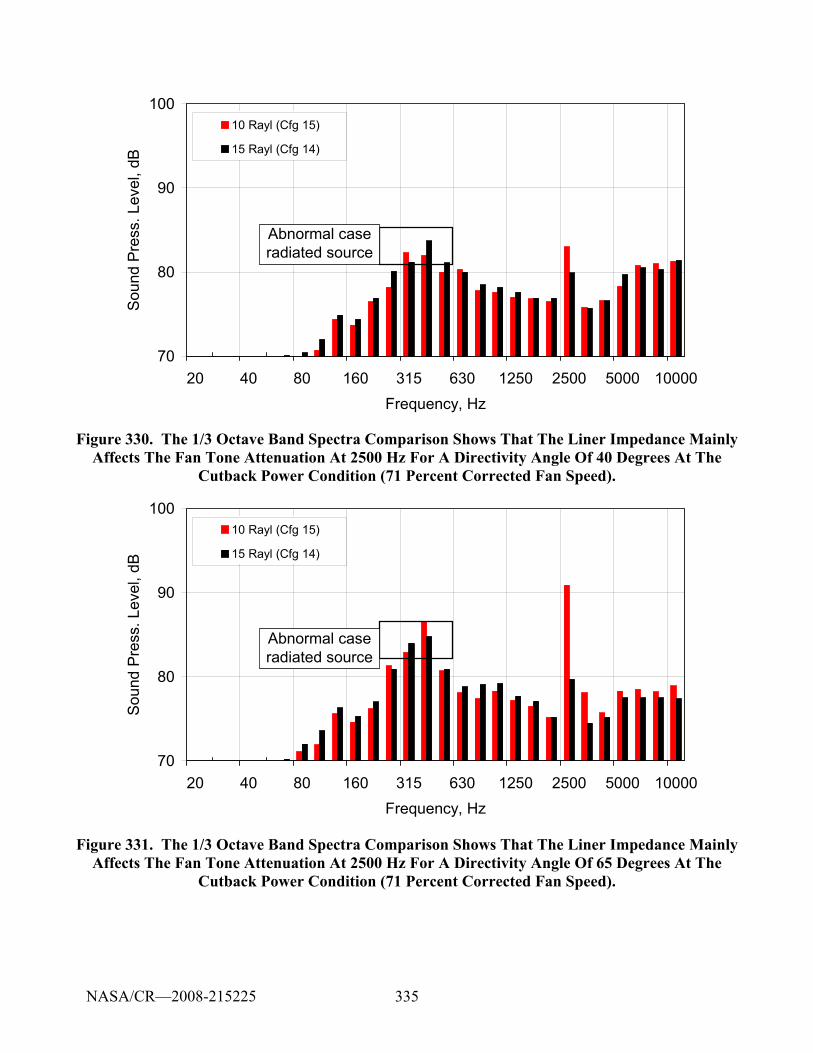
335

70

80

90

100

20 40 80 160 315 630 1250 2500 5000 10000Frequency, Hz

Soun

d Pr

ess.

Lev

el, d

B10 Rayl (Cfg 15)

15 Rayl (Cfg 14)


Figure 330. The 1/3 Octave Band Spectra Comparison Shows That The Liner Impedance Mainly Affects The Fan Tone Attenuation At 2500 Hz For A Directivity Angle Of 40 Degrees At The

Cutback Power Condition (71 Percent Corrected Fan Speed).

70

80

90

100

20 40 80 160 315 630 1250 2500 5000 10000Frequency, Hz

Soun

d Pr

ess.

Lev

el, d

B

10 Rayl (Cfg 15)

15 Rayl (Cfg 14)


Figure 331. The 1/3 Octave Band Spectra Comparison Shows That The Liner Impedance Mainly Affects The Fan Tone Attenuation At 2500 Hz For A Directivity Angle Of 65 Degrees At The

Cutback Power Condition (71 Percent Corrected Fan Speed).

NASA/CR—2008-215225

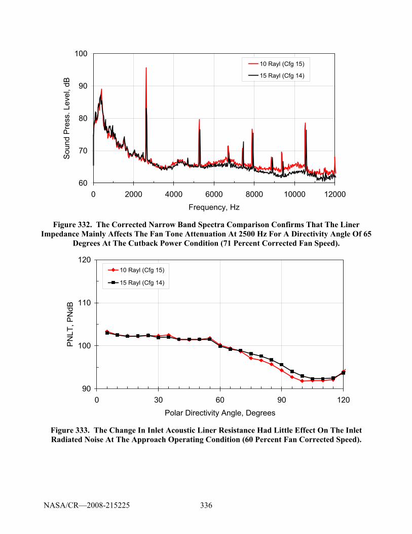
336

60

70

80

90

100

0 2000 4000 6000 8000 10000 12000Frequency, Hz

Soun

d P

ress

. Lev

el, d

B10 Rayl (Cfg 15)

15 Rayl (Cfg 14)

Figure 332. The Corrected Narrow Band Spectra Comparison Confirms That The Liner Impedance Mainly Affects The Fan Tone Attenuation At 2500 Hz For A Directivity Angle Of 65

Degrees At The Cutback Power Condition (71 Percent Corrected Fan Speed).

90

100

110

120


PN

LT, P

NdB

10 Rayl (Cfg 15)

15 Rayl (Cfg 14)

Figure 333. The Change In Inlet Acoustic Liner Resistance Had Little Effect On The Inlet Radiated Noise At The Approach Operating Condition (60 Percent Fan Corrected Speed).

NASA/CR—2008-215225

337

6.1.1.3 Inlet Treatment Sensitivity

The data acquired with varying lengths of inlet acoustic treatment showed that the treatment is very effective at reducing fan buzzsaw noise levels – treatment was progressively taped from the upstream end towards the fan (Figure 334 and Figure 335)

Further insight into the acoustic treatment effectiveness is gained from computing the liner attenuation. Figure 336 shows the computed liner attenuation for the three amounts of treatment for the inlet. The peak attenuation occurs in the 3150 1/3 octave band. The attenuation is clearly increasing for the 1/3 and 2/3 treated configurations. The final 1/3 of the treatment appears to increase the high frequency attenuation, while having little effect on the peak attenuation.

NASA/CR—2008-215225

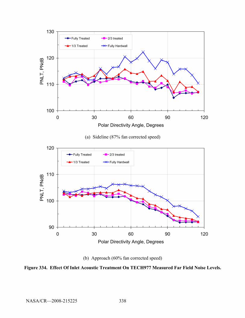
338

100

110

120

130


PN

LT, P

NdB

Fully Treated 2/3 treated

1/3 Treated Fully Hardwall


90

100

110

120


PN

LT, P

NdB




Figure 334. Effect Of Inlet Acoustic Treatment On TECH977 Measured Far Field Noise Levels.

NASA/CR—2008-215225

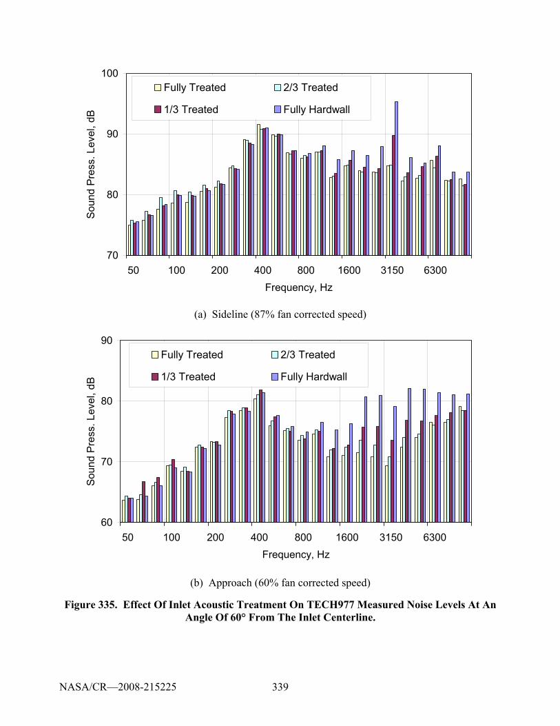
339

70

80

90

100

50 100 200 400 800 1600 3150 6300Frequency, Hz

Soun

d Pr

ess.

Lev

el, d

BFully Treated 2/3 Treated



60

70

80

90

50 100 200 400 800 1600 3150 6300Frequency, Hz

Soun

d Pr

ess.

Lev

el, d

B

Fully Treated 2/3 Treated



Figure 335. Effect Of Inlet Acoustic Treatment On TECH977 Measured Noise Levels At An Angle Of 60° From The Inlet Centerline.

NASA/CR—2008-215225

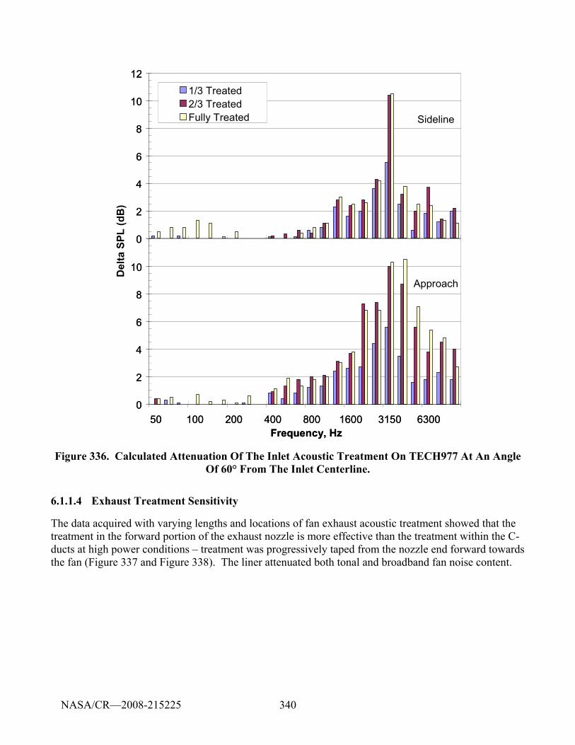
340

Del

ta S

PL (d

B)

0

2

4

6

8

10

121/3 Treated2/3 TreatedFully Treated

0

2

4

6

8

10

121/3 Treated2/3 TreatedFully Treated

0

2

4

6

8

10

50 100 200 400 800 1600 3150 6300Frequency, Hz

0

2

4

6

8

10

50 100 200 400 800 1600 3150 6300Frequency, Hz

Approach

Sideline

Figure 336. Calculated Attenuation Of The Inlet Acoustic Treatment On TECH977 At An Angle Of 60° From The Inlet Centerline.

6.1.1.4 Exhaust Treatment Sensitivity

The data acquired with varying lengths and locations of fan exhaust acoustic treatment showed that the treatment in the forward portion of the exhaust nozzle is more effective than the treatment within the C-ducts at high power conditions – treatment was progressively taped from the nozzle end forward towards the fan (Figure 337 and Figure 338). The liner attenuated both tonal and broadband fan noise content.

NASA/CR—2008-215225

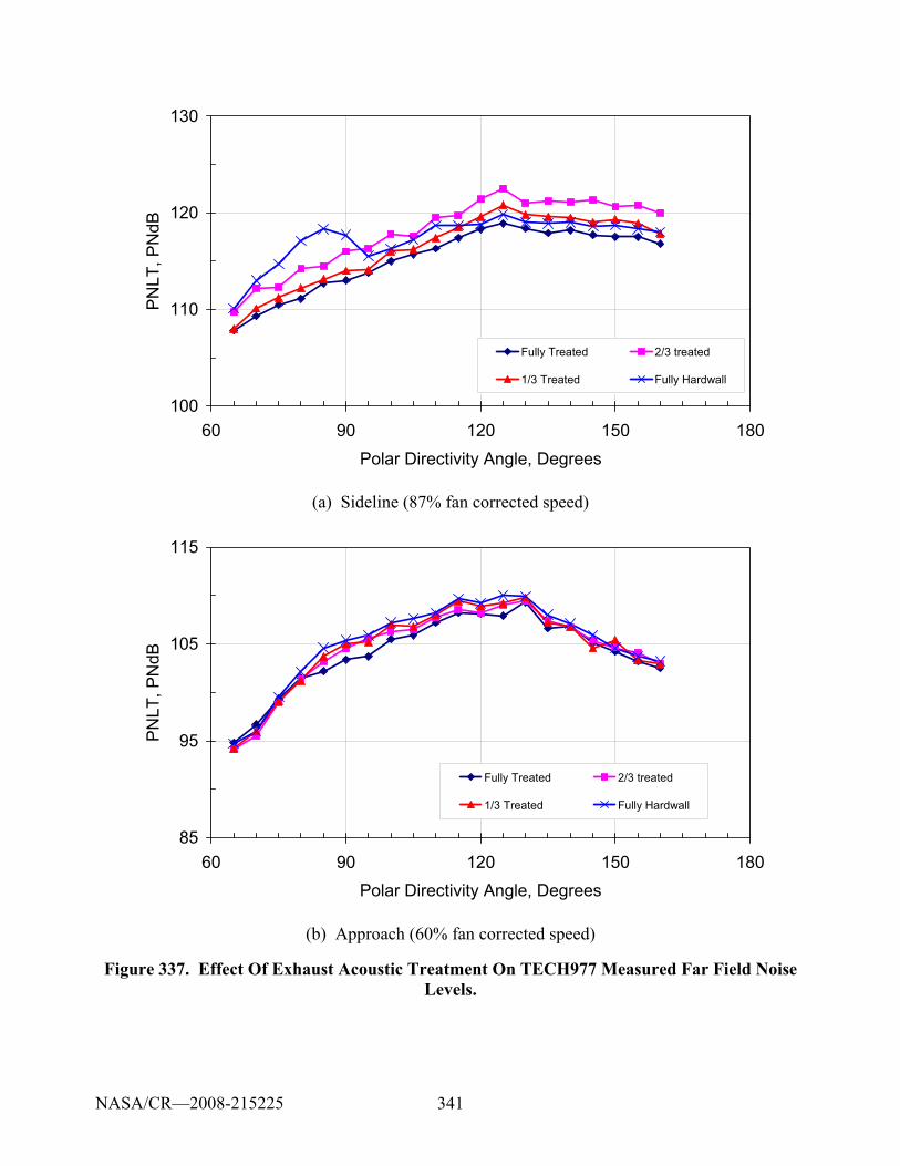
341

100

110

120

130


PNLT

, PN

dB




85

95

105

115


PN

LT, P

NdB




Figure 337. Effect Of Exhaust Acoustic Treatment On TECH977 Measured Far Field Noise Levels.

NASA/CR—2008-215225

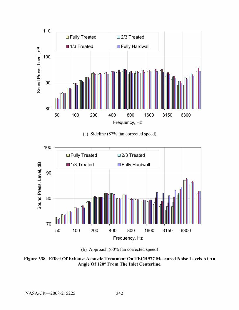
342

80

90

100

110

50 100 200 400 800 1600 3150 6300Frequency, Hz

Soun

d Pr

ess.

Lev

el, d

BFully Treated 2/3 Treated



70

80

90

100

50 100 200 400 800 1600 3150 6300Frequency, Hz

Sou

nd P

ress

. Lev

el, d

B

Fully Treated 2/3 Treated



Figure 338. Effect Of Exhaust Acoustic Treatment On TECH977 Measured Noise Levels At An Angle Of 120° From The Inlet Centerline.

NASA/CR—2008-215225

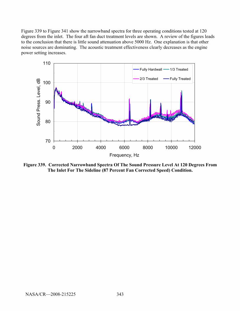
343

Figure 339 to Figure 341 show the narrowband spectra for three operating conditions tested at 120 degrees from the inlet. The four aft fan duct treatment levels are shown. A review of the figures leads to the conclusion that there is little sound attenuation above 5000 Hz. One explanation is that other noise sources are dominating. The acoustic treatment effectiveness clearly decreases as the engine power setting increases.

70

80

90

100

110

0 2000 4000 6000 8000 10000 12000Frequency, Hz

Soun

d Pr

ess.

Lev

el, d

B

Fully Hardwall 1/3 Treated

2/3 Treated Fully Treated

Figure 339. Corrected Narrowband Spectra Of The Sound Pressure Level At 120 Degrees From The Inlet For The Sideline (87 Percent Fan Corrected Speed) Condition.

NASA/CR—2008-215225

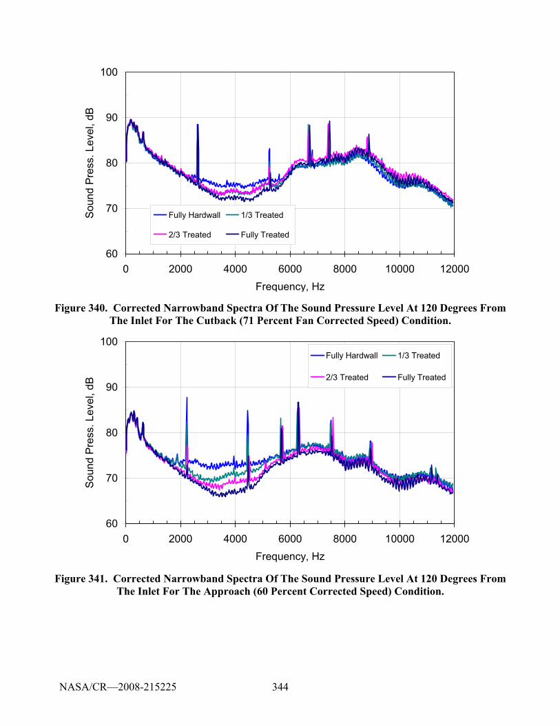
344

60

70

80

90

100

0 2000 4000 6000 8000 10000 12000Frequency, Hz

Soun

d Pr

ess.

Lev

el, d

B



Figure 340. Corrected Narrowband Spectra Of The Sound Pressure Level At 120 Degrees From The Inlet For The Cutback (71 Percent Fan Corrected Speed) Condition.

60

70

80

90

100

0 2000 4000 6000 8000 10000 12000Frequency, Hz

Sou

nd P

ress

. Lev

el, d

B



Figure 341. Corrected Narrowband Spectra Of The Sound Pressure Level At 120 Degrees From The Inlet For The Approach (60 Percent Corrected Speed) Condition.

NASA/CR—2008-215225

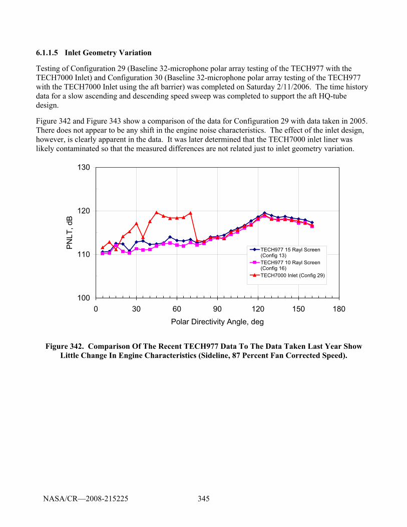
345

6.1.1.5 Inlet Geometry Variation

Testing of Configuration 29 (Baseline 32-microphone polar array testing of the TECH977 with the TECH7000 Inlet) and Configuration 30 (Baseline 32-microphone polar array testing of the TECH977 with the TECH7000 Inlet using the aft barrier) was completed on Saturday 2/11/2006. The time history data for a slow ascending and descending speed sweep was completed to support the aft HQ-tube design.

Figure 342 and Figure 343 show a comparison of the data for Configuration 29 with data taken in 2005. There does not appear to be any shift in the engine noise characteristics. The effect of the inlet design, however, is clearly apparent in the data. It was later determined that the TECH7000 inlet liner was likely contaminated so that the measured differences are not related just to inlet geometry variation.

100

110

120

130

0 30 60 90 120 150 180Polar Directivity Angle, deg

PNLT

, dB

TECH977 15 Rayl Screen(Config 13)TECH977 10 Rayl Screen(Config 16)TECH7000 Inlet (Config 29)

Figure 342. Comparison Of The Recent TECH977 Data To The Data Taken Last Year Show Little Change In Engine Characteristics (Sideline, 87 Percent Fan Corrected Speed).

NASA/CR—2008-215225

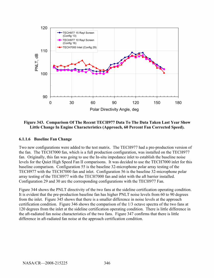
346

90

100

110

120


PNLT

, dB

TECH977 15 Rayl Screen(Config 13)TECH977 10 Rayl Screen(Config 16)TECH7000 Inlet (Config 29)

Figure 343. Comparison Of The Recent TECH977 Data To The Data Taken Last Year Show Little Change In Engine Characteristics (Approach, 60 Percent Fan Corrected Speed).

6.1.1.6 Baseline Fan Change

Two new configurations were added to the test matrix. The TECH977 had a pre-production version of the fan. The TECH7000 fan, which is a full production configuration, was installed on the TECH977 fan. Originally, this fan was going to use the In-situ impedance inlet to establish the baseline noise levels for the Quiet High Speed Fan II comparisons. It was decided to use the TECH7000 inlet for this baseline comparison. Configuration 55 is the baseline 32-microphone polar array testing of the TECH977 with the TECH7000 fan and inlet. Configuration 56 is the baseline 32-microphone polar array testing of the TECH977 with the TECH7000 fan and inlet with the aft barrier installed. Configuration 29 and 30 are the corresponding configurations with the TECH977 Fan.

Figure 344 shows the PNLT directivity of the two fans at the sideline certification operating condition. It is evident that the pre-production baseline fan has higher PNLT noise levels from 60 to 90 degrees from the inlet. Figure 345 shows that there is a smaller difference in noise levels at the approach certification condition. Figure 346 shows the comparison of the 1/3 octave spectra of the two fans at 120 degrees from the inlet at the sideline certification operating condition. There is little difference in the aft-radiated fan noise characteristics of the two fans. Figure 347 confirms that there is little difference in aft-radiated fan noise at the approach certification condition.

NASA/CR—2008-215225

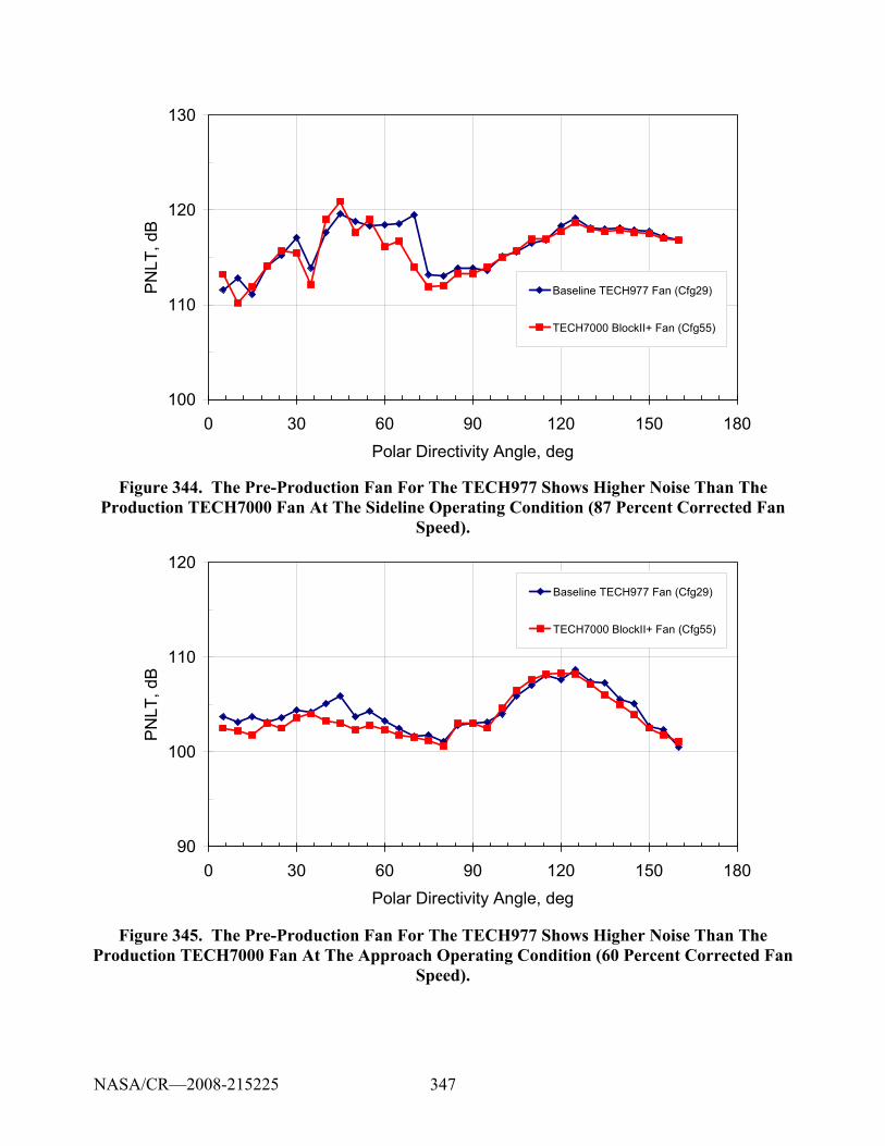
347

100

110

120

130


PN

LT, d

B

Baseline TECH977 Fan (Cfg29)

TECH7000 BlockII+ Fan (Cfg55)

Figure 344. The Pre-Production Fan For The TECH977 Shows Higher Noise Than The Production TECH7000 Fan At The Sideline Operating Condition (87 Percent Corrected Fan

Speed).

90

100

110

120


PN

LT, d

B



Figure 345. The Pre-Production Fan For The TECH977 Shows Higher Noise Than The Production TECH7000 Fan At The Approach Operating Condition (60 Percent Corrected Fan

Speed).

NASA/CR—2008-215225

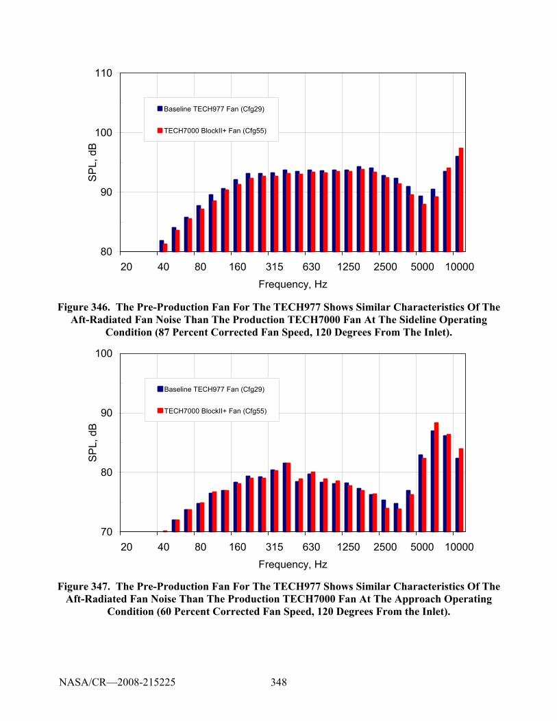
348

80

90

100

110

20 40 80 160 315 630 1250 2500 5000 10000Frequency, Hz

SP

L, d

BBaseline TECH977 Fan (Cfg29)


Figure 346. The Pre-Production Fan For The TECH977 Shows Similar Characteristics Of The Aft-Radiated Fan Noise Than The Production TECH7000 Fan At The Sideline Operating

Condition (87 Percent Corrected Fan Speed, 120 Degrees From The Inlet).

70

80

90

100

20 40 80 160 315 630 1250 2500 5000 10000Frequency, Hz

SP

L, d

B



Figure 347. The Pre-Production Fan For The TECH977 Shows Similar Characteristics Of The Aft-Radiated Fan Noise Than The Production TECH7000 Fan At The Approach Operating

Condition (60 Percent Corrected Fan Speed, 120 Degrees From the Inlet).

NASA/CR—2008-215225

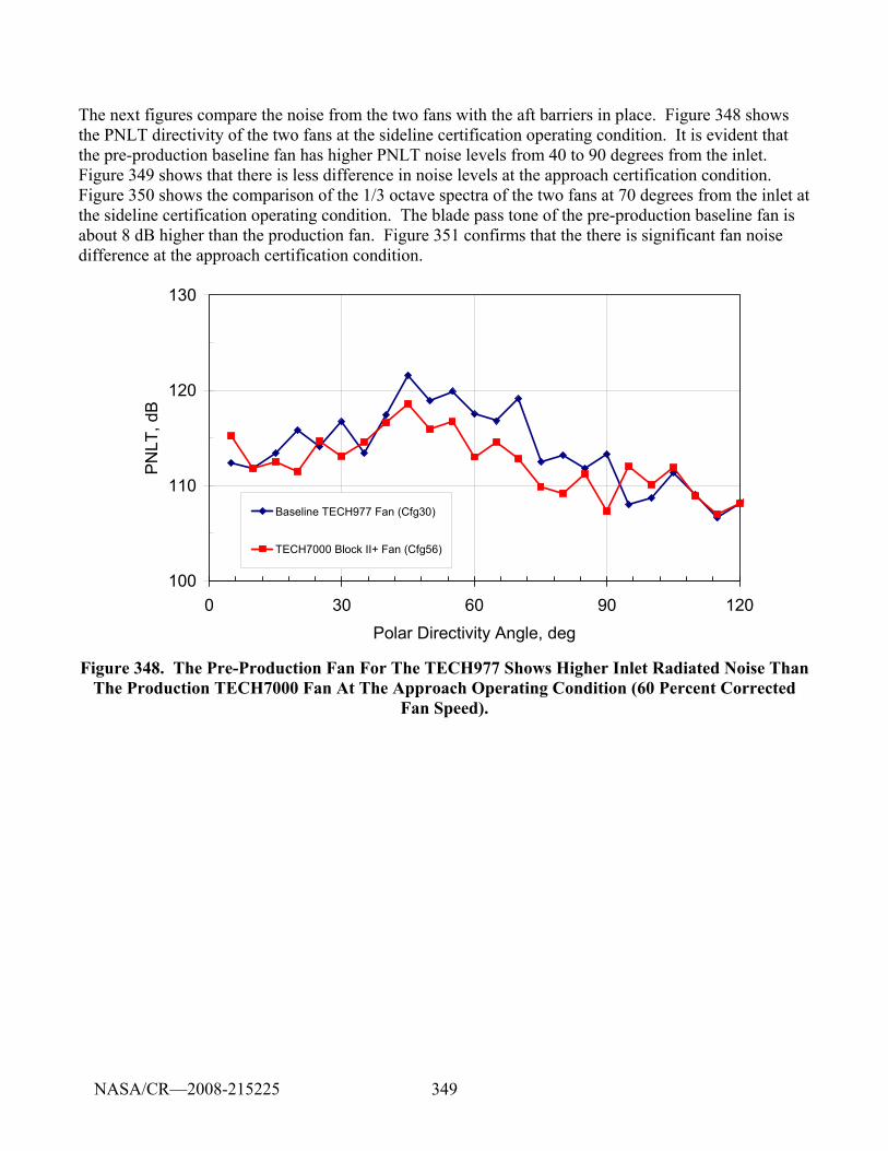
349

The next figures compare the noise from the two fans with the aft barriers in place. Figure 348 shows the PNLT directivity of the two fans at the sideline certification operating condition. It is evident that the pre-production baseline fan has higher PNLT noise levels from 40 to 90 degrees from the inlet. Figure 349 shows that there is less difference in noise levels at the approach certification condition. Figure 350 shows the comparison of the 1/3 octave spectra of the two fans at 70 degrees from the inlet at the sideline certification operating condition. The blade pass tone of the pre-production baseline fan is about 8 dB higher than the production fan. Figure 351 confirms that the there is significant fan noise difference at the approach certification condition.

100

110

120

130


PNLT

, dB


TECH7000 Block II+ Fan (Cfg56)

Figure 348. The Pre-Production Fan For The TECH977 Shows Higher Inlet Radiated Noise Than The Production TECH7000 Fan At The Approach Operating Condition (60 Percent Corrected

Fan Speed).

NASA/CR—2008-215225

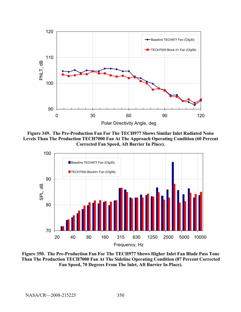
350

90

100

110

120


PNLT

, dB



Figure 349. The Pre-Production Fan For The TECH977 Shows Similar Inlet Radiated Noise Levels Than The Production TECH7000 Fan At The Approach Operating Condition (60 Percent

Corrected Fan Speed, Aft Barrier In Place).

70

80

90

100

20 40 80 160 315 630 1250 2500 5000 10000Frequency, Hz

SP

L, d

B



Figure 350. The Pre-Production Fan For The TECH977 Shows Higher Inlet Fan Blade Pass Tone Than The Production TECH7000 Fan At The Sideline Operating Condition (87 Percent Corrected

Fan Speed, 70 Degrees From The Inlet, Aft Barrier In Place).

NASA/CR—2008-215225

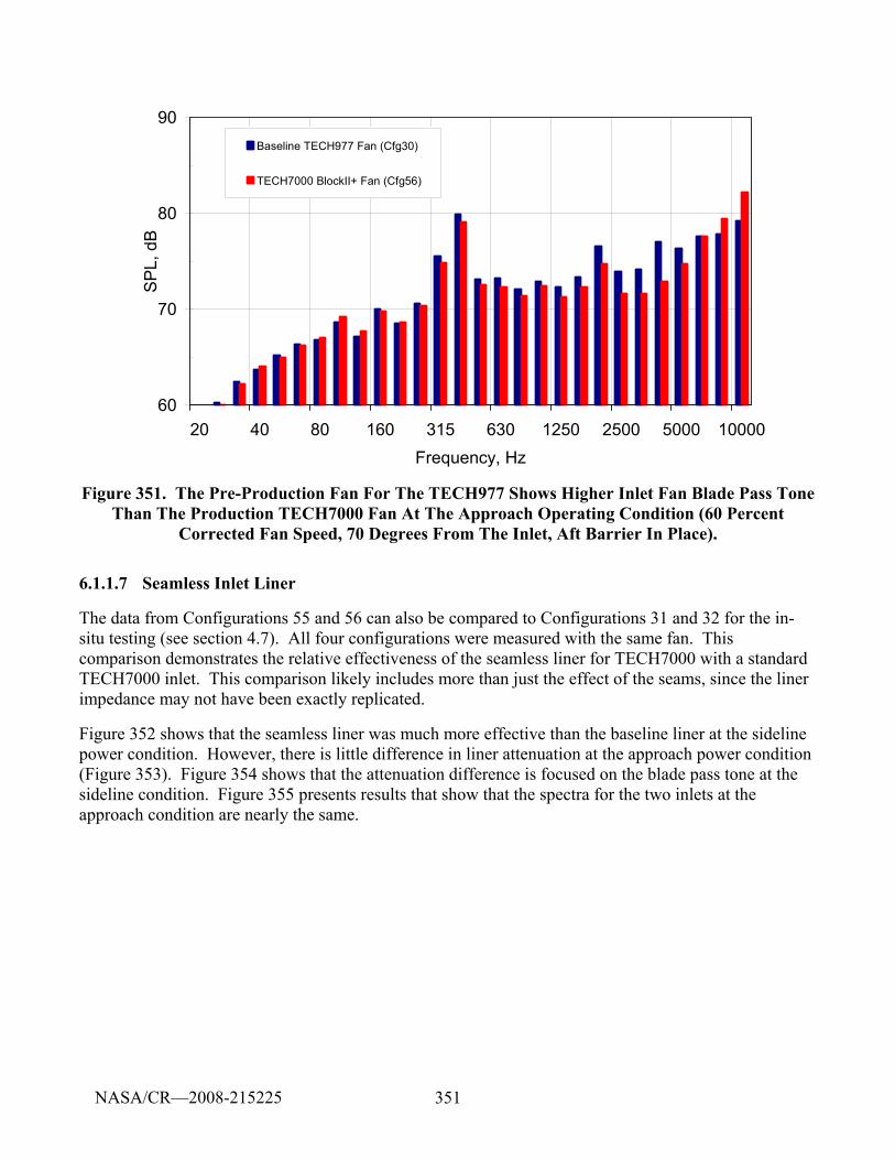
351

60

70

80

90

20 40 80 160 315 630 1250 2500 5000 10000Frequency, Hz

SP

L, d

BBaseline TECH977 Fan (Cfg30)


Figure 351. The Pre-Production Fan For The TECH977 Shows Higher Inlet Fan Blade Pass Tone Than The Production TECH7000 Fan At The Approach Operating Condition (60 Percent

Corrected Fan Speed, 70 Degrees From The Inlet, Aft Barrier In Place).

6.1.1.7 Seamless Inlet Liner

The data from Configurations 55 and 56 can also be compared to Configurations 31 and 32 for the in-situ testing (see section 4.7). All four configurations were measured with the same fan. This comparison demonstrates the relative effectiveness of the seamless liner for TECH7000 with a standard TECH7000 inlet. This comparison likely includes more than just the effect of the seams, since the liner impedance may not have been exactly replicated.

Figure 352 shows that the seamless liner was much more effective than the baseline liner at the sideline power condition. However, there is little difference in liner attenuation at the approach power condition (Figure 353). Figure 354 shows that the attenuation difference is focused on the blade pass tone at the sideline condition. Figure 355 presents results that show that the spectra for the two inlets at the approach condition are nearly the same.

NASA/CR—2008-215225

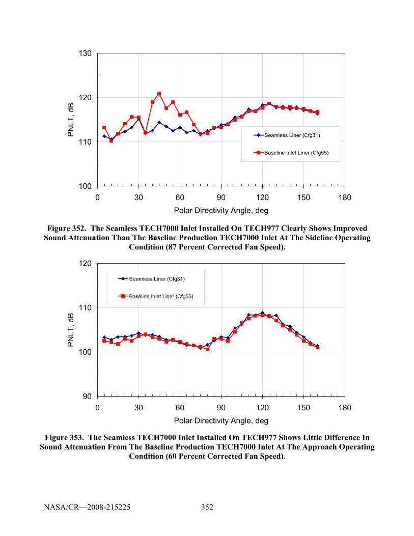
352

100

110

120

130


PN

LT, d

B

Seamless Liner (Cfg31)

Baseline Inlet Liner (Cfg55)

Figure 352. The Seamless TECH7000 Inlet Installed On TECH977 Clearly Shows Improved Sound Attenuation Than The Baseline Production TECH7000 Inlet At The Sideline Operating

Condition (87 Percent Corrected Fan Speed).

90

100

110

120


PNLT

, dB


Baseline Inlet Liner (Cfg55)

Figure 353. The Seamless TECH7000 Inlet Installed On TECH977 Shows Little Difference In Sound Attenuation From The Baseline Production TECH7000 Inlet At The Approach Operating

Condition (60 Percent Corrected Fan Speed).

NASA/CR—2008-215225

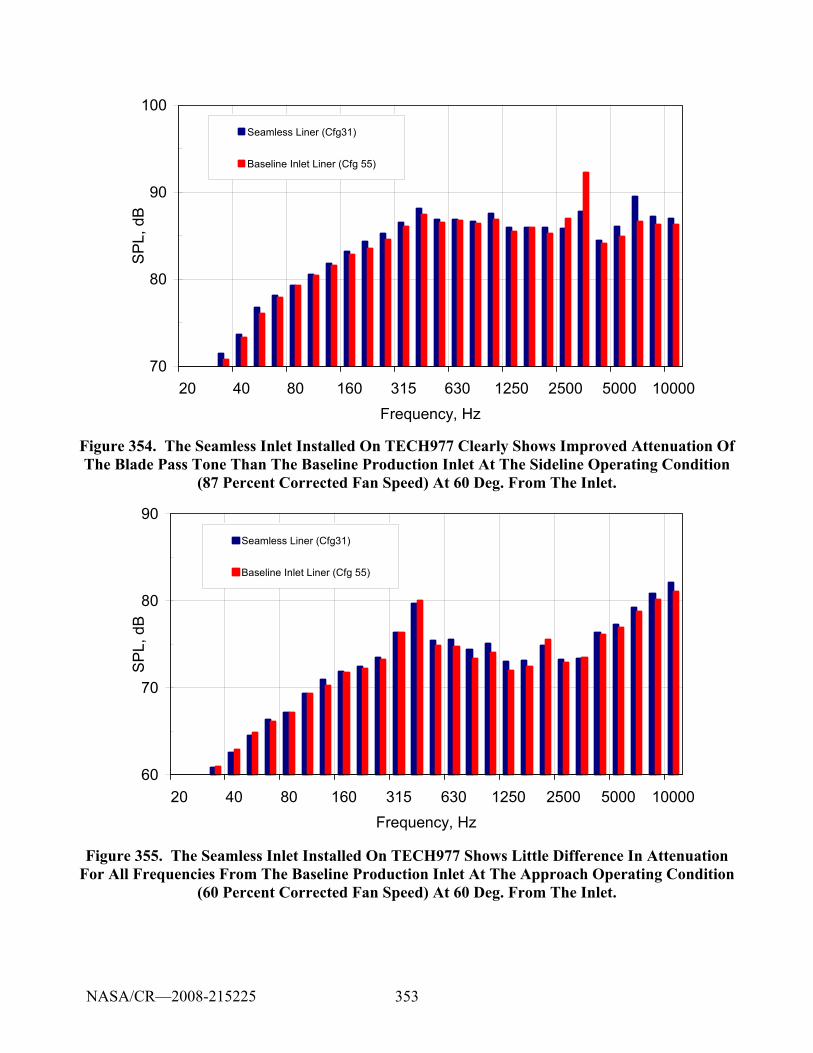
353

70

80

90

100

20 40 80 160 315 630 1250 2500 5000 10000Frequency, Hz

SP

L, d

BSeamless Liner (Cfg31)

Baseline Inlet Liner (Cfg 55)

Figure 354. The Seamless Inlet Installed On TECH977 Clearly Shows Improved Attenuation Of The Blade Pass Tone Than The Baseline Production Inlet At The Sideline Operating Condition

(87 Percent Corrected Fan Speed) At 60 Deg. From The Inlet.

60

70

80

90

20 40 80 160 315 630 1250 2500 5000 10000Frequency, Hz

SP

L, d

B


Baseline Inlet Liner (Cfg 55)

Figure 355. The Seamless Inlet Installed On TECH977 Shows Little Difference In Attenuation For All Frequencies From The Baseline Production Inlet At The Approach Operating Condition

(60 Percent Corrected Fan Speed) At 60 Deg. From The Inlet.

NASA/CR—2008-215225

354

6.1.1.8 Quiet High Speed Fan

6.1.1.8.1 Far Field Data

Baseline testing of the TECH977 with the Quiet High Speed Fan (QHSF) II and the in-situ inlet with all acoustic treatment taped was conducted on the evening of Wednesday, May 24th (Thursday Grave). Acoustic data were taken without and with the aft barrier (Configuration 51 and 52). Far field (32-microphone tarmac array) noise data were acquired at 8 engine speeds with 1 repeat point.

The fully hard wall configuration tested in the EVNERT program with a baseline fan is Configuration 25, which used the pre-production TECH977 fan. Unfortunately, Configuration 25 had the unanticipated case noise radiation source that was not seen in the QHSF II testing. Therefore spectral comparisons are restricted to frequencies in the 630 Hz 1/3 octave band and above. Plots of PNLT comparisons at 100 ft are for a frequency range of 50-10000 Hz 1/3 octave bands, so there may be a small contribution of the case noise source.

Figure 356 shows the PNLT comparison at the sideline operating condition (87% fan corrected speed). Note that for angles from 20 to 50 degrees from the inlet, the QHSF II has significantly higher noise levels than the pre-production TECH977 fan. Figure 357 shows that the noise increase at 30 degrees is across the entire frequency range where fan noise is expected to dominate. Even at 60 degrees, the QHSF II has higher noise levels as shown in Figure 358. The narrow band spectra shown in Figure 359 and Figure 360 confirm the Higher multiple pure tone noise levels of this engine scale QHSF II.

Figure 361 shows a comparison of the noise levels of the two fans at the cutback condition. The QHSF II shows lower noise levels from 100 to 160 degrees. The 1/3 octave data at 120 degrees shown in Figure 362 indicate that the QHSF II fan noise is lower over multiple 1/3 octave bands. The narrowband spectra in Figure 363 confirm that the noise reduction is primarily broadband.

Figure 364 shows a comparison of the noise levels of the two fans at the approach condition. The QHSF II shows lower noise levels from 80 to 160 degrees. The 1/3 octave data at 120 degrees shown in Figure 365 again indicate that the QHSF II fan noise is lower over multiple 1/3 octave bands. The narrowband spectra in Figure 366 show that the noise reduction is both tonal and broadband.

NASA/CR—2008-215225

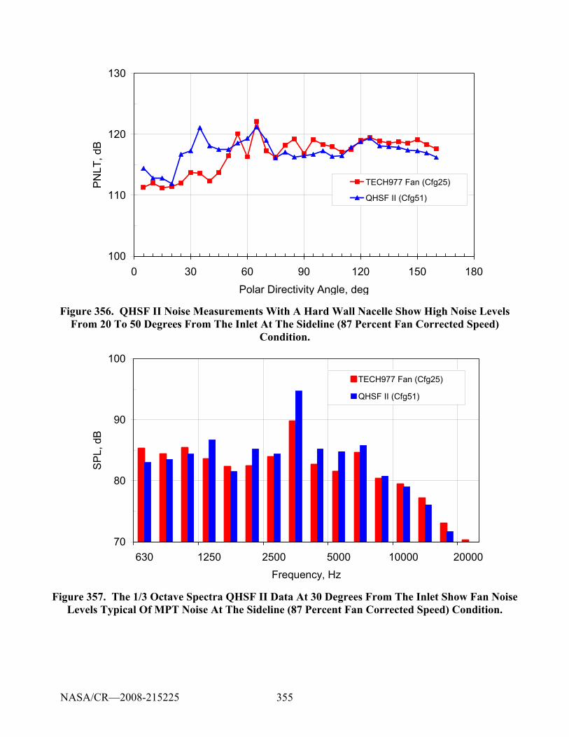
355

100

110

120

130


PNLT

, dB

TECH977 Fan (Cfg25)

QHSF II (Cfg51)

Figure 356. QHSF II Noise Measurements With A Hard Wall Nacelle Show High Noise Levels From 20 To 50 Degrees From The Inlet At The Sideline (87 Percent Fan Corrected Speed)

Condition.

70

80

90

100

630 1250 2500 5000 10000 20000Frequency, Hz

SP

L, d

B

TECH977 Fan (Cfg25)

QHSF II (Cfg51)

Figure 357. The 1/3 Octave Spectra QHSF II Data At 30 Degrees From The Inlet Show Fan Noise Levels Typical Of MPT Noise At The Sideline (87 Percent Fan Corrected Speed) Condition.

NASA/CR—2008-215225

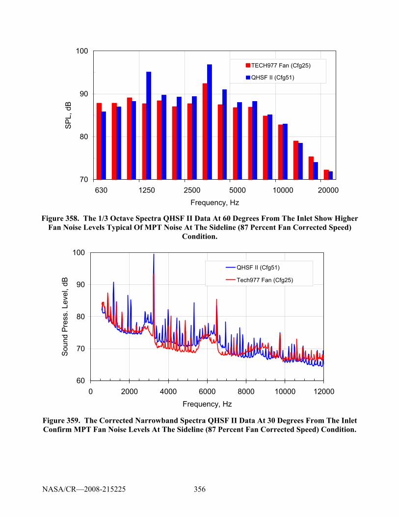
356

70

80

90

100

630 1250 2500 5000 10000 20000Frequency, Hz

SP

L, d

BTECH977 Fan (Cfg25)

QHSF II (Cfg51)

Figure 358. The 1/3 Octave Spectra QHSF II Data At 60 Degrees From The Inlet Show Higher Fan Noise Levels Typical Of MPT Noise At The Sideline (87 Percent Fan Corrected Speed)

Condition.

60

70

80

90

100

0 2000 4000 6000 8000 10000 12000Frequency, Hz

Soun

d Pr

ess.

Lev

el, d

B

QHSF II (Cfg51)

Tech977 Fan (Cfg25)

Figure 359. The Corrected Narrowband Spectra QHSF II Data At 30 Degrees From The Inlet Confirm MPT Fan Noise Levels At The Sideline (87 Percent Fan Corrected Speed) Condition.

NASA/CR—2008-215225

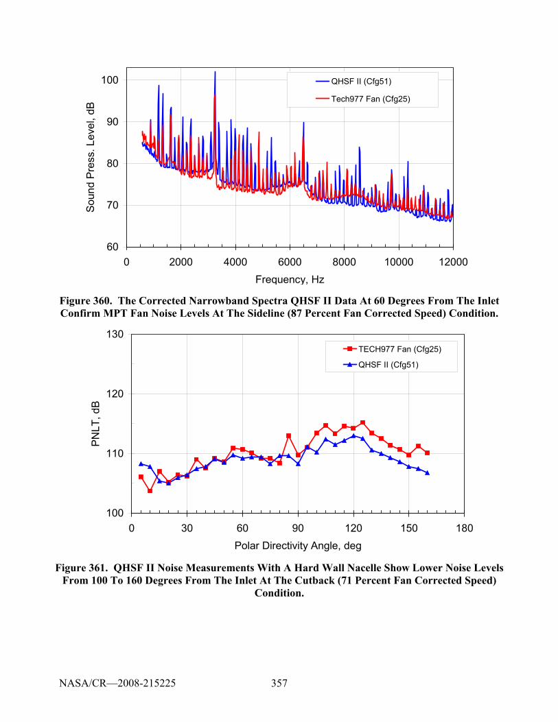
357

60

70

80

90

100

0 2000 4000 6000 8000 10000 12000Frequency, Hz

Soun

d Pr

ess.

Lev

el, d

BQHSF II (Cfg51)

Tech977 Fan (Cfg25)

Figure 360. The Corrected Narrowband Spectra QHSF II Data At 60 Degrees From The Inlet Confirm MPT Fan Noise Levels At The Sideline (87 Percent Fan Corrected Speed) Condition.

100

110

120

130


PN

LT, d

B

TECH977 Fan (Cfg25)

QHSF II (Cfg51)

Figure 361. QHSF II Noise Measurements With A Hard Wall Nacelle Show Lower Noise Levels From 100 To 160 Degrees From The Inlet At The Cutback (71 Percent Fan Corrected Speed)

Condition.

NASA/CR—2008-215225

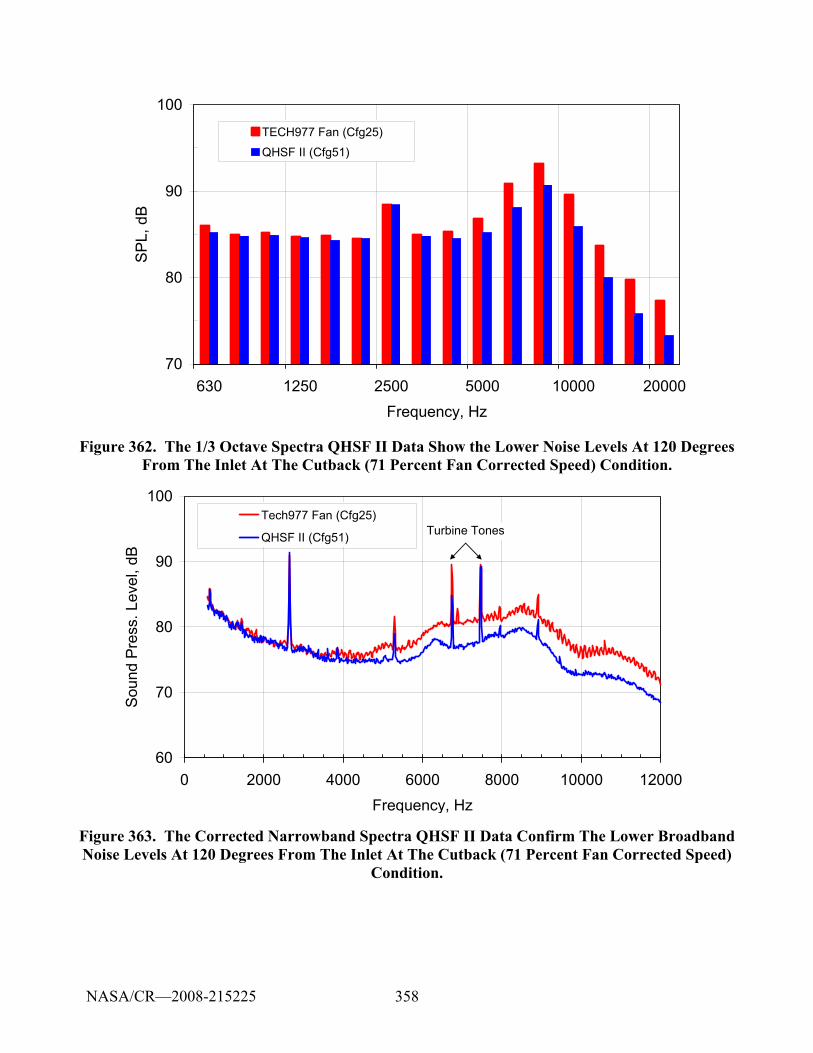
358

70

80

90

100

630 1250 2500 5000 10000 20000Frequency, Hz

SP

L, d

BTECH977 Fan (Cfg25)

QHSF II (Cfg51)

Figure 362. The 1/3 Octave Spectra QHSF II Data Show the Lower Noise Levels At 120 Degrees From The Inlet At The Cutback (71 Percent Fan Corrected Speed) Condition.

60

70

80

90

100

0 2000 4000 6000 8000 10000 12000Frequency, Hz

Soun

d Pr

ess.

Lev

el, d

B

Tech977 Fan (Cfg25)

QHSF II (Cfg51) Turbine Tones

Figure 363. The Corrected Narrowband Spectra QHSF II Data Confirm The Lower Broadband Noise Levels At 120 Degrees From The Inlet At The Cutback (71 Percent Fan Corrected Speed)

Condition.

NASA/CR—2008-215225

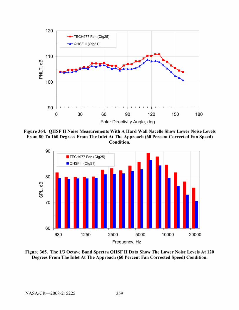
359

90

100

110

120


PNLT

, dB

TECH977 Fan (Cfg25)

QHSF II (Cfg51)

Figure 364. QHSF II Noise Measurements With A Hard Wall Nacelle Show Lower Noise Levels From 80 To 160 Degrees From The Inlet At The Approach (60 Percent Corrected Fan Speed)

Condition.

60

70

80

90

630 1250 2500 5000 10000 20000Frequency, Hz

SP

L, d

B

TECH977 Fan (Cfg25)

QHSF II (Cfg51)

Figure 365. The 1/3 Octave Band Spectra QHSF II Data Show The Lower Noise Levels At 120 Degrees From The Inlet At The Approach (60 Percent Fan Corrected Speed) Condition.

NASA/CR—2008-215225

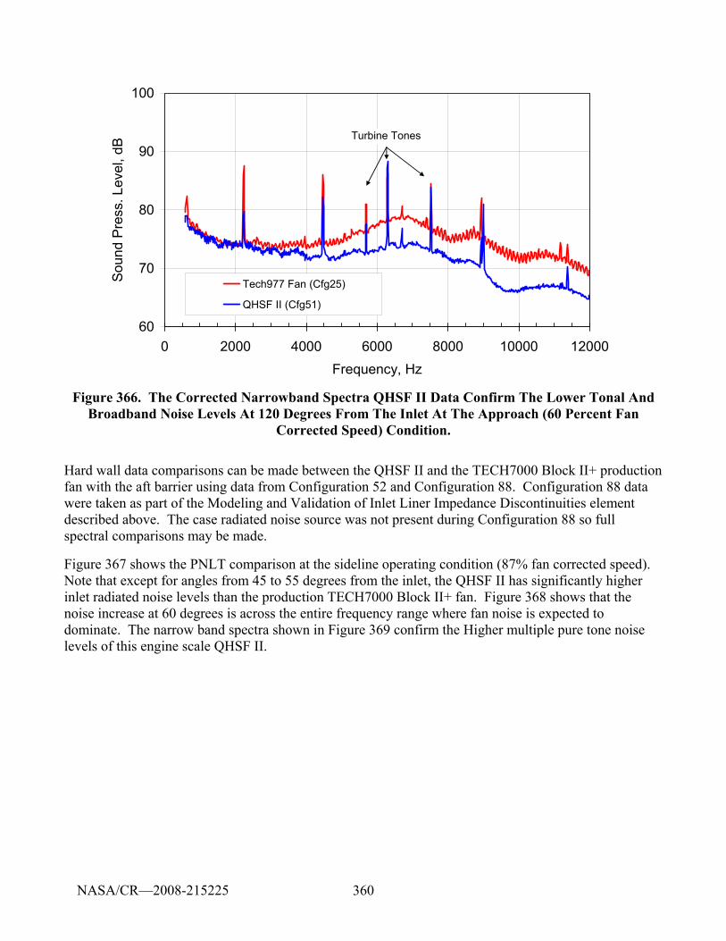
360

60

70

80

90

100

0 2000 4000 6000 8000 10000 12000Frequency, Hz

Sou

nd P

ress

. Lev

el, d

B

Tech977 Fan (Cfg25)

QHSF II (Cfg51)

Turbine Tones

Figure 366. The Corrected Narrowband Spectra QHSF II Data Confirm The Lower Tonal And Broadband Noise Levels At 120 Degrees From The Inlet At The Approach (60 Percent Fan

Corrected Speed) Condition.

Hard wall data comparisons can be made between the QHSF II and the TECH7000 Block II+ production fan with the aft barrier using data from Configuration 52 and Configuration 88. Configuration 88 data were taken as part of the Modeling and Validation of Inlet Liner Impedance Discontinuities element described above. The case radiated noise source was not present during Configuration 88 so full spectral comparisons may be made.

Figure 367 shows the PNLT comparison at the sideline operating condition (87% fan corrected speed). Note that except for angles from 45 to 55 degrees from the inlet, the QHSF II has significantly higher inlet radiated noise levels than the production TECH7000 Block II+ fan. Figure 368 shows that the noise increase at 60 degrees is across the entire frequency range where fan noise is expected to dominate. The narrow band spectra shown in Figure 369 confirm the Higher multiple pure tone noise levels of this engine scale QHSF II.

NASA/CR—2008-215225

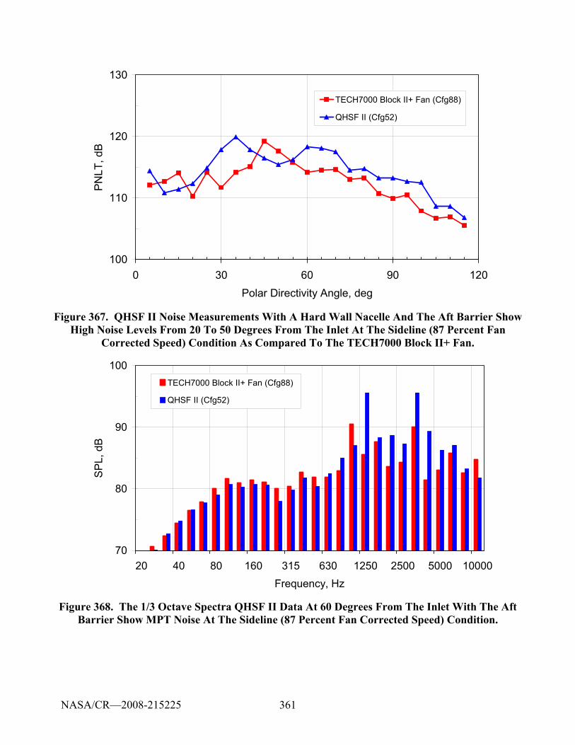
361

100

110

120

130


PNLT

, dB


QHSF II (Cfg52)

Figure 367. QHSF II Noise Measurements With A Hard Wall Nacelle And The Aft Barrier Show High Noise Levels From 20 To 50 Degrees From The Inlet At The Sideline (87 Percent Fan

Corrected Speed) Condition As Compared To The TECH7000 Block II+ Fan.

70

80

90

100

20 40 80 160 315 630 1250 2500 5000 10000Frequency, Hz

SP

L, d

B


QHSF II (Cfg52)

Figure 368. The 1/3 Octave Spectra QHSF II Data At 60 Degrees From The Inlet With The Aft Barrier Show MPT Noise At The Sideline (87 Percent Fan Corrected Speed) Condition.

NASA/CR—2008-215225

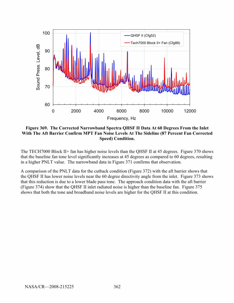
362

60

70

80

90

100

0 2000 4000 6000 8000 10000 12000Frequency, Hz

Soun

d Pr

ess.

Lev

el, d

BQHSF II (Cfg52)

Tech7000 Block II+ Fan (Cfg88)

Figure 369. The Corrected Narrowband Spectra QHSF II Data At 60 Degrees From the Inlet With The Aft Barrier Confirm MPT Fan Noise Levels At The Sideline (87 Percent Fan Corrected

Speed) Condition.

The TECH7000 Block II+ fan has higher noise levels than the QHSF II at 45 degrees. Figure 370 shows that the baseline fan tone level significantly increases at 45 degrees as compared to 60 degrees, resulting in a higher PNLT value. The narrowband data in Figure 371 confirms that observation.

A comparison of the PNLT data for the cutback condition (Figure 372) with the aft barrier shows that the QHSF II has lower noise levels near the 60 degree directivity angle from the inlet. Figure 373 shows that this reduction is due to a lower blade pass tone. The approach condition data with the aft barrier (Figure 374) show that the QHSF II inlet radiated noise is higher than the baseline fan. Figure 375 shows that both the tone and broadband noise levels are higher for the QHSF II at this condition.

NASA/CR—2008-215225

363

70

80

90

100

20 40 80 160 315 630 1250 2500 5000 10000Frequency, Hz

SP

L, d

BTECH7000 Block II+ Fan (Cfg88)

QHSF II (Cfg52)

Figure 370. The 1/3 Octave Spectra With The Aft Barrier At 45 Degrees From The Inlet Show An Increase In The Baseline Fan Tone Level At The Sideline (87 Percent Fan Corrected Speed)

Condition.

60

70

80

90

100

0 2000 4000 6000 8000 10000 12000Frequency, Hz

Soun

d Pr

ess.

Lev

el, d

B


QHSF II (Cfg52)

Figure 371. The Corrected Narrowband Spectra With The Aft Barrier At 45 Degrees From The Inlet Confirms The Increase In The Baseline Fan Tone Level At The Sideline (87 Percent Fan


NASA/CR—2008-215225

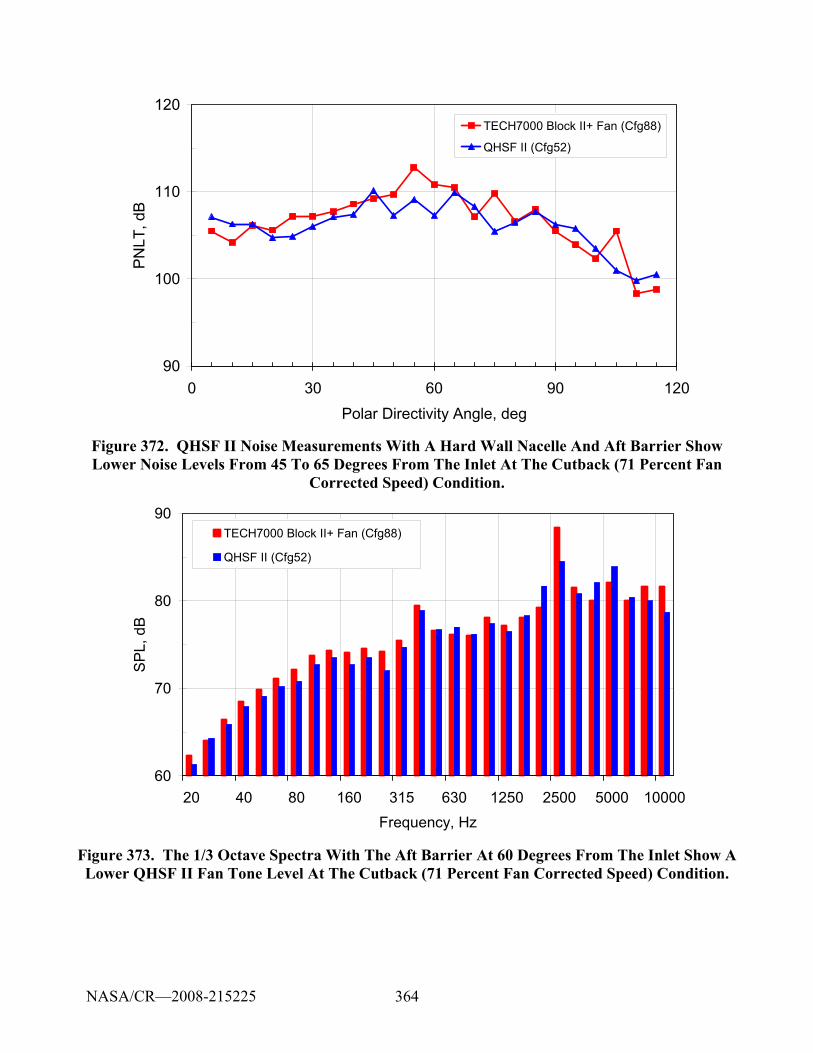
364

90

100

110

120


PNLT

, dB


QHSF II (Cfg52)

Figure 372. QHSF II Noise Measurements With A Hard Wall Nacelle And Aft Barrier Show Lower Noise Levels From 45 To 65 Degrees From The Inlet At The Cutback (71 Percent Fan


60

70

80

90

20 40 80 160 315 630 1250 2500 5000 10000Frequency, Hz

SPL

, dB


QHSF II (Cfg52)

Figure 373. The 1/3 Octave Spectra With The Aft Barrier At 60 Degrees From The Inlet Show A Lower QHSF II Fan Tone Level At The Cutback (71 Percent Fan Corrected Speed) Condition.

NASA/CR—2008-215225

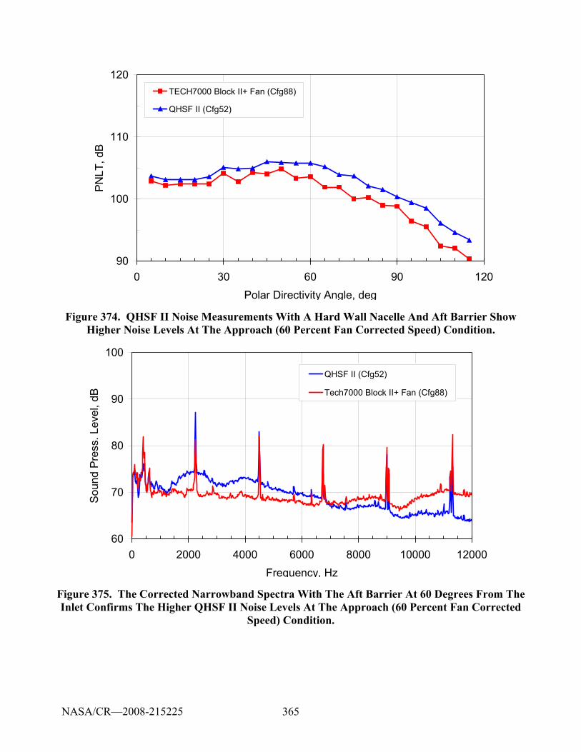
365

90

100

110

120


PN

LT, d

BTECH7000 Block II+ Fan (Cfg88)

QHSF II (Cfg52)

Figure 374. QHSF II Noise Measurements With A Hard Wall Nacelle And Aft Barrier Show Higher Noise Levels At The Approach (60 Percent Fan Corrected Speed) Condition.

60

70

80

90

100

0 2000 4000 6000 8000 10000 12000Frequency, Hz

Soun

d Pr

ess.

Lev

el, d

B

QHSF II (Cfg52)


Figure 375. The Corrected Narrowband Spectra With The Aft Barrier At 60 Degrees From The Inlet Confirms The Higher QHSF II Noise Levels At The Approach (60 Percent Fan Corrected

Speed) Condition.

NASA/CR—2008-215225

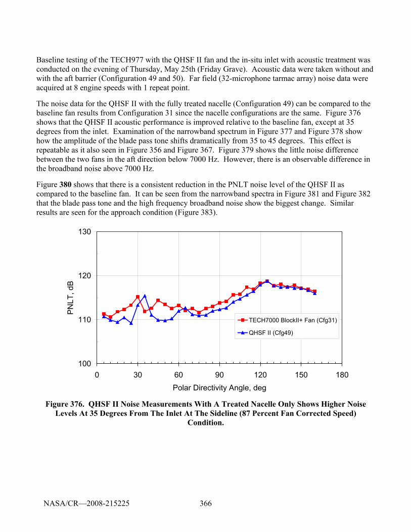
366

Baseline testing of the TECH977 with the QHSF II fan and the in-situ inlet with acoustic treatment was conducted on the evening of Thursday, May 25th (Friday Grave). Acoustic data were taken without and with the aft barrier (Configuration 49 and 50). Far field (32-microphone tarmac array) noise data were acquired at 8 engine speeds with 1 repeat point.

The noise data for the QHSF II with the fully treated nacelle (Configuration 49) can be compared to the baseline fan results from Configuration 31 since the nacelle configurations are the same. Figure 376 shows that the QHSF II acoustic performance is improved relative to the baseline fan, except at 35 degrees from the inlet. Examination of the narrowband spectrum in Figure 377 and Figure 378 show how the amplitude of the blade pass tone shifts dramatically from 35 to 45 degrees. This effect is repeatable as it also seen in Figure 356 and Figure 367. Figure 379 shows the little noise difference between the two fans in the aft direction below 7000 Hz. However, there is an observable difference in the broadband noise above 7000 Hz.

Figure 380 shows that there is a consistent reduction in the PNLT noise level of the QHSF II as compared to the baseline fan. It can be seen from the narrowband spectra in Figure 381 and Figure 382 that the blade pass tone and the high frequency broadband noise show the biggest change. Similar results are seen for the approach condition (Figure 383).

100

110

120

130


PNLT

, dB


QHSF II (Cfg49)

Figure 376. QHSF II Noise Measurements With A Treated Nacelle Only Shows Higher Noise Levels At 35 Degrees From The Inlet At The Sideline (87 Percent Fan Corrected Speed)

Condition.

NASA/CR—2008-215225

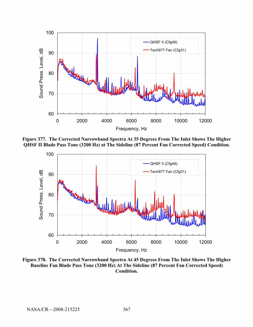
367

60

70

80

90

100

0 2000 4000 6000 8000 10000 12000Frequency, Hz

Soun

d Pr

ess.

Lev

el, d

BQHSF II (Cfg49)

Tech977 Fan (Cfg31)

Figure 377. The Corrected Narrowband Spectra At 35 Degrees From The Inlet Shows The Higher QHSF II Blade Pass Tone (3200 Hz) at The Sideline (87 Percent Fan Corrected Speed) Condition.

60

70

80

90

100

0 2000 4000 6000 8000 10000 12000Frequency, Hz

Soun

d Pr

ess.

Lev

el, d

B

QHSF II (Cfg49)

Tech977 Fan (Cfg31)

Figure 378. The Corrected Narrowband Spectra At 45 Degrees From The Inlet Shows The Higher Baseline Fan Blade Pass Tone (3200 Hz) At The Sideline (87 Percent Fan Corrected Speed)

Condition.

NASA/CR—2008-215225

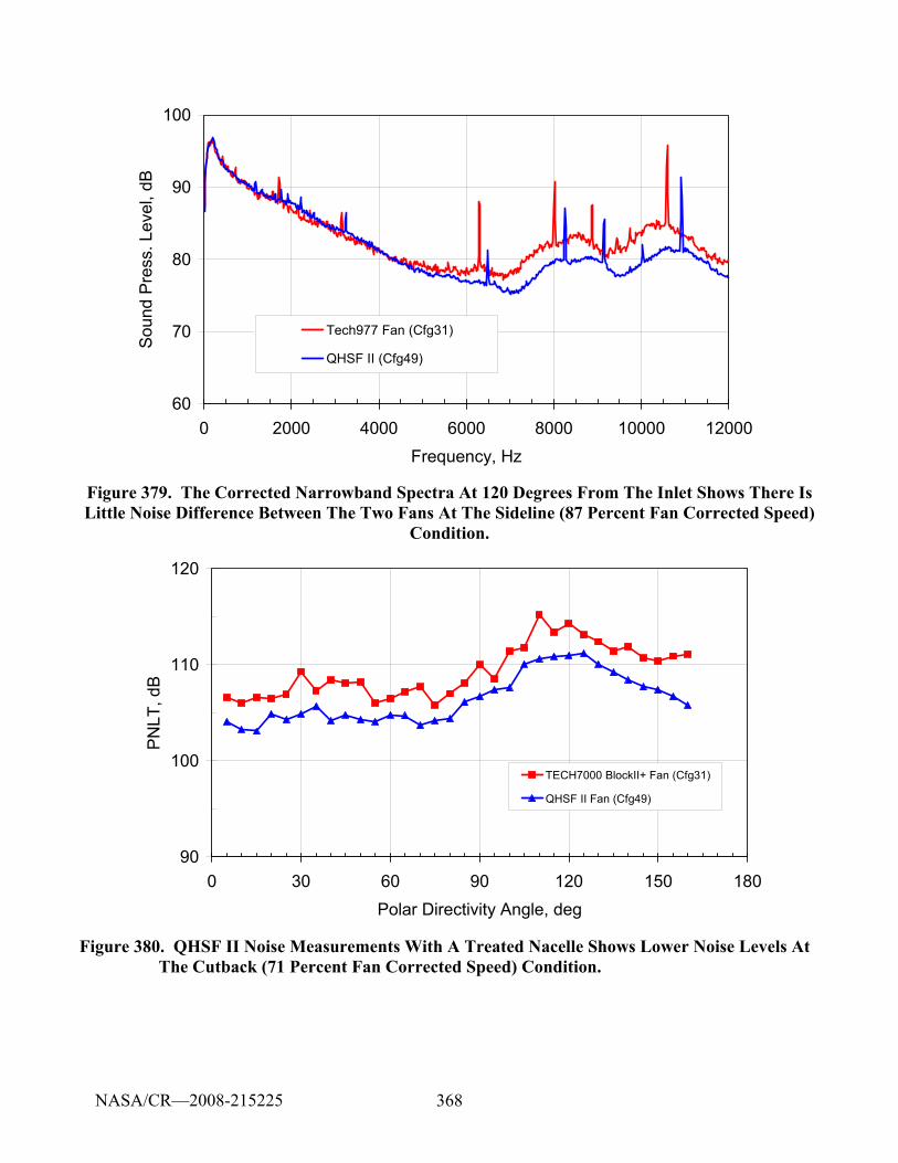
368

60

70

80

90

100

0 2000 4000 6000 8000 10000 12000Frequency, Hz

Soun

d Pr

ess.

Lev

el, d

B

Tech977 Fan (Cfg31)

QHSF II (Cfg49)

Figure 379. The Corrected Narrowband Spectra At 120 Degrees From The Inlet Shows There Is Little Noise Difference Between The Two Fans At The Sideline (87 Percent Fan Corrected Speed)

Condition.

90

100

110

120


PN

LT, d

B


QHSF II Fan (Cfg49)

Figure 380. QHSF II Noise Measurements With A Treated Nacelle Shows Lower Noise Levels At The Cutback (71 Percent Fan Corrected Speed) Condition.

NASA/CR—2008-215225

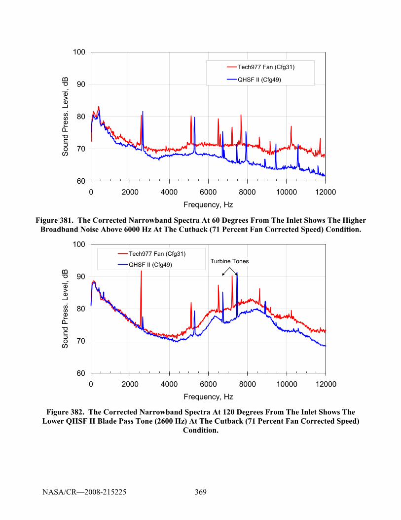
369

60

70

80

90

100

0 2000 4000 6000 8000 10000 12000Frequency, Hz

Sou

nd P

ress

. Lev

el, d

BTech977 Fan (Cfg31)

QHSF II (Cfg49)

Figure 381. The Corrected Narrowband Spectra At 60 Degrees From The Inlet Shows The Higher Broadband Noise Above 6000 Hz At The Cutback (71 Percent Fan Corrected Speed) Condition.

60

70

80

90

100

0 2000 4000 6000 8000 10000 12000Frequency, Hz

Sou

nd P

ress

. Lev

el, d

B

Tech977 Fan (Cfg31)

QHSF II (Cfg49) Turbine Tones

Figure 382. The Corrected Narrowband Spectra At 120 Degrees From The Inlet Shows The Lower QHSF II Blade Pass Tone (2600 Hz) At The Cutback (71 Percent Fan Corrected Speed)

Condition.

NASA/CR—2008-215225

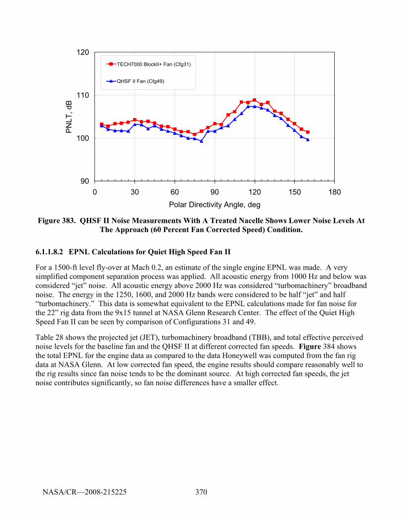
370

90

100

110

120


PN

LT, d

BTECH7000 BlockII+ Fan (Cfg31)

QHSF II Fan (Cfg49)

Figure 383. QHSF II Noise Measurements With A Treated Nacelle Shows Lower Noise Levels At The Approach (60 Percent Fan Corrected Speed) Condition.

6.1.1.8.2 EPNL Calculations for Quiet High Speed Fan II

For a 1500-ft level fly-over at Mach 0.2, an estimate of the single engine EPNL was made. A very simplified component separation process was applied. All acoustic energy from 1000 Hz and below was considered “jet” noise. All acoustic energy above 2000 Hz was considered “turbomachinery” broadband noise. The energy in the 1250, 1600, and 2000 Hz bands were considered to be half “jet” and half “turbomachinery.” This data is somewhat equivalent to the EPNL calculations made for fan noise for the 22” rig data from the 9x15 tunnel at NASA Glenn Research Center. The effect of the Quiet High Speed Fan II can be seen by comparison of Configurations 31 and 49.

Table 28 shows the projected jet (JET), turbomachinery broadband (TBB), and total effective perceived noise levels for the baseline fan and the QHSF II at different corrected fan speeds. Figure 384 shows the total EPNL for the engine data as compared to the data Honeywell was computed from the fan rig data at NASA Glenn. At low corrected fan speed, the engine results should compare reasonably well to the rig results since fan noise tends to be the dominant source. At high corrected fan speeds, the jet noise contributes significantly, so fan noise differences have a smaller effect.

NASA/CR—2008-215225

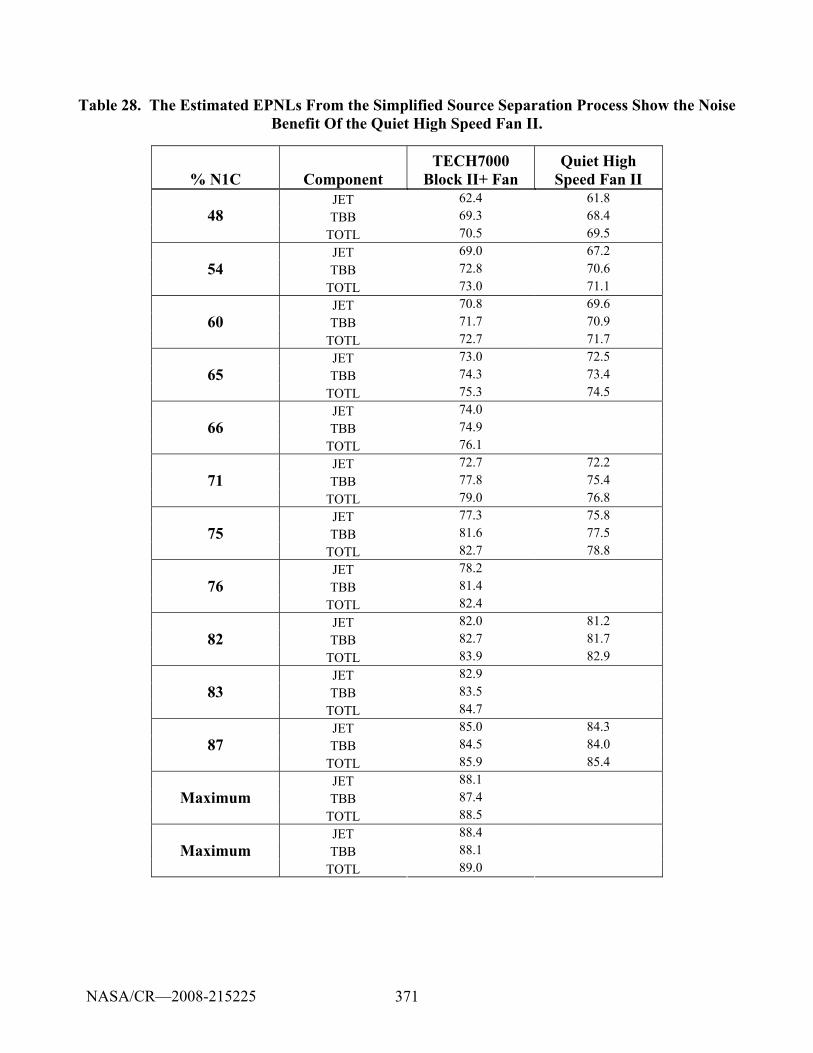
371

Table 28. The Estimated EPNLs From the Simplified Source Separation Process Show the Noise Benefit Of the Quiet High Speed Fan II.

% N1C Component TECH7000

Block II+ Fan Quiet High

Speed Fan II JET 62.4 61.8 TBB 69.3 68.4 48

TOTL 70.5 69.5 JET 69.0 67.2 TBB 72.8 70.6 54

TOTL 73.0 71.1 JET 70.8 69.6 TBB 71.7 70.9 60

TOTL 72.7 71.7 JET 73.0 72.5 TBB 74.3 73.4 65

TOTL 75.3 74.5 JET 74.0 TBB 74.9 66

TOTL 76.1 JET 72.7 72.2 TBB 77.8 75.4 71

TOTL 79.0 76.8 JET 77.3 75.8 TBB 81.6 77.5 75

TOTL 82.7 78.8 JET 78.2 TBB 81.4 76

TOTL 82.4 JET 82.0 81.2 TBB 82.7 81.7 82

TOTL 83.9 82.9 JET 82.9 TBB 83.5 83

TOTL 84.7 JET 85.0 84.3 TBB 84.5 84.0 87

TOTL 85.9 85.4 JET 88.1 TBB 87.4 Maximum

TOTL 88.5 JET 88.4 TBB 88.1 Maximum

TOTL 89.0

NASA/CR—2008-215225

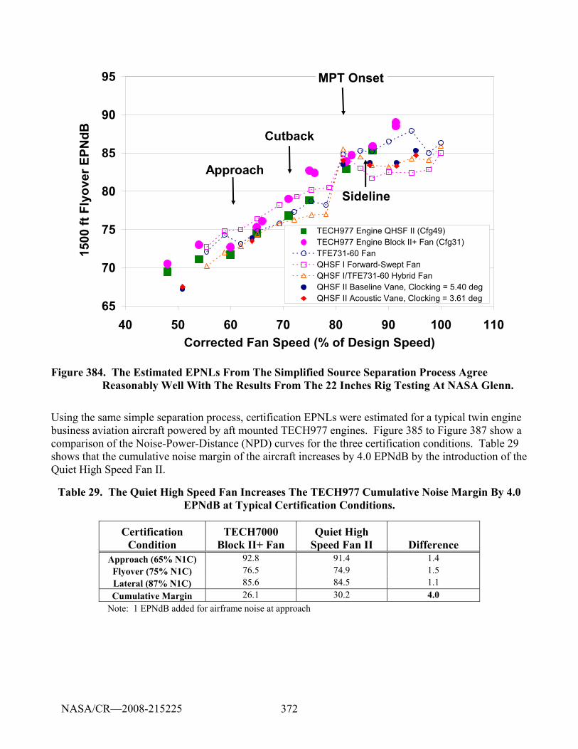
372

65

70

75

80

85

90

95

40 50 60 70 80 90 100 110Corrected Fan Speed (% of Design Speed)

1500

ft F

lyov

er E

PNdB

TECH977 Engine QHSF II (Cfg49)TECH977 Engine Block II+ Fan (Cfg31)TFE731-60 FanQHSF I Forward-Swept FanQHSF I/TFE731-60 Hybrid FanQHSF II Baseline Vane, Clocking = 5.40 degQHSF II Acoustic Vane, Clocking = 3.61 deg

Sideline

Approach

Cutback

MPT Onset

Figure 384. The Estimated EPNLs From The Simplified Source Separation Process Agree Reasonably Well With The Results From The 22 Inches Rig Testing At NASA Glenn.

Using the same simple separation process, certification EPNLs were estimated for a typical twin engine business aviation aircraft powered by aft mounted TECH977 engines. Figure 385 to Figure 387 show a comparison of the Noise-Power-Distance (NPD) curves for the three certification conditions. Table 29 shows that the cumulative noise margin of the aircraft increases by 4.0 EPNdB by the introduction of the Quiet High Speed Fan II.

Table 29. The Quiet High Speed Fan Increases The TECH977 Cumulative Noise Margin By 4.0 EPNdB at Typical Certification Conditions.

Certification Condition

TECH7000 Block II+ Fan

Quiet High Speed Fan II Difference

Approach (65% N1C) 92.8 91.4 1.4 Flyover (75% N1C) 76.5 74.9 1.5 Lateral (87% N1C) 85.6 84.5 1.1 Cumulative Margin 26.1 30.2 4.0

Note: 1 EPNdB added for airframe noise at approach

NASA/CR—2008-215225

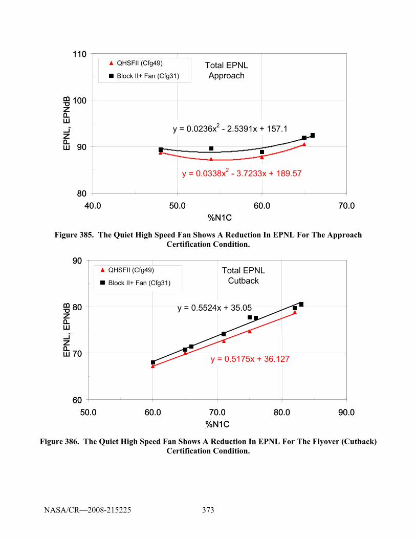
373

Total EPNLApproach

y = 0.0338x2 - 3.7233x + 189.57

y = 0.0236x2 - 2.5391x + 157.1

80

90

100

110

40.0 50.0 60.0 70.0%N1C

EP

NL,

EP

NdB

QHSFII (Cfg49)

Block II+ Fan (Cfg31)Total EPNLApproach

y = 0.0338x2 - 3.7233x + 189.57

y = 0.0236x2 - 2.5391x + 157.1

80

90

100

110

40.0 50.0 60.0 70.0%N1C

EP

NL,

EP

NdB

QHSFII (Cfg49)

Block II+ Fan (Cfg31)

Figure 385. The Quiet High Speed Fan Shows A Reduction In EPNL For The Approach Certification Condition.

Total EPNLCutback

y = 0.5175x + 36.127

y = 0.5524x + 35.05

60

70

80

90

50.0 60.0 70.0 80.0 90.0%N1C

EP

NL,

EP

NdB

QHSFII (Cfg49)


Total EPNLCutback

y = 0.5175x + 36.127

y = 0.5524x + 35.05

60

70

80

90

50.0 60.0 70.0 80.0 90.0%N1C

EP

NL,

EP

NdB

QHSFII (Cfg49)


Figure 386. The Quiet High Speed Fan Shows A Reduction In EPNL For The Flyover (Cutback) Certification Condition.

NASA/CR—2008-215225

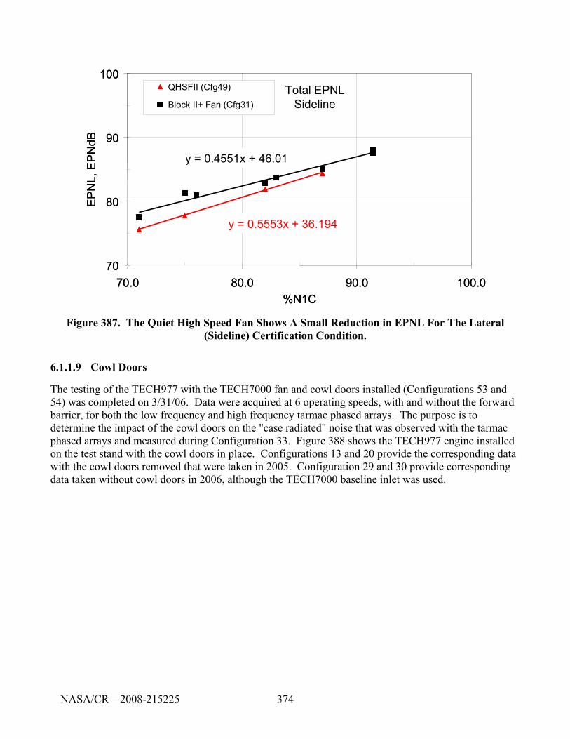
374

Total EPNLSideline

y = 0.5553x + 36.194

y = 0.4551x + 46.01

70

80

90

100

70.0 80.0 90.0 100.0%N1C

EP

NL,

EP

NdB

QHSFII (Cfg49)

Block II+ Fan (Cfg31)Total EPNL

Sideline

y = 0.5553x + 36.194

y = 0.4551x + 46.01

70

80

90

100

70.0 80.0 90.0 100.0%N1C

EP

NL,

EP

NdB

QHSFII (Cfg49)


Figure 387. The Quiet High Speed Fan Shows A Small Reduction in EPNL For The Lateral (Sideline) Certification Condition.

6.1.1.9 Cowl Doors

The testing of the TECH977 with the TECH7000 fan and cowl doors installed (Configurations 53 and 54) was completed on 3/31/06. Data were acquired at 6 operating speeds, with and without the forward barrier, for both the low frequency and high frequency tarmac phased arrays. The purpose is to determine the impact of the cowl doors on the "case radiated" noise that was observed with the tarmac phased arrays and measured during Configuration 33. Figure 388 shows the TECH977 engine installed on the test stand with the cowl doors in place. Configurations 13 and 20 provide the corresponding data with the cowl doors removed that were taken in 2005. Configuration 29 and 30 provide corresponding data taken without cowl doors in 2006, although the TECH7000 baseline inlet was used.

NASA/CR—2008-215225

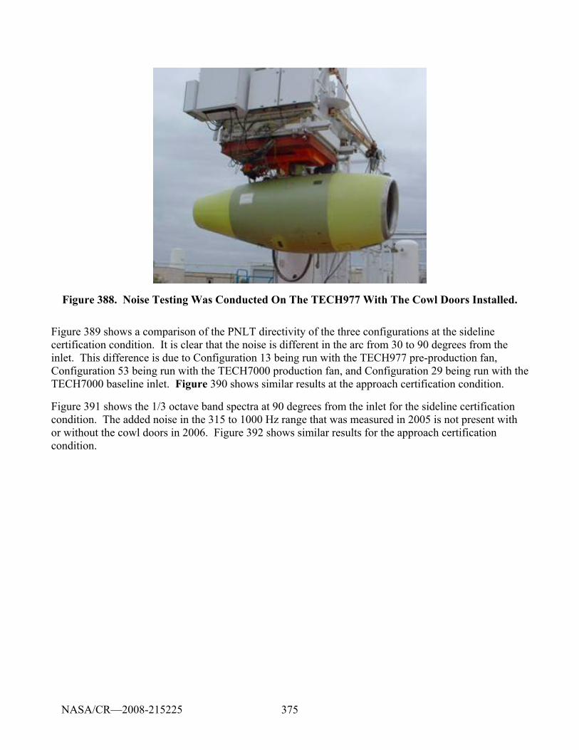
375

Figure 388. Noise Testing Was Conducted On The TECH977 With The Cowl Doors Installed.

Figure 389 shows a comparison of the PNLT directivity of the three configurations at the sideline certification condition. It is clear that the noise is different in the arc from 30 to 90 degrees from the inlet. This difference is due to Configuration 13 being run with the TECH977 pre-production fan, Configuration 53 being run with the TECH7000 production fan, and Configuration 29 being run with the TECH7000 baseline inlet. Figure 390 shows similar results at the approach certification condition.

Figure 391 shows the 1/3 octave band spectra at 90 degrees from the inlet for the sideline certification condition. The added noise in the 315 to 1000 Hz range that was measured in 2005 is not present with or without the cowl doors in 2006. Figure 392 shows similar results for the approach certification condition.

NASA/CR—2008-215225

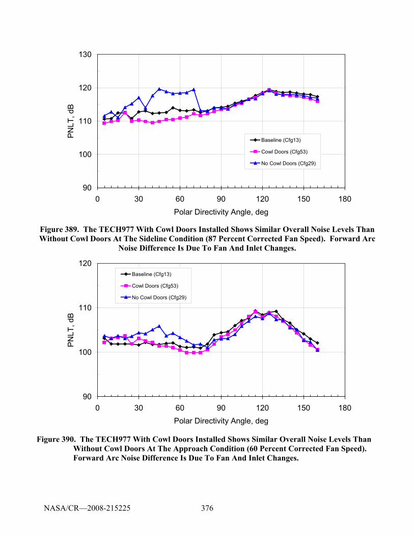
376

90

100

110

120

130


PNLT

, dB

Baseline (Cfg13)

Cowl Doors (Cfg53)

No Cowl Doors (Cfg29)

Figure 389. The TECH977 With Cowl Doors Installed Shows Similar Overall Noise Levels Than Without Cowl Doors At The Sideline Condition (87 Percent Corrected Fan Speed). Forward Arc

Noise Difference Is Due To Fan And Inlet Changes.

90

100

110

120


PNLT

, dB

Baseline (Cfg13)

Cowl Doors (Cfg53)


Figure 390. The TECH977 With Cowl Doors Installed Shows Similar Overall Noise Levels Than Without Cowl Doors At The Approach Condition (60 Percent Corrected Fan Speed). Forward Arc Noise Difference Is Due To Fan And Inlet Changes.

NASA/CR—2008-215225

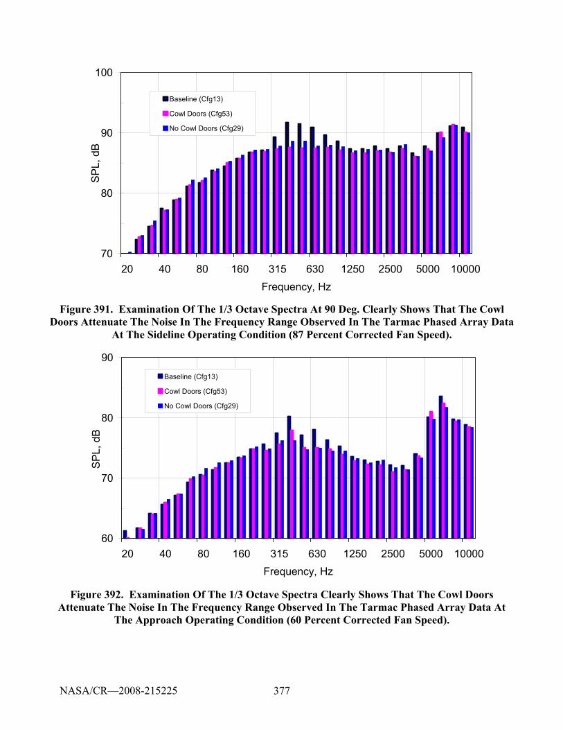
377

70

80

90

100

20 40 80 160 315 630 1250 2500 5000 10000Frequency, Hz

SP

L, d

BBaseline (Cfg13)

Cowl Doors (Cfg53)


Figure 391. Examination Of The 1/3 Octave Spectra At 90 Deg. Clearly Shows That The Cowl Doors Attenuate The Noise In The Frequency Range Observed In The Tarmac Phased Array Data

At The Sideline Operating Condition (87 Percent Corrected Fan Speed).

60

70

80

90

20 40 80 160 315 630 1250 2500 5000 10000Frequency, Hz

SP

L, d

B

Baseline (Cfg13)

Cowl Doors (Cfg53)


Figure 392. Examination Of The 1/3 Octave Spectra Clearly Shows That The Cowl Doors Attenuate The Noise In The Frequency Range Observed In The Tarmac Phased Array Data At

The Approach Operating Condition (60 Percent Corrected Fan Speed).

NASA/CR—2008-215225

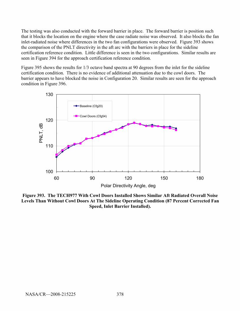
378

The testing was also conducted with the forward barrier in place. The forward barrier is position such that it blocks the location on the engine where the case radiate noise was observed. It also blocks the fan inlet-radiated noise where differences in the two fan configurations were observed. Figure 393 shows the comparison of the PNLT directivity in the aft arc with the barriers in place for the sideline certification reference condition. Little difference is seen in the two configurations. Similar results are seen in Figure 394 for the approach certification reference condition.

Figure 395 shows the results for 1/3 octave band spectra at 90 degrees from the inlet for the sideline certification condition. There is no evidence of additional attenuation due to the cowl doors. The barrier appears to have blocked the noise in Configuration 20. Similar results are seen for the approach condition in Figure 396.

100

110

120

130


PN

LT, d

B

Baseline (Cfg20)

Cowl Doors (Cfg54)

Figure 393. The TECH977 With Cowl Doors Installed Shows Similar Aft Radiated Overall Noise Levels Than Without Cowl Doors At The Sideline Operating Condition (87 Percent Corrected Fan

Speed, Inlet Barrier Installed).

NASA/CR—2008-215225

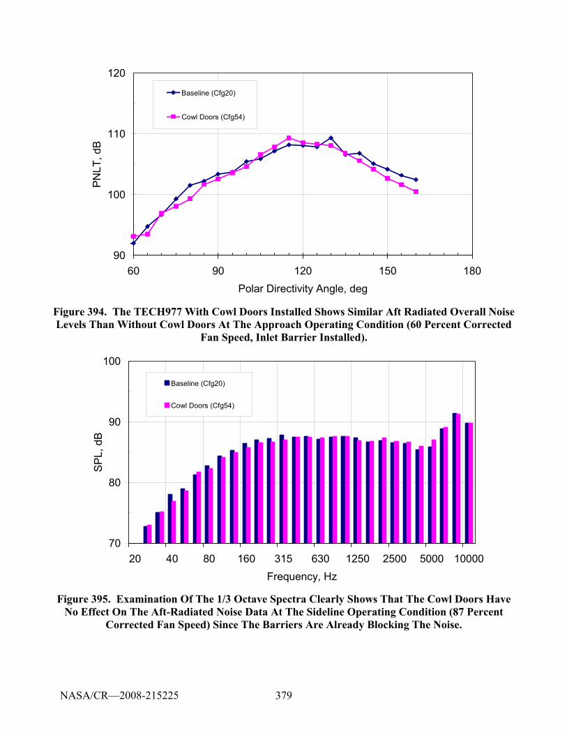
379

90

100

110

120


PN

LT, d

BBaseline (Cfg20)

Cowl Doors (Cfg54)

Figure 394. The TECH977 With Cowl Doors Installed Shows Similar Aft Radiated Overall Noise Levels Than Without Cowl Doors At The Approach Operating Condition (60 Percent Corrected

Fan Speed, Inlet Barrier Installed).

70

80

90

100

20 40 80 160 315 630 1250 2500 5000 10000Frequency, Hz

SP

L, d

B

Baseline (Cfg20)

Cowl Doors (Cfg54)

Figure 395. Examination Of The 1/3 Octave Spectra Clearly Shows That The Cowl Doors Have No Effect On The Aft-Radiated Noise Data At The Sideline Operating Condition (87 Percent

Corrected Fan Speed) Since The Barriers Are Already Blocking The Noise.

NASA/CR—2008-215225

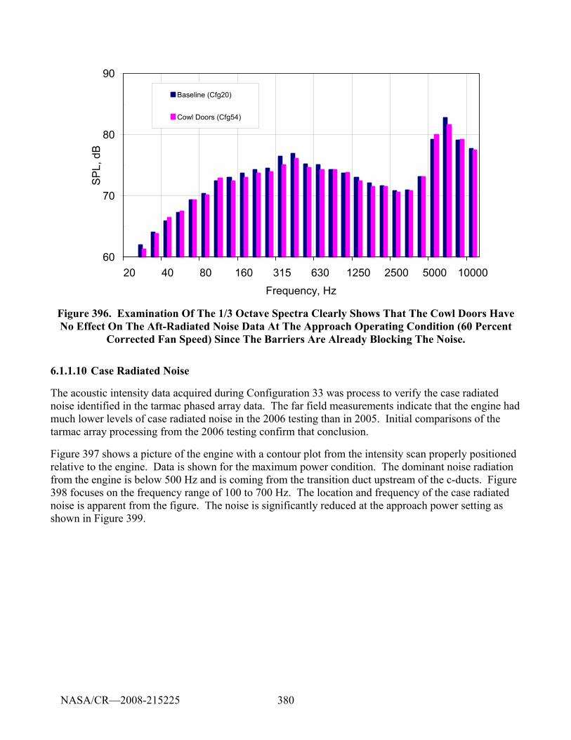
380

60

70

80

90

20 40 80 160 315 630 1250 2500 5000 10000Frequency, Hz

SP

L, d

BBaseline (Cfg20)

Cowl Doors (Cfg54)

Figure 396. Examination Of The 1/3 Octave Spectra Clearly Shows That The Cowl Doors Have No Effect On The Aft-Radiated Noise Data At The Approach Operating Condition (60 Percent

Corrected Fan Speed) Since The Barriers Are Already Blocking The Noise.

6.1.1.10 Case Radiated Noise

The acoustic intensity data acquired during Configuration 33 was process to verify the case radiated noise identified in the tarmac phased array data. The far field measurements indicate that the engine had much lower levels of case radiated noise in the 2006 testing than in 2005. Initial comparisons of the tarmac array processing from the 2006 testing confirm that conclusion.

Figure 397 shows a picture of the engine with a contour plot from the intensity scan properly positioned relative to the engine. Data is shown for the maximum power condition. The dominant noise radiation from the engine is below 500 Hz and is coming from the transition duct upstream of the c-ducts. Figure 398 focuses on the frequency range of 100 to 700 Hz. The location and frequency of the case radiated noise is apparent from the figure. The noise is significantly reduced at the approach power setting as shown in Figure 399.

NASA/CR—2008-215225

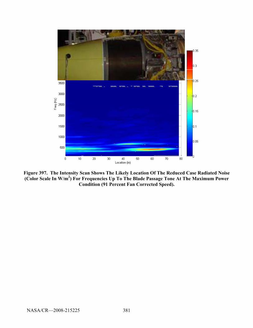
381

Figure 397. The Intensity Scan Shows The Likely Location Of The Reduced Case Radiated Noise (Color Scale In W/m2) For Frequencies Up To The Blade Passage Tone At The Maximum Power

Condition (91 Percent Fan Corrected Speed).

NASA/CR—2008-215225

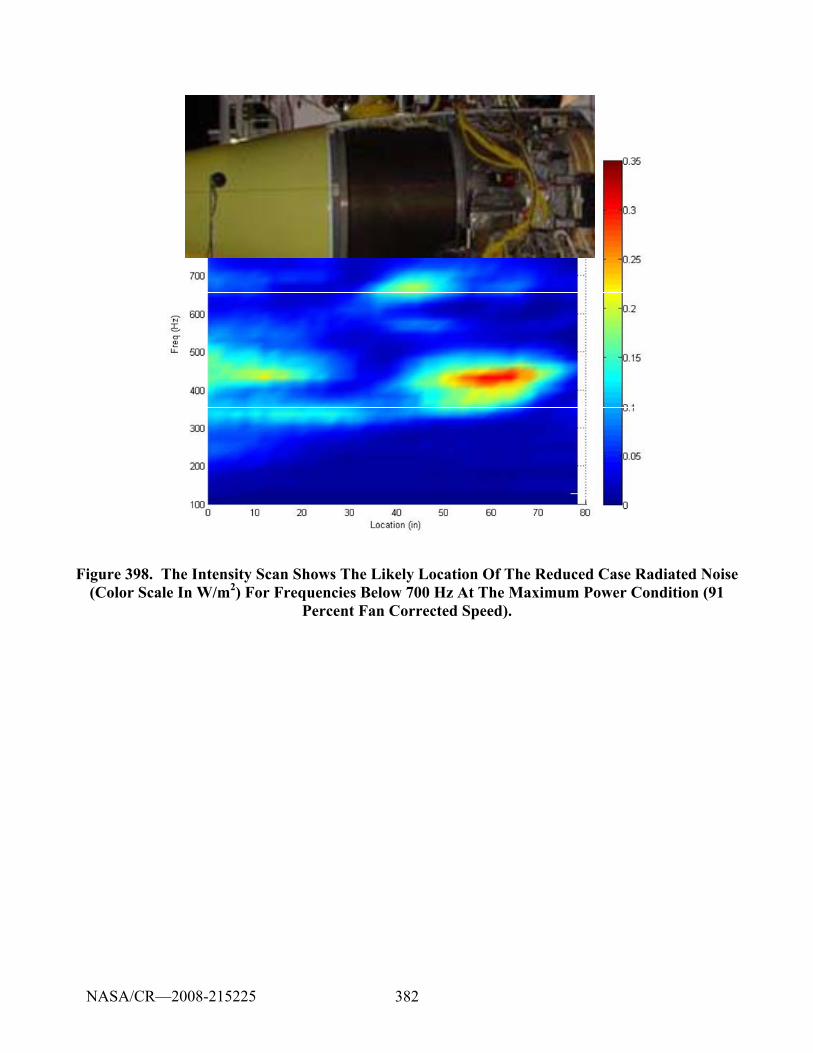
382

Figure 398. The Intensity Scan Shows The Likely Location Of The Reduced Case Radiated Noise (Color Scale In W/m2) For Frequencies Below 700 Hz At The Maximum Power Condition (91

Percent Fan Corrected Speed).

NASA/CR—2008-215225

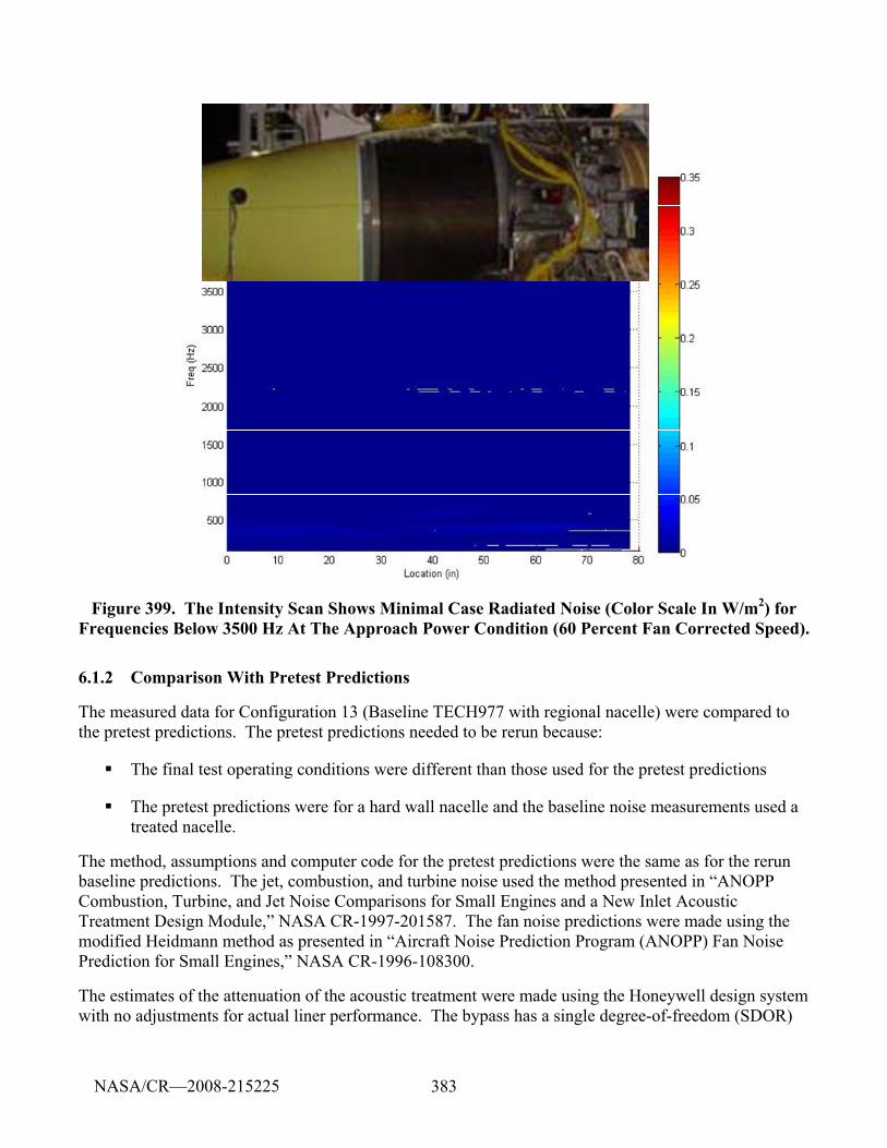
383

Figure 399. The Intensity Scan Shows Minimal Case Radiated Noise (Color Scale In W/m2) for Frequencies Below 3500 Hz At The Approach Power Condition (60 Percent Fan Corrected Speed).

6.1.2 Comparison With Pretest Predictions

The measured data for Configuration 13 (Baseline TECH977 with regional nacelle) were compared to the pretest predictions. The pretest predictions needed to be rerun because:

The final test operating conditions were different than those used for the pretest predictions

The pretest predictions were for a hard wall nacelle and the baseline noise measurements used a treated nacelle.

The method, assumptions and computer code for the pretest predictions were the same as for the rerun baseline predictions. The jet, combustion, and turbine noise used the method presented in “ANOPP Combustion, Turbine, and Jet Noise Comparisons for Small Engines and a New Inlet Acoustic Treatment Design Module,” NASA CR-1997-201587. The fan noise predictions were made using the modified Heidmann method as presented in “Aircraft Noise Prediction Program (ANOPP) Fan Noise Prediction for Small Engines,” NASA CR-1996-108300.

The estimates of the attenuation of the acoustic treatment were made using the Honeywell design system with no adjustments for actual liner performance. The bypass has a single degree-of-freedom (SDOR)

NASA/CR—2008-215225

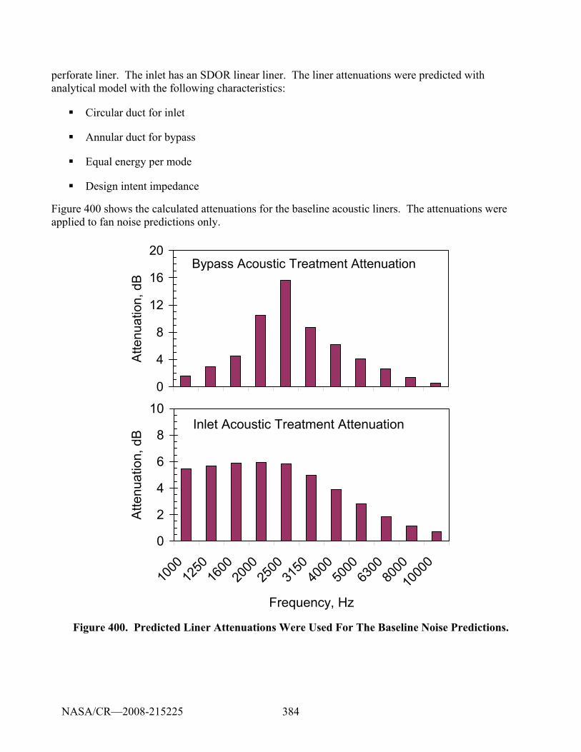
384

perforate liner. The inlet has an SDOR linear liner. The liner attenuations were predicted with analytical model with the following characteristics:

Circular duct for inlet

Annular duct for bypass

Equal energy per mode

Design intent impedance

Figure 400 shows the calculated attenuations for the baseline acoustic liners. The attenuations were applied to fan noise predictions only.

Bypass Acoustic Treatment Attenuation

0

4

8

12

16

20

Atte

nuat

ion,

dB

Inlet Acoustic Treatment Attenuation

0

2

4

6

8

10

1000

1250

1600

2000

2500

3150

4000

5000

6300

8000

1000

0

Frequency, Hz

Atte

nuat

ion,

dB

Figure 400. Predicted Liner Attenuations Were Used For The Baseline Noise Predictions.

NASA/CR—2008-215225

385

Figure 401 through Figure 406 show the results of the comparison between the measured data and the pretest prediction method. PNLT directivities and the spectra at five directivity angles are shown. Some additional observations of the quality of the predictions are also shown on the figures.

NASA/CR—2008-215225

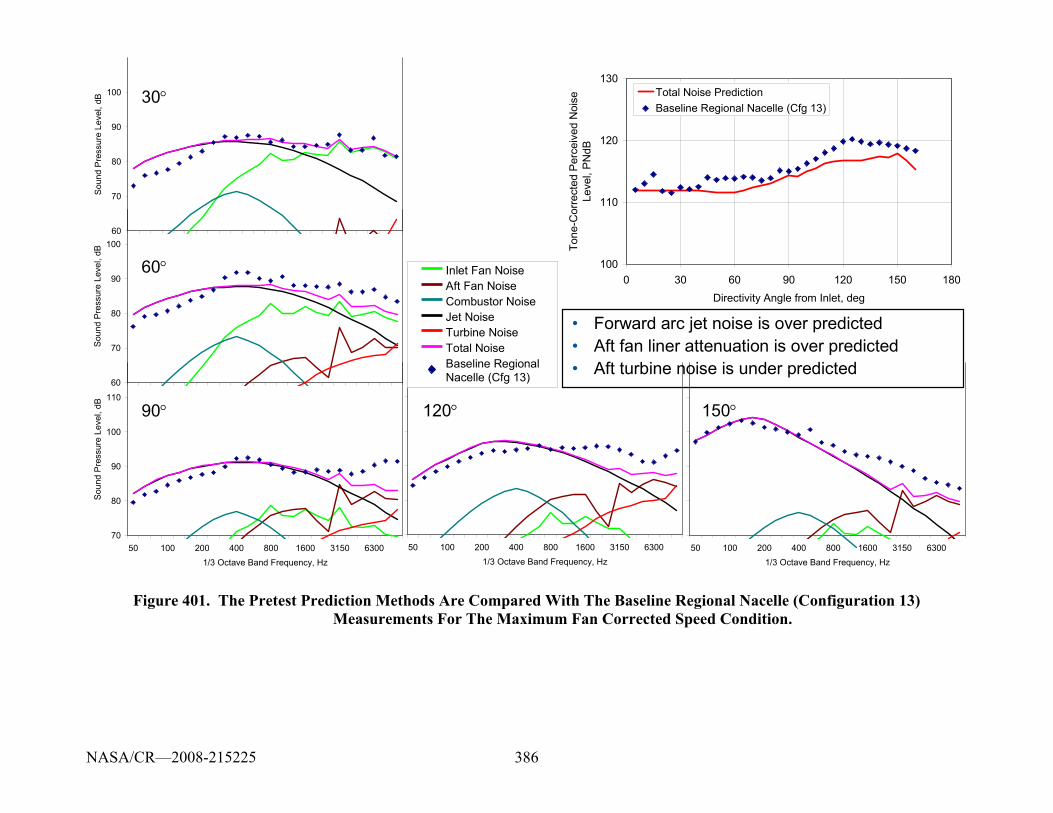
386

50 100 200 400 800 1600 3150 63001/3 Octave Band Frequency, Hz


70

80

90

100

110


Soun

d Pr

essu

re L

evel

, dB

60

70

80

90

100

Sou

nd P

ress

ure

Leve

l, dB

• Forward arc jet noise is over predicted• Aft fan liner attenuation is over predicted• Aft turbine noise is under predicted

30°

60°

90° 120° 150°

100

110

120

130

0 30 60 90 120 150 180Directivity Angle from Inlet, deg

Tone

-Cor

rect

ed P

erce

ived

Noi

se

Leve

l, P

NdB

Total Noise PredictionBaseline Regional Nacelle (Cfg 13)

Inlet Fan NoiseAft Fan NoiseCombustor NoiseJet NoiseTurbine NoiseTotal NoiseBaseline RegionalNacelle (Cfg 13)


60

70

80

90

100S

ound

Pre

ssur

e Le

vel,

dB

Figure 401. The Pretest Prediction Methods Are Compared With The Baseline Regional Nacelle (Configuration 13) Measurements For The Maximum Fan Corrected Speed Condition.

NASA/CR—2008-215225

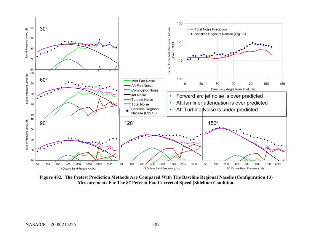
387

60

70

80

90

100

Sou

nd P

ress

ure

Leve

l, dB

70

80

90

100

110


Soun

d Pr

essu

re L

evel

, dB



30°

60°

90° 120° 150°

• Forward arc jet noise is over predicted• Aft fan liner attenuation is over predicted• Aft Turbine Noise is under predicted



60

70

80

90

100S

ound

Pre

ssur

e Le

vel,

dB

100

110

120

130


Tone

-Cor

rect

ed P

erce

ived

Noi

se

Leve

l, PN

dB


Figure 402. The Pretest Prediction Methods Are Compared With The Baseline Regional Nacelle (Configuration 13) Measurements For The 87 Percent Fan Corrected Speed (Sideline) Condition.

NASA/CR—2008-215225

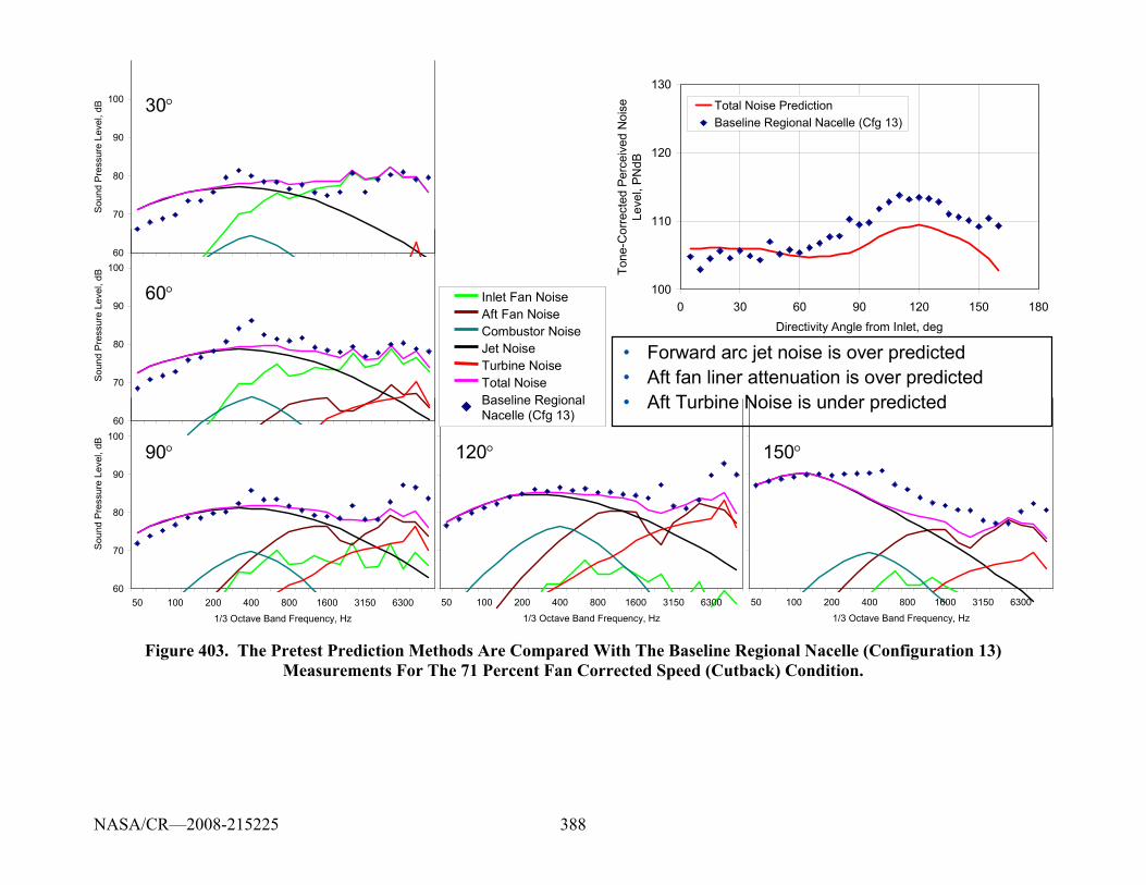
388

60

70

80

90

100

Soun

d Pr

essu

re L

evel

, dB

60

70

80

90

100


Sou

nd P

ress

ure

Leve

l, dB



30°

60°

90° 120° 150°




60

70

80

90

100S

ound

Pre

ssur

e Le

vel,

dB

100

110

120

130


Tone

-Cor

rect

ed P

erce

ived

Noi

se

Leve

l, PN

dB


Figure 403. The Pretest Prediction Methods Are Compared With The Baseline Regional Nacelle (Configuration 13) Measurements For The 71 Percent Fan Corrected Speed (Cutback) Condition.

NASA/CR—2008-215225

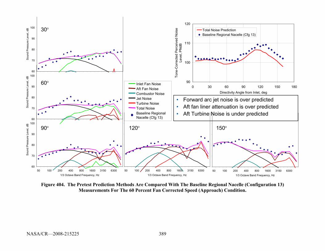
389

30°

60°

90° 120° 150°




90

100

110

120


Tone

-Cor

rect

ed P

erce

ived

Noi

se

Leve

l, PN

dB


60

70

80

90

100S

ound

Pre

ssur

e Le

vel,

dB

60

70

80

90

100


Sou

nd P

ress

ure

Leve

l, dB



60

70

80

90

100

Sou

nd P

ress

ure

Leve

l, dB

Figure 404. The Pretest Prediction Methods Are Compared With The Baseline Regional Nacelle (Configuration 13) Measurements For The 60 Percent Fan Corrected Speed (Approach) Condition.

NASA/CR—2008-215225

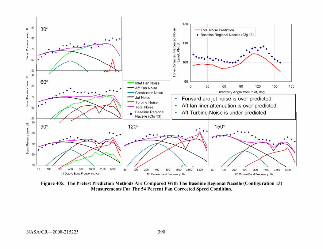
390

30°

60°

90° 120° 150°




90

100

110

120


Tone

-Cor

rect

ed P

erce

ived

Noi

se

Leve

l, P

NdB


50

60

70

80

90S

ound

Pre

ssur

e Le

vel,

dB

50

60

70

80

90

Sou

nd P

ress

ure

Leve

l, dB

50

60

70

80

90


Soun

d Pr

essu

re L

evel

, dB



Figure 405. The Pretest Prediction Methods Are Compared With The Baseline Regional Nacelle (Configuration 13) Measurements For The 54 Percent Fan Corrected Speed Condition.

NASA/CR—2008-215225

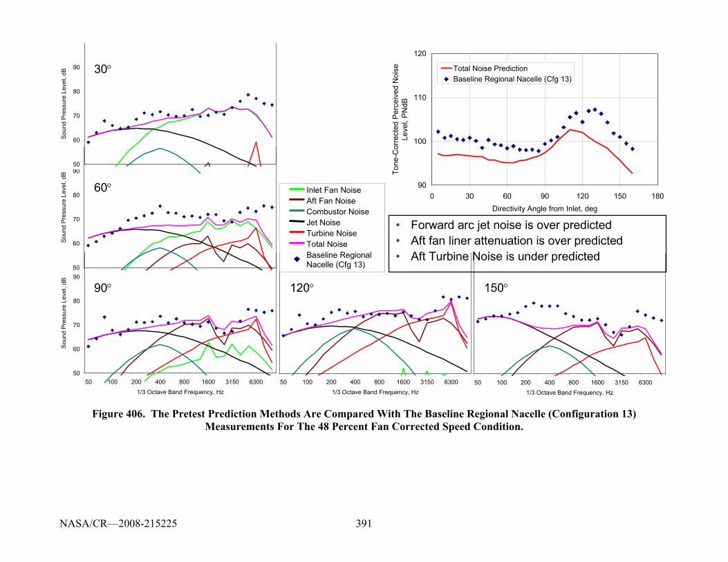
391

50

60

70

80

90

Sou

nd P

ress

ure

Leve

l, dB

50

60

70

80

90


Sou

nd P

ress

ure

Leve

l, dB



30°

60°

90° 120° 150°




90

100

110

120


Tone

-Cor

rect

ed P

erce

ived

Noi

se

Leve

l, PN

dB


50

60

70

80

90S

ound

Pre

ssur

e Le

vel,

dB

Figure 406. The Pretest Prediction Methods Are Compared With The Baseline Regional Nacelle (Configuration 13) Measurements For The 48 Percent Fan Corrected Speed Condition.

NASA/CR—2008-215225

392

6.1.3 Engine Noise Component Separation

Pretest predictions of the noise signature of the TECH7000 hard wall configuration were made as discussed in Section 5.2.3. These predictions were then updated to apply to the baseline regional nacelle configuration (Section 6.1.2).

6.1.3.1 Sideline Operating Condition

Figure 407 shows a comparison of the component noise predictions with the far field acoustic data (Configuration 13) for the sideline power setting (87% fan corrected speed) at 3 directivity angles. It can be seen from the figure that the main features of the noise spectra have been captured by the predictions. Note that the measured data is from the test series with the unwanted case-radiated noise source (see Section 6.1.1.9), so data from 315 Hz to 630 Hz should be ignored.

The first observation is that the jet noise prediction overpredicts the total noise from 50 to 160 Hz at directivity angles of 60° and 90°. Figure 408 shows measured results from Configurations 13, 14, and 20. Configuration 14 has the aft barrier in place and Configuration 20 has the inlet barrier in place. It is clear that the noise from 50 to 160 Hz is unaffected by either barrier. This evidence strongly suggests that the noise source in that frequency range is due to the jet at a large distance from the engine where it is not blocked by the aft barrier. Existing jet noise location models confirm that result.

At 60°, Figure 407a shows that the noise from 800 to 10000 Hz is dominated by inlet fan noise. Figure 408a confirms that very little exhaust radiated noise contributes to the spectra for that frequency range. However, the predictions underestimate the noise levels. At 90° (Figure 408b), the barrier results show that the aft noise is now dominating and little inlet fan noise is observed. Figure 408c shows that there is little fan inlet noise at 120° as well. The frequency extent of the fan noise can be seen by evaluating the data with and without acoustic treatment.

NASA/CR—2008-215225

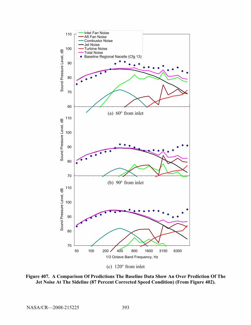
393

60

70

80

90

100

110

Soun

d Pr

essu

re L

evel

, dB

Inlet Fan NoiseAft Fan NoiseCombustor NoiseJet NoiseTurbine NoiseTotal NoiseBaseline Regional Nacelle (Cfg 13)

(a) 60° from inlet

70

80

90

100

110

Soun

d Pr

essu

re L

evel

, dB

(b) 90° from inlet

70

80

90

100

110


Soun

d P

ress

ure

Leve

l, dB

(c) 120° from inlet

Figure 407. A Comparison Of Predictions The Baseline Data Show An Over Prediction Of The Jet Noise At The Sideline (87 Percent Corrected Speed Condition) (From Figure 402).

NASA/CR—2008-215225

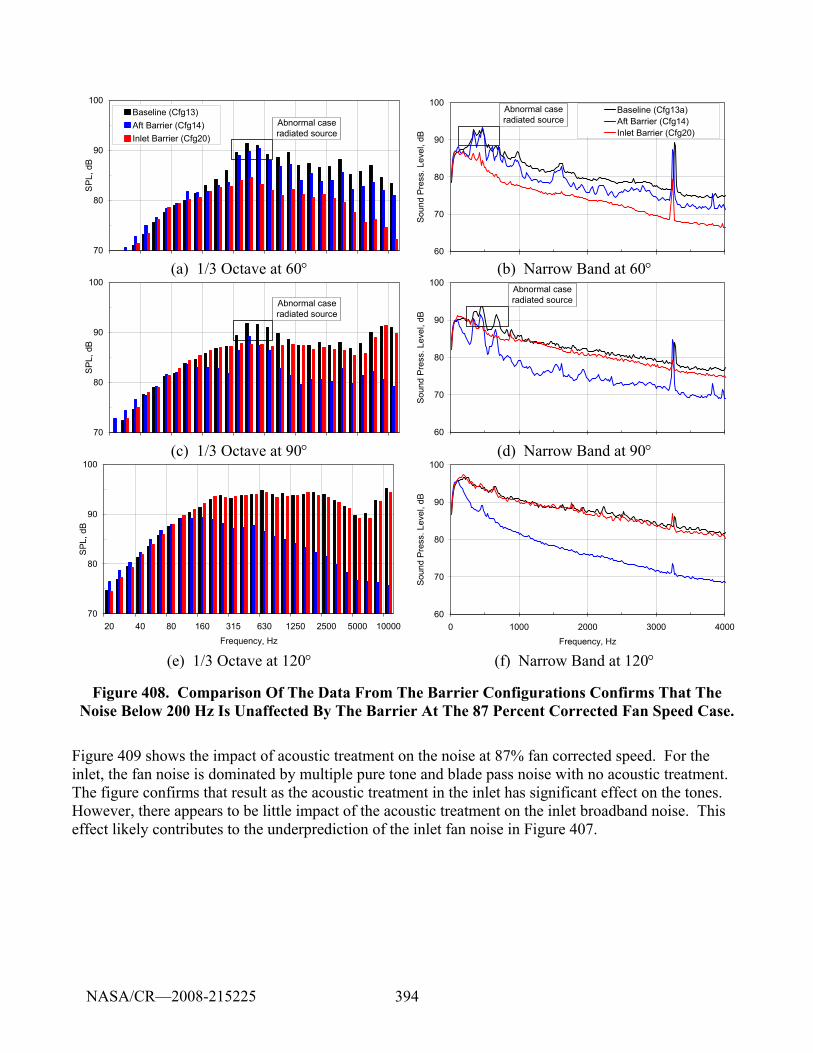
394

70

80

90

100S

PL, d

B

Baseline (Cfg13)Aft Barrier (Cfg14)Inlet Barrier (Cfg20)


60

70

80

90

100

Soun

d Pr

ess.

Lev

el, d

B

Baseline (Cfg13a)Aft Barrier (Cfg14)Inlet Barrier (Cfg20)


(a) 1/3 Octave at 60° (b) Narrow Band at 60°

70

80

90

100

SPL

, dB


60

70

80

90

100

Sou

nd P

ress

. Lev

el, d

B


(c) 1/3 Octave at 90° (d) Narrow Band at 90°

70

80

90

100

20 40 80 160 315 630 1250 2500 5000 10000Frequency, Hz

SPL

, dB

60

70

80

90

100

0 1000 2000 3000 4000Frequency, Hz

Sou

nd P

ress

. Lev

el, d

B

(e) 1/3 Octave at 120° (f) Narrow Band at 120°

Figure 408. Comparison Of The Data From The Barrier Configurations Confirms That The Noise Below 200 Hz Is Unaffected By The Barrier At The 87 Percent Corrected Fan Speed Case.

Figure 409 shows the impact of acoustic treatment on the noise at 87% fan corrected speed. For the inlet, the fan noise is dominated by multiple pure tone and blade pass noise with no acoustic treatment. The figure confirms that result as the acoustic treatment in the inlet has significant effect on the tones. However, there appears to be little impact of the acoustic treatment on the inlet broadband noise. This effect likely contributes to the underprediction of the inlet fan noise in Figure 407.

NASA/CR—2008-215225

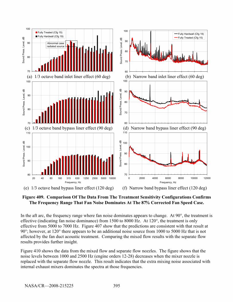
395

70

80

90

100

Sou

nd P

ress

. Lev

el, d

B

Fully Treated (Cfg 15)Fully Hardwall (Cfg 19)


60

70

80

90

100

Soun

d Pr

ess.

Lev

el, d

B

Fully Hardwall (Cfg 19)Fully Treated (Cfg 15)

(a) 1/3 octave band inlet liner effect (60 deg) (b) Narrow band inlet liner effect (60 deg)

70

80

90

100

Sou

nd P

ress

. Lev

el, d

B

60

70

80

90

100

Sou

nd P

ress

. Lev

el, d

B

(c) 1/3 octave band bypass liner effect (90 deg) (d) Narrow band bypass liner effect (90 deg)

80

90

100

110

20 40 80 160 315 630 1250 2500 5000 10000Frequency, Hz

Sou

nd P

ress

. Lev

el, d

B

70

80

90

100

110

0 2000 4000 6000 8000 10000 12000Frequency, Hz

Soun

d Pr

ess.

Lev

el, d

B

(e) 1/3 octave band bypass liner effect (120 deg) (f) Narrow band bypass liner effect (120 deg)

Figure 409. Comparison Of The Data From The Treatment Sensitivity Configurations Confirms The Frequency Range That Fan Noise Dominates At The 87% Corrected Fan Speed Case.

In the aft arc, the frequency range where fan noise dominates appears to change. At 90°, the treatment is effective (indicating fan noise dominance) from 1500 to 8000 Hz. At 120°, the treatment is only effective from 5000 to 7000 Hz. Figure 407 show that the predictions are consistent with that result at 90°; however, at 120° there appears to be an additional noise source from 1000 to 5000 Hz that is not affected by the fan duct acoustic treatment. Comparing the mixed flow results with the separate flow results provides further insight.

Figure 410 shows the data from the mixed flow and separate flow nozzles. The figure shows that the noise levels between 1000 and 2500 Hz (engine orders 12-28) decreases when the mixer nozzle is replaced with the separate flow nozzle. This result indicates that the extra mixing noise associated with internal exhaust mixers dominates the spectra at those frequencies.

NASA/CR—2008-215225

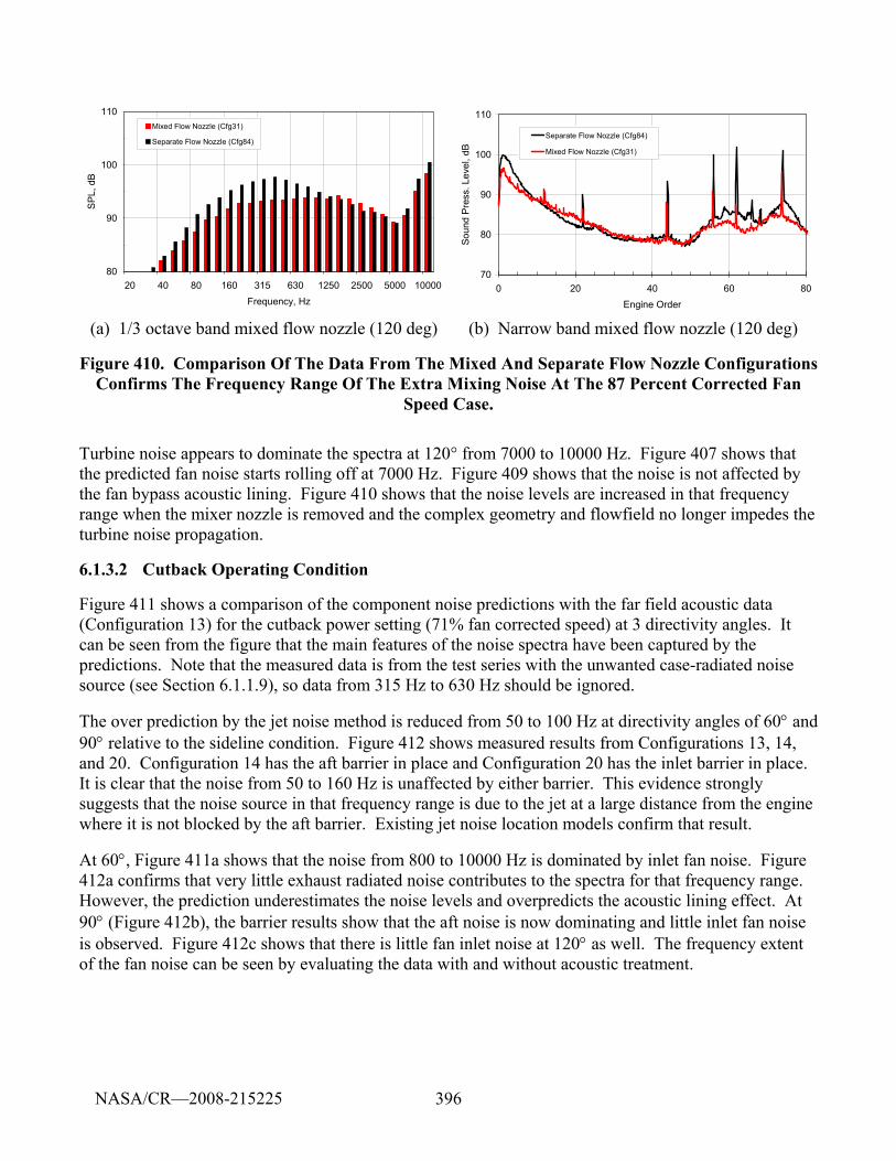
396

80

90

100

110

20 40 80 160 315 630 1250 2500 5000 10000Frequency, Hz

SP

L, d

B

Mixed Flow Nozzle (Cfg31)

Separate Flow Nozzle (Cfg84)

70

80

90

100

110


Soun

d P

ress

. Lev

el, d

B



(a) 1/3 octave band mixed flow nozzle (120 deg) (b) Narrow band mixed flow nozzle (120 deg)

Figure 410. Comparison Of The Data From The Mixed And Separate Flow Nozzle Configurations Confirms The Frequency Range Of The Extra Mixing Noise At The 87 Percent Corrected Fan

Speed Case.

Turbine noise appears to dominate the spectra at 120° from 7000 to 10000 Hz. Figure 407 shows that the predicted fan noise starts rolling off at 7000 Hz. Figure 409 shows that the noise is not affected by the fan bypass acoustic lining. Figure 410 shows that the noise levels are increased in that frequency range when the mixer nozzle is removed and the complex geometry and flowfield no longer impedes the turbine noise propagation.

6.1.3.2 Cutback Operating Condition

Figure 411 shows a comparison of the component noise predictions with the far field acoustic data (Configuration 13) for the cutback power setting (71% fan corrected speed) at 3 directivity angles. It can be seen from the figure that the main features of the noise spectra have been captured by the predictions. Note that the measured data is from the test series with the unwanted case-radiated noise source (see Section 6.1.1.9), so data from 315 Hz to 630 Hz should be ignored.

The over prediction by the jet noise method is reduced from 50 to 100 Hz at directivity angles of 60° and 90° relative to the sideline condition. Figure 412 shows measured results from Configurations 13, 14, and 20. Configuration 14 has the aft barrier in place and Configuration 20 has the inlet barrier in place. It is clear that the noise from 50 to 160 Hz is unaffected by either barrier. This evidence strongly suggests that the noise source in that frequency range is due to the jet at a large distance from the engine where it is not blocked by the aft barrier. Existing jet noise location models confirm that result.

At 60°, Figure 411a shows that the noise from 800 to 10000 Hz is dominated by inlet fan noise. Figure 412a confirms that very little exhaust radiated noise contributes to the spectra for that frequency range. However, the prediction underestimates the noise levels and overpredicts the acoustic lining effect. At 90° (Figure 412b), the barrier results show that the aft noise is now dominating and little inlet fan noise is observed. Figure 412c shows that there is little fan inlet noise at 120° as well. The frequency extent of the fan noise can be seen by evaluating the data with and without acoustic treatment.

NASA/CR—2008-215225

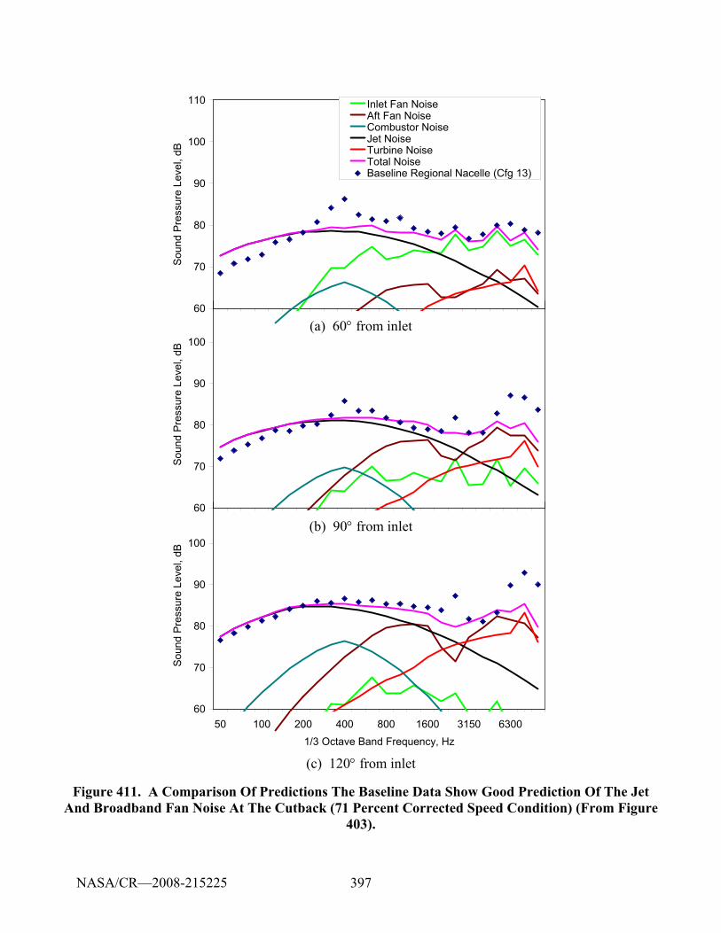
397

60

70

80

90

100

110

Sou

nd P

ress

ure

Leve

l, dB


(a) 60° from inlet

60

70

80

90

100

Sou

nd P

ress

ure

Leve

l, dB

(b) 90° from inlet

60

70

80

90

100


Sou

nd P

ress

ure

Leve

l, dB


Figure 411. A Comparison Of Predictions The Baseline Data Show Good Prediction Of The Jet And Broadband Fan Noise At The Cutback (71 Percent Corrected Speed Condition) (From Figure

403).

NASA/CR—2008-215225

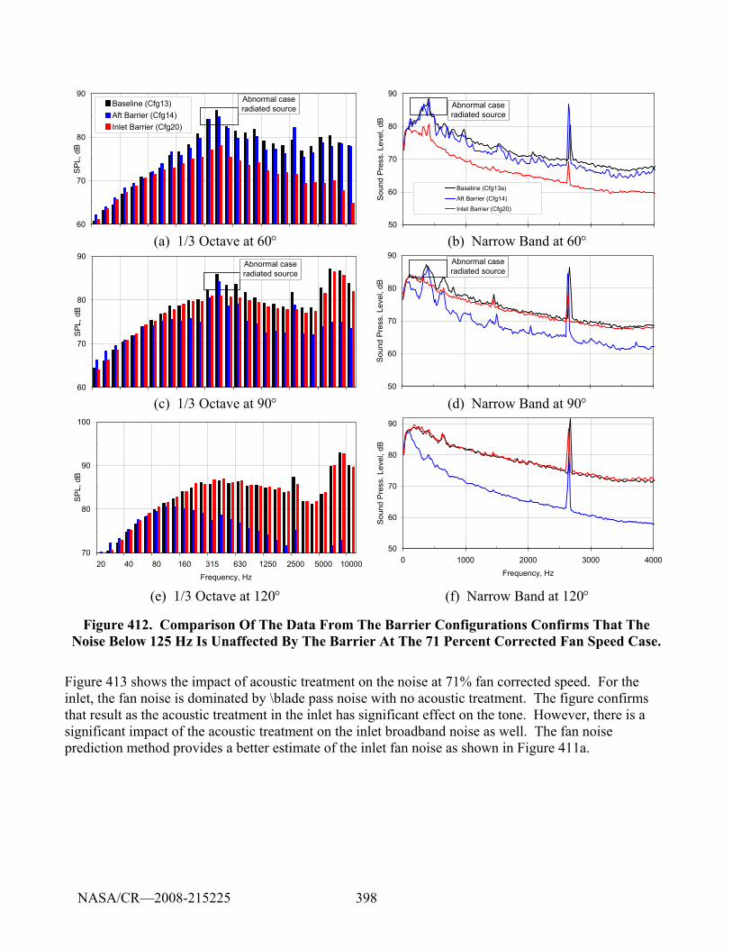
398

60

70

80

90

SPL,

dB



50

60

70

80

90

Soun

d P

ress

. Lev

el, d

B

Baseline (Cfg13a)

Aft Barrier (Cfg14)

Inlet Barrier (Cfg20)



60

70

80

90

SPL

, dB


50

60

70

80

90

Sou

nd P

ress

. Lev

el, d

B



70

80

90

100

20 40 80 160 315 630 1250 2500 5000 10000Frequency, Hz

SPL,

dB

50

60

70

80

90

0 1000 2000 3000 4000Frequency, Hz

Soun

d P

ress

. Lev

el, d

B



Figure 413 shows the impact of acoustic treatment on the noise at 71% fan corrected speed. For the inlet, the fan noise is dominated by \blade pass noise with no acoustic treatment. The figure confirms that result as the acoustic treatment in the inlet has significant effect on the tone. However, there is a significant impact of the acoustic treatment on the inlet broadband noise as well. The fan noise prediction method provides a better estimate of the inlet fan noise as shown in Figure 411a.

NASA/CR—2008-215225

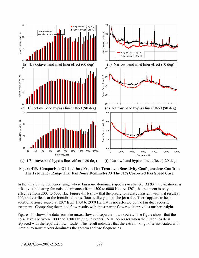
399

60

70

80

90

Soun

d Pr

ess.

Lev

el, d

B



50

60

70

80

90

Sou

nd P

ress

. Lev

el, d

B



60

70

80

90

Sou

nd P

ress

. Lev

el, d

B

50

60

70

80

90

Sou

nd P

ress

. Lev

el, d

B


70

80

90

100

20 40 80 160 315 630 1250 2500 5000 10000Frequency, Hz

Sou

nd P

ress

. Lev

el, d

B

60

70

80

90

100

0 2000 4000 6000 8000 10000 12000Frequency, Hz

Sou

nd P

ress

. Lev

el, d

B



In the aft arc, the frequency range where fan noise dominates appears to change. At 90°, the treatment is effective (indicating fan noise dominance) from 1500 to 6000 Hz. At 120°, the treatment is only effective from 2000 to 6000 Hz. Figure 411b show that the predictions are consistent with that result at 90°, and verifies that the broadband noise floor is likely due to the jet noise. There appears to be an additional noise source at 120° from 1500 to 2000 Hz that is not affected by the fan duct acoustic treatment. Comparing the mixed flow results with the separate flow results provides further insight.

Figure 414 shows the data from the mixed flow and separate flow nozzles. The figure shows that the noise levels between 1000 and 1500 Hz (engine orders 12-18) decreases when the mixer nozzle is replaced with the separate flow nozzle. This result indicates that the extra mixing noise associated with internal exhaust mixers dominates the spectra at those frequencies.

NASA/CR—2008-215225

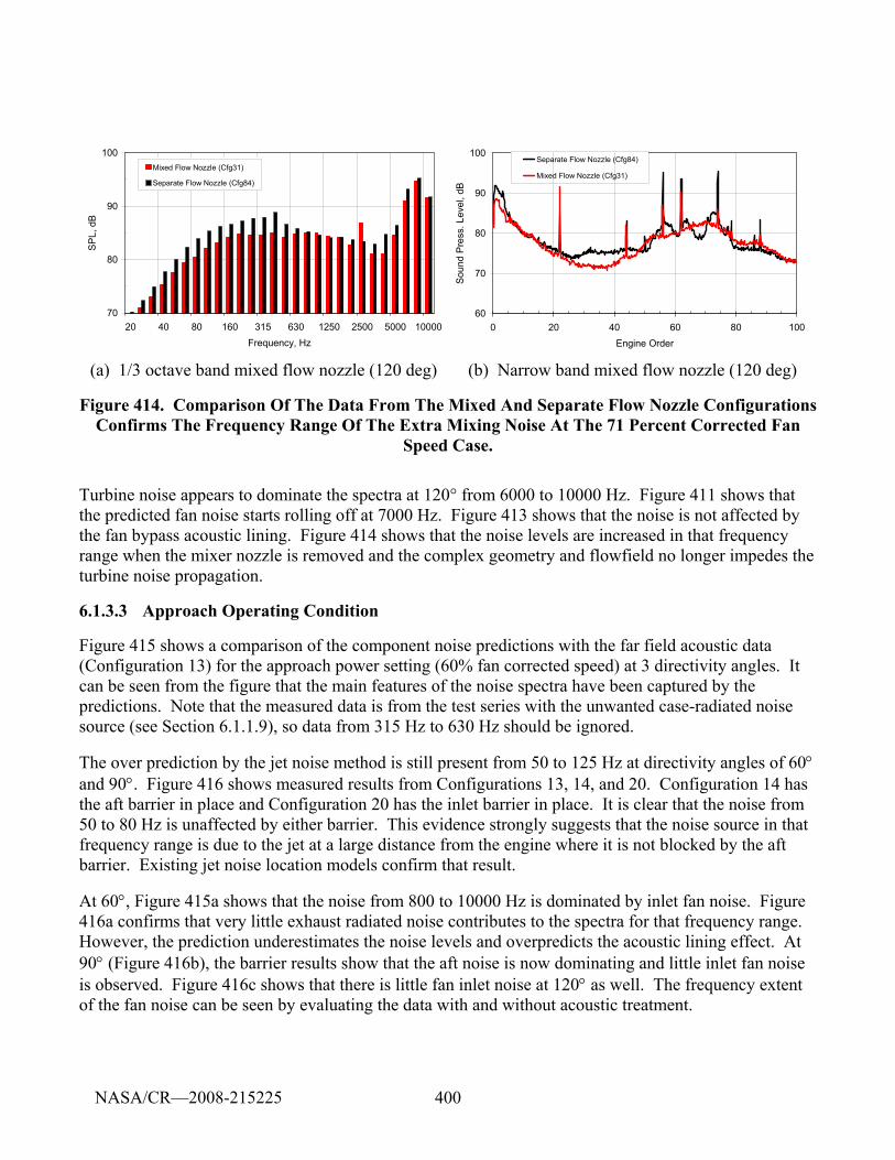
400

70

80

90

100

20 40 80 160 315 630 1250 2500 5000 10000Frequency, Hz

SP

L, d

B



60

70

80

90

100

0 20 40 60 80 100Engine Order

Sou

nd P

ress

. Lev

el, d

B





Speed Case.


6.1.3.3 Approach Operating Condition

Figure 415 shows a comparison of the component noise predictions with the far field acoustic data (Configuration 13) for the approach power setting (60% fan corrected speed) at 3 directivity angles. It can be seen from the figure that the main features of the noise spectra have been captured by the predictions. Note that the measured data is from the test series with the unwanted case-radiated noise source (see Section 6.1.1.9), so data from 315 Hz to 630 Hz should be ignored.

The over prediction by the jet noise method is still present from 50 to 125 Hz at directivity angles of 60° and 90°. Figure 416 shows measured results from Configurations 13, 14, and 20. Configuration 14 has the aft barrier in place and Configuration 20 has the inlet barrier in place. It is clear that the noise from 50 to 80 Hz is unaffected by either barrier. This evidence strongly suggests that the noise source in that frequency range is due to the jet at a large distance from the engine where it is not blocked by the aft barrier. Existing jet noise location models confirm that result.

At 60°, Figure 415a shows that the noise from 800 to 10000 Hz is dominated by inlet fan noise. Figure 416a confirms that very little exhaust radiated noise contributes to the spectra for that frequency range. However, the prediction underestimates the noise levels and overpredicts the acoustic lining effect. At 90° (Figure 416b), the barrier results show that the aft noise is now dominating and little inlet fan noise is observed. Figure 416c shows that there is little fan inlet noise at 120° as well. The frequency extent of the fan noise can be seen by evaluating the data with and without acoustic treatment.

NASA/CR—2008-215225

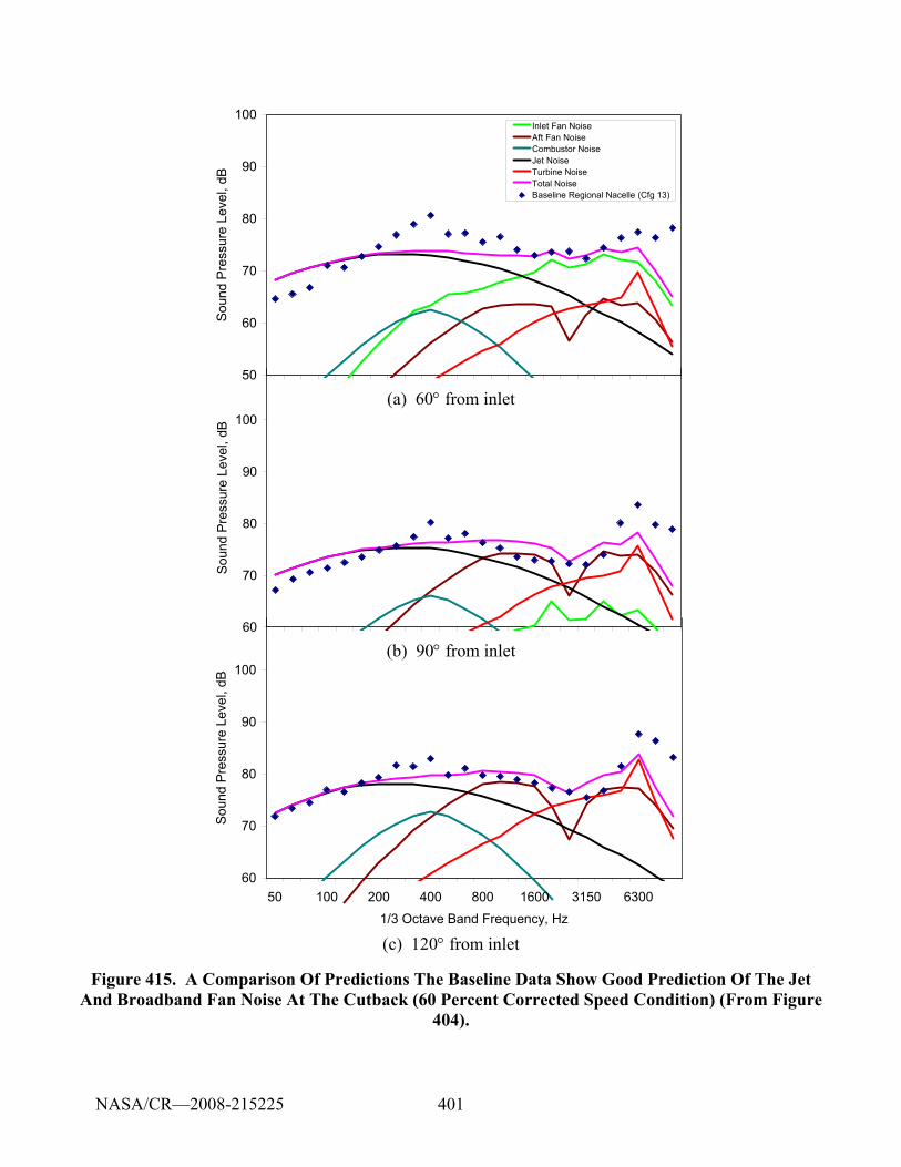
401

50

60

70

80

90

100

Sou

nd P

ress

ure

Leve

l, dB


(a) 60° from inlet

60

70

80

90

100

Soun

d Pr

essu

re L

evel

, dB

(b) 90° from inlet

60

70

80

90

100


Sou

nd P

ress

ure

Leve

l, dB


Figure 415. A Comparison Of Predictions The Baseline Data Show Good Prediction Of The Jet And Broadband Fan Noise At The Cutback (60 Percent Corrected Speed Condition) (From Figure

404).

NASA/CR—2008-215225

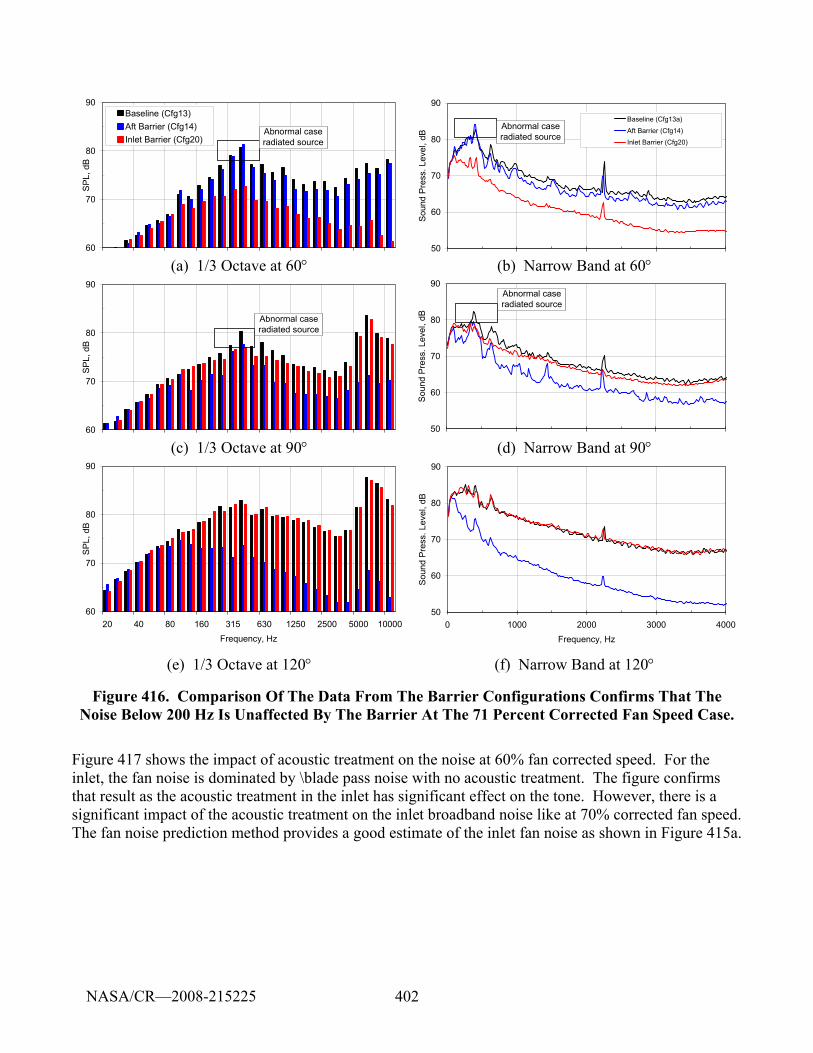
402

60

70

80

90

SP

L, d

B



50

60

70

80

90

Sou

nd P

ress

. Lev

el, d

B

Baseline (Cfg13a)

Aft Barrier (Cfg14)

Inlet Barrier (Cfg20)



60

70

80

90

SP

L, d

B


50

60

70

80

90

Soun

d P

ress

. Lev

el, d

B



60

70

80

90

20 40 80 160 315 630 1250 2500 5000 10000Frequency, Hz

SPL

, dB

50

60

70

80

90

0 1000 2000 3000 4000Frequency, Hz

Sou

nd P

ress

. Lev

el, d

B



Figure 417 shows the impact of acoustic treatment on the noise at 60% fan corrected speed. For the inlet, the fan noise is dominated by \blade pass noise with no acoustic treatment. The figure confirms that result as the acoustic treatment in the inlet has significant effect on the tone. However, there is a significant impact of the acoustic treatment on the inlet broadband noise like at 70% corrected fan speed. The fan noise prediction method provides a good estimate of the inlet fan noise as shown in Figure 415a.

NASA/CR—2008-215225

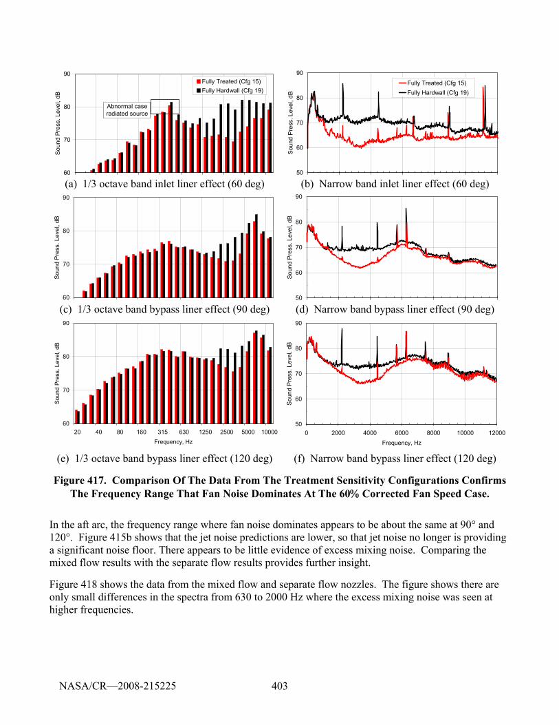
403

60

70

80

90

Sou

nd P

ress

. Lev

el, d

B



50

60

70

80

90

Sou

nd P

ress

. Lev

el, d

B



60

70

80

90

Sou

nd P

ress

. Lev

el, d

B

50

60

70

80

90

Sou

nd P

ress

. Lev

el, d

B


60

70

80

90

20 40 80 160 315 630 1250 2500 5000 10000Frequency, Hz

Sou

nd P

ress

. Lev

el, d

B

50

60

70

80

90

0 2000 4000 6000 8000 10000 12000Frequency, Hz

Sou

nd P

ress

. Lev

el, d

B



In the aft arc, the frequency range where fan noise dominates appears to be about the same at 90° and 120°. Figure 415b shows that the jet noise predictions are lower, so that jet noise no longer is providing a significant noise floor. There appears to be little evidence of excess mixing noise. Comparing the mixed flow results with the separate flow results provides further insight.

Figure 418 shows the data from the mixed flow and separate flow nozzles. The figure shows there are only small differences in the spectra from 630 to 2000 Hz where the excess mixing noise was seen at higher frequencies.

NASA/CR—2008-215225

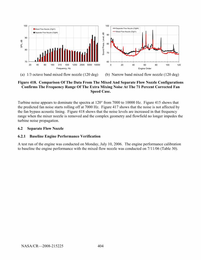
404

70

80

90

100

20 40 80 160 315 630 1250 2500 5000 10000Frequency, Hz

SP

L, d

B



60

70

80

90

100

0 20 40 60 80 100 120Engine Order

Sou

nd P

ress

. Lev

el, d

B





Speed Case.



6.2.1 Baseline Engine Performance Verification

A test run of the engine was conducted on Monday, July 10, 2006. The engine performance calibration to baseline the engine performance with the mixed flow nozzle was conducted on 7/11/06 (Table 30).

NASA/CR—2008-215225

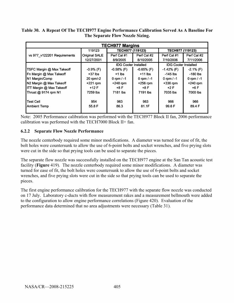
405

Table 30. A Repeat Of The TECH977 Engine Performance Calibration Served As A Baseline For The Separate Flow Nozzle Sizing.

TECH977 Margins119123

vs 977_v122201 Requirements Original SALE Perf Cal #1 Perf Cal #2 Perf Cal #1 Perf Cal #212/27/2001 8/9/2005 8/10/2005 7/10/2006 7/11/2006

TSFC Margin @ Max Takeoff -0.9% (F) -0.58% (F) -0.65% (F) -1.42% (F) -2.1% (F)Fn Margin @ Max Takeoff +37 lbs +1 lbs +11 lbs -145 lbs -180 lbsN1 Margin/Comp 20 rpm/-2 0 rpm / -1 0 rpm / -1 0 rpm / -1 0 rpm / -1N2 Margin @ Max Takeoff +221 rpm +248 rpm +256 rpm +336 rpm +240 rpmITT Margin @ Max Takeoff +12 F +8 F +8 F +2 F +6 FThrust @ 9174 rpm N1 7259 lbs 7181 lbs 7191 lbs 7035 lbs 7000 lbs

Test Cell 954 963 963 966 966Ambient Temp 55.8 F 86.3 81.1F 99.6 F 89.4 F

TECH977 (119123) TECH977 (119123)

IDG Cooler Installed IDG Cooler Installed

TECH977 Margins119123

vs 977_v122201 Requirements Original SALE Perf Cal #1 Perf Cal #2 Perf Cal #1 Perf Cal #212/27/2001 8/9/2005 8/10/2005 7/10/2006 7/11/2006

TSFC Margin @ Max Takeoff -0.9% (F) -0.58% (F) -0.65% (F) -1.42% (F) -2.1% (F)Fn Margin @ Max Takeoff +37 lbs +1 lbs +11 lbs -145 lbs -180 lbsN1 Margin/Comp 20 rpm/-2 0 rpm / -1 0 rpm / -1 0 rpm / -1 0 rpm / -1N2 Margin @ Max Takeoff +221 rpm +248 rpm +256 rpm +336 rpm +240 rpmITT Margin @ Max Takeoff +12 F +8 F +8 F +2 F +6 FThrust @ 9174 rpm N1 7259 lbs 7181 lbs 7191 lbs 7035 lbs 7000 lbs

Test Cell 954 963 963 966 966Ambient Temp 55.8 F 86.3 81.1F 99.6 F 89.4 F

TECH977 (119123) TECH977 (119123)

IDG Cooler Installed IDG Cooler Installed

Note: 2005 Performance calibration was performed with the TECH977 Block II fan, 2006 performance calibration was performed with the TECH7000 Block II+ fan.

6.2.2 Separate Flow Nozzle Performance

The nozzle centerbody required some minor modifications. A diameter was turned for ease of fit, the bolt holes were countersunk to allow the use of 6-point bolts and socket wrenches, and five prying slots were cut in the side so that prying tools can be used to separate the pieces.

The separate flow nozzle was successfully installed on the TECH977 engine at the San Tan acoustic test facility (Figure 419). The nozzle centerbody required some minor modifications. A diameter was turned for ease of fit, the bolt holes were countersunk to allow the use of 6-point bolts and socket wrenches, and five prying slots were cut in the side so that prying tools can be used to separate the pieces.

The first engine performance calibration for the TECH977 with the separate flow nozzle was conducted on 17 July. Laboratory c-ducts with flow measurement rakes and a measurement bellmouth were added to the configuration to allow engine performance correlations (Figure 420). Evaluation of the performance data determined that no area adjustments were necessary (Table 31).

NASA/CR—2008-215225

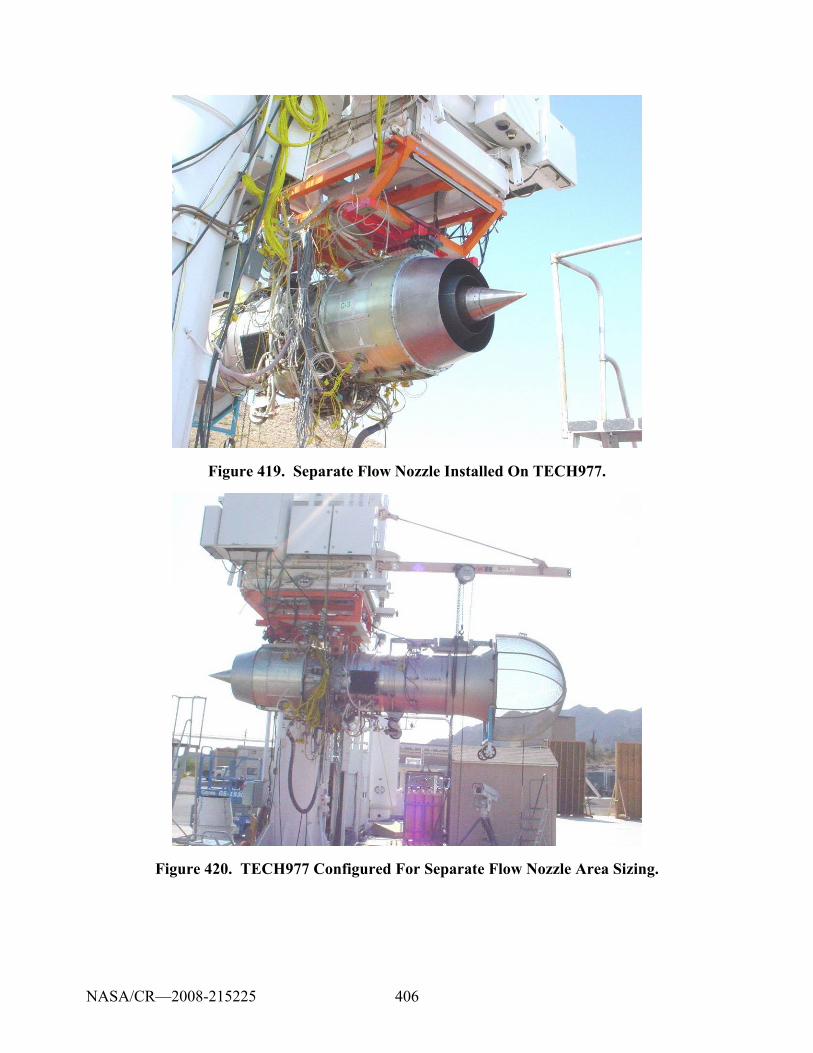
406

Figure 419. Separate Flow Nozzle Installed On TECH977.

Figure 420. TECH977 Configured For Separate Flow Nozzle Area Sizing.

NASA/CR—2008-215225

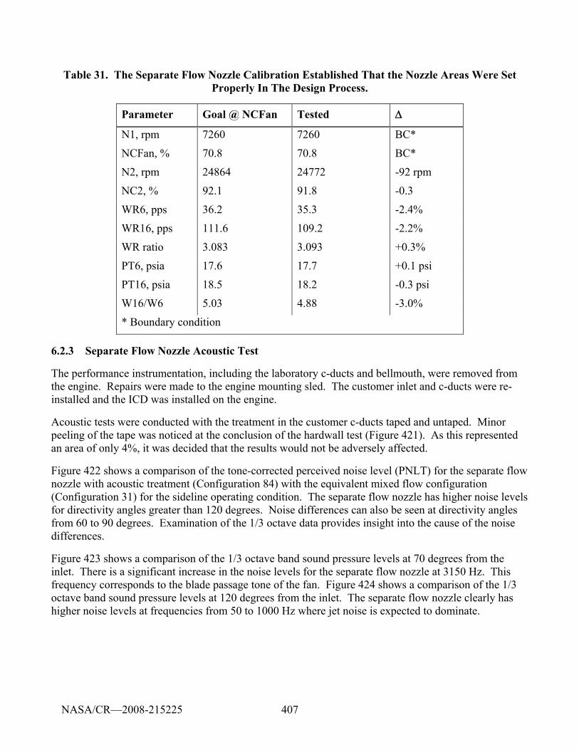
407

Table 31. The Separate Flow Nozzle Calibration Established That the Nozzle Areas Were Set Properly In The Design Process.

Parameter Goal @ NCFan Tested Δ

N1, rpm 7260 7260 BC*

NCFan, % 70.8 70.8 BC*

N2, rpm 24864 24772 -92 rpm

NC2, % 92.1 91.8 -0.3

WR6, pps 36.2 35.3 -2.4%

WR16, pps 111.6 109.2 -2.2%

WR ratio 3.083 3.093 +0.3%

PT6, psia 17.6 17.7 +0.1 psi

PT16, psia 18.5 18.2 -0.3 psi

W16/W6 5.03 4.88 -3.0%

* Boundary condition

6.2.3 Separate Flow Nozzle Acoustic Test

The performance instrumentation, including the laboratory c-ducts and bellmouth, were removed from the engine. Repairs were made to the engine mounting sled. The customer inlet and c-ducts were re-installed and the ICD was installed on the engine.

Acoustic tests were conducted with the treatment in the customer c-ducts taped and untaped. Minor peeling of the tape was noticed at the conclusion of the hardwall test (Figure 421). As this represented an area of only 4%, it was decided that the results would not be adversely affected.

Figure 422 shows a comparison of the tone-corrected perceived noise level (PNLT) for the separate flow nozzle with acoustic treatment (Configuration 84) with the equivalent mixed flow configuration (Configuration 31) for the sideline operating condition. The separate flow nozzle has higher noise levels for directivity angles greater than 120 degrees. Noise differences can also be seen at directivity angles from 60 to 90 degrees. Examination of the 1/3 octave data provides insight into the cause of the noise differences.

Figure 423 shows a comparison of the 1/3 octave band sound pressure levels at 70 degrees from the inlet. There is a significant increase in the noise levels for the separate flow nozzle at 3150 Hz. This frequency corresponds to the blade passage tone of the fan. Figure 424 shows a comparison of the 1/3 octave band sound pressure levels at 120 degrees from the inlet. The separate flow nozzle clearly has higher noise levels at frequencies from 50 to 1000 Hz where jet noise is expected to dominate.

NASA/CR—2008-215225

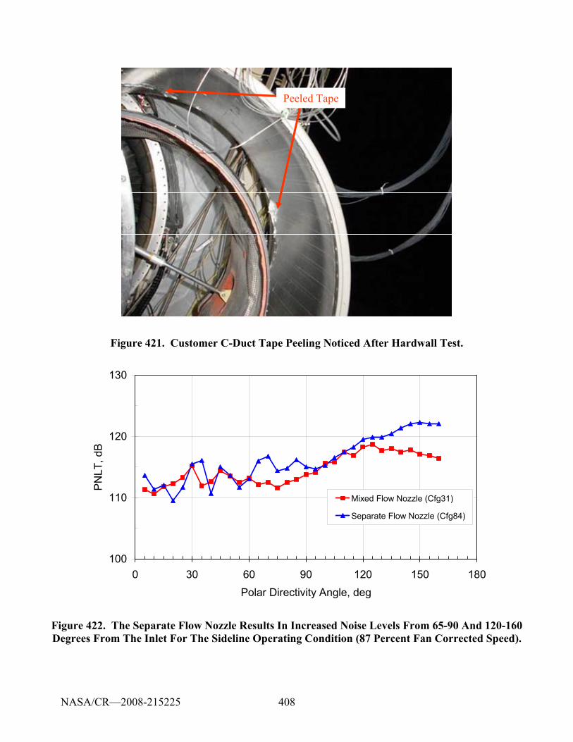
408

Peeled TapePeeled Tape

Figure 421. Customer C-Duct Tape Peeling Noticed After Hardwall Test.

100

110

120

130


PN

LT, d

B



Figure 422. The Separate Flow Nozzle Results In Increased Noise Levels From 65-90 And 120-160 Degrees From The Inlet For The Sideline Operating Condition (87 Percent Fan Corrected Speed).

NASA/CR—2008-215225

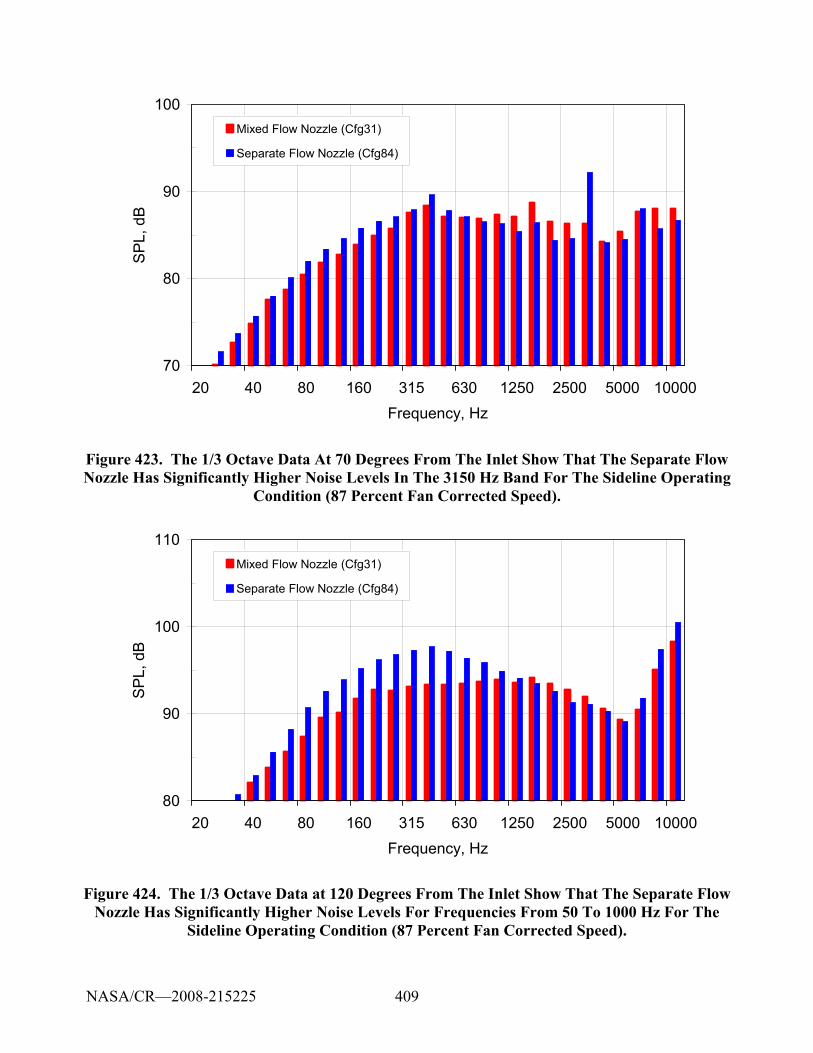
409

70

80

90

100

20 40 80 160 315 630 1250 2500 5000 10000Frequency, Hz

SP

L, d

BMixed Flow Nozzle (Cfg31)


Figure 423. The 1/3 Octave Data At 70 Degrees From The Inlet Show That The Separate Flow Nozzle Has Significantly Higher Noise Levels In The 3150 Hz Band For The Sideline Operating


80

90

100

110

20 40 80 160 315 630 1250 2500 5000 10000Frequency, Hz

SP

L, d

B



Figure 424. The 1/3 Octave Data at 120 Degrees From The Inlet Show That The Separate Flow Nozzle Has Significantly Higher Noise Levels For Frequencies From 50 To 1000 Hz For The

Sideline Operating Condition (87 Percent Fan Corrected Speed).

NASA/CR—2008-215225

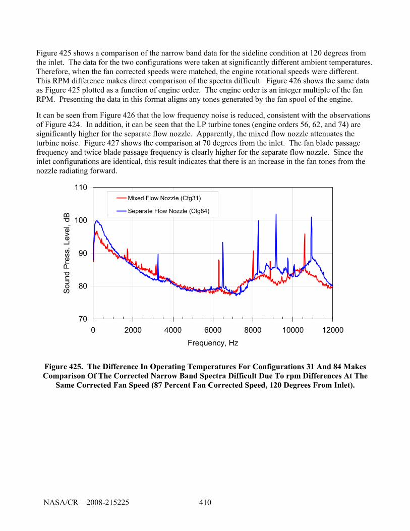
410

Figure 425 shows a comparison of the narrow band data for the sideline condition at 120 degrees from the inlet. The data for the two configurations were taken at significantly different ambient temperatures. Therefore, when the fan corrected speeds were matched, the engine rotational speeds were different. This RPM difference makes direct comparison of the spectra difficult. Figure 426 shows the same data as Figure 425 plotted as a function of engine order. The engine order is an integer multiple of the fan RPM. Presenting the data in this format aligns any tones generated by the fan spool of the engine.

It can be seen from Figure 426 that the low frequency noise is reduced, consistent with the observations of Figure 424. In addition, it can be seen that the LP turbine tones (engine orders 56, 62, and 74) are significantly higher for the separate flow nozzle. Apparently, the mixed flow nozzle attenuates the turbine noise. Figure 427 shows the comparison at 70 degrees from the inlet. The fan blade passage frequency and twice blade passage frequency is clearly higher for the separate flow nozzle. Since the inlet configurations are identical, this result indicates that there is an increase in the fan tones from the nozzle radiating forward.

70

80

90

100

110

0 2000 4000 6000 8000 10000 12000Frequency, Hz

Soun

d Pr

ess.

Lev

el, d

B



Figure 425. The Difference In Operating Temperatures For Configurations 31 And 84 Makes Comparison Of The Corrected Narrow Band Spectra Difficult Due To rpm Differences At The

Same Corrected Fan Speed (87 Percent Fan Corrected Speed, 120 Degrees From Inlet).

NASA/CR—2008-215225

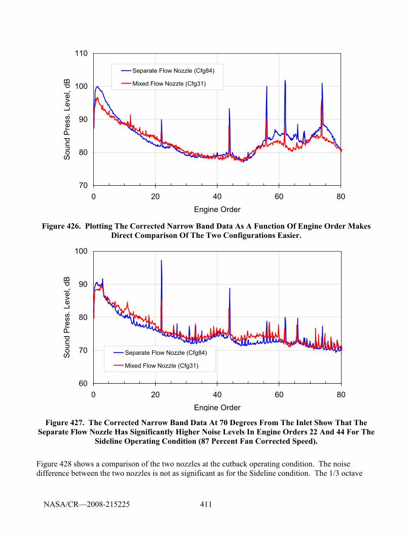
411

70

80

90

100

110


Soun

d Pr

ess.

Lev

el, d

BSeparate Flow Nozzle (Cfg84)


Figure 426. Plotting The Corrected Narrow Band Data As A Function Of Engine Order Makes Direct Comparison Of The Two Configurations Easier.

60

70

80

90

100


Sou

nd P

ress

. Lev

el, d

B



Figure 427. The Corrected Narrow Band Data At 70 Degrees From The Inlet Show That The Separate Flow Nozzle Has Significantly Higher Noise Levels In Engine Orders 22 And 44 For The

Sideline Operating Condition (87 Percent Fan Corrected Speed).

Figure 428 shows a comparison of the two nozzles at the cutback operating condition. The noise difference between the two nozzles is not as significant as for the Sideline condition. The 1/3 octave

NASA/CR—2008-215225

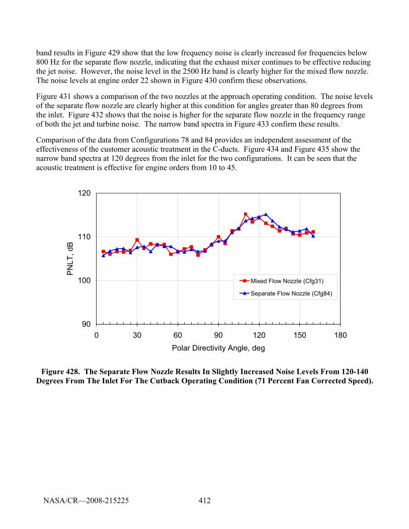
412

band results in Figure 429 show that the low frequency noise is clearly increased for frequencies below 800 Hz for the separate flow nozzle, indicating that the exhaust mixer continues to be effective reducing the jet noise. However, the noise level in the 2500 Hz band is clearly higher for the mixed flow nozzle. The noise levels at engine order 22 shown in Figure 430 confirm these observations.

Figure 431 shows a comparison of the two nozzles at the approach operating condition. The noise levels of the separate flow nozzle are clearly higher at this condition for angles greater than 80 degrees from the inlet. Figure 432 shows that the noise is higher for the separate flow nozzle in the frequency range of both the jet and turbine noise. The narrow band spectra in Figure 433 confirm these results.

Comparison of the data from Configurations 78 and 84 provides an independent assessment of the effectiveness of the customer acoustic treatment in the C-ducts. Figure 434 and Figure 435 show the narrow band spectra at 120 degrees from the inlet for the two configurations. It can be seen that the acoustic treatment is effective for engine orders from 10 to 45.

90

100

110

120


PN

LT, d

B



Figure 428. The Separate Flow Nozzle Results In Slightly Increased Noise Levels From 120-140 Degrees From The Inlet For The Cutback Operating Condition (71 Percent Fan Corrected Speed).

NASA/CR—2008-215225

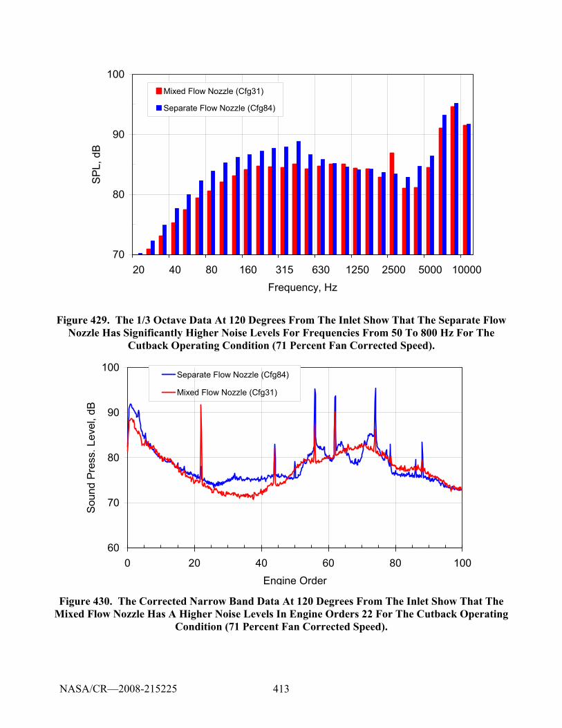
413

70

80

90

100

20 40 80 160 315 630 1250 2500 5000 10000Frequency, Hz

SP

L, d

BMixed Flow Nozzle (Cfg31)


Figure 429. The 1/3 Octave Data At 120 Degrees From The Inlet Show That The Separate Flow Nozzle Has Significantly Higher Noise Levels For Frequencies From 50 To 800 Hz For The

Cutback Operating Condition (71 Percent Fan Corrected Speed).

60

70

80

90

100

0 20 40 60 80 100Engine Order

Soun

d Pr

ess.

Lev

el, d

B



Figure 430. The Corrected Narrow Band Data At 120 Degrees From The Inlet Show That The Mixed Flow Nozzle Has A Higher Noise Levels In Engine Orders 22 For The Cutback Operating


NASA/CR—2008-215225

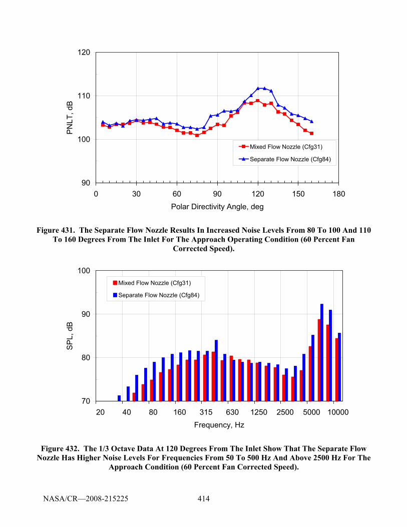
414

90

100

110

120


PN

LT, d

B



Figure 431. The Separate Flow Nozzle Results In Increased Noise Levels From 80 To 100 And 110 To 160 Degrees From The Inlet For The Approach Operating Condition (60 Percent Fan

Corrected Speed).

70

80

90

100

20 40 80 160 315 630 1250 2500 5000 10000Frequency, Hz

SP

L, d

B



Figure 432. The 1/3 Octave Data At 120 Degrees From The Inlet Show That The Separate Flow Nozzle Has Higher Noise Levels For Frequencies From 50 To 500 Hz And Above 2500 Hz For The

Approach Condition (60 Percent Fan Corrected Speed).

NASA/CR—2008-215225

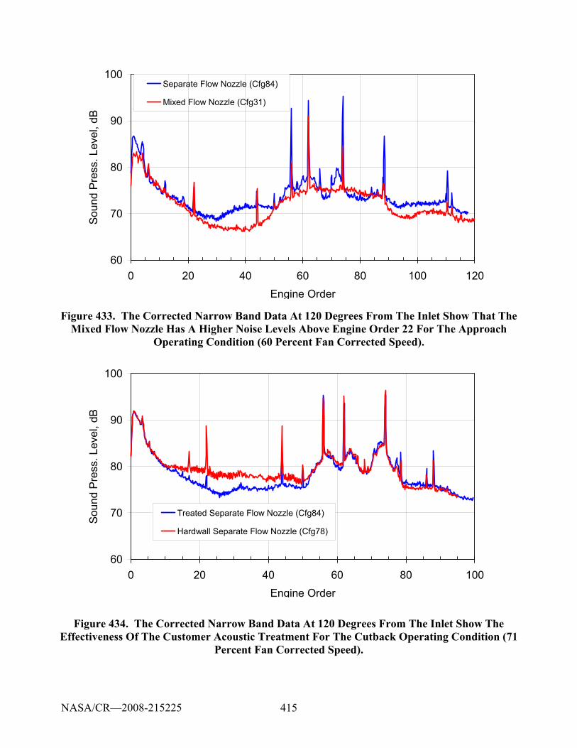
415

60

70

80

90

100

0 20 40 60 80 100 120Engine Order

Sou

nd P

ress

. Lev

el, d

BSeparate Flow Nozzle (Cfg84)


Figure 433. The Corrected Narrow Band Data At 120 Degrees From The Inlet Show That The Mixed Flow Nozzle Has A Higher Noise Levels Above Engine Order 22 For The Approach

Operating Condition (60 Percent Fan Corrected Speed).

60

70

80

90

100

0 20 40 60 80 100Engine Order

Sou

nd P

ress

. Lev

el, d

B

Treated Separate Flow Nozzle (Cfg84)

Hardwall Separate Flow Nozzle (Cfg78)

Figure 434. The Corrected Narrow Band Data At 120 Degrees From The Inlet Show The Effectiveness Of The Customer Acoustic Treatment For The Cutback Operating Condition (71


NASA/CR—2008-215225

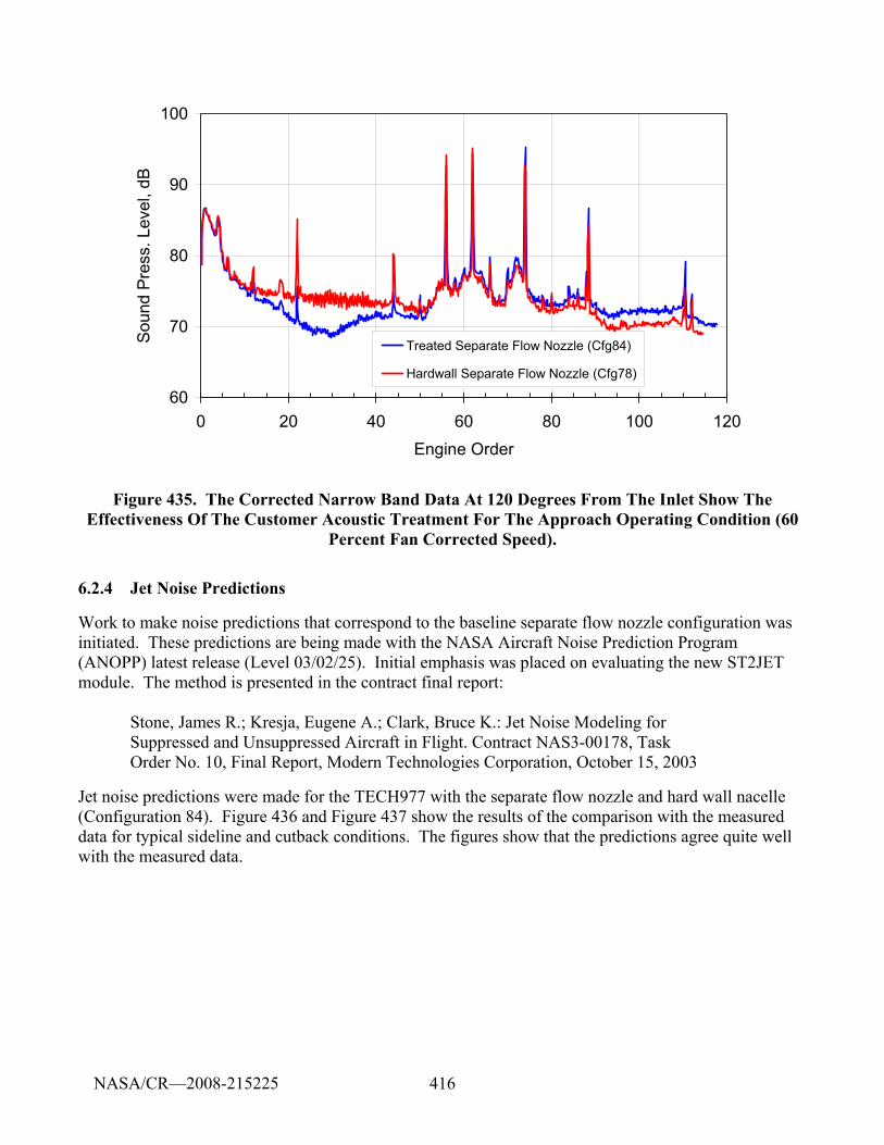
416

60

70

80

90

100

0 20 40 60 80 100 120Engine Order

Soun

d Pr

ess.

Lev

el, d

B

Treated Separate Flow Nozzle (Cfg84)


Figure 435. The Corrected Narrow Band Data At 120 Degrees From The Inlet Show The Effectiveness Of The Customer Acoustic Treatment For The Approach Operating Condition (60


6.2.4 Jet Noise Predictions

Work to make noise predictions that correspond to the baseline separate flow nozzle configuration was initiated. These predictions are being made with the NASA Aircraft Noise Prediction Program (ANOPP) latest release (Level 03/02/25). Initial emphasis was placed on evaluating the new ST2JET module. The method is presented in the contract final report:

Stone, James R.; Kresja, Eugene A.; Clark, Bruce K.: Jet Noise Modeling for Suppressed and Unsuppressed Aircraft in Flight. Contract NAS3-00178, Task Order No. 10, Final Report, Modern Technologies Corporation, October 15, 2003

Jet noise predictions were made for the TECH977 with the separate flow nozzle and hard wall nacelle (Configuration 84). Figure 436 and Figure 437 show the results of the comparison with the measured data for typical sideline and cutback conditions. The figures show that the predictions agree quite well with the measured data.

NASA/CR—2008-215225

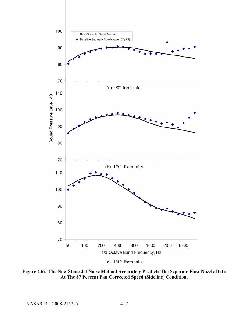
417

70

80

90

100New Stone Jet Noise Method

Baseline Separate Flow Nozzle (Cfg 78)

(a) 90° from inlet

70

80

90

100

110

Sou

nd P

ress

ure

Leve

l, dB

(b) 120° from inlet

70

80

90

100

110



Figure 436. The New Stone Jet Noise Method Accurately Predicts The Separate Flow Nozzle Data At The 87 Percent Fan Corrected Speed (Sideline) Condition.

NASA/CR—2008-215225

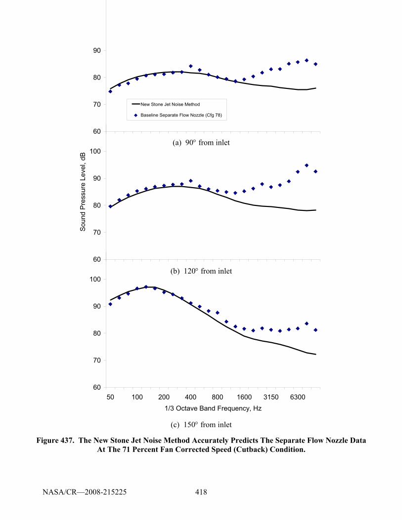
418

60

70

80

90

New Stone Jet Noise Method

Baseline Separate Flow Nozzle (Cfg 78)

(a) 90° from inlet

60

70

80

90

100

Sou

nd P

ress

ure

Leve

l, dB

(b) 120° from inlet

60

70

80

90

100



Figure 437. The New Stone Jet Noise Method Accurately Predicts The Separate Flow Nozzle Data At The 71 Percent Fan Corrected Speed (Cutback) Condition.

NASA/CR—2008-215225

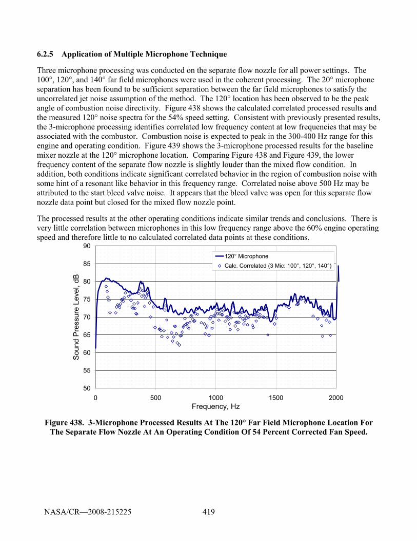
419

6.2.5 Application of Multiple Microphone Technique

Three microphone processing was conducted on the separate flow nozzle for all power settings. The 100°, 120°, and 140° far field microphones were used in the coherent processing. The 20° microphone separation has been found to be sufficient separation between the far field microphones to satisfy the uncorrelated jet noise assumption of the method. The 120° location has been observed to be the peak angle of combustion noise directivity. Figure 438 shows the calculated correlated processed results and the measured 120° noise spectra for the 54% speed setting. Consistent with previously presented results, the 3-microphone processing identifies correlated low frequency content at low frequencies that may be associated with the combustor. Combustion noise is expected to peak in the 300-400 Hz range for this engine and operating condition. Figure 439 shows the 3-microphone processed results for the baseline mixer nozzle at the 120° microphone location. Comparing Figure 438 and Figure 439, the lower frequency content of the separate flow nozzle is slightly louder than the mixed flow condition. In addition, both conditions indicate significant correlated behavior in the region of combustion noise with some hint of a resonant like behavior in this frequency range. Correlated noise above 500 Hz may be attributed to the start bleed valve noise. It appears that the bleed valve was open for this separate flow nozzle data point but closed for the mixed flow nozzle point.

The processed results at the other operating conditions indicate similar trends and conclusions. There is very little correlation between microphones in this low frequency range above the 60% engine operating speed and therefore little to no calculated correlated data points at these conditions.

50

55

60

65

70

75

80

85

90

0 500 1000 1500 2000Frequency, Hz

Sou

nd P

ress

ure

Leve

l, dB

120° MicrophoneCalc. Correlated (3 Mic: 100°, 120°, 140°)

Figure 438. 3-Microphone Processed Results At The 120° Far Field Microphone Location For The Separate Flow Nozzle At An Operating Condition Of 54 Percent Corrected Fan Speed.

NASA/CR—2008-215225

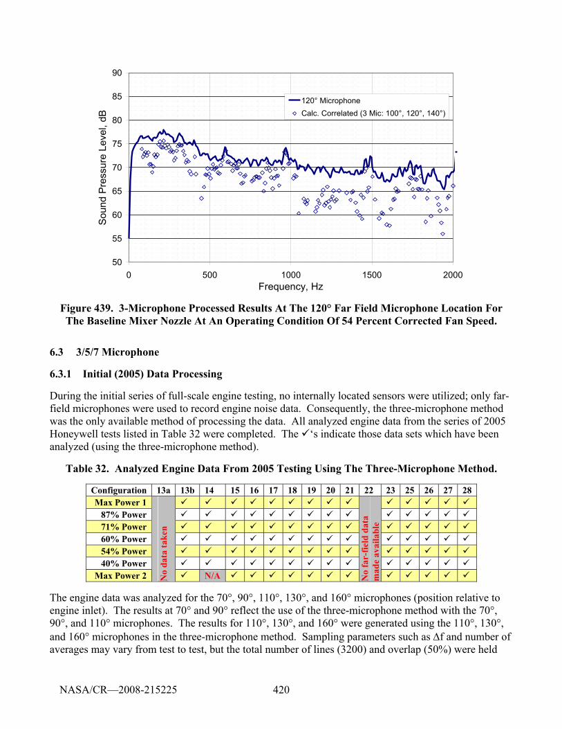
420

50

55

60

65

70

75

80

85

90

0 500 1000 1500 2000Frequency, Hz

Sou

nd P

ress

ure

Leve

l, dB

120° MicrophoneCalc. Correlated (3 Mic: 100°, 120°, 140°)

Figure 439. 3-Microphone Processed Results At The 120° Far Field Microphone Location For The Baseline Mixer Nozzle At An Operating Condition Of 54 Percent Corrected Fan Speed.


6.3.1 Initial (2005) Data Processing

During the initial series of full-scale engine testing, no internally located sensors were utilized; only far-field microphones were used to record engine noise data. Consequently, the three-microphone method was the only available method of processing the data. All analyzed engine data from the series of 2005 Honeywell tests listed in Table 32 were completed. The ‘s indicate those data sets which have been analyzed (using the three-microphone method).

Table 32. Analyzed Engine Data From 2005 Testing Using The Three-Microphone Method.

Configuration 13a 13b 14 15 16 17 18 19 20 21 22 23 25 26 27 28 Max Power 1

87% Power 71% Power 60% Power 54% Power 40% Power

Max Power 2 No

data

take

n

N/A No

far-

field

dat

a m

ade

avai

labl

e

The engine data was analyzed for the 70°, 90°, 110°, 130°, and 160° microphones (position relative to engine inlet). The results at 70° and 90° reflect the use of the three-microphone method with the 70°, 90°, and 110° microphones. The results for 110°, 130°, and 160° were generated using the 110°, 130°, and 160° microphones in the three-microphone method. Sampling parameters such as Δf and number of averages may vary from test to test, but the total number of lines (3200) and overlap (50%) were held

NASA/CR—2008-215225

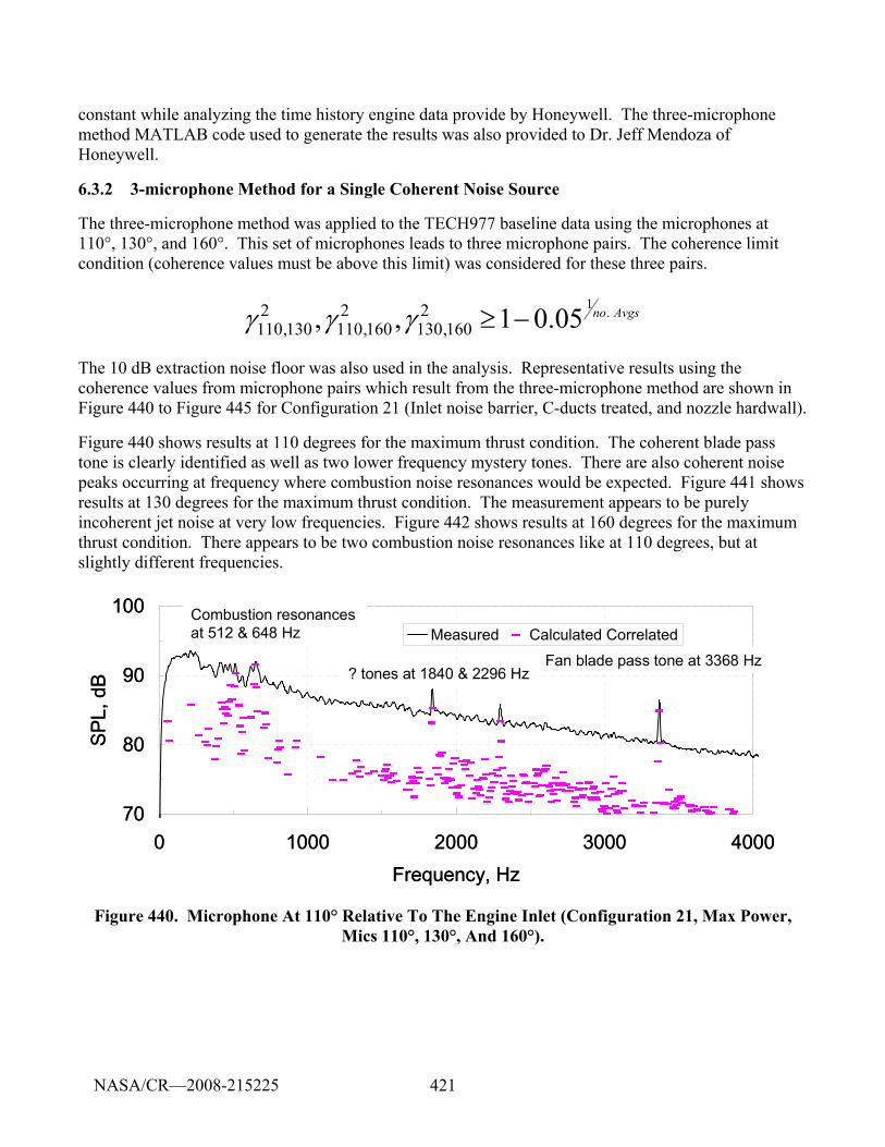
421

constant while analyzing the time history engine data provide by Honeywell. The three-microphone method MATLAB code used to generate the results was also provided to Dr. Jeff Mendoza of Honeywell.

6.3.2 3-microphone Method for a Single Coherent Noise Source

The three-microphone method was applied to the TECH977 baseline data using the microphones at 110°, 130°, and 160°. This set of microphones leads to three microphone pairs. The coherence limit condition (coherence values must be above this limit) was considered for these three pairs.

1. 2 2 2

110,130 110,160 130,160, , 1 0.05 no Avgsγ γ γ ≥ −

The 10 dB extraction noise floor was also used in the analysis. Representative results using the coherence values from microphone pairs which result from the three-microphone method are shown in Figure 440 to Figure 445 for Configuration 21 (Inlet noise barrier, C-ducts treated, and nozzle hardwall).

Figure 440 shows results at 110 degrees for the maximum thrust condition. The coherent blade pass tone is clearly identified as well as two lower frequency mystery tones. There are also coherent noise peaks occurring at frequency where combustion noise resonances would be expected. Figure 441 shows results at 130 degrees for the maximum thrust condition. The measurement appears to be purely incoherent jet noise at very low frequencies. Figure 442 shows results at 160 degrees for the maximum thrust condition. There appears to be two combustion noise resonances like at 110 degrees, but at slightly different frequencies.

70

80

90

100

0 1000 2000 3000 4000Frequency, Hz

SPL,

dB

Measured Calculated Correlated

Fan blade pass tone at 3368 Hz? tones at 1840 & 2296 Hz

Combustion resonances at 512 & 648 Hz

70

80

90

100

0 1000 2000 3000 4000Frequency, Hz

SPL,

dB


Fan blade pass tone at 3368 Hz? tones at 1840 & 2296 Hz


Figure 440. Microphone At 110° Relative To The Engine Inlet (Configuration 21, Max Power, Mics 110°, 130°, And 160°).

NASA/CR—2008-215225

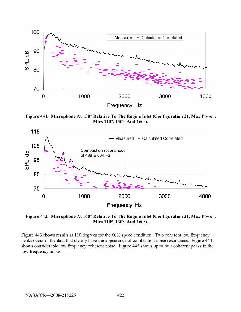
422

70

80

90

100

0 1000 2000 3000 4000Frequency, Hz

SP

L, d

B



75

85

95

105

115

0 1000 2000 3000 4000Frequency, Hz

SP

L, d

B



75

85

95

105

115

0 1000 2000 3000 4000Frequency, Hz

SP

L, d

B




Figure 443 shows results at 110 degrees for the 60% speed condition. Two coherent low frequency peaks occur in the data that clearly have the appearance of combustion noise resonances. Figure 444 shows considerable low frequency coherent noise. Figure 445 shows up to four coherent peaks in the low frequency noise.

NASA/CR—2008-215225

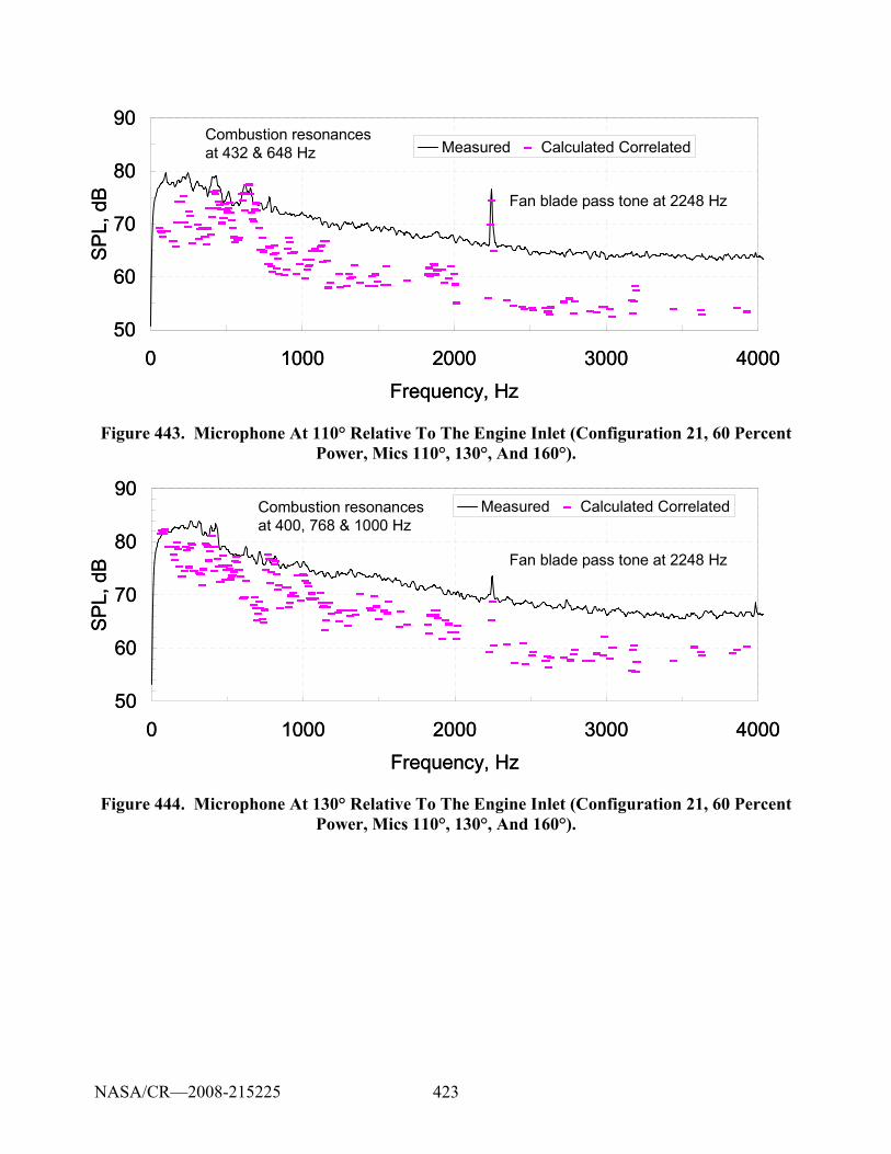
423

50

60

70

80

90

0 1000 2000 3000 4000Frequency, Hz

SP

L, d

B

Measured Calculated CorrelatedCombustion resonances at 432 & 648 Hz

Fan blade pass tone at 2248 Hz

50

60

70

80

90

0 1000 2000 3000 4000Frequency, Hz

SP

L, d

B

Measured Calculated CorrelatedCombustion resonances at 432 & 648 Hz


Figure 443. Microphone At 110° Relative To The Engine Inlet (Configuration 21, 60 Percent Power, Mics 110°, 130°, And 160°).

50

60

70

80

90

0 1000 2000 3000 4000Frequency, Hz

SPL,

dB

Measured Calculated CorrelatedCombustion resonances at 400, 768 & 1000 Hz


50

60

70

80

90

0 1000 2000 3000 4000Frequency, Hz

SPL,

dB

Measured Calculated CorrelatedCombustion resonances at 400, 768 & 1000 Hz



NASA/CR—2008-215225

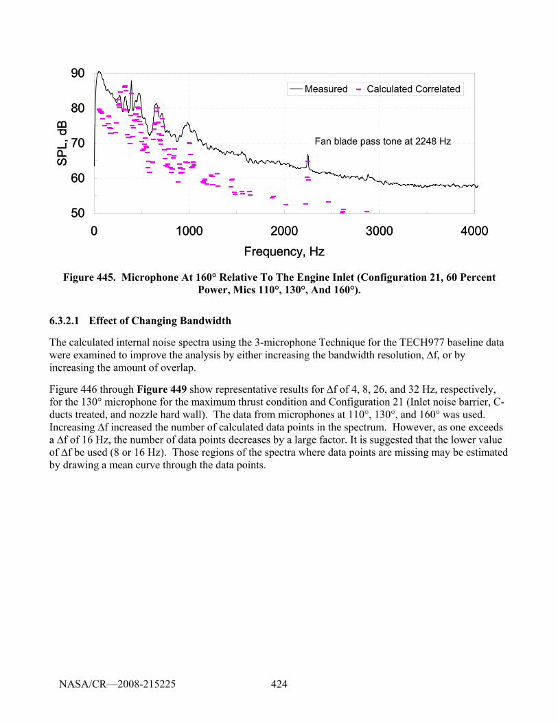
424

50

60

70

80

90

0 1000 2000 3000 4000Frequency, Hz

SP

L, d

B



50

60

70

80

90

0 1000 2000 3000 4000Frequency, Hz

SP

L, d

B




6.3.2.1 Effect of Changing Bandwidth

The calculated internal noise spectra using the 3-microphone Technique for the TECH977 baseline data were examined to improve the analysis by either increasing the bandwidth resolution, ∆f, or by increasing the amount of overlap.

Figure 446 through Figure 449 show representative results for ∆f of 4, 8, 26, and 32 Hz, respectively, for the 130° microphone for the maximum thrust condition and Configuration 21 (Inlet noise barrier, C-ducts treated, and nozzle hard wall). The data from microphones at 110°, 130°, and 160° was used. Increasing ∆f increased the number of calculated data points in the spectrum. However, as one exceeds a ∆f of 16 Hz, the number of data points decreases by a large factor. It is suggested that the lower value of ∆f be used (8 or 16 Hz). Those regions of the spectra where data points are missing may be estimated by drawing a mean curve through the data points.

NASA/CR—2008-215225

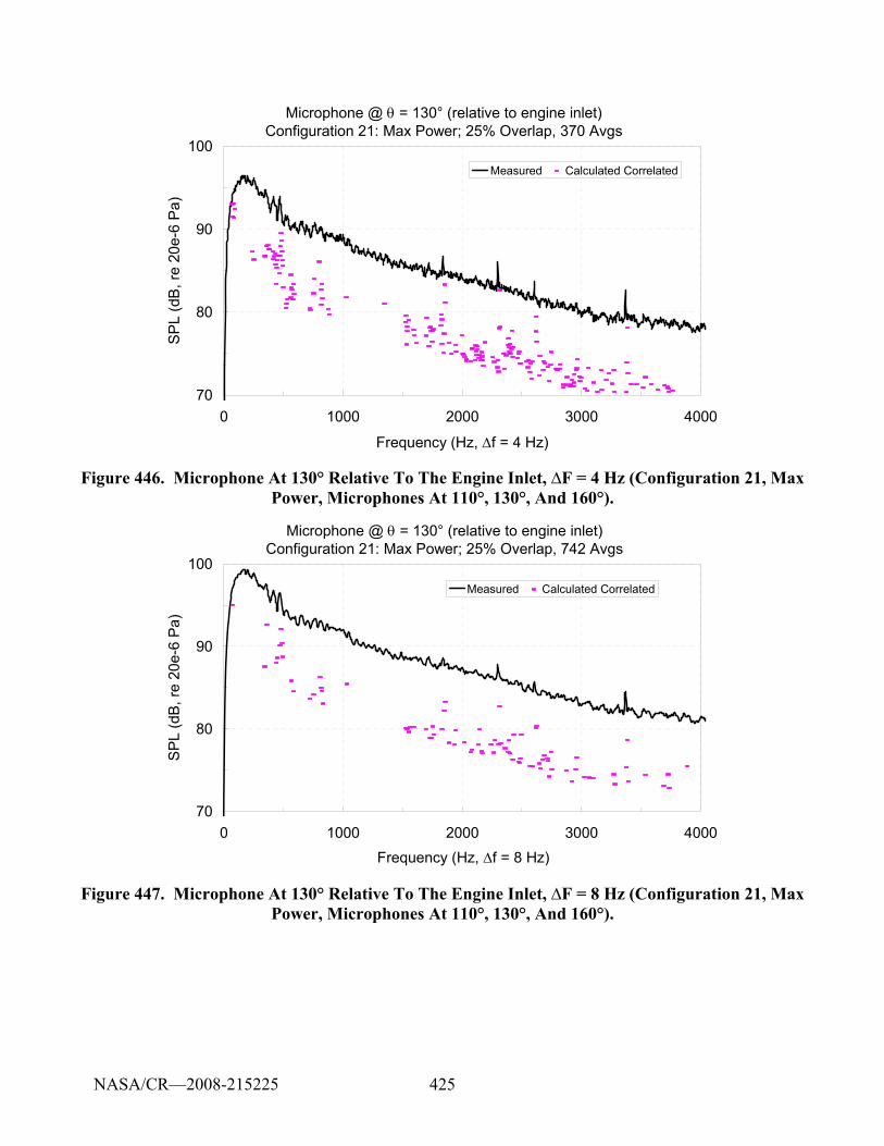
425

Microphone @ θ = 130° (relative to engine inlet)Configuration 21: Max Power; 25% Overlap, 370 Avgs

70

80

90

100

0 1000 2000 3000 4000

Frequency (Hz, Δf = 4 Hz)

SP

L (d

B, r

e 20

e-6

Pa)


Figure 446. Microphone At 130° Relative To The Engine Inlet, ∆F = 4 Hz (Configuration 21, Max Power, Microphones At 110°, 130°, And 160°).


70

80

90

100

0 1000 2000 3000 4000Frequency (Hz, Δf = 8 Hz)

SPL

(dB

, re

20e-

6 Pa

)



NASA/CR—2008-215225

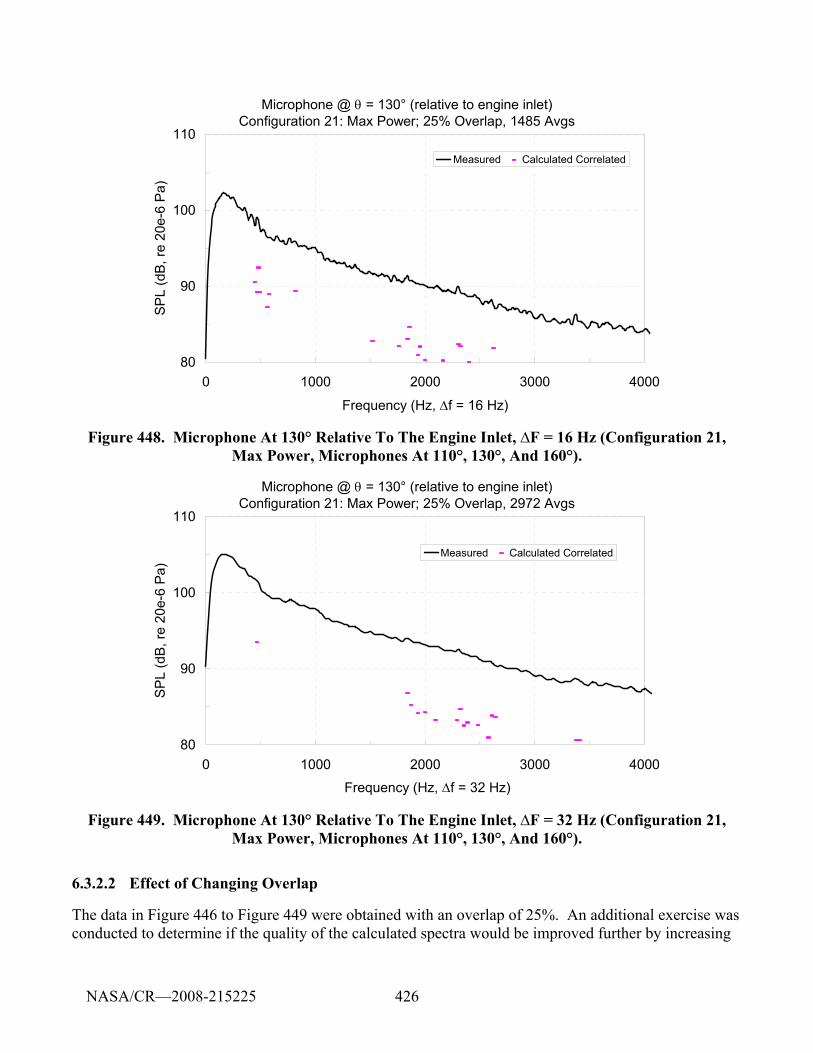
426


80

90

100

110

0 1000 2000 3000 4000


SPL

(dB,

re 2

0e-6

Pa)




80

90

100

110

0 1000 2000 3000 4000


SP

L (d

B, re

20e

-6 P

a)



6.3.2.2 Effect of Changing Overlap

The data in Figure 446 to Figure 449 were obtained with an overlap of 25%. An additional exercise was conducted to determine if the quality of the calculated spectra would be improved further by increasing

NASA/CR—2008-215225

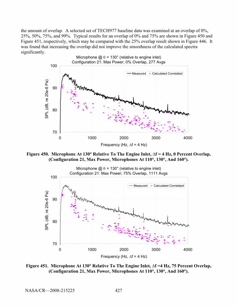
427

the amount of overlap. A selected set of TECH977 baseline data was examined at an overlap of 0%, 25%, 50%, 75%, and 99%. Typical results for an overlap of 0% and 75% are shown in Figure 450 and Figure 451, respectively, which may be compared with the 25% overlap result shown in Figure 446. It was found that increasing the overlap did not improve the smoothness of the calculated spectra significantly.


70

80

90

100

0 1000 2000 3000 4000


SP

L (d

B, r

e 20

e-6

Pa)


Figure 450. Microphone At 130° Relative To The Engine Inlet, ∆f = 4 Hz, 0 Percent Overlap, (Configuration 21, Max Power, Microphones At 110°, 130°, And 160°).


70

80

90

100

0 1000 2000 3000 4000


SPL

(dB

, re

20e-

6 P

a)


Figure 451. Microphone At 130° Relative To The Engine Inlet, ∆f =4 Hz, 75 Percent Overlap, (Configuration 21, Max Power, Microphones At 110°, 130°, And 160°).

NASA/CR—2008-215225

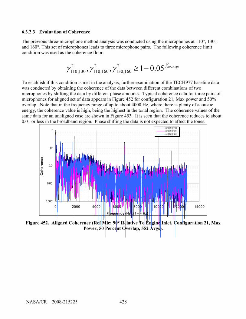
428

6.3.2.3 Evaluation of Coherence

The previous three-microphone method analysis was conducted using the microphones at 110°, 130°, and 160°. This set of microphones leads to three microphone pairs. The following coherence limit condition was used as the coherence floor:

Avgsno .1

05.01,, 2160,130

2160,110

2130,110 −≥γγγ

To establish if this condition is met in the analysis, further examination of the TECH977 baseline data was conducted by obtaining the coherence of the data between different combinations of two microphones by shifting the data by different phase amounts. Typical coherence data for three pairs of microphones for aligned set of data appears in Figure 452 for configuration 21, Max power and 50% overlap. Note that in the frequency range of up to about 4000 Hz, where there is plenty of acoustic energy, the coherence value is high, being the highest in the tonal region. The coherence values of the same data for an unaligned case are shown in Figure 453. It is seen that the coherence reduces to about 0.01 or less in the broadband region. Phase shifting the data is not expected to affect the tones.

0.0001

0.001

0.01

0.1

1

0 2000 4000 6000 8000 10000 12000 14000


Coh

eren

ce

coh[ 90] [ 110]coh[ 90] [ 130]coh[ 90] [ 160]

Figure 452. Aligned Coherence (Ref Mic: 90° Relative To Engine Inlet, Configuration 21, Max Power, 50 Percent Overlap, 552 Avgs).

NASA/CR—2008-215225

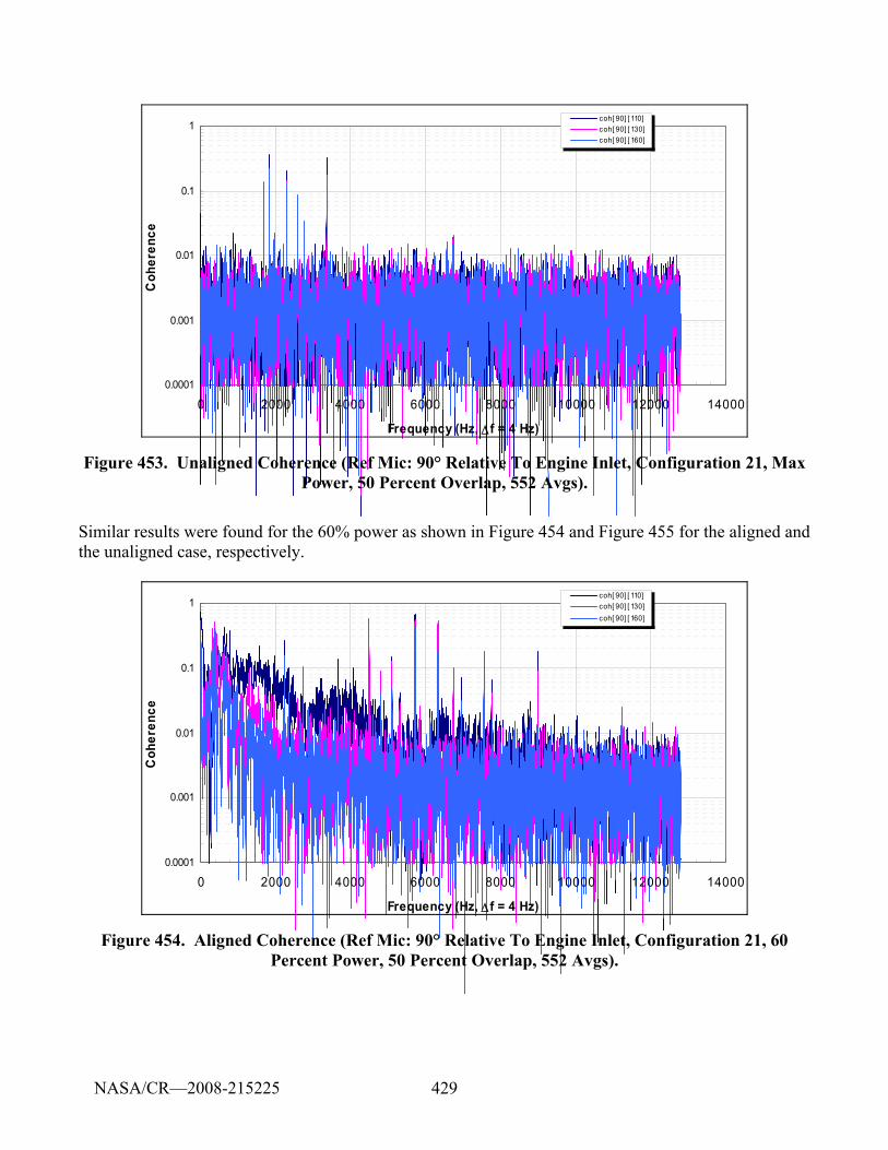
429

0.0001

0.001

0.01

0.1

1

0 2000 4000 6000 8000 10000 12000 14000


Coh

eren

ce

coh[ 90] [ 110]coh[ 90] [ 130]coh[ 90] [ 160]

Figure 453. Unaligned Coherence (Ref Mic: 90° Relative To Engine Inlet, Configuration 21, Max Power, 50 Percent Overlap, 552 Avgs).

Similar results were found for the 60% power as shown in Figure 454 and Figure 455 for the aligned and the unaligned case, respectively.

0.0001

0.001

0.01

0.1

1

0 2000 4000 6000 8000 10000 12000 14000


Coh

eren

ce

coh[ 90] [ 110]coh[ 90] [ 130]coh[ 90] [ 160]

Figure 454. Aligned Coherence (Ref Mic: 90° Relative To Engine Inlet, Configuration 21, 60 Percent Power, 50 Percent Overlap, 552 Avgs).

NASA/CR—2008-215225

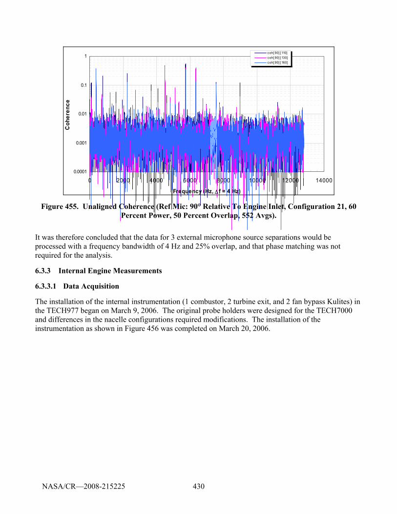
430

0.0001

0.001

0.01

0.1

1

0 2000 4000 6000 8000 10000 12000 14000

Frequency (Hz, Δ f = 4 Hz)

Coh

eren

ce

coh[ 90] [ 110]coh[ 90] [ 130]coh[ 90] [ 160]

Figure 455. Unaligned Coherence (Ref Mic: 90° Relative To Engine Inlet, Configuration 21, 60 Percent Power, 50 Percent Overlap, 552 Avgs).

It was therefore concluded that the data for 3 external microphone source separations would be processed with a frequency bandwidth of 4 Hz and 25% overlap, and that phase matching was not required for the analysis.

6.3.3 Internal Engine Measurements

6.3.3.1 Data Acquisition

The installation of the internal instrumentation (1 combustor, 2 turbine exit, and 2 fan bypass Kulites) in the TECH977 began on March 9, 2006. The original probe holders were designed for the TECH7000 and differences in the nacelle configurations required modifications. The installation of the instrumentation as shown in Figure 456 was completed on March 20, 2006.

NASA/CR—2008-215225

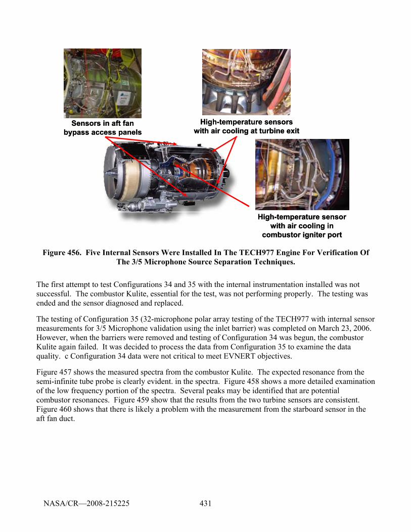
431

Sensors in aft fan bypass access panels

High-temperature sensor with air cooling in

combustor igniter port

High-temperature sensors with air cooling at turbine exit

Sensors in aft fan bypass access panels

High-temperature sensor with air cooling in

combustor igniter port

High-temperature sensors with air cooling at turbine exit

Figure 456. Five Internal Sensors Were Installed In The TECH977 Engine For Verification Of The 3/5 Microphone Source Separation Techniques.

The first attempt to test Configurations 34 and 35 with the internal instrumentation installed was not successful. The combustor Kulite, essential for the test, was not performing properly. The testing was ended and the sensor diagnosed and replaced.

The testing of Configuration 35 (32-microphone polar array testing of the TECH977 with internal sensor measurements for 3/5 Microphone validation using the inlet barrier) was completed on March 23, 2006. However, when the barriers were removed and testing of Configuration 34 was begun, the combustor Kulite again failed. It was decided to process the data from Configuration 35 to examine the data quality. c Configuration 34 data were not critical to meet EVNERT objectives.

Figure 457 shows the measured spectra from the combustor Kulite. The expected resonance from the semi-infinite tube probe is clearly evident. in the spectra. Figure 458 shows a more detailed examination of the low frequency portion of the spectra. Several peaks may be identified that are potential combustor resonances. Figure 459 show that the results from the two turbine sensors are consistent. Figure 460 shows that there is likely a problem with the measurement from the starboard sensor in the aft fan duct.

NASA/CR—2008-215225

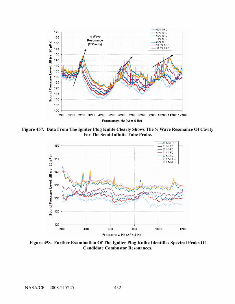
432

¼ Wave Resonance (2”Cavity)

¼ Wave Resonance (2”Cavity)

Figure 457. Data From The Igniter Plug Kulite Clearly Shows The ¼ Wave Resonance Of Cavity For The Semi-Infinite Tube Probe.

Figure 458. Further Examination Of The Igniter Plug Kulite Identifies Spectral Peaks Of Candidate Combustor Resonances.

NASA/CR—2008-215225

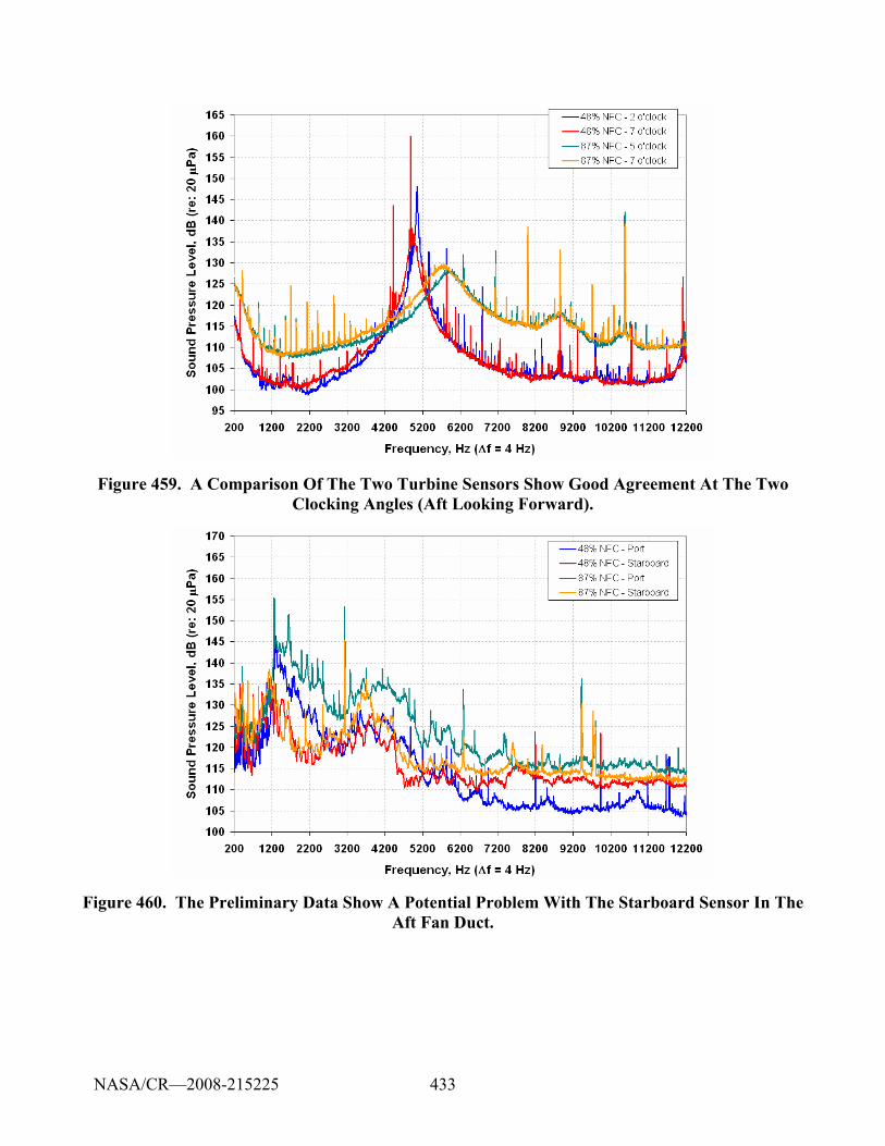
433

Figure 459. A Comparison Of The Two Turbine Sensors Show Good Agreement At The Two Clocking Angles (Aft Looking Forward).

Figure 460. The Preliminary Data Show A Potential Problem With The Starboard Sensor In The Aft Fan Duct.

NASA/CR—2008-215225

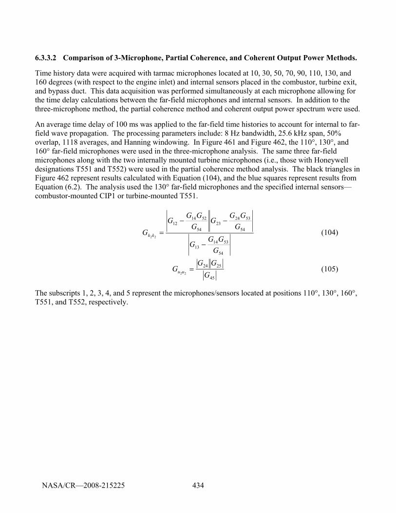
434

6.3.3.2 Comparison of 3-Microphone, Partial Coherence, and Coherent Output Power Methods.

Time history data were acquired with tarmac microphones located at 10, 30, 50, 70, 90, 110, 130, and 160 degrees (with respect to the engine inlet) and internal sensors placed in the combustor, turbine exit, and bypass duct. This data acquisition was performed simultaneously at each microphone allowing for the time delay calculations between the far-field microphones and internal sensors. In addition to the three-microphone method, the partial coherence method and coherent output power spectrum were used.

An average time delay of 100 ms was applied to the far-field time histories to account for internal to far-field wave propagation. The processing parameters include: 8 Hz bandwidth, 25.6 kHz span, 50% overlap, 1118 averages, and Hanning windowing. In Figure 461 and Figure 462, the 110°, 130°, and 160° far-field microphones were used in the three-microphone analysis. The same three far-field microphones along with the two internally mounted turbine microphones (i.e., those with Honeywell designations T551 and T552) were used in the partial coherence method analysis. The black triangles in Figure 462 represent results calculated with Equation (104), and the blue squares represent results from Equation (6.2). The analysis used the 130° far-field microphones and the specified internal sensors—combustor-mounted CIP1 or turbine-mounted T551.

54

531413

54

532423

54

521412

22

GGG

G

GGG

GG

GGG

G kk

−

−−= (104)

45

252422 G

GGG uu = (105)

The subscripts 1, 2, 3, 4, and 5 represent the microphones/sensors located at positions 110°, 130°, 160°, T551, and T552, respectively.

NASA/CR—2008-215225

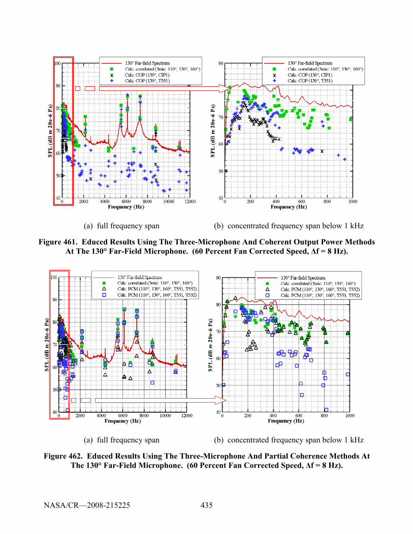
435

(a) full frequency span (b) concentrated frequency span below 1 kHz

Figure 461. Educed Results Using The Three-Microphone And Coherent Output Power Methods At The 130° Far-Field Microphone. (60 Percent Fan Corrected Speed, Δf = 8 Hz).

(a) full frequency span (b) concentrated frequency span below 1 kHz

Figure 462. Educed Results Using The Three-Microphone And Partial Coherence Methods At The 130° Far-Field Microphone. (60 Percent Fan Corrected Speed, Δf = 8 Hz).

NASA/CR—2008-215225

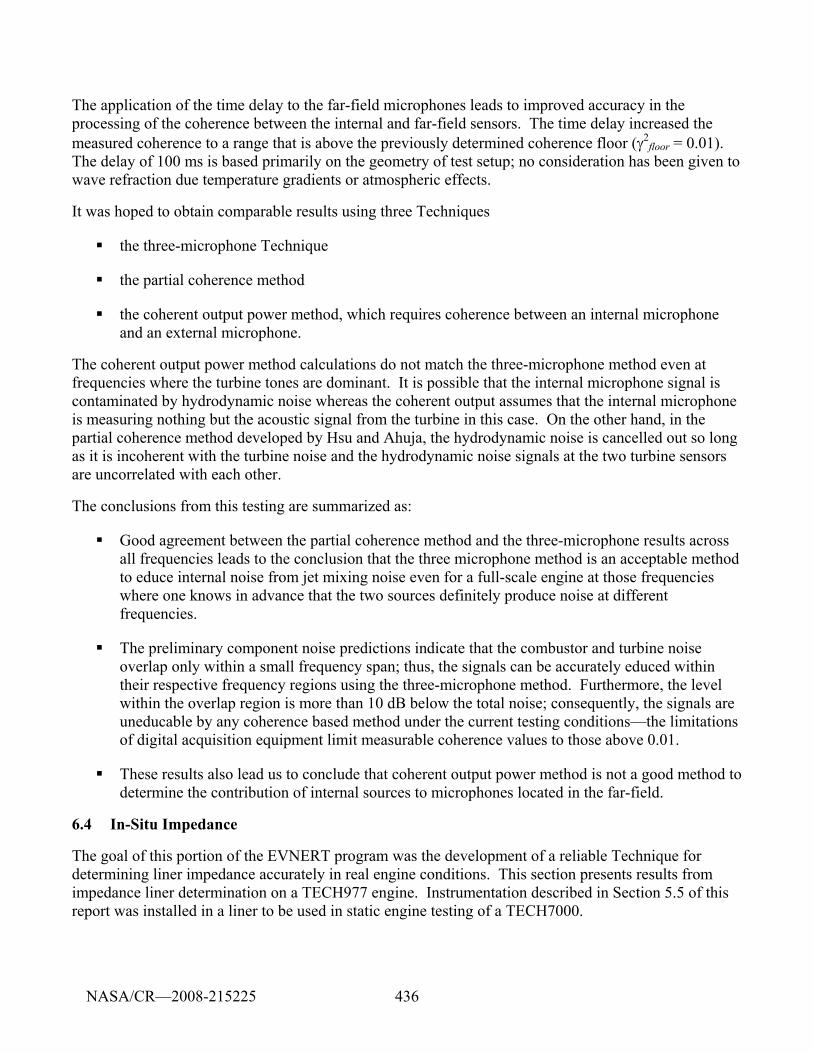
436

The application of the time delay to the far-field microphones leads to improved accuracy in the processing of the coherence between the internal and far-field sensors. The time delay increased the measured coherence to a range that is above the previously determined coherence floor (γ2

floor = 0.01). The delay of 100 ms is based primarily on the geometry of test setup; no consideration has been given to wave refraction due temperature gradients or atmospheric effects.

It was hoped to obtain comparable results using three Techniques

the three-microphone Technique

the partial coherence method

the coherent output power method, which requires coherence between an internal microphone and an external microphone.

The coherent output power method calculations do not match the three-microphone method even at frequencies where the turbine tones are dominant. It is possible that the internal microphone signal is contaminated by hydrodynamic noise whereas the coherent output assumes that the internal microphone is measuring nothing but the acoustic signal from the turbine in this case. On the other hand, in the partial coherence method developed by Hsu and Ahuja, the hydrodynamic noise is cancelled out so long as it is incoherent with the turbine noise and the hydrodynamic noise signals at the two turbine sensors are uncorrelated with each other.

The conclusions from this testing are summarized as:

Good agreement between the partial coherence method and the three-microphone results across all frequencies leads to the conclusion that the three microphone method is an acceptable method to educe internal noise from jet mixing noise even for a full-scale engine at those frequencies where one knows in advance that the two sources definitely produce noise at different frequencies.

The preliminary component noise predictions indicate that the combustor and turbine noise overlap only within a small frequency span; thus, the signals can be accurately educed within their respective frequency regions using the three-microphone method. Furthermore, the level within the overlap region is more than 10 dB below the total noise; consequently, the signals are uneducable by any coherence based method under the current testing conditions—the limitations of digital acquisition equipment limit measurable coherence values to those above 0.01.

These results also lead us to conclude that coherent output power method is not a good method to determine the contribution of internal sources to microphones located in the far-field.

6.4 In-Situ Impedance

The goal of this portion of the EVNERT program was the development of a reliable Technique for determining liner impedance accurately in real engine conditions. This section presents results from impedance liner determination on a TECH977 engine. Instrumentation described in Section 5.5 of this report was installed in a liner to be used in static engine testing of a TECH7000.

NASA/CR—2008-215225

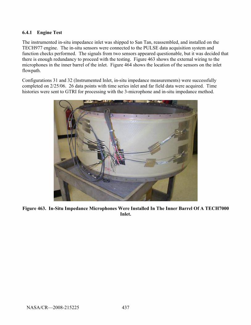
437

6.4.1 Engine Test

The instrumented in-situ impedance inlet was shipped to San Tan, reassembled, and installed on the TECH977 engine. The in-situ sensors were connected to the PULSE data acquisition system and function checks performed. The signals from two sensors appeared questionable, but it was decided that there is enough redundancy to proceed with the testing. Figure 463 shows the external wiring to the microphones in the inner barrel of the inlet. Figure 464 shows the location of the sensors on the inlet flowpath.

Configurations 31 and 32 (Instrumented Inlet, in-situ impedance measurements) were successfully completed on 2/25/06. 26 data points with time series inlet and far field data were acquired. Time histories were sent to GTRI for processing with the 3-microphone and in-situ impedance method.

Figure 463. In-Situ Impedance Microphones Were Installed In The Inner Barrel Of A TECH7000 Inlet.

NASA/CR—2008-215225

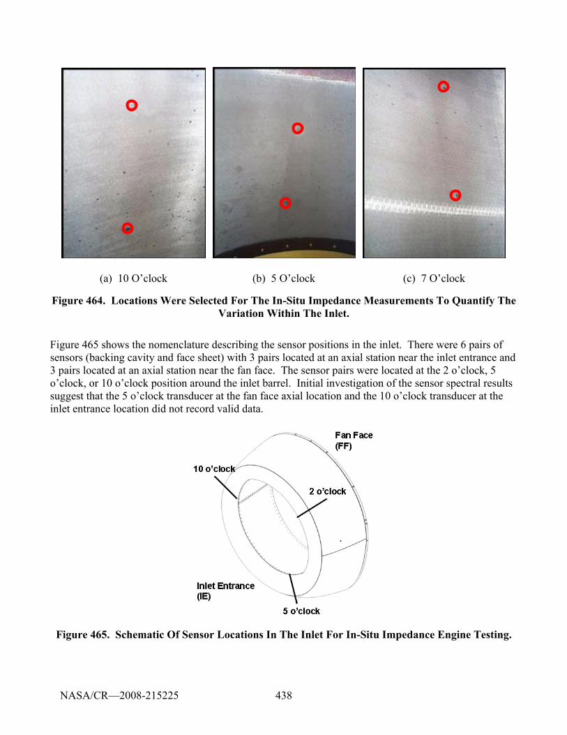
438

(a) 10 O’clock (b) 5 O’clock (c) 7 O’clock

Figure 464. Locations Were Selected For The In-Situ Impedance Measurements To Quantify The Variation Within The Inlet.

Figure 465 shows the nomenclature describing the sensor positions in the inlet. There were 6 pairs of sensors (backing cavity and face sheet) with 3 pairs located at an axial station near the inlet entrance and 3 pairs located at an axial station near the fan face. The sensor pairs were located at the 2 o’clock, 5 o’clock, or 10 o’clock position around the inlet barrel. Initial investigation of the sensor spectral results suggest that the 5 o’clock transducer at the fan face axial location and the 10 o’clock transducer at the inlet entrance location did not record valid data.

Figure 465. Schematic Of Sensor Locations In The Inlet For In-Situ Impedance Engine Testing.

NASA/CR—2008-215225

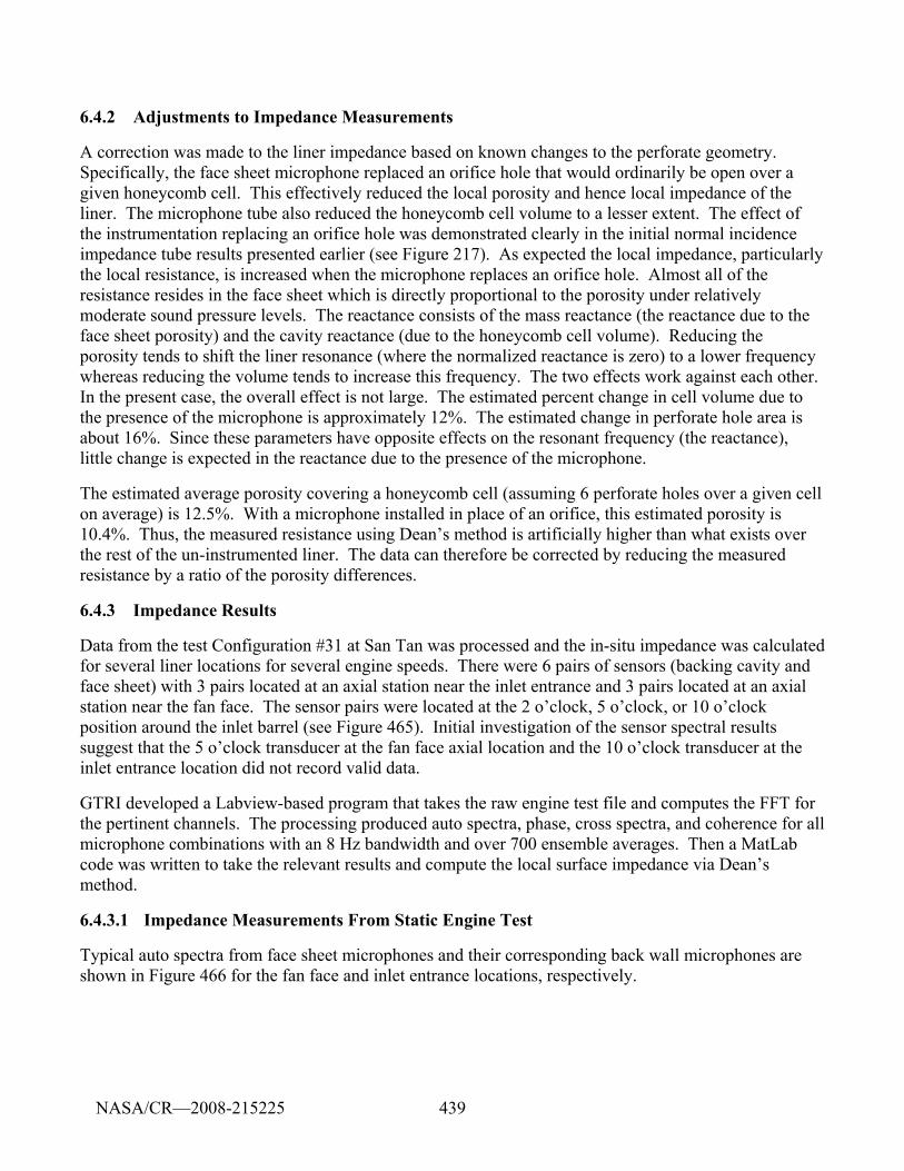
439

6.4.2 Adjustments to Impedance Measurements

A correction was made to the liner impedance based on known changes to the perforate geometry. Specifically, the face sheet microphone replaced an orifice hole that would ordinarily be open over a given honeycomb cell. This effectively reduced the local porosity and hence local impedance of the liner. The microphone tube also reduced the honeycomb cell volume to a lesser extent. The effect of the instrumentation replacing an orifice hole was demonstrated clearly in the initial normal incidence impedance tube results presented earlier (see Figure 217). As expected the local impedance, particularly the local resistance, is increased when the microphone replaces an orifice hole. Almost all of the resistance resides in the face sheet which is directly proportional to the porosity under relatively moderate sound pressure levels. The reactance consists of the mass reactance (the reactance due to the face sheet porosity) and the cavity reactance (due to the honeycomb cell volume). Reducing the porosity tends to shift the liner resonance (where the normalized reactance is zero) to a lower frequency whereas reducing the volume tends to increase this frequency. The two effects work against each other. In the present case, the overall effect is not large. The estimated percent change in cell volume due to the presence of the microphone is approximately 12%. The estimated change in perforate hole area is about 16%. Since these parameters have opposite effects on the resonant frequency (the reactance), little change is expected in the reactance due to the presence of the microphone.

The estimated average porosity covering a honeycomb cell (assuming 6 perforate holes over a given cell on average) is 12.5%. With a microphone installed in place of an orifice, this estimated porosity is 10.4%. Thus, the measured resistance using Dean’s method is artificially higher than what exists over the rest of the un-instrumented liner. The data can therefore be corrected by reducing the measured resistance by a ratio of the porosity differences.

6.4.3 Impedance Results

Data from the test Configuration #31 at San Tan was processed and the in-situ impedance was calculated for several liner locations for several engine speeds. There were 6 pairs of sensors (backing cavity and face sheet) with 3 pairs located at an axial station near the inlet entrance and 3 pairs located at an axial station near the fan face. The sensor pairs were located at the 2 o’clock, 5 o’clock, or 10 o’clock position around the inlet barrel (see Figure 465). Initial investigation of the sensor spectral results suggest that the 5 o’clock transducer at the fan face axial location and the 10 o’clock transducer at the inlet entrance location did not record valid data.

GTRI developed a Labview-based program that takes the raw engine test file and computes the FFT for the pertinent channels. The processing produced auto spectra, phase, cross spectra, and coherence for all microphone combinations with an 8 Hz bandwidth and over 700 ensemble averages. Then a MatLab code was written to take the relevant results and compute the local surface impedance via Dean’s method.

6.4.3.1 Impedance Measurements From Static Engine Test

Typical auto spectra from face sheet microphones and their corresponding back wall microphones are shown in Figure 466 for the fan face and inlet entrance locations, respectively.

NASA/CR—2008-215225

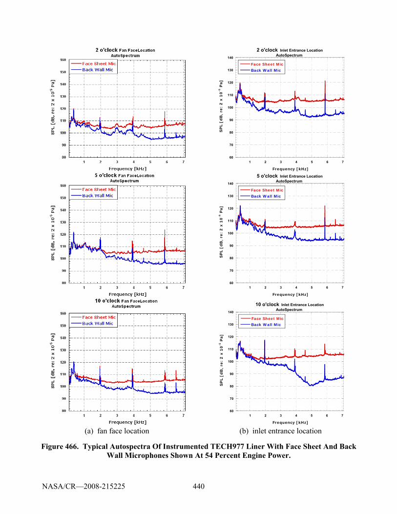
440

60

70

80

90

100

110

120

130

140

1 2 3 4 5 6 7

2 o'clock Inlet Entrance LocationAutoSpectrum

Face Sheet Mic

Back Wall Mic

SP

L [

dB

, re

: 2

x 1

0-5

Pa]

Frequency [kHz]

60

70

80

90

100

110

120

130

140

1 2 3 4 5 6 7


Face Sheet Mic

Back Wall Mic

SP

L [

dB

, re

: 2

x 1

0-5

Pa]

Frequency [kHz]

60

70

80

90

100

110

120

130

140

1 2 3 4 5 6 7


Face Sheet Mic

Back Wall Mic

SP

L [

dB

, re

: 2

x 1

0-5

Pa]

Frequency [kHz] (a) fan face location (b) inlet entrance location

Figure 466. Typical Autospectra Of Instrumented TECH977 Liner With Face Sheet And Back Wall Microphones Shown At 54 Percent Engine Power.

NASA/CR—2008-215225

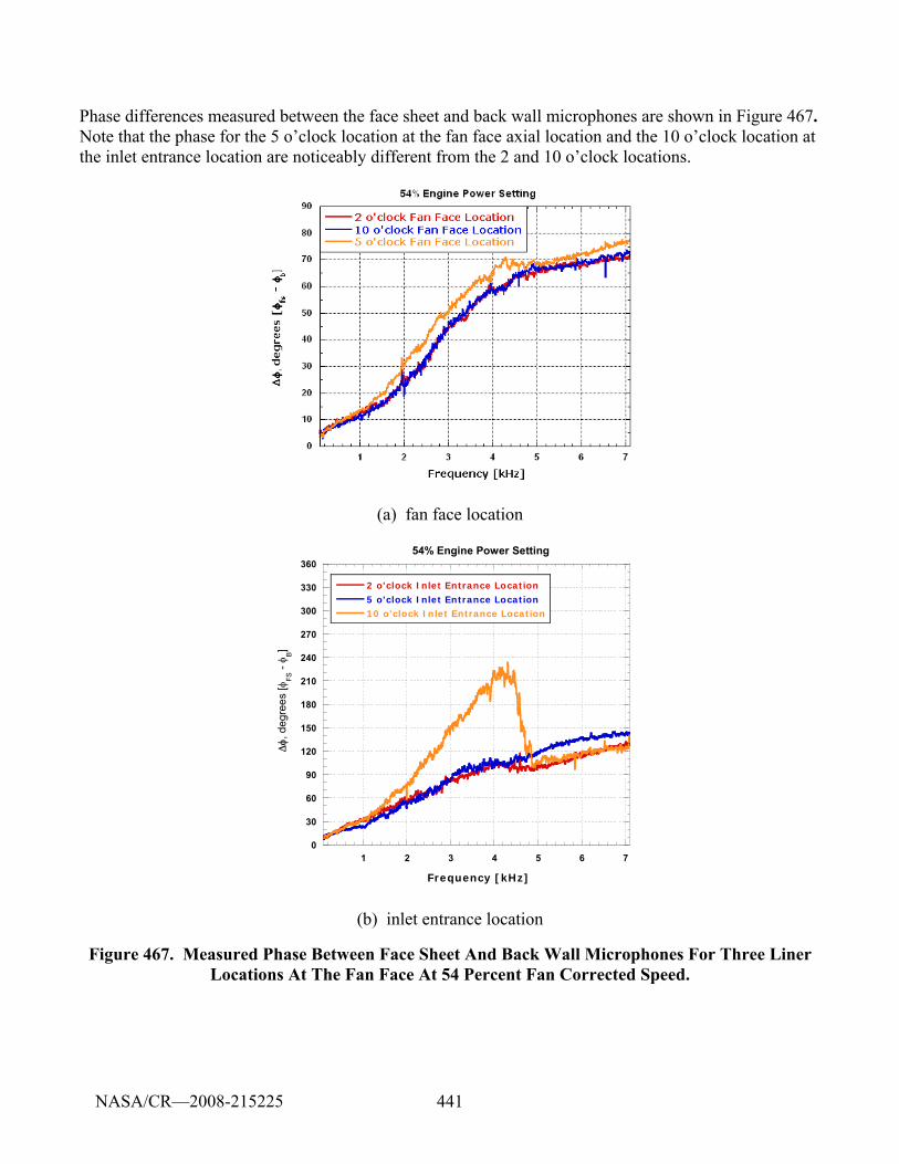
441

Phase differences measured between the face sheet and back wall microphones are shown in Figure 467. Note that the phase for the 5 o’clock location at the fan face axial location and the 10 o’clock location at the inlet entrance location are noticeably different from the 2 and 10 o’clock locations.

(a) fan face location

0

30

60

90

120

150

180

210

240

270

300

330

360

1 2 3 4 5 6 7

54% Engine Power Setting

2 o'clock Inlet Entrance Location5 o'clock Inlet Entrance Location10 o'clock Inlet Entrance Location

Δφ,

deg

rees

[φFS

- φ B]

Frequency [kHz]

(b) inlet entrance location

Figure 467. Measured Phase Between Face Sheet And Back Wall Microphones For Three Liner Locations At The Fan Face At 54 Percent Fan Corrected Speed.

NASA/CR—2008-215225

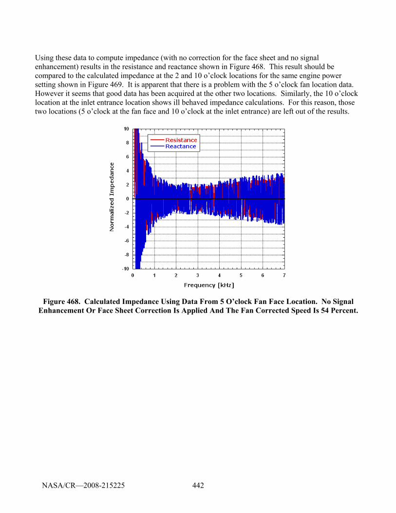
442

Using these data to compute impedance (with no correction for the face sheet and no signal enhancement) results in the resistance and reactance shown in Figure 468. This result should be compared to the calculated impedance at the 2 and 10 o’clock locations for the same engine power setting shown in Figure 469. It is apparent that there is a problem with the 5 o’clock fan location data. However it seems that good data has been acquired at the other two locations. Similarly, the 10 o’clock location at the inlet entrance location shows ill behaved impedance calculations. For this reason, those two locations (5 o’clock at the fan face and 10 o’clock at the inlet entrance) are left out of the results.

Figure 468. Calculated Impedance Using Data From 5 O’clock Fan Face Location. No Signal Enhancement Or Face Sheet Correction Is Applied And The Fan Corrected Speed Is 54 Percent.

NASA/CR—2008-215225

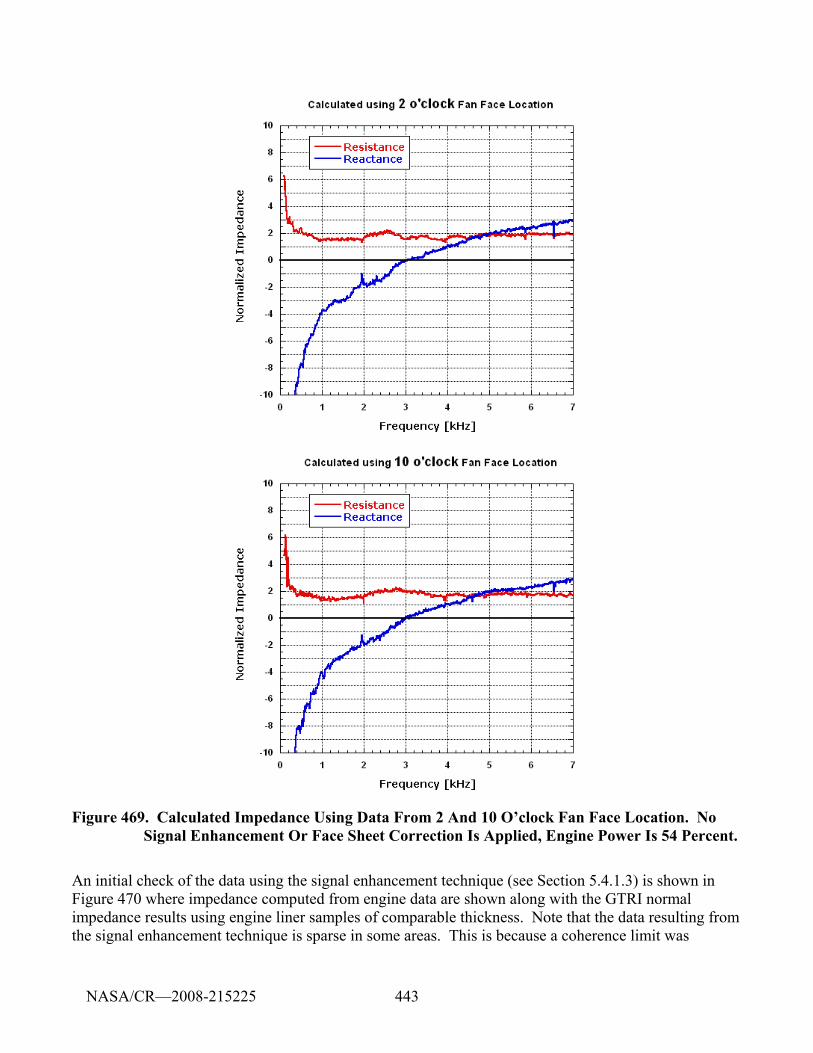
443

Figure 469. Calculated Impedance Using Data From 2 And 10 O’clock Fan Face Location. No Signal Enhancement Or Face Sheet Correction Is Applied, Engine Power Is 54 Percent.

An initial check of the data using the signal enhancement technique (see Section 5.4.1.3) is shown in Figure 470 where impedance computed from engine data are shown along with the GTRI normal impedance results using engine liner samples of comparable thickness. Note that the data resulting from the signal enhancement technique is sparse in some areas. This is because a coherence limit was

NASA/CR—2008-215225

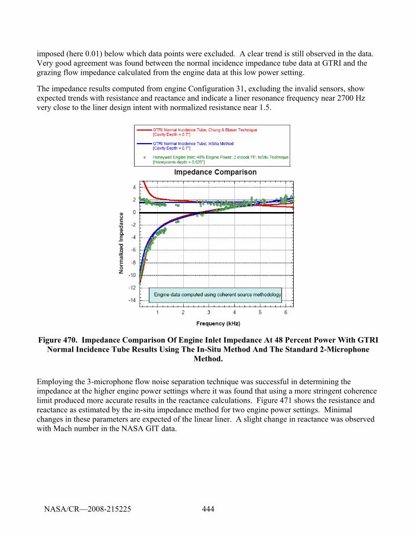
444

imposed (here 0.01) below which data points were excluded. A clear trend is still observed in the data. Very good agreement was found between the normal incidence impedance tube data at GTRI and the grazing flow impedance calculated from the engine data at this low power setting.

The impedance results computed from engine Configuration 31, excluding the invalid sensors, show expected trends with resistance and reactance and indicate a liner resonance frequency near 2700 Hz very close to the liner design intent with normalized resistance near 1.5.

Figure 470. Impedance Comparison Of Engine Inlet Impedance At 48 Percent Power With GTRI Normal Incidence Tube Results Using The In-Situ Method And The Standard 2-Microphone

Method.

Employing the 3-microphone flow noise separation technique was successful in determining the impedance at the higher engine power settings where it was found that using a more stringent coherence limit produced more accurate results in the reactance calculations. Figure 471 shows the resistance and reactance as estimated by the in-situ impedance method for two engine power settings. Minimal changes in these parameters are expected of the linear liner. A slight change in reactance was observed with Mach number in the NASA GIT data.

NASA/CR—2008-215225

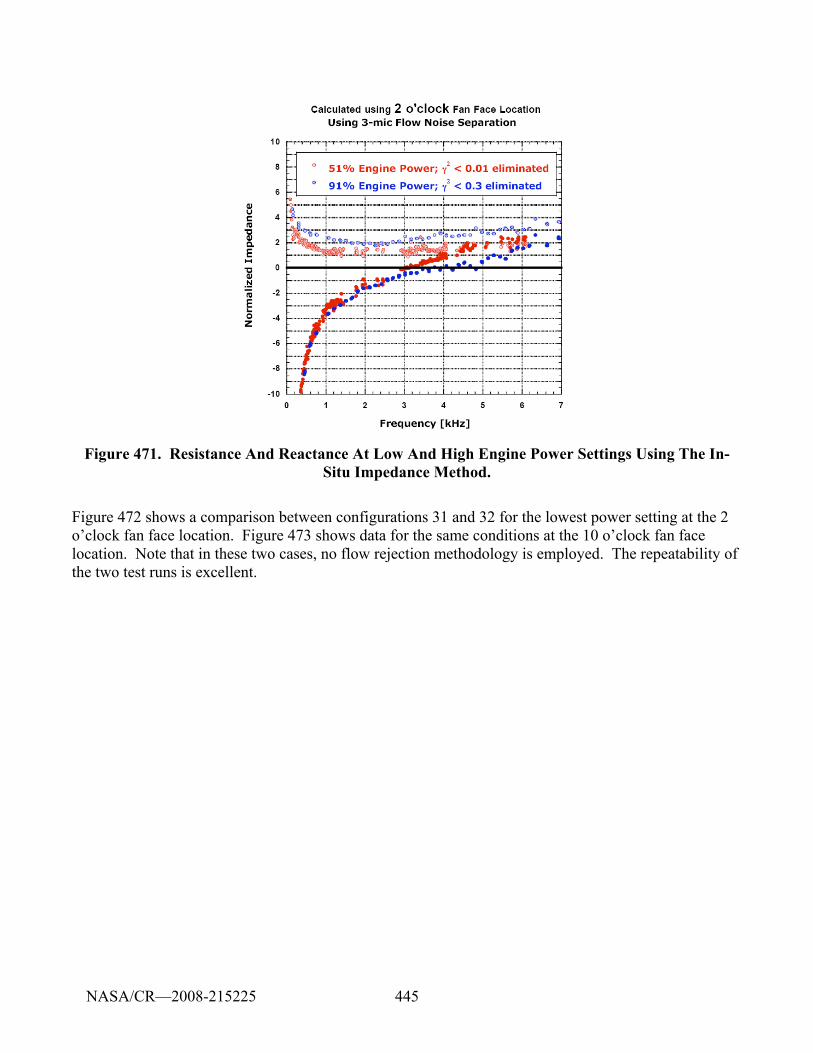
445

Figure 471. Resistance And Reactance At Low And High Engine Power Settings Using The In-Situ Impedance Method.

Figure 472 shows a comparison between configurations 31 and 32 for the lowest power setting at the 2 o’clock fan face location. Figure 473 shows data for the same conditions at the 10 o’clock fan face location. Note that in these two cases, no flow rejection methodology is employed. The repeatability of the two test runs is excellent.

NASA/CR—2008-215225

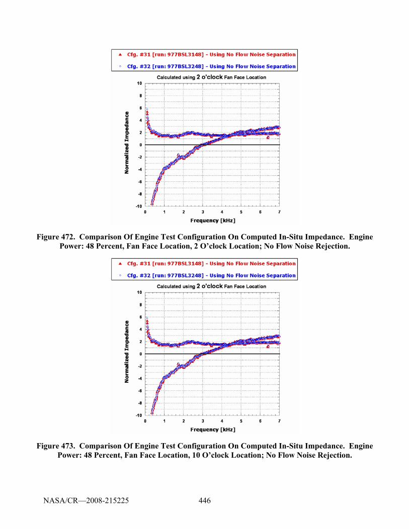
446

Figure 472. Comparison Of Engine Test Configuration On Computed In-Situ Impedance. Engine Power: 48 Percent, Fan Face Location, 2 O’clock Location; No Flow Noise Rejection.

Figure 473. Comparison Of Engine Test Configuration On Computed In-Situ Impedance. Engine Power: 48 Percent, Fan Face Location, 10 O’clock Location; No Flow Noise Rejection.

NASA/CR—2008-215225

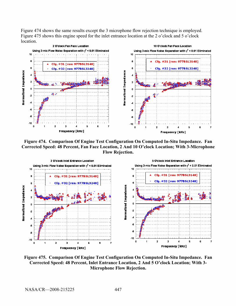
447

Figure 474 shows the same results except the 3 microphone flow rejection technique is employed. Figure 475 shows this engine speed for the inlet entrance location at the 2 o’clock and 5 o’clock location.

Figure 474. Comparison Of Engine Test Configuration On Computed In-Situ Impedance. Fan Corrected Speed: 48 Percent, Fan Face Location, 2 And 10 O’clock Location; With 3-Microphone

Flow Rejection.

Figure 475. Comparison Of Engine Test Configuration On Computed In-Situ Impedance. Fan Corrected Speed: 48 Percent, Inlet Entrance Location, 2 And 5 O’clock Location; With 3-

Microphone Flow Rejection.

NASA/CR—2008-215225

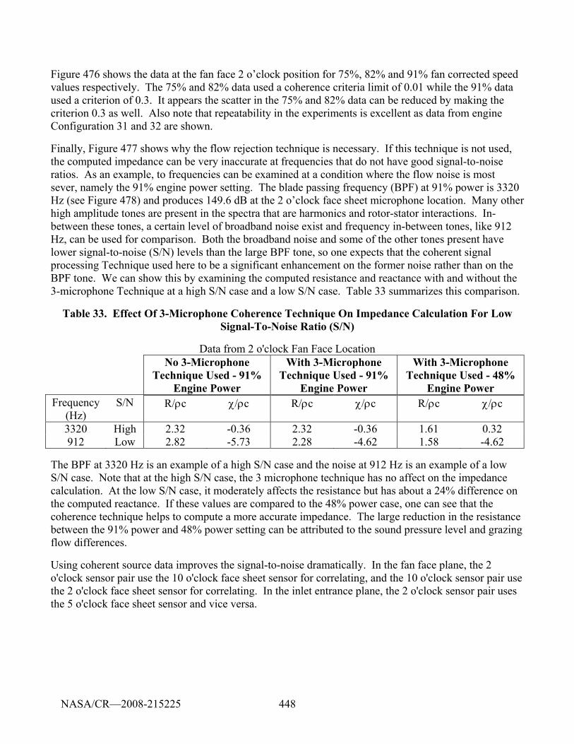
448

Figure 476 shows the data at the fan face 2 o’clock position for 75%, 82% and 91% fan corrected speed values respectively. The 75% and 82% data used a coherence criteria limit of 0.01 while the 91% data used a criterion of 0.3. It appears the scatter in the 75% and 82% data can be reduced by making the criterion 0.3 as well. Also note that repeatability in the experiments is excellent as data from engine Configuration 31 and 32 are shown.

Finally, Figure 477 shows why the flow rejection technique is necessary. If this technique is not used, the computed impedance can be very inaccurate at frequencies that do not have good signal-to-noise ratios. As an example, to frequencies can be examined at a condition where the flow noise is most sever, namely the 91% engine power setting. The blade passing frequency (BPF) at 91% power is 3320 Hz (see Figure 478) and produces 149.6 dB at the 2 o’clock face sheet microphone location. Many other high amplitude tones are present in the spectra that are harmonics and rotor-stator interactions. In-between these tones, a certain level of broadband noise exist and frequency in-between tones, like 912 Hz, can be used for comparison. Both the broadband noise and some of the other tones present have lower signal-to-noise (S/N) levels than the large BPF tone, so one expects that the coherent signal processing Technique used here to be a significant enhancement on the former noise rather than on the BPF tone. We can show this by examining the computed resistance and reactance with and without the 3-microphone Technique at a high S/N case and a low S/N case. Table 33 summarizes this comparison.

Table 33. Effect Of 3-Microphone Coherence Technique On Impedance Calculation For Low Signal-To-Noise Ratio (S/N)

Data from 2 o'clock Fan Face Location No 3-Microphone

Technique Used - 91% Engine Power

With 3-Microphone Technique Used - 91%

Engine Power

With 3-Microphone Technique Used - 48%

Engine Power Frequency

(Hz) S/N R/ρc χ/ρc R/ρc χ/ρc R/ρc χ/ρc

3320 High 2.32 -0.36 2.32 -0.36 1.61 0.32 912 Low 2.82 -5.73 2.28 -4.62 1.58 -4.62

The BPF at 3320 Hz is an example of a high S/N case and the noise at 912 Hz is an example of a low S/N case. Note that at the high S/N case, the 3 microphone technique has no affect on the impedance calculation. At the low S/N case, it moderately affects the resistance but has about a 24% difference on the computed reactance. If these values are compared to the 48% power case, one can see that the coherence technique helps to compute a more accurate impedance. The large reduction in the resistance between the 91% power and 48% power setting can be attributed to the sound pressure level and grazing flow differences.

Using coherent source data improves the signal-to-noise dramatically. In the fan face plane, the 2 o'clock sensor pair use the 10 o'clock face sheet sensor for correlating, and the 10 o'clock sensor pair use the 2 o'clock face sheet sensor for correlating. In the inlet entrance plane, the 2 o'clock sensor pair uses the 5 o'clock face sheet sensor and vice versa.

NASA/CR—2008-215225

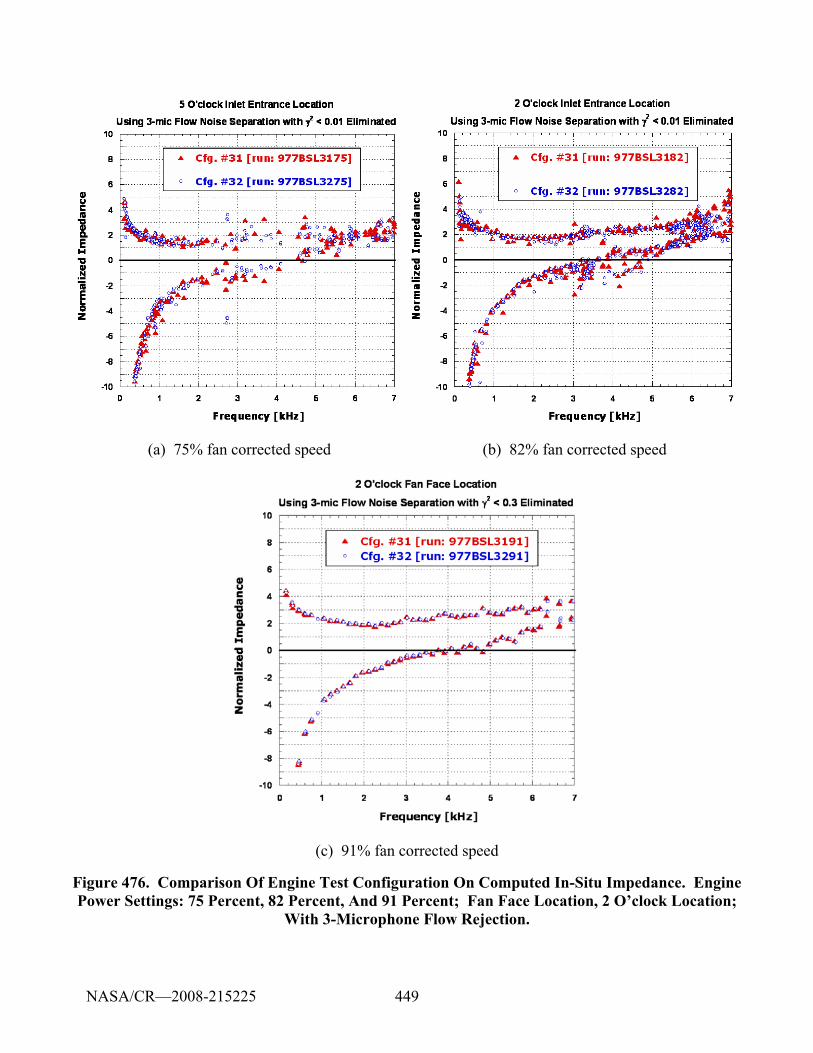
449

(a) 75% fan corrected speed (b) 82% fan corrected speed

(c) 91% fan corrected speed

Figure 476. Comparison Of Engine Test Configuration On Computed In-Situ Impedance. Engine Power Settings: 75 Percent, 82 Percent, And 91 Percent; Fan Face Location, 2 O’clock Location;

With 3-Microphone Flow Rejection.

NASA/CR—2008-215225

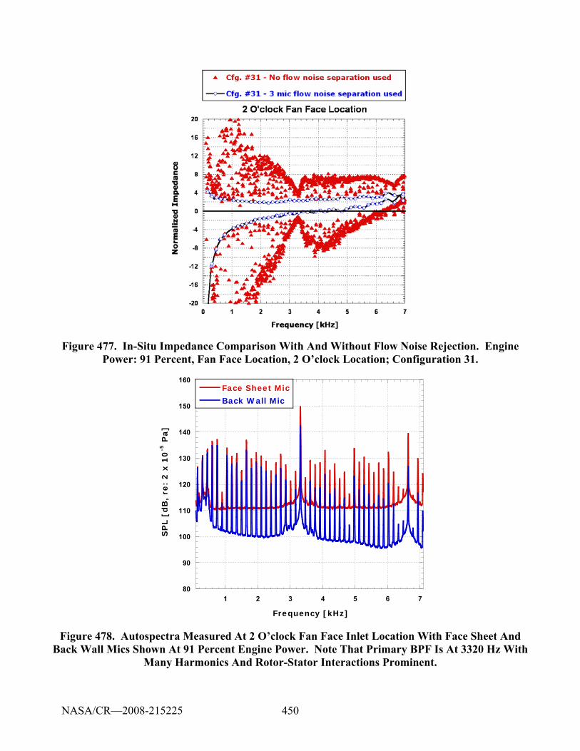
450

Figure 477. In-Situ Impedance Comparison With And Without Flow Noise Rejection. Engine Power: 91 Percent, Fan Face Location, 2 O’clock Location; Configuration 31.

80

90

100

110

120

130

140

150

160

1 2 3 4 5 6 7

Face Sheet Mic

Back Wall Mic

SP

L [

dB

, re

: 2

x 1

0-5

Pa]

Frequency [kHz]

Figure 478. Autospectra Measured At 2 O’clock Fan Face Inlet Location With Face Sheet And Back Wall Mics Shown At 91 Percent Engine Power. Note That Primary BPF Is At 3320 Hz With

Many Harmonics And Rotor-Stator Interactions Prominent.

NASA/CR—2008-215225

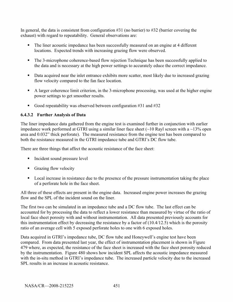
451

In general, the data is consistent from configuration #31 (no barrier) to #32 (barrier covering the exhaust) with regard to repeatability. General observations are:

The liner acoustic impedance has been successfully measured on an engine at 4 different locations. Expected trends with increasing grazing flow were observed.

The 3-microphone coherence-based flow rejection Technique has been successfully applied to the data and is necessary at the high power settings to accurately educe the correct impedance.

Data acquired near the inlet entrance exhibits more scatter, most likely due to increased grazing flow velocity compared to the fan face location.

A larger coherence limit criterion, in the 3-microphone processing, was used at the higher engine power settings to get smoother results.

Good repeatability was observed between configuration #31 and #32

6.4.3.2 Further Analysis of Data

The liner impedance data gathered from the engine test is examined further in conjunction with earlier impedance work performed at GTRI using a similar liner face sheet (~10 Rayl screen with a ~13% open area and 0.032” thick perforate). The measured resistance from the engine test has been compared to both the resistance measured in the GTRI impedance tube and GTRI’s DC flow tube.

There are three things that affect the acoustic resistance of the face sheet:

Incident sound pressure level

Grazing flow velocity

Local increase in resistance due to the presence of the pressure instrumentation taking the place of a perforate hole in the face sheet.

All three of these effects are present in the engine data. Increased engine power increases the grazing flow and the SPL of the incident sound on the liner.

The first two can be simulated in an impedance tube and a DC flow tube. The last effect can be accounted for by processing the data to reflect a lower resistance than measured by virtue of the ratio of local face sheet porosity with and without instrumentation. All data presented previously accounts for this instrumentation effect by decreasing the resistance by a factor of (10.4/12.5) which is the porosity ratio of an average cell with 5 exposed perforate holes to one with 6 exposed holes.

Data acquired in GTRI’s impedance tube, DC flow tube and Honeywell’s engine test have been compared. From data presented last year, the effect of instrumentation placement is shown in Figure 479 where, as expected, the resistance of the face sheet is increased with the face sheet porosity reduced by the instrumentation. Figure 480 shows how incident SPL affects the acoustic impedance measured with the in-situ method in GTRI’s impedance tube. The increased particle velocity due to the increased SPL results in an increase in acoustic resistance.

NASA/CR—2008-215225

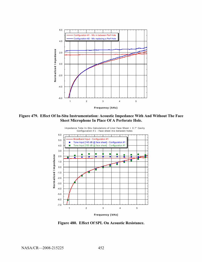
452

-6.0

-4.0

-2.0

0.0

2.0

4.0

6.0

1 2 3 4 5

Configuration #1 - Mic in between Perf HoleConfiguration #2 - Mic replacing a Perf Hole

No

rmali

zed

Im

ped

an

ce

Frequency (kHz)

Figure 479. Effect Of In-Situ Instrumentation: Acoustic Impedance With And Without The Face Sheet Microphone In Place Of A Perforate Hole.

-7.0

-6.0

-5.0

-4.0

-3.0

-2.0

-1.0

0.0

1.0

2.0

3.0

4.0

5.0

6.0

1 2 3 4 5

Broadband Input - Configuration #1Tone Input [145 dB @ face sheet] - Configuration #1Tone Input [155 dB @ face sheet] - Configuration #1

No

rmali

zed

Im

ped

an

ce

Frequency (kHz)

Impedance Tube In-Situ Calculations of Liner Face Sheet + 0.7" CavityConfiguration #1 - Face sheet mic between holes

Figure 480. Effect Of SPL On Acoustic Resistance.

NASA/CR—2008-215225

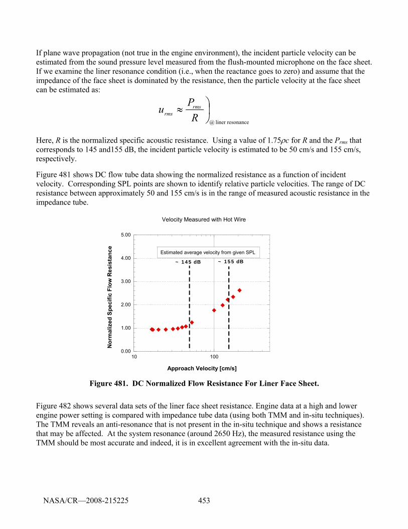
453

If plane wave propagation (not true in the engine environment), the incident particle velocity can be estimated from the sound pressure level measured from the flush-mounted microphone on the face sheet. If we examine the liner resonance condition (i.e., when the reactance goes to zero) and assume that the impedance of the face sheet is dominated by the resistance, then the particle velocity at the face sheet can be estimated as:

resonanceliner @

⎟⎠⎞≈

RPu rms

rms

Here, R is the normalized specific acoustic resistance. Using a value of 1.75ρc for R and the Prms that corresponds to 145 and155 dB, the incident particle velocity is estimated to be 50 cm/s and 155 cm/s, respectively.

Figure 481 shows DC flow tube data showing the normalized resistance as a function of incident velocity. Corresponding SPL points are shown to identify relative particle velocities. The range of DC resistance between approximately 50 and 155 cm/s is in the range of measured acoustic resistance in the impedance tube.

0.00

1.00

2.00

3.00

4.00

5.00

10 100

Velocity Measured with Hot Wire

Nor

mal

ized

Spe

cific

Flo

w R

esis

tanc

e

Approach Velocity [cm/s]

~ 145 dB ~ 155 dB

Estimated average velocity from given SPL

Figure 481. DC Normalized Flow Resistance For Liner Face Sheet.

Figure 482 shows several data sets of the liner face sheet resistance. Engine data at a high and lower engine power setting is compared with impedance tube data (using both TMM and in-situ techniques). The TMM reveals an anti-resonance that is not present in the in-situ technique and shows a resistance that may be affected. At the system resonance (around 2650 Hz), the measured resistance using the TMM should be most accurate and indeed, it is in excellent agreement with the in-situ data.

NASA/CR—2008-215225

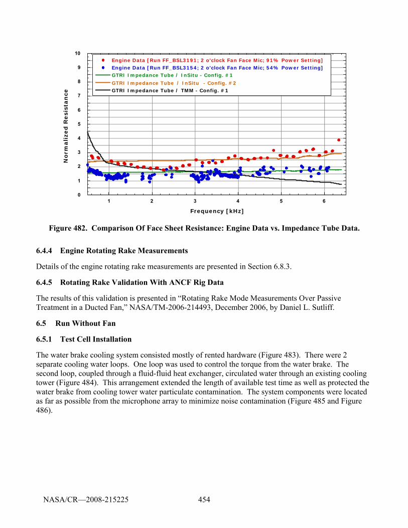
454

0

1

2

3

4

5

6

7

8

9

10

1 2 3 4 5 6

Engine Data [Run FF_BSL3191; 2 o'clock Fan Face Mic; 91% Power Setting]Engine Data [Run FF_BSL3154; 2 o'clock Fan Face Mic; 54% Power Setting]GTRI Impedance Tube / InSitu - Config. #1

GTRI Impedance Tube / InSitu - Config. #2GTRI Impedance Tube / TMM - Config. #1

No

rmali

zed

Resi

stan

ce

Frequency [kHz]

Figure 482. Comparison Of Face Sheet Resistance: Engine Data vs. Impedance Tube Data.

6.4.4 Engine Rotating Rake Measurements

Details of the engine rotating rake measurements are presented in Section 6.8.3.

6.4.5 Rotating Rake Validation With ANCF Rig Data

The results of this validation is presented in “Rotating Rake Mode Measurements Over Passive Treatment in a Ducted Fan,” NASA/TM-2006-214493, December 2006, by Daniel L. Sutliff.

6.5 Run Without Fan

6.5.1 Test Cell Installation

The water brake cooling system consisted mostly of rented hardware (Figure 483). There were 2 separate cooling water loops. One loop was used to control the torque from the water brake. The second loop, coupled through a fluid-fluid heat exchanger, circulated water through an existing cooling tower (Figure 484). This arrangement extended the length of available test time as well as protected the water brake from cooling tower water particulate contamination. The system components were located as far as possible from the microphone array to minimize noise contamination (Figure 485 and Figure 486).

NASA/CR—2008-215225

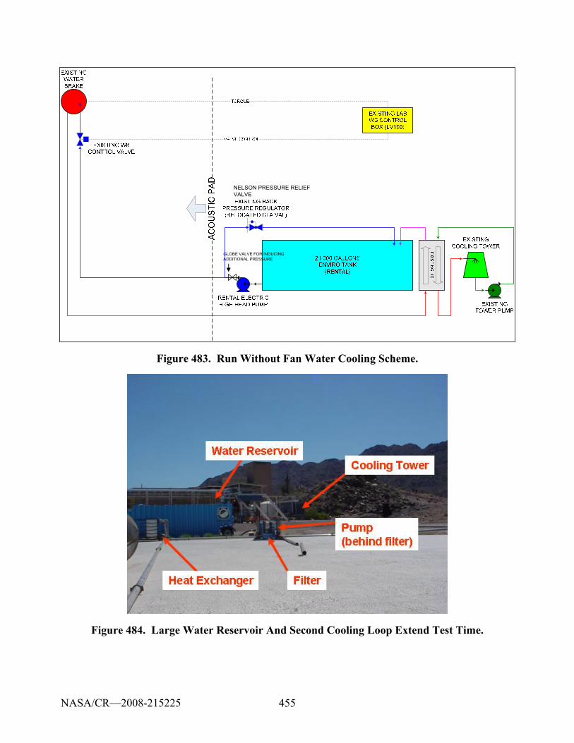
455

GLOBE VALVE FOR INDUCING ADDITIONAL PRESSURE

NELSON PRESSURE RELIEF VALVE

Figure 483. Run Without Fan Water Cooling Scheme.

Figure 484. Large Water Reservoir And Second Cooling Loop Extend Test Time.

NASA/CR—2008-215225

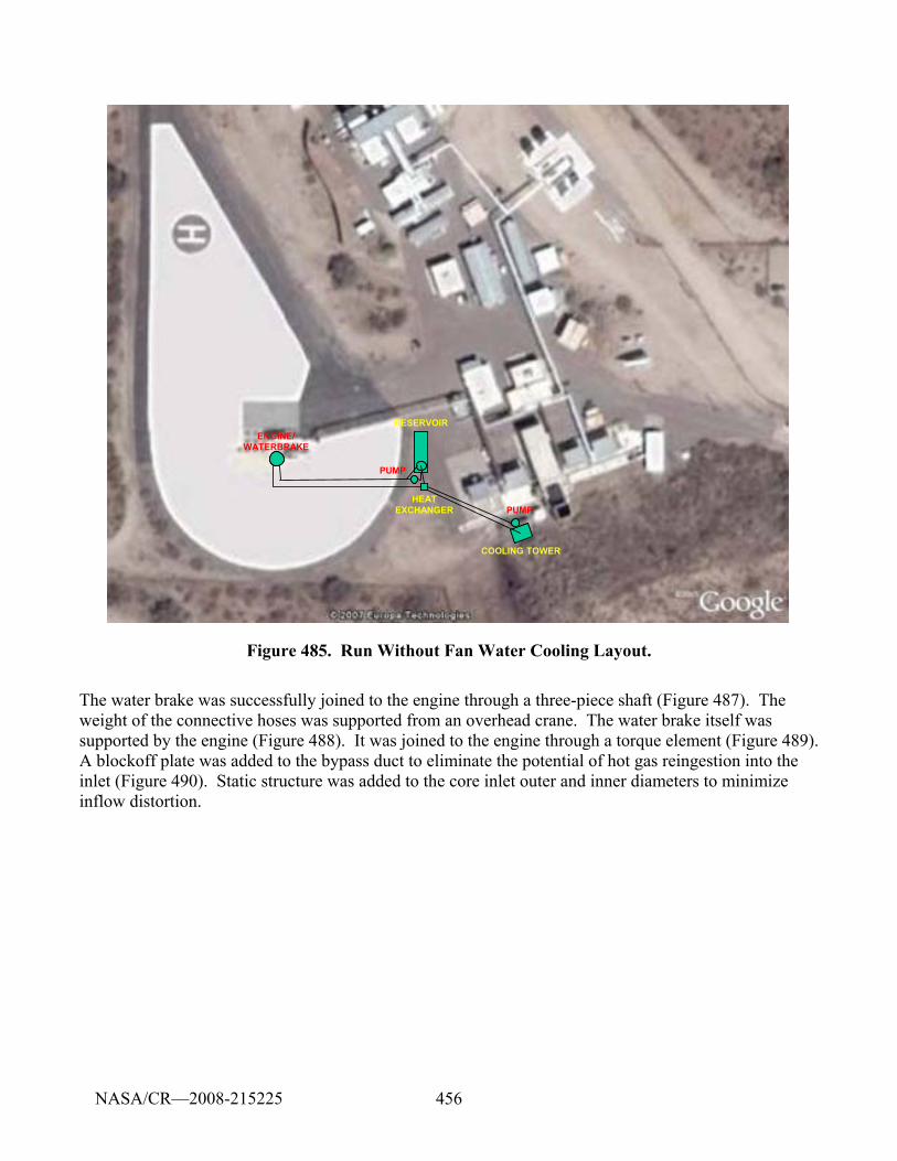
456

COOLING TOWER

RESERVOIRENGINE/

WATERBRAKE

HEATEXCHANGER

PUMP

PUMP

COOLING TOWER

RESERVOIRENGINE/

WATERBRAKE

HEATEXCHANGER

PUMP

PUMP

Figure 485. Run Without Fan Water Cooling Layout.

The water brake was successfully joined to the engine through a three-piece shaft (Figure 487). The weight of the connective hoses was supported from an overhead crane. The water brake itself was supported by the engine (Figure 488). It was joined to the engine through a torque element (Figure 489). A blockoff plate was added to the bypass duct to eliminate the potential of hot gas reingestion into the inlet (Figure 490). Static structure was added to the core inlet outer and inner diameters to minimize inflow distortion.

NASA/CR—2008-215225

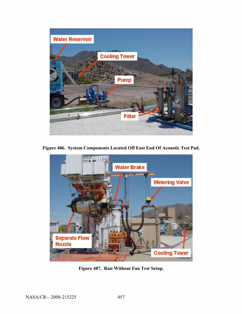
457

Figure 486. System Components Located Off East End Of Acoustic Test Pad.

Figure 487. Run Without Fan Test Setup.

NASA/CR—2008-215225

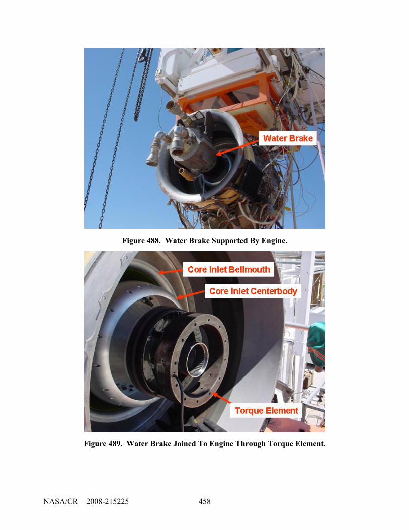
458

Figure 488. Water Brake Supported By Engine.

Figure 489. Water Brake Joined To Engine Through Torque Element.

NASA/CR—2008-215225

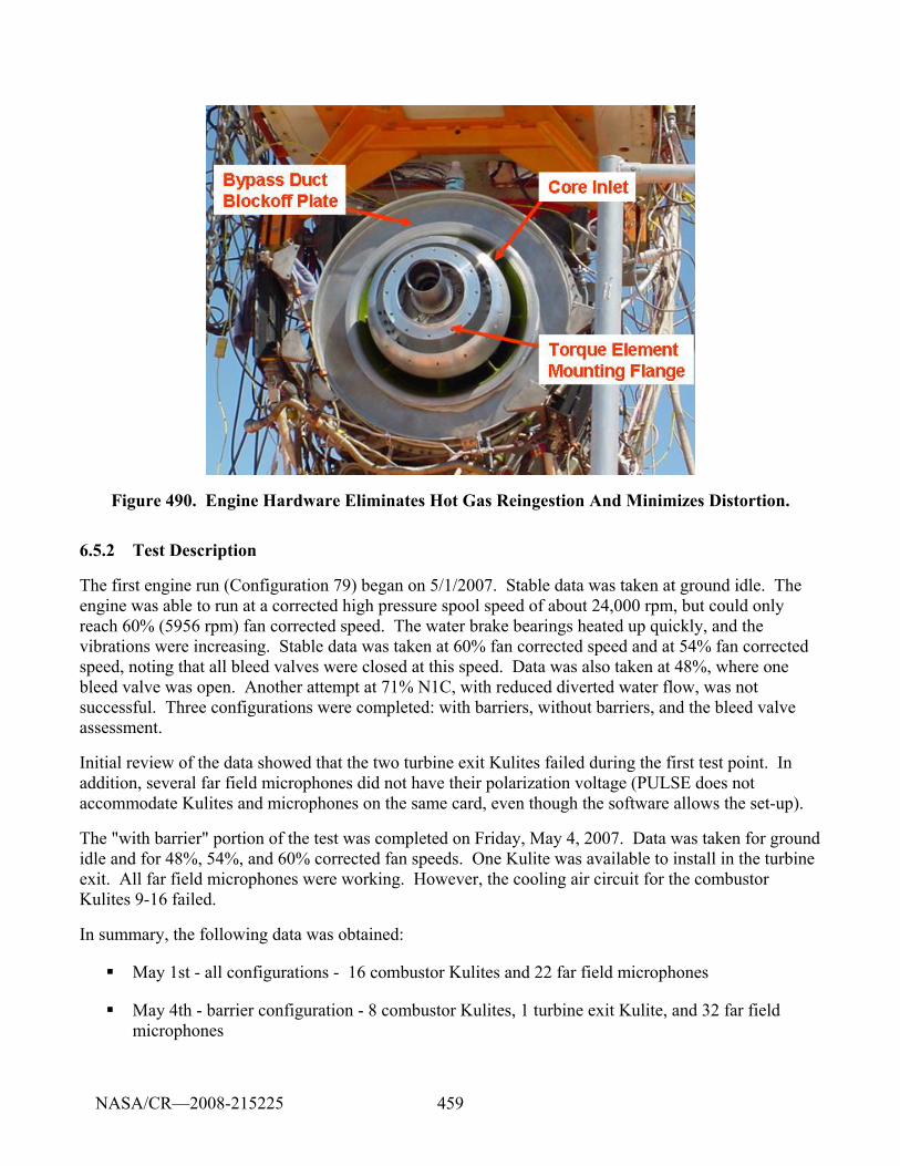
459

Figure 490. Engine Hardware Eliminates Hot Gas Reingestion And Minimizes Distortion.

6.5.2 Test Description

The first engine run (Configuration 79) began on 5/1/2007. Stable data was taken at ground idle. The engine was able to run at a corrected high pressure spool speed of about 24,000 rpm, but could only reach 60% (5956 rpm) fan corrected speed. The water brake bearings heated up quickly, and the vibrations were increasing. Stable data was taken at 60% fan corrected speed and at 54% fan corrected speed, noting that all bleed valves were closed at this speed. Data was also taken at 48%, where one bleed valve was open. Another attempt at 71% N1C, with reduced diverted water flow, was not successful. Three configurations were completed: with barriers, without barriers, and the bleed valve assessment.

Initial review of the data showed that the two turbine exit Kulites failed during the first test point. In addition, several far field microphones did not have their polarization voltage (PULSE does not accommodate Kulites and microphones on the same card, even though the software allows the set-up).

The "with barrier" portion of the test was completed on Friday, May 4, 2007. Data was taken for ground idle and for 48%, 54%, and 60% corrected fan speeds. One Kulite was available to install in the turbine exit. All far field microphones were working. However, the cooling air circuit for the combustor Kulites 9-16 failed.

In summary, the following data was obtained:

May 1st - all configurations - 16 combustor Kulites and 22 far field microphones

May 4th - barrier configuration - 8 combustor Kulites, 1 turbine exit Kulite, and 32 far field microphones

NASA/CR—2008-215225

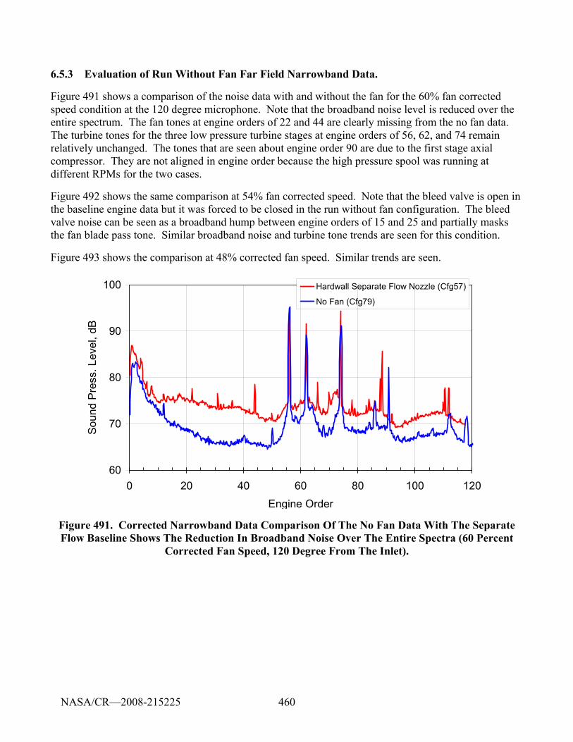
460

6.5.3 Evaluation of Run Without Fan Far Field Narrowband Data.

Figure 491 shows a comparison of the noise data with and without the fan for the 60% fan corrected speed condition at the 120 degree microphone. Note that the broadband noise level is reduced over the entire spectrum. The fan tones at engine orders of 22 and 44 are clearly missing from the no fan data. The turbine tones for the three low pressure turbine stages at engine orders of 56, 62, and 74 remain relatively unchanged. The tones that are seen about engine order 90 are due to the first stage axial compressor. They are not aligned in engine order because the high pressure spool was running at different RPMs for the two cases.

Figure 492 shows the same comparison at 54% fan corrected speed. Note that the bleed valve is open in the baseline engine data but it was forced to be closed in the run without fan configuration. The bleed valve noise can be seen as a broadband hump between engine orders of 15 and 25 and partially masks the fan blade pass tone. Similar broadband noise and turbine tone trends are seen for this condition.

Figure 493 shows the comparison at 48% corrected fan speed. Similar trends are seen.

60

70

80

90

100

0 20 40 60 80 100 120Engine Order

Sou

nd P

ress

. Lev

el, d

B


No Fan (Cfg79)

Figure 491. Corrected Narrowband Data Comparison Of The No Fan Data With The Separate Flow Baseline Shows The Reduction In Broadband Noise Over The Entire Spectra (60 Percent

Corrected Fan Speed, 120 Degree From The Inlet).

NASA/CR—2008-215225

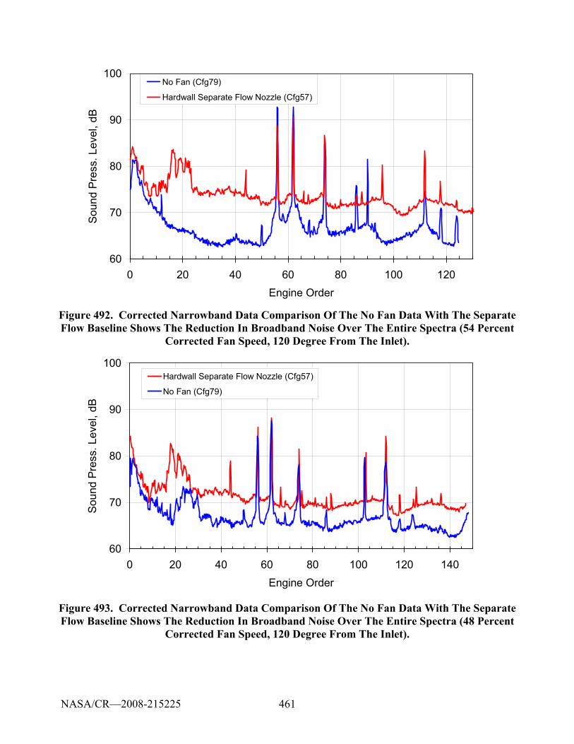
461

60

70

80

90

100

0 20 40 60 80 100 120Engine Order

Sou

nd P

ress

. Lev

el, d

BNo Fan (Cfg79)




60

70

80

90

100

0 20 40 60 80 100 120 140Engine Order

Soun

d Pr

ess.

Lev

el, d

B


No Fan (Cfg79)



NASA/CR—2008-215225

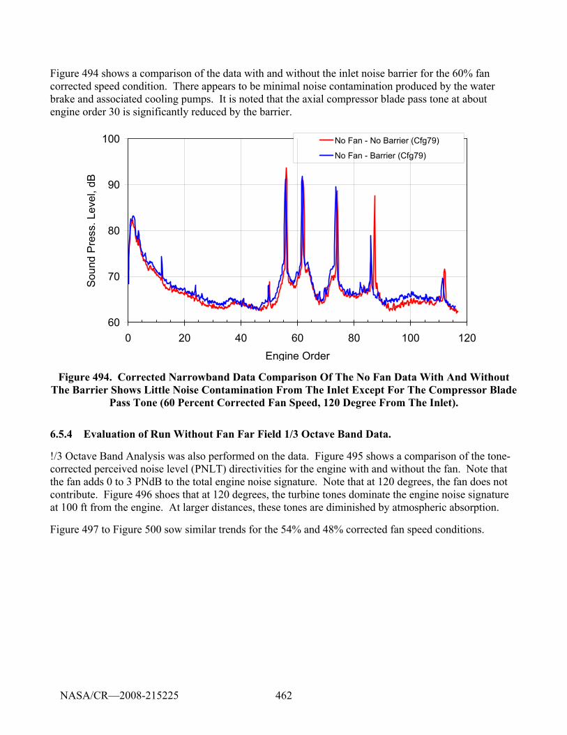
462

Figure 494 shows a comparison of the data with and without the inlet noise barrier for the 60% fan corrected speed condition. There appears to be minimal noise contamination produced by the water brake and associated cooling pumps. It is noted that the axial compressor blade pass tone at about engine order 30 is significantly reduced by the barrier.

60

70

80

90

100

0 20 40 60 80 100 120Engine Order

Soun

d Pr

ess.

Lev

el, d

B

No Fan - No Barrier (Cfg79)

No Fan - Barrier (Cfg79)

Figure 494. Corrected Narrowband Data Comparison Of The No Fan Data With And Without The Barrier Shows Little Noise Contamination From The Inlet Except For The Compressor Blade

Pass Tone (60 Percent Corrected Fan Speed, 120 Degree From The Inlet).

6.5.4 Evaluation of Run Without Fan Far Field 1/3 Octave Band Data.

!/3 Octave Band Analysis was also performed on the data. Figure 495 shows a comparison of the tone-corrected perceived noise level (PNLT) directivities for the engine with and without the fan. Note that the fan adds 0 to 3 PNdB to the total engine noise signature. Note that at 120 degrees, the fan does not contribute. Figure 496 shoes that at 120 degrees, the turbine tones dominate the engine noise signature at 100 ft from the engine. At larger distances, these tones are diminished by atmospheric absorption.

Figure 497 to Figure 500 sow similar trends for the 54% and 48% corrected fan speed conditions.

NASA/CR—2008-215225

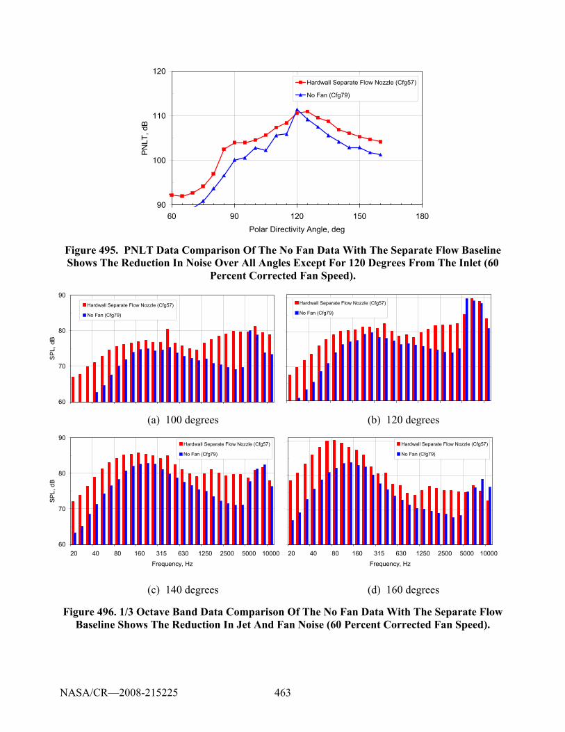
463

90

100

110

120


PN

LT, d

B


No Fan (Cfg79)

Figure 495. PNLT Data Comparison Of The No Fan Data With The Separate Flow Baseline Shows The Reduction In Noise Over All Angles Except For 120 Degrees From The Inlet (60

Percent Corrected Fan Speed).

60

70

80

90

SP

L, d

B


No Fan (Cfg79)


No Fan (Cfg79)

(a) 100 degrees (b) 120 degrees

60

70

80

90

20 40 80 160 315 630 1250 2500 5000 10000Frequency, Hz

SPL,

dB


No Fan (Cfg79)

20 40 80 160 315 630 1250 2500 5000 10000Frequency, Hz


No Fan (Cfg79)

(c) 140 degrees (d) 160 degrees

Figure 496. 1/3 Octave Band Data Comparison Of The No Fan Data With The Separate Flow Baseline Shows The Reduction In Jet And Fan Noise (60 Percent Corrected Fan Speed).

NASA/CR—2008-215225

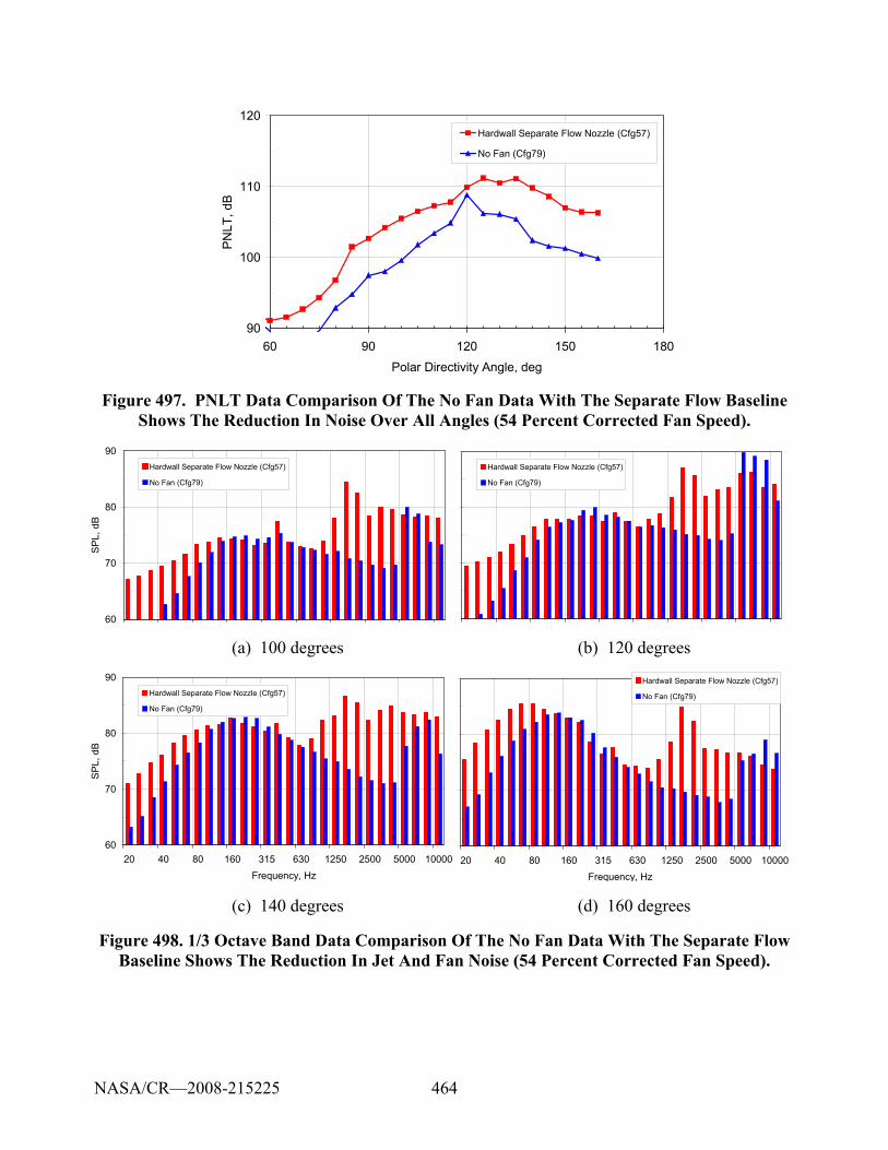
464

90

100

110

120


PN

LT, d

B


No Fan (Cfg79)

Figure 497. PNLT Data Comparison Of The No Fan Data With The Separate Flow Baseline Shows The Reduction In Noise Over All Angles (54 Percent Corrected Fan Speed).

60

70

80

90

SP

L, d

B


No Fan (Cfg79)


No Fan (Cfg79)


60

70

80

90

20 40 80 160 315 630 1250 2500 5000 10000Frequency, Hz

SP

L, d

B


No Fan (Cfg79)

20 40 80 160 315 630 1250 2500 5000 10000Frequency, Hz


No Fan (Cfg79)



NASA/CR—2008-215225

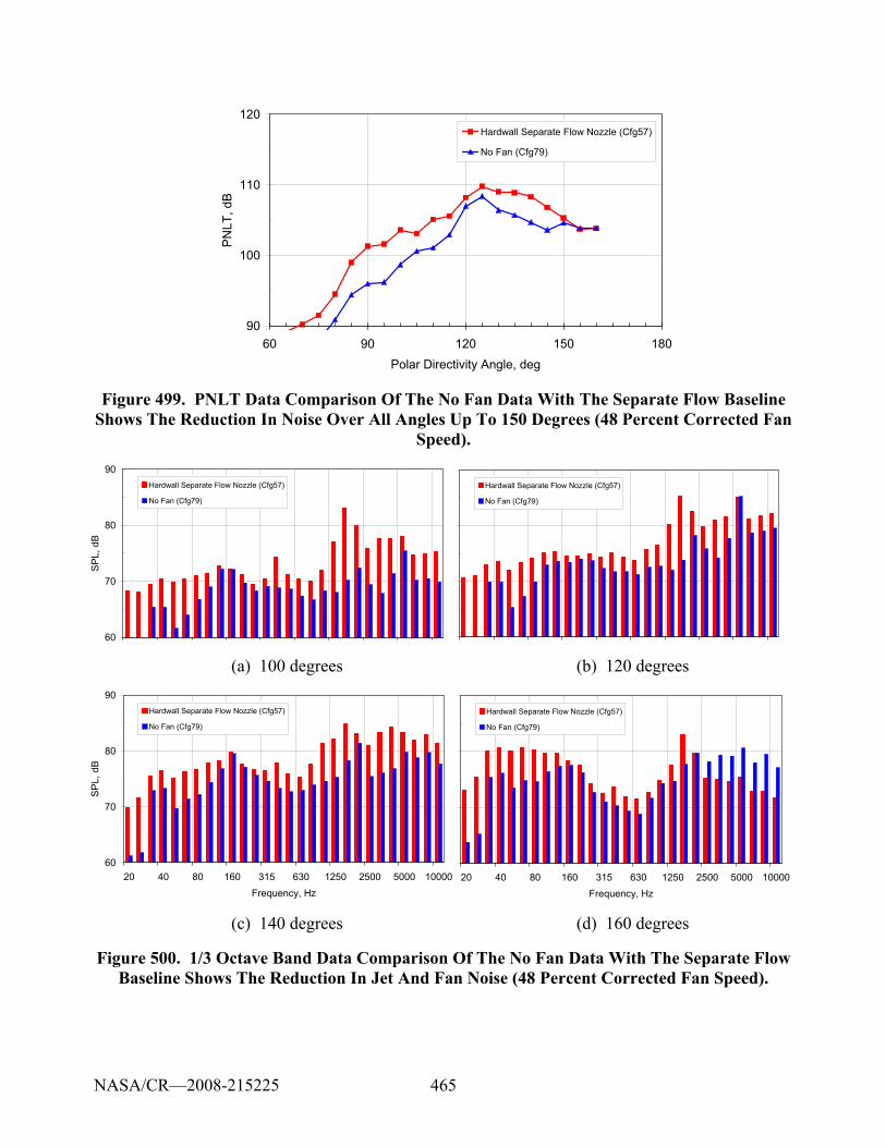
465

90

100

110

120


PN

LT, d

B


No Fan (Cfg79)

Figure 499. PNLT Data Comparison Of The No Fan Data With The Separate Flow Baseline Shows The Reduction In Noise Over All Angles Up To 150 Degrees (48 Percent Corrected Fan

Speed).

60

70

80

90

SPL,

dB


No Fan (Cfg79)


No Fan (Cfg79)


60

70

80

90

20 40 80 160 315 630 1250 2500 5000 10000Frequency, Hz

SP

L, d

B


No Fan (Cfg79)

20 40 80 160 315 630 1250 2500 5000 10000Frequency, Hz


No Fan (Cfg79)



NASA/CR—2008-215225

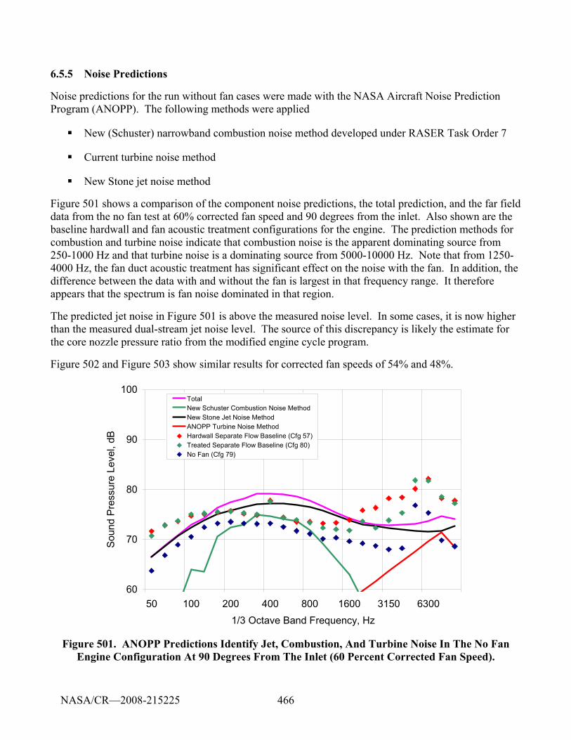
466

6.5.5 Noise Predictions

Noise predictions for the run without fan cases were made with the NASA Aircraft Noise Prediction Program (ANOPP). The following methods were applied

New (Schuster) narrowband combustion noise method developed under RASER Task Order 7

Current turbine noise method

New Stone jet noise method

Figure 501 shows a comparison of the component noise predictions, the total prediction, and the far field data from the no fan test at 60% corrected fan speed and 90 degrees from the inlet. Also shown are the baseline hardwall and fan acoustic treatment configurations for the engine. The prediction methods for combustion and turbine noise indicate that combustion noise is the apparent dominating source from 250-1000 Hz and that turbine noise is a dominating source from 5000-10000 Hz. Note that from 1250- 4000 Hz, the fan duct acoustic treatment has significant effect on the noise with the fan. In addition, the difference between the data with and without the fan is largest in that frequency range. It therefore appears that the spectrum is fan noise dominated in that region.

The predicted jet noise in Figure 501 is above the measured noise level. In some cases, it is now higher than the measured dual-stream jet noise level. The source of this discrepancy is likely the estimate for the core nozzle pressure ratio from the modified engine cycle program.

Figure 502 and Figure 503 show similar results for corrected fan speeds of 54% and 48%.

60

70

80

90

100


Sou

nd P

ress

ure

Leve

l, dB

TotalNew Schuster Combustion Noise MethodNew Stone Jet Noise MethodANOPP Turbine Noise MethodHardwall Separate Flow Baseline (Cfg 57)Treated Separate Flow Baseline (Cfg 80)No Fan (Cfg 79)

Figure 501. ANOPP Predictions Identify Jet, Combustion, And Turbine Noise In The No Fan Engine Configuration At 90 Degrees From The Inlet (60 Percent Corrected Fan Speed).

NASA/CR—2008-215225

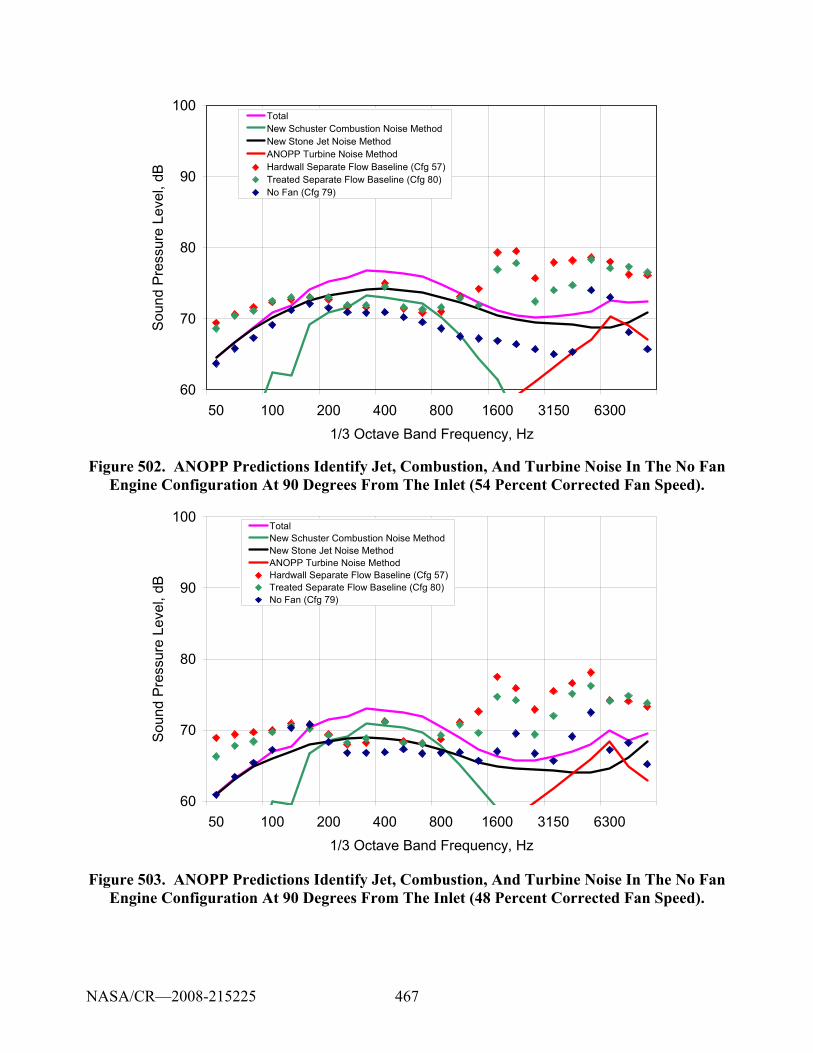
467

60

70

80

90

100


Sou

nd P

ress

ure

Leve

l, dB



60

70

80

90

100


Sou

nd P

ress

ure

Leve

l, dB



NASA/CR—2008-215225

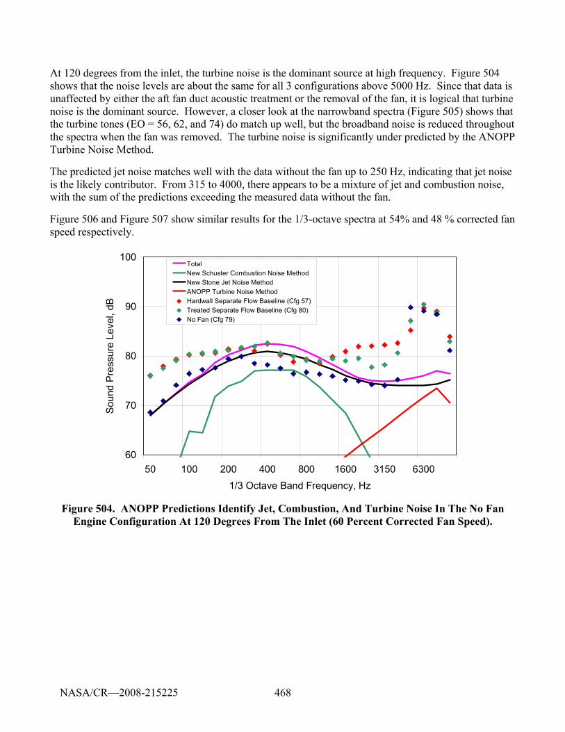
468

At 120 degrees from the inlet, the turbine noise is the dominant source at high frequency. Figure 504 shows that the noise levels are about the same for all 3 configurations above 5000 Hz. Since that data is unaffected by either the aft fan duct acoustic treatment or the removal of the fan, it is logical that turbine noise is the dominant source. However, a closer look at the narrowband spectra (Figure 505) shows that the turbine tones (EO = 56, 62, and 74) do match up well, but the broadband noise is reduced throughout the spectra when the fan was removed. The turbine noise is significantly under predicted by the ANOPP Turbine Noise Method.

The predicted jet noise matches well with the data without the fan up to 250 Hz, indicating that jet noise is the likely contributor. From 315 to 4000, there appears to be a mixture of jet and combustion noise, with the sum of the predictions exceeding the measured data without the fan.

Figure 506 and Figure 507 show similar results for the 1/3-octave spectra at 54% and 48 % corrected fan speed respectively.

60

70

80

90

100


Sou

nd P

ress

ure

Leve

l, dB



NASA/CR—2008-215225

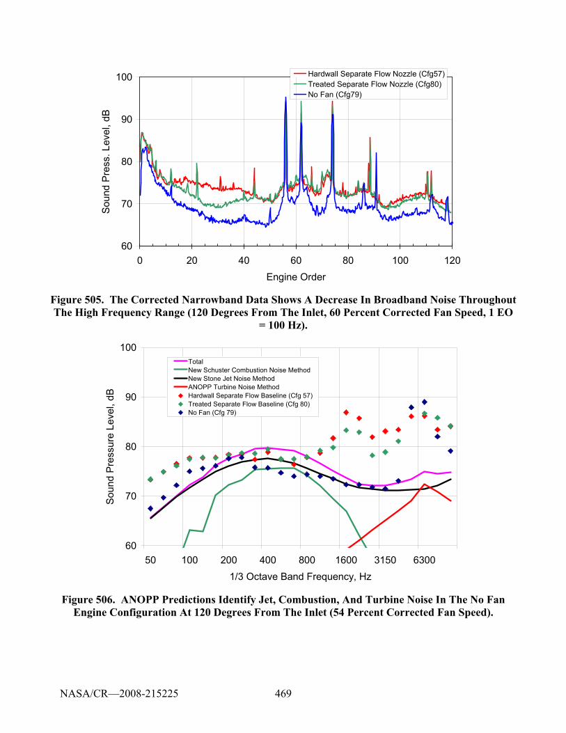
469

60

70

80

90

100

0 20 40 60 80 100 120Engine Order

Sou

nd P

ress

. Lev

el, d

B

Hardwall Separate Flow Nozzle (Cfg57)Treated Separate Flow Nozzle (Cfg80)No Fan (Cfg79)

Figure 505. The Corrected Narrowband Data Shows A Decrease In Broadband Noise Throughout The High Frequency Range (120 Degrees From The Inlet, 60 Percent Corrected Fan Speed, 1 EO

= 100 Hz).

60

70

80

90

100


Sou

nd P

ress

ure

Leve

l, dB



NASA/CR—2008-215225

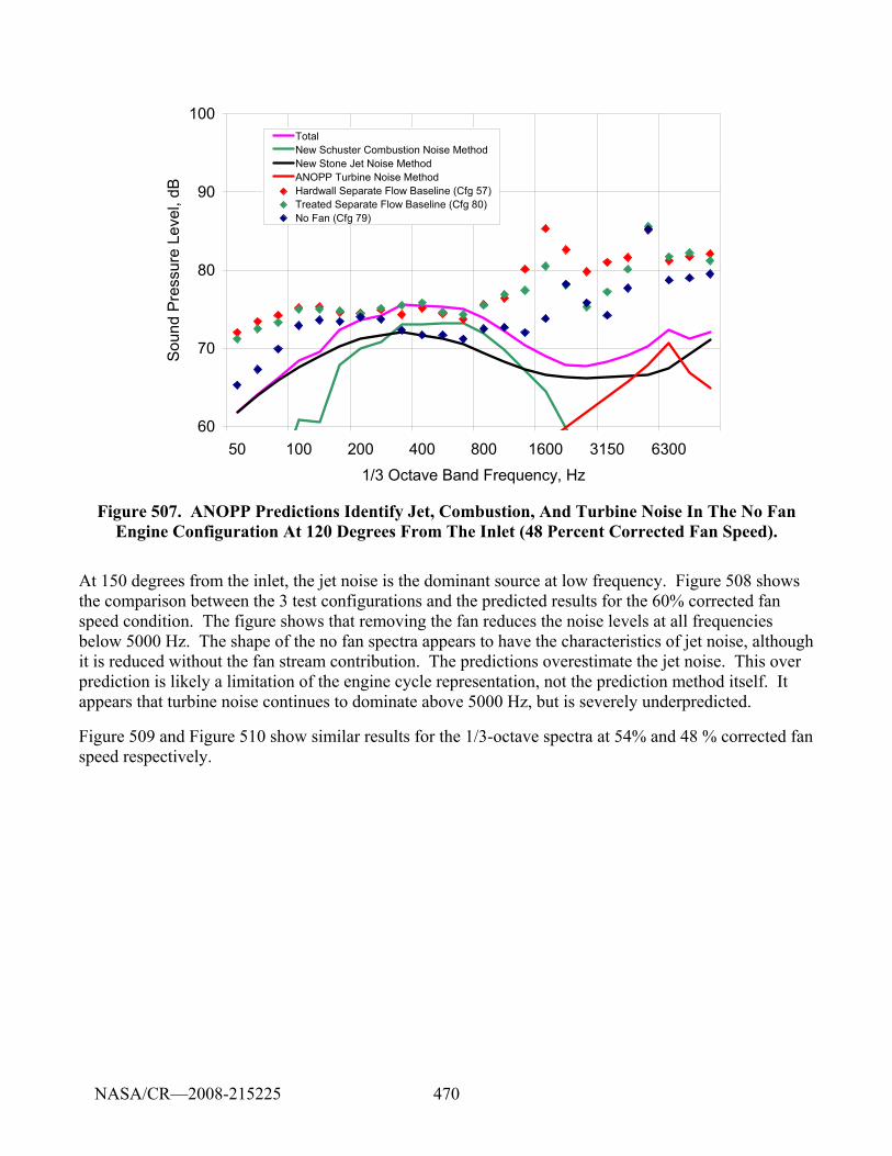
470

60

70

80

90

100


Sou

nd P

ress

ure

Leve

l, dB



At 150 degrees from the inlet, the jet noise is the dominant source at low frequency. Figure 508 shows the comparison between the 3 test configurations and the predicted results for the 60% corrected fan speed condition. The figure shows that removing the fan reduces the noise levels at all frequencies below 5000 Hz. The shape of the no fan spectra appears to have the characteristics of jet noise, although it is reduced without the fan stream contribution. The predictions overestimate the jet noise. This over prediction is likely a limitation of the engine cycle representation, not the prediction method itself. It appears that turbine noise continues to dominate above 5000 Hz, but is severely underpredicted.

Figure 509 and Figure 510 show similar results for the 1/3-octave spectra at 54% and 48 % corrected fan speed respectively.

NASA/CR—2008-215225

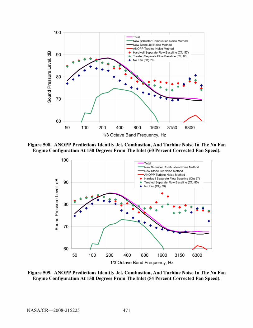
471

60

70

80

90

100


Sou

nd P

ress

ure

Leve

l, dB



60

70

80

90

100


Soun

d Pr

essu

re L

evel

, dB



NASA/CR—2008-215225

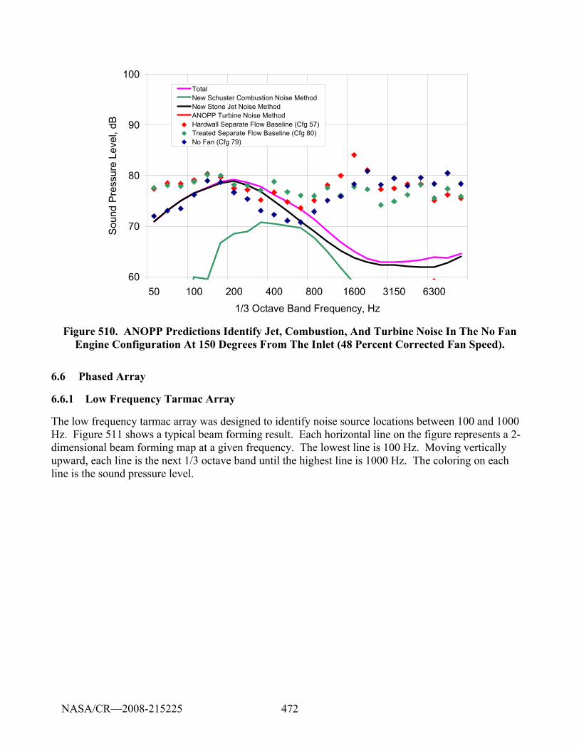
472

60

70

80

90

100


Soun

d Pr

essu

re L

evel

, dB



6.6 Phased Array

6.6.1 Low Frequency Tarmac Array

The low frequency tarmac array was designed to identify noise source locations between 100 and 1000 Hz. Figure 511 shows a typical beam forming result. Each horizontal line on the figure represents a 2-dimensional beam forming map at a given frequency. The lowest line is 100 Hz. Moving vertically upward, each line is the next 1/3 octave band until the highest line is 1000 Hz. The coloring on each line is the sound pressure level.

NASA/CR—2008-215225

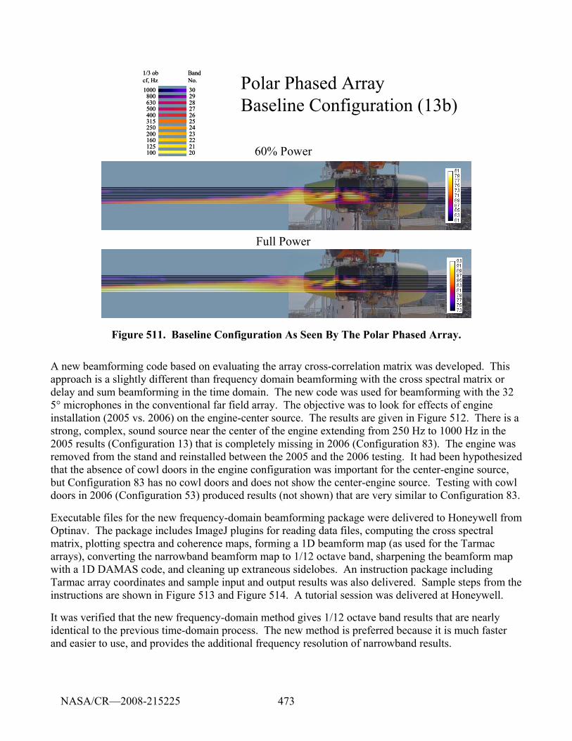
473

2021222324252627282930

100125160200250315400500630800

1000

1/3 obcf, Hz

BandNo.

2021222324252627282930

100125160200250315400500630800

1000

1/3 obcf, Hz

BandNo. Polar Phased Array

Baseline Configuration (13b)

60% Power

Full Power

Figure 511. Baseline Configuration As Seen By The Polar Phased Array.

A new beamforming code based on evaluating the array cross-correlation matrix was developed. This approach is a slightly different than frequency domain beamforming with the cross spectral matrix or delay and sum beamforming in the time domain. The new code was used for beamforming with the 32 5° microphones in the conventional far field array. The objective was to look for effects of engine installation (2005 vs. 2006) on the engine-center source. The results are given in Figure 512. There is a strong, complex, sound source near the center of the engine extending from 250 Hz to 1000 Hz in the 2005 results (Configuration 13) that is completely missing in 2006 (Configuration 83). The engine was removed from the stand and reinstalled between the 2005 and the 2006 testing. It had been hypothesized that the absence of cowl doors in the engine configuration was important for the center-engine source, but Configuration 83 has no cowl doors and does not show the center-engine source. Testing with cowl doors in 2006 (Configuration 53) produced results (not shown) that are very similar to Configuration 83.

Executable files for the new frequency-domain beamforming package were delivered to Honeywell from Optinav. The package includes ImageJ plugins for reading data files, computing the cross spectral matrix, plotting spectra and coherence maps, forming a 1D beamform map (as used for the Tarmac arrays), converting the narrowband beamform map to 1/12 octave band, sharpening the beamform map with a 1D DAMAS code, and cleaning up extraneous sidelobes. An instruction package including Tarmac array coordinates and sample input and output results was also delivered. Sample steps from the instructions are shown in Figure 513 and Figure 514. A tutorial session was delivered at Honeywell.

It was verified that the new frequency-domain method gives 1/12 octave band results that are nearly identical to the previous time-domain process. The new method is preferred because it is much faster and easier to use, and provides the additional frequency resolution of narrowband results.

NASA/CR—2008-215225

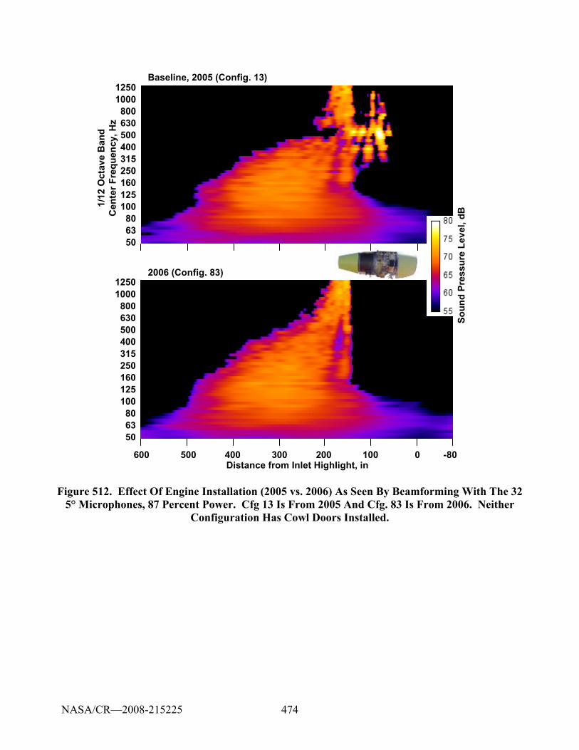
474

12501000

800630500400315250160125100806350

600 500 400 300 200 100 0 -80Distance from Inlet Highlight, in

Baseline, 2005 (Config. 13)

2006 (Config. 83)

12501000

800630500400315250160125100806350

1/12

Oct

ave

Ban

d C

ente

r Fre

quen

cy, H

z

Soun

d Pr

essu

re L

evel

, dB

Figure 512. Effect Of Engine Installation (2005 vs. 2006) As Seen By Beamforming With The 32 5° Microphones, 87 Percent Power. Cfg 13 Is From 2005 And Cfg. 83 Is From 2006. Neither

Configuration Has Cowl Doors Installed.

NASA/CR—2008-215225

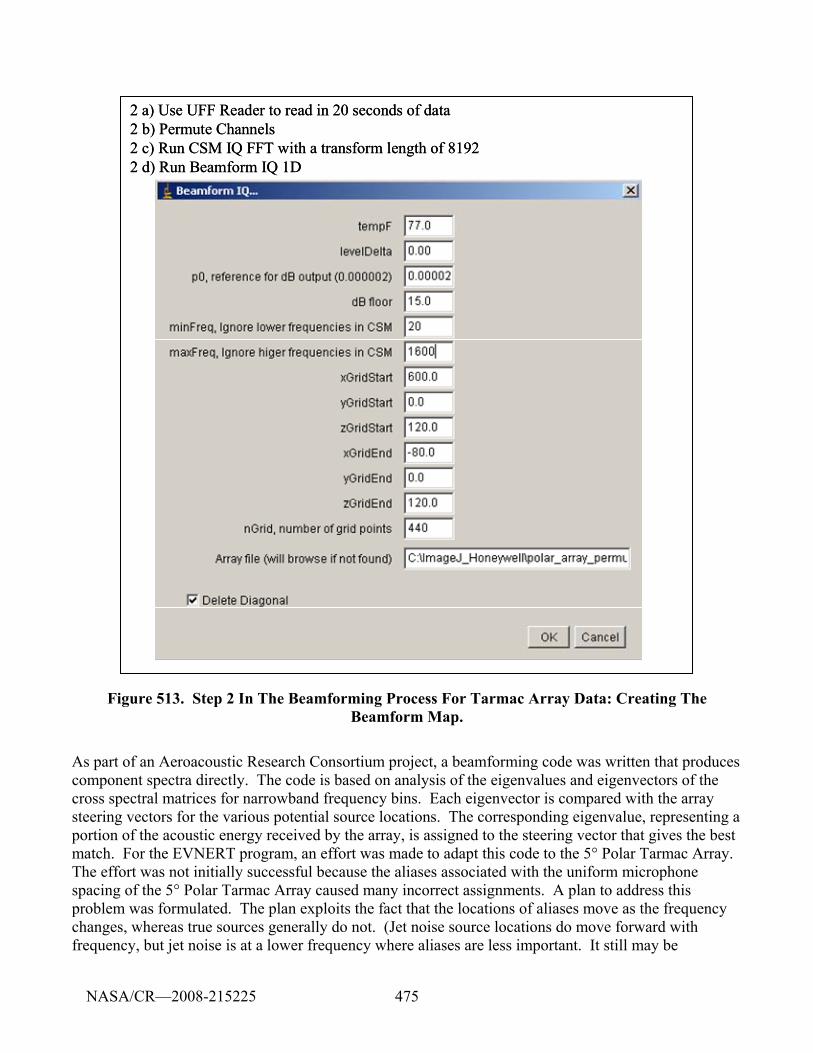
475

2 a) Use UFF Reader to read in 20 seconds of data2 b) Permute Channels2 c) Run CSM IQ FFT with a transform length of 81922 d) Run Beamform IQ 1D

2 a) Use UFF Reader to read in 20 seconds of data2 b) Permute Channels2 c) Run CSM IQ FFT with a transform length of 81922 d) Run Beamform IQ 1D

Figure 513. Step 2 In The Beamforming Process For Tarmac Array Data: Creating The Beamform Map.

As part of an Aeroacoustic Research Consortium project, a beamforming code was written that produces component spectra directly. The code is based on analysis of the eigenvalues and eigenvectors of the cross spectral matrices for narrowband frequency bins. Each eigenvector is compared with the array steering vectors for the various potential source locations. The corresponding eigenvalue, representing a portion of the acoustic energy received by the array, is assigned to the steering vector that gives the best match. For the EVNERT program, an effort was made to adapt this code to the 5° Polar Tarmac Array. The effort was not initially successful because the aliases associated with the uniform microphone spacing of the 5° Polar Tarmac Array caused many incorrect assignments. A plan to address this problem was formulated. The plan exploits the fact that the locations of aliases move as the frequency changes, whereas true sources generally do not. (Jet noise source locations do move forward with frequency, but jet noise is at a lower frequency where aliases are less important. It still may be

NASA/CR—2008-215225

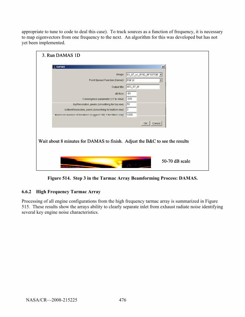
476

appropriate to tune to code to deal this case). To track sources as a function of frequency, it is necessary to map eigenvectors from one frequency to the next. An algorithm for this was developed but has not yet been implemented.

3. Run DAMAS 1D

Wait about 8 minutes for DAMAS to finish. Adjust the B&C to see the results

50-70 dB scale

3. Run DAMAS 1D

Wait about 8 minutes for DAMAS to finish. Adjust the B&C to see the results

50-70 dB scale

Figure 514. Step 3 in the Tarmac Array Beamforming Process: DAMAS.

6.6.2 High Frequency Tarmac Array

Processing of all engine configurations from the high frequency tarmac array is summarized in Figure 515. These results show the arrays ability to clearly separate inlet from exhaust radiate noise identifying several key engine noise characteristics.

NASA/CR—2008-215225

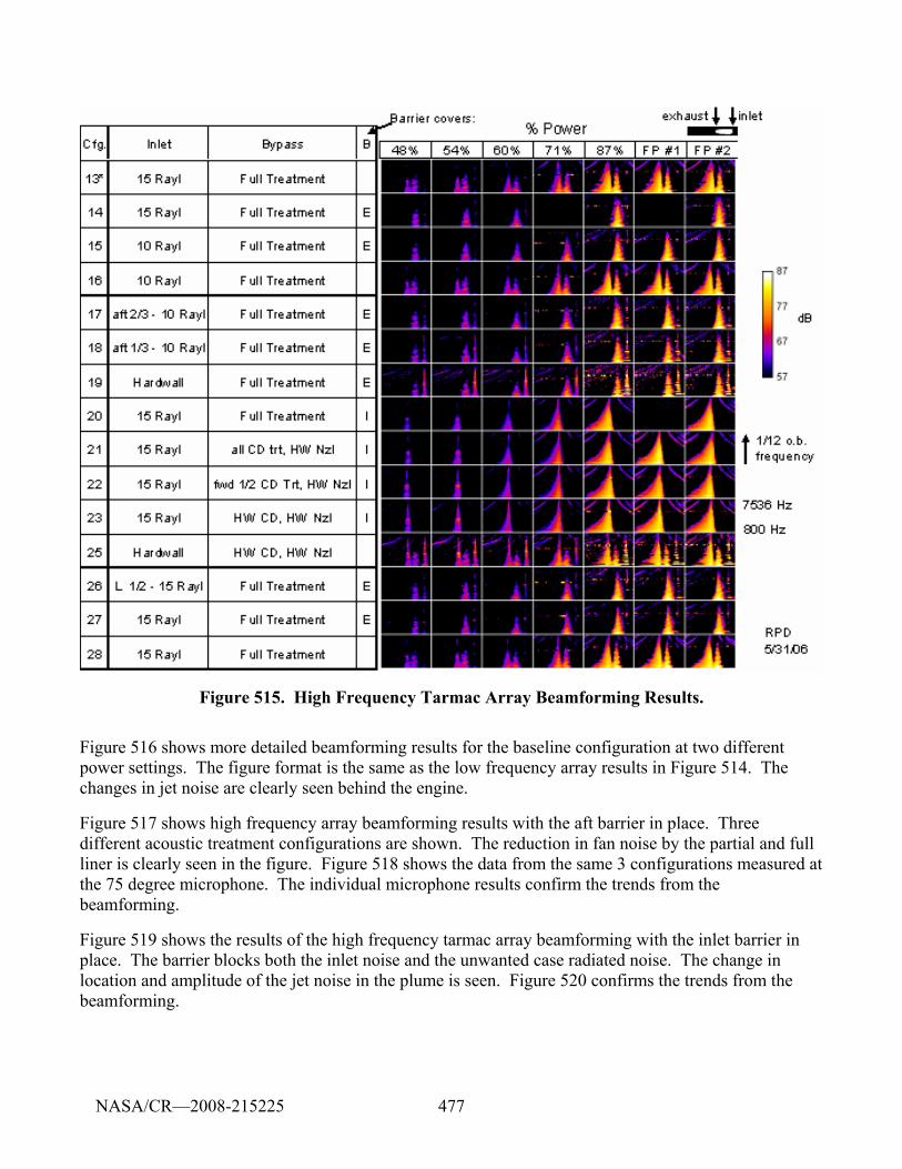
477

Figure 515. High Frequency Tarmac Array Beamforming Results.

Figure 516 shows more detailed beamforming results for the baseline configuration at two different power settings. The figure format is the same as the low frequency array results in Figure 514. The changes in jet noise are clearly seen behind the engine.

Figure 517 shows high frequency array beamforming results with the aft barrier in place. Three different acoustic treatment configurations are shown. The reduction in fan noise by the partial and full liner is clearly seen in the figure. Figure 518 shows the data from the same 3 configurations measured at the 75 degree microphone. The individual microphone results confirm the trends from the beamforming.

Figure 519 shows the results of the high frequency tarmac array beamforming with the inlet barrier in place. The barrier blocks both the inlet noise and the unwanted case radiated noise. The change in location and amplitude of the jet noise in the plume is seen. Figure 520 confirms the trends from the beamforming.

NASA/CR—2008-215225

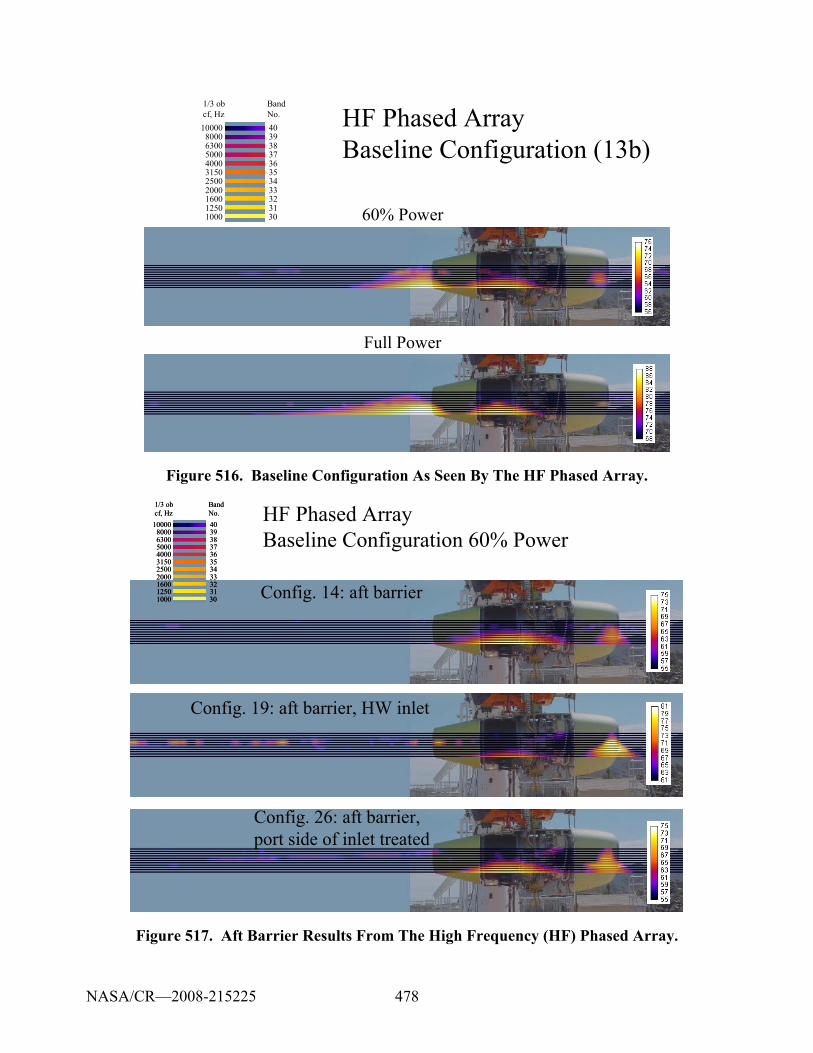
478

3031323334353637383940

1000125016002000250031504000500063008000

10000

1/3 obcf, Hz

BandNo. HF Phased Array

Baseline Configuration (13b)

60% Power

Full Power

Figure 516. Baseline Configuration As Seen By The HF Phased Array.

HF Phased ArrayBaseline Configuration 60% Power

Config. 14: aft barrier

Config. 19: aft barrier, HW inletConfig. 19: aft barrier, HW inlet

Config. 26: aft barrier,port side of inlet treated

3031323334353637383940

1000125016002000250031504000500063008000

10000

1/3 obcf, Hz

BandNo.

3031323334353637383940

1000125016002000250031504000500063008000

10000

1/3 obcf, Hz

BandNo.

Figure 517. Aft Barrier Results From The High Frequency (HF) Phased Array.

NASA/CR—2008-215225

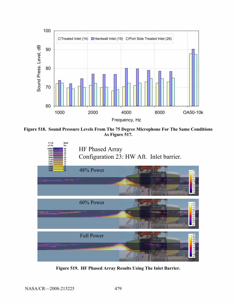
479

60

70

80

90

100

1000 2000 4000 8000 OA50-10kFrequency, Hz

Soun

d Pr

ess.

Lev

el, d

BTreated Inlet (14) Hardwall Inlet (19) Port Side Treated Inlet (26)

Figure 518. Sound Pressure Levels From The 75 Degree Microphone For The Same Conditions As Figure 517.

HF Phased ArrayConfiguration 23: HW Aft. Inlet barrier.

3031323334353637383940

1000125016002000250031504000500063008000

10000

1/3 obcf, Hz

BandNo.

3031323334353637383940

1000125016002000250031504000500063008000

10000

1/3 obcf, Hz

BandNo.

48% Power

Full Power

60% Power

Figure 519. HF Phased Array Results Using The Inlet Barrier.

NASA/CR—2008-215225

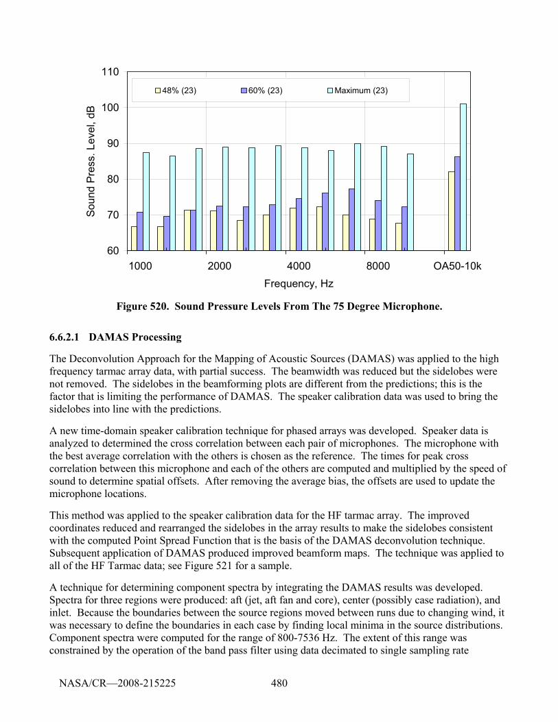
480

60

70

80

90

100

110

1000 2000 4000 8000 OA50-10kFrequency, Hz

Soun

d Pr

ess.

Lev

el, d

B48% (23) 60% (23) Maximum (23)

Figure 520. Sound Pressure Levels From The 75 Degree Microphone.

6.6.2.1 DAMAS Processing

The Deconvolution Approach for the Mapping of Acoustic Sources (DAMAS) was applied to the high frequency tarmac array data, with partial success. The beamwidth was reduced but the sidelobes were not removed. The sidelobes in the beamforming plots are different from the predictions; this is the factor that is limiting the performance of DAMAS. The speaker calibration data was used to bring the sidelobes into line with the predictions.

A new time-domain speaker calibration technique for phased arrays was developed. Speaker data is analyzed to determined the cross correlation between each pair of microphones. The microphone with the best average correlation with the others is chosen as the reference. The times for peak cross correlation between this microphone and each of the others are computed and multiplied by the speed of sound to determine spatial offsets. After removing the average bias, the offsets are used to update the microphone locations.

This method was applied to the speaker calibration data for the HF tarmac array. The improved coordinates reduced and rearranged the sidelobes in the array results to make the sidelobes consistent with the computed Point Spread Function that is the basis of the DAMAS deconvolution technique. Subsequent application of DAMAS produced improved beamform maps. The technique was applied to all of the HF Tarmac data; see Figure 521 for a sample.

A technique for determining component spectra by integrating the DAMAS results was developed. Spectra for three regions were produced: aft (jet, aft fan and core), center (possibly case radiation), and inlet. Because the boundaries between the source regions moved between runs due to changing wind, it was necessary to define the boundaries in each case by finding local minima in the source distributions. Component spectra were computed for the range of 800-7536 Hz. The extent of this range was constrained by the operation of the band pass filter using data decimated to single sampling rate

NASA/CR—2008-215225

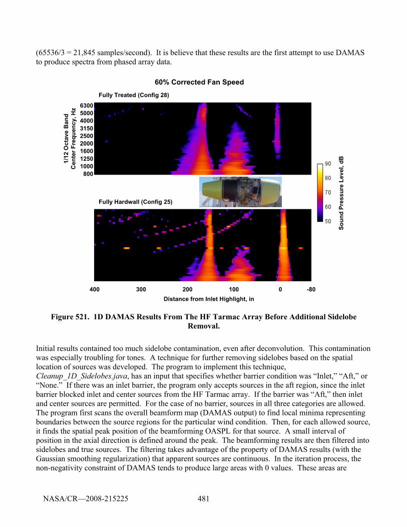
481

(65536/3 = 21,845 samples/second). It is believe that these results are the first attempt to use DAMAS to produce spectra from phased array data.

630050004000315025002000160012501000800

400 300 200 100 0 -80Distance from Inlet Highlight, in

1/12

Oct

ave

Ban

d C

ente

r Fre

quen

cy, H

z

Soun

d Pr

essu

re L

evel

, dB

Fully Treated (Config 28)

Fully Hardwall (Config 25)

60% Corrected Fan Speed

Figure 521. 1D DAMAS Results From The HF Tarmac Array Before Additional Sidelobe Removal.

Initial results contained too much sidelobe contamination, even after deconvolution. This contamination was especially troubling for tones. A technique for further removing sidelobes based on the spatial location of sources was developed. The program to implement this technique, Cleanup_1D_Sidelobes.java, has an input that specifies whether barrier condition was “Inlet,” “Aft,” or “None.” If there was an inlet barrier, the program only accepts sources in the aft region, since the inlet barrier blocked inlet and center sources from the HF Tarmac array. If the barrier was “Aft,” then inlet and center sources are permitted. For the case of no barrier, sources in all three categories are allowed. The program first scans the overall beamform map (DAMAS output) to find local minima representing boundaries between the source regions for the particular wind condition. Then, for each allowed source, it finds the spatial peak position of the beamforming OASPL for that source. A small interval of position in the axial direction is defined around the peak. The beamforming results are then filtered into sidelobes and true sources. The filtering takes advantage of the property of DAMAS results (with the Gaussian smoothing regularization) that apparent sources are continuous. In the iteration process, the non-negativity constraint of DAMAS tends to produce large areas with 0 values. These areas are

NASA/CR—2008-215225

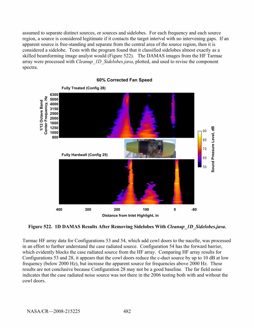
482

assumed to separate distinct sources, or sources and sidelobes. For each frequency and each source region, a source is considered legitimate if it contacts the target interval with no intervening gaps. If an apparent source is free-standing and separate from the central area of the source region, then it is considered a sidelobe. Tests with the program found that it classified sidelobes almost exactly as a skilled beamforming image analyst would (Figure 522). The DAMAS images from the HF Tarmac array were processed with Cleanup_1D_Sidelobes.java, plotted, and used to revise the component spectra.

630050004000315025002000160012501000800


1/12

Oct

ave

Ban

d C

ente

r Fre

quen

cy, H

z

Soun

d Pr

essu

re L

evel

, dB

Fully Treated (Config 28)

Fully Hardwall (Config 25)

60% Corrected Fan Speed

Figure 522. 1D DAMAS Results After Removing Sidelobes With Cleanup_1D_Sidelobes.java.

Tarmac HF array data for Configurations 53 and 54, which add cowl doors to the nacelle, was processed in an effort to further understand the case radiated source. Configuration 54 has the forward barrier, which evidently blocks the case radiated source from the HF array. Comparing HF array results for Configurations 53 and 28, it appears that the cowl doors reduce the c-duct source by up to 10 dB at low frequency (below 2000 Hz), but increase the apparent source for frequencies above 2000 Hz. These results are not conclusive because Configuration 28 may not be a good baseline. The far field noise indicates that the case radiated noise source was not there in the 2006 testing both with and without the cowl doors.

NASA/CR—2008-215225

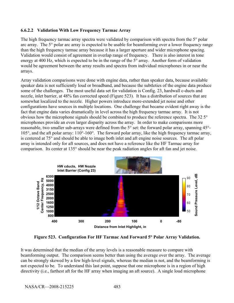
483

6.6.2.2 Validation With Low Frequency Tarmac Array

The high frequency tarmac array spectra were validated by comparison with spectra from the 5° polar arc array. The 5° polar arc array is expected to be usable for beamforming over a lower frequency range than the high frequency tarmac array because it has a larger aperture and wider microphone spacing. Validation would consist of agreement in overlap range of frequency. There is also interest in tone energy at 400 Hz, which is expected to be in the range of the 5° array. Another form of validation would be agreement between the array results and spectra from individual microphones in or near the arrays.

Array validation comparisons were done with engine data, rather than speaker data, because available speaker data is not sufficiently loud or broadband, and because the subtleties of the engine data produce some of the challenges. The most useful data set for validation is Config. 23, hardwall c-ducts and nozzle, inlet barrier, at 48% fan corrected speed (Figure 523). It has a distribution of sources that are somewhat localized to the nozzle. Higher powers introduce more-extended jet noise and other configurations have sources in multiple locations. One challenge that became evident right away is the fact that engine data varies dramatically in level across the high frequency tarmac array. It is not obvious how the microphone signals should be combined to produce the reference spectra. The 32 5° microphones provide an even larger disparity across the array. In order to make comparisons more reasonable, two smaller sub-arrays were defined from the 5° set: the forward polar array, spanning 45°-105°, and the aft polar array: 110°-160°. The forward polar array, like the high frequency tarmac array, is centered at 75° and should be able to image both inlet and aft engine noise sources. The aft polar array is intended only for aft sources, and does not have a reference like the HF Tarmac array for comparison. Its center at 135° should be near the peak radiation angles for aft fan and jet noise.

630050004000315025002000160012501000800


1/12

Oct

ave

Ban

d C

ente

r Fre

quen

cy, H

z

Soun

d Pr

essu

re L

evel

, dB

HW cducts, HW NozzleInlet Barrier (Config 23)

Figure 523. Configuration For HF Tarmac And Forward 5° Polar Array Validation.

It was determined that the median of the array levels is a reasonable measure to compare with beamforming output. The comparison seems better than using the average over the array. The average can be strongly skewed by a few high-level signals, whereas the median is not, and the beamforming is not expected to be. To understand this last point, suppose that one microphone is in a region of high directivity (i.e., farthest aft for the HF array when imaging an aft source). A single loud microphone

NASA/CR—2008-215225

484

does not strongly influence the beamforming output because there are not comparable microphones to create the constructive and destructive interference of beamforming. An alternative to use of the average or the median would be to choose a single microphone near the center of the array, but this would be subject to strong variations for tones that would not necessarily be present in the array results.

Comparing the median of the forward polar array with the integrated DAMAS results showed a large discrepancy at low frequency. In contrast, the older integration technique with normalization for peak spreading did not show this discrepancy. It was determined that that the 1D DAMAS code was inappropriately using a normalize point spread function. Correcting this problem produced good agreement at low frequency. At the upper end of the frequency range initially selected for the forward polar array (125-1182 Hz), the integrated DAMAS results were up to 10 dB lower than the array median. This difference was attributed to a combination of decorrelation by propagation through atmospheric turbulence and numerical errors associated with interpolating time series too close the Nyquist frequency. (The 5° polar array data was sampled at 32,768 samples per second, and was initially decimated by a factor of 9 to produce a rate of 3460.9 samples per second for analysis between 125 and 1182 Hz. The upper end of the analysis range is 68% of the Nyquist frequency of 1820.4 Hz, which is too high for the linear interpolation used in the delay and sum beamforming.) A new decimation and filtering strategy was developed that always places the analysis center frequency at a fixed fraction of the sampling rate (10% seems to be an appropriate choice). Use of this procedure reduced the discrepancy between the DAMAS beamforming result and the array average to at 1182 Hz to about 5 dB. This remaining difference is believed to be due to propagation effects combined with an array design that was not intended to be a phased array. Several attempts to reduce the difference by changing the beamforming technique were not successful. It would be possible to attempt to calibrate for this effect, but it would be risky because the decorrelation depends on atmospheric turbulence, and this can change from run to run. In the test data set, the difference is small (< 2 dB) for frequencies at or below 500 Hz. It is concluded that the upper limit of the quantitative frequency range of the forward polar array is 500 Hz. The lower end of the range was also expanded by the variable decimation strategy, since it is no longer constrained by the low pass filter. A lower limit of 50 Hz was selected for presenting results, since this is the lowest 1/3 octave band center frequency used in certification. Experiments and development with the HF Tarmac array showed similar trends to the forward polar array. This array also benefited from correcting the DAMAS bug and improving the decimation. The decorrelation effects at high frequency are less severe because the microphones are spaced more closely. The quantitative operating range is estimated at 315-6000 Hz. A typical result is shown in Figure 524.

NASA/CR—2008-215225

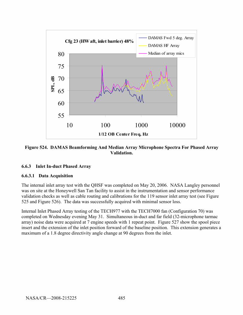
485

Cfg 23 (HW aft, inlet barrier) 48%

55

60

65

70

75

80

10 100 1000 100001/12 OB Center Freq, Hz

SPL

, dB

DAMAS Fwd 5 deg. Array

DAMAS HF Array

Median of array mics

Figure 524. DAMAS Beamforming And Median Array Microphone Spectra For Phased Array Validation.

6.6.3 Inlet In-duct Phased Array


The internal inlet array test with the QHSF was completed on May 20, 2006. NASA Langley personnel was on site at the Honeywell San Tan facility to assist in the instrumentation and sensor performance validation checks as well as cable routing and calibrations for the 119 sensor inlet array test (see Figure 525 and Figure 526). The data was successfully acquired with minimal sensor loss.

Internal Inlet Phased Array testing of the TECH977 with the TECH7000 fan (Configuration 70) was completed on Wednesday evening May 31. Simultaneous in-duct and far field (32-microphone tarmac array) noise data were acquired at 7 engine speeds with 1 repeat point. Figure 527 show the spool piece insert and the extension of the inlet position forward of the baseline position. This extension generates a maximum of a 1.8 degree directivity angle change at 90 degrees from the inlet.

NASA/CR—2008-215225

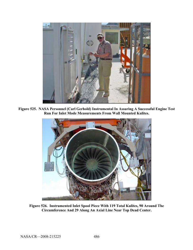
486

Figure 525. NASA Personnel (Carl Gerhold) Instrumental In Assuring A Successful Engine Test Run For Inlet Mode Measurements From Wall Mounted Kulites.

Figure 526. Instrumented Inlet Spool Piece With 119 Total Kulites, 90 Around The Circumference And 29 Along An Axial Line Near Top Dead Center.

NASA/CR—2008-215225

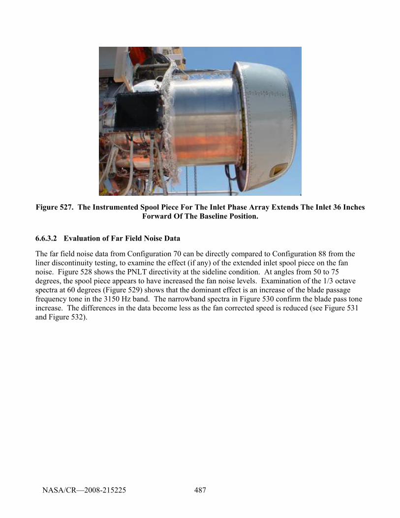
487

Figure 527. The Instrumented Spool Piece For The Inlet Phase Array Extends The Inlet 36 Inches Forward Of The Baseline Position.

6.6.3.2 Evaluation of Far Field Noise Data

The far field noise data from Configuration 70 can be directly compared to Configuration 88 from the liner discontinuity testing, to examine the effect (if any) of the extended inlet spool piece on the fan noise. Figure 528 shows the PNLT directivity at the sideline condition. At angles from 50 to 75 degrees, the spool piece appears to have increased the fan noise levels. Examination of the 1/3 octave spectra at 60 degrees (Figure 529) shows that the dominant effect is an increase of the blade passage frequency tone in the 3150 Hz band. The narrowband spectra in Figure 530 confirm the blade pass tone increase. The differences in the data become less as the fan corrected speed is reduced (see Figure 531 and Figure 532).

NASA/CR—2008-215225

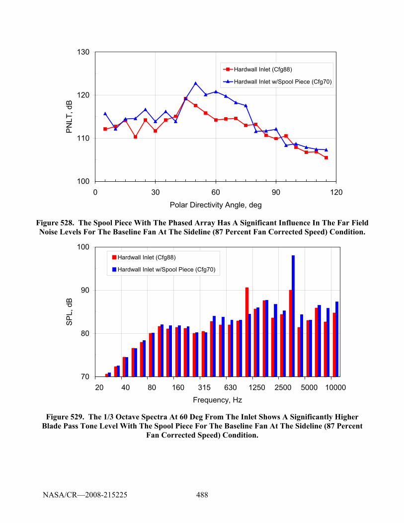
488

100

110

120

130


PNLT

, dB

Hardwall Inlet (Cfg88)

Hardwall Inlet w/Spool Piece (Cfg70)

Figure 528. The Spool Piece With The Phased Array Has A Significant Influence In The Far Field Noise Levels For The Baseline Fan At The Sideline (87 Percent Fan Corrected Speed) Condition.

70

80

90

100

20 40 80 160 315 630 1250 2500 5000 10000Frequency, Hz

SP

L, d

B



Figure 529. The 1/3 Octave Spectra At 60 Deg From The Inlet Shows A Significantly Higher Blade Pass Tone Level With The Spool Piece For The Baseline Fan At The Sideline (87 Percent

Fan Corrected Speed) Condition.

NASA/CR—2008-215225

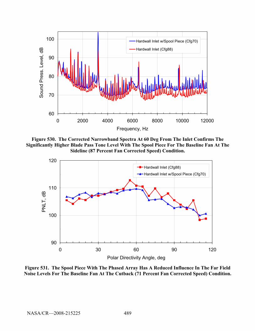
489

60

70

80

90

100

0 2000 4000 6000 8000 10000 12000Frequency, Hz

Sou

nd P

ress

. Lev

el, d

BHardwall Inlet w/Spool Piece (Cfg70)


Figure 530. The Corrected Narrowband Spectra At 60 Deg From The Inlet Confirms The Significantly Higher Blade Pass Tone Level With The Spool Piece For The Baseline Fan At The

Sideline (87 Percent Fan Corrected Speed) Condition.

90

100

110

120


PN

LT, d

B



Figure 531. The Spool Piece With The Phased Array Has A Reduced Influence In The Far Field Noise Levels For The Baseline Fan At The Cutback (71 Percent Fan Corrected Speed) Condition.

NASA/CR—2008-215225

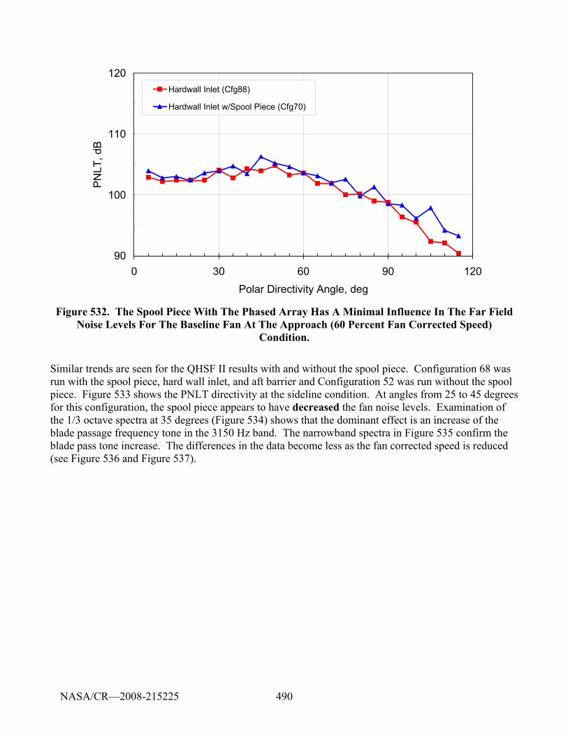
490

90

100

110

120


PN

LT, d

BHardwall Inlet (Cfg88)


Figure 532. The Spool Piece With The Phased Array Has A Minimal Influence In The Far Field Noise Levels For The Baseline Fan At The Approach (60 Percent Fan Corrected Speed)

Condition.

Similar trends are seen for the QHSF II results with and without the spool piece. Configuration 68 was run with the spool piece, hard wall inlet, and aft barrier and Configuration 52 was run without the spool piece. Figure 533 shows the PNLT directivity at the sideline condition. At angles from 25 to 45 degrees for this configuration, the spool piece appears to have decreased the fan noise levels. Examination of the 1/3 octave spectra at 35 degrees (Figure 534) shows that the dominant effect is an increase of the blade passage frequency tone in the 3150 Hz band. The narrowband spectra in Figure 535 confirm the blade pass tone increase. The differences in the data become less as the fan corrected speed is reduced (see Figure 536 and Figure 537).

NASA/CR—2008-215225

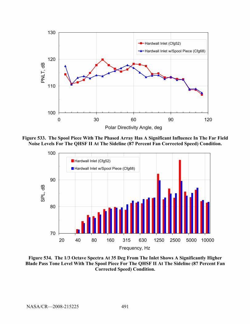
491

100

110

120

130


PN

LT, d



Figure 533. The Spool Piece With The Phased Array Has A Significant Influence In The Far Field Noise Levels For The QHSF II At The Sideline (87 Percent Fan Corrected Speed) Condition.

70

80

90

100

20 40 80 160 315 630 1250 2500 5000 10000Frequency, Hz

SP

L, d

B



Figure 534. The 1/3 Octave Spectra At 35 Deg From The Inlet Shows A Significantly Higher Blade Pass Tone Level With The Spool Piece For The QHSF II At The Sideline (87 Percent Fan


NASA/CR—2008-215225

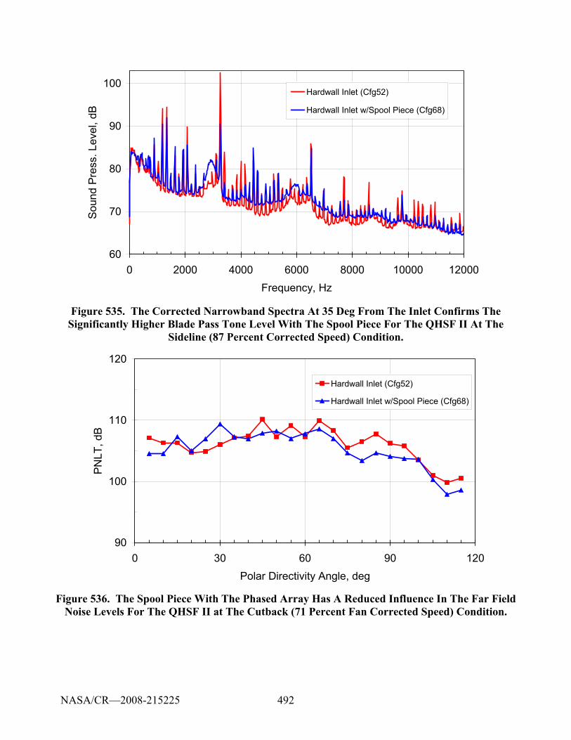
492

60

70

80

90

100

0 2000 4000 6000 8000 10000 12000Frequency, Hz

Sou

nd P

ress

. Lev

el, d



Figure 535. The Corrected Narrowband Spectra At 35 Deg From The Inlet Confirms The Significantly Higher Blade Pass Tone Level With The Spool Piece For The QHSF II At The

Sideline (87 Percent Corrected Speed) Condition.

90

100

110

120


PN

LT, d

B



Figure 536. The Spool Piece With The Phased Array Has A Reduced Influence In The Far Field Noise Levels For The QHSF II at The Cutback (71 Percent Fan Corrected Speed) Condition.

NASA/CR—2008-215225

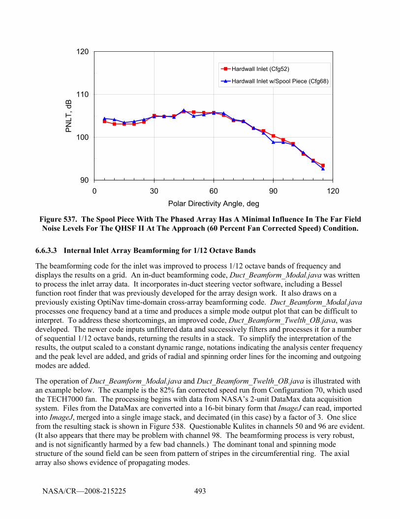
493

90

100

110

120


PN

LT, d



Figure 537. The Spool Piece With The Phased Array Has A Minimal Influence In The Far Field Noise Levels For The QHSF II At The Approach (60 Percent Fan Corrected Speed) Condition.

6.6.3.3 Internal Inlet Array Beamforming for 1/12 Octave Bands

The beamforming code for the inlet was improved to process 1/12 octave bands of frequency and displays the results on a grid. An in-duct beamforming code, Duct_Beamform_Modal.java was written to process the inlet array data. It incorporates in-duct steering vector software, including a Bessel function root finder that was previously developed for the array design work. It also draws on a previously existing OptiNav time-domain cross-array beamforming code. Duct_Beamform_Modal.java processes one frequency band at a time and produces a simple mode output plot that can be difficult to interpret. To address these shortcomings, an improved code, Duct_Beamform_Twelth_OB.java, was developed. The newer code inputs unfiltered data and successively filters and processes it for a number of sequential 1/12 octave bands, returning the results in a stack. To simplify the interpretation of the results, the output scaled to a constant dynamic range, notations indicating the analysis center frequency and the peak level are added, and grids of radial and spinning order lines for the incoming and outgoing modes are added.

The operation of Duct_Beamform_Modal.java and Duct_Beamform_Twelth_OB.java is illustrated with an example below. The example is the 82% fan corrected speed run from Configuration 70, which used the TECH7000 fan. The processing begins with data from NASA’s 2-unit DataMax data acquisition system. Files from the DataMax are converted into a 16-bit binary form that ImageJ can read, imported into ImageJ, merged into a single image stack, and decimated (in this case) by a factor of 3. One slice from the resulting stack is shown in Figure 538. Questionable Kulites in channels 50 and 96 are evident. (It also appears that there may be problem with channel 98. The beamforming process is very robust, and is not significantly harmed by a few bad channels.) The dominant tonal and spinning mode structure of the sound field can be seen from pattern of stripes in the circumferential ring. The axial array also shows evidence of propagating modes.

NASA/CR—2008-215225

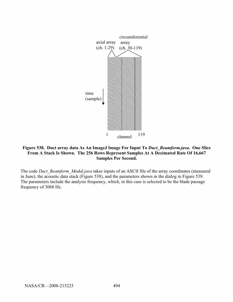
494

channel1 119

time(sample)

axial array(ch. 1-29)

circumferentialarray

(ch. 30-119)

Figure 538. Duct array data As An ImageJ Image For Input To Duct_Beamform.java. One Slice From A Stack Is Shown. The 256 Rows Represent Samples At A Decimated Rate Of 16,667

Samples Per Second.

The code Duct_Beamform_Modal.java takes inputs of an ASCII file of the array coordinates (measured in June), the acoustic data stack (Figure 538), and the parameters shown in the dialog in Figure 539. The parameters include the analysis frequency, which, in this case is selected to be the blade passage frequency of 3068 Hz.

NASA/CR—2008-215225

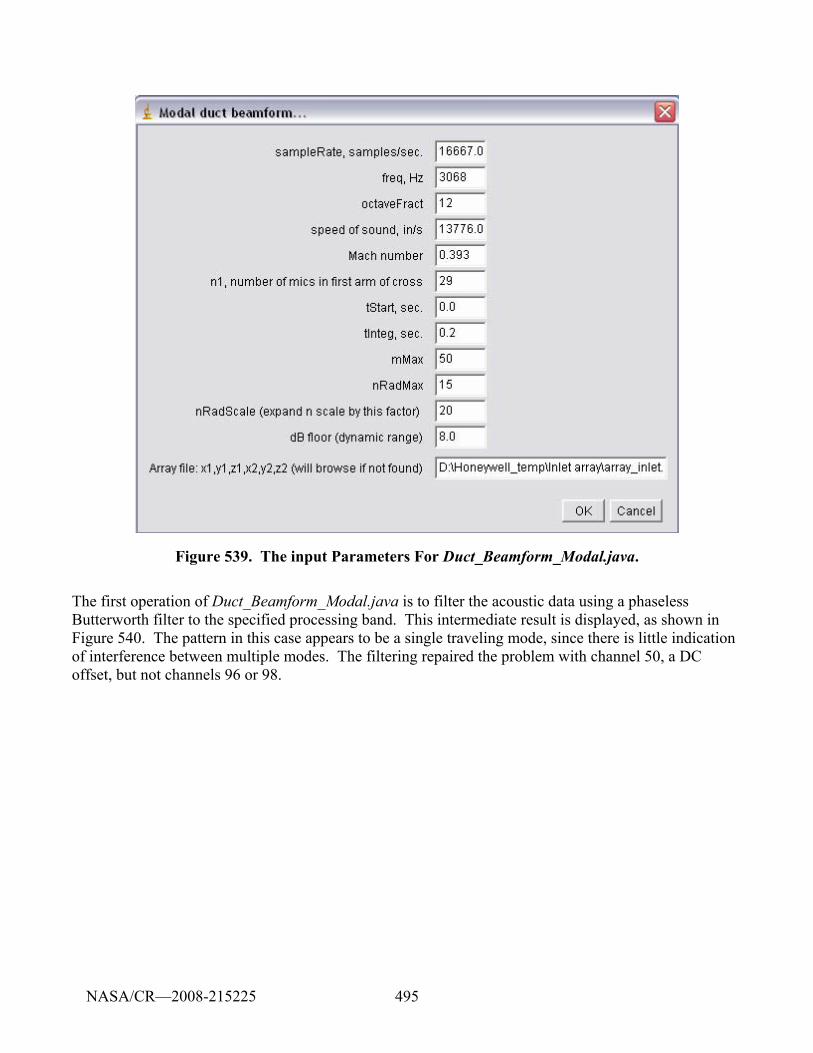
495

Figure 539. The input Parameters For Duct_Beamform_Modal.java.

The first operation of Duct_Beamform_Modal.java is to filter the acoustic data using a phaseless Butterworth filter to the specified processing band. This intermediate result is displayed, as shown in Figure 540. The pattern in this case appears to be a single traveling mode, since there is little indication of interference between multiple modes. The filtering repaired the problem with channel 50, a DC offset, but not channels 96 or 98.

NASA/CR—2008-215225

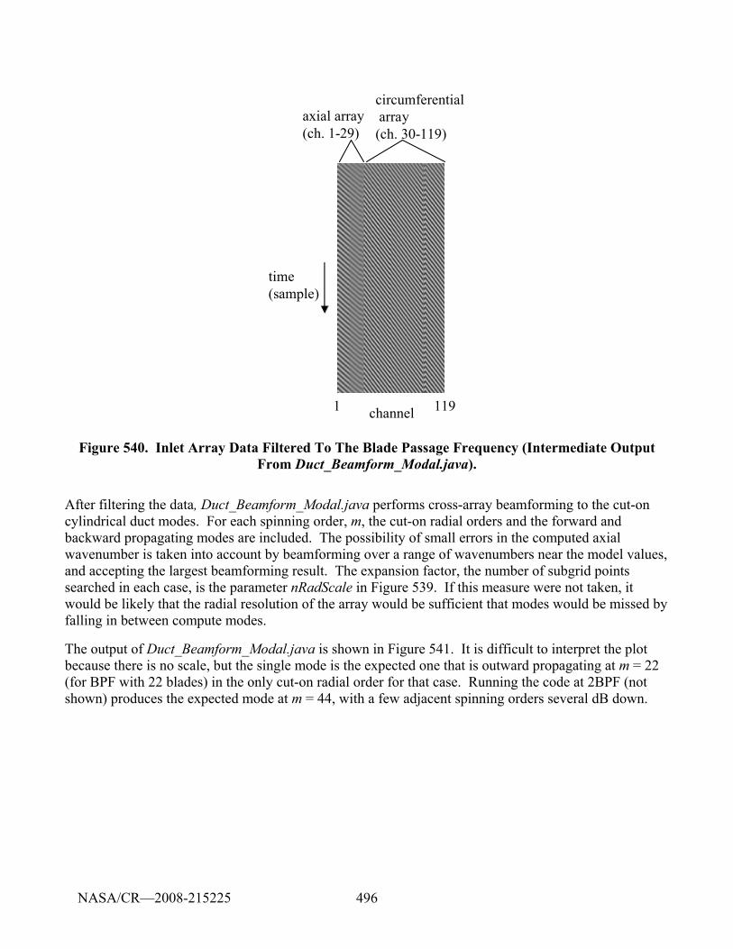
496

channel1 119

time(sample)

axial array(ch. 1-29)

circumferentialarray

(ch. 30-119)

Figure 540. Inlet Array Data Filtered To The Blade Passage Frequency (Intermediate Output From Duct_Beamform_Modal.java).

After filtering the data, Duct_Beamform_Modal.java performs cross-array beamforming to the cut-on cylindrical duct modes. For each spinning order, m, the cut-on radial orders and the forward and backward propagating modes are included. The possibility of small errors in the computed axial wavenumber is taken into account by beamforming over a range of wavenumbers near the model values, and accepting the largest beamforming result. The expansion factor, the number of subgrid points searched in each case, is the parameter nRadScale in Figure 539. If this measure were not taken, it would be likely that the radial resolution of the array would be sufficient that modes would be missed by falling in between compute modes.

The output of Duct_Beamform_Modal.java is shown in Figure 541. It is difficult to interpret the plot because there is no scale, but the single mode is the expected one that is outward propagating at m = 22 (for BPF with 22 blades) in the only cut-on radial order for that case. Running the code at 2BPF (not shown) produces the expected mode at m = 44, with a few adjacent spinning orders several dB down.

NASA/CR—2008-215225

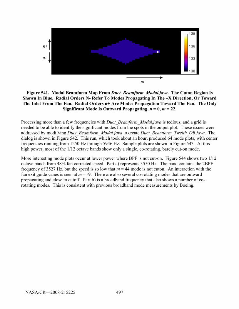
497

m

n-

n+

Figure 541. Modal Beamform Map From Duct_Beamform_Modal.java. The Cuton Region Is Shown In Blue. Radial Orders N- Refer To Modes Propagating In The –X Direction, Or Toward The Inlet From The Fan. Radial Orders n+ Are Modes Propagation Toward The Fan. The Only

Significant Mode Is Outward Propagating, n = 0, m = 22.

Processing more than a few frequencies with Duct_Beamform_Modal.java is tedious, and a grid is needed to be able to identify the significant modes from the spots in the output plot. These issues were addressed by modifying Duct_Beamform_Modal.java to create Duct_Beamform_Twelth_OB.java. The dialog is shown in Figure 542. This run, which took about an hour, produced 64 mode plots, with center frequencies running from 1250 Hz through 5946 Hz. Sample plots are shown in Figure 543. At this high power, most of the 1/12 octave bands show only a single, co-rotating, barely cut-on mode.

More interesting mode plots occur at lower power where BPF is not cut-on. Figure 544 shows two 1/12 octave bands from 48% fan corrected speed. Part a) represents 3550 Hz. The band contains the 2BPF frequency of 3527 Hz, but the speed is so low that m = 44 mode is not cuton. An interaction with the fan exit guide vanes is seen at m = -9. There are also several co-rotating modes that are outward propagating and close to cutoff. Part b) is a broadband frequency that also shows a number of co-rotating modes. This is consistent with previous broadband mode measurements by Boeing.

NASA/CR—2008-215225

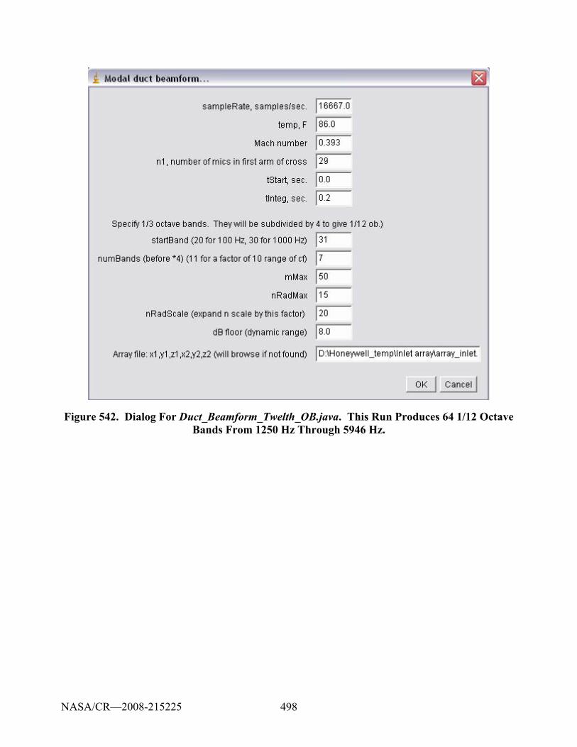
498

Figure 542. Dialog For Duct_Beamform_Twelth_OB.java. This Run Produces 64 1/12 Octave Bands From 1250 Hz Through 5946 Hz.

NASA/CR—2008-215225

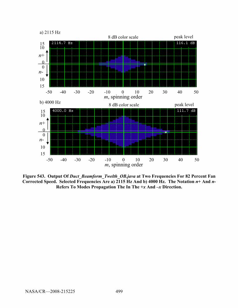
499

0 10 20 30 40 50-10-20-30-40-50m, spinning order

0

10

0

10

n+

n-

15

15

8 dB color scale peak level

0 10 20 30 40 50-10-20-30-40-50m, spinning order

0

10

0

10

n+

n-

15

15


b) 4000 Hz

a) 2115 Hz

Figure 543. Output Of Duct_Beamform_Twelth_OB.java at Two Frequencies For 82 Percent Fan Corrected Speed. Selected Frequencies Are a) 2115 Hz And b) 4000 Hz. The Notation n+ And n-

Refers To Modes Propagation The In The +x And –x Direction.

NASA/CR—2008-215225

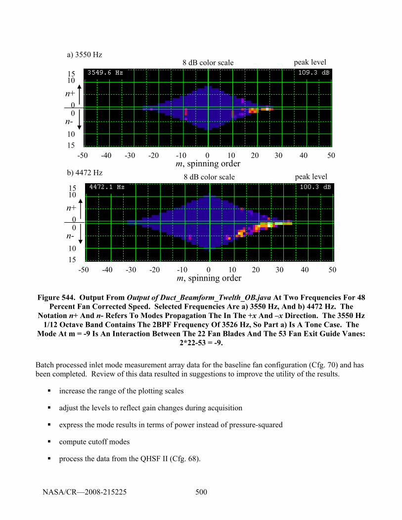
500

0 10 20 30 40 50-10-20-30-40-50m, spinning order

0

10

0

10

n+

n-

15

15


0 10 20 30 40 50-10-20-30-40-50m, spinning order

0

10

0

10

n+

n-

15

15


b) 4472 Hz

a) 3550 Hz

Figure 544. Output From Output of Duct_Beamform_Twelth_OB.java At Two Frequencies For 48 Percent Fan Corrected Speed. Selected Frequencies Are a) 3550 Hz, And b) 4472 Hz. The

Notation n+ And n- Refers To Modes Propagation The In The +x And –x Direction. The 3550 Hz 1/12 Octave Band Contains The 2BPF Frequency Of 3526 Hz, So Part a) Is A Tone Case. The

Mode At m = -9 Is An Interaction Between The 22 Fan Blades And The 53 Fan Exit Guide Vanes: 2*22-53 = -9.

Batch processed inlet mode measurement array data for the baseline fan configuration (Cfg. 70) and has been completed. Review of this data resulted in suggestions to improve the utility of the results.

increase the range of the plotting scales

adjust the levels to reflect gain changes during acquisition

express the mode results in terms of power instead of pressure-squared

compute cutoff modes

process the data from the QHSF II (Cfg. 68).

NASA/CR—2008-215225

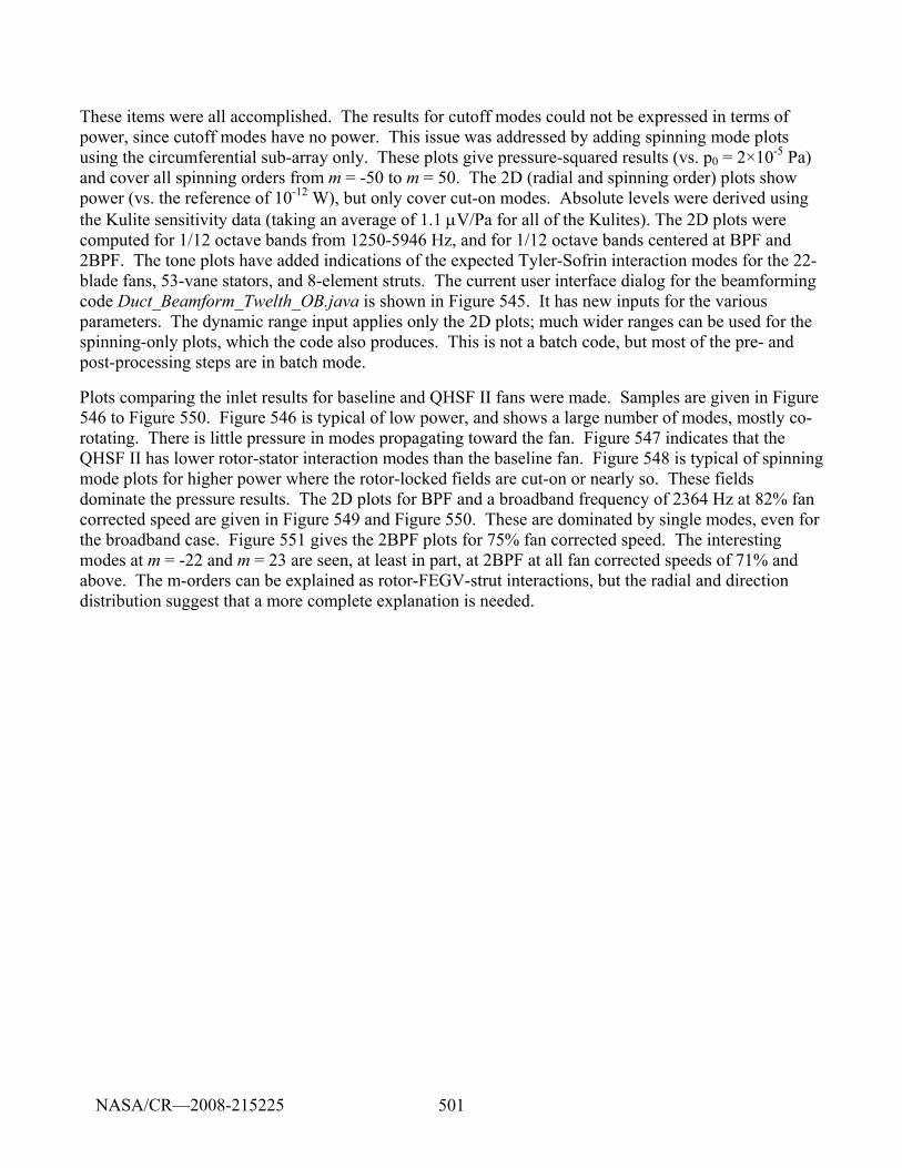
501

These items were all accomplished. The results for cutoff modes could not be expressed in terms of power, since cutoff modes have no power. This issue was addressed by adding spinning mode plots using the circumferential sub-array only. These plots give pressure-squared results (vs. p0 = 2×10-5 Pa) and cover all spinning orders from m = -50 to m = 50. The 2D (radial and spinning order) plots show power (vs. the reference of 10-12 W), but only cover cut-on modes. Absolute levels were derived using the Kulite sensitivity data (taking an average of 1.1 μV/Pa for all of the Kulites). The 2D plots were computed for 1/12 octave bands from 1250-5946 Hz, and for 1/12 octave bands centered at BPF and 2BPF. The tone plots have added indications of the expected Tyler-Sofrin interaction modes for the 22-blade fans, 53-vane stators, and 8-element struts. The current user interface dialog for the beamforming code Duct_Beamform_Twelth_OB.java is shown in Figure 545. It has new inputs for the various parameters. The dynamic range input applies only the 2D plots; much wider ranges can be used for the spinning-only plots, which the code also produces. This is not a batch code, but most of the pre- and post-processing steps are in batch mode.

Plots comparing the inlet results for baseline and QHSF II fans were made. Samples are given in Figure 546 to Figure 550. Figure 546 is typical of low power, and shows a large number of modes, mostly co-rotating. There is little pressure in modes propagating toward the fan. Figure 547 indicates that the QHSF II has lower rotor-stator interaction modes than the baseline fan. Figure 548 is typical of spinning mode plots for higher power where the rotor-locked fields are cut-on or nearly so. These fields dominate the pressure results. The 2D plots for BPF and a broadband frequency of 2364 Hz at 82% fan corrected speed are given in Figure 549 and Figure 550. These are dominated by single modes, even for the broadband case. Figure 551 gives the 2BPF plots for 75% fan corrected speed. The interesting modes at m = -22 and m = 23 are seen, at least in part, at 2BPF at all fan corrected speeds of 71% and above. The m-orders can be explained as rotor-FEGV-strut interactions, but the radial and direction distribution suggest that a more complete explanation is needed.

NASA/CR—2008-215225

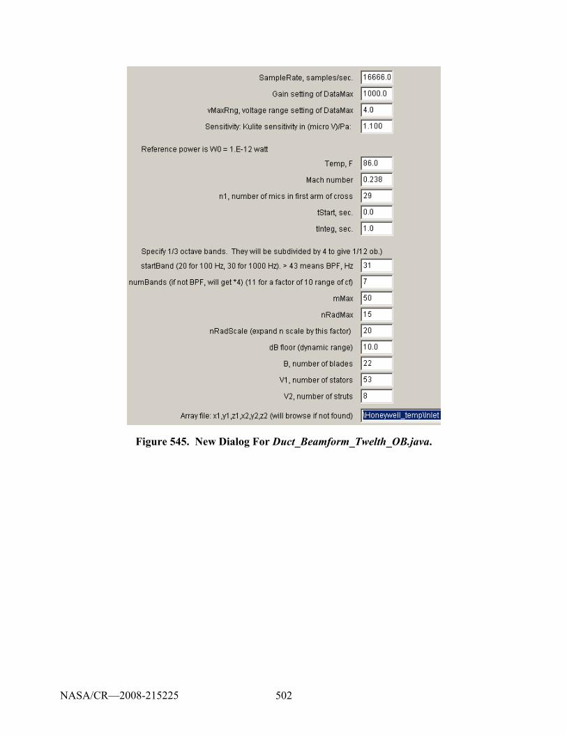
502

Figure 545. New Dialog For Duct_Beamform_Twelth_OB.java.

NASA/CR—2008-215225

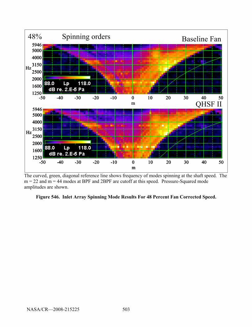
503

Hz

12501600200025003150400050005946

0 10 20 30 40 50-10-20-30-40-50m

Hz

12501600200025003150400050005946

Hz

1250160020002500315040005000

12501600200025003150400050005946

0 10 20 30 40 50-10-20-30-40-50m0 10 20 30 40 50-10-20-30-40-50m

Baseline Fan

QHSF II

48% Spinning orders

Hz

12501600200025003150400050005946

0 10 20 30 40 50-10-20-30-40-50m

Hz

12501600200025003150400050005946

Hz

1250160020002500315040005000

12501600200025003150400050005946

0 10 20 30 40 50-10-20-30-40-50m0 10 20 30 40 50-10-20-30-40-50m

The curved, green, diagonal reference line shows frequency of modes spinning at the shaft speed. The m = 22 and m = 44 modes at BPF and 2BPF are cutoff at this speed. Pressure-Squared mode amplitudes are shown.

Figure 546. Inlet Array Spinning Mode Results For 48 Percent Fan Corrected Speed.

NASA/CR—2008-215225

504

Baseline Fan

QHSF II

48% Twice Blade Passage Freq.

0 10 20 30 40 50-10-20-30-40-50m

05

10

5

15

10

15

0n

-x

+x

0 10 20 30 40 50-10-20-30-40-50m0 10 20 30 40 50-10-20-30-40-50m

05

10

5

15

10

15

0n

-x

+x

05

10

5

15

10

15

0n

-x

+x

0 10 20 30 40 50-10-20-30-40-50m

05

10

5

15

10

15

0n

-x

+x

0 10 20 30 40 50-10-20-30-40-50m0 10 20 30 40 50-10-20-30-40-50m

05

10

5

15

10

15

0n

-x

+x

05

10

5

15

10

15

0n

-x

+x

Radial order and direction of propagation (-x is forward) are given on the vertical axis. the spots along the bottom show the expected Tyler-Sofrin modes. the third row from the bottom give rotor-alone and rotor-FEGV interaction modes. this rotor-alone mode at m = 44 is cutoff. the fan-FEGV interaction mode with k1 = -1 is m = -9. this is seen baseline fan, but only very weakly in the QHSF II. The second row from the bottom gives rotor-strut interaction modes. These can be seen for the QHSF II at m = -12, 4, and 12. The bottom row gives 3-way interactions between the fan, the struts, and the FEGVs. Examples are the baseline fan at m = -22, -17, -6, -1, 7, 15, and 22.

Figure 547. Inlet Array 2D Mode Results For 48 Percent Fan Corrected Speed, 2BPF.

NASA/CR—2008-215225

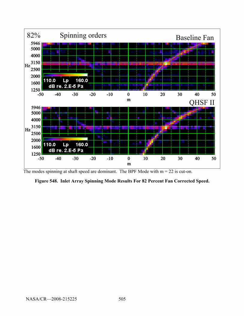
505

Hz

12501600200025003150400050005946

0 10 20 30 40 50-10-20-30-40-50m

Hz

12501600200025003150400050005946

Hz

1250160020002500315040005000

12501600200025003150400050005946

0 10 20 30 40 50-10-20-30-40-50m0 10 20 30 40 50-10-20-30-40-50m

Baseline Fan

QHSF II

82% Spinning orders

Hz

12501600200025003150400050005946

0 10 20 30 40 50-10-20-30-40-50m

Hz

12501600200025003150400050005946

Hz

1250160020002500315040005000

12501600200025003150400050005946

0 10 20 30 40 50-10-20-30-40-50m0 10 20 30 40 50-10-20-30-40-50m

The modes spinning at shaft speed are dominant. The BPF Mode with m = 22 is cut-on.

Figure 548. Inlet Array Spinning Mode Results For 82 Percent Fan Corrected Speed.

NASA/CR—2008-215225

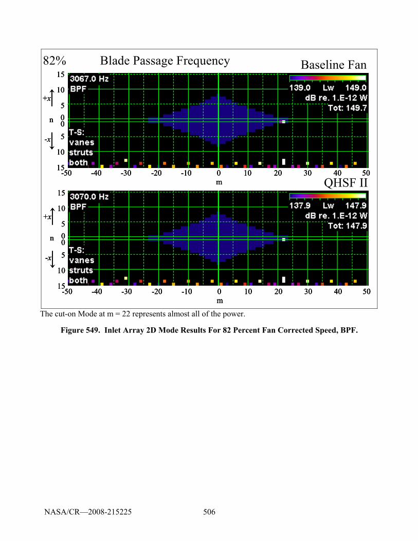
506

Baseline Fan

QHSF II

82% Blade Passage Frequency

0 10 20 30 40 50-10-20-30-40-50m

05

10

5

15

10

15

0n

-x

+x

0 10 20 30 40 50-10-20-30-40-50m0 10 20 30 40 50-10-20-30-40-50m

05

10

5

15

10

15

0n

-x

+x

05

10

5

15

10

15

0n

-x

+x

0 10 20 30 40 50-10-20-30-40-50m

05

10

5

15

10

15

0n

-x

+x

0 10 20 30 40 50-10-20-30-40-50m0 10 20 30 40 50-10-20-30-40-50m

05

10

5

15

10

15

0n

-x

+x

05

10

5

15

10

15

0n

-x

+x

The cut-on Mode at m = 22 represents almost all of the power.

Figure 549. Inlet Array 2D Mode Results For 82 Percent Fan Corrected Speed, BPF.

NASA/CR—2008-215225

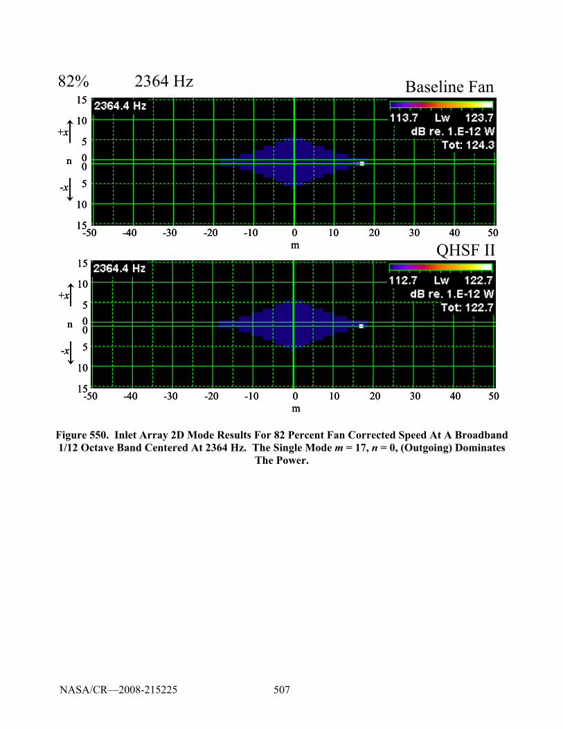
507

Baseline Fan

QHSF II

82% 2364 Hz

0 10 20 30 40 50-10-20-30-40-50m

05

10

5

15

10

15

0n

-x

+x

0 10 20 30 40 50-10-20-30-40-50m0 10 20 30 40 50-10-20-30-40-50m

05

10

5

15

10

15

0n

-x

+x

05

10

5

15

10

15

0n

-x

+x

0 10 20 30 40 50-10-20-30-40-50m

05

10

5

15

10

15

0n

-x

+x

0 10 20 30 40 50-10-20-30-40-50m0 10 20 30 40 50-10-20-30-40-50m

05

10

5

15

10

15

0n

-x

+x

05

10

5

15

10

15

0n

-x

+x

Figure 550. Inlet Array 2D Mode Results For 82 Percent Fan Corrected Speed At A Broadband 1/12 Octave Band Centered At 2364 Hz. The Single Mode m = 17, n = 0, (Outgoing) Dominates

The Power.

NASA/CR—2008-215225

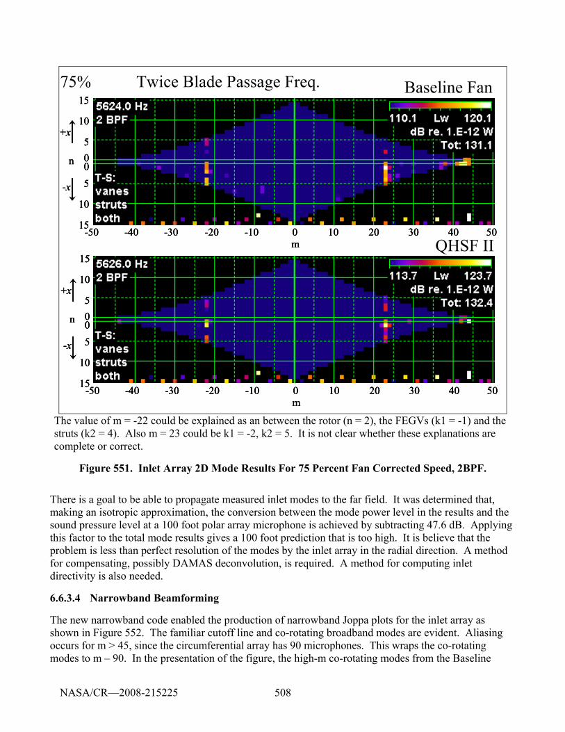
508

Baseline Fan

QHSF II

75% Twice Blade Passage Freq.

0 10 20 30 40 50-10-20-30-40-50m

05

10

5

15

10

15

0n

-x

+x

0 10 20 30 40 50-10-20-30-40-50m0 10 20 30 40 50-10-20-30-40-50m

05

10

5

15

10

15

0n

-x

+x

05

10

5

15

10

15

0n

-x

+x

0 10 20 30 40 50-10-20-30-40-50m

05

10

5

15

10

15

0n

-x

+x

0 10 20 30 40 50-10-20-30-40-50m0 10 20 30 40 50-10-20-30-40-50m

05

10

5

15

10

15

0n

-x

+x

05

10

5

15

10

15

0n

-x

+x

The value of m = -22 could be explained as an between the rotor (n = 2), the FEGVs (k1 = -1) and the struts (k2 = 4). Also m = 23 could be k1 = -2, k2 = 5. It is not clear whether these explanations are complete or correct.

Figure 551. Inlet Array 2D Mode Results For 75 Percent Fan Corrected Speed, 2BPF.

There is a goal to be able to propagate measured inlet modes to the far field. It was determined that, making an isotropic approximation, the conversion between the mode power level in the results and the sound pressure level at a 100 foot polar array microphone is achieved by subtracting 47.6 dB. Applying this factor to the total mode results gives a 100 foot prediction that is too high. It is believe that the problem is less than perfect resolution of the modes by the inlet array in the radial direction. A method for compensating, possibly DAMAS deconvolution, is required. A method for computing inlet directivity is also needed.

6.6.3.4 Narrowband Beamforming

The new narrowband code enabled the production of narrowband Joppa plots for the inlet array as shown in Figure 552. The familiar cutoff line and co-rotating broadband modes are evident. Aliasing occurs for m > 45, since the circumferential array has 90 microphones. This wraps the co-rotating modes to m – 90. In the presentation of the figure, the high-m co-rotating modes from the Baseline

NASA/CR—2008-215225

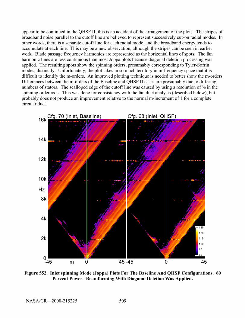
509

appear to be continued in the QHSF II; this is an accident of the arrangement of the plots. The stripes of broadband noise parallel to the cutoff line are believed to represent successively cut-on radial modes. In other words, there is a separate cutoff line for each radial mode, and the broadband energy tends to accumulate at each line. This may be a new observation, although the stripes can be seen in earlier work. Blade passage frequency harmonics are represented as the horizontal lines of spots. The fan harmonic lines are less continuous than most Joppa plots because diagonal deletion processing was applied. The resulting spots show the spinning orders, presumably corresponding to Tyler-Sofrin modes, distinctly. Unfortunately, the plot takes in so much territory in m-frequency space that it is difficult to identify the m-orders. An improved plotting technique is needed to better show the m-orders. Differences between the m-orders of the Baseline and QHSF II cases are presumably due to differing numbers of stators. The scalloped edge of the cutoff line was caused by using a resolution of ½ in the spinning order axis. This was done for consistency with the fan duct analysis (described below), but probably does not produce an improvement relative to the normal m-increment of 1 for a complete circular duct.

Cfg. 70 (Inlet, Baseline) Cfg. 68 (Inlet, QHSF)

2k

4k

8k

10k

12k

14k

16k

0

Hz

-45 0 45 -45 0 45m

Figure 552. Inlet spinning Mode (Joppa) Plots For The Baseline And QHSF Configurations. 60 Percent Power. Beamforming With Diagonal Deletion Was Applied.

NASA/CR—2008-215225

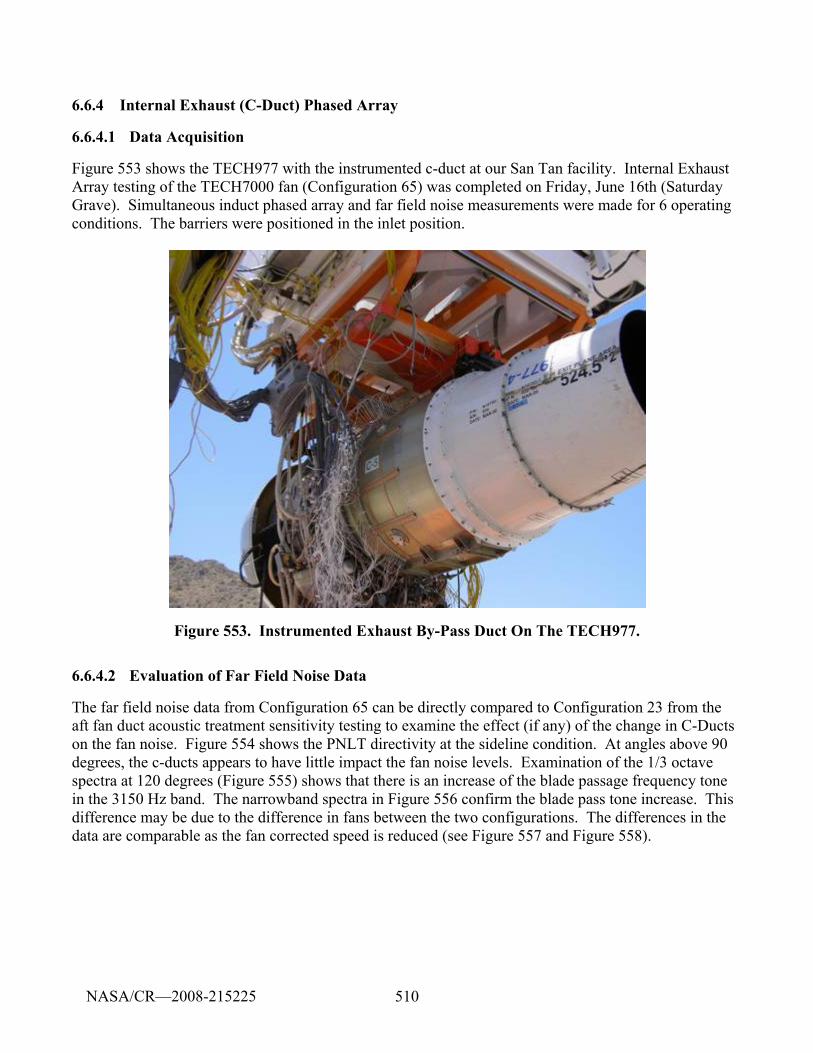
510

6.6.4 Internal Exhaust (C-Duct) Phased Array


Figure 553 shows the TECH977 with the instrumented c-duct at our San Tan facility. Internal Exhaust Array testing of the TECH7000 fan (Configuration 65) was completed on Friday, June 16th (Saturday Grave). Simultaneous induct phased array and far field noise measurements were made for 6 operating conditions. The barriers were positioned in the inlet position.

Figure 553. Instrumented Exhaust By-Pass Duct On The TECH977.

6.6.4.2 Evaluation of Far Field Noise Data

The far field noise data from Configuration 65 can be directly compared to Configuration 23 from the aft fan duct acoustic treatment sensitivity testing to examine the effect (if any) of the change in C-Ducts on the fan noise. Figure 554 shows the PNLT directivity at the sideline condition. At angles above 90 degrees, the c-ducts appears to have little impact the fan noise levels. Examination of the 1/3 octave spectra at 120 degrees (Figure 555) shows that there is an increase of the blade passage frequency tone in the 3150 Hz band. The narrowband spectra in Figure 556 confirm the blade pass tone increase. This difference may be due to the difference in fans between the two configurations. The differences in the data are comparable as the fan corrected speed is reduced (see Figure 557 and Figure 558).

NASA/CR—2008-215225

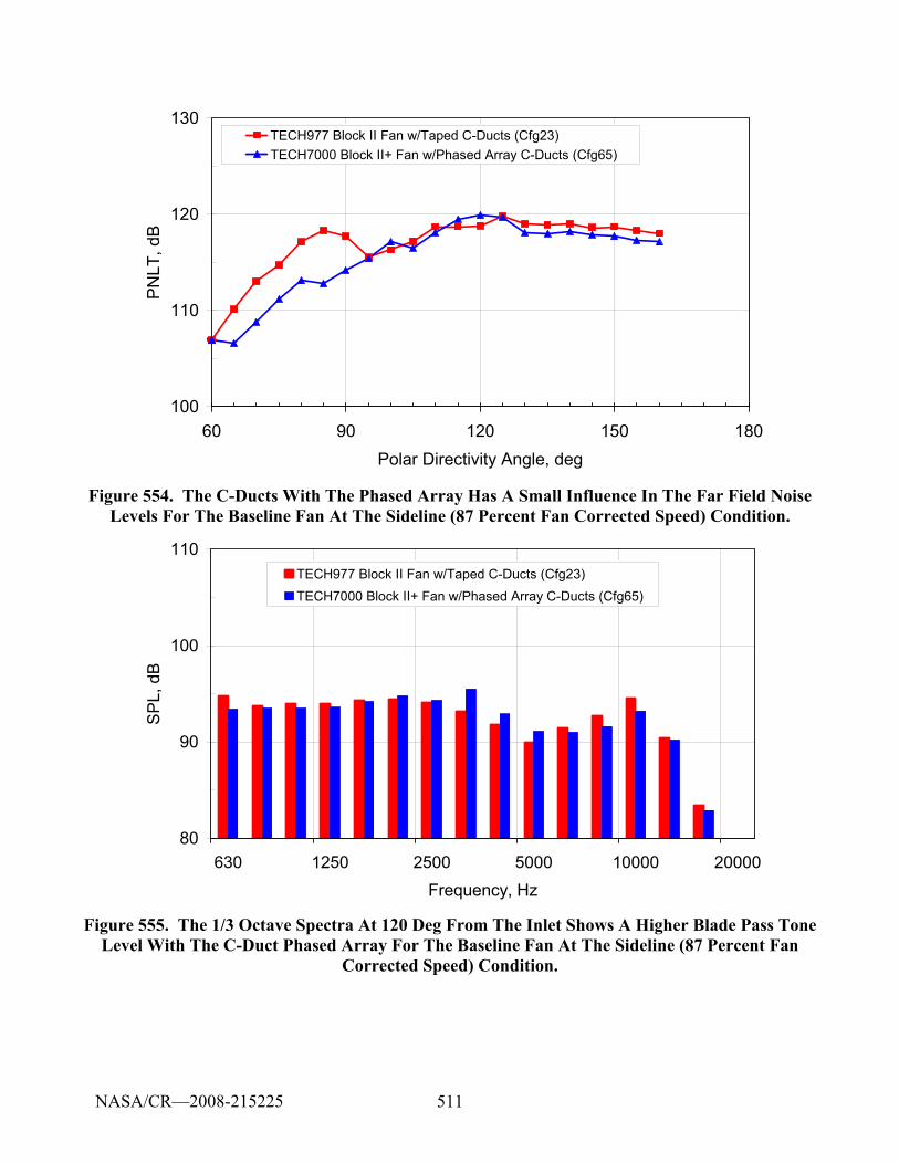
511

100

110

120

130


PN

LT, d

BTECH977 Block II Fan w/Taped C-Ducts (Cfg23)TECH7000 Block II+ Fan w/Phased Array C-Ducts (Cfg65)

Figure 554. The C-Ducts With The Phased Array Has A Small Influence In The Far Field Noise Levels For The Baseline Fan At The Sideline (87 Percent Fan Corrected Speed) Condition.

80

90

100

110

630 1250 2500 5000 10000 20000Frequency, Hz

SP

L, d

B

TECH977 Block II Fan w/Taped C-Ducts (Cfg23)TECH7000 Block II+ Fan w/Phased Array C-Ducts (Cfg65)

Figure 555. The 1/3 Octave Spectra At 120 Deg From The Inlet Shows A Higher Blade Pass Tone Level With The C-Duct Phased Array For The Baseline Fan At The Sideline (87 Percent Fan


NASA/CR—2008-215225

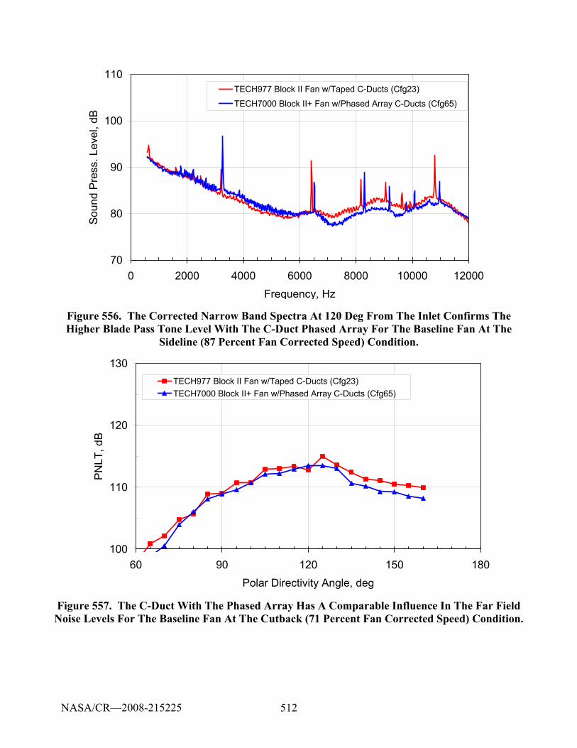
512

70

80

90

100

110

0 2000 4000 6000 8000 10000 12000Frequency, Hz

Sou

nd P

ress

. Lev

el, d

BTECH977 Block II Fan w/Taped C-Ducts (Cfg23)

TECH7000 Block II+ Fan w/Phased Array C-Ducts (Cfg65)

Figure 556. The Corrected Narrow Band Spectra At 120 Deg From The Inlet Confirms The Higher Blade Pass Tone Level With The C-Duct Phased Array For The Baseline Fan At The

Sideline (87 Percent Fan Corrected Speed) Condition.

100

110

120

130


PNLT

, dB


Figure 557. The C-Duct With The Phased Array Has A Comparable Influence In The Far Field Noise Levels For The Baseline Fan At The Cutback (71 Percent Fan Corrected Speed) Condition.

NASA/CR—2008-215225

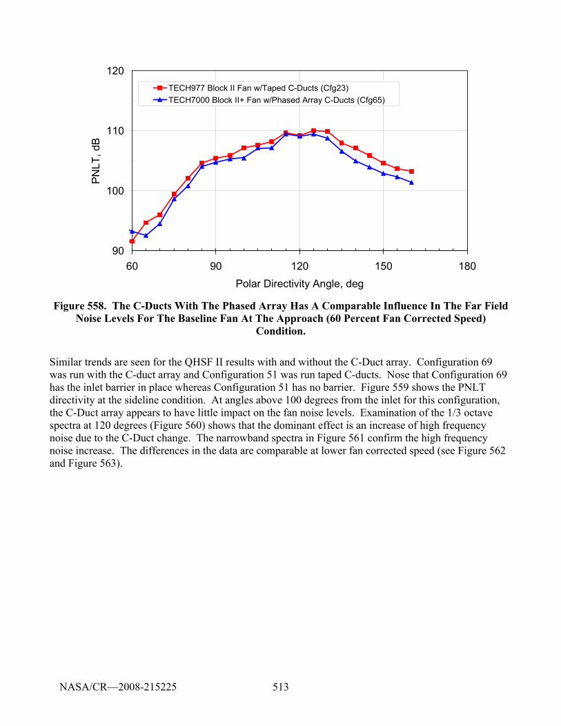
513

90

100

110

120


PNLT

, dB


Figure 558. The C-Ducts With The Phased Array Has A Comparable Influence In The Far Field Noise Levels For The Baseline Fan At The Approach (60 Percent Fan Corrected Speed)

Condition.

Similar trends are seen for the QHSF II results with and without the C-Duct array. Configuration 69 was run with the C-duct array and Configuration 51 was run taped C-ducts. Nose that Configuration 69 has the inlet barrier in place whereas Configuration 51 has no barrier. Figure 559 shows the PNLT directivity at the sideline condition. At angles above 100 degrees from the inlet for this configuration, the C-Duct array appears to have little impact on the fan noise levels. Examination of the 1/3 octave spectra at 120 degrees (Figure 560) shows that the dominant effect is an increase of high frequency noise due to the C-Duct change. The narrowband spectra in Figure 561 confirm the high frequency noise increase. The differences in the data are comparable at lower fan corrected speed (see Figure 562 and Figure 563).

NASA/CR—2008-215225

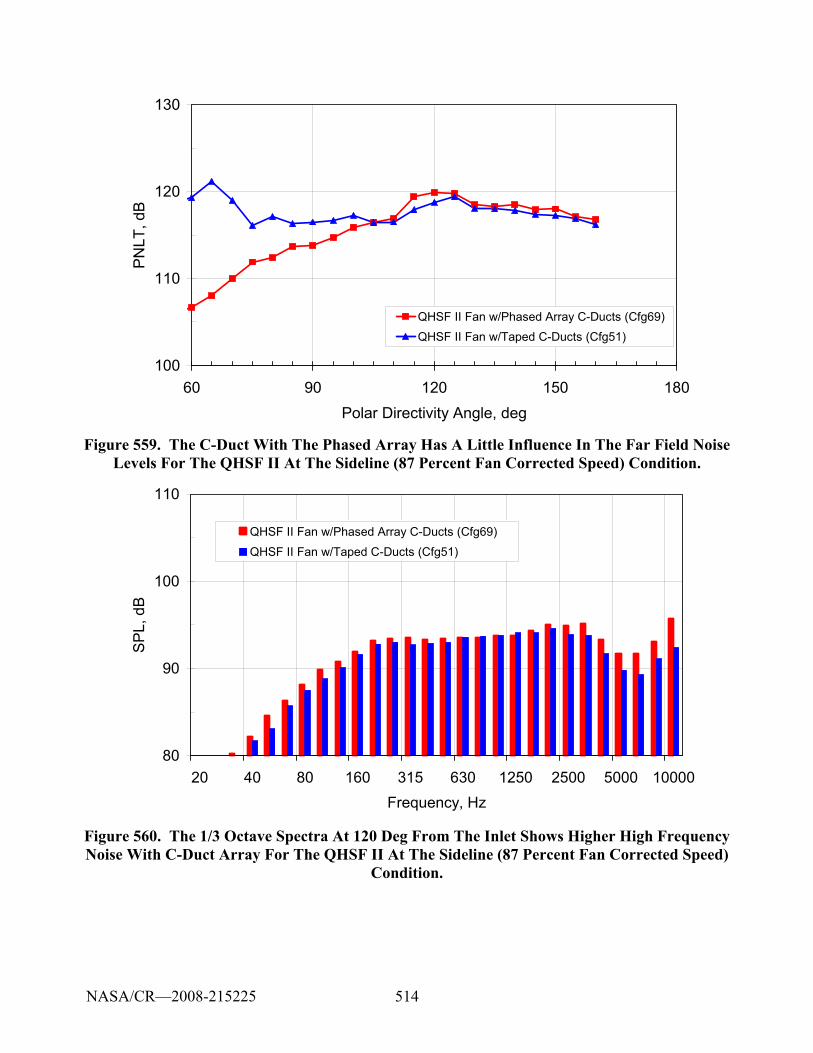
514

100

110

120

130


PN

LT, d

B

QHSF II Fan w/Phased Array C-Ducts (Cfg69)QHSF II Fan w/Taped C-Ducts (Cfg51)

Figure 559. The C-Duct With The Phased Array Has A Little Influence In The Far Field Noise Levels For The QHSF II At The Sideline (87 Percent Fan Corrected Speed) Condition.

80

90

100

110

20 40 80 160 315 630 1250 2500 5000 10000Frequency, Hz

SP

L, d

B

QHSF II Fan w/Phased Array C-Ducts (Cfg69)

QHSF II Fan w/Taped C-Ducts (Cfg51)

Figure 560. The 1/3 Octave Spectra At 120 Deg From The Inlet Shows Higher High Frequency Noise With C-Duct Array For The QHSF II At The Sideline (87 Percent Fan Corrected Speed)

Condition.

NASA/CR—2008-215225

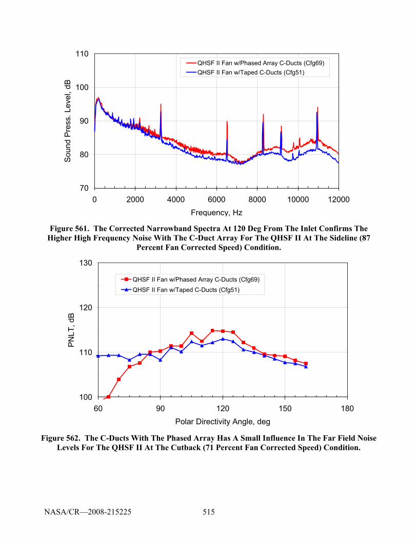
515

70

80

90

100

110

0 2000 4000 6000 8000 10000 12000Frequency, Hz

Sou

nd P

ress

. Lev

el, d

BQHSF II Fan w/Phased Array C-Ducts (Cfg69)QHSF II Fan w/Taped C-Ducts (Cfg51)

Figure 561. The Corrected Narrowband Spectra At 120 Deg From The Inlet Confirms The Higher High Frequency Noise With The C-Duct Array For The QHSF II At The Sideline (87

Percent Fan Corrected Speed) Condition.

100

110

120

130


PNLT

, dB

QHSF II Fan w/Phased Array C-Ducts (Cfg69)QHSF II Fan w/Taped C-Ducts (Cfg51)

Figure 562. The C-Ducts With The Phased Array Has A Small Influence In The Far Field Noise Levels For The QHSF II At The Cutback (71 Percent Fan Corrected Speed) Condition.

NASA/CR—2008-215225

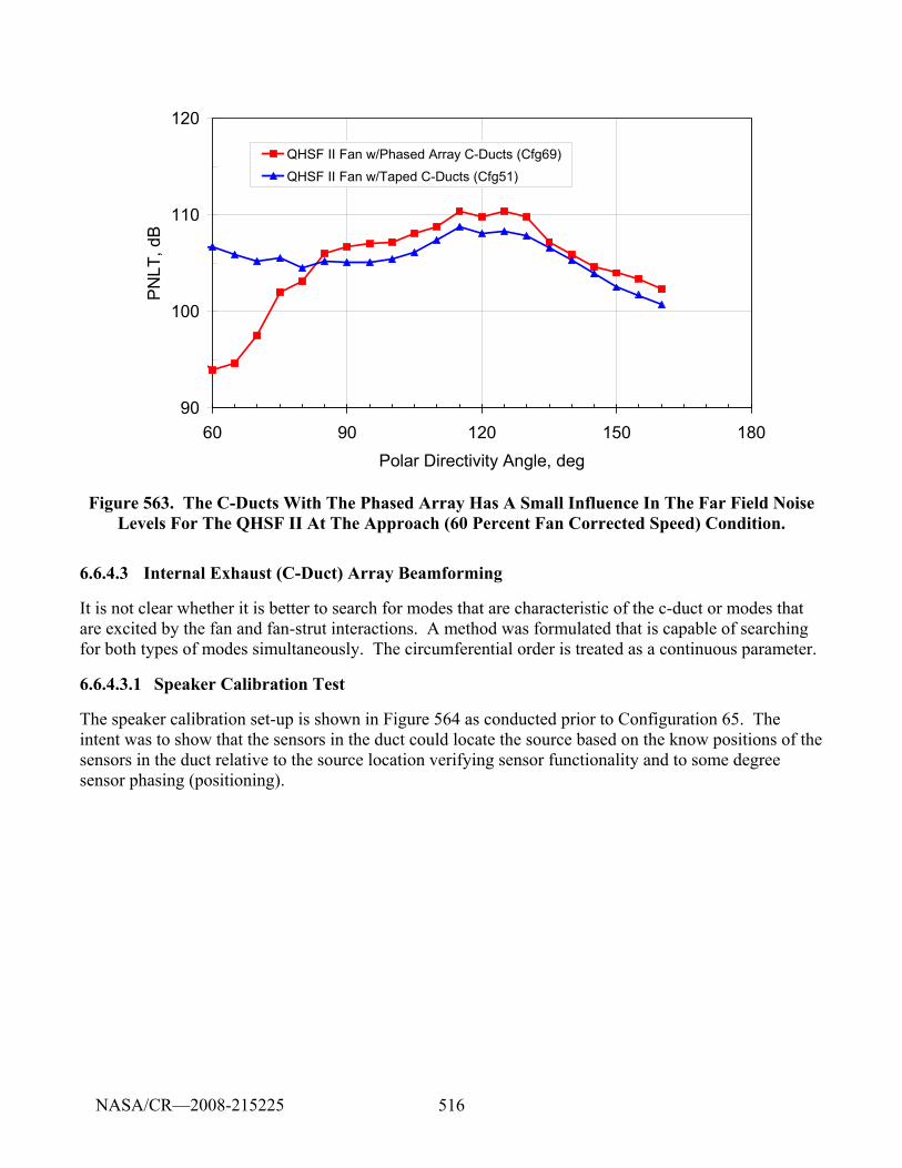
516

90

100

110

120


PN

LT, d

BQHSF II Fan w/Phased Array C-Ducts (Cfg69)

QHSF II Fan w/Taped C-Ducts (Cfg51)

Figure 563. The C-Ducts With The Phased Array Has A Small Influence In The Far Field Noise Levels For The QHSF II At The Approach (60 Percent Fan Corrected Speed) Condition.

6.6.4.3 Internal Exhaust (C-Duct) Array Beamforming

It is not clear whether it is better to search for modes that are characteristic of the c-duct or modes that are excited by the fan and fan-strut interactions. A method was formulated that is capable of searching for both types of modes simultaneously. The circumferential order is treated as a continuous parameter.

6.6.4.3.1 Speaker Calibration Test

The speaker calibration set-up is shown in Figure 564 as conducted prior to Configuration 65. The intent was to show that the sensors in the duct could locate the source based on the know positions of the sensors in the duct relative to the source location verifying sensor functionality and to some degree sensor phasing (positioning).

NASA/CR—2008-215225

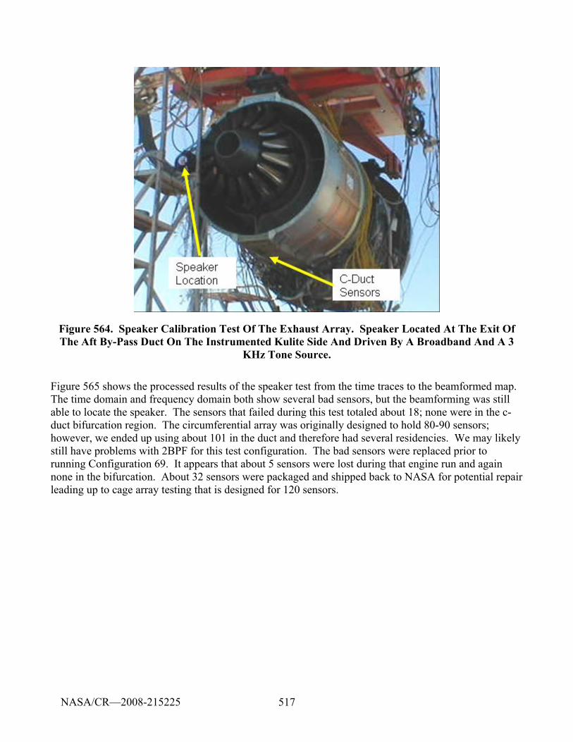
517

Figure 564. Speaker Calibration Test Of The Exhaust Array. Speaker Located At The Exit Of The Aft By-Pass Duct On The Instrumented Kulite Side And Driven By A Broadband And A 3

KHz Tone Source.

Figure 565 shows the processed results of the speaker test from the time traces to the beamformed map. The time domain and frequency domain both show several bad sensors, but the beamforming was still able to locate the speaker. The sensors that failed during this test totaled about 18; none were in the c-duct bifurcation region. The circumferential array was originally designed to hold 80-90 sensors; however, we ended up using about 101 in the duct and therefore had several residencies. We may likely still have problems with 2BPF for this test configuration. The bad sensors were replaced prior to running Configuration 69. It appears that about 5 sensors were lost during that engine run and again none in the bifurcation. About 32 sensors were packaged and shipped back to NASA for potential repair leading up to cage array testing that is designed for 120 sensors.

NASA/CR—2008-215225

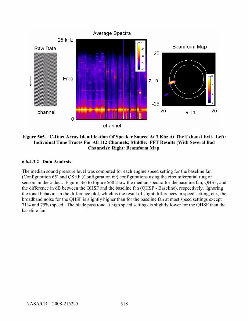
518

Figure 565. C-Duct Array Identification Of Speaker Source At 3 Khz At The Exhaust Exit. Left: Individual Time Traces For All 112 Channels; Middle: FFT Results (With Several Bad

Channels); Right: Beamform Map.

6.6.4.3.2 Data Analysis

The median sound pressure level was computed for each engine speed setting for the baseline fan (Configuration 65) and QSHF (Configuration 69) configurations using the circumferential ring of sensors in the c-duct. Figure 566 to Figure 568 show the median spectra for the baseline fan, QHSF, and the difference in dB between the QHSF and the baseline fan (QHSF - Baseline), respectively. Ignoring the tonal behavior in the difference plot, which is the result of slight differences in speed setting, etc., the broadband noise for the QHSF is slightly higher than for the baseline fan at most speed settings except 71% and 75%) speed. The blade pass tone at high speed settings is slightly lower for the QHSF than the baseline fan.

NASA/CR—2008-215225

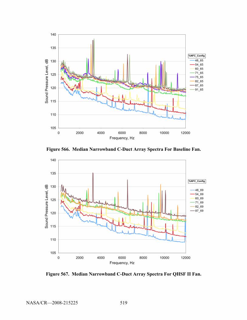
519

105

110

115

120

125

130

135

140

0 2000 4000 6000 8000 10000 12000Frequency, Hz

Sou

nd P

ress

ure

Leve

l, dB 48_65

54_6560_6571_6575_6582_6587_6591_65

%NFC_Config

Figure 566. Median Narrowband C-Duct Array Spectra For Baseline Fan.

105

110

115

120

125

130

135

140

0 2000 4000 6000 8000 10000 12000Frequency, Hz

Sou

nd P

ress

ure

Leve

l, dB 48_69

54_6960_6971_6982_6987_69

%NFC_Config

Figure 567. Median Narrowband C-Duct Array Spectra For QHSF II Fan.

NASA/CR—2008-215225

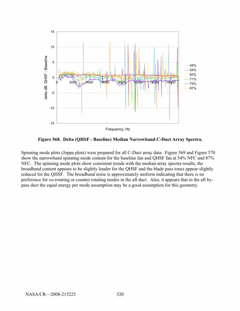
520

-15

-10

-5

0

5

10

15

0 2000 4000 6000 8000 10000 12000 14000

Frequency, Hz

delta

dB:

QH

SF

- Bas

elin

e

48%54%60%71%75%87%

Figure 568. Delta (QHSF - Baseline) Median Narrowband C-Duct Array Spectra.

Spinning mode plots (Joppa plots) were prepared for all C-Duct array data. Figure 569 and Figure 570 show the narrowband spinning mode content for the baseline fan and QHSF fan at 54% NFC and 87% NFC. The spinning mode plots show consistent trends with the median array spectra results, the broadband content appears to be slightly louder for the QHSF and the blade pass tones appear slightly reduced for the QHSF. The broadband noise is approximately uniform indicating that there is no preference for co-rotating or counter rotating modes in the aft duct. Also, it appears that in the aft by-pass duct the equal energy per mode assumption may be a good assumption for this geometry.

NASA/CR—2008-215225

521

(a) Baseline Fan (b) QHSF II

Figure 569. C-Duct Array Spinning Mode Plots At 54 Percent Corrected Fan Speed.

NASA/CR—2008-215225

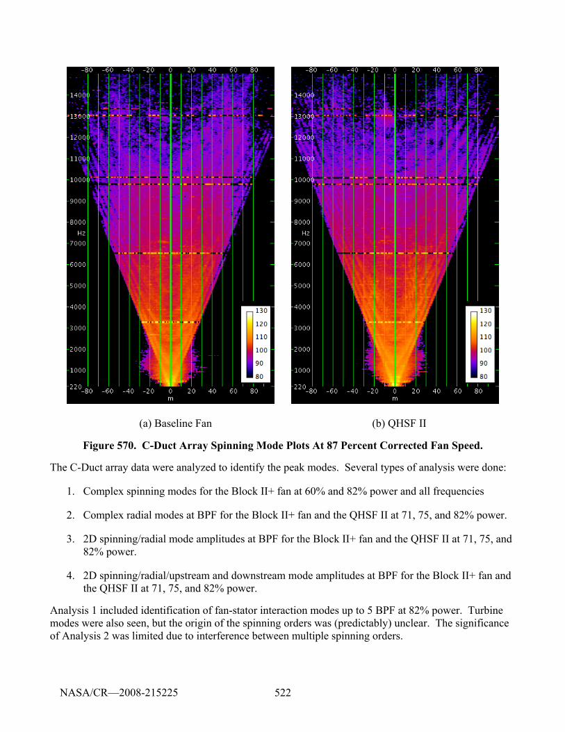
522

(a) Baseline Fan (b) QHSF II

Figure 570. C-Duct Array Spinning Mode Plots At 87 Percent Corrected Fan Speed.

The C-Duct array data were analyzed to identify the peak modes. Several types of analysis were done:

1. Complex spinning modes for the Block II+ fan at 60% and 82% power and all frequencies

2. Complex radial modes at BPF for the Block II+ fan and the QHSF II at 71, 75, and 82% power.

3. 2D spinning/radial mode amplitudes at BPF for the Block II+ fan and the QHSF II at 71, 75, and 82% power.

4. 2D spinning/radial/upstream and downstream mode amplitudes at BPF for the Block II+ fan and the QHSF II at 71, 75, and 82% power.

Analysis 1 included identification of fan-stator interaction modes up to 5 BPF at 82% power. Turbine modes were also seen, but the origin of the spinning orders was (predictably) unclear. The significance of Analysis 2 was limited due to interference between multiple spinning orders.

NASA/CR—2008-215225

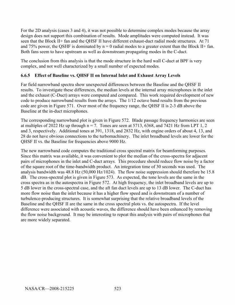
523

For the 2D analysis (cases 3 and 4), it was not possible to determine complex modes because the array design does not support this combination of results. Mode amplitudes were computed instead. It was seen that the Block II+ fan and the QHSF II have different exhaust-duct radial mode structures. At 71 and 75% power, the QSHF is dominated by n = 0 radial modes to a greater extent than the Block II+ fan. Both fans seem to have upstream as well as downstream propagating modes in the C-duct.

The conclusion from this analysis is that the mode structure in the hard wall C-duct at BPF is very complex, and not well characterized by a small number of expected modes.

6.6.5 Effect of Baseline vs. QHSF II on Internal Inlet and Exhaust Array Levels

Far field narrowband spectra show unexpected differences between the Baseline and the QHSF II results. To investigate these differences, the median levels at the internal array microphones in the inlet and the exhaust (C-Duct) arrays were computed and compared. This work required development of new code to produce narrowband results from the arrays. The 1/12 octave band results from the previous code are given in Figure 571. Over most of the frequency range, the QHSF II is 2-3 dB above the Baseline at the in-duct microphones.

The corresponding narrowband plot is given in Figure 572. Blade passage frequency harmonics are seen at multiples of 2022 Hz up through n = 7. Tones are seen at 5713, 6368, and 7421 Hz from LPT 1, 2 and 3, respectively. Additional tones at 391, 1318, and 2832 Hz, with engine orders of about 4, 13, and 28 do not have obvious connections to the turbomachinery. The inlet broadband levels are lower for the QHSF II vs. the Baseline for frequencies above 9000 Hz.

The new narrowband code computes the traditional cross spectral matrix for beamforming purposes. Since this matrix was available, it was convenient to plot the median of the cross-spectra for adjacent pairs of microphones in the inlet and C-duct arrays. This procedure should reduce flow noise by a factor of the square root of the time-bandwidth product. An integration time of 30 seconds was used. The analysis bandwidth was 48.8 Hz (50,000 Hz/1024). The flow noise suppression should therefore be 15.8 dB. The cross-spectral plot is given in Figure 573. As expected, the tone levels are the same in the cross spectra as in the autospectra in Figure 572. At high frequency, the inlet broadband levels are up to 5 dB lower in the cross-spectral case, and the aft fan duct levels are up to 13 dB lower. The C-duct has more flow noise than the inlet because it has a higher flow speed and is downstream of a number of turbulence-producing structures. It is somewhat surprising that the relative broadband levels of the Baseline and the QHSF II are the same in the cross spectral plots vs. the autospectra. If the level difference were associated with acoustic waves, the difference should have been enhanced by removing the flow noise background. It may be interesting to repeat this analysis with pairs of microphones that are more widely separated.

NASA/CR—2008-215225

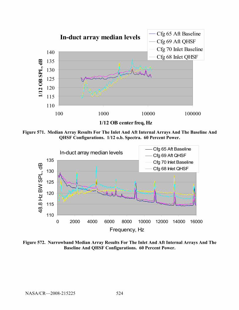
524

In-duct array median levels

110

115

120

125

130

135

140

100 1000 10000 100000

1/12 OB center freq, Hz

1/12

OB

SPL

, dB

Cfg 65 Aft BaselineCfg 69 Aft QHSFCfg 70 Inlet BaselineCfg 68 Inlet QHSF

Figure 571. Median Array Results For The Inlet And Aft Internal Arrays And The Baseline And QHSF Configurations. 1/12 o.b. Spectra. 60 Percent Power.

In-duct array median levels

110

115

120

125

130

135

0 2000 4000 6000 8000 10000 12000 14000 16000

Frequency, Hz

48.8

Hz

BW

SP

L, d

B


Figure 572. Narrowband Median Array Results For The Inlet And Aft Internal Arrays And The Baseline And QHSF Configurations. 60 Percent Power.

NASA/CR—2008-215225

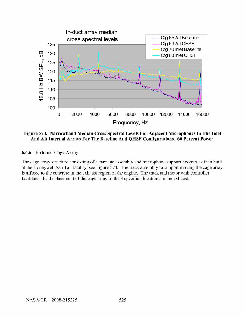
525

In-duct array median cross spectral levels

100

105

110

115

120

125

130

135

0 2000 4000 6000 8000 10000 12000 14000 16000

Frequency, Hz

48.8

Hz

BW

SP

L, d

B


Figure 573. Narrowband Median Cross Spectral Levels For Adjacent Microphones In The Inlet And Aft Internal Arrays For The Baseline And QHSF Configurations. 60 Percent Power.

6.6.6 Exhaust Cage Array

The cage array structure consisting of a carriage assembly and microphone support hoops was then built at the Honeywell San Tan facility, see Figure 574. The track assembly to support moving the cage array is affixed to the concrete in the exhaust region of the engine. The track and motor with controller facilitates the displacement of the cage array to the 3 specified locations in the exhaust.

NASA/CR—2008-215225

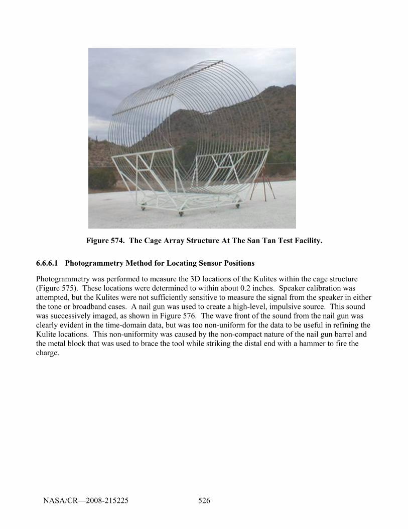
526

Figure 574. The Cage Array Structure At The San Tan Test Facility.

6.6.6.1 Photogrammetry Method for Locating Sensor Positions

Photogrammetry was performed to measure the 3D locations of the Kulites within the cage structure (Figure 575). These locations were determined to within about 0.2 inches. Speaker calibration was attempted, but the Kulites were not sufficiently sensitive to measure the signal from the speaker in either the tone or broadband cases. A nail gun was used to create a high-level, impulsive source. This sound was successively imaged, as shown in Figure 576. The wave front of the sound from the nail gun was clearly evident in the time-domain data, but was too non-uniform for the data to be useful in refining the Kulite locations. This non-uniformity was caused by the non-compact nature of the nail gun barrel and the metal block that was used to brace the tool while striking the distal end with a hammer to fire the charge.

NASA/CR—2008-215225

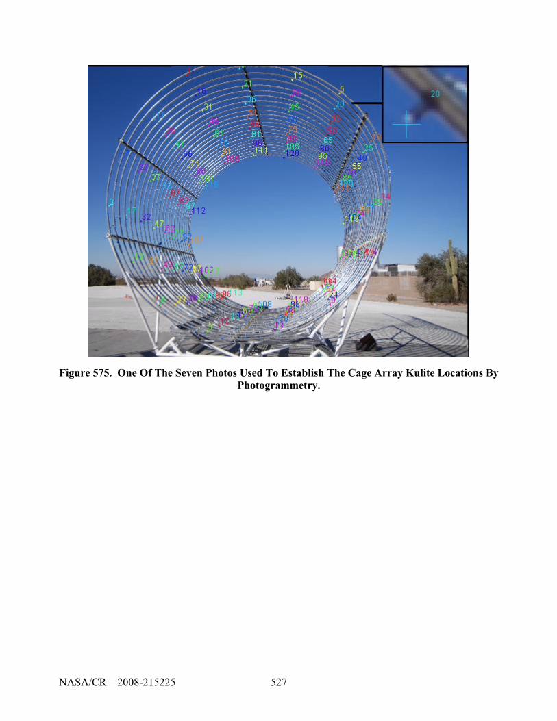
527

Figure 575. One Of The Seven Photos Used To Establish The Cage Array Kulite Locations By Photogrammetry.

NASA/CR—2008-215225

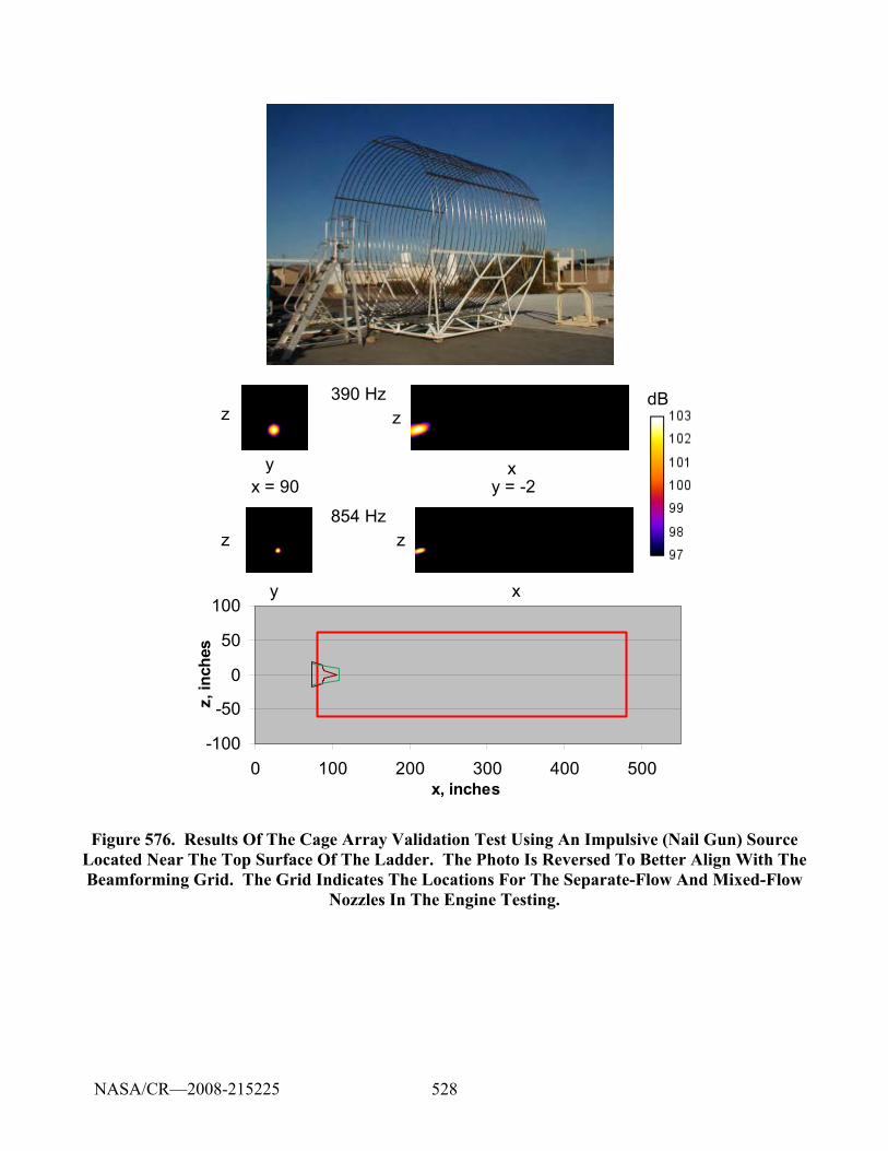
528

dB

-100

-50

0

50

100

0 100 200 300 400 500x, inches

z, in

ches

x = 90y

z

z

y

z

z

x

x

y = -2

390 Hz

854 Hz

Figure 576. Results Of The Cage Array Validation Test Using An Impulsive (Nail Gun) Source Located Near The Top Surface Of The Ladder. The Photo Is Reversed To Better Align With The Beamforming Grid. The Grid Indicates The Locations For The Separate-Flow And Mixed-Flow

Nozzles In The Engine Testing.

NASA/CR—2008-215225

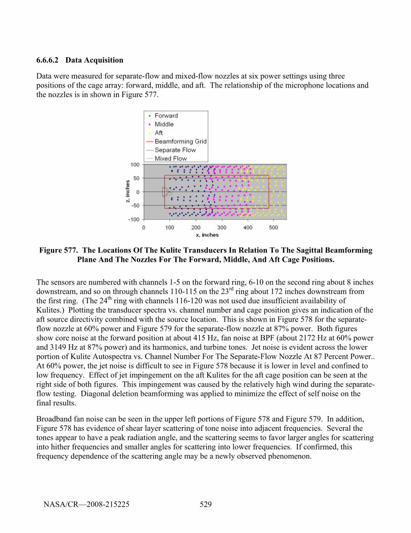
529


Data were measured for separate-flow and mixed-flow nozzles at six power settings using three positions of the cage array: forward, middle, and aft. The relationship of the microphone locations and the nozzles is in shown in Figure 577.

Figure 577. The Locations Of The Kulite Transducers In Relation To The Sagittal Beamforming Plane And The Nozzles For The Forward, Middle, And Aft Cage Positions.

The sensors are numbered with channels 1-5 on the forward ring, 6-10 on the second ring about 8 inches downstream, and so on through channels 110-115 on the 23rd ring about 172 inches downstream from the first ring. (The 24th ring with channels 116-120 was not used due insufficient availability of Kulites.) Plotting the transducer spectra vs. channel number and cage position gives an indication of the aft source directivity combined with the source location. This is shown in Figure 578 for the separate-flow nozzle at 60% power and Figure 579 for the separate-flow nozzle at 87% power. Both figures show core noise at the forward position at about 415 Hz, fan noise at BPF (about 2172 Hz at 60% power and 3149 Hz at 87% power) and its harmonics, and turbine tones. Jet noise is evident across the lower portion of Kulite Autospectra vs. Channel Number For The Separate-Flow Nozzle At 87 Percent Power.. At 60% power, the jet noise is difficult to see in Figure 578 because it is lower in level and confined to low frequency. Effect of jet impingement on the aft Kulites for the aft cage position can be seen at the right side of both figures. This impingement was caused by the relatively high wind during the separate-flow testing. Diagonal deletion beamforming was applied to minimize the effect of self noise on the final results.

Broadband fan noise can be seen in the upper left portions of Figure 578 and Figure 579. In addition, Figure 578 has evidence of shear layer scattering of tone noise into adjacent frequencies. Several the tones appear to have a peak radiation angle, and the scattering seems to favor larger angles for scattering into hither frequencies and smaller angles for scattering into lower frequencies. If confirmed, this frequency dependence of the scattering angle may be a newly observed phenomenon.

NASA/CR—2008-215225

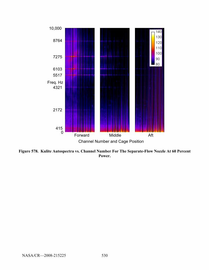
530

0

10,000

2172

4321

415

55176103

7275

Freq. Hz

Forward Middle AftChannel Number and Cage Position

8764

Figure 578. Kulite Autospectra vs. Channel Number For The Separate-Flow Nozzle At 60 Percent Power.

NASA/CR—2008-215225

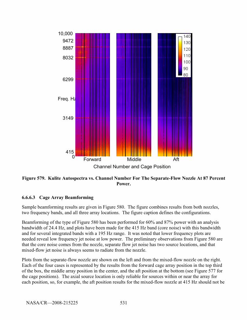
531

0

10,000

3149

6299

415

8032

88879472

Freq. Hz

Forward Middle AftChannel Number and Cage Position

Figure 579. Kulite Autospectra vs. Channel Number For The Separate-Flow Nozzle At 87 Percent Power.

6.6.6.3 Cage Array Beamforming

Sample beamforming results are given in Figure 580. The figure combines results from both nozzles, two frequency bands, and all three array locations. The figure caption defines the configurations.

Beamforming of the type of Figure 580 has been performed for 60% and 87% power with an analysis bandwidth of 24.4 Hz, and plots have been made for the 415 Hz band (core noise) with this bandwidth and for several integrated bands with a 195 Hz range. It was noted that lower frequency plots are needed reveal low frequency jet noise at low power. The preliminary observations from Figure 580 are that the core noise comes from the nozzle, separate flow jet noise has two source locations, and that mixed-flow jet noise is always seems to radiate from the nozzle.

Plots from the separate-flow nozzle are shown on the left and from the mixed-flow nozzle on the right. Each of the four cases is represented by the results from the forward cage array position in the top third of the box, the middle array position in the center, and the aft position at the bottom (see Figure 577 for the cage positions). The axial source location is only reliable for sources within or near the array for each position, so, for example, the aft position results for the mixed-flow nozzle at 415 Hz should not be

NASA/CR—2008-215225

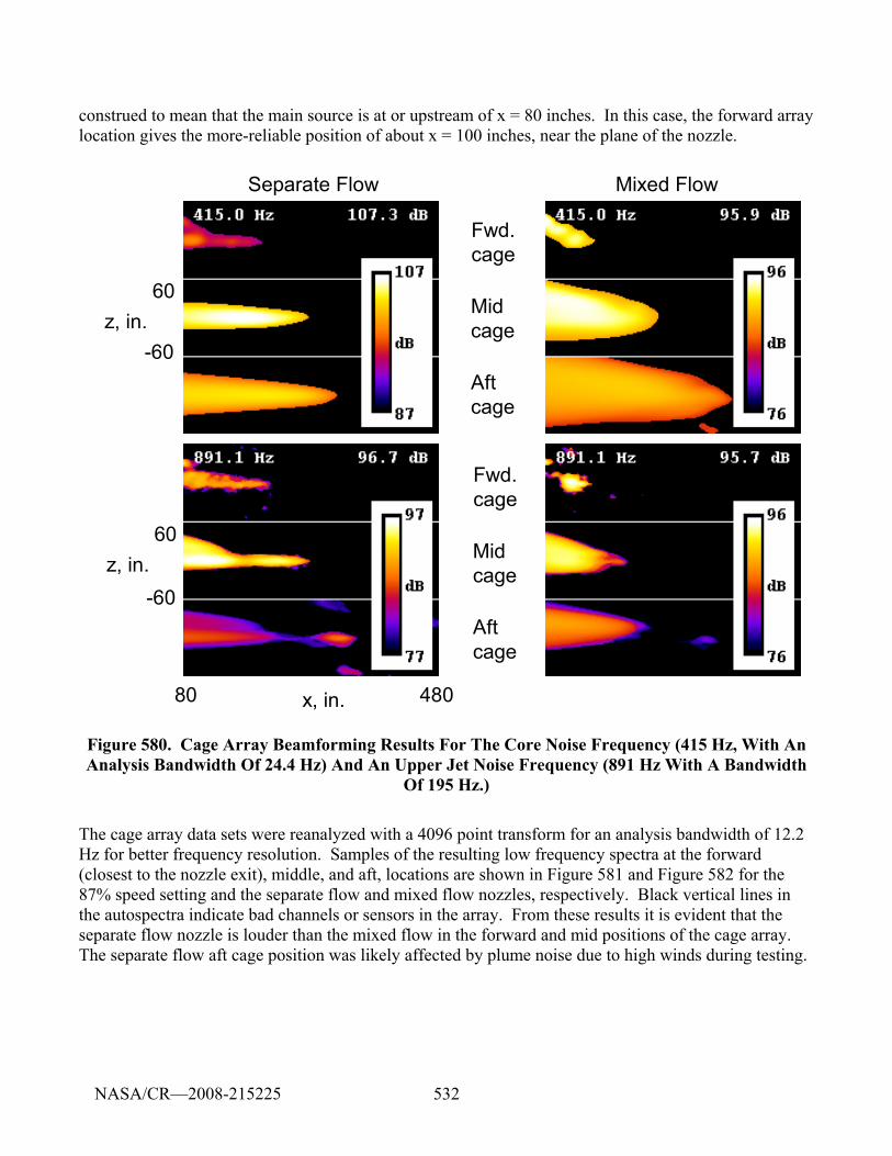
532

construed to mean that the main source is at or upstream of x = 80 inches. In this case, the forward array location gives the more-reliable position of about x = 100 inches, near the plane of the nozzle.

Separate Flow Mixed Flow

z, in.-60

60

Fwd.cage

Midcage

Aftcage

80 480x, in.

z, in.-60

60

Fwd.cage

Midcage

Aftcage

Figure 580. Cage Array Beamforming Results For The Core Noise Frequency (415 Hz, With An Analysis Bandwidth Of 24.4 Hz) And An Upper Jet Noise Frequency (891 Hz With A Bandwidth

Of 195 Hz.)

The cage array data sets were reanalyzed with a 4096 point transform for an analysis bandwidth of 12.2 Hz for better frequency resolution. Samples of the resulting low frequency spectra at the forward (closest to the nozzle exit), middle, and aft, locations are shown in Figure 581 and Figure 582 for the 87% speed setting and the separate flow and mixed flow nozzles, respectively. Black vertical lines in the autospectra indicate bad channels or sensors in the array. From these results it is evident that the separate flow nozzle is louder than the mixed flow in the forward and mid positions of the cage array. The separate flow aft cage position was likely affected by plume noise due to high winds during testing.

NASA/CR—2008-215225

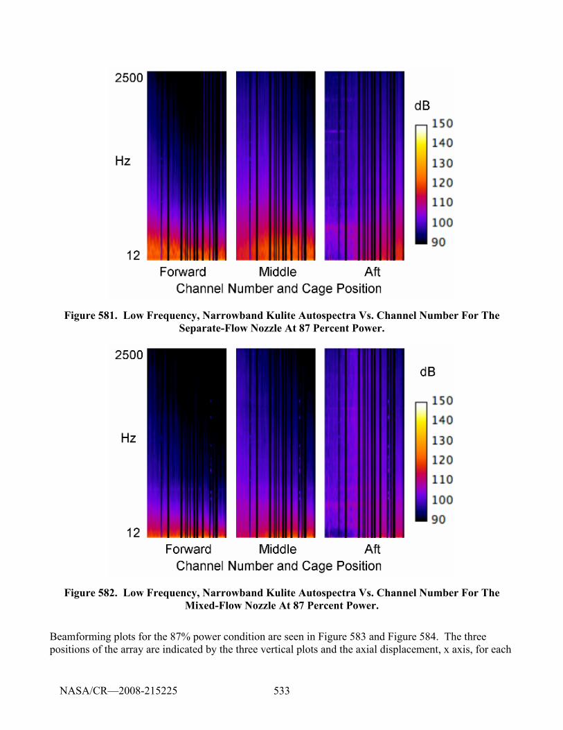
533

Figure 581. Low Frequency, Narrowband Kulite Autospectra Vs. Channel Number For The Separate-Flow Nozzle At 87 Percent Power.

Figure 582. Low Frequency, Narrowband Kulite Autospectra Vs. Channel Number For The Mixed-Flow Nozzle At 87 Percent Power.

Beamforming plots for the 87% power condition are seen in Figure 583 and Figure 584. The three positions of the array are indicated by the three vertical plots and the axial displacement, x axis, for each

NASA/CR—2008-215225

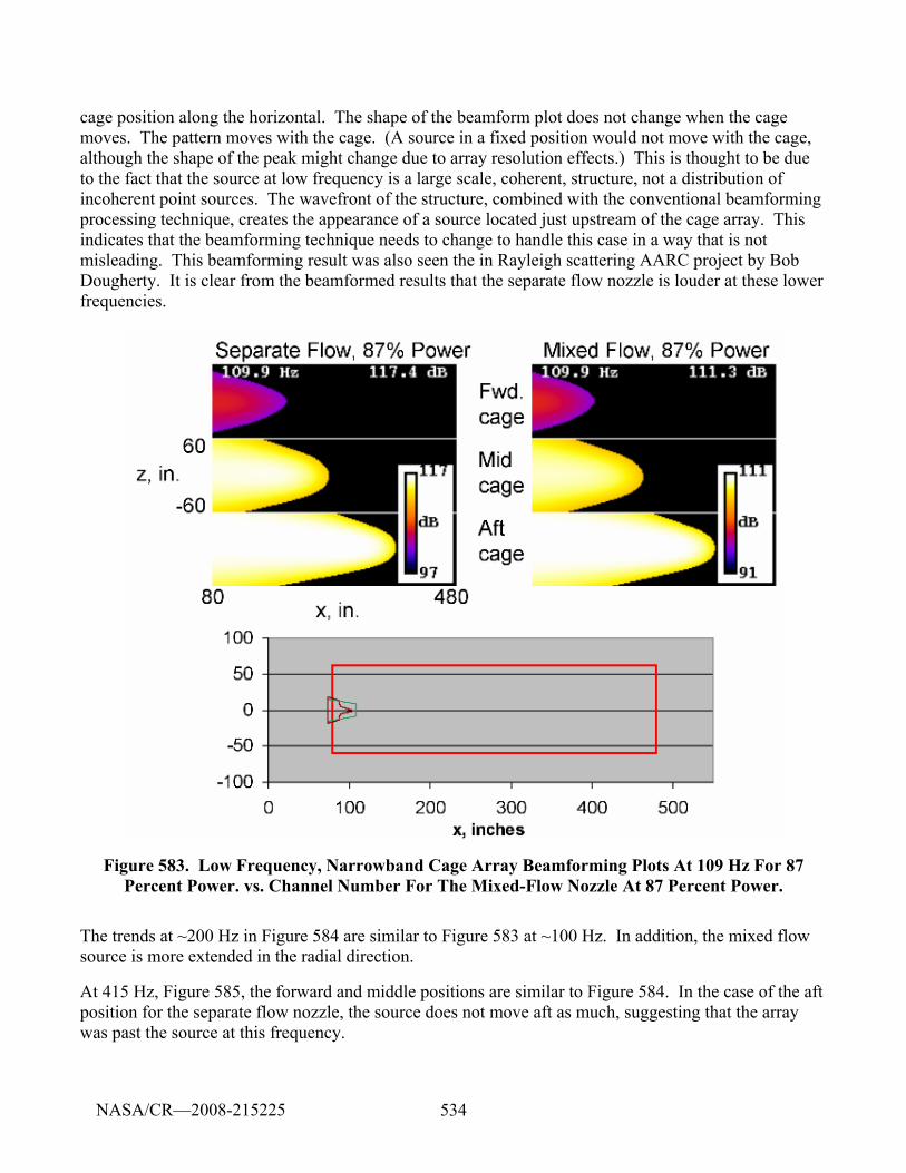
534

cage position along the horizontal. The shape of the beamform plot does not change when the cage moves. The pattern moves with the cage. (A source in a fixed position would not move with the cage, although the shape of the peak might change due to array resolution effects.) This is thought to be due to the fact that the source at low frequency is a large scale, coherent, structure, not a distribution of incoherent point sources. The wavefront of the structure, combined with the conventional beamforming processing technique, creates the appearance of a source located just upstream of the cage array. This indicates that the beamforming technique needs to change to handle this case in a way that is not misleading. This beamforming result was also seen the in Rayleigh scattering AARC project by Bob Dougherty. It is clear from the beamformed results that the separate flow nozzle is louder at these lower frequencies.

Figure 583. Low Frequency, Narrowband Cage Array Beamforming Plots At 109 Hz For 87 Percent Power. vs. Channel Number For The Mixed-Flow Nozzle At 87 Percent Power.

The trends at ~200 Hz in Figure 584 are similar to Figure 583 at ~100 Hz. In addition, the mixed flow source is more extended in the radial direction.

At 415 Hz, Figure 585, the forward and middle positions are similar to Figure 584. In the case of the aft position for the separate flow nozzle, the source does not move aft as much, suggesting that the array was past the source at this frequency.

NASA/CR—2008-215225

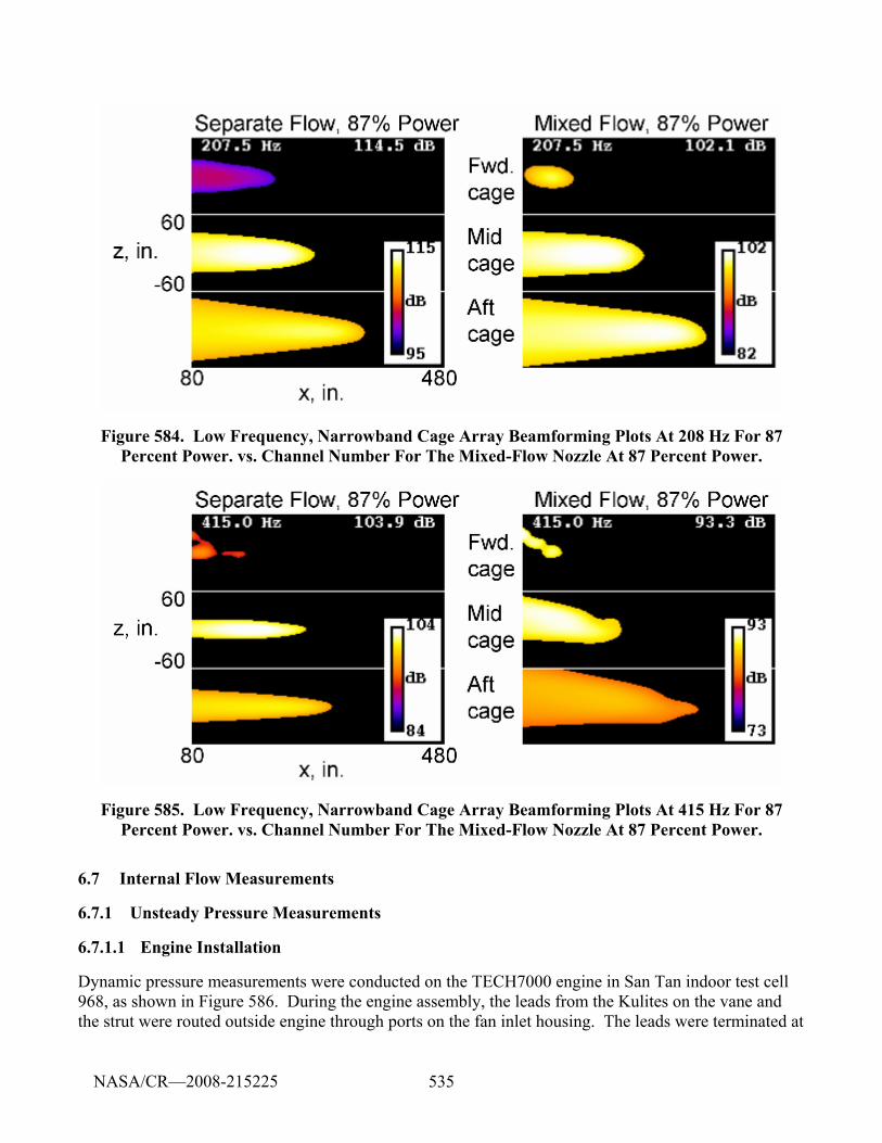
535




6.7.1 Unsteady Pressure Measurements

6.7.1.1 Engine Installation

Dynamic pressure measurements were conducted on the TECH7000 engine in San Tan indoor test cell 968, as shown in Figure 586. During the engine assembly, the leads from the Kulites on the vane and the strut were routed outside engine through ports on the fan inlet housing. The leads were terminated at

NASA/CR—2008-215225

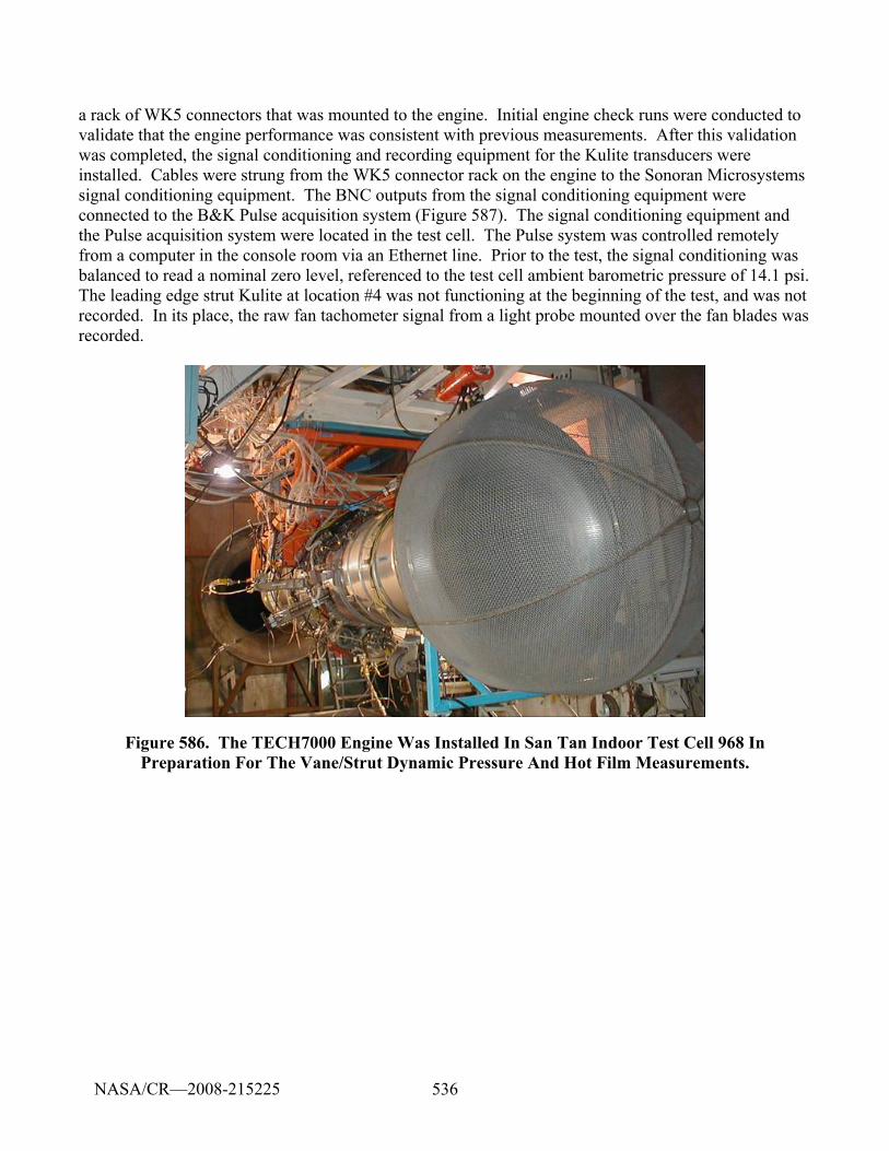
536

a rack of WK5 connectors that was mounted to the engine. Initial engine check runs were conducted to validate that the engine performance was consistent with previous measurements. After this validation was completed, the signal conditioning and recording equipment for the Kulite transducers were installed. Cables were strung from the WK5 connector rack on the engine to the Sonoran Microsystems signal conditioning equipment. The BNC outputs from the signal conditioning equipment were connected to the B&K Pulse acquisition system (Figure 587). The signal conditioning equipment and the Pulse acquisition system were located in the test cell. The Pulse system was controlled remotely from a computer in the console room via an Ethernet line. Prior to the test, the signal conditioning was balanced to read a nominal zero level, referenced to the test cell ambient barometric pressure of 14.1 psi. The leading edge strut Kulite at location #4 was not functioning at the beginning of the test, and was not recorded. In its place, the raw fan tachometer signal from a light probe mounted over the fan blades was recorded.

Figure 586. The TECH7000 Engine Was Installed In San Tan Indoor Test Cell 968 In Preparation For The Vane/Strut Dynamic Pressure And Hot Film Measurements.

NASA/CR—2008-215225

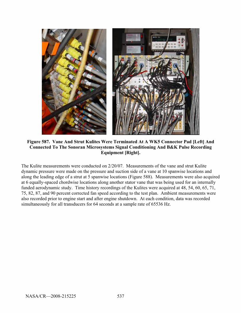
537

Figure 587. Vane And Strut Kulites Were Terminated At A WK5 Connector Pad [Left] And Connected To The Sonoran Microsystems Signal Conditioning And B&K Pulse Recording

Equipment [Right].

The Kulite measurements were conducted on 2/20/07. Measurements of the vane and strut Kulite dynamic pressure were made on the pressure and suction side of a vane at 10 spanwise locations and along the leading edge of a strut at 5 spanwise locations (Figure 588). Measurements were also acquired at 6 equally-spaced chordwise locations along another stator vane that was being used for an internally funded aerodynamic study. Time history recordings of the Kulites were acquired at 48, 54, 60, 65, 71, 75, 82, 87, and 90 percent corrected fan speed according to the test plan. Ambient measurements were also recorded prior to engine start and after engine shutdown. At each condition, data was recorded simultaneously for all transducers for 64 seconds at a sample rate of 65536 Hz.

NASA/CR—2008-215225

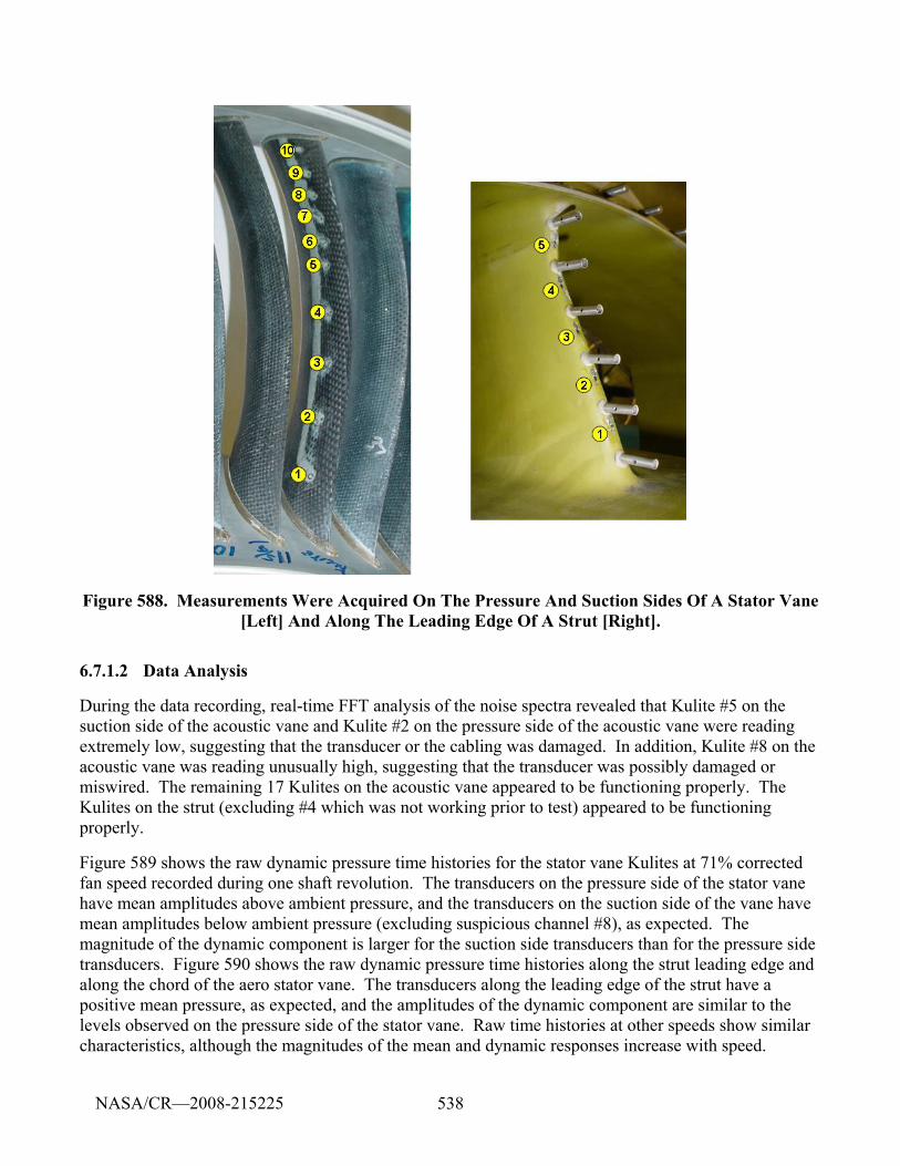
538

Figure 588. Measurements Were Acquired On The Pressure And Suction Sides Of A Stator Vane [Left] And Along The Leading Edge Of A Strut [Right].

6.7.1.2 Data Analysis

During the data recording, real-time FFT analysis of the noise spectra revealed that Kulite #5 on the suction side of the acoustic vane and Kulite #2 on the pressure side of the acoustic vane were reading extremely low, suggesting that the transducer or the cabling was damaged. In addition, Kulite #8 on the acoustic vane was reading unusually high, suggesting that the transducer was possibly damaged or miswired. The remaining 17 Kulites on the acoustic vane appeared to be functioning properly. The Kulites on the strut (excluding #4 which was not working prior to test) appeared to be functioning properly.

Figure 589 shows the raw dynamic pressure time histories for the stator vane Kulites at 71% corrected fan speed recorded during one shaft revolution. The transducers on the pressure side of the stator vane have mean amplitudes above ambient pressure, and the transducers on the suction side of the vane have mean amplitudes below ambient pressure (excluding suspicious channel #8), as expected. The magnitude of the dynamic component is larger for the suction side transducers than for the pressure side transducers. Figure 590 shows the raw dynamic pressure time histories along the strut leading edge and along the chord of the aero stator vane. The transducers along the leading edge of the strut have a positive mean pressure, as expected, and the amplitudes of the dynamic component are similar to the levels observed on the pressure side of the stator vane. Raw time histories at other speeds show similar characteristics, although the magnitudes of the mean and dynamic responses increase with speed.

NASA/CR—2008-215225

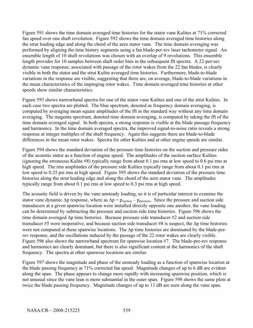
539

Figure 591 shows the time domain averaged time histories for the stator vane Kulites at 71% corrected fan speed over one shaft revolution. Figure 592 shows the time domain averaged time histories along the strut leading edge and along the chord of the aero stator vane. The time domain averaging was performed by aligning the time history segments using a fan blade-per-rev laser tachometer signal. An ensemble length of 10 shaft revolutions was chosen with an overlap of 9 revolutions. This ensemble length provides for 10 samples between shaft order bins in the subsequent fft spectra. A 22-per-rev dynamic vane response, associated with passage of the rotor wakes from the 22 fan blades, is clearly visible in both the stator and the strut Kulite averaged time histories. Furthermore, blade-to-blade variations in the response are visible, suggesting that there are, on average, blade-to-blade variations in the mean characteristics of the impinging rotor wakes. Time domain averaged time histories at other speeds show similar characteristics.

Figure 593 shows narrowband spectra for one of the stator vane Kulites and one of the strut Kulites. In each case two spectra are plotted. The blue spectrum, denoted as frequency domain averaging, is computed by averaging mean square amplitudes of the fft in the standard way without any time domain averaging. The magenta spectrum, denoted time domain averaging, is computed by taking the fft of the time domain averaged signal. In both spectra, a strong response is visible at the blade passage frequency and harmonics. In the time domain averaged spectra, the improved signal-to-noise ratio reveals a strong response at integer multiples of the shaft frequency. Again this suggests there are blade-to-blade differences in the mean rotor wakes. Spectra for other Kulites and at other engine speeds are similar.

Figure 594 shows the standard deviation of the pressure time histories on the suction and pressure sides of the acoustic stator as a function of engine speed. The amplitudes of the suction surface Kulites (ignoring the erroneous Kulite #8) typically range from about 0.1 psi rms at low speed to 0.6 psi rms at high speed. The rms amplitudes of the pressure side Kulites typically range from about 0.1 psi rms at low speed to 0.25 psi rms at high speed. Figure 595 shows the standard deviation of the pressure time histories along the strut leading edge and along the chord of the aero stator vane. The amplitudes typically range from about 0.1 psi rms at low speed to 0.3 psi rms at high speed.

The acoustic field is driven by the vane unsteady loading, so it is of particular interest to examine the stator vane dynamic Δp response, where as Δp = psuction – ppressure. Since the pressure and suction side transducers at a given spanwise location were installed directly opposite one another, the vane loading can be determined by subtracting the pressure and suction side time histories. Figure 596 shows the time domain averaged Δp time histories. Because pressure side transducer #2 and suction side transducer #5 were inoperative, and because suction side transducer #8 is suspect, the Δp time histories were not computed at these spanwise locations. The Δp time histories are dominated by the blade-per-rev response, and the oscillations induced by the passage of the 22 rotor wakes are clearly visible. Figure 596 also shows the narrowband spectrum for spanwise location #7. The blade-pre-rev response and harmonics are clearly dominant, but there is also significant content at the harmonics of the shaft frequency. The spectra at other spanwise locations are similar.

Figure 597 shows the magnitude and phase of the unsteady loading as a function of spanwise location at the blade passing frequency at 71% corrected fan speed. Magnitude changes of up to 6 dB are evident along the span. The phase appears to change more rapidly with increasing spanwise position, which is not unusual since the vane lean is more substantial in the outer span. Figure 598 shows the same plots at twice the blade passing frequency. Magnitude changes of up to 13 dB are seen along the vane span.

NASA/CR—2008-215225

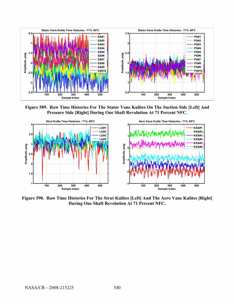
540

100 200 300 400 500-3.5

-3

-2.5

-2

-1.5

-1

-0.5

Sample Index

Am

plitu

de, p

sig

Stator Vane Kulite Time Histories - 71% NFC

SS#1SS#2SS#3SS#4SS#5SS#6SS#7SS#8SS#9SS#10

100 200 300 400 5000.5

1

1.5

2

2.5

3

3.5

Sample Index

Am

plitu

de, p

sig

Stator Vane Kulite Time Histories - 71% NFC

PS#1PS#2PS#3PS#4PS#5PS#6PS#7PS#8PS#9PS#10

rtfgvb

Figure 589. Raw Time Histories For The Stator Vane Kulites On The Suction Side [Left] And Pressure Side [Right] During One Shaft Revolution At 71 Percent NFC.

100 200 300 400 5001

1.5

2

2.5

3

3.5

4

Sample Index

Am

plitu

de, p

sig

Strut Kulite Time Histories - 71% NFC

LE#1LE#2LE#3LE#5

100 200 300 400 500-3

-2

-1

0

1

2

Sample Index

Am

plitu

de, p

sig

Aero Vane Kulite Time Histories - 71% NFC

KSS#1KSS#2KSS#3KSS#4KSS#5KSS#6

Figure 590. Raw Time Histories For The Strut Kulites [Left] And The Aero Vane Kulites [Right] During One Shaft Revolution At 71 Percent NFC.

NASA/CR—2008-215225

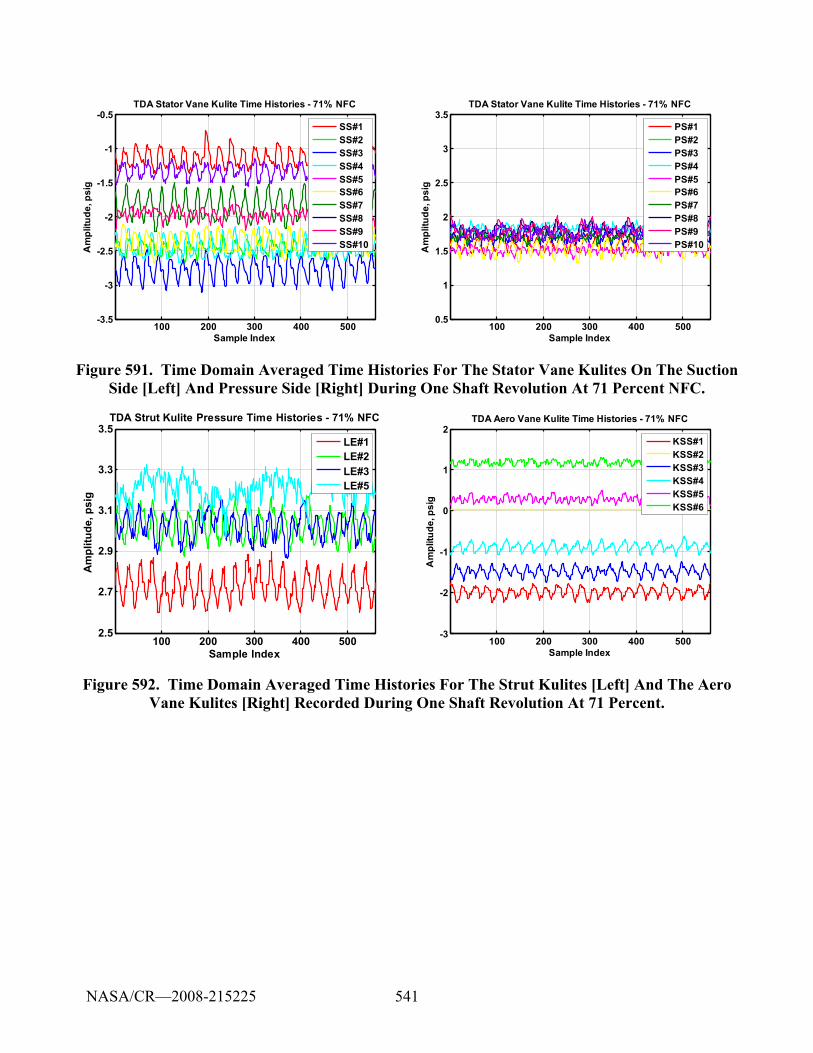
541

100 200 300 400 500-3.5

-3

-2.5

-2

-1.5

-1

-0.5

Sample Index

Am

plitu

de, p

sig

TDA Stator Vane Kulite Time Histories - 71% NFC


100 200 300 400 5000.5

1

1.5

2

2.5

3

3.5

Sample Index

Am

plitu

de, p

sig

TDA Stator Vane Kulite Time Histories - 71% NFC


Figure 591. Time Domain Averaged Time Histories For The Stator Vane Kulites On The Suction Side [Left] And Pressure Side [Right] During One Shaft Revolution At 71 Percent NFC.

100 200 300 400 5002.5

2.7

2.9

3.1

3.3

3.5

Sample Index

Am

plitu

de, p

sig

TDA Strut Kulite Pressure Time Histories - 71% NFC

LE#1LE#2LE#3LE#5

100 200 300 400 500-3

-2

-1

0

1

2

Sample Index

Am

plitu

de, p

sig

TDA Aero Vane Kulite Time Histories - 71% NFC


Figure 592. Time Domain Averaged Time Histories For The Strut Kulites [Left] And The Aero Vane Kulites [Right] Recorded During One Shaft Revolution At 71 Percent.

NASA/CR—2008-215225

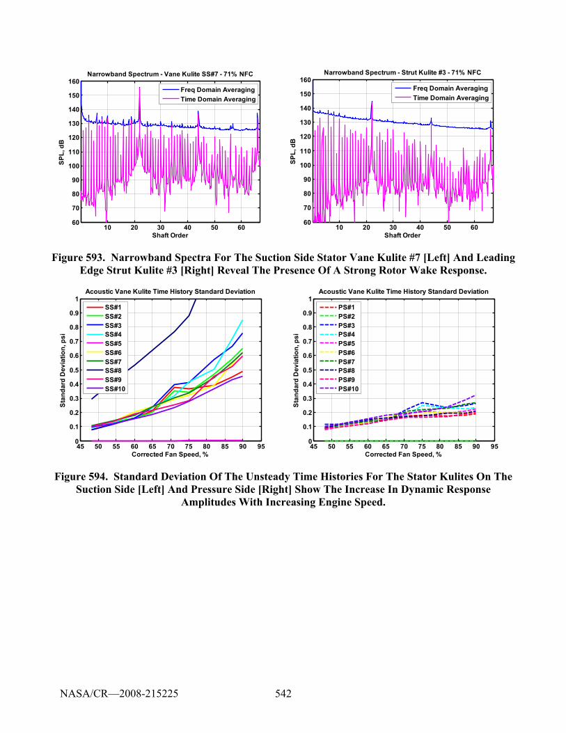
542

10 20 30 40 50 6060

70

80

90

100

110

120

130

140

150

160

Shaft Order

SPL,

dB

Narrowband Spectrum - Vane Kulite SS#7 - 71% NFC

Freq Domain AveragingTime Domain Averaging

10 20 30 40 50 6060

70

80

90

100

110

120

130

140

150

160

Shaft Order

SPL,

dB

Narrowband Spectrum - Strut Kulite #3 - 71% NFC

Freq Domain AveragingTime Domain Averaging

Figure 593. Narrowband Spectra For The Suction Side Stator Vane Kulite #7 [Left] And Leading Edge Strut Kulite #3 [Right] Reveal The Presence Of A Strong Rotor Wake Response.

45 50 55 60 65 70 75 80 85 90 950

0.1

0.2

0.3

0.4

0.5

0.6

0.7

0.8

0.9

1

Corrected Fan Speed, %

Stan

dard

Dev

iatio

n, p

si

Acoustic Vane Kulite Time History Standard Deviation


45 50 55 60 65 70 75 80 85 90 950

0.1

0.2

0.3

0.4

0.5

0.6

0.7

0.8

0.9

1


Stan

dard

Dev

iatio

n, p

siAcoustic Vane Kulite Time History Standard Deviation


Figure 594. Standard Deviation Of The Unsteady Time Histories For The Stator Kulites On The Suction Side [Left] And Pressure Side [Right] Show The Increase In Dynamic Response

Amplitudes With Increasing Engine Speed.

NASA/CR—2008-215225

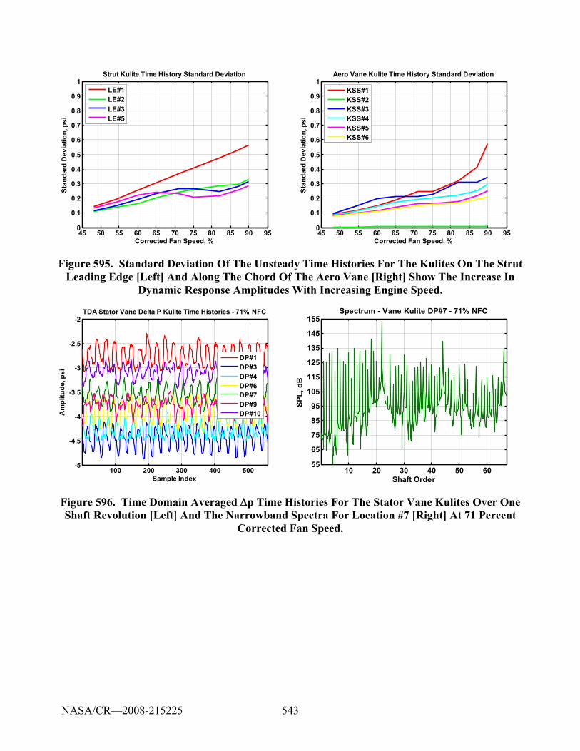
543

45 50 55 60 65 70 75 80 85 90 950

0.1

0.2

0.3

0.4

0.5

0.6

0.7

0.8

0.9

1


Stan

dard

Dev

iatio

n, p

siStrut Kulite Time History Standard Deviation

LE#1LE#2LE#3LE#5

45 50 55 60 65 70 75 80 85 90 950

0.1

0.2

0.3

0.4

0.5

0.6

0.7

0.8

0.9

1


Stan

dard

Dev

iatio

n, p

si

Aero Vane Kulite Time History Standard Deviation


Figure 595. Standard Deviation Of The Unsteady Time Histories For The Kulites On The Strut Leading Edge [Left] And Along The Chord Of The Aero Vane [Right] Show The Increase In

Dynamic Response Amplitudes With Increasing Engine Speed.

100 200 300 400 500-5

-4.5

-4

-3.5

-3

-2.5

-2

Sample Index

Am

plitu

de, p

si

TDA Stator Vane Delta P Kulite Time Histories - 71% NFC

DP#1DP#3DP#4DP#6DP#7DP#9DP#10

10 20 30 40 50 6055

65

75

85

95

105

115

125

135

145

155

Shaft Order

SPL,

dB

Spectrum - Vane Kulite DP#7 - 71% NFC

Figure 596. Time Domain Averaged Δp Time Histories For The Stator Vane Kulites Over One Shaft Revolution [Left] And The Narrowband Spectra For Location #7 [Right] At 71 Percent

Corrected Fan Speed.

NASA/CR—2008-215225

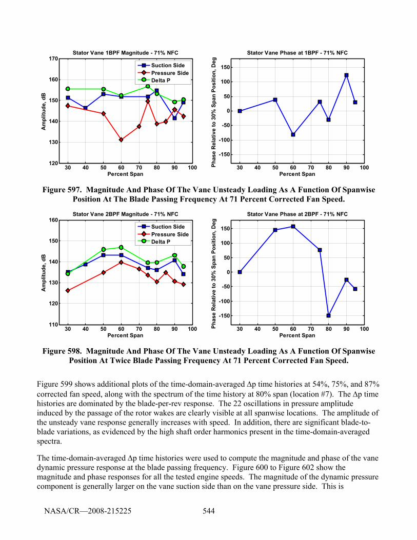
544

30 40 50 60 70 80 90 100120

130

140

150

160

170

Percent Span

Am

plitu

de, d

BStator Vane 1BPF Magnitude - 71% NFC

Suction SidePressure SideDelta P

30 40 50 60 70 80 90 100

-150

-100

-50

0

50

100

150

Percent Span

Phas

e R

elat

ive

to 3

0% S

pan

Posi

tion,

Deg

Stator Vane Phase at 1BPF - 71% NFC

Figure 597. Magnitude And Phase Of The Vane Unsteady Loading As A Function Of Spanwise Position At The Blade Passing Frequency At 71 Percent Corrected Fan Speed.

30 40 50 60 70 80 90 100110

120

130

140

150

160

Percent Span

Am

plitu

de, d

B

Stator Vane 2BPF Magnitude - 71% NFC

Suction SidePressure SideDelta P

30 40 50 60 70 80 90 100

-150

-100

-50

0

50

100

150

Percent Span

Phas

e R

elat

ive

to 3

0% S

pan

Posi

tion,

Deg

Stator Vane Phase at 2BPF - 71% NFC

Figure 598. Magnitude And Phase Of The Vane Unsteady Loading As A Function Of Spanwise Position At Twice Blade Passing Frequency At 71 Percent Corrected Fan Speed.

Figure 599 shows additional plots of the time-domain-averaged Δp time histories at 54%, 75%, and 87% corrected fan speed, along with the spectrum of the time history at 80% span (location #7). The Δp time histories are dominated by the blade-per-rev response. The 22 oscillations in pressure amplitude induced by the passage of the rotor wakes are clearly visible at all spanwise locations. The amplitude of the unsteady vane response generally increases with speed. In addition, there are significant blade-to-blade variations, as evidenced by the high shaft order harmonics present in the time-domain-averaged spectra.

The time-domain-averaged Δp time histories were used to compute the magnitude and phase of the vane dynamic pressure response at the blade passing frequency. Figure 600 to Figure 602 show the magnitude and phase responses for all the tested engine speeds. The magnitude of the dynamic pressure component is generally larger on the vane suction side than on the vane pressure side. This is

NASA/CR—2008-215225

545

particularly true at high speeds, where the suction-side dynamic pressure amplitude dominates over the pressure-side dynamic pressure amplitude over most of the span. The magnitude of the vane Δp response increases with engine speed, which is not surprising since this is generally true for the radiating blade passing tone level. The magnitude of the vane Δp response is seen to vary along the span by about ±6 dB about the mean level, regardless of speed. The phase of the vane Δp response appears to change more rapidly with increasing spanwise position, which is not unusual since the vane lean is more substantial in the outer span. Also, the phase spanwise variation appears to increase initially with engine speed, particularly near the vane tip, as evidenced by the increased slope in the phase plots at low speed.

NASA/CR—2008-215225

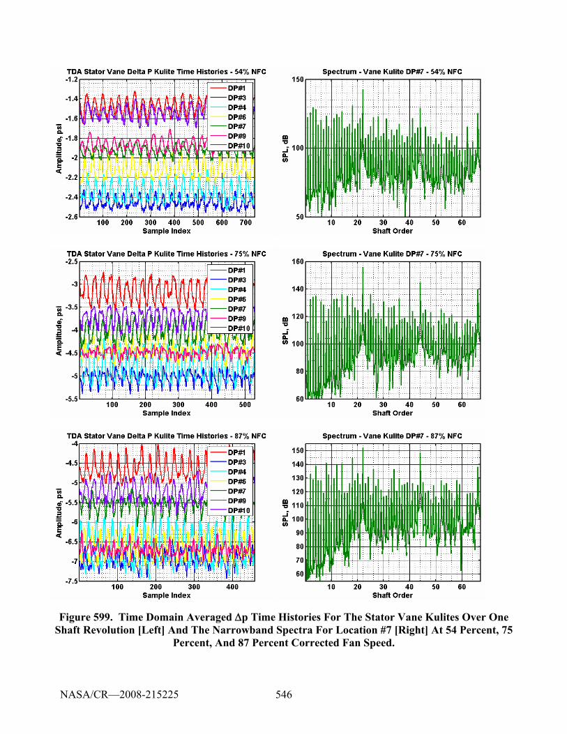
546

Figure 599. Time Domain Averaged Δp Time Histories For The Stator Vane Kulites Over One Shaft Revolution [Left] And The Narrowband Spectra For Location #7 [Right] At 54 Percent, 75

Percent, And 87 Percent Corrected Fan Speed.

NASA/CR—2008-215225

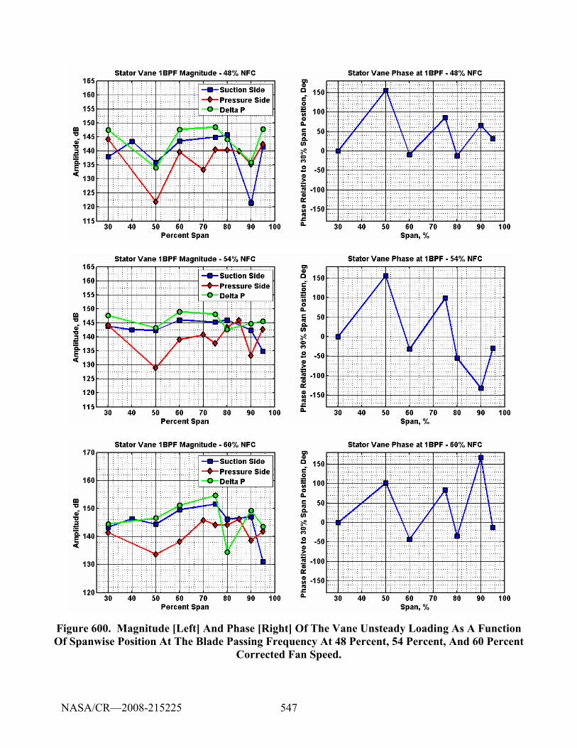
547

Figure 600. Magnitude [Left] And Phase [Right] Of The Vane Unsteady Loading As A Function Of Spanwise Position At The Blade Passing Frequency At 48 Percent, 54 Percent, And 60 Percent


NASA/CR—2008-215225

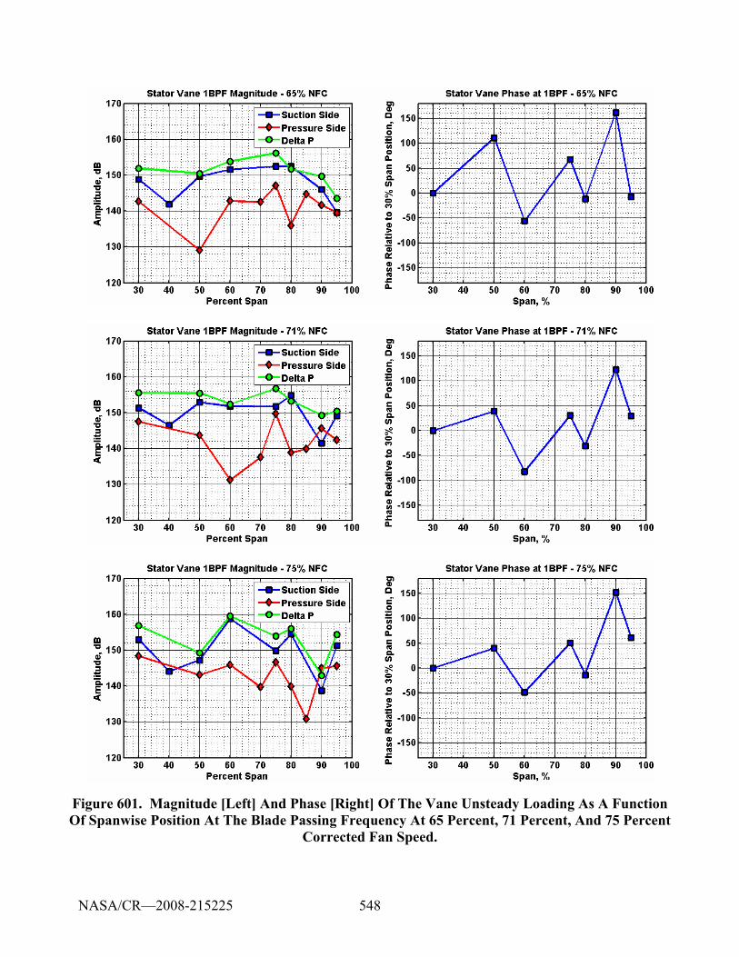
548



NASA/CR—2008-215225

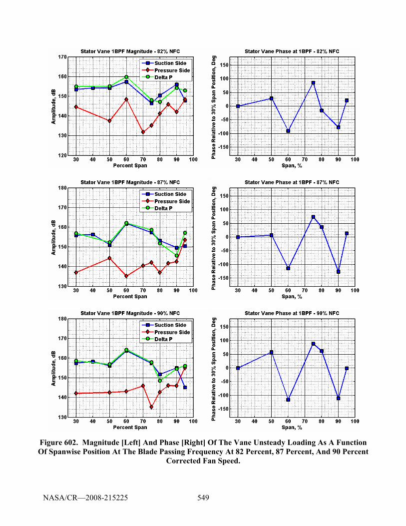
549



NASA/CR—2008-215225

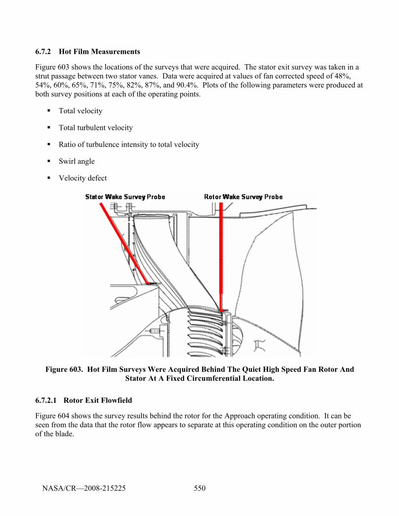
550

6.7.2 Hot Film Measurements

Figure 603 shows the locations of the surveys that were acquired. The stator exit survey was taken in a strut passage between two stator vanes. Data were acquired at values of fan corrected speed of 48%, 54%, 60%, 65%, 71%, 75%, 82%, 87%, and 90.4%. Plots of the following parameters were produced at both survey positions at each of the operating points.

Total velocity

Total turbulent velocity

Ratio of turbulence intensity to total velocity

Swirl angle

Velocity defect

Figure 603. Hot Film Surveys Were Acquired Behind The Quiet High Speed Fan Rotor And Stator At A Fixed Circumferential Location.

6.7.2.1 Rotor Exit Flowfield

Figure 604 shows the survey results behind the rotor for the Approach operating condition. It can be seen from the data that the rotor flow appears to separate at this operating condition on the outer portion of the blade.

NASA/CR—2008-215225

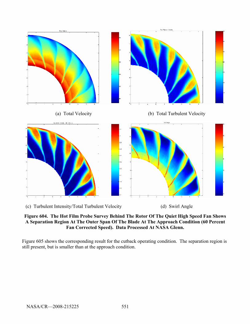
551

(a) Total Velocity (b) Total Turbulent Velocity

(c) Turbulent Intensity/Total Turbulent Velocity (d) Swirl Angle

Figure 604. The Hot Film Probe Survey Behind The Rotor Of The Quiet High Speed Fan Shows A Separation Region At The Outer Span Of The Blade At The Approach Condition (60 Percent

Fan Corrected Speed). Data Processed At NASA Glenn.

Figure 605 shows the corresponding result for the cutback operating condition. The separation region is still present, but is smaller than at the approach condition.

NASA/CR—2008-215225

552



Figure 605. The Hot Film Probe Survey Behind The Rotor Of The Quiet High Speed Fan Shows A Smaller Separation Region At The Outer Span Of The Blade At The Cutback Condition (71

Percent Fan Corrected Speed). Data Processed At NASA Glenn.

Finally, Figure 606 shows the results of the hot film survey behind the rotor of the Quiet High Speed Fan at the sideline condition. There is no longer any evidence of the flow separation. There is a high Mach number region at the root of the blade that is producing high turbulence levels.

NASA/CR—2008-215225

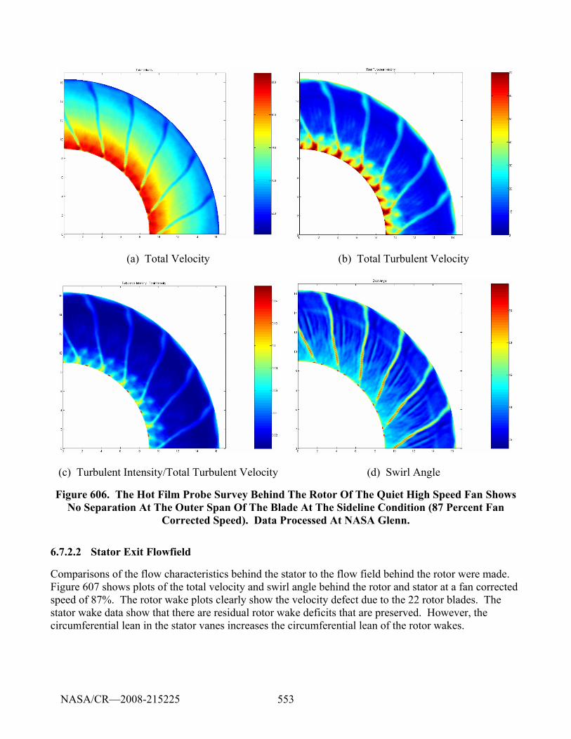
553



Figure 606. The Hot Film Probe Survey Behind The Rotor Of The Quiet High Speed Fan Shows No Separation At The Outer Span Of The Blade At The Sideline Condition (87 Percent Fan

Corrected Speed). Data Processed At NASA Glenn.

6.7.2.2 Stator Exit Flowfield

Comparisons of the flow characteristics behind the stator to the flow field behind the rotor were made. Figure 607 shows plots of the total velocity and swirl angle behind the rotor and stator at a fan corrected speed of 87%. The rotor wake plots clearly show the velocity defect due to the 22 rotor blades. The stator wake data show that there are residual rotor wake deficits that are preserved. However, the circumferential lean in the stator vanes increases the circumferential lean of the rotor wakes.

NASA/CR—2008-215225

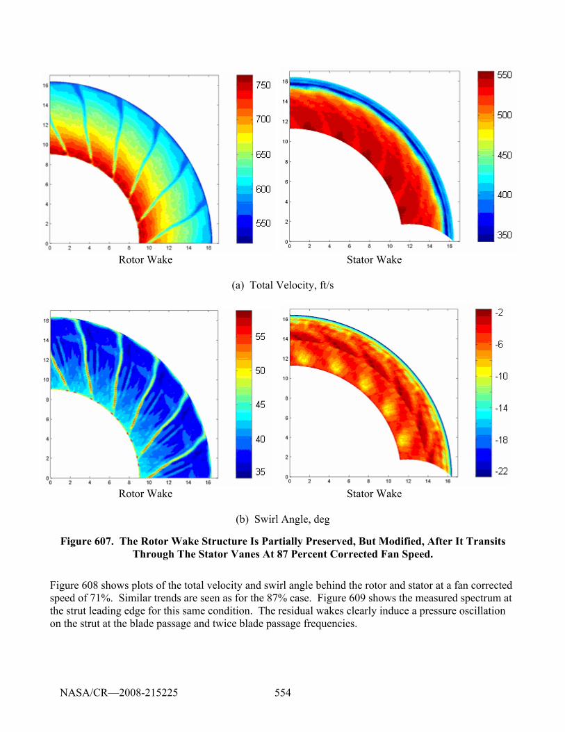
554

Rotor Wake Stator Wake

(a) Total Velocity, ft/s


(b) Swirl Angle, deg

Figure 607. The Rotor Wake Structure Is Partially Preserved, But Modified, After It Transits Through The Stator Vanes At 87 Percent Corrected Fan Speed.

Figure 608 shows plots of the total velocity and swirl angle behind the rotor and stator at a fan corrected speed of 71%. Similar trends are seen as for the 87% case. Figure 609 shows the measured spectrum at the strut leading edge for this same condition. The residual wakes clearly induce a pressure oscillation on the strut at the blade passage and twice blade passage frequencies.

NASA/CR—2008-215225

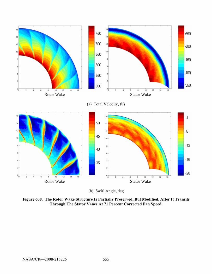
555






NASA/CR—2008-215225

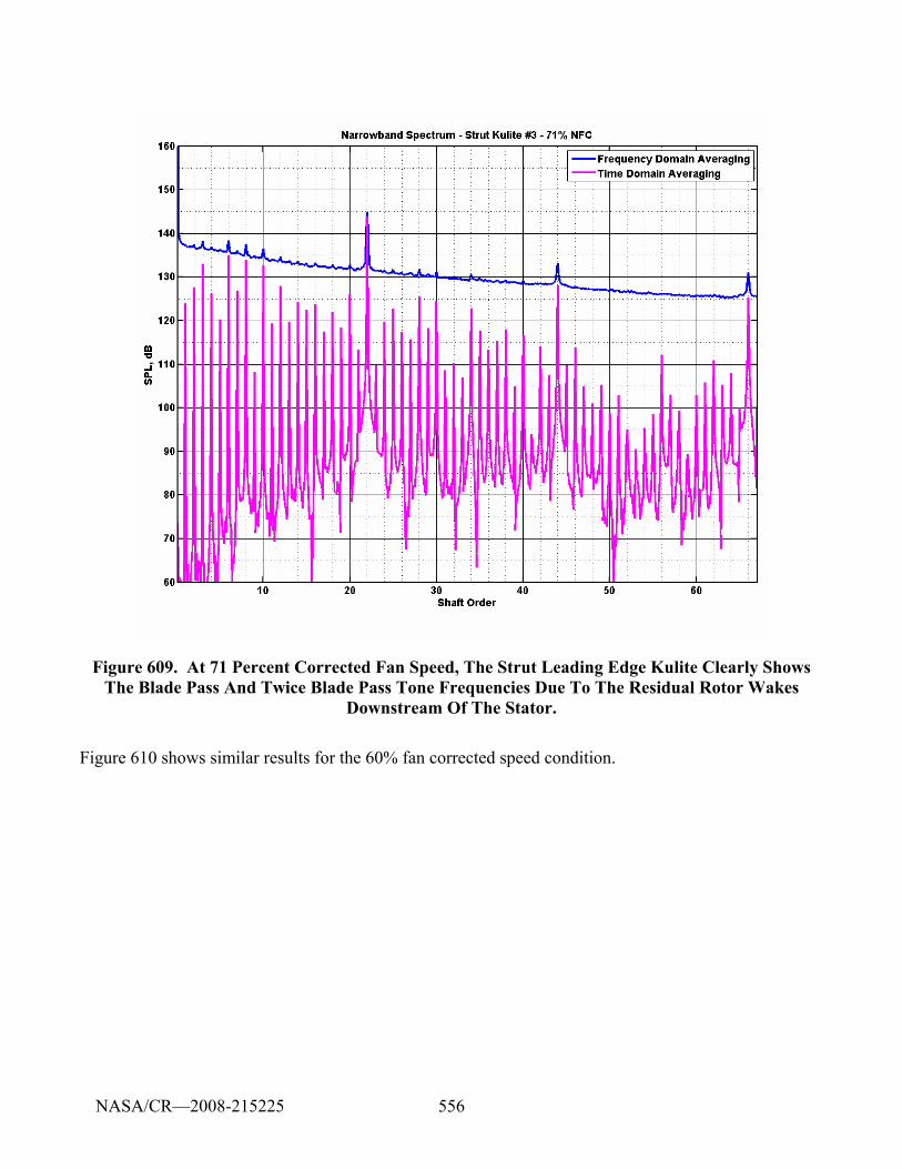
556

Figure 609. At 71 Percent Corrected Fan Speed, The Strut Leading Edge Kulite Clearly Shows The Blade Pass And Twice Blade Pass Tone Frequencies Due To The Residual Rotor Wakes

Downstream Of The Stator.

Figure 610 shows similar results for the 60% fan corrected speed condition.

NASA/CR—2008-215225

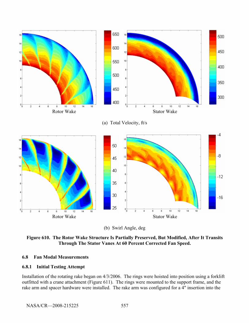
557







6.8.1 Initial Testing Attempt

Installation of the rotating rake began on 4/3/2006. The rings were hoisted into position using a forklift outfitted with a crane attachment (Figure 611). The rings were mounted to the support frame, and the rake arm and spacer hardware were installed. The rake arm was configured for a 4" insertion into the

NASA/CR—2008-215225

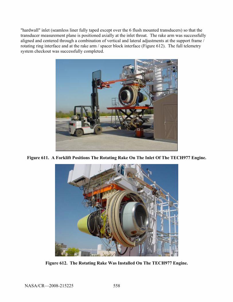
558

"hardwall" inlet (seamless liner fully taped except over the 6 flush mounted transducers) so that the transducer measurement plane is positioned axially at the inlet throat. The rake arm was successfully aligned and centered through a combination of vertical and lateral adjustments at the support frame / rotating ring interface and at the rake arm / spacer block interface (Figure 612). The full telemetry system checkout was successfully completed.

Figure 611. A Forklift Positions The Rotating Rake On The Inlet Of The TECH977 Engine.

Figure 612. The Rotating Rake Was Installed On The TECH977 Engine.

NASA/CR—2008-215225

559

The rake arm clearances were checked by installing a dial indicator on the top of the inlet and running the engine to different speeds. With the engine off, the rake arm wall clearance (with aluminum shield installed) is about 0.3" on average. However, the wall clearance is smaller at TDC than at BDC - the rake centerline is about 0.070" high compared to the engine centerline. When the engine was run to full power (~82% corrected fan speed), the inlet pitched up by 0.170". Thus at full power the rake centerline is about 0.100" low compared to the engine centerline. Thus somewhere in the mid-speed range the rake centerline and engine centerline are pretty-well aligned. The rake should not rub at any engine speed.

The drive motor was installed on the old 5:1 gearbox. Operation of the motor, motor programs, and remote control panel were checked with the motor unattached to the rotating ring. A signal generator was used to provide a per-rev TTL signal to the controller to test out the speed-following programs. The motor and control programs operated as expected, but adjustments to the motor controller parameters were needed to obtain smooth operation.

The motor was then mounted to the rotating rake. Some adjustment to the shaft axial position was required to align the sprocket on the chain. Some shimming of the bearing block was required to push the sprocket out radially so that the ring would rotate without vibration. The drive chain that was installed is not exactly what was ordered - it has mounting pads on every other link versus on every link like the EVNRC ring. As a result there is movement in some of the unsupported links that creates additional play in the drive system. This play is certainly undesirable but was not expected to pose a major problem.

Dan Sutliff and Kevin Konno arrived on 4/24/06 to calibrate the motor, set up instrumentation, and test. The following activities were completed:

Tuning of the rake motor control system

Installation of recording equipment

Installation of the engine and rake per-rev signals

Installation of the sailcloth and ICD

Calibration of the rake sensors

Test running of the engine and rake

The motor vibration caused by play in the unsupported links of the drive chain, imbalance in the weight distribution of the rotating ring, and potential out-of-roundness of the rake outer diameter (a machined surface) was minimized. The vibration was reduced to an acceptable level by shimming the motor at the bearing supports and by fabricating and bolting counterweights to the rotating ring opposite the rake arm.

The control parameters of the Gemini motor controller were adjusted and the rake control program was modified. Adjustment of parameters such as the current loop bandwidth, position loop bandwidth, and load-to-rotor inertia ratio were critical to achieving a smooth and responsive rake rotation. Checks were performed using a simulated square wave tachometer signal that was generated using a signal generator and ratio generator. The rake following programs were operated at a variety of simulated engine speeds

NASA/CR—2008-215225

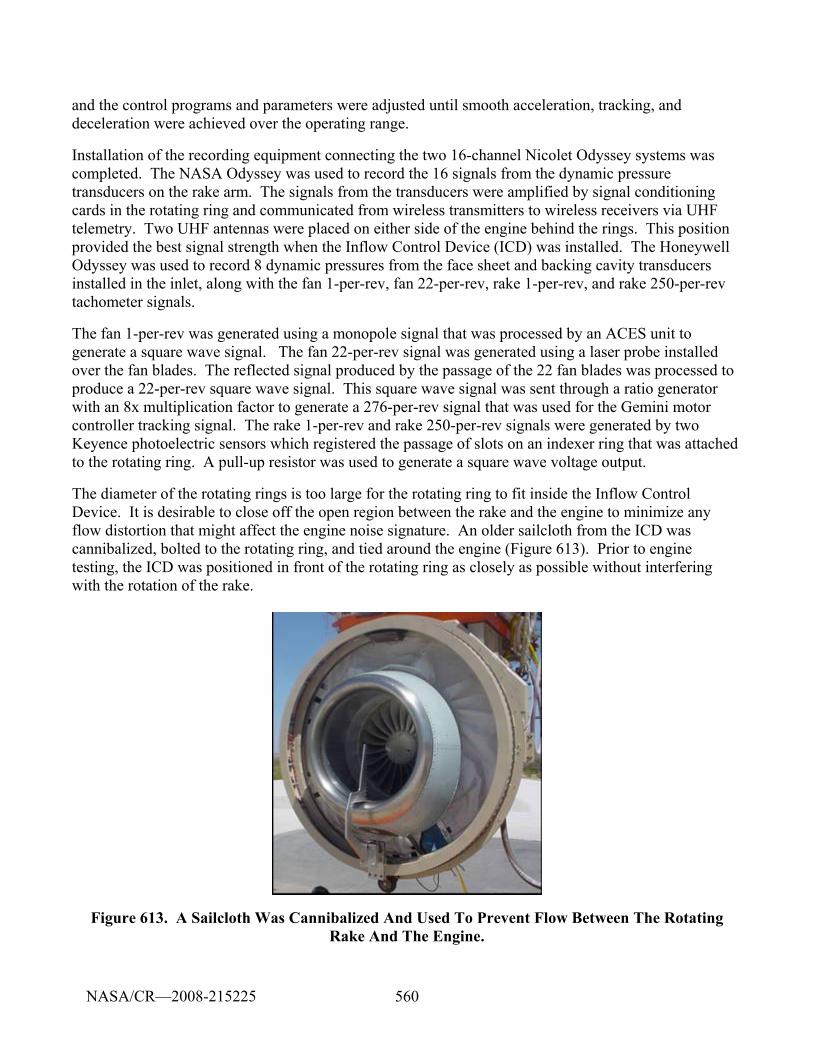
560

and the control programs and parameters were adjusted until smooth acceleration, tracking, and deceleration were achieved over the operating range.

Installation of the recording equipment connecting the two 16-channel Nicolet Odyssey systems was completed. The NASA Odyssey was used to record the 16 signals from the dynamic pressure transducers on the rake arm. The signals from the transducers were amplified by signal conditioning cards in the rotating ring and communicated from wireless transmitters to wireless receivers via UHF telemetry. Two UHF antennas were placed on either side of the engine behind the rings. This position provided the best signal strength when the Inflow Control Device (ICD) was installed. The Honeywell Odyssey was used to record 8 dynamic pressures from the face sheet and backing cavity transducers installed in the inlet, along with the fan 1-per-rev, fan 22-per-rev, rake 1-per-rev, and rake 250-per-rev tachometer signals.

The fan 1-per-rev was generated using a monopole signal that was processed by an ACES unit to generate a square wave signal. The fan 22-per-rev signal was generated using a laser probe installed over the fan blades. The reflected signal produced by the passage of the 22 fan blades was processed to produce a 22-per-rev square wave signal. This square wave signal was sent through a ratio generator with an 8x multiplication factor to generate a 276-per-rev signal that was used for the Gemini motor controller tracking signal. The rake 1-per-rev and rake 250-per-rev signals were generated by two Keyence photoelectric sensors which registered the passage of slots on an indexer ring that was attached to the rotating ring. A pull-up resistor was used to generate a square wave voltage output.

The diameter of the rotating rings is too large for the rotating ring to fit inside the Inflow Control Device. It is desirable to close off the open region between the rake and the engine to minimize any flow distortion that might affect the engine noise signature. An older sailcloth from the ICD was cannibalized, bolted to the rotating ring, and tied around the engine (Figure 613). Prior to engine testing, the ICD was positioned in front of the rotating ring as closely as possible without interfering with the rotation of the rake.

Figure 613. A Sailcloth Was Cannibalized And Used To Prevent Flow Between The Rotating Rake And The Engine.

NASA/CR—2008-215225

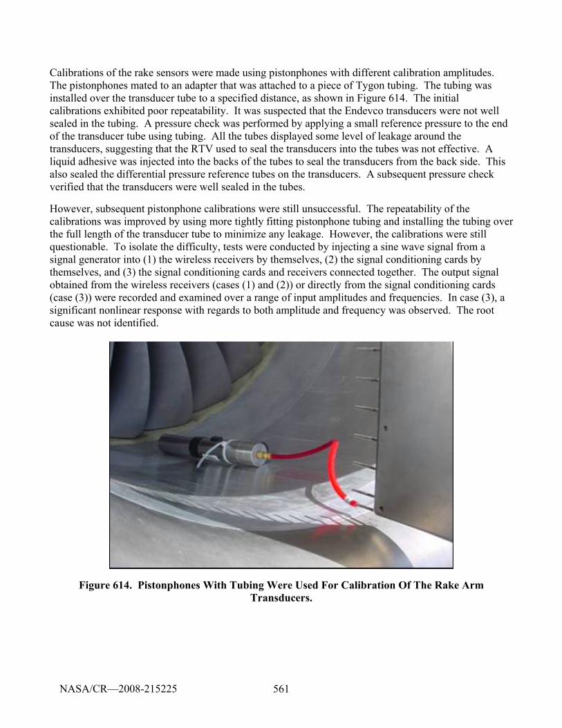
561

Calibrations of the rake sensors were made using pistonphones with different calibration amplitudes. The pistonphones mated to an adapter that was attached to a piece of Tygon tubing. The tubing was installed over the transducer tube to a specified distance, as shown in Figure 614. The initial calibrations exhibited poor repeatability. It was suspected that the Endevco transducers were not well sealed in the tubing. A pressure check was performed by applying a small reference pressure to the end of the transducer tube using tubing. All the tubes displayed some level of leakage around the transducers, suggesting that the RTV used to seal the transducers into the tubes was not effective. A liquid adhesive was injected into the backs of the tubes to seal the transducers from the back side. This also sealed the differential pressure reference tubes on the transducers. A subsequent pressure check verified that the transducers were well sealed in the tubes.

However, subsequent pistonphone calibrations were still unsuccessful. The repeatability of the calibrations was improved by using more tightly fitting pistonphone tubing and installing the tubing over the full length of the transducer tube to minimize any leakage. However, the calibrations were still questionable. To isolate the difficulty, tests were conducted by injecting a sine wave signal from a signal generator into (1) the wireless receivers by themselves, (2) the signal conditioning cards by themselves, and (3) the signal conditioning cards and receivers connected together. The output signal obtained from the wireless receivers (cases (1) and (2)) or directly from the signal conditioning cards (case (3)) were recorded and examined over a range of input amplitudes and frequencies. In case (3), a significant nonlinear response with regards to both amplitude and frequency was observed. The root cause was not identified.

Figure 614. Pistonphones With Tubing Were Used For Calibration Of The Rake Arm Transducers.

NASA/CR—2008-215225

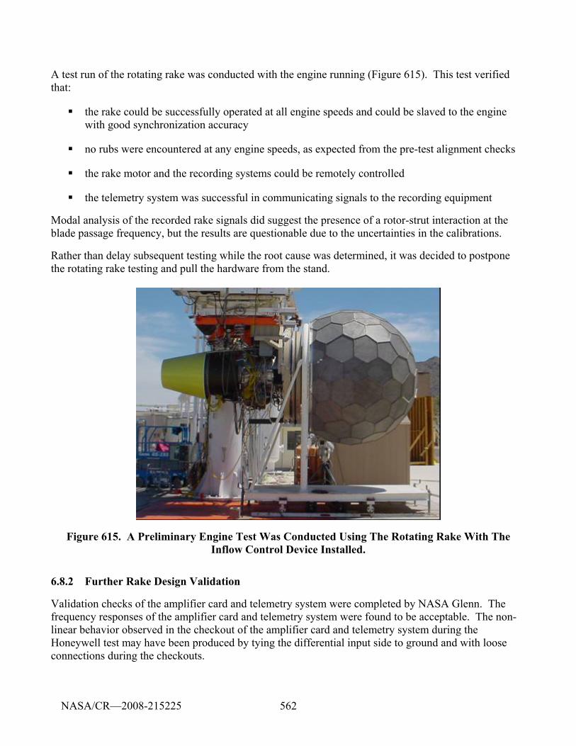
562

A test run of the rotating rake was conducted with the engine running (Figure 615). This test verified that:

the rake could be successfully operated at all engine speeds and could be slaved to the engine with good synchronization accuracy

no rubs were encountered at any engine speeds, as expected from the pre-test alignment checks

the rake motor and the recording systems could be remotely controlled

the telemetry system was successful in communicating signals to the recording equipment

Modal analysis of the recorded rake signals did suggest the presence of a rotor-strut interaction at the blade passage frequency, but the results are questionable due to the uncertainties in the calibrations.

Rather than delay subsequent testing while the root cause was determined, it was decided to postpone the rotating rake testing and pull the hardware from the stand.

Figure 615. A Preliminary Engine Test Was Conducted Using The Rotating Rake With The Inflow Control Device Installed.

6.8.2 Further Rake Design Validation

Validation checks of the amplifier card and telemetry system were completed by NASA Glenn. The frequency responses of the amplifier card and telemetry system were found to be acceptable. The non-linear behavior observed in the checkout of the amplifier card and telemetry system during the Honeywell test may have been produced by tying the differential input side to ground and with loose connections during the checkouts.

NASA/CR—2008-215225

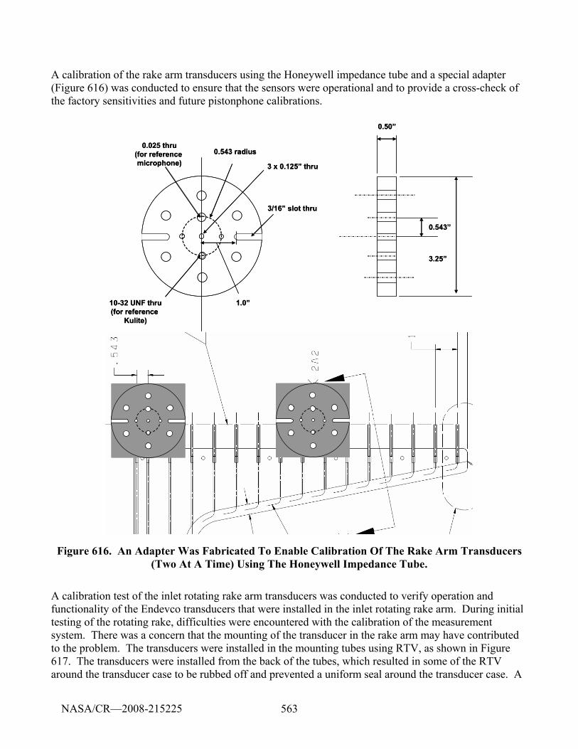
563

A calibration of the rake arm transducers using the Honeywell impedance tube and a special adapter (Figure 616) was conducted to ensure that the sensors were operational and to provide a cross-check of the factory sensitivities and future pistonphone calibrations.

3 x 0.125” thru

0.543 radius0.025 thru

(for reference microphone)

10-32 UNF thru(for reference

Kulite)

0.50”

0.543”

3.25”

3/16” slot thru

1.0”

3 x 0.125” thru

0.543 radius0.025 thru

(for reference microphone)

10-32 UNF thru(for reference

Kulite)

0.50”

0.543”

3.25”

3/16” slot thru

1.0”

Figure 616. An Adapter Was Fabricated To Enable Calibration Of The Rake Arm Transducers (Two At A Time) Using The Honeywell Impedance Tube.

A calibration test of the inlet rotating rake arm transducers was conducted to verify operation and functionality of the Endevco transducers that were installed in the inlet rotating rake arm. During initial testing of the rotating rake, difficulties were encountered with the calibration of the measurement system. There was a concern that the mounting of the transducer in the rake arm may have contributed to the problem. The transducers were installed in the mounting tubes using RTV, as shown in Figure 617. The transducers were installed from the back of the tubes, which resulted in some of the RTV around the transducer case to be rubbed off and prevented a uniform seal around the transducer case. A

NASA/CR—2008-215225

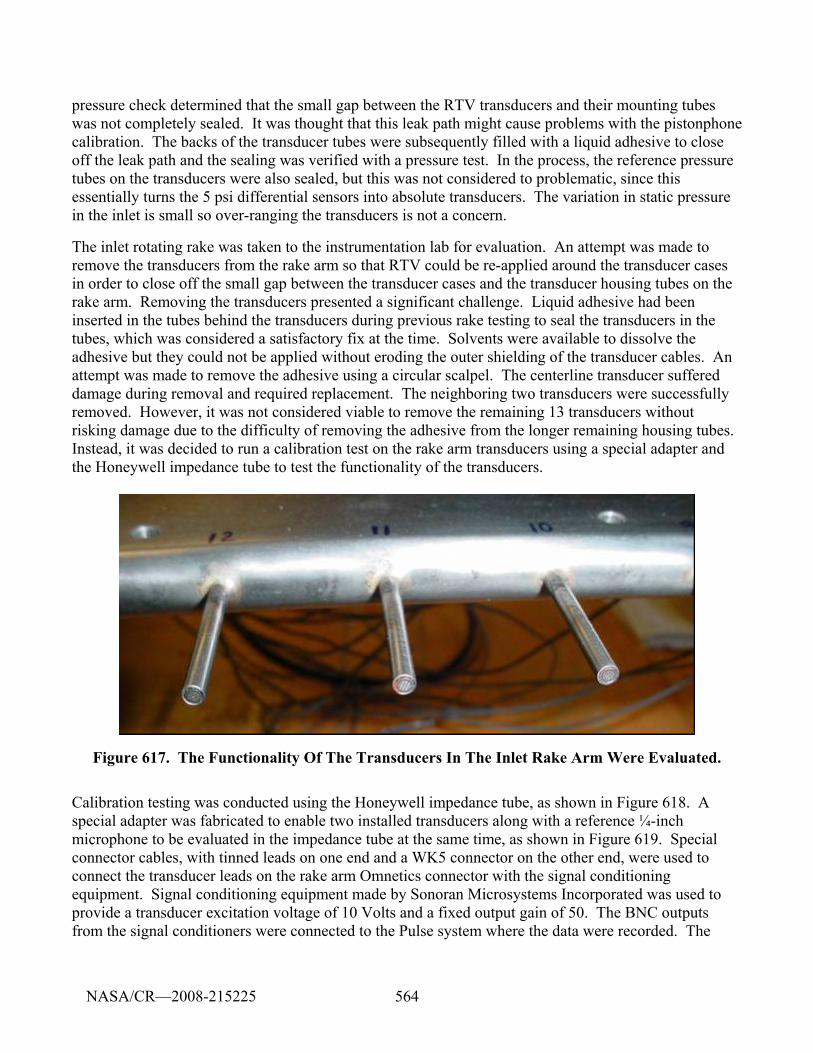
564

pressure check determined that the small gap between the RTV transducers and their mounting tubes was not completely sealed. It was thought that this leak path might cause problems with the pistonphone calibration. The backs of the transducer tubes were subsequently filled with a liquid adhesive to close off the leak path and the sealing was verified with a pressure test. In the process, the reference pressure tubes on the transducers were also sealed, but this was not considered to problematic, since this essentially turns the 5 psi differential sensors into absolute transducers. The variation in static pressure in the inlet is small so over-ranging the transducers is not a concern.

The inlet rotating rake was taken to the instrumentation lab for evaluation. An attempt was made to remove the transducers from the rake arm so that RTV could be re-applied around the transducer cases in order to close off the small gap between the transducer cases and the transducer housing tubes on the rake arm. Removing the transducers presented a significant challenge. Liquid adhesive had been inserted in the tubes behind the transducers during previous rake testing to seal the transducers in the tubes, which was considered a satisfactory fix at the time. Solvents were available to dissolve the adhesive but they could not be applied without eroding the outer shielding of the transducer cables. An attempt was made to remove the adhesive using a circular scalpel. The centerline transducer suffered damage during removal and required replacement. The neighboring two transducers were successfully removed. However, it was not considered viable to remove the remaining 13 transducers without risking damage due to the difficulty of removing the adhesive from the longer remaining housing tubes. Instead, it was decided to run a calibration test on the rake arm transducers using a special adapter and the Honeywell impedance tube to test the functionality of the transducers.

Figure 617. The Functionality Of The Transducers In The Inlet Rake Arm Were Evaluated.

Calibration testing was conducted using the Honeywell impedance tube, as shown in Figure 618. A special adapter was fabricated to enable two installed transducers along with a reference ¼-inch microphone to be evaluated in the impedance tube at the same time, as shown in Figure 619. Special connector cables, with tinned leads on one end and a WK5 connector on the other end, were used to connect the transducer leads on the rake arm Omnetics connector with the signal conditioning equipment. Signal conditioning equipment made by Sonoran Microsystems Incorporated was used to provide a transducer excitation voltage of 10 Volts and a fixed output gain of 50. The BNC outputs from the signal conditioners were connected to the Pulse system where the data were recorded. The

NASA/CR—2008-215225

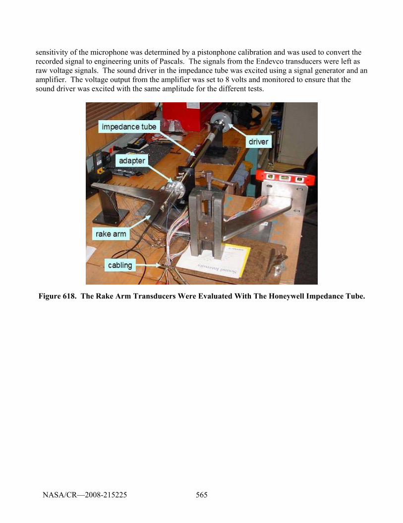
565

sensitivity of the microphone was determined by a pistonphone calibration and was used to convert the recorded signal to engineering units of Pascals. The signals from the Endevco transducers were left as raw voltage signals. The sound driver in the impedance tube was excited using a signal generator and an amplifier. The voltage output from the amplifier was set to 8 volts and monitored to ensure that the sound driver was excited with the same amplitude for the different tests.

Figure 618. The Rake Arm Transducers Were Evaluated With The Honeywell Impedance Tube.

NASA/CR—2008-215225

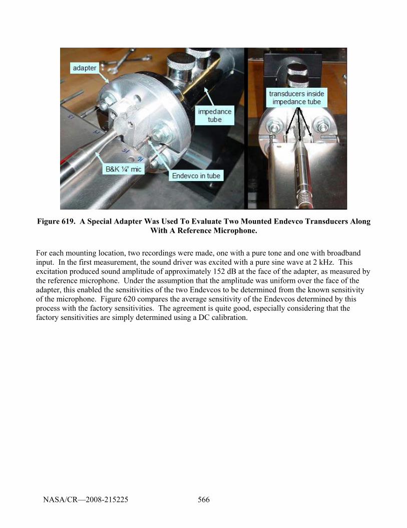
566

Figure 619. A Special Adapter Was Used To Evaluate Two Mounted Endevco Transducers Along With A Reference Microphone.

For each mounting location, two recordings were made, one with a pure tone and one with broadband input. In the first measurement, the sound driver was excited with a pure sine wave at 2 kHz. This excitation produced sound amplitude of approximately 152 dB at the face of the adapter, as measured by the reference microphone. Under the assumption that the amplitude was uniform over the face of the adapter, this enabled the sensitivities of the two Endevcos to be determined from the known sensitivity of the microphone. Figure 620 compares the average sensitivity of the Endevcos determined by this process with the factory sensitivities. The agreement is quite good, especially considering that the factory sensitivities are simply determined using a DC calibration.

NASA/CR—2008-215225

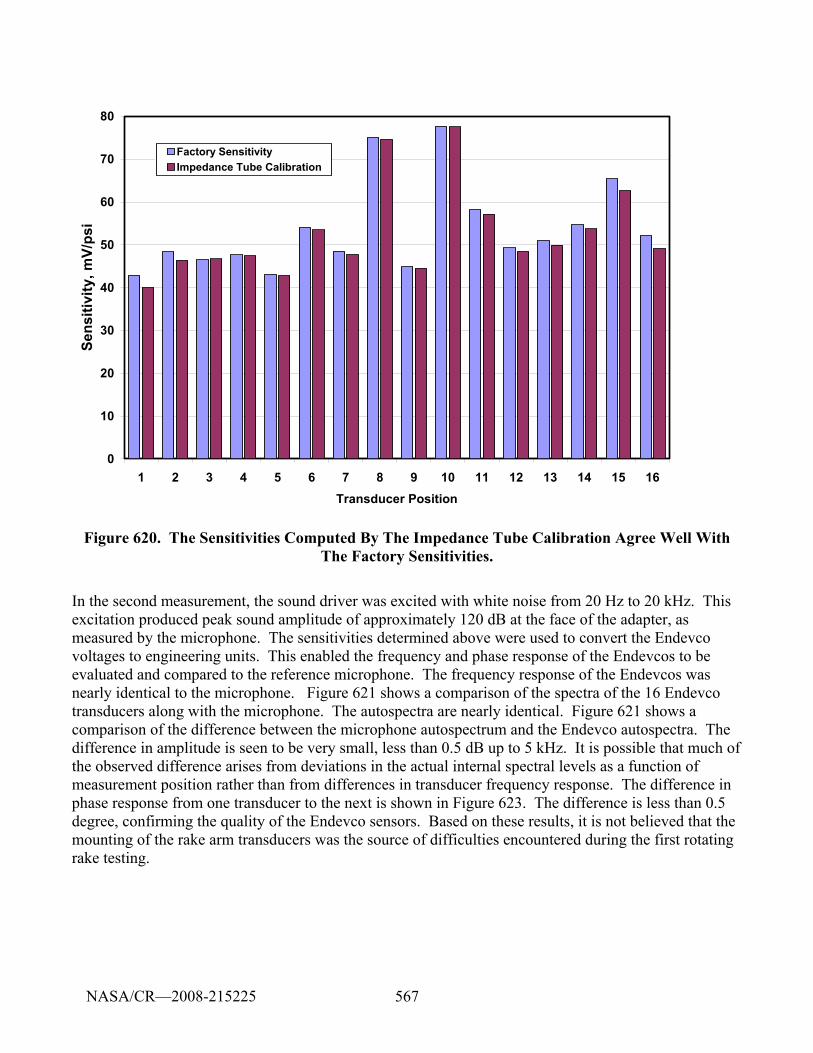
567

Figure 620. The Sensitivities Computed By The Impedance Tube Calibration Agree Well With The Factory Sensitivities.

In the second measurement, the sound driver was excited with white noise from 20 Hz to 20 kHz. This excitation produced peak sound amplitude of approximately 120 dB at the face of the adapter, as measured by the microphone. The sensitivities determined above were used to convert the Endevco voltages to engineering units. This enabled the frequency and phase response of the Endevcos to be evaluated and compared to the reference microphone. The frequency response of the Endevcos was nearly identical to the microphone. Figure 621 shows a comparison of the spectra of the 16 Endevco transducers along with the microphone. The autospectra are nearly identical. Figure 621 shows a comparison of the difference between the microphone autospectrum and the Endevco autospectra. The difference in amplitude is seen to be very small, less than 0.5 dB up to 5 kHz. It is possible that much of the observed difference arises from deviations in the actual internal spectral levels as a function of measurement position rather than from differences in transducer frequency response. The difference in phase response from one transducer to the next is shown in Figure 623. The difference is less than 0.5 degree, confirming the quality of the Endevco sensors. Based on these results, it is not believed that the mounting of the rake arm transducers was the source of difficulties encountered during the first rotating rake testing.

0

10

20

30

40

50

60

70

80

1 2 3 4 5 6 7 8 9 10 11 12 13 14 15 16Transducer Position

Sens

itivi

ty, m

V/ps

i

Factory SensitivityImpedance Tube Calibration

NASA/CR—2008-215225

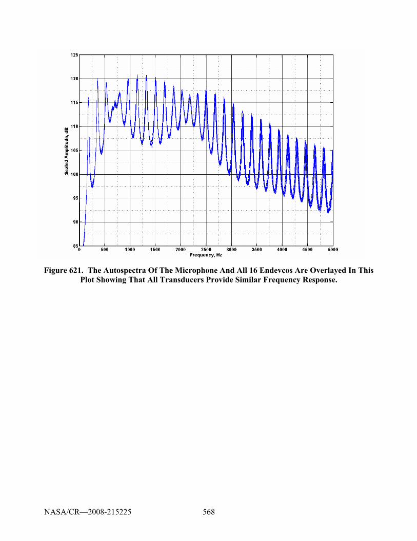
568

Figure 621. The Autospectra Of The Microphone And All 16 Endevcos Are Overlayed In This Plot Showing That All Transducers Provide Similar Frequency Response.

NASA/CR—2008-215225

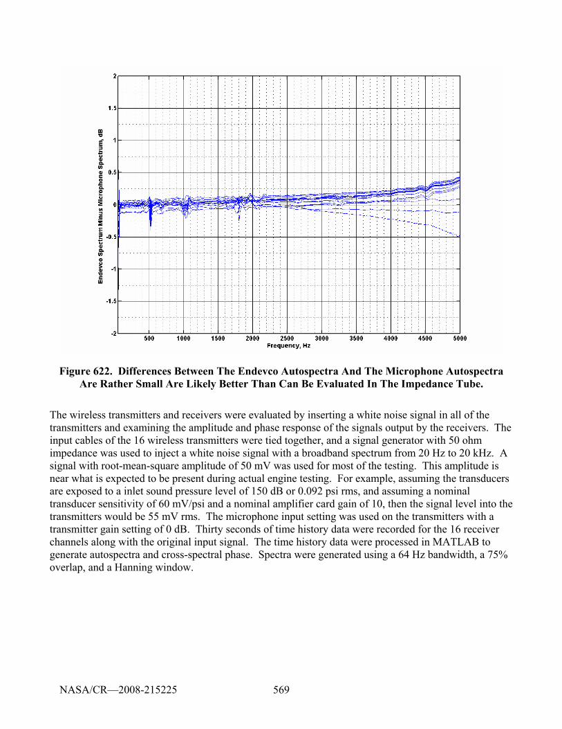
569

Figure 622. Differences Between The Endevco Autospectra And The Microphone Autospectra Are Rather Small Are Likely Better Than Can Be Evaluated In The Impedance Tube.

The wireless transmitters and receivers were evaluated by inserting a white noise signal in all of the transmitters and examining the amplitude and phase response of the signals output by the receivers. The input cables of the 16 wireless transmitters were tied together, and a signal generator with 50 ohm impedance was used to inject a white noise signal with a broadband spectrum from 20 Hz to 20 kHz. A signal with root-mean-square amplitude of 50 mV was used for most of the testing. This amplitude is near what is expected to be present during actual engine testing. For example, assuming the transducers are exposed to a inlet sound pressure level of 150 dB or 0.092 psi rms, and assuming a nominal transducer sensitivity of 60 mV/psi and a nominal amplifier card gain of 10, then the signal level into the transmitters would be 55 mV rms. The microphone input setting was used on the transmitters with a transmitter gain setting of 0 dB. Thirty seconds of time history data were recorded for the 16 receiver channels along with the original input signal. The time history data were processed in MATLAB to generate autospectra and cross-spectral phase. Spectra were generated using a 64 Hz bandwidth, a 75% overlap, and a Hanning window.

NASA/CR—2008-215225

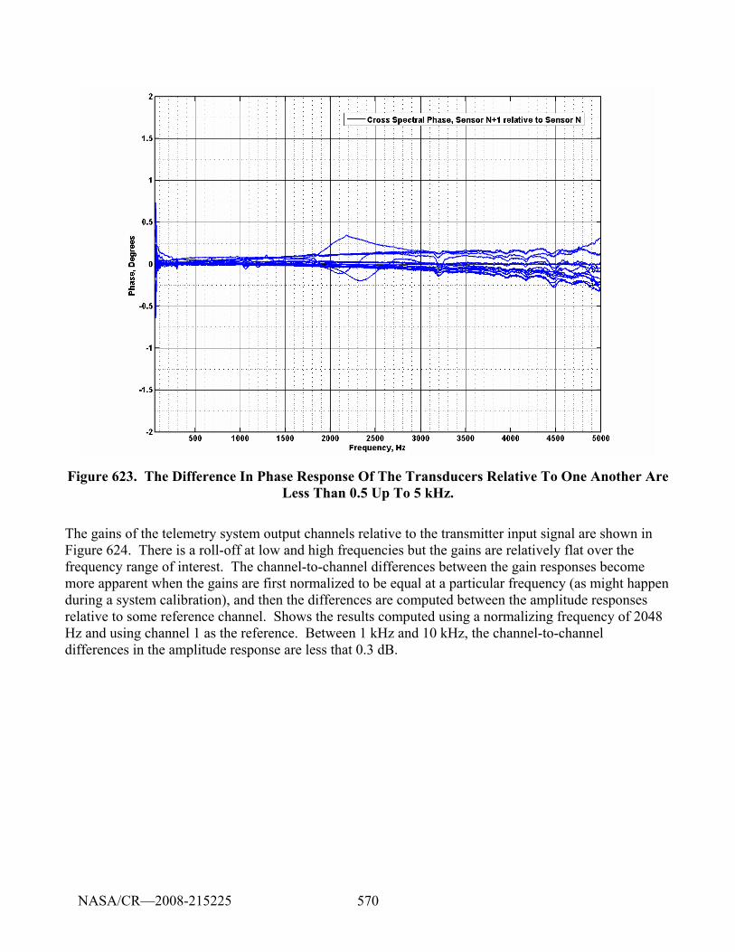
570

Figure 623. The Difference In Phase Response Of The Transducers Relative To One Another Are Less Than 0.5 Up To 5 kHz.

The gains of the telemetry system output channels relative to the transmitter input signal are shown in Figure 624. There is a roll-off at low and high frequencies but the gains are relatively flat over the frequency range of interest. The channel-to-channel differences between the gain responses become more apparent when the gains are first normalized to be equal at a particular frequency (as might happen during a system calibration), and then the differences are computed between the amplitude responses relative to some reference channel. Shows the results computed using a normalizing frequency of 2048 Hz and using channel 1 as the reference. Between 1 kHz and 10 kHz, the channel-to-channel differences in the amplitude response are less that 0.3 dB.

NASA/CR—2008-215225

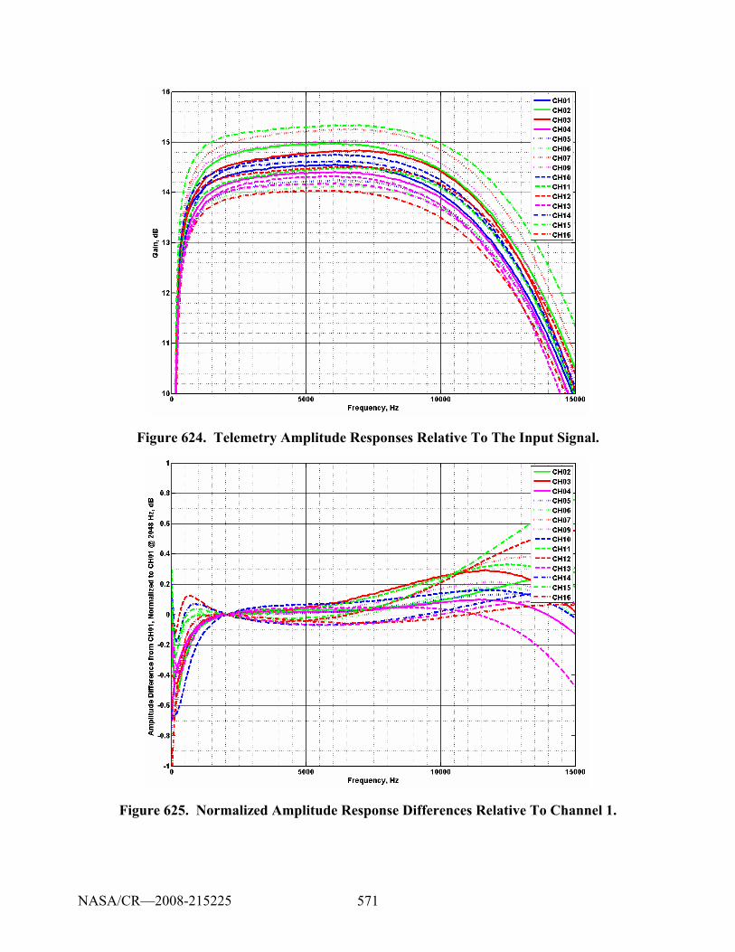
571

Figure 624. Telemetry Amplitude Responses Relative To The Input Signal.

Figure 625. Normalized Amplitude Response Differences Relative To Channel 1.

NASA/CR—2008-215225

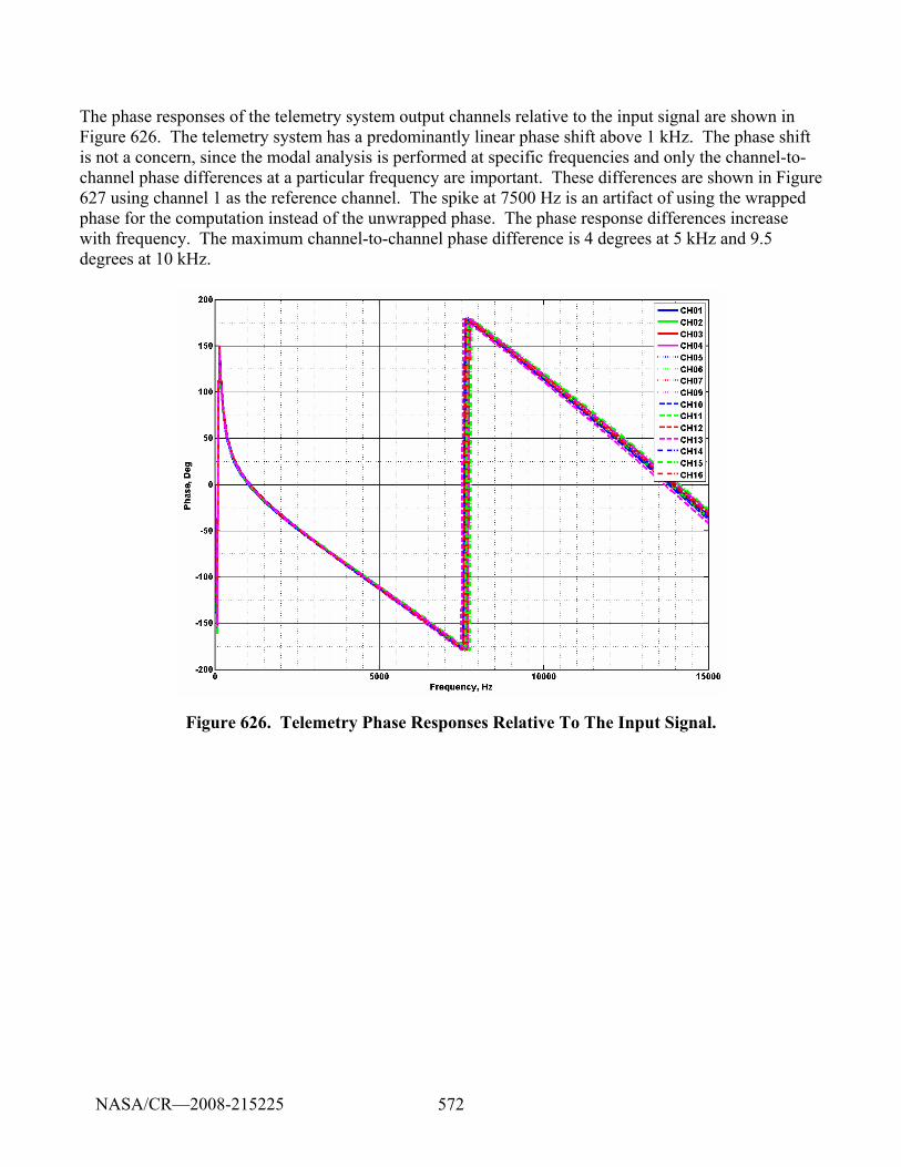
572

The phase responses of the telemetry system output channels relative to the input signal are shown in Figure 626. The telemetry system has a predominantly linear phase shift above 1 kHz. The phase shift is not a concern, since the modal analysis is performed at specific frequencies and only the channel-to-channel phase differences at a particular frequency are important. These differences are shown in Figure 627 using channel 1 as the reference channel. The spike at 7500 Hz is an artifact of using the wrapped phase for the computation instead of the unwrapped phase. The phase response differences increase with frequency. The maximum channel-to-channel phase difference is 4 degrees at 5 kHz and 9.5 degrees at 10 kHz.

Figure 626. Telemetry Phase Responses Relative To The Input Signal.

NASA/CR—2008-215225

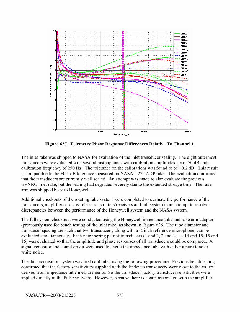
573

Figure 627. Telemetry Phase Response Differences Relative To Channel 1.

The inlet rake was shipped to NASA for evaluation of the inlet transducer sealing. The eight outermost transducers were evaluated with several pistonphones with calibration amplitudes near 150 dB and a calibration frequency of 250 Hz. The tolerance on the calibrations was found to be ±0.2 dB. This result is comparable to the ±0.1 dB tolerance measured on NASA’s 22” ADP rake. The evaluation confirmed that the transducers are currently well sealed. An attempt was made to also evaluate the previous EVNRC inlet rake, but the sealing had degraded severely due to the extended storage time. The rake arm was shipped back to Honeywell.

Additional checkouts of the rotating rake system were completed to evaluate the performance of the transducers, amplifier cards, wireless transmitters/receivers and full system in an attempt to resolve discrepancies between the performance of the Honeywell system and the NASA system.

The full system checkouts were conducted using the Honeywell impedance tube and rake arm adapter (previously used for bench testing of the inlet rake) as shown in Figure 628. The tube diameter and transducer spacing are such that two transducers, along with a ¼ inch reference microphone, can be evaluated simultaneously. Each neighboring pair of transducers (1 and 2, 2 and 3, …, 14 and 15, 15 and 16) was evaluated so that the amplitude and phase responses of all transducers could be compared. A signal generator and sound driver were used to excite the impedance tube with either a pure tone or white noise.

The data acquisition system was first calibrated using the following procedure. Previous bench testing confirmed that the factory sensitivities supplied with the Endevco transducers were close to the values derived from impedance tube measurements. So the transducer factory transducer sensitivities were applied directly in the Pulse software. However, because there is a gain associated with the amplifier

NASA/CR—2008-215225

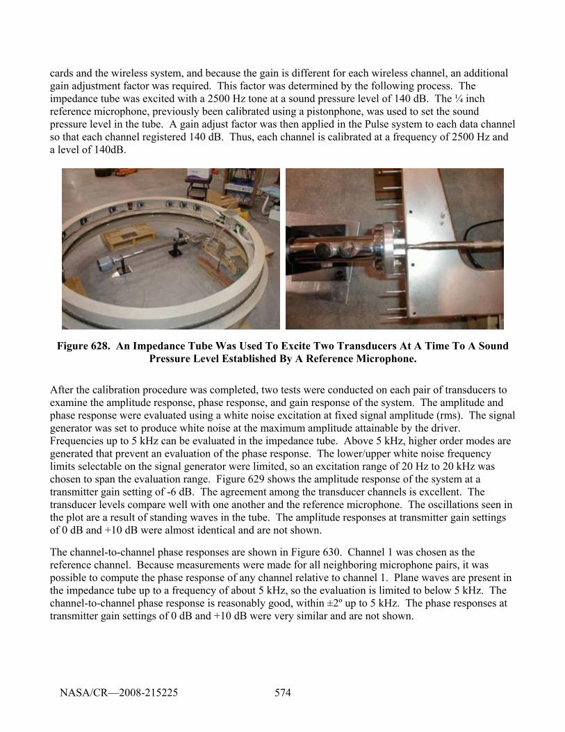
574

cards and the wireless system, and because the gain is different for each wireless channel, an additional gain adjustment factor was required. This factor was determined by the following process. The impedance tube was excited with a 2500 Hz tone at a sound pressure level of 140 dB. The ¼ inch reference microphone, previously been calibrated using a pistonphone, was used to set the sound pressure level in the tube. A gain adjust factor was then applied in the Pulse system to each data channel so that each channel registered 140 dB. Thus, each channel is calibrated at a frequency of 2500 Hz and a level of 140dB.

Figure 628. An Impedance Tube Was Used To Excite Two Transducers At A Time To A Sound Pressure Level Established By A Reference Microphone.

After the calibration procedure was completed, two tests were conducted on each pair of transducers to examine the amplitude response, phase response, and gain response of the system. The amplitude and phase response were evaluated using a white noise excitation at fixed signal amplitude (rms). The signal generator was set to produce white noise at the maximum amplitude attainable by the driver. Frequencies up to 5 kHz can be evaluated in the impedance tube. Above 5 kHz, higher order modes are generated that prevent an evaluation of the phase response. The lower/upper white noise frequency limits selectable on the signal generator were limited, so an excitation range of 20 Hz to 20 kHz was chosen to span the evaluation range. Figure 629 shows the amplitude response of the system at a transmitter gain setting of -6 dB. The agreement among the transducer channels is excellent. The transducer levels compare well with one another and the reference microphone. The oscillations seen in the plot are a result of standing waves in the tube. The amplitude responses at transmitter gain settings of 0 dB and +10 dB were almost identical and are not shown.

The channel-to-channel phase responses are shown in Figure 630. Channel 1 was chosen as the reference channel. Because measurements were made for all neighboring microphone pairs, it was possible to compute the phase response of any channel relative to channel 1. Plane waves are present in the impedance tube up to a frequency of about 5 kHz, so the evaluation is limited to below 5 kHz. The channel-to-channel phase response is reasonably good, within ±2º up to 5 kHz. The phase responses at transmitter gain settings of 0 dB and +10 dB were very similar and are not shown.

NASA/CR—2008-215225

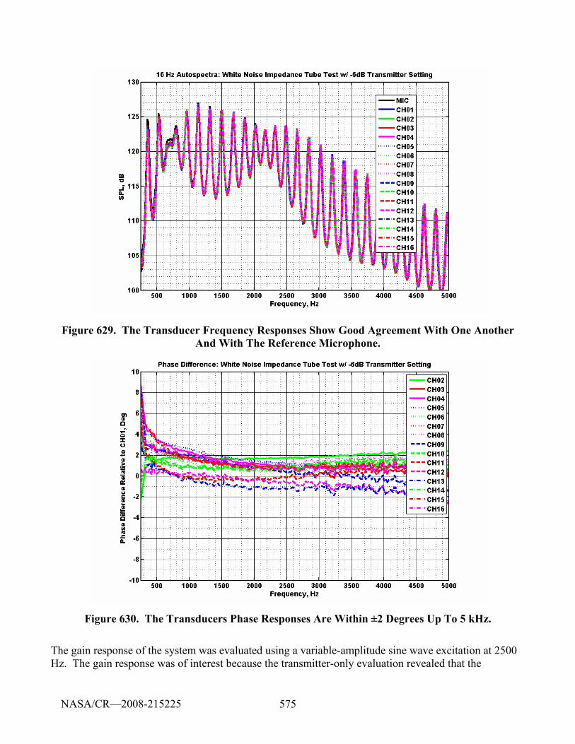
575

Figure 629. The Transducer Frequency Responses Show Good Agreement With One Another And With The Reference Microphone.

Figure 630. The Transducers Phase Responses Are Within ±2 Degrees Up To 5 kHz.

The gain response of the system was evaluated using a variable-amplitude sine wave excitation at 2500 Hz. The gain response was of interest because the transmitter-only evaluation revealed that the

NASA/CR—2008-215225

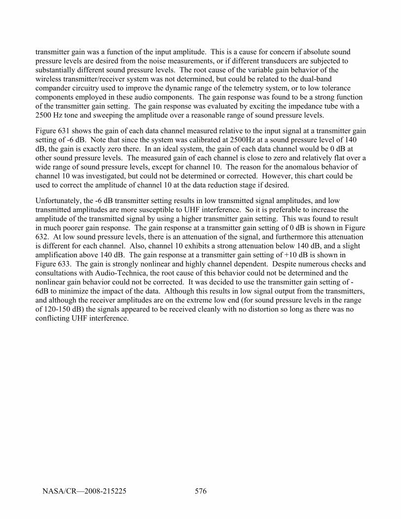
576

transmitter gain was a function of the input amplitude. This is a cause for concern if absolute sound pressure levels are desired from the noise measurements, or if different transducers are subjected to substantially different sound pressure levels. The root cause of the variable gain behavior of the wireless transmitter/receiver system was not determined, but could be related to the dual-band compander circuitry used to improve the dynamic range of the telemetry system, or to low tolerance components employed in these audio components. The gain response was found to be a strong function of the transmitter gain setting. The gain response was evaluated by exciting the impedance tube with a 2500 Hz tone and sweeping the amplitude over a reasonable range of sound pressure levels.

Figure 631 shows the gain of each data channel measured relative to the input signal at a transmitter gain setting of -6 dB. Note that since the system was calibrated at 2500Hz at a sound pressure level of 140 dB, the gain is exactly zero there. In an ideal system, the gain of each data channel would be 0 dB at other sound pressure levels. The measured gain of each channel is close to zero and relatively flat over a wide range of sound pressure levels, except for channel 10. The reason for the anomalous behavior of channel 10 was investigated, but could not be determined or corrected. However, this chart could be used to correct the amplitude of channel 10 at the data reduction stage if desired.

Unfortunately, the -6 dB transmitter setting results in low transmitted signal amplitudes, and low transmitted amplitudes are more susceptible to UHF interference. So it is preferable to increase the amplitude of the transmitted signal by using a higher transmitter gain setting. This was found to result in much poorer gain response. The gain response at a transmitter gain setting of 0 dB is shown in Figure 632. At low sound pressure levels, there is an attenuation of the signal, and furthermore this attenuation is different for each channel. Also, channel 10 exhibits a strong attenuation below 140 dB, and a slight amplification above 140 dB. The gain response at a transmitter gain setting of +10 dB is shown in Figure 633. The gain is strongly nonlinear and highly channel dependent. Despite numerous checks and consultations with Audio-Technica, the root cause of this behavior could not be determined and the nonlinear gain behavior could not be corrected. It was decided to use the transmitter gain setting of -6dB to minimize the impact of the data. Although this results in low signal output from the transmitters, and although the receiver amplitudes are on the extreme low end (for sound pressure levels in the range of 120-150 dB) the signals appeared to be received cleanly with no distortion so long as there was no conflicting UHF interference.

NASA/CR—2008-215225

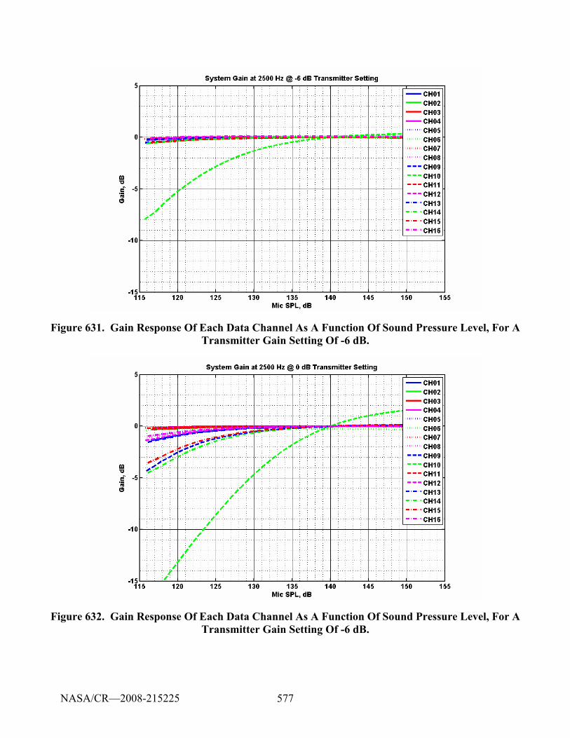
577

Figure 631. Gain Response Of Each Data Channel As A Function Of Sound Pressure Level, For A Transmitter Gain Setting Of -6 dB.

Figure 632. Gain Response Of Each Data Channel As A Function Of Sound Pressure Level, For A Transmitter Gain Setting Of -6 dB.

NASA/CR—2008-215225

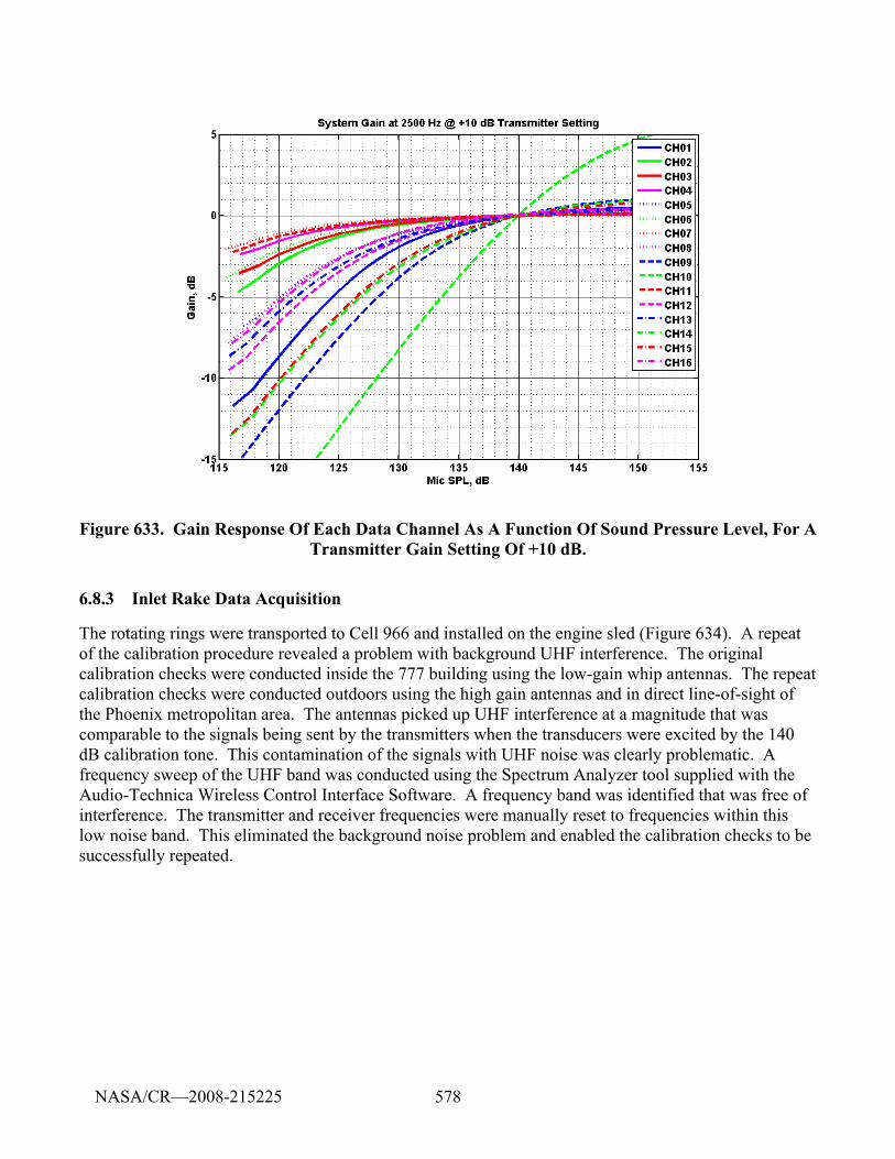
578

Figure 633. Gain Response Of Each Data Channel As A Function Of Sound Pressure Level, For A Transmitter Gain Setting Of +10 dB.

6.8.3 Inlet Rake Data Acquisition

The rotating rings were transported to Cell 966 and installed on the engine sled (Figure 634). A repeat of the calibration procedure revealed a problem with background UHF interference. The original calibration checks were conducted inside the 777 building using the low-gain whip antennas. The repeat calibration checks were conducted outdoors using the high gain antennas and in direct line-of-sight of the Phoenix metropolitan area. The antennas picked up UHF interference at a magnitude that was comparable to the signals being sent by the transmitters when the transducers were excited by the 140 dB calibration tone. This contamination of the signals with UHF noise was clearly problematic. A frequency sweep of the UHF band was conducted using the Spectrum Analyzer tool supplied with the Audio-Technica Wireless Control Interface Software. A frequency band was identified that was free of interference. The transmitter and receiver frequencies were manually reset to frequencies within this low noise band. This eliminated the background noise problem and enabled the calibration checks to be successfully repeated.

NASA/CR—2008-215225

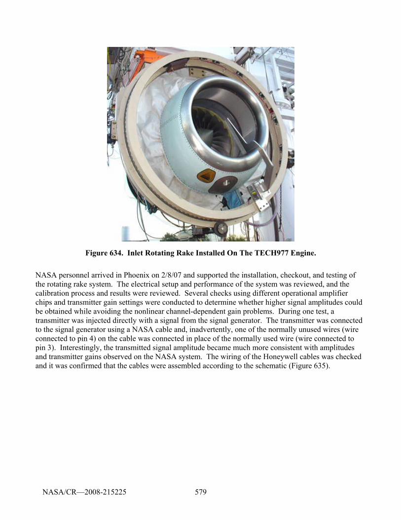
579

Figure 634. Inlet Rotating Rake Installed On The TECH977 Engine.

NASA personnel arrived in Phoenix on 2/8/07 and supported the installation, checkout, and testing of the rotating rake system. The electrical setup and performance of the system was reviewed, and the calibration process and results were reviewed. Several checks using different operational amplifier chips and transmitter gain settings were conducted to determine whether higher signal amplitudes could be obtained while avoiding the nonlinear channel-dependent gain problems. During one test, a transmitter was injected directly with a signal from the signal generator. The transmitter was connected to the signal generator using a NASA cable and, inadvertently, one of the normally unused wires (wire connected to pin 4) on the cable was connected in place of the normally used wire (wire connected to pin 3). Interestingly, the transmitted signal amplitude became much more consistent with amplitudes and transmitter gains observed on the NASA system. The wiring of the Honeywell cables was checked and it was confirmed that the cables were assembled according to the schematic (Figure 635).

NASA/CR—2008-215225

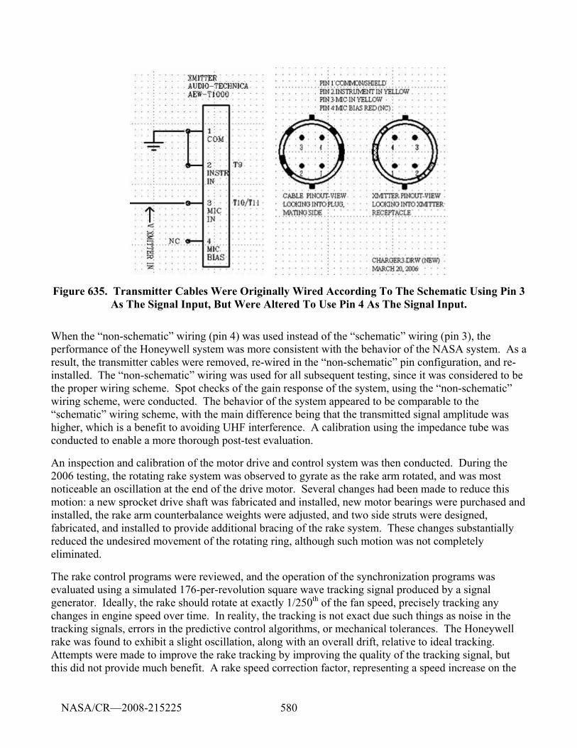
580

Figure 635. Transmitter Cables Were Originally Wired According To The Schematic Using Pin 3 As The Signal Input, But Were Altered To Use Pin 4 As The Signal Input.

When the “non-schematic” wiring (pin 4) was used instead of the “schematic” wiring (pin 3), the performance of the Honeywell system was more consistent with the behavior of the NASA system. As a result, the transmitter cables were removed, re-wired in the “non-schematic” pin configuration, and re-installed. The “non-schematic” wiring was used for all subsequent testing, since it was considered to be the proper wiring scheme. Spot checks of the gain response of the system, using the “non-schematic” wiring scheme, were conducted. The behavior of the system appeared to be comparable to the “schematic” wiring scheme, with the main difference being that the transmitted signal amplitude was higher, which is a benefit to avoiding UHF interference. A calibration using the impedance tube was conducted to enable a more thorough post-test evaluation.

An inspection and calibration of the motor drive and control system was then conducted. During the 2006 testing, the rotating rake system was observed to gyrate as the rake arm rotated, and was most noticeable an oscillation at the end of the drive motor. Several changes had been made to reduce this motion: a new sprocket drive shaft was fabricated and installed, new motor bearings were purchased and installed, the rake arm counterbalance weights were adjusted, and two side struts were designed, fabricated, and installed to provide additional bracing of the rake system. These changes substantially reduced the undesired movement of the rotating ring, although such motion was not completely eliminated.

The rake control programs were reviewed, and the operation of the synchronization programs was evaluated using a simulated 176-per-revolution square wave tracking signal produced by a signal generator. Ideally, the rake should rotate at exactly 1/250th of the fan speed, precisely tracking any changes in engine speed over time. In reality, the tracking is not exact due such things as noise in the tracking signals, errors in the predictive control algorithms, or mechanical tolerances. The Honeywell rake was found to exhibit a slight oscillation, along with an overall drift, relative to ideal tracking. Attempts were made to improve the rake tracking by improving the quality of the tracking signal, but this did not provide much benefit. A rake speed correction factor, representing a speed increase on the

NASA/CR—2008-215225

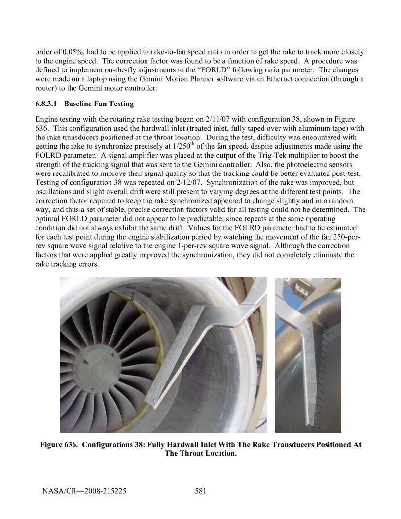
581

order of 0.05%, had to be applied to rake-to-fan speed ratio in order to get the rake to track more closely to the engine speed. The correction factor was found to be a function of rake speed. A procedure was defined to implement on-the-fly adjustments to the “FORLD” following ratio parameter. The changes were made on a laptop using the Gemini Motion Planner software via an Ethernet connection (through a router) to the Gemini motor controller.

6.8.3.1 Baseline Fan Testing

Engine testing with the rotating rake testing began on 2/11/07 with configuration 38, shown in Figure 636. This configuration used the hardwall inlet (treated inlet, fully taped over with aluminum tape) with the rake transducers positioned at the throat location. During the test, difficulty was encountered with getting the rake to synchronize precisely at 1/250th of the fan speed, despite adjustments made using the FOLRD parameter. A signal amplifier was placed at the output of the Trig-Tek multiplier to boost the strength of the tracking signal that was sent to the Gemini controller. Also, the photoelectric sensors were recalibrated to improve their signal quality so that the tracking could be better evaluated post-test. Testing of configuration 38 was repeated on 2/12/07. Synchronization of the rake was improved, but oscillations and slight overall drift were still present to varying degrees at the different test points. The correction factor required to keep the rake synchronized appeared to change slightly and in a random way, and thus a set of stable, precise correction factors valid for all testing could not be determined. The optimal FORLD parameter did not appear to be predictable, since repeats at the same operating condition did not always exhibit the same drift. Values for the FOLRD parameter had to be estimated for each test point during the engine stabilization period by watching the movement of the fan 250-per-rev square wave signal relative to the engine 1-per-rev square wave signal. Although the correction factors that were applied greatly improved the synchronization, they did not completely eliminate the rake tracking errors.

Figure 636. Configurations 38: Fully Hardwall Inlet With The Rake Transducers Positioned At The Throat Location.

NASA/CR—2008-215225

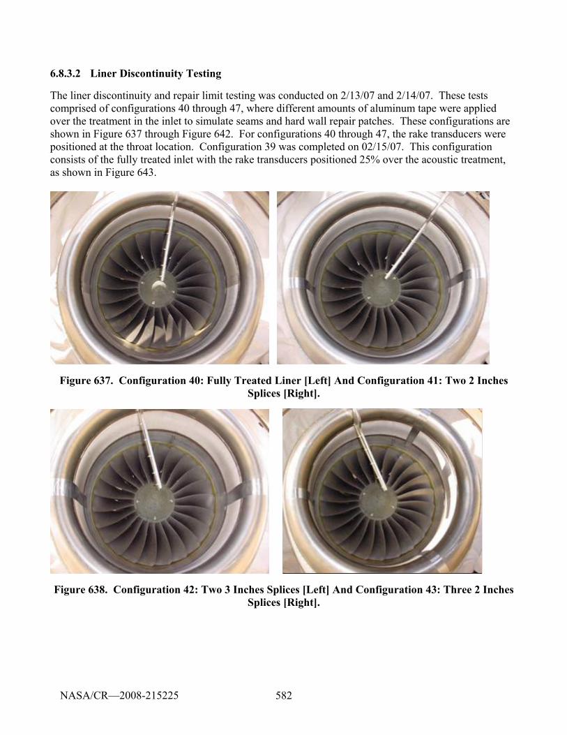
582

6.8.3.2 Liner Discontinuity Testing

The liner discontinuity and repair limit testing was conducted on 2/13/07 and 2/14/07. These tests comprised of configurations 40 through 47, where different amounts of aluminum tape were applied over the treatment in the inlet to simulate seams and hard wall repair patches. These configurations are shown in Figure 637 through Figure 642. For configurations 40 through 47, the rake transducers were positioned at the throat location. Configuration 39 was completed on 02/15/07. This configuration consists of the fully treated inlet with the rake transducers positioned 25% over the acoustic treatment, as shown in Figure 643.

Figure 637. Configuration 40: Fully Treated Liner [Left] And Configuration 41: Two 2 Inches Splices [Right].

Figure 638. Configuration 42: Two 3 Inches Splices [Left] And Configuration 43: Three 2 Inches Splices [Right].

NASA/CR—2008-215225

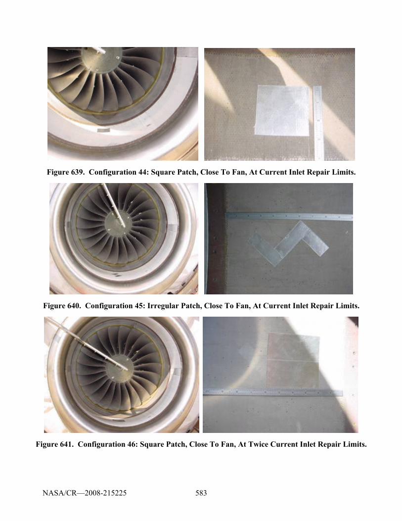
583

Figure 639. Configuration 44: Square Patch, Close To Fan, At Current Inlet Repair Limits.

Figure 640. Configuration 45: Irregular Patch, Close To Fan, At Current Inlet Repair Limits.

Figure 641. Configuration 46: Square Patch, Close To Fan, At Twice Current Inlet Repair Limits.

NASA/CR—2008-215225

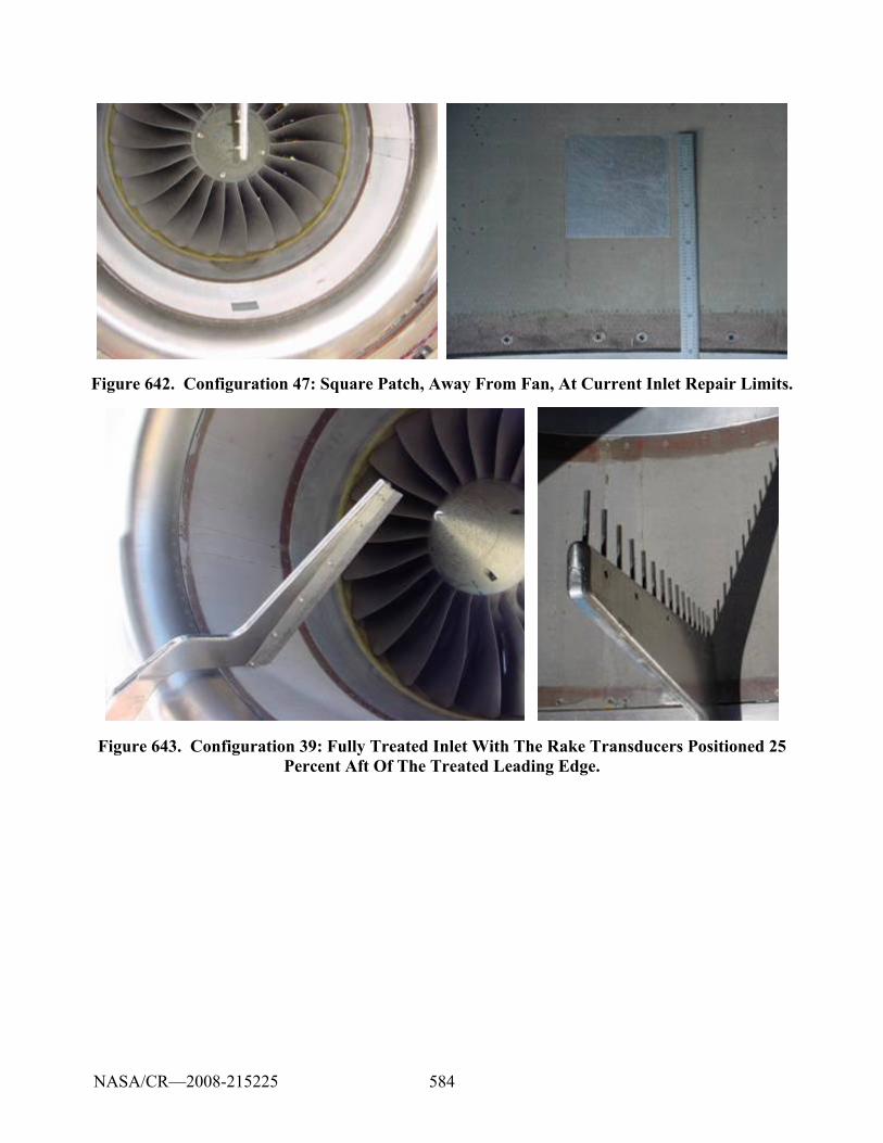
584

Figure 642. Configuration 47: Square Patch, Away From Fan, At Current Inlet Repair Limits.

Figure 643. Configuration 39: Fully Treated Inlet With The Rake Transducers Positioned 25 Percent Aft Of The Treated Leading Edge.

NASA/CR—2008-215225

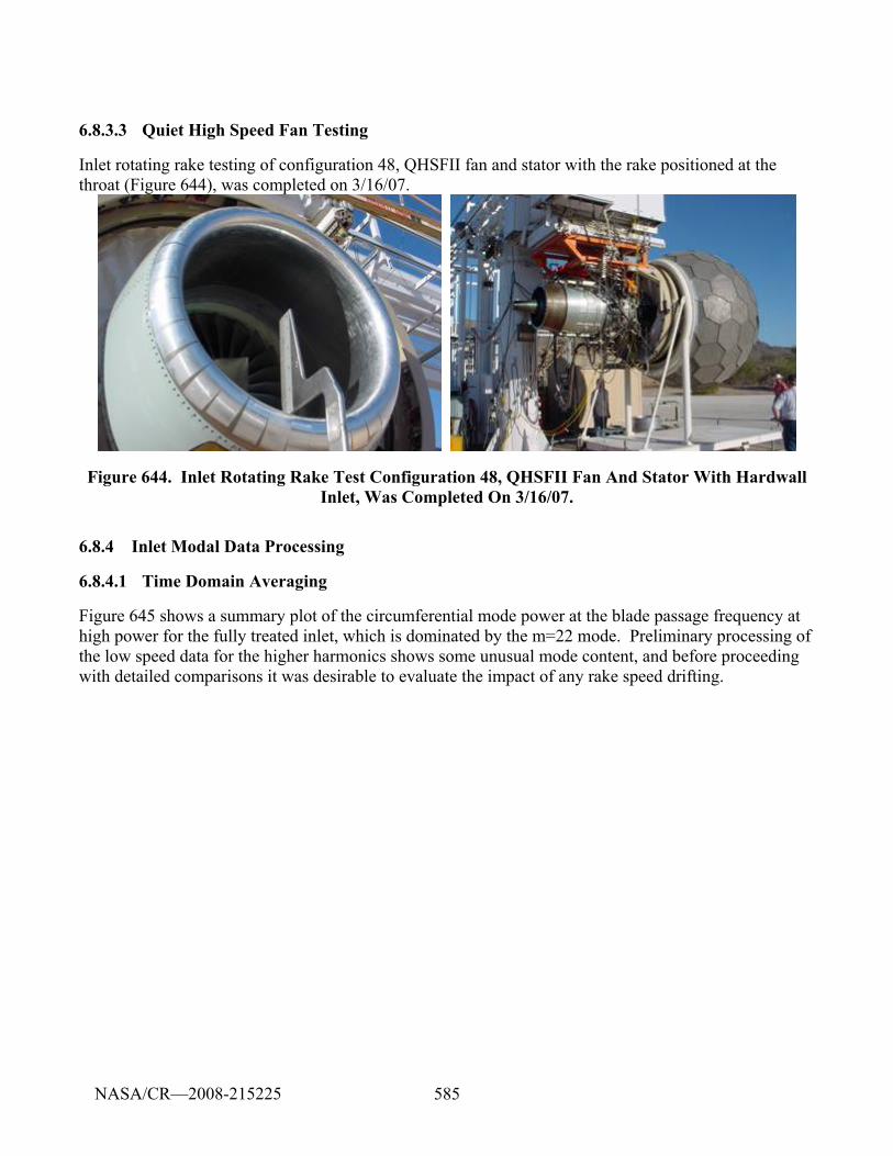
585

6.8.3.3 Quiet High Speed Fan Testing

Inlet rotating rake testing of configuration 48, QHSFII fan and stator with the rake positioned at the throat (Figure 644), was completed on 3/16/07.

Figure 644. Inlet Rotating Rake Test Configuration 48, QHSFII Fan And Stator With Hardwall Inlet, Was Completed On 3/16/07.

6.8.4 Inlet Modal Data Processing

6.8.4.1 Time Domain Averaging

Figure 645 shows a summary plot of the circumferential mode power at the blade passage frequency at high power for the fully treated inlet, which is dominated by the m=22 mode. Preliminary processing of the low speed data for the higher harmonics shows some unusual mode content, and before proceeding with detailed comparisons it was desirable to evaluate the impact of any rake speed drifting.

NASA/CR—2008-215225

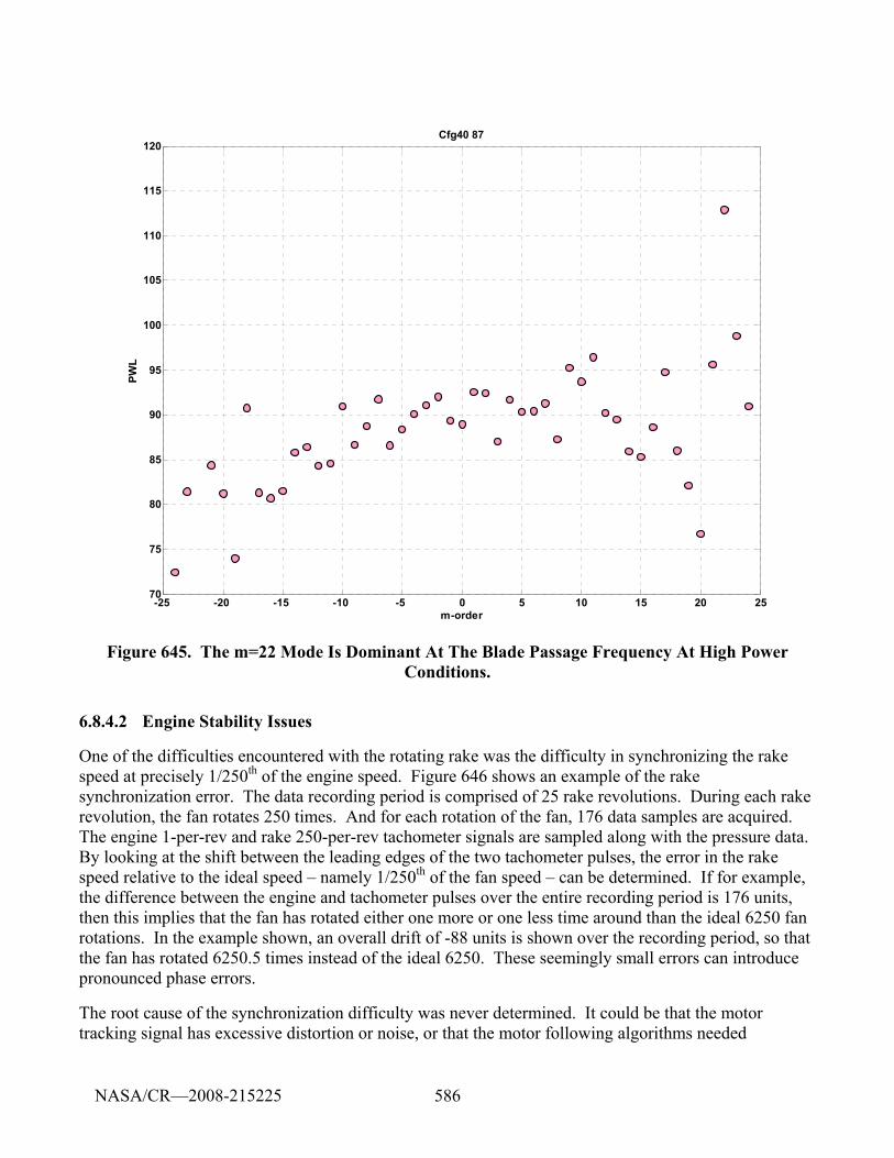
586

-25 -20 -15 -10 -5 0 5 10 15 20 2570

75

80

85

90

95

100

105

110

115

120Cfg40 87

m-order

PWL

Figure 645. The m=22 Mode Is Dominant At The Blade Passage Frequency At High Power Conditions.

6.8.4.2 Engine Stability Issues

One of the difficulties encountered with the rotating rake was the difficulty in synchronizing the rake speed at precisely 1/250th of the engine speed. Figure 646 shows an example of the rake synchronization error. The data recording period is comprised of 25 rake revolutions. During each rake revolution, the fan rotates 250 times. And for each rotation of the fan, 176 data samples are acquired. The engine 1-per-rev and rake 250-per-rev tachometer signals are sampled along with the pressure data. By looking at the shift between the leading edges of the two tachometer pulses, the error in the rake speed relative to the ideal speed – namely 1/250th of the fan speed – can be determined. If for example, the difference between the engine and tachometer pulses over the entire recording period is 176 units, then this implies that the fan has rotated either one more or one less time around than the ideal 6250 fan rotations. In the example shown, an overall drift of -88 units is shown over the recording period, so that the fan has rotated 6250.5 times instead of the ideal 6250. These seemingly small errors can introduce pronounced phase errors.

The root cause of the synchronization difficulty was never determined. It could be that the motor tracking signal has excessive distortion or noise, or that the motor following algorithms needed

NASA/CR—2008-215225

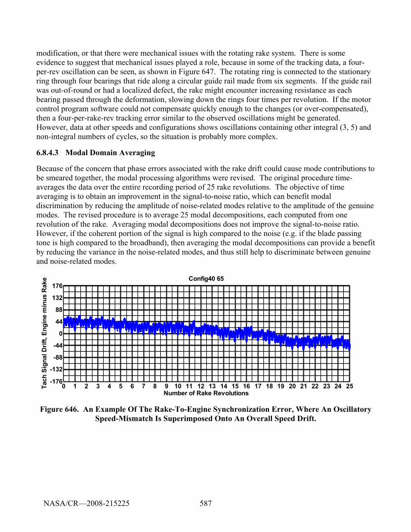
587

modification, or that there were mechanical issues with the rotating rake system. There is some evidence to suggest that mechanical issues played a role, because in some of the tracking data, a four-per-rev oscillation can be seen, as shown in Figure 647. The rotating ring is connected to the stationary ring through four bearings that ride along a circular guide rail made from six segments. If the guide rail was out-of-round or had a localized defect, the rake might encounter increasing resistance as each bearing passed through the deformation, slowing down the rings four times per revolution. If the motor control program software could not compensate quickly enough to the changes (or over-compensated), then a four-per-rake-rev tracking error similar to the observed oscillations might be generated. However, data at other speeds and configurations shows oscillations containing other integral (3, 5) and non-integral numbers of cycles, so the situation is probably more complex.

6.8.4.3 Modal Domain Averaging

Because of the concern that phase errors associated with the rake drift could cause mode contributions to be smeared together, the modal processing algorithms were revised. The original procedure time-averages the data over the entire recording period of 25 rake revolutions. The objective of time averaging is to obtain an improvement in the signal-to-noise ratio, which can benefit modal discrimination by reducing the amplitude of noise-related modes relative to the amplitude of the genuine modes. The revised procedure is to average 25 modal decompositions, each computed from one revolution of the rake. Averaging modal decompositions does not improve the signal-to-noise ratio. However, if the coherent portion of the signal is high compared to the noise (e.g. if the blade passing tone is high compared to the broadband), then averaging the modal decompositions can provide a benefit by reducing the variance in the noise-related modes, and thus still help to discriminate between genuine and noise-related modes.

Figure 646. An Example Of The Rake-To-Engine Synchronization Error, Where An Oscillatory Speed-Mismatch Is Superimposed Onto An Overall Speed Drift.

0 1 2 3 4 5 6 7 8 9 10 11 12 13 14 15 16 17 18 19 20 21 22 23 24 25-176

-132

-88

-44

0

44

88

132

176

Tach

Sig

nal D

rift,

Engi

ne m

inus

Rak

e

Number of Rake Revolutions

Config40 65

NASA/CR—2008-215225

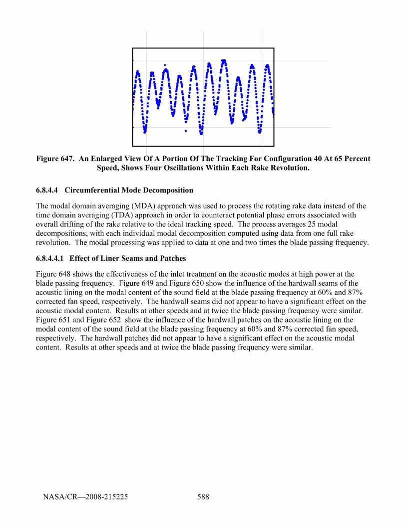
588

Figure 647. An Enlarged View Of A Portion Of The Tracking For Configuration 40 At 65 Percent Speed, Shows Four Oscillations Within Each Rake Revolution.

6.8.4.4 Circumferential Mode Decomposition

The modal domain averaging (MDA) approach was used to process the rotating rake data instead of the time domain averaging (TDA) approach in order to counteract potential phase errors associated with overall drifting of the rake relative to the ideal tracking speed. The process averages 25 modal decompositions, with each individual modal decomposition computed using data from one full rake revolution. The modal processing was applied to data at one and two times the blade passing frequency.

6.8.4.4.1 Effect of Liner Seams and Patches

Figure 648 shows the effectiveness of the inlet treatment on the acoustic modes at high power at the blade passing frequency. Figure 649 and Figure 650 show the influence of the hardwall seams of the acoustic lining on the modal content of the sound field at the blade passing frequency at 60% and 87% corrected fan speed, respectively. The hardwall seams did not appear to have a significant effect on the acoustic modal content. Results at other speeds and at twice the blade passing frequency were similar. Figure 651 and Figure 652 show the influence of the hardwall patches on the acoustic lining on the modal content of the sound field at the blade passing frequency at 60% and 87% corrected fan speed, respectively. The hardwall patches did not appear to have a significant effect on the acoustic modal content. Results at other speeds and at twice the blade passing frequency were similar.

NASA/CR—2008-215225

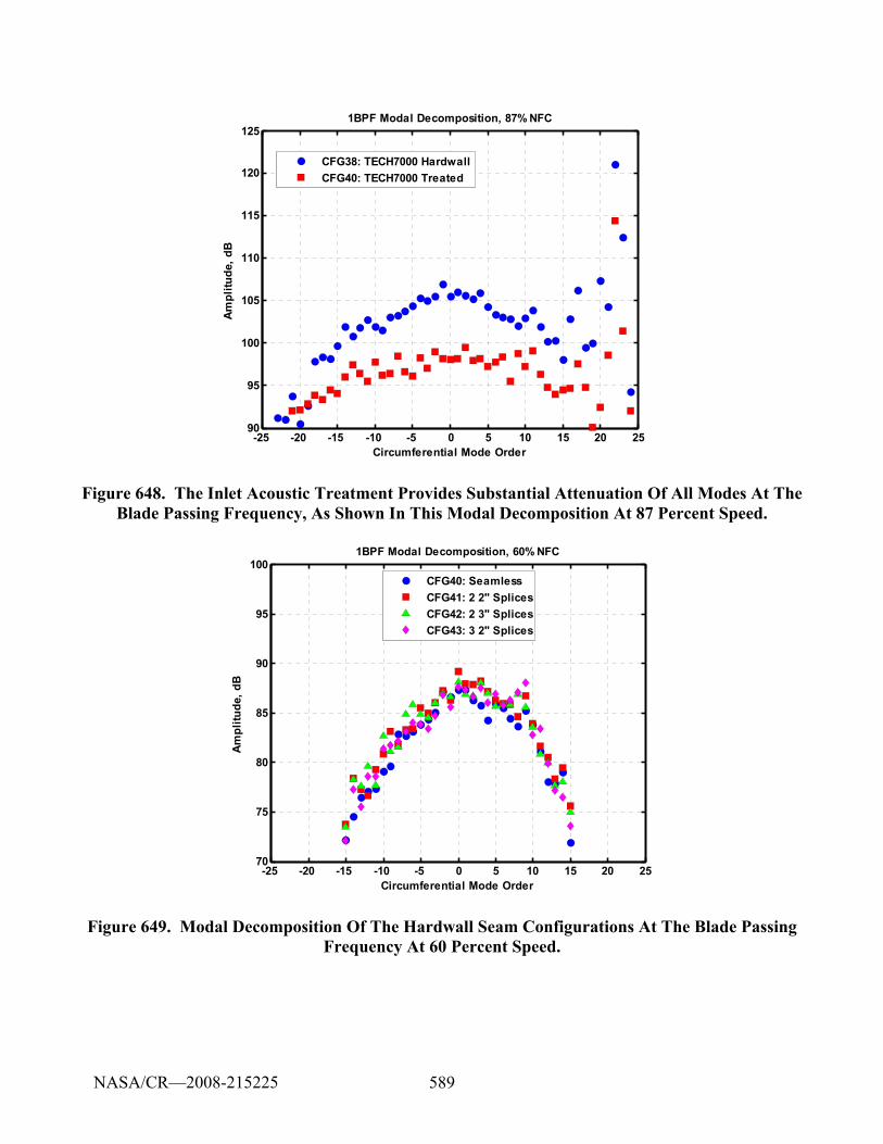
589

-25 -20 -15 -10 -5 0 5 10 15 20 2590

95

100

105

110

115

120

1251BPF Modal Decomposition, 87% NFC

Circumferential Mode Order

Ampl

itude

, dB

CFG38: TECH7000 HardwallCFG40: TECH7000 Treated

Figure 648. The Inlet Acoustic Treatment Provides Substantial Attenuation Of All Modes At The Blade Passing Frequency, As Shown In This Modal Decomposition At 87 Percent Speed.

-25 -20 -15 -10 -5 0 5 10 15 20 2570

75

80

85

90

95

100


Ampl

itude

, dB


CFG40: SeamlessCFG41: 2 2" SplicesCFG42: 2 3" SplicesCFG43: 3 2" Splices

Figure 649. Modal Decomposition Of The Hardwall Seam Configurations At The Blade Passing Frequency At 60 Percent Speed.

NASA/CR—2008-215225

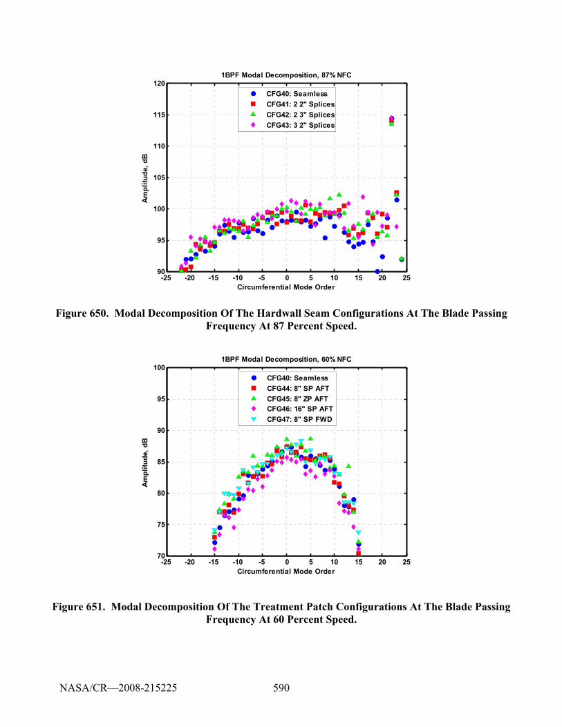
590

-25 -20 -15 -10 -5 0 5 10 15 20 2590

95

100

105

110

115

120


Ampl

itude

, dB


CFG40: SeamlessCFG41: 2 2" SplicesCFG42: 2 3" SplicesCFG43: 3 2" Splices

Figure 650. Modal Decomposition Of The Hardwall Seam Configurations At The Blade Passing Frequency At 87 Percent Speed.

-25 -20 -15 -10 -5 0 5 10 15 20 2570

75

80

85

90

95



Ampl

itude

, dB

CFG40: SeamlessCFG44: 8" SP AFTCFG45: 8" ZP AFTCFG46: 16" SP AFTCFG47: 8" SP FWD

Figure 651. Modal Decomposition Of The Treatment Patch Configurations At The Blade Passing Frequency At 60 Percent Speed.

NASA/CR—2008-215225

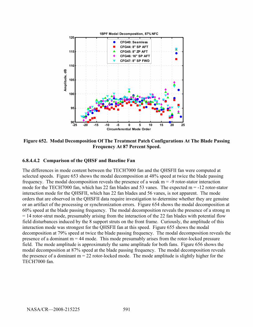
591

-25 -20 -15 -10 -5 0 5 10 15 20 2590

95

100

105

110

115



Ampl

itude

, dB

CFG40: SeamlessCFG44: 8" SP AFTCFG45: 8" ZP AFTCFG46: 16" SP AFTCFG47: 8" SP FWD

Figure 652. Modal Decomposition Of The Treatment Patch Configurations At The Blade Passing Frequency At 87 Percent Speed.

6.8.4.4.2 Comparison of the QHSF and Baseline Fan

The differences in mode content between the TECH7000 fan and the QHSFII fan were computed at selected speeds. Figure 653 shows the modal decomposition at 48% speed at twice the blade passing frequency. The modal decomposition reveals the presence of a weak m = -9 rotor-stator interaction mode for the TECH7000 fan, which has 22 fan blades and 53 vanes. The expected m = -12 rotor-stator interaction mode for the QHSFII, which has 22 fan blades and 56 vanes, is not apparent. The mode orders that are observed in the QHSFII data require investigation to determine whether they are genuine or an artifact of the processing or synchronization errors. Figure 654 shows the modal decomposition at 60% speed at the blade passing frequency. The modal decomposition reveals the presence of a strong m = 14 rotor-strut mode, presumably arising from the interaction of the 22 fan blades with potential flow field disturbances induced by the 8 support struts on the front frame. Curiously, the amplitude of this interaction mode was strongest for the QHSFII fan at this speed. Figure 655 shows the modal decomposition at 79% speed at twice the blade passing frequency. The modal decomposition reveals the presence of a dominant m = 44 mode. This mode presumably arises from the rotor-locked pressure field. The mode amplitude is approximately the same amplitude for both fans. Figure 656 shows the modal decomposition at 87% speed at the blade passing frequency. The modal decomposition reveals the presence of a dominant m = 22 rotor-locked mode. The mode amplitude is slightly higher for the TECH7000 fan.

NASA/CR—2008-215225

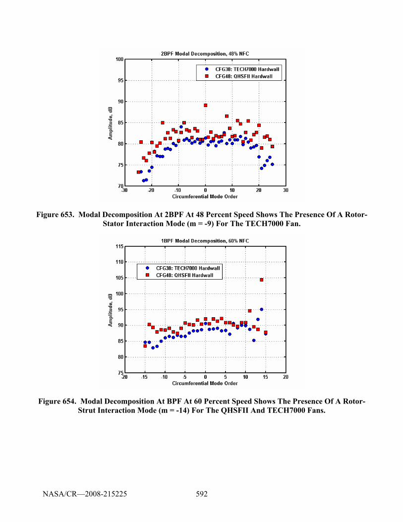
592

Figure 653. Modal Decomposition At 2BPF At 48 Percent Speed Shows The Presence Of A Rotor-Stator Interaction Mode (m = -9) For The TECH7000 Fan.

Figure 654. Modal Decomposition At BPF At 60 Percent Speed Shows The Presence Of A Rotor-Strut Interaction Mode (m = -14) For The QHSFII And TECH7000 Fans.

NASA/CR—2008-215225

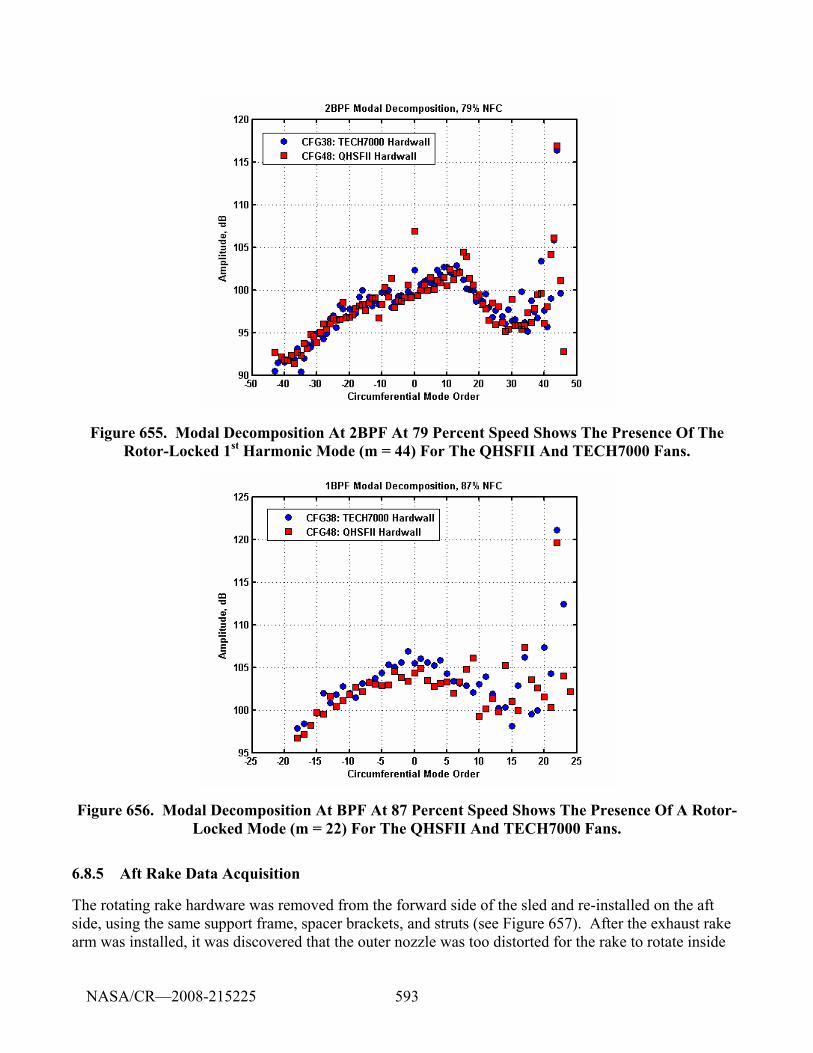
593

Figure 655. Modal Decomposition At 2BPF At 79 Percent Speed Shows The Presence Of The Rotor-Locked 1st Harmonic Mode (m = 44) For The QHSFII And TECH7000 Fans.

Figure 656. Modal Decomposition At BPF At 87 Percent Speed Shows The Presence Of A Rotor-Locked Mode (m = 22) For The QHSFII And TECH7000 Fans.

6.8.5 Aft Rake Data Acquisition

The rotating rake hardware was removed from the forward side of the sled and re-installed on the aft side, using the same support frame, spacer brackets, and struts (see Figure 657). After the exhaust rake arm was installed, it was discovered that the outer nozzle was too distorted for the rake to rotate inside

NASA/CR—2008-215225

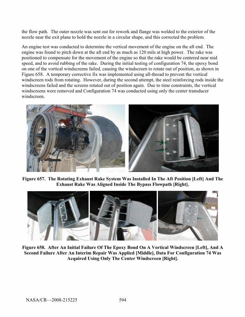
594

the flow path. The outer nozzle was sent out for rework and flange was welded to the exterior of the nozzle near the exit plane to hold the nozzle in a circular shape, and this corrected the problem.

An engine test was conducted to determine the vertical movement of the engine on the aft end. The engine was found to pitch down at the aft end by as much as 120 mils at high power. The rake was positioned to compensate for the movement of the engine so that the rake would be centered near mid speed, and to avoid rubbing of the rake. During the initial testing of configuration 74, the epoxy bond on one of the vortical windscreens failed, causing the windscreen to rotate out of position, as shown in Figure 658. A temporary corrective fix was implemented using all-thread to prevent the vortical windscreen rods from rotating. However, during the second attempt, the steel reinforcing rods inside the windscreens failed and the screens rotated out of position again. Due to time constraints, the vortical windscreens were removed and Configuration 74 was conducted using only the center transducer windscreen.

Figure 657. The Rotating Exhaust Rake System Was Installed In The Aft Position [Left] And The Exhaust Rake Was Aligned Inside The Bypass Flowpath [Right].

Figure 658. After An Initial Failure Of The Epoxy Bond On A Vortical Windscreen [Left], And A Second Failure After An Interim Repair Was Applied [Middle], Data For Configuration 74 Was

Acquired Using Only The Center Windscreen [Right].

NASA/CR—2008-215225

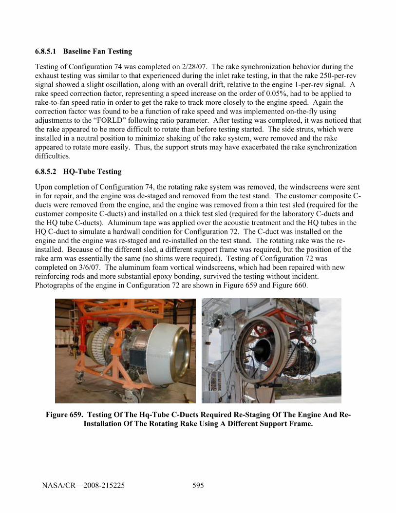
595

6.8.5.1 Baseline Fan Testing

Testing of Configuration 74 was completed on 2/28/07. The rake synchronization behavior during the exhaust testing was similar to that experienced during the inlet rake testing, in that the rake 250-per-rev signal showed a slight oscillation, along with an overall drift, relative to the engine 1-per-rev signal. A rake speed correction factor, representing a speed increase on the order of 0.05%, had to be applied to rake-to-fan speed ratio in order to get the rake to track more closely to the engine speed. Again the correction factor was found to be a function of rake speed and was implemented on-the-fly using adjustments to the “FORLD” following ratio parameter. After testing was completed, it was noticed that the rake appeared to be more difficult to rotate than before testing started. The side struts, which were installed in a neutral position to minimize shaking of the rake system, were removed and the rake appeared to rotate more easily. Thus, the support struts may have exacerbated the rake synchronization difficulties.

6.8.5.2 HQ-Tube Testing

Upon completion of Configuration 74, the rotating rake system was removed, the windscreens were sent in for repair, and the engine was de-staged and removed from the test stand. The customer composite C-ducts were removed from the engine, and the engine was removed from a thin test sled (required for the customer composite C-ducts) and installed on a thick test sled (required for the laboratory C-ducts and the HQ tube C-ducts). Aluminum tape was applied over the acoustic treatment and the HQ tubes in the HQ C-duct to simulate a hardwall condition for Configuration 72. The C-duct was installed on the engine and the engine was re-staged and re-installed on the test stand. The rotating rake was the re-installed. Because of the different sled, a different support frame was required, but the position of the rake arm was essentially the same (no shims were required). Testing of Configuration 72 was completed on 3/6/07. The aluminum foam vortical windscreens, which had been repaired with new reinforcing rods and more substantial epoxy bonding, survived the testing without incident. Photographs of the engine in Configuration 72 are shown in Figure 659 and Figure 660.

Figure 659. Testing Of The Hq-Tube C-Ducts Required Re-Staging Of The Engine And Re-Installation Of The Rotating Rake Using A Different Support Frame.

NASA/CR—2008-215225

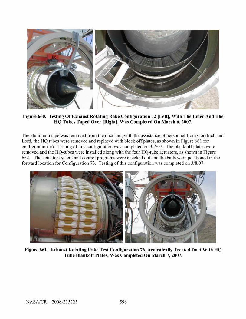
596

Figure 660. Testing Of Exhaust Rotating Rake Configuration 72 [Left], With The Liner And The HQ Tubes Taped Over [Right], Was Completed On March 6, 2007.

The aluminum tape was removed from the duct and, with the assistance of personnel from Goodrich and Lord, the HQ tubes were removed and replaced with block off plates, as shown in Figure 661 for configuration 76. Testing of this configuration was completed on 3/7/07. The blank off plates were removed and the HQ-tubes were installed along with the four HQ-tube actuators, as shown in Figure 662. The actuator system and control programs were checked out and the balls were positioned in the forward location for Configuration 73. Testing of this configuration was completed on 3/8/07.

Figure 661. Exhaust Rotating Rake Test Configuration 76, Acoustically Treated Duct With HQ Tube Blankoff Plates, Was Completed On March 7, 2007.

NASA/CR—2008-215225

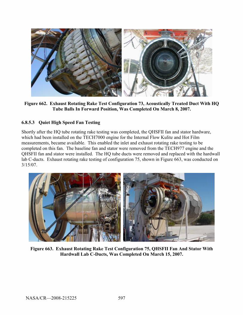
597

Figure 662. Exhaust Rotating Rake Test Configuration 73, Acoustically Treated Duct With HQ Tube Balls In Forward Position, Was Completed On March 8, 2007.

6.8.5.3 Quiet High Speed Fan Testing

Shortly after the HQ tube rotating rake testing was completed, the QHSFII fan and stator hardware, which had been installed on the TECH7000 engine for the Internal Flow Kulite and Hot Film measurements, became available. This enabled the inlet and exhaust rotating rake testing to be completed on this fan. The baseline fan and stator were removed from the TECH977 engine and the QHSFII fan and stator were installed. The HQ tube ducts were removed and replaced with the hardwall lab C-ducts. Exhaust rotating rake testing of configuration 75, shown in Figure 663, was conducted on 3/15/07.

Figure 663. Exhaust Rotating Rake Test Configuration 75, QHSFII Fan And Stator With Hardwall Lab C-Ducts, Was Completed On March 15, 2007.

NASA/CR—2008-215225

598

6.8.6 Aft Modal Data Processing

The modal domain averaging (MDA) approach was used to process the rotating rake data instead of the time domain averaging (TDA) approach in order to counteract potential phase errors associated with overall drifting of the rake relative to the ideal tracking speed. The process averages 25 modal decompositions, with each individual modal decomposition computed using data from one full rake revolution. The modal processing was applied to data at one and two times the blade passing frequency.

Initially, the exhaust rake modal decompositions were performed using all 8 microphones. However, the inner and outer microphones were apparently affected by wall turbulence and consequently the noise spectra had very high broadband noise levels. The inner microphone may have also been affected by wakes shed from the aft facing step on the inner flowpath. Processing of the modal data did not reveal much modal content, and in an attempt to improve the results it was decided to reprocess the data using the six inner microphones. This appeared to help but the modal decompositions still did not reveal much distinguishable modal content.

A natural expectation is that rotor-strut interaction modes might be visible at the blade passing frequency and rotor-stator interaction modes might be visible at twice blade-passing frequency. The hardwall configurations would likely show the most clear modal content. The TECH7000 and QHSFII rotors both have 22 blades. The front frame has 8 struts. So one might expect to see the m=14 rotor-strut interaction mode at the blade passing frequency. The TECH7000 stator has 53 vanes and the QHSFII stator has 56 vanes. So one might expect to see the m=-9 interaction mode for the TECH7000 and the m=-12 interaction mode for the QHSFII at twice the blade passing frequency. However, the presence of the duct bifurcations can significantly affect the acoustic propagation, so the presence of a clear modal structure is not guaranteed.

Figure 664 and Figure 665 show the exhaust rake modal decomposition for all the tested configurations at 48% speed and at the blade passing frequency and twice blade passing frequency, respectively. The acoustically treated duct configurations generally have lower modal amplitudes than the hardwall configurations, but the expected modal content is not present. The rotor-stator interaction mode was visible in the inlet data at twice the blade passing frequency, but it is not apparent in the exhaust. Figure 666 and Figure 667 show the exhaust rake modal decomposition for all the tested configurations at 60% speed and at the blade passing frequency and twice blade passing frequency, respectively. In the inlet, the rotor strut mode was visible at the blade passing frequency. However, it is not apparent in the exhaust. Figure 668 and Figure 669 show the exhaust rake modal decomposition for all the tested configurations at 87% speed and at the blade passing frequency and twice blade passing frequency, respectively. The modal amplitudes at the blade passing frequency appear almost random. At twice the blade passing frequency, there appears to be a strong m=-10 mode for all configurations, but the origin of this mode is unknown.

NASA/CR—2008-215225

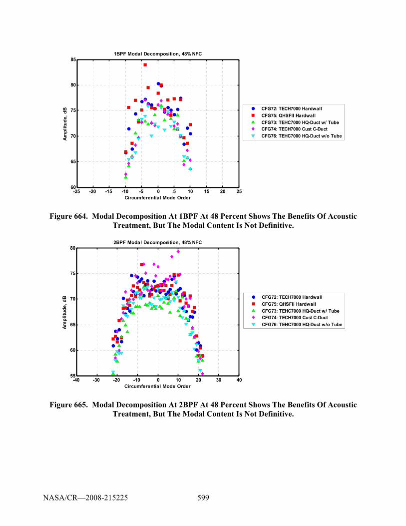
599

-25 -20 -15 -10 -5 0 5 10 15 20 2560

65

70

75

80



Ampl

itude

, dB CFG72: TECH7000 Hardwall

CFG75: QHSFII HardwallCFG73: TEHC7000 HQ-Duct w/ TubeCFG74: TECH7000 Cust C-DuctCFG76: TEHC7000 HQ-Duct w/o Tube

Figure 664. Modal Decomposition At 1BPF At 48 Percent Shows The Benefits Of Acoustic Treatment, But The Modal Content Is Not Definitive.

-40 -30 -20 -10 0 10 20 30 4055

60

65

70

75



Ampl

itude




NASA/CR—2008-215225

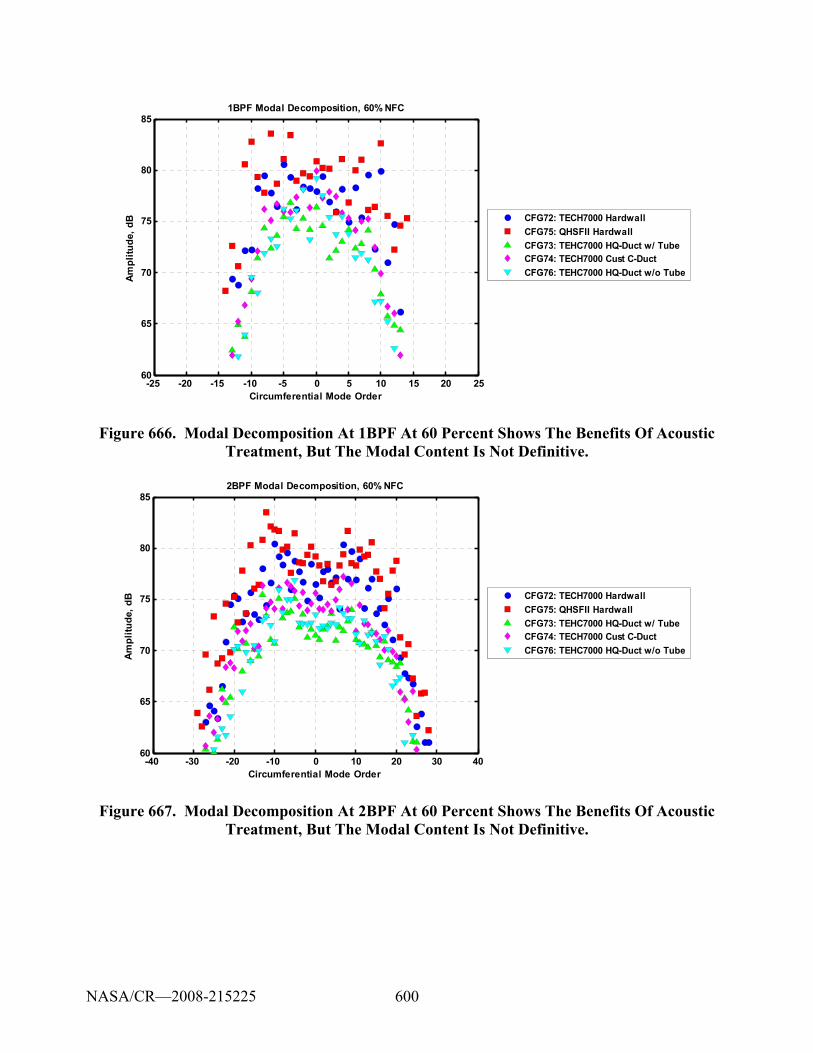
600

-25 -20 -15 -10 -5 0 5 10 15 20 2560

65

70

75

80



Ampl

itude




-40 -30 -20 -10 0 10 20 30 4060

65

70

75

80



Ampl

itude




NASA/CR—2008-215225

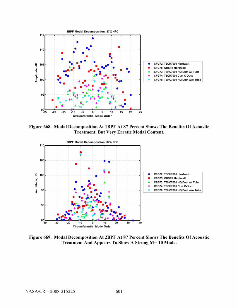
601

-25 -20 -15 -10 -5 0 5 10 15 20 2590

95

100

105

110



Ampl

itude



Figure 668. Modal Decomposition At 1BPF At 87 Percent Shows The Benefits Of Acoustic Treatment, But Very Erratic Modal Content.

-40 -30 -20 -10 0 10 20 30 4085

90

95

100

105



Ampl

itude



Figure 669. Modal Decomposition At 2BPF At 87 Percent Shows The Benefits Of Acoustic Treatment And Appears To Show A Strong M=-10 Mode.

NASA/CR—2008-215225

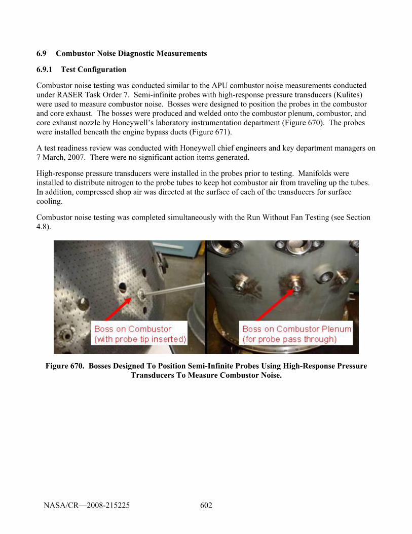
602


6.9.1 Test Configuration

Combustor noise testing was conducted similar to the APU combustor noise measurements conducted under RASER Task Order 7. Semi-infinite probes with high-response pressure transducers (Kulites) were used to measure combustor noise. Bosses were designed to position the probes in the combustor and core exhaust. The bosses were produced and welded onto the combustor plenum, combustor, and core exhaust nozzle by Honeywell’s laboratory instrumentation department (Figure 670). The probes were installed beneath the engine bypass ducts (Figure 671).

A test readiness review was conducted with Honeywell chief engineers and key department managers on 7 March, 2007. There were no significant action items generated.

High-response pressure transducers were installed in the probes prior to testing. Manifolds were installed to distribute nitrogen to the probe tubes to keep hot combustor air from traveling up the tubes. In addition, compressed shop air was directed at the surface of each of the transducers for surface cooling.

Combustor noise testing was completed simultaneously with the Run Without Fan Testing (see Section 4.8).

Figure 670. Bosses Designed To Position Semi-Infinite Probes Using High-Response Pressure Transducers To Measure Combustor Noise.

NASA/CR—2008-215225

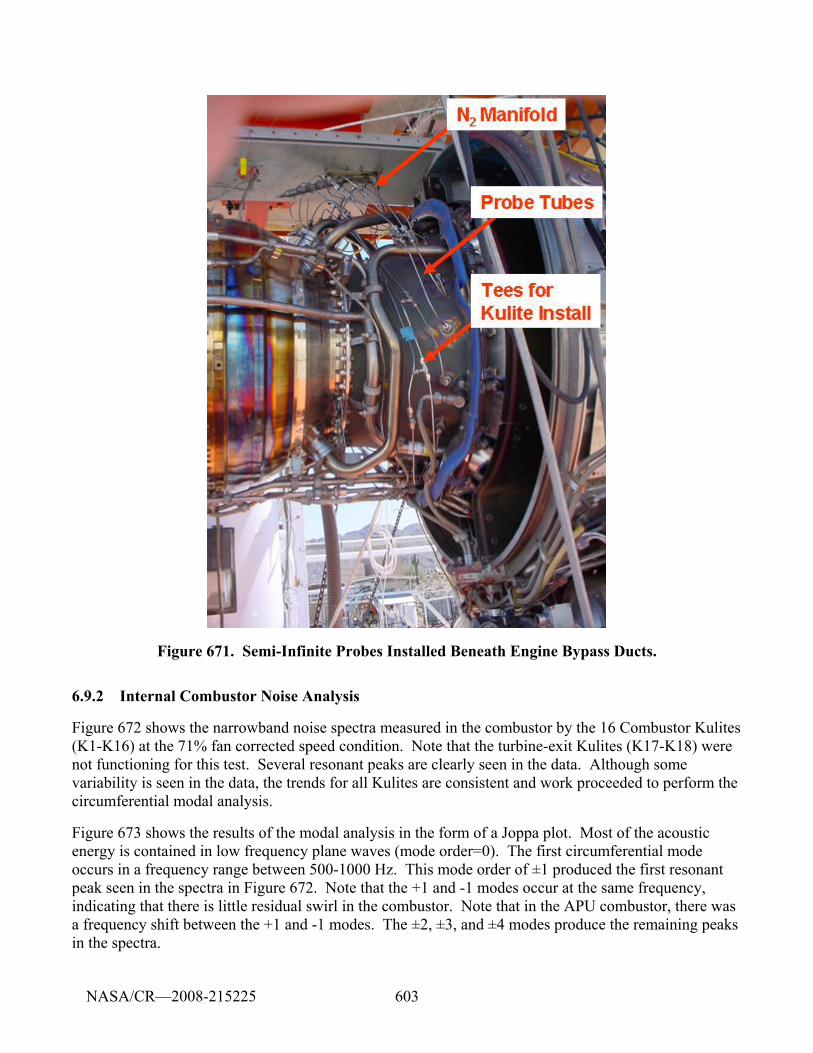
603

Figure 671. Semi-Infinite Probes Installed Beneath Engine Bypass Ducts.

6.9.2 Internal Combustor Noise Analysis

Figure 672 shows the narrowband noise spectra measured in the combustor by the 16 Combustor Kulites (K1-K16) at the 71% fan corrected speed condition. Note that the turbine-exit Kulites (K17-K18) were not functioning for this test. Several resonant peaks are clearly seen in the data. Although some variability is seen in the data, the trends for all Kulites are consistent and work proceeded to perform the circumferential modal analysis.

Figure 673 shows the results of the modal analysis in the form of a Joppa plot. Most of the acoustic energy is contained in low frequency plane waves (mode order=0). The first circumferential mode occurs in a frequency range between 500-1000 Hz. This mode order of ±1 produced the first resonant peak seen in the spectra in Figure 672. Note that the +1 and -1 modes occur at the same frequency, indicating that there is little residual swirl in the combustor. Note that in the APU combustor, there was a frequency shift between the +1 and -1 modes. The ±2, ±3, and ±4 modes produce the remaining peaks in the spectra.

NASA/CR—2008-215225

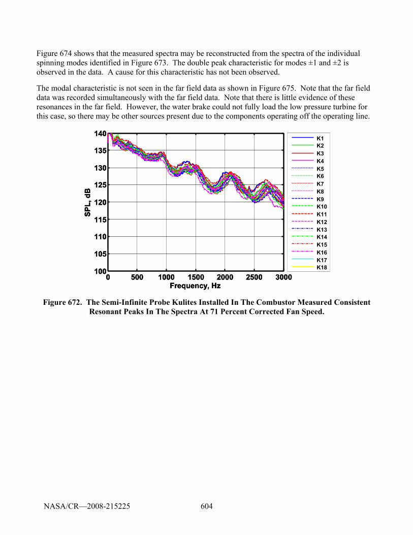
604

Figure 674 shows that the measured spectra may be reconstructed from the spectra of the individual spinning modes identified in Figure 673. The double peak characteristic for modes ±1 and ±2 is observed in the data. A cause for this characteristic has not been observed.

The modal characteristic is not seen in the far field data as shown in Figure 675. Note that the far field data was recorded simultaneously with the far field data. Note that there is little evidence of these resonances in the far field. However, the water brake could not fully load the low pressure turbine for this case, so there may be other sources present due to the components operating off the operating line.

0 500 1000 1500 2000 2500 3000100

105

110

115

120

125

130

135

140

Frequency, Hz

SPL,

dB

K1K2K3K4K5K6K7K8K9K10K11K12K13K14K15K16K17K18

0 500 1000 1500 2000 2500 3000100

105

110

115

120

125

130

135

140

Frequency, Hz

SPL,

dB

0 500 1000 1500 2000 2500 3000100

105

110

115

120

125

130

135

140

Frequency, Hz

SPL,

dB



Figure 672. The Semi-Infinite Probe Kulites Installed In The Combustor Measured Consistent Resonant Peaks In The Spectra At 71 Percent Corrected Fan Speed.

NASA/CR—2008-215225

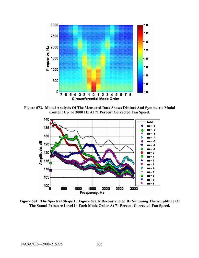
605

Figure 673. Modal Analysis Of The Measured Data Shows Distinct And Symmetric Modal Content Up To 3000 Hz At 71 Percent Corrected Fan Speed.

Figure 674. The Spectral Shape In Figure 672 Is Reconstructed By Summing The Amplitude Of The Sound Pressure Level In Each Mode Order At 71 Percent Corrected Fan Speed.

NASA/CR—2008-215225

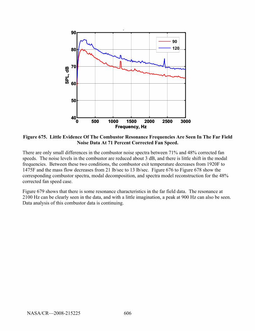
606

0 500 1000 1500 2000 2500 300040

50

60

70

80

90

Frequency, Hz

SPL,

dB

p

90120

0 500 1000 1500 2000 2500 300040

50

60

70

80

90

Frequency, Hz

SPL,

dB

p

9012090120

Figure 675. Little Evidence Of The Combustor Resonance Frequencies Are Seen In The Far Field Noise Data At 71 Percent Corrected Fan Speed.

There are only small differences in the combustor noise spectra between 71% and 48% corrected fan speeds. The noise levels in the combustor are reduced about 3 dB, and there is little shift in the modal frequencies. Between these two conditions, the combustor exit temperature decreases from 1920F to 1475F and the mass flow decreases from 21 lb/sec to 13 lb/sec. Figure 676 to Figure 678 show the corresponding combustor spectra, modal decomposition, and spectra model reconstruction for the 48% corrected fan speed case.

Figure 679 shows that there is some resonance characteristics in the far field data. The resonance at 2100 Hz can be clearly seen in the data, and with a little imagination, a peak at 900 Hz can also be seen. Data analysis of this combustor data is continuing.

NASA/CR—2008-215225

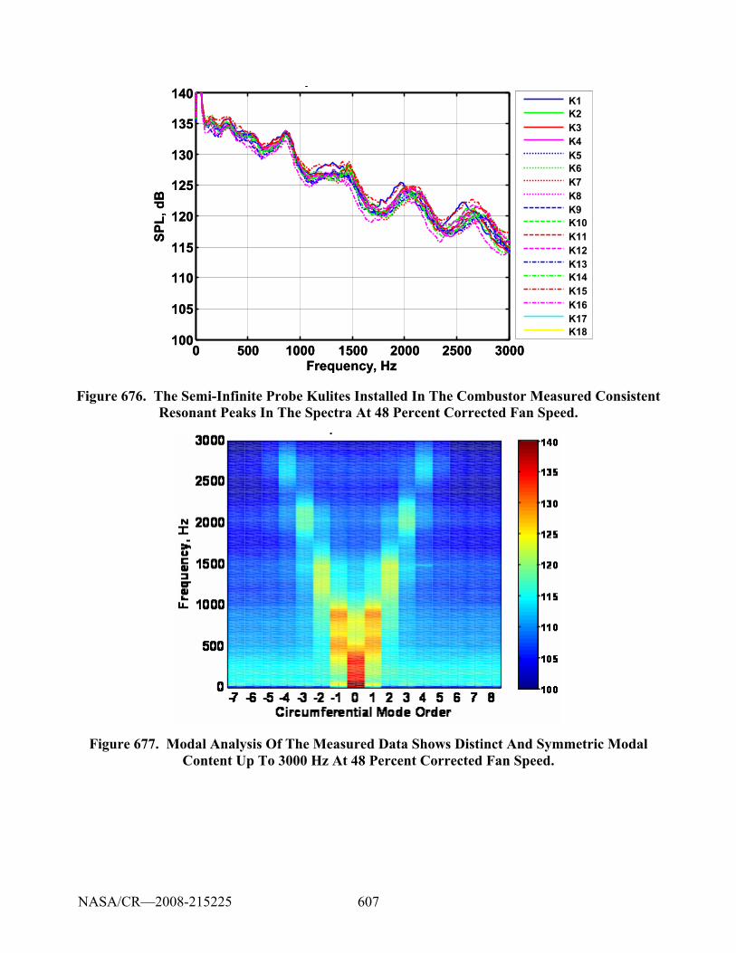
607


0 500 1000 1500 2000 2500 3000100

105

110

115

120

125

130

135

140

Frequency, Hz

SPL,

dB

pK1K2K3K4K5K6K7K8K9K10K11K12K13K14K15K16K17K18


0 500 1000 1500 2000 2500 3000100

105

110

115

120

125

130

135

140

Frequency, Hz

SPL,

dB

p

Figure 676. The Semi-Infinite Probe Kulites Installed In The Combustor Measured Consistent Resonant Peaks In The Spectra At 48 Percent Corrected Fan Speed.

Figure 677. Modal Analysis Of The Measured Data Shows Distinct And Symmetric Modal Content Up To 3000 Hz At 48 Percent Corrected Fan Speed.

NASA/CR—2008-215225

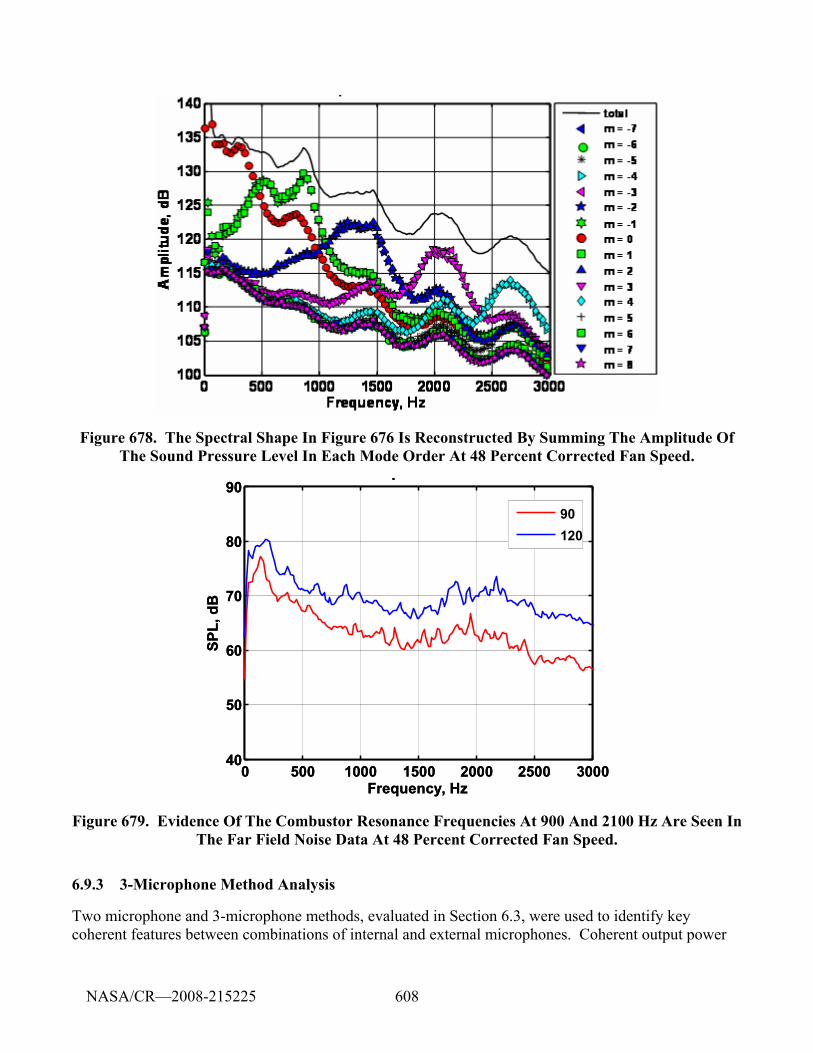
608

Figure 678. The Spectral Shape In Figure 676 Is Reconstructed By Summing The Amplitude Of The Sound Pressure Level In Each Mode Order At 48 Percent Corrected Fan Speed.

0 500 1000 1500 2000 2500 300040

50

60

70

80

90

Frequency, Hz

SPL,

dB

p

90120

0 500 1000 1500 2000 2500 300040

50

60

70

80

90

Frequency, Hz

SPL,

dB

p

9012090120

Figure 679. Evidence Of The Combustor Resonance Frequencies At 900 And 2100 Hz Are Seen In The Far Field Noise Data At 48 Percent Corrected Fan Speed.

6.9.3 3-Microphone Method Analysis

Two microphone and 3-microphone methods, evaluated in Section 6.3, were used to identify key coherent features between combinations of internal and external microphones. Coherent output power

NASA/CR—2008-215225

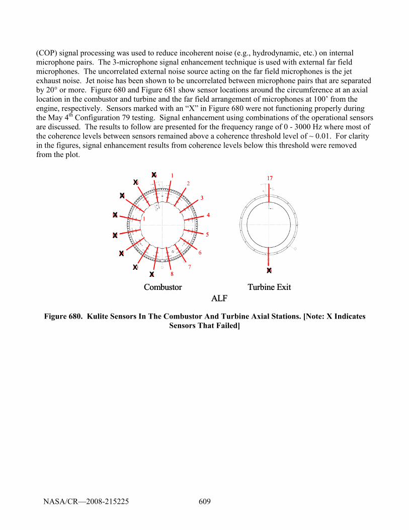
609

(COP) signal processing was used to reduce incoherent noise (e.g., hydrodynamic, etc.) on internal microphone pairs. The 3-microphone signal enhancement technique is used with external far field microphones. The uncorrelated external noise source acting on the far field microphones is the jet exhaust noise. Jet noise has been shown to be uncorrelated between microphone pairs that are separated by 20° or more. Figure 680 and Figure 681 show sensor locations around the circumference at an axial location in the combustor and turbine and the far field arrangement of microphones at 100’ from the engine, respectively. Sensors marked with an “X” in Figure 680 were not functioning properly during the May 4th Configuration 79 testing. Signal enhancement using combinations of the operational sensors are discussed. The results to follow are presented for the frequency range of 0 - 3000 Hz where most of the coherence levels between sensors remained above a coherence threshold level of ~ 0.01. For clarity in the figures, signal enhancement results from coherence levels below this threshold were removed from the plot.

ALFCombustor Turbine Exit

1 2

3

4

5

6

7 9 8

16 15

14

1 13

12

11

10

17

18 XX

X

X

X

X

XX

X

ALFCombustor Turbine Exit

1 2

3

4

5

6

7 9 8

16 15

14

1 13

12

11

10

17

18 XX

X

X

X

X

XX

X

Figure 680. Kulite Sensors In The Combustor And Turbine Axial Stations. [Note: X Indicates Sensors That Failed]

NASA/CR—2008-215225

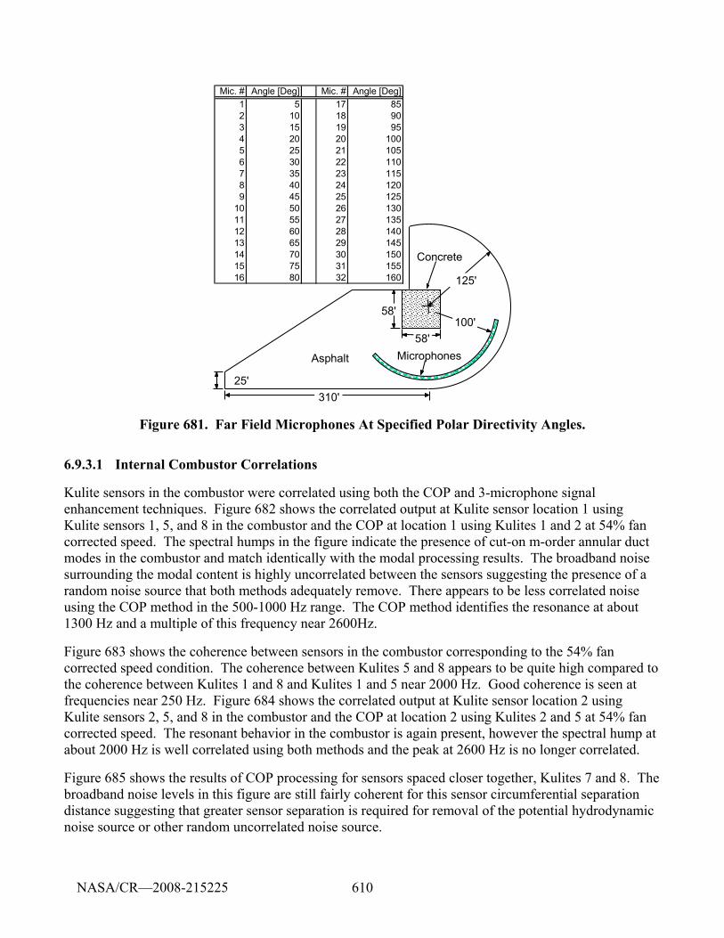
610

310'25'

58'

58'

Asphalt

125'

Concrete

100'

Microphones

Mic. # Angle [Deg] Mic. # Angle [Deg]1 5 17 852 10 18 903 15 19 954 20 20 1005 25 21 1056 30 22 1107 35 23 1158 40 24 1209 45 25 125

10 50 26 13011 55 27 13512 60 28 14013 65 29 14514 70 30 15015 75 31 15516 80 32 160

Figure 681. Far Field Microphones At Specified Polar Directivity Angles.

6.9.3.1 Internal Combustor Correlations

Kulite sensors in the combustor were correlated using both the COP and 3-microphone signal enhancement techniques. Figure 682 shows the correlated output at Kulite sensor location 1 using Kulite sensors 1, 5, and 8 in the combustor and the COP at location 1 using Kulites 1 and 2 at 54% fan corrected speed. The spectral humps in the figure indicate the presence of cut-on m-order annular duct modes in the combustor and match identically with the modal processing results. The broadband noise surrounding the modal content is highly uncorrelated between the sensors suggesting the presence of a random noise source that both methods adequately remove. There appears to be less correlated noise using the COP method in the 500-1000 Hz range. The COP method identifies the resonance at about 1300 Hz and a multiple of this frequency near 2600Hz.

Figure 683 shows the coherence between sensors in the combustor corresponding to the 54% fan corrected speed condition. The coherence between Kulites 5 and 8 appears to be quite high compared to the coherence between Kulites 1 and 8 and Kulites 1 and 5 near 2000 Hz. Good coherence is seen at frequencies near 250 Hz. Figure 684 shows the correlated output at Kulite sensor location 2 using Kulite sensors 2, 5, and 8 in the combustor and the COP at location 2 using Kulites 2 and 5 at 54% fan corrected speed. The resonant behavior in the combustor is again present, however the spectral hump at about 2000 Hz is well correlated using both methods and the peak at 2600 Hz is no longer correlated.

Figure 685 shows the results of COP processing for sensors spaced closer together, Kulites 7 and 8. The broadband noise levels in this figure are still fairly coherent for this sensor circumferential separation distance suggesting that greater sensor separation is required for removal of the potential hydrodynamic noise source or other random uncorrelated noise source.

NASA/CR—2008-215225

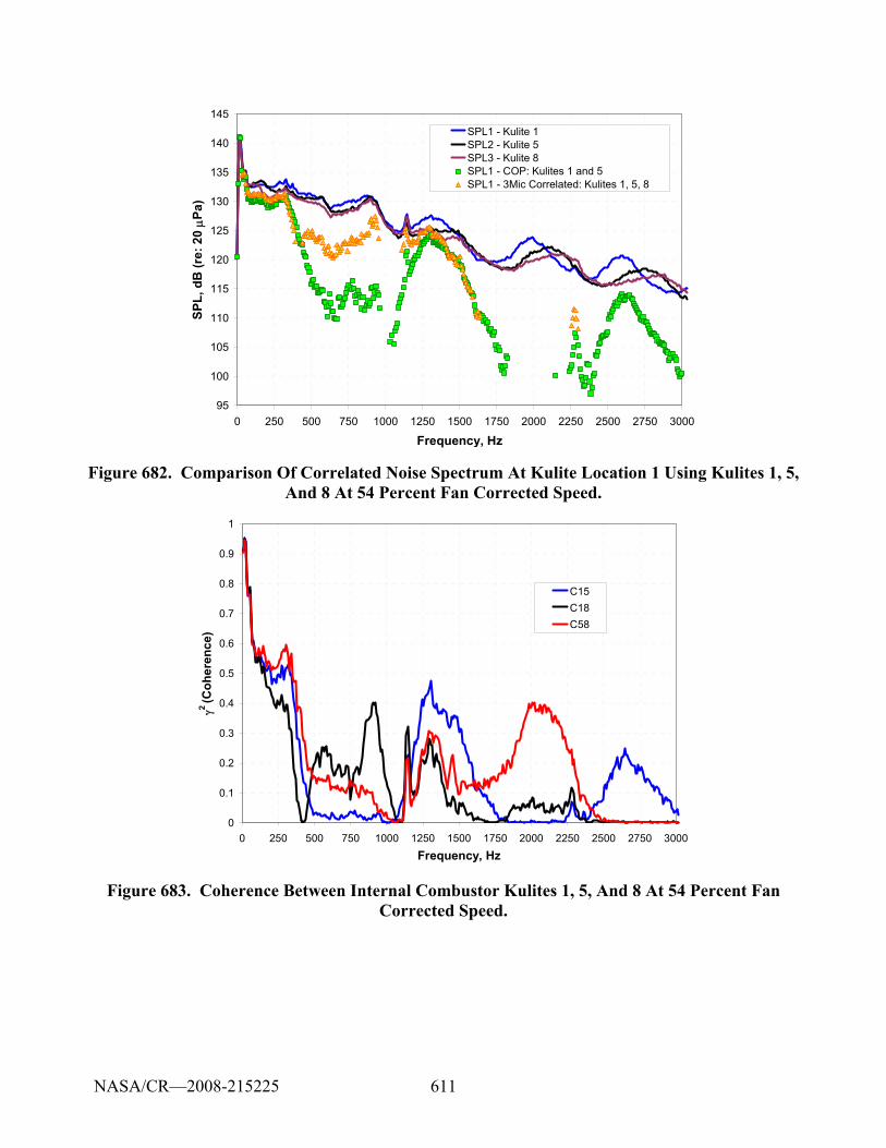
611

95

100

105

110

115

120

125

130

135

140

145

0 250 500 750 1000 1250 1500 1750 2000 2250 2500 2750 3000

Frequency, Hz

SPL,

dB

(re:

20

μPa)

SPL1 - Kulite 1SPL2 - Kulite 5SPL3 - Kulite 8SPL1 - COP: Kulites 1 and 5SPL1 - 3Mic Correlated: Kulites 1, 5, 8

Figure 682. Comparison Of Correlated Noise Spectrum At Kulite Location 1 Using Kulites 1, 5, And 8 At 54 Percent Fan Corrected Speed.

0

0.1

0.2

0.3

0.4

0.5

0.6

0.7

0.8

0.9

1

0 250 500 750 1000 1250 1500 1750 2000 2250 2500 2750 3000

Frequency, Hz

γ2 (C

oher

ence

)

C15C18C58

Figure 683. Coherence Between Internal Combustor Kulites 1, 5, And 8 At 54 Percent Fan Corrected Speed.

NASA/CR—2008-215225

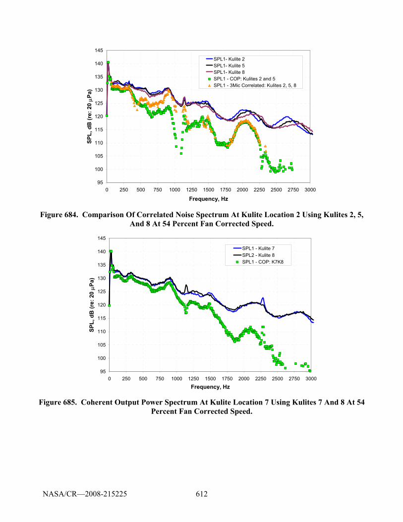
612

95

100

105

110

115

120

125

130

135

140

145

0 250 500 750 1000 1250 1500 1750 2000 2250 2500 2750 3000

Frequency, Hz

SPL,

dB

(re:

20

μPa)

SPL1- Kulite 2SPL1- Kulite 5SPL1- Kulite 8SPL1 - COP: Kulites 2 and 5SPL1 - 3Mic Correlated: Kulites 2, 5, 8

Figure 684. Comparison Of Correlated Noise Spectrum At Kulite Location 2 Using Kulites 2, 5, And 8 At 54 Percent Fan Corrected Speed.

95

100

105

110

115

120

125

130

135

140

145

0 250 500 750 1000 1250 1500 1750 2000 2250 2500 2750 3000

Frequency, Hz

SPL,

dB

(re:

20

μPa)

SPL1 - Kulite 7SPL2 - Kulite 8SPL1 - COP: K7K8

Figure 685. Coherent Output Power Spectrum At Kulite Location 7 Using Kulites 7 And 8 At 54 Percent Fan Corrected Speed.

NASA/CR—2008-215225

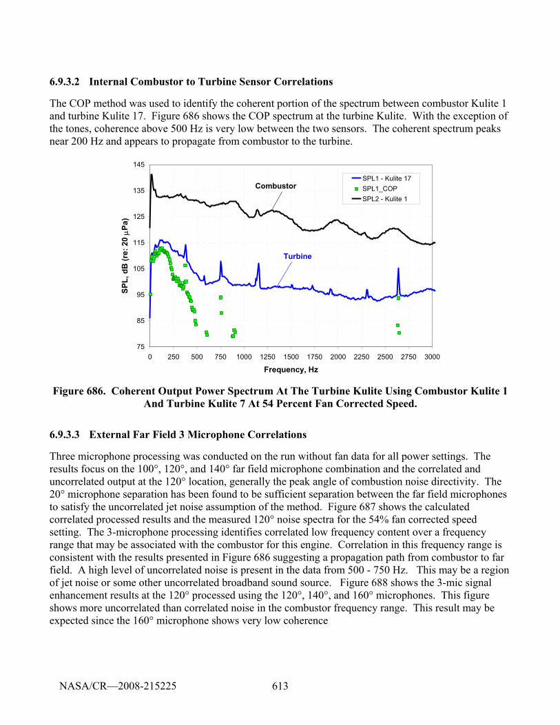
613

6.9.3.2 Internal Combustor to Turbine Sensor Correlations

The COP method was used to identify the coherent portion of the spectrum between combustor Kulite 1 and turbine Kulite 17. Figure 686 shows the COP spectrum at the turbine Kulite. With the exception of the tones, coherence above 500 Hz is very low between the two sensors. The coherent spectrum peaks near 200 Hz and appears to propagate from combustor to the turbine.

75

85

95

105

115

125

135

145

0 250 500 750 1000 1250 1500 1750 2000 2250 2500 2750 3000

Frequency, Hz

SPL,

dB

(re:

20

μPa)

SPL1 - Kulite 17SPL1_COPSPL2 - Kulite 1

Combustor

Turbine

Figure 686. Coherent Output Power Spectrum At The Turbine Kulite Using Combustor Kulite 1 And Turbine Kulite 7 At 54 Percent Fan Corrected Speed.

6.9.3.3 External Far Field 3 Microphone Correlations

Three microphone processing was conducted on the run without fan data for all power settings. The results focus on the 100°, 120°, and 140° far field microphone combination and the correlated and uncorrelated output at the 120° location, generally the peak angle of combustion noise directivity. The 20° microphone separation has been found to be sufficient separation between the far field microphones to satisfy the uncorrelated jet noise assumption of the method. Figure 687 shows the calculated correlated processed results and the measured 120° noise spectra for the 54% fan corrected speed setting. The 3-microphone processing identifies correlated low frequency content over a frequency range that may be associated with the combustor for this engine. Correlation in this frequency range is consistent with the results presented in Figure 686 suggesting a propagation path from combustor to far field. A high level of uncorrelated noise is present in the data from 500 - 750 Hz. This may be a region of jet noise or some other uncorrelated broadband sound source. Figure 688 shows the 3-mic signal enhancement results at the 120° processed using the 120°, 140°, and 160° microphones. This figure shows more uncorrelated than correlated noise in the combustor frequency range. This result may be expected since the 160° microphone shows very low coherence

NASA/CR—2008-215225

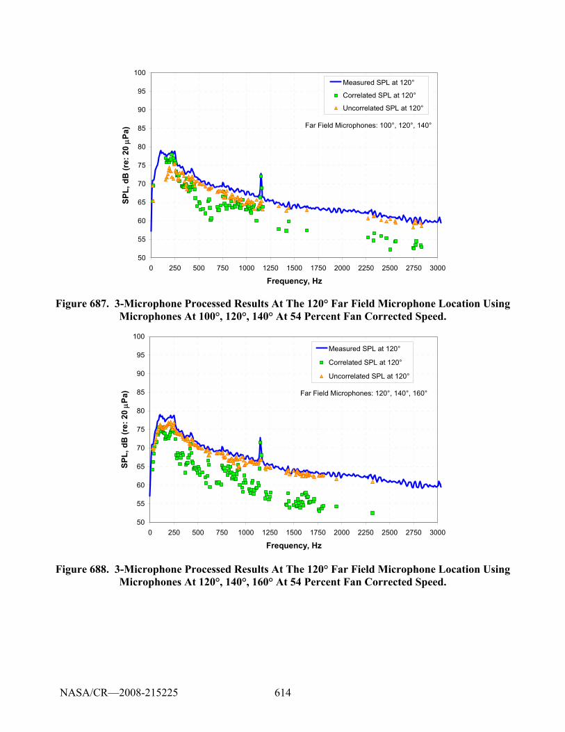
614

50

55

60

65

70

75

80

85

90

95

100

0 250 500 750 1000 1250 1500 1750 2000 2250 2500 2750 3000

Frequency, Hz

SPL,

dB

(re:

20

μPa)

Measured SPL at 120°

Correlated SPL at 120°

Uncorrelated SPL at 120°

Far Field Microphones: 100°, 120°, 140°

Figure 687. 3-Microphone Processed Results At The 120° Far Field Microphone Location Using Microphones At 100°, 120°, 140° At 54 Percent Fan Corrected Speed.

50

55

60

65

70

75

80

85

90

95

100

0 250 500 750 1000 1250 1500 1750 2000 2250 2500 2750 3000

Frequency, Hz

SPL,

dB

(re:

20

μPa)






NASA/CR—2008-215225

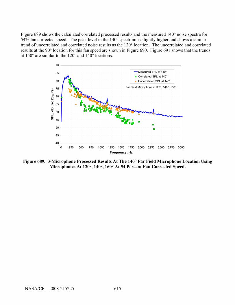
615

Figure 689 shows the calculated correlated processed results and the measured 140° noise spectra for 54% fan corrected speed. The peak level in the 140° spectrum is slightly higher and shows a similar trend of uncorrelated and correlated noise results as the 120° location. The uncorrelated and correlated results at the 90° location for this fan speed are shown in Figure 690. Figure 691 shows that the trends at 150° are similar to the 120° and 140° locations.

40

45

50

55

60

65

70

75

80

85

90

0 250 500 750 1000 1250 1500 1750 2000 2250 2500 2750 3000

Frequency, Hz

SPL,

dB

(re:

20

μPa)

Measured SPL at 140°Correlated SPL at 140°




NASA/CR—2008-215225

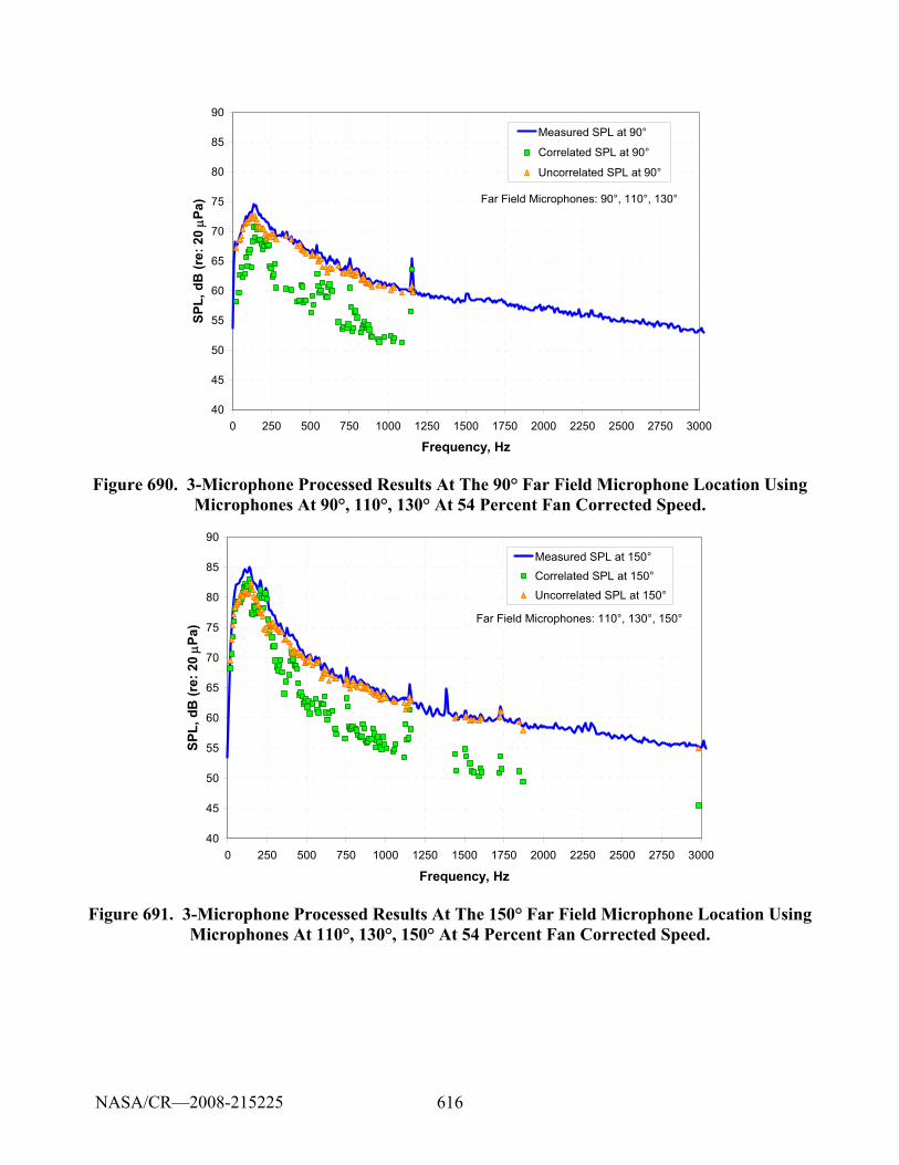
616

40

45

50

55

60

65

70

75

80

85

90

0 250 500 750 1000 1250 1500 1750 2000 2250 2500 2750 3000

Frequency, Hz

SPL,

dB

(re:

20

μPa)






40

45

50

55

60

65

70

75

80

85

90

0 250 500 750 1000 1250 1500 1750 2000 2250 2500 2750 3000

Frequency, Hz

SPL,

dB

(re:

20

μPa)

Measured SPL at 150°Correlated SPL at 150°




NASA/CR—2008-215225

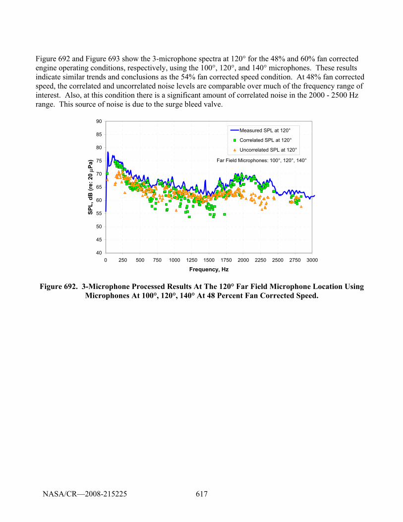
617

Figure 692 and Figure 693 show the 3-microphone spectra at 120° for the 48% and 60% fan corrected engine operating conditions, respectively, using the 100°, 120°, and 140° microphones. These results indicate similar trends and conclusions as the 54% fan corrected speed condition. At 48% fan corrected speed, the correlated and uncorrelated noise levels are comparable over much of the frequency range of interest. Also, at this condition there is a significant amount of correlated noise in the 2000 - 2500 Hz range. This source of noise is due to the surge bleed valve.

40

45

50

55

60

65

70

75

80

85

90

0 250 500 750 1000 1250 1500 1750 2000 2250 2500 2750 3000

Frequency, Hz

SPL,

dB

(re:

20

μPa)






NASA/CR—2008-215225

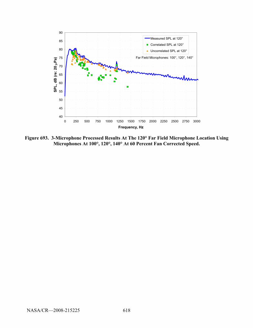
618

40

45

50

55

60

65

70

75

80

85

90

0 250 500 750 1000 1250 1500 1750 2000 2250 2500 2750 3000

Frequency, Hz

SPL,

dB

(re:

20

μPa)






NASA/CR—2008-215225

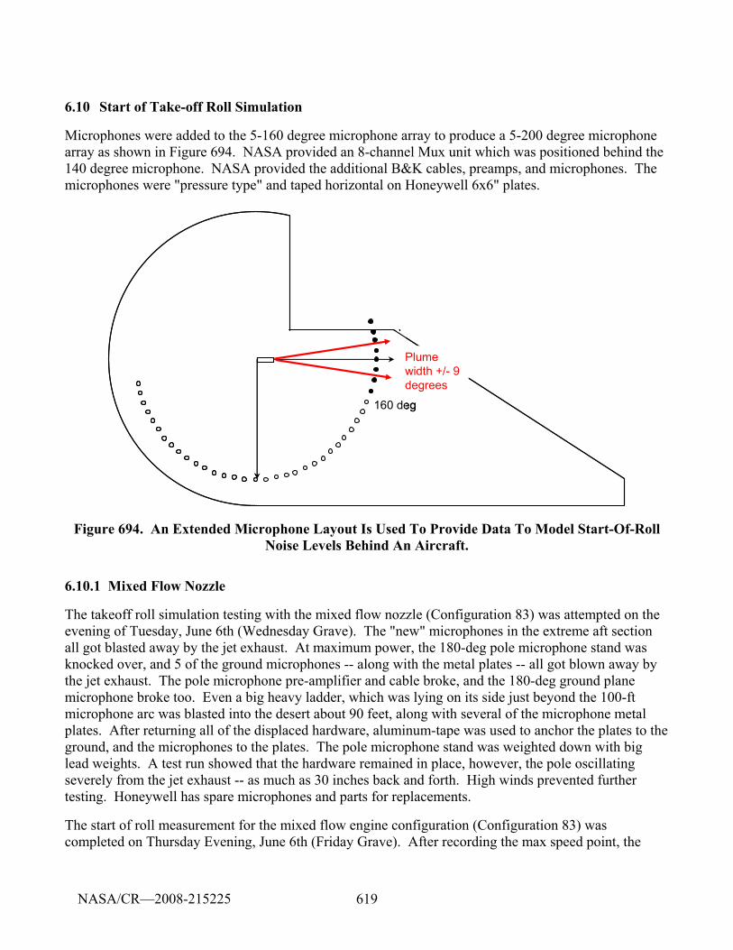
619

6.10 Start of Take-off Roll Simulation

Microphones were added to the 5-160 degree microphone array to produce a 5-200 degree microphone array as shown in Figure 694. NASA provided an 8-channel Mux unit which was positioned behind the 140 degree microphone. NASA provided the additional B&K cables, preamps, and microphones. The microphones were "pressure type" and taped horizontal on Honeywell 6x6" plates.

Plume width +/- 9 degrees

160 deg

Plume width +/- 9 degrees

160 deg

Figure 694. An Extended Microphone Layout Is Used To Provide Data To Model Start-Of-Roll Noise Levels Behind An Aircraft.

6.10.1 Mixed Flow Nozzle

The takeoff roll simulation testing with the mixed flow nozzle (Configuration 83) was attempted on the evening of Tuesday, June 6th (Wednesday Grave). The "new" microphones in the extreme aft section all got blasted away by the jet exhaust. At maximum power, the 180-deg pole microphone stand was knocked over, and 5 of the ground microphones -- along with the metal plates -- all got blown away by the jet exhaust. The pole microphone pre-amplifier and cable broke, and the 180-deg ground plane microphone broke too. Even a big heavy ladder, which was lying on its side just beyond the 100-ft microphone arc was blasted into the desert about 90 feet, along with several of the microphone metal plates. After returning all of the displaced hardware, aluminum-tape was used to anchor the plates to the ground, and the microphones to the plates. The pole microphone stand was weighted down with big lead weights. A test run showed that the hardware remained in place, however, the pole oscillating severely from the jet exhaust -- as much as 30 inches back and forth. High winds prevented further testing. Honeywell has spare microphones and parts for replacements.

The start of roll measurement for the mixed flow engine configuration (Configuration 83) was completed on Thursday Evening, June 6th (Friday Grave). After recording the max speed point, the

NASA/CR—2008-215225

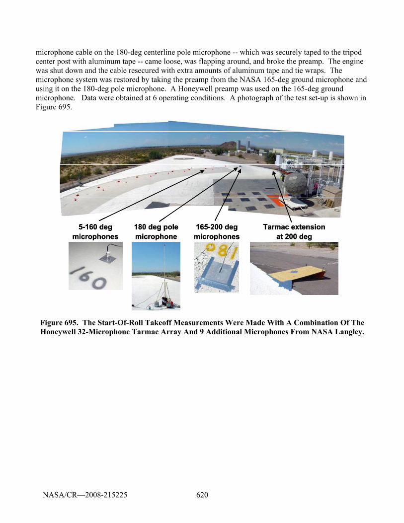
620

microphone cable on the 180-deg centerline pole microphone -- which was securely taped to the tripod center post with aluminum tape -- came loose, was flapping around, and broke the preamp. The engine was shut down and the cable resecured with extra amounts of aluminum tape and tie wraps. The microphone system was restored by taking the preamp from the NASA 165-deg ground microphone and using it on the 180-deg pole microphone. A Honeywell preamp was used on the 165-deg ground microphone. Data were obtained at 6 operating conditions. A photograph of the test set-up is shown in Figure 695.

5-160 deg microphones


180 deg pole microphone

Tarmac extension at 200 deg



180 deg pole microphone

Tarmac extension at 200 deg

Figure 695. The Start-Of-Roll Takeoff Measurements Were Made With A Combination Of The Honeywell 32-Microphone Tarmac Array And 9 Additional Microphones From NASA Langley.

NASA/CR—2008-215225

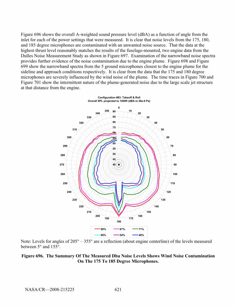
621

Figure 696 shows the overall A-weighted sound pressure level (dBA) as a function of angle from the inlet for each of the power settings that were measured. It is clear that noise levels from the 175, 180, and 185 degree microphones are contaminated with an unwanted noise source. That the data at the highest thrust level reasonably matches the results of the fuselage-mounted, two engine data from the Dulles Noise Measurement Study as shown in Figure 697. Examination of the narrowband noise spectra provides further evidence of the noise contamination due to the engine plume. Figure 698 and Figure 699 show the narrowband spectra from the 5 ground microphones closest to the engine plume for the sideline and approach conditions respectively. It is clear from the data that the 175 and 180 degree microphones are severely influenced by the wind noise of the plume. The time traces in Figure 700 and Figure 701 show the intermittent nature of the plume-generated noise due to the large scale jet structure at that distance from the engine.

Configuration #83: Takeoff & RollOverall SPL projected to 1000ft (dBA re 20e-6 Pa)

40

45

50

55

60

65

70

75

80

85

900

1020

30

40

50

60

70

80

90

100

110

120

130

140

150160

170180

190200

210

220

230

240

250

260

270

280

290

300

310

320

330340

350

90% 87% 71%

60% 54% 48% Note: Levels for angles of 205° – 355° are a reflection (about engine centerline) of the levels measured between 5° and 155°.

Figure 696. The Summary Of The Measured Dba Noise Levels Shows Wind Noise Contamination On The 175 To 185 Degree Microphones.

NASA/CR—2008-215225

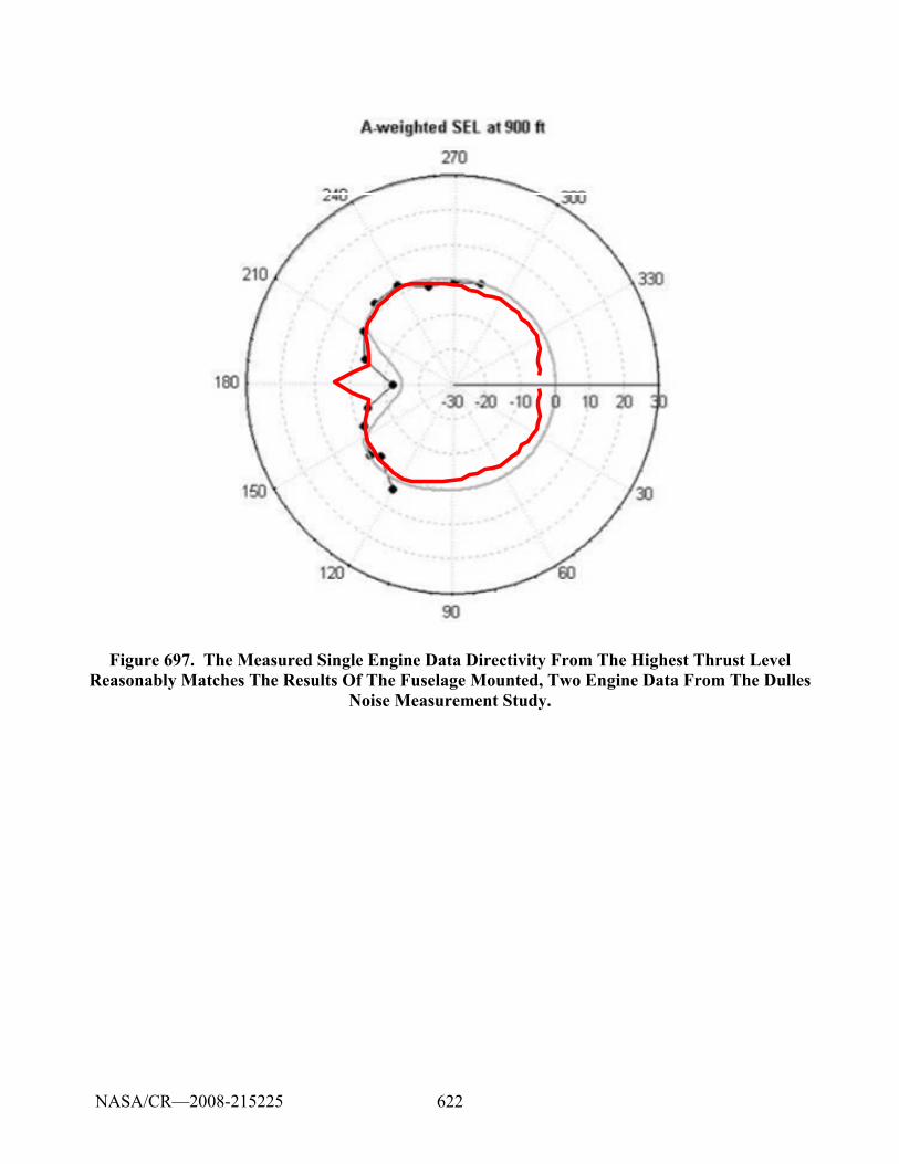
622

Figure 697. The Measured Single Engine Data Directivity From The Highest Thrust Level Reasonably Matches The Results Of The Fuselage Mounted, Two Engine Data From The Dulles

Noise Measurement Study.

NASA/CR—2008-215225

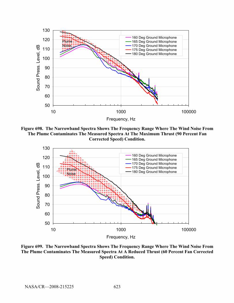
623

50

60

70

80

90

100

110

120

130

10 1000 100000Frequency, Hz

Sou

nd P

ress

. Lev

el, d

B160 Deg Ground Microphone165 Deg Ground Microphone170 Deg Ground Microphone175 Deg Ground Microphone180 Deg Ground Microphone

Plume Noise

Figure 698. The Narrowband Spectra Shows The Frequency Range Where The Wind Noise From The Plume Contaminates The Measured Spectra At The Maximum Thrust (90 Percent Fan


50

60

70

80

90

100

110

120

130

10 1000 100000Frequency, Hz

Sou

nd P

ress

. Lev

el, d

B

160 Deg Ground Microphone165 Deg Ground Microphone170 Deg Ground Microphone175 Deg Ground Microphone180 Deg Ground MicrophonePlume

Noise

Figure 699. The Narrowband Spectra Shows The Frequency Range Where The Wind Noise From The Plume Contaminates The Measured Spectra At A Reduced Thrust (60 Percent Fan Corrected

Speed) Condition.

NASA/CR—2008-215225

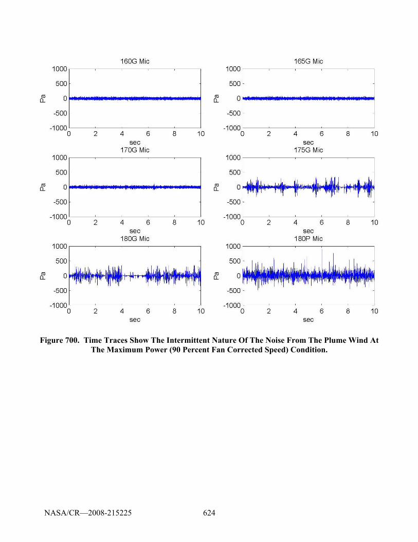
624

Figure 700. Time Traces Show The Intermittent Nature Of The Noise From The Plume Wind At The Maximum Power (90 Percent Fan Corrected Speed) Condition.

NASA/CR—2008-215225

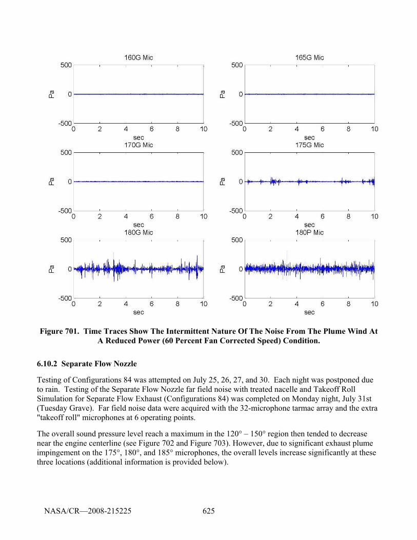
625

Figure 701. Time Traces Show The Intermittent Nature Of The Noise From The Plume Wind At A Reduced Power (60 Percent Fan Corrected Speed) Condition.

6.10.2 Separate Flow Nozzle

Testing of Configurations 84 was attempted on July 25, 26, 27, and 30. Each night was postponed due to rain. Testing of the Separate Flow Nozzle far field noise with treated nacelle and Takeoff Roll Simulation for Separate Flow Exhaust (Configurations 84) was completed on Monday night, July 31st (Tuesday Grave). Far field noise data were acquired with the 32-microphone tarmac array and the extra "takeoff roll" microphones at 6 operating points.

The overall sound pressure level reach a maximum in the 120° – 150° region then tended to decrease near the engine centerline (see Figure 702 and Figure 703). However, due to significant exhaust plume impingement on the 175°, 180°, and 185° microphones, the overall levels increase significantly at these three locations (additional information is provided below).

NASA/CR—2008-215225

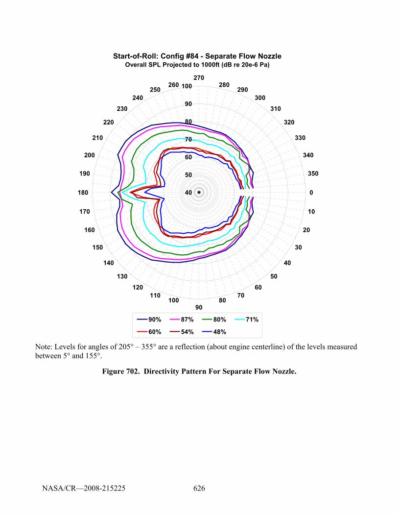
626

Start-of-Roll: Config #84 - Separate Flow NozzleOverall SPL Projected to 1000ft (dB re 20e-6 Pa)

40

50

60

70

80

90

100270

280290

300310

320

330

340

350

0

10

20

30

40

50

6070

8090

100110

120

130

140

150

160

170

180

190

200

210

220

230240

250260

90% 87% 80% 71%

60% 54% 48%

Note: Levels for angles of 205° – 355° are a reflection (about engine centerline) of the levels measured between 5° and 155°.

Figure 702. Directivity Pattern For Separate Flow Nozzle.

NASA/CR—2008-215225

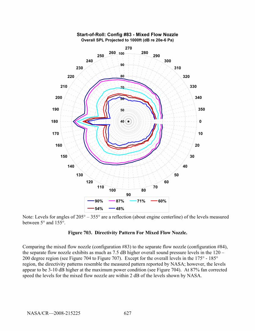
627

Start-of-Roll: Config #83 - Mixed Flow NozzleOverall SPL Projected to 1000ft (dB re 20e-6 Pa)

40

50

60

70

80

90

100270

280290

300310

320

330

340

350

0

10

20

30

40

5060

7080

90100

110120

130

140

150

160

170

180

190

200

210

220

230240

250260

90% 87% 71% 60%

54% 48%

Note: Levels for angles of 205° – 355° are a reflection (about engine centerline) of the levels measured between 5° and 155°.

Figure 703. Directivity Pattern For Mixed Flow Nozzle.

Comparing the mixed flow nozzle (configuration #83) to the separate flow nozzle (configuration #84), the separate flow nozzle exhibits as much as 7.5 dB higher overall sound pressure levels in the 120 – 200 degree region (see Figure 704 to Figure 707). Except for the overall levels in the 175° - 185° region, the directivity patterns resemble the measured pattern reported by NASA; however, the levels appear to be 3-10 dB higher at the maximum power condition (see Figure 704). At 87% fan corrected speed the levels for the mixed flow nozzle are within 2 dB of the levels shown by NASA.

NASA/CR—2008-215225

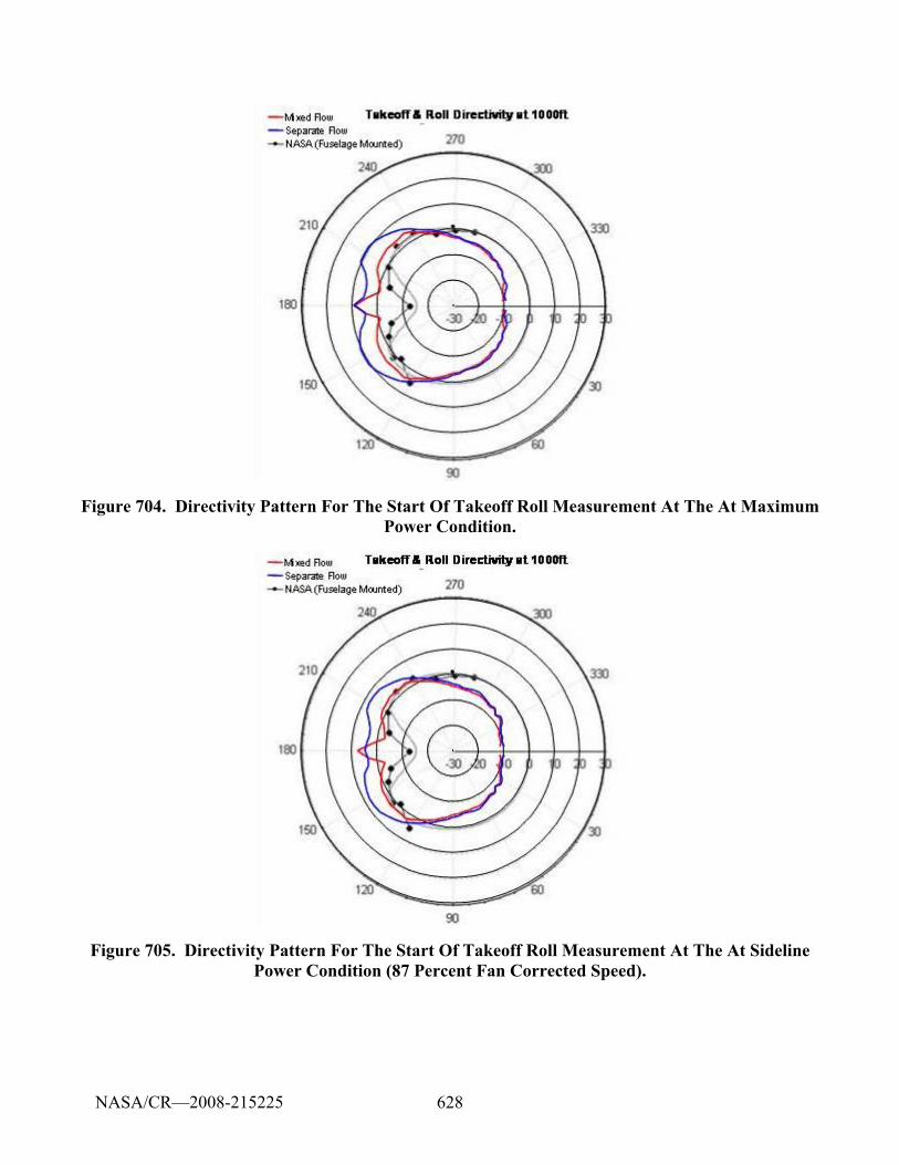
628

Figure 704. Directivity Pattern For The Start Of Takeoff Roll Measurement At The At Maximum Power Condition.

Figure 705. Directivity Pattern For The Start Of Takeoff Roll Measurement At The At Sideline Power Condition (87 Percent Fan Corrected Speed).

NASA/CR—2008-215225

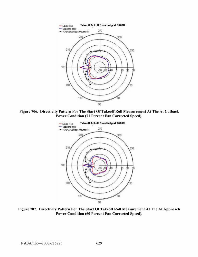
629

Figure 706. Directivity Pattern For The Start Of Takeoff Roll Measurement At The At Cutback Power Condition (71 Percent Fan Corrected Speed).

Figure 707. Directivity Pattern For The Start Of Takeoff Roll Measurement At The At Approach Power Condition (60 Percent Fan Corrected Speed).

NASA/CR—2008-215225

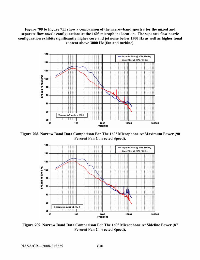
630

Figure 708 to Figure 711 show a comparison of the narrowband spectra for the mixed and separate flow nozzle configurations at the 160° microphone location. The separate flow nozzle

configuration exhibits significantly higher core and jet noise below 1500 Hz as well as higher tonal content above 3000 Hz (fan and turbine).

Figure 708. Narrow Band Data Comparison For The 160° Microphone At Maximum Power (90 Percent Fan Corrected Speed).

Figure 709. Narrow Band Data Comparison For The 160° Microphone At Sideline Power (87 Percent Fan Corrected Speed).

NASA/CR—2008-215225

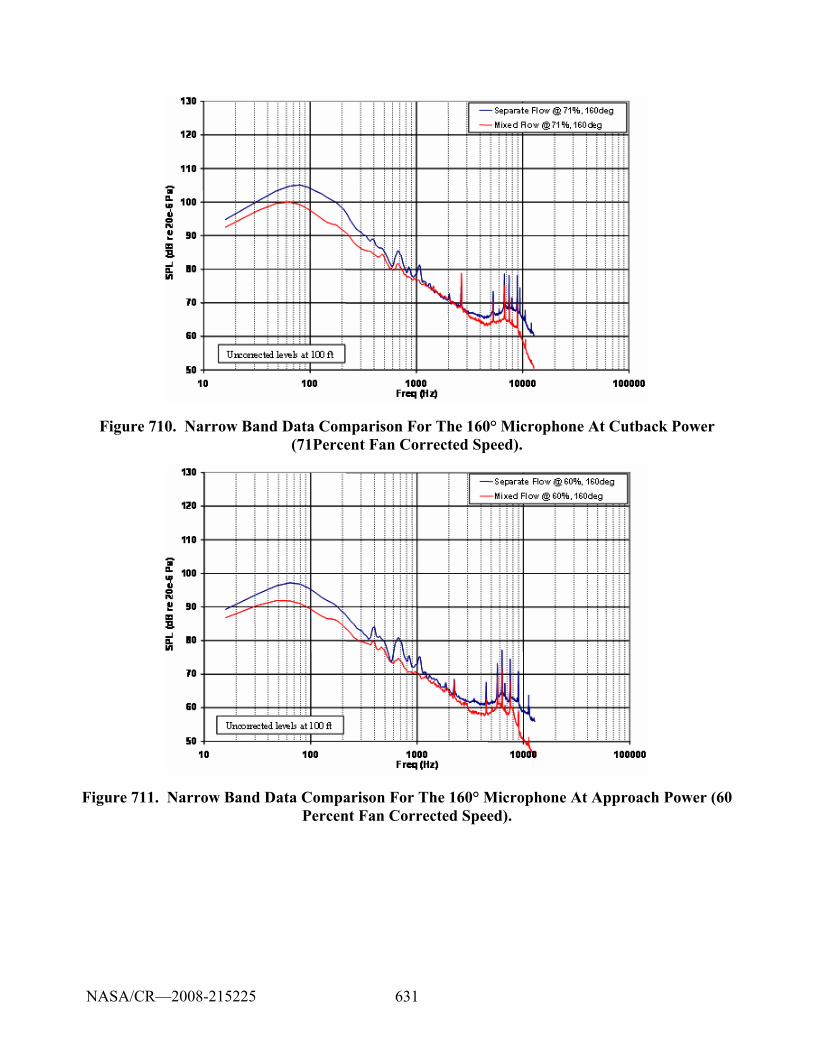
631

Figure 710. Narrow Band Data Comparison For The 160° Microphone At Cutback Power (71Percent Fan Corrected Speed).

Figure 711. Narrow Band Data Comparison For The 160° Microphone At Approach Power (60 Percent Fan Corrected Speed).

NASA/CR—2008-215225

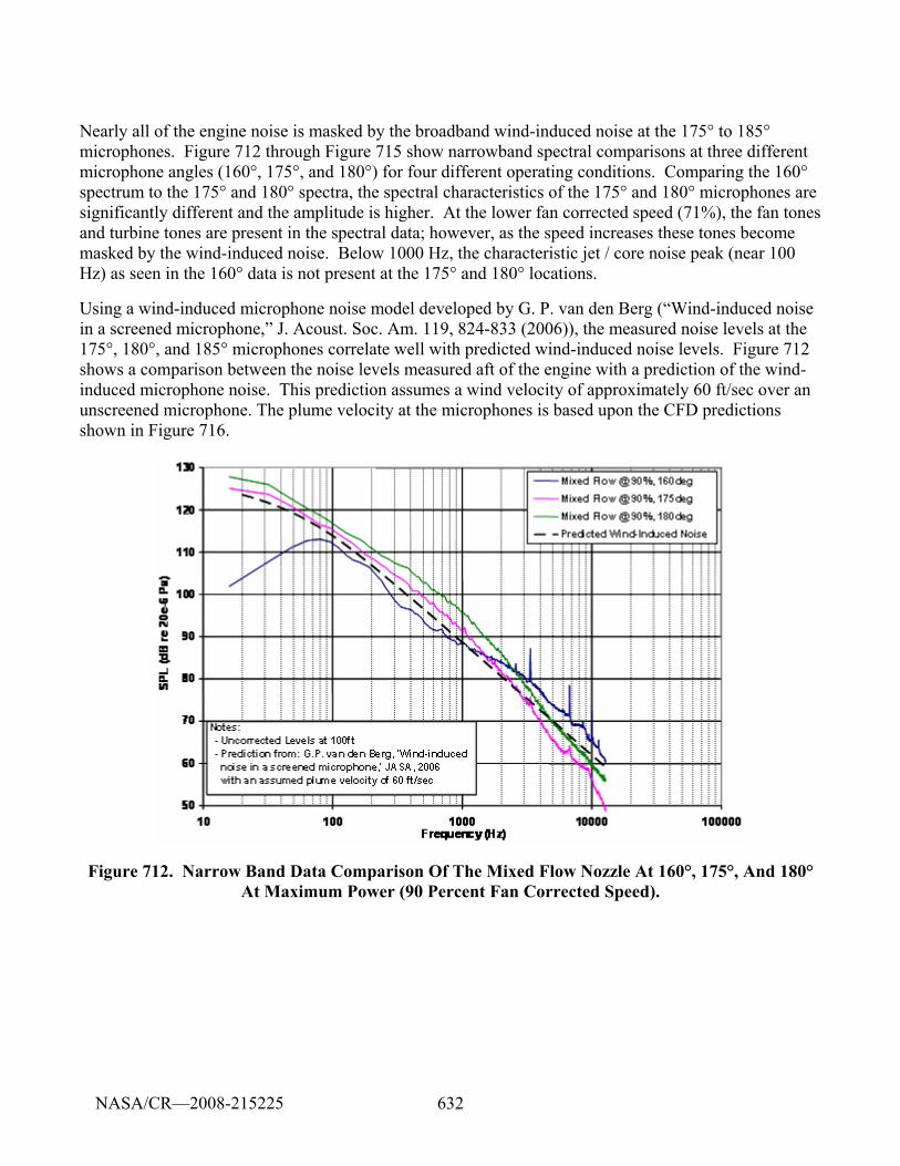
632

Nearly all of the engine noise is masked by the broadband wind-induced noise at the 175° to 185° microphones. Figure 712 through Figure 715 show narrowband spectral comparisons at three different microphone angles (160°, 175°, and 180°) for four different operating conditions. Comparing the 160° spectrum to the 175° and 180° spectra, the spectral characteristics of the 175° and 180° microphones are significantly different and the amplitude is higher. At the lower fan corrected speed (71%), the fan tones and turbine tones are present in the spectral data; however, as the speed increases these tones become masked by the wind-induced noise. Below 1000 Hz, the characteristic jet / core noise peak (near 100 Hz) as seen in the 160° data is not present at the 175° and 180° locations.

Using a wind-induced microphone noise model developed by G. P. van den Berg (“Wind-induced noise in a screened microphone,” J. Acoust. Soc. Am. 119, 824-833 (2006)), the measured noise levels at the 175°, 180°, and 185° microphones correlate well with predicted wind-induced noise levels. Figure 712 shows a comparison between the noise levels measured aft of the engine with a prediction of the wind-induced microphone noise. This prediction assumes a wind velocity of approximately 60 ft/sec over an unscreened microphone. The plume velocity at the microphones is based upon the CFD predictions shown in Figure 716.

Figure 712. Narrow Band Data Comparison Of The Mixed Flow Nozzle At 160°, 175°, And 180° At Maximum Power (90 Percent Fan Corrected Speed).

NASA/CR—2008-215225

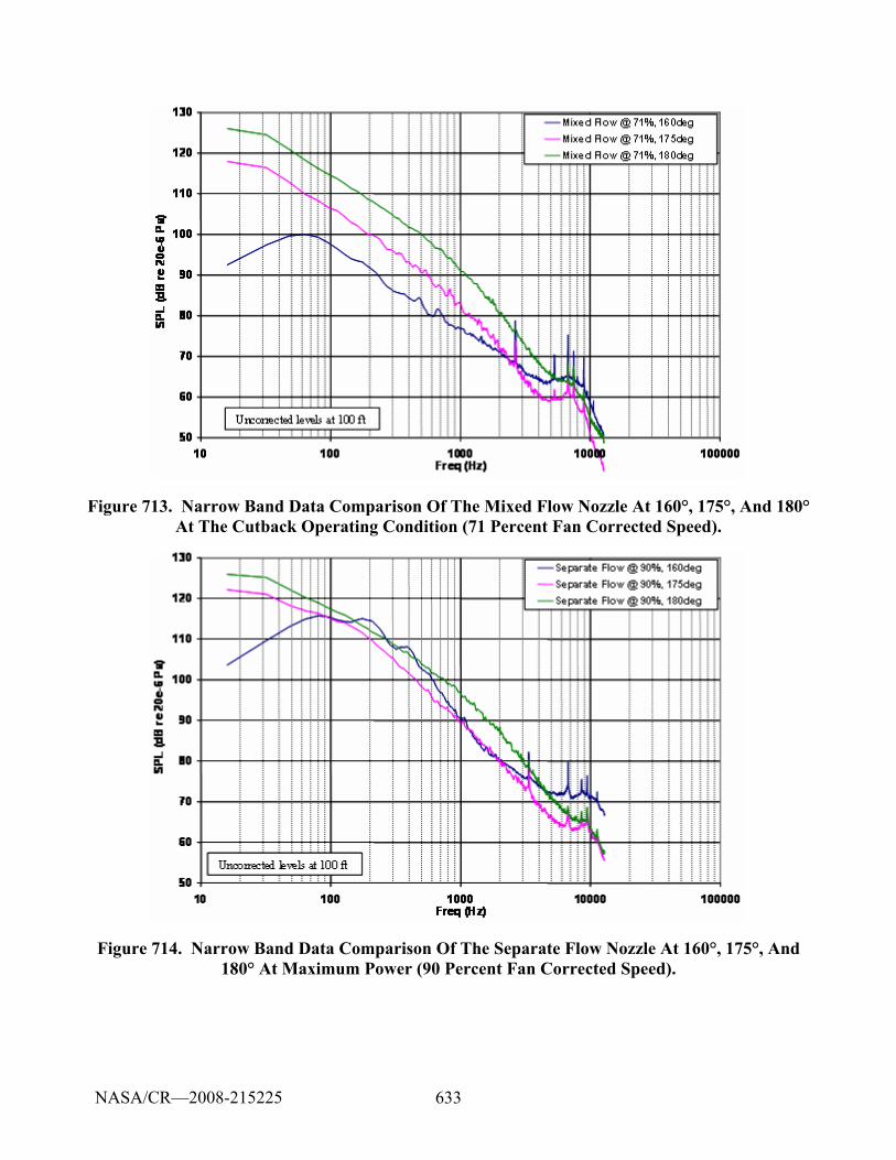
633

Figure 713. Narrow Band Data Comparison Of The Mixed Flow Nozzle At 160°, 175°, And 180° At The Cutback Operating Condition (71 Percent Fan Corrected Speed).

Figure 714. Narrow Band Data Comparison Of The Separate Flow Nozzle At 160°, 175°, And 180° At Maximum Power (90 Percent Fan Corrected Speed).

NASA/CR—2008-215225

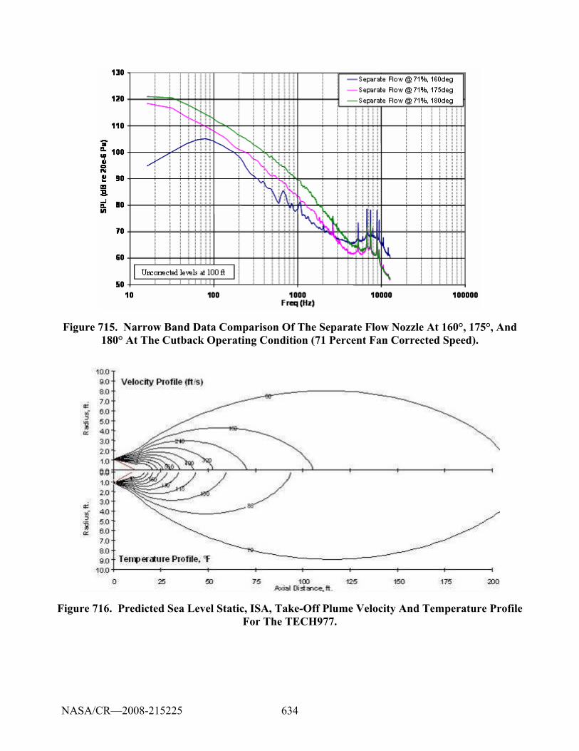
634

Figure 715. Narrow Band Data Comparison Of The Separate Flow Nozzle At 160°, 175°, And 180° At The Cutback Operating Condition (71 Percent Fan Corrected Speed).

Figure 716. Predicted Sea Level Static, ISA, Take-Off Plume Velocity And Temperature Profile For The TECH977.

NASA/CR—2008-215225

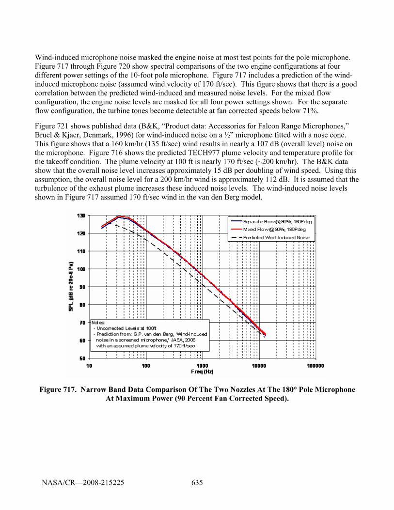
635

Wind-induced microphone noise masked the engine noise at most test points for the pole microphone. Figure 717 through Figure 720 show spectral comparisons of the two engine configurations at four different power settings of the 10-foot pole microphone. Figure 717 includes a prediction of the wind-induced microphone noise (assumed wind velocity of 170 ft/sec). This figure shows that there is a good correlation between the predicted wind-induced and measured noise levels. For the mixed flow configuration, the engine noise levels are masked for all four power settings shown. For the separate flow configuration, the turbine tones become detectable at fan corrected speeds below 71%.

Figure 721 shows published data (B&K, “Product data: Accessories for Falcon Range Microphones,” Bruel & Kjaer, Denmark, 1996) for wind-induced noise on a ½” microphone fitted with a nose cone. This figure shows that a 160 km/hr (135 ft/sec) wind results in nearly a 107 dB (overall level) noise on the microphone. Figure 716 shows the predicted TECH977 plume velocity and temperature profile for the takeoff condition. The plume velocity at 100 ft is nearly 170 ft/sec (~200 km/hr). The B&K data show that the overall noise level increases approximately 15 dB per doubling of wind speed. Using this assumption, the overall noise level for a 200 km/hr wind is approximately 112 dB. It is assumed that the turbulence of the exhaust plume increases these induced noise levels. The wind-induced noise levels shown in Figure 717 assumed 170 ft/sec wind in the van den Berg model.

Figure 717. Narrow Band Data Comparison Of The Two Nozzles At The 180° Pole Microphone At Maximum Power (90 Percent Fan Corrected Speed).

NASA/CR—2008-215225

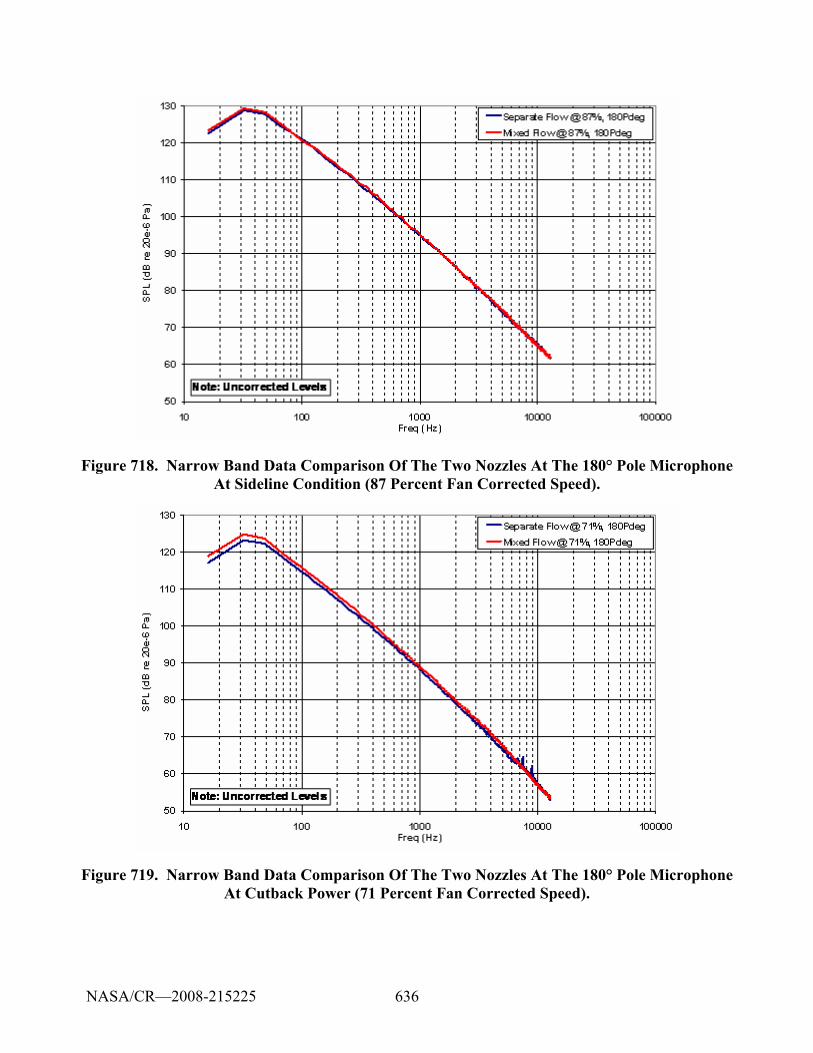
636

Figure 718. Narrow Band Data Comparison Of The Two Nozzles At The 180° Pole Microphone At Sideline Condition (87 Percent Fan Corrected Speed).

Figure 719. Narrow Band Data Comparison Of The Two Nozzles At The 180° Pole Microphone At Cutback Power (71 Percent Fan Corrected Speed).

NASA/CR—2008-215225

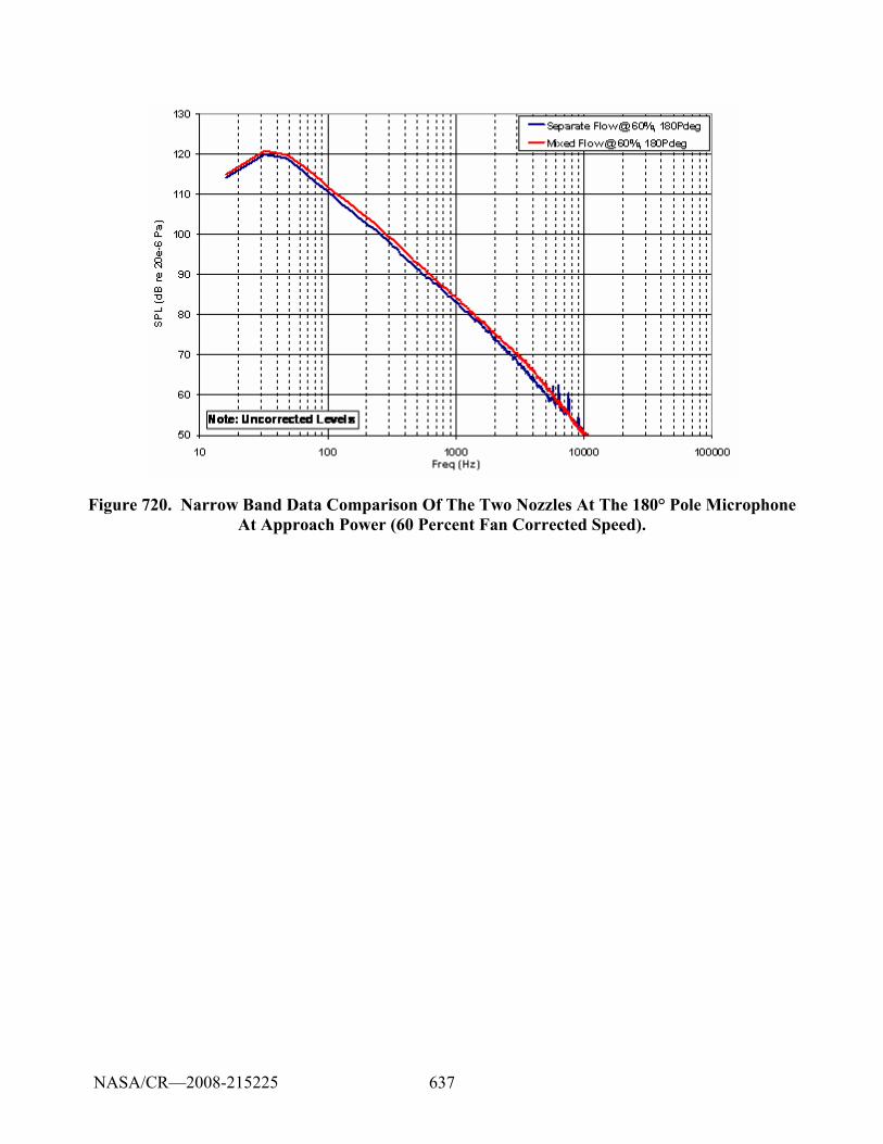
637

Figure 720. Narrow Band Data Comparison Of The Two Nozzles At The 180° Pole Microphone At Approach Power (60 Percent Fan Corrected Speed).

NASA/CR—2008-215225

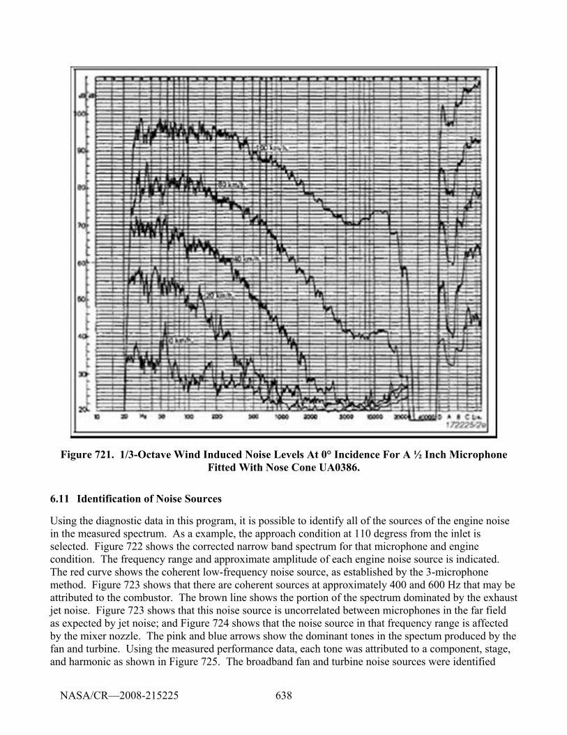
638

Figure 721. 1/3-Octave Wind Induced Noise Levels At 0° Incidence For A ½ Inch Microphone Fitted With Nose Cone UA0386.

6.11 Identification of Noise Sources

Using the diagnostic data in this program, it is possible to identify all of the sources of the engine noise in the measured spectrum. As a example, the approach condition at 110 degress from the inlet is selected. Figure 722 shows the corrected narrow band spectrum for that microphone and engine condition. The frequency range and approximate amplitude of each engine noise source is indicated. The red curve shows the coherent low-frequency noise source, as established by the 3-microphone method. Figure 723 shows that there are coherent sources at approximately 400 and 600 Hz that may be attributed to the combustor. The brown line shows the portion of the spectrum dominated by the exhaust jet noise. Figure 723 shows that this noise source is uncorrelated between microphones in the far field as expected by jet noise; and Figure 724 shows that the noise source in that frequency range is affected by the mixer nozzle. The pink and blue arrows show the dominant tones in the spectum produced by the fan and turbine. Using the measured performance data, each tone was attributed to a component, stage, and harmonic as shown in Figure 725. The broadband fan and turbine noise sources were identified

NASA/CR—2008-215225

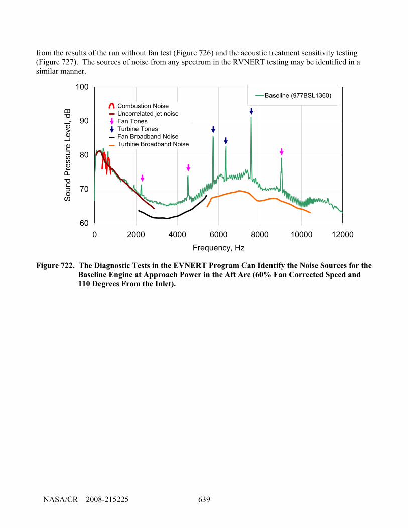
639

from the results of the run without fan test (Figure 726) and the acoustic treatment sensitivity testing (Figure 727). The sources of noise from any spectrum in the RVNERT testing may be identified in a similar manner.

60

70

80

90

100

0 2000 4000 6000 8000 10000 12000Frequency, Hz

Sou

nd P

ress

ure

Leve

l, dB

Baseline (977BSL1360)

Combustion NoiseUncorrelated jet noiseFan TonesTurbine TonesFan Broadband NoiseTurbine Broadband Noise

Figure 722. The Diagnostic Tests in the EVNERT Program Can Identify the Noise Sources for the Baseline Engine at Approach Power in the Aft Arc (60% Fan Corrected Speed and 110 Degrees From the Inlet).

NASA/CR—2008-215225

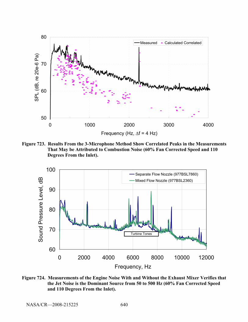
640

50

60

70

80

0 1000 2000 3000 4000


SP

L (d

B, r

e 20

e-6

Pa)


Figure 723. Results From the 3-Microphone Method Show Correlated Peaks in the Measurements That May be Attributed to Combustion Noise (60% Fan Corrected Speed and 110 Degrees From the Inlet).

60

70

80

90

100

0 2000 4000 6000 8000 10000 12000Frequency, Hz

Sou

nd P

ress

ure

Leve

l, dB

Separate Flow Nozzle (977BSL7860)

Mixed Flow Nozzle (977BSL2360)

Turbine Tones

Figure 724. Measurements of the Engine Noise With and Without the Exhaust Mixer Verifies that the Jet Noise is the Dominant Source from 50 to 500 Hz (60% Fan Corrected Speed and 110 Degrees From the Inlet).

NASA/CR—2008-215225

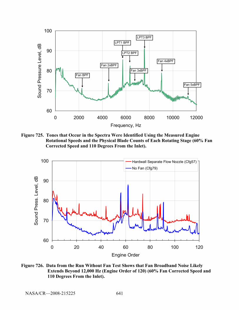
641

60

70

80

90

100

0 2000 4000 6000 8000 10000 12000Frequency, Hz

Soun

d Pr

essu

re L

evel

, dB

LPT3 BPF

Fan BPF

Fan 2xBPF

Fan 3xBPF

LPT1 BPF

LPT2 BPF

Fan 4xBPF

Fan 5xBPF

Figure 725. Tones that Occur in the Spectra Were Identified Using the Measured Engine Rotational Speeds and the Physical Blade Counts of Each Rotating Stage (60% Fan Corrected Speed and 110 Degrees From the Inlet).

60

70

80

90

100

0 20 40 60 80 100 120Engine Order

Sou

nd P

ress

. Lev

el, d

B


No Fan (Cfg79)

Figure 726. Data from the Run Without Fan Test Shows that Fan Broadband Noise Likely Extends Beyond 12,000 Hz (Engine Order of 120) (60% Fan Corrected Speed and 110 Degrees From the Inlet).

NASA/CR—2008-215225

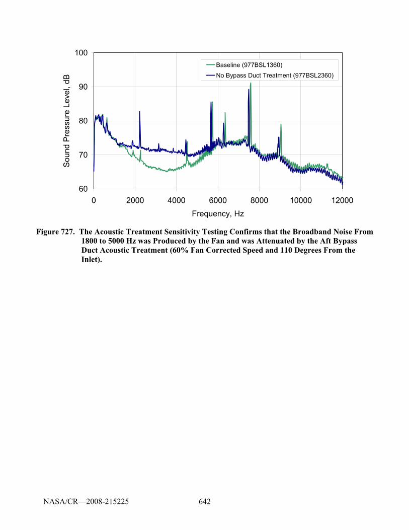
642

60

70

80

90

100

0 2000 4000 6000 8000 10000 12000Frequency, Hz

Sou

nd P

ress

ure

Leve

l, dB

Baseline (977BSL1360)

No Bypass Duct Treatment (977BSL2360)

Figure 727. The Acoustic Treatment Sensitivity Testing Confirms that the Broadband Noise From 1800 to 5000 Hz was Produced by the Fan and was Attenuated by the Aft Bypass Duct Acoustic Treatment (60% Fan Corrected Speed and 110 Degrees From the Inlet).

NASA/CR—2008-215225

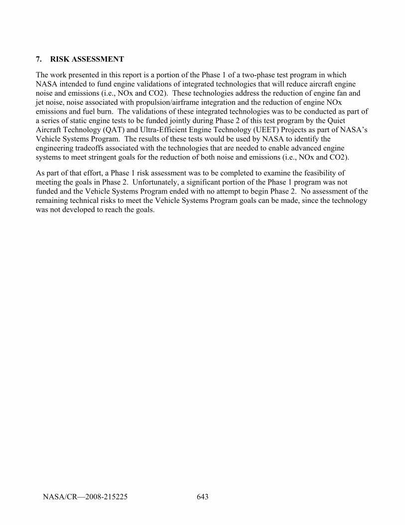
643

7. RISK ASSESSMENT

The work presented in this report is a portion of the Phase 1 of a two-phase test program in which NASA intended to fund engine validations of integrated technologies that will reduce aircraft engine noise and emissions (i.e., NOx and CO2). These technologies address the reduction of engine fan and jet noise, noise associated with propulsion/airframe integration and the reduction of engine NOx emissions and fuel burn. The validations of these integrated technologies was to be conducted as part of a series of static engine tests to be funded jointly during Phase 2 of this test program by the Quiet Aircraft Technology (QAT) and Ultra-Efficient Engine Technology (UEET) Projects as part of NASA’s Vehicle Systems Program. The results of these tests would be used by NASA to identify the engineering tradeoffs associated with the technologies that are needed to enable advanced engine systems to meet stringent goals for the reduction of both noise and emissions (i.e., NOx and CO2).

As part of that effort, a Phase 1 risk assessment was to be completed to examine the feasibility of meeting the goals in Phase 2. Unfortunately, a significant portion of the Phase 1 program was not funded and the Vehicle Systems Program ended with no attempt to begin Phase 2. No assessment of the remaining technical risks to meet the Vehicle Systems Program goals can be made, since the technology was not developed to reach the goals.

NASA/CR—2008-215225

644

8. CONCLUSIONS

8.1 Engine Preliminary Design

Engine requirements were derived for the TECH8000, a demonstrator for a future Honeywell HTF8000 engine. With the application of technology from the NASA Advanced Subsonic Technology (AST) Noise Reduction Program and the NASA Quiet Aircraft Technology Program, A cumulative certification noise level of Chapter 3 minus 30.5 was estimated. NOx reductions of up to 67% relative to CAEP6 levels were estimated.

8.2 HQ Tube/Optimum Liner - Aft Duct HQ Tubes

An adaptive HQ tube system was designed and fabricated with the following design targets:

Control the BPF tone around 71% RPM and 48-55% corrected fan speed.

Demonstrate adaptive capability through the 50-75% corrected fan speed range.

A passive linear liner was also designed to control the broadband component and provide a similar performance for the BPF tone. The design was implemented in the aft fan C-Ducts of the TECH977 engine and tested for far field noise, rotating rake modal measurements, and in-tube noise and flow characteristics.

The HQ-tube liner consistently reduced the engine noise levels over the operating range. A cumulative noise reduction benefit of up to 2 EPNdB can be achieved

8.3 Modeling of Liner With Discontinuities

The model was developed for the analysis of liner discontinuities. The model was developed based on previous work by Alonso and Burdisso (Reference 11). This model uses a close form solution of the Green’s function for a lined duct with flow to represent the sound field radiated by liner discontinuities. The initial model did not consider reflections induced by the change in wall impedance at the hard-wall/liner interfaces. Since reflections can be a significant contribution to the attenuation provided by the liner, modifications have been added to the model so that reflections at the interfaces can be calculated. Further modifications have been added to the model in order to investigate the effect of liner discontinuities on the sound pressure distribution in the far-field. The formulation was implemented in a FORTRAN computer code.

Predictions for different configurations have been compared to experimental data measured on the NASA Glenn ANCF Rig and the Honeywell TECH977 turbofan engine. This data has also been analyzed so as to assess, first hand, the effect of liner discontinuities. The initial goal was to use in-duct modal measurements collected in both systems to define the modal structure of the disturbance needed by the model. Unfortunately, the in-duct modal data for the engine was not available. In addition, the scattering effects in the ANCF rig due to the discontinuities were not strong enough to be detected by the measuring system (rotating rake). Thus, the validation of the model was limited by this lack of modal information. The model validating had to be based only on the far-field data.

NASA/CR—2008-215225

645

The model was then used to perform a parametric analysis of the rigid discontinuities, e.g. splices and repair patches. The objective of this initial parametric analysis was to investigate the influence of the main variables such as number of discontinuities, their size and location within the lined sector, and so forth.

8.3.1 Experimental results

8.3.1.1 NASA ANCF Rig

The configurations with rigid splices have had little effect on the performance of the liner, i.e. no significant scattering effects. The attenuation of the 2 and 3BPF tones and broadband component remained virtually the same when either 2 or 3 splices were used.

The segmented and checkered liner concepts didn’t perform as well as the original seamless 1.0ρc liner. However, since the interaction between the disturbance and the discontinuities was small, the lower performance for the segmented and checkered liners can be attributed to the acoustic properties of the liner/PU film combination rather than the scattering of acoustic energy.

Thus, the ANCF results are not useful as a validation set for the rigid splices model developed here. However, they are still valuable to check the code performance for liner attenuation, including the checkered and segmented configurations.

8.3.1.2 Honeywell TECH977 Turbofan Engine:

At low power setting, i.e. at or below 71%, the influence of the splices on the liner attenuation of the BPF tone is small, i.e. degradation between 2-4 dB.

A significant degradation of the BPF tone attenuation has been observed at power settings above 71% when rigid splices were incorporated. For instance, at 87% power setting the BPF tone attenuation went from 15 dB for the seamless liner to -2 dB when the splices were added (results at an elevation angle of 70º).

For the broadband component, degradation has clearly been observed due to the splices at all subsonic power setting. In general, degradation levels are small at low frequencies and lower power settings and steadily increases at higher frequencies and power settings, e.g. degradation of liner performance as much as ~6 dB.

8.3.2 Model Validation

8.3.2.1 NASA ANCF Rig:

It is important to mention that liner discontinuities did not have a strong effect on the performance of the liner in this rig. Within this limitation, the validation of the model using the NASA ANCF rig data produced encouraging results. In case of the 2BPF tone, the model has been able to reproduce fairly well the attenuation levels of the (4,0) and (4,1) modes as well as the combination of the two in all configurations. In case of the attenuation of the (4,0) mode and the total, differences are below 2.2 dB. In case of the (4,1) mode differences are larger at ~5 dB. The prediction of the broadband component also shows good levels of agreement with attenuation differences no larger than 1.0 dB. In the case of far-field radiation, the model has captured the general trend shown by experiments.

NASA/CR—2008-215225

646

8.3.2.2 Honeywell TECH977 Turbofan Engine:

The validation of the model using the TECH977 engine data has produced reasonably good results. However, the lack of precise disturbance information dictates that these results should be taken rather qualitatively instead of quantitatively. One of the main issues in this validation is that the predictions vs. experiments comparison was restricted to the radiation in the plane of the microphones. As illustrated in the parametric analysis, the radiation pattern around the axis of the engine changes significantly, in particular with discontinuities. Thus, validation by comparing results on a single plane is thus limited.

8.3.3 Parametric Analysis

For a constant surface area taken by the splices, increasing the number of splices increases reduces the scattering effects and thus the liner degradation, e.g. it is better to have many thin splices than a few thick ones as expected.

The key parameter that determines the amount of scattering is the ratio of the splice width to the circumferential order of the disturbance modes. Significant scattering can be expected when the splice width is about or more than half the circumferential wavelength of the disturbance mode.

The number of splices must be carefully selected such that the scattered modes do not form circumferential standing patterns, e.g. counter rotating spinning modes. It was determine that when standing waves are formed (due to the inappropriate number of splices for a given disturbance mode) results is a stronger degradation of the liner performance.

The effect of the axial position of the repair patch on the liner performance decreases logarithmically (or linear in decibel scale) as a function of the distance to the fan.

The key parameters that determine the amount of scattering due repair patches are the normalized width and length. Significant scattering can be expected when the repair patch width and length are about or more than half the circumferential and axial wavelength of the disturbance mode, respectively.

8.4 Baseline Testing

An extensive set of far field noise data was taken to characterize the noise sources of the TECH977 engine. The key results show that:

Inlet and exhaust barriers show that the transition from inlet-radiated to aft-radiated noise occurs at a polar directivity angle of 70° to 80° from the inlet. The barriers provide a peak noise attenuation approaching 10 dB for the inlet and 20 dB for the exhaust.

The inlet resistance sensitivity study shows that a 50% increase in the inlet impedance significantly affected the tone attenuation and had a slight impact on the broadband attenuation.

The axial length of the inlet treatment is a key design parameter for the acoustic attenuation. However, the incremental treatment benefit reduces as the liner length increases.

The axial length of the exhaust treatment is a key design parameter for the acoustic attenuation. However, the incremental treatment benefit reduces as the liner length increases.

NASA/CR—2008-215225

647

Small changes in fan geometry can result in significant noise changes. The pre-production baseline fan has PNLT noise levels up to 3 PNdB higher from 60 to 90 degrees from the inlet as compared to a final production fan.

The seamless liner had a significant increase in attenuation for the blade pass tone at high corrected fan speeds

The engine configuration of the Quiet High Speed Fan II produced comparable noise reductions as measured in the 22” rig test at NASA Glenn. The impact on an aircraft certification noise levels is estimated to be 2 EPNdB cumulative.

An unexpected noise source from 315-800 Hz. was observed in the initial set of test measurements (Configurations 13-28). This source was identified by the tarmac phased array measurements. Efforts to diagnose the source of the noise during subsequent testing were not successful because the noise was not present. Efforts to identify the source were not successful.

Comparison of the pretest predictions with the measured farfield data from the baseline testing identified that improvements are needed in all source prediction models. However, the prediction methods were a useful tool in performing noise source separations.


A separate flow nozzle was fabricated for the TECH977 engine and it was verified that the nozzle effective areas were designed properly to match the mixer nozzle performance at the cutback operating condition. No nozzle area adjustments were needed.

At the sideline condition, the separate flow nozzle has higher noise levels for directivity angles greater than 120 degrees. Noise differences can also be seen at directivity angles from 60 to 90 degrees. There is a significant increase in the noise levels for the separate flow nozzle at 3150 Hz. This frequency corresponds to the blade passage tone of the fan. It was also discovered that the mixed flow nozzle attenuates the turbine noise. Smaller reductions in jet noise were seen at the cutback and approach operating conditions.

The separate flow nozzle data also provided an evaluation of the customer acoustic treatment benefit on the C-duct portion of the aft bypass duct. Peak attenuations of up to 4 dB were observed.

Noise predictions of the separate flow nozzle data with the latest Stone jet noise prediction method were made. Good agreement between data and predictions was observed.

The separate flow nozzle data was also processed with the 2-microphone method. The method identified correlated low frequency content at low frequencies that may be associated with the combustor. Correlated noise above 500 Hz may be attributed to the start bleed valve.


Signal enhancement techniques including the coherent output power method, the three-microphone method, the partial coherence method, and the five-microphone method were studied to determine their applicability in educing core noise contributions at far-field measurement positions during full-scale engine testing. The applicable limitations of each technique for both the model-scale and full-scale problem were established and implemented. The proper positioning of far-field sensors and their

NASA/CR—2008-215225

648

measurement thresholds were determined. The coherent output power, three-microphone, partial coherence methods were used in the analysis of both model-scale experimentation and full-scale engine testing.

The GTRI analysis results of Honeywell engine data gathered under these conditions coupled with the findings of the model-scale experimentation and analysis conducted by the GTRI team indicate that the three-microphone method is an acceptable method to educe internal noise from jet mixing noise for a full-scale engine at those frequencies where one knows in advance that the two sources definitely produce noise at different frequencies. Furthermore, the preliminary predictions (from Honeywell) indicate that the combustor and turbine noise overlap only within a small frequency span; thus, it is believed that the signals have been accurately educed within their respective frequency regions using the three-microphone method. Moreover, the predicted level within the overlap region is more than 10 dB below the total noise; consequently, the signals are uneducable by any coherence based method under the current testing conditions. The three-microphone methodology does not work well in the spectral region where the combustion noise and the turbine noise spectrum overlap. The GTRI team recommends that the skirts of the spectrum of each source be extrapolated in the overlap regions. Good agreement between the partial coherence method and the three-microphone results across all frequencies further validates the three-microphone solution. The model-scale and full-scale findings also indicate that the coherent output power method is not a good method to determine the contribution of internal sources to microphones located in the far-field.

Further advances in the area of source separation for full-scale engine testing should included a thorough investigation into the solution of the five-microphone methodology by an expert in the field of mathematics, specifically the solving of the large systems of non-linear algebraic equations. The advancement of a five-microphone method solution procedure paired with knowledge gathered in this project concerning the applicability requirements of other similar multi-microphone techniques could possibly revolutionize the experimental procedures with which engine component noise separation is achieved.

8.7 In Situ Impedance

Results of this joint Honeywell/GTRI/NASA effort have demonstrated that it is possible to measure local liner impedance in an engine fan duct, in situ, with a reasonable degree of accuracy. This was accomplished by comparison of engine measured impedance data with both quiescent impedance tube and grazing flow duct impedance measurements.

The objective is for these in-situ measurements is to substantiate treatment design, provide understanding of flow effects on installed liner performance, and provide modeling input for fan noise propagation computations. In addition, a great deal of practical experience was gained in dealing with instrumentation installation that was critical to the success of this measurement technique. These “lessons learned” have been documented in this report.

Furthermore, it was demonstrated that higher fidelity results can be obtained by using a three-microphone coherence technique that can enhance signal-to-noise ratio at high engine power settings. This was clearly demonstrated at the higher engine power settings where the grazing flow velocity was the highest. A suitable correction can be applied to obtain an impedance that reflects an average impedance unaffected by the local instrumentation.

NASA/CR—2008-215225

649

8.8 Run Without Fan

The TECH977 engine was successfully run with a water brake substituting for the fan at operating conditions up to approach (60%) fan spool corrected speed levels. Overheating of the water brake bearings prevented the collection of data at higher power settings. The low pressure turbine and the high pressure spool ran at corrected speed conditions nearly identical to the engine in a normal configuration.

The far field noise results showed that the broadband noise and fan tones are reduced over the entire spectrum. Removal of the inlet noise barrier had little effect on the measured noise level (except the compressor blade passage tone), indicating that the measured noise was not contaminated by the water brake. The jet noise was reduced due to the absence of the fan bypass flow.

Predictions of the core jet, combustion, and low pressure turbine noise were made with ANOPP to compare with the measured far field noise data. The core jet and combustion noise were generally over predicted while the turbine noise was significantly under predicted.

8.9 Phased Array

Five phased array microphone configurations were designed and evaluated during the engine testing.

8.9.1 Low Frequency Tarmac Array

The low frequency tarmac array was designed to identify noise source locations between 100 and 1000 Hz. A new beamforming code based on evaluating the array cross-correlation matrix was developed to apply beamforming with the 32 5° microphones in the conventional far field array. The new method is preferred over frequency domain beamforming with the cross spectral matrix or delay and sum beamforming in the time domain because it is much faster and easier to use, and provides the additional frequency resolution of narrowband results.

The beamforming technique was applied to the TECH977 measurements. Source distributions of jet noise, separation of inlet and aft radiated noise, and identification of an unexpected case radiated noise source were completed in the program.

An effort was made to adapt this Aeroacoustic Research Consortium beamforming code, which produces component spectra directly, to the 5° Polar Tarmac Array. The effort was not initially successful because the aliases associated with the uniform microphone spacing of the 5° Polar Tarmac Array caused many incorrect assignments.

8.9.2 High Frequency Tarmac Array

Sixteen microphones are added to the 32 microphones at 5º increments along the 100-ft arc around the engine (low frequency tarmac array) to form a high frequency tarmac array. The array was designed at NASA Glenn.

The array was able to separate inlet from exhaust radiate noise identifying several key engine noise characteristics. The changes in jet noise due to changing power setting are clearly seen in the engine plume. With the aft barrier in place the sensitivity of the noise to varying amounts of acoustic treatment is clearly seen.

NASA/CR—2008-215225

650

The Deconvolution Approach for the Mapping of Acoustic Sources (DAMAS) was applied to the high frequency tarmac array data. The beamwidth was reduced but the sidelobes were not removed.

A new time-domain speaker calibration technique for phased arrays was developed. Speaker data is analyzed to determined the cross correlation between each pair of microphones which was processed to update the position of the microphones. The improved coordinates reduced and rearranged the sidelobes in the array results to make the sidelobes consistent with the computed Point Spread Function that is the basis of the DAMAS deconvolution technique.

A technique for determining component spectra by integrating the DAMAS results was developed. Spectra for the: aft (jet, aft fan and core), center (case radiation), and inlet noise were produced.

The high frequency tarmac array results were validated by comparison with results from the forward microphones of the low frequency tarmac array over the overlapping frequency range. The results agreed to within 2 dB.

8.9.3 Inlet In-duct Phased Array

A cross array was designed using an analytical design of experiments to measure the acoustic modes due to the fan in the inlet duct. A spool piece of approximately 27 inches long and 35 inches in diameter was built to accommodate final design of 90 sensors around the circumference and 29sensors in the axial direction.

The inlet in-duct phased array was used to evaluated both the baseline and quiet high speed fans. Examination of the far field data showed that the spool piece appears to alter the fan noise characteristics relative to baseline configurations without the spool piece. These noise differences were considered in evaluating the inlet phased array results.

The beamforming code used to design the inlet array was improved to process 1/12 octave bands of frequency and displays the results on a grid. Convenient displays of circumferential and radial modes were produced.

At this high power where the fan tip speed is supersonic, most of the 1/12 octave bands show only a single, co-rotating, barely cut-on mode. This mode corresponds to the multiple pure tone of the fan at the corresponding frequency. At low power, the results show a large number of modes, mostly co-rotating with the fan. There is little pressure in modes propagating toward the fan.

Comparison of the results of the baseline and quiet high speed fans were made. The quiet high speed fan has lower rotor-strut interaction modes than the baseline fan at the blade pass frequency.

The new narrowband code enabled the production of narrowband Joppa plots for the inlet array. The familiar cutoff line and co-rotating broadband modes were observed. Evidence of successively cut-on radial modes was also seen.

8.9.4 Aft Fan Duct Array

Several designs were evaluated with the Elias cross-array beamforming technique. The final design is a novel “split-cross” array featuring circumferential row of 85 transducers on the outer wall of the C-duct, and two staggered radial arrays totaling 11 transducers on the lower bifurcation.

NASA/CR—2008-215225

651

Farfield noise data was compared for the instrumented C-ducts and the standard customer C-ducts in a hard wall configuration. No significant changes in the noise signature were observed.

The since the modal structure of the noise in the c-ducts was not known, the circumferential order is treated as a continuous parameter. The median sound pressure level was computed for each engine speed setting for the baseline and quiet high speed fan configurations.

Based on the median sound pressure level in the duct, the broadband noise for the quiet high speed fan is slightly higher than for the baseline fan at most speed settings. The bladepass tone at high speed settings is slightly lower for the quiet high speed fan than the baseline fan.

Spinning mode plots (Joppa plots) show consistent trends with the median array spectra results. The broadband noise is approximately uniform indicating that there is no preference for co-rotating or counter rotating modes in the aft duct. Also, it appears that in the aft by-pass duct the equal energy per mode assumption may be a good assumption for this geometry.

The C-Duct array data were analyzed to identify the peak modes. The mode structure in the hard wall C-duct at blade pass frequency is very complex, and not well characterized by a small number of expected modes.

8.9.5 Cage Array

An assessment of previous cage array designs was performed and several cross array concepts were evaluated. A cylindrical array showed the trade of beamwidth and sidelobes. An extensive evaluation of cylinder arrays was performed for a series of aspect ratios (Length/Diameter) from 0.5 to 2. An aspect ratio near 1 showed balanced side lobes (axial and Saturn ring) and good resolution near the array center. A final configuration of 24 15-foot diameter rings with 5 microphones per ring. The rings were uniformly spaced in the axial direction over 15 ft and the microphones were clocked 23.7° relative to each other. The rings were assembled into a cage structure to allow the array to be translated to different axial positions to completely image the jet plume.

Photogrammetry was performed to measure the 3D locations of the Kulites within the cage structure. Calibration of the array positions using a speaker was not successful due to limitations of the sound power of the speaker. A nail gun was used as an impulsive source, but the wave front was too non-uniform to be useful.

Data were measured for separate-flow and mixed-flow nozzles at six power settings using three positions of the cage array. Plotting the transducer spectra vs. channel number and cage position gives an indication of the aft source directivity combined with the source location. The results show core noise at the forward position at about 415 Hz, fan noise at blade passage frequency and its harmonics, and turbine tones. Jet noise is evident across the lower portion of the spectra.

Beamforming results were obtained for both nozzles and three array positions for all power settings. Some observations from are that the core noise comes from the nozzle, separate flow jet noise has two source locations, and that mixed-flow jet noise is always seems to radiate from the nozzle. It appears that the source at low frequency is a large scale, coherent, structure, not a distribution of incoherent point sources. The wavefront of the structure, combined with the conventional beamforming processing technique, creates the appearance of a source located just upstream of the cage array.

NASA/CR—2008-215225

652


8.10.1 Unsteady Pressure Measurements

Measurements of the vane and strut Kulite dynamic pressure were made on the pressure and suction side of a vane at 10 spanwise locations and along the leading edge of a strut at 5 spanwise locations of the quiet high speed fan were made on the TECH7000 engine. Data was successfully acquired and analyzed on 21 of the sensors. Vane loadings were determined by subtracting the pressure and suction side time histories.

The amplitude of the unsteady loading varies up to 6 dB along the span. The phase changes more rapidly with increasing spanwise position, since the vane lean increases in the outer span. The amplitude of the unsteady vane response generally increases with speed. There are significant blade-to-blade variations, as evidenced by the high shaft order harmonics present in the time-domain-averaged spectra.

8.10.2 Hot Film Measurements

Rotor exit and stator exit surveys were acquired for the quiet high speed fan on the TECH7000 engine. At the approach operating condition, the rotor flow appears to separate on the outer portion of the blade, but decreases as the fan corrected speed is increased. The rotor wake plots clearly show the velocity defect due to the 22 rotor blades. The stator wake data show that there are residual rotor wake deficits that are preserved. However, the circumferential lean in the stator vanes increases the circumferential lean of the rotor wakes. The residual wakes clearly induce a pressure oscillation on the strut at the blade passage and twice blade passage frequencies.


8.11.1 Inlet Rake

Inlet rotating rake data were acquired to evaluate the baseline fan, quiet high speed fan, and liner discontinuities. Due to variations in rake speed, a modal domain analysis technique was used.

The inlet acoustic treatment had a significant effect on the acoustic modes at high power at the blade passing frequency. The hardwall seams and patches had a minor effect on the acoustic modal content.

The differences in mode content between the TECH7000 fan and the QHSFII fan were computed at selected speeds. Changes in the rotor alone, rotor-stator, and rotor-strut interactions were observed.

8.11.2 Aft Rake

Aft rotating rake data were acquired to evaluate the baseline fan, quiet high speed fan, and the Herschel-Quincke Tubes. Due to variations in rake speed, a modal domain analysis technique was used.

The acoustically treated duct configurations generally had lower modal amplitudes than the hardwall configurations, but the expected modal content is not present. The rotor-stator and rotor-strut interaction modes were visible in the inlet data at twice the blade passing frequency, but were not apparent in the exhaust. These observations are consistent with the in-duct array results. It appears that equal energy per mode is a good assumption in a c-duct configuration.

NASA/CR—2008-215225

653


Sixteen semi-infinite probes with high-response pressure transducers (Kulites) were used to measure combustor noise during the run without fan test. Most of the acoustic energy is contained in low frequency plane waves (mode order=0). This mode order of ±1 produced the first resonant peak seen in the spectra. The +1 and -1 modes occur at the same frequency, indicating that there is little residual swirl in the combustor. The ±2, ±3, and ±4 modes produce the remaining peaks in the spectra.

Far field data was recorded simultaneously with the far field data. There is little evidence of the internal resonances in the far field. Application of the 3-microphone method to the far field data allowed identification of the plan wave and first resonant mode.

NASA/CR—2008-215225

654

9. REFERENCES

1. Sarin, S.L., and Rademaker, E.R., “In-flight Acoustic Mode Measurements in the Turbofan Engine Inlet of Fokker 100 Aircraft”, AIAA paper 93-4414.

2. Henshaw, D.G., “Aeroacoustic Methods for Fan Noise Prediction and Control”, FANPAC Final Technical Report, FANPAC-RR-96-GR-9.1, Rolls-Royce, Derby, August, 1996.

3. Sarin, S.L., Rademaker, E.R., and Parente, C.A., “Experimental Investigation on the Influence of Liner Non-uniformities on Prevailing Modes”, AIAA paper 96-1682.

4. Reagan, B. and Eaton, J., “Finite Element Investigation of the Influence of Liner Splices on Duct Modes”, AIAA paper 98-30868.

5. McAlpine, A., and Wright, M., “Finite/Boundary Element Assessment of a Turbofan Spliced Intake Liner at Supersonic fan operating Conditions”, AIAA paper 2003-3305 presented at the 9th AIAA/CEAS Aeroacoustic Conference and Exhibits, Hilton Head, South Carolina, 2003.

6. Elnady, T. and Boden, H., “Hard Strips in Lined Ducts”, AIAA paper 2002-2444 presented at the 8th AIAA/CEAS Aeroacoustic Conference, Breckenridge, Colorado, 2002.

7. Bréard, C., Sayma, A., Imregun, M., Wilson, A.G., and Tester, B.J., “A CFD non-linear Model for the Prediction of Tone Noise in Lined Ducts”, AIAA paper 2001-2181 presented at the 7th AIAA/CEAS Aeroacoustic Conference, Maastricht, The Netherlands, 2001.

8. Cargill, A.M., “Scattering from Joins between Liners in Intake Ducts with Application to BR710 Buzz-saw Noise”, Rolls-Royce, Derby, TSG0688, June 1993.

9. Tester, B.J., Baker, N.J., Kempton, A.J., and Wright, M.C., “Validation of an Analytical Model for Scattering by Intake Liner Splices”, AIAA paper 2004-2906 presented at the 10th AIAA/CEAS Aeroacoustics Conference, Manchester, Great Britain, 2004.

10. Alonso, J., and Burdisso, R.A., “Sound Radiation from the Boundary in a Circular Lined Duct with Flow”, AIAA paper 2003-3144 presented at the 9th AIAA/CEAS Aeroacoustic Conference and Exhibits, Hilton Head, South Carolina, 2003.

11. Alonso, J., and Burdisso, R.., “Application of a Piston Radiation Model to Liner Non-uniformities and Rigid Splices”, AIAA paper 2006-2461 presented at the 12th AIAA/CEAS Aeroacoustic Conference, Cambridge, Massachusetts, 2006.

12. Alonso, S.A. “Theoretical Modeling with Validation of a Combined HQ-Liner System for Turbofan Engine Noise Control”, Ph.D. Thesis, Virginia Tech, September 2004.

13. Morse, P.M. and Ingard, K.U., Theoretical Acoustics, McGraw-Hill Book Company, 1968.

14. Ko, S.H., “Sound Attenuation in a Lined Rectangular Duct with Flow and Its Application to the Reduction of Aircraft Engine Noise”, The Journal of the Acoustical Society of America, 50 (6), 1418-1432, August 1971.

NASA/CR—2008-215225

655

15. Ko, S.H., “Theoretical Predictions of Sound Attenuation in Acoustically Lined Annular Ducts in the Presence of Uniform Flow and Shear Flow”, J. Acoust. Soc. Am., 54(6), 1592-1606, (1973).

16. Nelder, J.A. and Mead, R., “A simplex method for function minimization”. Computer Journal 7(1965), 308-301, 1965.

17. Zorumski, W.E., “Acoustic Theory of Axisymmetric Multisectioned Ducts”, NASA TR R-419, May 1974.

18. Risi, J.D. “Analytical Investigation of Active Control of Radiated inlet Noise from Turbofan Engines”, Master Thesis. Virginia Trch, 1995.

19. Lordi, J.A., Homicz, G.F., and Rhem, R.G., “Effects of Finite Duct Length and Blade Chord on Noise Generation by a Rotating Blade Row”, AIAA paper 74-555, presented at the 7th Fluid Dynamics and Plasma Conference, Palo Alto, California, 1974.

20. Joseph, P., Lam, Y.W., Pinker, R.A., Riordan, D.C., and Robinson, P., “Far-field Sound Radiation from Circular Ducts”, ESDU 01015, issued 2001.

21. Fahy, F., “Sound and Structural Vibration: Radiation, Transmission, and Response” .

22. Heidelberg, L.J., Hall, D.G., Bridges, J.E., and Nallasamy, M., “A Unique Ducted Fan Test Bed for Active Noise Control and Aeroacoustics Research”, AIAA-96-1740, NASA TM-107213, 1996.

23. Sutliff, D.L., Nallasamy M., Heidelberg, L.J., and Elliott D.M ,“Baseline Acoustic Levels of the NASA Active Noise Control Fan Rig”, AIAA 96-1745, NASA TM-107214, 1996.

24. Nallasamy, M. Sutliff, D.L. and Heidelberg, H., “Propagation of Spinning Acoustic Modes in Turbofan Exhaust Ducts”, J. Propulsion and Power, 16(5), 736-743, (2000).

25. Loew, R.A., Lauer, J.T., McAllister, J, and Sutliff, D.L., The Advanced Noise Control Fan” AIAA-2006-3150 & NASA/TM-2006-214368, 2006.

26. de la Riva, D.H., Burdisso, R.A., and Ng, W., “Aft-Fan Noise Control using Herschel/Quincke-Liner Systems”, AIAA paper presented at the 11th Aeroacoustics Conference, Monterrey, California, 2005

27. Watson, W.R., Robinson, J.H., Jones, M.G., and Parrot, T.L., “Design and Attenuation Properties of Periodic Checkerboard Liners”, AIAA paper 2003-3309, presented at the 9th AIAA/CEAS Aeroacoustic Conference and Exhibits, Hilton Head, South Carolina, 2003.

28. Watson, W.R., Robinson, J.H., Jones, M.G., and Parrot, T.L., “Computational of Optimum and Off-design Performance of Checkerboard Liners”, AIAA paper 2004-3030, presented at the 10th AIAA/CEAS Aeroacoustic Conference, Manchester, United Kingdom, 2004.

29. de la Riva, D.H., “Modeling of Herschel-Quincke/Liner Systems for the Control of Aft Fan Radiation in Turbofan Engines”, Ph.D. Thesis, Virginia Tech, July 2006.

NASA/CR—2008-215225

656

30. Halvorsen, W. G., and Bendat, J. S., “Noise Source Identification Using Coherent Output Power Spectra,” Journal of Sound and Vibration, Vol. 8, No. 9, Aug. 1975, pp. 15, 18-24.

31. Karchmer, A. M., and Reshotko, M., “Core Noise Source Diagnostics on a Turbofan Engine Using Correlation and Coherence Techniques,” NASA TMX-73535, 1979.

32. Karchmer, A. M., Reshotko, M., and Montegani, F. J., “Measurement of Far-field Combustion Noise from a Turbofan Engine Using Coherence Function,” Proceedings of the 4th AIAA Aeroacoustics Conference, Oct. 3-5, 1977.

33. Brooks, T. F., and Hodgson, T. H., “Trailing Edge Noise Prediction from Measured Surface Pressure,” Journal of Sound & Vibration, Vol. 78, No. 1, Sept. 8, 1981, pp. 69-117.

34. Chung, J. Y., “Rejection of Flow Noise Using a Coherence Function Method,” Journal of the Acoustical Society of America, Vol. 62, No. 2, Aug. 1977, pp. 388-395.

35. Shivashankara, B. N., “High Bypass Ratio Engine Noise Component Separation by Coherence Technique,” Journal of Aircraft, Vol. 23, No 10, Oct. 1986, pp. 763-767.

36. Stoker, R. W., Ahuja, K. K., and Hsu, J. S., “Separation of Wind-Tunnel Background Noise and Wind Noise from Interior Measurements,” Proceedings of the 2nd AIAA/CEAS Aeroacoustics Conference, May 6-8, 1996.

37. Hsu, J. S., and Ahuja, K. K., “A Coherence-Based Technique to Separate Ejector Internal Mixing Noise from Far-field Measurements,” Proceedings of the 4th AIAA/CEAS Aeroacoustics Conference, June 2-4, 1998.

38. Minami, T., and Ahuja, K. K., “Five-Microphone Method for Separating Two Different Correlated Noise Sources from Far-field Measurements Contaminated by Extraneous Noise,” Proceedings of the 9th AIAA/CEAS Aeroacoustics Conference, May 12-13, 2003.

39. Ahuja, K. K., “Designing Clean Jet Noise Research Facilities and Making Accurate Jet Noise Measurements,” International Journal of Aeroacoustics, Vol. 2, Nos. 3 & 4, 2003, pp. 371-412.

40. Carter, G. C., “Receiver Operating Characteristics for a Linearly Thresholded Coherence Estimation Detector,” IEEE Transactions on Acoustics, Speech, and Signal Processing, Vol. 25, No.1, 1977, pp. 90-92.

41. Guess, A. W. “Calculation of Perforated Plate Liner Parameters from Specified Acoustic Resistance and Reactance” Journal of Sound and Vibration, Vol. 40 No. 1, 1975.

42. Dean, P. D. “An In-Situ Method of Wall Acoustic Impedance Measurement in Flow Duct” Journal of Sound and Vibration, No. 34 (1), 1974

43. 3Hubbard, et al editor Aeroacoustics of Flight Vehicles: Theory and Practice Vol I. and Vol II NASA reference publication, 1995.

NASA/CR—2008-215225

657

44. ASTM E1050-98 Standard Test Method for Impedande and Absorption on Acoustical Materials Using A Tube, Two Microphones and a Digital Frequency Analysis System .

45. Chung, J. Y. and Blaser, D. A. Transfer Function Method of Measuring In-Duct Acoustic Properties: I. Theory Journal of the Acoustical Society of America, Volume 68, No. 3, Sept., 1980.

46. Mechel, F. Pl, Mertens, P.A. and Schilz, M. Interaction between Air Flow and Airborne Sound in a Duct AMRL-TR-69-53, 1969.

47. Feder, E. and Dean, L. W. Analytical and Experimental Studies for Predicting Noise Attenuation in Acoustically Treated Ducts for Turbofan Engines NASA Contractor Report CR-1373 September, 1969.

48. Rao, K., and Munjal, M. Experimental Evaluation of Impedance of Perforates with Grazing Flow Journal of Sound and Vibration, Vol. 108, No. 2, 1986.

49. Hersh, A. and Walker, B. Acoustic Behavior of Helmholtz Resonators, Part II: Effects of Grazing Flow CEAS/AIAA Paper 95-079, Presented at the 16th Aeroacoustics Conference, Munich, Germany, 1995.

50. Kraft, R. E. Theory and Measurement of Acoustic Wave Propagation in Multi-Segmented Rectangular Flow Ducts PhD Thesis, University of Cincinnati, 1976.

51. Mariano, S., Bohn, N., Russel, P., Schnell, A. and Parsons, G. A Study of the Suppression of Combustion Oscillations with Mechanical Damping Devices NASA CR90094, 1967.

52. Dean, P. D. “An In-Situ Method of Wall Acoustic Impedance Measurement in Flow Duct” Journal of Sound and Vibration, No. 34 (1), 1974.

53. Phillips, B. Effects of High Wave Amplitude and Mean Flow on a Helmholtz Resonator NASA TM X-1542.

54. Binek, J. M.Sc. Dissertation, Institute of Sound and Vibration Research, University of Southampton, Behavior of Acoustic Resistance of Typical Duct Liners in the Presence of Grazing Flow Measured by a Two Microphone Method

55. Murray, P., Ferrante, P. and Scofano, A. “Manufacturing Process and Boundary Layer Influences on Perforate Liner Impedance” AIAA-2005-2849 11th AIAA/CEAS Aeroacoustics Conference, Monterey, CA 23-25 May 2005.

56. Zandbergen, T., Laan, J. N., Zeemans, H.J., and Sarin, S. L. “In-Flight Acoustic Measurements in the Engine Intake of a Fokker F28 Aircraft” AIAA-83-0677 8th AIAA Aeroacoustics Conference, Atlanta, GA 11-13 April 1983.

57. Zandbergen, T.. “On the Practical Use of Three-Microphone Technique for In-Situ Acoustic Impedance Measurements on Double Layer Flow Duct Liners” AIAA-81-2000 7th AIAA Aeroacoustics Conference, Palo Alto, CA 5-7 October, 1981.

NASA/CR—2008-215225

658

58. Watson, W. Jones, M., Tanner, S. and Parrott, T “Validation of a Numerical Method for Extracting Liner Impedance” AIAA Journal vol. 34, No. 3, March 1996, pp548-554.

59. Hough, J. and Weir, D.: “Aircraft Noise Prediction Program (ANOPP) Fan Noise Prediction for Small Engines,” NASA CR-108300, 1996.

60. Hough, J., Royalty, C., and Weir, D.: “ANOPP Combustion, Turbine, and Jet Noise Comparisons for Small Engines and a New Inlet Acoustic Treatment Design Module,” NASA CR-201587, 1997.

NASA/CR—2008-215225

I-i

APPENDIX I

LINER DISCONTINUITY COMPUTER CODES

(9 PAGES)

NASA/CR—2008-215225

I-1

Liner Discontinuity Computer Codes

The theory outlined in sections 4.2.2.1 and 4.2.2.2 has been implemented in a FORTRAN computer code. The code is referred to as “Liner Discontinuity Code”. The theory described in section 4.2.2.3 i.e. far-field radiation, has been implemented in separate FORTRAN code named “Far-field radiation code”. This code reads the output of the “Liner Discontinuity Code” to compute the far-field radiation. The computer codes and example cases are included in an enclosed CD. The main characteristics of both codes are presented in the next two sections. Liner Discontinuity Code

The “Liner Discontinuity Code” is similar to that of the one previously developed by Alonso and Burdisso [12]. However, routines have been modified to handle rigid splices, repair patches, soft splices, and segmented and checkered liners. In addition, a new routine to estimate transmission-reflection effects has been included. The output of the code has been modified so that it can easily be used by the “Far-field radiation code”.

The flow chart for the code identifying the main routines is shown in Figure 722.

NASA/CR—2008-215225

I-2

“Liner discontinuity code”

Read input data

Find eigenvalues for soft wall case at the desired frequency.

Compute modal amplitudes of the Green’s functions

Determine modal amplitudes in the disturbance

Compute average pressure due to disturbance over piston sources

Compute cross impedance matrix Zos due to piston sources

Compute vibrating velocity of piston sources

Compute transmitted Amplitudes at liner’s upstream end

Calls transmission-reflection effects

routineCompute power attenuation on hard wall sector after liner

Save information into output files


routine

“Liner discontinuity code”

Read input data

Find eigenvalues for soft wall case at the desired frequency.

Compute modal amplitudes of the Green’s functions

Determine modal amplitudes in the disturbance

Compute average pressure due to disturbance over piston sources

Compute cross impedance matrix Zos due to piston sources

Compute vibrating velocity of piston sources

Compute transmitted Amplitudes at liner’s upstream end


routineCompute power attenuation on hard wall sector after liner

Save information into output files


routine

Figure 728. Major Routines Of The Liner Discontinuity Code.

Input files. A minimum of 5 different input files per case are required with an option for one more depending on whether the liner discontinuities are rigid or soft. The input files and their most important characteristics are listed next:

NASA/CR—2008-215225

I-3

1. Input file “Lbatchnames.inp”: This file includes the total number and the name of the cases to be run.

2. Input file “name.inp”: general input filename. This file has to be specified in “Lbatchnames.inp” without an extension. The information in this file is organized in 7 groups. These groups are:

1) Duct radius and Flow properties: Contains information on duct radius, flow Mach number, speed of sound, and fluid density.

2) Frequency and Modal Information: Contains information on the frequency range and number of modes to be included in calculations.

3) Liner/Discontinuity Information: Includes information on wall impedance. The type of discontinuity to be investigated is chosen in this section.

4) Model Parameters: Selects between pure tones and broadband

5) DUMPOL Parameters: Parameters that control the FORTRAN routine used to find the eigen-values.

6) Printing Information: Different printing options are selected in this section.

7) Pure Tones Information: If the pure tone incident mode case is selected in “ Model Parameters”, then this section specifies the modes included in the incidence modes and their respective complex amplitudes.

For details on each one of the variables included in every group refer to the sample case “sample_case.inp”.

Depending on the type of discontinuity being analyzed either one of the three following discontinuity files can be used.

3. Input file “name_sp.inp”: This file is used only when splices or segmented liners are being investigated. In general, this file contains information about the type of splice, i.e. rigid or soft and in this case, its acoustic properties. The number and discretization of the splices is also specified here. It is important to mention that a segmented liner is treated as a liner (whose properties have been specified in name.inp) with several soft splices. As with the previous file, for detailed information on each one of the variables refer to the sample case “sample_case_sp.inp”.

4. Input file “name_rp.inp”: This file is used for repair patches only. Information about the type of patch (rigid or soft), the number, dimensions and location of the patches is contained in this file. Detailed information about each one of the variables used here can be found in the sample file “sample_case_rp.inp”.

5. Input file “name_cl.inp”: file used for checkered liners only. It contains information about the acoustic properties of the checkered pattern. Checkered liners are treated similarly to segmented liners. There is an original liner whose properties have been given in “name.inp”, whereas the acoustic properties of the sectors that constitute the non-uniformities are given in this file. Detailed

NASA/CR—2008-215225

I-4

information about each one of the variables used here is found in the sample file “sample_case_cl.inp”.

6. Liner admittance file (“.dat” file): The name of this file is specified in “name.inp”. It contains the normalized liner acoustic admittance.

Splices/ repair patch/ segmented liner/ checkered liner admittance file (“.dat” file): The name of this file is specified in “name_sp.inp”, “name_rp.inp”, or “name_cl.inp” and contains the normalized acoustic admittance of the liner non-uniformities. This file is used only with soft discontinuities.

7. Input file “jprime_8dec5050.dat”: This file contains the normalized eigenvalue solution for the hard wall case for a total of 50 circumferential and 50 radial modes. The non-dimensionalization factor is the duct radius. This file does not need to be modified unless more modes are required.

Output files. The number of output files goes from a minimum of 7 up to a maximum of 12 files depending on the printing controller selected in “Printing Information” in input file “name.inp”. If the printing controller equals zero then a total of 7 output files are created.

1. Output file “name.out”: general information used by the code.

2. Output file” name_eigenvalues.out”: Eigenvalues used in calculations at the frequency/frequency range of interest.

3. Output file “name_power.dat”: Power and power attenuation at the desired frequency/ frequency range.

4. Output file “name_axial_modal_power.dat”: Contains power at the frequency/frequency range of interest at several axial locations. This file, even though created, is not used when dealing with repair patches.

5. Output file “name_modal_power.dat”: Contains total power and total circumferential power (total power for every circumferential mode used in calculations) at the frequency/frequency range of interest.

6. Output file “name_amplitudes_li.inp”: Contains the modal amplitudes for the seamless liner case calculated at the liner trailing edge on the hard wall sector after the liner. This case is always calculated. The information in this file is used as input by “Far-field radiation code” to compute the radiation into the far-field due to a continuous liner.

7. Output file “name_amplitudes_lisp.inp”: Contains the modal amplitudes for the non-uniform liner case (splices, repair patches, and segmented or checkered liner). These amplitudes are calculated at the liner trailing edge on the hard wall sector after the liner. The information in this file is used as input by “Far-field radiation code” to compute the radiation into the far-field for due to a non-uniform liner.

If the printing controller selected is larger than zero but less than one, then the following additional files are generated:

NASA/CR—2008-215225

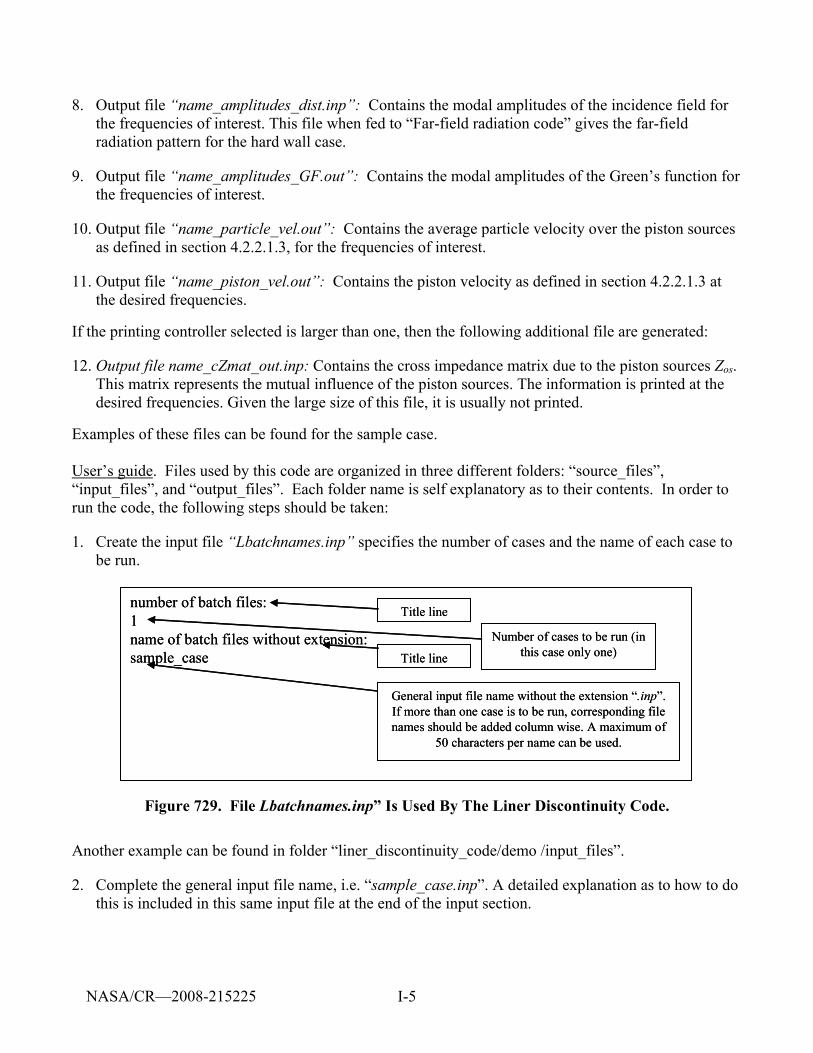
I-5

8. Output file “name_amplitudes_dist.inp”: Contains the modal amplitudes of the incidence field for the frequencies of interest. This file when fed to “Far-field radiation code” gives the far-field radiation pattern for the hard wall case.

9. Output file “name_amplitudes_GF.out”: Contains the modal amplitudes of the Green’s function for the frequencies of interest.

10. Output file “name_particle_vel.out”: Contains the average particle velocity over the piston sources as defined in section 4.2.2.1.3, for the frequencies of interest.

11. Output file “name_piston_vel.out”: Contains the piston velocity as defined in section 4.2.2.1.3 at the desired frequencies.

If the printing controller selected is larger than one, then the following additional file are generated:

12. Output file name_cZmat_out.inp: Contains the cross impedance matrix due to the piston sources Zos. This matrix represents the mutual influence of the piston sources. The information is printed at the desired frequencies. Given the large size of this file, it is usually not printed.

Examples of these files can be found for the sample case. User’s guide. Files used by this code are organized in three different folders: “source_files”, “input_files”, and “output_files”. Each folder name is self explanatory as to their contents. In order to run the code, the following steps should be taken:

1. Create the input file “Lbatchnames.inp” specifies the number of cases and the name of each case to be run.

number of batch files:1name of batch files without extension:sample_case


Number of cases to be run (in this case only one)

Title line

Title line

General input file name without the extension “.inp”. If more than one case is to be run, corresponding file names should be added column wise. A maximum of

50 characters per name can be used.


Title line

Title line

General input file name without the extension “.inp”. If more than one case is to be run, corresponding file names should be added column wise. A maximum of

50 characters per name can be used.

Figure 729. File Lbatchnames.inp” Is Used By The Liner Discontinuity Code.

Another example can be found in folder “liner_discontinuity_code/demo /input_files”.

2. Complete the general input file name, i.e. “sample_case.inp”. A detailed explanation as to how to do this is included in this same input file at the end of the input section.

NASA/CR—2008-215225

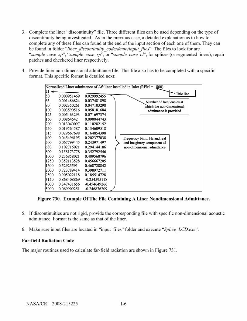
I-6

3. Complete the liner “discontinuity” file. Three different files can be used depending on the type of discontinuity being investigated. As in the previous case, a detailed explanation as to how to complete any of these files can found at the end of the input section of each one of them. They can be found in folder “liner_discontinuity_code/demo/input_files”. The files to look for are “sample_case_sp”, “sample_case_rp”, or “sample_case_cl”, for splices (or segmented liners), repair patches and checkered liner respectively.

4. Provide liner non-dimensional admittance file. This file also has to be completed with a specific format. This specific format is detailed next:

Normalized Liner admittance of Aft liner installed in Inlet (RPM = 1800) 21 50 0.000951469 0.029992455 63 0.001486824 0.037481898 80 0.002350261 0.047103298 100 0.003590516 0.058181684 125 0.005463293 0.071697374 160 0.00864642 0.090044743 200 0.013040097 0.110282152 250 0.019564587 0.134609518 315 0.029667698 0.164854398 400 0.045496195 0.202377038 500 0.067799445 0.243971497 630 0.102716021 0.294144186 800 0.158173778 0.352792546 1000 0.236858021 0.409560796 1250 0.352113528 0.456667205 1600 0.52925591 0.468728842 2000 0.723789414 0.398972711 2500 0.905022118 0.185514728 3150 0.868408869 -0.254595118 4000 0.347431656 -0.454649266 5000 0.069909251 -0.246876209

Title line

Number of frequencies at which the non-dimensional

admittance is provided

Frequency bin in Hz and real and imaginary component of non-dimensional admittance

Normalized Liner admittance of Aft liner installed in Inlet (RPM = 1800) 21 50 0.000951469 0.029992455 63 0.001486824 0.037481898 80 0.002350261 0.047103298 100 0.003590516 0.058181684 125 0.005463293 0.071697374 160 0.00864642 0.090044743 200 0.013040097 0.110282152 250 0.019564587 0.134609518 315 0.029667698 0.164854398 400 0.045496195 0.202377038 500 0.067799445 0.243971497 630 0.102716021 0.294144186 800 0.158173778 0.352792546 1000 0.236858021 0.409560796 1250 0.352113528 0.456667205 1600 0.52925591 0.468728842 2000 0.723789414 0.398972711 2500 0.905022118 0.185514728 3150 0.868408869 -0.254595118 4000 0.347431656 -0.454649266 5000 0.069909251 -0.246876209

Title line




Title line




Figure 730. Example Of The File Containing A Liner Nondimensional Admittance.

5. If discontinuities are not rigid, provide the corresponding file with specific non-dimensional acoustic admittance. Format is the same as that of the liner.

6. Make sure input files are located in “input_files” folder and execute “Splice_LCD.exe”. Far-field Radiation Code

The major routines used to calculate far-field radiation are shown in Figure 731.

NASA/CR—2008-215225

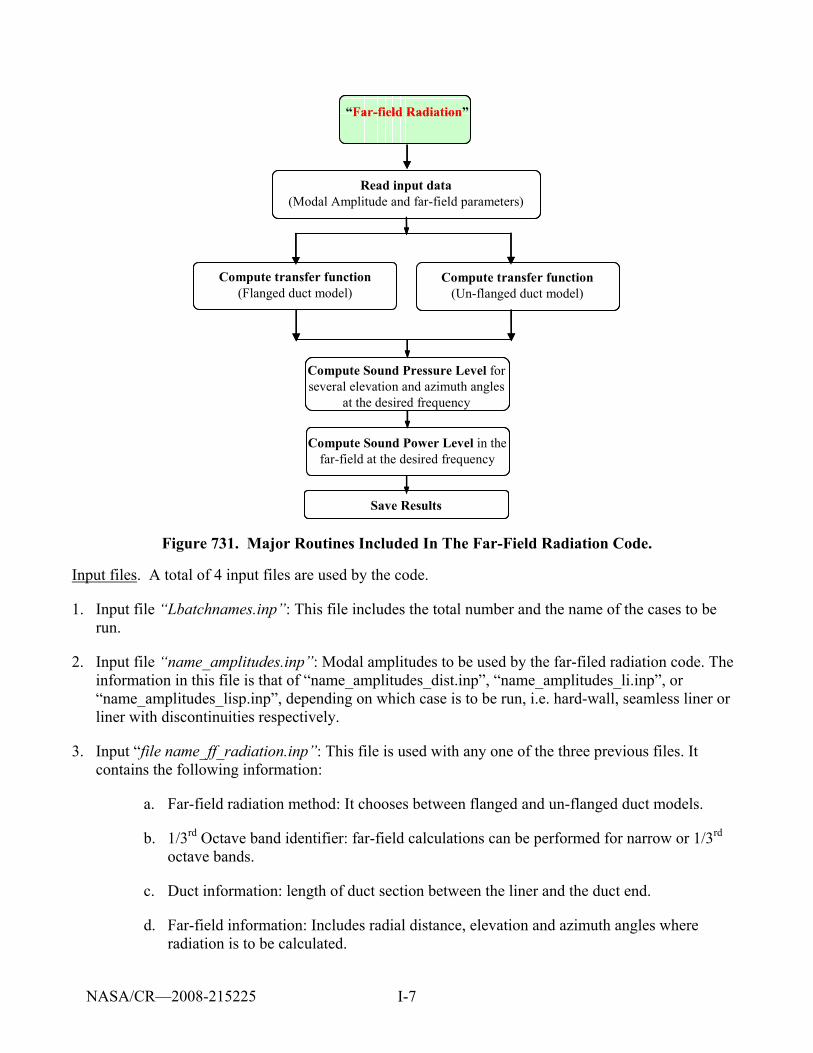
I-7

“Far-field Radiation”

Read input data (Modal Amplitude and far-field parameters)

Compute transfer function(Flanged duct model)

Compute transfer function(Un-flanged duct model)

Compute Sound Pressure Level for several elevation and azimuth angles

at the desired frequency

Compute Sound Power Level in the far-field at the desired frequency

Save Results

“Far-field Radiation”“Far-field Radiation”













Save ResultsSave Results

Figure 731. Major Routines Included In The Far-Field Radiation Code.

Input files. A total of 4 input files are used by the code.

1. Input file “Lbatchnames.inp”: This file includes the total number and the name of the cases to be run.

2. Input file “name_amplitudes.inp”: Modal amplitudes to be used by the far-filed radiation code. The information in this file is that of “name_amplitudes_dist.inp”, “name_amplitudes_li.inp”, or “name_amplitudes_lisp.inp”, depending on which case is to be run, i.e. hard-wall, seamless liner or liner with discontinuities respectively.

3. Input “file name_ff_radiation.inp”: This file is used with any one of the three previous files. It contains the following information:

a. Far-field radiation method: It chooses between flanged and un-flanged duct models.

b. 1/3rd Octave band identifier: far-field calculations can be performed for narrow or 1/3rd octave bands.

c. Duct information: length of duct section between the liner and the duct end.

d. Far-field information: Includes radial distance, elevation and azimuth angles where radiation is to be calculated.

NASA/CR—2008-215225

I-8

4. Input file “jprime_8dec5050.dat”: This file contains the non-dimensional eigenvalue solution for the hard wall case for a total of 50 circumferential and 50 radial modes. The non-dimensionalization factor is the duct radius. This file does not need to be modified unless more modes are required.

Output files. The number of output files varies from 4 up to a maximum of 7 depending on whether the 1/3rd octave band option is chosen.

1. Output file “name_rad_direct.out”: this file contains SPL for the locations specified in “name_ff_farfield.inp”, at the frequencies specified in any of the three amplitude files (see input section).

2. Output file “name_ff_power.out”: contains power radiated at the desired frequency or particular 1/3rd octave band.

3. Output file “name_direc2D.out”: contains same information as “name_ff_rad_direct.out” in TECPLOT format. 2D stands for two dimensional plots, i.e. at a given azimuth location.

4. Output file “name_direc3D.out”: contains same information as “name_ff_rad_direct.out” in TECPLOT format. 3D stands for three dimensional plots.

If the 1/3rd octave band is chosen in “name_ff_radiation.inp” then the following files are created:

5. Output file “name_13RD_rad_direc.out”: same information as “name_rad_direct.out” but for 1/3rd octave bands.

6. Output file “name_13RD_direc2D.out”: same information as “name_direc2D.out” but for 1/3rd octave bands.

7. Output file “name_direc3D.out”: same information as “name_direc3D.out” but for 1/3rd octave bands.

User’s guide. Files used by this code are also organized in three different folders: “source_files”, “input_files”, and “output_files”. In order to run the code, the following steps should be taken:

1. In input file “Lbatchnames.inp” specify the number of cases and the name of each case to be run (Figure 732).

NASA/CR—2008-215225

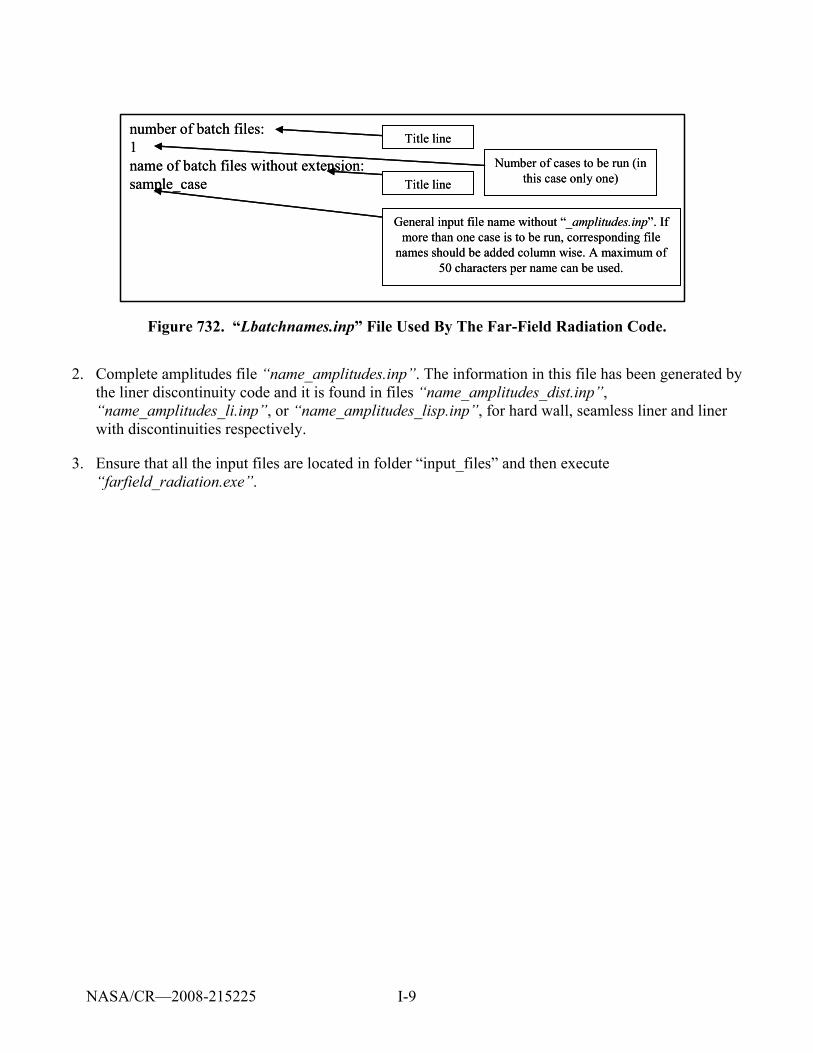
I-9




Title line

Title line

General input file name without “_amplitudes.inp”. If more than one case is to be run, corresponding file

names should be added column wise. A maximum of 50 characters per name can be used.


Title line

Title line

General input file name without “_amplitudes.inp”. If more than one case is to be run, corresponding file

names should be added column wise. A maximum of 50 characters per name can be used.

Figure 732. “Lbatchnames.inp” File Used By The Far-Field Radiation Code.

2. Complete amplitudes file “name_amplitudes.inp”. The information in this file has been generated by the liner discontinuity code and it is found in files “name_amplitudes_dist.inp”, “name_amplitudes_li.inp”, or “name_amplitudes_lisp.inp”, for hard wall, seamless liner and liner with discontinuities respectively.

3. Ensure that all the input files are located in folder “input_files” and then execute “farfield_radiation.exe”.

NASA/CR—2008-215225

II-i

APPENDIX II

EIGEN-VALUE PROBLEM FOR THE LINER DISCONTINUITY CODE

(5 PAGES)

NASA/CR—2008-215225

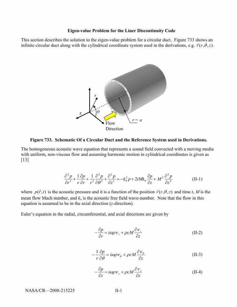
II-1

Eigen-value Problem for the Liner Discontinuity Code

This section describes the solution to the eigen-value problem for a circular duct. Figure 733 shows an infinite circular duct along with the cylindrical coordinate system used in the derivations, e.g. ( , , )r r zθr .

r

z θ

r = a Flow Direction

Figure 733. Schematic Of a Circular Duct and the Reference System used in Derivations.

The homogeneous acoustic wave equation that represents a sound field convected with a moving media with uniform, non-viscous flow and assuming harmonic motion in cylindrical coordinates is given as [13]

2

22

0202

2

2

2

22

2

211zpM

zpiMkpk

zpp

rrp

rrp

∂∂

+∂∂

+−=∂∂

+∂∂

+∂∂

+∂∂

θ (II-1)

where ( , )p r tr is the acoustic pressure and it is a function of the position ( , , )r r zθr and time t, M is the mean flow Mach number, and ko is the acoustic free field wave-number. Note that the flow in this equation is assumed to be in the axial direction (z-direction). Euler’s equation in the radial, circumferential, and axial directions are given by

z

cMirp r

r ∂∂

+=∂∂

−ν

ρωρν (II-2)

z

cMipr ∂

∂+=

∂∂

− θθ

νρωρνθ

1 (II-3)

z

cMizp z

z ∂∂

+=∂∂

−ν

ρωρν (II-4)

NASA/CR—2008-215225

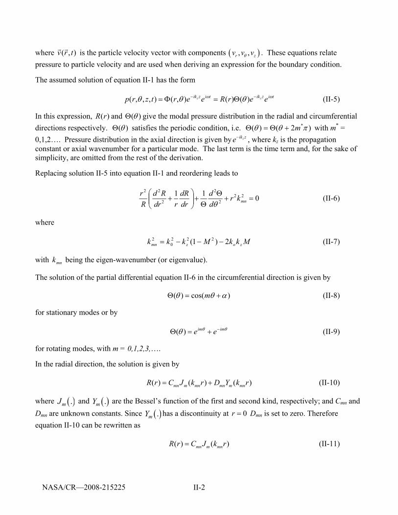
II-2

where ( , )v r tr r is the particle velocity vector with components ( ), ,r zv v vθ . These equations relate pressure to particle velocity and are used when deriving an expression for the boundary condition.

The assumed solution of equation II-1 has the form tiziktizik eerReertzrp zz ωω θθθ −− Θ=Φ= )()(),(),,,( (II-5)

In this expression, )(rR and )(θΘ give the modal pressure distribution in the radial and circumferential directions respectively. )(θΘ satisfies the periodic condition, i.e. )2()( *πθθ m+Θ=Θ with m* = 0,1,2…. Pressure distribution in the axial direction is given by zik ze− , where kz is the propagation constant or axial wavenumber for a particular mode. The last term is the time term and, for the sake of simplicity, are omitted from the rest of the derivation.

Replacing solution II-5 into equation II-1 and reordering leads to

011 222

2

2

22

=+Θ

Θ+⎟⎟

⎠

⎞⎜⎜⎝

⎛+ mnkr

dd

drdR

rdrRd

Rr

θ (II-6)

where MkkMkkk zozmn 2)1( 222

02 −−−= (II-7)

with mnk being the eigen-wavenumber (or eigenvalue).

The solution of the partial differential equation II-6 in the circumferential direction is given by )cos()( αθθ +=Θ m (II-8)

for stationary modes or by θθθ imim ee −+=Θ )( (II-9)

for rotating modes, with m = 0,1,2,3,….

In the radial direction, the solution is given by ( ) ( ) ( )mn m mn mn m mnR r C J k r D Y k r= + (II-10)

where ( ).mJ and ( ).mY are the Bessel’s function of the first and second kind, respectively; and Cmn and Dmn are unknown constants. Since ( ).mY has a discontinuity at 0r = Dmn is set to zero. Therefore equation II-10 can be rewritten as ( ) ( )mn m mnR r C J k r= (II-11)

NASA/CR—2008-215225

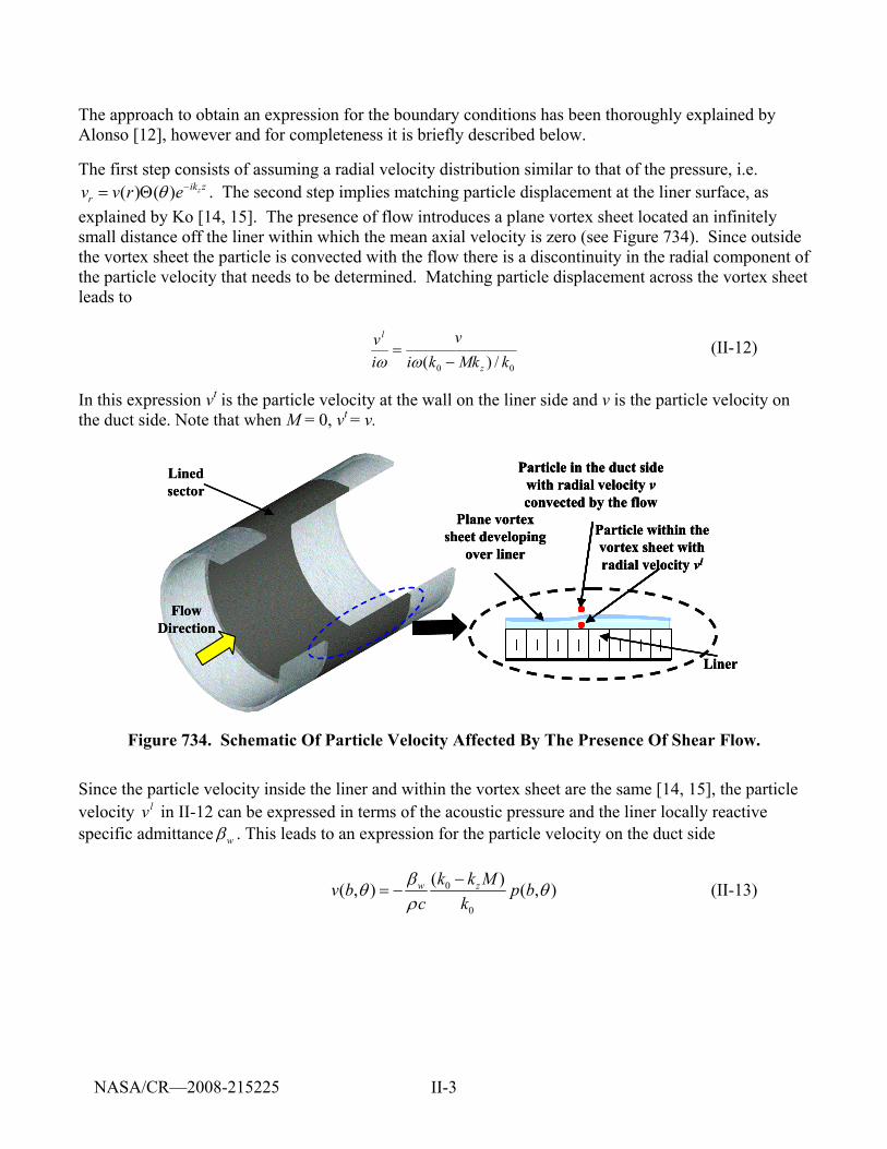
II-3

The approach to obtain an expression for the boundary conditions has been thoroughly explained by Alonso [12], however and for completeness it is briefly described below.

The first step consists of assuming a radial velocity distribution similar to that of the pressure, i.e. ( ) ( ) zik z

rv v r eθ −= Θ . The second step implies matching particle displacement at the liner surface, as explained by Ko [14, 15]. The presence of flow introduces a plane vortex sheet located an infinitely small distance off the liner within which the mean axial velocity is zero (see Figure 734). Since outside the vortex sheet the particle is convected with the flow there is a discontinuity in the radial component of the particle velocity that needs to be determined. Matching particle displacement across the vortex sheet leads to

00 /)( kMkki

viv

z

l

−=

ωω (II-12)

In this expression vt is the particle velocity at the wall on the liner side and v is the particle velocity on the duct side. Note that when M = 0, vt = v.

Flow Direction

Liner

Lined sector

Particle in the duct side with radial velocity vconvected by the flow

Plane vortex sheet developing

over liner

Particle within the vortex sheet with radial velocity vl

Flow Direction

Liner

Lined sector



over liner


Flow Direction

Liner

Lined sector



over liner


Figure 734. Schematic Of Particle Velocity Affected By The Presence Of Shear Flow.

Since the particle velocity inside the liner and within the vortex sheet are the same [14, 15], the particle velocity lv in II-12 can be expressed in terms of the acoustic pressure and the liner locally reactive specific admittance wβ . This leads to an expression for the particle velocity on the duct side

0

0

( )( , ) ( , )w zk k Mv b p bc k

βθ θρ

−= − (II-13)

NASA/CR—2008-215225

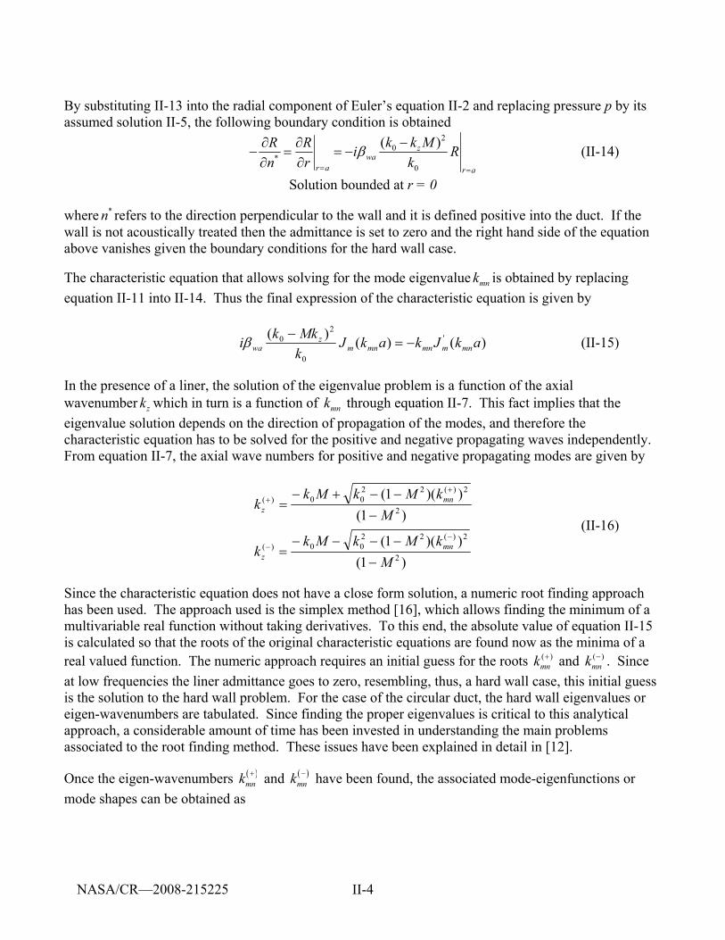
II-4

By substituting II-13 into the radial component of Euler’s equation II-2 and replacing pressure p by its assumed solution II-5, the following boundary condition is obtained

2

0*

0

( )zwa

r a r a

k k MR R i Rn r k

β= =

−∂ ∂− = = −

∂ ∂ (II-14)

Solution bounded at r = 0

where *n refers to the direction perpendicular to the wall and it is defined positive into the duct. If the wall is not acoustically treated then the admittance is set to zero and the right hand side of the equation above vanishes given the boundary conditions for the hard wall case.

The characteristic equation that allows solving for the mode eigenvalue mnk is obtained by replacing equation II-11 into II-14. Thus the final expression of the characteristic equation is given by

)()()( '

0

20 akJkakJ

kMkki mnmmnmnm

zwa −=

−β (II-15)

In the presence of a liner, the solution of the eigenvalue problem is a function of the axial wavenumber zk which in turn is a function of mnk through equation II-7. This fact implies that the eigenvalue solution depends on the direction of propagation of the modes, and therefore the characteristic equation has to be solved for the positive and negative propagating waves independently. From equation II-7, the axial wave numbers for positive and negative propagating modes are given by

)1())(1(

)1())(1(

2

2)(2200)(

2

2)(2200)(

MkMkMk

k

MkMkMk

k

mnz

mnz

−−−−−

=

−−−+−

=

−−

++

(II-16)

Since the characteristic equation does not have a close form solution, a numeric root finding approach has been used. The approach used is the simplex method [16], which allows finding the minimum of a multivariable real function without taking derivatives. To this end, the absolute value of equation II-15 is calculated so that the roots of the original characteristic equations are found now as the minima of a real valued function. The numeric approach requires an initial guess for the roots ( )

mnk + and ( )mnk − . Since

at low frequencies the liner admittance goes to zero, resembling, thus, a hard wall case, this initial guess is the solution to the hard wall problem. For the case of the circular duct, the hard wall eigenvalues or eigen-wavenumbers are tabulated. Since finding the proper eigenvalues is critical to this analytical approach, a considerable amount of time has been invested in understanding the main problems associated to the root finding method. These issues have been explained in detail in [12].

Once the eigen-wavenumbers ( )mnk + and ( )

mnk − have been found, the associated mode-eigenfunctions or mode shapes can be obtained as

NASA/CR—2008-215225

II-5

)()(),(

)()(),()()(

)()(

rkJr

rkJr

mnmmn

mnmmn−−

++

Θ=Φ

Θ=Φ

θθ

θθ (II-17)

for positive (+) and negative (-) propagating waves. The sound field inside the duct is written in terms of these eigen-functions or mode shapes.

NASA/CR—2008-215225

III-i

APPENDIX III

MODAL AMPLITUDES OF THE GREEN’S FUNCTION FOR THE LINER DISCUNTINUITY CODE

(2 PAGES)

NASA/CR—2008-215225

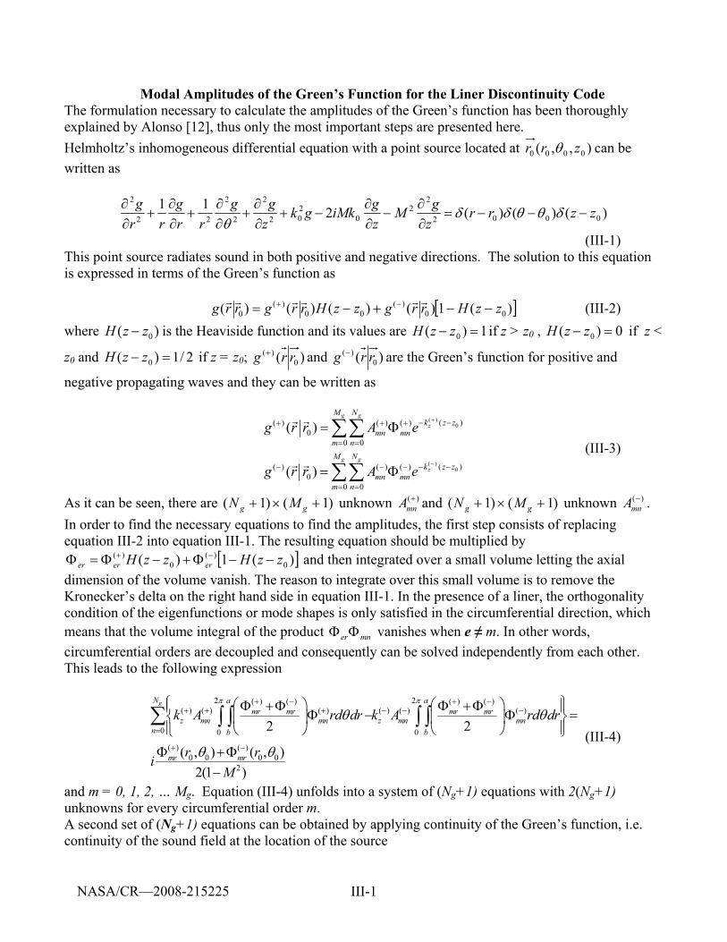
III-1

Modal Amplitudes of the Green’s Function for the Liner Discontinuity Code The formulation necessary to calculate the amplitudes of the Green’s function has been thoroughly explained by Alonso [12], thus only the most important steps are presented here. Helmholtz’s inhomogeneous differential equation with a point source located at ),,( 0000 zrr θ can be written as

)()()(2110002

22

0202

2

2

2

22

2

zzrrzgM

zgiMkgk

zgg

rrg

rrg

−−−=∂∂

−∂∂

−+∂∂

+∂∂

+∂∂

+∂∂ δθθδδ

θ

(III-1) This point source radiates sound in both positive and negative directions. The solution to this equation is expressed in terms of the Green’s function as [ ])(1)()()()( 00

)(00

)(0 zzHrrgzzHrrgrrg −−+−= −+ rrrrrr (III-2)

where )( 0zzH − is the Heaviside function and its values are 1)( 0 =− zzH if z > z0 , 0)( 0 =− zzH if z <

z0 and 2/1)( 0 =− zzH if z = z0; )( 0)( rrg + and )( 0

)( rrg − are the Green’s function for positive and

negative propagating waves and they can be written as

( )0

( )0

( )( ) ( ) ( )0

0 0

( )( ) ( ) ( )0

0 0

( )

( )

g g

z

g g

z

M Nk z z

mn mnm nM N

k z zmn mn

m n

g r r A e

g r r A e

+

−

− −+ + +

= =

− −− − −

= =

= Φ

= Φ

∑∑

∑∑

r r

r r (III-3)

As it can be seen, there are )1()1( +×+ gg MN unknown ( )mnA + and )1()1( +×+ gg MN unknown ( )

mnA − . In order to find the necessary equations to find the amplitudes, the first step consists of replacing equation III-2 into equation III-1. The resulting equation should be multiplied by

[ ])(1)( 0)(

0)( zzHzzH ererer −−Φ+−Φ=Φ −+ and then integrated over a small volume letting the axial

dimension of the volume vanish. The reason to integrate over this small volume is to remove the Kronecker’s delta on the right hand side in equation III-1. In the presence of a liner, the orthogonality condition of the eigenfunctions or mode shapes is only satisfied in the circumferential direction, which means that the volume integral of the product er mnΦ Φ vanishes when e ≠ m. In other words, circumferential orders are decoupled and consequently can be solved independently from each other. This leads to the following expression

2 2( ) ( ) ( ) ( )( ) ( ) ( ) ( ) ( ) ( )

0 0 0

( ) ( )0 0 0 0

2

2 2

( , ) ( , )2(1 )

gN a amr mr mr mr

z mn mn z mn mnn b b

mr mr

k A rd dr k A rd dr

r riM

π π

θ θ

θ θ

+ − + −+ + + − − −

=

+ −

⎧ ⎫⎛ ⎞ ⎛ ⎞Φ +Φ Φ +Φ⎪ ⎪Φ − Φ =⎨ ⎬⎜ ⎟ ⎜ ⎟⎪ ⎪⎝ ⎠ ⎝ ⎠⎩ ⎭

Φ +Φ−

∑ ∫ ∫ ∫ ∫ (III-4)

and m = 0, 1, 2, … Mg. Equation (III-4) unfolds into a system of (Ng+1) equations with 2(Ng+1) unknowns for every circumferential order m. A second set of (Ng+1) equations can be obtained by applying continuity of the Green’s function, i.e. continuity of the sound field at the location of the source

NASA/CR—2008-215225

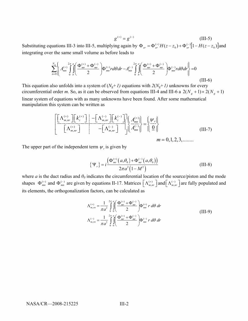
III-2

)()( −+ = gg (III-5) Substituting equations III-3 into III-5, multiplying again by [ ])(1)( 0

)(0

)( zzHzzH ererer −−Φ+−Φ=Φ −+ and integrating over the same small volume as before leads to

2 2( ) ( ) ( ) ( )

( ) ( ) ( ) ( )

0 0 0

02 2

gN a amr mr mr mr

mn mn mn mnn b b

A rd dr A rd drπ π

θ θ+ − + −

+ + − −

=

⎧ ⎫⎛ ⎞ ⎛ ⎞Φ + Φ Φ + Φ⎪ ⎪Φ − Φ =⎨ ⎬⎜ ⎟ ⎜ ⎟⎪ ⎪⎝ ⎠ ⎝ ⎠⎩ ⎭

∑ ∫ ∫ ∫ ∫

(III-6) This equation also unfolds into a system of (Ng+1) equations with 2(Ng+1) unknowns for every circumferential order m. So, as it can be observed from equations III-4 and III-6 a )1(2)1(2 +×+ gg NN linear system of equations with as many unknowns have been found. After some mathematical manipulation this system can be written as

( ) ( ) ( ) ( ) ( ), ,

( )( ) ( ), ,

0

0,1,2,3,..

m nr z m nr z rmn

mnm nr m nr

k k AA

m

ψ+ + − − +

−+ −

⎡ ⎤⎡ ⎤ ⎡ ⎤ ⎡ ⎤ ⎡ ⎤Λ − Λ ⎧ ⎫ ⎧ ⎫⎣ ⎦ ⎣ ⎦ ⎣ ⎦ ⎣ ⎦ ⎪ ⎪ ⎪ ⎪⎢ ⎥ = ⎨ ⎬ ⎨ ⎬⎢ ⎥⎡ ⎤ ⎡ ⎤Λ − Λ ⎪ ⎪⎪ ⎪ ⎩ ⎭⎩ ⎭⎣ ⎦ ⎣ ⎦⎣ ⎦ = ......

(III-7)

The upper part of the independent term rψ is given by

{ }( ) ( )( )

( )( ) ( )

0 0

2 2

, ,

2 1mr mr

r

a ai

a M

θ θ

π

+ −Φ + ΦΨ =

− (III-8)

where a is the duct radius and θ0 indicates the circumferential location of the source/piston and the mode shapes ( )

mn+Φ and ( )

mn−Φ are given by equations II-17. Matrices ( )

,m nr+⎡ ⎤Λ⎣ ⎦ and ( )

,m nr−⎡ ⎤Λ⎣ ⎦ are fully populated and

its elements, the orthogonalization factors, can be calculated as

2 ( ) ( )( ) ( )

, 20 0

2 ( ) ( )( ) ( )

, 20 0

12

12

amr mr

m rn mn

amr mr

m rn mn

r d dra

r d dra

π

π

θπ

θπ

+ −+ +

+ −− −

⎛ ⎞Φ + ΦΛ = Φ ⎜ ⎟

⎝ ⎠⎛ ⎞Φ + Φ

Λ = Φ ⎜ ⎟⎝ ⎠

∫ ∫

∫ ∫ (III-9)

NASA/CR—2008-215225

IV-i

APPENDIX IV

ADDITIONAL EXPERIMENTAL RESULTS FOR THE ANCF MODAL MEASUREMENTS

AND TECH977 FAR FIELD MEASUREMENTS OF LINER DISCONTINUITIES

(13 PAGES)

NASA/CR—2008-215225

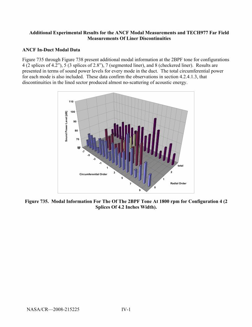
IV-1

Additional Experimental Results for the ANCF Modal Measurements and TECH977 Far Field Measurements Of Liner Discontinuities

ANCF In-Duct Modal Data

Figure 735 through Figure 738 present additional modal information at the 2BPF tone for configurations 4 (2 splices of 4.2”), 5 (3 splices of 2.8”), 7 (segmented liner), and 8 (checkered liner). Results are presented in terms of sound power levels for every mode in the duct. The total circumferential power for each mode is also included. These data confirm the observations in section 4.2.4.1.3, that discontinuities in the lined sector produced almost no-scattering of acoustic energy.

-9-7

-5-3

-1

1

3

5

7

90

1

2

total

60

70

80

90

100

110

Soun

d Po

wer

Lev

el [d

B]


Radial Order

Figure 735. Modal Information For The Of The 2BPF Tone At 1800 rpm for Configuration 4 (2 Splices Of 4.2 Inches Width).

NASA/CR—2008-215225

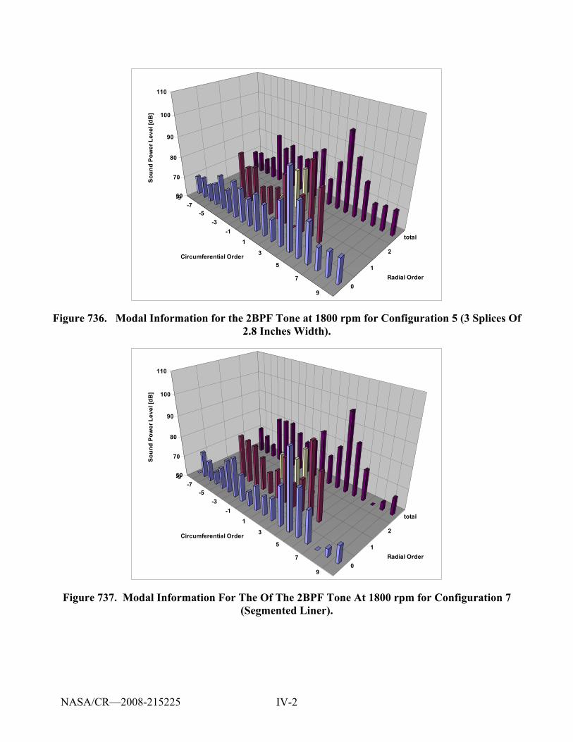
IV-2

-9-7

-5-3

-1

1

3

5

7

90

1

2

total

60

70

80

90

100

110

Soun

d Po

wer

Lev

el [d

B]


Radial Order

Figure 736. Modal Information for the 2BPF Tone at 1800 rpm for Configuration 5 (3 Splices Of 2.8 Inches Width).

-9-7

-5-3

-1

1

3

5

7

90

1

2

total

60

70

80

90

100

110

Soun

d Po

wer

Lev

el [d

B]


Radial Order

Figure 737. Modal Information For The Of The 2BPF Tone At 1800 rpm for Configuration 7 (Segmented Liner).

NASA/CR—2008-215225

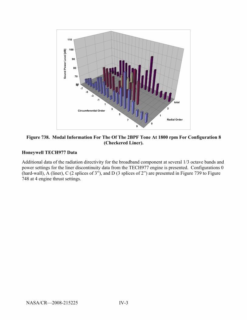
IV-3

-9-7

-5-3

-1

1

3

5

7

90

1

2

total

60

70

80

90

100

110

Soun

d Po

wer

Lev

el [d

B]


Radial Order

Figure 738. Modal Information For The Of The 2BPF Tone At 1800 rpm For Configuration 8 (Checkered Liner).

Honeywell TECH977 Data

Additional data of the radiation directivity for the broadband component at several 1/3 octave bands and power settings for the liner discontinuity data from the TECH977 engine is presented. Configurations 0 (hard-wall), A (liner), C (2 splices of 3”), and D (3 splices of 2”) are presented in Figure 739 to Figure 748 at 4 engine thrust settings.

NASA/CR—2008-215225

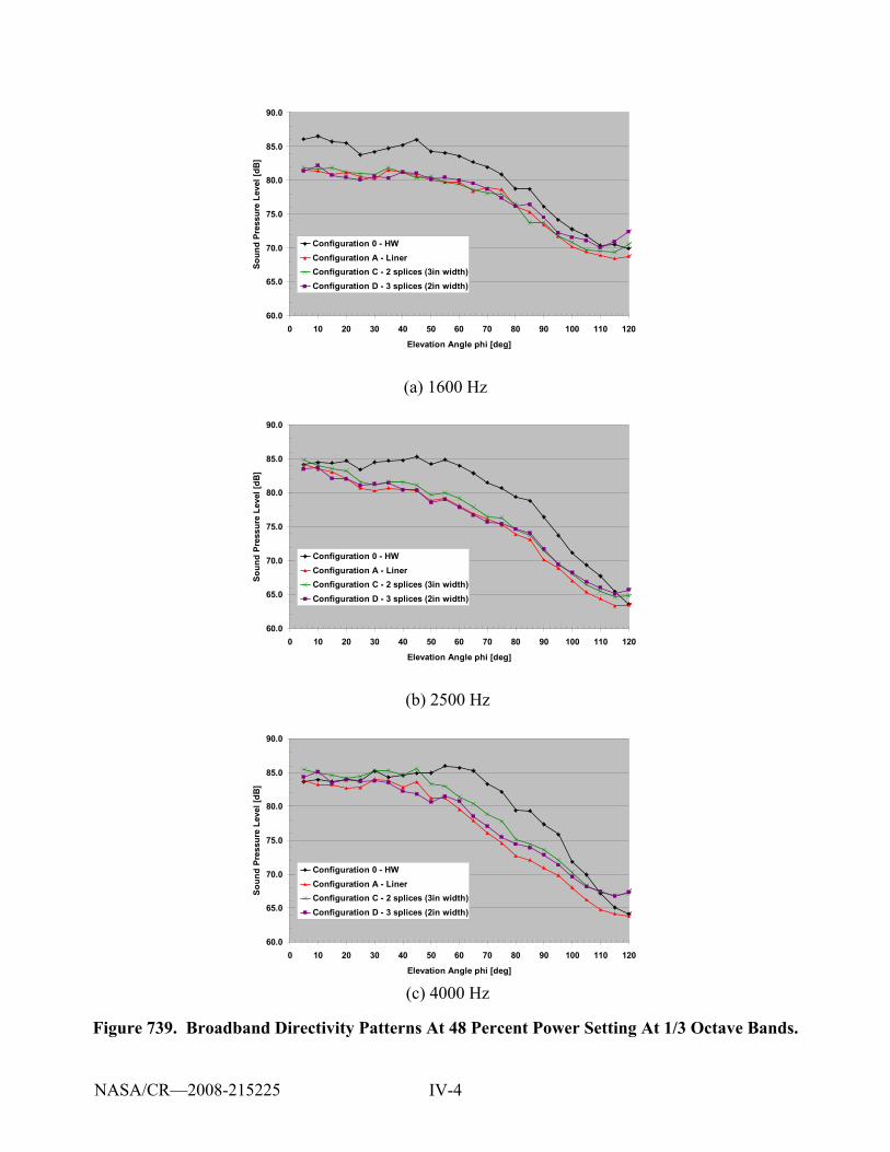
IV-4

60.0

65.0

70.0

75.0

80.0

85.0

90.0

0 10 20 30 40 50 60 70 80 90 100 110 120


Soun

d Pr

essu

re L

evel

[dB


(a) 1600 Hz

60.0

65.0

70.0

75.0

80.0

85.0

90.0

0 10 20 30 40 50 60 70 80 90 100 110 120


Soun

d Pr

essu

re L

evel

[dB

]


(b) 2500 Hz

60.0

65.0

70.0

75.0

80.0

85.0

90.0

0 10 20 30 40 50 60 70 80 90 100 110 120


Soun

d Pr

essu

re L

evel

[dB

]


(c) 4000 Hz


NASA/CR—2008-215225

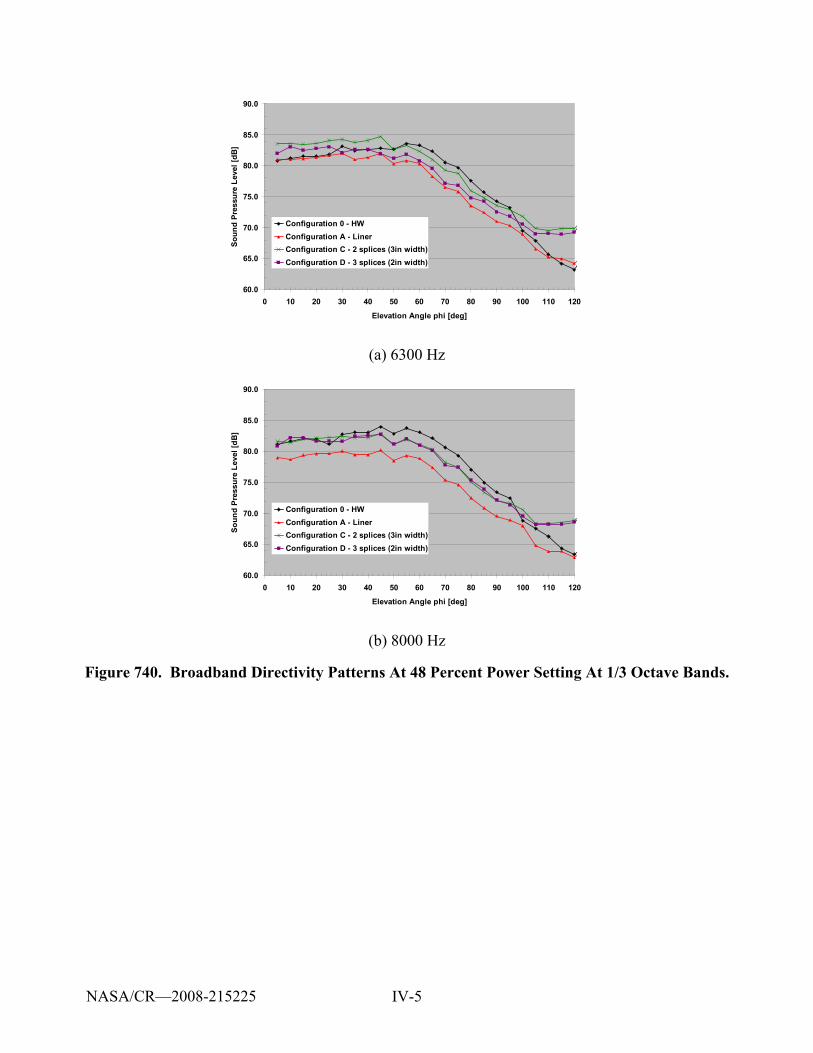
IV-5

60.0

65.0

70.0

75.0

80.0

85.0

90.0

0 10 20 30 40 50 60 70 80 90 100 110 120


Soun

d Pr

essu

re L

evel

[dB


(a) 6300 Hz

60.0

65.0

70.0

75.0

80.0

85.0

90.0

0 10 20 30 40 50 60 70 80 90 100 110 120


Soun

d Pr

essu

re L

evel

[dB

]


(b) 8000 Hz


NASA/CR—2008-215225

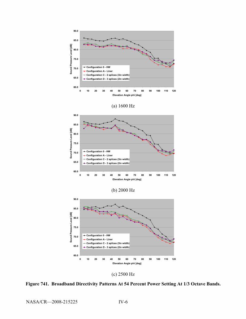
IV-6

60.0

65.0

70.0

75.0

80.0

85.0

90.0

0 10 20 30 40 50 60 70 80 90 100 110 120


Soun

d Pr

essu

re L

evel

[dB


(a) 1600 Hz

60.0

65.0

70.0

75.0

80.0

85.0

90.0

0 10 20 30 40 50 60 70 80 90 100 110 120


Soun

d Pr

essu

re L

evel

[dB

]


(b) 2000 Hz

60.0

65.0

70.0

75.0

80.0

85.0

90.0

0 10 20 30 40 50 60 70 80 90 100 110 120


Soun

d Pr

essu

re L

evel

[dB

]


(c) 2500 Hz


NASA/CR—2008-215225

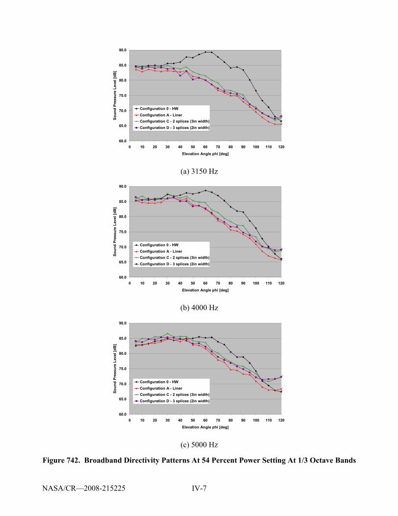
IV-7

60.0

65.0

70.0

75.0

80.0

85.0

90.0

0 10 20 30 40 50 60 70 80 90 100 110 120


Soun

d Pr

essu

re L

evel

[dB


(a) 3150 Hz

60.0

65.0

70.0

75.0

80.0

85.0

90.0

0 10 20 30 40 50 60 70 80 90 100 110 120


Soun

d Pr

essu

re L

evel

[dB

]


(b) 4000 Hz

60.0

65.0

70.0

75.0

80.0

85.0

90.0

0 10 20 30 40 50 60 70 80 90 100 110 120


Soun

d Pr

essu

re L

evel

[dB

]


(c) 5000 Hz

Figure 742. Broadband Directivity Patterns At 54 Percent Power Setting At 1/3 Octave Bands

NASA/CR—2008-215225

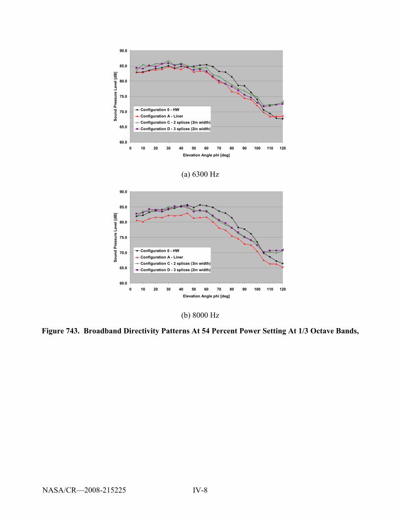
IV-8

60.0

65.0

70.0

75.0

80.0

85.0

90.0

0 10 20 30 40 50 60 70 80 90 100 110 120


Soun

d Pr

essu

re L

evel

[dB


(a) 6300 Hz

60.0

65.0

70.0

75.0

80.0

85.0

90.0

0 10 20 30 40 50 60 70 80 90 100 110 120


Soun

d Pr

essu

re L

evel

[dB

]


(b) 8000 Hz

Figure 743. Broadband Directivity Patterns At 54 Percent Power Setting At 1/3 Octave Bands,

NASA/CR—2008-215225

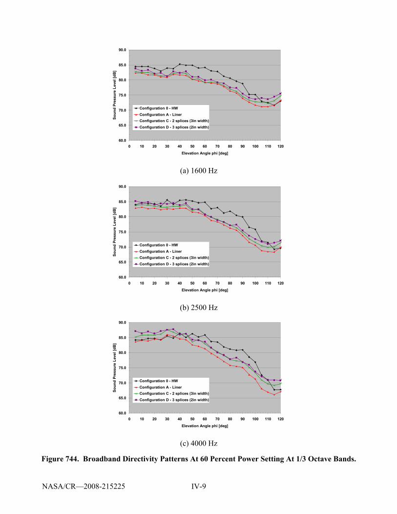
IV-9

60.0

65.0

70.0

75.0

80.0

85.0

90.0

0 10 20 30 40 50 60 70 80 90 100 110 120


Soun

d Pr

essu

re L

evel

[dB


(a) 1600 Hz

60.0

65.0

70.0

75.0

80.0

85.0

90.0

0 10 20 30 40 50 60 70 80 90 100 110 120


Soun

d Pr

essu

re L

evel

[dB

]


(b) 2500 Hz

60.0

65.0

70.0

75.0

80.0

85.0

90.0

0 10 20 30 40 50 60 70 80 90 100 110 120


Soun

d Pr

essu

re L

evel

[dB

]


(c) 4000 Hz


NASA/CR—2008-215225

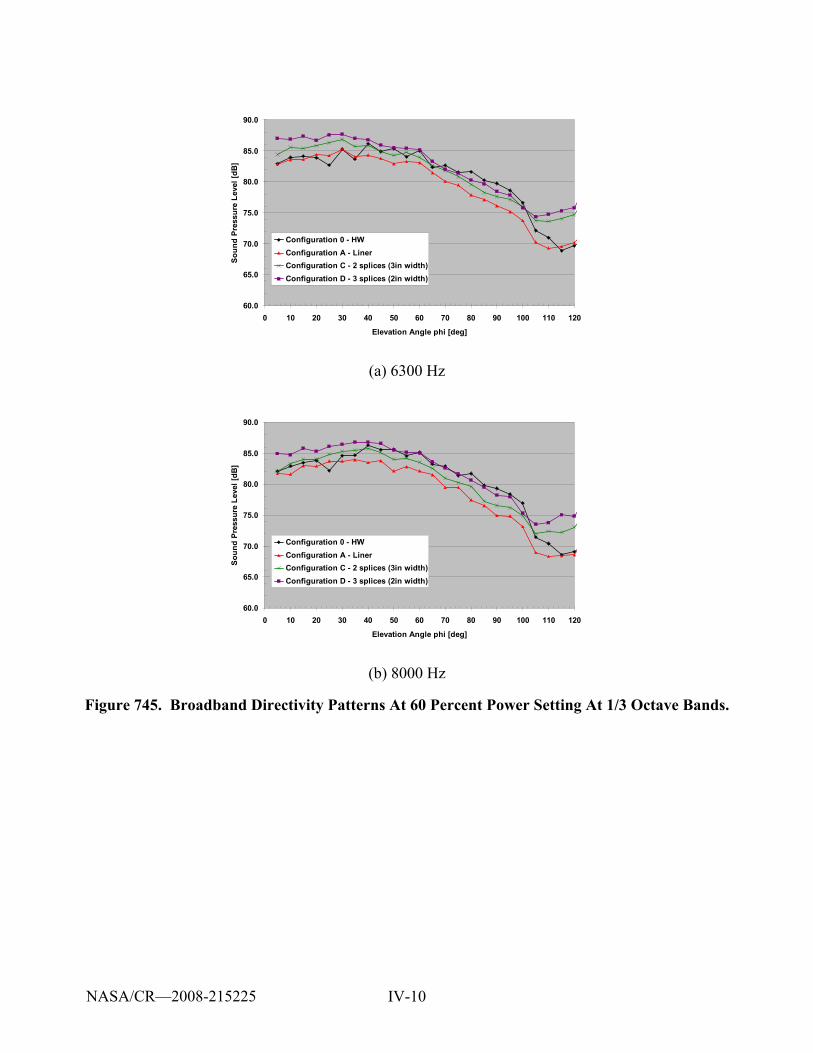
IV-10

60.0

65.0

70.0

75.0

80.0

85.0

90.0

0 10 20 30 40 50 60 70 80 90 100 110 120


Soun

d Pr

essu

re L

evel

[dB


(a) 6300 Hz

60.0

65.0

70.0

75.0

80.0

85.0

90.0

0 10 20 30 40 50 60 70 80 90 100 110 120


Soun

d Pr

essu

re L

evel

[dB

]


(b) 8000 Hz


NASA/CR—2008-215225

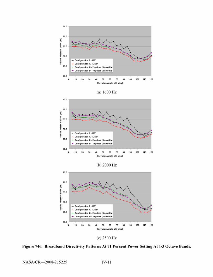
IV-11

70.0

75.0

80.0

85.0

90.0

95.0

0 10 20 30 40 50 60 70 80 90 100 110 120


Soun

d Pr

essu

re L

evel

[dB


(a) 1600 Hz

70.0

75.0

80.0

85.0

90.0

95.0

0 10 20 30 40 50 60 70 80 90 100 110 120


Soun

d Pr

essu

re L

evel

[dB

]


(b) 2000 Hz

70.0

75.0

80.0

85.0

90.0

95.0

0 10 20 30 40 50 60 70 80 90 100 110 120


Soun

d Pr

essu

re L

evel

[dB

]


(c) 2500 Hz


NASA/CR—2008-215225

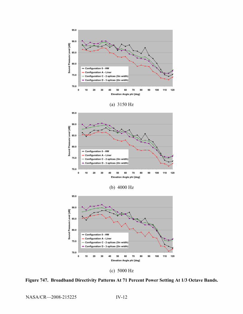
IV-12

70.0

75.0

80.0

85.0

90.0

95.0

0 10 20 30 40 50 60 70 80 90 100 110 120


Soun

d Pr

essu

re L

evel

[dB


(a) 3150 Hz

70.0

75.0

80.0

85.0

90.0

95.0

0 10 20 30 40 50 60 70 80 90 100 110 120


Soun

d Pr

essu

re L

evel

[dB

]


(b) 4000 Hz

70.0

75.0

80.0

85.0

90.0

95.0

0 10 20 30 40 50 60 70 80 90 100 110 120


Soun

d Pr

essu

re L

evel

[dB

]


(c) 5000 Hz


NASA/CR—2008-215225

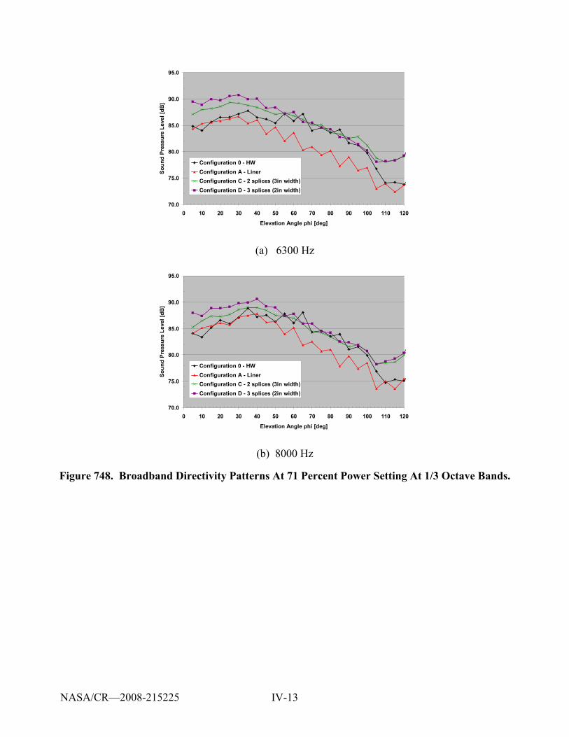
IV-13

70.0

75.0

80.0

85.0

90.0

95.0

0 10 20 30 40 50 60 70 80 90 100 110 120


Soun

d Pr

essu

re L

evel

[dB


(a) 6300 Hz

70.0

75.0

80.0

85.0

90.0

95.0

0 10 20 30 40 50 60 70 80 90 100 110 120


Soun

d Pr

essu

re L

evel

[dB

]


(b) 8000 Hz


NASA/CR—2008-215225

V-i

APPENDIX V

TECH977 ENGINE SWEEP DATA FOR LINER DISCONTINUITY EVALUATION

(4 PAGES)

NASA/CR—2008-215225

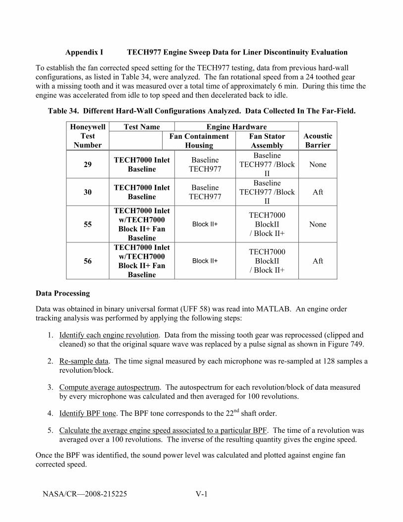
V-1

Appendix I TECH977 Engine Sweep Data for Liner Discontinuity Evaluation

To establish the fan corrected speed setting for the TECH977 testing, data from previous hard-wall configurations, as listed in Table 34, were analyzed. The fan rotational speed from a 24 toothed gear with a missing tooth and it was measured over a total time of approximately 6 min. During this time the engine was accelerated from idle to top speed and then decelerated back to idle.

Table 34. Different Hard-Wall Configurations Analyzed. Data Collected In The Far-Field.

Test Name Engine Hardware Honeywell Test

Number Fan Containment

Housing Fan Stator Assembly

Acoustic Barrier

29 TECH7000 Inlet Baseline

Baseline TECH977

Baseline TECH977 /Block

II None

30 TECH7000 Inlet Baseline

Baseline TECH977

Baseline TECH977 /Block

II Aft

55

TECH7000 Inlet w/TECH7000 Block II+ Fan

Baseline

Block II+ TECH7000

BlockII / Block II+

None

56

TECH7000 Inlet w/TECH7000 Block II+ Fan

Baseline

Block II+ TECH7000

BlockII / Block II+

Aft

Data Processing

Data was obtained in binary universal format (UFF 58) was read into MATLAB. An engine order tracking analysis was performed by applying the following steps:

1. Identify each engine revolution. Data from the missing tooth gear was reprocessed (clipped and cleaned) so that the original square wave was replaced by a pulse signal as shown in Figure 749.

2. Re-sample data. The time signal measured by each microphone was re-sampled at 128 samples a revolution/block.

3. Compute average autospectrum. The autospectrum for each revolution/block of data measured by every microphone was calculated and then averaged for 100 revolutions.

4. Identify BPF tone. The BPF tone corresponds to the 22nd shaft order.

5. Calculate the average engine speed associated to a particular BPF. The time of a revolution was averaged over a 100 revolutions. The inverse of the resulting quantity gives the engine speed.

Once the BPF was identified, the sound power level was calculated and plotted against engine fan corrected speed.

NASA/CR—2008-215225

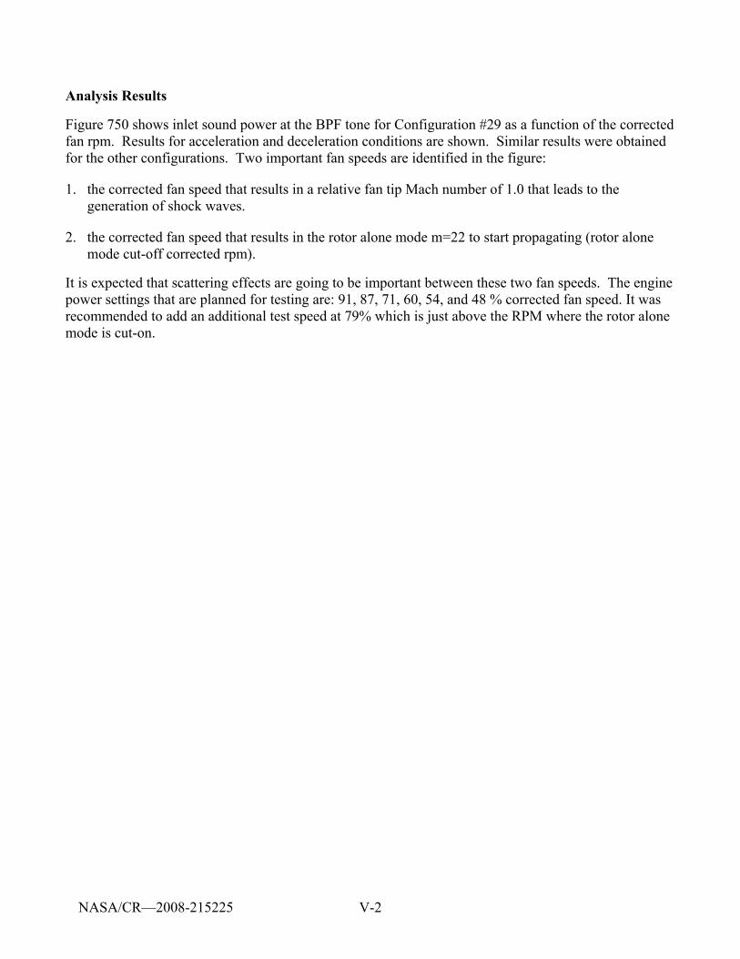
V-2

Analysis Results

Figure 750 shows inlet sound power at the BPF tone for Configuration #29 as a function of the corrected fan rpm. Results for acceleration and deceleration conditions are shown. Similar results were obtained for the other configurations. Two important fan speeds are identified in the figure:

1. the corrected fan speed that results in a relative fan tip Mach number of 1.0 that leads to the generation of shock waves.

2. the corrected fan speed that results in the rotor alone mode m=22 to start propagating (rotor alone mode cut-off corrected rpm).

It is expected that scattering effects are going to be important between these two fan speeds. The engine power settings that are planned for testing are: 91, 87, 71, 60, 54, and 48 % corrected fan speed. It was recommended to add an additional test speed at 79% which is just above the RPM where the rotor alone mode is cut-on.

NASA/CR—2008-215225

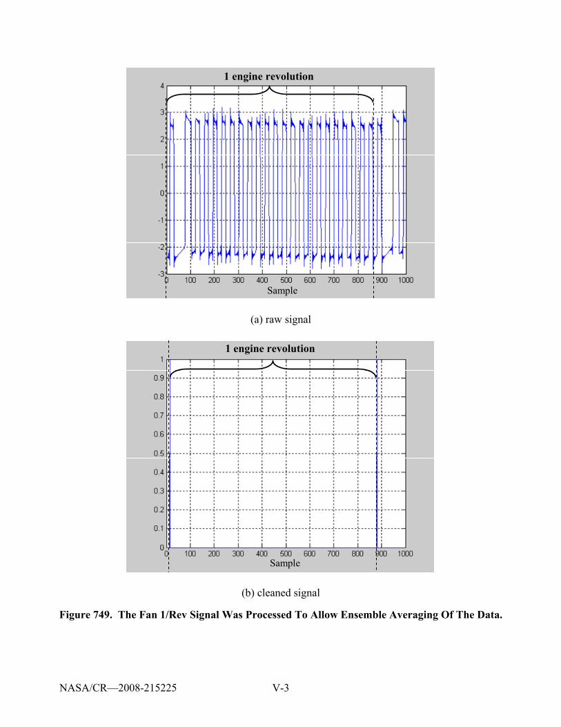
V-3

1 engine revolution

Sample

1 engine revolution

Sample

(a) raw signal

1 engine revolution

Sample

1 engine revolution

Sample

(b) cleaned signal

Figure 749. The Fan 1/Rev Signal Was Processed To Allow Ensemble Averaging Of The Data.

NASA/CR—2008-215225

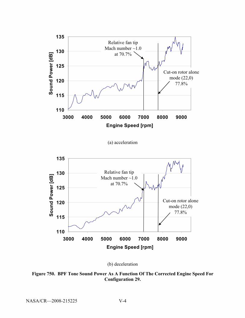
V-4

110

115

120

125

130

135

3000 4000 5000 6000 7000 8000 9000Engine Speed [rpm]

Soun

d Po

wer

[dB

]Relative fan tip

Mach number ~1.0 at 70.7%

Cut-on rotor alone mode (22,0)

77.8%

110

115

120

125

130

135

3000 4000 5000 6000 7000 8000 9000Engine Speed [rpm]

Soun

d Po

wer

[dB

]Relative fan tip

Mach number ~1.0 at 70.7%


77.8%

(a) acceleration

110

115

120

125

130

135

3000 4000 5000 6000 7000 8000 9000Engine Speed [rpm]

Soun

d Po

wer

[dB

] Relative fan tip Mach number ~1.0

at 70.7%


77.8%

110

115

120

125

130

135

3000 4000 5000 6000 7000 8000 9000Engine Speed [rpm]

Soun

d Po

wer

[dB

] Relative fan tip Mach number ~1.0

at 70.7%


77.8%

(b) deceleration

Figure 750. BPF Tone Sound Power As A Function Of The Corrected Engine Speed For Configuration 29.

NASA/CR—2008-215225

VI-i

APPENDIX VI

CONVERGENCE ANALYSIS FOR THE LINER DISCONTINUITY MODELS

(4 PAGES)

NASA/CR—2008-215225

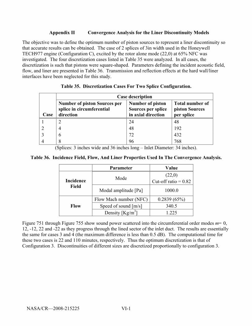
VI-1

Appendix II Convergence Analysis for the Liner Discontinuity Models

The objective was to define the optimum number of piston sources to represent a liner discontinuity so that accurate results can be obtained. The case of 2 splices of 3in width used in the Honeywell TECH977 engine (Configuration C), excited by the rotor alone mode (22,0) at 65% NFC was investigated. The four discretization cases listed in Table 35 were analyzed. In all cases, the discretization is such that pistons were square-shaped. Parameters defining the incident acoustic field, flow, and liner are presented in Table 36. Transmission and reflection effects at the hard wall/liner interfaces have been neglected for this study.

Table 35. Discretization Cases For Two Splice Configuration.

Case description

Case

Number of piston Sources per splice in circumferential direction

Number of piston Sources per splice in axial direction

Total number of piston Sources per splice

1 2 24 48 2 4 48 192 3 6 72 432 4 8 96 768

(Splices: 3 inches wide and 36 inches long – Inlet Diameter: 34 inches).

Table 36. Incidence Field, Flow, And Liner Properties Used In The Convergence Analysis.

Parameter Value

Mode (22,0)

Cut-off ratio = 0.82 Incidence Field

Modal amplitude [Pa] 1000.0

Flow Mach number (NFC) 0.2839 (65%) Speed of sound [m/s] 340.5 Flow

Density [Kg/m3] 1.225

Figure 751 through Figure 755 show sound power scattered into the circumferential order modes m= 0, 12, -12, 22 and -22 as they progress through the lined sector of the inlet duct. The results are essentially the same for cases 3 and 4 (the maximum difference is less than 0.5 dB). The computational time for these two cases is 22 and 110 minutes, respectively. Thus the optimum discretization is that of Configuration 3. Discontinuities of different sizes are discretized proportionally to configuration 3.

NASA/CR—2008-215225

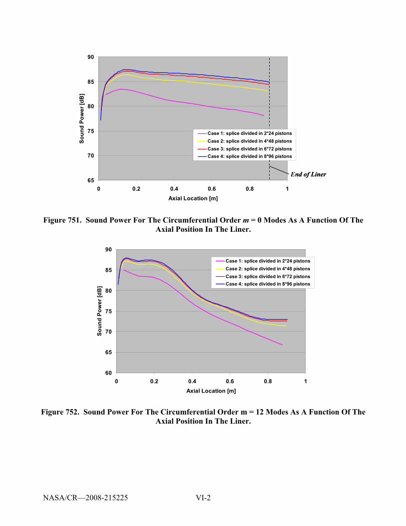
VI-2

65

70

75

80

85

90

0 0.2 0.4 0.6 0.8 1Axial Location [m]

Soun

d Po

wer

[dB

]

Case 1: splice divided in 2*24 pistonsCase 2: splice divided in 4*48 pistonsCase 3: splice divided in 6*72 pistonsCase 4: splice divided in 8*96 pistons

End of Liner65

70

75

80

85

90

0 0.2 0.4 0.6 0.8 1Axial Location [m]

Soun

d Po

wer

[dB

]


End of Liner

Figure 751. Sound Power For The Circumferential Order m = 0 Modes As A Function Of The Axial Position In The Liner.

60

65

70

75

80

85

90

0 0.2 0.4 0.6 0.8 1Axial Location [m]

Soun

d Po

wer

[dB

]



NASA/CR—2008-215225

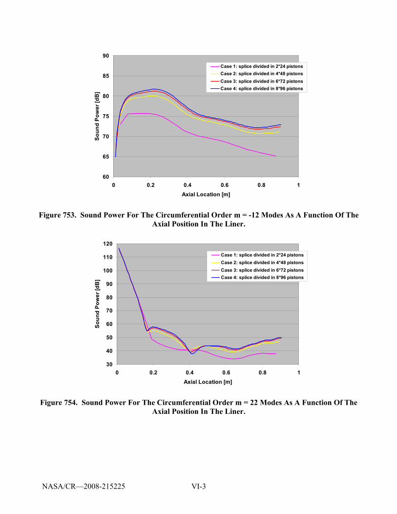
VI-3

60

65

70

75

80

85

90

0 0.2 0.4 0.6 0.8 1Axial Location [m]

Soun

d Po

wer

[dB

]


Figure 753. Sound Power For The Circumferential Order m = -12 Modes As A Function Of The Axial Position In The Liner.

30

40

50

60

70

80

90

100

110

120

0 0.2 0.4 0.6 0.8 1Axial Location [m]

Soun

d Po

wer

[dB

]



NASA/CR—2008-215225

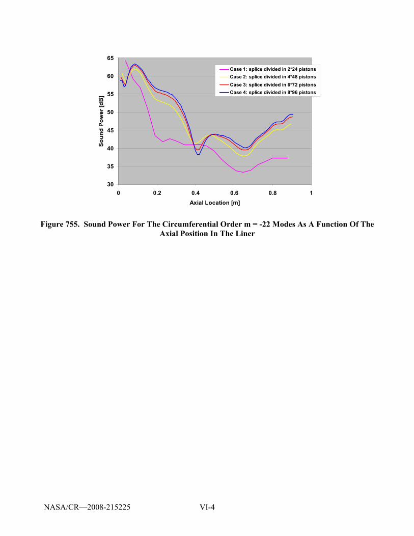
VI-4

30

35

40

45

50

55

60

65

0 0.2 0.4 0.6 0.8 1Axial Location [m]

Soun

d Po

wer

[dB

]


Figure 755. Sound Power For The Circumferential Order m = -22 Modes As A Function Of The Axial Position In The Liner

NASA/CR—2008-215225

REPORT DOCUMENTATION PAGE Form Approved OMB No. 0704-0188

The public reporting burden for this collection of information is estimated to average 1 hour per response, including the time for reviewing instructions, searching existing data sources, gathering and maintaining the data needed, and completing and reviewing the collection of information. Send comments regarding this burden estimate or any other aspect of this collection of information, including suggestions for reducing this burden, to Department of Defense, Washington Headquarters Services, Directorate for Information Operations and Reports (0704-0188), 1215 Jefferson Davis Highway, Suite 1204, Arlington, VA 22202-4302. Respondents should be aware that notwithstanding any other provision of law, no person shall be subject to any penalty for failing to comply with a collection of information if it does not display a currently valid OMB control number. PLEASE DO NOT RETURN YOUR FORM TO THE ABOVE ADDRESS. 1. REPORT DATE (DD-MM-YYYY) 01-05-2008

2. REPORT TYPE Final Contractor Report

3. DATES COVERED (From - To) Dec 2004 - Aug 2008

4. TITLE AND SUBTITLE Engine Validation of Noise and Emission Reduction Technology Phase I

5a. CONTRACT NUMBER NAS3-01136

5b. GRANT NUMBER

5c. PROGRAM ELEMENT NUMBER

6. AUTHOR(S) Weir, Don, editor(s)

5d. PROJECT NUMBER

5e. TASK NUMBER RASER Task No. 8

5f. WORK UNIT NUMBER WBS 561581.02.08.03.18.02

7. PERFORMING ORGANIZATION NAME(S) AND ADDRESS(ES) Honeywell Aerospace 111 South 34th Street P.O. Box 52181 Phoenix, Arizona 85072

8. PERFORMING ORGANIZATION REPORT NUMBER E-16521

9. SPONSORING/MONITORING AGENCY NAME(S) AND ADDRESS(ES) National Aeronautics and Space Administration Washington, DC 20546-0001

10. SPONSORING/MONITORS ACRONYM(S) NASA

11. SPONSORING/MONITORING REPORT NUMBER NASA/CR-2008-215225; Honeywell Report No. 21-13843A

12. DISTRIBUTION/AVAILABILITY STATEMENT Unclassified-Unlimited Subject Category: 05 Available electronically at http://gltrs.grc.nasa.gov This publication is available from the NASA Center for AeroSpace Information, 301-621-0390

13. SUPPLEMENTARY NOTES

14. ABSTRACT This final report has been prepared by Honeywell Aerospace, Phoenix, Arizona, a unit of Honeywell International, Inc., documenting work performed during the period December 2004 through August 2007 for the NASA Glenn Research Center, Cleveland, Ohio, under the Revolutionary Aero-Space Engine Research (RASER) Program, Contract No. NAS3-01136, Task Order 8, Engine Validation of Noise and Emission Reduction Technology Phase I. The NASA Task Manager was Dr. Joe Grady of the NASA Glenn Research Center. The NASA Contract Officer was Mr. Albert Spence of the NASA Glenn Research Center. This report is for a test program in which NASA funded engine validations of integrated technologies that reduce aircraft engine noise. These technologies address the reduction of engine fan and jet noise, and noise associated with propulsion/airframe integration. The results of these tests will be used by NASA to identify the engineering tradeoffs associated with the technologies that are needed to enable advanced engine systems to meet stringent goals for the reduction of noise. The objectives of this program are to (1) conduct system engineering and integration efforts to define the engine test-bed configuration; (2) develop selected noise reduction technologies to a technical maturity sufficient to enable engine testing and validation of those technologies in the FY06-07 time frame; (3) conduct engine tests designed to gain insight into the sources, mechanisms and characteristics of noise in the engines; and (4) establish baseline engine noise measurements for subsequent use in the evaluation of noise reduction. 15. SUBJECT TERMS Noise measurements; Engine diagnostics; Noise technology

16. SECURITY CLASSIFICATION OF: 17. LIMITATION OF ABSTRACT UU

18. NUMBER OF PAGES

758

19a. NAME OF RESPONSIBLE PERSON STI Help Desk (email:[email protected])

a. REPORT U

b. ABSTRACT U

c. THIS PAGE U

19b. TELEPHONE NUMBER (include area code) 301-621-0390

Standard Form 298 (Rev. 8-98)Prescribed by ANSI Std. Z39-18

Engine Validation of Noise and Emission Reduction ...

Documents