Energy Technology Environment Model with … Technology Environment Model with Smart Grid and Robust Nodal Electricity Prices Fred´ eric Babonneau´ 1cand Alain Haurie2 1 ORDECSYS

Energy Technology Environment Model with Smart Gridand Robust Nodal Electricity Prices

Frederic Babonneau1c and Alain Haurie2

1 ORDECSYS and Business School, University Adolfo Ibanez, Chile.2 ORDECSYS, Place de l’Etrier 4, CH-1224 Chene-Bougeries, Switzerland.

c Corresponding author: +41 78 889 36 73, [email protected]

1

Abstract

This paper deals with the modeling of power flow in a transmission grid within themulti-sectoral multi-energy long-term regional energy model ETEM-SG. This extensionof the model allows a better representation of demand response for flexible loads triggeredby nodal marginal cost pricing. To keep the global model in the realm of linear program-ming one uses a linearized DC power flow model that represent the transmission gridwith the main constraints on the power flowing through the different arcs of the electricitytransmission network. Robust optimization is used to take into account the uncertainty onthe capacity limits resulting from inter-regional transit. A numerical illustration is carriedout for a data set corresponding roughly to the Leman Arc region.

Keywords. OR in Energy; Long-term Energy Model; Power Flow; Robust Nodal ElectricityPrices; Robust Optimization.

Aknowledgment. This research is supported by the Qatar National Research Fund under GrantAgreement no 6-1035-5–126.

1 Introduction

The transition to sustainable energy system, in Europe as in the rest of OECD countries in-volves an increase of distributed power generation from variable renewable sources such aswind turbines and solar panels, the development of electric mobility, the linking of power andheat or cooling generation and the active use of demand response. ETEM-SG, that we useon this research, is a model developed recently [3, 16] to assess the future role of renewableand smart-grid technologies in the energy transition, at a regional level. It belongs to theMARKAL/TIMES family of models [10, 11, 13], which represents the optimal capacity ex-pansion in production technology and the flow of resources in the whole energy system of aregion or country. These models are well-known to lead to large-scale mathematical formula-tion and, as such, extensions to power flow and uncertainty modelling bring numerical issuesand challenges.

In this paper one presents an extension of the multi-sectoral multi-energy long-term re-gional energy model ETEM-SG permitting a robust representation of power flow constraintsin the regional transmission grid. This extension is needed because, in ETEM-SG, demand re-sponse is modeled as an optimal response of flexible loads and distributed energy resources totime of use pricing schemes, based on marginal cost. Since the loads and the generation unitsare geographically distributed these prices should be represented by nodal marginal costs asso-ciated with a representation of the transmission grid. A linearized DC power flow model, whichis quite pervasive in the planning of power systems, is now included in ETEM-SG, providing arepresentation of the transmission grid with the main constraints on the power flowing throughthe different arcs of the electricity transmission network. The scenarios obtained through run-ning ETEM-SG will thus propose, for each time slice an optimal dispatch of production units ofthe regional energy system with demand response activities triggered by marginal cost pricing,and at a larger time scale, the optimal location and timing of new capacities introduction for

2

power generation (in particular the technologies based on renewable sources), the developmentof distributed storage (e.g. through electric cars and PHEVs) and the investment in networkreinforcement.

Because the power flows circulating in a regional transmission grid depend on what hap-pens on the transmission grid for a much larger perimeter, a robust optimization (RO) technique[8, 6] is introduced to take into account the resulting uncertainty on the capacity limits for thedifferent arcs of the regional transmission grid. RO is an alternative to classical approaches (eg,Stochastic Programming, Chance Constraint Programming) that aims at overcoming numericalissues induced by calculus of probability and by the well-known curse of dimensionality. Themain idea of RO is to start with a non-probabilistic formulation of uncertainty, namely the un-certainty set, and look for solutions that remain satisfactory for all possible realizations in theuncertainty set. Solutions having this property are named robust. As no probability model isassigned to the uncertainty, computing robust solution becomes a numerically tractable opera-tion. The paradigm of robust linear optimization goes back to [20] and it has been revived inthe nineties by El-Gahoui and Lebret [12] and by Ben-Tal and Nemirovski [9]. Recently it hasbeen applied to long-term energy models to cope with different sources of uncertainties. In [6],the authors combined RO with Stochastic Programming in a power supply model under pol-lution constraints with uncertainties on demands and pollutants diffusion coefficients. Energysecurity of EU is analysed in [4] using the long-term TIAM-WORLD model in which energysupply routes are subject to random events. In [1], RO is also applied to deal with uncertaintyrelated to the impacts of climate change on the evolution of regional energy systems.

The paper is organized as follows. In Section 2, one gives a brief presentation of themulti-sectoral multi-energy long-term investment planning tool ETEM-SG. In Section 3, onedescribes the linearized DC power flow model to be introduced in ETEM- SG and one ad-dresses the implementation issues. Section 4 is devoted to the robust optimization approach todeal with uncertain power flow transits. In Section 5, a numerical illustration is provided andSection 6 we concludes.

2 ETEM-SG in short

A complete description of the ETEM-SG model is provided in [2]. ETEM-SG is a linearprogramming model, related to the MARKAL/TIMES family of models [10, 11, 13], whichrepresents the optimal capacity expansion in production technology and the flow of resourcesin the whole energy system. ETEM-SG is a multi-sectoral, multi-energy, technology rich model(See Figure 1) specifically designed to analyze energy transition at regional level.

In its standard version, the model is driven by exogenously defined useful energy demands,that is the demand for energy services, and imported energy prices. All technologies are definedas resource transformers and are characterized by technical coefficients describing input andoutput, efficiency, capacity bounds, date of availability (for new technologies), life duration, et.Economic parameters define investment, operation and maintenance costs for each technology.The planning horizon is generally long enough to offer a possibility for the energy system to

3

Figure 1: Reference Energy System

have a complete investment technology mix turnover.

Typically ETEM simulates the development of an efficient regional energy system witha planning horizon of 30 to 50 years usually divided in periods t ∈ T of 1 to 5 years. Ineach period one considers a few typical days (e.g., 6 days corresponding to the three seasons –Winter, Summer, Spring-Fall – and two week day types – working weekday, weekend-Holiday–). Each of these days is subdivided into groups of hours, to obtain finally a set of timeslicesS that will be used to represent load curves, distribution of demand and resource availability indifferent seasons and at different time of the day. This time structure is particularly importantto represent correctly demands dynamics and the way one can exploit their flexibility. Thismechanism is known as demand-response. The definition of timeslices in ETEM-SG shouldallow a representation through state equations of the dynamics of the energy services requiredduring a day, like e.g. maintaining a comfort zone in residential heat and recharging EVs andPHEVs.

3 Modeling optimal power flows in ETEM-SG

In this section one shows how to integrate a linearized DC power flow sub-model within thewhole energy model ETEM-SG. For a detailed description of power flow modeling, the readeris referred to [7].

3.1 Linearized load flow model

Consider a transmission network with N nodes (or buses) linked by L lines, described by thefollowing variables and parameters:

yj: net power injection at node j = 1, . . . , N ; y is the N vector with elements yj .

z`: flow along line ` = 1, . . . , L; z is the L vector with elements z`.

4

A: network incidence matrix L×N , with a`,j = 1 if line ` originates from j, a`,j = −1 if line` terminates on j, a`,j = 0 otherwise. Note that the sum of the columns of A is alwaysequal to the the null column.

A: an L× (N − 1) matrix obtained by removing a column corresponding to the swing bus inthe matrix A.

S: an L× L diagonal matrix, S = diag(S1, . . . , SL), where Sl is the susceptances1 matrix ofline l .

The linearized Power Flow equation can be written as

z = SAθ, (1)

where θ is the N -vector of angles at the different nodes (buses). Since y− = AT z, and byintroducing ATSA, one gets:

z = SA(ATSA)−1y−, (2)

which can be rewrittenz = Ψy−, (3)

where Ψ is now called the injection shift factor matrix.

3.2 The optimal dispatch problem and its dual solution

Assume that an accurate description of the transmission grid is obtained by using a linearizedDC load flow model and neglecting losses on the lines. The nodal prices can be obtained fromthe dual solution of an optimal dispatch problem under constraints of capacity of the generatorsand transmission network, as shown by Ruiz et al. [17, 18, 19] or Stiel [21].

The distribution of power in the different lines of the transmission network is given byEq. (2) which we rewrite as follows

Pf = Ψ(PG − PL), (4)

where Pf = z is the vector of power flows on each line of the network and PG−PL = y is thevector of net power injection (generation power PG minus load PL) at each bus (node) of thenetwork. The transmission sensitivity matrix Ψ = SA(ATSA)−1, also known as the injectionshift factor matrix, gives the variations in flows due to changes in the nodal injections. Theshift factor matrix is a function of the characteristics of the transmission elements and of thestate of the transmission switches. For a given point in time, the system operator dispatchesthe committed units so as to minimize the total costs of operations. Assume that the generationcosts are piecewise linear, and denote the vector of nodal generation annualized costs2 by cG.

1In electrical engineering, susceptance (B) is the imaginary part of admittance. The inverse of admittance isimpedance and the real part of admittance is conductance. In SI units, susceptance is measured in siemens.

2expressed in $/MWh or CHF/MWh.

5

The economic dispatch is formulated as the following linear program:

min cTG{PG}

· PG (5)

under the following set of constraints (with the associated dual variables indicated in the RHS):

1TN (PG − PL) = 0↔ λ, (6)

Pf min ≤ Ψ (PG − PL)− ≤ Pf max ↔ µmin, µmax, (7)

PGmin ≤ PG ≤ PGmax ↔ γmin, γmax, (8)

where 1N stands for an N vector whose components are all equal to 1. The constraint (6)ensures the total load-generation balance, (7) enforces the flow limits on transmission elementsand flowgates, where lower limits usually represent the limit in the opposite flow direction, and(8) models the lower and upper generation limits. In [19], it is shown that the nodal marginalprices is then given by

π = −(λ1 + ΨT (µmax − µmin)). (9)

One must now integrate this optimal dispatch model in a multi-energy long term LP modellike ETEM-SG [3]. The implicit nodal prices given by expressions similar to (9) in this largermodel will then serve to guide demand response, e.g. in charging of EVs or PHEVs and theuse of these technologiesfor distributed storage.

3.3 Introduction of a transmission grid sub-model in ETEM-SG

The optimal dispatch equations (with a proper representation of the power transmission grid)are introduced in the ETEM-SG equations at the finest level of time scale and geographicalinformation.

Time scales representation. The dispatch problem is to be solved explicitly in ETEM-SG forevery time slices s ∈ S and all periods t ∈ T under regular and peak load conditions. Powerflows on the transmission grid are thus computed for all time slices.

Geographical decomposition. Because the transmission grid defines some important con-straints in the dispatch problem, it is necessary to decompose the regional energy system rep-resented in ETEM-SG in subregions n ∈ N , each one corresponding to a node of the trans-mission grid. Useful demands are defined for each subregion separately and ETEM-SG willthus determine a complete energy sub-system at each node of the grid, describing in particular,electricity production units and technologies generating an electricity demand. Then electricitygeneration (injections) and loads are computed at each node for each time slices and used todetermine the resulting power flow.

Power flow equations in ETEM-SG. The new equations introduced in ETEM-SG and thelink with existing variables and constraints are described here: Let N be the set of subregionsrepresented in ETEM-SG and L the number of pairs of subregions that are connected and thatmay directly exchange electricity. Note that L ≤ L, L being the number of transmission lines,as two connected subregions can be linked by multiple line transmissions. In the standard

6

ETEM-SG formulation, there is a variable, denoted Exchange[t, s, n1, n2], that representsthe electricity energy exchanged between subregions n1 ∈ N and n2 ∈ N in period t andtimeslice s. A positive number means electricity goes from n1 to n2 while a negative onemeans the opposite.

The following new equation constraints links power flow variables with the electricity ex-changes:

Exchange[t, s, n1, n2] = αs∑

l∈Ln1,n2

zt,sl , ∀t ∈ T, ∀s ∈ S, ∀n1 ∈ N, ∀n2 ∈ N.

where Ln1,n2 ⊂ L is the subset of arcs between n1 and n2, zt,sl is the power flowing from n1 ton2 (or from n2 to n1 if negative) at period t and timeslice s, and αs is a coefficient to convertenergy to power.

Each power flow is constrained by line capacities c

− ctl ≤ zt,sl ≤ c

tl , ∀t ∈ T, ∀s ∈ S, ∀l ∈ L. (10)

Finally power flows are defined from equations (1):

zt,sl = (θt,sn1− θt,sn2

)sl, ∀t ∈ T, ∀s ∈ S, ∀l ∈ L

where θ are variables representing bus angles at transmission nodes, and sl is the susceptancefactor of line l.

4 Robust optimization to deal with uncertain power flow transits

The power flowing through a regional transmission grid depends on regional activity but alsoon what happens on the transmission grid on a much larger perimeter du to power flow transits.When dealing with long-term analysis, these activities are uncertain but have an impact onregional network congestion. An approach for simulating these power flow transits wouldconsist in using flow estimates from a model representing the aforementioned larger perimeter.Without a proper access to this information, it is proposed here the use a robust optimizationapproach to take into account the resulting uncertainty on the capacity limits for the differentarcs of the regional transmission grid.

In so doing, the randomness of the situation is formulated broadly. In other words, one doesnot model uncertain capacity on each transmission line separately but, instead, the entire set oflines is considered simultaneously when assessing the risk. This is justified by the fact that themodeler is not interested in knowing exactly what happens on each individual line but, rather,in defining power flows that may satisfy regional loads and injections at nodes at all time slicesand for all possible conditions of lines saturation.

7

One therefore creates aggregate capacity constraints by summing at each timeslice s ∈ Sand period t ∈ T the |L| constraints (10) to obtain :

−∑l∈L

βtl ctl ≤

∑l∈L

zt,sl ≤∑l∈L

βtl ctl , ∀t ∈ T, ∀s ∈ S, (11)

where βtl are random factor with values in [0, 1]. For the sake of simpler notations, the timeindices s and t are omitted in the following equaions.

4.1 Uncertainty model

Define the random coefficients βl as follows

βl = βl − βlξl

where βl represents the nominal congestion rate of transmission line l resulting from powertransits, βl the congestion variability and ξ is a set of independent random variables withsupport [−1, 1]. Using this definition, the capacity of line l available locally takes values in[cl(βl − βl); cl(βl + βl)]. Eq. (11) becomes:

−∑l∈L

(βl − βlξl)cl ≤∑l∈L

zl ≤∑l∈L

(βl − βlξl)cl, (12)

which can be written differently as:∑l∈L

(βlcl + zl)−∑l∈L

βlξlcl ≥ 0 (13a)∑l∈L

(βlcl − zl)−∑l∈L

βlξlcl ≥ 0, (13b)

where the first summation of two constraints is linear deterministic expressions whereas thesecond summations represent random terms.

4.2 Robust optimization for ETEM-SG

One applies Robust Optimization method [8] to (13a) and (13b). Although constraints areimmunized separately in the Robust Optimization paradigm, it has been showed in [6, 5] thattwo-sided inequality constraints such as (13a) and (13b) can be treated simultaneously.

One considers an uncertainty set defined as follows :

Ξ = {ξ | −1 ≤ ξl ≤ 1 and∑l∈L

ξl ≤ k}

8

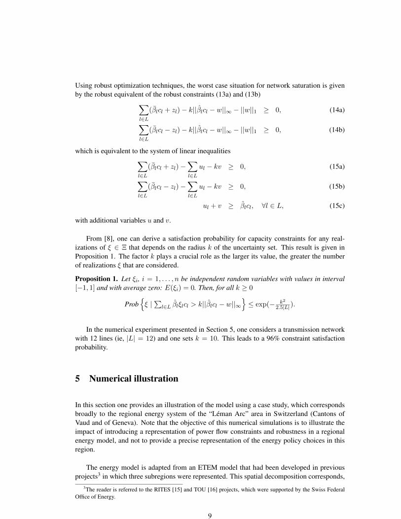
Using robust optimization techniques, the worst case situation for network saturation is givenby the robust equivalent of the robust constraints (13a) and (13b)∑

l∈L(βlcl + zl)− k||βlcl − w||∞ − ||w||1 ≥ 0, (14a)∑

l∈L(βlcl − zl)− k||βlcl − w||∞ − ||w||1 ≥ 0, (14b)

which is equivalent to the system of linear inequalities∑l∈L

(βlcl + zl)−∑l∈L

ul − kv ≥ 0, (15a)∑l∈L

(βlcl − zl)−∑l∈L

ul − kv ≥ 0, (15b)

ul + v ≥ βlcl, ∀l ∈ L, (15c)

with additional variables u and v.

From [8], one can derive a satisfaction probability for capacity constraints for any real-izations of ξ ∈ Ξ that depends on the radius k of the uncertainty set. This result is given inProposition 1. The factor k plays a crucial role as the larger its value, the greater the numberof realizations ξ that are considered.

Proposition 1. Let ξi, i = 1, . . . , n be independent random variables with values in interval[−1, 1] and with average zero: E(ξi) = 0. Then, for all k ≥ 0

Prob{ξ |

∑l∈L βlξlcl > k||βlcl − w||∞

}≤ exp(− k2

2.5|L|).

In the numerical experiment presented in Section 5, one considers a transmission networkwith 12 lines (ie, |L| = 12) and one sets k = 10. This leads to a 96% constraint satisfactionprobability.

5 Numerical illustration

In this section one provides an illustration of the model using a case study, which correspondsbroadly to the regional energy system of the “Leman Arc” area in Switzerland (Cantons ofVaud and of Geneva). Note that the objective of this numerical simulations is to illustrate theimpact of introducing a representation of power flow constraints and robustness in a regionalenergy model, and not to provide a precise representation of the energy policy choices in thisregion.

The energy model is adapted from an ETEM model that had been developed in previousprojects3 in which three subregions were represented. This spatial decomposition corresponds,

3The reader is referred to the RITES [15] and TOU [16] projects, which were supported by the Swiss FederalOffice of Energy.

9

globally, to the three power distribution companies operating in the region (i.e., SIG for Geneva,SIL for Lausanne and Romande Energie (ROM) for the rest of the region) but it does not matchany grid transmission aspect. One explains below how the regional energy system has beenreorganized into 9 subsystems connected through power transmission lines.

5.1 Data

Energy system of Lac Leman area. In 2010, the total annual energy consumption of the“Leman Arc” region was 114.3 PJ and, overall, CO2 emissions amounted to 5.48 Mt. Theregion is a net importer of electricity, around 5.5 TWh out of a total electricity consumption of7.1 TWh in Year 2010.4

Transmission grid. Figure 2 shows the Swiss transmission grid as reported in [22]. Thenetwork used in the ETEM-SG model will be a subgraph of this network, i.e., the one corre-sponding to the bottom-left corner. From the description of the swiss transmission grid onecan extract the sub-grid involved in the “Leman Arc” area. It is schematically represented inFigures of resuls 7 and 8 with 9 nodes each one connected to a local energy subsystem and 12transmission lines. Among the 9 nodes, three (Verboix, Romanel and Triphon) are connectedto the Swiss and European transmission grid for electricity import/export and transit. Linecapacities and reactances are set to values used in [22].

Figure 2: Swiss transmission grid in 2015 (Figure from [22])

Useful demands. Table 1 gives the regional useful demands considered in the case study andFigure 3 displays their assumed evolution up to 2050. For the present exercise, demands aredistributed geographically among the 9 subsystems connected to the transmission grid. Theallocation of demand to nodes is obtained by first satisfying the observed demands for the threepower distribution companies in the three main areas (Geneva, Lausanne and the rest of the

4For more details on the global energy system, the reader is referred to [16, 15].

10

region) and then by distributing uniformly the demand to the buses located in the consideredareas (2 buses for Geneva, 2 buses for Lausanne and 5 buses for the rest of the region).

Finally demands are distributed on a yearly basis, among the 12 timeslices defined, forthree seasons (Winter, Summer, Intermediate), and four parts of Day (Night, morning peak P1,Mid-Day and evening peak P2), as illustrated in Figure 4.

Sector Label Code Unit

Residential Heat Existing Buildings 2-9 appts RA PJHeat Existing Houses RB PJHeat New Buildings 2-9 appts RC PJHeat New Houses RD PJAppliances R1 PJLighting RL PJ

Transport Public Transports: Bus TA tkmv/dPublic Transports: Tramway TB tkmv/dPublic Transports: Train TC tkmv/dPublic Transports Misc. TD tkmv/dAutomobile TE tkmv/dTruck TH tkmv/dDelivery vehicles TL tkmv/d

Industry Food, textile, wood, paper, edition RNH PJChemistry, rubber, glass, metal RCI PJMachine manufacturing, equipments RMA PJConstruction RCO PJTertiary RTR PJOther RAL PJ

Table 1: Useful demands classification (PJ means PetaJoule and tkmv/d means thousand kmvehicle per day).

0  

10  

20  

30  

40  

50  

60  

70  

2010   2015   2020   2025   2030   2035   2040   2045   2050  

RF                        RE                        RD                        RC                        RB                        RA                        RL                        R1                        RTR                        RCO                        RAL                        RMA                        RCI                        RNH                        

0  

5000  

10000  

15000  

20000  

25000  

30000  

2010   2015   2020   2025   2030   2035   2040   2045   2050  

TL                        

TH                        

TE                        

TD                        

TC                        

TB                        

TA                        

Figure 3: Evolution of useful demands in PJ (left) and in tkmv/d (right).

11

Figure 4: Definition of timeslices

5.2 Scenario definition

The swiss energy strategy scenario. The Swiss Federal Office of Energy (SFOE) has pro-posed a scenario for energy transition, called Neue Energiepolitik (NEP). It describes the SwissEnergy Strategy at horizon 2050 [14]. We use similar boundary assumptions to those in NEPfor the three scenarios developed with ETEM-SG for “Leman Arc” area. These scenarios willillustrate the importance of taking into consideration power flow constraints at a regional scale.In particular, in the NEP scenario, the emissions of greenhouse gases are caped at a level of 1.5tons of CO2-eq per person in 2050. Since the population is expected to attain 1.37 M people inthe Arc Lemanique region by 2050 (’mittleres’ Szenario A-00-2010), we impose as a constraintthat the total 2050 emissions should not exceed 2.1 Mt CO2-eq in the region.

Simulating network congestion. In order to evaluate the impact of power flow constraints andin particular of network congestion on simulation results, three different network settings arecompared.

• In the first scenario, it is assumed that the full existing line capacities (i.e., 490 MW) isavailable for transmission in the region. Without considering inter-regional power transit,the proposed network is oversized and thus congestion does not occur.

• In the second scenario, one assumes that 90% of line capacities is used by power flowtransits related to the rest of Swiss and European transmission grid. The residual ca-pacities dedicated for regional activities is decreased by a factor 10 (ie, 49 MW). Thedeterministic version of ETEM-SG is solved with these reduced line capacities.

• In the third scenario, one take into account power flow transits using robust optimizationtechniques as described in Section 4. One assumes a nominal saturation rate βl = 0.5and variability βl = 0.5. This corresponds to a nominal capacity cl = 0.5cl. Herethe problem dimension increases in a controlled way (i.e., less than 1% of additionalvariables and constraints) and computational times remain reasonable.

12

5.3 Simulation results

The results of the simulations, performed for a 2015-2050 horizon planning, are detailed be-low. The global evolutions of the energy system that is common to the three scenarios is firstpresented. Then the nodal power balance and prices are compared for the three scenarios inperiod 2050.

5.3.1 Global energy system evolution

0

10

20

30

40

50

60

70

80

90

2015 2020 2025 2030 2035 2040 2045 2050

Other

GSL

DST

COA

NGA

DSL

MSW

Elec

Heat

Figure 5: Energy mix (in PJ/year)

In the electricity sector, Figure 6 shows that wind mills technology is the main carbonfree option to satisfy electricity consumption increase as well as environmental constraints.At global level, it can be observed that all scenarios lead to very similar situations. It seems

0

5

10

15

20

25

30

35

2025 2030 2035 2040 2045 2050

Imports

Other

GasCC

GasTurbine

Wind

PVs

Hydro2

Hydro1

Figure 6: Electricity production mix (in PJ/year)

that power flow constraints don’t affect investments globally but have instead a significant

13

impact at the nodal spatial scale, as shown in the next subsections. Figures 5 and 6 displaythe evolutions, observed for both scenarios, of regional energy mix and electricity production,respectively. On Figure 5, one notices an increase of electricity consumption, a reduction ofgas use and a gasoline removal. Indeed, to meet the emissions constraint the model replacesgas heaters by heat pumps in residential and building sectors and invest in hybrid and electricvehicles.

5.3.2 Impact of transmission constraints on the 2050 electricity sector

In this subsection one details the simulation results at each node and in particular on observesthe impact of power transmission constrainta on nodal electricity balance and nodal pricing.

Nodal electricity balance in 2050. Figure 7 shows (in PetaJoules) for the three scenarios i)total electricity production and consumption at nodes, ii) annual electricity exchanges for localconsumption on transmission lines and iii) total 2050 electricity imports at the three importnodes.

It can be observed that power flow constraints can have a significant impact on nodal elec-tricity consumption and production patterns. For example, one observes for Verboix a changefrom 2.10 PJ in Scenario 1 to 6.12 PJ in Scenario 3 for electricity generation and from 5.86to 10.35 PJ for total electricity consumption. These different production and consumptionpatterns are explained by different technological choices at nodes. As expected power flowconstraints affect strategic and operational decisions on the full energy system and not only onthe electricity sector.

However, in practice the transmission grid is not fixed over time and new investments areusually performed to follow consumption and production evolution. Modelling of investmentoptions on transmission lines would make it possible to increase line capacities and, as a con-sequence, would limit the changes in power consumption and production patterns.

Nodal electricity prices and congestion in 2050. Figure 8 summarises nodal electricity pricescomputed by ETEM-SG in 2050 in the three scenarios. It gives the minimum and maximumcomputed prices over the different timeslices. Figure 8 also displays the maximum utilisationrates of transmission lines over the different timeslices. In scenario 2, utilisation rates includeinterregional transits while in the robust scenario figures correspond to nominal utilisation rateswithout interregional transits.

First and as expected, in the first scenario with large transmission line capacities and with-out consideration of inter-regional power transit through the transmission grid, the network isoversized and nodal electricity prices are not affected by network congestion. In other wordselectricity prices are identical at all nodes and vary only in time. In the congested scenarios(scenarios 2 and 3), ETEM-SG generates very different nodal electricity prices. The highestprices are usually computed for central nodes that have no direct connection to imports.

Surprisingly, the minimum electricity price in Verbois, that is connected to imports, is

14

higher in the congested scenarios and higher than the import price. Indeed, this is the impactof power flow constraints. A marginal change in consumption in Verbois would modify theentire system and thus yields to an additional cost difficult to anticipate without a model likeETEM-SG.

Figure 8 demonstrates also a positive impact of robustness on nodal prices with maxi-mum electricity prices in scenario 3 that are always lower than the ones computed in the twoother scenarios. This results can be explained by the fact that robust optimization is a minmaxapproach and thus provides solutions that are robust for worst case situations, ie, congestednetwork situations. Note that in this first tentative of applying robust optimization in that con-text, it was not assumed any known information on inter-regional power flow transit. With suchinformation, one could deliver even more realistic and robust energy analysis.

6 Conclusion

In this paper, the multi-sectoral multi-energy long-term investment planning tool ETEM-SGhas been extended to the consideration of power flow constraints in regional transmission gridby implementing a linearized DC power flow model that represents the transmission grid withthe main constraints on the power flowing through the different arcs of the electricity transmis-sion network. Then as power flows circulating in a regional transmission grid depend on whathappens on the transmission grid for a much larger perimeter and it is uncertain, robust opti-mization technique is used to take into account the uncertainty on the capacity limits resultingfrom inter-regional transit.

The paper shows on a simple case study, that corresponds roughly to the “Leman Arc” re-gion, the relevance of such a modelling exercise for long-term simulations of regional energysystems. First one can notice that power flow constraints together with line capacities have asignificant impact on nodal electricity consumption and production patterns and thus on tech-nological choices. Then one can observe a significant effect on maximum nodal prices whenconsidering transit uncertainty using robust optimization.

Future work is envisioned to allow the model ETEM-SG to provide more realistic energyanalysis to support decision making. First one should couple the regional ETEM-SG modelwith a national one (eg, Swissmod [22]) in order to calibrate inter-regional power flow transitproperly on simulation results performed with this much larger model. This coupling exerciseis not straightforward as it requires an harmonisation of both model in term of assumptions andtechnological evolutions. For example, regional and national models must provide compatibleresults in term of Electric Vehicle penetration as it has a significant impact on electricity grids.A second work will consist in extending the new transmission grid module in ETEM-SG tonetwork improvement decisions. This way ETEM-SG will then be able to make investmenttrade-off between grid capacity expansions and localized generation technologies.

15

References

[1] C. Andrey, F. Babonneau, and A. Haurie. Modelisation stochastique et robuste del’attenuation et de l’adaptation dans un systeme energetique regional. application a laregion midi-pyrenees. Nature Science Societe, 23(2):133–149, 2015.

[2] F. Babonneau, M. Caramanis, and A. Haurie. Etem-sg: Optimizing regional smart energysystem with power distribution constraints and options. ORDECSYS Technical report,2016.

[3] F. Babonneau, A. Haurie, G. J. Tarel, and J. Thenie. Assessing the future of renewableand smart grid technologies in regional energy systems. Swiss Journal of Economics andStatistics, 148(2):229–273, 2012.

[4] F. Babonneau, A. Kanudia, M. Labriet, R. Loulou, and J.-P. Vial. Energy security : arobust programming approach and application to european energy supply via tiam. Envi-ronmental Modeling and Assessment, 17(1):19–37, 2012.

[5] F. Babonneau, O. Klopfenstein, A. Ouorou, and J.-P. Vial. Robust capacity expansionsolutions for telecommunication networks with uncertain demands. Network, 62(4):255–272, 2013.

[6] F. Babonneau, J.-P. Vial, and R. Apparigliato. Robust optimization for environmentaland energy planning. In J.A. Filar and A. Haurie eds., Uncertainty and EnvironmentalDecision Making, Springer, 2010.

[7] R. Bacher. Power system models, objectives and constraints in optimal power flow calcu-lations. In Bacher R. (Eds.) Frauendorfer K., Glavitsch H., editor, Optimization in Plan-ning and Operation of Electric Power Systems, Lecture Notes of the SVOR/ASRO Tu-torial Thun, Switzerland, October 14–16, 1992, pages 217–264, Heidelberg, May 1993.Physica-Verlag (Springer).

[8] A. Ben-Tal, L. El Ghaoui, and A. Nemirovski. Robust Optimization. Princeton UniversityPress, 2009.

[9] A. Ben-Tal and A. Nemirovski. Robust convex optimization. Mathematics of OperationsResearch, 23:769–805, 1998.

[10] Berger C., Dubois R., Haurie A., Lessard E., Loulou R., and J.-P. Waaub. CanadianMARKAL: An advanced linear programming system for energy and environmental mod-elling. INFOR, 30(3):222–239, 1992.

[11] Fragniere E. and Haurie A. A stochastic programming model for energy/environmentchoices under uncertainty. Int. J. Environment and Pollution, 6(4-6):587–603, 1996.

[12] L. El-Ghaoui and H. Lebret. Robust solutions to least- square problems to uncertain datamatrices. SIAM Journal of Matrix Analysis and Applications, 18:1035–1064, 1997.

[13] R. Loulou and M. Labriet. ETSAP-TIAM: the times integrated assessment model part i:Model structure. Computational Management Science, 5(1):7–40, 2008.

16

[14] Office federal de l’energie (OFEN). Die Energieperspektiven fur die Schweiz bis 2050.2012.

[15] ORDECSYS. Reseaux intelligents de transport/transmission de l’electricite en suisse.Technical report, ORDECSYS Technical report, 2013.

[16] ORDECSYS. Time of use (TOU) pricing: Adaptive and TOU pricing schemes for smarttechnology integration. Technical report, ORDECSYS Technical report, 2014.

[17] P. A. Ruiz, J. M. Foster, A. Rudkevich, and M. C. Caramanis. Tractable transmissiontopology control using sensitivity analysis. IEEE Transactions on Power Systems, toappear.

[18] P. A. Ruiz, A. Rudkevich, M.C. Caramanis, E. Goldis, E. Ntakou, and R. Philbrick. Re-duced mip formulation for transmission topology control. In USA University of Illi-nois at Urbana-Champaign, IL, editor, 50th Annual Allerton Conference on Communica-tion, Control, and Computing, Monticello 2012.

[19] P.A. Ruiz, J.M. Foster, A. Rudkevich, and M. Caramanis. On fast transmission topol-ogy control heuristics. In Proc. 2011 IEEE Power and Energy Society General Meeting,Detroit, MI. IEEE, July 2011.

[20] A. L. Soyster. Convex programming with set-inclusive constraints and applications toinexact linear programming. Operations Research, 21:1154–1157, 1973.

[21] A.D.J. Stiel. Modelling liberalised power markets. Master’s thesis, ETH Zurich, Centrefor Energy Policy and Economics, September 2011.

[22] H. Weigt and I. Schlecht. Swissmod a model of the Swiss electricity market. Technicalreport, WWZ-Discussion Paper, 2014.

17

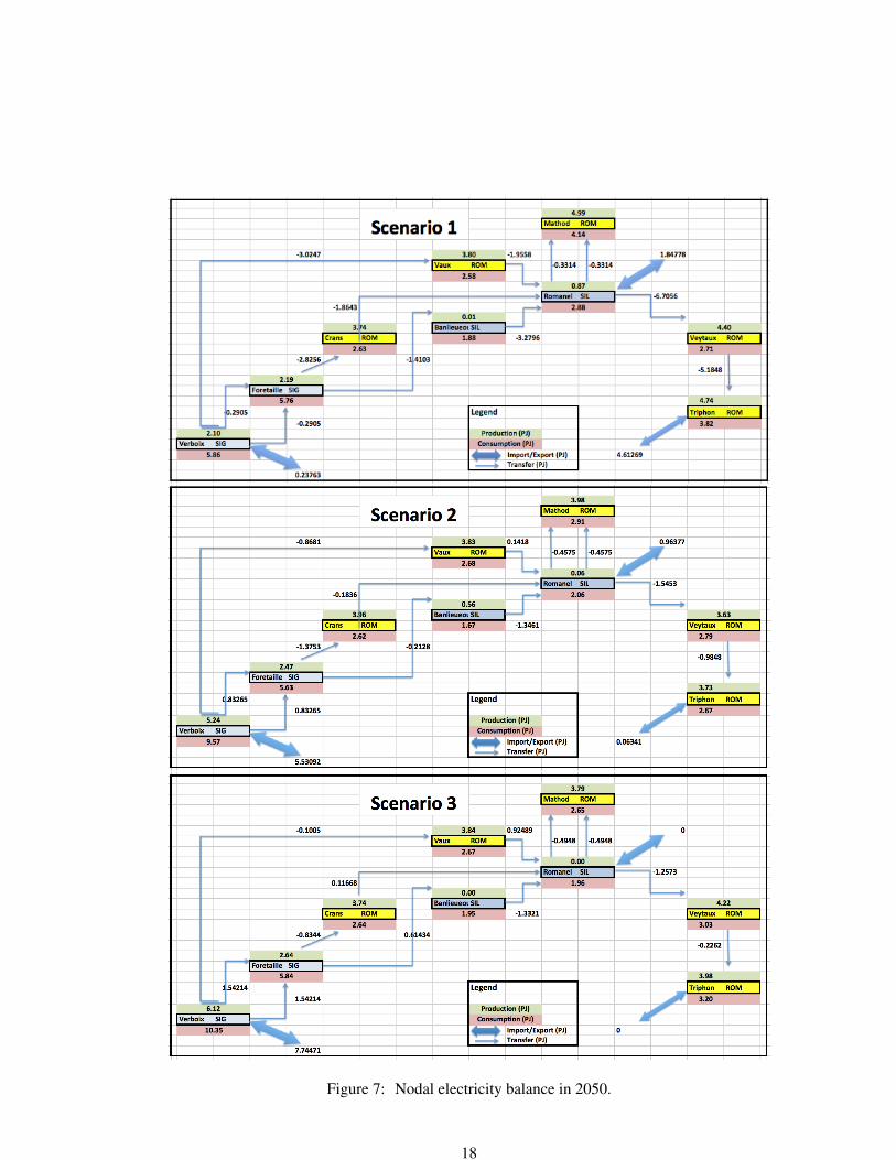
Figure 7: Nodal electricity balance in 2050.

18

Figure 8: Statistics on nodal electricity prices (in MCHF/PJ) and on line utilization rate (in %)in 2050.

19