Energy Technology alternatives for India till 2030

1

Energy Technology alternatives for India till 2030

Jyoti Parikh

Executive director,

Integrated Research and Action for Development, New Delhi India

Probal P. Ghosh

Research analyst,

Integrated Research and Action for Development, New Delhi India

2

Abstract

Purpose: India aspires for high economic growth of around 8 % to 9% over next few

years. Higher economic growth would lead to higher production and consumption, more

energy use and more CO2 emissions. At a time when CO2 emissions reductions are

becoming an important point of debate and fast erosion of fossil fuel reserves all over the

world, it is necessary to identify technological choices that reduce CO2 emission and

dependence on fossil fuels. A few modeling studies have explored India's technology

options. The Integrated Energy Policy (2006) report of the Planning commission of India

presents different scenarios for energy supply. The IEP model is however an energy

technology model and does not consider a feed back into the economy due to changes in

technological choice. This paper tries to follow the IEP (2006) in the kind of scenario’s

envisaged and attempts to investigate its macro economic impacts.

Design/ Methodology/Approach: The IRADe model is an activity analysis model that

uses a SAM to account for inter-sectoral influence and which allows for a two-way

interaction between energy sectors (coal, oil, natural gas, electricity) and other sectors of

the economy. We try to have three scenarios that are comparable to IEP (2006) in terms

of specifications and their resultant energy demand (mtoe)

Findings: The analyses prove that changing technological choice results reduction in

energy demand and CO2 emissions. But they also have costs in terms of GDP loses or

higher investment needs. The results show that the policies considered can have adverse

welfare impacts.

Originality/value: The paper helps in providing an insight into the macro-economic

impacts of the IEP (2006) scenarios. The two- way dependence of technological choice

and output shows the gains and loses out of moving to more costlier but low emission

based power generation technology.

Keywords: Technological choice, electricity, Activity analysis model, SAM, CO2

emission

Paper type: Research paper

3

1.0 Introduction:

India aspires for high economic growth of around 8 % to 9% over next few years.

High growth could help address several social objectives such as employment and

reduction of poverty. Higher economic growth would lead to higher production,

consumption and more energy use. Thus economic growth could have

environmental and energy consequence such as local pollution and Green House

Gases (GHG) emissions due to higher usage of fossil fuels like coal, crude oil and

natural gas required for production activities such as power, steel, cement and

manufacturing sector in general and household consumption of LPG and kerosene

and petrol, diesel for transport activities etc. The energy sector requires long term

planning as it is investment intensive with long gestation lags. Moreover, the

growing recent concern for GHG accumulation also requires India to think about

the country’s emissions till 2030 and beyond. This paper examines various ways

to meet country’s need for energy while keeping environmental goals in view.

The Integrated Energy Policy (2006) report of the Planning commission of India

presents different scenarios for energy supply. This was the first report that

looked at the energy sector policies from an integrated perspective. The cabinet

has approved Integrated Energy Policy based on the report as government policy.

The scenarios range from a total coal dependent economy to a renewable based

economy with low emissions. The energy implications of these scenarios have

also been described in the IEP report. The IEP model is however an energy

technology model. There have been various models in the past, as would be

discussed in the next section, that have tried to asses the impact of technological

choices on energy demand. Most of these models are technological models, which

assume constant GDP growth rates or constant sectoral growth rates. There have

also been attempts to model the real sector’s impact on technological choices but

such models lack in technological detail. However real life is more dynamic and

there is constant interaction between technological choices and economic

outcomes. The IEP (2006) document however can be considered as a benchmark

for assessing impact of technological choices on energy demand and CO2

emission. This paper therefore tries to follow the IEP (2006) in the kind of

4

scenario’s envisaged and attempts to investigate the macro economic impacts of

those scenarios particularly the growth and investment impacts.

2.0 Literature survey:

Models that assess economy energy interaction in the literature can be classified as

bottom-up, top-down and integrated. The bottom-up models bring technological

knowledge and specificity. However, often techno-economic evaluations are incomplete

and overtly optimistic in that the policy and institutional obstacles are not fully accounted

for. Top-down models bring macro-consistency but simplify the sectoral details by

judgments and assumptions. Among them are econometric models which use reduced

form equations and the implied policies behind them remain unclear. Another approach

of top-down modeling is the computable general equilibrium (CGE) approach where a

sequence of single period equilibrium is worked out. An activity analysis approach

permits macro-consistency, dynamic behavior, new and specific technological options,

and resource limitations and thus limits substitution. It can constitute a truly integrated

top-down- model.At the national level, computable general equilibrium models, which

incorporate behavior of individual agents in response to endogenous prices, have been

used for development policy analysis (Adelman & Robinson, 1978, Narayana et al.,

1991). These are either static models (Bergman, 1990) that give a snap shot for the target

year or the dynamic ones (Jorgenson and Wilcoxen, 1990) that give trajectories of the

growth path, the latter are useful for analyzing the effects of adopting alternative market-

based policy instruments.

A few modeling studies have explored India's technology options. Shukla (1996) uses

two models, the bottom-up MARKAL (Bergel et al, 1987) which is an energy system

model suitable for techno-economic analysis given exogenously specified sectoral growth

rates and the top-down SGM with endogenous macro variables such as growth rate. The

Indian component of SGM has been used to explore CO2 policy options for India

(Shukla, 1996 and Fisher-Vander et al, 1997). Gupta and Hall (1996) have tried to use a

simple econometric macro-model as a top-down model to integrate technological options

identified by techno-economic assessment of various technical options for carbon

abatement. Weyant and Parikh (2004) analyzed how various global models have

5

projected India’s emissions. Murthy et. al (1997a, b) made a study of interactions among

production, energy demand and CO2 emissions for the Indian economy using input-

output (I-O) table for 1989-90 and projected emissions for 2004-05. Parikh et. al (2009)

have estimated CO2 emissions for India by major sectors for the year 2003-04 (2008)

based on a Social Accounting Matrix (SAM), which incorporates the input-output flows

for that year. In this paper we use a framework similar to Murthy et. al (1997a, b) and

estimate a CGE model for India using the Social Accounting Matrix (SAM) for 2003-04

M.R. Saluja (2006). In the current work we go a step forward to analyze the impact of

emission reduction strategies on the economy.

3.0 Motivation:

The IEP (2006) assumes an exogenous GDP growth of 8% and computes the energy

demand and supply options to support such a GDP growth. It does not have feedback to

the economy of various energy strategies. In reality there is a lot of interdependence

between energy demand, GDP growth and technological choices. Apart from aggregated

GDP growth, sectoral growth and their relative importance in the economy is a more

determining factor for energy demand. Technological choices affect output and are in

turn also affected by the economic criterions of cost considerations and natural

endowments of resources. The IRADe model is an activity analysis model, which allows

for a two-way interaction between energy sectors (coal, oil, natural gas, electricity) and

other sectors of the economy. Such a structure would help in analyzing the sectoral

details of the source of energy demand and supply options to meet them. It also allows

through energy-economy interaction a more realistic assessment of economic growth

potential.

The IRADe model is a multi sector multi period activity analysis model. By connecting

material flows among economic sector, it provides consistent framework especially

relevant for sectoral impact of technological changes in the economy sector. The main

objective of the IRADe model is to explore various alternatives to meet energy demand

and their impact on the macro economic variables in general and poverty in particular.

Transition to a new set of technology has welfare impact – with many poor, small

changes in the livelihood opportunities and in incomes could have serious implications.

6

The model has endogenous income distribution with 10 expenditure classes, 5 rural and 5

urban. The use of various renewable energy resources, bio-fuels, and nuclear energy are

the possible solutions for this purpose. The consequences of shift in energy sources in

other sectors of the economy have been examined. Agricultural and trade sector can be

influenced by such shift in energy sources. We also calculate CO2 emissions as a follow

up of various energy strategies.

We therefore use IRADe model to articulate economy-energy interactions and trade offs.

The IEP (2006) presents several scenarios based on different technology mix. The Energy

mix corresponding to each scenario is also reported. These scenarios provide various

technology and energy options for India to support its energy requirements in future and

also in bringing down the CO2 emission to address climate change issues. An obvious

question from a policy point of view would be the expected economic impacts of these

scenarios. The investment requirements to implement such scenarios will be an important

question. The IEP model assumes a constant GDP growth rate and does not have

investments in it. Hence it would be unable to address these questions. In this paper we

try to reproduce IEP scenarios using the IRADe model where the GDP is endogenous.

We then compare the energy implications for the Indian economy with respect to IEP

scenarios and also estimate the investment needs for these scenarios to be implemented.

4.0 Detailed Methodology:

The IRADe model is a modified version of the model used by Murthy, Panda and Parikh

(1994). It is a linear programming activity analysis model based on input-output

framework. The input-output matrix used in the model is based on the updated SAM of

2003-04 prices. This structure is linked with a growth model on one hand and a detailed

analysis of the energy sector on the other hand. The model maximizes the present

discounted value of private consumption over the planning period (in our case 30 years

(2003-33)) subject to various demand and supply constraints.

Objective function: PCr

PCPOPMaxU

T

tt

tt

0 )1(

* …………………………… (1)

7

Where POPt and PCt are the total population and total per capita consumption at time t. T

is the planning horizon.

The consumption side of the economy is divided into rural and urban sectors. The model

assumes an income parity of 2.34 between rural and urban areas i.e. urban income, and

hence consumption is 2.34 times rural income. Total population is exogenously assumed

for urban and rural areas and is obtained from the data of the registrar general of India.

Five consumer expenditure based classes are assumed each in rural and urban sector. The

per capita consumption of each household class is represented using a set of equations of

Linear Expenditure System (LES) estimated based on the data of various NSS rounds of

household consumption survey for rural and urban areas separately. These equations as

shown below are introduced into the model as constrains.

i

ihthtihihoiht CECC )( ………………………….. (2)

Ciht = per capita consumption of the ith commodity, hth household group in tth time period,

Cih0 = minimum per capita consumption of the ith commodity, hth household.

βih = share of ith commodity in total per capita consumption of the hth household.

Eht = Total per capita consumption expenditure of the hth household.

As incomes rise, per capita consumptions rises, this results in a people moving from

lower expenditure classes to higher classes. Such changes would have impact on the

demand structure of the economy. The model has an endogenous income distribution

separately for rural and urban areas to incorporate such change in number of people in

different classes over time. The LES and endogenous income distribution together

provide a dynamically changing commodity wise non-linear demand structure of the

economy. The original I-O table consisting of 115 sectors was aggregated to 25

commodities being produced by 34 production activities. The model has each commodity

being produced by one production activity except electricity. To produce power the

model employs newer renewable (wind, solar thermal, solar photo voltaic, wood

gasification) and nuclear-based technologies apart from the traditional technologies of

thermal, hydro and gas similar to those assumed in the IEP model. Coal, Crude, Natural

8

gas and electricity are energy inputs into the model. Model ensures commodity wise

equilibrium between demand and supply in the optimal path.

ititititititit MYEIOIGC …………………… (3)

(Private consumption demand + government consumption demand+ investment demand

+ intermediate input demand+ export demand) = (domestic production + imports)

Government consumption (Gi,t) is exogenous and specified to grow at a growth rate of

9%. Intermediate demand (IOi,t) is determined endogenously by the input output

coefficients. Total private consumption (Ci,t) is obtained from the LES demand systems

and endogenous income distribution. Exports (Ei,t) and Imports (Mi,t) are determined

endogenously from the trade side equations of balance of payments and other constraints

explained later.

Domestic availability of commodities is assumed to come from domestic output (Yi,t) and

imports (Mi,t). Domestic production is constrained by capacity constraint (maximum

output that can be produced at the given capital stock).

jtjtjtjtj ICORKKXX /)()( 1,,1,, ………………………… (4)

(Incremental output is related to incremental capital).

Xj,t = domestic output of the jth sector at time t, Kj,t = capital of the jth sector at time t and

ICORj is the Incremental Capital Output Ratio of the jth sector which is exogenously

specified in the model.

Capital stock in sector j depends upon the rate of depreciation and investment and is

modeled using the relation,

tjtjtj IKJDELK ,1,, *)( …………………………… (5)

Where DEL(J) is the rate of depreciation in sector j, which is exogenous and Ij,t is the

investment in sector j.

Aggregate Investment demand is assumed to depend upon aggregate domestic investible

resources (domestic savings determined by marginal savings rate) and foreign investment

9

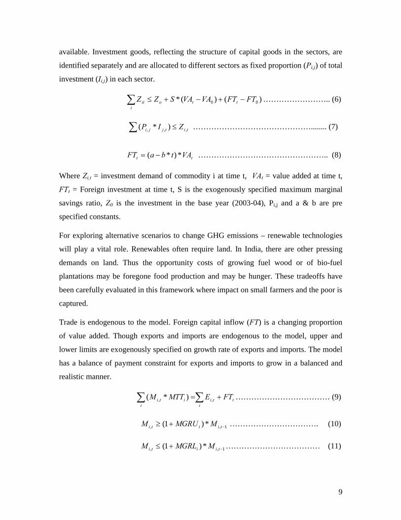
available. Investment goods, reflecting the structure of capital goods in the sectors, are

identified separately and are allocated to different sectors as fixed proportion (Pi,j) of total

investment (Ii,j) in each sector.

)()(* 00 FTFTVAVASZZ ttoi

it …………………….. (6)

titjji ZIP ,,, )*( ………………………………………........ (7)

tt VAtbaFT *)*( ………………………………………….. (8)

Where Zi,t = investment demand of commodity i at time t, VAt = value added at time t,

FTt = Foreign investment at time t, S is the exogenously specified maximum marginal

savings ratio, Z0 is the investment in the base year (2003-04), Pi,j and a & b are pre

specified constants.

For exploring alternative scenarios to change GHG emissions – renewable technologies

will play a vital role. Renewables often require land. In India, there are other pressing

demands on land. Thus the opportunity costs of growing fuel wood or of bio-fuel

plantations may be foregone food production and may be hunger. These tradeoffs have

been carefully evaluated in this framework where impact on small farmers and the poor is

captured.

Trade is endogenous to the model. Foreign capital inflow (FT) is a changing proportion

of value added. Though exports and imports are endogenous to the model, upper and

lower limits are exogenously specified on growth rate of exports and imports. The model

has a balance of payment constraint for exports and imports to grow in a balanced and

realistic manner.

ti

tii

iti FTEMTTM ,, )*( ……………………………… (9)

1,, *)1( tiiti MMGRUM ……………………………. (10)

1,, *)1( tiiti MMGRLM ……………………………… (11)

10

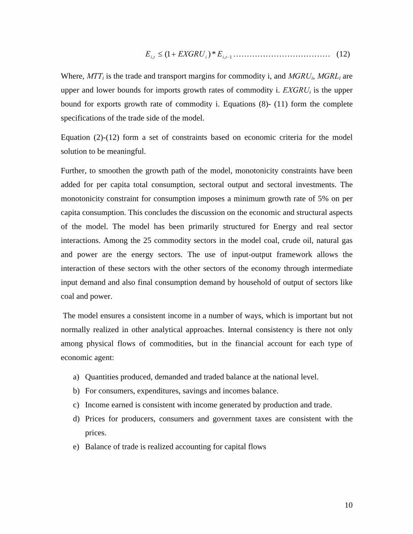
1,, *)1( tiiti EEXGRUE ……………………………… (12)

Where, MTTi is the trade and transport margins for commodity i, and MGRUi, MGRLi are

upper and lower bounds for imports growth rates of commodity i. EXGRUi is the upper

bound for exports growth rate of commodity i. Equations (8)- (11) form the complete

specifications of the trade side of the model.

Equation (2)-(12) form a set of constraints based on economic criteria for the model

solution to be meaningful.

Further, to smoothen the growth path of the model, monotonicity constraints have been

added for per capita total consumption, sectoral output and sectoral investments. The

monotonicity constraint for consumption imposes a minimum growth rate of 5% on per

capita consumption. This concludes the discussion on the economic and structural aspects

of the model. The model has been primarily structured for Energy and real sector

interactions. Among the 25 commodity sectors in the model coal, crude oil, natural gas

and power are the energy sectors. The use of input-output framework allows the

interaction of these sectors with the other sectors of the economy through intermediate

input demand and also final consumption demand by household of output of sectors like

coal and power.

The model ensures a consistent income in a number of ways, which is important but not

normally realized in other analytical approaches. Internal consistency is there not only

among physical flows of commodities, but in the financial account for each type of

economic agent:

a) Quantities produced, demanded and traded balance at the national level.

b) For consumers, expenditures, savings and incomes balance.

c) Income earned is consistent with income generated by production and trade.

d) Prices for producers, consumers and government taxes are consistent with the

prices.

e) Balance of trade is realized accounting for capital flows

11

These various consistencies ensure that all the feedbacks are taken into account and that

there are no unaccounted supply sources or demand sinks in the system. In other words,

there is no free lunch in such a system.

A distinguishing feature is that as far as possible all the parameters are estimated from

data and not benchmarked to one year’s data, as is the case for many CGE models in the

literature. Also since the model is validated so one can, with some measure of

confidence, say that it is a model that produces outcomes, which are credible for the

Indian economy.

Thus, the model is suited for, multi-sectoral inter-temporal dynamic optimization. This

permits exploration of alternative technologies and CO2 strategies from a long-term

dynamic perspective and permits substitution of various kinds.

The major instruments of control in the model are the commodity wise AEEI parameter,

the sector wise ICOR’s, the maximum marginal savings rate, the government

consumption growth rate, discount rate and the minimum consumption growth rate. The

assumptions about the above parameters are given in table 2 later. A detailed explanation

of their effects is also given section 6.

The model is solved using GAMS programming tool developed by Brooke et al. (1988).

For endogenous income distribution consistency, we iterate over optimal solutions

changing distribution parameters between iterations till they converge.

5.0 Major features of the model

We discuss below the features of the model and sub-models and what we have achieved

from the detailed analysis.

Sectors and Activities

The input-output table, provided by CSO consists of information on 115

sectors/activities. These have been aggregated to 34 sectors for better interpretation of

results, We have constructed four broad groups consisting of 34 production sectors as

follow:

12

Agriculture and allied activities (Cereal, Pulses, Sugarcane, Other crops, Animal

husbandry, Forestry and Fishing)

Energy sectors (Coal and lignite, Crude oil, Electricity and Gas, Electricity

Hydro, Electricity from Bio Fuel, Wind, Solar Photo voltaic, Solar Thermal,

Electricity from Wood, Electricity from low emission coal based technology)

Services sector consisting of Transportation (Railway and Other), and other

services. This sector is the largest chunk of the economy.

Industry consisting of sectors like, Agro processing, textiles, petroleum products,

Fertilizer, cement, steel, manufacturing, water supply & gas, mining and

quarrying, non-metallic minerals and construction.

Our main focus has been on agriculture and industrial sector since these sectors are

energy intensive and CO2 emissions are common in these sectors. The activities related to

these sectors in our model would be as follows.

Direct and Indirect energy use :

The Model captures both direct as well as indirect energy use. Such distinction arises

because both production and consumption use energy. To take an example to understand

direct and indirect emissions, let us consider the final use of output of the construction

sector. It has been observed that the construction sector does not take much of fossil-

fuel-based energy at the site, e.g., road or building, but it uses many energy intensive

materials such as bricks, cements, iron and steel, aluminum, glass etc. In this case, the

energy used for the construction activities at the site of construction are known as direct

energy use where as the energy used in producing the materials used in construction are

known to be indirect energy use.

Such an analysis gives deeper understanding of energy involved from final consumption

along with the production activities.

13

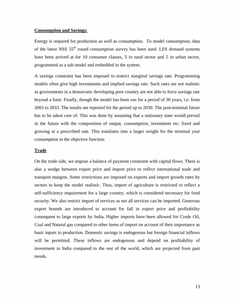
Consumption and Savings:

Energy is required for production as well as consumption. To model consumption, data

of the latest NSS 55th round consumption survey has been used. LES demand systems

have been arrived at for 10 consumer classes, 5 in rural sector and 5 in urban sector,

programmed as a sub model and embedded in the system.

A savings constraint has been imposed to restrict marginal savings rate. Programming

models often give high investments and implied savings rate. Such rates are not realistic

as governments in a democratic developing poor country are not able to force savings rate

beyond a limit. Finally, though the model has been run for a period of 30 years, i.e. from

2003 to 2033. The results are reported for the period up to 2030. The post-terminal future

has to be taken care of. This was done by assuming that a stationary state would prevail

in the future with the composition of output, consumption, investment etc. fixed and

growing at a prescribed rate. This translates into a larger weight for the terminal year

consumption in the objective function.

Trade

On the trade side, we impose a balance of payment constraint with capital flows. There is

also a wedge between export price and import price to reflect international trade and

transport margins. Some restrictions are imposed on exports and import growth rates by

sectors to keep the model realistic. Thus, import of agriculture is restricted to reflect a

self-sufficiency requirement for a large country, which is considered necessary for food

security. We also restrict import of services as not all services can be imported. Generous

export bounds are introduced to account for fall in export price and profitability

consequent to large exports by India. Higher imports have been allowed for Crude Oil,

Coal and Natural gas compared to other items of import on account of their importance as

basic inputs to production. Domestic savings is endogenous but foreign financial inflows

will be permitted. These inflows are endogenous and depend on profitability of

investment in India compared to the rest of the world, which are projected from past

trends.

14

6.0 Data , assumptions and scenario definitions

6.1 Data:

We have used the recent data for India to estimate the various parameters and initial

values of different variables to be included in the model structure. Input-output

coefficients and production functions for various activities form an important element of

the model (The latest I-O table (1998-99), published by the CSO and updated by Prof. M.

R. Saluja to 2003-04 prices, has been used).

The Census and NSS data has been used for rural and urban population and consumption

by expenditure classes.

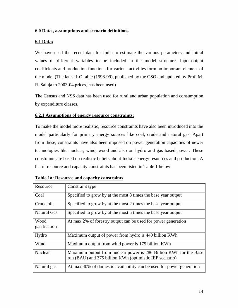
6.2.1 Assumptions of energy resource constraints:

To make the model more realistic, resource constraints have also been introduced into the

model particularly for primary energy sources like coal, crude and natural gas. Apart

from these, constraints have also been imposed on power generation capacities of newer

technologies like nuclear, wind, wood and also on hydro and gas based power. These

constraints are based on realistic beliefs about India’s energy resources and production. A

list of resource and capacity constraints has been listed in Table 1 below.

Table 1a: Resource and capacity constraints

Resource Constraint type

Coal Specified to grow by at the most 8 times the base year output

Crude oil Specified to grow by at the most 2 times the base year output

Natural Gas Specified to grow by at the most 5 times the base year output

Wood gasification

At max 2% of forestry output can be used for power generation

Hydro Maximum output of power from hydro is 440 billion KWh

Wind Maximum output from wind power is 175 billion KWh

Nuclear Maximum output from nuclear power is 286 Billion KWh for the Base run (BAU) and 375 billion KWh (optimistic IEP scenario)

Natural gas At max 40% of domestic availability can be used for power generation

15

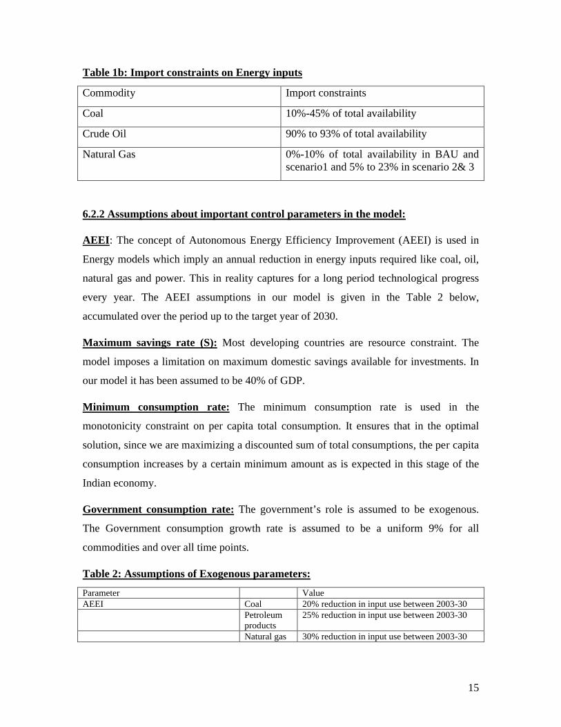
Table 1b: Import constraints on Energy inputs

Commodity Import constraints

Coal 10%-45% of total availability

Crude Oil 90% to 93% of total availability

Natural Gas 0%-10% of total availability in BAU and scenario1 and 5% to 23% in scenario 2& 3

6.2.2 Assumptions about important control parameters in the model:

AEEI: The concept of Autonomous Energy Efficiency Improvement (AEEI) is used in

Energy models which imply an annual reduction in energy inputs required like coal, oil,

natural gas and power. This in reality captures for a long period technological progress

every year. The AEEI assumptions in our model is given in the Table 2 below,

accumulated over the period up to the target year of 2030.

Maximum savings rate (S): Most developing countries are resource constraint. The

model imposes a limitation on maximum domestic savings available for investments. In

our model it has been assumed to be 40% of GDP.

Minimum consumption rate: The minimum consumption rate is used in the

monotonicity constraint on per capita total consumption. It ensures that in the optimal

solution, since we are maximizing a discounted sum of total consumptions, the per capita

consumption increases by a certain minimum amount as is expected in this stage of the

Indian economy.

Government consumption rate: The government’s role is assumed to be exogenous.

The Government consumption growth rate is assumed to be a uniform 9% for all

commodities and over all time points.

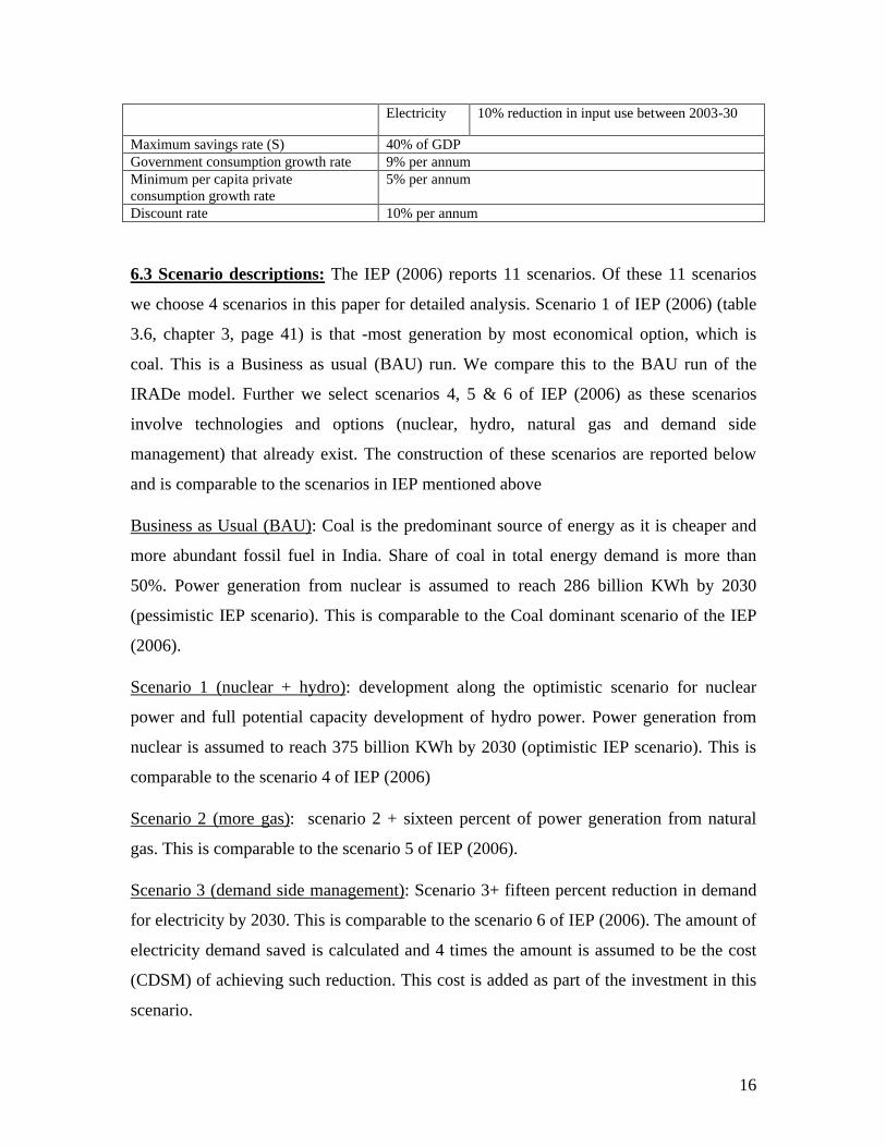
Table 2: Assumptions of Exogenous parameters:

Parameter ValueAEEI Coal 20% reduction in input use between 2003-30

Petroleum products

25% reduction in input use between 2003-30

Natural gas 30% reduction in input use between 2003-30

16

Electricity 10% reduction in input use between 2003-30

Maximum savings rate (S) 40% of GDPGovernment consumption growth rate 9% per annumMinimum per capita private consumption growth rate

5% per annum

Discount rate 10% per annum

6.3 Scenario descriptions: The IEP (2006) reports 11 scenarios. Of these 11 scenarios

we choose 4 scenarios in this paper for detailed analysis. Scenario 1 of IEP (2006) (table

3.6, chapter 3, page 41) is that -most generation by most economical option, which is

coal. This is a Business as usual (BAU) run. We compare this to the BAU run of the

IRADe model. Further we select scenarios 4, 5 & 6 of IEP (2006) as these scenarios

involve technologies and options (nuclear, hydro, natural gas and demand side

management) that already exist. The construction of these scenarios are reported below

and is comparable to the scenarios in IEP mentioned above

Business as Usual (BAU): Coal is the predominant source of energy as it is cheaper and

more abundant fossil fuel in India. Share of coal in total energy demand is more than

50%. Power generation from nuclear is assumed to reach 286 billion KWh by 2030

(pessimistic IEP scenario). This is comparable to the Coal dominant scenario of the IEP

(2006).

Scenario 1 (nuclear + hydro): development along the optimistic scenario for nuclear

power and full potential capacity development of hydro power. Power generation from

nuclear is assumed to reach 375 billion KWh by 2030 (optimistic IEP scenario). This is

comparable to the scenario 4 of IEP (2006)

Scenario 2 (more gas): scenario 2 + sixteen percent of power generation from natural

gas. This is comparable to the scenario 5 of IEP (2006).

Scenario 3 (demand side management): Scenario 3+ fifteen percent reduction in demand

for electricity by 2030. This is comparable to the scenario 6 of IEP (2006). The amount of

electricity demand saved is calculated and 4 times the amount is assumed to be the cost

(CDSM) of achieving such reduction. This cost is added as part of the investment in this

scenario.

17

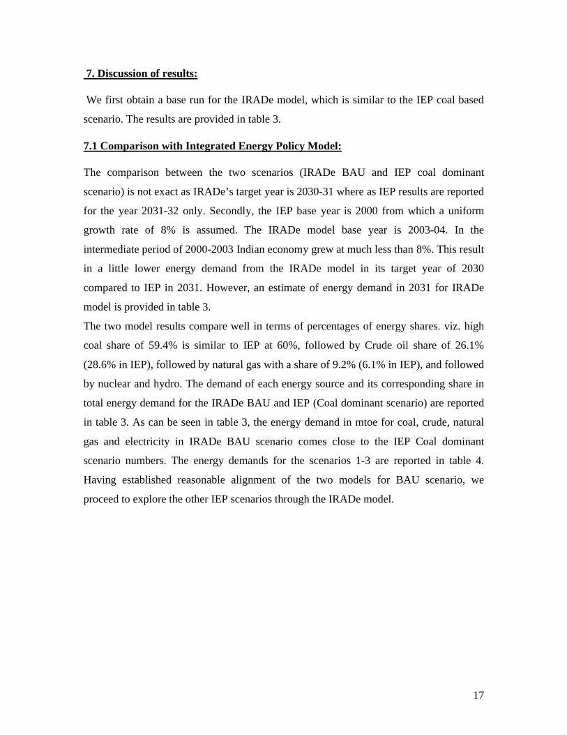
7. Discussion of results:

We first obtain a base run for the IRADe model, which is similar to the IEP coal based

scenario. The results are provided in table 3.

7.1 Comparison with Integrated Energy Policy Model:

The comparison between the two scenarios (IRADe BAU and IEP coal dominant

scenario) is not exact as IRADe’s target year is 2030-31 where as IEP results are reported

for the year 2031-32 only. Secondly, the IEP base year is 2000 from which a uniform

growth rate of 8% is assumed. The IRADe model base year is 2003-04. In the

intermediate period of 2000-2003 Indian economy grew at much less than 8%. This result

in a little lower energy demand from the IRADe model in its target year of 2030

compared to IEP in 2031. However, an estimate of energy demand in 2031 for IRADe

model is provided in table 3.

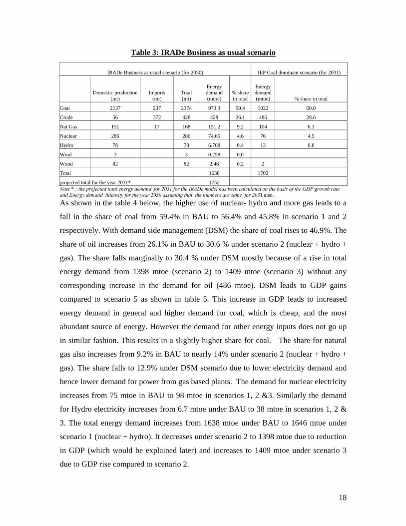
The two model results compare well in terms of percentages of energy shares. viz. high

coal share of 59.4% is similar to IEP at 60%, followed by Crude oil share of 26.1%

(28.6% in IEP), followed by natural gas with a share of 9.2% (6.1% in IEP), and followed

by nuclear and hydro. The demand of each energy source and its corresponding share in

total energy demand for the IRADe BAU and IEP (Coal dominant scenario) are reported

in table 3. As can be seen in table 3, the energy demand in mtoe for coal, crude, natural

gas and electricity in IRADe BAU scenario comes close to the IEP Coal dominant

scenario numbers. The energy demands for the scenarios 1-3 are reported in table 4.

Having established reasonable alignment of the two models for BAU scenario, we

proceed to explore the other IEP scenarios through the IRADe model.

18

Table 3: IRADe Business as usual scenario

IRADe Business as usual scenario (for 2030) IEP Coal dominant scenario (for 2031)

Domestic production (mt)

Imports(mt)

Total(mt)

Energy demand (mtoe)

% share in total

Energy demand (mtoe) % share in total

Coal 2137 237 2374 973.3 59.4 1022 60.0

Crude 56 372 428 428 26.1 486 28.6

Nat Gas 151 17 168 151.2 9.2 104 6.1

Nuclear 286 286 74.65 4.6 76 4.5

Hydro 78 78 6.708 0.4 13 0.8

Wind 3 3 0.258 0.0

Wood 82 82 2.46 0.2 2

Total 1638 1702

projected total for the year 2031* 1752Note * : the projected total energy demand for 2031 for the IRADe model has been calculated on the basis of the GDP growth rate and Energy demand intensity for the year 2030 assuming that the numbers are same for 2031 also.

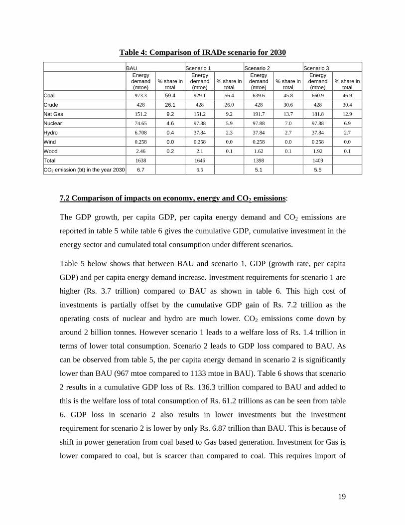
As shown in the table 4 below, the higher use of nuclear- hydro and more gas leads to a

fall in the share of coal from 59.4% in BAU to 56.4% and 45.8% in scenario 1 and 2

respectively. With demand side management (DSM) the share of coal rises to 46.9%. The

share of oil increases from 26.1% in BAU to 30.6 % under scenario 2 (nuclear + hydro +

gas). The share falls marginally to 30.4 % under DSM mostly because of a rise in total

energy demand from 1398 mtoe (scenario 2) to 1409 mtoe (scenario 3) without any

corresponding increase in the demand for oil (486 mtoe). DSM leads to GDP gains

compared to scenario 5 as shown in table 5. This increase in GDP leads to increased

energy demand in general and higher demand for coal, which is cheap, and the most

abundant source of energy. However the demand for other energy inputs does not go up

in similar fashion. This results in a slightly higher share for coal. The share for natural

gas also increases from 9.2% in BAU to nearly 14% under scenario 2 (nuclear + hydro +

gas). The share falls to 12.9% under DSM scenario due to lower electricity demand and

hence lower demand for power from gas based plants. The demand for nuclear electricity

increases from 75 mtoe in BAU to 98 mtoe in scenarios 1, 2 &3. Similarly the demand

for Hydro electricity increases from 6.7 mtoe under BAU to 38 mtoe in scenarios 1, 2 &

3. The total energy demand increases from 1638 mtoe under BAU to 1646 mtoe under

scenario 1 (nuclear + hydro). It decreases under scenario 2 to 1398 mtoe due to reduction

in GDP (which would be explained later) and increases to 1409 mtoe under scenario 3

due to GDP rise compared to scenario 2.

19

Table 4: Comparison of IRADe scenario for 2030

BAU Scenario 1 Scenario 2 Scenario 3 Energy demand (mtoe)

% share in total

Energy demand (mtoe)

% share in total

Energy demand (mtoe)

% share in total

Energy demand (mtoe)

% share in total

Coal 973.3 59.4 929.1 56.4 639.6 45.8 660.9 46.9

Crude 428 26.1 428 26.0 428 30.6 428 30.4

Nat Gas 151.2 9.2 151.2 9.2 191.7 13.7 181.8 12.9

Nuclear 74.65 4.6 97.88 5.9 97.88 7.0 97.88 6.9

Hydro 6.708 0.4 37.84 2.3 37.84 2.7 37.84 2.7

Wind 0.258 0.0 0.258 0.0 0.258 0.0 0.258 0.0

Wood 2.46 0.2 2.1 0.1 1.62 0.1 1.92 0.1

Total 1638 1646 1398 1409

CO2 emission (bt) in the year 2030 6.7 6.5 5.1 5.5

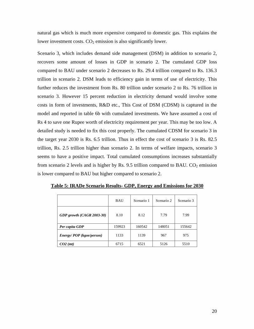
7.2 Comparison of impacts on economy, energy and CO2 emissions:

The GDP growth, per capita GDP, per capita energy demand and CO2 emissions are

reported in table 5 while table 6 gives the cumulative GDP, cumulative investment in the

energy sector and cumulated total consumption under different scenarios.

Table 5 below shows that between BAU and scenario 1, GDP (growth rate, per capita

GDP) and per capita energy demand increase. Investment requirements for scenario 1 are

higher (Rs. 3.7 trillion) compared to BAU as shown in table 6. This high cost of

investments is partially offset by the cumulative GDP gain of Rs. 7.2 trillion as the

operating costs of nuclear and hydro are much lower. CO2 emissions come down by

around 2 billion tonnes. However scenario 1 leads to a welfare loss of Rs. 1.4 trillion in

terms of lower total consumption. Scenario 2 leads to GDP loss compared to BAU. As

can be observed from table 5, the per capita energy demand in scenario 2 is significantly

lower than BAU (967 mtoe compared to 1133 mtoe in BAU). Table 6 shows that scenario

2 results in a cumulative GDP loss of Rs. 136.3 trillion compared to BAU and added to

this is the welfare loss of total consumption of Rs. 61.2 trillions as can be seen from table

6. GDP loss in scenario 2 also results in lower investments but the investment

requirement for scenario 2 is lower by only Rs. 6.87 trillion than BAU. This is because of

shift in power generation from coal based to Gas based generation. Investment for Gas is

lower compared to coal, but is scarcer than compared to coal. This requires import of

20

natural gas which is much more expensive compared to domestic gas. This explains the

lower investment costs. CO2 emission is also significantly lower.

Scenario 3, which includes demand side management (DSM) in addition to scenario 2,

recovers some amount of losses in GDP in scenario 2. The cumulated GDP loss

compared to BAU under scenario 2 decreases to Rs. 29.4 trillion compared to Rs. 136.3

trillion in scenario 2. DSM leads to efficiency gain in terms of use of electricity. This

further reduces the investment from Rs. 80 trillion under scenario 2 to Rs. 76 trillion in

scenario 3. However 15 percent reduction in electricity demand would involve some

costs in form of investments, R&D etc., This Cost of DSM (CDSM) is captured in the

model and reported in table 6b with cumulated investments. We have assumed a cost of

Rs 4 to save one Rupee worth of electricity requirement per year. This may be too low. A

detailed study is needed to fix this cost properly. The cumulated CDSM for scenario 3 in

the target year 2030 is Rs. 6.5 trillion. Thus in effect the cost of scenario 3 is Rs. 82.5

trillion, Rs. 2.5 trillion higher than scenario 2. In terms of welfare impacts, scenario 3

seems to have a positive impact. Total cumulated consumptions increases substantially

from scenario 2 levels and is higher by Rs. 9.5 trillion compared to BAU. CO2 emission

is lower compared to BAU but higher compared to scenario 2.

Table 5: IRADe Scenario Results- GDP, Energy and Emissions for 2030

BAU Scenario 1 Scenario 2 Scenario 3

GDP growth (CAGR 2003-30) 8.10 8.12 7.79 7.99

Per capita GDP 159923 160542 148051 155642

Energy/ POP (kgoe/person) 1133 1139 967 975

CO2 (mt) 6715 6521 5126 5510

21

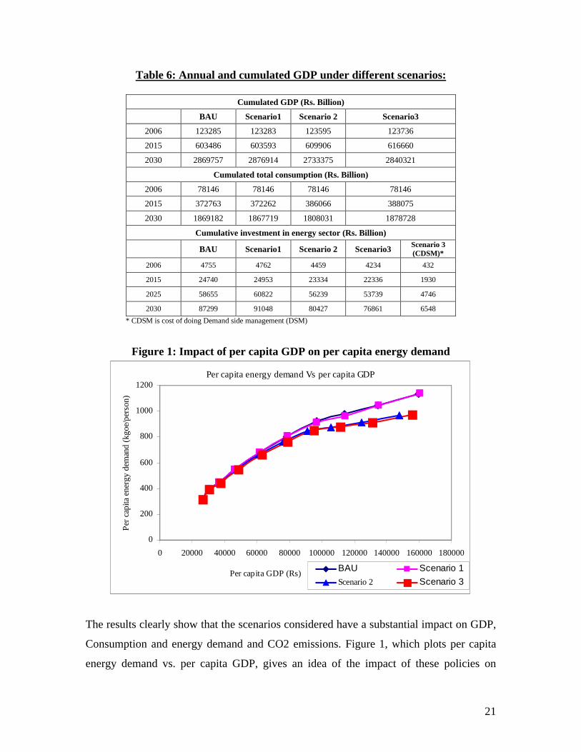
Table 6: Annual and cumulated GDP under different scenarios:

Cumulated GDP (Rs. Billion)

BAU Scenario1 Scenario 2 Scenario3

2006 123285 123283 123595 123736

2015 603486 603593 609906 616660

2030 2869757 2876914 2733375 2840321

Cumulated total consumption (Rs. Billion)

2006 78146 78146 78146 78146

2015 372763 372262 386066 388075

2030 1869182 1867719 1808031 1878728

Cumulative investment in energy sector (Rs. Billion)

BAU Scenario1 Scenario 2 Scenario3Scenario 3(CDSM)*

2006 4755 4762 4459 4234 432

2015 24740 24953 23334 22336 1930

2025 58655 60822 56239 53739 4746

2030 87299 91048 80427 76861 6548

* CDSM is cost of doing Demand side management (DSM)

Figure 1: Impact of per capita GDP on per capita energy demand

Per capita energy demand Vs per capita GDP

0

200

400

600

800

1000

1200

0 20000 40000 60000 80000 100000 120000 140000 160000 180000

Per capita GDP (Rs)

Per

cap

ita e

nerg

y de

man

d (k

goe/

pers

on)

BAU Scenario 1

Scenario 2 Scenario 3

The results clearly show that the scenarios considered have a substantial impact on GDP,

Consumption and energy demand and CO2 emissions. Figure 1, which plots per capita

energy demand vs. per capita GDP, gives an idea of the impact of these policies on

22

energy demand. Figure 1 shows a relatively lower trajectory for scenario 2 & 3 compared

to BAU and scenario 1. This suggests that a structural shift from coal use to gas use can

lower energy intensity of GDP with DSM giving the lowest intensity. The use of nuclear

and hydro does not seem to impact the energy and economy relationship however the use

of natural gas seems to substantially alter the relationship.

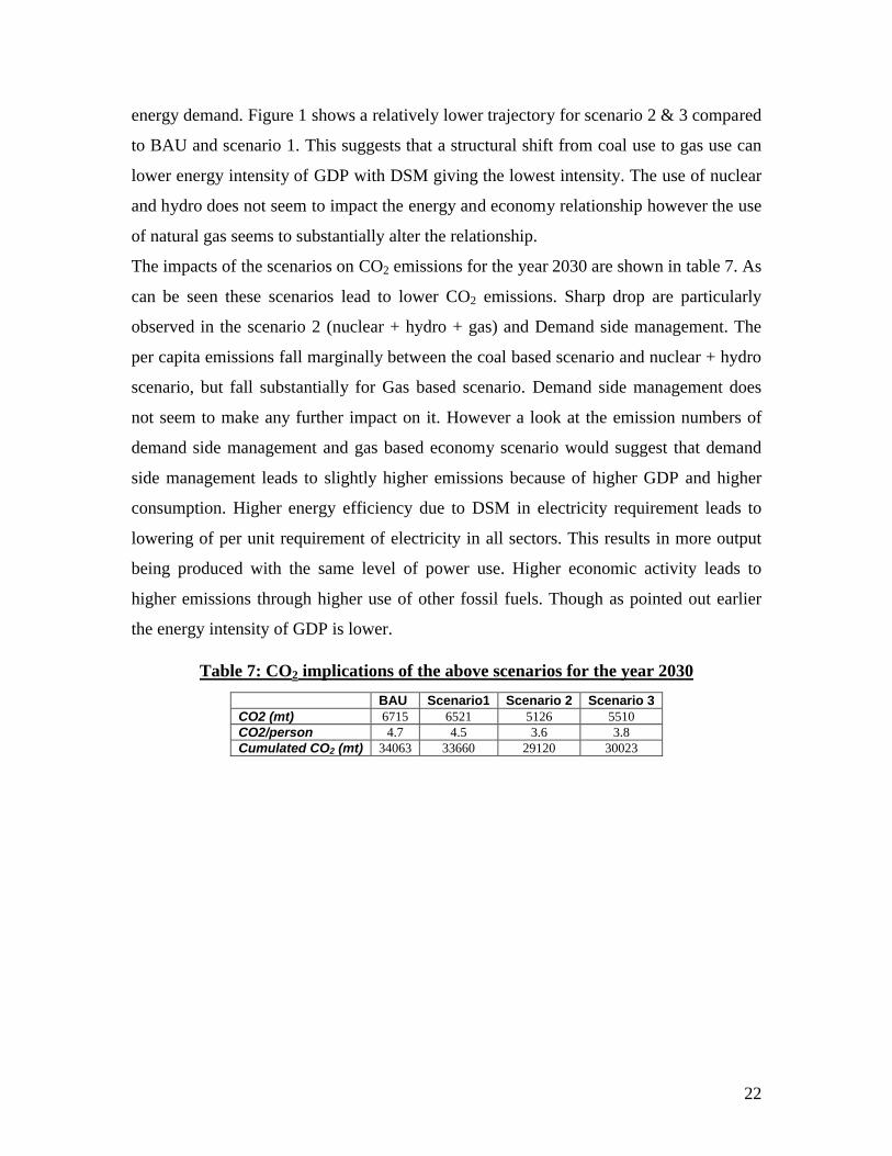
The impacts of the scenarios on CO2 emissions for the year 2030 are shown in table 7. As

can be seen these scenarios lead to lower CO2 emissions. Sharp drop are particularly

observed in the scenario 2 (nuclear + hydro + gas) and Demand side management. The

per capita emissions fall marginally between the coal based scenario and nuclear + hydro

scenario, but fall substantially for Gas based scenario. Demand side management does

not seem to make any further impact on it. However a look at the emission numbers of

demand side management and gas based economy scenario would suggest that demand

side management leads to slightly higher emissions because of higher GDP and higher

consumption. Higher energy efficiency due to DSM in electricity requirement leads to

lowering of per unit requirement of electricity in all sectors. This results in more output

being produced with the same level of power use. Higher economic activity leads to

higher emissions through higher use of other fossil fuels. Though as pointed out earlier

the energy intensity of GDP is lower.

Table 7: CO2 implications of the above scenarios for the year 2030

BAU Scenario1 Scenario 2 Scenario 3CO2 (mt) 6715 6521 5126 5510CO2/person 4.7 4.5 3.6 3.8Cumulated CO2 (mt) 34063 33660 29120 30023

23

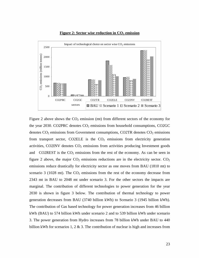
Figure 2: Sector wise reduction in CO2 emission

Impact of technological choice on sector wise CO2 emissions

0

500

1000

1500

2000

2500

CO2PRC CO2GC CO2TR CO2ELE CO2INV CO2REST

sectors

CO

2 em

issi

ons

(mill

ion

tonn

es)

BAU Scenario 1 Scenario 2 Scenario 3

Figure 2 above shows the CO2 emission (mt) from different sectors of the economy for

the year 2030. CO2PRC denotes CO2 emissions from household consumptions, CO2GC

denotes CO2 emissions from Government consumptions, CO2TR denotes CO2 emissions

from transport sector, CO2ELE is the CO2 emissions from electricity generation

activities, CO2INV denotes CO2 emissions from activities producing Investment goods

and CO2REST is the CO2 emissions from the rest of the economy. As can be seen in

figure 2 above, the major CO2 emissions reductions are in the electricity sector. CO2

emissions reduce drastically for electricity sector as one moves from BAU (1810 mt) to

scenario 3 (1028 mt). The CO2 emissions from the rest of the economy decrease from

2343 mt in BAU to 2048 mt under scenario 3. For the other sectors the impacts are

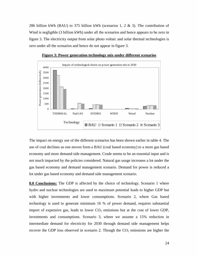
marginal. The contribution of different technologies to power generation for the year

2030 is shown in figure 3 below. The contribution of thermal technology to power

generation decreases from BAU (3740 billion kWh) to Scenario 3 (1945 billion kWh).

The contribution of Gas based technology for power generation increases from 46 billion

kWh (BAU) to 574 billion kWh under scenario 2 and to 539 billion kWh under scenario

3. The power generation from Hydro increases from 78 billion kWh under BAU to 440

billion kWh for scenarios 1, 2 & 3. The contribution of nuclear is high and increases from

24

286 billion kWh (BAU) to 375 billion kWh (scenarios 1, 2 & 3). The contribution of

Wind is negligible (3 billion kWh) under all the scenarios and hence appears to be zero in

figure 3. The electricity output from solar photo voltaic and solar thermal technologies is

zero under all the scenarios and hence do not appear in figure 3.

Figure 3: Power generation technology mix under different scenarios

Impact of technological choice on power generation mix in 2030

0

500

1000

1500

2000

2500

3000

3500

4000

THERMAL NatGAS HYDRO WIND Wood Nuclear

Technology

Pow

er g

ener

atio

n (b

illio

n kw

h)

BAU Scenario 1 Scenario 2 Scenario 3

The impact on energy use of the different scenarios has been shown earlier in table 4. The

use of coal declines as one moves form a BAU (coal based economy) to a more gas based

economy and more demand side management. Crude seems to be an essential input and is

not much impacted by the policies considered. Natural gas usage increases a lot under the

gas based economy and demand management scenario. Demand for power is reduced a

lot under gas based economy and demand side management scenario.

8.0 Conclusions: The GDP is affected by the choice of technology. Scenario 1 where

hydro and nuclear technologies are used to maximum potential leads to higher GDP but

with higher investments and lower consumptions. Scenario 2, where Gas based

technology is used to generate minimum 16 % of power demand, requires substantial

import of expensive gas, leads to lower CO2 emissions but at the cost of lower GDP,

investments and consumptions. Scenario 3, where we assume a 15% reduction in

intermediate demand for electricity for 2030 through demand side management helps

recover the GDP loss observed in scenario 2. Though the CO2 emissions are higher the

25

emission intensity is lower. Thus scenario 3 seems to be the most optimistic scenario with

gains all around. These technological scenarios considered result in lower energy demand

and reduced CO2 emission. The scenarios with more renewables are currently being

worked out and will be reported later. These scenarios though climate friendly but are not

all costless. These scenarios show the importance of factoring in energy economy

interactions in designing climate change mitigating strategies.

References

Adelman, I. And Robinson, (1978), Income Distribution Policy in Developing Countries, Standford University Press.

Bergel, C. Haurie, A. and Loulou, R. (1987), Modeling Long Range Energy/Technology Choices: The MARKAL Approach, Report. GERAD, Montreal.

Bergaman, L. (1990), ‘Energy and Environmental Constraints on Growth: a CGE Modeling Approach’, Journal of Policy Modeling, Vol. 12, No. 4.

Blitzer, C.R.,Eckaus, R. Lahiri,S.,and Meerhaus, A. (1992a), ‘Growth and Welfare Losses from Carbon Cmissions Restrictions: a general equilibrium analysis for Egypt’, The Energy Journal, Vol. 14, No. 1.

Fisher-Vanden, K., P.R.Shukla, J.A.Edmonds, S.H.Kim, and H.M.Pitcher (1997).‘Carbon Taxes and India’, Energy Economics, Vol.19, pp. 289-325.

Ginsburgh, V.A. and Waelbroeck, J.L. (1981), Activity Analysis and General Equilibrium Modeling, North-Holland, Amsterdam.

Gupta, S. and S.G. Hall (1996), ‘Carbon Abatement Costs: An Integrated Approach for India’, Environmental and Development Economics, I(1996), pp. 41-63.

IEP (2006), Integrated Energy Policy, report of the expert committee, Government of India, Planning Commission, New Delhi, August 2006.

Jorgenson, D.W. and Wilcoxen, P.J.(1990), ‘Intertemporal General Equilibrium Modeling of U.S. Environment; Regulation’, Journal of Policy Modeling, Vol. 94, No. 1. PP. 53-69.

Manne, A.S. and Richels, R.G. (1992), Buying Greenhouse Insurance: The Economic Costs of Carbon Dioxide Emission Limits, MIIT Press, Cambridge.

Narayana N.S.S., Parikh, K.S. and Srinivasan T.N. (1991), Agriculture, Growth and Re-distribution of Income: Policy Analysis with a General Equilibrium Model of Model. Contribution to Economic Analysis # 190, North Holland, Amsterdam.

26

Parikh, J., Panda, M. nad Murthy, N.S. (1994), Consumption Pattern Differences and Their Environmental Implications: A Case Study of India, Discussion Paper No. 116, Indira Gandhi Insitutute of Development Research, Bombay.

Parikh, J., Parikh K., Painuly, J.P., Shulka, V., Saha, B. and Gokarn, S. (1991), Consumption Patterns: The Driving Force of Global Environmental Stress, Report Submitted to the United Nations Conference on Environment, Trade and Development by the Indira Gandhi Institute for Development Research, Bombay.

Parikh, K., Panda, M. and Murthy, N.S. (1995), Modeling Framework for Sustainable Development: Integrating Environmental Considerations in Developing Strategies, Discussion Paper No. 127, Indira Gandhi Institute for Development Research, Bombay.

Parikh, J., Singh, V., Panda, M. and Kumar A.G. (2009), CO2 emissions structure of indian economy, forth coming issue, Energy journal.

Shukla, P.R. (1995), Greenhouse Gas Models and Abatement Costs for Developing Countries: A Critical Assessment, Energy Policy, 7, 1-11.

Shukla, P.R. (1996), The Modeling of Policy Options of Greenhouse GAS Mitigation In India, Ambio, 25(4), 241-248.

Weyant J., J. Parikh (2004), ‘India, Sustainable Development and the Global Common’, ICFAI Publication (Edited Book).