Universitat Polit ` ecnica de Catalunya PhD Thesis Energy Sustainability of Next Generation Cellular Networks through Learning Techniques Author: Marco Miozzo Director: Dr. Paolo Dini Tutor: Prof. Dr. Miquel Soriano A project thesis submitted in fulfilment of the requirements for the degree of Doctor of Philosophy in the Department of Telematic Engineering Barcelona, May 2018

Welcome message from author
This document is posted to help you gain knowledge. Please leave a comment to let me know what you think about it! Share it to your friends and learn new things together.
Transcript

Universitat Politecnica de Catalunya
PhD Thesis
Energy Sustainability of NextGeneration Cellular Networks through
Learning Techniques
Author:
Marco Miozzo
Director:
Dr. Paolo Dini
Tutor:
Prof. Dr. Miquel Soriano
A project thesis submitted in fulfilment of the requirements
for the degree of Doctor of Philosophy in the
Department of Telematic Engineering
Barcelona, May 2018


“Don’t judge each day by the harvest you reap, but by the seeds that you plant.”
Robert Louis Stevenson

UNIVERSITAT POLITECNICA DE CATALUNYA
Abstract
Department of Telematic Engineering
Doctor of Philosophy
Energy Sustainability of Next Generation Cellular Networks through
Learning Techniques
by Marco Miozzo
The trend for the next generation of cellular network, the Fifth Generation (5G), pre-dicts a 1000x increase in the capacity demand with respect to 4G, which leads to newinfrastructure deployments. To this respect, it is estimated that the energy consump-tion of ICT might reach the 51% of global electricity production by 2030, mainly dueto mobile networks and services. Consequently, the cost of energy may also becomepredominant in the operative expenses of a mobile network operator (MNO). Therefore,an efficient control of the energy consumption in 5G networks is not only desirable butessential. In fact, the energy sustainability is one of the pillars in the design of the nextgeneration cellular networks.
In the last decade, the research community has been paying close attention to the en-ergy efficiency (EE) of the radio communication networks, with particular care on thedynamic switch ON/OFF of the Base Stations (BSs). Besides, 5G architectures willintroduce the Heterogeneous Network (HetNet) paradigm, where small BSs (SBSs) aredeployed to assist the standard macro BS in satisfying the high traffic demand and re-duce the impact on the energy consumption. However, only with the introduction ofenergy harvesting (EH) capabilities the networks might reach the needed energy savingsfor mitigating both the high costs and the environmental impact. In the case of HetNetswith EH capabilities, the erratic and intermittent nature of renewable energy sourceshas to be considered, which entails some additional complexity. Solar energy has beenchosen as reference EH source due to its widespread adoption and its high efficiency interms of energy produced compared to its costs. To this end, in the first part of the the-sis, a harvested solar energy model has been presented based on an accurate stochasticMarkov processes for the description of the energy scavenged by outdoor solar sources.
The typical HetNet scenario involves dense deployments with a high level of flexibility,which suggests the usage of distributed control systems rather than centralized, wherethe scalability can become rapidly a bottleneck. For this reason, in the second part ofthe thesis, we propose to model the SBS tier as a multi-agent reinforcement learning(MRL) system, where each SBS is an intelligent and autonomous agent, which learns bydirectly interacting with the environment and by properly utilizing the past experience.The agents implemented in each SBS independently learns a proper switch ON/OFFcontrol policy, so as to jointly maximize the system performance in terms of throughput,drop rate and energy consumption, while adapting to the dynamic conditions of theenvironment, in terms of energy inflow and traffic demand.

However, multi-agent might suffer the problem of coordination when finding simultane-ously a solution among all the agents that is good for the whole system. In consequence,the Layered Learning paradigm has been adopted to simplify the problem by decomposeit in subtasks. In particular, the global solution is obtained in a hierarchical fashion:the learning process of a subtask is aimed at facilitating the learning of the next highersubtask layer. The first layer implements an MRL approach and it is in charge of thelocal online optimization at SBS level as function of the traffic demand and the energyincomes. The second layer is in charge of the network-wide optimization and it is basedon Artificial Neural Networks (ANNs) aimed at estimating the model of the overallnetwork.

Acknowledgements
It has been a very long journey arrive till here. When I started I was convinced that it
would taken a few years at most, after many years in the ambient of the research. On
the contrary, I realized soon that it would be a very tough task, especially for balancing
this important work with my job and my personal life. Therefore, I would like to thanks
all the people that with their great support helped me in finding that good balance both
from technical and non-technical perspective.
First and foremost, I would like to thank my family, that always provided me a very
important moral support during all the years that I spent in my formation. Despite of
being a bit far from me, you have contributed to all the successes in my educational
career. I would like to special thanks my mother, that has been always for me the
most important example of effort and dedication, grazie mamma. Of course, thanks to
all my friends, that helped me in disconnecting from the technical work and be more
productive.
I would like to express my sincere gratitude to my advisor Dr. Paolo Dini for the
continuous support of my Ph.D study and of all the related research. Throughout all
these years, he has patiently assisted me with motivation, constructive criticism and
moral support, both for my studies and my professional growth. Definitely, his guidance
helped me a lot in becoming a better researcher, thanks to his unceasing work for
provoking my creativity and sense of critic.
Finally, I would like to thanks all the colleagues that supported me during these years
with their motivation, with their inspiring technical conversations and also with won-
derful moments all around the world.
Marco Miozzo
Barcelona, September 2018
v


Contents
Abstract iii
Acknowledgements v
Contents vii
List of Figures x
List of Tables xiii
Abbreviations xiv
1 Introduction 1
1.1 Scenario and Motivation . . . . . . . . . . . . . . . . . . . . . . . . . . . . 1
1.2 Problem Statement . . . . . . . . . . . . . . . . . . . . . . . . . . . . . . . 5
1.3 Objectives and Methodology . . . . . . . . . . . . . . . . . . . . . . . . . 6
1.4 Outline of the thesis . . . . . . . . . . . . . . . . . . . . . . . . . . . . . . 8
2 State of the Art and Beyond 12
2.1 Introduction . . . . . . . . . . . . . . . . . . . . . . . . . . . . . . . . . . . 12
2.2 BS Energy Model . . . . . . . . . . . . . . . . . . . . . . . . . . . . . . . . 13
2.3 Techniques for Energy Efficiency . . . . . . . . . . . . . . . . . . . . . . . 15
2.3.1 Single Tier Networks . . . . . . . . . . . . . . . . . . . . . . . . . . 15
2.3.2 HetNets . . . . . . . . . . . . . . . . . . . . . . . . . . . . . . . . . 18
2.3.3 HetNet with Energy Harvesting Capabilities . . . . . . . . . . . . . 19
2.4 Beyond the State of the Art . . . . . . . . . . . . . . . . . . . . . . . . . . 27
2.5 Concluding Remarks . . . . . . . . . . . . . . . . . . . . . . . . . . . . . . 28
3 Machine Learning Background 30
3.1 Introduction . . . . . . . . . . . . . . . . . . . . . . . . . . . . . . . . . . . 30
3.2 Machine Learning . . . . . . . . . . . . . . . . . . . . . . . . . . . . . . . . 31
3.2.1 Learning in single agent systems . . . . . . . . . . . . . . . . . . . 32
3.2.2 Learning in multi-agent systems . . . . . . . . . . . . . . . . . . . 35
3.2.3 TD Learning . . . . . . . . . . . . . . . . . . . . . . . . . . . . . . 37
3.2.4 Q-learning algorithm . . . . . . . . . . . . . . . . . . . . . . . . . . 38
3.2.5 Challenges in MRL: Agents Coordination . . . . . . . . . . . . . . 39
vii

Contents viii
3.3 Neural Networks . . . . . . . . . . . . . . . . . . . . . . . . . . . . . . . . 41
3.3.1 Feed-forward Neural Networks . . . . . . . . . . . . . . . . . . . . 41
3.3.2 Neural Network Training . . . . . . . . . . . . . . . . . . . . . . . 42
3.4 Concluding Remarks . . . . . . . . . . . . . . . . . . . . . . . . . . . . . . 46
4 Photovoltaic Sources Characterization 47
4.1 Introduction . . . . . . . . . . . . . . . . . . . . . . . . . . . . . . . . . . . 47
4.2 System Model . . . . . . . . . . . . . . . . . . . . . . . . . . . . . . . . . . 48
4.2.1 Astronomical Model . . . . . . . . . . . . . . . . . . . . . . . . . . 49
4.2.2 PV Module . . . . . . . . . . . . . . . . . . . . . . . . . . . . . . . 50
4.2.3 Power Processor . . . . . . . . . . . . . . . . . . . . . . . . . . . . 51
4.2.4 Semi-Markov Model for Stochastic Energy Harvesting . . . . . . . 52
4.2.5 Estimation of Energy Harvesting Statistics . . . . . . . . . . . . . 53
4.3 Numerical Results . . . . . . . . . . . . . . . . . . . . . . . . . . . . . . . 54
4.3.1 Night-day clustering . . . . . . . . . . . . . . . . . . . . . . . . . . 54
4.3.2 Slot-based clustering . . . . . . . . . . . . . . . . . . . . . . . . . . 56
4.3.3 Panel size and location . . . . . . . . . . . . . . . . . . . . . . . . . 61
4.4 Conclusions . . . . . . . . . . . . . . . . . . . . . . . . . . . . . . . . . . . 62
5 Switch-ON/OFF Policies for EH SBSs through Distributed Q-Learning 63
5.1 Introduction . . . . . . . . . . . . . . . . . . . . . . . . . . . . . . . . . . . 63
5.2 System Model . . . . . . . . . . . . . . . . . . . . . . . . . . . . . . . . . . 65
5.3 Distributed Q-Learning . . . . . . . . . . . . . . . . . . . . . . . . . . . . 65
5.4 Algorithms . . . . . . . . . . . . . . . . . . . . . . . . . . . . . . . . . . . 66
5.4.1 ON/OFF switching through online distributed Q-learning . . . . . 66
5.4.2 ON/OFF switching based on trained distributed Q-learning . . . . 68
5.5 Performance Evaluation . . . . . . . . . . . . . . . . . . . . . . . . . . . . 69
5.5.1 Simulation Scenario . . . . . . . . . . . . . . . . . . . . . . . . . . 69
5.5.2 Online Algorithm Convergence . . . . . . . . . . . . . . . . . . . . 70
5.5.3 Policy Analysis . . . . . . . . . . . . . . . . . . . . . . . . . . . . . 72
5.5.4 Network Performance . . . . . . . . . . . . . . . . . . . . . . . . . 74
5.5.5 Energy Efficiency . . . . . . . . . . . . . . . . . . . . . . . . . . . . 76
5.6 Conclusions . . . . . . . . . . . . . . . . . . . . . . . . . . . . . . . . . . . 79
6 Layered Learning Load Control for Renewable Powered SBSs 80
6.1 Introduction . . . . . . . . . . . . . . . . . . . . . . . . . . . . . . . . . . . 80
6.2 Problem Statement . . . . . . . . . . . . . . . . . . . . . . . . . . . . . . . 82
6.2.1 BS Energy Model . . . . . . . . . . . . . . . . . . . . . . . . . . . . 84
6.2.2 Energy Harvesting Model . . . . . . . . . . . . . . . . . . . . . . . 84
6.2.3 Traffic Model . . . . . . . . . . . . . . . . . . . . . . . . . . . . . . 85
6.3 Layer 1: Local Optimization . . . . . . . . . . . . . . . . . . . . . . . . . . 85
6.3.1 Distributed Q-learning and HAMRL . . . . . . . . . . . . . . . . . 85
6.3.2 Our Solution . . . . . . . . . . . . . . . . . . . . . . . . . . . . . . 86
6.4 Layer 2: Centralized Optimization . . . . . . . . . . . . . . . . . . . . . . 87
6.4.1 MBS Load Estimator . . . . . . . . . . . . . . . . . . . . . . . . . 87
6.4.2 SBS Centralized Controller . . . . . . . . . . . . . . . . . . . . . . 88
6.5 Numerical Results and Discussion . . . . . . . . . . . . . . . . . . . . . . . 89

Contents ix
6.5.1 Simulation Scenario . . . . . . . . . . . . . . . . . . . . . . . . . . 89
6.5.2 MFNN Training Analysis . . . . . . . . . . . . . . . . . . . . . . . 90
6.5.3 Distributed Q-learning and Layered Learning Training Analysis . . 93
6.5.4 ON/OFF Policies . . . . . . . . . . . . . . . . . . . . . . . . . . . . 94
6.5.5 Network Performance . . . . . . . . . . . . . . . . . . . . . . . . . 96
6.5.6 Energy Assessment . . . . . . . . . . . . . . . . . . . . . . . . . . . 98
6.6 Concluding Remarks . . . . . . . . . . . . . . . . . . . . . . . . . . . . . . 101
7 Conclusions and Future Work 103
7.1 Summary of Results . . . . . . . . . . . . . . . . . . . . . . . . . . . . . . 104
7.1.1 Modeling Solar Sources through Stochastic Markov Processes . . . 104
7.1.2 EH HetNet Control through Distributed Q-Learning . . . . . . . . 105
7.1.3 EH HetNet Control through Layered Learning . . . . . . . . . . . 106
7.2 Future Work . . . . . . . . . . . . . . . . . . . . . . . . . . . . . . . . . . 106
7.2.1 Realistic Models of the Network Environment . . . . . . . . . . . . 106
7.2.2 Characterization of the RL based solutions . . . . . . . . . . . . . 107
7.2.3 Integration with Smart Grids . . . . . . . . . . . . . . . . . . . . . 109
Bibliography 110

List of Figures
1.1 HetNet powered with RES reference architecture. . . . . . . . . . . . . . . 7
1.2 Outline of the dissertation. . . . . . . . . . . . . . . . . . . . . . . . . . . 9
2.1 Power consumption dependency on relative linear output power in allBS types for a 10MHz bandwidth, 2x2 MIMO configurations and 3 sec-tors (only Macro) scenario based on the 2010 State-of-the-Art estima-tion. Legend: PA=Power Amplifier, RF=small signal RF transceiver,BB=Baseband processor, DC: DC-DC converters, CO: Cooling, PS: AC/DCPower Supply [1]. . . . . . . . . . . . . . . . . . . . . . . . . . . . . . . . . 14
2.2 Contour plot of the outage probability for a micro cell operated off-grid(battery voltage is 24V). Different colors indicate outage probability re-gions, whose maximum outage is specified in the color map in the righthand side of the plot. The white filled region indicates an outage proba-bility smaller than 1%. . . . . . . . . . . . . . . . . . . . . . . . . . . . . . 21
3.1 Learner-environment interaction. . . . . . . . . . . . . . . . . . . . . . . . 33
3.2 Network diagram for a MFNN with one hidden layer. . . . . . . . . . . . . 43
4.1 Diagram of a solar powered BS. . . . . . . . . . . . . . . . . . . . . . . . . 48
4.2 Result of the night-day clustering approach for the month of July consid-ering the radiance data from years 1999− 2010. . . . . . . . . . . . . . . . 54
4.3 g(i|xs) (solid line, xs = 0) obtained through the Kernel Smoothing (KS)technique for the month of February, for the night-day clustering method(2-state semi-Markov model), using radiance data from years 1999−2010.The empirical pdf (emp) is also shown for comparison. . . . . . . . . . . . 55
4.4 Pdf g(i|xs), for xs = 1, obtained through Kernel Smoothing for the night-day clustering method (2-state Markov model). . . . . . . . . . . . . . . . 56
4.5 Cumulative distribution function of the harvested current for xs = 1(solid lines), obtained through Kernel Smoothing (KS) for the night-dayclustering method (2-state Markov model). Empirical cdfs (emp) are alsoshown for comparison. . . . . . . . . . . . . . . . . . . . . . . . . . . . . . 57
4.6 Pdf f(τ |xs), for xs = 1, obtained through Kernel Smoothing for the night-day clustering method (2-state Markov model). . . . . . . . . . . . . . . . 57
4.7 Cumulative distribution function of the state duration for xs = 1 (solidlines), obtained through Kernel Smoothing (KS) for the night-day clus-tering method (2-state Markov model). Empirical cdfs (emp) are alsoshown for comparison. . . . . . . . . . . . . . . . . . . . . . . . . . . . . . 58
4.8 Result of slot-based clustering considering Ns = 12 time slots (states) forthe month of July, years 1999− 2010. . . . . . . . . . . . . . . . . . . . . 58
x

List of Figures xi
4.9 Pdf g(i|xs) for xs = 5, 6 and 7 for the slot-based clustering method forthe month of July. . . . . . . . . . . . . . . . . . . . . . . . . . . . . . . . 59
4.10 Comparison between KS and the empirical cdfs (emp) of the scavengedcurrent for xs = 5, 6 and 7 for the slot-based clustering method for themonth of July. . . . . . . . . . . . . . . . . . . . . . . . . . . . . . . . . . 59
4.11 Autocorrelation function for empirical data (“emp”, solid curve) and fora synthetic Markov process generated through the night-day clustering(2 slots) and the slot-based clustering (6, 12 and 24 slots) approaches,obtained for the month of January. . . . . . . . . . . . . . . . . . . . . . . 60
5.1 Examples of total traffic demand and amount of energy harvested. . . . . 70
5.2 Battery level for the month of January of a single SBS. . . . . . . . . . . . 71
5.3 Average daily outage with multiple SBSs. . . . . . . . . . . . . . . . . . . 71
5.4 Switch OFF rate of a SBS during the day with a single SBS. . . . . . . . 73
5.5 Switch OFF rate of a SBS during the day with multiple SBSs. . . . . . . 73
5.6 Example temporal behavior for a HetNet with 3 SBSs and one macro BS.Temporal traces show the status of the SBSs. . . . . . . . . . . . . . . . . 74
5.7 Average hourly load for the macro BS in a network with 3 SBSs. . . . . . 75
5.8 Average throughput gain [%] of QL and QLT with respect to the Gr scheme. 76
5.9 Traffic drop rate for QL, QLT and Gr. . . . . . . . . . . . . . . . . . . . . 76
5.10 Average energy efficiency of a SBS during the day with a single SBS. . . . 77
5.11 Energy efficiency improvement [%] of QL with respect to greedy vs num-ber of SBSs. . . . . . . . . . . . . . . . . . . . . . . . . . . . . . . . . . . . 77
5.12 Average redundant energy during the day for a single SBS. . . . . . . . . 78
6.1 Layered Learning control architecture overview. . . . . . . . . . . . . . . . 84
6.2 Mean squared error of the MFNN for different number of hidden layers. . 91
6.3 Sensitivity of the MFNN for different number of hidden layers. . . . . . . 92
6.4 Specificity of the MFNN for different number of hidden layers. . . . . . . 92
6.5 Example of battery level of an SBS in a network of 3 SBSs with Officetraffic profile. Scenario with 70 UEs per SBS with 20% and 50% of heavyusers. . . . . . . . . . . . . . . . . . . . . . . . . . . . . . . . . . . . . . . 94
6.6 Example of battery level of an SBS in a network of 3 SBSs with Residentialtraffic profile. Scenario with 70 UEs per SBS with 20% and 50% of heavyusers. . . . . . . . . . . . . . . . . . . . . . . . . . . . . . . . . . . . . . . 94
6.7 Daily average switch OFF rate for the LL and optimal solutions withOffice traffic profile. Scenario with 70 UEs per SBS with 20% and 50% ofheavy users. . . . . . . . . . . . . . . . . . . . . . . . . . . . . . . . . . . . 95
6.8 Daily average switch OFF rate for the LL and optimal solutions withResidential traffic profile. Scenario with 70 UEs per SBS with 20% and50% of heavy users. . . . . . . . . . . . . . . . . . . . . . . . . . . . . . . . 95
6.9 Throughput [%] gain of the LL and QL solutions with respect to the GRone. Scenario with 70 UEs per SBS with 50% of heavy users with Officeand Residential traffic profile. . . . . . . . . . . . . . . . . . . . . . . . . . 97
6.10 Traffic drop rate of the LL, QL and GR solutions. Scenario with 70 UEsper SBS with 50% of heavy users with Office and Residential traffic profile. 98
6.11 Traffic drop rate of the LL, QL and GR solutions. Scenario with 10 SBSsand varying the number of UEs per SBS with 50% of heavy users withOffice and Residential traffic profile. . . . . . . . . . . . . . . . . . . . . . 98

List of Figures xii
6.12 Average hourly traffic drop rate of the LL, QL and greedy solutions.Scenario with 10 SBSs and 70 UEs per SBS with 50% of heavy users withOffice and Residential traffic profile. . . . . . . . . . . . . . . . . . . . . . 99

List of Tables
2.1 Power model parameters for various types of BS. . . . . . . . . . . . . . . 14
2.2 PV and storage ratings and installation costs for both grid-powered andenergy-sustainable base stations. . . . . . . . . . . . . . . . . . . . . . . . 20
2.3 Net income and annual revenue for the city of Chicago. . . . . . . . . . . 23
2.4 Net income and annual revenue for the city of Los Angeles. . . . . . . . . 24
4.1 Results for different solar panel configurations with night-day clusteringin Los Angeles for the month of August . . . . . . . . . . . . . . . . . . . 61
4.2 Results for different solar panel configurations with night-day clusteringin Los Angeles for the month of December . . . . . . . . . . . . . . . . . . 61
4.3 Results for different solar panel locations for np = ns = 6 for the monthof August . . . . . . . . . . . . . . . . . . . . . . . . . . . . . . . . . . . . 62
4.4 Results for different solar panel locations for np = ns = 6 for the monthof December . . . . . . . . . . . . . . . . . . . . . . . . . . . . . . . . . . . 62
6.1 Simulation Parameters. . . . . . . . . . . . . . . . . . . . . . . . . . . . . 90
6.2 Energy consumption, carbon dioxide equivalence and exceed energy inthe winter period for a network composed of 5 and 10 SBSs, and 70 UEsper SBS with 50% of heavy users. . . . . . . . . . . . . . . . . . . . . . . . 100
6.3 Energy consumption, carbon dioxide equivalence and exceed energy inthe summer period for a network composed of 5 and 10 SBSs, and 70UEs per SBS with 50% of heavy users. . . . . . . . . . . . . . . . . . . . . 100
xiii

Abbreviations
3G 3-rd Generation
3GPP 3-rd Generation Partnership Project
4G 3-th Generation
5G 5-th Generation
ACF Auto Correlation Function
AI Artificial Intelligence
ANN Artificial Neural Network
ARPU Average Revenue Per Unit
BBU Base Band Unit
BS Base Station
CAGR Compound Annual Growth Rate
CAPEX CAPital EXpenditure
CoMP Cooordinated Multi Point
CTMC Continous Time Markov Chain
CRAN Cloud Radio Access Technology
CSI Channel State Information
DP Dynamic Programming
DR Demand Response
DSM Demand Side Management
EDS Energy Dependent Set
EPN Energy Packet Network
EE Energy Effciency
EH Energy Harvesting
EDR Energy Depleting Rate
ETSI European Telecommunications Standards Institute
xiv

Abbreviations xv
FPGA Field Programmable Gate Array
GOPS Giga Operation Per Second
GSMA Global System for Mobile communications Association
GPM Green Power for Mobile
HAMRL Heuristically Accelerated Multi-agent Reinforcement Learning
HCRAN Heteregeneous Cloud Radio Access Technology
HBS High-power Base Sation
ICIC Iter Cell Interference Coordination
KS Kernel Smoothing
ICT Information and Communication Technologies
LL Layered Learning
LTE Long Term Evolution
LBS Low-power Base Sation
MAC Media Access Control
MBS Macro Base Sation
MCS Modulation and Coding Scheme
MDP Markov Decision Process
MFNN Multi-layer FeedForward Neural Networks
MISO Midcontinent Independent System Operator
ML Machine Learning
MNO Mobile Network Operator
MPPT Maximum Power Point Tracking
MRL Mult-agent Reinforcement Learning
NN Neural Network
NFV Network Function Virtualization
NREL National Renewable Energy Laboratory
OPEX OPerative EXpenditure
PA Power Amplifier
PDCCH Physical Downlink Control Channel
PPDR Public Protection and Disaster Relief
PPP Point Poisson Process
PV Photo Voltaic
QoE Quality of Experience

Abbreviations xvi
QoS Quality of Service
RB Resource Block
RES Renewable Energy Source
RL Renforcement Learning
RRH Remote Radio Head
RRM Radio Resource Management
SBS Small Base Sation
SDN Software Defined Networking
SINR Signal to Interference plus Noise Ratio
TD Temporal Difference
UE User Equipment
UDN Utra Dense Network


Dedicated to my parents, Adriana and Aldo.
xviii


Chapter 1
Introduction
1.1 Scenario and Motivation
Energy efficiency in cellular networks is becoming a key requirement for network op-
erators to reduce their operative expenditure (OPEX) and to mitigate the footprint of
Information and Communication Technologies (ICT) on the environment. Costs and
greenhouse gases emissions of ICT grew in the last few years due to the escalation of
traffic demand from mobile devices such as smartphones and tablets. The global mobile
data traffic grew 63% in 2016 [2], also cloud-based and Internet of Things services are
expected to further aggravate this trend. In fact, mobile traffic will increase sevenfold
between 2016 and 2021, which correspond to an increase at a compound annual growth
rate (CAGR) of 47%, reaching 49.0 exabytes per month by 2021. Therefore, it is com-
monly accepted that the fifth generation (5G) of cellular networks will support 1, 000
times more capacity per unit area than 4G.
According to a recent report by Digital Power Group [3], the world’s ICT ecosystem
already consumes about 1500 TWh of electric energy annually, approaching 10% of the
world electricity generation and the 2− 4% of carbon footprint by human activity. For
example, the energy consumption of ICT represents the 25% of all car emissions in the
world and it is equal to all airplane emissions in the world. Telecom operators consume
254 TWh per year (77% of the worldwide electricity consumption of the ICT) with an
annual growth rate higher than 10% [4]. Telecom Italia is the second industry in Italy
for energy consumption after only the railway industry. Besides, considering the mobile
traffic growth rate, it is expected to reach up to the 51% in 2030 [5]. Nowadays the
energy bill of mobile network operators (MNO)s has become an important portion of
their OPEX, e.g., it already reaches the cost of the personnel required to manage the
network for a Western European MNO in 2007 [6]. Consequently, the Average Revenue
1

Chapter 1. Introduction 2
Per Unit (ARPU) has been decreasing across the years. A notable example is represented
by the case of Vodafone Germany, that experienced an annual shrinking of 6% on average
in the period 2000-2009 [6].
Consequently, many major industries have already put environmental sustainability in
their roadmap to 5G [7, 8]. This can be translated in a change of the design paradigm
of the next generation cellular networks, shifting from coverage and capacity oriented
systems, typical of 3G and 4G networks, to energy oriented in 5G. Many standardization
bodies already started working on this aspect, e.g., the European Telecommunications
Standards Institute (ETSI) [9] and the 3rd Generation Partnership Project (3GPP) [10].
In addition, governmental bodies have introduced policies fostering the usage of sus-
tainable energy for reducing the greenhouse gas emissions due to the human activity.
Recently, EU started a plan on energy and climate targets for 2030, which includes the
minimum target of 27% for the share of renewable energy consumed in the union [11].
The goal is to arrive with zero carbon emissions in 2060.
In the last decade, the research community has been paying close attention to the en-
ergy efficiency (EE) of the radio communication networks. The effort concentrated in
adjusting the network capacity according to the actual traffic conditions. In fact, up to
now, the predominant system design paradigm was to deploy networks able to satisfy the
peak of traffic, independently of the time they occur and their duration. However, the
most energy hungry component of the cellular network is represented by the access part,
which approaches the 80% of the total consumption [12]. In consequence, dynamically
switch ON/OFF base stations (BSs) [13] have been identified as one of the most promis-
ing EE technique. However, this solution has been received distant from MNOs since it
might generate problems of coverage holes and possible failures of network equipment
due to the frequent ON/OFF switches.
As a result, the introduction of energy harvesting (EH) capabilities represents an in-
teresting approach to further increase the energy savings allowing simultaneously to
mitigate both the costs and the environmental impact of new mobile telecommunication
systems. In fact, thanks to the progress in the hardware of the network equipment, the
BSs peak power consumption decreased from 3 KW for the 2G BSs to a thousand of W
for the 4G ones. In the last years, the idea of using renewable energy sources (RESs) in
cellular networks has been already proposed, like in [14] and [15]. However, it has been
exploited only in very specific scenarios where the grid connection was not present or
extremely unreliable, such as in rural areas. In these cases, solar and wind power has
been used in hybrid installation for integrating the diesel generators due the high energy
requirements of old BSs. Starting from 2008, the GSM Association (GSMA) has begun
the Green Power for Mobile Programme for promoting and investigating the usage of

Chapter 1. Introduction 3
renewable energies for powering the 118, 000 off-grid BSs in developing countries, which
would allow the saving of 2.5 billion of liter of diesel per year (0.35% of global diesel
consumption of the 700 billion). One of the main challenges for 5G networks for enabling
higher energy savings with EH will be its integration with the smart grid technology.
In particular, MNOs can adopt the micro-grids architecture, which has been defined
by the US Department of Energy as “a group of interconnected loads and distributed
energy resources (mainly renewables) within clearly defined electrical boundaries that
act as a single controllable entity with respect to the power grid”. A micro-grid would
enable to connect and disconnect from the grid and to operate in both grid connected
and island mode. A further step has been done by the European Union with recently
released the EU Winter Package, aimed at providing guidelines for the next generation
of power grids. The main idea is to foster cooperation among local energy communities
by providing them with the infrastructure to work in island mode and with market-based
retail energy prices.
Moreover, 5G will bring ultra-dense networks (UDN) of small BSs (SBSs), especially
for satisfying the high traffic demand in urban scenarios [16]. The UDNs consist on a
multi-tier network architecture where SBSs with reduced coverage (e.g., picocells, fem-
tocells and microcells) are deployed in massive numbers to provide primarily capacity
enhancements, while the traditional pre-planned tier of macro BSs (MBSs) is preserved
to provide baseline capacity and coverage. This architecture is also known as HetNet.
This paradigm has a twofold motivation: firstly the SBSs resources are shared among
a lower number of users due to the smaller coverage area of the SBS and, secondly, by
decreasing the distance between the transmitter and the receiver, communications ex-
perience better channel conditions which implies the usage of more efficient modulation
and coding schemes (MCSs). Moreover, SBSs have the potential of substantially reduc-
ing the energy consumption of the network [17], due to the low power dissipation of the
transmission components (i.e., power amplifier and its cooling system) combined with
the higher spectral efficiency. In fact, the energy consumption of the SBSs is reduced to
a hundred of W for the micro cells and tens of W for the pico ones. This implies that
applying switch ON/OFF strategies to this new architecture has limited impact on the
EE [18] but helps in introducing energy harvesting capabilities. The typical renewable
system is composed by a photovoltaic (PV) solar panels and a battery for the energy
storage, to allow the accumulation of the exceed energy that cannot be directly used and
make it available for the periods when PV source is not generating energy. Therefore,
a proper harvesting and storage system design is needed to provide a reliable energy
income to the BS. Standard design approaches are usual to model the system for guar-
anteeing its full self-sustainability. However, in this case the obtained PV sizes result
in impractical deployments, especially in urban scenarios (e.g., in street furniture) [19].

Chapter 1. Introduction 4
Therefore, an optimization of the energy utilization is needed. The SBSs together with
the distributed energy harvesters and storage systems can be coordinated by dynamic
renewable energy management, similarly to what done for micro-grids [20].
However, by reducing the capacity of the harvesting system, the intermittent and erratic
nature of the renewable energies has to be considered in order to be able to manage the
high variations in the incoming energy. In fact, even in summer and in good weather
conditions areas like Los Angeles, the harvested energy in the peak irradiation hour can
vary up to the 85%, as showed in [21]. Similarly, also seasons have a strong impact
in the energy income and have to be considered when optimizing for having a solution
working for the whole year.
Self-Organized Network (SON) paradigm is expected to be a key enabler in 5G to pro-
vide intelligence and autonomous adaptability to network elements for improving the
system efficiency and simplifying the management of such a complex architecture. In
particular, softwarization and Artificial Intelligence (AI) have been identified as the main
technologies for implementing the SON paradigm and providing a flexible and dynamic
Radio Resource Management (RRM). On the one hand, Software Defined Networking
(SDN) [22] and Network Function Virtualization (NFV) [23] provide a flexible infras-
tructure for collecting the necessary system information and reconfiguring the network
elements [24]. SDN separates control and data planes and, by centralizing the control,
enables many advantages such as programmability and automation. NFV enables soft-
warized implementation of network functions on a general purpose hardware, improving
scalability and flexibility. On the other hand, AI gives the tools for automatic and intel-
ligent system (re-)configuration [25]. Machine learning (ML) contributes with valuable
solutions to extract models that reflect the user and network behaviors. Reinforcement
Learning (RL) can be used for more dynamic decision making problem working in real-
time and at short time scales.
SBSs powered by renewable energies can help in reducing the impact of ICT in the carbon
emissions by saving energy in the SBS tier and allowing the adoption of energy efficiency
mechanisms in the macro BS. Like in a symbiotic process, SBSs can in parallel move
toward a more energy efficient network paradigm and, at the same time, help in solving
the problem of the huge demand. As presented in [26], the use of small-cell networks
represents a challenging solution for targeting the future traffic demand in a cost and
energy efficient way even without the usage of renewable energies. However, according
to the expected performance of Long Term Evolution (LTE) UDNs, cellular networks
can move to a more sustainable paradigm cutting down their energy grid dependency in
a seamless way with respect to the QoS provided becoming a reference architecture for
5G solutions.
Chapter 1. Introduction 5
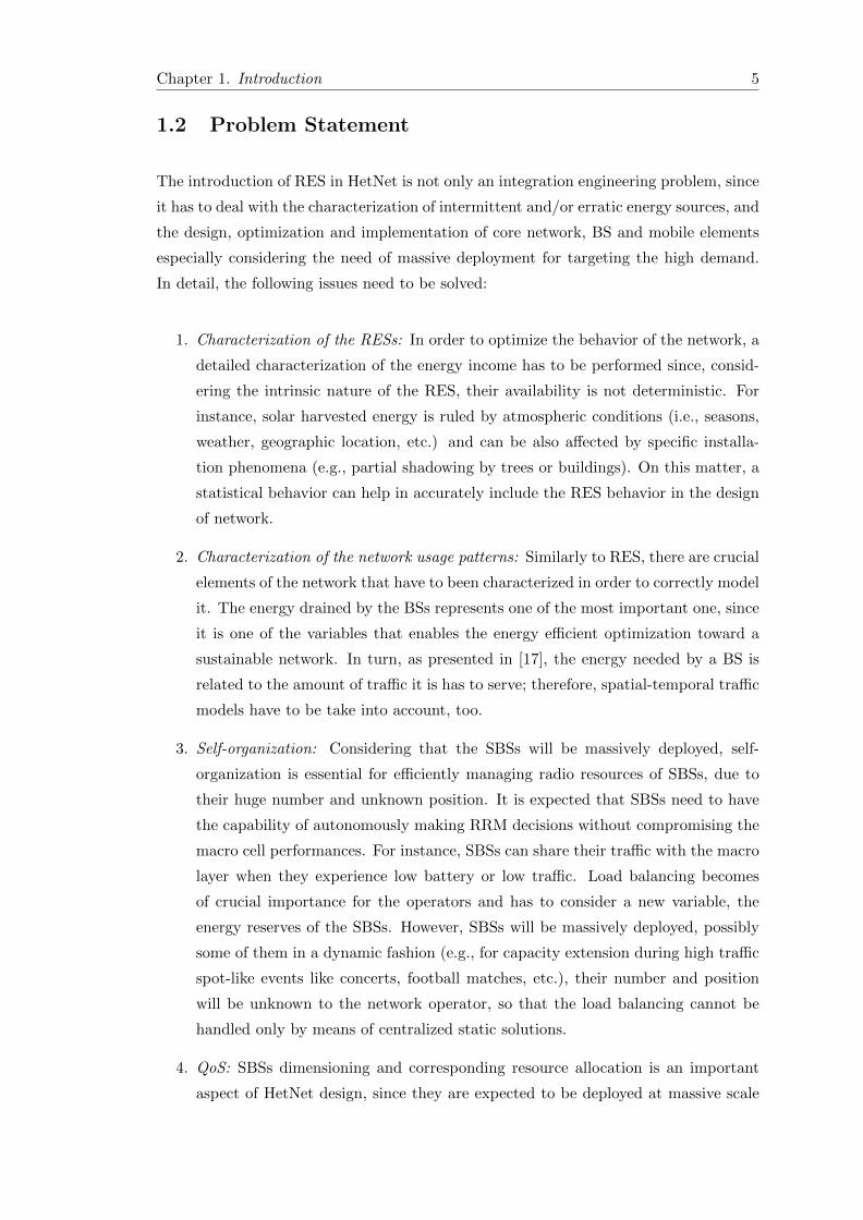
1.2 Problem Statement
The introduction of RES in HetNet is not only an integration engineering problem, since
it has to deal with the characterization of intermittent and/or erratic energy sources, and
the design, optimization and implementation of core network, BS and mobile elements
especially considering the need of massive deployment for targeting the high demand.
In detail, the following issues need to be solved:
1. Characterization of the RESs: In order to optimize the behavior of the network, a
detailed characterization of the energy income has to be performed since, consid-
ering the intrinsic nature of the RES, their availability is not deterministic. For
instance, solar harvested energy is ruled by atmospheric conditions (i.e., seasons,
weather, geographic location, etc.) and can be also affected by specific installa-
tion phenomena (e.g., partial shadowing by trees or buildings). On this matter, a
statistical behavior can help in accurately include the RES behavior in the design
of network.
2. Characterization of the network usage patterns: Similarly to RES, there are crucial
elements of the network that have to been characterized in order to correctly model
it. The energy drained by the BSs represents one of the most important one, since
it is one of the variables that enables the energy efficient optimization toward a
sustainable network. In turn, as presented in [17], the energy needed by a BS is
related to the amount of traffic it is has to serve; therefore, spatial-temporal traffic
models have to be take into account, too.
3. Self-organization: Considering that the SBSs will be massively deployed, self-
organization is essential for efficiently managing radio resources of SBSs, due to
their huge number and unknown position. It is expected that SBSs need to have
the capability of autonomously making RRM decisions without compromising the
macro cell performances. For instance, SBSs can share their traffic with the macro
layer when they experience low battery or low traffic. Load balancing becomes
of crucial importance for the operators and has to consider a new variable, the
energy reserves of the SBSs. However, SBSs will be massively deployed, possibly
some of them in a dynamic fashion (e.g., for capacity extension during high traffic
spot-like events like concerts, football matches, etc.), their number and position
will be unknown to the network operator, so that the load balancing cannot be
handled only by means of centralized static solutions.
4. QoS: SBSs dimensioning and corresponding resource allocation is an important
aspect of HetNet design, since they are expected to be deployed at massive scale

Chapter 1. Introduction 6
and in an uncoordinated fashion. Towards this objective, an efficient joint manage-
ment of the traffic demand and the energy reserves in the SBSs is also a challenge.
The design of online RRM solutions for cellular networks with energy constrained
elements is an open issue and is a novel topic in literature.
5. Low power consumption: Despite of the already low power consumption of the
SBSs, energy saving mechanisms for reducing the power consumption of the SBSs
by improving PHY related technologies and layer 2 algorithms will help in scale
down the equipment needed by RES and in, more in general, in their management.
Recently, the softwarization of the radio access part started attracting interest due
to the high flexibility it enables.
6. Energy market trends: The trend in energy market is that the energy price in future
power grids will change hourly. However, standard networks are not optimized to
this respect, since in general the network energy consumption directly depends on
the requested capacity. Using RES, the network will have now an energy reserve
which enables the possibility to trade some of the energy that they harvest.
In this Ph.D. dissertation we focus on a subset of the open issues of the energy sus-
tainability of self-organized HetNet partially powered by RES from an online RRM
perspective. In particular, we will pay special attention to the open issues described in
points 1, 3, 4 and 6.
1.3 Objectives and Methodology
The goal of this thesis is to investigate on scenarios where harvested ambient energy
is employed to steer LTE HetNets toward a more sustainable paradigm, reducing the
energy consumption from the grid and, more than that, where communication networks
blend with future electricity grids, as the one depicted in Fig. 1.1. The usage of RES
can be distinguished in two different operative cases: i) energy self-sustainable network
elements and ii) grid energy saving thanks to the efficient use of the network elements
powered with RES. In the first paradigm, the problem is to guarantee network reliability
by managing the limited available energy resources since there is no connection to the
electric grid. While, in the second vision, RESs are used as an alternative green solution
for powering part of the network in order to reduce its carbon footprint and represents
the core of the contribution. It is to be noted that, the second paradigm can, in turns,
have a further extension which comprises the possibility that future network elements
may trade some of the energy that they harvest to make profit and provide ancillary
services to the power grid. In pico deployments, for instance, it may occur in the form of

Chapter 1. Introduction 7
macro cell
micro cells
pico cells
electric gridrenewable
energy
Figure 1.1: HetNet powered with RES reference architecture.
supporting connected loads, such as street lighting or weather stations. Instead, selling
energy to the grid operator may make sense for micro and macro cells where the amount
of energy harvested easily matches or surpasses that of residential users.
Solar energy has been chosen as reference RES due to its widespread adoption and its
high efficiency in terms of energy produced compared to its costs. To this end, an
harvested solar energy model has been implemented through a simple but yet accurate
stochastic Markov processes for the description of the energy scavenged by outdoor solar
sources. The Markov models that we derived are obtained from extensive solar radiation
databases. The basic idea is to derive the corresponding amount of energy from hourly
radiance patterns that is accumulated over time in order to represent it in terms of its
relevant statistics. We tested Markov models with different number of states and data
clusterization models for having both simple solutions and accurate ones.
We characterized the problem of distributed energy aware SBS control by considering
the aforementioned Markov processes for modeling the solar energy harvested. The high
dynamism typical of the HetNet scenarios jointly with the complexity of the system
suggest the usage of distributed control systems rather than centralized, where the scal-
ability and the flexibility can become rapidly a bottleneck. We focus on the energy aware
online control for improving the energy-efficiency of the system by optimizing the usage
of the renewable energy reserves in the SBS tier. We propose to model the SBS tier
as a multi-agent system [27], where each SBS is an intelligent and autonomous agent,
which learns by directly interacting with the environment and by properly utilizing the
past experience. The novel solution will make able the SBS tier to work without the

Chapter 1. Introduction 8
knowledge of the traffic demand and the expected solar harvested energy income. Due
to the complexity and the dynamism of the scenario, which does not allow to define
an integrated probabilistic model, we propose to solve the RRM with a reinforcement
learning solution [28].
Multi-agent RL (MRL) systems are an effective way to treat complex, large and unpre-
dictable problems since they offer modularity in distributing the implementation of the
solution across different agents. However, such distribution might suffer the problem
of finding simultaneously a solution among all the agents that is good for the whole
system. Therefore, the Layered Learning (LL) [29] and heuristically accelerated MRL
(HAMRL) [30] paradigms are adopted to simplify the problem by decompose it in sub-
tasks. The global solution is then obtained in a hierarchical fashion: the learning process
of a subtask is aimed at facilitating the learning of the next higher subtask layer. We
adopted the logical layers classification intrinsic in the nature of the HetNet. The first
layer implements an MRL approach and is in charge of the local online optimization at
SBS level as function of the traffic demand and the energy incomes. The second layer is
in charge of the network-wide optimization and is based on Artificial Neural Networks
(ANNs) aimed at estimating the model of the overall network. The architecture for
implementing the two levels and enable their interaction is based on a SDN paradigm.
According to the review of the literature, this is the first work in the literature that has
proposed online solutions with realistic environmental conditions and considering the
optimization across different energy harvesting conditions, as will be also discussed in
Chapter 2.
1.4 Outline of the thesis
This section gives a brief overview of the contents of the following chapters, which are
summarized in Fig. 1.2.
Chapter 2
This chapter provides the necessary background information concerning the description
of network design and switching ON/OFF approaches presented in the literature. It
starts with the required background knowledge, including a description of the reference
scenarios and architectures. In continuation, a survey of the state-of-the-art and current
trends is given. The chapter examines the energy efficient solutions that are applied
in two different network architectures: single-tier and HetNet. In this chapter some
preliminary work devoted to evaluate the feasibility of the solutions investigated are
also presented for introducing the reference solutions for HetHet with EH capabilities.

Chapter 1. Introduction 9
IntroductionChapter 1
Photovoltaic Sources CharacterizationChapter 4
Switch-ON/OFF Policies for EH SBSs through Distributed Q-Learning
Chapter 5
Layered Learning Load Control for Renewable Powered SBSs
Chapter 6
Conclusions and Future WorkChapter 7
State of the Art in SBS Powered with Renewable Energies
& ML Overview
Chapter 2 & 3
Figure 1.2: Outline of the dissertation.
The work presented in this chapter has been published in the following papers:
• G. Piro, M. Miozzo, G. Forte, N. Baldo, L.A. Griego, G. Boggia, P. Dini, “Het-
Nets Powered by Renewable Energy Sources: Sustainable Next-Generation Cellu-
lar Networks”, in IEEE Internet Computing, vol. 17, no. 1, pp. 32-39, Jan.-Feb.
2013.
• D. Zordan, M. Miozzo, P. Dini, M. Rossi, “When telecommunications networks
meet energy grids: cellular networks with energy harvesting and trading capabil-
ities”, in IEEE Communications Magazine, vol. 53, no. 6, pp. 117-123, June
2015.
• N. Piovesan, A. Fernandez Gambin, M. Miozzo, M. Rossi, P. Dini, “Energy sus-
tainable paradigms and methods for future mobile networks: A survey”, Computer
Communications,Volume 119,2018,Pages 101-117.
• P. Dini, M. Miozzo, N. Bui, N. Baldo, “A Model to Analyze the Energy Savings
of Base Station Sleep Mode in LTE HetNets”, in Proceedings of IEEE GreenCom
2013, 20-23 August 2013, Beijing (China).

Chapter 1. Introduction 10
• N. Baldo, P. Dini, J. Mangues, M. Miozzo, J. Nunez-Martınez, “Small cells,
wireless backhaul and renewable energy: a solution for disaster aftermath com-
munications”, in Proceedings of 4th International Conference on Cognitive Ra-
dio and Advanced Spectrum Management (COGART 2011) - Cognitive and Self-
Organizing Networks for Disasters Aftermath Assistance, 26-29 October 2011,
Barcelona (Spain).
• M. Miozzo and N. Bartzoudis and M. Requena and O. Font-Bach and P. Har-
banau and D. Lopez-Bueno and M. Payaro and J. Mangues, “SDR and NFV
extensions in the ns-3 LTE module for 5G rapid prototyping”, in Proceedings of
2018 IEEE Wireless Communications and Networking Conference (WCNC), April
2018, Barcelona (Spain).
Chapter 3
The main principles of the theory behind the ML methods used in this thesis are pre-
sented in chapter 3. The overview of reinforcement learning algorithms is discussed for
both the single-agent and multi-agent case, introducing the algorithms used and their
main challenges in the application in the considered scenario. Finally, an introduction
on neural networks and on their training solutions is presented.
Chapter 4
Chapter 4 provides a novel model for the energy harvesting process, describing the
methodology to model the energy inflow as a function of time through stochastic Markov
processes. The proposed approach has been validated against real energy traces, showing
good accuracy in their statistical description in terms of first and second order statistics.
This model will be used for generating the solar harvested energy profile in the evaluation
of the HetNet control solutions proposed in this thesis.
The work presented in this chapter has been published in this paper:
• M. Miozzo, D. Zordan, P. Dini, M. Rossi, “ SolarStat: Modeling Photovoltaic
Sources through Stochastic Markov Processes”, in Proceedings of IEEE Energy
Conference, 13-16 May 2014, Dubrovnik (Croatia).
Chapter 5 In this chapter we present the innovative contribution of this thesis on the
online control of HetNet with EH capabilities. Different distributed Q-learning solutions
are investigated both analyzing their temporal behavior and their network performance.
The results presented, despite of being encouraging, show that scalability of the solution
might be a problem in case of dense SBSs networks.

Chapter 1. Introduction 11
The work presented in this chapter has been published in the following papers:
• M. Miozzo and L. Giupponi and M. Rossi and P. Dini, “Distributed Q-learning for
Energy Harvesting Heterogeneous Networks”, in Proceedings of 2015 IEEE Inter-
national Conference on Communication Workshop (ICCW), June 2015, London
(UK).
• M. Miozzo and L. Giupponi and M. Rossi and P. Dini, “Switch-On/Off Policies for
Energy Harvesting Small Cells through Distributed Q-Learning”, in Proceedings
of 2017 IEEE Wireless Communications and Networking Conference Workshops
(WCNCW), March 2017, San Francisco (USA).
Chapter 6
In Chapter 6, the Layered Learning solution for HetNet powered with solar energy is
presented. In particular, a hierarchical framework based on a two-layered optimization
has been adopted: where the bottom layer implementing multi-agent RL is enhanced
by the above layer through its network-wide view through a control based on neural
networks. The goal is to improve the coordination of the agent issues of distributed Q-
learning solutions for guaranteeing high EE in systems with dense deployment of SBSs.
Simulation results prove that the proposed layered framework outperforms both a greedy
and a completely distributed solution both in terms of throughput and energy efficiency.
The work presented in this chapter has been published in the following papers:
• M. Miozzo and P. Dini, “Layered Learning Radio Resource Management for En-
ergy Harvesting Small Base Stations”, in Proceedings of 2018 IEEE Vehicular
Technology Conference (VTC Spring), June 2018, Port (Portugal).
• M. Miozzo and N. Piovesan and P. Dini, “Layered Learning Load Control for
Renewable Powered Small Base Stations”, submitted to IEEE Transactions on
Green Communications and Networking.
Chapter 7
The document is closed with Chapter 7, where the high level assessment of the achieve-
ments accomplished through the research presented herein, the conclusions and perspec-
tives for future works are presented.

Chapter 2
State of the Art and Beyond
2.1 Introduction
In the last decade several solutions have been proposed for reducing the energy con-
sumption of the radio communication networks, as testified by the vivid literature on
this topic [31]. In general, this family of solutions has been named as green communi-
cation and networking and it includes models to characterize the energy consumption
of the network elements and strategies for energy optimization for all the layers of the
protocol stack, such as: power amplifiers, radio transmission techniques, media access
control (MAC) algorithms, networking solutions and architectures.
In terms of energy consumption, the most important element of the network is repre-
sented by the BS, according to it impact of 80% in the energy budget of the overall radio
access network [12]. Consequently, the main effort concentrated in optimizing the net-
work from BS usage perspective. To this end, two main approaches have been adopted
so far: offline and online optimization. The formers are usually based on stochastic ge-
ometric and are devoted to draw the general trends and guidelines for deploying optimal
energy architectures without considering specific details of the scenario. The latter are
usually sub-optimal solutions which however can consider more realistic models of the
system components and allows a closer approximation to realistic scenarios. To this end,
learning solutions represent a valuable way to implement a self-organization approach
that enables to deploy cellular network in a flexible way able to adapt to the most im-
portant environmental variables. This background information is important, since it
facilitates the understanding of the motivations behind the contributions of this thesis.
This chapter is structured as follows: Section 2.2 introduces the energy consumption
model of the different types of BSs, which allows to better understand the principles
12

Chapter 2. State of the Art and Beyond 13
behind the energy efficiency solutions. Section 2.3 presents the review of the existing
literature with the more consolidated energy efficiency techniques for both standard cel-
lular network and for the ones with EH capabilities. After presenting the most common
methods and widely used solutions found in the literature, a description of the research
challenges and open issues is given in Section 2.4, introducing the main contributions of
this thesis. Finally, Section 2.5 concludes the chapter.
2.2 BS Energy Model
Before delving into the description of the techniques to make the network energy effi-
cient and self-sufficient, next we review the main achievements in power consumption
measurement and models for base stations. One of the most detailed BS energy models
adopted in literature has been developed in the framework of the Energy Aware Radio
and neTwork tecHnologies (EARTH) EU founded project [32]. By taking in consid-
eration the principal elements that drain energy in a LTE BS (i.e., power amplifiers,
baseband unit, radio frequency module, AC-DC converters, the main supply unit and
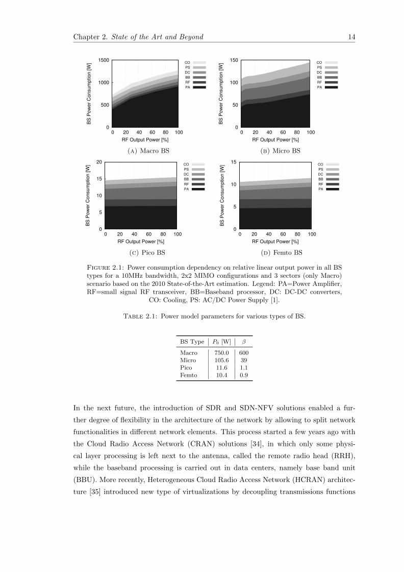
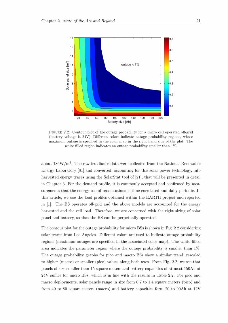
the cooling system), in [17] an accurate model has been derived. As depicted in Fig. 2.1,
the power amplifier (PA) is one of the main power draining component in all type of the
BSs. Moreover, PA generates a dependency on the load of the BS both in macro and
micro BS. In the former, the power consumption can change up to the 44%, while in
the latter 27%. Reducing the form factor and the PA needs, the cooling system (CO)
part disappears but the one of the baseband processor (BB) increases its contribution.
However, it is to be noted that, for very small BSs like pico and femto, the load of the
BS marginally affects the power consumption.
The BS power consumption model presented in Fig. 2.1 can be approximated with a
linear function, defined as follows:
P = P0 + βρ (2.1)
where ρ ∈ [0, 1] is the traffic load of the BS normalized to its maximum capacity, and
P0 is the power consumption when ρ = 0. The values of P0 and β for each type of BS
are reported in table 2.1.
Remarkably, P0 represents a significant part of the total energy consumed by any BS
and, due to this, researchers have investigated the use of sleep modes during low traffic
periods. Moreover, it is expected that P0 of new sites will be reduced by about 8%
on average thanks to recent technological advances [33], thus further decreasing the BS
energy cost during low traffic periods.
Chapter 2. State of the Art and Beyond 14
0
500
1000
1500
0 20 40 60 80 100
BS
Pow
er
Consum
ption [W
]
RF Output Power [%]
CO
PS
DC
BB
RF
PA
(a) Macro BS
0
50
100
150
0 20 40 60 80 100
BS
Pow
er
Consum
ption [W
]
RF Output Power [%]
CO
PS
DC
BB
RF
PA
(b) Micro BS
0
5
10
15
20
0 20 40 60 80 100
BS
Pow
er
Consum
ption [W
]
RF Output Power [%]
CO
PS
DC
BB
RF
PA
(c) Pico BS
0
5
10
15
0 20 40 60 80 100
BS
Pow
er
Consum
ption [W
]
RF Output Power [%]
CO
PS
DC
BB
RF
PA
(d) Femto BS
Figure 2.1: Power consumption dependency on relative linear output power in all BStypes for a 10MHz bandwidth, 2x2 MIMO configurations and 3 sectors (only Macro)scenario based on the 2010 State-of-the-Art estimation. Legend: PA=Power Amplifier,RF=small signal RF transceiver, BB=Baseband processor, DC: DC-DC converters,
CO: Cooling, PS: AC/DC Power Supply [1].
Table 2.1: Power model parameters for various types of BS.
BS Type P0 [W] β
Macro 750.0 600Micro 105.6 39Pico 11.6 1.1Femto 10.4 0.9
In the next future, the introduction of SDR and SDN-NFV solutions enabled a fur-
ther degree of flexibility in the architecture of the network by allowing to split network
functionalities in different network elements. This process started a few years ago with
the Cloud Radio Access Network (CRAN) solutions [34], in which only some physi-
cal layer processing is left next to the antenna, called the remote radio head (RRH),
while the baseband processing is carried out in data centers, namely base band unit
(BBU). More recently, Heterogeneous Cloud Radio Access Network (HCRAN) architec-
ture [35] introduced new type of virtualizations by decoupling transmissions functions
Chapter 2. State of the Art and Beyond 15
from proprietary hardware-dependent implementations, enabling their execution in dif-
ferent hardware resource of the network. Various splits at PHY, MAC, RLC and PDCP
layers are considered for relaxing the stringent requirements of CRAN while maintaining
its centralized processing benefits [36]. The energy model of such novel architectures has
not been yet proposed in literature. However, it can be estimated based on the model
introduced in [37], which is a general flexible power model of LTE base stations and
provides the power consumption in Giga Operation Per Second (GOPS). To this re-
spect, in [38] and [39] we provided a preliminary assessment on the energy consumption
figures of different HCRAN configurations through an emulation platform based on the
LTE module of the popular ns-3 Network simulator [40] and a real-time implementation
of the physical layer functionalities based on field-programmable gate array (FPGA).
From this analysis, we showed that important energy savings can be obtained at RRH
when moving part of the lower layer network functionalities to the BBU. Moreover, we
highlighted also that the bandwidth of the system is the most important parameter for
what concern the energy consumption of the RRH since it can affect up to 50% on the
overall energy budget of the RRH.
2.3 Techniques for Energy Efficiency
2.3.1 Single Tier Networks
In standard 3G architectures, where the type of BSs is reduced to macro and micro and
they are treated as a single tier, the most promising solution to optimize the BS energy
consumption is by putting them in sleep mode (or OFF mode). In this case, in order to
sleep a BS and guarantee the coverage, the BSs in the set of the ones that remain awake
(ON mode) have usual to re-adjust their transmission power and, possibly, the tilt of
the antenna, enabling the communications also the users that was previously served by
the BS slept, technique called cell zooming or cell breathing.
Sleep Mode
The cellular networks have been dimensioned to support traffic peaks, i.e., the number
of BSs deployed in a given area should be able to provide the required Quality of Service
(QoS) to the mobile subscribers during the highest load conditions. However, during
off-peak periods the network may be underutilized, which leads to an inefficient use
of spectrum resources and to an excessive energy consumption (note that the energy
drained during low traffic periods is non-negligible due to the high values of P0 in
Eq. (2.1)). For these reasons, sleep modes have been proposed to dynamically turn OFF

Chapter 2. State of the Art and Beyond 16
some of the BSs when the traffic load is low. This has been extensively studied in the
literature, considering different problem formulations [13]. However, since BSs cannot
serve any traffic when asleep, it is important to properly tune the enter/exit time of
sleep modes to avoid service outage.
The authors of [41] propose centralized and distributed clustering algorithms to clus-
ter those BSs exhibiting similar traffic profiles over time. Upon forming the clusters,
an optimization problem is formulated to minimize their power consumption. Optimal
strategies are found by brute force, since the solution space is rather small and its com-
plete exploration is still doable. A similar approach is presented in [42] where a dynamic
switching ON/OFF mechanism locally groups BSs into clusters based on location and
traffic load. The optimization problem is formulated as a non-cooperative game aiming
at minimizing the BS energy consumption and the time required to serve their traf-
fic load. Simulation results show energy costs and load reductions while also provide
insights of when and how the cluster-based coordination is beneficial.
User QoS is added to the optimization problem in [43]. In this case, as the problem
to solve is NP-hard, the authors propose a suboptimal, iterative and low-complexity
solution. The same approach is used in [44–47], playing with the trade-off between
energy consumption and QoS. The Quality of Experience (QoE) is included in [48],
where a dynamic programming (DP) switching algorithm is put forward. The user
QoE is utilized in place of standard network measures such as delay and throughput.
Other parameters that have been considered are the channel outage probability (also
referred to as coverage probability), i.e., the probability of guaranteeing the service
to the users located in the worst positions (e.g., at the cell edge) and the BS state
stability parameter, i.e., the number of ON/OFF state transitions. For instance, a set
of BS switching patterns engineered to provide full network coverage at all times, while
avoiding channel outage, is presented in [49]. The coverage probability, along with power
consumption and energy efficiency metrics, are derived using stochastic geometry in [50–
52]. The QoE is also affected by the user equipment (UE) positions according to the
channel propagation phenomena. To this respect, in [53] the selection of the BSs to be
switched OFF is taken in order to provoke less impact to the UEs’ QoE according to
their distance to the handed off BSs.
In order to support sleep modes, neighboring cells must be capable of serving the traffic
in OFF areas. To achieve this, proper user association strategies are required. In a sce-
nario where sleeping techniques are not applied, each user is associated with the BS that
provides the best Signal to Interference plus Noise Ratio (SINR). However, when BSs
can go to sleep, user association is more complex and requires traffic prediction as well
as very fast decision-making. Otherwise, users may suffer a deterioration of their QoS. A

Chapter 2. State of the Art and Beyond 17
framework to characterize the performance (outage probability and spectral efficiency)
of cellular systems with sleeping techniques and user association rules is proposed in [54].
In this paper, the authors devise a user association scheme where a user selects its serv-
ing BS considering the maximum expected channel access probability. This strategy is
compared against the traditional maximum SINR-based user association approach and
is found superior in terms of spectral efficiency when the traffic load is inhomogeneous.
According to the BS state stability concept, a bi-objective optimization problem is at-
tained in [55] and solved with two algorithms: (i) near optimal but not scalable, and (ii)
with low complexity, based on particle swarm optimization.
The authors in [56, 57] propose solutions based on stochastic analysis for designing the
deployment of macro BSs able to guarantee the QoS requirements and save energy by
switching OFF subsets of BSs.
In [58] the notion of energy partition, an association of powered-ON and powered-OFF
BSs, is used to enable network-level energy saving. It then elaborates how such con-
cept is applied to perform energy re-configuration to flexibly re-act to load variations
encouraging none or minimal extra energy consumption. Similarly, in [59] the authors
introduce the notion of network-impact, which takes into account the additional load
increments brought to its neighboring BSs, for detecting which BS to turn OFF as the
one that will minimally affect the network.
Finally, RL techniques are investigated in [60] to solve the energy saving problem in
order to make the system able to automatically reconfigure itself. In particular, the
BS switching operation problem has been modeled according to the actor-critic method.
The simulation results reported show the effectiveness of presented energy saving scheme
under various practical configurations.
Cell Zooming
This family of methods is complementary to the sleep techniques and has been intro-
duced to avoid the coverage gaps that may occur as BSs go to sleep. It amounts to
adjusting the cell size according to traffic conditions, leading to several benefits: (i) load
balancing is achieved by transferring traffic from highly to lightly congested BSs, (ii)
energy saving through sleeping strategies, (iii) user battery life and throughput enhance-
ments [61]. To compute the right cell size, cell zooming adaptively adjust the transmit
powers, antenna tilt angles, or height of active BSs. Centralized and distributed cell
zooming algorithms are proposed in [62], where a cell zooming server, which can be
either implemented in a centralized or distributed fashion, controls the zooming proce-
dure by setting its parameters based on traffic load distribution, user requirements, and

Chapter 2. State of the Art and Beyond 18
Channel State Information (CSI). A different approach is proposed in [63], where the
authors design a BS switching mechanism based on a power control algorithm that is
built upon non-cooperative game theory. A closed-form expression cell zooming factor is
defined in [64], where an adaptive cell zooming scheme is devised to achieve the optimal
user association. Then, a cell sleeping strategy is further applied to turn OFF light
traffic load cells for energy saving. In general, most zooming scenarios entail a compu-
tationally intractable formulation, so affordable solutions based on iterative algorithms
or heuristics abound in the literature, see, e.g., [65, 66].
Remarkably, cell zooming entails an increase in the transmit power of the active BSs,
which leads to a higher energy expenditure for the BSs that are on. However, when
used in combination with sleeping strategies, this leads to additional energy savings.
Some researchers are oriented towards the study of sleeping schemes in conjunction
with cooperative communication strategies for distributed antennas, also referred to as
Coordinated Multi Point (CoMP). This technique increases spectral efficiency and cell
coverage without entailing a higher BS transmit power and reducing the co-channel in-
terference. The authors of [67] prove the effectiveness of this approach in terms of energy
and capacity efficiency when sleep modes are combined with downlink CoMP. Despite
these advantages, their results also reveal that imperfect downlink channel estimations
and an incorrect CoMP setup can lead to energy inefficiency.
An online algorithm is proposed in [68] for a cell-breathing solution based on a clus-
tered architecture. Since it a distributed solution, it allows to improve the scalability
constraints given by a centralized approach and the risk of having one-point failure in
network coordination. Moreover, it dynamically adjusts the traffic thresholds to define
the BS behavior in order to be able to follow traffic fluctuations.
2.3.2 HetNets
Considering HetNet, the problem has been concentrated in defining strategies for sleep-
ing the SBSs rather than the macro BSs. Similarly to the macro BS case, stochastic
analysis has been used for defining the trends and the optimum deployment principles
of HetNet [69–71]. In [72] a distributed online scheduling algorithm for SON HetNets
is proposed which optimizes jointly the resource allocation, the transmission power and
the UE attachment in terms of call admission control. In [73] the authors propose a
noncooperative game among the BSs that seeks to minimize the trade-off between en-
ergy expenditure and load requirements when putting in sleep mode the SBSs. All the
techniques in the above do not consider the traffic demand in the optimization problem.

Chapter 2. State of the Art and Beyond 19
In [74], closed-form expressions of coverage probability and average user load are formu-
lated through stochastic geometry. Optimal resource allocation schemes are proposed
to minimize power consumption and maximize coverage probability in a HetNet, and
are validated numerically. User association mechanisms that maximize energy efficiency
in the presence of sleep modes are addressed in [75], where the energy efficiency is de-
fined as the ratio between the network throughput and the total energy consumption.
Since this leads to a highly complex integer optimization problem, the authors propose
a Quantum particle swarm optimization algorithm to obtain a suboptimal solution.
In [76] an offline algorithm that defines the timing for putting the SBSs in sleep mode as
function of the system load has been presented. However, in [18] we showed that, when
considering the energy model profiles in [17], the amount of energy saved is reduced due
to the fact that the macro BS has to manage the traffic of the users previously attached
to the SBS switched OFF. In fact, as highlighted in Fig. 2.1, when the macro BS is loaded
with more traffic, its power consumption might considerably increase affecting the one
of the whole network. This is coherent with HetNets paradigm, where the spectrum
efficiency of the SBSs is greater with respect to the one of the MBS.
2.3.3 HetNet with Energy Harvesting Capabilities
The increasing interest in energy harvesting (EH) application in cellular networks from
the research community is testified by the rich literature [77] on this relative new topic.
On this matter, the contributions can be divided, in turns, in two problems: commu-
nication cooperation and energy trading [78]. In communication cooperation scenarios
the solutions have to enable mechanisms to deal with the energy as a hard constraint,
since the system cannot work when the energy is finished. While in energy trading prob-
lem, the energy derived by RES has to be optimized to increase the energy efficiency of
the whole system or, in case of considering the energy market, to increase the benefits
generated thanks to the energy trading.
On this matter, we performed two feasibility studies on HetNet with EH capabilities for
assessing the actual challenges of such problems that will be detailed in what follows.
Then, a review of the main techniques proposed for the problem of energy cooperation
is discussed.
Feasibility Studies
In the context of communication cooperation solutions, we proposed a feasibility study
for LTE-like cellular network deployments with photovoltaic panels [79]. The system

Chapter 2. State of the Art and Beyond 20
Table 2.2: PV and storage ratings and installation costs for both grid-powered andenergy-sustainable base stations.
LTE BSMacro Micro Pico
PV ratings [kW] 8.45 0.9 0.09
Storage ratings [Ah] 1250 104.2 20.8
PV system land occupation [m2] 61.43 6.43 0.46
CAPEX for the grid connection [e] 16450 13650 12750
CAPEX for the PV+storage plant [e] 240100 11900 1190
design took in consideration all the principal elements of the access network, among
them:
1. The OPEX due to the electricity consumption according to the model presented
in Section 2.2.
2. The capital expenditure (CAPEX) of the grid-connected nodes has been modeled
as the cost of the infrastructure for providing grid electricity.
3. The CAPEX of the off-grid nodes includes both the cost of the photovoltaic solar
panel and of the batteries, both of them dimensioned for the worst case scenario
where solar panels do not generate energy during 7 contiguous days.
In Tab. 2.2 the installation costs for grid-powered nodes are reported for the worst
case scenario when the BS are always at full load. Looking at the PV system land
occupation, we noticed that RES can be a viable cost-effective solution for SBSs, while
it is still not possible to exploit it for MBS. However, it is to be noted that, with
these simple dimensioning solutions the solar panel dimensions are still rather large
for considering their deployment in street furniture (i.e., a micro BS would need a PV
module of 6.43m2).
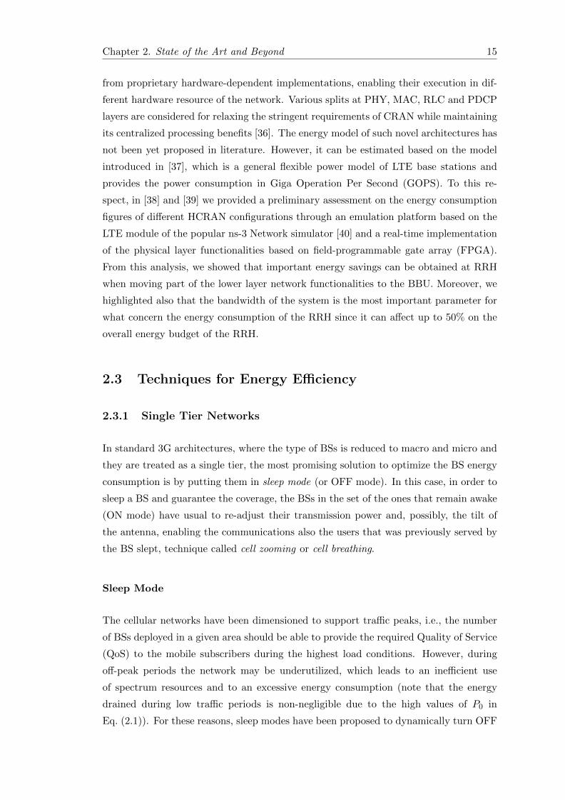
In [80], we advanced this study by considering a more realistic scenario with real energy
harvesting traces and traffic demand profiles. Moreover, we introduced the design con-
cept of outage probability, defined as the fraction of time during which the BS is unable to
serve the users’ demand due to an insufficient energy reserve. In that case, the BS has to
be momentarily switched OFF or put into a power saving mode. The size of harvesters
and batteries has been evaluated as a function of the outage probability for different
geographical locations. In detail, hourly energy generation traces from a solar source
have been obtained for the cities of Los Angeles (CA) and Chicago (IL), US. For the
solar modules, the commercially available Panasonic N235B photovoltaic technology has
been considered. These panels have single cell efficiencies as high as 21.1%, delivering
Chapter 2. State of the Art and Beyond 21
Battery size [Ah]
Sola
r panel siz
e [m
2]
20 40 60 80 100 120 140 160 180 200
2
4
6
8
10
12
14
16
18
0.1
0.2
0.3
0.4
0.5
0.6
0.7
outage < 1%
Figure 2.2: Contour plot of the outage probability for a micro cell operated off-grid(battery voltage is 24V). Different colors indicate outage probability regions, whosemaximum outage is specified in the color map in the right hand side of the plot. The
white filled region indicates an outage probability smaller than 1%.
about 186W/m2. The raw irradiance data were collected from the National Renewable
Energy Laboratory [81] and converted, accounting for this solar power technology, into
harvested energy traces using the SolarStat tool of [21], that will be presented in detail
in Chapter 3. For the demand profile, it is commonly accepted and confirmed by mea-
surements that the energy use of base stations is time-correlated and daily periodic. In
this article, we use the load profiles obtained within the EARTH project and reported
in [1]. The BS operates off-grid and the above models are accounted for the energy
harvested and the cell load. Therefore, we are concerned with the right sizing of solar
panel and battery, so that the BS can be perpetually operated.
The contour plot for the outage probability for micro BSs is shown in Fig. 2.2 considering
solar traces from Los Angeles. Different colors are used to indicate outage probability
regions (maximum outages are specified in the associated color map). The white filled
area indicates the parameter region where the outage probability is smaller than 1%.
The outage probability graphs for pico and macro BSs show a similar trend, rescaled
to higher (macro) or smaller (pico) values along both axes. From Fig. 2.2, we see that
panels of size smaller than 15 square meters and battery capacities of at most 150Ah at
24V suffice for micro BSs, which is in line with the results in Table 2.2. For pico and
macro deployments, solar panels range in size from 0.7 to 1.4 square meters (pico) and
from 40 to 80 square meters (macro) and battery capacities form 20 to 90Ah at 12V

Chapter 2. State of the Art and Beyond 22
(pico) and from 300 to 1500Ah at 48V (macro). Taking an outage of 1% as our design
parameter, all the points on the boundary of the white-filled region are equally good.
The results for the city of Los Angeles are rather good, indicating that the nearly-zero
energy is indeed a feasible goal. In fact, both battery and panel sizes are acceptable
given the dimensions of typical installation sites for the considered BSs. Instead, for the
city of Chicago the energy inflow is less abundant, and this is especially so during the
winter months. In that case, reasonable panel and battery sizes (even slightly higher
than those discussed for Los Angeles) lead to outages of 10% or higher. Due to this,
grid-connected operation is required for locations where the energy inflow is moderate
(especially during the winter).
Now, we consider the energy trading problem where a grid-connected BS that can sell or
buy energy from the grid. Most likely, the energy price in future power grids will change
hourly. This practice is not yet adopted worldwide but there are relevant programs
that already use it. A relevant example can be found in Illinois, US, where electrical
companies are offering new hourly electricity pricing programs where energy prices are
set a day-ahead by the hourly wholesale electricity market run by the Midcontinent
Independent System Operator (MISO). In this way, customers can optimize their usage
patterns, saving money in their energy bills. In this work, we use publicly available
historical energy price data from these programs to discuss suitable energy management
policies. From telecommunication perspective, energy harvesting and future market
policies will permit at least two additional optimization strategies. First, the system
could adapt its behavior to the energy price, i.e., it could be energy frugal when the
energy cost is high, whilst adopting more aggressive policies when the cost drops. Second,
part of the energy that is accumulated could be sold or re-distributed among other
network elements.
To this end, an energy manager intelligently chooses in which amounts and when energy
et (the decision variable) has to be purchased or sold so that the system maximizes its
profit. In detail, we considered a system that evolves in slotted time t, where the slot
duration is one hour. At any given time t, the BS may sell or buy a certain amount of
energy et, which is positive when energy is sold and negative when purchased. When
energy et < 0 is purchased from the grid operator, a monetary cost C(et) is incurred,
which corresponds to the price of energy in slot t. Instead, when energy et > 0 is
sold, a reward R(et) = rC(−et) is accrued, with r ≤ 1 being a discount factor. This
means that the energy sold is paid less than that purchased, as this is usually the
case in current energy markets and is expected to remain so for future ones. Also,
we use C(et) = 0 for et ≥ 0 and R(et) = 0 for et ≤ 0, meaning that no cost is
incurred when selling and no reward is accrued when buying. At each time t, the
demand dt has to be fully served and the energy required to do so is harvested, taken

Chapter 2. State of the Art and Beyond 23
from the battery or bought from the grid. This corresponds to maximizing the total
monetary reward, expressed as f(T ) =∑T
t=0[R(et) − C(et)], over the time horizon
of interest t ∈ T (with T = {0, 1, . . . , T}). The solution to this problem amounts
to finding the optimal allocation {e∗t }t∈T for all time slots t ∈ T . Here, we do so
through dynamic programming considering the actual traces for hourly energy prices,
user demand and harvested energy. Based on the optimization performed by the energy
manager, we studied how to dimension the solar add-on in order to maximize the net
profit, considering an amortization period T of ten years and given that the optimal
policy e∗t is used throughout. The net profit over this period is obtained summing the
revenue f(T ) to the cost incurred when the BS is powered in full by the energy grid,
and subtracting the CAPEX associated with the resulting harvesting hardware.
For the following example results, we have accounted for the current price of solar panels,
which is about 0.5$/kWh and a battery cost of 300$/kWh. Table 2.3 and Table 2.4
show the 10-year net income for pico, micro and macro cells that can be achieved in
the cities of Chicago and Los Angeles, respectively. For the net income the notation we
used “X$ (Y,Z)”, where X is the net income in US dollars, Y is the solar panel size
(square meters) and Z is the battery size (Ah). According to the considered CAPEX
cost, optimal designs tend to pick smaller battery capacities and invest more on solar
modules. In the tables, two designs D1 and D2 are shown for each type of BS, where
D2 returns the maximum net profit within the considered parameter range. Notably, a
positive income is accrued in almost all cases. As expected, Los Angeles allows for higher
revenues due to the more abundant energy inflow that is experienced at that location.
D1 was added to show that even a suboptimal design, which may be required due to
space limitations, still provides positive incomes and is a sensible alternative. The only
case returning a negative net profit is Chicago for Macro BSs, where an additional year
(eleven years) would be required to amortize the CAPEX.
Table 2.3: Net income and annual revenue for the city of Chicago.
BS type D1 (net income) D2 (net income) D2 (annual revenue)
Pico 19$ (1, 20) 58$ (2, 20) 71$Micro 232$ (10, 80) 607$ (20, 80) 709$Macro −1566$ (60, 500) −695$ (80, 500) 1395$
As one may expect, the actual sizing for the solar add-on depends on the energy selling
price as well as on the location. Nevertheless, the rather good results that we have shown
here are encouraging. These, are due to the modest cost of PV technology, that has been
plummeting over the last decade (10-fold reduction). In addition, we observe that while
commercial panels at the time of writing have maximum efficiencies of about 21%, new

Chapter 2. State of the Art and Beyond 24
Table 2.4: Net income and annual revenue for the city of Los Angeles.
BS type D1 (net income) D2 (net income) D2 (annual revenue)
Pico 51$ (1, 20) 117$ (2, 20) 130$Micro 544$ (10, 80) 1193$ (20, 80) 1295$Macro 446$ (60, 500) 1813$ (80, 500) 2568$
developments with efficiencies as high as 44% are on the way [82]. The battery cost is
still rather high, but trends are encouraging for it as well. As an example, since 2008, the
cost reduction has been of about one third for lithium ion cells, which is the technology
of choice at the time of writing. These facts can be found in numerous reports, see,
e.g., [83] and allow us to assert that the scenarios envisioned here are already feasible
and are expected to become even more appealing in the near future, as the harvesting
CAPEX will further drop and PV efficiencies will improve.
The main outcome of these studies is that the system may be feasible and cost-effective
in locations with relatively high solar irradiation, considering the cost and dimension of
the energy harvesting hardware and of the grid energy. However, as discussed in [21],
that there may be a high variability in the energy harvested during the day and this also
holds for the summer months. This means that, although the energy inflow pattern can
be known to a certain extent, intelligent and adaptive algorithms that control the BSs
based on current and past inflow patterns as well as predictions of future energy arrivals
have to be designed. Moreover, the design of energy efficient sleeping modes is expected
to be a very effective means to further reduce the energy consumption figure. For these
reasons, we have been motivated to concentrate our effort in the study of energy efficient
solutions for HetNet with EH capabilities, that constitutes the core of the contribution
of this thesis. The reference solutions of this scenario are presented in the following
subsection.
Energy Cooperation Solutions
The usage of RES in HetHets opens the door a new optimization paradigm: the standard
problem of energy saving for reducing the RES requirements is enriched by the one of en-
ergy constrained wireless networks, that is the optimization of the usage of the available
energy reserves. In [84], the authors extended the work on energy saving in k-tier Het-
Net ([69]) by including the EH variable in order to manage the SBSs powered with RES
with sleep mode strategies. In this model, the authors define a metric called availability
ρk which represents the fraction of time a kth tier BS can be kept on since it has enough
energy reserve. This work aims at defining the set of K-tuple (ρ1, ρ2, . . . , ρk), called

Chapter 2. State of the Art and Beyond 25
availability region that are achievable with uncorrelated strategies (i.e., the decision of
sleeping a BS is taken by each BS independently). The authors proved that there exists
a fundamental limit on the availabilities ρk which cannot surpassed by uncoordinated
strategies. The energy harvested a kth tier BS has been modeled as a Binomial process,
as approximation of its Poisson energy arrival process µk at each solar cells since they
number is usually large. The user allocation scheme considered is orthogonal, which
implies that there is no intra-cell interference. The user locations are assumed to be
taken from an independent Poisson Point Process (PPP) [85]. The level of energy of a
kth tier is modeled as a continuous time Markov chain (CTMC) with birth process as
described before and death process with a rate that depends on the number of users
served by the BS, that are assumed to require a fix amount of energy per second. The
authors present some general results on the battery capacity and the dimensioning of
the energy harvesting system for having the same performance of a similar network with
reliable energy sources. The method is flexible and general; therefore, it represents a
good solution for providing guidelines in the design of the cellular network. However, it
cannot be extended to realistic scenario due to the complex analytical models that are
made of, especially for what concern the user traffic model, the BS energy one and the
energy harvesting one.
In [86], the authors provided a solution to deal with the uncertainty of the renewable
energies for energy self-sustainable cellular networks. In detail, they propose an Intel-
ligent Energy Managed Service to be mounted in each BS that is able to control the
power consumption as function of the stored energy in the battery supply, the expected
amount of renewable energy to be harvested as function of the weather forecast and
historical base station power consumption information. The algorithm proposed adjusts
the power consumption as function of the battery level, the prediction of energy wasted
and the prediction of the energy incomes as function of the weather conditions. The
solution has been tested with field trial experiments carried out during the Mobile World
Congress 2010 hold in Barcelona (Spain), where Vodafone deployed a solar based 100%
green site (sponsored by Huawei) and supported by simulations on the long term with
historical weather data. The results show that with the prediction technique the outage
of the system is reduced and, in parallel, the harvesting system can be minimized.
In [87] the authors proposed an algorithm called Intelligent Cell brEathing (ICE) aimed
at minimizing the maximal energy depleting rate (EDR) of the low-power base sta-
tions powered by renewable energy with cell breathing techniques. In this case the
authors considered two types of base stations: high-power BSs (HBSs) and low-power
BSs (LBSs). The LBS are powered by RES while HBS are powered by the electric
grid. The authors proposed to dynamically change the transmission power of the LBSs
in order to minimize the maximum ratio between the total consumed power and the
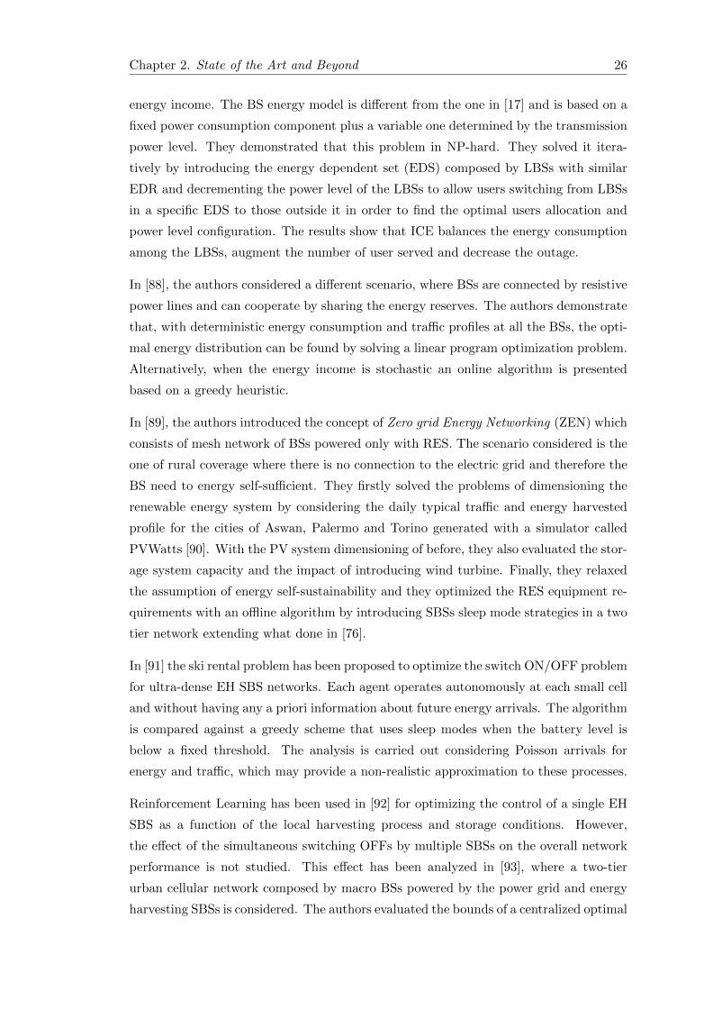
Chapter 2. State of the Art and Beyond 26
energy income. The BS energy model is different from the one in [17] and is based on a
fixed power consumption component plus a variable one determined by the transmission
power level. They demonstrated that this problem in NP-hard. They solved it itera-
tively by introducing the energy dependent set (EDS) composed by LBSs with similar
EDR and decrementing the power level of the LBSs to allow users switching from LBSs
in a specific EDS to those outside it in order to find the optimal users allocation and
power level configuration. The results show that ICE balances the energy consumption
among the LBSs, augment the number of user served and decrease the outage.
In [88], the authors considered a different scenario, where BSs are connected by resistive
power lines and can cooperate by sharing the energy reserves. The authors demonstrate
that, with deterministic energy consumption and traffic profiles at all the BSs, the opti-
mal energy distribution can be found by solving a linear program optimization problem.
Alternatively, when the energy income is stochastic an online algorithm is presented
based on a greedy heuristic.
In [89], the authors introduced the concept of Zero grid Energy Networking (ZEN) which
consists of mesh network of BSs powered only with RES. The scenario considered is the
one of rural coverage where there is no connection to the electric grid and therefore the
BS need to energy self-sufficient. They firstly solved the problems of dimensioning the
renewable energy system by considering the daily typical traffic and energy harvested
profile for the cities of Aswan, Palermo and Torino generated with a simulator called
PVWatts [90]. With the PV system dimensioning of before, they also evaluated the stor-
age system capacity and the impact of introducing wind turbine. Finally, they relaxed
the assumption of energy self-sustainability and they optimized the RES equipment re-
quirements with an offline algorithm by introducing SBSs sleep mode strategies in a two
tier network extending what done in [76].
In [91] the ski rental problem has been proposed to optimize the switch ON/OFF problem
for ultra-dense EH SBS networks. Each agent operates autonomously at each small cell
and without having any a priori information about future energy arrivals. The algorithm
is compared against a greedy scheme that uses sleep modes when the battery level is
below a fixed threshold. The analysis is carried out considering Poisson arrivals for
energy and traffic, which may provide a non-realistic approximation to these processes.
Reinforcement Learning has been used in [92] for optimizing the control of a single EH
SBS as a function of the local harvesting process and storage conditions. However,
the effect of the simultaneous switching OFFs by multiple SBSs on the overall network
performance is not studied. This effect has been analyzed in [93], where a two-tier
urban cellular network composed by macro BSs powered by the power grid and energy
harvesting SBSs is considered. The authors evaluated the bounds of a centralized optimal

Chapter 2. State of the Art and Beyond 27
direct load control of the SBS using an offline dynamic programming method that has all
the knowledge on the system variables a-priori. The optimization problem is represented
using Graph Theory and the problem is stated as a Shortest Path search. The results
show that an encouraging energy efficiency improvement can be theoretically achieved.
The authors in [94] provide useful insight on the impact of the parameters quantization
in networks of BS powered with solar energy. They discuss the choice of parameter
quantization for time, weather, and energy storage and provide guidelines for the de-
velopment of accurate and credible models that can support the power system design
to achieve a correct dimensioning. The main findings are that a credible and accurate
model requires: i) a time granularity equal to 1 hour that allows capturing the energy
production and consumption fluctuations during the day; ii) the discretization of the
weather conditions according to 5 or 7 levels of average daily solar irradiance; iii) a
storage energy quantum of the order of 1/5 of the minimum energy consumption per
time slot.
Finally, an interesting application of HetNet powered by RES is represented by the
so called public protection and disaster relief communications (PPDR), where the lack
of electrical grid is often impossible as a consequence of an emergency situation. As
we highlighted in [95], in such scenarios a flexible architecture like HetNet allows to
rapidly provide communication services to both emergency responders and civilians.
The proposed infrastructure is a network of energy self-sufficient LTE SBSs powered
by RES that features an all-wireless multi-hop backhaul network together with self-
organization capabilities which can replace the standard cellular network even when its
radio access part is totally compromised.
2.4 Beyond the State of the Art
The main goal of this thesis is to get closer to a real scenario with respect to the work
presented before on EH by investigating online solutions. In detail, considering [84] we
envisage that by taking into account the traffic profile, the system can work in a more
efficient way even when outside the availability region, allowing to reduce the capacity
of the RES system. Moreover, RL can optimize the system even without historical data
of the energy consumption and the users demand as in [86].
Similarly to [87], the target is to minimize the energy used by the part of the network
connected to the grid, the macro BS. However, we considered that SBSs can be put in
sleep mode in case of low traffic in order to save energy for the peaks, where it would
be more problematic to be managed by the network.

Chapter 2. State of the Art and Beyond 28
Therefore, the scenario in [89], well fit with our vision, except from the fact that we
concentrate on general HetNet scenarios, where SBSs are supporting the MBSs especially
for capacity extension rather than coverage extension. However, we coincide in the final
example scenario where they evaluate the sleep mode solutions apart from the fact that
the algorithm is based on the knowledge of traffic and harvested energy profiles.
To this end, learning solutions are adopted for avoiding the usage of deterministic o
statistical data in the design of the network in order to implement a self-organization
approach that enables to deploy SBSs in a flexible way independently from the most
important environmental variables (e.g., weather conditions, traffic profiles and BSs lo-
cation). Self-organization is defined as the ability of entities to spontaneously arrange
given parameters following some constraints and without any human intervention. To
do this, entities have to somehow represent the environment where they perform and the
gathered information has to be interpreted for them to correctly react. Consequently,
learning solutions represent a viable tool for self-organization since they allow to trans-
late the environmental sensed information into actions. Considering the specific problem
of this work, network of SBSs can be interpreted as multi-agent systems.
In the following chapter, the main ML principles used in this thesis are introduced.
2.5 Concluding Remarks
This chapter has provided some background information that is relevant to the con-
tributions of this thesis, which will be thoroughly presented in the following chapters.
Initially, the reference energy model for different type of BS has presented. The state-
of-the-art works concerning the energy efficiency algorithms have been discussed next.
In continuation, an overview of the schemes available in the literature when introducing
EH capabilities to HetNets highlighting the principles, the contributions, but also the
limitations of proposed solutions. Thus, after presenting open issues and challenges, the
main novel contributions of this thesis has been detailed with respect to the literature.
The remaining of this thesis is organized in four parts. The first part provides the
necessary principles of ML methods, presenting the Q-learning and the prediction solu-
tions that constitutes the main building blocks of the framework presented in this Ph.D.
dissertation. The second part (Chapter 4) is focused on proposing an accurate energy
model based on stochastic Markov processes for the description of the energy scavenged
by outdoor solar sources. The third part of the thesis (Chapter 5) is devoted to propose
a novel solution based on distributed Q-learning algorithm for improving the EE of the
system by switching ON/OFF SBSs powered with solar panels. Finally, in the fourth

Chapter 2. State of the Art and Beyond 29
part (Chapter 6), an enhanced switching OFF solution adopting Layered Learning is
given for solving the problem of conflicts among the agents.

Chapter 3
Machine Learning Background
3.1 Introduction
Machine Learning has recently attracted a remarkable attention from the research com-
munity for its flexibility in solving complex problems. ML-based tools are expected to be
the main enablers for providing the required flexibility to 5G system and implement the
SON functionalities. Machine Learning can contribute both for extracting models that
reflect the user and network behaviors and for more dynamic decision making problem
working in real-time. The former is commonly used in data analysis problem for evaluat-
ing the behavior of specific parameters of the system to drive the decisions made by 5G
SON functionalities. Typically, this is performed through learning-based classification,
prediction and clustering models. The latter are more adequate when independent and
dynamic problems are considered, as in the case of SBS with EH capabilities systems.
To this end, RL is the concept adopted in ML for implementing reactive agents, since
it works by learning from interactions with the environment, and observing the conse-
quences when a given action is executed. Therefore, multi-agent systems represent a
logical method to treat these types of problem, considering the intrinsic nature of the
scenario, which is composed of various SBSs that have to be controlled simultaneously.
For these reasons, we considered to adopt both solutions based on RL and prediction.
RL is used to provide the incremental learning behavior to the solution for obtaining
online algorithms that are able to adapt to the environment. These solutions typically
keep memory of the interactions by means of some representation mechanism, e.g., look-
up tables. Therefore, the complexity of RL methods is exponential in the number of
agents, because each agent has to store its own variables. To this end, we used prediction-
based tools for guiding the RL techniques in finding a solution. In detail we adopted
the Multi-layer FeedForward Neural Networks (MFNN) for being able to estimate the
30

Chapter 3. ML Background 31
effect of the RL decision making process of each agent on the overall system before it
takes place. This estimation is then used as a feedback for the RL solution thanks to
the heuristically accelerated RL paradigm. Finally, the overall architecture has been
organized in a hierarchical fashion for clearly divide the problem in subtasks.
In wireless communications, RL solutions has been already used in literature [60, 96]
both for reconfiguring the network elements to improve the energy efficiency according
to the actual traffic and to study which sleep policies, respectively. In [97, 98] it has
been used for the problem of interference coordination.
In this chapter, we present the main principle of the ML tools used in this thesis. In
Section 3.2 we introduce the ML philosophy. In Section 3.3, we present the main principle
of the neural networks. Finally, in Section 3.4 we conclude the chapter.
3.2 Machine Learning
Machine Learning methods can be classified in three main categories as function on
the type of feedback used for learning: unsupervised learning, supervised learning and
reinforcement learning.
In supervised learning the task of the learner is to predict the value of the outcome for any
valid input after having seen a number of training examples. The training examples are
pairs of input objects and desired outputs, usually represented in form of vectors. When
the outputs are continuous, the learning problem is called regression. Alternatively, the
problem is referred as classification when the outputs are discrete values. After the end
of the training phase, the learning solution predicts the value for any new valid input
object [99]. This method is called “supervised” learning since the learning process is
driven by the desired output variable.
In unsupervised learning the objective is to learn underlying statistical structure or
distribution of unlabeled input patterns with unknown probability distribution. The
trained system is able to reconstruct pattern from noisy input data though the learned
statistical structure. This type of learning is referred as “unsupervised” because of the
absence of explicit desired output, as in supervised learning, or any reward from the
environment, as in RL, in the evaluation of the solution [100].
Reinforcement learning is the family of learning solutions that has the ability of learn-
ing behaviors online and automatically adapting to the temporal dynamics of the sys-
tem [101]. At each time step, the agent senses the state of the environment and take
an action to transit in a new state. The environment returns a scalar reward (or cost),

Chapter 3. ML Background 32
which evaluates the impact of the selected action. Consequently, RL is applied for
creating autonomous system that improve themselves iteratively with the accumulated
experience at each cycle.
According to the specific problem to solve, the above methods can be more or less suit-
able. For instance, supervised and unsupervised learning methods are not appropriate
for interactive problems where the agents have to learn from their past experience and
be able to adapt to unpredictable environment characteristics, which is the scenario of
the problem we want to solve. However, they can help in understanding the behavior of
specific part of the environment, e.g., they can predict the value or classify some specific
sensible parameters. In literature RL solutions are typically formulated in a centralized
fashion, where a central entity takes decisions, e.g., a BS in an LTE system. However,
when considering network of SBSs, the process has to be distributed in order to better fit
the deployment model and be able to deal with the scalability of the system. Therefore,
we focus on decentralized learning processes based on RL.
The first studies in the field of distributed learning come from the game theory when
Brown proposed the fictitious play algorithm in 1951 [102]. The literature of single agent
learning in ML is extremely rich, while only recently the attention has been focused on
distributed learning aspects, in the context of multi-agent learning. Rapidly, it became
an interesting interdisciplinary area and the most significant interaction point between
computer science and game theory communities. The theoretical framework can be
found in Markov decision process (MDP) for the single agent system, and in stochastic
games, for a multi-agent system. In what follows, we give a brief introduction of learning
in single and multi-agent systems. In Section 3.2.1, we analyze RL for the case of the
single-agent, while in Section 3.2.2 the one of the multi-agent. Section 3.2.3 provides the
definition of TD algorithms, while Section 3.2.4 details on the Q-learning. Section 3.2.5
provides some open issues and challenges in the MRL.
3.2.1 Learning in single agent systems
A MDP provides a mathematical framework for modeling decision-making processes in
situations where outcomes are partly random and partly under the control of the decision
maker. MDP are valuable tool for describing a wide range of optimization problems.
A MDP is a discrete time stochastic optimal control problem. Here, operators take
the form of actions, i.e., inputs to a dynamic system, which probabilistically determine
successor states. A MDP is defined in terms of a discrete-time stochastic dynamic system
with finite state set S = {s1, . . . , sn} that evolves in time according to a sequence of
time steps, t = 0, 1, . . . ,∞. At each time step, a controller selects an action ak from a

Chapter 3. ML Background 33
Environment
Rewardrt
Agent
Actionat
Statest
Figure 3.1: Learner-environment interaction.
finite set of admissible actions A = {a1, . . . , al} based on the perceived system current
state si. The action is then executed by being applied as input to the system, which
consequently evolves from state si to sj , with a state transition probability Pi,j . As a
result of the execution of the action ak in state si, the environment return an immediate
reward r(si, ak). In what following, we refer to states, actions, and immediate reward
by the time steps at which they occur, by using st, at and rt, where at ∈ A, st ∈ S and
rt = r(st, at) are, respectively, the state, action and reward at time step t. A graphic
representation is shown in Fig. 3.1. Summarizing, a MDP consists of:
• a set of states S.
• a set of actions A.
• a reward function R : S ×A → <.
• a state transition function P : S × A → Π(S), where a member of Π(S) is a
probability distribution over the set S (i.e., it maps states to probabilities).
The state transition function probabilistically defines the next state of the environment
as a function of its current state and the agent’s action. The reward function specifies
expected instantaneous reward as a function of current state and action. In order to be a
Markov model, the state transitions have to be independent of any previous environment
states or agent actions. The goal of a MDP problem is to find the policy that maximizes
the reward of each state st. Therefore, the objective is to find an optimal policy for the

Chapter 3. ML Background 34
infinite-horizon discounted model, relying on the result that, in this case, there exists
an optimal deterministic stationary policy [101].
To solve RL problems there are three fundamental classes of methods, i.e., dynamic
programming, Monte Carlo and temporal difference (TD) learning. The first one rely
of the knowledge of the state transition probability function from state s to state v,
Ps,v(a). On the other hand, the second and the third solve the RL problems without
any knowledge of the transition probability function. When a sample transition model
of states, actions and rewards can be built, Monte Carlo method can be applied. Alter-
natively, if the only way to collect information about the environment is to interact with
it, TD methods have to be applied. In doing this, TD methods combine elements of DP
and Monte Carlos: they learn directly from experience, as in Monte Carlo methods, and
they gradually update prior estimates values, as in DP.
The core of RL algorithms is represented by the computation of the value functions. The
state-value function V (s) measures how good, based on the future expected reward, is
for an agent to be in a given state, while the state-action value function Q(s, a) measures
how good is to execute an action based on the future expected reward. The expected
rewards for the agent in the future are given by the action it will take, thus the value
functions depend on the policies being followed. The state-value of state s is defined as
the expected infinite discounted sum of the rewards that the agent gains starting from
state s and executing the complete decision policy π
V π(s) = Eπ
{ ∞∑t=0
γtrt|st = s
}(3.1)
where 0 ≤ γ < 1 is a discount factor which determines how much expected future
rewards affect decisions made now. Analogously, the Q-value Q(s, a) is the expected
decreased reward for executing action a at state s and then following policy π, in detail:
Qπ(s, a) = Eπ
{ ∞∑t=0
γtrt|st = s, at = a
}(3.2)
Therefore, in order to solve a RL problem the best return in the long term has to be
found. This is referred as finding an optimal policy, which will be the one that is giving
the maximum expected return. We define the optimal value of state s as:
V ∗(s) = maxπ
V π(s) (3.3)

Chapter 3. ML Background 35
This optimal value function is unique according to the principle of Bellman’s optimal-
ity [101], and can be defined as the solution to the equation:
V ∗(s) = maxa
(R(s, a) + γ
∑v∈S
Ps,v(a)V ∗(v)
)(3.4)
which means that the value of state s is the expected reward R(s, a) = E{r(s, a)}, plus
the expected discounted value of the next state, v, when taking the best available action.
Given the optimal value function, we can specify the optimal policy as:
π∗(s) = arg maxa
(R(s, a) + γ
∑v∈S
Ps,v(a)V ∗(v)
)(3.5)
Now we define an intermediate maximum of Q(s, a), denoted Q∗(s, a), applying the Bell-
man’s criterion in the action-value function, where the intermediate evaluation function
for every possible next state-action pair (v, a′) is maximized, and the optimal actions is
performed with respect to each next state v. Therefore, Q∗(s, a) is:
Q∗(s, a) = R(s, a) + γ∑v∈S
Ps,v(a) maxa′∈A
Q∗(v, a′) (3.6)
Finally, we can determine the optimal action a∗ with respect to the current state s,
which represents π∗. Thus, Q∗(s, a∗) is maximum, and can be expressed as:
Q∗(s, a∗) = maxa′∈A
Q∗(s, a′) (3.7)
3.2.2 Learning in multi-agent systems
The characteristics of the distributed learning systems are as follows: i) the intelligent
decisions are made by multiple intelligent and uncoordinated nodes; ii) the nodes par-
tially observes the overall scenario; and iii) their inputs to the intelligent decision process
are different from node to node since they come from spatially distributed sources of
information. Multi-agent system perfectly matches these characteristics, considering
each node as an independent intelligent agent. The theoretical framework is based on
stochastic games [103] and described by the five-tuple {N ;S;A;P ;R}. In detail
• |N | = N is the set of agents, ranging from 1, . . . N ;

Chapter 3. ML Background 36
• S = {s1, s2, . . . , sn} is the set of possible states, or equivalently, a set of N-agent
stage games;
• A is the joint action space defined by the product set A1 ×A2 × . . .×AN , where
Ai = {ai1, ai2, . . . , ail} is the set of actions available to the ith agent;
• P is a probabilistic transition function defining the probability of going from one
state to another provided the execution of a certain joint action;
• R = {r1× r2× . . .× rN}, where ri is the reward of the ith agent in a certain stage
of the game, which is a function of the joint actions of all N nodes.
In fully cooperative stochastic games, the reward functions coincide for all the agents:
r1 = · · · = rN . In this case the agents have the same goal: to maximize the common
return. If N = 2 and r1 = −r2, the two agents have opposite rewards and the game
is called fully competitive. Finally, mixed games are the ones that cannot be defined
neither as fully cooperative or competitive.
The typical problems in multi-agent systems are usually modeled as non-cooperative
games, since the distributed decisions made by the multiple nodes strongly affect the
one made by the others. Stochastic games form a natural model for such interactions.
A stochastic game is played over a state space, and is played in rounds. In each round,
each player chooses an available action simultaneously with and independently from
all other players, and the game moves to a new state under a possible probabilistic
transition relation based on the current state and the joint actions. We can distinguish
in this context two different forms of learning: i) the agent can learn the strategies of
the opponents in order to formulate the best response accordingly, and ii) the agent
can learn his own strategy that perform well against the opponents, independently from
learning the strategies of the opponents. The former is defined as model-based learning,
and it requires some partial information of the strategies of the other players. The
second approach is referred to as model-free learning, and it does not necessarily require
to learn a model of the strategies played by the other players. To facilitate distributed
and autonomous functioning of wireless networks, model-based learning approaches are
considered not to be appropriate since they require each node/agent to acquire knowledge
on the actions played by the other agents which might yield to high overheads. In fact,
this approach, generally adopted in game theory literature, is based on building some
model of other agents’ strategies, following which, the node can compute and play the
best response strategy. This model is then updated based on the observations of their
actions. On the other hand, model-free approaches, also known as TD learning, are
adequate since they avoid building explicit models of other agents’ strategies and learn
over time how properly the various available actions perform in the different states.

Chapter 3. ML Background 37
3.2.3 TD Learning
TD learning is a prediction method based on the future values of a given signal. The
name TD comes from the use of the differences in predictions over successive time steps
to drive the learning process [28]. Agents implementing TD methods are implemented in
an online fashion, thus learning from every transition without considering the subsequent
actions. Consequently, after the training phase, the agents can improve their behavior,
improvements that continue over time. The algorithms in this category typically keep
memory of the appropriateness of playing each action in a given state by means of some
representation mechanism, e.g., look-up tables, neural networks, etc. This approach
follows the general framework of RL and has its roots in the Bellman equations [101].
One of the main dilemma of RL algorithms is the trade-off between exploration and
exploitation. Exploration is the phase in which the agent learns across all available
actions in order to determine the best one to be used at the end of the learning process.
Alternatively, in the exploitation phase the agent uses the knowledge already acquired
to obtain the maximum reward.
A policy π maps state to actions, i.e., it defines the actions the agent has to follow
to maximize the reward. TD methods ca be classified in two groups with respect to
the policies, 1) the behavior policy, which learns the comportment of the agent in term
of the actual action to be selected by the agent, and 2) the estimation policy, which
determines the policy evaluated, or the action in the next state used for the evaluation
of behavior policy. In RL there are two methods to implement the exploration, the
on-policy and off-policy. They differ in the form the select the estimation policy. The
on-policy methods evaluate or improve the policy used to perform the decision, i.e., they
estimate the value of a policy while using it for control. This implies that, the policy
adopted by an agent is a given state, the behavior policy, is the same used to select the
action (estimation policy) based on which it evaluates the behavior followed. On the
contrary, off-policy methods distinguish between behavior and estimation policies. In
fact, the policy to generate the behavior is unrelated to the policy evaluated. In this
case, the policy evaluated is the one corresponding to the best action in the next state,
π∗, given the current agent experience.
The goal of the agents in TD learning is to select actions that maximize the discounted
reward they receive over the future. This is the role of the discount rate γ in the
state value function, Eq. 3.1 and in the state-action value function, Eq. 3.2. While, α
represents the weight of the new information in the state and state-action value update.
The action selection policy plays also a crucial role in RL, by defining the criterion the
agent have to follow in the selection of the action. The criterion can be either to perform

Chapter 3. ML Background 38
exploration or to exploit the acquired knowledge. As introduced before, exploration has
to be included in the action selection policies in order to achieve good behaviors based
on explicit trial-and-error processes.
Among the TD methods, we adopted the off-policy Q-learning algorithm, since it has
more efficient learning properties, as detailed in what following. Q-learning is proven to
converge to an optimal policy in a single agent system, as long as the learning period
is enough long, and can be extended to the multi-agent stochastic game by having each
agent ignore the other agents and pretend that the environment is stationary. Even
if this approach has been shown to correctly behave in many applications, it is not
characterized by a strict proof of convergence, since it ignores the multi-agent nature of
the environment and the Q-values are updated without regard for the actions selected
by the other agents. Therefore, the convergence of multi-agent Q-learning is an open
issue, as detailed in Section 3.2.5, and have to be evaluated on a case-by-case basis.
3.2.4 Q-learning algorithm
Q-learning algorithm has been proposed in 1989 by Watkins in his Ph.D. thesis [104] and
the proof of convergence of this algorithm was presented in 1992 by Watkins and Dayan
in [105]. The goal of Q-learning is to find Q∗(s, a) in a recursive manner using available
information (s, a, v, r), where s and v are the states at time t and t+ 1, respectively, a is
the action taken at time t and r is the reward of executing a in s. Q-learning estimates
π∗ while following π, as it is a off-policy algorithm. This means that the behavior of the
agent is determined by the action selection policy followed by it, which is the policy π,
while the Q-value updating process is performed based on the minimum Q-value in the
next state, independently of the policy being followed [28]. The Q-value is computed
according to the rule:
Q(s, a)← Q(s, a) + ∆Q(s, a) (3.8)
where ∆Q(s, a) is defined as:
∆Q(s, a) = α[r + γmaxa
Q(v, a)−Q(s, a)] (3.9)
where α is the learning rate, which weights the importance given to the information
observed after executing action a, and γ is the discount factor which determines the
importance of future rewards. When γ is equal to 0 will make the agent short-sighted

Chapter 3. ML Background 39
by only considering current rewards, while using values approaching to 1 will make it
strive for a long-term high reward. Algorithm 1 presents the Q-learning procedure.
The main advantage of Q-learning is that it does not include the cost of exploration in
the Q-value update. This characteristic makes Q-learning consistent with the principle
of knowledge exploitation. This implies that the policy found by the algorithm is applied
without including the exploration after the end of the learning process. Thus, the off-
policy learning solutions allow the agents to exploit the acquired knowledge in a very
effective way since the beginning of the learning process.
Algorithm 1 Q-learning
1: for each s ∈ S, a ∈ A do2: Initialize Q(s, a) arbitrarily3: end for4: for each step do5: Choose a from s following the action selection policy6: Execute a7: Collect r8: Observe v9: Q(s, a)← Q(s, a) + α[r + γmaxaQ(v, a)−Q(s, a)]
10: s← v11: end for
3.2.5 Challenges in MRL: Agents Coordination
The definition of a good MRL goal is a difficult challenge, since the agents’ environment
are correlated and cannot be maximized independently. Non-stationarity arises in MRL
because all the agents in the system are learning simultaneously. Each agent is therefore
faced with a moving-target learning problem: the best policy changes as the other
agents’ policies changes [106]. In fact, the exploration phase is further complicated in
MRL since agents explore to obtain information not only about their local environment,
but also about the other agents in order to adapt to their behavior. Therefore, any
agent’s action on the environment depends also on the action taken by the other agents,
which introduces the need of coordination. In fully cooperative stochastic games, the
common return can be jointly maximized. In other cases, as the one investigated in
this work, the agents’ returns are typically different and correlated, and they cannot be
maximized independently. Therefore, specifying a good general MRL goal is a difficult
problem. The goal has to incorporate the stability of the learning dynamics of the agent
on the one hand, and the adaptation to the changing behavior of the other agents on the
other hand. Stability means the convergence to a stationary policy, whereas adaptation
ensures that performance is maintained or improved as the other agents are changing
their policies.
Chapter 3. ML Background 40
Convergence to equilibria is a basic stability requirement [107], since agent’s strategies
should eventually converge to a coordinated equilibrium, like the Nash equilibria. How-
ever, it is unclear the connection between the Nash equilibria and the performance in the
dynamic stochastic game [108]. In [109] rationality is added as an adaptation criterion
upon the required convergence. Rationality is defined as the requirement that the agents
converges to a best-response when the other agents remain stationary. An alternative
to rationality is presented in [110] with the concept of no-regret, which is defined as the
requirement that the agent achieves a return that is at least as good as the return of a
any stationary strategy.
Another family of solutions is represented by the ones that define an empirical coordi-
nation among the agents. In [30], the authors suggest to increase the convergence rate
or RL algorithms by using a heuristic function for selecting actions in order to guide the
exploration of the stat-action space in a more efficient way. Heuristically accelerated
MRL approach, that has been originally proposed to improve the training phase of a
single-agent RL problem, has been be extended to the multi-agent scenario in [111].
The idea is to use case-based reasoning for heuristic acceleration to exploit similarities
between states of the environment already experienced in the past to make a guess
on which action has to be taken. HAMRL has been already successfully applied in the
wireless communication domain in the field of inter-cell interference coordination (ICIC)
problem in [112]. In this work HAMRL has been applied to distributed Q-learning for
implementing a decentralized ICIC controller aimed at reducing the interference in the
LTE downlink channel of a network of macro BSs.
The introduction of an external heuristic suggests the construction of a hierarchical
solution, which is able to coordinate the agents by having a centralized view of the
effect of the agent’s action on the overall environment. This type of ML paradigm is
called Layered Learning [113]. It has been originally designed for solving the robotic
soccer problem, and is intended in general for domains that are too complex for learning
a mapping directly from an agent’s sensory inputs to its actuator outputs. In fact,
robotic soccer has to deal with limited communication, real-time, noisy environments
with both team-mates and adversaries, which is too complex for agents to learn direct
mappings from their sensors to actuators. The appropriate behavior granularity for
the decomposition and the aspects of the behaviors to be learned are determined by
the specific domain. Therefore, the definition of the subtask in layered learning is not
automated. In fact, it is the domain that defines the layers. ML is used as a central part
of layered learning to exploit data in order to train and adapt the overall system. Like
the task decomposition itself, the choice of machine learning method depends on the
subtask. The main characteristic of layered learning is that each learned layer directly
affects the learning at the next layer. A learned subtask can affect the sub-sequent layer
Chapter 3. ML Background 41
either (i) by providing a portion of the behavior used during training or (ii) by creating
the input representation of the learning algorithm.
HAMRL and LL will be presented more in detail in Chapter 5, where have been used to
mitigate the coordination problem of distributed Q-learning when solving the problem
of SBSs powered with renewable energies.
3.3 Neural Networks
An artificial neural network (ANN), often called simply neural network (NN), is a model
of computation inspired by the neurons of the human brain. In simplified models, the
human brain consists of a large number of basic computing devices, the neurons, that
are connected to each other through synapses in a complex communication network.
The resulting network is the actual engine of the brain that allows to perform complex
computations. Artificial neural networks adopt the same principles of the brain for
solving problems through computational tools.
A neural network is implemented as a directed graph whose nodes correspond to neurons
and edges correspond to links between them [114]. Each neuron receives as input a
weighted sum of the outputs of the neurons connected to its incoming edges. In what
following we focus on feed-forward NN, which means that the correspondent graphs does
not contain cycles.
The neuron has two operative modes: training and using. The former mode corresponds
to the phase where data are supplied to a neuron along with the instruction to activate
or not, depending on the received input. In the latter, new data is presented and the
neuron is activated or not activated based on the similarity of the input pattern to those
for which the neuron was trained. In case the type of data presented during the training
is labeled, the training method belong to the supervised learning. Alternatively, for
unlabeled data the training method falls in the unsupervised learning category.
3.3.1 Feed-forward Neural Networks
The basic element of an ANN is represented by the neuron (also called perceptron),
which consists of a linear combination of fixed non-linear functions θj(x). In detail, for
a vector of input xi, i = 1 . . . , N , it takes the form:
y(x,w) = σ
N∑j=1
wjθj(x)
(3.10)
Chapter 3. ML Background 42
where wi are the weights associated to each input and σ(·) is a non-linear activation
function, typically the sigmoid function f(x) = 1/((1 + e−x)).
A feedforward neural network is described as a directed acyclic graph G of vertexes V
and edges D, G = (V,D), and a weight function over the edges, w : D → R. Each single
neuron is modeled as a simple scalar function, f : R → R. The basic neural network
model is composed by a series of neurons organized in L layers in a way that the input
information moves only in one direction (i.e., there are no cycle in the networks like in a
recurrent neural network). Let define I as the number of neurons in layer l. The bottom
layer, L0, is the input layer and it contains N + 1 neurons, which are the inputs plus
the “constant” neuron always at 1. The last layer is composed by only one neuron and
represents the output of the neural network. Each neuron in a layer l = 2, . . . , L has
Il = Il−1 inputs, each of which is connected to the output of a neuron in the previous
layer. Layers 2, . . . , L− 1 are called hidden layers. We denote by vt,i, the ith neuron of
the tth layer and by ot,i(x) the output of vt,i when the network is fed with the input
vector x. For every i ∈ [n], the output of neuron i in L0 is simply xi, where n is
dimensionality of the input space. The last neuron in L0 is the constant neuron, which
always outputs 1. Therefore, for i ∈ [n] we have o0,i(x) = xi and for i = n+ 1 we have
o0,i(x) = 1. The other outputs can be calculated iteratively, in a layer by layer manner.
Considering we have already calculated the output of a specific layer t, we can calculate
the output of layer t + 1 as follows. Fix some vt+1,j ∈ Lt+1. Let at+1,j(x) denote the
input to vt+1,j when the network is fed with the input vector x, then:
at+1,j(x) =∑
r:(vt,r,vt+1,j)∈E
w ((vt,r, vt+1,j)) ot,r(x) (3.11)
and
ot+1,j(x) = σ (at+1,j(x)) (3.12)
That is, the input of vt+1,j is a weighted sum of the outputs of the neurons in Lt that
are connected to vt+1,j , where weighting is according to w, and the output of vt+1,j is
simply the application of the activation function σ on its inputs. An example diagram
of a network with one hidden layer is provided in Fig. 3.2.
3.3.2 Neural Network Training
A MFNN can approximate arbitrary continuous functions defined over compact subsets
of RN by using a sufficient number of neurons at the hidden layers. In order to achieve

Chapter 3. ML Background 43
1x0
1
. .
. .
.
hidden nodes
. . .
. .
. . .
. .
x1
xNwDN wKD
w10
y1
yK(1)
(2)
(2)
inputs outputs
a0
a1
aD
o0
oD
Figure 3.2: Network diagram for a MFNN with one hidden layer.
this, it is necessary to determine the values of the weights correspondent to the function
to be approximated, the so called network training. Given a training set of input vectors
xn, where n = 1, . . . , N , together with a corresponding set of target vectors tn, the
training objective is to minimize the function
E(w) =1
2
N∑n=1
‖ y(xn,w)− tm ‖2 (3.13)
which implies to find the weight vector w so that
∇E(w) = 0. (3.14)
However, the error function typically has a high nonlinear dependence on the weights and
bias parameters, and so there will be many points in weight space at which the gradient
is very small. Because it is very difficult to find an analytical solution to Eq. (3.14), it
is common practice to rely on iterative numerical procedures. Most common techniques
involve choosing some initial value w(0) for the weight vector and then moving through
weight space in a succession of steps of the form
Chapter 3. ML Background 44
w(τ+1) = w(τ) + ∆w(τ) (3.15)
The simplest approach to comprise a small step in the correct direction is to choose the
weight update in Eq. (3.15) in the direction of the negative gradient, so that
w(τ+1) = w(τ) − η∇E(w(τ)
)(3.16)
where the parameter η > 0 is known as the learning rate. The error is defined with
respect to a training set, so the entire training set has to be processed at each step in
order to evaluate ∇E. Techniques that use the whole data set are called batch methods.
When the weight vector is moved toward the direction of the greatest rate of decrease of
the error function, the optimization is called gradient descent. This approach has been
demonstrated to be a poor algorithm in [99], despite of being intuitively reasonable. In
order to find a good minimum, it may be necessary to run a gradient-based algorithm
multiple times using different randomly chosen starting point, and comparing the result-
ing performance on an independent validation set. However, there is an online version
that has proved useful in practice for training neural networks [115]. In this case, the
error function is considered as a sum of terms defined per each data point:
E(w) =
N∑n=1
En(w) (3.17)
This variation, also known as sequential gradient descent, is based on updating the weight
vector one data point at a time, in detail
w(τ+1) = w(τ) − η∇En(w(τ)
)(3.18)
This method allows to easily escape from local minima, since a stationary point with
respect to the error function for the whole dataset is difficult to be a stationary point
also for each data point individually.
Therefore, the problem to solve now is to find an efficient technique for evaluating
the gradient of an error function E(w) for a feed-forward neural network. The most
widespread solution is called error backpropagation or simply backpropagation and is
based on a local message passing scheme in which the information is sent forwards
and backwards through the network [99]. For explaining the backpropagation, we start
considering the evaluation of the derivative of En with respect to a weight wij , where

Chapter 3. ML Background 45
the outputs of the units depend on the specific input pattern n. In order to keep the
notation uncluttered, we will omit the subscript n from the network variables. Applying
the chain rule for partial derivative we have
∂En∂wij
=∂En∂aj
∂aj∂wij
(3.19)
exploiting the fact that En depends on the weights wij via summed input aj to unit j.
Thanks to Eq. (3.19), we can introduce the errors, defined as
δj ≡∂En∂aj
(3.20)
Considering Eq. (3.11), we can rewrite Eq. (3.19) as
∂En∂wij
= δjoi (3.21)
since oi =∂aj∂wij
. Therefore, the derivative can be obtained by simply multiplying the
value of δ for the unit at the output end of the weight by the value of o for the unit at
the input end of the weight. Thus, the derivative can be calculated only evaluating the
values of δj for each hidden and output unit in the network, and then apply Eq. (3.21).
Using the chain rule for partial derivatives, we can rewrite Eq. (3.20) as
δj ≡∂En∂aj
=∑k
∂En∂ak
∂ak∂aj
(3.22)
where the sum is over all nodes k to which node j sends connections. Substituting
Eq. (3.11) and Eq. (3.12) in Eq. (3.22), we can obtain the backpropagation formula
δj = σ′(aj)∑k
wkjδk (3.23)
From Eq. (3.23), we can see how the value of δ for a particular hidden node can be
obtained by propagating the δs backward from nodes in the higher layers of the network.
Thanks to the values of δs from the output unit that we already know, we can evaluate
the δs for all the hidden nodes by recursively applying Eq. (3.23).

Chapter 3. ML Background 46
3.4 Concluding Remarks
This chapter has provided some background information of ML methods that constitute
the main building block of the solutions presented in this Ph.D. dissertation. In detail,
the TD learning methods has been presented for the multi-agent problem, focusing on
the Q-learning algorithm. Moreover, the NNs have been introduced as they will be used
in the layered learning framework.

Chapter 4
Photovoltaic Sources
Characterization
4.1 Introduction
The standard approaches for the integration of a solar panel into existing electrical
apparatuses are often not sufficient as keeping these devices fully operational at all times
would demand for unrealistically large solar modules, even for SBSs [79]. To overcome
this, the energy coming from the renewable sources should be wisely used, predicting
future energy arrival and the energy consumption that is needed by the system to remain
operational when needed. This calls for complex optimization approaches that will adapt
the behavior of modern systems to the current application needs as well as to their energy
reserves and the (estimated) future energy inflow [116].
A large body of work has been published so far to mathematically analyze these facts,
especially in the field of wireless sensor networks. However, often researchers have tested
their ideas considering deterministic [117, 118], independent and identically distributed
across time slots [119] or time-correlated Markov models [120]. While these contributions
are valuable for the establishment of the theory of energetically self-sufficient networks;
seldom, the actual energy production process in these papers has been linked to that
of real solar sources, to estimate the effectiveness of the proposed strategies in realistic
scenarios.
The work in this chapter aims at filling this gap, by providing a methodology and a tool
to obtain simple and yet accurate stochastic Markov processes for the description of the
energy scavenged by outdoor solar sources. In this study, we focus on solar modules as
those that are installed in wireless sensor networks or LTE SBSs, by devising suitable
47

Chapter 4. Photovoltaic Sources Characterization 48
Figure 4.1: Diagram of a solar powered BS.
Markov processes with first- and second-order statistics that closely match that of real
data traces. Our Markov models allow the statistical characterization of solar sources
in simulation and theoretical developments, leading to a higher degree of realism.
This chapter is organized as follows. In Section 4.2 we detail the system model and,
in particular, how the raw radiance data are processed to estimate the corresponding
instantaneous harvested power. This requires the combination of several building blocks,
including an astronomical model (Section 4.2.1) to estimate the actual irradiance that
hits the solar module, given the inclination of the sun during the day and the module
placement, an electrical model of photovoltaic cells (Section 4.2.2) and a model for the
DC/DC power processor (Section 4.2.3), which is utilized to maximize the amount of
power that is collected. Hence, in Section 4.2.4 we describe the Markov model that we
use to statistically describe the energy inflow, according to two clustering approaches
for the raw data. The results from this Markov model are shown in Section 4.3, whereas
our conclusions are presented in Section 4.4.
4.2 System Model
The system model adopted in this work is depicted in the diagram of Fig. 4.1 where
we identify the key building blocks for our study: the solar source (indicated as Isun),
the PV panel, the DC/DC power processor and the energy buffer (i.e., a rechargeable
battery). In following subsections we start with the characterization of the effective
solar irradiance, Ieff , that in general depends on the geographical coordinates of the
installation site, the season of the year and the hour of the day. Hence, Ieff is translated
by the PV module into some electrical power and a DC/DC power processor is used to
ensure that the maximum power is extracted from it.

Chapter 4. Photovoltaic Sources Characterization 49
4.2.1 Astronomical Model
The effective solar radiance that hits a photovoltaic module, Ieff , depends on physical
factors such as its location, the inclination of the solar module, the time of the year and
the hour of the day. Solar radiation databases are available for nearly all locations around
the Earth and their data can be used to obtain the statistics of interest. An astronomical
model is typically utilized to translate the instantaneous solar radiance Isun (expressed
in W/m2) into the effective sunlight that shines on the solar module. According to [121],
the effective solar radiance that hits the solar module, Ieff , is Ieff ∝ Isun cos Θ, where
Θ ∈ [−90◦, 90◦] is the angle between the sunlight and the normal to the solar module
surface1. Astronomical models can be found in, e.g., [121] and Chapter 8 of [122].
In short, Ieff depends on many factors such as the elliptic orbit of the Earth around the
sun (which causes a variation of the distance between Earth and sun across different
seasons), the fact that the Earth is itself tilted on its axis at an angle of 23.45◦. This
gives rise to a declination angle ν, which is the angular distance North or South of the
Earth’s equator, which is obtained as:
ν(N) ' sin−1 [sin(23.45◦) sin (D(N))] , (4.1)
where D(N) = 360(N − 81)/365◦ and N is the day number in a year with first of
January being day 1. Other key parameters are the latitude La ∈ [0, 90◦] (positive in
either hemisphere), the longitude Lo, the hour angle ζ(t,N) ∈ [0, 360◦], that corresponds
to the azimuth’s angle of the sun’s rays due to the Earth’s rotation, the inclination ξ
of the solar panel toward the sun on the horizon and the azimuthal displacement ψ,
which is different from zero if the normal to the plane of the solar module is not aligned
with the plane of the corresponding meridian, that is, the solar panel faces West or
East.2 ζ(t,N) is given by ζ(t,N) = 15(AST (t,N) − 12)◦, where AST (t,N) ∈ [0, 24]
hours, is the apparent solar time, which is the time based on the rotation of the Earth
with respect to the sun and is obtained as a scaled version of the local standard time
t (we refer to t′ as t adjusted accounting for the daylight savings time) for the time
zone where the solar module is installed. AST (t,N) is computed as follows. Briefly,
we obtain the Greenwich meridian angle, GMA = UTCoff × 15◦, which corresponds to
the angle between the Greenwich meridian and the meridian of the selected time zone:
UTCoff is the time offset between Greenwich and the time zone and 15 is the rotation
angle of the Earth per hour. Thus, we compute ∆t = (Lo − GMA)/15◦, i.e., the time
displacement between the selected time zone and the time at the reference Greenwich
meridian. At this point, AST (t,N) is obtained as AST (t,N) = t′ + ∆t + ET (N)
1Θ = 0 (Θ = ±90◦) if the sunlight arrives perpendicular (parallel) to the module.2ψ > 0 if the panel faces West and ψ < 0 if it faces East.
Chapter 4. Photovoltaic Sources Characterization 50
(expressed in hours), where ET (N) is known as the equation of time, with ET (N) '[9.87 sin(2D(N))− 7.53 cos(D(N))− 1.5 sin(D(N))]/60.
Finally, the power incident on the PV module depends on the angle Θ, for which we
have:
cos Θ(t,N) = sin ν(N) sinLa cos ξ −
− sin ν(N) cosLa sin ξ cosψ +
+ cos ν(N) cosLa cos ξ cos ζ(t,N) +
+ cos ν(N) sinLa sin ξ cosψ cos ζ(t,N)
+ cos ν(N) sin ξ sinψ sin ζ(t,N) . (4.2)
Once an astronomical model is used to track Θ, the effective solar radiance as a function
of time t is given by: Ieff(t,N) = Isun(t,N) max(0, cos Θ(t,N)), where the max(·) ac-
counts for the cases where the solar radiation is above or below the horizon, as in these
cases the sunlight arrives from below the solar module and is therefore blocked by the
Earth. The sun radiance, Isun(t,N), for a given location, time t and day N , has been
obtained from the database at [81].
4.2.2 PV Module
A PV module is composed of a number nsc of solar cells that are electrically connected
according to a certain configuration, whereby a number np of them are connected in
parallel and ns in series, with nsc = npns. A given PV module is characterized by its I-V
curve, which emerges from the composition of the I-V curves of the constituting cells.
Specifically, the I-V curve of the single solar cell is given by the superposition of the
current generated by the solar cell diode in the dark with the so called light-generated
current i` [123], where the latter is the photogenerated current, due to the sunlight
hitting the cell. The I-V curve of a solar cell can be approximated as:
iout ' i` − io[exp
( qv
nκT
)− 1], (4.3)
where q ≈ 1.6·10−19 C is the elementary charge, v is the cell voltage, κ ≈ 1.380·10−23 J/K
is the Boltzmann’s constant, T is the temperature in degree Kelvin3, n ≥ 1 is the diode
ideality factor and io is the dark saturation current. io corresponds to the solar cell diode
leakage current in the absence of light and depends on the area of the cell as well as on
the photovoltaic technology. The open circuit voltage voc and the short circuit current
3T is given by the sum of the ambient temperature, which can be obtained from the dew point andrelative humidity, and of a further factor due to the solar power hitting the panel.

Chapter 4. Photovoltaic Sources Characterization 51
isc are two fundamental parameters for a solar cell. The former is the maximum voltage
for the cell and occurs when the net current through the device is zero. isc is instead
the maximum current and occurs when the voltage across the cell is zero (i.e., when
the solar cell is short circuited). If vMoc and iMsc are the open circuit voltage and short
circuit current for the solar module M, the single solar cell parameters are obtained as:
isc = iMsc/np and voc = vMoc/ns (considering a module composed of homogeneous cells).
The light-generated current for the single solar cell is a time varying quantity, i`(t,N),
which depends on the amount of sunlight that hits the solar cell at time t, where N is the
day number. Here, we have used the following relation: i`(t,N) = iscF (t,N), where the
radiation rate F (t,N) ∈ [0, 1] is obtained as F (t,N) = 0.001Ieff(t,N), i.e., normalizing
the effective irradiance hitting the solar cell with respect to the maximum radiation of
1 kW/m2 (referred to in the literature as “one sun” [124]). Hence, i`(t,N) is plugged
into 4.3 to obtain iout(t,N) for a single solar cell as a function of the time t for day N .
The total current that is extracted from the solar module is: iMout(t,N) = npiout(t,N).
4.2.3 Power Processor
Generally speaking, every voltage or current source has a maximum power point, at
which the average power delivered to its load is maximized. For example, a Thevenin
voltage source delivers its maximum power when operating on a resistive load whose
value matches that of its internal impedance. However, in general the load of a generic
device does not match the optimal one, which is required to extract the maximum power
from the connected solar source. To cope with this, in practice the optimal load is emu-
lated through a suitable power processor, whose function is that of “adjusting” the source
voltage (section A of Fig. 4.1) until the power extracted from it is maximized,4 which
is also known as maximum power point tracking (MPPT). Ideally, through MPPT, the
maximum output power is extracted from the solar panel under any given tempera-
ture and irradiance condition, adapting to changes in the light intensity. Commercially
available power processors use “hill climbing techniques”; as an example, in [125] the au-
thors propose advanced control schemes based on the downhill simplex algorithm, where
the voltage and the switching frequency are jointly adapted for fast convergence to the
maximum power point. See also [126] for further information on MPPT algorithms and
their comparative evaluation and [127] for a low-power design targeted to wireless sensor
nodes. In the present work, we have taken into account the DC/DC power processor by
computing the operating point (iMout, vM) (see Eq. 4.3) for which the extracted power in
section A, P = iMoutvM, is maximized. Note that, if iout and v are the output current
4This corresponds to adapting the input impedance of the power processor to Zopt = Z∗source, where∗ indicates the complex conjugate.

Chapter 4. Photovoltaic Sources Characterization 52
and the voltage of the single solar cell, we have iMout = npiout and vM = nsv. For this
procedure, we have considered the parameters presented before (solar irradiance, rota-
tion of the Earth, etc.) and also the fact that isc and voc change as a function of the
environmental temperature, which affects the shape of the I-V curve in Eq. 4.3 (see, e.g.,
the dependence of i` on isc). Hence, we have computed the extracted power in two steps:
step 1) we have obtained the (ideal) maximum power PMPP that would be extracted by
the panel at the MPP by an ideal tracking system:
PMPP = maxv{iMoutv
M} = npns maxv{ioutv} , (4.4)
where iout = iout(t,N) is given by Eq. 4.3. Step 2) the power available after the power
processor (section B in Fig. 4.1) is estimated as P ′max = ηPMPP, where η ∈ (0, 1) is the
power processor conversion efficiency, which is defined as the ratio η = P ′max/PMPP and
can be experimentally characterized for a given MPP tracking circuitry [127]. P ′max is
the power that is finally transferred to the energy buffer.
4.2.4 Semi-Markov Model for Stochastic Energy Harvesting
The dynamics of the energy harvested from the environment is captured by a continuous
time Markov chain with Ns ≥ 2 states. This model is general enough to accommodate
different clustering approaches for the empirical data, as we detail shortly.
Formally, we consider an energy source that, at any given time, can be in any of the
states xs ∈ S = {0, 1, . . . , Ns−1}. We refer to tk, with k ≥ 0, as the time instants where
the source transitions between states, and we define τk = tk+1 − tk as the time elapsed
between two subsequent transitions. In what follows, we say that the system between
tk and tk+1 is in cycle k.
Right after the k-th transition to state xs(k), occurring at time tk, the source remains in
this state for τk seconds, where τk is governed by the probability density function (pdf)
f(τ |xs), with τ ∈ [τmin(xs), τmax(xs)]. At the next transition instant, tk+1, the source
moves to state xs(k + 1) ∈ S according to the probabilities puv = Prob{xs(k + 1) =
v|xs(k) = u}, with u, v ∈ S. When the source is in state xs(k), an input current ik
is fed to the rechargeable battery, where ik is drawn from the pdf g(i|xs), with i ≥ 0.
That is, when a state is entered, the input current i and the permanence time τ are
respectively drawn from g(i|xs) and f(τ |xs). Then, the input current remains constant
until the next transition, that occurs after τ seconds. In this work, we assume that the
voltage at the energy buffer (section B of Fig. 4.1) is constant, as typically considered

Chapter 4. Photovoltaic Sources Characterization 53
when a rechargeable battery is used. Given that, there is a one-to-one mapping between
instantaneous harvested power and harvested current.
4.2.5 Estimation of Energy Harvesting Statistics
Based on the aforementioned models, we have mapped the hourly irradiance patterns
obtained from [81] into the corresponding operating point, in terms of power P ′max and
current i after the power processor (section B of Fig. 4.1). Thus, we have computed the
statistics f(τ |xs) and g(i|xs) from these data according to the two approaches that we
describe next. These differ in the adopted clustering algorithm, in the number of states
Ns and in the structure of the transition probabilities puv, u, v ∈ S.
Night-day clustering: we have collected all the data points in [81] from 1991 to 2010,
grouping them by month. Thus, for each day in a given month we have classified the
corresponding points into two states xs ∈ {0, 1}, i.e., a low- (xs = 1) and a high-energy
state (xs = 0). To do this, we have used a current threshold ith, which is a parame-
ter set by the user, corresponding to a small fraction of the maximum current in the
dataset. According to ith, we have classified all the points that fall below that threshold
as belonging to state 0 (i.e., night) and those points above the threshold as belonging
to state 1 (day). After doing this for all the days in the dataset, we have estimated the
probability density function of the duration τ , f(τ |xs), and that of the input current i
(after the power processor), g(i|xs), for each state and for all months of the year. For
the estimation of the pdfs we have used the kernel smoothing technique see, e.g., [128].
The transition probabilities of the resulting semi-Markov chain are p10 = p01 = 1 and
p00 = p11 = 0 as a night is always followed by a day and vice versa.
Slot-based clustering: as above, we have collected and classified the irradiance data
by month. Then, we subdivided the 24 hours in each day into a number Ns ≥ 2 of time
slots of constant duration, equal to Ti hours, i = 1, . . . , Ns. Each slot is a state xs of our
Markov model. Hence, for each state xs we computed the pdf g(i|xs) for each month of
the year, considering the empirical data that has been measured in slot xs for all days in
the dataset for the month under consideration. Again, the kernel smoothing technique
has been utilized to estimate the pdf. For the statistics f(τ |xs), being the slot duration
constant by construction, we have that: f(τ |xs) = δ(τ−Txs), for all states xs ∈ S, where
δ(·) is the Dirac’s delta. The transition probabilities of the resulting Markov chain are
puv = 1, when u ∈ S and v = (u+ 1) mod Ns, and puv = 0 otherwise. This reflects the
temporal arrangement of the states.

Chapter 4. Photovoltaic Sources Characterization 54
0 5 10 15 20 250
0.005
0.01
0.015
0.02
0.025
0.03
0.035
0.04
0.045
Time of the day [h]
Cu
rre
nt
[A]
Low energy income
High energy income
Figure 4.2: Result of the night-day clustering approach for the month of July consid-ering the radiance data from years 1999− 2010.
4.3 Numerical Results
For the results in this section, we have used as reference the commercially available micro-
solar panels from Solarbotics, selecting the Solarbotics’s SCC-3733 Monocrystalline solar
technology [129]. It is to be noted that, the conclusions drawn in this subsection for this
type of panel are general and valid also for panel of bigger size, such as the one used for
SBSs since the harvested current is only scaled. For this product, the single cell area is
about 1 square centimeter, the solar cells have an efficiency of 21.1%, isc = 5 mA and
voc = 1.8 V. Next, we show some results on the stochastic model for the solar energy
source obtained considering a solar module with np = 6 and ns = 6 cells in parallel and
in series, respectively. We have selected Los Angeles as the installation site, consider-
ing ξ = 45◦, ψ = 30◦ and processing the data from [81] as described in the previous
section with a cluster threshold equal to 1/50−th of the maximum current in the dataset.
4.3.1 Night-day clustering
A first example for the night-day clustering approach is provided in Fig. 4.2, which
shows the result of the clustering process for the month of July. Two macro states are
evident: a low energy state (night), during which the power inflow is close to zero, and
a high energy state (day). As this figure shows, the harvested current during the day
follows a bell-shaped curve. However, contrarily to what one would expect, even for the

Chapter 4. Photovoltaic Sources Characterization 55
0
10
20
30
40
50
60
70
80
90
100
0 0.005 0.01 0.015 0.02 0.025 0.03 0.035 0.04
pro
ba
bili
ty d
en
sity f
un
ctio
n
harvested current i [A]
KSemp
Figure 4.3: g(i|xs) (solid line, xs = 0) obtained through the Kernel Smoothing (KS)technique for the month of February, for the night-day clustering method (2-state semi-Markov model), using radiance data from years 1999− 2010. The empirical pdf (emp)
is also shown for comparison.
month of July the high-energy state shows a high degree of variability from day-to-day,
as is testified by the considerable dispersion of points across the y-axis. This reflects the
variation in the harvested current due to diverse weather conditions. In general we have
a twofold effect: 1) for different months the peak and width of the bell vary substantially,
e.g., from winter to summer and 2) for all months we observe some variability across
the y-axis among different days. These facts justify the use of stochastic modeling, as
we do in this work, to capture such variability in a statistical sense.
Another example, regarding the accuracy of the Kernel Smoothing (KS) technique to
fit the empirical pdfs, is provided in Fig. 4.3, where we show the fitting result for the
month of February.
In Figs. 4.4 and 4.5 we show some example statistics for the months of February, July
and December. In Fig. 4.4, we plot the pdf g(i|xs), which has been obtained through
KS for the high-energy state xs = 0. As expected, the pdf for the month of July has
a larger support and has a peak around i = 0.04 A, which means that is likely to get
a high amount of input current during that month. For the months of February and
December, we note that their supports shrink and the peaks move to the left to about
0.03 A and 0.022 A, respectively, meaning that during these months the energy scav-
enged is lower and is it more likely to get a small amount of harvested current during
the day. Fig. 4.5 shows the cumulative distribution functions (cdf) obtained integrating
g(i|xs) and also the corresponding empirical cdfs. From this graph we see that the cdfs
obtained through KS closely match the empirical ones. In particular, all the cdfs that we
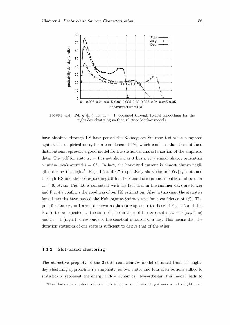
Chapter 4. Photovoltaic Sources Characterization 56
0
10
20
30
40
50
60
70
80
0 0.005 0.01 0.015 0.02 0.025 0.03 0.035 0.04 0.045 0.05
pro
ba
bili
ty d
en
sity f
un
ctio
n
harvested current i [A]
FebJulyDec
Figure 4.4: Pdf g(i|xs), for xs = 1, obtained through Kernel Smoothing for thenight-day clustering method (2-state Markov model).
have obtained through KS have passed the Kolmogorov-Smirnov test when compared
against the empirical ones, for a confidence of 1%, which confirms that the obtained
distributions represent a good model for the statistical characterization of the empirical
data. The pdf for state xs = 1 is not shown as it has a very simple shape, presenting
a unique peak around i = 0+. In fact, the harvested current is almost always negli-
gible during the night.5 Figs. 4.6 and 4.7 respectively show the pdf f(τ |xs) obtained
through KS and the corresponding cdf for the same location and months of above, for
xs = 0. Again, Fig. 4.6 is consistent with the fact that in the summer days are longer
and Fig. 4.7 confirms the goodness of our KS estimation. Also in this case, the statistics
for all months have passed the Kolmogorov-Smirnov test for a confidence of 1%. The
pdfs for state xs = 1 are not shown as these are specular to those of Fig. 4.6 and this
is also to be expected as the sum of the duration of the two states xs = 0 (daytime)
and xs = 1 (night) corresponds to the constant duration of a day. This means that the
duration statistics of one state is sufficient to derive that of the other.
4.3.2 Slot-based clustering
The attractive property of the 2-state semi-Markov model obtained from the night-
day clustering approach is its simplicity, as two states and four distributions suffice to
statistically represent the energy inflow dynamics. Nevertheless, this model leads to
5Note that our model does not account for the presence of external light sources such as light poles.

Chapter 4. Photovoltaic Sources Characterization 57
0
0.2
0.4
0.6
0.8
1
0 0.005 0.01 0.015 0.02 0.025 0.03 0.035 0.04 0.045 0.05
cu
mu
lative
dis
trib
utio
n f
un
ctio
n
harvested current i [A]
KSemp-Febemp-Julyemp-Dec
Figure 4.5: Cumulative distribution function of the harvested current for xs = 1 (solidlines), obtained through Kernel Smoothing (KS) for the night-day clustering method
(2-state Markov model). Empirical cdfs (emp) are also shown for comparison.
0
0.2
0.4
0.6
0.8
1
1.2
1.4
1.6
1.8
6 7 8 9 10 11
pro
ba
bili
ty d
en
sity f
un
ctio
n
duration [h]
FebJulyDec
Figure 4.6: Pdf f(τ |xs), for xs = 1, obtained through Kernel Smoothing for thenight-day clustering method (2-state Markov model).
a coarse-grained characterization of the temporal variation of the harvested current,
especially in the high-energy state.
Slot-based clustering has been proposed with the aim of capturing finer temporal details.
An example of the clustering result for this case is given in Fig. 4.8, for the month of
July for Ns = 12. All slots in this case have the same duration, which has been fixed a
priori and corresponds to 24/Ns hours.

Chapter 4. Photovoltaic Sources Characterization 58
0
0.2
0.4
0.6
0.8
1
6 7 8 9 10 11
cu
mu
lative
dis
trib
utio
n f
un
ctio
n
duration [h]
KSemp-Febemp-Julyemp-Dec
Figure 4.7: Cumulative distribution function of the state duration for xs = 1 (solidlines), obtained through Kernel Smoothing (KS) for the night-day clustering method
(2-state Markov model). Empirical cdfs (emp) are also shown for comparison.
0 5 10 15 20 250
0.005
0.01
0.015
0.02
0.025
0.03
0.035
0.04
0.045
Time of the day [h]
Cu
rre
nt
[A]
Slot 1Slot 2Slot 3Slot 4Slot 5Slot 6Slot 7Slot 8Slot 9Slot 10Slot 11Slot 12
Figure 4.8: Result of slot-based clustering considering Ns = 12 time slots (states) forthe month of July, years 1999− 2010.
Fig. 4.9 shows the pdf g(i|xs) for the first three states of the day (slots 5, 6 and 7, see
Fig. 4.8) for the month of July, which have been obtained through KS. As expected, the
peaks (and the supports) of the pdfs move to higher values, until reaching the maximum
of 0.04 A for slot 7, which is around noon. Due to the symmetry in the solar distribution
within the day, the results for the other daytime states are similar and therefore have
not been reported. In Fig. 4.10 we compare the cdfs obtained through KS against the

Chapter 4. Photovoltaic Sources Characterization 59
0
20
40
60
80
100
120
140
0 0.005 0.01 0.015 0.02 0.025 0.03 0.035 0.04 0.045 0.05
pro
ba
bili
ty d
en
sity f
un
ctio
n
input current i [A]
Slot 5Slot 6Slot 7
Figure 4.9: Pdf g(i|xs) for xs = 5, 6 and 7 for the slot-based clustering method forthe month of July.
0
0.2
0.4
0.6
0.8
1
0 0.01 0.02 0.03 0.04 0.05 0.06
cu
mu
lative
dis
trib
utio
n f
un
ctio
n
input current i [A]
KSemp-Slot 5emp-Slot 6emp-Slot 7
Figure 4.10: Comparison between KS and the empirical cdfs (emp) of the scavengedcurrent for xs = 5, 6 and 7 for the slot-based clustering method for the month of July.
empirical ones. Also in this case, all the cdfs have passed the Kolmogorov-Smirnov test
for a confidence of 1%.
A last but important results is provided in Fig. 4.11, where we plot the autocorrelation
function (ACF) for the empirical data and the Markov processes obtained by slot-based
clustering for a number of states Ns ranging from 2 to 24 for the month of January.
With the ACF we test how well the Markov generated processes match the empirical
data in terms of second-order statistics. As expected, a 2-state Markov model poorly
resembles the empirical ACF, whereas a Markov process with Ns = 12 states performs

Chapter 4. Photovoltaic Sources Characterization 60
-0.6
-0.4
-0.2
0
0.2
0.4
0.6
0.8
1
0 10 20 30 40 50 60 70
AC
F
Time [hours]
24 slots12 slots6 slots2 slots
emp
Figure 4.11: Autocorrelation function for empirical data (“emp”, solid curve) and fora synthetic Markov process generated through the night-day clustering (2 slots) andthe slot-based clustering (6, 12 and 24 slots) approaches, obtained for the month of
January.
quite satisfactorily. Note also that 5 of these 12 states can be further grouped into a
single macro-state, as basically no current is scavenged in any of them (see Fig. 4.8).
This leads to an equivalent Markov process with just eight states.
We highlight that our Markov approach keeps track of the temporal correlation of the
harvested energy within the same day, though the Markovian energy generation pro-
cess is independent of the “day type” (e.g., sunny, cloudy, rainy, etc.) and also on
the previous day’s type. Given this, one may expect a good fit of the ACF within a
single day but a poor representation accuracy across multiple days. Instead, Fig. 4.11
reveals that the considered Markov modeling approach is sufficient to accurately rep-
resent second-order statistics. This has been observed for all months. Hence, one may
be thinking of extending the state space by additionally tracking good (g) and bad (b)
days so as to also model the temporal correlation associated with these qualities. This
would amount to defining a Markov chain with the two macro-states g and b, where
pgb = Prob{day k is g| day k − 1 is b}, with k ≥ 1. Hence, in each state g or b, the
energy process could still be tracked according to one of the two clustering approaches
of Section 4.2.4, where the involved statistics would be now conditioned on being in the
macro-state. The good approximation provided by our model, see Fig. 4.11, show that
this further level of sophistication is unnecessary.

Chapter 4. Photovoltaic Sources Characterization 61
Table 4.1: Results for different solar panel configurations with night-day clusteringin Los Angeles for the month of August
np × ns Size i max(i) τ min(τ) max(τ)[cm2] [mA] [mA] [h] [h] [h]
2 x 2 2.99 2.16 4.52 9.73 8.17 10.174 x 4 11.98 9.25 19.77 10.18 9.00 10.676 x 6 26.96 21.29 45.56 10.26 9.17 10.678 x 8 47.92 38.15 82.10 10.32 9.17 10.83
10 x 10 74.88 59.97 129.19 10.34 9.17 10.8312 x 12 107.83 86.73 186.91 10.35 9.17 10.83
Table 4.2: Results for different solar panel configurations with night-day clusteringin Los Angeles for the month of December
np × ns Size i max(i) τ min(τ) max(τ)[cm2] [mA] [mA] [h] [h] [h]
2 x 2 2.99 1.11 2.48 7.74 5.00 8.334 x 4 11.98 4.85 11.03 8.27 6.50 8.676 x 6 26.96 11.19 25.67 8.38 6.67 8.838 x 8 47.92 20.16 46.01 8.42 6.83 8.83
10 x 10 74.88 31.65 72.44 8.44 6.83 8.8312 x 12 107.83 45.79 104.83 8.45 6.83 9.00
4.3.3 Panel size and location
To conclude, we show some illustrative results for different solar panel sizes and lo-
cations. Table 4.1 and Table 4.2 present the main outcomes for different solar cells
configurations for the night-day clustering approach for the months of August and De-
cember. Two representative months are considered: the month with the highest energy
harvested, August, and the one with the lowest, December. As expected, the current
inflow strongly depends on the panel size (linearly). Also, note that the day duration
slightly increases for an increasing panel area as this value is obtained by measuring when
the energy is above a certain (clustering) threshold. Although we scaled this threshold
proportionally with an increasing harvested current, the longer duration of the day is
due to the exponential behavior introduced by the scaling factor in Eq. 4.3, see the RHS
of this equation.
Finally, in table 4.3 and table 4.4 we show some energy harvesting figures for a solar
panel with np = ns = 6 for some representative cities for the months of August and
December, respectively.

Chapter 4. Photovoltaic Sources Characterization 62
Table 4.3: Results for different solar panel locations for np = ns = 6 for the monthof August
Location i max(i) τ min(τ) max(τ)[mA] [mA] [h] [h] [h]
Chicago, IL 17.03 46.74 10.57 8.50 11.33Los Angeles, CA 21.29 45.56 10.26 9.17 10.67New York, NY 17.17 44.62 10.42 8.83 11.00Reno, NV 22.91 48.52 10.72 9.16 11.00
Table 4.4: Results for different solar panel locations for np = ns = 6 for the monthof December
Location i max(i) τ min(τ) max(τ)[mA] [mA] [h] [h] [h]
Chicago, IL 5.24 16.08 6.95 4.83 8.00Los Angeles, CA 11.19 25.67 8.38 6.67 8.83New York, NY 6.81 18.95 7.57 5.67 8.33Reno, NV 8.24 21.12 7.85 6.00 8.50
4.4 Conclusions
In this chapter we have considered micro-solar power sources, providing a methodology
to model the energy inflow as a function of time through stochastic Markov processes.
The latter, find application in energy self-sustainable systems, such as the one considered
in this thesis (i.e., the simulation of energy harvesting communication networks) and are
as well useful to extend current theoretical work through more realistic energy models.
Thus, it allows to accurate model one of the most important environment variable,
i.e., the energy. The proposed approach has been validated against real energy traces,
showing good accuracy in their statistical description in terms of first and second order
statistics. As final remark, it is to be noted that the tool has been developed using
MatlabTMand is available under the GPL license at [130].

Chapter 5
Switch-ON/OFF Policies for EH
SBSs through Distributed
Q-Learning
5.1 Introduction
Massive deployment of SBSs represents the most promising architecture to meet the high
capacity demands of mobile networks. Their reduced energy requirements encourage
the use of RES as distributed power suppliers. Their adoption is expected to have
a twofold positive effect: 1) it will increase the use of renewable sources to provide
energy, and consequently to reduce the carbon footprint of ICT, and 2) it will allow
savings on power grid bills. Solar energy is probably the most important RES, due
to its widespread availability, the good efficiency of photovoltaic technology and its
competitive cost [79]. However, the resulting panel sizes may represent an obstacle for
urban scenarios, where SBSs are likely to be installed in street furniture (i.e., traffic
lamps, street lights, transportation hubs, etc.). Small form-factor solar panels can also
be adopted by intelligently allocating energy to the SBSs, putting them in power saving
(OFF) mode when necessary, and exploiting the macro BS to compensate for their OFF
time. The bottom line is that the panel size can be made small at the cost of some extra
processing / optimization, which entails a tight interaction among SBSs and between
SBSs and the macro BS.
However, with the introduction of energy harvesting, we also need to consider the erratic
and intermittent nature of RES, which further complicates the EE problem and the
corresponding ON/OFF strategies. Most of the previous papers published in this area
have only provided guidelines for dimensioning the network, while online approaches
63

Chapter 5. Switch-ON/OFF Policies for EH SBSs through Distributed Q-Learning 64
to control network elements have appeared only recently. In [91], the authors present
an algorithm for determining when to switch OFF the SBSs by solving a ski rental
problem. The analysis is carried out considering Poisson arrivals for energy and traffic,
which may provide a non-realistic approximation to these processes. A solution based
on Reinforcement Learning is presented in [92], where the authors concentrate on the
performance of a single SBS. However, the impact of multiple SBSs simultaneously
switching OFFs within the same area is not considered.
In this chapter, we fill these gaps by proposing a solution considering multiple SBSs in
a macro BS area, realistic traffic conditions and solar radiation data from real measure-
ments. SBS network is modeled as a multi-agent system where each agent (SBS) makes
autonomous decisions, according to a Decentralized SON paradigm. SBSs supplied by
solar energy and batteries (energy storage) are utilized as an overlay layer in a two-tier
network with a macro BS powered by the electricity grid. The behavior of small cells can
be optimized to offload the traffic from the macro BS according to the energy income
and the traffic demand. To this purpose, we designed a distributed online solution based
on multi-agent RL, known as distributed Q-learning, which allows SBSs to independently
learn a RRM policy. This main contribution of this study lies on the following points:
1. proposing a distributed Q-learning solution to control SBSs powered with solar
energy
2. extend the standard Q-learning solution with offline trained algorithm
3. investigating the convergence of the algorithms
4. characterizing the ON/OFF switching policies
5. evaluate the network system performance with the proposed solutions compared
to a baseline solution
6. calculating the surplus energy that cannot be stored, due to the energy storage
capacity constraints
The remainder of the chapter is organized as follows. In Section 5.2 we present the
system model. Section 5.3 gives an overview on the distributed Q-learning algorithm,
whereas the two proposed algorithms are presented in Section 5.4. In Section 5.5 we
discuss some performance results. In Section 5.6 we draw our conclusions and discuss
future research directions.

Chapter 5. Switch-ON/OFF Policies for EH SBSs through Distributed Q-Learning 65
5.2 System Model
We consider a two-tier network composed of clusters of one macro BSs and N SBSs.
The macro BSs are connected to the power grid and provide baseline coverage. The
SBSs are deployed in a hotspot manner to increase the system capacity, where needed
(e.g., shopping hall, city center, etc.). SBSs are solely powered through solar-harvested
energy and possess rechargeable batteries to store the harvested energy.
For the BS power consumption model we use the linear model presented in Section 2.2,
P = P0 + βρ, where ρ ∈ [0, 1] is the BS traffic load, normalized with respect to its
maximum capacity, and P0 is its baseline power consumption. We consider medium scale
factor “metro cells” as SBSs, featuring a maximum transmission power of 38 dBm. The
values of β and P0 for the macro BS (SBS) are 600 (39)W and 750 (105.6), respectively.
The user equipment resource allocation scheme uses the methodology defined in [131].
This includes a detailed wireless channel model and the dynamic selection of the mod-
ulation and coding scheme for each user as function of its channel state.
5.3 Distributed Q-Learning
In this Section we present the distributed Q-learning algorithm already introduced in
Chapter 3 and we define the variables used in this work. Distributed Q-learning is an
online optimization technique to control multi-agent systems, i.e., a system featuring
N distributed agents (the SBSs) which make decisions (switch-ON/OFF) in an unco-
ordinated fashion. Each agent has to independently learn a policy (switch-ON/OFF)
through real-time interactions with the environment. These interactions entail taking
actions for the agents and receiving, in return, a reward from the environment. In dis-
tributed Q-learning each agent i maintains a local policy and a local Q-function Q(xit, ait)
that only depends on its state xit and actions ait, with t being the decision epoch (time).
The agents only have a partial view of the overall system and their local states may
differ since traffic load and energy income may be unevenly distributed. In particular,
the input of the switch-ON/OFF algorithm depends on the SBS location and on the
geographical distribution of its users, affecting for instance, the experienced traffic load.
The decision making process of each agent is defined according to a MDP with state
vector xt = (x1t , x
2t , . . . , x
Nt ), where xit is the state associated with SBS i at time t. Agent
i independently chooses an action ait from an action set A based on its own state xit.
At the next decision epoch t+ 1, the agent receives a reward rit from the environment.
The agent dependent reward rit is then used to locally update the Q-value, Q(xit, ait),

Chapter 5. Switch-ON/OFF Policies for EH SBSs through Distributed Q-Learning 66
indicating the level of convenience of selecting action ait when in state xit. The Q-value
is updated as follows:
Q(xit, ait)← Q(xit, a
it) + α
[rit + γmax
aQ(xit+1, a
′)−Q(xit, a)]
(5.1)
where α is the learning rate, γ is the discount factor and xit+1 is the next state for agent
i and a′ is the associated optimal action, as introduced in Section 3.2.2. This procedure
is executed by each agent at each epoch of the system in a synchronized manner. The
asynchronous Q-learning algorithm proposed in [132], uses a learning rate given by a
polynomial function that at time t accounts for the number of visits, up to and including
time t, to state-action pair (x, a), termed n(x, a, t). In detail αω(x, a) = α/n(x, a, t)ω,
where ω = 1 leads to a linear learning rate, ω ∈ (1/2, 1) to a polynomial one and ω = 0
to a constant learning rate.
To make the best decisions (exploitation) the algorithm must have gathered enough
information from the environment (exploration). The exploration phase is commonly
controlled by an ε-greedy approach, in which random states are visited by the agents with
probability ε. Since rigorous convergence results for multi-agent reinforcement learning
algorithms are still an open research question, here we refer to the convergence time
as the first instant in which the Q-values remain stable within a certain tolerance. In
particular, we say that the system has reached convergence when all the SBS batteries
are below BOFFth for a certain amount of time (e.g., within a window of consecutive days).
The rationale behind this definition is to foster the energy sustainability of the SBSs.
5.4 Algorithms
5.4.1 ON/OFF switching through online distributed Q-learning
In this section we provide details on the Q-learning algorithm, by defining state, action
set and reward function, for the N agents.
State: The local state xit is defined by:
xit = {Sit , Bit, L
it} , (5.2)
where Sit is the state of the renewable energy source based on the incoming amount
harvested energy (e.g., day and night), Bit is the normalized battery energy level, Lit is
the normalized load for SBS i in slot t, which depends on the number of users served
by this SBS. We uniformly quantize Sit , Bit and Lit into 2, 5 and 3 levels, respectively,
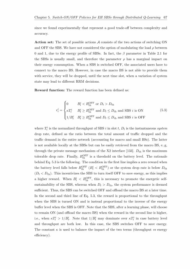
Chapter 5. Switch-ON/OFF Policies for EH SBSs through Distributed Q-Learning 67
since we found experimentally that represent a good trade-off between complexity and
accuracy.
Action set: The set of possible actions A consists of the two actions of switching ON
and OFF the SBS. We have not considered the option of modulating the load ρ between
0 and 1, due to the energy profile of SBSs. In fact, the β parameter in Table 2.1 for
the SBSs is usually small, and therefore the parameter ρ has a marginal impact on
their energy consumption. When a SBS is switched OFF, the associated users have to
connect to the macro BS. However, in case the macro BS is not able to provide them
with service, they will be dropped, until the next time slot, when a variation of system
state may lead to different RRM decisions.
Reward function: The reward function has been defined as:
rit =
0 Bi
t < BOFFth or Dt > Dth
κT it Bit ≥ BOFF
th and Dt ≤ Dth and SBS i is ON
1/Bit Bi
t ≥ BOFFth and Dt ≤ Dth and SBS i is OFF
(5.3)
where T it is the normalized throughput of SBS i in slot t, Dt is the instantaneous system
drop rate, defined as the ratio between the total amount of traffic dropped and the
traffic demand in the entire network (accounting for macro and small BSs). The latter
is not available locally at the SBSs but can be easily retrieved from the macro BS, e..g,
through the private message mechanism of the X2 interface [133]. Dth is the maximum
tolerable drop rate. Finally, BOFFth is a threshold on the battery level. The rationale
behind Eq. 5.3 is the following. The condition in the first line implies a zero reward when
the battery level falls below BOFFth (Bi
t < BOFFth ) or the system drop rate is below Dth
(Dt < Dth). This incentivizes the SBS to turn itself OFF to save energy, as this implies
a higher reward. When Bit < BOFF
th , this is necessary to promote the energetic self-
sustainability of the SBS, whereas when Dt > Dth, the system performance is deemed
sufficient. Thus, the SBS can be switched OFF and offload the macro BS at a later time.
In the second and third line of Eq. 5.3, the reward is proportional to the throughput
when the SBS is turned ON and is instead proportional to the inverse of the energy
buffer level when the SBS is OFF. Note that the SBS, after a learning phase, will choose
to remain ON (and offload the macro BS) when the reward in the second line is higher,
i.e., when κT it > 1/Bit. Note that 1/Bi
t may dominate over κT it in case battery level
and throughput are both low. In this case, the SBS switches OFF to save energy.
The constant κ is used to balance the impact of the two terms (throughput vs energy
efficiency).

Chapter 5. Switch-ON/OFF Policies for EH SBSs through Distributed Q-Learning 68
5.4.2 ON/OFF switching based on trained distributed Q-learning
Online learning algorithms suffer from an initial exploration phase to gather information
from the environment and, based on this acquired knowledge, make good decisions. This
process produces instability and poor performance potentially for a long time, i.e., until
a sufficient amount of knowledge is gathered. We proposed an offline training period for
the algorithm to setup initial switch OFF/ON policies. In detail, the training phase
consists of running the agent with the energy statistics of a specific month for generating
the Q-tables in an offline fashion. This returns the trained Q-values that can be used for
initializing the Q-tables of the SBSs when they are deployed in their online operative
mode. The pseudo-code of this solution is presented in Alg. 2. This initial training helps
reduce the initial exploration phase and, in case the algorithm is not able to follow the
dynamics of the environment, it also helps improve the system performance, by avoiding
slow recalibration phases. We note that, the training phase can be either performed
with a simulation approach, as we propose, or obtained by other expert SBSs that have
been already deployed, as in the transfer learning paradigm [98].
Algorithm 2 Trained Distributed Q-learning
1: procedure Training(Qminit(xi, ai))
2: Qminit(xi, ai)← 0
3: for m ∈M do4: Run Q-learning(EHm)5: Qminit(x
i, ai)← Q-table(xi, ai)6: end for7: end procedure
1: procedure Online2: for m ∈M do3: for m ∈ Dm do4: Q-table(xi, ai)← Qminit(x
i, ai)5: Run Q-learning(EHm)6: end for7: end for8: end procedure
whereM is the set on monthsEHm = Energy Traces for month mDm is the set of days in month m

Chapter 5. Switch-ON/OFF Policies for EH SBSs through Distributed Q-Learning 69
5.5 Performance Evaluation
5.5.1 Simulation Scenario
We consider a deployment of a varying number of SBSs within a square macro cell area
with a side of 1 km. The macro BS is placed in the center of it, whereas the SBSs are
randomly positioned with the constraint that their cells do not overlap. This translates
into a minimum inter-SBS distance of 50 m, which corresponds to the coverage radius of
a SBS with transmission power of 38 dBm. The coverage area of each SBS is populated
with 120 uniformly placed UEs, which allow congesting the SBS in peak traffic hours.
Data load is modeled using an urban profile [89], where traffic is concentrated around
working hours and has one peak in the morning and one in the afternoon. According
to [1], we considered that 20% of the UEs are “heavy users” with a data volume of
900 MB/h, while the remaining UEs are “ordinary users” (112.5 MB/h). As for the
RES system, we consider the Panasonic N235B solar modules, which have single cell
efficiencies of about 21%, delivering about 186 W/m2. Each SBS is equipped with an
array of 16× 16 solar cells (i.e., 4.48 m2). The battery size is 2 kWh (panel and battery
sizes have been chosen so that SBS batteries can be replenished in a full winter day).
Realistic harvested energy traces are obtained using the SolarStat tool [21], considering
the city of Los Angeles as the deployment location. Fig. 5.1 shows typical profiles for
the traffic demand and the harvested energy across two subsequent days. Interestingly,
we see that the maxima in the energy inflow and in the traffic demand are not aligned.
This means that some optimization actions that could be taken are e.g., saving energy
resources and use them when the next traffic peak occurs.
The analysis is performed as follows. We first elaborate on the convergence of the online
algorithm, then we characterize the switch ON/OFF policies in different representa-
tive months (i.e., January, April and July) and compare the performance of the online
distributed Q-learning (“QL” in the figures) against that of a distributed Q-learning
algorithm trained in an offline fashion (“QLT”). We conclude our investigation with
an assessment of the energy efficiency of the considered techniques. The Q-learning
based algorithms are independently implemented by each SBS. The learning rate is set
to α = 0.5 and the discount factor to γ = 0.9 for all SBS, according to our simulation
analysis. The constant κ (see Eq. 5.3) is set to 10 as this provides a good trade-off
for the considered system parameters. Both algorithms also implement exploration fea-
tures [134], i.e., random states are visited by the learning agents with probability ε = 0.1.
The threshold on the instantaneous traffic drop rate is set to Dth = 0.05. QL and QLT
are contrasted with a greedy scheme (“Gr” in the figures) where the i − th SBS is
switched OFF at time t when its battery level Bit drops below BOFF
th , and is reactivated
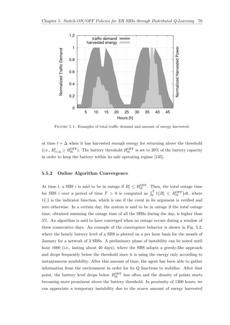
Chapter 5. Switch-ON/OFF Policies for EH SBSs through Distributed Q-Learning 70
0
0.2
0.4
0.6
0.8
1
1.2
5 10 15 20 25 30 35 40 45
Norm
aliz
ed T
raffic
Dem
and
Norm
aliz
ed H
arv
este
d P
ow
er
Hours [h]
traffic demandharvested energy
Figure 5.1: Examples of total traffic demand and amount of energy harvested.
at time t + ∆ when it has harvested enough energy for returning above the threshold
(i.e., Bit+∆ ≥ BOFF
th ). The battery threshold BOFFth is set to 20% of the battery capacity
in order to keep the battery within its safe operating regime [135].
5.5.2 Online Algorithm Convergence
At time t, a SBS i is said to be in outage if Bit ≤ BOFF
th . Then, the total outage time
for SBS i over a period of time T > 0 is computed as∫ T
0 1{Bit ≤ BOFF
th }dt, where
1{·} is the indicator function, which is one if the event in its argument is verified and
zero otherwise. In a certain day, the system is said to be in outage if the total outage
time, obtained summing the outage time of all the SBSs during the day, is higher than
5%. An algorithm is said to have converged when no outage occurs during a window of
three consecutive days. An example of the convergence behavior is shown in Fig. 5.2,
where the hourly battery level of a SBS is plotted on a per hour basis for the month of
January for a network of 3 SBSs. A preliminary phase of instability can be noted until
hour 1000 (i.e., lasting about 40 days), where the SBS adopts a greedy-like approach
and drops frequently below the threshold since it is using the energy only according to
instantaneous availability. After this amount of time, the agent has been able to gather
information from the environment in order for its Q functions to stabilize. After that
point, the battery level drops below BOFFth less often and the density of points starts
becoming more prominent above the battery threshold. In proximity of 1300 hours, we
can appreciate a temporary instability due to the scarce amount of energy harvested

Chapter 5. Switch-ON/OFF Policies for EH SBSs through Distributed Q-Learning 71
0
0.2
0.4
0.6
0.8
1
0 500 1000 1500 2000 2500 3000 3500
Battery
Level
Hour [h]
Battery Threshold
Figure 5.2: Battery level for the month of January of a single SBS.
0
0.05
0.1
0.15
0.2
0.25
0.3
0.35
0.4
0.45
3 4 5 6 7 8 9 10
Daily
Outa
ge
Number of SBSs
SumWin
Figure 5.3: Average daily outage with multiple SBSs.
during several consecutive days. However, we note that the algorithm promptly reacts
and drives the system toward a good (zero-outage) region.
Similar considerations hold for scenarios involving more SBSs. Nonetheless, in such
case the instability during the winter can be more frequent, as depicted in Fig. 5.3,
which presents the average daily outage rate when varying the number of SBSs. During
the summer period, the system is always able to maintain the batteries levels in a
safe operative window. On the other hand, in winter periods the daily outage rate
is increasing with the number of SBSs, reaching the 40% for 10 SBSs. Multi-agent RL

Chapter 5. Switch-ON/OFF Policies for EH SBSs through Distributed Q-Learning 72
suffers the problem of the coordination among agents, since they may incur in conflicting
behaviors, as highlighted in Section 3.2.5. In particular, in this case the SBSs need to
find a coordination on when switching OFF for avoiding to overload the macro BS. This
task becomes more difficult when the number of SBSs in the network is high, since the
SBSs share the macro BSs resources when temporary switching OFF, which implies that
they have less opportunities to do this.
5.5.3 Policy Analysis
The switch OFF rate of a single SBS during 24 hours is reported in Fig. 5.4 for polynomial
(ω = 0.5) and constant (ω = 0) learning rates for the months of January, April and July.
The rate is calculated by simulating 180 days, so as to allow for the completion of the
training phase and increase the statistical confidence of the results.
Switch OFFs are more intensive during early morning hours (from 0am to 4am) and in
the night (from 9pm to 11pm), due to the scarce harvested energy and the low traffic
demand at night-time. When the SBS is turned OFF, the SBS agent chooses to recharge
its battery and relies on the macro cell for serving the UEs within its coverage. This
behavior is similar for all months. In January, another less intensive switch OFF period
can be appreciated from 5am to 9am (switch OFF rate of about 0.3). This is due to
a feeble harvesting process during those months. Moreover, it can be noticed that the
two values of ω do not significantly affect the shape of the policy. This implies that a
constant learning rate (ω = 0) provides the needed flexibility for Q-learning to effectively
cope with the system dynamics.
In Fig. 5.5, the switch OFF rate of a SBS in a multi-cell scenario with 10 SBSs is
presented. The policies are similar to those in Fig. 5.4 (single cell case). However, we
can appreciate a slight reduction in the switch OFF intensity in the early morning. Here,
the SBSs switch OFF less often in order not to overload the macro cell and maintain
the traffic drop rate below Dth. In the months of April and July, the number of switch
OFFs is lower than in January, due to an increase in the harvested energy income.
According to this, we can appreciate that the algorithm is able both to learn the policy
as function of the energy and traffic patterns and to adapt to different scenarios with
different number of SBSs.
In Fig. 5.6, we plot an example of the temporal system behavior for a HetNet including 3
SBSs and a macro BS for the last week of December. Here, from top to bottom we show
temporal traces concerning traffic demand and instantaneous harvested energy (in the
same plot), battery level, policy adopted at the SCs (y-label “Action”) and normalized
load at the macro BS (y-label “Macro Load”). From these results various observations

Chapter 5. Switch-ON/OFF Policies for EH SBSs through Distributed Q-Learning 73
0
0.1
0.2
0.3
0.4
0.5
0.6
0.7
0.8
0.9
1
0 5 10 15 20 25
Sw
itch O
ff R
ate
Hour [h]
Jan ω=0
Apr ω=0
Jul ω=0
Jan ω=0.5
Apr ω=0.5
Jul ω=0.5
Figure 5.4: Switch OFF rate of a SBS during the day with a single SBS.
0
0.1
0.2
0.3
0.4
0.5
0.6
0.7
0.8
0.9
1
0 5 10 15 20 25
Sw
itch O
ff R
ate
Hour [h]
Jan ω=0
Apr ω=0
Jul ω=0
Figure 5.5: Switch OFF rate of a SBS during the day with multiple SBSs.
can be made. First, the policy adopted by QL tends to save energy during the night,
and this makes it possible to offload more the macro BS during the day, as it can be seen
in the bottom plot of Fig. 5.6 in correspondence of the points marked with “(a)”. Also,
the impact of our reward function (see Eq. 5.3) can be appreciated in correspondence of
label “(b)”. Here, the QL keeps the SBSs ON, as the traffic demand is high, and in this
case sleeping would cause congestion at the macro BS. We remark that QL is capable of
doing this as it proactively saves some of the harvested energy when the energy inflow
is abundant. In contrast, the greedy scheme shows a more aggressive behavior and, as

Chapter 5. Switch-ON/OFF Policies for EH SBSs through Distributed Q-Learning 74
0 20 40 60 80 100 120 140 160 1800
2x 10
4
Tra
ffic
Re
qu
ire
me
nts
[M
bp
s]
0 20 40 60 80 100 120 140 160 1800
0.5
Ha
rve
ste
d P
ow
er
[W]
Traffic
Harvested Power
0 20 40 60 80 100 120 140 160 1800
0.5
1B
att
ery
Le
ve
lQL
Gr
20 40 60 80 100 120 140 160
0
0.5
1
Actio
n
QL
Gr
20 40 60 80 100 120 140 160
0
0.5
1
Ma
cro
Lo
ad
Hour of the week [h]
QL
Gr
(a) (a) (a)
(b) (b)
Figure 5.6: Example temporal behavior for a HetNet with 3 SBSs and one macro BS.Temporal traces show the status of the SBSs.
a result, it has no residual energy to compensate for an upsurge in the traffic load.
We observe that the energy harvesting traces are the same for all SBSs. We implement
this choice since it is expected that the level of solar irradiation will not change much
within a macro cell area. In addition, this sort of synchronization with respect to the
experienced energy inflow from RESs is enforced by the traffic demand processes, as
different SBSs will as well undergo similar traffic profiles. This implies that, in the
considered setup, SBSs are often switched ON/OFF simultaneously.
This can be appreciated from Fig. 5.7, where the average load is plotted as a function
of the hour of the day for a network with 3 SBSs. The greedy scheme usually leads
to a higher load for the macro BS during the morning peak hours, where the batteries
are likely to be drained, and therefore most of the SBSs must be turned OFF. On the
contrary, QL loads the macro BS slightly more during most of the day in order to put
some of the SBSs to sleep (saving energy at these SBSs) and serve more traffic during
the morning peak.
5.5.4 Network Performance
In Fig. 5.8 we show the average throughput gain of QL and QLT with respect to the
greedy scheme by varying the number of SBSs, whereas in Fig. 5.9 we show the traffic
drop rate of QL, QLT and of the greedy algorithm. The results are achieved running
simulations across a full year. Statistics are gathered only when the algorithm has

Chapter 5. Switch-ON/OFF Policies for EH SBSs through Distributed Q-Learning 75
0
0.2
0.4
0.6
0.8
1
5 10 15 20
Norm
aliz
ed L
oad
Norm
aliz
ed T
raffic
Dem
and
Hour [h]
traffic profile
QL
Gr
Figure 5.7: Average hourly load for the macro BS in a network with 3 SBSs.
converged and for a duration of 365 days. Since the harvesting process substantially
differs for different seasons, we have presented our results separately for the winter and
the summer periods, respectively termed “Win” and “Sum” in the plots. January,
February, October, November and December are considered winter months.
The effect of ω is not relevant from the throughput and traffic drop perspective. QL
and QLT outperform greedy: the throughput gain of Q-learning with respect to greedy
is of up to 16% in the winter, which results in a drop rate smaller than 5% for QL and
QLT, whereas the drop rate reaches 20% for the greedy scheme. The difference between
winter and summer resides in the corresponding switch OFF policies, as discussed in the
previous section.
We also note that QL and QLT have similar performance, both in terms of throughput
and traffic drop, but they have a different convergence time. In fact, QLT presents 6
times shorter convergence times on average, taking at most 10 days to converge in the
worst case scenario of 10 SBSs, with respect to the 40 days needed by QL in the same
settings. However, QL can rapidly adapt to the changing dynamics of the harvesting
process across the months (as reported in Fig. 5.8 and Fig. 5.9), thus rendering useless
the per-month-training of QLT. Therefore, SBS agents shall only be trained to gather
the necessary information during their initial exploration phase. Upon that, they can
be used in an online fashion and further training is no longer required.

Chapter 5. Switch-ON/OFF Policies for EH SBSs through Distributed Q-Learning 76
8
10
12
14
16
18
3 4 5 6 7 8 9 10
Thro
ughput G
ain
[%
]
Number of SBSs
QL Sum
QL Win
QLT Sum
QLT Win
Figure 5.8: Average throughput gain [%] of QL and QLT with respect to the Grscheme.
0
0.1
0.2
0.3
0.4
0.5
3 4 5 6 7 8 9 10
Tra
ffic
Dro
p
Number of SBSs
QL Sum
QL Win
QLT Sum
QLT Win
Gr Sum
Gr Win
Figure 5.9: Traffic drop rate for QL, QLT and Gr.
5.5.5 Energy Efficiency
In this section, the energy performance of QLT is not shown as is the same as that of
QL. The energy efficiency is defined as EE = TS/ES , where TS is the system throughput
and ES is the total energy drained by the macro BS (from the power grid). The traffic
demand profile is also shown.

Chapter 5. Switch-ON/OFF Policies for EH SBSs through Distributed Q-Learning 77
0
0.5
1
1.5
2
2.5
3
0 5 10 15 20 25
Energ
y E
ffic
iency [M
bps/K
Wh]
Tra
ffic
Pro
file
[%
]
Hour [h]
Traffic Profile
Gr Jan
Gr Apr
Gr Jul
QL Jan
QL Apr
QL Jul
Figure 5.10: Average energy efficiency of a SBS during the day with a single SBS.
0
5
10
15
3 4 5 6 7 8 9 10Energ
y E
ffic
iency Im
pro
vem
ent [%
]
Number of SBSs
Sum
Win
Figure 5.11: Energy efficiency improvement [%] of QL with respect to greedy vsnumber of SBSs.
The energy consumption metric is shown in Fig. 5.10, where the QL energy efficiency is
compared with that of the greedy scheme for January, April and July. QL outperforms
the greedy scheme during the morning slot (e.g., from 6am to 12pm), since it saves
energy during the nocturnal low traffic period in order to have enough energy reserve
for the morning peaks of traffic, without compromising the throughput performance.
Fig. 5.11 reports the energy efficiency improvement of QL with respect to greedy, varying
the number of SBSs. QL offers a considerable gain, which reaches 15% in the winter

Chapter 5. Switch-ON/OFF Policies for EH SBSs through Distributed Q-Learning 78
0
0.1
0.2
0.3
0.4
0.5
0.6
0 5 10 15 20 25
Excess E
nerg
y [K
Wh]
Hour [h]
Gr Jan
Gr Apr
Gr Jul
QL Jan
QL Apr
QL Jul
Figure 5.12: Average redundant energy during the day for a single SBS.
months. This is due to its higher throughput, which follows from a proper usage of the
available energy reserves. The lower gain during the summer months and its decreasing
behavior for an increasing number of SBSs are motivated by the fact that the RES
system has been dimensioned to provide the necessary energy in the worst case, which
is a winter day. This implies that, during the summer, there are days in which the
algorithm does not have to smartly save energy, since the harvested energy is enough
for the whole day and therefore greedy and QL have similar performance. In this case,
the abundant energy has to be discarded by the SBSs, i.e., it can neither be used for
transmission nor stored in the battery. This fact is shown in Fig. 5.12 (“excess energy”).
With QL, the total amount of grid energy drained by the system spans from 7.3 KWh for
a network of 3 SBSs, to 7.9 KWh with 10 SBSs (as compared to 7.5 KWh for the greedy
scheme). Note that QL has a worse annual energy consumption performance since it
serves more traffic, as we have discussed in Section 5.5.4. QL has a higher energy surplus
than greedy. In fact, QL (greedy) reserves 0.124 (0.064) KWh in January, 2.115 (1.619)
KWh in April and 2.021 (1.513) KWh in July. This translates into a total amount of
energy not used by QL of 400 KWh in the summer (300 for greedy), and of 65 KWh in
the winter (36 for the greedy scheme). Considering the higher energy efficiency and the
energy surplus of QL, we conclude that QL uses less energy to offload the macro BS.
In such a context, SBSs may act as prosumers (i.e., an energy consumer and producer)
and offer/trade their excess energy to provide ancillary services to the smart grid.

Chapter 5. Switch-ON/OFF Policies for EH SBSs through Distributed Q-Learning 79
5.6 Conclusions
In this chapter, we have presented a distributed implementation of a switch OFF/ON
algorithm aimed at optimizing the energy usage in a dense small cell deployment with
solar energy harvesting capability. The solution uses Q-learning techniques to learn the
dynamics of energy harvesting and traffic processes and make switch ON/OFF decisions
accordingly. Our numerical results demonstrate that distributed learning is a promis-
ing approach to make decisions in complex, dense and dynamic scenarios, leading to
substantial advantages with respect to greedy schemes, such as higher throughput and
energy efficiency. In our future work, we are planning to analyze the behavior of the
proposed solution for different types of traffic profiles with different traffic demands for
studying the flexibility in adapting to the various 5G operative cases. In addition, we
would like to enhance the control performed by the SBSs in order to enable a cooperative
optimal computation of the policies that accounts for common (and global) performance
objectives. In fact, in the current algorithm, the cooperation is only marginally achieved
through the use of the global drop rate in the reward functions that are locally computed
by the SBSs.

Chapter 6
Layered Learning Load Control
for Renewable Powered SBSs
6.1 Introduction
In this chapter, motivated by the promising results of the distributed MRL solutions
presented in Chapter 5, we propose a novel energy efficient framework specifically de-
signed to deal with dense HetNets. In doing this, we will consider the newest techniques
that are expected to the be key enabler in 5G of the SON paradigm, i.e., softwarization
and AI. On the one hand, SDN and NFV provide a flexible infrastructure for collecting
the necessary system information and reconfiguring the network elements. SDN sepa-
rates control and data planes and, by centralizing the control, enables many advantages
such as programmability and automation. NFV enables softwarized implementation of
network functions on a general purpose hardware, improving scalability and flexibility.
And on the other hand, AI gives the tools for automatic and intelligent system (re-
)configuration thanks to ML and RL methods. ML contributes with valuable solutions
to extract models that reflect the user and network behaviors, while RL can be used for
interactive decision making problem working in real-time and at short time scales.
Recently, the interest in online approaches to control network elements attracted more
attention with the goal of optimizing the system by considering its actual instantaneous
conditions and introducing more accurate models of harvested energy and traffic demand
with respect to the ones used in offline approaches. This type of optimization is based
on agents that control each BS, generating a multi-agent optimization problem. Multi-
agent systems are an effective way to treat complex, large and unpredictable problems;
however, such distribution might suffer the problem of finding simultaneously a solution
80

Chapter 6. Layered Learning Load Control for Renewable Powered SBSs 81
among all the agents that is good for the whole system, as we introduced in Section 3.2.5
and we will show with numerical results in this chapter.
The main contribution of this chapter is to present an online solution for switching
ON/OFF SBS powered by solar PV panels and batteries in an HetNet scenario. The
proposed framework is based on a MRL approach for controlling the SBS. The Layered
Learning paradigm is adopted to simplify the problem by decompose it in subtasks.
Thus, the overall solution for the multi-agent optimization is performed by decomposing
the general problem in subtasks. In particular, the global solution is obtained in a
hierarchical fashion: the learning process of a subtask is aimed at facilitating the learning
of the next higher subtask layer. The first layer implements an MRL approach and it is
in charge of the local online optimization at SBS level as function of the traffic demand
and the energy incomes. The second layer is in charge of the network-wide optimization
and it is based on Artificial Neural Networks (ANNs) aimed at estimating the model of
the overall network. The architecture for implementing the two levels and enabling their
interaction is based on a SDN paradigm. To the best of the authors’ knowledge, this is
the first work in the literature that has proposed an online control system for HetNet
with EH capabilities based on a learning solution with realistic environmental conditions
and considering the optimization across different energy harvesting conditions, as has
been discussed in 2.4. Moreover, in this work we compare it against an optimal solution.
As a result, the innovative contribution of this chapter can be summarized as follows:
1. Definition of a control framework based on a SDN/NFV paradigm for networks
with SBS powered with renewable energies.
2. Design of an online solution based on Layered Learning for the optimization of
SBS with energy harvesting capabilities.
3. Characterization of the temporal behavior
4. Characterization of the performance of the whole framework and of the specific
algorithms at each layer.
5. Comparison with an optimal solution evaluated offline.
The rest of this chapter is organized as follows. Section 6.2 defines the system model
and the architecture of the control framework. Section 6.3 and 6.4 describe the solutions
adopted in the two layers with details. Section 6.5 is devoted to the presentation of the
simulation scenario where the proposed approach has been evaluated and to describe
the correspondent numerical results. Finally, Section 6.6 concludes by summarizing the
main results of the work.

Chapter 6. Layered Learning Load Control for Renewable Powered SBSs 82
6.2 Problem Statement
We consider a two-tier network composed of clusters of one MBS and N SBSs. The
MBS provides baseline connectivity and is powered by the electric grid. The SBSs
are deployed for increasing the capacity in a hot-spot manner (e.g., shopping hall, city
center, etc.). SBSs are solely powered through the energy harvested by a solar panel
and are equipped with rechargeable batteries.
The system evolves in cycles, based on the variation of the traffic demand and the energy
arrivals in time. The time granularity ∆T is the time difference between two consecutive
cycles. The energy harvested by the SBSs at time t is defined by St = [St1, St2, . . . , S
tN ]
and the energy stored by each SBS at time t is defined by Bt = [Bt1, B
t2, . . . , B
tN ]. The
traffic load experienced at time t by each SBS due to the traffic of the UEs is defined as
Lt = [Lt1, Lt2, . . . , L
tN ].
At each cycle t, the LL control framework decides the configuration of the cluster of the
SBSs in terms of ON/OFF states. When a SBS is switched OFF, the associated users
have to connect to the macro BS. However, in case the macro BS is overloaded, it will
not able to provide them with service and the users will be dropped, until the next time
slot. We define this situation as system outage.
The core our proposed solution is based on a multi-agent system, being each agent
located at the SBSs. Such a distributed approach is indicated for providing system
scalability and allows SON implementation for controlling the different SBSs. Each
agent is in charge of defining the ON/OFF policy based on its local environment. In
fact, each SBS may experience different traffic and energy harvesting profiles. The agents
can be either endowed with an offline behavior or learn new behaviors online, such that
the performance of the single agent or of the whole system are improved gradually.
The former is usually solved thanks to game theory solution. However, sometimes the
complexity of the environment makes difficult or impossible the offline design of the agent
behavior. In this case, the latter solution represents a viable approach for optimizing
the agent behaviors and it is known as Multi-agent Reinforcement Learning (MRL). A
RL agent learns by interacting with its environment. At each time step, the agent takes
an action according to the state its perceived from the environment. The action causes
the environment to transit to a new state and allows the agent to evaluate the benefits
incurred in the transition, the so called reward. By trying different actions, the agent
has to learn the optimal behavior of the system thanks to the cumulative rewards. This
phase is called exploration and provides the inputs to the stable phase, in which the
agents will use the learned policies, called exploitation. MRL and Q-learning will be
described more in detail in Section 6.3.

Chapter 6. Layered Learning Load Control for Renewable Powered SBSs 83
The fundamental dilemma in RL is the trade-off between exploration and exploitation.
In MRL, this dilemma is even more sensitive, since the exploration phase is further
complicated. In fact, agents in MRL explore to obtain information not only about
their local environment, but also about the other agents in order to adapt to their
behavior. In fact, any agent’s action on the environment depends also on the action
taken by the other agents. In order to overcome this problem, the agents have to be
coordinated for choosing actions that are consistent to achieve their goal. A promising
solution to this issue is the heuristically-accelerated MRL [30]. The goal of HAMRL is to
guide the exploration using additional heuristic information. A successful application of
HAMRL in the telecommunication domain has been presented in [112] for the problem
of interference management in LTE networks.
In order to provide a valuable heuristic to the HAMRL control system, the global per-
formance of the system has been considered here. In fact, the agents at each SBS have
a local view of the system for maintaining the algorithm complexity at reasonable levels
and avoiding to have too large phase of exploration, which is one of main reason of agents
conflicts. Therefore, we advocate for a hierarchical management of the system through
a Layered Learning solution. The goal of LL is to decompose the problem in subtasks in
order to reduce the complexity of the whole optimization problem. The proposed LL so-
lution is based on two-layers in charge of local and network-wide EE control, respectively.
The two layers can interact thanks to a SDN framework that provides the infrastructure
for collecting the needed parameters and distributing the control policies, as shown in
Fig. 6.1. An example of such SDN solution is the EMMA SDN application defined in
the H2020 5G Crosshaul project [136]. EMMA is an infrastructure-related application
based on the SDN paradigm aimed at monitoring the status of the RAN, fronthaul and
backhaul elements and triggering reactions to minimize the energy footprint. The first
layer is a set of local agents in the SBSs, each of those in charge of learning switching
ON/OFF policies according to the harvested energy arrivals, the available energy bud-
get, the user traffic demand and the energy consumption of the SBSs. To address this
objective, agents are implementing a HAMRL algorithm based on our proposal in [137],
presented in Chapter 5. Layer 2 is a central manager in charge of collecting local agent
state information and assisting Layer 1 in learning intelligent switch ON/OFF policies
according to a network global perspective. The second layer implements a MFNN to
forecast the MBS load based on the environmental variables of each SBS and a SBSs
Centralized Controller (SCC) that decides whether to enforce the local policies of a
specific set of SBSs. The algorithm implemented in the two layers will be detailed in
Sections 6.3 and 6.4.

Chapter 6. Layered Learning Load Control for Renewable Powered SBSs 84
...
L1t
L2t
LNt ...
...
LMBSt System
underdimensionedoverdimensioned?
Activate/deactivate SBS for finding a
better configuration of the system
MFNN MBSLoad Estimator
SBS CentralizedController
SDN Application
Influence the SBSs
SDN Controller
SBS 1
HAMRL
SBS 2
HAMRL
SBS N
HAMRL. . .
^
Layer 2
Layer 1
Figure 6.1: Layered Learning control architecture overview.
6.2.1 BS Energy Model
The BS power consumption model adopted is one presented in Section 2.2: P = P0 +
βρ, where ρ ∈ [0, 1] is the BS traffic load, normalized with respect to its maximum
capacity, and P0 is its baseline power consumption. This model is supported by real
measurements [1] and closely matches the real power profile of LTE BSs.
6.2.2 Energy Harvesting Model
The energy harvesting process is based on model presented in chapter 4. It consists of a
Markov model that provides accurate statistics per month basis by processing the hourly
solar energy arrival data over 20 years. In detail, the 24 hours are divided into a number
Ns ≥ 2 of time slots of constant duration, equal to Ti hours, i = 1, . . . , Ns. Each slot
is a state of the Markov model and the pdf is evaluated through the kernel smoothing
technique per month basis, considering the empirical data that has been measured for
all days in the dataset for the month under consideration.

Chapter 6. Layered Learning Load Control for Renewable Powered SBSs 85
6.2.3 Traffic Model
The user equipment (UE) resource allocation scheme uses the methodology defined
in [131]. This includes a detailed wireless channel model and the dynamic selection
of the modulation and coding scheme (MCS) for each user as function of its SINR,
which is given by
SINR =|h0|2Pt,0∑NI
i=1 |hi|2Pt,i + σ20
, (6.1)
where Pt,0 and h0 are the transmission power and the channel gain for the useful trans-
mission respectively, NI is the number of interferers, whereas |hi|2 and Pt,i represent the
channel gain and the transmission power of the i-th interferer. σ20 is the power of the
thermal noise. The profile of the traffic of each user is obtained according to the model
presented in [138]. The model combines time, location and frequency information for
analyzing the traffic patterns of thousands of cellular towers. The analysis demonstrates
that the urban mobile traffic usage can be described by only five basic time domain
patterns that corresponds to functional regions, i.e., residential, office, transportation,
entertainment and comprehensive.
6.3 Layer 1: Local Optimization
6.3.1 Distributed Q-learning and HAMRL
The first layer is composed of a set of distributed agents implementing HAMRL with
the goal of dynamically switching ON and OFF the SBSs according to the available
harvested energy budget, the user traffic demand and the energy consumption of the
SBS. The control decisions are made by multiple intelligent and uncoordinated agents,
which can only partially observe the overall scenario. Therefore, the local environment
may differ from agent to agent, since they come from spatially distributed sources of
information. To this end, the distributed Q-learning technique has been considered [134].
The decision making problem of each agent is defined by an MDP with state vector
~xt = {x1t , x
2t , . . . , x
Nt }, where xit is the state associated with SBS i (described in the next
Section 6.3.2), at time t. At every MDP state transition, the energy level the batteries
Bt+1 at the beginning of the next slot is evaluated as the sum of the energy already in the
battery at the beginning of the current slot Bt, plus the energy produced during the time
slot St, minus the energy consumed in the same time slot, that depends on the traffic
Lt. Each agent i maintains a local policy and a local Q-function Q(xti, ati) representing
the level of convenience in taking actions ati in state xti, with t being the decision epoch
(time). As a result of the execution of this action, the environment returns an agent

Chapter 6. Layered Learning Load Control for Renewable Powered SBSs 86
dependent reward rit, which allows the local update of a Q-value, Q(xit, ait). The Q-value
is computed according to the rule:
Q(xit, ait)← Q(xit, a
it) + α
[rit + γmax
aQ(xit+1, a
′)−Q(xit, a)]
(6.2)
where α is the learning rate, γ is the discount factor, xit+1 is the next state for agent i and
a′ is the associated optimal action, as introduced in Section 3.2.2. Therefore, thanks to
Eq. (6.2) and the reward, the control policy can be learned by exploring the environment.
The most common exploration procedure is the ε-greedy, which consists on randomly
choosing a sub-optimal action with probability ε, and the one with highest Q-value with
probability 1-ε, i.e., a = arg maxai
(Q(xti, ati)). The choice of the maximum Q-value makes
Q-learning an off-policy algorithm, since it uses the greedy exploration for estimating
the long term reward, while the Q-values are evaluated according to Eq. (6.2).
The idea of HAMRL is to use a heuristic function H(xti, ati) derived from additional
knowledge not in its state variables for influencing the action choices of the learning
agent in order to modify its current policy Π(xti) and guide the exploration. The new
combined policy selection formula is:
Π(xti) = arg maxai
(Q(xti, a
ti) +H(xti, a
ti))
(6.3)
where H(xti, ati) is a heuristic function derived from additional knowledge not in the
state variables. It is used for influencing the action choices and modify the current
policy Π(xti). Therefore, H(xti, ati) have to be compliant with the Q-table used by the
agent (i.e., values and dimensions), in order to be able to properly influence the action
to be taken. If H(xti, ati) = 0 the algorithm behaves like a regular QL for the i-th SBS.
6.3.2 Our Solution
To represent the environment, we define the local state xti of agent i at time t as
xti = (Sti , Bti , L
ti), for including the most representative variables, i.e., the instantaneous
energy harvested, the battery level and the SBS load. Since these parameters assumes a
continuous value, they have been quantized for having a reasonable number of states to
be explored. The possible actions are to switching ON and OFF the SBS. The reward
of an agent i at time t is defined as follow:
rit =
0 Bt
i < BOFFth or Dt > Dth
κT ti Bti ≥ BOFF
th and Dt ≤ Dth and SBS i is ON
1/Bti Bt
i ≥ BOFFth and Dt ≤ Dth and SBS i is OFF
(6.4)

Chapter 6. Layered Learning Load Control for Renewable Powered SBSs 87
where Dt is the traffic dropped by the network (i.e., non-served users), T ti is the through-
put of the SBS. Dth is the threshold on system drop-rate (i.e., macro and SBS), whereas
BOFFth is the security threshold of the battery state of charge (SOC). The constant κ is
used to balance the impact of the throughput and energy saving rewards. The reward
rit is designed to avoid critical status such as low battery level or too high system drop
rates. SBSs are incentivized to save energy in normal load conditions (i.e., Dt ≤ Dth),
by putting a reward proportional to the inverse of the energy buffer level (1/Bit) when
the SBS is OFF. Alternatively, when the SBS is ON, the reward is proportional to the
throughput, as this promotes offloading the macro BS in high traffic situations. The
rationale behind this state/action model is borrowed from our previous work [137], pre-
sented in Chapter 5. The choice of the H(xti, ati) values is made by Layer 2 and will be
detailed in Section 6.4.
6.4 Layer 2: Centralized Optimization
The task of this layer is to guide the agents of the Layer 1 for avoiding conditions of
high traffic drop or the wasting of energy. In particular, the second layer is in charge
of deciding the local agent(s) to be influenced and returns the most appropriate set of
heuristics values Ht = [H(xt1, at1), H(xt2, a
t2), . . . ,H(xtN , a
tN )] according to network-wide
parameters that are not present in the HAMRL optimization. Layer 2 comprises an
MBS load estimator based on a MFNN which provides the input to an SBS Centralized
Controller, in charge of evaluating the system load conditions of the whole cluster and
selecting the SBSs to be influenced.
6.4.1 MBS Load Estimator
A MFNN estimates the normalized MBS load LtMBS at the time t as a function of the
load of each SBS Lti and of their ON/OFF policy Πti. We define the estimated load of the
MBS at the time t as LtMBS. A supervised approach has been adopted, i.e., a training
set of input-output is used to train the neural network according to the backpropagation
algorithm [99].
The basic element of a MFNN is represented by the neuron (also called perceptron),
which consists of a linear combination of fixed non-linear functions θj(x). In detail, for
a vector of input xi, i = 1 . . . , N , it takes the form:
y(x,w) = f
N∑j=1
wjθj(x)
(6.5)

Chapter 6. Layered Learning Load Control for Renewable Powered SBSs 88
where wi are the weights associated to each input and f(·) is a non-linear activation
function, A MFNN is composed by a series of neurons organized in L layers in a way
that the input information moves only in one direction (i.e., there are no cycle in the
networks like in a recurrent neural network). Let define I as the number of neurons in
layer l. The bottom layer, L0, is the input layer and it contains N + 1 neurons, which
are the inputs plus the “constant” neuron always at 1. The last layer is composed by
only one neuron and represents the output of the neural network. Each neuron in a
layer l = 2, . . . , L has Il = Il−1 inputs, each of which is connected to the output of a
neuron in the previous layer. Layers 2, . . . , L − 1 are called hidden layers. A MFNN
can approximate arbitrary continuous functions defined over compact subsets of RN by
using a sufficient number of neurons at the hidden layers. In order to achieve this, it
is necessary to determine the values of the weights correspondent to the function to
be approximated (also known as training phase). More details on the MFFN and its
training algorithms has been provided in 3.3.
6.4.2 SBS Centralized Controller
We identify two different operational cases based on the MFNN estimation output LtMBS:
i) the system is under-dimensioned, i.e. when LtMBS is above the threshold LthrHighMBS and
ii) the system is over-dimensioned, i.e. when LtMBS is below the threshold LthrLowMBS . The
former can happen when the SBSs have scarce energy reserves and many agents decide
to switch OFF simultaneously. In this case, the switching OFF of some SBSs can be
delayed, when the battery levels allow such operation. More in detail, the SBS Central-
ized Controller defines the set of candidate SBSs that can be switched ON (SBStON)
among those that are in OFF state and have enough battery reserves. Alternatively, in
case ii), the SBSs are providing the overlay capacity just for a few traffic, which can be
managed by the macro BS, especially in case some SBSs do not have a huge amount
of energy stored. In detail, in this case, the set of candidate SBSs to be switched OFF
(SBStOFF) is defined among those that are in ON state and have scarce energy reserves
(i.e., Bti ≤ BLOW
th ). The number of SBSs in SBStON and SBStOFF and their relevant
heuristics values Ht are derived based on Algorithm 3. For each SBS i that has been ac-
tivated or deactivated in this process, the correspondent heuristic value is set to −QMAXi
in Ht, which was initialized to a vector of 0. In fact, H(xti, ati) must be the lowest value
that can influence the choice of action in order to minimize the distortion in the Q-value
function due to the use of heuristics [30]. Therefore, for influencing the choice of ac-
tion of SBS i in state xti, H(xti, ati) should be negative and higher than the maximum
Q-value in xti (i.e., QMAXi ). Alternatively, when H(xti, a
ti) = 0 the correspondent agent
will behave like in a regular Q-learning solution.

Chapter 6. Layered Learning Load Control for Renewable Powered SBSs 89
Algorithm 3 SBS Enforcing
1: procedure Evaluate Ht(Lt,Πt)2: Ht ← 03: Evaluate LtMBS with Lt,Πt
4: if LtMBS > LthrHighMBS then . Case i)
5: SBStON ← SBSs in OFF with Bti ≥ BOFF
th
6: Order SBStON from the lowest QMAXi
7: while LtMBS > LthrHighMBS do
8: K ← index of the first SBS in SBStON
9: HtK ← −QMAX
K
10: Evaluate LtMBS with kthSBS ON11: SBStON ← SBStON − kth SBS12: end while13: else if LtMBS < LthrLowMBS then . Case ii)14: SBStOFF ← SBSs in ON with Bt
i ≤ BLOWth
15: Order SBStOFF from the lowest QMAXi
16: while LtMBS < LthrLowMBS do17: K ← index of the first SBS in SBStOFF
18: HtK ← −QMAX
K
19: Evaluate LtMBS with kthSBS OFF20: SBStOFF ← SBStOFF − kth SBS21: end while22: end if23: end procedure
6.5 Numerical Results and Discussion
6.5.1 Simulation Scenario
The scenario considered in this analysis is composed of a single cluster with 1 MBS
placed in the middle of a 1× 1 m2 area and a varying number of SBSs randomly placed
and non-overlapping. We consider medium scale factor “metro cells” as SBSs, featur-
ing a maximum transmission power of 38 dBm, which corresponds approximatively to
50 meters of coverage range. The values of β and P0 of the energy model presented in
Section 2.2 for the MBS (SBS) are 600 (39)W and 750 (105.6), respectively.
Each SBS is supplied by an array of 16×16 solar cells of Panasonic N235B solar modules
(area 4.48 m2), that have single cell efficiencies of about 21%, and a lithium ion battery
of 1.5 KWh, which has been proven to be the optimal dimensioning for the worst case of
winter season [139]. The solar energy arrivals are generated with the SolarStat tool [21]
for the city of Los Angeles. The traffic demand is modeled as in [138]. In detail, the office
and residential traffic profiles has been considered, respectively termed “Res” and “Off”
in the following. Both of them present an intense activity during the day. However,
they differ in the profile: the office concentrates the traffic during the daylight hours

Chapter 6. Layered Learning Load Control for Renewable Powered SBSs 90
(e.g., from 10 AM to 6 PM), while the residential has only one peak during the early
night hours (e.g., from 6 PM to 12 PM). Users have been classified according to [1],
where heavy users request 900 MB/h while ordinary ones need 112.5 MB/h. The main
simulation parameters are given in Table 6.1.
Table 6.1: Simulation Parameters.
Parameter Value
Scenario Solar panel size (m2) 4.48 (16×16)Solar panel efficiency (%) 21Battery capacity (kWh) 1.5MBS transmission power (dBm) 43SBS transmission power (dBm) 38Bandwidth (MHz) 5Epoch duration (h) 1
HAMRL α 0.5γ 0.9ε 0.1κ 10Battery threshold BOFF
th (%) 20System drop-rate threshold Dth (%) 3
MFNN Learning rate (%) 0.1First hidden layer nodes no. I1 = d3/2NeSecond hidden layer nodes no. I2 = d2/3NeThird hidden layer nodes no. I3 = max(d2/3Ne, 2)
SCC High congestion threshold LthrHighMBS (%) 85
Low load threshold LthrLowMBS (%) 5
6.5.2 MFNN Training Analysis
We start the analysis of the framework presenting the training phase behavior of the
MFNN used in Layer 2. Based on simulative analysis, the best number of neurons per
layer is I1 = d3/2Ne, I2 = d2/3Ne and I3 = max(d2/3Ne, 2). Fig. 6.2 presents the
overall mean squared error (mse) of this configuration for a MFNN with two and three
hidden layers (respectively “2L” and “3L” in the figures) as a function of the day, which
includes 24 system evolution epochs. MFNN with three hidden layers starts with a
higher mse; however, it presents lower mse asymptotically (after 500 days). The two
MFNNs have a different starting behavior, the one with two hidden layers performs
better till 50 days. After that, the errors
As an additional illustrative result, we evaluate two different statistical measures that
return the performance of the SBS Centralized Controller decision making process: the
sensitivity and the specificity. The sensitivity is defined as the proportion of positive

Chapter 6. Layered Learning Load Control for Renewable Powered SBSs 91
0
0.05
0.1
0.15
0.2
0.25
0.3
0 200 400 600 800 1000
Mean S
quare
d E
rror
Days no.
2L 10 SBSs
3L 10 SBSs
Figure 6.2: Mean squared error of the MFNN for different number of hidden layers.
cases that are correctly identified as such, in detail:
sensitivity =true positive no.
true positive no. + false negative no.(6.6)
where define the false negatives as the cases when the MFNN does not estimate that the
system is under-dimensioned (i.e., LtMBS ≤ LthrHighMBS ) but it is really in outage. Fig. 6.3
provides the sensitivity as a function of the day. From Fig. 6.3, we can observe that
the MFNN with two hidden layers takes approximatively 50 days for reaching a stable
behavior, whereas the one with three hidden layers takes 10 times longer and passes the
500 days.
Besides, the specificity measures the proportion of negative cases that are correctly
identified as such, which corresponds to:
specificity =true negative no.
true negative no. + false positive no.(6.7)
where false positives have been defined as the cases when the MFNN expects that the
system in under-dimensioned (i.e., LtMBS > LthrHighMBS ) but it is not in outage. Fig. 6.4
depict the specificity as function of the system evolution epochs. In this case, the MFNNs
reach a stable behavior at 1500 days. However, the MFNN with two hidden layers
presents less variance on the specificity. We can also note that the asymptotic value of
the specificity is lower than the sensitivity. This is due to the fact that we have adopted
a guard margin to guarantee the MBS not to be overloaded (i.e. LthrHighMBS = 0.85).
Therefore, some false positives are MFNN estimations that fall between LthrHighMBS and 1,

Chapter 6. Layered Learning Load Control for Renewable Powered SBSs 92
0.9
0.91
0.92
0.93
0.94
0.95
0.96
0.97
0.98
0.99
1
0 500 1000 1500 2000 2500 3000
Days no.
3L 10 SBSs
2L 10 SBSs
Figure 6.3: Sensitivity of the MFNN for different number of hidden layers.
0.4
0.5
0.6
0.7
0.8
0.9
1
0 500 1000 1500 2000 2500 3000
Specific
ity
Days no.
3L 10 SBSs
2L 10 SBSs
Figure 6.4: Specificity of the MFNN for different number of hidden layers.
which do not represent a system outage.
Based on the analysis in the above, the MFNN with two hidden layers has been used
due to its better sensitivity and specificity, and a faster training phase.

Chapter 6. Layered Learning Load Control for Renewable Powered SBSs 93
6.5.3 Distributed Q-learning and Layered Learning Training Analysis
The training phases of both distributed Q-learning and Layered Learning algorithms
have been evaluated considering the stability of the system to avoid conditions of battery
failure, which we defined as the case when the battery level drops below the security
threshold of the battery SOC BOFFth . The reason behind this choice is that we considered
the energy as the most important parameter allowing the SBS to be operative and
avoiding a rapid degradation of the batteries [135]. In detail, in the epoch t, a SBS i is
said to be in battery failure if Bit ≤ Bth. Then, the total battery failure time for SBS i
over a period of time T > 0 is computed as∫ T
0 1{Bit ≤ Bth}dt, where 1{·} is the indicator
function, which is one if the event in its argument is verified and zero otherwise. In a
certain day, we define that the system is stable if the sum of the battery failure time of
all the SBSs during the day is higher than 5%. An algorithm is said to have converged
when is stable during a window of three consecutive days.
An example of the convergence behavior of QL and LL algorithms is shown in Fig. 6.5
and Fig. 6.6, where the hourly battery level of a SBS is plotted on a per hour basis for a
scenario with 3 SBSs and different traffic profiles. The simulations start with the month
of January and runs for 400 days spanning across the correspondent months. In both
cases, the system starts with a short-sighted approach, since it is using the energy only
according to the instantaneous availability, and drops frequently below the threshold.
During this period, the agent is at the beginning of the exploration phase and has to
gather information from the environment in order for its Q functions to stabilize. The
resulting training phase is very shorter in case of the office traffic profile (almost 40 days
for both 20% and 50% of heavy users) than the residential one that presents a duration
of 50 and 80 for the case of 20% and 50% of heavy users, respectively. After these points,
the battery level drops below Bth less often and the density of points starts becoming
more prominent above the battery threshold. Similarly to what experienced with the
duration of the training phase, the number of points falling below the threshold in case
of office traffic profile are less with respect to the residential one. This phenomenon is
due to the fact that the hour profile of the office traffic is more similar to the one of the
harvested energy (i.e., both of them are concentrated during the daylight hours), which
helps the MRL in finding a policy that avoids the battery failure problem, as will be
also showed in the following sections. In such case, the improvement of the LL approach
with respect to the QL one is more evident, as depicted in Fig. 6.6a and Fig. 6.6b. In
fact, in Fig. 6.6a the LL is able to avoid that the battery level falls outside the ideal SOC
window (i.e., below BOFFth ), while QL presents many points below the battery security
threshold starting from 300 days, which is approximatively the beginning of the winter
season. The effect of the traffic demand can be appreciated in both Fig. 6.5 and Fig. 6.6.

Chapter 6. Layered Learning Load Control for Renewable Powered SBSs 94
0
0.2
0.4
0.6
0.8
1
1.2
1.4
0 50 100 150 200 250 300 350 400
Battery
Level
Days no.
QL
LL
Battery Threshold
(a) 20% of heavy users
0
0.2
0.4
0.6
0.8
1
1.2
1.4
0 50 100 150 200 250 300 350 400
Battery
Level
Days no.
QL
LL
Battery Threshold
(b) 50% of heavy users
Figure 6.5: Example of battery level of an SBS in a network of 3 SBSs with Officetraffic profile. Scenario with 70 UEs per SBS with 20% and 50% of heavy users.
0
0.2
0.4
0.6
0.8
1
1.2
1.4
0 50 100 150 200 250 300 350 400
Battery
Level
Days no.
QL
LL
Battery Threshold
(a) 20% of heavy users
0
0.2
0.4
0.6
0.8
1
1.2
1.4
0 50 100 150 200 250 300 350 400
Battery
Level
Days no.
QL
LL
Battery Threshold
(b) 50% of heavy users
Figure 6.6: Example of battery level of an SBS in a network of 3 SBSs with Residentialtraffic profile. Scenario with 70 UEs per SBS with 20% and 50% of heavy users.
In case of the Office traffic profile, the minimum average battery level decreases from
0.6 to 0.4. In case of the residential traffic profile, only the LL is able to guarantee the
minimum battery level and only for the case of 20% of heavy users. Therefore, despite
of converging as in the definition above, the system in the last case is less stable and
presents still some problem in finding a solution that guarantees a longer battery lifetime.
It is to be noted that, the system is dimensioned for the worst case scenario of working
in the winter season. Thus, during the summer the energy reserves are abundant and,
usually, both LL and QL have an easier task when optimizing the system.
6.5.4 ON/OFF Policies
In this section, we analyze the behavior of the switch ON/OFF policies of the LL solu-
tion. The LL policies are compared with optimal direct load control based on Dynamic
Programming (DP) introduced in [93]. The policies have been evaluated across a full
year of simulation with the HAMRL algorithm already trained offline. The results are
presented separately for the winter and the summer periods, respectively termed “Win”

Chapter 6. Layered Learning Load Control for Renewable Powered SBSs 95
0
0.2
0.4
0.6
0.8
1
5 10 15 20 0
2
4
6
8
10
Sw
itch O
FF
rate
Tra
ffic
[G
B/h
]
Hour [h]
traffic profile
LL Win
LL Sum
Opt Win
Opt Sum
(a) 20% of heavy users
0
0.2
0.4
0.6
0.8
1
5 10 15 20 0
2
4
6
8
10
12
14
16
18
Sw
itch O
FF
rate
Tra
ffic
[G
B/h
]
Hour [h]
traffic profile
LL Win
LL Sum
Opt Win
Opt Sum
(b) 50% of heavy users
Figure 6.7: Daily average switch OFF rate for the LL and optimal solutions withOffice traffic profile. Scenario with 70 UEs per SBS with 20% and 50% of heavy users.
0
0.2
0.4
0.6
0.8
1
5 10 15 20 0
2
4
6
8
10
Sw
itch O
FF
rate
Tra
ffic
[G
B/h
]
Hour [h]
traffic profile
LL Win
LL Sum
Opt Win
Opt Sum
(a) 20% of heavy users
0
0.2
0.4
0.6
0.8
1
5 10 15 20 0
2
4
6
8
10
12
14
16
18
Sw
itch O
FF
rate
Tra
ffic
[G
B/h
]
Hour [h]
traffic profile
LL Win
LL Sum
Opt Win
Opt Sum
(b) 50% of heavy users
Figure 6.8: Daily average switch OFF rate for the LL and optimal solutions withResidential traffic profile. Scenario with 70 UEs per SBS with 20% and 50% of heavy
users.
and “Sum” in the plots, since the harvesting process substantially differs for different
seasons. January, February, October, November and December are considered winter
months. Thus, it is impossible to evaluate the optimal solution over a full simulated year
for networks with more than 3 SBSs. The daily average switch OFF rate of the SBSs
for the LL and optimal policy with Office and Residential traffic profile is reported in
Fig 6.7 and Fig 6.8, respectively, jointly with the total traffic requested by the 3 SBSs.
Regarding the latter, it is to be noted that, the two traffic profiles considerably differ
in the amount of traffic requested during the day. In fact, while the office traffic arrives
to 61 GB/h for 20% of heavy users and to 115 GB/h for the case of 50% ones, the
residential almost double the capacity requirements reaching up to 116 GB/h and 218
GB/h, respectively.
In Fig. 6.7 we observe that the policies substantially converge in having a high switch
OFF rate during the night in order to save energy for the daily peak of traffic. However,
the LL algorithm is more conservative with respect to the optimal one, i.e., it is starting
the high switch OFF rate period already in the late afternoon (i.e., at 8 pm). The total

Chapter 6. Layered Learning Load Control for Renewable Powered SBSs 96
amount of traffic in the network influences the policies of the LL algorithm moving the
beginning of the high switch OFF zone from the 8 pm till 12 pm. Therefore, the main
difference between the optimal and the LL solutions is in the duration of the high switch
OFF period. The latter presents a more conservative approach and needs to switch OFF
with higher intensity for being able to reach the design goals.
In Fig. 6.8 we observe that the policies have a similar behavior during the night and
differs during the day. In fact, considering the case of high traffic in Fig. 6.8b, the
optimal solution reports an extra switching OFF period during the afternoon in order
to save energy for the peak of traffic during the night. On the contrary, LL is maintaining
the behavior of the office traffic profile with only switch OFF period during the night.
However, LL reacts to the higher traffic demand during the night by reducing of 50%
the switch OFF rate with respect to the case of the office traffic profile.
6.5.5 Network Performance
In this section the LL framework is compared with a distributed QL solution and a greedy
(GR) algorithm. The GR switches OFF an SBS when its battery is below a security
threshold BOFFth , and reactivates it when the battery returns above the threshold. BOFF
th
is set to 20% for maintaining the batteries in the correct SOC operative range and avoid
to rapidly jeopardize the battery performance [135]. Results are obtained averaging
simulations spanning over different months for an overall duration of 365 simulated days
with framework already trained. Despite of the fact that the training is performed offline,
the exploration phase is not stopped in order to be able to follow the slower dynamics of
the harvesting energy process across the seasons. It is worth noting that, the performance
behavior evaluated including the training phase does not change substantially, since the
training phase is relatively short with respect to the assessment window. Moreover, the
training can be reduced by using offline solution like the one presented in [137], where Q-
tables are initialized with trained Q-values evaluated either with a simulation approach
or obtained by other expert SBSs that have been already deployed, as in the transfer
learning paradigm. As for Section 6.5.4, two representative periods are considered for
presenting the results: winter and summer, respectively termed “Win” and “Sum”. We
considered a high-traffic intensity involving 70 UEs (50% heavy), since the results with
low-traffic present a similar behavior and will not presented for space reasons.
Fig. 6.9 presents the system average percentage gain in throughput of the LL and QL
schemes with respect to the GR. The LL framework presents always a higher throughput.
Moreover, the LL has better scalability than QL, which shows a degradation starting
from 5 SBSs. This phenomenon is of particular intensity in case of residential traffic

Chapter 6. Layered Learning Load Control for Renewable Powered SBSs 97
-3
-2
-1
0
1
2
3
4
3 4 5 6 7 8 9 10
Thro
ughput G
ain
[%
]
Number of SBSs
QL Sum
QL Win
LL Sum
LL Win
(a) Office Traffic Profile
0
2
4
6
8
3 4 5 6 7 8 9 10
Thro
ughput G
ain
[%
]
Number of SBSs
QL Sum
QL Win
LL Sum
LL Win
(b) Residential Traffic Profile
Figure 6.9: Throughput [%] gain of the LL and QL solutions with respect to the GRone. Scenario with 70 UEs per SBS with 50% of heavy users with Office and Residential
traffic profile.
profile, where it leads to a throughput lower than the GR in the summer period, as
depicted in Fig. 6.9a. This is the typical problem of a distributed QL solutions, since
the lack of coordination may generate conflicting behaviors among the agents. This issue
may occur with higher probability for a higher number of agents, as clearly demonstrated
by the QL performance in Fig. 6.9. It is to be noted that, during summer the gain in
throughput is lower since the renewable source system has been dimensioned to provide
the necessary energy in winter season. This implies that during summer the harvested
energy is generous and both LL and QL have fewer margins for policy optimization.
Fig. 6.10 reports the average traffic drop rate of the three schemes and confirms the
analysis in the above. The QL solution is able to reduce the drop rate with respect to
the GR in most of the cases for the case of Residential traffic profile, where it has a
higher drop rate only in case of 10 SBSs during the summer. However, the scalability
issue with the drop rate is more clear in the case of the Office traffic profile, where
the GR solution has better performance both in summer, starting from 8 SBSs, and
in winter, in case of 10 SBSs. Alternatively, LL is able to always present the lowest
traffic drop rate and to maintain it almost always below the HAMRL system drop rate
threshold Dth of the 3%. The only exception is for the case of Residential traffic profile
in the winter season, where the traffic drop rate reaches the 8%, which corresponds to
approximately the half of the one experienced by the GR.
We now analyze the average daily performance during the summer and winter periods
in the scenario with 10 SBS in order to highlight the differences between QL and LL
in the most sensitive zones. In Fig. 6.11, we report the traffic drop rate of the LL, QL
and GR solutions in a cluster of 10 SBSs varying the number of UEs per SBS. The LL
solution is able to reduce the traffic drop rate of more than 50% with respect to GR. On
the contrary, QL has always worst performance in summer period and also in the winter
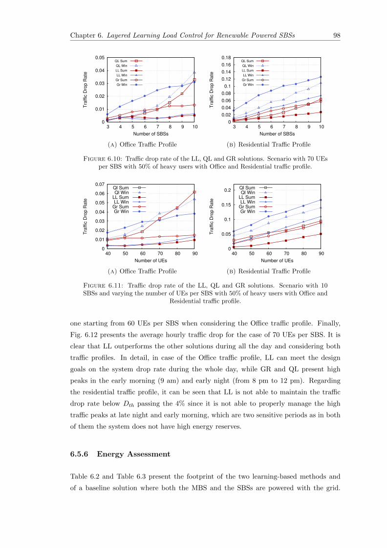
Chapter 6. Layered Learning Load Control for Renewable Powered SBSs 98
0
0.01
0.02
0.03
0.04
0.05
3 4 5 6 7 8 9 10
Tra
ffic
Dro
p R
ate
Number of SBSs
QL Sum
QL Win
LL Sum
LL Win
Gr Sum
Gr Win
(a) Office Traffic Profile
0
0.02
0.04
0.06
0.08
0.1
0.12
0.14
0.16
0.18
3 4 5 6 7 8 9 10
Tra
ffic
Dro
p R
ate
Number of SBSs
QL Sum
QL Win
LL Sum
LL Win
Gr Sum
Gr Win
(b) Residential Traffic Profile
Figure 6.10: Traffic drop rate of the LL, QL and GR solutions. Scenario with 70 UEsper SBS with 50% of heavy users with Office and Residential traffic profile.
0
0.01
0.02
0.03
0.04
0.05
0.06
0.07
40 50 60 70 80 90
Tra
ffic
Dro
p R
ate
Number of UEs
Ql Sum Ql Win
LL Sum LL Win
Gr Sum Gr Win
(a) Office Traffic Profile
0
0.05
0.1
0.15
0.2
40 50 60 70 80 90
Tra
ffic
Dro
p R
ate
Number of UEs
Ql Sum Ql Win
LL Sum LL Win
Gr Sum Gr Win
(b) Residential Traffic Profile
Figure 6.11: Traffic drop rate of the LL, QL and GR solutions. Scenario with 10SBSs and varying the number of UEs per SBS with 50% of heavy users with Office and
Residential traffic profile.
one starting from 60 UEs per SBS when considering the Office traffic profile. Finally,
Fig. 6.12 presents the average hourly traffic drop for the case of 70 UEs per SBS. It is
clear that LL outperforms the other solutions during all the day and considering both
traffic profiles. In detail, in case of the Office traffic profile, LL can meet the design
goals on the system drop rate during the whole day, while GR and QL present high
peaks in the early morning (9 am) and early night (from 8 pm to 12 pm). Regarding
the residential traffic profile, it can be seen that LL is not able to maintain the traffic
drop rate below Dth passing the 4% since it is not able to properly manage the high
traffic peaks at late night and early morning, which are two sensitive periods as in both
of them the system does not have high energy reserves.
6.5.6 Energy Assessment
Table 6.2 and Table 6.3 present the footprint of the two learning-based methods and
of a baseline solution where both the MBS and the SBSs are powered with the grid.

Chapter 6. Layered Learning Load Control for Renewable Powered SBSs 99
0
0.05
0.1
0.15
0.2
0.25
0.3
0.35
5 10 15 20 0
10
20
30
40
50
60
Tra
ffic
Dro
p R
ate
Tra
ffic
[G
B/h
]
Hour [h]
traffic profile
QL Sum
QL Win
LL Sum
LL Win
GR Sum
GR Win
(a) Office Traffic Profile
0
0.1
0.2
0.3
0.4
0.5
0.6
0.7
5 10 15 20 0
10
20
30
40
50
60
Tra
ffic
Dro
p R
ate
Tra
ffic
[G
B/h
]
Hour [h]
traffic profile
QL Sum
QL Win
LL Sum
LL Win
GR Sum
GR Win
(b) Residential Traffic Profile
Figure 6.12: Average hourly traffic drop rate of the LL, QL and greedy solutions.Scenario with 10 SBSs and 70 UEs per SBS with 50% of heavy users with Office and
Residential traffic profile.
In particular, the comparison is performed in terms of grid energy consumption and
carbon dioxide equivalent (CO2e) production for a scenario with 50% of heavy users.
The CO2e has been evaluated by considering the average grid electricity CO2 intensity
of UK in 2016, which corresponds to 320 gCO2eq/kWh [140]. In addition, the column
excess energy reports the values of the harvested energy that cannot be used by the
SBSs nor stored in the batteries, since the harvesting/storage system is dimensioned for
the worst case (i.e., winter).
The learning solutions can reach energy and carbon savings of up to 50% during the
summer, as for the scenarios with 10 SBSs. However, the savings are strongly affected by
the number of SBSs deployed. In fact, for small numbers of SBSs, the energy footprints
of the three methods are closer, and the savings are limited to 20 − 30% for networks
with 5 SBSs. The traffic profile is another important factor that influences the footprint,
since it varies in the total amount of data exchanged in the network and in temporal
dynamics, as discussed in Section 6.5.4. The energy savings for the scenarios with office
traffic profile are in general 10% greater with respect to the ones obtained with the
office traffic profile. The reason behind this fact is that the latter has a peak of traffic
during the night (12 am), which is where the energy reserves are scarce and the learning
solutions differ more with respect to the optimal and rely more on the MBS, as can be
seen in the longer high switch OFF period depicted in Fig. 6.8. Considering the two
learning methods, the amount of traffic delivered influences the behavior of the energy
consumption, as expected. Thus, LL, that drops less traffic, usually consumes more
energy with respect to the QL solution. However, the gap between them is almost null
when considering scenarios with 10 SBSs, which is where QL experiences the highest
drop error rate since it suffers of agents’ coordination problem, as presented in Fig. 6.10.
Finally, looking at the excess energy values in Table 6.2 and Table 6.3, we can appreciate

Chapter 6. Layered Learning Load Control for Renewable Powered SBSs 100
Table 6.2: Energy consumption, carbon dioxide equivalence and exceed energy in thewinter period for a network composed of 5 and 10 SBSs, and 70 UEs per SBS with 50%
of heavy users.
Traffic Solution Energy Used CO2e Excess Energy(kWh) (kg) (kWh)
5 10 5 10 5 10SBSs SBSs SBSs SBSs SBSs SBSs
Off grid 4784 6854 1435 2139 0 0QL 3320 3745 1066 1198 770 1499LL 3324 3647 1064 1167 776 1310
Res grid 4921 7130 1574 2281QL 3634 4180 1163 1338 501 999LL 3854 4200 1233 1344 536 949
Table 6.3: Energy consumption, carbon dioxide equivalence and exceed energy in thesummer period for a network composed of 5 and 10 SBSs, and 70 UEs per SBS with
50% of heavy users.
Traffic Solution Energy Used CO2e Excess Energy(kWh) (kg) (kWh)
5 10 5 10 5 10SBSs SBSs SBSs SBSs SBSs SBSs
Off grid 6871 9713 2199 3108 0 0QL 4584 5184 1455 1659 2662 5295LL 4592 5069 1469 1622 2651 5033
Res grid 6975 10106 2232 3234 0 0QL 4923 5651 1575 1808 3912 6995LL 5188 5647 1660 1807 3941 7892
how the harvested energy process is abundant in summer, where the energy that cannot
be used can be greater than the grid energy used by the system, as in the summer for the
case of 10 SBSs. As for the energy savings, this circumstance occurs with particularly
intensity with the residential traffic profile, that is the scenario in which the learning
algorithms experience more difficulties in optimizing the system. The performance of
QL and LL are similar in this case, expect for the case of summer with 10 SBSs, where
the QL consumes 10% more of harvested energy despite of the fact that is dropping more
traffic. This behavior confirms that LL scales better and is able to use more efficiently
the available energy reserves, i.e., it utilizes less solar energy than QL and delivers more
traffic.
In the light of the above results, future work need to consider enhancements in the
decisions making process for enabling the system to reduce the exceed energy and work
with the same performance under different traffic conditions. Moreover, tolerating an
increment in the complexity of the problem, the exceed energy can be a new variable

Chapter 6. Layered Learning Load Control for Renewable Powered SBSs 101
in an extended optimization problem than can control the process of sharing it with
other network elements, as in a micro-grid scenario, and/or trading it, as done by the
prosumers in the smart grid architecture.
6.6 Concluding Remarks
In this chapter we have presented a comprehensive framework for the management of
two tiers networks with SBS powered with solar power. A Layered Learning approach
to improve the EE of the system while maintaining the performance requirements has
been proposed.
The first layer implements a MRL algorithm for learning the control policies locally
at each SBS. Each agent (SBS) makes autonomous decisions to independently learn
when switching ON/OFF for adapting to the dynamic conditions of the environment, in
terms of energy inflow and traffic demand. Layer 2 is in charge of improving the Layer 1
policies through a MFNN-based solution by considering network-wide parameters and,
in doing this, helping in mitigating the effects of the conflicting behavior of the agents.
The interaction between the two layers is provided by the heuristically accelerated MRL
paradigm.
We compared the policies with respect to an optimal offline solution based on dynamic
programming, obtaining that the behaviors correspond in almost all cases, proving the
fact the online learning can be a viable tool for managing dense network of SBSs. Then,
we analyzed the training phase of both MFNN and MRL algorithms. The latter high-
lighted the improvements obtained thanks the introduction of the proposed LL approach
with respect to a distributed MRL solution. The network performance of the proposed
LL algorithm has been contrasted with respect to the one of a greedy and distributed
MRL solutions. Simulations results show that the proposed solution outperforms the
other ones in terms of throughput and drop rate. The energy savings achieved are
considerable with respect to standard solution where both MBS and SBSs are powered
with the grid, reaching up to the 50%. Moreover, the exceed energy is also abundant,
which opens the door to the possibility of extending the problem for including it in the
optimization framework.
Finally, there are several ways in which this work can be extended. The traffic model
is deterministic due to the lack of models considering the geographical and temporal
statistical distributions. However, HetNet scenarios are characterized for specific spatial
distribution of users (i.e., hotspot) that varies during the day according to the zone
(e.g., residential, office, transportation). The effect of these dynamics in the learning

Chapter 6. Layered Learning Load Control for Renewable Powered SBSs 102
process is important to be evaluated for considering the deployment of this framework
in real networks. The proposed solution has shown some stability problem for network
of very dense SBSs with high traffic. The proposed heuristically accelerated RL together
with the layered learning paradigm represent a good starting point, since they combine
the flexibility of a distributed learning solution with the efficiency of a centralized one.
Further work can be done for a deeper integration between the solutions adopted in the
two layers. The results on the excess energy encourages to integrate its control in the
optimization problem. In fact, the presence of abundant energy perfectly matches with
Demand Response method of the smart grid, where the energy can be either shared
among elements and/or traded with the energy operators.

Chapter 7
Conclusions and Future Work
The trend for the next generation of cellular network, the Fifth Generation (5G), pre-
dicts a 1000x increase in the capacity demand with respect to 4G, which leads to new
infrastructure deployments. In order to deal with this huge demand, one of the most
promising solution is to support macro BSs with small form scale factor BSs, which
helps in improving the spectrum efficiency and provides broadband connection in hot
spot manner. However, this will translate in a important increase in energy consump-
tion. It is estimated that the energy footprint of the whole ICT ecosystem might reach
the 51% of global electricity production by 2030, mainly due to mobile networks and ser-
vices [5]. Consequently, the cost of energy may also become predominant in the OPEX
of a mobile network operator and, cellular communication networks will have greater
ecological impact in the coming years. Therefore, an efficient control of the energy
consumption in 5G networks is not only desirable but essential.
The research community has been paying close attention to the energy efficiency (EE)
of the radio communication networks, with particular emphasis on the dynamic switch
ON/OFF of the base stations (BSs). However, only with the introduction of energy
harvesting (EH) capabilities is possible to enable the needed energy savings, especially in
scenario with dense deployments of SBSs. The objective of this Ph.D thesis is to present
a solid contribution on the control of the SBSs by evaluating online switch ON/OFF
policies based on ML tools. According to the study of the state-of-the-art literature, a
set of new opportunities were identified on the field of online control solution, which has
been recognized as novel topic that enable the optimization of the system considering a
more realistic scenario, i.e., with accurate traffic and energy models.
The adoption of learning methods for the control of SBSs enables a highly adaptive
and autonomous behavior, which is in-line with the paradigms of HetNet and self-
organization of 5G wireless communications. The proposed framework is based on a
103

Chapter 7. Conclusions and Future Work 104
multi-agent RL approach for controlling the SBS together with a Layered Learning
paradigm to simplify the problem by decompose it in subtasks. The technical chapters
of this thesis have hence been focused on the design of learning approaches analyzing
MRL solutions and their extension with LL.
The novelties presented in this Ph.D thesis include not only the development of online
switching ON/OFF algorithm for improving the EE of HetNet, but also, the definition of
a methodology to model the energy inflow of solar panels as a function of time through
stochastic Markov processes. Thus, the frameworks developed have been successfully
applied to investigate realistic scenarios under different environmental conditions, such
as traffic profiles of residential and office areas, and considering the different seasons of
the year for what concern the energy harvesting process.
7.1 Summary of Results
The goal of this thesis is to contribute on making more sustainable the ICT ecosystem,
by focusing on the next generation cellular networks. The focus has been put on the de-
sign and performance analysis and evaluation of new energy-efficient control algorithms
HetNet with energy harvesting capabilities. The thesis is organized into one preliminary
part and three main parts:
• Chapter 1, Chapter 2 and Chapter 3: introducing the problem, the state-of the
art and the theoretical background.
• Chapter 4: presenting the first technical part on an accurate stochastic Markov
processes for the description of the energy scavenged by outdoor solar sources.
• Chapter 5: presenting the second technical part on the definition and analysis of
a control solution for SBSs powered with solar panels based on distributed MRL.
• Chapter 6: presenting the third technical part on the definition and analysis of a
control framework for HetNet with EH capabilities based on LL.
In what follows, the contributions and conclusions of the three main technical parts are
summarized.
7.1.1 Modeling Solar Sources through Stochastic Markov Processes
The research work presented in this Ph.D. thesis started by presenting a methodology to
derive simple and accurate stochastic Markov processes for the description of the energy
Chapter 7. Conclusions and Future Work 105
scavenged by outdoor solar sources. The proposed models are especially useful for the
theoretical investigation and the simulation of energetically self-sufficient communication
systems that include these devices. In fact, a large body of work has been published
so far to mathematically analyze these facts considering deterministic, independent and
identically distributed across time slots or time-correlated Markov models, which do not
guarantee to estimate the effectiveness of the proposed strategies in realistic scenarios.
The Markov models that we derived in this paper are obtained from extensive solar
radiation databases, that are widely available online. Basically, from hourly radiance
patterns, we derive the corresponding amount of energy (current and voltage) that is
accumulated over time, and we finally use it to represent the scavenged energy in terms
of its relevant statistics. Toward this end, two clustering approaches for the raw radiance
data are described and the resulting Markov models are compared against the empirical
distributions. Our results indicate that Markov models with just two states provide a
rough characterization of the real data traces. While these could be sufficiently accurate
for certain applications, slightly increasing the number of states to, e.g., eight, allows
the representation of the real energy inflow process with an excellent level of accuracy
in terms of first and second order statistics.
7.1.2 EH HetNet Control through Distributed Q-Learning
The massive deployment of SBS represents one of the most promising solutions adopted
by 5G cellular networks to meet the foreseen huge traffic demand. The high number of
network elements entails a significant increase in the energy consumption suggesting the
usage of renewable energies for powering the SBSs for reducing both the environmental
impact of mobile networks and enabling cost saving on operators’ electric bills. In this
work, we proposed an ON/OFF switching algorithm, based on reinforcement learning,
that autonomously learns energy income and traffic demand patterns. The algorithm
is based on distributed multi-agent Q-learning for jointly optimizing the system perfor-
mance and the self-sustainability of the SBSs. We analyze the algorithm by assessing its
convergence time, characterizing the obtained ON/OFF policies, and evaluating an of-
fline trained variant. Simulation results demonstrate that our solution is able to increase
the energy efficiency of the system with respect to simpler approaches. Moreover, the
proposed method provides an harvested energy surplus, which can be used by mobile
operators to offer ancillary services to the smart electricity grid. Nevertheless, there are
various aspects that need to be further investigated. First, we would like to enhance the
decisions made by the SBSs so that they will cooperatively compute optimal policies
accounting for common (and global) performance objectives. Note that in the current
algorithm this cooperation is only marginally achieved through the use of the global
Chapter 7. Conclusions and Future Work 106
drop rate in the reward functions that are locally computed by the SBSs. Finally, we
need to explore more scenarios considering different traffic profiles with different traffic
demands for studying the behavior of the algorithm in more 5G operative cases.
7.1.3 EH HetNet Control through Layered Learning
In the last part of this Ph.D. thesis, we investigated techniques based on Layered Learn-
ing for the Radio Resource Management of dense cellular networks with SBSs powered
solely by renewable energy. The goal of the proposed solution is to improve the system
scalability, which has been demonstrated to be an issue in MRL system. In the first
layer, reinforcement learning agents locally select switch ON/OFF policies of the SBSs
according to the energy income and the traffic demand based on a heuristically acceler-
ated RL paradigm similar to the one defined in Chapter 5. The second layer relies on
an Artificial Neural Network that estimates the network load conditions to implement a
centralized controller enforcing local agent decisions. The proposed framework has been
compared with an optimal bound obtained offline based on dynamic programming. The
resulting learned behavior of the SBSs matches quite well the optimal one, except in
extreme cases as for high load with residential traffic profile. Simulation results prove
that the proposed layered framework outperforms both a greedy and a completely dis-
tributed solution like the one presented in Chapter 5 both in terms of throughput and
energy efficiency under various conditions and with different traffic demand profiles.
7.2 Future Work
The road toward the sustainability of wireless networks represents one of the main
challenges for the future. This Ph.D dissertation aimed at starting the investigation on
some open topics that have not been covered in the state-of-the-art, and some others
have been identified through the course of the thesis. In the light of the conclusions
presented above, multiple research lines have been left open for future work. In what
follows, we summarize the most important ones.
7.2.1 Realistic Models of the Network Environment
In Chapter 4 we presented an accurate Markov model for the harvested energy by solar
panels. The model is accurate and allows to have realistic energy harvesting profiles
for different cities of US. However, such model is difficult to reproduce for other cities
in the world and, nowadays, even for the same cities it has been developed. In fact,

Chapter 7. Conclusions and Future Work 107
in order to maintain it flexibility in defining the solar panel type, it needs information
like extraterrestrial radiation, dry-bulb temperature and of the dew point temperature
which are not easily to find in the free available data-bases. Moreover, in order to have a
good statistical confidence, the data set should span over several years, which is usually
another constraint of the open data-bases. Future work includes to find a more simple
methodologies to retrieve accurate model for the solar harvested energy and, possibly,
also for other renewable energies source type. For example, clusterization and feature
extraction methods represent tools that are suitable for solving this kind of problem.
The issues faced for the RES energy models are even more important for what concern
the traffic demand ones. In fact, the models we adopted in the work carried out in
this thesis, despite of proving a realistic representation of the real phenomenon, do not
provide any specification on the geographical and temporal statistical distributions. In
fact, HetNet scenarios are characterized for specific spatial distribution of users (i.e.,
hotspot) that varies during the day according to the zone (e.g., residential, office, trans-
portation). The model in literature do not provide any reference to this respect. All
the models define only the temporal variations of the total amount of traffic requested
per hour basis. Therefore, it is impossible to reproduce realistic scenarios in which the
traffic profiles have specific distributions for both the time and the space, instead of a
deterministic value. In literature, the common solution is to make assumption on the
spatial distribution and analyze the different profiles separately, has been done in this
thesis. Further investigations to fill this gap remain a future work. Some preliminary
work have been already performed on this field. For instance, in [141] an LTE sniffer ca-
pable of decoding the unencrypted LTE Physical Downlink Control Channel (PDCCH)
has been used for analyzing the temporal and spatial analysis of the recorded traces and
deriving the stochastic characterization for the daily-varying LTE traffic. However, the
process of retrieving the needed data is long and, at the time of this writing, the model
is limited only to a few cases.
7.2.2 Characterization of the RL based solutions
One of most important problem when using learning solutions in multi-agent systems is
the duration of the training phase and the convergence to the point of equilibrium. As
highlighted in chapter 6, the proposed solutions have still margin for improvement for
both aspects.
The duration of the training is important in real network for enabling the rapid de-
ployment of new SBSs and allowing the network to rapidly reconfigure and adapting to

Chapter 7. Conclusions and Future Work 108
the new architecture. The offline training has been investigated in this thesis provid-
ing interesting results. However, it is not always possible to simulate offline a specific
change in the network deployment. Therefore, solutions like transfer learning have to
evaluated. Regarding the convergence, ML literature offers different algorithms that
can find interesting solutions (e.g., NashQ [142] or DynaQ [28]). However, the space
of possible solutions becomes too big, making unfeasible it usage in real network due
to the increased time of training. Therefore, future work has to consider more research
on multi-agent systems. The proposed heuristically accelerated RL together with the
layered learning paradigm represent a good starting point, since they combine the flexi-
bility of a distributed learning solution with the efficiency of a centralized one. Further
work can be done for a deeper integration between the solutions adopted in the two
layers. For example, the centralized controller can take directly part of the single SBS
control process, by estimating the SBSs behavior in a more detail fashion. For instance
deep learning and deep neural networks can be an interesting solution to exploit thanks
to their abilities in predicting the relation among different patterns, in this case the ones
of the energy income and the traffic demand.
The solutions proposed in Chapter 5 and Chapter 6 have been presented from a dis-
tributed perspective, for highlighting the advantages that these methods have in the
problem studied. However, a comparison with the optimal bound has been carried out
only partially, due to complexity of the problem. This aspect is important for having
a quantitative evaluation of the gap of the learning solution with respect to the opti-
mum. In fact, considering all the dynamics of system, it is impossible that the learning
solutions found the optimal, as it is demonstrated in Chapter 6. Similarly, a compar-
ison with a centralized solution is needed to quantify the gap of distributed solutions
with respect to the centralized ones. In fact, centralized solution typically have better
performance provided that they have complete knowledge of the system. This, in turns,
translates in a high complexity due to the higher signaling and dimension of the problem.
The centralized approach is of particular interest when considering the SDN/NFV-like
approach, where, thanks to the SDN framework, the network can provide a large num-
ber of parameter in data centers. In addition, the layered learning paradigm can be a
valuable architecture for distributed NFV approaches [143], where virtualized functions
should be located where they are the most effective and least expensive. To this respect,
future work included the development of more lightweight models for finding the optimal
solution and the evaluation of centralized and distributed NFV-like solutions.

Chapter 7. Conclusions and Future Work 109
7.2.3 Integration with Smart Grids
The huge energy consumption estimation of mobile networks for the next future encour-
age their integration with the upcoming smart grid architectures. In fact, as showed in
Chapter 5 and Chapter 6, the HetNet with EH capabilities can become a prosumer and
share or trade the energy during the day, according to the energy incomes.
In case of sharing, the SBSs can either help other SBSs when running out of energy or
provide energy to ancillary services. In this respect, Energy Packet Networks (EPN)
are envisaged to be an interesting solution to be further explored for energy transfer
among network nodes. In an EPN, discrete units of energy, termed energy packets, can
be exchanged among network elements of the micro-grid.
Trading is a solution of the Demand Response (DR) family that aimed at helping in
solving the problem of managing the peaks of energy demand in the smart grid, namely
Demand-Side Management (DSM). As we introduced in [80], this solution will be inter-
esting when a proper pricing schemes will be in place, which should incentivize BSs to
sell their excess energy, while also making these transactions convenient for the electric-
ity grid. In the next future, the energy price will depend on the cost of production and
on the expected demand. In this scenario, future work can evaluate decision-making
solutions to find the best energy-purchasing policies for the BSs taking into account: (i)
current and forecast renewable energy income, (ii) current and forecast traffic load and
(iii) the future evolution of the energy prices. In this scenario, BSs act as prosumers of
the smart grids.

Bibliography
[1] EARTH: Energy Aware Radio and neTwork tecHnologies. D2.3: Energy efficiency
analysis of the reference systems, areas of improvements and target breakdown.
Project Deliverable D2.3, www.ict-earth.eu, 2010.
[2] Cisco Systems Inc. Cisco Visual Networking Index: Global Mobile Data Traffic
Forecast Update, 2016 – 2021. White Paper, http://www.cisco.com/, February
2017.
[3] M. P. Mills. The Cloud Begins with Coal: Big Data, Big Networks, Big Infras-
tructure, and Big Power. Digital Power Group, August 2013.
[4] Ward Van Heddeghem, Sofie Lambert, Bart Lannoo, Didier Colle, Mario Pickavet,
and Piet Demeester. Trends in worldwide ict electricity consumption from 2007 to
2012. Computer Communications, 50:64 – 76, 2014. ISSN 0140-3664. doi: https://
doi.org/10.1016/j.comcom.2014.02.008. URL http://www.sciencedirect.com/
science/article/pii/S0140366414000619. Green Networking.
[5] Anders S. G. Andrae and Tomas Edler. On global electricity usage of communi-
cation technology: Trends to 2030. Challenges, 6(1):117, 2015.
[6] Albrecht Fehske, J. Malmodin, G. Biczok, and Gerhard Fettweis. The Global
Footprint of Mobile Communications: The Ecological and Economic Perspective.
IEEE Communications Magazine, issue on Green Communications, 49(8):55–62,
August 2011. ISSN 0163-6804. doi: 10.1109/MCOM.2011.5978416.
[7] Ericsson. 5G radio access: research and vision. White Paper, available on-line.
[8] Nokia Solutions Networks. Looking ahead to 5G. White Paper, http://nsn.com/
innovative-thinking/technology-vision.
[9] ETSI. ES 203 208; Environmental Engineering (EE); Assessment of mobile net-
work energy efficiency (v1.2.1), 2017.
[10] 3GPP. TR 21.866.; Study on Energy Efficiency Aspects of 3GPP Standards
(Rel.14), 2017.
110
Bibliography 111
[11] European Council 23 and 24 October 2014 conclusions. 2030 climate and energy
policy framework for the European Union. White Paper, available on-line.
[12] Z. Hasan, H. Boostanimehr, and V.K. Bhargava. Green cellular networks: A
survey, some research issues and challenges. Communications Surveys Tutorials,
IEEE, 13(4):524–540, Fourth 2011.
[13] F. Han, S. Zhao, L. Zhang, and J. Wu. Survey of Strategies for Switching Off
Base Stations in Heterogeneous Networks for Greener 5G Systems. IEEE Access,
4:4959–4973, August 2016. ISSN 2169-3536. doi: 10.1109/ACCESS.2016.2598813.
[14] E. Palm, F. Heden, and A. Zanma. Solar powered mobile telephony. In Proc. of
EcoDesign, Second International Symposium on Environmentally Conscious De-
sign and Inverse Manufacturing, pages 219 –222, Tokyo, Japan, Dec. 2001.
[15] B. Lindemark and G. Oberg. Solar power for radio base station (RBS) sites appli-
cations including system dimensioning, cell planning and operation. In Proc. of Int.
Telecommunications Energy Conference, INTELEC, pages 587 –590, Edinburgh,
UK, Oct. 2001.
[16] David Lopez-Perez, Ming Ding, Holger Claussen, and Amir H Jafari. Towards 1
Gbps/UE in cellular systems: Understanding ultra-dense small cell deployments.
IEEE Communications Surveys & Tutorials, 17(4):2078–2101, June 2015. ISSN
1553-877X. doi: 10.1109/COMST.2015.2439636.
[17] G. Auer, V. Giannini, C. Desset, I. Godor, P. Skillermark, M. Olsson, M.A. Imran,
D. Sabella, M.J. Gonzalez, O. Blume, and A. Fehske. How much energy is needed
to run a wireless network? IEEE Wireless Communications, 18(5):40–49, October
2011.
[18] P. Dini, M. Miozzo, N. Bui, and N. Baldo. A model to analyze the energy savings
of base station sleep mode in lte hetnets. In Green Computing and Communica-
tions (GreenCom), 2013 IEEE and Internet of Things (iThings/CPSCom), IEEE
International Conference on and IEEE Cyber, Physical and Social Computing,
pages 1375–1380, Aug 2013.
[19] Giuseppe Piro, Marco Miozzo, Giuseppe Forte, Nicola Baldo, Luigi Alfredo Grieco,
Gennaro Boggia, and Paolo Dini. HetNets Powered by Renewable Energy Sources.
IEEE Internet Computing, 17(1):32–39, 2013.
[20] A. G. Tsikalakis and N. D. Hatziargyriou. Centralized control for optimizing
microgrids operation. In 2011 IEEE Power and Energy Society General Meeting,
pages 1–8, July 2011. doi: 10.1109/PES.2011.6039737.

Bibliography 112
[21] M. Miozzo, D. Zordan, P. Dini, and M. Rossi. SolarStat: Modeling Photovoltaic
Sources through Stochastic Markov Processes. In IEEE Energy Conference (EN-
ERGYCON), Dubrovnik, Croatia, May 2014.
[22] Open Networking Foundation. Software-Defined Networking: The New Norm for
Networks. ONF White Paper, 2:2–6, April 2012.
[23] Yong Li and Min Chen. Software-Defined Network Function Virtualization: A
Survey. IEEE Access, 3:2542–2553, December 2015. ISSN 2169-3536. doi: 10.
1109/ACCESS.2015.2499271.
[24] M. Y. Arslan, K. Sundaresan, and S. Rangarajan. Software-defined networking in
cellular radio access networks: potential and challenges. IEEE Communications
Magazine, 53(1):150–156, January 2015. ISSN 0163-6804. doi: 10.1109/MCOM.
2015.7010528.
[25] J. Perez-Romero, O. Sallent, R. Ferrus, and R. Agustı. Knowledge-based 5g radio
access network planning and optimization. In 2016 International Symposium on
Wireless Communication Systems (ISWCS), pages 359–365, Sept 2016. doi: 10.
1109/ISWCS.2016.7600929.
[26] J. Hoydis, M. Kobayashi, and M. Debbah. Green Small-Cell Networks: A Cost-
and Energy-Efficient Way of Meeting the Future Traffic Demands . IEEE Veh.
Technol. Mag., Mar. 2011.
[27] K. P. Sycara. Multiagent systems. AI Magazine, 19(2):79–92, 1998.
[28] R. S. Sutton and A. G. Barto. Reinforcement Learning: An Introduction. MIT
Press, 1998.
[29] Peter Stone and Manuela Veloso. Using decision tree confidence factors for multi-
agent control, pages 99–111. Springer Berlin Heidelberg, Berlin, Heidelberg, 1998.
[30] R. A. C. Bianchi, M. F. Martins, C. H. C. Ribeiro, and A. H. R. Costa.
Heuristically-accelerated multiagent reinforcement learning. IEEE Transactions
on Cybernetics, 44(2):252–265, Feb 2014. ISSN 2168-2267. doi: 10.1109/TCYB.
2013.2253094.
[31] M. H. Alsharif, R. Nordin, and M. Ismail. Survey of green radio communications
networks: Techniques and recent advances. Journal of Computer Networks and
Communications, 2013:13, 2013.
[32] EARTH (Energy Aware Radio and neTwork tecHnologies). EU Funded Research
Project FP7-ICT-2009-4-247733-EARTH, Jan. 2010 - Jun. 2012. https://www.
ict-earth.eu.
Bibliography 113
[33] Dario Sabella, Damiano Rapone, Maurizio Fodrini, Cicek Cavdar, Magnus Ols-
son, Pal Frenger, and Sibel Tombaz. Energy Management in Mobile Networks
Towards 5G, pages 397–427. Springer International Publishing, 2016. doi:
10.1007/978-3-319-27568-0 17.
[34] C-RAN: the road towards green RAN. China Mobile Research Institute, White
Paper, 2011.
[35] NEC. NFV C-RAN for Efficient RAN Resource Allocation. http://www.nec.
com/en/global/solutions/nsp/sc2/doc/wp_c-ran.pdf. Online White Paper;
accessed on March 16, 2016.
[36] Small Cell Forum. Virtualization for small cells: overview. White Paper (available
on-line, 2015.
[37] C. Desset, B. Debaillie, V. Giannini, A. Fehske, G. Auer, H. Holtkamp, W. Wajda,
D. Sabella, F. Richter, M. J. Gonzalez, H. Klessig, I. Godor, M. Olsson, M. A.
Imran, A. Ambrosy, and O. Blume. Flexible power modeling of LTE base stations.
In 2012 IEEE Wireless Communications and Networking Conference (WCNC),
pages 2858–2862, April 2012. doi: 10.1109/WCNC.2012.6214289.
[38] N. Bartzoudis, O. Font-Bach, M. Miozzo, C. Donato, P. Harbanau, M. Requena,
D. Lopez, I. Ucar, A. A. Salona, P. Serrano, J. Mangues, and M. Payaro. Energy
footprint reduction in 5g reconfigurable hotspots via function partitioning and
bandwidth adaptation. In 2017 Fifth International Workshop on Cloud Technolo-
gies and Energy Efficiency in Mobile Communication Networks (CLEEN), pages
1–6, June 2017. doi: 10.23919/CLEEN.2017.8045934.
[39] M. Miozzo, N. Bartzoudis, M. Requena, O. Font-Bach, P. Harbanau, D. Lopez-
Bueno, M. Payaro, and J. Mangues. Sdr and nfv extensions in the ns-3 lte module
for 5g rapid prototyping. In 2018 IEEE Wireless Communications and Networking
Conference (WCNC), April 2018.
[40] Nicola Baldo, Marco Miozzo, Manuel Requena-Esteso, and Jaume Nin-Guerrero.
An open source product-oriented lte network simulator based on ns-3. In Proceed-
ings of the 14th ACM International Conference on Modeling, Analysis and Sim-
ulation of Wireless and Mobile Systems, MSWiM ’11, pages 293–298, New York,
NY, USA, 2011. ACM. ISBN 978-1-4503-0898-4. doi: 10.1145/2068897.2068948.
URL http://doi.acm.org/10.1145/2068897.2068948.
[41] Hong Zhang, Jun Cai, and Xiaolong Li. Energy-efficient base station control with
dynamic clustering in cellular network. In IEEE International Conference on

Bibliography 114
Communications and Networking (CHINACOM), pages 384–388, Guilin, China,
August 2013. doi: 10.1109/ChinaCom.2013.6694626.
[42] Sumudu Samarakoon, Mehdi Bennis, Walid Saad, and Matti Latva-aho. Dynamic
Clustering and ON/OFF Strategies for Wireless Small Cell Networks. IEEE Trans-
actions on Wireless Communications, 15(3):2164–2178, March 2016. ISSN 1536-
1276. doi: 10.1109/TWC.2015.2499182.
[43] Shijie Cai, Limin Xiao, Haibin Yang, Jing Wang, and Shidong Zhou. A cross-
layer optimization of the joint macro and picocell deployment with sleep mode for
green communications. In IEEE Wireless and Optical Communication Conference
(WOCC), pages 225–230, Chongqing, China, May 2013. doi: 10.1109/WOCC.
2013.6676373.
[44] Yutao Zhu, Zhimin Zeng, Tiankui Zhang, and Dantong Liu. A QoS-Aware Adap-
tive Access Point Sleeping in Relay Cellular Networks for Energy Efficiency. In
IEEE Vehicular Technology Conference (VTC Spring), pages 1–5, Seoul, Korea,
May 2014. doi: 10.1109/VTCSpring.2014.7023152.
[45] Ran Tao, Jie Zhang, and Xiaoli Chu. An Energy Saving Small Cell Sleeping
Mechanism with Cell Expansion in Heterogeneous Networks. In IEEE Vehicular
Technology Conference (VTC Spring), pages 1–5, Porto, Portugal, May 2016. doi:
10.1109/VTCSpring.2016.7504126.
[46] Alexandra Bousia, Elli Kartsakli, Luis Alonso, and Christos Verikoukis. Energy
efficient base station maximization switch off scheme for LTE-advanced. In IEEE
International Workshop on Computer Aided Modeling and Design of Communica-
tion Links and Networks (CAMAD), pages 256–260, Barcelona, Spain, September
2012. doi: 10.1109/CAMAD.2012.6335345.
[47] Hakim Ghazzai, Muhammad Junaid Farooq, Ahmad Alsharoa, Elias Yaacoub, Ab-
dullah Kadri, and Mohamed-Slim Alouini. Green Networking in Cellular HetNets:
A Unified Radio Resource Management Framework With Base Station ON/OFF
Switching. IEEE Transactions on Vehicular Technology, 66(7):5879–5893, July
2017. ISSN 0018-9545. doi: 10.1109/TVT.2016.2636455.
[48] Yuan Yuan and Ping Gong. A QoE-orientated base station sleeping strategy for
multi-services in cellular networks. In International Conference on Wireless Com-
munications & Signal Processing (WCSP), pages 1–5, Nanjing, China, October
2015. doi: 10.1109/WCSP.2015.7341051.
[49] Feng Han, Zoltan Safar, and KJ Ray Liu. Energy-efficient base-station cooperative
operation with guaranteed QoS. IEEE Transactions on Communications, 61(8):

Bibliography 115
3505–3517, August 2013. ISSN 0090-6778. doi: 10.1109/TCOMM.2013.061913.
120743.
[50] Ying Wang, Yuan Zhang, Yongce Chen, and Rong Wei. Energy-efficient de-
sign of two-tier femtocell networks. EURASIP Journal on Wireless Commu-
nications and Networking, 2015(1):1, February 2015. ISSN 1687-1499. doi:
10.1186/s13638-015-0242-4.
[51] Anqi He, Dantong Liu, Yue Chen, and Tiankui Zhang. Stochastic geometry anal-
ysis of energy efficiency in HetNets with combined CoMP and BS sleeping. In
IEEE Annual International Symposium on Personal, Indoor, and Mobile Radio
Communication (PIMRC), pages 1798–1802, Washington DC, USA, September
2014. doi: 10.1109/PIMRC.2014.7136461.
[52] Yong Sheng Soh, Tony QS Quek, Marios Kountouris, and Hyundong Shin. Energy
Efficient Heterogeneous Cellular Networks. IEEE Journal on Selected Areas in
Communications, 31(5):840–850, May 2013. ISSN 0733-8716. doi: 10.1109/JSAC.
2013.130503.
[53] A. Bousia, A. Antonopoulos, L. Alonso, and C. Verikoukis. Green distance-
aware base station sleeping algorithm in LTE-Advanced. In IEEE Interna-
tional Conference on Communications (ICC), pages 1347–1351, June 2012. doi:
10.1109/ICC.2012.6364240.
[54] Hina Tabassum, Uzma Siddique, Ekram Hossain, and Md Jahangir Hossain.
Downlink performance of cellular systems with base station sleeping, user associ-
ation, and scheduling. IEEE Transactions on Wireless Communications, 13(10):
5752–5767, October 2014. ISSN 1536-1276. doi: 10.1109/TWC.2014.2336249.
[55] Chang Liu, Yi Wan, Lin Tian, Yiqing Zhou, and Jinglin Shi. Base Station Sleeping
Control with Energy-Stability Tradeoff in Centralized Radio Access Networks. In
IEEE Global Communications Conference (GLOBECOM), pages 1–6, San Diego,
CA, USA, Dec 2015. doi: 10.1109/GLOCOM.2015.7417363.
[56] D. Tsilimantos, J.-M. Gorce, and E. Altman. Stochastic analysis of energy savings
with sleep mode in ofdma wireless networks. In INFOCOM, 2013 Proceedings
IEEE, pages 1097–1105, April 2013.
[57] Y. S. Soh, T. Q.S. Quek, M. Kountouris, and H. Shin. Energy efficient heteroge-
neous cellular networks. Selected Areas in Communications, IEEE Journal on, 31
(5):840–850, 2013.

Bibliography 116
[58] K. Samdanis, T. Taleb, D. Kutscher, and M. Brunner. Self organized network
management functions for energy efficient cellular urban infrastructures. Mob.
Netw. Appl., 17(1):119–131, February 2012. ISSN 1383-469X.
[59] E. Oh, K. Son, and B. Krishnamachari. Dynamic base station switching-on/off
strategies for green cellular networks. Wireless Communications, IEEE Transac-
tions on, 12(5):2126–2136, 2013.
[60] R. Li, Z. Zhao, X. Chen, and H. Zhang. Energy saving through a learning frame-
work in greener cellular radio access networks. In Global Communications Con-
ference (GLOBECOM), 2012 IEEE, pages 1556–1561, 2012.
[61] Khaled Al Haj Ismaiil, Bachir Assaf, Milad Ghantous, and Michel Nahas. Reduc-
ing power consumption of cellular networks by using various cell types and cell
zooming. In International Conference on e-Technologies and Networks for Devel-
opment (ICeND), pages 33–38, Beirut, Lebanon, April 2014. doi: 10.1109/ICeND.
2014.6991188.
[62] Zhisheng Niu, Yiqun Wu, Jie Gong, and Zexi Yang. Cell zooming for cost-efficient
green cellular networks. IEEE Communications Magazine, 48(11):74–79, Novem-
ber 2010. ISSN 0163-6804. doi: 10.1109/MCOM.2010.5621970.
[63] Long Bao Le. QoS-aware BS switching and cell zooming design for OFDMA green
cellular networks. In IEEE Global Communications Conference (GLOBECOM),
pages 1544–1549, Anaheim, CA, USA, December 2012. doi: 10.1109/GLOCOM.
2012.6503333.
[64] Xiaodong Xu, Chunjing Yuan, Wenwan Chen, Xiaofeng Tao, and Yan Sun. Adap-
tive Cell Zooming and Sleeping for Green Heterogeneous Ultra-Dense Networks.
IEEE Transactions on Vehicular Technology, 2017. doi: 10.1109/TVT.2017.
2749058.
[65] Zujie Hu, Yifei Wei, Xiaojuan Wang, and Mei Song. Green relay station assisted
cell zooming scheme for cellular networks. In International Conference on Natu-
ral Computation, Fuzzy Systems and Knowledge Discovery (ICNC-FSKD), pages
2030–2035, Changsha, China, August 2016. doi: 10.1109/FSKD.2016.7603493.
[66] Yutao Zhu, Tian Kang, Tiankui Zhang, and Zhimin Zeng. QoS-aware user as-
sociation based on cell zooming for energy efficiency in cellular networks. In
IEEE International Symposium on Personal, Indoor and Mobile Radio Commu-
nications (PIMRC Workshops), pages 6–10, London, UK, September 2013. doi:
10.1109/PIMRCW.2013.6707826.

Bibliography 117
[67] Gencer Cili, Halim Yanikomeroglu, and F Richard Yu. Cell switch off tech-
nique combined with coordinated multi-point (CoMP) transmission for energy
efficiency in beyond-LTE cellular networks. In IEEE International Conference
on Communications (ICC), pages 5931–5935, Ottawa, Canada, June 2012. doi:
10.1109/ICC.2012.6364869.
[68] L.A. Suarez, L. Nuaymi, and J. Bonnin. Energy performance of a distributed
bs based green cell breathing algorithm. In Wireless Communication Systems
(ISWCS), 2012 International Symposium on, pages 341–345, 2012.
[69] H.S. Dhillon, R.K. Ganti, F. Baccelli, and J.G. Andrews. Modeling and analysis
of k-tier downlink heterogeneous cellular networks. Selected Areas in Communi-
cations, IEEE Journal on, 30(3):550–560, 2012.
[70] S. Cho and W. Choi. Energy-efficient repulsive cell activation for heterogeneous
cellular networks. Selected Areas in Communications, IEEE Journal on, 31(5):
870–882, 2013.
[71] L. Saker, S-E Elayoubi, R. Combes, and T. Chahed. Optimal control of wake up
mechanisms of femtocells in heterogeneous networks. Selected Areas in Commu-
nications, IEEE Journal on, 30(3):664–672, 2012.
[72] I-Hong Hou and Chung Shue Chen. An energy-aware protocol for self-organizing
heterogeneous lte systems. Selected Areas in Communications, IEEE Journal on,
31(5):937–946, 2013.
[73] S. Samarakoon, M. Bennis, W. Saad, and M. Latva-aho. Opportunistic sleep mode
strategies in wireless small cell networks. In Communications (ICC), 2014 IEEE
International Conference on, pages 2707–2712, June 2014.
[74] Chenlong Jia and Teng Joon Lim. Resource partitioning and user association with
sleep-mode base stations in heterogeneous cellular networks. IEEE Transactions
on Wireless Communications, 14(7):3780–3793, July 2015. ISSN 1536-1276. doi:
10.1109/TWC.2015.2411737.
[75] Yutao Zhu, Zhimin Zeng, Tiankui Zhang, Lu An, and Lin Xiao. An energy efficient
user association scheme based on cell sleeping in LTE heterogeneous networks.
In International Symposium on Wireless Personal Multimedia Communications
(WPMC), pages 75–79, Sydney, Australia, September 2014. doi: 10.1109/WPMC.
2014.7014794.
[76] M.A. Marsan, S. Buzzi, D. Ciullo, and M. Meo. Multiple daily base station switch-
offs in cellular networks. In Communications and Electronics (ICCE), 2012 Fourth
International Conference on, pages 245–250, 2012.

Bibliography 118
[77] H. Al Haj Hassan, L. Nuaymi, and A Pelov. Renewable energy in cellular networks:
A survey. In Online Conference on Green Communications (GreenCom), 2013
IEEE, pages 1–7, Oct 2013.
[78] J. Xu, L. Duan, and R. Zhang. Cost-aware green cellular networks with energy
and communication cooperation. IEEE Communications Magazine, 53(5):257–263,
May 2015. ISSN 0163-6804. doi: 10.1109/MCOM.2015.7105673.
[79] G. Piro, M. Miozzo, G. Forte, N. Baldo, L.A. Grieco, G. Boggia, and P. Dini.
Hetnets powered by renewable energy sources: Sustainable next-generation cellular
networks. Internet Computing, IEEE, 17(1):32–39, 2013.
[80] Davide Zordan, Marco Miozzo, Paolo Dini, and Michele Rossi. When telecommu-
nications networks meet energy grids: Cellular networks with energy harvesting
and trading capabilities. IEEE Communications Magazine, 53(6):117–123, June
2015. ISSN 0163-6804. doi: 10.1109/MCOM.2015.7120026.
[81] NREL, National Renewable Energy Laboratory. Renewable Resource Data Center.
http://www.nrel.gov/rredc/, .
[82] NREL, National Renewable Energy Laboratory. Best Research-Cell Efficiencies.
http://www.nrel.gov/ncpv/images/efficiency_chart.jpg, .
[83] Bloomerg New Energy Finance. World Energy Perspective – The Cost of Energy
Technologies. World Energy Council’s White Paper, http://about.bnef.com,
October 2013.
[84] H.S. Dhillon, Ying Li, P. Nuggehalli, Zhouyue Pi, and J.G. Andrews. Fundamen-
tals of heterogeneous cellular networks with energy harvesting. Wireless Commu-
nications, IEEE Transactions on, 13(5):2782–2797, May 2014.
[85] H.S. Dhillon, R.K. Ganti, and J.G. Andrews. A tractable framework for cover-
age and outage in heterogeneous cellular networks. In Information Theory and
Applications Workshop (ITA), 2011, pages 1–6, Feb 2011.
[86] D. Valerdi, Qiang Zhu, K. Exadaktylos, Suhua Xia, M. Arranz, Rui Liu, and
D. Xu. Intelligent energy managed service for green base stations. In GLOBECOM
Workshops (GC Wkshps), 2010 IEEE, pages 1453–1457, Dec 2010.
[87] T. Han and N. Ansari. On greening cellular networks via multicell cooperation.
Wireless Communications, IEEE, 20(1):82–89, 2013.
[88] Y.K. Chia, S. Sun, and R. Zhang. Energy cooperation in cellular networks with
renewable powered base stations. In Wireless Communications and Networking
Conference (WCNC), 2013 IEEE, pages 2542–2547, April 2013.

Bibliography 119
[89] M.A. Marsan, G. Bucalo, A. Di Caro, M. Meo, and Yi Zhang. Towards zero grid
electricity networking: Powering bss with renewable energy sources. In Communi-
cations Workshops (ICC), 2013 IEEE International Conference on, pages 596–601,
June 2013.
[90] National Renewable Energy Laboratory (NREL). PVWatts Simulator. http:
//rredc.nrel.gov/solar/calculators/pvwatts/version1/.
[91] G. Lee, W. Saad, M. Bennis, A. Mehbodniya, and F. Adachi. Online Ski Rental
for ON/OFF Scheduling of Energy Harvesting Base Stations. IEEE Transactions
on Wireless Communications, 16(5):2976–2990, May 2017. ISSN 1536-1276. doi:
10.1109/TWC.2017.2672964.
[92] M. Mendil, A. De Domenico, V. Heiries, R. Caire, and N. Hadj-said. Fuzzy Q-
Learning based energy management of small cells powered by the smart grid.
In 2016 IEEE 27th Annual International Symposium on Personal, Indoor, and
Mobile Radio Communications (PIMRC), pages 1–6, Valencia, Spain, September
2016. doi: 10.1109/PIMRC.2016.7794880.
[93] Nicola Piovesan and Paolo Dini. Optimal direct load control of renewable powered
small cells: A shortest path approach. Internet Technology Letters, pages e7–n/a,
2017. ISSN 2476-1508. doi: 10.1002/itl2.7. e7.
[94] A. P. Couto da Silva, D. Renga, M. Meo, and M. Ajmone Marsan. The impact of
quantization on the design of solar power systems for cellular base stations. IEEE
Transactions on Green Communications and Networking, 2(1):260–274, March
2018. doi: 10.1109/TGCN.2017.2762402.
[95] N. Baldo, P. Dini, J. Mangues, M. Miozzo, and J. Nunez. Small cells, wireless back-
haul and renewable energy: a solution for disaster aftermath communications. In
4th International Conference on Cognitive Radio and Advanced Spectrum Man-
agement (COGART 2011), Barcelona, Spain, October 2011.
[96] W. Guo, S. Wang, C. Turyagyenda, and T. O’Farrell. Integrated cross-layer energy
savings in a smart and flexible cellular network. In Communications in China
Workshops (ICCC), 2012 1st IEEE International Conference on, pages 79–84,
2012.
[97] A. Galindo-Serrano and L. Giupponi. Downlink femto-to-macro interference man-
agement based on fuzzy q-learning. In Modeling and Optimization in Mobile, Ad
Hoc and Wireless Networks (WiOpt), 2011 International Symposium on, pages
412–417, May 2011.

Bibliography 120
[98] Lorenza Giupponi, Ana M. Galindo-Serrano, and Mischa Dohler. From cognition
to docition: The teaching radio paradigm for distributed & autonomous deploy-
ments. Comput. Commun., 33(17):2015–2020, November 2010. ISSN 0140-3664.
[99] Christopher M. Bishop. Pattern Recognition and Machine Learning (Information
Science and Statistics). Springer-Verlag New York, Inc., Secaucus, NJ, USA, 2006.
ISBN 0387310738.
[100] Dayan P. Unsupervised learning. The MIT Encyclopedia of the Cognitive Science,
1999.
[101] R. Bellman. Dynamic Programming. Princeton, NJ: Princeton Univ. Press, 1957.
[102] G. W. Brown. Iterative solution of games by fictitious play, in: Activity Analysis
of Production and Allocation, chapter 24, pages 374–376. John Wiley and Sons,
New York, 1951.
[103] D. Fudenberg and D. K. Levine. The Theory of Learning in Games, volume 1 of
MIT Press Books. The MIT Press, June 1998.
[104] C. J. C. H. Watkins. Learning from Delayed Rewards. PhD thesis, King’s College,
Oxford, 1989.
[105] Christopher J.C.H. Watkins and Peter Dayan. Technical note: Q-learning. Ma-
chine Learning, 8(3):279–292, May 1992. ISSN 1573-0565. doi: 10.1023/A:
1022676722315. URL https://doi.org/10.1023/A:1022676722315.
[106] Lucian Busoniu, Robert Babuska, and Bart De Schutter. Multi-agent Reinforce-
ment Learning: An Overview, pages 183–221. Springer Berlin Heidelberg, Berlin,
Heidelberg, 2010. doi: 10.1007/978-3-642-14435-6 7. URL https://doi.org/10.
1007/978-3-642-14435-6_7.
[107] Amy Greenwald and Keith Hall. Correlated-q learning. In Proceedings of the Twen-
tieth International Conference on International Conference on Machine Learn-
ing, ICML’03, pages 242–249. AAAI Press, 2003. ISBN 1-57735-189-4. URL
http://dl.acm.org/citation.cfm?id=3041838.3041869.
[108] Yoav Shoham, Rob Powers, and Trond Grenager. If multi-agent learning is the
answer, what is the question? Artif. Intell., 171(7):365–377, May 2007. ISSN
0004-3702. doi: 10.1016/j.artint.2006.02.006. URL https://doi.org/10.1016/
j.artint.2006.02.006.
[109] Michael Bowling and Manuela Veloso. Rational and convergent learning in stochas-
tic games. In Proceedings of the 17th International Joint Conference on Artificial
Bibliography 121
Intelligence - Volume 2, IJCAI’01, pages 1021–1026, San Francisco, CA, USA,
2001. Morgan Kaufmann Publishers Inc. ISBN 1-55860-812-5, 978-1-558-60812-2.
URL http://dl.acm.org/citation.cfm?id=1642194.1642231.
[110] Michael Bowling. Convergence and no-regret in multiagent learning. In Proceedings
of the 17th International Conference on Neural Information Processing Systems,
NIPS’04, pages 209–216, Cambridge, MA, USA, 2004. MIT Press. URL http:
//dl.acm.org/citation.cfm?id=2976040.2976067.
[111] Reinaldo A. C. Bianchi and Ramon Lopez de Mantaras. Case-based multiagent
reinforcement learning: Cases as heuristics for selection of actions. In Proceedings
of the 2010 Conference on ECAI 2010: 19th European Conference on Artificial
Intelligence, pages 355–360, Amsterdam, The Netherlands, The Netherlands, 2010.
IOS Press. ISBN 978-1-60750-605-8. URL http://dl.acm.org/citation.cfm?
id=1860967.1861038.
[112] N. Morozs, T. Clarke, and D. Grace. Distributed heuristically accelerated q-
learning for robust cognitive spectrum management in lte cellular systems. IEEE
Transactions on Mobile Computing, 15(4):817–825, April 2016. ISSN 1536-1233.
doi: 10.1109/TMC.2015.2442529.
[113] Peter Stone and Manuela M. Veloso. Layered learning. In Proceedings of the 11th
European Conference on Machine Learning, ECML ’00, pages 369–381, London,
UK, UK, 2000. Springer-Verlag. ISBN 3-540-67602-3. URL http://dl.acm.org/
citation.cfm?id=645327.649544.
[114] Shai Shalev-Shwartz and Shai Ben-David. Understanding Machine Learning: From
Theory to Algorithms. Cambridge University Press, New York, NY, USA, 2014.
ISBN 1107057132, 9781107057135.
[115] Y. LeCun, B. Boser, J. S. Denker, D. Henderson, R. E. Howard, W. Hubbard,
and L. D. Jackel. Backpropagation applied to handwritten zip code recognition.
Neural Computation, 1(4):541–551, Dec 1989. ISSN 0899-7667. doi: 10.1162/neco.
1989.1.4.541.
[116] D. Gunduz, K. Stamatiou, N. Michelusi, and M. Zorzi. Designing intelligent energy
harvesting communication systems. Communications Magazine, IEEE, 52(1):210–
216, January 2014.
[117] O. Ozel, K. Tutuncuoglu, J. Yang, S. Ulukus, and A. Yener. Transmission with
Energy Harvesting Nodes in Fading Wireless Channels: Optimal Policies. IEEE
Journal on Selected Areas in Communications, 29(8):1732–1743, 2011.

Bibliography 122
[118] M. Gregori and M. Payaro. Energy-Efficient Transmission for Wireless Energy
Harvesting Nodes. IEEE Transactions on Wireless Communications, 12(3):1244–
1254, 2013.
[119] M. Gatzianas, L. Georgiadis, and L. Tassiulas. Control of wireless networks with
rechargeable batteries. IEEE Transactions on Wireless Communications, 9(2):
581–593, 2010.
[120] N. Michelusi, K. Stamatiou, and M. Zorzi. Transmission Policies for Energy Har-
vesting Sensors with Time-Correlated Energy Supply. IEEE Transactions on Com-
munications, to appear, PP(99):1–14, 2013.
[121] J.V. Dave, P. Halpern, and H.J. Myers. Computation of incident solar energy.
IBM Journal of Research and Development, 19(6):539–549, November 1975.
[122] A. F. Zobaa and R. C. Bansal. Handbook of Renewable Energy Technology. World
Scientific Publishing Co., 2011. Edited Book.
[123] F.A. Lindholm, J.G Fossum, and E.L. Burgess. Application of the superposition
principle to solar-cell analysis. IEEE Transactions on Electron Devices, 26(3):
165–171, 1979.
[124] A. Luque and S. Hegedus. Handbook of Photovoltaic Science and Engineering.
Wiley, 2003.
[125] F. Ongaro, S. Saggini, S. Giro, and P. Mattavelli. Two-dimensional MPPT for pho-
tovoltaic energy harvesting systems. In IEEE Workshop on Control and Modeling
for Power Electronics (COMPEL), Boulder, Colorado, USA, June 2010.
[126] D. P. Hohm and M. E. Ropp. Comparative study of maximum power point tracking
algorithms. Wiley Progress in Photovoltaics: Research and Applications, 11(1):47–
62, January 2003.
[127] D. Brunelli, L. Benini, C. Moser, and L. Thiele. An Efficient Solar Energy Har-
vester for Wireless Sensor Nodes. In IEEE Design, Automation and Test in Europe
(DATE), pages 104–109, Munich, Germany, March 2008.
[128] Jeffrey S. Simonoff. Smoothing Methods in Statistics. Springer-Verlag, 1996.
[129] Solarbotics Ltd. SCC-3733 Monocrystalline solar cells. http://solarbotics.
com/.
[130] Solar-Stat: an Open Source Framework to Model Photovoltaic Sources through
stochastic Markov Processes, 2013. URL http://www.dei.unipd.it/~rossi/
software.html.
Bibliography 123
[131] M. Mezzavilla, M. Miozzo, M. Rossi, N. Baldo, and M. Zorzi. A lightweight and
accurate link abstraction model for system-level simulation of lte networks in ns-3.
In Proc. of ACM MSWIM, October 2012.
[132] Eyal Even-Dar and Yishay Mansour. Learning rates for q-learning. J. Mach.
Learn. Res., 5:1–25, December 2004. ISSN 1532-4435.
[133] 3GPP. TS 36.423; X2 Application Protocol (Rel.15), 2018.
[134] M. E. Harmon and S. S. Harmon. Reinforcement learning: A tutorial. 2000. URL
http://www.nbu.bg/cogs/events/2000/Readings/Petrov/rltutorial.pdf.
[135] Languang Lu, Xuebing Han, Jianqiu Li, Jianfeng Hua, and Minggao Ouyang. A
review on the key issues for lithium-ion battery management in electric vehicles.
Journal of Power Sources, 226:272–288, 2013.
[136] Xi Li, G. Landi, J. Nunez-Martınez, R. Casellas, S. Gonzalez, C. F. Chiasserini,
J. Rivas Sanchez, D. Siracusa, L. Goratti, D. Jimenez, and L. M. Contreras.
Innovations through 5g-crosshaul applications. In 2016 European Conference
on Networks and Communications (EuCNC), pages 382–387, June 2016. doi:
10.1109/EuCNC.2016.7561067.
[137] M. Miozzo, L. Giupponi, M. Rossi, and P. Dini. Switch-on/off policies for en-
ergy harvesting small cells through distributed q-learning. In 2017 IEEE Wireless
Communications and Networking Conference Workshops (WCNCW), pages 1–6,
March 2017. doi: 10.1109/WCNCW.2017.7919075.
[138] Fengli Xu, Yong Li, Huandong Wang, Pengyu Zhang, and Depeng Jin. Under-
standing Mobile Traffic Patterns of Large Scale Cellular Towers in Urban Environ-
ment. IEEE/ACM Trans. Netw., 25(2):1147–1161, April 2017. ISSN 1063-6692.
doi: 10.1109/TNET.2016.2623950. URL https://doi.org/10.1109/TNET.2016.
2623950.
[139] Paolo Dini, Nicola Piovesan, Dagnachew A. Temesgene, and Marco Miozzo. To-
ward the Energy Self-Sufficiency of Mobile Networks via Intelligent Traffic Load
Management. submitted to IEEE Communications Magazine - Green Communi-
cations and Computing Networks Series.
[140] Earth Notes. On Variations in GB Grid Electricity CO2 Intensity. http://www.
earth.org.uk/note-on-UK-grid-CO2-intensity-variations.html.
[141] H. D. Trinh, N. Bui, J. Widmer, L. Giupponi, and P. Dini. Analysis and modeling
of mobile traffic using real traces. In 2017 IEEE 28th Annual International Sym-
posium on Personal, Indoor, and Mobile Radio Communications (PIMRC), pages
1–6, Oct 2017. doi: 10.1109/PIMRC.2017.8292200.

Bibliography 124
[142] J. Hu and M. P. Wellman. Nash Q-learning for general-sum stochastic games.
Journal on Machine Learning Research, 4:1039–1069, 2003.
[143] A. Aissioui, A. Ksentini, A. M. Gueroui, and T. Taleb. Toward elastic distributed
sdn/nfv controller for 5g mobile cloud management systems. IEEE Access, 3:
2055–2064, 2015. doi: 10.1109/ACCESS.2015.2489930.
Related Documents