Energy profiling in practical sensor networks: Identifying ...

CURVE is the Institutional Repository for Coventry University

Energy profiling in practical sensor networks: Identifying hidden consumers Brusey, J. , Kemp, J. , Gaura, E. , Wilkins, R. and Allen, M. Author post-print (accepted) deposited in CURVE May 2016 Original citation & hyperlink: Brusey, J. , Kemp, J. , Gaura, E. , Wilkins, R. and Allen, M. (2016) Energy profiling in practical sensor networks: Identifying hidden consumers. IEEE Sensors Journal, volume (In Press)

http://dx.doi.org/10.1109/JSEN.2016.2570420 DOI 10.1109/JSEN.2016.2570420 ISSN 1530-437X Publisher: IEEE © 2016 IEEE. Personal use of this material is permitted. Permission from IEEE must be obtained for all other uses, in any current or future media, including reprinting/republishing this material for advertising or promotional purposes, creating new collective works, for resale or redistribution to servers or lists, or reuse of any copyrighted component of this work in other works. Copyright © and Moral Rights are retained by the author(s) and/ or other copyright owners. A copy can be downloaded for personal non-commercial research or study, without prior permission or charge. This item cannot be reproduced or quoted extensively from without first obtaining permission in writing from the copyright holder(s). The content must not be changed in any way or sold commercially in any format or medium without the formal permission of the copyright holders. This document is the author’s post-print version, incorporating any revisions agreed during the peer-review process. Some differences between the published version and this version may remain and you are advised to consult the published version if you wish to cite from it.

http://dx.doi.org/10.1109/JSEN.2016.2570420

1530-437X (c) 2016 IEEE. Translations and content mining are permitted for academic research only. Personal use is also permitted, but republication/redistribution requires IEEE permission. Seehttp://www.ieee.org/publications_standards/publications/rights/index.html for more information.

This article has been accepted for publication in a future issue of this journal, but has not been fully edited. Content may change prior to final publication. Citation information: DOI 10.1109/JSEN.2016.2570420, IEEE SensorsJournal

1

Energy profiling in practical sensor networks:Identifying hidden consumers

James Brusey John Kemp Elena Gaura Ross Wilkins Mike Allen

Abstract—Reducing energy consumption of wirelesssensor nodes extends battery life and / or enables theuse of energy harvesting and thus makes feasible manyapplications that might otherwise be impossible, too costlyor require constant maintenance. However, theoretical ap-proaches proposed to date that minimise WSN energyneeds generally lead to less than expected savings inpractice. We examine experiences of tuning the energyprofile for two near-production wireless sensor systems anddemonstrate the need for (a) microbenchmark-based energyconsumption profiling, (b) examining start-up costs, and(c) monitoring the nodes during long-term deployments.The tuning exercise resulted in reductions in energy con-sumption of a) 93% for a multihop Telos-based system(average power 0.029 mW) b) 94.7% for a single hop Ti-8051-based system during startup, and c) 39% for a Ti-8051 system post start-up. The work reported shows thatreducing the energy consumption of a node requires a wholesystem view, not just measurement of a “typical” sensingcycle. We give both generic lessons and specific applicationexamples that provide guidance for practical WSN designand deployment.

I. INTRODUCTION

Practical wireless sensor nodes must use minimalpower since:

• batteries, when provided, impose a restricted energybudget

• energy harvesting, when provided, imposes a re-stricted power budget.

A variety of low-power approaches exist (see Anastasiet al. [1], for a summary), addressing different aspectsof WSN energy efficiency. Commonly, such approacheshave only been validated in terms of simulation or amathematical model. In practice, energy efficiency ap-proaches can be thwarted by real-world implementationfactors not considered in their design:

• an algorithm or approach that reduces cost in onearea might increase it in another [2],

• the true energy cost of a component might bea small proportion of the total and thus a largepercentage improvement in that component’s costwill have a much lower percentage impact on theoverall energy consumption [3],

• a behaviour that occurs rarely may, despite itsrarity, consume much of the available energy, thussignificantly increasing the average consumption.

Table IRESEARCH-BASED WSN DEPLOYMENTS ORDERED BY

PUBLICATION YEAR (UPDATED TABLE BASED ON KUORILEHTO ETAL., [4]). N/S = NOT STATED.

System/Location Year Nodes DurationZebraNet [5] 2004 4 10 daysPicoRadio [6] 2004 25 1–2 monthsGDI [7] 2004 150 4 monthsVineyard [8] 2004 65 6 monthsOil tanker (starboard) [9] 2005 16 19 weeksExScal [10] 2005 1000+ 2 weeksMacroscope [11] 2005 33 44 daysOil tanker (centre) [9] 2005 10 6 weeksHeathland [12] 2006 24 16 daysVolcano [13] 2006 16 3 weeksGolden Gate Bridge [14] 2008 64 2 monthsTorre Aquila [15] 2009 16 4 monthsGlacsWeb [16] 2009 8 2 yearsJindo Bridge [17] 2010 70 4 monthsSensorScope [18] 2010 97 180 daysFlying foxes [19] 2015 N/S 12 months

Based on two case study applications, which are presen-ted in Section II, this paper demonstrates the need for:

1) measurement-based energy profiling (described inSection III) to identify and reduce both the normaloperating cycle costs (Section IV) and the start-upcost (Section V), and,

2) examining long-term system behaviour (Sec-tion VI) through longer term measurement of en-ergy use while in-situ.

Section VII concludes the paper.

II. CASE STUDY APPLICATIONS

Although energy efficiency is core to WSNs, low-energy techniques are rarely tested in practice. Eventhose few research systems that have been deployed, asTable I shows (also see Gaura et al. [20]), are typicallyonly tested for a relatively short period of time andtheir energy performance is rarely analysed in detail inthe literature. Large deployments exist but are rare andusually short-lived.

For the above reasons, we believe that it is timelyto examine the energy use results for a home monitor-ing application (based on our Cogent-House PassivHaus(CH-PH) deployment [21], which involved more than



2

176 nodes deployed over more than 3 years). To ensuregenerality, we also investigate energy use for anotherapplication, Gas Turbine Engine Monitoring (GTEM),that we developed and deployed a system for and whichhas different parameters and requirements compared toCH-PH. These two case study applications are repres-entative of two common WSN application classes (onebeing a long-term in-situ low data rate application, theother being a shorter term, deploy-on-demand, high datarate application). The case studies provided insight intoissues that can occur during the operation of many typesof WSN and that might not be discovered without thethree types of analysis (measurement-based profiling, ex-amining start-up costs, and long-term energy monitoring)and accurate energy exploration that forms the focus ofthis paper. All three analyses are equally important anddemonstrate the need to take a whole system view whencharacterising the performance of an in-situ WSN.

Observing systems over a longer-term, in particu-lar, has benefits beyond identifying hidden energy con-sumers. In our long-term deployments, we uncoveredissues, such as:

• an increased rate of corrupt packets that pass CRC-16 checks in large, active networks,

• network energy holes that isolate parts of the net-work due to early/sudden battery depletion,

• disruption in USB communication between rootnode and gateway due to gateway kernel softwareproblems,

• the need to address potential, temporary serveroutages (e.g., using on-node buffering) at designstage.

For the two case study applications, we examine theenergy consumption profile for each along with the effectof actions taken to reduce energy use.

A. Cogent-House PassivHaus Deployment (CH-PH)The first case study discussed here is based on Cogent-

House1, a wireless home environment and energy monit-oring system. Cogent-House gathers sensor data (such astemperature, humidity, electricity usage, gas usage, heatmetering, CO2, and VOCs) from inhabited residentialbuildings at 5 minute intervals and transmits that data toa remote database where the energy and environmentalperformance of the building can be evaluated. The systemis built on the TelosB platform (with an MSP430 F1611CPU, a 2.4 GHz CC2420 802.15.4 radio, and integratedSensirion SHT11 temperature and humidity sensor). Apackaged sensor node is shown in Figure 2. The exampledeployment, referred to here as CH-PH, involved a mixof 23 flats and houses built to PassivHaus standard (see

1Cogent House is an open-source project available for downloadfrom https://github.com/jbrusey/cogent-house

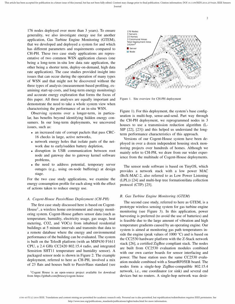
176 Nodes3 Servers23 Homes 3 Communal AreasTotal Deployment Area 1414m2

Server

Node

Figure 1. Site overview for CH-PH deployment

Figure 1). For this deployment, the system’s base config-uration is multi-hop, sense-and-send. Part way throughthe CH-PH deployment, we reprogrammed nodes in 3houses to use a transmission reduction algorithm (L-SIP [22], [23]) and this helped us understand the long-term performance characteristics of this approach.

Versions of our Cogent-House system have been de-ployed in over a dozen independent housing stock mon-itoring projects over hundreds of homes. Although wemainly refer to CH-PH, we draw from our wider exper-ience from the multitude of Cogent-House deployments.

The sensor node software is based on TinyOS, whichprovides a network stack with a low power MAC(BoX-MAC-2, also referred to as Low Power Listening(LPL)) [24] and multi-hop tree formation/data collectionprotocol (CTP) [25].

B. Gas Turbine Engine Monitoring (GTEM)

The second case study, referred to here as GTEM, is aprototype wireless sensing system for gas turbine enginemonitoring (see Figure 3). In this application, powerharvesting is preferred (to avoid the use of batteries) andis feasible due to the large amount of vibration and hightemperature gradients caused by an operating engine. Oursystem is aimed at monitoring gas path temperatures in-side the engine (peak values of 1000 °C) and is based onthe CC2530 hardware platform with the Z-Stack networkstack [26], a certified ZigBee compliant stack. The nodesare built from CC2530 evaluation modules combinedwith our own carrier boards for sensor interfacing andpower. The base station uses the same CC2530 evalu-ation module combined with a SmartRF05EB board. Thenodes form a single-hop ZigBee-compatible 802.15.4network, i.e., one coordinator (or sink) and several enddevices but no routers. A single-hop network was desir-



3

Figure 2. Packaged TelosB sensor node for CH-PH in a basicconfiguration above and with additional air quality sensors below.

Figure 3. Gas Turbine Engine Monitoring (GTEM) wireless nodesinstalled on test engine (above) and internals (below).

able since: a) the network structure is simplified, b) end-to-end packet delivery time is small with low variance,and c) packet forwarding is not needed, thus reducing thenode energy requirement. Sampling rate for this systemwas 1 Hz. We performed multiple deployments withdurations of 20–50 minutes.

III. NODE ENERGY PROFILING

We propose that profiling the energy use of nodes isan important step in reducing their energy requirementsas it allows one to determine the main consumers andtherefore make informed choices about what action totake to reduce the overall, system-level energy consump-tion. Furthermore, such profiling needs to be performedbefore and after individual interventions to ensure theyhave had the desired effect.

Energy profiling is based on identifying the node’soverall and component power consumption. Correctlyand accurately identifying average power consumptionis difficult due to two factors:

1) load to be measured is a mix of small (⇡ 1 µA)and large (⇡ 100 mA) currents,

2) under normal operation, power use varies rapidlyover time.

Klues et al., [27] proposed a microbenchmarking ap-proach that establishes operation time and current usefor individual components by repeatedly iterating thatcomponent to establish the time per operation, whilesimultaneously using a precision ammeter (possibly withan analog low-pass filter) to measure average current. Aless accurate, oscilloscope-based approach can also beused. In this case, the oscilloscope measures the voltagedrop over a precision shunt resistor that is in serieswith the load. In either approach, the voltage V is fixedand the resulting measurement, per component i, is theaverage current Ii and per operation time ⌧i.

For CH-PH, we used microbenchmarking and an am-meter, whereas for GTEM, we used oscilloscope-basedmeasurements, mainly due to the difficulty of iteratingover components within the Z-Stack software.

These measurements are then aggregated to identifythe average power consumption as follows. Consideringa node’s total energy use to be composed of a set ofcomponents C (e.g., CPU operations, radio transmission,sensor reading, sleeping), energy per use of componenti 2 C is given by average power by elapsed time.

Ei = V Ii⌧i

where it is assumed that the voltage V is constantallowing one to measure just the average current Ii andtime per iteration ⌧i. For a chosen fixed period T , eachcomponent executes, on average, wi 2 <+ times. We



4

Process

Radio Sensor

TransmitListenAckRetry

Warm-upSample

CPU

Start-up

Normal operation

Long-term behaviour

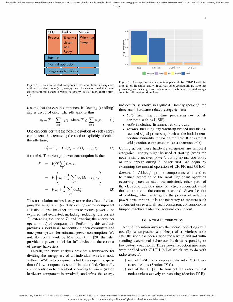
Figure 4. Hardware related components that contribute to energy usewithin a wireless node (e.g., energy used for sensing) and the cross-cutting temporal aspect of when that energy is used (e.g., during start-up).

assume that the zeroth component is sleeping (or idling)and is executed once. The idle time is thus

⌧0 = T �X

i6=0

wi⌧i where T �X

i6=0

wi⌧i (1)

One can consider just the non-idle portion of each energycomponent, thus removing the need to explicitly calculatethe idle time,

E0i = Ei � V I0⌧i = V (Ii � I0) ⌧i (2)

for i 6= 0. The average power consumption is then

P = V/TX

i

Iiwi⌧i

= V

0

@I0 +1

T

X

i6=0

wi (Ii � I0) ⌧i

1

A

= V I0 +1

T

X

i6=0

wiE0i (3)

This formulation makes it easy to see the effect of chan-ging the weights wi (or duty cycling) some componenti. It also allows for other options to reduce power to beexplored and evaluated, including: reducing idle currentI0, extending the period T , and lowering the energy peroperation E0

i of component i. Performing this analysisprovides a solid basis to identify hidden consumers andtune your system for minimal power consumption. Wenote the recent work by Martinez et al., [28] that alsoprovides a power model for IoT devices in the contextof energy harvesters.

Overall, the above analysis provides a framework fordividing the energy use of an individual wireless nodewithin a WSN into components but leaves open the ques-tion of how components should be identified. Generallycomponents can be classified according to where (whichhardware component is involved) and when the energy

0.0

0.1

0.2

0.3

0.4

Base L−SIP CTP L−SIP B−CTP BN B−CTP

Avg.

Pow

er (m

W)

Processing Sense Idle Transmit Listen

Figure 5. Average power consumption per node for CH-PH with theoriginal profile (Base) and with various other configurations. Note thatprocessing and sensing form only a small fraction of the total energycosts for all configurations here.

use occurs, as shown in Figure 4. Broadly speaking, thethree main hardware-related categories are:

• CPU (including run-time processing cost of al-gorithms such as L-SIP);

• radio (including listening, retrying); and• sensors, including any warm-up needed and the as-

sociated signal processing (such as the built-in tem-perature humidity sensor on the TelosB or externalcold-junction compensation for a thermocouple).

Cutting across these hardware categories are temporalcategories—energy might be used at start-up (when thenode initially receives power), during normal operation,or only appear during a longer trial. We begin byexamining the normal operation of CH-PH and GTEM.Remark 1. Although profile components will tend tobe named according to the most significant operationoccurring (such as radio transmission), other parts ofthe electronic circuitry may be active concurrently andthus contribute to the current measured. Given the aimof profiling, which is to guide the process of reducingpower consumption, it is not necessary to separate suchconcurrent usage and all such concurrent consumption islumped together under the nominal component.

IV. NORMAL OPERATION

Normal operation involves the normal operating cycle(usually sense-process-send-sleep) of a wireless nodeafter the node has been started for a while and not with-standing exceptional behaviour (such as responding tolow battery conditions). Three power reduction measureswere applied with CH-PH (all of which are to do withradio aspects):

1) use of L-SIP to compress data into 95% fewertransmissions (Section IV-C),

2) use of B-CTP [21] to turn off the radio for leafnodes unless actively transmitting (Section IV-B),



5

0

2

4

6

Base CJC duty cycle L−SIP New acks

Avg.

Pow

er (m

W)

L−SIP Acknowledge Shutdown Sense Transmit Polling CJC

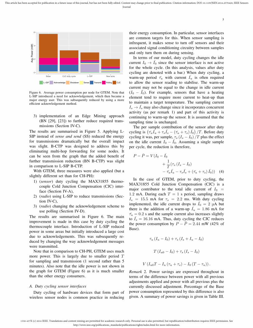
Figure 6. Average power consumption per node for GTEM. Note thatL-SIP introduced a need for acknowledgement, which then became amajor energy user. This was subsequently reduced by using a moreefficient acknowledgement method.

3) implementation of an Edge Mining approach(BN [29], [23]) to further reduce required trans-missions (Section IV-C).

The results are summarised in Figure 5. Applying L-SIP instead of sense and send (SS) reduced the energyfor transmissions dramatically but the overall impactwas slight. B-CTP was designed to address this byeliminating multi-hop forwarding for some nodes. Itcan be seen from the graph that the added benefit offurther transmission reduction (BN B-CTP) was slightin comparison to L-SIP B-CTP.

With GTEM, three measures were also applied (but aslightly different set than for CH-PH):

1) (sensor) duty cycling the MAX31855 thermo-couple Cold Junction Compensation (CJC) inter-face (Section IV-A),

2) (radio) using L-SIP to reduce transmissions (Sec-tion IV-C),

3) (radio) changing the acknowledgement scheme touse polling (Section IV-D).

The results are summarised in Figure 6. The mainimprovement is made in this case by duty cycling thethermocouple interface. Introduction of L-SIP reducedpower in some areas but initially introduced a large costdue to acknowledgements. This was subsequently re-duced by changing the way acknowledgement messageswere transmitted.

Note that in comparison to CH-PH, GTEM uses muchmore power. This is largely due to smaller period Tfor sampling and transmission (1 second rather than 5minutes). Also note that the idle power is not shown inthe graph for GTEM (Figure 6) as it is much smallerthan the other energy consumers.

A. Duty cycling sensor interfacesDuty cycling of hardware devices that form part of

wireless sensor nodes is common practice in reducing

their energy consumption. In particular, sensor interfacesare common targets for this. When sensor sampling isinfrequent, it makes sense to turn off sensors and theirassociated signal conditioning circuitry between samplesand only turn them on during sensing.

In terms of our model, duty cycling changes the idlecurrent I0 ! I0 since the sensor interface is not activefor the whole cycle. (In this analysis, values after dutycycling are denoted with a bar.) When duty cycling, awarm-up period ⌧u with current Iu is often requiredto allow the sensor reading to stabilise. The warm-upcurrent may not be equal to the change in idle current(I0 � I0). For example, sensors that have a heatingelement tend to require more current to heat-up thanto maintain a target temperature. The sampling currentIs ! Is may also change since it incorporates concurrentactivity (as per remark 1) and part of this activity iscontinuing to warm-up the sensor. It is assumed that thesampling time is unchanged.

The per sample contribution of the sensor after dutycycling is

�⌧uIu + ⌧sIs � (⌧u + ⌧s) I0

�/T . Before duty

cycling it was, per sample, ⌧s (Is � I0) /T plus the effecton the idle current I0 � I0. Assuming a single sampleper cycle, the reduction is therefore,

P � P = V (I0 � I0

+1

T(⌧s (Is � I0)

� ⌧uIu � ⌧sIs + (⌧u + ⌧s) I0)) (4)

In the case of GTEM, prior to duty cycling, theMAX31855 Cold Junction Compensation (CJC) is amajor contributor to the total idle current of I0 =1.2 mA. During each T = 1 s period, sampling drawsIs = 15.5 mA for ⌧s = 2.2 ms. With duty cyclingimplemented, the idle current drops to I0 = 2 mA butthere is the addition of a warm-up Iu = 1.86 mA for⌧u = 0.2 s and the sample current also increases slightlyto Is = 16.16 mA. Thus, duty cycling the CJC reducesthe power consumption by P � P = 2.44 mW (42% ofBase).

⌧u (Iu � I0) + ⌧s (Is + Iu � I0)

T (Iu0 � I0) + ⌧s (Is � I0)

V (Iu0T � Iu (⌧u + ⌧s)� I0 (T � ⌧u)) .

Remark 2. Power savings are expressed throughout interms of the difference between power with all previousadjustments applied and power with all previous plus thecurrently discussed adjustment. Percentage of the Basepower consumption represented by this difference is alsogiven. A summary of power savings is given in Table III.



6

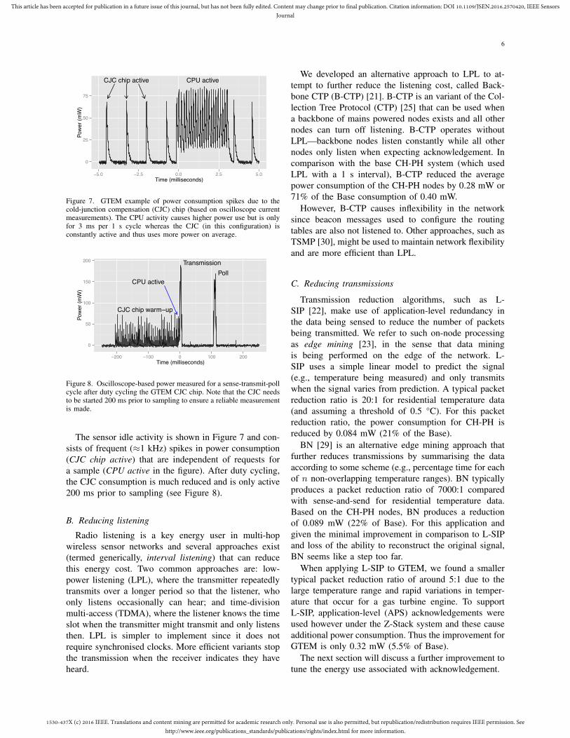
CPU activeCJC chip active

0

25

50

75

−5.0 −2.5 0.0 2.5 5.0Time (milliseconds)

Powe

r (m

W)

Figure 7. GTEM example of power consumption spikes due to thecold-junction compensation (CJC) chip (based on oscilloscope currentmeasurements). The CPU activity causes higher power use but is onlyfor 3 ms per 1 s cycle whereas the CJC (in this configuration) isconstantly active and thus uses more power on average.

CPU active

CJC chip warm−up

TransmissionPoll

0

50

100

150

200

−200 −100 0 100 200Time (milliseconds)

Powe

r (m

W)

Figure 8. Oscilloscope-based power measured for a sense-transmit-pollcycle after duty cycling the GTEM CJC chip. Note that the CJC needsto be started 200 ms prior to sampling to ensure a reliable measurementis made.

The sensor idle activity is shown in Figure 7 and con-sists of frequent (⇡1 kHz) spikes in power consumption(CJC chip active) that are independent of requests fora sample (CPU active in the figure). After duty cycling,the CJC consumption is much reduced and is only active200 ms prior to sampling (see Figure 8).

B. Reducing listening

Radio listening is a key energy user in multi-hopwireless sensor networks and several approaches exist(termed generically, interval listening) that can reducethis energy cost. Two common approaches are: low-power listening (LPL), where the transmitter repeatedlytransmits over a longer period so that the listener, whoonly listens occasionally can hear; and time-divisionmulti-access (TDMA), where the listener knows the timeslot when the transmitter might transmit and only listensthen. LPL is simpler to implement since it does notrequire synchronised clocks. More efficient variants stopthe transmission when the receiver indicates they haveheard.

We developed an alternative approach to LPL to at-tempt to further reduce the listening cost, called Back-bone CTP (B-CTP) [21]. B-CTP is an variant of the Col-lection Tree Protocol (CTP) [25] that can be used whena backbone of mains powered nodes exists and all othernodes can turn off listening. B-CTP operates withoutLPL—backbone nodes listen constantly while all othernodes only listen when expecting acknowledgement. Incomparison with the base CH-PH system (which usedLPL with a 1 s interval), B-CTP reduced the averagepower consumption of the CH-PH nodes by 0.28 mW or71% of the Base consumption of 0.40 mW.

However, B-CTP causes inflexibility in the networksince beacon messages used to configure the routingtables are also not listened to. Other approaches, such asTSMP [30], might be used to maintain network flexibilityand are more efficient than LPL.

C. Reducing transmissions

Transmission reduction algorithms, such as L-SIP [22], make use of application-level redundancy inthe data being sensed to reduce the number of packetsbeing transmitted. We refer to such on-node processingas edge mining [23], in the sense that data miningis being performed on the edge of the network. L-SIP uses a simple linear model to predict the signal(e.g., temperature being measured) and only transmitswhen the signal varies from prediction. A typical packetreduction ratio is 20:1 for residential temperature data(and assuming a threshold of 0.5 °C). For this packetreduction ratio, the power consumption for CH-PH isreduced by 0.084 mW (21% of the Base).

BN [29] is an alternative edge mining approach thatfurther reduces transmissions by summarising the dataaccording to some scheme (e.g., percentage time for eachof n non-overlapping temperature ranges). BN typicallyproduces a packet reduction ratio of 7000:1 comparedwith sense-and-send for residential temperature data.Based on the CH-PH nodes, BN produces a reductionof 0.089 mW (22% of Base). For this application andgiven the minimal improvement in comparison to L-SIPand loss of the ability to reconstruct the original signal,BN seems like a step too far.

When applying L-SIP to GTEM, we found a smallertypical packet reduction ratio of around 5:1 due to thelarge temperature range and rapid variations in temper-ature that occur for a gas turbine engine. To supportL-SIP, application-level (APS) acknowledgements wereused however under the Z-Stack system and these causeadditional power consumption. Thus the improvement forGTEM is only 0.32 mW (5.5% of Base).

The next section will discuss a further improvement totune the energy use associated with acknowledgement.



7

Transmit

Waitingfor ack

Ack Poll

0

50

100

150

200

−0.1 0.0 0.1 0.2 0.3Time (seconds)

Powe

r (m

W)

Figure 9. GTEM node with APS acknowledgement showing theelevated power use while waiting for acknowledgement.

CJCwarm−up

Transmit

Idle

Poll Data(ack)

0

50

100

150

−0.2 −0.1 0.0 0.1 0.2Time (seconds)

Powe

r (m

W)

Figure 10. Oscilloscope-based power measurement of GTEM nodeusing data polling to provide acknowledgement showing reduced poweruse while waiting for the acknowledgement.

D. Alternative acknowledgement schemesFor the GTEM system, acknowledgements are costly

but needed for L-SIP to be used [23]. To obtain the bestbenefit from L-SIP, we needed to tune the acknowledge-ment approach. Instead of using the standard ZStack APSacknowledgement mechanism, we instead use ZigBeepolling after each transmit.

In ZigBee polling, an end device polls or requests amessage from the coordinator. As shown in Figure 9,ordinary APS acknowledgements cause the processorstay active while waiting. In comparison, with polling,as shown in Figure 10, the node sleeps (and thus is idle)while waiting for the receipt of the acknowledgement.

The resulting reduction in energy is 0.98 mW (17%of Base), which is significant.

V. START-UP ENERGY

The energy required to start-up each wireless node isan important consideration for:

• episodic systems (ones which are turned on for aperiod and then turned off again), since start-up isa regular occurrence, and,

• power harvesting systems (where the main sourceof energy is acquired gradually) since the system

Networkdiscoverybeacons

0

50

100

150

0 1 2 3 4Time (seconds)

Powe

r (m

W)

Figure 11. Power consumption for GTEM node during node startupwith network discovery beacons shaded.

Table IIGTEM NODE STARTUP WITH AND WITHOUT NETWORK

INITIALISATION. WHEN NOT INITIALISING, ROUTING TABLES ARERESTORED FROM NON-VOLATILE MEMORY.

Start-uptime (s)

Avg.power(mW)

Energy(mJ)

With network creation 3.00 54.6 164Without network creation 0.85 10.2 8.7

may not be able to start at all until sufficient powerhas been harvested.

GTEM is both episodic and ultimately aimed to be usedwith power harvesters rather than batteries.

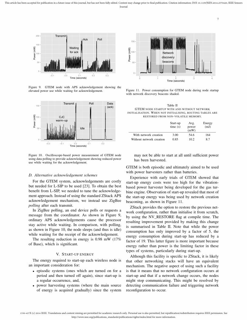
Experience with early trials of GTEM showed thatstart-up energy costs were too high for the vibration-based power harvester being developed for the gas tur-bine engine. Observation of start-up revealed that most ofthe start-up energy was being used by network creationbeaconing, as shown in Figure 11.

ZStack provides the option to restore the previous net-work configuration, rather than initialise it from scratch,by using the NV_RESTORE flag at compile time. Theresulting improvement provided by making this changeis summarised in Table II. Note that while the powerconsumption has only improved by a factor of 5, theenergy consumption during start-up has reduced by afactor of 19. This latter figure is more important becauseenergy rather than power is the limiting factor in thesetypes of systems, particularly during start-up.

Although this facility is specific to ZStack, it is likelythat other networking stacks will have an equivalentmechanism. The negative aspect of using such a facilityis that it means that no network configuration occurs atstart-up and that if a network change occurs, the nodesmight stop communicating. This might be resolved bydetecting communication failure and triggering networkreconfiguration to occur.



8

VI. LONG-TERM MEASUREMENT

Long-term deployments can help identify problemsthat were not discovered by analysing energy consump-tion in normal operation regime for individual nodes orthe node / network start-up phase.

While energy profiling of normal operation providesan estimate of battery life, the true lifetime may beconsiderably different and this might only be discoveredthrough long-term trials. Unfortunately, long-term resultsmay take years to emerge and thus it is commonplaceto also capture a log of battery voltage, as a proxyfor residual charge, during deployment. Battery voltageprovides a predictor of residual charge, although therelationship between the two is non-linear and somehysteresis effects may occur [31], [32]. A detailed batteryvoltage log will also allow for causes of unexpectedvoltage drops to be identified early. Moreover, continuouslogging of voltage allows for maintenance and batterychanges to be scheduled in a timely manner to avoidnetwork down time and data loss.

Note that different batteries may have dramatically dif-ferent lifetimes depending on the load that is applied andthe chemistry of the battery. Using a consistent batterytype from the same manufacturer across a deploymentthus simplifies any comparison of the lifetime results.However it should be noted that even using the samebattery brand and type will not necessarily guaranteeconsistent lifetime results.

We logged voltage in CH-PH and GTEM and thisallowed us to observe some long-term effects that mightotherwise have remained unexplained. Figure 12 showsbattery voltage for a number of nodes during one ofour long term Cogent-House deployments that employsL-SIP. Normally, the gradient of this curve is a gentlenegative trend with the expected battery life being around4 years for 2 ordinary AA batteries. However, if theserver is turned off (or fails in some other way), batterydepletion becomes much more rapid (the lifetime for afully charged set of batteries reduces to 140 days). In thefigure, the longest outage (of 39 days) caused a drop of0.21 V corresponding to roughly 1/3 of the total batterycharge.

The reasons for the increased power consumptionduring server (or sink) failure include:

• increased transmission retries (up to 20 for CTP),• longer time spent listening for acknowledgement,• no transmission reduction with L-SIP (due to the

lack of acknowledgement).

We believe that an efficient solution to server / sinkfailure has not yet been found and the fact that the impactof sink failure is identified by long-term monitoringemphasises the importance of this analysis.

2.6

2.7

2.8

2.9

3.0

2014−01 2014−07 2015−01 2015−07 2016−01

Batte

ry V

olta

ge (V

)

nodeId 33 97 161 193 225 257

Figure 12. Typical battery voltage for a set of Cogent-House sensornodes. The large drops in voltage that occur for many nodes simul-taneously are due to server outage, which causes each node to try totransmit more often and perform the maximum retries for each transmit,thus expending more power than usual. This effect occurs several timesin this graph. Note that this graph is from a more recent deploymentof Cogent-House than CH-PH.

CH-PH GTEMEnergy % of Energy % of

reduction base reduction baseReduce 0.28 mW 71% — —Listening

Duty cycle — — 2.44 mW 42%sensorsReduce 0.084 mW 21% 0.32 mW 5.50%Transmissions

Alternative — — 0.98 mW 17%AcknowledgementsTable III

SUMMARY OF ACHIEVED POWER SAVINGS FOR THE CH-PH ANDGTEM SYSTEMS.

VII. CONCLUSIONS

While energy conservation is a common theme forwireless sensor research, energy saving schemes arerarely evaluated through measurement in a practicalsetting. This paper addresses that gap.

When profiling a WSN node, per cycle energy is gen-erally the primary consideration, however start-up energymay also be critical in an energy harvesting system andlong-term practical issues may also be important. Natur-ally, it is impossible to fully tune all aspects of a systemin a research setting and results may compare poorly withoff-the-shelf systems. However, we have shown that theenergy consumption of wireless sensing nodes can besignificantly reduced by analysing the node behaviourthrough a combination of short-term measurements andlong-term instrumented deployments. We have describedthe measurement and analysis techniques we used andthe results obtained when targeting specific aspects ofnode operation. Our aim is to guide Wireless SensorNetwork (WSN) researchers towards the typical problemareas found and the types of approach that can be usedto reduce node energy consumption in these areas. Theareas of a) startup, b) sensing, c) processing, d) trans-



9

mitting data, and e) routing are generally applicable toall wireless node designs and it is likely that, generally,savings can be made in at least one area, particularlyin transmitting and routing. It is important that the nodeenergy consumption be profiled before, during, and aftermodifications are made in order to correctly identifyproblem areas, confirm that the modifications have beeneffective, and find side-effects that may result in lower-than-expected savings.

In the case of the two systems we discussed in thispaper, we have reduced the power consumption of thenodes in a home environment monitoring system (CH-PH) by 93% and the power consumption of a gas turbineengine monitoring system (GTEM) by 65%. We havealso reduced the startup costs of the latter nodes by95%, an important achievement when targeting the useof power harvesters, and identified long-term issues thatmay not be apparent from short-term analysis.

ACKNOWLEDGEMENTS

Part of the research leading to these results hasreceived funding from the European Union’s SeventhFramework Programme (FP7/2007-2013) under grantagreement n° 314061.

REFERENCES

[1] G. Anastasi, M. Conti, M. Di Francesco, and A. Passarella, “En-ergy conservation in wireless sensor networks: A survey,” Ad HocNetworks, vol. 7, no. 3, pp. 537–568, 2009. [Online]. Available:http://linkinghub.elsevier.com/retrieve/pii/S1570870508000954

[2] T. Srisooksai, K. Keamarungsi, P. Lamsrichan, and K. Araki,“Practical data compression in wireless sensor networks: Asurvey,” Journal of Network and Computer Applications,vol. 35, no. 1, pp. 37–59, 2012. [Online]. Available: http://www.sciencedirect.com/science/article/pii/S1084804511000555

[3] U. Raza, A. Camerra, A. L. Murphy, T. Palpanas, andG. P. Picco, “What does model-driven data acquisition reallyachieve in wireless sensor networks?” 2012 IEEE InternationalConference on Pervasive Computing and Communications, pp.85–94, March 2012. [Online]. Available: http://ieeexplore.ieee.org/lpdocs/epic03/wrapper.htm?arnumber=6199853

[4] M. Kuorilehto, M. Kohvakka, J. Suhonen, P. Hämäläinen,M. Hännikäinen, and T. Hamalainen, Ultra-Low EnergyWireless Sensor Networks in Practice: Theory, Realizationand Deployment. Wiley, 2008. [Online]. Available: https://books.google.co.uk/books?id=\_GRcbB4doJUC

[5] P. Zhang, C. M. Sadler, S. A. Lyon, and M. Martonosi, “Hard-ware design experiences in zebranet,” in Proceedings of the 2ndinternational conference on Embedded networked sensor systems(SenSys ’04), Baltimore, Maryland, USA, 3–5 November 2004,pp. 227–238.

[6] J. M. Reason and J. M. Rabaey, “A study of energy consumptionand reliability in a multi-hop sensor network,” ACM SIGMOBILEMobile Computing and Communications Review - Special issueon wireless pan & sensor networks, vol. 8, no. 1, pp. 84–97,January 2004.

[7] R. Szewczyk, A. Mainwaring, J. Polastre, J. Anderson, andD. Culler, “An analysis of a large scale habitat monitoringapplication,” in Proceedings of the 2nd International Conferenceon Embedded Networked Sensor Systems (SenSys ’04), Baltimore,MD, USA, 2004, pp. 214–226.

[8] R. Beckwith, D. Teibel, and P. Bowen, “Report from the field:Results from an agricultural wireless sensor network,” in Pro-ceedings of the 29th Annual IEEE International Conference onLocal Computer Networks (LCN ’04), Tampa, FL, USA, 16–18November 2004, pp. 471–478.

[9] L. Krishnamurthy, R. Adler, P. Buonadonna, J. Chhabra,M. Flanigan, N. Kushalnagar, L. Nachman, and M. Yarvis,“Design and deployment of industrial sensor networks: ex-periences from a semiconductor plant and the north sea,” inProceedings of the 3rd international conference on Embeddednetworked sensor systems (SenSys ’05), San Diego, CA, USA,2–4 November 2005, pp. 64–75.

[10] A. Arora, R. Ramnath, E. Ertin, P. Sinha, S. Bapat, V. Naik,V. Kulathumani, H. Zhang, H. Cao, M. Sridharan, S. Kumar,N. Seddon, C. Anderson, T. Herman, N. Trivedi, M. Nesterenko,R. Shah, S. Kulkami, M. Aramugam, L. Wang, M. Gouda,Y. ri Choi, D. Culler, P. Dutta, C. Sharp, G. Tolle, M. Grimmer,B. Ferriera, and K. Parker, “ExScal: elements of an extreme scalewireless sensor network,” in Proceedings of the 11th IEEE In-ternational Conference on Embedded and Real-Time ComputingSystems and Applications, 2005., Aug 2005, pp. 102–108.

[11] G. Tolle, J. Polastre, R. Szewczyk, D. Culler, N. Turner, K. Tu,S. Burgess, T. Dawson, P. Buonadonna, D. Gay, and W. Hong,“A macroscope in the redwoods,” in Proceedings of the 3rd In-ternational Conference on Embedded Networked Sensor Systems(SenSys ’05), San Diego, CA, USA, 2–4 November 2005, pp.51–63.

[12] V. Turau, M. Witt, and C. Weyer, “Analysis of a real multi-hop sensor network deployment: The heathland experiment,” inProceedings of the 3rd International Conference on NetworkedSensing Systems (INSS ’06), Chicago, IL, USA, 31 May–2 June2006.

[13] G. Werner-Allen, K. Lorincz, M. Ruiz, O. Marcillo, J. Johnson,J. Lees, and M. Welsh, “Deploying a wireless sensor network onan active volcano,” IEEE Internet Computing, vol. 10, no. 2, pp.18–25, March-April 2006.

[14] S. N. Pakzad, G. L. Fenves, S. Kim, and D. E. Culler, “Design andimplementation of scalable wireless sensor network for structuralmonitoring,” Journal of Infrastructure Systems, vol. 14, no. 1, pp.89–101, March 2008.

[15] M. Ceriotti, L. Mottola, G. P. Picco, A. L. Murphy, S. Guna,M. Corra, M. Pozzi, D. Zonta, and P. Zanon, “Monitoringheritage buildings with wireless sensor networks: The TorreAquila deployment,” in Proceedings of the 2009 InternationalConference on Information Processing in Sensor Networks,ser. IPSN ’09, 2009, pp. 277–288. [Online]. Available:http://dl.acm.org/citation.cfm?id=1602165.1602191

[16] J. K. Hart, K. C. Rose, K. Martinez, and R. Ong, “Subglacialclast behaviour and its implication for till fabric development:new results derived from wireless subglacial probe experiments,”Quaternary Science Reviews, vol. 28, no. 7–8, pp. 597–607, April2009.

[17] S. Jang, H. Jo, S. Cho, K. Mechitov, J. A. Rice, S.-H. Sim, H.-J.Jung, C.-B. Yun, J. Billie F. Spencer, and G. Agha, “Structuralhealth monitoring of a cable-stayed bridge using smart sensortechnology: deployment and evaluation,” Smart Structures andSystems, vol. 6, no. 5–6, pp. 439–459, July–August 2010.

[18] F. Ingelrest, G. Barrenetxea, G. Schaefer, M. Vetterli, O. Cou-ach, and M. Parlange, “Sensorscope: Application-specific sensornetwork for environmental monitoring,” ACM Transactions onSensor Networks, vol. 6, no. 2, February 2010.

[19] P. Sommer, B. Kusy, R. Jurdak, N. Kottege, J. Liu, K. Zhao,A. McKeown, and D. Westcott, “From the lab into thewild: Design and deployment methods for multi-modal track-ing platforms,” Pervasive and Mobile Computing, 2015, doi:10.1016/j.pmcj.2015.09.003 (In press at time of writing.).

[20] E. Gaura, L. Girod, J. Brusey, M. Allen, andG. Challen, Eds., Wireless Sensor Networks. Boston,MA: Springer US, 2010, vol. 1. [Online]. Available:http://www.springer.com/us/book/9781441958334?wt{\_}mc=ThirdParty.SpringerLink.3.EPR653.About{\_}eBookhttp://link.springer.com/10.1007/978-1-4419-5834-1



10

[21] R. Wilkins, “Generalised approaches to transmission reductionprotocols in fielded Wireless Sensor Networks,” Ph.D. disserta-tion, Coventry University, September 2014.

[22] J. Brusey and D. Goldsmith, “The Spanish InquisitionProtocol: Model based transmission reduction for wirelesssensor networks,” in Proceedings of IEEE Sensors, Kona, HI,USA, 1–4 November 2010, pp. 2043–2048. [Online]. Available:http://dx.doi.org/10.1109/ICSENS.2010.5690285

[23] E. I. Gaura, J. Brusey, M. Allen, R. Wilkins, D. Goldsmith, andR. Rednic, “Edge mining the internet of things,” IEEE SensorsJournal, vol. 13, no. 10, pp. 3816–3825, 2013.

[24] D. Moss and P. Levis, “BoX-MACs: Exploiting Physical and LinkLayer Boundaries in Low-Power Networking,” Stanford, Tech.Rep., 2008.

[25] O. Gnawali, R. Fonseca, K. Jamieson, D. Moss, and P. Levis,“Collection Tree Protocol,” in Proceedings of the 7th ACMConference on Embedded Networked Sensor Systems (SenSys’09), Berkeley, CA, USA, 3 November 2009.

[26] Texas Instruments Incorporated, “A fully compliant ZigBee 2012solution: Z-Stack,” Online: http://www.ti.com/tool/z-stack.

[27] K. Klues, V. Handziski, C. Lu, A. Wolisz, D. Culler, D. Gay,and P. Levis, “Integrating concurrency control and energymanagement in device drivers,” in Proceedings of Twenty-firstACM SIGOPS Symposium on Operating Systems Principles,ser. SOSP ’07, 2007, pp. 251–264. [Online]. Available:http://doi.acm.org/10.1145/1294261.1294286

[28] B. Martinez, M. Monton, I. Vilajosana, and J. D. Prades,“The power of models: Modeling power consumption foriot devices,” IEEE Sensors Journal, vol. 15, no. 10, pp.5777–5789, 2015. [Online]. Available: http://ieeexplore.ieee.org/lpdocs/epic03/wrapper.htm?arnumber=7122861

[29] E. I. Gaura, J. Brusey, and R. Wilkins, “Bare Necessities—Knowledge-driven WSN design,” in Proceedings of IEEESensors, 2011.

[30] K. S. J. Pister and L. Doherty, “TSMP: Time synchronized meshprotocol,” in Proc IASTED Intl. Symp., November 2008, pp. 391–398.

[31] R. J. Lajara, J. J. Perez-solano, and J. Pelegrí-sebastia, “A methodfor modeling the battery state of charge in wireless sensornetworks,” IEEE Sensors Journal, vol. 15, no. 2, pp. 1186–1197,Feb 2015.

[32] C. Chau, Y. Wang, and Y. Yang, “Harnessing Battery RecoveryEffect in Sensor Networks,” IEEE Journal on Selected Areas inCommunications, vol. 28, no. 7, pp. 1222–1232, 2010. [Online].Available: http://discovery.ucl.ac.uk/178418/

James Brusey (M ’13) received his B.Ap.Sc.and Ph.D. degrees from RMIT University in1996 and 2003, respectively. His Ph.D. disser-tation won the Australian Computer ScienceAssociation award for Best Thesis in 2004.Since 2007, James has worked in the CogentComputing Applied Research Centre at Cov-entry University. In 2012, he was awardeda Readership in Pervasive Computing. Hiscurrent research interests include exploringpractical issues with the deployment of wire-

less sensor networks, reinforcement learning, and thermal comfort inbuildings and car cabins.

John Kemp received his B.Sc. and Ph.D. incomputer science from Coventry Universityin 2006 and 2010 respectively. From 2010to 2016 he worked with Cogent Labs atCoventry University as a Research Assistantand then Research Fellow. During this timehe investigated a range of topics, spanningareas such as body sensor networks, thermalcomfort, reinforcement learning based HVACcontrol, sensor node transmission suppres-sion, and gas turbine engine monitoring.

Elena Gaura (M ’13) received her B.Sc. andM.Sc. degrees in Electrical Engineering in1989, and 1991 (Technical University of ClujNapoca, Romania), and her Ph.D. degree inintelligent sensor systems in 2000 (CoventryUniversity). Elena was awarded a Professor-ship in Pervasive Computing in 2009. Shewas the director of the Coventry University’sCogent Computing Applied Research Centre(2006–2013). Presently her research is withthe development of deployable WSNs for

real-life applications with a focus on: i) robust end-to-end systemdesign and technologies integration, ii) MEMS technology integrationin multi-sensor systems, iii) real-time, model based sensor fusion andinformation extraction from wireless sensor networks, iv) integrationof decision engines within poorly resourced WSN systems v) fieldphenomena event detection and representation using WSNs and vi)long-lived, resource constrained WSNs.

Ross Wilkins received his B.Sc. and Ph.D. incomputer science from Coventry Universityin 2009 and 2014 respectively. Since 2014,he has been working as a Senior ResearchAssociate at Cogent Labs, Coventry Univer-sity. During this time he has worked on thedevelopment of IoT and support systems forbuilt environment monitoring, structural mon-itoring, and factory monitoring. His researchinterests include the development of robust,usable and reliable WSNs, data processing

and visualisation in WSNs, and processes to achieve longevity in nodelifetimes.

Mike Allen is a Research Fellow in CogentLabs, Faculty of Engineering and Computing,Coventry University. He received his B.Sc.and Ph.D. degrees in computer science fromCoventry University in 2005 and 2009 re-spectively. His research interests lie aroundthe development and integration of high data-rate wireless embedded sensing systems andthe on-line data processing algorithms theyuse.

Energy profiling in practical sensor networks: Identifying ...

Documents