Energy Level Statistics of the U(5) and O(6) Symmetries in the Interacting Boson …dean.pku.edu.cn/bksky/1999tzlwj/9.pdf ·  · 2004-07-22arXiv:nucl-th/0211033 v2 27 Nov 2002 Energy

arX

iv:n

ucl-

th/0

2110

33 v

2 2

7 N

ov 2

002

Energy Level Statistics of the U(5) and O(6)

Symmetries in the Interacting Boson Model

Jing Shu1, Ying Ran1, Tao Ji1, Yu-xin Liu1,2,3,4,∗

1 Department of Physics, Peking University, Beijing 100871, China

2 The Key Laboratory of Heavy Ion Physics of the Chinese Ministry of Education,

Peking University, Beijing 100871, China

3 Institute of Theoretical Physics, Academia Sinica, Beijing 100080, China

4 Center of Theoretical Nuclear Physics, National Laboratory of

Heavy Ion Accelerator, Lanzhou 730000, China

November 27, 2002

Abstract

We study the energy level statistics of the states in U(5) and O(6) dynamical

symmetries of the interacting boson model and the high spin states with back-

bending in U(5) symmetry. In the calculations, the degeneracy resulting from the

additional quantum number is eliminated manually. The calculated results indicate

that the finite boson number N effect is prominent. When N has a value close

to a realistic one, increasing the interaction strength of subgroup O(5) makes the

∗Corresponding author

1

statistics vary from Poisson-type to GOE-type and further recover to Poisson-type.

However, in the case of N → ∞, they all tend to be Poisson-type. The fluctuation

property of the energy levels with backbending in high spin states in U(5) symme-

try involves a signal of shape phase transition between spherical vibration and axial

rotation.

PACS No. 21.60.Fw, 21.10.Re, 24.60.Lz

2

1 INTRODUCTION

Random-matrices theory (RMT)[1] provides a basis to study quantum chaotic systems.

Particularly, the fluctuation properties of fully chaotic systems with time reversal sym-

metry follow the Gaussian orthogonal ensemble (GOE) whereas nonchaotic ones follow

Poisson ensemble[2]. Notice that dynamical symmetry means the integrability of the

system in classical limit and constants of motion associated with a symmetry govern the

integrability of the system, investigating the effects of symmetry is of importance to study

the dynamics of a quantum system. In recent years, many numerical studies concerning

different types of symmetries and their relations to the onset of chaos have been carried

out[3, 4, 5, 6, 7, 8, 9], however the case that different types of symmetries coexist and

compete with each other in one quantum system has not yet been analyzed carefully.

In this point of view, we study the nucleus in certain dynamical symmetries which were

expected to be completely integrable in the past.

It has been known that the interacting boson model (IBM)[10] is a realistic theoretical

model in describing the low-energy collective states and the electromagnetic transitions of

a large number of even-even nuclei successfully. In the original version of the IBM (IBM1),

nuclei are regarded as systems composed of s- and d-bosons with symmetry U(6), and

it has three dynamical symmetries U(5), SU(3) and O(6), geometrically corresponding

to spherical vibration, axial rotation and γ-unstable rotation[11], respectively. Because

collective motion is described by a hamiltonian matrix of finite dimension, one can diag-

onalize the matrix easily and study the energy level statistics such as nearest-neighbor

spacing distribution(NSD) numerically to check whether the motion is chaotic or regu-

lar. Then there have been many works to investigate the fluctuations of the nucleus by

3

analyzing the energy level statistics (see, for example, Refs.[12, 13, 14]) in the framework

of the IBM. However, except for the case of SU(3) symmetry, the energy level statistics

has not yet been analyzed for dynamical symmetries. Such a neglect is quite natural

since, according to the symmetry paradigm, the energy level statistics should be Poisson-

type. Nevertheless, the investigation on the SU(3) symmetry showed that the statistics

depended strongly on the boson number of the system N and it was quite close to GOE

statistics in the realistic cases where N was not very large.[6]. In this aspect, the energy

level statistics of the states in a dynamical symmetry may be more complicated than the

symmetry paradigm predicts. We will then analyze the energy level statistics of the U(5)

and O(6) symmetries in this work. For comparison, we also involve the SU(3) limit.

More recently, a breakthrough has been carried out by Iachello in the study of critical

point behavior of the nucleus undergoing a shape-phase transition. It has been shown that

the critical point of the transition between vibration and γ-unstable rotation and that

between vibration and axial rotation hold the symmetry E(5), X(5)[15, 16], respectively.

Although fluctuation properties of these transitional regions have been studied by Alhassid

and collaborates[12, 13, 14], the statistics at the critical points has not been discussed

in detail. On the other hand, investigating the property of high spin nuclear states and

the mechanism of backbending of high spin states has long been a significant topic in

nuclear physics. It has been known that the backbending comes from the breaking of

nucleon pairs and the alignment of the angular momenta. Recently, another way for the

backbending, more concretely, the collective backbending to appear has been proposed to

be a property of the U(5) symmetry of the IBM[17]. In such a formalism, with a special

way to fix the parameters, the yrast states with the U(5) symmetry change from the

vibrational ones with different d-boson numbers to the rotational ones with full d-boson

4

configuration(nd = N) when the angular momentum L reaches a critical value Lc. In this

sense, the energy level structure of the states in the U(5) symmetry might have a sign

of shape phase transition. We then analyze the statistics as the first step to explore the

fluctuations of a shape phase transition system.

The paper is organized as follows. In Section 2, we survey the framework of the IBM

and the method to analyze the energy level statistics briefly. In Section 3, we represent

the numerical results and give some discussions. Finally, a summary and some remarks

are given in Section 4.

2 METHOD

In the original version of the IBM (IBM1), the collective states of nuclei are described by

s- and d-bosons. The corresponding dynamical group is U(6), and it has three dynamical

symmetry limits U(5), O(6) and SU(3). Taking into account one- and two-body interac-

tions among the bosons, one has the Hamiltonian of the nucleus with one of the three

dynamical symmetries as[10]

HU(5) = E0 + εC1U(5) + αC2U(5) + βC2O(5) + γC2O(3) , (1)

HO(6) = E0 + ηC2O(6) + βC2O(5) + γC2O(3) , (2)

HSU(3) = E0 + δC2SU(3) + γC2O(3) . (3)

In case of the U(5), O(6) or SU(3) symmetry, the wave-function can be expressed as

|ψU(5)〉 = |NndτKL〉 , (4)

5

|ψO(6)〉 = |NστKL〉 , (5)

|ψSU(3)〉 = |N(λ, µ)KL〉 , (6)

where N is the total number of the bosons, nd, σ, (λ, µ), τ, L are the irreducible repre-

sentations(IRREPs) of the group U(5), O(6), SU(3), O(5) and O(3), respectively. K is

the additional quantum number to distinguish the degenerate states which have the same

quantum number of the parent group.

If a nucleus is in one of the above mentioned dynamical symmetries, its energy can

be given by the IRREPs as

EU(5) = E0 + εnd + αnd(nd + 4) + βτ(τ + 3) + γL(L+ 1) , (7)

EO(6) = E0 + ησ(σ + 4) + βτ(τ + 3) + γL(L+ 1) , (8)

ESU(3) = E0 + δ(λ2 + µ2 + λµ+ 3λ+ 3µ) + γL(L+ 1) . (9)

To analyze the energy level statistics of the states in the dynamical symmetries, we

take the following process. At first, with Eqs.(7), (8) and (9), we calculate the energy

levels of the nucleus in U(5), O(6) or SU(3) symmetry in IBM with different total boson

number N , spin-parity Jπ and several sets of parameters α, β, γ, δ, ε, η.

For a given spectrum {Ei}, it is necessary to separate it into the fluctuation part and

the smoothed average part whose behavior is nonuniversal and can not be described by

random-matrix theory(RMT)[1]. To do so we take the unfolding process for the energy

spectrum (see for example Ref.[12]). At first we count the number of the levels below E

and write it as

N(E) = Nav(E) +Nfluct(E) . (10)

6

Then we fix the Nav(Ei) semiclassically by taking a smooth polynomial function of degree

6 to fit the staircase function N(E). We obtain finally the unfolded spectrum with the

mapping

{Ei} = N(Ei) . (11)

This unfolded level sequence {Ei} is obviously dimensionless and has a constant average

spacing of 1, but the actual spacings exhibit frequently strong fluctuation.

We have used two statistical measures to determine the fluctuation properties of

the unfolded levels: the nearest neighbor level spacings distribution(NSD) P (S) and the

spectral rigidity ∆3(L). The nearest neighbor level spacing is defined as Si = (Ei+1)−(Ei).

The distribution P (S) is defined as that P (S)dS is the probability for the Si to lie within

the infinitesimal interval [S, S+dS]. It has been shown that the nearest neighbor spacing

distribution P (S) measures the level repulsion (the tendency of levels to avoid clustering)

and short-range correlations between levels. For a regular system, it is expected to behave

like the Poisson statistics

P (S) = e−S , (12)

whereas if the system is chaotic, one expects to obtain the Wigner distribution

P (S) = (π/2)S exp(−πS2/4) , (13)

which is consistent with the GOE statistics[1, 2, 18]. With the Brody parameter ω in the

Brody distribution

Pω(S) = α(1 + ω)Sωexp(−αS(1+ω)) , (14)

7

where

α = Γ[(2 + ω)/(1 + ω)]1/2 (15)

and Γ[x] is the Γ function, the transition from regularity to chaos can be measured with

the Brody parameters ω quantitatively. It is evident that ω = 1 corresponds to the GOE

distribution, while ω = 0 to the Poisson-type distribution. A value 0 < ω < 1 means an

interplay between the regular and the chaotic.

As to the spectral rigidity ∆3(L), it is defined as

∆3(L) =

⟨minA,B

1

L

∫ L/2

−L/2[N(x) − Ax−B]2dx

⟩, (16)

where N(x) is the staircase function of a unfolded spectrum in the interval [−L/2, x].

The minimum is taken with respect to the parameters A and B. The average denoted

by 〈· · ·〉 is taken over a suitable energy interval over x. Thus from this definition ∆3(L)

is the local average least square deviation of the staircase function N(x) from the best

fitting straight line. It has also been shown that the spectral rigidity ∆3(L) signifies the

long-range correlation of quantum spectra[2] which make it possible that for a chaotic

spectrum very small fluctuation of the staircase function around its average can be found

in an interval of given length (the interval may cover dozens of level spacings). For the

GOE the expected value of ∆3(L) can only be evaluated numerically, but it approaches

the value

∆3(L) ∼= (lnL− 0.0687)/π2 (17)

for large L. and for Poisson statistics

∆3(L) = L/15 . (18)

8

3 NUMERICAL RESULTS AND DISCUSSION

At first, we analyze the energy levels given in Eqs.(7) and (8) for the U(5) and O(6)

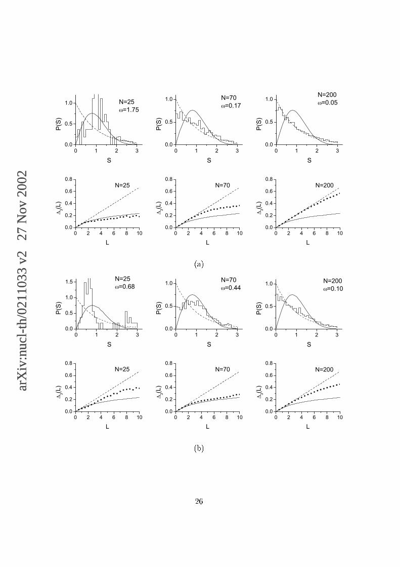
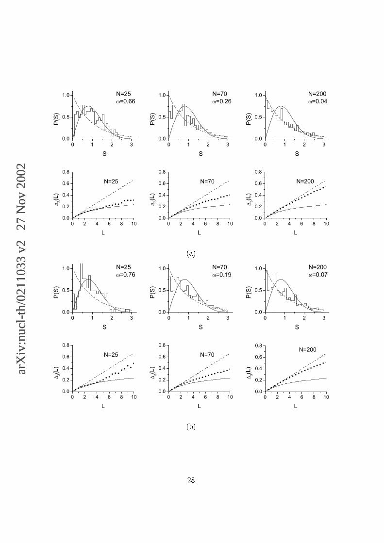
dynamical symmetries, respectively. In Fig.1(a), (b), (c) and (d), we represent the NSD

and the ∆3 statistics of the states with low spin-parity Jπ = 6+ in U(5) symmetry, but

different sets of parameter β. In Fig.2(a), (b), (c) and (d), we display the results of the

states with high spin-parity Jπ = 24+ in U(5) symmetry. Since numerical results show

that the statistics of the O(6) symmetry is quite close to that of the U(5) symmetry, we

illustrate then only the result for the states Jπ = 6+ with several sets of parameter β in

Fig.3(a), (b), (c) and (d). It has been known that the classical limit of IBM corresponds

to the system with boson number N → ∞. To show the finite boson number effect, we

have calculated the level statistics (NSD P (S) and the ∆3(L) statistics) in each case for

N = 25, N = 70 and N = 200, respectively. Meanwhile the Brody parameter ω of the

level spacing distribution[2] is also evaluated. The obtained result is shown in the figures.

Looking through the Figs. 1-3, one can realize that, when the boson number N has

a value not very large (e.g., 25, which is close to a realistic one in nuclei), the statistics

may show Poisson-type, GOE-type, intermediate between Poisson-type and GOE-type,

depending on the values of the parameters. However, when N → ∞, they all trend to be

Poisson-type. It indicates that the finite boson number effect is prominent. Meanwhile,

the figures show generally that the statistics does not depend on the angular momentum

obviously. Nevertheless, comparing Fig.2 with Fig. 1 more cautiously, one can know

that, in case that the boson number is not very large(N = 25), the ∆3 statistics gets a

little more decreased as the angular momentum increases, especially when L is large, i.e.,

long-range correlations are taken into account.

9

It should be mentioned that, in our calculations, all the degenerate states are taken

into consideration just as one single state. That means, if the quantum numbers of some

states differing from others only in an additional quantum number, we take the energy

levels of these states as one single level when the energy level statistics is carried out.

On the contrary, if we regard them as distinctive levels, the degeneracy causes so many

zero level spacings that the distribution is over-Poisson type and the difference is quite

large. In practical calculation, nearly 1/4 levels of all are abandoned when we have chosen

just one level out of each set of the degenerate states. It is obvious that such a manual

selection of the levels introduces a finite symmetry breaking to lift the degeneracy.

It has been known that the degeneracy results from the existence of additional quan-

tum numbers due to symmetry. In previous numerical calculations where the transitions

from one dynamical symmetry to the others were investigated, since the symmetries have

been broken, the degeneracy is then broken, such a problem seems do not exist. How-

ever, when we analyze the statistics in the dynamical symmetries, we have to handle the

problem since the additional quantum number K in Eqs.(4-6) can be quite large if the

boson number N is large. In the previous investigations on the statistics of the energy

levels in SU(3) symmetry[5, 6], Paar and collaborators discussed the case of Jπ = 0+,

where the additional quantum number K takes only one value K = 0, and also the case

of Jπ ≥ 2+, where K could have more than one values. Such an additional quantum

number K may be viewed as a result of a “hidden symmetry” since the states with the

same angular momentum but different K are degenerate. The calculated results showed

that, for N = 20 which is not very large, the statistics of the states Jπ = 0+ is close to

GOE-type. As the boson number N increases, the statistics gets close to Poisson-type.

For the states Jπ = 2+, if the K is fixed to a certain number, the energy level statistics

10

is closed to GOE-type. In the present work, we also analyze the case of SU(3) symmetry

with different boson numbers. In the analysis we select only one level from each set of

degenerate states to establish the level set for statistics, which is just the same as that

taken for the U(5) and O(6) symmetries, and is equivalent to that with K ≡ 0 in Paar’s

work. The obtained results for the case of boson number N = 25, 70 and 200 in the states

of Jπ = 6+ are illustrated in Fig.4. The calculated results show that the trend of statistics

from GOE-type to Poisson-type as N increases is clear, which coincides with the result

of Paar and collaborators[6].

In order to show how the manually introduced symmetry breaking affect the statistics,

we also calculate the statistics with distinctive degenerate states. The results for the case

with N = 25 are shown in Fig.5. Comparing Fig. 5 with Figs. 1 and 2 in the case of

the same parameters. One can easily recognize that the manually introduced symmetry

breaking makes the statistics from over-Poisson type to GOE type. The results are quite

consistent with Paar and collaborators’ work[5], where they introduce an additional term

which breaks the K quantum number but conserves SU(3) dynamical symmetry. Their

results show that increasing the strength of the K breaking term makes the statistics

change continuously from over-Poisson type to GOE type. One thing we need then to point

out here is that in practical calculation, the “hidden symmetry” are completely broken

not in the case that the degeneracy resulting from the existence of additional quantum

number is removed(types of the interaction), but in the case that the strength to break the

symmetry reaches a certain value(strength of the interaction). This might interpret why in

Alhassid and collaborates’ work[12], the statistics near the dynamical symmetries is in an

“overintegral” situation with negative Brody parameter ω. When the Hamiltonian they

use become very close to the one in the dynamical symmetry, for instance, when c0 = 0 and

11

χ = −0.01 in the self-consistent Q formalism[19] near the O(6) dynamical symmetry, the

broken strength is too weak to break the “hidden symmetry” resulting from the missing

labels though the degeneracy does not exist. Then the question comes out that which

way to determine the level set can better describe the statistics of the realistic nucleus in

the dynamical symmetry. In the present O(5)⊃ O(3) reduction, the degeneracy due to

the “hidden symmetry” is distinguished by the manually introduced additional quantum

number but no interaction is involved to link the states with different additional quantum

number K. Therefore the degenerate states with different additional quantum numbers

are in fact statistically uncorrelated. When we calculate the fluctuations of the energy

levels, such a large amount of the statistically uncorrelated states should be removed.

Otherwise, a mixed ensemble (with different good quantum number K) is taken into

consideration and the over-Poisson type distribution would be obtained (because nearly

1/4 of the spacings of all are zero in practical calculations). In this point of view, the

“overintegral” situation in Ref.[12] may arise from that some statistically uncorrelated

energy levels were taken into consideration.

In Fig.4, we display the results with only one set of parameters γ = 0.01, δ = −0.7

(in arbitrary unit), because from Eq.(9), one can know that different values of parameters

γ and δ cause only a linear transformation of the energies. Then it does not affect the

statistics. Analogously, one may get a conclusion from Eqs.(7) and (8) that changing the

parameter should not affect the statistics in U(5) and O(6) symmetries since the type of

the interaction and the structure of the energy levels remain the same. However, recalling

Figs. 1, 2 and 3, one can realize that, if the boson number is not very large(e.g. N=25 ),

the statistics in U(5) or O(6) symmetry depends obviously on the absolute value of the

parameter β. This indicates that the relative strengths of the interactions with different

12

symmetries also affect the statistics. If we take the results more carefully, we will find that

the increase of the relative value β (in fact |β/α|, |β/η|) makes the statistics in realistic

case (N = 25) change gradually from the Poisson-type to GOE-type. In order to show

the dependence of the statistics on the interaction strengths more obviously, we calculate

the Brody parameter ω of the level spacing distribution in a wide range of parameter β in

U(5) and O(6) symmetries, respectively. The obtained results are given in Fig.6 (a),(b),

respectively. The figures show that the statistics varies from Poisson-type to GOE-type,

and further to Poisson-type again with respect to the increasing of |β/α|, |β/η|. Recalling

Eqs.(7) and (8), we can realize that for a small value of |β/α|, |β/η|, the interaction with

the O(5) symmetry is only a perturbation on the U(5), O(6) symmetries, the quantum

system is then approximately regular. While the ratio increases, the interaction strength

of the O(5) becomes comparable to the strength of the parent group U(5) or O(6), the

statistics appears in GOE-type. It indicates that, when the strengths of the interactions

with different symmetries are comparable and compete with each other in one quantum

system, chaos may come out. This mechanism of onset of chaos can also be seen in

Alhassid and collaborates’ work of investigating the broken pairs in nuclei[20], where when

the Coriolis interaction is comparable to the pairing interaction, the degree of chaoticity

seems to be maximal. As the ratio of the interactions changes further and becomes so

large that the interaction of the parent group plays only a role as a “perturbation”, the

quantum system recovers approximately regular.

It is worth mentioning that the above results are quite similar to the well-know case

of the hydrogen atom in a uniform magnetic field[21]. The Sturm-Coulomb problem is an

integrable one since it holds O(4) symmetry. When one puts the atom into a magnetic

field, the O(4) symmetry is broken and reduced to the O(2) symmetry. The problem

13

becomes then nonintegrable. The chaos arises and is being obvious when the energy or

the magnetic strength (connected to O(2) strength) increases. The present U(5)⊃ O(5)

and O(6)⊃ O(5) reductions are analogous to the O(4)⊃ O(2). The onset of chaos in

the U(5) and O(6) symmetry is a direct result against the corresponding increase of the

interaction strength of O(5) symmetry since the symmetry is, in fact, broken.

Aside from the above analogy, another problem might have some relation with the

above results. In the geometric analysis of IBM, the subgroup O(5) in the dynamical

algebra U(6) corresponds only to the kinetic part of the Hamitonian[22], which can be

written as

Tγ = p2γ +

1

4

3∑

m=1

L2m

sin2(γ − 2πm/3)(19)

in the classical limit. As a result, the O(5) symmetric term can be viewed as the kinetic

interaction that does not affect the β−γ dependence of the potential surface and contains

only the collective motion of the nucleus according to Leviatan and collaborates’ work[23].

Indeed, the interaction strength of the subgroups in the system, such as that of the O(5)

symmetric one in the IBM, can be viewed as parts of the dynamical origin of the chaotic

behavior, or more concretely, the GOE fluctuations in nuclei. Just as Bohigas pointed

out[24] :“In our opinion, the static nuclear mean field is too regular to be held responsible,

and chaos must be caused by the residual interaction.” In this point of view, the onset

of chaos in nucleus results not only from the symmetry breaking of the potential(mean

field), but also from the increasing of the interaction strength of the subgroup(residual

interaction), which is competing with the parent group.

Furthermore, Eq.(7) shows that the energy of the states in U(5) symmetry depends not

only on parameter β, but also on the other parameters, such as α and ε. Considering the

14

geometric model correspondence of the IBM, one knows that U(5) symmetry corresponds

to an inharmonic vibration with frequency hω = ε+(nd +4)α. It is obvious that, with the

increasing of the d-boson number, if α > 0, the vibration frequency increases; if α < 0,

the vibration frequency decreases. It has recently been shown that the U(5) symmetry

with parameter α < 0 can describe the collective backbending of high spin states well[17].

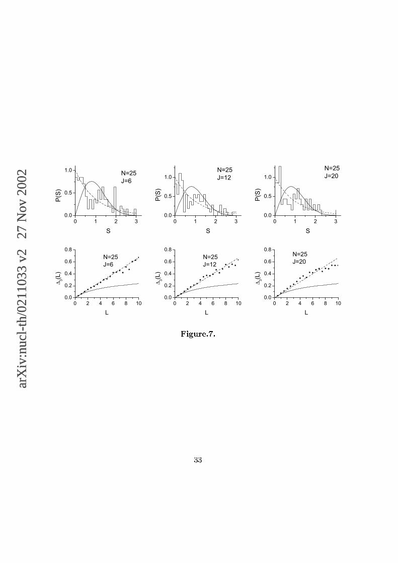
For a given set of parameters with α < 0, there exists a critical angular momentum

Lc ≈ −2(ε+ 4α)

α− 2N , (20)

where N is the total boson number. As the angular momentum L ≥ Lc, the yrast states

are no longer the inharmonic vibrational states, but the rotational ones with nd = N . For

a system with N=25 and parameters ε = 3.53, α = −0.101(in arbitrary unit), in which

Lc=12, we analyze the energy level statistics of the states L = 6(< Lc), L = 12(= Lc)

and L = 20(> Lc). The obtained results are illustrated in Fig.7. It is apparent that two

maxima appear in the nearest neighbor level spacing distribution P (S). Such a behavior

is quite different from the fluctuation properties in other cases. In theoretical point of

view, the term ndε enlarges the level spacing, whereas the term nd(nd + 4)α with α < 0

compresses the level spacing. The simultaneous appearance of these two effects induces

a competition which makes the energy of the states in the ground state band of the U(5)

symmetry

Egsb(nd) = (α+ β + 4γ)nd2 + (ε+ 4α+ 3β + 2γ)nd (21)

not increase with respect to the increasing of the d-boson number monotonously. Then a

maximal d-boson number limit n(m)d for the energy to increase correspondingly exists

n(m)d =

ε+ 4α + 3β + 2γ

−2(α + β + 4γ)≈ε+ 4α

−2α. (22)

15

Considering the property of the parabola Egsb(nd), one can know that there exists also

a boson number n(u)d = 2n

(m)d − N , with which the energy of the system equates to that

with nd = N , and those with nd ∈ (n(u)d , n

(m)d ) are larger than those of the states with the

same angular momentum but nd = N . It means that the states in the intrinsic ground

state band with d-boson number nd ∈ (n(u)d , N) are no longer the yrast states. Then the

structure of the yrast band changes from the U(5) states to the rotational states with

d-boson number nd = N and the energy of the states in the yrast band changes in the

way L(L+1). It implies that a phase transition of collective motion mode may happen as

the angular momentum reaches the critical value (Lc = 2n(u)d ) in Eq.(20). The state with

such a critical d-boson number n(u)d or angular momentum Lc is analogous to the states

with X(5) symmetry in the evolution from U(5) to SU(3) symmetry[16]. In the present

energy level statistics analysis, the ensemble with the same angular momentum L involves

in fact two sequences, one of which is in vibration, another one is in rotation. When we

unfold the above spectrum {Ei(L)}, the two sequences are normalized with an unique

total average spacing, and their maxima of the spacing distributions do not appear at the

same value of s, As a consequence, two maxima emerge. It should be noted that there

are only few overlaps between the two different sequences, otherwise the overlap of the

two sequences will change the nearest neighbor distribution. Analyzing the energy level

statistics of the X(5) symmetry, we found that its NSD P (S) is quite similar to that of

the present U(5) symmetry with collective backbending and exhibits also two maxima(the

full result will be published elsewhere[25]). Recalling the above discussions one can know

that the levels in the U(5) symmetry with α < 0 contain both the vibration ones and the

rotation ones.

To manifest the constituent of the level ensemble, we also evaluate the rigidity ∆3(L)

16

more meticulously. The result is illustrated in Fig.8. Fig.8 shows that the ∆3(L) of the

spectrum with collective backbending exhibits a drastic fluctuation. It has been known

that the variance of the ∆3 statistics (〈∆23〉 − 〈∆3〉

2) is connected with the 3- and 4-level

correlations, which is expected to be very small in the past[1]. The conflicts between the

obtained results and past conjecture indicts that the system undergoing a shape phase

transition might exhibit a much strong fluctuations than the usual systems discussed in

the past.

For comparison, we evaluate the statistics of the system with N = 70, 200 for α < 0,

too. The calculated results for L = 6 states are represented in Fig.9. One can know

from Eq.(20) that, for N=70 or 200, Lc < 0 if ε and α maintain their values as the same

as those for N=25, the competition mentioned above does not play any role for all the

states. Then the two maxima in the NSD statistics and the drastic fluctuation in the

∆3 statistics no longer exist. The appearance of the Poisson-type distribution indicates

that only the rotational mode plays important role in the system. Comparing the result

with N=25 and those with N=70, 200, one can reach a conclusion that the appearance of

the collective backbending is a signal of phase transition from a vibration to a rotation.

Meanwhile the emergence of two maxima in the P (S) distribution may be a characteristic

of the shape phase transition.

4 SUMMARY AND REMARKS

In summary, we have analyzed the energy level statistics of the U(5), O(6) and SU(3)

dynamical symmetries in the interacting boson model(IBM) in this paper. In the analysis,

the degeneracy resulting from the additional quantum number was eliminated manually,

17

i.e. we took only one level from each set of degenerate states. The calculated results

indicate that the finite boson number N effect is prominent. If N takes a value not very

large(e.g., 25, which is close to a realistic one), the statistics depends strongly on the

interaction strength of the subgroup O(5). While N → ∞, they all trend to be Poisson-

type. We would like then to mention that the interaction of the subgroup O(5) which

only possess the collective motions of the nucleus can be viewed as the dynamical origin of

chaos in nucleus and the symmetry paradigm deserves more careful consideration. In fact,

exceptions to the symmetry paradigm have been found for many years (see, for example,

Ref.[26]).

In this paper, we also analyze the level statistics of the states holding the collective

backbending in high spin states. We found that the nearest neighbor level spacing dis-

tribution P (S) of the states with the collective backbending involved two maxima and

the ∆3 statistics exhibited a fierce fluctuation, which were drastically different from the

general properties in each symmetry of the IBM at usual situation. It indicates that the

spectrum involves a shift between two modes of collective motions. It provides then a

clue that the collective backbending is a characteristic of shape phase transition. Further-

more, looking through all the process, we can suggest that the statistics of the system can

result from not only the form of interaction (the Hamiltonian or perturbation) but also

the interaction strength.

This work is supported by the National Natural Science Foundation of China under

the contract No. 19875001, 10075002, and 10135030 and the Major State Basic Research

Development Program under contract No.G2000077400. One of the author (J. S.) thanks

also the support from the Taizhao Foundation at Peking University. Another author (Y.X.

18

L.) thanks the support by the Foundation for University Key Teacher by the Ministry of

Education, China, too.

19

References

[1] M. L. Mehta, Random Matrices, 2nd ed. (Academic, New York, 1991).

[2] T. A. Brody, J. Flores, J. B. French, P. A. Mello, A. Pandey, and S. S. M. Wong,

Rev. Mod. Phys. 53, 385 (1981).

[3] W. M. Zhang, C. C. Martens, D. H. Feng, and J. M. Yuan, Phys. Rev. Lett. 61, 2167

(1988) ; W. M. Zhang, D. H. Feng, J. M. Yuan, and S. J. Wang, Phys. Rev. A 40,

438 (1989).

[4] D. C. Meredith, S. E. Koonin, and M. R. Zirnbauer, Phys. Rev. A 37, 3499 (1988).

[5] V. Paar, and D. Vorkapic, Phys. Rev. C 41, 2397 (1990).

[6] V. Paar, D. Vorkapic, and A. E. L. Dierperink, Phys. Rev. Lett. 69, 2184 (1992).

[7] N. Whelan, Y. Alhassid and A. Leviatan, Phys. Rev. Lett. 71, 2208 (1993).

[8] D. M. Leitner, H. Koppel and L. S. Cederbaum, Phys. Rev. Lett. 73, 2970 (1994).

[9] A. Leviatan, and N. D. Whelan, Phys. Rev. Lett. 77, 5202 (1996).

[10] F. Iachello, and A. Arima, The Interacting Boson Model (Cambridge University

Press, Cambridge, 1987).

[11] J. N. Ginocchio, and M. W. Kirson, Phys. Rev. Lett. 44, 1744 (1980).

[12] Y. Alhassid, and A. Novoselsky, Phys. Rev. C 45, 1677 (1992).

[13] Y. Alhassid, and N. Whelan, Phys. Rev. Lett. 67, 816 (1991).

[14] Y. Alhassid, A. Novoselsky, and N. Whelan, Phys. Rev. Lett. 65, 2971 (1990); Y.

Alhassid, and N. Whelan, Phys. Rev. C 43, 2637 (1991).

20

[15] F. Iachello, Phys. Rev. Lett. 85, 3580 (2000).

[16] F. Iachello, Phys. Rev. Lett. 87, 052502 (2001).

[17] G. L. Long, Phys. Rev. C 55, 3163 (1997).

[18] C. E. Porter, Statistical Theories of Spectra: Fluctuations (Academic, New York,

1965).

[19] D. D. Warner, R. F. Casten, Phys. Rev. Lett. 48, 1385 (1982); Phys. Rev. C 28,

1798 (1983).

[20] Y. Alhassid, and D. Vretenar, Phys. Rev. C 46, 1334 (1992).

[21] H. Friedrich, and D. Wintgen, Phys. Rep. 183, 37 (1989).

[22] R. L. Hatch, and S. Levit, Phys. Rev. C 25, 614 (1982).

[23] A. Leviatan, Ann. Phys. (N.Y.) 179, 201 (1987).

[24] O. Bohigas, Ann. Rev. Nucl. Part. Sci. 38, 421 (1988).

[25] J. Shu, H. B. Jia, and Y. X. Liu, (to be published).

[26] T. Cheon, and T. D. Cohen, Phys. Rev. Lett. 62, 2769 (1989).

21

Figures and Their Captions:

Fig. 1. Comparison of energy level statistics of the states Jπ = 6+ in U(5) symmetry

with four sets of parameters: (a) for ε = 1.76, α = 0.1, β = 0.02, γ = 0.001, (b)

for ε = 1.76, α = 0.1, β = 0.01, γ = 0.001, (c) for ε = 1.76, α = 0.1, β = 0.005,

γ = 0.001, and (d) for ε = 1.76, α = 0.1, β = −0.01, γ = 0.001. In all figures, the

solid lines and dashed lines describe the GOE and Poisson statistics, respectively.

Fig. 2. The same as Fig. 1 but for high angular momentum and parity Jπ = 24+.

Fig. 3. Comparison of energy level statistics of the states Jπ = 6+ in O(6) symmetry with

four sets of parameters: (a) for η = −0.5, β = 0.15, γ = 0.001, (b) for η = −0.5,

β = 0.10, γ = 0.001, (c) for η = −0.5, β = 0.05, γ = 0.001, and (d) for η = −0.5,

β = −0.10, γ = 0.001.

Fig. 4. Energy level statistics for the SU(3) symmetry with different number of bosons.

Fig. 5. Energy level statistics for U(5) and O(6) symmetries with distinctive degenerate

states caused by additional quantum number in the states Jπ = 6+ when boson

number N = 25. (a) For U(5) symmetry, the parameters are ε = 1.76, α = 0.1,

β = 0.01, γ = 0.001. (b) For O(6) symmetry, the parameters are η = −0.5, β = 0.15,

γ = 0.001.

Fig. 6. Quantum measures of chaos in different interaction strength of O(5) symmetry:

(a) Brody parameter ω versus |β/α| for ε = 1.76, α = 0.1, γ = 0.001 in U(5)

symmetry, (b) Brody parameter ω versus |β/η| for η = −0.5, γ = 0.001 in O(6)

symmetry.

22

Fig. 7. Energy level statistics of the states with boson number N = 25, angular momen-

tum and parity Jπ = 6+(L < Lc), 12+(L = Lc), 20+(L = Lc) in U(5) symmetry

when it has collective backbending at high spin states (The parameters are ε = 3.51,

α = −0.101, β = 0.01, γ = 0.001).

Fig. 8. Comparison of ∆3 statistics of the states in U(5) symmetry with boson number

N = 25 with collective backbending and without collective backbending: (a) for

ε = 3.51, α = −0.101, β = 0.01, γ = 0.001, Jπ = 6+(L < Lc), (b) the same

parameters with (a) but for Jπ = 12+(L = Lc), (c) the same parameters with (a)

but for Jπ = 20+(L = Lc), and (d) for ε = 1.76, α = 0.1, β = 0.02, γ = 0.001,

Jπ = 6+.

Fig. 9. the same as Fig. 7 but with boson number N = 70 and 200 for the Jπ = 6+

states.

23

arX

iv:n

ucl-

th/0

2110

33 v

2 2

7 N

ov 2

002

arX

iv:n

ucl-

th/0

2110

33 v

2 2

7 N

ov 2

002

���

�� �

��

���

�� �

������ ��

�

arX

iv:n

ucl-

th/0

2110

33 v

2 2

7 N

ov 2

002

arX

iv:n

ucl-

th/0

2110

33 v

2 2

7 N

ov 2

002

���

�� �

��

���

�� �

������ � �

�

arX

iv:n

ucl-

th/0

2110

33 v

2 2

7 N

ov 2

002

arX

iv:n

ucl-

th/0

2110

33 v

2 2

7 N

ov 2

002

���

�� �

��

���

�� �

������ � �

�

arX

iv:n

ucl-

th/0

2110

33 v

2 2

7 N

ov 2

002

arX

iv:n

ucl-

th/0

2110

33 v

2 2

7 N

ov 2

002

������ �� �

�

arX

iv:n

ucl-

th/0

2110

33 v

2 2

7 N

ov 2

002

arX

iv:n

ucl-

th/0

2110

33 v

2 2

7 N

ov 2

002

���

�� �� ���� �

�

arX

iv:n

ucl-

th/0

2110

33 v

2 2

7 N

ov 2

002

arX

iv:n

ucl-

th/0

2110

33 v

2 2

7 N

ov 2

002

������ �� �

�

arX

iv:n

ucl-

th/0

2110

33 v

2 2

7 N

ov 2

002

arX

iv:n

ucl-

th/0

2110

33 v

2 2

7 N

ov 2

002

������ �� �

��

arX

iv:n

ucl-

th/0

2110

33 v

2 2

7 N

ov 2

002

arX

iv:n

ucl-

th/0

2110

33 v

2 2

7 N

ov 2

002

���

�� �

��

���

�� �

������ � �

�

arX

iv:n

ucl-

th/0

2110

33 v

2 2

7 N

ov 2

002

arX

iv:n

ucl-

th/0

2110

33 v

2 2

7 N

ov 2

002

������ �� �

�