Energy Intensity: A Decomposition and Counterfactual Exercise for Latin American Countries Energy Intensity: A Decomposition and Counterfactual Exercise for Latin American Countries

1

Energy Intensity: A Decomposition and Counterfactual Exercise for Latin

American Countries*

Raul Jimenez a** Jorge Mercado b

a Inter-American Development Bank and University of Rome Tor Vergata

b Energy Division, Infrastructure Department, Inter-American Development Bank.

Keywords: energy intensity; decomposition; panel data; synthetic control

method.

JEL Code: O5; O13; Q40; Q43

* The opinions expressed in this article are strictly those of the authors and do not necessarily reflect those of the

Inter-American Development Bank (IDB), its Board of Executive Directors or the countries they represent.

A previous version was published as a working paper by the IDB. The authors are grateful for the support of

Ramon Espinasa and the Research Department at the IDB, as well as for the helpful comments and suggestions of

Lenin Balza, Diego Margot, Juan Jose Miranda, Tomas Serebrisky, Rodolfo Stucchi and four anonymous peer

reviewers. All remaining errors are our own responsibility.

** Corresponding author: [email protected], address: 1300 New York Avenue, N.W. Washington, DC 20577;

phone: 1-202-623-2170.

Abstract

This paper investigates trends in energy intensity over the last 40 years.

Based on a sample of 75 countries, it applies the Fisher Ideal Index to

decompose the energy intensity into the relative contributions of energy

efficiency and economic structure. Then, the determinants of these energy

indexes are examined through panel data regression techniques. Special

attention is lent to Latin American countries (LAC) by comparing its

performance to that of a similar set of countries chosen through the

synthetic control method. When analyzed by income level, energy

intensity has decreased in a range between 40 and 54 percent in low and

medium income countries respectively. Efficiency improvements drive

these changes, while the structural effect does not represent a clear source

of change. The regression analysis shows that per capita income,

petroleum prices, fuel-energy mix, and GDP growth are main

determinants of energy intensity and efficiency, while there are no clear

correlations with the activity component. In the case of LAC the energy

intensity decreased around 20 percent which could be interpreted as an

under-performance. However, the counterfactual exercise suggests that

LAC has closed the gap with respect to its synthetic control.

2

Energy Intensity: A Decomposition and Counterfactual Exercise for Latin American

Countries

1. INTRODUCTION

As both energy prices and concerns about global warming continue to increase, measures to

improve the energy use have become important components of public policy agenda. In

particular, there is a focus on identifying factors that influence change in energy intensity and

distinguishing the contribution of energy efficiency from other relevant factors. This

information is useful as it provides a basis for policy decisions and evaluation. Further, energy

efficiency represents a cost-effective strategy to address crosscutting issues such as energy

security, climate change and competitiveness.

In this context, this paper aims to investigate trends in energy intensity based on a

sample of 75 countries with annual data during the period 1971-2010. To this end, three specific

objectives are addressed. First, analyze the evolution of the aggregate energy intensity and its

main components. Then, identify the main determinants of these energy indexes. Finally, the

article lends special interest to the Latin American region by evaluating its relative performance

in terms of energy intensity and efficiency.

Following the World Energy Outlook (IEA, 2012) energy intensity would have

decreased about 20% in the World and 35% in OECD countries between 1980 and 2010.

Accordantly, empirical literature suggests a downward trend in energy intensity, with the

efficiency effect as its most important source of variation. However, the magnitudes of those

improvements tend to be heterogeneous depending on the case and period analyzed. Previous

studies could be divided in two groups. One with a rich and large body decomposing and

examining trends in energy intensity within a specific sector, where the manufacture has

received great attention. The other group has been less explored and bases its analysis on more

aggregate data mainly at multi-sector level within a country.

With respect to previous research in the industrial sector, some relevant figures emerge

of the well-studied cases as China, India and United States. China represents a notable case of

improvement decreasing its level of energy intensity more than 70 percent between 1980–2010.

Sinton and Levine (1994); Zhang (2003), and Ma and Stern (2008) show that this was mostly a

3

sustained decrease in industrial energy intensity, with efficiency explaining most of this

variation. As reported by Ke et al. (2012), during the period 1996–2010, the efficiency effect

explains 30 percent of the energy savings in industrial energy consumption. Another remarkable

fact occurring in the industrial sector is that intensity actually increase in the period 2003 to

2005, related to a notably increase in the levels of energy consumption. Still, the industrial

energy intensity continued to decrease.

In contrast, studies of the Indian industrial sector found mixed results from 1981 to

2005, showing only slight improvement in energy intensity (see Reddy and Ray, 2011).

Interesting cases where both efficiency and activity have played a role in reducing the overall

energy intensity index are found in studies of the United States. Hasanbeigi, Rue du Can, and

Sathaye (2012) show that in California, from 1997 to 2008, the energy intensity ratio decreased

43 percent mainly explained by two events: (i) a shift in value added participation from the oil

and gas extraction sector to the electric and electronic manufacturing sector, which uses less

energy per value added; and (ii) an escalation in energy prices that led the industries to improve

efficiency in order to reduce energy costs. Over a similar period, Huntington (2010) analyzes 65

U.S. industries in the commercial, industrial, and transportation sectors, showing that an

estimated 40 percent of reduction in aggregate energy intensity was due to structural change.

In one of the first studies available on energy intensity at the state/country level, Metcalf

(2008) performs a decomposition exercise at state level in the United States for the period

between 1970 and 2001. He finds a reduction in energy intensity of approximately 75 percent as

a result of efficiency improvements. Further, through a panel data analysis, he shows that rising

per capita income and higher energy prices play an important part in lowering energy intensity.

Bernstein et al. (2003) analyze a similar period using a sample of 48 states in the U.S., finding

that population, energy prices, climate temperatures, and indicators of sector activities, are

strongly correlated with energy intensity. In a recent study, Voigt et al (2014) perform a

decomposition analysis finding that intensity decreased by 18 percent on a sample of 40 major

economies over the period 1995 and 2007. The results also suggest that this improvement is

largely attributable to technological change.

Using a similar approach, Bhattacharya and Shyamal (2001) decompose the aggregate

energy intensity of India into pure intensity or efficiency and the economic activity composition

4

effect. They take broad sectors including agriculture, industry, and transport for the period

between 1980 and 1986, finding that the efficiency effect contributed significantly to energy

conservation.

This paper focuses on energy intensity indicators at broad end-use sectors at the country

level. This implies the observation of (aggregate) energy indexes (i.e., the indicators of energy

intensity and its decomposition into efficiency and the activity mix) at the country level. For this

purpose, we adopt the monetary-based definition, where energy efficiency improvement

generally means using less energy to produce the same amount (value added) of services or

output (Nanduri, 2002 and Ang, 2004).

In this context, the paper has three main contributions. Strengthen the literature by

analyzing a greater sample over a longer period than previous studies. A further step is provided

by the analysis of the determinants of energy intensity and its components. Second, the paper

shows results by income level set of countries with a focus in Latin American region, where

appears to be lacking of evidence. Finally, a methodological contribution to this specific

literature is the comparison analysis using the synthetic control method in order to overcome

heterogeneity issues in a benchmark exercise.

The paper is structured as follows. Next section provides methodological strategies for

(i) the decomposition of aggregate energy intensity into activity and pure intensity, which is

interpreted as efficiency, (ii) the specification of the panel data analysis in order to evaluate the

determinant of those three indexes (intensity, efficiency and activity), and (iii) the synthetic

control method used to construct a comparison set of countries to evaluate the relative

performance of Latin America. Section 3 presents the empirical results of these methodologies,

and Section 4 concludes.

2. EMPIRICAL STRATEGIES

2.1. Decomposition through the Fisher Ideal Index

A key limitation in empirical analysis is related with availability of data. Based on different

levels of data disaggregation, methodological contributions have been made in order to estimate

energy efficiency measures. Those methods are mostly based on decomposing energy intensity

into different factors, including energy efficiency, economic structure, production levels, and/or

5

fuel sources. The more disaggregate the data, the more accurate the efficiency contribution

estimations would be. The election of the specific method to be used depends on the objectives

and data availability. Some extensive methodological studies and surveys on decomposition

methods can be found in Boyd, Hanson, and Sterner (1988); Ang and Lee (1994); Ang and Liu

(2003); Ang (2004); Boyd and Roop (2004); and Ang, Huang, and Mu (2009). They suggest a

certain degree of academic consensus that using price index numbers is preferred when dealing

with aggregate data at the country level.

Following those recommendations, the method applied herein to perform the

decomposition is the Fisher Ideal Index. Its main advantage is that it does not have residual

term, referring to a portion of the change in intensity which is not assigned to a particular

source; that is, a portion of energy intensity that remains unexplained (Boyd and Roop, 2004).

The presence of residual term makes it difficult to interpret the relative importance of factors

being evaluated. Specifically, Ang, Mu, and Zhou (2010) emphasize that the perfect

decomposition methods should be adopted in the case of cross-country/region studies. In

addition, as mentioned by Ang (2004; 2006), Boyd and Roop (2004), and Ang and Liu (2003),

these methods are also preferred in the case of two-factor decomposition due to their theoretical

foundation and their adaptability, as well as the ease in interpreting their results. In our case,

energy intensity is decomposed into its efficiency and activity components. Besides the

references above Ang and Lee (1994), Greening et al (1997), Ang, Mu and Zhou (2010) provide

a compressive review and applications of alternative decomposition methods.

In this context, the problem is set in terms of total energy consumption (E) and total

production (Y), as well as sub-indexes for economic sector (i) and years (t). In our application 𝑖

refers to the agricultural, industrial, services, and residential sectors. Thus, the aggregate energy

intensity (e) can be written as:

𝑒𝑡 =𝐸𝑡

𝑌𝑡= ∑

𝐸𝑖𝑡

𝑌𝑖𝑡

𝑛𝑖

𝑌𝑖𝑡

𝑌𝑡= ∑ 𝑒𝑖𝑡𝑠𝑖𝑡

𝑛𝑖 (1)

Expression 1 indicates that a change in 𝑒𝑡 may be due to changes in the sector energy

intensity (𝑒𝑖𝑡) and/or the product mix or compositional effect (𝑠𝑖𝑡). By construction, the energy

uses in the different sectors need to form a partition (i.e., they must not overlap), but the

measures of economic activities do not need to satisfy this condition. The last represents one of

the main operative/practical advantages of this approach. What is more, they do not even need

6

to be in the same units, facilitating the identification of good indicators to account for the

activity mix (𝑠𝑖𝑡).

Following the index number theory, we proceed to derive the two components of the

Fischer index. Dividing equation (1) by the aggregate energy intensity for a base year (𝑒0 =

∑ ei0si0ni ), and factorizing by

∑ ei0si0ni

∑ ei0si0ni

and ∑ eitsit

ni

∑ eitsitni

, it is obtained the Laspeyres and Paasche indexes

respectively.

Laspeyres indexes : 𝐿𝑡𝑎𝑐𝑡 =

∑ 𝑒𝑖0𝑠𝑖𝑡𝑛𝑖

∑ 𝑒𝑖0𝑠𝑖0𝑛𝑖

𝐿𝑡𝑒𝑓𝑓

=∑ 𝑒𝑖𝑡𝑠𝑖0

𝑛𝑖

∑ 𝑒𝑖0𝑠𝑖0𝑛𝑖

Paasche indexes : 𝑃𝑡𝑎𝑐𝑡 =

∑ 𝑒𝑖𝑡𝑠𝑖𝑡𝑛𝑖

∑ 𝑒𝑖𝑡𝑠𝑖0𝑛𝑖

𝑃𝑡𝑒𝑓𝑓

=∑ 𝑒𝑖𝑡𝑠𝑖𝑡

𝑛𝑖

∑ 𝑒𝑖0𝑠𝑖𝑡𝑛𝑖

Equations (2.1) and (2.2) reflect the components that could be attributed to changes in the

activity mix or to pure intensity changes, which will be interpreted as efficiency effect. Then,

the activity and efficiency index are constructed as follows:

𝐹𝑡𝑎𝑐𝑡 = √𝐿𝑡

𝑎𝑐𝑡𝑃𝑡𝑎𝑐𝑡 (2.1) 𝐹𝑡

𝑒𝑓𝑓= √𝐿𝑡

𝑒𝑓𝑓𝑃𝑡

𝑒𝑓𝑓 (2.2)

They are the Fisher Ideal Indexes, which is a geometric mean of the Laspeyres and Paasche

indicators. By multiplying both, it can be recovered the aggregate energy intensity index:

𝑒𝑡

𝑒0≡ 𝐼𝑡 = 𝐹𝑡

𝑎𝑐𝑡𝐹𝑡𝑒𝑓𝑓

… (3)

Then, the method allows a perfect decomposition of the aggregate energy intensity index

into 𝐹𝑒𝑓𝑓 and 𝐹𝑎𝑐𝑡 indexes with no residual. By taking the logarithm of (3), it is possible to

observe the additive contribution of the activity-mix effect and the energy efficiency effect to

the total variation in energy intensity. For a detailed review and derivation of this method see

Ang, Liu and Chung (2004); Boyd and Roop (2004), and de Boer (2008).

It is important to highlight that at working with aggregate end-use data; it will not be

possible to detect shifts between subsectors in each broad activity. Thus, the current study does

not capture structural changes between sub-industries with high-energy intensity versus low-

energy intensity within the industrial sector. To identify specific trends in each subsector, or in

products and services, it would be necessary to use more detailed information.

7

A potential drawback to this strategy is that the estimations herein could be sensitive to

the degree of data disaggregation. For example, within a broad activity, changes from more

energy-intensive sub-activities to less energy-intensive sub-activities could lead to overestimate

the gains in energy efficiency (and vice versa). Then, it is possible to interpret a result as an

energy efficiency effect when it is really a compositional effect within a broad activity. In

general, it is preferable to have more disaggregated good quality data to obtain better estimates.

In the case of California industry, an interesting finding by Metcalf (2008) is that a higher level

of disaggregation did not significantly affect his estimations. However, Huntington (2010)

found contrasting results using a more detailed dataset.1

2.2. Panel Data Determinants Analysis

In line with the approach taken by Galli (1998) and Metcalf (2008) the current paper relies on a

dynamic panel data specification to analyze the determinants of the energy indexes. By adding

the lagged dependent variable, it allows modeling the state dependence of the energy indexes

and estimates its partial adjustment process. That is, energy indexes could react slowly to

changes in the explanatory variables. Besides, having the lagged dependent variable makes it

possible to estimate the elasticity of the short and long run, where 𝛾 is interpreted as the speed

of the adjustment to the long-run equilibrium relationship.

In equation 4, the dependent variable (𝑦) refers to intensity, efficiency, or the activity

index. That is, it will be performed three regressions for each energy index calculated through

the Fisher Ideal Method as explained in section 1.1. The matrix (X) represents the set of

variables of interest suggested by the literature –e.g. Bernstein, et al., 2003; Metcalf, 2008– and

includes per capita income, energy prices, population growth, fossil fuel energy consumption,

and the investment capital ratio. Besides, we also include, as part of X, the economic growth rate

and rent from natural resources. In order to account for invariable characteristics specific to

each country, we include the country fixed effect (𝜇). In addition, to account for effects that

change over time, the specification contains a trend by country (𝑡). The inclusion of this cross-

1 It is important to mention that both authors use different datasets and analyze different periods. In their study of

the energy intensity trend in China, Ma and Stern (2008) provide another example where the data disaggregation

could affect the decomposition results. They found that the contribution of the industry mix goes from positive to

negative, after performing the decomposition with more detailed data.

8

section specific effects, as well as previous covariates ( 𝑋 ), are expected to capture the

heterogeneity across countries over time. The proposed specification is as follows:

𝑦𝑖𝑡 = 𝛽𝑋𝑖𝑡 + 𝛾𝑦𝑖𝑡−1 + ∑ 𝛼𝑖𝜇𝑖𝑖 + ∑ 𝜃𝑖𝑡𝑖𝑖 + 휀𝑖𝑡 … (4)

With respect to the expected relationship between the explanatory variables and the

energy indexes, there is a certain degree of consensus about the effect of energy prices on

intensity and efficiency. However, there is no conclusive evidence about the effects of the other

variables. In the case of prices, higher prices would lead to reduced intensity through improving

efficiency and/or turning to less intense activities.2 Sue Wing (2008) emphasizes three channels

through which prices would influence energy intensity: (i) production input substitution due to

changes in relative energy prices, given constant technology; (ii) innovation, capturing both

secular scientific progress and inducement effects of high energy prices; and (iii) changes in the

composition of the stock of quasi-fixed inputs to production.3

The effects of per capita income on the energy indexes remains an issue of empirical

discussion, as the level of energy intensity could change according to the level of economic

development; see for example Galli (1998) and Metcalf (2008). On one hand, it is expected that

income would put pressure on the demand for energy, increasing intensity. On the other, as

income broadly reflects the stage of development, it is expected that it would correlate

positively with the degree of efficiency, reducing energy intensity. This justifies considering the

square of per capita income to allow nonlinearities that capture both effects.

The effects of new investments (measured through the investment capital ratio) on

energy indexes are also not certain. While they would improve energy intensity and efficiency

by making the stock of available capital more productive, they could also be targeted primarily

at enhancing production capacities without significant effects on energy savings. Further,

investments oriented toward improving energy efficiency are usually very specific, and not

necessarily aligned with other types of investments.

2 It would be preferable to account for energy prices, however since there is no uniform data on energy prices for

all countries, we use international petroleum prices in real terms from 2005 as a proxy. Oil prices play a significant

role several oil-imported economies and even in those oil producers countries with market oriented industries. 3 In a study of 35 industries in the United States during the period 1958–2000, Sue Wing shows that the energy

prices influenced a decline in energy intensity, mainly due to the quasi-fixed variable costs, particularly vehicle

stocks and disembodied autonomous technological progress.

9

With respect to the population dimension, fast-growing population rates may be

associated with agglomeration economies that tend to make energy use more efficient.

However, these economies of scale depend on infrastructure growing fast enough to cover the

needs of the growing population. For example, a direct consequence of population and

infrastructure growing at different rates is traffic congestion, which leads to greater use of fossil

fuels per the same unit of distance traveled.

The fossil fuel mix, measured as the ratio of fossil fuel energy consumption to total

energy use, does not have a clear influence on the energy indexes. In recent studies, Ma and

Stern (2008), and Shahiduzzaman and Khorshed (2013) suggest an inverse relationship. It can

also be argued that high fuel consumption makes a country sensitive to price variation,

providing an incentive for increased efficiency. However, it is important to note that there is

little evidence of the mechanism by which this relationship operates. For example, the level of

fossil fuel consumption could be endogenous, resulting from abundance in resources, which

could provide a perverse incentive to maintain a high use of fossil fuels without improving

efficiency.

For this reason, we include as a regressor the rent from natural resources, which is

expected to capture the effects of being a country with relative abundance in extractive

resources over the energy indexes. Based on the literature on natural resources and economic

growth (e.g., Sachs and Warner, 1995), one could argue that a country rich in fossil fuels, with

subsidized energy prices, would not have an incentive to change its fuel mix or invest in more

energy efficient technologies, leading it to maintain a high level of energy intensity.

Moreover, to take into account the performance of the economy, we include the Gross

Domestic Product (GDP) growth rate as another co-variable. It is expected that a country’s

economic growth will encourage energy efficient investments and/or boost other sectors in the

economy that have differing energy intensities.

The method of estimation for eq. (4) is Least Square Dummy Variable (LSDV). It is

expected that this estimator would perform well in samples with large T, which is the case

herein, since we restrict our exercise to the countries with the longest sets of information. Still

in the appendix 3, it is provided two robustness exercises under Bias Corrected LSDV or Kiviet

estimator which is suggested by the Monte Carlo experiments (Judson and Owen, 1999, and

10

Galiani and Gonzalez-Rozada, 2002), and the most commonly used Arellano and Bond

estimator.

The presence of Heteroskedasticity was tested (Modified Wald Test) and corrected

through the estimation of robust standard errors. The presence of unit root was rejected (tests of

Im-Pesaran-Shin and Fisher) in the residuals of eq. 4 for each of the energy indexes as

dependent, suggesting that our variables are co-integrated. Since the power of previous test

could be low due to the presence of structural breaks, the test of Zivot-Andrews which allows

for multiple structural breaks was also applied to the residual of eq. (4) as well as to each

variable by country. In the case of the residuals, in levels, the test rejects the presence of unit

root in most countries supporting previous results. The dependent and independent variables

have in most countries unit root in level but are stationary in first differences.

No systematic autocorrelation in the residuals of eq. (4) were found until lag 10

(Arellano and Bond test). Only in lag 5 for the intensity and activity indexes, and in lag 4 for

efficiency; serial correlation cannot be rejected at 5 percent of statistical significance. We

interpret these results in favor of specification (4) in the sense that there is not serial correlation

which could lead to bias estimations.

2.3. Synthetic Control Method for the Average Latin American Country

As will be shown in next section, over the last decades LA region seems to have a particular

pattern of energy intensity trends. Then, in order to perform a credible comparison of the energy

indexes of Latin America it is necessary to construct a similar set of countries. A suitable

methodology for this task is the synthetic control approach (Synth) proposed by Abadie and

Gardeazabal (2003) and detailed by Abadie, Diamond, and Hainmueller (2010). This method

would allow us to build a unit comparable to the Latin American region in terms of energy

indexes. The authors emphasize that this approach goes a step further than the panel data

analysis by avoiding the shortcoming of pooling countries side by side, regardless of whether

they have similar or radically different characteristics. Even after controlling for such

differences, the regression approach is not clear about the relative contribution of each

comparison unit.

11

Synth is a data-driven procedure that allows us to construct a comparison unit as a

weighted average from the available comparison countries. That is, since it is often difficult to

find a single country that approximates the most relevant characteristics of Latin American

countries, this procedure allows for combining countries in order to provide a better comparison

unit. The advantages of this method are: (i) as a data-driven procedure, this method reduces

discretion in the choice of peers, forcing researchers to demonstrate affinities between the

comparison units; (ii) it makes explicit the weights used to build the comparison unit; and (iii)

because the weights can be restricted to be positive and sum to one, this method provides a

safeguard against extrapolation. Further, Abadie, Diamond, and Hainmueller (2010)

demonstrate that the conditions of Synth are more general than the conditions under which

linear panel data or difference-in-differences estimators are valid. That is, it generalizes the

traditional fixed effects model by allowing the effects of unobserved, confounding

characteristics to vary over time.

As described in Abadie, Diamond, and Hainmueller (2010; 2011), Synth could be

applied when multiple units are exposed to an intervention; as for example, the evaluation of

policies in states or countries. In particular, our strategy considers the characteristics of the

average Latin American country to build a convex combination of non-Latin American

countries with similar characteristics, and provides equal weights to each country to avoid over-

representing a given country. The average is taken because three countries (Brazil, Mexico, and

Argentina) represent more than 60 percent of the GDP and the total energy consumption in the

LAC region (see figure 4). Thus, searching for a synthetic of the aggregate LAC –instead of the

average– region would over-represent the biggest economies.

The selection of the characteristics (or predictors) by which the comparison unit is

chosen is usually based on literature standards. The validity of the predictors is a key factor for

the validity of this method. In our context, this requires to identify the determinants of the

energy indexes. This exercise was performed in the previous section when selecting the set of

variables in 𝑋. The panel data estimation also provides some insights into the relevance of each

variable and the final variables to be considered as predictors (see equation 4).

Following Abadie and Gardeazabal (2003), 𝑋𝜏 represents the matrix of predictors by

countries which is partitioned into 𝑋1 and 𝑋0. The problem is minimize (𝑋1 − 𝑋0𝑊)′𝑉(𝑋1 −

12

𝑋0𝑊) subject to 𝑤𝑗 ≥ 0 and ∑ 𝑤𝑗𝑗 =1; in order to find the optimal vector of weight (𝑊∗). 𝜏

refers to the condition (𝜏 = 1; 0) to be evaluated and 𝑗 indicates each country. Solving this

problem allows finding a comparison unit only if 𝑋1 lies on the predictors’ support, avoiding

extrapolations. The comparison unit takes the form of 𝑋0𝑊∗ (≈ 𝑋1) and is called the synthetic

control. 𝑉 represents a diagonal matrix, whose elements reflect the importance of each

predictor. Following Abadie, Diamond, and Hainmueller (2011), an optimal choice of 𝑉 assigns

weights that minimize the mean square error of the synthetic control estimator—that is, the

expectation of (𝑋1 − 𝑋0𝑊)′(𝑋1 − 𝑋0𝑊).

Note that 𝜏 has a time dimension connotation, for example the occurrence of an event in

a sub-set of countries in a given year. Then, Synth would choose a control group based on pre-

event characteristics, and to attribute post-outcome differences only to the occurrence of that

event. Our strategy does not have such a source of temporal variability, but only the distinction

between Latin American and non-Latin American countries. This means that we must choose a

year in which we assume an event occurs. This arbitrary decision makes the results potentially

sensitive to the year chosen. The results could also be sensitive to the time window in which we

restrict the algorithm to match the predictors—that is, changing the time window in which we

match the predictors could change the gap between Latin America and its synthetic control.

This would occur because each possible window would return a different set of comparison

countries and/or weights. To address this problem, we apply Synth recursively, which allows us

to capture the average gap-trend of Latin American energy indexes, taking into account

different time windows or periods. We use the three following strategies to choose the time

windows:

a) Enlarging matching periods, where the windows are chosen from (1972) to (1972 +

p), with 𝑝𝜖[3 (3)27]. The cut-off is given by (1972+p). The weights of the sets of countries

that resemble Latin America are estimated for each period. That is, the synthetic is constructed

in the period before each cut-off and the energy indexes are evaluated after each cut-off. This

strategy allows for the introduction of more memory each time, starting from early 1970s, the

window in which we look for a synthetic LAC gradually increases until a maximum of 27 years

(1972-1999).

13

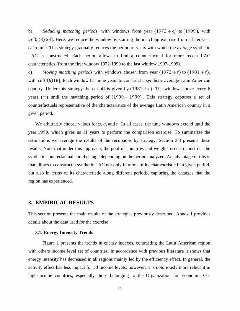
b) Reducing matching periods, with windows from year (1972 + q) to (1999 ), with

𝑞𝜖[0 (3) 24]. Here, we reduce the window by starting the matching exercise from a later year

each time. This strategy gradually reduces the period of years with which the average synthetic

LAC is constructed. Each period allows to find a counterfactual for more recent LAC

characteristics (from the first window 1972-1999 to the last window 1997-1999).

c) Moving matching periods with windows chosen from year (1972 + r) to (1981 + r),

with 𝑟𝜖[0(6)18]. Each window has nine years to construct a synthetic average Latin American

country. Under this strategy the cut-off is given by (1981 + 𝑟). The windows move every 6

years ( 𝑟 ) until the matching period of (1990 − 1999) . This strategy captures a set of

counterfactuals representative of the characteristics of the average Latin American country in a

given period.

We arbitrarily choose values for 𝑝, 𝑞, and 𝑟. In all cases, the time windows extend until the

year 1999, which gives us 11 years to perform the comparison exercise. To summarize the

estimations we average the results of the recursions by strategy. Section 3.3 presents these

results. Note that under this approach, the pool of countries and weights used to construct the

synthetic counterfactual could change depending on the period analyzed. An advantage of this is

that allows to construct a synthetic LAC not only in terms of its characteristic in a given period,

but also in terms of its characteristic along different periods, capturing the changes that the

region has experienced.

3. EMPIRICAL RESULTS

This section presents the main results of the strategies previously described. Annex 1 provides

details about the data used for the exercise.

3.1. Energy Intensity Trends

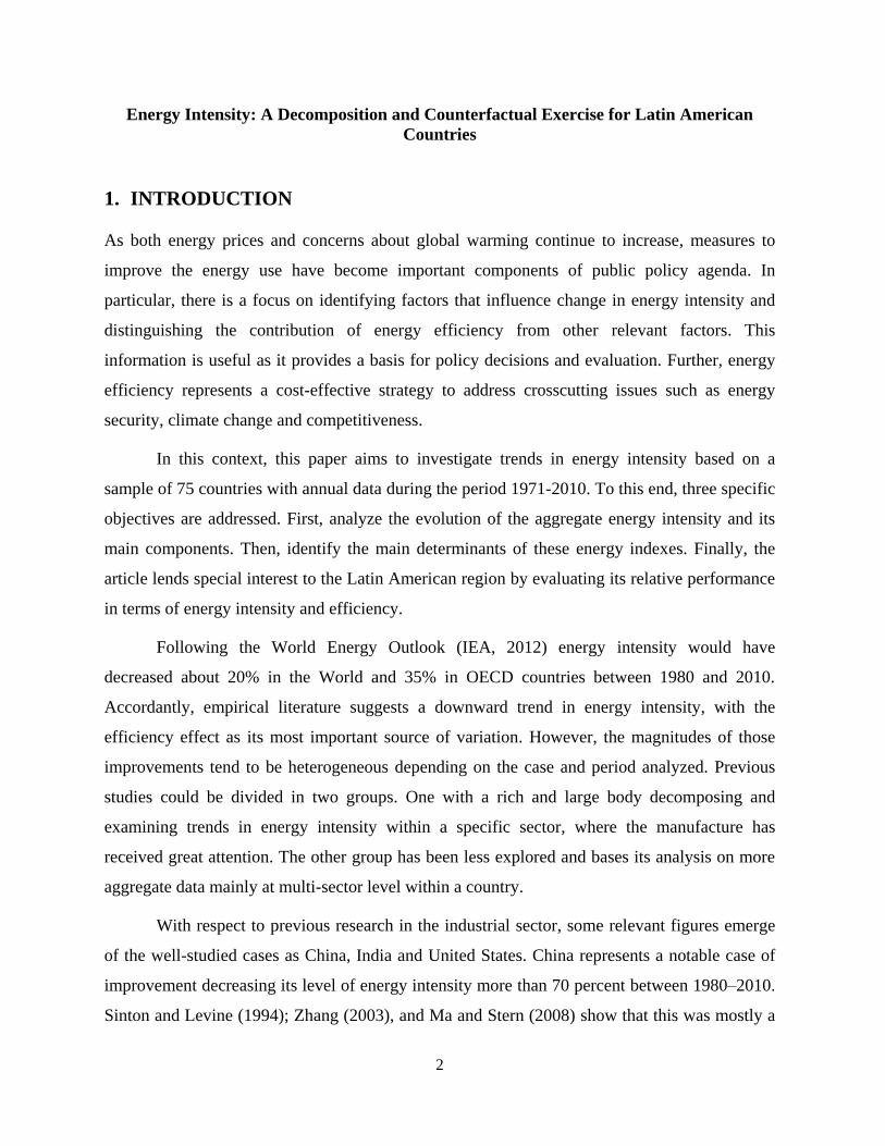
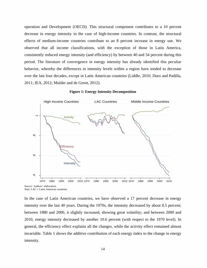
Figure 1 presents the trends in energy indexes, contrasting the Latin American region

with others income level set of countries. In accordance with previous literature it shows that

energy intensity has decreased in all regions mainly led by the efficiency effect. In general, the

activity effect has less impact for all income levels; however, it is notoriously more relevant in

high-income countries, especially those belonging to the Organization for Economic Co-

14

operation and Development (OECD). This structural component contributes to a 10 percent

decrease in energy intensity in the case of high-income countries. In contrast, the structural

effects of medium-income countries contribute to an 8 percent increase in energy use. We

observed that all income classifications, with the exception of those in Latin America,

consistently reduced energy intensity (and efficiency) by between 40 and 54 percent during this

period. The literature of convergence in energy intensity has already identified this peculiar

behavior, whereby the differences in intensity levels within a region have tended to decrease

over the last four decades, except in Latin American countries (Liddle, 2010; Duro and Padilla,

2011; IEA, 2012; Mulder and de Groot, 2012).

Figure 1: Energy Intensity Decomposition

Source: Authors’ elaboration.

Note: LAC = Latin American countries.

In the case of Latin American countries, we have observed a 17 percent decrease in energy

intensity over the last 40 years. During the 1970s, the intensity decreased by about 8.5 percent;

between 1980 and 2000, it slightly increased, showing great volatility; and between 2000 and

2010, energy intensity decreased by another 10.6 percent (with respect to the 1970 level). In

general, the efficiency effect explains all the changes, while the activity effect remained almost

invariable. Table 1 shows the additive contribution of each energy index to the change in energy

intensity.

Activity

Efficiency

Intensity

.4.6

.81

1970 1980 1990 2000 2010 1970 1980 1990 2000 2010 1970 1980 1990 2000 2010

High Income Countries LAC Countries Middle Income Countries

15

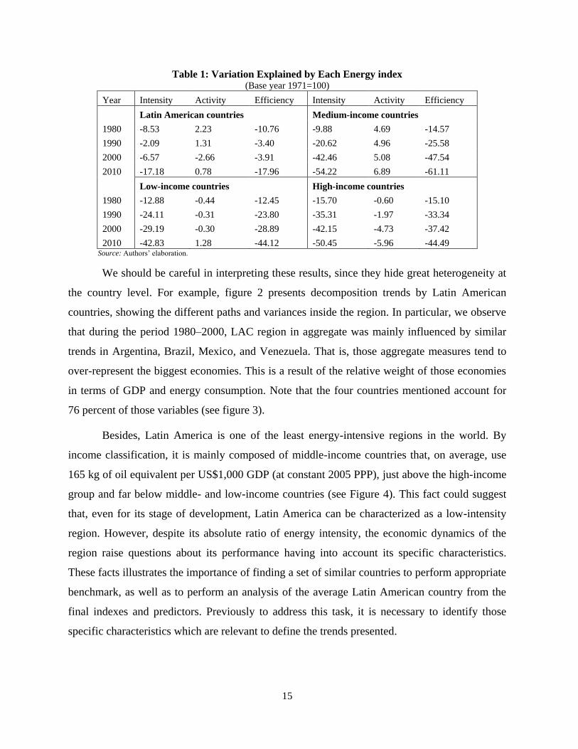
Table 1: Variation Explained by Each Energy index (Base year 1971=100)

Year Intensity Activity Efficiency Intensity Activity Efficiency

Latin American countries Medium-income countries

1980 -8.53 2.23 -10.76 -9.88 4.69 -14.57

1990 -2.09 1.31 -3.40 -20.62 4.96 -25.58

2000 -6.57 -2.66 -3.91 -42.46 5.08 -47.54

2010 -17.18 0.78 -17.96 -54.22 6.89 -61.11

Low-income countries High-income countries

1980 -12.88 -0.44 -12.45 -15.70 -0.60 -15.10

1990 -24.11 -0.31 -23.80 -35.31 -1.97 -33.34

2000 -29.19 -0.30 -28.89 -42.15 -4.73 -37.42

2010 -42.83 1.28 -44.12 -50.45 -5.96 -44.49 Source: Authors’ elaboration.

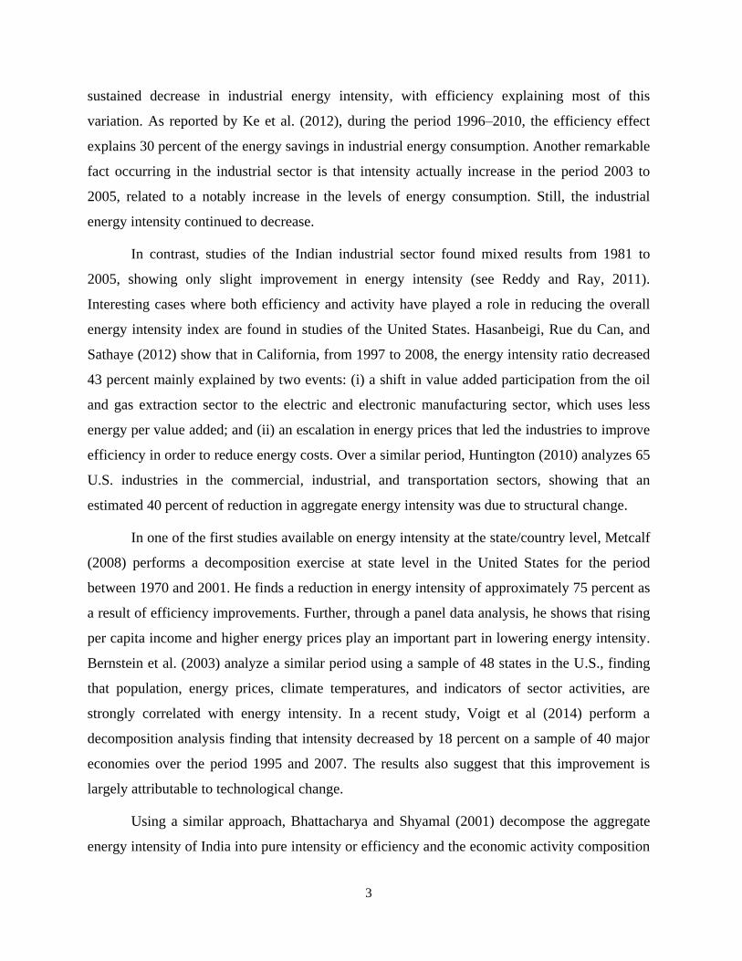
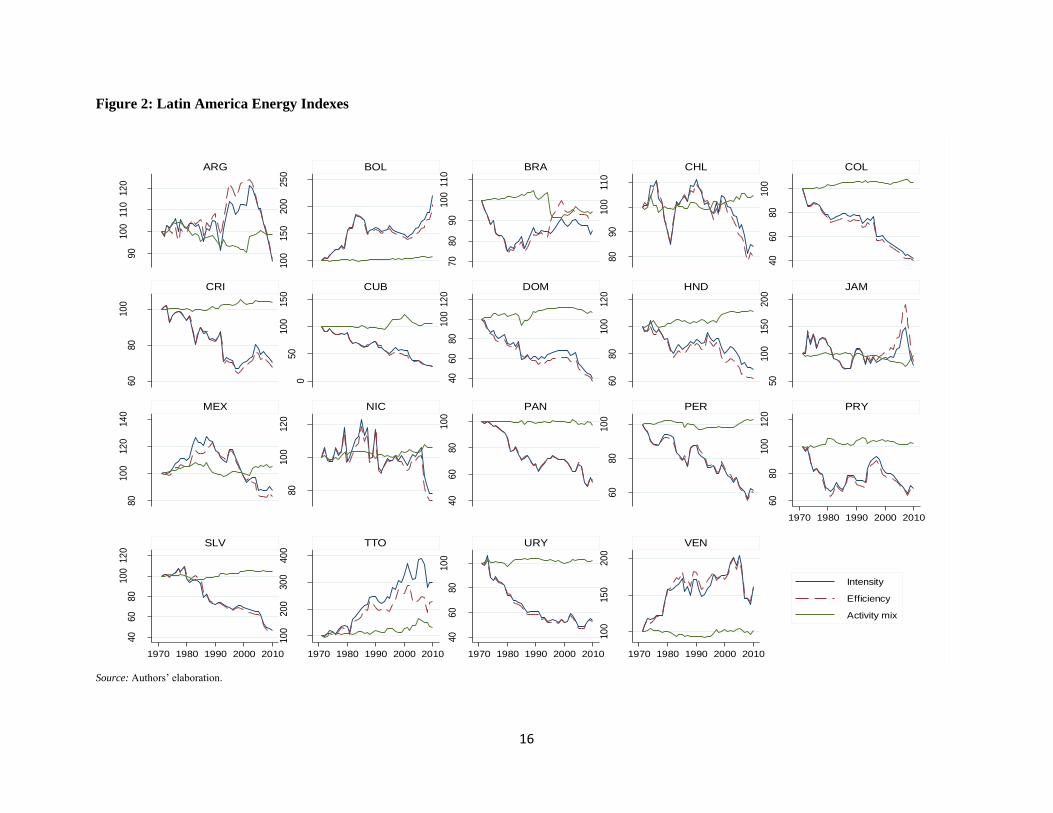
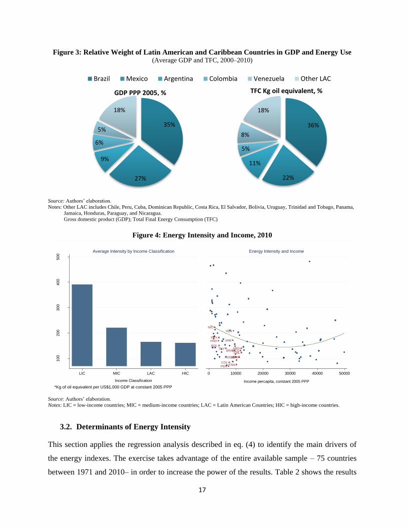
We should be careful in interpreting these results, since they hide great heterogeneity at

the country level. For example, figure 2 presents decomposition trends by Latin American

countries, showing the different paths and variances inside the region. In particular, we observe

that during the period 1980–2000, LAC region in aggregate was mainly influenced by similar

trends in Argentina, Brazil, Mexico, and Venezuela. That is, those aggregate measures tend to

over-represent the biggest economies. This is a result of the relative weight of those economies

in terms of GDP and energy consumption. Note that the four countries mentioned account for

76 percent of those variables (see figure 3).

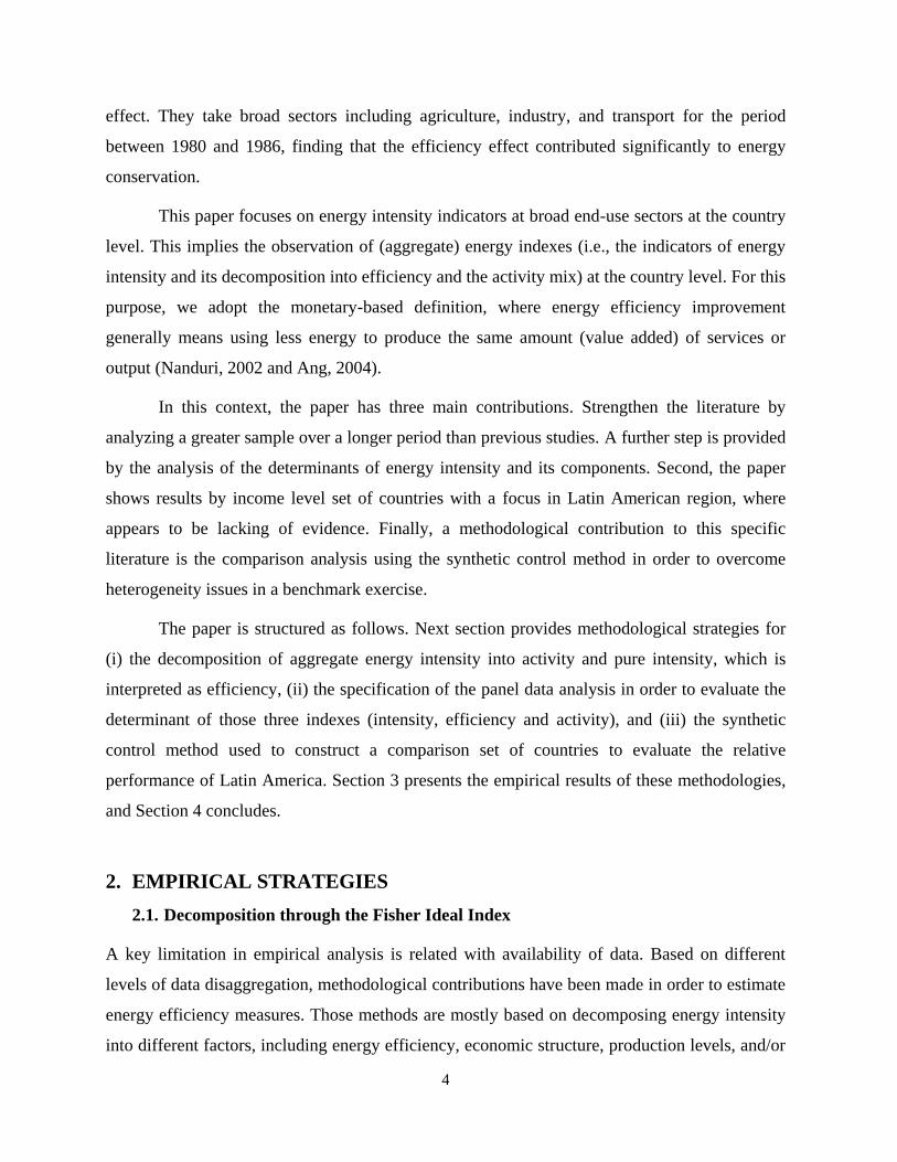
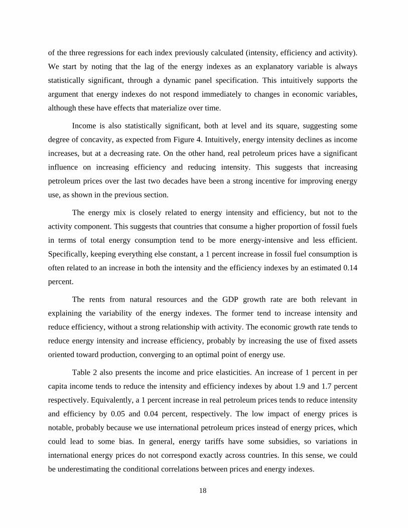
Besides, Latin America is one of the least energy-intensive regions in the world. By

income classification, it is mainly composed of middle-income countries that, on average, use

165 kg of oil equivalent per US$1,000 GDP (at constant 2005 PPP), just above the high-income

group and far below middle- and low-income countries (see Figure 4). This fact could suggest

that, even for its stage of development, Latin America can be characterized as a low-intensity

region. However, despite its absolute ratio of energy intensity, the economic dynamics of the

region raise questions about its performance having into account its specific characteristics.

These facts illustrates the importance of finding a set of similar countries to perform appropriate

benchmark, as well as to perform an analysis of the average Latin American country from the

final indexes and predictors. Previously to address this task, it is necessary to identify those

specific characteristics which are relevant to define the trends presented.

16

Figure 2: Latin America Energy Indexes

Source: Authors’ elaboration.

90

10

011

012

0

10

015

020

025

0

70

80

90

10

011

0

80

90

10

011

0

40

60

80

10

0

60

80

10

0

050

10

015

0

40

60

80

10

012

0

60

80

10

012

0

50

10

015

020

0

80

10

012

014

0

80

10

012

0

40

60

80

10

0

60

80

10

0

60

80

10

012

0

40

60

80

10

012

0

10

020

030

040

0

40

60

80

10

0

10

015

020

0

1970 1980 1990 2000 2010

1970 1980 1990 2000 2010 1970 1980 1990 2000 2010 1970 1980 1990 2000 2010 1970 1980 1990 2000 2010

ARG BOL BRA CHL COL

CRI CUB DOM HND JAM

MEX NIC PAN PER PRY

SLV TTO URY VEN

Intensity

Efficiency

Activity mix

17

Figure 3: Relative Weight of Latin American and Caribbean Countries in GDP and Energy Use (Average GDP and TFC, 2000–2010)

Source: Authors’ elaboration.

Notes: Other LAC includes Chile, Peru, Cuba, Dominican Republic, Costa Rica, El Salvador, Bolivia, Uruguay, Trinidad and Tobago, Panama,

Jamaica, Honduras, Paraguay, and Nicaragua.

Gross domestic product (GDP); Total Final Energy Consumption (TFC)

Figure 4: Energy Intensity and Income, 2010

Source: Authors’ elaboration.

Notes: LIC = low-income countries; MIC = medium-income countries; LAC = Latin American Countries; HIC = high-income countries.

3.2. Determinants of Energy Intensity

This section applies the regression analysis described in eq. (4) to identify the main drivers of

the energy indexes. The exercise takes advantage of the entire available sample – 75 countries

between 1971 and 2010– in order to increase the power of the results. Table 2 shows the results

10

02

00

30

04

00

50

0

En

erg

y In

ten

sity*

LIC MIC LAC HIC

Income Classification

Average Intensity by Income Classification

NIC

HNDPRY

BOLSLV

PER

COL

JAM

VEN

BRA

DOM

PAN

URYCRI

MEXARG

CHL

0 10000 20000 30000 40000 50000

Income percapita, constant 2005 PPP

Energy Intensity and Income

*Kg of oil equivalent per US$1,000 GDP at constant 2005 PPP

Brazil Mexico Argentina Colombia Venezuela Other LAC

GDP PPP 2005, % TFC Kg oil equivalent, %

36%

22%

11%

5%

8%

18%

35%

27%

9%

6%

5%

18%

18

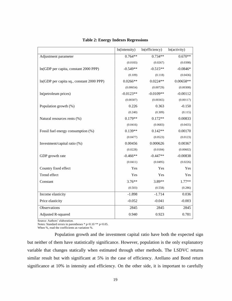
of the three regressions for each index previously calculated (intensity, efficiency and activity).

We start by noting that the lag of the energy indexes as an explanatory variable is always

statistically significant, through a dynamic panel specification. This intuitively supports the

argument that energy indexes do not respond immediately to changes in economic variables,

although these have effects that materialize over time.

Income is also statistically significant, both at level and its square, suggesting some

degree of concavity, as expected from Figure 4. Intuitively, energy intensity declines as income

increases, but at a decreasing rate. On the other hand, real petroleum prices have a significant

influence on increasing efficiency and reducing intensity. This suggests that increasing

petroleum prices over the last two decades have been a strong incentive for improving energy

use, as shown in the previous section.

The energy mix is closely related to energy intensity and efficiency, but not to the

activity component. This suggests that countries that consume a higher proportion of fossil fuels

in terms of total energy consumption tend to be more energy-intensive and less efficient.

Specifically, keeping everything else constant, a 1 percent increase in fossil fuel consumption is

often related to an increase in both the intensity and the efficiency indexes by an estimated 0.14

percent.

The rents from natural resources and the GDP growth rate are both relevant in

explaining the variability of the energy indexes. The former tend to increase intensity and

reduce efficiency, without a strong relationship with activity. The economic growth rate tends to

reduce energy intensity and increase efficiency, probably by increasing the use of fixed assets

oriented toward production, converging to an optimal point of energy use.

Table 2 also presents the income and price elasticities. An increase of 1 percent in per

capita income tends to reduce the intensity and efficiency indexes by about 1.9 and 1.7 percent

respectively. Equivalently, a 1 percent increase in real petroleum prices tends to reduce intensity

and efficiency by 0.05 and 0.04 percent, respectively. The low impact of energy prices is

notable, probably because we use international petroleum prices instead of energy prices, which

could lead to some bias. In general, energy tariffs have some subsidies, so variations in

international energy prices do not correspond exactly across countries. In this sense, we could

be underestimating the conditional correlations between prices and energy indexes.

19

Table 2: Energy Indexes Regressions

ln(intensity) ln(efficiency) ln(activity)

Adjustment parameter 0.764** 0.734** 0.670**

(0.0183) (0.0267) (0.0398)

ln(GDP per capita, constant 2000 PPP) -0.549** -0.515** -0.0846*

(0.109) (0.118) (0.0436)

ln(GDP per capita sq., constant 2000 PPP) 0.0266** 0.0224** 0.00658**

(0.00654) (0.00729) (0.00308)

ln(petroleum prices) -0.0123** -0.0109** -0.00112

(0.00307) (0.00365) (0.00117)

Population growth (%) 0.226 0.363 -0.150

(0.240) (0.309) (0.115)

Natural resources rents (%) 0.179** 0.172** 0.00833

(0.0416) (0.0683) (0.0435)

Fossil fuel energy consumption (%) 0.139** 0.142** 0.00170

(0.0477) (0.0523) (0.0123)

Investment/capital ratio (%) 0.00456 0.000626 0.00367

(0.0228) (0.0184) (0.00602)

GDP growth rate -0.466** -0.447** -0.00838

(0.0411) (0.0495) (0.0226)

Country fixed effect Yes Yes Yes

Trend effect Yes Yes Yes

Constant 3.76** 3.89** 1.77**

(0.503) (0.558) (0.286)

Income elasticity -1.898 -1.714 0.036

Price elasticity -0.052 -0.041 -0.003

Observations 2845 2845 2845

Adjusted R-squared 0.940 0.923 0.781

Source: Authors’ elaboration.

Notes: Standard errors in parentheses * p<0.10 ** p<0.05.

When %, read the coefficients as variation %.

Population growth and the investment capital ratio have both the expected sign

but neither of them have statistically significance. However, population is the only explanatory

variable that changes statically when estimated through other methods. The LSDVC returns

similar result but with significant at 5% in the case of efficiency. Arellano and Bond return

significance at 10% in intensity and efficiency. On the other side, it is important to carefully

20

consider the results with respect to investment, since this variable is estimated by constructing

the series on stocks of capital (see Annex 1). What is more, we assumed a common depreciation

rate across time and across countries. Nonetheless, these results are in line with the specificity

of energy-efficient investment, supporting the fact that investments do not necessarily reduce

energy intensity at the aggregate level.

By the exception of population, the results presented are robust to different estimation

methodologies. See annex 2 the results of the same regressions under different estimators –

Corrected LSDV and the Bond estimators–. Besides, the inspection for multi-collinearity

reveals that it does not seems to be the source of these low statistical significant or coefficient of

the independent variables.

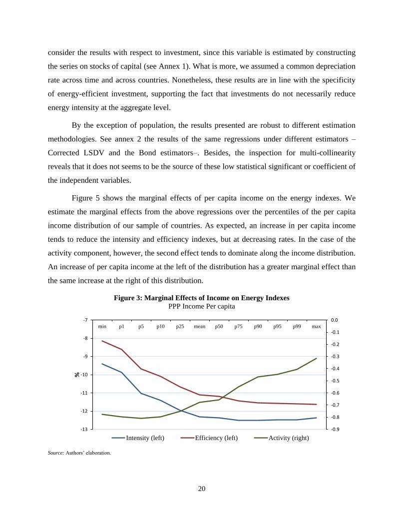
Figure 5 shows the marginal effects of per capita income on the energy indexes. We

estimate the marginal effects from the above regressions over the percentiles of the per capita

income distribution of our sample of countries. As expected, an increase in per capita income

tends to reduce the intensity and efficiency indexes, but at decreasing rates. In the case of the

activity component, however, the second effect tends to dominate along the income distribution.

An increase of per capita income at the left of the distribution has a greater marginal effect than

the same increase at the right of this distribution.

Figure 3: Marginal Effects of Income on Energy Indexes

PPP Income Per capita

Source: Authors’ elaboration.

-0.9

-0.8

-0.7

-0.6

-0.5

-0.4

-0.3

-0.2

-0.1

0.0

-13

-12

-11

-10

-9

-8

-7min p1 p5 p10 p25 mean p50 p75 p90 p95 p99 max

%

Intensity (left) Efficiency (left) Activity (right)

21

Even as this analysis allows us to identify the main drivers of the energy indexes, it does

not allow us to distinguish the relative performance of Latin American countries. The next

section addresses this limitation by comparing the average Latin American country with another

set of countries with similar characteristics thought to drive the energy indexes.

3.3. Synthetic Comparisons in Latin American Countries

This section returns to the comparison exercise, searching in each window of time for a set of

countries with similar characteristics to those of the average Latin American country.4 It is

necessary to choose those characteristics in terms of their ability to predict the outcomes’

variables—in this case, the energy indexes. Taking a conservative position, we use the whole

set of variables in 𝑋 and apply the synthetic control method under each of the strategies

described in the methodological section. Figure 6 compares the trends between the average and

synthetic Latin American country. The synthetic LAC represents the average of the sets of

countries that best resemble the average Latin American country under each strategy.5

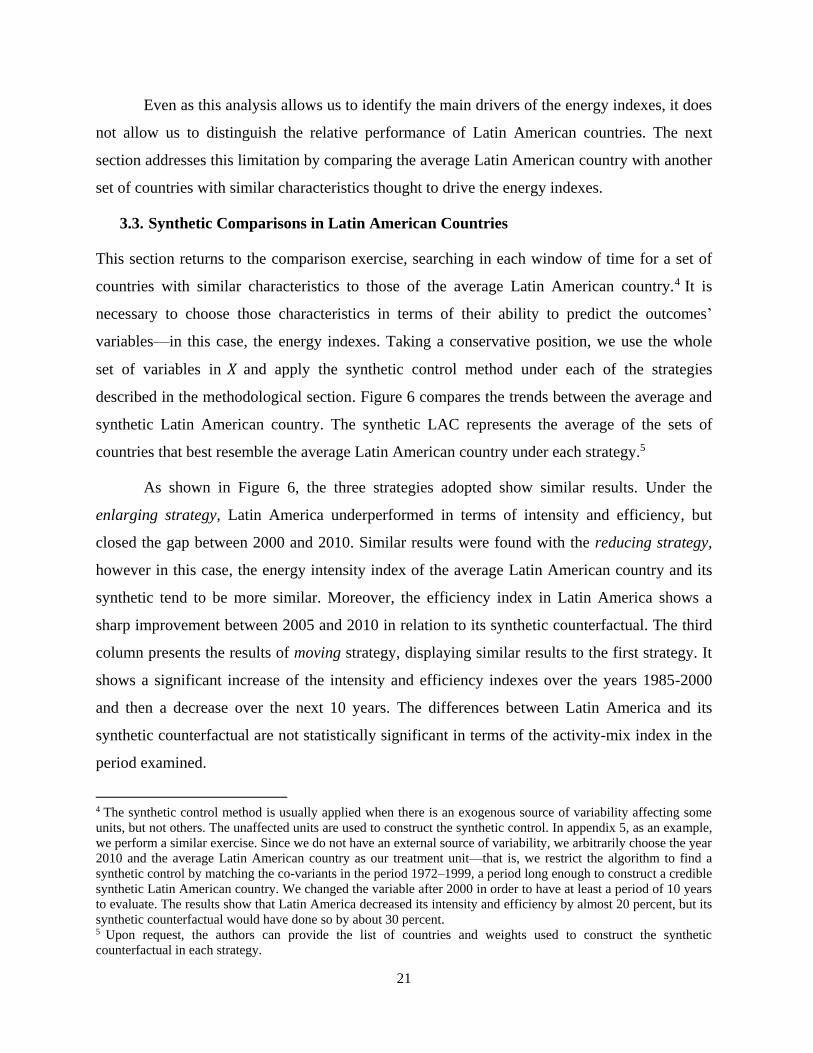
As shown in Figure 6, the three strategies adopted show similar results. Under the

enlarging strategy, Latin America underperformed in terms of intensity and efficiency, but

closed the gap between 2000 and 2010. Similar results were found with the reducing strategy,

however in this case, the energy intensity index of the average Latin American country and its

synthetic tend to be more similar. Moreover, the efficiency index in Latin America shows a

sharp improvement between 2005 and 2010 in relation to its synthetic counterfactual. The third

column presents the results of moving strategy, displaying similar results to the first strategy. It

shows a significant increase of the intensity and efficiency indexes over the years 1985-2000

and then a decrease over the next 10 years. The differences between Latin America and its

synthetic counterfactual are not statistically significant in terms of the activity-mix index in the

period examined.

4 The synthetic control method is usually applied when there is an exogenous source of variability affecting some

units, but not others. The unaffected units are used to construct the synthetic control. In appendix 5, as an example,

we perform a similar exercise. Since we do not have an external source of variability, we arbitrarily choose the year

2010 and the average Latin American country as our treatment unit—that is, we restrict the algorithm to find a

synthetic control by matching the co-variants in the period 1972–1999, a period long enough to construct a credible

synthetic Latin American country. We changed the variable after 2000 in order to have at least a period of 10 years

to evaluate. The results show that Latin America decreased its intensity and efficiency by almost 20 percent, but its

synthetic counterfactual would have done so by about 30 percent. 5 Upon request, the authors can provide the list of countries and weights used to construct the synthetic

counterfactual in each strategy.

22

In general, the main finding of this approach is that Latin America underperformed in

energy intensity and efficiency during the period 1985–2000. However, the gap closed over the

next 10 years, showing a sharp improvement.

Figure 6: Energy Indexes of LAC vs Synth

Source: Authors’ elaboration.

Note: LAC = Latin American countries.

4. CONCLUSIONS

Energy intensity has shown a decreasing trend in all sets of countries regardless of their income

level. Empirical literature suggests that the main sources explaining this variation are related

with improvements in energy efficiency; however, less research has analyzed the determinants

of such trends at country level. Besides, Latin America seems to represent a peculiarity as its

reduction of energy use levels are less pronounced than in other regions. In this context, based

on a dataset composed of 75 countries over the period 1971-2010, we investigated the energy

intensity trends with a particular focus in LAC. First, the Fisher Ideal Index was used in order to

decompose energy intensity into two components; activity mix and efficiency. Then, the main

drivers of the energy indexes were analyzed through panel data techniques. Taken as inputs the

previous results, a comparison exercise is performed by applying the Synthetic Control Method.

80

90

10

0

Inte

nsity

Enlarging Matching Periods Reducing Matching Periods Moving Matching Periods

80

90

10

0

Effic

ien

cy

80

90

10

0

Activity

1970 1980 1990 2000 2010 1970 1980 1990 2000 2010 1970 1980 1990 2000 2010

Dash line: Synthetic; Straight line: LAC; both in 95% C.I.

23

This allowed constructing a counterfactual LAC in order to evaluate the performance of the

Region.

The intensity decomposition corroborates that energy intensity decreased in all income-level-

countries, mainly explained by pure intensity which is interpreted as efficiency-effect. Over the

last 40 years, the size of the reduction range between 40 percent in low income countries to 54

percent in medium income countries. In contrast, Latin America reduced its energy intensity by

around 20 percent, suggesting that the region under-performed during the period analyzed. The

econometric analysis shows that the main determinants behind those general trends are per

capita income, petroleum prices, and economic growth. These variables have statistical strength

in explaining the improvement in energy use over the last four decades. On the other hand, the

fuel mix and the abundance of extractive natural resources are directly correlated with the

energy indexes. These results could help to explain the stagnant energy intensity in LAC

between the mid-1980s and mid-1990s, a period characterized by difficult economic conditions

and relatively low international oil prices, especially in those abundance resource countries.

The comparison exercise complement the previous analysis by providing a set of

countries which are comparable to LAC along the period analyzed. The results suggest that

Latin America is not behind other regions in terms of energy intensity and efficiency: the 20

percent improvement in the Latin American region is similar to the improvement in its synthetic

counterfactual. Even when we observe an increase in energy intensity between the mid-1980s

and mid-1990s, the analysis shows that Latin America gradually closed the gap between 2000

and 2010. Since no major measures were taken in the region in terms of energy efficiency, this

suggests that market signals were enough to correct the trends in energy indexes.

Further studies could perform a more detailed decomposition and a more complete set of

covariates could be added to the regression analysis. To this end, better and comparable data

need to be systematically collected in areas as energy prices, efficiency characteristics of the

investments, fuels mix of the industries, among others. A topic which is particularly relevant for

energy intensity industries is the need to perform specific analysis by industry (i.e.,

manufacture, mining, etc.).

24

REFERENCES

Abadie, A., and J. Gardeazabal. 2003. “Economic Costs of Conflict: A Case Study of the Basque Country.”

American Economic Review 93(1): 113–132.

Abadie, A., A. Diamond, and J. Hainmueller. 2010. “Synthetic Control Methods for Comparative Case Studies:

Estimating the Effect of California’s Tobacco Control Program.” Journal of the American Statistical

Association 105(490): 493–505.

———. 2011. “Synth: An R Package for Synthetic Control Methods in Comparative Case Studies.” Journal of

Statistical Software 42(13): 1–17. Available at http://www.jstatsoft.org/v42/i13/paper.

Ang, B. W. 2004. “Decomposition Analysis for Policymaking in Energy: Which is the Preferred Method?” Energy

Policy 32: 1131–39.

———. 2006. “Monitoring Changes in Economy-wide Energy Efficiency: From Energy-GDP Ratio to Composite

Efficiency Index.” Energy Policy 34(5): 574–82.

Ang, B. W. and S. Y. Lee. 1994. “Decomposition of Industrial Energy Consumption: Some Methodological and

Application Issues.” Energy Economics 16(2): 83–92.

Ang, B.W. and F. L. Liu. 2003. “Eight Methods for Decomposing the Aggregate Energy-intensity of Industry.”

Applied Energy 76(1–3): 15–23.

Ang, B. W., F. L. Liu, and H. Chung. 2004. “A generalized Fisher index approach to energy decomposition

analysis.” Energy Economics (26): 757-763.

Ang, B.W., and N. Liu. 2007a. “Handling Zero Values in the Logarithmic Mean Divisia Index Decomposition

Approach.” Energy Policy 35(1): 238–46.

———. 2007b. “Negative-value Problems of the Logarithmic Mean Divisia Index Decomposition Approach.”

Energy Policy 35(1): 739–42.

Ang, B. W., H. C. Huang, and A. R. Mu. 2009. “Properties and Linkages of Some Index Decomposition Analysis

Methods.” Energy Policy (37): 4624–32.

Ang, B.W., A. R. Mu, and P. Zhou. 2010. “Accounting Frameworks for Tracking Energy Efficiency Trends.”

Energy Economics 32(5): 1209–19

Balza, L. and R. Jimenez. 2013. “Models for Forecasting Energy Use and Electricity Demand: An Application to

Central American Countries, Mexico and Dominican Republic.” Washington, DC: Inter-American

Development Bank. Forthcoming.

Bernstein, M., K. Fonkych, S. Loeb, and D. Loughran. 2003. “State-Level Changes in Energy Intensity and Their

National Implications.” Monograph Reports. Santa Monica, CA: RAND Corporation.

Bhattacharya, R. and P. Shyamal. 2001. “Sectoral Changes in Consumption and Intensity Energy in India.” Indian

Economic Review 36(2): 381–92

Boyd, G.A., D. A. Hanson, and T. N. S. Sterner. 1988. “Decomposition of Changes in Energy Intensity: A

Comparison of the Divisia Index and Other Methods.” Energy Economics 10(4): 309–12.

Boyd, G.A. and J. M. Roop. 2004. “A Note on the Fisher Ideal Index Decomposition for Structural Change in

Energy Intensity.” The Energy Journal 25(1): 87–101.

de Boer, P.M.C.. (2008). Energy decomposition analysis: the generalized Fisher index revisited. Report /

Econometric Institute, Erasmus University Rotterdam (pp. 1–11). Erasmus School of Economics (ESE).

Duro, J. A. and E. Padilla. 2011. “Inequality across Countries in Energy Intensities: An Analysis of the Role of

Energy Transformation and Final Energy Consumption.” Energy Economics 33: 474–79.

Galiani, S. and M. Gonzalez-Rozada. 2002. “Inference and Estimation in Small Sample Dynamic Panel Data

Models.” Business School Working Papers 02/2002. Buenos Aires, Argentina: Centro de Investigación en

Finanzas, Universidad Torcuato Di Tella. Available at www.utdt.edu/departamentos/empresarial/cif/pdfs-

wp/wpcif-022002.pdf.

Galli, R. 1998. The Relationship Between Energy Intensity and Income Levels: Forecasting Long Term Energy

Demand in Asian Emerging Countries. The Energy Journal. 19(4): 85-105.

25

Greening, L. A., W. B. Davis, L. Schipper, and M. Khrushch. 1997. “Comparison of Six Decomposition Methods:

Application to Aggregate Energy Intensity for Manufacturing in 10 OECD Countries.” Energy Economics

19(3): 375–90.

Hall, R. E. and C. I. Jones. 1999. “Why Do Some Countries Produce So Much More Output Per Worker Than

Others?” The Quarterly Journal of Economics 114(1): 83–116.

Hasanbeigi, A., S. Rue du Can, and S. Sathaye. 2012. “Analysis and Decomposition of the Energy Intensity of

Industries in California.” Energy Policy 46.

Huntington, H. G., 2010. “Structural Change and U.S. Energy Use: Recent Patterns.” Energy Journal 31: 25–39.

IEA (International Energy Agency). 2012. “Energy Indicators System: Index Construction Methodology.” Paris,

France: IEA.

Judson, R. A. and A. L. Owen. 1999. “Estimating Dynamic Panel Data Models: A Guide for Macroeconomists.”

Economics Letters 65(1): 9–15.

Ke, J., L. Price, S. Ohshita, D. Fridley, N. Zheng, N. Zhou, and M. Levine. 2012. “China's Industrial Energy

Consumption Trends and Impacts of the Top-1000 Enterprises Energy-Saving Program and the Ten Key

Energy-Saving Projects.” Energy Policy 50: 562–69.

Liddle, B., 2010. “Revisiting World Energy Intensity Convergence of Regional Differences.” Applied Energy 87:

3218–25.

Nanduri, M., J. Nyboer, and M. Jaccard. 2002. “Aggregating Physical Intensity Indicators: Results of Applying the

Composite Indicator Approach to the Canadian Industrial Sector.” Energy Policy 30(2): 151–63.

Ma, C., and D. I. Stern. 2008. “China's Changing Energy Intensity Trend: A Decomposition Analysis.” Energy

Economics 30: 1037–53.

Metcalf, G. 2008. “An Empirical Analysis of Energy Intensity and its Determinants at the State Level.” The Energy

Journal 29(3): 1–26.

Mulder, P. and H. L. F. de Groot. 2012. “Structural Change and Convergence of Energy Intensity across OECD

Countries, 1970–2005.” Energy Economics 34: 1910–21.

Reddy, B. S. and B. K. Ray. 2011. “Understanding Industrial Energy Use: Physical Energy Intensity Changes in

Indian Manufacturing Sector.” Energy Policy 39(11): 7234–43.

Sachs, J. D. and A. M. Warner. 1995. “Natural Resource Abundance and Economic Growth.” NBER Working

Paper No. 5398. Cambridge, MA: National Bureau of Economic Research (NBER). Available at

http://www.nber.org/papers/w5398.pdf.

Shahiduzzaman, M. D. and A. Khorshed. 2013. “Changes in Energy Efficiency in Australia: A Decomposition of

Aggregate Energy Intensity Using Logarithmic Mean Divisia Approach.” Energy Policy 56(3): 341–351.

Sinton, J. E. and M. D. Levine. 1994. “Changing Energy Intensity in Chinese Industry: The Relatively Importance

of Structural Shift and Intensity Change.” Energy Policy 22(3): 239–55.

Sue Wing, I., 2008. “Explaining the Declining Energy Intensity of the U.S. Economy.” Resources and Energy

Economics 30(1): 21–49.

Voigt, S. De Cain, E. Schymura, M. and Verdolini, E. 2014. “Energy Intensity Developments in 40 Major

Economies: Structural Change or Technology Improvement?” Energy Economics 41(1): 47-62.

Zhang, Z. X. 2003. “Why Did the Energy Intensity Fall in China's Industrial Sector in the 1990s? The Relative

Importance of Structural Change and Intensity Change.” Energy Economics 25(6): 625–38.

26

ANNEXES

Annex 1: Data Sources

This study analyzes the period 1971–2010 and uses a sample of 75 countries (19 from Latin America).

The data on energy come from the International Energy Agency (IEA), while the measures of economic

activity are based on World Bank Development Indicators. The PPP GDP at constant 2005 prices is taken

from the Penn tables. Since those tables only provide data through 2009, we use growth projections from

the IMF to complete the year 2010. To account for a longer dataset, we drop those countries with less

than 20 observations in any variable.

In the first step, we calculate the energy intensity series (EI) as the ratio of the total final

consumption of energy by sector (from IEA) and the PPP GDP at constant prices of 2005, in thousands

(from Penn Tables). We analyze data from the agricultural, industrial, service, and residential sectors

(from IEA), which allows us to form a partition for these sectors. Since activity indicators can overlap,

appropriate proxies are value added in the agricultural, industrial, and service sectors. For the residential

sector, we consider the household final expenditure. To build the energy indexes, the methodology

requires that there be no missing values in economic activity indicator or sector energy use. Ang and Liu

(2007a; 2007b) evaluate and propose different strategies for the case of zero values. In order to preserve

trends, we adopt the compound rate of the growth method, which is a standard practice of IEA to forecast

trends. As revised in Balza and Jimenez (2013), this method tends to offer accurate estimations of energy

use trends. Thus, we input those missing values with estimations based on the compound growth rate

method as described in the next expression: 𝑦𝑡 = 𝑦𝑡−𝑙(1 + 𝑔𝑦)𝑙.

Where y represents the variable with missing/zero values, t the period, l the number of periods from the

last not missing/zero value, and g the growth rate of the variable of interest.

We extract other variables from the World Bank Development Indicator (fossil fuel consumption,

total labor force, fuel exports, population growth, and gross capital formation) and the International

Monetary Fund (petroleum prices). Following Metcalf (2008), we incorporate the ratios (stock of

capital/labor force) and (investment/stock of capital). Since the stock of capital is not available for all

countries, we construct a proxy based on the perpetual inventory method: 𝐾𝑡 = (1 − 𝛿)𝐾𝑡−1 + 𝐺𝐹𝐾𝑡.

Where K and GFK represent the stock of capital and the gross capital formation, respectively. The

depreciation rate (delta) is assumed to be 6 percent. The initial value K is calculated as 𝐾0 =𝐺𝐹𝐾0

(𝛿 + 𝑔𝐺𝐹𝐾)⁄ , with 𝑔𝐺𝐹𝐾 representing the growth rate in gross fixed capital formation. Hall and

Jones (1999) provide further details on this method.

27

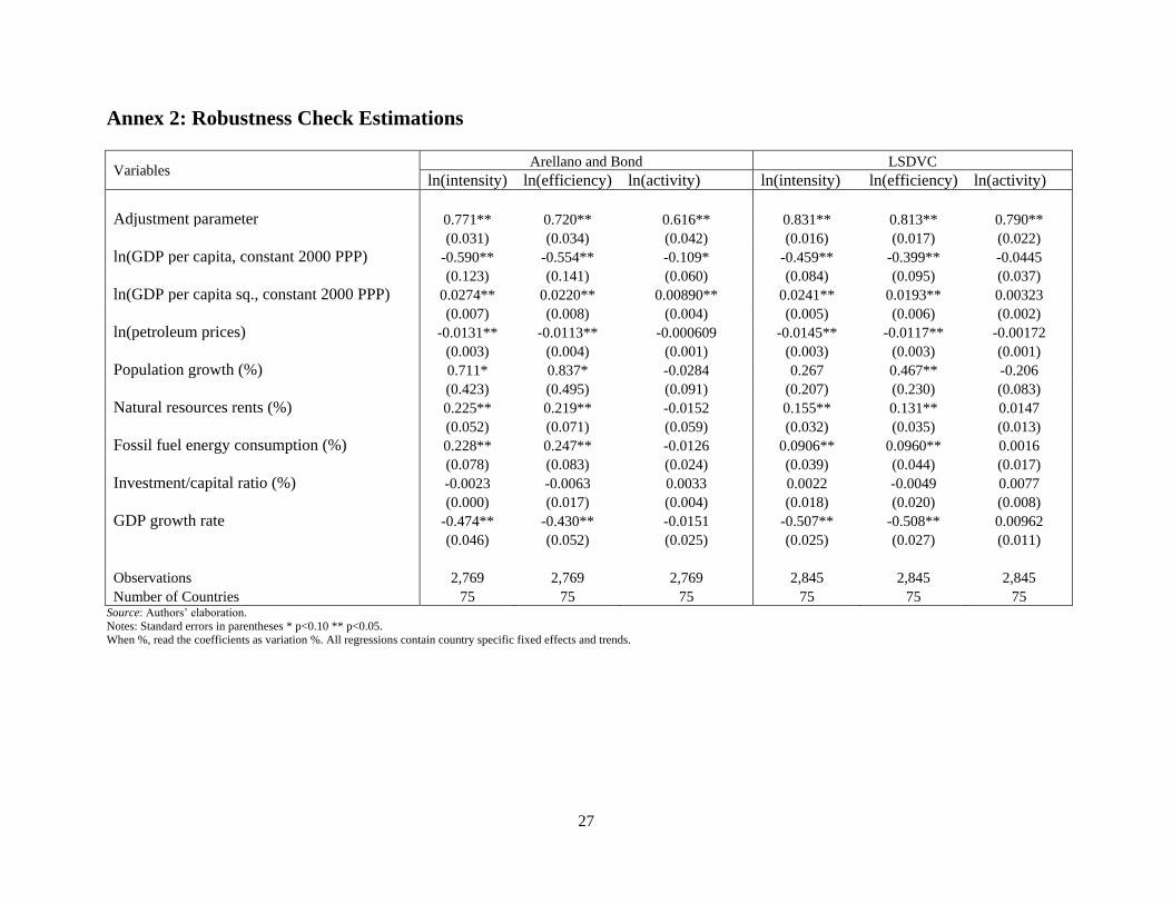
Annex 2: Robustness Check Estimations

Variables Arellano and Bond LSDVC

ln(intensity) ln(efficiency) ln(activity) ln(intensity) ln(efficiency) ln(activity)

Adjustment parameter 0.771** 0.720** 0.616** 0.831** 0.813** 0.790**

(0.031) (0.034) (0.042) (0.016) (0.017) (0.022)

ln(GDP per capita, constant 2000 PPP) -0.590** -0.554** -0.109* -0.459** -0.399** -0.0445

(0.123) (0.141) (0.060) (0.084) (0.095) (0.037)

ln(GDP per capita sq., constant 2000 PPP) 0.0274** 0.0220** 0.00890** 0.0241** 0.0193** 0.00323

(0.007) (0.008) (0.004) (0.005) (0.006) (0.002)

ln(petroleum prices) -0.0131** -0.0113** -0.000609 -0.0145** -0.0117** -0.00172

(0.003) (0.004) (0.001) (0.003) (0.003) (0.001)

Population growth (%) 0.711* 0.837* -0.0284 0.267 0.467** -0.206

(0.423) (0.495) (0.091) (0.207) (0.230) (0.083)

Natural resources rents (%) 0.225** 0.219** -0.0152 0.155** 0.131** 0.0147

(0.052) (0.071) (0.059) (0.032) (0.035) (0.013)

Fossil fuel energy consumption (%) 0.228** 0.247** -0.0126 0.0906** 0.0960** 0.0016

(0.078) (0.083) (0.024) (0.039) (0.044) (0.017)

Investment/capital ratio (%) -0.0023 -0.0063 0.0033 0.0022 -0.0049 0.0077

(0.000) (0.017) (0.004) (0.018) (0.020) (0.008)

GDP growth rate -0.474** -0.430** -0.0151 -0.507** -0.508** 0.00962

(0.046) (0.052) (0.025) (0.025) (0.027) (0.011)

Observations 2,769 2,769 2,769 2,845 2,845 2,845

Number of Countries 75 75 75 75 75 75 Source: Authors’ elaboration.

Notes: Standard errors in parentheses * p<0.10 ** p<0.05.

When %, read the coefficients as variation %. All regressions contain country specific fixed effects and trends.

28

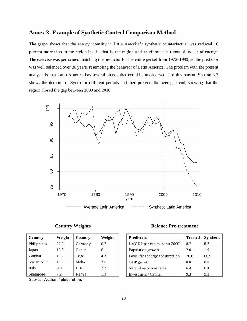
Annex 3: Example of Synthetic Control Comparison Method

The graph shows that the energy intensity in Latin America’s synthetic counterfactual was reduced 10

percent more than in the region itself—that is, the region underperformed in terms of its use of energy.

The exercise was performed matching the predictor for the entire period from 1972–1999, so the predictor

was well balanced over 30 years, resembling the behavior of Latin America. The problem with the present

analysis is that Latin America has several phases that could be unobserved. For this reason, Section 3.3

shows the iteration of Synth for different periods and then presents the average trend, showing that the

region closed the gap between 2000 and 2010.

Country Weights

Country Weight Country Weight

Philippines 22.9 Germany 6.7

Japan 13.5 Gabon 6.1

Zambia 11.7 Togo 4.3

Syrian A. R. 10.7 Malta 3.6

Italy 9.8 U.K. 2.2

Singapore 7.2 Kenya 1.3

Balance Pre-treatment

Predictors Treated Synthetic

Ln(GDP per capita, const 2000) 8.7 8.7

Population growth 2.0 1.9

Fossil fuel energy consumption 70.6 66.9

GDP growth 0.0 0.0

Natural resources rents 6.4 6.4

Investment / Capital 9.3 9.3

Source: Authors’ elaboration.

75

80

85

90

95

10

0

inte

nsity in

dex

1970 1980 1990 2000 2010year

Average Latin America Synthetic Latin America