Energy-efficient Reprogramming of Heterogeneous Wireless Sensor Networks Seán Harte 1,2 , Emanuel M. Popovici 1,2 , Stefano Rollo 1 and Brendan O'Flynn 1 1 Tyndall National Institute, Cork, Ireland 2 University College Cork, Cork, Ireland 1. Introduction In order to build wireless sensor network (WSN) applications, there are many challenges. WSNs are distributed networks with a potentially high number of nodes and unreliable inter node communications, and energy constraints due to the limited power. Much research is ongoing into efficient communication protocols, device level software for energy- efficient control of hardware, and higher level software for network control. The challenge that this chapter is concerned with is efficiently reprogramming WSNs after they have been deployed. This can be due to bugs in the original software, or if parameters in the current application need to be changed, or the nodes are being re-tasked. Microcontrollers are typically programmed by a wired connection to a PC. This can be done by the software developer or can be done as part of the node manufacture process if the application is already developed. However, after deployment it is not practical to physically connect to each node to upload new code to its microcontroller. There are a number of reasons for this: in a large network it can be too costly to go to each node; some nodes may not be accessible if they are in remote areas, or inside industrial machinery; or it may be required to update many nodes. If the node supports a method to receive data and reprogram itself with this data, then it can be reprogrammed wirelessly. However programs can be quite large. This requires a lot of energy to send, and may cause communication problems due to flooding the network. If we consider a node which is sending 8 bytes of sensor data every 15 minutes, and has a battery long enough to last one year, then sending a 15 kByte program would shorten the lifespan by 20 days (if the energy cost for receiving and transmitting are similar). If the entire network is being reprogrammed, then the effect would be far more dramatic on nodes that have to forward code to other nodes. It is for this reason that two more energy-aware solutions are looked at in this chapter. The first is delta encoding, which is used to analyse the binary program images for two applications to find similarities between them. This information can be used to send a set of update commands, instead of sending the full new application. The second technique presented is data compression, based on the Lempel-Ziv-Welch (LZW) algorithm 22

Welcome message from author
This document is posted to help you gain knowledge. Please leave a comment to let me know what you think about it! Share it to your friends and learn new things together.
Transcript
Energy-efficient Reprogramming of Heterogeneous Wireless Sensor Networks 501
Energy-efficient Reprogramming of Heterogeneous Wireless Sensor Networks
Seán Harte, Emanuel M. Popovici, Stefano Rollo and Brendan O’Flynn
X
Energy-efficient Reprogramming of Heterogeneous Wireless Sensor Networks
Seán Harte1,2, Emanuel M. Popovici1,2, Stefano Rollo1 and Brendan O'Flynn1
1 Tyndall National Institute, Cork, Ireland 2 University College Cork, Cork, Ireland
1. Introduction
In order to build wireless sensor network (WSN) applications, there are many challenges. WSNs are distributed networks with a potentially high number of nodes and unreliable inter node communications, and energy constraints due to the limited power. Much research is ongoing into efficient communication protocols, device level software for energy-efficient control of hardware, and higher level software for network control. The challenge that this chapter is concerned with is efficiently reprogramming WSNs after they have been deployed. This can be due to bugs in the original software, or if parameters in the current application need to be changed, or the nodes are being re-tasked. Microcontrollers are typically programmed by a wired connection to a PC. This can be done by the software developer or can be done as part of the node manufacture process if the application is already developed. However, after deployment it is not practical to physically connect to each node to upload new code to its microcontroller. There are a number of reasons for this: in a large network it can be too costly to go to each node; some nodes may not be accessible if they are in remote areas, or inside industrial machinery; or it may be required to update many nodes. If the node supports a method to receive data and reprogram itself with this data, then it can be reprogrammed wirelessly. However programs can be quite large. This requires a lot of energy to send, and may cause communication problems due to flooding the network. If we consider a node which is sending 8 bytes of sensor data every 15 minutes, and has a battery long enough to last one year, then sending a 15 kByte program would shorten the lifespan by 20 days (if the energy cost for receiving and transmitting are similar). If the entire network is being reprogrammed, then the effect would be far more dramatic on nodes that have to forward code to other nodes. It is for this reason that two more energy-aware solutions are looked at in this chapter. The first is delta encoding, which is used to analyse the binary program images for two applications to find similarities between them. This information can be used to send a set of update commands, instead of sending the full new application. The second technique presented is data compression, based on the Lempel-Ziv-Welch (LZW) algorithm
22
Sustainable Wireless Sensor Networks502
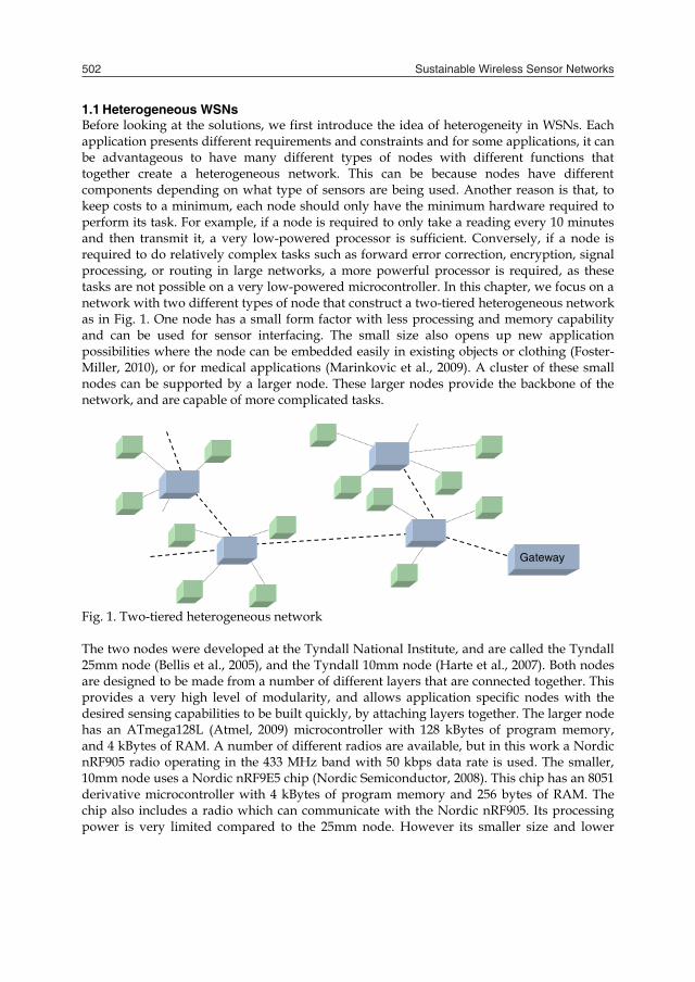
1.1 Heterogeneous WSNs Before looking at the solutions, we first introduce the idea of heterogeneity in WSNs. Each application presents different requirements and constraints and for some applications, it can be advantageous to have many different types of nodes with different functions that together create a heterogeneous network. This can be because nodes have different components depending on what type of sensors are being used. Another reason is that, to keep costs to a minimum, each node should only have the minimum hardware required to perform its task. For example, if a node is required to only take a reading every 10 minutes and then transmit it, a very low-powered processor is sufficient. Conversely, if a node is required to do relatively complex tasks such as forward error correction, encryption, signal processing, or routing in large networks, a more powerful processor is required, as these tasks are not possible on a very low-powered microcontroller. In this chapter, we focus on a network with two different types of node that construct a two-tiered heterogeneous network as in Fig. 1. One node has a small form factor with less processing and memory capability and can be used for sensor interfacing. The small size also opens up new application possibilities where the node can be embedded easily in existing objects or clothing (Foster-Miller, 2010), or for medical applications (Marinkovic et al., 2009). A cluster of these small nodes can be supported by a larger node. These larger nodes provide the backbone of the network, and are capable of more complicated tasks.
Gateway
Fig. 1. Two-tiered heterogeneous network The two nodes were developed at the Tyndall National Institute, and are called the Tyndall 25mm node (Bellis et al., 2005), and the Tyndall 10mm node (Harte et al., 2007). Both nodes are designed to be made from a number of different layers that are connected together. This provides a very high level of modularity, and allows application specific nodes with the desired sensing capabilities to be built quickly, by attaching layers together. The larger node has an ATmega128L (Atmel, 2009) microcontroller with 128 kBytes of program memory, and 4 kBytes of RAM. A number of different radios are available, but in this work a Nordic nRF905 radio operating in the 433 MHz band with 50 kbps data rate is used. The smaller, 10mm node uses a Nordic nRF9E5 chip (Nordic Semiconductor, 2008). This chip has an 8051 derivative microcontroller with 4 kBytes of program memory and 256 bytes of RAM. The chip also includes a radio which can communicate with the Nordic nRF905. Its processing power is very limited compared to the 25mm node. However its smaller size and lower
energy requirements give it advantages. Fig. 2 shows the two nodes, and Table 1 shows the energy usage of the nodes in different modes.
Mode 10mm Node 25mm Node
Sleeping, with wakeup timer 20.0 μW 52.9 μW Processing 9.73 mW 29.3 mW
Accessing memory 13.3 mW 31.0 mW Radio receiving/listening 55.1 mW 75.1 mW
Radio transmitting at –10 dBm 42.2 mW 62.5 mW Radio transmitting at +10 dBm 109 mW 128 mW
Table 1. Power used by Tyndall nodes from a 3.7 V Li-ion battery
Fig. 2. Tyndall 10mm node and 25mm node
2. Related Work
One of the big problems with network reprogramming is how to efficiently propagate the updates through the network. The simplest case for reprogramming is when each node in a network has the same application and they need to be updated. The new program can be sent across the entire network using a flooding protocol, where each node forwards the updated program to every node within its RF range. This helps ensure that every node receives the update, but it is also wasteful as some nodes receive the update more than once. To help improve data dissemination, the Trickle (Levis et al., 2004) algorithm was developed. Using Trickle, nodes regularly broadcast which version of data they currently have. If a neighbouring node detects has a different version, then the transfer of the update can begin. This algorithm requires far less power to propagate the update across the network, and scales to larger networks. TinyOS (Berkeley, 2010) which is one of the most popular operating systems used in WSNs uses a Trickle based algorithm called Deluge (Hui and Culler, 2004) to support wireless reprogramming. Deluge modifies Trickle to support sending very large amounts of data.

Energy-efficient Reprogramming of Heterogeneous Wireless Sensor Networks 503
1.1 Heterogeneous WSNs Before looking at the solutions, we first introduce the idea of heterogeneity in WSNs. Each application presents different requirements and constraints and for some applications, it can be advantageous to have many different types of nodes with different functions that together create a heterogeneous network. This can be because nodes have different components depending on what type of sensors are being used. Another reason is that, to keep costs to a minimum, each node should only have the minimum hardware required to perform its task. For example, if a node is required to only take a reading every 10 minutes and then transmit it, a very low-powered processor is sufficient. Conversely, if a node is required to do relatively complex tasks such as forward error correction, encryption, signal processing, or routing in large networks, a more powerful processor is required, as these tasks are not possible on a very low-powered microcontroller. In this chapter, we focus on a network with two different types of node that construct a two-tiered heterogeneous network as in Fig. 1. One node has a small form factor with less processing and memory capability and can be used for sensor interfacing. The small size also opens up new application possibilities where the node can be embedded easily in existing objects or clothing (Foster-Miller, 2010), or for medical applications (Marinkovic et al., 2009). A cluster of these small nodes can be supported by a larger node. These larger nodes provide the backbone of the network, and are capable of more complicated tasks.
Gateway
Fig. 1. Two-tiered heterogeneous network The two nodes were developed at the Tyndall National Institute, and are called the Tyndall 25mm node (Bellis et al., 2005), and the Tyndall 10mm node (Harte et al., 2007). Both nodes are designed to be made from a number of different layers that are connected together. This provides a very high level of modularity, and allows application specific nodes with the desired sensing capabilities to be built quickly, by attaching layers together. The larger node has an ATmega128L (Atmel, 2009) microcontroller with 128 kBytes of program memory, and 4 kBytes of RAM. A number of different radios are available, but in this work a Nordic nRF905 radio operating in the 433 MHz band with 50 kbps data rate is used. The smaller, 10mm node uses a Nordic nRF9E5 chip (Nordic Semiconductor, 2008). This chip has an 8051 derivative microcontroller with 4 kBytes of program memory and 256 bytes of RAM. The chip also includes a radio which can communicate with the Nordic nRF905. Its processing power is very limited compared to the 25mm node. However its smaller size and lower
energy requirements give it advantages. Fig. 2 shows the two nodes, and Table 1 shows the energy usage of the nodes in different modes.
Mode 10mm Node 25mm Node
Sleeping, with wakeup timer 20.0 μW 52.9 μW Processing 9.73 mW 29.3 mW
Accessing memory 13.3 mW 31.0 mW Radio receiving/listening 55.1 mW 75.1 mW
Radio transmitting at –10 dBm 42.2 mW 62.5 mW Radio transmitting at +10 dBm 109 mW 128 mW
Table 1. Power used by Tyndall nodes from a 3.7 V Li-ion battery
Fig. 2. Tyndall 10mm node and 25mm node
2. Related Work
One of the big problems with network reprogramming is how to efficiently propagate the updates through the network. The simplest case for reprogramming is when each node in a network has the same application and they need to be updated. The new program can be sent across the entire network using a flooding protocol, where each node forwards the updated program to every node within its RF range. This helps ensure that every node receives the update, but it is also wasteful as some nodes receive the update more than once. To help improve data dissemination, the Trickle (Levis et al., 2004) algorithm was developed. Using Trickle, nodes regularly broadcast which version of data they currently have. If a neighbouring node detects has a different version, then the transfer of the update can begin. This algorithm requires far less power to propagate the update across the network, and scales to larger networks. TinyOS (Berkeley, 2010) which is one of the most popular operating systems used in WSNs uses a Trickle based algorithm called Deluge (Hui and Culler, 2004) to support wireless reprogramming. Deluge modifies Trickle to support sending very large amounts of data.

Sustainable Wireless Sensor Networks504
The program update can be broken up into a number of pages. When a node has received a page, it can then start sending that page to other nodes that request it. Therefore it does not have to wait for the complete program update, before it can begin propagating the update. A big limitation of Deluge is that it assumes that every node in the network is running the same code. Aqueduct (Phillips, 2005) extends Deluge to support heterogeneous networks. This is done by adding an identifier to each program update. A node only updates itself if its current identifier matches the identifier of the incoming update. However nodes must still cache updates and forward them to other nodes even if the identifiers do not match, to ensure that every node can receive updated code. This greatly increases memory requirements. A big problem with the above solutions is that the entire updated program needs to be sent, even if only a small fraction of the code has changed. One solution to this is to a have an interpreter running on the nodes. An interpreter called Maté (Levis and Culler, 2002) has been developed using TinyOS. It can receive a script which describes the functions for the node to perform in a very condensed format. This means that far less data needs to be sent to update the node. However, the application is limited by what functions are possible in the scripting language and also requires the programmer to become familiar with the scripting language. The concept of mobile agents is another method for making easily reprogrammable wireless sensor networks (Georgoulas and Blow, 2008). In this approach a virtual machine is running on each node. This virtual machine supports “agents” which can move from node to node to carry out their desired task. Each agent contains code that executes on the virtual machine and data that can be modified by the code. For example a tracking agent can follow an event of interest by sending itself to the node it believes to be closest to the event. New agents can be inserted into the network, which is ideal when it is expected that the function of a network will require many changes over its lifetime. However, the agent approach requires sending the agent from node to node, which is wasteful of radio transmission energy when a smaller packet could be sent, and more complicated logic on each node to interpret the packet. A different approach is taken in the Contiki operating system (Dunkels, 2010). This operating system has core code that runs on the node constantly. This kernel supports loading and unloading of modules which are developed in C. This means that modules can be updated without having the reprogram the entire memory. The modules can either linked with each other at compile time, if the addresses of functions are known, or can be linked dynamically at run-time. However there is still a problem if the kernel needs to be changed due to newer versions becoming available or bugs. A similar approach supporting dynamic linking of modules at run-time in TinyOS is implemented by FlexCup (Marrón et al., 2006). In FlexCup an extra step is done after compiling to generate meta-data describing how to integrate individual components. The above systems were based on operating systems with very low footprints. However, these operating systems may still not be suitable for very resource constrained systems. The
overheads required for scheduling, and the demands placed on the stack by context switching etc., limit the complexity of possible applications. Applications can be developed that manage their own scheduling, and carefully limit the amount of context switching caused by interrupts. Such an optimized program rules out the use of an interpreter, or loadable modules. So another way to limit the amount of data that has to be sent is to only send the parts of the application that have changed. This is called delta encoding. A bug that is found might require just changing a single value in the source code of an application. However this single change can cause many changes in the binary code. The addresses of instructions could change and therefore all JMP instructions will need different operands etc. In this case, the minimum data that could be sent is a description of what changed in the source code. However this would require the application to be able to decompile its code, make the change and recompile. This is too complex for the typical hardware of wireless sensor nodes. The UNIX tool Rsync (Tridgell, 1999) was developed for synchronizing data efficiently over a network connection. Assuming the receiver has first detected that the sender has a newer version of code, the receiver splits its data up into chunks of n bytes, and calculates a hash value for each chunk. The sender calculates a hash value for every chunk of n bytes. The hash values can then be compared to find out which sections of the data need to be updated. A compact list of commands can then be sent to the receiver telling it how to construct the new file, from a combination of its existing data, and new data. (Jeong and Culler, 2009) analyses a wireless network reprogramming technique based on the Rsync algorithm. The Rsync algorithm can work for any type of data; however there are more efficient algorithms for executable code. (Reijers and Langendoen, 2003) presents a method for efficient code updating. It is based on analyzing the op-codes to find the minimum amount if data that needs to be sent in order to update the current code. To do this, it relies on knowing the structure of the op-codes, and is thus tied to be used for nodes using a Texas Instruments MSP430 type microcontroller. (Panta, 2009) modifies the compiler to introduce a function indirection table. Function calls are replaced to a jump to a specific location within a function table. This location then contains the call to the real function. This allows functions to be moved easily without requiring all addresses to be changed. However it requires an extra compiler step which will be difficult in a heterogeneous network where multiple processor architectures are being used. A more general algorithm, called Bsdiff, for finding the difference between executable files is presented in (Percival, 2006). This algorithm begins by calculating which sections are the same with similar methods as Rsync. The difference is that sections which almost match are also noted. This can be done extending the matching areas until a limit of mismatched bytes is reached. This decreases the size of the list of commands that needs to be sent, as in binary program files, there are often sections that almost match, but just have different addresses in the instructions. This means it performs much better than Rsync for executable code and small changes in source code do not introduce large changes in the compiled program file, as they can with Rsync. This is shown by the comparison in (Motta et al., 2007). As this tool is not dependent on a specific instruction set, it is advantageous in a heterogeneous network such as the one presented in this work.
Energy-efficient Reprogramming of Heterogeneous Wireless Sensor Networks 505
The program update can be broken up into a number of pages. When a node has received a page, it can then start sending that page to other nodes that request it. Therefore it does not have to wait for the complete program update, before it can begin propagating the update. A big limitation of Deluge is that it assumes that every node in the network is running the same code. Aqueduct (Phillips, 2005) extends Deluge to support heterogeneous networks. This is done by adding an identifier to each program update. A node only updates itself if its current identifier matches the identifier of the incoming update. However nodes must still cache updates and forward them to other nodes even if the identifiers do not match, to ensure that every node can receive updated code. This greatly increases memory requirements. A big problem with the above solutions is that the entire updated program needs to be sent, even if only a small fraction of the code has changed. One solution to this is to a have an interpreter running on the nodes. An interpreter called Maté (Levis and Culler, 2002) has been developed using TinyOS. It can receive a script which describes the functions for the node to perform in a very condensed format. This means that far less data needs to be sent to update the node. However, the application is limited by what functions are possible in the scripting language and also requires the programmer to become familiar with the scripting language. The concept of mobile agents is another method for making easily reprogrammable wireless sensor networks (Georgoulas and Blow, 2008). In this approach a virtual machine is running on each node. This virtual machine supports “agents” which can move from node to node to carry out their desired task. Each agent contains code that executes on the virtual machine and data that can be modified by the code. For example a tracking agent can follow an event of interest by sending itself to the node it believes to be closest to the event. New agents can be inserted into the network, which is ideal when it is expected that the function of a network will require many changes over its lifetime. However, the agent approach requires sending the agent from node to node, which is wasteful of radio transmission energy when a smaller packet could be sent, and more complicated logic on each node to interpret the packet. A different approach is taken in the Contiki operating system (Dunkels, 2010). This operating system has core code that runs on the node constantly. This kernel supports loading and unloading of modules which are developed in C. This means that modules can be updated without having the reprogram the entire memory. The modules can either linked with each other at compile time, if the addresses of functions are known, or can be linked dynamically at run-time. However there is still a problem if the kernel needs to be changed due to newer versions becoming available or bugs. A similar approach supporting dynamic linking of modules at run-time in TinyOS is implemented by FlexCup (Marrón et al., 2006). In FlexCup an extra step is done after compiling to generate meta-data describing how to integrate individual components. The above systems were based on operating systems with very low footprints. However, these operating systems may still not be suitable for very resource constrained systems. The
overheads required for scheduling, and the demands placed on the stack by context switching etc., limit the complexity of possible applications. Applications can be developed that manage their own scheduling, and carefully limit the amount of context switching caused by interrupts. Such an optimized program rules out the use of an interpreter, or loadable modules. So another way to limit the amount of data that has to be sent is to only send the parts of the application that have changed. This is called delta encoding. A bug that is found might require just changing a single value in the source code of an application. However this single change can cause many changes in the binary code. The addresses of instructions could change and therefore all JMP instructions will need different operands etc. In this case, the minimum data that could be sent is a description of what changed in the source code. However this would require the application to be able to decompile its code, make the change and recompile. This is too complex for the typical hardware of wireless sensor nodes. The UNIX tool Rsync (Tridgell, 1999) was developed for synchronizing data efficiently over a network connection. Assuming the receiver has first detected that the sender has a newer version of code, the receiver splits its data up into chunks of n bytes, and calculates a hash value for each chunk. The sender calculates a hash value for every chunk of n bytes. The hash values can then be compared to find out which sections of the data need to be updated. A compact list of commands can then be sent to the receiver telling it how to construct the new file, from a combination of its existing data, and new data. (Jeong and Culler, 2009) analyses a wireless network reprogramming technique based on the Rsync algorithm. The Rsync algorithm can work for any type of data; however there are more efficient algorithms for executable code. (Reijers and Langendoen, 2003) presents a method for efficient code updating. It is based on analyzing the op-codes to find the minimum amount if data that needs to be sent in order to update the current code. To do this, it relies on knowing the structure of the op-codes, and is thus tied to be used for nodes using a Texas Instruments MSP430 type microcontroller. (Panta, 2009) modifies the compiler to introduce a function indirection table. Function calls are replaced to a jump to a specific location within a function table. This location then contains the call to the real function. This allows functions to be moved easily without requiring all addresses to be changed. However it requires an extra compiler step which will be difficult in a heterogeneous network where multiple processor architectures are being used. A more general algorithm, called Bsdiff, for finding the difference between executable files is presented in (Percival, 2006). This algorithm begins by calculating which sections are the same with similar methods as Rsync. The difference is that sections which almost match are also noted. This can be done extending the matching areas until a limit of mismatched bytes is reached. This decreases the size of the list of commands that needs to be sent, as in binary program files, there are often sections that almost match, but just have different addresses in the instructions. This means it performs much better than Rsync for executable code and small changes in source code do not introduce large changes in the compiled program file, as they can with Rsync. This is shown by the comparison in (Motta et al., 2007). As this tool is not dependent on a specific instruction set, it is advantageous in a heterogeneous network such as the one presented in this work.

Sustainable Wireless Sensor Networks506
3. Self Programming Methods
Before examining further how to minimise to data that needs to be sent, we will now look at the methods used to allow the nodes to update their own code. The two nodes that we use, the 25mm node, and the 10mm node, have different microcontrollers and memory structures so two different update mechanisms have been developed. First, we will look at the 10mm node with its 8051-based microcontroller, and then consider the case of the 25mm node with its Atmel AVR based microcontroller.
3.1 Tyndall 10mm node The 8051-derivative microcontroller in the nRF9E5 chip has a Harvard architecture with different memory address spaces for instructions and data. For node programming, only the memory containing instructions (program memory) is relevant. Fig. 3 shows how this program memory is arranged in the 10mm node. There is a RAM and a ROM within the nRF9E5, and an external EEPROM, which is communicated with using the SPI protocol. The EEPROM provides persistent storage of the code, but the actual code is run from the internal RAM.
Program memory
(4kBytes)
Boot-Loader
(512 bytes)
RAM ROM0x0FFF
0x0000 0x8000
0x81FF
nRF9E5
8kBytes
EEPROM
SPI
Fig. 3. nRF9E5 program memory structure When the node is first powered up, it starts executing at address 0x8000, which is located in the internal ROM. This ROM contains boot-loader code that copies the lower 4 kBytes of data from the external EEPROM to internal RAM. Then the node program counter jumps to address 0x0000, and starts executing the application. In order to reprogram the node it is necessary to change the lower 4 kBytes of the EEPROM. When the update is complete the node can then restart itself and start executing the new application. However, there is still a potential problem with this method. It is likely that reprogramming would take a relatively long time, due to receiving commands over the radio, and allowing the current application to send other application data still. If the node should inadvertently restart itself (due to power problems, or a watchdog timer timeout) it is likely that a partially updated program would not function correctly. It is for this reason that an 8 kByte external EEPROM is used. This allows the updated program to be first written to the upper half of the EEPROM. When the entire program is fully written the top half of memory is copied to the bottom half, and
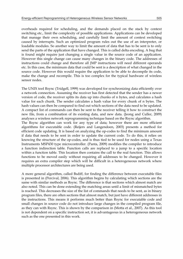
the node is restarted. This greatly reduces the potential for a corrupted application due to unexpected restarts. Fig. 4 shows how the program code is stored in the EEPROM. The first 3 bytes are used by the boot-loader to know where the actual code starts, and how much of the memory is used by the program code. This means it is possible to insert some extra data into the EEPROM. Four bytes are added: two bytes are a count of bytes in the actual program code; and two bytes contain a CRC checksum of the program code. The upper 4 kBytes of memory has the same contents as the lower 4 kBytes.
CRC
Program Length (N)
Num. of 256 byte blocks
Program start (0x0007)
Configuration byte
0x0FFF
0x0003
0x0002
0x0001
0x0000
0x0007
Unused
(N + 0x0007)(N + 0x0007) – 1
0x0005
Program Code
Fig. 4. nRF9E5 EEPROM memory format (lower 4 kBytes)
When all updates have been received, the current application uses the program length to calculate a CRC of the program code. This is then compared with the CRC stored in the EEPROM, and only if they match is the code copied to the lower half of memory, and the node reset (by forcing a watchdog timer timeout). If the CRC values do not match, then the node has to request the program to be fully retransmitted.
3.2 Tyndall 25mm node The ATmega128L microcontroller used on the 25mm node also has a Harvard architecture. Its program memory is in an internal 128 kByte flash. This provides persistent storage, and the microcontroller can execute instructions directly from the flash memory. The ATmega128L provides support for reprogramming using the SPM instruction. However, this instruction only works when executed from the bootloader section of flash, which is the top 8 kBytes. This means that two approaches for reprogramming are possible. The first is that the bootloader section can be entirely self-contained. When the application detects an update is available, it can jump to the bootloader section. The bootloader can then handle receiving the data over RF, and creating the new application. When the application is fully updated, the bootloader can jump back to the application section. The second option is to split the memory in half, and write the new application to the upper half, as with the 10mm node. With this option the application handles receiving the data. It can call a function in the
Energy-efficient Reprogramming of Heterogeneous Wireless Sensor Networks 507
3. Self Programming Methods
Before examining further how to minimise to data that needs to be sent, we will now look at the methods used to allow the nodes to update their own code. The two nodes that we use, the 25mm node, and the 10mm node, have different microcontrollers and memory structures so two different update mechanisms have been developed. First, we will look at the 10mm node with its 8051-based microcontroller, and then consider the case of the 25mm node with its Atmel AVR based microcontroller.
3.1 Tyndall 10mm node The 8051-derivative microcontroller in the nRF9E5 chip has a Harvard architecture with different memory address spaces for instructions and data. For node programming, only the memory containing instructions (program memory) is relevant. Fig. 3 shows how this program memory is arranged in the 10mm node. There is a RAM and a ROM within the nRF9E5, and an external EEPROM, which is communicated with using the SPI protocol. The EEPROM provides persistent storage of the code, but the actual code is run from the internal RAM.
Program memory
(4kBytes)
Boot-Loader
(512 bytes)
RAM ROM0x0FFF
0x0000 0x8000
0x81FF
nRF9E5
8kBytes
EEPROM
SPI
Fig. 3. nRF9E5 program memory structure When the node is first powered up, it starts executing at address 0x8000, which is located in the internal ROM. This ROM contains boot-loader code that copies the lower 4 kBytes of data from the external EEPROM to internal RAM. Then the node program counter jumps to address 0x0000, and starts executing the application. In order to reprogram the node it is necessary to change the lower 4 kBytes of the EEPROM. When the update is complete the node can then restart itself and start executing the new application. However, there is still a potential problem with this method. It is likely that reprogramming would take a relatively long time, due to receiving commands over the radio, and allowing the current application to send other application data still. If the node should inadvertently restart itself (due to power problems, or a watchdog timer timeout) it is likely that a partially updated program would not function correctly. It is for this reason that an 8 kByte external EEPROM is used. This allows the updated program to be first written to the upper half of the EEPROM. When the entire program is fully written the top half of memory is copied to the bottom half, and
the node is restarted. This greatly reduces the potential for a corrupted application due to unexpected restarts. Fig. 4 shows how the program code is stored in the EEPROM. The first 3 bytes are used by the boot-loader to know where the actual code starts, and how much of the memory is used by the program code. This means it is possible to insert some extra data into the EEPROM. Four bytes are added: two bytes are a count of bytes in the actual program code; and two bytes contain a CRC checksum of the program code. The upper 4 kBytes of memory has the same contents as the lower 4 kBytes.
CRC
Program Length (N)
Num. of 256 byte blocks
Program start (0x0007)
Configuration byte
0x0FFF
0x0003
0x0002
0x0001
0x0000
0x0007
Unused
(N + 0x0007)(N + 0x0007) – 1
0x0005
Program Code
Fig. 4. nRF9E5 EEPROM memory format (lower 4 kBytes)
When all updates have been received, the current application uses the program length to calculate a CRC of the program code. This is then compared with the CRC stored in the EEPROM, and only if they match is the code copied to the lower half of memory, and the node reset (by forcing a watchdog timer timeout). If the CRC values do not match, then the node has to request the program to be fully retransmitted.
3.2 Tyndall 25mm node The ATmega128L microcontroller used on the 25mm node also has a Harvard architecture. Its program memory is in an internal 128 kByte flash. This provides persistent storage, and the microcontroller can execute instructions directly from the flash memory. The ATmega128L provides support for reprogramming using the SPM instruction. However, this instruction only works when executed from the bootloader section of flash, which is the top 8 kBytes. This means that two approaches for reprogramming are possible. The first is that the bootloader section can be entirely self-contained. When the application detects an update is available, it can jump to the bootloader section. The bootloader can then handle receiving the data over RF, and creating the new application. When the application is fully updated, the bootloader can jump back to the application section. The second option is to split the memory in half, and write the new application to the upper half, as with the 10mm node. With this option the application handles receiving the data. It can call a function in the
Sustainable Wireless Sensor Networks508
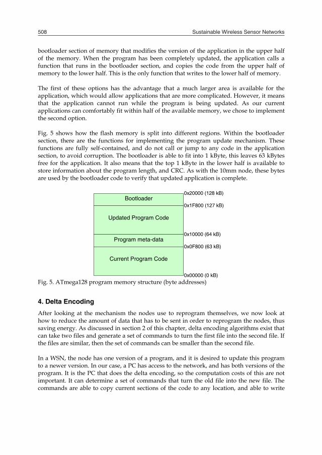
bootloader section of memory that modifies the version of the application in the upper half of the memory. When the program has been completely updated, the application calls a function that runs in the bootloader section, and copies the code from the upper half of memory to the lower half. This is the only function that writes to the lower half of memory. The first of these options has the advantage that a much larger area is available for the application, which would allow applications that are more complicated. However, it means that the application cannot run while the program is being updated. As our current applications can comfortably fit within half of the available memory, we chose to implement the second option. Fig. 5 shows how the flash memory is split into different regions. Within the bootloader section, there are the functions for implementing the program update mechanism. These functions are fully self-contained, and do not call or jump to any code in the application section, to avoid corruption. The bootloader is able to fit into 1 kByte, this leaves 63 kBytes free for the application. It also means that the top 1 kByte in the lower half is available to store information about the program length, and CRC. As with the 10mm node, these bytes are used by the bootloader code to verify that updated application is complete.
Bootloader
Updated Program Code
0x00000 (0 kB)
Program meta-data
Current Program Code
0x0F800 (63 kB)
0x10000 (64 kB)
0x1F800 (127 kB)
0x20000 (128 kB)
Fig. 5. ATmega128 program memory structure (byte addresses)
4. Delta Encoding
After looking at the mechanism the nodes use to reprogram themselves, we now look at how to reduce the amount of data that has to be sent in order to reprogram the nodes, thus saving energy. As discussed in section 2 of this chapter, delta encoding algorithms exist that can take two files and generate a set of commands to turn the first file into the second file. If the files are similar, then the set of commands can be smaller than the second file. In a WSN, the node has one version of a program, and it is desired to update this program to a newer version. In our case, a PC has access to the network, and has both versions of the program. It is the PC that does the delta encoding, so the computation costs of this are not important. It can determine a set of commands that turn the old file into the new file. The commands are able to copy current sections of the code to any location, and able to write
new data to any location. Although it requires some processing and extra memory reads to implement the handling of these commands, it is advantageous over just sending the new file, as less data is transmitted. In WSNs it has been shown that processing data uses much less energy per bit than transmission and reception (Raghunathan et al., 2002). Therefore, the savings from less radio usage will be greater than the extra processing required.
4.1 Bsdiff Algorithm To generate the commands, our work uses the Bsdiff algorithm. This algorithm analyses two files, and finds sections that partially match. It outputs data that are arranged in three sections. The third section (extra section) contains new data that is written directly. The second section (difference section) contains a list of values that are added byte-wise to the current data. As there are many similarities, most values in this section have the value 0, and it is therefore very compressible. The first section (control section) is an array of 3-tuples (X, Y, Z). X is the number of bytes that are copied from the old data to the new data, adding byte-wise X bytes from the difference section. Y is the number of bytes from the extra section that are written. A pointer to the last offset read in the new file is moved Z bytes before starting the next operation. The three sections output by the Bsdiff algorithm are actual larger than the file itself. In the freely available Bsdiff application (Percival, 2010) the bzip2 compression algorithm is used to compress all the sections. The data in the difference section is very compressible, and if the compared data is similar there will be far more data in this section than in the extra section. This is how the overall data size is greatly reduced, achieving a average compression ratio of 8.33% for program updates in the tests carried out in (Motta et al., 2007). As the nodes do not have processors powerful enough to decompress bzip2 data, it is not used here. Alternatives to work around this limitation are presented in the next section.
4.2 Adapting Bsdiff for use in WSNs Besides being unable to use bzip2, another potential problem is that we do not want to wait for the node to receive all the Bsdiff output sections before starting to create the new program code. This would require too much buffering of data. To solve this, the difference and extra sections are broken up, and attached to the relevant 3-tuple from the control section. We will refer to this new structure as a command. In each command, the first three values (X, Y, Z), are the control 3-tuple. Then there is a value, P, which specifies how many bytes within X bytes of the diff section are non-zero. After this, there is array of P pairs. The first element of the pair says where to add this byte, and the second element is the byte to add. At the end, there are Y bytes taken from the extra section. Each command is structured as shown in Fig. 6. In the case where commands are still too large, there might not be enough memory available to buffer the commands. For this reason, commands sent to 10mm nodes are limited to 28 bytes, and for 25mm nodes, a size of 112 bytes is used. The value for the 10mm node was picked as it is the size of the data payload that is sent in each radio packet and the 10mm node has very limited memory for buffering. The 25mm node has more buffering space available, so the effect of a command size limit against compression ratio was measured.

Energy-efficient Reprogramming of Heterogeneous Wireless Sensor Networks 509
bootloader section of memory that modifies the version of the application in the upper half of the memory. When the program has been completely updated, the application calls a function that runs in the bootloader section, and copies the code from the upper half of memory to the lower half. This is the only function that writes to the lower half of memory. The first of these options has the advantage that a much larger area is available for the application, which would allow applications that are more complicated. However, it means that the application cannot run while the program is being updated. As our current applications can comfortably fit within half of the available memory, we chose to implement the second option. Fig. 5 shows how the flash memory is split into different regions. Within the bootloader section, there are the functions for implementing the program update mechanism. These functions are fully self-contained, and do not call or jump to any code in the application section, to avoid corruption. The bootloader is able to fit into 1 kByte, this leaves 63 kBytes free for the application. It also means that the top 1 kByte in the lower half is available to store information about the program length, and CRC. As with the 10mm node, these bytes are used by the bootloader code to verify that updated application is complete.
Bootloader
Updated Program Code
0x00000 (0 kB)
Program meta-data
Current Program Code
0x0F800 (63 kB)
0x10000 (64 kB)
0x1F800 (127 kB)
0x20000 (128 kB)
Fig. 5. ATmega128 program memory structure (byte addresses)
4. Delta Encoding
After looking at the mechanism the nodes use to reprogram themselves, we now look at how to reduce the amount of data that has to be sent in order to reprogram the nodes, thus saving energy. As discussed in section 2 of this chapter, delta encoding algorithms exist that can take two files and generate a set of commands to turn the first file into the second file. If the files are similar, then the set of commands can be smaller than the second file. In a WSN, the node has one version of a program, and it is desired to update this program to a newer version. In our case, a PC has access to the network, and has both versions of the program. It is the PC that does the delta encoding, so the computation costs of this are not important. It can determine a set of commands that turn the old file into the new file. The commands are able to copy current sections of the code to any location, and able to write
new data to any location. Although it requires some processing and extra memory reads to implement the handling of these commands, it is advantageous over just sending the new file, as less data is transmitted. In WSNs it has been shown that processing data uses much less energy per bit than transmission and reception (Raghunathan et al., 2002). Therefore, the savings from less radio usage will be greater than the extra processing required.
4.1 Bsdiff Algorithm To generate the commands, our work uses the Bsdiff algorithm. This algorithm analyses two files, and finds sections that partially match. It outputs data that are arranged in three sections. The third section (extra section) contains new data that is written directly. The second section (difference section) contains a list of values that are added byte-wise to the current data. As there are many similarities, most values in this section have the value 0, and it is therefore very compressible. The first section (control section) is an array of 3-tuples (X, Y, Z). X is the number of bytes that are copied from the old data to the new data, adding byte-wise X bytes from the difference section. Y is the number of bytes from the extra section that are written. A pointer to the last offset read in the new file is moved Z bytes before starting the next operation. The three sections output by the Bsdiff algorithm are actual larger than the file itself. In the freely available Bsdiff application (Percival, 2010) the bzip2 compression algorithm is used to compress all the sections. The data in the difference section is very compressible, and if the compared data is similar there will be far more data in this section than in the extra section. This is how the overall data size is greatly reduced, achieving a average compression ratio of 8.33% for program updates in the tests carried out in (Motta et al., 2007). As the nodes do not have processors powerful enough to decompress bzip2 data, it is not used here. Alternatives to work around this limitation are presented in the next section.
4.2 Adapting Bsdiff for use in WSNs Besides being unable to use bzip2, another potential problem is that we do not want to wait for the node to receive all the Bsdiff output sections before starting to create the new program code. This would require too much buffering of data. To solve this, the difference and extra sections are broken up, and attached to the relevant 3-tuple from the control section. We will refer to this new structure as a command. In each command, the first three values (X, Y, Z), are the control 3-tuple. Then there is a value, P, which specifies how many bytes within X bytes of the diff section are non-zero. After this, there is array of P pairs. The first element of the pair says where to add this byte, and the second element is the byte to add. At the end, there are Y bytes taken from the extra section. Each command is structured as shown in Fig. 6. In the case where commands are still too large, there might not be enough memory available to buffer the commands. For this reason, commands sent to 10mm nodes are limited to 28 bytes, and for 25mm nodes, a size of 112 bytes is used. The value for the 10mm node was picked as it is the size of the data payload that is sent in each radio packet and the 10mm node has very limited memory for buffering. The 25mm node has more buffering space available, so the effect of a command size limit against compression ratio was measured.

Sustainable Wireless Sensor Networks510
The commands for converting between the two applications were generated with different maximum command sizes, and the compression ratio recorded. The results are shown in Fig. 7. 112 bytes was chosen because increasing the size further has very little effect on the compression ratio, and it is a multiple of 28. As the node has to remember the location that it last read from in the current code, and the location in the new code that it last wrote to, it is also necessary to handle the commands in the correct sequence.
typedef struct {
uint8_t index; /* Where to add this byte */ uint8_t value; /* Byte to add to original data */
} pair_t
typedef struct { uint16_t copy; /* How many bytes to copy (adding to diff section) */
uint8_t write; /* How many bytes to write from extra section */ int16_t seek; /* How many places to move pointer */
uint8_t numPairs; /* How many pairs in the diff section */ pair_t diff(); /* Array that is 'numPairs' long */
uint8_t extra(); /* Array that is 'write' bytes in size */ } command_t;
Fig. 6. Reprogramming command structure and examples
0
20
40
60
80
100
120
0 32 64 96 128 160 192 224 256
Maximum command size (bytes)
Com
pres
sion
Rat
io (%
)
Fig. 7. Effect of command size on compression ratio
4.3 Analysis of delta encoding To analyse the benefit of delta encoding, we compare the amount of data that would be sent if the complete new program were transmitted, and the amount of data that is sent with delta encoding. This is done using a real WSN application where nodes are arranged in a tree. Each node takes a sensor reading regularly and transmits to its parent node, and it also forwards sensor readings it receives from its children. The effects of changing the sampling frequency; replacing an framelet based (Roedig et al., 2006) MAC algorithm with a very simple form of CSMA (Carrier Sense Multiple Access); changing the sensor used from a Sensirion SHT11 temperature/humidity sensor, to an Analog Devices AD7998 ADC; and
changing the application completely, to an application for implementing the Modbus protocol over wireless links are measured. Table 2 and Table 3 show the compression ratio achieved using delta encoding in each of these cases on the 10mm node, and 25mm node code, respectively.
Change Full Size Delta-encoded size Details of commands Compression Ratio
Changing sampling frequency
2896 bytes 14 bytes 2 command
0.48% 1 diff pair 0 extra bytes
Enabling CSMA 2922 bytes 208 bytes
13 commands 7.12% 52 diff pairs
26 extra bytes
Changing sensor 2744 bytes 919 bytes
36 commands 33.49% 164 diff pairs
375 extra bytes
Different application 2548 bytes 2228 bytes
83 commands 87.48% 95 diff pairs
1540 extra bytes Table 2. Effects of changing application on 10mm node
Change Full Size Delta-encoded size Details of commands Compression Ratio
Changing sampling frequency
3407 bytes 14 bytes 2 commands
0.41% 1 diff pairs 0 extra bytes
Enabling CSMA 3419 bytes 78 bytes
6 commands 2.28% 15 diff pairs
12 extra bytes
Changing sensor 3365 bytes 1054 bytes
22 commands 31.32% 194 diff pairs
534 extra bytes
Different application 4238 bytes 3323 bytes
54 commands 78.41% 94 diff pairs
2811 extra bytes Table 3. Effects of changing application on 25mm node The tables show that our implementation of Bsdiff reduces greatly the data that needs to be sent to update a node, especially when only small changes are made. In a homogeneous network, the overall savings will be as above, as the same set of commands need to be sent to each node. Limiting the size of reprogramming commands on the 10mm node increases the compression ratio compared to the 25mm node, as more commands must be sent. The tables also show how as the amount of change in the program files increases, more of the sent data is in the extra section, and not the difference section. In our current network, nodes are arranged in a fixed pre-defined tree. In the tree, nodes can transmit to their parent node, to one of their child nodes, or to all of their child nodes with a multicast transmission. To expand our Bsdiff technique to a heterogeneous network, with multiple different types of nodes, and multiple different node functions, the simplest

Energy-efficient Reprogramming of Heterogeneous Wireless Sensor Networks 511
The commands for converting between the two applications were generated with different maximum command sizes, and the compression ratio recorded. The results are shown in Fig. 7. 112 bytes was chosen because increasing the size further has very little effect on the compression ratio, and it is a multiple of 28. As the node has to remember the location that it last read from in the current code, and the location in the new code that it last wrote to, it is also necessary to handle the commands in the correct sequence.
typedef struct {
uint8_t index; /* Where to add this byte */ uint8_t value; /* Byte to add to original data */
} pair_t
typedef struct { uint16_t copy; /* How many bytes to copy (adding to diff section) */
uint8_t write; /* How many bytes to write from extra section */ int16_t seek; /* How many places to move pointer */
uint8_t numPairs; /* How many pairs in the diff section */ pair_t diff(); /* Array that is 'numPairs' long */
uint8_t extra(); /* Array that is 'write' bytes in size */ } command_t;
Fig. 6. Reprogramming command structure and examples
0
20
40
60
80
100
120
0 32 64 96 128 160 192 224 256
Maximum command size (bytes)
Com
pres
sion
Rat
io (%
)
Fig. 7. Effect of command size on compression ratio
4.3 Analysis of delta encoding To analyse the benefit of delta encoding, we compare the amount of data that would be sent if the complete new program were transmitted, and the amount of data that is sent with delta encoding. This is done using a real WSN application where nodes are arranged in a tree. Each node takes a sensor reading regularly and transmits to its parent node, and it also forwards sensor readings it receives from its children. The effects of changing the sampling frequency; replacing an framelet based (Roedig et al., 2006) MAC algorithm with a very simple form of CSMA (Carrier Sense Multiple Access); changing the sensor used from a Sensirion SHT11 temperature/humidity sensor, to an Analog Devices AD7998 ADC; and
changing the application completely, to an application for implementing the Modbus protocol over wireless links are measured. Table 2 and Table 3 show the compression ratio achieved using delta encoding in each of these cases on the 10mm node, and 25mm node code, respectively.
Change Full Size Delta-encoded size Details of commands Compression Ratio
Changing sampling frequency
2896 bytes 14 bytes 2 command
0.48% 1 diff pair 0 extra bytes
Enabling CSMA 2922 bytes 208 bytes
13 commands 7.12% 52 diff pairs
26 extra bytes
Changing sensor 2744 bytes 919 bytes
36 commands 33.49% 164 diff pairs
375 extra bytes
Different application 2548 bytes 2228 bytes
83 commands 87.48% 95 diff pairs
1540 extra bytes Table 2. Effects of changing application on 10mm node
Change Full Size Delta-encoded size Details of commands Compression Ratio
Changing sampling frequency
3407 bytes 14 bytes 2 commands
0.41% 1 diff pairs 0 extra bytes
Enabling CSMA 3419 bytes 78 bytes
6 commands 2.28% 15 diff pairs
12 extra bytes
Changing sensor 3365 bytes 1054 bytes
22 commands 31.32% 194 diff pairs
534 extra bytes
Different application 4238 bytes 3323 bytes
54 commands 78.41% 94 diff pairs
2811 extra bytes Table 3. Effects of changing application on 25mm node The tables show that our implementation of Bsdiff reduces greatly the data that needs to be sent to update a node, especially when only small changes are made. In a homogeneous network, the overall savings will be as above, as the same set of commands need to be sent to each node. Limiting the size of reprogramming commands on the 10mm node increases the compression ratio compared to the 25mm node, as more commands must be sent. The tables also show how as the amount of change in the program files increases, more of the sent data is in the extra section, and not the difference section. In our current network, nodes are arranged in a fixed pre-defined tree. In the tree, nodes can transmit to their parent node, to one of their child nodes, or to all of their child nodes with a multicast transmission. To expand our Bsdiff technique to a heterogeneous network, with multiple different types of nodes, and multiple different node functions, the simplest

Sustainable Wireless Sensor Networks512
approach is to generate the commands needed to update each node individually. However, if we consider a heterogeneous network where some nodes have almost the same program, it may be better to first reprogram all nodes so that they have the same application. Then perform the update using multicast transmissions, and then make the changes to each node so that they are unique again. To illustrate the usefulness of this method, we can use data in the above tables. If there are a number of nodes which differ only in sampling frequency and it is desired to change the sensors on each node, then the size of the commands needed to change the sensor compared to the size of commands needed to change the sampling frequency means that the simple approach of sending a single set of commands to each node may be far from optimal. To decide which method is better we need to calculate the energy cost of each approach. In the tables above, the compression ration is used as the metric to examine the effectiveness of our Bsdiff implementation. This is valid, as when programming a single node, the number of bytes transmitted will be directly related to the energy used. However, the use of multicast transmissions in a heterogeneous network complicates this, as the energy per bit will change depending on how many nodes receive the message. For this reason, a new metric is required to analyse the use of Bsdiff in a heterogeneous network. The radio we use is capable of sending a 32 byte payload, with a 6 byte header, and 10 bit preamble, added by the radio. From this 32 byte payload, 4 bytes are used for routing control, packetisation, and a message type identifier, leaving 28 bytes for use. This means that a full packets is 314 bits long, of which 90 bits are overhead. The radio sends data at a rate of 50 kpbs, and has a 650 μs start-up time. Therefore, for a message with len bytes, the time to send it, T, can be calculated:
28/00065.0
5000090)28mod(8128/314
)( lenlenlen
lenT
(1)
For a message to be sent to a particular node, or set of nodes, S, the message will have to be sent STX times, received by 25mm nodes SRX25 times, and by 10mm nodes SRX10 times. In out network the 10mm nodes only act as leaf nodes, so they are never required to transmit the commands. Using values for transmission PTX and reception PRX25 and PRX10 from Table 1, the energy required to send the message can be calculated:
)()()(),( 10102525 lenTSPlenTSPlenTSPSlenE RXRXRXRXTXTX (2) This value is not fully accurate due to ACKs, and other network management costs, however these costs will affect every message similarly, so it is still a valid metric for comparing the cost of send a message. This metric can be used to help reduce the energy cost of reprogramming a heterogeneous network. In the network, there are nodes 0, 1, ... , n, and applications iα and iβ refer to different versions of an application that run on node i. B(iα, iβ) is the sum of the number of bytes in the commands that are needed to convert a node from running application iα to running application iβ.
n
iseparate iiiBEc
0
}){),,((
(3)
n
i
n
icombined iiBEnBEiiBEc
11
}){),,0((}),...,1,0{),0,0(()}{),0,((
(4)
If each node were updated separately, the cost of update in terms of bytes transmitted would be cseparate. If we take the approach of converting every node to have the same application then the cost will be ccombined. Depending on the current state of the nodes, and the desired changes, either approach could require less data to be transmitted. This idea can be expanded further. Instead of reprogramming the entire network to have the same application, the technique is restricted to sub sections, which have very similar applications. For example, a large network carrying out environmental monitoring could have different types of sensors in different areas. In this case, if we want to update the network with a new communication protocol, it might be best to convert all the nodes with the same sensors to run the same application, and the reprogram them all using multicast transmissions.
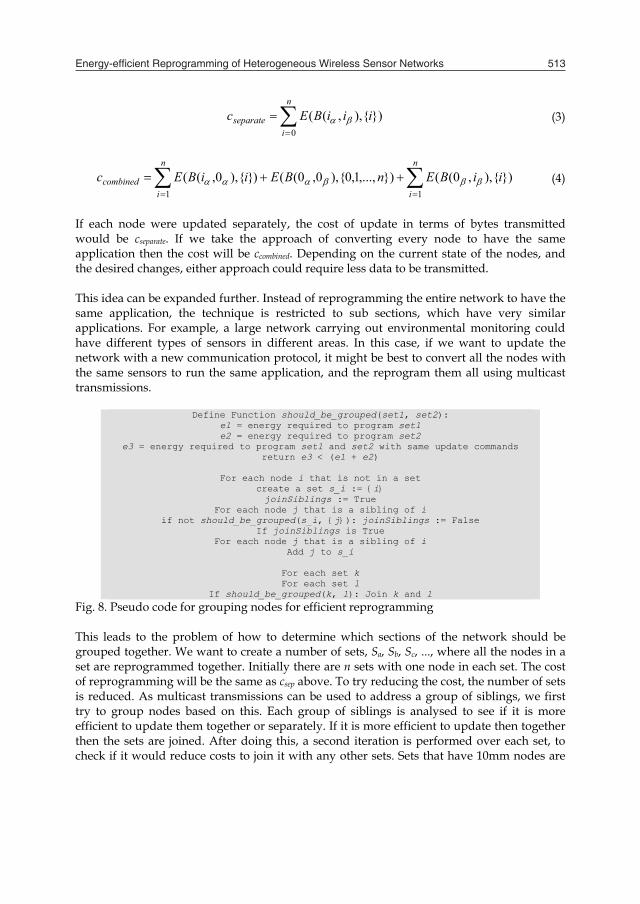
Define Function should_be_grouped(set1, set2): e1 = energy required to program set1 e2 = energy required to program set2
e3 = energy required to program set1 and set2 with same update commands return e3 < (e1 + e2)
For each node i that is not in a set
create a set s_i := {i} joinSiblings := True
For each node j that is a sibling of i if not should_be_grouped(s_i, {j}): joinSiblings := False
If joinSiblings is True For each node j that is a sibling of i
Add j to s_i
For each set k For each set l
If should_be_grouped(k, l): Join k and l Fig. 8. Pseudo code for grouping nodes for efficient reprogramming This leads to the problem of how to determine which sections of the network should be grouped together. We want to create a number of sets, Sa, Sb, Sc, ..., where all the nodes in a set are reprogrammed together. Initially there are n sets with one node in each set. The cost of reprogramming will be the same as csep above. To try reducing the cost, the number of sets is reduced. As multicast transmissions can be used to address a group of siblings, we first try to group nodes based on this. Each group of siblings is analysed to see if it is more efficient to update them together or separately. If it is more efficient to update then together then the sets are joined. After doing this, a second iteration is performed over each set, to check if it would reduce costs to join it with any other sets. Sets that have 10mm nodes are
Energy-efficient Reprogramming of Heterogeneous Wireless Sensor Networks 513
approach is to generate the commands needed to update each node individually. However, if we consider a heterogeneous network where some nodes have almost the same program, it may be better to first reprogram all nodes so that they have the same application. Then perform the update using multicast transmissions, and then make the changes to each node so that they are unique again. To illustrate the usefulness of this method, we can use data in the above tables. If there are a number of nodes which differ only in sampling frequency and it is desired to change the sensors on each node, then the size of the commands needed to change the sensor compared to the size of commands needed to change the sampling frequency means that the simple approach of sending a single set of commands to each node may be far from optimal. To decide which method is better we need to calculate the energy cost of each approach. In the tables above, the compression ration is used as the metric to examine the effectiveness of our Bsdiff implementation. This is valid, as when programming a single node, the number of bytes transmitted will be directly related to the energy used. However, the use of multicast transmissions in a heterogeneous network complicates this, as the energy per bit will change depending on how many nodes receive the message. For this reason, a new metric is required to analyse the use of Bsdiff in a heterogeneous network. The radio we use is capable of sending a 32 byte payload, with a 6 byte header, and 10 bit preamble, added by the radio. From this 32 byte payload, 4 bytes are used for routing control, packetisation, and a message type identifier, leaving 28 bytes for use. This means that a full packets is 314 bits long, of which 90 bits are overhead. The radio sends data at a rate of 50 kpbs, and has a 650 μs start-up time. Therefore, for a message with len bytes, the time to send it, T, can be calculated:
28/00065.0
5000090)28mod(8128/314
)( lenlenlen
lenT
(1)
For a message to be sent to a particular node, or set of nodes, S, the message will have to be sent STX times, received by 25mm nodes SRX25 times, and by 10mm nodes SRX10 times. In out network the 10mm nodes only act as leaf nodes, so they are never required to transmit the commands. Using values for transmission PTX and reception PRX25 and PRX10 from Table 1, the energy required to send the message can be calculated:
)()()(),( 10102525 lenTSPlenTSPlenTSPSlenE RXRXRXRXTXTX (2) This value is not fully accurate due to ACKs, and other network management costs, however these costs will affect every message similarly, so it is still a valid metric for comparing the cost of send a message. This metric can be used to help reduce the energy cost of reprogramming a heterogeneous network. In the network, there are nodes 0, 1, ... , n, and applications iα and iβ refer to different versions of an application that run on node i. B(iα, iβ) is the sum of the number of bytes in the commands that are needed to convert a node from running application iα to running application iβ.
n
iseparate iiiBEc
0
}){),,((
(3)
n
i
n
icombined iiBEnBEiiBEc
11
}){),,0((}),...,1,0{),0,0(()}{),0,((
(4)
If each node were updated separately, the cost of update in terms of bytes transmitted would be cseparate. If we take the approach of converting every node to have the same application then the cost will be ccombined. Depending on the current state of the nodes, and the desired changes, either approach could require less data to be transmitted. This idea can be expanded further. Instead of reprogramming the entire network to have the same application, the technique is restricted to sub sections, which have very similar applications. For example, a large network carrying out environmental monitoring could have different types of sensors in different areas. In this case, if we want to update the network with a new communication protocol, it might be best to convert all the nodes with the same sensors to run the same application, and the reprogram them all using multicast transmissions.
Define Function should_be_grouped(set1, set2): e1 = energy required to program set1 e2 = energy required to program set2
e3 = energy required to program set1 and set2 with same update commands return e3 < (e1 + e2)
For each node i that is not in a set
create a set s_i := {i} joinSiblings := True
For each node j that is a sibling of i if not should_be_grouped(s_i, {j}): joinSiblings := False
If joinSiblings is True For each node j that is a sibling of i
Add j to s_i
For each set k For each set l
If should_be_grouped(k, l): Join k and l Fig. 8. Pseudo code for grouping nodes for efficient reprogramming This leads to the problem of how to determine which sections of the network should be grouped together. We want to create a number of sets, Sa, Sb, Sc, ..., where all the nodes in a set are reprogrammed together. Initially there are n sets with one node in each set. The cost of reprogramming will be the same as csep above. To try reducing the cost, the number of sets is reduced. As multicast transmissions can be used to address a group of siblings, we first try to group nodes based on this. Each group of siblings is analysed to see if it is more efficient to update them together or separately. If it is more efficient to update then together then the sets are joined. After doing this, a second iteration is performed over each set, to check if it would reduce costs to join it with any other sets. Sets that have 10mm nodes are
Sustainable Wireless Sensor Networks514
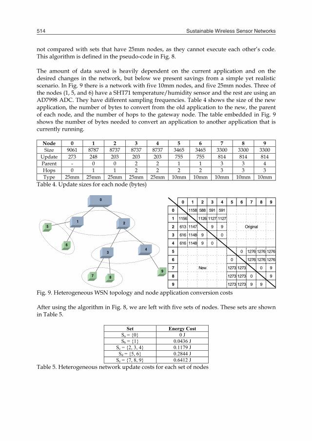
not compared with sets that have 25mm nodes, as they cannot execute each other’s code. This algorithm is defined in the pseudo-code in Fig. 8. The amount of data saved is heavily dependent on the current application and on the desired changes in the network, but below we present savings from a simple yet realistic scenario. In Fig. 9 there is a network with five 10mm nodes, and five 25mm nodes. Three of the nodes (1, 5, and 6) have a SHT71 temperature/humidity sensor and the rest are using an AD7998 ADC. They have different sampling frequencies. Table 4 shows the size of the new application, the number of bytes to convert from the old application to the new, the parent of each node, and the number of hops to the gateway node. The table embedded in Fig. 9 shows the number of bytes needed to convert an application to another application that is currently running.
Node 0 1 2 3 4 5 6 7 8 9 Size 9061 8787 8737 8737 8737 3465 3465 3300 3300 3300
Update 273 248 203 203 203 755 755 814 814 814 Parent - 0 0 2 2 1 1 3 3 4 Hops 0 1 1 2 2 2 2 3 3 3 Type 25mm 25mm 25mm 25mm 25mm 10mm 10mm 10mm 10mm 10mm
Table 4. Update sizes for each node (bytes)
6
7
4
2
89
1
3
5
0 0 1 2 3 4 5 6 7 8 9
0 1158 588 591 591
1 1156 1126 1127 1127
2 613 1147 9 9 Original
3 616 1148 9 0
4 616 1148 9 0
5 0 1276 1276 1276
6 0 1276 1276 1276
7 New 1273 1273 0 9
8 1273 1273 0 9
9 1273 1273 9 9 Fig. 9. Heterogeneous WSN topology and node application conversion costs After using the algorithm in Fig. 8, we are left with five sets of nodes. These sets are shown in Table 5.
Set Energy Cost Sa = {0} 0 J Sb = {1} 0.0436 J
Sc = {2, 3, 4} 0.1179 J Sd = {5, 6} 0.2844 J
Se = {7, 8, 9} 0.6412 J Table 5. Heterogeneous network update costs for each set of nodes
In Table 6, the energy cost for reprogramming the entire network is given. For this particular scenario the energy cost has been reduced to 6.57% of the energy cost of sending the full application program data. Taking advantage of the similarities between nodes in a heterogeneous network reduces the energy cost to 55.15% the cost of sending program update commands to each node separately.
Method Energy Cost Energy cost compared to uncompressed
Uncompressed 16.54 J 100% All nodes separate 1.971 J 11.91%
Grouping nodes into sets 1.087 J 6.57% Table 6. Comparison of reprogramming methods 5. LZW Compression
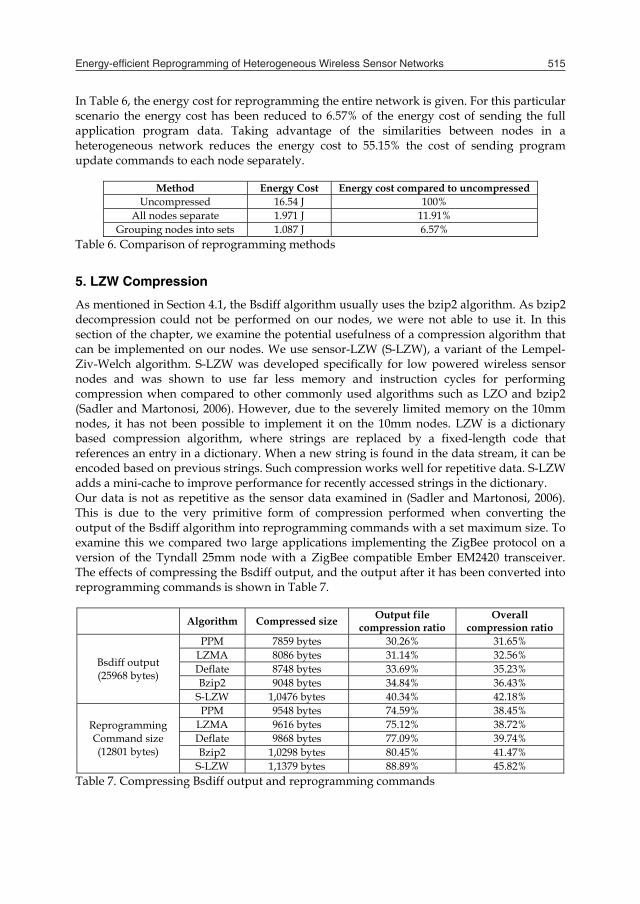
As mentioned in Section 4.1, the Bsdiff algorithm usually uses the bzip2 algorithm. As bzip2 decompression could not be performed on our nodes, we were not able to use it. In this section of the chapter, we examine the potential usefulness of a compression algorithm that can be implemented on our nodes. We use sensor-LZW (S-LZW), a variant of the Lempel-Ziv-Welch algorithm. S-LZW was developed specifically for low powered wireless sensor nodes and was shown to use far less memory and instruction cycles for performing compression when compared to other commonly used algorithms such as LZO and bzip2 (Sadler and Martonosi, 2006). However, due to the severely limited memory on the 10mm nodes, it has not been possible to implement it on the 10mm nodes. LZW is a dictionary based compression algorithm, where strings are replaced by a fixed-length code that references an entry in a dictionary. When a new string is found in the data stream, it can be encoded based on previous strings. Such compression works well for repetitive data. S-LZW adds a mini-cache to improve performance for recently accessed strings in the dictionary. Our data is not as repetitive as the sensor data examined in (Sadler and Martonosi, 2006). This is due to the very primitive form of compression performed when converting the output of the Bsdiff algorithm into reprogramming commands with a set maximum size. To examine this we compared two large applications implementing the ZigBee protocol on a version of the Tyndall 25mm node with a ZigBee compatible Ember EM2420 transceiver. The effects of compressing the Bsdiff output, and the output after it has been converted into reprogramming commands is shown in Table 7.
Algorithm Compressed size Output file compression ratio
Overall compression ratio
Bsdiff output (25968 bytes)
PPM 7859 bytes 30.26% 31.65% LZMA 8086 bytes 31.14% 32.56% Deflate 8748 bytes 33.69% 35.23% Bzip2 9048 bytes 34.84% 36.43%
S-LZW 1,0476 bytes 40.34% 42.18%
Reprogramming Command size (12801 bytes)
PPM 9548 bytes 74.59% 38.45% LZMA 9616 bytes 75.12% 38.72% Deflate 9868 bytes 77.09% 39.74% Bzip2 1,0298 bytes 80.45% 41.47%
S-LZW 1,1379 bytes 88.89% 45.82% Table 7. Compressing Bsdiff output and reprogramming commands
Energy-efficient Reprogramming of Heterogeneous Wireless Sensor Networks 515
not compared with sets that have 25mm nodes, as they cannot execute each other’s code. This algorithm is defined in the pseudo-code in Fig. 8. The amount of data saved is heavily dependent on the current application and on the desired changes in the network, but below we present savings from a simple yet realistic scenario. In Fig. 9 there is a network with five 10mm nodes, and five 25mm nodes. Three of the nodes (1, 5, and 6) have a SHT71 temperature/humidity sensor and the rest are using an AD7998 ADC. They have different sampling frequencies. Table 4 shows the size of the new application, the number of bytes to convert from the old application to the new, the parent of each node, and the number of hops to the gateway node. The table embedded in Fig. 9 shows the number of bytes needed to convert an application to another application that is currently running.
Node 0 1 2 3 4 5 6 7 8 9 Size 9061 8787 8737 8737 8737 3465 3465 3300 3300 3300
Update 273 248 203 203 203 755 755 814 814 814 Parent - 0 0 2 2 1 1 3 3 4 Hops 0 1 1 2 2 2 2 3 3 3 Type 25mm 25mm 25mm 25mm 25mm 10mm 10mm 10mm 10mm 10mm
Table 4. Update sizes for each node (bytes)
6
7
4
2
89
1
3
5
0 0 1 2 3 4 5 6 7 8 9
0 1158 588 591 591
1 1156 1126 1127 1127
2 613 1147 9 9 Original
3 616 1148 9 0
4 616 1148 9 0
5 0 1276 1276 1276
6 0 1276 1276 1276
7 New 1273 1273 0 9
8 1273 1273 0 9
9 1273 1273 9 9 Fig. 9. Heterogeneous WSN topology and node application conversion costs After using the algorithm in Fig. 8, we are left with five sets of nodes. These sets are shown in Table 5.
Set Energy Cost Sa = {0} 0 J Sb = {1} 0.0436 J
Sc = {2, 3, 4} 0.1179 J Sd = {5, 6} 0.2844 J
Se = {7, 8, 9} 0.6412 J Table 5. Heterogeneous network update costs for each set of nodes
In Table 6, the energy cost for reprogramming the entire network is given. For this particular scenario the energy cost has been reduced to 6.57% of the energy cost of sending the full application program data. Taking advantage of the similarities between nodes in a heterogeneous network reduces the energy cost to 55.15% the cost of sending program update commands to each node separately.
Method Energy Cost Energy cost compared to uncompressed
Uncompressed 16.54 J 100% All nodes separate 1.971 J 11.91%
Grouping nodes into sets 1.087 J 6.57% Table 6. Comparison of reprogramming methods 5. LZW Compression
As mentioned in Section 4.1, the Bsdiff algorithm usually uses the bzip2 algorithm. As bzip2 decompression could not be performed on our nodes, we were not able to use it. In this section of the chapter, we examine the potential usefulness of a compression algorithm that can be implemented on our nodes. We use sensor-LZW (S-LZW), a variant of the Lempel-Ziv-Welch algorithm. S-LZW was developed specifically for low powered wireless sensor nodes and was shown to use far less memory and instruction cycles for performing compression when compared to other commonly used algorithms such as LZO and bzip2 (Sadler and Martonosi, 2006). However, due to the severely limited memory on the 10mm nodes, it has not been possible to implement it on the 10mm nodes. LZW is a dictionary based compression algorithm, where strings are replaced by a fixed-length code that references an entry in a dictionary. When a new string is found in the data stream, it can be encoded based on previous strings. Such compression works well for repetitive data. S-LZW adds a mini-cache to improve performance for recently accessed strings in the dictionary. Our data is not as repetitive as the sensor data examined in (Sadler and Martonosi, 2006). This is due to the very primitive form of compression performed when converting the output of the Bsdiff algorithm into reprogramming commands with a set maximum size. To examine this we compared two large applications implementing the ZigBee protocol on a version of the Tyndall 25mm node with a ZigBee compatible Ember EM2420 transceiver. The effects of compressing the Bsdiff output, and the output after it has been converted into reprogramming commands is shown in Table 7.
Algorithm Compressed size Output file compression ratio
Overall compression ratio
Bsdiff output (25968 bytes)
PPM 7859 bytes 30.26% 31.65% LZMA 8086 bytes 31.14% 32.56% Deflate 8748 bytes 33.69% 35.23% Bzip2 9048 bytes 34.84% 36.43%
S-LZW 1,0476 bytes 40.34% 42.18%
Reprogramming Command size (12801 bytes)
PPM 9548 bytes 74.59% 38.45% LZMA 9616 bytes 75.12% 38.72% Deflate 9868 bytes 77.09% 39.74% Bzip2 1,0298 bytes 80.45% 41.47%
S-LZW 1,1379 bytes 88.89% 45.82% Table 7. Compressing Bsdiff output and reprogramming commands

Sustainable Wireless Sensor Networks516
The other algorithms are PPM (Prediction by Partial Matching), LZMA (Lempel Ziv Markov-chain Algorithm), Deflate (as used in Zip files), and BZip2 (Huffman based encoding). These algorithms were performed by the 7-Zip application with default parameters (Pavlov, 2010). The table shows that converting the Bsdiff output into standalone commands, as we did in Section 4.2, leads to a larger end file size in each case. However, this is necessary due to the limited memory available for buffering. Table 7 also shows that S-LZW is not as effective as other compression algorithms, which was expected due to its speed and low memory usage. S-LZW has a number of parameters that affect the compression ratio: the dictionary size; the mini-cache size; and the block size. LZW can compress streams of data of any length, so here block size refers to the size of chunks that the data stream is split into. This is necessary because of limited memory on the sensor nodes. These parameters can have positive effects by increasing the compression ratio, and negative effects by increasing the time taken to decode, or the memory required. Another method to increase the compression ratio is to use the Burrows Wheeler Transform (BWT) (Burrows and Wheeler, 1994). This algorithm can sort the data into an order that should compress better. It is a reversible transform so the original data can be regenerated.
80
85
90
95
100
105
0 256 512 768 1024 1280 1536 1792 2048
Block size (bytes)
Com
pres
sion
ratio
(%)
S-LZW-MC4S-LZW-MC4-BWTS-LZW-MC8S-LZW-MC8-BWTS-LZW-MC16S-LZW-MC16-BWTS-LZW-MC32S-LZW-MC32-BWT
Fig. 10. Effects of mini-cache, block size, and BWT on compression ratio The effect of the changing the dictionary size was found to be very small, and so was set at 512 entries. Fig. 10 shows the effects of the mini-cache size, how big a block is compressed, and BWT on compressing a set of commands 2,082 bytes in size (this is actually all the commands that are sent to node 0, in the network in Fig. 9). It can be seen that BWT has a positive effect on the compression ratio, and that an increased mini-cache size leads to increased compression too. Fig. 10 shows only the effect on compression ratio. However, the effect on energy consumption is more important. For this, it is necessary to analyse the processing costs of decompressing the data. The data compression is done on a PC, so it is not considered here, as the data sets used here are very small compared to the available processing power of a PC.
To analyse the cost of decompressing the code we measure the time taken to decompress a single block of data. The results of this are shown in Table 8 along with memory requirements in Flash (program memory) and RAM (data memory) for implementing S-LZW on the 25mm node. The memory used by BWT is minimised by sharing buffers with S-LZW. The results show that the mini-cache size has a negligible effect on processing time, and only a small effect on RAM size. For this reason, a 32 byte mini-cache is optimal, as it has a better compression ratio. The results also show that the time to decompress a single byte is not dependent on the block size that was compressed. The block-size should therefore be chosen based on the size that gives the best compression ratio, and still fits within the memory requirements (less than 4096 bytes). From Fig. 10 it can be seen that a block size that is a power of 2 is not always optimal. The PC that is compressing the commands can use a range of block sizes and chose the option that gives the best compression ratio.
Block size Algorithm Compressed
Size (bytes) Flash
(bytes) RAM
(bytes) Time (ms)
Time/byte (μs)
512 bytes
S-LZW-MC4 438 1768 3348 12.27 28.01 S-LZW-MC8 426 1744 3356 13.02 30.57 S-LZW-MC16 415 1744 3372 12.21 29.42 S-LZW-MC32 417 1744 3404 11.87 28.46
S-LZW-MC4-BWT 420 2116 3604 21.28 50.66 S-LZW-MC8-BWT 415 2092 3612 20.77 50.05 S-LZW-MC16-BWT 417 2092 3628 20.97 50.28 S-LZW-MC32-BWT 416 2092 3660 20.71 49.79
256 bytes
S-LZW-MC32 213 1482 2892 6.39 29.98 S-LZW-MC32-BWT 215 1826 3148 11.59 53.90
128 bytes
S-LZW-MC32 98 1354 2636 3.2 32.78 S-LZW-MC32-BWT 88 1698 2892 6.5 74.14
Table 8. Memory usage and time for decompression Our implementation of BWT requires memory that is twice the block size, however we have minimised the impact of this by using the same buffer that S-LZW uses for storing its dictionary. BWT however has a large impact on processing time, and still has some impact on memory usage. Whether or not it should be used depends on the increased compression ratio it offers. From Fig. 10, we see that BWT has very little advantage at the range of block sizes that can be decompressed (less than 512 bytes). If more memory were available, it would be more useful. To consider the energy savings by compression, the energy to send and receive the data and the energy required for decompression must be determined. The 2,082 byte file above can be compressed to 1,826 bytes using S-LZW-MC32 with a block size of 416 bytes. Using the power consumption values from Table 1, we can calculate the energy required with and without compression. The time to decompress a byte is from the table above, for S-LZW-MC32.
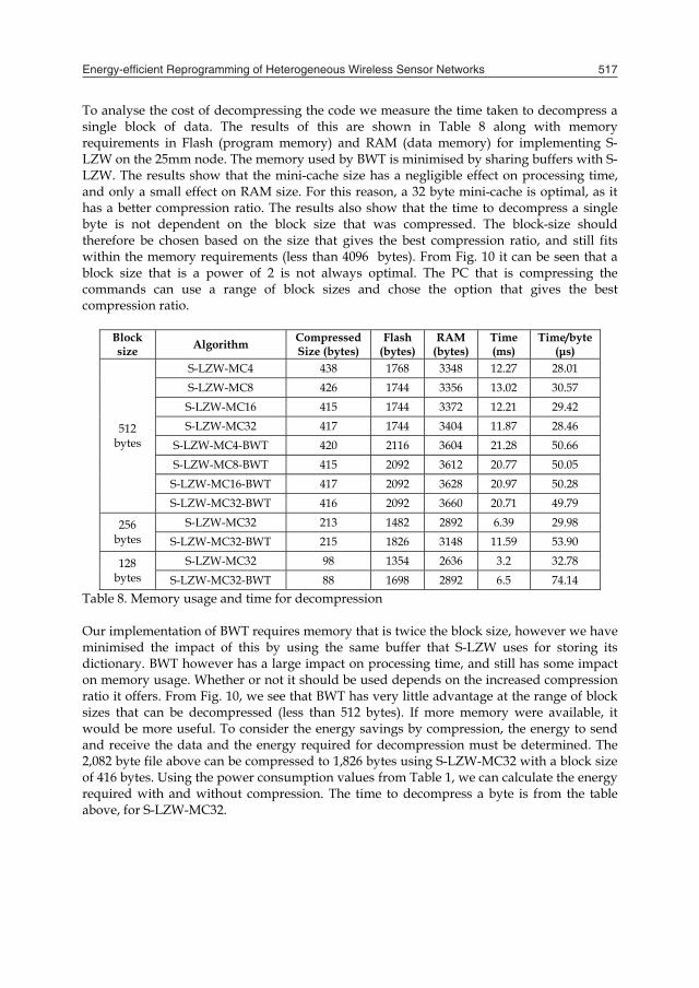
Energy-efficient Reprogramming of Heterogeneous Wireless Sensor Networks 517
The other algorithms are PPM (Prediction by Partial Matching), LZMA (Lempel Ziv Markov-chain Algorithm), Deflate (as used in Zip files), and BZip2 (Huffman based encoding). These algorithms were performed by the 7-Zip application with default parameters (Pavlov, 2010). The table shows that converting the Bsdiff output into standalone commands, as we did in Section 4.2, leads to a larger end file size in each case. However, this is necessary due to the limited memory available for buffering. Table 7 also shows that S-LZW is not as effective as other compression algorithms, which was expected due to its speed and low memory usage. S-LZW has a number of parameters that affect the compression ratio: the dictionary size; the mini-cache size; and the block size. LZW can compress streams of data of any length, so here block size refers to the size of chunks that the data stream is split into. This is necessary because of limited memory on the sensor nodes. These parameters can have positive effects by increasing the compression ratio, and negative effects by increasing the time taken to decode, or the memory required. Another method to increase the compression ratio is to use the Burrows Wheeler Transform (BWT) (Burrows and Wheeler, 1994). This algorithm can sort the data into an order that should compress better. It is a reversible transform so the original data can be regenerated.
80
85
90
95
100
105
0 256 512 768 1024 1280 1536 1792 2048
Block size (bytes)
Com
pres
sion
ratio
(%)
S-LZW-MC4S-LZW-MC4-BWTS-LZW-MC8S-LZW-MC8-BWTS-LZW-MC16S-LZW-MC16-BWTS-LZW-MC32S-LZW-MC32-BWT
Fig. 10. Effects of mini-cache, block size, and BWT on compression ratio The effect of the changing the dictionary size was found to be very small, and so was set at 512 entries. Fig. 10 shows the effects of the mini-cache size, how big a block is compressed, and BWT on compressing a set of commands 2,082 bytes in size (this is actually all the commands that are sent to node 0, in the network in Fig. 9). It can be seen that BWT has a positive effect on the compression ratio, and that an increased mini-cache size leads to increased compression too. Fig. 10 shows only the effect on compression ratio. However, the effect on energy consumption is more important. For this, it is necessary to analyse the processing costs of decompressing the data. The data compression is done on a PC, so it is not considered here, as the data sets used here are very small compared to the available processing power of a PC.
To analyse the cost of decompressing the code we measure the time taken to decompress a single block of data. The results of this are shown in Table 8 along with memory requirements in Flash (program memory) and RAM (data memory) for implementing S-LZW on the 25mm node. The memory used by BWT is minimised by sharing buffers with S-LZW. The results show that the mini-cache size has a negligible effect on processing time, and only a small effect on RAM size. For this reason, a 32 byte mini-cache is optimal, as it has a better compression ratio. The results also show that the time to decompress a single byte is not dependent on the block size that was compressed. The block-size should therefore be chosen based on the size that gives the best compression ratio, and still fits within the memory requirements (less than 4096 bytes). From Fig. 10 it can be seen that a block size that is a power of 2 is not always optimal. The PC that is compressing the commands can use a range of block sizes and chose the option that gives the best compression ratio.
Block size Algorithm Compressed
Size (bytes) Flash
(bytes) RAM
(bytes) Time (ms)
Time/byte (μs)
512 bytes
S-LZW-MC4 438 1768 3348 12.27 28.01 S-LZW-MC8 426 1744 3356 13.02 30.57 S-LZW-MC16 415 1744 3372 12.21 29.42 S-LZW-MC32 417 1744 3404 11.87 28.46
S-LZW-MC4-BWT 420 2116 3604 21.28 50.66 S-LZW-MC8-BWT 415 2092 3612 20.77 50.05 S-LZW-MC16-BWT 417 2092 3628 20.97 50.28 S-LZW-MC32-BWT 416 2092 3660 20.71 49.79
256 bytes
S-LZW-MC32 213 1482 2892 6.39 29.98 S-LZW-MC32-BWT 215 1826 3148 11.59 53.90
128 bytes
S-LZW-MC32 98 1354 2636 3.2 32.78 S-LZW-MC32-BWT 88 1698 2892 6.5 74.14
Table 8. Memory usage and time for decompression Our implementation of BWT requires memory that is twice the block size, however we have minimised the impact of this by using the same buffer that S-LZW uses for storing its dictionary. BWT however has a large impact on processing time, and still has some impact on memory usage. Whether or not it should be used depends on the increased compression ratio it offers. From Fig. 10, we see that BWT has very little advantage at the range of block sizes that can be decompressed (less than 512 bytes). If more memory were available, it would be more useful. To consider the energy savings by compression, the energy to send and receive the data and the energy required for decompression must be determined. The 2,082 byte file above can be compressed to 1,826 bytes using S-LZW-MC32 with a block size of 416 bytes. Using the power consumption values from Table 1, we can calculate the energy required with and without compression. The time to decompress a byte is from the table above, for S-LZW-MC32.
Sustainable Wireless Sensor Networks518
J 0.367977.1075.07977.1128.0
)2082()2082(
TPTPE RXTXeduncompress
(5)
J 0.32052.00293.0577.1075.0577.1128.0
)1046.281826()1826()1826( 6
CPURXTXcompressed PTPTPE
(6)
The transceivers throughput rate of 50 kbps is very slow compared to the Atmega128L processor running at 8 MHz, so the time taken for decompressing the data is minimal compared to the time taken for transmitting the data. Therefore even for very modest compression ratios, it is worthwhile to use S-LZW.
6. Conclusions
We presented efficient methods for reducing the energy cost of reprogramming wireless sensor networks, by using delta encoding and LZW based compression. We have modified the Bsdiff delta encoding algorithm to make suitable it for use in WSNs, and also tuned the S-LZW algorithm for energy efficiency. In our example heterogeneous network with two different hardware nodes, and two different sensor types we reduced the cost of updating the communication protocol to 6.57 % of an approach that requires sending the full application program. The use of S-LZW gives a further reduction to about 90% of this value. The solutions we provided can be applied to any type of reprogramming. The Bsdiff algorithm is not dependent on knowledge of instruction sets, and does not require any special compilation methods to keep functions at the same addresses. Very limited support is needed in the existing program. Support could be added on top of existing operating systems such as TinyOS or Contiki. This work has been implemented on a two-tiered heterogeneous network, but can be extended for multi-tier networks. The techniques presented are useful for simpler homogeneous networks. The work presented in this chapter is already of great use in reducing the energy costs to reprogram a wireless node or network. However, in ad-hoc networks where the topology is not centrally managed, algorithms such as MSP (Kulkarni and Wang, 2009) or Freshet (Krasniewski et al., 2008) are suitable for managing the propagation of commands, and would complement the techniques presented in this chapter.
7. Acknowledgments
This work was supported by Science Foundation Ireland under grant 07/CE/I1147.
8. References
Atmel (2009). Atmega128L datasheet, rev. S. http://www.atmel.com Bellis, S. J.; Delaney, K.; O'Flynn, B.; Barton, J.; Razeeb, K. M. & Ó Mathúna, S. C. (2005).
Development of field programmable modular wireless sensor network nodes for ambient systems. Computer Communications, 28, 13, Aug. 2005, pp. 1531-1544, ISSN:01403664
Berkeley (2010), University of California. Tinyos Community Forum, http://www.tinyos.net Burrows, M. & Wheeler, D. J. (1994). A block-sorting lossless data compression algorithm.
Digitial SRC Research Report 124 Dunkels, A. (2010) The Contiki Operating System, http://www.sics.se/contiki/ Foster-Miller (2010). Electrotextiles, http://www.foster-miller.com/m_m_electrotextiles.htm Georgoulas, D. & Blow, K. (2008). Intelligent Mobile Agent Middleware for Wireless Sensor
Networks: A Real Time Application Case Study. Proceedings of 4th Advanced Int. Conf. Telecommunications, pp. 95-100, ISBN:9780769531625, Athens, Greece, Jun. 2008, IEEE Computer Society, Washington DC
Harte, S.; O'Flynn, B.; Martínez-Catalá, R. V. & Popovici, E. M. (2007). Design and implementation of a miniaturised, low power wireless sensor node. Proceedings 18th Euro. Conf. Circuit Theory and Design, pp. 894-897, ISBN:9781424413416, Seville, Spain, Aug. 2007, IEEE Press, New Jersey
Hui, J. W. & Culler, D. (2004). The dynamic behavior of a data dissemination protocol for network programming at scale. Proceedings of 2nd Int. Conf. Embedded Networked Sensor Systems, pp. 81-94. ISBN:1581138792, Baltimore, USA, Nov. 2004, ACM, New York
Jeong, J. & Culler, D. (2009). Incremental network programming for wireless sensors. International Journal of Communications, Network and System Sciences. 2, 5, Aug. 2009, pp. 433-452, ISSN:17543924
Krasniewski, M. D.; Panta, R. K.; Bagchi, S.; Yang, C. & Chappell, W. J. (2008). Energy-efficient on-demand reprogramming of large-scale sensor networks. ACM Trans. Sensor Networks, 4, 1, Jan. 2008, pp 1-38, ISSN:15504859
Kulkarni, S. & Wang, L. (2009). Energy-efficient multihop reprogramming for sensor networks. ACM Trans. Sensor Networks, 5, 2, Mar. 2009, pp. 1-40, ISSN:15504859
Levis, P. & Culler, D. (2002). Maté: a tiny virtual machine for sensor networks. Proceedings of 10th Int. Conf. Architectural Support for Programming Languages and Operating Systems, pp. 85-95, ISBN:1581135742, San Jose, USA, Oct. 2002, ACM, New York
Levis, P.; Patel, N.; Culler, D. & Shenker, S. (2004). Trickle: a self-regulating algorithm for code propagation and maintenance in wireless sensor networks. Proceedings of 1st Conf. on Networked Systems Design and Implementation, pp. 15-18, San Francisco, USA, Mar. 2004
Marinkovic, S.; Spagnol, C. & Popovici, E. M. (2009). Energy-efficient TDMA-based MAC protocol for wireless body area networks. Proceedings of 3rd Int. Conf. Sensor Technologies and Applications, pp. 604-609, ISBN:9780769536699, Athens, Greece, June 2009, IEEE Computer Society, Washington DC
Marrón P. J.; Gauger, M.; Lachenmann, A.; Minder, D.; Saukh, O. & Rothermel, K. (2006). FlexCup: A Flexible and Efficient Code Update Mechanism for Sensor Networks. Proceedings of 3rd Euro. Workshop on Wireless Sensor Networks, pp. 212-227, ISBN:3540321586, Zurich, Switzerland, Feb. 2006, Springer, Berlin

Energy-efficient Reprogramming of Heterogeneous Wireless Sensor Networks 519
J 0.367977.1075.07977.1128.0
)2082()2082(
TPTPE RXTXeduncompress
(5)
J 0.32052.00293.0577.1075.0577.1128.0
)1046.281826()1826()1826( 6
CPURXTXcompressed PTPTPE
(6)
The transceivers throughput rate of 50 kbps is very slow compared to the Atmega128L processor running at 8 MHz, so the time taken for decompressing the data is minimal compared to the time taken for transmitting the data. Therefore even for very modest compression ratios, it is worthwhile to use S-LZW.
6. Conclusions
We presented efficient methods for reducing the energy cost of reprogramming wireless sensor networks, by using delta encoding and LZW based compression. We have modified the Bsdiff delta encoding algorithm to make suitable it for use in WSNs, and also tuned the S-LZW algorithm for energy efficiency. In our example heterogeneous network with two different hardware nodes, and two different sensor types we reduced the cost of updating the communication protocol to 6.57 % of an approach that requires sending the full application program. The use of S-LZW gives a further reduction to about 90% of this value. The solutions we provided can be applied to any type of reprogramming. The Bsdiff algorithm is not dependent on knowledge of instruction sets, and does not require any special compilation methods to keep functions at the same addresses. Very limited support is needed in the existing program. Support could be added on top of existing operating systems such as TinyOS or Contiki. This work has been implemented on a two-tiered heterogeneous network, but can be extended for multi-tier networks. The techniques presented are useful for simpler homogeneous networks. The work presented in this chapter is already of great use in reducing the energy costs to reprogram a wireless node or network. However, in ad-hoc networks where the topology is not centrally managed, algorithms such as MSP (Kulkarni and Wang, 2009) or Freshet (Krasniewski et al., 2008) are suitable for managing the propagation of commands, and would complement the techniques presented in this chapter.
7. Acknowledgments
This work was supported by Science Foundation Ireland under grant 07/CE/I1147.
8. References
Atmel (2009). Atmega128L datasheet, rev. S. http://www.atmel.com Bellis, S. J.; Delaney, K.; O'Flynn, B.; Barton, J.; Razeeb, K. M. & Ó Mathúna, S. C. (2005).
Development of field programmable modular wireless sensor network nodes for ambient systems. Computer Communications, 28, 13, Aug. 2005, pp. 1531-1544, ISSN:01403664
Berkeley (2010), University of California. Tinyos Community Forum, http://www.tinyos.net Burrows, M. & Wheeler, D. J. (1994). A block-sorting lossless data compression algorithm.
Digitial SRC Research Report 124 Dunkels, A. (2010) The Contiki Operating System, http://www.sics.se/contiki/ Foster-Miller (2010). Electrotextiles, http://www.foster-miller.com/m_m_electrotextiles.htm Georgoulas, D. & Blow, K. (2008). Intelligent Mobile Agent Middleware for Wireless Sensor
Networks: A Real Time Application Case Study. Proceedings of 4th Advanced Int. Conf. Telecommunications, pp. 95-100, ISBN:9780769531625, Athens, Greece, Jun. 2008, IEEE Computer Society, Washington DC
Harte, S.; O'Flynn, B.; Martínez-Catalá, R. V. & Popovici, E. M. (2007). Design and implementation of a miniaturised, low power wireless sensor node. Proceedings 18th Euro. Conf. Circuit Theory and Design, pp. 894-897, ISBN:9781424413416, Seville, Spain, Aug. 2007, IEEE Press, New Jersey
Hui, J. W. & Culler, D. (2004). The dynamic behavior of a data dissemination protocol for network programming at scale. Proceedings of 2nd Int. Conf. Embedded Networked Sensor Systems, pp. 81-94. ISBN:1581138792, Baltimore, USA, Nov. 2004, ACM, New York
Jeong, J. & Culler, D. (2009). Incremental network programming for wireless sensors. International Journal of Communications, Network and System Sciences. 2, 5, Aug. 2009, pp. 433-452, ISSN:17543924
Krasniewski, M. D.; Panta, R. K.; Bagchi, S.; Yang, C. & Chappell, W. J. (2008). Energy-efficient on-demand reprogramming of large-scale sensor networks. ACM Trans. Sensor Networks, 4, 1, Jan. 2008, pp 1-38, ISSN:15504859
Kulkarni, S. & Wang, L. (2009). Energy-efficient multihop reprogramming for sensor networks. ACM Trans. Sensor Networks, 5, 2, Mar. 2009, pp. 1-40, ISSN:15504859
Levis, P. & Culler, D. (2002). Maté: a tiny virtual machine for sensor networks. Proceedings of 10th Int. Conf. Architectural Support for Programming Languages and Operating Systems, pp. 85-95, ISBN:1581135742, San Jose, USA, Oct. 2002, ACM, New York
Levis, P.; Patel, N.; Culler, D. & Shenker, S. (2004). Trickle: a self-regulating algorithm for code propagation and maintenance in wireless sensor networks. Proceedings of 1st Conf. on Networked Systems Design and Implementation, pp. 15-18, San Francisco, USA, Mar. 2004
Marinkovic, S.; Spagnol, C. & Popovici, E. M. (2009). Energy-efficient TDMA-based MAC protocol for wireless body area networks. Proceedings of 3rd Int. Conf. Sensor Technologies and Applications, pp. 604-609, ISBN:9780769536699, Athens, Greece, June 2009, IEEE Computer Society, Washington DC
Marrón P. J.; Gauger, M.; Lachenmann, A.; Minder, D.; Saukh, O. & Rothermel, K. (2006). FlexCup: A Flexible and Efficient Code Update Mechanism for Sensor Networks. Proceedings of 3rd Euro. Workshop on Wireless Sensor Networks, pp. 212-227, ISBN:3540321586, Zurich, Switzerland, Feb. 2006, Springer, Berlin
Sustainable Wireless Sensor Networks520
Motta, G.; Gustafson, J. & Chen, S. (2007). Differential compression of executable code. Proceedings of Data Compression Conf., pp. 103-112, ISBN:0769527914, Snowbird, USA, Mar 2007, IEEE Computer Society, Washington DC
Nordic Semiconductor (2008). nRF9E5 datasheet, rev. 1.5. http://www.nordicsemi.com Pavlov, I. (2010). 7-zip file archiver. http://www.7-zip.org Percival, C. (2006). Matching with Mismatches and Assorted Applications, Ph.D. Dissertation.
University of Oxford Percival, C. (2010). Binary diff/patch utility. http://www.daemonology.net/bsdiff Phillips, L. A. (2005). Aqueduct: robust and efficient code propagation in heterogeneous wireless
sensor networks. Master’s thesis, University of Nebraska Raghunathan, V.; Schurgers, C.; Park, S. & Srivastava, M. B., 2002. Energy-aware wireless
microsensor networks. IEEE Signal Processing Magazine, 19, 2, Aug. 2002, pp. 40-50, ISSN:10535888
Roedig, U.; Barroso, A. & Sreenan, C. J. (2006). f-MAC: a deterministic media access control protocol without time synchronization. Proceedings of 3rd Euro. Workshop on Wireless Sensor Networks, pp. 276-291, ISBN:3540321586, Zurich, Switzerland, Feb. 2006, Springer, Berlin
Reijers, N. & Langendoen, K. (2003). Efficient code distribution in wireless sensor networks. Proceedings of 2nd ACM Int. Conf. Wireless sensor networks and applications, pp. 60-67, ISBN:1581137648, San Diego, USA, Sept. 2003, ACM, New York
Sadler, C. M. & Martonosi, M. (2006). Data compression algorithms for energy-constrained devices in delay tolerant networks. Proceedings of 4th Int. Conf. Embedded Networked Sensor Systems, pp. 265-278, ISBN:1595933433, Boulder USA, Nov. 2006, ACM, New York
Tridgell, A. (1999). Efficient algorithms for sorting and synchronization. Ph.D. Dissertation, Australian National University
Related Documents