Energy-Efficient Design of Adhoc and Sensor Networksd-scholarship.pitt.edu/6381/1/sameh-thesis.pdf · ABSTRACT ENERGY-EFFICIENT DESIGN OF ADHOC AND SENSOR NETWORKS Sameh Gobriel,

ENERGY-EFFICIENT DESIGN OF ADHOC AND

SENSOR NETWORKS

by

Sameh Gobriel

B.E., Cairo University, Egypt, 1999

M.Sc., University of Pittsburgh, 2007

Submitted to the Graduate Faculty of

Arts and Science in partial fulfillment

of the requirements for the degree of

Doctor of Philosophy

University of Pittsburgh

2008

UNIVERSITY OF PITTSBURGH

DEPARTMENT OF COMPUTER SCIENCE

This dissertation was presented

by

Sameh Gobriel

It was defended on

February 2008

and approved by

Dr. Rami Melhem

Dr. Daniel Mosse

Dr. Ahmed Amer

Dr. Tarek Abdelzaher

Dissertation Advisors: Dr. Rami Melhem,

Dr. Daniel Mosse

ii

Copyright c© by Sameh Gobriel

2008

iii

ABSTRACT

ENERGY-EFFICIENT DESIGN OF ADHOC AND SENSOR NETWORKS

Sameh Gobriel, PhD

University of Pittsburgh, 2008

Adhoc and sensor networks (ASNs) are emerging wireless networks that are expected to have

significant impact on the efficiency of many military and civil applications. However, building

ASNs efficiently poses a considerable technical challenge because of the many constraints

imposed by the environment, or by the ASN nodes capabilities themselves. One of the main

challenges is the finite supply energy. Since the network hosts are battery operated, they

need to be energy conserving so that the nodes and hence the network itself does not expire.

In this thesis different techniques for an energy-efficient design for ASNs are presented. My

work spans two layers of the network protocol stack; these are the Medium Access Layer

(MAC) and the Routing Layer.

This thesis first identifies and highlights the different sources of energy inefficiency in

ASNs, and then it describes how each of these inefficiencies is handled. Toward this goal,

I first focus on the Medium Access (MAC) Layer and present my work that handles the

wasted energy in transmission and describe how the transmission distance is optimized to

extend the network lifetime. I then describe BLAM, an energy-efficient extension for the

IEEE 802.11, that handles the wasted energy in collisions. Next, TDMA-ASAP, a new MAC

protocol for sensor networks, is introduced. TDMA-ASAP targets the wasted energy in idle

listening.

I also investigate energy-efficiency at the routing layer level. First, the “Flooding-Waves”

problem is identified. This is a problem in any cost-based energy-efficient routing protocol

for adhoc networks, different ways of solving this problem are presented. For sensor networks

iv

routing trees are usually used, I introduce a new routing scheme called RideSharing which is

energy-efficient and fault-tolerant. RideSharing will deliver a better aggregate result to the

end user while masking network link failures. Next, I present how to extend the RideSharing

scheme to handle different link quality models. Finally, I introduce GroupBeat, a new health

detection system for sensor networks, which when combined with RideSharing can deliver

the information to the end user even in case of node failures.

v

TABLE OF CONTENTS

1.0 INTRODUCTION . . . . . . . . . . . . . . . . . . . . . . . . . . . . . . . . . 1

1.1 Design Challenges of ASNs . . . . . . . . . . . . . . . . . . . . . . . . . . . 2

1.2 Contributions and Roadmap . . . . . . . . . . . . . . . . . . . . . . . . . . . 3

2.0 BACKGROUND MATERIAL . . . . . . . . . . . . . . . . . . . . . . . . . 6

2.1 Classification of Wireless Networks . . . . . . . . . . . . . . . . . . . . . . . 6

2.1.1 Cellular Networks . . . . . . . . . . . . . . . . . . . . . . . . . . . . 7

2.1.2 Mobile Adhoc Networks (MANETs) . . . . . . . . . . . . . . . . . . 7

2.1.3 Wireless Sensor Networks (WSN’s) . . . . . . . . . . . . . . . . . . . 8

2.1.4 Wireless Mesh Networks . . . . . . . . . . . . . . . . . . . . . . . . . 9

2.1.5 Wireless Hybrid Networks . . . . . . . . . . . . . . . . . . . . . . . 10

2.2 Energy Consumption of Wireless Nodes . . . . . . . . . . . . . . . . . . . . 11

2.3 Categorizing Medium Access (MAC) Layer Protocols for ASN’s . . . . . . . 12

2.3.1 IEEE 802.11: a contention-based MAC protocol . . . . . . . . . . . . 13

2.3.2 TDMA: a contention-free MAC protocol . . . . . . . . . . . . . . . . 14

2.4 Routing Layer Protocols for ASN’s . . . . . . . . . . . . . . . . . . . . . . . 15

2.4.1 Routing Layer protocols in Adhoc Networks . . . . . . . . . . . . . . 15

2.4.2 Routing in Sensor Networks . . . . . . . . . . . . . . . . . . . . . . . 15

3.0 ENERGY-EFFICIENT MAC LAYER OPTIMIZATIONS FOR AD-

HOC NETWORKS . . . . . . . . . . . . . . . . . . . . . . . . . . . . . . . . 17

3.1 Optimal MAC Transmission Power . . . . . . . . . . . . . . . . . . . . . . . 18

3.1.1 Background and Minimum Transmission Distance Concept . . . . . . 18

3.1.2 Tradeoffs in Choosing Transmission Distance . . . . . . . . . . . . . 19

vi

3.1.3 Model Background . . . . . . . . . . . . . . . . . . . . . . . . . . . . 20

3.1.4 Interference Model . . . . . . . . . . . . . . . . . . . . . . . . . . . . 21

3.1.5 Collision Model . . . . . . . . . . . . . . . . . . . . . . . . . . . . . . 25

3.1.6 Estimation of Average Hop Count . . . . . . . . . . . . . . . . . . . 28

3.1.6.1 Random Traffic Pattern . . . . . . . . . . . . . . . . . . . . . 29

3.1.6.2 Local Traffic Pattern . . . . . . . . . . . . . . . . . . . . . . 30

3.1.7 Energy Computation . . . . . . . . . . . . . . . . . . . . . . . . . . . 31

3.1.8 Numerical Results . . . . . . . . . . . . . . . . . . . . . . . . . . . . 33

3.1.8.1 Total Network Throughput . . . . . . . . . . . . . . . . . . . 34

3.1.8.2 Total Energy Consumption . . . . . . . . . . . . . . . . . . . 35

3.1.8.3 Energy Consumption per Message . . . . . . . . . . . . . . . 36

3.1.8.4 Effect of Changing the Node Density . . . . . . . . . . . . . 37

3.1.8.5 Effect of Changing the CW Size . . . . . . . . . . . . . . . . 38

3.1.8.6 Local Traffic Case . . . . . . . . . . . . . . . . . . . . . . . . 40

3.1.8.7 Numerical Results Summary . . . . . . . . . . . . . . . . . . 41

3.2 Minimizing Wasted Collision Energy . . . . . . . . . . . . . . . . . . . . . . 42

3.2.1 Motivation and Significance of Collision Energy . . . . . . . . . . . . 42

3.2.2 Modifications to IEEE 802.11 DCF . . . . . . . . . . . . . . . . . . . 43

3.2.3 Collision Analysis . . . . . . . . . . . . . . . . . . . . . . . . . . . . 45

3.2.3.1 Probability of transmission . . . . . . . . . . . . . . . . . . . 46

3.2.3.2 Model results and validation . . . . . . . . . . . . . . . . . . 47

3.2.4 Simulation Results . . . . . . . . . . . . . . . . . . . . . . . . . . . . 49

3.3 Conclusion . . . . . . . . . . . . . . . . . . . . . . . . . . . . . . . . . . . . 53

4.0 ENERGY-EFFICIENT ROUTING LAYER OPTIMIZATIONS FOR

ADHOC NETWORKS . . . . . . . . . . . . . . . . . . . . . . . . . . . . . . 54

4.1 Dynamic Source Routing (DSR) Protocol . . . . . . . . . . . . . . . . . . . 55

4.2 Energy-Efficient Cost-Based Routing . . . . . . . . . . . . . . . . . . . . . . 57

4.2.1 Wireless Link Cost Function . . . . . . . . . . . . . . . . . . . . . . . 58

4.2.2 Cost Aggregation and Balanced Energy Concept . . . . . . . . . . . 58

4.3 Flooding Waves in Cost-Based Energy-Efficient Routing . . . . . . . . . . . 60

vii

4.3.1 Flooding Waves Problem Definition . . . . . . . . . . . . . . . . . . . 60

4.3.2 Simulation Results Showing Effect of Flooding-Waves . . . . . . . . . 62

4.3.2.1 Simulation Setup . . . . . . . . . . . . . . . . . . . . . . . . 62

4.3.2.2 Simulation Results for Low-Density Network . . . . . . . . . 63

4.3.2.3 Simulation Results for High-Density Network . . . . . . . . . 64

4.3.3 Delayed Forwarding . . . . . . . . . . . . . . . . . . . . . . . . . . . 65

4.3.4 Analytical Model for a Linear Network . . . . . . . . . . . . . . . . . 66

4.3.5 Simulation Analysis for Delayed-Forwarding . . . . . . . . . . . . . . 69

4.4 Conclusion . . . . . . . . . . . . . . . . . . . . . . . . . . . . . . . . . . . . 72

5.0 ENERGY-EFFICIENT MAC LAYER OPTIMIZATIONS FOR SEN-

SOR NETWORKS . . . . . . . . . . . . . . . . . . . . . . . . . . . . . . . . . 73

5.1 Conventional MAC Layer Protocols for WSN . . . . . . . . . . . . . . . . . 75

5.2 TDMA-ASAP: TDMA with Adaptive Slot stealing And Parallelism . . . . . 76

5.2.1 Network and Node Models . . . . . . . . . . . . . . . . . . . . . . . . 76

5.2.2 Outline and General Idea . . . . . . . . . . . . . . . . . . . . . . . . 77

5.2.3 1-Level Coloring for Parallel Transmissions . . . . . . . . . . . . . . . 79

5.2.4 Slot Stealing . . . . . . . . . . . . . . . . . . . . . . . . . . . . . . . 81

5.2.4.1 Determine Potential Stealers: . . . . . . . . . . . . . . . . . . 81

5.2.4.2 Detect Unused Slots: . . . . . . . . . . . . . . . . . . . . . . 82

5.2.4.3 Stealing Algorithms: . . . . . . . . . . . . . . . . . . . . . . . 82

5.2.5 Evaluation . . . . . . . . . . . . . . . . . . . . . . . . . . . . . . . . 85

5.2.5.1 Simulation Environment . . . . . . . . . . . . . . . . . . . . 85

5.2.5.2 End-to-End Delay . . . . . . . . . . . . . . . . . . . . . . . . 86

5.2.5.3 Energy . . . . . . . . . . . . . . . . . . . . . . . . . . . . . . 87

5.2.5.4 Energy-Delay Product . . . . . . . . . . . . . . . . . . . . . . 89

5.2.5.5 Effects of Transition Time and Packet Size . . . . . . . . . . 91

5.2.5.6 Average time awake per level . . . . . . . . . . . . . . . . . . 91

5.3 Conclusion . . . . . . . . . . . . . . . . . . . . . . . . . . . . . . . . . . . . 92


SENSOR NETWORKS . . . . . . . . . . . . . . . . . . . . . . . . . . . . . . 94

viii

6.1 Hash-Based Schemes for Delivering Aggregate Data in WSNs . . . . . . . . 95

6.2 RideSharing: Energy-Efficient Fault Tolerant Routing for Sensor Networks . 96

6.2.1 Track Topology . . . . . . . . . . . . . . . . . . . . . . . . . . . . . . 97

6.2.2 Error Detection and Correction . . . . . . . . . . . . . . . . . . . . . 98

6.2.3 Illustrating Example . . . . . . . . . . . . . . . . . . . . . . . . . . . 99

6.2.4 Cascaded RideSharing . . . . . . . . . . . . . . . . . . . . . . . . . . 99

6.2.5 Diffused RideSharing . . . . . . . . . . . . . . . . . . . . . . . . . . . 101

6.2.6 RideSharing Enhancements . . . . . . . . . . . . . . . . . . . . . . . 102

6.2.6.1 Co-tracking . . . . . . . . . . . . . . . . . . . . . . . . . . . . 102

6.2.6.2 Parent Clique . . . . . . . . . . . . . . . . . . . . . . . . . . 103

6.2.6.3 Transmission Order . . . . . . . . . . . . . . . . . . . . . . . 103

6.2.7 Evaluation . . . . . . . . . . . . . . . . . . . . . . . . . . . . . . . . 104

6.2.7.1 Simulation Setup . . . . . . . . . . . . . . . . . . . . . . . . 104

6.2.7.2 Accuracy Comparison . . . . . . . . . . . . . . . . . . . . . . 105

6.2.7.3 Overhead Comparison . . . . . . . . . . . . . . . . . . . . . . 107

6.2.7.4 Effect of Network Density and Number of parents . . . . . . 108

6.2.7.5 Optimizations Effect . . . . . . . . . . . . . . . . . . . . . . . 109

6.3 Link Qualities Assessments and Fault-Tolerant Aggregation . . . . . . . . . 111

6.3.1 Hash-Based Schemes with Link Qualities . . . . . . . . . . . . . . . . 111

6.3.1.1 Evaluation and Simulation Analysis . . . . . . . . . . . . . . 112

6.3.2 RideSharing with Link Qualities . . . . . . . . . . . . . . . . . . . . 113

6.3.2.1 NP-Hard Problem Reduction . . . . . . . . . . . . . . . . . . 115

6.3.2.2 Evaluation and Simulation Analysis . . . . . . . . . . . . . . 117

6.4 GroupBeat: Handling Node Errors in RS . . . . . . . . . . . . . . . . . . . . 118

6.4.1 GroupBeat: General Idea and Overview . . . . . . . . . . . . . . . . 119

6.4.2 GroupBeat using Communication by Signaling . . . . . . . . . . . . 121

6.4.3 Combining RideSharing and GroupBeat . . . . . . . . . . . . . . . . 123

6.5 Conclusion . . . . . . . . . . . . . . . . . . . . . . . . . . . . . . . . . . . . 125

7.0 CONCLUSIONS AND FUTURE WORK . . . . . . . . . . . . . . . . . . 126

7.1 Contributions . . . . . . . . . . . . . . . . . . . . . . . . . . . . . . . . . . . 127

ix

7.2 Key Questions: Reasoning Vs. Intuition . . . . . . . . . . . . . . . . . . . . 128

7.3 Future Work . . . . . . . . . . . . . . . . . . . . . . . . . . . . . . . . . . . 129

BIBLIOGRAPHY . . . . . . . . . . . . . . . . . . . . . . . . . . . . . . . . . . . . 131

x

LIST OF TABLES

2.1 Cellular Networks Vs. MANETs . . . . . . . . . . . . . . . . . . . . . . . . 8

3.1 Average Hopcount for Local Traffic Pattern . . . . . . . . . . . . . . . . . . . 30

3.2 Network Parameters for Unified Collision/Interference Model . . . . . . . . . 33

3.3 Network Parameters for BLAM Model Verification . . . . . . . . . . . . . . . 48

3.4 Simulation Parameters for BLAM and 802.11 Comparison . . . . . . . . . . . 50

4.1 Simulation Parameters to Show the Flooding-Waves Problem . . . . . . . . . . . 62

6.1 Effect of RideSharing Optimizations on the Relative RMS . . . . . . . . . . . 110

xi

LIST OF FIGURES

1.1 Thesis Contribution . . . . . . . . . . . . . . . . . . . . . . . . . . . . . . . . 5

2.1 Example of Wireless Cellular Networks . . . . . . . . . . . . . . . . . . . . . 7

2.2 Example of an Adhoc Wireless Network . . . . . . . . . . . . . . . . . . . . . 8

2.3 Energy Consumption of Wireless Node . . . . . . . . . . . . . . . . . . . . . 11

2.4 IEEE 802.11 DCF Protocol . . . . . . . . . . . . . . . . . . . . . . . . . . . . 13

2.5 Contention-Free Medium Access Schemes . . . . . . . . . . . . . . . . . . . . 14

2.6 MANET Routing Protocol Classification . . . . . . . . . . . . . . . . . . . . 15

2.7 Sensors Tree Routing Structure . . . . . . . . . . . . . . . . . . . . . . . . . 16

3.1 Adhoc Networks MAC Layer Contribution . . . . . . . . . . . . . . . . . . . 17

3.2 Hidden Terminal Jamming . . . . . . . . . . . . . . . . . . . . . . . . . . . . 18

3.3 Control Frames at Max. Power . . . . . . . . . . . . . . . . . . . . . . . . . . 18

3.4 Interfering Nodes Constellation . . . . . . . . . . . . . . . . . . . . . . . . . . 21

3.5 Honey Grid Interference Model . . . . . . . . . . . . . . . . . . . . . . . . . . 21

3.6 Interfering Nodes per Ring . . . . . . . . . . . . . . . . . . . . . . . . . . . . 23

3.7 Wireless Channel State Transition Diagram . . . . . . . . . . . . . . . . . . . 25

3.8 Node State Transition Diagram . . . . . . . . . . . . . . . . . . . . . . . . . 27

3.9 Hidden Area From the Sender . . . . . . . . . . . . . . . . . . . . . . . . . . 27

3.10 Route of Length i Hops for Random Traffic Pattern . . . . . . . . . . . . . . 29

3.11 Average Hopcount in Random Traffic . . . . . . . . . . . . . . . . . . . . . . 29

3.12 Total Network Throughput per Node . . . . . . . . . . . . . . . . . . . . . . 35

3.13 Total Energy Consumption . . . . . . . . . . . . . . . . . . . . . . . . . . . . 36

3.14 Total Energy Consumption per Message . . . . . . . . . . . . . . . . . . . . . 37

xii

3.15 ρ Effect on Throughput per Node . . . . . . . . . . . . . . . . . . . . . . . . 37

3.16 ρ Effect on Energy Consumption . . . . . . . . . . . . . . . . . . . . . . . . . 38

3.17 CW Effect on Throughput per Node . . . . . . . . . . . . . . . . . . . . . . . 39

3.18 CW Effect on Energy Consumption . . . . . . . . . . . . . . . . . . . . . . . 39

3.19 Locality Index Effect on Throughput . . . . . . . . . . . . . . . . . . . . . . 40

3.20 Locality Index Effect on Energy Consumption . . . . . . . . . . . . . . . . . 41

3.21 Deferring Time Distribution . . . . . . . . . . . . . . . . . . . . . . . . . . . 44

3.22 Transmission Probability PDF . . . . . . . . . . . . . . . . . . . . . . . . . . 47

3.23 No. of Collisions BLAM Model Verification . . . . . . . . . . . . . . . . . . . 48

3.24 Network Throughput BLAM Model Verification . . . . . . . . . . . . . . . . 48

3.25 Total Number of Collisions BLAM Vs. 802.11 . . . . . . . . . . . . . . . . . 51

3.26 Network Lifetime (in seconds) BLAM Vs. 802.11 . . . . . . . . . . . . . . . . 52

3.27 Total Number of Received Packets BLAM vs. 802.11 . . . . . . . . . . . . . 52

4.1 Adhoc Networks Routing Layer Contribution . . . . . . . . . . . . . . . . . . 55

4.2 Route Discovery Operation . . . . . . . . . . . . . . . . . . . . . . . . . . . . 56

4.3 Aggregate Energy Capacity per Route . . . . . . . . . . . . . . . . . . . . . . 59

4.4 Arithmetic, Geometric and Harmonic Mean . . . . . . . . . . . . . . . . . . . 59

4.5 Flooding Waves Problem in a High-Density Network . . . . . . . . . . . . . . . . 61

4.6 Significant Improvement in Low-Density Network . . . . . . . . . . . . . . . 63

4.7 Route Discovery Overhead in High-Density Network . . . . . . . . . . . . . . 64

4.8 Random Forwarding Delay at Each Relay Node . . . . . . . . . . . . . . . . . . 66

4.9 Route Request Overhead . . . . . . . . . . . . . . . . . . . . . . . . . . . . . . 67

4.10 A Linear Adhoc Network . . . . . . . . . . . . . . . . . . . . . . . . . . . . . . 68

4.11 Cumulative No. of Forwarded RREQ . . . . . . . . . . . . . . . . . . . . . . 70

4.12 Cumulative No. of Dead Nodes . . . . . . . . . . . . . . . . . . . . . . . . . 71

4.13 Cumulative No. of Received Packets . . . . . . . . . . . . . . . . . . . . . . . 71

5.1 Sensor Networks MAC Layer Contribution . . . . . . . . . . . . . . . . . . . 74

5.2 Example of a Sensor Network . . . . . . . . . . . . . . . . . . . . . . . . . . 78

5.3 Parallel TDMA Schedule . . . . . . . . . . . . . . . . . . . . . . . . . . . . . 78

5.4 Slot Stealing and Collision . . . . . . . . . . . . . . . . . . . . . . . . . . . . 83

xiii

5.5 StealG and Stealing Advertising . . . . . . . . . . . . . . . . . . . . . . . . . 84

5.6 TDMA-ASAP Delay Vs. Different MAC protocols . . . . . . . . . . . . . . . 87

5.7 Energy Consumption with Parallel Transmission . . . . . . . . . . . . . . . . 88

5.8 Energy consumption with Slot Stealing . . . . . . . . . . . . . . . . . . . . . 89

5.9 Energy-Delay Product in TDMA-ASAP . . . . . . . . . . . . . . . . . . . . . 90

5.10 Effect of Transition Time and Packet Size in TDMA-ASAP . . . . . . . . . . 90

5.11 Average Awake Time per Level in TDMA-ASAP . . . . . . . . . . . . . . . . 91

6.1 Sensor Networks Routing Layer Contribution . . . . . . . . . . . . . . . . . . 95

6.2 Hash-Based Schemes Count Aggregate . . . . . . . . . . . . . . . . . . . . . 96

6.3 Track Topology . . . . . . . . . . . . . . . . . . . . . . . . . . . . . . . . . . 97

6.4 Cascaded RideSharing . . . . . . . . . . . . . . . . . . . . . . . . . . . . . . 100

6.5 Diffused RideSharing . . . . . . . . . . . . . . . . . . . . . . . . . . . . . . . 102

6.6 RS vs. Hash-Based RMS for 100% Participation . . . . . . . . . . . . . . . . 105

6.7 RS vs. Hash-Based RMS for 2% Participation . . . . . . . . . . . . . . . . . 106

6.8 RS vs. Hash-Based Average Energy Consumption per Sensor . . . . . . . . . 107

6.9 RS vs. Hash-Based Effect of Node Density . . . . . . . . . . . . . . . . . . . 109

6.10 RS vs. Hash-Based Effect of Number of Parents . . . . . . . . . . . . . . . . 110

6.11 Hash-Based with Known Link Qualities . . . . . . . . . . . . . . . . . . . . . 111

6.12 HBS with Link Qualities Relative RMS . . . . . . . . . . . . . . . . . . . . . 112

6.13 HBS with Link Qualities Relative RMS vs. No. of Parents . . . . . . . . . . 113

6.14 Minimizing Aggregate Error as a Scheduling Problem . . . . . . . . . . . . . 114

6.15 NP-Hard Reduction . . . . . . . . . . . . . . . . . . . . . . . . . . . . . . . . 115

6.16 RS with Link Qualities Relative RMS . . . . . . . . . . . . . . . . . . . . . . 117

6.17 RS with Link Qualities Relative RMS vs. No. of Parents . . . . . . . . . . . 118

6.18 GroupBeat Network Example . . . . . . . . . . . . . . . . . . . . . . . . . . 120

6.19 Communication By Signaling Slot Extension . . . . . . . . . . . . . . . . . . 122

6.20 Combined RS and GB Relative RMS . . . . . . . . . . . . . . . . . . . . . . 124

xiv

1.0 INTRODUCTION

Wireless communications is one of the most active areas of technology development of our

time. The ability to communicate with people on the move has evolved remarkably in the

last few years, and since their emergence in 1970s, wireless networks are rapidly becoming

a major component of the modern communications infrastructure competing with wireline

networking. Wireless networks until recently were based on a fixed structure, basically

network nodes communicating through a fixed infrastructure or a central access point.

Mobile Adhoc and Sensor Networks (ASNs), on the other hand, are wireless infra-

structureless networks in which a system of wireless hosts setup a network just for the

communications needs of the moment, communicating through each other without any as-

sistance from an existing infrastructure. Nodes rely on each other to establish and maintain

communication paths, thus each node acts as a data originator, a forwarder, and/or a data

sink. As will be discussed later, the dynamic and self-organizing nature of ASNs networks

makes them particular useful in situations where on the fly network deployments are re-

quired or it is prohibitively costly to deploy and manage a network infrastructure. From the

network perspective, the main characteristics of ASNs include:

• Lack of pre-configuration, meaning network configuration and management must be au-

tomatic and dynamic.

• Potentially large networks, e.g. a network of sensors may comprise thousands or even

tens of thousands of nodes.

• Wireless channel communication, which typically has the following properties: (a) limited

bandwidth, as multiple nodes are sharing the same channel (b) frequent communication

errors, due to wireless propagation properties, and (c) connectivity, loss rate and link

1

qualities among neighboring nodes change dynamically due to the change in the received

signal strength.

• Multi-hop data communication. In this thesis, it is assumed that in adhoc networks

data sources and destinations can be any arbitrarily nodes, while in sensor networks the

data is usually destined to a fixed base station. In both cases, the data typically travels

through multiple hops until reaching its final destination.

• Node mobility, resulting in constantly changing network topologies. However, it is as-

sumed that sensor networks are not as dynamic as adhoc networks and topology changes

are not as frequent.

ASN’s are expected to have significant impact on the efficiency of many military and civil

applications, such as, combat field surveillance, data gathering, meetings and conferences,

security and disaster management. For example, the terrorist attacks on the World Trade

Center and the Pentagon on September 11, 2001 or the Tsunami’s disaster that resulted in

the death of more than 150,000 human life, or lately, the hurricane Katrina should draw an

increasing attention on improving rescue efforts following a disaster. One of the technolo-

gies that can be effectively deployed during disaster recovery is wireless adhoc and sensor

networking. For example, rescue forces can use a mobile adhoc network in the lack of fixed

communication systems due to the expected structural collapse. Furthermore, a wireless

sensor network can be quickly deployed following a chemical or biological attack in order to

identify areas affected by the chemical/biological agents.

1.1 DESIGN CHALLENGES OF ASNS

Building ASNs efficiently poses a considerable technical challenge because of the many con-

straints imposed by the environment, or by the ASN node capabilities themselves.

One of the main challenges faced by the ASNs designers is the finite supply of energy.

Since the network hosts are battery operated, they need to be energy conserving so that

the nodes and hence the network itself does not expire. For example, some environmental

monitoring networks must have a lifetime on the order of months to years. Excluding the

2

battery replacement (recharging) as an option for networks with thousands of physically

embedded nodes, an energy-conserving design is one of the most important factors that

determines the usability of such networks.

My research goal is to devise a complete bottom-up energy-efficient design for

ASN’s, extending the network lifetime and increasing the network usability. My

research methodology is best described by three main steps divide, question and conquer.

First, different sub-problems (energy inefficiencies) are identified, and the interaction among

sub-problems is understood. Second, the correctness of possible sub-problem solutions, many

of which are already proposed in the literature, is questioned. Finally, the problem is tackled

and solutions that take into consideration the global picture (application, network topology,

interaction with lower and higher protocol layers, etc.) is proposed, analyzed and evaluated.

Aside from devising energy-efficient techniques for ASN’s, my work emphasizes three

main principles. First, energy-awareness should be one of the driving constraints in designing

future ASN’s. Second, the conventional network paradigm is inadequate for ASN’s and many

of the developed solutions can not be readily used in this new domain. Finally, some ideas,

at first, might seem very appealing, but considerable thinking has to be applied first before

any of these ideas is adopted.

1.2 CONTRIBUTIONS AND ROADMAP

The trend of energy consumption and the sources of wasted energy in a wireless node are

highlighted in Section 2.2. In my work I try to handle each of these energy-inefficiencies

in a simple and effective way. My work spans two layers of the network protocol stack;

these are the Medium Access Layer (MAC) and the Routing Layer. Figure 1.1 depicts the

contributions of this work.

Although both the adhoc and sensor networks are wireless multi-hop networks with

severely constrained energy supply, this thesis differentiates the solutions proposed for adhoc

networks from that proposed for sensor networks as shown in Figure 1.1. Typically, each

network has some unique characteristics (as discussed in Chapter 2) and a solution that

accounts for these characteristics is more efficient. In this dissertation I first describe my

3

work that targets the adhoc networks (MANETs) in Chapters 3 and 4 and then the work

that targets the sensor networks (WSNs) in Chapters 5 and 6.

Chapter 3 presents the work on the MAC layer for MANETs. First, I focus on energy-

consumption in the transmission mode. A lot of previous work, motivated by the non-linear

relation between the transmission energy and the transmission distance, has proposed using

the nearest neighbor to forward a node’s data instead of a farther neighbor. However, it is

argued in section 3.1, that the minimum transmission distance concept is not always optimal,

and using an analytical model that I propose, the optimal transmission distance in an adhoc

network can be evaluated.

Section 3.2 highlights the significance of the wasted energy in collisions and collision

resolutions and shows how the conventional IEEE 802.11 MAC protocol can operate very

poorly when deployed in an adhoc network. Thus, I propose BLAM as an energy-efficient

extension to the 802.11 and show how BLAM can reduce contention between low-energy and

high-energy nodes and save the energy wasted in collision to extend the network lifetime.

Moving up towards the routing layer level the energy-efficiency at the routing layer for

MANETs is investigated in Chapter 4. Section 4.3 highlights the “Flooding-waves” problem,

it shows that as the density of the network increases the energy-gain from an energy-efficient

routing diminishes because of the high overhead associated with discovering and maintaining

the data routes. To the best of my knowledge, no previous research work has identified or

tried to solve this problem. Section 4.3.3 proposes the “‘Delayed-forwarding” scheme as a

solution to this problem and shows that the performance of this solution is near-optimal.

Chapter 5 presents the work on the MAC layer for WSNs. It proposes TDMA with

Adaptive Slot-Stealing And Parallelism (TDMA-ASAP) as an energy-efficient MAC protocol

for WSNs. TDMA-ASAP targets the wasted idle-listening and overhearing energies. It

allows for an adaptive WSN with quick response times in the case of an event reporting, and

energy conservation during times of minimal activity.

Chapter 6 presents the work on the routing layer for WSNs. A routing tree is usually

used in WSNs, and typically the sensor measurements are aggregated within the network to

filter redundancy and reduce communication overhead. However, the routing tree structure

4

Figure 1.1: Thesis Contribution

is not robust against (frequent) communication failures and node errors. When a packet

is lost, so is a complete subtree of values. Section 6.2 proposes RideSharing, an energy-

efficient fault-tolerant routing algorithm for WSNs. RS uses the inherent redundancy of the

wireless medium to mask link errors. Compared to the state-of-art RideSharing is much

more energy-efficient while delivering a better accurate aggregate result to the end user.

Furthermore, I also illustrate how to extend the basic RideSharing scheme to handle

more general cases. First, different link quality models are used, as discussed in Section 6.3,

to adapt to the different communication properties between neighboring nodes. Second,

RideSharing is extended to handle node failures, as discussed in Section 6.4, using my pro-

posed failure detection system called “GroupBeat”.

5

2.0 BACKGROUND MATERIAL

Recent years have seen a wide, increasing interest in Adhoc and Sensor networks. Much

research has been conducted in the field of ASN’s and different energy-efficient protocols

have been proposed for these networks. However, I defer the review of the state of the art

in energy-efficient protocol design to each chapter where the specific related previous work

is presented.

In this chapter some key concepts are reviewed, these are presented here to provide

the reader with a background material essential to grasp the ideas proposed throughout this

dissertation. Section 2.1 points out the similarities and differences between adhoc and sensor

networks. In Section 2.2 the trend of energy consumption and the sources of wasted energy in

wireless nodes are highlighted. Section 2.3 summarizes and categorizes the different wireless

MAC protocols, and examples of MAC protocols for ASN’s are given. Finally, Section 2.4

presents the main categories of routing protocols proposed for the ASN’s.

2.1 CLASSIFICATION OF WIRELESS NETWORKS

Wireless networks play a crucial role in the communication systems nowadays. User mobility,

affordability, flexibility and ease of use are few of many reasons for making them very ap-

pealing to new application and more users everyday. Many types of wireless communication

systems exist and wireless networks fall into several categories.

6

2.1.1 Cellular Networks

A cellular network is an infrastructure-based wireless network made up of a number of radio

cells each served by a fixed transmitter, known as an access point or a cell site or a base

station. These cells are used to cover different areas in order to provide radio coverage over

a wider area than the area of one cell. Cellular networks are inherently asymmetric with a

set of fixed main transceivers each serving a cell and a set of distributed (generally, but not

always, mobile) transceivers which provide services to the network’s users. The path setup

for a message route between two nodes, say, node S to node D, is completed through the

base station that works as a gateway and a switching center, as illustrated in Figure 2.1.

Figure 2.1: Example of Wireless Cellular Networks

2.1.2 Mobile Adhoc Networks (MANETs)

As mentioned in Chapter 1, Mobile adhoc wireless networks (MANETs) are wireless networks

that utilize multi-hop radio relaying and are capable of operating without the support of any

fixed infrastructure. As illustrated in Figure 2.2, the path setup for a call between two nodes

is completed through the intermediate mobile nodes.

The major differences between cellular networks and adhoc wireless networks are sum-

marized in Table 2.1[80].

7

Figure 2.2: Example of an Adhoc Wireless Network (cell boundaries are shown for comparison)

Table 2.1: Cellular Networks Vs. MANETs

Cellular Networks MANETsFixed infrastructure-based Infrastructureless with mobile nodesSingle-hop wireless links Multi-hop wireless links

Centralized routing Distributed routingSeamless connectivity Frequent path breaks due to mobility

Geographical reuse of frequency spectrum Carrier sensing and dynamic channel sharing

2.1.3 Wireless Sensor Networks (WSN’s)

WSN’s are a category of infrastructureless wireless networks that are used to provide a

wireless communication infrastructure among the sensors deployed in a specific application

domain. Sensor nodes are tiny devices that have the capability of sensing physical parame-

ters, processing the data gathered, and communicating over the network to the monitoring

station. An WSN is a collection of a large number of sensor nodes that are deployed in a

particular region. The activity of sensing can be periodic or sporadic. The issues that make

WSNs distinct from MANETs are the following:

• Mobility of nodes: Mobility of nodes is not a mandatory requirement in WSNs. For

example, the nodes deployed for periodic monitoring of soil properties are not required

to be mobile. However, the sensor nodes that are fitted on the bodies of patients in a

post-surgery ward of a hospital may be designed to support limited or partial mobility.

8

• Size of the network: The number of nodes in an WSN can be much larger than that in

a typical MANET.

• Messages destination: In MANETs data sources and destinations can be any arbitrary

nodes, while in WSNs the data is usually destined to a fixed monitoring center.

• Density of deployment: The density of nodes in an WSN varies with the domain of

application but, typically, WSNs are much denser than MANETs.

• Energy Constraints: The energy constraints in WSNs are much more stringent than those

in MANETs. This is mainly because the sensor nodes are usually expected to operate

in harsh environmental conditions, with minimum or no human supervision for extended

period of times.

• Data/information fusion: The limited bandwidth and power constraints demand aggre-

gation of bits and information at the intermediate relay nodes that are responsible for

relaying. Data fusion refers to the aggregation of multiple packets into one before relay-

ing it. This mainly aims at reducing the bandwidth consumed by redundant headers of

the packets and reducing the media access delay involved in transmitting multiple pack-

ets. Information fusion aims at processing the sensed data at the intermediate nodes and

relaying the outcome to the monitor node.

• Traffic distribution: The communication traffic pattern varies with the domain of ap-

plication in WSNs. For example, the environmental sensing application generates short

periodic packets indicating the status of the environmental parameter under observation

to a central monitoring station. On the other hand, The WSN employed in detecting

border intrusions in a military application generates traffic on detection of certain events;

in most cases these events might have time constraints for delivery. In contrast, adhoc

wireless networks generally carry user traffic such as digitized and packetized voice stream

or data traffic, which demands higher bandwidth.

2.1.4 Wireless Mesh Networks

Wireless mesh networks are an infrastructureless wireless network in which a group of wireless

relaying equipment is spread across the area to be covered by the network. In wireless

9

mesh networks there are at least two pathways of communication to each node, resulting

in quick reconfiguration of the path when the existing path fails due to node failures. The

possible deployment scenarios of wireless mesh networks include: residential areas where

broadband Internet connectivity is required, highways where a communication facility for

moving automobiles is required, and business areas where an alternate communication system

to cellular networks is required. The major advantages of wireless mesh networks are support

for a high data rate, quick and low cost of deployment, high scalability and easy extendability.

2.1.5 Wireless Hybrid Networks

One of the major application areas of adhoc wireless networks is in hybrid wireless archi-

tectures such as multi-hop cellular networks (MCNs) [70, 110] and integrated cellular adhoc

relay (iCAR) networks [16]. The tremendous growth in the subscriber base of existing cellu-

lar networks has shrunk the cell size up to the pico-cell level. The primary concept behind

cellular networks is geographical channel reuse. Several techniques such as cell sectoring,

cell resizing, and multi-tier cells have been proposed to increase the capacity of cellular net-

works. Most of these schemes also increase the equipment cost. The capacity (maximum

throughput) of a cellular network can be increased if the network incorporates the properties

of multi-hop relaying along with the support of existing fixed infrastructure. Wireless hybrid

networks combine the reliability and support of fixed base stations of cellular networks with

flexibility and multi-hop relaying of adhoc wireless networks. In these networks, when two

nodes (which are not in direct transmission range) in the same cell want to communicate

with each other, the connection is routed through multiple wireless hops over the interme-

diate nodes. The base station maintains the information about the topology of the network

for efficient routing. The base station may or may not be involved in this multi-hop path.

The major advantages of hybrid wireless networks are as follows:

• Higher capacity than cellular networks obtained due to the better channel reuse provided

by reduction of transmission power, as mobile nodes use a power range that is a fraction

of the cell radius.

• Increased flexibility and reliability in routing. The flexibility is in terms of selecting

10

the best suitable nodes for routing, which is done through multiple mobile nodes or

through base stations, or by a combination of both. The increased reliability is in terms

of resilience to failure of base stations, in which case a node can reach other nearby base

stations using multi-hop paths.

• Better coverage and connectivity in holes (areas that are not covered due to transmission

difficulties such as antenna coverage or the direction of antenna) of a cell can be provided

by means of multiple hops through intermediate nodes in the cell.

2.2 ENERGY CONSUMPTION OF WIRELESS NODES

Many previous work (e.g. [19] and [24]) has reported measurement results of energy con-

sumption in different wireless interface cards, including energy dissipation in transmit, re-

ceive, idle and doze modes. The objective in this section is not to report these numerical

results, but to highlight the trend of energy consumption and the sources of wasted energy

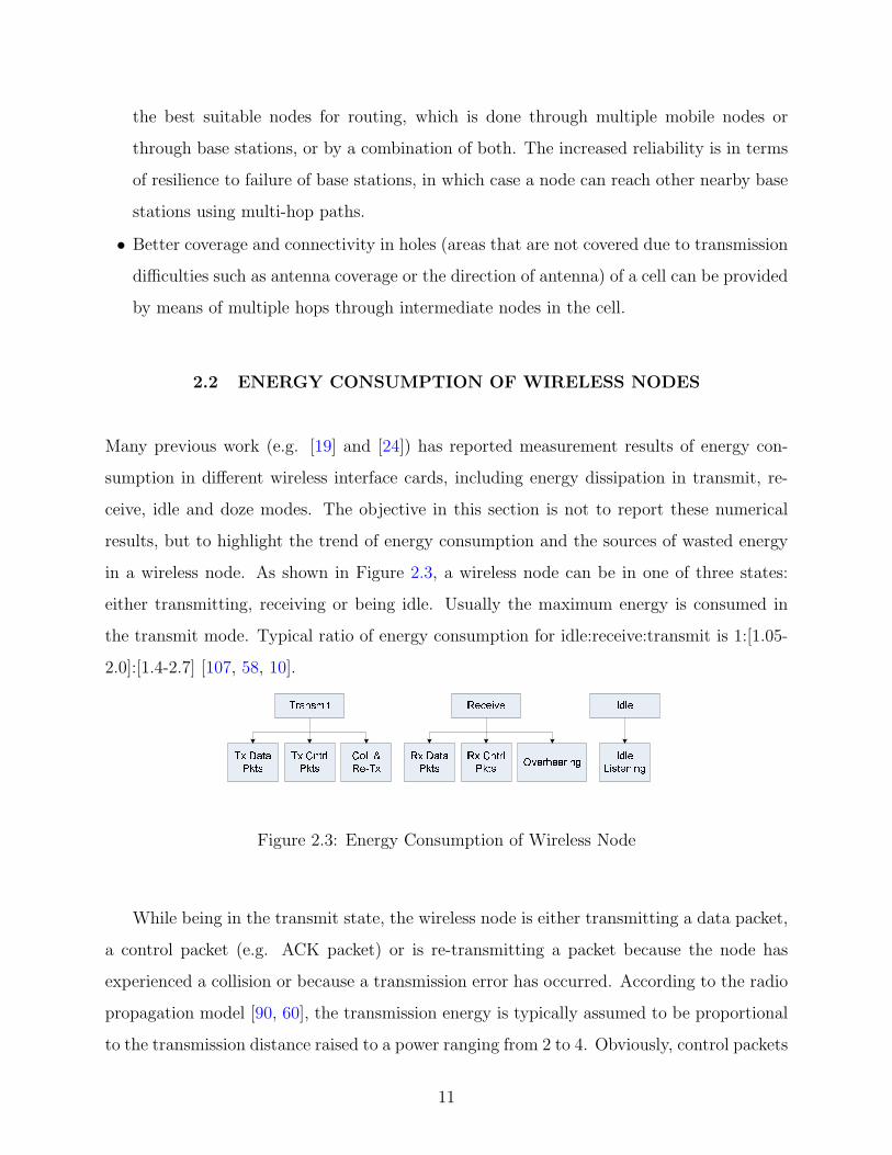
in a wireless node. As shown in Figure 2.3, a wireless node can be in one of three states:

either transmitting, receiving or being idle. Usually the maximum energy is consumed in

the transmit mode. Typical ratio of energy consumption for idle:receive:transmit is 1:[1.05-

2.0]:[1.4-2.7] [107, 58, 10].

Figure 2.3: Energy Consumption of Wireless Node

While being in the transmit state, the wireless node is either transmitting a data packet,

a control packet (e.g. ACK packet) or is re-transmitting a packet because the node has

experienced a collision or because a transmission error has occurred. According to the radio

propagation model [90, 60], the transmission energy is typically assumed to be proportional

to the transmission distance raised to a power ranging from 2 to 4. Obviously, control packets

11

transmission and the retransmission of a corrupted packet are the sources of energy overhead

in transmission mode.

While being in the receive state, the wireless node is either receiving data frames, control

frames or overhearing a packet intended for another node. Typically the energy consumption

during the receive mode is assumed to be proportional to the data rate being used [90].

Wasted energy in the receive mode arises from receiving control packets and from overhearing

the packets of other nodes.

The final state for the wireless transceiver is the idle state, in which the radio is turned

on and the node is not sending and receiving any packets. As previously mentioned, the idle

energy consumption is less than the transmit and the receive energy. However, and as will

be discussed later, idle listening, i.e., listening to receive possible traffic that is not sent, is

a major source of inefficiency. This is especially true in many sensor network applications.

If nothing is sensed, nodes are in idle mode for most of the time. However, in many MAC

protocols such as IEEE 802.11 or CDMA, nodes must continuously listen to the channel to

receive any possible traffic.

2.3 CATEGORIZING MEDIUM ACCESS (MAC) LAYER PROTOCOLS

FOR ASN’S

To accommodate data transmission by multiple stations sharing the scarce wireless band-

width, a medium access control (MAC) protocol plays a crucial role in scheduling packet

transmission fairly and efficiently. MAC protocols are either contention-based or contention-

free.

Contention-based MAC protocols are also known as random access protocols, requiring

no coordination among the nodes accessing the channel. Contention occurs when two nearby

nodes both attempt to access the channel simultaneously. Contention causes message colli-

sions. In Section 2.3.1 I describe the IEEE 802.11 MAC protocol, which is a contention-based

MAC protocol typically used in adhoc networks.

A MAC protocol is contention-free if it does not allow collisions. In these protocols,

the nodes are following some particular schedule which guarantees collision free transmission

12

times. Typical examples of such protocols are: Frequency Division Multiple Access (FDMA);

Time Division Multiple Access (TDMA) [76]; Code Division Multiple Access (CDMA) [114].

In addition to TDMA, FDMA and CDMA, various reservation based [61] or token based

schemes [13, 22] are proposed for distributed channel access control. Among these schemes,

TDMA and its variants are most relevant to my work. I describe the basic TDMA access

protocol in section 2.3.2.

2.3.1 IEEE 802.11: a contention-based MAC protocol

In the IEEE 802.11 DCF [51] medium access protocol, when a node wants to send packets to

another node, it first sends an RTS (Request to Send) packet to the destination after sensing

the medium to be idle for a so-called DIFS interval. When the destination receives an RTS

frame, it transmits a CTS frame immediately after sensing an idle channel for a so-called

SIFS interval. The source transmits its data frame only if it receives the CTS correctly. If

not, it is assumed that a collision occurred and an RTS retransmission is scheduled. After the

data frame is received by the destination station, it sends back an acknowledgment frame.

Nodes overhearing RTS, CTS, data or ACK packets have to defer their access to the medium.

Each host maintains a Network Allocation Vector (NAV) that records the duration during

which it must defer its transmission. Figure 2.4 illustrates the operation of the IEEE 802.11

DCF.

Figure 2.4: IEEE 802.11 DCF Protocol

A collision occurs when two or more stations within the transmission range of each other

transmit in the same time slot. As a result, the transmitted packet is corrupted and the

13

colliding hosts have to schedule a retransmission after deferring for a period randomly chosen

in the interval [0 .. (CW −1)], where CW is the current value of the contention window. CW

depends on the number of failed transmissions, it is doubled for each failed transmission

attempt and is reset back to its minimum value upon a successful one.

2.3.2 TDMA: a contention-free MAC protocol

As previously mentioned, WSNs contain many nodes, typically dispersed at high, possibly

non-uniform, densities; sensors may turn on and off in order to conserve energy; and, the

communication traffic is space and time correlated. Consequently, Contention-based MAC

protocols are typically not adequate for WSNs but rather a contention-free one should be

used. Time Division Multiple Access (TDMA) is an example of such protocols.

(a) TDMA (b) FDMA (c) CDMA

Figure 2.5: Contention-Free Medium Access Schemes

As shown in Figure 2.5(a), TDMA systems divide the radio spectrum into time slots,

and in each slot only one user is allowed to either transmit or receive. Each user occupies

a cyclically repeating time slot. The transmission from various users is interlaced into a

repeating frame structure. TDMA has an advantage that it is possible to allocate different

numbers of time slots per frame to different users. Thus bandwidth can be supplied on

demand to different users by concatenating and reassigning time slots based on priority. On

the other hand tight synchronization is needed for proper operation of TDMA and assigned

time slots may be wasted if the intended users do not transmit in them.

14

2.4 ROUTING LAYER PROTOCOLS FOR ASN’S

2.4.1 Routing Layer protocols in Adhoc Networks

Mobile adhoc networks (MANETs) are infrastructureless wireless networks where nodes are

supposed to communicate with each other, without the help of any other (fixed) devices.

Typically each node needs to act as a router to relay packets to nodes out of direct commu-

nication range and nodes have to discover and maintain routes among each other.

Figure 2.6: MANET Routing Protocol Classification

As shown in Figure 2.6, MANET routing protocols can be categorized into (1) Proac-

tive Routing which is a table-driven routing protocol that tries to maintain correct routing

information to all the network nodes at all times (e.g. DSDV [44, 85], OLSR [14]), (2)

Reactive Routing which obtains the routing information on-demand when a route is needed

(e.g. DSR [55], AODV [41]), (3) Hybrid Routing which utilizes both proactive and on-

demand routing (e.g. ZRP [42, 43], HSLS [96, 63]), (4) Hierarchical Routing that maps

the network nodes into a hierarchical structure like clusters or a tree, (e.g. CEDAR [104],

LANMAR [83]), one example of hierarchical routing is described in Section 2.4.2 and (5)

Geographical Routing where nodes utilize geographical information and nodes position to

route data packets to their final destination (e.g. LAR [62], DREAM [3]). Interested readers

can refer to [93, 23, 65] for a complete survey and classification of available MANET routing

protocols.

2.4.2 Routing in Sensor Networks

In adhoc networks a network flow can start and end at any network node, routing protocols

discussed in Section 2.4.1 are used to route data packets along the paths from sources to

15

destinations. Routing in sensor networks, on the other hand, is different in the sense that

all the network flows are destined to a central data collection point.

Figure 2.7: Sensors Tree Routing Structure

In sensor networks, typically, a tree-based routing scheme is used, as shown in Figure 2.7.

One sensor is appointed to be the root, usually because it is the point where the user interfaces

to the network. The root broadcasts a message asking nodes to organize into a routing tree;

in that message it specifies its own id and its level, or distance from the root (in this case,

zero.) Any node without an assigned level that hears this message assigns its own level to

be the level in the message plus one. It also chooses the sender of the message as its parent,

through which it will route messages to the root. Each of these sensors then rebroadcasts

the routing message, inserting their own ids and levels. The routing message floods down

the tree in this fashion, with each node rebroadcasting the message until all nodes have been

assigned a level and a parent.

16

3.0 ENERGY-EFFICIENT MAC LAYER OPTIMIZATIONS FOR ADHOC

NETWORKS

In this chapter I present my work that focuses on the energy-efficient MAC for MANETs,

as illustrated in Figure 3.1.

Figure 3.1: Adhoc Networks MAC Layer Contribution

First, in Section 3.1, I focus on the energy-consumption in the transmission mode. I

investigate the problem of optimizing the transmission energy in MANETs. I show that,

unlike what is proposed in previous research, the minimum transmission energy is not optimal

for the total energy consumption. I present an analytical model that models the collision

and interference in MANETs. Using the proposed model, for a given network, the effect of

different network configuration parameters can be evaluated and the optimal transmission

energy is determined.

Second, in Section 3.2, motivated by the significance of the wasted energy in collisions

and collision resolutions, I propose BLAM as an energy-efficient MAC protocol for MANETs.

I evaluate BLAM using analytical models and simulations. I show that BLAM can achieve an

improvement of 15% in the network lifetime and 39% in the total number of received packets

compared to the 802.11. The IEEE 802.11 is the prevailing widely used MAC protocol for

17

MANETs, however, it can operate very poorly and much channel bandwidth and energy can

be wasted in collisions. BLAM’s biggest advantage, in addition to saving wasted collision

energy and extending the network lifetime, is its backward compatibility with the 802.11,

hence, it can be easily incorporated in this widely used MAC protocol.

3.1 OPTIMAL MAC TRANSMISSION POWER

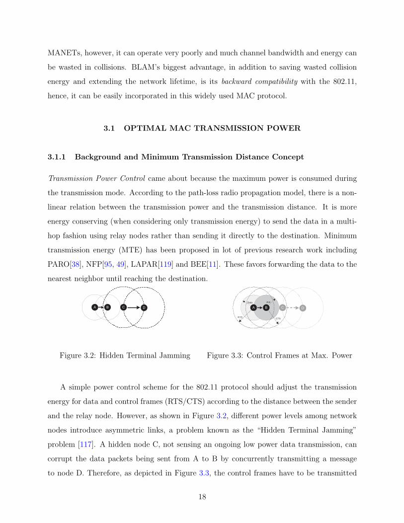
3.1.1 Background and Minimum Transmission Distance Concept

Transmission Power Control came about because the maximum power is consumed during

the transmission mode. According to the path-loss radio propagation model, there is a non-

linear relation between the transmission power and the transmission distance. It is more

energy conserving (when considering only transmission energy) to send the data in a multi-

hop fashion using relay nodes rather than sending it directly to the destination. Minimum

transmission energy (MTE) has been proposed in lot of previous research work including

PARO[38], NFP[95, 49], LAPAR[119] and BEE[11]. These favors forwarding the data to the

nearest neighbor until reaching the destination.

C A B D

Figure 3.2: Hidden Terminal Jamming

C D A B

Data Ack

RTS CTS

Figure 3.3: Control Frames at Max. Power

A simple power control scheme for the 802.11 protocol should adjust the transmission

energy for data and control frames (RTS/CTS) according to the distance between the sender

and the relay node. However, as shown in Figure 3.2, different power levels among network

nodes introduce asymmetric links, a problem known as the “Hidden Terminal Jamming”

problem [117]. A hidden node C, not sensing an ongoing low power data transmission, can

corrupt the data packets being sent from A to B by concurrently transmitting a message

to node D. Therefore, as depicted in Figure 3.3, the control frames have to be transmitted

18

using a high power level, while the DATA and ACK can be transmitted using the minimum

power level necessary for the nodes to communicate [37, 87].

3.1.2 Tradeoffs in Choosing Transmission Distance

As previously mentioned, a lot of previous work (example, [64, 38]) proposed the idea of

minimizing the transmission power and sending the data in a multi-hop fashion to the des-

tination by relaying the packets at intermediate closer nodes. Although the transmission

energy is reduced by such scheme, the effect of transmission power control schemes on the

total network throughput and the overall energy consumption were not investigated.

My work is based on the observation that there is a tradeoff in the choice of the trans-

mission distance. When reducing the transmission power, the number of nodes included

within the transmission range of the sender and competing for wireless channel access is

reduced and hence the number of collisions is reduced. However, at every relay node, the

data message is relayed and forwarded, consequently, the probability of collision per message

is increased. As a result, in the multihop scheme, collision resolution may end up using more

energy than the one hop direct transmission scenario. With respect to interference, on the

other hand, it is intuitive that using reduced power minimizes the interference level between

neighboring nodes. However, there is an increase in the number of concurrent transmissions

because the transmission range of each node is reduced. Consequently, the overall Signal to

Interference Ratio (SIR) might degrade when using a lower transmission power.

In this section, by taking into consideration the energy wasted in the collision resolutions

and the energy used to overcome the interference signal level of neighboring nodes, I argue

that the minimum transmission distance will not always deliver optimal energy consumption.

The transmission power adjustment problem to minimize the energy consumption of an adhoc

network is investigated, based on the 802.11 (CSMA/CA) MAC protocol. A unified collision

and interference model is constructed for a uniformly distributed adhoc network [35, 36].

From these models the total network throughput and the total energy consumption in the

network are derived. The next subsections briefly describe the details of these models.

19

3.1.3 Model Background

In the network model, assume that a set of homogeneous adhoc nodes are distributed over

a large two dimensional area with a given node density of ρ nodes per unit area. Each

node can communicate and receive data directly from all the nodes within its coverage area,

where the coverage area of the node is defined by the radius which the control frames can

reach (defined as aRTS). The MAC layer used in such communication is the IEEE 802.11

DCF MAC protocol, as described in Section 2.3.1. Based on the uniformly distributed nodes

model, all the network hosts will use the same transmission power for DATA/ACK frames

and thus will have the same transmission range, defined as adata. Similarly, all hosts use the

same power for transmitting the control frames and this has the same coverage area defined

by aRTS (which can be different from adata).

Furthermore, it is assumed that the time is slotted with slot time τ . I define the number

of time slots needed to send an RTS packet as LRTS slots. Analogously, the number of time

slots needed to send a CTS, a data packet, and an acknowledgment packets are LCTS, Ldata,

and Lack, respectively.

According to the path-loss radio propagation model, the ratio between the received signal

power, PRx, at distance r from the transmitter, to the transmitted signal power, PTx, is:

PRx

PTx

= C · r −γ (3.1)

where C is a constant that depends on the antenna gains, the wavelength, and the antenna

heights, r is the transmission distance, and γ is the path loss factor, ranging from 2 (line of

sight free space) to 6 (indoor) [60].

The expected number of hops, H, needed between any source and any destination node

is given by:

H = bL/adatac (3.2)

where L is the average path length of a message in the adhoc network and adata is the radius

by which the DATA/ACK packets are sent, that is, the distance between two consecutive

relay nodes. The expected path length, L, is a function of the node distribution, dynamic

patterns of mobility and traffic patterns in the network [68] [72] [78]. In Section 3.1.6 a

simple way to compute L is presented.

20

3.1.4 Interference Model

Gupta and Kumar [40] showed that the transmission capacity of an adhoc network is inversely

proportional to the square root of the number of nodes in the network due to the increased

number of collisions. A collision, as defined by IEEE 802.11, occurs when two or more nodes

within the sender coverage area transmits RTS packets at the same time or when an RTS

collides with the CTS sent by the receiver node. Collisions can only occur during what is

called Contention Window(see Section 2.3.1).

In addition to collisions the network throughput is also affected by the interference level

caused by hosts concurrently sending their data. Interference occurs during the transmission

time of a data frame, where nodes outside the RTS sensing area of the sender and the CTS

sensing area of the receiver may concurrently transmit causing a background interference

signal that degrades the Signal to Interference Ratio (SIR), causing an increase in the Bit

Error Rate (BER).

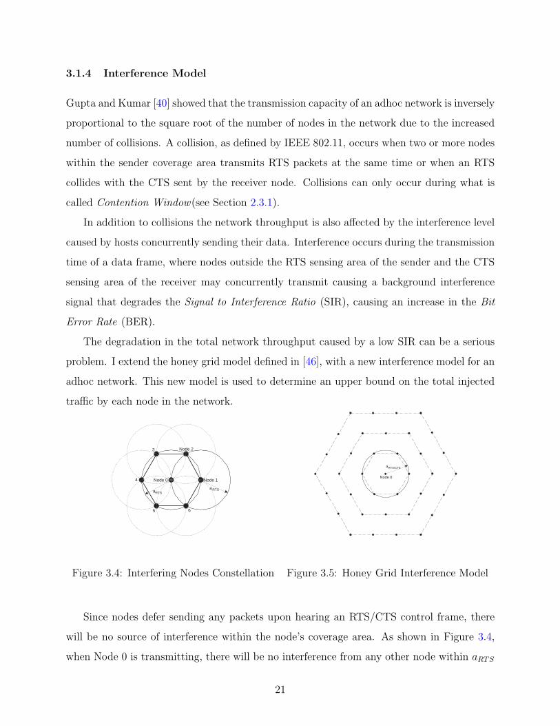
The degradation in the total network throughput caused by a low SIR can be a serious

problem. I extend the honey grid model defined in [46], with a new interference model for an

adhoc network. This new model is used to determine an upper bound on the total injected

traffic by each node in the network.

Node 0 Node 1

Node 2 3

4

5 6

a RTS a RTS

Figure 3.4: Interfering Nodes Constellation

Node 0

a RTS/CTS

Figure 3.5: Honey Grid Interference Model

Since nodes defer sending any packets upon hearing an RTS/CTS control frame, there

will be no source of interference within the node’s coverage area. As shown in Figure 3.4,

when Node 0 is transmitting, there will be no interference from any other node within aRTS

21

from it. In the worst case, the first interfering node is just outside the coverage area of

Node 0 (e.g., Node 1 at distance aRTS + ε from Node 0). The next interferer could only

be outside the coverage areas of both nodes, and in the worst case at the crossing point of

two circles each with radius aRTS + ε. The constellation of interfering nodes is as shown in

Figure 3.4.

Furthermore, for the worst case scenario of signals interfering with the data packet cur-

rently being received at Node 0 there are at most 6 interfering nodes at distance aRTS + ε,

and on the next interfering ring, at distance 2 · (aRTS + ε), there are at most 12 interfering

nodes and so on. This results in the Honey Grid Model, depicted in Figure 3.5.

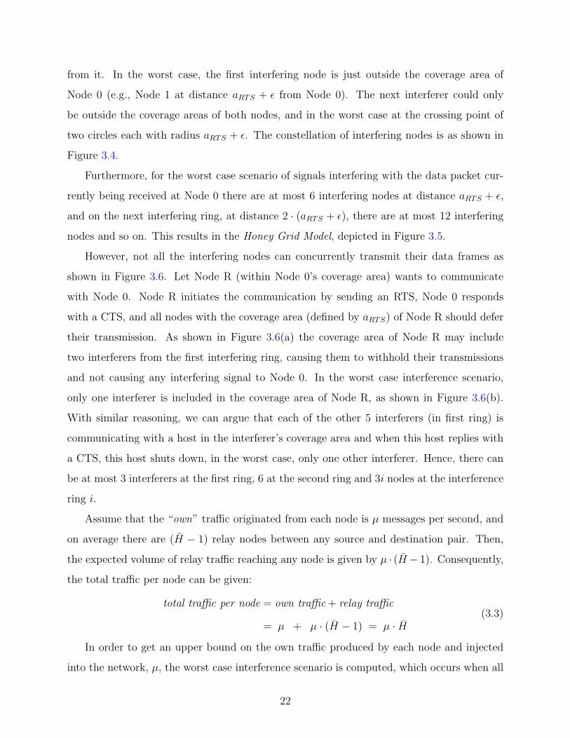
However, not all the interfering nodes can concurrently transmit their data frames as

shown in Figure 3.6. Let Node R (within Node 0’s coverage area) wants to communicate

with Node 0. Node R initiates the communication by sending an RTS, Node 0 responds

with a CTS, and all nodes with the coverage area (defined by aRTS) of Node R should defer

their transmission. As shown in Figure 3.6(a) the coverage area of Node R may include

two interferers from the first interfering ring, causing them to withhold their transmissions

and not causing any interfering signal to Node 0. In the worst case interference scenario,

only one interferer is included in the coverage area of Node R, as shown in Figure 3.6(b).

With similar reasoning, we can argue that each of the other 5 interferers (in first ring) is

communicating with a host in the interferer’s coverage area and when this host replies with

a CTS, this host shuts down, in the worst case, only one other interferer. Hence, there can

be at most 3 interferers at the first ring, 6 at the second ring and 3i nodes at the interference

ring i.

Assume that the “own” traffic originated from each node is µ messages per second, and

on average there are (H − 1) relay nodes between any source and destination pair. Then,

the expected volume of relay traffic reaching any node is given by µ · (H − 1). Consequently,

the total traffic per node can be given:

total traffic per node = own traffic + relay traffic

= µ + µ · (H − 1) = µ · H(3.3)

In order to get an upper bound on the own traffic produced by each node and injected

into the network, µ, the worst case interference scenario is computed, which occurs when all

22

a data

a RTS

a CTS

1

2

R

(a)

a RTS

a data

a CTS

1

R

(b)

Figure 3.6: Interfering Nodes per Ring

the interferers are actively transmitting. The received interference power from 3 nodes in

the first ring at distance aRTS, and 6 nodes in the second ring at 2aRTS, and so on are added.

Since the network is uniformly distributed, we can assume that all the data/ack packets are

sent with signal level Pdata covering a radius of adata. On the other hand the control frames

are sent with a high power covering a radius of aRTS. From Equation (3.1), for a fixed Bit

Error Rate, the ratio between the control packets transmission power to the data packets

transmission power is equal to the ratio of distances raised to the power of γ. Hence, the

power by which the control frames are sent, PRTS/CTS, is given as:

PRTS/CTS = Pdata ·(

aRTS

adata

)γ

(3.4)

where γ is the path loss factor (see Equation (3.1)).

Let Ttotal = LRTS + LCTS + Ldata + Lack be the total time in slots to send one frame

(without any retransmissions). Then the average interference level, Ir, of a single interferer

located at distance r from the receiving node is

Ir = q · (Pdata · r−γ · Ldata + Lack

Ttotal

+ Pdata ·(

aRTS

adata

)γ

· r−γ · LRTS + LCTS

Ttotal

) (3.5)

where q is the probability of transmission per node. The first term inside the brackets

represents the interference level caused by the data/ack packets with power Pdata, and the

second term accounts for sending the control frames (RTS/CTS) with the power defined in

Equation (3.4).

23

Using Equation (3.5), we can compute the total interference at Node 0 caused by other

network nodes in the honey grid model as:

I =3 · q · Pdata · a−γ

RTS

Ttotal

∞∑i=1

{i−(γ−1) × [(Ldata + Lack) + (aRTS

adata

)γ(LRTS + LCTS)]} (3.6)

This is done by substituting distance r with i ·aRTS (the radius of the ith interfering ring)

and summing up for all 3i interfering nodes in this ring. Since the series in Equation (3.6)

is a converging series, the interference level caused by a distant node can be neglected if it

is below a certain threshold, which depends on the type of the interface card used.

The SIR at Node 0 can be derived as the ratio between the signal level of the sender at

distance adata away from Node 0 to the total interference level at this node, as defined by

Equation (3.6). Hence, the SIR can be given as:

SIR = G · Pdata · a−γdata

I(3.7)

where G is the spread spectrum “Processing Gain” [88] used in the network physical layer.

Assuming that the total traffic per node is a Poisson process1 then the probability that

a node transmits, q, is given as:

q = 1− e−µ · H (3.8)

By using the value of H as given in Equation (3.2) and by substituting q in Equation (3.6)

and then substituting back the total interference level, I, in Equation (3.7), we can calculate

the maximum traffic that a node can produce, µ, while keeping SIR = SIRmin at all other

nodes:

µ = −adata

L·ln[1− Ttotal ·G · a−γ

data

3 · SIRmin · a−γRTS ·

∑∞i=1 i−(γ−1)

· 1

(Ldata + Lack) + (aRTS/adata)γ · (LRTS + LCTS)]

(3.9)

As illustrated in Section 3.1.8, µ will be used to derive and evaluate the total network

throughput. The network throughput is defined as the sum of the throughputs of each node

that can concurrently transmit without causing a collision. Evaluating the total throughput

at different values for both adata and aRTS will demonstrate the presence of a certain optimum

transmission range for the control and data messages at which the throughput is maximized.

1A Poisson process is considered to be an accurate model of traffic generation per node in MANETs [46,94], especially for FTP traffic. Possible future extension of my work is to analyze the effect of other trafficgeneration models (e.g., ON/OFF model).

24

3.1.5 Collision Model

The nodes included within the coverage area of a certain host may send control messages

that collide with the RTS/CTS frames transmitted by this node. A collision resolution

scheme (exponential backoff) [48] is applied whenever a collision is detected. The higher the

number of collisions, the lower the network throughput and the higher the energy consumed

resolving these collisions. I extend the model proposed in [116] for a multihop adhoc network,

and using this model, the effect of collisions on both the throughput and the total energy

consumption is derived.2

IDLE RTS-col

Transmit

CTS-col

1

1

1

P it

P ir

P ic

P ii

Figure 3.7: Wireless Channel State Transition Diagram

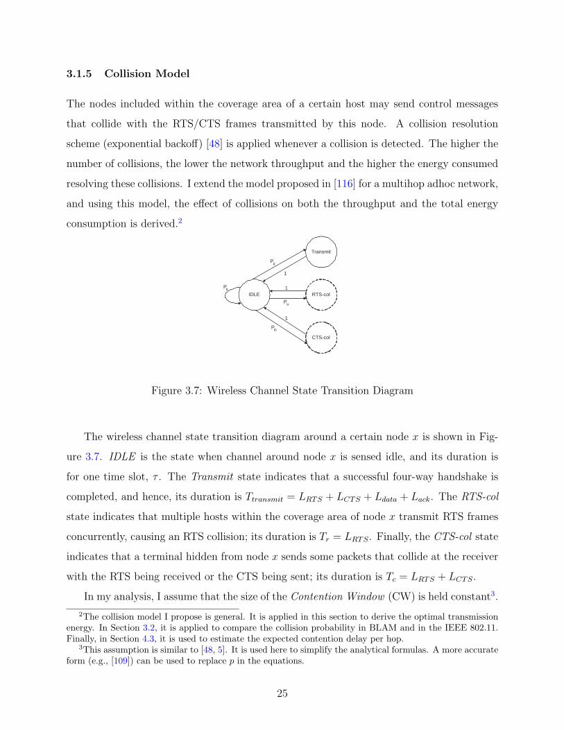
The wireless channel state transition diagram around a certain node x is shown in Fig-

ure 3.7. IDLE is the state when channel around node x is sensed idle, and its duration is

for one time slot, τ . The Transmit state indicates that a successful four-way handshake is

completed, and hence, its duration is Ttransmit = LRTS + LCTS + Ldata + Lack. The RTS-col

state indicates that multiple hosts within the coverage area of node x transmit RTS frames

concurrently, causing an RTS collision; its duration is Tr = LRTS. Finally, the CTS-col state

indicates that a terminal hidden from node x sends some packets that collide at the receiver

with the RTS being received or the CTS being sent; its duration is Tc = LRTS + LCTS.

In my analysis, I assume that the size of the Contention Window (CW) is held constant3.

2The collision model I propose is general. It is applied in this section to derive the optimal transmissionenergy. In Section 3.2, it is applied to compare the collision probability in BLAM and in the IEEE 802.11.Finally, in Section 4.3, it is used to estimate the expected contention delay per hop.

3This assumption is similar to [48, 5]. It is used here to simplify the analytical formulas. A more accurateform (e.g., [109]) can be used to replace p in the equations.

25

As proved in [48] and [5], the probability that a fully saturated node, a node that is always

having a packet waiting in the output buffer to be sent, transmits at a given time slot, p, is

given by

p =2

CW + 1(3.10)

Using p we can derive the transition probabilities for the collision model as follows. The

probability Pii is the transition probability from IDLE to IDLE, that is, the probability that

none of the nodes within the coverage area of x transmits at this time slot. Pii is given by:

Pii = (1− p)M (3.11)

where M = ρ · π a2RTS is the total number of nodes included in the coverage area of node x.

The probability Pit is the transition probability from IDLE to Transmit. It is the prob-

ability that exactly one node transmits at this time slot and starts a successful four-way

handshake (i.e., other nodes withhold their transmission). Pit is given by:

Pit = M · Πs · (1− p)M−1 (3.12)

where Πs denotes the probability that a node begins a successful four-way handshake at this

time slot. Πs is a function of the number of hidden terminals and the distance between the

sender and the receiver as will be discussed later in this section.

The probability Pir is the transition probability from IDLE to RTS-col. It is the proba-

bility that more than one node transmits an RTS packet at the same time slot. In other words,

Pir is (1−probability that none of the nodes transmits−probability that exactly one node transmits):

Pir = 1− (1− p)M −M · p · (1− p)M−1 (3.13)

Finally, Pic, the transition probability from IDLE to CTS-col, can be simply computed

as:

Pic = 1− Pii − Pit − Pir (3.14)

Having calculated Pii, Pit, Pir and Pic, the equilibrium equations of the wireless channel

state transition diagram can be deduced and solved, so that the Transmit state limiting

probability, θt, can be computed. θt represents the percentage of time in which the node is

26

successfully transmitting, or in other words, it is the ratio between successful transmission

time to the total network time (defined as the summation of transmission time and contention

time). The solution of the state model equilibrium equations is:

θt =Pit

1 + Pit · Ttransmit + Pir · Tr + Pic · Tc

(3.15)

All the terms of Equation (3.15) have been derived with the exception of Pit as it depends

on Πs, the probability that a node starts a successful four-way handshake in the given time

slot. In order to determine, Πs, the state transition diagram of a wireless node is constructed

as shown in Figure 3.8. Node x is in the succeed state when it can complete a successful

four-handshake with the other nodes, it enters the fail state when the node initiates an

unsuccessful handshake, and the wait state accounts for deferring for other nodes. Πs is the

limiting probability of the succeed state, as computed next.

wait

succeed

fail

1

P ws

P ww

1

P wf

Figure 3.8: Node State Transition Diagram

a CTS

Hidden Area from

sender

a RTS

x R

a data

Coverage Area of x

Figure 3.9: Hidden Area From the Sender

Let’s define B(adata) to be the hidden area from node x when communicating with node

R located at adata away from it, as illustrated in Figure 3.9. Takagi [109] has proved that

B(adata) takes the form:

B(adata) = π · a2RTS − 2 · a2

RTS · {arccos(adata

2 · aRTS

)− adata

2 · aRTS

·√

1− a2data

4 · a2RTS

} (3.16)

The number of nodes hidden from the sender, computed as ρ B(adata), are not included

in the sender coverage area but are within the receiver node coverage and can collide with

the RTS frame being received or the CTS frame transmitted by the receiver.

27

The transition probability Pww, from wait state to wait state, is the probability that

neither node x nor any node within its coverage area is initiating any transmissions. Pww is

given by:

Pww = (1− p)M (3.17)

The transition probability, Pws, from wait state to succeed state is the probability that

node x transmits at this time slot and none of the terminals within aRTS of it transmits in

the same slot, and also that none of the hidden nodes in B(adata) transmits for (LRTS +LCTS)

slots. Pws can be written as:

Pws = p · (1− p)M · [(1− p)ρ·B(adata)]LRTS+LCTS (3.18)

Finally, the transition probability Pwf , from wait state to fail state can be simply calcu-

lated as:

Pwf = 1− Pww − Pws (3.19)

Solving the equilibrium equations of the wireless node state transition diagram, the

limiting probability of state succeed, Πs can be given by:

Πs =Pws

2− Pww

=p · (1− p)M · [(1− p)ρ·B(adata)]LRTS+LCTS

2− (1− p)M(3.20)

The value of Πs is substituted into Equation (3.12). Then the obtained value of Pit is

substituted back into Equation (3.15) so that θt, the ratio between successful transmission

time to the total network time, can be derived. As illustrated in Section 3.1.8, the value of

θt will be used to evaluate the total network throughput. Also, θt will be used to get the

percentage of the total time consumed in collisions, hence, the energy consumption can be

evaluated.

3.1.6 Estimation of Average Hop Count

As mentioned in Section 3.1.3, the expected path length is a function in the node distribution

and the dynamic traffic patterns in the network. In this section I present a simple way to

compute the average hopcount (H) when having different types of traffic.

28

3.1.6.1 Random Traffic Pattern In the random traffic pattern, the source and the

destination nodes of each traffic flow are randomly chosen from the network nodes.

Figure 3.10: Route of Length i Hops for

Random Traffic Pattern

Figure 3.11: Average Hopcount in Random

Traffic (total network radius=λ · adata)

Neglecting the effect of the network boundaries, the probability of having a route of

length i hops from the sender (S) to the destination (D) is proportional (See Figure 3.10)

to the number of relay nodes (Rj) included in the area inscribed by two discs of radii i ·adata

and (i− 1) · adata (shaded area in Figure 3.10), and is given by:

p(H = i) =ρ · π · ((i · adata)

2 − ((i− 1) · adata)2)

N(3.21)

where N is the total number of nodes in the network and ρ is the node density. If the total

radius of the network is denoted by λ · adata (where λ =√

Nρ·π·a2

data) then p(H = i) can be

evaluated as:

p(H = i) =2 · i− 1

λ2(3.22)

As a result, the expected hopcount H can be computed as:

H =λ∑

i=1

p(H = i) · i =2 · (λ + 1)3

3 · λ2− 3 · (λ + 1)2

2 · λ2+

5 · (λ + 1)

6 · λ2+

5

6 · λ2(3.23)

As shown in Figure 3.11, the average hopcount for the random traffic pattern is almost

linearly increasing with the increase in the total network radius.

29

3.1.6.2 Local Traffic Pattern Li et al. [68] noticed that some networks (e.g., LAN

users) may have a predominantly local traffic pattern in which it is more probable that a

node communicates with a near host rather than a farther one. The traffic pattern in that

case can be described as a Pareto Law (also known as power-law distribution), as given by

Equation 3.24:

p[L > x] ∝ x−k (3.24)

where p[L > x] is the probability that the path length is larger than x and is proportional

to an inverse power of x, where k is a positive constant that represents the “locality” of

traffic. The larger the value of k is, the closer the destinations are to the sources. It should

be noted that L is lower bounded by a value ε that is a function in the node density (ρ). ε is

determined such that there is at least one receiver in the transmission range of the sender,

hence, ε =√

2/ρ · π. Similar to the random traffic pattern case, the expected hopcount H

can be computed as:

H =λ∑

i=1

p(H = i) · i =

∫ 1

ε/adatax−(k+1)dx

∫ λ

ε/adatat−(k+1)dt

+λ∑

i=2

i · ∫ i

x=i−1x−(k+1)dx

∫ λ

ε/adatat−(k+1)dt

(3.25)

Table 3.1: Average Hopcount for Local Traffic Pattern

Network 1 Network 2(ρ = 1, λ = 30) (ρ = 3, λ = 15)

k=0 8.745 4.752k=1 3.455 2.212k=2 2.061 1.322

Using Equation (3.25) the average hopcount in the network can be computed for the

local traffic pattern. Table 3.1 presents an instance of such computation for two networks

at different values for the locality index k. For comparison the Hrandom values for the two

networks are 20.49 and 10.49 respectively.

30

3.1.7 Energy Computation

In this section I derive the total transmission energy consumption in the network. The

transmission energy is consumed in transmitting the data frames, the control frames and

in re-transmitting RTS/CTS packets in case of collisions. I first investigate the power con-

sumption in data and control message transmissions. Second, the time spent in successful

transmission and that consumed during collisions is derived. The energy is the product of

the power consumed and the time spent in transmissions and collisions.

Power Consumption: Due to the free space power loss, as indicated by Equation (3.1),

the transmission power for data messages, Pdata, is:

Pdata = C · aγdata (3.26)

where C is a constant that depends on the wireless network interface card and γ is the path

loss factor.

Similar to the data frames, the power consumed in transmitting the RTS control frames

is also proportional the transmission distance (aRTS) raised to the power of γ. However,

retransmissions occur due to collisions with the RTS frames sent by other nodes. Hence, the

power consumption in RTS transmission, PRTS, is the summation of the power consumed

in sending i RTS frames multiplied by the probability that i nodes transmit an RTS frame

at the same time slot4 , where i ranges from 1 to M and M is the total number of nodes

included in the sender coverage area. PRTS, is given by:

PRTS =M∑i=1

(M

i

)· i · C · aγ

RTS · pi · (1− p)M−i (3.27)

where p is the probability that a node transmits at this time slot as given by Equation (3.10).

Furthermore, PCTS, the power consumed in transmitting the CTS frame, takes the same

form as PRTS. However, the number of nodes contending for accessing the wireless channel

4The probability that i nodes transmit an RTS frame follows a binomial distribution where the singletrial succes probability is p.

31

are those nodes hidden from the sender as illustrated by Figure 3.9. The number of hidden

terminals, K, can be given as ρ ·B(adata). Hence, PCTS takes the form:

PCTS =K∑

i=1

(K

i

)· i · C · aγ

RTS · pi · (1− p)K−i (3.28)

Time: By definition, θt in Equation (3.15) is the percentage of time the node is in a successful

data transmission state to the total consumed time (the summation of transmission time and

contention time). Hence the total consumed time, Ttotal, can be given as:

Ttotal =Ttransmit

θt

=LRTS + LCTS + Ldata + Lack

θt

(3.29)

Solving the equilibrium equations of the wireless channel state transition diagram, dis-

cussed in Section3.1.5, we can derive the percentage of time the system is in RTS-col relative

to the total time, θr, as:

θr =θt

Pit

· Pir (3.30)

where Pit and Pir are given by Equations (3.12) and (3.13) respectively. Similarly, the

percentage of time the system is in CTS-col relative to the total time, θc, is:

θc =θt

Pit

· Pic (3.31)

Hence the total contention time during collisions and control frame retransmissions has

an RTS component, TRTS = θr · Ttotal, and a CTS component, TCTS = θc · Ttotal.

Energy: Having derived both the time and power consumption in transmitting the data

frames and in the collision/retransmissions, we can simply evaluate the total expected energy

consumption in the network, E, by multiplying the energy per hop by the expected number

of hops, L/adata, in the network:

E =L

adata

· {Pdata · Ttransmit + PRTS · TRTS + PCTS · TCTS} (3.32)

In the next section we use Equation (3.32) to evaluate the total energy consumption in

the network and also to investigate the energy consumption per message for different node

transmission power ranges. we determine the optimum transmission power for both the

control and data messages based on the given network parameters.

32

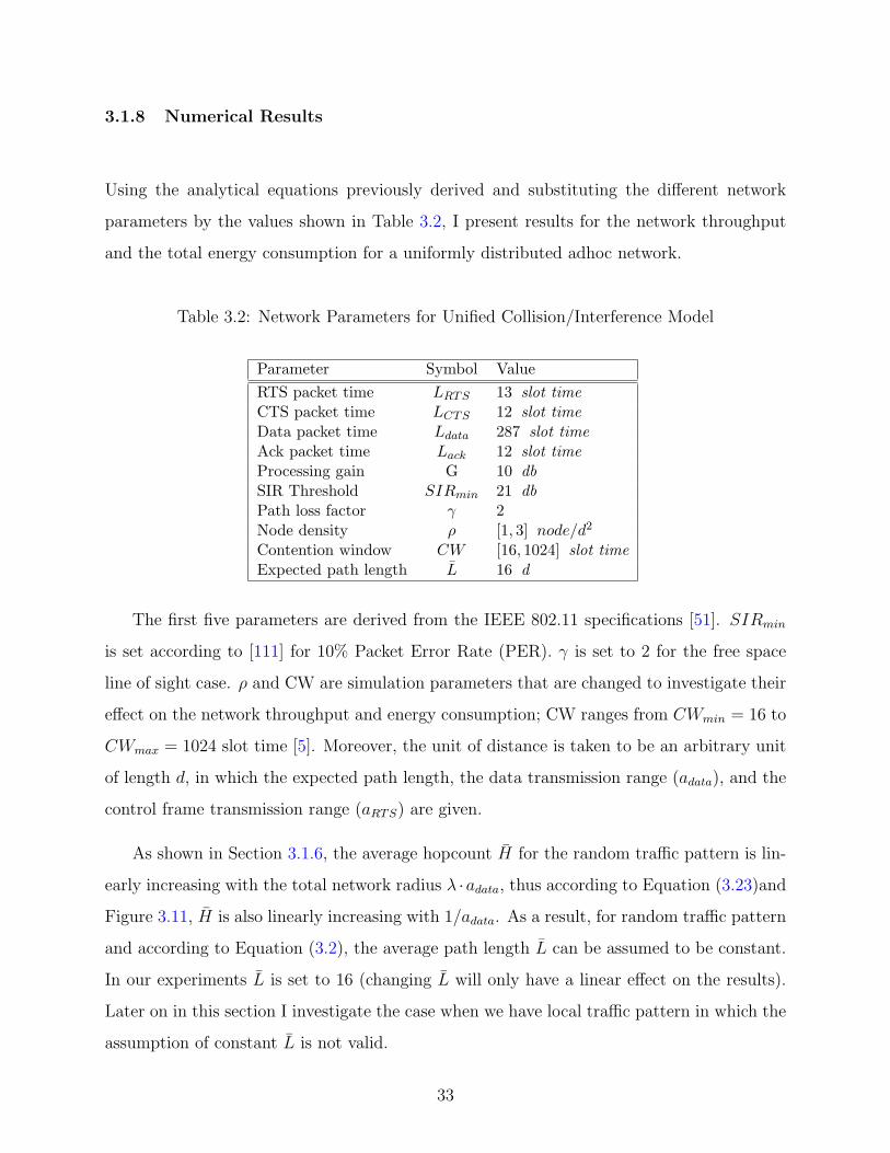
3.1.8 Numerical Results

Using the analytical equations previously derived and substituting the different network

parameters by the values shown in Table 3.2, I present results for the network throughput

and the total energy consumption for a uniformly distributed adhoc network.

Table 3.2: Network Parameters for Unified Collision/Interference Model

Parameter Symbol ValueRTS packet time LRTS 13 slot timeCTS packet time LCTS 12 slot timeData packet time Ldata 287 slot timeAck packet time Lack 12 slot timeProcessing gain G 10 dbSIR Threshold SIRmin 21 dbPath loss factor γ 2Node density ρ [1, 3] node/d2

Contention window CW [16, 1024] slot timeExpected path length L 16 d

The first five parameters are derived from the IEEE 802.11 specifications [51]. SIRmin

is set according to [111] for 10% Packet Error Rate (PER). γ is set to 2 for the free space

line of sight case. ρ and CW are simulation parameters that are changed to investigate their

effect on the network throughput and energy consumption; CW ranges from CWmin = 16 to

CWmax = 1024 slot time [5]. Moreover, the unit of distance is taken to be an arbitrary unit

of length d, in which the expected path length, the data transmission range (adata), and the

control frame transmission range (aRTS) are given.

As shown in Section 3.1.6, the average hopcount H for the random traffic pattern is lin-

early increasing with the total network radius λ ·adata, thus according to Equation (3.23)and

Figure 3.11, H is also linearly increasing with 1/adata. As a result, for random traffic pattern

and according to Equation (3.2), the average path length L can be assumed to be constant.

In our experiments L is set to 16 (changing L will only have a linear effect on the results).

Later on in this section I investigate the case when we have local traffic pattern in which the

assumption of constant L is not valid.

33

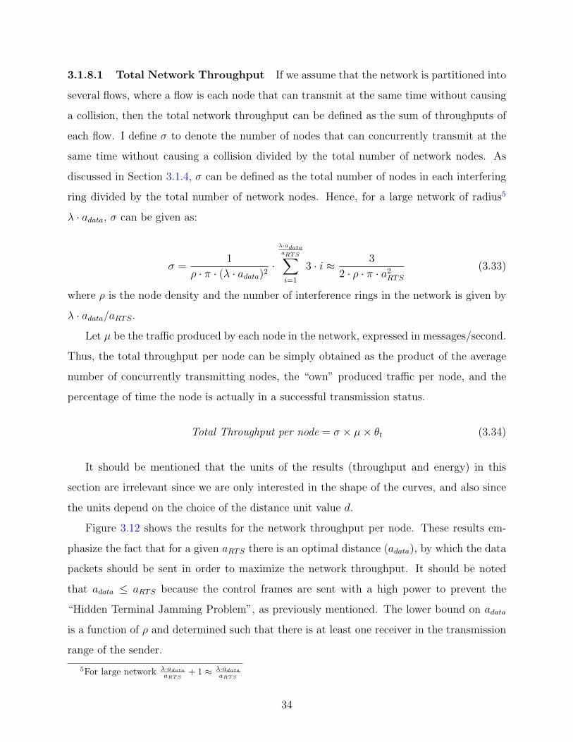
3.1.8.1 Total Network Throughput If we assume that the network is partitioned into

several flows, where a flow is each node that can transmit at the same time without causing

a collision, then the total network throughput can be defined as the sum of throughputs of

each flow. I define σ to denote the number of nodes that can concurrently transmit at the

same time without causing a collision divided by the total number of network nodes. As

discussed in Section 3.1.4, σ can be defined as the total number of nodes in each interfering

ring divided by the total number of network nodes. Hence, for a large network of radius5

λ · adata, σ can be given as:

σ =1

ρ · π · (λ · adata)2·

λ·adataaRTS∑i=1

3 · i ≈ 3

2 · ρ · π · a2RTS

(3.33)

where ρ is the node density and the number of interference rings in the network is given by

λ · adata/aRTS.

Let µ be the traffic produced by each node in the network, expressed in messages/second.

Thus, the total throughput per node can be simply obtained as the product of the average

number of concurrently transmitting nodes, the “own” produced traffic per node, and the

percentage of time the node is actually in a successful transmission status.

Total Throughput per node = σ × µ× θt (3.34)

It should be mentioned that the units of the results (throughput and energy) in this

section are irrelevant since we are only interested in the shape of the curves, and also since

the units depend on the choice of the distance unit value d.

Figure 3.12 shows the results for the network throughput per node. These results em-

phasize the fact that for a given aRTS there is an optimal distance (adata), by which the data

packets should be sent in order to maximize the network throughput. It should be noted

that adata ≤ aRTS because the control frames are sent with a high power to prevent the

“Hidden Terminal Jamming Problem”, as previously mentioned. The lower bound on adata

is a function of ρ and determined such that there is at least one receiver in the transmission

range of the sender.

5For large network λ·adata

aRT S+ 1 ≈ λ·adata

aRT S

34

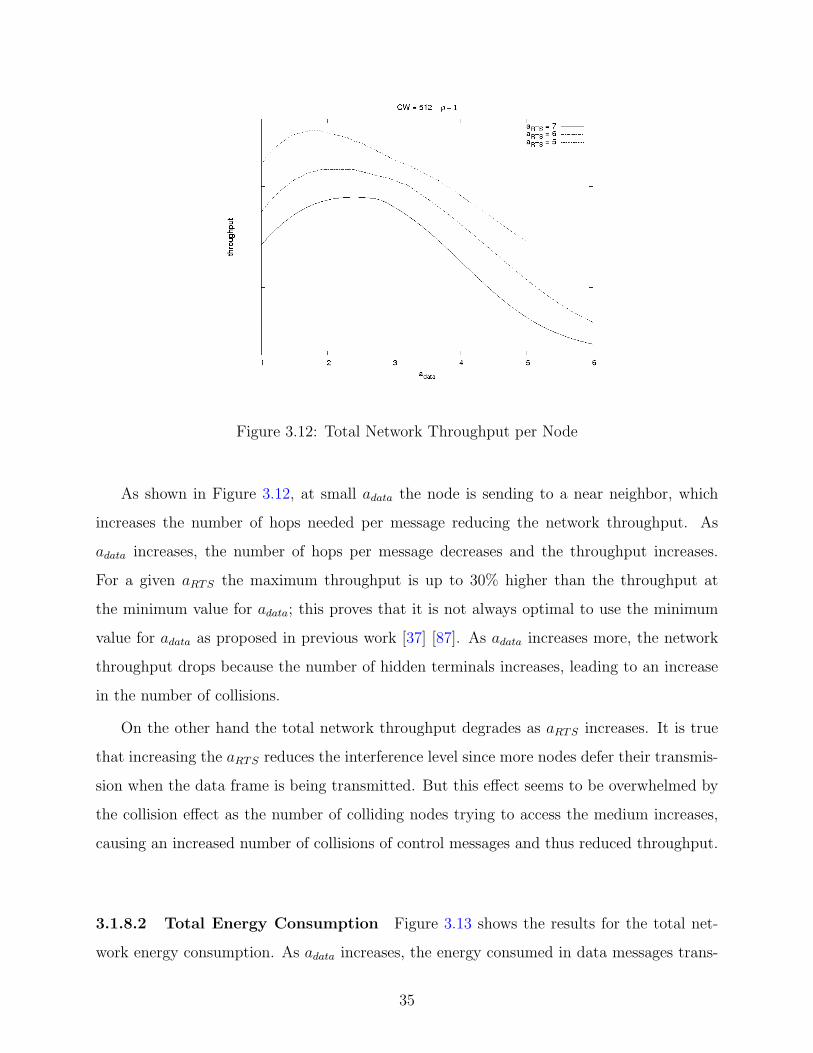
Figure 3.12: Total Network Throughput per Node

As shown in Figure 3.12, at small adata the node is sending to a near neighbor, which

increases the number of hops needed per message reducing the network throughput. As

adata increases, the number of hops per message decreases and the throughput increases.

For a given aRTS the maximum throughput is up to 30% higher than the throughput at

the minimum value for adata; this proves that it is not always optimal to use the minimum

value for adata as proposed in previous work [37] [87]. As adata increases more, the network

throughput drops because the number of hidden terminals increases, leading to an increase

in the number of collisions.

On the other hand the total network throughput degrades as aRTS increases. It is true

that increasing the aRTS reduces the interference level since more nodes defer their transmis-

sion when the data frame is being transmitted. But this effect seems to be overwhelmed by

the collision effect as the number of colliding nodes trying to access the medium increases,

causing an increased number of collisions of control messages and thus reduced throughput.

3.1.8.2 Total Energy Consumption Figure 3.13 shows the results for the total net-

work energy consumption. As adata increases, the energy consumed in data messages trans-

35

Figure 3.13: Total Energy Consumption

mission dominates the total energy consumption. At large adata the number of hidden ter-

minals from the sender increases and the energy wasted during CTS collision dominates the

network energy consumption. Additionally, the message reaches its destination with fewer

hops, but the energy per hop is high due to the rγ factor in Equation (3.26).

3.1.8.3 Energy Consumption per Message When evaluating the energy consump-

tion per message (that is, the energy normalized by the throughput) in the network, an

interesting result is obtained. As shown in Figure 3.14 the energy consumption per mes-

sage increases with larger aRTS. Regarding the effect of adata the curve is flat especially at

lower values of adata, hence, one can choose a slightly larger adata than the minimum, at

the benefit of increasing throughput (see Figure 3.12), without severely affecting the energy

consumption.

The results from Figures 3.12–3.14 show that for a uniform network, the power by which

the control frames are transmitted should be minimized to the level that just keeps the

network fully connected. Further, adata should not be necessarily set to the smallest possible

value.

36

Figure 3.14: Total Energy Consumption per Message

Figure 3.15: ρ Effect on Throughput per Node

3.1.8.4 Effect of Changing the Node Density Figure 3.15 shows the effect of chang-

ing the node density on the network throughput. It should be noted that ρ is lower bounded

by a value that keeps the network connected, i.e., at least one receiver is within the range

37

of the sender. As expected, when the density (number of nodes) increases the throughput

decreases since the number of collisions increase as more nodes are contending to access the

wireless channel. However, the reduction in the throughput (e.g., the large drop between

ρ = 1 and ρ = 2) is much larger than that reported by [40] since I take into account the

combined effect of both the collision and interference.

Figure 3.16: ρ Effect on Energy Consumption

The effect of changing the node density on the overall energy consumption is shown in

Figure 3.16. At a specific hop length (adata) the number of nodes within the node coverage

area increases with the increase of ρ and hence the number of contending nodes to access

the wireless channel increases leading to an increase in the energy wasted during collision

and retransmissions.

3.1.8.5 Effect of Changing the CW Size Figure 3.17 shows the effect of changing

the contention window size on the network throughput. From Equation (3.10), with smaller

CW the probability that a node transmits at the current slot time increases and hence the

probability of collision increases. Thus, the smaller the CW, the lower the throughput. It

should also be noted that as CW decreases the optimal adata approaches its minimum value.

Therefore, at smaller contention window size, it is better to use the minimum data power

38

Figure 3.17: CW Effect on Throughput per Node

between relay nodes.

Figure 3.18: CW Effect on Energy Consumption

The effect of changing the contention window size on the energy consumption is shown

in Figure 3.18. When CW decreases, the probability that a node transmits at the current

39

slot time increases and hence the probability of collision increases, causing more energy to

be wasted during collision.

Figure 3.19: Locality Index Effect on Throughput

3.1.8.6 Local Traffic Case All the previous results are obtained under the assumption

of random traffic patten and, hence, the assumption of a fixed L holds. For the local

traffic pattern case, this assumption is not valid anymore. Therefore, the value of L/adata in

Equation (3.9) and in Equation (3.32) has to be replaced with the value of H in the local

traffic pattern as defined be Equation (3.25).

Figures 3.19 and 3.20 show the effect of changing the traffic locality index on the net-

work throughput and the energy consumption respectively. When we have a network of 2000

nodes, for local traffic pattern, it is always optimal for both the network throughput and

total energy consumption to use the minimum adata which is equivalent to using the mini-

mum transmission power for data and ACK frames. Moreover, as indicated in Figures 3.19

and 3.20, the more local the traffic is (higher value for k), the higher the network throughput

is and lower energy is consumed to deliver the packets to their final destinations.

40

Figure 3.20: Locality Index Effect on Energy Consumption

3.1.8.7 Numerical Results Summary To summarize the results presented in this sec-

tion, it is proved that it is not always optimal to send the data packets to the nearest

neighbor. For a given expected path length and a given node density, expressions are de-

rived to compute the optimal transmission distance that will yield maximum throughput

of the network and minimized energy consumption per message. Furthermore, the results

showed that the control messages should not be sent with the maximum power as was sug-

gested by previous work. By investigating the energy consumption per message, it is shown

that the transmission power for control frames should be minimized to the extent of keeping

the network connected.

I also investigated the effect of changing the nodes density and the collision window

size. My results suggest that: First, the effect of changing the density is more profound

when taking into account both the collisions and interference than that reported in previous

research work that only accounted for collisions. Second, the contention window should be

initialized to a larger value than currently proposed by protocol specifications.

On the other hand, for the case of local traffic pattern, in which it is more probable that

a node communicates with a near host than a farther one, it is always optimal for both the

41

network throughput and the total energy consumption that a node uses its nearest neighbor

to forward its traffic.

3.2 MINIMIZING WASTED COLLISION ENERGY

As shown in Section 3.1.8, the IEEE 802.11 MAC protocol when deployed in an adhoc

network, can operate very far from optimality, and much channel bandwidth and energy are

wasted in collisions and collision resolutions. In this section I propose, Battery Level Aware

MAC (BLAM) [33, 34] an energy-aware MAC layer enhancement for the IEEE 802.11.

Relevant to my work are also the work in [7, 8, 120, 50] that address the problem of

energy savings at the 802.11 DCF MAC layer. In [7] a distributed mechanism is proposed

that enables each station to estimate the channel utilization during a backoff period and to

compute the probability to successfully transmit. In [8] the authors present an analytical

framework to calculate the appropriate value of the minimum contention window to be used

in a WLAN so as to maximize the throughput and minimize energy consumption. In [120] the

impact of the RTS (Request-to-Send) Threshold on energy consumption is studied. Finally,

the authors in [50] present a scheme to select the station transmission rate, which minimizes

the average waiting time of each transmission. As will be discussed later, BLAM advantage

over these protocols is that it only depends on local node information available at the MAC

layer. Hence, it doesn’t need any message exchange with neighboring nodes and it does not

change any of 802.11 frame formats. Also it does not need any cross-layer information from

either the physical nor the routing layer, and hence, no modification to the protocol stack is

needed.

3.2.1 Motivation and Significance of Collision Energy

In wireless LANs, the nodes included in the coverage area of a certain host may send control

messages that collide with the RTS/CTS frames transmitted by this host. The higher the

number of collisions the lower the network throughput is and the higher energy is consumed

resolving them.

42

The situation might be worse in a multihop wireless adhoc network, because each message

potentially encounters collisions at each hop. The multihop effect is augmented in power-

aware adhoc networks because the basic power control scheme (as mentioned in Section 3.1.1)

favors transmitting the data to the nearest neighbor instead of transmitting it to a further

one. Accordingly, the power-aware route will be composed of a big number of shorter hops

causing the number of collisions to increase. Furthermore, as mentioned in Section 3.1.1, a

smarter energy-efficient scheme will transmit the short control frames using a higher power

than the data frames [37] [87]. However, the drawback of this scheme is that the control

frames are the ones that face collisions and the ones being retransmitted using the high

transmission power. Thus, the collision effect on the total energy consumption is much

worse than first thought. Based on the above observations, BLAM conserves the channel

bandwidth and energy by decreasing the total number of collisions. As discussed later,

BLAM decreased the total number of collision by 48% compared to the 802.11.

Furthermore, in IEEE 802.11, all nodes involved in a collision are equally treated and all

of them attempt retransmissions in subsequent time slots after applying the random backoff

algorithm. Thus, it is possible that energy-poor nodes waste additional energy in subsequent

unsuccessful attempts because they are contending with high-energy nodes. BLAM proposes

a new philosophy so that the nodes are probabilistically split into virtual groups according

to the amount of residual battery energy left. As a result, the simultaneous contention of

low and high-energy nodes is reduced.

3.2.2 Modifications to IEEE 802.11 DCF

BLAM modifies the IEEE 802.11 DCF in two ways, changing the wait time before trans-

mitting fresh data packets and changing the distribution of the random deferring time after

an unsuccessful transmission attempt. As depicted in Figure 2.4, in IEEE 802.11 DCF, if a

fresh data packet arrives at a node, it first senses the medium, and if found idle for a DIFS

interval, it immediately sends an RTS. In contrast, in BLAM, after sensing an idle channel

for a DIFS interval, the node waits for a random amount of time before sending the RTS.

This random wait time is picked from a normal distribution with mean and variance that

43

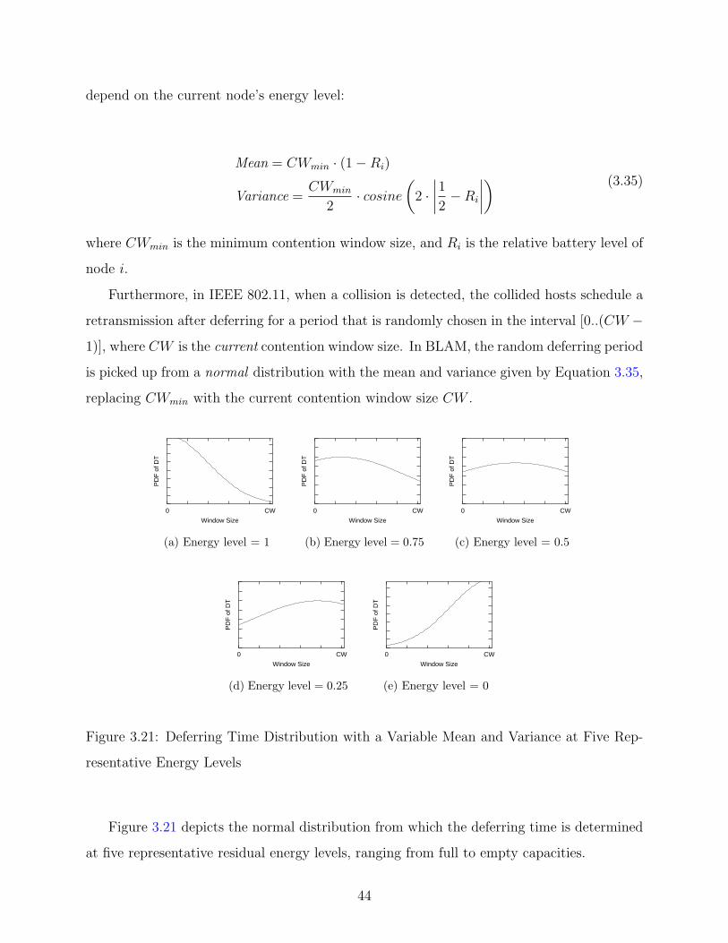
depend on the current node’s energy level:

Mean = CWmin · (1−Ri)

Variance =CWmin

2· cosine

(2 ·

∣∣∣∣1

2−Ri

∣∣∣∣) (3.35)

where CWmin is the minimum contention window size, and Ri is the relative battery level of

node i.

Furthermore, in IEEE 802.11, when a collision is detected, the collided hosts schedule a

retransmission after deferring for a period that is randomly chosen in the interval [0..(CW −1)], where CW is the current contention window size. In BLAM, the random deferring period

is picked up from a normal distribution with the mean and variance given by Equation 3.35,

replacing CWmin with the current contention window size CW .

0 CW

PD

F o

f DT

Window Size

(a) Energy level = 1

0 CW

PD

F o

f DT

Window Size

(b) Energy level = 0.75

0 CW

PD

F o

f DT

Window Size

(c) Energy level = 0.5

0 CW

PD

F o

f DT

Window Size

(d) Energy level = 0.25

0 CW

PD

F o

f DT

Window Size

(e) Energy level = 0

Figure 3.21: Deferring Time Distribution with a Variable Mean and Variance at Five Rep-

resentative Energy Levels

Figure 3.21 depicts the normal distribution from which the deferring time is determined

at five representative residual energy levels, ranging from full to empty capacities.

44

When a node has full battery, the distribution of the random deferring time will be as

shown in Figure 3.21(a). As a result, it is most probable that a high-energy node will pick a

short deferring time. This means that these nodes will have more chance to access the channel

and thus have a higher priority. As the node residual energy starts decreasing, the mean

of the normal distribution will start moving to the right, as shown in Figures 3.21(b)-(e),

causing the probability of choosing a longer deferring time to increase. A low-energy node

will have the mean close to the Contention Window size (CW), as depicted in Figure 3.21(e),

and thus these nodes will probably pick longer deferring time and will have less chance to

access the medium and thus, a low priority. The idea is the same for fresh data transmission

probability. Consequently, the transmission probability of fresh data will be higher in the

high-energy nodes (higher priority) and will decrease as the node consumes its battery.

In that manner, the network nodes are divided among a continuous set of priorities based

solely on local information, that is, based on their energy levels. Therefore, the transmission

attempts are distributed in time causing the total number of collisions to be reduced and

the energy wasted in collision to be conserved. Additionally, low-energy nodes will not waste

their scarce energy colliding with high-energy nodes and thus, the useful network lifetime is

extended.

It should be noted that all the modifications that BLAM introduces to the MAC protocol

operations are based on the local host information and are only implemented within the

wireless node itself. Accordingly, BLAM does not require any changes in the frame formats

or in the way the frames are handled by the network interface card during transmission,

reception or forwarding. Also, it does not require any specific support from the routing layer

above or from the physical layer beneath. That is, BLAM is backward compatible with a

network that uses the IEEE 802.11 MAC protocol and can be easily incorporated in this

widely used protocol.

3.2.3 Collision Analysis

In Section 3.1.5 I proposed a general collision model for the IEEE 802.11. In this section,

the same model is applied to model the BLAM protocol, the analytical results are then

45

used to compare the worst-case and best-case behavior of BLAM and the IEEE 802.11 DCF

protocol. Note that the same set of model assumptions discussed in Section 3.1.3 are also

assumed here.

3.2.3.1 Probability of transmission The difference between BLAM and the IEEE

802.11 lies in the probability of transmission, p. However, the probability of transmission

differs for each time slot. I denote the probability of transmission in a given time slot i as

p(i). p(i) in the BLAM case depends on the node’s current energy level and the number of

retries, while p(i) in the 802.11 case only depends on the number of retries. To distinguish

between the two protocols, I call p(i) in the BLAM case pblam(i) while in the 802.11 case it

is called p802.11(i).

In the analysis, as an approximation, I assume that the size of the Contention Window

(CW) is held constant (see Section 3.1.5). Consequently, (As proved in [5] and [48]) the

probability of transmission in a given time slot for the IEEE 802.11, p802.11(i), is constant

and is given by

p802.11(i) =2

CW + 1(3.36)

In BLAM, on the other hand, using the same approximation, the probability of trans-

mission in a given time slot, pblam(i), depends only on the energy distribution among the

wireless hosts.

For a given node X, with relative energy level RX (normalized to full energy), the prob-

ability that Node X transmits during slot i, pblam(i, RX) can be computed as given by Equa-

tion 3.37 (and as depicted in Figure 3.22):

pblam(i, RX) =

∫ i

i−1

pBLAM(t, RX) dt (3.37)

where pBLAM(t, RX) is the Probability Distribution Function (PDF) of transmission for

Node X versus time at the fixed relative energy level RX when using the BLAM protocol.

As a generalization for the previous case, for any neighborhood with a given distribution

of energies among M wireless nodes (a snapshot of the network), pblam(i) can be defined as

46

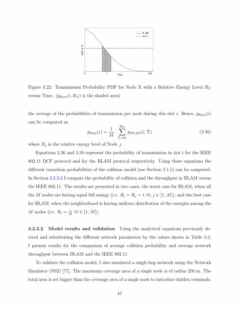
Figure 3.22: Transmission Probability PDF for Node X with a Relative Energy Level RX

versus Time. (pblam(i, RX) is the shaded area)

the average of the probabilities of transmission per node during this slot i. Hence, pblam(i)

can be computed as

pblam(i) =1

M·

RM∑Υ=R1

pBLAM(i, Υ) (3.38)

where Rj is the relative energy level of Node j.

Equations 3.36 and 3.38 represent the probability of transmission in slot i for the IEEE

802.11 DCF protocol and for the BLAM protocol respectively. Using these equations the

different transition probabilities of the collision model (see Section 3.1.5) can be computed.

In Section 3.2.3.2 I compare the probability of collision and the throughput in BLAM versus

the IEEE 802.11. The results are presented in two cases, the worst case for BLAM, when all

the M nodes are having equal full energy (i.e. Ri = Rj = 1 ∀i, j ∈ [1..M ]), and the best case

for BLAM, when the neighborhood is having uniform distribution of the energies among the

M nodes (i.e. Ri = iM∀i ∈ [1..M ]).

3.2.3.2 Model results and validation Using the analytical equations previously de-

rived and substituting the different network parameters by the values shown in Table 3.3,

I present results for the comparison of average collision probability and average network

throughput between BLAM and the IEEE 802.11.

To validate the collision model, I also simulated a single-hop network using the Network

Simulator (NS2) [77]. The maximum coverage area of a single node is of radius 250 m. The

total area is set bigger than the coverage area of a single node to introduce hidden terminals,

47

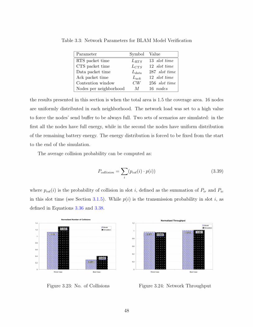
Table 3.3: Network Parameters for BLAM Model Verification

Parameter Symbol ValueRTS packet time LRTS 13 slot timeCTS packet time LCTS 12 slot timeData packet time Ldata 287 slot timeAck packet time Lack 12 slot timeContention window CW 256 slot timeNodes per neighborhood M 16 nodes

the results presented in this section is when the total area is 1.5 the coverage area. 16 nodes

are uniformly distributed in each neighborhood. The network load was set to a high value

to force the nodes’ send buffer to be always full. Two sets of scenarios are simulated: in the

first all the nodes have full energy, while in the second the nodes have uniform distribution

of the remaining battery energy. The energy distribution is forced to be fixed from the start

to the end of the simulation.

The average collision probability can be computed as:

Pcollision =∑

i

(pcol(i) · p(i)) (3.39)

where pcol(i) is the probability of collision in slot i, defined as the summation of Pir and Pic

in this slot time (see Section 3.1.5). While p(i) is the transmission probability in slot i, as

defined in Equations 3.36 and 3.38.

Figure 3.23: No. of Collisions Figure 3.24: Network Throughput

48

Figure 3.23 compares the total number of collisions in the network in both the worst-case

and the best-case for BLAM normalized to the number of collision faced when using the IEEE

802.11. As shown in Figure 3.23, in the worst-case, when all the nodes are having full energy,

the number of collisions in BLAM is higher than that of the IEEE 802.11. Analytically, the

probability of collision is higher by only 13%. Using the simulation, the number of collisions

is higher by 29.3%. On the other hand when the nodes are having uniform distribution of the

remaining energy, the best case for BLAM, analytically, the probability of collision in BLAM

is 29.1% that of the IEEE 802.11. Using simulations, the best-case of BLAM decreased the

total number of collisions to 40.5% of its value. It should be mentioned that the difference

between the analytical and the simulation results is mainly because the collision model

assumes a fixed mid-range contention window size (256 slot time) while in the simulations

the CW lies in the range [31..1023] slot time (as mentioned in Section 2.3.1).

As proved in Section 3.1.8, the total network throughput is proportional to the percentage

of time in which the node is successfully transmitting, θt. Figure 3.24 compares the analytical

and simulation results for the ratio of the average throughput between BLAM and the IEEE

802.11. The results are presented both in the worst-case for BLAM, when all the nodes

are having full energy, and in the best-case for BLAM, when the nodes are having uniform

distribution of the remaining energy. As shown in Figure 3.24, when BLAM is used the total

network throughput is almost equal to the network throughput offered by the IEEE 802.11.

However, it should be noted that BLAM extends the total network lifetime6 (as shown in

Section 3.2.4), as a result, the network lives longer and hence, the total number of correctly

received packets (network utility) is increased.

3.2.4 Simulation Results

In Section 3.2.3.2 simulation results are presented to validate the proposed collision model,

where a single-hop network with fixed-energy fully-saturated uniform-distributed wireless

hosts are simulated. In this section I present simulation results for a real network scenario.

I compare BLAM with two versions of the IEEE 802.11 DCF. The first version is the

6The lifetime can not be compared in these synthetic simulation scenarios because the energy distributionis forced to be fixed from the start to the end of the simulation in order to mimic the worst and best cases.

49

basic protocol, as defined in Section 2.3.1, I call it Basic 802.11. The second version, which

I call Modified 802.11, applies one modification to the basic protocol: when a fresh data

packet arrives at a network node, it first senses the medium for a period of a DIFS, and if

found idle, the station waits a random amount of time uniformly distributed in the interval

[0..(CWmin − 1)] before attempting to transmit this frame.

I used the Network Simulator (NS2) [77] to simulate a single-hop network that covers

an area of 375 × 375 m2, with 32 nodes randomly distributed in this area. A total number

of 60 flows are generated, each flow is assumed to be a constant bit rate (CBR) flow. Each

flow has the rate of 6 packets/source/sec and the packet size is 512 bytes. For each flow

the source and a single-hop-away destination are randomly chosen. It should be noted that

reported results for BLAM’s performance in multi-hop network scenarios (see my paper [33])

have a very similar trend7 to that of single-hop networks, consequently, they are not included

in thesis for brevity.

Table 3.4: Simulation Parameters for BLAM and 802.11 Comparison

Parameter ValueNumber of Simulation runs 10Network Size 375 × 375 m2

Node range 250 mNode initial energy 5.0 JNumber of connections 60Packet Size 512 bytesTransmission rate per source 6 pkts/secSimulation time 1600 sec

In the simulations I assume that the transmission energy depends on both the message

length and the distance of transmission while the receive energy is only dependent on the

message length. The maximum transmit power of a node covers the whole transmission

range (250 m). The receive power is set to 45% of the maximum transmit power[107, 10].

Initially, all the nodes are assumed to have full battery level of 5 joules; battery capacity

was set to a small value to scale down the simulation time. The total simulation time is

7For example, when 60 nodes are randomly distributed in an area of 1000× 1000 m2 and the node rangeof 150 m with a total number of 50 CBR flows, BLAM increased the network lifetime by 13% and the totalnumber of received packets by 37% [33]

50

1600 seconds, the flow sources start transmitting at a time that is randomly chosen from the

start of simulation time up until 800 seconds. A flow stops transmitting at a time that is

uniformly distributed between the flow start time and the simulation end time. Simulation

parameters are summarized in Table 3.4.

Figure 3.25 compares the total number of RTS/CTS frame collisions in the network for

the period of the network lifetime (i.e., until the first node dies). As shown in Figure 3.25,

BLAM successfully decreased the total number of collisions by 40% over the Basic 802.11

and by 31% over the Modified 802.11.

Figure 3.25: Total Number of Collisions BLAM Vs. 802.11

At the beginning, all the nodes will have a full battery and the distribution presented in

Figure 3.21 will have a small variance. Therefore, the nodes will pickup comparable values

for the random deferring time. As a result, initially the number of collisions faced in BLAM

should be higher than that faced in the Modified 802.11. However, once a node is able to

access the medium its energy is consumed in transmitting the data frames and will move

towards another priority class where there is no contention. Thus, the node will be able to

send its data packets with fewer collisions. It should be mentioned that towards the end of

the simulation, a lot of the network nodes are having low energy and belong to one priority

class, which might increase the contention probability. However, this effect is insignificant

because it occurs when almost all the links in the network are broken and no packets can be

transmitted.

51

Figure 3.26: Network Lifetime (in seconds) BLAM Vs. 802.11

As previously discussed, the prioritized nature of BLAM decreases contention between

high-energy nodes and low-energy nodes and hence the useful lifetime of the network is

extended. Moreover, when the number of collisions is reduced in the network, less energy

is wasted in collisions, collision resolution and retransmission. Thus, the network will live

longer. Figure 3.26 reports the time duration from the beginning of the simulation un-

til the instant when the First Node Dies (FND). As shown in Figure 3.26, the FND time

for BLAM is 15% more than that of the Basic 802.11 and 9% more than the Modified 802.11.

Figure 3.27: Total Number of Received Packets BLAM vs. 802.11

Decreasing the number of collisions and increasing the network lifetime could be easily

achieved by forcing the nodes to send less data. However, this scheme would have the

52

drawback of decreasing the network utilization and decreasing the total number of received

packets. BLAM, however, does not force the network nodes to send less data (as proved

in the collision model, BLAM and IEEE 802.11 network throughput are almost equal) but

rather forces them to decrease the number of retransmitted control frames (which saves

energy and extends network lifetime). Moreover, since the network lifetime is extended, as

discussed before, then more data packets are able to reach their final destinations during the

useful operation time of the network. Figure 3.27 compares the total number of data packets

that are correctly received by the destination application in the three MAC protocols. As

shown in Figure 3.27, BLAM increased the total number of received data packets by 39%

over the Basic 802.11 and by 16% over the Modified 802.11.

3.3 CONCLUSION

I focused in this chapter on my contributions at the MAC layer for adhoc networks. I

presented analytical models for the IEEE 802.11 MAC protocol modeling its performance

when applied to a multihop adhoc network. I presented results for the transmission energy

optimization problem and proved that it is not always optimal to send the data packets to

the nearest neighbor. Furthermore, given a uniform network, I derived expressions for the

optimal transmission energy.

Motivated, by the significance of the wasted energy in collisions and collision resolution

when the 802.11 MAC protocol is deployed in a multihop adhoc network, I presented BLAM

as an energy-efficient extension to the 802.11. I showed (using analytical models and sim-

ulation results) that BLAM can reduce the contention among low-energy and high-energy

nodes and can extend the network lifetime by saving the energy wasted in collisions, without

degrading the network throughput.

53


ADHOC NETWORKS

In the previous chapter I discussed my work that handles energy-efficiency at the MAC

layer for MANETs. I presented BLAM as an energy-efficient extension for the IEEE 802.11.

BLAM targets the wasted energy overhead (transmission of collided control frames) at the

MAC. In this chapter I present my work that handles the energy-efficiency at the routing

layer for MANETs. In this chapter, and similar to Chapter 3, I am interested in minimizing

the wasted energy-overhead. I analyze the problem of the excessive energy route-discovery

overhead in energy-efficient routing and propose a near-optimal solution for it. It should be

clear that the work discussed in this chapter is orthogonal to that described in Chapter 3.

In Section 2.4.1 the different routing protocols that have been proposed for MANETs

are categorized. Cost-based routing protocols (e.g., [55, 41, 14]) use some form of a cost

function to select a route from the set of the available routes. Conventional MANET routing

protocols, being concerned with end-to-end delay, tried to minimize the cost (number of

hops) of a route between a source and a destination. In Section 4.1, I describe the Dynamic

Source Routing (DSR) routing protocol, as an example of such protocols.

In the case of energy-efficient routing, a lot of previous research work (e.g., [103, 39, 74])

has proposed cost-based energy-efficient routing. Different forms of energy metrics and cost

functions are used, these include: nodes energy levels, relative remaining energy, maximum

transmission cost, energy variance, etc., as the routing metric in the network. The ultimate

goal of these protocols is to use the high-energy nodes in traffic forwarding and bypass the

critical energy-poor nodes.

In this chapter I am not trying to introduce a new routing algorithm to be added to

the already proposed stack of energy-efficient protocols. Rather, I am interested in a more

54

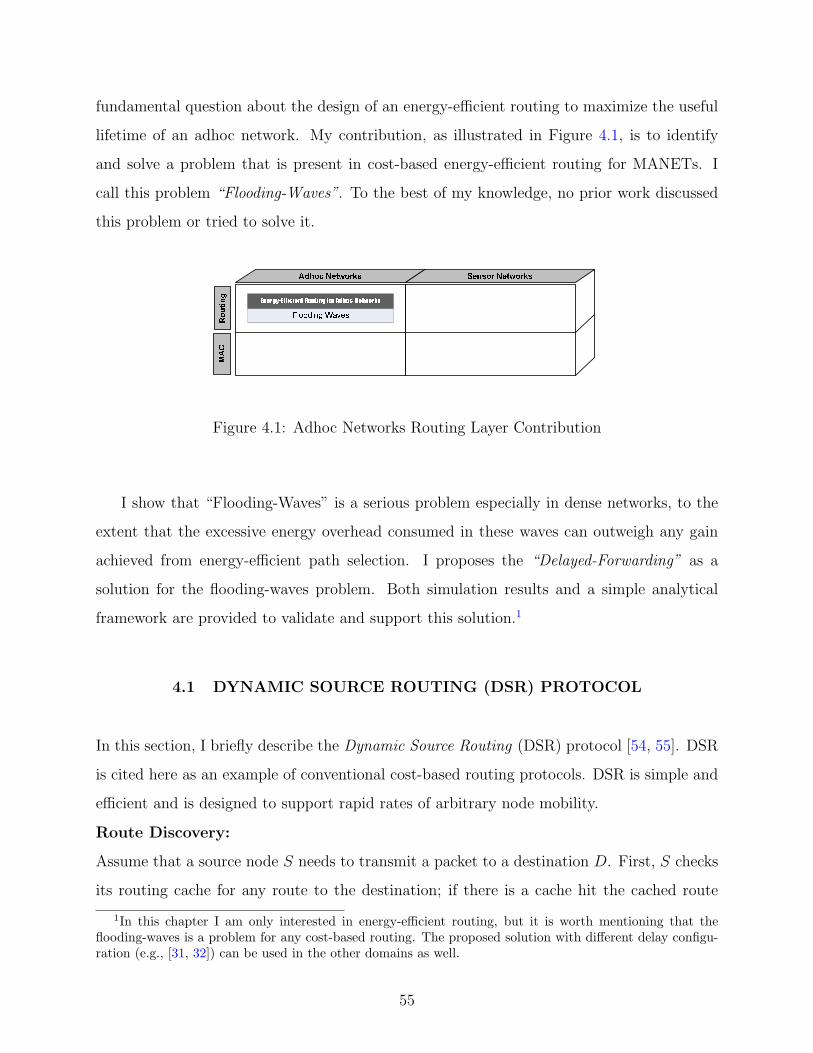
fundamental question about the design of an energy-efficient routing to maximize the useful

lifetime of an adhoc network. My contribution, as illustrated in Figure 4.1, is to identify

and solve a problem that is present in cost-based energy-efficient routing for MANETs. I

call this problem “Flooding-Waves”. To the best of my knowledge, no prior work discussed

this problem or tried to solve it.

Figure 4.1: Adhoc Networks Routing Layer Contribution

I show that “Flooding-Waves” is a serious problem especially in dense networks, to the

extent that the excessive energy overhead consumed in these waves can outweigh any gain

achieved from energy-efficient path selection. I proposes the “Delayed-Forwarding” as a

solution for the flooding-waves problem. Both simulation results and a simple analytical

framework are provided to validate and support this solution.1

4.1 DYNAMIC SOURCE ROUTING (DSR) PROTOCOL

In this section, I briefly describe the Dynamic Source Routing (DSR) protocol [54, 55]. DSR

is cited here as an example of conventional cost-based routing protocols. DSR is simple and

efficient and is designed to support rapid rates of arbitrary node mobility.

Route Discovery:

Assume that a source node S needs to transmit a packet to a destination D. First, S checks

its routing cache for any route to the destination; if there is a cache hit the cached route

1In this chapter I am only interested in energy-efficient routing, but it is worth mentioning that theflooding-waves is a problem for any cost-based routing. The proposed solution with different delay configu-ration (e.g., [31, 32]) can be used in the other domains as well.

55

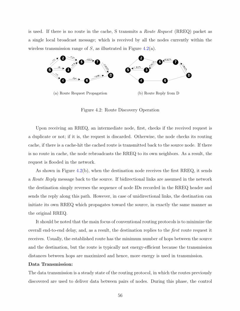
is used. If there is no route in the cache, S transmits a Route Request (RREQ) packet as

a single local broadcast message; which is received by all the nodes currently within the

wireless transmission range of S, as illustrated in Figure 4.2(a).

(a) Route Request Propagation (b) Route Reply from D

Figure 4.2: Route Discovery Operation

Upon receiving an RREQ, an intermediate node, first, checks if the received request is

a duplicate or not; if it is, the request is discarded. Otherwise, the node checks its routing

cache, if there is a cache-hit the cached route is transmitted back to the source node. If there

is no route in cache, the node rebroadcasts the RREQ to its own neighbors. As a result, the

request is flooded in the network.

As shown in Figure 4.2(b), when the destination node receives the first RREQ, it sends

a Route Reply message back to the source. If bidirectional links are assumed in the network

the destination simply reverses the sequence of node IDs recorded in the RREQ header and

sends the reply along this path. However, in case of unidirectional links, the destination can

initiate its own RREQ which propagates toward the source, in exactly the same manner as

the original RREQ.

It should be noted that the main focus of conventional routing protocols is to minimize the

overall end-to-end delay, and, as a result, the destination replies to the first route request it

receives. Usually, the established route has the minimum number of hops between the source

and the destination, but the route is typically not energy-efficient because the transmission

distances between hops are maximized and hence, more energy is used in transmission.

Data Transmission:

The data transmission is a steady state of the routing protocol, in which the routes previously

discovered are used to deliver data between pairs of nodes. During this phase, the control

56

traffic is minimized and the routes are kept constant as long as they are not invalidated.

Route Invalidation:

High mobility is a typical feature of MANETs: neighbor nodes can move outside the trans-

mission range of each other, causing what is known as broken links. To account for such

communication loss between nodes along a specific route path a mechanism called Route

invalidation or Route Maintenance has to be used.

When originating or forwarding a packet using DSR, each transmitting node is responsi-

ble for confirming that the packet has been received by the next hop. If the packet can’t be

transmitted up to a maximum number of retrials, the node returns a Route Invalid message

to the source stating which link is broken. Upon receiving this message, the source can

initiate a new RREQ or use another cached route to the destination.

4.2 ENERGY-EFFICIENT COST-BASED ROUTING

In a cost-based routing protocol (e.g., [54, 55, 41]), each node adds its current cost to the

received RREQ and rebroadcasts it. Upon receiving the first request, the destination sets a

timer. During a specified interval, the destination collects all incoming requests. When the

timer expires, the destination selects the best route and includes it in the generated route

reply. There is a tradeoff in determining this timeout value: it should be long enough to

collect all the route requests and at the same time it shouldn’t increase the overall end-to-

end delay or cause the source to timeout and send a new request. In my simulations, as

discussed later, the value of the timeout is set to be proportional to travel time of the first

route request received. This is done to factor in the distance between the source and the

destination and the congestion level of the network.

In energy-efficient cost-based routing (e.g., [103, 39, 74]), the network designer should

answer two questions: (1) How to assign a cost for a wireless link and (2) how to aggregate

the cost of a complete route from the source to the destination. In this section, I briefly

describe each design choice.

57

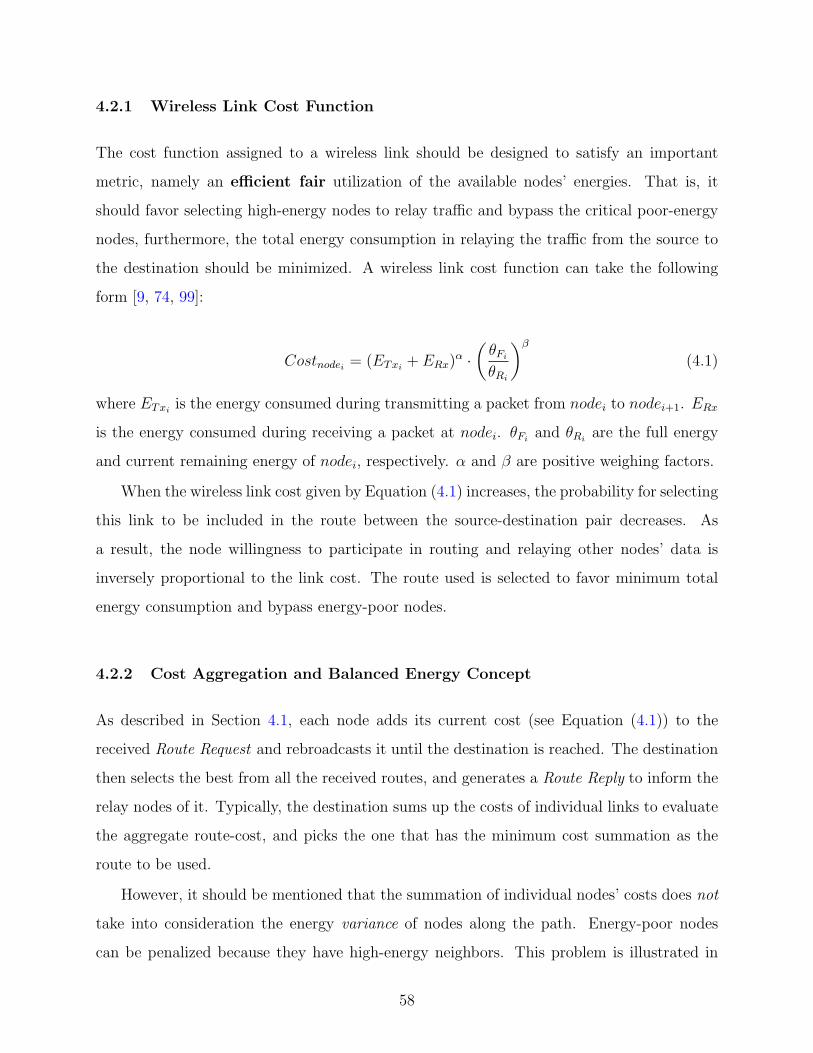
4.2.1 Wireless Link Cost Function

The cost function assigned to a wireless link should be designed to satisfy an important

metric, namely an efficient fair utilization of the available nodes’ energies. That is, it

should favor selecting high-energy nodes to relay traffic and bypass the critical poor-energy

nodes, furthermore, the total energy consumption in relaying the traffic from the source to

the destination should be minimized. A wireless link cost function can take the following

form [9, 74, 99]:

Costnodei= (ETxi

+ ERx)α ·

(θFi

θRi

)β

(4.1)

where ETxiis the energy consumed during transmitting a packet from nodei to nodei+1. ERx

is the energy consumed during receiving a packet at nodei. θFiand θRi

are the full energy

and current remaining energy of nodei, respectively. α and β are positive weighing factors.

When the wireless link cost given by Equation (4.1) increases, the probability for selecting

this link to be included in the route between the source-destination pair decreases. As

a result, the node willingness to participate in routing and relaying other nodes’ data is

inversely proportional to the link cost. The route used is selected to favor minimum total

energy consumption and bypass energy-poor nodes.

4.2.2 Cost Aggregation and Balanced Energy Concept

As described in Section 4.1, each node adds its current cost (see Equation (4.1)) to the

received Route Request and rebroadcasts it until the destination is reached. The destination

then selects the best from all the received routes, and generates a Route Reply to inform the

relay nodes of it. Typically, the destination sums up the costs of individual links to evaluate

the aggregate route-cost, and picks the one that has the minimum cost summation as the

route to be used.

However, it should be mentioned that the summation of individual nodes’ costs does not

take into consideration the energy variance of nodes along the path. Energy-poor nodes

can be penalized because they have high-energy neighbors. This problem is illustrated in

58

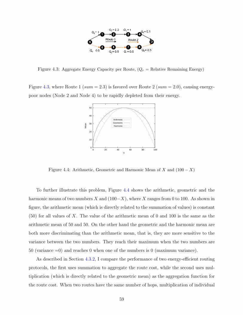
Figure 4.3: Aggregate Energy Capacity per Route, (Qr = Relative Remaining Energy)

Figure 4.3, where Route 1 (sum = 2.3) is favored over Route 2 (sum = 2.0), causing energy-

poor nodes (Node 2 and Node 4) to be rapidly depleted from their energy.

0

10

20

30

40

50

0 20 40 60 80 100

Mea

n

X

Arithmetic

Geometric

Harmonic

Figure 4.4: Arithmetic, Geometric and Harmonic Mean of X and (100−X)

To further illustrate this problem, Figure 4.4 shows the arithmetic, geometric and the

harmonic means of two numbers X and (100−X), where X ranges from 0 to 100. As shown in

figure, the arithmetic mean (which is directly related to the summation of values) is constant

(50) for all values of X. The value of the arithmetic mean of 0 and 100 is the same as the

arithmetic mean of 50 and 50. On the other hand the geometric and the harmonic mean are

both more discriminating than the arithmetic mean, that is, they are more sensitive to the

variance between the two numbers. They reach their maximum when the two numbers are

50 (variance =0) and reaches 0 when one of the numbers is 0 (maximum variance).

As described in Section 4.3.2, I compare the performance of two energy-efficient routing

protocols, the first uses summation to aggregate the route cost, while the second uses mul-

tiplication (which is directly related to the geometric mean) as the aggregation function for

the route cost. When two routes have the same number of hops, multiplication of individual

59

link costs will yield a better energy-balanced route. It should be clear that the node’s cost is

designed to be ≥ 1 and hence, the aggregated cost function is a non-negative monotonically

increasing function.

Note that the balanced energy problem is not the main objective of my work. Cost

multiplication is one way, although not very efficient, that can be used to account for the

variance of the nodes energies along a route. However, it should be clear that the main

objective of this chapter is to define and analyze the “Flooding-Waves” problem, defined in

Section 4.3.1, and this is orthogonal, as will be shown, to optimizing for balanced energy

usage, which can be a separate research issue.

4.3 FLOODING WAVES IN COST-BASED ENERGY-EFFICIENT

ROUTING

4.3.1 Flooding Waves Problem Definition

In Section 4.3.2.2 I provide simulation results showing a significant improvement in the

performance of the energy-efficient routing over conventional energy-oblivious routing pro-

tocols. However, this improvement is only for low-density networks. When the node density

increases, a problem arises and the performance of the network is severely degraded. In this

section I am going to discuss the origin of this problem, which I call the “Flooding Waves”

problem.

Figure 4.5 shows the neighborhood of the source in a high-density network. For simplicity,

assume that all the network nodes have the same energy. Hence, the transmission distance

(energy consumption) is the only factor that determines the efficiency of a route. Moreover,

consider a snapshot of the network every τ , where τ is long enough for the contention between

the transmitting nodes in one neighborhood to be resolved.

When a source node S needs to transmit a packet and it doesn’t know the route to the

destination, it sends out a route request. All the nodes in the transmission range of the

source receive this request after time τ . In this case there is a difference in the behavior of

the conventional DSR and that of an energy-efficient routing, as described next.

60

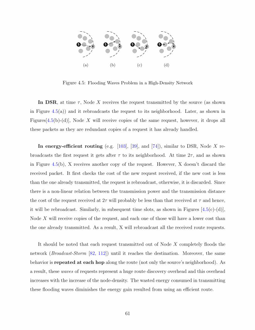
(a) (b) (c) (d)

Figure 4.5: Flooding Waves Problem in a High-Density Network

In DSR, at time τ , Node X receives the request transmitted by the source (as shown

in Figure 4.5(a)) and it rebroadcasts the request to its neighborhood. Later, as shown in

Figures[4.5(b)-(d)], Node X will receive copies of the same request, however, it drops all

these packets as they are redundant copies of a request it has already handled.

In energy-efficient routing (e.g. [103], [39], and [74]), similar to DSR, Node X re-

broadcasts the first request it gets after τ to its neighborhood. At time 2τ , and as shown

in Figure 4.5(b), X receives another copy of the request. However, X doesn’t discard the

received packet. It first checks the cost of the new request received, if the new cost is less

than the one already transmitted, the request is rebroadcast, otherwise, it is discarded. Since

there is a non-linear relation between the transmission power and the transmission distance

the cost of the request received at 2τ will probably be less than that received at τ and hence,

it will be rebroadcast. Similarly, in subsequent time slots, as shown in Figures [4.5(c)-(d)],

Node X will receive copies of the request, and each one of those will have a lower cost than

the one already transmitted. As a result, X will rebroadcast all the received route requests.

It should be noted that each request transmitted out of Node X completely floods the

network (Broadcast-Storm [82, 112]) until it reaches the destination. Moreover, the same

behavior is repeated at each hop along the route (not only the source’s neighborhood). As

a result, these waves of requests represent a huge route discovery overhead and this overhead

increases with the increase of the node-density. The wasted energy consumed in transmitting

these flooding waves diminishes the energy gain resulted from using an efficient route.

61

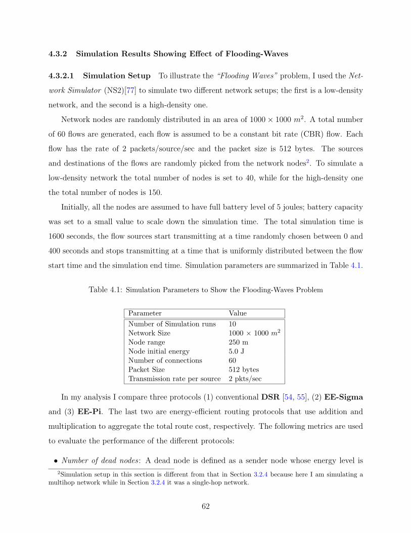
4.3.2 Simulation Results Showing Effect of Flooding-Waves

4.3.2.1 Simulation Setup To illustrate the “Flooding Waves” problem, I used the Net-

work Simulator (NS2)[77] to simulate two different network setups; the first is a low-density

network, and the second is a high-density one.

Network nodes are randomly distributed in an area of 1000× 1000 m2. A total number

of 60 flows are generated, each flow is assumed to be a constant bit rate (CBR) flow. Each

flow has the rate of 2 packets/source/sec and the packet size is 512 bytes. The sources

and destinations of the flows are randomly picked from the network nodes2. To simulate a

low-density network the total number of nodes is set to 40, while for the high-density one

the total number of nodes is 150.

Initially, all the nodes are assumed to have full battery level of 5 joules; battery capacity

was set to a small value to scale down the simulation time. The total simulation time is

1600 seconds, the flow sources start transmitting at a time randomly chosen between 0 and

400 seconds and stops transmitting at a time that is uniformly distributed between the flow

start time and the simulation end time. Simulation parameters are summarized in Table 4.1.

Table 4.1: Simulation Parameters to Show the Flooding-Waves Problem

Parameter ValueNumber of Simulation runs 10Network Size 1000 × 1000 m2

Node range 250 mNode initial energy 5.0 JNumber of connections 60Packet Size 512 bytesTransmission rate per source 2 pkts/sec

In my analysis I compare three protocols (1) conventional DSR [54, 55], (2) EE-Sigma

and (3) EE-Pi. The last two are energy-efficient routing protocols that use addition and

multiplication to aggregate the total route cost, respectively. The following metrics are used

to evaluate the performance of the different protocols:

• Number of dead nodes : A dead node is defined as a sender node whose energy level is

2Simulation setup in this section is different from that in Section 3.2.4 because here I am simulating amultihop network while in Section 3.2.4 it was a single-hop network.

62

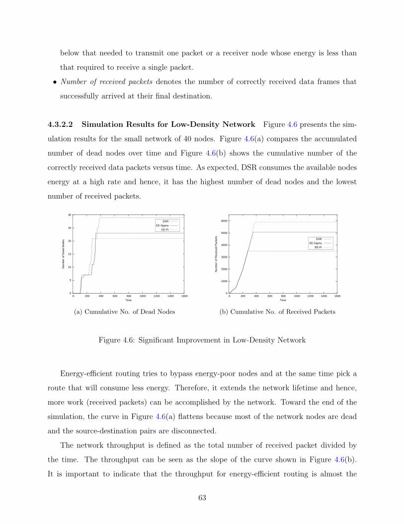
below that needed to transmit one packet or a receiver node whose energy is less than

that required to receive a single packet.

• Number of received packets denotes the number of correctly received data frames that

successfully arrived at their final destination.

4.3.2.2 Simulation Results for Low-Density Network Figure 4.6 presents the sim-

ulation results for the small network of 40 nodes. Figure 4.6(a) compares the accumulated

number of dead nodes over time and Figure 4.6(b) shows the cumulative number of the

correctly received data packets versus time. As expected, DSR consumes the available nodes

energy at a high rate and hence, it has the highest number of dead nodes and the lowest

number of received packets.

0

5

10

15

20

25

30

0 200 400 600 800 1000 1200 1400 1600

Num

ber

of D

ead

Nod

es

Time

DSR

EE-Sigma

EE-Pi

(a) Cumulative No. of Dead Nodes

0

1000

2000

3000

4000

5000

6000

0 200 400 600 800 1000 1200 1400 1600

Num

ber

of R

ecei

ved

Pac

kets

Time

DSR

EE-Sigma

EE-Pi

(b) Cumulative No. of Received Packets

Figure 4.6: Significant Improvement in Low-Density Network

Energy-efficient routing tries to bypass energy-poor nodes and at the same time pick a

route that will consume less energy. Therefore, it extends the network lifetime and hence,

more work (received packets) can be accomplished by the network. Toward the end of the

simulation, the curve in Figure 4.6(a) flattens because most of the network nodes are dead

and the source-destination pairs are disconnected.

The network throughput is defined as the total number of received packet divided by

the time. The throughput can be seen as the slope of the curve shown in Figure 4.6(b).

It is important to indicate that the throughput for energy-efficient routing is almost the

63

same as that offered by DSR. As a result, the destination dynamic timeout value used has

an insignificant effect on the throughput. Toward the end of the simulation the curve in

Figure 4.6(b) flattens which indicates that the throughput of the network is close to zero

and no more messages are being received. This is because most of the network nodes are

dead and no data packets can reach their destinations. As shown in Figure 4.6(b) EE-sigma

increased the number of received packets by 44% while EE-Pi boosted up the number of

received packets by 68%.

0

10

20

30

40

50

60

70

80

90

0 200 400 600 800 1000 1200 1400 1600

Num

ber

of D

ead

Nod

es

Time

DSR

EE-Sigma

(a) Cumulative No.of Dead Nodes

0

500

1000

1500

2000

2500

3000

3500

0 200 400 600 800 1000 1200 1400 1600

Num

ber

of R

ecei

ved

Pac

kets

Time

DSR

EE-Sigma

(b) Cumulative No. of Received Packets

Figure 4.7: Route Discovery Overhead in High-Density Network

4.3.2.3 Simulation Results for High-Density Network Figure 4.7 presents the sim-

ulation results for a dense network of 150 nodes (EE-Pi is omitted for visual clarity). Fig-

ure 4.7(a) compares the accumulated number of dead nodes over time and Figure 4.7(b)

shows the cumulative number of the correctly received data packets versus time. As shown

in Figure 4.7(a), the number of dead nodes when using DSR is almost the same as that when

using an energy efficient routing algorithm. This surprising result is because the forwarding

nodes waste a lot of energy in the route discovery overhead for each new route discovered.

Figure 4.7(b) represents another result that seems, at first, surprising: For high node-density

networks, DSR is actually delivering almost the same total number of packets to their final

destinations as that delivered when using EE-sigma. As shown in the figure, the energy gain

achieved by energy-efficient routing is canceled out by the huge overhead the nodes are pay-

64

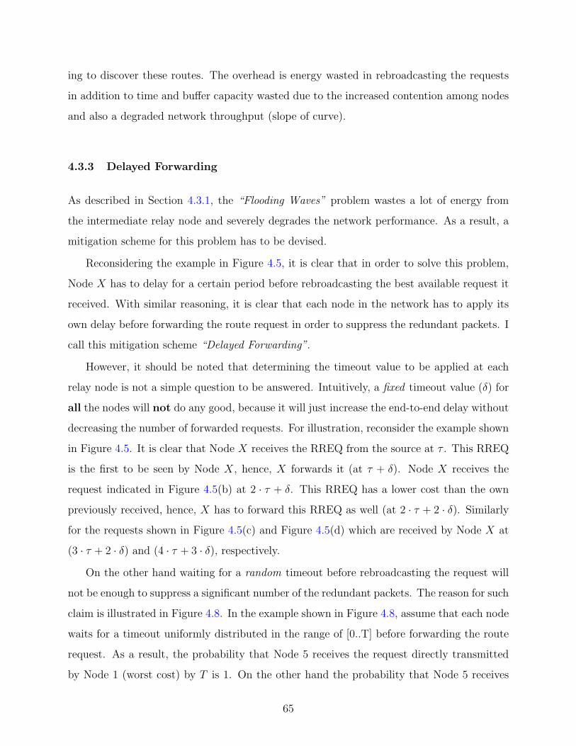
ing to discover these routes. The overhead is energy wasted in rebroadcasting the requests

in addition to time and buffer capacity wasted due to the increased contention among nodes

and also a degraded network throughput (slope of curve).

4.3.3 Delayed Forwarding

As described in Section 4.3.1, the “Flooding Waves” problem wastes a lot of energy from

the intermediate relay node and severely degrades the network performance. As a result, a

mitigation scheme for this problem has to be devised.

Reconsidering the example in Figure 4.5, it is clear that in order to solve this problem,

Node X has to delay for a certain period before rebroadcasting the best available request it

received. With similar reasoning, it is clear that each node in the network has to apply its

own delay before forwarding the route request in order to suppress the redundant packets. I

call this mitigation scheme “Delayed Forwarding”.

However, it should be noted that determining the timeout value to be applied at each

relay node is not a simple question to be answered. Intuitively, a fixed timeout value (δ) for

all the nodes will not do any good, because it will just increase the end-to-end delay without

decreasing the number of forwarded requests. For illustration, reconsider the example shown

in Figure 4.5. It is clear that Node X receives the RREQ from the source at τ . This RREQ

is the first to be seen by Node X, hence, X forwards it (at τ + δ). Node X receives the

request indicated in Figure 4.5(b) at 2 · τ + δ. This RREQ has a lower cost than the own

previously received, hence, X has to forward this RREQ as well (at 2 · τ + 2 · δ). Similarly

for the requests shown in Figure 4.5(c) and Figure 4.5(d) which are received by Node X at

(3 · τ + 2 · δ) and (4 · τ + 3 · δ), respectively.

On the other hand waiting for a random timeout before rebroadcasting the request will

not be enough to suppress a significant number of the redundant packets. The reason for such

claim is illustrated in Figure 4.8. In the example shown in Figure 4.8, assume that each node

waits for a timeout uniformly distributed in the range of [0..T] before forwarding the route

request. As a result, the probability that Node 5 receives the request directly transmitted

by Node 1 (worst cost) by T is 1. On the other hand the probability that Node 5 receives

65

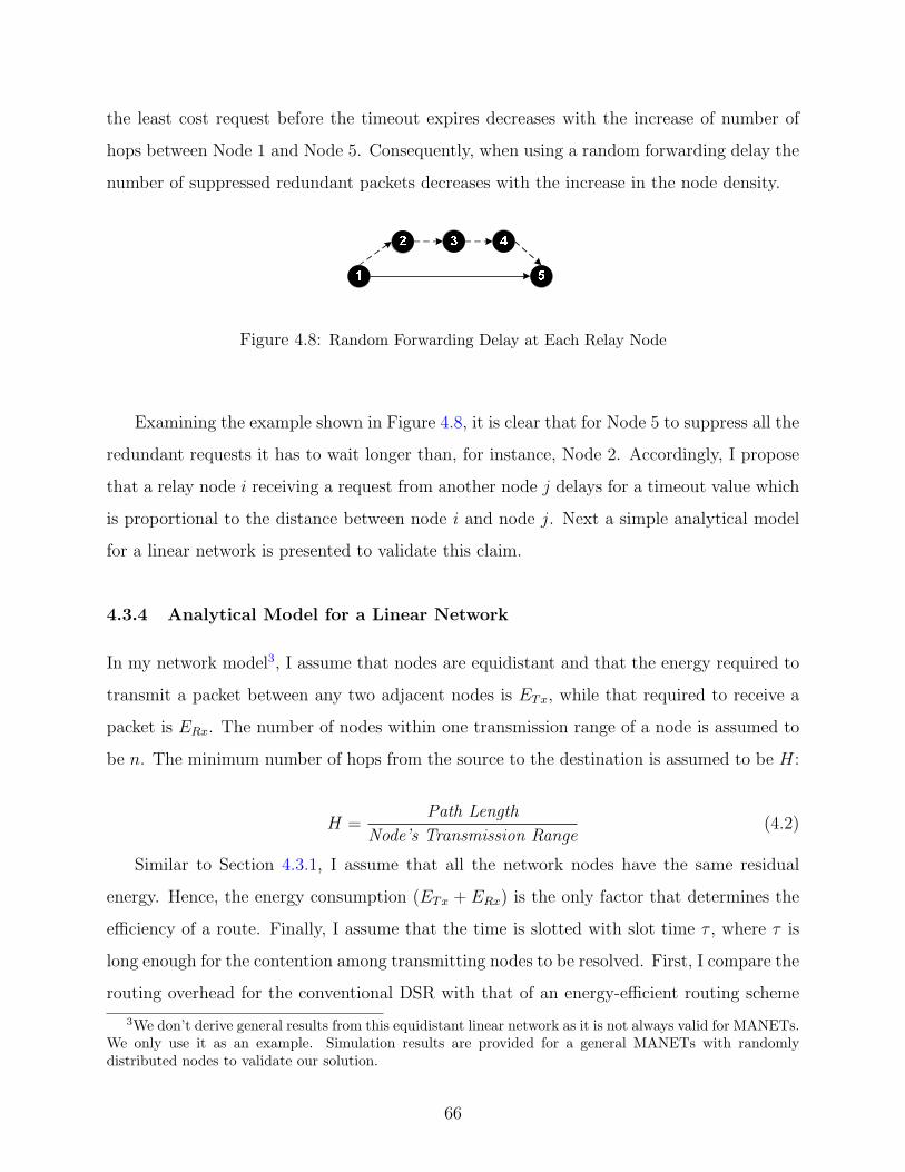
the least cost request before the timeout expires decreases with the increase of number of

hops between Node 1 and Node 5. Consequently, when using a random forwarding delay the

number of suppressed redundant packets decreases with the increase in the node density.

Figure 4.8: Random Forwarding Delay at Each Relay Node

Examining the example shown in Figure 4.8, it is clear that for Node 5 to suppress all the

redundant requests it has to wait longer than, for instance, Node 2. Accordingly, I propose

that a relay node i receiving a request from another node j delays for a timeout value which

is proportional to the distance between node i and node j. Next a simple analytical model

for a linear network is presented to validate this claim.

4.3.4 Analytical Model for a Linear Network

In my network model3, I assume that nodes are equidistant and that the energy required to

transmit a packet between any two adjacent nodes is ETx, while that required to receive a

packet is ERx. The number of nodes within one transmission range of a node is assumed to

be n. The minimum number of hops from the source to the destination is assumed to be H:

H =Path Length

Node’s Transmission Range(4.2)

Similar to Section 4.3.1, I assume that all the network nodes have the same residual

energy. Hence, the energy consumption (ETx + ERx) is the only factor that determines the

efficiency of a route. Finally, I assume that the time is slotted with slot time τ , where τ is

long enough for the contention among transmitting nodes to be resolved. First, I compare the

routing overhead for the conventional DSR with that of an energy-efficient routing scheme

3We don’t derive general results from this equidistant linear network as it is not always valid for MANETs.We only use it as an example. Simulation results are provided for a general MANETs with randomlydistributed nodes to validate our solution.

66

that does not use a forwarding delay. Then the optimal forwarding delay that each node

should wait before rebroadcasting the received request is derived.

In DSR, each relay node broadcasts the request once, regardless of its cost, and discards

all redundant copies of the same request. Intuitively, the number of requests transmitted

(overhead) is just the total number of nodes in the network and is given by:

OverheadDSR = n ·H (4.3)

In energy-efficient routing, the relay nodes do not drop duplicate requests but forward the

duplicate if it has a lower cost. Figure 4.9 shows a simple example for a linear network where

the node’s transmission range includes two other nodes (a total of 3 nodes per neighborhood).

In the figure, time flows from top to bottom where each row represents a new time slot. Dark

nodes are those forwarding the requests. For example, the dark node in the 2nd row, 3rd

column means that Node 3 forward the RREQ received from S. Analogously, dark node in

3rd row, 3rd column sends the RREQ received from Node 2.

Figure 4.9: Route Request Overhead

The reader might think that since the number of transmitting nodes in 4th row is larger

than that of the 3rd row, then the time needed for transmission (τ) should be different for

each row. However, it should be kept in mind that transmissions from different neighbor-

hoods can occur concurrently: As a result, τ is fixed and is equal to the time needed for

the nodes in one neighborhood ( 2 · n nodes because of hidden terminals) to resolve their

contention. In the example given in Figure 4.9, τ is assumed to be long enough for 6 nodes

67

to resolve contention. In general, the collision model presented in Section3.1.5, can be used

to determine τ as the time needed for n nodes to resolve the contention.

As shown in Figure 4.9, at τ = 0, S broadcasts a route request which is received by 2 and

3. At τ = 1, both 2 and 3 forward the request. When 2 transmits 3 and 4 receive. Similarly,

4 and 5 receives from 3. At τ = 2, 3 transmits because the request received from 2 has a

lower cost than that received from S. As shown in figure, the number of nodes transmitting

grows (by n − 1) until the edge of the expanding wave reaches the destination (at τ = H),

and then, it decreases by one for each subsequent time slot. The overhead is the number

of requests transmitted, which is equivalent to the number of dark nodes. As a result, for

a general linear network, it is easy to prove that the overhead of routing in energy-efficient

network is:

OverheadEE =

((n− 1) ·

H∑i=1

i

)+

(n−1)·H∑i=1

i

=H · (n− 1) · (n ·H − 2)

2

(4.4)

where the first term represents the number of growing nodes until the destination is reached

and the second term represents the number of decreasing transmitters after that.

Comparing Equation (4.3) and Equation (4.4) illustrates the huge overhead imposed

by an typical energy-efficient routing scheme. I propose using the “Delayed Forwarding”

mechanism to reduce this effect. Optimally, the routing overhead in an energy efficient

protocol is equal to that of the DSR, where each node forwards the request only once. Next

the optimal delay for the linear network is derived.

S 1 D2 i n

Figure 4.10: A Linear Adhoc Network

68

Consider the linear network shown in Figure 4.10. After one slot time, Node i (i hops

away from source) receives a request from the source. The cost of this request is ETx · i2.After two time slots, Node i receives n−1 requests. The best cost request from those received

is the one that is forwarded form a node at exactly mid distance between the source and

Node i. The cost of this request is ETx · (i2/2) + ERx. With similar reasoning, after d time

slots the best received request has a cost of:

Cost = ETx · i2

d+ (d− 1) · ERx (4.5)

For Node i to suppress all redundant requests, it has to wait d time slots, such that the

cost of the request received at d+1 is greater than or equal that received at d. This is shown

in Equation (4.6)

(ETx · i2

d+ (d− 1) · ERx) ≥ (ETx · i2

d + 1+ (d) · ERx) (4.6)

Solving the inequality given by Equation (4.6), we can deduce that each relay node has

to wait for:

Delaynodei∝

√ETxi

ERx

(4.7)

where Delaynodeiis the timeout value to be applied at node i and ETxi

is the transmission

energy required to reach node i from the previous forwarding node. As a result, the optimal

timeout value at node i is proportional (at least for the linear network) to the the distance

between this node and the previous forwarding node.

4.3.5 Simulation Analysis for Delayed-Forwarding

To evaluate the performance of the adhoc network when the proposed delayed forwarding

is used I used NS2 to re-simulate the same high-density network setup as that described in

Section 4.3.2.1. In my analysis I compare four protocols (1) conventional DSR, (2) energy-

efficient routing that does not use “delayed forwarding”, as describe in Section 4.3.2.1, EE-

Sigma, (3) energy-efficient routing that use delayed forwarding and addition to aggregate the

total route cost, EE-Sigma-Delay, and (4) energy-efficient routing that use multiplication

69

as the cost aggregation function and use delayed forwarding at intermediate relay nodes,

EE-Pi-Delay.

0

5000

10000

15000

20000

25000

0 200 400 600 800 1000 1200 1400 1600

Num

ber

of F

orw

arde

d R

eque

sts

Time

EE-Pi-Delay

EE-Sigma

DSR

Figure 4.11: Cumulative No. of RREQ Forwarded at Relay Nodes; Total Nodes = 150

Figure 4.11 shows the number of route requests forwarded at intermediate relay nodes

versus time. The number of requests forwarded when no delay is applied (EE-Sigma) is

significantly larger than that forwarded when using DSR. The relay node’s energy is not

used to deliver data packets to their destinations but rather it is wasted in forwarding these

overhead packets. When the delayed forwarding (EE-Pi-Delay) is applied, the number of

requests forwarded in energy-efficient routing is almost as low as that forwarded when using

DSR and hence, the energy overhead is minimized. For visual clarity, the curve for EE-

Sigma-Delay is omitted as it is very close to that of EE-Pi-Delay.

Figure 4.12 compares the accumulated number of dead nodes over time. As shown in

figure, and similar to the result shown in Figure 4.7(a), the performance of EE-Sigma is

severely degraded due to the wasted overhead and therefore, the number of dead nodes is

slightly more than that when using DSR. However, when the suggested forwarding delay

(EE-Sigma-Delay and EE-Pi-Delay) is used, the route discovery overhead is minimized and

therefore, the energy savings from using an efficient route decreased the total number of

dead nodes in the network.

70

0

10

20

30

40

50

60

70

80

90

100

0 200 400 600 800 1000 1200 1400 1600

Num

ber

of D

ead

Nod

es

Time

EE-Pi-Delay

EE-Sigma-Delay

EE-Sigma

DSR

Figure 4.12: Cumulative No. of Dead Nodes; Total Nodes = 150

0

500

1000

1500

2000

2500

3000

3500

4000

4500

5000

0 200 400 600 800 1000 1200 1400 1600

Num

ber

of R

ecei

ved

Pac

kets

Time

EE-Pi-Delay

EE-Sigma-Delay

EE-Sigma

DSR

Figure 4.13: Cumulative No. of Received Packets; Total Nodes = 150

Figure 4.13 shows the cumulative number of the correctly received data packets versus

time. Figure 4.13 shows a similar trend of results as that shown in Figure 4.12. When

no forwarding delay is applied the performance of EE-Sigma is as bad as that of the DSR.

However, when a forwarding delay is applied a significant performance improvement can

71

be seen. EE-Sigma-Delay increased the number of received packets by 22% over the DSR.

While EE-Pi-Delay boosted the number of received packets by 46% over DSR.

4.4 CONCLUSION

In this chapter I introduced some guidelines to be applied to the family of cost-based energy-

efficient routing protocols. I identified the problem of “Flooding Waves”, which is a common

problem in cost-based energy-efficient routing scheme. I showed that as the density of the

network increases the energy-gain from an energy-efficient routing diminishes because of the

high overhead associated with discovering and maintaining the data routes. I introduced

a simple analytical model for a linear network to illustrate this problem and proposed the

forwarding delay as a solution.

Through simulations I showed that the forwarding delay boosts the performance of

energy-efficient cost-based routing protocol. I showed that the total number of received

packets for a given energy budget increases by 46% for high-density networks.

72

5.0 ENERGY-EFFICIENT MAC LAYER OPTIMIZATIONS FOR SENSOR

NETWORKS

Adhoc and sensors networks are both multi-hop wireless networks with severely constrained

energy supply. However, as discussed in Section 2.1, WSNs might have some characteristics

that make them distinct from MANETs (e.g., limited nodes mobility, low duty cycle, different

traffic pattern, in-network processing, etc.). An energy-efficient solution that accounts for

the unique characteristics of each network is clearly more efficient. In Chapters 3 and 4 I

described my work that targets the energy-efficient design of MANETs. In this chapter I

present my work that focuses on energy-efficiency at the MAC layer for WSNs, and in the

next chapter the work that targets energy-efficiency at the routing layer for WSNs.

Environmental monitoring and emergency reporting scenarios are key applications for

WSNs. In areas that are prone to such events, a set of well-placed sensors will lead to better

management of the larger amount of information that can be delivered by the network.

Typically, sensor nodes report only substantial changes that occur in the WSN in response

to an event, rather than continuously reporting the sensed data (e.g., [100]).

In the case of sensed events, many nodes in the event area attempt to transmit their data

simultaneously. To avoid collisions in the WSN, nodes coordinate transmissions through

MAC (medium access) protocols [1]. Contention-based MAC protocols, see Section 2.3.1,

are popular in wireless networks because of their simplicity, flexibility and robustness. They

do not require much infrastructure support: no clock synchronization and no global topology

information are required, and dynamic node joining and leaving are handled gracefully.

These advantages, however, come at a cost and, unfortunately, it is precisely when there

is high traffic load (e.g., an emergency condition) that contention-based MACs fail us the

most: too many collisions lead to lower throughput, higher latencies, and higher energy

73

consumption, which is crucial to the battery-operated devices. Moreover, when the network

is lightly loaded the overhead is in idle listening. Lastly, no upper bound on the delay can

be derived.

Time-Division Multiple Access (TDMA), see Section 2.3.2, has emerged as a viable alter-

native, because slots are reserved for each node to transmit and thus TDMA does not suffer

from collisions and end-to-end delay bounds are guaranteed. When the network is highly

loaded and all the nodes have some data to send, TDMA is the optimal MAC protocol to

be used. However, TDMA schemes have the following disadvantages: (i) when the network

is lightly loaded much bandwidth and energy is wasted; (ii) the need for clock synchroniza-

tion, (iii) scalability, and (iv) handling frequent topology changes and time varying channel

conditions.

In this chapter1, as illustrated in Figure 5.1, I propose a hybrid MAC layer protocol for

WSNs, namely TDMA with Adaptive Slot-Stealing And Parallelism (TDMA-ASAP)[27], as

an efficient protocol that allows for an adaptive WSN with quick response times in the case

of an event reporting, and energy conservation during times of minimal activity. Because

time and energy are crucial in sensor networks, my focus is on improved energy consumption

and decreased transmission times, when sensors typically do sensing on a periodic basis but

only transmit the results of extraneous activities to the base station on an event-driven basis.

Figure 5.1: Sensor Networks MAC Layer Contribution

TDMA-ASAP adds the following techniques to TDMA: (a) the use of parallel transmis-

sions to improve end-to-end transmission delay and energy consumption; (b) “slot-stealing”,

1The work presented in this chapter is a result of a collaboration with Robert Cleric [27] who helped inimplementing the described schemes in CSIM

74

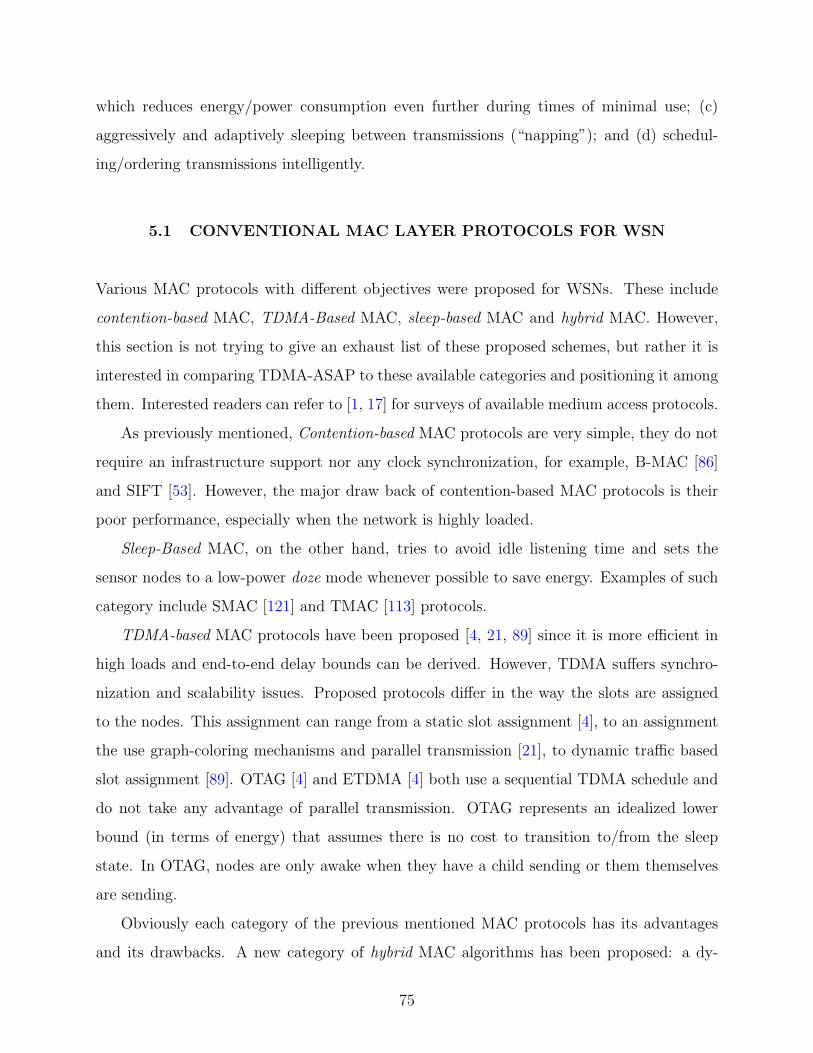
which reduces energy/power consumption even further during times of minimal use; (c)

aggressively and adaptively sleeping between transmissions (“napping”); and (d) schedul-

ing/ordering transmissions intelligently.

5.1 CONVENTIONAL MAC LAYER PROTOCOLS FOR WSN

Various MAC protocols with different objectives were proposed for WSNs. These include

contention-based MAC, TDMA-Based MAC, sleep-based MAC and hybrid MAC. However,

this section is not trying to give an exhaust list of these proposed schemes, but rather it is

interested in comparing TDMA-ASAP to these available categories and positioning it among

them. Interested readers can refer to [1, 17] for surveys of available medium access protocols.

As previously mentioned, Contention-based MAC protocols are very simple, they do not

require an infrastructure support nor any clock synchronization, for example, B-MAC [86]

and SIFT [53]. However, the major draw back of contention-based MAC protocols is their

poor performance, especially when the network is highly loaded.

Sleep-Based MAC, on the other hand, tries to avoid idle listening time and sets the

sensor nodes to a low-power doze mode whenever possible to save energy. Examples of such

category include SMAC [121] and TMAC [113] protocols.

TDMA-based MAC protocols have been proposed [4, 21, 89] since it is more efficient in

high loads and end-to-end delay bounds can be derived. However, TDMA suffers synchro-

nization and scalability issues. Proposed protocols differ in the way the slots are assigned

to the nodes. This assignment can range from a static slot assignment [4], to an assignment

the use graph-coloring mechanisms and parallel transmission [21], to dynamic traffic based

slot assignment [89]. OTAG [4] and ETDMA [4] both use a sequential TDMA schedule and

do not take any advantage of parallel transmission. OTAG represents an idealized lower

bound (in terms of energy) that assumes there is no cost to transition to/from the sleep

state. In OTAG, nodes are only awake when they have a child sending or them themselves

are sending.

Obviously each category of the previous mentioned MAC protocols has its advantages

and its drawbacks. A new category of hybrid MAC algorithms has been proposed: a dy-

75

namic combination of conventional MAC schemes based on the network conditions targeting

alleviating all the possible drawbacks of these schemes while combining their advantages.

TDMA-ASAP, falls into this category. Other examples of this category include TRAMA [89],

DMAC[71] and ZMAC [91] that combine TMDA and contention-based protocols. In ZMAC

each a time slot is assigned to a node (owner) and all neighbors contend for the slot, if it is

not used by the owner. In DMAC, each receiver has a fixed slot, but its children contend for

the sending. In TRAMA, there is a contention phase within a 2-hop distance neighborhood,

but the TDMA schedule is established after that contention on a changing (dynamic) basis.

However, as discussed in detail later, the contribution of TDMA-ASAP is not only to

combine the conventional MAC protocols together in a smart way, but also, because it is

designed with a specific application (disaster recovery networks) in mind. TDMA-ASAP

make use of the unique features of this environment which includes data burstiness [53],

region activity [100] and data-aggregation [73, 56] to develop a near optimal MAC protocol

for such networks.

5.2 TDMA-ASAP: TDMA WITH ADAPTIVE SLOT STEALING AND

PARALLELISM

5.2.1 Network and Node Models

As previously mentioned, in typical WSN environment, sensors are usually just sensing

the environment and very little data is to be sent to the end user. Therefore, the overall

network load is typically low. When an event is detected, all nodes within some region report

their data to the BS, where data must arrive with low delay. Therefore, the network load

typically has some bursts of activity. Network topology changes are not very frequent (nodes

are mostly static) and channel quality is consistent. sensor measurements are assumed to

be aggregated within the network (in-network processing) to filter redundancy and reduce

communication overhead and energy consumption [52, 45, 97].

I assume for presentation that the set of sensors uses a tree-based (see Section 2.4.2)

routing scheme [73] (TDMA-ASAP can be easily adapted for multipath routing schemes [28,

76

81, 15]). For simplicity, I also focus on a single BS in the network, and therefore a single

tree is typically formed; this, of course, can be easily generalized when multiple trees are

considered [4, 105].

Three passes through the tree are required to obtain the final schedule. The first pass

is to construct the tree routing structure. The second pass propagates the tree structure

and neighborhood list to the base station. The base station computes the schedule, based

on nodes’ level and neighbors.On the third and final pass the schedule is distributed by the

BS to the sensors. It is easy to see that there are O(n) messages for the tree construction,

where n is the number of sensors.

The power consumption model is based on MICA-2 sensors [101], which corresponds to

the typical sensor nodes: the power used to transmit is slightly higher than to receive, which

is much higher than power needed to be idle and listening. Furthermore, sensors can go into

a sleep mode, but have a transition time overhead to move to/from sleep mode. The values

used for power consumption, transition time and different packets transmission times are

listed in Section 5.2.5.1.

Similar to all TDMA-based MAC protocols [105], clock synchronization is achieved

through various mechanisms [108]. However, TDMA-ASAP requires only local clock syn-

chronization among nodes within two-hop neighborhoods. This is much easier to achieve

than global clock synchronization, which requires much tighter bounds on end-to-end syn-

chronization [69].

5.2.2 Outline and General Idea

To illustrate TDMA-ASAP protocol, consider the simple network shown in Figure 5.2, where

dotted circles represent neighborhood regions. Node 0 represents the base station to which

all data should be routed. A conventional TDMA scheme will assign one time slot for each

sensor node to yield a linear schedule with a total of 12 time slots. However, it is easy to

notice that sensors outside each others’ range can simultaneously transmit (e.g., sensors 5 &

7), and thus, the schedule length can be shortened. Finding the shortest schedule is known to

be an NP-hard problem, and several approximation algorithms (e.g., graph coloring [2, 47])

77

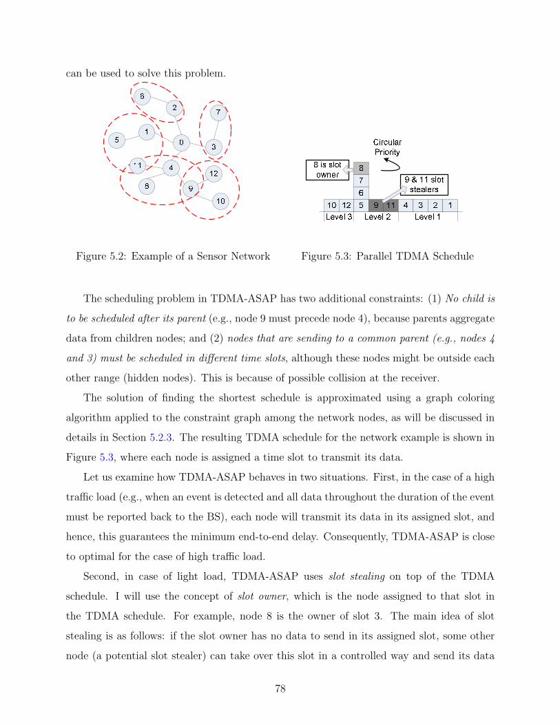
can be used to solve this problem.

Figure 5.2: Example of a Sensor Network Figure 5.3: Parallel TDMA Schedule

The scheduling problem in TDMA-ASAP has two additional constraints: (1) No child is

to be scheduled after its parent (e.g., node 9 must precede node 4), because parents aggregate

data from children nodes; and (2) nodes that are sending to a common parent (e.g., nodes 4

and 3) must be scheduled in different time slots, although these nodes might be outside each

other range (hidden nodes). This is because of possible collision at the receiver.

The solution of finding the shortest schedule is approximated using a graph coloring

algorithm applied to the constraint graph among the network nodes, as will be discussed in

details in Section 5.2.3. The resulting TDMA schedule for the network example is shown in

Figure 5.3, where each node is assigned a time slot to transmit its data.

Let us examine how TDMA-ASAP behaves in two situations. First, in the case of a high

traffic load (e.g., when an event is detected and all data throughout the duration of the event

must be reported back to the BS), each node will transmit its data in its assigned slot, and

hence, this guarantees the minimum end-to-end delay. Consequently, TDMA-ASAP is close

to optimal for the case of high traffic load.

Second, in case of light load, TDMA-ASAP uses slot stealing on top of the TDMA

schedule. I will use the concept of slot owner, which is the node assigned to that slot in

the TDMA schedule. For example, node 8 is the owner of slot 3. The main idea of slot

stealing is as follows: if the slot owner has no data to send in its assigned slot, some other

node (a potential slot stealer) can take over this slot in a controlled way and send its data

78

(earlier than its own slot). Instead of contending for accessing a free/empty slot like in other

proposed hybrid schemes, TDMA-ASAP uses a priority scheme. For simplicity, the priority

can be statically assigned, say, based on the ordering in the time schedule. For example, if

node 8 doesn’t use its slot, node 9 will use it if it has data; if 9 doesn’t have any data, node

11 can take over. Similarly, the priority for accessing slot 4 is node 9, node 11 and then

node 8.

Two issues should be mentioned. First, slot-stealing is only proposed to be used for

nodes sending to the same parent (e.g., nodes 8, 9 and 11), because the parent (e.g., node 4)

is already awake and is listening to the medium for possible data transmission from the slot-

owner. Second, if a parent detects a free time slot, that is, neither the owner nor any stealer

used the slot, this means that none of its remaining children has anything to transmit. As a

result, the parent node can turn its radio off (napping), which saves idle energy consumption.

Napping can also be used when a parent knows all its children have already finished their

transmission, but there is still plenty of time until its own slot for transmission (i.e., parent

node is not yet awake to receive the aggregated values).

5.2.3 1-Level Coloring for Parallel Transmissions

As previously described, the problem of finding the shortest schedule for TDMA-ASAP

can be reduced to the problem of coloring the constraint graph for the network using the

minimum number of colors (both problems are known to be NP-hard). The constraint graph

is constructed taking into account not only the parent-child and parent-parent constraints,

but also on the interference constraints; in fact, the constraint graph can be build with the

RID proposed in [123]. In that way, the graph considered is such that an edge between two

vertices (nodes) indicates that there is a color constraint between these two vertices and they

can not be colored the same, that is, these nodes can not be scheduled to transmit in the

same time slot. The following is a simplified set of RID constraints:

1. Two nodes that share the same parent cannot have the same color.

2. For any other pair of nodes A and B cannot share the same color if

a. Node A interferes with node B’s parent

79

b. Node B interferes with node A’s parent

Clearly, satisfying the above constraints, and by one-to-one mapping of colors to transmission

slots, it is guaranteed that the resultant transmission schedule is collision-free. This is be-

cause the first constraint prevents collision among the nodes within the same neighborhood,

while the second one prevents collisions among hidden nodes.

On the other hand, the above constraints are not sufficient to handle the case of aggre-

gation because they do not obey precedence constraints: a parent should not be scheduled

to transmit earlier than the slot assigned to one of its children. One way of handling ag-

gregation is by augmenting the network constraint graph with new edges corresponding to

these new order constraints among the nodes, and then applying the coloring algorithm to

obtain the minimum set of colors.

However, TDMA-ASAP adopts another solution and proposes level-by-level approach

to reduce the coloring complexity. The main idea of this solution is to apply the coloring

algorithm on each level by itself starting from the leaves (level d, where d is the tree depth),

followed by level d− 1 and continue coloring until the root is reached. Intuitively, the local

coloring approach TMDA-ASAP adopts might result in slightly longer schedules than those

achieved by the former coloring method, especially for the case of unbalanced routing trees.

On the other hand, level-by-level coloring has the following attractive properties: First, it

guarantees that aggregation ordering constraints are never violated. By construction, a node

in level L has all its children nodes in level L + 1, and hence, by scheduling the whole level

L+1 before level L, it is always the case that children are scheduled to transmit before their

parents. Second, the number of constraints handled by the level-by-level coloring approach

are much lower than that handled in the case of tree coloring, consequently, the running time

of the coloring algorithm is much smaller and can be implemented very efficiently. Finally,

level-by-level coloring is a local coloring approach, and hence, it can also be implemented as

a distributed coloring algorithm and executed among the sensor nodes themselves.

Mapping the minimum set of colors to transmission slots is a straightforward process,

where nodes with the same color are scheduled to send in the same time slot. However,

after examining the schedules generated by the coloring algorithm, the following heuris-

tics are devised to further shorten the transmission schedule and/or to decrease the energy

80

consumption:

• Reverse scheduling: Rather than ordering colors by frequency when mapping of col-

ors to time slots (i.e., the color that is used the most is schedule first), the reverse-order

scheduling can be used, that is, the color that is used the least is scheduled first. Remem-

ber that the least used color is probably used for a child node that has a lot of siblings.

As a result, if reverse scheduling is used, parents with few children will be scheduled

later, and hence, reverse scheduling allows the parent with only 1 child to sleep the first

few slots, and to only wakes up later to receive the child’s data. This reduces the idle

time that the parent is awake between when it receives data from its child and the time

when it actually transmits aggregated data to its own parent.

• m-level coloring: Rather than a single level coloring approach as described above, A

limited multi-level coloring scheme is tested. it adds an additional step to single-level

coloring, as follows: After each color c for a given level i has been colored, the coloring

algorithm then checks m levels above (i − 1, i − 2, ..., i − m) for any leaf nodes that

can be scheduled along with color c, that is, any nodes that have no children and do not

have conflicts with any of the nodes in level i. All such nodes are scheduled to transmit

in parallel with the other nodes of color c on level i.

5.2.4 Slot Stealing

After executing the scheduling algorithm above, each node X in a single neighborhood is

the owner of a time slot τx and uses it to transmit its own data. However, if X has no data

to transmit, and neighbor Y does2, then Y can use τx in transmitting Y ’s data, or what I

term slot stealing.

5.2.4.1 Determine Potential Stealers: The conditions that have to be satisfied for Y

to be considered as a potential slot stealer of X’s slot are the following:

• X and Y have to be direct neighbors. Y should be able to listen to X’s data to detect

an unused slot τx.

2If we assume region activity then this case is common especially at the levels near the sink node

81

• X and Y should be transmitting to the same common parent P , because a common

parent is already awake during τx, waiting to receive some message from X.

• If X and Z are scheduled in the same time slot (i.e., τz = τx), then either Y should

not be a hidden terminal from Z and thus Y and Z’s messages do not collide, or such

collision is permissible but the system is able to recover from it (see Stealing Algorithms

below, Section 5.2.4.3).

5.2.4.2 Detect Unused Slots: Since Y is a direct neighbor of X, then Y can detect an

unused slot by simply listening to τx. However, the length of one time slot in this case must

be extended to include time for listening for unused slots and sending data. As a result, τx

is extended with k so-called “∆-slots”, where k is the number of children per node and ∆ is

the time needed to detect that the channel is free, including clock synchronization skews.

The energy overhead associated with slot-stealing is because Y has to wake up earlier

than its assigned slot and listen to τx for a possible stealing opportunity. However, as shown

later, the energy gain achieved by slot stealing significantly outweighs this overhead.

5.2.4.3 Stealing Algorithms: As previously mentioned, if Z is a hidden node from

Y and τx = τz then a collision can occur between Y and Z, if Y steals X’s slot. Next,

three possible ”stealing” methods are described, that differ in the way they handle such

collision. These are (1) moderate stealing (StealM), (2) conservative stealing (StealC) and

(3) aggressive stealing (StealG).

StealM augments the constraint graph to avoid collisions among hidden nodes, as follows.

After the initial coloring of the tree, the algorithm considers all the nodes that may be able

to steal from their neighbors. Let node Y be one such potential stealer, stealing a slot from

node X. It then checks the neighborhood list and if it is found that node Y could cause a

collision with another node, say Z, it adds an additional edge (constraint) between Y and

Z (i.e., the potential stealer and the potential interference sufferer). This is done for all

possible stealing situations. After all of the additional edges have been added, the algorithm

then re-colors the constraint graph taking into consideration the additional edges. The end

result is a newly colored tree that removes any potential conflicts a priori.

82

Figure 5.4: Slot Stealing and Collision

For illustration consider the network shown in Figure 5.4: a parent node P1 has three

children c1, c2, and c3, scheduled in this order and colored red, blue, and green (recall that

each color transmits in one time slot). Another parent P2 is located at the same level as P1.

P2’s child of interest, c5, is also colored red (no conflict with c1). Assume that only nodes c3

and c5 have data to transmit. Because node c3 is within range of parent P2, if nodes c3 and

c5 were to transmit in the same slot (in case c3 steals c1’s slot) there would be a collision at

parent P2 (a typical collision scenario between two hidden nodes c3 and c5). In StealM , edges

will be added to the constraint graph (from c5 to both c1 and c2), and hence, re-coloring the

resulting graph c5 will not be colored the same color (red) as c1.

The down side of StealM is that it reduces parallelism (because it adds additional colors–

and thus slots–to the schedule), increasing the end to end delay (schedule length), in addition

to the overhead of adding edges and re-coloring the graph at tree setup time.

StealC is ”conservative slot stealing”; contrarily to StealM , sacrifices stealing for paral-

lelism. The main idea of StealC is to guarantee maximum transmission parallelism, that is,

no new constraints (edges) are added to the graph to be colored, and at the same time allow

slot stealing but only if collisions will not occur between any two nodes.

Reconsidering the network example shown in Figure 5.4. StealC will determine that

node c3 will not be able to steal the slot assigned for node c1, a priori, because of possible

collision with node c5, hence, c1’s slot (and also c2’s slot) will be marked as unstealable for

node c3. Clearly, StealC does not unnecessarily increase the latency and schedule length by

introducing extra edges but, on the other hand, wastes some stealing opportunities.

StealG, the last proposed method, is more aggressive. Rather than preventing collision

a priori during the scheduling time, StealG recovers from collisions online during the data

83

transmission time. If a node will cause a collision when stealing a higher priority node’s slot,

the stealer node will give up stealing this slot. It may then either wait for its assigned slot

(of which it is the owner) or it may attempt stealing a new free slot (if any exists).

Figure 5.5: StealG and Stealing Advertising

StealG uses a handshake between a child node and its parent to avoid collision, similar to

the RTS/CTS handshake used in IEEE 802.11 networks, but a much more efficient version.

As illustrated in Figure 5.5, this is achievable by extending the data slot for each node by

one extra ∆-slot, that is, each data slot is extended by (k + 1) ∆-slots instead of k ∆-slots,

where k is the number of children per node.

In StealG, the ∆-slots are used differently from the other two algorithms. A ∆-slots is

used by a child to detect unused time slots and also to advise the parents whether it has data

to transmit or not, as follows. Consider a child node ci whose order (priority) to access the

current time slot is i. ci keeps sensing the medium for i− 1 ∆-slots, and the channel is free,

ci sends its “I-have-data” signal in the ith ∆-slot. The parent, upon detecting a signal in the

i ∆-slot, responds by signaling continuously from ∆-slot i + 1 to ∆-slot k + 1 and hence all

the remaining lower priority children (including those that may be hidden from the highest

priority node) will remain silent during the data transmission phase and collision is avoided.

As a result, the highest priority child among those who have data to transmit will always be

granted access to the time slot. Moreover, as previously described, a circular transmission

priority–based on the order in the schedule–is used (see Figure 5.3). Hence, the owner of a

slot will always have the highest priority and will be granted the slot if it has some data to

send, followed by the neighbor sending to the same parent and is next in the schedule.

The energy overhead associated with StealG is due to three factors: parents having

84

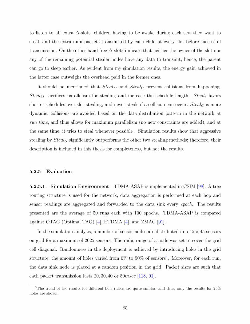
to listen to all extra ∆-slots, children having to be awake during each slot they want to

steal, and the extra mini packets transmitted by each child at every slot before successful

transmission. On the other hand free ∆-slots indicate that neither the owner of the slot nor

any of the remaining potential stealer nodes have any data to transmit, hence, the parent

can go to sleep earlier. As evident from my simulation results, the energy gain achieved in

the latter case outweighs the overhead paid in the former ones.

It should be mentioned that StealM and StealC prevent collisions from happening.

StealM sacrifices parallelism for stealing and increase the schedule length. Stealc favors

shorter schedules over slot stealing, and never steals if a collision can occur. StealG is more

dynamic, collisions are avoided based on the data distribution pattern in the network at

run time, and thus allows for maximum parallelism (no new constraints are added), and at

the same time, it tries to steal whenever possible . Simulation results show that aggressive

stealing by StealG significantly outperforms the other two stealing methods; therefore, their

description is included in this thesis for completeness, but not the results.

5.2.5 Evaluation

5.2.5.1 Simulation Environment TDMA-ASAP is implemented in CSIM [98]. A tree

routing structure is used for the network, data aggregation is performed at each hop and

sensor readings are aggregated and forwarded to the data sink every epoch. The results

presented are the average of 50 runs each with 100 epochs. TDMA-ASAP is compared

against OTAG (Optimal TAG) [4], ETDMA [4], and ZMAC [91].

In the simulation analysis, a number of sensor nodes are distributed in a 45× 45 sensors

on grid for a maximum of 2025 sensors. The radio range of a node was set to cover the grid

cell diagonal. Randomness in the deployment is achieved by introducing holes in the grid

structure; the amount of holes varied from 0% to 50% of sensors3. Moreover, for each run,

the data sink node is placed at a random position in the grid. Packet sizes are such that

each packet transmission lasts 20, 30, 40 or 50msec [118, 91].

3The trend of the results for different hole ratios are quite similar, and thus, only the results for 25%holes are shown.

85

The value for ∆-slot used in the implementation of both StealG and ZMAC4 was set to

∆ = 0.4ms, after ZMAC [91] in order not to favor the proposed TDMA-ASAP protocol.

It should be noted that for current sensor hardware and TinyOS platforms a ∆-slot of size

192µsec is achievable [84, 118].

The power consumption is based on MICA-2 sensors: 43mW to transmit, 35.5mW to

receive, and 11mW when idle. The transition times used in the simulations for a node to

either transition to or from the sleep state ranged from 15ms to 100ms.

The sensed events (seismic, environmental) are assumed to be localized, and therefore,

affect a certain region of the network. The percentage of nodes that have data to transmit,

called event load, is varied from 0% to 30%, in increments of 5%.

The following metrics are used for comparison: end-to-end delay, energy, the energy-

delay product, and the average awake time of a node at each level. These metrics excludes

the tree-setup phase.

5.2.5.2 End-to-End Delay Figure 5.6 shows the effect of parallel transmission schedul-

ing on end-to-end delay when compared to traditional sequential TDMA scheduling. Results

reported in Figure 5.6 are when the packet transmission time is 50 msec while the transition

time overhead from sleep to awake is 15 msec, other values for these two parameters show a

similar trend in the results.

Because OTAG and ETDMA do not schedule non-interfering nodes to transmit in par-

allel they suffer from much longer end-to-end delay (6 times longer delay) compared to the

other schemes that allow for parallel transmission. On the other hand, the 1-level coloring

(1L-color) has no additional overhead (no extra ∆-slots), and thus, outperforms (in terms

of delay) both StealG and ZMAC. ZMAC and StealG extend the slot time, but ZMAC’s

overhead is larger to account for possible contention among the neighboring nodes. StealG,

on the other hand, adds a fixed number ∆-slots for stealing advertising, and the channel

access is deterministic based on the priority. As a result, StealG outperforms ZMAC in the

average end-to-end delay.

It is worth mentioning that the multi-level (L-level) coloring scheme (see Section 5.2.3)

4ZMAC did not define a term called ∆-slot. We use this term to refer to the clear channel detection time.

86

0

10

20

30

40

50

60

70

80

ETDMA OTAG 1L-color StealG ZMAC

Del

ay (

seco

nds)

Protocol

Figure 5.6: TDMA-ASAP Delay Vs. Different MAC protocols

is also simulated. Obviously, L-level coloring will result in an even higher reduction in the

latency. The results for 3-level coloring has an additional improvement of 32% over 1-level

coloring. However, this improvement in delay comes at the expense of increased complexity.

That is, the time needed for scheduling in L-level coloring is 28 times higher than for 1-level

coloring. As a result, for practical reasons, I believe that the gain in delay does not justify

the huge overhead associated with a more complex scheduling algorithm.

5.2.5.3 Energy Figure 5.7 examines the effect of parallel transmission scheduling and

slot stealing on energy consumption, shown (in µJ), when packet transmission time is

50 msec and the transition time from sleep to awake is 15 msec.

As shown in Figure 5.7, OTAG is an optimal lower energy bound, because it assumes

no overhead associated with transitions between states, and moreover, nodes are only awake

when they need to send or receive data and are switched off otherwise. ZMAC, on the other

hand, has the largest energy overhead consumption, due to two reasons: first, in ZMAC a

parent node can not turn its radio off except after receiving the data of all its children. The

parent node can not anticipate which node will win the contention and acquire the medium

and whether this node is one of its children or not. Second, ZMAC extends the time slots

87

0

500

1000

1500

2000

2500

3000

3500

4000

4500

0 5 10 15 20 25 30

Ene

rgy

(uJ)

Event Load (%)

ZMACETDMA

StealGOTAG

Figure 5.7: Energy Consumption with Parallel Transmission

with additional ∆-slots (used for contention), which consumes extra energy overhead.

ETDMA consumes less energy than ZMAC, because time slots in ETDMA are shorter

than that used in ZMAC; however, the energy consumption of ETDMA is still high because

a node in ETDMA does not go to sleep (nap) between receiving data from its children and

transmission to its parent. That is, a parent node in ETDMA is awake when its first child

starts transmitting and is switched off only after it transmits its aggregated data message.

StealG consumes far less energy than both ZMAC and ETDMA and is close to the

optimal energy consumption especially when the event load is low. This can be attributed

to three reasons: First, the extra ∆-slots are deterministic in the case of StealG. Second,

because of the circular priority-based access of time slots in StealG, K empty ∆-slots mean

that no more data are to be transmitted, and hence, the parent can turn its radio off, such

inferences are not possible for ZMAC and ETDMA. Finally, in StealG a node is able to nap

between reception and transmission while this is not possible for ZMAC.

To further highlight and focus on the effect of slot stealing on the energy consumption,

StealG is compared against two baselines as shown in Figure 5.8. The first baseline is OTAG

which is the optimal lower bound on energy, and the second baseline is reverse-coloring.

Reverse-coloring (actually, 1L-reversed) is used as a baseline because it is the least energy-

88

0

200

400

600

800

1000

1200

1400

1600

0 5 10 15 20 25 30

Ene

rgy

(uJ)

Event Load (%)

1L-reversedStealGOTAG

Figure 5.8: Energy consumption with Slot Stealing

overhead achieved by parallel scheduling because it allows the parent with only few children

to sleep longer (see Section 5.2.3 for details).

As shown in Figure 5.8, and comparing StealG to the two baselines, it is clear that

slot-stealing further decreased the total energy consumption beyond that achieved by 1L-

reversed. Moreover, the energy savings increase with the decrease in the event load, that is,

StealG approaches the optimal behavior of OTAG at low event load. This is because with a

light event load many nodes have no data to transmit. In this case, as previously described,

K empty ∆-slots mean that a parent should not expect any data from any of its remaining

children. On the other hand at high event loads the energy consumption increases, because

the higher the load, the less stealing can occur, and thus, the overhead of StealG (due to

listening to the neighbors and extended time slots) cannot be amortized.

5.2.5.4 Energy-Delay Product In WSNs there is usually a tradeoff between the to-

tal energy consumption and the end-to-end latency. Thus, some believe that energy-delay

product represents a more fair metric of comparison.

Figure 5.9 illustrates the energy-delay product as a function of event load. We omitted

ETDMA because its extremely high latency made its energy-delay product too high. The

89

0

0.01

0.02

0.03

0.04

0.05

0.06

0.07

0.08

0.09

0 5 10 15 20 25 30

Ene

rgy

X D

elay

(JS

ec)

Event Load (%)

OTAGZMACStealG

Figure 5.9: Energy-Delay Product in TDMA-ASAP

result presented in Figure 5.9 concurs with the previous results. Slot-stealing clearly out-

performs ZMAC and OTAG. On the other hand, StealG has a better performance when the

network is lightly loaded.

ZMACStealGOTAG

20 25

30 35

40 45

50 55

Packet Size 10 20 30 40 50 60 70 80 90 100

Transition Time

0 500

1000 1500 2000 2500 3000 3500 4000

Energy (uJ)

Figure 5.10: Effect of Transition Time and Packet Size in TDMA-ASAP

90

5.2.5.5 Effects of Transition Time and Packet Size Figure 5.10 highlights the effect

of changing the transition time and packet size on the different schemes at a fixed event load

of 15%. For visual clarity StealG is only compared with the optimal energy lower bound

(OTAG) and ZMAC. It is clear from the figure that the performance of the different schemes

is mostly unchanged with varying transition time and packet size. This indicates that the

type of results presented in Section 5.2.5.3 and the relative performance of the different

schemes tend to remain unchanged with varying these parameters. Consequently, the slot-

stealing schemes will always be near optimal, outperforming other tested MAC protocols.

0

50

100

150

200

250

300

350

400

0 5 10 15 20 25 30

Ave

rage

Tim

e A

wak

e (m

s)

Tree Level

ZMAC1L-reversed

ETDMAStealG

Figure 5.11: Average Awake Time per Level in TDMA-ASAP

5.2.5.6 Average time awake per level Finally, I discuss the average awake time per

level per node. This metric reflects the energy-fairness of the MAC protocol and is represen-

tative of network lifetime5. Figure 5.11 shows the average time awake per level per node as a

function of the node’s level when there is no data reported to the sink and the network nodes

are idle listening. Typically, a bottleneck exists in WSN in the sense that there is a small

subset of nodes that are heavily loaded (usually those near the base station) as these nodes

5Lifetime is a difficult quantity to define, since the network can expire when any/all node dies, whenany/all connection is severed, etc. This discussion is avoided by presenting the more quantitative metric oftime awake.

91

are located in the confluence of many routes from the sensors to the base station. These

nodes are quickly depleted from their energy because they have to stay awake for longer

period of times to listen and report data messages to the final data sink node.

As shown in Figure 5.11, ZMAC and ETDMA experience this unfairness in energy-

consumption. The base station and nodes surrounding it are indeed awake orders of magni-

tude longer than the rest of the nodes in the network. This happens for different reasons for

each protocol, but the basic idea is that the nodes near the root must listen for all (or most)

of its children to determine whether or not they have data to transmit, limiting the amount

of time these nodes can sleep. On the other hand, because StealG uses advertising ∆-slots,

it allows a node to detect whether or not its children have data within (k + 1) ·∆ (where k

is the maximum number of children per node on a given level). As a result, and especially

in low network loads, a node can quickly act according to the data load. As a result, and as

shown in Figure 5.11, all the sensors in the network are awake for a much shorter and more

proportional time than in any of the other protocols.

5.3 CONCLUSION

In the case of sensed events, many nodes in the event area attempt to transmit their data

simultaneously. To avoid collisions in the WSN, nodes coordinate transmissions through

MAC (medium access) protocols [1]. Contention-based MAC protocols are popular in wire-

less networks because of their simplicity, flexibility and robustness. They do not require

much infrastructure support: no clock synchronization and no global topology information

are required, and dynamic node joining and leaving are handled gracefully.

These advantages, however, come at a cost and, unfortunately, it is precisely when there

is high traffic load (e.g., an emergency condition) that contention-based MACs fail us the

most: too many collisions lead to lower throughput, higher latencies, and higher energy

consumption, which is crucial to the battery-operated devices. Moreover, when the network

is lightly loaded the overhead is in idle listening. Lastly, no upper bound on the delay can

be derived.

Time-Division Multiple Access (TDMA) has emerged as a viable alternative, because

92

slots are reserved for each node to transmit and thus TDMA does not suffer from collisions

and end-to-end delay bounds are guaranteed. When the network is highly loaded and all the

nodes have some data to send, TDMA is the optimal MAC protocol to be used. However,

TDMA schemes have the following disadvantages: (i) when the network is lightly loaded

much bandwidth and energy is wasted; (ii) the need for clock synchronization, (iii) scalability,

and (iv) handling frequent topology changes and time varying channel conditions.

In this chapter I propose, a hybrid MAC layer protocol for WSNs, namely TDMA with

Adaptive Slot-Stealing And Parallelism (TDMA-ASAP)[27], as an efficient protocol that

allows for an adaptive WSN with quick response times in the case of an event reporting, and

energy conservation during times of minimal activity. Because time and energy are crucial

in sensor networks, my focus is on improved energy consumption and decreased transmission

times, when sensors typically do sensing on a periodic basis but only transmit the results of

extraneous activities to the base station on an event-driven basis.

TDMA-ASAP adds the following techniques to TDMA: (a) the use of parallel transmis-

sions to improve end-to-end transmission delay and energy consumption; (b) “slot-stealing”,

which reduces energy/power consumption even further during times of minimal use; (c)

aggressively and adaptively sleeping between transmissions (“napping”); and (d) schedul-

ing/ordering transmissions intelligently.

93


SENSOR NETWORKS

In the previous chapter I discussed my work that handles energy-efficiency at the MAC

layer for WSNs. I presented TDMA-ASAP as an energy-efficient MAC protocol. TDMA-

ASAP targets the wasted energy overhead in idle listening and overhearing. In this chapter

I present my work that handles the energy-efficiency at the routing layer for WSNs. In this

chapter I am interested in minimizing the wasted energy-overhead in routing. I propose

the RideSharing (RS) scheme as a fault-tolerant routing algorithm for WSNs. As discussed

later, the performance of RS is improved when a schedule-based MAC layer protocol, where

each node is assigned a transmission slot, is used. Consequently, RS is more efficient when

it works in parallel with TDMA-ASAP.

In WSNs the users’ objective is to extract useful global information by collecting indi-

vidual sensors’ readings. Conventionally, this is done using spanning tree routing structure,

as discussed in Section 2.4.2.

Moreover, as previously mentioned, in large-scale WSN deployments, sensor measure-

ments are often aggregated within the network (in-network processing) to filter redundancy

and reduce communication overhead and energy consumption [52, 45, 97]. However, commu-

nication errors are frequent in WSNs [122], and when a spanning-tree is used for aggregation

(e.g., [73]), a packet loss can result in the loss of the result of a complete subtree. Multipath

routing can overcome losses by duplicating and forwarding each sensor measurement over

multiple paths [26]. Some aggregate functions, such as MIN and MAX, are unaffected by

duplicates, but some others, such as SUM, COUNT, and AVG, are duplicate-sensitive and

may produce wrong results with duplicate aggregation.

94

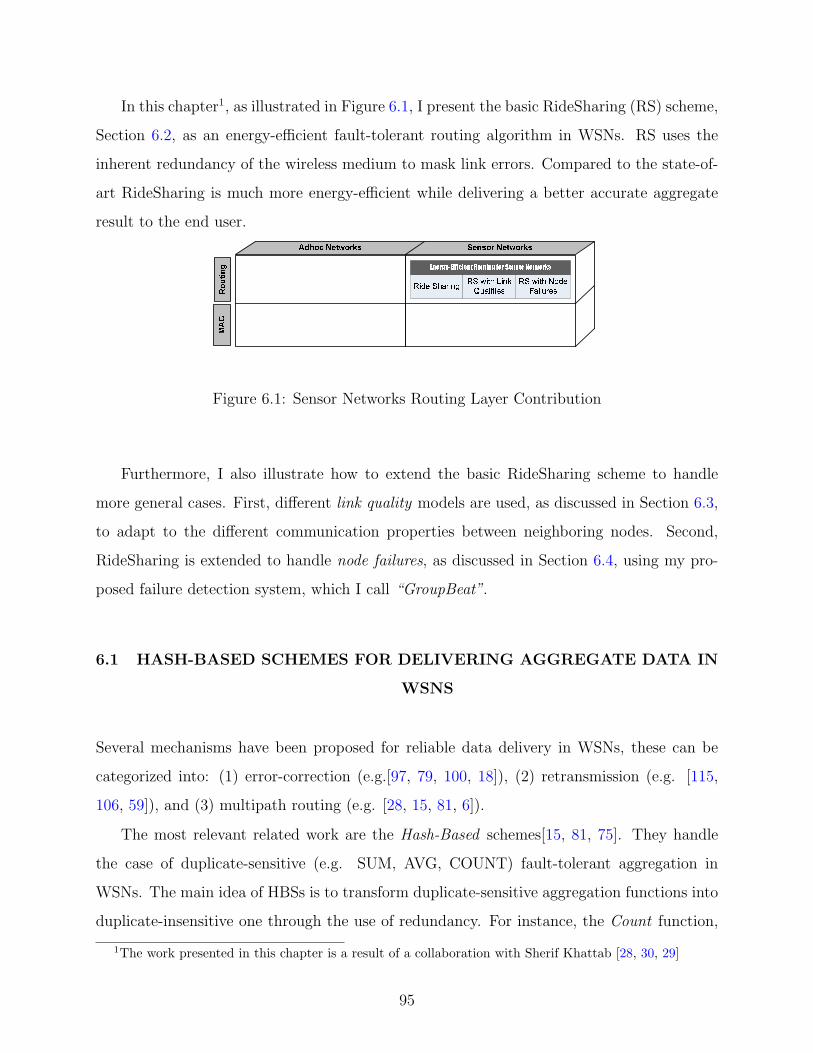
In this chapter1, as illustrated in Figure 6.1, I present the basic RideSharing (RS) scheme,

Section 6.2, as an energy-efficient fault-tolerant routing algorithm in WSNs. RS uses the

inherent redundancy of the wireless medium to mask link errors. Compared to the state-of-

art RideSharing is much more energy-efficient while delivering a better accurate aggregate

result to the end user.

Figure 6.1: Sensor Networks Routing Layer Contribution

Furthermore, I also illustrate how to extend the basic RideSharing scheme to handle

more general cases. First, different link quality models are used, as discussed in Section 6.3,

to adapt to the different communication properties between neighboring nodes. Second,

RideSharing is extended to handle node failures, as discussed in Section 6.4, using my pro-

posed failure detection system, which I call “GroupBeat”.

6.1 HASH-BASED SCHEMES FOR DELIVERING AGGREGATE DATA IN

WSNS

Several mechanisms have been proposed for reliable data delivery in WSNs, these can be

categorized into: (1) error-correction (e.g.[97, 79, 100, 18]), (2) retransmission (e.g. [115,

106, 59]), and (3) multipath routing (e.g. [28, 15, 81, 6]).

The most relevant related work are the Hash-Based schemes[15, 81, 75]. They handle

the case of duplicate-sensitive (e.g. SUM, AVG, COUNT) fault-tolerant aggregation in

WSNs. The main idea of HBSs is to transform duplicate-sensitive aggregation functions into

duplicate-insensitive one through the use of redundancy. For instance, the Count function,

1The work presented in this chapter is a result of a collaboration with Sherif Khattab [28, 30, 29]

95

which is duplicate sensitive, is transformed into a bitwise OR operation (ORing is duplicate-

insensitive: x OR y = x OR (y OR y OR y · · · )).

Figure 6.2: Hash-Based Schemes Count Aggregate

Because straight redundancy would be too expensive with respect to space and energy,

HBSs use hash tables to statistically compress the data. For example, in a Count aggregate,

the ORed bit vectors are generated by hashing each sensor id into one bit in a hash table.

Each value sets a bit in the hash table to 1. Suppose the position of the least significant 0

in the resulting hash table is z. Then, the number of distinct values is estimated as 2z

0.77351

[15]. For higher accuracy, m > 1 hash tables are used. Assume the position of the least

significant 0 is zi in hash table i, and the average of the zi’s is z. The estimated value in this

case is[15]2z

0.77351×m (6.1)

Examples of HBSs are Sketches[15], Synopsis Diffusion[81] and Tributaries and Deltas[75].

In these schemes, sensors broadcast a single message to multiple neighbors simultaneously,

and the value of a specific node is included in the final aggregate result as long as there is at

least one error-free path from this node to the data sink. It should be mentioned that a large

bit vector (e.g., O(log(n)) for Count, where n is the total number of sensors) is attached to

each data message in the network.

6.2 RIDESHARING: ENERGY-EFFICIENT FAULT TOLERANT

ROUTING FOR SENSOR NETWORKS

RideSharing (RS) exploits the inherent redundancy of the shared wireless medium to detect

and correct communication errors with low overhead. When a message between two nodes is

96

lost, one or more other sensors could have correctly overheard the lost message. When some

of the overhearing sensors have not yet transmitted their own values, they can aggregate the

missing value into theirs (RideSharing).

It should be mentioned that the assumption of overhearing sensors (which has also been

adopted in other work, e.g. [26, 18, 6]) does not constrain RS to only dense networks because

such assumption is easily justified when a sensor has more than one neighbor within its range.

In Section 6.2.6 an optimization is presented to be used in low densities, and in Section 6.2.7

RS is simulated for different network densities.

6.2.1 Track Topology

RS organizes sensors in a track graph [25]. A directed edge from node X to node Y , indicates

that Y listens to X’s communication. In a track graph, edges are not only between adjacent

tracks as in [15, 81], but can also exist between sensors in the same track (level).

Figure 6.3: Track Topology

Serving different purposes, edges are classified into three types: primary, backup, and

side edges; primary and backup edges are between a sensor node and its parents (between

adjacent tracks). Side edges exist between parents within the same track. Each sensor selects

one parent (and correspondingly one edge) as its primary parent and zero or more parents

as backups. Primary edges form a spanning tree and deliver the data efficiently as long as

no communication error occurs. If an error occurs in a primary edge, it is possible that some

backup edges have successfully delivered the sent value. Parents coordinate using side edges

so that the missing value is aggregated at most once. It should be noted that a sensor can be

97

a primary parent for some children and at the same time a backup parent for some others.

Also, I assume that errors occur independently in primary, backup and/or side edges2.

6.2.2 Error Detection and Correction

To singal to other nodes, each parent attaches a small bit vector to each data message it sends.

The bit vector efficiently encodes the ids of children whose values have been correctly received

and aggregated. By overhearing the bit vectors over side edges, backup parents detect link

errors when one or more children are missing from the bit vector. Each parent determines the

bit positions of its children inside the other parents’ bit vectors during topology construction,

whereby each parent broadcasts children ids and their bit positions inside its bit vector.

The bit vector contains two bits for each child of which the sensor is primary or backup

parent. The first bit, the e-bit, indicates error in the child’s primary edge. If the primary

parent does not receive from a child, it sets the e-bit for that child to 1. Overhearing the

primary parent signal an error, a backup parent sets its e-bit to 1 as well to propagate the

error signal. The other bit, the r-bit, indicates that the sensor is correcting or helping correct

the error. The detailed use of the e-bit and the r-bit will be explained in the next subsections.

It should be noted that there is a difference in functionality between a backup-parent and

what “backup” means in fault-tolerance literature. Traditionally, a backup is a stand-by

element which operates only whenever an error is detected. In RS case, the backup-parent

is an active sensor having its own children and aggregating its value with the values of its

children whether or not an error occurs; when an error is detected, the backup accounts

for the missed value in the message that it is going to transmit anyway, that is, without

sending extra messages. As a result, the RS overhead is only associated with error detection

(receiving children’s and parents’ messages), while there is no overhead associated with error

correction.

2This assumption is relaxed in Section 6.3.2

98

6.2.3 Illustrating Example

As an example, Figure 6.3 shows a sensor C in track T2 with two parents, primary P1 and

backup P2. Assuming no error, both P1 and P2 receive C’s value, but only P1 aggregates it.

Now, assume a link error in the primary edge. P2 will receive the bit vector of P1 over the

side edge P1 ↔ P2, detect that C is missing because the e-bit is set, and correct the error

by aggregating C’s value into its own.

To support duplicate-sensitive aggregation, the errors are corrected in such a way that

every sensor reading is aggregated at most once. When there is only one backup parent, as

in the previous example, the solution is trivial. On the other hand, handling this issue for

more than one backup parent requires coordination between the parents. Two mechanisms,

namely cascaded RS and diffused RS, are proposed to achieve such coordination.

6.2.4 Cascaded RideSharing

In cascaded RS, as long as no error occurs, primary parents aggregate and forward their

children’s values. When an error occurs in a primary link, each backup parent decides

whether or not to correct the error based on its order in a correction sequence. This correction

sequence can be, for example, an ascending order of parent ids. The first backup parent in

this sequence (parent with smallest id) attempts error correction first. Had the first backup

parent not received the child’s value, or not detected the error, the second backup parent

attempts the correction, and so on. Deciding the correction sequence based on other criteria

(e.g., link qualities) is discussed in Section 6.3.

The cascaded RS can be viewed as if each backup parent is assigned a virtual token

for each child. The token is released when the parent transmits without aggregating the

child’s value. Every parent that hears a token released acquires the token. A backup parent

aggregates a child’s value and sets the r-bit if (1) it has received a bit vector with the e-bit

set (indicating an error in the primary link), (2) it has correctly received the child’s value,

and (3) it has acquired tokens of all parents preceding it in the correction sequence. Token

release is detected when the r-bit is unset. To avoid multiple counting, if a parent fails to

acquire preceding parents’ tokens, it takes no corrective action.

99

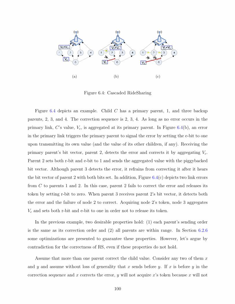
(a) (b) (c)

Figure 6.4: Cascaded RideSharing

Figure 6.4 depicts an example. Child C has a primary parent, 1, and three backup

parents, 2, 3, and 4. The correction sequence is 2, 3, 4. As long as no error occurs in the

primary link, C’s value, Vc, is aggregated at its primary parent. In Figure 6.4(b), an error

in the primary link triggers the primary parent to signal the error by setting the e-bit to one

upon transmitting its own value (and the value of its other children, if any). Receiving the

primary parent’s bit vector, parent 2, detects the error and corrects it by aggregating Vc.

Parent 2 sets both r-bit and e-bit to 1 and sends the aggregated value with the piggybacked

bit vector. Although parent 3 detects the error, it refrains from correcting it after it hears

the bit vector of parent 2 with both bits set. In addition, Figure 6.4(c) depicts two link errors

from C to parents 1 and 2. In this case, parent 2 fails to correct the error and releases its

token by setting r-bit to zero. When parent 3 receives parent 2’s bit vector, it detects both

the error and the failure of node 2 to correct. Acquiring node 2’s token, node 3 aggregates

Vc and sets both r-bit and e-bit to one in order not to release its token.

In the previous example, two desirable properties hold: (1) each parent’s sending order

is the same as its correction order and (2) all parents are within range. In Section 6.2.6

some optimizations are presented to guarantee these properties. However, let’s argue by

contradiction for the correctness of RS, even if these properties do not hold.

Assume that more than one parent correct the child value. Consider any two of them x

and y and assume without loss of generality that x sends before y. If x is before y in the

correction sequence and x corrects the error, y will not acquire x’s token because x will not

100

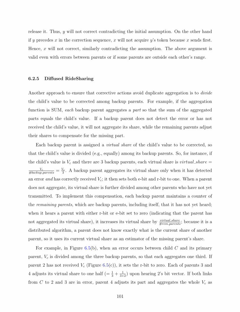
release it. Thus, y will not correct contradicting the initial assumption. On the other hand

if y precedes x in the correction sequence, x will not acquire y’s token because x sends first.

Hence, x will not correct, similarly contradicting the assumption. The above argument is

valid even with errors between parents or if some parents are outside each other’s range.

6.2.5 Diffused RideSharing

Another approach to ensure that corrective actions avoid duplicate aggregation is to divide

the child’s value to be corrected among backup parents. For example, if the aggregation

function is SUM, each backup parent aggregates a part so that the sum of the aggregated

parts equals the child’s value. If a backup parent does not detect the error or has not

received the child’s value, it will not aggregate its share, while the remaining parents adjust

their shares to compensate for the missing part.

Each backup parent is assigned a virtual share of the child’s value to be corrected, so

that the child’s value is divided (e.g., equally) among its backup parents. So, for instance, if

the child’s value is Vc and there are 3 backup parents, each virtual share is virtual share =

Vc

#backup parents= Vc

3. A backup parent aggregates its virtual share only when it has detected

an error and has correctly received Vc; it then sets both e-bit and r-bit to one. When a parent

does not aggregate, its virtual share is further divided among other parents who have not yet

transmitted. To implement this compensation, each backup parent maintains a counter of

the remaining parents, which are backup parents, including itself, that it has not yet heard;

when it hears a parent with either r-bit or e-bit set to zero (indicating that the parent has

not aggregated its virtual share), it increases its virtual share by virtual share#rem parents

; because it is a

distributed algorithm, a parent does not know exactly what is the current share of another

parent, so it uses its current virtual share as an estimator of the missing parent’s share.

For example, in Figure 6.5(b), when an error occurs between child C and its primary

parent, Vc is divided among the three backup parents, so that each aggregates one third. If

parent 2 has not received Vc (Figure 6.5(c)), it sets the r-bit to zero. Each of parents 3 and

4 adjusts its virtual share to one half (= 13

+ 13×2

) upon hearing 2’s bit vector. If both links

from C to 2 and 3 are in error, parent 4 adjusts its part and aggregates the whole Vc as

101

(a) (b) (c) (d)

Figure 6.5: Diffused RideSharing

shown in Figure 6.5(d).

As a proof of correctness, the total aggregated value of each child never overshoots Vc. If

there is no error, Vc is aggregated only at the primary parent. Upon detecting an error, if all

backup parents aggregate their shares, the total aggregated value is also Vc, the sum of the

virtual shares. When a parent fails to aggregate its share, the virtual shares of the remaining

backup parents are increased. The total increase, however, never exceeds the missed share,

because the local remaining parents counter (the denominator) never underestimates the

actual value.

6.2.6 RideSharing Enhancements

In RS, backup parents correct primary link error. RS’s fault-tolerance and accuracy can be

further improved by applying any of the following optimizations:

6.2.6.1 Co-tracking Normally, each child selects its parents from the adjacent track

that is closer to the data sink (e.g., in Figure 6.3, C in track T2 selects P1 and P2 in track

T1). When there is only one3 reachable sensor in that track, the child selects parents from

its own track. This co-tracking is to allow the child’s value to be corrected had there been

an error in the primary link. The primary parent is selected from the same track, so that

3The threshold is set to one here for illustration. In general co-tracking can be used whenever the numberof reachable parents is below a design threshold that can be larger than one.

102

the backup parent in the adjacent track will have a chance to correct an error in the primary

link. To avoid loops, whereby two sensors end up selecting each other as primary, the parents

selected from the same track have a higher node id than the child.

6.2.6.2 Parent Clique The ability of a backup parent to correct an error depends on

hearing the other parents. Thus, to increase the probability of error correction, it is possible

for each child to select parents that hear each other (i.e., the parents thus form a clique).

This optimization is proposed because a backup parent needs to overhear a bit vector with

the e-bit set before attempting to correct an error. In cascaded RS, the backup parent has

to acquire the preceding parents’ tokens and in diffused RS, by hearing other parents, each

backup parent maintains an accurate estimate of the number of remaining parents.

6.2.6.3 Transmission Order To increase the probability that an error is corrected,

backup parents should send their messages after primary parents. Such transmission order

can be achieved deterministically by a TDMA scheme or probabilistically by a prioritized

contention-based scheme.

A naive but inefficient (longer delay) TDMA allocates a time slot for each node. For

example, the schedule starts by the farthest track from the data sink and proceeds inward,

whereby the first sensor to send in each track is the one with the smallest id within the track

followed by the second smallest and so on. In such transmission order, each child selects the

primary parent as the parent with the smallest id. TDMA-ASAP, discussed in Chapter 5,

can also be used. In TDMA-ASAP a graph-coloring algorithm is used to assign transmission

slots for nodes. Nodes outside each other’s range can transmit simultaneously (have the

same color). Thus, the schedule is compacted and the end-to-end delay is minimized. In this

scheme, the child selects the parents with distinct colors and the primary parent is selected

to be the one transmitting first.

The transmission order can also be enforced with a contention based scheme (e.g., BLAM

as discussed in Section 3.2) in which each node is assigned a priority (contention window size)

to access the medium. The transmission priorities can be based on id’s, residual energies

or any other criteria. In this case the child picks as primary the parent with the highest

103

priority in the child’s parents list.

6.2.7 Evaluation

In the evaluation I compare the RS scheme (cascaded and diffused) with a hash-based scheme,

namely Synopsis Diffusion (SD). I present results for two SD schemes, SD-20 [81] and SD-

40 [75], the first uses 20 hash tables per message while the second uses 40 hash table (increased

accuracy but with higher overhead). The spanning tree approach [73] (which provides no

fault-tolerance) is used as the basis for the comparison. The following metrics are used to

evaluate the performance of the different schemes:

• Average relative RMS, that is, the average root mean square error in the aggregate result,

normalized to the correct result value. This metric is a good measure of the accuracy of

the estimated value.

• Average energy per node per epoch, that is, the total transmission, listening, and reception

energy consumed per node averaged over the number of epochs. This metric reflects the

overhead of each scheme.

The RS and the SD schemes are implemented in CSIM [98] using the TAG simulator[73].

In the the TAG model [73], sensor readings are aggregated to the data sink every epoch. I

present results for COUNT query. It should be mentioned that I am comparing against the

best aggregate result for SD (COUNT); other aggregates (e.g., SUM) have a larger RMS for

SD but not for RS.

6.2.7.1 Simulation Setup In the simulation analysis, a number of sensor nodes are

randomly distributed in a 300 × 300 ft area. The radio range of each node is assumed

to be 30 ft. The data sink is the nearest node to the center. Each simulation run has 100

epochs, 300 msec each, and the results shown are the average of 10 runs. Based on the Mica2

motes Power model[102], the power consumption is 65 mW for transmission, 21.0 mW for

listening and reception, and 0 mW in sleep mode. The network bandwidth is assumed to be

38.4 Kbps [12]. The payload is different based on the scheme used; for the spanning tree it

is 2 bytes, for RS it is 2 bytes + 2 bits × number of children, for the SD-20 it is 12 bytes (20

104

bit vectors ×2 bytes each ×0.3 compression ratio) [15], and for SD-40 it is 24 bytes. Similar

to the SD paper [81]; link errors are independent and uncorrelated and links between track

1 and the data sink are error-free. In the simulations I varied the link error rate, the total

number of sensor nodes, the number of participating nodes in the query, and the maximum

number of parents per node.

6.2.7.2 Accuracy Comparison First, let’s consider the case when the total number

of nodes is 1000 and all of them are participating in the query. Figure 6.6 shows the rel-

ative RMS versus the link error rate. The error bars represent 90% confidence intervals.

As expected, when the error rate increases the performance of the spanning tree severely

degrades. The RMS reaches 67% for a link error rate of 35%. This is because the spanning

tree topology is not robust against errors, and if a packet is lost, so is a complete subtree of

values which increases the error in the final result.

0

10

20

30

40

50

60

70

80

0 0.05 0.1 0.15 0.2 0.25 0.3 0.35

RM

S E

rror

(%

)

Link Error Rate

Tree

SD-20

Diffused RideSharing

Cascaded RideSharing

SD-40

Figure 6.6: RideSharing vs. Hash-Based RMS for 100% Participation

(parents/node = 3, total nodes = 1000)

SD, on the other hand, is robust to link losses. The value of a node will be delivered as

long as there exist at least one error-free path from this node to the sink. SD-20 achieves

a relative RMS of about 12.5% at a link error rate upto 10%, while SD-40 achieves 7.5%.

105

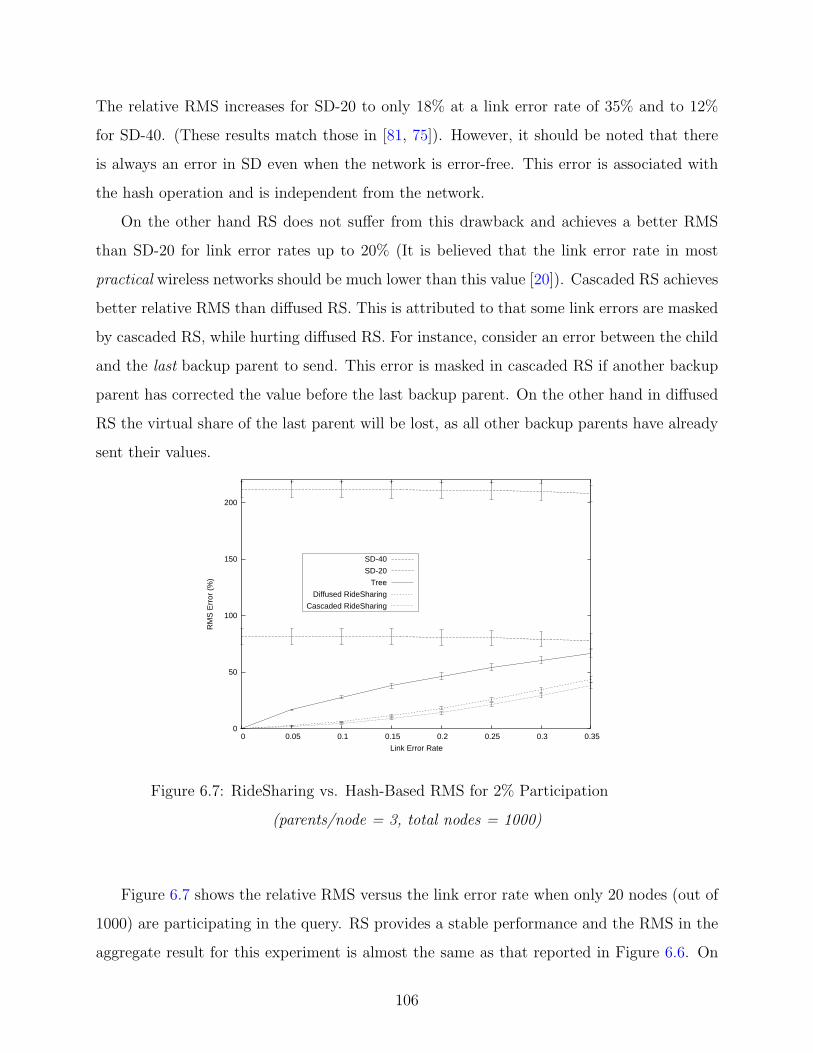
The relative RMS increases for SD-20 to only 18% at a link error rate of 35% and to 12%

for SD-40. (These results match those in [81, 75]). However, it should be noted that there

is always an error in SD even when the network is error-free. This error is associated with

the hash operation and is independent from the network.

On the other hand RS does not suffer from this drawback and achieves a better RMS

than SD-20 for link error rates up to 20% (It is believed that the link error rate in most

practical wireless networks should be much lower than this value [20]). Cascaded RS achieves

better relative RMS than diffused RS. This is attributed to that some link errors are masked

by cascaded RS, while hurting diffused RS. For instance, consider an error between the child

and the last backup parent to send. This error is masked in cascaded RS if another backup

parent has corrected the value before the last backup parent. On the other hand in diffused

RS the virtual share of the last parent will be lost, as all other backup parents have already

sent their values.

0

50

100

150

200

0 0.05 0.1 0.15 0.2 0.25 0.3 0.35

RM

S E

rror

(%

)

Link Error Rate

SD-40

SD-20

Tree



Figure 6.7: RideSharing vs. Hash-Based RMS for 2% Participation

(parents/node = 3, total nodes = 1000)

Figure 6.7 shows the relative RMS versus the link error rate when only 20 nodes (out of

1000) are participating in the query. RS provides a stable performance and the RMS in the

aggregate result for this experiment is almost the same as that reported in Figure 6.6. On

106

the other hand SD has a very serious drawback. The relative RMS of SD-20 jumps to 80%

while for SD-40 it is more than 200%. This huge error is much worse than that achieved

when using a non-fault tolerant spanning tree. This surprising result is because the hash

vector size sets a limit on the minimum count that can be estimated accurately (for details

refer to [28]).

It should be mentioned that determining the number of participating nodes beforehand

is not a trivial problem because (1) it is data dependent; for example, a node might send its

value only when a significant change occurs [100], and (2) it is query dependent; for example,

a query can be dispatched and not all sensors satisfy its WHERE clause. RS, on the other

hand, does not need such dynamic tuning and provides an acceptable RMS for any number

of participating nodes.

6.2.7.3 Overhead Comparison To evaluate the energy consumed in communication

for each scheme, Figure 6.8 shows the average energy consumption per sensor per epoch in

the network, when 1000 sensors participate in the query.

0

0.1

0.2

0.3

0.4

0.5

0.6

0.7

0 0.05 0.1 0.15 0.2 0.25 0.3 0.35

Ave

rage

Sen

sor

Ene

rgy

per

Epo

ch (

mJ)

Link Error Rate

SD-40

SD-20

RideSharing

Tree

Figure 6.8: RS vs. Hash-Based Average Energy Consumption per Sensor

(parents/node = 3, total nodes = 1000, participation = 100%)

As shown in the figure, the spanning tree consumes the least energy because each node

107

is transmitting to only one parent, and it has the smallest message size (no added bit

vectors). RS consumes approximately 50% the energy consumed in SD-20 and almost 25%

that consumed in SD-40. Although RS uses the same number of parents as SD, it only adds

a small bit vector (2 bits per child). SD, on the other hand, consumes the highest energy

overhead, as it uses a large number of hash bit vectors and the resulting message size is

large even when compression/decompression is applied at each node. It should be clear that

the energy consumption for cascaded and diffused RS is the same because the two schemes

have the same number of awake nodes and the same number of messages transmitted and

received.

6.2.7.4 Effect of Network Density and Number of parents Figure 6.9 shows the

effect of the network density on the performance of RS. At low density (total nodes =

300) the probability that a node finds 3 parents decrease, and consequently, so does the

probability of error correction (because there are no backup parents to mask link errors);

as a result, the RMS increases. As the network density increases the accuracy of the RS

scheme improves because more nodes can find backup parents. It should be noted that the

effect of the network density on RS is the almost the same as that on SD. This is because

SD needs multiple parents per node so that the hashed value of a sensor node is not lost

when an error occur. In fact, any fault-tolerant scheme needs some form of redundancy to

be able to detect and/or correct errors.

Figure 6.10 evaluates the effect of changing the total number of parents on the perfor-

mance of RS. Max Parents indicated in figure is an upper bound on the number of parents

per node. The actual number of parents per node might be less than this bound depending

on the network connectivity. As shown in figure, as the number of parents per node increases

the accuracy of both RS and SD improves. Note that RS benefits more than does SD from

increasing the number of parents (e.g., for cascaded RS, RMS decreases from 19.56% @ 3

parents to 11.98% @ 5 parents). This is because increasing the number of parents in SD

decreases the error associated with the network but, on the other hand, it has no effect on

the error associated with the hash operation and the RMS curve for SD flattens as this is

the maximum accuracy that can be delivered using this scheme.

108

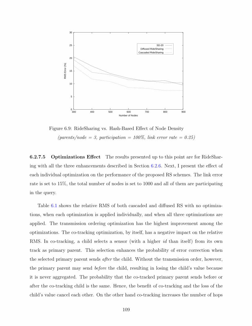
0

5

10

15

20

25

30

300 400 500 600 700 800 900

RM

S E

rror

(%

)

Number of Nodes

SD-20



Figure 6.9: RideSharing vs. Hash-Based Effect of Node Density

(parents/node = 3, participation = 100%, link error rate = 0.25)

6.2.7.5 Optimizations Effect The results presented up to this point are for RideShar-

ing with all the three enhancements described in Section 6.2.6. Next, I present the effect of

each individual optimization on the performance of the proposed RS schemes. The link error

rate is set to 15%, the total number of nodes is set to 1000 and all of them are participating

in the query.

Table 6.1 shows the relative RMS of both cascaded and diffused RS with no optimiza-

tions, when each optimization is applied individually, and when all three optimizations are

applied. The transmission ordering optimization has the highest improvement among the

optimizations. The co-tracking optimization, by itself, has a negative impact on the relative

RMS. In co-tracking, a child selects a sensor (with a higher id than itself) from its own

track as primary parent. This selection enhances the probability of error correction when

the selected primary parent sends after the child. Without the transmission order, however,

the primary parent may send before the child, resulting in losing the child’s value because

it is never aggregated. The probability that the co-tracked primary parent sends before or

after the co-tracking child is the same. Hence, the benefit of co-tracking and the loss of the

child’s value cancel each other. On the other hand co-tracking increases the number of hops

109

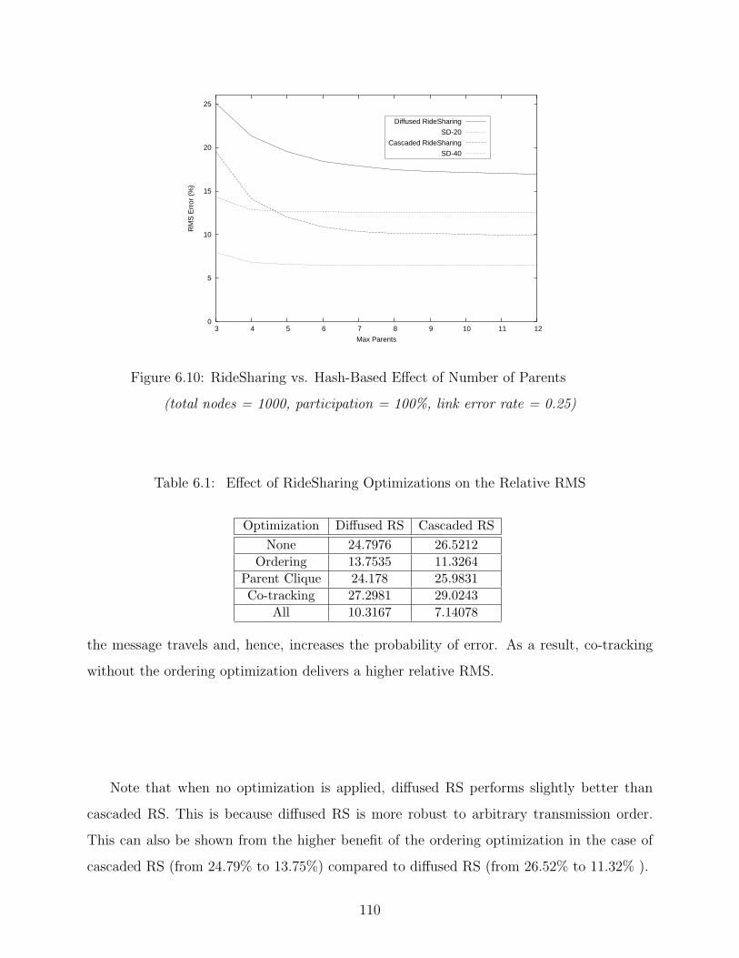
0

5

10

15

20

25

3 4 5 6 7 8 9 10 11 12

RM

S E

rror

(%

)

Max Parents


SD-20


SD-40

Figure 6.10: RideSharing vs. Hash-Based Effect of Number of Parents

(total nodes = 1000, participation = 100%, link error rate = 0.25)

Table 6.1: Effect of RideSharing Optimizations on the Relative RMS

Optimization Diffused RS Cascaded RSNone 24.7976 26.5212

Ordering 13.7535 11.3264Parent Clique 24.178 25.9831Co-tracking 27.2981 29.0243

All 10.3167 7.14078

the message travels and, hence, increases the probability of error. As a result, co-tracking

without the ordering optimization delivers a higher relative RMS.

Note that when no optimization is applied, diffused RS performs slightly better than

cascaded RS. This is because diffused RS is more robust to arbitrary transmission order.

This can also be shown from the higher benefit of the ordering optimization in the case of

cascaded RS (from 24.79% to 13.75%) compared to diffused RS (from 26.52% to 11.32% ).

110

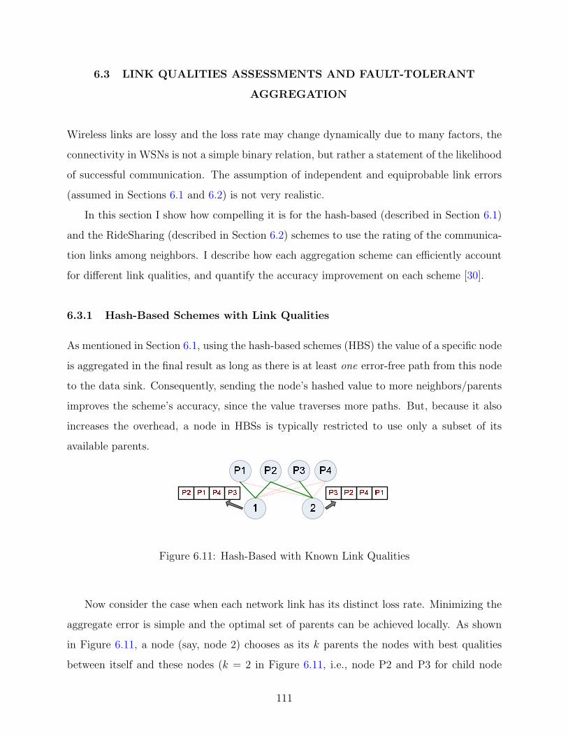
6.3 LINK QUALITIES ASSESSMENTS AND FAULT-TOLERANT

AGGREGATION

Wireless links are lossy and the loss rate may change dynamically due to many factors, the

connectivity in WSNs is not a simple binary relation, but rather a statement of the likelihood

of successful communication. The assumption of independent and equiprobable link errors

(assumed in Sections 6.1 and 6.2) is not very realistic.

In this section I show how compelling it is for the hash-based (described in Section 6.1)

and the RideSharing (described in Section 6.2) schemes to use the rating of the communica-

tion links among neighbors. I describe how each aggregation scheme can efficiently account

for different link qualities, and quantify the accuracy improvement on each scheme [30].

6.3.1 Hash-Based Schemes with Link Qualities

As mentioned in Section 6.1, using the hash-based schemes (HBS) the value of a specific node

is aggregated in the final result as long as there is at least one error-free path from this node

to the data sink. Consequently, sending the node’s hashed value to more neighbors/parents

improves the scheme’s accuracy, since the value traverses more paths. But, because it also

increases the overhead, a node in HBSs is typically restricted to use only a subset of its

available parents.

Figure 6.11: Hash-Based with Known Link Qualities

Now consider the case when each network link has its distinct loss rate. Minimizing the

aggregate error is simple and the optimal set of parents can be achieved locally. As shown

in Figure 6.11, a node (say, node 2) chooses as its k parents the nodes with best qualities

between itself and these nodes (k = 2 in Figure 6.11, i.e., node P2 and P3 for child node

111

2). The assigned parents are then notified by the child node that they were picked for its

hash vector aggregation. During the data collection phase, the child node broadcasts its

hash vector but only the node’s assigned parents will be awake listening to the channel and

aggregating the node’s hash vector into theirs, while other parents (nodes P1 and P4 in this

case) can switch off their transceivers.

6.3.1.1 Evaluation and Simulation Analysis I investigate the performance of a HBS,

namely Synopsis Diffusion (SD)[81], with and without taking into consideration link qual-

ity information. The simulation setup is that used in Section 6.2.7, with one difference:

Link errors among neighboring nodes are assumed to be uniformly distributed in interval

[0,max link error]. In the experiments the max link error is varied within [0, 0.5]. HBSs

with no link qualities (SD-20RandomK and SD-40RandomK ) are compared with HBSs with

link qualities (SD-20BestK and SD-40BestK ), where K is the number of selected parents

per node.

0

5

10

15

20

25

30

0 0.05 0.1 0.15 0.2 0.25

RM

S E

rror

(%

)

Average Link Error

SD-20Random3SD-20Best3


Figure 6.12: HBS with Link Qualities Relative RMS (parents/node = 3, total nodes = 1000)

Figure 6.12 shows the relative RMS as a function of the average link error rate. The

error bars represent 90% confidence intervals. Note that the confidence intervals are large

and independent of the average link qualities. This is because HBSs are a statistical approach

112

to aggregation (the hash tables are a lossy compression method). As shown in Figure 6.12,

taking the link quality among the nodes into consideration slightly improves the performance

of the SD scheme. Because the network is using more reliable paths, it is more probable to

find at least one error free path from every node to the sink. As a result, the RMS error is

smaller with SD-20Best3 than that in the case of SD-20Random3 (and similarly for SD-40).

0

5

10

15

20

25

30

1 2 3 4 5 6 7 8 9 10

RM

S E

rror

(%

)

Number of Parents



Figure 6.13: HBS with Link Qualities Relative RMS vs. No. of Parents

Figure 6.13 presents the effect of changing the number of parents (k) on the performance

of the SD scheme. As shown in the figure, increasing the number of parents per node beyond

3 has almost no effect on the SD accuracy. This saturation in the performance is because the

error is no longer a network error (no errors in all links connecting a node to its parents),

rather, it is a hashing error. These results suggest that in SD, a small number of parents

per node (for example 3) is sufficient to deliver as accurate a result as possible to the sink.

6.3.2 RideSharing with Link Qualities

Similar to HBSs, there is a trade-off in RS between accuracy and overhead: increasing

the number of backup parents improves the accuracy, but it increases the energy overhead.

Other factors that affect the quality of RS (but not the hash-based) are (1) the link qualities

113

between the parents, because in RS the parents listen to each other; and (2) the transmission

schedule (order) among the parents.

The problem of minimizing the error in the aggregate result when the link qualities

among the neighboring nodes are known can be looked upon in two different ways. First, we

can assume that a transmission schedule for the network nodes is given and link qualities

are known between each node and all of its neighbors. The objective is then to select for

each node a subset k of its neighbors to be used as parents (primary and backup). Second,

we can assume that each node in the network assigns itself to a set of parents (known k) and

the link qualities between the network nodes are known. The objective is then to establish

a transmission order among the network nodes to minimize the error in the data message.

Figure 6.14: Minimizing Aggregate Error as a Scheduling Problem

An example is depicted in Figure 6.14, where Nodes 1 and 2 have the same parents

(P1, P2 and P3). Assuming that all link qualities among neighboring nodes qxy are known,

six different transmission schedules (orders) are possible by permutations among the parent

nodes ([P1, P2, P3], [P2, P1, P3], ..., [P3, P1, P2]). Each schedule is equivalent to assigning

a primary parent (node scheduled to transmit first) and backup parents (those scheduled

later) for Nodes 1 and 2. For each schedule we can compute the error in the aggregate result

delivered to the base station. The objective is to choose the schedule that will minimize the

error in the aggregate result. I prove in Section 6.3.2.1, that finding this schedule is NP-hard

and resort to devising a low-overhead, distributed heuristic, as follows.

1. A node only considers the link qualities between itself and its parents. The link qualities

among the parents themselves are ignored.

2. A node at track i selects its parents to be one with the best k links with from track i− 1

(similar to the hash-based schemes). In Section 6.3.2.2 the value k will be investigated.

114

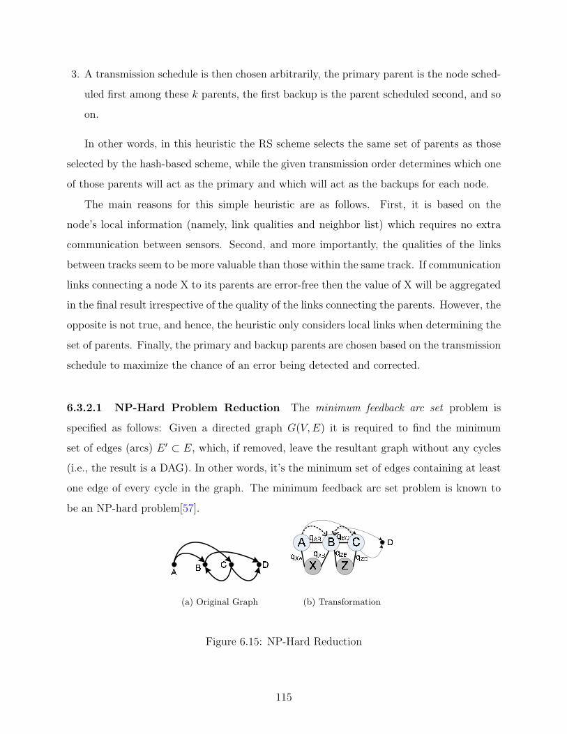
3. A transmission schedule is then chosen arbitrarily, the primary parent is the node sched-

uled first among these k parents, the first backup is the parent scheduled second, and so

on.

In other words, in this heuristic the RS scheme selects the same set of parents as those

selected by the hash-based scheme, while the given transmission order determines which one

of those parents will act as the primary and which will act as the backups for each node.

The main reasons for this simple heuristic are as follows. First, it is based on the

node’s local information (namely, link qualities and neighbor list) which requires no extra

communication between sensors. Second, and more importantly, the qualities of the links

between tracks seem to be more valuable than those within the same track. If communication

links connecting a node X to its parents are error-free then the value of X will be aggregated

in the final result irrespective of the quality of the links connecting the parents. However, the

opposite is not true, and hence, the heuristic only considers local links when determining the

set of parents. Finally, the primary and backup parents are chosen based on the transmission

schedule to maximize the chance of an error being detected and corrected.

6.3.2.1 NP-Hard Problem Reduction The minimum feedback arc set problem is

specified as follows: Given a directed graph G(V, E) it is required to find the minimum

set of edges (arcs) E ′ ⊂ E, which, if removed, leave the resultant graph without any cycles

(i.e., the result is a DAG). In other words, it’s the minimum set of edges containing at least

one edge of every cycle in the graph. The minimum feedback arc set problem is known to

be an NP-hard problem[57].

(a) Original Graph (b) Transformation

Figure 6.15: NP-Hard Reduction

115

Now assume that we are given a directed graph G(V,E), for example the graph in Fig-

ure 6.15(a). For each arc i → j connecting two vertices i, j construct the following network,

as shown in Figure 6.15(b). Specifically, insert node i at vertex i, node j at vertex j and

node k as a child for both nodes i and j such that the following conditions are satisfied:

qki > qkj, and 0 ≤ qij < 1 where qxy is the quality of the link connecting nodes x and y

(qxy = qyx). (In Figure 6.15(b), as an example the transformation is applied for arcs A → B

and C → B. qXA > qXB, & 0 ≤ qAB < 1, and similarly, qZC > qZB, & 0 ≤ qCB < 1).

Now consider an example network ABX. If RS is used then node X will pick A as its

primary parent and B as its backup parent if A is scheduled to transmit first, and vice

versa. If A transmits first then the expected value of X to be aggregated in the final result

is (assuming cascaded RS):

MeanAfirst = Vx · (qXA + (1− qXA)qXBqAB) (6.2)

On the other hand if B was scheduled to transmit first then the expected value is:

MeanBfirst = Vx · (qXB + (1− qXB)qXAqBA) (6.3)

Where Vx is the value at Node X. Now since by construction qXA > qXB and 0 ≤ qAB =

qBA < 1, then MeanAfirst > MeanBfirst. Hence, the error when A transmits first is smaller

than that when it transmits later. Consequently, there is an ordering constraint relation

between nodes A and B (A → B).

Now given the resultant network from the transformation, finding the minimum-error

schedule is equivalent to finding the schedule that satisfies the maximum number (equiva-

lently, violates the minimum number) of ordering constraints (i → j).

Since each node is scheduled to transmit once then, intuitively, any path that traverses

the network nodes in the forward direction of the schedule (i.e., any topological sort of the

nodes) can not have cycles. Now since the optimal schedule minimizes the violations in the

ordering constraints, then, as a result, it minimizes the arcs that traverse in the opposite

direction of the schedule. Hence, finding the minimum set of ordering constraints violations

is equivalent to finding the minimum set of arcs in the reverse direction of the schedule (those

causing cycles). Hence, it is equivalent to the minimum arc feedback set in the original graph.

116

6.3.2.2 Evaluation and Simulation Analysis To evaluate the performance of RideShar-

ing schemes with and without taking into consideration link quality information, the same

simulation setup as Section 6.3.1.1 is used. I compare the following schemes: RS schemes

with link qualities (Cascaded-BestK and Diffused-BestK ) and RS schemes with no link qual-

ities (Cascaded-RandomK and Diffused-RandomK )4.

0

5

10

15

20

25

30

0 0.05 0.1 0.15 0.2 0.25

RM

S E

rror

(%

)

Average Link Error

Diffused-Random3Cascaded-Random3

Diffused-Best3Cascaded-Best3

Figure 6.16: RS with Link Qualities Relative RMS (parents/node = 3, total nodes = 1000)

Figure 6.16 shows the relative RMS as a function of the average link error rate for three

parents. The error bars represent 90% confidence intervals. Note that there is no error in the

aggregate result when the network is error free (unlike the 6-12% error in Section 6.3.1.1).

Moreover, although the heuristic proposed for considering the link quality among the nodes

is very simple, it is very efficient and significantly improves the performance of the RS scheme

(compare Cascaded-Random3 and Cascaded-Best3 ). Note that Cascaded RS achieves better

relative RMS than Diffused RS for both Best3 and Random3 schemes. This is because some

link errors are masked by Cascaded RS, while hurting Diffused RS (for instance, an error

between the child and the last backup parent to send).

Figure 6.17 presents the effect of varying the number of parents (k) on the performance

4In this section I am only analyzing the improvement in the scheme’s accuracy. The energy-consumptionis the same as that evaluated in Section 6.2.7 (i.e., RS consumes approximately 50% the energy consumedin SD-20 and almost 25% that consumed in SD-40.)

117

0

5

10

15

20

25

30

1 2 3 4 5 6 7 8 9 10

RM

S E

rror

(%

)

Number of Parents

Diffused-Random3Diffused-Best3

Cascaded-Random3Cascaded-Best3

Figure 6.17: RS with Link Qualities Relative RMS vs. No. of Parents

of the RS scheme. As shown in the figure, increasing the number of parents per node beyond

a specific value has an insignificant effect on the accuracy. This saturation in performance

is attributed to two reasons: (1) As the number of parents increases, the probability that

all parents hear each other decreases; (2) Based on my heuristic, nodes are added to the list

of backup parents in a decreasing order of their link quality to the child. Consequently, the

rate at which the RMS error decreases gets smaller as more parents are being considered.

6.4 GROUPBEAT: HANDLING NODE ERRORS IN RS

Node outages are frequent in WSNs and can result from different reasons. For instance,

nodes can be depleted from energy, can be physically damaged, or can turn off their radios

to save energy. As a result, detecting node outages and delivering the information to the

end user while those nodes are non-functional is essential.

In WSNs nodes usually exchange some sort of “I am alive” messages and use this simple

heartbeat application to detect node failures. For example, when the nodes are organized

in a spanning tree (e.g., [73]), a child node C detects a failed parent P when it misses

successive heartbeats that should have been sent by P (see Figure 6.18). C can infer that P

118

has failed and can associate itself to another parent (e.g., P1) that can be used to forward

C’s data. However, because wireless links are usually lossy, it is important to distinguish

node failures from intermittent link failures; this is typically done by requiring a number of

missed heartbeats before declaring a node as dead. Consequently, each node has to wait for

a long time delay before declaring a neighbor to be dead. Rost et al. [92], reported that in

typical deployments of WSNs, on average twelve successive heartbeats, each with a period

of 3 seconds, have to be lost before a node declares a neighbor dead with a false negative5

accuracy of about 7%. During this time delay and until the failed nodes are bypassed by

their neighbors, all the data packets originating at or being forwarded by these failed nodes

are lost.

In this section I present and analyze “GroupBeat”, a scheme to detect node failures

accurately, energy-efficiently, and faster than direct heartbeats, allowing for delivering the

sensed data from the rest of the network nodes in the presence of a subset of failed nodes.

In GroupBeat, multiple neighbors monitor each node and the node’s health is decided upon

collectively. Moreover, when GroupBeat is combined with RideSharing (see Section 6.2) data

is delivered even before failed nodes are bypassed by the health monitoring system. Further-

more, a low-overhead energy-efficient implementation of GroupBeat, namely “communication

by signaling”, is proposed and results of applying it to MICA2 motes are provided.

6.4.1 GroupBeat: General Idea and Overview

The main idea of GroupBeat is to make use of the available inherent wireless path redundancy

to improve both the accuracy and the delay of the failure detection system. In GroupBeat

instead of relying on the direct path between the sender and the receiver of an “I am alive”

message, other available redundant paths can relay the same information to the intended

receiver. In effect, using GroupBeat, multiple neighbors monitor each node and the node’s

health is determined collectively with better accuracy than direct heartbeat.

A heartbeat between a sender node, S, and a receiver node, R, can be missed due to

two possible reasons: (a) because a communication error has occurred in the wireless link

5A false negative occurs when a node is falsely declared dead, while this node is still alive

119

S-R, or (b) because node S has failed. In the former case, one or more other nodes might

have correctly overheard the lost heartbeat message. These overhearing nodes can then

collaboratively decide whether node S is still alive. If node S actually died, none of the

overhearing sensors receives the heartbeat, and similarly, a collective decision can affirm this

failure.

Figure 6.18: GroupBeat Network Example

In order to illustrate the idea, consider the network example shown in Figure 6.18. When

the network is error-free node C sends its data to P which aggregates C’s value into its own

before forwarding the aggregate to the next level. C is monitoring (thorough heartbeats

sent by P ) the health status of P and when P fails C is supposed to route its data over

another alternate path (parent P1, for example). It is important to know that for duplicate

sensitive aggregates (e.g. SUM, AVG, COUNT), C’s value has to be aggregated only once

(i.e., at either P or P1 but not both). The objectives of my system are (1) to inform C that

P has failed as soon as possible, and (2) to correctly aggregate C’s value until C decides to

establish its parent relationship with another node (e.g., P1 instead of P ).

Clearly, using direct heartbeats, C depends on the link P − C to determine the health

status of P , hence, it can not differentiate the case of P failing from a communication error

in this one-hop link. GroupBeat, on the other hand, exploits all the available two-hop paths

from P to C (for example, P − P1 − C and P − C2 − C) and redundantly forwards the

heartbeat of P over these paths. In this case, if P is alive, communication errors have to

occur simultaneously in the paths P − C, P − P1− C, and P − C2− C for P to be falsely

120

declared failed. There is a much lower probability of all these links failing simultaneously,

and hence the false negative probability is significantly reduced. Interested readers can

refer to my paper[29], where analytical models are presented to compare the false negative

probability of GroupBeat Scheme to that of direct HeartBeat scheme for the case of both

uncorrelated as well as correlated link errors. These models were not included in this thesis

for brevity.

Several issues should be mentioned, now that the main idea has been presented. First, the

assumption of overhearing sensors (which has also been adopted in other work, e.g. [26, 18, 6])

does not constrain GroupBeat to only dense networks because such assumption is easily

justified when a sensor has more than one neighbor. In the worst case (no redundant paths),

GroupBeat accuracy is the same as that of direct heartbeat.

Second, the health information of a node is duplicate insensitive. That is, if we assume

that P ’s health can be conveyed as 1 or 0, corresponding to P being alive or dead, then

C can combine P ’s health information received from P , P1 and C2 by ORing the health

bit received from these nodes. Consequently, the health information can be redundantly

transmitted over multiple paths without causing an error.

Third, different schemes can be used to implement GroupBeat. These differ in when

and how to convey the health information of a node through the other redundant paths.

In the next section, I propose using what I call “communication by signaling” as an effi-

cient low-overhead implementation (Interested readers can refer to [29] for other possible

implementations). .

6.4.2 GroupBeat using Communication by Signaling

In “communication by signaling”, the transmission slot of each node (during which the node

is supposed to send its heartbeat) is extended by a short health-band, to convey the health

status of that node. To illustrate the scheme, consider again the network in Figure 6.18. Node

P transmits in its assigned slot and all the nodes that have overheard P will simultaneously

transmit during the health-band, as shown in Figure 6.19. The intended receiver (C) will

be awake (waiting to receive the health status of P ), continuously monitoring the received

121

signal strength (RSSI) sampled by its radio transceiver. When the direct neighbors of P

(P1 & C2) transmit (either simultaneously or individually) in the health-band, the RSSI

sampled by C will have a higher value than the current estimate of the background noise

level, indicating that P is alive, even if an error in link P − C has occurred. When P fails

none of the nodes will transmit in the health-band, and, as a result, the failure of node P is

conveyed by the silence of all its neighbors.

Figure 6.19: Communication By Signaling Slot Extension

It should be noted that C will not be able to receive meaningful data when P1 and C2

are simultaneously transmitting. Nevertheless, C does not interpret the data transmitted

and only monitors the elevation (if any) of the channel RSSI value to signal an alive node.

In order to show the feasibility of the “communication by signaling”, this scheme is

implemented on Mica2 sensor motes. Mica2 motes use ATmega128L as their micro-controller,

the Chipcon CC1000 radio transceiver, and run TinyOS, an open-source operating system

designed for WSNs. m nodes (m = [1, 5]) are positioned in a circle (radius = 4 m) around

a receiver sensor. The MAC protocol in TinyOS is altered in two ways: (1) The radio stack

is bypassed to transmit a GroupBeat pulse, rather than a regular message. For that the

pulse width is changed in byte increments until the appropriate length of the GroupBeat

pulse is verified. (2) The nodes are altered to simultaneously transmit a GroupBeat signal,

to indicate that a neighbor is alive, without waiting for a Clear Channel Assessment (CCA)

signal before transmitting. At the receiving end (the center node) the received signal strength

(RSSI) samples are recorded, for a 24-hours period. The experiments were conducted in an

indoor office environment.

The empirical results show that the RSSI values sampled increased by more than 130

dBm, when one or more motes were simultaneously transmitting. The RSSI values are a

122

trustworthy measurement, because there were no false positives. That is, I couldn’t encounter

a single instance of an elevated background noise level of a comparable value. Moreover, it

is observed that a GroupBeat pulse width of 1 − 2 bytes is enough to convey the health

information. Note that the minimum size data message (0 bytes payload) is 17 bytes.

6.4.3 Combining RideSharing and GroupBeat

Although efficient, RideSharing’s (see Section 6.2) main shortcoming is that it can only

handle link errors and can not deal with node failures. A link error between a child node

C and a parent node P1 is detected when P1 sends its data message indicating that the

aggregate is missing C’s value. However, when node P1 fails, it will not send any message,

and a neighboring node, X, will not be able to detect and correct this error, as node X can

not differentiate between P1 failing and a link error in the link P1−X.

The general idea of combining GroupBeat and RideSharing is as follows. If node X

receives no GroupBeat signaling that a node P1 is suspected to be failed, X simply treats

this signal as if the error bit(s) in P1’s message is set. That is, if X is a backup parent with

P1 for some child C, X will aggregate C’s value into X’s message before sending its message

to its parent. Clearly, when combining GroupBeat with RideSharing, no data items are lost,

and the correct aggregate is delivered to the base station (with the exception of the failed

node’s own value). This is also true when a percentage of the network nodes are in error,

as long as the network is not partitioned. The combined scheme continues to deliver the

information until the children nodes bypass the failed parents in their routes to the root.

Note that primary and backup parents are already awake according to RideSharing and

these nodes listen to and forward the GroupBeat signaling. As a result, the energy overhead

of combining GroupBeat with RideSharing is slightly (10%) higher than that of RideSharing

alone. This increase in energy consumption is due to the fact that data slots have been

extended with short signaling health-bands, as discussed in Section 6.4.2. The energy con-

sumption trend shown in Figure 6.8 remains the same; RS consumes approximately6 55%

the energy consumed in SD-20 and almost 27.5% that consumed in SD-40.)

6These energy consumption figures are 10% higher than that evaluated in Section 6.2.7 due to the overheadof GroupBeat.

123

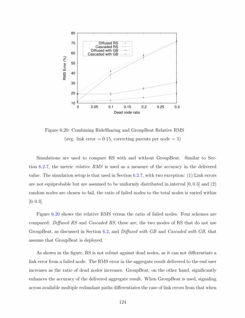
10

20

30

40

50

60

70

80

0 0.05 0.1 0.15 0.2 0.25 0.3

RM

S E

rror

(%)

Dead node ratio

Diffused RSCascaded RS

Diffused with GBCascaded with GB

Figure 6.20: Combining RideSharing and GroupBeat Relative RMS

(avg. link error = 0.15, correcting parents per node = 5)

Simulations are used to compare RS with and without GroupBeat. Similar to Sec-

tion 6.2.7, the metric relative RMS is used as a measure of the accuracy in the delivered

value. The simulation setup is that used in Section 6.2.7, with two exception: (1) Link errors

are not equiprobable but are assumed to be uniformly distributed in interval [0, 0.3] and (2)

random nodes are chosen to fail, the ratio of failed nodes to the total nodes is varied within

[0, 0.3].

Figure 6.20 shows the relative RMS versus the ratio of failed nodes. Four schemes are

compared: Diffused RS and Cascaded RS, these are, the two modes of RS that do not use

GroupBeat, as discussed in Section 6.2, and Diffused with GB and Cascaded with GB, that

assume that GroupBeat is deployed.

As shown in the figure, RS is not robust against dead nodes, as it can not differentiate a

link error from a failed node. The RMS error in the aggregate result delivered to the end user

increases as the ratio of dead nodes increases. GroupBeat, on the other hand, significantly

enhances the accuracy of the delivered aggregate result. When GroupBeat is used, signaling

across available multiple redundant paths differentiates the case of link errors from that when

124

nodes have failed. When a node detects that a neighbor has failed, it acts as if the error bits

were set in the failed node bit-vector and RS acts accordingly to mask this error. Hence, the

improvement in the aggregate delivered.

6.5 CONCLUSION

In WSNs typically a spanning tree routing structure is used to collect the individual sensors

readings to the end-user located at the root of the tree. Moreover, sensor measurements

are often aggregated within the network (in-network processing) to filter redundancy and

reduce communication overhead and energy consumption. Unfortunately, communication

errors and node failures are frequent in WSN and a packet loss can result in the loss of the

result of a complete subtree of values leading to an unacceptable result being reported to

the end-user.

In this chapter, I presented different schemes to be used for energy-efficient reliable

routing of data in WSN. The basic RideSharing scheme is proposed to handle the case of

communication errors and link failures. An extension of the basic RideSharing proposed

to adapt to the different communication properties between neighboring nodes. Finally,

GroupBeat is presented to handle the case of node failures and is combined with RideSharing

for data delivery in presence of failed nodes even before they are bypassed by the nodes’

health monitoring system.

125

7.0 CONCLUSIONS AND FUTURE WORK

Adhoc and sensor networks are wireless infra-structureless networks in which a system of

wireless hosts rely on each other to setup the network and establish and maintain communi-

cation paths between nodes. ASNs are expected to have significant impact on the efficiency

of many military and civil applications. However, one of the most critical design issues of

ASNs is the limited nodes’ energy supply. The functioning lifetime and the usability of the

network strictly depend on the network energy-efficiency.

This dissertation summarizes and presents my doctoral work; energy-efficient design

of adhoc and sensor networks. It first highlights the sources of wasted energy in a

wireless node and then it presents how each of these energy-inefficiencies are handled. My

work spans two layers of the network protocol stack; the Medium Access (MAC) Layer and

the Routing Layer.

First, I focused on the energy inefficiencies at the MAC layer for MANETs. I inves-

tigated the problem of optimizing the transmission energy and proposed a unified inter-

ference/collision model for the MAC protocol. Using this model the optimal transmission

energy is evaluated. I also highlighted the significance of wasted energy in collisions and

proposed BLAM as an energy-efficient extension to the IEEE 802.11 MAC protocol. BLAM

reduces contention between low-energy and high-energy nodes and saves the energy wasted

in collisions and collision resolution.

Second, I focused on energy inefficiencies at the routing layer for MANETs. I highlighted

the Flooding-Waves problem for cost-based energy-efficient routing protocols. I proposed the

Delayed-Forwarding scheme as a near-optimal solution to this problem.

Since WSNs might have some unique characteristics and particular applications that

make them distinct from MANETs. My proposed schemes for WSNs are different from that

126

proposed for MANETs. First, I focused on the MAC layer for WSNs. I proposed TDMA-

ASAP as an energy-efficient MAC protocol for WSNs. TDMA-ASAP targets the wasted

idle-listening and overhearing energies. It allows for an adaptive WSN with quick response

times in the case of an event reporting, and energy conservation during times of minimal

activity.

Second, I focused on the routing layer for WSNs. I presented the RideSharing energy-

efficient fault-tolerant routing framework for WSNs which, compared to the state-of-art, is

much more energy-efficient while delivering a better accurate aggregate result to the end

user. Furthermore, I also presented how to extend the basic RideSharing scheme to handle

different communication properties and to handle node failures.

7.1 CONTRIBUTIONS

In summary, the contributions of my doctoral work to the state of the art in energy-efficient

ASNs are as follows:

• Proposing an analytical model for the IEEE 802.11 MAC protocol taking into consider-

ation both collisions and interference. The same analytical framework can be extended

to model different network configuration scenarios or to model other contention-based

MAC protocols1 (e.g. IEEE 802.11e). To the best of my knowledge, this is the first work

to consider the combined effect of collisions and interference

• An energy-efficient extension is proposed for the 802.11 to account for wasted energy in

collisions. This extension, BLAM, is backward compatible with the 802.11 and can be

easily incorporated in this widely used protocol.

• Identifying the Flooding-Waves problem in cost-based routing, and proposing the Delayed-

Forwarding solution for it. To the best of my knowledge, this is the first work to consider

this problem.

• Proposing TDMA-ASAP as a new energy-efficient MAC protocols for WSNs. TDMA-

ASAP combines the contention-based, contention-free and sleep-based MAC protocols

1In this dissertation, for example, this model has been extended to model BLAM.

127

together in a hybrid near-optimal protocol for these networks.

• Proposing the RideSharing as an energy-efficient fault-tolerant routing scheme for WSNs

and analyzing how to account for different communication qualities among the nodes.

• Proposing GroupBeat as a node failure detection system for WSNs. GroupBeat detects

node failures accurately, energy-efficiently, and faster than the state-of-art in WSNs.

• The concept of communication by signaling is proposed and empirically tested on MICA2

sensor motes. Communication by signaling is used to convey the health status of a node

in GroupBeat. To the best of my knowledge, this is the first work to propose the using

of signaling.

• Proposing the combined scheme of RideSharing and GroupBeat. This new combined

scheme delivers the data to the end user even before failed nodes are bypassed by the

health monitoring system.

7.2 KEY QUESTIONS: REASONING VS. INTUITION

Aside from devising techniques to maximize the network lifetime and increase the usability

of ASNs, my research poses some fundamental questions. One of the main themes that my

research introduces is “intuitions are not always true”. Some ideas, at first, might seem very

appealing, but, as the work in this dissertation shows, considerate thinking has to be applied

first before any of these ideas is adopted.

My work on the energy-efficient MAC layer for MANETs poses the first fundamental

question: “Can the minimum be non-optimal?”. Intuitively, using the minimum transmis-

sion energy at each node should minimizes the total transmission energy in the network.

However, as shown in Chapter 3, the minimum transmission energy is not always optimal.

An extra energy, to overcome collisions and interference, might be needed as a side-effect of

using the minimum transmission energy and, consequently, the overall transmission energy

consumption might increase.

My work on the energy-efficient routing layer for MANETs questions the correctness

of another principal: “energy-efficient schemes consumes less energy than energy-oblivious

128

ones.”. Intuitively, an energy-efficient scheme has to be more “efficient” than an energy-

oblivious one. However, as shown in Chapter 4, an energy-efficient scheme should not

be applied blindly. First we have to consider the overhead associated with it because this

overhead can outweigh any of its promised gains.

The final fundamental principle that my work questions is: “Collided frames are garbled

useless data.”. In typical MAC protocols when a packet collision occurs that data is lost and

collided nodes re-schedule their transmission. In Chapter 6 I show that collided frames are

not always useless and can be used to convey information to other nodes.

7.3 FUTURE WORK

Adhoc and sensor networks are an active research area and the problems I considered in this

dissertation can be expanded in various directions. In what follows, I elaborate on promising

extensions to my work.

In Chapter 3 a unified collision/interference model is proposed for MANETs. The net-

work model assumes that (1) a set of network nodes are uniformly distributed in the network

coverage area and (2) the collision window is held constant. These two assumptions can be

relaxed and their effect on the reported results can be evaluated. The first assumption is

used to justify the uniform transmission energy. A specific scenario for a network with given

node positions can be used instead. The second assumption is used to simplify the analytical

formulas. A more accurate form for the probability of transmission per node (e.g., [109]) can

be used instead. Moreover, the unified collision/interference analytical model can be used

to model different contention-based MAC protocols other than the IEEE 802.11.

In Chapter 4, I discussed the flooding-waves problem in energy-efficient cost-based rout-

ing. The flooding-waves is a problem for any cost-based routing. The applicability of the

proposed solution with different delay configuration or a different solution can be investigated

for these other domains. Furthermore, in the same chapter, I proposed using multiplication

of the individual nodes’ costs to account for the residual energies variance along the network

routes. The concept of balanced-energy routing can be be more thoroughly investigated and

different routing metrics can be used.

129

In Chapters 5 and 6 I focused on WSNs having specific characterisitics, namely, tree-

based routing, limited nodes mobility, and in-network processing. The performance of the

proposed schemes (TDMA-ASAP, RideSharing and GroupBeat) are optimized to make use

of these properties. As previously mentioned, WSNs have a wide variety of applications

and various deployments. In some of these domains (e.g. body implant sensors) these

characterisitcs do not hold. New application-sepecific energy-efficient designs for the MAC

and the routing layer (e.g. [66, 67]) can be proposed for these networks.

130

BIBLIOGRAPHY

[1] I.F. Akyildiz, W. Su, Y. Sankarasubramaniam, and E. Cayirci. A Survey on SensorNetworks. IEEE Communications Magazine, 40(8):102–116, August 2002.

[2] M. Arumugam and S. S. Kulkarni. ”self-stabilizing deterministic tdma for sensor net-works”. In 5th European Dependable Computing Conference, 2005.

[3] Stefano Basagni, Imrich Chlamtac, Violet R. Syrotiuk, and Barry A. Woodward. Adistance routing effect algorithm for mobility (DREAM). In Mobicom, 1998.

[4] A. Berfield and D. Mosse. Efficient scheduling for sensor networks. In IWASN, July2006.

[5] Giuseppe Bianchi. Performance analysis of the IEEE 802.11 distributed coordinationfuntion. IEEE JSAC, 18(3), March 2000.

[6] Sanjit Biswas and Robert Morris. ExOR:opportunistic multi-hop routing for wirelessnetworks. In SIGCOMM, 2005.

[7] L. Bononi, M. Conti, and L. Donatiello. A distributed mechanism for power saving inieee 802.11 wireless LANs. In ACM MONET, June 2001.

[8] R. Bruno, M. Conti, and E. Gregori. Optimization of efficiency and energy consumptionin p-persistent CSMA-based wireless LANs. IEEE Trans on Mobile Computing, 2002.

[9] J. Chang and L. Tassiulas. Energy conserving routing in wireless ad-hoc networking.In Infocom, March 2000.

[10] B. Chen, K. Jamieson, H. Balakrishnan, and R. Morris. SPAN:an energy-efficientcoordination algorithm for topology maintenance in ad hoc wireless networks. WirelessNetworks, 2002.

[11] C. Chiasserini and R. Rao. Routing protocols to maximize battery efficiency. In IEEEMilcom, Oct. 2000.

[12] Chipcon AS. The CC1100 multi-channel RF transceiver. http://www.chipcon.com.

131

[13] I. Chlamtac, W. Franta, and K. Levin. Bram: The broadcast recognizing accessmethod. IEEE Trans on Communications, 1979.

[14] T. Clausen and P. Jacquet. Optimized link state protocol OLSR. Internet experimentalRFC 3626, October 2003.

[15] Jeffrey Considine, Feifei Li, George Kollios, and John Byers. Approximate aggregationtechniques for sensor databases. In ICDE, 2004.

[16] S. De, O. Tonguz, H. Wu, and C. Qiao. Integrated cellular and ad hoc relay (iCAR)systems: Pushing the performance limits of conventional wireless networks. In IEEEHICSS, 2002.

[17] I. Demrikol, C. Ersoy, and F. Alagoz. MAC protocols for wireless sensor networks: asurvey. IEEE Communications Magazine, 2006.

[18] Henri Dubois-Ferrier, Deborah Estrin, and Martin Vetterli. Packet combining in sensornetworks. In SenSys, 2005.

[19] J. Ebert, B. Burns, and A. Wolsiz. A trace-based approach for determining the energyconsumption of a WLAN network interface. In European Wireless, 2002.

[20] David Eckhardt and Peter Steenkiste. Measurement and analysis of the error charac-teristics of an in-building wireless network. In SIGCOMM, 1996.

[21] S.C. Ergen and P. Varaiya. Tdma scheduling algorithms for sensor networks. Technicalreport, Department of Electrical Engineering and Computer Sciences University ofCalifornia, Berkeley, 2005.

[22] D. Farber, J. Feldman, F. Heinrich, M. Hopwood, K. Larson, D. Loomis, and L. Rowe.The distributed computing system. In IEEE COMPCON, 1973.

[23] L. Feeney. A taxonomy for routing protocols in mobile ad hoc networks. Technicalreport, Swedish Institute of Computer Science, 1999.

[24] L.M. Feeney and M. Nilsson. Investigating the energy consumption of a wireless net-work interface in an adhoc networking environment. In IEEE Infocom, 2001.

[25] Stefan Felsner, Giuseppe Liotta, and Stephen K. Wismath. Straight-line drawings onrestricted integer grids in two and three dimensions. In Revised Papers from the 9thInternational Symposium on Graph Drawing, 2002.

[26] Deepak Ganesan, Ramesh Govindan, Scott Shenker, and Deborah Estrin. Highly-resilient, energy-efficient multipath routing in wireless sensor networks. SIGMOBILEMob. Comput. Commun. Rev., 5(4):11–25, 2001.

[27] S. Gobriel, R. Cleric, and D. Mosse. TDMA-ASAP: sensor network tdma schedulingwith adaptive slot stealing and parallelism. Submitted to SECON 08.

132

[28] S. Gobriel, S. Khattab, D. Mosse, J. Brustloni, and R. Melhem. RideSharing: faulttolerant aggregation in sensor networks using corrective actions. In IEEE SECON,2006.

[29] S. Gobriel, S. Khattab, D. Mosse, and R. Melhem. GroupBeat: wireless sensor networksmade reliable. Submitted to SECON 08.

[30] S. Gobriel, S. Khattab, D. Mosse, and R. Melhem. On link quality assesment and faulttolerant aggergation in wireless sensor networks. Submitted to ICDCS 08.

[31] S. Gobriel, A. Krishnakumar, P. Krishnan, and S. Yajnik. Multi-hop ad-hoc wirelessip telephony. Provisional US Patent Application (60/865132), November 2006.

[32] S. Gobriel, A. Krishnakumar, P. Krishnan, and S Yajnik. Self-configuring multi-hopad-hoc wireless telephony for small enterprises. In IEEE WCNC, 2007.

[33] S. Gobriel, R. Melhem, and D. Mosse. BLAM: an energ-efficient mac layer enhancementfor wireless adhoc networks. In IEEE WCNC, 2004.

[34] S. Gobriel, R. Melhem, and D. Mosse. Modeling an energy-efficient mac layer protocol.In IEEE Icenco, 2004.

[35] S. Gobriel, R. Melhem, and D. Mosse. A unified interference/collision analysis forpower-aware adhoc networks. In IEEE Infocom, March 2004.

[36] S. Gobriel, R. Melhem, and D. Mosse. Unified interference/collision analysis for optimalMAC transmission power in adhoc networks. IJWMC, 2005.

[37] Javier Gomez, Andrew T. Campbell, Mahmoud Naghshineh, and Cristian Bisdikian.Conserving transmission power in wireless ad hoc networks. In ICNP, November 2001.

[38] Javier Gomez, Andrew T. Campbell, Mahmoud Naghshineh, and Cristian Bisdikian.PARO: supporting dynamic power controlled routing in wireless ad-hoc networks.WINET, 2003.

[39] N. Gupta and S. Das. Energy-aware on-demand routing for mobile adhoc networks.In IWDC, 2002.

[40] Piyush Gupta and P. R. Kumar. The capacity of wireless networks. IEEE Transactionson Information Theory, 46(2), March 2000.

[41] S. Gwalani, E. Belding-Royer, and C. Perkins. Aodv-pa: Aodv with path accumulation.In IEEE ICC, 2003.

[42] Zygmunt J. Haas. A new routing protocol for the reconfigurable wireless networks. InIEEE ICUPC, 1997.

133

[43] Zygmunt J. Haas, Marc R. Pearlman, and Prince Samar. The zone routing protocol(ZRP) for ad hoc networks. Internet-Draft, 2002.

[44] Guoyou He. Destination-sequenced distance vector DSDV protocol. Technical report,Network Laboratory Helsinki University of Technology, 1994.

[45] Wendi Rabiner Heinzelman, Anantha Chandrakasan, and Hari Balakrishnan. Energy-efficient communication protocol for wireless microsensor networks. In HICSS, 2000.

[46] R. Hekmat and P. Van Mieghem. Interference in wireless multi-hop ad-hoc network.In Med-hoc-Net, Sardegna, Italy, September 2002.

[47] T. Herman and S. Tixeuil. ”a distributed tdma slot assignment algorithm for wirelesssensor networks”. In 1st International Workshop on Algorithmic Aspects of WirelessSensor Networks, 2004.

[48] T. Ho and K. Chen. Performance evaluation and enhancement of the CSMA/CA MACprotocol for 802.11 wireless LAN’s. In PIMRC, pages 392–396, Taipei, Taiwan, October1996.

[49] T. Hou and V. Li. Transmission range control in multihop packet radio networks. IEEETrans. on Communications, Jan. 1986.

[50] C. Hsu, J. Sheu, and Y. Tseng. Minimize waiting time and conserve energy by schedul-ing transmissions in IEEE 802.11-based adhoc networks. In ICT, 2003.

[51] IEEE Std 802.11: Wireless LAN Medium Access Control (MAC)and Physical Layer(PHY) Specifications. IEEE Standards Board, 1997.

[52] Chalermek Intanagonwiwat, Ramesh Govindan, Deborah Estrin, John Heidemann,and Fabio Silva. Directed diffusion for wireless sensor networking. IEEE/ACM Trans.Netw., 11(1):2–16, 2003.

[53] K. Jamieson, H. Balakrishnan, and Y. Tay. SIFT: A mac protocol for event-drivenwireless sensor networks. Technical report, MIT, 2003.

[54] D. Jhonson, D. Maltz, and J. Broch. Dynamic source routing in adhoc wireless net-works. Mobile Computing, 1996.

[55] David B. Johnson, David A. Maltz, and Josh Broch. DSR: the dynamic source routingprotocol for multi-hop wireless ad hoc networks. In Ad Hoc Networking, 2001.

[56] H. Karl, M. Lobbers, and T. Nieberg. A data aggregation framework for wireless sensornetworks. In ProRISC, November 2003.

[57] R.M. Karp. Reducibility among combinatorial problems. Complexity of ComputerComputations. Plenum Press, 1972.

134

[58] O. Kasten. Energy consumption. Technical report, Swiss Federal Institute of Technol-ogy, 2001.

[59] Gunjan Khanna, Saurabh Bagchi, and Yu-Sung Wu. Fault tolerant energy aware datadissemination protocol in sensor networks. In DSN, 2004.

[60] Jarmo Kivinen, Xiongwen Zhao, and Pertti Vainikainen. Empirical characterization ofwideband indoor radio channel at 5.3 GHz. IEEE trans. on Antenna and Prop., 49(8),August 2001.

[61] L. Kleinrock and M. Scholl. Packet switching in radio channels: New conflict-freemultiple access schemes. IEEE Trans. on Communications, 1980.

[62] Young-Bae Ko and Nitin H. Vaidya. Location-aided routing (LAR) in mobile ad hocnetworks. Wireless Networks, 2000.

[63] G. Koltsidas, G. Dimitriadis, and F. Pavlidou. On the performance of the HSLS routingprotocol for mobile ad hoc networks. Wireless Personal Communications, 2005.

[64] M. Kubisch and H. Karl. Analyzing energy consumption in wireless networks by re-laying. Technical report, Tech. Univ. Berlin, Berlin, Germany, June 2001.

[65] D. Lang. A comprehensive overview about selected ad hoc networking routing proto-cols. Master’s thesis, Technische Universitat Munchen, 2003.

[66] Huaming Li and Jindong Tan. An ultra-low-power medium access control protocol forbody sensor networks. In International Conference of the Engineering in Medicine andBiology Society, 2005.

[67] Huaming Li and Jindong Tan. Heartbeat driven medium access control for body sensornetworks. In International Conference On Mobile Systems, Applications And Services,2007.

[68] Jinyang Li, Charles Blake, Douglas S. J. De Couto, Hu Imm Lee, and Robert Morris.Capacity of ad hoc wireless networks. In MobiCom”, pages 61–69, Rome, Italy, July2001.

[69] Qun Li and Daniela Rus. ”global clock synchronization in sensor networks”. In Info-comm, 2004.

[70] Y. Lin and Y. Hsu. Multihop cellular: A new architecture for wireless communications.In IEEE Infocom, 2000.

[71] G. Lu, B. Krishnamachari, and C. Raghavendra. An adaptive energy-efficient andlow-latency mac for data gathering in wireless sensor networks. In IEEE IPDPS, 2004.

135

[72] R. Luo, D. Bellis, and R. M. Edwards. Estimation of average hop count using gridpattern in multi-hop wireless ad-hoc networks. In London Communication Symposium,pages 13–16, September 2002.

[73] Samuel Madden, Michael Franklin, Joseph Hellerstein, and Wei Hong. TAG: A tinyaggregation service for ad-hoc sensor networks. In USENIX OSDI, 2002.

[74] M. Maleki, K. Dantu, and M. Pedram. Power-aware source routing protocol for mobilead hoc networks. In ISLPED, 2002.

[75] Amit Manjhi, Suman Nath, and Phillip Gibbons. Tributaries and deltas: Efficient androbust aggregation in sensor network streams. In ACM SIGMOD, 2005.

[76] J. Martin. Communication Satellite Systems. Prentice Hall, 1978.

[77] S. McCanne. Ns-2 (network simulator version 2). URL:http://mash.cs.berkeley.edu/ns, 1997.

[78] P. Mieghem, G. Hooghiemstra, and R. Hofstad. A scaling law for the hopcount. Tech-nical report, Delft Univ. of Tech., Netherlands, October 2000.

[79] Shoubhik Mukhopadhyay, Debashis Panigrahi, and Sujit Dey. Data aware, low costerror correction for wireless sensor networks. In WCNC, 2004.

[80] C. Murthy and B. Manoj. Ad Hoc Wireless Networks Architectures and Protocols.Prentice Hall, 2004.

[81] Suman Nath, Phillip Gibbons, Srinivasan Seshan, and Zachary Anderson. Synopsisdiffusion for robust aggregation in sensor networks. In ACM SenSys, 2004.

[82] S. Ni, Y. Tseng, Y. Chen, and J. Sheu. The broadcast storm problem in a mobile adhoc network. In MobiCom, 1999.

[83] Guangyu Pei, Mario Gerla, and Xiaoyan Hong. LANMAR: landmark routing for largescale wireless ad hoc networks with group mobility. In Mobihoc, 2000.

[84] Nuno Pereira, Bjorn Andersson, and Eduardo Tovar. Implementation of a dominanceprotocol for wireless medium access. In RTCSA, 2006.

[85] Charles Perkins and Pravin Bhagwat. Highly dynamic destination-sequenced distance-vector routing (dsdv) for mobile computers. In conference on Communications archi-tectures, protocols and applications, 1994.

[86] J. Polastre, J. Hill, and D. Culler. Versatile low power media access for wireless sensornetworks. In SenSys, 2004.

136

[87] M. Pursley, H. Russell, and J. Wysocarski. Energy-efficient transmission and routingprotocols for wireless multiple-hop networks and spread-spectrum radios. In EURO-COMM, 2000.

[88] Olav Queseth. Coexistence in spread spectrum systems. In PCC Workshop, November1999.

[89] V. Rajendran, K. Obraczka, and J. Garcia-Luna-Aceves. Energy-efficient, collision-freemedium access control for wireless sensor networks. In SenSys, 2003.

[90] T. Rappaport. Wireless Communications. Prentice Hall, 1996.

[91] Injong Rhee, Ajit Warrier, Mahesh Aia, and Jeongki Min. Z-MAC: a hybrid mac forwireless sensor networks. In SenSys, 2005.

[92] Stanislav Rost and Hari Balakrishnan. Memento: A health monitoring system forwireless sensor networks. In Secon, 2006.

[93] E. Royer and C. Toh. A review of current routing protocols for ad-hoc mobile wirelessnetworks. IEEE Personal Communications Magazine, 1999.

[94] S. Sadiq. Traffic estimation in mobile adhoc networks. Master’s thesis, KTH-RoyalInstitute of Technology, 2004.

[95] Y. Sanada and M. Nakagawa. Power control techniques in a multihop CDMA packetradio networks. IEEE Trans. on Communications, Sept. 1996.

[96] C. Santivanez and R. Ramanathan. Hazy sighted link state (HSLS) routing: A scalablelink state algorithm. Technical report, BBN Technologies, 2001.

[97] Mina Sartipi and Faramarz Fekri. Source and channel coding in wireless sensor net-works using LDPC codes. In IEEE SECON, 2004.

[98] Herb Schwetman. CSIM reference manual. http://www.mesquite.com/.

[99] R. Shah and J. Rabaey. Energy aware routing for low energy ad hoc sensor networks.In WCNC, March 2002.

[100] Mohamed A. Sharaf, Jonathan Beaver, Alexandros Labrinidis, and Panos K. Chrysan-this. TiNA: a scheme for temporal coherency-aware in-network aggregation. In Mo-biDE, 2003.

[101] V. Shnayder, M. Hempstead, B. Chen, G. Allen, and Matt Welsh. Simulating thepower consumption of large-scale sensor network applications. In SenSys, 2004.

[102] V. Shnayder, M. Hempstead, B. Chen, G. Allen, and Matt Welsh. Simulating thepower consumption of large-scale sensor network applications. In SenSys, 2004.

137

[103] S. Singh and C. S. Raghavendra. Power efficient mac protocol for multihop radionetworks. In IEEE PIMRC, 1998.

[104] Raghupathy Sivakumar, Prasun Sinha, and Vaduvur Bharghavan. CEDAR: a core-extraction distributed ad hoc routing algorithm. In IEEE Infocom, 1999.

[105] Katayoun Sohrabi, Jay Gao, Vishal Ailawadhi, and Gregory J Pottie. ”protocols for aself-organizing wireless sensor network”. In IEEE Personal Communications, 2000.

[106] Fred Stann and John Heidemann. RMST: Reliable data transport in sensor networks.In SNPA, 2003.

[107] M. Stemm and R. H. Katz. Measuring and reducing energy consumption of networkinterfaces in hand-held devices. IEICE Transactions on Communications, 1997.

[108] B. Sundararaman, U. Buy, and A.D. Kshemkalyani. ”clock synchronization in wirelesssensor networks: A survey”. In Ad-Hoc Networks, 3(3), May 2005.

[109] H. Takagi and L. Kleinrock. Optimal transmition range for randomly distributed packetradio terminals. IEEE Transactions on Communications, 32(3):246–257, 1984.

[110] Y. Tam, H. Hassanein, S. Akl, and Robert Benkoczi. Optimal multi-hop cellulararchitecture for wireless communications. In IEEE LCN, 2006.

[111] J. Thomson, B.Baas, E. Cooper, and J. Gilbert. An integrated 802.11a Baseband andMAC processor. In ISSCC, San Fransisco. CA, February 2002.

[112] Y. Tseng, S. Ni, Y. Chen, and J. Sheu. The broadcast storm problem in a mobile adhoc network. ACM Wireless Networks, March 2002.

[113] Tijs van Dam and Koen Langendoen. An adaptive energy-efficient mac protocol forwireless sensor networks. In SenSys, 2003.

[114] A. Viterbi. CDMA: Principles of Spread Spectrum Communication. Addison-Wesley,1995.

[115] Chieh-Yih Wan, Andrew T. Campbell, and Lakshman Krishnamurthy. PSFQ: a reliabletransport protocol for wireless sensor networks. In WSNA, 2002.

[116] Yu Wang and J. Garcia-Luna-Aceves. Performance of collision avoidance protocols insingle channel ad hoc networks. In IEEE ICNP, pages 68–78, Paris, France, November2002.

[117] C. Ware, T. Wysocki, and J. Chicharo. On the hidden terminal jamming problem inIEEE 802.11 mobile ad hoc networks. In ICC, 2001.

[118] K. Whitehouse, A. Woo, F. Jiang, J. Polastre, and D. Culler. Exploiting the captureeffect for collision detection and recovery. In EmNetS-II, 2005.

138

[119] Y. Xue and B. Li. A location-aided power-aware routing protocol in mobile adhocnetworks. In IEEE GlobeCom, Nov. 2001.

[120] S. Yan, Y. Zhuo, and S. Wu. An adaptive RTS threshold adjust algorithm based inminimum energy consumption in IEEE 802.11 DCF. In ICCCT, April 2003.

[121] Wei Ye, John Heidemann, and Deborah Estrin. Medium access control with coordi-nated adaptive sleeping for wireless sensor networks. IEEE/ACM TON, 2004.

[122] Jerry Zhao and Ramesh Govindan. Understanding packet delivery performance indense wireless sensor networks. In SenSys, 2003.

[123] G. Zhou, T. He, J. Stankovic, and T. Abdelzaher. RID: radio interference detection inwireless sensor networks. In Infocom, 2005.

139

Energy-Efficient Design of Adhoc and Sensor Networksd-scholarship.pitt.edu/6381/1/sameh-thesis.pdf · ABSTRACT ENERGY-EFFICIENT DESIGN OF ADHOC AND SENSOR NETWORKS Sameh Gobriel,

Documents