Energy Efficient Resource Allocation for Non-Orthogonal Multiple Access (NOMA) Systems by Fang Fang M.A.Sc., Lanzhou University, 2013 B.Sc., Lanzhou University, 2010 A THESIS SUBMITTED IN PARTIAL FULFILLMENT OF THE REQUIREMENTS FOR THE DEGREE OF DOCTOR OF PHILOSOPHY in THE COLLEGE OF GRADUATE STUDIES (Electrical Engineering) THE UNIVERSITY OF BRITISH COLUMBIA (Okanagan) December 2017 c Fang Fang, 2017

Welcome message from author
This document is posted to help you gain knowledge. Please leave a comment to let me know what you think about it! Share it to your friends and learn new things together.
Transcript

Energy Efficient Resource Allocationfor Non-Orthogonal Multiple Access
(NOMA) Systemsby
Fang Fang
M.A.Sc., Lanzhou University, 2013B.Sc., Lanzhou University, 2010
A THESIS SUBMITTED IN PARTIAL FULFILLMENT OFTHE REQUIREMENTS FOR THE DEGREE OF
DOCTOR OF PHILOSOPHY
in
THE COLLEGE OF GRADUATE STUDIES
(Electrical Engineering)
THE UNIVERSITY OF BRITISH COLUMBIA
(Okanagan)
December 2017
c© Fang Fang, 2017

The following individuals certify that they have read, and recommend to the College
of Graduate Studies for acceptance, a thesis/dissertation entitled: Energy Efficient
Resource Allocation for Non-Orthogonal Multiple Access (NOMA) Systems
submitted by Fang Fang in partial fulfilment of the requirements of the degree of Doctor
of Philosophy
Dr. Julian Cheng, School of Engineering
Supervisor
Dr. Md. Hossain Jahangir, School of Engineering
Supervisory Committee Member
Dr. Feng Chen, School of Engineering
Supervisory Committee Member
Dr. Joshua Brinkerhoff, School of Engineering
University Examiner
Dr. Lin Cai, Electrical & Computer Engineering, University of Victoria
External Examiner
ii
Abstract
Non-orthogonal multiple access (NOMA) is a promising technique for the fifth genera-
tion (5G) mobile communication due to its capability of achieving high spectral efficiency
and high data rate. A popular NOMA scheme uses power domain to achieve multiple
access. By applying successive interference cancellation (SIC) technique at the receivers,
multiple users with different power levels can be multiplexed on the same frequency band,
providing higher sum rate than that of conventional orthogonal multiple access (OMA)
schemes. The energy consumption has increased rapidly in recent years. To save energy
and meet the requirement of green communications in 5G, we focus on the energy efficient
resource optimization for NOMA systems. Our research aim is to maximize the system
energy efficiency in NOMA systems by considering perfect channel state information (CSI)
and imperfect CSI via resource management.
We first study the energy efficient resource allocation for a downlink single cell NOMA
network with perfect CSI. The energy efficient resource allocation is formulated as a non-
convex problem. A low-complexity suboptimal algorithm based on matching theory is
proposed to allocate users to subchannels. A novel power allocation is designed to further
maximize the system energy efficiency. However, the perfect CSI is challenging to obtain in
practice. We subsequently investigate energy efficiency improvement for a downlink NOMA
single cell network by considering imperfect CSI. To balance the system performance and
computational complexity, we propose a new suboptimal user scheduling scheme, which
closely attains the optimal performance. By utilizing Lagrangian approach, an iterative
power allocation algorithm is proposed to maximize the system energy efficiency.
Implementing NOMA in Heterogeneous networks (HetNets) can alleviate the cross-
iii

Abstract
tier interference and highly improve the system throughput via resource optimization. By
considering the cochannel interference and cross-tier interference, an iterative algorithm is
proposed to maximize the macro cell and small cells energy efficiency. Simulations results
show that the proposed algorithm can converge within ten iterations and can achieve higher
system energy efficiency than that of OMA schemes.
iv

Preface
A list of my publications at The University of British Columbia is provided in the
following.
Refereed Journal Publications
J1. Haijun Zhang, Fang Fang, Julian Cheng, Wei Wang, Keping Long, and Victor
C. M. Leung,“Energy-efficient resource allocation in 5G NOMA heterogeneous net-
works,”IEEE Wireless Communications Magazine, Feb. 2017. (Submitted)
J2. Fang Fang, Haijun Zhang, Julian Cheng, Sebastien Roy, and Victor C. M. Leung,
“Joint user scheduling and power allocation optimization for energy efficient NOMA
systems with imperfect CSI,” Accepted for publication in IEEE Journals on Selected
Areas on Communications, 2017.
J3. Fand Fang, Haijun Zhang, Julian Cheng, and Victor C. M. Leung, “Energy-efficient
resource allocation for downlink non-orthogonal multiple access (NOMA) network,”
IEEE Transactions on Communications, vol. 64, no. 9, pp. 3722–3732, July 2016.
Refereed Conference Publications
C1. Fang Fang, Haijun Zhang, Julian Cheng, and Victor C. M. Leung, “Energy-efficient
resource scheduling for NOMA systems with imperfect channel state information,”
Proceedings of IEEE International Conference on Communications (ICC 2017), Paris,
France, May 21-25, 2017.
v

Preface
C2. Fang Fang, Haijun Zhang, Julian Cheng, and Victor C. M. Leung, “Energy effi-
ciency of resource scheduling for non-orthogonal multiple access (NOMA) wireless
network,” Proceedings of IEEE International Conference on Communications (ICC
2016), Kuala Lampur, Malaysia, May 23-27, 2016.
vi

Table of Contents
Abstract . . . . . . . . . . . . . . . . . . . . . . . . . . . . . . . . . . . . . . . . iii
Preface . . . . . . . . . . . . . . . . . . . . . . . . . . . . . . . . . . . . . . . . . v
Table of Contents . . . . . . . . . . . . . . . . . . . . . . . . . . . . . . . . . . . vii
List of Figures . . . . . . . . . . . . . . . . . . . . . . . . . . . . . . . . . . . . . xi
List of Acronyms . . . . . . . . . . . . . . . . . . . . . . . . . . . . . . . . . . . xiii
List of Symbols . . . . . . . . . . . . . . . . . . . . . . . . . . . . . . . . . . . . xvi
Acknowledgements . . . . . . . . . . . . . . . . . . . . . . . . . . . . . . . . . . xvii
Chapter 1: Introduction . . . . . . . . . . . . . . . . . . . . . . . . . . . . . . . 1
1.1 Background and Motivation . . . . . . . . . . . . . . . . . . . . . . . . . . . 1
1.2 Literature Review . . . . . . . . . . . . . . . . . . . . . . . . . . . . . . . . 4
1.3 Thesis Outline and Contributions . . . . . . . . . . . . . . . . . . . . . . . . 7
Chapter 2: Background on Energy Efficient Non-Orthogonal Multiple Ac-
cess (NOMA) Systems . . . . . . . . . . . . . . . . . . . . . . . . 10
2.1 Non-Orthogonal Multiple Access (NOMA) Systems . . . . . . . . . . . . . . 10
2.1.1 Successive Interference Cancelation (SIC) Technology in NOMA Sys-
tems . . . . . . . . . . . . . . . . . . . . . . . . . . . . . . . . . . . . 10
2.1.2 Performance Analysis for NOMA Systems . . . . . . . . . . . . . . . 13
vii
TABLE OF CONTENTS
2.2 Energy Efficiency in Communication Networks . . . . . . . . . . . . . . . . 16
2.2.1 Research Motivation of Energy Efficiency . . . . . . . . . . . . . . . 16
2.2.2 Energy Efficiency Definition in Wireless Communications Networks . 17
2.2.3 Resource Optimization and Convex Optimization Approaches . . . . 18
2.3 Summary . . . . . . . . . . . . . . . . . . . . . . . . . . . . . . . . . . . . . 19
Chapter 3: Energy Efficient Resource Allocation for Downlink NOMA
Network with Perfect CSI . . . . . . . . . . . . . . . . . . . . . . 20
3.1 System Model . . . . . . . . . . . . . . . . . . . . . . . . . . . . . . . . . . . 20
3.2 Problem Formulation . . . . . . . . . . . . . . . . . . . . . . . . . . . . . . . 24
3.3 Subchannel Allocation . . . . . . . . . . . . . . . . . . . . . . . . . . . . . . 25
3.3.1 Subchannel Matching Problem Formulation . . . . . . . . . . . . . . 26
3.3.2 Suboptimal Matching for Subchannel Assignment Algorithm in NOMA 28
3.3.3 Power Ratio Factor Determination . . . . . . . . . . . . . . . . . . . 30
3.3.4 Complexity Analysis . . . . . . . . . . . . . . . . . . . . . . . . . . . 31
3.4 Power Allocation . . . . . . . . . . . . . . . . . . . . . . . . . . . . . . . . . 32
3.4.1 DC Programming . . . . . . . . . . . . . . . . . . . . . . . . . . . . 32
3.4.2 Power Proportional Factor . . . . . . . . . . . . . . . . . . . . . . . . 33
3.4.3 Subchannel Power Allocation by DC Programming . . . . . . . . . . 34
3.5 Simulation Results . . . . . . . . . . . . . . . . . . . . . . . . . . . . . . . . 37
3.6 Summary . . . . . . . . . . . . . . . . . . . . . . . . . . . . . . . . . . . . . 43
Chapter 4: Energy Efficient Resource Allocation for Downlink NOMA
Network with Imperfect CSI . . . . . . . . . . . . . . . . . . . . . 47
4.1 System Model . . . . . . . . . . . . . . . . . . . . . . . . . . . . . . . . . . . 48
4.1.1 Imperfect Channel Model . . . . . . . . . . . . . . . . . . . . . . . . 49
4.1.2 Scheduled Channel Capacity and Outage Capacity . . . . . . . . . . 49
4.2 Problem Formulation . . . . . . . . . . . . . . . . . . . . . . . . . . . . . . . 51
4.3 Methodology and Problem Solution . . . . . . . . . . . . . . . . . . . . . . . 52
viii

TABLE OF CONTENTS
4.3.1 Optimization Problem Transformation . . . . . . . . . . . . . . . . . 52
4.4 Energy Efficient Resource Allocation Scheme . . . . . . . . . . . . . . . . . 56
4.4.1 User Scheduling Scheme Design . . . . . . . . . . . . . . . . . . . . . 57
4.4.2 Energy Efficient Power Allocation Algorithm . . . . . . . . . . . . . 59
4.4.3 Power Allocation Expression Derivation . . . . . . . . . . . . . . . . 62
4.5 Simulation Results . . . . . . . . . . . . . . . . . . . . . . . . . . . . . . . . 63
4.6 Summary . . . . . . . . . . . . . . . . . . . . . . . . . . . . . . . . . . . . . 72
Chapter 5: Energy Efficient Resource Allocation for NOMA Heteroge-
neous Networks (HetNets) . . . . . . . . . . . . . . . . . . . . . . 73
5.1 System Model and Problem Formulation . . . . . . . . . . . . . . . . . . . . 74
5.1.1 NOMA HetNet System Model . . . . . . . . . . . . . . . . . . . . . 74
5.1.2 Channel Description . . . . . . . . . . . . . . . . . . . . . . . . . . . 75
5.1.3 Problem Formulation . . . . . . . . . . . . . . . . . . . . . . . . . . 77
5.2 Energy Efficient Resource Allocation for NOMA HetNets . . . . . . . . . . 80
5.2.1 Energy Efficiency Optimization for the Entire System Algorithm Design 80
5.2.2 Energy Efficiency Optimization for Small Cells . . . . . . . . . . . . 82
5.2.3 Algorithm Design . . . . . . . . . . . . . . . . . . . . . . . . . . . . . 89
5.2.4 Macro Cell Energy Efficiency Maximization . . . . . . . . . . . . . . 89
5.3 Simulation Results . . . . . . . . . . . . . . . . . . . . . . . . . . . . . . . . 93
5.4 Imperfect CSI Discussion . . . . . . . . . . . . . . . . . . . . . . . . . . . . 96
5.5 Summary . . . . . . . . . . . . . . . . . . . . . . . . . . . . . . . . . . . . . 100
Chapter 6: Conclusions . . . . . . . . . . . . . . . . . . . . . . . . . . . . . . . 101
6.1 Summary of Contributions . . . . . . . . . . . . . . . . . . . . . . . . . . . . 101
6.2 Future Works . . . . . . . . . . . . . . . . . . . . . . . . . . . . . . . . . . . 102
Bibliography . . . . . . . . . . . . . . . . . . . . . . . . . . . . . . . . . . . . . . 104
Appendix . . . . . . . . . . . . . . . . . . . . . . . . . . . . . . . . . . . . . . . . 116
ix

TABLE OF CONTENTS
Appendix A: Proof of Convergence of Algorithm 6 . . . . . . . . . . . . . . . . . 116
Appendix B: Derivation of the Optimal Power Allocation Policy in Chapter 4 . . 118
Appendix C: Derivation of the Optimal Power Allocation {ps,∗u,n} for SUEs in Chap-
ter 5 . . . . . . . . . . . . . . . . . . . . . . . . . . . . . . . . . . . 120
x

List of Figures
Figure 1.1 Mobile data traffic growth predicted by Ericsson [7]. . . . . . . . . . 3
Figure 2.1 OFDMA versus NOMA systems. . . . . . . . . . . . . . . . . . . . . 13
Figure 3.1 System model of a downlink NOMA single-cell network. . . . . . . . 21
Figure 3.2 Sum rate of the system versus different number of users. . . . . . . 38
Figure 3.3 Energy efficiency of the system versus different number of users. . . 39
Figure 3.4 Sum rate of the system versus BS power. . . . . . . . . . . . . . . . 40
Figure 3.5 Energy efficiency of the system versus the maximum BS power Ps. . 41
Figure 3.6 Energy efficiency of the system versus Pc/Ps. . . . . . . . . . . . . . 44
Figure 3.7 Energy efficiency of the system versus different number of users. . . 45
Figure 4.1 Energy efficiency performance versus the number of users . . . . . . 64
Figure 4.2 Energy efficiency performance versus the number of iterations for
Algorithm 6. . . . . . . . . . . . . . . . . . . . . . . . . . . . . . . . 65
Figure 4.3 Energy efficiency performance versus the number of users. . . . . . 67
Figure 4.4 Energy efficiency performance versus the number of iterations for
Algorithm 4. . . . . . . . . . . . . . . . . . . . . . . . . . . . . . . . 68
Figure 4.5 Energy efficiency performance versus BS maximum power. . . . . . 70
Figure 4.6 Energy efficiency performance versus users. . . . . . . . . . . . . . . 71
Figure 5.1 NOMA based heterogeneous networks. . . . . . . . . . . . . . . . . 74
Figure 5.2 Energy efficiency versus the number of iterations for Algorithm 8. . 94
Figure 5.3 Energy efficiency versus number of small cells with perfect CSI. . . 95
xi
LIST OF FIGURES
Figure 5.4 Energy efficiency of the system versus the number of the small cells
with the estimation error variance 0.05. . . . . . . . . . . . . . . . . 98
Figure 5.5 Energy efficiency of the system versus the number of the small cell
with different estimation error variances. . . . . . . . . . . . . . . . 99
xii
List of Acronyms
Acronyms Definitions
1G First Generation
2G Second Generation
3G Third Generation
4G Fourth Generation
5G Fifth Generation
AMPS Advanced Mobile Phone System
ATSC Advanced Television Systems Committee
AWGN Additive White Gaussian Noise
BS Base Station
CRNN Channel Response Normalized by Noise
CSI Channel State Information
EE Energy Efficiency
FDE Frequency Domain Equalization
FTPA Fractional Transmit Power Allocation
GPRS General Packet Radio Service
GPS Global Positioning System
GSM Global System for Mobile Communications
xiii
List of Acronyms
HetNet Heterogeneous Network
ICT Information and Communication Technology (ICT)
IMT International Mobile Telecommunications
IoT Internet of Things
IP Internet Protocol
LTE Long Term Evolution
LTE-Advanced Long Term Evolution-Advanced
ITU International Telecommunication Union
ITU-R International Telecommunications Union-Radio
KKT Karush-Kuhn-Tucker
LDM Layer Division Multiplexing
MBS Macro Base Station
MIMO Multiple-Input Multiple-Output
MUE Macro User Equipments
MUST Multiple-User Superposition Transmission
NOMA Non-orthogonal Multiple Access
OFDMA Orthogonal Frequency Division Multiple Access
OMA Orthogonal Multiple Access
Q1 First Quarter
QoS Quality of Service
SBS Small Base Station
SC Subchannel
xiv
List of Acronyms
SIC Successive Interference Cancellation
SINR Signal-to-Interference-plus-Noise Ratio
SNR Signal-to-Noise Ratio
SOMSA Suboptimal Matching Scheme for Subchannel Assignment
SUE Small User Equipment
UE User Equipment
UT User Terminals
xv
List of Symbols
Symbols Definitions
arg max {·} Points of the domain of the function at which the function
values are maximized
log2(·) The log function with base 2
max {·} The maximum value of the function
min {·} The minimum value of the function
s.t. Subject to
E[·] The statistical expectation operation
Q1(·) The first-order Marcum Q-function
log(·) The log function with base 10
Pr[·] The probability of an event
| · | The absolute value of the argument
xvi

Acknowledgements
I am deeply grateful to my supervisor Dr. Julian Cheng for his constant guidance,
advice, encouragement and support for my PhD study. He granted me a great flexibility
and freedom in my research work. He taught me academic knowledge, research skills and
writing skills. I will continue to be deeply influenced by his work enthusiasm, rigorous
scholarship, clarity in thinking and professional integrity. It is my honor to study and do
research under his supervision.
I would like to express my thanks to Dr. Lin Cai from University of Victoria to serve
as my external examiner. I am honored to have her on my committee. I would also like
to thank Dr. Joshua Brinkerhoff for being my University Examiner and Dr. Md. Jahangir
Hossian and Dr. Chen Feng for being my committee members. I really appreciate their
valuable time. Besides, I would like to give special thanks to Dr. Huijun Zhang for insightful
discussions and valuable suggestions on my research work.
I want to thank my love Tianlong Liu for his continuing encouragement and accom-
panying on my PhD adventure. I would also like to thank my dear landlord family (Taiji
family) in Kelowna, Bruce Taiji, Jane Taiji, Sian Taiji, grandma and grandpa, for their
continuing support and encouragement when I was in depression during my PhD journey.
I would like to thank my dear colleagues Bingcheng Zhu, Md. Zoheb Hassan, Hui
Ma, Guanshan Ye and Fan Yang for sharing their academic experiences and constructive
viewpoints during my PhD study at The University of British Columbia. I also would like
to thank all my dear friends who helped me a lot when I was in Kelowna and I miss the
fun we had together.
Finally, I would like to thank my parents and my younger sister for their patience,
xvii

Acknowledgements
understanding, unconditional love and support over all these years. All my achievements
would not have been possible without their constant encouragement and support.
xviii
Chapter 1
Introduction
1.1 Background and Motivation
The evolution of communication systems began with use of drums, smoke signal and
semaphore in the early human history [1]. Since the invention of the telephone by Alexan-
der Graham Bell in 1876, the instant communication across long distance has ignited the
revolution of communication systems. The discovery of radio waves demonstrated commu-
nication systems using radio signals. The time of wireless communication had begun since
Marconi first demonstrated radio transmission in 1895 from the Isle of Wight to a tugboat
that was 18 miles away. Radio technology was developed rapidly to enable transmission
over longer distances with better quality, less power, and smaller, cheaper devices, thereby
enabling public and private radio communications, television, and wireless networking [2].
The researchers at AT&T Bell Laboratories developed the cellular concept to solve the
capacity problem emerged during the 1950s and 1960s [3].
During the 1980s, the first generation (1G) mobile telecommunication systems were
invented for commercial use. The first analogue cellular system, advanced mobile phone
system (AMPS), was widely deployed in North America. With the increasing demand of
capacity and high quality of communications, the development of digital cellular technology
became significant. The second generation (2G) mobile telecommunication networks were
commercially launched in Finland by Radiolinja in 1991. This network used the global sys-
tem for mobile communications (GSM) standard [2]. The 2G systems had higher spectrum
efficiency and offered more mobile data services than the 1G systems. The introduction
of the general packet radio service (GPRS) became the first major step in the evolution
1

1.1. Background and Motivation
of GSM networks towards the third generation (3G) telecommunication technology. In
the early 1980s, the third generation telecommunication technology was developed by the
International Telecommunication Union (ITU). Compered with the 2G networks, the 3G
networks offered higher data rate and greater security. By using the bandwidth and loca-
tion information of 3G devices, global positioning system (GPS), location-based services,
mobile Internet access, video calls and mobile TV were developed into applications. A new
generation of cellular standards has appeared approximately every ten years since the 1G
systems were introduced. In March 2008, requirements of the fourth generation mobile
telecommunication (4G) technology standards were specified by the International Telecom-
munications Union-Radio communications sector (ITU-R) [4]. A major step from 3G to
4G is that the 4G systems can support all-Internet Protocol (IP) based communication,
such as IP telephony, instead of traditional circuit-switched telephony service. The spread
spectrum radio technology used in the 3G networks was abandoned in the 4G systems.
The main technology in 4G systems were the orthogonal frequency division multiple ac-
cess (OFDMA) multi-carrier transmission and other frequency domain equalization (FDE)
schemes.
In the fourth generation mobile communication systems such as long-term evolution
(LTE) and LTE-Advanced [5], OFDMA has been widely adopted to achieve higher data
rate. The demand for mobile traffic data volume is expected to be 500-1,000 times larger
in 2020 than that in 2010 [6].
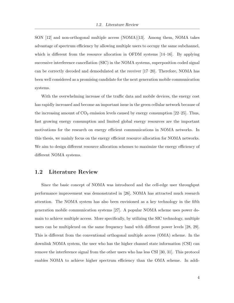
Figure 1.1 shows total global monthly data (ExaBytes per month) and voice traffic from
Q1 2012 to Q1 2017 [7]. It depicts a continued strong growth in data traffic. This growth is
driven by increased smart phone subscriptions and average data volume per subscription,
which has been fueled primarily by more viewing of video content. Data traffic grew around
12% quarter-on-quarter and around 70% year-on-year.
To further meet the overwhelming requirement of data rates, various new techniques
have been proposed in recent years, and these techniques include massive multiple-input
multiple output (MIMO) [8], millimeter wave communications [9], LTE-U[10], C-RAN [11],
2

1.1. Background and Motivation
Figure 1.1: Mobile data traffic growth predicted by Ericsson [7].
3
1.2. Literature Review
SON [12] and non-orthogonal multiple access (NOMA)[13]. Among them, NOMA takes
advantage of spectrum efficiency by allowing multiple users to occupy the same subchannel,
which is different from the resource allocation in OFDM systems [14–16]. By applying
successive interference cancellation (SIC) in the NOMA systems, superposition coded signal
can be correctly decoded and demodulated at the receiver [17–20]. Therefore, NOMA has
been well considered as a promising candidate for the next generation mobile communication
systems.
With the overwhelming increase of the traffic data and mobile devices, the energy cost
has rapidly increased and become an important issue in the green cellular network because of
the increasing amount of CO2 emission levels caused by energy consumption [22–25]. Thus,
fast growing energy consumption and limited global energy resources are the important
motivations for the research on energy efficient communications in NOMA networks. In
this thesis, we mainly focus on the energy efficient resource allocation for NOMA networks.
We aim to design different resource allocation schemes to maximize the energy efficiency of
different NOMA systems.
1.2 Literature Review
Since the basic concept of NOMA was introduced and the cell-edge user throughput
performance improvement was demonstrated in [26], NOMA has attracted much research
attention. The NOMA system has also been envisioned as a key technology in the fifth
generation mobile communication systems [27]. A popular NOMA scheme uses power do-
main to achieve multiple access. More specifically, by utilizing the SIC technology, multiple
users can be multiplexed on the same frequency band with different power levels [28, 29].
This is different from the conventional orthogonal multiple access (OMA) scheme. In the
downlink NOMA system, the user who has the higher channel state information (CSI) can
remove the interference signal from the other users who has less CSI [30, 31]. This protocol
enables NOMA to achieve higher spectrum efficiency than the OMA scheme. In addi-
4

1.2. Literature Review
tion to its spectral efficiency gain, academic and industrial research has also demonstrated
that NOMA can effectively support massive connectivity, which is important for ensuring
that the forthcoming 5G network can support the Internet of Things (IoT) functionalities
[32–35].
The multiuser superposition transmission scheme has been proposed in the third gen-
eration partnership project long-term evolution advanced (3GPP-LTE-A) networks [36],
where NOMA is referred to as multi-user superposition transmission (MUST). A variation
of NOMA, termed layer division multiplexing (LDM) was proposed for next generation
digital TV standard advanced television systems committee (ATSC) 3.0. Extensive studies
for NOMA system have been conducted. By considering a single frequency band in the
NOMA system with uniformly deployed mobile users, the outage probability was first de-
rived with perfect CSI, and the numerical results confirmed the derived outage probability
expressions [37]. Furthermore, the outage performance of a NOMA system with two types
of imperfect CSI was analyzed for the downlink single cell NOMA system, and numerical
results showed that the average sum rate matches well with the Monte Carlo simulations
[38]. By exploiting the outage probability from [38], the problem of energy efficient user
scheduling and power allocation was investigated for NOMA systems by considering only
two users multiplexed on one subchannel and imperfect CSI [39].
Besides the performance analysis, the resource allocation was investigated in NOMA
systems. By using fractional transmit power allocation (FTPA) among users and equal
power allocation across subchannels, the authors in [40, 41] compared system-level per-
formance of the NOMA system with the OMA system, and showed that the overall cell
throughput, cell-edge user throughput, and the degree of proportional fairness of NOMA
are all superior to those of the OMA scheme. Though FTPA is simple to implement, it
fails to optimally allocate power among multiplexed users on each subchannel. Thus, a
new power allocation scheme based on water filling was proposed to achieve high spectral
efficiency [42]. A cooperative relay system based on NOMA was proposed in [43], where
the improvement of the spectral efficiency was presented by numerical results. A greedy
5

1.2. Literature Review
subchannel and power allocation algorithm was proposed for the NOMA system [44], and
a cooperative NOMA transmission scheme, where some users have prior information of the
other users’ message, was proposed in [45] to improve spectrum efficiency. Driven by the
rapidly increasing of the energy cost, the energy-efficient power allocation was investigated
for NOMA systems [46]. By using statistical channel state information at the transmit-
ter, a near optimal power allocation scheme was proposed to maximize the system energy
efficiency [46].
The problem of joint subcarrier allocation and power allocation was investigated in
a full-duplex NOMA system [47], where the proposed suboptimal iterative scheme with
low computation complexity can achieve close-to-optimal performance. The application of
combining NOMA with MIMO technologies has attracted recent research attention. The
MIMO NOMA design for small packet transmission and the multi-user detection for uplink
NOMA systems were investigated in [48] and [49], respectively. The fairness clustering
problem was solved in MIMO NOMA scenarios [50], where an algorithm was proposed to
achieve a good tradeoff between the complexity and the throughput.
Driven by the rapid increase of wireless terminal equipments and wide usage of mobile
Internet, HetNets have emerged as one of the most promising network infrastructures to
provide high system throughput and large coverage of indoor and cell edge scenarios in the
5G wireless communication systems. In such an architecture, a macro cell is overlaid by
several small cells, e.g., microcell, picocell and femtocell, to significantly improve the system
throughput and the spectral efficiency. For HetNets, frequency band sharing between macro
cell and small cells is viable, and it is also more efficient to reuse the frequency bands within
a macro cell. However, the cross-tier interference can severely degrade the quality of the
wireless transmission. The advantage of the HetNet also comes with fundamental challenges
such as cross-tier interference mitigation and resource scheduling. In previous research,
the cross-tier interference control and cancellation in HetNets have been investigated, e.g.
precoding technique and resource management [15]. In the traditional OFDMA HetNets,
the frequency band can be divided into several sub frequency bands, and users in the same
6

1.3. Thesis Outline and Contributions
small cell are assigned to different sub frequency bands in order to avoid the inter-cell
interference [15]. Spectrum sharing between macro cell and small cells is applicable in
HetNets; however, the cross-tier interference and the co-channel interference can severely
degrade the communication quality in HetNet. Therefore, implementing NOMA in HetNets
can alleviate the cross-tier interference and significantly improve the system throughput via
resource optimization [51]. To maximize the sum rate of small cells, an iterative subchannel
allocation and power allocation algorithm is proposed to closely approach the optimal
solution within limited iterations [51].
To this end, most research works on NOMA systems have focused on the case that the
base station (BS) knows the perfect knowledge of the CSI [40, 41, 52]. Since the perfect CSI
is challenging to obtain in practice, power-efficient resource allocation scheme was designed
to minimize the total transmit power [53], where the proposed scheme can achieve close-to-
optimal performance. We assume that a channel estimation error model where the BS only
knows the estimated channel gain and a priori knowledge of the variance of the estimation
error [54, 55]. In this situation, the scheduled user data rate may exceed the maximum
achievable data rate due to the estimated channel gain. Therefore, an outage probability
requirement should be considered for the resource allocation to maximize system energy
efficiency.
1.3 Thesis Outline and Contributions
In this thesis, we present the research work conducted on the following three topics:
− Energy efficient resource allocation for downlink NOMA networks with perfect CSI
− Energy efficient resource allocation for downlink NOMA networks with imperfect CSI
− Energy efficient resource allocation for downlink NOMA HetNets.
The summary and contributions of each chapter are as follows.
7
1.3. Thesis Outline and Contributions
Chapter 1 presents background knowledge on the history and development of cellular
communication systems. In addition, this chapter provides a detailed literature review
related to the rest of the thesis.
Chapter 2 presents the required technical background for the entire thesis. We first in-
troduce the SIC technology and discuss practical issues associated with SIC implementation.
After that, we introduce the NOMA system and analyze its performance gain compared
to the conventional OMA scheme. As the energy efficient design has an important role
in modern communications, a detailed introduction of energy efficiency in communication
is provided. Finally, we discuss the resource allocation types and optimization tools in
wireless communication systems.
Chapter 3 studies the energy efficient resource allocation for NOMA system with the
perfect channel state information. Unlike most previous works focusing on resource allo-
cation to maximize the throughput, we aim to optimize subchannel assignment and power
allocation to maximize the energy efficiency for the downlink NOMA network. Assuming
perfect knowledge of the channel state information at the base station, we propose a low-
complexity suboptimal algorithm which includes energy-efficient subchannel assignment
and power proportional factors determination for subchannel multiplexed users. We also
propose a novel power allocation across subchannels to further maximize energy efficiency.
Since both optimization problems are non-convex, difference of convex programming is used
to transform and approximate the original non-convex problems to convex optimization
problems. Solutions to the resulting optimization problems can be obtained by iteratively
solving the convex subproblems.
In Chapter 4, we investigate energy efficiency improvement for a downlink NOMA sin-
gle cell network by considering imperfect CSI. The energy-efficient resource optimization
problem is formulated as a non-convex optimization problem with the constraints of outage
probability limit, the maximum power of the system, the minimum user data rate and the
maximum number of multiplexed users sharing the same subchannel. To efficiently solve
this problem, the probabilistic mixed problem is first transformed into a non-probabilistic
8
1.3. Thesis Outline and Contributions
problem. An iterative algorithm for user scheduling and power allocation is proposed to
maximize the system energy efficiency. The optimal user scheduling based on exhaustive
search serves as a system performance benchmark, but it has high computational com-
plexity. To balance the system performance and the computational complexity, a new
suboptimal user scheduling scheme is proposed to schedule users on different subchannels.
Based on the user scheduling scheme, the optimal power allocation expression is derived
by the Lagrange approach. By transforming the fractional-form problem into an equivalent
subtractive-form optimization problem, an iterative power allocation algorithm is proposed
to maximize the system energy efficiency. Simulation results demonstrate that the proposed
user scheduling algorithm closely attains the optimal performance. In this work, multiple
users can occupy the same subchannel, which is different from [39, 56, 57] where only two
users can be supported on the same subchannel.
In Chapter 5, NOMA is extended and applied to HetNets. In this chapter, we design a
joint resource allocation scheme to maximize the system energy efficiency via the Lagrangian
approach. We maximize not only small cells energy efficiency but also macro cell energy
efficiency. Simulation results show that our proposed resource allocation scheme for NOMA
HetNets can achieve higher energy efficiency than that of the conventional OMA scheme.
Chapter 6 summarizes the entire thesis and lists our contributions. In addition, some
future works related to our current research are also suggested.
9
Chapter 2
Background on Energy Efficient
Non-Orthogonal Multiple Access
(NOMA) Systems
In this chapter, we provide a brief description of NOMA system and SIC, and SIC is the
main technology applied at the receiver in NOMA systems. Then, the resource allocation
background knowledge in wireless network is presented. Finally, we introduce the energy
efficiency concept in wireless communications and present our research motivations.
2.1 Non-Orthogonal Multiple Access (NOMA) Systems
2.1.1 Successive Interference Cancelation (SIC) Technology in NOMA
Systems
Non-orthogonal multiple access has been recognized as a promising multiple access
technique for the fifth generation networks due to its superior spectral efficiency. In NOMA
systems, the main technology is SIC technology. Considering a downlink transmission
scenario where a single base station transmits superposition coded information to two users.
The channel gains from the base station to these two users are h1 and h2, respectively.
Assume that |h1| < |h2|, and both h1 and h2 are perfectly known to both the transmitter
10

2.1. Non-Orthogonal Multiple Access (NOMA) Systems
and receivers. The transmit signal or the sum of two signals, can be expressed as
x = x1 + x2 (2.1)
where xk is the signal intended for user k, k = 1, 2. Therefore, the received signal at user k
can be written by
yk = hkx+ wk, k = 1, 2 (2.2)
where wk ∼ CN(0, σ2
n
)is independent and identically distributed (i.i.d.) complex additive
white Gaussian noise (AWGN) with mean zero and variance σ2n. The transmit signal x
has an average power constraint of P = P1 + P2 where P1 and P2 are the transmit powers
for User 1 and User 2, respectively. The key idea of SIC technique is that users who have
higher channel gains can decode the data that has been successfully decoded by the users
who have less channel gains [58]. In this case, since User 2 has a higher channel gain than
User 1, User 2 can decode the data that has been successfully decoded by User 1. Thus,
the superposition coding scheme can be implemented by the following steps [59]:
1. The transmit signal is superposition coded signals of the two users.
2. At the receiver, User 1 treats User 2’s signal as noise and decodes its data from y1.
3. User 2 with better channel performs SIC, i.e., it decodes the data of User 1 and
subtracts User 1’s signal from y2. After that, User 2 can decode its data.
According to the Shannon’s capacity formula, the data rate for User 1 and User 2 with
bandwidth B can be achieved by
R1 = B log
(1 +
P1|h1|2
P2|h1|2 + σ2n
)bits/s (2.3)
R2 = B log
(1 +
P2|h2|2
σ2n
)bits/s. (2.4)
We consider K users are distributed in a downlink network with SIC at the receivers
11
2.1. Non-Orthogonal Multiple Access (NOMA) Systems
and |hK | ≥ |hK−1| ≥ · · · ≥ |h1|. The boundary of the capacity region is given by
Rk = B log
1 +Pk|hk|2
σ2n + |hk|2
K∑j=k+1
Pj
, k = 1, 2, · · · ,K (2.5)
for all possible splits P =K∑k=1
Pk of the total power at the base station. The optimal points
are achieved by superposition coding at the transmitter and SIC at each of the receivers.
The cancellation order at every receiver is always to decode the weaker users before decoding
its own data.
We have discussed the advantages of SIC technology in the downlink network. SIC
has a significant performance gain over the conventional orthogonal multiple access (OMA)
techniques. It takes advantage of the strong channel of the nearby user to give it high rate
while providing the weak user with the best possible performance. Here we discuss several
potential practical issues in applying SIC in a wireless system [59].
− Complexity will increase when the number of the users increases: In the downlink,
applying SIC at the mobile receivers means that the user needs to decode information
intended for some of the other users, which would not happen in the conventional
system. Thus the decoding complexity at each mobile user will increase when the
number of users multiplexed on the same frequency band increases. However, we have
seen that superposition coding in conjunction with SIC has the largest performance
gain when the users have large disparate channels from the base station. To avoid
the high complexity of SIC, user grouping can be a solution in practice. In order to
reduce the complexity of decoding, it is suggested to separate users in the cell into
groups containing small number of users. Each group users can be multiplexed on
the same subchannel and superposition coding based SIC is performed. Therefore,
the SIC can achieve the performance gain with low complexity.
− Imperfect channel state information estimation: The interfering signal from the other
12
2.1. Non-Orthogonal Multiple Access (NOMA) Systems
users must be reconstructed before it is removed from the received signal. This
contribution depends on the estimation of channel state information. The imperfect
estimation of CSI will lead to residual cancellation errors. One concern is that if the
difference of the users’ received powers is large, the residual error from cancelling the
stronger user can still swamp the weaker users signal. On the other hand, it is also
easier to get an accurate channel estimate when the user has high CSI. It turns out
that these two effects compensate each other and the effect of residual errors does not
grow with the power disparity.
− Analog-to-digital quantization error: When the difference of received powers of the
users is large, a large dynamic range of the analog-to-digital (A/D) converter is re-
quired. For example, if the power disparity is 20 dB, even 1-bit accuracy for the weak
signal would require an 8-bit A/D converter. This may well pose an implementation
constraint on how much gain SIC can offer.
2.1.2 Performance Analysis for NOMA Systems
UE2
Frequency
Pow
er
OFDMA
UE1(better CSI)
UE2(worse CSI)
Frequency
Pow
er
UE1
NOMA: SIC
Figure 2.1: OFDMA versus NOMA systems.
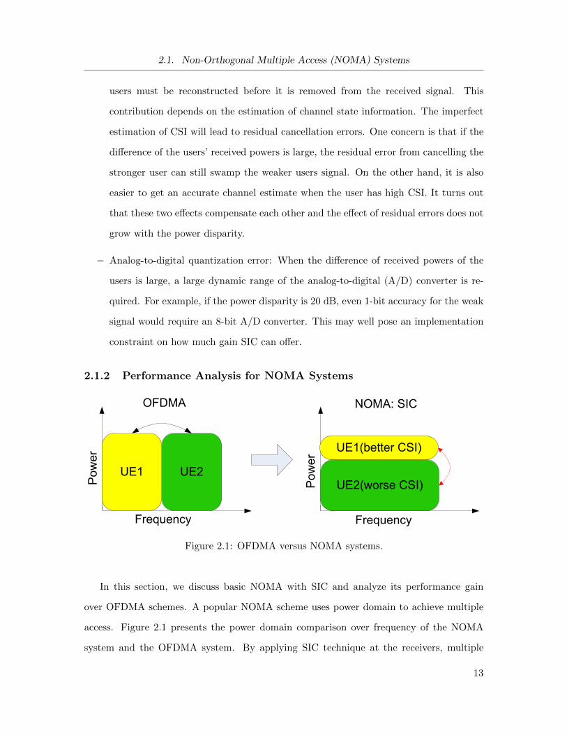
In this section, we discuss basic NOMA with SIC and analyze its performance gain
over OFDMA schemes. A popular NOMA scheme uses power domain to achieve multiple
access. Figure 2.1 presents the power domain comparison over frequency of the NOMA
system and the OFDMA system. By applying SIC technique at the receivers, multiple
13

2.1. Non-Orthogonal Multiple Access (NOMA) Systems
users with different power levels can be multiplexed on the same frequency band, providing
higher sum rate than that of conventional orthogonal multiple access (OMA) schemes.
In NOMA systems, SIC is applied at the receivers. Let us focus on the two-user case for
a downlink NOMA system. Consider that two users are multiplexed on the same subchannel
with the channel gains |h1|2 ≥ |h2|2 shown in Fig. 2.1, where hm = gm ·PL−1(d),m = 1, 2,
and where gm is assumed to be the Rayleigh fading channel gain and PL−1(d) is the path
loss function between the BS and UTm at distance d. Denote the assigned power on SCn
by pn. The bandwidth of the subchannel is Bsc and the power proportional factors for User
1 and User 2 are β1 and β2, respectively.
For NOMA systems, SIC is applied at User 1 with a higher channel gain than User 2.
According to the SIC protocol, User 1 can cancel the interference signal from User 2. The
data rates of User 1 and User 2 in NOMA systems can be respectively represented as
R1 = Bsclog2
(1 +|h1|2β1pn
σ2n
)(2.6)
and
R2 = Bsclog2
(1 +
|h2|2β2pn
|h2|2β1pn + σ2n
). (2.7)
The sum rate can be written by
RNOMA = Bsclog2
(1 +|h1|2β1pn
σ2n
)+Bsclog2
(1 +
|h2|2β2pn
|h2|2β1pn + σ2n
). (2.8)
In OFDMA systems, we assume OFDMA with orthogonal user multiplexing. The total
bandwidth Bsc is occupied by these two users (assume that each user has half bandwidth).
The data rates of User 1 and User 2 in OFDMA systems can be respectively represented as
R1 =1
2Bsclog2
(1 +|h1|2pnσ2n
)(2.9)
14

2.1. Non-Orthogonal Multiple Access (NOMA) Systems
and
R2 =1
2Bsclog2
(1 +|h2|2pnσ2n
). (2.10)
Therefore, the sum rate of these two users in OFDM system can be expressed as
ROFDM =1
2Bsclog2
(1 +|h1|2pnσ2n
)+
1
2Bsclog2
(1 +|h2|2pnσ2n
). (2.11)
Using the parameters values in [60], we set β1 = 1/5, β2 = 4/5, B = 1 Hz, |h1|2pnσ2n
= 20
dB and |h2|2pnσ2n
= 0 dB . Assume each user has the same weighted bandwidth (Bsc = 1
Hz). Therefore, ROFDM = 3.33 + 0.50 = 3.83 bits/sec and RNOMA = 4.39 + 0.74 = 4.53
bits/sec. The gain of the NOMA system is 34% more than that of the OFDMA scheme.
Now consider better channel conditions, which means we improve the channel gains by
setting |h1|2pnσ2n
= 30 dB and |h2|2pnσ2n
= 10 dB. Assume each user has the same weighted
bandwidth (Bsc = 1 Hz), β1 = 1/5, β2 = 4/5. Therefore, ROFDM = 4.99 + 1.73 = 6.72
bits/sec and RNOMA = 7.65 + 1.87 = 9.52 bits/sec. The gain of the NOMA system is 42%
more than that of the OFDMA scheme.
Based on the above numerical examples, it can be concluded that the sum data rate of
the NOMA system will be improved when the channel gains increase, and the performance
gain of NOMA over OFDMA increases when the channel conditions improve.
The difference of two systems’s sum rate in high signal-to-noise ratio (SNR) region can
be calculated. Consider that two users are multiplexed on the same subchannel with the
15
2.2. Energy Efficiency in Communication Networks
channel gains |h1|2 ≥ |h2|2. Therefore, the difference of sum rate can be written as [61]
RNOMA −ROFDM
=Bsclog2
(1 +|h1|2β1pn
σ2n
)+Bsclog2
(1 +
|h2|2β2pn
|h2|2β1pn + σ2n
)
− 1
2Bsclog2
(1 +|h1|2pnσ2n
)− 1
2Bsclog2
(1 +|h2|2pnσ2n
)
→pnσ2n→∞
log2
(pnσ2n
|h1|2β1
)+ log2
(1
β1
)− log2
(pnσ2n
|h1| |h2|)
=log2 (|h1|)− log2 (|h2|)
(2.12)
which is not a function of SNR. From (2.12), it can be concluded that the sum rate gap
between NOMA and OFDMA will be increased when the channel gain difference of the two
users is enlarged. Therefore, NOMA systems can outperform OFDMA systems only if the
channel gain difference exists.
2.2 Energy Efficiency in Communication Networks
2.2.1 Research Motivation of Energy Efficiency
From an operation point of view, approximately 600 TWh of the world wide electri-
cal energy is consumed by the information and communication technology (ICT). By the
end of 2030, this number is expected to grow to 1700 TWh [21]. This increasing energy
consumption becomes an important issue in the green cellular network because of the in-
creasing amount of CO2 emission levels caused by energy consumption [22–25]. Therefore,
the fast growing energy consumption and limited global energy resources are the important
motivations for the research on energy efficient wireless communication systems.
16

2.2. Energy Efficiency in Communication Networks
2.2.2 Energy Efficiency Definition in Wireless Communications
Networks
During the past decades, many research works have been conducted to improve sys-
tem throughput. However, with the exponential growth of wireless data traffic, energy
consumption of wireless networks has been rapidly increasing. Therefore, finding the trade-
off of high data rate and energy saving is an urgent task in the next generation wireless
communication systems.
Energy efficiency is commonly defined as the ratio of data rate to the power consump-
tion. Bits per Joule is commonly used to measure energy efficiency performance in wireless
networks [62, 63]. For energy-efficient communication, it is desirable to send the maximum
amount of data with a given amount of energy. With bandwidth B, the achievable data rate
R = B log(
1 + P |h|2σ2n
), where P is the transmit power, σ2
n is the AWGN power and |h|2 is
the channel power gain between transmitter and receiver. Given an amount of energy ∆E
that is consumed in a duration ∆T , we have ∆E = P∆T . Therefore, the energy efficiency
(EE) is defined as
EE =R∆T
∆E=R
Pbits/Joule. (2.13)
The power consumption includes transmit power and circuit power consumption. The
circuit power consumption is the additional device power consumption, which includes
signal processing and active circuit blocks such as analog-to-digital converter, digital-to-
analog converter, synthesizer, and mixer during the transmission [64]. Denote the additional
device power consumption, circuit power, as Pc. Thus, the overall power assumption is
P + Pc. Energy efficiency needs to be redefined as data rate bits/s per unit energy, where
an additional circuit power factor, Pc, needs to be taken into consideration. Therefore, the
energy efficiency is defined as
EE =R∆T
∆E=
R
P + Pcbits/Joule. (2.14)
17

2.2. Energy Efficiency in Communication Networks
Note that the circuit power consumption Pc is independent of the transmit power.
In this thesis, we consider two definitions of system energy efficiency. In Chapter 3, the
system energy efficiency is formulated as a summation of each subchannel energy efficiency.
In Chapter 4, the system energy efficiency is formulated as the ratio of system sum rate
to the total power consumption. Different resource allocation schemes are proposed to
improve the system energy efficiency. Regardless different definitions of system energy
efficiency, our research conclusion will be the same. By resource allocation, the energy
efficiency of a NOMA system can be made higher than that of an OFDMA system.
2.2.3 Resource Optimization and Convex Optimization Approaches
Resource management plays an important role to improve the energy efficiency in wire-
less communication systems. The main resource management in wireless communications
is frequency, time and power optimization. There are different mechanisms for resource
management in wireless networks. The most important ones include congestion control,
routing, subchannel allocation and power control [65]. In this thesis, we mainly focus on
subchannel allocation (user scheduling) and power allocation to maximize the system en-
ergy efficiency in NOMA networks. Subchannel allocation means that the schedular needs
to assign different users to different subchannels. Since different subchannels have different
gains, different subchannel allocation schemes can achieve different performance. Power
allocation means that the schedular needs to allocate different powers to the users, which
can also achieve different performance gains. One of the most common and effective math-
ematical tools to solve the resource allocation problem in wireless communication networks
is the convex optimization method.
18

2.3. Summary
Let us consider a standard form convex problem:
minx
f0(x)
s.t. fi(x) ≤ 0, i = 1, 2, ...,m
hi(x) = 0, i = 1, 2, ..., p
x ∈ C.
(2.15)
Equation (2.15) describes the problem of finding an x that minimizes f0(x) among all x
values that satisfy the conditions fi(x) ≤ 0, i = 1, 2, ...,m, hi(x) = 0, i = 1, 2, ..., p and
x ∈ C. We call x ∈ C the optimization variable and f0 the objective function or cost
function. fi(x) and hi(x) are the inequality and equality constraint functions, respectively,
and C is the constraint set. The domain of the objective and constraint functions are defined
as
D =m⋂i=0
dom fi ∩m⋂i=0
dom hi ∩ C. (2.16)
The convexity of this problem can be proved by the following conditions [66]. First
the objective function f0(x) should be convex. Second the inequality constraint functions
fi (i = 1, 2, ...,m) and equality constraint functions hi (i = 1, 2, ..., p) should be convex.
Thus, it is proved that the problem (2.15) is convex, and we can find a global optimal
solution x∗ ∈ D to this problem by using standard algorithms from convex optimization
theory [66], e.g, interior point method and sequential quadratic programming.
2.3 Summary
In this chapter, we presented the essential technical background knowledge on the
NOMA system. Compared with the OFDMA system, the performance gain of the NOMA
system is presented. Moreover, energy efficiency aspect in wireless communications was
provided and the convex optimization approach was briefly introduced.
19

Chapter 3
Energy Efficient Resource
Allocation for Downlink NOMA
Network with Perfect CSI
In this chapter, we aim to optimize subchannel assignment and power allocation to maxi-
mize the energy efficiency for the downlink NOMA network. Assuming perfect knowledge of
the channel state information at base station, we propose a low-complexity suboptimal algo-
rithm that includes energy-efficient subchannel assignment and power proportional factors
determination for subchannel multiplexed users. We also propose a novel power allocation
across subchannels to further maximize energy efficiency. Since both optimization problems
are non-convex, difference of convex programming is used to transform and approximate the
original non-convex problems to convex optimization problems. Solutions to the resulting
optimization problems can be obtained by iteratively solving the convex subproblems. Sim-
ulation results show that the NOMA system equipped with the proposed algorithms yields
much better sum rate and energy efficiency performance than the conventional orthogonal
frequency division multiple access scheme.
3.1 System Model
Figure 3.1 shows a downlink NOMA network. A BS transmits its signals to M user
terminals (UTs) through N subchannels, and SIC is employed at the receiver of UTs.
We denote n as index for the nth subchannel where n ∈ {1, 2, · · · , N} and denote m
20

3.1. System Model
UT
UT
UT
DL
DL
DL
UTUT
UT
DL
DL
UT
DL
DL
UT
DL
BS
Figure 3.1: System model of a downlink NOMA single-cell network.
as index for the mth mobile user where m ∈ {1, 2, · · · ,M}. In the cell, M users are
uniformly distributed in a circular region with radius R. The total bandwidth of the system,
BW , is equally divided into N subchannels where the bandwidth of each subchannel is
Bsc = BW/N . Let Mn ∈ {M1,M2, · · · ,MN} be the number of users allocated on the
subchannel n (SCn) and the power allocated to the lth user on SCn is denoted by pl,n.
Then, the subchannel and BS power constraints are given byMn∑l=1
pl,n = pn andN∑n=1
pn = Ps,
where pn and Ps are, respectively, the allocated power on SCn and the total transmitted
power of the BS. In NOMA systems, we assume that the BS has full knowledge of the
channel state information. According to the NOMA protocol [26], multiple users can be
allocated to the same subchannel with SIC technique. A block fading channel is considered
in the system model, where the channel fading of each subchannel remains the same, but it
varies independently across different subchannels. Based on the parameters and constraints
of the system, the BS needs to assign multiple users (with different power levels) to different
subchannels and allocate different powers across subchannels. Considering Mn users are
allocated on SCn, the symbol transmitted by the BS on each subchannel SCn can be
expressed as
xn =
Mn∑i=1
√pi,nsi (3.1)
21

3.1. System Model
where si is the modulated symbol of the ith user on SCn, which is denoted by UTi,n1. The
received signal at the lth user on SCn is
yl,n = hl,nxn + zl,n =√pl,nhl,nsl +
Mn∑i=1,i 6=l
√pi,nhl,nsi + zl,n (3.2)
where hl,n = gl,n · PL−1(d) is the coefficient of SCn from the BS to UTl,n, and where gl,n
is assumed to have Rayleigh fading channel gain, and PL−1(d) is the path loss function
between the BS and UTl,n at distance d. The impact of users’ channel conditions on
the performance gain of NOMA over OFDMA was studied in [61]. In this work, the
authors presented that the performance gain of the NOMA over OFDMA will increase
when the difference of channel gain of users become larger. The authors in [37] showed
that the distances between BS and UTs will affect the performance of the NOMA system.
In this paper, we assume these distances of different users are known by BS. Let zl,n ∼
CN(0, σ2
n
)be the additive white Gaussian noise with mean zero and variance σ2
n. In a
downlink NOMA network, each subchannel can be shared by multiple users. Each user on
SCn receives its signals as well as interference signals from the other users on the same
subchannel. Therefore, without SIC at receiver, the received signal-to-interference-plus-
noise ratio (SINR) of the lth user on the SCn is written by
SINRl,n =pl,n|hl,n|2
σ2n +
Mn∑i=1,i 6=l
pi,n|hl,n|2=
pl,nHl,n
1 +Mn∑
i=1,i 6=lpi,nHl,n
(3.3)
where σ2n = E[|zl,n|2] is the noise power on SCn and Hl,n , |hl,n|2/σ2
n represents the channel
response normalized by noise (CRNN) of the lth user on SCn. Based on the Shannon’s
capacity formula, the achievable sum rate of SCn is written by
Rn = Bsc
Mn∑l=1
log2 (1 + SINRl,n) = Bsc
Mn∑l=1
log2
(1 +
pl,nHl,n
1 + Il,n
)(3.4)
1Without causing notational confusion, UTi,n denotes the ith user on SCn, while UTm denotes the mthuser in the cell, where m ∈ {1, 2, · · · ,M}.
22
3.1. System Model
where Il,n is the interference that UTl,n receives from the other users on the SCn, which
can be expressed as
Il,n =
Mn∑i=1,i 6=l
pi,nHl,n. (3.5)
In NOMA systems, the SIC process is implemented at UT receiver to reduce the inter-
ference from the other users on the same subchannel. The optimal decoding order for SIC is
the increasing order of CRNNs. Based on this order, any user can successfully and correctly
decode the signals of the other users with smaller CRNN values. Thus, the interference
from the users having poorer channel condition can be cancelled and removed by the user
who has better channel condition. In order to maximize the sum rate of SCn, the NOMA
protocol allocates higher power to the users with lower CRNN [26], i.e., for two users UTi,n
and UTj,n sharing the same SCn with CRNNs |Hi,n| ≥ |Hj,n| 2, we always set pi,n ≤ pj,n to
guarantee the weak user’s communication quality. This assumption is widely used in the
NOMA scheme [40, 41]. Consider that Mn users are allocated on SCn with CRNNs order
|H1,n| ≥ |H2,n| ≥ · · · ≥ |Hl,n| ≥ |Hl+1,n| ≥ · · · ≥ |HMn,n| . (3.6)
According to the optimal SIC decoding order, User l can successfully decode and remove
the interference symbols from users i > l. However, the interference symbol from User i
(i < l) cannot be removed and will be treated as noise by User l. Therefore, the SINR of
User l with SIC at receiver can be written as
SINRl,n =pl,nHl,n
1 +l−1∑i=1
pi,nHl,n
. (3.7)
2Without causing notational confusion, hl,n is the channel gain of UTl,n, while Hl,n , |hl,n|2/σ2n denotes
the channel response normalized by noise of UTl,n
23

3.2. Problem Formulation
Then the data rate of the lth user on SCn can be expressed as
Rl,n (pl,n) = Bsclog2
1 +pl,nHl,n
1 +l−1∑i=1
pi,nHl,n
. (3.8)
Therefore, the overall sum rate of the NOMA system can be written as
R =
N∑n=1
Mn∑l=1
Rl,n (pl,n) =
N∑n=1
Rn (pn) . (3.9)
3.2 Problem Formulation
In this section, we formulate the energy-efficient subchannel assignment and power
allocation as an optimization problem. For energy-efficient communication, it is desirable
to maximize the amount of transmitted data bits with a unit energy, which can be measured
by energy efficiency. For each subchannel in the NOMA system, given assigned power pn
on SCn and additional circuit power consumption Pc, the energy efficiency over SCn is
defined as
EEn =Rn
Pc + pn. (3.10)
Then the overall energy efficiency of the system can be given by
EE =N∑n=1
EEn. (3.11)
For the downlink NOMA network, SIC technique is well investigated in [17, 20]. The
implementation complexity of SIC at the receiver increases with the maximum number
of the users allocated on the same subchannel. In order to keep the receiver complexity
comparatively low, we consider a simple case where only two users are allocated on the same
subchannel. This assumption is important because it also restricts the error propagation.
24

3.3. Subchannel Allocation
In this case, given that the two users sharing SCn with CRNNs |H1,n| ≥ |H2,n|, the sum
rate of SCn can be expressed as
Rn (pn) = Bsclog2 (1 + βnpnH1,n) +Bsclog2
(1 +
(1− βn) pnH2,n
1 + βnpnH2,n
)(3.12)
where βn is the power proportional factor for the two users on SCn. Generally, βn is used
for the user who performs SIC on SCn and βn ∈ (0, 1). The optimal power proportional
factor can be decided within our proposed subchannel assignment scheme. To obtain an
energy-efficient resource allocation scheme for this system, we formulate the energy effi-
ciency optimization problem as
maxpn>0
N∑n=1
Rn (pn)
Pc + pn(3.13)
subject to C1 : Rl,n(pn) ≥ Rmin
C2 :N∑n=1
pn = Ps
(3.14)
where C1 guarantees user minimum data rate constraint and Rmin is denoted as minimum
data rate determined by quality of service (QoS) requirement. The constraint C2 ensures
the maximum BS power constraint. Since this optimization problem is non-convex and
NP-hard, it is challenging to find the global optimal solution within polynomial time. To
solve this problem efficiently, we will treat subchannel assignment and subchannel power
allocation separately.
3.3 Subchannel Allocation
In this section, we investigate the energy-efficient matching algorithm for subchannel
assignment in the NOMA network. For the optimization problem (3.13), it can be shown
that the subchannel assignment and power allocation for subchannels are coupled with each
other in terms of energy efficiency. Due to the considerable complexity of global optimum
solution, we decouple subchannel assignment and power allocation to obtain a suboptimal
25

3.3. Subchannel Allocation
solution. We first propose a greedy subchannel-user matching algorithm by assuming equal
power is allocated on each subchannel, in which each power proportional factor βn is also
determined to allocate different powers to the multiplexed users on the same subchannel.
We define the parameter βn as the proportional factor of assigned power to the user who
performs SIC on SCn. By decomposing the objective function into difference of convex
functions, the suboptimal matching scheme for subchannel assignment is decided by a DC
programming approach.
3.3.1 Subchannel Matching Problem Formulation
To describe the dynamic matching between the users and the subchannels, we consider
subchannel assignment as a two-sided matching process between the set of M users and
the set of N subchannels. Considering only two users can be multiplexed on the same
subchannel due to the complexity of decoding, we assume M = 2N [26]. We say UTm and
SCn are matched with each other if UTm is allocated on SCn. Based on the perfect channel
state information, the preference lists of the users and subchannels can be denoted by
PF UT = [PF UT (1), · · · , PF UT (m), · · · , PF UT (M)]T
PF SC = [PF SC(1), · · · , PF SC(n), · · · , PF SC(N)]T(3.15)
where PF UT (m) and PF SC(n) are the preference lists of UTm and SCn, respectively.
We say UTm prefers SCi to SCj if UTm has higher channel gain on SCi than that on SCj ,
and it can be expressed as
SCi (m) � SCj (m) . (3.16)
As an example, we consider four users and two subchannels with the following channel gain
matrix
H =
[0.197, 0.778; 0.437, 0.143; 0.322, 0.545; 0.272, 0.478
]
26
3.3. Subchannel Allocation
where row index denotes the users and column index denotes the subchannels. Therefore,
we have the preference list of the users as
PF UT (1) =
[2 1
]T, PF UT (2) =
[1 2
]TPF UT (3) =
[2 1
]T, PF UT (4) =
[2 1
]Tand the preference list of the subchannels as
PF SC(1) =
[2 3 4 1
]TPF SC(2) =
[1 3 4 2
]T.
We say SCn prefers user set qm to user set qn (qn, qm is denoted as subsets of {1, 2, · · · ,M})
if the users in set qm can provide higher energy efficiency than users in set qn on SCn, and
we represent this scenario as
EEn (qm) > EEn (qn) , qm, qn ⊂ {UT1, UT2, · · · , UTMn} . (3.17)
Matching theory has been studied in [67, 68], where various properties and types of pref-
erences have been discussed. Based on the preference lists of users and subchannels, the
subchannel assignment problem is formulated as a two-sided matching problem [67, 68].
Definition 1 : (Two-sided Matching) Consider users and subchannels as two disjoint
sets, M = {1, 2, · · · ,M} and N = {1, 2, · · · , N}. A two-to-one, two-sided matching M is
a mapping from all the subsets of users M into the subchannel set N satisfying UTm ∈M
and SCn ∈N
1) M(UTm) ∈N .
2) M−1(SCn) ⊆M .
3) |M(UTm)| = 1, |M−1(SCn)| = 2.
4) SCn ∈M(UTm)⇔ UTm ∈M−1(SCn).
27
3.3. Subchannel Allocation
Condition 1) states that each user matches with one subchannel, and Condition 2) repre-
sents each subchannel can be matched with a subset of users. Condition 3) states that the
number of users can be allocated on each subchannel is limited to two. Condition 4) means
that UTm and SCn are matched with each other.
Definition 2 : (Preferred Matched Pair) Given a matching M that UTm /∈ M−1(SCn)
and SCn /∈ M(UTm). If EEn (Snew) > EEn(M−1(SCn)
)where Snew ⊆ {UTm} ∪ S and
S =M−1(SCn), where S is the user set that has been assigned to SCn, Snew becomes the
preferred users set for subchannel n and (UTm, SCn) is a preferred matched pair. Based
on the above definition, we will describe in Section 3.3.2 the matching action between the
users and the subchannels. If each subchannel has to select the best subset of users to
allocate, it will cause considerable complexity especially when the number of users is large.
Because the optimal solution requires to search all the possible combinations of the users
to maximize energy efficiency. To reduce the complexity, a suboptimal matching algorithm
is proposed for subchannel assignment as follows.
3.3.2 Suboptimal Matching for Subchannel Assignment Algorithm in
NOMA
In this subsection, we propose a suboptimal matching algorithm for subchannel assign-
ment. The main idea of this matching model is that each user sends the matching request
to its most preferred subchannel according to its preference list. This preferred subchannel
has the right to accept or reject the user according to energy efficiency that the all users
can provide on this subchannel. Based on the equal power allocation across subchannels,
the user selection algorithm is a process of finding the preferred matching pair for each user
and subchannel.
Algorithm 1 describes the proposed low-complexity suboptimal matching scheme for a
subchannel assignment (SOMSA) scheme to maximize the system energy efficiency. This
algorithm includes initialization and matching procedures. In the initialization step, prefer-
ences lists of subchannels and users are decided according to the channel state information,
28

3.3. Subchannel Allocation
Algorithm 1: Suboptimal Matching for Subchannel Assignment
1: Initialize the matched list SMatch(n) to record users matched on SCn for all thesubchannels ∀n ∈ {1, 2, · · · , N}.
2: Initialize preference lists PF UT (m) and PF SC (n) for all the users∀m ∈ {1, 2, · · · ,M} and all the subchannels ∀n ∈ {1, 2, · · · , N} according to CRNNs.
3: Initialize the set of unmatched users SUnMatch to record users who has not beenallocated to any subchannel.
4: while {SUnMatch} is not empty do5: for m = 1 to M do6: Each user sends matching request to its most preferred subchannel n according to
PL UT (m).7: if |SMatch (n)| < 2 then8: Subchannel n adds user m to SMatch (n), and removes user m from {SUnMatch}9: end if
10: if |SMatch (n)| = 2 then11: a) Find power proportional factor βn for every two users in Sqm ,
Sqm ⊂ {Smatch(n),m} by using (3.18), or exhaustive search method or DCprogramming algorithm in Section 3.4.1.
12: b) Subchannel n selects a set of 2 users Sqm satisfying maximum energyefficiency En(qm) ≥ En(qn), qm, qn ⊂ {Smatch(n),m}.
13: c) Subchannel n sets Smatch(n) = qm, and rejects other users. Remove theallocated users from {SUnMatch}, add the unallocated user to {SUnMatch}.
14: d) The rejected user removes subchannel from their preference lists.15: end if16: end for17: end while
29
3.3. Subchannel Allocation
and SMatch(n), ∀n ∈ {1, 2, · · · , N} and SUnMatch are initialized to record the allocated
users on SCn and unallocated users of the system, respectively. In the matching procedure,
at each round, each user sends the matching request to its most preferred subchannel. Ac-
cording to the preferred list of each user (PF UT (m), ∀m ∈ {1, 2, · · · ,M}) which is a list
of subchannels ordered by decreasing channel gains, the mth user will find the first non-
zero entry in PF UT (m) and send matching request to the corresponding subchannel. The
subchannel accepts the user directly if the number of allocated users on this subchannel is
less than two. When the number of the allocated users equals to two, only the subset of
users that can provide higher energy efficiency will be accepted or it will be rejected. This
matching process will terminate when there is no user left to be matched. After that, the
allocated user and the corresponding subchannels in the preference list are set to zero. The
proposed SOMSA converges to a stable matching after a limited number of iterations [68].
3.3.3 Power Ratio Factor Determination
In Algorithm 1, it is required to determine the power proportional factor βn for every
two subchannel users. In this section, we will first review the existing fractional transmit
power allocation scheme and the exhaustive searching method. Then we will introduce a
new energy-efficient power allocation algorithm based on DC programming in Section 3.4.1.
It will be shown in the simulation results that the new algorithm can result in improved
energy efficiency.
Fractional transmit power allocation
According to the SINR expression in (3.7), the transmit power allocation to one user
affects the achievable sum rate as well as the energy efficiency on each subchannel. Due to
its low computational complexity, FTPA is widely adopted in OFDMA systems and NOMA
systems [20, 26]. In the FTPA scheme, the transmit power of UTm on SCn is allocated
30

3.3. Subchannel Allocation
according to the channel gains of all the multiplexed users on SCn, which is given as
pl,n = pnHl,n
−α
Mn∑i=1
Hi,n−α
(3.18)
where α (0 ≤ α ≤ 1) is a decay factor. In the case α = 0, it corresponds to equal power
allocation among the allocated users. From (3.18), it is clear that when α increases, more
power is allocated to the user with poorer CRNN. Note that the same decay factor should
be applied to all subchannels and transmission times.
Exhaustive searching method
In finding power proportional factor βn, the method of exhaustion can also be exploited
for βn ∈ (0, 1). The optimal value can be found through searching all βn values in (0, 1)
using a sufficiently small step size. Therefore, the optimal power proportional factors for
the multiplexed users can be obtained. However, the computational complexity of the
exhaustion method is much higher than FTPA. Therefore, in the following, we consider
a suboptimal but efficient DC programming to allocate power among multiple users to
maximize the energy efficiency.
3.3.4 Complexity Analysis
The optimal subchannel assignment scheme can only be obtained by searching over all
possible combinations of the users and selecting the one that maximizes the system energy
efficiency. If we have M users and N subchannels (M = 2N). The scheduler needs to
search (2N)!2N
combinations. The time complexity of exhaustive searching is O( (2N)!2N
). In
order to compare the complexity of different algorithms, we take natural logarithm of the
complexity. The logarithm complexity is O(ln((2N)!) −N) = O(ln((2N)!)). By using the
Stirling’s formula, ln(n!) = n lnn−n+O(ln(n)), the logarithm complexity of the exhaustive
searching can be written as O(N lnN). In the SOMSA algorithm, the complexity of the
worst case is O(N2). Taking natural logarithm of the complexity, the logarithm complexity
31

3.4. Power Allocation
is O(lnN). Since O(lnN) < O(N lnN) and actual complexity of SOMSA is much less than
the complexity of the worst case, the complexity of SOMSA algorithm is much less than
the optimal subchannel assignment scheme. It can be shown that for a small number of
users (M = 4), the SOMSA will yield the identical results from the exhaustive search.
3.4 Power Allocation
As mentioned in Section 3.3, equal power allocation is assumed across subchannels in
SOMSA. In order to further improve the energy efficiency of the NOMA system, we consider
to obtain the energy-efficient subchannel power allocation instead of equal power allocation.
In this section, we introduce the DC programming approach and discuss its application in
finding power proportional factors as well as power allocation across subchannels.
3.4.1 DC Programming
DC programming approach has been studied recently to solve non-convex optimization
problems [69]. It is shown that DC programming can be applied if the objective function can
be written as a minimization of a difference of two convex functions, which is represented
as
minx∈χ
q (x) = f (x)− g (x) (3.19)
where x = [x1, x2, · · ·xL]T and χ is a convex set; f (x) and g (x) are continuous, convex or
quasi-convex [69]. In general, the problem defined in (3.19) is non-convex. However, it can
be solved suboptimally by using Algorithm 2. The key idea of Algorithm 2 is to convert a
non-convex problem to convex subproblems by using successive convex approximations. In
this algorithm, ε is the difference tolerance and the term −g (x) in the objective function
(3.19) is replaced by −g(x(k)
)−∇gT
(x(k)
) (x− x(k)
)in (3.20). The convex optimization
problem in (3.20) can be solved by using standard algorithms from convex optimization
theory [66, 70, 71], i.e., interior point method and sequential quadratic programming.
32

3.4. Power Allocation
Algorithm 2: Iterative, Suboptimal Solution for DC Problems [70]
Initialize x(0), set iteration number k = 0.while
∣∣q (x(k+1))− q
(x(k)
)∣∣ > ε do
Define convex approximation of q(k) (x) as
q(k) (x) = f (x)− g(x(k)
)−∇gT
(x(k)
)(x− x(k)
)(3.20)
Solve the convex problem
x(k+1) = arg minx∈χ
q(k) (x) (3.21)
k ← k + 1end while
The convergence of Algorithm 2 can be easily proved by
q(x(k)
)= q(k)
(x(k)
)≥ q(k)
(x(k+1)
)≥ q
(x(k+1)
)(3.22)
where q(x(k)
)= q(k)
(x(k)
)is the kth iteration step, and q(k)
(x(k)
)≥ q(k)
(x(k+1)
)can be
obtained by (3.21). Therefore, q(x(k)
)monotonically decreases when k increases. Under
an additional assumption that f (x) and g (x) are continuous and differentiable on the
constraint set. In this case, Algorithm 2 always returns a point of q (x), which may not be
the global optimal solution [69].
3.4.2 Power Proportional Factor
Considering two users UT1 and UT2 who are to be multiplexed over SCn with CRNNs
H1,n ≥ H2,n. According to the principle of SIC decoding sequences, UT1 can cancel the
interfering power term of UT2, whereas UT2 treats the symbol power UT1 as noise. The
problem of finding βn to maximize energy efficiency of SCn can be formulated as
maxβn∈(0,1)
Bsclog2 (1 + βnpnH1,n)
Pc + pn+Bsclog2
(1 +
(1−βn)pnH2,n
1+βnpnH2,n
)Pc + pn
(3.23)
33

3.4. Power Allocation
which can be rewritten as
maxβn∈(0,1)
Bsclog2 (1 + βnpnH1,n) +Bsclog2
(1+pnH2,n
1+βnpnH2,n
)Pc + pn
. (3.24)
In order to use the DC programming approach, we can convert (3.24) to DC representation
minβn∈(0,1)
− Bsclog2 (1 + βnpnH1,n)
Pc + pn−Bsclog2
(1+pnH2,n
1+βnpnH2,n
)Pc + pn
(3.25)
or
minβn∈(0,1)
(f (βn)− g (βn)) (3.26)
where f (βn) = −Bsclog2(1+βnpnH1,n)Pc+pn
and g (βn) =Bsclog2
(1+pnH2,n
1+βnpnH2,n
)Pc+pn
, and both terms are
convex functions with respect to βn because ∇2f (βn) > 0 and ∇2g (βn) > 0. Therefore,
the DC programming approach can be used to find βn by replacing x with βn in Algorithm
2.
3.4.3 Subchannel Power Allocation by DC Programming
Given the subchannel-user matching scheme and power proportional factors on different
subchannels by Algorithm 1, the optimization problem in (3.13) can rewritten as
maxpn≥0
N∑n=1
Bsclog2 (1 + βnpnH1,n)
Pc + pn+Bsclog2
(1+pnH2,n
1+βnpnH2,n
)Pc + pn
(3.27)
subject to C1 : Rl,n(pn) ≥ Rmin; C2 :N∑n=1
pn = Ps (3.28)
where Rl,n(pl,n) is defined in (3.8). Since Rl,n(pl,n) is a linear function respect to the
assigned power pn on SCn. The constraint C1 can be converted to pn > pn,min, where
pn,min is the minimum assigned power on SCn and it is determined by Rmin. Condition C2
in (3.28) guarantees BS power constraint. Note that the optimization problem in (3.27) is
34

3.4. Power Allocation
non-convex with respect to pn. However, the representation of (3.27) is similar to the DC
problem representation. Thus (3.27) can be rewritten as
minpn≥0
−N∑n=1
Bsclog2 (1 + βnpnH1,n)
Pc + pn+Bsclog2
(1+pnH2,n
1+βnpnH2,n
)Pc + pn
minpn≥0
F (P)−G (P)
(3.29)
where P = [p1, p2, · · · , pn, · · · , pN ]T represents the allocated powers on the subchannels,
and
F (P) = −N∑n=1
Bsclog2 (1 + βnpnH1,n)
Pc + pn−
N∑n=1
Bsclog2 (1 + pnH2,n)
Pc + pn;
G (P) = −N∑n=1
(Bsclog2 (1 + βnpnH2,n)
Pc + pn
).
Problem (3.27) can be written as
minP�0
Q (P) = minP�0
F (P)−G (P)
subject to C1 : P � Pmin; C2 : ‖P‖1 = Ps (3.30)
where Pmin = [p1,min, p2,min, · · · , pn,min, · · · , pN,min]T and P � Pmin means all the elements
in P are larger than the corresponding elements in Pmin, pn > pn,min. Proposition 1 proves
convexity of F (P) and G (P), Therefore, the DC programming approach can be applied
to realize energy-efficient power allocation using Algorithm 3. Once the power allocation
over subchannels is obtained, we replace the equal power allocation with our new power
allocation scheme to achieve higher energy efficiency of the system.
In Algorithm 3, ∇G(P(k)
)is the gradient of G(P) at the point P(k) and it is calculated
35

3.4. Power Allocation
Algorithm 3: DC Programming Algorithm for Power Allocation across Subchannels
Initialize P(0), set iteration number k = 0. The Objective function Q (P), convexfunctions F (P) and G (P) .
while∣∣∣Q(P(K+1)
)−Q
(P(k)
)∣∣∣ > ε do
Define convex approximation of G(k) (P) at P(k) as
Q(k) (P) = F (P)−G(P(k)
)−∇GT
(P(k)
)(P−P(k)
)(3.31)
Solve the convex problem
P(k) = arg minpn≥pn,min, ‖P‖1=Ps
Q(k) (P) (3.32)
k ← k + 1end while
by
∇G(P(k)
)=
N∑n=1
Bsclog2 (1 + βnpnH2,n)− (Pc + pn)βnH2,n
(1+βnpnH2,n) ln 2
(Pc + pn)2 . (3.33)
Since (3.32) and the power domain are convex, problem (3.33) can be solved by either the
interior point method or the sequential quadratic programming. In order to use the DC
programming approach, the quasi-convexity of F (P) and G (P) needs to be established. It
is easy to show that
f (P) = −N∑n=1
Bsclog2 (1 + βnpnH1,n)−N∑n=1
Bsclog2 (1 + pnH2,n)
and
g (P) = −N∑n=1
Bsclog2 (1 + βnpnH2,n)
are convex since ∇2f (P) and ∇2g (P) are positive semi-definite matrices.
Proposition 1 : If
−f1 (pn) = Bsclog2 (1 + βnpnH1,n) +Bsclog2 (1 + pnH2,n)
36

3.5. Simulation Results
and
−g1 (pn) = Bsclog2 (1 + βnpnH2,n)
are strictly concave in pn, −F1 (pn) = −f1(pn)Pc+pn
and −G1 (pn) = −g1(pn)Pc+pn
are quasi-concave
with constant Pc. Inspired by [72], we can prove Proposition 1 as follows.
Proof : Denote the α-sublevel sets of function −F1 (pn) as
Sα = {pn > 0| − F1 (pn) ≥ α} . (3.34)
−F1 (pn) is strictly quasi-concave if and only if Sα is strictly convex for any α. In this case,
when α < 0, there are no points satisfying −F1 (pn) = α. Therefore, Sα is strictly convex
when α ≤ 0. When α > 0, we can rewrite Sα as Sα = {pn > 0|α (Pc + pn) + f1 (pn) ≤ 0}.
Since f (pn) is strictly convex in pn, Sα is therefore also strictly convex. Hence, −F1 (pn)
and −G1 (pn) are strictly quasi-concave. Therefore, F1 (pn) and G1 (pn) are quasi-convex.
As a result, F (P) and G (P) are quasi-convex. �
3.5 Simulation Results
In this section, Monte Carlo simulation results are presented to evaluate the performance
of the proposed resource allocation algorithms for NOMA systems. In the simulations, we
consider one base station located in the cell center and all the user terminals are uniformly
distributed in a circular range with radius of 500 m. We set the minimum distance among
all the users to be 40 m, and the minimum distance from users to BS is 50 m. The
bandwidth is 5 MHz. Let M users be randomly distributed in the cell. In NOMA systems,
to reduce demodulating complexity of the SIC receiver, we consider each subchannel is
only allocated with two users. In OFDMA schemes, each user can only be assigned to
one subchannel. In the simulations, we compare the performance of NOMA systems with
OFDMA systems, both with resource allocation algorithms. For the subchannel power
37

3.5. Simulation Results
10 20 30 40 50 6048
50
52
54
56
58
60
62
Number of users per BS
Tot
al s
um r
ate
of s
yste
m (
Mbp
s)
NOMA−DCNOMA−EQOFDMA
Figure 3.2: Sum rate of the system versus different number of users.
38

3.5. Simulation Results
10 15 20 25 30 35 40 45 50 55 601
1.5
2
2.5
3
3.5
4
4.5
5x 10
7
Number of UE per BS
Tot
al E
nerg
y E
ffici
ency
of S
yste
m (
bits
/Jou
le)
NOMA−DC−DC Pc=1wNOMA−DC−EQ Pc=1wOFDMA
Figure 3.3: Energy efficiency of the system versus different number of users.
allocation, we compare our proposed suboptimal algorithm with equal power allocation
scheme based on our proposed subchannel assignment scheme. FTPA for multiplexed users
on subchannel is also compared with our proposed algorithms. In our simulations, we
set BS peak power, Ps, to be 41 dBm and circuit power consumption Pc = 1 W [73]. The
maximum number of users is 60 and σ2n = BW
N N0, where N0 = −174 dBm/Hz is the AWGN
power spectral density. In the simulations, we set the value of α as 0.4 [40].
In Fig. 3.2, the performance of the total sum rate is evaluated with the number of users
M (M varies from 10 to 60). We set difference tolerance ε = 0.01, and the bandwidth is
limited to 5 MHz. It is shown that the total sum rate increases when the number of the
users grows. As the number of users grows larger, the sum rate continues to increase, but
the rate of growth becomes slower, as expected from the Shannon’s formula in calculating
39
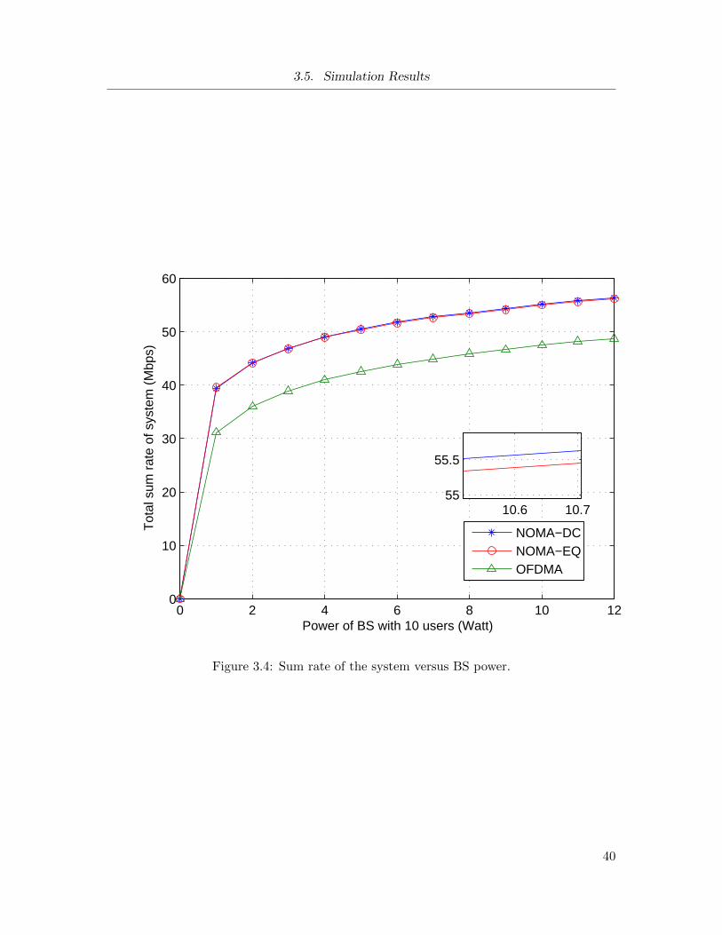
3.5. Simulation Results
0 2 4 6 8 10 120
10
20
30
40
50
60
Power of BS with 10 users (Watt)
Tot
al s
um r
ate
of s
yste
m (
Mbp
s)
10.6 10.755
55.5
NOMA−DCNOMA−EQOFDMA
Figure 3.4: Sum rate of the system versus BS power.
40

3.5. Simulation Results
0 2 4 6 8 10 120
0.5
1
1.5
2
2.5
3
3.5
4x 10
7
Power of BS with 10 users (Watt)
Ene
rgy
effie
ncy
of s
yste
m (
bits
/Jou
le)
NOMA−DCNOMA−EQOFDMA
Figure 3.5: Energy efficiency of the system versus the maximum BS power Ps.
41
3.5. Simulation Results
the sum rate. From Fig. 3.2, we observe that the performance of NOMA system with
the proposed resource allocation algorithms, including subchannel assignment and power
allocation, is much better than the OFDMA scheme. For example, when the number of
users is 30, the sum rate of the proposed algorithm (NOMA-DC) 3 is 12.5% more than that
of the OFDMA scheme, and the sum rate of equal power allocation (NOMA-EQ) is 11.9%
more than that of the OFDMA scheme. That is because in the OFDMA scheme, each
subchannel can only be used by one user. As a result, BS cannot fully use the spectrum
resources. For different subchannel power allocation schemes, the sum rate of NOMA-DC
is higher than that of NOMA-EQ.
Figure 3.3 shows the energy efficiency versus the number of users with the same con-
straints of Fig. 3.2. It can be observed that the energy efficiency also increases when the
number of users grows. The trend of curve is similar to the sum rate curves due to the
energy efficiency expression. From this figure, the performance of our proposed subchan-
nels and power allocation is much more energy-efficient than the OFDMA scheme. Our
proposed subchannel power allocation through the DC programming achieves better per-
formance than the equal power allocation. When the number of users is 30, the energy
efficiency of NOMA-DC is 33% more than that of the OFDMA scheme and 19% more than
NOMA-EQ.
In Fig. 3.4, the performance of the total sum rate versus BS power with a fixed circuit
power of Pc = 1 W, the total number of users M = 10, and the BS power is from 1 W to
12 W. In Fig. 3.4, the sum rate of the system increases as the BS power grows. In NOMA
systems, our proposed algorithm using DC for subchannel power allocation performs better
than equal power allocation. Both algorithms outperform the OFDMA system.
Figure 3.5 illustrates the total energy efficiency versus BS power with the fixed circuit
power of Pc = 1 W, and the number of users is M = 10, and the BS power ranges
from 1 W to 12 W. It shows that the total energy efficiency first increases from 0 when BS
transmit power increases. After the power reaches a certain level, the total energy efficiency
3NOMA-DC uses DC programming to allocate power across subchannels.
42

3.6. Summary
begins to decrease. That is because there is a tradeoff between transmission capacity and
power consumption for the energy-efficient power allocation. From Fig. 3.5, it is seen that
NOMA-DC can achieve better performance than NOMA-EQ and the OFDMA scheme. For
larger BS power levels, NOMA-DC achieves much better performance than NOMA-EQ and
OFDMA.
Figure 3.6 shows the total energy efficiency versus circuit power to BS power ratio
Pc/Ps. The system energy efficiency decreases when the ratio Pc/Ps increases. With the
fixed BS power of 12 W, the system achieves less energy efficiency when the circuit power
increases. According to the definition of energy efficiency, its value will become smaller
when Pc increases. However, the NOMA system equipped with the proposed resource
allocation algorithms still outperforms the OFDMA system.
In Fig. 3.7, FTPA among multiplexed users with equal subchannel power scheme is
compared with the NOMA-DC, NOMA-EQ and OFDMA schemes. Fig. 3.7 shows that
the energy efficiency increases as the number of users grows. NOMA-DC-DC4 performs the
best among those schemes. When user number is 20, the energy efficiency of NOMA-DC-
DC is 35% more than that of the OFDMA scheme and 30% more than NOMA-FTPA-EQ5.
NOMA-DC-EQ6achieves 12% more than the OFDMA scheme in terms of energy efficiency.
3.6 Summary
By assigning only two users to the same subchannel, we proposed energy-efficient re-
source allocation algorithms for a downlink NOMA wireless network. These algorithms
include subchannel assignment, power proportional factors determination for multiplexed
users and power allocation across subchannels. By formulating the subchannel assignment
problem as a two-sided matching problem, we proposed the SOMSA algorithm to maximize
4NOMA-DC-DC uses DC programming approach to determine the power proportional factors and allo-cate different powers across the subchannels.
5NOMA-FTPA-EQ uses FTPA to determine the power proportional factors, and equal power allocationacross the subchannels.
6NOMA-DC-DC uses DC programming approach to determine the power proportional factors and equalpower allocation across the subchannels.
43

3.6. Summary
0.05 0.1 0.15 0.2 0.25 0.3 0.35 0.4 0.45 0.50.5
1
1.5
2
2.5
3x 10
7
Pc/Ps with 10 users
Ene
rgy
effie
ncy
of s
yste
m (
bits
/Jou
le)
NOMA−DCNOMA−EQOFDMA
Figure 3.6: Energy efficiency of the system versus Pc/Ps.
44

3.6. Summary
10 15 20 25 30 35 40 45 50 55 601
1.5
2
2.5
3
3.5
4
4.5
5x 10
7
Number of users per BS
Ene
rgy
effic
ienc
y of
sys
tem
(bi
ts/J
oule
)
NOMA−DC−DC Pc=1wNOMA−DC−EQ Pc=1wOFDMANOMA−FTPA−EQ Pc=1w
Figure 3.7: Energy efficiency of the system versus different number of users.
45
3.6. Summary
the system energy efficiency. Power proportional factors for the multiplexed users on each
subchannel are determined by SOMSA. In the power allocation across subchannels scheme,
since the objective function is non-convex, DC programming was utilized to approximate
the non-convex optimization problem into the convex subproblem. Therefore, a subopti-
mal power allocation across subchannels was obtained by solving the convex subproblems
iteratively. Based on the resource scheduling from the proposed SOMSA algorithm, fur-
ther improvement in the system energy efficiency was achieved by the proposed subchannel
power allocation scheme. Through extensive simulations, the performance of the proposed
algorithms for resource allocation was compared with the OFDMA system. It was shown
that the total sum rate and energy efficiency of NOMA system are both higher than the
OFDMA scheme. The proposed power allocation for subchannel users outperforms the
FTPA scheme. Moreover, the proposed subchannel power allocation achieves better per-
formance than the equal power allocation scheme.
46
Chapter 4
Energy Efficient Resource
Allocation for Downlink NOMA
Network with Imperfect CSI
In this chapter, we investigate energy efficiency improvement for a downlink NOMA
single-cell network by considering imperfect CSI. The energy efficient resource scheduling
problem is formulated as a non-convex optimization problem with the constraints of out-
age probability limit, the maximum power of the system, the minimum user data rate
and the maximum number of multiplexed users sharing the same subchannel. Different
from previous works, the maximum number of multiplexed users can be greater than two,
and the imperfect CSI is first studied for resource allocation in NOMA. The probabilis-
tic mixed problem is first transformed into a non-probabilistic problem. To balance the
system performance and the computational complexity, a new suboptimal user scheduling
scheme is proposed to schedule users on different subchannels. Based on the user scheduling
scheme, the optimal power allocation expression is derived by the Lagrangian approach. By
transforming the fractional-form problem into an equivalent subtractive-form optimization
problem, an iterative power allocation algorithm is proposed to maximize the system en-
ergy efficiency. Finally, we present some selected numerical results to demonstrate that the
proposed user scheduling algorithm closely attains the optimal performance.
47

4.1. System Model
4.1 System Model
We consider a downlink single cell NOMA network where a BS is located in the cell
center and M users are uniformly distributed within the cell. We define M and N as
the numbers of users and subchannels, respectively. The BS transmits its signals to M
users through N subchannels. We denote n as the index for the subchannel where n ∈
{1, 2, · · · , N}. The total bandwidth B is shared by N subchannels and each subchannel
occupies a bandwidth of Bsc = B/N . According to the NOMA protocol, multiple users
can share the same subchannel. We denote the set of users on subchannel n (SCn) as Un
and denote the number of users on SCn as Mn∆= |Un| , n ∈ {1, 2, · · · , N} where M = M1 +
M2 + · · ·+MN . We denote m as the index of the mth user multiplexed on each subchannel.
PT is denoted as the total transmitted power of the system and letN∑n
Mn∑mpm,n ≤ PT where
pm,n is the allocated power to the mth user (UEm) on SCn.
We assume that Mn users are multiplexed on the subchannel n. The signal transmitted
by the BS through SCn can be expressed as
xn =
Mn∑m=1
√pm,nsm (4.1)
where sm is the modulated symbol, which represents the transmitted symbol of UEm on
SCn. We define hm,n as the channel gain from the BS to the mth user on SCn. Without
loss of generality, we assume channel gains of the Mn users on SCn are perfectly known
and are sorted as |hMn,n| ≥ |hMn−1,n| ≥ · · · ≥ |hm,n| ≥ · · · ≥ |h1,n|. In the NOMA system,
by exploiting the SIC technique at the receivers, the signal received by UEm on SCn can
be formulated as
ym,n = hm,nxn + zm,n
= hm,n√pm,nsm + hm,n
Mn∑i=m+1
√pi,nsi + zm,n
(4.2)
where hm,n = Dm,ngm,n, where Dm,n = d− 1
2m,n and gm,n ∼ CN (0, 1) respectively account for
48
4.1. System Model
path loss coefficient and the Rayleigh fading channel gain between the BS to the mth user
on SCn, and where dm,n is the distance from the BS to the mth user on SCn. The noise
term zm,n is a zero-mean complex AWGN random variable with variance σ2z .
4.1.1 Imperfect Channel Model
Most previous works assumed that the BS has the whole knowledge of CSI. However,
the perfect CSI is challenging to obtain in practice. In this paper, we investigate the energy
efficiency optimization by assuming that the small scale fading channel is estimated at the
BS. Since the path loss and shadowing are large scale fading factors and are slowly varying,
we assume that the path loss and shadowing coefficients Dm,n can be estimated perfectly
by the BS [74, 75]. By using the minimum mean square error channel estimation error
model [73, 76, 77], we can model the Rayleigh fading coefficient between the BS and the
mth user on SCn as
gm,n = gm,n + em,n (4.3)
where gm,n is the real Rayleigh fading channel coefficient between the BS to the mth user
on SCn; gm,n ∼ CN (0, 1−σ2e) denotes the estimated channel gain and em,n is the estimated
error which follows a complex Gaussian distribution with mean zero and the variance σ2e .
We assume that random variables gm,n and em,n are uncorrelated.
4.1.2 Scheduled Channel Capacity and Outage Capacity
If the BS has the perfect CSI hm,n = Dm,ngm,n, according to the Shannon’s capacity
formula, the maximum achievable data rate of the mth user on SCn can be written as
Cm,n = Bsclog2 (1 + Γm,n) (4.4)
49
4.1. System Model
where
Γm,n =pm,n|hm,n|2
|hm,n|2Mn∑
i=m+1pi,n + σ2
z
.(4.5)
In (5), Γm,n is the signal-to-interference-plus-noise ratio for themth user on SCn; |hm,n|2Mn∑
i=m+1pi,n
is the interference from the users who have higher channel gains on SCn. However, in prac-
tice, the BS only has the estimated fading channel coefficient gm,n. The data rate may
exceed the maximum achievable data rate. Therefore, in this paper, we adopt outage prob-
ability as a metric to measure the performance of the case when the scheduled data rate
exceeds the achievable data rate with imperfect CSI. The scheduled data rate of the mth
user on SCn can be written as
rm,n = Bsclog2 (1 + Φm,n) (4.6)
where
Φm,n =pm,n|hm,n|2
|hm,n|2Mn∑
i=m+1pi,n + σ2
z
(4.7)
and where hm,n = Dm,ngm,n. Therefore, the system average outage sum rate is defined as
[73]
R(U ,P) =
N∑n=1
Mn∑m=1
rm,n Pr [rm,n ≤ Cm,n|gm,n] (4.8)
where Pr [rm,n ≤ Cm,n|gm,n] denotes the probability of the event when the scheduled data
rate rm,n, which is based on the estimated channel gain gm,n, is less than or equal to the
maximum data rate Cm,n, which is based on the real channel gain gm,n. The resource allo-
cation includes user scheduling policy (U) and power allocation policy (P = {pm,n, ∀m,n}
for pm,n).
50

4.2. Problem Formulation
4.2 Problem Formulation
For energy efficient communication, we aim to maximize the total communication data
rate with the unit power cost. Therefore, we formulate the system energy efficiency as a
ratio of the system sum rate to the total power consumption. The energy efficiency of the
system is formulated as
EE(U ,P) =R(U ,P)
Ps(U ,P)(4.9)
where Ps(U ,P) = Pc + PT is the total power consumption of the system; Pc and PT =N∑n=1
Mn∑m=1
pm,n are the circuit power consumption and transmission power, respectively. The
energy efficiency maximization problem can be formulated as
maxU ,P
EE(U ,P) (4.10)
s.t. C1 : Pr[Cm,n < rm,n|gm,n] ≤ εout, ∀m,n
C2 :N∑n=1
Mn∑m=1
pm,n ≤ Pmax,
C3 : rm,n ≥ Rmin, ∀m,n
C4 : pm,n ≥ 0,∀m,n
C5 : |Un| ≤ Umax,∀n
(4.11)
where C1 specifies the channel outage probability requirement εout; C2 is the transmission
power limit constraint for the BS in the downlink single cell network and Pmax is the
maximum transmitted power of the BS; C3 describes that each user data rate must be larger
than the minimum user data rate Rmin, which is determined by the QoS requirement; C4
ensures that the power allocated to each user is positive, and C5 specifies the user number
allocated on each subchannel must be less than the maximum number of the users Umax,
which can be greater than two.
51

4.3. Methodology and Problem Solution
4.3 Methodology and Problem Solution
The objective function in (4.10) is a non-convex function with non-convex probabilistic
constraints. The global optimal resource allocation cannot easily be obtained in practice
since this problem cannot be optimally solved in polynomial time. In order to solve this
optimization problem efficiently, we first deal with the non-convex probabilistic constraint
C1 in (4.11) and transform the probabilistic mixed problem into a non-probabilistic prob-
lem. An iterative resource allocation algorithm for user scheduling and power allocation is
shown as Algorithm 4.
4.3.1 Optimization Problem Transformation
The outage probability requirement in C1 is a complicated non-convex function of sched-
uled data rate and powers. Therefore, the exact closed form expression for resource alloca-
tion cannot be obtained. However, we can address this issue by the following approxima-
tions. We first rewrite the scheduled data rate as
rm,n = Bsclog2 (1 + Φm,n)
= Bsclog2
(1 +
am,nbm,n
) (4.12)
where Φm,n =am,nbm,n
= 2rm,nBsc − 1 and am,n = bm,n(2
rm,nBsc − 1), and the achievable data rate is
Cm,n = Bsclog2 (1 + Γm,n)
= Bsclog2
(1 +
cUm,ncDm,n
)(4.13)
52

4.3. Methodology and Problem Solution
where cUm,n = pm,nD2m,n|gm,n|
2, cDm,n = D2m,n|gm,n|
2Mn∑
i=m+1pi,n + σ2
z . The outage probability
condition can be bounded by
Pr[Cm,n < rm,n|gm,n] ≤ εout
= Pr[Γm,n < Φm,n|gm,n] ≤ εout.(4.14)
According to the total probability theorem, the outage probability can be written as
Pr[Γm,n < Φm,n|gm,n]
= Pr
[cUm,ncDm,n
< 2rm,nBsc − 1|gm,n
]
= Pr[E1] · Pr[cUm,n ≤ am,n|gm,n
]+ Pr[E2] · Pr
[cUm,n > am,n|gm,n
](4.15)
where
Pr[E1] = Pr
[cUm,ncDm,n
< 2rm,nBsc − 1|cUm,n ≤ am,n, gm,n
]
Pr[E2] = Pr
[cUm,ncDm,n
< 2rm,nBsc − 1|cUm,n > am,n, gm,n
].
(4.16)
Following [73, 76, 77], we can show that the outage probability constraint C1 can be derived
from
Pr[cDm,n ≥ bm,n|gm,n
]≤ εout/2 (4.17)
and
Pr[cUm,n ≤ am,n|gm,n
]= εout/2. (4.18)
53

4.3. Methodology and Problem Solution
To show this, we note that since bm,n = am,n/(2rm,nBsc − 1), we have
Pr[cDm,n ≥ bm,n|gm,n
]= Pr
[cDm,n ≥ am,n/(2
rm,nBsc − 1)|gm,n
]= Pr
[am,ncDm,n
≤ 2rm,nBsc − 1|gm,n
].
(4.19)
Therefore, eq. (4.17) can be rewritten as Pr[am,ncDm,n
≤ 2rm,nBsc − 1|gm,n
]≤ εout
2 . When cUm,n >
am,n, we can always have
Pr[E2] = Pr
[cUm,ncDm,n
≤ 2rm,nBsc − 1|gm,n
]≤ εout/2. (4.20)
From (4.18), we have Pr[cUm,n > am,n|gm,n
]= 1 − εout/2. Since Pr[E1] ≤ 1, we have from
(4.15), (4.17) and (4.18)
Pr[Γm,n < Φm,n|gm,n] ≤ εout/2 + (εout/2)(1− εout/2)
= εout − ε2out/4 ≈ εout, for εout � 1.
(4.21)
Therefore, the constraint C1 can be rewritten as (4.17) and (4.18).
We now integrate the probabilistic constraints in (4.17) and (4.18) into (4.10) and
transform to a revised optimization problem as follows. By using the Markov inequality,
we have [73, 77, 78]
Pr[cDm,n ≥ bm,n|gm,n
]= Pr
[D2m,n|gm,n|
2Mn∑
i=m+1
pi,n ≥ bm,n − σ2z |gm,n
]
≤E
[D2m,n|gm,n|
2Mn∑
i=m+1pi,n
]bm,n − σ2
z
=
D2m,n|gm,n|
2Mn∑
i=m+1pi,n
bm,n − σ2z
.
(4.22)
54
4.3. Methodology and Problem Solution
According to (4.17), let the right side of (4.22) equals to εout/2, we have
D2m,n|gm,n|
2Mn∑
i=m+1pi,n
bm,n − σ2z
=εout
2. (4.23)
Since |gm,n|2 ∼ CN (gm,n, σ2e) is a non-central chi-squared distributed random variable with
two degrees of freedom, the left side of (4.18) can be rewritten as
Pr[cUm,n ≤ am,n|gm,n
]= Pr
[pm,nD
2m,n|gm,n|
2 ≤ am,n|gm,n]
= Pr
[|gm,n|2 ≤
am,nD2m,npm,n
|gm,n]
=F|gm,n|2
(am,n
D2m,npm,n
)
=1−Q1
√2|gm,n|2
σ2e
,
√2
σ2e
am,nD2m,npm,n
(4.24)
where
Q1 (a, b) = exp
(−a
2 + b2
2
) ∞∑k=0
(ab
)kIk (ab)
is the first-order Marcum Q-function and Ik(·) is the kth order modified Bessel function of
the first kind. Based on (4.19), let (4.24) equal to εout/2, then we have
am,n = F−1|gm,n|2
(εout/2) ·D2m,npm,n (4.25)
where F−1|gm,n|2
(·) is the inverse function of F|gm,n|2(·). Based on |gm,n|2 = |gm,n|2 + σ2e ,
bm,n = am,n/(2rm,nBsc − 1), (4.23) and (4.24), we have
D2m,n|gm,n|
2Mn∑
i=m+1pi,n
am,n/(2rm,nBsc − 1)− σ2
z
=
Mn∑i=m+1
pi,nD2m,n
(|gm,n|2 + σ2
e
)F−1
|gm,n|2(εout/2)·D2
m,npm,n
2rm,nBsc −1
− σ2z
=εout
2.
(4.26)
55

4.4. Energy Efficient Resource Allocation Scheme
Therefore, the data rate for the mth user on SCn (rm,n) with the outage probability con-
straint can be written by
Rm,n = Bsclog2
(1 + Φm,n
)(4.27)
where
Φm,n =εoutF
−1|gm,n|2
(εout/2) ·D2m,npm,n
εoutσ2z + 2D2
m,n
(|gm,n|2 + σ2
e
) Mn∑i=m+1
pi,n
. (4.28)
Now, the transformed average sum rate for the entire system can be written by [59]
R(U ,P) =
N∑n=1
Mn∑m=1
(1− εout) Rm,n. (4.29)
The energy efficient optimization problem can be reformulated as
maxU ,P
EE(U ,P) =R(U ,P)
Ps(U ,P)(4.30)
s.t. C1 :N∑n=1
Mn∑m=1
pm,n ≤ Pmax,
C2 : Rm,n ≥ Rmin, ∀m,n
C3 : pm,n ≥ 0,∀m,n
C4 : |Un| ≤ Umax, ∀n.
(4.31)
The transformed non-probabilistic optimization problem (4.30) is still non-convex. The
optimal solution to this non-convex optimization problem (4.30) is challenging to obtain
in practice. In order to solve (4.30) efficiently, we will design an iterative algorithm to
maximize the system energy efficiency.
4.4 Energy Efficient Resource Allocation Scheme
In this section, we design an iterative algorithm for the energy efficient joint user schedul-
ing and power allocation, as shown in Algorithm 4. This algorithm includes user scheduling
56

4.4. Energy Efficient Resource Allocation Scheme
subproblem and power allocation subproblem. In each iteration, user scheduling and power
allocation are updated iteratively until convergence. We first assume equal power allocation
for all the users. The user scheduling is optimized by the proposed Algorithm 5 which pro-
vides better performance than the corresponding algorithm in [57]. Based on the obtained
user scheduling scheme, the power allocation scheme can be updated by Algorithm 6, where
the optimal power allocation policy can be obtained by the Lagrangian approach. An it-
erative power allocation scheme is proposed and the optimal closed form power expression
is derived for each user. Due to the non-convexity of the problem in (4.30), the optimal
solution cannot be obtained in polynomial time. However, in this iterative algorithm, the
system energy efficiency slightly improves at each iteration and it converges at the end of
the procedure. It is observed that the constraints in (4.31) satisfy the necessary Karush-
Kuhn-Tucker (KKT) conditions. Algorithm 4 finds at least one locally optimal solution
with the potential of being a global optimum.
Algorithm 4: Energy Efficient Resource Allocation Algorithm
1: Initialize the power allocation for each user pm,n = Pmax/M .2: Initialize the maximum iterations Lmax, the index l = 1 and maximum tolerance ε.3: while
∣∣EE(l) − EE(l−1)∣∣ > ε or l ≤ Lmax do
4: 1. Given P (l), obtain user scheduling scheme U l by the proposed suboptimalalgorithm (Algorithm 5).
5: 2. Update the power allocation scheme P (l+1) according to the propose powerallocation policy shown in Algorithm 6 of Section 4.4.2.
6: 3. Set l = l + 1 and compute EE(l+1).7: end while
4.4.1 User Scheduling Scheme Design
In this section, we design a user scheduling scheme to assign users to different subchan-
nels in order to maximize the system energy efficiency. Since the maximum number of
users that can be multiplexed on the same subchannel is less than Umax, the global optimal
solution can only be obtained by the exhaustive search method, which has exponential com-
plexity with respect to the number of subchannels. Thus we propose a novel suboptimal
57

4.4. Energy Efficient Resource Allocation Scheme
user scheduling scheme to reduce the complexity. The user scheduling can be expressed as
Uoptimal = arg maxU
EE(U) =R(U)
Ps(U). (4.32)
Algorithm 5: A Novel Suboptimal User Scheduling Algorithm
1: Initialize the power allocation for each user Pm,n.
2: Construct the estimate channel gain H ∆= [|hm,n|]M×N .
3: Initialize the sets Uun to record the unallocated user in the system.4: Initialize the lists for all the subchannels EE(n) to record the energy efficiency ofSCn.
5: while Uunun 6= ∅ do6: Find the maximum value |hm,n| in H using
|hm,n| = arg maxm∈Uun,n∈Hun
(H) .
7: EEn,possible=∅.8: EEn,i=∅.9: if the number of multiplexed users on this subchannel is less than Umax then
10: a) Schedule the user m onto the subchannel n.11: b) Uun=Uun\UEm.12: end if13: if the number of multiplexed users on this subchannel equals Umax then14: a) Assume UEm is allocated on SCn and the user set is now Un,possible.15: b) Calculate the energy efficiency EEn possible of the Umax users from Un,possible
on SCn.16: c) Un = arg max
U∈Un,possible(EEn possible) and UEi /∈ Un.
17: d) Uun=Uun\Un.18: Let the ith and nth row’s elements in H be zeros.19: Let the nth column’s elements in H be zeros.20: end if21: end while
Algorithm 5 describes the proposed suboptimal user scheduling process. We first initial-
ize the power allocation scheme. When Algorithm 5 is used for the first time, we assume
equal power allocation for each user pm,n = PmaxM . Uun is initialized to record the users
who have not been allocated to any subchannel. In the scheduling procedure, we need
to find the user who has the maximum channel gain and allocate it to the corresponding
58

4.4. Energy Efficient Resource Allocation Scheme
subchannel if the number of users multiplexed on this subchannel is less than Umax. If the
user number is equal to Umax, the users should be selected from the user set Un,possible. The
users who can provide the maximum energy efficiency on this subchannel will be allocated
on this subchannel. The user who has been selected will be returned to Uun. This process
terminates if there is no user left to be allocated.
The complexity of the proposed algorithm is less than the optimal exhaustive search.
Since the user scheduling subproblem is non-convex, the optimal user scheduling algorithm
can only be obtained through exhaustive search. For a given power allocation scheme, the
best user scheduling scheme can be obtained to maximize the system energy efficiency by
searching all the combinations of users and subchannels. The exhaustive search depends
on the maximum number of users multiplexed on each subchannel Umax. For the opti-
mal solution, the BS needs to search N !((M1
)+(M2
)+ · · ·+
(MUmax
))combinations. The
time complexity of exhaustive search is O(N !2M ). The performance of the proposed user
scheduling algorithm is compared with the optimal solution and the existing scheme in [57].
Simulation comparison is shown in Section 4.5. With the same complexity, the proposed
algorithm can achieve improved energy efficiency performance.
4.4.2 Energy Efficient Power Allocation Algorithm
After user scheduling, the power allocation for all the users is still equal power allocation
scheme. In order to further improve the system energy efficiency, a closed form optimal
power allocation expression is derived. Given the user scheduling scheme, the optimization
problem in (4.30) is still a non-convex optimization problem with respect to pm,n. The
objective function in (4.30) has a non-linear fractional form which makes the problem
challenging to solve. In order to reduce the complexity in solving the power allocation
problem, successive convex approximation and parameter transformation are exploited to
solve this problem. We design an iterative algorithm for power allocation in Algorithm 6.
The lower bound of log2(1+q) can be expressed as αlog2q+β ≤ log2(1+q) for any q ≥ 0
[79]. The bound will become tight when q = q, α = q1+q and β = log2 (1 + q)− q
1+q log2q. By
59

4.4. Energy Efficient Resource Allocation Scheme
utilizing the lower bound, the lower bound of data rate for the mth user on the subchannel
n can be written as
R∗m,n = Bscαm,nlog2
(Φm,n
)+ βm,n. (4.33)
Therefore, the energy efficient optimization problem can be rewritten by
maxP�0
EE(P) =R∗ (P)
Ps (P)(4.34)
s.t. C1 :N∑n=1
Mn∑m=1
pm,n ≤ Pmax,
C2 : R∗m,n ≥ Rmin, ∀m,n
(4.35)
where R∗ =N∑n=1
Mn∑m=1
(1− εout)R∗m,n, P∆= [pm,n]Mn×N and P � 0 means all elements of P are
positive. The objective function in (4.34) is non-convex. In order to avoid high complexity of
the solution to this problem, we introduce the following parameter transformation. Without
loss of generality, we define the maximum energy efficiency of the system as
t∗ = maxP�0
R∗ (P)
Ps (P)=R∗ (P∗)
P ∗s (P∗). (4.36)
Note that the problem in (4.34) is a concave-convex fractional optimization problem
which is a nonlinear fractional program, and it can be transformed to an equivalent param-
eterized non-fractional form as follows [66]
maxP�0
R∗ (P)− tPs (P) (4.37)
s.t. C1 :N∑n=1
Mn∑m=1
pm,n ≤ Pmax,
C2 : Rm,n ≥ Rmin, ∀m,n
(4.38)
where t is a parameter introduced to scale the weight of Ps. For a given value t, the solution
to problem (4.37) is denoted by P and the optimal solution to (4.37) is defined as P∗. Let
60
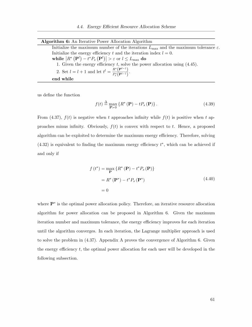
4.4. Energy Efficient Resource Allocation Scheme
Algorithm 6: An Iterative Power Allocation Algorithm
Initialize the maximum number of the iterations Lmax and the maximum tolerance ε.Initialize the energy efficiency t and the iteration index l = 0.while
∣∣R∗ (Pl)− t∗Ps
(Pl)∣∣ > ε or l ≤ Lmax do
1. Given the energy efficiency t, solve the power allocation using (4.45).
2. Set l = l + 1 and let tl =R∗(Pl−1)P ∗s (Pl−1)
.
end while
us define the function
f(t)∆= max
P�0{R∗ (P)− tPs (P)} . (4.39)
From (4.37), f(t) is negative when t approaches infinity while f(t) is positive when t ap-
proaches minus infinity. Obviously, f(t) is convex with respect to t. Hence, a proposed
algorithm can be exploited to determine the maximum energy efficiency. Therefore, solving
(4.32) is equivalent to finding the maximum energy efficiency t∗, which can be achieved if
and only if
f (t∗) = maxP{R∗ (P)− t∗Ps (P)}
= R∗ (P∗)− t∗Ps (P∗)
= 0
(4.40)
where P∗ is the optimal power allocation policy. Therefore, an iterative resource allocation
algorithm for power allocation can be proposed in Algorithm 6. Given the maximum
iteration number and maximum tolerance, the energy efficiency improves for each iteration
until the algorithm converges. In each iteration, the Lagrange multiplier approach is used
to solve the problem in (4.37). Appendix A proves the convergence of Algorithm 6. Given
the energy efficiency t, the optimal power allocation for each user will be developed in the
following subsection.
61
4.4. Energy Efficient Resource Allocation Scheme
4.4.3 Power Allocation Expression Derivation
In Algorithm 6, given the energy efficiency t, the optimization in (4.37) is a concave
maximization problem with respect to power allocation policy P. This problem can be
solved by its dual problem and the difference between the primal and dual solution is zero
when strong duality holds [66, 80]. In this section, we solve the primal problem of (4.37)
by solving its associated dual problem. The Lagrangian function can be written by
L (P, λ,υ) =
N∑n=1
Mn∑m=1
(1− εout)R∗m,n (P)− tPs (P)
+λ
(Pmax −
N∑n=1
Mn∑m=1
pm,n
)
+N∑n=1
Mn∑m=1
υm,n(R∗m,n (P)−Rmin
)(4.41)
where λ and υ = [υm,n]Mn×N are the Lagrange multipliers corresponding to the constraints
C1 and C2 in (4.36). The constraints are KKT conditions [66] for optimizing power allo-
cation, thus the dual problem of (4.37) is
minλ,υ
g (λ,υ) (4.42)
s.t. λ ≥ 0,υ � 0 (4.43)
where
g (λ,υ) = maxP�0
L (P, λ,υ) . (4.44)
To solve (4.37), we decompose it into two layers: inner layer and outer layer. We first solve
the inner layer problem to obtain the power allocation policy, and then use the outer layer
to compute the dual variables λ and υm,n iteratively.
For a fixed Lagrange multiplier and a given energy efficiency t, the problem is a standard
optimization problem with the KKT conditions. The optimal power allocation policy for
62
4.5. Simulation Results
the mth user on SCn can be derived in Appendix B as
pm,n =αm,n
BN (1− εout + υm,n)
ln 2 (λ+ t) +m−1∑l=1
A(pl,n)(4.45)
where
A(pl,n) = (1− εout + υl,n)αl,n2(|gl,n|2 + σ2
e
)D2l,nΦl,n
pl,nεoutF−1
|gl,n|2(εout/2)
. (4.46)
Given the power allocation scheme in (4.43), the outer layer primal problem can be solved
by the gradient method since the objective function is differentiable. Therefore, the dual
variables can be updated with gradient descent as
λ(l′+ 1)
=
[λ(l′)− ξ1
(l′)(
Pmax −N∑n=1
Mn∑m=1
pm,n
)]+
(4.47)
υm,n
(l′+ 1)
=[υm,n
(l′)− ξ2
(l′) (R∗m,n −Rmin
)]+,
∀m,n(4.48)
where l′is the iteration index. ξ1
(l′)
and ξ2
(l′)
are positive step sizes at iteration l′. Since
the transformed problem (4.37) is concave, this guarantees that the iteration converges to
an optimal solution to problem (4.37) based on appropriate step sizes.
4.5 Simulation Results
In this section, we evaluate the performance of our proposed resource allocation algo-
rithms for NOMA system through Monte Carlo simulations. The system parameters used
in our simulations are given as follows. We consider one BS located in the cell center and
M users are uniformly distributed on the circular range with radius of 500 m. In the sim-
ulations, we set the minimum distance among users as 40 m and the minimum distance
between base station and users as 50 m. The total bandwidth in this system is 5 MHz
that is divided into N subchannels. In the NOMA and OFDMA systems, we assume the
63

4.5. Simulation Results
10 20 30 40 50 60 70 802
2.5
3
3.5
4
4.5
5x 10
6
Number of UE per BS
Tot
al E
nerg
y E
ffici
ency
of S
yste
m (
bits
/Jou
le)
EE−NOMA−DCEE−NOMA−ProposedEE−NOMA−ExistingEE−OFDMA
Figure 4.1: Energy efficiency performance versus the number of users
64

4.5. Simulation Results
1 2 3 4 5 6 7 8 9 101.6
1.8
2
2.2
2.4
2.6
2.8
3
3.2
3.4
3.6x 10
7
Iterations
Ene
rgy
Effi
cien
cy (
bits
/Jou
le)
|U|=30, Algorithm 3|U|=45, Algorithm 3|U|=60, Algorithm 3
Figure 4.2: Energy efficiency performance versus the number of iterations for Algorithm 6.
65

4.5. Simulation Results
small-scale Rayleigh fading channels between the base station and users, and the 3GPP
urban path loss model with a path loss factor of 3.76 [81] 7. In OFDMA systems, each
user can only be assigned to one subchannel. In NOMA systems, the maximum users
can be multiplexed on the same subchannel is three. In the simulations, we compare our
proposed resource allocation algorithms for NOMA systems with a conventional OFDMA
system. We set circuit power consumption Pc = 30 dBm and the BS peak power Pmax is
from 10 dBm and 40 dBm. The maximum number of users is 75 and σ2z = B
NN0, where
N0 = −174 dBm/Hz is the AWGN power spectral density. The maximum error tolerance
for the algorithms is set to ε = 0.01.
Figure 4.1 compares the proposed user scheduling scheme with the suboptimal sub-
channel allocation in [57]. In this figure, we set Pmax = 41 dBm. The outage probability is
0.05 and the variance of estimated error for channel gain is 0.1. Based on the equal power
allocation for users, the new proposed user scheme can achieve higher energy efficiency than
the existing schemes in [44] and [57]. For example, when the number of users is 60, the
energy efficiency of our proposed resource allocation scheme for the NOMA system is 2%
more than the subchannel algorithm in [57] and 30% more than that of the existing scheme
in [44] with equal power allocation.
Figure 4.2 evaluates the energy efficiency performance versus the number of iterations
of Algorithm 6. We set the minimum normalized data rate normalized by bandwidth for
each user as 7 bits/s/Hz and the maximum transmit power as Pmax = 40 dBm. The outage
probability is 0.1 and the variance of estimated error for channel gain is 0.1. Based on the
user scheduling scheme shown in Algorithm 4, the convergence of the proposed iterative
power allocation algorithm (Algorithm 6) is presented with different number of users. As
observed from Fig. 4.2, the system energy efficiency converges after 4 iterations. The
system with 60 users can achieve higher energy efficiency than the system with 45 and 30
users.
7Let D be the distance from the base station to the different users. The path loss model from the basestation to its users is PL dB = 15.3 + 37.6log10D.
66

4.5. Simulation Results
10 15 20 25 30 35 401
2
3
4
5
6
7
8x 10
6
Pmax (dBm)
Tot
al E
nerg
y E
ffici
ency
of S
yste
m (
bits
/Jou
le)
EE−NOMA−Proposed−Var(e)=0.1EE−NOMA−Proposed−Var(e)=0.01EE−Exhaustive−Var(e)=0.1EE−Exhaustive−Var(e)=0.01
Figure 4.3: Energy efficiency performance versus the number of users.
67

4.5. Simulation Results
1 2 3 4 5 6 7 8 9 101.8
1.9
2
2.1
2.2
2.3
2.4
2.5x 10
7
Iterations
Ene
rgy
Effi
cien
cy (
bits
/Jou
le)
|U|=60, Algorithm 1|U|=45, Algorithm 1|U|=30, Algorithm 1
Figure 4.4: Energy efficiency performance versus the number of iterations for Algorithm 4.
68

4.5. Simulation Results
Figure 4.3 shows the proposed user scheduling comparison with the optimal user schedul-
ing through exhaustive search. To evaluate the performance of the proposed user scheduling
algorithm, we adopt the equal power allocation scheme for each user and the total transmit
power for this system is set from 10 dBm to 40 dBm. Since the number of users is fixed,
the energy efficiency decreases when the total transmit power consumption increases. This
is because the transmit power consumption grows faster than the system sum rate. As
shown in this figure, the energy efficiency of the NOMA system with our proposed user
scheduling scheme is close to the exhaustive search solution especially when the transmit
power is large. The complexity of the proposed user scheduling scheme is lower than the
optimal solution especially when the user number is large. When Pmax = 25 dBm, the
optimal algorithm can only achieve 1.1% more than the proposed user scheduling scheme.
Figure 4.4 shows the convergence of the joint user scheduling and power allocation
algorithm for different number of users with Pmax = 40 dBm. It is observed that the overall
iterative algorithm converges after 5 iterations. This result demonstrates that the energy
efficiency increases when the user number increases.
In Fig. 4.5, the performance of energy efficiency is evaluated versus the number of users.
In our simulation, we set the channel estimation error variance as σ2e = 0.05 and the outage
probability εout as 0.1. It is observed that the system energy efficiency increases when the
number of users increases. As the number of users grows, the energy efficiency continues
to increase, but the rate of growth becomes slower. The performance of our proposed
resource allocation scheme for the NOMA system achieves higher energy efficiency than
that of OFDMA scheme as well as NOMA system with equal power allocation scheme. For
example, when the number of users is 30, the energy efficiency of the proposed resource
allocation scheme for the NOMA system is 38% more than that of the OFDMA scheme
with equal power allocation.
Figure 4.6 demonstrates the energy efficiency performance of NOMA systems with dif-
ferent estimation error variances versus the number of users M . As observed in Fig. 6,
the energy efficiency of the system deteriorates when the error variances increases. When
69

4.5. Simulation Results
10 20 30 40 50 60 70 800
0.5
1
1.5
2
2.5
3x 10
7
Number of UE per BS
Tot
al E
nerg
y E
ffici
ency
of S
yste
m (
bits
/Jou
le)
EE−NOMA−Proposed Pc=1wEE−NOMA−EQ Pc=1wEE−OFDM Pc=1w
Figure 4.5: Energy efficiency performance versus BS maximum power.
70

4.5. Simulation Results
10 20 30 40 50 60 70 801.02
1.03
1.04
1.05
1.06
1.07
1.08
1.09
1.1
1.11
1.12x 10
8
Number of UE per BS
Tot
al E
nerg
y E
ffici
ency
of S
yste
m (
bits
/Jou
le)
EE−NOMA Var(e)=0.1EE−NOMA Var(e)=0.05EE−NOMA Var(e)=0.01
Figure 4.6: Energy efficiency performance versus users.
71

4.6. Summary
the number of users is 60, the energy efficiency of the proposed resource allocation scheme
with σ2e = 0.01 is 1.2% more than that with σ2
e = 0.05 and is 2.2% more than that with
σ2e = 0.1. Thus, as expected, the channel estimation error can degrade the energy efficiency
performance.
4.6 Summary
For the NOMA system with imperfect CSI, we solved the resource allocation optimiza-
tion problem by transforming a probabilistic mixed non-convex optimization problem to a
non-probabilistic problem. A novel low-complexity suboptimal user scheduling algorithm
was proposed to maximize the system energy efficiency. Given the user scheduling scheme,
we proposed an optimal power allocation scheme and derived a closed form power allocation
expression for users on each subchannel where the maximum user number can be greater
than two. The effectiveness of the proposed scheme was verified by computer simulations
and compared to the existing scheme in terms of energy efficiency. It was shown that the
energy efficiency of the NOMA system with the proposed resource allocation scheme is
higher than the considered referential scheme as well as the OFDMA scheme.
72

Chapter 5
Energy Efficient Resource
Allocation for NOMA
Heterogeneous Networks
(HetNets)
Implementing NOMA in HetNets can alleviate the cross-tier interference and improve
the system throughput via resource optimization. In this chapter, we aim to maximize
the whole system energy efficiency in NOMA HetNet via subchannel allocation and power
allocation. The task of energy efficient subchannel and power allocation in both macro
cell and small cells is formulated as an integer mixed nonconvex problem. An iterative
algorithm is proposed to maximize the macro cell and small cells energy efficiency. By
considering the cochannel interference and cross-tier interference, an iterative algorithm is
proposed to solve this optimization problem. In the proposed algorithm, convex relaxation
and dual decomposition approaches are exploited to find the closed form optimal power
allocation expression in each iteration. Finally, the complexity analysis and simulation
results are provided to evaluate the system energy efficiency performance.
73

5.1. System Model and Problem Formulation
Macro BS
UEUE
Femtocell
Picocell
Small RRH
Optical fiber
Wireless link
MUE
UE7
UE1
UE3UE6
UE2
UE4
UE5
Po
wer
OFDMA
NOMA:
Superposition &
power allocationFrequency
MUE
MUE
MUE
MUE
MUE
MUE
MUE
Figure 5.1: NOMA based heterogeneous networks.
5.1 System Model and Problem Formulation
5.1.1 NOMA HetNet System Model
In this system, we consider a downlink NOMA heterogeneous small cell network shown
as Fig. 1, where one macro base station (MBS) is located in the center of macro cell. We
assume that M macro user equipments (MUEs) are uniformly distributed within the macro
cell overlaid by S small cells, e.g., picocells and femtocells. The index for the MUE and small
cells are defined as m ∈ {1, 2, · · · ,M} and s ∈ {1, 2, · · · , S}, respectively. In each small
cell, one small base station (SBS) is located in the small cell center and U user equipments
(SUEs) are uniformly distributed within the small cell. We define u ∈ {1, 2, · · · , U} as
the index of SUEs in each small cell. The MBS transmits signals to M MUEs through N
subchannels and each small cell occupies one SC. The total bandwidth is B, which is divided
into N subchannels and each subchannel occupies bandwidth Bsc = B/N .The maximum
transmit power for MBS is PMmax and the maximum transmit power of all small cells is PSmax.
A block fading channel is adopted in this system model, where the channel fading of
74

5.1. System Model and Problem Formulation
each subcarrier is assumed to be the same within a subchannel, but it varies independently
across different subchannels. In this system, we allow MUEs and SUEs to reuse these N
subchannels in order to improve the system spectrum efficiency. The cross-tier interference
caused by the macro cell will be effectively mitigated by applying the NOMA technique.
Note that the interference between small cells is neglected due to the following two reasons:
first, because different small cells will occupy different subchannels and the subchannels are
independent with each other; second, the inter-cell interference can be ignored due to the
severe wall penetration loss [16]. We assume each UE (MUE or SUE) is equipped with one
single antenna and is connected to one BS (MBS or SBS). We assume user association to the
MBS and SBSs are completed before the resource allocation, which means that the users in
the small cell are only connected to their corresponding SBS, and MUEs are connected to
the MBS. Both the MBS and SBSs have the full knowledge of the channel state information
obtained by the backhaul between the MBS and SBSs.
5.1.2 Channel Description
According to the NOMA protocol, superposition coding and successive interference
cancelation are implemented in the BSs and UEs, respectively. In NOMA HetNets, each
small cell applies NOMA, which means that the users in the same cell can be multiplexed
on the same subchannel. The MUEs share the same subchannels with the SUEs. On each
subchannel, by applying the NOMA protocol, the users who have larger channel gain will
decode and remove the message from the users who have smaller channel gain. Denote psu,n
and pm,n as the assigned power to the uth UE in the small cell s on the nth subchannel and
transmit power from MBS to MUE m on SC n. The SBS s sends messages to SUE u through
subchannel n. Define gsu,n and hMSs,u,n, respectively, as the channel gain on subchannel n from
SBS s to SUE u and the channel gain on the link n from MBS to SUE u in SBS s. Denote
α = [αs,n]S×N as the subchannel indicator matrix for the small cells, where αs,n = 1 denotes
that subchannel n is assigned to the small cell s. Denote β = [βm,n]M×N as subchannel
indicator matrix for the MUEs, where βm,n = 1 denotes that subchannel n is assigned to
75

5.1. System Model and Problem Formulation
the MUE m. We assume that each small cell has U SUEs. Generally, the channel gains of
SUEs are sorted as |gsU,n| ≥ |gsU−1,n| ≥ · · · ≥ |gsu,n| ≥ · · · ≥ |gs1,n|. The received signal by
SUE u by SBS s on subchannel n is
ysu,n = gsu,n√psu,ns
su,n + gsu,n
U∑l=u+1
√psl,ns
sl,n +
M∑m=1
βm,nhMSs,u,n√pm,nsm,n + zsu,n. (5.1)
The first term is the expected received signal from SBS s to SUE u; the second term
is the interference from the users in the same small cell; the third term is the cross-tier
interference; zsu,n ∼ CN (0, σ2z) is the zero-mean complex additive white Gaussian noise
random variable with variance σ2z . We assume that the MBS and SBS know the perfect
CSI and are connected by wired links [83]. According to the Shannon’s capacity formula,
the data rate from SBS s to SUE u on SC n is
Rsu,n = Bsc log2(1 + γsu,n) (5.2)
where
γsu,n =
∣∣gsu,n∣∣2psu,n∣∣gsu,n∣∣2 U∑l=u+1
psl,n +M∑m=1
βm,n∣∣hMSs,u,n
∣∣2pm,n + σ2z
(5.3)
is the SINR of SUE u in small cell s. The total sum rate of small cells is
RS =S∑s=1
U∑u=1
N∑n=1
αs,nRsu,n. (5.4)
The energy efficiency of small cell tier is defined as a ratio of the total sum rate of small
cells to the total power consumption of small cells
EES =RS
PST + PSc(5.5)
where PST =S∑s=1
N∑n=1
U∑u=1
αs,npsu,n is the total transmit power consumption and PSc is the
total circuit power consumption of the small cells.
76

5.1. System Model and Problem Formulation
In the macro cell, we define H = [hMm,n]M×N as the channel gain on the link from MBS
to MUE m on subchannel n. The interference from the small cell is also considered in this
work. Denote fSMs,m as the channel gain between SBS s to MUE m on the same subchannel.
Without loss of generality, we assume Mn users are multiplexed on the subchannel n and
channel gains are sorted as |hMMn,n| ≥ · · · ≥ |hMm,n| ≥ · · · ≥ |hM1,n|. According to the
Shannon’s capacity formula, the data rate of MUE m can be written as
Rm,n = Bsc log2(1 + γm,n) (5.6)
where
γm,n =
∣∣hMm,n∣∣2pm,nMn∑
i=m+1βm,n
∣∣∣hMi,n∣∣∣2pi,n +N∑n=1
U∑u=1
αs,npsu,n∣∣fSMs,m ∣∣2 + σ2
z
. (5.7)
Therefore, the sum rate of macro cell is
RM =
M∑m=1
N∑n=1
βm,nRm,n. (5.8)
The energy efficiency of the macro cell tier is defined as a ratio of the total sum rate to
the total power consumption in the macro cell
EEM =RM
PMT + PMc(5.9)
where PMT =M∑m=1
N∑n=1
βm,npm,n is the total transmit power consumption of the macro cell
and PMc is the total circuit power consumption of the macro cell.
5.1.3 Problem Formulation
Our goal is to maximize the entire system energy efficiency including macro cell energy
efficiency and small cell energy efficiency. For each tier, network’s energy efficiency is
formulated as a ratio of system sum rate to the total power consumption. The objective
77

5.1. System Model and Problem Formulation
is to maximize summation of network tier energy efficiency. Assume the MBS and SBSs
have the perfect CSI. The resource allocation is performed by the entire system under the
following definitions and constraints:
− The total power constraint:
PST =S∑s=1
N∑n=1
U∑u=1
αs,npsu,n ≤ PSmax (5.10)
PMT =
M∑m=1
N∑n=1
βm,npm,n ≤ PMmax. (5.11)
− Quality of service requirement: The SUE data rate should be guaranteed for their
basic communication, which requires the following constraint:
Rsu,n ≥ Rmin,∀s, u, n. (5.12)
The MUE data rate should also be guaranteed for their basic communication, which
requires
Rm,n ≥ Rmin,∀m,n. (5.13)
− Cross-tier interference constraints: The interference from SBS s to MUEs who are
also multiplexed on subchannel n. The cross-tier interference limit is constrained by
a threshold Isn,th
Isn =N∑n=1
αs,n
U∑u=1
psu,n∣∣fSMs,m ∣∣2 ≤ Isn,th, ∀n. (5.14)
The interference from MBS to SUE u in small cell s is also limited by a threshold
IMn,th
IMn =M∑m=1
βm,npm,n|hMSs,u,n|2 ≤ IMn,th, ∀n. (5.15)
78
5.1. System Model and Problem Formulation
The energy efficiency of NOMA HetNets can be defined as
EE = EES + EEM . (5.16)
Therefore, the energy efficient resource allocation for a downlink NOMA HetNet system
can be formulated as
max{αs,n},{βm,n},{psu,n},{pm,n}
EE (5.17)
s.t. C1 : PST ≤ PSmax;PMT ≤ PMmax,
C2 : psu,n ≥ 0, ∀s, u, n; pm,n ≥ 0,∀m,n
C3 : Rsu,n ≥ Rmin, ∀s, u, n;Rm,n ≥ Rmin, ∀m,n
C4 : Isn ≤ Isn,th, ∀s; IMn ≤ IMn,th, ∀n
C5 : αs,n ∈ {0, 1}∀s, n;βm,n ∈ {0, 1},∀m,n
C6 :S∑s=1
αs,n ≤ 1,∀n
C7 :S∑s=1
U∑u=1
αs,n +M∑m=1
βm,n ≤ Umax,∀n
(5.18)
where constraint C1 is the transmitted power limitation for all SBSs and MBS; Constraint
C2 demonstrates that the transmitted power of BS should be no less than zero; Constraint
C3 describes the heterogeneous QoS requirement that the data rata of each UE should be
no less than the minimum user data rate Rmin. In constraint C4, the cross-tier interferences
from small cell and macro cell are limited by Isn,th and IMn,th, respectively; Constraints C5
and C6 are imposed to guarantee that each subchannel can only be assigned to at most one
small cell according to C5; Constraint C7 limits the user number on the same subchannel.
79

5.2. Energy Efficient Resource Allocation for NOMA HetNets
5.2 Energy Efficient Resource Allocation for NOMA
HetNets
It is challenging to find the global optimal solution to the problem (5.17) within poly-
nomial time. To solve this problem efficiently, we first deal with macro cell subchannel
allocation to MUEs with equal power allocation policy. Based on the value of βm,n, the
energy-efficient subchannel allocation and power allocation for SUEs can be iteratively
solved by Algorithm 8 where a closed form optimal power allocation expression is derived
by the Lagrangian approach. Finally, we update the power allocation for MUEs to further
improve the system energy efficiency shown in Algorithm 9.
5.2.1 Energy Efficiency Optimization for the Entire System Algorithm
Design
Assume the MBS knows the entire knowledge of channel statement information H =
[hMm,n]M×N . To reduce the complexity of the global optimal solution, we first decouple the
problem into macro cell energy efficiency maximization and small cell energy efficiency max-
imization subproblems. A low-complexity suboptimal algorithm is designed to maximize
the system energy efficiency, as shown in Algorithm 7.
In this algorithm, we first determine subchannel allocation for MUEs in macro cell.
Equal power is allocated for all MUEs. We define a set as UMun to record the unallocated
MUEs and let it equal to 1, 2, · · · ,M . For each user, we will find subchannel n∗ who has the
maximum channel gain among N subchannels. We need to check the number of MUEs on
subchannel n∗. Allocate this MUE on subchannel n∗ if the user number is less than UMmax.
However, if the MUE number is equal to UMmax, this subchannel n∗ will choose the user set
who can provide the maximum energy efficiency [57]. The MUE who has not been chosen
will be put back into the set UMun. For this unallocated MUE, we will repeat the allocation
progress until it has been allocated on one subchannel. This subchannel allocation for
MUEs procedure will terminate until all the MUEs has been allocated on subchannels.
80

5.2. Energy Efficient Resource Allocation for NOMA HetNets
Algorithm 7: An Iterative Energy Efficient Resource Allocation Algorithm forNOMA HetNets
1: Initialize the power allocation for MUEs pm,n = Pmax/M .2: Initialize the sets UMun = 1, 2, · · · ,M to record the unallocated user in the system.3: while UMun is not empty do4: for m = 1 to M do5: 1. Find the subchannel n∗ who has the maximum channel gain in H
n∗ = maxnH
6: if the number of MUEs on this subchannel n∗ is less than UMmax then7: a) Schedule the MUE m onto the subchannel n∗.8: b) UMun=UMun\m.9: end if
10: if the number of multiplexed users on this subchannel equals Umax then11: a) Subchannel n∗ selects a set of UMmax users who can provide maximum energy
efficiency.12: b) UMun=UMun\m.13: c) The unchosen MUE will go back to Step 1 and find the maximum channel
gain among {1, 2, · · · , N}\n∗ repeat this step until it have been allocated onone subchannel.
14: end if15: end for16: end while17: After all MUEs are allocated on subchannels, αs,n and P su,n can be optimized for small
cells by Algorithm 8.18: Power allocation for MUEs can be updated by Algorithm 9.
81

5.2. Energy Efficient Resource Allocation for NOMA HetNets
After all the MUEs have been assigned to different subchannels, we focus on subchannel
allocation for small cells and power allocation for SUEs. An iterative algorithm is proposed
to solve this problem, as shown in Algorithm 8. To further improve the entire system energy
efficiency, another iterative algorithm is proposed to update the power allocation for MUEs,
as shown in Algorithm 9 of Section 5.2.4. In both Algorithm 8 and Algorithm 9, closed form
power allocation expressions for SUEs and MUEs are derived by the Lagrangian approach.
Details of the derivation can be found in Appendix C.
5.2.2 Energy Efficiency Optimization for Small Cells
In this subsection, we design an iterative algorithm to allocate subchannels to small
cell and power allocation for SUEs in order to maximize the small cells energy efficiency.
Based on the value of βm,n, the energy efficient resource allocation for small cells can be
formulated as
max{αs,n},{psu,n}
S∑s
U∑u=1
N∑n=1
αs,nRsu,n
S∑s
U∑u=1
N∑n=1
αs,npsu,n + PSc
(5.19)
s.t. C1 :
S∑s=1
N∑n=1
U∑u=1
αs,npsu,n ≤ PSmax,
C2 : psu,n ≥ 0, ∀s, u, n
C3 : αs,nRsu,n ≥ Rmin,∀s, u, n
C4 :
S∑s=1
U∑u=1
αs,npsu,n
∣∣fSMs,m ∣∣2 ≤ Isn,th,∀nC5 : αs,n ∈ {0, 1}, ∀s, n
C6 :S∑s=1
αs,n ≤ 1, ∀n.
(5.20)
This problem is mixed-integer programming due to constraint C5. The optimal solution
to this non-convex problem has an extremely high complexity. To efficiently solve this
82

5.2. Energy Efficient Resource Allocation for NOMA HetNets
problem, by using convex relaxation, we first relax the subchannel indication variable αs,n
to be a continuous real variable in [0,1]. Since the range of αs,n is between zero and one,
we could consider it as a time-sharing factor for subchannel n. It denotes the fraction of
time that small cell s occupies subchannel n during one block transmission. This relaxation
was first proposed to modify the integer mixed problem with the relaxed constraints for
subcarrier allocation in OFDM [84]. The duality gap of the relaxed problem is proved to
be zero [85].
Since the problem is fractional nonlinear programming, and it can be transformed to
an equivalent parameterized non-fractional form [66]. The equivalent subtractive problem
with relaxation can be formulated as
max{αs,n},{psu,n}
S∑s
U∑u=1
N∑n=1
αs,nRsu,n − t
(S∑s
U∑u=1
N∑n=1
αs,npsu,n + PSc
)(5.21)
s.t. C1 :S∑s=1
N∑n=1
U∑u=1
αs,npsu,n ≤ PSmax,
C2 : psu,n ≥ 0, ∀s, u, n
C3 : αs,nRsu,n ≥ Rmin,∀s, u, n
C4 :S∑s=1
U∑u=1
αs,npsu,n
∣∣fSMs,m ∣∣2 ≤ Isn,th,∀nC5 : αs,n ∈ [0, 1],∀s, n
C6 :S∑s=1
αs,n ≤ 1, ∀n
(5.22)
where t is a parameter introduced to scale the weight of the total power consumption of
small cells. For a given value t, the solution to the problem can be denoted as {αs,n} and
{psu,n}. We define
f (t) , max{αs,n},{psu,n}
S∑s
U∑u=1
N∑n=1
αs,nRsu,n − t
(S∑s
U∑u=1
N∑n=1
αs,npsu,n + PSc
). (5.23)
83

5.2. Energy Efficient Resource Allocation for NOMA HetNets
It is observed that f (t) is negative when t approaches infinity, while f (t) is positive when
t approaches minus infinity. Therefore, f (t) is convex with respect to t. Define {α∗s,n} and
{ps,∗u,n} are the optimal subchannel allocation policy and power allocation policy for problem
(5.20). Therefore, the maximum energy efficiency t∗ can be achieved if and only if
f (t∗) = RS({α∗s,n},{ps,∗u,n}
)− t∗
(PST({α∗s,n},{ps,∗u,n}
)+ PSc
)= 0 (5.24)
where the maximum energy efficiency of the small cells can be defined as
t∗ =RS({α∗s,n},{p
s,∗u,n}
)PST({α∗s,n},{p
s,∗u,n}
)+ PSc
. (5.25)
For notational simplicity, we denote the actual power allocation to SUE u in small cell
s on subchannel n as psu,n = αs,npsu,n. Thus, the data rate of SUE u in small cell s on
subchannel n can be written by
Rsu,n = Bsclog2
1 +
∣∣gsu,n∣∣2psu,n∣∣gsu,n∣∣2 U∑l=u+1
psl,n + αs,nIMn + αs,nσ2z
. (5.26)
Then the problem can be rewritten as
max{αs,n},{psu,n}
S∑s
U∑u=1
N∑n=1
αs,nRsu,n − t
(S∑s
U∑u=1
N∑n=1
psu,n + PSc
)(5.27)
84

5.2. Energy Efficient Resource Allocation for NOMA HetNets
s.t. C1 :S∑s=1
N∑n=1
U∑u=1
psu,n ≤ P smax,
C2 : psu,n ≥ 0,∀s, u, n
C3 : αs,nRsu,n ≥ Rmin, ∀s, u, n
C4 :S∑s=1
U∑u=1
psu,n∣∣fSMs,m ∣∣2 ≤ Isn,th,∀n
C5 : αs,n ∈ [0, 1], ∀s, n
C6 :
S∑s=1
αs,n ≤ 1, ∀n.
(5.28)
For a given value t, the Hessian matrix of the objective function in (5.27) with respect to
psu,n and αs,n is negative semi-definite. The objective function (5.27) is concave [66]. As the
inequality constraints in (5.28) are convex, the feasible set of objective function is convex.
Being a convex optimization problem, the transformed optimization problem in (5.27) has
a unique optimal solution, i.e., the local solution is the optimal solution, and it can be
obtained in polynomial time. Therefore, the dual decomposition method can be used to
solve this problem. The Lagrangian function of the problem (5.27) can be written by
L({αs,n} ,
{psu,n
}, t, λs,νs,µs,ηs
)=
S∑s
U∑u=1
N∑n=1
αs,nRsu,n − t
(S∑s
U∑u=1
N∑n=1
psu,n + PSc
)
+ λs
(P smax −
S∑s=1
N∑n=1
U∑u=1
psu,n
)
+
S∑s
U∑u=1
N∑n=1
νsu,n
(αs,nR
su,n −Rmin
)+
N∑n=1
µsn
(Isn,th −
S∑s=1
U∑u=1
psu,n∣∣fSMs,m ∣∣2
)
+N∑n=1
ηsn
(1−
S∑s=1
αs,n
)
(5.29)
where λs ≥ 0, νs � 0, µs � 0, and ηs � 0 are the Lagrange multipliers corresponding to
85

5.2. Energy Efficient Resource Allocation for NOMA HetNets
the power constraints. The Lagrangian function can be rewritten as
L({αs,n} ,
{psu,n
}, t, λs,νs,µs,ηs
)=
S∑s=1
N∑n=1
Ls,n({αs,n} ,
{psu,n
}, λs,νs,µs,ηs
)− tPSc + λs
(PSmax
)−
S∑s=1
N∑n=1
U∑u=1
νsu,nRmin +N∑n=1
µsnIsn,th +
N∑n=1
ηn
(5.30)
where
Ls,n({αs,n} ,
{psu,n
}, t, λs,νs,µs,ηs
)=
U∑u=1
αs,nRsu,n − t
U∑u=1
psu,n − λsU∑u=1
psu,n +
U∑u=1
νsu,nαs,nRsu,n
− µsnU∑u=1
psu,n∣∣fSMs,m ∣∣2 − ηsnαs,n.
(5.31)
Given by t, the dual problem of (5.27) is
minλs,νs,µs,ηs
g (λs,νs,µs,ηs) (5.32)
s.t. λs ≥ 0,νs,µs,ηs � 0 (5.33)
where
g (λs,νs,µs,ηs) = max{αs,n},{psu,n}
L({αs,n} ,
{psu,n
}, t, λs,νs,µs,ηs
). (5.34)
We decompose the dual problem into two layers: inner layer and outer layer. We first
solve the inner layer problem to obtain the subchannel allocation power allocation policy
for small cells, and then outer layer to compute the dual variables iteratively. To reduce
the complexity of the optimal solutions, the lower bound is applied to achieve the optimal
solution iteratively. With lower bound [79], the data rate of SUE u in small cell s on
subchannel n can be rewritten by
Rsu,n = Bscasu,nlog2(γsu,n) + bsu,n. (5.35)
86

5.2. Energy Efficient Resource Allocation for NOMA HetNets
According to (5.30), the Lagrangian dual function can be decomposed into S × N
subproblems. We define the actual optimal power allocation to SUE u in small cell s on
subchannel n as ps,∗u,n = αs,nps,∗u,n. According to the KKT conditions, assume we have the
channel gains satisfying |gsU,n| ≥ |gsU−1,n| ≥ · · · ≥ |gs1,n|, the optimal power allocation for
SUEs in small cell s can be derived as
ps,∗u,n =ps,∗u,nαs,n
=Bsca
su,n
(1 + νsu,n
)u−1∑l=1
Bscasl,n
(1 + νsl,n
)(γsl,nps,∗l,n
)+ ln 2
(ηs + λs + µsn
∣∣fSMs,m ∣∣2) (5.36)
where
γsu,n =
∣∣gsu,n∣∣2ps,∗u,n∣∣∣gs1,n∣∣∣2 U∑l=u+1
ps,∗l,n + IMn + σ2z
. (5.37)
It can be observed from (5.36) and (5.37) that the power allocation policy is a fixed point
equation. Denote α = {psu,n} and P S = {psu,n} where s = 1, 2, · · · , S, u = 1, 2, · · · , U and
n = 1, 2, · · · , N . According to the positivity, monotonicity and scalability of variable P S ,
the power allocation can be updated by each iteration with (5.36) and (5.37).
To obtain αs,n, the partial derivation of the Lagrangian can be expressed as
∂Ls,n (· · · )∂αs,n
= ∆s,n − ηsn
< 0, αs,n = 0
= 0, 0 < αs,n < 1
> 0, αs,n = 1
∀s, n (5.38)
87

5.2. Energy Efficient Resource Allocation for NOMA HetNets
where
∆s,n =
U∑u=1
(1 + νsu,n
)Bsca
su,nlog2
∣∣gsu,n∣∣2ps,∗u,n∣∣gsu,n∣∣2 U∑
l=u+1
ps,∗l,n + IMn + σ2z
−U∑u=1
(1 + νsu,n
) Bscasu,nln 2
IMn + σ2z∣∣gsu,n∣∣2 U∑
l=u+1
ps,∗l,n + IMn + σ2z
− (t+ λs)
U∑u=1
ps,∗u,n − µsnU∑u=1
ps,∗u,n∣∣fSMs,m ∣∣2.
(5.39)
Subchannel n∗ is assigned to small cell s with the largest ∆s,n, that is
α∗s,n = 1|n∗=maxn
∆s,n ,∀s. (5.40)
The outer layer primal problem can be solved by the gradient method since the objec-
tive function is differentiable. Therefore, the dual variables can be updated with gradient
descent as
λs (i+ 1) =
[λs (i)− ξ1 (i)×
(P smax −
S∑s=1
N∑n=1
U∑u=1
psu,n
)]+
, (5.41)
νsu,n (i+ 1) =[νsu,n (i)− ξ2 (i)×
(αs,nR
su,n −Rmin
)]+,∀s, u, n (5.42)
µsn (i+ 1) =
[µsn (i)− ξ3 (i)×
(Isn,th −
S∑s=1
U∑u=1
psu,n∣∣fSMs,m ∣∣2
)]+
, ∀n (5.43)
ηsn (i+ 1) =
[ηsn (i)− ξ4 (i)×
(1−
S∑s=1
αs,n
)]+
,∀n (5.44)
where i is the iteration index. ξ1 (i), ξ3 (i), ξ3 (i) and ξ4 (i) are positive step sizes at iteration
i. Since the transformed problem (5.27) is concave, this guarantees that the iteration process
converges to an optimal solution to problem (5.27) based on appropriate step sizes.
88
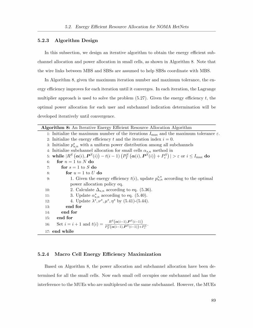
5.2. Energy Efficient Resource Allocation for NOMA HetNets
5.2.3 Algorithm Design
In this subsection, we design an iterative algorithm to obtain the energy efficient sub-
channel allocation and power allocation in small cells, as shown in Algorithm 8. Note that
the wire links between MBS and SBSs are assumed to help SBSs coordinate with MBS.
In Algorithm 8, given the maximum iteration number and maximum tolerance, the en-
ergy efficiency improves for each iteration until it converges. In each iteration, the Lagrange
multiplier approach is used to solve the problem (5.27). Given the energy efficiency t, the
optimal power allocation for each user and subchannel indication determination will be
developed iteratively until convergence.
Algorithm 8: An Iterative Energy Efficient Resource Allocation Algorithm
1: Initialize the maximum number of the iterations Imax and the maximum tolerance ε.2: Initialize the energy efficiency t and the iteration index i = 0.3: Initialize psu,n with a uniform power distribution among all subchannels4: Initialize subchannel allocation for small cells αs,n method in5: while |RS
(α(i),P S(i)
)− t(i− 1)
(PST(α(i),P S(i)
)+ PSc
)| > ε or i ≤ Imax do
6: for n = 1 to N do7: for s = 1 to S do8: for u = 1 to U do9: 1. Given the energy efficiency t(i), update ps,∗u,n according to the optimal
power allocation policy eq.10: 2. Calculate ∆s,n according to eq. (5.36).11: 3. Update α∗s,n according to eq. (5.40).12: 4. Update λs, νs, µs, ηs by (5.41)-(5.44).13: end for14: end for15: end for
16: Set i = i+ 1 and t(i) =RS(α(i−1),PS(i−1))
PST (α(i−1),PS(i−1))+PSc.
17: end while
5.2.4 Macro Cell Energy Efficiency Maximization
Based on Algorithm 8, the power allocation and subchannel allocation have been de-
termined for all the small cells. Now each small cell occupies one subchannel and has the
interference to the MUEs who are multiplexed on the same subchannel. However, the MUEs
89

5.2. Energy Efficient Resource Allocation for NOMA HetNets
on the same subchannel are allocated with equal power. To improve the energy efficiency
of the macro cell, we now update the power allocation of MUEs. We define the power
allocation policy of MUEs as PM = {pm,n}. The macro cell energy efficiency optimization
problem can be formulated as
maxPM
M∑m=1
N∑n=1
Rm,n
M∑m=1
N∑n=1
pm,n + PMc
(5.45)
s.t. C1 :M∑m=1
N∑n=1
pm,n ≤ PMmax
C2 : pm,n ≥ 0,∀m,n
C3 : Rm,n ≥ Rmin, ∀m,n
C4 :
M∑m=1
βm,npm,n|hMSs,u,n|2 ≤ IMn,th.
(5.46)
For the power allocation, this optimization problem can be transformed into an equiv-
alent subtractive problem with a parameter ηM [66], which is defined as the system energy
efficiency based on given power allocation following by the similar steps (5.23)-(5.25). We
define a function of ηM function as
f(ηM), max{pm,n}
M∑m=1
N∑n=1
Rm,n − ηM(
M∑m=1
N∑n=1
pm,n + PMc
)(5.47)
which is convex with respect to ηM . Therefore, the optimal energy efficiency for macro cell
ηM,∗ can be achieved when
f(ηM,∗) = RM
({p∗m,n}
)− ηM,∗ (PMT (
p∗m,n)
+ PMc)
= 0 (5.48)
with the optimal power allocation PM,∗ = {p∗m,n} for MUEs. Therefore, the transformed
90

5.2. Energy Efficient Resource Allocation for NOMA HetNets
subtractive form problem can be written by
maxpM
M∑m=1
N∑n=1
Rm,n − ηM(
M∑m=1
N∑n=1
pm,n + PMc
)(5.49)
s.t. C1 :
M∑m=1
N∑n=1
pm,n ≤ PMmax,
C2 : pm,n ≥ 0,∀m,n,
C3 : Rm,n ≥ Rmin,∀m,n
C4 :
M∑m=1
pm,n|hMSs,u,n|2 ≤ IMu,n,th, ∀u, n.
(5.50)
To solve (5.49), an iterative algorithm is proposed to find the optimal power allocation for
MUEs by iteratively solving the convex subproblems, as shown in Algorithm 9. By utilizing
the dual decomposition method, the Lagrangian function of problem (5.49) can be written
by
L({pm,n} , ηM , λM ,νM ,µM
)=
Mn∑m=1
N∑n=1
Rm,n − ηM(
M∑m=1
N∑n=1
pm,n + PMc
)+ λM
(PMmax −
M∑m=1
N∑n=1
pm,n
)
+M∑m=1
N∑n=1
νMm,nRm,n −Rmin +N∑n=1
U∑u=1
µMu,n
(IMu,n,th −
M∑m=1
pm,n|hMSu,n |2
)
=
Mn∑m=1
N∑n=1
Lm,n({pM}, ηM , λM ,νM ,µM
)− ηMPMc + λM (P smax)
−M∑m=1
N∑n=1
νMm,nRm,n +N∑n=1
µMn IMu,n,th
(5.51)
where
Lm,n({pm,n} , ηM , λM ,νM ,µM
)=(1 + νMm,n
)Rm,n −
(ηM + λM
)pm,n −
U∑u=1
µMu,npm,n|hMSu,n |2
(5.52)
λM , νM and µM are the Lagrange multipliers corresponding to the power constraints.
91

5.2. Energy Efficient Resource Allocation for NOMA HetNets
Given ηM , the corresponding dual problem of (5.49) is
minλM≥0,νM ,µM�0
max{pm,n}
L({pm,n} , ηM , λM , νM , µM
). (5.53)
The dual decomposition approach is exploited to solve the dual problem (5.53). Given by
the parameter ηM and fixed Lagrangian multipliers λM , νM and µM , the inner subproblem
is a convex problem. Therefore, the optimal power allocation for MUEs on subchannel n
can be written by
pM,∗m,n =
BscaM2,n
(1 + νM1,n
)m−1∑l=1
BscaMl,n
(1 + νMl,n
)(γMl,n
pM,∗l,n
)+ ln 2
(ηM + λM +
U∑u=1
µMu,n∣∣hMSu,n
∣∣2) (5.54)
where
γMm,n =
∣∣hMm,n∣∣2pm,nMn∑
i=m+1
∣∣hMm,n∣∣2pi,n +N∑n=1
U∑u=1
αs,npsu,n∣∣fSMs,m ∣∣2 + σ2
z
. (5.55)
Given the power allocation scheme in (5.54), the outer layer primal problem can be
solved by the gradient method since the objective function is differentiable. Therefore, the
dual variables can be updated with gradient descent as
λM (i+ 1) =
[λM (i)− ζ1 (i)×
(PMmax −
M∑m=1
N∑n=1
pm,n
)]+
, (5.56)
νMm,n (i+ 1) =[νsu,n (i)− ζ2 (i)× (Rm,n −Rmin)
]+, ∀m,n, (5.57)
µMu,n (i+ 1) =
[µMu,n (i)− ζ3 (i)×
(IMu,n,th −
M∑m=1
pm,n|hMSu,n |2
)]+
,∀u, n (5.58)
where i is the iteration index; ζ1 (i), ζ2 (i) and ζ3 (i) are positive step sizes at iteration i.
Based on (5.42)-(5.55), Algorithm 9 is proposed to update the power allocation for
MUEs in macro cell. Since the transformed problem (5.49) is concave, this guarantees
that the iteration process converges to an optimal solution to problem (5.49) based on
appropriate step sizes.
92
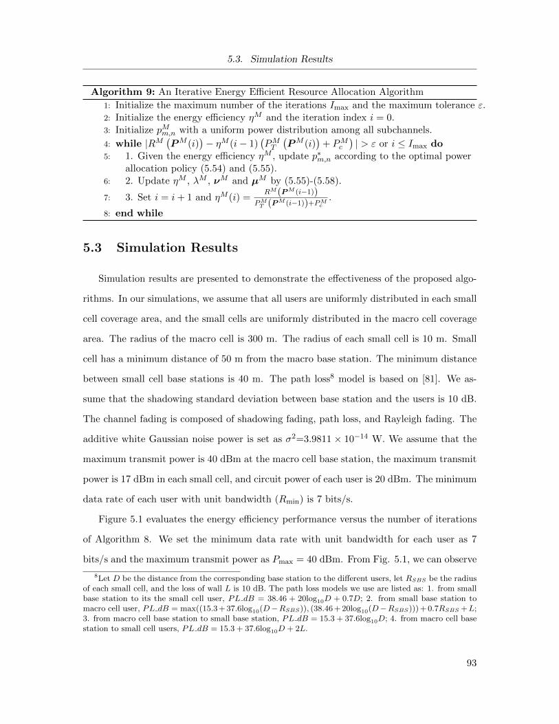
5.3. Simulation Results
Algorithm 9: An Iterative Energy Efficient Resource Allocation Algorithm
1: Initialize the maximum number of the iterations Imax and the maximum tolerance ε.2: Initialize the energy efficiency ηM and the iteration index i = 0.3: Initialize pMm,n with a uniform power distribution among all subchannels.
4: while |RM(PM (i)
)− ηM (i− 1)
(PMT
(PM (i)
)+ PMc
)| > ε or i ≤ Imax do
5: 1. Given the energy efficiency ηM , update p∗m,n according to the optimal powerallocation policy (5.54) and (5.55).
6: 2. Update ηM , λM , νM and µM by (5.55)-(5.58).
7: 3. Set i = i+ 1 and ηM (i) =RM(PM (i−1))
PMT (PM (i−1))+PMc.
8: end while
5.3 Simulation Results
Simulation results are presented to demonstrate the effectiveness of the proposed algo-
rithms. In our simulations, we assume that all users are uniformly distributed in each small
cell coverage area, and the small cells are uniformly distributed in the macro cell coverage
area. The radius of the macro cell is 300 m. The radius of each small cell is 10 m. Small
cell has a minimum distance of 50 m from the macro base station. The minimum distance
between small cell base stations is 40 m. The path loss8 model is based on [81]. We as-
sume that the shadowing standard deviation between base station and the users is 10 dB.
The channel fading is composed of shadowing fading, path loss, and Rayleigh fading. The
additive white Gaussian noise power is set as σ2=3.9811 × 10⁻¹⁴ W. We assume that the
maximum transmit power is 40 dBm at the macro cell base station, the maximum transmit
power is 17 dBm in each small cell, and circuit power of each user is 20 dBm. The minimum
data rate of each user with unit bandwidth (Rmin) is 7 bits/s.
Figure 5.1 evaluates the energy efficiency performance versus the number of iterations
of Algorithm 8. We set the minimum data rate with unit bandwidth for each user as 7
bits/s and the maximum transmit power as Pmax = 40 dBm. From Fig. 5.1, we can observe
8Let D be the distance from the corresponding base station to the different users, let RSBS be the radiusof each small cell, and the loss of wall L is 10 dB. The path loss models we use are listed as: 1. from smallbase station to its the small cell user, PL dB = 38.46 + 20log10D + 0.7D; 2. from small base station tomacro cell user, PL dB = max((15.3 + 37.6log10(D−RSBS)), (38.46 + 20log10(D−RSBS))) + 0.7RSBS +L;3. from macro cell base station to small base station, PL dB = 15.3 + 37.6log10D; 4. from macro cell basestation to small cell users, PL dB = 15.3 + 37.6log10D + 2L.
93
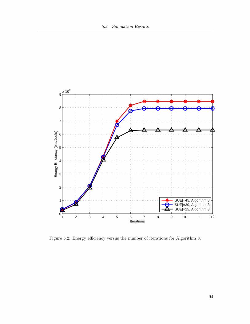
5.3. Simulation Results
1 2 3 4 5 6 7 8 9 10 11 120
1
2
3
4
5
6
7
8
9x 10
9
Iterations
Ene
rgy
Effi
cien
cy (
bits
/Jou
le)
|SUE|=45, Algorithm 8|SUE|=30, Algorithm 8|SUE|=15, Algorithm 8
Figure 5.2: Energy efficiency versus the number of iterations for Algorithm 8.
94

5.3. Simulation Results
10 20 30 40 50 60 70 802.6
2.8
3
3.2
3.4
3.6
3.8
4
4.2
4.4x 10
8
Number of SBS Per MBS
Tot
al E
nerg
y E
ffici
ency
of S
yste
m (
bits
/Jou
le)
EE_NOMA_HetNet_Proposed EE_OFDM_HetNet
Figure 5.3: Energy efficiency versus number of small cells with perfect CSI.
95

5.4. Imperfect CSI Discussion
that the convergence of the proposed iterative resource allocation algorithm (Algorithm 8)
converges within 10 iterations, which suggests that the proposed scheme is practical. The
system with 60 SUEs can achieve higher energy efficiency than the system with 45 and 15
users.
Figure 5.2 shows the performance of the system energy efficiency versus the number
of the small cells. The bandwidth is limited to 10 MHz, and we set the peak power of
the entire system to be 20 W and circuit power to be 0.1 W on each subchannel. Figure
5.2 indicates that the total energy efficiency increases when the number of the small cells
increases. From Fig. 5.2, we can observe that the NOMA HetNet outperforms the OFDM
heterogeneous network (OFDM HetNet) because OFDM HetNet cannot fully utilize the
spectrum resources.
5.4 Imperfect CSI Discussion
In this subsection, we study the energy efficient resource allocation for the downlink
NOMA heterogeneous network with imperfect CSI. In practice, perfect CSI at the trans-
mitter is difficult to achieve due to channel estimation errors, feedback and quantization
errors. To maximize the energy efficiency, we can formulate the energy efficient resource
allocation as a probabilistic mixed non-convex optimization problem under the constraints
of outage probability limitation, the maximum transmitted power and the number of mul-
tiplexed users on one subchannel.
The resource allocation scheme is optimized based on the imperfect CSI. To solve this
problem, we decouple the problem into subchannel allocation and power allocation sub-
problems separately to maximize the system energy efficiency. We assume that the BSs
have the estimated value of the CSI. In this situation, the user data rate may not meet the
minimum data requirement determined by QoS. Therefore, an outage probability require-
ment is considered for the resource scheduling to maximize the system energy efficiency.
The energy efficient optimization problem is formulated as a probabilistic mixed non-convex
96

5.4. Imperfect CSI Discussion
optimization problem. In order to efficiently solve the optimization problem, we can first
transform the probabilistic mixed non-convex optimization problem to a non-probabilistic
optimization problem. The outage probability constraint can be transformed to minimum
power constraints for UEs sharing the same subchannel. In this transformed problem, we
can treat subchannel allocation and power allocation separately. The subchannel allocation
starts with assigning equal power allocation on subchannels. The optimal solution to the
user subchannel allocation subproblem is challenging to obtain in practice as it is required
to search all the possible combinations. A suboptimal subchannel allocation algorithm can
be obtained by using the estimated CSI. In order to cancel the interference from the other
small cells, we let each small cell only occupy one subchannel. MUEs will multiplex on
these subchannels, and hence the SUEs will not interfere with each other. The MUE with
large channel gain will be chosen to multiplex on its corresponding subchannel. For the
each subchannel, we set the maximum number of multiplexed users to reduce the complex-
ity of decoding at the receivers. The subchannel allocation will terminate if there is no
MUE left to be allocated. During the subchannel allocation, the power allocation for the
multiplexed users on one subchannel can be determined by FTPA. The complexity of the
proposed suboptimal algorithm is less than the optimal solution that can only be obtained
by the exhaustive search.
Given the user subchannel allocation scheme, the underlying optimization problem can
be shown to be a convex function respect to the power variable under the constraint of the
maximum power of the system. Therefore, a unique optimal solution can be found by a
gradient assisted binary search algorithm. Therefore, the new power allocation scheme can
replace the equal power allocation to further improve the system energy efficiency.
Figure 5.4 shows the energy efficiency versus the number of the small cells with the
channel gain estimation error variance 0.05. As shown, the energy efficiency increases when
the number of the small cells grows. From Fig. 5.2, the NOMA HetNet outperforms OFDM
HetNet in terms of energy efficiency.
Fig. 5.5 shows the energy efficiency of the NOMA HetNet performance with different
97

5.4. Imperfect CSI Discussion
10 20 30 40 500
1
2
3
4
5
6
7x 10
8
Number of SBS Per MBS
Tot
al E
nerg
y E
ffici
ency
of S
yste
m (
bits
/Jou
le)
EE_OFDM_HetNet_EQ_ImperfectCSI EE_NOMA_HetNet_EQ_ImperfectCSI EE_NOMA_HetNet_FTPA_ImperfectCSI
Figure 5.4: Energy efficiency of the system versus the number of the small cells with theestimation error variance 0.05.
98

5.4. Imperfect CSI Discussion
10 20 30 40 50 60 70 802.6
2.8
3
3.2
3.4
3.6
3.8
4
4.2
4.4x 10
8
Number of SBS Per MBS
Tot
al E
nerg
y E
ffici
ency
of S
yste
m (
bits
/Jou
le)
EE_OFDM_HetNet_EQ_Var(error)=0.1 EE_OFDM_HetNet_EQ_Var(error)=0.01 EE_OFDM_HetNet_EQ_Var(error)=0 EE_NOMA_HetNet_FTPA_Var(error)=0.1 EE_NOMA_HetNet_FTPA_Var(error)=0.01 EE_NOMA_HetNet_FTPA_Var(error)=0
Figure 5.5: Energy efficiency of the system versus the number of the small cell with differentestimation error variances.
99
5.5. Summary
estimation error variances. When the number of small cells is 20, the energy efficiency of
NOMA HetNet with FTPA power allocation scheme is 27% more than that of the OFDM
HetNet with the equal power (EQ) allocation scheme under the imperfect channel CSI.
5.5 Summary
In this chapter, we introduced the concept of NOMA HetNets and proposed an energy
efficient subchannel allocation and power allocation scheme for a downlink NOMA HetNet
with perfect CSI. We solved the resource optimization problem with the help of convex
optimization. It is envisioned that a joint subchannel and power allocation approach can
further enhance the energy efficiency of the overall system. We also discussed the energy
efficiency maximization problem in the NOMA HetNet with imperfect CSI. The effective-
ness of the proposed schemes was compared to the existing scheme and verified computer
simulations to in terms of energy efficiency.
100

Chapter 6
Conclusions
In this chapter, we summarize the contributions of this thesis. Also, we present several
potential future research topics that are related to our accomplished work.
6.1 Summary of Contributions
In this thesis, we investigated the energy efficient resource allocation design for downlink
NOMA networks. We first studied the energy efficient resource allocation for a single cell
NOMA network with perfect CSI. Then we extended the energy efficient resource allocation
to the imperfect CSI case. Furthermore, the entire system energy efficiency maximization
problem was studied in a NOMA HetNet. In the end, we discussed the related future work.
Here we summarize the results obtained in each chapter.
Contribution 1: the energy-efficient resource allocation problem was formulated for a
downlink NOMA wireless network by assigning only two users to the same subchannel. To
efficiently solve this problem, we first decoupled it into subchannel allocation and power
allocation subproblems. Matching theory was exploited by subchannel assignment subprob-
lem formulation and a low-complexity suboptimal algorithm was proposed to maximize the
system energy efficiency. To allocate powers across subchannels, DC programming was
utilized to approximate the non-convex optimization problem into the convex subproblem.
Therefore, a suboptimal power allocation across subchannels was obtained by solving the
convex subproblems iteratively. The system energy efficiency was further improved by the
proposed subchannel power allocation scheme. Numerical results showed that both sum
rate and energy efficiency performance of the proposed resource allocation scheme outper-
101

6.2. Future Works
formed the OFDMA system.
Contribution 2: For the NOMA system with imperfect CSI, the formulated probabilis-
tic mixed non-convex resource optimization problem was first transformed into to a non-
probabilistic problem. Based on the proposed low-complexity suboptimal user scheduling
scheme, we proposed an iterative allocation algorithm for power allocation. In power allo-
cation, we derived a closed form power allocation expression for users on each subchannel
where the maximum user number can be greater than two. The performance of the pro-
posed scheme was verified by computer simulations and compared to the existing scheme
in terms of energy efficiency. It was shown that the energy efficiency of the NOMA system
with our proposed resource allocation scheme is higher than the existing scheme in [57] as
well as the OFDMA scheme.
Contribution 3: the single-cell NOMA system model was extended into HetNets. To
maximize the entire NOMA HetNet, an energy efficient subchannel allocation and power
allocation scheme was proposed for a downlink NOMA HetNet with perfect CSI. We solved
the resource optimization problem with the help of convex optimization. The energy ef-
ficiency maximization was considered on both small cells and marco cell. In small cell, a
joint subchannel and power allocation approach can enhance the system energy efficiency.
The optimal power allocation scheme in macro cell was proposed to further improve the
overall system energy efficiency. Moreover, imperfect CSI case was also discussed. Simu-
lation results show that our proposed resource allocation scheme for NOMA HetNets can
achieve higher energy efficiency than that of conventional OMA systems. Finally, the en-
ergy efficiency for NOMA HetNets with imperfect CSI was discussed, and the performance
was evaluated by the simulation results.
6.2 Future Works
In Chapter 5, we presented an energy efficient resource scheme for a downlink NOMA
HetNet. Resource allocation is one of the methods to improve the energy efficiency of 5G
102

6.2. Future Works
NOMA networks. Small cell in HetNet can also be energy efficient because low power is
typically required due to the short distance between transmitter and receiver. However,
there are still many challenges and open issues in achieving energy-efficient 5G NOMA
networks. 1) NOMA with MIMO: Not only user scheduling and power allocation, but also
beamforming can be considered in the energy efficient resource allocation. Furthermore,
different antenna configurations for macro cell and small cell in HetNet will make the
problem more complex. Finding effective ways to combine NOMA and massive MIMO is a
challenging but important topic in future research works. 2) NOMA with energy harvesting:
To save more energy, 5G NOMA HetNet is expected to harvest energy from solar, wind,
thermoelectric, and so on. One open problem is how to manage those renewable energy
source because they are intermittent over time and space. 3) NOMA with game theory:
User pairing is a key research direction in energy-efficient 5G NOMA networks. Matching
game theory can be an effective tool to optimize the user pairing of energy-efficient 5G
NOMA networks. 4) NOMA with open/closed access small cells: There are three access
modes in small cell networks: open access, closed access, and hybrid access. Different access
modes of NOMA small cells require different energy saving methods. Therefore, the energy
efficient resource allocation in 5G NOMA networks can be both challenging and promising.
103

Bibliography
[1] A. A. Huurdeman, The Worldwide History of Telecommunications. New Jersey: John
Wiley & Sons Press, 2003. → pages 1
[2] A. Goldsmith, Wireless Communications. Cambridge: Cambridge University Press,
2005. → pages 1
[3] F. A. Tobagi, “Modeling and performance analysis of multihop packet radio networks,”
Proceedings of the IEEE, pp. 135-155, Jan. 1987. → pages 1
[4] “Report ITU-R M.2134: Requirements related to technical performance for IMT-
advanced radio interface(s),” ITU-R, 2008. → pages 2
[5] 3GPP TR 36.913 (V8.0.0), “Requirements for further advancements for E-UTRA (LTE-
Advanced),” June 2008. → pages 2
[6] Qualcomm, “3GPP RAN Rel-12 and beyond,”Workshop on release 12, June 2012. →
pages 2
[7] “Ericsson mobility report June 2017,” Ericsson, 2017. → pages xi, 2, 3
[8] Z. Gao, L. Dai, Z. Wang, and S. Chen, “Spatially common sparsity based adaptive chan-
nel estimation and feedback for FDD massive MIMO,” IEEE Transactions on Signal
Processing, vol. 63, no. 23, pp. 6169–6183, Dec. 2015. → pages 2
[9] X. Gao, L. Dai, S. Han, C.-L.I, and R. W. Heath, “Energy-efficient hybrid analog
and digital precoding for mmWave MIMO systems with large antenna arrays,” IEEE
104

Bibliography
Journal on Selected Areas in Communications, vol. 34, no. 4, pp. 998–1009, Apr. 2016.
→ pages 2
[10] H. Zhang, X. Chu, W. Guo, and S. Wang, “Coexistence of Wi-Fi and heterogeneous
small cell networks sharing unlicensed spectrum,” IEEE Communications Magazine,
vol. 53, no. 3, pp. 158–164, Mar. 2015. → pages 2
[11] H. Zhang, C. Jiang, J. Cheng, and V. C. M. Leung, “Cooperative interference miti-
gation and handover management for heterogeneous cloud small cell networks,” IEEE
Wireless Communications, vol. 22, no. 3, pp. 92–99, June 2015.
[12] H. Zhang, C. Jiang, Q. Hu, and Y. Qian, “Self-organization in disaster resilient het-
erogeneous small cell networks,” IEEE Network, vol. 30, no. 2, pp. 116–121, Mar. 2016.
→ pages 2
[13] J. Thompson, X. Ge, H. Wu, R. Irmer, H. Jiang, G. Fettweis, and S. Alamouti,
“5G wireless communcation systems: Prospects and challenges,” IEEE Communica-
tions Magazine, vol. 52, no. 2, pp. 62–64, Feb. 2014. → pages 4
[14] H. Zhang, C. Jiang, X. Mao, and H. Chen, “Interference-limit resource optimization in
cognitive femtocells with fairness and imperfect spectrum sensing,” IEEE Transactions
on Vehicular Technology, vol. 65, no. 3, pp. 1761–1771, Mar. 2016. → pages 4
[15] H. Zhang, C. Jiang, N. C. Beaulieu, X. Chu, X. Wang, and T. Quek, “Resource
allocation for cognitive small cell networks: A cooperative bargaining game theoretic
approach,” IEEE Transactions Wireless Communications, vol. 14, no. 6, pp. 3481–3493,
June 2015. → pages 4
[16] H. Zhang, C. Jiang, N. C. Beaulieu, X. Chu, X. Wen, and M. Tao, “Resource al-
location in spectrum-sharing OFDMA femtocells with heterogeneous services,” IEEE
Transactions on Communications, vol. 62, no. 7, pp. 2366–2377, July 2014. → pages 6,
7
105
Bibliography
[17] K. Higuchi and Y. Kishiyama, “Non-orthogonal access with random beamforming and
intra-beam SIC for cellular MIMO downlink,” in Proceedings of IEEE 78th Vehicular
Technology Conference (VTC2013-Fall), pp. 1–5, Sept. 2013. → pages 4, 75
→ pages 4, 24
[18] Y. Endo, Y. Kishiyama, and K. Higuchi, “Uplink non-orthogonal access with MMSE-
SIC in the presence of inter-cell interference,” in Proceedings of IEEE International
Symposium on Wireless Communication Systems (ISWCS 2012), Paris, France, Aug.
2012. → pages
[19] J. Umehara, Y. Kishiyama, and K. Higuchi, “Enhancing user fairness in non-orthogonal
access with successive interference cancellation for cellular downlink,” Proceedings of
IEEE International Conference on Complex Systems (ICCS), Nov. 2012. → pages
[20] N. Otao, Y. Kishiyama, and K. Higuchi, “Performance of non-orthogonal access with
SIC in cellular downlink using proportional fair-based resouce allocation,” Proceedings
of IEEE International Symposium on Wireless Communication Systems (ISWCS 2012),
pp. 476–480, Aug. 2012. → pages 4, 24, 30
[21] I. Humar, X. Ge, L. Xiang, M. Jo, M. Chen, and J. Zhang, “Rethinking energy effi-
ciency models of cellular networks with embodied energy,” IEEE Network, vol. 25, no.
2, pp. 40-49, Mar./Apr. 2011. → pages 16
[22] A. Fehske, G. Fettweis, J. Malmodin, and G. Biczok, “The global footprint of mobile
communications: The ecological and economic perspective,” IEEE Communications
Magazine, vol. 49, no. 8, pp. 55–62, Aug. 2011. → pages 4, 16
[23] Y. Chen, S. Zhang, S. Xu, and G. Y. Li, “Fundamental tradeoffs on green wireless
networks,” IEEE Communications Magazine, vol. 49, no. 6, pp. 30–37, June 2011. →
pages
[24] G. Auer, V. Giannini, C. Desset, I. Godor, P. Skillermark, M. Olsson, M.A. Imran, D.
Sabella, M.J. Gonzalez, O. Blume, and A. Fehske, “How much energy is needed to run
106

Bibliography
a wireless network?” IEEE Wireless Communications, vol. 18, no. 5, pp. 40–49, Oct.
2011. → pages
[25] Z. Hasan, H. Boostanimehr, and V. K. Bhargava, “Green cellular networks: A survey,
some research issues and challenges,” IEEE Communications Surveys & Tutorials, vol.
13, no. 4, pp. 524–540, Nov. 2011. → pages 4, 16
[26] Y. Saito, Y. Kishiyama, A. Benjebbour, T. Nakamura, A. Li, and K. Higuchi, “Non-
orthogonal multiple access (NOMA) for cellular future radio access,” Proceedings of
IEEE 77th Vehicular Technology Conference (VTC2013-Spring), vol. 62, no. 7, pp. 1–5,
Dresden, Germany, June 2013. → pages 4, 21, 23, 26, 30
[27] L. Dai, B. Wang, Y. Yuan, S. Han, C.-L. I, and Z. Wang, “Nonorthogonal multiple
access for 5G: Solutions, challenges, opportunities, and future research trends,” IEEE
Communications Magazine, vol. 53, no. 9, pp. 74–81, Sept. 2015. → pages 4
[28] Z. Ding, Y. Liu, J. Choi, Q. Sun, M. Elkashlan, and H. V. Poor, “Application of non-
orthogonal multiple access in LTE and 5G networks,” IEEE Communications Magazine,
vol. 55, no. 2, pp. 185–191, Feb. 2017. → pages 4
[29] Z. Wei, Y. Jinhong, D. W. K. Ng, M. Elkashlan, and Z. Ding, “A survey of downlink
non-orthogonal multiple access for 5G wireless communication networks,” ZTE Com-
munications, vol. 14, no. 4, pp. 17-25, Oct. 2016. → pages 4
[30] B. Wang, L. Dai, T. Mir, and Z. Wang, “Joint user activity and data detection based
on structured compressive sensing for NOMA,” IEEE Communications Letters, vol. 20,
no. 7, pp. 1473–1476, July 2016. → pages 4
[31] Z. Yang, Z. Ding, P. Fan, and N. Al-Dhahir, “A general power allocation scheme to
guarantee quality of service in downlink and uplink NOMA systems,” IEEE Transac-
tions on Wireless Communications, vol. 15, no. 11, pp. 7244–7257, Nov. 2016. → pages
4
107

Bibliography
[32] “5G radio access: Requirements, concepts and technologies,” NTT DoCoMo, Inc.,
Tokyo, Japan, 5G White Paper, July 2014. → pages 5
[33] “5G, a technology vision,” Huawei, Inc., Shenzhen, China, 5G White Paper, Mar.
2015. → pages
[34] “NGMN 5G white paper,” NGMN Alliance, Frankfurt, Germany, White Paper, Feb.
2015. → pages
[35] “5G innovation opportunities- a discussion paper,” techUK, London, U.K., 5G White
Paper, Aug. 2015. → pages 5
[36] “Study on downlink multiuser supersition transmission (MUST) for LTE (Release 13),”
3GPP TR 36.859, Tech. Rep., Dec. 2015. → pages 5
[37] Z. Ding, Z. Yang, P. Fan, and H. V. Poor, “On the performance of non-orthogonal
multiple access in 5G systems with randomly deployed users,” IEEE Signal Processing
Letters, vol. 21, no. 12, pp. 1501–1505, Dec. 2014. → pages 5, 22
[38] Z. Yang, Z. Ding, P. Fan, and G. K. Karagiannidis, “On the performance of non-
orthogonal multiple access systems with partial channel information,” IEEE Transac-
tions on Communications, vol. 64, no. 2, pp. 654–667, Feb. 2016. → pages 5
[39] F. Fang, H. Zhang, J. Cheng, and V. C. M. Leung, “Energy-efficient resource scheduling
for NOMA systems with imperfect channel state information,” Proceedings of IEEE
International Conference on Communications (ICC 2017), Paris, France, 21–25 May
2017. → pages 5, 9
[40] Y. Saito, A. Benjebbour, Y. Kishiyama, and T. Nakamura, “System-level performance
evaluation of downlink non-orthogonal multiple access (NOMA),” Proceedings of IEEE
Annual International Symposium on Personal, Indoor, and Mobile Radio Communica-
tions (PIMRC), pp. 611–615, Sept. 2013. → pages 5, 7, 23, 39
108
Bibliography
[41] A. Benjebbour, A. Li, Y. Saito, Y. Kishiyama, A. Harada, and T. Nakamura, “System-
level performance of downlink NOMA for future LTE enhancements,” in IEEE Globecom
Workshops, pp. 66–70, Dec. 2013. → pages 5, 7, 23
[42] M. R. Hojeij, J. Farah, C. A. Nour, and C. Douillard, “Resource allocation in downlink
non-orthogonal multiple access (NOMA) for future radio access,” IEEE 81st Vehicular
Technology Conference (VTC2015-Spring), pp. 1–6, Glasgow, U.K., May 2015. → pages
5
[43] J.-B. Kim and I.-H. Lee, “Capacity analysis of cooperative relaying systems using
non-orthogonal multiple access,” IEEE Communications Letters, vol. 19, no. 11, pp.
1949–1952, Nov. 2015. → pages 5
[44] P. Parida and S. Das, “Power allocation in OFDM based NOMA system: A DC
programming approach,” in IEEE Globecom Workshops, pp. 1026–1031, Dec. 2014. →
pages 6, 66
[45] Z. Ding, M. Peng, and H. V. Poor, “Cooperative non-orthogonal multiple access in 5G
systems,” IEEE Communications Letters, vol. 19, no. 8, pp. 1462–1465, June 2015. →
pages 6
[46] Q. Sun, S. Han, C.-L. I, and Z. Pan, “Energy efficiency optimization for fading MIMO
non-orthogonal multiple access systems,” Proceedings of IEEE International Conference
on Communications (ICC 2015), pp. 2668–2673, London, U.K., June 2015. → pages 6
[47] Y. Sun, D. W. K. Ng, Z. Ding, and R. Schober, “Optimal joint power and subcarrier
allocation for full-duplex multicarrier non-orthogonal multiple access systems,” IEEE
Transactions on Communications, vol. 65, no. 3, pp. 1077-1091, Mar. 2017. → pages 6
[48] Z. Ding, L. Dai, and H. V. Poor, “MIMO-NOMA design for small packet transmission
in the internet of things,” IEEE Access, vol. 4, pp. 1393–1405, Apr. 2016. → pages 6
109
Bibliography
[49] B. Wang, L. Dai, T. Mir, and Z. Wang, “Joint user activity and data detection based
on structured compressive sensing for NOMA,” IEEE Communications Letters, vol. 20,
no. 7, pp. 1473–1476, July 2016. → pages 6
[50] Y. Liu, M. Elkashlan, Z. Ding, and G. K. Karagiannidis, “Fairness of user clustering
in MIMO non-orthogonal multiple access syste,” IEEE Communications Letters, vol.
20, no. 7, pp. 1465-1468, July 2016. → pages 6
[51] J. Zhao, Y. Liu, K. K. Chai, A. Nallanathan, Y. Chen, and Z. Han, “Spectrum alloca-
tion and power control for non-orthogonal multiple access in HetNets,” IEEE Transac-
tions on Wireless Communications, vol. 16, no. 9, pp. 5825–5837, Sept. 2017. → pages
7
[52] Y. Sun, D. W. K. Ng, Z. Ding, and R. Schober, “Optimal joint power and subcarrier
allocation for MC-NOMA systems,” Proceedings of IEEE Globecom, Washington, DC,
USA, Dec. 2016. → pages 7
[53] Z. Wei, D. W. K. Ng, J. Yuan, and H.-M. Wang, “Optimal resource allocation for
power-efficient MC-NOMA with imperfect channel state information,” IEEE Transac-
tions on Communications, vol. 65, no. 9, pp. 3944-3961, Sept. 2017. → pages 7
[54] T. Yoo and A. Goldsmith, “Capacity and power allocation for fading MIMO channels
with channel estimation error,” IEEE Transactions on Information Theory, vol. 52, no.
5, pp. 2203-2214, May 2006. → pages 7
[55] S. Han, S. Ahn, E. Oh, and D. Hong, “Effect of channel-estimation error on BER
performance in cooperative transmission,” IEEE Transactions on Vehicular Technology,
vol. 58, no. 4, pp. 2083-2088, May 2009. → pages 7
[56] F. Fang, H. Zhang, J. Cheng, and V. C. M. Leung, “Energy efficiency of resource
scheduling for non-orthogonal multiple access (NOMA) wireless network,” Proceedings
of IEEE International Conference on Communications (ICC 2016), Kuala Lampur,
Malaysia, May 2016. → pages 9
110
Bibliography
[57] F. Fang, H. Zhang, J. Cheng, and V. C. M. Leung, “Energy-efficient resource allocation
for downlink non-orthogonal multiple access (NOMA) network,” IEEE Transactions on
Communications, vol. 64, no. 9, pp. 3722–3732, July 2016. → pages 9, 57, 59, 66, 80,
102
[58] N. I. Miridakis and D. D. Vergados, “A survey on the successive interference can-
cellation performance for single-antenna and multipleantenna OFDM systems,” IEEE
Communications Surveys & Tutorials, vol. 15, no. 1, pp. 312-335, Jan. 2013. → pages
11
[59] D. Tse and P. Viswanath, Fundamentals of Wireless Communication. Cambridge,
U.K.: Cambridge Univ. Press, 2005. → pages 11, 12, 56
[60] A. Benjebbour, Y. Saito, Y. Kishiyama, A. Li, A. Harada, andT. Nakamura, “Concept
and practical considerations of non-orthogonal multiple access (NOMA) for future radio
access,” Proceedings of International Symposium on Intelligent Signal Processing and
Communication Systems (ISPACS) 2013, Naha, Japan, Nov. 2013. → pages 15
[61] Z. Ding, P. Fan, and H. V. Poor, “Impact of user pairing on 5G nonorthogonal multiple
access downlink transmissions,” IEEE Transactions on Vehicular Technology, vol. 65,
no. 8, pp. 6010–6023, Sept. 2016. → pages 16, 22
[62] T. Mao, G. Feng, L. Liang, X. Chu, S. Qin, and B. Wu, “Distributed energyefficient
power control for macrofemto networks,” IEEE Transactions on Vehicular Technology,
vol. 65, no. 2, pp. 718-731, Feb. 2016. → pages 17
[63] R. Xie, F. R. Yu, H. Ji, and Y. Li, “Energy-efficient resource allocation for heteroge-
neous cognitive radio networks with femtocells,” IEEE Transactions on Wireless Com-
munications, vol. 11, no. 11, pp. 3910-3920, Nov. 2012. → pages 17
[64] S. Cui, A. J. Goldsmith, and A. Bahai, “Energy-efficiency of MIMO and cooperative
MIMO techniques in sensor networks,” IEEE Journal on Selected Areas in Communi-
cations, vol. 22, no. 6, pp. 1089-1098, Aug. 2004. → pages 17
111

Bibliography
[65] A. J. Goldsmith and S. B. Wicker, “Design challenges for energy-constrained Ad-Hoc
wireless networks,” IEEE Communications Magazine, vol. 9, no. 4, pp. 1536–1284, Aug.
2002. → pages 18
[66] S. Boyd and L. Vandenberghe, Convex Optimization. Cambridge University Press, New
Yourk, USA, 2004. → pages 19, 32, 60, 62, 83, 85, 90
[67] A. Roth and M. Sotomayor, Two-Sided Matching: A Study in Game Theoretic Mod-
eling and Analysis. Cambridge University Press, 1992. → pages 27
[68] S. Bayat, R. Louie, Z. Han, B. Vucetic, and Y. Li, “Distributed user association and
femtocell allocation in heterogeneous wireless networks,” IEEE Transactions on Wire-
less Communications, vol. 62, no. 8, pp. 3027–3043, Aug. 2014. → pages 27, 30
[69] N. Vucic, S. Shi, and M. Schubert, “DC programming approach for resource allocation
in wireless networks,” Proceedings of International Symposium on Modeling and Opti-
mization in Mobile, Ad Hoc and Wireless Networks (WiOpt), pp. 380–386, June 2010.
→ pages 32, 33
[70] D. P. Beretsekas, Nonlinear Programming. Athena Scientific, Belmont, MA, USA, 1999.
→ pages 32, 33
[71] A. Ben-Tal and A. Nemirovski, Lectures on Modern Convex Optimization: Anal-
ysis, Algorithms, and Engineering Applications. MPS-SIAM Series on Optimization,
Philadelphia, PA, USA, 2001 → pages 32
[72] G. Miao, N. Himayat, and G. Y. Li, “Energy-efficient link adaptation in frequency-
selective channels,” IEEE Transactions on Communications, vol. 58, no. 2, pp. 545–554,
Feb. 2010. → pages 37
[73] D. W. K. Ng, E. Lo, and R. Schober, “Energy-efficient resource allocation in OFDMA
systems with large numbers of base station antennas,” IEEE Transactions on Wireless
Communications, vol. 11, no. 9, pp. 3292-3304, Sept. 2012. → pages 39, 49, 50, 53, 54
112

Bibliography
[74] S. Ikki and S. Aissa, “Two-way amplify-and-forward relaying with Gaussian imperfect
channel estimations,” IEEE Communications Letters, vol. 16, no. 7, pp. 956–959, July
2012. → pages 49
[75] C. Wang, T. K. Liu, and X. Dong, “Impact of channel estimation error on the per-
formance of amplify-and-forward two-way relaying,” IEEE Transactions on Vehicular
Technology, vol. 61, no. 3, pp. 1197–1207, Mar. 2012. → pages 49
[76] X. Wang, F.-C. Zheng, P. Zhu, and X. You, “Energy-efficient resource allocation in
coordinated downlink multicell OFDMA systems,” IEEE Transactions on Vehicular
Technology, vol. 65, no. 3, pp. 1395-1408, Mar. 2016. → pages 49, 53
[77] D. W. K. Ng and R. Schober, “Cross-layer scheduling for OFDMA amplify-and-forward
relay networks,” IEEE Transactions on Vehicular Technology, vol. 59, no. 3, pp. 1443-
1458, Mar. 2010. → pages 49, 53, 54
[78] R. Ganti and M. Haenggi, “Interference and outage in clustered wireless ad hoc net-
works” IEEE Transactions on Information Theory, no. 9, pp. 4067–4086, Aug. 2009. →
pages 54
[79] J. Papandriopoulos and J. S. Evans, “SCALE: A low-complexity distributed protocol
for spectrum balancing in multiuser DSL networks,” IEEE Transactions on Information
Theory, vol. 55, no. 8, pp. 3711–3724, Aug. 2009. → pages 59, 86
[80] J. Brehmer, Utility Maximization in Nonconvex Wireless Systems. Springer, New York,
NY, 2012. → pages 62
[81] “Evolved universal terrestrial radio access: Further advancements for E-UTRA physi-
cal layer aspects,” 3GPP TR 36.814, Tech. Rep., 2010. → pages 66, 93
[82] W. Dinkelbach, “On nonlinear fractional programming,” Management Science, vol. 13,
pp. 492–498, Mar. 1967. → pages 116
113

Bibliography
[83] V. Chandrasekhar and J. G. Andrews, “Femtocell networks: A survey,” IEEE Com-
munications Magazine, vol. 46, no. 9, pp. 59–67, Sept. 2008. → pages 76
[84] C. Y. Wong, R. Cheng, K. Lataief, and R. Murch, “Multiuser OFDM with adaptive
subcarrier, bit, power allocation,” IEEE Journal on Selected Areas in Communications,
vol. 17, no. 10, pp. 1747–1758, Oct. 1999. → pages 83
[85] W. Yu and R. Lui, “Dual methods for nonconvex spectrum optimization of multicarrier
systems,” IEEE Transactions on Communications, vol. 54, no. 7, pp. 1310–1322, July
2006. → pages 83
114

Appendix
115

Appendix A
Proof of Convergence of Algorithm
6
We will now prove the convergence of Algorithm 6 [82]. Based on (4.37) and (4.38), we
first prove that f(t) is a strictly monotonic decreasing function of t, i.e., if t(1) < t(2), then
f(t(1)) > f(t(2)).
Proof: Let P(1) and P(2) be the optimal power allocation schemes for f(t(1)) and f(t(2)),
respectively. We have
f(t(2))
= maxP�0
{R∗ (P)− t(2)Ps (P)
}= R∗
(P(2)
)− t(2)Ps
(P(2)
)> R∗
(P(1)
)− t(2)Ps
(P(1)
)> R∗
(P(1)
)− t(1)Ps
(P(1)
)= f
(t(1)).
(A.1)
Let t(1) =R∗(P(1))Ps(P(1))
and P be an arbitrary power allocation policy. We have f(t(1))≥ 0
because f(t(1))
= maxP�0
{R∗ (P)− t(1)Ps (P)
}≥ R∗
(P(1)
)− t(1)Ps
(P(1)
)= 0. Now we are
ready to prove the convergence of Algorithm 3. During each iteration, the energy efficiency
t increases. We assume t∗ is the maximum energy efficiency and its corresponding power
allocation scheme is P∗. Now we want to prove that the energy efficiency t is increased
to the optimal t∗ when f(t∗) = 0. First, let P(l) be the optimal power allocation schemes
in the lth iteration. We assume that t(l) 6= t∗ and t(l+1) 6= t∗. Based on (38), we have
116
Appendix A. Proof of Convergence of Algorithm 6
f(t(l))> 0 and f
(t(l+1)
)> 0. In Algorithm 3, t(l+1) =
R∗(P(l))Ps(P(l))
, then we have
f(t(l))
= R∗(P(l)
)− t(l)Ps
(P(l)
)= t(l+1)Ps
(P(l)
)− t(l)Ps
(P(l)
)= Ps
(P(l)
)(t(l+1) − t(l)
)> 0.
(A.2)
Since Ps(P(l)
)> 0, we have t(l+1) − t(l). When the number of iterations is sufficiently
large, we will have f(t(l))
= 0 and find t∗.
117

Appendix B
Derivation of the Optimal Power
Allocation Policy in Chapter 4
For each subchannel, we assume that channel estimation has error and the users are
assorted according to the estimated channel gains |h1,n| ≤ · · · ≤ |hm,n| ≤ · · · ≤ |hMn,n|.
When m = 1, decode the first user and let
∂L (P, λ)
∂p1,n=B
N(1− εout + υ1,n)α1,n
1
ln 2
1
p1,n− t− λ = 0. (B.1)
p1,n =
(BN (1− εout + υ1,n)
)α1,n
ln 2 (t+ λ). (B.2)
When m = 2, decode the second user and let
∂L (P, λ)
∂p2,n=B
N(1− εout)α2,n
1
ln 2
1
p2,n
+B
N(1− εout)
α1,n1
ln 2Φ1,n
2(|g1,n|2 + σ2
e
)D2
1,n
p1,nεoutF−1|g1,n|2
(εout/2)
+B
Nυ2,nα2,n
1
ln 2
1
p2,n
+B
Nυ2,n
α1,n1
ln 2Φ1,n
2(|g1,n|2 + σ2
e
)D2
1,n
p1,nεoutF−1|g1,n|2
(εout/2)
− t− λ = 0.
(B.3)
Then we can have
p2,n =α2,n
BN (1− εout + υ2,n)
ln 2 (t+ λ) +A(p1,n)(B.4)
118

Appendix B. Derivation of the Optimal Power Allocation Policy in Chapter 4
where
A (p1,n) =B
N(1− εout + υ1,n)α1,n2(|g1,n|2 + σ2
e
)D2
1,nΦ1,n
p1,nεoutF−1|g1,n|2
(εout/2)
(B.5)
and
Φ1,n =εoutF
−1|g1,n|2
(εout/2) ·D21,np1,n
εoutσ2z + 2D2
1,n
(|g1,n|2 + σ2
e
)Mn∑i=2
pi,n
. (B.6)
When m = 3, decode the second user and let
∂L (P, λ,υ)
∂p3,n=B
N(1− εout + υ3,n)α3,n
1
ln 2
1
p3,n
+∂
∂p3,n
(B
N(1− εout + υ2,n)α2,nlog2
(Φ2,n
))+
∂
∂p3,n
(B
N(1− εout + υ1,n)α1,nlog2
(Φ1,n
))− t− λ = 0.
(B.7)
We can obtain
p3,n =α3,n
(BN (1− εout + υ3,n)
)ln 2 (t+ λ) +A (p1,n) +A (p2,n)
. (B.8)
Therefore, by deduction, the power of the mth users on SCn can be derived as (4.43).
119
Appendix C
Derivation of the Optimal Power
Allocation {ps,∗u,n} for SUEs in
Chapter 5
For any subchannel n, we assume that the users are assorted according to the channel
gains |gs1,n| 6 |gs2,n| 6 · · · 6 |gsU,n|.
To obtain ps1,n, we let
∂Ls,n (· · · )∂ps1,n
=αs,nBnas1,n
(1 + νs1,n
) 1
ln 2
1
ps1,n− t− λs − µsn
∣∣fSMs,m ∣∣2=0.
(C.1)
Then we have
ps,∗1,n =ps,∗1,n
αs,n=
Bnas1,n
(1 + νs1,n
)ln 2
(t+ λs + µsn
∣∣fSMs,m ∣∣2) . (C.2)
To obtain ps,∗2,n, we let
∂Ls,n (· · · )∂ps2,n
=αs,nBnas1,n
(1 + νs1,n
) 1
ln 2
(−γs1,nps1,n
)
+ αs,nBnas2,n
(1 + νs2,n
) 1
ln 2
(1
ps2,n
)− t− λs − µn
∣∣fSMs,m ∣∣2=0.
(C.3)
120

Appendix C. Derivation of the Optimal Power Allocation {ps,∗u,n} for SUEs in Chapter 5
Then we can have
ps,∗2,n =ps,∗2,n
αs,n=
Bnas2,n
(1 + νs2,n
)Bnas1,n
(1 + νs1,n
)(γs1,nps,∗1,n
)+ ln 2
(t+ λs + µsn
∣∣fSMs,m ∣∣2) (C.4)
where
γs1,n =|gs1,n|
2ps,∗1,n
|gs1,n|2
U∑l=u+1
ps,∗l,n + IMn + σ2z
.(C.5)
Similarly, to obtain ps,∗3,n, we let
∂Ls,n (· · · )∂ps3,n
=αs,nBnas1,n
(1 + νs1,n
) 1
ln 2
(−γs1,nps3,n
)
+ αs,nBnas2,n
(1 + νs2,n
) 1
ln 2
(−γs2,nps3,n
)
+ αs,nBnas3,n
(1 + νs3,n
) 1
ln 2
(1
ps3,n
)− t− λs − µsn
∣∣fSMs,m ∣∣2=0.
(C.6)
We can obtain
ps,∗3,n =ps,∗3,n
αs,n=
Bnas3,n
(1 + νs3,n
)Bnas1,n
(1 + νs1,n
)(γs1,nps,∗1,n
)+Bnas2,n
(1 + νs2,n
)(γs2,nps,∗2,n
)+ C
(C.7)
where
C = ln 2(t+ λs + µsn
∣∣fSMs,m ∣∣2) . (C.8)
Therefore, by deduction, the optimal power allocated on SUE u in small cell s on subchannel
n can be derived as (5.35).
121
Related Documents


![DSA: More E cient Budgeted Pruning via Di erentiable ...DSA: More E cient Budgeted Pruning via Di erentiable Sparsity Allocation Xuefei Ning1?[00000003 2209 8312], Tianchen Zhao2 0002](https://static.cupdf.com/doc/110x72/60a5f158e67bce056d5168ac/dsa-more-e-cient-budgeted-pruning-via-di-erentiable-dsa-more-e-cient-budgeted.jpg)