Energy consumption and execution time estimation of embedded system applications

Microprocessors and Microsystems 35 (2011) 426–440

Contents lists available at ScienceDirect

Microprocessors and Microsystems

journal homepage: www.elsevier .com/locate /micpro

Energy consumption and execution time estimation of embeddedsystem applications

Gustavo Callou ⇑, Paulo Maciel, Eduardo Tavares, Ermeson Andrade, Bruno Nogueira, Carlos Araujo,Paulo CunhaCenter for Informatics (CIn), Federal University of Pernambuco, Recife, PE, Brazil

a r t i c l e i n f o

Article history:Available online 17 August 2010

Keywords:Petri netsStochastic simulationEmbedded systemEnergy consumptionPerformance

0141-9331/$ - see front matter � 2010 Elsevier B.V. Adoi:10.1016/j.micpro.2010.08.006

⇑ Corresponding author.E-mail addresses: [email protected] (G. Callou), pr

[email protected] (E. Tavares), [email protected] (E. ANogueira), [email protected] (C. Araujo), [email protected]

a b s t r a c t

Embedded systems often have conflicting constraints such as energy and time which considerably hardenthe design of those systems. In this context, this work proposes a mechanism for supporting design deci-sions on energy consumption and performance of embedded system applications. In order to depict thepractical usability of the proposed methodology, a real case study as well as customized examples arepresented. The estimates obtained through the conceived model are 93% close to the respective measuresobtained from the real hardware platform.

� 2010 Elsevier B.V. All rights reserved.

1. Introduction

Nowadays, embedded systems are present in many areas of hu-man activity. Mobile phones, refrigerators, microwaves, oscillo-scopes and routers are a few examples of those devices that havea digital processor responsible for performing specific tasks. Inaddition, advances in microelectronics have allowed for the devel-opment of embedded systems with several complex features,thereby upholding the development of powerful mobile devicessuch as military gadgets (e.g.: spy satellites and guide missiles)and medical devices (e.g.: thermometers and pulse-oximeters).These devices generally rely on constrained energy sources (e.g.:battery), in such a way that if the energy source is depleted, thesystem stops functioning. Moreover, embedded system may alsohave timing constraints, in the sense that not only the logical re-sults of computations are important, but also the time instant inwhich they are obtained. Hence, energy consumption and execu-tion time estimation are essential issues on the development lifecycle of those systems.

Without loss of generality, there are two basic approachesbased on simulation for estimating embedded software energyconsumption and execution time: (i) instruction based simulationand (ii) hardware based simulation [20]. In hardware simulation,despite the great computational effort, more accurate results mightbe obtained in comparison with instruction simulation due to the

ll rights reserved.

[email protected] (P. Maciel),ndrade), [email protected] (B..br (P. Cunha).

laborious system specification. However, instruction simulationhas been adopted by many works in order to provide energy con-sumption estimation in a satisfactory period of time. Some worksconcern hardware and instruction simulation, but to the best ofour knowledge, only a small number adopts formal models as basisfor simulation.

This work proposes a methodology that aims to evaluate the en-ergy consumption and execution time of embedded real-timeapplications in early design phases. From an assembly code or Cprogram, a Coloured Petri net (CPN) model is generated to estimatethrough stochastic simulation the energy consumption and execu-tion time. Furthermore, a tool, named ALUPAS, was developed forsupporting automatic measurement on hardware platform.

This paper is organized as follows: Section 2 presents the re-lated works. Section 3 introduces the background information forthis paper. Section 4 depicts the methodology as well as the pro-posed framework for estimating energy consumption and execu-tion time of embedded system application. Section 5 details theadopted basic CPN models. Section 6 presents the proposed simu-lation environment. Section 7 considers some experiments and re-sults. Section 8 concludes the paper.

2. Related works

In general, the energy consumption of a software is describedconsidering the instruction set of the processor under study. Theinstruction can consume energy basically in two situations: (i) dur-ing the instruction execution, in which a sequence of internal pro-cessor states is generated and the state transitions result in ahardware energy consumption pattern, named Instruction Base

G. Callou et al. / Microprocessors and Microsystems 35 (2011) 426–440 427

Cost [17]; (ii) due to the instruction operands, the instruction canperform register changes and memory accesses that imply in adynamic energy consumption. Furthermore, some factors can in-crease the base cost energy consumption through register transi-tions and memory accesses. The register numbers, registervalues, immediate values of the instructions, operand addressand the operand values are examples of those factors [21].Although these factors have some impact, a mean value of the en-ergy consumption can be obtained for each instruction.

Many works have considered hardware simulation tools, whichsimulate hardware operations in components such as CPUs ormemories, in order to estimate the energy consumption or execu-tion time. For instance, a tool named SimplePower [25,11] wasdeveloped to provide the energy consumed in the memory systemand on-chip buses using analytical energy models. Another work[9] adopted a modified version of the Sim-outorder simulator fromthe SimpleScalar suite [4,3] in order to investigate some techniquesfor improving the performance of memory hierarchies for embed-ded systems. The PowerTimer toolset [6] is another simulatordeveloped to be used in early-stage microarchitecture-levelpower-performance analysis of microprocessors. In this research,analytical equations were adopted in order to perform the energyconsumption estimates.

Other works, however, simulate the software behavior insteadof representing all hardware operations. Tiware et al. [24] devel-oped an instruction level simulation mechanism that quantifiesthe energy cost of individual instruction. This approach dividesthe code in basic blocks, which define a contiguous section withexactly one entry and exit points. Thus, it is possible to get the en-ergy cost of a program after multiplying each base cost block by thenumber of times it was executed. The main limitation of this ap-proach is that it will not work for programs with larger executiontimes since the ammeter may not show a stable reading.

An approach for power-aware code exploration, through ananalysis mechanism based on Coloured Petri net (CPN), is pre-sented in [15]. In that approach, a methodology for stochastic mod-eling of 8051 based microcontroller instruction set isdemonstrated. The methodology allows setting probabilities onconditional instructions for representing complex application sce-narios. The main drawback of this work is the model complexity,and as a direct consequence, a higher runtime evaluation is re-quired. Another drawback is the adoption of a generic engine forthe CPN models evaluation. These restrictions does not allow theevaluation of a real life complex application or even reasonablelarge programs. Besides, only assembly codes were considered.

Another work related to energy consumption estimation isbased on functional decomposition [22]. The power consumptionof each functional block is computed from a set of consumptionrules represented as mathematical functions. Despite providinginteresting results that work does not provide means for structuraland behavioral property analysis and verification.

Another paper [16] presents an energy consumption modelingtechnique for embedded systems, in which the number of cyclesis considered instead of the number of executed instructions. Be-sides, it computes the energy by a polynomial expression. Thiswork adopts analytical models that may require so many simplifi-cations and assumptions that may affect the results accuracy.

Muttreja et al. [19] presented a methodology to speed up simu-lation-based software-performance/energy estimation adoptingmacromodeling. However, this methodology is only applicable todata that follows the same distribution as the data used to trainthe model. Thus, this restriction reduces the applicability of thatmethodology.

In several works, tools were developed in order to model thehardware operations through microcontroller descriptions.Although these techniques can provide accurate results, their

computational costs are too high which reduce their applicabilityin many situations. In contrast to these hardware simulations,approaches that make use of software simulation techniques pro-vide their results in a shorter runtime. Nevertheless, the majorityof such approaches adopts some methods (e.g.: analytical models)in which their results are less accurate than the hardware ones.

As an alternative, this work proposes a methodology that aimsto evaluate the energy consumption and execution time of embed-ded system applications in early design phases. From the embed-ded software, a CPN model is generated to estimate throughstochastic simulation the energy consumption and execution time.It is important to highlight that designers can specify the properaccuracy to obtain the results.

3. Preliminaries

This section aims at presenting fundamental concepts, i.e., somebackground information related to energy consumption and per-formance evaluation as well as Coloured Petri net definition.

3.1. Energy consumption and performance evaluation

Energy is one of the most prominent non-functional require-ments for embedded system design. It is important to stress thatthe energy consumption of embedded systems depends not onlyon the hardware platform, but also on the software components.In this context, energy design techniques may be classified intotwo groups: (i) analysis and (ii) optimization [26]. Analysis is con-cerned with the accuracy of energy consumption estimation in or-der to assure that a given energy constraint is not violated. On theother hand, optimization is defined as the process that improvesthe design without violating the specification.

The performance evaluation can be classified into performancemodeling and performance measurement [14]. Nevertheless, as allconceivable techniques, there are advantages and drawbacks. Themost direct method for performance as well as energy evaluationare based on actual measurement of the system under study.Although measurement techniques can provide exact answersregarding the performance and energy consumption, during thedesign phase, the system (hardware prototype) is not always avail-able for such experiments, and yet performance of a given designneeds to be predicted to verify that it meets design requirementsand to carry out necessary trade-offs [5]. Another drawback ofthe measurement approach is that performance (energy consump-tion also) of only the existing configuration can be measured or, inthe best cases, it might allow limited reconfiguration through codechanging. Furthermore, the measurement results may or may notbe accurate depending on the current states of the system, inwhich such technique has been performed. It is also important tostate that an alternative solution for such issue could be the adop-tion of statistical approaches, which may assure the measurementresults. However, the computational effort (human also) may turnthis solution inadequate.

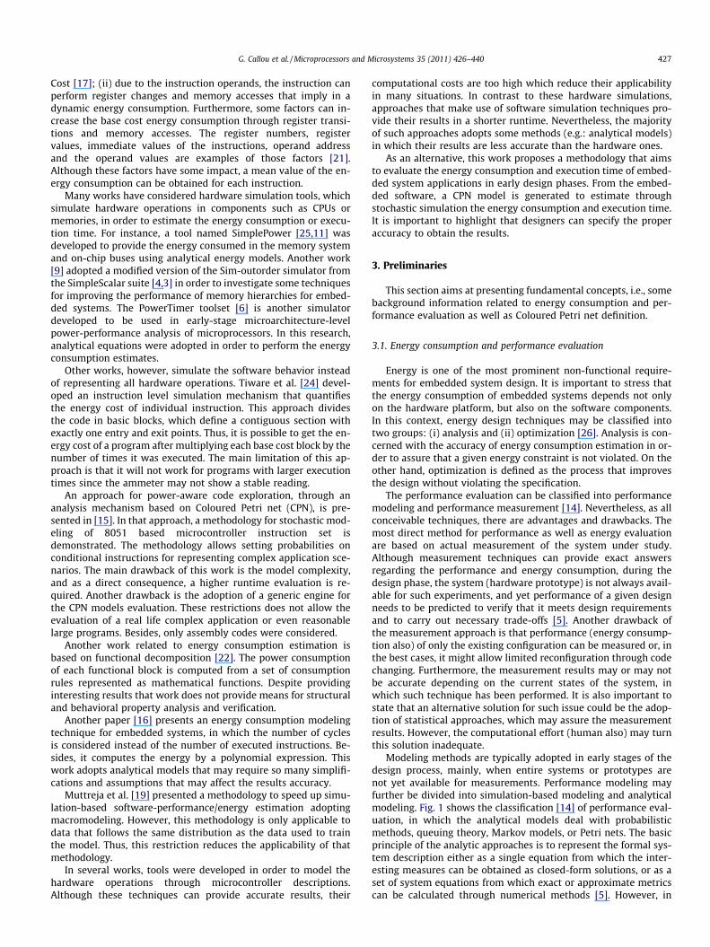
Modeling methods are typically adopted in early stages of thedesign process, mainly, when entire systems or prototypes arenot yet available for measurements. Performance modeling mayfurther be divided into simulation-based modeling and analyticalmodeling. Fig. 1 shows the classification [14] of performance eval-uation, in which the analytical models deal with probabilisticmethods, queuing theory, Markov models, or Petri nets. The basicprinciple of the analytic approaches is to represent the formal sys-tem description either as a single equation from which the inter-esting measures can be obtained as closed-form solutions, or as aset of system equations from which exact or approximate metricscan be calculated through numerical methods [5]. However, in

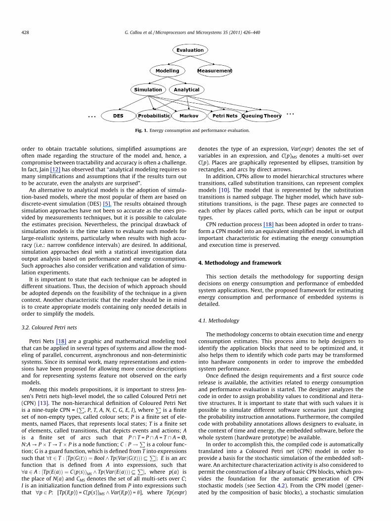
Fig. 1. Energy consumption and performance evaluation.

428 G. Callou et al. / Microprocessors and Microsystems 35 (2011) 426–440

order to obtain tractable solutions, simplified assumptions areoften made regarding the structure of the model and, hence, acompromise between tractability and accuracy is often a challenge.In fact, Jain [12] has observed that ‘‘analytical modeling requires somany simplifications and assumptions that if the results turn outto be accurate, even the analysts are surprised”.

An alternative to analytical models is the adoption of simula-tion-based models, where the most popular of them are based ondiscrete-event simulation (DES) [5]. The results obtained throughsimulation approaches have not been so accurate as the ones pro-vided by measurements techniques, but it is possible to calculatethe estimates precision. Nevertheless, the principal drawback ofsimulation models is the time taken to evaluate such models forlarge-realistic systems, particularly when results with high accu-racy (i.e.: narrow confidence intervals) are desired. In additional,simulation approaches deal with a statistical investigation dataoutput analysis based on performance and energy consumption.Such approaches also consider verification and validation of simu-lation experiments.

It is important to state that each technique can be adopted indifferent situations. Thus, the decision of which approach shouldbe adopted depends on the feasibility of the technique in a givencontext. Another characteristic that the reader should be in mindis to create appropriate models containing only needed details inorder to simplify the models.

3.2. Coloured Petri nets

Petri Nets [18] are a graphic and mathematical modeling toolthat can be applied in several types of systems and allow the mod-eling of parallel, concurrent, asynchronous and non-deterministicsystems. Since its seminal work, many representations and exten-sions have been proposed for allowing more concise descriptionsand for representing systems feature not observed on the earlymodels.

Among this models propositions, it is important to stress Jen-sen’s Petri nets high-level model, the so called Coloured Petri net(CPN) [13]. The non-hierarchical definition of Coloured Petri Netis a nine-tuple CPN = (

P, P, T, A, N, C, G, E, I), where

Pis a finite

set of non-empty types, called colour sets; P is a finite set of ele-ments, named Places, that represents local states; T is a finite setof elements, called transitions, that depicts events and actions; Ais a finite set of arcs such that P \ T = P \ A = T \ A = Ø,N:A ? P � T ? T � P is a node function; C : P !

Pis a colour func-

tion; G is a guard function, which is defined from T into expressionssuch that 8t 2 T : ½TpðGðtÞÞ ¼ Bool ^ TpðVarðGðtÞÞÞ#

P�; E is an arc

function that is defined from A into expressions, such that8a 2 A : ½TpðEðaÞÞ ¼ CðpðsÞÞMS ^ TpðVarðEðaÞÞÞ#

P�, where p(a) is

the place of N(a) and CMS denotes the set of all multi-sets over C;I is an initialization function defined from P into expressions suchthat "p 2 P: [Tp(I(p)) = C(p(s))MS ^ Var(I(p)) = ;], where Tp(expr)

denotes the type of an expression, Var(expr) denotes the set ofvariables in an expression, and C(p)MS denotes a multi-set overC(p). Places are graphically represented by ellipses, transition byrectangles, and arcs by direct arrows.

In addition, CPNs allow to model hierarchical structures wheretransitions, called substitution transitions, can represent complexmodels [10]. The model that is represented by the substitutiontransitions is named subpage. The higher model, which have sub-stitutions transitions, is the page. These pages are connected toeach other by places called ports, which can be input or outputtypes.

CPN reduction process [18] has been adopted in order to trans-form a CPN model into an equivalent simplified model, in which allimportant characteristic for estimating the energy consumptionand execution time is preserved.

4. Methodology and framework

This section details the methodology for supporting designdecisions on energy consumption and performance of embeddedsystem applications. Next, the proposed framework for estimatingenergy consumption and performance of embedded systems isdetailed.

4.1. Methodology

The methodology concerns to obtain execution time and energyconsumption estimates. This process aims to help designers toidentify the application blocks that need to be optimized and, italso helps them to identify which code parts may be transformedinto hardware components in order to improve the embeddedsystem performance.

Once defined the design requirements and a first source coderelease is available, the activities related to energy consumptionand performance evaluation is started. The designer analyzes thecode in order to assign probability values to conditional and itera-tive structures. It is important to state that with such values it ispossible to simulate different software scenarios just changingthe probability instruction annotations. Furthermore, the compiledcode with probability annotations allows designers to evaluate, inthe context of time and energy, the embedded software, before thewhole system (hardware prototype) be available.

In order to accomplish this, the compiled code is automaticallytranslated into a Coloured Petri net (CPN) model in order toprovide a basis for the stochastic simulation of the embedded soft-ware. An architecture characterization activity is also considered topermit the construction of a library of basic CPN blocks, which pro-vides the foundation for the automatic generation of CPNstochastic models (see Section 4.2). From the CPN model (gener-ated by the composition of basic blocks), a stochastic simulation

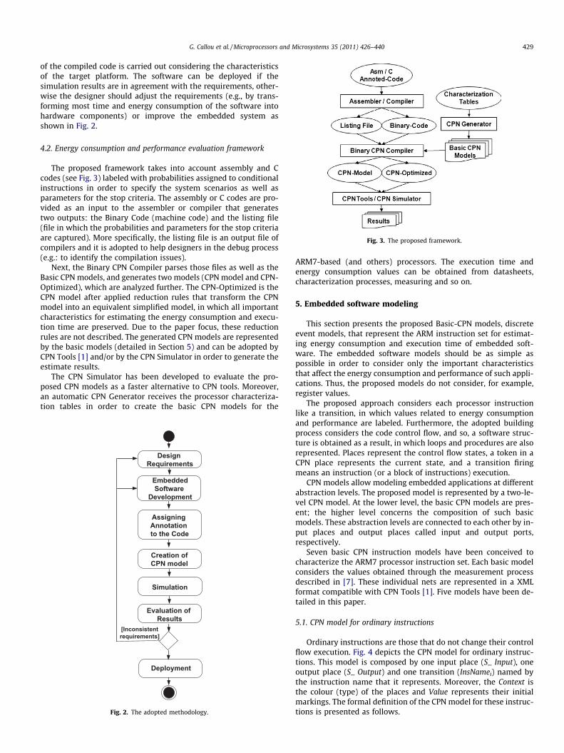
Fig. 3. The proposed framework.

G. Callou et al. / Microprocessors and Microsystems 35 (2011) 426–440 429

of the compiled code is carried out considering the characteristicsof the target platform. The software can be deployed if thesimulation results are in agreement with the requirements, other-wise the designer should adjust the requirements (e.g., by trans-forming most time and energy consumption of the software intohardware components) or improve the embedded system asshown in Fig. 2.

4.2. Energy consumption and performance evaluation framework

The proposed framework takes into account assembly and Ccodes (see Fig. 3) labeled with probabilities assigned to conditionalinstructions in order to specify the system scenarios as well asparameters for the stop criteria. The assembly or C codes are pro-vided as an input to the assembler or compiler that generatestwo outputs: the Binary Code (machine code) and the listing file(file in which the probabilities and parameters for the stop criteriaare captured). More specifically, the listing file is an output file ofcompilers and it is adopted to help designers in the debug process(e.g.: to identify the compilation issues).

Next, the Binary CPN Compiler parses those files as well as theBasic CPN models, and generates two models (CPN model and CPN-Optimized), which are analyzed further. The CPN-Optimized is theCPN model after applied reduction rules that transform the CPNmodel into an equivalent simplified model, in which all importantcharacteristics for estimating the energy consumption and execu-tion time are preserved. Due to the paper focus, these reductionrules are not described. The generated CPN models are representedby the basic models (detailed in Section 5) and can be adopted byCPN Tools [1] and/or by the CPN Simulator in order to generate theestimate results.

The CPN Simulator has been developed to evaluate the pro-posed CPN models as a faster alternative to CPN tools. Moreover,an automatic CPN Generator receives the processor characteriza-tion tables in order to create the basic CPN models for the

Design Requirements

[Inconsistentrequirements]

EmbeddedSoftware

Development

Creation ofCPN model

Evaluation of Results

Assigning Annotation to the Code

Deployment

Simulation

Fig. 2. The adopted methodology.

ARM7-based (and others) processors. The execution time andenergy consumption values can be obtained from datasheets,characterization processes, measuring and so on.

5. Embedded software modeling

This section presents the proposed Basic-CPN models, discreteevent models, that represent the ARM instruction set for estimat-ing energy consumption and execution time of embedded soft-ware. The embedded software models should be as simple aspossible in order to consider only the important characteristicsthat affect the energy consumption and performance of such appli-cations. Thus, the proposed models do not consider, for example,register values.

The proposed approach considers each processor instructionlike a transition, in which values related to energy consumptionand performance are labeled. Furthermore, the adopted buildingprocess considers the code control flow, and so, a software struc-ture is obtained as a result, in which loops and procedures are alsorepresented. Places represent the control flow states, a token in aCPN place represents the current state, and a transition firingmeans an instruction (or a block of instructions) execution.

CPN models allow modeling embedded applications at differentabstraction levels. The proposed model is represented by a two-le-vel CPN model. At the lower level, the basic CPN models are pres-ent; the higher level concerns the composition of such basicmodels. These abstraction levels are connected to each other by in-put places and output places called input and output ports,respectively.

Seven basic CPN instruction models have been conceived tocharacterize the ARM7 processor instruction set. Each basic modelconsiders the values obtained through the measurement processdescribed in [7]. These individual nets are represented in a XMLformat compatible with CPN Tools [1]. Five models have been de-tailed in this paper.

5.1. CPN model for ordinary instructions

Ordinary instructions are those that do not change their controlflow execution. Fig. 4 depicts the CPN model for ordinary instruc-tions. This model is composed by one input place (S_ Input), oneoutput place (S_ Output) and one transition (InsNamei) named bythe instruction name that it represents. Moreover, the Context isthe colour (type) of the places and Value represents their initialmarkings. The formal definition of the CPN model for these instruc-tions is presented as follows.

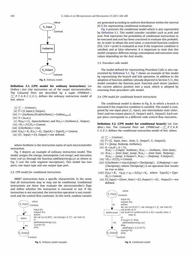
Fig. 4. Ordinary model.

430 G. Callou et al. / Microprocessors and Microsystems 35 (2011) 426–440

Definition 5.1. (CPN model for ordinary instructions) LetOrdInst 2 Inst (the instruction set of the target microcontroller).The Coloured Petri net described by a tuple CPNMOrd ¼ðP; P; T;A;N;C;G; E; IÞ, defines the ordinary instruction model of

Inst, where

(i)P¼ fContextg,

(ii) P = {S_Input,S_Output},(iii) T = {InsNameijFCod(InsNamei) = CodInstname},(iv) A = {a0,a1},(v) N(a0) = (S_ Input,InsName) and N(a1) = (InsName,S_ Output),

(vi) "Pk 2 P,C(Pk) = Context,(vii) G(InsNamei) = true,

(viii) E(a0) = Ki, E(a1) = Koj Type(Ki) = Type(Ko) = Context,(ix) I(S_ Input) = I(S_Output) = not defined.

where InstName is the instruction name of each microcontrollerinstruction.

Fig. 5 depicts an example of ordinary instruction model. Thismodel assigns the energy consumption (val energy) and executiontime (val cy) through the function addData(energy,cy) as shown inFig. 5 (see the code segment inscriptions). This model has twoports, one input type and one output type port.

5.2. CPN model for conditional instructions

ARM7 instructions have a specific characteristic in the sensethat all instructions may or may not be conditional. Conditionalinstructions are those that evaluate the microcontroller’s flagsand define whether the instruction is executed or not. If theinstruction is not executed, the instruction operation is not consid-ered and the control flow continues. In this work, random variates

Fig. 5. Ordinary model example.

are generated according to uniform distribution within the interval[0,1] for representing conditional evaluation.

Fig. 6 presents the conditional model which is also representedby Definition 5.1. This model consider variables such as prob andaval. Prob represents the probability of conditional instructions tobe executed and aval has been conceived to evaluate this probabil-ity. In order to obtain the aval value, a conceived function (uniform(0.0, 1.0)< = prob) is evaluated as true if the respective condition issatisfied, and as false otherwise. It is important to state that thismodel computes different energy consumption and execution timevalues depending on the Aval results.

5.3. Procedure calls model

The model defined for representing Procedure Calls is also rep-resented by Definition 5.1. Fig. 7 shows an example of this modelby representing the branch and link operation. In addition to theadoption of function addData (already depicted in Section 5.1), thismodel considers the function push. Function push stores (pushes)the current address position into a stack, which is adopted byreturning from procedure calls model.

5.4. CPN model for conditional branch instructions

The conditional model is shown in Fig. 8, in which a branch isexecuted if the respective condition is satisfied. This model is com-posed by one input place (S_ Input), one intermediate state (Inter_State) and two output places (S_ Output1 and S_ Output2). Each out-put place corresponds to a different code control flow execution.

Definition 5.2. (CPN model for conditional branch) Let Con-dInst 2 Inst. The Coloured Petri net CPNMCond ¼ ð

P; P; T;A;N;

C;G; E; IÞ defines the conditional instruction model of Inst, where

(i)P¼ fContextg ,

(ii) P = {S_ Input, Inter_ State, S_ Output1, S_ Output2}.(iii) T = {Jump, NotJump, InsNamei},(iv) A = {akj0 6 k 6 5},

(v)Nða0Þ ¼ ðS Input; InsNameiÞ;Nða1Þ ¼ ðInsNamei; Inter StateÞ;Nða2Þ ¼ ðInter State; JumpÞ;Nða3Þ ¼ ðInter State; NotJumpÞ;Nða4Þ ¼ ðJump; S Output1Þ;Nða5Þ ¼ ðNotJump; S Output2Þ;

(vi) "Pk 2 P,C(Pk) = Context,(vii) G(InsName) = true,G(Jump) = CheckJump(), G(NotJump) = not-

(CheckJump), where CheckJump() is an operation that resultson true or false.

(viii) E(a0) = Ki; "aj,aj – a0 2 A,E(aj) = Ko, where Type(Ki) = Type-(Ko) = Context,

(xi) I(S_Input) = I(Inter_State) = I(S_Output1) = I(S_ Output2) = notdefined.

Fig. 6. Conditional model.

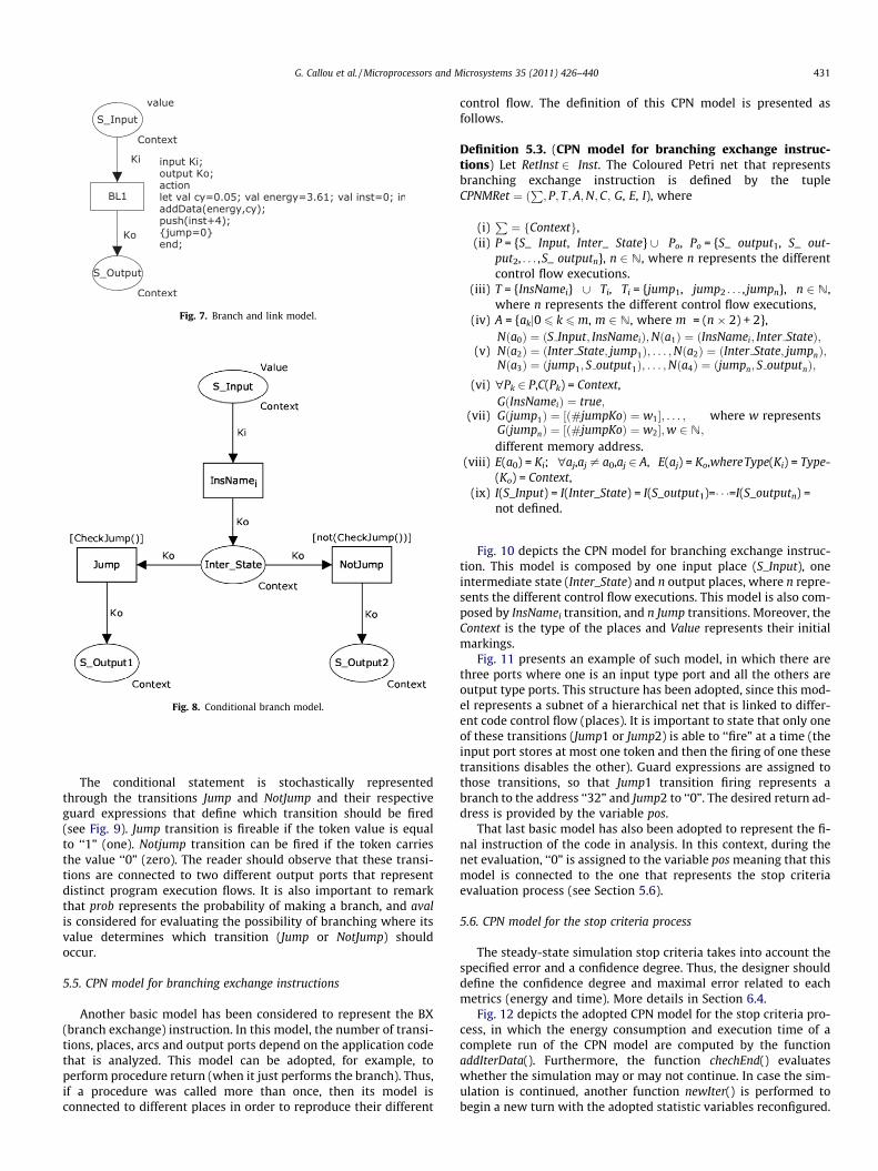
Fig. 7. Branch and link model.

Fig. 8. Conditional branch model.

G. Callou et al. / Microprocessors and Microsystems 35 (2011) 426–440 431

The conditional statement is stochastically representedthrough the transitions Jump and NotJump and their respectiveguard expressions that define which transition should be fired(see Fig. 9). Jump transition is fireable if the token value is equalto ‘‘1” (one). Notjump transition can be fired if the token carriesthe value ‘‘0” (zero). The reader should observe that these transi-tions are connected to two different output ports that representdistinct program execution flows. It is also important to remarkthat prob represents the probability of making a branch, and avalis considered for evaluating the possibility of branching where itsvalue determines which transition (Jump or NotJump) shouldoccur.

5.5. CPN model for branching exchange instructions

Another basic model has been considered to represent the BX(branch exchange) instruction. In this model, the number of transi-tions, places, arcs and output ports depend on the application codethat is analyzed. This model can be adopted, for example, toperform procedure return (when it just performs the branch). Thus,if a procedure was called more than once, then its model isconnected to different places in order to reproduce their different

control flow. The definition of this CPN model is presented asfollows.

Definition 5.3. (CPN model for branching exchange instruc-tions) Let RetInst 2 Inst. The Coloured Petri net that representsbranching exchange instruction is defined by the tupleCPNMRet ¼ ð

P; P; T;A;N;C; G, E, I), where

(i)P¼ fContextg,

(ii) P = {S_ Input, Inter_ State} [ Po, Po = {S_ output1, S_ out-put2, . . . ,S_ outputn}, n 2 N, where n represents the differentcontrol flow executions.

(iii) T = {InsNamei} [ Ti, Ti = {jump1, jump2 . . . , jumpn}, n 2 N,where n represents the different control flow executions,

(iv) A = {akj0 6 k 6m, m 2 N, where m = (n � 2) + 2},

(v)Nða0Þ ¼ ðS Input; InsNameiÞ;Nða1Þ ¼ ðInsNamei; Inter StateÞ;Nða2Þ ¼ ðInter State; jump1Þ; . . . ;Nða2Þ ¼ ðInter State; jumpnÞ;Nða3Þ ¼ ðjump1; S output1Þ; . . . ;Nða4Þ ¼ ðjumpn; S outputnÞ;

(vi) "Pk 2 P,C(Pk) = Context,

(vii)GðInsNameiÞ ¼ true;Gðjump1Þ ¼ ½ð#jumpKoÞ ¼ w1�; . . . ;GðjumpnÞ ¼ ½ð#jumpKoÞ ¼ w2�;w 2 N;

where w represents

different memory address.(viii) E(a0) = Ki; "aj,aj – a0,aj 2 A, E(aj) = Ko,whereType(Ki) = Type-

(Ko) = Context,(ix) I(S_Input) = I(Inter_State) = I(S_output1)=� � �=I(S_outputn) =

not defined.

Fig. 10 depicts the CPN model for branching exchange instruc-tion. This model is composed by one input place (S_Input), oneintermediate state (Inter_State) and n output places, where n repre-sents the different control flow executions. This model is also com-posed by InsNamei transition, and n Jump transitions. Moreover, theContext is the type of the places and Value represents their initialmarkings.

Fig. 11 presents an example of such model, in which there arethree ports where one is an input type port and all the others areoutput type ports. This structure has been adopted, since this mod-el represents a subnet of a hierarchical net that is linked to differ-ent code control flow (places). It is important to state that only oneof these transitions (Jump1 or Jump2) is able to ‘‘fire” at a time (theinput port stores at most one token and then the firing of one thesetransitions disables the other). Guard expressions are assigned tothose transitions, so that Jump1 transition firing represents abranch to the address ‘‘32” and Jump2 to ‘‘0”. The desired return ad-dress is provided by the variable pos.

That last basic model has also been adopted to represent the fi-nal instruction of the code in analysis. In this context, during thenet evaluation, ‘‘0” is assigned to the variable pos meaning that thismodel is connected to the one that represents the stop criteriaevaluation process (see Section 5.6).

5.6. CPN model for the stop criteria process

The steady-state simulation stop criteria takes into account thespecified error and a confidence degree. Thus, the designer shoulddefine the confidence degree and maximal error related to eachmetrics (energy and time). More details in Section 6.4.

Fig. 12 depicts the adopted CPN model for the stop criteria pro-cess, in which the energy consumption and execution time of acomplete run of the CPN model are computed by the functionaddIterData(). Furthermore, the function chechEnd() evaluateswhether the simulation may or may not continue. In case the sim-ulation is continued, another function newIter() is performed tobegin a new turn with the adopted statistic variables reconfigured.

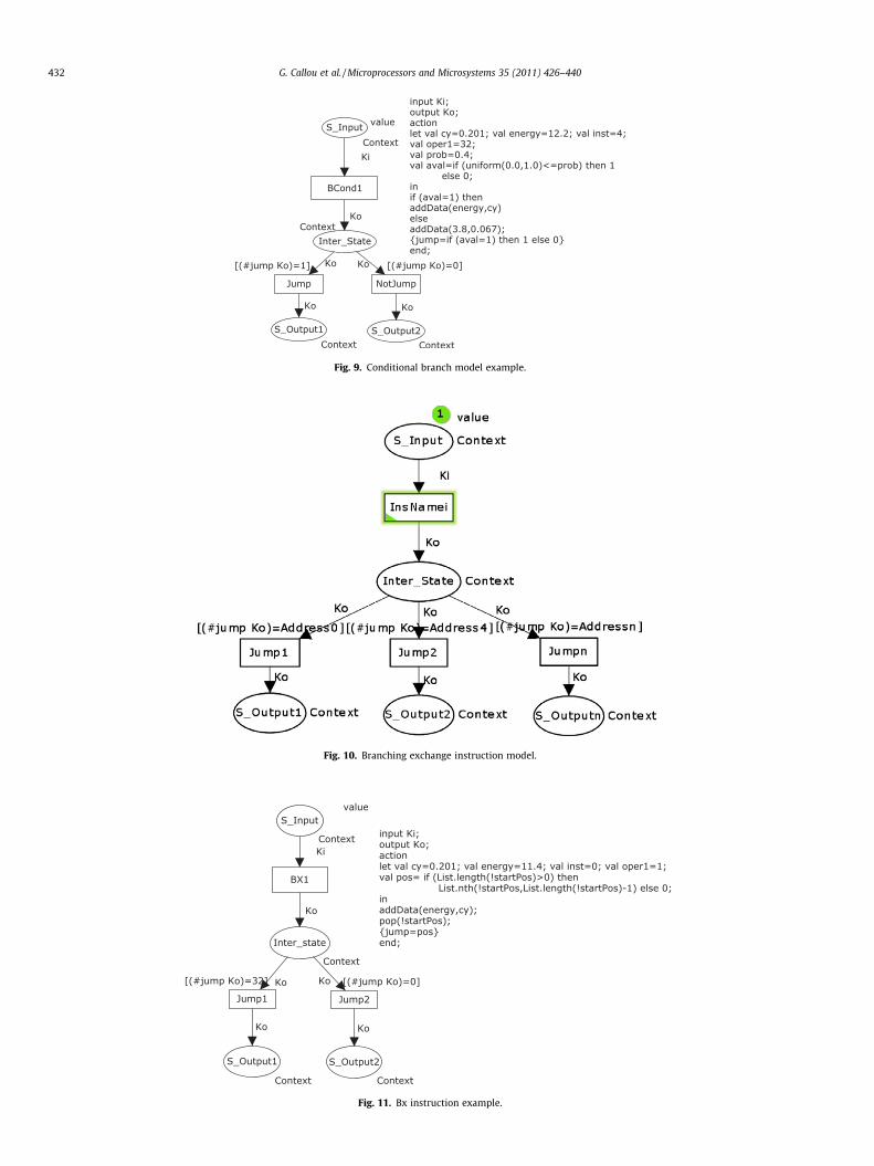
Fig. 9. Conditional branch model example.

Fig. 10. Branching exchange instruction model.

Fig. 11. Bx instruction example.

432 G. Callou et al. / Microprocessors and Microsystems 35 (2011) 426–440

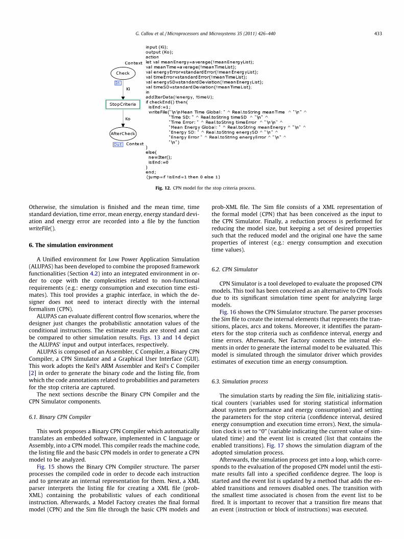
Fig. 12. CPN model for the stop criteria process.

G. Callou et al. / Microprocessors and Microsystems 35 (2011) 426–440 433

Otherwise, the simulation is finished and the mean time, timestandard deviation, time error, mean energy, energy standard devi-ation and energy error are recorded into a file by the functionwriteFile().

6. The simulation environment

A Unified environment for Low Power Application Simulation(ALUPAS) has been developed to combine the proposed frameworkfunctionalities (Section 4.2) into an integrated environment in or-der to cope with the complexities related to non-functionalrequirements (e.g.: energy consumption and execution time esti-mates). This tool provides a graphic interface, in which the de-signer does not need to interact directly with the internalformalism (CPN).

ALUPAS can evaluate different control flow scenarios, where thedesigner just changes the probabilistic annotation values of theconditional instructions. The estimate results are stored and canbe compared to other simulation results. Figs. 13 and 14 depictthe ALUPAS’ input and output interfaces, respectively.

ALUPAS is composed of an Assembler, C Compiler, a Binary CPNCompiler, a CPN Simulator and a Graphical User Interface (GUI).This work adopts the Keil’s ARM Assembler and Keil’s C Compiler[2] in order to generate the binary code and the listing file, fromwhich the code annotations related to probabilities and parametersfor the stop criteria are captured.

The next sections describe the Binary CPN Compiler and theCPN Simulator components.

6.1. Binary CPN Compiler

This work proposes a Binary CPN Compiler which automaticallytranslates an embedded software, implemented in C language orAssembly, into a CPN model. This compiler reads the machine code,the listing file and the basic CPN models in order to generate a CPNmodel to be analyzed.

Fig. 15 shows the Binary CPN Compiler structure. The parserprocesses the compiled code in order to decode each instructionand to generate an internal representation for them. Next, a XMLparser interprets the listing file for creating a XML file (prob-XML) containing the probabilistic values of each conditionalinstruction. Afterwards, a Model Factory creates the final formalmodel (CPN) and the Sim file through the basic CPN models and

prob-XML file. The Sim file consists of a XML representation ofthe formal model (CPN) that has been conceived as the input tothe CPN Simulator. Finally, a reduction process is performed forreducing the model size, but keeping a set of desired propertiessuch that the reduced model and the original one have the sameproperties of interest (e.g.: energy consumption and executiontime values).

6.2. CPN Simulator

CPN Simulator is a tool developed to evaluate the proposed CPNmodels. This tool has been conceived as an alternative to CPN Toolsdue to its significant simulation time spent for analyzing largemodels.

Fig. 16 shows the CPN Simulator structure. The parser processesthe Sim file to create the internal elements that represents the tran-sitions, places, arcs and tokens. Moreover, it identifies the param-eters for the stop criteria such as confidence interval, energy andtime errors. Afterwards, Net Factory connects the internal ele-ments in order to generate the internal model to be evaluated. Thismodel is simulated through the simulator driver which providesestimates of execution time an energy consumption.

6.3. Simulation process

The simulation starts by reading the Sim file, initializing statis-tical counters (variables used for storing statistical informationabout system performance and energy consumption) and settingthe parameters for the stop criteria (confidence interval, desiredenergy consumption and execution time errors). Next, the simula-tion clock is set to ‘‘0” (variable indicating the current value of sim-ulated time) and the event list is created (list that contains theenabled transitions). Fig. 17 shows the simulation diagram of theadopted simulation process.

Afterwards, the simulation process get into a loop, which corre-sponds to the evaluation of the proposed CPN model until the esti-mate results fall into a specified confidence degree. The loop isstarted and the event list is updated by a method that adds the en-abled transitions and removes disabled ones. The transition withthe smallest time associated is chosen from the event list to befired. It is important to recover that a transition fire means thatan event (instruction or block of instructions) was executed.

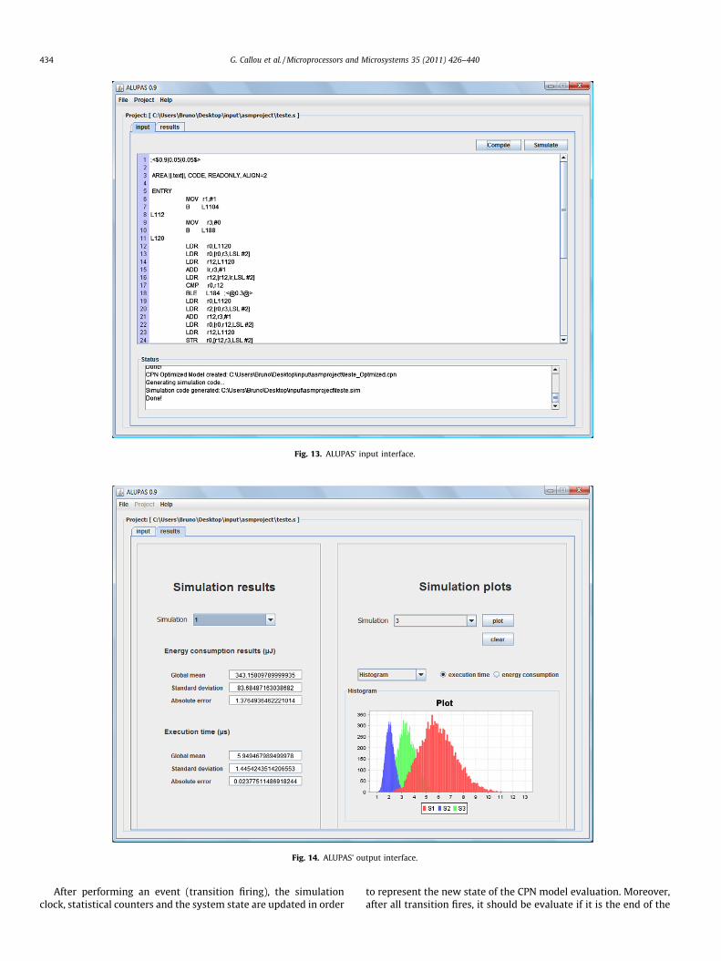
Fig. 13. ALUPAS’ input interface.

Fig. 14. ALUPAS’ output interface.

434 G. Callou et al. / Microprocessors and Microsystems 35 (2011) 426–440

After performing an event (transition firing), the simulationclock, statistical counters and the system state are updated in order

to represent the new state of the CPN model evaluation. Moreover,after all transition fires, it should be evaluate if it is the end of the

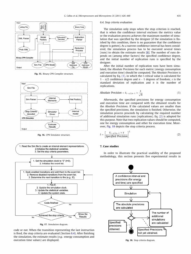
Fig. 15. Binary CPN Compiler structure.

Fig. 16. CPN Simulator structure.

Fig. 17. Simulation diagram.

Fig. 18. Stop criteria diagram.

G. Callou et al. / Microprocessors and Microsystems 35 (2011) 426–440 435

code or not. When the transition representing the last instructionis fired, the stop criteria are evaluated (Section 6.4). After finishingthe simulation, the estimate results (e.g.: energy consumption andexecution time values) are displayed.

6.4. Stop criteria evaluation

The simulation only stops when the stop criterion is reached,that is when the confidence interval encloses the metrics valueor the evaluation process achieves the maximum number of simu-lation that was specified by the designer (if the simulation is fin-ished by this condition, there is no guarantee that the confidencedegree is gotten). As a narrow confidence interval has been consid-ered, the simulation process has to be executed several times(runs) to obtain the estimate results [8]. The number of runs de-pends on (among other factors) the specified confidence degree,and the initial number of replication runs is specified by thedesigner.

After the initial number of replication runs have been simu-lated, the Absolute Precisions for each metric (energy consumptionand execution time) should be computed. The Absolute Precision iscalculated by Eq. (1), in which the t critical value is calculated for1 � a/2 confidence degree and n � 1 degrees of freedom; s is thestandard deviation of replication and n is the number ofreplications.

Absolute Precision ¼ t1�a=2;n�1 �sffiffiffinp ð1Þ

Afterwards, the specified precisions for energy consumptionand execution time are compared with the obtained results forthe Absolute Precisions. If the calculated values are smaller thanthe specified precisions, the simulation is finished. Otherwise, thesimulation process proceeds by calculating the required numberof additional simulation runs (replications). Eq. (2) is adopted forthis purpose. Note that two replication values should be computed,one for energy consumption and other for execution time. More-over, Fig. 18 depicts the stop criteria process.

i ¼ t1�a=2;n�1 � sSpecified Precision

� �2

ð2Þ

7. Case studies

In order to illustrate the practical usability of the proposedmethodology, this section presents five experimental results in

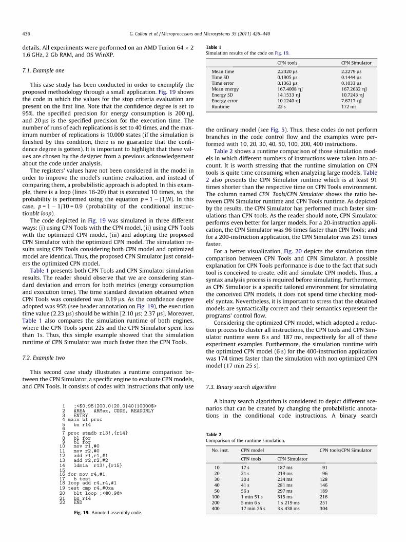
Table 1Simulation results of the code on Fig. 19.

CPN tools CPN Simulator

Mean time 2.2320 ls 2.2279 lsTime SD 0.1905 ls 0.1444 lsTime error 0.1363 ls 0.1033 lsMean energy 167.4008 gJ 167.2632 gJEnergy SD 14.1533 gJ 10.7243 gJEnergy error 10.1240 gJ 7.6717 gJRuntime 22 s 172 ms

436 G. Callou et al. / Microprocessors and Microsystems 35 (2011) 426–440

details. All experiments were performed on an AMD Turion 64 � 21.6 GHz, 2 Gb RAM, and OS WinXP.

7.1. Example one

This case study has been conducted in order to exemplify theproposed methodology through a small application. Fig. 19 showsthe code in which the values for the stop criteria evaluation arepresent on the first line. Note that the confidence degree is set to95%, the specified precision for energy consumption is 200 gJ,and 20 ls is the specified precision for the execution time. Thenumber of runs of each replications is set to 40 times, and the max-imum number of replications is 10.000 states (if the simulation isfinished by this condition, there is no guarantee that the confi-dence degree is gotten). It is important to highlight that these val-ues are chosen by the designer from a previous acknowledgementabout the code under analysis.

The registers’ values have not been considered in the model inorder to improve the model’s runtime evaluation, and instead ofcomparing them, a probabilistic approach is adopted. In this exam-ple, there is a loop (lines 16-20) that is executed 10 times, so, theprobability is performed using the equation p = 1 � (1/N). In thiscase, p = 1 � 1/10 = 0.9 (probability of the conditional instruc-tionblt loop).

The code depicted in Fig. 19 was simulated in three differentways: (i) using CPN Tools with the CPN model, (ii) using CPN Toolswith the optimized CPN model, (iii) and adopting the proposedCPN Simulator with the optimized CPN model. The simulation re-sults using CPN Tools considering both CPN model and optimizedmodel are identical. Thus, the proposed CPN Simulator just consid-ers the optimized CPN model.

Table 1 presents both CPN Tools and CPN Simulator simulationresults. The reader should observe that we are considering stan-dard deviation and errors for both metrics (energy consumptionand execution time). The time standard deviation obtained whenCPN Tools was considered was 0.19 ls. As the confidence degreeadopted was 95% (see header annotation on Fig. 19), the executiontime value (2.23 ls) should be within [2.10 ls; 2.37 ls]. Moreover,Table 1 also compares the simulation runtime of both engines,where the CPN Tools spent 22s and the CPN Simulator spent lessthan 1s. Thus, this simple example showed that the simulationruntime of CPN Simulator was much faster then the CPN Tools.

7.2. Example two

This second case study illustrates a runtime comparison be-tween the CPN Simulator, a specific engine to evaluate CPN models,and CPN Tools. It consists of codes with instructions that only use

Fig. 19. Annoted assembly code.

the ordinary model (see Fig. 5). Thus, these codes do not performbranches in the code control flow and the examples were per-formed with 10, 20, 30, 40, 50, 100, 200, 400 instructions.

Table 2 shows a runtime comparison of those simulation mod-els in which different numbers of instructions were taken into ac-count. It is worth stressing that the runtime simulation on CPNtools is quite time consuming when analyzing large models. Table2 also presents the CPN Simulator runtime which is at least 91times shorter than the respective time on CPN Tools environment.The column named CPN Tools/CPN Simulator shows the ratio be-tween CPN Simulator runtime and CPN Tools runtime. As depictedby the results, the CPN Simulator has performed much faster sim-ulations than CPN tools. As the reader should note, CPN Simulatorperforms even better for larger models. For a 20-instruction appli-cation, the CPN Simulator was 96 times faster than CPN Tools; andfor a 200-instruction application, the CPN Simulator was 251 timesfaster.

For a better visualization, Fig. 20 depicts the simulation timecomparison between CPN Tools and CPN Simulator. A possibleexplanation for CPN Tools performance is due to the fact that suchtool is conceived to create, edit and simulate CPN models. Thus, asyntax analysis process is required before simulating. Furthermore,as CPN Simulator is a specific tailored environment for simulatingthe conceived CPN models, it does not spend time checking mod-els’ syntax. Nevertheless, it is important to stress that the obtainedmodels are syntactically correct and their semantics represent theprograms’ control flow.

Considering the optimized CPN model, which adopted a reduc-tion process to cluster all instructions, the CPN tools and CPN Sim-ulator runtime were 6 s and 187 ms, respectively for all of theseexperiment examples. Furthermore, the simulation runtime withthe optimized CPN model (6 s) for the 400-instruction applicationwas 174 times faster than the simulation with non optimized CPNmodel (17 min 25 s).

7.3. Binary search algorithm

A binary search algorithm is considered to depict different sce-narios that can be created by changing the probabilistic annota-tions in the conditional code instructions. A binary search

Table 2Comparison of the runtime simulation.

No. inst. CPN model CPN tools/CPN Simulator

CPN tools CPN Simulator

10 17 s 187 ms 9120 21 s 219 ms 9630 30 s 234 ms 12840 41 s 281 ms 14650 56 s 297 ms 189

100 1 min 51 s 515 ms 216200 5 min 6 s 1 s 219 ms 251400 17 min 25 s 3 s 438 ms 304

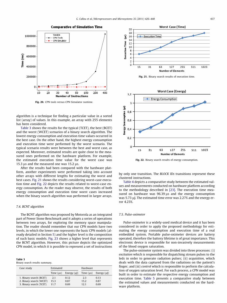
Fig. 20. CPN tools versus CPN Simulator runtime.

Fig. 21. Binary search results of execution time.

Fig. 22. Binary search results of energy consumption.

G. Callou et al. / Microprocessors and Microsystems 35 (2011) 426–440 437

algorithm is a technique for finding a particular value in a sortedlist (array) of values. In this example, an array with 255 elementshas been considered.

Table 3 shows the results for the typical (TCET), the best (BCET)and the worst (WCET) scenarios of a binary search algorithm. Thelowest energy consumption and execution time values occurred inthe best case. On the other hand, the highest energy consumptionand execution time were performed by the worst scenario. Thetypical scenario results were between the best and worst case, asexpected. Moreover, estimated results are quite close to the mea-sured ones performed on the hardware platform. For example,the estimated execution time value for the worst case was15.3 ls and the measured one was 15.2 ls.

After the results had been compared with the hardware plat-form, another experiments were performed taking into accountother arrays with different lengths for estimating the worst andbest cases. Fig. 21 shows the results considering worst-case execu-tion time and Fig. 22 depicts the results related to worst-case en-ergy consumption. As the reader may observe, the results of bothenergy consumption and execution time worst cases increasedwhen the binary search algorithm was performed in larger arrays.

7.4. BCNT algorithm

The BCNT algorithm was proposed by Motorola as an integratedpart of Power Stone Benchmark and it adopts a series of operationsbetween two arrays, for exploring the memory space manipula-tion. The reader should remember that our CPN models have twolevels, in which the lower one represents the basic CPN models (al-ready detailed in Section 5) and the higher level is the compositionof such basic models. Fig. 23 shows a higher level that representsthe BCNT algorithm. However, this picture depicts the optimizedCPN model, in which it is possible to represent a set of instructions

Table 3Binary search results summary.

Case study Estimated Hardware

Time (ls) Energy (lJ) Time (ls) Energy (lJ)

1. Binary search (BCET) 2.1 0.12 2.3 0.132. Binary search (WCET) 15.3 0.87 15.2 0.873. Binary search (TCET) 11.7 0.69 12.1 0.69

by only one transition. The BLOCK IDs transitions represent theseclustered instructions.

Table 4 depicts a comparative study between the estimated val-ues and measurements conducted on hardware platform accordingto the methodology described in [23]. The execution time mea-sured on hardware was 96.39 ls and the energy consumptionwas 5.73 lJ. The estimated time error was 2.27% and the energy er-ror 4.23%.

7.5. Pulse-oximeter

Pulse-oximeter is a widely-used medical device and it has beenconsidered in order to apply the proposed methodology for esti-mating the energy consumption and execution time of a realembedded system. Portable pulse-oximeter devices are batteryoperated, therefore the battery lifetime is of great importance. Thiselectronic device is responsible for non-invasively measurementsof the blood oxygen saturation.

The pulse-oximeter system was divided into three processes: (i)excitation which is responsible for dispatching stream pulses to theleds in order to generate radiation pulses; (ii) acquisition, whichdeals with the data captured from the radiations on the patient’sfinger; and (iii) control which is responsible to perform the calcula-tion of oxygen saturation level. For each process, a CPN model wasbuilt in order to estimate the respective energy consumption andexecution time. Table 5 presents a comparative study betweenthe estimated values and measurements conducted on the hard-ware platform.

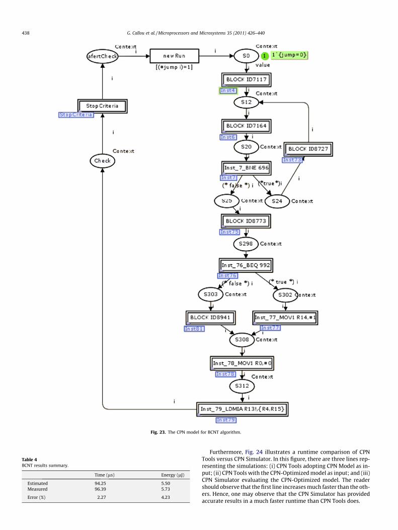
Fig. 23. The CPN model for BCNT algorithm.

Table 4BCNT results summary.

Time (ls) Energy (lJ)

Estimated 94.25 5.50Measured 96.39 5.73

Error (%) 2.27 4.23

438 G. Callou et al. / Microprocessors and Microsystems 35 (2011) 426–440

Furthermore, Fig. 24 illustrates a runtime comparison of CPNTools versus CPN Simulator. In this figure, there are three lines rep-resenting the simulations: (i) CPN Tools adopting CPN Model as in-put; (ii) CPN Tools with the CPN-Optimized model as input; and (iii)CPN Simulator evaluating the CPN-Optimized model. The readershould observe that the first line increases much faster than the oth-ers. Hence, one may observe that the CPN Simulator has providedaccurate results in a much faster runtime than CPN Tools does.

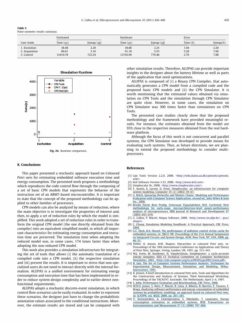
Table 5Pulse-oximeter results summary.

Estimated Hardware Error

Case study Time (ls) Energy (lJ) Time (ls) Energy (lJ) Time (%) Energy(%)

1. Excitation 38.48 2.20 38.88 2.25 1.04 2.202. Acquisition 86.61 5.16 91.18 5.55 5.28 7.663. Control 12410.78 722.54 12745.99 779.46 2.70 7.88

Fig. 24. Runtime comparison.

G. Callou et al. / Microprocessors and Microsystems 35 (2011) 426–440 439

8. Conclusions

This paper presented a stochastic approach based on ColouredPetri nets for estimating embedded software execution time andenergy consumption. The presented work proposes a methodologywhich reproduces the code control flow through the composing ofa set of basic CPN models that represents the behavior of theinstruction set of an ARM7-based microcontroller. It is importantto state that the concept of the proposed methodology can be ap-plied to other families of processors.

CPN models can also be analyzed by means of reduction, wherethe main objective is to investigate the properties of interest and,then, to apply a set of reduction rules by which the model is sim-plified. This work adopted a set of reduction rules in order to trans-form the original CPN model (the one directly obtained from thecompiler) into an equivalent simplified model, in which all impor-tant characteristics for estimating energy consumption and execu-tion time are preserved. The simulation time when adopting thereduced model was, in some cases, 174 times faster than whenadopting the non-reduzed CPN model.

This work also provides a simulation infrastructure for integrat-ing the set of tools that allows (i) the automatic translation of acompiled code into a CPN model, (ii) the respective simulationand (iii) present the results. It is important to stress that non-spe-cialized users do not need to interact directly with the internal for-malism. ALUPAS is a unified environment for estimating energyconsumption and execution time that has been implemented in or-der to reduce system design complexity and to earlier detect non-functional requirements.

ALUPAS adopts a stochastic discrete-event simulation, in whichcontrol flow scenarios can be easily evaluated. In order to representthese scenarios, the designer just have to change the probabilisticannotation values associated to the conditional instructions. More-over, the estimate results are stored and can be compared with

other simulation results. Therefore, ALUPAS can provide importantinsights to the designer about the battery lifetime as well as partsof the application that need optimizations.

ALUPAS is composed of (i) a Binary CPN Compiler, that auto-matically generates a CPN model from a compiled code and theproposed basic CPN models and (ii) the CPN Simulator. It isworth mentioning that the estimated values obtained via simu-lation on CPN Tools and the simulation through CPN Simulatorare quite close. However, in some cases, the simulation onCPN Simulator was 300 times faster than simulations on CPNTools.

The presented case studies clearly show that the proposedmethodology and the framework have provided meaningful re-sults. For instance, the estimates obtained from the model are93% close to the respective measures obtained from the real hard-ware platform.

Although the focus of this work is not concurrent and parallelsystems, the CPN Simulator was developed to provide means forevaluating such systems. Thus, as future directions, we are plan-ning to extend the proposed methodology to consider multi-processors.

References

[1] Cpn Tools Version 2.2.0, 2008. <http://wiki.daimi.au.dk/cpntools/cpntools.wiki>.

[2] Keil Software Version 3.33, 2008. <http://www.keil.com>.[3] Simplescalar llc, 2008. <http://www.simplescalar.com/>.[4] T. Austin, E. Larson, D. Ernst, Simplescalar: an infrastructure for computer

system modeling, Computer 35 (2) (2002) 59–67.[5] G. Bolch, Queueing Networks and Markov Chains: Modeling and Performance

Evaluation with Computer Science Applications, second ed., John Wiley & SonsInc., 2006.

[6] Brooks David, Bose Pradip, Srinivasan Vijayalakshmi, M.K. Gschwind, Newmethodology for early-stage, microarchitecture-level power-performanceanalysis of microprocessors, IBM Journal of Research and Development 47(2003) 653–670.

[7] G. Callou, P. Maciel, Alupas Software, 2008. <http://www.cin.ufpe.br/� grac/alupas>.

[8] C. Chung, Simulation Modeling Handbook: A Practical Approach, CRC Press,2004.

[9] G.C. Heck, R.A. Hexsel, The performance of pollution control victim cache forembedded systems, in: SBCCI ’08: Proceedings of the 21st Annual Symposiumon Integrated Circuits and System Design, ACM, New York, NY, USA, 2008, pp.46–51.

[10] Huber, K. Jensen, R.M. Shapiro, Hierarchies in coloured Petri nets, in:Proceedings of the 10th International Conference on Applications and Theoryof Petri Nets, Springer, Verlag, London, UK, 1991, pp. 313–341.

[11] M.J. Irwin, M. Kandemir, N. Vijaykrishnan, Simplepower: a cycle-accurateenergy simulator, IEEE CS Technical Committee on Computer ArchitectureNewsletter, 2001. <http://tab.computer.org/tcca/NEWS/jan2001/irwin.pdf>.

[12] R. Jain, The Art of Computer Systems Performance Analysis: Techniques forExperimental Design, Measurement, Simulation, and Modeling, Wiley-Interscience, 1991.

[13] K. Jensen, A brief introduction to coloured Petri nets, Tools and Algorithms forthe Construction and Analysis of Systems, Third International Workshop,Proceedings of the TACAS’97, Enschede, The Netherlands, April 2–4, 1997.

[14] L. John, Performance Evaluation and Benchmarking, CRC Press, 2006.[15] M.N.O. Junior, S. Neto, P. Maciel, R. Lima, A. Ribeiro, R. Barreto, E. Tavares, F.

Braga, Analyzing software performance and energy consumption of embeddedsystems by probabilistic modeling: an approach based on coloured Petri nets,in: ICATPN, vol. 4024, 2006, pp. 261–281.

[16] V. Konstantakos, A. Chatzigeorgiou, S. Nikolaidis, T. Laopoulos, Energyconsumption estimation in embedded systems, IEEE Transactions onInstrumentation and Measurement 57 (3) (2008) 797–804.

440 G. Callou et al. / Microprocessors and M

[17] M.T.-C. Lee, M. Fujita, V. Tiwari, S. Malik, Power analysis and minimizationtechniques for embedded dsp software, IEEE Transactions on Very Large ScaleIntegration Systems 5 (1) (1997) 123–135.

[18] T. Murata, Petri nets: properties, analysis and applications, Proceedings of theIEEE 77 (4) (1989) 541–580.

[19] A. Muttreja, A. Raghunathan, S. Ravi, N. Jha, Automated energy/performancemacromodeling of embedded software, IEEE Transactions on Computer-AidedDesign of Integrated Circuits and Systems 26 (2007) 2229–2256.

[20] N. Nikolaidis, P. Neofotistos, Instruction-level Power MeasurementMethodology, Electronics Lab, Physics Dept., Aristotle University ofThessaloniki Greece, March, 2002. .

[21] S. Nikolaidis, N. Kavvadias, P. Neofotistos. Instruction Level Power Models forEmbedded Processors, Technical Report, IST-2000-30093/EASY Project, Deliv.21, December 2002.

[22] E. Senn, J. Laurent, N. Julien, E. Martin, SoftExplorer: estimationcharacterization and optimization of the power and energy consumption atthe algorithmic level, in: PATMOS, 2004, pp. 342–351.

[23] E. Tavares, P. Maciel. Amalghma Tool, 2008. <http://www.cin.ufpe.br/�eagt/tools/>.

[24] V. Tiwari, S. Malik, A. Wolfe, Power Analysis of Embedded Software: A FirstStep Towards Software Power Minimization, Readings in Hardware/SoftwareCo-Design, 1994.

[25] W. Ye, N. Vijaykrishnan, M. Kandemir, M.J. Irwin, The design and use ofsimplepower: a cycle accurate energy estimation tool, in: Proceedings ofDesign Automation Conference, 2000.

[26] G.K. Yeap, Practical Low Power Digital VLSI Design, Kluwer AcademicPublishers, Norwell, MA, USA, 1998.

Gustavo Callou is a Brazilian Ph.D. student in ComputerScience at the Federal University of Pernambuco. Hegraduated in Computer Science from the Catholic Uni-versity of Pernambuco in 2005. He received his M.S.degree in Computer Science at the Federal University ofPernambuco in 2009. His research focuses on Perfor-mance and Energy consumption estimation, embeddedsystems, Stochastic and Coloured Petri nets, reliabilityand availability modeling.

Paulo Maciel graduated in Electronic Engineering in1987, and received his M.Sc. and PhD degrees in Elec-tronic Engineering and Computer Science from Univer-sidade Federal de Pernambuco, respectively. He wasfaculty member of the Electric Engineering Departmentof Universidade de Pernambuco from 1989 to 2003.Since 2001 he has been a member of the InformaticsCenter of Universidade Federal de Pernambuco, wherehe is currently Associate Professor. He is member of theBrazilian research council (CNPq), IEEE member, andhas acted as consultant and coordinator of many fundedresearch projects. His research interests include per-

formance and dependability evaluation, Petri nets, formal models, and embeddedsystems.

Paulo Cunha was born in Recife, Brazil. He received theB.Sc. degree in electrical engineering in 1974, the M.Sc.degree in computer science in 1977, both from theFederal University of Pernambuco (UFPE), Brazil, and Ph.D. degree in computer science from the University ofWaterloo, Canada, in 1981. Dr. Cunha is currently a FullProfessor and the Director of the Center of Informaticsat UFPE. He has published numerous papers in the areasof programming languages and methodologies, formaldescription techniques and distributed systems. Hisresearch interests include computer networks and dis-tributed systems, formal methods and distributed soft-ware architectures.

Ermeson Andrade is a Brazilian Ph.D. student in Com-puter Science at the Federal University of Pernambuco.He graduated in Computer Science from the CatholicUniversity of Pernambuco in 2006. He received his M.S.degree in Computer Science at the Federal University ofPernambuco in 2009. His research focuses on embeddedreal-time systems.

icrosystems 35 (2011) 426–440

Bruno Nogueira was born in Recife, Brazil. He receivedthe B.Sc. degree in computer engineering in 2009 andthe M.Sc. degree in computer science in 2010, both fromthe Federal University of Pernambuco. Bruno Nogueirais currently an Assistant Professor at Garanhuns Aca-demic Unit (UAG) – Federal Rural University of Per-nambuco (UFRPE) and Ph.D. student in ComputerScience at the Federal University of Pernambuco (UFPE).His research interests include petri nets, embeddedsystems and performance evaluation.

Carlos Araujo is a Brazilian Ph.D. student in ComputerScience at the Federal University of Pernambuco. Hegraduated in Industrial Automation from the CEFET-CEin 2005 and Electromechanical from the CENTEC-CE in2005. His research focuses on performance modeling,reliability and availability modeling, Stochastic Petri netand fault tolerant computing.

Eduardo Tavares graduated in Computer Science fromthe Catholic University of Pernambuco in 2002. Hereceived his M.Sc. and Ph.D. degrees in Computer Sci-ence at Universidade Federal de Pernambuco in 2006and 2010, respectively. Since 2009 he has been amember of the Informatic Center of Universidade Fed-eral Rural de Pernambuco, where he is currently Asso-ciate Professor. His research focuses on SoftwareSynthesis in Hard Real-Time Systems and Petri nets.