Energy-conserving numerical simulations of electron holes in two-species plasmas

Energy-Conserving Numerical Simulations of ElectronHoles in Two-Species Plasmas

Yingda Cheng ∗ Andrew J. Christlieb † Xinghui Zhong ‡

February 3, 2015

Abstract

In this paper, we apply our recently developed energy-conserving discontinuousGalerkin (DG) methods [2] for the two-species Vlasov-Ampere system to simulate theevolution of electron holes (EHs). The EH is an important Bernstein-Greene-Kurskal(BGK) state and is constructed based on the Schamel distribution in our simulation.Even though the knowledge of steady state EHs has advanced significantly, little isknown about the full dynamics of EHs that nonlinearly interact with ions in plasmas.In this paper, we simulate the full dynamics of EHs with DG finite element methods,coupled with explicit and implicit time integrators. Our methods are demonstratedto be conservative in the total energy and particle numbers for both species. Byvarying the mass and temperature ratios, we observe the stationary and moving EHs,as well as the break up of EHs at later times upon initial perturbation of the electrondistribution. In addition, we perform a detailed numerical study for the BGK statesfor the nonlinear evolutions of EH simulations. Our simulation results should help tounderstand the dynamics of large amplitude EHs that nonlinearly interact with ionsin space and laboratory plasmas.

Keywords: Two-species Vlasov-Ampere system, energy conservation, discontinuousGalerkin methods, electron holes, Schamel distribution

1 Introduction

In this paper, we apply our recently developed energy-conserving discontinuous Galerkin(DG) methods [2] to simulate the evolution of electron holes (EHs) in two-species plasmas.In such multiscale dynamics, it is important not to introduce any artificial numerical heatingor cooling to the electrons. Our methods can conserve the total particle number and total

∗Department of Mathematics, Michigan State University, East Lansing, MI 48824 [email protected]†Department of Mathematics and Department of Electrical and Computer Engineering, Michigan State

University, East Lansing, MI 48824 U.S.A. [email protected]‡Department of Mathematics, Michigan State University, East Lansing, MI 48824 U.S.A.

[email protected]

1

energy simultaneously regardless of the mesh size, and thus are suitable candidates for suchsimulations.

Experiments on a bounded, magnetized plasma wave-guide exhibit the existence of twodifferent types of solitary pulses. These pulses are characterized by a potential bump in whichelectrons can be trapped. They have a speed which is comparable to the electron thermalspeed. Resonant electrons, therefore, are expected to play a decisive role and consequentlyresort to a kinetic description. A single depression of the electron density in real spaceproduced by hollow vortices in phase space yields an electron hole. Schamel [14] presented atheory for electron holes, where a votex distribution “Schamel distribution” is assigned forthe trapped electrons, and where the integration over the trapped and untapped electrons invelocity space gives the electron number density as a function of the electrostatic potential,which is then calculated self-consistently from Poisson’s equation.

Even though the knowledge of steady state EHs has advanced significantly, little is knownabout the full dynamics of EHs that nonlinearly interact with ions in plasmas. Besides, theEH is an important Bernstein-Greene-Kurskal (BGK) state [1] in plasmas, and representselectrons that are trapped in a self-created positive electrostatic potential. Such BGK-likestates are observed experimentally in laboratory and space plasmas and studied numericallysince decades ago. For a complete reference, one can refer to the review paper [7]. Numericalsimulations and discussions on approximations of BGK states have been well developed forVlasov-Poisson (VP) systems in [8, 9, 3, 4]. The objective of our numerical experimentsis to study the nonlinear interactions of EHs with ions in the plasmas. In this paper,we simulate the full dynamics of EHs with discontinuous Galerkin finite element methods,coupled with explicit and implicit time integrators. In addition, we perform a detailednumerical study for the BGK states for the nonlinear evolutions of EH simulations. We usean initial configuration of EHs constructed based on the Schamel distribution [14, 12, 13].By varying the mass and temperature ratios between electrons and ions, the EH can developquite different structures later on. We focus on two case scenarios, one with smaller EHspeed and another with EH speed on the order of the ion-acoustic speed. The first wasobserved to sustain the stationary and moving EH holes [6], while the second causes wavetransformations [11]. We not only provide the systematic study of a newly proposed schemewhich verifies the conservation properties, but also show that electron holes can be trappedby local ion density maxima, but are repelled by ion minima. A standing EH creates an iondensity cavity which after some time ejects the EH, which propagates away from the ion holewith a speed close to half the electron thermal speed. Thus, standing large-amplitude EHscan exist only for a short period of time, before the EH is accelerated by the self-createdion density cavity. Our simulation results should help to understand the dynamics of largeamplitude EHs that nonlinearly interact with ions in space and laboratory plasmas.

Our model equation under consideration is the two-species non-relativistic Vlasov-Ampere(VA) system for electrons and ions. Under the scaling that density, time and space vari-ables are in units of the background electron number density n0, the electron plasma period

ω−1pe =

(n0e

2

ε0me

)−1/2

and the electron Debye radius λDe =

(ε0kBTen0e2

)1/2

, respectively, the

distribution function fα is scaled by n0/VTe , where VTe = (kBTe/me)1/2 is the electron ther-

mal speed, Te is the electron temperature; the electric field E and the current density are

2

scaled by kBTe/eλDe and n0eVTe , we arrive at the dimensionless equations

∂tfα + v · ∇xfα + µαE · ∇vfα = 0 , (x,v) ∈ (Ωx,Rn), α = e, i (1.1a)

∂tE = −J, x ∈ Ωx (1.1b)

where Ωx is the physical domain, α = e, i, e for electrons and i for ions, µα =qαme

emα

, i.e.

µe = −1, µi = memi

. J = Ji − Je, with Jα =∫Rn fα(x,v, t)vdv. Our numerical method [2] is

verified to preserve the total particle number for each species∫

Ωx

∫Rn fα dvdx, α = e, i, and

the total energy

TE =1

2

∫Ωx

∫Rnfe|v|2dvdx +

1

2µi

∫Ωx

∫Rnfi|v|2dvdx +

1

2

∫Ωx

|E|2dx.

In the absence of external fields, the two-species VA system (1.1) is equivalent to thefollowing two-species VP system

∂tfα + v · ∇xfα + µαE · ∇vfα = 0 , (1.2a)

−∆φ = ρi − ρe, (1.2b)

E = −∇xφ, (1.2c)

where φ is the potential, when the charge continuity equation

(ρα)t +∇x · Jα = 0, α = e, i

is satisfied.The rest of this paper is organized as follows: in Section 2, we review the energy-

conserving schemes developed in [2]. Section 3 is devoted to numerical simulations of EHs.We specify the numerical parameters and the initial conditions, and discuss the behaviors ofEHs in those two cases. Finally, we conclude with a few remarks in Section 4.

2 Numerical Algorithms

In this section, we highlight the numerical algorithms used to discretize the two-species VAsystem (1.1). For complete details of the methods as well as their properties, we refer thereaders to [2].

Our numerical discretizations use two types of time stepping algorithms: one is theexplicit method denoted by Scheme-1(∆t) given as follows

fn+1/2α − fnα

∆t/2+ v · ∇xf

nα + µαE

n · ∇vfnα = 0, α = e, i (2.1a)

En+1 − En

∆t= −Jn+1/2, where Jn+1/2 =

∫Rn

(fn+1/2i − fn+1/2

e )vdv (2.1b)

fn+1α − fnα

∆t+ v · ∇xf

n+1/2α +

1

2µα(En + En+1) · ∇vf

n+1/2α = 0. (2.1c)

3

The other is the implicit scheme using the splitting approach. Namely, we define

fn+1α − fnα

∆t+ v · ∇x

fnα + fn+1α

2= 0, (2.2a)

En+1 − En

∆t= 0, (2.2b)

as Scheme-a(∆t) as in [2], and

fn+1α − fnα

∆t+

1

2µα(En + En+1) · ∇v

fnα + fn+1α

2= 0 , α = e, i (2.3a)

En+1 − En

∆t= −1

2(Jn + Jn+1), (2.3b)

as Scheme-b(∆t) as in [2]. Then the fully implicit method is given by Strang Splitting

Scheme-2(∆t) := Scheme-a(∆t/2)Scheme-b(∆t)Scheme-a(∆t/2).

Those second-order accurate time discretizations coupled with DG finite element meth-ods in (x,v) space yield fully discrete methods that are total particle number and energy-conserving when quadratic and above polynomials are used in the phase space. A side remarkis that a truncation of the velocity domain is necessary for the numerical computation. Inparticular, we denote Ωvα , α = e, i to be the truncated velocity domain for electrons andions. We assume that such domains are taken large enough, so that the distribution functionsvanish on the velocity boundary.

3 Simulation Results

In this section, we discuss the simulation results. In particular, two cases are considered. Oneset of simulations follows [6] with Te/Ti = 1, and mi/me = 29500. Another set of simulationsfollows [11] with Te/Ti = 40 and mi/me = 100. They demonstrate quite different behaviorsas detailed in Section 3.2.2 .

3.1 Initial conditions

In our numerical experiments, the initial condition of the electron distribution fe is set tobe the Schamel distribution [14] for the free and trapped electrons, which in the rest frameof the bulk plasma has the form

fe =

1√2πexp

(−1

2[(|v −M |2 − 2φ)

12 +M ]2

), v −M >

√2φ

1√2πexp

(−1

2[−(|v −M |2 − 2φ)

12 +M ]2

), v −M < −

√2φ

1√2πexp

(−1

2[β((v −M)2 − 2φ) +M2]

), |v −M | ≤

√2φ

(3.1)

4

where M is the mach number (the speed of the electron hole) and β is the trapping parameter[12, 13]. The initial condition for the ion distribution function fi is taken to be the Maxwelliandistribution

fi =1√2πγ

e−v2/2γ, (3.2)

where γ = Time/Temi. After integrating the untapped and trapped electrons over velocityspace [14], we get the electron density

ρe = e−M2/2

I(φ) + κ

(M2

2, φ

)+

2√π|β|

WD

(√−βφ

), (3.3)

where

I(x) = ex(1− erf(

√x)), (3.4a)

κ(x, y) =2√π

∫ π/2

0

√x cosψ exp(−y tan2(ψ) + x cos2(ψ))erf(

√x cosψ)dψ, (3.4b)

wD(x) = e−x2

∫ x

0

et2

dt. (3.4c)

Clearly, ρi = 1. Poisson’s equation with ρe given by (3.3), is solved as a nonlinear boundaryvalue problem, where φ is set to zero far away on each side of the EH. A central differenceapproximation is used for the second derivative in Poisson’s equation, leading to a systemof nonlinear equations, which is solved iteratively with Newton’s method. The potentialobtained (and fitted into a piecewise quadratic polynomial) is then inserted in to (3.1) toobtain the electron distribution. In Figure 3.1, we plot the EH electric potential and electrondensity for different M and β. We note that larger values of M and |β| give smaller maximaof the potential and less deep electron density minima, in agreement with Figure 1 in [6]. Inparticular, we measure the maximum and half width of the potential for M = 0, β = −0.7to be 4.02 and 4.61, M = 0, β = −0.5 to be 7.37 and 4.48.

We also use the potentials obtained in Figure 3.1 to construct the numerical initialconditions for the electron and ion distribution functions of EHs. Following [6], in oursimulations, we test the following three initial conditions as perturbed state of the Schameldistribution. By adding the small perturbations, we will be able to study the stabilityproperties of the EHs in those three settings.

(1) Single EH with β = −0.7. We take M = 0 and β = −0.7 (the solid line in Figure3.1), with a small local perturbation of the plasma near the EH. The perturbationconsists of a Maxwellian distribution of electrons added to the initial condition for theelectron hole, with the same temperature as the background electrons and with densityperturbation of the form δρe = −0.008 sinh(x/2)/ cosh2(x/2).

(2) Single EH with β = −0.5. We take M = 0 and β = −0.5 (the dotted line in Figure 3.1),corresponding to a larger EH and the same perturbations with density perturbation ofthe form δρe = 0.008 sinh(x/2)/ cosh2(x/2).

5

x

Po

ten

tia

l

­20 ­10 0 10 200

5

10 M=0, β=­0.7M=0, β=­0.5M=0.5, β=­0.7

(a) Potential

x

Ele

ctr

on

De

nsity

­20 ­10 0 10 20

0.8

1

1.2

1.4M=0, β=­0.7M=0, β=­0.5M=0.5, β=­0.7

(b) Electron density

Figure 3.1: The potential and the electron density, associated with a standing electron hole(M = 0) with the trapping parameters β = −0.7 (solid lines) and β = −0.5 (dotted lines),and a moving electron hole with M = 0.5 and β = −0.7 (lines with square symbols) inplasmas with fixed ion background (Ni = 1).

(3) Two EHs. In this case, two EHs with β = −0.5 and β = −0.7 are initially placed atx = −40 and x = 40, respectively. A local electron density perturbation is taken to beMaxwellian with the density

δρe = 0.08(sinh((x+ 40)/2)/ cosh2((x+ 40)/2)− sinh((x− 40)/2)/ cosh2((x− 40)/2)

).

We run four numerical simulations with the parameters described as follows.

Run 1 Te/Ti = 1, and mi/me = 29500. Single EH with β = −0.7. Ωx = [−130, 30]. Ωve =[−15.7, 15.7], Ωvi = [−0.118, 0.118].

Run 2 Te/Ti = 1, and mi/me = 29500. Single EH with β = −0.5. Ωx = [−20, 140]. Ωve =[−15.7, 15.7], Ωvi = [−0.118, 0.118].

Run 3 Te/Ti = 1, and mi/me = 29500. Two EHs. Ωx = [−80, 80]. Ωve = [−15.7, 15.7],Ωvi = [−0.118, 0.118].

Run 4 Te/Ti = 40 and mi/me = 100. Single EH with β = −0.7. Ωx = [−80, 80]. Ωve =[−15.7, 15.7], Ωvi = [−1, 1].

We take a mesh of uniform Nx = 512 cells in the x direction, and Nv = Nv,e = Nv,i = 300cells in the v direction for all runs. Quadratic polynomial spaces are used in the phasespace. For the explicit method Scheme-1, we take CFL to be 0.13 due to the stabilityrestriction, while for Scheme-2, CFL is taken to be 10. For Scheme-2, we use KINSOLfrom SUNDIALS [10] to solve the nonlinear algebraic systems with the tolerance parameterset to be εtol = 10−11. We notice that the conservation results will depend on the size of

6

Ωve ,Ωvi , and the tolerance parameter [2]. Another remark is that our schemes can easilyhandle nonuniform grids, and higher order polynomials can be used in the calculations toreduce numerical diffusion, but we do not pursue them in this paper.

3.2 Discussion of simulation results

3.2.1 Conservation properties

First, we verify the conservation properties of the numerical methods for the above foursimulations. Figures 3.2 and 3.3 show the absolute value of relative errors of the totalparticle number and total energy for our four simulations with Scheme-1 and Scheme-2.The total time is chosen corresponding to the feature of each simulation, which will bediscussed later in details. We can see that most errors stay small, below 10−12 for thewhole duration of the simulations for Scheme-1 and below 10−9 for Scheme-2. The errorsof total energy for Scheme-2 are slightly larger mainly due to the error caused by theNewton-Krylov solver relating to the preset tolerance parameter εtol = 10−11. Because ofthe slightly larger variations in the conservation, the errors for Scheme-2 are plotted in thelog scale, compared to the normal scale used for Scheme-1. The simulation results validatethe excellent conservation properties of our numerical schemes.

3.2.2 Nonlinear Evolutions of EHs

Next, we will provide interpretation of the four numerical runs. To save space, we only showresults of one scheme for each case. For runs 1 and 3, we use the explicit method Scheme-1,while for runs 2 and 4, we use the implicit method Scheme-2. For all the contour figuresbelow, we zoom in velocity space in order to see the details of the distribution functions.

Run 1In Figure 3.4, we show the time evolution of the electron density, the ion density, the

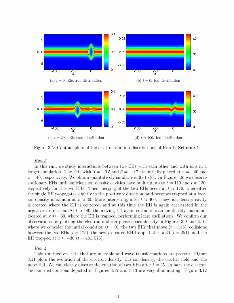
electric field and the potential of an initially stationary electron hole. The results agree wellwith the simulations obtained in [6] by the Fourier transformed methods [5]. In particular,we observe that the EH starts moving in the negative x direction at t ∈ [130, 140] with aMach number M ≈ 0.55. This sudden acceleration can be explained by the cavity in theion density that has built up and made the EH unstable. After t ≈ 140, ion density cavitycontinues to deepen and an electron density cavity is created at the same place, neutralizingthe plasma. In Figure 3.5, we plot the electron and ion distributions at t = 0, the initialcondition and t = 200 when the EH has moved to x ≈ −40. We confirm the observationmade in Figure 3.4 about the behavior of the distribution functions for both species.

Run 2This simulation has qualitatively similar results as the first run. Notice that due to the

difference in the sign of the perturbation, the direction of propagation of the EH is reversedto the positive x direction. In Figure 3.6, we show the time development of this EH. Inthis case, the EH starts moving after t ∈ [120, 130] also with a Mach number M ≈ 0.55.In Figure 3.7, we plot the electron and ion distributions at t = 0, the initial condition andt = 200 when the EH has moved to x ≈ 60.

7

t

Re

letive

Err

or

0 100 200 300

0

2E­14

4E­14

6E­14

Electron particle numberIon partical numberTotal energy

(a) Scheme-1. Run 1.

t

Re

letive

Err

or

0 100 200 300

10­15

10­14

10­13

10­12

10­11

10­10

Electron particle numberIon partical numberTotal energy

(b) Scheme-2. Run 1.

t

Re

letive

Err

or

0 100 200 300

0

5E­14

1E­13

1.5E­13

Electron particle numberIon partical numberTotal energy

(c) Scheme-1. Run 2.

t

Re

letive

Err

or

0 100 200 300

10­15

10­14

10­13

10­12

10­11

10­10

Electron particle numberIon partical numberTotal energy

(d) Scheme-2. Run 2.

Figure 3.2: Evolution of absolute value of relative errors in total particle number and totalenergy. Runs 1 & 2.

8

t

Re

letive

Err

or

0 200 400

0

2E­14

4E­14

6E­14 Electron particle numberIon partical numberTotal energy

(a) Scheme-1. Run 3.

t

Re

letive

Err

or

0 200 40010

­15

10­14

10­13

10­12

10­11

10­10

Electron particle numberIon partical numberTotal energy

(b) Scheme-2. Run 3.

t

Re

letive

Err

or

0 50 1000

1E­13

2E­13

Electron particle numberIon partical numberTotal energy

(c) Scheme-1. Run 4

t

Re

letive

Err

or

0 50 100

10­14

10­13

10­12

10­11

10­10

Electron particle numberIon partical numberTotal energy

(d) Scheme-2. Run 4

Figure 3.3: Evolution of absolute value of relative errors in total particle number and totalenergy. Runs 3 & 4.

9

(a) Electron density (b) Ion density

(c) Electric field (d) Potential

Figure 3.4: Evolution of the electron density, the ion density, the electric field and thepotential of Run 1. Scheme-1.

10

(a) t = 0. Electron distribution (b) t = 0. Ion distribution

(c) t = 200. Electron distribution (d) t = 200. Ion distribution

Figure 3.5: Contour plots of the electron and ion distributions of Run 1. Scheme-1.

Run 3In this run, we study interactions between two EHs with each other and with ions in a

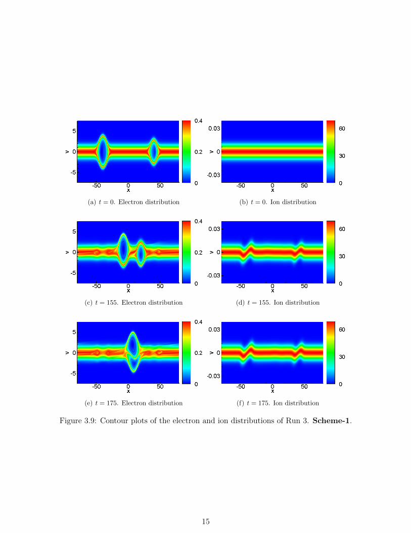
longer simulation. The EHs with β = −0.5 and β = −0.7 are initially placed at x = −40 andx = 40, respectively. We obtain qualitatively similar results to [6]. In Figure 3.8, we observestationary EHs until sufficient ion density cavities have built up, up to t ≈ 110 and t ≈ 130,respectively for the two EHs. Then merging of the two EHs occur at t ≈ 170, whereafterthe single EH propagates slightly in the positive x direction, and becomes trapped at a localion density maximum at x ≈ 30. More interesting, after t ≈ 400, a new ion density cavityis created where the EH is centered, and at this time the EH is again accelerated in thenegative x direction. At t ≈ 480, the moving EH again encounters an ion density maximumlocated at x ≈ −30, where the EH is trapped, performing large oscillations. We confirm ourobservations by plotting the electron and ion phase space density in Figures 3.9 and 3.10,where we consider the initial condition (t = 0), the two EHs that move (t = 155), collisionsbetween the two EHs (t = 175), the newly created EH trapped at x ≈ 30 (t = 251), and theEH trapped at x ≈ −30 (t = 481, 576).

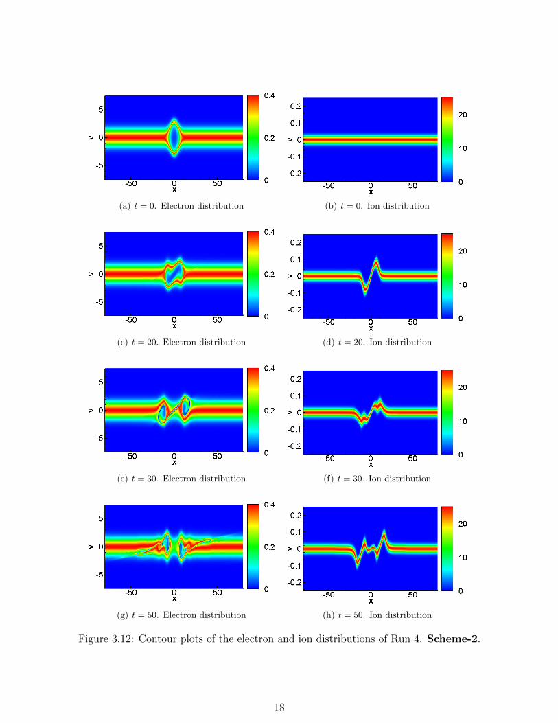
Run 4This run involves EHs that are unstable and wave transformations are present. Figure

3.11 plots the evolution of the electron density, the ion density, the electric field and thepotential. We can clearly observe the creation of two EHs after t ≈ 25. In fact, the electronand ion distributions depicted in Figures 3.12 and 3.13 are very illuminating. Figure 3.12

11

(a) Electron density (b) Ion density

(c) Electric field (d) Potential

Figure 3.6: Evolution of the electron density, the ion density, the electric field and thepotential of Run 2. Scheme-2.

12

(a) t = 0. Electron distribution (b) t = 0. Ion distribution

(c) t = 200. Electron distribution (d) t = 200. Ion distribution

Figure 3.7: Contour plots of the electron and ion distributions of Run 2. Scheme-2.

shows the initial formation of the two EHs up to t = 50. Those two EHs seem to stayunstable at later times as shown in Figure 3.13. The main reason for this different behaviorcompared to previous runs is due to the choice of mass and temperature ratios, making theEH speed comparable to the ion-acoustic speed, causing the EH to transform and break up.We notice such unstable behaviors are also observed in [11] for a large EH initially placedat x = 0.

3.2.3 Numerical study of BGK modes

EH is an important BGK state [1, 12]. In this subsection, we check if the electron andion distribution functions fe, fi are aligned with the particle energy εe = v2/2 − φ(x, t),εi = v2/2/µi + φ(x, t), respectively, which is well-known to be the case for an equilibriumstate of the two-species Vlasov equation. To this end, we plot the ordered pairs (εe =v2/2− φ(x, t), fe(x, v, t)), (εi = v2/2/µ− φ(x, t), fi(x, v, t)) at various t in Figures 3.14-3.19for the four numerical runs. The use of this kind of plot as a diagnostic was first reported in[8, 9] for electrostatic VP equations and later in [3, 4] for the gravitational VP equations. Tosave space, we only show results of one scheme for each case. Similarly as in Section 3.2.2,for runs 1 and 3, we use the explicit method Scheme-1, while for runs 2 and 4, we use theimplicit method Scheme-2. We notice that the range of εe is between −5 and 123 for allfour runs. The range of εi is between 0 and 205 for Run 1-3 and between 0 and 50 for Run 4due to different initial settings of parameter µi. However, to demonstrate the main featuresof the plot, we focus on the range of εe between −7 and 20 and the range of εi between 0

13

(a) Electron density (b) Ion density

(c) Electric field (d) Potential

Figure 3.8: Evolution of the electron density, the ion density, the electric field and thepotential of Run 3. Scheme-1.

14

(a) t = 0. Electron distribution (b) t = 0. Ion distribution

(c) t = 155. Electron distribution (d) t = 155. Ion distribution

(e) t = 175. Electron distribution (f) t = 175. Ion distribution

Figure 3.9: Contour plots of the electron and ion distributions of Run 3. Scheme-1.

15

(a) t = 251. Electron distribution (b) t = 251. Ion distribution

(c) t = 481. Electron distribution (d) t = 481. Ion distribution

(e) t = 576. Electron distribution (f) t = 576. Ion distribution

Figure 3.10: Contour plots of the electron and ion distributions of Run 3. Scheme-1.

16

(a) Electron density (b) Ion density

(c) Electric field (d) Potential

Figure 3.11: Evolution of the electron density, the ion density, the electric field and thepotential of Run 4. Scheme-2.

17

(a) t = 0. Electron distribution (b) t = 0. Ion distribution

(c) t = 20. Electron distribution (d) t = 20. Ion distribution

(e) t = 30. Electron distribution (f) t = 30. Ion distribution

(g) t = 50. Electron distribution (h) t = 50. Ion distribution

Figure 3.12: Contour plots of the electron and ion distributions of Run 4. Scheme-2.

18

(a) t = 60. Electron distribution (b) t = 60. Ion distribution

(c) t = 70. Electron distribution (d) t = 70. Ion distribution

(e) t = 90. Electron distribution (f) t = 90. Ion distribution

(g) t = 120. Electron distribution (h) t = 120. Ion distribution

Figure 3.13: Contour plots of the electron and ion distributions of Run 4. Scheme-2.

19

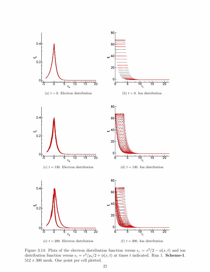
and 22 in Figures 3.14-3.19.As for Run 1 in Figure 3.14, the plot of the electron distribution function fe at t = 0

(Figure 3.14(a)) shows that the EH is in a BGK state at this time. This BGK state is asmall perturbation of BGK states derived in [12] for stationary EHs in electrostatic Vlasovsystems, since the initial condition for electron distribution function in Run 1 is a stationaryEH with a small local perturbation. As discussed in Section 3.2.2, the EH starts moving inthe negative x direction at t ∈ [130, 140] with Mach number M ≈ 0.55, therefore, the plot offe in Figure 3.14(c) shows that the EH is close to a BGK state when the EH has not movedat t = 130, while the BGK state at t = 200 is plotted in the moving frame, i.e. fe versusεe = (v+M)2/2 +φ. We notice a different curve from the initial state in Figure 3.14(e). Forthe ion distribution function fi versus εi at t = 0, Figure 3.14(b) looks like steps instead of asmooth curve because ions are much heavier than electrons (mi/me = 29500), which causesthat the Gaussian is more concentrated. However, if more resolution is available, the plot offi versus εi would look like a curve.

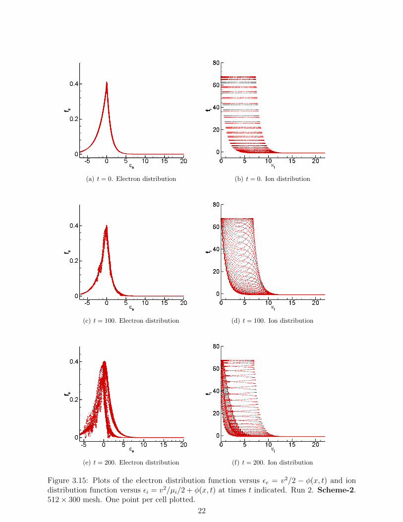
As for Run 2, we have similar conclusions as Run 1. The plots for Run 2 are shown inFigure 3.15. The EH starts moving in the positive x direction at t ∈ [100, 110] with Machnumber M ≈ 0.55. We also plot the BGK state at t = 200 in the moving frame, i.e. feversus εe = (v −M)2/2 + φ.

As for Run 3, in which the interactions between two EHs with each other and with ionsare studied, this simulation is more nonlinear than other three simulations. The study ofBGK states for Run 3 are shown in Figures 3.16-3.17. At t = 0, Figure 3.16(a) shows twocurves since two EHs are placed in this simulation and each represents a BGK state.

As Run 4, we use a different mass and temperature setting to study unstable EHs andwave transformations, where the EH speed is comparable to the ion-acoustic speed, causingthe EH to transform and break up. The plots for Run 4 are shown in Figures 3.18-3.19. Thephenomena of ion distribution function is more prominent for Run 4 in Figure 3.18(b) dueto more concentrated Gaussian, since the temperature setting in Run 4 is taken Te/Ti = 40while it is taken Te/Ti = 1 for Run 1-3.

From the pictures in Figures 3.16-3.19, we do not see the formation of BGK state innumerical runs. The cause of this is subject to future investigation.

4 Conclusion

In this paper, we use the energy-conserving DG schemes to simulate the nonlinear evolutionof EHs. We verify the behaviors of EHs corresponding to different mass and temperatureratios. We demonstrate that our methods are conservative in particle number and totalenergy, and provide a detailed study of the fully dynamics of EHs that nonlinearly interactwith ions in plasma. We perform a numerical study of the BGK states for the nonlinearevolutions of EH simulations. Our simulation results should help to understand the dynamicsof large amplitude EHs that nonlinearly interact with ions in space and laboratory plasmas.Our next goal is to study the theory of BGK states of the EHs.

20

(a) t = 0. Electron distribution (b) t = 0. Ion distribution

(c) t = 130. Electron distribution (d) t = 130. Ion distribution

(e) t = 200. Electron distribution (f) t = 200. Ion distribution

Figure 3.14: Plots of the electron distribution function versus εe = v2/2 − φ(x, t) and iondistribution function versus εi = v2/µi/2 + φ(x, t) at times t indicated. Run 1. Scheme-1.512× 300 mesh. One point per cell plotted.

21

(a) t = 0. Electron distribution (b) t = 0. Ion distribution

(c) t = 100. Electron distribution (d) t = 100. Ion distribution

(e) t = 200. Electron distribution (f) t = 200. Ion distribution

Figure 3.15: Plots of the electron distribution function versus εe = v2/2 − φ(x, t) and iondistribution function versus εi = v2/µi/2 + φ(x, t) at times t indicated. Run 2. Scheme-2.512× 300 mesh. One point per cell plotted.

22

(a) t = 0. Electron distribution (b) t = 0. Ion distribution

(c) t = 155. Electron distribution (d) t = 155. Ion distribution

(e) t = 175. Electron distribution (f) t = 175. Ion distribution

Figure 3.16: Plots of the electron distribution function versus εe = v2/2 − φ(x, t) and iondistribution function versus εi = v2/µi/2 + φ(x, t) at times t indicated. Run 3. Scheme-1.512× 300 mesh. One point per cell plotted.

23

(a) t = 251. Electron distribution (b) t = 251. Ion distribution

(c) t = 481. Electron distribution (d) t = 481. Ion distribution

(e) t = 576. Electron distribution (f) t = 576. Ion distribution

Figure 3.17: Plots of the electron distribution function versus εe = v2/2 − φ(x, t) and iondistribution function versus εi = v2/µi/2 + φ(x, t) at times t indicated. Run 3. Scheme-1.512× 300 mesh. One point per cell plotted.

24

(a) t = 0. Electron distribution (b) t = 0. Ion distribution

(c) t = 20. Electron distribution (d) t = 20. Ion distribution

(e) t = 30. Electron distribution (f) t = 30. Ion distribution

Figure 3.18: Plots of the electron distribution function versus εe = v2/2 − φ(x, t) and iondistribution function versus εi = v2/µi/2 + φ(x, t) at times t indicated. Run 4. Scheme-2.512× 300 mesh. Three points per cell plotted.

25

(a) t = 50. Electron distribution (b) t = 50. Ion distribution

(c) t = 60. Electron distribution (d) t = 60. Ion distribution

(e) t = 120. Electron distribution (f) t = 120. Ion distribution

Figure 3.19: Plots of the electron distribution function versus εe = v2/2 − φ(x, t) and iondistribution function versus εi = v2/µi/2 + φ(x, t) at times t indicated. Run 4. Scheme-2.512× 300 mesh. Three points per cell plotted.

26

Acknowledgments

YC is supported by grants NSF DMS-1217563, DMS-1318186, AFOSR FA9550-12-1-0343and the startup fund from Michigan State University. AJC is supported by AFOSR grantsFA9550-11-1-0281, FA9550-12-1-0343 and FA9550-12-1-0455, NSF grant DMS-1115709 andMSU foundation SPG grant RG100059. We gratefully acknowledge the support from Michi-gan Center for Industrial and Applied Mathematics. We also thank the anonymous refereewho suggested the numerical study of the BGK states.

References

[1] I. Bernstein, J. M. Greene, and M. D. Kruskal. Exact nonlinear plasma oscillations.Phys. Rev., 108:546–550, 1957.

[2] Y. Cheng, A. J. Christlieb, and X. Zhong. Numerical Study of the Two-Species Vlasov-Ampere System: Energy-Conserving Schemes and the Current-Driven Ion-Acoustic In-stability. 2014.

[3] Y. Cheng and I. M. Gamba. Numerical study of one-dimensional Vlasov-Poisson equa-tions for infinite homogeneous stellar systems. Communications in Nonlinear Scienceand Numerical Simulation, 17(5):2052 – 2061, 2012. Special Issue: Mathematical Struc-ture of Fluids and Plasmas Dedicated to the 60th birthday of Phil Morrison.

[4] Y. Cheng, I. M. Gamba, and P. J. Morrison. Study of conservation and recurrenceof Runge–Kutta discontinuous Galerkin schemes for Vlasov-Poisson systems. J. Sci.Comput., 56:319–349, 2013.

[5] B. Eliasson. Numerical modelling of the two-dimensional fourier transformed vlasov–maxwell system. Journal of Computational Physics, 190(2):501–522, 2003.

[6] B. Eliasson and P. K. Shukla. Dynamics of electron holes in an electron-oxygen-ionplasma. Phys. Rev. Lett., 93:045001, Jul 2004.

[7] B. Eliasson and P. K. Shukla. Formation and dynamics of coherent structures involvingphase-space vortices in plasmas. Physics reports, 422(6):225–290, 2006.

[8] R. Heath, I. Gamba, P. Morrison, and C. Michler. A discontinuous Galerkin methodfor the Vlasov-Poisson system. Journal of Computational Physics, 231(4):1140 – 1174,2012.

[9] R. E. Heath. Numerical analysis of the discontinuous Galerkin method applied to plasmaphysics. 2007. Ph. D. dissertation, the University of Texas at Austin.

[10] A. C. Hindmarsh, P. N. Brown, K. E. Grant, S. L. Lee, R. Serban, D. E. Shumaker,and C. S. Woodward. Sundials: Suite of nonlinear and differential/algebraic equationsolvers. ACM T. Math. Software, 31(3):363–396, 2005.

27

[11] K. Saeki and H. Genma. Electron-hole disruption due to ion motion and formationof coupled electron hole and ion-acoustic soliton in a plasma. Physical review letters,80(6):1224, 1998.

[12] H. Schamel. Stationary solutions of the electrostatic vlasov equation. Plasma Physics,13:491–506, 1971.

[13] H. Schamel. Stationary solitary, snoidal and sinusoidal ion acoustic waves. PlasmaPhysics, 14:905–924, 1972.

[14] H. Schamel. Theory of electron holes. Physica Scripta, 20:336–342, 1979.

28