Energy-aware lazy scheduling algorithm for energy-harvesting sensor nodes

ISNN2012

Energy-aware lazy scheduling algorithm for energy-harvestingsensor nodes

Marco Severini • Stefano Squartini •

Francesco Piazza

Received: 3 April 2012 / Accepted: 10 July 2012 / Published online: 27 July 2012

� Springer-Verlag London Limited 2012

Abstract The main problem in dealing with energy-

harvesting (EH) sensor nodes is represented by the scarcity

and non-stationarity of powering, due to the nature of the

renewable energy sources. In this work, the authors address

the problem of task scheduling in processors located in

sensor nodes powered by EH sources. Some interesting

solutions have appeared in the literature in the recent past,

as the lazy scheduling algorithm (LSA), which represents a

performing mix of scheduling effectiveness and ease of

implementation. With the aim of achieving a more efficient

and conservative management of energy resources, a new

improved LSA solution is here proposed. Indeed, the

automatic ability of foreseeing at run-time the task energy

starving (i.e. the impossibility of finalizing a task due to the

lack of power) is integrated within the original LSA

approach. Moreover, some modifications have been applied

in order to reduce the LSA computational complexity and

thus maximizing the amount of energy available for task

execution. The resulting technique, namely energy-aware

LSA, has then been tested in comparison with the original

one, and a relevant performance improvement has been

registered both in terms of number of executable tasks and

in terms of required computational burden.

Keywords Energy-aware approach � Lazy scheduling

algorithm � Task scheduling � Computational complexity �Energy harvesting � Wireless sensor networks

1 Introduction

Wireless sensor networks (WSNs) have encountered a

big interest among the scientific community in the last

decade, and many commercial products are already avail-

able on the market. One of the major challenges in certain

WSN applications is represented by the capability of self-

powering the network sensor nodes by means of suitable

energy-harvesting (EH) techniques [1]. This is typically

required to reduce the costs related to the usage of batteries

or to the connection to the electrical grid. However, the

nature of the energy captured from the environment is often

inconstant and unpredictable, and therefore, some smart

solution is required to efficiently use it for information

processing at the sensor level. Two possible ways of

intervention can be foreseen on purpose: the optimal dis-

tribution of acquired energy to the task to be executed, with

the aim of avoiding the overflow of the accumulator in idle

phases and task starving under high-activity conditions,

and the efficient usage of available energy, in order to

maximize the amount of energy dedicated to the tasks.

The most relevant energy resources requirement for

energy-harvesting sensor nodes (EHNS) devices is due to

networking functionalities; therefore, the biggest efforts in

the scientific literature have been oriented in the recent past

to keep low the computational and energetic burden of such

functionalities, by proposing efficient solutions for cryp-

tography [2], protocols [3], routing schemes and congestion

avoidance [4–6].

Also, the problem of energy resources management has

been carefully studied, and different methods have been

advanced. Some of them suggest to improve the device

efficiency through dynamic power management technique,

as the dynamic voltage scaling and the dynamic frequency

scaling [7–9], or containing the energy conversion overhead

M. Severini � S. Squartini (&) � F. Piazza

3MediaLabs, Department of Information Engineering,

Universita Politecnica delle Marche, Ancona, Italy

e-mail: [email protected]

123

Neural Comput & Applic (2013) 23:1899–1908

DOI 10.1007/s00521-012-1088-x

[10]; others suggest how to adapt the load of the sensor node

[11], but there are also approaches that diversify the nature

of energy sources for the device powering [12, 13], and

others that suggest how to predict the energy availability

[14, 15].

Clearly, since sensor nodes are part of a network, the

same problem can be faced from the overall network per-

spective, which means maximizing the network lifetime

and coverage. However, since a network might be a fairly

complex reality, there are several aspects that require not to

be overlooked. For example, optimizing the nodes place-

ment may help to maximize the harvester performances of

the nodes [16]; also, a proper base station placement may

help in containing the energy needs of the nodes [17].

The optimization process may also involve the redundancy

of the network itself by means of a proper turnover among the

nodes in order to equalize the residual energy of the nodes

while maintaining a proper coverage of the area in terms of

communication and computational load [18–24].

While these examples adopt a run-time approach, Moser

et al. [25, 26] propose an offline optimal scheme for energy

assignment to the tasks relative to each single node. In

general, the more conservative a resource management

policy is, the bigger is the number of operations that can be

accomplished by the single WSN device and therefore the

overall network accordingly. A conservative approach can

be performed by reducing the amount of processing non-

specifically contributing to the device ‘‘throughput’’:

among these, we have the scheduling overhead [27], that is,

the computational complexity associated with the proce-

dure required for optimal task allocation, and the task that

are destined to be violated due to resource starving. This

can be achieved by integrating an offline scheduling pro-

cedure, able to guarantee an optimal resource allocation,

with a run-time control of the effective possibility to

complete a task on the basis of the available resources. This

means adopting a strategy based on the complementary

employment of offline and online scheduling schemes. In

this paper, such an innovative paradigm has been addressed

and a suitable algorithm implemented to verify its effec-

tiveness. The proposed technique has been derived from

the offline solution proposed in [25, 26], namely lazy

scheduling algorithm (LSA), and due to its capability of

predicting the task, energy starving has been named

energy-aware LSA (EA–LSA).

In Sect. 2, a brief review of the LSA approach will be

proposed, whereas Sect. 3 is devoted to the discussion of the

interventions applied to LSA to obtain the innovative

EA–LSA. Section 4 deals with the computer simulations

performed to evaluate the performances of the new algo-

rithm, in comparison with the original one, in terms

of reduced number of violated tasks and reduced com-

putational complexity. Section 5 discusses some further

relevant issues about the proposed technique, and Sect. 6

concludes the paper.

2 Lazy scheduling algorithm

The LSA approach, proposed in [25, 26] as ‘‘clairvoyant’’

algorithm, assumes the knowledge of future availability of

environmental power, described by the function PH(t), and

therefore the energy EH(t1, t2) acquired in the time interval

[t1, t2]. The overall algorithm pseudo-code is reported

below (Algorithm 1).

Jn identifies the generic nth task, and all parameters

related to it are characterized by n as follows:

• an: the arrival time, namely ‘‘phase’’

• dn: the deadline

• fn: the task completion time instant

• sn: the optimal starting time

• en: the required energy for task completion

Other relevant parameters are:

• Q: the task index set

• PS(t): the power absorbed by the device

• PH(t): the acquired power

• pd: the power drain maximum value

• EC(t): the energy stored in the accumulator

• C: the accumulator energy capacity

The optimal starting time sn is defined as the maximum

value between the two quantities s�i and s0i:

s�i ¼ di �ECðaiÞ þ EHðai; diÞ

pd

ð1Þ

s0

i ¼ di �C þ EHðs

0i; diÞ

pd

: ð2Þ

As pointed out in the algorithm pseudo-code, the routine

is able to ensure the optimal allocation of stored energy,

Algorithm 1 Lazy scheduling with pd = constant

Require: maintain a set of indices i 2 Q of all ready

but not finished tasks Ji

Ps(t) ( 0;

while (true)

dj ( min{di : i 2 Q};

calculate sj;

process task Jj with power PS(t);

t ( current time;

if t = ak then add index k to Q; end if

if t = fj then remove index j from Q; end if

if EC(t) = C then PS(t) ( PH(t); end if

if t C Sj then PS(t) ( Pd; end if

endwhile

1900 Neural Comput & Applic (2013) 23:1899–1908

123

but it is not able to guarantee the total absence of task energy

and time starving. In order to face this issue, the LSA

authors [26] suggested to employ a kind of admissibility

test aimed at verifying that the energy required by the

allocated tasks is compatible with the energy attainable

from the environment and with the device processing

capabilities.

Such a test consists in two comparisons, to check the

absence of energy and time starving, respectively: one is

between the total energy demand function A(D) relative to

the task set and the term representing the minimum energy

availability (i.e. the lowest energy variability character-

ization functions), denoted by el; the other is between the

total energy demand function and the energy drain gener-

ated by the device and calculated as pd � D, where D is the

amplitude of the time interval of interest. These compari-

sons are reported as follows:

AðDÞ� elðDÞ þ C ð3Þ

pd � max0�D

AðDÞD

ð4Þ

3 Energy-aware LSA

In this section, the new proposed LSA solution, namely

EA–LSA, will be discussed. As aforementioned, two are

the main innovative contribution w.r.t. the original algo-

rithm: one focused on the energy management and

the other oriented to the reduction in computational

complexity.

3.1 Energy management

The main limitation in (3) is that the curve el establishes the

minimum energy availability from a statistical perspective,

and therefore, it does not provide any guarantee about the

effective acquired amount of energy. It follows that even

though a task satisfies the condition in (3), this does not

mean that energy starving does not occur. If an energy

deficit takes place, since the original routine is not able to

foresee the occurrence of task starving, the task execution

will be accomplished even if it will not be finalized, thus

determining an effective usage of energy but with no useful

processing results. It seems obvious that avoiding per-

forming a task, which is not going to be completed due to

the lack of energy resources, will not affect the deadline

violation for that task, but it allows preserving useful

resources for succeeding tasks.

It can be observed that a task, characterized by the

parameters (ai, di, ei), can be completed if the available

energy (given by the sum of energy acquired during the

task execution and accumulated before the task starting

time) is equal or superior to the energy demand of that

task:

ei�ECðaiÞ þ EHðai; diÞ: ð5Þ

This constraint, preceding the actual management of

each task, gives LSA the property to be EA by expending

resources only on those tasks that can be completed. The

resulting algorithm is reported above (Algorithm 2).

It can be noted that the quantity at the right side of the

inequality expressed in (5) coincides with the numerator of

the fraction in (1); therefore, implementing such an oper-

ation requires at most a comparison and a memory slot to

store the task energy demand value.

3.2 Computational complexity

Besides the task accomplishment, also the operations

related to the algorithm execution ask for computational

resources. Within the LSA, the most relevant burden comes

from the calculation of the optimal starting time si by

means of Eqs. (1–2). Note that this operation is actually

included in the Algorithms 1 and 2 reported above.

The formula expressing the acquired energy, needed for

the calculation of s�i , as indicated in [25] is:

EHðt1; t2Þ ¼Zt1

t2

PHðtÞdt: ð6Þ

By applying (6) to the time interval [ai, di] and taking

the discrete nature of the scheduler into account, we can

derive the following:

Algorithm 2 EA-lazy scheduling with pd = constant

Require: maintain a set of indices i 2 Q of all ready

but not finished tasks Ji

Ps(t) ( 0;

while (true)

dj ( min{di: i 2 Q};

if ej [ (EC(t) ? EH(t, dj)) then remove index j from Q;

else

calculate sj;

process task Jj with power PS(t)

t ( current time;

if t = ak then add index k to Q; end if

if t = fj then remove index j from Q; end if

if EC(t) = C then PS(t) ( PH(t); end if

if t C Sj then PS(t) ( Pd; end if

endif

endwhile

Neural Comput & Applic (2013) 23:1899–1908 1901

123

EHðai; diÞ ¼Xdi

D¼ai

PHðDÞ ð7Þ

In this case, D is the discrete-time variable and PH(D) is

the vector of values describing the available input power,

obtained by sampling the continuous-time stochastic

process PH(t).

To calculate s0

i, it must be noticed that its definition

directly comes from Eq. (8) expressing the balance

between the available energy and the consumed one. By

discretizing such an equation and by means of simple

algebraic manipulation, we can easily obtain Eq. (11) to

calculate the term s0i

ðdi � s0

iÞ � pd ¼ C þ EHðs0

i � diÞ ð8Þ

C ¼Xdi

D¼s0i

pd �Xdi

D¼s0i

PHðDÞ ð9Þ

C ¼Xs0i

D¼di

pd �Xs0i

D¼di

PHðDÞ ð10Þ

C ¼Xs0i

D¼di

ðpd � PHðDÞÞ ð11Þ

The routine used to calculate s0i is therefore:

Routine Search for s0

i

energy_sum ( 0;

for D ( di : -1: s�ienergy_sum ( energy_sum ? pd - PH(D);

if C [ energy_sum then s0

i ( D else break;

Note that it has been chosen to interrupt the loop to yield

s�i observing that si is defined as the maximum value

between s�i and s0

i. Since Eqs. (7) and (11) are applied for

each task and considering that one of the quantities is

always ignored, if it would be possible to calculate only the

quantity of interest, then a significant reduction in com-

putational burden would be achieved.

For what concerns Eq. (7), it can be observed that the

computational resources for calculating s0

i increase as the time

interval [ai, di] or the sampling frequency does. Therefore,

once defined the task set and the device specifications, the

related computational complexity is fixed. It could be possi-

ble to reduce the related computational burden by approxi-

mating (7), but this would also lead to an approximated way

of working of the LSA, which is not advisable.

Regarding Eq. (11), the computational overhead due to

the s0

i term increases as C does and as pd decreases, i.e. as

one drifts away from the ideal case. However, rewriting (1)

and (2) and applying simple algebra, we have:

ðs0i � s�i Þ � pd ¼ ECðaiÞ � C þ EHðai; s0

iÞ ð12Þ

If we indicate with sC the time instant, in correspondence

of which the accumulator reaches the maximum charge,

Eq. (12) can be written as in (13). Here the terms of energy

transferred to the accumulator (14), of energy transferred to

the tasks (15) can be identified. It follows that s0

i can be

expressed as a function of s�i ; as in (16):

ðs0i � s�i Þ � pd ¼ ECðaiÞ � C þ EHðai; sCÞ þ EHðsC; s0

iÞð13Þ

C � ECðaiÞ ¼ EHðai; sCÞ ð14Þ

ðs0i � s�i Þ � pd ¼ EHðsC � s0

iÞ ð15Þ

s0

i ¼ s�i þEHðsC; s

0

iÞpd

ð16Þ

Since the PHðDÞ� 0 8D holds, there exists a quantity s00i

so that:

s00

i ¼ s�i þEHðSC; S

�i Þ

pd

ð17Þ

and therefore the following inequalities hold as well:

s�i � s00i and s

00i � s

0i.

Moving from these premises, Eq. (17) can be general-

ized as follows:

skþ1 ¼ sk þ EHðsk�1; skÞpd

ð18Þ

Equation (18) allows us to determine s0

i through a

process that, starting from s�i , increases its value till

reaching the s0i target. We can reasonably assume that the

available power in the time range [sC, s0

i] is slowly varying.

Now, since such a time range is proportional to the energy

surplus expressed in (15), it seems reasonable assuming

that PH(D) [ 0 over all range [sC, s0i]. It follows that

skþ1 [ sk and thus 9�k so that skþ1 � s0

i8k [ �k. Moreover,

observing that only discrete values are acceptable by our

routine, it is sufficient to interrupt it when the following is

satisfied:

sk þ EHðsk�1; skÞpd

� �¼ sk� �

ð19Þ

The proposed solution limits the calculation of si to the

sole term s�i when there is no energy surplus, thus reducing

the computational overhead. In contrast, when there is

exceeding energy, the routine delays si until the amount of


123

energy EHðsk�1; skÞ transferred to the task reduces the task

execution time, at full power, of at least one single time

instant. This means that the delay computation takes place

only if the energy surplus is enough to justify the related

overhead, enforcing a conservative management of energy

in EHSNs.

It must be observed that if the acquired energy in the

time interval [sk; s0

i] is zero, waiting for the time instant s0

i

to launch the task execution does not carry any benefit, and

thus, executing the task at the instant skþ1, which belongs

to the interval [sk; s0i], does not deteriorate the performances

w.r.t. the original solution.

The computational overhead is thus zero if the surplus

energy is low and increases as such a surplus does, that is,

when the amount of acquired energy increases. Conclud-

ing, we can calculate the amount of acquired energy by

using the following:

EHðs�;k�1i ; s�;ki Þ ¼ EHð0; s�;ki Þ � EHð0; s�;k�1

i Þ ð20Þ

Note that the related overhead is limited to two

operations.

4 Computer simulations

4.1 Experimental setup

In order to evaluate the effectiveness of the proposed

solution, some experimental tests have been performed,

putting in comparison the original LSA and the innovative

EA–LSA. All simulations have been conducted on a PC

(32-bit single-threaded processor, Windows 7 OS) and by

means of Matlab 7.12.0 software environment.

The same test condition addressed in [25, 26] has been

considered here. In particular, we specifically refer to the

task set T1 characterized by:

• Thirty tasks periodically located at 300 time instants of

distance, within a scheduling session of 3,000 time

instants.

• The arrival time, the related deadline and the energy

demand of the tasks are uniformly distributed over a

preset range.

• The absolute deadlines are uniformly distributed over a

period of 300 time instants, thus avoiding the overlap of

two T1 consecutive instances.

• The absolute task set energy demand has been normal-

ized w.r.t. the average energy acquired in one period in

order to guarantee the deadline violation.

• The vector of values used to simulate the power harvest

has been generated by selecting the positive values of a

normally distributed random variable with null mean

and unitary variance, while replacing the negative ones

with zeros, in order to have a profile similar to the one

used in [11].

Results relative to task set T2 addressed in [25, 26] are

compliant with those related to task set T1 here discussed

and therefore omitted for the sake of conciseness.

4.2 Test results: deadline violation

The test sessions have been performed by varying the

energy capacity of the accumulator and considering two

case studies for the assigned device power: pd = ? (which

is the only case considered in [25]) and pd = 2. Such a

finite power value is inferior to the maximum value of

acquired power and the minimum attainable with the

admissibility test (approximately equal to 2.5—note that

the admissibility test assumes for all task an arrival time

equal to zero, and therefore it executes an excess estimate

of the minimum device power needed to avoid the task

time starving). It must be underlined that the lower is the

available device power, the more relevant is the anticipa-

tion of the task execution time with respect to the deadline

and thus the bigger is the probability of task concurrence.

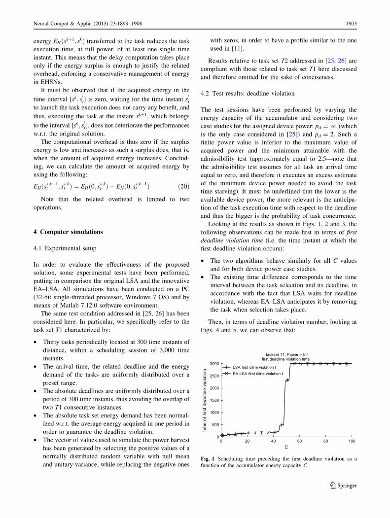
Looking at the results as shown in Figs. 1, 2 and 3, the

following observations can be made first in terms of first

deadline violation time (i.e. the time instant at which the

first deadline violation occurs):

• The two algorithms behave similarly for all C values

and for both device power case studies.

• The existing time difference corresponds to the time

interval between the task selection and its deadline, in

accordance with the fact that LSA waits for deadline

violation, whereas EA–LSA anticipates it by removing

the task when selection takes place.

Then, in terms of deadline violation number, looking at

Figs. 4 and 5, we can observe that:

Fig. 1 Scheduling time preceding the first deadline violation as a

function of the accumulator energy capacity C


123

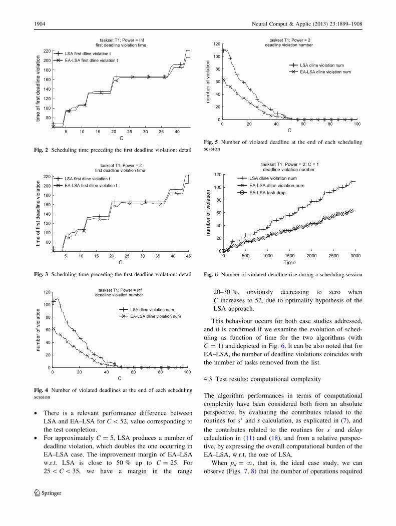
• There is a relevant performance difference between

LSA and EA–LSA for C \ 52, value corresponding to

the test completion.

• For approximately C = 5, LSA produces a number of

deadline violation, which doubles the one occurring in

EA–LSA case. The improvement margin of EA–LSA

w.r.t. LSA is close to 50 % up to C = 25. For

25 \ C \ 35, we have a margin in the range

20–30 %, obviously decreasing to zero when

C increases to 52, due to optimality hypothesis of the

LSA approach.

This behaviour occurs for both case studies addressed,

and it is confirmed if we examine the evolution of sched-

uling as function of time for the two algorithms (with

C = 1) and depicted in Fig. 6. It can be also noted that for

EA–LSA, the number of deadline violations coincides with

the number of tasks removed from the list.

4.3 Test results: computational complexity

The algorithm performances in terms of computational

complexity have been considered both from an absolute

perspective, by evaluating the contributes related to the

routines for s� and s calculation, as explicated in (7), and

the contributes related to the routines for s0

and delay

calculation in (11) and (18), and from a relative perspec-

tive, by expressing the overall computational burden of the

EA–LSA, w.r.t. the one of LSA.

When pd = ?, that is, the ideal case study, we can

observe (Figs. 7, 8) that the number of operations required

Fig. 2 Scheduling time preceding the first deadline violation: detail

Fig. 3 Scheduling time preceding the first deadline violation: detail

Fig. 4 Number of violated deadlines at the end of each scheduling

session

Fig. 5 Number of violated deadline at the end of each scheduling

session

Fig. 6 Number of violated deadline rise during a scheduling session


123

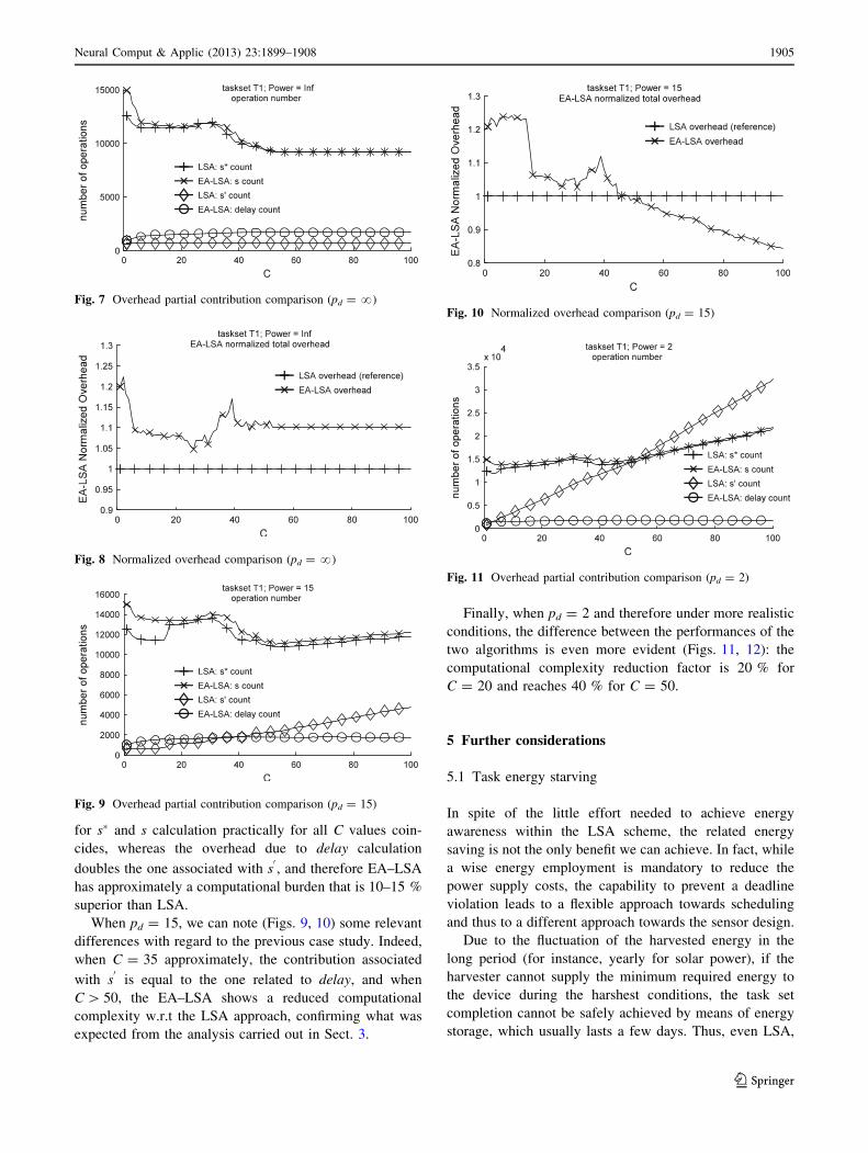
for s� and s calculation practically for all C values coin-

cides, whereas the overhead due to delay calculation

doubles the one associated with s0, and therefore EA–LSA

has approximately a computational burden that is 10–15 %

superior than LSA.

When pd = 15, we can note (Figs. 9, 10) some relevant

differences with regard to the previous case study. Indeed,

when C = 35 approximately, the contribution associated

with s0

is equal to the one related to delay, and when

C [ 50, the EA–LSA shows a reduced computational

complexity w.r.t the LSA approach, confirming what was

expected from the analysis carried out in Sect. 3.

Finally, when pd = 2 and therefore under more realistic

conditions, the difference between the performances of the

two algorithms is even more evident (Figs. 11, 12): the

computational complexity reduction factor is 20 % for

C = 20 and reaches 40 % for C = 50.

5 Further considerations

5.1 Task energy starving

In spite of the little effort needed to achieve energy

awareness within the LSA scheme, the related energy

saving is not the only benefit we can achieve. In fact, while

a wise energy employment is mandatory to reduce the

power supply costs, the capability to prevent a deadline

violation leads to a flexible approach towards scheduling

and thus to a different approach towards the sensor design.

Due to the fluctuation of the harvested energy in the

long period (for instance, yearly for solar power), if the

harvester cannot supply the minimum required energy to

the device during the harshest conditions, the task set

completion cannot be safely achieved by means of energy

storage, which usually lasts a few days. Thus, even LSA,

Fig. 7 Overhead partial contribution comparison (pd = ?)

Fig. 8 Normalized overhead comparison (pd = ?)

Fig. 9 Overhead partial contribution comparison (pd = 15)

Fig. 10 Normalized overhead comparison (pd = 15)

Fig. 11 Overhead partial contribution comparison (pd = 2)


123

whose main objective is ensuring the task set completion,

cannot reach this goal under those conditions. It must be

also noted that the maximum energy harvest can exceed ten

times the minimum (at least in the solar power case study

[28]); therefore, if we choose the right harvester to guar-

antee the task set completion during the harshest condi-

tions, since the energy demand remains unchanged, during

the favourable conditions we have an energy surplus that

cannot be used, meaning that in this case the harvester

represents an extra cost.

Now, as EA–LSA can foresee the task energy-starving

occurrence and drop the task that cannot be completed, the

scheduler can be designed to replace that task with a less

demanding one that can be completed instead. What we

suggest is a ‘‘fall-back’’ mechanism that automatically

reduces the load applied to the device. Simply, let us

assume that we can define a high-load task set providing,

for each of the most demanding tasks, a low-load alterna-

tive. Then, we can assign the high-load task set to the

device, to obtain the maximum energy employment, while

the device is free to ‘‘fall back’’ to the low-cost alternative

and each time the energy harvest is lacking. As added

benefit, if the tasks are interdependent, the completion of

the entire set can be achieved further avoiding energy

misspending, by means of a proper task selection.

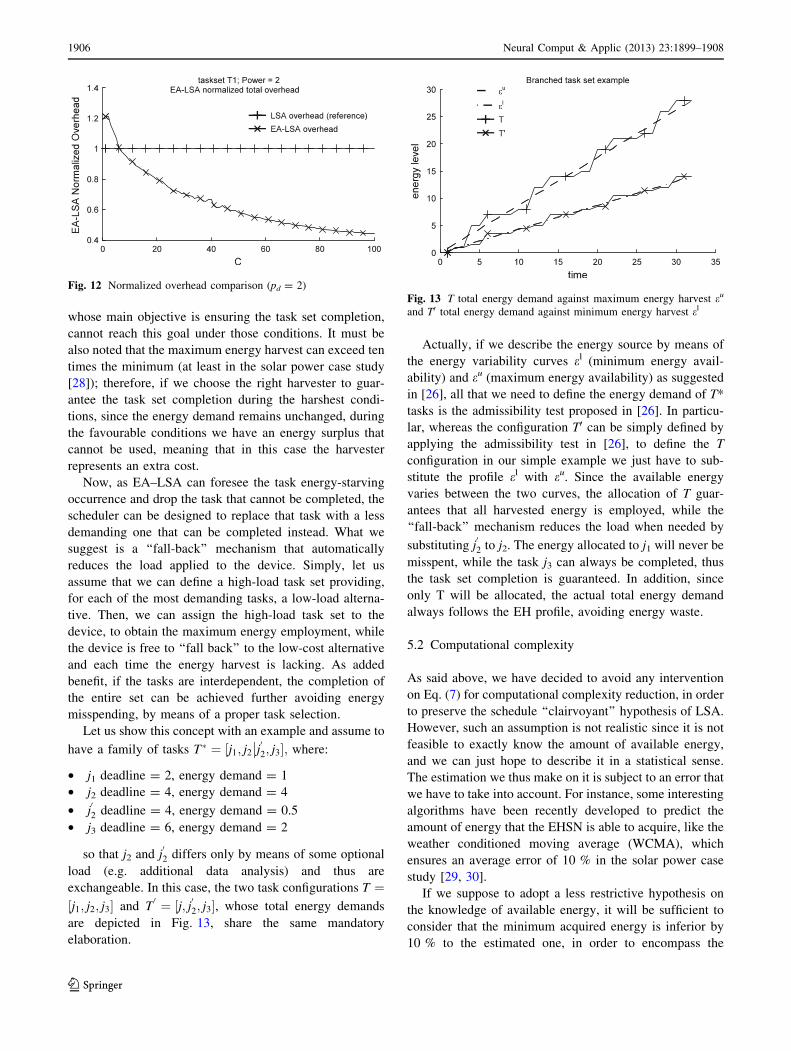
Let us show this concept with an example and assume to

have a family of tasks T� ¼ ½j1; j2 j02; j3�;�� where:

• j1 deadline = 2, energy demand = 1


• j02 deadline = 4, energy demand = 0.5


so that j2 and j02 differs only by means of some optional

load (e.g. additional data analysis) and thus are

exchangeable. In this case, the two task configurations T ¼½j1; j2; j3� and T

0 ¼ ½j; j02; j3�, whose total energy demands

are depicted in Fig. 13, share the same mandatory

elaboration.

Actually, if we describe the energy source by means of

the energy variability curves el (minimum energy avail-

ability) and eu (maximum energy availability) as suggested

in [26], all that we need to define the energy demand of T*

tasks is the admissibility test proposed in [26]. In particu-

lar, whereas the configuration T0 can be simply defined by

applying the admissibility test in [26], to define the T

configuration in our simple example we just have to sub-

stitute the profile el with eu. Since the available energy

varies between the two curves, the allocation of T guar-

antees that all harvested energy is employed, while the

‘‘fall-back’’ mechanism reduces the load when needed by

substituting j02 to j2. The energy allocated to j1 will never be

misspent, while the task j3 can always be completed, thus

the task set completion is guaranteed. In addition, since

only T will be allocated, the actual total energy demand

always follows the EH profile, avoiding energy waste.

5.2 Computational complexity

As said above, we have decided to avoid any intervention

on Eq. (7) for computational complexity reduction, in order

to preserve the schedule ‘‘clairvoyant’’ hypothesis of LSA.

However, such an assumption is not realistic since it is not

feasible to exactly know the amount of available energy,

and we can just hope to describe it in a statistical sense.

The estimation we thus make on it is subject to an error that

we have to take into account. For instance, some interesting

algorithms have been recently developed to predict the

amount of energy that the EHSN is able to acquire, like the

weather conditioned moving average (WCMA), which

ensures an average error of 10 % in the solar power case

study [29, 30].

If we suppose to adopt a less restrictive hypothesis on

the knowledge of available energy, it will be sufficient to

consider that the minimum acquired energy is inferior by

10 % to the estimated one, in order to encompass the

Fig. 12 Normalized overhead comparison (pd = 2)

Fig. 13 T total energy demand against maximum energy harvest eu

and T0 total energy demand against minimum energy harvest el


123

occurrence of energy-starving situations even in the most

unfavourable situations and guarantee the execution of all

assigned tasks. By using this simple modification, the

employment of available energy will keep the optimal

characteristics given by the flexible scheduling methodol-

ogy here discussed.

Nevertheless, admitting that our knowledge of available

energy is subject to an error, we can propose a simpler way

to calculate Eq. (7), leading to some computational

resources savings. Indeed, assuming that within the time

interval [t1, t2] of length wL, the energy increment is linear

with time as it is equal to E at t2, and we can calculate the

amount of energy acquired in the interval [ai, di], internal

to [t1, t2], by using the following:

EHðai; diÞ ¼E � ðdi � aiÞ

wL

ð21Þ

Since (21) requires at most three operations, it

introduces less computation overhead with respect to

Eq. (7) if the interval [ai, di] is longer than three time

instants, which is what typically happens in LSA

applications.

It can be thus concluded that considering a more real-

istic modelling of the problem allows us to improve the

EA–LSA performances in terms of computational com-

plexity, with a limited impact on the optimal management

of energy.

6 Conclusions

In this paper, an improved version of the LSA, suitable for

applications with EHNS, has been proposed. The new

algorithm has been named energy-aware LSA (EA–LSA)

since, due to its capability of predicting the occurrence of

task energy starving, it allows obtaining a more conser-

vative and efficient management of energy with respect to

the original LSA. Such a result allows concluding that if

a certain percentage of missed tasks is tolerated, the

EA–LSA allows using an energy accumulator with reduced

capacity (and thus price) than the one attainable with LSA

analysis.

Regarding the computational complexity, the number of

operations required by EA–LSA does not present a sig-

nificant dependence on the device characteristics, and the

improvement in performances from this perspective with

respect to the LSA increases as we move towards real

conditions (finite power device) and we augment the

energy capacity assigned to the system. The approximation

introduced to achieve such a result, consisting in detaining

the optimal starting time of task execution, does not have a

negative impact on the overall algorithm performances,

confirming the validity of adopted assumptions.

A further reduction in the computational complexity is

possible by employing an approximated evaluation of

acquired energy. Such a possibility has not been investi-

gated so far and can represent an interesting research

development for the future.

The authors are also actually involved in applying the

EA–LSA algorithm in a real embedded platform for

energy-harvesting sensor nodes (by means of the CBC-

EVAL09 module by CYMBET [31] for energy harvesting

and management and the eZ430-RF2500 Development

Tool by Texas Instrument [32] for information processing

and communications).

References

1. Beeby S, White N (2010) Energy harvesting for autonomous

systems. Artech House Publishers, Boston

2. Hagras EAAA, EI-Saied D, Aly HH (2011) Energy efficient key

management scheme based on elliptic curve signcryption for

wireless sensor networks. In: 28th National radio science con-

ference (NRSC), pp 1–9

3. Sun P, Zhang X, Dong Z, Zhang Y (2008) A novel energy effi-

cient wireless sensor MAC protocol. In: Fourth international

conference on networked computing and advanced information

management (NCM ‘08), pp 68–72

4. Liu Z, Wang L, Zhang Z, Zhang A, Jiang Z (2010) Small world-

based query mechanism. In: International symposium on intelli-

gence information processing and trusted computing (IPTC),

28–29 Oct. 2010, pp 250–253

5. Ting Y, Ang L, Jiaowen W, Zhiheng C, Zhang Q (2011) A fast

fasten control algorithm for wireless sensor networks. In: 3rd

international workshop on intelligent systems and applications

(ISA), 28–29 May 2011, pp 1–4

6. Tao LQ, Qi Yu F (2010) ECODA: enhanced congestion detection

and avoidance for multiple class of traffic in sensor networks. In:

IEEE transactions on consumer electronics, vol 56(3), pp 1387–

1394

7. Liu S, Lu J, Wu Q, Qiu Q (2011) Harvesting-aware power

management for real-time systems with renewable energy. In:

IEEE transactions on very large scale integration (VLSI) systems,

pp 1–14

8. Tuming W, Sijia Y, Hailong W (2010) A dynamic voltage scaling

algorithm for wireless sensor networks. In: 3rd international

conference on advanced computer theory and engineering (IC-

ACTE), pp V1-554–V1-557

9. Ravinagarajan A, Dondi D, Rosing TS (2010) DVFS based task

scheduling in a harvesting WSN for structural health monitoring.

In: Design, automation and test in Europe conference and exhi-

bition (DATE), pp 1518–1523

10. Liu S, Lu J, Wu Q, Qiu Q (2010) Load-matching adaptive task

scheduling for energy efficiency in energy harvesting real-time

embedded systems. In: ACM/IEEE international symposium on

low-power electronics and design (ISLPED), pp 325–330

11. Renner C, Meier F, Turau V (2012) Policies for predictive energy

management with supercapacitors. In: IEEE international con-

ference on pervasive computing and communications workshops

(PERCOM workshops), pp 314–319

12. Carli D, Brunelli D, Benini L, Ruggeri M (2011) An effective

multi-source energy harvester for low power applications. In:

Design, automation and test in Europe conference and exhibition

(DATE), pp 1–6


123

13. Huang C, Chakrabartty S (2011) A hybrid energy scavenging

sensor for long-term mechanical strain monitoring. In: 2011 IEEE

international symposium on circuits and systems (ISCAS),

pp 2473–2476

14. Lu J, Liu S, Wu Q, Qiu Q (2010) Accurate modeling and pre-

diction of energy availability in energy harvesting real-time

embedded systems. In: International green computing conference,

pp 469–476

15. Sharma N, Gummeson J, Irwin D, Shenoy P (2010) Cloudy

computing: leveraging weather forecasts in energy harvesting

sensor systems. In: 7th annual IEEE communications society

conference on sensor mesh and ad hoc communications and

networks (SECON), pp 1–9

16. Misra S, Majd NE, Huang H (2011) Constrained relay node

placement in energy harvesting wireless sensor networks. In:

IEEE 8th international conference on mobile adhoc and sensor

systems (MASS), pp 25–34

17. Wang F, Wang D, Liu J (2012) EleSense: elevator-assisted

wireless sensor data collection for high-rise structure monitoring.

In: Proceedings of the IEEE INFOCOM, pp 163–171

18. Zhao Y, Li F (2012) On maximizing the lifetime of wireless

sensor networks using virtual backbone scheduling. In: IEEE

transactions on parallel and distributed systems, pp 1528–1535

19. Zairi S, Zouari B, Niel E, Dumitrescu E (2012) Nodes self-

scheduling approach for maximizing wireless sensor network

lifetime based on remaining energy. In: Wireless sensor systems,

IET, pp 52–62

20. Toyoda S, Sato F (2012) Energy-effective clustering algorithm

based on adjacent nodes and residual electric power in wireless

sensor networks. In: 26th International conference on advanced

information networking and applications workshops (WAINA),

pp 601–606

21. Fateh B, Manimaran G (2010) Energy-aware joint scheduling of

tasks and messages in wireless sensor networks. In: IEEE inter-

national symposium on parallel and distributed processing,

workshops and Phd forum (IPDPSW), pp 1–4

22. Dai L, Shen Z, Chang Y (2010) DTSWC: a task scheduling

algorithm in wireless sensor networks with co-processor based on

divisible load theory. In: International conference on computer

and communication technologies in agriculture engineering

(CCTAE), vol 3, pp 494-497

23. Jin Y, Wei D, Gluhak A, Moessner K (2010) Latency and energy-

consumption optimized task allocation in wireless sensor networks.

In: IEEE wireless communications and networking conference

(WCNC), pp 1–6

24. De Pauw T, Verstichel S, Volckaert B, De Turck F, Ongenae V

(2010) Resource-aware scheduling of distributed ontological

reasoning tasks in wireless sensor networks. In: IEEE interna-

tional conference on sensor networks, ubiquitous, and trustworthy

computing (SUTC), pp 131–137

25. Moser C, Brunelli D, Thiele L, Benini L (2006) Lazy scheduling

for energy-harvesting sensor nodes. In: Fifth working conference

on distributed and parallel embedded systems, DIPES, pp 125–

134, Braga, Portugal, October 11–13 2006

26. Moser C, Brunelli D, Thiele L, Benini L (2007) Real-time

scheduling for energy harvesting sensor nodes. Real Time Syst

37(3):233–260

27. Chetto M, Zhang H (2010) Performance evaluation of real-time

scheduling heuristics for energy harvesting systems. In: The 2010

international symposium on energy-aware computing and net-

working (EaCN-2010), Hangzhou, China

28. Kruger D, Fischer S, Buschmann C (2009) Solar power

harvesting—modeling and experiences, vol 8. GI/ITG KuVS

Fachgesprach Drahtlose Sensornetze

29. Bergonzini C, Brunelli D, Benini L (2009) Algorithms for har-

vested energy prediction in batteryless wireless sensor networks.

In: 3rd international workshop on advances in sensors and

interfaces (IWASI 2009)

30. Piorno JR, Bergonzini C, Atienza D, Rosing TS (2009) Prediction

and management in energy harvested wireless sensor nodes. In:

1st international conference on wireless communication, vehic-

ular technology, information theory and aerospace and electronic

systems technology (wireless VITAE)

31. Cymbet Corporation, CBC-EVAL-09 Data Sheet (2011) [Online]

URL: www.cymbet.com/pdfs/DS-72-13.pdf

32. Texas Instruments (2009) eZ430-RF2500 development tool user’s

guide. [Online] URL: www.ti.com/lit/ug/slau227e/slau227e.pdf


123

http://www.cymbet.com/pdfs/DS-72-13.pdf

http://www.ti.com/lit/ug/slau227e/slau227e.pdf

Energy-aware lazy scheduling algorithm for energy-harvesting sensor nodes

Documents