ENDOW(efficient development of offshore wind farms): modelling wake and boundary layer interactions

1

ENDOW: EfficieNt Development of Offshore Windfarms

Rebecca Barthelmie1, Gunner Larsen1, Sara Pryor1, Hans Bergström2, Mikael Magnusson2, Wolfgang Schlez3, Kostas Rados4, Bernhard Lange5, Per Vølund6, Søren Neckelmann7, Søren

Mogensen8, Gerard Schepers9, Terry Hegberg9, Luuk Folkerts10

1Wind Energy Department, Risoe National Laboratory, 4000 Roskilde (DK) [email protected], 2Uppsala University (SE), 3Garrad Hassan and Partners (GB),4Robert Gordon University (GB),5University of Oldenburg (D),6SEAS WEC (DK),7Techwise AS (DK),8Neg Micon

(DK),9ECN (NL),10Ecofys (NL)

1. ABSTRACT Europe has large offshore wind energy potential that is poised for exploitation to make a significant contribution to the objective of providing a clean, renewable and secure energy supply. Offshore wind energy developments are underway in many European countries with planned projects of several thousand megawatts to be installed in addition to the 250 MW installed by the end of 2002. While experience gained through the demonstration projects currently operating is valuable, a major uncertainty in estimating power production lies in the prediction of the dynamic links between the atmosphere and wind turbines in offshore regimes. The objective of the ENDOW project was to evaluate, enhance and interface wake and boundary-layer models for utilisation offshore. The project resulted in a significant advance in the state of the art in both wake and marine boundary layer models leading to improved prediction of wind speed and turbulence profiles within large offshore wind farms. Use of new databases from existing offshore wind farms and detailed wake profiles collected using a sodar provided a unique opportunity to undertake the first comprehensive evaluation of offshore wake model performances. The wake models evaluated vary in complexity from empirical solutions to the most advanced models based on solutions of the Navier-Stokes equations using eddy viscosity combined with a k-epsilon turbulence closure. Results of wake model performance in different wind speed, stability and roughness conditions provided criteria for their improvement. Mesoscale model simulations were used to evaluate the impact of thermal flows, roughness and orography on offshore wind speeds. The model hierarchy developed under ENDOW forms the basis of design tools for use by wind energy developers and turbine manufacturers to optimise power output from offshore wind farms through minimised wake effects and optimal grid connections. The design tools are being built onto existing regional scale models and wind farm design software which was developed with EU funding and is in use currently by wind energy developers. This will maximise the expected impact of this project through efficient use of existing resources and ease of upgrade for end-users.

2. WAKE MODEL EVALUATION 2.1 Observations and databases Databases were compiled from two offshore wind farms at which both meteorological observations and power output were available. These were Vindeby in Denmark (Figure 1) (Barthelmie et al. 1996) and Bockstigen in Sweden (Lange et al. 1999). Note that the Vindeby wind farm is relatively close to the coast (about 2 km). The site was chosen because it is one of very few operating offshore wind farms and has three monitoring masts (two offshore and one at the coast) providing detailed meteorological measurements to 48 m height. The land mast is about 1.5 km south of the turbine 5W and the two offshore masts are located south west and south of the array as indicated in Figure 1. The wind farm consists of 11 BONUS 450 kW turbines in two rows oriented towards the

2

south-west (prevailing wind direction). The hub-height is 38 m and the rotor diameter is 35.5 m. Layout of the wind farm and the two offshore masts is also shown in Figure 1. The site has the advantage of shallow water (2-5 m) with relatively low wave heights and swell compared to more exposed sites. A more detailed description of data and instruments can be found in (Barthelmie et al. 2002). 2.2 Wake models Once scenarios had been agreed covering different wind speeds, stability and turbulence conditions, six different wake models were evaluated:

• Partner ECN: Wakefarm • Partner RGU: 3D-NS • Partner UOL: FlaP • Partner MIUU: Transportation time model • Partner GH: WindFarmer (Eddy Viscosity model) • Partner RISO: Engineering model

All models, with exception of the model used by MIUU, are based on the approximate solution of the Navier Stokes Equations. The model used by MIUU is significantly different as it uses an empirical approach that is based on the time needed to transport the wake to the point of interest. The differences between the other models are to be found in one or several of the following points:

• the degree of approximations used • representation of the turbine • the modelling of the near wake and initial profile • the turbulence closure used • the parameterisation of the turbulence • the description of the boundary layer • the wake superposition

An unexpectedly large difference in the predictions of the six models between each other and between most of the models and the observational data became apparent in the first evaluation undertaken. This prompted the wake modelling groups to investigate the causes for these differences, and to undertake model modifications. Model improvements were made by the wake modelling groups mainly with regards to:

• The modelling of the near wake and the initial profile • The turbulence parameterisation • The description of the boundary layer • The wake superposition • Turbulence representation

Details of these improvements can be found in (Schlez et al. 2002). Subsequently, the models were employed in the same simulations as before to evaluate their performance in comparison with each other and with the measurements. The results from the Risoe model are prior to modification. 2.3 Model simulations The meteorological masts were located such that their positions relative to the wind turbines correspond to the same unchanged distances between the rows and the turbines. The wind speed was measured at seven heights at masts SMS and SMW and at four different heights at mast LM. A database of 1 minute data was created as part of the ENDOW project from the years 1994 and 1995 with more than 400,000 simultaneous data points from the three masts. From these data a number of scenarios were developed for a range of wind speeds, turbulence and stability conditions. The four wake cases analysed were one single wake, two double wake and one quintuple wake case that are presented in Figure 1 and Table 1. Note, the MIUU transport time model was not modified and changes in the Risoe model were not included in these evaluations.

3

Figure 1. Layout of the wind turbines and masts at Vindeby

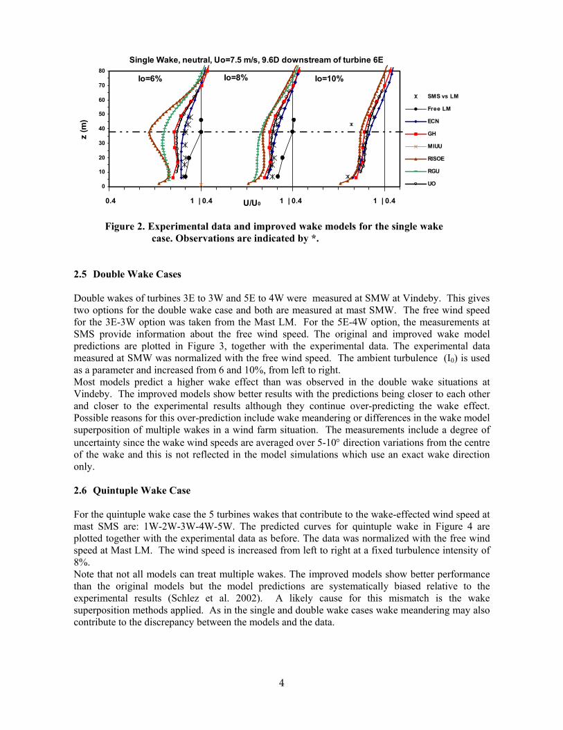
Table 1. Wake cases from Vindeby Wake Type Wind Direction range Wake Mast Free Mast Single 18° to 28° LM SMS Double 18° to 28° LM SMW Double 70° to 78° SMS SMW Quintuple 314° to 323° SMW SMS LM: Land Mast; SMS: Sea Mast South; SMW: Sea Mast West 2.4 Single Wake Case The cases presented here are single, double, quintuple wake at three different velocities (5, 7.5 and 10 m/s), different turbulence intensities and for neutral atmospheric stability. In the following figures the crosses represent the free measurements, the continuous line with symbols represents the free wind speed at LM and other the continuous lines represent the predictions of each of the different wake models. The single wake case was examined in detail in (Rados et al. 2002) and so only one single wake case is presented showing the improved wake model results. The six predicted curves for the single wake case are plotted in Figure 2 together with experimental data for three different turbulence intensities. All graphs are normalized with the free wind speed measured at 38 meters height at LM. The comparison showed initially a surprisingly wide variation of the predictions between each other on the one hand and the experimental results on the other hand. The differences were highest for low turbulence cases that are of special interest in offshore wind farms and at low wind speeds where wake effects are most pronounced. The predicted curves follow the experimental data very well for high turbulence intensities, although some predictions still differ significantly for lower turbulence intensity (6%). When looking at the measurement it has to be taken into account that the data is normalised with the wind speed from the LM that is located on land about 1.4 km south. The model predictions were much improved by the new parameterizations, particularly in the case of the ECN and UO models. The variability between the predictions was reduced and the model simulations show better agreement with the experimental results.

4

Single Wake, neutral, Uo=7.5 m/s, 9.6D downstream of turbine 6E

0

10

20

30

40

50

60

70

80

0.40 1.00 1.60 2.20U/U0

z (m

)SMS vs LM

Free LM

ECN

GH

MIUU

RISOE

RGU

UO

0.4 1 | 0.4

Io=6% Io=10%Io=8%

1 | 0.4 1 | 0.4

Figure 2. Experimental data and improved wake models for the single wake

case. Observations are indicated by *. 2.5 Double Wake Cases Double wakes of turbines 3E to 3W and 5E to 4W were measured at SMW at Vindeby. This gives two options for the double wake case and both are measured at mast SMW. The free wind speed for the 3E-3W option was taken from the Mast LM. For the 5E-4W option, the measurements at SMS provide information about the free wind speed. The original and improved wake model predictions are plotted in Figure 3, together with the experimental data. The experimental data measured at SMW was normalized with the free wind speed. The ambient turbulence (I0) is used as a parameter and increased from 6 and 10%, from left to right. Most models predict a higher wake effect than was observed in the double wake situations at Vindeby. The improved models show better results with the predictions being closer to each other and closer to the experimental results although they continue over-predicting the wake effect. Possible reasons for this over-prediction include wake meandering or differences in the wake model superposition of multiple wakes in a wind farm situation. The measurements include a degree of uncertainty since the wake wind speeds are averaged over 5-10° direction variations from the centre of the wake and this is not reflected in the model simulations which use an exact wake direction only. 2.6 Quintuple Wake Case For the quintuple wake case the 5 turbines wakes that contribute to the wake-effected wind speed at mast SMS are: 1W-2W-3W-4W-5W. The predicted curves for quintuple wake in Figure 4 are plotted together with the experimental data as before. The data was normalized with the free wind speed at Mast LM. The wind speed is increased from left to right at a fixed turbulence intensity of 8%. Note that not all models can treat multiple wakes. The improved models show better performance than the original models but the model predictions are systematically biased relative to the experimental results (Schlez et al. 2002). A likely cause for this mismatch is the wake superposition methods applied. As in the single and double wake cases wake meandering may also contribute to the discrepancy between the models and the data.

5

Figure 3. Double wake cases showing experimental data, original (lower) and improved (upper) wake model simulations.

Quintuple Wake, neutral, Io=8% , 8.6D

0

10

20

30

40

50

60

70

80

0.40 1.00 1.60 2.20U/U0

z (m

)

SM S vs LM

Fre e LM

ECN

GH

RISOE

UO

RGU0.4 1 | 0.4

5 m/s 10m/s7.5 m/s

1 | 0.4 1 | 0.4

Figure 4. The quintuple wake case The partners have undertaken various improvements to their wake models (see e.g. (Lange et al. 2002)). The most important of which focus on the parameterisation of the near wake, the modelling of wind profile and most critically the treatment of turbulence. Different approaches for wake superposition have been used by the partners, advantages and disadvantages of the approaches became apparent in the quintuple wake comparisons. For further investigation it is recommended to focus on the understanding and modelling of the near wake, the wake

Double Wake, neutral, Io=6% , 9.6D downstream

0

10

20

30

40

50

60

70

80

0.40 1.00 1.60 2.20U/Uo

z (m

)

SMW vs SMS

SMW vs LM

Free LM

ECN

GH

RISOE

RGU

UO

0.4 1 | 0.4

5 m/s 10m/s7.5 m/s

1 | 0.4 1 | 0.4

Double Wake, neutral, Io=6%, 9.6D downstream

0

10

20

30

40

50

60

70

80

0.40 1.00 1.60 2.20U/Uo

z (m

)SMW vs LM

SMW vs SMS

Free LM

ECN

GH

RISOE

RGU

UO

MIUU0.4 1 | 0.4

5 m/s 10m/s7.5 m/s

1 | 0.4 1 | 0.4

6

superposition and effects related to the statistics, dynamics and magnitude of wind direction changes and associated effects like wake meandering. Subsequent to this analysis, comparison of the wake model incorporated within WAsP (Mortensen et al. 1993) with the Vindeby scenarios has been conducted. Results are summarized below. Predicted wind speeds at hub-height are close to those observed (root mean square (RMS) error of 0.37 m/s) in the three lowest wind speed scenarios (up to 10 m/s) at a distance of 9.6 D but the WAsP wake algorithms under-predict the wake magnitude at high wind speeds, possibly indicating the wake recovery as manifest in the algorithms is too rapid, although this discrepancy may also reflect the influence of stability on turbulence profiles and hence wake decay and the influence of wake meandering on the observations. Table 2. Wake calculation using (1) and (2) of Vindeby scenario using WAsP. The wake wind speeds represent the hub-height (m/s). Also shown are the observed wake wind speeds at 9.6D. Distance as rotor diameters

3 5 7 9.6 9.6 observed

Difference UWAsP-Ufreestream

10

Distance (m) 106.5 177.5 248.5 340.8 355 Freestream wind speed (m/s)

5.02 2.89 3.42 3.77 4.08 4.33 -0.25 4.12 7.27 5.03 5.59 5.96 6.29 6.42 -0.13 6.32 9.75 7.40 8.02 8.40 8.73 8.80 -0.07 8.78 13.70 11.50 11.96 12.23 12.46 11.74 0.69 12.49

3. BOUNDARY-LAYER MODELLING The offshore wind climate over the Baltic Sea area has been investigated using the three-dimensional higher-order closure MIUU-model from Uppsala University. A technique for modelling the wind climate with this type of model is presented. Following the good agreement between model estimates and observations, it was judged that the model output may be used to analyse different aspects of the offshore winds in detail. For example, the influence from land/sea temperature differences on the wind climate and the effects of the related thermally driven flows were investigated and an attempt was made to quantify these effects on the offshore wind power potential over the Baltic Sea. Since stability effects tend to average out over the course of the year, the RMS-error of the monthly wind speed differences between model simulations with and without effects from thermally driven flows give an alternative and to some extent more relevant estimate of the true influence from land/sea temperature differences. The RMS error for all offshore grid points was estimated to be 6-11% on a monthly basis. Such errors are about five times larger than the ±2% errors determined for the annual average wind speed. The most extreme RMS errors found offshore were –52% and +75%. Figure 5 shows the seasonal differences and Figure 6 the annual differences between winds simulated with and without temperature differences between land and sea. These results indicate significant spatial variability with largest differences in spring and summer. Without temperature variations wind speeds tend to be lower in the northern Baltic during spring and higher in the southern Baltic during summer. This might be expected in near-surface wind speeds if stable conditions in the northern Baltic during spring were producing wind speed profiles which were more stable than logarithmic. Conversely warmer seas in the southern Baltic might produce slightly

7

unstable conditions giving an unstable wind speed profile (so slightly lower wind speeds than predicted by the logarithmic profile at the same height). Further details of this work are presented in (Bergström 2002).

0 200 400 600 800 10000

100

200

300

400

500

600

700

800

x−distance (km)

y−di

stan

ce (

km)

MIUU model: January − noT−v2 diff. (%). Height:48 m

0 200 400 600 800 10000

100

200

300

400

500

600

700

800

x−distance (km)y−

dist

ance

(km

)

MIUU model: April − noT−v2 diff. (%). Height:48 m

−14

−12

−10

−8

−6

−4

−2

0

2

4

6

8

10

12

14

0 200 400 600 800 10000

100

200

300

400

500

600

700

800

x−distance (km)

y−di

stan

ce (

km)

MIUU model: July − noT−v2 diff. (%). Height:48 m

0 200 400 600 800 10000

100

200

300

400

500

600

700

800

x−distance (km)

y−di

stan

ce (

km)

MIUU model: October − noT−v2 diff. (%). Height:48 m

−14

−12

−10

−8

−6

−4

−2

0

2

4

6

8

10

12

14

Figure 5. Average wind speed differences (%) between the model runs made with no land/sea temperature differences, and the full climatological runs. Monthly averages for January, April, July, and October

0 200 400 600 800 10000

100

200

300

400

500

600

700

800

x−distance (km)

y−di

stan

ce (

km)

MIUU model: Annual − noT−v2 diff. (%). Height:48 m

−6

−5

−4

−3

−2

−1

0

1

2

3

4

Figure 6. Annual average of difference (%) in mean wind speed between the model runs made with no land/sea temperature differences and the full climate runs.

8

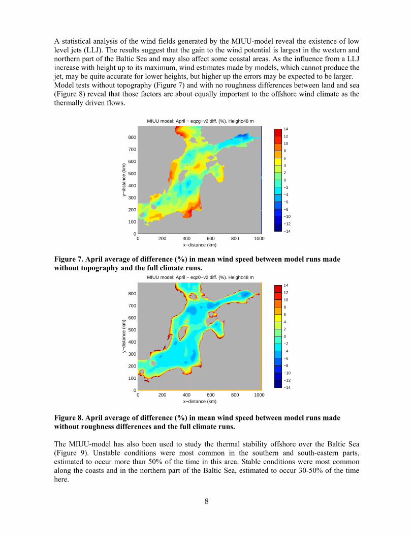
A statistical analysis of the wind fields generated by the MIUU-model reveal the existence of low level jets (LLJ). The results suggest that the gain to the wind potential is largest in the western and northern part of the Baltic Sea and may also affect some coastal areas. As the influence from a LLJ increase with height up to its maximum, wind estimates made by models, which cannot produce the jet, may be quite accurate for lower heights, but higher up the errors may be expected to be larger. Model tests without topography (Figure 7) and with no roughness differences between land and sea (Figure 8) reveal that those factors are about equally important to the offshore wind climate as the thermally driven flows.

0 200 400 600 800 10000

100

200

300

400

500

600

700

800

x−distance (km)

y−di

stan

ce (

km)

MIUU model: April − eqzg−v2 diff. (%). Height:48 m

−14

−12

−10

−8

−6

−4

−2

0

2

4

6

8

10

12

14

Figure 7. April average of difference (%) in mean wind speed between model runs made without topography and the full climate runs.

0 200 400 600 800 10000

100

200

300

400

500

600

700

800

x−distance (km)

y−di

stan

ce (

km)

MIUU model: April − eqz0−v2 diff. (%). Height:48 m

−14

−12

−10

−8

−6

−4

−2

0

2

4

6

8

10

12

14

Figure 8. April average of difference (%) in mean wind speed between model runs made without roughness differences and the full climate runs. The MIUU-model has also been used to study the thermal stability offshore over the Baltic Sea (Figure 9). Unstable conditions were most common in the southern and south-eastern parts, estimated to occur more than 50% of the time in this area. Stable conditions were most common along the coasts and in the northern part of the Baltic Sea, estimated to occur 30-50% of the time here.

9

0 200 400 600 800 10000

100

200

300

400

500

600

700

800

x−distance (km)

y−di

stan

ce (

km)

Annual − percent stable

0 200 400 600 800 10000

100

200

300

400

500

600

700

800

x−distance (km)

y−di

stan

ce (

km)

Annual − percent neutral

0 200 400 600 800 10000

100

200

300

400

500

600

700

800

x−distance (km)

y−di

stan

ce (

km)

Annual − percent unstable

0

10

20

30

40

50

60

70

80

Figure 9. Percentage of stable, neutral (|Ri|<0.05), and unstable stratification conditions. Annual average estimated from climate runs with the MIUU-model In synthesis these results indicate:

• The critical importance of boundary conditions for the correct treatment of stability and in situ turbulence which are as important to wind resource predictions as roughness and topography

• That conditions offshore are frequently non-neutral which will impact the dissipation of wind turbine wakes

• That wind speed/stability/turbulence appear to vary on scales which are comparable to those of proposed large offshore wind farms and therefore should be taken into account.

4. SODAR MEASUREMENTS 4.1 Experimental data A ship-mounted sodar was used to measure wind turbine wakes at the Vindeby offshore wind farm in Denmark. The wake magnitude and vertical extent were determined by measuring the wind speed profile behind an operating turbine, then shutting down the turbine and measuring the free-stream wind profile. These measurements were compared with meteorological measurements on two offshore and one coastal mast at the same site. The main purposes of the experiment were to evaluate the utility of sodar for determining wind speed profiles offshore and to provide the first offshore wake measurements with varying distance from a wind turbine. Over the course of a week 36 experiments were conducted in total. The results are presented here in the context of wake measurements at other coastal locations. The velocity deficit is predicted with an empirical model derived from onshore measurements based on transport time dependent on surface roughness. The measurements are closer to those predicted using an onshore rather than an offshore roughness despite the relatively low turbulence experienced during the experiments. April was chosen for the experiment to avoid periods of very high wind speeds (which mainly occur in winter). However, to measure wakes, wind speeds also have to be above turbine cut-in wind speeds of 4 m s-1 making summer months less attractive. Mean wind speeds measured at 10 m above mean sea level at SMW in April for the period 1996-1999 inclusive are 7.4 m s-1 with mean air temperatures of 5.9°C and a mean water temperature of 5.8°C. The positions of the ship and turbines were measured using a GPS to an accuracy of ± 4 m. As in (Fairall et al. 1997) recording of the tilt and yaw were made. Data were discarded if the tilt angle exceeded ± 4°. After quality control of the data (mainly to exclude rain periods), 13 turbine-on, turbine-off pairs were analysed to provide the velocity deficit at hub-height as a function of the distance from the turbine. Details are given in Table 3. In Figure 10 the velocity deficit profiles have been grouped according to distance from the turbine (expressed as number of rotor diameters D). Out of the three near-wake experiments, (#4 and 9) two show a distinct minimum at the height of the turbine nacelle and maximum at the mid-points of the blades (29 and 48 m).

10

Table 3. Details of single wake experiments. # refers to the designation of the experiment (also shown in Figure 10). Relative velocity deficit is calculated from sodar wind speed profiles using a height of 40 m. Free stream wind (U) at 48 m and direction (dir.) are measurements from the meteorological mast, and D the distance to the turbine expressed as number of rotor diameters. Max. disp. is the largest distance from the centre of the wake due to the directional variability of the wind during each experiment (expressed as a fraction of rotor diameter). Ambient turbulence is designated I0 (%).

# ∆U/U U (m s-1) at 48 m

Dir (°) D Max. disp. I0 (%)

1 0.36 10.54±0.30 336.4±0.9 3.8 0.3 5.8 2 0.13 8.76±0.43 341.2±2.3 6.5 0.75 8.0 3 0.53 8.76±0.43 342.8±1.9 4.1 0.3 7.6 4 0.37 5.74±0.20 226.6±1.1 2.8 0.3 4.2 5 0.30 5.74±0.20 226.6±1.1 3.6 0.5 4.2 6 0.21 5.74±0.20 226.6±1.1 4.5 0.5 4.2 7 0.24 6.37±0.25 152.2±3.1 3.4 0.5 7.7 8 0.32 3.76±0.33 133.1±4.8 4.1 0.5 5.3 9 0.44 6.90±0.59 219.6±2.3 1.7 0.3 7.7 A 0.35 7.54±0.45 205.8±3.3 2.9 0.5 9.0 B 0.11 6.12±0.74 207.8±3.2 7.4 0.5 15.1 C 0.27 8.19±0.46 221.9±3.0 3.4 0.3 8.7 D 0.22 8.19±0.46 221.9±3.0 5.0 0.5 8.7

This is not so evident in the third experiment (#A) which was also at less than 3 D. Of the 5 experiments between 3.3 and 3.9 D all except #5 show a similarly shaped profile with a maximum velocity deficit close to 40 m height. However, there is quite a large variation in the velocity deficits and the two experiments conducted in near-neutral conditions (# 1 and 3) have the highest velocity deficits. Theory predicts that wake recovery should be faster in near-neutral conditions. Three experiments were conducted at distances of 4.1-5.0 D and these show a fairly flat profile. There are two 'far wake' experiments (D>6) which show good agreement in the velocity deficit profile. More details of the experiment can be found in (Barthelmie et al. 2003). Figure 11 shows the Magnusson and Smedman (1994) summarised wake data from a number of coastal (onshore) and inland sites. Rather than repeat this exercise we show here (Figure 11) the relative velocity deficit against D from the SODAR experiment with a regression line estimated from the data in Magnusson and Smedman (1994) as:

97.0*03.1 −=∆ DUU (2)

Relative velocity deficits from the SODAR experiment (Table 4) are also shown. Regression of these data give the following fit:

11.1*07.1 −=∆ DUU (3)

Correlation coefficient for this fit (velocity deficit versus distance in rotor diameters) is 0.91 if the two points outside of the data ellipse are neglected. Although the velocity deficits from the SODAR experiment are smaller than those from Magnusson and Smedman (1994) (for the same distance), the difference is small compared to the uncertainty in the measurements. The agreement between the distance decay of the velocity deficit from the offshore Vindeby experiment and the onshore data from Magnusson and Smedman (1994) may also partly reflect the coastal location of many of the measurement sites used in that study. The velocity deficit profile depends on a number of factors including wind speed profile, the wind speed related thrust coefficient of the wind turbine, ambient (mechanical and thermal) and turbine generated turbulence, the possible presence of an internal boundary layer or non-equilibrium

11

conditions as flow adjusts in the coastal area. Hence it is difficult to analyse the data further without use of wake/meteorological models. The next phase of this work involves a comparison of the wake models with this data set.

0 0.2 0.4 0.6∆U/U

30

40

50

60

Hei

ght (

m)

0 0.2 0.4 0.6∆U/U

30

40

50

60

0 0.2 0.4 0.6∆U/U

30

40

50

60

0 0.2 0.4 0.6∆U/U

30

40

50

60

D=1.7-2.9 D=3.3-3.9 D=4.1-5.0 D=6.5-7.0

Figure 10. Velocity deficit profiles determined by sodar for single wake conditions

1 102 3 4 5 6 7 8 9D

0.1

1

0.2

0.3

0.4

0.5

0.6

0.70.80.9

∆U/U

Regression fit from Magnusson & Smedman (1994)SODAR dataFit to SODAR data

Figure 11. Relative velocity deficit by distance (shown here as number of rotor diameters D). The ellipse shows the 'data cloud' from Magnusson and Smedman (1994).

12

2 4 6 8Wind speed (m/s)

100

90

80

70

60

50

40

30

20

Hei

ght (

m)

#4

sodar freestreamWAsPUO wakeRisoe wakeRGU wakeECN wakeGH wake

3 4 5 6 7 8

Wind speed (m/s)

100

90

80

70

60

50

40

30

20

Hei

ght (

m)

#7

sodar freestreamWAsPUO wakeRisoe wakeRGU wakeECN wakeGH wake

2 4 6 8 10 12Wind speed (m/s)

100

90

80

70

60

50

40

30

20

Hei

ght (

m)

#9

sodar freestreamWAsPRisoe wakeRGU wakeECN wakeGH wake

4 6 8 10 12

Wind speed (m/s)

100

90

80

70

60

50

40

30

20

Hei

ght (

m)

#10

sodar freestreamWAsPUO wakeRisoe wakeRGU wakeECN wakeGH wake

4 6 8 10 12Wind speed (m/s)

100

90

80

70

60

50

40

30

20

Hei

ght (

m)

#11

sodar freestreamWAsPUO wakeRisoe wakeRGU wakeECN wakeGH wake

4 6 8 10 12Wind speed (m/s)

100

90

80

70

60

50

40

30

20

Hei

ght (

m)

#12

sodar freestreamWAsPUO wakeRisoe wakeRGU wakeECN wakeGH wake

Figure 12. Comparison of sodar measurements

13

4.2 Comparison of sodar results with wake model simulations Figure 12 shows the results of the wake model comparisons with the sodar data. While there is some variability between the results and the measurements, discussions with the wake modellers revealed that not all the simulations were made on an equal basis using the same free-stream wind profile. Hence, the model simulations are now being re-evaluated using three sets of pre-agreed simulations which assume different free-stream conditions according to whether the sodar or the meteorological masts are used and with fixed or Charnock roughness length.

5. DESIGN TOOL DEVELOPMENT The final objective of the project is to produce a design tool which can be used to improve the layout of offshore wind farms (Schepers et al. 2002). The design tool was originally intended to use the following modules based on the concept shown in Figure 13. 1) Meteorological model 2) Improved wake model 3) Grid connections 4) Combination of results

Figure 11. Design tool concept. The meteorological interface uses a combination of models to predict wind speed and turbulence which can be used as input to one of the wake models implemented. To date, the transport time model (Magnusson and Smedman 1996), a semi-analytical model based on Prandtl’s turbulence boundary equations (Larsen et al. 1996) and the PARK model (Sanderhoff 1993) have been implemented allowing comparison of the reduced wind speeds in wind turbine wakes predicted by the different models (Figure 12). Two grid tools have also been developed, one comprehensive model implemented in the Windfarmer program and a simpler grid tool developed by Techwise which can be used to calculate cable lengths for different turbine positions. Further work involves implementing the more comprehensive multiple wake models in the tool.

ATMOSPHERIC MODEL

WAsP/CDM2

WIND FARM MODEL

WAsP, FLAP, Windfarmer

LINK wind field, dir, T.I., L

Input TIME

SERIES Measured U, Dir (or geostrophic), fetch

in 12 sectors ∆T (air-sea)

Input= windfarm layout

Input= Ct, power curve

(Turbine type)

WAKE MODELS RGU,RISOE,ECN,

UO, UU, GH

GRID TOOL

POWER OUTPUT

14

Figure 13. Illustration of design tool capabilities. Comparison of wind speeds behind a wind turbine from three wake models (left), wakes in a wind farm (right).

6. CONCLUSIONS The products and primary results of the ENDOW project can be summarised as:

• New databases have been constructed containing one minute data from Vindeby which are suitable for examining wake case studies or creating scenarios

• Six wake models were evaluated in a number of scenarios at different wind speeds, turbulence and stability

• A sodar experiment was conducted offshore to provide near-wake wind speed profiles for further wake model evaluation

• The parameterizations of the wake models have been improved mainly in relation to turbulence treatment but also with regard to wake profiles

• Boundary-layer models have been utilised to illustrate the importance of thermal and other effects on predicted wind resources

• A design tool has been assembled in which free-stream wind and turbulence are predicted and a number of wake models can be compared

• A workshop was held to discuss power prediction of offshore wind farms focused on wake effects (Barthelmie et al. 2002)

7. ACKNOWLEDGEMENTS This research funded in part by THE EUROPEAN COMMISSION in the framework of the Non Nuclear Energy Programme Fifth Framework, Contract ERK6-CT1999-00001.

8. REFERENCES Barthelmie, R. J., M. S. Courtney, J. Højstrup and S. E. Larsen (1996). "Meteorological aspects of

offshore wind energy - observations from the Vindeby wind farm." Journal of Wind Engineering and Industrial Aerodynamics 62(2-3): 191-211.

15

Barthelmie, R. J., L. Folkerts, F. Ormel, P. Sanderhoff, P. Eecen, O. Stobbe and N. M. Nielsen (2003). "Offshore wind turbine wakes measured by SODAR." Journal of Atmospheric and Oceanic Technology in press.

Barthelmie, R. J., G. Larsen, H. Bergstrom, Magnusson, W. Schlez, K. Rados, B. Lange, P. Vølund, et al. (2002). "ENDOW: Efficient Development of Offshore Windfarms." Wind Engineering 25: 263-270.

Bergström, H. (2002). "Boundary-layer modelling for wind climate estimates." Wind Engineering 25(5): 289-299.

Fairall, C. W., A. B. White, J. B. Edson and J. E. Hare (1997). "Integrated shipboard measurements of the marine boundary layer." Journal of Atmospheric and Oceanic Technology 14: 338-359.

Lange, B., E. Aagard, P. E. Andersen, A. Møller, S. Niklassen and A. Wickman (1999). Offshore wind farm Bockstigen - installation and operation experience. Proceedings of the 1999 European Wind Energy Conference and Exhibition, Nice, March 1999.

Lange, B., H. P. Waldl, A. Guerrero and R. Barthelmie (2002). Improvement of the wind farm model FLaP (Farm Layout Program) for offshore applications. 2002 Global Windpower, Paris.

Larsen, G. C., J. Højstrup and H. A. Madsen (1996). Wind field in wakes. European Wind Energy Conference and Exhibition, Gothenberg, Sweden.

Magnusson, M. and A. S. Smedman (1996). "A practical method to estimate wind turbine wake characteristics from turbine data and routine wind measurements." Wind Engineering 20(2): 73-91.

Mortensen, N. G., L. Landberg, I. Troen and E. L. Petersen (1993). Wind Analysis and Application Program (WASP). Roskilde, Denmark, Risø National Laboratory.

Rados, K., G. Larsen, R. Barthelmie, W. Schelz, B. Lange, G. Schepers, T. Hegberg and M. Magnusson (2002). "Comparison of wake models with data for offshore wind farms." Wind Engineering(25): 271-280.

Sanderhoff, P. (1993). PARK -Users guide. Roskilde, Risø National Laboratory. Schepers, G., R. Barthelmie, K. Rados, B. Lange and W. Schlez (2002). Large off-shore

windfarms: linking wake models with atmospheric boundary layer models. Proceedings of the ENDOW: Offshore Wakes: Measurements and Modelling Workshop, Risoe National Laboratory, Risø-R-1326(EN) (Electronic).

Schlez, W., A. Umana, R. Barthelmie, G. C. Larsen, K. Rados, B. Lange, G. Schepers, T. Hegberg and M. Magnusson (2002). "ENDOW: Improvements of wake models within offshore windfarms." Wind Engineering(25): 281-289.

Schlez, W., A. E. Umaña, R. Barthelmie, S. Larsen, K. Rados, B. Lange, G. Schepers and T. Hegberg (2002). ENDOW: Improvement of wake models. Proceedings of the ENDOW: Offshore Wakes: Measurements and Modelling Workshop, Risoe National Laboratory, Risø-R-1326(EN) (Electronic).