End-to-End Delay Performance Evaluation for VoIP in the LTE network Md. Ebna Masum Md. Jewel Babu This thesis is presented as part of Degree of Master of Science in Electrical Engineering Blekinge Institute of Technology June 2011 Blekinge Institute of Technology School of Engineering Department of Telecommunication Systems Supervisor: Dr. Jörgen Nordberg Examiner: Dr. Jörgen Nordberg

Welcome message from author
This document is posted to help you gain knowledge. Please leave a comment to let me know what you think about it! Share it to your friends and learn new things together.
Transcript
End-to-End Delay Performance Evaluation
for VoIP in the LTE network
Md. Ebna Masum
Md. Jewel Babu
This thesis is presented as part of Degree of
Master of Science in Electrical Engineering
Blekinge Institute of Technology
June 2011
Blekinge Institute of Technology
School of Engineering
Department of Telecommunication Systems
Supervisor: Dr. Jörgen Nordberg
Examiner: Dr. Jörgen Nordberg

*Dedicated to our parents*
i
ABSTRACT
Long Term Evolution (LTE) is the last step towards the 4th
genera-
tion of cellular networks. This revolution is necessitated by the un-
ceasing increase in demand for high speed connection on LTE net-
works. This thesis mainly focuses on performance evaluation of
end-to end delay (E2E) for VoIP in the LTE networks. In the course
of E2E performance evaluation, simulation approach is realized
using simulation tool OPNET 16.0. Three scenarios have been
created. The first one is the baseline network while among other
two, one consists of VoIP traffic solely and the other consisted of
FTP along with VoIP. E2E delay has been measured for both scena-
rios in various cases under the varying mobility speed of the node.
Furthermore, packet loss for two network scenarios has been studied
and presented in the same cases as for E2E delay measurement.
Comparative performance analysis of the two networks has been
done by the simulation output graphs. In light of the result analysis,
the performance quality of a VoIP network (with and without the
presence of additional network traffic) in LTE has been determined
and discussed. The default parameters in OPNET 16.0 for LTE have
been used during simulation.
Keywords: LTE, VoIP, E2E delay, Throughput and OPNET.

ii
**This page is intentionally left blank**

iii
Acknowledgement
In the name of Allah, the most Merciful & Beneficent
First of all, we would like to thanks to Almighty ALLAH for blessing us with the ability and
patience to finish this thesis work.
We would like to thank our advisor and examiner, Dr. Jörgen Nordberg for his excellent sup-
port and guidance during this thesis work. Without his suggestions this work would not have
been possible.
We want to extend our gratitude to our beloved parents & family for their heartless love, sup-
port and encouragement during our thesis work, in particular our mother for her kind love and
encouragement advice.
Last but not least, we are grateful to our friends for their supports, discussions, comments and
entertaining fun during our thesis work that helped us to feel relax.
Masum & Jewel
iv
Table of Contents
ABSTRACT ................................................................................................................................ i
Acknowledgement ..................................................................................................................... iii
Table of Contents....................................................................................................................... iv
List of Figures ........................................................................................................................... vi
List of Tables ............................................................................................................................ vii
List of Acronyms ..................................................................................................................... viii
CHAPTER 1 ............................................................................................................................... 1
1.1 Introduction ....................................................................................................................... 1
1.2 Aims and Objectives ......................................................................................................... 2
1.3 Scope of the Thesis ........................................................................................................... 3
1.4 Research Questions ........................................................................................................... 3
1.5 Research Methodology ..................................................................................................... 3
1.6 Motivation ......................................................................................................................... 4
1.7 Contribution ...................................................................................................................... 4
1.8 Thesis Outline ................................................................................................................... 4
CHAPTER 2 ............................................................................................................................... 6
2.1 Background ....................................................................................................................... 6
2.2 Requirements for Long Term Evolution (LTE) ................................................................. 6
2.3 Multiple Access Techniques .............................................................................................. 7
2.3.1 OFDMA for DL...................................................................................................................................... 8
2.3.2 SC-FDMA for UL .................................................................................................................................. 8
2.4 Generic Frame Structure ................................................................................................... 9
2.4.1 Type 1 LTE Frame Structure .................................................................................................................. 9
2.4.2 Type 2 LTE Frame Structure ................................................................................................................ 10
2.5 Physical Resource Block Parameters .............................................................................. 11
2.6 LTE Radio Access Network Architecture ....................................................................... 12
2.6.1 Core Network ....................................................................................................................................... 12
2.6.2Radio Access Network .......................................................................................................................... 13
2.7 Multi-Antenna Technique ............................................................................................... 13
CHAPTER 3 ............................................................................................................................. 15
3.1 LTE QoS Framework ...................................................................................................... 15
3.2 Real-time Transport Protocol .......................................................................................... 17
3.3 VoIP Principle ................................................................................................................. 17
3.4 VoIP Codec ...................................................................................................................... 18
3.5 Characteristics of VoIP .................................................................................................... 19
3.6 End-to-End Delay ........................................................................................................... 19
v
CHAPTER 4 ............................................................................................................................. 21
4.1 Evaluation Platform ........................................................................................................ 21
4.1.1 Why OPNET? ...................................................................................................................................... 21
4.2 Network Model Configuration ........................................................................................ 22
4.2.1 Network Components ........................................................................................................................... 22
4.2.2 Network traffic Generation .................................................................................................................. 22
4.2.3 Simulation General Parameters ............................................................................................................ 24
4.3 Simulation Scenarios for Throughput Performance ........................................................ 25
4.3.1 Throughput performance ...................................................................................................................... 25
4.3.2 Throughput performance in scenarios .................................................................................................. 26
4.4 Simulation Design ........................................................................................................... 27
4.4.1 Scenario 1: Baseline VoIP Network ..................................................................................................... 27
4.4.2 Scenario 2: Congested VoIP network ................................................................................................... 28
4.4.3 Scenario 3: VoIP congested with FTP Network ................................................................................... 29
4.5 Simulation Run-Time ...................................................................................................... 29
CHAPTER 5 ............................................................................................................................. 30
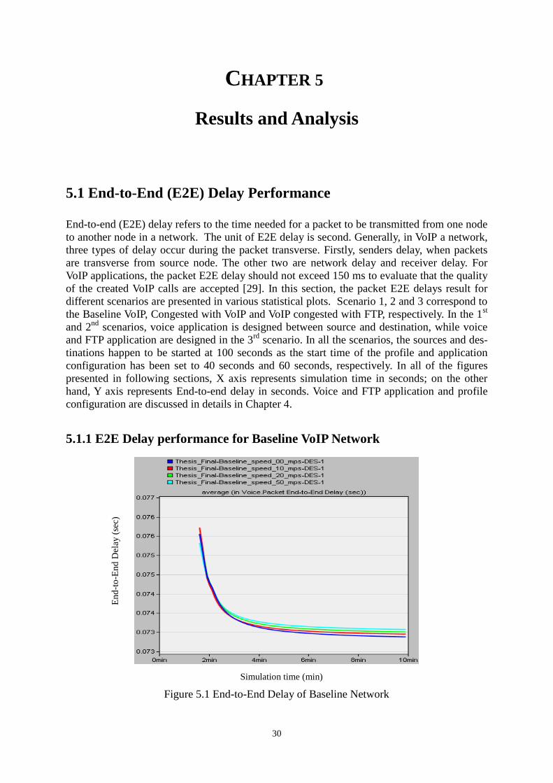
5.1 End-to-End (E2E) Delay Performance ........................................................................... 30
5.1.1 E2E Delay performance for Baseline VoIP Network ........................................................................... 30
5.1.2 E2E Delay performance for Congested VoIP network ......................................................................... 31
5.1.3 E2E Delay performance for VoIP Congested with FTP network ......................................................... 32
5.1.4 Summary of E2E Delay Performance .................................................................................................. 33
5.2 Packet Loss Performance ................................................................................................ 34
5.2.1 Packet Loss Performance for Baseline VoIP Network ......................................................................... 34
5.2.2 Packet Loss Performance for Congested VoIP Network ...................................................................... 36
5.2.3 Packet Loss Performance for VoIP Congested with FTP Network ....................................................... 37
5.2.4 Summary of Packet Loss Performance ................................................................................................ 38
CHAPTER 6 ............................................................................................................................. 39
Conclusion ................................................................................................................................ 39
BIBLIOGRAPHY .................................................................................................................... 40
vi
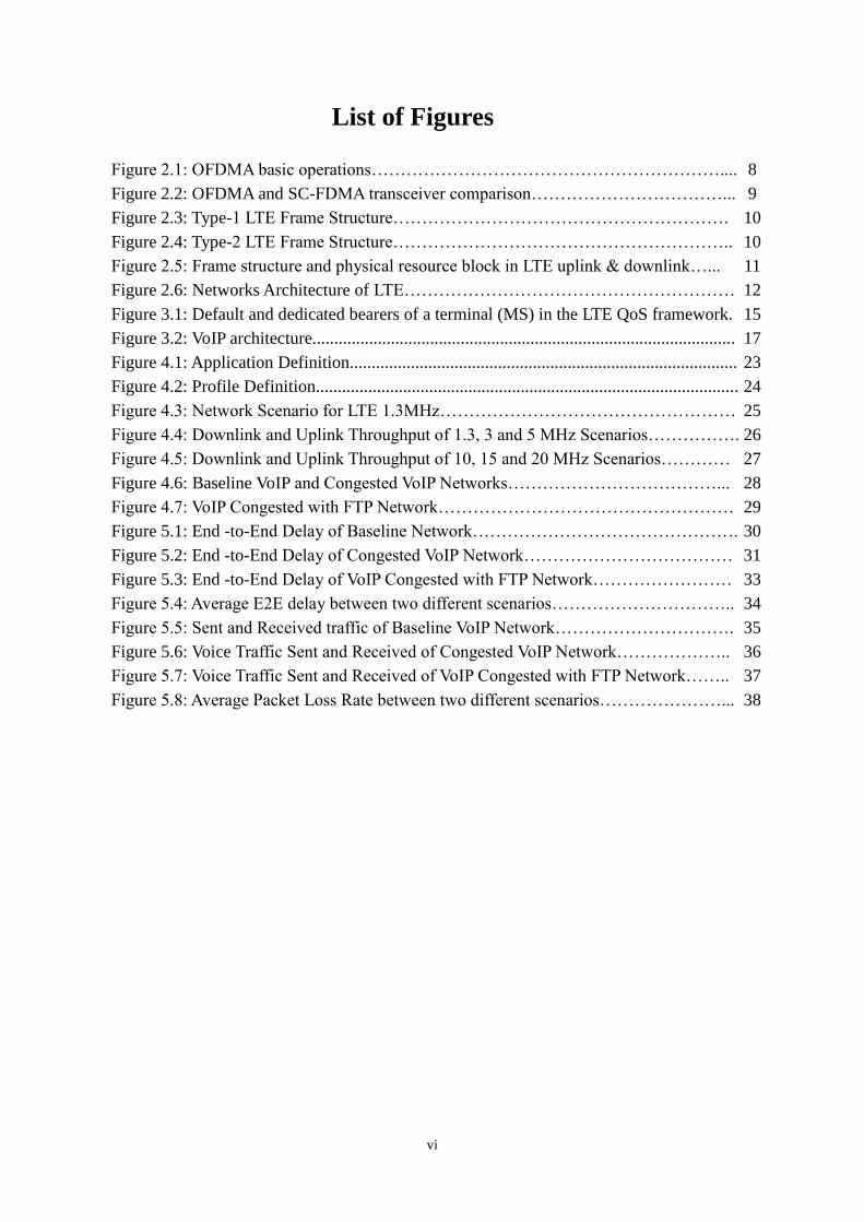
List of Figures
Figure 2.1: OFDMA basic operations…………………………………………………….... 8
Figure 2.2: OFDMA and SC-FDMA transceiver comparison……………………………... 9
Figure 2.3: Type-1 LTE Frame Structure…………………………………………………. 10
Figure 2.4: Type-2 LTE Frame Structure………………………………………………….. 10
Figure 2.5: Frame structure and physical resource block in LTE uplink & downlink…... 11
Figure 2.6: Networks Architecture of LTE………………………………………………… 12
Figure 3.1: Default and dedicated bearers of a terminal (MS) in the LTE QoS framework. 15
Figure 3.2: VoIP architecture................................................................................................. 17
Figure 4.1: Application Definition......................................................................................... 23
Figure 4.2: Profile Definition................................................................................................. 24
Figure 4.3: Network Scenario for LTE 1.3MHz…………………………………………… 25
Figure 4.4: Downlink and Uplink Throughput of 1.3, 3 and 5 MHz Scenarios……………. 26
Figure 4.5: Downlink and Uplink Throughput of 10, 15 and 20 MHz Scenarios………… 27
Figure 4.6: Baseline VoIP and Congested VoIP Networks………………………………... 28
Figure 4.7: VoIP Congested with FTP Network…………………………………………… 29
Figure 5.1: End -to-End Delay of Baseline Network………………………………………. 30
Figure 5.2: End -to-End Delay of Congested VoIP Network……………………………… 31
Figure 5.3: End -to-End Delay of VoIP Congested with FTP Network…………………… 33
Figure 5.4: Average E2E delay between two different scenarios………………………….. 34
Figure 5.5: Sent and Received traffic of Baseline VoIP Network…………………………. 35
Figure 5.6: Voice Traffic Sent and Received of Congested VoIP Network……………….. 36
Figure 5.7: Voice Traffic Sent and Received of VoIP Congested with FTP Network…….. 37
Figure 5.8: Average Packet Loss Rate between two different scenarios…………………... 38
vii
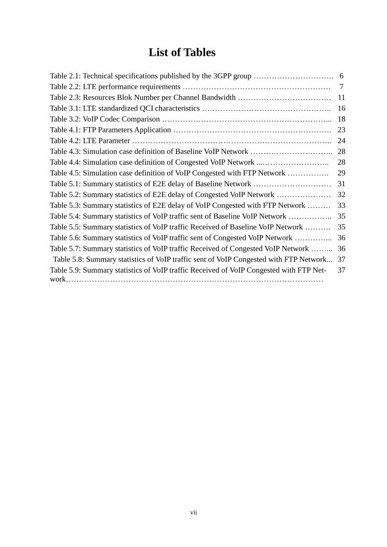
List of Tables
Table 2.1: Technical specifications published by the 3GPP group …………………………. 6
Table 2.2: LTE performance requirements ………………………………………………… 7
Table 2.3: Resources Blok Number per Channel Bandwidth ……………………………… 11
Table 3.1: LTE standardized QCI characteristics ………………………………………….. 16
Table 3.2: VoIP Codec Comparison ………………………………………………………... 18
Table 4.1: FTP Parameters Application ……………………………………………………. 23
Table 4.2: LTE Parameter ………………………………………………………………….. 24
Table 4.3: Simulation case definition of Baseline VoIP Network ………………………….. 28
Table 4.4: Simulation case definition of Congested VoIP Network ...…………………….. 28
Table 4.5: Simulation case definition of VoIP Congested with FTP Network ……………. 29
Table 5.1: Summary statistics of E2E delay of Baseline Network ………………………… 31
Table 5.2: Summary statistics of E2E delay of Congested VoIP Network ………………… 32
Table 5.3: Summary statistics of E2E delay of VoIP Congested with FTP Network ……… 33
Table 5.4: Summary statistics of VoIP traffic sent of Baseline VoIP Network …………….. 35
Table 5.5: Summary statistics of VoIP traffic Received of Baseline VoIP Network ………. 35
Table 5.6: Summary statistics of VoIP traffic sent of Congested VoIP Network …………... 36
Table 5.7: Summary statistics of VoIP traffic Received of Congested VoIP Network ……... 36
Table 5.8: Summary statistics of VoIP traffic sent of VoIP Congested with FTP Network... 37
Table 5.9: Summary statistics of VoIP traffic Received of VoIP Congested with FTP Net-
work………………………………………………………………………………………
37
viii
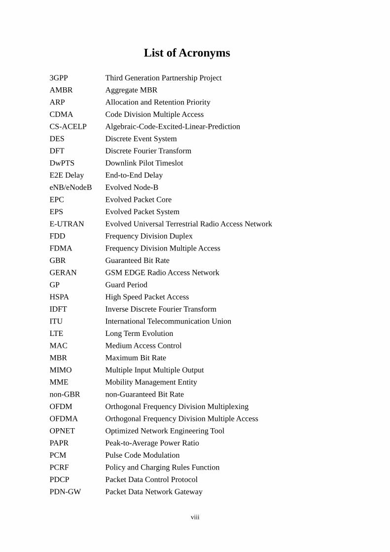
List of Acronyms
3GPP Third Generation Partnership Project
AMBR Aggregate MBR
ARP Allocation and Retention Priority
CDMA Code Division Multiple Access
CS-ACELP Algebraic-Code-Excited-Linear-Prediction
DES Discrete Event System
DFT Discrete Fourier Transform
DwPTS Downlink Pilot Timeslot
E2E Delay End-to-End Delay
eNB/eNodeB Evolved Node-B
EPC Evolved Packet Core
EPS Evolved Packet System
E-UTRAN Evolved Universal Terrestrial Radio Access Network
FDD Frequency Division Duplex
FDMA Frequency Division Multiple Access
GBR Guaranteed Bit Rate
GERAN GSM EDGE Radio Access Network
GP Guard Period
HSPA High Speed Packet Access
IDFT Inverse Discrete Fourier Transform
ITU International Telecommunication Union
LTE Long Term Evolution
MAC Medium Access Control
MBR Maximum Bit Rate
MIMO Multiple Input Multiple Output
MME Mobility Management Entity
non-GBR non-Guaranteed Bit Rate
OFDM Orthogonal Frequency Division Multiplexing
OFDMA Orthogonal Frequency Division Multiple Access
OPNET Optimized Network Engineering Tool
PAPR Peak-to-Average Power Ratio
PCM Pulse Code Modulation
PCRF Policy and Charging Rules Function
PDCP Packet Data Control Protocol
PDN-GW Packet Data Network Gateway
ix
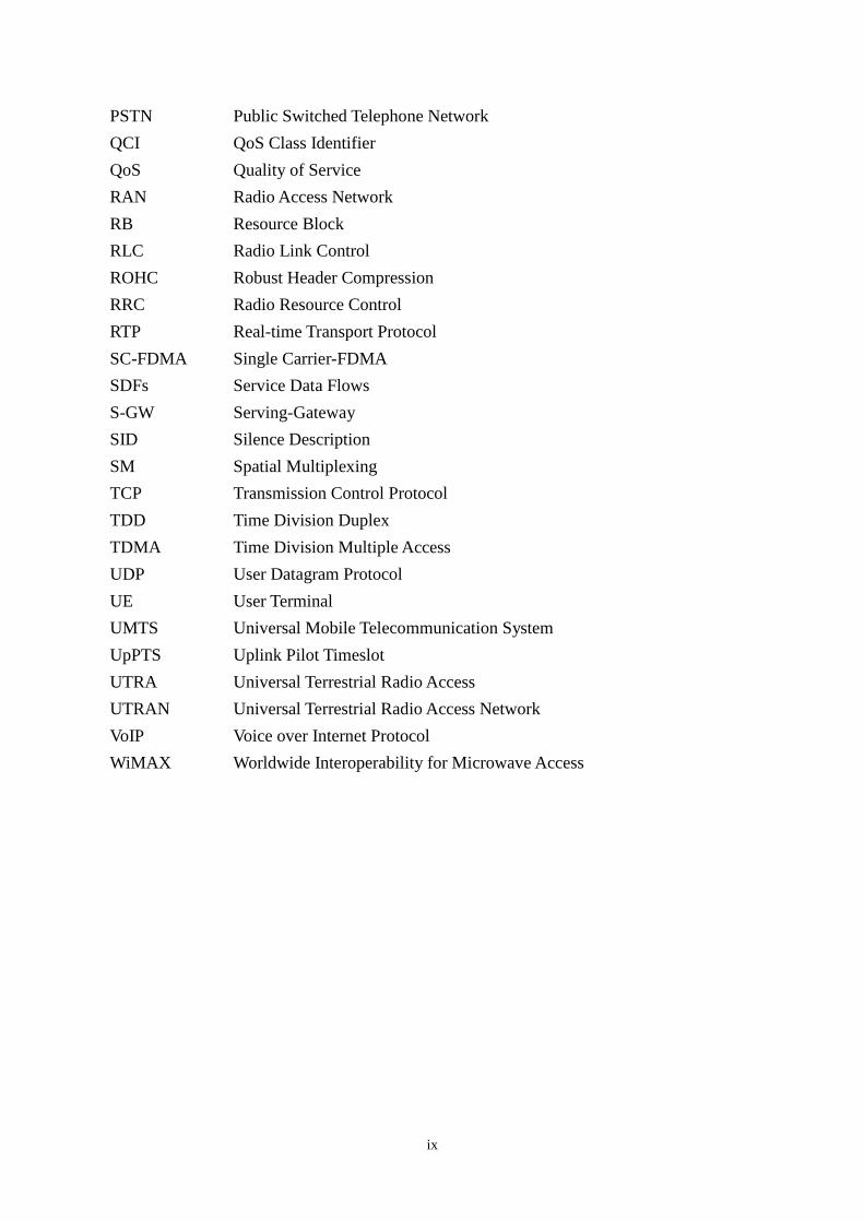
PSTN Public Switched Telephone Network
QCI QoS Class Identifier
QoS Quality of Service
RAN Radio Access Network
RB Resource Block
RLC Radio Link Control
ROHC Robust Header Compression
RRC Radio Resource Control
RTP Real-time Transport Protocol
SC-FDMA Single Carrier-FDMA
SDFs Service Data Flows
S-GW Serving-Gateway
SID Silence Description
SM Spatial Multiplexing
TCP Transmission Control Protocol
TDD Time Division Duplex
TDMA Time Division Multiple Access
UDP User Datagram Protocol
UE User Terminal
UMTS Universal Mobile Telecommunication System
UpPTS Uplink Pilot Timeslot
UTRA Universal Terrestrial Radio Access
UTRAN Universal Terrestrial Radio Access Network
VoIP Voice over Internet Protocol
WiMAX Worldwide Interoperability for Microwave Access
1
CHAPTER 1
INTRODUCTION
1.1 Introduction
The trend of the modern society is as the days go by, time is getting more expensive and
commodity is getting cheaper. To create a world compatible for this, it is necessary to create a
network backbone for the whole world so the information along with communication, is in-
stantaneous. As internet is the main information database, cellular technology is required to
merge with the core internet structure, with all its bandwidth and fast trafficking facility in the
cheapest way possible. This has been the fundamental premise behind the development of
LTE. The study of the performance of Voice-over-IP (VoIP) over LTE thus has a great signi-
ficance. Nowadays, communication and network technology have expanded significantly. As
LTE is relatively a new technology, there are not enough technical documents to get a deeper
knowledge of LTE for real time application. Introduction of Long Term Evolution (LTE), the
4th
Generation (4G) network technology release 8 specifications are being finalized in 3GPP
have developed and planning to globalize extensively compared to 3rd
Generation (3G) and 2nd
Generation (2G) networks [1]. LTE determines goals peak data rate for Downlink (DL) 100
Mbps and Uplink (UL) data rate for 50Mbps, increased cell edge user throughput, improved
spectral efficiency and scalable bandwidth 1.4 MHz to 20 MHz [2]. VoIP capacity of LTE has
to show better performance as Circuit Switch voice of UMTS. LTE should be at least as good
as the High Speed Packet Access (HSPA) evolution track also in voice traffic. The core net-
work of LTE is purely packet switched and optimized for packet data transfer, thus speech is
also transmitted purely with VoIP protocols. Simultaneously, demand for the higher quality of
wireless communications has increased as well. Use of demand driven applications and ser-
vices have been growing rapidly to satisfy users. Meeting such demand poses a challenge for
the researchers to solve till now. Among such demands, enhance quality of voice and data
transfer rates are one of the main aspects to improve. Thus, to improve the performance of
such important aspects, performance evaluation of VoIP can point out the issues which can be
resolved to improve the overall performance of LTE networks. In this paper, VoIP application
is used to represent the class of inelastic, real-time interactive applications that is sensitive to
end-to-end delay but may tolerate packet loss. This need is much more expedient in real-time
application such as voice has enormous importance in providing efficient services in order to
fulfill the users expectation, and hence to the researchers to improve the technology to meet
the ever growing demand of efficient use of the system. It is expected that LTE should support
a significantly higher number of VoIP users. The important factor is now the quality of service
(QoS) of VoIP. To measure QoS of VoIP in a LTE network, the first basic evaluation can be
done in terms of maximum end to end delay and acceptable packet loss [3].
2
1.2 Aims and Objectives
The main objective of this thesis work is to evaluate the End-to-End Delay performance in
terms of application such as VoIP and FTP server in the LTE networks. OPNET Modeler 16.0
is used for doing the simulation. In order to achieve the goal the followings have been done:
Applying both qualitative and quantitative research methods that will guide the study
in suitable direction.
Doing literature study about LTE and real time application.
Setting up a platform for performing the simulation in OPNET and becoming familiar
with different tools of OPNET software.
Creating different scenarios and analyzing the way of running the simulation in
OPNET platform.
Studying the individuality of voice and FTP server over LTE networks. To
understanding how way we can do the configuration in the LTE environment and set
their networks attributes into the OPNET Modeler 16.0.
To select the quantitative metrics such as end-to-delay and throughput.
Discussing the different constraints that affect the E2E delay performance of VoIP in
LTE network and critically examine various approaches that are suggested in the
literature for improving the E2E delay performance.
Developing, testing and evaluating strategic scenario in OPNET.
Verifying the way of how to minimize the effects of network congestion using FTP
server in LTE platform.
Construing the simulation result and predicting which technology is the best our
network modeling objectives.
Simulating different network scenarios with different network load and analyzing the
simulation results.
Drawing conclusions by presenting and interpreting the outcomes.
3
1.3 Scope of the Thesis
This thesis covers the technical issues and factors that need to be considered for the imple-
mentation of VoIP in the computer networks. It discusses the challenging issues that need to
be faced by computer networks to transmit the VoIP applications. It gives the description idea
about the VoIP over LTE and their functionality and design parameters of the LTE networks.
In this thesis, qualitative and quantitative analysis of E2E delay performance over LTE net-
works have been done in a simple and understandable fashion so that it might be helpful for
those who have some intention to do further research.
1.4 Research Questions
After determining the problems it is necessary to indentify the research questions that lead the
research process to be in the scope. The formulated questions are described as follows.
Q1. How much the maximum throughput is support in the different bandwidth
(e.g. 1.4 MHz, 3 MHz, 5 MHz, 10 MHz, 15 MHz and 20 MHz)?
Q2. What is the impact on the VoIP quality in terms of E2E delay when the net-
work is congested with VoIP only or VoIP with FTP?
Q3. To what extent do the performances of packet loss for interactive voice vary
from Congested VoIP to VoIP congested with FTP network?
1.5 Research Methodology
The research methodology presented in this thesis is based on both Qualitative and Quantita-
tive approach suggested by John W. Creswell [4]. In this Qualitative approach, three steps are
considered:
1. Identify the key factors influencing VoIP performance in LTE networks by
considering the existing research and knowledge based on famous scholars, relevant
articles and journals i.e. IEEE Xplore, Inspec, Google and Google Scholar.
2. Determine the suitable VoIP model to support real-time application.
3. Justify the VoIP performance thresholds on the basis of strong facts and figures.
In this Quantitative approach, following four steps are considered:
1. Develop a network model based on qualitative approach and experimental research.
Experimental research typically starts with the formulation of hypothesis. Design
and analysis of the network model need to validate or invalidate the hypothesis [5].
With respect to the present study, the LTE network models are designed in the
OPNET simulator based on different network entities. The OPNET simulator is
well-known for network design and attractive features. In the OPNET simulator,
different network entities are needed to accurately configure support selective
4
application services of the network.
2. Evaluate the performance of different simulation scenarios in terms of VoIP when
LTE is deployed.
3. Collect quantitative data regarding throughput, end-to-end delay and packet loss for
analysis of the network performance.
4. The simulation results are collected using OPNET in terms of different statistical
graphs and tables as furnished in chapter 5.
1.6 Motivation
The 3GPP LTE is a new standard with comprehensive performance targets, therefore it is ne-
cessary to evaluate the performance and stability of this new system at an early stage to pro-
mote its smooth and cost-efficient introduction and deployment. The motivation behind the
design models presented in this report is to discuss issues related to traffic behavior for VoIP
alone as well as along with other traffic in the LTE network. E2E delay for VoIP is a matter of
fact for performing real-time application efficiently over the Internet. Today, emergence of the
real-time application demands more resources. The main motivation of our thesis work is to
ensure fast and reliable voice communication for huge number of users in wireless network.
In our framework, the evaluate and analyze the E2E delay performance of voice based on the
performance metrics such as throughput, E2E delay and packet loss over LTE network.
1.7 Contribution
This thesis is focused on the comprehensively analyzed for VoIP performance metrics such as
end-to-end delay and throughput for real-time applications over the LTE networks. In our dis-
sertation, a number of important system parameters such as network load and fixed node
speed are taken into consideration. OPNET Modeler 16.0 is used to design the model for si-
mulation (Baseline VoIP network scenario, congested VoIP network scenario and VoIP con-
gested with FTP network scenario) to realize different realistic LTE scenarios as well as to
determine the extent of their impact on network and VoIP performance.
1.8 Thesis Outline
The outline of this thesis paper is organized as following structure:
Chapter 1 provides the introduction, aims and objectives, research methodology, motivation
and contribution of this research are discussed, and also discusses about the research question
and scope of the thesis.

5
Chapter 2 covers the general overview of the 3GPP LTE technology standard, multiple access
technique, frame structure and network architecture. Furthermore, Multiple-antenna technique
is described in briefly at the end of this chapter.
Chapter 3 presents the Quality of Service (QoS) of LTE where guaranteed bit rate (GBR),
non-guaranteed bit rate (non-GBR) and characteristics of QCI are described in briefly. More-
over, Voice over IP (VoIP) principle, codec and characteristic are focused in this chapter.
Chapter 4 dedicates a discussion the experiment setup, network scenarios and the parameters
required to configure them.
Chapter 5 explains the simulation result followed by chapter 4.
Chapter 6 concludes the entire thesis work.
6
CHAPTER 2
Theoretical Knowledge
2.1 Background
Lately, the demand for high data rates to support the Internet services and the wide range of
multimedia has received a substantial attraction around the globe from mobile researchers and
industries. An international collaboration project, known as, Third Generation Partnership
Project (3GPP), takes a host of members into account, specially, from both mobile industries
and research institutes in a bid to delivering a globally applicable third generation (3G) mo-
bile phone system specification [6]. The organization started their journey on December 1998
and was initially based on 2nd generation (2G) mobile system, i.e. Global System for Mobile
Communications, which is nowadays known as Universal Mobile Telecommunications Sys-
tem (UMTS). The key function of 3GPP involves improving the UMTS standard to cope with
the ever-evolving future requirements such as services boosting, exploiting the spectrum facil-
ities, lowering costs, efficiency improvement and better integration with other standards. The
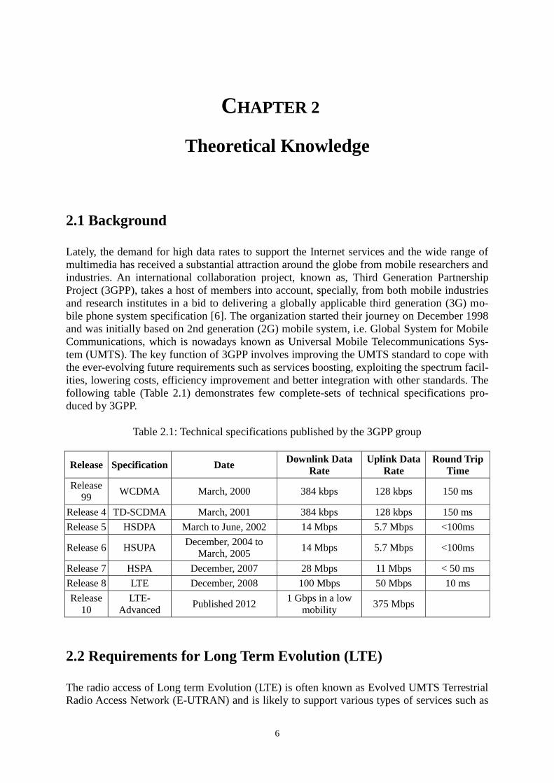
following table (Table 2.1) demonstrates few complete-sets of technical specifications pro-
duced by 3GPP.
Table 2.1: Technical specifications published by the 3GPP group
Release Specification Date Downlink Data
Rate
Uplink Data
Rate
Round Trip
Time
Release
99 WCDMA March, 2000 384 kbps 128 kbps 150 ms
Release 4 TD-SCDMA March, 2001 384 kbps 128 kbps 150 ms
Release 5 HSDPA March to June, 2002 14 Mbps 5.7 Mbps <100ms
Release 6 HSUPA December, 2004 to
March, 2005 14 Mbps 5.7 Mbps <100ms
Release 7 HSPA December, 2007 28 Mbps 11 Mbps < 50 ms
Release 8 LTE December, 2008 100 Mbps 50 Mbps 10 ms
Release
10
LTE-
Advanced Published 2012
1 Gbps in a low
mobility 375 Mbps
2.2 Requirements for Long Term Evolution (LTE)
The radio access of Long term Evolution (LTE) is often known as Evolved UMTS Terrestrial
Radio Access Network (E-UTRAN) and is likely to support various types of services such as
7
video streaming, FTP, web browsing, VoIP, real time video, online gaming, push-to-talk,
push-to-view and so on. Consequently, it has been immensely important for the LTE to be
designed as a high data rate and low latency system as pointed out by the key performance
criteria in Table 2.2. For both transmission and reception, the bandwidth capability of a UE is
required to be 20MHz [15]. Though, the service provider can deploy the cells with any of the
bandwidths specified in given table. This eventually allows the service providers to alter their
offering dependent on the amount of available spectrum or the ability to initiate with fixed
spectrum for lower upfront cost and grow the spectrum for additional capacity.
In LTE, the interworking with existing UTRAN/GERAN systems and non-3GPP systems
should be ensured. Multimode terminals need to support handover from and to UTRAN and
GERAN and also the inter-RAT measurements. In real time services, the interruption time of
handover between E-UTRAN and UTRAN/GERAN should be less than 300 ms, and in-case
of no real time services, the time should be less than 500 ms. Ability of cost effective migra-
tion from release 6 UTRA radio interface and architecture should be available. Cost and pow-
er consumption, reasonable system and terminal complexity are to be provided. It is mandato-
ry for all the interfaces to be open for multi-vendor equipment interoperability.
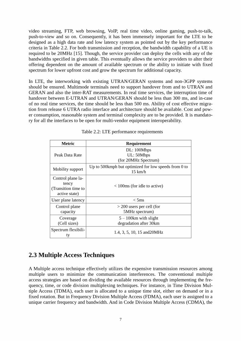
Table 2.2: LTE performance requirements
Metric Requirement
Peak Data Rate
DL: 100Mbps
UL: 50Mbps
(for 20MHz Spectrum)
Mobility support Up to 500kmph but optimized for low speeds from 0 to
15 km/h
Control plane la-
tency
(Transition time to
active state)
< 100ms (for idle to active)
User plane latency < 5ms
Control plane
capacity
> 200 users per cell (for
5MHz spectrum)
Coverage
(Cell sizes)
5 – 100km with slight
degradation after 30km
Spectrum flexibili-
ty 1.4, 3, 5, 10, 15 and20MHz
2.3 Multiple Access Techniques
A Multiple access technique effectively utilizes the expensive transmission resources among
multiple users to minimize the communication interferences. The conventional multiple
access strategies are based on dividing the available resources through implementing the fre-
quency, time, or code division multiplexing techniques. For instance, in Time Division Mul-
tiple Access (TDMA), each user is allocated to a unique time slot, either on demand or in a
fixed rotation. But in Frequency Division Multiple Access (FDMA), each user is assigned to a
unique carrier frequency and bandwidth. And in Code Division Multiple Access (CDMA), the
8
users will belong to the unique code for transmission, allowing each user to share the entire
bandwidth and the time slots [7].
Meanwhile, two candidate standards of IMT-Advanced (i.e., mobile WiMAX and LTE) make
use of OFDMA as the multiple access technique in the downlink direction. However, with
different resource grouping, frame structures, and allocation. On the other hand, the two sys-
tems implement different techniques in the uplink direction, for instance, the mobile WiMAX
uses OFDMA and 3GPP standardization group uses SC-FDMA in LTE [8]. The SCFDMA
technique explores a modified version of OFDM scheme (also known as DFT-spread ortho-
gonal frequency division multiple access) to mitigate the high PAPR problem [9]. The SC-
FDMA becomes more attractive for uplink transmission due to having its low PAPR property
especially when this is a case of low-cost device with limited energy resources.
2.3.1 OFDMA for DL
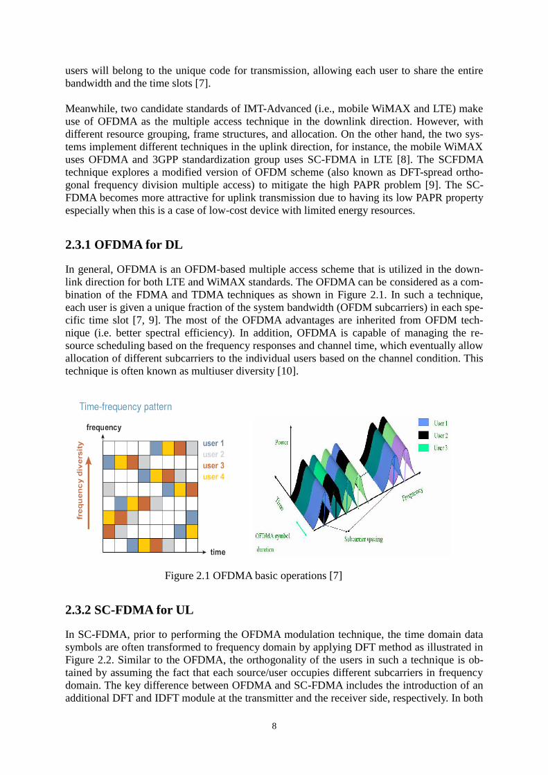
In general, OFDMA is an OFDM-based multiple access scheme that is utilized in the down-
link direction for both LTE and WiMAX standards. The OFDMA can be considered as a com-
bination of the FDMA and TDMA techniques as shown in Figure 2.1. In such a technique,
each user is given a unique fraction of the system bandwidth (OFDM subcarriers) in each spe-
cific time slot [7, 9]. The most of the OFDMA advantages are inherited from OFDM tech-
nique (i.e. better spectral efficiency). In addition, OFDMA is capable of managing the re-
source scheduling based on the frequency responses and channel time, which eventually allow
allocation of different subcarriers to the individual users based on the channel condition. This
technique is often known as multiuser diversity [10].
Figure 2.1 OFDMA basic operations [7]
2.3.2 SC-FDMA for UL
In SC-FDMA, prior to performing the OFDMA modulation technique, the time domain data
symbols are often transformed to frequency domain by applying DFT method as illustrated in
Figure 2.2. Similar to the OFDMA, the orthogonality of the users in such a technique is ob-
tained by assuming the fact that each source/user occupies different subcarriers in frequency
domain. The key difference between OFDMA and SC-FDMA includes the introduction of an
additional DFT and IDFT module at the transmitter and the receiver side, respectively. In both
9
cases, equalization technique is implemented in frequency domain though OFDMA performs
modulation and demodulation operations in the frequency domain while SC-FDMA performs
these operations in the time domain.
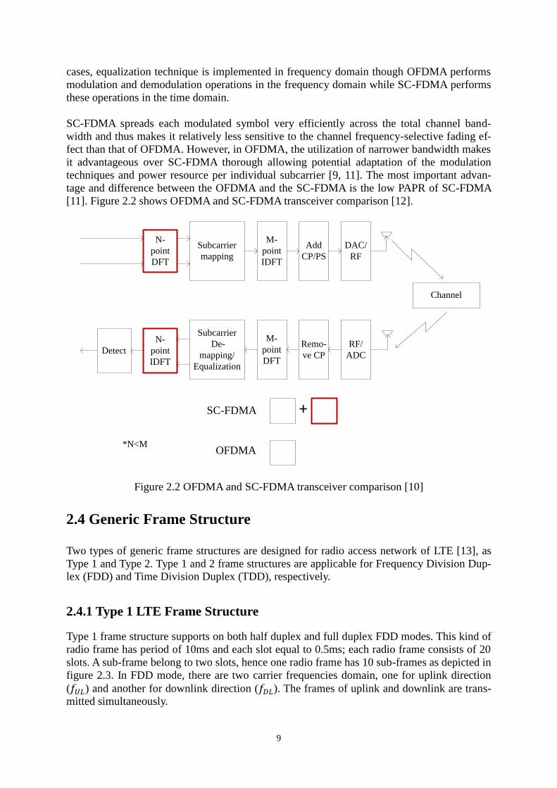
SC-FDMA spreads each modulated symbol very efficiently across the total channel band-
width and thus makes it relatively less sensitive to the channel frequency-selective fading ef-
fect than that of OFDMA. However, in OFDMA, the utilization of narrower bandwidth makes
it advantageous over SC-FDMA thorough allowing potential adaptation of the modulation
techniques and power resource per individual subcarrier [9, 11]. The most important advan-
tage and difference between the OFDMA and the SC-FDMA is the low PAPR of SC-FDMA
[11]. Figure 2.2 shows OFDMA and SC-FDMA transceiver comparison [12].
N-
point
DFT
Subcarrier
mapping
M-
point
IDFT
Add
CP/PS
DAC/
RF
Channel
N-
point
IDFT
Subcarrier
De-
mapping/
Equalization
M-
point
DFT
Remo-
ve CP
RF/
ADCDetect
SC-FDMA +
OFDMA*N<M
Figure 2.2 OFDMA and SC-FDMA transceiver comparison [10]
2.4 Generic Frame Structure
Two types of generic frame structures are designed for radio access network of LTE [13], as
Type 1 and Type 2. Type 1 and 2 frame structures are applicable for Frequency Division Dup-
lex (FDD) and Time Division Duplex (TDD), respectively.
2.4.1 Type 1 LTE Frame Structure
Type 1 frame structure supports on both half duplex and full duplex FDD modes. This kind of
radio frame has period of 10ms and each slot equal to 0.5ms; each radio frame consists of 20
slots. A sub-frame belong to two slots, hence one radio frame has 10 sub-frames as depicted in
figure 2.3. In FDD mode, there are two carrier frequencies domain, one for uplink direction
( ) and another for downlink direction ( ). The frames of uplink and downlink are trans-
mitted simultaneously.
10
#0 #1 #2 #3 #4 #18 #19
LTE frame lengthLTE frame length
Sub-frameSub-frame
slotslot
OneOne
Figure 2.3 Type-1 LTE Frame Structure
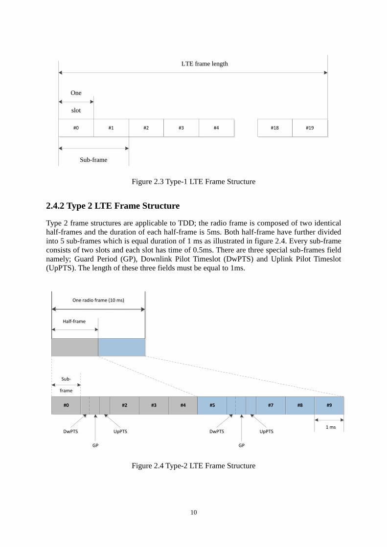
2.4.2 Type 2 LTE Frame Structure
Type 2 frame structures are applicable to TDD; the radio frame is composed of two identical
half-frames and the duration of each half-frame is 5ms. Both half-frame have further divided
into 5 sub-frames which is equal duration of 1 ms as illustrated in figure 2.4. Every sub-frame
consists of two slots and each slot has time of 0.5ms. There are three special sub-frames field
namely; Guard Period (GP), Downlink Pilot Timeslot (DwPTS) and Uplink Pilot Timeslot
(UpPTS). The length of these three fields must be equal to 1ms.
#2 #3 #9#8#0 #7#4 #5
Sub-Sub-
frameframe
Half-frameHalf-frame
One radio frame (10 ms)One radio frame (10 ms)
DwPTSDwPTS
GPGP
UpPTSUpPTS DwPTSDwPTS
GPGP
UpPTSUpPTS1 ms1 ms
Figure 2.4 Type-2 LTE Frame Structure
11
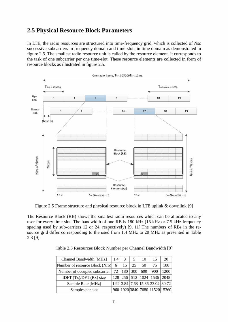
2.5 Physical Resource Block Parameters
In LTE, the radio resources are structured into time-frequency grid, which is collected of Nsc
successive subcarriers in frequency domain and time-slots in time domain as demonstrated in
figure 2.5. The smallest radio resource unit is called by the resource element. It corresponds to
the task of one subcarrier per one time-slot. These resource elements are collected in form of
resource blocks as illustrated in figure 2.5.
Figure 2.5 Frame structure and physical resource block in LTE uplink & downlink [9]
The Resource Block (RB) shows the smallest radio resources which can be allocated to any
user for every time slot. The bandwidth of one RB is 180 kHz (15 kHz or 7.5 kHz frequency
spacing used by sub-carriers 12 or 24, respectively) [9, 11].The numbers of RBs in the re-
source grid differ corresponding to the used from 1.4 MHz to 20 MHz as presented in Table
2.3 [9].
Table 2.3 Resources Block Number per Channel Bandwidth [9]
Channel Bandwidth [MHz] 1.4 3 5 10 15 20
Number of resource Block (Nrb) 6 15 25 50 75 100
Number of occupied subcarrier 72 180 300 600 900 1200
IDFT (Tx)/DFT (Rx) size 128 256 512 1024 1536 2048
Sample Rate [MHz] 1.92 3.84 7.68 15.36 23.04 30.72
Samples per slot 960 1920 3840 7680 11520 15360
0 1 2 3
0 1 16 17 18 19
18 19
Tslot = 0.5msTslot = 0.5ms Tsubframe = 1msTsubframe = 1ms
One radio frame, Tf = 307200Ts = 10msOne radio frame, Tf = 307200Ts = 10ms
Up-link
Up-link
Down-link
Down-link
(NTA*Ts)(NTA*Ts)
I = 0I = 0 I = Nsymb(UL) - 1I = Nsymb(UL) - 1 I = 0I = 0 I = Nsymb(DL) - 1I = Nsymb(DL) - 1N
RB(D
L)*N
SC(R
B)
NR
B(D
L)*N
SC(R
B)
Resource Element (k,l)
Resource Element (k,l)
Resource Block (RB)
Resource Block (RB)
NSC
(RB
)N
SC(R
B)
NRB
(UL)*N
SC(R
B)N
RB
(UL)*N
SC(R
B)
12
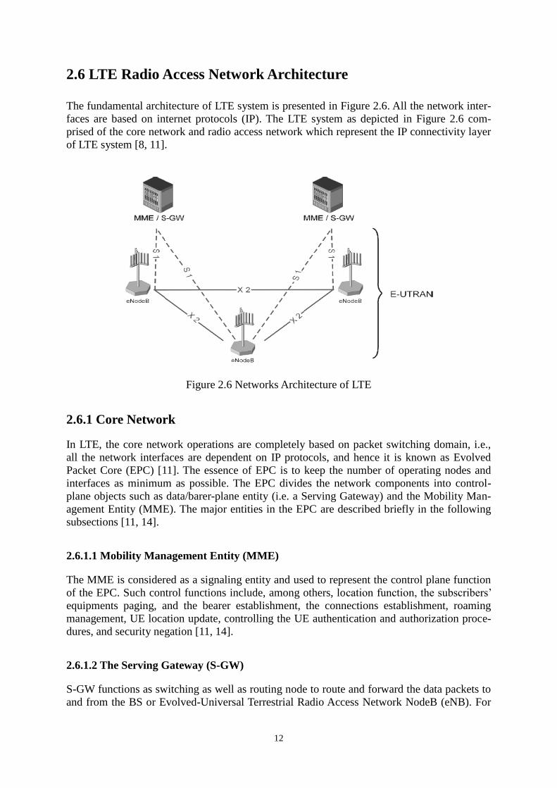
2.6 LTE Radio Access Network Architecture
The fundamental architecture of LTE system is presented in Figure 2.6. All the network inter-
faces are based on internet protocols (IP). The LTE system as depicted in Figure 2.6 com-
prised of the core network and radio access network which represent the IP connectivity layer
of LTE system [8, 11].
Figure 2.6 Networks Architecture of LTE
2.6.1 Core Network
In LTE, the core network operations are completely based on packet switching domain, i.e.,
all the network interfaces are dependent on IP protocols, and hence it is known as Evolved
Packet Core (EPC) [11]. The essence of EPC is to keep the number of operating nodes and
interfaces as minimum as possible. The EPC divides the network components into control-
plane objects such as data/barer-plane entity (i.e. a Serving Gateway) and the Mobility Man-
agement Entity (MME). The major entities in the EPC are described briefly in the following
subsections [11, 14].
2.6.1.1 Mobility Management Entity (MME)
The MME is considered as a signaling entity and used to represent the control plane function
of the EPC. Such control functions include, among others, location function, the subscribers‟
equipments paging, and the bearer establishment, the connections establishment, roaming
management, UE location update, controlling the UE authentication and authorization proce-
dures, and security negation [11, 14].
2.6.1.2 The Serving Gateway (S-GW)
S-GW functions as switching as well as routing node to route and forward the data packets to
and from the BS or Evolved-Universal Terrestrial Radio Access Network NodeB (eNB). For
13
instance, the S-GW produces a tunnel during the connection mode (i.e. UE is connected) to
transmit data traffic between the P-GW (Packet Data Network Gateway) and UE (via specific
BS) [14, 15].
2.6.1. 3 Packet Data Network Gateway (PDN-GW)
Between the EPC and the external packet data network, a PDN-GW is often used as an inter-
face point or an edge router. It is also possible that a UE has synchronized connectivity with
more than one PDN GW [14, 15].
The responsibilities of the PDN-GW include establishment, maintenance, and deletion of GTP
tunnels to S-GW or SGSN in the case of inter-RAT mobility scenarios. The PDN-GW routes
the user plane packets by allocating the user‟s dynamic IP addresses. Apart from that, it pro-
vides functions for lawful interception, policy/QoS control, and charging.
2.6.1.4 The Policy and Charging Rules Function (PCRF)
The PCRF mainly performs the Policy and Charging Control (PCC) functions. It is used to
control the QoS configuration and tariff making of each individual user. The specified tariff
and QoS policies for each UE are given to the P-GW and the S-GW [14, 15].
2.6.2Radio Access Network
The radio access network of LTE is termed as Evolved Universal Terrestrial Radio Access
Network (E-UTRAN). The evolved RAN for LTE comprises of a single node, i.e., BS or eNB,
which often involves with the UEs. The BS or e-NB involves controlling all the radio inter-
face related functions. Between UE and EPC, the eNB acts as a gateway, and manipulates all
the communications towards the UE and forwards radio connection to core network (EPC) by
using the related radio protocols and the corresponding IP based connectivity, respectively. To
gain its function as interface between the core and the radio parts of the network, the eNB
hosts two bunches of protocols, namely, the control plane protocols and the Evolved Univer-
sal Terrestrial Radio Access (E-UTRA) user plane protocols. The first bunch, i.e., the user
plane contains Radio Link Control (RLC), the Physical (PHY), Medium Access Control
(MAC), and Packet Data Control Protocol (PDCP) layers protocols where it is necessary to
relay the data traffic to and from the UE. The other protocol i.e. the control plane is associated
with the Radio Resource Control (RRC) and it manipulates functions such as the radio re-
source management, admission control and resource scheduling [15, 16].
2.7 Multi-Antenna Technique
In LTE system, multi-antenna transmission techniques can be realized to establish better sys-
tem performance ( i.e. increasing the capacity and providing higher data rate per user) [17].
Three schemes regarding this technique are described as follows [8]:
Spatial Diversity: the reason of implementing this technique is to achieve transmission
or reception diversity by minimizing the instantaneous fading effects caused due to the
multipath propagation. The spatial diversity technique creates a host of independent
14
paths. To receive higher gain at the receiver side, it transmits and receives with low
fading correlation.
Beam-forming: The purpose of this technique is to allow the base station to conduct a
direct transmission, or to allow the radiation beam to move toward the specific user in
for boosting the received signal power.
Spatial multiplexing (SM) or multiple-input and multiple-output (MIMO): Through
employing this technique, a high data transmission rate is achieved by transmitting
various data streams over independent parallel channels. This is done by utilizing mul-
tiple transmitting and receiving antennas, without increasing the channel bandwidth or
the total transmitted power.
LTE realizes different multi-antenna techniques such as single user (SU)-MIMO, multiuser
(MU)-MIMO, transmit diversity and dedicated beam-forming [8, 18].
15
CHAPTER 3
LTE QoS and Voice over IP
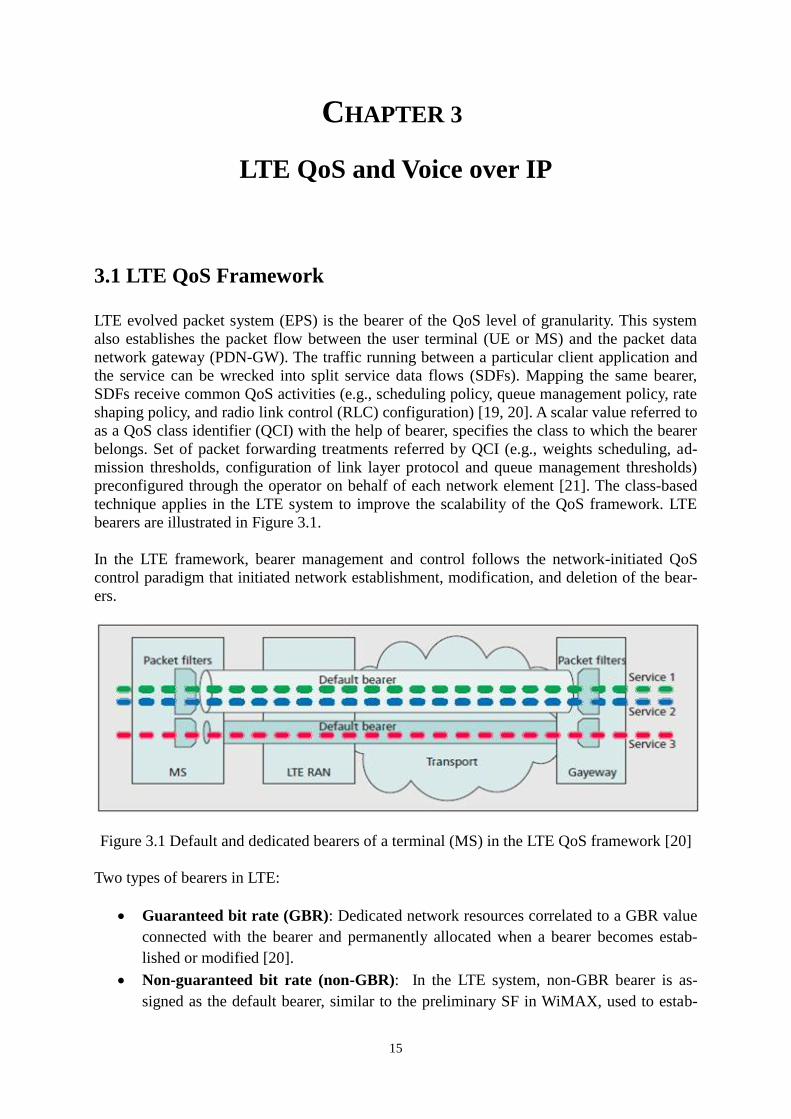
3.1 LTE QoS Framework
LTE evolved packet system (EPS) is the bearer of the QoS level of granularity. This system
also establishes the packet flow between the user terminal (UE or MS) and the packet data
network gateway (PDN-GW). The traffic running between a particular client application and
the service can be wrecked into split service data flows (SDFs). Mapping the same bearer,
SDFs receive common QoS activities (e.g., scheduling policy, queue management policy, rate
shaping policy, and radio link control (RLC) configuration) [19, 20]. A scalar value referred to
as a QoS class identifier (QCI) with the help of bearer, specifies the class to which the bearer
belongs. Set of packet forwarding treatments referred by QCI (e.g., weights scheduling, ad-
mission thresholds, configuration of link layer protocol and queue management thresholds)
preconfigured through the operator on behalf of each network element [21]. The class-based
technique applies in the LTE system to improve the scalability of the QoS framework. LTE
bearers are illustrated in Figure 3.1.
In the LTE framework, bearer management and control follows the network-initiated QoS
control paradigm that initiated network establishment, modification, and deletion of the bear-
ers.
Figure 3.1 Default and dedicated bearers of a terminal (MS) in the LTE QoS framework [20]
Two types of bearers in LTE:
Guaranteed bit rate (GBR): Dedicated network resources correlated to a GBR value
connected with the bearer and permanently allocated when a bearer becomes estab-
lished or modified [20].
Non-guaranteed bit rate (non-GBR): In the LTE system, non-GBR bearer is as-
signed as the default bearer, similar to the preliminary SF in WiMAX, used to estab-
16
lish the IP connectivity. A non-GBR bearer has enough knowledge about congestion-
related packet loss. In the framework, additional bearer is assigned as a dedicated
bearer which is GBR or non-GBR.
Dedicated bearer is classified by IP five-tuple based packet filter moreover provisioned in
PCRF or defined by the application layer signaling in the mapping of SDFs in LTE. In the
mapping, SDF is not equivalent to the existing dedicated bearer packet filters. As a result,
traffic is rerouted to the default bearers, if the dedicated bearer packet is dropped [21].
LTE ensures the multivendor deployments and roaming because of a number of standardized
QCI values with homogeneous characteristics which reorganizes the network elements. Table
2 shows the mapping of standardized QCI values to standardized characteristics [22].
Table 3.1 LTE standardized QCI characteristics [22]
QCI Resource
type Priority
Packet delay
budget
Packet error
loss rate Example services
1
GBR
2 100 ms Conversational voice
2 4 150 ms Conversational video (live streaming)
3 3 50 ms Real time gaming
4 5 300 ms Non-Conversational video (buffered stream-
ing)
5
Non-GBR
1 100 ms IMS signaling
6 7 100 ms
Voice,
Video (live streaming),
Interactive gaming
7 6
300 ms
Video (buffered streaming),
TCP-based (e.g., www, e-mail, chat, ftp, p2p
file, sharing, progressive video, etc.)
8 8
9 9
Following QoS attributes associated with the LTE bearer:
QCI: A set of packet forwarding treatments represented by the scalar (e.g., scheduling
weights, admission thresholds, queue management thresholds, and link layer protocol
configuration)
Allocation and retention priority (ARP): Call admission control and overload con-
trol plane treatment of a bearer uses a restriction. To decide then whether a bearer es-
tablishment or modification, call admission control uses the ARP, is to be accepted or
rejected. Similarly, the overload control uses the ARP to decide which bearer to re-
lease during overload situations [21]
Maximum bit rate (MBR): Bearer may not exceed the maximum sustained traffic
rate; it is only valid for GBR bearers
GBR: The minimum reserved traffic rate the network guarantees; it is only valid for
GBR bearers
Aggregate MBR (AMBR): A group of non-GBR bearers is the total amount of bit
rate. It distinguishes between its subscribers by transmitting higher values of AMBR
17
to its higher-priority customers compared to lower-priority ones by the help of AMBR.
3GPP releases 8 number of MBR which is equal to the GBR and another 3GPP releas-
es an MBR that are greater than a GBR
3.2 Real-time Transport Protocol
IEFT developed many standardized network protocols; Real-time Transport Protocol (RTP) is
one of them for audio and video transmission [23]. It was originally designed for multicast
protocol published in 1996, although, this protocol is now widely used in unicast applications.
RTP can independently carry any type of real-time data without help of underlying protocol.
The most popular protocol is the Transmission Control Protocol (TCP) or the User Datagram
Protocol (UDP). RTP applied above them is intended for real-time applications and such ap-
plications normally are more sensitive to delay than packet-loss. RTP usually chooses the
UDP as an underlying protocol.
RTP is the basic protocol in Voice over Internet Protocol (VoIP) engineering, which is, not
only for transporting media streams but also to initialize the media session in concord with
SIP. It is also used for media stream supervision and intended to provide out-of-band control
information for the RTP flow. In response to the media quality that supplies to the other mem-
bers in the media session via separate UDP port, there are many additional functionalities of
RTP. Audio and video synchronization and quality improvements through low compression
instead of high compression are a few of them.
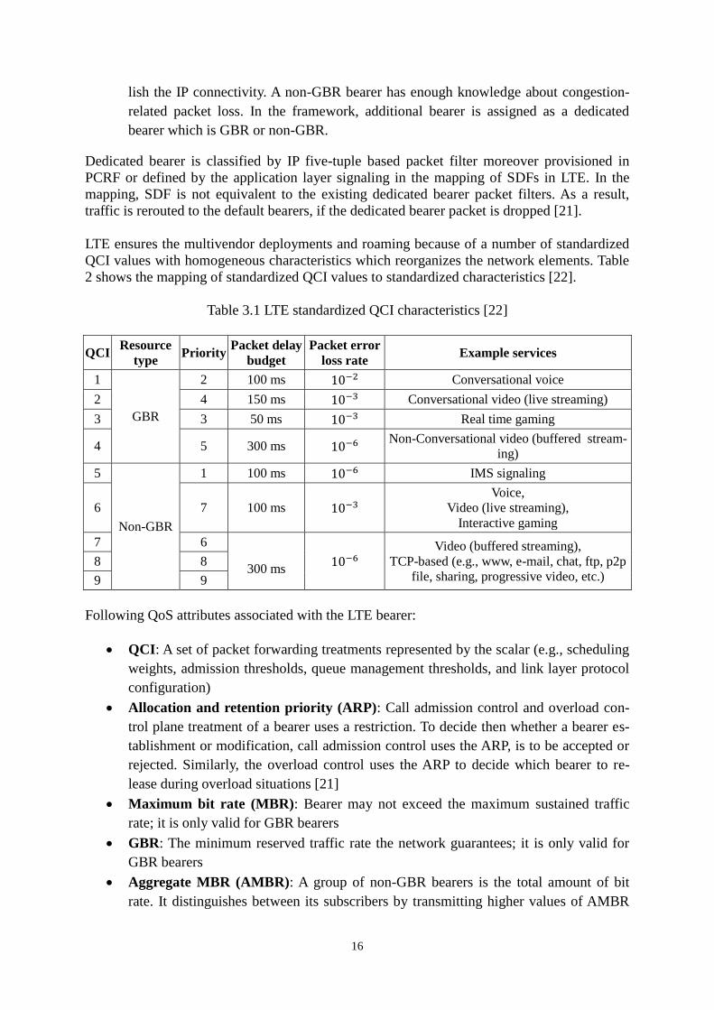
3.3 VoIP Principle
VoIP is a technology that delivers voice communications over computer networks like the
Internet or any other IP-based network. Using the Internet‟s packet-switching capabilities,
VoIP technology has been implemented to provide telephone services and offers substantial
cost savings over traditional long distance telephone calls. VoIP transmissions are deployed
through traditional routing [24]. A typical VoIP structural design is showed on the Figure 3.2,
though many “possible” modifications of this architecture are implemented in existing sys-
tems.
Figure 3.2 VoIP architecture
Phone
Encoding
Packetization
Streaming Buffering Play-out
Depacketization
Decoding
Phone
Network
18
In VoIP engineering, original voice signal is sampled and is encoded to a constant bit rate
digital stream at the end of the sending process. This compressed digital stream data is then
encapsulated into equal sized packets to broadcast it easily over the Internet.
Every packet contains the compress voice data along with the information of the packet‟s ori-
gin, projected destination address and have the packet stream to be reconstructed in the cor-
rect order with the help of timestamp. In place of circuit-switched voice transmission and tra-
ditional dedicated lines, these packets flow over a general-purpose packet-switched digital to
analog signal in the receiving end for it to be easily detected by human ear.
Generally, voice data information is sent in digital form in discrete packets rather than using
the traditional circuit-committed protocols of the Public Switched Telephone Network
(PSTN). In addition, VoIP technology ensures the precise time packet delivery with the help
of RTP. In the last few years, VoIP took the place of existing telephone networks and is pro-
gressively gaining more popularity for voice quality and the cost. It has the potential to com-
pletely substitute for the world‟s current phone systems.
3.4 VoIP Codec
Human voices are analog. In modern technology, transmit the digital signal for better commu-
nication. For that case, a codec (coder/decoder) is used during the voice communication. In
the transmitting end, a codec converts the analog signal to a compress digital bitstream, and at
the receiving end, another codec converts the digital bitstream back into analog signal. For
RTP packet, codec used the payload type or the encoding method in the VoIP technology.
Generally, codec provides a compression capability to save network bandwidth and also sup-
ports silence containment, where silence is not encoded or transmitted. Compression capabili-
ties of the codecs save the network bandwidth and support the silence suppression. Size of the
resulting encoded data stream, speed of the encoding/decoding operations and the quality and
fidelity of sound and/or video signal are the three most important factors to be optimized by
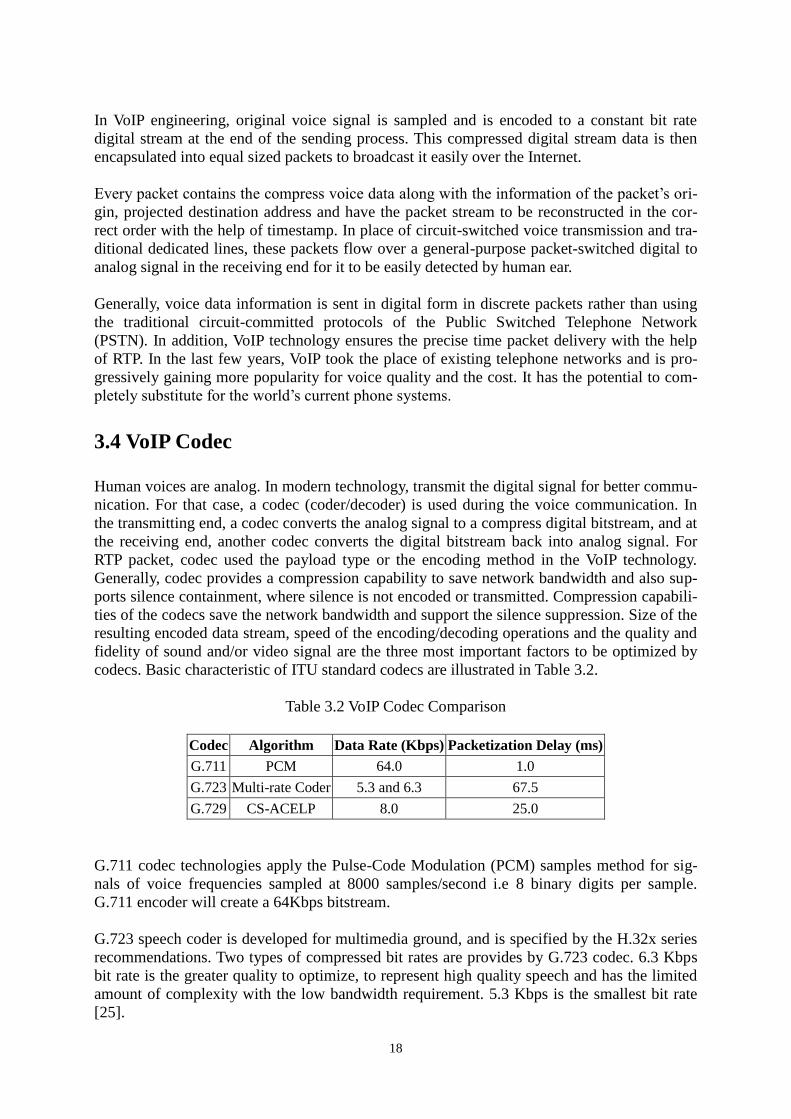
codecs. Basic characteristic of ITU standard codecs are illustrated in Table 3.2.
Table 3.2 VoIP Codec Comparison
Codec Algorithm Data Rate (Kbps) Packetization Delay (ms)
G.711 PCM 64.0 1.0
G.723 Multi-rate Coder 5.3 and 6.3 67.5
G.729 CS-ACELP 8.0 25.0
G.711 codec technologies apply the Pulse-Code Modulation (PCM) samples method for sig-
nals of voice frequencies sampled at 8000 samples/second i.e 8 binary digits per sample.
G.711 encoder will create a 64Kbps bitstream.
G.723 speech coder is developed for multimedia ground, and is specified by the H.32x series
recommendations. Two types of compressed bit rates are provides by G.723 codec. 6.3 Kbps
bit rate is the greater quality to optimize, to represent high quality speech and has the limited
amount of complexity with the low bandwidth requirement. 5.3 Kbps is the smallest bit rate
[25].
19
G.729 codec technologies apply the Conjugate-Structure Algebraic-Code-Excited-Linear-
Prediction (CS-ACELP) speech compression algorithm, approved by ITU-T. It is an 8Kpbs
bit rate and offers tax quality speech at low bit rate and also allows reasonable transmission
delays. It will be perfect for teleconferencing or visual telephony where quality, delay and
bandwidth are important [26].
3.5 Characteristics of VoIP
The major characteristics of VoIP traffic is authoritarian delay requirements. AMR codec pro-
vides the VoIP traffic along with the Voice Activity Detector, Relieve Noise Generation and
Discontinuous Transmission. Depending on the speed activity of the traffic, AMR provides a
constant rate of small packets transmission. During the active period, one VoIP packet took at
20 ms intervals and 160 ms interval for one Silence Description (SID) packet during silent
period. To improve the spectral efficiency of the VoIP traffic, UDP, IP and RTP headers in
LTE are also compressed with Robust Header Compression (ROHC). According to [27], for
voice signal, 250 ms is the maximum tolerable mouth-to-ear delay and around 100 ms delay
for the Core Network and also less than 150 ms acceptable delay for Medium Access Control
(MAC) buffering and Radio Link Control (RLC). Both end users are LTE users and assume
less than 80 ms acceptable delay for buffering and scheduling. For 3 GPP performance eval-
uations 50 ms delay has been bound for variability in network end-to-end delays.
The outage limit of maximal VoIP capacity for LTE is limited in TR 25.814 [28] and R1-
070674 is updated in contribution. Based on the above limitation, VoIP capacity can be de-
fined as follows:
The system capacity is defined as the number of users in the cell when more than 95 %
of the users are satisfied.
A VoIP user is satisfied if more than 98 % of its speech packets are delivered success-
fully.
It is required for VoIP user that the packet End-to-end delay shouldn‟t exceed 150 mil-
liseconds [29].
3.6 End-to-End Delay
End-to-end delay means the time required for a packet to be traversed from source to destina-
tion in the network and is measured in seconds. Generally, in VoIP network there are three
types of delays occurring during the packet transverse. They are: sender delays when packets
are transverse from source node, network delay and receiver delay.
In one direction from sender to receiver for VoIP stream flow, end-to-end delay can be calcu-
lated by the equation [30]:
(3.1)
where, D is the end-to-end delay and is the delay due to packetization at the source.
During the packet encoding in the source site, there is also and . Encoding
delay occurs while conversion of A/D signal into samples. PC of IP phone processing is
20
defined by including encapsulation. and , are 20 ms and 1ms respective-
ly in G.711 technology.
By using the equation 3.1, in the worst case scenario, an approximate delay of 25 ms is being
introduced at the source. At the end of the transmission, is the playback delay together
with jitter buffer delay where jitter delay is at most 40 ms because of two packets.
Similarly, at the receiving site, total fixed delay is 45 ms including . Due to transmis-
sion, propagation and queuing in the packet network through each hop h, the path from the
sender to the receiver, the total delays are , is the transmission delay,
is the queuing delay and is the propagation delay. We apply the queuing theory to cal-
culate the transmission and the queuing delay are expressed as
and propa-
gation delay will be added for WAN, which is typically ignored for LAN.
21
CHAPTER 4
Simulation Design and Implementation
4.1 Evaluation Platform
In real world scenarios, performance evaluation of a well designed network model and the
model itself carries significant importance. Though, the performance evaluation process is a
complex and challenging task in a real scenario. In-order to cope with the challenge, different
simulators is being used in practice to simulate the network model from different perspec-
tives. For example, well known open source simulator such as NS-2, gives simulators the
flexibility to extend the simulation environment. Nevertheless, modeling in real world scena-
rios are too complex to model in NS-2.
On the other hand, OPNET (Optimized Network Engineering Tool), introduced by OPNET
Technologies [31], is a commercial simulator where the kernel source code is not open. How-
ever it has a rich and comprehensive development features built in, which eases the process of
designing the real world scenario and simulating the network models [32]. It adds comprehen-
sive options as being both an object oriented and Discrete Event System (DES) based network
simulator. In our studies, we used OPNET modeler 16.0 for its reliable and efficiency for si-
mulation. The motivation of choosing OPNET will discuss in below section.
4.1.1 Why OPNET?
Through DES, OPNET models the system behavior by each event in the system effectively.
It‟s efficiency can be measured from the below mentioned features:
Provides more features than any other simulator in practice.
Allows modelers to directly include models in it with a wide range of available stan-
dard and vendor specific communication networks. It also helps to reduce the devel-
opment time greatly.
Has a dynamic development environment with rich features that support both distri-
buted systems and modeling of communication networks.
Has a large and user friendly documentation to guide users.
Provides easy graphical interface to work and view the results.
OPNET results are flexibly interpretable (i.e. exported to spreadsheets), and have
comprehensive tools to support display, plot and analyze time series, histograms,
probability, parametric curves, and confidence intervals.
22
4.2 Network Model Configuration
4.2.1 Network Components
This section briefly describes about the following network elements used in our study network
models running on OPNET [33].
The lte_access_gw_atm8_ethernet8_slip8_adv node models are used to represent an
IP-based gateway running LTE and supporting up to 8 Ethernet interfaces and up to 8
serial line interfaces at a selectable data.
The lte_enodeb_4ethernet_4atm_4slip_adv node model is used to represent a base sta-
tion which is called eNodeB in LTE. This type of base station is maintained up to 4
Ethernet interfaces and up to 4 serial line interfaces at a selectable data.
The lte_wkstn_adv node model is used to represent a workstation with source-
destination application running over TCP/IP and UDP/IP.
The PPP_DS3 link is used to represent the Ethernet connection operating 44.736
Mbps. This node is connected to two nodes in running IP. The type of this link is dup-
lex.
The Application_Config comprises a name and a description table which is specified
different parameters for the various applications (i.e. voice and FTP applications). The
individual application name is used while inventing user profile on “Profile_Config”
object.
The Profile_Config node can be used to create user profiles. These user profiles can be
precise on various nodes in the network to generate application layer traffic. The ap-
plications distinct in the Application_Config are applied by this object to configure
profiles. Traffic patterns can be precise followed by the application as well as the con-
figured profiles.
The Lte_attr_definer_adv node is used to store PHY configurations and EPS bearer
definition which can be referenced by all LTE nodes in the network.
The Mobility_Config node is used to define mobility profiles that individual nodes
reference to model mobility. This node controls the movement of nodes based on the
configuration parameters.
4.2.2 Network traffic Generation
In order to create an application in OPNET, an object is presented which is called application
definition attribute. This attribute consists of predefined applications that can be customized
as per the demands of the user. In application definition attribute, there are several predefined
applications i.e. HTTP, E-mail, Video, FTP, Voice, Database etc.
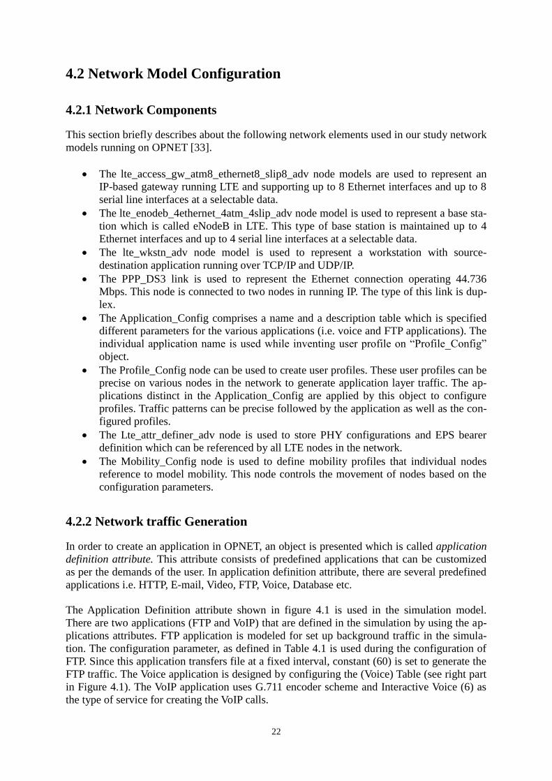
The Application Definition attribute shown in figure 4.1 is used in the simulation model.
There are two applications (FTP and VoIP) that are defined in the simulation by using the ap-
plications attributes. FTP application is modeled for set up background traffic in the simula-
tion. The configuration parameter, as defined in Table 4.1 is used during the configuration of
FTP. Since this application transfers file at a fixed interval, constant (60) is set to generate the
FTP traffic. The Voice application is designed by configuring the (Voice) Table (see right part
in Figure 4.1). The VoIP application uses G.711 encoder scheme and Interactive Voice (6) as
the type of service for creating the VoIP calls.
23
Figure 4.1 Application Definition
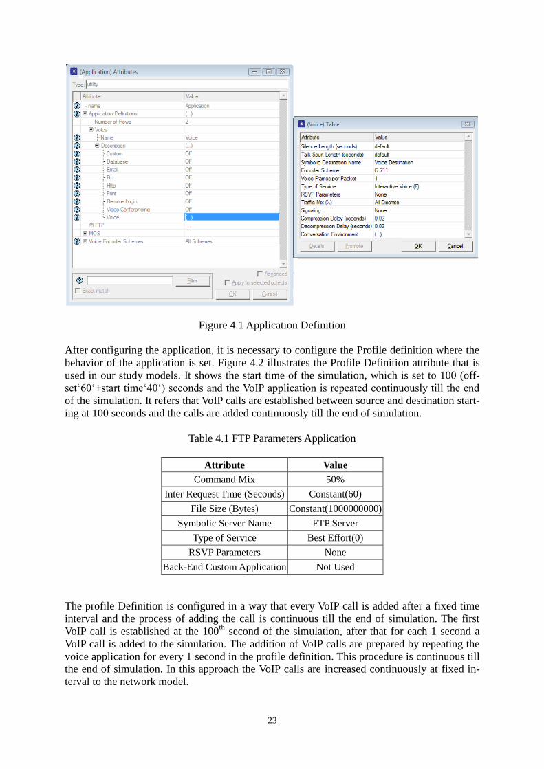
After configuring the application, it is necessary to configure the Profile definition where the
behavior of the application is set. Figure 4.2 illustrates the Profile Definition attribute that is
used in our study models. It shows the start time of the simulation, which is set to 100 (off-
set„60„+start time„40„) seconds and the VoIP application is repeated continuously till the end
of the simulation. It refers that VoIP calls are established between source and destination start-
ing at 100 seconds and the calls are added continuously till the end of simulation.
Table 4.1 FTP Parameters Application
Attribute Value
Command Mix 50%
Inter Request Time (Seconds) Constant(60)
File Size (Bytes) Constant(1000000000)
Symbolic Server Name FTP Server
Type of Service Best Effort(0)
RSVP Parameters None
Back-End Custom Application Not Used
The profile Definition is configured in a way that every VoIP call is added after a fixed time
interval and the process of adding the call is continuous till the end of simulation. The first
VoIP call is established at the 100th
second of the simulation, after that for each 1 second a
VoIP call is added to the simulation. The addition of VoIP calls are prepared by repeating the
voice application for every 1 second in the profile definition. This procedure is continuous till
the end of simulation. In this approach the VoIP calls are increased continuously at fixed in-
terval to the network model.
24
Figure 4.2 Profile Definition
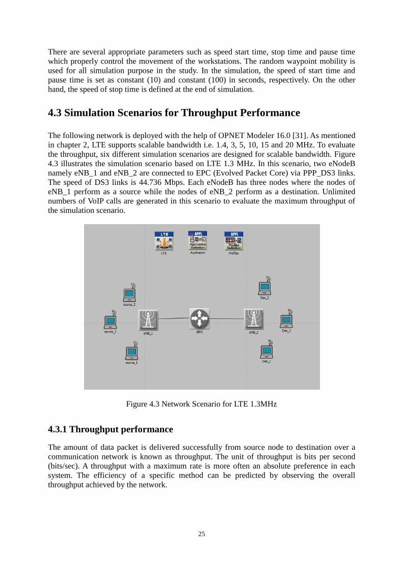
4.2.3 Simulation General Parameters
Table 4.2 demonstrates the LTE general parameters used in the process of all simulation mod-
els of the study. One of the other important entities is the mobility configuration, which is
used to determine the mobility model of the workstations.
Table 4.2 LTE Parameter
LTE Parameter Value
QoS Class Identifier (Voice) 1(GBR)
QoS Class Identifier (FTP) 6(Non-GBR)
Uplink Guaranteed Bit Rate (bps) 1 Mbps
Downlink Guaranteed Bit Rate (bps) 1 Mbps
Uplink Maximum Bit Rate (bps) 1 Mbps
Downlink Maximum Bit Rate (bps) 1 Mbps
UL Base Frequency (GHz) 1920 MHz
UL Bandwidth (MHz) 20 MHz
UL Cyclic Prefix Type 7 symbols per slot
DL Base Frequency (GHz) 2110 MHz
DL Bandwidth (MHz) 20 MHz
DL Cyclic Prefix Type 7 symbols per slot
25
There are several appropriate parameters such as speed start time, stop time and pause time
which properly control the movement of the workstations. The random waypoint mobility is
used for all simulation purpose in the study. In the simulation, the speed of start time and
pause time is set as constant (10) and constant (100) in seconds, respectively. On the other
hand, the speed of stop time is defined at the end of simulation.
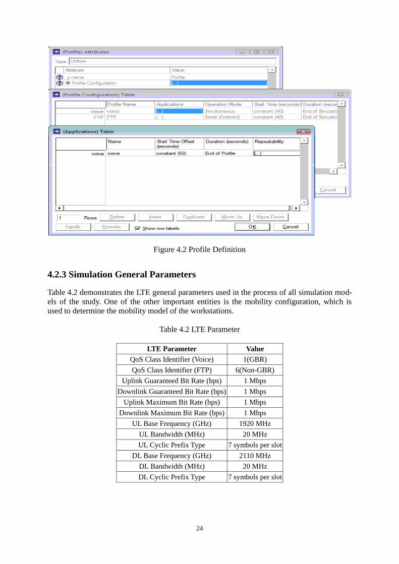
4.3 Simulation Scenarios for Throughput Performance
The following network is deployed with the help of OPNET Modeler 16.0 [31]. As mentioned
in chapter 2, LTE supports scalable bandwidth i.e. 1.4, 3, 5, 10, 15 and 20 MHz. To evaluate
the throughput, six different simulation scenarios are designed for scalable bandwidth. Figure
4.3 illustrates the simulation scenario based on LTE 1.3 MHz. In this scenario, two eNodeB
namely eNB_1 and eNB_2 are connected to EPC (Evolved Packet Core) via PPP_DS3 links.
The speed of DS3 links is 44.736 Mbps. Each eNodeB has three nodes where the nodes of
eNB_1 perform as a source while the nodes of eNB_2 perform as a destination. Unlimited
numbers of VoIP calls are generated in this scenario to evaluate the maximum throughput of
the simulation scenario.
Figure 4.3 Network Scenario for LTE 1.3MHz
4.3.1 Throughput performance
The amount of data packet is delivered successfully from source node to destination over a
communication network is known as throughput. The unit of throughput is bits per second
(bits/sec). A throughput with a maximum rate is more often an absolute preference in each
system. The efficiency of a specific method can be predicted by observing the overall
throughput achieved by the network.
26
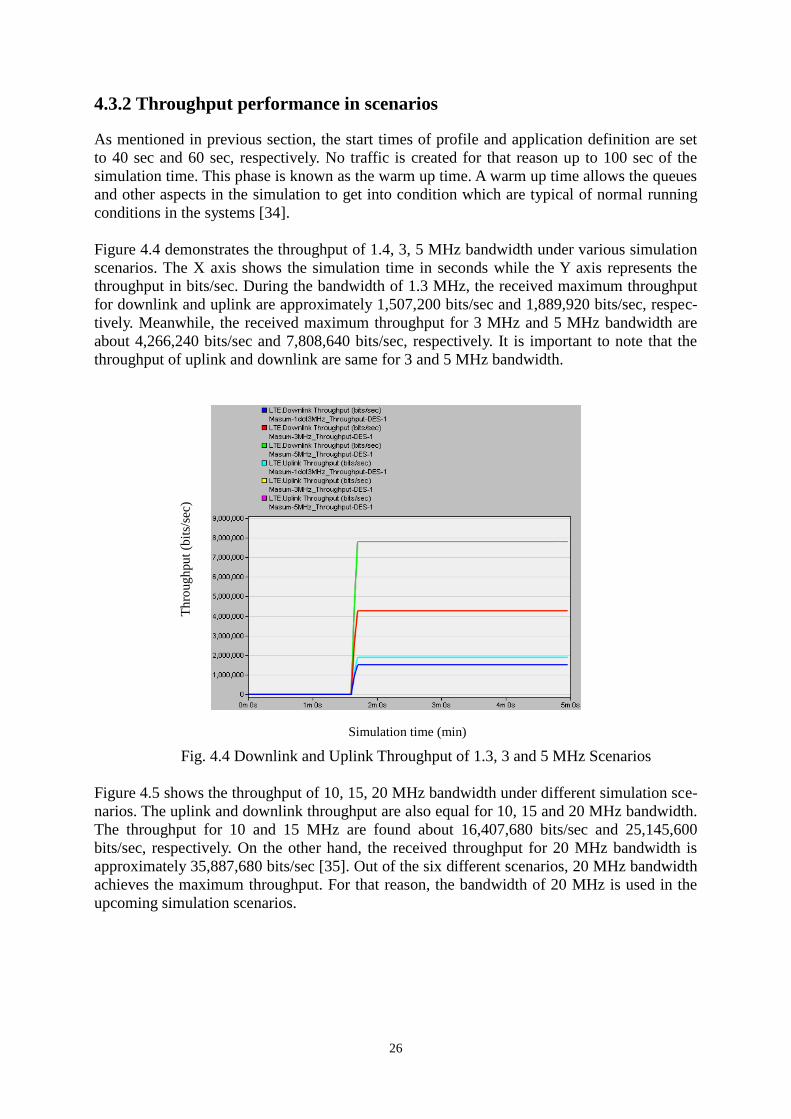
4.3.2 Throughput performance in scenarios
As mentioned in previous section, the start times of profile and application definition are set
to 40 sec and 60 sec, respectively. No traffic is created for that reason up to 100 sec of the
simulation time. This phase is known as the warm up time. A warm up time allows the queues
and other aspects in the simulation to get into condition which are typical of normal running
conditions in the systems [34].
Figure 4.4 demonstrates the throughput of 1.4, 3, 5 MHz bandwidth under various simulation
scenarios. The X axis shows the simulation time in seconds while the Y axis represents the
throughput in bits/sec. During the bandwidth of 1.3 MHz, the received maximum throughput
for downlink and uplink are approximately 1,507,200 bits/sec and 1,889,920 bits/sec, respec-
tively. Meanwhile, the received maximum throughput for 3 MHz and 5 MHz bandwidth are
about 4,266,240 bits/sec and 7,808,640 bits/sec, respectively. It is important to note that the
throughput of uplink and downlink are same for 3 and 5 MHz bandwidth.
Fig. 4.4 Downlink and Uplink Throughput of 1.3, 3 and 5 MHz Scenarios
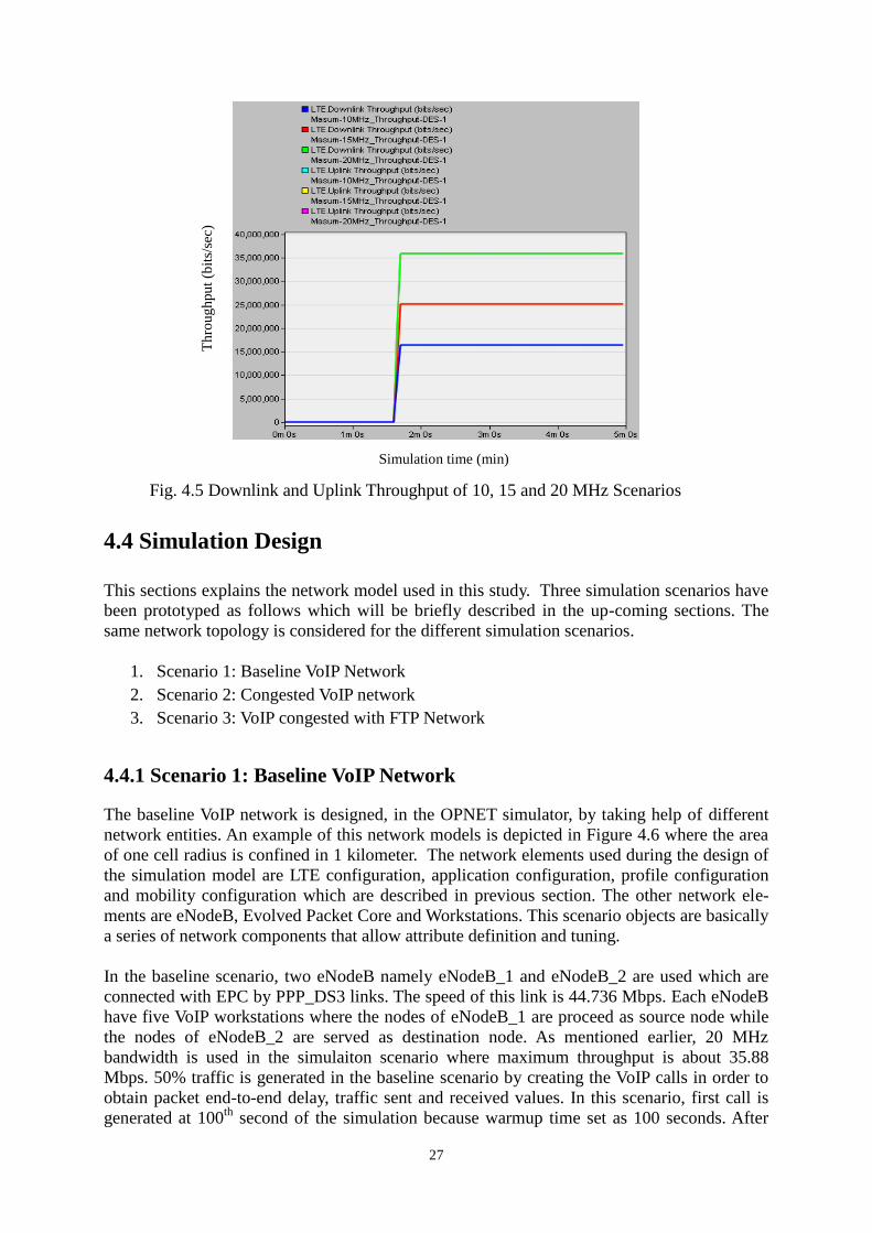
Figure 4.5 shows the throughput of 10, 15, 20 MHz bandwidth under different simulation sce-
narios. The uplink and downlink throughput are also equal for 10, 15 and 20 MHz bandwidth.
The throughput for 10 and 15 MHz are found about 16,407,680 bits/sec and 25,145,600
bits/sec, respectively. On the other hand, the received throughput for 20 MHz bandwidth is
approximately 35,887,680 bits/sec [35]. Out of the six different scenarios, 20 MHz bandwidth
achieves the maximum throughput. For that reason, the bandwidth of 20 MHz is used in the
upcoming simulation scenarios.
Th
roug
hpu
t (b
its/
sec)
Simulation time (min)
27
Fig. 4.5 Downlink and Uplink Throughput of 10, 15 and 20 MHz Scenarios
4.4 Simulation Design
This sections explains the network model used in this study. Three simulation scenarios have
been prototyped as follows which will be briefly described in the up-coming sections. The
same network topology is considered for the different simulation scenarios.
1. Scenario 1: Baseline VoIP Network
2. Scenario 2: Congested VoIP network
3. Scenario 3: VoIP congested with FTP Network
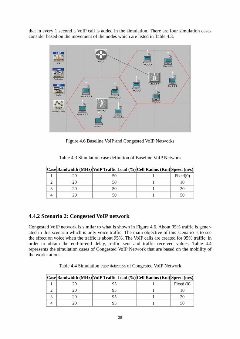
4.4.1 Scenario 1: Baseline VoIP Network
The baseline VoIP network is designed, in the OPNET simulator, by taking help of different
network entities. An example of this network models is depicted in Figure 4.6 where the area
of one cell radius is confined in 1 kilometer. The network elements used during the design of
the simulation model are LTE configuration, application configuration, profile configuration
and mobility configuration which are described in previous section. The other network ele-
ments are eNodeB, Evolved Packet Core and Workstations. This scenario objects are basically
a series of network components that allow attribute definition and tuning.
In the baseline scenario, two eNodeB namely eNodeB_1 and eNodeB_2 are used which are
connected with EPC by PPP_DS3 links. The speed of this link is 44.736 Mbps. Each eNodeB
have five VoIP workstations where the nodes of eNodeB_1 are proceed as source node while
the nodes of eNodeB_2 are served as destination node. As mentioned earlier, 20 MHz
bandwidth is used in the simulaiton scenario where maximum throughput is about 35.88
Mbps. 50% traffic is generated in the baseline scenario by creating the VoIP calls in order to
obtain packet end-to-end delay, traffic sent and received values. In this scenario, first call is
generated at 100th
second of the simulation because warmup time set as 100 seconds. After
Th
roug
hpu
t (b
its/
sec)
Simulation time (min)
28
that in every 1 second a VoIP call is added in the simulation. There are four simulation cases
consider based on the movement of the nodes which are listed in Table 4.3.
Figure 4.6 Baseline VoIP and Congested VoIP Networks
Table 4.3 Simulation case definition of Baseline VoIP Network
Case Bandwidth (MHz) VoIP Traffic Load (%) Cell Radius (Km) Speed (m/s)
1 20 50 1 Fixed(0)
2 20 50 1 10
3 20 50 1 20
4 20 50 1 50
4.4.2 Scenario 2: Congested VoIP network
Congested VoIP network is similar to what is shown in Figure 4.6. About 95% traffic is gener-
ated in this scenario which is only voice traffic. The main objective of this scenario is to see
the effect on voice when the traffic is about 95%. The VoIP calls are created for 95% traffic, in
order to obtain the end-to-end delay, traffic sent and traffic received values. Table 4.4
represents the simulation cases of Congested VoIP Network that are based on the mobility of
the workstations.
Table 4.4 Simulation case definition of Congested VoIP Network
Case Bandwidth (MHz) VoIP Traffic Load (%) Cell Radius (Km) Speed (m/s)
1 20 95 1 Fixed (0)
2 20 95 1 10
3 20 95 1 20
4 20 95 1 50
29
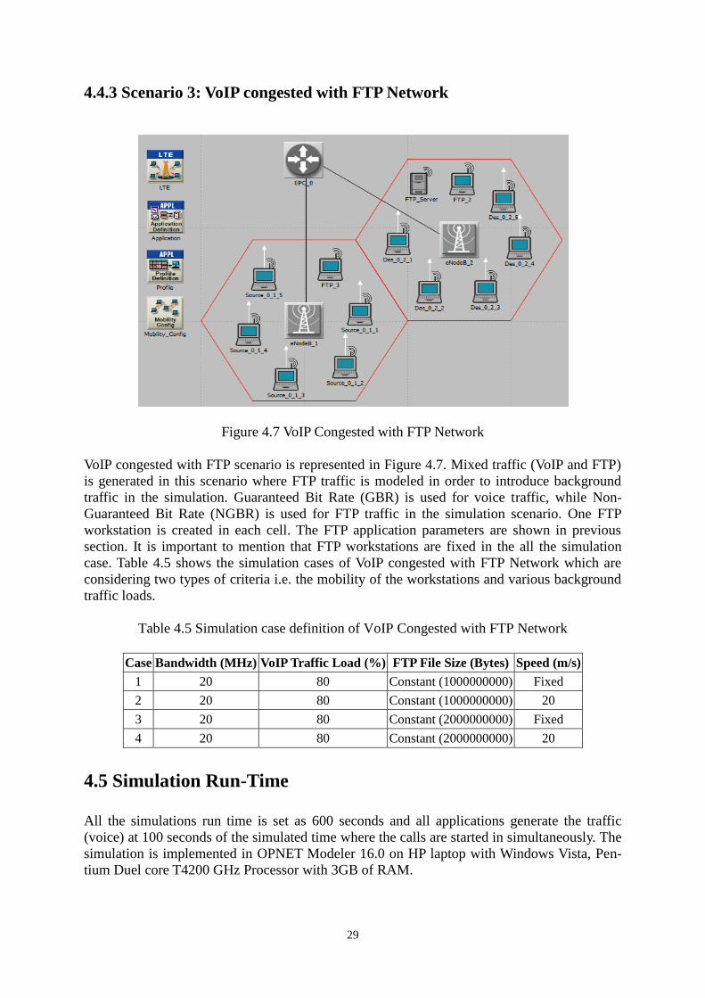
4.4.3 Scenario 3: VoIP congested with FTP Network
Figure 4.7 VoIP Congested with FTP Network
VoIP congested with FTP scenario is represented in Figure 4.7. Mixed traffic (VoIP and FTP)
is generated in this scenario where FTP traffic is modeled in order to introduce background
traffic in the simulation. Guaranteed Bit Rate (GBR) is used for voice traffic, while Non-
Guaranteed Bit Rate (NGBR) is used for FTP traffic in the simulation scenario. One FTP
workstation is created in each cell. The FTP application parameters are shown in previous
section. It is important to mention that FTP workstations are fixed in the all the simulation
case. Table 4.5 shows the simulation cases of VoIP congested with FTP Network which are
considering two types of criteria i.e. the mobility of the workstations and various background
traffic loads.
Table 4.5 Simulation case definition of VoIP Congested with FTP Network
Case Bandwidth (MHz) VoIP Traffic Load (%) FTP File Size (Bytes) Speed (m/s)
1 20 80 Constant (1000000000) Fixed
2 20 80 Constant (1000000000) 20
3 20 80 Constant (2000000000) Fixed
4 20 80 Constant (2000000000) 20
4.5 Simulation Run-Time
All the simulations run time is set as 600 seconds and all applications generate the traffic
(voice) at 100 seconds of the simulated time where the calls are started in simultaneously. The
simulation is implemented in OPNET Modeler 16.0 on HP laptop with Windows Vista, Pen-
tium Duel core T4200 GHz Processor with 3GB of RAM.
30
CHAPTER 5
Results and Analysis
5.1 End-to-End (E2E) Delay Performance
End-to-end (E2E) delay refers to the time needed for a packet to be transmitted from one node
to another node in a network. The unit of E2E delay is second. Generally, in VoIP a network,
three types of delay occur during the packet transverse. Firstly, senders delay, when packets
are transverse from source node. The other two are network delay and receiver delay. For
VoIP applications, the packet E2E delay should not exceed 150 ms to evaluate that the quality
of the created VoIP calls are accepted [29]. In this section, the packet E2E delays result for
different scenarios are presented in various statistical plots. Scenario 1, 2 and 3 correspond to
the Baseline VoIP, Congested with VoIP and VoIP congested with FTP, respectively. In the 1st
and 2nd
scenarios, voice application is designed between source and destination, while voice
and FTP application are designed in the 3rd
scenario. In all the scenarios, the sources and des-
tinations happen to be started at 100 seconds as the start time of the profile and application
configuration has been set to 40 seconds and 60 seconds, respectively. In all of the figures
presented in following sections, X axis represents simulation time in seconds; on the other
hand, Y axis represents End-to-end delay in seconds. Voice and FTP application and profile
configuration are discussed in details in Chapter 4.
5.1.1 E2E Delay performance for Baseline VoIP Network
Figure 5.1 End-to-End Delay of Baseline Network
Simulation time (min)
En
d-t
o-E
nd
Del
ay (
sec)
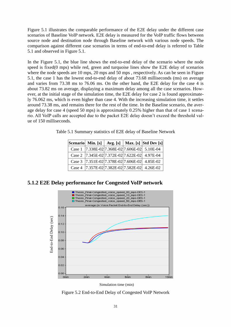
31
Figure 5.1 illustrates the comparable performance of the E2E delay under the different case
scenarios of Baseline VoIP network. E2E delay is measured for the VoIP traffic flows between
source node and destination node through Baseline network with various node speeds. The
comparison against different case scenarios in terms of end-to-end delay is referred to Table
5.1 and observed in Figure 5.1.
In the Figure 5.1, the blue line shows the end-to-end delay of the scenario where the node
speed is fixed(0 mps) while red, green and turquoise lines show the E2E delay of scenarios
where the node speeds are 10 mps, 20 mps and 50 mps , respectively. As can be seen in Figure
5.1, the case 1 has the lowest end-to-end delay of about 73.68 milliseconds (ms) on average
and varies from 73.38 ms to 76.06 ms. On the other hand, the E2E delay for the case 4 is
about 73.82 ms on average, displaying a maximum delay among all the case scenarios. How-
ever, at the initial stage of the simulation time, the E2E delay for case 2 is found approximate-
ly 76.062 ms, which is even higher than case 4. With the increasing simulation time, it settles
around 73.38 ms, and remains there for the rest of the time. In the Baseline scenario, the aver-
age delay for case 4 (speed 50 mps) is approximately 0.25% higher than that of case 1 scena-
rio. All VoIP calls are accepted due to the packet E2E delay doesn‟t exceed the threshold val-
ue of 150 milliseconds.
Table 5.1 Summary statistics of E2E delay of Baseline Network
Scenario Min. [s] Avg. [s] Max. [s] Std Dev [s]
Case 1 7.338E-02 7.368E-02 7.606E-02 5.10E-04
Case 2 7.345E-02 7.372E-02 7.622E-02 4.97E-04
Case 3 7.351E-02 7.378E-02 7.606E-02 4.85E-02
Case 4 7.357E-02 7.382E-02 7.582E-02 4.26E-02
5.1.2 E2E Delay performance for Congested VoIP network
Figure 5.2 End-to-End Delay of Congested VoIP Network
Simulation time (min)
En
d-t
o-E
nd
Del
ay (
sec)
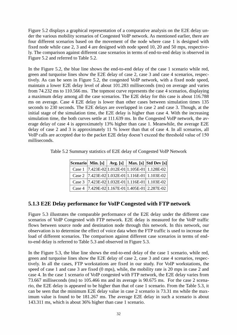
32
Figure 5.2 displays a graphical representation of a comparative analysis on the E2E delay un-
der the various mobility scenarios of Congested VoIP network. As mentioned earlier, there are
four different scenarios based on the movement of the node where case 1 is designed with
fixed node while case 2, 3 and 4 are designed with node speed 10, 20 and 50 mps, respective-
ly. The comparison against different case scenarios in terms of end-to-end delay is observed in
Figure 5.2 and referred to Table 5.2.
In the Figure 5.2, the blue line shows the end-to-end delay of the case 1 scenario while red,
green and turquoise lines show the E2E delay of case 2, case 3 and case 4 scenarios, respec-
tively. As can be seen in Figure 5.2, the congested VoIP network, with a fixed node speed,
maintain a lower E2E delay level of about 101.283 milliseconds (ms) on average and varies
from 74.232 ms to 110.566 ms. The topmost curve represents the case 4 scenarios, displaying
a maximum delay among all the case scenarios. The E2E delay for this case is about 116.788
ms on average. Case 4 E2E delay is lower than other cases between simulation times 135
seconds to 230 seconds. The E2E delays are overlapped in case 2 and case 3. Though, at the
initial stage of the simulation time, the E2E delay is higher than case 4. With the increasing
simulation time, the both curves settle at 111.639 ms. In the Congested VoIP network, the av-
erage delay of case 4 is approximately 13% higher than case 1. Meanwhile, the average E2E
delay of case 2 and 3 is approximately 11 % lower than that of case 4. In all scenarios, all
VoIP calls are accepted due to the packet E2E delay doesn‟t exceed the threshold value of 150
milliseconds.
Table 5.2 Summary statistics of E2E delay of Congested VoIP Network
Scenario Min. [s] Avg. [s] Max. [s] Std Dev [s]
Case 1 7.423E-02 1.012E-01 1.105E-01 1.128E-02
Case 2 7.423E-02 1.032E-01 1.116E-01 1.103E-02
Case 3 7.423E-02 1.032E-01 1.116E-01 1.103E-02
Case 4 7.429E-02 1.167E-01 1.405E-01 2.287E-02
5.1.3 E2E Delay performance for VoIP Congested with FTP network
Figure 5.3 illustrates the comparable performance of the E2E delay under the different case
scenarios of VoIP Congested with FTP network. E2E delay is measured for the VoIP traffic
flows between source node and destination node through this network. In this network, our
observation is to determine the effect of voice data when the FTP traffic is used to increase the
load of different scenarios. The comparison against different case scenarios in terms of end-
to-end delay is referred to Table 5.3 and observed in Figure 5.3.
In the Figure 5.3, the blue line shows the end-to-end delay of the case 1 scenario, while red,
green and turquoise lines show the E2E delay of case 2, case 3 and case 4 scenarios, respec-
tively. In all the cases, FTP workstations are fixed in our study. For VoIP workstations, the
speed of case 1 and case 3 are fixed (0 mps), while, the mobility rate is 20 mps in case 2 and
case 4. In the case 1 scenario of VoIP congested with FTP network, the E2E delay varies from
73.667 milliseconds (ms) to 105.466 ms and its average is 90.675 ms. For the case 2 scena-
rio, the E2E delay is appeared to be higher than that of case 1 scenario. From the Table 5.3, it
can be seen that the minimum E2E delay value in case 2 scenario is 73.31 ms while the max-
imum value is found to be 181.267 ms. The average E2E delay in such a scenario is about
143.311 ms, which is about 36% higher than case 1 scenario.
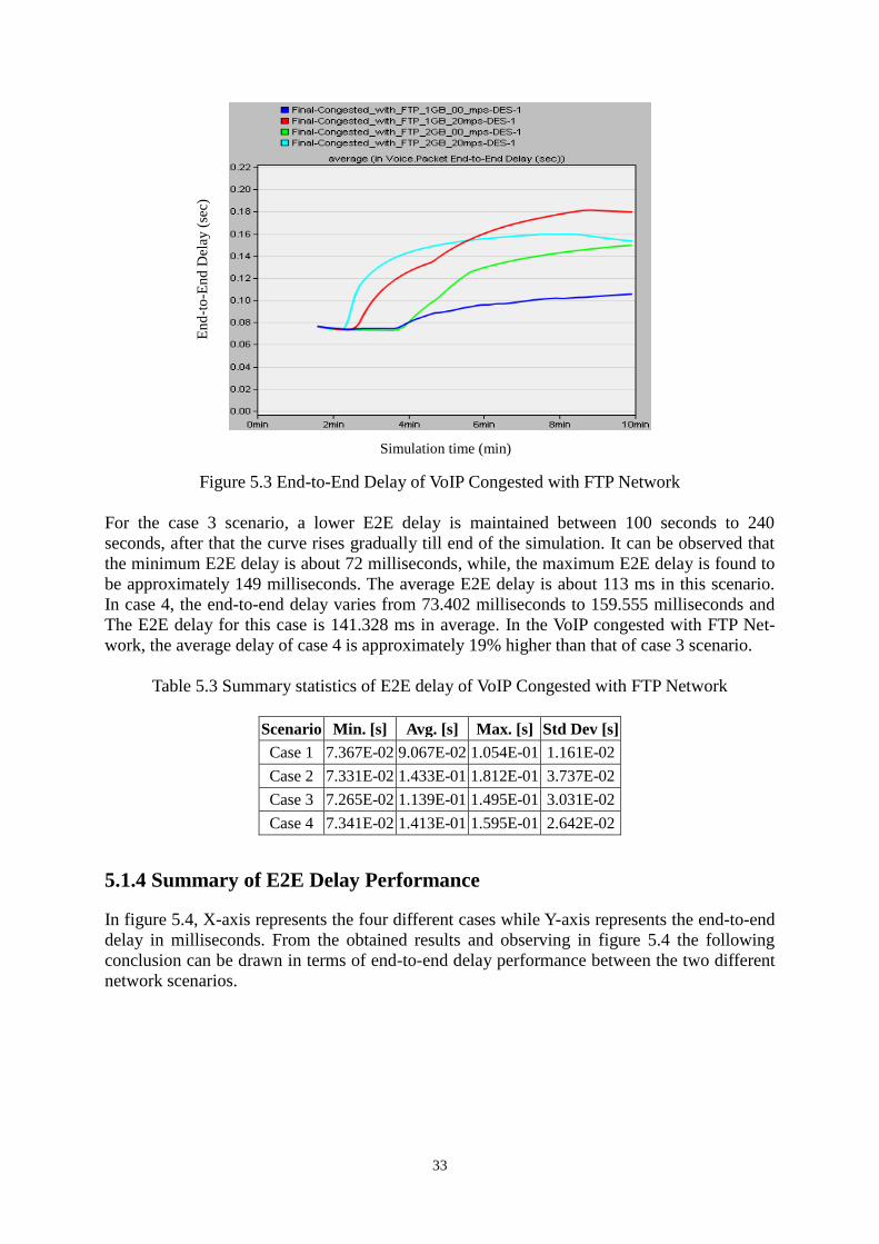
33
Figure 5.3 End-to-End Delay of VoIP Congested with FTP Network
For the case 3 scenario, a lower E2E delay is maintained between 100 seconds to 240
seconds, after that the curve rises gradually till end of the simulation. It can be observed that
the minimum E2E delay is about 72 milliseconds, while, the maximum E2E delay is found to
be approximately 149 milliseconds. The average E2E delay is about 113 ms in this scenario.
In case 4, the end-to-end delay varies from 73.402 milliseconds to 159.555 milliseconds and
The E2E delay for this case is 141.328 ms in average. In the VoIP congested with FTP Net-
work, the average delay of case 4 is approximately 19% higher than that of case 3 scenario.
Table 5.3 Summary statistics of E2E delay of VoIP Congested with FTP Network
Scenario Min. [s] Avg. [s] Max. [s] Std Dev [s]
Case 1 7.367E-02 9.067E-02 1.054E-01 1.161E-02
Case 2 7.331E-02 1.433E-01 1.812E-01 3.737E-02
Case 3 7.265E-02 1.139E-01 1.495E-01 3.031E-02
Case 4 7.341E-02 1.413E-01 1.595E-01 2.642E-02
5.1.4 Summary of E2E Delay Performance
In figure 5.4, X-axis represents the four different cases while Y-axis represents the end-to-end
delay in milliseconds. From the obtained results and observing in figure 5.4 the following
conclusion can be drawn in terms of end-to-end delay performance between the two different
network scenarios.
En
d-t
o-E
nd
Del
ay (
sec)
Simulation time (min)
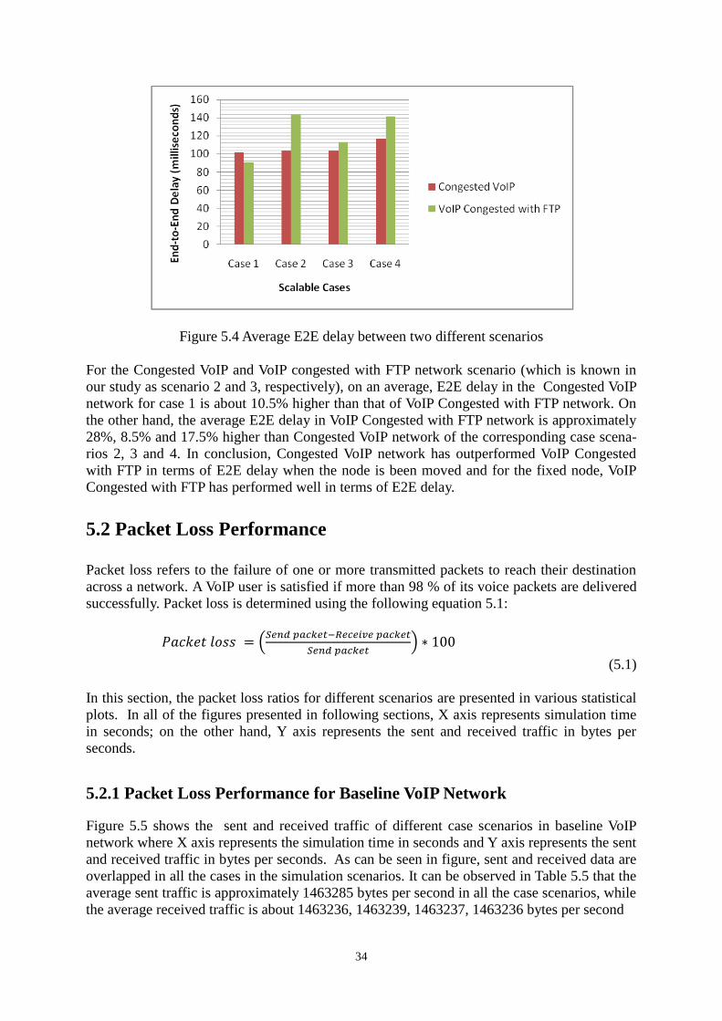
34
Figure 5.4 Average E2E delay between two different scenarios
For the Congested VoIP and VoIP congested with FTP network scenario (which is known in
our study as scenario 2 and 3, respectively), on an average, E2E delay in the Congested VoIP
network for case 1 is about 10.5% higher than that of VoIP Congested with FTP network. On
the other hand, the average E2E delay in VoIP Congested with FTP network is approximately
28%, 8.5% and 17.5% higher than Congested VoIP network of the corresponding case scena-
rios 2, 3 and 4. In conclusion, Congested VoIP network has outperformed VoIP Congested
with FTP in terms of E2E delay when the node is been moved and for the fixed node, VoIP
Congested with FTP has performed well in terms of E2E delay.
5.2 Packet Loss Performance
Packet loss refers to the failure of one or more transmitted packets to reach their destination
across a network. A VoIP user is satisfied if more than 98 % of its voice packets are delivered
successfully. Packet loss is determined using the following equation 5.1:
(5.1)
In this section, the packet loss ratios for different scenarios are presented in various statistical
plots. In all of the figures presented in following sections, X axis represents simulation time
in seconds; on the other hand, Y axis represents the sent and received traffic in bytes per
seconds.
5.2.1 Packet Loss Performance for Baseline VoIP Network
Figure 5.5 shows the sent and received traffic of different case scenarios in baseline VoIP
network where X axis represents the simulation time in seconds and Y axis represents the sent
and received traffic in bytes per seconds. As can be seen in figure, sent and received data are
overlapped in all the cases in the simulation scenarios. It can be observed in Table 5.5 that the
average sent traffic is approximately 1463285 bytes per second in all the case scenarios, while
the average received traffic is about 1463236, 1463239, 1463237, 1463236 bytes per second
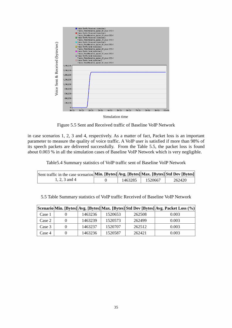
35
Figure 5.5 Sent and Received traffic of Baseline VoIP Network
in case scenarios 1, 2, 3 and 4, respectively. As a matter of fact, Packet loss is an important
parameter to measure the quality of voice traffic. A VoIP user is satisfied if more than 98% of
its speech packets are delivered successfully. From the Table 5.5, the packet loss is found
about 0.003 % in all the simulation cases of Baseline VoIP Network which is very negligible.
Table5.4 Summary statistics of VoIP traffic sent of Baseline VoIP Network
Sent traffic in the case scenarios
1, 2, 3 and 4
Min. [Bytes] Avg. [Bytes] Max. [Bytes] Std Dev [Bytes]
0 1463285 1520667 262420
5.5 Table Summary statistics of VoIP traffic Received of Baseline VoIP Network
Scenario Min. [Bytes] Avg. [Bytes] Max. [Bytes] Std Dev [Bytes] Avg. Packet Loss (%)
Case 1 0 1463236 1520653 262508 0.003
Case 2 0 1463239 1520573 262499 0.003
Case 3 0 1463237 1520707 262512 0.003
Case 4 0 1463236 1520587 262421 0.003
Simulation time
Vo
ice
Sen
t &
Rec
eiv
ed (
by
tes/
sec)
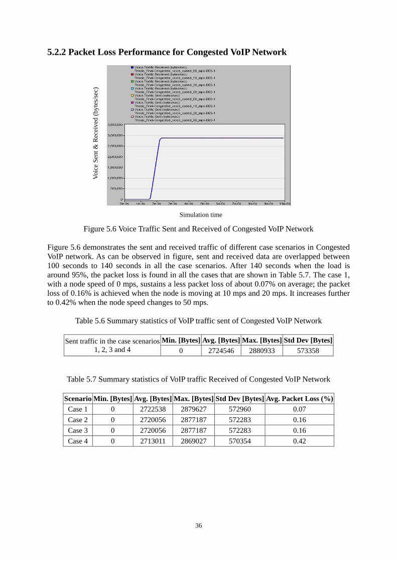
36
5.2.2 Packet Loss Performance for Congested VoIP Network
Figure 5.6 Voice Traffic Sent and Received of Congested VoIP Network
Figure 5.6 demonstrates the sent and received traffic of different case scenarios in Congested
VoIP network. As can be observed in figure, sent and received data are overlapped between
100 seconds to 140 seconds in all the case scenarios. After 140 seconds when the load is
around 95%, the packet loss is found in all the cases that are shown in Table 5.7. The case 1,
with a node speed of 0 mps, sustains a less packet loss of about 0.07% on average; the packet
loss of 0.16% is achieved when the node is moving at 10 mps and 20 mps. It increases further
to 0.42% when the node speed changes to 50 mps.
Table 5.6 Summary statistics of VoIP traffic sent of Congested VoIP Network
Sent traffic in the case scenarios
1, 2, 3 and 4
Min. [Bytes] Avg. [Bytes] Max. [Bytes] Std Dev [Bytes]
0 2724546 2880933 573358
Table 5.7 Summary statistics of VoIP traffic Received of Congested VoIP Network
Scenario Min. [Bytes] Avg. [Bytes] Max. [Bytes] Std Dev [Bytes] Avg. Packet Loss (%)
Case 1 0 2722538 2879627 572960 0.07
Case 2 0 2720056 2877187 572283 0.16
Case 3 0 2720056 2877187 572283 0.16
Case 4 0 2713011 2869027 570354 0.42
Simulation time
Vo
ice
Sen
t &
Rec
eiv
ed (
by
tes/
sec)
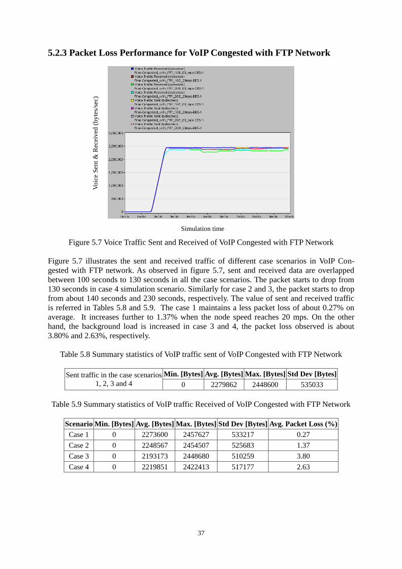
37
5.2.3 Packet Loss Performance for VoIP Congested with FTP Network
Figure 5.7 Voice Traffic Sent and Received of VoIP Congested with FTP Network
Figure 5.7 illustrates the sent and received traffic of different case scenarios in VoIP Con-
gested with FTP network. As observed in figure 5.7, sent and received data are overlapped
between 100 seconds to 130 seconds in all the case scenarios. The packet starts to drop from
130 seconds in case 4 simulation scenario. Similarly for case 2 and 3, the packet starts to drop
from about 140 seconds and 230 seconds, respectively. The value of sent and received traffic
is referred in Tables 5.8 and 5.9. The case 1 maintains a less packet loss of about 0.27% on
average. It increases further to 1.37% when the node speed reaches 20 mps. On the other
hand, the background load is increased in case 3 and 4, the packet loss observed is about
3.80% and 2.63%, respectively.
Table 5.8 Summary statistics of VoIP traffic sent of VoIP Congested with FTP Network
Sent traffic in the case scenarios
1, 2, 3 and 4
Min. [Bytes] Avg. [Bytes] Max. [Bytes] Std Dev [Bytes]
0 2279862 2448600 535033
Table 5.9 Summary statistics of VoIP traffic Received of VoIP Congested with FTP Network
Scenario Min. [Bytes] Avg. [Bytes] Max. [Bytes] Std Dev [Bytes] Avg. Packet Loss (%)
Case 1 0 2273600 2457627 533217 0.27
Case 2 0 2248567 2454507 525683 1.37
Case 3 0 2193173 2448680 510259 3.80
Case 4 0 2219851 2422413 517177 2.63
Vo
ice
Sen
t &
Rec
eiv
ed (
by
tes/
sec)
Simulation time
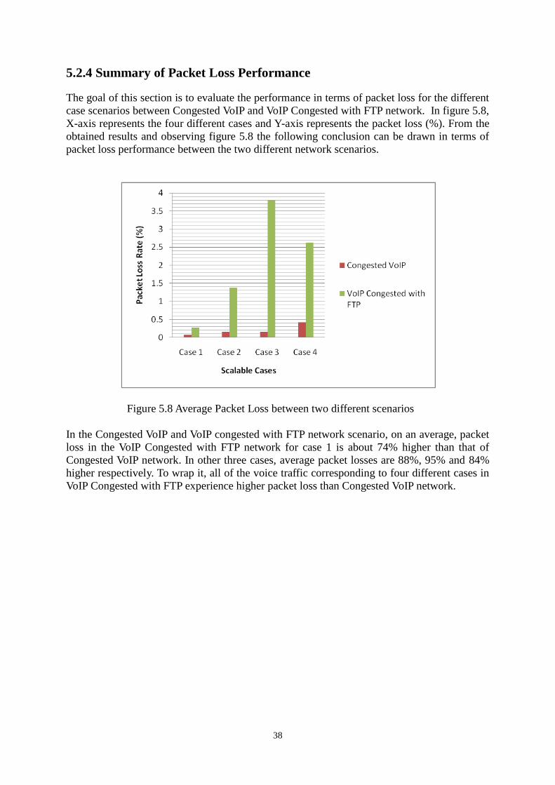
38
5.2.4 Summary of Packet Loss Performance
The goal of this section is to evaluate the performance in terms of packet loss for the different
case scenarios between Congested VoIP and VoIP Congested with FTP network. In figure 5.8,
X-axis represents the four different cases and Y-axis represents the packet loss (%). From the
obtained results and observing figure 5.8 the following conclusion can be drawn in terms of
packet loss performance between the two different network scenarios.
Figure 5.8 Average Packet Loss between two different scenarios
In the Congested VoIP and VoIP congested with FTP network scenario, on an average, packet
loss in the VoIP Congested with FTP network for case 1 is about 74% higher than that of
Congested VoIP network. In other three cases, average packet losses are 88%, 95% and 84%
higher respectively. To wrap it, all of the voice traffic corresponding to four different cases in
VoIP Congested with FTP experience higher packet loss than Congested VoIP network.
39
CHAPTER 6
Conclusion
In this thesis work, an effective study, analysis and evaluation of the end-to-end delay perfor-
mance evaluation for VoIP in the LTE network have been done. The evaluation is made by
simulating in OPNET Modeler 16.0 based on some performance metrics such as end-to-end
delay and throughput. Three network scenarios have been simulated: Baseline VoIP network
scenario, congested VoIP network scenario and VoIP congested with FTP network scenario.
During simulation, answers for the research questions of this thesis have been attained in
terms of the graphical results. It has been found that maximum throughput increased as the
bandwidth incremented. Out of the six scenarios created for throughput measurement, the
scenario with highest bandwidth (i.e. 20 MHz) exhibited maximum throughput. After that,
quality measurement of VoIP has been done with respect to E2E delay, both for a network
congested exclusively with VoIP and VoIP with FTP. Four scenarios have been created for this
evaluation, one case with stationary node and other three cases with mobile nodes (gradually
increasing the node speed). The simulation results showed that when the node is not moving,
E2E delay is slightly higher for network congested with VoIP only. In other cases, better E2E
is obtained for this network due to the presence of moving node. Finally, rate of packet loss
for the two networks in the previously mentioned four cases have been analyzed. Packet loss
remains quite minimal for congested with VoIP network regardless of the node speed. Mean-
while, for VoIP with FTP network, packet loss rate is also quite insignificant for fixed node
case but the rate upshots as the node starts moving.
40
BIBLIOGRAPHY
[1] 3GPP, Release 8 V0.0.3, “Overview of 3GPP Release 8: Summery of all Release 8 Fea-
tures,” November 2008.
[2] J. Puttonen, H.-H. Puupponen, K. Aho, T. Henttonen, and M. Moisio, “Impact of Control
Channel Limitations on the LTE VoIP Capacity,” in 2010 Ninth International Conference on
Networks, Menuires, France, 2010, pp. 77-82.
[3] J. Puttonen, T. Henttonen, N. Kolehmainen, K. Aschan, M. Moisio, and P. Kela, “Voice-
Over-IP Performance in UTRA Long Term Evolution Downlink,” in VTC Spring 2008 - IEEE
Vehicular Technology Conference, Marina Bay, Singapore, 2008, pp. 2502-2506.
[4] J. Creswell, Research Design: Qualitative, Quantitative, and Mixed Methods Approaches.
Sage Publications, 2009.
[5] G. Swallow, “MPLS advantages for traffic engineering,” IEEE Communications Maga-
zine, vol. 37, no. 12, pp. 54-57, Dec. 1999.
[6] 3GPP, ―Third Generation Partnership Project (3GPP).‖ [Online]. Available:
http://www.3gpp.org/
[7] J. G. Andrews, “Orthogonal Frequency Division Multiple Access (OFDMA),” THE UNI-
VERSITY OF TEXAS AT AUSTIN, 2006.
[8] T. Satio, Y. Tanaka, and T. Kato, “Trends in WiMaX/LTE system,” Fujitsu scientific and
technical journal, vol. 45, pp. 355-362, Apr. 2009.
[9] H. Myung and D. Goodman, Single carrier FDMA a new air interface for long term evo-
lution, 1st ed. Chichester U.K. ;New York: J. Wiley & Sons, 2008.
[10] S. Srikanth, V. Kumarn, C. Manikandan, and Murugesapandian, “Orthhognal Frequency
Divison Multiplexing: is it the Multiple Access System of the future?”,” AU-KBC Research
center, Anna University.
[11] F. Khan, LTE for 4G Mobile Broadband: Air Interface Technologies and Performance,
1st ed. Cambridge University Press, 2009.
[12] H. Myung, “Introduction To Single Carrier Fdma,” presented at the 15th European Sig-
nal Processing Conference, (Eusipco2007).
[13]“3GPP TS 36.71 Evolved Universal Terrestrial Radio Access (E-UTRA); Physical chan-
nels and modulation.”
41
[14] D. Martín-Sacristán, J. F. Monserrat, J. Cabrejas-Peñuelas, D. Calabuig, S. Garrigas, and
N. Cardona, “On the Way towards Fourth-Generation Mobile: 3GPP LTE and LTE-
Advanced,” EURASIP Journal on Wireless Communications and Networking, vol. 2009, pp.
1-10, 2009.
[15] H. Holma and A. Toskala, LTE for UMTS - OFDMA and SC-FDMA Based Radio Access.
Finland: John Wiley & Sons Ltd, 2009.
[16] “Technical White Paper: Long Term Evolution (LTE): A Technical Overview”, Motorola,
Inc. www.motorola.com, 2007
[17] E. Dahlman, S. Parkvall, J. Skold, and P. Beming, 3G Evolution HSPA and LTE for Mo-
bile Broadband, 2nd ed. Burlington, MA: Elsevier Ltd., 2008.
[18] J. Lee, J.-K. Han, and J. (Charlie) Zhang, “MIMO Technologies in 3GPP LTE and LTE-
Advanced,” EURASIP Journal on Wireless Communications and Networking, vol. 2009, pp.
1-10, 2009.
[19] “General Packet Radio Service (GPRS) enhancements for Evolved Universal Terrestrial
Radio Access Network (E-UTRAN) access.” 3GPP TS 23.401 v. 8.8.0, Dec-2009.
[20]“Evolved Universal Terrestrial Radio Access (E-UTRA) and Evolved Universal Terrestri-
al Radio Access Network (E-UTRAN).” 3GPP TS 36.300 version 8.11.0, Jan-2010.
[21] H. Ekstrom, “QoS control in the 3GPP evolved packet system,” IEEE Communications
Magazine, vol. 47, no. 2, pp. 76-83, Feb. 2009.
[22] “Policy and charging control architecture.” 3GPP TS 23.203 v. 8.8.0, Dec-2009.
[23] J.-M. Chung, S.-C. Kim, E. Marroun, and H. Sandhu, “VoIP over MPLS Networking
Requirements,” in Networking — ICN 2001, vol. 2094, Berlin, Heidelberg: Springer Berlin
Heidelberg, 2001, pp. 735-744.
[24] O. Olorunda and A. Olorunda, “Bridging the Digital Divide - The Social and Cultural
Impact of VoIP in Developing Countries: Nigeria as a Case Study,” In Proc. of PTC’06, Ho-
nolulu, Hawaii, Jan. 2006.
[25] “Dual rate speech coder for multimedia communications transmitting at 5.3 and 6.3
kbit/s.” ITU-T Recommendation G.723.1, Mar-1996.
[26] “Coding of speech at 8 kbit/s using conjugate-structure algobraic-code-excited linear-
prediction (cs-acelp).” ITU-T Recommendation G.729, Mar-1996.
[27] “One Way Transmission Time.” ITU-T recommendation G.114, May-2003.
[28] “LTE physical layer framework for performance verification.” 3GPP R1-070674, Feb-
2007.
42
[29] K. Salah and A. Alkhoraidly, “An OPNET-based simulation approach for deploying
VoIP,” International Journal of Network Management, vol. 16, no. 3, pp. 159-183, May. 2006.
[30] M. J. Karam and F. A. Tobagi, “Analysis of delay and delay jitter of voice traffic in the
Internet,” Speedtrak Communications, San Mateo, CA 94401, USA, Computer Systems La-
boratory, Department of Electrical Engineering, Stanford University, Stanford, CA 94305,
USA, vol. 40, pp. 711-726, Dec-2002.
[31] OPNET. Opnet modeler 16.0. [Online].
Available: http://www.opnet.com/solutions/network_rd/modeler.html
[32] M. Rahman, A. Pakstas, and F. Wang, “Network modelling and simulation tools,” Elsevi-
er B.V., vol. 17, pp. 1011–1031, 2009.
[33] OPNET, Modeler Release, 16th ed. [Online]. Available: http://www.opnet.com
[34] B. Sang, X. Kaixin, L. Sungwook and M. Gerla, “Measured Analysis of TCP Behavior
across Multihop Wireless and Wired Networks, ” In proceedings of the Global Telecommuni-
cations Conference, 2002. GLOBECOM '02. IEEE, vol.1, no. 1, pp. 153-157, March. 2003.
[35] Mobile broadband with HSPA and LTE – capacity and cost aspects. Finland: Nokia Sie-
mens Networks, White Paper, 2010.
Related Documents