End-Point Model for Optimization of Multilateral Well ...

energies

Article

End-Point Model for Optimization of MultilateralWell Placement in Hydrocarbon Field Developments

Damian Janiga 1,* , Daniel Podsobinski 1,2, Paweł Wojnarowski 1 and Jerzy Stopa 1

1 Department of Petroleum Engineering, Faculty of Drilling, Oil and Gas, AGH University of Science andTechnology, al. Mickiewicza 30, 30-059 Kraków, Poland; [email protected] (D.P.);[email protected] (P.W.); [email protected] (J.S.)

2 Polish Oil and Gas Company (PGNiG S.A)., M. Kasprzaka 25, 01-234 Warszawa, Poland* Correspondence: [email protected]

Received: 26 June 2020; Accepted: 29 July 2020; Published: 31 July 2020

Abstract: Drilling cost is one of the most critical aspects in the reservoir management plan. Costs mayexceed a million dollars; thus, optimal designing of the well trajectory in the reservoir and completionare essential. The implementation of a multilateral well (MLW) in reservoir management has greatpotential to optimize oil production. The object of this study is to develop an integrated workflow ofend-point multilateral well placement optimization integrated with the reservoir simulator supportedby artificial intelligence (AI) methods. The paper covers various types of MLW construction, including:horizontal, bi-, tri-, and quad-lateral wells. For quad-lateral wells, the capital expenditure is highest;nevertheless, acceleration of oil production affects the project’s NPV (net present value) , indicatingthe type of well that is most promising to implement in the reservoir. Tri- and quad-lateral wellscan operate for 12.1 and 9.8 years with a constant production rate. The decreasing hydrocarbonproduction rate is affected by reservoir pressure and the reservoir water production rate. Other welldesign patterns can accelerate water production. The well’s optimal trajectory was evaluated bythe genetic algorithm (GA) and particle swarm optimization (PSO). The major difference betweenthe GA and PSO optimization runs is visible with respect to water production and is related tothe modification of one well branch trajectory in a reservoir. The proposed methodology has theadvantage of easy implementation in a closed-loop optimization system coupled with numericalreservoir simulation. The paper covers the solution background, an implementation example, andthe model limitations.

Keywords: multilateral well; optimization; end-point model

1. Introduction

We provide a state-of-the-art background and place the proposed approach among other solutions.The Introduction consists of a review of the application of multilateral well system in variousproduction and injection scenarios, a review of previous works related to multilateral well optimization,a brief description of the optimization algorithms that can be employed in the solution with specialconsideration of the genetic algorithm and particle swarm optimization.

1.1. Multilateral Wells as an Asset in Reservoir Management

In recent years, the interest in multilateral wells has increased. The advanced technologies for thecompletion of productive horizons using multilateral or intelligent wells offer several possibilities tooptimize hydrocarbon recovery and economic results [1]. The biggest advantages of multilateral wellsare the increased formation drainage area and enhancement of productivity. This technology bringsthe benefits of reducing water cresting and coning due to complex structured branch wells usually

Energies 2020, 13, 3926; doi:10.3390/en13153926 www.mdpi.com/journal/energies

Energies 2020, 13, 3926 2 of 23

having a higher production rate with a smaller production pressure difference compared to a verticalor single horizontal well [2]. Therefore, it helps to significantly postpone water breakthrough especiallyin reservoirs with a strong bottom water drive mechanism. Additionally, the technology of multilateralwells can considerably decrease capital expenditures in the field development phase, owing to a largepart of the costs being incurred when drilling the main hole [3], in that one multilateral well canreplace multiple vertical or horizontal wells in overall production and recovery [4]. Currently, mostoffshore wells start vertically, but they typically contain numerous out-of-plane horizontal or dippingdrain holes whose flow areas interact [5]. Designing the trajectory, quantity, and placement of lateralwells from one mainbore requires a detailed analysis of the reservoir and fluid that will be produced.The optimal placement may bring high gas or oil recovery and substantial profits to the investment,but finding the best solution for the objective function is extremely challenging and involves plenty ofvariables. Among the factors that can affect overall reservoir performance and project profitability,several major groups emerge. Petroleum fluids, reservoir rock properties, and management schemacontribute to the oil recovery and its production [6]. As an example of the physical phenomenaaffecting production performance, multiphase flow, oil-aqueous interfacial tension, and the contactangle between phases can be listed. Furthermore, fluid properties and pressure-temperature changescan play a major role in recovery [7]. Song et al. [8] introduced a novel method of the utilization ofmultilateral wells in the oil shale in situ conversion process. The proposed method employs radialbranches from the main trunk in the upper and lower oil shale formation as injection and productionpoints. Due to the temperatures of the injected fluid to initiate the pyrolization process, the authorsperformed a sensitivity analysis to evaluate the impact of the oil properties and the arrangements ofradial branches’ placement. One of the crucial parameters that has a significant impact on multilateralwell performance is pressure drop in the horizontal part. Wei et al. [9] developed a semi-analyticalmodel to investigate the pressure drop within a multilateral horizontal well. The proposed modelcovers a wide range of flow regimes. Model verification was conducted on the two most commonwell patterns. Apart from the application of a multilateral well in a conventional reservoir productionsystem, a multilateral well (MLW) can be used in coalbed methane, heavy oil, or geothermal systems.Yang et al. [10] analyzed CMB (coal bed methane) occurrence and the multilateral horizontal welltrajectory in the Qinshui Basin, Shanxi Province. The investigation made an effort to provide a solutionto the problem of slack coal production in gas recovery by reduction of the permeability due to watersaturation. Chen et al. [11] investigated the characteristics of coal permeability anisotropy and itsimpact on the optimal multilateral well design. The results showed that the optimal well direction ofthe quad-lateral well is parallel to the cleat. However, stress changes during the production period mayalso have a significant impact on multilateral well design. Zhou et al. [12] proposed an investigation ofthe limits of sand production from offshore heavy oil reservoirs through laboratory experiments and anumerical simulation. The obtained results suggested the number of branches be limited to two orthree, taking into account the design parameters, especially the branch angle. Shi et al. [13] evaluatedthe possibility of increasing the heat extraction from CO2 enhanced geothermal systems (CO2-EGS) bythe application a multilateral well system. The authors used a coupled wellbore–reservoir model withfluid flow and heat transfer. The multilateral well construction was optimized to achieve the maximumheat insulation. The results provided suggestions for the wellbore design pattern. According to [14],the most efficient way to maximize hydrocarbon recovery is long directional wells. The author gave asan example the Troll field, one of the biggest oil and gas fields in the North Sea in Norway, which ismade up of huge and thin reservoirs. This field deployed multilateral wells with horizontal lengthsup to 5.5 km. Moreover, the wells are equipped with intelligent control devices that help to maintainuniform inflow rates across the entire length of the interval and delay water or gas breakthrough.This makes them very useful and important from a production perspective.

Energies 2020, 13, 3926 3 of 23

1.2. State-Of-The-Art in Multilateral Well Placement Optimization

Many studies propose different methods for the optimization of multilateral well design, andeach of them takes into account different aspects. Lyu et al. presented a semi-analytical methodfor a multilateral well design, which was based on the drainage area [15]. The objective functionwas to exploit the entire reservoir as efficiently as possible within a certain time. The proposedalgorithm can determine the number of lateral wells, the lateral length, and the spacing of the lateralwells. The advantages of the method are that it is applicable to different types of reservoirs and thecomputation time is short. However, to represent the heterogeneity of the reservoir, it uses only a 2Dmodel of the geological properties. You et al. proposed a model that enables estimating the waterbreakthrough time and breakthrough locations in multilateral horizontal wells [2]. The method ismainly applicable to bottom water-drive reservoirs. A properly designed well can substantially delaythe water breakthrough time, resulting in extend production time and hydrocarbon recovery. Themodel proposed by You et al. considered many factors, including the well trajectory (distance betweenthe wellbore and bottom boundary, main wellbore length, each branch’s well length), wellbore verticallocation, reservoir and fluid properties (oil viscosity and density, formation water density), as well aspetrophysical properties (formation isotropic permeability). Lyu et al. proposed the multilateral welltrajectory and configuration optimization method for fractured reservoirs based on the connectivityratio [16]. They employed a fast marching method. The objective function was to maximize the ratiobetween the total length of effectively connected fractures to the well, granted that greater penetrationof the fractures improves the productivity of the well. The proposed method optimizes the welltrajectory taking into account the geological properties, but does not consider such factors as the fluidflow in fractures and matrix and stress sensitivity. Only the azimuths of lateral wells are determinedwithout an inclination angle. The proposed model is very fast even for complex reservoirs. Currently,artificial intelligence (AI) with different techniques (such as neural networks, fuzzy logic, the geneticalgorithm, particle swarm algorithm, etc.) is used broadly in many disciplines including the oil andgas industry. These methods imitate intelligent human behavior in solving engineering problemsrelated to prediction, drawing conclusions, and actions. In a complex task with multiple variables, it isdifficult to find an optimal solution employing analytical methods due to the lack of direct dependencybetween individual variables, the objective function, and the constraints [1]. AI methods have beenworked out in optimization tasks, as well as in predicting various parameters associated with highuncertainties. Buhulaigah et al. [17] in their study compared the analytical model using Borisov’scorrelation with the artificial neural network (ANN) approach to predict the average oil flow rate ofmultilateral wells. The obtained results indicated the great accuracy and advantage of AI methodsover analytical ones. ANN gave a forecast error of 7.85% against actual rates compared to the 50.4%calculated from Borisov’s correlation. Among AI techniques, the expert system plays a crucial rolein combining expert knowledge with self-learning algorithms. Garrouch et al. [18] introduced aweb-based fuzzy expert system for preliminary planning and completion of a multilateral well.

1.3. Genetic Algorithm and Particle Swarm Optimization Procedure

The necessities of the continuity and differentiability of the objective function significantly limitthe possibility of using the application of gradient methods in real optimization problems. Therefore,a number of optimization methods were developed and implemented, which were aggregatedaccording to the common name for evolutionary methods, which are inspired by biological analogies,mainly natural evolution. Contrary to gradient methods, they are based on a single solution;evolutionary methods are based on a certain set of solutions (populations of individual solutions).Evolutionary methods assume that the solution population changes to fit the optimization problem,creating a new population. The individual solution is assessed in terms of the quality of the objectivefunction, and on this basis, the probability of the transition to a new population (survival) is given.Solutions with a worse quality are abandoned during the algorithm’s operation. Evolutionary methodsonly require that an objective function value be assigned to each individual solution. This enables the

Energies 2020, 13, 3926 4 of 23

use of a reservoir simulator, which can act as a black box, calculating the value of the objective functionfor a given vector of decision variables. Among evolutionary algorithms, the genetic algorithm (GA)and particle swarm optimization (PSO) techniques have been the most intensively studied during thelast few years. In this paper, the genetic algorithm is chosen as an industrial standard procedure foroptimization, and PSO is selected as the second algorithm for solution comparison.

1.3.1. Genetic Algorithm

GA is a search-based optimization technique based on the principles of natural selection. It isused to find optimal or near-optimal solutions to difficult problems. The terminology used to describethe genetic algorithm is derived directly from biological nomenclature. Each potential solution to anoptimization problem is named as an individual (chromosome). The essential step of each iterationof the algorithm is to calculate the matching of individuals included in the population by calculatingthe corresponding value of the objective function. Fit is a measure showing the effectiveness of asolution by a given individual. During a GA run, the parental population is selected. Individualsmaking up this pool are subjected to crossover and mutation, leading to the creation of a descendantpopulation [19]. The selection of the parental population is most often made on the basis of a singletournament method [20,21]. It consists of dividing the population into small subsets, usually composedof several individuals. From each group, a pair of individuals with the highest matching is selectedto be the parents of the child solution. The best-matched individual in each iteration can have atmost one descendant, which prevents premature convergence of the algorithm. The genetic algorithmis based on characteristic operators. The role of the crossover operator is to exchange informationbetween the parents, with a certain probability of obtaining offspring representing a better qualitymatch. The crossover operator is based on a random selection of the intersection of the chromosomechains. The first offspring is made by copying the first part of the parent’s genes to the cut point, andthe rest are selected from the second parent, as presented in Figure 1.

Figure 1. Basic principle of the crossover operator in GA.

The second offspring is created in an analogous manner from the rest of the parents’ genes.Mutation operators turn a chromosome into a different chromosome. The essence of the crossoveroperator is the exchange of information between individuals, while the role of mutation is to introducesmall random changes in individuals, as presented in Figure 2.

Figure 2. Basic principle of the mutation operator in GA.

Energies 2020, 13, 3926 5 of 23

1.3.2. Particle Swarm Optimization

Particle swarm optimization is a stochastic population-based optimization method proposed byEberhardt and Kennedy [22,23]. The algorithm mimics social swarm behavior where, while gainingexperience, particles interact with each other and exchange information, moving to better areas of thesolution space, thus striving for the global optimum [24]. In each iteration, each particle representingan individual solution moves in the solution space with a certain speed (speed as a change in theposition of the particles in the solution space for a certain number of iterations performed, where theposition should be notified as the location of the vector of decision variables in the search space).It follows that the particle representing the vector of decision variables moves in n-dimensional space,as shown in Figure 3.

Figure 3. Particle moving in the PSO algorithm based on the inertia, social, and cognitive components.

PSO’s principles are based on the exchange of information about the location of a better qualityarea in the solution space between adjacent particles.

1.4. The Article’s Objective

Multilateral wells are concerned as a requirement in the effective management of hydrocarbonreservoirs, especially in off-shore applications; thus, the optimization of the trajectory planning shouldbe taken into consideration. The paper aims to develop a methodology for a multilateral well patternfor any number of branches’ end-point conjunction with a numerical simulator and optimizationalgorithm to provide the optimal well topology in the reservoir management system.

2. Methodology

In connection with the growing interest in multilateral wells in oil and gas reservoir management,the enhanced optimization model is presented. The modeling of multilateral wells is based on thedivision of trajectories into nodal points and segments that are assigned to blocks of the simulationmodel, as presented in Figure 4.

2.1. End-Point Multilateral Well Model

In this section, the details of the optimization workflow will be presented. The end-point modelworkflow will be introduced, and the implementation example will be demonstrated.

Energies 2020, 13, 3926 6 of 23

2.1.1. Workflow

The end-point multilateral well optimization model is based on the reservoir numerical simulator.The basic principles require dividing the reservoir into a series of cells. Each cell of the reservoir modelhas discrete coordinates s related to the block center point, as presented in Figure 5.

s =[s(x) s(y) s(z)

](1)

where s(x), s(y), s(z) are the spatial coordinates of the reservoir model cell in the x, y, z directions,respectively. Thus, the simulation model domain Ω can be expressed as a set of reservoir blocks:

Ω = s1, s2, . . . , sN (2)

where N is the total cell number in the reservoir model.

Wellhead

Cell

Well segment

Point

Reservoir horizon

Trunk

Branch

Figure 4. Multilateral well representation schema.

Energies 2020, 13, 3926 7 of 23

Figure 5. Dividing the reservoir model into discrete cells; the principles of numerical modeling.

The implementation of the end-point model requires a numerical model with orthogonal cells.The following steps are necessary to obtain the input to the numerical simulation:

1. Create end-point well set P by picking Ng points (where Ng ≥ 2) from the reservoir domain Ω,where Ng numbers of total end-points are determined (Figure 6):

P = s1, . . . , sNg, P ∈ Ω (3)

2. Due to the well construction assumption, the total number of lateral wells (branches) is equal toNg − 1, meaning that for a horizontal well (one branch), Ng = 2 is required; for a bi-lateral well,Ng = 3 is mandatory, etc.;

3. Individual branch gi,j is represented by the section connected at the junction point: Pi → Pj; thus,we elaborate all possible connections between points in the set (Figure 7 represents the connectionpossibilities depending on the central point);

4. The end-point well optimization algorithm focuses on minimizing the total branches’ lengths

|∑Ng−1i=1 gi| → min. In other words, we want to find such a point-to-point connection pattern that

minimizes the sum of the branches’ lengths. In this manner, the central point has to determine P;5. In end-point well set P, get the central point (well trunk) P fulfilling the following assumption of

the minimizing total branch length:

P = Pk, where:k = argminNg

∑i,j=1

d(Pi, Pj

)(4)

where the distance between each point in the set is calculated by the following equation:

d(Pi, Pj

)=

Ng

∑i,j=1

√√√√ 3

∑n=1

(sn

i − snj

)2, i, j ∈ 1, . . . , Ng, n ∈ x, y, z, i 6= j (5)

and argmin is a function returning the index of the point:

argminP

Ng

∑i,j=1

d(Pi, Pj) = P ∈ Ω ∧ ∀P ∈ Ω : d(P, Pj) = mind(Pi, Pj) (6)

6. The reservoir simulation used in this study (Schlumberger Eclipse, version: 2019a Manufacturer:Schlumberger) requires discrete approximation of the well trajectory; thus, the trajectory of the

Energies 2020, 13, 3926 8 of 23

well must be approximated to a center point block of the simulation grid. Branch matrix Ucontains the well trajectory:

U =

ˇs(x) ˇs(y) ˇs(z)

s(x)1,1 s(y)1,1 s(z)1,1

s(x)1,2 s(y)1,2 s(z)1,2...

......

→ Trunk

→ first branch, first node→ first branch, second node

...

(7)

7. The common part of individual trajectories can be written as a set of points with coordinates(s(x), s(y), s(z)

), which belong to both the side branch Uk and branch Ul :

Uk ∩Ul =s(x), s(y), s(z) : s(x), s(y), s(z) ∈ gk ∧ s(x), s(y), s(z) ∈ gl

,

k 6= l, k, l ∈

1, . . . , Ng − 1 (8)

8. The analysis of the mutual part of the lateral well trajectory allows determining which cellsshould be treated as open (perforated) according to the algorithm, because multiple connectionsin the same cell are forbidden:

Pfa =

0 if Uk ∩Ul 6=Ø1 if Uk ∩Ul =Ø

,a ∈ Ω (9)

9. Cells marked with the index Pfa = 1 are treated as open, while those with index Pfa = 0 are closedfor the well. The following assumptions allow avoiding sharing the same block by differentside wells.

10. The perforation matrix is translated to the simulator keyword and is included in thesimulation run.

2.1.2. Implementation Example

An example implementation of the node search P is presented in Figures 6–9. It was assumedthat the trajectory of the well would run in one plane of the model (s(z) = const.). The construction ofthe well trajectory will be based on Ng = 4 nodal points, which will lead to the creation of a planartri-lateral well.

P1

P2

P3

P4

x

y

Figure 6. Picking Ng = 4 end-points for multilateral well placement optimization.

Energies 2020, 13, 3926 9 of 23

The center nodal point (P) search is based on calculating the length of the branches for all possiblecombinations of point connections, as shown in Figure 7.

Based on the argmin function evaluation, central nodal point P is set as P3. As in the case ofvertical wells, the actual trajectory of the well must be approximated to a center point block of thesimulation grid. An example of the trajectory approximation on a numerical grid is shown in Figures 8and 9. As a result of the approximation, we get the U trajectory matrix containing individual branchtrajectories, which are described by the points

[s(x) s(y) s(z)

]on a discrete reservoir grid. According

to Steps 6–9 in the workflow: the final multilateral well trajectory is presented in Figure 10, where thegreen block represents perforated cells, and the red color is shut for flow.

The results of the implementation in a real case study are presented in Figure 11.

P1

P2

P3

P4

x

y

g1,2

g1,3 g1,4

(a) d(P1, Pj),j = 2, 3, 4

P1

P2

P3

P4

x

y

g2,1

g2,3

g2,4

(b) d(P2, Pj),j = 1, 3, 4

P1

P2

P3

P4

x

y

g3,1

g3,2

g3,4

(c) d(P3, Pj),j = 1, 2, 4

P1

P2

P3

P4

x

y

g4,1

g4,2

g4,3

(d) d(P4, Pj),j = 1, 2, 3

Figure 7. Total well length calculations, based on nodal point search.

Energies 2020, 13, 3926 10 of 23

P1

P2

P

P4

x

y

Figure 8. Multilateral well trajectory with nodal center point P.

P1

P3

x

y

(a) P− P1

P2

P3

x

y

(b) P− P2

P3

P4

x

y

(c) P− P4

Figure 9. Approximation of wells’ trajectories in a simulation grid.

P1

P2

P3

P4

x

y

(a) Multilateral well projection on reservoir grid

P1

P2

P3

P4

x

y

(b) Perforated part of multilateral well

Figure 10. Projection of the multilateral well trajectory into blocks of a dynamic model, viewed in theplane of the well trajectory.

Energies 2020, 13, 3926 11 of 23

(a) Tri-lateral well, Ng = 4 (b) Quad-lateral well, Ng = 5

Figure 11. Examples of using the developed algorithm for generating multilateral trajectories based onthe end-point approach.

2.2. Optimization of Multilateral Well Placement

This section provides a background for the optimization procedure. The core algorithms (geneticalgorithm and particle swarm optimization) will be introduced. To provide better clarification, a visualconnection between optimization modules is provided. An NPV based optimization cost function isintroduced and adapted to multilateral well placement problems.

2.2.1. Objective Function

The optimization problem is to find such a vector of decision variables containing end-pointposition U∗ that maximize the objective function:

J : J(U∗) ≥ J(U),∀P ∈ Ω (10)

where function J has the following form:

J(U) =∫ t f

t0

CF (U, t) e−btdt (11)

In the case of the exploitation of a hydrocarbon reservoir, the most common objective functionsare: cumulative oil production, NPV, and production plateau time. Almeida et al. [25] incorporatedICV (inflow control valve) optimization in a smart well to establish a configuration that promotedincreasing the NPV project value by delaying water breakthrough. They utilized GA as the optimizationcore. Awotunde et al. [26] developed an optimization workflow to optimal well placement based on amultiobjective cost function combining NPV with the voidage replacement ratio. The authors evaluatedtwo optimization algorithms: the covariance matrix adaptation evolutionary strategy (CMA-ES) anddifferential evolution (DE). Bellout [27] evaluated the sequential and joint optimization of well theplacement-control problem. The solution quality was evaluated based on the project net presentvalue. As a result of the joint optimization procedure, the project NPV could be up to 20% whencompared to a sequential approach. The project profitability as an objective indicator can be combinedwith the recovery ratio. Brouwer [28] used optimal control theory as an optimization algorithm forthe valve settings in smart wells. According to the well control procedure, the application of ICVcan significantly reduce water production or accelerate oil production, which have a direct impacton economic assets. Doublet et al. [29] utilized smart well technology in an injection–productionhorizontal well doublet. The proposed solution finds the optimal injection and production ratesfor every well segment. The optimization was carried out to maximize the project NPV value. Themajor outcome of the optimization procedure was a meaningful increase in oil production plateautime. NPV was also used in a derivative-free approach. Forouzanfar and Reynolds [30] established a

Energies 2020, 13, 3926 12 of 23

novel well placement algorithm to maximize the life-cycle net present value of the production from areservoir. Each well was characterized by a six degree of freedom function. That solution providedbetter feasibility and ensured a smooth response of the objective function, reducing the risk of localextreme aggregation. Besides the direct application of the optimization routine, the response surfacecan play a significant role in the decision-making process. Gross’s [31] solution used simulationinput uncertainties directly in the decision algorithms by extending the existing probabilistic reservoirsimulation tool. As a target, the increase in production plateau was set. Recently, an effort was made toestablish procedures that can hold multiple, possibly conflicting, objectives and evaluate this in termsof project NPV. Isebor et al. [32] introduced the novel approach BiPSOMADS based on particle swarmoptimization-mesh adaptive direct search. The procedure was evaluated in terms of generalized fielddevelopment and well control problems.

In this paper, the NPV function is used to integrate technical and economic production ratios,taking into account the change in the value of money over time and capital cost, which is particularlyimportant in the case of planning long-term investments. The objective function J representing thereservoir response to the control vector (U) corresponds to the cash flows in the assumed time domain.Cash flow in the mth iteration of the optimization run is as follows:

CF (Um, t) =

Revenue︷ ︸︸ ︷[ro

rg

]T [Qo (Um, t)Qg (Um, t)

] Production OPEX︷ ︸︸ ︷−

So

Sg

Swp

T Qo (Um, t)

Qg (Um, t)Qwp (Um, t)

−

Well drilling CAPEX︷ ︸︸ ︷Cw(Um) −

Other CAPEX︷ ︸︸ ︷Kp(t))

(12)

where:

r − oil and gas price per volume unit ($/m3),Q − total production (m3/s),S − production OPEX ($/m3),Cw −well drilling cost ($),Kp − production CAPEX ($/s),o, g, wp− oil, gas, and water

For multilateral well drilling CAPEX, the authors suggest the following algorithm:

Cw =N(P)

∑j=1

Ng,j

∑g=1

(amlwdbmlw

j,g + cmlw

)+ Sv,j (13)

where:

amlw, bmlw, cmlw − factors for CAPEX calculations, a ($/m),b (-), c ($),d − branch length g (m),Sv − trunk drilling cost ($)N(P) − number of production wells, N(P) = 1

2.2.2. Optimization Algorithm

The optimization algorithm used for multilateral well placement optimization contains severalmodules, which allow easily enhancing its capability. The algorithm runs in a closed-loop iteration, aspresented in Figure 12.

Energies 2020, 13, 3926 13 of 23

amlw, bmlw, cmlw − factors for CAPEX calculations, a [$/m],b [-], c [$] ,d − branch length g [m],Sv − trunk drilling cost [$]N (P ) − number of production wells, N (P ) = 1

331

2.2.2. Optimization algorithm332

The optimization algorithm used for multilateral well placement opti-333

mization contains several modules, which allow to easily enhance capability.334

Algorithm run in closed-loop iteration presented in Fig.12.335

Reservoir model,Initial control vector

Reservoir simulation Production profileObjective

function evaluation

Terminationcriteria

OptimizationAlgorithm (H)

Updatedcontrol vector

End

J∗,P ∗

Fig. 12: Multilateral well placement optimization loop

As inputs for optimization loop, reservoir model and initial control vec-336

tor (sets of end-points) are required. In simulation module, control vector is337

translated into simulator key-words and call external simulator (in this case338

we used Schlumberger Eclipse software). Completed simulation returns pro-339

duction profile including oil, gas water production as well water, gas injection340

23

Figure 12. Multilateral well placement optimization loop.

As the inputs for the optimization loop, the reservoir model and initial control vector (sets ofend-points) are required. In the simulation module, the control vector is translated into simulatorkeywords and called the external simulator (in this case, we used Schlumberger Eclipse software).The completed simulation returns the production profile including oil, gas, and water production,as well water and gas injection if present for each well in the simulation in the given time domain.The production profile is pushed into the objective function evaluation module where project NPVis determined. The project value (NPV) is passed through the termination criterion (the differencebetween the iteration or a total number of iterations); if the criterion is not fulfilled, the optimizationcore algorithm is called. The optimization core (H) involves control vector Um and the objectivefunction value for that control vector J(Um). In this paper, we introduce GA and PSO as theoptimization core algorithm. Thus, updates to the solution of the control vector can be expressed asUm+1 = H (Um, J(Pm)). The optimization algorithms used in this work are used for a certain set ofsolutions, called the population—u. The population is a set consisting of H solution individuals:

u = U1,U2, . . . ,UHT (14)

To illustrate the population, assume that the population consists of H = 5 individual solutions.In the generation of m (the iteration of the optimization algorithm), individual solutions Uh,h =

1 . . . , H are located in the solution space. Each individual solution represents a certain vector ofdecision variables. The assessment of the population is based on the value of the objective functionJ(Uh),h = 1 . . . , H for each vector of decision variables. Then, as a result of the optimization algorithm,a new population of solutions is generated: Um+1 = H (Um, J(Pm)). As a result of the optimizationalgorithm, a population is created in which there is at least one solution satisfying the relationship:(∃Uh,h ∈ H)(J(Um+1

h ) ≥ J(Umh )).

3. Case Study

3.1. Reservoir Simulation Model

The synthetic reservoir model used in this study is a three-dimensional system and consists ofa 94 × 75 × 10 grid cell arrangement (Nx, Ny, Nz) corresponding to the x, y, z directions, covering

Energies 2020, 13, 3926 14 of 23

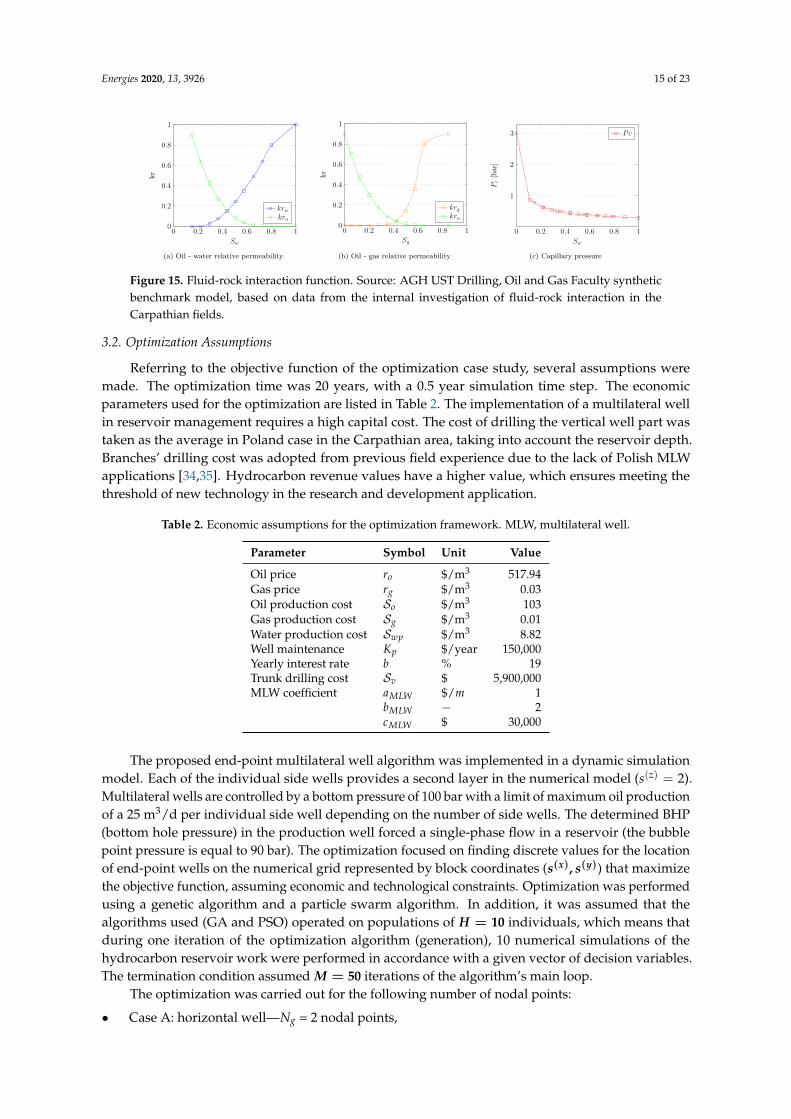
an area of 17.625 km2. The individual cell size is 50 × 50 × 3 m. The spatial distributions of porosity,permeability, NTG (net to gross) , oil saturation, and pressure are presented in Figures 13 and 14.The statistical analysis of the petrophysical properties is presented in Table 1. Fluid-rock interaction isillustrated in Figure 15.

Table 1. Statistical analysis of the basic petrophysical parameters in the evaluated reservoir.Source: typical values for reservoirs located in the Carpathian area of Poland, internal AGH USTDrilling, Oil and Gas faculty report. Adapted from Janiga et al. [33].

Unit Mean Min Med Max

Permeability mD 29.205 15.800 27.070 65.456Porosity (-) 0.06 0.022 0.062 0.119

Net to gross (-) 0.696 0.025 0.713 0.999Oil saturation (-) 0.127 0 0 0.909

Pressure (bar) 278.833 271.690 277.967 289.096

Figure 13. Distributions of the porosity (left), permeability (right), and net-to-gross ratio (center) in thereservoir model. Source: the synthetic reservoir model was developed by AGH UST Drilling, Oil andGas Faculty for academic research purpose. The reservoir horizon map, as well as the petrophysicalproperties determined by the generally available data in the Carpathian area in Poland. The syntheticreservoir is an internal benchmark model for optimization purposes.

Figure 14. Distributions of oil saturation (left) and initial pressure (right) in the reservoir model.Source: AGH UST Drilling Oil and Gas Faculty synthetic benchmark model.

Energies 2020, 13, 3926 15 of 23

Fig. 14: Distributions of oil saturation (left) and initial pressure (right) in reservoir model.Source: AGH UST Drilling Oil and Gas Faculty synthetic benchmark model

0 0.2 0.4 0.6 0.8 10

0.2

0.4

0.6

0.8

1

Sw

kr

krwkro

(a) Oil - water relative permeability

0 0.2 0.4 0.6 0.8 10

0.2

0.4

0.6

0.8

1

Sg

kr

krgkro

(b) Oil - gas relative permeability

0 0.2 0.4 0.6 0.8 1

1

2

3

Sw

Pc

[bar

]

Pc

(c) Capillary pressure

Fig. 15: Fluid - rock interaction function. Source: AGH UST Drilling Oil and Gas Fac-ulty synthetic benchmark model, based on data from internal investigation of fluid-rockinteraction in Carpathian fields.

Table 1: Statistical analysis of basic petrophysical parameters in evaluated reservoir.Source: Typical values for reservoirs located in Carpathian area of Poland, internal AGHUST Drilling, Oil and Gas faculty report. Adapted from Janiga et al.[33]

Unit Mean Min Med Max

Permeability mD 29.205 15.800 27.070 65.456Porosity [-] 0.06 0.022 0.062 0.119Net to gross [-] 0.696 0.025 0.713 0.999Oil saturation [-] 0.127 0 0 0.909Pressure [bar] 278.833 271.690 277.967 289.096

26

Figure 15. Fluid-rock interaction function. Source: AGH UST Drilling, Oil and Gas Faculty syntheticbenchmark model, based on data from the internal investigation of fluid-rock interaction in theCarpathian fields.

3.2. Optimization Assumptions

Referring to the objective function of the optimization case study, several assumptions weremade. The optimization time was 20 years, with a 0.5 year simulation time step. The economicparameters used for the optimization are listed in Table 2. The implementation of a multilateral wellin reservoir management requires a high capital cost. The cost of drilling the vertical well part wastaken as the average in Poland case in the Carpathian area, taking into account the reservoir depth.Branches’ drilling cost was adopted from previous field experience due to the lack of Polish MLWapplications [34,35]. Hydrocarbon revenue values have a higher value, which ensures meeting thethreshold of new technology in the research and development application.

Table 2. Economic assumptions for the optimization framework. MLW, multilateral well.

Parameter Symbol Unit Value

Oil price ro $/m3 517.94Gas price rg $/m3 0.03Oil production cost So $/m3 103Gas production cost Sg $/m3 0.01Water production cost Swp $/m3 8.82Well maintenance Kp $/year 150,000Yearly interest rate b % 19Trunk drilling cost Sv $ 5,900,000MLW coefficient aMLW $/m 1

bMLW − 2cMLW $ 30,000

The proposed end-point multilateral well algorithm was implemented in a dynamic simulationmodel. Each of the individual side wells provides a second layer in the numerical model (s(z) = 2).Multilateral wells are controlled by a bottom pressure of 100 bar with a limit of maximum oil productionof a 25 m3/d per individual side well depending on the number of side wells. The determined BHP(bottom hole pressure) in the production well forced a single-phase flow in a reservoir (the bubblepoint pressure is equal to 90 bar). The optimization focused on finding discrete values for the locationof end-point wells on the numerical grid represented by block coordinates (s(x), s(y)) that maximizethe objective function, assuming economic and technological constraints. Optimization was performedusing a genetic algorithm and a particle swarm algorithm. In addition, it was assumed that thealgorithms used (GA and PSO) operated on populations of H = 10 individuals, which means thatduring one iteration of the optimization algorithm (generation), 10 numerical simulations of thehydrocarbon reservoir work were performed in accordance with a given vector of decision variables.The termination condition assumed M = 50 iterations of the algorithm’s main loop.

The optimization was carried out for the following number of nodal points:

• Case A: horizontal well—Ng = 2 nodal points,

Energies 2020, 13, 3926 16 of 23

• Case B: bilateral well—Ng = 3 nodal points,• Case C: trilateral well—Ng = 4 nodal points,• Case D: quad-lateral well—Ng = 5 nodal points.

4. Results and Discussion

According to the workflow procedure and example implementation schemas, the obtained resultswere gathered and post-processed. Optimization runs were examined in terms of convergence andtermination criteria. The reservoir performance for well design patterns was investigated, and ageneral cause-effect observation was made.

4.1. Reservoir Production Performance and Optimization Results

Firstly, the effect of reservoir performance on the objective function trends will be evaluated.According to Figures 16 and 17, a horizontal well maintains the oil production rate control duringthe whole production period. With the individual control of each side well, it is possible to maintainthe production at a constant level for a period of eight to 20 years with the assumed case study.The horizontal well works with constant performance throughout the entire period, regardless ofthe optimization algorithm chosen. The bilateral well can operate at a constant production rate forover nine years apart from the optimization algorithm. Tri- and quad-lateral wells, due to the highproduction rate, can operate 12.1 and 9.8 years respectively. Decreasing the hydrocarbon productionrate affects the reservoir pressure and reservoir water production rate. The horizontal well pattern hasthe advantage of delaying reservoir water breakthrough. Reservoir brine is produced from the 10thyear of the simulation time. Other well design schema have accelerated water production. The majordifference between the GA and PSO optimization run is visible for the water production in Case C andis related to the modification of one well branch trajectory in a reservoir. In terms of total oil production,Cases C and D have similar end values. However, Case D promotes faster oil production, which has asignificant impact on project NPV. It can be seen that increasing the number of side wells (from threeto four) for both the genetic algorithm and the swarm algorithm does not increase production, but onlyits acceleration over time. The values of the objective function for selected locations of the end-pointnode are presented in Table 3.

0 10 20

0

20

40

60

80

100

Time [yr]

Oil

pro

du

ctio

nra

te[m

3/d

] ABCD

0 10 20

0

0.1

0.2

0.3

Time [yr]

Oil

pro

du

ctio

nto

tal

[mln

m3]

ABCD

0 10 20

0

5

10

Time [yr]

Wat

erp

rod

uct

ion

rate

[m3/d

]

ABCD

0 10 20

100

150

200

250

Time [yr]

Res

ervo

irp

ress

ure

[bar

] ABCD

Fig. 16: Reservoir performance parameters, base on GA optimization run.

30

Figure 16. Reservoir performance parameters, based on the GA optimization run.

Energies 2020, 13, 3926 17 of 23

0 10 20

0

20

40

60

80

100

Time [yr]

Oil

pro

duct

ion

rate

[m3/d

] ABCD

0 10 20

0

0.1

0.2

0.3

Time [yr]

Oil

pro

duct

ion

tota

l[m

lnm

3]

ABCD

0 10 20

0

5

10

15

Time [yr]

Wat

erpro

duct

ion

rate

[m3/d

]

ABCD

0 10 20

100

150

200

250

Time [yr]

Res

ervo

irpre

ssure

[bar

] ABCD

Fig. 17: Reservoir performance parameters, base on PSO optimization run.

31

Figure 17. Reservoir performance parameters, based on the PSO optimization run.

Table 3. The value of the objective function depending on the considered case; optimization of thelocation of multilateral wells.

Objective Function Value (×106$)

Variant GA PSO

A 61.644 61.628B 138.183 138.175C 179.539 181.774D 202.976 206.480

The genetic algorithm and particle swarm optimization algorithm implement mechanisms toavoid local attraction areas in the objective function; however due to the stochastic realization andpopulation upgrade mechanism, a difference between the algorithms can be noticed. Case B has minordivergence in the GA and PSO realization, but even a small well pattern design can affect the objectivefunction. It also should be noted that for the quad-lateral well, capital expenditure is the highest;nevertheless, the acceleration of oil production affects the project NPV, indicating that type of wellas the most promising to implement in the reservoir. The best results were obtained by implementthe PSO algorithm for Case D, outperforming the GA run by 3.5 mln $. A major concern in Case D isthe relatively high reservoir water production from the beginning of production. The end-point welllocation can affect the reservoir’s performance and project profitability.

4.2. Results of Multilateral Well Placement in the 3D Spatial Domain

The optimal solutions for the location of the nodal points of the multilateral wells obtained usingoptimization algorithms are presented in Tables 4 and 5.

Table 4. Coordinate of the block s(x), s(y) enclosed end-point set for the multilateral well, GA algorithm.

Nodal Points s(x), s(y)

Case Center Point P End-Points P

A (38,60) (40,61)B (44,61) (34,59)(48,40)C (46,38) (36,31)(40,64)(48,49)D (46,55) (51,41)(39,31)(29,58)(33,61)

Table 5. Coordinate of the block s(x), s(y) enclosed end-point set for multilateral well, PSO algorithm.

Nodal Points s(x), s(y)

Case Center Point P End-Points P

A (45,40) (47,41)B (44,61) (33,59)(50,40)C (44,57) (47,37)(31,30)(45,64)D (45,49) (37,32)(36,63)(42,63)(55,42)

Energies 2020, 13, 3926 18 of 23

Small changes of the end-point positions can change the project profitability, increase the waterproduction rate, accelerate water breakthrough, and increase the utilization of reservoir energy. Theresult of the optimization algorithm, multilateral trajectories, was implemented on a numerical grid,which is presented in Figures 18 and 19. The objective function for wells with a complex trajectorytakes into account their length; therefore, the results obtained should be treated as optimal in terms oflocation and length. A list of the lengths of individual well branches is shown in Table 6. Consideringthe total well length, GA and PSO propose the same length for Case A. PSO promotes a shorter totalwell length pattern, which can be addressed as drilling risk mitigation.

Table 6. Multilateral well length including individual branches.

Case Distance between Points (m) Total (m)

GA algorithm

A 111.8 111.8B 509.9 1068.88 1578.78C 559.02 850 1081.67 2490.69D 715.89 743.3 863.13 1250 3572.32

PSO algorithm

A 111.8 111.8B 559.02 1092.02 1651.04C 403.11 522.02 1044.03 1969.16D 570.09 640.31 672.68 1077.03 2960.11

(a) Case A (b) Case B

(c) Case C (d) Case D

Figure 18. Multilateral well trajectories—optimal solution, GA algorithm.

Energies 2020, 13, 3926 19 of 23

(a) Case A (b) Case B

(c) Case C (d) Case D

Figure 19. Multilateral well trajectories—optimal solution, PSO algorithm.

4.3. Optimization Run Convergence

Changes in the average and best population fit for the considered case study of implementationof the multi-bottom well are shown in Figures 20 and 21. For both the genetic algorithm and theparticle swarm algorithm, a monotonic increase in the maximum values of the target function wasobserved during the algorithm operation. The optimization run for each of the multilateral wellpatterns was terminated in the case of exceeding the number of iterations or the flattening of objectionfunction trends. In all of the cases, the optimization was terminated by the number of iterations. Thegenetic algorithm has a slower convergence ratio, especially for complex problems (Cases C and D).This is related to the number of decision variables; enhancing the problem search space simultaneouslyrequired several iterations to meet the convergence criteria. Both GA and PSO implement a fine-tuningmechanism; however, that part was not evaluated on this paper.

Energies 2020, 13, 3926 20 of 23

0 20 40 60

25

30

35

40

45

50

55

60

65Fi

tnes

s fu

nctio

n va

lue

[106 $]

Iteration

Max AveNg=2

0 20 40 6070

80

90

100

110

120

130

140

Fitn

ess

func

tion

valu

e [1

06 $]

Iteration

Max AveNg=3

0 20 40 60

80

100

120

140

160

180

Fitn

ess

func

tion

valu

e [1

06 $]

Iteration

Max AveNg=4 Ng=5

0 20 40 6060

80

100

120

140

160

180

200

Fitn

ess

func

tion

valu

e [1

06 $]

Iteration

Max Ave

Figure 20. Changing the value of the objective function (maximum-max and averange-avg) duringGA progress.

0 20 40 600

10

20

30

40

50

60

70

Fitn

ess

func

tion

valu

e [1

06 $]

Iteration

Max AveNg=2

0 20 40 60

60

70

80

90

100

110

120

130

140

Fitn

ess

func

tion

valu

e [1

06 $]

Iteration

Max AveNg=3

0 20 40 6080

90

100

110

120

130

140

150

160

170

180

190

Fitn

ess

func

tion

valu

e [1

06 $]

Iteration

Max AveNg=4 Ng=5

0 20 40 6060

80

100

120

140

160

180

200

220

Fitn

ess

func

tion

valu

e [1

06 $]

Iteration

Max Ave

Figure 21. Changing the value of the objective function (maximum-max and averange-avg) duringPSO progress.

Energies 2020, 13, 3926 21 of 23

4.4. Model Limitation

The proposed model is currently under further improvement; thus, some limitations of applicationcan be listed. The current end-point model development required extensive testing with variousreservoir grid sizes and numbers of cells. However, all tests were performed on orthogonal celldistributions along with the numerical model. That assumption is fulfilled by the Schlumberger Petrel(Version: 2019, Manufacturer: Schlumberger) software used in this study, which develops a reservoirnumerical model from geological model forcing cell orthogonality. The impact of cell geometryon the multilateral well trajectory is meaningless, due to the fact that the model evaluates truespatial coordinates. Our preliminary investigation shows that the end-point model can be effectivelyimplemented in any numerical model as long as a multilateral well is placed in a global grid or a localgrid directly. The mixing of global and local grid placement is currently forbidden. It also shouldbe noted that the increase of the total cell number in the reservoir model can significantly increasethe solution search space, which may lead to optimization conversion failure. We recommendedperforming a coarse optimization run to establish a promising search space and reduce the searchspace in the case of fine grid optimization.

5. Conclusions

The assumed goal of the work was achieved, and based on the results obtained, the followingconclusions can be made:

• It seems necessary to use a minimum of two different optimization methods to validate the qualityof the solutions obtained,

• The optimization model developed can be used to complement the manual search method,• Multilateral wells will be concerned as a must in the effective management of hydrocarbon

reservoirs, especially in an off-shore application; thus, optimization of trajectory planning shouldbe taken into consideration,

• The proposed end-point optimization model integrates well trajectory planning with the reservoirmodel; thus, the obtained results can be used in effective reservoir management in different timedomains,

• Our end-point algorithm is easily implemented in the reservoir model and, based on theapplication of the population-type optimization algorithm, is time-efficient, as well as effortlesslyscalable among various models.

Author Contributions: Conceptualization, D.J.; methodology, D.J.; software, D.J.; validation, D.J. and P.W.;writing–original draft preparation, D.J. and D.P.; writing–review and editing, D.J.; supervision, J.S. and P.W. Allauthors have read and agreed to the published version of the manuscript.

Funding: This research received no external funding.

Conflicts of Interest: The authors declare no conflict of interest

References

1. Janiga, D. Model Optymalizacji Udostepnienia i Eksploatacji Zloza Weglowodorow z WykorzystaniemSztucznej Inteligencji. Ph.D. Thesis, AGH University of Science and Technology, Krakow, Poland, 2017.

2. Yue, P.; Jia, B.; Sheng, J.; Lei, T.; Tang, C. A coupling model of water breakthrough time for a multilateralhorizontal well in a bottom water-drive reservoir. J. Pet. Sci. Eng. 2019, 177, 317–330. [CrossRef]

3. Stopa, J.; Rychlicki, S.; Wojnarowski, P.; Kosowski, P. Zastosowanie odwiertow rozgalezionych w eksploatacjizloz ropy i gazu. Wiertnictwo Naft. Gaz 2007, 24, 869–876.

4. Elyasi, S. Assessment and evaluation of degree of multilateral well’s performance for determination of theirrole in oil recovery at a fractured reservoir in Iran. Egypt. J. Pet. 2016, 25, 1–14. [CrossRef]

5. Chin, W.C. Quantitative Methods in Reservoir Engineering; Gulf Professional Publishing: Houston, TX,USA, 2002.

Energies 2020, 13, 3926 22 of 23

6. Tangparitkul, S. Evaluation of effecting factors on oil recovery using the desirability function. J. Pet. Explor.Prod. Technol. 2018, 8, 1199–1208. [CrossRef]

7. Abusahmin, B.S.; Karri, R.R.; Maini, B.B. Influence of fluid and operating parameters on the recoveryfactors and gas oil ratio in high viscous reservoirs under foamy solution gas drive. Fuel 2017, 197, 497–517.[CrossRef]

8. Song, X.; Zhang, C.; Shi, Y.; Li, G. Production performance of oil shale in-situ conversion with multilateralwells. Energy 2019, 189, 116145. [CrossRef]

9. Wei, Y.; Jia, A.; Wang, J.; Luo, C.; Qi, Y. Semi-analytical Modeling of Pressure-Transient Response ofMultilateral Horizontal Well with Pressure Drop along Wellbore. J. Nat. Gas Sci. Eng. 2020, 80, 103374.[CrossRef]

10. Yang, Y.; Cui, S.; Ni, Y.; Zhang, G.; Li, L.; Meng, Z. Key technology for treating slack coal blockage in CBMrecovery: A case study from multi-lateral horizontal wells in the Qinshui Basin. Nat. Gas Ind. B 2016,3, 66–70. [CrossRef]

11. Chen, D.; Pan, Z.; Liu, J.; Connell, L.D. Characteristic of anisotropic coal permeability and its impact onoptimal design of multi-lateral well for coalbed methane production. J. Pet. Sci. Eng. 2012, 88, 13–28.[CrossRef]

12. Zhou, S.W.; Sun, F.J.; Zeng, X.L.; Fang, M.J. Application of multilateral wells with limited sand productionto heavy oil reservoirs. Pet. Explor. Dev. 2008, 35, 630–635. [CrossRef]

13. Shi, Y.; Song, X.; Wang, G.; McLennan, J.; Forbes, B.; Li, X.; Li, J. Study on wellbore fluid flow and heattransfer of a multilateral-well CO2 enhanced geothermal system. Appl. Energy 2019, 249, 14–27. [CrossRef]

14. Aadnøy, B.S. Technology Focus: Multilateral and Complex-Trajectory Wells. J. Pet. Technol. 2019, 71, 71.[CrossRef]

15. Lyu, Z.; Song, X.; Li, G. A semi-analytical method for the multilateral well design in different reservoirsbased on the drainage area. J. Pet. Sci. Eng. 2018, 170, 582–591. [CrossRef]

16. Lyu, Z.; Song, X.; Geng, L.; Li, G. Optimization of multilateral well configuration in fractured reservoirs.J. Pet. Sci. Eng. 2019, 172, 1153–1164. [CrossRef]

17. Buhulaigah, A.; Al-Mashhad, A.S.; Al-Arifi, S.A.; Al-Kadem, M.S.; Al-Dabbous, M.S. Multilateral wellsevaluation utilizing artificial intelligence. In Proceedings of the SPE Middle East Oil & Gas Show andConference, Manama, Bahrain, 6–9 March 2017; Society of Petroleum Engineers: Richardson, TX, USA, 2017.Available online: https://www.onepetro.org/conference-paper/SPE-183688-MS (accessed on 15 June 2020).

18. Garrouch, A.A.; Lababidi, H.M.; Ebrahim, A.S. A web-based expert system for the planning and completionof multilateral wells. J. Pet. Sci. Eng. 2005, 49, 162–181. [CrossRef]

19. Xu, B.; Baird, R.; Vukovich, G. Fuzzy evolutionary algorithms and automatic robot trajectory generation.In Methods and Applications of Intelligent Control; Springer: Dordrecht, The Netherlands, 1997; pp. 423–449.

20. Miller, B.L.; Goldberg, D.E. Genetic algorithms, tournament selection, and the effects of noise. Complex Syst.1995, 9, 193–212.

21. Alajmi, A.; Wright, J. Selecting the most efficient genetic algorithm sets in solving unconstrained buildingoptimization problem. Int. J. Sustain. Built Environ. 2014, 3, 18 – 26. [CrossRef]

22. Eberhart, C.; Kennedy, J. A new optimizer using particle swarm theory. In Proceedings of the SixthInternational Symposium on Micro Machine and Human Science, Nagoya, Japan, 4–6 October 1995; IEEE:New York, NY, USA, 1995; Volume 1, pp. 39–43.

23. Kennedy, J. Particle swarm optimization. In Encyclopedia of Machine Learning; Springer: Berlin/Heidelberg,Germany, 2011; pp. 760–766.

24. Shi, Y.; Eberhart, R. A modified particle swarm optimizer. In Proceedings of the 1998 IEEE InternationalConference on Evolutionary Computation Proceedings. IEEE World Congress on Computational Intelligence(Cat. No.98TH8360), Anchorage, AK, USA, 4–9 May 1998; pp. 69–73.

25. Almeida, L.F.; Tupac, Y.J.; Pacheco, M.A.C.; Vellasco, M.M.B.R.; Lazo, J.G.L. Evolutionary optimizationof smart-wells control under technical uncertainties. In Proceedings of the Latin American & CaribbeanPetroleum Engineering Conference, Buenos Aires, Argentina, 15–18 April 2007; Society of PetroleumEngineers: Richardson, TX, USA, 2007. Available online: https://www.onepetro.org/conference-paper/SPE-107872-MS (accessed on 15 June 2020).

26. Awotunde, A.A.; Sibaweihi, N. Consideration of voidage-replacement ratio in well-placement optimization.SPE Econ. Manag. 2014, 6, 40–54. [CrossRef]

Energies 2020, 13, 3926 23 of 23

27. Bellout, M.C.; Echeverría Ciaurri, D.; Durlofsky, L.; Foss, B.; Kleppe, J. Joint optimization of oil wellplacement and controls. Comput. Geosci. 2012, 16, 1061–1079. [CrossRef]

28. Brouwer, D.; Jansen, J. Dynamic Optimization of Waterflooding With Smart Wells Using Optimal ControlTheory. In Proceedings of the European Petroleum Conference, Aberdeen, UK, 29–31 October 2002.[CrossRef]

29. Doublet, D.C.; Aanonsen, S.I.; Tai, X.C. An efficient method for smart well production optimisation. J. Pet.Sci. Eng. 2009, 69, 25–39. [CrossRef]

30. Forouzanfar, F.; Reynolds, A. Well-placement optimization using a derivative-free method. J. Pet. Sci. Eng.2013, 109, 96–116. [CrossRef]

31. Gross, H. Response surface approaches for large decision trees: Decision making under uncertainty.In Proceedings of the ECMOR XIII-13th European Conference on the Mathematics of Oil Recovery, Biarritz,France, 10–13 September 2012.

32. Isebor, O.J.; Durlofsky, L.J. Biobjective optimization for general oil field development. J. Pet. Sci. Eng. 2014,119, 123–138. [CrossRef]

33. Janiga, D.; Czarnota, R.; Stopa, J.; Wojnarowski, P. Self-adapt reservoir clusterization method to enhancerobustness of well placement optimization. J. Pet. Sci. Eng. 2019, 173, 37–52. [CrossRef]

34. El-Sayed, A.A.H.; AI-Awad, M.; Al-Blehed, M.; Al-Saddiqui, M. An Economic Model for Assessing theFeasibility of Multilateral Wells. J. King Saud Univ.-Eng. Sci. 2001, 13, 153–176. [CrossRef]

35. Manshad, A.K.; Dastgerdi, M.E.; Ali, J.A.; Mafakheri, N.; Keshavarz, A.; Iglauer, S.; Mohammadi, A.H.Economic and productivity evaluation of different horizontal drilling scenarios: Middle East oil fields ascase study. J. Pet. Explor. Prod. Technol. 2019, 9, 2449–2460. [CrossRef]

c© 2020 by the authors. Licensee MDPI, Basel, Switzerland. This article is an open accessarticle distributed under the terms and conditions of the Creative Commons Attribution(CC BY) license (http://creativecommons.org/licenses/by/4.0/).