EMTL: A GENERATIVE DOMAIN ADAPTATION APPROACH

Under review as a conference paper at ICLR 2021

EMTL: A GENERATIVE DOMAIN ADAPTATIONAPPROACH

Anonymous authorsPaper under double-blind review

ABSTRACT

We propose an unsupervised domain adaptation approach based on generativemodels. We show that when the source probability density function can be learned,one-step Expectation–Maximization iteration plus an additional marginal densityfunction constraint will produce a proper mediator probability density functionto bridge the gap between the source and target domains. The breakthrough isbased on modern generative models (autoregressive mixture density nets) thatare competitive to discriminative models on moderate-dimensional classificationproblems. By decoupling the source density estimation from the adaption steps,we can design a domain adaptation approach where the source data is locked awayafter being processed only once, opening the door to transfer when data securityor privacy concerns impede the use of traditional domain adaptation. We demon-strate that our approach can achieve state-of-the-art performance on synthetic andreal data sets, without accessing the source data at the adaptation phase.

1 INTRODUCTION

In the classical supervised learning paradigm, we assume that the training and test data come fromthe same distribution. In practice, this assumption often does not hold. When the pipeline includesmassive data labeling, models are routinely retrained after each data collecion campaign. However,data labeling costs often make retraining impractical. Without labeled data, it is still possible totrain the model by using a training set which is relevant but not identically distributed to the test set.Due to the distribution shift between the training and test sets, the performance usually cannot beguaranteed.

Domain adaptation (DA) is a machine learning subdomain that aims at learning a model from biasedtraining data. It explores the relationship between source (labeled training data) and target (test data)domains to find the mapping function and fix the bias, so that the model learned on the source datacan be applied in target domain. Usually some target data is needed during the training phase tocalibrate the model. In unsupervised domain adaptation (UDA) only unlabeled target data is neededduring training phase. UDA is an appealing learning paradigm since obtaining unlabeled data isusually easy in a lot of applications. UDA allows the model to be deployed in various target domainswith different shifts using a single labeled source data set.

Due to these appealing operational features, UDA has became a prominent research field with var-ious approaches. Kouw & Loog (2019) and Zhuang et al. (2020) surveyed the latest progress onUDA and found that most of the approaches are based on discriminative models, either by reweight-ing the source instances to approximate the target distribution or learning a feature mapping functionto reduce the statistical distance between the source and target domains. After calibrating, a discrim-inative model is trained on the adjusted source data and used in target domain. In this workflow, theadaptation algorithm usually have to access the source and target data simultaneously. However,accessing the source data during the adaptation phase is not possible when the source data is sensi-tive (for example because of security or privacy issues). In particular, in our application workflowan industrial company is selling devices to various service companies which cannot share their cus-tomer data with each other. The industrial company may contract with one of the service companiesto access their data during an R&D phase, but this data will not be available when the industrialcompany sells the device (and the predictive model) to other service companies.

1


In this paper we propose EMTL, a generative UDA algorithm for binary classification that does nothave to access the source data during the adaptation phase. We use density estimation to estimatethe joint source probability function ps(x, y) and the marginal target probability function pt(x) anduse them for domain adaption. To solve the data security issue, EMTL decouples source densityestimation from the adaptation steps. In this way, after the source preprocessing we can put away ordelete the source data. Our approach is motivated by the theory on domain adaptation (Ben-Davidet al., 2010) which claims that the error of a hypothesis h on the target domain can be bounded bythree items: the error on the source domain, the distance between source and target distributions, andthe expected difference in labeling functions. This theorem motivated us to define a mediator densityfunction pm(x, y) i) whose conditional probability y|x is equal to the conditional probability of thesource and ii) whose marginal density on x is equal to the marginal density of the target. We canthen construct a Bayes optimal classifier on the target domain under the assumption of covariateshift (the distribution y|x is the same in the source and target domains).

Our approach became practical with the recent advances in (autoregressive) neural density estima-tion (Uria et al., 2013). We learn pm(x, y) from ps(x, y) and pt(x) to bridge the gap between thesource and target domains. We regard the label on the target data as a latent variable and show thatif ps(x |y = i) be learned perfectly for i ∈ {0, 1}, then a one-step Expectation–Maximization (andthis is why our algorithm named EMTL) iteration will produce a density function pm(x, y) withthe following properties on the target data: i) minimizing the Kullback–Leibler divergence betweenpm(yi|xi) and ps(yi|xi); ii) maximizing the log-likelihood

∑log pm(xi). Then, by adding an

additional marginal constraint on pm(xi) to make it close to pt(xi) on the target data explicitly,we obtain the final objective function for EMTL. Although this analysis assumes a simple covariateshift , we will experimentally show that EMTL can go beyond this assumption and work well inother distribution shifts.

We conduct experiments on synthetic and real data to demonstrate the effectiveness of EMTL. First,we construct a simple two-dimensional data set to visualize the performance of EMTL. Second, weuse UCI benchmark data sets and the Amazon reviews data set to show that EMTL is competitivewith state-of-the-art UDA algorithms, without accessing the source data at the adaptation phase.To our best knowledge, EMTL is the first work using density estimation for unsupervised domainadaptation. Unlike other existing generative approaches (Kingma et al., 2014; Karbalayghareh et al.,2018; Sankaranarayanan et al., 2018), EMTL can decouple the source density estimation processfrom the adaption phase and thus it can be used in situations where the source data is not availableat the adaptation phase due to security or privacy reasons.

2 RELATED WORK

Zhuang et al. (2020), Kouw & Loog (2019) and Pan & Yang (2009) categorize DA approaches intoinstance-based and feature-based techniques. Instance-based approaches reweight labeled sourcesamples according to the ratio of between the source and the target densities. Importance weightingmethods reweight source samples to reduce the divergence between the source and target densities(Huang et al., 2007; Gretton et al., 2007; Sugiyama et al., 2007). In contrast, class importanceweighting methods reweight source samples to make the source and target label distribution the same(Azizzadenesheli et al., 2019; Lipton et al., 2018; Zhang et al., 2013). Feature-based approacheslearn a new representation for the source and the target by minimizing the divergence between thesource and target distributions. Subspace mapping methods assume that there is a common subspacebetween the source and target (Fernando et al., 2013; Gong et al., 2012). Courty et al. (2017)proposed to use optimal transport to constrain the learning process of the transformation function.Other methods aim at learning a representation which is domain-invariant among domains (Gonget al., 2016; Pan et al., 2010).

Besides these shallow models, deep learning has also been widely applied in domain adaptation(Tzeng et al., 2017; Ganin et al., 2016; Long et al., 2015). DANN (Ganin et al., 2016) learnsa representation using a neural network which is discriminative for the source task while cannotdistinguish the source and target domains from each other. Kingma et al. (2014) and Belhaj et al.(2018) proposed a variational inference based semi-supervised learning approach by regarding themissing label as latent variable and then performing posterior inference.

2


3 NOTATION AND PROBLEM DEFINITION

We consider the unsupervised domain adaptation problem in a binary classification setting (the setupis trivial to extend to multi-class classification). Let p(x, y) be a joint density function defined onX × Y , where x ∈ Rp is the feature vector and y ∈ {0, 1} is the label. We denote the conditionalprobability p(y = 1|x) by q(x). A hypothesis or model is a function h : X 7→ [0, 1]. We define theerror of h as the expected disagreement between h(x) and q(x), i.e.,

ε(h) = Ex∼p |h(x)− q(x)|. (1)

We use superscripts s and t to distinguish the source and target domains, that is, ps(x, y) and pt(x, y)are the joint density functions in the source and target domains respectively. In general, we assumethat ps(x, y) 6= pt(x, y).

Let Ds = {(xsi , y

si)}n

s

i=1 and U t = {xti}n

t

i=1 be i.i.d. data sets generated from the source distributionps(x, y) and the marginal target distribution pt(x), respectively, where ns and nt are source andtarget sample sizes. The objective of unsupervised domain adaptation is to learn a model h by usinglabeled Ds and unlabeled U t, which achieves lowest error in target domain.

4 GENERATIVE APPROACH

Ben-David et al. (2010) proved that the error of a hypothesis h in the target domain εt(h) can bebounded by the sum of error in source domain εs(h), the distribution distance between the twodomains, and the expected L1 distance between two conditional probabilities.

Theorem 1 (Ben-David et al. (2010), Theorem 1) For a hypothesis h,

εt(h) ≤ εs(h) + d1(ps(x), pt(x)) + min{Ex∼ps |qs(x)− qt(x)|,Ex∼pt |qs(x)− qt(x)|}, (2)

where d1(ps(x), pt(x)) = 2supB∈B|Prs(B) − Prt(B)| is the twice the total variation distance of two

domain distributions and qs(x) and qt(x) are the source and target probabilities of y = 1|x, re-spectively.

In the covariate shift setting, we assume that the conditional probability p(y|x) is invariant betweenthe source and the target domains. Thus in the right hand side of Eq. (2), the third component willbe zero, which means that the target error is bounded by the source error plus the distance betweentwo domains. Many current unsupervised domain adaptation solutions work on how to reduce thedistance between the two domain densities. Importance-sampling-based approaches manage to re-sample the source data to mimic the target data distribution, and feature-mapping-based approachesdo that by learning a transformation function φ(x) for the source data. However, both approachesneed to access source and target data simultaneously.

In this paper, we propose a domain adaptation approach based on generative models. First, we learnall multivariate densities using RNADE (Uria et al., 2013), an autoregressive version of Bishop(1994)’s mixture density nets. We found RNADE excellent in learning medium-dimensional densi-ties, and in a certain sense it is RNADE that made our approach feasible. Second, we introduce amediator joint density function pm(x, y) that bridges the gap between ps(x, y) and pt(x, y). Sincethe source distribution information is stored in the learned generative model after training, we donot need to access source data in the adaptation phase.

4.1 DENSITY FUNCTION

Due to recent developments in neural density estimation, we can estimate moderate-dimensionaldensities efficiently. In this paper, we use real-valued autoregressive density estimator (RNADE) ofUria et al. (2013). RNADE is an autoregressive version of mixture density nets of Bishop (1994)which fights the curse of dimensionality by estimating conditional densities, and provides explicitlikelihood by using mixtures of Gaussians.

To estimate p(x), let x = [x1, x2, · · · , xp] be a p dimensional random vector. RNADE decom-poses the joint density function using the chain rule and models each p(xi|x<i) with a mixture of

3


Gaussians whose parameters depend on observed x<i. Formally,

p(x) =

p∏i=1

p(xi|x<i) =p∏i=1

( d∑j=1

αj(x<i)N (xi;µj(x<i), σ2j (x<i))

), (3)

where x<i = [x1, · · · , xi−1] and d is the number of Gaussian components. The weights αj , meansµj , and variances σj are modeled by a single neural net whose architecture makes sure that theparameter ·j(x<i) depends only on x<i. The neural net is trained to maximize the likelihood ofthe training data. We denote the RNADE model by the function f(x;ω), where ω represents all theparameters (neural net weights) in RNADE, and use it to approximate p(x). The conditional densityp(x |y) can be estimated in the same way by just selecting x |y as the training data. In followingsections, we denote the maximum likelihood parameters of ps(x |y = 0), ps(x |y = 1), and pt(x)by ωs0, ωs1, and ωt, respectively. We further denote the proportion of class 0 in the source domainby τs0 = #{ys=0}

ns . The full parameter vector [ωs0, ωs1, τs0] of ps(x, y) and ps(x) is denoted by θs.

4.2 THE MEDIATOR DISTRIBUTION

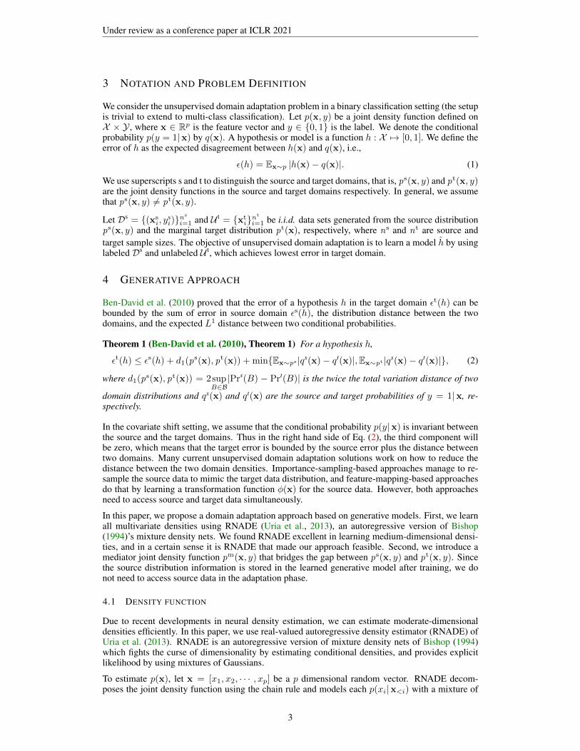
By Eq. (2), the target error can be bounded by the source error plus the distance between the twomarginal distributions plus the expected difference in p(y = 1|x) between two domains. Thismotivated us to construct a mediator distribution pm(x, y) (Figure 1) which has two properties:

• it has the same conditional distribution as the source: pm(y|x) = ps(y|x), and• it has the same marginal distribution as the target: pm(x) = pt(x).

ps (x, y) −−−−−−−−−−→ pm︸︷︷︸ps(y|x)=pm(y|x)

pm(x)=pt(x)︷︸︸︷(x, y) −−−−−−−−−−→ pt(x, y)

Figure 1: The mediator has the same conditional probability as the source and the same marginalprobability as target. According to Theorem 1, we will have εt(h) ≤ εm(h) for any hypotheses hsince the last two terms are zero.

In the covariate shift setting, we can then solve the unsupervised domain adaptation problemperfectly: i) the first property forces p(y|x) to be the same in source and mediator distribu-tions, and in the covariate shift setting we have ps(y|x) = pt(y|x), then this property makespm(y|x) = pt(y|x); ii) the second property makes the marginal distributions of the mediator andthe target the same, which leads to d1(pm(x), pt(x)) = 0. Under these two conditions, for anymodel h, we will have εt(h) ≤ εm(h) since the last two terms of Eq. (2) will be zero. Furthermore,given the mediator distribution pm(x, y), it is easy to learn the best model (Bayes classifier)

h(x) =pm(x |y = 1) pm(y = 1)

pm(x), (4)

which achieves the tightest bound for the target error. In summary, by introducing the mediator dis-tribution pm(x, y), we can bound the target error by the mediator error. In the following sections, wewill introduce how to learn pm(x, y) from ps(x, y) and pt(x) using the expectation-maximization(EM) algorithm combined with a marginal constraint term.

5 EMTL

If we regard the missing label y as a latent variable that generates observed x in the target domain,we can use the EM algorithm to infer y. We consider that the target density p(x; θ) is a mixturewith two components p(x |y = i; θ) where i ∈ {0, 1}. When θ converges to its limit θ∗ in EM, wecan recover the joint density function p(x, y; θ∗). We denote this joint density function by pm(x, y).However, this pm(x, y) may be far away from the ground truth pt(x, y). The mismatch comes fromtwo facts: i) EM can easily converge to a bad local minimum because of a bad initialization, andii) EM tends to find inner structure (e.g., clusters) of the data but this structure may be irrelevant

4


to the true label. The local minimum problem is due to parameter initialization, and the structure-label mismatching problem comes from not having a-priori information of the label. When we havea fully known source distribution ps(x, y), these two issues can be solved by selecting a properinitialization plus a constraint on marginal distribution.

The first observation is that in a lot of cases we can directly use the source model in the target domainand it is better than random guess. We use this intuition to make the source model ps(x, y) as theinitial guess of pm(x, y). Following section 4.1, we use RNADE to model pm(x |y) and denoteparameters of pm(x, y) by θm = [ωm0, ωm1, τm0]. Initializing pm(x, y) by using ps(x, y) meanswe set θ(0)m , the initial state of θm in the EM algorithm, to θs. The next EM iterations can be seenas a way to fine-tune θm using the target data. In the next sections we will formally analyze thisintuitive algorithm.

5.1 ANALYSIS θ(1)m

First we link the EM algorithm with initial θ(0)m = θs to Theorem 1. In each iteration, EM alternatesbetween two steps: E step defines a Q function as Q(θ|θ(t)) = Ey|x,θ(t) log p(θ;x, y) and M stepdo the maximization θ(t+1) = argmaxθ Q(θ|θ(t)). After the first EM iteration, we have

θ(1)m = argmaxθ

Q(θ| θ(0)m ) = argmaxθ

1

nt

nt∑i=1

Eyi|xti ,θs

log p(xti , yi; θ). (5)

Suppose θs is learned perfectly from source data, which means that we can replace p(x, y; θ(0)m ) byps(x, y). Thus the expectation operation in Eq. (5) can be written as

Eyi|xti ,θs

[ξ] =∑

j∈{0,1}

p(yi = j|xti ; θs)ξ =

∑j∈{0,1}

ps(yi = j|xti)ξ (6)

for any random variable ξ. This expectation links the source distribution with the target. We rewritethe full expectation expression of Eq. (5) as

Eyi|xti ,θs

log p(xti , yi; θ) =

∑j∈{0,1}

ps(yi = j|xti) log p(x

ti , yi = j; θ)

= −DKL(ps(yi|xt

i)‖p(yi|xti ; θ)) + log p(xt

i ; θ)−Hps(yi|xti),

(7)

where Hps(yi|xti) is the conditional entropy on probability ps. This equation shows that the ex-

pected log-likelihood can be decomposed into the sum of three items. the first item is the negativeKL-divergence between the two conditional distributions ps(yi|xt

i) and p(yi|xti ; θ); the second item

is the target log-likelihood log p(xti |θ); the last item is the negative entropy of the source conditional

distribution, which is irrelevant to parameter θ so can be ignored during the optimization.

Therefore, by setting θ(0)m as θs and maximizing the Q function in the first EM iteration, we willget a pm(x, y) which minimizes the KL-divergence between pm(y|x) with ps(y|x) and maximizeslog pm(x). Minimizing the KL-divergence reduces the third term of Eq. (2) and maximizing thelog-likelihood forces pm(x) to move towards pt(x) implicitly, which reduces the second item ofEq. (2). This suggests that the Bayes classifier pm(y|x) can be a proper classifier for target domain.

5.2 MARGINAL CONSTRAINT

In the previous section, we implicitly reduce the distance between pm(x) and pt(x) by maximizingthe log-likelihood of p(x; θ) on the target data. To further control the target error bound Eq. (2),we explicitly add a marginal constraint for pm(x, y) by minimizing the distance between the twomarginal distributions. Rather than calculating d1(pm(x), pt(x)) directly, we use the KL-divergenceto measure the distance between two distributions since we can explicitly calculate the pm(xt

i) andpt(xt

i) by using our density estimators. Furthermore, according to Pinsker’s inequality (Tsybakov,2008), we have

d1(pm(x), pt(x)) ≤

√2DKL(pm(x)‖ pt(x)), (8)

5


thus minimizing the KL-divergence also controls d1(pm(x), pt(x)). Since we only have samples xti

from the target domain, we use an empirical version of the KL-divergence. The marginal constraintis defined as

M(θ) =√2×

( nt∑i=1

pt(xti) log

pt(xti)

pm(xti)

) 12

=√2×

( nt∑i=1

f(xti ;ωt) log

f(xti ;ωt)

p(xti ; θ)

) 12

, (9)

where p = p/∑p and f = f/

∑f are normalized discrete distributions on the target samples.

5.3 OBJECTIVE FUNCTION OF EMTL

By putting the Q and M functions together, we get the objective function

θ∗ = argminθ−Q(θ| θ(0)m ) + ηM(θ) (10)

of our generative domain adaptation approach, where θ(0)m = θs and η is a non-negative hyperpa-rameter that controls the trade-off of the two terms.

In real-life scenarios, both p(x) and p(y|x) can be different in the source and target domains sothe covariate shift assumption may be violated. To go beyond this assumption, we need to relaxthe constraint on ps(y|x) = pt(y|x) which is used in justifying Q(θ|θ(0)). As we will show inSection 6, by setting a large η and doing more iterations, EMTL will reduce the weight on theQ function and allow us to escape from covariate shift constraints. We summarize the process ofEMTL in Algorithm 1.

Algorithm 1: EMTL AlgorithmResult: EMTL classifier pm(y = 1|x)Initialize θs = [ωs0, ωs1, τs0] and ωt using Ds and U t, respectively;Initialize θ(0)m by θs and t = 1;while t ≤ n itr do

θ(t)m = argminθ −Q(θ|θ(t−1)m ) + ηM(θ);t = t+ 1;

endpm(x, y) = p(x, y; θ

(t)m );

pm(y = 1|x) = pm(x |y=1) pm(y=1)pm(x) =

(1−τ(t)m0 )f(x;ω

(t)m1 )

(1−τ(t)m0 )f(x;ω

(t)m1 )+τ

(t)m0 f(x;ω

(t)m0 )

;

6 EXPERIMENTS

In this section, we present experiments on both synthetic (Section 6.1) and real-life data (Section 6.2)to validate the effectiveness of EMTL.

6.1 EXPERIMENTS ON SYNTHETIC DATA SET

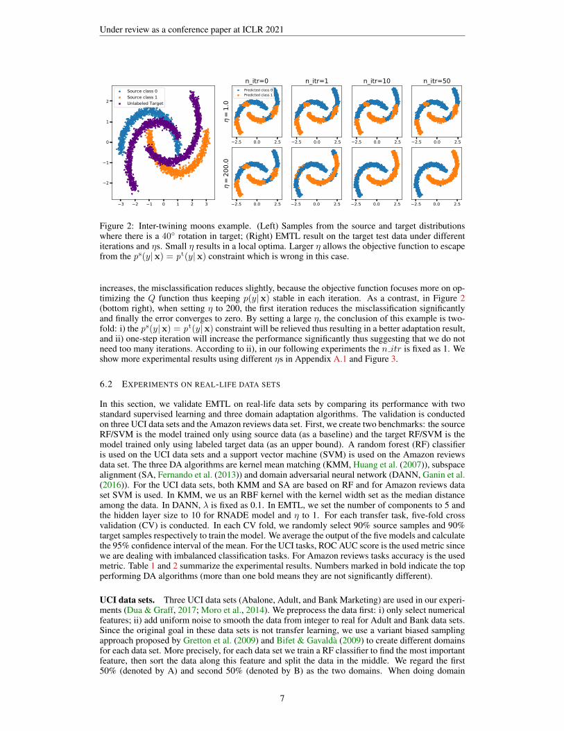
We study the performance of EMTL under conditional shift where ps(x |y) 6= pt(x |y) using avariant of inter-twinning moons example (Ganin et al., 2016). In the source domain we generatean upper moon (class 0) and a lower moon (class 1) with 1000 points in each class. In the targetdomain, we first generate 2000 samples as in the source then rotate the data by 40◦ to make thetarget distribution of x |y different from the source. Figure 2 (left) shows the source and targetdistributions. In this experiments, we set the number of Gaussian components to 10 and the hiddenlayer dimension to 30 in the RNADE model.

We set η to 1 and 200 to illustrate how a large η helps the model to escape from covariate shiftconstraint. Figure 2 (upper right) shows the prediction results in the target data using η = 1. Whenn itr = 0, the EMTL classifier is the source Bayes classifier. In the upper moon, the model mis-classifies the middle and the tail parts as class 1. This is because according to the source distribu-tion, these areas are closer to class 1. The same misclassification occurs in lower moon. As n itr

6


3 2 1 0 1 2 3

2

1

0

1

2

Source class 0Source class 1Unlabeled Target

2.5 0.0 2.5

=1.

0

n_itr=0Predicted class 0Predicted class 1

2.5 0.0 2.5

n_itr=1

2.5 0.0 2.5

n_itr=10

2.5 0.0 2.5

n_itr=50

2.5 0.0 2.5

=20

0.0

2.5 0.0 2.5 2.5 0.0 2.5 2.5 0.0 2.5

Figure 2: Inter-twining moons example. (Left) Samples from the source and target distributionswhere there is a 40◦ rotation in target; (Right) EMTL result on the target test data under differentiterations and ηs. Small η results in a local optima. Larger η allows the objective function to escapefrom the ps(y|x) = pt(y|x) constraint which is wrong in this case.

increases, the misclassification reduces slightly, because the objective function focuses more on op-timizing the Q function thus keeping p(y|x) stable in each iteration. As a contrast, in Figure 2(bottom right), when setting η to 200, the first iteration reduces the misclassification significantlyand finally the error converges to zero. By setting a large η, the conclusion of this example is two-fold: i) the ps(y|x) = pt(y|x) constraint will be relieved thus resulting in a better adaptation result,and ii) one-step iteration will increase the performance significantly thus suggesting that we do notneed too many iterations. According to ii), in our following experiments the n itr is fixed as 1. Weshow more experimental results using different ηs in Appendix A.1 and Figure 3.

6.2 EXPERIMENTS ON REAL-LIFE DATA SETS

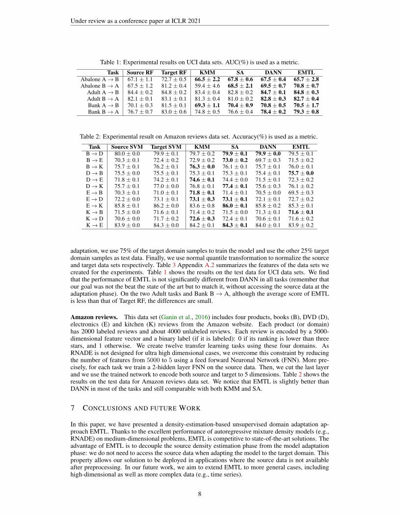
In this section, we validate EMTL on real-life data sets by comparing its performance with twostandard supervised learning and three domain adaptation algorithms. The validation is conductedon three UCI data sets and the Amazon reviews data set. First, we create two benchmarks: the sourceRF/SVM is the model trained only using source data (as a baseline) and the target RF/SVM is themodel trained only using labeled target data (as an upper bound). A random forest (RF) classifieris used on the UCI data sets and a support vector machine (SVM) is used on the Amazon reviewsdata set. The three DA algorithms are kernel mean matching (KMM, Huang et al. (2007)), subspacealignment (SA, Fernando et al. (2013)) and domain adversarial neural network (DANN, Ganin et al.(2016)). For the UCI data sets, both KMM and SA are based on RF and for Amazon reviews dataset SVM is used. In KMM, we us an RBF kernel with the kernel width set as the median distanceamong the data. In DANN, λ is fixed as 0.1. In EMTL, we set the number of components to 5 andthe hidden layer size to 10 for RNADE model and η to 1. For each transfer task, five-fold crossvalidation (CV) is conducted. In each CV fold, we randomly select 90% source samples and 90%target samples respectively to train the model. We average the output of the five models and calculatethe 95% confidence interval of the mean. For the UCI tasks, ROC AUC score is the used metric sincewe are dealing with imbalanced classification tasks. For Amazon reviews tasks accuracy is the usedmetric. Table 1 and 2 summarize the experimental results. Numbers marked in bold indicate the topperforming DA algorithms (more than one bold means they are not significantly different).

UCI data sets. Three UCI data sets (Abalone, Adult, and Bank Marketing) are used in our experi-ments (Dua & Graff, 2017; Moro et al., 2014). We preprocess the data first: i) only select numericalfeatures; ii) add uniform noise to smooth the data from integer to real for Adult and Bank data sets.Since the original goal in these data sets is not transfer learning, we use a variant biased samplingapproach proposed by Gretton et al. (2009) and Bifet & Gavalda (2009) to create different domainsfor each data set. More precisely, for each data set we train a RF classifier to find the most importantfeature, then sort the data along this feature and split the data in the middle. We regard the first50% (denoted by A) and second 50% (denoted by B) as the two domains. When doing domain

7


Table 1: Experimental results on UCI data sets. AUC(%) is used as a metric.

Task Source RF Target RF KMM SA DANN EMTLAbalone A→ B 67.1 ± 1.1 72.7 ± 0.5 66.5 ± 2.2 67.8 ± 0.6 67.5 ± 0.4 65.7 ± 2.8Abalone B→ A 67.5 ± 1.2 81.2 ± 0.4 59.4 ± 4.6 68.5 ± 2.1 69.5 ± 0.7 70.8 ± 0.7

Adult A→ B 84.4 ± 0.2 84.8 ± 0.2 83.4 ± 0.4 82.8 ± 0.2 84.7 ± 0.1 84.8 ± 0.3Adult B→ A 82.1 ± 0.1 83.1 ± 0.1 81.3 ± 0.4 81.0 ± 0.2 82.8 ± 0.3 82.7 ± 0.4Bank A→ B 70.1 ± 0.3 81.5 ± 0.1 69.3 ± 1.1 70.4 ± 0.9 70.8 ± 0.5 70.5 ± 1.7Bank B→ A 76.7 ± 0.7 83.0 ± 0.6 74.8 ± 0.5 76.6 ± 0.4 78.4 ± 0.2 79.3 ± 0.8

Table 2: Experimental result on Amazon reviews data set. Accuracy(%) is used as a metric.

Task Source SVM Target SVM KMM SA DANN EMTLB→ D 80.0 ± 0.0 79.9 ± 0.1 79.7 ± 0.2 79.9 ± 0.1 79.9 ± 0.0 79.5 ± 0.1B→ E 70.3 ± 0.1 72.4 ± 0.2 72.9 ± 0.2 73.0 ± 0.2 69.7 ± 0.3 71.5 ± 0.2B→ K 75.7 ± 0.1 76.2 ± 0.1 76.3 ± 0.0 76.1 ± 0.1 75.7 ± 0.1 76.0 ± 0.1D→ B 75.5 ± 0.0 75.5 ± 0.1 75.3 ± 0.1 75.3 ± 0.1 75.4 ± 0.1 75.7 ± 0.0D→ E 71.8 ± 0.1 74.2 ± 0.1 74.6 ± 0.1 74.4 ± 0.0 71.5 ± 0.1 72.3 ± 0.2D→ K 75.7 ± 0.1 77.0 ± 0.0 76.8 ± 0.1 77.4 ± 0.1 75.6 ± 0.3 76.1 ± 0.2E→ B 70.3 ± 0.1 71.0 ± 0.1 71.8 ± 0.1 71.4 ± 0.1 70.5 ± 0.0 69.5 ± 0.3E→ D 72.2 ± 0.0 73.1 ± 0.1 73.1 ± 0.3 73.1 ± 0.1 72.1 ± 0.1 72.7 ± 0.2E→ K 85.8 ± 0.1 86.2 ± 0.0 83.6 ± 0.8 86.0 ± 0.1 85.8 ± 0.2 85.3 ± 0.1K→ B 71.5 ± 0.0 71.6 ± 0.1 71.4 ± 0.2 71.5 ± 0.0 71.3 ± 0.1 71.6 ± 0.1K→ D 70.6 ± 0.0 71.7 ± 0.2 72.6 ± 0.3 72.4 ± 0.1 70.6 ± 0.1 71.6 ± 0.2K→ E 83.9 ± 0.0 84.3 ± 0.0 84.2 ± 0.1 84.3 ± 0.1 84.0 ± 0.1 83.9 ± 0.2

adaptation, we use 75% of the target domain samples to train the model and use the other 25% targetdomain samples as test data. Finally, we use normal quantile transformation to normalize the sourceand target data sets respectively. Table 3 Appendix A.2 summarizes the features of the data sets wecreated for the experiments. Table 1 shows the results on the test data for UCI data sets. We findthat the performance of EMTL is not significantly different from DANN in all tasks (remember thatour goal was not the beat the state of the art but to match it, without accessing the source data at theadaptation phase). On the two Adult tasks and Bank B→ A, although the average score of EMTLis less than that of Target RF, the differences are small.

Amazon reviews. This data set (Ganin et al., 2016) includes four products, books (B), DVD (D),electronics (E) and kitchen (K) reviews from the Amazon website. Each product (or domain)has 2000 labeled reviews and about 4000 unlabeled reviews. Each review is encoded by a 5000-dimensional feature vector and a binary label (if it is labeled): 0 if its ranking is lower than threestars, and 1 otherwise. We create twelve transfer learning tasks using these four domains. AsRNADE is not designed for ultra high dimensional cases, we overcome this constraint by reducingthe number of features from 5000 to 5 using a feed forward Neuronal Network (FNN). More pre-cisely, for each task we train a 2-hidden layer FNN on the source data. Then, we cut the last layerand we use the trained network to encode both source and target to 5 dimensions. Table 2 shows theresults on the test data for Amazon reviews data set. We notice that EMTL is slightly better thanDANN in most of the tasks and still comparable with both KMM and SA.

7 CONCLUSIONS AND FUTURE WORK

In this paper, we have presented a density-estimation-based unsupervised domain adaptation ap-proach EMTL. Thanks to the excellent performance of autoregressive mixture density models (e.g.,RNADE) on medium-dimensional problems, EMTL is competitive to state-of-the-art solutions. Theadvantage of EMTL is to decouple the source density estimation phase from the model adaptationphase: we do not need to access the source data when adapting the model to the target domain. Thisproperty allows our solution to be deployed in applications where the source data is not availableafter preprocessing. In our future work, we aim to extend EMTL to more general cases, includinghigh-dimensional as well as more complex data (e.g., time series).

8


REFERENCES

Kamyar Azizzadenesheli, Anqi Liu, Fanny Yang, and Animashree Anandkumar. Regularized learn-ing for domain adaptation under label shifts. In International Conference on Learning Represen-tations, 2019. URL https://openreview.net/forum?id=rJl0r3R9KX.

Marouan Belhaj, Pavlos Protopapas, and Weiwei Pan. Deep variational transfer: Transfer learningthrough semi-supervised deep generative models. arXiv preprint arXiv:1812.03123, 2018.

Shai Ben-David, John Blitzer, Koby Crammer, Alex Kulesza, Fernando Pereira, and Jennifer Wort-man Vaughan. A theory of learning from different domains. Machine learning, 79(1-2):151–175,2010.

Albert Bifet and Ricard Gavalda. Adaptive learning from evolving data streams. In InternationalSymposium on Intelligent Data Analysis, pp. 249–260. Springer, 2009.

Christopher M. Bishop. Mixture density networks. Technical report, 1994.

N. Courty, R. Flamary, D. Tuia, and A. Rakotomamonjy. Optimal transport for domain adaptation.IEEE Transactions on Pattern Analysis and Machine Intelligence, 39(9):1853–1865, Sep. 2017.ISSN 1939-3539. doi: 10.1109/TPAMI.2016.2615921.

Dheeru Dua and Casey Graff. UCI machine learning repository, 2017. URL http://archive.ics.uci.edu/ml.

Basura Fernando, Amaury Habrard, Marc Sebban, and Tinne Tuytelaars. Unsupervised visual do-main adaptation using subspace alignment. In Proceedings of the IEEE international conferenceon computer vision, pp. 2960–2967, 2013.

Yaroslav Ganin, Evgeniya Ustinova, Hana Ajakan, Pascal Germain, Hugo Larochelle, FrancoisLaviolette, Mario Marchand, and Victor Lempitsky. Domain-adversarial training of neural net-works. The Journal of Machine Learning Research, 17(1):2096–2030, 2016.

Boqing Gong, Yuan Shi, Fei Sha, and Kristen Grauman. Geodesic flow kernel for unsuperviseddomain adaptation. In 2012 IEEE Conference on Computer Vision and Pattern Recognition, pp.2066–2073. IEEE, 2012.

Mingming Gong, Kun Zhang, Tongliang Liu, Dacheng Tao, Clark Glymour, and BernhardScholkopf. Domain adaptation with conditional transferable components. In International con-ference on machine learning, pp. 2839–2848, 2016.

Arthur Gretton, Karsten Borgwardt, Malte Rasch, Bernhard Scholkopf, and Alex J Smola. A kernelmethod for the two-sample-problem. In Advances in neural information processing systems, pp.513–520, 2007.

Arthur Gretton, Alex Smola, Jiayuan Huang, Marcel Schmittfull, Karsten Borgwardt, and BernhardScholkopf. Covariate shift by kernel mean matching. Dataset shift in machine learning, 3(4):5,2009.

Jiayuan Huang, Arthur Gretton, Karsten Borgwardt, Bernhard Scholkopf, and Alex J Smola. Cor-recting sample selection bias by unlabeled data. In Advances in neural information processingsystems, pp. 601–608, 2007.

Alireza Karbalayghareh, Xiaoning Qian, and Edward R Dougherty. Optimal bayesian transfer learn-ing. IEEE Transactions on Signal Processing, 66(14):3724–3739, 2018.

Durk P Kingma, Shakir Mohamed, Danilo Jimenez Rezende, and Max Welling. Semi-supervisedlearning with deep generative models. In Advances in neural information processing systems, pp.3581–3589, 2014.

Wouter Marco Kouw and Marco Loog. A review of domain adaptation without target labels. IEEEtransactions on pattern analysis and machine intelligence, 2019.

Zachary C Lipton, Yu-Xiang Wang, and Alex Smola. Detecting and correcting for label shift withblack box predictors. arXiv preprint arXiv:1802.03916, 2018.

9

https://openreview.net/forum?id=rJl0r3R9KX

http://archive.ics.uci.edu/ml

http://archive.ics.uci.edu/ml


Mingsheng Long, Yue Cao, Jianmin Wang, and Michael Jordan. Learning transferable features withdeep adaptation networks. In International conference on machine learning, pp. 97–105, 2015.

Sergio Moro, Paulo Cortez, and Paulo Rita. A data-driven approach to predict the success of banktelemarketing. Decision Support Systems, 62:22–31, 2014.

Sinno Jialin Pan and Qiang Yang. A survey on transfer learning. IEEE Transactions on knowledgeand data engineering, 22(10):1345–1359, 2009.

Sinno Jialin Pan, Ivor W Tsang, James T Kwok, and Qiang Yang. Domain adaptation via transfercomponent analysis. IEEE Transactions on Neural Networks, 22(2):199–210, 2010.

Swami Sankaranarayanan, Yogesh Balaji, Carlos D Castillo, and Rama Chellappa. Generate toadapt: Aligning domains using generative adversarial networks. In Proceedings of the IEEEConference on Computer Vision and Pattern Recognition, pp. 8503–8512, 2018.

Masashi Sugiyama, Matthias Krauledat, and Klaus-Robert MAzller. Covariate shift adaptation byimportance weighted cross validation. Journal of Machine Learning Research, 8(May):985–1005,2007.

Alexandre B Tsybakov. Introduction to nonparametric estimation. Springer Science & BusinessMedia, 2008.

Eric Tzeng, Judy Hoffman, Kate Saenko, and Trevor Darrell. Adversarial discriminative domainadaptation. In Proceedings of the IEEE conference on computer vision and pattern recognition,pp. 7167–7176, 2017.

Benigno Uria, Iain Murray, and Hugo Larochelle. Rnade: The real-valued neural autoregressivedensity-estimator. In Advances in Neural Information Processing Systems, pp. 2175–2183, 2013.

Kun Zhang, Bernhard Scholkopf, Krikamol Muandet, and Zhikun Wang. Domain adaptation undertarget and conditional shift. In International Conference on Machine Learning, pp. 819–827,2013.

Fuzhen Zhuang, Zhiyuan Qi, Keyu Duan, Dongbo Xi, Yongchun Zhu, Hengshu Zhu, Hui Xiong,and Qing He. A comprehensive survey on transfer learning. Proceedings of the IEEE, 2020.

A APPENDIX

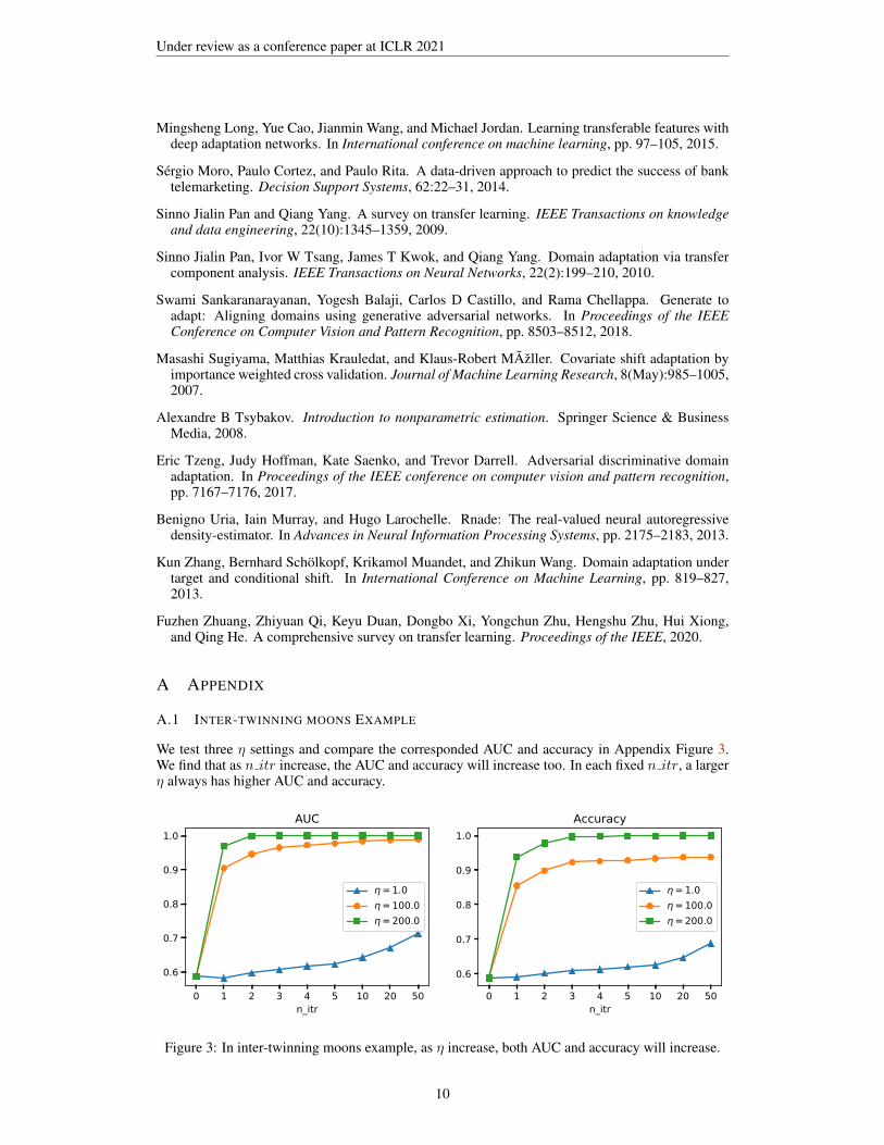
A.1 INTER-TWINNING MOONS EXAMPLE

We test three η settings and compare the corresponded AUC and accuracy in Appendix Figure 3.We find that as n itr increase, the AUC and accuracy will increase too. In each fixed n itr, a largerη always has higher AUC and accuracy.

0 1 2 3 4 5 10 20 50n_itr

0.6

0.7

0.8

0.9

1.0AUC

= 1.0= 100.0= 200.0

0 1 2 3 4 5 10 20 50n_itr

0.6

0.7

0.8

0.9

1.0Accuracy

= 1.0= 100.0= 200.0

Figure 3: In inter-twinning moons example, as η increase, both AUC and accuracy will increase.

10


A.2 UCI EXPERIMENTS

We summarize the size and class ratio information of UCI data sets in Appendix Table 3.

Table 3: UCI data setsTask Source Target Test Dimension Class 0/1(Source)

Abalone A→ B 2,088 1,566 523 7 24% vs. 76%Abalone B→ A 2,089 1,566 522 7 76% vs. 24%

Adult A→ B 16,279 12,211 4,071 6 75% vs. 25%Adult B→ A 16,282 12,209 4,070 6 77% vs. 23%Bank A→ B 22,537 17,005 5,669 7 97% vs. 03%Bank B→ A 22,674 16,902 5,635 7 80% vs. 20%

Parameter settings in UCI data sets. We enumerate the parameter settings on UCI experimenthere.

• Random forest models with 100 trees are used as the classifier.• For DANN, we set the feature extractor, the label predictor, and the domain classifier as

two-layer neural networks with hidden layer dimension 20. The learning rate is fixed as0.001.

• For EMTL, we fix the learning rate as 0.1 except for the task Abalone B→ A (where weset it to 0.001) as it did not converge. As mentioned in section 6.1, we only do one EMiteration.

Parameter settings in Amazon reviews dataset. We enumerate the parameter settings choice ofAmazon reviews experiment here.

• SVM has been chosen over RF because it showed better results in the case of Amazonreviews experimentation

• We run a grid search to find the best C parameter for SVM over one task (from books todvd) the best result C = 4.64E − 04 is then used for all tasks and for source svm, targetsvm, KMM and SA solutions.

• For DANN, we set the feature extractor, the label predictor, and the domain classifier asone-layer neural networks with hidden layer dimension 50. The learning rate is fixed as0.001.

• FNN is composed of 2 hidden layers of dimensions 10 and 5 (the encoding dimension).we added a Gaussian Noise, Dropout, Activity Regularization layers in order to generalizebetter and guarantee better encoding on target data.

• For EMTL, we fix the learning rate as 0.001 and only do one EM iteration.

Note that the presented result of Amazon reviews data set in Table 2 have been rounded to one digit.This explains why the 95% confidence interval of the mean is sometimes equal to 0.0 and why somevalues are not in bold.

11

EMTL: A GENERATIVE DOMAIN ADAPTATION APPROACH

Documents