EMS Performance Targets and Travel Times EMS Planning Conference, August 2008 Armann Ingolfsson [email protected] Academic Director Centre.

EMS Performance Targets and Travel Times

EMS Planning Conference, August 2008

Armann [email protected]

Academic DirectorCentre for Excellence in Operations

School of Business, University of Alberta

Based on joint work with S. Budge, E. Erdogan, E. Erkut, and D. Zerom

and using data from Calgary EMS and Edmonton EMS

Typical EMS Performance Targets: Coverage

• US EMS Act, 1973: 95% in 10 min.

• North America, current: 90% of urgent urban calls in 8:59 min.

• UK: – 75% of all calls in 8 min.– 95% of urban calls in 14 min.– 95% of rural calls in 19 min.

• Germany: – 95% in X min.– X varies across the country

from 10 to 15 min.

• Questions:– What are targets based on?– How can we predict

compliance to these targets, using a map?

– Are there better targets?

What are Coverage Targets Based on?

• Cardiac Arrest Survival Studies

• Focus on limiting the longest possible response time– As opposed to average response time

• Consistency: it’s what other operators do– Although the details vary widely

• Simple to interpret and compute

Let’s do this for a location in Twin Brooks, Edmonton

• Pick a location in the city• Find closest station• Predict performance for that location• Repeat for all locations in the city• Colour-code the map• Compute weighted average performance for the

whole city– Weights = call volumes

• (What we’re leaving out: ambulance availability)

Using a Map to Predict Performance

Closest Station: Terwillegar

Call location

Closest station

How Far is it? Take 1

Call location

Closest station

4.5 km

As the crow flies

“Euclidean distance”

How Far is it? Take 2

Call location

Closest station

5.8 km

North-south and east-west travel only

“Manhattan metric”

“Rectilinear distance”

How Far is it? Take 3

8.6 km

Using Google Maps

“Network distance”

OK, so I Measured the DistanceWhat’s Next?

DistanceDifferent ways to measure

Station locations

Ambulance availability

Zone sizes

Response TimeWhen to start and stop the clock

Variability

“Outcome”Less or more than 8:59?

Medical outcome?

Psychological outcome?

Transform

Transform

Traffic conditions

Driver behaviour

Construction

Pre-travel and post-travel

…

Paramedic training

Patient’s condition

…

What we’ll do next

Distance Travel Time

• 8.6 km ? min.• Google Maps says 14 min.• Better: use historical call data to compute

average speed• Even better (?)

compute different average speeds for:– Downtown vs. elsewhere– Different road types– Urgent vs. non-urgent– Rush hour vs. other times– Winter vs. summer– And so on …

Complicated!

Is there a simpler approach that is useful?

A Simpler Approach

Time

Speed

acceleration

cruising speed

deceleration

A long trip:

A Simpler Approach

Time

Speed

A short trip:

The Simpler Approach vs. RealityD

P

EN AR

0

30

60

90

0 2 4 6 8 10 12 14

Time from dispatch (min)

Spee

d (k

m/h

r)

AVL speed

K WH predictionLong trip

DP

EN AR

0

30

60

90

0 2 4 6

Time from dispatch (min)

Spee

d (k

m/h

r)

AVL speed

K WH predictionShort trip

Good enough to estimate average travel time, but lots of variability around the average

(Average) Travel Time Curve

-123456789

10

- 2 4 6 8 10

Distance (km)

Tra

vel t

ime

(m

in.)

Short trips Long trips

Estimates from Edmonton and Calgary data:

• Cruising speed: 100 kph.

• Acceleration: 5 min. (4.2 km) to reach cruising speed

Travel time Formula

• Short trips (< 4.2 km):Travel time in min.

= 2.45 × SQRT(distance in km)

• Long trips (> 4.2 km):Travel time in min.

= 2.5 + 0.6 × (distance in km)

• Twin Brooks: 2.5 + 0.6 × (8.6 km) = 7:42 min.• 8:59 min. 10.8 km• Twin Brooks is covered!

Not coveredCovered!

Is Twin Brooks Really Covered?Terwillegar station Twin Brooks

8:597:42But travel times are not always the same:

• Traffic

• Driver behaviour

• Construction

Twin Brooks may be covered on average, but it would be useful to know the probability of coverage

Terwillegar station Twin Brooks

8:597:42

Probability of Coverage Curve

8.6 km, 70%

0%10%20%30%40%50%60%70%80%90%

100%

- 5 10 15 20 25

Distance (km)

Pro

b. o

f co

vera

ge Twin Brooks:

Implications for deployment:

3 km is twice as good as 11 km

vs.

< 11 km good, > 11 km bad

Probability of Coverage Map

0%20%40%60%80%

100%

Prob. of Coverage

G

G

G

G

GG

G

G

G

G

G

G

G

G

G

G

G

G

G

GG

G

G

GG

G

G

G

G

9

8

6

5

4

32

1

94

34

32

31

30

28

26

24

23

22

21

20

19

18

1715

14

12

11

AMC

Cochrane

Created using probability of coverage curve, for all locations in a city

The Formulas

• Travel time = ((distance) + f(time of day))× exp((distance) )

• (distance) avg. travel time curve

• (distance) next slide

• f(time of day) the slide after that

• ~ t distribution with 3.3 d.f.

Coefficient of Variation: (distance)

Time-of-day Effect

~ 5 PM

Afternoon rush hour

~ 4 AM ??

How About Medical Outcomes instead of % in 8:59?

DistanceDifferent ways to measure

Station locations

Ambulance availability

Zones sizes

Response TimeWhen to start and stop the clock

Variability

“Outcome”Less or more than 8:59?

Medical outcome?

Psychological outcome?

Transform

Transform

Traffic conditions

Driver behaviour

Construction

Pre-travel and post-travel

…

Paramedic training

Patient’s condition

…

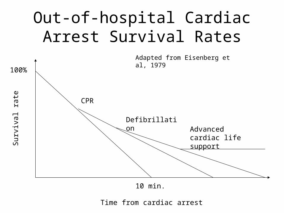
Out-of-hospital Cardiac Arrest Survival Rates

Sur

viva

l rat

e

100%

Time from cardiac arrest

10 min.

CPR

Defibrillation

Adapted from Eisenberg et al, 1979

Advanced cardiac life support

Casino Study (Valenzuela et al, 2000)

• Casino security officers trained in CPR and defibrillation

• Time of collapse from videotapes

• Response times ≈ 3 min – much shorter than most EMS calls

• Survival rates:– 74% when response time < 3 min.– 49% when response time > 3 min.

Estimated Survival Functions

• Here’s one of four that we found:

• “Response time” is nowhere to be seen!• Need to make assumptions so can

“average over” non-response-time factors• A good thing – allows calibration of a

function estimated in one city for use in another city with a different EMS system

1)0.1390.156 0.26-DefibCPR

DefibCPR1),( IIeIIs

Arrest to CPR time Arrest to defibrillation time

Calibrating Survival Functions: Assumptions

• Is collapse witnessed?61% yes, average access time = 1.2 min

39% no, average access time = 30 min

• Bystander CPR: 64%, 1 min after 911

• Response time: Average pre-travel delay = 3 min

+ Average travel time (based on distance)

• EMS arrival to defibrillation: 2 min

Add Variability around the Averages, Stir, and Bake, to get …

0%

2%

4%

6%

8%

10%

12%

14%

16%

18%

20%

- 10,000 20,000 30,000 40,000 50,000

Distance (meters)

Sur

viva

l pro

babi

lity

… a probability of survival curve

Implications for deployment:

2 km is twice as good as 11 km

vs.

< 11 km good, > 11 km bad

Sensitivity Analysis: Avg. Access Time, Un-Witnessed Arrest

0%

5%

10%

15%

20%

0 10,000 20,000 30,000

Distance (m)

Su

rviv

al p

rob

ab

ility

30

5

60

“Optimal” Allocation of Ambulances to Stations

• Change target from avg. response time to coverage: save 65 lives

• Account for uncertainty about coverage: save 47 lives• Change target from coverage to survival (but ignore

uncertainty): save 47 lives

Incorporation of uncertainty

None Response times

Ambulance availability

Both

Min. avg. response time

697 745

Max. avg. coverage 762 809 809 809

Max. avg. lives saved 809 809 809 809

Observations

• Survival rates vs. response time:– Out-of-hospital cardiac arrest survival rates have

been studied extensively– These are the most “saveable lives”

• Possible to incorporate survival rates based on medical research into planning models

• Coverage is a poor proxy for survival rates …– … but consideration of uncertainty improves it

Why does Maximizing Survival Rates and Maximizing Expected Coverage give Similar Results?

0%

10%

20%

30%

40%

50%

60%

70%

80%

90%

100%

- 5 10 15 20 25

Distance (km)

Pro

b. o

f co

vera

ge

0%

2%

4%

6%

8%

10%

12%

14%

Pro

b. o

f su

rviv

al

0/1 coverage

Potential Reasons to Focus on Survival Rates instead of Coverage• Coverage is an imperfect proxy for survival rates …

– … assuming that that’s the real objective

• Abstract units– $ or lives saved get more attention than “% in 8:59”

• All of the following are arbitrary and vary among EMS systems:– The time standard– The percentage goal– When the clock starts and stops

Potential Problems (and Solutions) with a Focus on Survival Rates

• Only know survival rates for cardiac arrest– Do more studies of non-cardiac arrest patients– Use coverage target for other patients?

• Insufficient data to calibrate survival functions– Maybe the data should be collected anyway for cardiac arrest

patients?– Plans to collect the data in some cities

• “90% covered” sounds better than “8% survived”– Important to include benchmarks: 2% survival without EMS?– Focus on “lives saved” instead of “% survival”?

• ?– ?

For More Information

• Erkut, E., A. Ingolfsson, G. Erdoğan. 2008. Ambulance deployment for maximum survival. Naval Research Logistics 55 42-58

• Budge, S., A. Ingolfsson, D. Zerom. Empirical Analysis of Ambulance Travel Times (ready later this month)

• [email protected]• www.business.ualberta.ca/aingolfsson/publications.htm

Questions?