Empiricism and/or Instrumentalism?

ORI GIN AL ARTICLE

Empiricism and/or Instrumentalism?

Prasanta S. Bandyopadhyay • Mark Greenwood •

Gordon Brittan Jr. • Ken A. Aho

Received: 4 October 2010 / Accepted: 9 October 2013 / Published online: 13 December 2013

� Springer Science+Business Media Dordrecht 2013

Abstract Elliott Sober is both an empiricist and an instrumentalist. His empiri-

cism rests on a principle called actualism, whereas his instrumentalism violates this.

This violation generates a tension in his work. We argue that Sober is committed to

a conflicting methodological imperative because of this tension. Our argument

illuminates the contemporary debate between realism and empiricism which is

increasingly focused on the application of scientific inference to testing scientific

theories. Sober’s position illustrates how the principle of actualism drives a wedge

between two conceptions of scientific inference and at the same time brings to the

surface a deep conflict between empiricism and instrumentalism.

A version of the paper was presented at the American Philosophical Association meetings, Central

Division.

P. S. Bandyopadhyay (&) � G. Brittan Jr.

Department of History and Philosophy, Montana State University, Bozeman, MT, USA

e-mail: [email protected]

G. Brittan Jr.


M. Greenwood

Department of Mathematical Sciences, Montana State University, Bozeman, MT, USA


K. A. Aho

Department of Biological Sciences, Idaho State University, Pocatello, ID, USA


123

Erkenn (2014) 79:1019–1041

DOI 10.1007/s10670-013-9567-8

1 Introduction

Elliott Sober writes that empiricism is a thesis about the significance of observation

(Sober 1993). According to him, any credible scientific hypothesis must be tied to

what we actually observe, and this fact is the one to which we should attach

epistemological significance. Sober also is an instrumentalist who takes the notion

of (expected) predictive accuracy as the goal of science. In spelling out the notion of

predictive accuracy, he makes reference to data which are merely possible, as yet

unobserved. Sober’s two approaches, empiricism and instrumentalism, thus conflict;

one tells us to take possible data into account, the other proscribes them.

The paper is divided into four sections. In the first section, we introduce the so-

called principle of actualism (PA) and explain its ramifications for scientific

inference.1 In the second section, we broach Sober’s empiricism and discuss how his

empiricism incorporates PA in the background of the realism/antirealism debate. In

the third section, we discuss Sober’s AIC-based notion of instrumentalism, which is

inconsistent with the PA because the former violates the PA. In the fourth, we

consider two issues. We first discuss a conflicting methodological imperative in his

work for his attempt to combine empiricism with instrumentalism by bringing in

two conflicting strands in his philosophy described above (see, Godfrey-Smith 1999

for a different type of tension in Sober’s work).2 His empiricism rests on the PA,

whereas his instrumentalism violates it. Second, we consider, and then reject a

possible objection which contends that the AIC framework respects the PA, and as a

result, it is alleged, there is no inconsistency in his methodology.

2 The Principle of Actualism in a Larger Context

According to PA, one should make judgments about the correctness of the

hypothesis based on data we actually have, rather than on unobserved, possible data.

In the words of Sober,

we should form our judgments about hypotheses based on evidence we actually

possess; possible but nonfactual evidence does not count (Sober 1993, p. 43).

We call this the Principle of Actualism (PA hereafter). One could construe the thesis

in terms of its epistemological or decision-based features. In this section, we

consider it epistemologically. We will explore its decision-based feature in Sect. 4

when we evaluate an objection to our account. Consider the epistemological

consequences of the PA stated in terms of its two conditions. We call the first

epistemological condition, the Principle of Actualism’s Evidential Equivalence

Condition for two experiments (PAT) and the second one, the Principle of

1 The PA or what is often called the ‘‘conditionality principle’’ is a corner-stone in Bayesian inference.

For an excellent treatment of Bayesian inference, see (Howson and Urbach 2006). The paper does not try

to defend or criticize the PA.2 Godfrey-Smith has pointed out that when Sober’s earlier view on simplicity is domain-specific; his

current use of the AIC framework that exploits the notion of simplicity is, however, ‘‘domain-

independent.’’ (Godfrey-Smith 1999, p. 181).

1020 P. S. Bandyopadhyay et al.

123

Actualism’s Empirical Significance Condition for a single experiment (PAS). The

letter ‘‘T’’ in ‘‘PAT’’ represents ‘‘two experiments to share equal evidential

support.’’ The letter ‘‘S’’ in ‘‘PAS’’ represents a ‘‘single’’ experiment ‘‘having the

evidential significance.’’Although epistemological consequences of PA are moti-

vated by two fundamental principles in Bayesian statistics,—the PAT is an analogue

for the likelihood principle, and the PAS is an analogue for the conditionality

principle—one need not be a Bayesian to accept them (Birnbaum 1962; Cassella

and Berger 1990; Berger 1985; Pawitan 2001).3 At least Sober adopts this line of

thought that one need not to be a Bayesian to subscribe to these principles. We will

first sketch these two epistemological consequences of PA and bring out their

significance in the foundations of statistical inference, and also formulate a

consequence of PA in light of our discussion of them.4 Then, following Sober, we

discuss the bearing of PA on the realism/antirealism debate in next section. This

way of relating PA to the foundations of statistical inference and the realism/

antirealism debate is crucial for him because he is one of the few epistemologists

who bring those two issues together under one principle. The purpose of this section

is to address what he might have meant by the PA.

Consider first the two consequences of PA.

The Principle of Actualism’s Evidential Equivalence Condition for Two

Experiments (PAT):

Two experiments, E1 and E2, provide equal evidential support for a

hypothesis, that is, the parameter in question, if and only if their likelihood

functions are proportional to each other as functions of the hypothesis, and

therefore, any inference about the hypothesis based on these experiments

should be identical.

The Principle of Actualism’s Evidential Significance Condition for a single

experiment (PAS):

If two experiments, E1 and E2 are available for the hypothesis (i.e., the

parameter in question) and if one of the two experiments is selected randomly,

then the resulting inference about the hypothesis should only depend on the

selected (actually performed) experiment and the evidence received from that

experiment alone.

The notion of an experiment is a key to understanding both consequences of the

PA. Usually the notion of an experiment involves causing something to happen,—

perhaps making a measurement—and observing the result. Here, an experiment is

taken to mean making an observation, usually under known or reproducible

circumstances. Consider an example of the PAT to see how this principle works.

Suppose a biologist asks a statistical consultant to evaluate evidence that the true

3 Evans (2013) has recently questioned whether the likelihood principle is at all a ‘‘must’’ for a Bayesian.

He argues that it is completely irrelevant to Bayesianism.4 Hereafter we have dropped the use of ‘‘epistemological’’ features of the PA when we address the PA

unless otherwise stated. We return to this usage when we distinguish epistemological features of the PA

from its decision-based feature in Sect. 4.

Empiricism and/or Instrumentalism? 1021

123

proportion of birds in a particular population that are male is larger than �. The

biologist emails the statistician that 20 out of 30 birds obtained were male but

provides no further information about how the birds were collected. If no additional

data are available on the experiment, what could she infer about the hypothesis that

the true proportion, h, is equal to �? We call this initial hypothesis, h = �, a

constrained hypothesis because the parameter value is set at h = �. Its contrasting

hypothesis could be that the true proportion is larger than �, parameter h[ �. This

contrasting hypothesis will be called the unconstrained hypothesis. Both hypotheses

are taken to be simple statistical hypotheses. We investigate this kind of inductive

problem with the help of our background knowledge about the problem in question

together with the available data to see whether the hypotheses posited might be able

to account for those data. In fact, the investigator has realized that two types of

probability models that rely on two types of experiments could be proposed to

explain the data. In this scenario, the experiment E1 consists of randomly selecting

30 birds from the population and then determining 20 to be male and 10 to be

female. The experiment E1 might have led to those data. Then the Binomial

probability model for E1 would be Bin(30, h). Or the experimental set-up could be

like E2 which consists of collecting birds until one gets 10 females so that it could

be represented by a Negative Binomial model, NBin(10, h). (For information about

both Binomial and Negative Binomial models, see Berger 1985.) According to the

PAT, two experiments, E1 and E2 modeled by two distinct probability models,

provide identical evidential support for the hypothesis that h = � because the

likelihood function under both models is proportional to h20ð1� hÞ10. The

likelihood function provides an answer to the question, ‘‘how likely are the data

given the model?’’ Therefore, most importantly by the PAT the inference about the

hypothesis h should be identical for both experiments. The PAT is a version of PA

because evidence at hand is actual evidence which, according to the PA, is alone

relevant for making the inference about the hypothesis.

Consider PA’s Evidential Significance Condition for a single experiment (PAS).

Suppose in another setting, an investigator would like to know whether the

hypothesis that the true proportion of males in a population of birds is �. She is

considering two experiments, E1 and E2, to see whether they could give her a

verdict about the correctness of the hypothesis. As before, E1 consists of collecting

the predetermined 30 birds and enumerating how many males the investigator

observes. E2 consists of sampling birds until the investigator observes 10 female

birds, which implies that E2 could continue forever. Suppose the investigator

randomly got to conduct E1 and found 20 males. The PAS states that the inference

about the correctness of the hypothesis depends solely on both the selected

experiment and the data received from the selected experiment being actually

performed. Data of the actually performed experiment and not what data the other

experiment could have yielded are evidentially relevant for examining the

credibility of the hypothesis in question.

There is a further elaboration of the PAS in terms of the selected actually

performed experiment. It says that had the actual experiment been chosen non-

randomly from the very beginning and resulted in the same observation as the


123

randomly performed experiment, then both actually performed experiments would

have provided an equal evidential support for the parameter h. This elaboration, at

first blush, seems to bring the PAS closer to the PAT. However, one needs to be

careful that the PAS refers to two instances of the same type of experiment, whereas

the PAT refers to two types of experiments. If, for example, the experiment in

question is Binomial, then in case of the PAS, both are instances of the same

Binomial experiment. In contrast, in the case of the PAT, if one is a Binomial

experiment then the other can’t be a Binomial experiment, and conversely, if one is

a Negative Binomial experiment then the other can’t be a Negative Binomial

experiment. Sober accepts the PA and also seems to accept at least a combination of

both the consequences of PA as we shall see in Sect. 2. Ellery Eells (1993) and Ian

Hacking (1965) also accept the PA in something like the two consequences already

discussed.

However, the connection between two consequences of PA and the PA itself

needs to be made clearer. The latter has been stated so far without reference to any

experiment, while the former have been stated with reference to experiments (see

the quote from Sober about the PA in the beginning of Sect. 1). To connect the two

consequences of the PA to the Principle of Actualism, as does Sober, we

reformulate the PA as follows:

(PA): We should form our judgment about the correctness of hypotheses based

on evidence we gather from any actually performed experiment/test; possible

but nonfactual evidence from any yet to be performed experiment/test does not

count.

Here, ‘‘test’’ could mean a host of things ranging from a diagnostic test, a statistical

test, to non-statistical tests like tests to see whether some chemical reactions take

place, to testing theories of high-level theories. However, there are disagreements

regarding both consequences of PA and the epistemological stance that accompa-

nies the PA. Many statisticians who work within the frequentist interpretation of

probability tend to disagree as to the value of these consequences of the PA in

statistical inference. The focal point of the frequency interpretation is the idealized

repetition of an experiment in which the probability of an event is construed to be its

long run probability. The framework of classical statistics is one example which is

based on this frequency interpretation. The Akaikean Information Criterion (AIC)

framework also rests on this interpretation. We will return to it in Sect. 3. According

to classical statistics, a proper classical treatment of the two models, Binomial and

Negative Binomial, can lead to different answers when we are concerned with

finding evidence that the proportion of male birds is greater than �. As a result, the

PAT which treats both models as having equal evidential support is rejected in

classical statistics. In the same vein, classical statisticians argue for averaging over

all the possible samples. This is especially important for the experiment E2 which, if

repeated, could have yielded a different number of birds for the investigator than

what she has in fact gathered. The mere possibility of different outcomes from E2

has led classical statisticians to question the legitimacy of the PAS. So they also

reject the PAS. They contend the need for incorporating possible data in performing

statistical inference. Since the refrain of their contention captures a single theme


123

applicable to both consequences of the PA, we will only confine ourselves to their

epistemological stance toward the PAT.

The principal motivation behind classical frequentist statistics is to produce a

statistic which does not depend on the nature of the hypothesis (i.e., parameter h) or

any prior knowledge about h. Statisticians of that stripe have proposed instead a

procedure p(x) and some criterion function (h, p(x)) and a number R such that a

repeated use of p would yield average long run performance of R. The idea behind

this is that if we use p repeatedly on a series of independent random samples where

the hypothesis about h is true, then it is easy to show with probability one that this

procedure on repeated use will reject the hypothesis 100R % of the time. The term

‘‘R’’ captures this idea of ‘‘significance level’’ within classical statistics. When data

are gathered to check whether a hypothesis is correct, the investigator within this

framework is typically looking for a significant result. The latter means that she has

found something out of the ordinary relative to the hypothesis which she is willing

to reject based on this significant result. A statistically significant result is one that

would have a very small probability of happening by chance. Given this difference

between classical statistics sympathizers and the PAT sympathizers, we are able to

explain why a classical treatment of the two models can lead to different answers

with regard to the first consequence of the PA.

Recall that when we computed the likelihood functions under two models,

Binomial and Negative Binomial, we computed the likelihood function under each

model relative to the observed data which are Y = 20. However, the significance

calculations involve not just the observed Y = 20, but also, for example the

potentially observed ‘‘more extreme’’ Y C21, assessing the rarity of the observed

result by incorporating the probability of unobserved results that contain similar or

stronger evidence against the hypothesis. Since classical p values take into account

those extreme or more extreme results as possible results, classical statistics violates

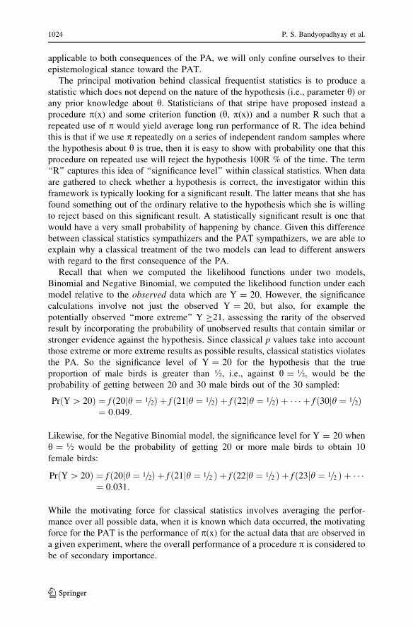
the PA. So the significance level of Y = 20 for the hypothesis that the true

proportion of male birds is greater than �, i.e., against h = �, would be the

probability of getting between 20 and 30 male birds out of the 30 sampled:

PrðY [ 20Þ ¼ f 20jh ¼ 1=2ð Þ þ f 21jh ¼ 1=2ð Þ þ f 22jh ¼ 1=2ð Þ þ � � � þ f 30jh ¼ 1=2ð Þ¼ 0:049:

Likewise, for the Negative Binomial model, the significance level for Y = 20 when

h = � would be the probability of getting 20 or more male birds to obtain 10

female birds:

PrðY [ 20Þ ¼ f 20jh ¼ 1=2ð Þ þ f 21jh ¼ 1=2ð Þ þ f 22jh ¼ 1=2ð Þ þ f 23jh ¼ 1=2ð Þ þ � � �¼ 0:031:

While the motivating force for classical statistics involves averaging the perfor-

mance over all possible data, when it is known which data occurred, the motivating

force for the PAT is the performance of p(x) for the actual data that are observed in

a given experiment, where the overall performance of a procedure p is considered to

be of secondary importance.


123

In our example, the likelihood function for E1 is f1ð20jhÞ ¼ 30

20

� �h20ð1� hÞ10

and for E2 it is f2ð20jhÞ ¼ 29

9

� �h20ð1� hÞ10: Under both E1 and E2, there are two

different likelihoods we can calculate, the likelihood of the data given that h = �and another where h is estimated via maximum likelihood estimation (MLE)

techniques. Then for E1 or E2, the ratio of these two likelihoods generates the

likelihood ratio which is a measure of the relative evidential support for one

hypothesis over its rival. It is based only on the actual observations, so it does not

violate the PA. The likelihood ratios for both E1 and E2 are identical for either E1

or E2, providing a result of 5.5 in our example, suggesting how the PAT is at work.

The PAT says that two models based on two experiments provide the same

evidential support for a hypothesis if and only if the likelihoods of these models are

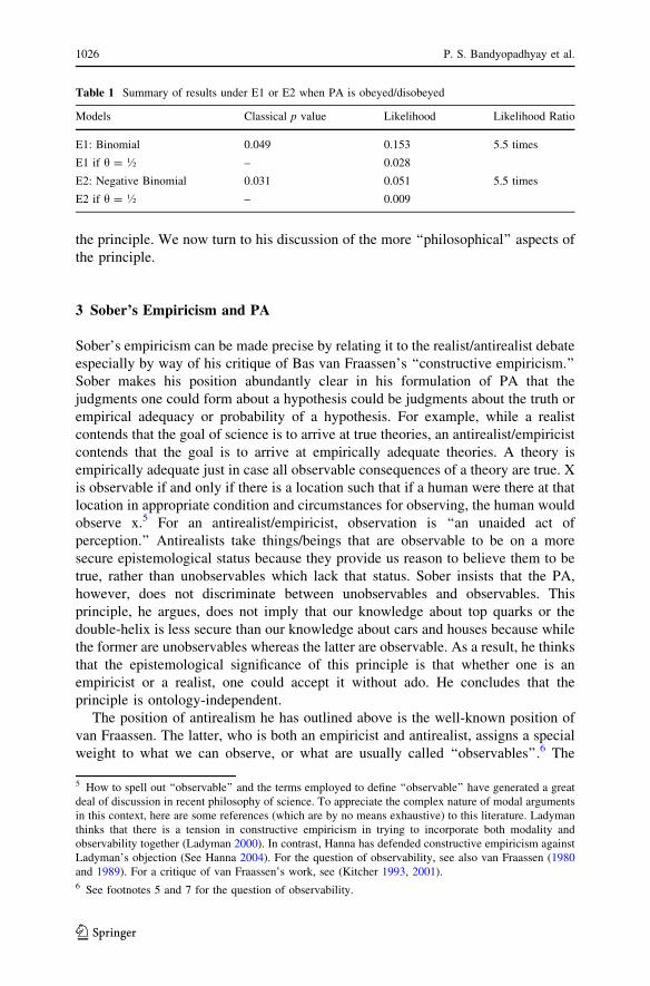
proportional. Table 1 provides the four likelihoods and the resulting likelihood

ratios for each probability model along with the classical p values under different

models. The need for four likelihoods is as follows.

We are considering two probability models, the Binomial model and the

Negative Binomial model. Under each probability model, we are considering two

hypotheses. For example, under the Binomial model we are considering two

hypotheses: one is that the true proportion is h[ � and the second one is that

h = �. Under the Negative Binomial model we are similarly considering the same

two hypotheses as for Binomial. Column 2 represents the classical p value that

violates PA, whereas columns 3 and 4 represent likelihoods and likelihood ratios

that respect PA. The rationale for the likelihoods being different in column 3, while

still respecting PA is due to the fact that E1 and E2 lead to different likelihood

functions because they are based on two distinct probability models discussed

above. However, their likelihood ratio under E1 or E2 in column 4 is the same.

According to the likelihood approach, the ratio is what matters in measuring

evidence against the hypotheses.

One gets a conflicting recommendation regarding the amount of evidential

strength against the hypothesis, h = �, in question depending on whether one

disobeys or obeys the PA. The classical statistics framework using p values disobeys

the PA. The former rejects both the Binomial and Negative Binomial model-based

hypothesis, i.e., h = � as the correct hypothesis, since the p values are ‘‘small’’ in

both cases. However, under E1 or E2, the evidence against the initial hypothesis,

h = �, represented by p values is unequal, i.e., 0.049 under E1 and 0.031 under E2.

In contrast, the likelihood ratios, which obey the PA, provide equal evidential

support against h = � under E1 or E2. The likelihood ratio for the hypothesis,

h[ �, versus the hypothesis, h = �, provides 5.5 times more evidential support

for the hypothesis, h[ � under E1 or E2. So we find a conflicting recommendation

regarding the amount of evidence that exists against the initial hypothesis under E1

or E2 depending on whether we reject or accept PA.

So far, we have discussed the PA together with its two consequences and their

application in statistical inference. It was in this context that Sober first introduced


123

the principle. We now turn to his discussion of the more ‘‘philosophical’’ aspects of

the principle.

3 Sober’s Empiricism and PA

Sober’s empiricism can be made precise by relating it to the realist/antirealist debate

especially by way of his critique of Bas van Fraassen’s ‘‘constructive empiricism.’’

Sober makes his position abundantly clear in his formulation of PA that the

judgments one could form about a hypothesis could be judgments about the truth or

empirical adequacy or probability of a hypothesis. For example, while a realist

contends that the goal of science is to arrive at true theories, an antirealist/empiricist

contends that the goal is to arrive at empirically adequate theories. A theory is

empirically adequate just in case all observable consequences of a theory are true. X

is observable if and only if there is a location such that if a human were there at that

location in appropriate condition and circumstances for observing, the human would

observe x.5 For an antirealist/empiricist, observation is ‘‘an unaided act of

perception.’’ Antirealists take things/beings that are observable to be on a more

secure epistemological status because they provide us reason to believe them to be

true, rather than unobservables which lack that status. Sober insists that the PA,

however, does not discriminate between unobservables and observables. This

principle, he argues, does not imply that our knowledge about top quarks or the

double-helix is less secure than our knowledge about cars and houses because while

the former are unobservables whereas the latter are observable. As a result, he thinks

that the epistemological significance of this principle is that whether one is an

empiricist or a realist, one could accept it without ado. He concludes that the

principle is ontology-independent.

The position of antirealism he has outlined above is the well-known position of

van Fraassen. The latter, who is both an empiricist and antirealist, assigns a special

weight to what we can observe, or what are usually called ‘‘observables’’.6 The

Table 1 Summary of results under E1 or E2 when PA is obeyed/disobeyed

Models Classical p value Likelihood Likelihood Ratio

E1: Binomial 0.049 0.153 5.5 times

E1 if h = � – 0.028

E2: Negative Binomial 0.031 0.051 5.5 times

E2 if h = � – 0.009

5 How to spell out ‘‘observable’’ and the terms employed to define ‘‘observable’’ have generated a great

deal of discussion in recent philosophy of science. To appreciate the complex nature of modal arguments

in this context, here are some references (which are by no means exhaustive) to this literature. Ladyman

thinks that there is a tension in constructive empiricism in trying to incorporate both modality and

observability together (Ladyman 2000). In contrast, Hanna has defended constructive empiricism against

Ladyman’s objection (See Hanna 2004). For the question of observability, see also van Fraassen (1980

and 1989). For a critique of van Fraassen’s work, see (Kitcher 1993, 2001).6 See footnotes 5 and 7 for the question of observability.


123

moons of Jupiter, dinosaurs and distant stars are observable, but microbes are not.

According to him, the former counterfactual possibility (i.e., to be able to observe

the moons of Jupiter and the like), is epistemologically relevant whereas the latter

(i.e., to be unable to observe the microbes and the like) is not. For example, had we

been in front of the moons of Jupiter, then, we could have observed them without

any aid to our vision. However, had we been in front of microbes, he contends, then,

we could not have observed them without instruments. So what we can or cannot

observe plays a crucial role in van Fraassen’s antirealist empiricism.

Unlike the constructive empiricist, Sober argues that there should be an

asymmetry between what things are seen and what are not, (and not between what is

seeable and what is not), because our knowledge about things unseen is both

mediated and understood by our knowledge about things we see. As a result, he

thinks that what we actually observe has a special status for us. The PA captures that

epistemological status of actual data. However, he argues that constructive

empiricism violates the PA. Given this construal of constructive empiricism, Sober

assumes that it accepts the principle which we will call the Principle of Possible

Evidence (or in short PPE).7

(PPE): If one’s actual evidence for the hypothesis H2 is about as good as one’s

actual evidence for another hypothesis H1, and it is possible to have better

evidence for H1, but not for H2, then we should form the judgment about the

correctness of H1 solely based on possible, nonfactual evidence.8

He uses this example to illustrate and make his point that the PPE is false. Consider

a doctor making a diagnosis about whether a patient has diabetes (H2) or small pox

(H1). Two laboratory tests are actually carried out and their results contain both

‘‘positive’’ and ‘‘negative’’ outcomes. As is usually the case, both tests have error

probabilities associated with them. Assume that both tests are equally reliable: if a

positive outcome on the first test strongly supports the hypothesis that the patient

suffers from diabetes (H2), then a positive outcome on the second test strongly

supports the hypothesis that a patient suffers from small pox (H1), and conversely.

The same assumption holds with respect to negative outcomes. Suppose,

counterfactually, that there is an infallible third test that detects correctly if the

patient suffers from diabetes (H2). It is crucial for Sober’s argument to assume that

7 One might worry that anyone including van Fraassen will ever disagree with Sober regarding the

implications of the following example. In an email communication, Joseph Hanna wrote to one of the

authors of the paper the following. He writes that a theory is empirically adequate, according to van

Fraassen, if and only if it saves all the actual observables, past, present and future. So, empirical adequacy

depends on all sorts of ‘‘observables’’ no one has ever, in fact, observed. But these observables are actual

events that occur in the history of the world. On the other hand, the actual status of a theory—depends

only on actual observations. So, Hanna concludes that there is nothing in van Fraassen’s empiricism that

violates PA and respects PPE (see Hanna 2004 for his stance toward constructive empiricism). We

sympathasize with Hanna along with those who might share the same concern with him that Sober errors

in mistakenly attributing the PPE to van Fraassen. However, we are not interested in whether Sober is

right in thinking that van Fraassen’s position violates PA. We are only interested in the kind of argument

Sober employs to defend the principle.8 One worry against Sober’s work here is that ‘‘the notion of evidence’’ being possible ‘‘is slippery here’’.

To do a full justice to this worry we refer the reader to footnote 9 as the ensuing discussion will help to

understand both this point and our stance toward Sober’s view.


123

there is no such infallible test for small pox. Such a possible test for diabetes would

apparently have evidential significance for someone like van Fraassen; it tells us

what would be the case if certain observations were made. But our supposition is

that there is no such test as it has not been carried out.9 The mere possibility of a

third test, albeit infallible, if it is not carried out has no import. Therefore, the

counterfactual that there exists a possible infallible third test for diabetes is, for

Sober, in this sense empty, because only actual tests count. But this is his just a

short-hand way of rejecting the PPE and thus linking the principle of actualism with

empiricism properly construed.

For our purposes it does not matter whether van Fraassen himself is committed,

as Sober thinks, to the significance of (merely) possible evidence or, in fact, whether

this particular counter-example to ‘‘constructive empiricism’’ is very telling. The

general point is that ‘‘observable’’ means ordinarily something like ‘‘capable of

being observed.’’ If the emphasis is placed on observability, then it would seem to

follow that possible as well as actual observations be taken into epistemic account.

But Sober thinks that this is deeply counter-intuitive. There are cases, such as the

one he imagines, in which there is a possible test procedure which does not in fact

exist. That it does not exist entails that it cannot supply evidence. Evidence has to do

with actual observations.

In fact, his rejection of constructive empiricism rests on the PA because the

outcomes of the first two tests in his example are outcomes of actually performed

tests, whereas the third test is yet to be performed. So the latter’s outcome has

turned out to be epistemologically irrelevant for evaluating its impact on the

9 This is in continuation with the previous footnote regarding why one might think that the notion of

‘‘possible’’ in the notion of evidence being possible is a ‘‘slippery slope’’. The worry is that if we imagine

that there is not actually any test for X, then there is a sense in which evidence for the test is impossible.

But such a non-actual test is still possible (in a broader sense) and so the evidence from it is possible.

There is a scope of ambiguity concerning the example of the test for X being possible in one sense and

impossible in others. The reason for this is that to which does the variable ‘‘X’’ refer? Does ‘‘X’’ refer to

the (infallible) possible test which has not been carried out for diabetes or the test for small-pox which

does not exist in Sober’s example, yet it is still possible in a broader sense? However, a charitable

interpretation of the worry might be able to reveal its true spirit. It is likely that the imaginary critic who

presents this worry means by ‘‘the test for X,’’ a possible test for small-pox which does not exist at this

point, but it is still possible in some sense. We agree with the critic that although Sober’s example clearly

assumes that there is no such (infallible) test possible for small-pox, such a test for small-pox is

undeniably ‘‘possible’’ in some broader sense. The relevant question, however, is ‘‘does such a test for X

being possible pose a threat to Sober’s criticism of constructive empiricism’’? We have two comments

here. First, if we allow such a test for X to be possible then this will force us to revise the PPE in terms of

the Revised Principle of Possible Evidence (RPPE). According to the RPPE, if one’s actual evidence for

the hypothesis H2 is about as good as one’s actual evidence for another hypothesis H1, and although it is

possible to have evidence for both H1 and H2, but it is only possible to have better evidence for H1, but

not for H2, we should form the judgment about the correctness of H1 solely based on better possible,

nonfactual evidence. However, the RPPE will still be regarded by Sober as dubious as it violates the PA.

In short, this revision will complicate the PPE, without disputing his rejection of the principle. Our second

comment has to do with Sober’s own example (see, Sober 1993). Since we would to like to follow him in

this regard, we would continue to stick to his usage by saying that there is a possible infallible test for

diabetes, but there is no such ‘‘possible’’ test for small-pox; consequently, the PPE is the principle to be

investigated and not any of its variants. The point of this along with footnote 7 is to discuss how Sober has

construed the PPE and its relationship to the PA without trying to evaluate whether his argument against

constructive empiricism is tenable.


123

competing hypotheses. Sober’s counterexample contains some features of both

consequences of the PA, the Evidential Significance Condition for a Single

Experiment (PAS) and the Evidential Equivalence Condition for Two Experiments

(PAT) discussed in Sect. 1. Like both consequences, two relevant diagnostic tests

sharing equal evidential strength are actually performed tests, and what data we

could have obtained from the third test becomes irrelevant for his counterexample.

Like the PAS, his rejection exploits the idea of an actually performed test. In

addition, like the PAT, both tests are evidentially equivalent.

4 Sober’s AIC-Based Notion of Instrumentalism and PA

Sober discusses and motivates his brand of instrumentalism in connection with

curve fitting. Malcolm Forster and Sober wrote an influential paper together on the

curve fitting problem (Forster and Sober 1994).10 This problem arises when an

investigator is confronted with optimizing two conflicting desiderata, (i) simplicity

and (ii) goodness-of-fit, together.11 In this section, we will discuss their work on the

curve fitting problem and then explain how their Akaikean Information Criterion

(AIC) framework helps Sober develop his version of instrumentalism. In general,

with regard to the curve fitting problem, their goal is to measure the closeness of a

family of curves to the truth. They use the Akaikean Information Criterion (AIC,

Akaike 1973), to achieve this goal. Based on AIC, they propose an important

measure of a curve’s closeness to truth in terms of the curve’s predictive accuracy.

AIC assumes that a true probability distribution exists that generates independent

data points, Y1, Y2, Y3, … YN. However, in most cases we have no way of knowing

the true curve. We could only estimate parameters of the curve based on the data.

Forster and Sober explain how an agent can predict future data from past data.

First, an agent uses the available data (Y) to obtain the best-fitting estimates of the

parameters of the true distribution, e.g., to find the maximum likelihood estimator

(MLE) of that distribution family. This best-fitting member of the family is then

used to approximate what future data will look like. The question is how well the

curve in the family that best fits the data will perform in predicting the future data. A

family might fare well in these two-stage processes, (i.e., (i) to find optimal

parameter estimates and (ii) to predict future data) on one occasion, but fail to do so

on another. The estimated predictive accuracy of a family depends on how well it

would do on average, were these processes repeated again and again.

10 For a Bayesian approach to the curve-fitting problem, see Bandyopadhyay et al. (1996),

Bandyopadhyay and Boik (1999), Bandyopadhyay and Brittan (2001), and also Banyopadhyay (2007).11 See Miller 1987 for a critique of Sober’s account of simplicity. Miller argues that one needs to

incorporate causal simplicity in theory choice. In this case, as in many others, formal simplicity which

Sober has advanced must be distinguished from causal simplicity. As Richard Miller (1987, 247) reminds

us, ‘‘by adding a variety of novel propositions, without any corresponding simplification, evolutionary

theory reduces the formal simplicity of science. [But] An enormous gain in causal simplicity results.’’

According to Miller, the regularities that we observe in the variation of species, for example, have causal

explanations only when the evolutionary explanations are added.


123

One goal of AIC is to minimize the average (expected) distance between the true

curve and its estimate. It is equivalent to choosing the family of curves, which

minimizes the distance between the true distribution and the estimated distribution,

by choosing the family of curves which maximizes predictive accuracy. AIC was

designed to be an estimator of the expected Kullback–Leibler (KL, Kullback and

Leibler 1951) distance between a fitted MLE candidate model and the model

generating the data, which we consider the truth. The expected KL distance provides

a measure of the distance or divergence from a model to the true distribution based

on all possible data. Specifically AIC can be considered an approximately unbiased

estimator for the expected KL divergence which uses a maximum likelihood

estimator (MLE) to create estimates for the parameters of the model. By an

‘‘unbiased estimator’’, we mean that in the long run the average or expected value of

the estimator will equal the population parameter, with the long run being relative to

repeated random samples obtained in the same fashion as our original sample. Our

two sampling methods lead to the probability models used in E1 and E2. If the

researcher were to repeat the experiment, the number of male birds would likely

vary, possibly providing 21 male birds out of the total of 30 in E1 or 21 male birds

out of 31 in E2. These realizations of the sampling process would provide similar

but not identical evidence against the hypothesis as in our original sample in both

models. Another possible realization of each sampling process could provide 19 out

of 30 for E1 and 19 out of 29 for E2, but each case represents one possible

realization from all the possible realizations which AIC averages across. Using AIC,

the investigator attempts to select the model with minimum expected KL distance

across these repeated, equally possible, random samples, based on a single observed

random sample. Models with smaller values of AIC are better than models with

larger values of AIC. Akaike has proved that maximizing the predictive accuracy of

a hypothesis is asymptotically equivalent to choosing the hypothesis that minimizes

the quantity

AIC ¼ �2� logðLÞ þ k � s:

Here ‘‘k’’ represents the number of parameters and ‘‘s’’ is a constant to be multiplied

by the number of parameters; usually ‘‘s’’ equals 2. Likelihood represented by L is

simply the probability of a particular outcome given maximum likelihood estimates

for model parameters.

Five comments are in order. First, the K-L distance is a crucial concept in the

AIC framework. Akaike suggests that we search for the model that minimizes the

average KL information over all possible realizations of Y, which reduces to

EYðKLðg; fiÞÞ ¼ EY �R

ln fiðzjhÞh i

gðzÞdzh i

where gðzÞ is the unknown true distri-

bution, and fiðzjhÞ is an approximating distribution (more details available in Boik

2004). This model will then have the minimum estimated predictive accuracy across

repeated realizations of the random sample from the population. This is an

advantage of the AIC approach in that we attempt to select a model that has this

property on average (Burnham and Anderson 1998).

Our second comment follows from the first. Any AIC-based framework violates

the PA because AIC rests on unobserved, possible data that could be generated by


123

repeated samplings. The average K-L distance relies on the average across all

possible realizations of the data and because of this sort of realization of the data it

results in a violation of the PA. Although we have paraphrased Sober’s stance

toward the PA while discussing the AIC framework, we think that it would be

appropriate to quote him at this point. He has diagnosed correctly that the AIC

framework has violated the PA when he writes,

A family might do well in this two stage [the first stage is to use the available

data to get the best-fitting member of the family and the second is to use this

best-fitting member of the family to predict what new data will look like]

prediction task on one occasion, but not so well on another. Intuitively

speaking, the predictive accuracy of a family is how well it would perform on

average, were this two-step processes repeated again and again. (Sober 1996)

Consider the last sentence in the quote. Sober wrote ‘‘how well the predictive

accuracy of a family would perform’’, not how well it did perform. His use of

subjective conditional under any standard account of the same entails possible cases

for its analysis.

Third, it is important to understand what the expectation is taken with respect to

in order to discern potential violation of the PA. Taking any expectation does not

necessarily violate the PA. For example, we could calculate the mean using an

expectation based on a completely enumerated population without relying on

unobserved data. Suppose that we know that in a population of 1,000 birds there are

600 males. Then, the expected value for a single randomly selected bird is 0.6,

which demonstrates expected value use that does not violate the PA since we have

observed the population that each possible random sample can be taken from. The

expectation used in the derivation of the expected KL distance, however, averages

over all possible samples where we know we will only observe a single random

sample thus violating PA. To be precise, the AIC-based framework violates PA

because of its goal, which is to find the expected K-L distance.

Fourth, consider Sober’s instrumentalism as a consequence of his AIC-based

framework of scientific inference. To understand Sober’s new form of intrumen-

talism, his view can be contrasted with traditional conception of instrumentalism.

Traditionally, instrumentalism stands for the position that theories are just

instruments for making predictions; they are neither true nor false about the world.

For him, however, instrumentalism stands for two things, (i) theories have truth-

values, in fact, to be more specific, key theories of science are all false and (ii)

(estimated) predictive accuracy is the primary consideration for science. He thinks

that the AIC provides a mathematical framework for capturing these themes about

his new version of instrumentalism. According to him, ‘‘real’’ scientists, contra

realists, are not always interested in the truth; rather they are interested in

maximizing estimated predictive accuracy. His view about models being false has

been echoed by many working scientists. In the words of George Box ‘‘all models

are wrong’’ (Box 1979). Sober’s paradigmatic example in this regard is the

scientist’s use of the null hypothesis, which represents the hypothesis of ‘‘no

difference.’’ If the purpose of science, he argues, is to find the truth, then scientists


123

should not have employed the null hypothesis, which is known to be false from the

very moment of its construction.12 However, scientists use it routinely.

AIC provides a mathematical background for instrumentalism about the use of

null hypotheses.13 AIC can be used to compare the hypothesis where h = � with

the situation where h is estimated via MLE to be 0.67 = 20/30 for either E1 or E2.

In both experiments, AIC suggests that estimating h, the hypothesis, h[ �,

provides smaller estimated average predictive accuracy than assuming the

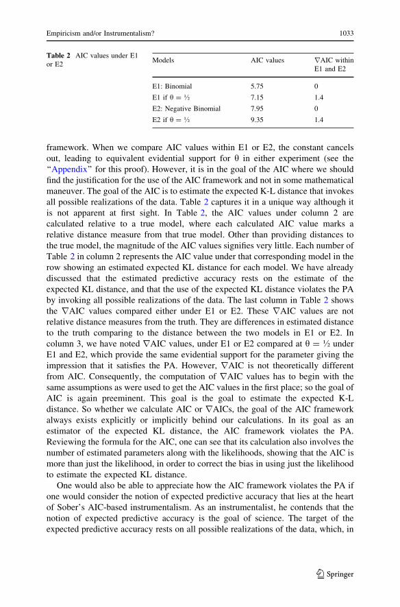
hypothesis, h = �. Column 2 of Table 2 shows different AIC values respectively

under model E1: Binomial, with h[ � versus with h = �, and under E2: Negative

Binomial with h[ 1/2 versus with h = �. They are, 5.75 under E1: Binomial with

h[ 1/2 versus 7.15 under E1: Binomial with h = �. In the same column of

Table 2, we also find 7.95 under E2: Negative Binomial with h[ � versus 9.35

under Negative Binomial with h = �.

In both E1 and E2, the difference in AIC values is 1.4, which would be referred to

as the ‘‘rAIC’’ for the constrained model under E1 or E2. The rAIC is the

difference between each calculated AIC and the minimum AIC in the set of models.

For example, the rAIC model under E1: h[ �, is 5.75–5.75 = 0, where the first

number stands for its AIC value and the second number for the minimum AIC

value. However, the interesting feature of the application of the rAIC is to observe

the evidential support for a pairwise comparison between E1: Binomial, with h[ �versus with h = �, and E2: Negative Binomial with h[ � versus with h = �. The

difference between these two pair-wise comparisons of models under the rAIC is

1.4. This difference suggests the same evidential support between the two models

under each experimental setup. This satisfies the PA’s evidential equivalence

condition for two experiments (PAT) which seems to suggest that AIC satisfies

PAT. In this regard, the likelihood and AIC frameworks seem to share some similar

feature regarding the evidential support between two competing models. If the

likelihood ratio provides the same results in either experiment, then the likelihoods

share the same proportionality and according to the PAT, both experiments provide

equal evidential support for the parameter in question. In the same vein, when

rAIC comparisons are made between candidates with equally proportional

likelihoods and the same difference in the number of estimated parameters in the

constrained and unconstrained models, the AIC provides the same evidential

support regardless of the experiment that is assumed to have been conducted (see

the ‘‘Appendix’’ for a proof of this result). Here, both unconstrained models have

one estimated parameter (h) while the constrained models have 0 since h is assumed

to be �, and the difference in the number of estimated parameters between the

constrained and unconstrained models is the same in both experiments. Since the

rAIC provides the same comparisons here regardless of whether E1 or E2 was

conducted, it appears to satisfy the PA in the same way that the likelihood ratio

satisfies the PA.

The apparent similarity between the likelihood ratio and the AIC framework to

seem to obey the PA stems from a mathematical maneuver within the AIC

12 Whether Sober’s view is correct here goes beyond the objective of this paper.13 For his recent position about the AIC, see (Sober 2008).


123

framework. When we compare AIC values within E1 or E2, the constant cancels

out, leading to equivalent evidential support for h in either experiment (see the

‘‘Appendix’’ for this proof). However, it is in the goal of the AIC where we should

find the justification for the use of the AIC framework and not in some mathematical

maneuver. The goal of the AIC is to estimate the expected K-L distance that invokes

all possible realizations of the data. Table 2 captures it in a unique way although it

is not apparent at first sight. In Table 2, the AIC values under column 2 are

calculated relative to a true model, where each calculated AIC value marks a

relative distance measure from that true model. Other than providing distances to

the true model, the magnitude of the AIC values signifies very little. Each number of

Table 2 in column 2 represents the AIC value under that corresponding model in the

row showing an estimated expected KL distance for each model. We have already

discussed that the estimated predictive accuracy rests on the estimate of the

expected KL distance, and that the use of the expected KL distance violates the PA

by invoking all possible realizations of the data. The last column in Table 2 shows

the rAIC values compared either under E1 or E2. These rAIC values are not

relative distance measures from the truth. They are differences in estimated distance

to the truth comparing to the distance between the two models in E1 or E2. In

column 3, we have noted rAIC values, under E1 or E2 compared at h = � under

E1 and E2, which provide the same evidential support for the parameter giving the

impression that it satisfies the PA. However, rAIC is not theoretically different

from AIC. Consequently, the computation of rAIC values has to begin with the

same assumptions as were used to get the AIC values in the first place; so the goal of

AIC is again preeminent. This goal is the goal to estimate the expected K-L

distance. So whether we calculate AIC or rAICs, the goal of the AIC framework

always exists explicitly or implicitly behind our calculations. In its goal as an

estimator of the expected KL distance, the AIC framework violates the PA.

Reviewing the formula for the AIC, one can see that its calculation also involves the

number of estimated parameters along with the likelihoods, showing that the AIC is

more than just the likelihood, in order to correct the bias in using just the likelihood

to estimate the expected KL distance.

One would also be able to appreciate how the AIC framework violates the PA if

one would consider the notion of expected predictive accuracy that lies at the heart

of Sober’s AIC-based instrumentalism. As an instrumentalist, he contends that the

notion of expected predictive accuracy is the goal of science. The target of the

expected predictive accuracy rests on all possible realizations of the data, which, in

Table 2 AIC values under E1

or E2Models AIC values rAIC within

E1 and E2

E1: Binomial 5.75 0

E1 if h = � 7.15 1.4

E2: Negative Binomial 7.95 0

E2 if h = � 9.35 1.4


123

turn, leads to his brand of instrumentalism. Thus, for him, instrumentalism follows

from the AIC framework in which unobserved possible data play a crucial role.

Fifth, and finally, noting that AIC violates the PA need not be counted as a

criticism on the use of AIC. AIC-based frameworks have been both successfully and

widely used in building models from data, with the AIC providing a means of

comparing models in terms of support for the different models while also avoiding

various issues associated with the p value. However, it is important to acknowledge

the implications of the theoretical justification for the method one uses. The

violation of the PA is one such implication of AIC.

5 A Conflicting Methodological Imperative and a Possible Objection

In this section, we will discuss two points. First, we summarize our argument which

we will brand as Sober’s conflicting methodological imperative. Second, we

evaluate an objection to our impossibility result argument. Consider the first point

first. Sober’s two accounts, empiricism and instrumentalism, pull in opposite

directions. His account of empiricism exploits the PA, whereas his AIC-based

account of instrumentalism violates it. Further evidence of this tension is indicated

if one combines Sober’s instrumentalism with his empiricism.

Recall the earlier example involving two experiments, E1 and E2, in which an

agent will evaluate whether the proportion of males and females is the same in a

population of birds. According to the example, E1 consists of sampling 30 birds,

whereas E2 consists of sampling birds until one gets 10 females. We came to know

from the example that we have obtained 20 male birds as our data. We argued that it

is possible that an agent could have performed both E1 and E2 successively, and

found 20 males out of 30 birds in both cases. However, we don’t know which

experiment she conducted. If the agent accepts PA, then she is bound to say that E1

and E2 are on the same epistemological footing regarding the true proportion,

whether she decides to conduct E1 or E2. The rationale for this is that 20 males out

of 30 birds are actual observed data. However, she could also reject the PA on the

grounds that it is possible that she could have gotten outcomes in E2 different from

what she actually obtained. Therefore, she might conclude that E1 and E2 are not

necessarily on the same epistemological footing regarding the probability of the

hypothesis being true. From a broader philosophical perspective, like the agent in

our example, acceptance and rejection of PA generates a tension in Sober’s

philosophy. This tension is what we call ‘‘a conflicting methodological imperative’’

in his philosophy. Although depending on which choice about PA the agent makes,

she is led to holding incompatible stances toward PA, we have explained in Sect. 3

why this tension in selection of the correct hypotheses in two scenarios does not get

reflected and subsequently could be confusing for the reader that AIC in fact relies

on the PA instead of violating the PA. This ends the summary of our argument for

Sober’s conflicting methodological imperative.

Consider a possible objection to our argument. We argued that the AIC

framework violates the PA. The objector, however, contends that this is a mistake,

contending that the AIC actually respects it. According to this objection, the PA


123

needs to be taken in the AIC framework as a principle of hypothesis choice, a

decision rule. This is what we call the decision-based understanding of the PA to be

distinguished from the epistemic understanding broached in Sect. 1 as a criterion of

evidence. The objector continues ‘‘if there is a decision rule which suggests

decisions that depend only on the available evidence, and if someone tries to justify

the rule with an argument which refers to unobserved entities, this does not change

the fact that the decisions suggested by the rule depend only on the available

evidence.’’14 In our bird example, 20 male birds out of 30 birds are actual/observed

data; we should make our hypotheses with respect to them, even though the spelling

and grounding of the AIC requires that we consider all possible realizations of data

when we estimate the expected K-L distance. Thus, the objector has offered a

decision-based distinction that the AIC framework, after all, respects the PA, not in

the estimation of the K-L distance (an epistemic consideration), but in the

hypothesis we eventually should choose (a practical consideration).

Our response is that if this sort of response were taken seriously, it would have

consequences reaching far beyond the plausibility of the AIC framework. Recall our

earlier argument that classical statistics, when it involves the logic of significance

testing, disobeys the PA. In our bird example, when we computed the likelihood

functions under two models, Binomial and Negative Binomial models, we

computed the likelihood functions under each model relative to the observed data,

Y = 20. Significant testing involves our actual/observed data to be a sample of 20

male birds out 30, although the potentially observed ‘‘more extreme’’ Y [ 21,

Y [ 22 and so on have entered in significance testing computations. If the decision

rule in this example suggests that a decision regarding the null hypothesis (i.e.,

h = 1/2) ought to be made only on the available data then, it follows, according to

this response, that the logic of significance testing in fact obeys the PA, although the

logic of significance testing spells out and grounds the rule by reference to

unobserved data. Otherwise stated, if the PA is re-cast as a ‘‘decision rule’’ in the

way indicated, then the ongoing epistemic debate concerning what to count as

‘‘evidence’’ between those who accept the PA and those who question it should be

regarded as pointless. From our point of view, the response goes forward simply by

changing the subject, and in the process treating merely possible data instrumen-

tally, as posits for the sake of clarification and explanation. One could, of course,

claim that the considerable discussion among statisticians concerning the status of

the PA has been beside the point, but this involves throwing out a great deal of

bathwater just to save one’s (controversial) baby.

However, a more charitable construal of the objection is possible, although it

won’t in the final analysis salvage the objection. The PA taken as a decision rule

could be given (i) a narrow interpretation and (ii) a wide interpretation. According

to a narrow interpretation, the decision regarding which hypothesis to be chosen

should be based on an investigator’s stopping rule (e.g., to stop at 30 sampling of

birds consisting of males and females or stop at whenever one will obtain 10

females.) The wide interpretation implies that the decision regarding which

hypothesis to be chosen should be based on available evidence. The objection

14 This objection has been raised by a critic after reading the previous version of the paper.


123

makes use of a wide interpretation (ii) although as we have just claimed the only

way to make sense of the contemporary debate about the status of the PA in the

foundation of statistics is to construe it narrowly (i). Both interpretations assume

that the PA consists of a decision rule and a theoretical justification for the former.

According to the narrow interpretation, the rationale for trusting its decision rule is

rooted in the PA, whereas the wide one takes the justification for its decision rule to

fall back on the expected K-L distance that invokes both actual and possible data.

Consider our bird example to see how both interpretations work. In both narrow

and wide interpretations, how the decision rule functions in the bird example is the

same, i.e., one should base one’s judgment about theories/models only on actual/

observed data in which actual/observed data are 20 male birds out of 30 birds. There

is no disagreement between them about how the PA as a decision rule works with

regard to the bird example. However, their justification for the use of the rule falls

apart. In the case of the narrow interpretation, the justification for the decision rule

could be that we have seen 20 male birds out of 30 birds, and this is why the rule

should rely only on actual/observed data. This justification is rooted in the

epistemological feature of the PA. The former, as we can see, does not involve any

reference to unobserved evidence. In contrast, the justification for the wide

interpretation involves reference to all possible data because of integration over the

sample space. In fact, Akaike’s (1973) theorem makes reference to unobserved

entities, because the definition of unbiasedness contains an integral which extends

over the space of all possible samples. In our bird example, if the investigator were

to repeat the experiment, as we have noted in Sect. 3, the number of male birds

would be likely to vary, possibly 21 male birds out of the total 30 in Binomial

experiment, or 21 male birds out of 31 in Negative Binomial experiment. These are

some of the other possible realizations of the data. So to make the debate over the

PA worthwhile, the debate over acceptance and rejection of the PA really boils

down to which justificatory rationale each statistical school (e.g., classical statistics

and AIC followers on the one hand, and Bayesians and likelihood followers, on the

other) invokes. Classical statisticians and AIC followers subscribe to a wide

interpretation, and Bayesian and Likelihood followers to a narrow interpretation

about the epistemological status of the PA.

In light of our above construal of the PA, it becomes evident that whether the

AIC framework violates the PA depends on which construal, wide or narrow, turns

out to be crucial for a proper understanding of the PA. The rationale for rejecting a

wide interpretation of the PA is that it disregards contemporary debate over the

status of the PA in the foundations of statistics. The upshot of this section is to

reinstate our objection that Forster and Sober’s AIC framework violates the PA in

its goal. Recall that its goal is to find the expected K-L distance which rests on all

possible realizations of sample data. The use of AIC rests on that goal which

provides a theoretical justification for its use in the first place. Use of any statistical

inferential methodology requires a theoretical justification regarding why one

should trust it, otherwise any successes or failures of a methodology would be

anecdotal not inferential. Since the AIC methodology draws its justification from

the estimate of the K-L distance from all possible realizations of data, the core of the

application of the AIC methodology lies in its theoretical foundation. And it is


123

precisely at this point where the AIC framework violates the PA. Our point, to put it

as simply as possible, is that the AIC theorist wants to have it both ways: possible

data (in the spelling out and grounding of Akaike’s theorem) and actual data (in the

choice between rival hypotheses). In the process, ‘‘empiricism’’ has been emptied of

its traditional epistemic content. Indeed it would seem to have very little content

left.

There is a broader implication of questioning the objector’s wide interpretation of

the PA. The objector’s way of construing the PA as a decision rule makes the rule

vacuous. If the possible objection stemming from a wide interpretation is about the

PA being a decision rule, then (most) statistical methods would be taken to satisfy

the PA, because all use actual data to make decisions. However, as we have already

reported, it is the justification for the decision rule which is most important, and it is

at this level that it matters whether the PA is violated or not. In previous sections,

we discussed the epistemological aspects of the debates over the PA, focusing on

the justification for the methods, which figures prominently in the assessment of the

narrow and wide interpretations. This is why we think that epistemological features

for the grounding of the PA are the most significant aspects in appreciating the

debate over the status of the PA in scientific inference as well as for the possibility

of empiricism-instrumentalism coupling.

6 Summing Up

We argued that Sober’s two accounts, (i) the AIC-based notion of instrumentalism,

which violates the principle of actualism, and (ii) his empiricism, which respects it,

have led to a tension in his impressive philosophical work. However, the purpose of

this paper is not just to report a tension in Sober’s work. A larger significance of this

paper lies in making explicit the bearings of our varying intuitions about the

principle of actualism on our understanding of scientific inference and whether the

empiricism/instrumentalism coupling can be conjoined consistently. These intu-

itions are so fundamentally rooted in us that whether one is a Bayesian/

Likelihoodist15 or a non-Bayesian/Akaikean turns on whether one rejects or accepts

PA. Sober realizes how fundamental, yet divergent our intuitions about PA are. Torn

between them, he wants to have the best of both views on scientific inference,

Bayesian and non-Bayesian. We have touched on how two Bayesian principles, the

likelihood principle and the Conditionality Principle, have motivated two conse-

quences of PA. In the case of Sober, what is significant is that these conflicting

intuitions about PA have generated two divergent but at the same time inter-related

views about his stances toward scientific inference and the empiricism/instrument-

alism coupling. The first lesson we would like to take home from this is that perhaps

one should adopt a definite stance toward scientific inference; one cannot have both

a little bit of Bayesianism coupled with a little bit of non-Bayesianism in one’s

15 Sober defends a likelihood approach to both evidence and scientific inference. Although there are

fundamental differences between a likelihoodist and a Bayesian, for our present purpose, those

differences are unimportant.


123

epistemology of inference. Otherwise, like Sober, we are likely to end up with a

conflicting methodological imperative. The second lesson would be that his

conflicting stances toward PA results in a conceptual difficulty in combining

empiricism with instrumentalism. Whether this conceptual difficulty for the

empiricism/instrumentalism coupling is much more general remains a desideratum

for further study.16

Acknowledgments We would like to thank Prajit Basu, John G. Bennett, Robert Boik, Abhijit

Dasgupta, Michael Evans, Roberto Festa, Dan Flory, Malcolm Forster, Jayanta Ghosh, Dan Goodman,

Jason Grossman, Joseph Hanna, Bijoy Mukherjee, Megan Raby, Tasneem Sattar, Mark Taper, Susan

Vineberg, and C. Andy Tsao for discussion/comments regarding the content of the paper. We are thankful

to three anonymous referees of this journal and a dozen other referees from different journals for their

helpful feedback. We owe special thanks to Elliott Sober for serving as an official commentator for our

paper at the APA divisional meetings, and John G. Bennett for several correspondences regarding the

issues raised in the paper. The research for the paper has been funded by our university’s NASA’s

Astrobiology Center (Grant No. 4w1781) with which some of the authors of this paper are affiliated.

Appendix A: Proof of equivalent rAICs if the equivalent condition for twoexperiments (PAT) holds

Recall the PAT: two experiments, E1 and E2, provide equal evidential support for a

model, that is, the parameter in question, if and only if their likelihood functions are

proportional to each other as functions of the models, and therefore, any inference

about the model based on these experiments should be identical. If we assume that

under two different experimental designs, E1 and E2, their likelihoods have the

same proportionality under two different models regarding the same parameter,

then, it follows from the PAT that both models provide equal evidential support for

the parameter. First, define L1ðhÞ and L1ðhÞ as the likelihoods under E1 for the

model using the MLE of h and the model with h = 0.5, respectively. We could

define L2ðhÞ and L2ðhÞ similarly. We also define the likelihood ratio for each

experiment as the constants c1 and c2 in L1ðhÞ ¼ c1L1ðhÞ and L2ðhÞ ¼ c2L2ðhÞ.These constants are also the likelihood ratios reported in the Table (1) above, which

weighs the evidence between the two models in either E1 and E2. Then if

c1 = c2 = c, then we find equal evidential support using the likelihood ratio,

satisfying the PAT.

Now we show how if the PAT holds, thenrAIC will also provide equal evidence

between the hypotheses. First, we assume that the AIC is reduced for the

unconstrained model. Also, we use dim(h) to indicate the number of parameters that

are estimated. Then consider the definition of rAIC for, say, E1:

16 Van Fraassen’s constructive empiricism that combines empiricism with instrumentalism also leads to a

contradiction (see Bandyopadhyay 1997).


123

rAIC ¼ AICh � AICh ¼ �2 logðL1ðhÞÞ þ 2 � dimðhÞ þ 2 logðL1ðhÞÞ � 2 � dimðhÞ

¼ �2 log L1ðhÞ.

L1ðhÞ� �

þ 2 � dimðhÞ � 2 � dimðhÞ

But L1ðhÞ.

L1ðhÞ ¼ 1=c ¼ L2ðhÞ.

L2ðhÞ by the PAT. Thus, rAIC will be the same

under E1 or E2 if the PAT holds and the difference in the dimensions of h and h are

the same across the experiments. Note that this is a stronger condition than just

assuming that the PAT holds since it also involves the number of estimated

parameters in the constrained and unconstrained models, in addition to propor-

tionality of the likelihoods.

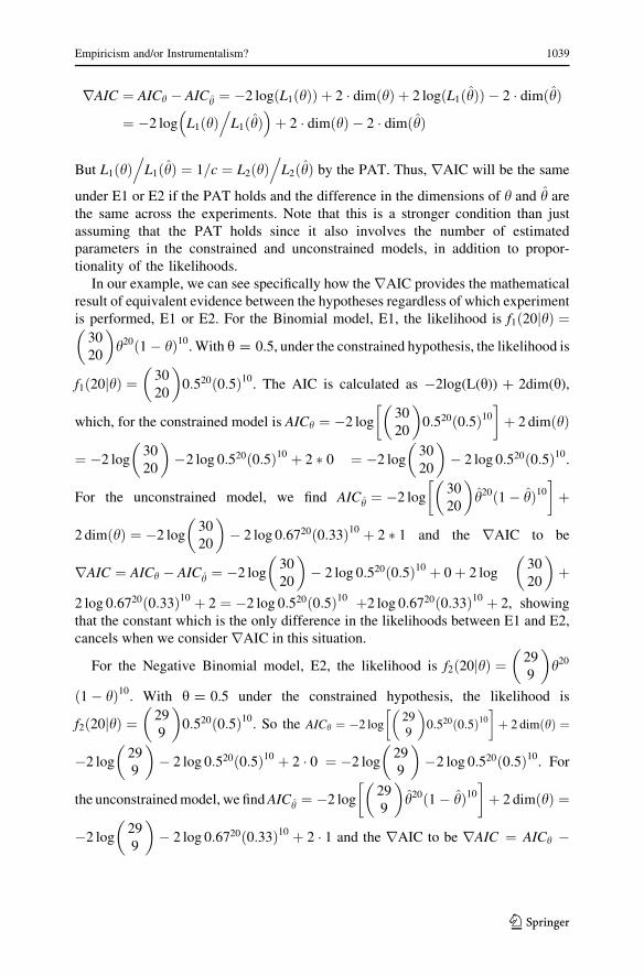
In our example, we can see specifically how therAIC provides the mathematical

result of equivalent evidence between the hypotheses regardless of which experiment

is performed, E1 or E2. For the Binomial model, E1, the likelihood is f1ð20jhÞ ¼30

20

� �h20ð1� hÞ10

. With h = 0.5, under the constrained hypothesis, the likelihood is

f1ð20jhÞ ¼ 30

20

� �0:520ð0:5Þ10

. The AIC is calculated as -2log(L(h)) ? 2dim(h),

which, for the constrained model is AICh ¼ �2 log30

20

� �0:520ð0:5Þ10

� �þ 2 dimðhÞ

¼ �2 log30

20

� ��2 log 0:520ð0:5Þ10 þ 2 � 0 ¼ �2 log

30

20

� �� 2 log 0:520ð0:5Þ10

.

For the unconstrained model, we find AICh ¼ �2 log30

20

� �h20ð1� hÞ10

� �þ

2 dimðhÞ ¼ �2 log30

20

� �� 2 log 0:6720ð0:33Þ10 þ 2 � 1 and the rAIC to be

rAIC ¼ AICh � AICh ¼ �2 log30

20

� �� 2 log 0:520ð0:5Þ10 þ 0þ 2 log

30

20

� �þ

2 log 0:6720ð0:33Þ10 þ 2 ¼ �2 log 0:520ð0:5Þ10 þ2 log 0:6720ð0:33Þ10 þ 2, showing

that the constant which is the only difference in the likelihoods between E1 and E2,

cancels when we consider rAIC in this situation.

For the Negative Binomial model, E2, the likelihood is f2ð20jhÞ ¼ 29

9

� �h20

ð1� hÞ10. With h = 0.5 under the constrained hypothesis, the likelihood is

f2ð20jhÞ ¼ 29

9

� �0:520ð0:5Þ10

. So the AICh ¼ �2 log29

9

� �0:520ð0:5Þ10

� �þ 2 dimðhÞ ¼

�2 log29

9

� �� 2 log 0:520ð0:5Þ10 þ 2 � 0 ¼ �2 log

29

9

� ��2 log 0:520ð0:5Þ10

. For

the unconstrained model, we find AICh ¼ �2 log29

9

� �h20ð1� hÞ10

� �þ 2 dimðhÞ ¼

�2 log29

9

� �� 2 log 0:6720ð0:33Þ10 þ 2 � 1 and the rAIC to be rAIC ¼ AICh �


123

AICh ¼ �2 log29

9

� �� 2 log 0:520ð0:5Þ10 þ 0 þ 2 log

29

9

� �þ 2 log 0:6720 ð0:33Þ10 þ

2 ¼ �2 log 0:520ð0:5Þ10 þ 2 log 0:6720ð0:33Þ10 þ 2 as in E1, showing that since

the constant cancels in either experiment, that samerAIC is found. The constant also

cancels in the likelihood ratio when the likelihood ratios in either E1 or E2 are

considered.

References

Akaike, H. (1973). Information theory and an extension of the maximum likelihood principle. In B.

N. Petrov & F. Csaki (Eds.), Second international symposium on information theory (pp. 267–281).

Budapest: Akademia Kaido.

Bandyopadhyay, P. S. (1997). On an inconsistency in constructive empiricism. Philosophy of Science, 64,

511–514.

Bandyopadhyay, P. S. (2007). Why Bayesianism? A primer on a probabilistic philosophy of science. In S.

K. Upadhyay, U. Sing, & D. K. Dey (Eds.), Bayesian statistics and its applications (pp. 42–62).

New Delhi: Anamaya Publishers.

Bandyopadhyay, P. S., & Boik, R. (1999). The curve-fitting problem: A Bayesian rejoinder. Philosophy of

Science, 66, S390–S402.

Bandyopadhyay, P. S., Boik, R., & Basu, P. (1996). The curve-fitting problem: A Bayesian approach.

Philosophy of Science, 63, S265–S272.

Bandyopadhyay, P. S., & Brittan, G., Jr. (2001). Logical consequence and beyond: A close look at model

selection in statistics. In J. Woods & B. Hepburb (Eds.), Logical consequence (pp. 1–17). Oxford:

Hermes Science Publishing Company.

Berger, J. (1985). Statistical decision theory and Bayesian analysis. New York: Springer.

Birnbaum, A. (1962). On the foundations of statistical inference. Journal of the American Statistical

Association, 57, 269–306.

Boik, R. (2004). Commentary. In M. Taper & S. Lele (Eds.), The nature of scientific evidence (pp.

167–180). Chicago: The University of Chicago Press.

Box, G. (1979). Robustness in scientific model building. In R. I. Launer & G. N. Wilkinson (Eds.),

Robustness in statistics (pp. 201–236). New York: Academic Press.

Boyd, R. (1985). Observations, explanatory power, and simplicity. In P. Achinstein & O. Hannaway

(Eds.), Observation, experiment, and hypothesis in modern physical science. Cambridge, MA: MIT

Press.

Burnham, K., & Anderson, D. (1998). Model selection and inference. New York: Springer.

Cassella, G., & Berger, R. (1990). Statistical Inference. California: Wadsworth & Brooks.

Eells, E. (1993). Probability, inference, and decision. In J. Fetzer (Ed.), Foundations of philosophy of

science (pp. 192–208). New York: Paragon House.

Evans, M. (2013). What does the proof of Birnbaum’s theorem prove? Electronic Journal of Statistics,

1–9.

Forster, M., & Sober, E. (1994). How to tell when simpler, more unified, or less ad hoc theories will

provide more accurate predictions. British Journal for the Philosophy of Science, 45, 1–35.

Forster, M., & Sober, E. (2004a). Why likelihood? In M. Taper & S. Lele (Eds.), The nature of scientific

evidence. Chicago: University of Chicago Press.

Forster, M., & Sober, E. (2004b). Rejoinder to why likelihood? In M. Taper & S. Lele (Eds.), The nature

of scientific evidence. Chicago: University of Chicago Press.

Godfrey-Smith, P. (1999). Procrustes probably. Philosophical Studies, 95, 175–180.

Good, I. J. (1983). The white shoe is a red herring. First published in BJPS, 1967, 17: p. 332. Reprinted in

good thinking. Minnesota: University of Minnesota Press.

Hacking, I. (1965). Logic of statistical inference. Cambridge: Cambridge University Press.

Hanna, J. (2004). Contra Ladyman: What really is right with constructive Empiricism. British Journal for

the Philosophy of Science, 55, 767–777.


123

Howson, C., & Urbach, P. (2006). Scientific reasoning: The Bayesian approach (3rd ed.). La Salle, IL:

Open Court.

Jeffreys, W., & Berger, J. (1992). Ockham’s Razor and Bayesian analysis. American Scientists, 80,

64–72.

Kitcher, P. (1993). The advancement of science. New York: Oxford University Press.

Kitcher, P. (2001). Science, truth, and democracy. Oxford: Oxford University Press.

Kullback, S., & Leibler, R. (1951). On information and sufficiency. Annals of Mathematical Statistics, 22,

79–86.

Ladyman, J. (2000). What’s really wrong with constructive Empiricism? Van Fraassen and the

metaphysics of modality. British Journal for the Philosophy of Science, 51, 837–856.

Miller, R. (1987). Explanation, confirmation, and reality in the natural and social sciences. Princeton:

Princeton University Press.

Pawitan, Y. (2001). All likelihood: Statistical modelling and inference using likelihood. Oxford: Oxford

University Press.

Roberts, C. (1994). The Bayesian choice. New York: Springer.

Royall, R. (1997). Statistical evidence. New York: Chapman & Hall.

Sober, E. (1988). Reconstructing the past: Parsimony, evolution, and inference. Cambridge: MIT Press.

Sober, E. (1993). Epistemology for empiricists. In P. French, T. Uehling, & H. Weinstein (Eds.), Midwest

studies in philosophy, XVIII.

Sober, E. (1995). From a biological point of view. Cambridge: Cambridge University Press.

Sober, E. (1996). Parsimony and predictive equivalence. Erkenntnis, 44, 167–197.

Sober, E. (1998). Instrumentalism revisited. Critica, 31, 3–38.

Sober, E. (2001). Instrumentalism, Parsimony, and the Akaike framework. Philosophy of science

(Proceedings), Fall.

Sober, E. (2008). Evidence and evolution: The logic behind the science. Cambridge: Cambridge

University Press.

Swinburne, R. (2001). Epistemic justification. Oxford: Clarendon Press.

Van Fraassen, B. (1980). The scientific image. Oxford: Oxford University Press.

Van Fraassen, B. (1989). Laws and symmetry. Oxford: Oxford University Press.


123

Empiricism and/or Instrumentalism?

Documents