The Pennsylvania State University The Graduate School Department of Economics EMPIRICAL STUDIES OF MICROECONOMIC AGENTS’ BEHAVIOR A Dissertation in Economics by Hae Won Byun c 2008 Hae Won Byun Submitted in Partial Fulfillment of the Requirements for the Degree of Doctor of Philosophy August 2008

Welcome message from author
This document is posted to help you gain knowledge. Please leave a comment to let me know what you think about it! Share it to your friends and learn new things together.
Transcript

The Pennsylvania State University
The Graduate School
Department of Economics
EMPIRICAL STUDIES OF
MICROECONOMIC AGENTS’ BEHAVIOR
A Dissertation in
Economics
by
Hae Won Byun
c© 2008 Hae Won Byun
Submitted in Partial Fulfillmentof the Requirements
for the Degree of
Doctor of Philosophy
August 2008

The dissertation of Hae Won Byun was reviewed and approved∗ by the following:
Coenraad PinkseAssociate Professor of EconomicsDissertation AdviserChair of Committee
N. Edward CoulsonProfessor of Economics
Mark J. RobertsProfessor of Economics
Andrew N. KleitProfessor of Energy and Environmental Economics
Vijay KrishnaProfessor of EconomicsDirector of Graduate Studies
∗Signatures are on file in the Graduate School.

iii
Abstract
The economic decisions of rational agents can be analyzed by theoretical mod-
els and/or empirical models. This dissertation consists of two different applications of
empirical models on two different economic conundrums, both based on theoretical hy-
potheses. The first chapter introduces the related literatures and background of each
paper. In the second chapter, I analyze the concert ticket market by extending the the-
ory present in the economic literature and estimating a parametric empirical model. In
the third chapter we estimate the affiliation effect (Pinkse and Tan [26]) in a specific
common value auction setting.
The second chapter investigates promoters’ and bands’ ticket price decisions and
presents a theoretical model that demonstrates how their seemingly suboptimal decisions
can be profit-maximizing. Here, I model the ticket price decision of a promoter and an
artist based on two potential explanations: the effects of an artist’s future profit as well
as merchandising profit on the pricing decision. When artists or promoters consider their
future profit as well as their current profit, or they consider merchandising revenue as
well as ticket revenue, they may charge a price lower than the price which maximizes only
their static ticket profit. In order to test the credibility of these potential explanations, I

iv
estimate a ticket supply equation with Pollstar Boxoffice historical data. The estimation
results suggest that both the future profit of an artist and merchandising profit are
credible explanations as to why promoters and bands set the ticket price lower than the
static ticket profit maximizing price.
The third chapter estimates the affiliation effect defined in Pinkse and Tan [26]
in which they showed that bids can be decreasing in the number of bidders in private
value auctions provided that the bidders’ private values are affiliated. We use the Outer
Continental Shelf auction data set to estimate three effects nonparametrically: the af-
filiation effect, the competition effect, and the winner’s curse effect. We find that the
affiliation effect is in fact the smallest of the three.

v
Table of Contents
List of Tables . . . . . . . . . . . . . . . . . . . . . . . . . . . . . . . . . . . . . . vii
List of Figures . . . . . . . . . . . . . . . . . . . . . . . . . . . . . . . . . . . . . viii
Acknowledgments . . . . . . . . . . . . . . . . . . . . . . . . . . . . . . . . . . . ix
Chapter 1. Introduction . . . . . . . . . . . . . . . . . . . . . . . . . . . . . . . . 1
1.1 Monopolistic Behavior . . . . . . . . . . . . . . . . . . . . . . . . . . 1
1.2 Auction Theory . . . . . . . . . . . . . . . . . . . . . . . . . . . . . . 3
1.3 Supply Function Estimation . . . . . . . . . . . . . . . . . . . . . . . 7
1.4 Nonparametric Estimation Methodology . . . . . . . . . . . . . . . . 9
1.4.1 Kernel Density Estimation . . . . . . . . . . . . . . . . . . . . 10
1.4.2 Kernel Regression Estimation . . . . . . . . . . . . . . . . . . 12
1.5 The Bootstrap . . . . . . . . . . . . . . . . . . . . . . . . . . . . . . 13
Chapter 2. Why Rock Stars Do Not Raise Their Ticket Prices . . . . . . . . . . 14
2.1 Introduction . . . . . . . . . . . . . . . . . . . . . . . . . . . . . . . . 14
2.2 Music Industry . . . . . . . . . . . . . . . . . . . . . . . . . . . . . . 16

vi
2.3 Model . . . . . . . . . . . . . . . . . . . . . . . . . . . . . . . . . . . 18
2.3.1 Setup . . . . . . . . . . . . . . . . . . . . . . . . . . . . . . . 19
2.3.2 Ticket Price . . . . . . . . . . . . . . . . . . . . . . . . . . . . 23
2.4 Data and Results . . . . . . . . . . . . . . . . . . . . . . . . . . . . . 27
2.4.1 Data Description . . . . . . . . . . . . . . . . . . . . . . . . . 27
2.4.2 Estimation Results . . . . . . . . . . . . . . . . . . . . . . . . 29
2.5 Conclusion . . . . . . . . . . . . . . . . . . . . . . . . . . . . . . . . . 33
Chapter 3. The Size of the Affiliation Effect . . . . . . . . . . . . . . . . . . . . 36
3.1 Introduction . . . . . . . . . . . . . . . . . . . . . . . . . . . . . . . . 36
3.2 The Effects . . . . . . . . . . . . . . . . . . . . . . . . . . . . . . . . 39
3.3 Estimation . . . . . . . . . . . . . . . . . . . . . . . . . . . . . . . . . 43
3.3.1 Normalization . . . . . . . . . . . . . . . . . . . . . . . . . . . 43
3.3.2 Nonparametric Estimation . . . . . . . . . . . . . . . . . . . . 45
3.3.3 Confidence Bands . . . . . . . . . . . . . . . . . . . . . . . . . 46
3.4 Data . . . . . . . . . . . . . . . . . . . . . . . . . . . . . . . . . . . . 46
3.5 Limitations . . . . . . . . . . . . . . . . . . . . . . . . . . . . . . . . 48
3.6 Results . . . . . . . . . . . . . . . . . . . . . . . . . . . . . . . . . . . 51
Appendix. The Confidence Bands . . . . . . . . . . . . . . . . . . . . . . . . . . 58
References . . . . . . . . . . . . . . . . . . . . . . . . . . . . . . . . . . . . . . . . 59

vii
List of Tables
2.1 Summary Statistics . . . . . . . . . . . . . . . . . . . . . . . . . . . . . . 29
2.2 2SLS Estimation of Price Equation with Instrumental Variables∗ . . . . 31
2.3 First Stage Regression∗ . . . . . . . . . . . . . . . . . . . . . . . . . . . 35
3.1 Number of Bids (low and high ℓ tracts) . . . . . . . . . . . . . . . . . . 48
3.2 Summary Statistics for Tract Data . . . . . . . . . . . . . . . . . . . . . 49
3.3 Summary Statistics for Bid Data . . . . . . . . . . . . . . . . . . . . . . 50

viii
List of Figures
2.1 Attendance Rate . . . . . . . . . . . . . . . . . . . . . . . . . . . . . . . 28
2.2 Capacity . . . . . . . . . . . . . . . . . . . . . . . . . . . . . . . . . . . . 28
3.1 Affiliation Effect for low ℓ tracts (n=3) . . . . . . . . . . . . . . . . . . . 52
3.2 Affiliation Effect for low ℓ tracts (n=5) . . . . . . . . . . . . . . . . . . . 52
3.3 Competition Effect for low ℓ tracts (n=3) . . . . . . . . . . . . . . . . . 53
3.4 Competition Effect for low ℓ tracts (n=5) . . . . . . . . . . . . . . . . . 53
3.5 Winner’s Curse Effect for low ℓ tracts (n=3) . . . . . . . . . . . . . . . . 54
3.6 Winner’s Curse Effect for low ℓ tracts (n=5) . . . . . . . . . . . . . . . . 54
3.7 Affiliation Effect for high ℓ tracts (n=4) . . . . . . . . . . . . . . . . . . 55
3.8 Affiliation Effect for high ℓ tracts (n=6) . . . . . . . . . . . . . . . . . . 55
3.9 Competition Effect for high ℓ tracts (n=4) . . . . . . . . . . . . . . . . . 56
3.10 Competition Effect for high ℓ tracts (n=6) . . . . . . . . . . . . . . . . . 56
3.11 Winner’s Curse Effect for high ℓ tracts (n=4) . . . . . . . . . . . . . . . 57
3.12 Winner’s Curse Effect for high ℓ tracts (n=6) . . . . . . . . . . . . . . . 57

ix
Acknowledgments
I am deeply grateful to Joris Pinkse, Edward Coulson, Mark Roberts, and Andrew
Kleit for their insightful guidance and constant encouragement. I also thank Edward
Green, Kalyan Chatterjee, and Neil Wallace for their meaningful commentary. Financial
support for this research is provided by the College of Liberal Arts, the Pennsylvania
State University. The second chapter has also benefited from conversations with Bernie
Punt from the Bryce Jordan Center, University Park, PA, and Michael Friedman from
BandMerch, LLC. Lastly, I would like to thank my family for their love and support and
my friends who became my second family here at Penn State. Any remaining errors are
mine.

Dedication
To my parents, Young Il Byun and Kwang Hae Chung, who are praying for me even at
this very moment.

1
Chapter 1Introduction
The economic decisions of rational agents can be analyzed by theoretical mod-
els and/or empirical models. This dissertation consists of two different applications of
empirical models on two different economic conundrums, both based on theoretical hy-
potheses. This chapter introduces background information relevant for chapters two and
three.
1.1 Monopolistic Behavior
Chapter two studies a ticket pricing decision. Behavior similar to the seemingly
non-profit-maximizing decision making by Rock stars or promoters can be witnessed
in many other settings, such as underpricing of video game consoles or initial public
offerings (IPOs). This section explains some of the underlying theory.
Tirole [29] provides several models of relevant monopolistic behavior. The most
important of these to my research is a model of a multi-product monopolistic firm which
produces n goods, and faces demand function qi(p) and cost function C(q1, · · · , qn),
where p = (p1, · · · , pn) and i = 1, · · · , n. The monopolist sets the price for each good

2
where it maximizes the following profit function Πmulti,
Πmulti =n
∑
i=1
piqi(p) − C(q1(p), · · · , qn(p)) .
The first order condition for the maximization problem is given in equation (1.1).
qi + pi∂qi∂pi
+∑
j 6=i
pj
∂qj
∂pi−
∑
j
∂C
∂qj
∂qj
∂pi= 0, i = 1, · · · , n (1.1)
If the third term of the first order condition (1.1) is non-zero, i.e. the demand for a good
depends on the price of other goods as well as its own price, the profit maximizing price
is different from the price maximizing a single product monopolist’s profit. Equation
(1.1) can be rearranged as follows:
pi − ∂Ci/∂qipi
=1
eii−
∑
j 6=i
(pj − ∂Cj/∂qj)qjeij
piqieii, (1.2)
where eij = −∂qj/qj∂pi/pi
. Note that the left hand side of equation (1.2) is the Lerner
index, which is the ratio of profit to price, which in turn is the markup rate that the
monopolist charges. The first term on the right hand side of equation (1.2) is the inverse
price elasticity. If the firm were a single product monopolist, the Lerner index would
equal the inverse price elasticity. In other words the second term on the right hand side
of equation (1.2) would necessarily equal zero.
The second term on the right had side of equation (1.2) includes eij = −∂qj/qj∂pi/pi
.
This term is negative if the goods are substitutes and positive if they are complements. If

3
two of the goods produced by the multi-monopolist are substitutes, then eij is negative.
The markup will be higher than the markup if the firm were a single product monopolist.
If the monopolist’s goods are complements, then eij is positive and the markup will be
lower than the markup if the firm were a single product monopolist.
Intuitively, decreasing the price for good i will cause the demand for good j to
increase if the goods are complements. Therefore, the multi-product monopolist will
charge a relatively lower price for each good. Inversely, decreasing the price of good i
will cause the demand of good j to decrease if the goods are substitutes. Therefore, the
multi-product monopolist will charge a relatively higher price for each good.
My paper deals with a multi-product monopolist who is selling complementary
goods that have dependent demands: merchadising demand which is positively correlated
with concert ticket demand, and future ticket demand which depends on current ticket
demand.
1.2 Auction Theory
In the third chapter we estimate the affiliation effect defined in Pinkse and Tan [26]
in a specific common value auction case. In their paper, they showed that bids can be
decreasing in the number of bidders in private value auctions provided that the bidders’
private values are affiliated.
Before moving on to the discussion of auction paradigms, the concept of affiliation
of random variables needs to be explained. The following definition is from Krishna [17].
Consider vectors s and s′ in Rn where s = (X1, · · · ,Xn) and s′ = (X′
1, · · · ,X′
n) with

4
the density function f(·). Random variables X1, · · · ,Xn are affiliated if for all s and s′,
f(s ∨ s′)f(s ∧ s′) ≥ f(s)f(s′) ,
where s∨s′ is the component-wise maximum of s and s′, and s∧s′ is the component-wise
minimum of s and s′. In this case, the p.d.f. f is also called affiliated. In the context
of auctions, if bidders’ private signals X1, · · · ,Xn are affiliated, then it means that if a
subset Xi values are high, other Xj values are more likely to be high. See Krishna [17]
and Milgrom and Weber [20] for more rigorous and detailed discussions.
Auctions can be categorized according to the characteristics of bidders’ valuation
of the auction object. In a private value auction, each bidder is aware of her own valuation
of the auction object when she bids for it, and this value is her private information. A
bidder’s valuation does not affect other bidders’ valuations or vice versa in this setting.
If bidders compete for an object that is only for their consumption not for resale or
investment, the auction can be considered a private value auction. An art auction can
be an example, if no bidders are involved in the auction for the purpose of investment
or resale of the object.
In a pure common value auction, there exists a value of the auction object which
is universal to all bidders. Bidders do not know the exact value ex ante, and they
only have their own signals, which are correlated with the value. Oil drilling rights
auctions are good examples of common value auction because at the time of the auction,
bidders do not know the real value of the tract. However, bidders have access to various

5
geological test results are correlated with the actual value of the tract. See Krishna [17]
and Klemperer [16] for more examples and discussions.
Milgrom and Weber [20] introduced affiliation in bidders’ values into the auction
literature. They provide a general symmetric model which includes the independent
private value and the common value models as extreme cases. A symmetric auction
occurs when:
• The function mapping the bidders’ private signals and the common components to
the value of the auctioned object is the same for all bidders and this function is
symmetric in the other bidders’ signals; and
• The joint density function of the signals is symmetric in its arguments.
These symmetry assumptions are a different generalization of the symmetry assumption
in an independent private value auction model, which is that bidders are symmetric if
their private values are drawn from the same distribution.
There are n bidders, and each bidder gets a signal, which is a private information.
Let Xi be the private signal of bidder i. There are some variables Zj , which affect the
bidders’ common valuation of the object (j = 1, · · · ,m). Bidder i’s valuation of the
object is given by the function u:
Vi = u(X1, · · · ,Xn;Z1, · · · , Zm).
Note that in an independent private value auction, m = 0 and Vi = Xi, while in a pure
common value auction, m = 1 and Vi = Z1. Bidders are risk neutral, so they maximize
their expected profits.

6
Milgrom and Weber [20] characterize Bayesian-Nash equilibrium bid functions in
the first price auction case. Note that in a first price (sealed bid) auction, bidders submit
their bids, then the bidder with the highest bid wins the object and pays what he bid.
This is different from second price auction, where the bidder submitting the highest bid
wins the object but pays the second highest bid.
Let X = X1 be bidder 1’s private signal and Y be the maximum of rivals’ signals,
i.e. Y = max(X2, · · · ,Xn). Suppose that the other bidders choose an increasing and
differentiable bid function B∗(·). Define r to be the bidder’ reserve price. Then for any
r ≤ x ≤ x the expected payoff of bidder 1 is:
Π(b;x) = E[(V1 − b)I(B∗(Y ) < b)|X = x]
= E[E[(V1 − b)I(B∗(Y ) < b)|X,Y ]|X = x]
= E[(v(X,Y ) − b)I(B∗(Y ) < b)|X = x]
=
∫ B∗−1(b)
r(vn(x, t) − b)fY (t|x)dt ,
where
vn(x, y) = E[V1|X = x, Y = y].
The first order condition for bidder 1’s expected profit maximization problem is as fol-
lows:
∂Π
∂b(b;x) =
(vn(x,B∗−1(b) − b)fY (B∗−1(b)|x)
B∗′(B∗−1(b))− FY (B∗−1(b)|x) = 0 ,

7
such that
B∗′
(x) = (wn(x) − B∗(x))
fY (x|x)
FY (x|x), (1.3)
where wn(x) = vn(x, x)
From the first order differential equation (1.3), the equilibrium bid function B∗(·)
is:
B∗(x) =
∫ x
rwn(t)Rn(t)exp
(
−∫ x
tRn(s)ds
)
dt ,
where
Rn(x) =fY (x|x)
FY (x|x).
In chapter three, we will begin from the bid function B∗(x) to decompose the total effect
of the number of bidders on bid level based on the equilibrium bid function above in a
common value auction model.
1.3 Supply Function Estimation
This section discusses the use of two stage least squares (2SLS). In the second
chapter, I estimate a ticket supply function with 2SLS in order to deal with an endogene-
ity problem which arises when any regressor in ordinary least squares (OLS) estimation is
correlated with the regression error. When a regressor is endogenous, then OLS estima-
tors are inconsistent. This problem occurs when there is measurement error in regressors,
when there are omitted variables, or because of simultaneity.
Consider for example supply and demand functions. Observed price pi and quan-
tity qi are equilibrium price and quantity determined by supply and demand functions,
8
i.e.
pi = qiγ1 + z′i1
β1 + ui1, (Supply function)
qi = piγ2 + z′i2
β2 + ui2, (Demand function)
i = 1, · · · , n.
In the demand and supply system, quantity qi is generally correlated with error term
ui1. In order to deal with this endogeneity problem due to simultaneity, I use 2SLS
estimation methods.
Consider a linear model
yi = x′iβ + ui, i = 1, · · · , n ,
where xi and β are K × 1 vectors and {(xi, yi, zi)} is an independently and identically
distributed (i.i.d) sequence. Suppose that there exists an endogeneity problem, in other
words E(ui|xi) 6= 0. With this instrumental variables estimation, one can obtain a
consistent estimator of β. Valid instruments zi should satisfy the following conditions:
zi is orthogonal to the errors and rank(E(z1x′1)) = K.
Let X be an n × K matrix with x′i
as its ith row element, y be a n × 1 vector
with yi as its ith element, and Z be n× b instrumental variable matrix with z′i
as its ith
row vector where b ≥ K. Then the 2SLS estimator can be written as,
β2SLS = (X′Z(Z ′Z)−1Z ′ZX)−1X′Z(Z ′Z)−1Z ′y .
This can be interpreted in the following way. First, one conducts OLS estimation
with xi as regressands and zi as regressors, then obtains the predictions xi. Second, the

9
OLS regression of yi on xi provides the instrumental variables estimator β2SLS .
β2SLS = (X′X)−1X′y ,
where X = Z(Z ′Z)−1Z ′X. This two stage method of estimation is why the technique is
called two stage least squares. 1 This estimator has the following limiting distribution
√n(β2SLS − β) −→L N
(
0,(
E(x1z′1)(
E(u21z1z′
1))−1
E(z1x′1))−1)
.
If Zi contains valid instruments, then a Durbin-Wu-Hausman test can be used to
test the exogeneity of regressors.
DWH = (β2SLS − βOLS)′(
σ2((X′Z(Z ′Z)−1Z ′X)−1− (X′X)−1))−1
(β2SLS − βOLS)
(1.4)
Under the null of exogeneity, this DWH test statistic has an asymptotic chi-square dis-
tribution χ2K
.
1.4 Nonparametric Estimation Methodology
In order to estimate the three different effects of the number of bidders on bid
level, we exploit nonparametric estimation methodology. Nonparametric methods are
different from parametric ones in the sense that they do not impose assumptions of any
specific functional form. These methods have been developed since the early 1950’s in
Statistics and are sometimes referred as distribution free methods. Since nonparametric
1See Wooldridge [32] and Pinkse [25].

10
methods do not depend on any functional specification, nonparametric estimation re-
sults are robust to functional misspecification. Also, preliminary analysis of data with
nonparametric methods can give some guidance for the correct parametric specifica-
tion. However, nonparametric estimation methods have many challenges such as their
slow convergence rate, computational complexity, difficulty in establishing asymptotic
properties, and the need for a large data set. There are many different nonparametric
mothods such as kernels, splines, series, nearest-neighbor, and local polynomials. See
Hardle [11], and Pagan and Ullah [22] for more discussion. Here I describe kernel esti-
mation methods since we will use these methods to estimate conditional means and their
derivatives in the third chapter.2
1.4.1 Kernel Density Estimation
Let X1, · · · ,Xn be independently and identically distributed (i.i.d.) random vari-
ables in ℜ, where each Xi is drawn from a distribution function F (·) with a twice con-
tinuously differentiable density function f(·). For any bounded, symmetric around zero,
and integrable kernel function k(·) with∫
k(x)dx = 1, and a bandwidth h > 0, a kernel
density estimator of the density f(x) at x is defined as follows:
f(x) =1
nh
n∑
i=1
k(x − Xi
h
)
.
The bandwidth h determines the degree of smoothness of the density estimate, and it
should have the properties h → 0 and nh → ∞ as n → ∞. By increasing the value of
2See Vuong [30] and Pinkse [24].

11
the bandwidth, one decreases the variance but increases the bias of the estimates, and
vice versa.
The kernel estimator has the following finite sample properties.
E(
f(x))
=1
hE
(
k(x − Xi
h
))
=1
h
∫
k(t − Xi
h
)
f(t)dt
=
∫
k(s)f(x + sh)ds .
Therefore, the bias is:
bias(f(x)) = E(
f(x))
− f(x) =
∫
k(s)[
∫
f(x + sh) − f(x)]ds .
Also, its variance can be written as:
V (f(x)) =1
nh
∫
k2(s)f(x + sh)ds − 1
n[
∫
k(s)f(x + sh)ds]2 .
Kernel density estimation provides a consistent and asymptotically unbiased es-
timator, however the kernel density estimator with a finite sample size is biased. The
bias of the kernel density estimator is greater as it is closer to the boundaries. To deal
with this problem, we use a boundary kernel kb(·) instead of a standard kernel:
kb
(x − Xih
)
=k(
x−Xih
)
K(
x−xh
)
− K(
x−xh
) , (1.5)
where Xi ∈ [x, x] and K(·) is the cumulative kernel density function.

12
1.4.2 Kernel Regression Estimation
Again let X1, · · · ,Xn be i.i.d. random variables drawn from the distribution
function F (·) with density function f(·), and {(Xi, Yi)} be i.i.d. Consider a regression
model:
Yi = m(Xi) + Ui ,
where m(x) = E[Y1|X1 = x]. This function can also be estimated using the kernel
estimation method, and the kernel regression estimator for m(x) can be written as:
m(x) =1
nh
∑ni=1
k(
x−Xih
)
Yi
f(x). (1.6)
This can be interpreted as a weighted sum of the Yi’s, which gives more weight towards
Yi if Xi is close to x.
Equation (1.6) can be viewed as an effort to fit a horizontal line at x if it is
rewritten as follows:
m(x) = arg mint
n∑
i=1
(Yi − t)2k(x − Xi
h
)
.
One can try to fit a polynomial locally, to use a local polynomial estimator for m(x)
defined as:
ta0(x), · · · , taa(x) = arg mint1,··· ,ta
n∑
i=1
(
Y − i −a
∑
j=0
tj(x − Xi)j)2
k(x − Xi
h
)
ma(x) = ta0(x) .

13
The local polynomial smoothing method can be used as a solution to a boundary problem
along with boundary kernels.
1.5 The Bootstrap
In chapter three to construct confidence bands for the estimates, we use boot-
strap resampling. Bootstrap is a resampling method for test statistics or estimators.
This method can be used when there are computational difficulties in obtaining the
asymptotic distribution of an estimator or asymptotic approximations for test statis-
tics, such as confidence intervals, standard errors, etcetera. In many finite sample cases
the bootstrap provides approximations which are more accurate than first order asymp-
totic approximations, called an ‘asymptotic refinement’. See Horowitz [13] for extensive
discussions on the bootstrap: sampling procedures, consistency conditions, asymptotic
refinements, and evidence on the numerical performance of the bootstrap.

14
Chapter 2Why Rock Stars Do Not Raise Their Ticket Prices
2.1 Introduction
Popular music concert tickets ordinarily resell at prices well above their face val-
ues. For example, $39.50 tickets for Nickelback, a popular rock band, concerts are traded
at around $120 in the resale ticket market.1 This fact may imply that most promoters
and bands are not optimizing their profits. This paper investigates the reason that ticket
prices are chosen such that ticket resale is profitable. I model the ticket price decision of
a promoter and an artist, where they may consider the artist’s future profit, their mer-
chandising profit, or both, in addition to their static ticket profit. This model suggests
that when artists and promoters consider their future profits or merchandising profits as
well as their current ticket profits, they may charge a lower price than the price which
maximizes only their static ticket profit. In order to test the credibility of these potential
explanations, I estimate a supply side ticket price equation with Pollstar U.S. Boxoffice
historical data between March 1981 and January 2007. The estimation results suggest
1These are for open air seats of Nickelback’s concert on July 13, 2007, at Tweeter Center forthe Performing Arts in Mansfield, MA.
15
that both the potential future profit of an artist and merchandising profit are credible
explanations.
This paper extends the existing literature, which suggests several reasons for
the existence of the ticket resale market. These include the possible existence of other
sources of revenue, such as complementary concessions sales (Happel and Jennings [10]
and Marburger [19]), and the interrelation between current and future ticket demand
(Diamond [5] and Swofford [27]).2
I first look at future profits of an artist as a potential explanation. If current
ticket sales of an artist affect her popularity, then it will affect the artist’s income in the
future. Therefore, the artist who considers her future profits may price her concert ticket
lower than the static ticket profit maximizing price. This explanation was considered by
Swofford [27].3 He points out the tradeoffs between current profit gain and the future
sales loss that might come from raising prices. Diamond [5] also mentions a possible
relationship between promoters’ reputations and the success of future events.
The second explanation considers merchandising profits as another possible rea-
son why promoters or bands do not raise their ticket prices. Some studies argue that
ticket underpricing stems from the existence of complementary goods. (See Happel and
Jennings [10] and Marburger [19].) Marburger [19] models ticket pricing for performance
2While all of these studies consider the supply side, there are other studies which focus on thenature of the ticket demand: the variance in the timing of realization of demand over consumers(Courty [3]), interdependence among consumers (Becker [1], DeSerpa [1994]), and consumers’views on fairness (Kahneman et al. [15]). However, since the limitation of data on ticket demandmakes it challenging to explore these explanations empirically, I do not consider them here.
3Swofford also presents different cost functions for promoters versus scalpers, which allow theresale markets exist.

16
goods when the price setter gets a part of the profit from concessions, which can be pur-
chased only if a consumer attends the event. Since the demand for concessions depends
on attendance rate, the promoter may have an incentive to set their ticket price lower
than market rate.4
Instead of considering each explanation separately, I combine them in a ticket price
decision model, where I implicitly assume that ticket scalping does not affect promoters’
or bands’ decisions. I estimate a parsimonious ticket price equation, which allows me not
only to test the credibility of these two explanations, but also to estimate the relative
importance of these effects. Even though the literature provides insights into possible
reasons for underpricing or the existence of ticket resale markets in the entertainment
industry, few studies have tested the credibility of their hypotheses empirically.
The next section defines key players and describes some basic features of several
contracts in the music concert market. Section 3 describes a simple model of a concert
ticket price decision problem of a promoter and a band. In section 4, I estimate the
ticket price equation to test the model. Section 5 provides conclusions and implications
for future research.
2.2 Music Industry
A professional music artist has relationships with specialized agents: promoters
and venues related to concert tours, record labels related to records and music videos,
4Marburger [19] finds that Major League Baseball (MLB) tickets are priced in the inelasticpart of the demand and argues that this fact supports his model. However, an artist who considerher profits also may price in the inelastic part of the demand.
17
and publishing companies related to copyrights.5 Promoters in particular play a promi-
nent role in concert scheduling. They hire artists for shows, book venues, advertise the
events, and collect the revenue from ticket sales. Venues provide the place for events on
specific dates, and receive rental fees and part of the merchandising sales. Record labels
deal with producing, manufacturing, and promoting records and music videos. Pub-
lishing companies collect publishing royalties on reproductions and distributed copies
of songs and public performances on behalf of songwriters through performance rights
organizations, such as BMI (Broadcast Music Incorporated).
The main sources of artists’ incomes are concert ticket sales, merchandising sales,
and record sales. In addition, if songs are written by the artist, then the copyrights on
the songs can also be a source of an artist’s income. In general, the sharing rule - the
percentage of sales that the artist receives - for concert ticket profits and merchandising
royalties are higher than artist royalties for record deals.6 Also, the contracts on record
deals are generally long term, while the contracts on concerts are shorter than record
deals. Therefore, concert ticket profits and merchandising profits may be more important
for artists than record profits. Moreover, since downloading music on the Internet was
introduced in the popular music market, record sales have decreased; consequently, the
importance of concert profits will likely continue to increase.7 In this context, I will
focus on concert profits and merchandising profits.
5Passman [23] provides an extensive review on the popular music industry.6Artist royalty varies with the popularity of an artist. According to Passman [23], the royalties
are 9% - 14% of SRLP for new artists, 15% - 16% of SRLP for mid level artists, and 18% - 20%or more of SRLP for superstars.
7According to RIAA.com, total album sales has dropped since 2000, except a small peakbetween 2003 and 2004. However, the relation between the diffusion of digital music and recordsales is controversial (See Burkart and McCourt [2]).

18
The key players and their payoffs of the contracts on concert deals and merchan-
dising contracts are as follows. First, concert deals are made by artists and promoters
and they share ticket profits after the shows. They bargain over ticket price and the
sharing rule for concert ticket profits.8 Contracts for payment methods may be differ-
ent depending on the popularity of the artist. However, the promoter generally pays a
‘guarantee’ to the artist in advance, then pays the rest of the net revenue from the show
according to their ‘split rate’ after the show. The split rate for artists is usually 85 - 90 %
of the net profits of the concert (See Passman [23]). Next, at a concert venue, people can
buy T-shirts, posters, or other products as souvenirs. Merchandisers, artists, and venues
split the merchandising profits. Merchandisers produce merchandising goods with the
license from the artists. They generally pay 25 - 40 % of gross sales as merchandising
royalties to the artists, and give 35 - 40 % of gross sales to venues (See Passman [23]
and Thall [28]). The contracts on concert deals between promoters and artists and the
contracts for merchandising are usually separate contracts. In some cases the promoter
who promotes an event can be the owner of the venue.9 Then the promoter will get a
part of the merchandising profit as well as a part of the ticket sales profit.
2.3 Model
This section introduces the concert ticket price decision problem of a promoter
and a band. First, I define the demands for tickets and T-shirts, the profit function
8Sometimes promoters contract with booking agents, instead of contracting directly withartists. Booking agents take charge of the artist’s live appearance for certain periods and arepaid with 5 - 10 % of the artist’s revenue from concerts.
9In my data set, 27% of the events are held at venues owned by the promoters.

19
for each player, and the ticket price decision by the two players. Then I show how the
different types of promoters or bands affect their ticket prices.
2.3.1 Setup
There are two players: a band and a promoter, with two types of each player.
The band can be young or old, and the promoter can be the owner of the venue or not
the owner. Every band exists for two periods. A young band considers forthcoming
future profit as well as current profit, while an old band considers only current profit. A
promoter who does not own the venue (type τ = 0) gets only a part of the ticket sales
revenue for the event, while a promoter who owns the venue (type τ = 1) receives the
profit from a part of the merchandising revenue as well as a part of the ticket revenue.
There exist two goods: tickets and T-shirts.10 In period 1, the band’s popularity is given
as a1 and they provide a concert. After the concert, the popularity a2 in period two is
formed. If the band is young, they offer another concert in period 2.
The demand for concert tickets qt in period t depends on the price. Ticket demand
is decreasing in the ticket price, i.e.∂qt∂pt
≤ 0. At the concert venue, T-shirts with the
band logo are sold at price pm, which is set by the merchandiser and the band before the
ticket prices are determined. The demand for T-shirts qtm depends on their price, but
also on the demand for tickets. Since the T-shirts can be purchased only at the venue,
the number of concert tickets sold can be considered equal to the number of potential
T-shirt buyers. Consequently, merchandising demand is affected by the ticket price via
10Here T-shirts represent all of the merchandising. Merchandising includes artists’ individualnames, photographs, artwork identified with artists, etc. (Thall [28])

20
the ticket demand. I assume that both ticket demand and T-shirt demand are linear. In
other words, for constant at, ticket demand qt and T-shirt demand qtm are:
qt(pt) = at − bpt, and
qtm(pt, pm) = cqt − dpm = −bcpt − dpm + atc, t = 1, 2, (2.1)
where b, c > 0 and d ≥ 0.
Current demand affects future demand via the band’s popularity. The popularity
of the band in the second period depends on the band’s popularity a1 in the first period
as well as ticket demand q1 in the first period. I assume that there is always a positive
relationship between popularity and concert attendance. In other words, if a person
attends a concert of a band, the person tends to like the band and to return to the
concert of the band in the future. Then
a2(p1) = a1 + αq1(p1), and
q2(p1, p2) = a2(p1) − bp2, and
q2m(p1, p2) = cq2(p1, p2) − dpm. (2.2)
where α > 0 and b, c, and d are the same parameters as in (2.1).
I next define ticket profit, merchandising profit, and future profit, which together
constitute each player’s profit. Let κ be the fixed cost for concert production, and
κm be the marginal cost for T-shirt production.11 Then the ticket profit Πt and the
11In reality, the band and the venue get certain portions of the merchandising revenue, thenthe merchandiser, who produced the merchadise, gets the rest of the merchandising revenue.

21
merchandising profit Πtm are
Πt = ptqt(pt) − κ, and
Πtm = pmqm(pt) − κmqm(pt),
where pm ≥ κm. Define Πf as the future profit of a young band. A young band gets a
part of the current profits, but also will receive a part of the profits in the next period.
In the second period, the band can have a contract with a promoter who may or may
not own the venue. The future profit of a young band is thus as follows:
Πf =δ
2E
[
Π2(p1, p2) + Π2m(p1, p2)]
, where
p2 =
pτ=02
, with probability β, and
pτ=12
, with probability (1 − β),
where pτ∗
2= arg max
p2Π2(p1, p2) +
1 + τ∗
2Π2m(p1, p2), and 0 < δ ≤ 1 is a discount rate.
Since current ticket price p1 affects the future popularity of the band, which shifts the
future ticket demand and the future merchandising demand, the future profit Πf is a
function of p1 as well as future ticket price p2.
Now I define each player’s profit, and describe their ticket price decision process.
First, I consider the profit of the promoter from the concert. Assume that the split ratio
of the ticket sales profit as well as the merchandising profit is 1:1; and, for simplicity,
However, for the simplicity of the model, here I assume that the venue and the band share themerchandising profit.

22
that the band and the promoter maximize joint profit. This eliminates the necessity to
model the players’ bargaining structure. Then the promoter’s profit Πp is:
Πp =1
2Π1(p1) + τ
1
2Π1m(p1),
where τ = 0, 1; where Πt is the profit from ticket sales; and Πtm is the merchandising
profit. A band may earn future profit which is affected by current ticket demand. Let
η = 0 for an old band and η = 1 for a young band. The band’s profit Πb is:
Πb =1
2Π1(p1) +
1
2Π1m(p1) + ηΠf (p1, p2), where η = 0, 1.
I assume that the promoter and the band set the ticket price for the concert where it
maximizes their joint profit (2.3):12
Π1 +1 + τ
2Π1m + ηΠf . (2.3)
Since the joint profit varies over different types of players, the ticket price depends on
the types.
12I assume there is no capacity constraint. This is reasonable because they players have thechoice of multiple shows for each run.

23
2.3.2 Ticket Price
The band and the promoter maximize the joint profit (2.3), so the first order
condition for the maximization problem is: 13
a1 − 2bp1 − 1 + τ
2bc(pm − κm) + η
∂Πf
∂p1= 0 (2.4)
During the first period, it is still unknown with which type of promoter a band will book.
Therefore ticket price p2 in the second period takes one of two possible values, depending
on the type of promoters: pτ=02
and pτ=12
with probability β and (1 − β) respectively,
where pτ=02
is the optimal ticket price of the concert presented by a promoter who does
not own the venue, and pτ=12
is the optimal ticket price of the concert presented by the
promoter who owns the venue. Then the future profit of a young band is:
Πf =δ
2E
[
p2q2(p2, p1) − κ + (pm − κm)q2m(p2, p1)]
.
The second period maximization problem in cases with different promoter types gives
ticket prices pτ=02
and pτ=12
, and the partial derivative of future profit with respect to
13If the band and the promoter consider only their static ticket sales profits, then they will settheir ticket price p1 such that maximizes Π1.

24
current ticket price can be written as follows: 14
∂Πf
∂p1= −αδ
4
[
a1 + α(a1 − bp1) + bc(pm − κm)]
.
Therefore, the optimal current ticket price p∗1
can be derived:
p∗1
=1
(8 − α2δη)b
[
4a1−2(1+ τ)bc(pm −κm)−αδη(
a1 +αa1 + bc(pm−κm))]
. (2.5)
Proposition 2.1 (Venue Ownership). Suppose that the demand for tickets and the
demand for T-shirts in each period are defined as (2.1) and (2.2). When a band gives
a concert, the concert presented by a promoter who owns the venue for the event has a
lower current ticket price than the one presented by a promoter who does not own the
venue.
14Let pτ=02
be the optimal ticket price in the second period when the concert is presented
by a promoter who does not own the venue, and pτ=12
be the optimal ticket price in second
period, when the concert is presented by the promoter who owns the venue. Then I have themaximization problems:
max p2q2(p2, p1) − κ +1
2(pm − κm)q2m(p2, p1), and
max p2q2(p2, p1) − κ + (pm − κm)q2m(p2, p1).
Maximizing gives the following optimal ticket prices:
pτ=12
=a1 + α(a − bp1) − bc(pm − κm)
2band
pτ=02
=a1 + α(a1 − bp1) − 1
2bc(pm − κm)
2b.
25
Proof By equation (2.5) the difference between the optimal price in each case is
pτ=01
− pτ=11
=2
8 − α2δηc(pm − κm). (2.6)
Note that (pm−κm) is non-negative. Therefore, for an old band (η = 0), equation (2.6)
is positive. For a young band, since the ticket demand q1 at the optimal price is positive,
(8−α2δ) is non-negative, consequently, pτ=11
is lower than pτ=01
.15 Therefore, for both
a young band and an old band, the ticket price of the concert presented by a promoter
who owns the venue is lower than the ticket price of the concert presented by a promoter
who does not own the venue.
�
Proposition 2.2 (Band Age). Suppose that the demand for tickets and the demand
for T-shirts in each period are defined as (2.1) and (2.2). Consider two types of bands:
a young band with η = 1 and an old band with η = 0. The young band charges a lower
ticket price than the old band.
Proof By equation (2.5) the difference between the optimal price for a young band and
the optimal price for an old band can be written:
pη=01
− pη=11
=1
8(8 − α2δ)b
[
8αδa1 + 4α2δa1 + 2αδbc(pm − κm)(α(1 + τ) + 4)]
. (2.7)
15The ticket demand which a young band faces at their optimal ticket price is can be writtenas:
q1(pη=11
) =1
8 − α2δ
[
4a1 + αδa1 + 2(1 + τ)bc(pm − κm) + αδbc(pm − κm)]
.

26
Since the ticket demand q1(pη=11 ) at the optimal price is positive, (8 − α2δ) is non-
negative. Consequently, equation (2.7) is weakly positive. This fact implies that an old
band charges a higher ticket price than a young band, under the linear ticket demand
assumption.
�
Proposition 2.3. Let po1
be the optimal ticket price when a promoter and a band con-
sider only their static ticket profit. The ticket price set by a promoter and a band who
consider their merchandising profit, their future profit, or both is lower than po1.
Proof
po1
= arg max(a1 − bp1)p1 − κ
po1− pη=0
1=
1
4(1 + τ)c(pm − κm) ≥ 0, τ = 0, 1
By Proposition(2.3.2) the following inequality holds:
po1≥ pη=0
1≥ pη=1
1, τ = 0, 1.
Therefore, the static profit maximizing ticket price, po1, is higher than any ticket price
set by a promoter and a band, when at least one of them considers her merchandising
profit or her future profit.
�

27
2.4 Data and Results
The model derived in section three predicts how the ownership of the venue or
the age of a band may affect ticket price. In order to test whether those factors are
important in the U.S. popular concert market, I will estimate the price equation with
Pollstar Boxoffice historical data.16
2.4.1 Data Description
The Pollstar Boxoffice historical data set contains information on venue location
and capacity, gross sales, the number of attendees, ticket prices (face value), and promot-
ers for 14,231 concerts held in the U.S. between August 1981 and April 2007.17 Artists’
information, such as debut years, musical styles, and the ages of the artists, are collected
from Billboard.com, allmusic.com and the artists’ official web sites.18 Venue character-
istics information, such as location and ownership, is collected from each venue’s web
page and each promoter’s web page.
Table 2.1 presents summary statistics. The main variables used in this study are
the number of tickets sold, ticket prices, the ages of artists, and venue capacities. All
prices are real values calculated with U.S. city average Consumer Price Index (CPI) for
all urban consumers with 2006 = 100.19 Here I use the age of artists when the event
took place. The number of tickets sold is the total number of tickets sold for the events
16Polllstar is a company which provides concert tour schedules, music industry contact direc-tories, and concert tour database.
17The data set includes 72 artists, who offered comparatively many shows in different locations,among relatively prominent artists who have at least more than 1 golden album award.
18For bands, the ages of the lead singers of the bands are used as the ages of artists.19CPI’s are collected from the Bureau of Labor Statistics. http://www.bls.gov/cpi/home.htm

28
by an artist at a venue for all dates of a given show.20 Therefore, if an artist performs
multiple shows at the same venue over consecutive days, the number of tickets sold may
be greater than the capacity of the venue. Most of the events (61%) were held at venues
with seat capacity of between 5,000 and 30,000 (See Figure 2.2).21
Fig. 2.1. Attendance Rate
0 20 40 60 80 1000
1000
2000
3000
4000
5000
6000
7000
8000
9000
attendance rate (%)
num
ber
of o
bser
vatio
ns
(total number of observations = 14231)
Fig. 2.2. Capacity
0 20 40 60 80 1000
1000
2000
3000
4000
5000
6000
capacity (thousands)
num
ber
of o
bser
vatio
ns
(total number of observations = 14231)
In order to account for demand side information and real market situations, I use
additional data. The U.S. Census Bureau provides population and per capita income
for each state.22 The Recording Industry Association of America provides the numbers
of awards, such as golden albums and platinum albums, for the artists, via RIAA.com.
20About 54% of the shows were sold out. See Figure 2.1.21In this data set, 36% of the events took place at the venue with capacity of less than 5,000
and 3% of the events took place at the venue with capacity of greater than 30,000.22http://quickfacts.census.gov/qfd/index.html

29
Table 2.1. Summary Statistics
mean stdTicket price for the cheapest seats for each concert(2006 dollars) 31.90 14.50Ticket price for the most expensive seats for each concert(2006 dollars) 49.00 90.60Age of artist 37 11Number of tickets sold (thousands) 11 17Venue capacity (thousands) 12 17Number of observations (thousands) 14
I also include information on anti-scalping laws for each state, which is provided by the
National Conference of State Legislatures because ticket scalping can affect ticket prices.
2.4.2 Estimation Results
The key question is whether the future profits, the merchandising profits, or both,
can be the explanation for the ticket underpricing practice in the popular music concert
market. To answer this question, I estimate the following supply equation:
log(ticket price) = α1 + α2 log(attendance) + α3Down + α4(age) + α5Dlaw + u.
When I estimate the supply equation, I run into an endogeneity problem arising
from simultaneity and omitted variables. Note that what I observe are the ticket prices
and the number of attendees in equilibrium. Since these are determined simultaneously,
attendance is correlated with error term u, therefore the number of attendees is endoge-
nous. I suspect that the ownership dummy is also endogenous because both ticket price
and the ownership dummy may determined by such factors as attractiveness of location

30
and cost reference. Since these factors are not observable, these may be part of the error
term u.
In order to deal with the endogeneity problem, I employ 2SLS estimation method
allowing attendance and the ownership dummy to be endogenous with instrumental
variables (IVs) which affect the endogenous variables but do not directly affect ticket
price. The instrumental variables that I have chosen are population and income of the
state where the event was held, how many years the artist has been playing since his/her
debut, and the total number of multi-platinum album awards for each artist before the
event takes place as a proxy of the popularity of an artist. These are good instruments
because they are correlated with the endogenous variables, but uncorrelated with supply
side error term.
Table 2.2 presents the estimation results of the price equations. Ticket prices are
for the most expensive seats, the ticket price for the cheapest seats, and the average
of both, after accounting for endogeneity. 23 The regressors are attendance, a venue
ownership dummy, the age of each artist, and an anti-scalping law dummy. The number
of tickets sold for each concert is used as the number of individuals attending the concert.
The venue ownership dummy, Down, is one if the venue is owned by the promoter, and
zero otherwise. In order to analyze how the future profits of artists affect their ticket
price decision, I use the age of an artist. In addition to the variables above, I include
the anti-scalping law dummy as a regressor, since some studies on the entertainment
23Since there are six concerts which have a ticket price of zero, the number of observations usedin the estimation for the cheapest ticket price is smaller than the number used in the estimationof the other ticket prices. The result for the first stage estimation is presented in Table 2.3.

31
industry indicate that anti-scalping laws can affect ticket prices.24 The anti-scalping law
dummy Dlaw is one if the state where the event was held has an anti-scalping law, and
zero otherwise.
Table 2.2. 2SLS Estimation of Price Equation with Instrumental Variables∗
log(max(price)) log(mid(price)) log(min(price))OLS 2SLS OLS 2SLS OLS 2SLS
log(attendance) 0.16 0.53 0.15 0.47 0.12 0.38(51.48) (25.82) (53.07) (25.76) (43.9) (21.95)
D(ownership) 0.03 -0.22 -0.02 -0.28 -0.11 -0.47(4.35) (-1.67) (-3.06) (-2.36) (-16.99) (-4.23)
age of artist 0.03 0.02 0.03 0.01 0.02 0.00(99.95) (13.54) (91.23) (10.89) ( 49.99) (1.48)
D(anti-scalping law) -0.01 -0.07 -0.02 -0.06 -0.03 -0.06(-1.65) (-4.58) (-2.86) (-4.96) (-4.68) (-4.69)
constant 0.94 -1.41 1.24 -0.79 1.78 0.21(37.44) (-9.15) (56.04) (-5.84) (79.72) (1.61)
DWH∗∗ 365.77 358.69 270.59number of observations 14231 14225
* The values in parentheses are t-values.**DWH is Durbin-Wu-Hausman Statistics (See 1.4)
The main interests of this paper are in the coefficient of the dummy for venue
ownership, which indicates the effect of the merchandising profits on ticket prices, and
the coefficient of the age of the artist, which suggests the effect of the future profits on
ticket prices. The coefficient for the venue ownership dummy is negative and significant
24Williams [31] tests the effect of anti-scalping laws on ticket prices in the National FootballLeague (NFL) and finds that the NFL charges higher prices on tickets with the absence of anti-scalping laws. Also, Depken, II [4] finds that NFL and National Baseball League (NBL) chargehigher ticket prices with the presence of anti-scalping laws.
32
for the prices for the cheapest seats and the average prices; in other words, the ticket
price for a concert presented by a promoter who owns the venue is lower than the ticket
price for a concert presented by a promoter who does not own the venue. For example,
the ticket price for the cheapest seats in a concert presented by a promoter who owns
the venue is about 37% lower than it would be if the concert were held in a venue which
is not owned by the promoter. This supports the explanation that promoters may price
tickets under market clearing price in order to maximize their merchandising profits as
well as ticket sales profits, because a promoter who does not own the venue does not
consider merchandising profits.
For the prices for the most expensive seats and the average prices, the coefficients
of the age of the artist are significant and positive. This fact implies that an older artist
charges a higher ticket price than a younger artist. In the case of two artists who are
identical in popularity, venue characteristics, etc., but are different ages, the older artist
will charge 2% more for each year difference between their ages for the most expensive
tickets . This supports the theory that artists may price tickets below static equilibrium
price in order to maximize their future profits, which depend on current ticket demand,
as well as their current static profits.
The estimation results also suggest that there are significant and negative effects
of anti-scalping laws on ticket prices. For example, in the case of the most expensive
seats, the ticket price for a concert held in a state with anti-scalping laws is about 7%
lower than the ticket price for a concert in a state without anti-scalping law. This fact is
consistent with Williams (1994)’s results that ticket scalping provides information about
ticket demand.

33
2.5 Conclusion
This paper investigates the reason that promoters and bands choose their concert
ticket price such that ticket resale is profitable. Even though there exists persistent
excess demand in the primary ticket market, i.e, the face values of the tickets are lower
than resale market prices, promoters and bands do not raise their ticket prices. In order
to explain this puzzle, I modelled the ticket price decision of a promoter and a band
who may consider other profit sources besides ticket sales profits. The model predicted
that when the promoter and the band consider merchandising revenue as well as ticket
revenue, or when the band considers their future profit as well as their current profit,
they may charge a price lower than the price which maximizes their static ticket profit.
I tested the credibility of these potential explanations by estimating a ticket supply
equation with Pollstar Boxoffice historical data. I found that the ticket price for a
concert presented by a promoter who owns the venue is lower than the ticket price for a
concert presented by a promoter who does not own the venue. This supports the theory
that promoters price tickets below market clearing price in order to maximize their
merchandising profits as well as ticket profits. My results imply that an older artist may
charge a higher ticket price than a younger artist, provided that other conditions are the
same. This supports the theory that artists may price tickets below static equilibrium
price in order to maximize their future profit, which depends on current ticket demand,
as well as their current static profits.
The estimation results suggest that the existence of ticket resale markets may
affect the price decision in the primary market. A valuable extension of the model in

34
this paper would add the secondary market. This addition would necessitate introducing
demand uncertainty into the primary market. My future research plans include devel-
oping this model as well as an estimation of the effects of the secondary market on the
primary ticket sales market.

35
Table 2.3. First Stage Regression∗
log(attendance) D(ownership)the age of the artist 0.04 0.00
(16.70) (-1.03)D(anti-scalping law) 0.10 0.03
(4.72) (2.94)log(population) 0.06 0.02
(5.76) (4.92)log(per capita income) 0.39 0.21
(5.56) (6.98)# of multi-platinum albums 0.03 0.00
(26.52) (-4.82)(event year) - (debut year) 0.00 0.00
(-0.62) (-0.69)constant 1.73 -2.38
(2.21) (-7.00)
R2 0.26 0.01
* The values in parentheses are t-values.
36
Chapter 3The Size of the Affiliation Effect
3.1 Introduction
It was traditionally believed that in order to differentiate empirically between the
private and common value paradigms in first price sealed bid auctions, it was sufficient
to explore the variation in bids in terms of the number of bidders n (see e.g. Gilley and
Karels [7]). The belief was that if bids are anywhere decreasing in n, then the implica-
tion is that the common value paradigm applies because the winner’s curse only occurs
in common value models. This belief is correct if the number of bidders is exogenous,
there is no heterogeneity in the value distributions across auctions and bidders’ informa-
tion/values are independent of each other (conditional on the common value). The need
for exogeneity of n and the absence of auction–specific heterogeneity (that cannot be
corrected by conditioning on covariates) were well–known. What was not known until
recently, however, is that dependence across values/signals within a given auction also
invalidates this practice. Pinkse and Tan [26] have shown that if signals in a private

37
value model are affiliated,1 then bids can be decreasing in the number of bidders due to
an affiliation effect. Hence, even under favorable circumstances, a structural approach,
such as Paarsch [21], Haile, Hong and Shum [9] or Hortacsu and Kastl [14], appears
necessary. The purpose of this chapter is to estimate the size of the affiliation effect
relative to that of other effects and in particular to see whether the affiliation effect
can realistically offset the competition effect in practice. The discussion below assumes
symmetry across bidders.
Pinkse and Tan [26] identify two separate effects to explain the variation in bids
in private value models (without unobserved heterogeneity) due to exogenous variation
in n, namely the competition effect and the affiliation effect. In common value models,
there is an additional effect, namely the winner’s curse effect. The competition effect
arises because an increase in the number of bidders increases the degree of competition
for the object, thereby causing a bidder to bid more at a given level of her private value
(or signal). The winner of a (pure) common value auction has a signal that is higher
than that of her rivals and hence the true unknown value of the object is likely less than
her signal suggested. The greater is the number of rivals, the larger (in a probabilistic
sense) is the discrepancy between the true value of the object and the winner’s signal,
which causes bidders to bid less as n increases. Because in private value models bidders
know the value of the object, the winner’s curse effect is absent in private value models.
Like the winner’s curse effect, the affiliation effect involves the use of the discrep-
ancy between prior and posterior knowledge but, unlike the winner’s curse effect, the
affiliation effect is strategic in nature. Pinkse and Tan [26] give the example of a modern
1See 1.2.

38
art auction in an affiliated private value model setting. Suppose that there are two states
of the world. In one of these states, the distribution of tastes in the population from
which bidders are drawn at random is such that most people dislike a given painting
(state L). In the other state (state H) tastes are more evenly distributed. Assume that
bidders do not know which state applies; they assign a prior probability to each state
which depends on their private value. A bidder knows that if she wins the auction, then
the posterior probability of state L exceeds her prior probability of state L. Further, the
posterior probability of state L is increasing in n. And because her bid is decreasing in
the probability of state L (she bids less if her perceived probability of being in state L is
greater), she will bid less when n is greater. So with the winner’s curse effect, the event
of winning the auction provides information about the ex post (common) value of the
object to the winner, whereas with the affiliation effect it provides information about the
value distribution of the other bidders. Please note that for the affiliation effect to exist
in the above example, there must be dependence across signals, which is generated by
the state of the world variable. In an independent private value model, there is nothing
to learn about the state of the world from the event of winning, so the affiliation effect
is then zero.
If instead of analyzing the variation of bids as a function of n, one considers the
variation of price (the winning bid) as a function of n, then an additional effect arises:
the sampling effect ; see Pinkse and Tan [26]. The reason for this effect is that the highest
value/signal in auctions with n + 1 bidders exceeds that in auctions with n bidders in 1
out of n+1 cases. Pinkse and Tan [26] have shown analytically that the affiliation effect

39
can exceed the competition effect, but have not been able to show that the affiliation
effect can (or cannot) exceed the sum of the competition and sampling effects.
Here we estimate the affiliation, competition and winner’s curse effects using the
Outer Continental Shelf (OCS) data set of drilling rights in the Gulf of Mexico. Details
of this data set are provided in section 3.4. We use the OCS data set for several reasons.
First, the data set is rich in the sense that the number of objects is large, all bids are
observed and (this is rare) it contains data on ex post revenues. Further, all bidders
are (mostly large) oil companies, so some of the usual concerns relating to inexperienced
bidders and credit constraints are mitigated, albeit that the analysis here does have
limitations, which are spelled out in section 3.5. The OCS data set is moreover well–
known and has been used in a number of existing papers, including Hendricks, Pinkse
and Porter [12] and Li, Perrigne and Vuong [18]. Finally, although the OCS data is
analyzed using the tools of affiliated private value models in one paper (Li, Perrigne and
Vuong [18]), the OCS mineral rights auctions are generally considered to be common
value auctions.
We will proceed with the definition of the objects of estimation in section 3.2,
discuss their estimation in section 3.3, and present our estimation results in section 3.6.
3.2 The Effects
Consider a first price pure common value auction with n symmetric bidders
and a reserve price r. Let X = X1 denote the signal of bidder 1 (one) and Y =
max(X2, . . . ,Xn) the maximum signal of bidders 2, . . . , n, and V the common value of

40
the object. Assume that, conditional on the common value, the signals are drawn in-
dependently, i.e. the signals are independent conditional on V . Assume that the joint
support of the signals is the n–fold Carthesian product of [0, x], where 0 ≤ r < x < ∞.
Assume further that the conditional distribution of Y given X is continuous with dis-
tribution function Fn(y|x) = FY |X ;n(y|x) and corresponding density function fn(y|x).
Then by theorem 14 of Milgrom and Weber [20], the bid function for any r ≤ x ≤ x is
given by
Bn(x) =
∫ x
rwn(t)Rn(t) exp
(
−∫ x
tRn(s)ds
)
dt, (3.1)
where wn(x) = E(V |X = x, Y = x;n) and Rn(x) = fn(x|x)/Fn(x|x). See the derivation
of the equilibrium bid function in 1.2.
Given symmetry and given that signals are drawn independently conditional on
V , it follows that the joint distribution function FXY ;n(x, y) of X,Y is given by
FXY ;n(x, y) = P (X ≤ x, Y ≤ y;n) = P (X1 ≤ x,X2 ≤ y, . . . ,Xn ≤ y)
= E(
P (X1 ≤ x,X2 ≤ y, . . . ,Xn ≤ y|V ))
= E(
P (X1 ≤ x|V )n
∏
i=2
P (Xi ≤ y|V ))
= E(
H(x|V )Hn−1(y|V ))
=
∫
H(x|v)Hn−1(y|v)dG(v),
where G is the distribution function of V . Hence
Fn(y|x) = P (Y ≤ y|X = x;n) =
∂FXY ;n∂x (x, y)
fX(x)=
∫
h(x|v)Hn−1(y|v)dG(v)∫
h(x|v)dG(v),

41
where fX(x) is the density function of X. Thus,
fn(y|x) = (n − 1)
∫
h(x|v)h(y|v)Hn−2(y|v)dG(v)∫
h(x|v)dG(v),
such that
Rn(x) =fn(x|x)
Fn(x|x)= (n − 1)
∫
Hn−2(x|v)h2(x|v)dG(v)∫
Hn−1(x|v)h(x|v)dG(v).
The only missing component to determine the bid function in (3.1) is wn(x). Since by
Bayes’ theorem,
E(V |X = x, Y = y) =
∫
vfXY |V ;n(x, y|v)dG(v)
fXY ;n(x, y)=
∫
vHn−2(y|v)h(x|v)h(y|v)dG(v)∫
Hn−2(y|v)h(x|v)h(y|v)dG(v),
it follows that
wn(x) =
∫
vHn−2(x|v)h2(x|v)dG(v)∫
Hn−2(x|v)h(x|v)dG(v).
Pinkse and Tan [26] showed that the change in bid Bn(x) for a given signal x due
to a change in n can be decomposed into three additive terms provided that n is treated
as a continuous variable. We follow Pinkse and Tan [26] here and write
∂Bn∂n
(x) = ECE;n(x) + EWC;n(x) + EAE;n(x), (3.2)
where the right hand side terms are the competition, winner’s curse and affiliation effects,
respectively. The affiliation effect due to a change from n to n + 1 bidders at x is then
the integral over EAE;n(x) from n to n + 1 with x fixed, which in most instances will

42
be between EAE;n and EAE;n+1 and fairly close to both. Here we concentrate on the
computation of each of the right hand side terms in (3.2).
The effects definitions below are those of Pinkse and Tan [26]. As mentioned
in the introduction, the winner’s curse effect measures the change in expected ex post
revenue (conditional on winning) due to a change in n and is hence defined as
EWC =
∫ x
r
∂wn∂n
(t)Rn(t) exp(
−∫ x
tRn(s)ds
)
dt. (3.3)
Both the competition effect and the affiliation effect are related to the way Rn changes
with n. Indeed, by (3.2) and (3.3),
ECE +EAE =
∫ x
rwn(t)
(∂Rn∂n
(t)−Rn(t)
∫ x
t
∂Rn∂n
(s)ds)
exp(
−∫ x
tRn(s)ds
)
dt. (3.4)
The affiliation effect incorporates the change in Rn due to changes in the (posterior)
distribution of V conditional on winning whereas with the competition effect we use the
change in Rn with the posterior distribution equal to the prior distribution. Let
Q(y|x) = FY |X ;n=2(y|x) =
∫
H(y|v)h(x|v)dG(v)∫
h(x|v)dG(v), (3.5)
and q(y|x) the corresponding density function. Q is the marginal distribution (function)
of a rival’s signals that a bidder infers from its signal x alone. Define RQn = (n −
1)q(x|x)/Q(x|x), which is the R–function in an independent private value model in

43
which private values (signals here) are drawn from Q. Then
∂Rn∂n
(x) =∂RQn
∂n(x) +
(
∂Rn∂n
(x) −∂RQn
∂n(x)
)
, (3.6)
which leads to
ECE =
∫ x
rwn(t)
(∂RQn
∂n(t) − Rn(t)
∫ x
t
∂RQn
∂n(s)ds
)
exp(
−∫ x
tRn(s)ds
)
dt, (3.7)
and
EAE =
∫ x
rwn(t)
(
(∂Rn∂n
(t) −∂RQn
∂n(t)
)
− Rn(t)
∫ x
t
(∂Rn∂n
(s) −∂RQn
∂n(s)
)
ds
)
× exp(
−∫ x
tRn(s)ds
)
dt. (3.8)
We now turn to the question of how to estimate EWC , ECE and EAE defined in equations
(3.3), (3.7) and (3.8)
3.3 Estimation
3.3.1 Normalization
To estimate the three effects defined in section 3.2 it suffices to estimate H(x|v)
and h(x|v) at all values of x, v. Although the OCS data set provides us the luxury of
having data on ex post revenue V , we do not observe bidders’ signals, only their bids. In
fact, although in independent private value models the private values can be recovered
using a method like that of Guerre, Perrigne and Vuong [8], the signal distributions in

44
common value models are not identified, not even in pure common value models, so there
is no hope of recovering the actual signals.
To see that this is true, suppose that a new set of signals X∗1, . . . ,X∗
nis for some
monotonic function m defined by X∗i
= m(Xi) for i = 1, . . . , n. If ηn, η∗n
are the old and
new inverse bid functions, respectively, then the new profit function bidders maximize is
E[
(V − b)I(
Y ∗ ≤ η∗n(b)
)
|X∗ = x∗]
= E[
(V − b)I(
Y ≤ m−1(η∗n(b))
)
|X = m−1(x∗)]
,
so ηn(b) = m−1(
η∗n(b)
)
such that B∗n(x∗) = Bn
(
m−1(x∗))
= Bn(x). So arbitrary
monotonic transformations of all signals do not change the bids and hence the signal
distributions are not identified.
It is however possible to apply a normalization such that the signal distributions
are identified. We follow Hendricks, Pinkse and Porter [12] in using the normalization
E(V |X = x) = x. (3.9)
To see how (3.9) helps, note that
ηn(b) = E(
V |X = ηn(b);n)
= E(V |B = b;n),
so the inverse bid distribution is then identified.

45
3.3.2 Nonparametric Estimation
Our nonparametric estimation strategy is simple. We estimate all conditional
means and their derivatives by their nonparametric kernel estimation counterparts (see
1.4). Xi is the i–th signal, Bi is the corresponding bid, and likewise for other symbols.
Thus, Xi = ηn(Bi), where
ηn(b) =
∑Ni=1
Vik(
(b − Bi)/a1)
∑Ni=1
k(
(b − Bi)/a1)
, (3.10)
where k is a kernel and a a bandwidth. Using the estimated signals Xti we then estimate
H and h by
H(x|v) =
∑Ni=1
I(Vi≤0)K(
(x−Xi)/a2
)
∑Ni=1
I(vi≤0), if v ≤ 0
∑Ni=1
I(Vi>0)K(
(x−Xi)/a2
)
k(
(v−Vi)/a3
)
∑Ni=1
I(Vi>0)k(
(v−Vi)/a3
) , if v > 0
(3.11)
and
h(x|v) =
∑Ni=1
I(Vi≤0)k(
(x−Xi)/a2
)
∑Ni=1
I(Vi≤0), if v ≤ 0
∑Ni=1
I(Vi>0)k(
(x−Xi)/a2
)
k(
(v−Vi)/a3
)
∑Ni=1
I(Vi>0)k(
(v−Vi)/a3
) , if v > 0
(3.12)
The functions H, h, together with a similar estimator wn (and ∂wn/∂n), are then
used in lieu of H,h,wn in equations (3.3), (3.7) and (3.8).
As in some other nonparametric estimation problems, there is a boundary problem
here which arises because of the implicit discontinuity in a density or regression function
when either is nonzero at the boundary of the regressor support. Guerre, Perrigne
and Vuong [8] resolve this by ignoring signals close to the boundary and Gabrielli and

46
Vuong [6] do likewise using local polynomials, both in a much simpler setting than the
present one. We instead use boundary kernels, as introduced in equation (1.5).
3.3.3 Confidence Bands
For each function we construct confidence bands by means of the bootstrap (see
e.g. Horowitz [13] and section 1.5). We do so because obtaining analytic critical values
in the present context is difficult. Since the object that is bootstrapped is nonpivotal,
i.e. it depends on unknown population quantities, no asymptotic refinements obtain, i.e.
the accuracy of the confidence bands is no better than those obtained using first order
asymptotic theory. The confidence bands are pointwise, not uniform, in that we took
the 95% quantile of the bootstrap sample estimates at each individual point.
3.4 Data
As mentioned earlier, we use the OCS data set, available from the Center for
the Study of Auctions, Procurements and Competition Policy website, to carry out our
analysis. The OCS data set contains the results of all auctions of drilling rights in the
Outer Continental Shelf, an area of sea off the coasts of Louisiana and Texas, from
1954 onwards. At each auction (drilling rights to) a large number of tracts were sold
off simultaneously, each of the tracts going as an individual lot.2 Oil companies submit
sealed bids and the tract is assigned to the highest bidder, except in cases in which the
announced reserve price is not met (exceedingly rare) or in which the government decided
to refuse the bid (occurred mostly if there were too few bids). The winner of each tract
2There are a few cases in which tracts were subdivided into blocks or zones.

47
obtains the right to drill on the specified tract. If the winner does not commence drilling
within five years, then the mineral rights revert to the government, otherwise she will
have the right to all minerals until the resources of the tract are depleted.
The data set contains characteristics of the tract offered, including its size (almost
invariably 5,000 acres) and location, all bids, bidder identities and even production data.
Like Hendricks, Pinkse and Porter [12], we limit ourselves to tracts auctioned between
1954 and 1970, inclusive, to limit the effect of the first oil crisis and to avoid complications
due to major technological advances from the late 1970’s onward. We further only
consider wildcat tracts, i.e. tracts in whose vicinity no drilling has taken place prior to
its sale, again to improve the ex ante degree of homogeneity across tracts.
The information available to bidders prior to the sale is hence limited to some
preliminary seismic studies they may have conducted and is hence similar across bidders.
There are twelve large firms participating and a large number of fringe firms, which win
only a small fraction of the total number of tracts. Like Hendricks, Pinkse and Porter [12]
we hence only use bids submitted by the big twelve firms.
Our remaining data set consists of a total of 3363 bids on 1168 tracts. Summary
statistics can be found in tables 3.1–3.3. To control for some tract–specific heterogeneity
we follow Hendricks, Pinkse and Porter [12] and analyze tracts with a high (seven or
more) number of potential bidders separately from those with a low number of potential
bidders. A bidder is classified as a potential bidder for a given tract if she bid on the
tract in question or a neighboring tract at or before the time of the auction. The net
revenue figures are computed by computing the discounted future revenue stream and

48
subtracting estimated drilling costs (if drilling took place) and royalty rates. All amounts
are in 1982 dollars.
Table 3.1. Number of Bids (low and high ℓ tracts)
# of potential bidders # of bids # of tracts # of potential bidders # of bids # of tracts1 41 41 7 416 1362 92 69 8 435 1483 176 107 9 712 1754 118 66 10 562 1445 219 89 11 311 816 234 97 12 47 15
880 469 2483 699
As one would expect, tracts with a high number of potential bidders are on average
more valuable, have more bidders and higher bids than tracts with a low number of
potential bidders. Bids and revenues are moreover highly dispersed. Indeed, Hendricks,
Pinkse and Porter [12] found that even on a single tract log bids rather than bids are
approximately symmetrically distributed. So bidders face substantial uncertainty about
the value of a tract.
3.5 Limitations
We have made a number of assumptions to keep our analysis tractable, but which
may not hold in practice. We have assumed bidders to be symmetric even though
the oil companies in question differ in size, often participate in consortia and include

49
Table 3.2. Summary Statistics for Tract Data
low ℓ tractmean stdev
net revenue 7.63 3.39actual number of bidders 1.88 1.18winning bids 2.89 4.64
high ℓ tractmean stdev
net revenue 12.08 44.62actual number of bidders 3.55 2.26winning bids 9.04 14.30
*Net revenues are in $1,000,000 (1982).
a large number of infrequently participating fringe firms. We have also assumed the
number of bidders to be exogenous for a given number of potential bidders. Related to
this, we ignore the presence of a reserve price in our estimations. Further, there may
be unobserved heterogeneity across tracts. Finally, the assumption of a pure common
values model excludes the presence of cost differences across firms and affiliation is an
extreme assumption on the signal dependence structure.
But the theory for common value auctions with asymmetric bidders is not well–
developed and is beyond the scope of our current analysis and affiliation is a standard
assumption in the literature. We have no information on the nature of any possible
unobserved heterogeneity, so any attempt at modelling it here would be ad hoc and
arbitrary, would complicate the estimations and could well lead to less accurate estimates.
The reserve price in the OCS auctions is set very low and ignoring it is unlikely to affect
our conclusions qualitatively.

50
Table 3.3. Summary Statistics for Bid Data
low ℓ tractmean stdev
bids 2.02 3.14high ℓ tract
mean stdevbids 5.73 10.05
*Bids are in $1,000,000 (1982).
The most serious limitation here is the assumption of an exogenous entry decision.
Entry can be endogenous because tracts that have a higher value ex ante on average
attract more bidders and have a higher value ex post. Conditioning on the number of
potential bidders mitigates but does not remove this effect.
As stated in the introduction, the objective here is to determine whether the
affiliation effect is of the same order of magnitude as the competition and winner’s curse
effects. Endogeneity of n can have a large effect on the winner’s curse effect estimates,
especially when a larger number of bidders is associated with higher tract values, as is the
case here.3 It is more difficult to see how it can substantively change the affiliation and
competition effects since both effects only depend on the relationship between signals
and ex post value, not on the relationship between ex post value and the number of
bidders. For the purpose of this paper, it hence suffices to make an order–of–magnitude
comparison between the competition and affiliation effects.
3See the tables in Hendricks, Pinkse and Porter [12] for more detailed information.

51
3.6 Results
The estimation results are depicted in figures 3.1 through 3.12. They are organized
by the number of potential bidders ℓ, the number of actual bidders n and the type of
effect (competition/winner’s curse/affiliation). Each graph contains separate curves for
the estimated curve and (one–sided) bootstrapped confidence bands, both 90% and 95%.
It is evident from the distance between the estimates and the corresponding confi-
dence bands that our estimates are inaccurate. Although our data set is large, this is not
surprising because bids and revenues (even conditional on each other) are highly variable
and our estimation procedure consists of several steps, each one involving nonparametric
estimation. A second observation is that in most instances the estimated effects are
significantly different from zero, albeit not always by much.
The most interesting aspect of the comparison, however, is that the affiliation
effect appears small compared to the winner’s curse and competition effects. As men-
tioned earlier, in the case of the winner’s curse effect this may be due to endogeneity of
the number of bidders, which we do not address here. But at least in this application it
appears unlikely that the affiliation effect would often offset the competition effect.

52
Fig. 3.1. Affiliation Effect for low ℓ tracts (n=3)
6.3 6.4 6.5 6.6 6.7 6.8 6.9 7 7.1 7.2−20000
−18000
−16000
−14000
−12000
−10000
−8000
−6000
−4000
−2000
0
signal
Affi
liatio
n E
ffect
low l tract, n=3
Fig. 3.2. Affiliation Effect for low ℓ tracts (n=5)
6.3 6.4 6.5 6.6 6.7 6.8 6.9 7 7.1 7.2−20000
−18000
−16000
−14000
−12000
−10000
−8000
−6000
−4000
−2000
0
signal
Affi
liatio
n E
ffect
low l tract, n=5
*blue solid line: 95% quantile, blue dotted line: 90% quantile.

53
Fig. 3.3. Competition Effect for low ℓ tracts (n=3)
6.3 6.4 6.5 6.6 6.7 6.8 6.9 7 7.1 7.20
2
4
6
8
10
12
14
16
18x 10
5
signal
Com
petit
ion
Effe
ct
low l tract, n=3
Fig. 3.4. Competition Effect for low ℓ tracts (n=5)
6.3 6.4 6.5 6.6 6.7 6.8 6.9 7 7.1 7.20
2
4
6
8
10
12
14
16
18x 10
5
signal
Com
petit
ion
Effe
ct
low l tract, n=5
*blue solid line: 95% quantile, blue dotted line: 90% quantile
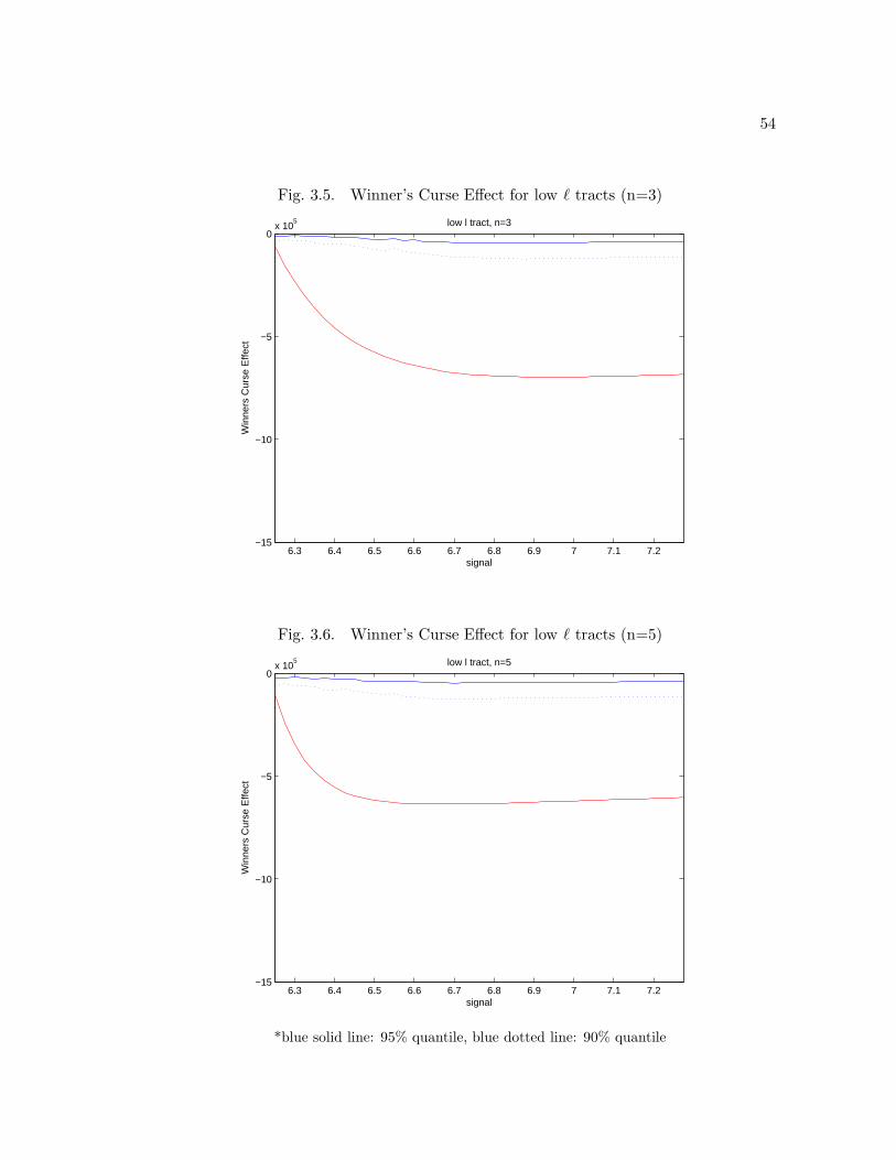
54
Fig. 3.5. Winner’s Curse Effect for low ℓ tracts (n=3)
6.3 6.4 6.5 6.6 6.7 6.8 6.9 7 7.1 7.2−15
−10
−5
0x 10
5
signal
Win
ners
Cur
se E
ffect
low l tract, n=3
Fig. 3.6. Winner’s Curse Effect for low ℓ tracts (n=5)
6.3 6.4 6.5 6.6 6.7 6.8 6.9 7 7.1 7.2−15
−10
−5
0x 10
5
signal
Win
ners
Cur
se E
ffect
low l tract, n=5
*blue solid line: 95% quantile, blue dotted line: 90% quantile

55
Fig. 3.7. Affiliation Effect for high ℓ tracts (n=4)
6.9 7 7.1 7.2 7.3 7.4 7.5 7.6−20000
−18000
−16000
−14000
−12000
−10000
−8000
−6000
−4000
−2000
0
signal
Affi
liatio
n E
ffect
high l tract, n= 4
Fig. 3.8. Affiliation Effect for high ℓ tracts (n=6)
6.9 7 7.1 7.2 7.3 7.4 7.5 7.6−20000
−18000
−16000
−14000
−12000
−10000
−8000
−6000
−4000
−2000
0
signal
Affi
liatio
n E
ffect
high l tract, n= 6
*blue solid line: 95% quantile, blue dotted line: 90% quantile

56
Fig. 3.9. Competition Effect for high ℓ tracts (n=4)
6.9 7 7.1 7.2 7.3 7.4 7.5 7.60
2
4
6
8
10
12
14
16
18x 10
5
signal
Com
petit
ion
Effe
ct
high l tract, n= 4
Fig. 3.10. Competition Effect for high ℓ tracts (n=6)
6.9 7 7.1 7.2 7.3 7.4 7.5 7.60
2
4
6
8
10
12
14
16
18x 10
5
signal
Com
petit
ion
Effe
ct
high l tract, n= 6
*blue solid line: 95% quantile, blue dotted line: 90% quantile

57
Fig. 3.11. Winner’s Curse Effect for high ℓ tracts (n=4)
6.9 7 7.1 7.2 7.3 7.4 7.5 7.6−15
−10
−5
0x 10
5
signal
Win
ners
Cur
se E
ffect
high l tract, n= 4
Fig. 3.12. Winner’s Curse Effect for high ℓ tracts (n=6)
6.9 7 7.1 7.2 7.3 7.4 7.5 7.6−15
−10
−5
0x 10
5
signal
Win
ners
Cur
se E
ffect
high l tract, n= 6
*blue solid line: 95% quantile, blue dotted line: 90% quantile

58
Appendix AThe Confidence Bands
We follow the following bootstrap procedure to obtain the confidence bands for
specific estimators in 3.6. First, we randomly draw T tract numbers, where T is the
number of tracts in our original sample. Then, a random sample is constructed with the
bids for the drawn tracts. We estimate the three effects with this sample and label them
E1WC
, E1CE
and E1AE
. Note that the number of observations N can be different for each
sample because the number of bids for each tract can be different from one another. We
repeat this procedure S = 1000 times, and compute the three effects for each bootstrap
iteration. Those estimates are ordered by their magnitudes at each x point. We obtain
95% and 90% confidence intervals for EAE and EWC by finding 95 and 90 percentiles
of {EsAE
, EsWC
: s = 1, · · · , S}. The 95% and 90% confidence intervals for ECE are
constructed with 5% and 10% percentiles of {EsCE
: s = 1, · · · , S}.

59
References
[1] Gary S. Becker. A note on restaurant pricing and other examples of social influences
on price. Journal of Political Economy, 99:1109–1116, 1991.
[2] Patrick Burkart and Tom McCourt. Digital Music Wars: Ownership and Control
of the Celestial Jukebox. Rowman & Littlefield Publishers, Inc., MD, 2006.
[3] Pascal Courty. Ticket pricing under demand uncertainty. Journal of Law and
Economics, 46:627–652, 2003.
[4] Craig Depken II. Another look at anti-scalping laws: Theory and evidence. Public
Choice, 130:55–77, 2006.
[5] Thomas A. Diamond. Ticket scalping: A new look at an old problem. University
of Miami Law Review, 37:71–92, 1982.
[6] M. Florencia Gabrielli and Quang Vuong. Semiparametric estimation of first price
auction models. Working Paper, 2008.
[7] Otis W. Gilley and Gordon V. Karels. The competitive effect in bonus bidding:
New evidence. The Bell Journal of Economics, 12:637–648, 1981.

60
[8] Emmanuel Guerre, Isabelle Perrigne, and Quang Vuong. Optimal nonparametric
estimation of first-price auctions. Econometrica, 68:525–574, 2000.
[9] Phil Haile, Han Hong, and Matt Shum. Nonparametric tests for common values in
first-price auctions. Working Papers, 501:1–57, 2003.
[10] Stephen K. Happel and Marianne M. Jennings. The folly of anti-scalping laws. The
CATO Journal, 15:65–80, 1995.
[11] Wolfgang Hardle. Applied Nonparametric Regression. Cambridge University Press,
NY, 2002.
[12] Ken Hendricks, Joris Pinkse, and Robert Porter. Empirical implications of equilib-
rium bidding in first price common value auctions. The Review of Economic Studies,
70:115–146, 2003.
[13] Joel L. Horowitz. The Bootstrap in Handbook of Econometrics, vol 5, James .J.
Heckman and Edward E. Leamer (Eds.). Elsevier Science, Amsterdam, 2001.
[14] Ali Hortacsu and Jakub Kastl. Testing for common valuation in canadian treasury
bill market. Working Paper, 2008.
[15] Daniel Kahneman, Jack Knetsch, and Richard Thaler. Fairness as a constraint on
profit seeking: Entitlements in the market. American Economic Review, 76:728–741,
1986.
[16] Paul Klemperer. Auctions: Theory and Practice. Princeton University Press, NJ,
2004.

61
[17] Vijay Krishna. Auction Theory. Academin Press, CA, 2002.
[18] Tong Li, Isabelle Perrigne, and Quang Vuong. Conditionally independent private
infromation in ocs wildcat auctions. Journal of Econometrics, 98:129–161, 2000.
[19] Daniel R. Marburger. Optimal ticket pricing for performance goods. Managerial
and Decision Economics, 18:375–381, 1997.
[20] Paul R. Milgrom and Robert J. Weber. A theory of auctions and competitive
bidding. Econometrica, 50:1089–1122, 1982.
[21] Harry Paarsch. Deciding between common and private vluaes paradigms in empirical
models of auctions. Journal of Econometrics, 51:191–215, 1992.
[22] Adrian Pagan and Aman Ullah. Nonparametric Econometrics. Cambridge Univer-
sity Press, NY, 1999.
[23] Donald S. Passman. All You Need to Know about the Music Business. Simon &
Schuster, NY, 2000.
[24] Joris Pinkse. Lecture Notes: Nonparmetric Estimation. mimeo, 2002.
[25] Joris Pinkse. Lecture Notes: Econometrics I. mimeo, 2004.
[26] Joris Pinkse and Guofu Tan. The affiliation effect in first price auctions. Economet-
rica, 73:263–277, 2005.
[27] James L. Swofford. Arbitrage, speculation, and public policy toward ticket scalping.
Public Finance Review, 27:531–540, 1999.

62
[28] Peter M. Thall. What They’ll Never Tell You about the Music Business: The Myths,
Secrets and Lies (a Few Truths). Billboard Books, NY, 2006.
[29] Jean Tirole. The Thoery of Industrial Organization. The MIT Press, MA, 2000.
[30] Quang Vuong. Lecture Notes: Nonparametric and SemiParametirc Estimation.
mimeo, 2003.
[31] Andrew T. Williams. Do anti-ticket scalping laws make a difference? Managerial
and Decision Economics, 15:503–509, 1994.
[32] Jeffrey M. Wooldridge. Econometric Analysis of Cross Section and Panel Data. The
MIT Press, MA, 2002.

Vita
Hae Won Byun was born in Seoul, Korea on December 13, 1974. She received
a B.A. degree and an M.A. degree in Economics from Yonsei University, Seoul, Korea,
in 1997 and 1999 respectively. She enrolled in the Ph.D. program in Economics at the
Pennsylvania State University in August 2000.
Related Documents