Empirical singular vector method for ensemble El …climate.snu.ac.kr/2005_new/pub/papers/p129.pdf · 2012-07-09 · Empirical singular vector method for ensemble El Niño–Southern

Empirical singular vector method for ensemble El Niño–SouthernOscillation prediction with a coupled general circulation model

Jong‐Seong Kug,1 Yoo‐Geun Ham,2,3 Eun‐Jeong Lee,4 and In‐Sik Kang4

Received 30 November 2010; revised 26 May 2011; accepted 3 June 2011; published 25 August 2011.

[1] Optimal initial perturbation is an important issue related to the improvement of thecurrent seasonal climate prediction. In this study, we have applied the empirical singularvector method to ensemble El Niño–Southern Oscillation (ENSO) prediction with theSeoul National University coupled general circulation model. It is found that from theempirical linear operator, the leading singular mode, which represents the fast growingerror mode in the tropical Pacific, shows El Niño–like perturbation in the present coupledmodel. When the singular vector is used as an initial perturbation, the forecast skill ofENSO is significantly improved. Further, it is demonstrated that the predictions with thesingular vector have a more reliable ensemble spread, suggesting a potential merit for aprobabilistic forecast.

Citation: Kug, J.‐S., Y.‐G. Ham, E.‐J. Lee, and I.‐S. Kang (2011), Empirical singular vector method for ensemble El Niño–Southern Oscillation prediction with a coupled general circulation model, J. Geophys. Res., 116, C08029,doi:10.1029/2010JC006851.

1. Introduction

[2] It is known that ensemble prediction can reduce aprediction error that originates from an initial uncertainty[Molteni and Palmer, 1993; Buizza et al., 1998]. Further,the use of an optimal perturbation for an ensemble pre-diction is an effective way to improve the forecast skill byrepresenting the uncertainty of the estimate for the initialconditions. While several optimal perturbation methodshave been well suited for the medium‐range weatherforecast in the operational centers [Farrell, 1989; Mureauet al., 1993; Palmer et al., 1994; Molteni et al., 1996;Toth and Kalnay, 1993, 1997; Corazza et al., 2003], thesemethods are still immature with respect to the seasonalclimate prediction. The ensemble seasonal prediction atoperational centers is still facing a difficulty: ensembleperturbations have limited growth at early forecast leadtimes with respect to the amplitude of mean error [Vialardet al., 2003; Palmer et al., 2004; Saha et al., 2006]. Thisindicates that there is room for improvement of the cur-rent prediction skills in the seasonal‐to‐interannual timescales.

[3] Several studies have attempted to develop an appro-priate optimal perturbation method for seasonal prediction,particularly El Niño–Southern Oscillation (ENSO) predic-tion. A breeding method has been implemented in theintermediate ENSO model and complex coupled generalcirculation models (GCMs) for ENSO prediction [Cai et al.,2003; Yang et al., 2006, 2008; Ham et al., 2009]. In par-ticular, Yang et al. [2006] showed that the forecast skill ofthe seasonal prediction is improved when the oceanic andatmospheric perturbations are initialized with coupled bredvectors. In the meantime, Kug et al. [2010] suggestedanother way to generate optimal perturbations in the sea-sonal prediction. They developed an empirical singularvector (ESV) method, which extracts the leading singularvector as a fast growing perturbation based on an empiricallinear operator. They showed that fast growing perturbationis successfully captured without tangent linear operator,which is the primary obstacle to apply the singular vectormethods to complex coupled GCMs. By using an interme-diate coupled model, they showed that the forecast skill forENSO was significantly improved when the ESV was usedfor optimal perturbation.[4] A significant advantage of this method is that it is very

simple and can be easily applied to any type of numericalmodel. However, thus far, this method has not been appliedto sophisticated coupled GCMs (CGCMs). It should benoted that several studies already tried to extract optimalperturbations using empirical linear operator, however, theyare focused on decadal variability over the Atlantic ocean,and they did not show that the optimal perturbations isbeneficial to prediction problem [Tziperman et al., 2008;Hawkins and Sutton, 2009]. In this study, we apply the ESVmethod to the Seoul National University (SNU) CGCM.

1Korea Ocean Research and Development Institute, Ansan, SouthKorea.

2Global Modeling and Assimilation Office, NASA Goddard SpaceFlight Center, Greenbelt, Maryland, USA.

3Also at Goddard Earth Sciences Technology and Research Studies andInvestigations, Universities Space Research Association, Columbia,Maryland, USA

4School of Earth and Environment Sciences, Seoul National University,Seoul, South Korea.

Copyright 2011 by the American Geophysical Union.0148‐0227/11/2010JC006851

JOURNAL OF GEOPHYSICAL RESEARCH, VOL. 116, C08029, doi:10.1029/2010JC006851, 2011

C08029 1 of 9

Finally, we show that the ESV method improve the forecastskill of the CGCM.

2. Model and Methods

2.1. SNU Coupled GCM

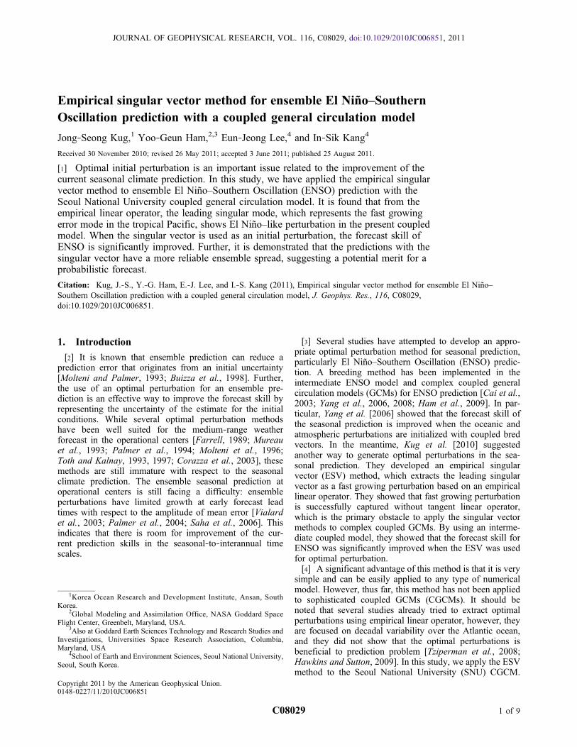
[5] In this study, we used seasonal prediction data fromthe SNU CGCM [Kug et al., 2008; Kim et al., 2008; Hamet al., 2010]. The oceanic part of the coupled model is themodular ocean model developed at the Geophysical FluidDynamics Laboratory. The atmospheric part of the coupledmodel is the SNU atmospheric general circulation model,which is a global spectral model at T42 resolution, with 20vertical sigma levels. The details on the SNU CGCM arediscussed by Kug et al. [2008]. To investigate the ENSOsimulation in SNU CGCM, Figure 1 shows the standarddeviation of monthly mean sea surface temperature (SST)anomalies in the observations and model. It is shown thatthe SST anomaly during ENSO is about twice that in theobservations. For example, the maximum SST anomaly in

SNU CGCM is over 2°C, while that in the observations isabout 1.2°C. In addition, the longitudinal maximum of theSST anomaly is shifted westward by about 20° comparedto that observed. Note that a westward tilt for the SSTvariability during ENSO is also reported in other CGCMs[AchutaRao and Sperber, 2002; Davey et al., 2002; Latifet al., 2001]. The seasonal forecast experiments have beencarried out using the SNU CGCM. In order to obtain theinitial conditions, the SNU CGCM is integrated for the timeperiod of January 1980 to December 2000 by nudging theobserved variables of both the ocean and the atmosphere. Inthe case of the ocean, the ocean temperature and salinityobtained from the Global Ocean Data Assimilation System[Behringer, 2007] reanalysis are nudged with a 5 dayrestoring time scale, and in the case of the atmosphere, thezonal and meridional winds, temperature, and moisturefields obtained from the ERA40 reanalysis are nudged witha 6 h restoring time scale. Given the initial conditions, the 20year hindcast are carried out with a 7 month lead time,starting from 1 May in the period 1981–2000. Six ensemblemembers, generated by a 1 day lag using lagged averagedforecast method, are used for ensemble forecasts. The detailsabout the seasonal forecast experiments are given by Hamand Kang [2011].

2.2. Empirical Singular Vector Method

[6] The ESV method used in this study follows basicallythe same procedure as used by Kug et al. [2010]. It is basedon the concept of the singular vector method [Farrell, 1989;Palmer et al., 1994; Molteni et al., 1996], but it derives anempirical operator from a number of initial and final states,then extract singular vector within the linear system, insteadof extracting singular vectors directly from a nonlineardynamical operator.[7] Let us assume that nonlinear integration can be

approximately expressed by a simple linear operator (L) ofthe evolution of the state vector from time n to time n + t asfollows:

Yn ¼ Xnþ� ¼ LXn þ " ð1Þ

where, Xn, Yn, and " is a state vector at time, n, n + t anderrors from the linear approximations. Then, the linear

Figure 1. The standard deviation of monthly mean sea sur-face temperature (SST) (in °C) in (a) observations and (b) freeintegration of SNU CGCM. Note that the integration periodfor SNU CGCM is 40 years.

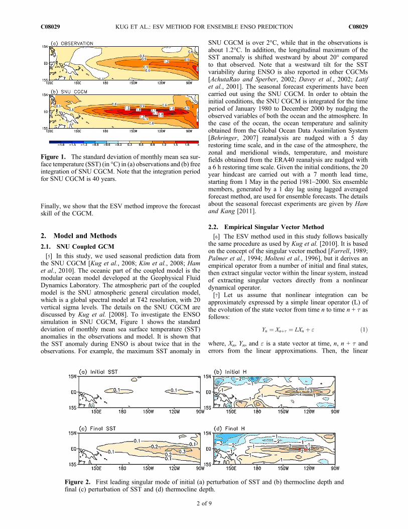
Figure 2. First leading singular mode of initial (a) perturbation of SST and (b) thermocline depth andfinal (c) perturbation of SST and (d) thermocline depth.

KUG ET AL.: ESV METHOD FOR ENSEMBLE ENSO PREDICTION C08029C08029

2 of 9

operator can be derived from state vectors at time n, andn + t.

L ¼ YX T XXT� ��1 ð2Þ

where X and Y are the historical state vectors of theprediction model. The parameter, t, is the lead time formodel integration. In the case of a seasonal prediction, Xand Y can be regarded as the initial condition and theprediction with lead time, t, respectively. In the con-ventional singular vector method, the linear operator, L, iscalculated by linearizing the governing equation of theprediction model. However, in the ESV method, the linearoperator is estimated empirically from the historical data.[8] By solving for the singular values of the linear oper-

ator, L, we can calculate the singular vectors.

uiY ¼ siviX ð3Þ

where si, ui, and vi are the ith singular value and its corre-sponding singular vectors, respectively. When the singularvalue is greater than one, we regard that the correspondingsingular vector is a growing mode in the linear system.Therefore, the singular vector, which has the maximumsingular value larger than one can be the optimal perturba-tion in an ensemble seasonal prediction as far as the linearassumption is valid for target phenomena.[9] In order to apply the ESV method to the prediction of

the SNU CGCM, the linear operator is obtained in a reducedspace through an empirical orthogonal function (EOF)analysis from the hindcast data of 1981–2000. For the initialstate vector, Xn in equation (1), the EOF analysis is appliedto the instantaneous heat content data of the tropical Pacificbasin (120°E–80°W, 15°S–15°N from the initial conditions.For the prediction state, Y in equation (1), the EOF analysis

is also applied to the 6 month lead monthly mean SST data.Note that the spatial pattern of ESV is not sensitive to theselection of optimal time when optimal time is longer than 3months (not shown). In this study, only the first five modesare used for estimating the linear operator, but a majority ofour results are not sensitive to the number of EOF modes.The five dominant EOF modes explain over 76% and 82%of the total variance of the heat content and the SST,respectively.[10] The linear operator (L) is estimated based on the

principal components (PCs) of the EOF modes. From theestimated linear operator, five singular modes are extracted.

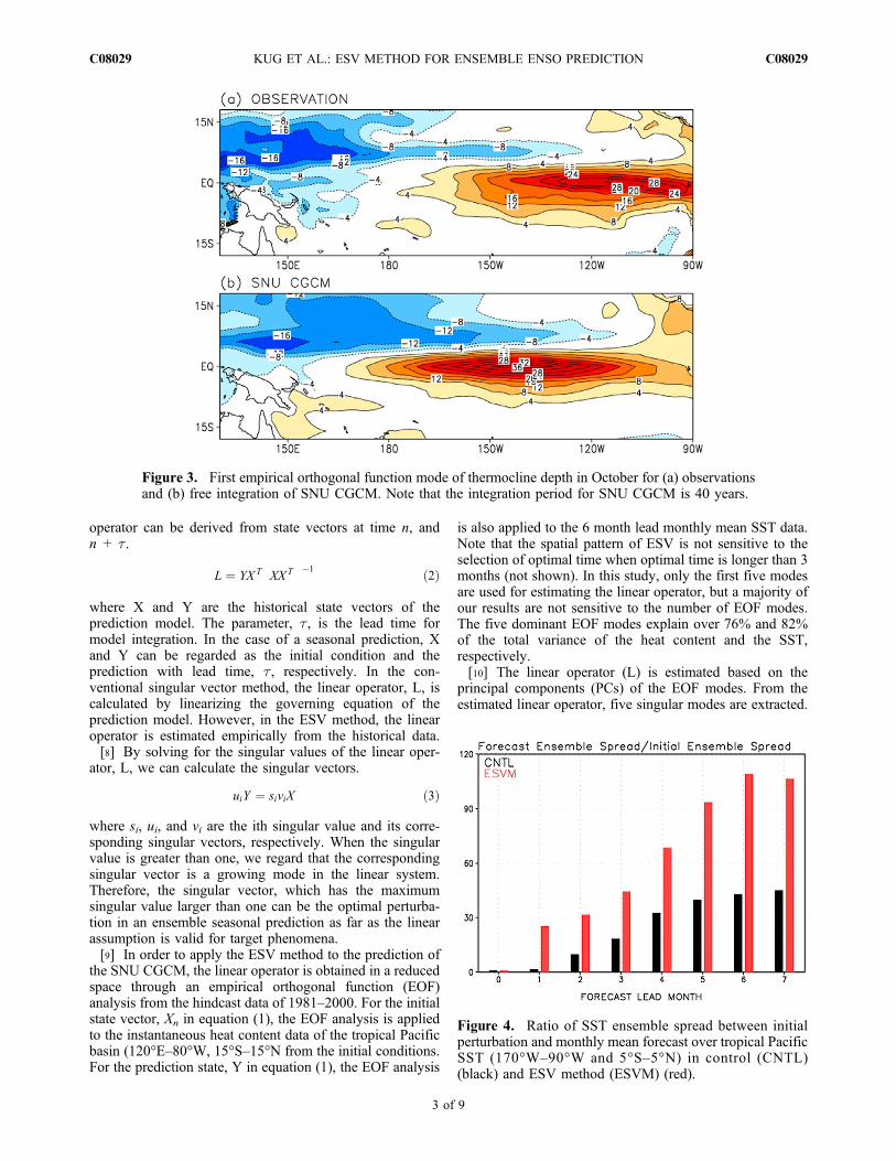
Figure 3. First empirical orthogonal function mode of thermocline depth in October for (a) observationsand (b) free integration of SNU CGCM. Note that the integration period for SNU CGCM is 40 years.

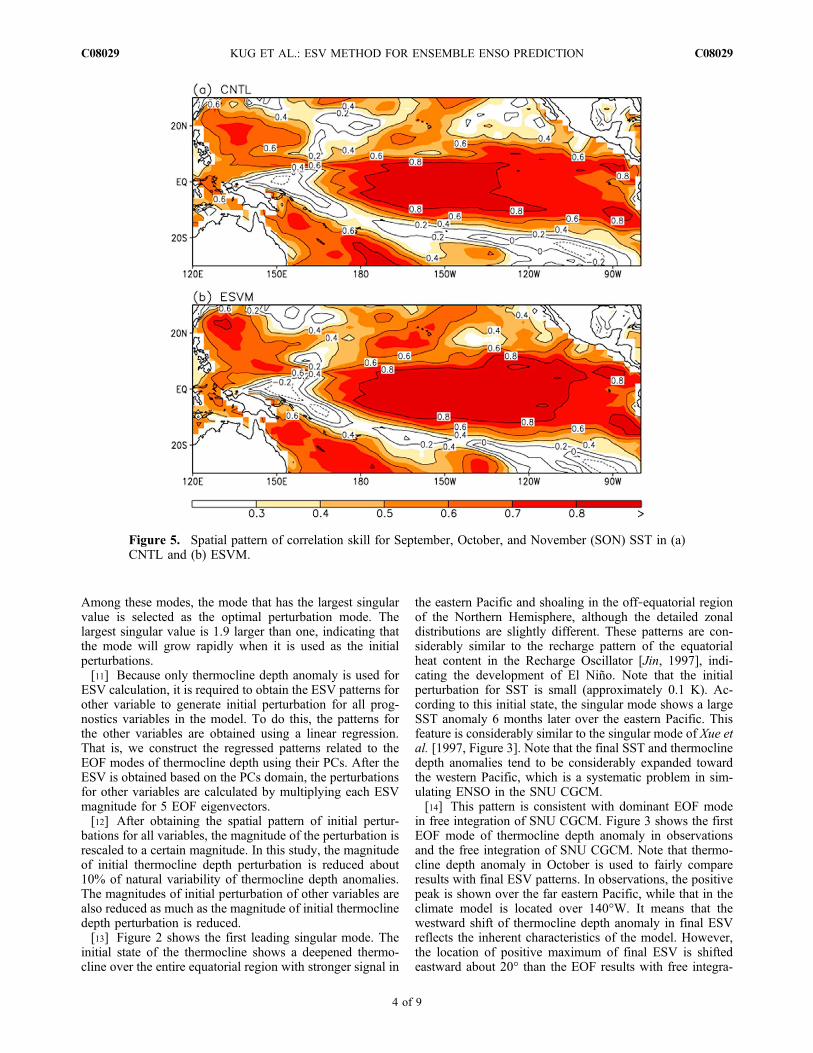
Figure 4. Ratio of SST ensemble spread between initialperturbation and monthly mean forecast over tropical PacificSST (170°W–90°W and 5°S–5°N) in control (CNTL)(black) and ESV method (ESVM) (red).

KUG ET AL.: ESV METHOD FOR ENSEMBLE ENSO PREDICTION C08029C08029

3 of 9

Among these modes, the mode that has the largest singularvalue is selected as the optimal perturbation mode. Thelargest singular value is 1.9 larger than one, indicating thatthe mode will grow rapidly when it is used as the initialperturbations.[11] Because only thermocline depth anomaly is used for

ESV calculation, it is required to obtain the ESV patterns forother variable to generate initial perturbation for all prog-nostics variables in the model. To do this, the patterns forthe other variables are obtained using a linear regression.That is, we construct the regressed patterns related to theEOF modes of thermocline depth using their PCs. After theESV is obtained based on the PCs domain, the perturbationsfor other variables are calculated by multiplying each ESVmagnitude for 5 EOF eigenvectors.[12] After obtaining the spatial pattern of initial pertur-

bations for all variables, the magnitude of the perturbation isrescaled to a certain magnitude. In this study, the magnitudeof initial thermocline depth perturbation is reduced about10% of natural variability of thermocline depth anomalies.The magnitudes of initial perturbation of other variables arealso reduced as much as the magnitude of initial thermoclinedepth perturbation is reduced.[13] Figure 2 shows the first leading singular mode. The

initial state of the thermocline shows a deepened thermo-cline over the entire equatorial region with stronger signal in

the eastern Pacific and shoaling in the off‐equatorial regionof the Northern Hemisphere, although the detailed zonaldistributions are slightly different. These patterns are con-siderably similar to the recharge pattern of the equatorialheat content in the Recharge Oscillator [Jin, 1997], indi-cating the development of El Niño. Note that the initialperturbation for SST is small (approximately 0.1 K). Ac-cording to this initial state, the singular mode shows a largeSST anomaly 6 months later over the eastern Pacific. Thisfeature is considerably similar to the singular mode of Xue etal. [1997, Figure 3]. Note that the final SST and thermoclinedepth anomalies tend to be considerably expanded towardthe western Pacific, which is a systematic problem in sim-ulating ENSO in the SNU CGCM.[14] This pattern is consistent with dominant EOF mode

in free integration of SNU CGCM. Figure 3 shows the firstEOF mode of thermocline depth anomaly in observationsand the free integration of SNU CGCM. Note that thermo-cline depth anomaly in October is used to fairly compareresults with final ESV patterns. In observations, the positivepeak is shown over the far eastern Pacific, while that in theclimate model is located over 140°W. It means that thewestward shift of thermocline depth anomaly in final ESVreflects the inherent characteristics of the model. However,the location of positive maximum of final ESV is shiftedeastward about 20° than the EOF results with free integra-

Figure 5. Spatial pattern of correlation skill for September, October, and November (SON) SST in (a)CNTL and (b) ESVM.

KUG ET AL.: ESV METHOD FOR ENSEMBLE ENSO PREDICTION C08029C08029

4 of 9

tion output. This slight difference between dominant EOFmode in free run and final ESV is from the fact that the finalESV is extracted from the prediction results. Being differentfrom free integration, prediction results are still influencedby the initial condition, which is constrained by the ob-servations, therefore, the westward shift in the model wouldbe less of a problem in the prediction output.

3. Results

[15] Using the initial conditions with the optimal pertur-bations, we carried out a 7 month lead prediction. We com-pared two prediction sets from different initial perturbationmethods. One is control (CNTL) prediction, which is basedon the lagged method, the other is ESV method (ESVM)prediction, based on ESV method. Prior to the comparison ofthe forecast skills, we checked whether the ESV perturba-tions grow rapidly as compared to the lagged perturbations.Because we use the fast growing perturbation, the initialperturbation will grow rapidly as the prediction starts, so thatthe ensemble spread of the initial perturbation in the case ofthe ESV would be larger than that of the other initial per-turbations. In order to check the growth of the spread, wedefined an ensemble spread by area‐averaged variance ofSST perturbations over 170°W–90°W and 5°S–5°N. Theensemble spread indicates an averaged magnitude of the SSTperturbations from the ensemble mean. By calculating theratio between the ensemble spread of the initial condition andmonthly mean forecast at each forecast lead time, we canroughly estimate the growth rate for SST perturbation.

[16] As shown in Figure 4, the small initial ensemblespread grows rapidly as the prediction begins in the cases ofboth the prediction methods. However, the spread of theESVM is larger than that of the CNTL over all the monthlead times. The ratio of the growth rates for the twoprediction sets is the largest at the initial stage of pre-diction (1 month lead); then, the ratio decreases gradually.However, the growth rate of the ESVM is still significantlylarger until the 7 month lead time. At a 6 month leadforecast, the spread of the ESVM is 2.5 times larger thanthat of the CNTL. This indicates that the ESV perturba-tions are growing perturbations, and their growth is fasterthan the perturbations from the lagged method. From theseresults, we can expect that the ENSO prediction will beimproved when the ESV perturbations are used as theinitial perturbations.[17] In order to evaluate the role of the optimal initial

perturbation, the forecast skill is compared between theCNTL and the ESVM predictions. This skill representsthe correlation skill of the six‐member ensemble mean.Figures 5a and 5b show the spatial patterns of the correlationskill for SST during September, October, and November.Both the prediction sets exhibit predictable skill over thetropical Pacific. In particular, the correlation skills over thecentral Pacific exhibit correlation of more than 0.8 in boththe prediction sets. However, the highest correlation skill(>0.8) is only confined in the central Pacific (170–130°W) inthe CNTL, while in the ESVM, an area higher than 0.8 isexpanded to the eastern Pacific (100°W), indicating that theprediction skill is considerably improved over the eastern

Figure 6. (a) Correlation and (b) RMS errors of NINO3 SST in CNTL (black) and ESVM (red). Graylines denote 99% and 95% confidence levels.

KUG ET AL.: ESV METHOD FOR ENSEMBLE ENSO PREDICTION C08029C08029

5 of 9

Pacific. Presumably, it is related to the fact that a large SSTperturbation of the final singular vector, shown in Figure 1b,appears over the eastern Pacific. There is also a notableimprovement in the forecast skill over the off‐equatorial andsubtropical regions of the Northern hemisphere.[18] Figures 6a and 6b show the correlation skill and the

root‐mean‐square (RMS) error of the NINO3 SST, respec-tively. The ESVM prediction has a better forecast skill thanthe CNTL prediction over all forecast lead times. In order toconfirm whether this improvement is significant, predictionskills with eight ensemble members and all possible forecastsets of the six ensemble members (a total of 28 cases) aregenerated. Then, the 95% and 99% confidence levels aredefined from the standard deviation of each month byassuming a Gaussian distribution. Based on the distribution,a statistical confidence level for the correlation or RMS error(RMSE) difference is calculated as shown in Figure 6. It isclear that the forecast skill improvement of the ESVMprediction is significant because the ESV prediction skill is

out of the range of the 99% confidence level (gray line). TheRMS errors also show consistent results that the ESV pre-diction is significantly improved as compared to the CNTLprediction. These results are basically consistent with theresults from Kug et al. [2010] obtained using an interme-diate coupled model. These consistent results support theview that the optimal initial perturbation with ESVs canimprove the prediction skill on a seasonal time scale.[19] One can ask why the prediction skill recover after the

5 month lead time. Because ENSO behavior shows strongseasonal dependency, the predictability of ENSO exhibitsstrong seasonal dependency. Therefore, many models havehigher predictive skill during boreal winter, and lower skillduring boreal spring and summer. Therefore, forecast skillof the climate model can be strongly modulated by season aswell as the forecast lead time. As forecast target time ap-proaches to the season of ENSO mature phase (e.g., borealwinter season), the ENSO prediction skill can be increased,even though the lead time is longer. For example, the

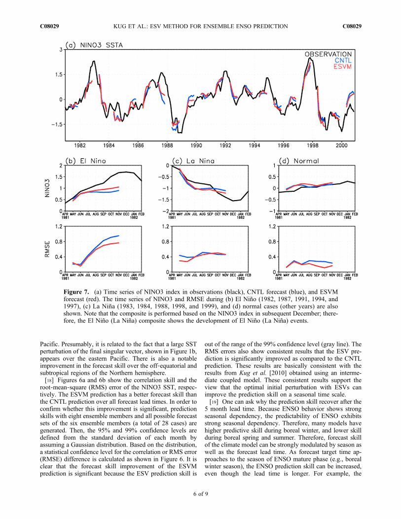
Figure 7. (a) Time series of NINO3 index in observations (black), CNTL forecast (blue), and ESVMforecast (red). The time series of NINO3 and RMSE during (b) El Niño (1982, 1987, 1991, 1994, and1997), (c) La Niña (1983, 1984, 1988, 1998, and 1999), and (d) normal cases (other years) are alsoshown. Note that the composite is performed based on the NINO3 index in subsequent December; there-fore, the El Niño (La Niña) composite shows the development of El Niño (La Niña) events.

KUG ET AL.: ESV METHOD FOR ENSEMBLE ENSO PREDICTION C08029C08029

6 of 9

forecast experiments starting from boreal winter (December,January, and February) season, do not show the rebounds(not shown).[20] Then, how about the individual forecasts? To inves-

tigate the forecast results for specific forecasts, Figure 7shows the time series of NINO3 index for all hindcastperiod, and that of El Niño (1982, 1987, 1991, 1994, and1997), La Niña (1983, 1984, 1988, 1998, and 1999), andnormal cases (other years) composite. In addition, RMSEfor the El Niño, La Niña, and normal cases are also shown.Note that the composite is performed based on the NINO3index in subsequent December, therefore, the El Niño (LaNiña) composite shows the development of El Niño (LaNiña) events. Some of the forecasts in ESVM like 1998summer forecast are slightly worse than that in CNTL.However, most of the forecast like 1981, 1987, 1989, 1997,and 2000 summer cases show systematical improvementwith ESV perturbations. Similarly, the RMSE during ElNiño cases is smaller in ESVM than that in CNTL. It meansthat the weaker ENSO in CNTL forecast is caused by theinitial uncertainty to some extents, and this initial uncer-tainty is effectively reduced in ESVM forecast especiallyduring El Niño events. In addition, the RMSE during normal

cases is also smaller in ESVM than that in CNTL. It showsthat there is positive impact of ESVM in most of the forecastcases, even though negative impact is observed in somecases, and ESV introduced in this study successfully cap-tures the true unstable mode in most hindcast years.[21] Thus far, we have shown that the ESVM exhibits a

better deterministic (ensemble mean) forecast. In addition,there is a possibility to improve the probability forecastbecause the ESV perturbation improves the ensemblespread. In general, the current seasonal prediction producesa small spread as compared to the magnitude of the meanforecast error, indicating that the ensemble spread is notadequate to represent the prediction uncertainty [Vialardet al., 2003; Palmer et al., 2004; Saha et al., 2006]. Thisproblem plays a role in degrading the forecast skill of aprobabilistic forecast in current seasonal prediction. Since theESV perturbation plays a role in increasing the ensemblespread, as shown in Figure 4, the ESV prediction can providea better representation of the forecast uncertainty.[22] In order to check whether the model spread represents

the uncertainty of the ensemble mean prediction appropri-ately, we calculate the noise‐to‐error ratio. The error iscalculated from the error variance of the ensemble mean

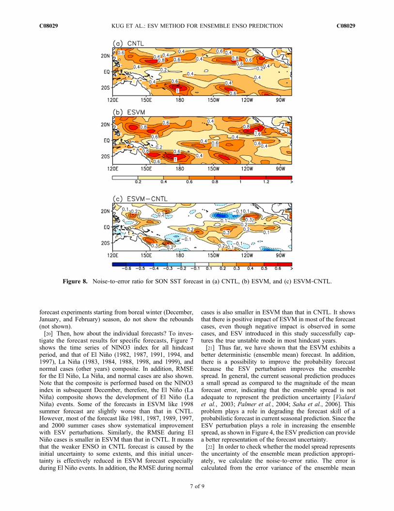
Figure 8. Noise‐to‐error ratio for SON SST forecast in (a) CNTL, (b) ESVM, and (c) ESVM‐CNTL.

KUG ET AL.: ESV METHOD FOR ENSEMBLE ENSO PREDICTION C08029C08029

7 of 9

SST. The noise is estimated from the ensemble spread, i.e.,the variance of the SST perturbation which is deviated fromthe ensemble mean.[23] Figure 8 shows the noise‐to‐error ratio for the CNTL

and ESVM predictions, and the ratio difference betweenESVM and CNTL. If the ratio is considerably smaller thanone, the ensemble spread does not represent the uncertaintyof the prediction appropriately. In this case, the ensemblespread underestimates the uncertainty of the forecast. Asshown in Figure 8a, the overall noise‐to‐error ratio in theCNTL is smaller than one. In particular, the ratio is con-siderably small in the equatorial region, indicating that theensemble spread is significantly small as compared to theforecast error. This implies that the lagged method has aserious problem with respect to the representation of theinitial uncertainty. The ESV prediction also exhibits a noise‐to‐error ratio of less than one. However, the ratio in ESVMis overall greater than that of the CNTL. In particular, thisratio is considerably increased in the equatorial Pacific(Figure 8c). This is slightly expected from Figure 4. Theunderestimated spread of the CNTL can degrade the skill ofthe probabilistic forecast as well as that of the deterministicforecast. Therefore, the ESV prediction would produce abetter probabilistic forecast with a more reliable spread.

4. Summary and Discussion

[24] In this study, we applied the ESV method as anoptimal perturbation method to the ensemble ENSO pre-diction of the SNU coupled GCM. By using this method, wecould extract a fast growing mode on the basis of anempirical linear operator. It was shown that the ESVM had asignificantly higher skill as compared to the CNTL. Inaddition, we found that the present optimal perturbationmethod could be more advantageous with respect to aprobabilistic forecast because of its ability to provide areliable ensemble spread. Overall, the present results wereconsistent with those of Kug et al. [2010] with an inter-mediate coupled model, indicating the robust merits of theESV method with respect to seasonal prediction.[25] This paper is following work of Kug et al. [2010],

and both introduce the same ESV process to improve theseasonal prediction skill. However, there are several differ-ences between them. First, this study confirms that the linearassumption for calculating ESV is still valid and rigorous tothe coupled GCM. In intermittent model used by Kug et al.[2010] is simpler than the coupled GCM, and oceanic part isalmost linear because the oceanic basic state is prescribed.Therefore, the success in the intermediate models cannotguarantee the success in the fully nonlinear CGCMs. Byshowing the ESV is successfully applied to coupled GCM,this study confirms this method is still powerful tool for theprediction with complex GCM with nonlinear dynamics.[26] The second advantage of this study is that this study

applied ESV method to real cases. Therefore, improvementby using ESVM shows that extracting fast‐growing mode toreduce the initial uncertainty is essential to improve theseasonal prediction skills with model errors. In addition, it ispossible to investigate how much improvement is archivedfor the specific forecasts as shown in Figure 7. This kind ofanalysis is only possible in this study to perform hindcastexperiment for real cases. With these benefits, it is expected

that this method can improve the current seasonal predictionskill of the other CGCMs.

[27] Acknowledgment. ISK is supported by the Korea Meteorologi-cal Administration Research and Development Program under grantCATER_2006‐4206 and the second stage of the Brain Korea 21 Project.The model integration was carried out based on the support by grantKSC‐2009‐S03‐0002 from Korea Institute of Science and TechnologyInformation.

ReferencesAchutaRao, K., and K. R. Sperber (2002), Simulation of the El NiñoSouthern Oscillation: Results from the Coupled Model IntercomparisonProject, Clim. Dyn., 19, 191–209, doi:10.1007/s00382-001-0221-9.

Behringer, D. W. (2007), The global ocean data assimilation system(GODAS) at NCEP, paper presented at 11th Symposium on IntegratedObserving and Assimilation Systems for the Atmosphere, Oceans, andLand Surface, Am. Meteorol. Soc., San Antonio, Tex.

Buizza, R., T. Petroliagis, T. N. Palmer, M. Hamrud, A. Hollingsworth,A. Simmons, and N. Wedi (1998), Impact of model resolution andensemble size on the performance of an ensemble prediction system,Q. J. R. Meteorol. Soc., 124, 1935–1960.

Cai, M., E. Kalnay, and Z. Toth (2003), Bred vectors of the Zebiak‐Canemodel and their potential application to ENSO predictions, J. Clim., 16,40–56, doi:10.1175/1520-0442(2003)016<0040:BVOTZC>2.0.CO;2.

Corazza, M., E. Kalnay, D. J. Patil, S.‐C. Yang, R. Morss, M. Cai,I. Szunyogh, B. R. Hunt, and J. A. Yorke (2003), Use of the breedingtechnique to estimate the structure of the analysis “errors of the day,”Nonlinear Processes Geophys., 10, 233–243, doi:10.5194/npg-10-233-2003.

Davey, M., et al. (2002), STOIC: A study of coupled model climatologyand variability in tropical ocean regions, Clim. Dyn., 18, 403–420,doi:10.1007/s00382-001-0188-6.

Farrell, B. F. (1989), Optimal excitation of baroclinic waves, J. Atmos. Sci.,46, 1193–1206, doi:10.1175/1520-0469(1989)046<1193:OEOBW>2.0.CO;2.

Ham, Y.‐G., and I.‐S. Kang (2011), Improvement of seasonal forecastswith inclusion of tropical instability waves on initial conditions, Clim.Dyn., 36, 1277–1290, doi:10.1007/s00382-010-0743-0.

Ham, Y.‐G., J.‐S. Kug, and I.‐S. Kang (2009), Optimal initial perturbationsfor El Niño ensemble prediction with Ensemble Kalman Filter, Clim.Dyn., 33, 959–973, doi:10.1007/s00382-009-0582-z.

Ham, Y.‐G., J.‐S. Kug, I.‐S. Kang, F.‐F. Jin, and A. Timmermann (2010),Impact of diurnal atmosphere–ocean coupling on tropical climate simula-tions using a coupled GCM, Clim. Dyn., 34, 905–917, doi:10.1007/s00382-009-0586-8.

Hawkins, E., and R. Sutton (2009), Decadal predictability of the AtlanticOcean in a coupled GCM: Forecast skill and optimal perturbations usinglinear inverse modeling, J. Clim., 22, 3960–3978, doi:10.1175/2009JCLI2720.1.

Jin, F.‐F. (1997), An equatorial ocean recharge paradigm for ENSO. Part I:Conceptual model, J. Atmos. Sci., 54, 811–829, doi:10.1175/1520-0469(1997)054<0811:AEORPF>2.0.CO;2.

Kim, D., J.‐S. Kug, I.‐S. Kang, F.‐F. Jin, and A. Wittenberg (2008), Trop-ical Pacific impacts of convective momentum transport in the SNU cou-pled GCM, Clim. Dyn., 31, 213–226, doi:10.1007/s00382-007-0348-4.

Kug, J.‐S., I.‐S. Kang, and D.‐H. Choi (2008), Seasonal climate predict-ability with tier‐one and tier‐two prediction systems, Clim. Dyn., 31,403–416, doi:10.1007/s00382-007-0264-7.

Kug, J.‐S., Y.‐G. Ham, M. Kimoto, F.‐F. Jin, and I.‐S. Kang (2010), Newapproach for optimal perturbation method in ensemble climate predictionwith singular vector, Clim. Dyn., 35, 331–340, doi:10.1007/s00382-009-0664-y.

Latif, M., et al. (2001), ENSIP: The El Niño simulation intercomparisonproject, Clim. Dyn., 18, 255–276, doi:10.1007/s003820100174.

Molteni, F., and T. N. Palmer (1993), Predictability and finite time insta-bility of the northern winter circulation, Q. J. R. Meteorol. Soc., 119,269–298, doi:10.1002/qj.49711951004.

Molteni, F., R. Buizza, T. N. Palmer, and T. Petroliagis (1996), TheECMWF ensemble prediction system: Methodology and validation,Q. J. R. Meteorol. Soc., 122, 73–119, doi:10.1002/qj.49712252905.

Mureau, R., F. Molteni, and T. N. Palmer (1993), Ensemble predictionusing dynamically conditioned perturbations, Q. J. R. Meteorol. Soc.,119, 299–323, doi:10.1002/qj.49711951005.

KUG ET AL.: ESV METHOD FOR ENSEMBLE ENSO PREDICTION C08029C08029

8 of 9

Palmer, T. N., R. Buizza, E. Molteni, Y.‐Q. Chen, and S. Corti (1994), Sin-gular vectors and the predictability of weather and climate, Philos. Trans.R. Soc. London A, 348, 459–475, doi:10.1098/rsta.1994.0105.

Palmer, T. N., et al. (2004), Development of a European multimodelensemble system for seasonal‐to‐interannual prediction (DEMETER),Bull. Am. Meteorol. Soc., 85, 853–872, doi:10.1175/BAMS-85-6-853.

Saha, S., et al. (2006), The NCEP climate forecast system, J. Clim., 19,3483–3517, doi:10.1175/JCLI3812.1.

Toth, Z., and E. Kalnay (1993), Ensemble forecasting and NMC: The gen-eration of perturbations, Bull. Am. Meteorol. Soc., 74, 2317–2330,doi:10.1175/1520-0477(1993)074<2317:EFANTG>2.0.CO;2.

Toth, Z., and E. Kalnay (1997), Ensemble forecasting at NCEP and thebreeding method, Mon. Weather Rev., 125, 3297–3319, doi:10.1175/1520-0493(1997)125<3297:EFANAT>2.0.CO;2.

Tziperman, E., L. Zanna, and C. Penland (2008), Nonnormal thermohalinecirculation dynamics in a coupled ocean–atmosphere GCM, J. Phys.Oceanogr., 38, 588–604, doi:10.1175/2007JPO3769.1.

Vialard, J., F. Vitart, M. A. Balmaseda, T. N. Stockdale, and D. L.Anderson (2003), An ensemble generation method for seasonal forecast-ing with an ocean–atmosphere coupled model, Mon. Weather Rev., 133,441–453, doi:10.1175/MWR-2863.1.

Xue, Y., M. A. Cane, and S. E. Zebiak (1997), Predictability of a coupledmodel of ENSOusing singular vector analysis. Part I: Optimal growth in sea-sonal background and ENSO cycles, Mon. Weather Rev., 125, 2043–2056,doi:10.1175/1520-0493(1997)125<2043:POACMO>2.0.CO;2.

Yang, S.‐C., M. Cai, E. Kalnay, M. Rienecker, G. Yuan, and Z. Toth(2006), ENSO bred vectors in coupled ocean–atmosphere general circu-lation models, J. Clim., 19, 1422–1436, doi:10.1175/JCLI3696.1.

Yang, S.‐C., E. Kalnay, M. Cai, and M. M. Rienecker (2008), Bred vectorsand tropical pacific forecast errors in the NASA coupled general circula-tion model, Mon. Weather Rev., 136, 1305–1326, doi:10.1175/2007MWR2118.1.

Y.‐G. Ham, Global Modeling and Assimilation Office, NASA GoddardSpace Flight Center, Bldg. 33, Greenbelt, MD 20771, USA. (yoo‐[email protected])I.‐S. Kang and E.‐J. Lee, School of Earth and Environment Sciences,

Seoul National University, Seoul 151‐742, South Korea.J.‐S. Kug, Korea Ocean Research and Development Institute,

1270 Sang‐rok gu, Ansan 425‐600, South Korea.

KUG ET AL.: ESV METHOD FOR ENSEMBLE ENSO PREDICTION C08029C08029

9 of 9