Empirical Methods for Microeconomic Applications William Greene Department of Economics Stern School of Business.

Empirical Methods for Microeconomic Applications

William Greene

Department of Economics

Stern School of Business

Lab 4. Ordered Choice and Count Data

Upload Your Project File

Binary Dependent Variables

DOCTOR = visited the doctor at least once

HOSPITAL = went to the hospital at least once.

PUBLIC = has public health insurance (1=YES)

ADDON = additional health insurance.(1=Yes)

ADDON is extremely unbalanced.

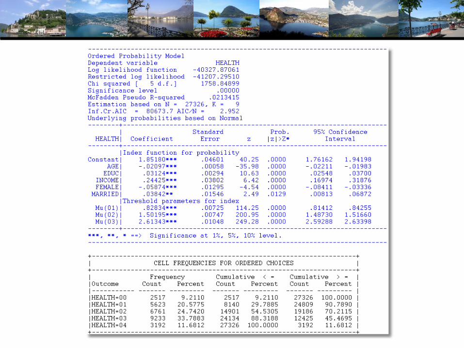
Ordered Dependent Variable

HSAT = ordered reported health satisfaction, coded 0,1,…,10.

Use with ORDEREDor ORDERED ; LogitorOPROBIT and OLOGIT

HISTOGRAM ; Rhs = hsat $

HISTOGRAM ; Rhs = hsat ; Group = female ; Labels = Male,Female ; Title = Health Satisfaction by Gender $

Ordered Choice ModelsOrdered ; Lhs = dependent variable

; Rhs = One, … independent variables $

Remember to include the constant term

For ordered logit i stead of ordered probit, use

Ordered ; Logit ; Lhs = dependent variable

; Rhs = One, … independent variables $

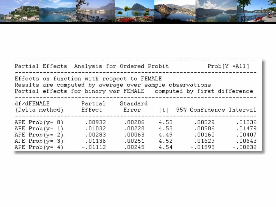
To get marginal effects, use ; Margin as usual.

There are fixed and random effects estimators for this model:

; FEM ; Panel

; Random ; Panel

Sample Selection in Ordered Choice

j-1

Selection Model - The usual binary choice model

z* = +w

z = 1 if z* > 0

When (and only when) z = 1, we observe the ordered probit.

y* , we assume x contains a constant term

y = j if <

γz

βx

j

-1 o J j-1 j,

y* , j = 0,1,...,J

, 0, , j = 1,...,J

If =Cor(w, ) 0, the ML estimator of the ordered probit

model is inconsistent.

Sample Selection Ordered Probit

PROBIT ; Lhs = … ; Rhs = … ; HOLD $

ORDERED ; Lhs = … ; Rhs = … ; Selection $

This is a maximum likelihood estimator, not a least squares estimator. There is no ‘lambda’ variable. The various parameters are present in the likelihood function.

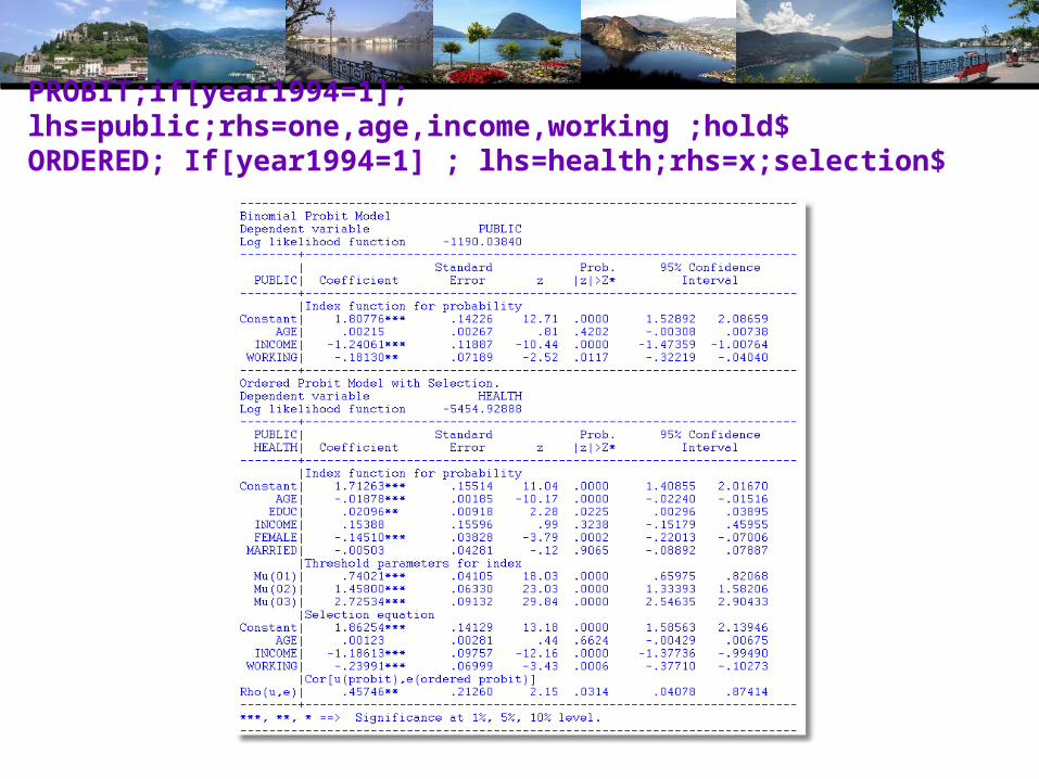
PROBIT;if[year1994=1]; lhs=public;rhs=one,age,income,working ;hold$ORDERED; If[year1994=1] ; lhs=health;rhs=x;selection$

Hierarchical Ordered Probit

Hierarchical ordered probit. Ordered probit in which threshold parameters depend on variables. Two forms:

HO1: μ(i,j) = exp[θ(j) + δ’z(i)]. HO2, different δ vector for each j.

Use ORDERED ; … ; HO1 = list of variables or ORDERED ; … ; HO2 = list of variables.

Can combine with SELECTION models and ZERO INFLATION models.

This is also the Pudney and Shields generalized ordered probit from Journal of Applied Econometrics, August 2000, with the modification of using exp(…) and internally, a way to make sure that the thresholds are ordered..

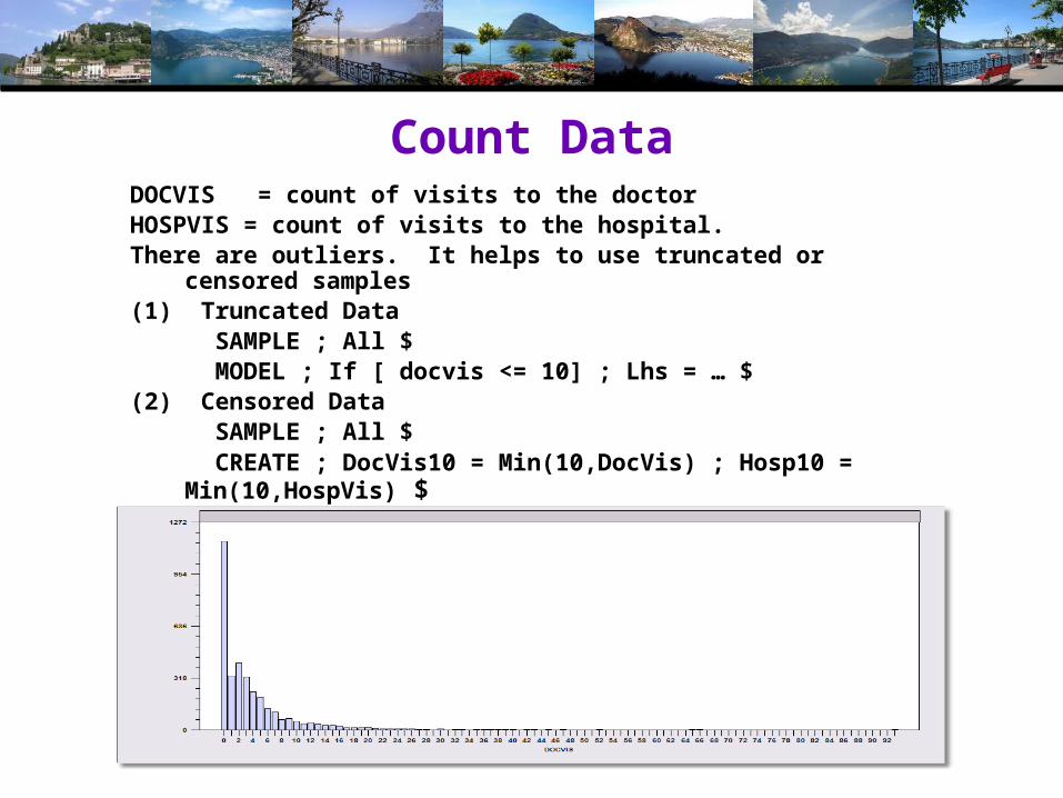
Count DataDOCVIS = count of visits to the doctorHOSPVIS = count of visits to the hospital.There are outliers. It helps to use truncated or censored samples(1) Truncated Data SAMPLE ; All $ MODEL ; If [ docvis <= 10] ; Lhs = … $(2) Censored Data SAMPLE ; All $

CREATE ; DocVis10 = Min(10,DocVis) ; Hosp10 = Min(10,HospVis) $There are also excess zeros. ZIP or HURDLE model suggested.

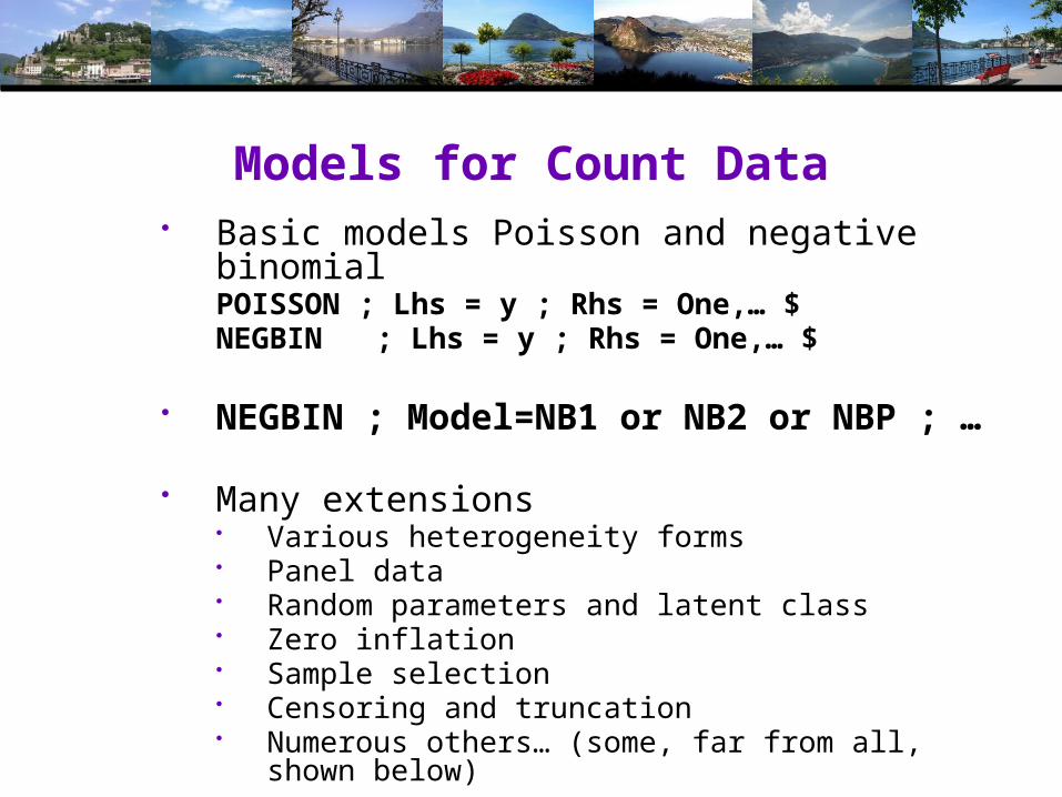
Models for Count Data• Basic models Poisson and negative binomial

POISSON ; Lhs = y ; Rhs = One,… $NEGBIN ; Lhs = y ; Rhs = One,… $

• NEGBIN ; Model=NB1 or NB2 or NBP ; …

• Many extensions• Various heterogeneity forms• Panel data• Random parameters and latent class• Zero inflation• Sample selection• Censoring and truncation• Numerous others… (some, far from all, shown below)

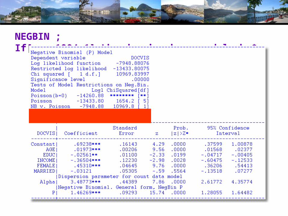
NEGBIN ; If[year1994=1];Lhs=docvis;rhs=x;model=nbp$

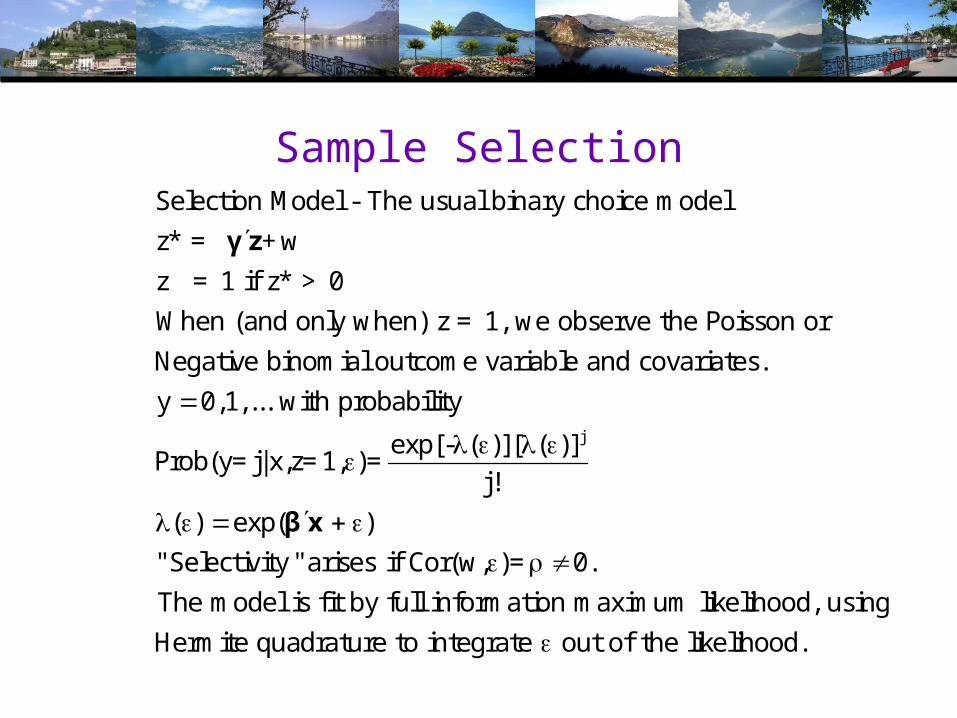
Sample SelectionSelection Model - The usual binary choice model

z* = +w

z = 1 if z* > 0

When (and only when) z = 1, we observe the Poisson or

Negative binomial outcome variable and covariates.

y 0,1,... with probabi

γz

j

lity

exp[- ( )][ ( )]Prob(y=j|x,z=1, )=

j!

( ) exp( )

"Selectivity"arises if Cor(w, )= 0.

The model is fit by full information maximum likelihood, using

Hermite quadrature to integrate out of th

βx

e likelihood.

Selection Model

Probit ; Lhs = … ; Rhs = … ; Hold $

Poisson ; Lhs = … ; Rhs = … ; Selection ; MLE$

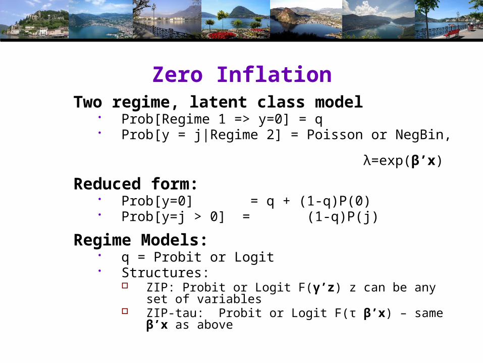
Zero InflationTwo regime, latent class model

• Prob[Regime 1 => y=0] = q• Prob[y = j|Regime 2] = Poisson or NegBin,

λ=exp(β’x)

Reduced form:• Prob[y=0] = q + (1-q)P(0)• Prob[y=j > 0] = (1-q)P(j)

Regime Models:• q = Probit or Logit• Structures:

ZIP: Probit or Logit F(γ’z) z can be any set of variables

ZIP-tau: Probit or Logit F(τ β’x) – same β’x as above

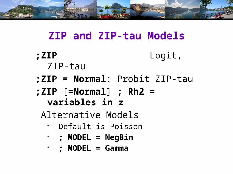
ZIP and ZIP-tau Models

;ZIP Logit, ZIP-tau;ZIP = Normal: Probit ZIP-tau;ZIP [=Normal] ; Rh2 = variables in z

Alternative Models• Default is Poisson• ; MODEL = NegBin• ; MODEL = Gamma

Hurdle Model

Two Part Model:• Prob[y=0] = Logit or Probit using β’x from the

count model or γ’z as specified with ;RH2=list• Prob[y=j|j>0] = Truncated Poisson or NegBin

Two part decision: POISSON ; … ; Hurdle $ POISSON ; … ; Hurdle ; Rh2 = List $

POISSON ; If[year1994=1]; Lhs = docvis;rhs=x ; hurdle ; Rh2 = one,age,income,working $PARTIALS ; If[year1994=1] ; effects: x ; summary $

Poisson and NB Mixture Models with Normal Heterogeneity

j

y 0,1,... with probability

exp[- ( )][ ( )]Prob(y=j|x,z=1, )=

j!

( ) exp( )

The model is fit by full information maximum likelihood, using

Hermite quadrature to integrate out of the likelihood. N

βx

1

ote,

this is precisely the negative binomial model if exp( ) has a

gamma distribution with mean 1; f[exp( )]= exp( ).( )

In this model, has a normal distribution, so exp( ) is lognormal.

Add ; to the command.NORMAL