Empirical Evaluation of Asset Pricing Models: A Comparison of the SDF and Beta Methods Ravi Jagannathan and Zhenyu Wang ∗ ABSTRACT The stochastic discount factor (SDF) method provides a unified general framework for econometric analysis of asset pricing models. There have been concerns that, compared to the classical beta method, the generality of the SDF method comes at the cost of efficiency in parameter estimation and power in specification tests. We establish the correct framework for comparing the two methods and show that the SDF method is as efficient as the beta method for estimating risk premiums. Also, the specification test based on the SDF method is as powerful as the one based on the beta method. ∗ Jagannathan is from the Kellogg School of Management at Northwestern University and the National Bureau of Economic Research and Wang is from the Graduate School of Business at Columbia University. For helpful comments, we thank Mikhail Chernov, John Cochrane, Wayne Ferson, Bob Hodrick, Narayana Kocherlakota, Ren´ e Stulz (editor), Guofu Zhou, the anonymous referee, and the seminar participants at the Federal Reserve Bank of New York, Columbia University, the University of Southern California, Washington University at St. Louis, the University of British Columbia, the NBER Conference on Asset Pricing and Portfolio Choice held in May 2000, and the Western Finance Association Meeting held in June 2000. We especially benefited from discussions with Kent Daniel, Lars Hansen, and John Heaton. Adam Kolasinski provided excellent research assistance, and both Adam Kolasinski and Lolotte Olkowski provided editorial help. First draft: September 12, 1999. An earlier draft was circulated under the title “Efficiency of the stochastic discount factor method for estimating risk premiums.”

Welcome message from author
This document is posted to help you gain knowledge. Please leave a comment to let me know what you think about it! Share it to your friends and learn new things together.
Transcript

Empirical Evaluation of Asset Pricing Models:
A Comparison of the SDF and Beta Methods
Ravi Jagannathan and Zhenyu Wang∗
ABSTRACT
The stochastic discount factor (SDF) method provides a unified general framework foreconometric analysis of asset pricing models. There have been concerns that, comparedto the classical beta method, the generality of the SDF method comes at the cost ofefficiency in parameter estimation and power in specification tests. We establish thecorrect framework for comparing the two methods and show that the SDF method is asefficient as the beta method for estimating risk premiums. Also, the specification testbased on the SDF method is as powerful as the one based on the beta method.
∗Jagannathan is from the Kellogg School of Management at Northwestern University and the National Bureauof Economic Research and Wang is from the Graduate School of Business at Columbia University. For helpfulcomments, we thank Mikhail Chernov, John Cochrane, Wayne Ferson, Bob Hodrick, Narayana Kocherlakota, ReneStulz (editor), Guofu Zhou, the anonymous referee, and the seminar participants at the Federal Reserve Bank of NewYork, Columbia University, the University of Southern California, Washington University at St. Louis, the Universityof British Columbia, the NBER Conference on Asset Pricing and Portfolio Choice held in May 2000, and the WesternFinance Association Meeting held in June 2000. We especially benefited from discussions with Kent Daniel, LarsHansen, and John Heaton. Adam Kolasinski provided excellent research assistance, and both Adam Kolasinski andLolotte Olkowski provided editorial help. First draft: September 12, 1999. An earlier draft was circulated under thetitle “Efficiency of the stochastic discount factor method for estimating risk premiums.”
The use of the stochastic discount factor (SDF) method for econometric evaluation of asset pricing
models has become common in the recent empirical finance literature. A SDF has the following
property: The value of a financial asset equals the expected value of the product of the payoff on
the asset and the SDF. An asset pricing model identifies a particular SDF that is a function of
observable variables and model parameters. For example, a linear factor pricing model identifies
a specific linear function of the factors as a SDF. The SDF method involves estimating the asset
pricing model using its SDF representation and the generalized method of moments (GMM). As
Cochrane (2001) points out, the SDF method is sufficiently general that it can be used for analysis
of linear as well as nonlinear asset-pricing models, including pricing models for derivative securities.
In spite of its wide use, little is known about the estimation efficiency of the SDF method relative
to the classical beta method. The latter method estimates the parameters in a linear factor pricing
model using its beta representation, in which the expected return on an asset is a linear function
of its factor betas. A question that arises is whether the generality of the SDF framework comes
at the costs of estimation efficiency for risk premiums and testing power for model specification.
When returns and factors are jointly normally distributed and independent over time, the
classical beta method provides the most efficient unbiased estimator of factor risk premiums in
linear models. If the SDF method turns out to be inefficient relative to the classical beta method
for linear models under these assumptions, some variation of the beta method may well dominate
the SDF method for nonlinear models as well in terms of estimation efficiency. On the other hand,
if the SDF method is as efficient as the beta method, it would become the preferred method because
of its generality.
We establish the correct framework for comparing the precision of the risk premium estimators
in the two methods. The risk premium parameter in the SDF method is not identical to the risk
premium parameter in the beta method. However, they are related to each other by a one-to-
one transformation. Since the two methods use different parameters to represent the factor risk
premium, it is necessary to take into account how they are related to each other before a valid
comparison of the risk premium estimators can be made. We find that asymptotically the SDF
method provides as precise an estimate of the risk premium as the beta method. Using Monte
Carlo simulations, we demonstrate that the two methods provide equally precise estimates in fi-
nite samples as well. The sampling errors in the two methods are similar even under nonnormal
distribution assumptions, which allow conditional heteroskedasticity. Therefore, linearizing nonlin-
ear asset pricing models and estimating risk premiums using the beta method will not lead to an
1

increase in estimation efficiency.
Kan and Zhou (1999) make an inappropriate comparison of the SDF method and the beta
method for estimating the parameters related to the factor risk premium. They ignore the fact
that the risk premium parameters in the two methods are not identical and directly compare the
asymptotic variances of the two estimators by assuming that the risk premium parameters in the
two methods take special and equal values. For that purpose, they make the simplifying assumption
that the economy-wide pervasive factor can be standardized to have zero mean and unit variance.
Based on their special assumption, they argue that the SDF method is far less efficient than the
beta method. The sampling error in the SDF method is about 40 times as large as that in the
beta method. They also conclude that the SDF method is less powerful than the beta method in
specification tests.
Kan and Zhou’s (1999) comparison, as well as their conclusion about the relative inefficiency
of the SDF method, is inappropriate for two reasons. First, it is incorrect to ignore the fact that
the risk premium measures in the two methods are not identical, even though they are equal at
certain parameter values. Second, the assumption that the factor can be standardized to have
zero mean and unit variance is equivalent to the assumption that the factor mean and variance
are known or predetermined by the econometricians. By making that assumption, they give an
informational advantage to the beta method but not to the SDF method. For a correct comparison
of the two methods, it is necessary to incorporate explicitly the transformation between the risk
premium parameters in the two methods and the information about the mean and the variance of
the factor while estimating the risk premium. When this is done, the SDF method is asymptotically
as efficient as the beta method.
We also examine the specification tests associated with the two methods. An intuitive test
for model mis-specification is to examine whether the model assigns the correct expected return
to every asset, i.e., whether the vector of pricing errors for the model is zero. We show that the
sampling analog of pricing errors has smaller asymptotic variance in the beta method. However,
this advantage of the beta method does not show up in the specification tests based on Hansen’s
(1982) J-statistics. Unlike Kan and Zhou (1999), we demonstrate that the SDF method has the
same power as the beta method.
We organize the rest of the paper as follows. In Section I, we briefly describe the SDF and the
beta methods for estimating linear factor pricing models. In Section II, we develop the analytical
2
results for the comparison of the two methods. In Section III we demonstrate our results by Monte
Carlo simulations. We conclude in Section IV. For the proof of the theorems in the paper, we refer
the readers to the Appendix.
I. Description of the Two Methods
A. The Beta Method
Let rt be a vector of n asset returns in excess of the risk-free rate. To reduce notational
complexity, we assume that there is only one economy-wide pervasive risk factor ft. Let µ and
σ2 be the mean and variance of the factor ft. Then the asset pricing model under the beta
representation is given by:
E[rt] = δβ , (1)
where δ is the factor risk premium, and β, defined as Cov[rt, ft]/σ2, is the sensitivity of asset returns
to the factor.
When the economy-wide factor ft is the return on a portfolio of traded assets, we call it a traded
factor. An example of a traded factor would be the return on the value-weighted portfolio of stocks
used in empirical studies of Sharpe’s (1964) Capital Asset Pricing Model (CAPM). Examples of non-
traded factors can be found in Chen, Roll, and Ross (1986), who use the growth rate of industrial
production and the rate of inflation, and Breeden, Gibbons and Litzenberger (1989), who use the
growth rate in per capita consumption as a factor.
When the factor is the excess return on a traded asset, equation (1) implies µ = δ, i.e., the risk
premium is the mean of the factor. This restriction allows us to use the sample mean of the factor
as an estimator of the risk premium. If the factor is not traded, this restriction does not hold, and
we have to estimate the risk premium using returns on traded assets. We focus on the case where
the factor is not traded, although we also consider the case where the factor is traded.
Note that the vector β can be consistently estimated using the time-series regression: rt =
φ + βft + εt. The residual εt has zero mean and is uncorrelated with the factor ft. The asset
pricing model (1) imposes a restriction on the intercept, φ, i.e., φ = (δ − µ)β. By substituting this
expression for φ in the regression equation, we obtain the following:
rt = (δ − µ + ft)β + εt . (2)
The beta method uses the beta representation (1), which gives rise to the factor model (2),
3

to estimate the risk premium. The classic two-step cross-sectional regression approach proposed
by Black, Jensen, and Scholes (1972) and Fama and MacBeth (1973) is widely used in finance
literature. For example, Fama and French (1992) use this approach to show that there is no
relationship between the expected stock return and beta, and Chen, Roll, and Ross (1986) use this
approach to study a linear multi-factor asset pricing model. A shortcoming of the cross-sectional
regression approach is that it ignores the sampling errors associated with the estimated betas.
Shanken (1992) shows that the Fama-MacBeth method overstates the precision of the estimated
parameters when returns and factors are conditionally homoskedastic and temporally independent.
Jagannathan and Wang (1998) point out that this is not always the case when returns and factors
exhibit conditional heteroskedasticity. Shanken and Jagannathan and Wang provide formulas for
calculating the precision of the estimated parameters.
Assuming identical and independent normal distributions for returns and factors, we can apply
the maximum likelihood procedure to the beta representation and thereby avoid the shortcomings
associated with the two-step cross-sectional regression approach. When the factor is the excess
return on a traded asset, Gibbons, Ross, and Shanken (1989) show that this approach is equivalent
to estimating the parameters using standard linear multivariate time-series regression. Shanken
(1992) shows that the cross-sectional regression method is equivalent to the normal maximum
likelihood method if the estimation errors in betas are properly taken into account.
While the application of the maximum likelihood procedure to the beta representation pro-
vides the most efficient estimates for risk premiums, the assumption of identical and independent
normal distribution is a major limitation. Returns on financial assets may exhibit conditional
heteroskedasticity, serial dependence and non-normality.1 Hansen’s (1982) generalized method of
moments (GMM) has become popular because it allows for conditional heteroscedasticity, serial
correlation, and non-normal distributions. Also, the GMM reduces to the maximum likelihood
estimation and standard regression approaches when the assumptions that justify those procedures
are imposed (see Hamilton (1994) and Cochrane (2001)). We therefore conduct our analysis using
the GMM.
We make use of the following moment restrictions implied by the factor model (2): the zero
mean of the residuals, the zero covariance between the residuals and the factor, and the definition
of the mean and the variance of the factor:2
E[rt − (δ − µ + ft)β] = 0n×1 (3)
4

E[(rt − (δ − µ + ft)β)ft] = 0n×1 (4)
E[ft − µ] = 0 (5)
E[(ft − µ)2 − σ2] = 0 , (6)
where 0n×1 is the vector of n zeros. The vector of unknown parameters is θ = (δ, β′, µ, σ2)′.
Throughout the paper, we assume that the regularity conditions mentioned in Hansen (1982) are
satisfied. Let θ∗ = (δ∗, β∗′, µ∗, σ∗2)′ denote the parameters estimated with the GMM, and Avar[δ∗]
denote the asymptotic variance of the estimated risk premium δ∗.
When returns and factors exhibit conditional homoskedasticity and independence over time,
MacKinlay and Richardson (1991) show that the GMM estimator is equivalent to the multivariate
regression estimator suggested by Gibbons, Ross, and Shanken (1989). For large samples, the
two are also equivalent to the maximum likelihood estimator. Ferson and Harvey (1997) extend
the equivalence argument to models where betas are linear functions of observable variables. The
advantage of the GMM estimator is that it is robust to the presence of conditional heteroskedasticity.
MacKinlay and Richardson thus recommend estimating the parameters using the GMM and the
beta representation. We refer to the combination of the GMM and the beta representation as the
beta method.
It is important to emphasize that we compare GMM estimates in the SDF and beta methods,
not the maximum likelihood estimates. Although it is well known that the GMM estimates are no
more efficient than the maximum likelihood estimates, the advantages of the maximum likelihood
estimates vanishes if one does not know the joint distribution of the returns and the factors. If we
make the wrong distribution assumption, the maximum likelihood estimates can be biased, while
the GMM does not suffer from the same problem. This point is well explained by Hansen and
Singleton (1982).
Hansen’s J-statistic is often used as a specification test to examine whether the data are con-
sistent with the model. When the linear factor pricing model holds, the J-statistic converges to
a central χ2 distribution as T becomes large. Another way to examine the validity of the pricing
model is to test if Jensen’s alpha, given by α = E[r] − δβ, is zero. Jensen’s alpha measures the
deviation of the vector of excess returns from what the corresponding object should be according
to the pricing model. The sample analog of Jensen’s alpha is given by:
α∗ = r − δ∗β∗ , where r =1T
T∑t=1
rt . (7)
5

B. The SDF Method
By substituting the expression for β into equation (1) and rearranging the terms, we obtain the
following representation of the linear asset pricing model given below:
E[rtmt] = 0n×1 , (8)
where mt = 1 − λft. Any random variable mt that satisfies equation (8) is referred to as a
stochastic discount factor (SDF). In general, a number of random variables satisfying equation (8)
exist and hence there is more than one stochastic discount factor. An asset pricing model designates
a particular random variable as a stochastic discount factor. The linear factor pricing model (8)
designates the random variable mt = 1−λft as a stochastic discount factor. In the above expression
the parameter λ is the following non-linear transformation of the risk premium δ:
λ =δ
σ2 + µδor δ =
λσ2
1 − µλ. (9)
The SDF representation can be traced back to Dybvig and Ingersoll (1982), who derive the
SDF representation for the CAPM. Ingersoll (1987) derives the SDF representation for a number
of theoretical asset pricing models.3 Hansen and Jagannathan (1991, 1997) develop diagnostic
tests for asset pricing models based on the SDF representation. Ferson (1995), Campbell, Lo, and
MacKinlay (1997), and Cochrane (2001) provide introductions to the stochastic discount factor
framework.
Farnsworth et al (2000) find that adding the nominally risk-free security to the collection of
assets increases estimation efficiency. However there is a cost to doing so. Nominal interest rates
exhibit very persistent near unit root like behavior at the empirically relevant frequencies. Hence
it may not be appropriate to rely on the asymptotic standard errors. For that reason we, following
the common practice in the empirical asset pricing literature, use excess returns and ignore the
restriction that the asset pricing model should also correctly value the nominally risk-free asset.
This also facilitates comparison of our results with those reported by Kan and Zhou (1999).
For the linear one-factor pricing model of excess returns, a simple moment restriction for the
GMM is given by:
E[rt(1 − λft)] = 0n×1 . (10)
Using moment restriction (10) and the GMM we obtain an estimate of the parameter λ. We denote
the associated J-statistic by J . We are also interested in studying the pricing error, which is
6
defined as π = E[rt]− λE[rtft]. Hansen and Jagannathan (1997) develop diagnostic tests based on
the pricing error. The sample analog of the vector of pricing errors is given by:
π = r − λ(rf) , where r =1T
(T∑
t=1
rt
)and rf =
1T
(T∑
t=1
rtft
). (11)
Classical tests of asset pricing models examine whether the vector of pricing errors are different
from zero after allowing for sampling errors. Substituting equation (9) into π = E[rt] − λE[rtft],
we obtain
π =
(σ2
σ2 + µδ
)α or α =
(σ2 + µδ
σ2
)π . (12)
Hence Jensen’s alpha will be zero if and only if the pricing error is zero.
The SDF method, which is the combination of the SDF representation and the GMM, provides
a convenient and general framework for analyzing linear and nonlinear asset pricing models. The
comparison of the SDF method with the beta method has important implications for the empir-
ical evaluation of asset pricing models. A nonlinear model can often be well approximated by a
linear one. For example, Cochrane (1996) advocates that nonlinear stochastic discount factors be
approximated by linear functions of macroeconomic variables. Campbell (1993, 1996) uses linear
approximations for the consumption-based CAPM. If the beta method is more efficient, using it to
estimate the linearized models may be more efficient than using the SDF to estimate the nonlinear
models.
II. Analytical Results
A. Comparison of the Two Methods
First consider the estimates of the risk premium obtained using the two methods. The beta
method gives the GMM estimate δ∗ from the moment restrictions of the beta model, while the SDF
method gives the GMM estimate λ from the moment restriction of the SDF model. We cannot
compare the precision of the two estimates directly because δ and λ will not in general be equal.
We therefore first transform the estimate of δ obtained with the beta method into an estimate of
λ:
λ∗ =δ∗
σ∗2 + µ∗δ∗, (13)
and then compare the asymptotic variances of λ∗ and λ.
To understand why it is important to transform δ∗ to λ∗ for the comparison, consider the
case when the factor is the consumption growth rate measured in real numbers. If we switch the
7
measurement of the factor to percent, δ∗ should be multiplied by 100, while λ should be divided
by 100. The asymptotic variance of δ∗ is then multiplied by 10,000 but the asymptotic variance
of λ is divided by 10,000. Clearly, the scaling of the factor affects the relative magnitude of the
asymptotic variances of δ∗ and λ. A correct comparison of the SDF and beta methods should be
independent of the scaling of factors or returns. It is therefore incorrect to compare the asymptotic
variance of δ∗ and λ directly without proper transformation. However, transformation (13) implies
that the asymptotic variance of λ∗ will be scaled by 1/10,000, making it comparable to the scaled
asymptotic variance of λ.
Notice that transformation (13) requires the estimates of µ and σ2. The estimation errors in µ∗
and σ∗2 affect the asymptotic variance of λ∗. In order to calculate the asymptotic variance of λ∗,
we need to make use of the joint distribution of δ∗, µ∗, and σ∗2. Equivalently, we can substitute
equation (9) into moment restrictions (3) and (4) to express them in terms of λ and then estimate
λ, β, µ, and σ2 jointly. The standard errors for the estimate of λ will then automatically take into
account the estimation errors in µ∗ and σ∗2.
To simplify the mathematics involved, we assume that the asset returns and the factors are
generated by an i.i.d. joint normal process, unless specially mentioned. Under the i.i.d. joint
normal assumption, the beta-method estimator of the risk premium is equivalent to the maximum-
likelihood estimator. It is well known that the latter is asymptotically the most efficient consistent
estimator. It is therefore important to compare the SDF method with the beta method in this
special case. However, our results hold under more general distribution assumptions. This is
demonstrated by the Monte Carlo simulations in Section III.
The main result of our comparison of the two methods are summarized in the next theorem.
The proof of the theorem is provided in the Appendix.
THEOREM 1: Assume that the beta representation (1) and the equivalent SDF representation (8)
hold. The risk premium estimated using the SDF method has the same asymptotic variance as the
risk premium estimated using the beta method, i.e., Avar[λ] = Avar[λ∗].
Next, consider pricing errors π and Jensen’s α. The vector of sample pricing errors, π, in the
SDF method is calculated using equation (11). The sample analog of Jensen’s alpha, α∗, in the
beta method is calculated using equation (7). In general, π and α will not be equal. The pricing
error π and Jensen’s α are related to each other by equation (12). In view of this, we need to
8

transform the sample analog of Jensen’s α∗ to get the sample pricing errors:
π∗ =
(σ∗2
σ∗2 + µ∗δ∗
)α∗ , (14)
which is referred to as the sample pricing errors obtained in the beta method. We can then compare
the asymptotic variances of π∗ and π. In the following theorem, we show that asymptotically the
beta method has smaller variance of the sampling pricing error.
THEOREM 2: Assume that the beta representation (1) and the equivalent SDF representation (8)
hold. The asymptotic variance of the sampling pricing error in the SDF method is at least as large
as that in the beta method, i.e., Avar[π] − Avar[π∗] is positive semi-definite.
For the SDF method, testing α = 0 with α is algebraically equivalent to Hansen’s (1982) tests of
over-identification using the J-statistic. This is not the case for the beta method. The J-statistics
in the two methods have the same asymptotic distribution. To be more precise, Hansen’s J-statistic
for the beta method as well as the SDF method has an asymptotic χ2 distribution with n−1 degrees
of freedom, i.e., Jd−→ χ2
n−1 and J∗ d−→ χ2n−1 as T → ∞. The SDF method has n − 1 degrees of
freedom because there are n restrictions and one parameter in equation (10). The beta method
also has n − 1 degrees of freedom because there are 2n + 2 restrictions in equations (3), (4), (5),
and (6) and n + 3 parameters. Therefore, the asymptotic variances of J and J∗ must be the same.
The distributions of J and J∗ can only be different in finite samples. Later, we use Monte Carlo
simulation to address the issue of finite-sample distributions.
We can also consider the parameter δ and Jensen’s α. In the beta method, the estimates δ∗ and
α∗ are obtained as described in Section I.A. For proper comparison we transform the estimates
λ and π obtained using the SDF method as described in Section I.B to get estimates δ and α
using formula (9) and (12). It can be readily shown, by mimicking the proof of Theorem 1, that
Avar[δ] = Avar[δ∗] and that Avar[α] − Avar[α∗] is positive semi-definite.
In Theorem 1, the factor can be either a return on a tradable asset or a nontradable macroeco-
nomic variable. As we have discussed in the earlier section, if the factor is a tradable asset return,
the asset pricing model implies the restriction δ = µ. It can be shown that Theorem 1 continues
to hold even when this restriction is imposed during estimation. In fact, under this restriction the
asymptotic variances of Avar(δ) and Avar(δ∗) are both equal to the asymptotic variance of the
sample average of ft. Therefore, imposing the restriction δ = µ, we only need to estimate the risk
premium from the observations of the factor. This has been pointed out previously by Shanken
(1992).
9

B. The Effects of Standardizing Factors
According to Theorem 1 the beta method and the SDF method provide risk premium estimates
that are equally precise. This result contradicts Kan and Zhou’s (1999) conclusion. In this section,
we examine why this is so. When comparing the two methods, Kan and Zhou suggest comparing
the asymptotic variance of the estimated δ and λ by looking at special parameter values that make δ
and λ equal in numbers. Specifically, they assume that the factor has zero mean and unit variance,
i.e., µ = 0 and σ = 1. At these special values of the parameters, they notice that λ = δ and directly
compare the estimation errors of δ and λ.
Since this assumption applies to the SDF method as well as the beta method, one may expect
that it would not give an advantage to one method over the other. In this subsection we show that
this is not the case. Predetermining the mean and the variance of the factor increases the efficiency
of the estimator in the beta method but not in the SDF method. However, by adding additional
moment conditions to incorporate the information brought in through the moments of the factor,
the SDF method estimator can be made as efficient as the beta-method estimator.
Since the mean and the variance of the factor are predetermined to be zero and one, Kan and
Zhou (1999) drop equations (5) and (6). For the beta method, they obtain the estimator of the
parameter δ from the moment restriction
E[rt − (δ + ft)β] = 0n×1 (15)
E[(rt − (δ + ft)β)ft] = 0n×1. (16)
For the SDF method, they obtain the estimator of the parameter λ from the moment restriction
E[rt(1 − λft)] = 0n×1 , (17)
which is equation (10). Then, they directly compare the asymptotic variance of the estimated δ
with the asymptotic variance of the estimated λ.
The most important aspect of the assumption made by Kan and Zhou (1999) is that the
mean and variance of the factor are predetermined without estimation. This assumption is the
equivalent of ignoring the sampling errors associated with the estimates of µ and σ2. In order
to fully understand how this assumption affects the precision of the risk premium estimators, we
assume that µ and σ2 are known, but not necessarily zero and one.
In general, predetermining a subset of the parameters reduces the sampling error of the remain-
ing estimates. The following lemma summarizes this effect.
10

LEMMA 1: Let xt be the observed data in period t and g(xt, θ1, θ2) be a vector function of (xt, θ1, θ2),
where θ1 is the vector of parameters of interest. Suppose that E[g(xt, θ1, θ2)] = 0 defines the GMM
moment restrictions. Let (θ′1, θ′2)′ be the GMM estimator of (θ′1, θ′2)′. When θ2 is pre-determined,
let θ1 be the GMM estimator of θ1. Then, Avar[θ1]−Avar[θ1] is positive semi-definite. In addition,
if
limT→∞
E
[1T
T∑t=1
∂g(xt, θ1, θ2)∂θ′2
]= 0 , (18)
then Avar[θ1] = Avar[θ1].
When the factor moments are predetermined, the asymptotic variance of the estimated risk
premium becomes smaller. Thus, Kan and Zhou (1999) understate the variances of the parameter
estimates in the beta method relative to the realistic case where µ and σ must be estimated.
Nonetheless, the variance of the estimates in the SDF method is not understated because condition
(18) is satisfied.
Kan and Zhou (1999) do not use the two moment conditions that restrict the first and second
sample moments of the factor. In general, dropping the moment restrictions in the GMM will
increase the sampling error of the estimated parameters. However, when certain conditions are
met, moment conditions can be dropped without affecting the sampling error of the estimated
parameters. It turns out that these conditions are satisfied for the beta method. Thus, Kan and
Zhou’s analysis still gives the beta method an efficiency advantage after dropping the moment
restrictions for µ and σ. The following lemma makes these statements precise.
LEMMA 2: Let xt be the observed data in period t, g1(xt, θ) be a vector function of (xt, θ), where θ
is the vector of parameters, and g2(xt) be a vector function of xt. Let g(xt, θ)′ = (g1(xt, θ)′, g2(xt)′)′.
Suppose E[g(xt, θ)] = 0. Let θ be the GMM estimator from the moment restriction E[g(xt, θ)] = 0.
Let θ be the GMM estimator of θ from the moment restriction E[g1(xt, θ)] = 0. Then, Avar[θ] −Avar[θ] is negative semi-definite. In addition, if however
∞∑j=−∞
E[g1(xt, θ)g2(xt+j)′] = 0, (19)
then Avar[θ] = Avar[θ].
In order to apply Lemma 2 to the beta method, let θ = (δ, β′)′ and
g1(xt, θ) =
(rt − (δ − µ + ft)β
(rt − (δ − µ + ft)β)ft
)and g2(xt) =
(ft − µ
(ft − µ)2 − σ2
). (20)
11

where µ and σ are predetermined. It is easy to show that g1 and g2 are uncorrelated. Hence,
condition (19) is satisfied, and dropping the factor moment restrictions does not affect the variance
of the risk premium estimator in the beta method.
Under the assumption of zero mean and unit variance of the factor, however, Kan and Zhou
(1999) show that the beta method is strictly more efficient than the SDF method. More generally, we
can show that the strict inequality holds when the first two moments of the factor are predetermined,
not necessarily to be zero and one. Let δ† be the estimator of δ obtained from moment restrictions
(15)–(16) and λ† = δ†/(σ2 + µδ†). Our derivation in the Appendix shows
Avar[λ†] < Avar[λ] . (21)
We have shown in Theorem 1 that the SDF method is as efficient as the beta method when the
factor moments are not predetermined and have to be estimated. Hence, we conclude that Kan
and Zhou reached a different conclusion because they ignored the estimation error associated with
the first two moments of the factor and treat them as though they are known with certainty.
To summarize, the estimated risk premiums in the SDF and beta methods have the same sam-
pling error when the factor moments are not predetermined. Predetermining the factor moments
reduces the sampling error of the estimate in the beta method, even though the moment conditions
corresponding to the predetermined parameters are ignored. In the SDF method, however, the
variance of the estimator is not reduced when factor moments are predetermined. This explains
why Kan and Zhou (1999) find that the SDF method is less efficient.
When the factor moments are predetermined, the information about the factor moments should
be properly incorporated into the SDF method. From Lemma 2, we know that the restriction
E[g2(xt)] = 0 might affect the estimation efficiency if g1(xt, θ) and g2(xt) are correlated. For this
reason, we add the factor moment restrictions to the moment restriction (10) in the SDF method.
Thus, we obtain the GMM estimate, denoted by λ, of the parameter λ from the following moment
restrictions:
E[rt(1 − λft)] = 0 (22)
E[ft − µ] = 0 (23)
E[(ft − µ)2 − σ2] = 0 , (24)
where µ and σ are predetermined. Our derivation in the Appendix shows
Avar[λ] = Avar[λ†] . (25)
12

Therefore, a simple remedy to the inefficiency of SDF method when factor moments are predeter-
mined is to incorporate the factor-moment restrictions. This further explains why the additional
information about the factor is incorporated into the beta method but not the standard SDF
method when we predetermine the factor moments.
A natural question that arises is whether we can increase the estimation efficiency by incorpo-
rating the factor moment restrictions when the factor mean and variance are not predetermined.
More specifically, we want to know whether the asymptotic variance of λ estimated together with
µ and σ2 from the moment restrictions
E[rt(1 − λft)] = 0n×1 (10′)
E[ft − µ] = 0
E[(ft − µ)2 − σ2] = 0,
is smaller than the asymptotic variance of the corresponding estimators that are obtained from
the first moment restriction (10′) alone. The answer is no because the number of added moment
restrictions is the same as the number of added unknown parameters. Readers can verify this easily.
III. Monte Carlo Simulations
A. Estimation Efficiency
In the first set of simulations, we assume that the returns and the factor are drawn from a
multivariate normal distribution. To be consistent with the beta model and its equivalent SDF
model, we generate the excess returns and the factor from the following process:
rt = (δ − µ + ft)β + εt , εt|ft ∼ N(0n×1,Ω) , ft ∼ N(µ, σ2) , (26)
where t = 1, · · · , T . For T , we consider the following four different time horizons in our simulations:
60 months, 120 months, 360 months and 600 months. The first two horizons are often used for
estimating betas and risk premiums using rolling windows. The third horizon is similar to that
used in many related empirical studies.4 The fourth is a half-century, which may be considered a
“large” sample for monthly returns. The estimators are calculated based on the T samples of the
factor and returns generated from the above process. We repeat this independently to obtain 1,000
draws of the estimator of λ.
We choose the values for the parameters to match the sample moments of the data. Monthly
returns from January 1926 to December 1998 for the ten size-decile portfolios, the value-weighted
13
market index portfolio of stocks traded on the NYSE, AMEX, and Nasdaq, and the one-month
Treasury Bills are obtained from the Center for Research on Security Prices (CRSP). Excess returns
are obtained by subtracting the Treasury Bill returns. We set µ and σ2 to equal the sample mean
and the sample variance of the excess return on the market index portfolio. We set β for each
size-decile portfolio to equal the slope coefficient in the OLS regressions of the size-decile excess
returns on the excess market return. The covariance matrix, Ω = E[εtε′t|ft], is set equal to the
sample covariance matrix of the residuals obtained in the ten OLS regressions. We set the risk
premium δ to be the value of the slope coefficient obtained from the cross-sectional regression of
the historical average excess returns on betas. The parameter λ satisfies λ = δ/(σ2 + µδ). Table I
provides all the parameters used in the simulation.
Insert Table I about here
In the population, we set risk premium δ = 1.3740 for monthly returns. This implies λ = 4.3790.
This large risk premium reflects the firm-size premium since β is strongly negatively correlated with
firm size in the sample we use for calibration purposes.5 We do not set the values of δ and µ to be
equal. Therefore, we do not impose the restriction that the factor is the return on a portfolio of
tradable assets.6 The asymptotic standard deviations of the estimated λ implied by the parameters
are reported in panel A of Table II. For comparison with the simulation results, the asymptotic
standard deviations are divided by the square-root of T .
Insert Table II about here
In implementation of the GMM, we follow Ferson and Foerster (1994), who suggest iterating
between the estimation of the weighting matrix and the estimation of parameters until the estimates
converge. The simulation results for λ are reported in panel B of Table II. For each estimator of
λ, the table gives the standard deviation of the 1,000 estimated risk premiums. When the mean
and variance of the factor are estimated along with the risk premium parameter, the estimator
λ obtained using the SDF method and the estimator λ∗ obtained using the beta method have
essentially the same precision for all sample sizes considered. This is true even when the sample
size is as small as 60 months. Therefore, there is no efficiency gain from the use of the beta method
over the SDF method. Our simulations also show similar results for the estimated δ — we do not
report them in order to save space. We refer those who are interested in the numerical results of δ
to Jagannathan and Wang (1999).
If we predetermine the mean and variance of the factor and ignore the related moment restric-
14

tions, the SDF method is much less efficient than the beta method. This is true in both small as
well as large samples. When we have 30 years of monthly observations (T = 360), the standard
deviation of λ obtained using the SDF method is about 35 times as high as the standard deviation
of λ† obtained using the beta method. This result is similar to that reported by Kan and Zhou
(1999). It confirms that when the factor moments are predetermined, the classical beta method
substantially overstates the precision of the estimated risk premiums.
When the factor moment restrictions are added to the SDF method, the efficiency of the SDF
method improves substantially. Notice that the standard error of λ is nearly the same as that of
λ†. The increase in efficiency of the SDF method after adding the factor moments restrictions is
expected because in this case the two methods have the same asymptotic variance for the estimated
risk premium. Thus, the sharp disadvantage of the SDF method relative to the beta method
reported by Kan and Zhou (1999) is mainly due to ignoring the estimation error in the factor
moments.
In our theoretical derivation of the asymptotic variance, we assume that the variance of the
returns do not depend on the realized value of the factor. This may be a rather restrictive as-
sumption. We therefore examine the applicability of our results when returns exhibit conditional
heteroscedasticity. For this purpose, following MacKinlay and Richardson (1991), we make inde-
pendent draws of the returns and the factor from a multivariate t-distribution rather than a joint
normal distribution. When the multivariate t-distribution has ν degrees of freedom, the conditional
covariance matrix of the residuals in the regression equation, conditional on the realized value of
the factor, is given by (see MacKinlay and Richardson, equation 14):
Var[εt|ft] =ν − 2 + (ft − µ)2/σ2
ν − 1Ω . (27)
Notice that dependence of the conditional covariance on the realized value of the factor increases
as the number of the degree of freedom, ν, decreases. There is, however, a lower bound on our
choice of the number of degrees of freedom. The asymptotic distribution theory for the GMM
requires that returns and factors have finite fourth moments. Hence, there must be more than four
degrees of freedom. In view of this restriction, we use five degrees of freedom for the multivariate
t-distribution, following MacKinlay and Richardson.
The simulation results corresponding to the t distribution are presented in panel C of Table II.
The standard errors computed using the asymptotic theory and through simulation are about the
same. It is also true that predetermining the factor mean and variance causes the estimator λ†
15

obtained with the beta method to be more efficient than the estimator λ obtained with the SDF
method, but incorporation of the factor moment restrictions makes the estimator λ as efficient as
the estimator λ†. When the mean and variance of the factor are not predetermined, which is a
more realistic and correct approach, the two estimators λ∗ and λ obtained with the two methods
have almost the same precision in every sample size. This indicates that our results are robust to
the existence of conditional heteroskedasticity.
As an alternative to the multi-variate t-distribution, we also consider the joint empirical dis-
tribution of the excess returns and the factor. The monthly observations of the return on the
value-weighted index of NYSE, AMEX, and Nasdaq are used for ft. The residuals in the regression
of decile returns on the index return are used for εt. Independent samples (ft, ε′t)′t=1,···,T are
drawn from an estimated empirical distribution of the data.7 Excess returns on 10 portfolios are
constructed to satisfy rt = (δ − µ + ft)β + εt for t = 1, · · · , T . The parameters, λ, δ, β, and µ,
are set to the values in Table 1. Each estimator is then calculated based on the T observations
to obtain a random draw of the estimator. We repeat this process independently 1,000 times to
obtain 1,000 independent random draws of each estimator.
The simulation results are given in panel D of Table II. When the mean and variance of the
factor are estimated together with the risk premium, the sampling errors for the risk premium using
the SDF method and the beta method are almost identical. Ignoring the estimation error in the
factor moments causes the beta method to be far more precise than the SDF method. When the
factor mean and variance are predetermined, incorporating the factor moment restrictions greatly
improves the precision of the SDF method.
B. Specification Tests
It is common to evaluate model mis-specification by examining the sample pricing errors. Our
Theorem 2 states that the sample pricing errors in the beta method have a smaller covariance matrix
than those in the SDF method, applied to excess returns. To assess the quantitative importance
of the difference between the two methods, we set λ, δ, β, µ, σ, and Ω to the values in Table I
and calculate the asymptotic standard deviations of the estimated pricing errors for the ten size-
decile portfolios. The calculations are based on the formulae given in the Appendix under the null
hypothesis of E[r] = δβ. The observations of the factor and returns are assumed to have a joint
normal distribution, identical and independent across time.
In panel A of Table III we report the asymptotic standard deviations divided by the square root
16

of T . We only consider the general case where the factor mean and variance are not predetermined.
As claimed by the theorems in this paper, the standard deviations of the pricing errors estimated
using the SDF method are larger than those using the beta method. However, the differences are
quite small. Such small differences would be difficult to detect using Monte Carlo methods.
Insert Table III about here
When we use the same parameter values, the standard deviations of the estimated pricing errors
obtained from Monte Carlo simulations are not very different for the two methods. Panel B of Table
III reports the results of our Monte Carlo simulation for the pricing errors in finite samples. The
design of the simulation is exactly the same as the design for Table II. To save space, we only report
the results for the normal distribution. As can be seen in Table III, the standard deviations of the
sample pricing errors obtained in the two methods are very similar for all the assets. This is similar
to what Cochrane (2000) obtained. Based on Monte Carlo simulations, it would be tempting to
conclude that the beta and SDF methods give the same standard deviation of the sample pricing
errors. Our theorem shows that such conclusion would be wrong, and the difference can be large
for some parameter values. However, for the parameter values that are likely to be encountered in
most empirical studies, the differences between the two methods are often negligible.
A convenient way of examining model specification is the test based on Hansen’s J-statistics.
As we have pointed out in Section II.A, the J-statistics in the SDF and the beta methods have
the same asymptotic distribution. Therefore, the sampling distribution of the J-statistics can be
different only in finite samples or in misspecified models. In what follows, we therefore examine
the size and power of the specification tests in finite samples.
To examine the test size in the two methods, we use Monte Carlo simulations to compute the
rejection rates under the null hypothesis that E[rt(1 − λft)] = 0n×1. For this purpose, indepen-
dent samples (ft, ε′t)′t=1,···,T are drawn from a normal distribution, student-t distribution, or the
empirical distribution as we have described earlier. Excess returns on the 10 portfolios are then
generated to satisfy rt = (δ + ft − µ)β + εt for t = 1, · · · , T so that the asset pricing model holds.
The parameters, λ, δ, β, µ, σ, and Ω, are set to the values in Table 1. We obtain the parameter
estimates and the J-statistic for each method based on a sample of T simulated observations. We
repeat to obtain 10,000 independent random draws of the J-statistic. The test size for a significant
level is calculated as the rejection rates. We report the test size for three significance levels: one
percent, five percent and 10 percent. This requires estimating the tails of the sampling distribution
17

of the J-statistics. Therefore, we need a large number of simulations, which is chosen to be 10,000.
The simulation results for the normal and t-distributions8 are reported in panels A and B of
Table IV. For the numbers we considered for T , the rejection rates in the SDF method are all close
to the theoretical p-values based on the χ2 distribution. When T increases, the test size moves
closer to the theoretical p-value. It is clear that the SDF method works as well as the beta method.
Insert Table IV about here
To examine the power of the two methods, we conduct similar Monte Carlo simulations, except
that we add a nonzero Jensen’s alpha to the model for generating excess returns. The nonzero
Jensen’s alpha makes the asset-pricing model mis-specified. To be specific, excess returns are
constructed to satisfy rt = α + (δ + ft −µ)β + εt. Jensen’s alpha, α, for each portfolio is calibrated
from the data and listed in Table I. As reported in the empirical finance literature, portfolios of
small stocks are associated with large pricing errors. The power is the fraction of the simulated
J-statistics that are larger than the critical value based on the sampling distribution of the J-
statistics under the null hypothesis of α = 0. The results are reported in panels C and D of Table
IV. Clearly, the SDF method is as powerful as the beta method.
Our simulation results on the power are strikingly different than those reported by Kan and
Zhou (1999), who show that the beta method is much more powerful than the SDF method for
specification tests. To obtain their results, they introduce mis-specification by assuming that econo-
metricians mistakenly specify some “useless” factors that are uncorrelated with asset returns in the
model (see Kan and Zhou for the artificial construction of their “noisy,” “unsystematic,” or “use-
less” factors). In contrast, we introduce mis-specification by adding Jensen’s alpha calibrated from
the data. Thus, the relative power of the two approaches may depend on the nature of the hy-
pothesis. It is however reasonable to assume nonzero Jensen’s alpha because a mis-specified model
by definition has nonzero pricing errors. Kan and Zhou’s assumption that econometricians pick
useless factors is not interesting because the prespecified factors that are typically used in empirical
analysis of asset pricing models are based on meaningful economic analysis and exhibit nonzero
correlation with asset returns.
IV. Conclusion
The stochastic discount factor (SDF) method has received wide attention in the theoretical
and empirical asset pricing literature. The main attraction of the SDF method is its generality. It
18

provides an elegant framework for econometric evaluation of both linear and nonlinear asset pricing
models, including pricing models for derivative securities. We examine whether the generality of
the SDF framework comes at the cost of estimation efficiency for risk premiums and test power for
model specifications.
For that purpose we compare the classical beta method with the SDF method for linear factor-
pricing models. For such models, the beta method is equivalent to the maximum likelihood method
under suitable assumptions regarding the statistical properties of returns and factors. Hence the
beta method has a natural advantage for such models. If the SDF method provides as precise an
estimate of factor risk premiums even for linear factor-pricing models, then there would be less
need for concern that the generality of the SDF method comes at a cost.
We show that in spite of its generality, the SDF method has the same asymptotic precision as the
beta method for estimating risk premiums in linear factor-pricing models. Monte Carlo simulations
suggest that they provide estimates with similar precision even in finite samples. We also find
that the two methods have similar power of specification tests against the alternative hypothesis
of nonzero pricing errors. If our findings were otherwise there would have been some advantage to
applying the beta method to nonlinear asset pricing models through linear approximations. Our
results suggest that there are no such gains.
The above results show that it is inappropriate to compare directly the risk premium parameters
in the two methods at special values without proper transformation. In addition, by assuming that
factors can be standardized to zero mean and unit variance, Kan and Zhou (1999) ignore the
random errors associated with the sample mean and variance of the factors and treat them as
known. It follows from our analysis that this practice leads to substantial overstatement of the
precision with which risk premiums are estimated using the beta method. In contrast, the reported
standard errors will be correct if the SDF method is used, which is an important advantage rather
than a disadvantage of the SDF method.
19

Appendix: Proofs
Proof of Theorems 1 and 2:
Let Ω be the variance of εt in equation (2). In order to calculate the asymptotic variance of
the estimator λ obtained with the SDF method, let us consider the following vector of random
variables gs(rt, ft, λ) = rt(1 − λft). Substituting rt with equation (2) and λ by equation (9), we
obtain the covariance matrix of gs as
Ss = E[gs(rt, ft, λ)gs(rt, ft, λ)′] =σ2(σ4 + δ4)(σ2 + µδ)2
ββ′ +σ2(σ2 + δ2)(σ2 + µδ)2
Ω , (A1)
and its inverse is
S−1s =
(σ2 + µδ)2
σ2(σ2 + δ2)Ω−1 − (σ2 + µδ)2
σ2(σ2 + δ2)
(β′Ω−1β +
σ4 + δ4
σ2 + δ2
)−1
Ω−1ββ′Ω−1 . (A2)
The expected value of the derivative of gs with respect to λ is
Ds = E[∂gs/∂λ] = −(σ2 + µδ)β . (A3)
The asymptotic variance of the estimator of λ is (D′sS
−1s Ds)−1, which gives
Avar(λ) =σ2(σ2 + δ2)(σ2 + µδ)4
(β′Ω−1β)−1 +σ2(σ4 + δ4)(σ2 + µδ)4
. (A4)
To calculate the asymptotic variance of the sampling pricing error, we define
es(λ) =1T
(T∑
t=1
gs(rt, ft, λ)
). (A5)
It follows from Hansen (1982) that
Avar[es(λ)] = Ss − Ds[D′sS
−1s Ds]−1D′
s . (A6)
The sampling pricing error is π = es(λ), which gives
Avar[π] =σ2(σ2 + δ2)(σ2 + µδ)2
[Ω − (β′Ω−1β)−1ββ′]. (A7)
Next, let us calculate the asymptotic variance of λ∗. In the beta method, the vector of unknown
parameters is θ = (δ, β′, µ, σ2)′. Let us define a random variable gb(rt, ft, θ) as
gb(rt, ft, θ) =
rt − (δ + ft − µ)β(rt − (δ + ft − µ)β)ft
ft − µ(ft − µ)2 − σ2
=
εt
εtft
ft − µ(ft − µ)2 − σ2
. (A8)
20
The covariance matrix of gb and its inverse are
Sb =
Ω µΩ 0 0µΩ (µ2 + σ2)Ω 0 00 0 σ2 00 0 0 2σ4
, S−1
b =1σ2
(σ2 + µ2)Ω−1 −µΩ−1 0 0−µΩ−1 Ω−1 0 0
0 0 1 00 0 0 1
2σ2
. (A9)
The expected value of the derivative of gb with respect to θ is
Db = E
[∂gb
∂θ′
]=
−β −δIn β 0−µβ −(σ2 + µδ)In µβ 0
0 0 −1 00 0 0 −1
. (A10)
It follows that
D′bS
−1b Db =
β′Ω−1β δβ′Ω−1 −β′Ω−1β 0δΩ−1β (σ2 + δ2)Ω−1 −δΩ−1β 0
−β′Ω−1β −δβ′Ω−1 1σ2 + β′Ω−1β 0
0 0 0 12σ4
. (A11)
The asymptotic covariance matrix of the estimator θ∗ is (D′bS
−1b Db)−1. We find that the inverse
matrix of D′bS
−1b Db is
σ2+δ2
σ2 (β′Ω−1β)−1 + σ2 − δσ2 (β′Ω−1β)−1β′ σ2 0
− δσ2 (β′Ω−1β)−1β 1
σ2+δ2 Ω + δ2
σ2(σ2+δ2)(β′Ω−1β)−1ββ′ 0 0
σ2 0 σ2 00 0 0 2σ4
. (A12)
The asymptotic variance of the estimator for δ is the first element of the above matrix, which is
then
Avar(δ∗) =σ2 + δ2
σ2(β′Ω−1β)−1 + σ2 . (A13)
Using equation (13) and the Delta method, we find that
Avar(λ∗) =σ2(σ2 + δ2)(σ2 + µδ)4
(β′Ω−1β)−1 +σ2(σ4 + δ4)(σ2 + µδ)4
. (A14)
To calculate the asymptotic variance of the sampling pricing error obtained with the beta
method, we define
eb(θ) = T−1T∑
t=1
gb(rt, ft, θ) . (A15)
It follows from Hansen (1982) that
Avar[eb(θ∗)] = Sb − Db(D′bS
−1b Db)−1D′
b
=
σ2
σ2+δ2 [Ω − (β′Ω−1β)−1ββ′] A12 0n×1 0n×1
A21 A22 0n×1 0n×1
01×n 01×n 0 001×n 01×n 0 0
(A16)
21
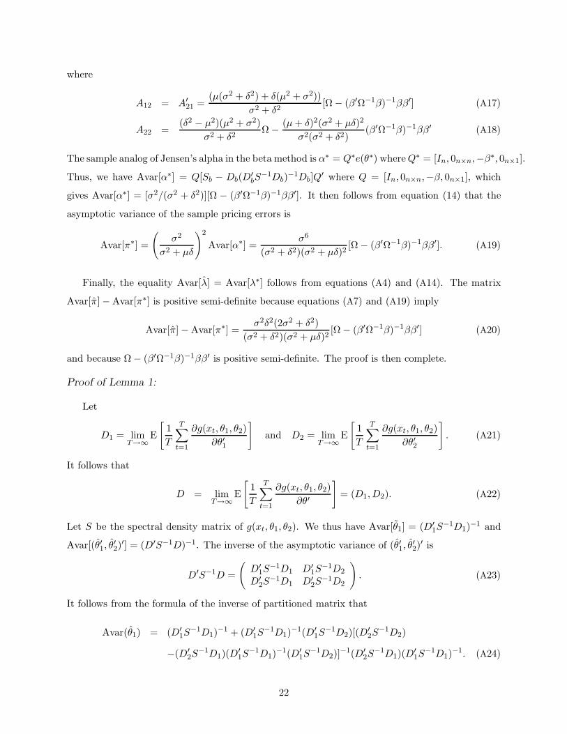
where
A12 = A′21 =
(µ(σ2 + δ2) + δ(µ2 + σ2))σ2 + δ2
[Ω − (β′Ω−1β)−1ββ′] (A17)
A22 =(δ2 − µ2)(µ2 + σ2)
σ2 + δ2Ω − (µ + δ)2(σ2 + µδ)2
σ2(σ2 + δ2)(β′Ω−1β)−1ββ′ (A18)
The sample analog of Jensen’s alpha in the beta method is α∗ = Q∗e(θ∗) where Q∗ = [In, 0n×n,−β∗, 0n×1].
Thus, we have Avar[α∗] = Q[Sb − Db(D′bS
−1Db)−1Db]Q′ where Q = [In, 0n×n,−β, 0n×1], which
gives Avar[α∗] = [σ2/(σ2 + δ2)][Ω − (β′Ω−1β)−1ββ′]. It then follows from equation (14) that the
asymptotic variance of the sample pricing errors is
Avar[π∗] =
(σ2
σ2 + µδ
)2
Avar[α∗] =σ6
(σ2 + δ2)(σ2 + µδ)2[Ω − (β′Ω−1β)−1ββ′]. (A19)
Finally, the equality Avar[λ] = Avar[λ∗] follows from equations (A4) and (A14). The matrix
Avar[π] − Avar[π∗] is positive semi-definite because equations (A7) and (A19) imply
Avar[π] − Avar[π∗] =σ2δ2(2σ2 + δ2)
(σ2 + δ2)(σ2 + µδ)2[Ω − (β′Ω−1β)−1ββ′] (A20)
and because Ω − (β′Ω−1β)−1ββ′ is positive semi-definite. The proof is then complete.
Proof of Lemma 1:
Let
D1 = limT→∞
E
[1T
T∑t=1
∂g(xt, θ1, θ2)∂θ′1
]and D2 = lim
T→∞E
[1T
T∑t=1
∂g(xt, θ1, θ2)∂θ′2
]. (A21)
It follows that
D = limT→∞
E
[1T
T∑t=1
∂g(xt, θ1, θ2)∂θ′
]= (D1,D2). (A22)
Let S be the spectral density matrix of g(xt, θ1, θ2). We thus have Avar[θ1] = (D′1S
−1D1)−1 and
Avar[(θ′1, θ′2)′] = (D′S−1D)−1. The inverse of the asymptotic variance of (θ′1, θ′2)′ is
D′S−1D =
(D′
1S−1D1 D′
1S−1D2
D′2S
−1D1 D′2S
−1D2
). (A23)
It follows from the formula of the inverse of partitioned matrix that
Avar(θ1) = (D′1S
−1D1)−1 + (D′1S
−1D1)−1(D′1S
−1D2)[(D′2S
−1D2)
−(D′2S
−1D1)(D′1S
−1D1)−1(D′1S
−1D2)]−1(D′2S
−1D1)(D′1S
−1D1)−1. (A24)
22

The difference, Avar[θ1]−Avar[θ1], must be positive semidefinite because the first term on the right-
hand side of equation (A24) equals Avar[θ1] and the other term is positive semidefinite. In view of
equation (A24), it is obvious that equation (18) implies D2 = 0 and thus Avar[θ1] = (D1S−1D1)−1,
which is the same as Avar[θ1].
Proof of Lemma 2:
Suppose that the dimensions of g1(xt, θ) and g2(xt) are m and n, respectively, and that the
dimensions of θ is k. Let
Sij =∞∑
j=−∞E[gi(xt, θ)gj(xt+j , θ)′], ∀ i, j = 1, 2. (A25)
Let us denote the spectral density matrix of g(xt, θ) and its inverse by
S =
(S11 S12
S21 S22
)and S−1 =
(S11 S12
S21 S22
). (A26)
Define
D1 = limT→∞
E
[1T
T∑t=1
∂g1(xt, θ)∂θ′
]and D =
(D1
0n×k
). (A27)
The asymptotic variances of θ and θ are, respectively,
Avar[θ] = (D′S−1D)−1 and Avar[θ] = (D′1S
−111 D1)−1. (A28)
By the formula of the inverse of partitioned matrix, we have
S11 = S−111 + S−1
11 S12(S22 − S21S−111 S12)−1S21S
−111 , (A29)
which implies
D′S−1D = D′1S
11D1 = D′1S
−111 D1 + D′
1S−111 S12(S22 − S21S
−111 S12)−1S21S
−111 D1. (A30)
The inverse is then
(D′S−1D)−1 = (D′1S
−111 D1)−1 − (D′
1S−111 D1)−1D′
1S−111 S12[S22 − S21S
−111 S12
+ S21S−111 D1(D′
1S−111 D1)−1D′
1S−111 S12]S21S
−111 D1(D′
1S−111 D1)−1 (A31)
Since both S22 − S21S−111 S12 and S21S
−111 D1(D′
1S−111 D1)−1D′
1S−111 S12 are positive semi-definite, it
follows from equation (A31) that (D′S−1D)−1 − (D′1S
−111 D1)−1 is negative semi-definite, which
implies that Avar[θ] − Avar[θ] is negative semi-definite. If equation (19) holds, then S12 = 0 and
S21 = 0, which imply Avar[θ] = Avar[θ] by equation (A31).
23

Proof of Inequality (21):
As with the derivation of Avar[λ∗] and Avar[π∗] in the proof of Theorem 1, one can obtain the
asymptotic variances of λ† and π† as
Avar(λ†) =σ2(σ2 + δ2)(σ2 + µδ)4
(β′Ω−1β)−1. (A32)
The inequality Avar[λ] > Avar[λ†] is obtained by comparing equations (A4) and (A32).
Proof of Equation (25):
In order to calculate the asymptotic variance of the estimator λ obtained with the SDF method,
let us consider the following vector of random variables
g(rt, ft, λ) =
rt(1 − λft)
ft − µ(ft − µ)2 − σ2
. (A33)
Substituting rt with equation (2), which is implied by the i.i.d.-normal assumption, and λ with
equation (9), we obtain the covariance matrix of g as
S =
σ2
(σ2+µδ)2[(σ4 + δ4)ββ′ + (σ2 + δ2)Ω] σ2(σ2−δ2)
σ2+µδβ − 2δσ4
σ4+µδβ
σ2(σ2−δ2)σ2+δµ β′ σ2 0− 2δσ4
σ2+µδβ′ 0 2σ4
. (A34)
The expected value of the derivative of g with respect to λ is
D = E[∂g
∂λ
]=
−(σ2 + µδ)β
00
. (A35)
After some algebraic manipulation, we obtain
D′S−1D =(σ2 + µδ)4
σ2(σ2 + δ2)(β′Ω−1β). (A36)
The asymptotic variance of the estimator of λ is (D′S−1D)−1, which gives
Avar(λ) =σ2(σ2 + δ2)(σ2 + µδ)4
(β′Ω−1β)−1. (A37)
Finally, we obtain the equality Avar[λ] = Avar[λ†] by comparing equations (A37) and (A32).
24

REFERENCES
Black, Fischer, Michael Jensen, and Myron S. Scholes, 1972, The capital asset pricing model: Some
empirical tests, in Michael Jensen, ed.: Studies in the Theory of Capital Markets (Praeger,
New York).
Bollerslev, Tim, Ray Chou and Kenneth Kroner, 1992, ARCH modeling in finance, Journal of
Econometrics 52, 5-59.
Breeden, Douglas, Michael Gibbons, and Robert Litzenberger, 1989, Empirical tests of the consumption-
oriented CAPM, Journal of Finance 44, 231–262.
Campbell, John, 1993, Intertemporal asset pricing without consumption data, American Economic
Review 83, 487–512.
Campbell, John, 1996, Understanding risk and return, Journal of Political Economy 104, 298–345.
Campbell, John, Andrew Lo, and Craig MacKinlay, 1997, The Econometrics of Financial Markets
(Princeton University Press, Princeton, New Jersey).
Chen, Naifu., Richard Roll, and Stephen Ross, 1986, Economic forces and the stock market, Journal
of Business 59, 383–404.
Cochrane, John, 1996, A cross-sectional test of an investment-based asset pricing model, Journal
of Political Economy 104, 572–621.
Cochrane, John, 2000, A resurrection of the stochastic discount factor/GMM methodology, Manu-
script, Graduate School of Business, University of Chicago.
Cochrane, John, 2001, Asset Pricing (Princeton University Press, Princeton, New Jersey).
Dybvig, Philip, and Jonathan Ingersoll, 1982, Mean-variance theory in complete markets, Journal
of Business 55, 233–252.
Fama, Eugene, and Kenneth French, 1992, The cross-section of expected stock returns, Journal of
Finance 47, 427–465.
Fama, Eugene, and Kenneth French, 1993, Common risk factors in the returns on stocks and bonds,
Journal of Financial Economics 33, 3–56.
Fama, Eugene, and James MacBeth, 1973, Risk, return, and equilibrium: Empirical tests, Journal
of Political Economy 71, 607–636.
Farnsworth, Heber., Wayne Ferson, David Jackson, and Steven Todd, 2000, Performance evaluation
with stochastic discount factors, Journal of Business forthcoming.
25

Ferson, Wayne, 1995, Theory and empirical testing of asset pricing models, in Robert Jarrow,
Vojislav Maksimovic, and William Ziemba, ed.: Handbooks in Operations Research and Man-
agement Science 9, 145–200.
Ferson, Wayne, Stephen Foerster, 1994, Finite sample properties of the generalized method of
moments in tests of conditional asset pricing models, Journal of Financial Economics 36,
29–55.
Ferson, Wayne, and Campbell Harvey, 1997, Fundamental determinants of national equity market
returns: A perspective on conditional asset pricing, Journal of Banking and Finance 21, 1625–
1665.
French, Kenneth, William Schwert, and Robert Stambaugh, 1987, Expected stock returns and
volatility, Journal of Financial Economics 17, 5–26.
Gibbons, Michael, Stephen Ross, and Jay Shanken, 1989, A test of the efficiency of a given portfolio,
Econometrica 57, 1121–1152.
Glosten, Lawrence, Ravi Jagannathan, and David Runkle, 1992, On the relation between the
expected value and the volatility of the nominal excess return on stocks,” Journal of Finance
48, 1779-1801.
Hamilton, James, 1994, Time Series Analysis (Princeton University Press, Princeton, New Jersey).
Hansen, Lars, 1982, Large sample properties of the generalized method of moments estimators,
Econometrica 50, 1029–1054.
Hansen, Lars, and Ravi Jagannathan, 1991, Implications of security market data for models of
dynamic economies, Journal of Political Economy 99, 225–262.
Hansen, Lars, and Ravi Jagannathan, 1997, Assessing specification errors in stochastic discount
factor models, Journal of Finance 52, 557–590.
Hansen, Lars, and Scott Richard, 1987, The role of conditioning information in deducing testable
restrictions implied by dynamic asset pricing models, Econometrica 55, 587–613.
Hansen, Lars, and Kenneth Singleton, 1982, Generalized instrumental variables estimation of non-
linear rational expectations models, Econometrica 50, 1269–1286.
Ingersoll, Jonathan, 1987, Theory of Financial Decision Making (Rowman & Littlefield, Totowa,
New Jersey).
26

Jagannathan, Ravi, and Zhenyu Wang, 1996, The conditional CAPM and the cross-section of
expected returns, Journal of Finance 51, 3–53.
Jagannathan, Rave, and Zhenyu Wang, 1998, An asymptotic theory for estimating beta-pricing
models using cross-sectional regression, Journal of Finance 53, 1285–1309.
Jagannathan, Ravi, and Zhenyu Wang, 1999, Efficiency of the stochastic discount factor method
for estimating risk premium, Working paper, Columbia University.
Kan, Raymond, and Guofu Zhou, 1999, A critique of the stochastic discount factor methodology,
Journal of Finance 54, 1221–1248.
Lucas, Robert, 1978, Asset prices in an exchange economy, Econometrica 46, 1429–1446.
MacKinlay, Craig, and Mathew Richardson, 1991, Using generalized method of moments to test
mean-variance efficiency, Journal of Finance 46, 511–527.
Ross, Stephen, 1976, The arbitrage theory of capital asset pricing, Journal of Economics Theory
13, 341–360.
Shanken, Jay, 1992, On the estimation of beta-pricing models, Review of Financial Studies 5, 1–34.
Sharpe, William, 1964, Capital asset prices: A theory of market equilibrium under conditions of
risk, Journal of Finance 19, 425–422.
Taylor, Malcolm, and James Thompson, 1986, Data based random number generation for a mul-
tivariate distribution via stochastic simulation, Computational Statistics & Data Analysis 4,
93–101.
27
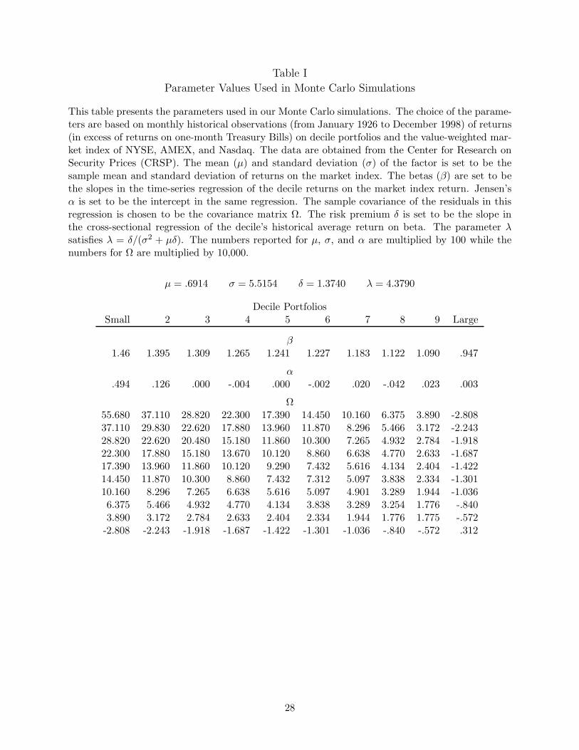
Table I
Parameter Values Used in Monte Carlo Simulations
This table presents the parameters used in our Monte Carlo simulations. The choice of the parame-ters are based on monthly historical observations (from January 1926 to December 1998) of returns(in excess of returns on one-month Treasury Bills) on decile portfolios and the value-weighted mar-ket index of NYSE, AMEX, and Nasdaq. The data are obtained from the Center for Research onSecurity Prices (CRSP). The mean (µ) and standard deviation (σ) of the factor is set to be thesample mean and standard deviation of returns on the market index. The betas (β) are set to bethe slopes in the time-series regression of the decile returns on the market index return. Jensen’sα is set to be the intercept in the same regression. The sample covariance of the residuals in thisregression is chosen to be the covariance matrix Ω. The risk premium δ is set to be the slope inthe cross-sectional regression of the decile’s historical average return on beta. The parameter λsatisfies λ = δ/(σ2 + µδ). The numbers reported for µ, σ, and α are multiplied by 100 while thenumbers for Ω are multiplied by 10,000.
µ = .6914 σ = 5.5154 δ = 1.3740 λ = 4.3790
Decile PortfoliosSmall 2 3 4 5 6 7 8 9 Large
β1.46 1.395 1.309 1.265 1.241 1.227 1.183 1.122 1.090 .947
α.494 .126 .000 -.004 .000 -.002 .020 -.042 .023 .003
Ω55.680 37.110 28.820 22.300 17.390 14.450 10.160 6.375 3.890 -2.80837.110 29.830 22.620 17.880 13.960 11.870 8.296 5.466 3.172 -2.24328.820 22.620 20.480 15.180 11.860 10.300 7.265 4.932 2.784 -1.91822.300 17.880 15.180 13.670 10.120 8.860 6.638 4.770 2.633 -1.68717.390 13.960 11.860 10.120 9.290 7.432 5.616 4.134 2.404 -1.42214.450 11.870 10.300 8.860 7.432 7.312 5.097 3.838 2.334 -1.30110.160 8.296 7.265 6.638 5.616 5.097 4.901 3.289 1.944 -1.0366.375 5.466 4.932 4.770 4.134 3.838 3.289 3.254 1.776 -.8403.890 3.172 2.784 2.633 2.404 2.334 1.944 1.776 1.775 -.572
-2.808 -2.243 -1.918 -1.687 -1.422 -1.301 -1.036 -.840 -.572 .312
28
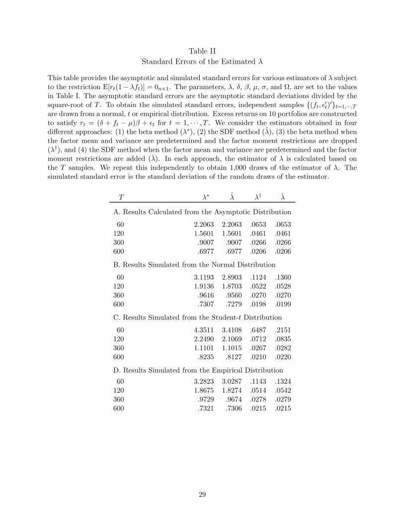
Table II
Standard Errors of the Estimated λ
This table provides the asymptotic and simulated standard errors for various estimators of λ subjectto the restriction E[rt(1− λft)] = 0n×1. The parameters, λ, δ, β, µ, σ, and Ω, are set to the valuesin Table I. The asymptotic standard errors are the asymptotic standard deviations divided by thesquare-root of T . To obtain the simulated standard errors, independent samples (ft, ε
′t)′t=1,···,T
are drawn from a normal, t or empirical distribution. Excess returns on 10 portfolios are constructedto satisfy rt = (δ + ft − µ)β + εt for t = 1, · · · , T . We consider the estimators obtained in fourdifferent approaches: (1) the beta method (λ∗), (2) the SDF method (λ), (3) the beta method whenthe factor mean and variance are predetermined and the factor moment restrictions are dropped(λ†), and (4) the SDF method when the factor mean and variance are predetermined and the factormoment restrictions are added (λ). In each approach, the estimator of λ is calculated based onthe T samples. We repeat this independently to obtain 1,000 draws of the estimator of λ. Thesimulated standard error is the standard deviation of the random draws of the estimator.
T λ∗ λ λ† λ
A. Results Calculated from the Asymptotic Distribution
60 2.2063 2.2063 .0653 .0653120 1.5601 1.5601 .0461 .0461360 .9007 .9007 .0266 .0266600 .6977 .6977 .0206 .0206
B. Results Simulated from the Normal Distribution
60 3.1193 2.8903 .1124 .1360120 1.9136 1.8703 .0522 .0528360 .9616 .9560 .0270 .0270600 .7307 .7279 .0198 .0199
C. Results Simulated from the Student-t Distribution
60 4.3511 3.4108 .6487 .2151120 2.2490 2.1069 .0712 .0835360 1.1101 1.1015 .0267 .0282600 .8235 .8127 .0210 .0220
D. Results Simulated from the Empirical Distribution
60 3.2823 3.0287 .1143 .1324120 1.8675 1.8274 .0514 .0542360 .9729 .9674 .0278 .0279600 .7321 .7306 .0215 .0215
29
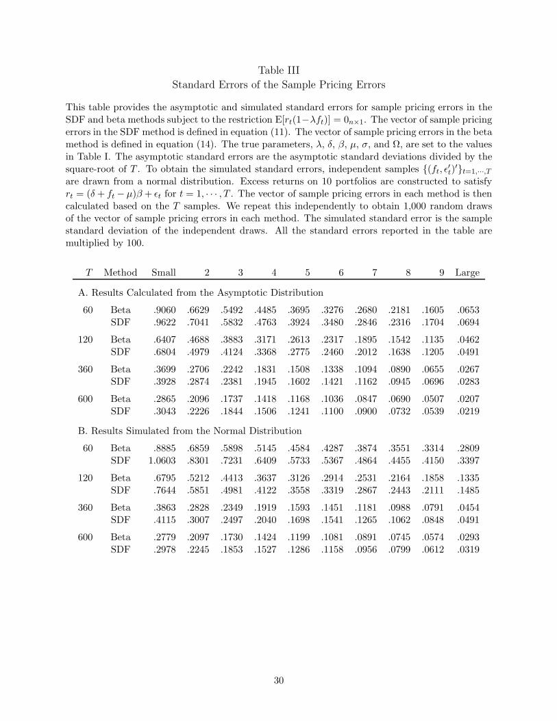
Table III
Standard Errors of the Sample Pricing Errors
This table provides the asymptotic and simulated standard errors for sample pricing errors in theSDF and beta methods subject to the restriction E[rt(1−λft)] = 0n×1. The vector of sample pricingerrors in the SDF method is defined in equation (11). The vector of sample pricing errors in the betamethod is defined in equation (14). The true parameters, λ, δ, β, µ, σ, and Ω, are set to the valuesin Table I. The asymptotic standard errors are the asymptotic standard deviations divided by thesquare-root of T . To obtain the simulated standard errors, independent samples (ft, ε
′t)′t=1,···,T
are drawn from a normal distribution. Excess returns on 10 portfolios are constructed to satisfyrt = (δ + ft − µ)β + εt for t = 1, · · · , T . The vector of sample pricing errors in each method is thencalculated based on the T samples. We repeat this independently to obtain 1,000 random drawsof the vector of sample pricing errors in each method. The simulated standard error is the samplestandard deviation of the independent draws. All the standard errors reported in the table aremultiplied by 100.
T Method Small 2 3 4 5 6 7 8 9 Large
A. Results Calculated from the Asymptotic Distribution
60 Beta .9060 .6629 .5492 .4485 .3695 .3276 .2680 .2181 .1605 .0653SDF .9622 .7041 .5832 .4763 .3924 .3480 .2846 .2316 .1704 .0694
120 Beta .6407 .4688 .3883 .3171 .2613 .2317 .1895 .1542 .1135 .0462SDF .6804 .4979 .4124 .3368 .2775 .2460 .2012 .1638 .1205 .0491
360 Beta .3699 .2706 .2242 .1831 .1508 .1338 .1094 .0890 .0655 .0267SDF .3928 .2874 .2381 .1945 .1602 .1421 .1162 .0945 .0696 .0283
600 Beta .2865 .2096 .1737 .1418 .1168 .1036 .0847 .0690 .0507 .0207SDF .3043 .2226 .1844 .1506 .1241 .1100 .0900 .0732 .0539 .0219
B. Results Simulated from the Normal Distribution
60 Beta .8885 .6859 .5898 .5145 .4584 .4287 .3874 .3551 .3314 .2809SDF 1.0603 .8301 .7231 .6409 .5733 .5367 .4864 .4455 .4150 .3397
120 Beta .6795 .5212 .4413 .3637 .3126 .2914 .2531 .2164 .1858 .1335SDF .7644 .5851 .4981 .4122 .3558 .3319 .2867 .2443 .2111 .1485
360 Beta .3863 .2828 .2349 .1919 .1593 .1451 .1181 .0988 .0791 .0454SDF .4115 .3007 .2497 .2040 .1698 .1541 .1265 .1062 .0848 .0491
600 Beta .2779 .2097 .1730 .1424 .1199 .1081 .0891 .0745 .0574 .0293SDF .2978 .2245 .1853 .1527 .1286 .1158 .0956 .0799 .0612 .0319
30

Table IV
Simulation Results for Specification Tests
This table provides the results of Monte Carlo simulations on the rejection rate of J-statistics.Independent samples (ft, ε
′t)′t=1,···,T are drawn from a normal or t distribution. Excess returns
on 10 portfolios are generated to satisfy rt = α + (δ + ft − µ)β + εt for t = 1, · · · , T , where λ, δ,β, µ, σ, and Ω are set to the values in Table I. For the size of specification tests, α is set to azero vector. For the power of specification tests, α is set to the values in Table I. We consider theJ-statistics obtained in four different approaches: (1) the beta method (J∗), (2) the SDF method(J), (3) the beta method when the factor mean and variance are predetermined and the factormoment restrictions are dropped (J†), and (4) the SDF method when the factor mean and varianceare predetermined and the factor moment restrictions are added (J). In each approach, the GMMis applied to the T samples to obtain a J-statistic. We repeat this independently to obtain 10,000random draws of the J-statistics. The table presents the percent of the simulated J-statistics thatare larger than the critical point at the significance levels of 10 percent, five percent and one percentbased on the sampling distribution of the J-statistics under the null hypothesis of α = 0.
10 Percent Five Percent One PercentT J∗ J J† J J∗ J J† J J∗ J J† J
A. Size of Specification Tests Simulated from the Normal Distribution
60 7.2 7.9 7.2 12.7 2.9 3.2 2.9 6.4 .2 .2 .2 1.6120 8.9 9.0 8.9 11.7 4.0 4.2 4.0 6.4 .6 .6 .6 1.6360 9.4 9.5 9.4 10.3 4.7 4.7 4.7 5.2 .9 .9 .9 1.2600 9.8 9.8 9.8 10.3 4.8 4.8 4.8 5.1 .9 .9 .9 1.1
B. Size of Specification Tests Simulated from the Student-t Distribution
60 5.4 7.3 5.4 23.0 1.8 2.8 1.8 14.4 .1 .2 .1 5.1120 7.7 8.9 7.7 20.9 3.0 4.0 3.1 13.2 .4 .5 .4 5.1360 8.9 9.3 8.9 16.3 4.1 4.3 4.1 10.1 .7 .8 .7 3.5600 9.9 10.2 9.9 15.0 4.5 4.7 4.5 8.8 .8 .9 .8 2.5
C. Power of Specification Tests Simulated from the Normal Distribution
60 11.1 12.1 11.1 16.9 4.6 5.3 4.6 9.1 .3 .6 .3 2.1120 19.7 20.2 19.7 22.1 10.4 10.9 10.4 12.5 2.2 2.4 2.2 3.8360 50.3 50.3 50.3 47.7 36.7 36.9 36.7 34.6 15.9 16.1 15.9 14.9600 74.5 74.5 74.5 71.1 62.3 62.3 62.3 58.9 37.6 37.7 37.6 34.6
D. Power of Specification Tests Simulated from the Student-t Distribution
60 9.6 12.6 9.6 28.8 3.9 5.6 3.9 18.4 .4 .6 .4 6.9120 18.4 20.8 18.4 31.9 9.4 11.2 9.4 21.8 1.8 2.5 1.8 9.0360 49.8 50.6 49.8 53.6 35.9 36.9 35.9 41.4 14.7 15.6 14.7 20.6600 73.0 73.5 73.0 72.6 60.7 61.3 60.7 61.0 34.6 35.4 34.6 37.0
31

Footnotes
1 See French, Schwert, and Stambaugh (1987), Glosten, Jagannathan and Runkle (1992), and
Bollerslev, Chou, and Kroner (1992) for evidence.
2 When it is not necessary to estimate the variance, σ2, of the factor, the last moment restric-
tions can be ignored. If the factor is the return on a tradable asset, we have δ = µ and the
first two moment restrictions become E[rt − ftβ] = 0n×1 and E[(rt − ftβ)ff ] = 0n×1 which
do not depend on the mean and variance of the factor. In this case, we can estimate β from
these two moment restrictions and separately estimate µ and σ2 from moment restrictions
(5) and (6). The estimate of µ is also the estimate of the risk premium.
3 However, he does not use the term “stochastic discount factor” — Hansen and Richard (1987)
coined the term.
4 For example, Fama and French (1992) and Jagannathan and Wang (1996) use 330 monthly
observations. Fama and French (1993) use 342 monthly observations.
5 If we were to construct portfolios by ranking firms by both market capitalization and estimated
beta, the betas would not be as highly negatively correlated with firm size. In that case, as
in Fama and French (1992) and Jagannathan and Wang (1996), the risk premium on beta
would be close to zero, and the risk premium on firm size would be large in magnitude and
negative.
6 Our simulation results also hold well when we set δ = µ.
7 We can estimate the empirical distribution either by the Bootstrap method or the method
described by Taylor and Thompson (1986). The results are the same, and we only report the
former.
8 We have also drawn samples from the empirical distribution for 1,000 simulations. The results
are very similar to the results obtained from the normal and student-t distributions. We do
not report the results for the empirical distribution because it takes very long time to conduct
10,000 simulations with the empirical distribution.
32
Related Documents