EMPIRICAL EFFECTS OF DIVISION II INTERCOLLEGIATE ATHLETICS JONATHAN M. ORSZAG PETER R. ORSZAG COMMISSIONED BY THE NATIONAL COLLEGIATE ATHLETIC ASSOCIATION JUNE 2005

Welcome message from author
This document is posted to help you gain knowledge. Please leave a comment to let me know what you think about it! Share it to your friends and learn new things together.
Transcript
EMPIRICAL EFFECTS OF DIVISION II INTERCOLLEGIATE ATHLETICS
JONATHAN M. ORSZAG PETER R. ORSZAG
COMMISSIONED BY THE NATIONAL COLLEGIATE ATHLETIC ASSOCIATION JUNE 2005

2
ABOUT THIS REPORT
This study was commissioned by the National Collegiate Athletic Association (NCAA) as an independent analysis of the empirical effects of intercollegiate athletics in Division II. It builds upon previous empirical analyses, including of intercollegiate athletics in Division I and of capital expenditures associated with intercollegiate athletics. The views and opinions expressed in this study are solely those of the authors and do not necessarily reflect the views and opinions of the NCAA, or the institutions with which the authors are or have been associated. The authors of the study are: Jonathan Orszag ([email protected]) is the Managing Director of Competition Policy Associates, Inc., an economic policy consulting firm. Previously, Mr. Orszag served as the Assistant to the Secretary of Commerce and Director of the Office of Policy and Strategic Planning. Peter Orszag ([email protected]) is a Director at Competition Policy Associates and the Joseph A. Pechman Senior Fellow in Economic Studies at the Brookings Institution. Dr. Orszag previously served as Special Assistant to the President for Economic Policy at the White House. The authors also thank Chris Clapp, Yair Eilat, Jillian Ingold, Jeanne Johnson, and Jim Isch and other NCAA officials for their comments and assistance.
3
Executive Summary
The NCAA commissioned this study as part of an ongoing effort to gather more accurate and timely financial information on the effects of intercollegiate athletics in higher education. In a previous report released in 2003 (“The Effects of Collegiate Athletics: An Interim Report”), we explored the financial effects of operating expenditures associated with collegiate athletics in Division I-A. More recently, we have updated the Division I-A analysis (“The Effects of Collegiate Athletics: An Update”) and also examined the effects of the capital stock used in athletics (“The Physical Capital Stock Used in Collegiate Athletics”).
This study focuses on the empirical effects of collegiate athletics among Division
II schools, including an analysis of moving from Division II to Division I. Our key findings include: Characteristics of Division II athletic programs
• Average operating athletic spending and revenue are significantly lower in Division II than in Division I. Among Division II schools with football, operating revenue averaged $2.6 million in 2003 and operating spending averaged $2.7 million. Within Division I-AA and I-AAA, operating athletic budgets are significantly larger; for example, in Division I-AAA, operating revenue averaged $6.2 million in 2003 and operating spending averaged $6.5 million.
• Net revenue excluding institutional support exhibits much smaller average deficits
in Division II than in Division I-AA or I-AAA. In 2003, net operating deficits without institutional support averaged about $2 million less per school in Division II than in Division I-AA and I-AAA. The differences are even more significant when state government support and student fees are excluded; some analysts believe that this concept of net revenue excluding institutional support, state government support, and student fees represents the most insightful perspective on the financial impact of athletics. On this basis, net operating deficits averaged $3 million to $5 million less per school in Division II than in Division I-AA and I-AAA.
• Within Division II, operating athletic spending amounted to 2.7 percent of total
institutional spending in 2003. That share was slightly smaller than in Division I; athletic spending represented 3.0 percent of total institutional spending in Division I-AAA, 3.6 percent in Division I-AA, and 3.8 percent in Division I-A.
• Athletic spending and revenue within Division II both exhibit some degree of
mobility. For example, of the Division II schools in the middle 20 percent of the athletic spending distribution in 1993, slightly more than half were at the same point in the spending distribution in 2003; a little over a quarter had moved down; and about one-sixth had moved up.

4
• Athletic spending in Division II has grown most rapidly outside football and men’s basketball over the past decade. At Division II schools with football programs, average football and men’s basketball spending has increased at an average inflation-adjusted rate of just over two percent per year between 1993 and 2003. By comparison, inflation-adjusted spending on women’s basketball and other men’s sports has increased at a rate of roughly four percent per year, and inflation-adjusted spending on other women’s sports (excluding basketball) has increased at an average annual rate of roughly nine percent.
Effects of increases in operating athletic spending within Division II
• On average, each additional operating dollar that a Division II university spends on athletics is associated with between 20 and 60 cents of additional revenue. The implication is that increases in operating spending on athletics within Division II trigger a modest increase in revenue, but the increase in revenue is insufficient to offset the increased cost. As a result, net revenue falls.
• The results for specific sports are similar. Across a range of sports, increased
spending is associated with a statistically significant reduction in net revenue. Our conclusion is that increased operating spending on athletics is associated with little or no change in revenue, and therefore a significant decline in net revenue, for Division II schools.
• Within Division II, there is no robust relationship between athletic spending and
alumni giving; no robust relationship between athletic spending and average incoming SAT scores; and no robust relationship between athletic spending and the university’s acceptance rate (that is, the percentage of applicants accepted by the university).
Effects of moving from Division II to Division I
• Since the mid-1980s, nearly 50 schools have moved or committed to moving from Division II to Division I-AA or I-AAA. At least three other schools have switched from Division II to Division I in a particular sport (e.g., men’s ice hockey). Our data allow analysis of up to 20 schools that moved either completely or in a particular sport between 1994 and 2002.
• In our dataset, the schools switching divisions for all sports experienced an
average real increase in spending of $3.7 million. Their revenue, by contrast, increased by an average of only $2.5 million – even including changes in institutional support, state government support, and student fees dedicated to athletics. As a result, the schools experienced an average deterioration in net operating revenue associated with intercollegiate athletics of more than $1 million. Furthermore, institutional support to athletics among these schools increased by an average of almost $2 million, implying that the net operating results excluding institutional support deteriorated by an average of more than $3
5
million. Student fees and state support also increased following a move to Division I. Excluding these increases further exacerbates the financial impact of switching on net operating revenue.
• Every school for which we have data experienced a decline in net operating
revenue excluding institutional support, state support, and student activity fees when moving from Division II to Division I. The median decline was almost $2 million and 90 percent of schools switching experienced a reduction of more than $740,000.
• Statistical analyses show that schools that switched divisions did not tend to
experience a systematic and statistically significant increase in enrollment, although some examples exist of schools experiencing rapid increases in enrollment after switching divisions.
• Our interviews with campus decision-makers revealed that many schools
switching divisions did not engage in detailed or rigorous cost-benefit analyses before making the switch. The interviews also suggested that most of the schools that switched did not experience significant financial returns, which is consistent with our analysis.

6
I. Introduction
The National Collegiate Athletics Association (NCAA) commissioned this study as part of an ongoing effort to gather more accurate and timely financial information on the effects of intercollegiate athletics in higher education. In a previous interim report released in 2003 (“The Effects of Collegiate Athletics: An Interim Report”), we explored the financial effects of operating expenditures associated with collegiate athletics in Division I-A. More recently, we have updated the Division I-A analysis (“The Effects of Collegiate Athletics: An Update”) and also examined the effects of the athletic capital stock (“The Physical Capital Stock Used in Collegiate Athletics”). This study focuses on the empirical effects of collegiate athletics among Division II schools, including an analysis of moving from Division II to Division I.
Collegiate sports in Division II are the subject of various empirical beliefs, yet just as in Division I, many of these widely believed “facts” are not actually based on rigorous empirical analysis. Our goal in this paper is to use empirical evidence to evaluate several key questions surrounding athletic programs in Division II. For example, how does athletic spending and revenue in Division II compare to other divisions? Does switching from Division II to Division I generate benefits or costs, either in financial terms or in other quantifiable ways? Does increased spending on athletics within Division II generate gains or reductions in net revenue? Our hope is that the evidence presented below will prove helpful to campus decision-makers within Division II struggling with these questions.
The paper draws on the available empirical evidence contained in previous
academic studies; statistical analysis of school-specific information collected as part of the Equity in Athletics Disclosure Act (EADA) merged with data from other sources (such as the Integrated Post-Secondary Education Data System managed by the Department of Education); and our survey of capital associated with intercollegiate athletics (as described in our previous paper on that topic). These various sources of data each have limitations, but they nonetheless represent the most comprehensive empirical resource to date for shedding light on the key issues related to college athletics in Division II.
The paper has seven sections including this brief introduction. The second
section provides basic comparisons of Division II athletic spending and revenue, relative to other divisions. The third section examines the financial and other returns to increased athletic spending within Division II. The fourth section uses econometric and other statistical methods to explore the effects of moving from Division II to Division I. The fifth section supplements the statistical analysis with the results of interviews we conducted with campus decision-makers at schools that have either switched divisions or considered doing so. A sixth section summarizes the existing literature on schools that have moved divisions. The seventh section offers conclusions.

7
II. Division II Finances: Comparisons to Other Divisions
As a first step in analyzing intercollegiate athletics within Division II, we simply compare many key indicators in Division II to other divisions. The core of the database we use for this purpose is based on reports filed under EADA. Under EADA, institutions are required to report the total revenues and expenses attributable to the institution's intercollegiate athletic activities; the revenues and expenses attributable to specific sports, such as football, men's basketball, and women's basketball; the number of participants for each varsity team and an unduplicated head count of individuals (by gender) who participate on at least one varsity team; and whether a coach is assigned to a team full- or part-time, and if part-time, whether the coach is a full- or part-time employee of the institution.
The NCAA collects supplemental data that provides more detail than available on the EADA form. These NCAA data are proprietary. As part of our ongoing research project, we were granted access to the NCAA/EADA data since 1993, the first year in which they are electronically available.1 The data are available for 1993, 1995, 1997, 1998, 1999, 2000, 2001, 2002, and 2003.2
Figure 1 shows that average operating athletic spending and revenue are
significantly lower in Division II than in Division I. Among Division II schools with football, for example, operating revenue (which includes institutional support, state government support, and student fees) averaged $2.6 million in 2003 and operating spending averaged $2.7 million. Among Division II schools without football, the figures were even lower: $1.7 million and $1.9 million respectively. By contrast, among Division I-A schools, athletic budgets were substantially larger: Operating athletic revenue averaged $29.4 million, and operating athletic spending averaged $27.2 million.
Even in Division I-AA and I-AAA, operating athletic budgets are significantly
larger than in Division II; for example, in Division I-AAA, operating revenue averaged $6.2 million in 2003 and operating spending averaged $6.5 million. Operating athletic revenue and spending are significantly larger even in smaller Division I-AA and I-AAA conferences than in larger Division II conferences; for example, average operating revenue and spending in the Horizon Conference (Division I-AA) are significantly higher than in the Great Lakes Intercollegiate Athletic Conference (Division II).
1 The year “1993” corresponds to the academic year 1992-1993. 2 For years prior to 1993, data on individual athletic programs by school are unavailable, but overall summaries are available from an NCAA publication. See Fulks (2005).

8
Figure 1: Operating revenue and spending by Division
The revenue numbers in Figure 1 include institutional support, state government support, and student fees dedicated to the athletic department. For many purposes, it is more insightful to exclude some or all of these transfers. In Figure 2, we therefore show three figures: operating net revenue, operating net revenue without institutional support, and operating net revenue without institutional support, state government support, and student fees. Many analysts believe that the final concept -- net revenue excluding institutional support, state government support, and student activity fees -- best measures the concept of “earned” net revenue from athletics, and therefore for many purposes represents the most insightful perspective on the financial impact of athletics. As Figure 2 shows, on this basis, net operating deficits averaged $3 million to $5 million less per school in Division II than in Division I-AA and I-AAA.
Another point of comparison is the share of the university’s overall budget
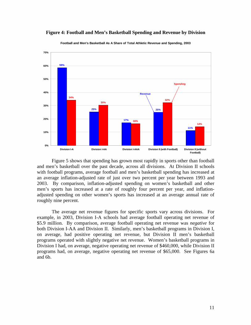
devoted to operating spending on athletics. Figure 3 shows that within Division II, operating athletic spending amounted to 2.7 percent of total institutional spending in 2003. That share was slightly smaller than in Division I; athletic spending represented 3.0 percent of total institutional spending in Division I-AAA, 3.6 percent in Division I-AA, and 3.8 percent in Division I-A. These figures may seem surprising, since Division I-A schools tend to be significantly larger than other schools, and at least within Division I-A, the share of spending devoted to athletics is smaller for larger schools. Figure 4 suggests, however, that the fixed costs associated with running an athletics program are significantly larger in Division I-A (as well as in I-AA and I-AAA) than in Division II, more than offsetting the larger total institutional spending in Division I-A.
Average Athletic Operating Revenue and Spending, 2003
$29,400
$7,200$6,200
$2,600$1,700
$27,200
$7,500$6,500
$2,700$1,900
$0
$5,000
$10,000
$15,000
$20,000
$25,000
$30,000
$35,000
Division I-A Division I-AA Division I-AAA Division II (with Football) Division II (withoutFootball)
in T
hous
ands
Revenue Spending

9
Figure 2: Operating net revenue by Division
These figures on the share of the university’s budget devoted to operating athletic spending on athletics exclude capital spending. This exclusion is unlikely to alter the fundamental conclusion that athletics represent a small share of the overall university budget in Division II (as in Division I). Data from a survey of the physical capital stock of Division II schools, combined with data from the Department of Education, can be used to compute the athletic share of overall institutional spending, including capital costs both in the athletic and overall figures.3 Of the Division II respondents to the capital survey, we were able to obtain data on total institutional capital values for eight public universities.4 For these eight schools, operating athletic spending represented 3.3 percent of total operating spending for the institutions. Including athletic and overall institutional capital costs, the share of spending attributed to athletics rose by one percentage point, to 4.3 percent. In other words, including capital costs does not alter the qualitative result that athletic spending currently represents a relatively small share of total institutional spending in Division II, at least for the schools for which data were available.
3 The most recent available total institutional capital values were for 2001. We converted those figures into 2003 dollars using the Consumer Price Index. To compute the annual capital costs, we adopt the same assumptions as athletic capital costs (i.e., depreciation plus financing costs equal 10 percent of the capital stock). 4 The Department of Education does not publish data on total institutional capital values for private universities.
Average Athletic Operating Net Revenue, 2003
$2,200
-$300 -$300-$100 -$200
-$600
-$3,700-$3,500
-$1,600-$1,300
-$2,900
-$5,200
-$6,600
-$2,100
-$1,600
-$8,000
-$7,000
-$6,000
-$5,000
-$4,000
-$3,000
-$2,000
-$1,000
$0
$1,000
$2,000
$3,000
Division I-A Division I-AA Division I-AAA Division II (with Football) Division II (withoutFootball)
In T
hous
ands
Net Revenue with
Institutional Support
Net Revenue without
Institutional Support
Net Revenue withoutInstitutional Support,
State Support, and Student Activity Fees

10
Figure 3: Athletic spending as share of university spending by Division
Athletic spending and revenue within Division II both exhibit some degree of
mobility. For example, of the Division II schools in the middle 20 percent of the athletic spending distribution in 1993, 56 percent were at the same point in the spending distribution in 2003; 28 percent had moved down; and 16 percent had moved up. Of the Division II schools in the middle 20 percent of the athletic net revenue distribution in 1993, roughly 22 percent were at the same point in the net revenue distribution in 2003; 35 percent had moved down; and 43 percent had moved up. Of the schools in the top of the net revenue distribution in 1993, roughly a quarter were in the bottom of the net revenue distribution in 2003.
Specific sports Figure 4 shows that football and men’s basketball account for roughly one-third of overall athletic spending for Division I-A, I-AA, and Division II (with football). For schools without football programs, men’s basketball represents roughly 15 percent of overall athletic spending for both Division I-AAA and Division II (without football). The share of athletic revenue derived from football and men’s basketball is much higher for Division I-A (nearly 60 percent from these two sports alone) relative to Division I-AA and Division II with football (roughly one-quarter from these two sports).
Athletic Operating Spending As A Share of Total Institutional Spending, 2003
3.8%3.6%
3.0%
2.7%
0.0%
0.5%
1.0%
1.5%
2.0%
2.5%
3.0%
3.5%
4.0%
4.5%
5.0%
Division I-A Division I-AA Division I-AAA Division II
11
Figure 4: Football and Men’s Basketball Spending and Revenue by Division
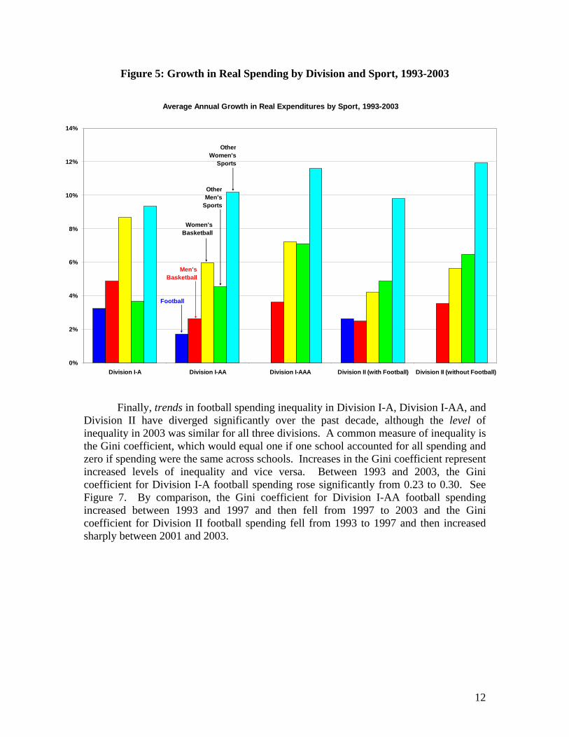
Figure 5 shows that spending has grown most rapidly in sports other than football and men’s basketball over the past decade, across all divisions. At Division II schools with football programs, average football and men’s basketball spending has increased at an average inflation-adjusted rate of just over two percent per year between 1993 and 2003. By comparison, inflation-adjusted spending on women’s basketball and other men’s sports has increased at a rate of roughly four percent per year, and inflation-adjusted spending on other women’s sports has increased at an average annual rate of roughly nine percent.
The average net revenue figures for specific sports vary across divisions. For
example, in 2003, Division I-A schools had average football operating net revenue of $5.9 million. By comparison, average football operating net revenue was negative for both Division I-AA and Division II. Similarly, men’s basketball programs in Division I, on average, had positive operating net revenue, but Division II men’s basketball programs operated with slightly negative net revenue. Women’s basketball programs in Division I had, on average, negative operating net revenue of $460,000, while Division II programs had, on average, negative operating net revenue of $65,000. See Figures 6a and 6b.
Football and Men's Basketball As A Share of Total Athletic Revenue and Spending, 2003
59%
25%
17%
25%
11%
34%
30%
16%
32%
14%
0%
10%
20%
30%
40%
50%
60%
70%
Division I-A Division I-AA Division I-AAA Division II (with Football) Division II (withoutFootball)
Spending
Revenue
12
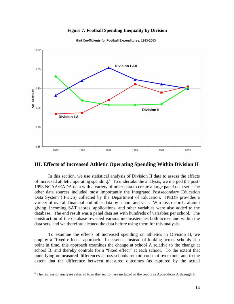
Figure 5: Growth in Real Spending by Division and Sport, 1993-2003 Finally, trends in football spending inequality in Division I-A, Division I-AA, and Division II have diverged significantly over the past decade, although the level of inequality in 2003 was similar for all three divisions. A common measure of inequality is the Gini coefficient, which would equal one if one school accounted for all spending and zero if spending were the same across schools. Increases in the Gini coefficient represent increased levels of inequality and vice versa. Between 1993 and 2003, the Gini coefficient for Division I-A football spending rose significantly from 0.23 to 0.30. See Figure 7. By comparison, the Gini coefficient for Division I-AA football spending increased between 1993 and 1997 and then fell from 1997 to 2003 and the Gini coefficient for Division II football spending fell from 1993 to 1997 and then increased sharply between 2001 and 2003.
Average Annual Growth in Real Expenditures by Sport, 1993-2003
0%
2%
4%
6%
8%
10%
12%
14%
Division I-A Division I-AA Division I-AAA Division II (with Football) Division II (without Football)
Football
Men's Basketball
Women's Basketball
Other Men's
Sports
Other Women's
Sports

13
Average Basketball Operating Net Revenue, 2003
$752
-$67
-$460
-$65
-$600
-$400
-$200
$0
$200
$400
$600
$800
$1,000
Division I Division II
In T
hous
ands
Men's Basketball
Women's Basketball
Figure 6a and 6b: Average Football and Basketball Operating Net Revenue by Division
Average Football Operating Net Revenue, 2003
$5,921
-$408-$149
-$1,000
$0
$1,000
$2,000
$3,000
$4,000
$5,000
$6,000
$7,000
Division I-A Division I-AA Division II
In T
hous
ands
14
Figure 7: Football Spending Inequality by Division
III. Effects of Increased Athletic Operating Spending Within Division II
In this section, we use statistical analysis of Division II data to assess the effects of increased athletic operating spending.5 To undertake the analysis, we merged the post-1993 NCAA/EADA data with a variety of other data to create a large panel data set. The other data sources included most importantly the Integrated Postsecondary Education Data System (IPEDS) collected by the Department of Education. IPEDS provides a variety of overall financial and other data by school and year. Win-loss records, alumni giving, incoming SAT scores, applications, and other variables were also added to the database. The end result was a panel data set with hundreds of variables per school. The construction of the database revealed various inconsistencies both across and within the data sets, and we therefore cleaned the data before using them for this analysis.
To examine the effects of increased spending on athletics in Division II, we employ a “fixed effects” approach. In essence, instead of looking across schools at a point in time, this approach examines the change at school A relative to the change at school B, and thereby controls for a “fixed effect” at each school. To the extent that underlying unmeasured differences across schools remain constant over time, and to the extent that the difference between measured outcomes (as captured by the actual
5 The regression analyses referred to in this section are included in the report as Appendices A through F.
Gini Coefficients for Football Expenditures, 1993-2003
0.15
0.20
0.25
0.30
0.35
0.40
1993 1995 1997 1999 2001 2003
Gin
i Coe
ffici
ent
Division II
Division I-A
Division I-AA
15
accounting system at each school) and a consistent indicator of outcomes (as would be captured if the same accounting system were used at each school) is constant over time, the fixed effects approach should more precisely identify the effects of changes in college athletic spending, rather than being confounded by accounting and other differences across schools.6
Throughout our analysis of revenue or net revenue in this section, we generally
exclude institutional support from revenue. The qualitative conclusions are similar if we also exclude state government support and student activity fees.
Total operating spending on athletics We begin our analysis with total operating spending within Division II (see Appendix A for more details). On average, each additional dollar that a Division II university spends on athletics is associated with between 20 and 60 cents of additional revenue (as noted above, “revenue” here generally excludes institutional support). The implication is that increases in operating spending on athletics within Division II trigger a modest increase in revenue, but the increase in revenue is insufficient to offset the increased cost. As a result, net revenue falls. In other words, on average, each additional operating dollar that a Division II university spends on athletics is associated with well under one additional dollar of revenue – so spending increases are associated with declines in net operating revenue. Football spending When the focus is shifted specifically to Division II football spending (Appendix B), the results suggest that increases in football spending are associated with little or no increase in football revenue. As with overall spending, the implication is that expanding football spending is associated with a reduction in net revenue from the sport.
We also explore the relationship between football spending and winning, and the relationship between winning and football revenue (Appendix C). At least over our sample period, there appears to be no statistical relationship between changes in football spending and changes in football winning or between changes in football winning and changes in football revenue. Other sports The results are generically similar for basketball (Appendix D). For men’s basketball, increases of $1 in operating expenditures on men’s basketball were associated with between zero and 60 cents in additional revenue, on average. For women’s basketball, increases in spending of $1 were associated with increases in revenue of between 40 and 70 cents. For both men’s basketball and women’s basketball, the net
6 It should be noted that the fixed-effects approach is not a panacea; it can exacerbate measurement errors if these assumptions do not hold. For further discussion of the fixed-effects approach, see our earlier paper on Division I athletics.

16
result is that increases in spending were generally associated with reductions in net revenue.7
The results for sports other than football and men’s basketball suggest that increases in operating spending were also, on average, associated with declines in net revenue (Appendix E). Across a range of model specifications, increased spending of $1 was associated with either no increase in revenue or an increase below $1.
Our overall conclusion from this analysis is that increased operating spending on
athletics is generally associated with little or no change in revenue, and a significant decline in net revenue, for Division II schools. Other quantifiable effects Increased spending on athletic programs could generate benefits for institutions of higher education other than increased athletic revenue. These benefits could manifest themselves in a variety of ways, including increased applications, increased student quality, and increased annual giving. Our database allows us to examine some of these issues statistically (Appendix F).
Although some of the econometric specifications suggest a positive effect from increased athletic spending, the bulk of the analysis suggests no relationship. Our conclusion is therefore that within Division II, there is no robust relationship between athletic spending and alumni giving; no robust relationship between athletic spending and average incoming SAT scores; and no robust relationship between athletic spending and the university’s acceptance rate (that is, the percentage of applicants accepted by the university).8 In addition to these quantifiable effects, athletic programs may have non-quantifiable effects on higher education. For example, it is possible that athletic programs boost “school spirit” and the enjoyment of the educational experience in ways that do not manifest themselves in measurable indicators. On the other hand, it is also possible that athletic programs lead to a “beer and circus” environment in which the principles and standards of higher education are eroded by the distraction of a non-academic presence on campus. Limitations The econometric analyses in this section are subject to four important caveats:
7 In some cases, however, the standard error on the spending coefficient was so large that it was impossible to reject a one-sided hypothesis that the coefficient was statistically smaller than the critical threshold of $1. This also occasionally occurred in some cases in other appendices, but in most regressions, the coefficient was statistically smaller than $1. 8 For Division I-A schools, the existing empirical literature on these issues is mixed. For a further discussion of the empirical literature, see our earlier paper on Division I-A athletics.

17
• Limited time-series database: Our database extends only from 1993 to 2003. It is possible that increased spending on athletics has long lags – that is, it produces significant benefits or costs after a long period of time. If this were the case, our database may be too short to capture the true effects of increased spending. Since the detailed NCAA/EADA data are not available before 1993, the effects of athletic spending over longer periods of time can be examined only in coming years, after more data have been collected.
• Omitted variables: As with any statistical exercise, it is possible that omitted
variables bias the results. The omitted variables that could bias our results include factors such as changes in “school spirit” that are artificially correlated with changes in athletic spending, and that also affect athletic revenue.
• Endogeneity: Many of the regressions treat spending as an exogenous variable,
but it may itself be affected by revenue. This may bias any estimate of the effect of spending on revenue upward. Alternative econometric techniques that are designed to address this concern did not significantly alter the fundamental results.
• Measurement error: The reported data may be biased, which could affect the
estimates. We know that various components of spending – such as staff compensation from all sources and total capital spending – are poorly measured and likely biased downward in the reported data.
Despite these limitations, the empirical results strongly suggest that increased
spending on athletics in Division II does not “pay for itself,” either in terms of increased revenue or in terms of other quantifiable effects (e.g., alumni giving). IV. Analysis of Effects from Switching Divisions Many Division II schools have likely at least considered moving to Division I-AAA or Division I-AA at some point, and some have actually done so. Since the mid-1980s, nearly 50 schools have moved or committed to moving from Division II to Division I-AA or I-AAA. At least three other schools have switched from Division II to Division I in a particular sport (e.g., men’s ice hockey). In this section, we analyze the effects of switching divisions.
NCAA/EADA data allow analysis of only about 20 schools that moved either completely or in a particular sport between 1994 and 2002. In certain cases, missing data limit the analysis to an even smaller number of schools. The Division II schools that have switched divisions have tended to be public schools (more than three-fifths were public) and larger than schools that did not switch division (for example, among private schools, enrollment at schools that switched divisions averaged 3,200 students, compared to 2,600 at private schools that remained in Division II). Schools that switched also tended to have somewhat lower SAT/ACT
18
scores (for example, incoming SAT scores at public schools that switched divisions were roughly five percent lower than non-switching public schools) and tended to have slightly lower acceptance rates.
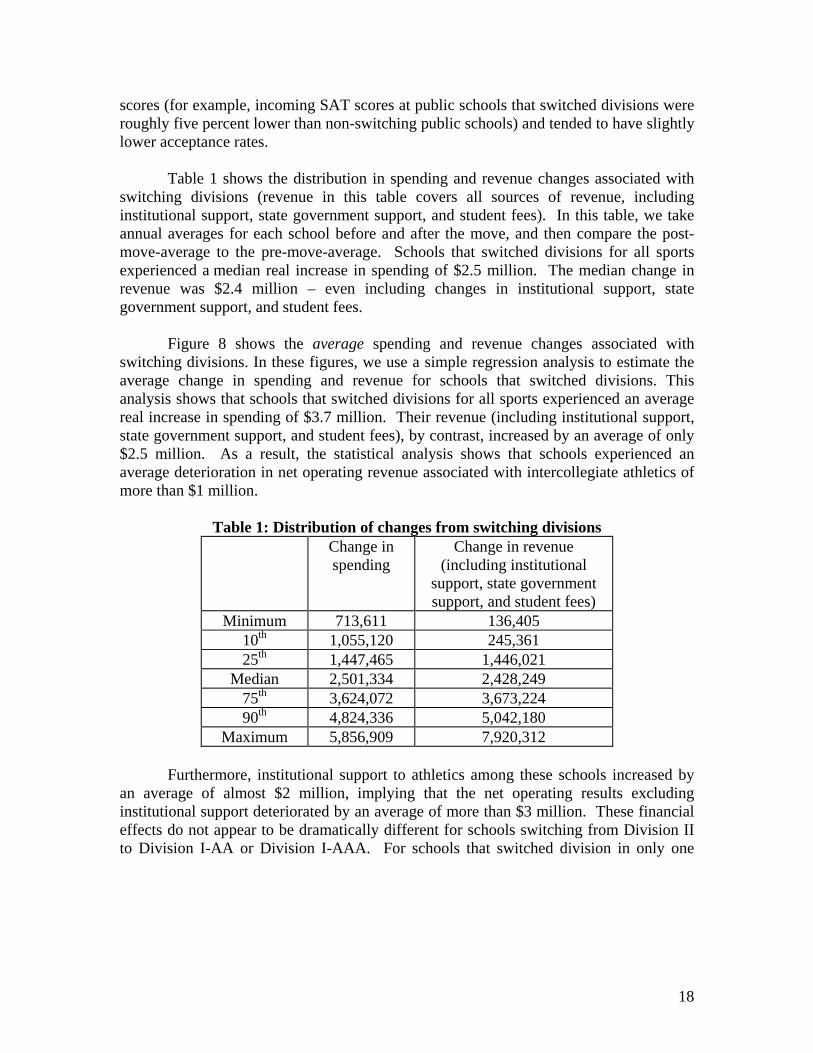
Table 1 shows the distribution in spending and revenue changes associated with switching divisions (revenue in this table covers all sources of revenue, including institutional support, state government support, and student fees). In this table, we take annual averages for each school before and after the move, and then compare the post-move-average to the pre-move-average. Schools that switched divisions for all sports experienced a median real increase in spending of $2.5 million. The median change in revenue was $2.4 million – even including changes in institutional support, state government support, and student fees.
Figure 8 shows the average spending and revenue changes associated with switching divisions. In these figures, we use a simple regression analysis to estimate the average change in spending and revenue for schools that switched divisions. This analysis shows that schools that switched divisions for all sports experienced an average real increase in spending of $3.7 million. Their revenue (including institutional support, state government support, and student fees), by contrast, increased by an average of only $2.5 million. As a result, the statistical analysis shows that schools experienced an average deterioration in net operating revenue associated with intercollegiate athletics of more than $1 million.
Table 1: Distribution of changes from switching divisions Change in
spending Change in revenue
(including institutional support, state government support, and student fees)
Minimum 713,611 136,405 10th 1,055,120 245,361 25th 1,447,465 1,446,021
Median 2,501,334 2,428,249 75th 3,624,072 3,673,224 90th 4,824,336 5,042,180
Maximum 5,856,909 7,920,312 Furthermore, institutional support to athletics among these schools increased by
an average of almost $2 million, implying that the net operating results excluding institutional support deteriorated by an average of more than $3 million. These financial effects do not appear to be dramatically different for schools switching from Division II to Division I-AA or Division I-AAA. For schools that switched division in only one
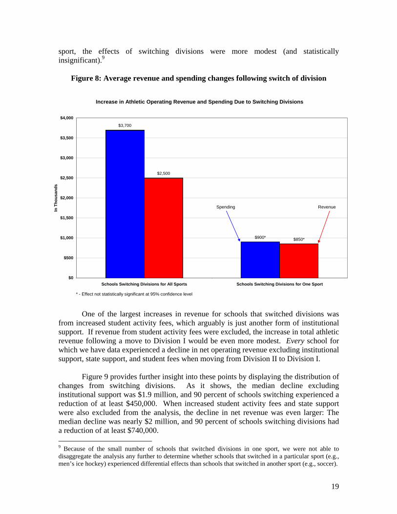
19
sport, the effects of switching divisions were more modest (and statistically insignificant).9
Figure 8: Average revenue and spending changes following switch of division
Increase in Athletic Operating Revenue and Spending Due to Switching Divisions
$3,700
$2,500
$900* $850*
$0
$500
$1,000
$1,500
$2,000
$2,500
$3,000
$3,500
$4,000
Schools Switching Divisions for All Sports Schools Switching Divisions for One Sport
In T
hous
ands
* - Effect not statistically significant at 95% confidence level
Spending Revenue
One of the largest increases in revenue for schools that switched divisions was
from increased student activity fees, which arguably is just another form of institutional support. If revenue from student activity fees were excluded, the increase in total athletic revenue following a move to Division I would be even more modest. Every school for which we have data experienced a decline in net operating revenue excluding institutional support, state support, and student fees when moving from Division II to Division I.
Figure 9 provides further insight into these points by displaying the distribution of changes from switching divisions. As it shows, the median decline excluding institutional support was $1.9 million, and 90 percent of schools switching experienced a reduction of at least $450,000. When increased student activity fees and state support were also excluded from the analysis, the decline in net revenue was even larger: The median decline was nearly $2 million, and 90 percent of schools switching divisions had a reduction of at least $740,000. 9 Because of the small number of schools that switched divisions in one sport, we were not able to disaggregate the analysis any further to determine whether schools that switched in a particular sport (e.g., men’s ice hockey) experienced differential effects than schools that switched in another sport (e.g., soccer).

20
Figure 9: Average net operating revenue changes following switch of division
We have disaggregated the increases in athletic spending associated with switching divisions into each of the components collected as part of the NCAA/EADA form. The three largest increases in spending among those schools that switched occurred in grant-in-aid spending; coaches’ salaries; and team travel. Those three components explain the vast majority of the overall average increase in athletic spending at schools that switched divisions. We have similarly disaggregated the increases in athletic revenue into each of the components collected as part of the NCAA/EADA form. Besides institutional support, state support, and student activity fees, which were discussed above, the largest increases in revenue among switching schools were cash contributions (e.g., from alumni); ticket sales to the public and university faculty/staff; and NCAA/conference distributions. Switching divisions is associated with significant increases in spending on specific sports (e.g., football, men’s and women’s basketball, and other men’s and women’s sports). No individual sport, however, tends to experience an increase in net revenue, on average, after the school switched divisions.
We also analyzed the impact of switching divisions on other quantifiable metrics. For example, we found that schools that switched divisions did not on average tend to experience a systematic and statistically significant increase in enrollment, although some schools did experience rapid increases in enrollment after switching divisions.
Changes in Measures of Athletic Net Revenue
-$4,000,000
-$3,500,000
-$3,000,000
-$2,500,000
-$2,000,000
-$1,500,000
-$1,000,000
-$500,000
$0
$500,000
$1,000,000
10th Percentile 25th Percentile Median 75th Percentile 90th Percentile
Net Revenue With
Institutional Support
Net Revenue Without
Institutional Support
Net Revenue Without Institutional Support,
State Support, and Student Fees
21
V. Interviews with Campus Decision-Makers As a supplement to the statistical analysis in Section IV, we interviewed campus decision-makers at schools that have switched divisions and at schools that have considered switching, but decided against it.10 Our goal in conducting these interviews was to gain a better understanding of the process through which schools made these decisions and deeper insight into what has occurred at schools that did switch.
The interviews were illuminating. For example, they revealed that many schools that switched divisions did not engage in detailed or rigorous cost-benefit analyses before making the switch. This lack of analysis may be changing. One school currently considering a move to Division I has commissioned a study to analyze the costs and benefits of switching divisions. Another school – Virginia State University – recently commissioned an analysis of the benefits and costs of switching divisions. The study found that moving to Division I would produce various benefits, including a new level of competition, increased visibility, increased funding from the NCAA, and more game guarantees and corporate sponsorships. The study also found that the risks of moving to Division I included increased financial obligations for grant-in-aid, personnel, and facilities, major investments (which would require increased donations), a transition process, and a potential change in the campus culture. Virginia State University concluded that the athletic budget would have to increase by $4 million to fund the costs of a move to Division I. Based in significant part on this analysis, Virginia State University decided against switching divisions.
The interviews also suggested that most of the schools that switched did not
experience significant financial returns, which is consistent with our analysis in Section IV above:
• One school noted that sports revenue did not increase significantly as a result of the switch, while costs did – largely due to increased scholarships.
• Two schools noted that they put in place new student fees to cover some athletic
costs.
• Two other schools noted that they had not anticipated, before moving, the modest impact on revenues and the large increase in costs.
• Among the new costs noted by one of the schools were hiring more coaches,
trainers, and other personnel; travel expenses; the awarding of more scholarships; and increased spending on marketing and development.
Schools that have considered switching, but have decided to stay in Division II,
generally do so for financial reasons:
10 Due to confidentiality reasons, we do not cite the experience of the particular schools.

22
• One official noted that he did not believe that the increased expenses associated with switching divisions would be compensated by increased revenues.
• One Division II school that offers a Division I sport noted that the Division I sport
produces revenue that helps support other non-revenue sports.
School officials generally note that the primary motivation to switch divisions was the desire to increase visibility or the public perception of the school, increase school spirit, or that the school was “out of place” in Division II because of either its size or that nearby rival schools were in Division I:
• One school official stated “you are who you play,” and “it is an honor to play the best, even if you lose by forty points.” Also, school officials note that the switch pleased the local media.
• One school official stated that the move was worth it because of psychological
impact of Division I.
• A school official at a school that considered switching stated that he did not believe being a weak Division I program would increase national exposure from its current level as a successful Division II program. He stated, for example, that most fans were probably not aware that Oakland University, who made this year’s NCAA tournament, was in Michigan.
Other aspects of the interviews were also consistent with the statistical analysis
above. For example, no school officials stated that the switch had affected applications; one noted that it was “the least of the reasons” students apply to the school. (An official at a school considering switching divisions stated that it has no desire to increase enrollment because it is already at capacity.) Another school that considered moving to Division I noted that its enrollment was already growing rapidly while it remained in Division II.
School officials believe that switching divisions did not have any quantifiable impact on alumni giving, but one Division II school that has a Division I sport noted that it believed it obtained fundraising and legislative appropriations benefits due to the combination of its success in the Division I sport and its quality academic programs. An official at a school considering switching noted that the perception was that the state legislature would more generously fund the university if it were in Division I. VI. Previous Literature
Although there is a vast literature on college athletics, few papers have focused on the financial impact of switching divisions. Perhaps the most relevant paper is a 1999
23
Ph.D. dissertation, which analyzed four case studies of schools switching divisions.11 Three of the schools – UNC-Greensboro (UNCG), the University of Buffalo, and the College of Charleston – switched from Division II to Division I; and one school – Augusta State – switched from Division I to Division II. The paper attempted to answer two questions: (1) what was the rationale for the switch; and (2) to what extent were the anticipated effects of the switch realized.
The findings of the 1999 study were broadly consistent with the empirical
findings presented above and the interviews of key campus decision-makers. The analysis found that reasons for switching to Division I included improving institutional competitiveness, image, and exposure. In reality, the study found that benefits to admissions were mixed. The College of Charleston did experience significant benefits in this area, but it had an unusual degree of athletic success. UNCG’s benefits were unclear and the University of Buffalo could not demonstrate any benefits. Switching to Division I increased alumni donations specifically earmarked for athletics, but did not produce conclusive evidence on general alumni donations. Finally, the study concluded that the schools achieved their aims of increased visibility/exposure.
A 2001 analysis considered three case studies.12 It first examined the College of
Charleston. The report concluded that, “Because of its NAIA success, its sizable student body (11,620), and its location in South Carolina’s largest city, [The College of] Charleston was courted by several conferences, which allowed it to bypass the usual scheduling hassles for new Division I schools…Yet Charleston’s Division I fairy tale remains an anomaly, the result of felicitous circumstances.” The 2001 report suggested less positive results for the University of Buffalo and Northeastern Illinois. For example, the study noted that the University of Buffalo had a two-year record in Division I of 7-44 at the time of the article, despite its large student body. And after seven years in Division I, the trustees of Northeastern Illinois voted to drop all sports and focus on academics in the face of large sports deficits. The authors concluded that, “The vast majority [of schools that move to Division I] soldier away in obscurity, negotiating a treacherous landscape that features chronic losing, uninterested fans, wacky conference affiliations (or even worse, none at all) and, not least crushing financial deficits.”
Several recent newspaper articles have used case studies to highlight the pros and
cons of switching divisions. For example, a recent Kentucky Post article stated that Savannah State, which switched to Division I, received bad publicity about the move after it completed “an embarrassing winless basketball season.”13 A recent story in the Grand Folks Herald noted that North Dakota State University (NDSU) needs to raise $1 million a year for two years to support the school’s move to Division I and that NDSU
11 Michael Edward Cross, “The Run to Division I: Intercollegiate Athletics and the Broader Interests of Colleges and Universities,” University of Michigan, 1999. 12 Grant Wahl and George Dohrmann, “Welcome to the Big Time,” in Scott Rosner, editor, The Business of Sports, (Jones and Bartlett Publishers, Boston, MA: 2004). 13 “NKU Looks at Move to Division I,” Kentucky Post, March 10, 2005.

24
Associate Athletic Director Erv Inniger stated that the task has not been difficult, since donors are willing to give more to support the school’s move to Division I.14 VII. Conclusion Our previous analysis of athletic operating spending in Division I-A suggested that increases in such spending had, on average, no effect on net revenue. By contrast, this analysis of Division II athletics strongly suggests that increases in athletic operating spending are associated with declines in net revenue over the medium term. Similarly, our analysis suggests that moving from Division II to Division I generally fails to produce increases in net revenue and instead entails a substantial decline, as costs increase with little increase in revenue.
14 “College Athletics: The Dollars Behind Division I--NDSU’s First-Year Finance Show School Needs Big Off-Campus Commitment,” Grand Forks Herald, December 12, 2004.
25
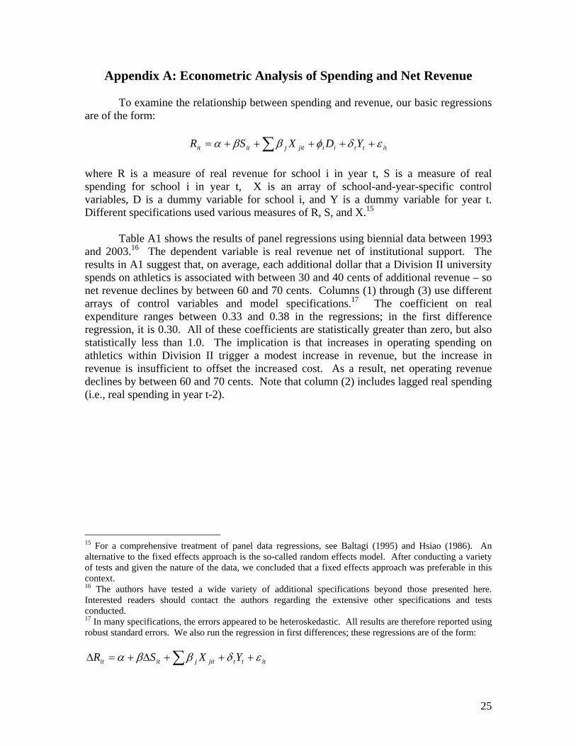
Appendix A: Econometric Analysis of Spending and Net Revenue To examine the relationship between spending and revenue, our basic regressions are of the form:
itttiijitjitit YDXSR εδφββα +++++= ∑ where R is a measure of real revenue for school i in year t, S is a measure of real spending for school i in year t, X is an array of school-and-year-specific control variables, D is a dummy variable for school i, and Y is a dummy variable for year t. Different specifications used various measures of R, S, and X.15
Table A1 shows the results of panel regressions using biennial data between 1993 and 2003.16 The dependent variable is real revenue net of institutional support. The results in A1 suggest that, on average, each additional dollar that a Division II university spends on athletics is associated with between 30 and 40 cents of additional revenue – so net revenue declines by between 60 and 70 cents. Columns (1) through (3) use different arrays of control variables and model specifications.17 The coefficient on real expenditure ranges between 0.33 and 0.38 in the regressions; in the first difference regression, it is 0.30. All of these coefficients are statistically greater than zero, but also statistically less than 1.0. The implication is that increases in operating spending on athletics within Division II trigger a modest increase in revenue, but the increase in revenue is insufficient to offset the increased cost. As a result, net operating revenue declines by between 60 and 70 cents. Note that column (2) includes lagged real spending (i.e., real spending in year t-2).
15 For a comprehensive treatment of panel data regressions, see Baltagi (1995) and Hsiao (1986). An alternative to the fixed effects approach is the so-called random effects model. After conducting a variety of tests and given the nature of the data, we concluded that a fixed effects approach was preferable in this context. 16 The authors have tested a wide variety of additional specifications beyond those presented here. Interested readers should contact the authors regarding the extensive other specifications and tests conducted. 17 In many specifications, the errors appeared to be heteroskedastic. All results are therefore reported using robust standard errors. We also run the regression in first differences; these regressions are of the form:
itttjitjitit YXSR εδββα +++∆+=∆ ∑

26
Table A1: Panel regressions of real revenue excluding institutional support (robust t-statistics in parentheses)
Variables: Column (1) Column (2)
Column (3)First
Difference0.38 0.33
(6.89)** (5.85)**0.151.72
0.30(4.68)**
-119,359 -131,830 170,3070.52 0.41 1.35
-368,779 -357,486 47,188(2.49)* (2.38)* 0.16
-446,160 -948,209 -548,0401.07 1.17 1.2
90,137 124,601 125,701(2.15)* (3.56)** (3.25)**
-1,049,889 -1,578,853 -17,510(5.61)** (2.83)** 0.46-253,207 -855,100 -10,761
0.52 1.3 0.26Institutional Dummies Yes Yes No
Year Dummies Yes Yes YesRobust Std. Errors Yes Yes Yes
Observations 822 608 602R-squared 0.92 0.94 0.3
Robust t statistics in parentheses* significant at 5%; ** significant at 1%
Real Total Athletic Exp. Minus Cap. & Debt Service
Lagged Real Total Athletic Exp. Minus Cap. & Debt Service
Change in Real Total Athletic Exp. Minus Cap. & Debt Service
Dummy = 1 if Institution No Longer in DII in Year, Instead DIAA
Dummy = 1 if Institution has a Football Team
Dummy = 1 if Institution No Longer in DII in Year, Instead DIAAA
Dummy = 1 if M Ice Hockey @ Inst. Left DII in Data Range
Dummy = 1 if M/W Soccer @ Inst. Left DII in Data Range
Dummy = 1 if School is Private
Variables: Column (1) Column (2)
Column (3)First
Difference0.38 0.34
(7.01)** (6.09)**0.141.63
0.30(4.39)**
-229,341 -241,628 128,5671.36 1.13 1.13
-250,797 -477,900 -383,8610.84 0.85 1.03
-255,761 -855,317 -9830.53 1.3 0.02
Institutional Dummies Yes Yes NoYear Dummies Yes Yes Yes
Robust Std. Errors Yes Yes YesObservations 822 608 602
R-squared 0.92 0.94 0.3Robust t statistics in parentheses* significant at 5%; ** significant at 1%
Dummy = 1 if One Sport @ Institution No Longer in DII in Year
Dummy = 1 if Institution has a Football Team
Real Total Athletic Exp. Minus Cap. & Debt Service
Lagged Real Total Athletic Exp. Minus Cap. & Debt Service
Change in Real Total Athletic Exp. Minus Cap. & Debt Service
Dummy = 1 if Institution No Longer in DII in Year

27
Table A2 attempts to address one concern about these regressions: that current spending is not exogenous, as is assumed in the classical regression model. Instead, spending could be affected by some third factor that also affects revenue, introducing a spurious correlation between revenue and spending. A typical approach in the presence of such an econometric problem is an instrumental variables regression. The goal is to find a variable highly correlated with current spending, but not with current revenue. That instrument is then used to identify the underlying relationship between current revenue and current spending while attenuating or eliminating the spurious correlation potentially induced by other factors. A common instrument is the lagged variable of the independent variable, in this case spending. Table A2 therefore presents alternative regressions in which lagged operating expenditure is used as an instrument for current operating expenditure.
Table A2: Panel regressions of revenue excluding institutional support using instrumental variables (robust t-statistics in parentheses)
Variables: Column (1) Column (2)
Column (3)First
Difference0.38 0.59 0.21
(6.89)** (2.65)** 0.79-119,359 -648,406 435,615
0.52 0.87 1.27-368,779 -511,165 -376,287(2.49)* 1.62 0.79
-446,160 -560,405 512,0631.07 0.49 0.31
90,137 137,968 -2,691,874(2.15)* (3.71)** 1.47
-1,049,889 -667,166 1,386,367(5.61)** 1 (3.08)**-253,207 -931,137 -2,625,070
0.52 1.68 1.51
Use Lag in Spending as Instrumental Variable for Spending No Yes Yes
Institutional Dummies Yes Yes NoYear Dummies Yes Yes Yes
Robust Std. Errors Yes Yes YesObservations 822 615 350
R-squared 0.92 0.92 0.59Robust t statistics in parentheses* significant at 5%; ** significant at 1%
Dummy = 1 if M/W Soccer @ Inst. Left DII in Data Range
Dummy = 1 if School is Private
Dummy = 1 if Institution has a Football Team
Real Total Athletic Exp. Minus Cap. & Debt Service
Dummy = 1 if Institution No Longer in DII in Year, Instead DIAA
Dummy = 1 if Institution No Longer in DII in Year, Instead DIAAA
Dummy = 1 if M Ice Hockey @ Inst. Left DII in Data Range

28
Variables: Column (1) Column (2)
Column (3)First
Difference0.38 0.58 0.18
(7.01)** (2.63)** 0.67-229,341 -549,591 -12,493
1.36 1.09 0.02-250,797 -264,709 -868,930
0.84 0.32 0.56-255,761 -925,424 -2,606,791
0.53 1.68 1.5Use Lag in Spending as Instrumental No Yes Yes
Institutional Dummies Yes Yes NoYear Dummies Yes Yes Yes
Robust Std. Errors Yes Yes YesObservations 822 615 350
R-squared 0.92 0.92 0.58Robust t statistics in parentheses* significant at 5%; ** significant at 1%
Real Total Athletic Exp. Minus Cap. & Debt Service
Dummy = 1 if Institution No Longer in DII in Year
Dummy = 1 if One Sport @ Institution No Longer in DII in Year
Dummy = 1 if Institution has a Football Team
Finally, Table A3 makes three modifications. First, it includes institutional
support as revenue (Tables A1 and A2 had excluded institutional support from revenue). Second, it includes the limited data on capital expenditures and debt service recorded in EADA. Finally, it limits the sample to schools that have data in each year, and thus represents what is called a “balanced panel.” In the previous regressions, schools were included even if their data were missing in one of the years. The results in Table A3 show that an additional dollar of spending is associated with between 30 and 67 cents of additional revenue.

29
Table A3: Balanced panel regressions of revenue (robust t-statistics in parentheses)
Variables: Column (1) Column (2)
Column (3)First
Difference Column (4)0.63 0.67 -1.09
(2.96)** (3.54)** 1.130.30
(2.53)*0.301.88
-1,915,799 -4,958,588 -1,205,990 429,910(2.14)* (5.93)** 1.26 0.15
-154,496 -460,066 -272,105 1,598,6500.27 1 0.64 1.390.00 0.00 0.00 0.00(.) (.) (.) (.)
0.00 0.00 0.00 0.00(.) (.) (.) (.)
-548,579 -120,555 256,238 -6,973,0241.59 0.92 1.7 (2.29)*
-105,950 -547,373 348,223 5,780,3100.26 0.65 0.36 (2.70)**
Use Lag in Spending as Instrumental Variable for Spending No No No Yes
Institutional Dummies Yes Yes No NoYear Dummies Yes Yes Yes Yes
Robust Std. Errors Yes Yes Yes YesObservations 269 235 235 235
R-squared 0.67 0.76 0.33 0.64Robust t statistics in parentheses* significant at 5%; ** significant at 1%
Real Total Athletic Expenditures
Lagged Real Total Athletic Expenditures
Change in Real Total Athletic Expenditures
Dummy = 1 if Institution No Longer in DII in Year, Instead DIAA
Dummy = 1 if Institution has a Football Team
Dummy = 1 if Institution No Longer in DII in Year, Instead DIAAA
Dummy = 1 if M Ice Hockey @ Inst. Left DII in Data Range
Dummy = 1 if M/W Soccer @ Inst. Left DII in Data Range
Dummy = 1 if School is Private

30
Variables: Column (1) Column (2)
Column (3)First
Difference Column (4)0.60 0.60 -0.99
(2.79)** (3.01)** 0.810.231.65
0.301.85
-1,009,787 -1,357,491 -494,237 1,167,4021.94 1.68 1.18 0.580.00 0.00 0.00 0.00(.) (.) (.) (.)
-623,836 -3,760,777 1,122,021 -2,296,6821.27 (5.25)** 0.85 (2.07)*
Use Lag in Spending as Instrumental Variable for Spending No No No Yes
Institutional Dummies Yes Yes No NoYear Dummies Yes Yes Yes Yes
Robust Std. Errors Yes Yes Yes YesObservations 269 235 235 235
R-squared 0.66 0.71 0.33 0.62Robust t statistics in parentheses* significant at 5%; ** significant at 1%
Dummy = 1 if Institution No Longer in DII in Year
Dummy = 1 if One Sport @ Institution No Longer in DII in Year
Dummy = 1 if Institution has a Football Team
Real Total Athletic Expenditures
Lagged Real Total Athletic Expenditures
Change in Real Total Athletic Expenditures
31
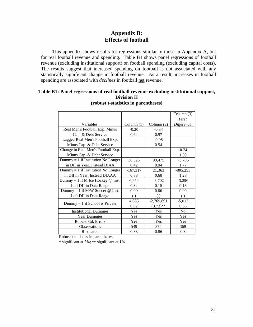
Appendix B: Effects of football
This appendix shows results for regressions similar to those in Appendix A, but for real football revenue and spending. Table B1 shows panel regressions of football revenue (excluding institutional support) on football spending (excluding capital costs). The results suggest that increased spending on football is not associated with any statistically significant change in football revenue. As a result, increases in football spending are associated with declines in football net revenue.
Table B1: Panel regressions of real football revenue excluding institutional support, Division II
(robust t-statistics in parentheses)
Variables: Column (1) Column (2)
Column (3)First
Difference-0.20 -0.340.64 0.97
-0.080.54
-0.241.08
38,525 99,475 73,7050.42 0.94 1.77
-167,317 21,363 -805,2550.88 0.68 1.28
6,854 -3,702 -3,2960.34 0.15 0.180.00 0.00 0.00(.) (.) (.)
4,685 -2,769,891 -5,0120.02 (3.73)** 0.36
Institutional Dummies Yes Yes NoYear Dummies Yes Yes Yes
Robust Std. Errors Yes Yes YesObservations 549 374 369
R-squared 0.83 0.86 0.3Robust t statistics in parentheses* significant at 5%; ** significant at 1%
Change in Real Men's Football Exp. Minus Cap. & Debt Service
Dummy = 1 if M/W Soccer @ Inst. Left DII in Data Range
Dummy = 1 if School is Private
Real Men's Football Exp. Minus Cap. & Debt Service
Dummy = 1 if Institution No Longer in DII in Year, Instead DIAA
Dummy = 1 if Institution No Longer in DII in Year, Instead DIAAA
Dummy = 1 if M Ice Hockey @ Inst. Left DII in Data Range
Lagged Real Men's Football Exp. Minus Cap. & Debt Service
32
Variables: Column (1) Column (2)
Column (3)First
Difference-0.19 -0.340.62 0.97
-0.070.52
-0.431.39
12,935 82,372 55,1590.15 1.02 1.43
6,752 -3,760 -1,6920.34 0.15 0.1
Institutional Dummies Yes Yes NoYear Dummies Yes Yes Yes
Robust Std. Errors Yes Yes YesObservations 549 374 369
R-squared 0.82 0.86 0.18
Dummy = 1 if One Sport @ Institution No Longer in DII in Year
Real Men's Football Exp. Minus Cap. & Debt Service
Lagged Real Men's Football Exp. Minus Cap. & Debt Service
Change in Real Men's Football Exp. Minus Cap. & Debt Service
Dummy = 1 if Institution No Longer in DII in Year
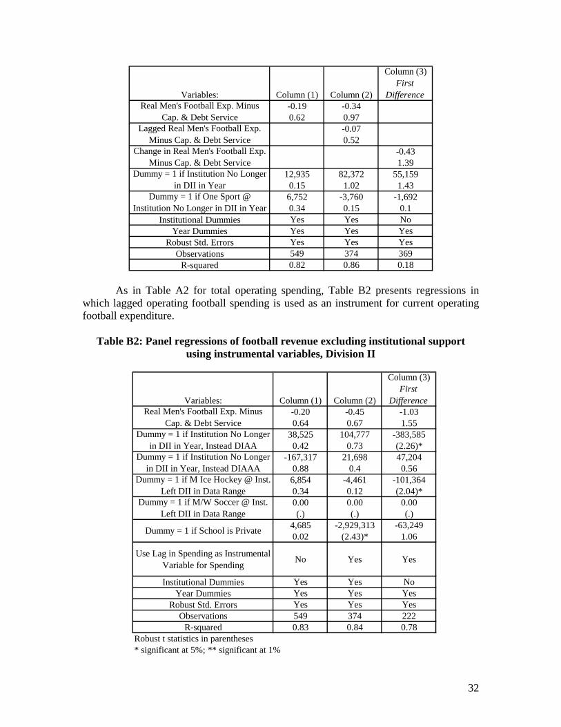
As in Table A2 for total operating spending, Table B2 presents regressions in which lagged operating football spending is used as an instrument for current operating football expenditure.
Table B2: Panel regressions of football revenue excluding institutional support using instrumental variables, Division II
Variables: Column (1) Column (2)
Column (3)First
Difference-0.20 -0.45 -1.030.64 0.67 1.55
38,525 104,777 -383,5850.42 0.73 (2.26)*
-167,317 21,698 47,2040.88 0.4 0.56
6,854 -4,461 -101,3640.34 0.12 (2.04)*0.00 0.00 0.00(.) (.) (.)
4,685 -2,929,313 -63,2490.02 (2.43)* 1.06
Use Lag in Spending as Instrumental Variable for Spending No Yes Yes
Institutional Dummies Yes Yes NoYear Dummies Yes Yes Yes
Robust Std. Errors Yes Yes YesObservations 549 374 222
R-squared 0.83 0.84 0.78Robust t statistics in parentheses* significant at 5%; ** significant at 1%
Dummy = 1 if M/W Soccer @ Inst. Left DII in Data Range
Dummy = 1 if School is Private
Real Men's Football Exp. Minus Cap. & Debt Service
Dummy = 1 if Institution No Longer in DII in Year, Instead DIAA
Dummy = 1 if Institution No Longer in DII in Year, Instead DIAAA
Dummy = 1 if M Ice Hockey @ Inst. Left DII in Data Range

33
Variables: Column (1) Column (2)
Column (3)First
Difference-0.19 -0.44 -0.920.62 0.68 1.58
12,935 86,199 -162,6570.15 0.8 1.89
6,752 -4,416 -36,0310.34 0.12 0.68
Use Lag in Spending as Instrumental No Yes YesInstitutional Dummies Yes Yes No
Year Dummies Yes Yes YesRobust Std. Errors Yes Yes Yes
Observations 549 374 222R-squared 0.82 0.84 0.78
Robust t statistics in parentheses* significant at 5%; ** significant at 1%
Real Men's Football Exp. Minus Cap. & Debt Service
Dummy = 1 if Institution No Longer in DII in Year
Dummy = 1 if One Sport @ Institution No Longer in DII in Year
Finally, as in Table A3 for overall athletic spending, Table B3 makes three
modifications for football spending: it includes institutional support as revenue; it includes the limited recorded data on capital expenditures and debt service; and it is a balanced panel. The results in Table B3 show that an additional dollar of football spending is associated with between 0 and 42 cents of additional revenue. The key conclusion, that higher football spending is associated with lower net revenue, is thus unchanged: An increase of $1 in football spending is associated with a decline in net revenue of between 58 cents and $1.

34
Table B3: Balanced panel regressions of revenue, Division II
Variables: Column (1) Column (2)
Column (3)First
Difference Column (4)0.60 0.60
(2.79)** (3.01)**0.231.65
0.301.85
-0.990.81
-1,009,787 -1,357,491 -494,237 1,167,4021.94 1.68 1.18 0.580.00 0.00 0.00 0.00(.) (.) (.) (.)
Institutional Dummies Yes Yes No NoYear Dummies Yes Yes Yes Yes
Robust Std. Errors Yes Yes Yes YesObservations 133 101 153 105
R-squared 0.72 0.85 0.21 0.85Robust t statistics in parentheses* significant at 5%; ** significant at 1%
Dummy = 1 if Institution No Longer in DII in Year
Dummy = 1 if One Sport @ Institution No Longer in DII in Year
Real Men's Football Expenditures
Lagged Real Men's Football Expenditures
Change in Real Men's Football Expenditures
Fitted values
Variables: Column (1) Column (2)
Column (3)First
Difference Column (4)0.42 0.24 0.01
(2.21)* 0.74 0.350.050.25
0.010.6
-161,433 -262,074 11,611 -71,5931.29 1.3 0.2 1
-144,363 -83,934 46,529 -106,1851.04 0.56 0.16 0.760.00 0.00 0.00 0.00(.) (.) (.) (.)
0.00 0.00 0.00 0.00(.) (.) (.) (.)
95,866 342,005 -435,020 -442,9270.32 1.31 1.1 (11.12)**
Use Lag in Spending as Instrumental Variable for Spending No No No Yes
Institutional Dummies Yes Yes No NoYear Dummies Yes Yes Yes Yes
Robust Std. Errors Yes Yes Yes YesObservations 133 101 153 105
R-squared 0.72 0.85 0.21 0.85Robust t statistics in parentheses* significant at 5%; ** significant at 1%
Dummy = 1 if M/W Soccer @ Inst. Left DII in Data Range
Dummy = 1 if School is Private
Real Men's Football Expenditures
Dummy = 1 if Institution No Longer in DII in Year, Instead DIAA
Dummy = 1 if Institution No Longer in DII in Year, Instead DIAAA
Dummy = 1 if M Ice Hockey @ Inst. Left DII in Data Range
Lagged Real Men's Football Expenditures
Change in Real Men's Football Expenditures

35
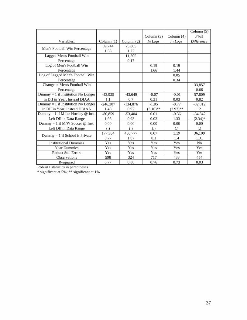
Appendix C: Relationships Between Spending And Winning, Between Winning And Revenue, And Between Winning And Net
Revenue This appendix explores the relationships between operating football spending and winning, between winning and operating revenue, and between winning and operating net revenue. Table C1 shows panel regressions of football winning percentages on real football spending, lagged real football spending, and a set of control dummies. The results suggest no statistically significant relationship between winning percentages and spending on football.
Table C1: Panel regressions of football winning percentages, Division II
Variables: Column (1) Column (2)Column (3)
In LogsColumn (4)
In Logs
Column (5)First
Difference33.99 3.641.51 0.23
-24.221.02
0.10 0.011.23 0.06
-0.020.2
0.001.05
0.02 0.05 0.06 0.04 -0.010.28 0.54 0.28 0.18 0.230.07 0.07 0.09 0.07 0.11
(2.41)* 1.63 1.41 0.76 (4.50)**-0.07 -0.06 -0.09 -0.06 -0.110.65 0.4 0.47 0.26 0.990.00 0.00 0.00 0.00 0.00(.) (.) (.) (.) (.)
-0.08 0.19 0.86 1.11 0.020.71 1.03 (2.35)* 1.92 0.83
Institutional Dummies Yes Yes Yes Yes NoYear Dummies Yes Yes Yes Yes Yes
Robust Std. Errors Yes Yes Yes Yes YesObservations 762 473 737 459 462
R-squared 0.59 0.58 0.55 0.57 0.01Robust t statistics in parentheses* significant at 5%; ** significant at 1%
Lagged Real Men's Football Exp. (Billions)
Log of Real Men's Football Exp.
Real Men's Football Exp. (Billions)
Dummy = 1 if Institution No Longer in DII in Year, Instead DIAA
Change in Real Men's Football Expenditures
Log of Lagged Real Men's Football Expenditures
Dummy = 1 if M/W Soccer @ Inst. Left DII in Data Range
Dummy = 1 if School is Private
Dummy = 1 if Institution No Longer in DII in Year, Instead DIAAA
Dummy = 1 if M Ice Hockey @ Inst. Left DII in Data Range

36
Variables: Column (1) Column (2)Column (3)
In LogsColumn (4)
In Logs
Column (5)First
Difference33.67 3.541.51 0.23
-24.431.06
0.10 0.011.24 0.06
-0.020.21
0.001.19
0.03 0.06 0.06 0.04 -0.010.35 0.67 0.31 0.25 0.12-0.07 -0.06 -0.09 -0.06 -0.100.65 0.4 0.47 0.26 0.96
Institutional Dummies Yes Yes Yes Yes NoYear Dummies Yes Yes Yes Yes Yes
Robust Std. Errors Yes Yes Yes Yes YesObservations 762 473 737 459 462
R-squared 0.59 0.58 0.55 0.57 0.01Robust t statistics in parentheses* significant at 5%; ** significant at 1%
Change in Real Men's Football Expenditures
Dummy = 1 if Institution No Longer in DII in Year
Dummy = 1 if One Sport @ Institution No Longer in DII in Year
Real Men's Football Exp. (Billions)
Lagged Real Men's Football Exp. (Billions)
Log of Real Men's Football Exp.
Log of Lagged Real Men's Football Expenditures
Table C2 examines the effect of winning on operating football revenue; Table C3 examines the effect of winning on operating football net revenue. Neither the coefficient on the winning percentage nor the coefficient on the lagged winning percentage is statistically significant in either table. Tables C1, C2, and C3 collectively suggest no statistically significant relationship between (a) operating spending and winning, (b) winning and operating revenue, and (c) winning and operating net revenue, at least during the sample period.
Table C2: Panel regressions of football revenue, Division II
37
Variables: Column (1) Column (2)Column (3)
In LogsColumn (4)
In Logs
Column (5)First
Difference89,744 75,805
1.68 1.2211,305
0.170.19 0.191.66 1.44
0.050.34
33,8570.66
-43,925 -43,649 -0.07 -0.01 57,8091.1 0.7 0.31 0.03 0.82
-246,307 -134,876 -1.05 -0.77 -32,8121.48 0.92 (3.10)** (2.97)** 1.21
-80,859 -53,404 0.01 -0.36 -84,8421.95 0.93 0.02 1.33 (2.34)*0.00 0.00 0.00 0.00 0.00(.) (.) (.) (.) (.)
177,954 456,777 0.07 1.19 36,1090.77 1.07 0.1 1.4 1.31
Institutional Dummies Yes Yes Yes Yes NoYear Dummies Yes Yes Yes Yes Yes
Robust Std. Errors Yes Yes Yes Yes YesObservations 598 324 717 438 454
R-squared 0.77 0.88 0.76 0.73 0.03Robust t statistics in parentheses* significant at 5%; ** significant at 1%
Dummy = 1 if M/W Soccer @ Inst. Left DII in Data Range
Dummy = 1 if School is Private
Log of Lagged Men's Football Win Percentage
Dummy = 1 if Institution No Longer in DII in Year, Instead DIAA
Dummy = 1 if Institution No Longer in DII in Year, Instead DIAAA
Dummy = 1 if M Ice Hockey @ Inst. Left DII in Data Range
Men's Football Win Percentage
Lagged Men's Football Win Percentage
Log of Men's Football Win Percentage
Change in Men's Football Win Percentage

38
Variables: Column (1) Column (2)Column (3)
In LogsColumn (4)
In Logs
Column (5)First
Difference89,583 76,050
1.68 1.229,8580.15
0.19 0.191.66 1.44
0.050.33
35,2680.68
-59,335 -62,646 -0.14 -0.14 59,8471.4 0.97 0.62 0.35 0.89
-79,959 -53,483 0.01 -0.36 -76,2371.95 0.94 0.03 1.34 (2.23)*
Institutional Dummies Yes Yes Yes Yes NoYear Dummies Yes Yes Yes Yes Yes
Robust Std. Errors Yes Yes Yes Yes YesObservations 598 324 717 438 454
R-squared 0.76 0.88 0.76 0.73 0.03Robust t statistics in parentheses* significant at 5%; ** significant at 1%
Change in Men's Football Win Percentage
Dummy = 1 if Institution No Longer in DII in Year
Dummy = 1 if One Sport @ Institution No Longer in DII in Year
Men's Football Win Percentage
Lagged Men's Football Win Percentage
Log of Men's Football Win Percentage
Log of Lagged Men's Football Win Percentage
Table C3: Panel regressions of football net revenue, Division II
Variables: Column (1) Column (2)Column (3)
In LogsColumn (4)
In Logs
Column (5)First
Difference-79,105 -31,622
0.95 0.36-205,369
1.840.29 0.110.66 0.22
-0.460.83
-29,2530.42
-399,573 -549,968 2.30 1.80 1,5531.75 1.41 (2.41)* 1.35 0.01
-65,577 -103,121 -1.52 -1.47 -32,4270.41 0.53 1.15 1.24 0.52
-66,241 -47,381 0.00 0.00 -51,1470.93 0.58 (.) (.) 0.740.00 0.00 0.00 0.00 0.00(.) (.) (.) (.) (.)
1,364,615 -219,411 1.80 0.55 -34,145(5.19)** 0.77 1.8 0.55 0.42
Institutional Dummies Yes Yes Yes Yes NoYear Dummies Yes Yes Yes Yes Yes
Robust Std. Errors Yes Yes Yes Yes YesObservations 739 460 126 94 451
R-squared 0.49 0.56 0.91 0.92 0.01Robust t statistics in parentheses* significant at 5%; ** significant at 1%
Lagged Men's Football Win Percentage
Log of Men's Football Win Percentage
Men's Football Win Percentage
Dummy = 1 if Institution No Longer in DII in Year, Instead DIAA
Change in Men's Football Win Percentage
Log of Lagged Men's Football Win Percentage
Dummy = 1 if M/W Soccer @ Inst. Left DII in Data Range
Dummy = 1 if School is Private
Dummy = 1 if Institution No Longer in DII in Year, Instead DIAAA
Dummy = 1 if M Ice Hockey @ Inst. Left DII in Data Range

39
Variables: Column (1) Column (2)Column (3)
In LogsColumn (4)
In Logs
Column (5)First
Difference-78,665 -30,623
0.95 0.36-203,692
1.840.29 0.110.66 0.22
-0.460.83
-31,2970.46
-375,921 -477,501 -1.52 -1.47 -3,4751.75 1.41 1.15 1.24 0.02
-66,795 -46,980 0.00 0.00 -59,2180.93 0.57 (.) (.) 0.94
Institutional Dummies Yes Yes Yes Yes NoYear Dummies Yes Yes Yes Yes Yes
Robust Std. Errors Yes Yes Yes Yes YesObservations 739 460 126 94 451
R-squared 0.49 0.56 0.91 0.92 0Robust t statistics in parentheses* significant at 5%; ** significant at 1%
Change in Men's Football Win Percentage
Dummy = 1 if Institution No Longer in DII in Year
Dummy = 1 if One Sport @ Institution No Longer in DII in Year
Men's Football Win Percentage
Lagged Men's Football Win Percentage
Log of Men's Football Win Percentage
Log of Lagged Men's Football Win Percentage

40
Appendix D: Basketball
This appendix shows the results of panel regressions of basketball revenue on
basketball spending and control variables. Table D1 shows the results for men’s basketball. The results are similar to those in Appendix B: increases in spending on men’s basketball of $1 are associated with either no increase, or an increase of less than $1, in revenue. The upshot is that expanded spending on men’s basketball is associated with a reduction in net revenue from the sport.
Table D1: Panel regressions of men’s basketball revenue, Division II
Variables: Column (1) Column (2)
Column (3)First
Difference0.61 0.18
(6.48)** 0.730.261.25
-0.230.56
-19,403 -123,448 65,4070.61 1.85 0.75
24,230 -74,120 -1,346,5280.41 0.54 1.44
-68,210 -60,351 -80,750(3.79)** 0.85 (2.03)*-157,690 0.00 0.00
1.49 (.) (.)-138,855 319,980 34,440(2.20)* 0.72 1.23-5,330 -52,070 -35,0180.24 (3.12)** (2.11)*
Institutional Dummies Yes Yes NoYear Dummies Yes Yes Yes
Robust Std. Errors Yes Yes YesObservations 1120 340 476
R-squared 0.77 0.93 0.12Robust t statistics in parentheses* significant at 5%; ** significant at 1%
Dummy = 1 if Institution has a Football Team
Dummy = 1 if Institution No Longer in DII in Year, Instead DIAAA
Dummy = 1 if M Ice Hockey @ Inst. Left DII in Data Range
Dummy = 1 if M/W Soccer @ Inst. Left DII in Data Range
Dummy = 1 if School is Private
Real Men's Basketball Expenditures
Lagged Real Men's Basketball Expenditures
Change in Real Men's Basketball Expenditures
Dummy = 1 if Institution No Longer in DII in Year, Instead DIAA

41
Variables: Column (1) Column (2)
Column (3)First
Difference0.61 0.16
(6.48)** 0.70.251.17
-0.150.37
-5,317 -108,862 2,3200.18 1.63 0.02
-110,772 -59,046 -71,404(2.01)* 0.85 (2.10)*-8,445 -51,854 -20,223
0.4 (3.16)** 1.09Institutional Dummies Yes Yes No
Year Dummies Yes Yes YesRobust Std. Errors Yes Yes Yes
Observations 1120 340 476R-squared 0.77 0.93 0.01
Robust t statistics in parentheses* significant at 5%; ** significant at 1%
Change in Real Men's Basketball Expenditures
Dummy = 1 if Institution has a Football Team
Real Men's Basketball Expenditures
Lagged Real Men's Basketball Expenditures
Dummy = 1 if Institution No Longer in DII in Year
Dummy = 1 if One Sport @ Institution No Longer in DII in Year
Table D2 shows the results for women’s basketball, which are somewhat different than those for men’s basketball. Increases of $1 in spending on women’s basketball is associated with between 40 and 69 cents in additional revenue.
Table D2: Panel regressions of women’s basketball revenue, Division II
Variables: Column (1) Column (2)
Column (3)First
Difference0.69 0.66
(4.63)** (3.75)**0.281.83
0.40(3.48)**
-100,735 -102,382 -2,851(3.14)** (2.09)* 0.07-40,612 -59,707 -46,701
0.87 1 0.87-48,836 -49,851 -43,773(2.89)** 1.9 (2.97)**-62,292 -137,842 -92,860
1.01 1.73 0.98-100,908 -23,827 -380,748
1.64 0.2 (4.30)**-3,491 -27,427 -42,8640.16 1.59 0.83
Institutional Dummies Yes Yes NoYear Dummies Yes Yes Yes
Robust Std. Errors Yes Yes YesObservations 1037 782 743
R-squared 0.74 0.79 0.37Robust t statistics in parentheses* significant at 5%; ** significant at 1%
Real Women's Basketball Expenditures
Lagged Real Women's Basketball Expenditures
Change in Real Women's Basketball Expenditures
Dummy = 1 if Institution No Longer in DII in Year, Instead DIAA
Dummy = 1 if Institution has a Football Team
Dummy = 1 if Institution No Longer in DII in Year, Instead DIAAA
Dummy = 1 if M Ice Hockey @ Inst. Left DII in Data Range
Dummy = 1 if M/W Soccer @ Inst. Left DII in Data Range
Dummy = 1 if School is Private

42
Variables: Column (1) Column (2)
Column (3)First
Difference0.68 0.65
(4.59)** (3.79)**0.281.86
0.403(3.47)**
-77,689 -79,597 -23,418(2.52)* 1.76 0.7-48,773 -49,427 -44,260(2.89)** 1.89 (2.99)**-7,975 -27,609 -42,5450.37 1.6 0.83
Institutional Dummies Yes Yes NoYear Dummies Yes Yes Yes
Robust Std. Errors Yes Yes YesObservations 1037 782 743
R-squared 0.74 0.79 0.37Robust t statistics in parentheses* significant at 5%; ** significant at 1%
Dummy = 1 if Institution has a Football Team
Real Women's Basketball Expenditures
Lagged Real Women's Basketball Expenditures
Dummy = 1 if Institution No Longer in DII in Year
Dummy = 1 if One Sport @ Institution No Longer in DII in Year
Change in Real Women's Basketball Expenditures

43
Appendix E: Other Sports
Table E1 shows the regression results for non-football, non-men’s basketball sports. It suggests that each additional dollar that a Division I-A university spends on sports other than football or men’s basketball is associated with between 2 and 4 cents of additional revenue.
Table E1: Panel regressions of non-football, non-men’s
basketball revenue, Division II
Variables: Column (1) Column (2)0.02 0.041.11 (2.17)*
0.03(2.03)*
852,896 697,0841.83 0.83
1,424,197 1,001,7741.87 1.4
-133,854 -387,5940.33 0.56
-744,083 -719,198(3.30)** (2.47)*-404,009 76,335
0.56 0.08202,565 238,087
1.02 0.84Institutional Dummies Yes Yes
Year Dummies Yes YesRobust Std. Errors Yes Yes
Observations 1142 815R-squared 0.77 0.81
Robust t statistics in parentheses* significant at 5%; ** significant at 1%
Real No FB, No MBB Expenditures
Dummy = 1 if Institution No Longer in DII in Year, Instead DIAA
Dummy = 1 if Institution No Longer in DII in Year, Instead DIAAA
Dummy = 1 if M Ice Hockey @ Inst. Left DII in Data Range
Dummy = 1 if M/W Soccer @ Inst. Left DII in Data Range
Dummy = 1 if School is Private
Dummy = 1 if Institution has a Football Team
Lagged Real No FB, No MBB Expenditures

44
Variables: Column (1) Column (2)0.02 0.041.12 (2.17)*
0.03(2.03)*
1,032,487 841,001(2.59)** 1.5-426,230 -586,880
1.55 1.73161,234 237,489
0.82 0.84Institutional Dummies Yes Yes
Year Dummies Yes YesRobust Std. Errors Yes Yes
Observations 1142 815R-squared 0.77 0.81
Robust t statistics in parentheses* significant at 5%; ** significant at 1%
Dummy = 1 if Institution has a Football Team
Real No FB, No MBB Expenditures
Lagged Real No FB, No MBB Expenditures
Dummy = 1 if Institution No Longer in DII in Year
Dummy = 1 if One Sport @ Institution No Longer in DII in Year
Table E2 shows the results for women’s sports. One of the regressions suggests a
statistically significant increase in revenue associated with an increase in spending, but the increase in revenue is less than dollar-for-dollar. As a result, increased expenditures are associated with a reduction in net revenue.
Table E2: Panel regressions of women’s expenditures, Division II
Variables: Column (1) Column (2)-0.01 0.331.24 (2.39)*
0.33(2.39)*
-185,855 -379,3881.44 1.78
173,611 34,3750.85 0.12
-31,726 -34,1790.54 0.63
-330,757 -285,866(3.01)** (5.26)**142,146 -595,271
0.53 0.89-25,334 -193,358
0.25 0.77Institutional Dummies Yes Yes
Year Dummies Yes YesRobust Std. Errors Yes Yes
Observations 850 592R-squared 0.74 0.81
Robust t statistics in parentheses* significant at 5%; ** significant at 1%
Dummy = 1 if M/W Soccer @ Inst. Left DII in Data Range
Dummy = 1 if School is Private
Dummy = 1 if Institution has a Football Team
Dummy = 1 if M Ice Hockey @ Inst. Left DII in Data Range
Lagged Real All Women's Expenditures
Real All Women's Expenditures
Dummy = 1 if Institution No Longer in DII in Year, Instead DIAA
Dummy = 1 if Institution No Longer in DII in Year, Instead DIAAA

45
Variables: Column (1) Column (2)
-0.01 0.331.24 (2.38)*
0.33(2.38)*
-73,830 -189,2460.58 0.89
-160,876 -176,5741.52 1.82
-58,966 -194,2090.59 0.77
Institutional Dummies Yes YesYear Dummies Yes Yes
Robust Std. Errors Yes YesObservations 850 592
R-squared 0.73 0.81Robust t statistics in parentheses* significant at 5%; ** significant at 1%
Dummy = 1 if Institution has a Football Team
Real All Women's Expenditures
Lagged Real All Women's Expenditures
Dummy = 1 if Institution No Longer in DII in Year
Dummy = 1 if One Sport @ Institution No Longer in DII in Year

46
Appendix F: Other Quantifiable Effects
This appendix explores three other quantifiable channels through which athletics could affect higher education: alumni giving, average incoming SAT scores, and university selectivity (as measured by the share of applicants accepted). Some specifications suggest a relationship between spending and these other quantifiable metrics, but many others do not. Our conclusion is that athletic spending does not appear to have a robust, significant influence on alumni giving, SAT scores, or selectivity, at least over the medium-term horizon of this study. Alumni giving
Table F1 shows panel regressions of alumni giving on spending and winning percentages. It suggests no robust relationship between football spending and alumni giving over the medium term (e.g., a period of a little under a decade or so); although some regressions do suggest a relationship, many do not. The existing empirical literature on this issue is also mixed.
Table F1: Panel regressions of alumni giving
Variables: Column (1) Column (2)
Column (3)First
Difference Column (4) Column (5)
Column (6)First
Difference-0.09 0.350.66 (2.88)**
0.191.63
0.241.26
-4,920 20,0910.11 0.29
4,0500.07
17,7480.63
136,073 -2,466 70,032 104,989 114,208 75,725(2.52)* 0.05 1.85 (2.77)** (3.14)** (2.28)*
-232,279 -190,577 -594,267 -236,019 -233,405 -197,0121.41 1.06 0.54 1.43 1.31 (10.28)**
433,824 219,725 62,633 430,922 204,479 57,8571.94 (2.48)* 0.4 1.91 (2.37)* 0.350.00 0.00 0.00 0.00 0.00 0.00(.) (.) (.) (.) (.) (.)
145,222 983,728 -49,760 351,903 273,552 -13,8531.29 (2.24)* (1.99)* (4.38)** (4.37)** 0.96
Institutional Dummies Yes Yes No Yes Yes NoYear Dummies Yes Yes Yes Yes Yes Yes
Robust Std. Errors Yes Yes Yes Yes Yes YesObservations 444 350 291 459 362 290
R-squared 0.75 0.8 0.24 0.75 0.78 0.15Robust t statistics in parentheses* significant at 5%; ** significant at 1%
Dummy = 1 if M Ice Hockey @ Inst. Left DII in Data Range
Dummy = 1 if M/W Soccer @ Inst. Left DII in Data Range
Dummy = 1 if School is Private
Dummy = 1 if Institution No Longer in DII in Year, Instead DIAA
Dummy = 1 if Institution No Longer in DII in Year, Instead DIAAA
Lagged Men's Football Win Percentage
Change in Men's Football Win Percentage
Real Men's Football Expenditures
Lagged Real Men's Football Expenditures
Change in Real Men's Football Expenditures
Men's Football Win Percentage
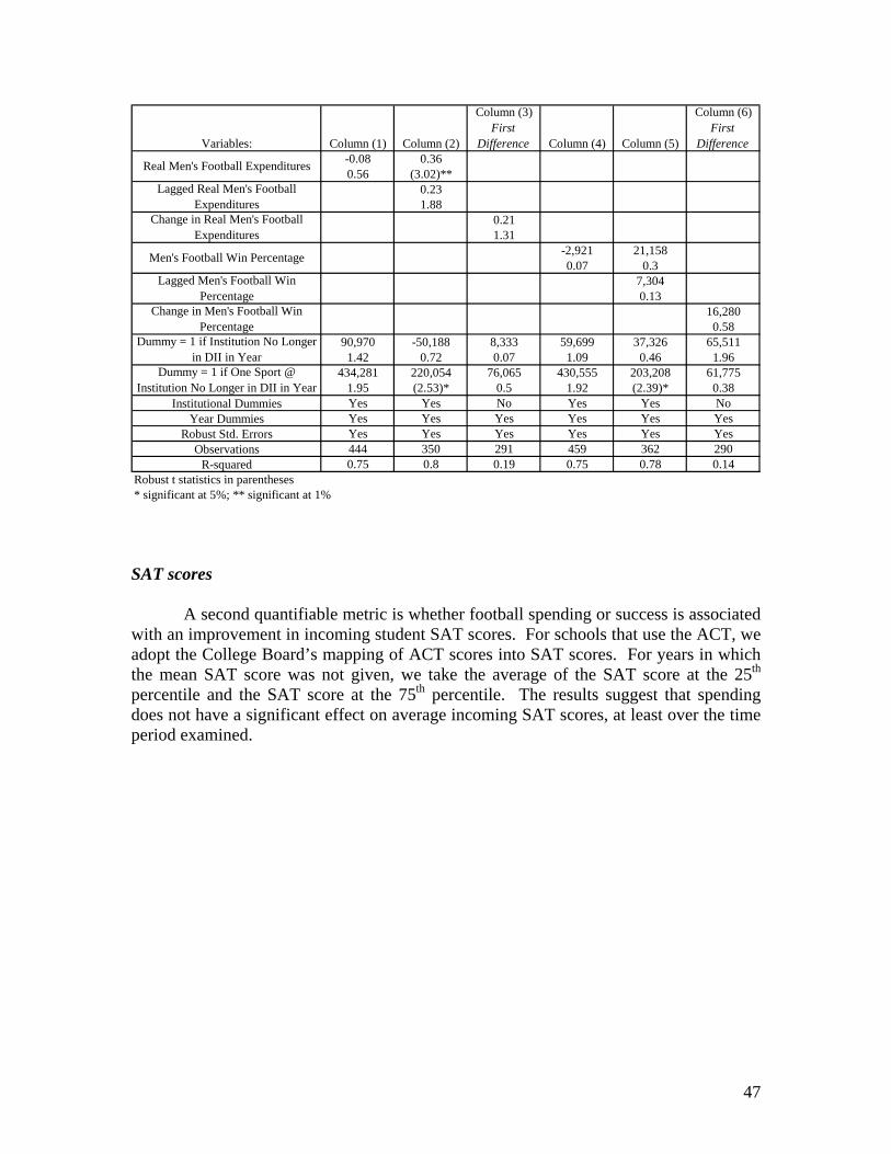
47
Variables: Column (1) Column (2)
Column (3)First
Difference Column (4) Column (5)
Column (6)First
Difference-0.08 0.360.56 (3.02)**
0.231.88
0.211.31
-2,921 21,1580.07 0.3
7,3040.13
16,2800.58
90,970 -50,188 8,333 59,699 37,326 65,5111.42 0.72 0.07 1.09 0.46 1.96
434,281 220,054 76,065 430,555 203,208 61,7751.95 (2.53)* 0.5 1.92 (2.39)* 0.38
Institutional Dummies Yes Yes No Yes Yes NoYear Dummies Yes Yes Yes Yes Yes Yes
Robust Std. Errors Yes Yes Yes Yes Yes YesObservations 444 350 291 459 362 290
R-squared 0.75 0.8 0.19 0.75 0.78 0.14Robust t statistics in parentheses* significant at 5%; ** significant at 1%
Dummy = 1 if One Sport @ Institution No Longer in DII in Year
Men's Football Win Percentage
Lagged Men's Football Win Percentage
Dummy = 1 if Institution No Longer in DII in Year
Real Men's Football Expenditures
Lagged Real Men's Football Expenditures
Change in Real Men's Football Expenditures
Change in Men's Football Win Percentage
SAT scores
A second quantifiable metric is whether football spending or success is associated with an improvement in incoming student SAT scores. For schools that use the ACT, we adopt the College Board’s mapping of ACT scores into SAT scores. For years in which the mean SAT score was not given, we take the average of the SAT score at the 25th percentile and the SAT score at the 75th percentile. The results suggest that spending does not have a significant effect on average incoming SAT scores, at least over the time period examined.
48
Table F2: Panel regressions of average incoming SAT scores, Division II
Variables: Column (1) Column (2) Column (3) Column (4)0.00 0.000.55 0.25
0.000.35
-7 -0.530.46 0.03
-90.49
22 24 29 171.74 1.63 (2.09)* 1.615 -140 14 -133
(2.34)* (9.47)** (1.99)* (11.38)**Institutional Dummies Yes Yes Yes Yes
Year Dummies Yes Yes Yes YesRobust Std. Errors Yes Yes Yes Yes
Observations 371 226 374 232R-squared 0.93 0.93 0.93 0.94
Robust t statistics in parentheses* significant at 5%; ** significant at 1%
Dummy = 1 if Institution No Longer in DII in Year
Dummy = 1 if One Sport @ Institution No Longer in DII in Year
Real Men's Football Expenditures
Lagged Real Men's Football Expenditures
Men's Football Win Percentage
Lagged Men's Football Win Percentage
Variables: Column (1) Column (2) Column (3) Column (4)0.00 0.000.55 0.25
0.000.35
-6.73 -0.530.46 0.03
-8.810.49
22 24 29 171.74 1.63 (2.09)* 1.619 0.00 291 0.000.7 (.) (110.46)** (.)15 -140 14 -133
(2.34)* (9.47)** (1.99)* (11.38)**0.00 0.00 0.00 0.00(.) (.) (.) (.)67 369 342 62
(2.89)** (10.04)** (20.73)** (2.74)**Institutional Dummies Yes Yes Yes Yes
Year Dummies Yes Yes Yes YesRobust Std. Errors Yes Yes Yes Yes
Observations 371 226 374 232R-squared 0.93 0.93 0.93 0.94
Robust t statistics in parentheses* significant at 5%; ** significant at 1%
Dummy = 1 if School is Private
Real Men's Football Expenditures
Lagged Real Men's Football Expenditures
Men's Football Win Percentage
Lagged Men's Football Win Percentage
Dummy = 1 if Institution No Longer in DII in Year, Instead DIAA
Dummy = 1 if Institution No Longer in DII in Year, Instead DIAAA
Dummy = 1 if M Ice Hockey @ Inst. Left DII in Data Range
Dummy = 1 if M/W Soccer @ Inst. Left DII in Data Range

49
University selectivity Finally, we adopt a different measure of university selectivity: the share of applicants accepted by the university. Table F3 shows the panel regression results. In one regression, a statistically significant positive relationship is shown; in the others, no significant relationship is found.
Table F3: Panel regressions of acceptance rates, Division II
Variables: Column (1) Column (2) Column (3) Column (4)0.00 0.001.42 1.24
0.001.19
0.00 0.000.07 0.1
0.031.14
-0.03 0.00 -0.01 0.011.28 0.15 0.28 0.40.03 -0.01 0.03 0.010.73 0.17 0.76 0.440.00 0.01 0.00 0.010.1 0.32 0.02 0.84
0.00 0.00 0.00 0.00(.) (.) (.) (.)
0.17 -0.21 0.00 0.06(2.28)* (2.91)** 0.06 1.17
Institutional Dummies Yes Yes Yes YesYear Dummies Yes Yes Yes Yes
Robust Std. Errors Yes Yes Yes YesObservations 676 399 677 406
R-squared 0.78 0.76 0.76 0.74Robust t statistics in parentheses* significant at 5%; ** significant at 1%
Dummy = 1 if School is Private
Real Men's Football Expenditures
Lagged Real Men's Football Expenditures
Men's Football Win Percentage
Lagged Men's Football Win Percentage
Dummy = 1 if Institution No Longer in DII in Year, Instead DIAA
Dummy = 1 if Institution No Longer in DII in Year, Instead DIAAA
Dummy = 1 if M Ice Hockey @ Inst. Left DII in Data Range
Dummy = 1 if M/W Soccer @ Inst. Left DII in Data Range

50
Variables: Column (1) Column (2) Column (3) Column (4)0.00 0.001.35 1.25
0.001.23
0.00 0.000.07 0.1
0.031.15
-0.02 0.00 0.00 0.011.09 0.1 0.15 0.50.00 0.01 0.00 0.010.08 0.32 0.01 0.84
Institutional Dummies Yes Yes Yes YesYear Dummies Yes Yes Yes Yes
Robust Std. Errors Yes Yes Yes YesObservations 676 399 677 406
R-squared 0.78 0.76 0.76 0.74Robust t statistics in parentheses* significant at 5%; ** significant at 1%
Dummy = 1 if Institution No Longer in DII in Year
Dummy = 1 if One Sport @ Institution No Longer in DII in Year
Real Men's Football Expenditures
Lagged Real Men's Football Expenditures
Men's Football Win Percentage
Lagged Men's Football Win Percentage
Related Documents


