INSTITUT FÜR INFORMATIONS- UND KOMMUNIKATIONSTECHNIK (IIKT) Emotional and User-Specific Cues for Improved Analysis of Naturalistic Interactions DISSERTATION zur Erlangung des akademischen Grades Doktoringenieur (Dr.-Ing.) von Dipl.-Ing. Ingo Siegert geb. am 13.05.1983 in Wernigerode genehmigt durch die Fakultät für Elektrotechnik und Informationstechnik der Otto-von-Guericke-Universität-Magdeburg Gutachter: Prof. Dr. rer. nat. Andreas Wendemuth Prof. Dr.-Ing. Christian Diedrich Prof. Dr.-Ing. Michael Weber Promotionskolloquium am 18.03.2015

Welcome message from author
This document is posted to help you gain knowledge. Please leave a comment to let me know what you think about it! Share it to your friends and learn new things together.
Transcript

INSTITUT FÜR INFORMATIONS- UNDKOMMUNIKATIONSTECHNIK (IIKT)
Emotional and User-Specific Cuesfor Improved Analysis ofNaturalistic Interactions
DISSERTATION
zur Erlangung des akademischen GradesDoktoringenieur (Dr.-Ing.)
vonDipl.-Ing. Ingo Siegert
geb. am 13.05.1983 in Wernigerode
genehmigt durch dieFakultät für Elektrotechnik und Informationstechnik
der Otto-von-Guericke-Universität-Magdeburg
Gutachter: Prof. Dr. rer. nat. Andreas WendemuthProf. Dr.-Ing. Christian DiedrichProf. Dr.-Ing. Michael Weber
Promotionskolloquium am 18.03.2015


Wenn wir das Muster nicht erkennendann heißt das noch lange nicht, dass es kein Muster gibt.
WITTGENSTEIN – LUMEN


Danksagung
Nach vielen Jahren intensiver Arbeit liegt sie nun vor Ihnen: meine Dissertation. Damitist es an der Zeit, mich bei denjenigen zu bedanken, die mich in dieser spannendenPhase meiner akademischen Laufbahn begleitet haben.
Als Erstes möchte ich mich bei meinem Doktorvater Prof. Dr. Andreas Wendemuthbedanken. Nicht nur für die Möglichkeit diese Arbeit am Lehrstuhl Kognitive Systemedurchführen zu können sowie die Unterstützung während der Bearbeitung, sondernauch für das Vertrauen und die Wertschätzung, die mir während der gesamten Pro-motionszeit entgegen gebracht wurde.
Bedanken möchte ich mich auch bei Herrn Prof. Dr. Michael Weber (Universität Ulm)und Herrn Prof. Dr. Christian Diedrich (Otto-von-Guericke-Universität Magdeburg)für die Bereitschaft die vorgelegte Dissertation zu begutachten.
Ein nicht unwesentlicher Teil dieser Arbeit ist am Lehrstuhl für Kognitive Systemeentstanden. Dass dies gelingen konnte, habe ich auch meinen Kollegen und Kolleginnenzu verdanken. Dr. Ronald Böck danke ich besonders für die Nachsicht, wenn ich malwieder mit meinen Ideen in sein Büro gestürmt bin, da daraus am Ende gute Veröf-fentlichungen entstanden sind. David Philippou-Hübner und Tobias Grosser danke ichdafür, mich in den Anfangszeiten in der Arbeitsgruppe willkommen geheißen zu haben.Kim Hartmann danke ich besonders für die vielen Diskussionen und Nachfragen, diemich dazu gebracht haben, meine Ideen noch besser auszuformulieren. Ich danke auchallen hier nicht namentlich genannten Kollegen und Kolleginnen für die bereichern-den Tipps und Diskussionsbeiträge, die mich wiederholt in neue thematische Bahnengelenkt haben.
Dem Land Sachsen-Anhalt sei für die Bereitstellung meiner Stelle gedankt, dadurchwar es mir möglich viel Erfahrung in der Betreuung von Studierenden und in Lehrver-anstaltungen zu sammeln.
Außerdem möchte ich dem Sonderforschungsbereich SFB/TRR 62 „Eine CompanionTechnologie für Kognitive Technische Systeme“, gefördert durch die Deutsche For-schungsgemeinschaft, danken. Dieses Projekt bot mir eine Plattform, um mich mitanderen Doktoranden auszutauschen und meine Forschung im Kontext der sprachba-sierten Emotionserkennung auch interdisziplinär zu vertiefen.
Ganz besonders danken möchte ich auch meiner Familie und meinen Freunden, diemich in all der Zeit unterstützt haben. Ohne euch wäre diese Arbeit nicht möglichgeworden und ich nicht der, der ich bin.
iii

Einen besonderen Dank möchte ich an meine Eltern richten, die mir mein Studiumüberhaupt ermöglicht haben. Bastian Ansorge für eine besondere Freundschaft seitfast 30 Jahren. Meiner Tochter Lea danke ich dafür, mir meine Zeit mit Ihr immer zuganz besonderen Momenten gemacht zu haben. Meiner Verlobten Stephanie danke ichvon ganzem Herzen für ihre unermüdliche Unterstützung, ihre Liebe und Motivation.

Zusammenfassung
D IE Mensch-Maschine-Interaktion erfährt in letzter Zeit immer größere Aufmerk-samkeit. Hierbei geht es nicht nur darum, eine möglichst einfache Bedienung von
technischen Systemen zu ermöglichen, sondern auch darum, eine möglichst natürlicheInteraktion abzubilden. Gerade der sprachbasierten Interaktion kommt hierbei eineerhöhte Aufmerksamkeit zu. Zum Beispiel bieten moderne Smartphones und Fernsehereine robuste Sprachsteuerung an, was auf vielfältige technische Verbesserungen derletzten Jahre zurückzuführen ist.
Dabei wirkt die Sprachsteuerung immer noch artifiziell. Es können nur in sich geschlos-sene Dialoge mit kurzen Aussagen geführt werden. Zudem wird nur der Sprachinhaltausgewertet. Die Art undWeise, wie etwas gesagt wird, bleibt unberücksichtigt, obwohlvon der menschlichen Kommunikation bekannt ist, dass insbesondere die geäußerteEmotion für eine erfolgreiche Kommunikation wichtig ist. Ein relativ neuer Forschungs-zweig, das „Affective Computing“, hat unter anderem zum Ziel, technische Geräte zuentwickeln, die Emotionen erkennen, interpretieren sowie adäquat darauf reagierenkönnen. Hierbei kommt der automatischen Emotionserkennung eine gewichtige Rollezu.
Für die Emotionserkennung ist es wichtig zu wissen, wie sich Emotionen darstellenund wie sie sich äußern. Hierfür ist es hilfreich, sich auf empirische Erkenntnisse derEmotionspsychologie zu stützen. Leider gibt es keine einheitliche Darstellung vonEmotionen. Auch die Beschreibung geeigneter emotionsunterscheidender akustischerMerkmale ist in der Psychologie eher deskriptiv gehalten. Deshalb wird für die au-tomatische Erkennung auf erprobte Methoden der automatischen Spracherkennungzurückgegriffen, die sich auch für die Emotionserkennung als geeignet gezeigt haben.
Die automatische Emotionserkennung ist, wie auch die Spracherkennung, ein Zweig derMustererkennung und im Gegensatz zur Emotionspsychologie datengetrieben, d.h., dieErkenntnisse werden aus Beispieldaten gewonnen. In der Emotionserkennung lassensich die Phasen „Annotation“, „Modellierung“ und „Erkennung“ unterscheiden. DieAnnotation kategorisiert Sprachdaten nach vordefinierten Emotionsbegriffen. Die Mo-dellierung erzeugt Erkenner, um Daten automatisch zu kategorisieren. Die Erkennungs-phase führt eine vorher unbekannte Zuordnung von Daten zu Emotionsklassen durch.
In den Anfangszeiten hat sich die automatische Emotionserkennung aufgrund desMangels an geeigneten Datensätzen meist auf gespielte und sehr expressive Emoti-onsausdrücke gestützt. Hier konnten, mit aus der Spracherkennung bekannten Merk-malen und Erkennungsmethoden, sehr gute Erkennungsergebnisse von über 80% bei
v

der Unterscheidung von bis zu sieben Emotionen erzielt werden. Für die Mensch-Maschine-Interaktion waren diese Erkenner jedoch ungeeignet, da in dieser die Emo-tionen weniger stark ausgeprägt sind. Daher wurden in Zusammenarbeit mit Psycho-logen naturalistische Interaktionsszenarien beschrieben und entsprechende Datensätzemit Probanden aus unterschiedlichen Personengruppen erhoben, denen keine „zu spie-lenden“ Vorgaben gemacht wurden, da sie natürlich reagieren sollten. Das hat dazugeführt, dass sich die Erkennungsraten auf diesen Daten verschlechtert haben und nurnoch um die 60% betragen. Aus dieser Entwicklung ergeben sich offene Fragen, diein dieser Arbeit untersucht werden sollen. Es wird vor allem untersucht, ob zusätzlichtechnische beobachtbare Marker die Emotionserkennung und Interaktionssteuerungin natürlicher Mensch-Maschine-Interaktion verbessern.
Die erste offene Frage beschäftigt sich mit der Generierung einer reliablen Klassenzu-ordnung für Emotionsdaten. Da bei natürlichen Interaktionen die Emotionsreaktionennicht mehr vorgegeben sind, muss eine Klassenzuordnung durch geeignete Annota-tion im Nachhinein erstellt werden. Dabei ist vor allem die erreichbare Reliabilitätwichtig. In der vorliegenden Arbeit konnte gezeigt werden, dass für eine naturali-stische Mensch-Maschine-Interaktion die Reliabilität gesteigert werden kann, wennAudio- und Video-Daten in Verbindung mit dem Kontext zur Annotation genutztwerden. Eine weitere Steigerung der Reliabilität und die Vermeidung des zweitenKappa-Paradoxes kann erreicht werden, wenn die emotionalen Bereiche der Datenvorselektiert werden. Damit ist es möglich, eine Annotation hoher Güte zu erhalten.
Die zweite offene Frage untersucht inwieweit bestimmte Sprechercharakteristiken zurVerbesserung der Emotionserkennung herangezogen werden können. Der Vokaltraktunterscheidet sich zwischen Männern und Frauen und ist auch durch Alterserschei-nungen einer Veränderung unterworfen. Dies beeinflusst akustische Merkmale, diefür die Emotionserkennung charakteristisch sind. Diese Arbeit untersucht, ob sowohldas Geschlecht als auch die Altersgruppe der Sprecher für die Emotionserkennungberücksichtigt werden müssen. Anhand von Experimenten mit verschiedenen Daten-sätzen konnte gezeigt werden, dass die Erkennungsleistung durch Berücksichtigungdes Geschlechts oder der Altersgruppe nicht nur verbessert wurden, sondern dies invielen Fällen auch signifikant war. In einigen Fällen konnte die Kombination beiderSprechercharakteristiken sogar eine weitere Verbesserung erzielen. Ein Vergleich miteiner Technik, die die anatomischen Unterschiede des Vokaltrakts normalisiert, zeigt,dass diese zwar auch eine Verbesserung gegenüber einer Nichtnormalisierung bringt,aber hinter den geschlechts- und altersgruppenspezifischen Modellen zurückbleibt.
Anschließend wurde die geschlechts- und altersgruppenspezifische Modellierung für dieFusion kontinuierlicher, fragmentierter, multimodaler Daten genutzt. Es konnte gezeigt

werden, dass auch in diesem Fall, obwohl die Sprachdaten nicht über den komplettenDatenstrom verfügbar waren, eine Verbesserung der Fusionsleistung möglich ist.
Die dritte offene Frage erweitert den Untersuchungsgegenstand auf Interaktionen unduntersucht, ob bestimmte akustische Feedbacksignale für eine emotionale Auswertunggenutzt werden können. Hierbei konzentriert sich diese Arbeit auf Diskurspartikel,wie z.B. „hm“ oder „äh“. Dies sind kurze sprachliche Äußerungen, die den Sprech-fluss unterbrechen. Da sie semantisch bedeutungslos sind, ist ausschließlich Ihre In-tonation relevant. Zuerst wird untersucht, ob diese Partikel als Indikator für eineBedienungsunsicherheit beim Benutzer dienen können. Es konnte gezeigt werden, dassbei anspruchsvollen Dialogen signifikant mehr Diskurspartikel genutzt werden als beiunkomplizierten Dialogen. Das Besondere an den Diskurspartikeln ist weiterhin, dasssie je nach Intonationsverlauf bestimmte Bedeutungen im Dialog übernehmen. Siekönnen Nachdenken, Initiativübernahme oder Nachfragen ankündigen. In dieser Ar-beit konnte gezeigt werden, dass alleine über den Intonationsverlauf die am häufigstenauftretende Bedeutung „nachdenkend“ robust von allen anderen Dialogfunktionenunterschieden werden kann.
Die Bearbeitung der vierten und letzten offenen Frage beschäftigt sich mit der zeit-lichen Modellierung von Emotionen. Wenn im technischen System die Emotionendes Nutzers sprechergruppenspezifisch erfasst und auch die jeweils geäußerten Inter-aktionssignale richtig gedeutet werden können, muss das System adäquat reagieren.Diese Reaktion sollte jedoch nicht auf einer einzelnen Äußerung des Nutzers beruhen,sondern seine langfristige emotionale Entwicklung berücksichtigen. Für diesen Zweckwurde in der Arbeit ein Stimmungsmodell vorgestellt, welches durch beobachteteEmotionsverläufe die Stimmung berechnet. Weiterhin konnte auch der Individuali-tät des Nutzers Rechnung getragen werden, indem das Persönlichkeitsmerkmal der„Extraversion“ in das Modell integriert werden konnte.
Natürlich ist es nicht möglich, die in dieser Arbeit identifizierten offenen Fragen restloszu klären. Die Erweiterung der puren akustischen Emotionserkennung durch Berück-sichtigung von anderen Modalitäten, Sprechercharakteristiken, Feedbacksignalen undPersönlichkeitsmerkmalen erlaubt es jedoch, länger andauernde natürliche Interaktio-nen zu untersuchen und dialogkritische Situationen zu erkennen. Technische Systeme,die diese erweiterte Emotionserkennung nutzen, passen sich an ihren Nutzer an undwerden so zu seinem Begleiter und letztendlich zu seinem Companion.


Abstract
THE Human-Computer Interaction recently received an increased attention. Thisis not just a matter of making the operation of technical systems as simple as
pissuble, but also to enable a possibly natural interaction. In this context, especiallythe speech-based operation gained an increased attention. For example, modern smartphones and televisions offer a robust voice control, which is attributed to varioustechnical improvements in recent years.
Nevertheless, voice control still seems artificial. Only self-contained dialogues withshort statements can be managed. Furthermore, just the content of speech is evaluated.The way in which something is said remains unconsidered, although it is known fromhuman communication, that the transmitted emotion is important in order to commu-nicate successfully. A relatively new branch of research, the “Affective Computing”,has, amongst other objectives, the aim to develop technical systems that recogniseand interpret emotions and respond to them appropriately. In this case, speech-basedautomatic emotion recognition has a major role.
For emotion recognition, it is important to know how emotions can be presented andhow they are expressed. For this purpose, it is helpful to rely on empirical evidencesof the psychology of emotions. Unfortunately, there is no uniform representation ofemotions. Also the definition of appropriate emotion-distinctive acoustic features israther descriptive in psychology. Therefore, the automatic detection of emotions isbased on proven methods of automatic speech recognition, which have also been shownas appropriate for emotion recognition.
Automatic emotion recognition is, as speech recognition, a branch of pattern recog-nition. Contrary to emotion psychology, it is data-driven, that means insights aregathered from sampled data. For emotion recognition the phases “annotation”, “mod-elling” and “recognition” are distinguishable. The annotation categorises speech dataaccording to predefined emotion-terms. Modelling generates recognisers to categorisedata automatically. Recognition performs a previously unknown allocation of data toemotional classes.
In the beginning, automatic emotion recognition was usually based – due to the lackof suitable data sets – on acted and very expressive emotional expressions. In this case,based on features and detection methods known from speech recognition, very goodrecognition results of over 80% in distinguishing of up to seven emotions could beachieved. However, for human-machine interaction these recognisers were unsuitablebecause in this case emotions are not that expressive. Therefore, in collaboration with
ix

psychologists, naturalistic interaction scenarios were developed to collect relevant datasets with subjects from different groups of persons, who were not given specificationsfor “acting”.
This led to decreased recognition rates of only 60% on these data. From this devel-opment, open issues arise, which will be investigated in this thesis. In particular, thisthesis examines if further technically observable cues improve the emotion recognitionand interaction control in naturalistic human-machine interaction.
The first open issue deals with the generation of a reliable class assignment of emotionaldata. Since in natural interactions the emotional reactions are not specified, a classallocation has to be created after the recording by a suitable annotation. In doingso, the achievable reliability is particularly important. In the present thesis, it couldbe shown that for a naturalistic human-machine interaction the reliability can beincreased if audio and video data in combination with the context are used for theannotation. A further increase of reliability and an avoidance of the second Kappaparadox can be achieved if the emotional phases of the data are preselected. Thismakes it possible to obtain a high quality annotation.
The second open issue examines to what extent certain speaker characteristics canbe utilised to improve the emotion recognition. The vocal tract differs between maleand female speakers and is also changed due to aging, which affects the acousticfeatures that are characteristic for emotion recognition. This work investigated whetherboth the gender and the age-group of speakers have to be considered for emotionrecognition. Through experiments with different datasets it could be shown that therecognition performance was significantly improved considering the gender or the agegroup. In some cases a combination of both speaker characteristics could achievean even further improvement. A comparison show that a method normalising thevocal tract’s anatomical differences improves the recognition in comparison to thenon-normalised case, however it falls behind results using the gender and age-groupspecific models.
Subsequently, the gender and age-group specific modelling was extended to the fusionof continuous, fragmentary, multimodal data. It could be shown that also in this case,although the speech data were not available for the entire data stream, an improvementin the fusion recognition is possible.
The third open issue expands the object of investigation to interactions and examineswhether certain acoustic feedback signals can be used for an emotional evaluation.This work focuses on discourse particles, such as “hm” or “uh”. These are shortvocalizations, interrupting the flow of speech. As they are semantically meaningless,

only their intonation is relevant. First, it is examined whether they can serve as anindicator of a user operating under uncertainty. It could been shown that in challengingdialogues significantly more discourse particles are used than in simple dialogues. Afurther special feature of discourse particles is that they have specific functions in adialogue depending on their intonation. So they can denote thinking, turn-taking, orrequests. In this work, it could be shown that the most common meaning “thinking” isrobustly distinguishable from all other dialogue functions by using the intonation only.
The fourth and final open issue deals with a temporal modelling of emotions. If atechnical system is able to capture emotions in a speaker-group-specific manner and tocorrectly interpret the uttered interaction patterns, the system finally has to respondproperly. However, this reaction should not only be based on a single utterance ofthe user, but should also consider his long-term emotional development. For thispurpose, a mood-model was presented, where the mood is calculated from the courseof observed emotions. Furthermore, the individuality of the user is taken into accountby integrating the personality trait of extraversion into the model.
Of course it is not possible to resolve the open issues identified in this thesis completely.The extension of the pure acoustic emotion recognition by considering further mod-alities, speaker characteristics, feedback signals and personality traits allows howeverto examine longer-lasting natural interactions and dialogues and to identify criticalsituations. Technical systems that use this extended emotion recognition adapt totheir users and thus become his attendant and ultimately his companion.


Contents
List of Figures xviii
List of Tables xx
1 Introduction 11.1 Enriched Human Computer Interaction . . . . . . . . . . . . . . . . . 21.2 Emotion Recognition from Speech . . . . . . . . . . . . . . . . . . . . 61.3 Thesis structure . . . . . . . . . . . . . . . . . . . . . . . . . . . . . . 8
2 Measurability of Affects 112.1 Representation of Emotions . . . . . . . . . . . . . . . . . . . . . . . 12
2.1.1 Categorial Representation . . . . . . . . . . . . . . . . . . . . 122.1.2 Dimensional Representation . . . . . . . . . . . . . . . . . . . 13
2.2 Measuring Emotions . . . . . . . . . . . . . . . . . . . . . . . . . . . 162.2.1 Emotional Verbalisation . . . . . . . . . . . . . . . . . . . . . 172.2.2 Emotional Response Patterns . . . . . . . . . . . . . . . . . . 18
2.3 Mood and Personality Traits . . . . . . . . . . . . . . . . . . . . . . . 202.4 Summary . . . . . . . . . . . . . . . . . . . . . . . . . . . . . . . . . 23
3 State-of-the-Art 253.1 Reviewing the Evolution of Datasets for Emotion Recognition . . . . 26
3.1.1 Databases with Simulated Emotions . . . . . . . . . . . . . . 273.1.2 Databases with Naturalistic Affects . . . . . . . . . . . . . . . 28
3.2 Reviewing the speech-based Emotion Recognition Research . . . . . . 323.3 Classification Performances in Simulated and Naturalistic Interactions 373.4 Open issues . . . . . . . . . . . . . . . . . . . . . . . . . . . . . . . . 41
3.4.1 A Reliable Ground Truth for Emotional Pattern Recognition . 413.4.2 Incorporating Speaker Characteristics . . . . . . . . . . . . . . 423.4.3 Interactions and their Footprints in Speech . . . . . . . . . . . 433.4.4 Modelling the Temporal Sequence of Emotions in HCI . . . . 44
4 Methods 454.1 Annotation . . . . . . . . . . . . . . . . . . . . . . . . . . . . . . . . 46
4.1.1 Transcription, Annotation and Labelling . . . . . . . . . . . . 464.1.2 Emotional Labelling Methods . . . . . . . . . . . . . . . . . . 474.1.3 Calculating the Reliability . . . . . . . . . . . . . . . . . . . . 55
4.2 Features . . . . . . . . . . . . . . . . . . . . . . . . . . . . . . . . . . 63
xiii

4.2.1 Short-Term Segmental Acoustic Features . . . . . . . . . . . . 644.2.2 Longer-Term Supra-Segmental Features . . . . . . . . . . . . . 72
4.3 Classifiers . . . . . . . . . . . . . . . . . . . . . . . . . . . . . . . . . 804.3.1 Hidden Markov Models . . . . . . . . . . . . . . . . . . . . . . 804.3.2 Defining Optimal Parameters . . . . . . . . . . . . . . . . . . 844.3.3 Incorporating Speaker Characteristics . . . . . . . . . . . . . . 864.3.4 Common Fusion Techniques . . . . . . . . . . . . . . . . . . . 88
4.4 Evaluation . . . . . . . . . . . . . . . . . . . . . . . . . . . . . . . . . 904.4.1 Validation Methods . . . . . . . . . . . . . . . . . . . . . . . . 914.4.2 Classifier Performance Measures . . . . . . . . . . . . . . . . . 924.4.3 Measures for Significant Improvements . . . . . . . . . . . . . 95
4.5 Summary . . . . . . . . . . . . . . . . . . . . . . . . . . . . . . . . . 100
5 Datasets 1015.1 Datasets of Simulated Emotions . . . . . . . . . . . . . . . . . . . . . 101
5.1.1 Berlin Database of Emotional Speech . . . . . . . . . . . . . . 1025.2 Datasets of Naturalistic Emotions . . . . . . . . . . . . . . . . . . . . 104
5.2.1 NIMITEK Corpus . . . . . . . . . . . . . . . . . . . . . . . . 1055.2.2 Vera am Mittag Audio-Visual Emotional Corpus . . . . . . . . 1065.2.3 LAST MINUTE corpus . . . . . . . . . . . . . . . . . . . . . . 108
5.3 Summary . . . . . . . . . . . . . . . . . . . . . . . . . . . . . . . . . 112
6 Improved Methods for Emotion Recognition 1136.1 Annotation of Naturalistic Interactions . . . . . . . . . . . . . . . . . 114
6.1.1 ikannotate . . . . . . . . . . . . . . . . . . . . . . . . . . . . . 1156.1.2 Emotional Labelling of Naturalistic Material . . . . . . . . . . 1196.1.3 Inter-Rater Reliability for Emotion Annotation . . . . . . . . 125
6.2 Speaker Group Dependent Modeling . . . . . . . . . . . . . . . . . . 1366.2.1 Parameter tuning . . . . . . . . . . . . . . . . . . . . . . . . . 1376.2.2 Defining the Speaker-Groups . . . . . . . . . . . . . . . . . . . 1426.2.3 Initial Experiments utilising LMC . . . . . . . . . . . . . . . . 1446.2.4 Experiments including additional Databases . . . . . . . . . . 1476.2.5 Intermediate Results . . . . . . . . . . . . . . . . . . . . . . . 1536.2.6 Comparison with Vocal Tract Length Normalisation . . . . . . 1546.2.7 Discussion . . . . . . . . . . . . . . . . . . . . . . . . . . . . . 158
6.3 SGD-Modelling for Multimodal Fragmentary Data Fusion . . . . . . . 1606.3.1 Utilised Corpus . . . . . . . . . . . . . . . . . . . . . . . . . . 1616.3.2 Fusion of Fragmentary Data without SGD Modelling . . . . . 1616.3.3 Using SGD Modelling to Improve Fusion of Fragmentary Data 166

6.3.4 Discussion . . . . . . . . . . . . . . . . . . . . . . . . . . . . . 1686.4 Summary . . . . . . . . . . . . . . . . . . . . . . . . . . . . . . . . . 170
7 Discourse Particles as Interaction Patterns 1717.1 Discourse Particles in Human Communication . . . . . . . . . . . . . 1727.2 The Occurrence of Discourse Particles in HCI . . . . . . . . . . . . . 174
7.2.1 Distribution of Discourse Particles for different Dialogue Styles 1777.2.2 Distribution of Discourse Particles for Dialogue Barriers . . . 178
7.3 Experiments assessing the Form-Function-Relation . . . . . . . . . . 1807.3.1 Acoustical Labelling of the Dialogue Function . . . . . . . . . 1817.3.2 Form-type Extraction . . . . . . . . . . . . . . . . . . . . . . . 1827.3.3 Visual Labelling of the Form-type . . . . . . . . . . . . . . . . 1837.3.4 Automatic Classification . . . . . . . . . . . . . . . . . . . . . 184
7.4 Discourse Particles and Personality Traits . . . . . . . . . . . . . . . 1867.5 Summary . . . . . . . . . . . . . . . . . . . . . . . . . . . . . . . . . 188
8 Modelling the Emotional Development 1918.1 Motivation . . . . . . . . . . . . . . . . . . . . . . . . . . . . . . . . . 1928.2 Mood Model Implementation . . . . . . . . . . . . . . . . . . . . . . 193
8.2.1 Mood as three-dimensional Object with adjustable Damping . 1958.2.2 Including Personality Traits . . . . . . . . . . . . . . . . . . . 196
8.3 Experimental Model Evaluation . . . . . . . . . . . . . . . . . . . . . 1988.3.1 Plausibility Test . . . . . . . . . . . . . . . . . . . . . . . . . . 1988.3.2 Test of Comparison with experimental Guidelines . . . . . . . 200
8.4 Summary . . . . . . . . . . . . . . . . . . . . . . . . . . . . . . . . . 204
9 Conclusion and Open Issues 2079.1 Conclusion . . . . . . . . . . . . . . . . . . . . . . . . . . . . . . . . . 2079.2 Open Questions for Future Research . . . . . . . . . . . . . . . . . . 214
Glossary 217
Abbreviations 221
List of Symbols 225
Abbreviations of Emotions 227
References 229
List of Authored Publications 259


List of Figures
1.1 Influence of different disciplines on speech-based Affective Computing 51.2 Overall scheme of a supervised pattern recognition system . . . . . . 7
2.1 Plutchik’s structural model of emotions . . . . . . . . . . . . . . . . . 132.2 Representations of dimensional emotion theories . . . . . . . . . . . . 142.3 Scherer’s Multi-level Sequential Check Model . . . . . . . . . . . . . . 172.4 Scherer’s modes of representation of changes in emotion components . 18
4.1 Geneva Emotion Wheel as introduced by Scherer . . . . . . . . . . . 494.2 Self-Assessment Manikins . . . . . . . . . . . . . . . . . . . . . . . . 504.3 FEELTRACE as seen by a user . . . . . . . . . . . . . . . . . . . . . 514.4 Example FEELTRACE/GTrace plot . . . . . . . . . . . . . . . . . . 534.5 The AffectButton graphical labelling method . . . . . . . . . . . . . . 544.6 Generalising π along three dimensions . . . . . . . . . . . . . . . . . . 574.7 Comparison of different kappa-like agreement interpretations . . . . . 624.8 Acoustic speech production model . . . . . . . . . . . . . . . . . . . . 634.9 Computation Scheme of Shifted Delta Cepstra features . . . . . . . . 744.10 Block diagram of a cepstral pitch detector . . . . . . . . . . . . . . . 774.11 Workflow of an HMM . . . . . . . . . . . . . . . . . . . . . . . . . . . 814.12 Overview of feature and decision level fusion architectures . . . . . . 884.13 Graphical representation of a MFN . . . . . . . . . . . . . . . . . . . 904.14 Scheme of one- and two-sided region of rejection . . . . . . . . . . . . 97
5.1 Distribution of emotional samples for emoDB . . . . . . . . . . . . . 1035.2 Distribution of emotional samples for VAM . . . . . . . . . . . . . . . 1075.3 Number of samples for the different dialogue barriers in LMC . . . . 112
6.1 Annotation module excerpt of ikannotate . . . . . . . . . . . . . . . . 1176.2 The three emotional labelling methods implemented in ikannotate . . 1186.3 Resulting distribution of labels using a basic emotion EWL . . . . . . 1216.4 Resulting distribution of labels utilising the GEW . . . . . . . . . . . 1216.5 Resulting distribution of labels using SAM . . . . . . . . . . . . . . . 1226.6 Number of resulting labels utilising each labelling method . . . . . . . 1236.7 Distribution of MV emotions over the events of LMC . . . . . . . . . 1346.8 Compilation of reported IRRs . . . . . . . . . . . . . . . . . . . . . . 1356.9 Classification performances utilising different mixture components . . 1386.10 Classification performances utilising different iteration steps . . . . . 139
xvii

6.11 UARs using different contextual characteristics . . . . . . . . . . . . . 1406.12 UARs using different channel normalisation techniques . . . . . . . . 1416.13 Distribution of subjects into speaker groups on LMC . . . . . . . . . 1446.14 UARs for two-class LMC for SGI and different SGD configurations . 1476.15 Distribution of subjects into speaker groups and their abbreviations . 1486.16 UARs for emoDB’s two- and six-class problem for SGI and SGDg . . 1506.17 UARs for the two-class problem on VAM for SGI and SGDg . . . . . 1526.18 Estimated warping factors for emoDB and VAM . . . . . . . . . . . . 1556.19 Estimated warping factors for LMC . . . . . . . . . . . . . . . . . . . 1556.20 UARs of VTLN-based classifiers in comparison to the SGI results . . 1576.21 Observable features of challenge for subject 20101117auk of LMC . 1626.22 UARs for acoustic classification using SGD and SGI modelling . . . . 1676.23 UARs after decision fusion comparing SGI and SGD modelling . . . . 168
7.1 Number of extracted DPs . . . . . . . . . . . . . . . . . . . . . . . . 1747.2 Verbosity values regarding the two experimental phases for LMC . . . 1767.3 Number of DPs regarding different speaker groups for LMC . . . . . 1787.4 Number of DPs distinguishing dialogue barriers for LMC . . . . . . . 1797.5 Samples of extracted pitch-contours . . . . . . . . . . . . . . . . . . . 1827.6 Comparison of the numbers of acoustically labelled functions with the
visual presented form-types of the DP “hm” . . . . . . . . . . . . . . 1837.7 UARs of the implemented automatic DP form-function recognition
based on the pitch-contour . . . . . . . . . . . . . . . . . . . . . . . . 1857.8 Mean and standard deviation for the DPs divided into the two dialogue
styles regarding different groups of user characteristics . . . . . . . . 1877.9 Mean and standard deviation for the DPs of the two barriers regarding
different groups of user characteristics . . . . . . . . . . . . . . . . . . 188
8.1 Illustration of the temporal evolution of the mood . . . . . . . . . . . 1948.2 Block scheme of the presented mood model . . . . . . . . . . . . . . . 1968.3 Mood model block scheme, including a personality trait . . . . . . . . 1978.4 Mood development over time for separated dimensions on SAL . . . . 1998.5 Gathered average labels of the dimension pleasure for ES2 and ES5 2018.6 Mood development for different settings of κη . . . . . . . . . . . . . 2018.7 Mood development for different settings of κpos and κneg . . . . . . . 2028.8 Course of the mood model using the whole experimental session . . . 204

List of Tables
2.1 Vocal emotion characteristics . . . . . . . . . . . . . . . . . . . . . . 20
3.1 Overview of selected emotional speech corpora . . . . . . . . . . . . . 313.2 Classification results on different databases with simulated and natur-
alistic emotions . . . . . . . . . . . . . . . . . . . . . . . . . . . . . . 39
4.1 Common word lists and related corpora . . . . . . . . . . . . . . . . . 484.2 Commonly used functionals for longer-term contextual information . 744.3 Averaged fundamental frequency for male and female speakers at dif-
ferent age ranges . . . . . . . . . . . . . . . . . . . . . . . . . . . . . 764.4 Comparison of different speech rate investigations for various emotions 794.5 Confusion matrix for a binary problem . . . . . . . . . . . . . . . . . 934.6 Types of errors for statistical tests . . . . . . . . . . . . . . . . . . . . 96
5.1 Available training material of emoDB clustered into A− and A+ . . . 1035.2 Reported emotional labels for the NIMITEK corpus . . . . . . . . . . 1065.3 Available training material of VAM . . . . . . . . . . . . . . . . . . . 1085.4 Distribution of speaker groups in LMC . . . . . . . . . . . . . . . . . 109
6.1 Utilised emotional databases regarding IRR . . . . . . . . . . . . . . 1266.2 Calculated IRR for VAM . . . . . . . . . . . . . . . . . . . . . . . . . 1276.3 IRR-values for selected functionals of SAL . . . . . . . . . . . . . . . 1286.4 Comparison of IRR for EWL, GEW, and SAM on NIMITEK . . . . . 1296.5 Number of resulting MVs and the IRR for the investigated sets . . . . 1316.6 Definition of feature sets . . . . . . . . . . . . . . . . . . . . . . . . . 1426.7 Overview of common speaker groups distinguishing age and gender . 1436.8 Overview of available training material of LMC . . . . . . . . . . . . 1456.9 Applied FSs and achieved performance of the SGI set on LMC . . . . 1456.10 Achieved UAR using SGD modelling on LMC . . . . . . . . . . . . . 1466.11 Achieved UAR in percent of the SGI set on emoDB and VAM . . . . 1496.12 Achieved UARs using SGD modelling for all available speaker groupings
on emoDB . . . . . . . . . . . . . . . . . . . . . . . . . . . . . . . . . 1506.13 Achieved UARs using SGD modelling for for all available speaker group-
ings on VAM . . . . . . . . . . . . . . . . . . . . . . . . . . . . . . . 1516.14 Achieved UARs for all corpora using SGD modelling . . . . . . . . . 1536.15 Achieved UARs of SGD, VTLN and SGD classification . . . . . . . . 1586.16 Detailed information for selected speakers of LMC . . . . . . . . . . . 161
xix

6.17 Unimodal classification results for the 13 subjects . . . . . . . . . . . 1646.18 Multimodal classification results for the 13 subjects using an MFN . . 1656.19 Distribution of utilised speaker groups in the “79s” set of LMC . . . . 166
7.1 Form-function relation of the DP “hm” . . . . . . . . . . . . . . . . . 1737.2 Distribution of utilised speaker groups in the “90s” set of LMC . . . . 1757.3 Replacement sentences for the acoustic form-type labelling . . . . . . 1817.4 Number and resulting label for all considered DPs . . . . . . . . . . . 1817.5 Utilised FSs for the automatic form-function classification . . . . . . 1847.6 Example confusion matrix for one fold of the recognition experiment
for FS4 . . . . . . . . . . . . . . . . . . . . . . . . . . . . . . . . . . . 1857.7 Achieved level of significance regarding personality traits. . . . . . . . 187
8.1 Mood terms for the PAD-space according . . . . . . . . . . . . . . . . 1928.2 Initial values for mood model . . . . . . . . . . . . . . . . . . . . . . 1998.3 Sequence of ES and expected PAD-positions . . . . . . . . . . . . . . 2008.4 Suggested κpos and κneg values based on the extraversion . . . . . . 203

Chapter 1
Introduction
Contents1.1 Enriched Human Computer Interaction . . . . . . . . . . . . 21.2 Emotion Recognition from Speech . . . . . . . . . . . . . . . 61.3 Thesis structure . . . . . . . . . . . . . . . . . . . . . . . . . . 8
IN the present time, technology plays an increasingly important role in people’s lives.Especially their operation requires an interaction between human and machine.
But this interaction is predominantly unidirectional. The technical system offerscertain input options, the human operator only utters a selected option in a command-transmitting fashion and the system (hopefully) performs the desired action or givesan appropriate respond. However, in the everyday use of modern technology, theHuman-Computer Interaction (HCI) is getting more complex, whereas it should stillremain user-friendly. This requires flexible interfaces allowing a bidirectional dialogue,where humans and machines are equal.
In this context, the importance of speech-based interfaces is increasing over theclassical HCI interfaces, such as keyboard and display. Through continually improvedspeech recognition and speech understanding ability in recent years, the efficiency ofdialogue systems has increased rapidly. Automatic Speech Recognition (ASR) systemsget more robust and popular. Today they can be found in several everyday technologies,such as smart-phones or navigation devices (cf. [Carroll 2013]).
Although these technical systems imitate the human interaction to allow also naiveusers to easily operate them, they do not take into account that Human-Human In-teraction (HHI) is always socially situated and that interactions are not just isolatedbut part of larger social interplays. Thus, today’s HCI research argues that computersystems should be capable of sensing agreement or inattention, for instance. Further-more, they should be and capable of adapting and responding to these social signalsin a polite, unintrusive, or persuasive manner (cf. [Vinciarelli et al. 2009]). Therefore,these systems have to be adaptable to the users’ individual skills, preferences, andcurrent emotional states (cf. [Wendemuth & Biundo 2012]). This aim however, is onlysuccessful, if engineers, psychologists, and computer scientists cooperate.

2 Chapter 1. Introduction
This chapter introduces the development of HCI briefly with the purpose of ex-plaining the need for an enriched HCI and provides the reader with its basic ideas.Afterwards, the basic principle of a technical affect recognition is discussed, which isthe motivation for my specific research topics. At the end of this chapter, the structureof this thesis is presented.
1.1 Enriched Human Computer Interaction
HCI research has gone through a huge development in the last decades. The researchwas and is focused on developing easy-to-use interfaces that could be used by experts aswell as by novices. Today, several kinds of interfaces can be distinguished. A historicaloverview on HCI is given in [Carroll 2013]. Important developments, discussed byCarroll, showing the need for an enriched HCI, are presented in the following.
In the beginning of computer systems, the operation was mostly reserved for thedeveloping institutions and selected scientists. Only experts were able to interactwith these systems. Furthermore, the development was focused on improving thesystem’s performance. Thus, the development of easy-to-use user interfaces was ofscant importance. Up to the 1970s, the way of interaction was fixed to CommandLine Interfaces, where the user had to type textualised commands to control thesystem (cf. [Carroll 2013]). This changed in the 1980s when home computers andlater personal computers became more important and the Graphical User Interface(GUI) emerged. At this time, the upcoming computers systems could be easily usedby trained users. A GUI allowed the user to use a pointing device to control theinteraction. The GUI mimics a real desktop with objects that can be placed1. Thus,the interaction is simplified as it is supposed that the user is used to working at adesk and hence, manages the interaction with a computer as well. Since the 1990s, thedesktop metaphor went through several adjustments, for instance, additional menubars or docks. Even today, the interaction with technical systems still follows thisWindow, Icon, Menu, Pointing device (WIMP) paradigm. Smart-phone devices stilluse WIMP elements. But they open up a new era of post-WIMP interfaces: Touch-screen-based interaction now allows new manipulation actions such as “pinching” and“rotating”, as well as presenting additional information more naturally (cf. [Elsholzet al. 2009]). This kind of interaction is considered as more natural, as the user nowcan directly manipulate the icons instead of making a detour by using a computermouse (cf. [Elsholz et al. 2009]). But, icons and folders are still parts of these post-WIMP GUIs (cf. [Rogers et al. 2011]). Moreover a new era of ubiquitous computing
1This is known as the desktop metaphor (cf. [Carroll 2013]).

1.1. Enriched Human Computer Interaction 3
devices is showing up, demanding for a more natural way of interaction, as the standardcomputer devices are moving to the background and the interaction is more integrated(cf. [Elsholz et al. 2009; Carroll 2013]).
Unfortunately, this kind of interaction is quite unnaturalistic as the users haveto manipulate iconic presentations. Thus, also research on speech-based interactiongained a lot of interest. The technological development of speech recognition systemsis given in [Juang & Rabiner 2006]. The Speech User Interface (SUI) research wasmotivated by the fact that speech is the primary mode of communication. It hasgained a great deal of attention since the 1950s. The first speech recognition systemscould only understand a few digits or words, spoken in an isolated form and thus,implicitly assuming that the unknown utterance contained one and only one completeterm (cf. [Davis et al. 1952]). Ten years later, the work of Sakay and Doshita involvedthe first use of a speech segmenter to overcome this limitation. Their work can be con-sidered as a precursor to a continuous speech recognition (cf. [Sakai & Doshita 1962]).Another early speech recognition system made use of statistical information aboutthe allowable phoneme sequence of words (cf. [Denes 1959]). This technique was laterconsidered again for statistical language modelling. In the 1970s, speech recognitiontechnology made major strides, thanks to the interest of and funding from the U.S.Department of Defense. The fundamental concepts of Linear Predictive Coding (LPC)were formulated by Atal & Hanauer. This technique greatly simplified the estima-tion of the vocal tract response from a speech waveform (cf. [Atal & Hanauer 1971]).Main efforts are made in n-gram language modelling, which are used to transcribea sequence of words, and in statistical modelling techniques controlling the acousticvariability of various speech representations across different speakers (cf. [Jelinek et al.1975]). Furthermore, the concept of dynamic time warping has become an indispens-able technique for ASR systems (cf. [Sakoe & Chiba 1978]). In the 1980s, a morerigorous statistical modelling framework for ASR systems became popular. Althoughthe basic idea of Hidden Markov Model (HMM) was known earlier2, this techniquedid not have its breakthrough till then (cf. [Levinson et al. 1983]). In the 1990s, ASRsystems became more sophisticated and supported large vocabulary and continuousspeech. Furthermore, the first customer speech recognition products emerged. Also,well-structured systems arose for researching and developing new concepts. The Hid-den Markov Toolkit (HTK) developed by the Cambridge University team was and isone of the most widely used software for ASR research (cf. [Young et al. 2006]).
Today the interaction can rely on plentiful resources. GUIs and SUIs co-exist inmany technical devices. GUIs are well known and in transition due to touch-screen-based interfaces, allowing a more direct manipulation (cf. [Elsholz et al. 2009; Kameas
2The idea of HMMs was described first in the late 1960s (cf. [Baum & Petrie 1966]).

4 Chapter 1. Introduction
et al. 2009; Rogers et al. 2011]). Today’s SUIs can be used to control technical systemsspeaker-independently and also under noisy conditions (cf. [Juang & Rabiner 2006]).But speaker dependent continuous large vocabulary transcription also achieves highaccuracy rates (cf. [Zhan & Waibel 1997]). Although these types of interaction arequite reliable and robust, they are still very artificial, since only the speech contentof the user input is processed. Especially in comparison to an HHI, these interfacesare still lacking of the opportunities of a HHI. In HHI, speech is the natural way ofinteraction, it is not only used to transmit the pure content of the message but alsoto transmit further aspects, as appeal, relationship, or self-revelation.
Two researchers are heavily related with the human communication theory, Thunand Watzlawick. Thun discussed the many aspects of human communication andintroduced his “four-sides model” (cf. [Thun 1981]). This model illustrates that everycommunication has four aspects. Regarding its understanding, a message can beinterpreted by both sender and receiver. The factual information is just one perspectiveand not always the most important one. The appeal, the relationship, and the self-revelation also play important roles. The self-revelation is of special importance forthe appraisal of the speaker’s message. Although this could complicate the humancommunication, it is very important to make assumptions about the user’s affectivestate, his wishes and intentions (cf. [Thun 1981]). Watzlawick investigated humancommunication and formulates five axioms (cf. [Watzlawick et al. 1967]), where theaxiom: “One cannot not communicate” [Watzlawick et al. 1967] is the most important.By this, they emphasised the importance of the non-verbal behaviour. Thus, for themHHI is usually understood as a mixture of speech, facial expressions, gestures, andbody postures. This is what in HCI research is called multimodal interaction.
These considerations are not only valid for HHI but also for HCI. Although factualinformation is in the focus, users also create a relationship with the system (cf.[Lange & Frommer 2011]). Thus, it it important to know how something has be saidin HCI as well. Further motivated by the book “Affective Computing” by Picard& Cook, the vision emerged that future technical systems should provide a morehuman-like way of interaction while taking into account human affective signals (cf.[Picard & Cook 1984]). This area of research has received increased attention sincethe mid-2000’s, as more and more researchers combined psychological findings withcomputer science (cf. [Zeng et al. 2009]). The terms “affect” and “affective state” areused quite all-encompassing to describe the topics of emotion, feelings, and moods,even though “affect” is commonly used interchangeably with the term “emotion”.In the following thesis I will use the term “affective state” when talking aboutaffects in general and the term “emotion”, when a specific emotional concept is meant.

1.1. Enriched Human Computer Interaction 5
EmotionalPsychology
(Automatic)Speech Recognition
Human-Computer-Interaction
Speech UserInterface
(Automatic)EmotionRecognition
User Experience Design
AffectiveComputing
Figure 1.1: Influence of different disciplines on speech-based Affective Computing.
In Figure 1.1, the influence of different disciplines on affective computing are visu-alised. Affective computing incorporates the research disciplines speech recognition,emotional psychology and HCI3. Additionally there are also overlaps between pairs ofthese disciplines that are related to affective computing. For instance, (speech based)emotion recognition research is influenced by speech recognition and emotional psy-chology, speech user interfaces are a combination of HCI research and ASR research.The discipline combining HCI and emotional psychology deals with user experience.
Wilks was envisioned machines equipped with affective computing to become con-versionational systems for which he introduced the term “companion”.
whose function will be to get to know their owners [..] and focusing notonly on assistance [..] but also on providing company and Companionship[..] by offering aspects of personalization [Wilks 2005].
This kind of HCI-system needs more methods of understanding and intelligence thanactually present (cf. [Levy et al. 1997; Wilks 2005]), to be able to adjust onto a user.
A DFG-founded research programme contributing to this aim was started in 2009,the SFB/TRR 62 “A Companion-Technology for Cognitive Technical Systems”, underwhich this work originated. The vision of this programme is to explore methods allow-ing technical systems to provide completely individual functionality, adapted to eachuser. Technical systems should adapt themselves to the user’s abilities, preferences,requirements, and current needs. These technical systems are called “Companion Sys-tems” (cf. [Wendemuth & Biundo 2012]). Furthermore, a Companion System reflectsthe user’s current situation and emotional state. It is always available, cooperative,
3Although, in Affective Computing several input modalities are considered, for instance facialrecognition, this thesis will only regard the speech channel.

6 Chapter 1. Introduction
trustworthy, and interacts with its users as a competent and cooperative partner. Asmain research task, future systems have to recognise automatically the user’s emotionalstate. This task should be considered in parts in this thesis.
1.2 Emotion Recognition from Speech
In order to enable technical systems to recognise emotional states automatically,these systems have to measure input signals, extract emotional characteristics, andassign them to appropriate categories. This approach, known from pattern recognition,has been widely used since the 1980s in computer science. Pattern recognition issuccessfully applied for instance image processing, speech processing, or computer-aided medical diagnostics [Jähne 1995; Anusuya & Katti 2009; Wolff 2006].Within pattern recognition, the community distinguishes between two types of
learning, supervised and unsupervised learning. Supervised learning estimates anunknown mapping from given samples. Classification and regression tasks are commonexamples of this learning technique. In unsupervised learning the training data is notlabelled and the algorithms are required to discover the hidden structure within thedata. This learning technique is mostly used to cluster data or perform a dimensionreduction. In my thesis, I concentrate on supervised learning approaches.
A necessary step for the supervised pattern recognition is to model the assignmentof objects to categories. For this, two approaches are distinguished: the syntacticand the statistical approach. The syntactic approach (cf. [Fu 1982]) is the moretraditional one. It models the assignment by sequences of symbols grouped togetherwith objects of the same category by defining an interrelationship. Furthermore, itearns a hierarchical perspective where a complex pattern is composed from simplerprimitives. Using specific knowledge of, for instance, the structure of the face to locatethe mouth and eye regions, and afterwards applying different emotional classifierswhich are finally combined, the recognition problem can be simplified [Felzenszwalb& Huttenlocher 2005]. The syntactic approach is most promising for problems, havinga definite structure that can be captured by a set of rules [Fu 1982].The statistical approach is currently most widely used [Jain et al. 2000]. Each
object is represented by n measurements (data samples) and constituted as a cloud ofpoints in a d-dimensional space covering the values of all measurements. These valuesare called features as they represent meaningful characteristics of the actual patternrecognition problem. The aim is to group these features into different categories, alsoknown as clusters, by forming compact and disjoint regions. To separate the differentcategories, decision boundaries have to be established. In the statistical approach, the

1.2. Emotion Recognition from Speech 7
distinction of categories is modelled by probability distributions, whose parametershave to be learned [Bishop 2011]. An advantage of this approach is that no deeperknowledge of the underlying process generating the data samples is needed. Thegeneral process of a supervised pattern recognition is depicted in Figure 1.2.
data collection(offline)
emotionallabelling
labelled data
pre-processing featureextraction
featureselection
learning
emotion model
pre-processing extraction ofselected features classification
data input(online)
emotionalassignment
Annotation
Modelling
Recognition
Figure 1.2: Overall scheme of a supervised pattern recognition system.
Three major parts are necessary to successfully develop a system that is capableof recognising an emotion: Annotation, modelling, and recognition. Within the an-notation an emotional assignment, called label, is performed between a sample of thetraining material and an emotional category. For most applications of pattern recogni-tion this task is quite easy. Data collected for specific objective phenomena can be usedand categorised accordingly, for instance, recorded speech and its literal transcription.For affect or emotion recognition, this task could be quite challenging. The appearingclasses are not as obvious and depending on their context (cf. Section 4.1). At first, thedetermining characteristics, called features, are extracted and pre-processed. Withinthe modelling part, a classifier is trained to automatically assign the labels to thecollected data. Finally, in the recognition part, unknown or unseen data is processedby the classifier to obtain an emotional assignment.
Furthermore, additional steps are performed during modelling and recognition to

8 Chapter 1. Introduction
enhance the classification performance. Pre-processing is used to remove or reduceunwanted and irrelevant signal components. This could include, for instance, a channelcompensation. Afterwards, important characteristics are extracted automatically ap-plying various signal processing methods. It is dependent on the particular application,whose features are essential. Spectral and prosodical features are mostly used for acous-tic affect recognition. Furthermore, temporal information or higher order statisticalcontext is also added to infer information about the temporal evolution of the affect(cf. Section 4.2). This can result in a very huge number of features. So far, a properset of features for emotion recognition from speech covering all aspects is still missingand thus a whole bunch of features are used. By using an optional feature selectionprocess, the huge set of features is reduced by eliminating less promising ones. Eitheran analysis of variance or a Principal Component Analysis (PCA) is utilised for this.The first approach tests, if one or more features have a good separation capability. Thesecond one uses a space transformation to achieve a good representation of featuresand decide about a possible reduction of dimensionality.
The recognition can be pursued on material collected offline that has not been usedfor training to perform a classifier evaluation. This collection is called a “dataset” or“corpus”, including the assignment of labels. The trained classifier can also be appliedto live data, this method of operation is called “online classification”.
1.3 Thesis structure
After the subject of investigation has been motivated and the general topics have beenpresented, the remaining parts of this thesis are structured as follows.Chapter 2 presents the psychological aspects of emotion recognition and discusses
the question how emotions can be described and how they can be measured. Addi-tionally, further psychological concepts as moods and personality traits are discussedinsofar as they are necessary for the subsequent work.Chapter 3 reviews the state-of-the-art in emotion recognition from speech. Start-
ing with the description of the development of emotional speech corpora, naturalisticaffect databases as the recent object of investigation are introduced. Afterwards im-portant features, classification methods, and evaluation aspects common for emotionrecognition are reviewed. The review is followed by giving an overview of achievableclassification performances using different datasets, features and classifiers. Finally,four open issues are identified, which will be pursued during this thesis.Chapter 4 presents the various methods utilised in this thesis. First the emotional
annotation methods are introduced. In this context the kappa-statistic as an import-

1.3. Thesis structure 9
ant reliability measure for annotation is presented. Subsequently necessary acousticfeatures and their extraction are described, while distinguishing short-term segmentaland longer-term supra-segmental features. Furthermore, their connection to emotionalcharacteristics and further influences, such as ageing, are depicted. Then speech-basedemotion recognition techniques, parameters and their optimisation are introduced. Anoutlook on concepts of classifier combination techniques is also given. This chapter isclosed with a description of classifier validation and performance measures as well asstatistical significance measures.
Chapter 5 presents the datasets used in this thesis in more detail. Here, one datasetof simulated affects and three datasets of naturalistic affects are distinguished. Thisillustrates the direction of this thesis by leaving simulated affects and turning towardsnaturalistic interactions with all their facets and problems.
Chapter 6 describes the author’s own work and addresses the first two open issues. Atoolkit for emotional labelling is described, followed by methodological improvementsto find a reliable ground truth of emotional labels. Afterwards, the second open issue isaddressed, by using a speaker group dependent modelling to utilise information aboutthe speaker’s age and gender for the improvement of speech-based emotion recognition.This method is applied to various emotional speech databases. Additionally, thismethod is applied within recent multimodal emotion recognition systems, to investigatethe expectable performance gain.
Chapter 7 also addresses the author’s own work and describes a new type of interac-tion pattern, whose usefulness for emotion recognition within naturalistic interactionsis investigated. Its ability to indicate situations of higher cognitive load is shown es-pecially. First experiments to automatically classify different types of this interactionpattern are presented. Furthermore, the influence of different user characteristics suchas age, gender and personality traits is analysed.
Chapter 8 describes a further aspect needed to analyse naturalistic interactionsinvestigated by the author. The presented mood modelling aims to allow the system tomake a prediction on the longer-term affective development of its human conversationalpartner. The underlying techniques with an additional included personality factor aswell as experimental model evaluations are presented and discussed.
In order to allow a strict separation of the authors own contribution, Chapters 1 to5 introduce the requirements for this thesis with corresponding foreign authors given.The authors own work are discussed separately in the Chapters 6 to 8.
Finally, in Chapter 9 the presented work is concluded and the direction for futureresearch is indicated.


Chapter 2
Measurability of Affects from aPsychological Perspective
Contents2.1 Representation of Emotions . . . . . . . . . . . . . . . . . . . 12
2.2 Measuring Emotions . . . . . . . . . . . . . . . . . . . . . . . 16
2.3 Mood and Personality Traits . . . . . . . . . . . . . . . . . . 20
2.4 Summary . . . . . . . . . . . . . . . . . . . . . . . . . . . . . . 23
IN the previous chapter, I introduced the aim of this thesis. The main concepts anddefinitions were given and discussed. The problem of the affect recognition could
be traced back to a pattern recognition problem (cf. Section 1.2).
As a requirement for successfully training a pattern recognition system, the observedphenomena have to be entitled and measurable characteristics to distinguish the differ-ent phenomena which have to be found. For a technical implementation on recognisingemotions, it is important to first review important impacts given by psychologicalresearch on emotions and its answers on what emotions are, how emotions can bedescribed, and how they become manifest in measurable characteristics. In order tomeet the variety of different theories of emotion, different approaches that deal withthe emotion detection and identification were followed. The validity and reliabilityof these approaches depend very much on the employed theory and method. In thefollowing, I will therefore depict only some of these theories that are of importancefor the engineering perspective on emotion recognition.
First, I review common theories on the representation of emotions (cf. Section 2.1).This will be important later, when discussing different emotional labelling methods(cf. Section 4.1) and presenting my own research on methodological improvements ofthe annotation process (cf. Section 6.1).
Afterwards, I describe the problem of measuring emotional experiences (cf. Sec-tion 2.2). There, I depict the appraisal theory, which gives an explanation on the

12 Chapter 2. Measurability of Affects
subjectiveness of the verbalisation. The correct verbalisation of emotional experi-ences is a quite error-prone subjective task. Furthermore, the appraisal theory makespredictions on bodily response patterns, showing that emotional reactions can becharacterised by measurable features.
In the last section of this chapter, I briefly describe psychological insights on moodsand personality as two longer lasting traits (cf. Section 2.3). These concepts are laterimportant, for analysing the individuality in the HCI (cf. Chapter 7).
2.1 Representation of Emotions
Psychologists’ research on emotions has sought to determine the nature of emotionsfor a long time, starting from the description of emotions either in a categorial (cf.[McDougall 1908]) or dimensional way (cf. [Wundt 1919]) to the finding of universalemotions [Plutchik 1980; Ekman 2005], up to formulating emotional components[Schlosberg 1954; Scherer et al. 2006]. Emotions can generally be illustrated either ina categorial or a dimensional way.
2.1.1 Categorial Representation
At the beginning of the 20th century, McDougall introduced the concept of primaryemotions as psychologically primitive building blocks (cf. [McDougall 1908]), allow-ing to assemble these primitives into “non-basic” mixed or blended emotions. Thefunctional behaviour patterns are named with descriptive labels, such as anger orfear. Ekman extended this concept by investigating emotions that are expressed andrecognised with similar facial expressions in all cultures (cf. [Ekman 2005]). Thesebasic emotions are also called primary or fundamental emotions, whereas non-basicemotions are referred to as secondary ones.
Ortony & Turner established two concepts of grouping emotions into basic andnon-basic emotions: a biological primitiveness concept and a psychological one. Thefirst concepts emphasises the evolutionary origin of basic or primitive emotions, thesecond one describes them as irreducible components (cf. [Ortony & Turner 1990]).The concepts of McDougall and Ekman are examples of the first concept.
Another description made by Plutchik arranges eight basic emotional categoriesinto a three-dimensional space to allow a structured representation of emotions (cf.[Plutchik 1980]). Plutchik makes use of the second concept by Ortony & Turner, whichis also called the “palette theory of emotions” (cf. [Scherer 1984]). This representation

2.1. Representation of Emotions 13
of emotions is comparable to a set of basic colors with a specific relation used togenerate secondary emotions. Regarding Plutchik’s emotional model, this makes itpossible to infer the effects of bipolarity, similarity, and intensity (cf. Figure 2.1). It isstill an open question, which emotions are single categories or components of “emotionfamilies” and also which categories should be taken into account for HCI [Ververidis& Kotropoulos 2006; Schuller & Batliner 2013].
Figure 2.1: Plutchik’s structural model of emotions (after [Plutchik 1991], p.157).
One disadvantage of the categorial theories presented here is the estimation of rela-tionships between emotions. The similarity of emotions depends on the utilised typeof measure: facial expression, subjective feeling, or perceived emotion. Furthermore,the concept of mixed emotions introduced by Plutchik leads to the problem that auniform and especially distinctive naming of these new emotions is very difficult:
That it is not always easy to name all the combinations of emotions may bedue to one or more reasons: perhaps our language does not contain emotionwords for certain combinations [..] or certain combinations may not occurat all in human experience, [..] or perhaps the intensity differences involvedin the combinations mislead us. [Plutchik 1980]
2.1.2 Dimensional Representation
Another approach was made by Wundt, who found McDougalls concept of primaryemotions misleading. He introduced a so-called “total-feeling” representing a mixtureof potentially conflicting, elementary feelings consisting of a certain quality and intens-ity. The elementary feelings are constituted by a single point in a three dimensionalemotion space with the axes “Lust” (pleasure) ↔ “Unlust” (unpleasure), “Erre-gung” (excitement) ↔ “Beruhigung” (inhibition), and “Spannung” (tension) ↔“Lösung” (relaxation) (cf. Figure 2.2(a)). In Wundt’s understanding an external

14 Chapter 2. Measurability of Affects
event results in a specific continuous movement in this space, described by a tra-jectory. This theory provided for the first time a clear explanation for the transitionof emotions. Furthermore, Wundt was able to verify a relation between pleasureand unpleasure and respiration or pulse changes (cf. [Wundt 1919]). An additionaladvantage of Wundt’s approach is that emotions may be described independently ofcategories and that emotional transitions are inherent for this model. Unfortunately,this theory does not locate single emotions into the emotional space and does notexplain how intensity could be integrated or determined given a distinct perception.
Lösung
Unlust
Beruhigung
Spannung
Lust
Erregung
(a) Emotion space with emotion traject-ory (-) (after [Wundt 1919], p.246).
sleep
unpleasant
pleasant
attentionrejection
activation level
(b) Schlosberg’s conic emotion diagram(after [Schlosberg 1954], p. 87).
Figure 2.2: Representations of dimensional emotion theories.
Wundt’s concept can be seen as a starting point for later research on dimensionalemotion concepts, whereas later research groups deal with the exact configurationand number of the dimension axes. Schlosberg examined the activation axes (com-parable to excitement ↔ inhibition), on the basis of emotional picture ratings(cf. [Schlosberg 1954]). He uses the dimensions pleasantness ↔ unpleasantness,attention ↔ rejection, and activation level. Schlosbergs activation can beidentified as an intensity similar to Plutchik (cf. Figure 2.2(b)).Particularly, the question of a need for a third dimension and their description is
subject of ongoing discussions. In this way, Russel argued against the necessity ofintensity as a third dimension. By a further investigation, Mehrabian & Russellcould emphasise the fact that another dimension is needed to distinguish certain emo-tional states. They examined differences between anger and anxiety, by presentingemotional terms arguing for the need of a third dimension, they called dominance (cf.[Mehrabian & Russell 1977]). In this study they also presented the localization of 151English emotional terms into their so-called Pleasure-Arousal-Dominance (PAD)-space. In a comprehensive study by [Gehm & Scherer 1988], using German words

2.1. Representation of Emotions 15
describing emotions, the findings by Russel and Mehrabian could not be replicated.Moreover, they found that pleasure and dominance are the dimensions having themost discriminating power to distinguish emotional terms. Gehm & Scherer criticisethat Mehrabian & Russell did not take into account the underlying process of thesubjects’ ability to rate the emotionally relevant adjectives or pictures [Scherer et al.2006]. This could be one indicator for the difference in the selected axes.
Becker-Asano summarised the discussions surrounding different dimensions andpresented an overview of utilised components that can be condensed (cf. [Becker-Asano 2008]): The most important component is called either pleasure, valence, orevaluation. The valence of an emotion is always either positive or negative. Thesecond component is mostly regarded as the activation, arousal, or excitementdimension. It determines the level of psychological arousal or neurological activation(cf. [Becker-Asano 2008]). For some researchers (cf. [Mehrabian & Russell 1977]) nofurther dimension is needed. But the works of [Schlosberg 1954] and [Scherer et al.2006] highlight the need for a third dimension. Especially for cases of both, highpleasure and high activation, the incorporation of a third dimension indicatingdominance, control, or social power is useful to distinguish certain emotions.
The reviewed research on emotional representation illustrates the dilemma theaffective computing community has to fight with. Unfortunately, there are manyconcurrent emotional representations. When it comes to name individual reactions,reference is made to categories. But they are depending on the chosen setting andinvestigated question. There is agreement only on a small number of “basic emotions”:anger, disgust, fear, happiness/joy, sadness, and surprise. They are used inmost categorial systems (cf. [Ekman 2005; Plutchik 1980]). In addition, there areusually more categories, but there is no consensus on them (cf. [Mauss & Robinson2009]). The emotion recognition community choose depending on the investigationseveral additional categories, mostly arbitrarily seeming ones. Therefore, a comparisonof results is difficult and a rather artificial merging of emotional labels is needed, ifresults are compared across different corpora (cf. [Schuller et al. 2009a]).
If the variability of emotions is in the foreground, the dimensional approach is ratherpreferable. The emotion is presented as a point in a (multi-)dimensional space. Thisperspective argues that emotional states are organised by underlying factors such asvalence and arousal. However, type and exact number of dimensions is still a subjectof research. It is agreed that valence is the most important dimension, but whetherarousal and/or dominance are further needed has not been definitively resolved (cf.[Mehrabian & Russell 1977; Scherer et al. 2006]). Of special appeal for the affectivecomputing community is the PAD-space, as it allows to distinguish many differentemotional states. Additionally, dimensional and discrete perspectives can be reconciled

16 Chapter 2. Measurability of Affects
to some extent by conceptualising discrete emotions in terms of combinations ofmultiple dimensions (e.g., anger = negative valence, high arousal) that appeardiscrete because they are salient (cf. [Mauss & Robinson 2009]).
2.2 Measuring Emotions
In the previous section, I presented concepts to distinct emotions, but moved overto the question of their origin. In psychological research it is common sense thatemotions reflect short-term states, usually bound to a specific event, action, or object(cf. [Becker 2001]). Hence, an observed emotion reflects a distinct user assessmentrelated to a specific experience. The appraisal theory (cf. [Scherer 2001]) now statesthat emotions are the result of the evaluation of events causing specific reactions.In appraisal theory, it is supposed that the subjective significance of an event is
evaluated against a number of variables. The important aspect of the appraisal theoryis that it takes into account individual variances of emotional reactions to the sameevent. Thus, according to this theory, an emotional reaction is occurring after theinterpretation and explanation of such an event. This results in the following sequence:event, evaluation, emotional body reaction (cf. Figure 2.3). The body reactions arethan resulting in specific emotions. The appraisal theory is quite interesting for theprocess of automatic emotion recognition as it also defines specific bodily responsepatterns for appraisal evaluations [Scherer 2001].One appraisal theory model that is considered in this thesis is the Multi-level Se-
quential Check Model by Scherer (cf. [Scherer 1984]). It helps to explain the underlyingprocess between appraisals and the elicited emotions and captures the dynamics ofemotions by integrating a dynamic component.The basic principles of the Multi-level Sequential Check Model were proposed by
Scherer in 1984, focussing on the underlying appraisal processes in humans (cf. [Scherer1984]). The proposed model explains the differentiation of organic subsystem responses.Therefore, it includes a specific sequence of evaluation checks, which allow to observethe stimuli at different points in the process sequence: 1) a relevance check (noveltyand relevance to goals), 2) an implication check (cause, goal conduciveness, and ur-gency), 3) coping potential check (control and power), and 4) a check for normativesignificance (compatibility with one’s standards). Each check uses other appraisal vari-ables, for instance relevance tests for novelty and intrinsic pleasantness whereasimplication checks for causality and urgency. This results in a sequence of specificevent evaluation checks (appraisals), where the organic subsystems NES, SNS, andANS are synchronised. These subsystems manifest themselves in response patterns,

2.2. Measuring Emotions 17
which can be described using emotional labels. Furthermore, during event evaluationcognitive structures are involved and considered respectively (cf. Figure 2.3). Thismodel encouraged several theoretical extensions over the past decades (cf. [Marsella& Gratch 2009; Smith 1989; Scherer 2001]).
attention memory motivation reasoning self
event
noveltyintrinsic-
pleasantness
causalitydiscrepancyurgency
controlpower
adjustment
internal-standard
compatibility
NESSNSANS
NESSNSANS
NESSNSANS
NESSNSANS
bodily response patterns
relevance implication coping significance
Figure 2.3: Scherer’s Multi-level Sequential Check Model, with associated cognitive struc-tures, example appraisal variables and peripheral systems (after [Scherer 2001], p. 100).
According to Scherer, verbal labels are language-based categories for frequently anduniversally occurring events and situations, which undergo similar appraisal profiles[Scherer 2005a]. This consideration seems to be connected to Ekman’s investigationsof basic emotions. They are expressed and recognised universally through similarfacial expressions, regardless of cultural, ethical, gender, or age differences. However,the theories have a contrary view on the emotional response: basic emotion theoristsassume integrated response patterns for each (basic) emotion, while appraisal theoristsbelieve that the response pattern is a result of the appraisal process, which than isobserved as a specific emotional reaction. Both theories predict that there is a similaritybetween response patterns and emotions, only the temporal order of that similarityis object of an ongoing debate [Scherer 2005a; Colombetti 2009].
2.2.1 Emotional Verbalisation
Another impact that Scherer’s appraisal model implies is the problem of the verbalisa-tion and the communicative ability of emotional experiences. In his understanding, thechanges in the emotion components can be divided into three modes: unconsciousness,consciousness, and verbalisation. To illustrate the notion, Scherer uses a Venn diagramto show the possible relation between the modes (cf. Figure 2.4).

18 Chapter 2. Measurability of Affects
AB
C
Unconscious reflection andregulation Conscious representation
and regulation
Verbalisation ability ofemotional experience
Zone of valid self-reportmeasurement
Figure 2.4: Scherer’s three modes of representation of changes in emotion components(after [Scherer 2005a], p. 322).
In this figure, circle (A) represents the raw reflection in all synchronised components.These processes are unconscious but of central importance for response preparation.Scherer called the content of this circle “integrated process representation”. The secondcircle (B) becomes relevant, when the “integrated process representation” becomesconscious. Furthermore, it represents the quality and intensity generated by the trig-gering event [Scherer 2005a]. The third circle (C) reflects processes enabling a subjectto verbally report its subjective emotional experience. Scherer notes by the incom-plete overlap it should be pointed out that we can verbalise only a small part of ourconscious experience. He gives two reasons for this assumption. First, the lack ofappropriate verbal categories and second, the intention of a subject to control or hidespecific feelings [Scherer 2005a]. This problem of valid and comprehensible emotionallabelling is reviewed in Section 4.1 and further investigated in Section 6.1.
2.2.2 Emotional Response Patterns
The appraisal theory also tries to make predictions of bodily response patterns (cf.[Scherer 2001]). They describe measurable changes in the nervous systems and derivedchanges in face, voice, and body, which then can be observed by the sensors of atechnical system. Appraisal theorists argue that only if conscious schemata for the typeof event are established, the various nervous systems’ processing modules (memory,motivation, hierarchy, reasoning) are involved [Scherer 2001]. Furthermore, differentaction tendencies are invoked, which will activate parts of the Neuro-Endocrine System(NES), Autonomic Nervous System (ANS), and Somatic Nervous System (SNS). Thegeneral assumption is that different organic subsystems are highly interdependent.Changes in one subsystem will affect others. These changes will even affect observableresponses in voice, face, and body.

2.2. Measuring Emotions 19
Examining facial expressions to be able to indicate the underlying unobservableemotional processes has a long tradition in emotion psychology. In quantified facialbehaviour using componential coding, trained coders detect facial muscle movementsor Action Units (AUs) using reliable scoring protocols (cf. [Mauss & Robinson 2009]).The most widely used componential coding system is the Facial Action Coding System(FACS). FACS is an anatomically based, comprehensive measurement system thatassesses 44 different muscle movements (e.g., raising of the brows, tightening of thelips) (cf. [Ekman & Friesen 1978]). As such, it measures all possible combinationsof movements that are observable in the face rather than just movements that havebeen theoretically postulated. Researchers were able to define prototypical patterns(AUs) for some basic emotions in still images [Ekman 2005], but they are not able tointerpret the various occurring facial expressions in spontaneous interactions.
In contrast, several appraisal theories suggest to link specific appraisal dimensionswith certain facial actions (cf. [Frijda 1969; Smith 1989]). Thus, facial expressionsare not seen as a “direct readout” of emotions but as indicators of the underlyingmental states and evaluations. A study taking into account the temporal structureis presented in [Kaiser & Wehrle 2001]. By analysing facial expressions, some “pure”appraisal and reappraisal processes could be specified, but the full variety of observedfacial expressions is still not described.
Another very prominent response pattern are vocal characteristics. Scientific studieshave examined them most commonly by decomposing the acoustic waveform of speechand afterwards, assessing whether such acoustic properties are associated with theemotional state of the speaker. In [Johnstone et al. 2001], the authors notice thatonly limited research has been done in terms of acoustic emotional patterns. Studiestypically investigated acted basic emotions or real, but bipolar inductions (e.g. lowvs. high stress). Also other studies could define only in a few cases a regularitybetween acoustic characteristics and emotions. They mostly refer to investigationsfound in [Johnstone et al. 2001; Scherer et al. 1991].
Most acoustic research reported correlations between arousal and pitch: higherlevels of arousal have been linked to higher-pitched vocal samples (cf. [Bachorowski1999; Mauss & Robinson 2009]). Only a few studies could differentiate emotionalresponses on the valence or dominance dimension (cf. [Frijda 1986; Iwarsson &Sundberg 1998]). A broad study conducted by Banse & Scherer, measured differencesin acoustic changes of 14 emotions, including various intensities of the same emotionfamily (e.g., cold anger, hot anger) and 29 acoustic variables (cf. [Banse & Scherer1996]). Therefore, twelve actors were provided with emotion-eliciting scenarios. Toavoid influences of different phonetic structures, two meaningless German utterancesare used. For analysis the acoustic parameters fundamental frequency, intensity, and

20 Chapter 2. Measurability of Affects
speech rate were analysed. The authors found that a combination of ten acousticproperties distinguish discrete emotions to a greater extent than could be attributedto valence and arousal alone. However, these links were complex and multivariatein nature, involving post hoc comparisons. Furthermore, the acoustic characteristicsare described mostly in a qualitative manner, such as medium low frequency energyor increase of pitch over time (cf. Table 2.1). Unfortunately, the predictions made bythe utilised appraisal theory and the actual measured acoustics differed remarkable.It should be noted that work of this complex type is just beginning and much remainsto be learned (cf. [Juslin & Scherer 2005; Mauss & Robinson 2009]).
Table 2.1: Vocal emotion characteristics (after [Scherer et al. 1991], p. 136). The symbol +denotes increase, − denotes decrease compared to neutral utterances; double symbols ofthe same type indicate the strength of the change, double symbols with opposite directionsigns indicate that both increase and decrease are possible.
Fear Joy Sadness AngerFundamental frequency ++ + +− +−Fundamental frequency variance + + − +Intensity mean + + −− +Intensity variance + + − +High-frequency energy ++ +− +− ++Speech rate ++ + − +
2.3 Mood and Personality Traits
As already stated in the previous section, emotions reflect short-term states, usuallybound to a specific event, action, or object (cf. [Becker 2001]). Hence, an observedemotion reflects a distinct user assessment that is related to a specific experience.
In contrast to emotions,moods reflect medium-term states, generally not related to aconcrete event (cf. [Morris 1989]), but a subject of certain situational fluctuations thatcan be caused by emotional experiences [Morris 1989; Nolen-Hoeksema et al. 2009].In general, moods are distinguished by their positive or negative value. As moods arenot directly caused by intentional objects, they do not have a specific start or endpoint. Thus, moods can last for hours, days, or weeks and are more stable states thanemotions. In [Mehrabian 1996] the PAD-space octands are used to distinct specificmood categories.
Moods influence the user’s cognitive functions directly as they can manipulate howsubjects interpret and perceive their actual situation, which influences their behaviour

2.3. Mood and Personality Traits 21
and judgements. A study conducted by Niedenthal et al. reveals that subjects tendto assess things as negative, when a negative mood is induced (cf. [Niedenthal et al.1997]). The mood’s motivational influence is especially important in HCI. Severalstudies found that a positive mood enhances the individual (creative) problem solvingability and expands the attention so that relevant information becomes more accessible(cf. [Rowe et al. 2007; Nadler et al. 2010; Carpenter et al. 2013]). The measuring ofthe users’ mood has to rely on self-reports, for instance the Positive and NegativeAffect Schedule (PANAS) (cf. [Watson et al. 1988]).
Personality reflects long-term states and individual differences in mental character-istics. According to [Nolen-Hoeksema et al. 2009], personality comprises
[..] distinctive and characteristic patterns of thought, emotion, and beha-viour that make up an individual’s personal style of interacting with thephysical and social environment.
To this end, in the beginning of personality research mostly describing adjectiveswere used, to describe different personality traits (cf. [Allport & Odbert 1936; Nolen-Hoeksema et al. 2009]). Today, it is agreed that personality is a rather complex entitycontaining different aspects. Personality traits are important for the user’s behaviourin both HHI and HCI [Daily 2002]. Certain personality traits such as optimism andneuroticism could also influence certain types of moods [Morris 1989].
To identify the specific personality traits of a user, mostly questionnaires are used.There are several questionnaires used depending on which trait should be analysed. ForHCI the subject’s affinity for technology can be additionally measured by AttrakDiff(cf. [Hassenzahl et al. 2003]) or TA-EG (cf. [Bruder et al. 2009]). In the following, Iwill only present one most important questionnaires used for the present work.
A common model to characterise personality is the “Five Factor Model”. The “FiveFactor Model” describe five broad dimensions of personality. Initial work on the theoryof the Five Factor Model has been published by Allport & Odbert, who used a lexicalapproach to find essential personality traits through language terms (cf. [Allport& Odbert 1936]). Through factor analysis Goldberg could identify five very strong,independent factors, the “Big Five” [Goldberg 1981]. Based on these findings, Costa& McCrae developed the NEO4 five-factor personality inventory (cf. [Costa & McCrae1992]), widely used today. The questionnaire uses 60 items on a five point Likertscale, capturing the five personality dimensions. The NEO-FFI focus on the “general
4 In a former version of their personality inventory Costa & McCrae only considered the three factorsneuroticism, extraversion, and openness (NEO-I). This inventory was later revised includingthe presently known five traits and renamed to NEO Personality Inventory (NEO PI), where“NEO” is now considered as part of the name and no longer as acronym (cf. [Costa & McCrae1995]).

22 Chapter 2. Measurability of Affects
population” in a non-clinical environment (cf. [Nolen-Hoeksema et al. 2009]). Thedimensions are described as follows (cf. [Doost et al. 2013]):
Openness for experience Appreciation for art, adventure, and unusual ideas. Open-ness reflects the degree of intellectual curiosity, creativity, and a preference for nov-elty and variety. Some disagreement remains about how to interpret the opennessfactor, which is sometimes called “intellect” rather than openness to experience.
Conscientiousness A tendency to show self-discipline, act dutifully, and aim forachievement; planned rather than spontaneous behaviour; organised and depend-able.
Extraversion Energy, positive emotions, assertiveness, sociability and the tendencyto seek stimulation in the company of others, and talkativeness.
Agreeableness A tendency to be compassionate and cooperative rather than suspi-cious and antagonistic towards others.
Neuroticism The tendency to experience unpleasant emotions easily, such as anger,anxiety, depression, or vulnerability. Neuroticism also refers to the degree of emo-tional stability and impulse control, and is sometimes referred by its low pole –“emotional stability”.
Nowadays, the “Big Five” are widely confirmed and represent the most influentialpersonality model (cf. [John et al. 1991; Ozer & Benet-Martinez 2006]).
In contrast to the “Big Five”, other theories of personality focuses more on interper-sonal relationships, like the inter-psychic model of personality as proposed by [Sullivan1953] focussing on interpersonal relationships, covered by the Inventory of Interper-sonal Problems (IIP) [Horowitz et al. 2000]. It models conceptualising, organising,and assessing interpersonal behaviour, traits, and motives. Eight scales mark the inter-personal circumplex by selecting items (domineering, vindictive, cold, sociallyavoidant, nonassertive, exploitable, overly nurturant, and intrusive). Thequestionnaire uses 64 items on a five point Likert scale.
A questionnaire, dealing with the stress-coping ability is the Stressverarbeitungs-fragebogen (stress-coping questionnaire) (SVF) [Jahnke et al. 2002]. It includes 20scales, for instance deviation, self-affirmation, or control of reaction, for dif-ferent types of responses to an unspecific selection of situations that could impair,adversely affect, irritate, or disturb the emotional stability or balance of the subject.
In HCI, personality plays an important role as well (cf. [Cuperman & Ickes 2009;Funder & Sneed 1993]). For instance, Weinberg identified personality traits as well asinterpersonal relationship as relevant aspects in the field of HCI (cf. [Weinberg 1971]).Research studies that investigated extraversion as a personality trait discoveredthat people with high extraversion values are more satisfied and emotional stable

2.4. Summary 23
[Pavot et al. 1990]. According to Larsen & Ketelaar, extroverted persons respondedmore strongly to positive emotions than to negative emotions during an emotioninduction experiment (cf. [Larsen & Ketelaar 1991]). Furthermore, Tamir claims thatextroverted persons regulate their emotions more efficiently, showing a slower decreaseof positive emotions (cf. [Tamir 2009]). Summarising, there is some evidence suggest-ing that extraversion is related to computer aptitude and achievement [Veer et al.1985]. Furthermore, many user characteristics are discussed having an influence onthe interaction towards technical systems, for instance attributional style, anxiety,problem solving and stress coping abilities.
2.4 Summary
The presented studies show that psychological research has already covered substantialground in the field of emotion research. Although most studies investigate specific areasas medical diseases, social interaction, or the behaviour after strong experiences, theydeliver a quite adequate understanding of how to categorise and describe emotionalobservations. Important for automatic emotion recognition is the consensus thatemotions are reflected in (external) observable phenomena. These can be measuredin both facial expressions and acoustic characteristics.
Ekman’s investigation provides a very accurate description, how certain basic emo-tions are reflected in facial expressions. Unfortunately, there are no similar studies foremotional acoustic characteristics, yet. The investigations presented by [Scherer 2001]lead in such direction, but as they stick on the appraisal level, they are not directlyusable for automatic emotion recognition from speech.
But the appraisal theory provides another important finding, as it postulates that areliable self-assessment of emotions is not possible in all cases. This makes it difficult forautomatic emotion recognition to generate a valid ground truth, and further methodshave to be applied to secure it (cf. Section 4.1).
Two concepts that receive little attention within the HCI research are mood andpersonality. Although, psychological research revealed a huge influence on the usersbehaviour, the conceptualisation of both traits does not go beyond a description. Areliable measuring of mood changes or specific personality traits can only be assuredby using questionnaires, which is not feasible for technical systems in an actual on-going interaction. An approach, how a mood-like representation based on emotionalobservations can be modelled is presented in Chapter 8.


Chapter 3
State-of-the-Art
Contents3.1 Reviewing the Evolution of Datasets for Emotion Recognition 26
3.2 Reviewing the speech-based Emotion Recognition Research 32
3.3 Classification Performances in Simulated and NaturalisticInteractions . . . . . . . . . . . . . . . . . . . . . . . . . . . . . 37
3.4 Open issues . . . . . . . . . . . . . . . . . . . . . . . . . . . . . 41
IN the previous chapters, I introduced the aim of this thesis. As pointed out in Sec-tion 2.2 there is only limited psychological research on acoustic emotional patterns
and thus, for automatic emotion recognition new approaches have to be developed,which are mainly related to pattern recognition methods. As from a technical perspect-ive, emotion recognition from speech is very similar to Automatic Speech Recognition(ASR), hence the community uses similar characteristics and classifiers (cf. [Schulleret al. 2011c]). Recently emotion specific techniques, such as gender specific modellingor perceptually more adequate features for emotion recognition are incorporated (cf.[Dobrisek et al. 2013; Cullen & Harte 2012]).
In the following, the state-of-the-art in emotion recognition from speech will bepresented. Research activities in this field are heavily related to the field of affectivecomputing, arising in the mid 1990s by the book “Affective Computing” by RosalindPicard. In this book Picard states “many computers will need the ability to recognisehuman emotion.” As speech is the most natural way to interact, it seems adequateto analyse emotions expressed in it. Automatic emotion recognition from speech is aquite emerging field of research starting with spurious papers in the late 1990s andgetting a growing interest since 2004 (cf. [Schuller et al. 2011c]).
Initially, I review the development of sets of emotional data, highlighting the recentchange from acted emotions towards naturalistic interactions (cf. Section 3.1). After-wards, I focus on important trends for emotion recognition from speech by reviewingspecific developments in this area necessary to position my own research. This in-cludes utilised features and pre-processing steps, applied classifiers as well as methods

26 Chapter 3. State-of-the-Art
in evaluating the results (cf. Section 3.2). Additionally, I review the development ofachieved recognition results on different types of emotional material, which are laterused for my own research (cf. Section 3.3). This chapter is completed by emphasisingcertain open issues, which are under-represented in the actual research-discussions (cf.Section 3.4). These topics serve as framework for my own research.
It is obvious that this chapter can only be a spotlight of the research activities dueto the enormous amount of work done in this field. Especially the speech recognitioncommunity has already been established for a long time. The same holds true ingeneral for pattern recognition. Thus, I only discuss issues where affective speechrecognition and pattern recognition fields overlap and that have a strong relation tomy own research and I am aware that it is not possible to cover all aspects of thecommunity within this thesis.
3.1 Reviewing the Evolution of Datasets for Emo-tion Recognition
Classifiers trained on emotional material are needed to efficiate automatic emotionrecognition. This material is usually denoted as “dataset” or “corpus”. A datasetcommonly focuses a certain set of emotions or emotional situations. Furthermore, itcovers a specific language within a certain domain. To train optimal classifiers, itwould be desirable if the dataset is quite large and covers a broad set of emotionswithin a widely valid domain. Furthermore, it should contain additional informationabout the users (age, gender, dialect, or personality) and should be available to andaccepted by the research community. As one can easily imagine, there is no singlecorpus that meets all of these requirements.
The demand on high quality emotional material was raised at times where no corpusmeeting these requirements was available. Thus, the research community started withsmall mostly self-recorded datasets containing acted non-interactional emotions. Laterthe community switched to larger datasets of induced emotional episodes. Afterwards,naturalistic emotions got in the focus. Just recently the community switched to corporacontaining longer lasting naturalistic interactions. Several surveys give an overviewon the growing number of emotional corpora. [Ververidis & Kotropoulos 2006] aswell as [Schuller et al. 2010a] are good sources to compare well-known emotionalspeech databases. An almost comprehensive list of emotional speech databases forvarious purposes and languages can be found in the Appendix of [Pittermann et al.2010]. I distinguish between databases with simulated emotions, containing acted orinduced emotions, and databases with naturalistic emotions, containing spontaneous

3.1. Reviewing the Evolution of Datasets for Emotion Recognition 27
or naturalistic emotional interactions. In this section, I give a general non-exhaustiveoverview about the various available databases used for emotion recognition. Anin-depth description about the the corpora used in this thesis is given in Chapter 5.
3.1.1 Databases with Simulated Emotions
The research on emotion recognition started in the late 1990s, where no commonemotional corpora were available. Thus, based on the established methods for speechrecognition database generation, emotional material was generated. The first availablecorpora on emotional speech were quite small and consisted only of a few subjects,not more than ten. These corpora have a quite high recording quality, since they arerecorded in studios. This also shows their direct relationship to speech corpora.
As the spoken content was mostly pre-defined, consisting of single utterances, thesecorpora contain acted emotions without any interaction. Due to its pre-defined char-acteristic, the emotional content was evaluated via perception tests to secure theobservability of emotions and their naturalness [Burkhardt et al. 2005]. These corporawere rarely made publicly available. Additionally, some of these databases were notoriginally recorded to serve as material for emotion recognition classifiers. Instead,their purpose was to serve as quality assessment of speech synthesis. Well-known rep-resentatives are the Berlin Database of Emotional Speech (emoDB) [Burkhardt et al.2005] and the Danish Emotional Speech (DES) database [Engberg & Hansen 1996]using actors to pose specific emotions in German or Danish. These databases mostlyhave the flaw of very over-expressed emotional statements that are easy to recognisebut hardly present in naturalistic scenarios. Furthermore, they only cover a specificrange of emotions, mostly comparable with Ekman’s set of basic emotions (anger,sadness, happiness, fear, disgust, sadness, and boredom) [Ekman 1992]. But re-cently corpora with a broader set of emotional states were generated, for instancethe GEneva Multimodal Emotion Portrayals (GEMEP) corpus, featuring audio-visualrecordings of 18 emotional states, with different verbal contents and different modesof expression [Bänziger et al. 2012].
Another approach is to extract emotional parts from movies. This procedure shouldassure a more naturally expressed emotion. Databases using this method are theSituation Analysis in a Fictional and Emotional Corpus (SAFE) [Clavel et al. 2006] forEnglish or the New Italian Audio and Video Emotional Database (NIAVE) [Esposito& Riviello 2010] for Italian. These types of corpora need a more elaborative annotationto segment the video material and annotate these segments afterwards. But using aproper selection of movie material, specific emotions, such as different types of fear(SAFE) or irony (NIAVE) can be collected.

28 Chapter 3. State-of-the-Art
The next step in data collection was the emotional inducement. Emotional stimuliare presented to a subject, whose reactions were recorded. From psychological researchit is known that movies, music, or pictures are useful to elicit an emotional reaction.Although these methods are quite common in psychological research (cf. [Pedersenet al. 2008; Forgas 2002]), there are nearly no speech databases available that aregenerated utilising these methods. Instead, participants are instructed to form imagesof emotional memories or hypothetical events, of which they afterwards have to talkabout or react onto properly. These answers are recorded to build the database.Corpora of this type are the emotional speech corpus on Hebrew [Amir et al. 2000]and the eNTERFACE’05 Audio-Visual Emotion Database (eNTERFACE) [Martinet al. 2006]. The emotional episodes the participants should memorise and reactto mostly cover basic emotions comparable to Ekman’s set [Ekman 1992]. Anothermethod that is used to generate emotional speech databases is to confront subjectswith a task that has to be solved under stress. This method is used in the SpeechUnder Simulated and Actual Stress Database (SUSAS) [Tolkmitt & Scherer 1986],the Airplane Behavior Corpus (ABC) [Schuller et al. 2007b], or the emotional SpeechDataBase (emoSDB) (cf. [Fernandez & Picard 2003]).
All of these inducement methods have in common that the emotional content hasto be assessed afterwards. For this, a perception test is sufficient to select successfulinducements as the intended emotional reaction is pre-defined. An overview of allmentioned databases with simulated affects can be found in Table 3.1 on page 31.
3.1.2 Databases with Naturalistic Affects
The databases presented so far mostly contain single phrases not originated froma longer interaction. Therefore, researchers also used excerpts of human to humaninteractions, which are expected to contain emotional episodes. Typically, excerptsfrom TV-shows are used, especially chat shows, for instance the Belfast NaturalisticDatabase (BNDB) [Douglas-Cowie et al. 2000] or the Vera am Mittag Audio-VisualEmotional Corpus (VAM) [Grimm et al. 2008]. Furthermore, reality TV-shows areutilised, for instance the Castaway database [Devillers & Vidrascu 2006]. Anotherpreferred sources are interviews as in the EmoTV corpus [Abrilian et al. 2005]. Thesedatabases are similar to databases based on movie excerpts. It is assumed that theoccurring emotions are more natural and spontaneous than in databases of actedemotions (cf. [Devillers & Vidrascu 2006; Grimm et al. 2008]).
In order to carry out an emotional assessment, these databases have to be annotatedusing several annotators, ranging from 2 to 17. Furthermore, different emotional

3.1. Reviewing the Evolution of Datasets for Emotion Recognition 29
representations are utilised, for instance, emotion categories, dimensional labels, ordimensional emotion traces (cf. Table 3.1 on page 31).
Another method is used for the ISL Meeting Corpus, where three or more individualsare recorded during a meeting with a pre-defined topic. By this procedure an increasedexpressiveness of the interaction is assured. But the resulting emotional annotationbears no relationship to the effort of generation, as the so far discerned emotions arepositive, negative, and neutral (cf. [Burger et al. 2002]).
Another method for collecting emotional speech data is to use recordings from tele-phone based dialogue systems. These dialogues are mostly from a very specific domain,and the collection is very easy, as for call-center agencies the data-recording is alreadyestablished. The only difficulty is to generate valid and reliable labels. Thus, the Mes-sages corpus only contains the assessments positive emotion, negative emotion,and no emotion (neutral) [Chateau et al. 2004]. Other telephone based corpora put alot more effort into the annotation, but mostly covering negative and high arousalemotions. Representatives are the CEMO corpus containing recordings obtained frommedical emergency call centers [Devillers & Vidrascu 2006], the Affective CallcenterCorpus (ACC ) for English [Lee & Narayanan 2005] and the UAH emotional speechcorpus (UAH)5 for Spanish [Callejas & López-Cózar 2008]. In contrast, the “Emo-tional Enriched LDC CallFriend corpus” (CallfriendEmo) [Yu et al. 2004] containsseveral emotions and uses general telephone conversations. But all of these corporahave the disadvantage that the material is of varying quality and the interaction istotally uncontrolled. Thus, the question whether and which emotions arise cannot becontrolled and the material has to be labelled by an extensive number of labellers.Moreover, these databases utilize HHI, but it is not clear and still a matter of researchwhether the same emotions are occurring within HCI.
To be able to conduct interaction studies under controlled surroundings and toinvestigate the emotions within HCI, several databases are recorded in a so-calledWizard-of-Oz (WOZ) scenario. In this case, the application is controlled by an invisiblehuman operator, while the subjects believe to talk to a machine. The system can bedirectly used to frustrate the user and provoke emotional reactions within a game-likesetting as used in the NIMITEK Corpus [Gnjatović & Rösner 2008]. The experimentcan be focussed on specific emotional situations, for instance the level of interest,as used in the Audivisual Interest Corpus (TUM AVIC) [Schuller et al. 2009b]. Itcould also be focussing on a pure interaction task as with an imperfect system as inSmartKom (cf. [Wahlster 2006]) or ITSPOKE (cf. [Ai et al. 2006]). These corpora alsodepend on an exhaustive manual annotation. But due the WOZ-style the expected
5UAH is the abbreviation for the spoken dialogue system “University on the Phone” (UniversidadAl Habla) developed at the University of Granada (cf. [Callejas & López-Cózar 2005]).

30 Chapter 3. State-of-the-Art
user reactions are in control of the experimentators. A speciality can be seen in thecorpus EmoRec [Walter et al. 2011]. Although this corpus uses a WOZ-controlled gamescenario to evoke emotional reactions as well, this corpus aims to put the subjectsinto distinct emotional states within the emotional PAD-space. This is controlledvia a calibration phase and bio-sensor monitoring. Thus, an annotation is not neededafterwards. The FAU AIBO corpus (cf. [Batliner et al. 2004]) also uses WOZ-simulatedinteractions, but with children instead of adults. It records emotional interactions ofchildren playing with a WOZ-controlled robot in English and German. This corpuswas labelled during the Combining Efforts for Improving automatic Classification ofEmotional user States (CEICES)-initiative (cf. [Batliner et al. 2006]) and containssome basic emotions but also a broad spectrum of secondary emotions, for instancemotherese or reprimanding. The WOZ data corpus (WOZdc) collected by Zhanget al. worked with children and recorded emotional episodes within an intelligenttutoring system (cf. [Zhang et al. 2004]). This system was used to analyse the users’reaction on system malfunctions and thus, the emotional annotation also covers thesekind of states.
A data corpus emphasising rather the dialogical character, but using a WOZ scen-ario to induce emotional reactions is the Belfast Sensitive Artificial Listener (SAL)database. This corpus uses interactive characters with different personalities, to induceemotions during an interaction (cf. [McKeown et al. 2010]). Special characteristic ofthis corpus is its method of emotional annotation. Different emotional dimensions arelabelled continuously, to be able to follow the emotional evolvement (cf. Section 4.1.2).A similar corpus emphasising the naturalistic interaction even more is the LASTMINUTE corpus (LMC). It also used a WOZ-scenario, but, instead of inducing emo-tional reactions, relied more on specific critical dialogue parts, called “barriers”, toforce the subjects to re-plan their interaction strategy (cf. [Rösner et al. 2012]). Thisprovokes more natural reactions, as the subjects are not forced to show emotional reac-tions. They could also use verbal markers as swearwords or feedback signals indicatingtheir trouble within the communication (cf. [Prylipko et al. 2014a]).
SAL and LMC represent a “new generation” of corpora, as they place a greatervalue on the naturalness of the interaction and particularly for LMC, the emotioninducement is relegated to the side. An overview of all mentioned corpora is givenin Table 3.1. Some of the presented corpora contain several modalities, audio, video,or even bio-physiological data. As the focus of this thesis is on acoustical information,these additional modalities are just denoted in Table 3.1 and not used in the presentedexperiments.

3.1. Reviewing the Evolution of Datasets for Emotion Recognition 31Tab
le3.1:
Overview
ofselected
emotiona
lspe
echcorpora.
Nam
eLa
ngua
geEm
otions
Leng
th/R
ecording
sSu
bjects
Type
Mod
ality
emoD
BGerman
angbo
rdisfeaha
pne
usad
00:22
5m5f
sima
DES
Dan
ishan
gha
pne
usadsur
00:28
2m2f
sima
GEM
EPFren
chha
nde
san
xam
uintpleprijoy
relp
anirr
sadad
mtendiscotsur
1260
utt
5m5f
simav
SAFE
English
feane
gpo
sne
u07
:00
14m
12f2
csim
av
ABC
German
aggcheinxne
r11
:30
4m4f
simav
NIA
VE
Italian
hapiro
feaan
gsursad
00:07
13m
13f
simav
Amir
Heb
rew
angdisfeajoysadne
u15
:30
16m
15f
ind
ab
eNTER
FACE
English
angdisfeaha
psadsur
01:00
34m
8find
av
SUSA
SEn
glish
hstmst
neuscr
01:01
13m
13f
ind
aem
oSDB
English
four
cond
ition
sof
stress
00:20
4ind
a
BNDB
English
continuo
ustraces
01:26
31m
94f
nat
av
VAM
German
discrete
values
ofA
andV
00:48
15m
32f
nat
av
Castawa
yEn
glish
36’everyda
y’em
otions
05:00
10na
tav
EmoT
VFren
chan
gde
sdisdo
uexafeairr
joypa
isad
sersurwo
rne
u00
:12
48na
tav
ISLMeetin
gEn
glish
posne
gne
u10
3:00
660
nat
aAC
CEn
glish
negnn
e13
67utt
691m
776f
nat
aMessages
Fren
chpo
sne
gne
u47
8rec
103
nat
aCEM
OFren
chan
gfeahu
rpo
srels
adsurne
u20
:00
271m
513f
nat
aUAH
Span
ishan
gbo
rdo
une
u02
:30
60na
ta
Callfriend
Emo
English
borha
pha
nintpa
nsadne
u18
88utt
4m4f
nat
aNIM
ITEK
German
angne
rsadjoycom
borfeadisne
u15
:00
3m7f
evo
av
TUM
AVIC
English
LoI−
2Lo
I−1Lo
I0Lo
I+1Lo
I+2
10:30
11m
10f
nat
av
ITSP
OKE
English
posne
gne
u10
0rec
20na
ta
EmoR
ecGerman
four
quad
rantsof
VAem
otionspace
33:00
35m
65f
evo
avb
AIB
OGerman
angbo
rem
phe
ljoy
mot
repsurirr
neuoth
912rec
51c
nat
aEn
glish
01:30
30c
nat
aWOZd
cEn
glish
cofp
uzhe
s00
:50
17c
nat
av
SAL
English
continuo
ustraces
10:00
20ind
av
LMC
German
four
dialog
ueba
rriers
(bsl
lstchawa
i)56
:00
64m
66f
nat
av(b)
Tim
esgivenin
italic
deno
tethecompletecorpus,the
emotiona
lcon
tent
may
beless.A
bbreviations:a
:aud
io,v
:video,
b:bio-ph
ysiological,sim
:sim
ulated
,ind
:ind
uced
,evo:e
voked,
nat:na
turalistic
,emotiona
ltermsaregivenin
theap
pend
ix.

32 Chapter 3. State-of-the-Art
3.2 Reviewing the speech-based Emotion Recogni-tion Research
As already mentioned, automatic emotion recognition is based on pattern recognitionmethods. Thus, this chapter first introduced datasets which are suitable to train classi-fiers to recognise simulated and naturalistic emotions. Afterwards, emotional acousticcharacteristics have to be extracted and classifiers to recognise different emotionshave to be modelled. Therefore, in the following, commonly used methods for featureextraction, feature selection and classification are described and several attempts toevaluate classifiers for emotional speech are discussed. A detailed description of themethods applied in my experiments is given in Chapter 4 and thus, the followingcollection is intended to be an overview, only.For general pattern recognition problems, as well as for emotion recognition from
speech, the first and fore-most important step is to extract a meaningful and in-formative set of features. From speech two basic characteristics can be distinguished:1) “What has been said?” and 2) “How has it been said?”. The first aspect is describedby linguistic features, the second aspect by acoustic features, which will be of greaterinterest for this thesis. Mostly, the acoustic features are further divided into short-termacoustic features also called Low Level Descriptors (LLDs) and longer-term supra-segmental features. Furthermore, researchers distinguish between spectral, prosodic,and paralinguistic (non-linguistic) features [Schuller et al. 2010a].As a starting point a comparably small set of features consisting of static charac-
teristics are employed. In this case, mostly pitch, duration, intensity (energy) andspectral features – such as Mel-Frequency Cepstral Coefficients (MFCCs), PerceptualLinear Predictions (PLPs) (cf. [Bitouk et al. 2010; Böck et al. 2010]) – or formants areapplied (cf. [Bozkurt et al. 2011; Gharavian et al. 2013]). Less frequently, voice qualityfeatures as Harmonics-to-Noise Ratio (HNR), jitter, or shimmer are used (cf. [Li et al.2007]). However, they recently gain greater attention (cf. [Kane et al. 2013; Scherer2011]). Lately, also the supra-segmental nature of emotions is taken into account.When investigating supra-segmental speech units, as for instance words or turns, theextracted short-term features have to be normalised over time by using descriptivestatistical functionals, as such speech units vary over time. In this case, the applica-tion of statistical functionals assures that each entity has the same number of featurevectors independent of the unit’s spoken length (cf. [Schuller et al. 2011c]). Popularstatistic functionals covering, for instance, the first four moments (mean, standarddeviation, skewness, and kurtosis), order statistics, quartiles, and regression statistics.A very comprehensive list can be found in [Batliner et al. 2011]. This approach resultsin very large feature vectors containing thousands of features. On the other hand, they

3.2. Reviewing the speech-based Emotion Recognition Research 33
are showing promising results in emotion recognition [Cullen & Harte 2012; Schulleret al. 2009a]. The application of supra-segmental information has become very popular.But it is still unclear what is the best unit for emotion recognition from speech (cf.[Batliner et al. 2010; Vlasenko & Wendemuth 2013]).
Other feature extraction approaches, rarely used, utilise expert-based features knownto characterise hard to find but perceptually more adequate information. Applied foremotion recognition are the Teager Energy Operator (TEO) (cf. [Cullen & Harte2012]), perceptual quality metrics features (cf. [Sezgin et al. 2012]), or formant shiftinformation (cf. [Vlasenko 2011]).
Unfortunately, to date there is neither a large-scale comprehensive comparison ofthe usefulness of various feature sets for emotion recognition, nor a psychologicallyderived description of emotional speech patterns comparable to the FACS for facialexpressions. Some preliminary efforts are made by [Vogt & André 2005; Cullen &Harte 2012], comparing some feature sets to a greater extend. It has to be furthermentioned that only few research even investigated automatically extractable emotionspecific acoustic feature sets (cf. [Albornoz et al. 2011; Cullen & Harte 2012]), althoughsuch a set is predicted by psychological research (cf. [Johnstone et al. 2001]).
In addition to a discriminating feature set, a powerful classification technique isalso needed. As emotion recognition from speech is related to Automatic SpeechRecognition (ASR), the same dynamic classifiers as Hidden Markov Models (HMMs)are often used (cf. [Nwe et al. 2003; Zeng et al. 2009]). They implicitly warp theobserved features over time and thus allow to skip additional computation steps toobtain the same number of feature vectors for different lengths of investigated units.Also the one-state HMM, called Gaussian Mixture Model (GMM), is used (cf. [Böcket al. 2010; Zeng et al. 2009]). This classifier is known to be very robust for speakerand language identification tasks, where the acoustic characteristics are just slowlychanging over time (cf. [Kockmann et al. 2011; Vlasenko et al. 2014]). These classifiershave been proven to achieve quite high and robust recognition results for differenttypes of emotions. Furthermore, several methods for model adaptation exists, forinstance Maximum Likelihood Linear Regression (MLLR) or Maximum A Posteriori(MAP) estimation, allowing to overcome the problem of few data (cf. [Gajšek et al.2009]) or to perform a speaker adaptation (cf. [Hassan et al. 2013; Kim et al. 2012a]).Another quite popular classifier is the Support Vector Machine (SVM) (cf. [Schulleret al. 2011c]), it is able to handle very large feature spaces and can avoid the “curse ofdimensionality” (cf. [Bellman 1961]). Also discriminative classifiers such as ArtificalNeural Networks (ANNs) and decision trees are used (cf. [Glüge et al. 2011; Wöllmeret al. 2009]). But, as these classifiers are less robust to overfitting and thus requiregreater amounts of data, they are used just rarely (cf. [Schuller et al. 2011c]).

34 Chapter 3. State-of-the-Art
Just recently a further approach was used by combining several classifiers andthus improving the training stability (cf. [Albornoz et al. 2011; Ruvolo et al. 2010]).This approach is called ensemble-classifiers. Therein, the most crucial point is thecombination of the different classifier outputs. Simple but also promising approachesare based on majority voting (cf. [Anagnostopoulos & Skourlas 2014]), more complexapproaches integrate a “meta-classifier” that learns how to combine the outputs ofthe “base-classifiers” (cf. [Wagner et al. 2011]). This method of combining severalclassifiers is called fusion, when various modalities are combined (cf. Section 4.3.4).
Another important topic is the classifier validation. Here the majority of researchersstill relies on speaker-dependent strategies such as cross-validation (cf. [Schuller et al.2011c]). Within the last five years some researchers ensured true speaker independ-ence by using a Leave-One-Speaker-Out (LOSO) or Leave-One-Speaker-Group-Out(LOSGO) validation strategy (cf. [Schuller et al. 2009a])), sometimes also called in-terindividual validation (cf. [Böck et al. 2012b]). When reporting about performancemeasures, significance tests are mostly ignored in the speech emotion recognition com-munity, with the exception of [Seppi et al. 2010], for instance. It should be noted thatsignificant improvements can only rarely be achieved by a single new method. However,it is important to report about this method and by several methods in combinationsignificant improvements are possible (cf. [Seppi et al. 2010]).
Especially in [Schuller et al. 2011c], it is emphasised that the comparability betweenresearch results is quite low, as differences in the applied feature sets, classifiers, andmainly in the validation strategy exist. Moreover, the utilised data differ in theiracoustic conditions, speaker-groups and emotional labels. This issue on the diverseemotional corpora was already discussed in more detail in Section 3.1.
The research community attempted to overcome these problems by announcing sev-eral competitions and benchmark datasets, allowing the competition and comparisonof ones own methods. The first attempts where made by the CEICES-initiative, whereseven research groups combined their efforts in generating an emotionally labelleddatabase and unified their feature selection [Batliner et al. 2006]. The correspondinglygenerated database, the FAU AIBO Corpus, served as a basis for the INTERSPEECH2009 Emotion Challenge (cf. [Schuller et al. 2009c]), the first open public evaluation ofspeech-based emotion recognition systems and starting point for an annual challengeseries. The corresponding challenges defined test, development, and training partitions,and provided the acoustic feature set with baseline results, allowing a real comparisonof all participants. The INTERSPEECH 2009 EMOTION Challenge had three sub-challenges: Open Performance, Classifier and Feature, where five-class or two-classemotion problem had to be solved. In Open Performance participants could use theirown features. The best results were 41.7% Unweighted Average Recall (UAR) for the

3.2. Reviewing the speech-based Emotion Recognition Research 35
five-class task (cf. [Dumouchel et al. 2009]) and 70.3% UAR for the two task class (cf.[Kockmann et al. 2009]). In the Classifier sub-challenge participants had to use a setof provided features. Only for the five-class task a UAR of 41.6% could be achieved(cf. [Lee et al. 2009]). In the two-class task, the baseline was not exceeded by anyof two participants. In the Feature sub-challenge participants had to design the 100best features to be tested under equal conditions. The feature sets provided could notexceed the baseline feature set provided by the organisers.
The INTERSPEECH 2010 Paralinguistic Challenge (cf. [Schuller et al. 2010b]),aimed to provide an agreed-upon evaluation set for the use of paralinguistic analysis.In three different sub-challenges, researchers were encouraged to compete in the de-termination of the speakers’ age, the speakers’ gender, and the speakers’ affect. Theorganisers used the “level-of-interest” as affect. The TUM AVIC corpus,having fivedifferent classes, was utilised for the affect sub-challenge (cf. [Schuller et al. 2009b]).An extended version of the INTERSPEECH 2009 Emotion Challenge was providedas feature set extended with paralinguistic features, such as F0-envelope, jitter andshimmer (cf. [Schuller et al. 2010b]). The best Correlation Coefficient (CC) for theaffect sub-challenge is 0.627 (cf. [Jeon et al. 2010]).
This type of challenges was continued with the INTERSPEECH 2011 Speaker StateChallenge (cf. [Schuller et al. 2011a]). It aimed to evaluate speech-based speakerstate recognition systems on the mid-term states of intoxication and sleepiness. Twosub-challenges addressed both two-class problem with a provided corpus. For theintoxication challenge, a UAR of 70.5% (cf. [Bone et al. 2011]) and for the sleepinesschallenge a UAR of 71.7% (cf. [Huang et al. 2011]) could be achieved at best.
The INTERSPEECH 2012 Speaker Trait Challenge provided a basis to assess speech-based trait evaluation. It consisted of three sub-challenges, a five-class personality sub-challenge, a two-class likability sub-challenge and a two-class pathology sub-challenge(cf. [Schuller et al. 2012a]). The best UARs are 69.3% for the personality (cf. [Ivanov& Chen 2012]), 64.1% for the likability (cf. [Montacié & Caraty 2012]), and 68.9%for the pathology sub-challenge (cf. [Kim et al. 2012b]). The INTERSPEECH 2013Computational Paralinguistics Challenge was centred around the evaluation of socialsignal, conflict, emotion, and autism detection (cf. [Schuller et al. 2013]). For the socialsignal sub-challenge, non-linguistic events such as laughter or sigh from a speaker had tobe detected. The conflict sub-challenge analysed group discussions to detect conflictsituations. In the autism sub-challenge the type of pathology of a speaker had tobe determined. Again, this challenge has an emotional sub-challenge, consisting ofa 12-class problem using the GEMEP corpus of acted emotions (cf. [Bänziger et al.2012]). The best participant achieved 42.3% UAR in this sub-challenge (cf. [Gosztolyaet al. 2013]). The last challenge of this series to date is the INTERSPEECH 2014

36 Chapter 3. State-of-the-Art
Computational Paralinguistics Challenge having the two sub-challenges CognitiveLoad and Physical Load, the results will be presented at the INTERSPEECH 2014held from 14th to 18th September in Singapore.
In 2011 another series of challenges started with the Audio/Visual Emotion Chal-lenge and Workshop (AVEC). This challenge aimed at combining the acoustic and thevisual emotion recognition community efforts on naturalistic material. It always con-sisted of three sub-challenges, focussing on audio analysis, video analysis and the com-bined audio-visual analysis. The first and second challenge of this series aimed on thedetection of emotions in the SEMAINE SAL corpus in terms of positive/negativevalence, and high/low arousal, expectancy and power on pre-defined chunks forthe 2011 Challenge (cf. [Schuller et al. 2011b]) and continuous time and dimensionvalues for the 2012 Challenge (cf. [Schuller et al. 2012b]). As best recognition result inthe audio sub-challenge 2011 on pre-defined chunks a UAR of 57.7% could be achieved(cf. [Meng & Bianchi-Berthouze 2011]). In 2012 testing against continuous time anddimension values a CC of 0.168% could be achieved (cf. [Savran et al. 2012]).
The 2013 and 2014 AVEC challenges were extended to investigate a more complexmental state, the depression, of the user. Thus, these challenges consisted of twosub-challenges: First, the fully-continuous emotion detection from audio, video andaudio-video information on the three dimensions arousal and valence. The secondsub-challenge dealt with the detection of depression, also from audio, video and audio-video information (cf. [Valstar et al. 2013]). The 2013 best participant achieved a CCof 0.168% on the affective audio-visual sub-challenge (cf. [Meng et al. 2013]).
These challenges, where test conditions are strictly pre-defined, have the disadvant-age that due to the pre-defined set of features merely different classification systemsand learning methods are evaluated. These challenges did not help for the evaluation ofnew feature sets or in identifying new characteristic patterns. For this purpose certaindatabases are established in the community. These databases are publicly available,well described and widely used (cf. [Böck et al. 2010; Ruvolo et al. 2010; Schulleret al. 2007a; Schuller et al. 2009a; Vogt & André 2006]). Therefore, they are generallyreferred as benchmark corpora. Unfortunately, these corpora are not used in the abovementioned challenges. The benchmark corpora include emoDB, eNTERFACE for sim-ulated databases and VAM for spontaneous interactions. These databases also serveas basis for my investigations. So far, there is no generally accepted representativedatabase for naturalistic interactions. In my investigations, I rely on the LMC, as itcontains naturalistic interactions within a WOZ-controlled HCI. The effort in creatingsuch a database is quite high and thus, these databases are often not fully publicavailable. Furthermore, the annotation process is quite expensive and emotional labelsare not as reliable as for acted emotional data.

3.3. Classification Performances in Simulated and NaturalisticInteractions 37
3.3 Classification Performances in Simulated andNaturalistic Interactions
As stated earlier, emotion recognition from speech started with a few small databasesof acted emotions, for instance emoDB. The results achieved on these databases werequite promising. In the following section, I sketch the achieved results and conductedefforts on selected databases with simulated and naturalistic affects. For this, I restrictthe report on results that are comparable since the same corpora and validationmethods are used. Some corpora will later serve as database for my own investigationsas well (cf. Chapter 6) and are presented in more detail in Chapter 5. Finally, acomparison of the reported achieved recognition results on acted and naturalisticdatabases is given in Table 3.2 on page 39.
The authors of [Böck et al. 2010] compared different feature sets and several ar-chitectures of HMMs on emoDB’s seven emotional classes anger, boredom, disgust,fear, joy, neutral, and sadness. Using a ten-fold cross validation and 39 spectralfeatures, an overall accuracy of 79.6% was reported. The authors in [Schuller et al.2007a] employed the same emotions on emoDB with roughly 4 000 acoustic and pros-odic features and trained a Random Forest (RF) classifier. Additionally, they applied atwo-fold cross-validation with a division into two stratified sub-folds to assure speaker-independence. They achieved an recognition rate (accuracy) of 72.3%. In [Schulleret al. 2009a] an UAR of 73.2% for GMMs and 84.6% for SVMs with linear kernelcould be achieved by using the same features. For validation a two-fold cross-validationwith a division into two stratified sub-folds was used as well.
By using a novel feature extraction, the Spectro-Temporal-Box-Filters containingshort time scale, medium time scale, and long time scale features, the authors in[Ruvolo et al. 2010] achieved an overall accuracy of 78.8% on emoDB’s seven emotions,by performing a hierarchical classification with late fusion of multi-class SVMs. Forvalidation a LOSO strategy is applied. The authors of [Vogt & André 2006] performeda gender differentiation to improve the automatic emotion recognition from speech.They generated a gender-independent and gender-specific set of features. By usinga Naïve Bayes classifier with a LOSO validation strategy, the emotion identificationperformance for emoDB’s seven emotion classes improved to an accuracy of 86.0%. Theauthors used the gender information known a-priori. When employing an automaticgender identification system, the emotion recognition achieves just 82.8%.
In [Schuller et al. 2009a], a two class UAR of 91.5% for GMMs and 96.8% for SVMswith linear kernel could be achieved by clustering emoDB’s emotional sentences intorepresentatives of low arousal (A−) and high arousal (A+) emotions. For this, the

38 Chapter 3. State-of-the-Art
authors used 6 552 features from 56 acoustic characteristics and 39 functionals andapplied a ten-fold cross-validation strategy with a division into two stratified sub-foldshaving an equal portion of male and female speakers to assure speaker-independence.
In recent years, the research community shifted from data with simulated emotionalexpressions to more naturalistic emotional speech data, also due to results stating thatin realistic recordings the expressions are of higher variability and not obvious at all (cf.[Truong et al. 2012]). Faced with such kind of data, the remarkable results of emotionrecognition achieved on simulated data dropped, when using corpora with naturalisticemotions. Two explanations can be given: First, naturalistic interactions contain moreblended emotions and second the expressiveness is lower than for simulated emotions[Batliner et al. 2000; Mower et al. 2009].
One of the first freely available databases containing naturalistic data was VAM. Asthis database is labelled within the arousal-valence space, a clustering into discreteemotional clusters has to be performed. In [Tarasov & Delany 2011] the dimensionsare discretised in low, middle and high values of the dimension. Using an SVM withRadial Basis Function (RBF) Kernel, they achieved a weighted accuracy of 62.0% onarousal in a five-fold cross validation with 384 acoustical and spectral features6.
The authors of [Schuller et al. 2009a] also conducted experiments on VAM, forcomparison with their results achieved on emoDB. Using the same 6 552 features andLOSGO validation, they achieved a UAR of 76.5% using GMMs and 72.4% for SVMswith linear kernel on VAM to distinguish between high and low arousal. Anotherapproach investigated by Zhang et al. tries to compensate the data sparseness byagglomerating different emotional speech data for training. The normalised acousticmaterial of the databases ABC, TUM AVIC, DES, SAL, and eNTERFACE are usefor this to train the SVM with a linear Kernel using 6 552 features. They uses thesame emotional recombination as presented in [Schuller et al. 2009a] to perform thecross-corpora training. An UAR of 69.2% could be achieved (cf. [Zhang et al. 2011]).
Another approach is presented in [Sezgin et al. 2012]. The authors introduce a newset of acoustic features for emotion recognition based on perceptual quality metricsinstead of the speech production modelling used as basis for common spectral features(cf. Section 4.2.1). They extracted seven perceptual features7. The motivation forusing these perceptual features is the fact that “the harmonic structure of emotionalspeech is much more similar to a periodical signal with stable harmonics with respect
6This feature set is identical to the Interspeech 2009 Challenge feature set [Schuller et al. 2009c].7Their perceptual features are: a) average harmonic structure magnitude of the emotional difference,b) average number of emotion blocks, c) perceptual bandwidth, d) normalised spectral envelope,e) normalised spectral envelope difference, f) normalised emotional difference, and g) emotionalloudness.

3.3. Classification Performances in Simulated and NaturalisticInteractions 39
to unemotional speech” [Sezgin et al. 2012]. To evaluate their perceptual features, theyapplied them on the same two-class arousal recognition problem defined by [Schulleret al. 2009a] for VAM. They achieved an UAR of 69.4% using an SVM applying animproved Soft-Majority Vote (S-MV) (cf. [Sezgin et al. 2012]).
As already discussed in Section 3.1.2 another type of corpora recently emerged,namely naturalistic interactions without the purpose to induce specific emotions butrather to evoke general emotional reactions during an interaction. One representativeis the audio-visual SAL database, which is part of the final HUMAINE database[McKeown et al. 2010]. The data contains audio-visual recordings from a naturalisticHCI, where users are driven through a range of emotional states. The data has beenlabelled continuously by four annotators with respect to the activation dimension8
using FEELtrace (cf. [Cowie et al. 2000], Section 4.1.2). The authors in [Schuller et al.2009a] extracted 1 692 turns by an automatic voice activity detection system andaveraged the continuous arousal labels over one complete turn to decide betweenA− (mean below zero) and A+ (mean above zero). Afterwards, they extracted theirset of 6 552 acoustic features and achieved an UAR of 55.0% on an SVM with alinear kernel and 61.2% utilising a GMM. Furthermore, the cross-corpora approachby Zhang et al. is applied on SAL as well. For this, the normalised acoustic materialABC, TUM AVIC, DES, VAM, and eNTERFACE is used to train an SVM with alinear kernel on the same two class problem as for [Schuller et al. 2009a]. By using6 552 features, an UAR of 61.6% could be achieved for the classification of A− andA+ [Zhang et al. 2011].
Table 3.2: Classification results in percent on different databases with simulated and nat-uralistic emotions. Furthermore, comparable results between several corpora are high-lighted.
Corpus Result Classes CommentemoDB
72.3Acc
7 4000 acoustic and prosodic features, two-fold cross val-idation, RF [Schuller et al. 2007a]
73.2UAR
2 6 552 acoustic features, LOSO validation, GMM[Schuller et al. 2009a]
78.8Acc
7 STBF features, LOSO, hierarchical classification ofmulti-class SVMs [Ruvolo et al. 2010]
79.6Acc
7 39 spectral features, ten-fold cross validation, HMM[Böck et al. 2010]
Continued on next page8As stated in Section 2.1, activation is a synonymously used term for arousal.

40 Chapter 3. State-of-the-Art
Table 3.2 – Continued from previous pageCorpus Result Classes CommentemoDB
84.6UAR
2 6 552 acoustic features, LOSO validation, SVM withlinear kernel [Schuller et al. 2009a]
86.0Acc
7 Naive Bayes, gender-differentiation, a-priori gender in-formation [Vogt & André 2006]
91.5UAR
2 6 552 acoustic features, LOSO validation, GMM[Schuller et al. 2009a]
96.8UAR
2 6 552 acoustic features, LOSO validation, SVM withlinear kernel [Schuller et al. 2009a]
VAM62.0Acc
3 384 acoustic features, five-fold cross validation, SVM-RBF [Tarasov & Delany 2011]
69.2UAR
2 6 552 acoustic features, cross-corpora, LOSGO valida-tion, SVM with linear kernel [Zhang et al. 2011]
69.4UAR
2 9 perceptual features, LOSGO validation, SVM-RBFand S-MV [Sezgin et al. 2012]
72.4UAR
2 6 552 acoustic features, LOSGO validation, SVM withlinear kernel [Schuller et al. 2009a]
76.5UAR
2 6 552 acoustic features, LOSGO validation, GMM[Schuller et al. 2009a]
SAL55.0UAR
2 6 552 acoustic features, LOSGO validation, SVM withlinear kernel [Schuller et al. 2009a]
61.2UAR
2 6 552 acoustic features, LOSGO validation, GMM[Schuller et al. 2009a]
61.6UAR
2 6 552 acoustic features, cross-corpora, LOSGO valida-tion, SVM with linear kernel [Zhang et al. 2011]
This comparison demonstrated that the promising results using databases with sim-ulated affects cannot be reproduced with naturalistic affect databases, even if thenumber of classes is reduced. The results drop down from 96.8% for a two-class prob-lem and simulated emotions to 61.6% for naturalistic emotions. This decrease cannoteven be compensated, when sophisticated feature extraction methods or thousandsof features are being used. The investigations presented in this section will be laterconsidered again to discuss my own contributions on the improvement of emotionrecognition from speech. This comparison further reveals that the achieved results

3.4. Open issues 41
by SVMs and GMMs are quite similar. Sometimes an SVM approach achieves betterresults (two-class problem on emoDB), sometimes the GMM has a better performance(two-class problem on VAM or SAL). Thus, both methods promise a good classifica-tion performance. In [Böck 2013] it is shown that GMMs can be used on a wide rangeof corpora. Hence, they appear better suited for naturalistic emotional corpora.
3.4 Open issues
Although the review of the previous section shows that the field of emotion recognitionreceives a strong attention, there are still (many) open questions. In the following,I discuss certain developments and show the gaps, which I would like to close withmy work. The first two open issues directly follow from considerations made in theASR community and thus are examined together in one chapter. These issues examinemethodological improvements for the emotion recognition from speech. The next twoissues go beyond this classical emotion recognition approach as they broaden the short-term emotion recognition towards a longer-term interactional emotion recognition. Inthis context, the third issue expands the type of acoustical patterns that have tobe considered to understand the conversational relationship within an HCI, and thefourth open issue describes the problem that to date in affective computing onlyshort-term emotions are considered although longer-term affective states are known,amongst others, to influence the user’s behaviour and problem solving ability.
3.4.1 A Reliable Ground Truth for Emotional Pattern Re-cognition
A first prerequisite for emotion recognition is the availability of data for training andtesting classifiers. In the psychological research it is still an open debate whether acategorial or dimensional approach should be used, and which number of categoriesor dimensions are needed for an adequate modelling of the users behaviour (cf. Sec-tion 2.1). Schuller et al. pointed out that for the emotion recognition community arather straightforward engineering approach was used: “we take what we get, and sofar, performance has been the decisive criterion” [Schuller et al. 2011c]. This verypractical approach allows the evaluation of various feature extraction and classifica-tion methods. If the results should be used to regulate and control the reactions ofthe system adequately, according to the user’s behaviour, the interpretation of thedata labels can no longer be neglected. This problem has been addressed by many

42 Chapter 3. State-of-the-Art
researchers in the community (cf. [Batliner et al. 2011; Ververidis & Kotropoulos 2006;Zeng et al. 2009]), but a proper solution has not appeared yet.
Especially for naturalistic interactions one has to rely on the emotional annotationof data, as the emotional labels are not a-priori given. But as already shown in[Scherer 2005a], it is very difficult to correctly identify and entitle one’s own emotionalexperiences. Truong et al. also shows that it makes a difference whether a self- orforeign rating is carried out. However, both types of ratings are reliable (cf. [Truonget al. 2012]). Besides this and some other investigations (cf. [Grimm & Kroschel2005; Lefter et al. 2012]), there are only a few emotional speech corpora giving anannotation reliability, as it is known and common, for instance, in computationallinguistic analysis (cf. [Artstein & Poesio 2008; Hayes & Krippendorff 2007]).
Also the label generation has so far just been insufficiently treated. No known pub-lication deals with the usefulness of different methods for emotional speech labelling.The expected reliability is also just rarely being investigated on single corpora (cf.[Grimm & Kroschel 2005; McKeown et al. 2012]). Furthermore, there are only fewpublications that deal with methods to improve and increase the reliability of emo-tional speech labelling. Mostly only single datasets are considered for methodologicalimprovements (cf. [Callejas & López-Cózar 2008; Clavel et al. 2006; McKeown et al.2012]). Furthermore, it can be seen in Table 3.1 on page 31 that there are barely twodatasets, using the same emotions. Thus, for cross-corpora analyses researchers haveto apply a trick and, for instance, cluster different emotional classes (cf. [Schuller et al.2010a]). This evidences that a unifying labelling method is needed. The issue of aproper emotional labelling as well as its reliability is addressed in Section 6.1.
3.4.2 Incorporating Speaker Characteristics
Another issue that has only been rarely investigated for emotion recognition is thespeaker clustering or speaker adaptation, to improve the emotional modelling. Al-though the incorporation of age and gender differences has been used to improvespeech and speaker recognition [Kelly & Harte 2011; Kinnunen & Li 2010] it hasonly rarely been used for emotion recognition. As a first factor for speaker adapta-tion, a gender differentiation was used. The authors of [Dobrisek et al. 2013] utiliseda gender-specific Universal Background Model (UBM)-MAP approach to improvethe recognition performance, but did not compare their results on a broader context.Another publication used a two-stage approach to automatically detect the genderand afterwards perform the emotion classification (cf. [Shahin 2013]). Based on the“Emotional Prosody Speech and Transcripts database” (Six basic emotions includingthe neutral state), they could improve the classification performance by an average of

3.4. Open issues 43
11% utilising supra-segmental HMMs. The authors of [Vogt & André 2006] applieda gender differentiation to improve the automatic emotion recognition from speech.They noticed an absolute difference of approx. 3% between the usage of correct andrecognised gender information.
But these publications only investigate the obvious gender-dependency. No otherfactors as, for instance, age is considered. Although it is known that age has an impacton both the vocal characteristics (cf. [Harrington et al. 2007; Linville 2001]) andthe emotional response (cf. [Gross et al. 1997; Lipovčan et al. 2009]), it is also notinvestigated whether the previously mentioned improvements by [Shahin 2013; Vogt& André 2006] are dependent on the utilised material or other factors. Additionally,these studies are conducted on databases of simulated affects. Thus a proof that thesemethods are suitable for natural interactions as well is missing. My extension to thesestudies is presented in Section 6.2. A further integration of my approach into a fusionof fragmentary data is discussed in Section 6.3.
3.4.3 Interactions and their Footprints in Speech
Speech contains more than just emotions. It includes information about the speaker’sfeelings and his mental state. More importantly it also determines the nature andquality of the user’s relationship to its interlocutor. Vinciarelli et al. called this“behavioural cues”, which in most cases accompanies the verbal communication. Thecues are sensed and interpreted outside conscious awareness, but greatly influence theperception and interpretation of messages and situations (cf. [Vinciarelli et al. 2009]).
From psychological as well as linguistic research these cues consist of linguisticvocalisations, including all non-words typically such as “uhm”, and non-linguisticvocalisations, including non-verbal sounds like laughing or crying. Linguistic vocal-isations serve as a replacement of words that actually cannot be uttered and thus,indicate a high cognitive load (cf. [Corley & Stewart 2008]). They are also used asso-called “back-channelling” to signalise the progress of the dialogue and regulateturn-taking (cf. [Allwood et al. 1992]). Non-linguistic vocalisations provide some in-formation about the speakers attitude towards situations and are mostly uttered as“vocal outbursts” (cf. [Hawk et al. 2009; Schröder 2003]).
Although linguistic and non-linguistic vocalisations have been a subject of extensiveresearch, they have rarely been interpreted in terms of behavioural cues within HCI.The detection has mostly aimed at the improvement of ASR systems, where thesevocalisations are seen as a form of noise rather than a source of information (cf. [Liuet al. 2005]). The function within the dialogue is well known for linguistic vocalisations,

44 Chapter 3. State-of-the-Art
but to the best of my knowledge only preliminary efforts have been made so far toinvestigate the use and purpose of linguistic vocalisations within HCI. If they areinvestigated, then the main research question is how to embed these behavioural cuesinto conversational agents to mimic a human being and improve the conversation (cf.[Kopp et al. 2008]). But, the detection and interpretation of human uttered linguisticvocalisations with the aim to distinguish several interactional functions has not beenpursued. An exception is the detection of the non-linguistic vocalisations laughter andcrying, which are of special interest because of their ubiquitous presence in interactions(cf. [Knox & Mirghafori 2007; Scherer et al. 2012]). My research presented in Chapter 7deals with the issue whether specific linguistic vocalisations can be used to interpretan ongoing HCI and which user characteristics have to be taken into account.
3.4.4 Modelling the Temporal Sequence of Emotions in HCI
The observation of emotional states and interaction signals alone is not sufficientto understand or predict the human behaviour and intelligence needed for futureCompanion systems. In addition to emotional observations and interaction patterns,a description about the progress of an interaction is necessary as well. Only by a long-term emotional observation of a user, the individual behaviour can be estimated. Thepure observation of short-term affective states, the emotions, is not able to providesuch a description of the user’s behaviour. Thus, besides short-term emotions thesystem should also observe the user’s longer-term affective development. These longer-term affective states are called moods. Moods influence the user’s cognitive functions,his behaviour and judgements, and – of importance for HCI – also the individual(creative) problem solving ability (cf. [Morris 1989; Nolen-Hoeksema et al. 2009]). Asmoods cannot be observed directly from human’s bodily reactions, they have to beestimated indirectly.
This aspect has to date not been addressed from a human perspective in the HCI.Instead the community aims to equip the computational agent with a more human-likebehaviour by using a mood modelling that changes the agents behaviour (cf. [Becker-Asano 2008; Gebhard 2005]). Techniques that try to model an emotional developmentwithin the ongoing interaction, to predict, for instance, changes of the mood frompositive valence to negative valence are not presented so far. In Chapter 8, Ipresent my mood modelling technique to enable a technical system to predict themood development of the human dialogue partner based on the observation of theuser’s directly assessable emotional responses.

Chapter 4
Methods
Contents4.1 Annotation . . . . . . . . . . . . . . . . . . . . . . . . . . . . . 46
4.2 Features . . . . . . . . . . . . . . . . . . . . . . . . . . . . . . . 63
4.3 Classifiers . . . . . . . . . . . . . . . . . . . . . . . . . . . . . . 80
4.4 Evaluation . . . . . . . . . . . . . . . . . . . . . . . . . . . . . . 90
4.5 Summary . . . . . . . . . . . . . . . . . . . . . . . . . . . . . . 100
AS discussed in Chapter 3, several steps are necessary, in order to be able torecognise emotions within a naturalistic interaction. First, the training material
have to be recorded and enriched with emotional labels. These labels should cover thevariety of occurring emotions. Furthermore, the reliability of these labels need to beassured. Hence, in Section 4.1 I introduce methods for the emotional annotation ofdatasets and utilised reliability measures.
Afterwards, acoustic characteristics like changes in pitch or loudness describingthe emotional state of the speaker have to be identified. Such obtained features foremotion recognition and their origin are introduced in Section 4.2. Furthermore, acommon arrangement in short-term and longer-term features as well as spectral andprosodic ones is applied. Additionally, side-effects such as age or gender influences arealso discussed.
Based on the extracted features and the labelled data suitable classifiers can betrained. In my research I focussed on HMMs and GMMs as classifiers. The mainprinciples behind these classifiers are introduced in Section 4.3. Furthermore, optimalfeature and parameter sets are investigated and will serve as a best practice for mylater research.
Finally, common evaluation methods are presented (cf. Section 4.4). These coverthe different arrangements of the utilised data material, to generate the validationset. Furthermore, different classifier performance measures are introduced and theirdifferences are discussed. Additionally, utilised significance measures are depicted.

46 Chapter 4. Methods
4.1 Annotation
As I have stated in Section 1.2, the emotional annotation of speech material is thevery first step for affect recognition. In the case, where simulated emotional data isused, this task can be solved quite easy. In the case of emotional acted data, the labelis clearly instructed to the actor by the experimenter. The expressive quality canafterwards easily be assessed via perception tests [Burkhardt et al. 2005]. For inducedemotions, the experimental design mostly ensures a valid ground truth. In this case,this can be secured via perception tests as well [Martin et al. 2006]. But, for datagathered within a naturalistic interaction or, if the previous mentioned procedure ofperception tests cannot be conducted, manual annotation is needed.
Unfortunately, this task is quite challenging, as it has to be done fully manual bywell-trained labellers, who need to be familiar with assessing emotional phenomena.As emotions and their assessments are quite subjective (cf. Section 2.2.1), a largenumber of labellers is commonly utilised to label the emotional data. Afterwards amajority vote is used to come up with an assessment that can be regarded as valid.To furthermore evaluate the labelling quality and give a statement on the correctnessof the found phenomena the Inter-Rater Reliability (IRR) has to be computed.
4.1.1 Transcription, Annotation and Labelling
Several terms are used, to distinguish the different labelling pre-proocessing steps,namely (literal) transcription, (phonetic) annotation, and (emotional) labelling.
Transcription denotes the process of translating the spoken content into a textualdescription. Hereby, it is purely written down what has been said, including mispro-nunciations, dialects or paralinguistic expressions e.g. laughter or discourse particles.It depends on the subsequent task, at which precision the timing information areprovided. This precision can be done on (dialogue) turn, sentence, utterance, or wordlevel. It should be noted that there is no assessment of the spoken content.
The second term, annotation, describes the optional step of adding the informa-tion how something has been said. This provides the option of easily interpretingthe previous gained textualization and finding particular phenomena. These phe-nomena contains for instance pauses, breathing, accents/emphases, word lengthening.Particularly linguistic research developed several methods to add meaning to thepure textual description. Such approaches are, for instance, the GesprächsanalytischesTranskriptionssystem (dialogue analytic transcription system) (GAT) [Selting et al.2009], halb-interpretative Arbeits-Transkription (semi-interpretive working transcrip-

4.1. Annotation 47
tion) (HIAT) [Rehbein et al. 2004], or Codes for the Human Analysis of Transcripts(CHAT) [MacWhinney 2000].
The last term labelling describes further levels of meaning. These levels are detachedfrom the textual transcription and describe e.g. affects, emotions, or interaction pat-terns. To assess these meanings, a broader textual context of the interaction is needed,which could even imply the utilisation of further information as facial expressions[Lefter et al. 2012]. These phenomena are detached from specific timing levels andheavily depend on subjective interpretations. Several labellers are needed for a validassessment and a reliability calculation has to be performed.
Unfortunately, the introduced terms are not strictly separated. Since in linguisticanalysis, the knowledge about how something is said is the base for research, themethod described here is referred to as transcription, too. In pattern recognition theterms annotation and labelling are used synonymously to define the task of addingadditional information to the pure data material. A literal transcription is normallynot needed for affect recognition.
4.1.2 Emotional Labelling Methods
As I have mentioned before, the data gathered in naturalistic interactions lacks of emo-tional labels. Therefore, this information has to be added in an additional labellingstep. A broad field of research deals with the question of how to label emotionalaffects within experiments. The most promising method of obtaining a valid assign-ment would be a self-assessment by the observed subject itself [Grimm & Kroschel2005]. Unfortunately, this is not always feasible and reproducing valid labels has someflaws, as a subject is not always able to verbalise the emotional state actual felt (cf.[Scherer 2005a]). Especially in situations where the subject is highly involved in theexperimental scenario, it is counterproductive to interrupt the experiment for regu-lar self-assessments. Therefore, several labelling methods are devised where anothersubject, called labeller or rater, has to assess the experimental data and has to as-sign an emotional label. They are mostly based on questionnaires. To obtain a validassessment mostly several labellers (>6) are required.
Sadly, also this kind of labelling does not necessarily reflect the emotion truly feltby a subject, as a number of “input- and output-specific issues” [Fragopanagos &Taylor 2005] influence the assessment, such as display rules and cognitive effects, orfelt emotions are not always perceivable by observers [Truong et al. 2012]. To overcomethese issues it is advisable to employ several raters to label the same content and usea majority voting [Fragopanagos & Taylor 2005]. Furthermore, [Truong et al. 2008]

48 Chapter 4. Methods
found that the averaged agreement between repeated self-rating was lower than theinter-rater agreement of external raters.
Several studies also investigated the influence of contextual information on theannotation. In [Cauldwell 2000] the authors present a study, where they investigatethe influence of context on the perception of anger. They argue that traditionalassociations between tones and attitudes are misleading and that contextual factors canneutralise the anger perception. A further study (cf. [Lefter et al. 2012]) investigatesthe role of modality information onto aggression annotation utilising three differentsettings: audio only, video only, and multimodal (audio plus video). They stated thatfor 46% of their material the annotation of all three settings differs.
These considerations show that the labellers have to be experienced in emotionalassessment and should be supported by suitable labelling methods. Furthermore, theresults gained have to be secured by reliability measures (cf. Section 4.1.3).
Word Lists
A common method for assigning emotional labels is an Emotion Word List (EWL).Descriptive labels, usually not more than ten, are selected to describe the emotionalstate of an observed subject (see Table 4.1). These labels can be formed from counter-parts like positive vs. negative, or designed for a specific task (e.g. aggressiondetection) [Devillers & Vasilescu 2004; Lee & Narayanan 2005; Lefter et al. 2012].EWLs are utilised in several databases and comprise different emotional terms.
Table 4.1: Common word lists and related corpora.
Emotional Labels Used innegative, non-negative ACC [Lee & Narayanan 2005]angry, bored, doubtful, neutral UAH [Callejas & López-Cózar 2008]fear, negative, positive, neutral SAFE [Clavel et al. 2006]positive, neutral, negative ISL Meeting Corpus [Burger et al. 2002]Ekman’s six basic emotions and neut-ral
DES [Engberg & Hansen 1996], emoDB[Burkhardt et al. 2005]
joyful, emphatic, suprised, ironic,helpless, touchy, angry, bored, AIBO database [Batliner et al. 2004]motherese, reprimanding, rest
One disadvantage of EWLs is the missing relationship between labels. This makesit difficult for the labeller to give an evaluative assessment [Sacharin et al. 2012]. Thelabels and their meaning also have to be introduced to the labeller as the subjective

4.1. Annotation 49
interpretation can differ from labeller to labeller [Morris 1995]. Furthermore, theapplication of EWLs to other languages requires a complex task of translation andvalidation [Bradley & Lang 1994]. Another flaw is that the selection of emotionalterms is mostly limited to a specific domain or selection of emotions. This can causesome emotional phenomena within the data to get lost or to be merged into oneemotional term. This may later complicate the emotion recognition since the emotionalcharacteristics of these merged phenomena also differ.
Geneva Emotion Wheel
Low Control
High Control
Unp
leas
antn
ess
Ple
asan
tnes
s
Pride
Elation
Joy
Relief
Hope
Interest
SurpriseSadness
Fear
Shame
Guilt
Anger
SatisfactionEnvy
Disgust
Contempt
none
other
Figure 4.1: Geneva Emotion Wheel as introduced by Scherer (cf. [Siegert et al. 2014b]). Thearrangement supports the labelling process: e.g. decision for high control, the • semicircle,then decision for pleasantness, the • semicircle. This defines the resulting quadrant (•).Than the labeller has to choose from four emotions and chooses pride, marked with •.
A prominent solution to overcome the mentioned problems of EWL is the GenevaWheel of Emotions (GEW) (cf. Figure 4.1) by Scherer [Scherer 2005b]. This assessmenttool is highly related to Scherers’ appraisal theory [Scherer 2001]. It is a theoreticallyderived and empirically tested instrument to measure emotional reactions to objects,events, and situations and consists of 16 emotion categories, called “emotion families”,each with five degrees of intensity, arranged in a wheel shape in the control andpleasantness space. Additionally, the options no emotion and neutral are added to

50 Chapter 4. Methods
provide the rater with the opportunity to assign neutral or unspecific situations. Thisarrangement supports the labeller in assessing a single emotion family with a specificintensity by guiding him with the axes and quadrants (cf. [Sacharin et al. 2012]).Unfortunately, the labelling effort using GEW is quite high since the labeller has
to mark the emotion via a multi-step approach: 1) decide on the control axis to getthe semicircle, 2) choose the value for pleasantness to get the quadrant, and 3) decidebetween the remaining four emotion families. This gets even more complex, when theintensity of an emotion should be assessed, too. A newer version of the GEW utilises 20newly arranged emotion families, containing, for instance amusement, interest, regret,and disappointment (cf. [Scherer et al. 2013]).A disadvantage of the GEW is its reference to control as second dimension in-
stead of the strong physiologically related dimension of arousal [Grandjean et al.2008]. Commonly the dimensions pleasure and arousal are used to describe humanemotions [Grimm & Kroschel 2005; Russel 1980]. The dimension control, also calleddominance, is an object of ongoing discussions (cf. Section 2.1), mostly because thestudies rely on different methods and interpretations, varying from “not needful” [Rus-sel & Mehrabian 1974; Yang et al. 2007] to “immanent” [Gehm & Scherer 1988] todistinguish certain emotions.
(Self)-Assessment Manikins
Figure 4.2: Five-scale Self-Assessment manikins, each row represents another dimensionwithin the PAD-space [manikins after Lang 1980].
Having a verbal description of emotional affects can cause some challenges as wellsince the application for another language requires a translation and validation [Brad-ley & Lang 1994]. Furthermore, the relation between each literal label can differ from

4.1. Annotation 51
labeller to labeller. Thus, the relations differ not only from the subjective observationbut also from the subjective interpretation of the verbal description [Morris 1995].To address these issues, Lang invented a picture-oriented instrument to assess thepleasure, arousal, and dominance dimension directly [Lang 1980]. In their opinion,a dimensional representation supports the labellers to judge the relation between ob-served emotions much better than a literal transcription is able to. At the same time,it reduces the evaluation effort. For example, the Semantic Differential Scale uses 18bipolar adjective pairs to generate judgements along three axes (cf. [Mehrabian 1970]),whereas the so-called Self Assessment Manikins (SAM) depict the same dimensionsby 3× 5 figures, see Figure 4.2. These figures depict the main characteristic for eachdimension in changing intensity, for instance changing from a happy smiling manikinto a weeping, unhappy one to represent pleasure.
The granularity of the representation is adjustable and spans from five figures foreach dimension [Morris & McMullen 1994] to a nine-point scale with intermediatesteps between the figures [Ibáñez 2011]. This method has been used to assess differentscenarios. It is also usable with labellers that are not “linguistically sophisticated”,like children (cf. [Morris 1995]). But resulting from the dimensional description, theability to evaluate distinct or blended emotions is missing.
FEELTRACE
Very Passive
Very Active
Very Negative Very Positive
exhilarated
delighted
serene
depressed
despairing
disgusted
blisful
furious
terrified
sad
bored content
relaxed
angry
afraid
interested
excited
happy
pleased
Figure 4.3: FEELTRACE as seen by a user. The color-scheme is derived from Plutchik’swheel of emotions. Furthermore, “verbal landmarks” are visible [after Cowie et al. 2000].

52 Chapter 4. Methods
An entirely different approach to assess emotional affects is introduced by FEEL-TRACE [Cowie et al. 2000]. This framework is designed to track the assessed affectover time, so that the emotional evolvement can be examined. These assessments arestored in a numeric format, which allows a statistical handling. FEELTRACE is basedon the arousal-valence space and is circularly arranged, see Figure 4.3. This spacecan be seen as a variant of the pleasure-arousal space (cf. Section 2.1).
Using a mouse, the labeller can change the assessment by modifying the trajectoryin this two-dimensional space. This trajectory represents the emotional change overtime. To differentiate the actual cursor position from previous positions the olderpositions are gradually shrinking over time. To support the labeller, two further typesof feedback are implemented (cf. [Cowie et al. 2000]). First “verbal landmarks” areadded. Hereby, strong archetypal emotions associated with broader sectors are placedat the periphery and less extreme emotions, where a location within the circle ispossible, are placed at these coordinates. Furthermore, the cursor is colour coded,utilising a colour scheme derived from Plutchik. It uses the colours red, green, yellow,and blue to indicate specific positions within the activation-evaluation space. Awhite pointer indicates the origin of the space (cf. [Cowie et al. 2000]).
This tool induces a high cognitive load on the labeller, as a real-time processing ofthe observations is needed. As it is indicated in [Koelstra et al. 2009], there is a gapbetween observation and verbalisation. Thus, the generated traces cannot be directlymapped onto the underlying material. Furthermore, it is necessary for the labellerto assess the whole material, as the contextual influence for a correct label is muchhigher than for other labelling tools (cf. [Cowie et al. 2000]).
In 2010, Cowie & McKeown presented GTrace, the successor of FEELTRACE (cf.[Cowie & McKeown 2010]). This tool allows to customise the set of used emotionalscales. It contains a set of 50 different scales and was used to label the SEMAINEdatabase (cf. [McKeown et al. 2010]). This tool has the advantage of decoupling thetwo-dimensional space into separate axes. Thus, the labeller can concentrate solely onone observation. But this advantage is associated with a further increased processingtime, as for each scale the material has to be processed completely.
Although this tool allows to handle intermediate emotional states and to capturelong term and short term temporal progress, the evaluation of the resulting labels isproblematic, since each labeller produces a constant track with a step width of 0.02 s onthe time axis. The minimal resolution of the emotional values is 0.0003 in the intervalof [−1, 1]. As the relations of observed changes are very individual, only a trend canbe extracted, rather than a distinct point within the emotion space (see Figure 4.4for an example of FEELTRACE/GTrace assessments).

4.1. Annotation 53
0 20 40 60 80 100 120 140 160 180 200
−0.5
0
0.5
Trace for the activation dimension in seconds
Arou
sal
Figure 4.4: Example FEELTRACE/GTrace trace plot from five labellers for the femalespeaker 1 trace 29 from SAL (cf. [McKeown et al. 2012]).
Further Methods
The Product Emotion Measurement Tool (PrEmo) is designed to measure typ-ical emotions related to a commercial product [Desmet et al. 2007]. It usesdifferent animated cartoon characters to express 14 emotional categories, sevenpositive (inspiration, desire, satisfaction, pleasant surprise, fascination,amusement, and admiration) and seven negative (disgust, indignancy, contempt,disappointment, dissatisfaction, boredom, and unpleasant surprise). Each an-imation is about 1 s and consists of a gesticulating character with sound to increasethe comprehensibility of each emotion. But PrEmo “focuses on the emotions thatconstitute a wow-experience” [Desmet et al. 2007]. So its usefulness for the emotionalassessment of HCI is questionable.
Another tool, introduced by Broekens & Brinkman is related to SAM and measuresemotions within the PAD-space, by using an interactive mouse-controlled button.The resulting label is extracted from the x-y coordinates of the cursor within theAffectButton window, which I will explain in the following. As a three-dimensionalspace has to be mapped onto a two dimensional plane, the authors of the AffectButtonneglected the independence of arousal from the other dimensions in some cases.Therefore, the button consists of three parts, a center part, an inner border and anouter border (cf. Figure 4.5(a)). In the center only P and D are changed, with the centerpoint being [0, 0]. In the inner border the user also controls A, which is interpolatedfrom −1.0 (start of inner border) to 1.0 (start of outer border) based on its distanceto the outer border. The following outer border is only added to allow the expressionof extreme affects, without moving outside the AffectButton. In this case, A is always1.0 while P and D are mapped to their nearest point on the inner border [Broekens &Brinkman 2009]. The three different parts of the button are not visualised, so that alonger training phase is needed, before a rater can use that method.

54 Chapter 4. Methods
The resulting emotional expressions are depicted by different positions of eyebrows,eye and mouth. They consist of ten prototypical expressions for each extreme casewithin the PAD-space (e.g., -1,1,-1 for afraid), the neutral case, which represents thecentre of the emotion-space, and transitions between them, see Figure 4.5(b).
P
D-1 1
-1
1
(a) Mapping of pleasure,arousal, and dominanceaxis onto AffectButton [afterBroekens & Brinkman 2009].
•D
P A
(b) The AffectButton extremecases and their location withinthe PAD-space [after Broekens &Brinkman 2009].
Figure 4.5: The AffectButton graphical labelling method
By this arrangement the labeller can assess transitions of emotional observations.This method is validated by different experiments assessing emotional words or emo-tional annotation of music with a following questionnaire (cf. [Broekens & Brinkman2013]). But, due to its design to manually adjust the intensity of the perceived emotionand the difficulty to reproduce former x-y coordinates, the effort using this method isquite high. Furthermore, the P and D axis are mapped onto the button quite unintuit-ively and the labeller cannot track back his assessment transitions as the AffectButtononly depicts the actual assessment and not the trace of former assessments, as inFEELTRACE. Furthermore, the advantage of a non-verbal scale that is also usablewith not “linguistically sophisticated” labellers gets lost since this tool requires a lotof explanation beforehand.
In clinical trials questionnaires covering multiple scales are mostly used to assessaffective dimensions. The PANAS measures the current feeling using a verbal self-report. It measures the two higher order affects negative (NA) and positive affectivity(PA) (cf. [Watson et al. 1988]) Each affect comprises ten mood items, for instanceattentive and enthusiastic for PA and distressed or nervous for NA utilising two five-point scales, each. This method is reliable and valid, but [Crawford & Henry 2004]rejected a complete independence of PA and NA. The 26-item scale Berlin EverydayLanguage Mood Inventory (BELMI) [Schimmack 1997] is used to assess the current

4.1. Annotation 55
mood. The 5-point Differential Emotions Scale (Version 4) (DES-IV) [Izard et al.1993] can be used to distinguish ten emotional terms. The 18-items bipolar SemanticDifferential Scale is used to assess emotions within the three dimensions evaluation,potency, and activity [Mehrabian & Russell 1974]. All these reported methods arepursued in the form of self-reports and using lexical items to measure specific emotionalscales. They support the self-rating by forcing the subject to reflect on the currentsituation. But they cannot be utilised for rating observations of other subjects.
4.1.3 Calculating the Reliability
As I have stated in Section 2.2.1, emotions are very subjective. When applying an-notation methods (cf. Section 4.1.2), human coders, also called raters or annotators,subjectively judge the emotional information of the data. Thus, an objective measureis needed. Applying such measures, other researchers can make a reliable judgement ofthe research. Additionally this measure should also allow a statement on the validityof the utilised labelling scheme, where reliability is one prerequisite [Artstein & Poesio2008]. This means the gathered annotations should provide a measure that allows acomparison with other investigations.
For this purpose, Inter-Rater Reliability seems to be a good measure [Carletta 1996;Artstein & Poesio 2008]. It determines the extent to which two or more raters obtainthe same result measuring a certain object [Kraemer 2008]. In contrast, the Intra-RaterReliability compares the variation of the assessment, which is completed by the samerater on two or more occasions. Here the self-consistency of the rater’s subsequentlabellings is in the focus [Gwet 2008a].
Kappa-like statistics are the most common used measures for assessing agreementon categorial classes showing that independent coders agree to a determined extent onthe categories assigned to the samples. [Carletta 1996] discussed the kappa statisticas a general measure for quality of a labelling that fulfils the requirement of a reliablejudgement for linguistic dialogue annotation. There are several variants of kappa-like coefficients in the literature, whose advantages and disadvantages are object ofmultiple discussions, especially in medical research, e.g. [Berry 1992; Kraemer 1980;Soeken & Prescott 1986]. Galton was the first who mentioned a kappa-like statistic (cf.[Galton 1892]). All follow the general formula presented in Eq. 4.1, where Ao denotesthe observed agreement and Ae denotes the expected agreement.
reliability =Ao − Ae
1− Ae(4.1)

56 Chapter 4. Methods
The term Ao − Ae is used to determine the actually achieved degree of agreementabove chance. Whereas, the term 1 − Ae defines the degree of agreement that isgenerally attainable above chance. So the ratio between both terms determines theproportion of the actual agreement beyond chance.
The observed agreement Ao is similar to the “percent agreement” (cf. [Holsti 1969]).Therefore, the agreement value agri is defined for each item i, to denote agreement with1 and disagreement with 0 (cf. Eq. 4.2). Afterwards, Ao is defined as the arithmeticmean of the agreement value agri for all items i ∈ I :
agri =1 if the two coders assign i to the same category
0 otherwise(4.2)
Ao =1I
I∑i=1
agri (4.3)
The expected agreement Ae is defined by Artstein & Poesio as the probability of theraters r1 and r2 agreeing on any category c. Eq. 4.4 presents Ae for a general tworaters’ case. Hereby the calculation is based on the independence assumption thatthe raters assigning the labels acting independently. Thus, the chance of r1 and r2agreeing on any given category c is expressed as the produkt of the chance of each ofthem assigning an item to that category:
Ae =∑c∈C
P(c|r1) · P(c|r2) (4.4)
Common Kappa-Like Coefficients
The difference between the individual kappa-like coefficients is the particular definitionof the expected agreement, which ultimately falls into two categories: 1) using aglobal probability distribution for the expected agreement of all raters or 2) using anindividual probability distribution for each rater. Further differences are the numberof supported raters and the possibility to apply distance metrics. [Artstein & Poesio2008] visualised a coefficient cube to demonstrate the relationship between the differentkappa-like coefficients (cf. Figure 4.6)9. The most common coefficients will be presentedbriefly in the following.
8The independence assumption has been subject of much critisism, as pointed out in [Powers 2012].9The coefficient in the lower left rear corner is not defined. But as this generalises Scott’s π onlyalong the application of weighting, it is only of theoretical interest. This case can be easily adoptedby Krippendorff’s αK .

4.1. Annotation 57
single distribution individual distributions
two raters
multiple raters
weighted
nominalπ
αK
K multi-κ
ακ
κ
κw
Figure 4.6: Generalising π along three dimensions, according to [Artstein & Poesio 2008].The depicted abbreviations are discussed in the text.
Nominal Agreement Coefficients: π, κ, K , and multi-κ To calculate the expec-ted agreement Scott assumed that the raters have the same distribution of responsesP(c|r1) = P(c|r2) = P(c), which is the ratio of the total number of assignments nc tocategory c by both raters r1 and r2 and the overall number of assignments, which forthe two-coders case is twice the number of items I (cf. Eq. 4.5, [Scott 1955]).
Aπe =
∑c∈C
P(c) · P(c) = 14I 2
∑c∈C
n2c (4.5)
Cohen moved away from Scott’s assumption that raters have the same response-distribution [Artstein & Poesio 2008]. Instead, he measures the individual proportionP(c|ri) for each rater ri assigning items to a category [Cohen 1960]. This individualprobability is estimated by nrc the number of assignments to a category by a coderdivided by the number of items I . Cohens Ae can be formulated as the sum of thejoint probabilities of each rater providing the assignment nrc independently.
Aκe =
∑c∈C
P(c|r1) · P(c|r2) = 1I 2
∑c∈C
nr1cnr2c (4.6)
Scott’s π (cf. Eq. 4.5) and Cohen’s κ (cf. Eq. 4.6) are only for a two coders’ case,but for emotional annotation this is usually not considered as a sufficient number ofraters (cf. Section 4.1.2). Thus, a multi-coder coefficient is needed.
Fleiss’ K (cf. [Fleiss 1971]) is able to calculate the degree of agreement for morethan two coders10. In order to accomplish this, the observed agreement Ao cannot10Fleiss itself called the coefficient κ, which led to much confusion. Artstein & Poesio called it multi-π,seeing it as an extension of Scott’s π, as also a single probability distribution for all raters is used.In contrast, Siegel & Castellan called it K , since Fleiss himself does not span the link to π.

58 Chapter 4. Methods
be defined as the percentage of items on which the observers agree. In a multi-coderscenario items may exist on which only some coders agree. Thus, Fleiss defined theamount of agreement on an item as the proportion of agreement on judgement pairsgiven the total number of judgement pairs for each item (cf. Eq. 4.7). A detaileddescription for the calculation can be found in [Fleiss 1971] and [Artstein & Poesio2008]. Let nic be the number of coders who assigned item i to category c and R bethe total number of raters, the pairwise agreement AK
o can be estimated as follows:
AKo =1
I∑i∈I
Pi where Pi = 1IR(R − 1)
∑i∈I
∑c∈C
nic(nic − 1) (4.7)
The same method, calculating the pairwise agreement, is also used to estimate theexpected agreement [Artstein & Poesio 2008]. Fleiss further assumes that a singleprobability distribution can be used. For this, Artstein & Poesio span the link toScott’s π (cf. Figure 4.6). The probability that two random raters assign an item to acategory can then be expressed by the ratio of the joint probability and the numberof items I multiplied with the number of categories (cf. Eq. 4.8). In this case, ncexpresses the total number of items assigned by all raters to category c.
AKe =
∑c∈C
(P(c))2 where P(c) = 1IRnc (4.8)
Another coefficient, also able to deal with multi-coder agreement, was suggestedby [Davies & Fleiss 1982]. This coefficient represents a generalization of Cohen’s κand utilises separate distributions for every annotator. It is called multi-κ in theliterature. The calculation of Ao follows Fleiss’ definition, but Ae is expressed bythe individual probability distributions of each rater. An implementation of such anexpected agreement can be found in [Artstein & Poesio 2008].
Weighted Agreement Coefficients: αK , κw and ακ The former presented inter-rater reliability measures are only suitable for nominal values, where the differencesbetween all categories have an equal effect on the reliability. But especially for affectiveor emotional observations, disagreements are not all alike. Even for simple categorialemotions the disagreement between an emotional valence of positive (arousal)and negative (arousal), for instance, is more serious than a disagreement betweenpositive (arousal) and neutral (arousal). For such tasks, where reliability isdetermined by measuring agreement, an allowance for degrees of disagreement becomesessential. Under these circumstances, the nominal kappa statistics attain low values,which does not necessarily reflect the true reliability.

4.1. Annotation 59
Hence, coefficients taking into account the degree of disagreements are needed, sincea distance measure between the given labels is applied. The resulting agreement isgiven by the complementary event (cf. Eq. 4.9). In this work three reliability measuresare discussed, namely Krippendorff’s αK , Cohen’s κw, and Artstein & Poesio’s ακ.To obtain comparability, the terms Do denoting the observed disagreement and Dedenoting the expected disagreement are used. The disagreement-reliability measuresare generally defined as follows:
α, κw =1− Do
De(4.9)
Given Do = 1 − A0 and De = 1 − De, the reliability coefficients αK , κw and ακ areequivalent to π and κ using the agreement formulation of Eq. 4.1 on page 55.
A distance metric is needed in order to be able to specify the different disagreements.In [Krippendorff 2012] several distance metrics for nominal, ordinal, interval, and ratiodata are presented11. Generally, d(ca, cb) is a function that maps category pairs to non-negative real numbers that specify the quantity of unlikeness between these categories.The appropriate distance metric is determined by the nature of the categories foran individual coding task. For the given introduction example the position can beassigned as follows: positive 1, neutral 0, and negative −1. Thus, when using aEuclidean distance, the disagreement between positive and negative is weightedwith 2. Different metrics for emotional labelling are presented in Section 6.1. [Artstein& Poesio 2008] define two constraints that a general distance metric should fulfil:
(1) For every category c ∈ C , d(ca, ca) = 0.(2) For every two categories ca, cb ∈ C , d(ca, cb) = d(cb, ca).
To calculate the observed disagreement Do an average disagreement value is defined,where in contrast to the observed agreement all disagreement values for a specific classare considered12. The calculation is done over pairs of judgement. One disagreementpair nicanicb for one item i can be considered as the number of raters coding the itemeither as class ca or cb multiplied with the distance d(cb, ca) between these classes.
disagri =C∑
j=1
C∑l=1
nicj nicld(cj , cl) (4.10)
11By using distance metrics Krippendorff’s αK comprises several known reliability coefficients, likeScott’s π for two-rater nominal data and Pearson’s intraclass-correlation coefficient for two-raterinterval data [Hayes & Krippendorff 2007].
12Hereby, it is not necessary to exclude the agreement pairs, following Artstein & Poesio’s definitionof the distance for agreement pairs d = 0.

60 Chapter 4. Methods
The overall observed disagreement is the arithmetic mean of these pairs of judgement(disagri) over all items I and the number of all ordered judgement pairs R(R − 1):
Do = 1IR(R − 1)
∑i
disagri∈I (4.11)
As already stated for the nominal versions of the IRR, αK and κw also differ mostlyin the choice of the definition for the expected disagreement De. Krippendorff as-sumes that the expected disagreement is the result of a single probability distribution[Krippendorff 2012], whereas in Cohen’s weighted kappa an individual probabilitydistribution is assumed [Cohen 1968]. The overall probability Pα(c) (cf. Eq. 4.12) forαK is defined as nc, the total number of assignments of an item to category c byall raters, divided by the overall number of assignments IR. The overall probabilityPκw (c|r) for κw is defined as the probability of the number of assignments nrc of anitem to category c by rater r divided by the number of items I (cf. Eq. 4.13).
Pα(c) = 1IRnc (4.12)
Pκw (c|r) =1I nrc (4.13)
Both coefficients interpret the expected disagreement as a distinct probability dis-tribution for each rater. De is defined as the mean of the distance between categoriesweighted by these distinct probabilities for all category pairs. Artstein & Poesio statethat Krippendorff used a slightly different definition for the expected disagreement[Artstein & Poesio 2008]. Krippendorff defines it as the mean of distances without anyregard to items. Hence, he normalises with IR(IR − 1) instead of (IR)2 (cf. Eq. 4.14).Cohen’s κw is restricted to two coders, as shown in Eq. 4.15. Through division by themaximum weight dmax the observed disagreement is normalised to the interval [0, 1].
Dαe = 1
IR(IR − 1)
C∑j=1
C∑l=1
ncj ncl dcjcl (4.14)
Dκwe = 1
dmax
1I 2
C∑j=1
C∑l=1
nr1cj nr2cl dcjcl (4.15)
Artstein & Poesio proposed an additional agreement coefficient, which can be appliedfor multiple coders and calculates the expected agreement utilising an individualprobability distribution for each coder. The observed disagreement is equivalent toαK and κw (cf. Eq. 4.11). The expected disagreements distinguish the individualdistributions for each pair of coders. Hence, the expected disagreement infers the

4.1. Annotation 61
number of items assigned to a category by a specific rater nrc instead of the numberof items assigned to a category by all raters nc (cf. Eq. 4.16).
Dακe = 1
I 2(
R2
) C∑j=1
C∑l=1
R−1∑m=1
R∑n=m+1
nrmcj nrncl dcjcl (4.16)
Interpretation of Reliability Measures
Although kappa statistics are often used to state the reliability, they have some flawsthat sometimes makes the calculation of the measurement inappropriate. Feinstein& Cicchetti addressed two paradoxa of kappa calculation (cf. [Feinstein & Cicchetti1990; Cicchetti & Feinstein 1990]).
The first paradox occurs when a relatively high value of the observed agreementAo is not accompanied with a high inter-rater reliability. Kraemer justifies this by thefact that the proportion of agreement is not equally distributed over all classes, whichalso simultaneously enlarged the expected agreement Ae. Kraemer first identified thisproblem as the “prevalence problem”: The tendency for raters to identify one classmore often due to highly skewed events in the data [Kraemer 1979]. Artstein & Poesiofurther stated that chance-corrected coefficients are sensitive to agreements on rarecategories. Thus, they suggest in cases where the reliability is low despite a highobserved agreement have been found to report Ao, too (cf. [Artstein & Poesio 2008]).
The second paradox can occur for the counterpart of the prevalence problem, calledthe “bias problem” [Feinstein & Cicchetti 1990]. The bias is the extent to which theraters disagree: the larger the bias, the higher the resulting kappa value, despite thevalue of the observed agreement. However the second paradox is appreciated to beless severe, because observed agreement and expected agreement are not independent,as “both are gathered from the same underlying ratings” [Artstein & Poesio 2008].
However, the choice of the coefficient is dependent on the desired information. Tomeasure the reliability of the used coding, the single-distributed coefficients (e.g. π,K or αK ) should be used. Independent-distributed coefficients (e.g. κ or κw) are ap-propriate to measure data correctness [Artstein & Poesio 2008]. These considerationshave not such a strong effect, if more than two annotators are used [Artstein & Poesio2008]. In this case, the impact of the variance of the raters’ distribution decreasesas the number of labellers grows, and becomes more similar to random noise. Thenumerical difference is also very small for a high agreement [Artstein & Poesio 2008].
The kappa statistics presented examine the level of concordance that is archivedin contrast to reachable agreement through “random estimation”. Typical values for

62 Chapter 4. Methods
are between 1 (observed agreement = 1) and −Ae/(1−Ae) (no observed agreement),with a value of 0 signifying chance agreement (Ao = Ae), see Eq. 4.17.
−Ae/(1− Ae) ≤ κ ≤ 1 (4.17)
There are several interpretations of kappa values. In medical diagnosis, where kappa-like statistics are used as well, the interpretation suggested by [Landis & Koch 1977]is used. This interpretation is similar to that used for correlation coefficients and seenas an appropriate interpretation, as values above 0.4 are seen as adequate [Artstein &Poesio 2008]. The interpretation by [Altman 1991] also has the same origin, he justdenoted every value lower than 0.2 as poor. In contrast, Fleiss et al. and Krippendorffproposed different interpretations of agreement, directly related to content analysis.In this area of research, a more stringent convention is utilised, as the assessment ofcontent analysis-categories leaves less room for interpretations or subjective evaluation.Fleiss et al. states that values greater than 0.75 depict a very good agreement andvalues below 0.4 a poor agreement. Values in between are fair to good. Hereby theauthor of [Krippendorff 2012] express an even stronger interpretation than in [Fleisset al. 2003]. Krippendorff considers a reliability higher than 0.75 or 0.8 as good, valuesbetween 0.67 and 0.8 are good and all values below 0.67 are poor.
−0.1 0 0.1 0.2 0.3 0.4 0.5 0.6 0.7 0.8 0.9 1
[Krippendorff 2012]
[Fleiss et al. 1991]
[Altmann 1991]
[Landis & Koch 1977]
excellentgoodpoor
very goodfair to goodpoor
very goodgoodmoderatefairpoor
exellentsubstantialmoderatefairslightpoor
Kappa values
Figure 4.7: Comparison of different agreement interpretations of kappa-like coefficientsutilised in medical diagnosis and content analysis.
These differences in the interpretation intervals make it hard to examine the values,see Figure 4.7 for a comparison. Therefore, besides the interpretation value, the purekappa coefficient should also be given. For content analysis mostly the interpretationof [Krippendorff 2012] is used, but for the subjective emotional annotation no pre-ferred interpretation exists so far. In my thesis, I will thus consider the interpretationsuggested by [Landis & Koch 1977], as they offer the most divisions, which allows amore graduated statement.

4.2. Features 63
4.2 Features
In this section, I will give an overview of all features utilised in this thesis. As I men-tioned in Section 2.2, the psychological research has made some assumptions aboutacoustical features involved in the emotional response patterns, but characterisationis still on a descriptive level. Therefore, pattern recognition researchers, dealing withautomatic emotion recognition from speech, started with features they could extractrobustly and investigated their usability for emotion recognition. Researchers utilisedwell known acoustic features used for automatic speech recognition and speaker veri-fication [Kinnunen & Li 2010; Schuller et al. 2011c; Pieraccini 2012]. Most of theutilised features are based on a model representation of human speech production,see Figure 4.8. For speech production, three systems must be taken into account: therespiratory system, the vocal system, and the resonance system.
voicedexcitation
nasal cavity
lungs glottal model ⊕ speech
unvoicedexcitation
pharynx oral cavity radiationmodel
respiratory system resonance system
vocal tract
E(z)
quasi-periodic excitation signal
noise-like excitation signal
H(z)
R(z)
Figure 4.8: Acoustic speech production model [after Fant 1960]. The red boxes denotesthe possible input and the blue box denotes the produced speech signal.
The lungs in the respiratory system generate an airflow, which is pressed throughthe glottis. If the vocal chords are tensed, a periodic signal with fixed frequency isproduced. In this case a quasi-periodic excitation signal is generated. Otherwise, awhite noise-like excitation signal is produced. Thus, in the respiratory system eithera voiced or an unvoiced sound is produced. These sounds are expand into the vocaltract of the resonance system. The vocal tract itself consist of pharynx, nasal cavity,and oral cavity. Its shape can be changed by several muscles resulting in differenttransmission properties to articulate different tones. Finally these tones are emittedthrough the mouth’s radiation model and the nose (cf. [Wendemuth 2004]).
The different systems can be modelled as filters with specific transfer functions (e.g.E(z), H (z), and R(z)). Based on the findings of Fant, the vocal tract can be modelledas a series of tubes with similar length but different areas, [Fant 1960]. Within a short-time range the filters have invariant properties, thus enabling an estimation of thefilter parameters within this short time range. Fant called this technical description
64 Chapter 4. Methods
the “source-filter model”. The resonance frequencies of the vocal tract are commonlycalled format-frequencies or “formants” shortly denoted as F1, F2, or F3, for instance.For a more detailed explanation of the respiratory systems and its characteristics Irefer the reader to [Benesty et al. 2008; Schukat-Talamazzini 1995; Wendemuth 2004].
The human speech production is controlled by both Autonomic Nervous System(ANS) and Somatic Nervous System (SNS). The influence of these systems is normallyignored for modelling speech production. But, as the they are affected by appraisals(cf. Section 2.2), the “emotional state” is decoded in the acoustics, too. For instance,the resonance of the vocal tract is influenced by the production of saliva and mucus.Their production is regulated by parasympathic and sympathic activity. Johnstoneet al. argue that the evaluation of specific (emotional) events can change these activityregardless of their usually task [Johnstone et al. 2001] and contribute to an increasedproduction of salvia and mucus. This changes the vocal tract resonance. Thus, theuse of features related to speech recognition is also promising for affect recognition,even if the deeper interrelationship is still unclear.
The acoustic characteristics are distinguished in short-term segmental acoustics alsocalled LLDs, often carrying linguistic information, and longer-term supra-segmentalfeatures, carrying a mixture of linguistic, paralinguistic, and non-linguistic information.Also spectral, prosodic and paralinguistic features are distinguished (cf. [Schuller et al.2010a]). But as the concrete assignment is not always clear, I distinguish betweenshort-term segmental and longer term supra-segmental features.
4.2.1 Short-Term Segmental Acoustic Features
Most feature extraction methods for speech and emotion recognition are based on theanalysis of the short-time spectrum of an acoustic signal, since these are allocated tospecific tones as well as emotional reactions (cf. [Johnstone et al. 2001]). The resultingfeatures are denoted as “spectral features” and are used to recover the resonancefrequencies generated by the vocal tract and motivated by the human auditory system(cf. [Honda 2008]). By way of introduction, I refer to the following books [Benestyet al. 2008; Young et al. 2006; Rabiner & Juang 1993; Wendemuth 2004] that alsoserve as foundation of this section.
The activity of single auditory nerves is depending on the allocated frequency bands.Furthermore, the resonance frequencies, influenced by the different shapes of the vocaltract, are extractable easily within the spectral domain. As the filter parameters, whichare responsible for different tones, are invariant within a short time range of 15msto 25ms, this period serves as segment for short-term segmental features [Mporas

4.2. Features 65
et al. 2007]. It is still unclear, whether the same time range applies for emotionalcharacteristics as well (cf. [Paliwal & Rao 1982]), but in several experiments thisrange showed promising recognition results.
Windowing
To be able to process the short-time spectrum of a speech signal, the analoge signal s(t)is transferred into a discrete signal s(n), by sampling with the sampling frequency fs.By further applying a quantization the analoge value ranges of the signal are mergedinto several single discrete values. The Fast Fourier Transformation (FFT) is applied,to afterwards transform the signal from time-domain to spectral domain. The DiscreteFourier Transformation (DFT) as well as the FFT only produces correct results whenthey are applied to a periodic function. A speech signal is obviously not a periodicfunction, but its characteristics are stable within a short period of time. Thus, bywindowing the original signal and periodically continuing the windowed signal, theapplication of a FFT ensures correct values. The window length is in the range of15ms to 25ms. As the extracted and continued window causes jump discontinuitiesat the window edges, leading to high frequencies after transformation, special windowfunctions are used for windowing the speech signal (cf. [Young et al. 2006]). In speechrecognition as well as in emotion recognition a Hamming window is typically used,see Eq. 4.18, where n is the input’s index and N the length of the window:
ω(n) = 0.54− 0.46 cos( 2πnN − 1
), 0 ≤ n ≤ N (4.18)
The resulting windowed signal value sk(n) is then calculated by multiplying thespeech signal s(n) with the window ω(n). This approach results in a sequence ofweighted time-discrete signals (cf. Eq. 4.19), each representing one short-term segment(frame), which is continuously moved with a certain number of time steps.
sk(n) = ω(n) · s(kτ0 + n) (4.19)
Disposing of Glottis Waveform and Lip Radiation
Furthermore, a simplified model of acoustic speech production is used which neglectsthe lip radiation and the glottis waveform. Both lip radiation, which normally causes adecrease of the magnitude of higher frequencies, and glottis waveform, which changesthe phonotation type, have a substantial influence on the perceived speech signal[Chasaide & Gobl 1993]. To compensate these effects, a further filtering is applied to

66 Chapter 4. Methods
the speech-signal before the coefficients are calculated (cf. Eq. 4.20). The parameterµ of this first-order high pass filter is normally set in the range of 0.9 to 0.99.
s(n) = s(n)− µ · s(n − 1) (4.20)
Reducing Channel Influence
To reduce the channel influence two methods can be used, Cepstral Mean Subtraction(CMS) and RelAtive SpecTrAl (RASTA)-filtering. CMS works in the log-cepstraldomain. In this domain, the channel transfer-function becomes a simple addition inthe same way as the excitation. As it is supposed that these channel changes aremuch slower than the changing of the phonetic speech content itself, the long-termaverage of the cepstrum is subtracted from the cepstrum of each windowed frame[Atal 1974]. Environmental noise and channel changes are thereby eliminated. Thismethod is applied after the cepstrum is calculated for several associated segments.
The RASTA-filter (cf. Eq. 4.21) removes slow and very fast spectral changes whichdo not appear in natural speech or are not needed for ASR [Hermansky & Morgan1994]. The background noise results in slowly varying spectral elements, the speaker-generated high-frequency modulations convey little information. Thus, by applying aband-pass filter prior to the computation of coefficients, very low spectral componentsare suppressed and very high spectral components are normalised across the speakers:
H (z) = 0.1 ∗ 2 + z−1 − z−3 − 2z−4
z−4(1− 0.982z−1) (4.21)
Although RASTA-filtering is commonly applied when using PLP-coefficients [Her-mansky et al. 1992], it can be used for MFCCs, as well (cf. [Kockmann et al. 2011]).
Both techniques minimise the influence of channel characteristics. As recommenda-tion these methods might be applied to speech material, that where recorded undervarying conditions. In particular, RASTA-filtering improves the recognition, when theenvironmental and speech properties are quite different [Veth & Boves 2003].
Spectral (Acoustic) Features
Due to the vocal tract’s resonance properties, specific frequency ranges are increasedwith respect to other frequencies. The frequency ranges with the highest relativeamplification are denoted as “Formants” and are manifested as peaks in the spec-tral domain. Thus, a signal analysis within the spectral domain is able to identify

4.2. Features 67
these peaks [Gold & Morgan 2000]. To extract the underlying vocal tract parameters,the resonance frequencies have to be uncoupled from the excitation frequency. Twomethods are commonly used, spectral deconvolution and linear prediction.
Mel-Frequency Cepstral Coefficients Spectral deconvolution separates the im-pulse response h(n) from the excitation u(n). According to Fant’s source-filter modelthe response signal corresponds to the resonance frequencies constituted by the vocaltract while the glottis generates the excitation (cf. Eq. 4.22). The signal is transformedinto spectral domain by an FFT F(·) (cf. Eq. 4.23). But even in spectral domain, thespeech signal spectrum is formed by a multiplication of excitation and response signalspectrum. Thus, in spectral deconvolution a logarithmic function is then applied to thesignal to convert the multiplication into a summation (cf. Eq. 4.24). Afterwards theDiscrete Cosine Transformation (DCT) F−1(·) is applied to the magnitude spectrum,to obtain the inverse transformation (cf. Eq. 4.25). As the utilised logarithmic functionis still included, the inverse transformation does not lead back to the time domain,instead it leads to an artificial domain, the “cepstrum” with its unit “quefrency”. Bothare neologisms arising from “spectrum” and “frequency” (cf. [Bogert et al. 1963]).
s(n) = u(n) ∗ h(n) (4.22)F{s(n)} = F{u(n)} · F{h(n)} (4.23)
logF{s(n)} = logF{u(n)}+ logF{h(n)} (4.24)F−1{log |F{s(n)}|} = F−1{log |F{u(n)}|}+ F−1{log |F{h(n)}|} (4.25)
The excitation frequency can be found as a cepstral peak at the inverse excitationfrequency. This peak can be filtered out very easily, this method is called “liftering”.The remaining cepstral peaks describe the resonance quefrencies of the vocal tract.
Although the cepstral analysis is designed to deconvolute the vocal tract resonancesfrom excitation, which means voiced speech, it can also be used for unvoiced speech.In both cases the cepstral analysis creates a smoothed signal, whose peaks are usedas cepstral coefficients [Wendemuth 2004]. The strong relation between the spectralpeaks and the formant frequencies has already been examined by Pols et al. They statethat the first two principal components of the spectrum result in a pattern similar tothe vowel triangle of F1 and F2 (cf. [Pols et al. 1969]). To furthermore incorporate theauditory perception of humans, the Mel frequency warping is applied beforehand tothe transformation of the signal into spectral domain (cf. [Stevens et al. 1937]). Thiswarping corrects the human loudness perception of the frequencies f (cf. Eq. 4.26).The made-up word “Mel” comes from melody, to indicate that this warping is basedon pitch comparisons.

68 Chapter 4. Methods
mel(f ) = 2 595Hz · log10
(1 + f
700Hz
)(4.26)
In principle, the mel-spectrum can be obtained from the DFT-spectrum (F(s(k), k =0, . . . ,N − 1). But as the frequencies are decoded by the index k and dependent fromthe window lengthN , Eq. 4.26 cannot be used directly. Instead, the Mel-frequencies arecomputed by using a filter bank with triangular filters, where the unit-pulse responsebecomes broader with increasing frequency (cf. [Wendemuth 2004]). Afterwards, theMel-cepstrum is computed by applying the DCT on the Mel scaled logarithmic spec-trum (cf. [Davis & Mermelstein 1980]). The resulting coefficients are called MFCCs:
c(q) =M∑
m=1mel(f ) cos
(πq(2m + 1)
2M
), q = 1 . . . M2 , (4.27)
where M is the desired number of cepstral coefficients and mel(k) is the Mel spectrumgained by the filter bank. In speech recognition normally the first twelve to thirteencoefficients are used13 [Mporas et al. 2007]. This turn out, to be also a sufficientnumber for emotion recognition [Schuller et al. 2008b; Böck et al. 2010]. The mainsteps of the MFCC calculation algorithm are given in [Sahidullah & Saha 2012]:1 Window the speech signal2 Perform an FFT of the windowed excerpt3 Compute the absolute spectrum4 Perform a Mel frequency warping5 Quantise frequency band by utilising triangular filter banks6 Apply logarithmic function7 Compute the DCT to obtain the cepstrum8 Extract the amplitudes of the resulting spectrum .
Perceptual Linear Predictive Coefficients The basic idea of linear predictionis to model the vocal tract by a LPC model whose parameters are comparable to theenhanced frequency bands produced by the vocal tract. This technique relies on thesource-filter model by Fant, as the important features are the resonance frequenciesgenerated by the vocal tract’s characteristic. The model of acoustic speech production13 It seems that the use of 12 to 13 coefficients is due to historical reasons. It mainly depended on earlyempirical investigations. When using Dynamic Time Warping (DTW) with cepstral coefficients itquickly became obvious that very high cepstral coefficients are not helpful for recognition but theircalculation was very complex and time consuming. Thus, the MFCCs were optimised by special“liftering” methods. Thereby it turns out that this weighting ended up close to zero when reachingthe 12th or 13th coefficient [Tohkura 1987].

4.2. Features 69
(Figure 4.8 on page 63) is considered in a very simplified manner. This model neglectsthe nasal cavity as well as the lip’s radiation model. For the speech production ofs(n) only the excitation u(n) with an amplification σ and the vocal tract’s transferfunction, represented by its coefficients ai , are considered (cf. Eq. 4.28).
s(n) = σu(n) +P∑
i=1ais(n − i) (4.28)
V (z) = 1A(z) = 1
1−∑Pi=1 aiz−i (4.29)
where P is the order of the model. The coefficients ai are then converted into spectraldomain, by concatenating them into a vector and applying a DFT with the length Nafterwards. As the model order P is much smaller than N , a zero-padding, where theremaining parts are filled with zeros, is necessary. The peaks in the spectrum representthe formants of the vocal tract. The Z-Transformation V (z) of the transfer functionshows the characteristics of an autoregressive model, also called all-pole model sincethe function only has poles (cf. Eq. 4.29). As the order P of the linear predictive modeland thus the number of sampling points is much smaller than the sample length N ,this is equal to a smoothing, by which the most prominent spectral peaks – the formingresonance frequencies – are accentuated.The difficulty is to accurately estimate the coefficients ai . It is based on the con-
sideration that the actual signal s(n) can be estimated from a superposition of Pweighted previous signal values, with estimated coefficients ai . Afterwards the errore(n) between the estimated signal and the original signal can be calculated:
s(n) = a1s(n − 1) + a2s(n − 2) + . . .+ aps(n − p) (4.30)
e(n) = s(n)− s(n) = s(n)−P∑
i=1αis(n − i) (4.31)
The relation of Eq. 4.30 can be used to coefficients optimal coefficients by using thespeech signal s(n) and its history s(n − i) and minimising the mean square error Egained over a given sample length N , so that ∂E
∂αi= 0.
E = e(n)2 =N−1∑n=0
(s(n)−
P∑i=1
αis(n − i))2
(4.32)
The partial derivation results in a covariance matrix, which can be estimated eitherby a covariance approach or an autocorrelation approach (cf. [Wendemuth 2004]). Thecovariance approach calculates the mean square error over a fixed range and suppresses

70 Chapter 4. Methods
transient effects and decay processes. A common method using the autocorrelationapproach is the Levinson Durbin Recursion. This iterative method determines thecoefficients ai without performing a matrix inversion [Rabiner & Juang 1993]. Bothmethods have some flaws, as the autocorrelation approach is not unbiased due totransient effects and the covariance method does not produce a minimal-phase solution.
To overcome these problems, Burg presented a method that minimises both, forwardand backward prediction errors (cf. [Burg 1975]). The gained LPC coefficients candirectly be used as features for speech recognition, describing the smoothed spectrumof the speech signal. The following empirical formula to determine the necessary orderof P has been proven to be practically (cf. [Wendemuth 2004]):
P = fa1kHz + 4 (4.33)
The PLP coefficients are deduced from this method by taking into account thehuman auditory perception (cf. [Hermansky 1990]). A frequency and intensity cor-rection is applied to the spectrum by either a Mel-frequency warping, weighted byan equal-loudness curve and afterwards compressed by taking the cubic root [Younget al. 2006] or a similar technique consisting of spectral resampling, equal loudnesspre-emphasis and intensity loudness conversion as suggested by Hermansky. The PLPapproach leads to a better noise robustness in comparison to the cepstral approach.The main steps of the PLP calculation algorithm by Hermansky are as follows:1 Window the speech signal2 Perform an FFT of the windowed excerpt3 ( Spectral resampling of human auditory perception )4 ( Compute equal loudness pre - emphasis )5 ( Perform intensity loudness conversion )6 Compute the inverse DFT7 Solve the linear equation system ( either with Levinson
Durbin Recursion or Burg)
The method of linear predictive coding is also used for signal compression, sinceonly the predicted coefficients and the predictive error have to be transmitted ratherthan the whole audio signal (cf. [Atal & Stover 1975]).
Formant Position and Formant Bandwidth Starting from the description ofthe vocal tract by Fant, formants are the most descriptive characteristic of differenttones. Most often the two first formants are sufficient to disambiguate vowels, asthey describe the dominant characteristics of speech production. The first formant F1

4.2. Features 71
determines open and closed vowels, whereas the second formant F2 determines the frontor back vowels. The third and fourth formant mainly characterise the anatomy of thevocal tract and the timbre of the voice (cf. [de Boer 2000]). To indicate different vowels,they are can be plotted in the F1-F2 space. Besides the vowel-formant relation thereis also an affect-formant relation (cf. [Vlasenko et al. 2014]). An emotional reactionleads to a shift of the formants, which can be used to recognise the emotion [Scherer2005b; Vlasenko 2011]. As the formant positions are influenced by the gender of aspeaker, this analysis has to be performed for both groups individually. The positionof F2 is an especially good indicator to distinguish male and female speakers [Vlasenko2011]. Another Investigation further suggest that the position of F1 (decreasing) andF3 (raising) is influenced by the age of the speaker (cf. [Harrington et al. 2007]).
To estimate the formants’ location and bandwidth, the LPC-smoothed spectrumis used according to Eq. 4.29 on page 69. Mostly the Burg algorithm is applied todetermine this spectrum. By performing a DFT, a signal in spectral domain is obtained.This signal comprises a smoothed version of the original signal with spectral peaksat the formant positions. To extract these positions, which are the frequencies at thespectral peaks, these peaks have to be identified. The formant positions F and theformant bandwidth BW can be determined by either a “peak-picking” method onthe smoothed spectral curve or by solving the complex root pairs z = r0e±θ0 of theLPC-filter equation in the case A(z) = 0 [Snell & Milinazzo 1993]. This algorithm is,for instance, implemented in Praat [Boersma 2001].
F = fs2πθ0 (4.34)
BW = − fsπ
ln r0 (4.35)
where θ0 is the angle in rad of the complex root, r0 is the absolute value of z and fsand is the sampling frequency in Hz, BW is defined as the frequency range aroundthe formant with a −3dB decrease of the formant’s power [Snell & Milinazzo 1993].
Short-Time Energy The energy feature is used to represent the loudness (i.e.energy) of a sound. For speech analysis mostly the short-time energy is calculated.Thus, the sound energy is computed for each speech frame individually as the log ofthe signal energy over all speech samples sn within a window:
E = logN∑
n=1s2
n (4.36)

72 Chapter 4. Methods
Furthermore, energy measures of several adjoint segments can be normalised in therange of −Emin and 1.0. Therefore, from each energy measure the maximum energyvalue of the corresponding investigated segment is subtracted and afterwards a 1 isadded (cf. [Young et al. 2006]).All presented spectral features can be calculated regardless of the excitation. Al-
though MFCC and PLP-coefficient extraction was designed to work for voiced partsof speech (vowels), the coefficients gathered for unvoiced parts (consonants) have beensuccessfully used for speech recognition tasks (cf. [Schuller et al. 2009a; Hermansky2011]). Their applicability for emotion recognition has been investigated in [Dumouchelet al. 2009; Zeng et al. 2009; Böck et al. 2010]. Popular tools for extracting thesefeatures are HTK [Young et al. 2006] or openSMILE [Eyben et al. 2010].
4.2.2 Longer-Term Supra-Segmental Features
In contrast to spectral features, prosodic features appear when sounds are concat-enated, which goes beyond the short-term segmental parts of speech. In linguistics,the prosodic information covers the rhythm, stress, and intonation of speech. Thisinformation is also important to model the transition from one tone or phoneme toanother. But they also transmit the utterance’s type (e.g. question) or the emotion ofthe user (cf. [Scherer 2005b]). The typical characteristic of prosodic features is theirsupra-segmentality. They are not bounded by a specific segment but depict identifiablechunks in the speech [McLennan et al. 2003]. It is still an open debate, which is theright chunk level, especially for emotional investigations. The statements vary fromphoneme-level over word-level up to utterance-level chunking (cf. [Batliner et al. 2010;Bitouk et al. 2010; Vlasenko & Wendemuth 2013]).
Thus, for automatic extraction of these features two approaches are commonly used.Either longer-term and long-term (statistical) features of extracted spectral featuresare calculated, called supra-segmental modelling [Schuller et al. 2009a]. On the otherhand, prosodic cues on specific chunk levels are extracted and used to describe thesupra-segmental evolvement [Devillers et al. 2006].For emotional speech analysis the prosodic features are highly important, as emo-
tional feelings are transported by different tones and intensities, which already Darwinfound out [Darwin 1874]. But one problem for automatic extraction of prosodic fea-tures is their mixing with contextual information, since also vowels are produced bydifferent tones [Cutler & Clifton 1985]. So a variation in the tone can be caused fromeither different contextual information or different emotions of the speaker, or even amixture of both types. The following books [Cutler et al. 1983; Fox 2000] serve as afoundation of the current section.

4.2. Features 73
Longer-Term and Long-Term (Statistical) Features
Short-term segmental features only contain information on the currently windowedspeech signal, but inferring contextual characteristics gives additional informationabout the evolvement of speech and the tone-composition. As a first consideration,frame-wise differences could act as additional features to transport longer-term con-textual characteristics. This approach could increase the recognition ability for bothspeech [Siniscalchi et al. 2013] and emotion recognition [Kockmann et al. 2011].
Inferring Contextual Information To infer contextual information, a commonmethod is to include delta (∆) and double delta (∆∆, also called acceleration) regres-sion coefficients. These coefficients represent the difference between the coefficient ofthe actual frame and the coefficient of the previous or succeeding frame. The regressioncoefficients can be computed by using the formula presented in [Young et al. 2006]:
dt =∑L
l=1 l(ct+l − ct−l)2∑L
l=1 l2(4.37)
with dt being the regression coefficient for the time-frame t of the static coefficient ctand the shift length L. To obtain the ∆∆ coefficients, the formula is applied to thedelta coefficients. THus, when using the double coefficients, the delta coefficients haveto be calculated as well. This results in two more coefficients per static feature. Thesetechniques can be implied to all short-term features. In HTK, the commonly usedvalue for L is 2 [Young et al. 2006]. To be able to apply Eq. 4.37 at the beginning andend of the speech frame, the first or last coefficient is replicated as often as needed.
In [Torres-Carrasquillo et al. 2002] the authors presented the “Shifted Delta Cepstra(SDC) coefficients”. These coefficients utilise a much broader contextual informationthat lead to an improved language identification performance. The authors of [Kock-mann et al. 2011] adopted this method for emotion recognition. The basic idea is, tostack delta coefficients, which are computed across a longer range of speech frames.According to [Torres-Carrasquillo et al. 2002], three parameters are defined, L, P andi; L represents the window shift for the regression coefficient’s calculation, i denotesthe number of the blocks whose coefficients are concatenated, and P is the time shiftbetween the consecutive blocks. The SDC coefficients are calculated according to:
sdct = c(t+iP+L) − c(t+iP−L) (4.38)
The authors of [Kockmann et al. 2011] suggest an index i in the range of [−3, 3], ashift factor of P = 3, and a shift length of L = 1. This adds seven coefficients per

74 Chapter 4. Methods
static coefficient and results in a temporal incorporation of ±10 frames (cf. Figure 4.9).
t
. . .
t
Figure 4.9: Computation Scheme of SDC features. By using the defined values i = [−3, 3],P = 3, and L = 1, a 7-dimensional SDC vector (�) is gathered from a temporal contextof ten consecutive frames around our actual frame (�).
Inferring functional descriptions To incorporate the general supra-segmentalcharacteristic of speech, specific functionals are utilised on frame-wise extracted fea-tures (cf. [Patel 2009; Schuller et al. 2009a]). These functionals describe the shape ofthe speech signal mathematically. Table 4.2 lists some generally used functionals.
Table 4.2: Commonly used functionals for longer-term contextual information (cf. [afterSchuller et al. 2009a, p. 556]).
Functionals NumberRespective rel. position of max./min. value 2Range (max.-min.) 1Max. and min. value - arithmetic mean 2Arithmetic mean, Quadratic mean 2Number of non-zero values 1Geometric, and quadratic mean of non-zero values 2Mean of absolute values, Mean of non-zero abs. values 2Quartiles and inter-quartile ranges 695% and 98% percentile 2Std. deviation, variance, kurtosis, skewness 4Centroid 1Zero-crossing rate 1
Linear regression coefficients and corresp. approximation error 4Quadratic regression coefficients and corresp. approximation error 5
A common tool for extracting these features is the openSMILE toolkit [Eyben et al.2010]. Hereby, the high order features represent either statistical characteristics of theframe-level coefficients, describing the width or range of the distribution or specificregression coefficients (cf. [Albornoz et al. 2011]).

4.2. Features 75
Prosodic Cues as Features
As stated before, specific prosodic values are distinguishable for different emotions.Especially a change of the prosodic characteristics indicates a change of the user’semotion. Although these characteristics are extracted on short-term speech segments,only the analysis of the long-term evolvement indicates a changed emotion. Commonprosodic features are intensity, fundamental frequency and pitch, jitter and shimmer,and speech rate, which will be introduced in the following.
Intensity Apart from the slight increase in loudness to indicate stress, it generallyindicates emotions such as fear or anger. The intensity I is a measure for the amountof transported energy E past a given area A per unit of time t (cf. [Fahy 2002]).
I = Et · A (4.39)
Since Et = Pac (sound power), the intensity is commonly denoted as:
I = Pac
A (4.40)
The unit of I is given in W/m2. In general, the greater the amplitude of vibrations,the greater the rate of the transported energy. Furthermore, a more intense soundwave is observed.
Since the human auditory perception is very sensitive with a large dynamic range,the distinguishable intensity varies from 1× 10⁻¹² W
m2 to 1× 10⁴ Wm2 , normally the
decibel dB scale is preferred [Fahy 2002]. Therefore, the intensity is measured in rela-tion to the reference level I0. Commonly the “threshold of hearing” (1× 10⁻¹² W/m2
= 0 dB) is used as I0. This metric is then called sound intensity level LI :
LI = 10 log10
(II0
)(4.41)
Assuming a spherical propagation of sound pressure around the sound source, theintensity is reduced quadratically with the distance r . Even small changes in thedistance between sound source and drain cause quite high changes of intensity. Fromthis it follows that intensity measures the acoustic pressure in dependency of thedistance from the sound source. As the distance of the speaker and the recording devicecannot be controlled within naturalistic environments, this metric is not suitable as ameaningful feature.

76 Chapter 4. Methods
Fundamental Frequency and Pitch In contrast to the presented methods in Sec-tion 4.2.1, where the resonance frequencies are in the focus, the pitch estimation triesto determine the excitation frequency. A common method related to pitch detectionis the estimation of the fundamental frequency F0. In this thesis, I will distinguishthe fundamental frequency as the excitation frequency within a short-term segmentand the pitch as the course of F0 in a supra-segmental context.
It is known that different pitch levels indicate different meaning, for instance theway in which speakers raise the pitch at the end of a question. However, pitch patternsof rise and fall can indicate such feelings as astonishment, boredom, or puzzlement[Scherer 2001; Patel 2009]. Besides the emotional influence, F0 also differs for maleand female speakers as well as for children (cf. Table 4.3). Also, ageing changes thefundamental frequency. The average F0 of female voices remains stable over a longperiod of time and declining only in the alternate years about 10Hz to 15Hz [Linville2001]. In addition, [Hollien & Shipp 1972] noticed for male speakers a continuousdecrease of F0 until the age of 40 years to 50 years, which is accompanied with adrastic increase in further ageing up to 35Hz with a maximum at 85 years.
Table 4.3: Averaged fundamental frequency for male and female speakers at different ageranges [after Linville 2001].
Age Male Female< 10 260
20 120 20040 110 20060 115 19080 140 180
To extract F0, the voiced speech segments are located and the F0-period is measuredwithin these segments. According to [Rabiner et al. 1976] three categories of F0-detection algorithms can be distinguished utilising different signal properties: 1) timedomain, 2) spectral domain, or 3) time and spectral domain.
Time domain related methods rely on the assumption that a quasi-periodic signalcan be suitably processed to minimise the effect of the formant structure. Thesemethods often implement an event rate detection by counting either signal peaks,signal valleys, or zero-crossings [Gerhard 2003]. The number of these events withina specific time range is counted to calculate F0. A further widely used method isthe correlation of shifted waveforms either as autocorrelation sXX(κ) (cf. Eq. 4.42) orcross-correlation sXY (κ) (cf. Eq. 4.43) [Gerhard 2003]. This method is implementedin Praat [Boersma 2001].

4.2. Features 77
sXX(κ) = limN→∞
12N + 1
+N∑κ=−N
x [n]x [n + κ] (4.42)
sXY (κ) = limN→∞
12N + 1
+N∑κ=−N
x [n]y[n + κ] (4.43)
The first peak of sXX(κ) or sXY (κ) corresponds to the period of the waveform. To beable to calculate sXX(κ) the signal must fulfil ergodicity, which can be assumed forshort-term speech signals (cf. [Wendemuth 2004]).
In spectral domain analysis, it is taken advantage of the property that a periodicsignal in time-domain will have a series of impulses at the fundamental frequencyand its harmonics in spectral-domain. These methods normally use a non-lineartransformed space and locate the spectral peaks. The cepstral pitch detector computesthe cepstrum of a windowed signal, locates the highest peak, which is the signal period,and uses the zero-crossing rate to make a voiced- / unvoiced decision [Noll 1967]. Anblock diagram is given in Figure 4.10.
The third class of methods utilises a hybrid approach which for instance will spec-trally flatten the waveform and afterwards uses time-domain measurements to extractF0. Thus, the Simplified Inverse Filtering Technique (SIFT) filter uses a 4th orderLPC filter to smooth the signal, for instance. Afterwards the fundamental frequencyis obtained by interpolating the autocorrelation function in the neighbourhood of theautocorrelation function’s peak (cf. [Markel 1972]).
speechsignal Windowing Cepstrum Peak
Detector
V/U based oncepstral peak &zero crossings
Pitchperiod
zero crossingsmeasurement
silencedetector silence
voiced,period=IPOS1
unvoiced
Figure 4.10: Block diagram of a cepstral pitch detector [after Rabiner et al. 1976].
According to [Rabiner et al. 1976], an accurate and reliable F0-detection is oftenquite difficult, as the glottal excitation waveform is not a perfect pulse sequence.Although, the interference of the vocal tract and the glottal excitation complicatesthe measure. Furthermore, the determination of the exact beginning and end of eachpitch during voiced segments complicates the reliable measurement.

78 Chapter 4. Methods
Jitter and Shimmer Jitter and Shimmer measure slight variations of either thefundamental frequency or the amplitude. These measures are a kind of voice qualityfeatures but are also encounted to micro-prosody analysis, as they comprise microscopicchanges of the speech signal. The analysis of these effects is used for speaker recognitionas well as an early diagnosis of larynxal diseases [Teixeira et al. 2013].
The absolute shimmer Shimmerabs (cf. Eq. 4.44) is defined as the difference indecibel of the peak-to-peak amplitudes:
Shimmerabs = 1N − 1
N−1∑i=1|20 log(Ai+1/Ai)| (4.44)
where Ai is the extracted peak-to-peak signal amplitude and N is the number ofextracted F0 periods. The average value for a healthy person is between 0.05dB and0.22 dB [Haji et al. 1986]. The relative shimmer measures the absolute differencebetween the amplitudes, normalised by the average amplitude. The three-point, five-point, and 11-point amplitude perturbation quotient calculates the shimmer within aneighbourhood of three, five, or eleven peaks (cf. [Farrús et al. 2007]).
The absolute jitter Jitterabs (cf. Eq. 4.45) measures fluctuations of F0. It is calculatedby averaging the absolute difference between consecutive periods, Ti are the extractedF0 period lengths and N is the number of extracted periods [Michaelis et al. 1998].
Jitterabs = 1N − 1
N−1∑i=1|(Ti − Ti+1)| (4.45)
The average jitter measures the absolute difference between two consecutive periodsnormalised with the average period time. As for shimmer, two further measures includea broader temporal context. The Relative Average Perturbation takes into account theneighbourhood of three periods, while the five-point Period Perturbation calculatesthe jitter within a five period neighbourhood (cf. [Farrús et al. 2007]).
Praat is commonly used to extract jitter and shimmer measures. Although thesetwo micro-prosodic measures are related to voice quality and therefore can indicate avocal disease, Scherer listed them as emotional bodily response patterns (cf. Section 2.2and [Scherer 2001]). These features are also related to stress-indications [Li et al. 2007].Several studies identify a correlation of ageing and shimmer, which is increasing forelderly speakers (cf. [Ptacek et al. 1966; Ramig & Ringel 1983]), whereas for jitter nosuch correlation could be identified (cf. [Brückl & Sendlmeier 2005]).

4.2. Features 79
Speech Rate A prosodic measure taking into account the whole utterance is thespeech rate, sometimes also called speaking rate. Although a quite obvious measureand, at least, on a subjective level (slow, normal fast) easily assessable by humans, itis only rarely taken into account for automatic emotion recognition. Murray & Arnottdescribed qualitative results for emotional voices, which documented the usability asa feature also for emotion recognition (cf. [Murray & Arnott 1993]).
Several measures exist for the estimation of the speech rate. Most of them calculatethe speech rate from samples of connected speech per time unit, as in Words PerMinute (WPM) or Syllables Per Minute (SPM) and Syllables Per Second (SPS). ButWPM is not language independent, as words itself can be quite short or quite long.SPM has the problem of ambiguities in syllable estimation [Cotton 1936]. Thus, ameasure called Global Speech Rate (GSR) defines the speech rate as a ratio of theoverall duration of a target sentence and the overall duration of a reference sentencewith equal phonetic content, according to [Mozziconacci & Hermes 2000]. But thephonetic content has to be known.Thus, a robust and reliable automatic estimationof the speech rate is still a challenging task.
The Phonemes Per Second (PPS) metric estimates the number of uttered phon-emes based on broad phonetic class recognisers (cf. [Yuan & Liberman 2010]). Theserecognisers combine acoustically similar phonemes into 6-8 classes, which providesrobustness with respect to different languages and speech genres [Yuan & Liberman2010]. As for speech rate measurements, only the number of uttered phonemes is ofinterest, these broad phonetic class recognisers are perfectly suited for this task.
Table 4.4: Comparison of different speech rate investigations for various emotions, A =[Mozziconacci & Hermes 2000], B = [Philippou-Hübner et al. 2012], C = [Braun & Oba2007], and D = [Murray & Arnott 1993]. SR denotes Syllable Rate and AR denotesArticulation Rate. In cases where a reference has been used, this reference is highlighted.
Investigation A (SR) B (AR) C (SR) C (AR) DMeasure GSR PPS SPS SPS qualitative
fear 1.11 16.5 4.9 5.5 much fasterneutral 1.00 15.3 5.3 5.5 reference
joy 1.01 14.5 4.7 6.2 slower or fasteranger 0.94 14.0 5.1 5.5 slightly faster
boredom 0.82 13.5 n.s. n.s n.s.disgust n.s. 10.5 n.s. n.s very much slowersadness 0.92 9.9 4.5 6.0 slightly slower
indignation 0.85 n.s. n.s. n.s n.s.
Although speech rate investigations utilise different time-units and duration ratios,

80 Chapter 4. Methods
they come to the same results for emotional speech rates (cf. Table 4.4). Furthermore,when investigating the speech rate characteristics, the pauses within an utterancehave a large influence on the calculated speech rate. Therefore, a second rate hasto be distinguished, the Articulation Rate (AR). While the speech rate is calculatedfrom the whole utterance including pauses, the AR calculation omittes the pauses.Especially, to emphasise specific utterance parts, or to indicate expressions of highcognitive load, or to represent emotional statements, pauses are an important part ofspontaneous speech [Rochester 1973]. The difference of Syllable Rate (SR) and AR isinvestigated for instance in [Braun & Oba 2007]. Their results are given in Table 4.4.
4.3 Classifiers
For emotion recognition from speech, as well as for general pattern recognition prob-lems, several classification methods are established (cf. Chapter 3). In particular,already utilised classifiers for speech recognition are also used for emotion and af-fect recognition. As already stated in Section 1.2, the community mostly relies onsupervised approaches. For these approaches, classifiers are trained from examples,consisting of an input feature vector and its true output value. The utilised learn-ing algorithm analyses the training data and produces an inferred function, which isafterwards used for mapping new (unknown) examples.
Depending on which property is highlighted, there are different orderings of classi-fication approaches. I would like differentiate the type of class assignment. Therefore,I introduce GMMs and HMMs (cf. Section 4.3.1) as production models. As mentionedbefore (cf. Section 3.2) other approaches are utilised, mainly Multi Layer Perceptrons(MLPs), SVMs or Simple Recurrent Neural Networks (SRNs). In my research I fo-cus on GMMs and HMMs. Therefore, a detailed introduction of other classificationapproaches is neglected, but I refer the reader to [Benesty et al. 2008; Glüge 2013].
4.3.1 Hidden Markov Models
The human speech production can generate different variants of the same acoustics.These variants can be either stretched or shrinked. This results in an acoustic obser-vation which basically consists of the same characteristics, but varies in the temporaloccurrence of the observation. However, in the case of a stretched acoustic, theseobservation can be seen as consisting of repeating sub-parts whereas for the shrinkedcase some sub-parts are very small or even non-existent. This kind of observation

4.3. Classifiers 81
causes troubles in the recognition since the same meaning can be produced with dif-ferent (temporal) variants. To overcome this problem, HMMs are utilised. An HMMis constituted by a twofold production process: 1) a temporal evolution, to decodethe temporal stretching and shrinking 2) and an output production, to decode theobserved acoustic sub-part. This architecture enables the HMM to uncouple the tem-poral resolution of the speech signal from the observed features. Thus, the HMMproduces at first the most possible sequence of states, whereupon a repetition of oneor mores states is possible. Afterwards, for each selected state the most likely outputis produced. The basic unit of a sound represented by an HMM is either a word, aphoneme, or a short utterance [Young 2008].HMMs have long been used successfully in speech recognition as well as emotion
recognition, thus I only depict the most important parts of this modelling technique.For further details, I refer to the corresponding literature: (cf. mathematical descriptionof HMMs [Eppinger & Herter 1993; Wendemuth 2004; Young 2008], HMMs andemotions [Schuller & Batliner 2013; Vlasenko et al. 2014], parameter optimization[Böck et al. 2010], fusion architecture [Glodek et al. 2012]).
An HMM is a finite state machine hmm = {S ,K , π, aij , bjk} where S = {s1, . . . , sn}denotes the set of states, V = {v1, . . . , vn} denotes the output alphabet, πs denotesthe initial probability of a state s, {aij} = P(qt = sj |qt−1 = si) are the transition prob-abilities, and {bjk} = P(Ot = vk |qt = sj) are the production probabilities. Figure 4.11shows the graphical representation of a commonly used left-to-right HMM.
s1
a11
s2a12
a22
s3a23
a33
s4a34
a44
b1(O1) b2(O2) b3(O3) b4(O4)
a13
a14
a24
Figure 4.11: Workflow of a four states HMM, aij is the transition probability from statesi to state sj and bj(Ov) is the probability to emit the symbol Ov in state sj .
The HMM produces for every time step t = 1, . . . ,T one observable output Ot ∈ Kand passes through an unobservable sequences of states. In speech and emotion recog-nition it is common to use mixtures of Gaussians as output observation probabilities:
bjk =M∑
m=1ck
jmN (o, µkjm, σ
kjm) (4.46)

82 Chapter 4. Methods
whereN denotes a normal distribution with the parameters mean (µjm) and covariance(σjm). The parameter M denotes the number of Gaussians and is determined by thelength of the feature vector, i.e. the number of used features. Diagonal variance matricesare used to reduce the effort of variance estimation (cf. [Wendemuth 2004; Younget al. 2006]). This restriction has the consequence that the estimated distributionsare oriented according to the pre-defined coordinate axes. This constraint can becircumvented by using mixture distributions (cf. [Wendemuth 2004]).
Production modelling tries to find the sequence of words or emotional patternsW = {w1, . . . ,wk} that most likely have generated the observed output sequence O:
W = arg maxW
[P(W |O)] (4.47)
As P(W |O) is difficult to model directly, the Bayes’ rule is used to transform Eq. 4.47into the equivalent problem:
W = arg maxW
[P(O|W )P(W )] (4.48)
The likelihood P(O|W ) is determined by acoustic modelling, namely the HMM. Theprior probability P(W ) is defined by a language modelling. These terms show thestrong connection to speech recognition. The language model indicates how likely itis that a particular word was spoken or a certain affect occurred given the currentcontext. Therefore, empirically obtained scaling factors are used, for instance n-grammodelling [Brown et al. 1992]. For emotion recognition, the use of a language model isshortly discussed in [Schuller et al. 2011c]. It is stated that due to the data sparsenessmostly uni-grams have been applied and they serve as linguistic features (salientwords), to define the amount of information a specific word contains about an emotioncategory [Steidl 2009]. There are no findings yet, on proper “language models” foremotions.
In acoustic modelling, two issues have to be solved: 1) calculate the probabilityfor each model λ generating the observation sequence O, and 2) find the best statesequence matching the given observation. To solve the first issue, the produced ob-servations over all possible state sequences are summarised and multiplied with thelikelihood that these state sequences are generated by this model (cf. Eq. 4.49). There-fore, all possible state sequences 1 . . .N and all possible output sequences 1 . . .T haveto be considered. These calculations can be further simplified (cf. Eq. 4.51) and bymaking use of the consideration that the likelihood of the actual state is only depend-

4.3. Classifiers 83
ing on the previous state14. The corresponding algorithm is called forward-backwardalgorithm [Rabiner & Juang 1993].
P(O|λ) =∑
qP(O|q, λ) · P(q|λ) (4.49)
P(O|λ) =∑
qπqi
T∏t=1
aqt−i ,qtbqtOt (4.50)
To solve the second issue, finding the most likely path of states qmax through themodel, the sequence of states with the highest likelihood have to be calculated:
qmax = maxq
P(q|O, λ) (4.51)
P(O,q∗|λ) = maxq∈QT
P(O,q|λ) (4.52)
Eq. 4.52 is evaluating efficiently with the Viterbi algorithm [Viterbi 1967] by takingadvantage of the Markov property. The Viterbi algorithm iteratively calculates themaximum attainable probabilities for a sub-part of the observation under the addi-tional condition to end in a certain gradually increasing state sj and at the same timestoring the requested sequence by a backtracking matrix (cf. [Wendemuth 2004]).
But before the the most likely path can be calculated, the HMM’s parameters {aij}and {bjk} have to be estimated. To calculate these parameters, a training corpus withacoustic examples and pre-defined labels have to be utilised. For an efficient estimationthe Baum-Welch (BW) algorithm is used (cf. [Wendemuth 2004]). This algorithm usesthe forward-backward algorithm and is an instance of the Expectation-Maximization(EM) algorithm [Dempster et al. 1977]. The iterative EM algorithm consists of anE-step to compute state occupation probabilities and an M-step to obtain updatedparameter estimates utilising maximum-likelihood calculations (cf. [Young 2008]).
As a special case, GMMs are distinguished from HMMs by having only one emittingstate15. GMMs are used to capture the observed features within one state withoutinferring transitions. It is assumed that these models will better capture the emotionalcontent of a whole utterance without comprising the spoken content, which is varyingwithin the utterance. The same methods as for HMMs are used for training and testing.The only difference is that due to the self-loop all observations in a GMM are mappedto the same state. When considering an HMM the number of Gaussian mixture14This is called first order Markov property. The actual state only depends on the previous stateand not a sequence of states that preceded it.
15 In the literature (cf. [Vlasenko et al. 2007a]) these classifiers are also denoted as HMM/GMM, asfor training and testing the GMM is seen as an one-state HMM with a self-loop. Thus, differentlengths of utterances results in different numbers of self-loops.

84 Chapter 4. Methods
components is normally between 10 and 20 [Young 2008], for GMMs commonly manymore mixture components are used, 70-140 for emotion recognition [Vlasenko et al.2014] and up to 2 048 for speaker verification [Reynolds et al. 2000]. To increase thenumber of mixture components, a technique called mixture splitting is mostly applied(cf. [Young et al. 2006]). Hereby, the mixture component with the highest correctedmixture weight16 (“heaviest” mixture) is copied, the weights are divided by 2, and themean is perturbed by ±0.2 of the corresponding standard deviations (cf. [Young et al.2006]). Afterwards, all parameters are re-estimated by applying the BW algorithm.
4.3.2 Defining Optimal Parameters
When using classifiers an initial problem is an optimal selection of the model para-meters. For a GMM classifier these are the number of mixtures and the number ofiteration steps. For HMMs an additional parameter, namely the number of hiddenstates, has to be defined. Furthermore, the choice of utilised feature sets also has aneffect on the classification performance. Afterwards, the classifier can be trained todetermine the values of the parameters, accordingly.
Optimal Parameters for HMMs
The number of hidden states for emotion recognition was investigated by [Böck et al.2010], for instance. In a comparative experiment with three different databases thenumber of states was changed step-wise from one state to four states. As an optimalnumber, three states were identified. In the case of very short utterances consistingonly of a few phonemes, even one state, leading to a GMM classifier system, wasidentified as sufficient [Böck et al. 2010].
The second parameter, the number of iterations, was also investigated in [Böcket al. 2010] for HMMs. This number specifies the iterations for the BW algorithm andwas changed between 1 and 30. The authors concluded that three iterations providethe best recognition performance utilising a three-state HMM on simulated material,whereas on naturalistic material five iterations provide the best performance utilisingthe same classifier. The use of more iterations results in a decreased performance.Thus, it can be concluded that the models lose their capability to generalise, which iscomparable to the over-fitting problem for ANNs (cf. [Böck 2013]).16The corrected mixture weight is calculated by subtracting the number of already performed splitsin the actual step from the corresponding mixture component. This method assures that repeatedsplitting of the same mixture component is discouraged (cf. [Young et al. 2006]).

4.3. Classifiers 85
Also, the influence of different spectral features sets was analysed in [Böck et al. 2010]and [Böck 2013]. The difference of the zeroth cepstral coefficient (C0), which representsthe mean of the logarithmic Mel spectrum and thus closely related to the signal energy(cf. [Marti et al. 2008]), and the short-term energy (E) itself were investigated. To thisend, two different spectral feature sets, MFCC, PLP, their temporal information (∆and ∆∆), are compared once utilising the C0 and once using E . These investigationsare pursued on both simulated and naturalistic material. Böck et al. stated that forsimulated material the performance of the feature sets according to the additionalterm is quite similar. For naturalistic material, the performance utilising short-termenergy degrades [Böck 2013]. This is attributed to the fact that in naturalistic materialthis energy term is influenced by several factors (distance speaker to microphone,different loudness of speakers). In comparison of PLP and MFCC features, the authorconcluded that MFCCs should be preferred. This is supported by observations of theINTERSPEECH 2009 Emotion Challenge [Schuller et al. 2011c]. The importanceof temporal information for HMMs using ∆ and ∆∆ coefficients are confirmed in,for instance, [Glüge et al. 2011], by comparing the classification results for emotionrecognition of SRNs, having temporal information by design.
Another study by Cullen & Harte compared five different feature sets to classifyvarious dimensional affects on a naturalistic affect corpus using HMMs. The utilisedfeature sets are (1) energy, spectral, and pitch related features, (2) pure spectralfeatures (MFCC), (3) glottal features, (4) Teager Energy Operator (TEO) features, and(5) long term static and dynamic modulation spectrum (SDMS) features . The authorscompared the performance of these feature sets for different emotional dimensions,as activation, valence, power, expectation, and overall emotional intensity.Cullen & Harte concluded that for different emotional dimensions, different featuresets gain an optimal performance. Feature set (1) gains the best performance onactivation and also captures power and valence. These findings are also approvedby [Schuller et al. 2009a]. Feature set (2) provides the best results for power andvalence. Using glottal features, the classifier performance decreases for all dimensions.An HMM trained with TEO features gains high performance for expectation andvalence. The long-term SDMS features perform well on expectation and it is assumedthat this affect may vary quite slowly (cf. [Cullen & Harte 2012]).
Optimal Parameters for GMMs
In contrast to HMMs, only two parameters have to be investigated for GMMs. ApplyingGMMs for emotion recognition gives better classification results than HMMs, as shownin [Vlasenko et al. 2014]. The optimal number of mixtures and iterations depends

86 Chapter 4. Methods
largely on the type of material. Especially in [Vlasenko et al. 2007b] and [Vlasenko etal. 2014] the number of mixtures needed for GMMs utilising simulatedmaterial (emoDBwith low and high arousal emotional clustering, cf. Section 5.1.1) and naturalisticmaterial (VAM, cf. Section 5.2.2) was investigated. To this end, the authors varied thenumber of mixtures in the range of 2 to 120 and concluded that the optimal number ofmixtures to gain stable and robust results is 117 for the simulated (emoDB) and in therange of 77 to 90 for the used naturalistic affect database (VAM) when applying theirphonetic pattern independent classifiers. As features they used the first 12 MFCCsand the zeroth cepstral coefficient (C0) with ∆ and ∆∆ coefficients. The authors usedfive iteration steps for their experiments. The authors of [Vlasenko et al. 2014] and[Vlasenko et al. 2007b] could furthermore show that the results gained with GMMs aremore stable and robust in comparison to HMMs with two to five states. The gainedUAR on HMMs was roughly 10% lower than the UAR gained with GMMs.
My own experiments on the influence of different features, the effect on over-fittingwhen incorporating investigations about the number of iterations and the optimalnumber of mixtures can be found in Section 6.2.1.
4.3.3 Incorporating Speaker Characteristics
As emotional expressions are very individual, it would be the best to utilise individual-ised classifiers or adopt the classifers onto the emotional reaction of a specific user. Butthese methods are not always feasible since the material for each emotional reaction ofa user has to be present. However, the problem of speaker variability has been alreadyaddressed for ASR systems (cf. [Burkhardt et al. 2010; Bahari & Hamme 2012]).
In ASR, the problem of inter-speaker variability caused a performance degradationwhile recognising many different users [Emori & Shinoda 2001]. This is due to differentspeaker characteristics, where gender is the most significant influence. This gendereffect is caused by different sizes of the vocal tract between male and female users.The vocal tract of male users is approx. 18 cm long and generates a lower frequencyspectrum, whereas female users’ vocal tract is approx. only 13 cm long, resulting inhigher frequencies [Lee & Rose 1996]. These differences affect the spectral formantpositions by as much as 25% (cf. [Lee & Rose 1998]). Apart from these anatomicalreasons, different speaking habits also have an effect on speech production, as forinstance the speaking rate or the intonation (cf. [Ho 2001]). The authors in [Dellwoet al. 2012] also argue that speech is a highly complex brain-operated series of musclemovements allowing to a certain degree an individual operation. This is called an“idiosyncratic motion” and also affects the speech signal [Dellwo et al. 2012].

4.3. Classifiers 87
Therefore, two different approaches, to deal with these inter-user variabilities, havebeen used successfully in speech recognition: Either the speaker variabilities are norm-alised or speaker-group dependent models are used. Vocal Tract Length Normalisation(VTLN) normalises the speaker variabilities by estimating a warping factor to correctthe different vocal tract lengths of the speakers [Emori & Shinoda 2001], which iseither compressed (female users) or expanded (male users). Therefore, a piecewiselinear transformation of the frequency axis is pursued (cf. [Zhan & Waibel 1997]):
f ′ =β−1f if f < f0
bf + c if f ≥ f0(4.53)
where f ′ is the normalised frequency, β is the user-specific warping factor, f0 is a fixedfrequency to handle the bandwidth mismatching problem during the transformation,b and c can be calculated with a known f0 [Wong & Sridharan 2002]. The warpedMFCCs are then created for all files with warping factors in a range of 0.88-1.22.
An important condition for VTLN is the estimation of the warping factors. A roughrule for these factors can be deduced from the application of VTLN. As it is used tonormalise anatomical differences of the vocal tract for different speakers, the factorshould e.g. “reduce” the length of the vocal tract for male speakers and “stretch”the vocal tract length for female speakers. Childrens’ vocal tract should be stretchedeven more [Giuliani & Gerosa 2003]. Here, an investigation is presented, showing thatVTLN also has an age dependency for children. In the age of 7 to 13 the characteristicsof speech changes drastically. It can be assumed that these age-dependent changesalso apply to adults, but in much longer ranges of years.
For speaker-group dependent modelling, different speaker groups are defined andgroup-specific models are trained with each utilised speaker group and emotion. Forthis, the corresponding speaker group has to be identified in advance. Unnormalisedfeatures are used with the group-specific models [Vergin et al. 1996]. In order toachieve recognition, the speaker group of the actual speaker has to be known, eithera priori or, for instance, by upstreamed gender-recognition. Then the acoustics arerecognised applying the selected speaker-group dependent model.
Recognising age and gender automatically is well known in ASR systems. This canbe done in the very first beginning of a dialogue, by using just a few words of thesubject. Typical architectures to distinguish age and gender uses SVMs, MLPs orHMMs [Bocklet et al. 2008; Burkhardt et al. 2010]. An advanced method is to utilisean UBM together with a GMM to take advantage of the adjustable threshold [Bahari &Hamme 2012; Gajšek et al. 2009]. The authors of [Burkhardt et al. 2010; Li et al. 2010]utilise a decision-level fusion to combine several age and gender detectors. Typically

88 Chapter 4. Methods
spectral and prosodic features are used, as PLPs and MFCCs, F0, jitter and shimmer[Meinedo & Trancoso 2011]. They can be enriched by their first order regressioncoefficients to incorporate contextual information. The application of functionals canbe used to generate long-term statistical information (cf. [Bocklet et al. 2008; Li et al.2010]). Automatic approaches clustering the user regarding age and gender reachaccuracies of approx. 96% (cf. [Lee & Kwak 2012; Mengistu 2009]).
4.3.4 Common Fusion Techniques
Multimodal approaches are an arising topic for emotion recognition, especially in thecase of naturalistic interactions. This approach copies the human way of understandingemotions by inferring information from several modalities simultaneously. In general,two types of fusion approaches are distinguished (cf. [Wagner et al. 2011]): featurelevel fusion (cf. Figure 4.12(a)) and decision level fusion (cf. Figure 4.12(b)).
Modality 1 . . . Modality N
Concatenated Features
Classifier
Result
Feature Extraction
(a) Sketch of a feature level fusion architec-ture. Features of each modality are concat-enated. The final decision is generated bya classifier on the concatenated features.
Modality 1 . . . Modality N
Combination Rule
Result
Feature Extraction
Classification
(b) Sketch of a decision level fusion archi-tecture. The features of each modality areclassified separately. The final decision isgenerated by any kind of combination rule.
Figure 4.12: Overview of feature and decision level fusion architectures.
In the first case, the different modalities are concatenated directly on feature levelinto a single high-dimensional feature set (cf. [Busso et al. 2004]). For this, it is assumedthat this resulting feature set contains a larger amount of information than singlemodalities and thus, achieves a higher classification performance. One constraint thathas to be considered here is that the features of all involved modalities are extractedon the same time scales. Thus, it has to be secured that the emotional characteristics

4.3. Classifiers 89
present, for instance, in acoustics are matching the expressed facial expressions. Thismeans in other words that the involved multimodal response patterns are present atthe time of the investigation.
In decision level fusion, the contrary approach is used. Specific feature sets on singleclassifiers for each modality are applied. The final decision is gained afterwards, bycombining the single results using rules like for instance, Bayes’ Rule or Dempster’sRule of Combination (cf. [Paleari et al. 2010]). The decision level fusion has manybenefits over the use of a feature level fusion. Different time scales of single modalitiescan be adjusted in the individual classifiers. Besides the obvious training efficiencyattainable by using several small feature vectors instead of one high-dimensionalone, the resistance against fragmentary data of real-time data is rising. Especially,when different classifiers for different modalities are used, the malfunction of onesensor device will only result in a malfunction of the corresponding classifier andjust marginally influence the final decision [Wagner et al. 2011]. Additionally, alsocombinations of both approaches, called “hybrid fusion” are investigated (cf. [Kim2007; Hussain et al. 2011]). In this case, both feature level fusion and decision levelfusion are pursued and the final decision is achieved by combining all single decisionsusing a third fusion level.
Most works in emotion recognition use a bi-modal approach and focus on audiovisualinformation [Busso et al. 2004; Zeng et al. 2009]. There, most fusion approachesutilise either feature level fusion or decision level fusion. Surprisingly only rarely othermodalities such as body gestures [Balomenos et al. 2005] or physiological information[Kim 2007; Walter et al. 2011] are utilised. These studies mostly rely on decision levelfusion, as the time scales of the modalities are quite different and thus difficult tocombine on feature level. Just a few studies try to integrate more than two modalities(cf. [Wagner et al. 2011]).
The Markov Fusion Network
To perform the fusion of several modalities under the constraint of fragmentary data,a late fusion approach utilised by colleagues at the Ulm University (cf. [Glodek et al.2012]) should be shortly introduced. The Markov Fusion Network (MFN) (cf. Fig-ure 4.13) reconstructs a non-fragmented stream of decisions y based on an arbit-rary number of fragmented streams of given decisions xtm where m = 1, . . . ,M andt = 1, . . . ,T . In this case, M is the number of different modalities and T is the time-point a decision is available. In an MFN, the relationship of the reconstructed decisionsover time is represented by a Markov chain, whereas the decisions of the modalities(input decisions) are connected to the Markov chain of final decisions whenever they

90 Chapter 4. Methods
are available (cf. Glodek et al. 2012). The model is originated from the application ofMarkov random fields in image processing.
w w w w w
. . .
. . .
. . .
k1 k1 k1 k1
k2 k2 k2 k2y
x2
x1
t 1 2 3 4 5 6 T
Figure 4.13: Graphical representation of an MFN. The estimates yt are influenced by theavailable decisions xtm of the source m at time t and the adjacent estimates yt−1, yt+1.
Once the input decisions and parameters are determined, the most likely streamof final decisions needs to be estimated. The most important parameters of a MFNare k and w. The parameter vector k defines the strength of the influence of eachsingle modality. Thus, in the presented approach, we distinguish between kv for thevisual modality, ka defining the acoustics’ modality influence, and kg adjusting thegesture influence. The parameter vector w weights the cost of a difference betweentwo adjacent nodes of the MFN. Due to the limited number of dependencies, it issufficient to perform a gradient descent optimization. More details about the trainingalorithm can be found in [Glodek et al. 2012].
4.4 Evaluation
The main goal of evaluation is to assess the performance of the investigated method,for instance in affect recognition or prediction. This infers to choose between severalfeature sets, classifiers, and training algorithms. For this, at first the data sampleshave to be prepared in such a way that data bias and overfitting can be avoided.Second, the classification performance or the prediction error has to be estimated andthe classifier minimising this criterion has to be selected. A good survey on modelselection procedures is given in [Arlot & Celisse 2010].
A validation is utilised to be able to estimate the classifier performance. For sucha set the assignment of classes to the data samples is a priori known. This allowsthe indication of the performance of a chosen model or classifier. Therein, commonstatistical quality criteria are used (cf. [Olson & Delen 2008; Powers 2011]). In speechrecognition as well as in emotion recognition several methods exist how trainingand test sets are arranged and how the performance of a classifier utilising different
4.4. Evaluation 91
emotional classes and speakers is calculated. The most common types are shortlydescibed in the following.
4.4.1 Validation Methods
The most common validation method splits the dataset randomly into j mutuallyexclusive subsets or folds. The j − 1 partitions provide material for the training andthe remaining partition is used for testing. This method is called j-fold cross-validation(cf. [Kohavi 1995]). The j indicates the number of partitions. This procedure is repeatedj times, to compensate a possible influence of the selection. The individual resultsare then averaged over the number of runs. This method assumes that the data isidentically distributed and training and test data samples are independent. Thesetwo assumptions are usually valid and, thus cross validation can be applied to almostany learning-algorithm within almost any framework. The question of choosing j isdiscussed extensively in [Arlot & Celisse 2010]. In speech recognition as well as inaffect recognition from speech commonly a 10-fold cross-validation is used [Schaffer1993; Kohavi 1995]. Audio data from several speakers is usually used when applyingcross-validation. This method utilises samples of all speakers for training and testing.Thus the learning algorithm has been faced with samples of every speaker. Hence, theclassifier should learn a general characteristic that is valid for all speakers, althoughtraining and validation set are disjoint subsets of the data material.An extension of this approach is the stratified j-fold cross-validation (cf. [Diaman-
tidis et al. 2000]). In this case, each part contains the same portions of all classes orlabels as the complete dataset. This approach is applied in cases, where the assumptionof equally distributed data samples cannot be ensured.
Another extension, intended to represent a realistic speech and emotion recognitionscenario, separates the subsets according to the number of speakers within the dataset.This method takes into account the subject-to-subject variation. The users of speechrecognition systems are mostly not known before and thus, their characteristics candiffer from the characteristics of the speakers used for training. To test the overallgeneralization ability of the implemented methods, the dataset is split into the ndifferent speakers. One speaker is reserved for testing and the remaining n − 1 onesare used for training, which is then repeated n times. Afterwards the average is usedto describe the performance of the classification. Thus, the speech characteristics ofthe particular test speaker is never seen by the classifier. This approach is derivedfrom the Leave-One-Out (LOO) cross-validation procedure (cf. [Picard & Cook 1984]),where j corresponds to the number of samples in the dataset and denoted as LOSO17
17 In literature, especially in fMRI studies, also the term Leave-One-Subject-Out is common.

92 Chapter 4. Methods
to clearly indicate the connection to the involved speakers (cf. [Schuller et al. 2008a]).This approach is similar to cross-validation, except that the characteristics of theutilised test pattern are not included into training. In terms of conformity with reality,LOSO is a more accurate approach, but also a more exhaustive splitting method, asthe number of speakers n is normally greater than 10, which is the common numberof folds for j-fold cross-validation. But for LOSO, the researcher have to take intoaccount that different each speaker could have different amounts of data and especiallya different distribution of data for each class. As for the j-fold cross-validation theLOSO validation has a stratified version, to adjust the different amount of data foreach speaker. In this case, the distribution of different classes in the training data isartificially aligned, by presenting under-represented data more often.
To avoid the high number of test runs for LOSO, sometimes a so-called Leave-One-Speaker-Group-Out (LOSGO) is utilised. [Schuller et al. 2009a]. In there, a fixednumber of speakers are omitted during training but used for testing. This methoduses the advantages of the LOSO-training method that the characteristics of the test-speakers have not been seen during training, but it avoids the required high numberof training folds. The size of the speaker group is commonly chosen in such a way thatthe number of cycles does not exceed ten (cf. [Schuller et al. 2009a]). Both methods,LOSO and LOSGO do not guarantee the same class distribution in training and testdata. Therefore, the chosen performance measure has to correct this case.
4.4.2 Classifier Performance Measures
When evaluating a classifier, there are different ways to measure its performance. Thesimplest measure would be the percentage of correctly classified instances. But thismeasure provides no statements about failed classification which must be taken intoaccount to compare the results of different classifications. Therefore, in informationretrieval and pattern recognition several other measures have been established (cf.[Olson & Delen 2008; Powers 2011]). These measures are mostly based on the confusionmatrix (cf. Table 4.5). Each column represents the predicted items from classifieroutput, while each row represents the true items in the classes. This visualisationhighlights the classification confusion between classes; see Table 4.5 for a binaryclassification problem. In this example, the two classes are denoted as Positive andNegative. Furthermore, the values in the individual cells are commonly denoted asTrue Positive (TP), True Negative (TN), False Positive (FP), and False Negative (FN)[Powers 2011]. TP denotes the examples which are correctly predicted as positive, TNis the number of items correctly classified as negative. FP indicates the number ofitems wrongly predicted as positive, which are originally from the negative class. The

4.4. Evaluation 93
same applies to FN, this value specifies the wrongly negative predicted items, whosetrue class is positive.
Table 4.5: Confusion matrix for a binary problem. Additionally the marginal sums aregiven. N is the total number of samples in the dataset.
Predicted ClassTrue Class Positive Negative
Positive TP FN TP+FNNegative FP TN FP+FN
TP+FP FN+TN N
The most commonly used evaluation measure is the accuracy rate (Acc). It measuresthe percentage of correct predictions:
Acc = TN + TPFN + FP + TN + TP = TN + TP
N (4.54)
The error rate (Err) is the complement of Acc. It evaluates the percentage of incorrectpredictions. Both measures are measures that can be directly applied to multiclassclassification problems:
Err = FN + FPFN + FP + TN + TP = 1− Acc (4.55)
Further measures are used to estimate the effectiveness for each class in the binaryproblem. The recall Rec (cf. Eq. 4.56) measures the proportion of items belongingto the positive class and being correctly classified as positive. This measure is alsoknown as sensitivity or true positive rate. The specificity Spe (cf. Eq. 4.57) measuresthe percentage of correctly predicted negative items.
Rec = TPTP + FN (4.56)
Spe = TNFP + TN (4.57)
The precision Pre, also called positive predictive value (PPV), estimates the probab-ility that a positive prediction is correct, whereas the inverse measure, the negative

94 Chapter 4. Methods
predictive value (NPV) denotes the probability that a negative prediction is correct.
Pre = TPTP + FP (4.58)
NPV = TNTN + FN (4.59)
It should be noted that it is not possible to optimise all measures simultaneously.In particular, recall and specificity are negatively correlated with each other [Altman1991]. Hence, combined measures are used to have a single value judging the qualityof a classification and balancing this effects. The F-measure (cf. Eq. 4.60) combinesprecision and recall using the harmonic mean. Therein, a constant β controls thetrade-off between both measures. For most evaluations the F1-measure is used, whichweights precision and recall equally (cf. Eq. 4.61).
Fβ = (1 + β2) · Pre · Rec(β2 · Pre) + Rec (4.60)
F1 = 2 · Pre · RecPre + Rec = 2 · TP
2TP + FP + FN (4.61)
But mostly, the emotion classification is not binary, since several classes are utilised(cf. Section 3.1). Therefore, the confusion matrix spans several classes. In this case,the performance measures introduced become limited to “per class rates”. Thus, anoverall classifier evaluation measure is needed. We denote the confusion matrix Awhere each element Aij indicates the number of items belonging to class i assessed toclass j. The dimension of A is c × c, where c is the number of classes. An exampleof a “per class rate” is given in [Olson & Delen 2008] as an extension of the recalldefinition. Olson & Delen define a true classification rate as the number of correctlyassessed items to a class divided by all samples assigned to the corresponding class:
per class ratei = aii∑cj=1 aij
(4.62)
A commonly used overall classifier evaluation measure that can be deviated fromOlson & Delen’s definition, is described in [Rosenberg 2012]. It applies an averagingover the number of classes summing each “per class rates”.
AvR = 1c
c∑i=1
aii∑cj=1 aij
(4.63)
Rosenberg called this measure Average Recall (AvR), but most of the researchers in the

4.4. Evaluation 95
speech community call this measure Unweighted Average Recall (UAR) (cf. [Schulleret al. 2009a; Schuller et al. 2010a; Schuller et al. 2011c]). When a LOSO validation isperformed, the average over all UARs of all folds is reported as UAR.
As a further consideration, the number of samples for each class could be takeninto account to correct highly unbalanced class distributions. Thus, the ratio of allsamples per class to the overall number of samples N is utilised as a weighting factor.Hence, the Weighted Average Recall (WAR) can be calculated as
WAR =c∑
i=1
∑cj=1 aij
Naii∑c
j=1 aij=
c∑i=1
aii
N . (4.64)
Given Eq. 4.64 it is obvious that WAR is equivalent to the accuracy Acc. Thus, Schulleret al. argued “the primary measure to optimise will be unweighted average (UA) recall,and secondly the weighted average (WA) recall (i.e. accuracy)” [Schuller et al. 2009c].
4.4.3 Measures for Significant Improvements
Reporting and comparing the classifier’s performance and its improvement alone, isnot sufficient to derive a statement that the performance enhancement is caused by theinvestigated method. The results of the performed experiment itself may be subject tofluctuations, thus further tests are necessary. These tests are known as statistical testmethods. In the following, required terms and methods will be explained shortly. For adetailed introduction I refer the reader to [Bortz & Schuster 2010; NIST/SEMATECH2014], which also serve as a foundation of this section.
The classifier’s improvement serves as a starting point and will be denoted as thehypothesis H1. This hypothesis describes a phenomenon θ which is to be confirmed byan experiment. For this, two types of hypotheses are distinguished: a directional anda non-directional hypothesis. A directional hypothesis assumes that the phenomenondiffers either positively or negatively from a given phenomenon θ0 (cf. Eq. 4.65). Thenon-directional hypothesis just assumes a difference of θ and θ0 (cf. Eq. 4.66). Thecertain kind of hypothesis has an influence on the later choice of the test statistic.
H1 : θ > θ0 or H1 : θ < θ0 (4.65)H1 : θ 6= θ0 (4.66)
To prove the correctness of H1, the method called “reductio ad impossibilem” isused (cf. [Salmon 1983]). By this method it is tried to prove H1 by showing that the

96 Chapter 4. Methods
experimental results are incompatible with a H0, assuming the opposite of H1. As H1is the opposite of H0 this hypothesis must then be valid.
H0 : θ = θ0 ↔ H1 : θ > θ0 or H1 : θ < θ0 (4.67)H0 : θ = θ0 ↔ H1 : θ 6= θ0 (4.68)
Despite this procedure, a correct decision cannot be guaranteed as it is still possibleto choose the wrong hypothesis (cf. Table 4.6) because the results of the experimentsare just samples. Thus, a test statistic T representing an estimated true distributionhas to be calculated.
Table 4.6: Types of errors for statistical tests.
H0 is true H1 is true
H0 was accepted right decision wrong decision Type II ErrorH0 was rejected wrong decision Type I Error right decision
Furthermore, a boundary needs to be specified to define the threshold between“still with H0 compatible” and “already incompatible with H0”. This boundary α iscalled “level of significance”. By adjusting α, the Type I error can be controlled. Aconventional value for α is 0.05 that is the probability of producing a Type I error at5%. I further use 0.01 and 0.001 as level of significance.Usually the p-value is given additionally on the rejection of the null hypothesis
at specified α. This value specifies the actually observed level of significance and itcorresponds to probability of α at which the test result is barely significant under theassumption that H0 is true [NIST/SEMATECH 2014].
Afterwards, a test statistic T can be estimated based on the data. The calculationassumes that the null hypothesis is true. The level of significance determines the regionwhich leads to rejection of the null hypothesis. This region of rejection now dependson the type of hypothesis. For a directed hypothesis the region is limited by a “criticalvalue (Tcritic)”:
H1 : θ > θ0, H0 : θ = θ0 (4.69)↪→T ≥ Tcritic → reject H0 (4.70)↪→T < Tcritic → keep H0 (4.71)
In the case of a non-directional hypothesis both a too small and a too large valueof T leads to a rejection of the hypothesis. Therefore, the region of rejection consists

4.4. Evaluation 97
of two intervals with a halved level of significance (cf. Figure 4.14).
0 T95%
5 %
one-tailed test, the regionof rejection is bounded
by the critical value T95%
T2.5% 0 T97.5%
2.5 %2.5 %
two-tailed test, the region ofrejection is bounded by the
critical values T2.5% and T97.5%
Figure 4.14: Scheme of one- and two-sided region of rejection for the directional andnon-directional hypothesis H1 : p > p0 for α = 0.05.
The specific configuration of the test statistic T depends on the intended use,number of samples, dependence or independences of the samples, and assumptionsabout the underlying samples’ population(s) (cf. [NIST/SEMATECH 2014]). In myexperiments, I am interested on testing the influence of an improved method (factor)on the recognition performance having different samples sizes in the range of 5 to 80.Therefore, I use an one-way Analysis of Variance (ANOVA)18 as test statistic.
The basic concept of an ANOVA is to investigate whether the impact of a dependentvariable is caused by specific factors. Mostly, the dependent variable describes an effect,whereas the factors are used to group the samples. The null hypothesis is that theeffects present in the different groups are similar since the groups are just randomsamples of the same population. Hence, it is now investigated if the variance betweenthese groups is bigger than the variance within the groups. The calculation of the teststatistic for ANOVA assumes independent observations, normal distributed residuals,and homogeneous variances (homoscedasticity) between the groups. As for my laterapplication neither the group samples nor the models used for classification dependon each other, I can state that the observations are independent.Another assumption for ANOVA which needs to be tested is normal distributed,
although it is reported in the literature that the ANOVA is quite robust against theviolation of this assumption (cf. [Khan & Rayner 2003; Tan 1982]). The Shapiro Wilkstest WSW (cf. [NIST/SEMATECH 2014]), is a very robust test of normal distribution.It utilises H0 assuming normal distributed samples (F0) and tries to prove19 H0 for a18The ANOVA is a generalization of the t-test along the number of groups. For two groups the testoutcome is identical to the t-test [Bortz & Schuster 2010].
19Test on assumptions of statistical tests are proved against H0, to avoid Type I Errors. Thus, thesetests are calculating a probability of error that the assumption is right. In this case, an α of 0.1 ispreferred.

98 Chapter 4. Methods
given α (cf. Eq. 4.74). The calculation of the test statistic is given in Eq. 4.73.
H0 :F0 = N and H1 : F0 6= N (4.72)
WSW =
(∑ni=1 aix(i)
)2
∑ni=1(xi − x)2 , (4.73)
where x(i) is the ith-smallest number in the sample, x is the sample mean and ai areconstants generated from the means, variances, and covariances of the order statisticsof a sample of size n from a normal distribution N . The exact calculation of ai isdescribed in [Pearson & Hartley 1972]. This test is proven to have a high statisticalpower especially for small test samples n < 50 [NIST/SEMATECH 2014]. The ANOVAis quite robust against the violation of the assumption of normal distribution.
To test homoscedasticity, usually the Levene-test WL is used20. This test assumesnormal distributed data but is quite robust against a violation of this assumption[Bortz & Schuster 2010]. As null hypothesis, it is assumed that the k groups have asimilar variance, the alternative hypothesis assumes the opposite (cf. Eq. 4.74). Toprove H0, for all groups the deviations from the mean are calculated. If the groups havedifferent variances, the average mean deviation should be different. The calculationof the test statistic is given in Eq. 4.75.
H0 :σ21 = σ2
2 and H1 : σ21 6= σ2
2 (4.74)
WL =(N − k)(k − 1)
∑ki=1 Ni(Zi − Z )2
(k − 1)∑ki=1(Zij − Zi)2 , (4.75)
where N is the total number of cases in all groups and Ni is the number of cases inthe ith group. Furthermore, Z is the mean of all Zij and Zi is the mean on the Zij forthe ith group. In this case, Zij is defined as Zij = |Yij −Y i |, where Y i is the mean ofthe ith subgroup and Yij is the value of the measured variable for the jth case fromthe ith group21. Afterwards, the calculated WL value is compared to the critical valueWLcritic = F(α, k − 1,N − k) derived from statistics tables [Bortz & Schuster 2010],where F is a quantile of the F -test distribution.
The ANOVA uses an H0 where the samples in the groups are derived from popula-
20As a rough rule of thumb a simplification of the F-Test (Hartley’s test) can be utilised: The ratioof the largest group variance and the smallest group variance should not exceed 2.
21An extension of Levene’s test was proposed by [Brown & Forsythe 1974] to use either the median orthe trimmed mean in addition to standard mean and showed that hereby the robustness increasedfor non-normal data [NIST/SEMATECH 2014].

4.4. Evaluation 99
tions with the same mean values, whereas the H0 assumes the opposite:
H0 :µ1 = µ2 (4.76)H1 :µ1 6= µ2 (4.77)
To calculate the test statistic, the ratio of the variance between the groups (SSF)and the variance within the groups (SSE) is calculated. Both variances are calculatedas sums of squares. For the comparison of both values, the degrees of freedom areconsidered, which k being the number of groups and N the total number of samples:
FANOVA =SSFk−1SSEN−k
(4.78)
The gained value is then compared to the F -distribution. If the calculated FANOVA-value is greater than the value of the F -distribution for a chosen α and a given degreeof freedom, the differences between the groups are significant [Bortz & Schuster 2010].
When the assumptions of normality distributed samples or homoscedasticity cannotbe fullfilled, a non-parametric verson of ANOVA can be used, although the standardANOVA is quite robust against the violations of its assumptions [Bortz & Schuster2010]. The Kruskal–Wallis one-way analysis of variance by ranks (cf. [Kruskal &Wallis 1952]) is a non-parametric method for testing whether samples originate fromthe same distribution. To calculate the test statistic FRW , the samples are ranked bytheir value regardless of their group and a rank sums is calculated:
FRW = 12N (N − 1)
g∑i=1
nir2i − 3(N + 1) (4.79)
where N is the total number of all samples across the groups g, ni is the number ofsamples in group i and r2
i is the average rank of all samples in group i. The F -valueis appromimated by by Pr(χ2
g−1 ≥ K ), which follows a chi-squared distribution, thedegree of freedom is one less than the group size (cf. [Bortz & Schuster 2010]). Formy significance tests, I used the Statistical Package for the Social Sciences (SPSS)software developed by IBM to calculate WSW , WL, FANOVA and FRW .
In addition to the tests on statistical significance, hypotheses are also a commonscientific method generally based on previous observations. According to Schick &Vaughn, when proposing a scientific hypotheses the following considerations have tobe taken into account:
Testability The hypothesis must have properties that can be tested.

100 Chapter 4. Methods
Parsimony Avoid the postulation of excessive numbers of entities22.Scope The evidently application to multiple cases of phenomena.Fruitfulness A hypothesis may explain further phenomena.Conservatism The degree of “fit” with existing knowledge.
In empirical investigations, most hypotheses can be seen as “working hypotheses”.A working hypothesis is based on observed facts, from which results may be deducedthat can be tested by an experiment. Working hypotheses are also often used as aconceptual framework in qualitative research (cf. [Kulkarni & Simon 1988]).
4.5 Summary
The successful recognition of affective states needs several steps, which were depictedand discussed in this chapter. First, the material has to be annotated using suitablemethods. This includes the evaluation on the reliability of the utilised annotation. Bothaspects were discussed in Section 4.1. Afterwards, adequate features describing theemotional characteristics of the underlying acoustics have to be extracted. Commonlyused features and their extraction were presented in Section 4.2. These features andthe previously gained annotation serve as input-pairs for the classifiers. In generalseveral kinds of classifiers can be used for affect recognition. In my thesis I mainlyutilise HMMs and GMMs. They are introduced in Section 4.3.1, in which optimalparameter sets are discussed as well. Finally, evaluation strategies, validation methods,performance measures and significance tests are presented in Section 4.4.
All these methods presented will serve as a basis for my own experiments, which arepresented in Chapter 6. As discussed in Section 4.3.2, the performance of classifiers ishighly depending on the applied corpora. Thus, in the following chapter the datasetsused for my investigations are introduced in greater detail.
22This property is known as “Occam’s razor”: among competing hypotheses, the one with the fewestassumptions should be selected (cf. [Smart 1984]). Although this maxime represents the generaltendency of Ockham’s philosophy, it has not been found in any of his writings. (cf. [Flew 2003]).

Chapter 5
Datasets
Contents5.1 Datasets of Simulated Emotions . . . . . . . . . . . . . . . . 1015.2 Datasets of Naturalistic Emotions . . . . . . . . . . . . . . . 1045.3 Summary . . . . . . . . . . . . . . . . . . . . . . . . . . . . . . 112
IN this chapter, I describe all datasets that were used in the experiments presentedin this thesis. A broader overview of emotional speech databases can be found
in Section 3.1. Furthermore, I recommend the following survey articles [Ververidis &Kotropoulos 2006] as well as [Schuller et al. 2008a].I distinguish between simulated and naturalistic datasets. For simulated material
the emotions are either posed by actors or non-professionals or induced by externalevents. These types of databases consist of recordings representing several isolatedutterances. The observed emotions are mostly very expressive.
In contrast, naturalistic databases attempt to reproduce a more naturalistic reactionto events. Thus, these recordings consist of longer interactions within a naturalisticsetting and represent less expressive emotional utterances. Therein, an external in-ducement can be persued, but a more subtle method (e.g. simulating malfunctions)is predominantly used to elicit emotional reactions. In these types of databases, itis assumed that the emotional reactions are less expressive and reproduce a broadervariety of human emotional reactions.
5.1 Datasets of Simulated Emotions
In the beginning of emotion recognition from speech most databases were quite smalland the recordings were based on recording experience for speech recognition cor-pora generation. Thus, the recordings were conducted under controlled conditionsand contained short, acted emotional statements. The emotional output was knownbeforehand and no emotional assessment was needed. By using perception tests, themost recognisable and natural utterances were selected.

102 Chapter 5. Datasets
Since the emotions were acted, the expressiveness of these emotions is quite high(cf. [Batliner et al. 2000]). Although, this kind of utterance will most likely not occurwithin naturalistic interactions, these type of corpora served as a good starting pointas the way the different emotions can be characterised by acoustic features was stillunknown. The assumption made in the emotion recognition community was thatexperiences made with simulated material can be transferred to naturalistic material.
Additionally, as the conditions of simulated material are under control, some ofthese simulated databases served as a benchmark test to compare and evaluate newmethods (cf. [Schuller et al. 2009a]). I have chosen one well know simulated corporusfor method development and evaluation, namely emoDB.
5.1.1 Berlin Database of Emotional Speech
One of the most common emotional acoustic databases is the Berlin Database of Emo-tional Speech (emoDB) [Burkhardt et al. 2005]. Although this database is nowadaysused widely for automatic emotion recognition, its intention was to generate suitablematerial to investigate and evaluate emotional speech synthesis [Burkhardt et al. 2005].Especially due to the high recording quality, this corpus served as a benchmark of actedemotional speech, enabling the comparison of different methods for feature extraction,feature selection, and emotion classification (cf. [Schuller et al. 2009a; Schuller et al.2007a; Ruvolo et al. 2010]).
This corpus contains seven emotional states: anger, boredom, disgust, fear, joy,neutral, and sadness, comparable to Ekman’s set of basic emotions (cf. [Ekman1992]). The content is pre-defined and spoken by ten actors (five male, five female).The age of the actors is in the range of 21 to 35, with a mean of 29.7 years and astandard deviation of 4.1 years.
The recordings were done in an anechoic cabin using a Sennheiser MKH40P48microphone at 48 kHz and a Tascam DA-P1 portable DAT recorder. Afterwards, theaudio recordings were downsampled to 16 kHz. The distance from the speaker to themicrophone was fixed to about 30 cm. Thus, the energy and intensity can be seenas a reliable measure related to the acoustic expression rather than representing achanged recording distance. Additionally, the electro-glotto-grams were recorded usinga portable laryngograph.
Each emotion is uttered utilising ten different German sentences. The mean lengthof the recordings is 2.76 s and the standard deviation is 1.01 s. The content of theutterances is not related to the emotional expression, decoupling literal meaning fromthe acoustics. This procedure enables researchers to investigate the emotional acoustic

5.1. Datasets of Simulated Emotions 103
variations detached from the acoustics of the content [Burkhardt et al. 2005]. Thisresulted in about 800 recorded utterances.
In a perception test, conducted by the corpus creators, all utterances below 60%naturalness and 80% recognizability of emotions were discarded, resulting in 494phrases with a total length of 22.5min. Unfortunately, due to the removal of severalrecordings, the gained distribution of emotional samples is unbalanced. The meanaccuracy of this perception test for human listeners is reported as 84.3% [Burkhardtet al. 2005]. An overview of available material per speaker-group and emotion isgiven in Figure 5.1. Due to the conducted perception test, the gained distribution ofemotional samples is unbalanced.
ang bor dis fea joy neu sad0
50
100
150
5.57 min 3.65 min 2.05 min 2.72 min 3.01 min 3.35 min 2.15 minEmotion and
Amount of material
Num
ber
ofsa
mpl
es MaleFemale
Figure 5.1: Distribution of emotional samples for emoDB. The mean length of the samplesis 2.76 s, with a standard deviation of 1.01 s.
In addition to the original defined set of emotions, [Schuller et al. 2009a] gener-ated a two-class emotional set on arousal and valence dimensions. The authorscombined boredom, disgust, neutral, and sadness as A- (low arousal) and anger,fear, and joy as A+ (high arousal). V- (negative valence) is clustered by anger,boredom, disgust, fear, and sadness, whereas V+ (positive valence) is clusteredby happiness and surprise. The reordered available material is given in Table 5.1.Thus, Schuller et al. are able to compare the results of several databases that do notcover exactly the same emotional categories but can be grouped into such kind ofclusters.
Table 5.1: Available training material of emoDB clustered into A− and A+.
A− A+samples 249 246length 12.16min 10.34min

104 Chapter 5. Datasets
5.2 Datasets of Naturalistic Emotions
Batliner et al. argued for the need of real live material to be able to utilise emotionrecognition from speech and pointed out recognition difficulties with realistic material[Batliner et al. 2000]. In [Grimm & Kroschel 2005] the difference between simulatedand naturalistic material is investigated and it is stated that the emotional express-iveness in realistic material is much lower than in simulated material. Furthermore,in Section 6.1.2 I will show that for naturalistic material the bandwidth of emotionsis expected to be much broader than in simulated material and that the set of basicemotions by Ekman is not sufficient to cover all observed emotional variations.
The research community employs several ways of generating naturalistic corpora.I refer to Section 3.1 for an overview of naturalistic corpora. For instance research-ers used excerpts of human to human interactions, which are expected to containemotional episodes, as TV-shows for VAM. But this type of database generation hasthe disadvantage that neither the recording conditions nor the interaction can becontrolled by researchers. The material has to be taken “as is”.
Another method for collecting emotional speech data is to conduct a so-calledWizard-of-Oz (WOZ) scenario, where the application is controlled by an invisiblehuman operator, while the subjects believe to talk to a machine, and investigate theemotional statements within an HCI. Whith this method, the researcher is in thecontrol of the experiment. Such emotional inducement and the progress of the experi-ment can be defined in advance. Furthermore, the scenario can be planned in such away that the interactions only consist of specific dialogue barriers. These are specificpre-defined breakpoints where a user reaction can be expected, but the specific typeof reaction is not determined. This enables the researchers to study the whole varietyof HCI. This procedure has been applied for the LAST MINUTE corpus (LMC).
Both methods have the advantage that a complete interaction can be observed,which is helpful for the needed annotation process. As it can be assumed that thelabeller can consider the contextual information of the interaction, this leads to anincreased reliability (cf. Section 6.1.3 on page 125). An annotation has to be performedas a proper emotional labelling of the material is missing.
Switching from simulated to naturalistic material increases variability of the occur-ring emotions but at the same time variations in term of acoustics, individuality, andrecording conditions are increased as well. The impact of this development on theclassification performance was already discussed in Section 3.3.

5.2. Datasets of Naturalistic Emotions 105
5.2.1 NIMITEK Corpus
The NIMITEK Corpus (cf. [Gnjatović & Rösner 2008]) was designed to investigateemotional speech during HCI. It comprises emotionally rich audio and video materialthat was gathered during a WOZ setup. The conducted experiments used a hybridapproach to elicit emotionally coloured expressions: On the one hand, a motivatingexperiment was conducted – the user was told to participate in an intelligence test.On the other hand, different strategies of the wizard were pursued to increase thestress level of the user to induce negative emotions. For example, for a short periodin which the user gets to know the system, the wizard recognised the user’s inputcorrectly, and the system performed the right actions and provided useful commentsand answers. However, this strategy changed in the second part of the experiment. Inthis part, the wizard began to simulate malfunctions of the system which provokedemotional reactions of the user by inappropriate system behaviour.The language of the corpus is German. Ten native German speakers, three male
and seven female with an average age of 21.7 (ranged from 18 to 27) participated inthe experiments. Thus, the participants are belonging to the young adults age group.None of the participants had a background with spoken dialogue systems and theywere not aware of the wizard at any time.
The corpus consists of ten sessions with an approximate duration of 90min persession. Since the task of the experiment, namely simulating an intelligence test withspecial questions to solve, is very specific, the vocabulary is limited. However, thecomments of the users were recorded as well, and since the wizard stimulated the userto express emotions verbally too, the corpus is emotionally rich [Gnjatović & Rösner2008]. The first emotion labelling experiments, presented by Gnjatović & Rösner,showed a majority of negative emotions, as it was intended by the study’s design.This labelling task was performed with German as well as Serbian native labellers, totest the influence of the lexical meaning on the annotation process. Four randomlyselected sessions (approx. 5 h) were chosen from the whole corpus. As evaluation unitone dialogue turn or a group of several successive turns were defined. Each unit hadto be labelled with one or more labels. The labellers had the opportunity to chosefrom a basic set of emotional terms, comparable to Ekman’s set of basic emotions[Ekman 1992], but were allowed to extend this set. It is not clear, how the additionallabels are combined into the final labels of nervousness, contentment, and boredom.As a result of this labelling study, it can be stated that this corpus contains severalemotional utterances with a broad variability and a shift to negative emotions. As Iuse this corpus for labelling purposes only, I only report the emotional distribution(cf. Table 5.2) given in [Gnjatović & Rösner 2008]. For my investigations on emotions,I refer to Section 6.1.

106 Chapter 5. Datasets
Table 5.2: Reported emotional labels gathered via majority voting for two different labellergroups for four randomly selected sessions of the NIMITEK corpus (cf. [Gnjatović &Rösner 2008]). Total denotes the total assignments, weak denotes a majority of twolabellers, strong a majority of all three labellers.
Labels German speaker non-German speakerstotal weak strong total weak strong
Anger 77 46 31 18 12 6Nervousness 8 8 – 224 131 93Sadness 6 7 1 1 1 –Joy 17 14 3 1 1 –Contentment 12 12 – 4 4 –Boredom 9 5 4 13 10 3Fear – – – – – –Disgust – – – – – –Neutral 205 124 81 54 45 9
5.2.2 Vera am Mittag Audio-Visual Emotional Corpus
The Vera am Mittag Audio-Visual Emotional Corpus (VAM) contains spontaneousand unscripted discussions from a German talk show [Grimm et al. 2008]. The creatorsmentioned two reasons for this kind of data source. First the discussions are quitespontaneous and thus reflect naturalistic emotions for both audio and video channel.Second, by using TV-show recordings the authors were able to collect a sufficientamount of data material for each of the 47 speakers. The chosen talk show (Veraam Mittag) assures that the guests were not paid to perform as lay actors [Grimmet al. 2008]. Ten broadcasts of this show were used to create the corpus. Each of themshowed a guided discussion led by the moderator. The discussions consists of dialoguesbetween two to five persons. This material can be seen as a collection of spontaneousnaturalistic data. The acoustic recordings are available as 16 bit wav-files at 44.1 kHzdownsampled to 16 kHz. Due to the origin of the data, the emotional content coversa huge range of expressiveness (cf. Figure 5.2), which is a bit contrary to commonlyexpected low expressiveness of naturalistic emotional data (cf. [Batliner et al. 2000]).Thus, this corpus is seen as a (special kind) of naturalistic corpora.
The broadcasts were manually segmented into associated discussions and afterwardsinto single utterances. These utterances mostly contain complete sentences, but alsocontain exclamations, “affect bursts”23 or ellipses. Furthermore, the speakers were23According to [Schröder 2003], affect bursts are defined as short emotional expressions of non-speech acoustics interrupting regular speech, for instance laughter or interjections. A more generalinvestigation can be found in [Scherer 1994].

5.2. Datasets of Naturalistic Emotions 107
roughly separated into four classes denoting the expected emotional content of thespeakers in terms of the amount of sentences and the spectrum of emotions. Thisresults in 1 018 emotional sentences, 499 of “very good quality” speakers and 519 of“good quality” speakers. But the authors also stated that many utterances have to beskipped because of background noise hindering a further acoustical analysis [Grimmet al. 2008]. Due to this approach, the interaction course gets lost as the remainingutterances depict only some speakers within the ten broadcasts.
−1 −0.8 −0.6 −0.4 −0.2 0.2 0.4 0.6 0.8 1
−1
−0.8
−0.6
−0.4
−0.2
0.2
0.4
0.6
0.8
1
Valence
Arousal
Female Male
Figure 5.2: Distribution of VAM samples distinguished for male and female speakers withinthe valence-arousal space.
After this preselection, the sentences of the very good and good quality speakers werelabelled using Self Assessment Manikins (SAM) (cf. [Morris 1995]). Each dimension isdivided into a five-point scale in the interval of [−1, 1]. The labelling was done in tworounds, at first only the sentences of the very good quality speakers were labelled by17 human annotators. As this selection was quite unbalanced in terms of emotionalcontent, in a second round also the sentences from the good quality speakers werelabelled. Unfortunately only six annotators were still available [Grimm et al. 2008].The single evaluations for each sentence were combined afterwards using an evaluatorweighted estimator24 (cf. [Grimm et al. 2007]).24The evaluator weighted estimator averages the individual responses of the labellers. For this purpose,it is taken into account that each evaluator is subject to an individual amount of disturbance duringthe evaluation, by applying evaluator-dependent weights. These weights measure the the correlationbetween the labeller’s responses and the average ratings of all evaluators (cf. [Grimm & Kroschel2005]).

108 Chapter 5. Datasets
In the end, this database contains 946 sentences with a total length of approx.48min with a mean utterance length of 3.03 s and a standard deviation of 2.16 s. Thisdatabase also gives additional information on the speakers, such as age and gender.The age of participants ranges from 16 years to 69 years with a mean of 30.8 yearsand a standard deviation of 11.4 years. Eleven speakers are male and 31 are female.The number of samples per speaker is quite unbalanced. In total, this database has196 samples for male speakers and 750 samples for female speakers. An overviewof the available material grouped according to gender within the two-dimensionalvalence-arousal space is given in Figure 5.2.
To guarantee a sufficient number of training material as well as a robust classification,Schuller et al. proposed to consider the samples separately on the valence and arousaldimension. Therefore, all positive values on the arousal axis are clustered as A+ andall negative values are clustered as A- (cf. [Schuller et al. 2009a]). A similar clusteringis performed for the valence axis, to define V- and V+. This results in 445 (502)samples for A+ (A-) and 71 (876) samples for V+ (V-), respectively. The resultingduration for the subsequently considered A+ and A- samples is given in Table 5.3.
Table 5.3: Available training material of VAM.
A− A+samples 443 503length 26.31min 20.93min
5.2.3 LAST MINUTE corpus
The LAST MINUTE corpus (LMC) (cf. [Rösner et al. 2012]) contains multimodalrecordings of a so-called WOZ experiment with the aim to collect naturalistic userreactions within a defined course of dialogue. The participants are briefed that theyhave won a trip to an unknown place called “Waiuku”. As background information theywere told to test a new natural language communication interface. The experimentalsetup was strictly designed and follows a manual (cf. [Frommer et al. 2012a]). Trainedwizards were used to ensure an equal experimental cycle for all subjects.
This corpus was collected in the SFB/TRR 62 by colleagues of both the knowledge-based systems and document processing group and the department of psychosomaticmedicine and psychotherapy at the Otto von Guericke University Magdeburg. Usingvoice commands, the participants have to prepare the journey, equip the baggage, andselect clothing. A visual screen feedback was given depicting the available items percategory. The task contains the need for planning, change of strategy and re-planning,

5.2. Datasets of Naturalistic Emotions 109
and is designed to generate emotional enriched material for prosody, gestures, facialexpressions, and linguistic analysis. The entire corpus contains 130 participants withnearly 56h of material. But as the experiment was set up as an interaction study onlyfew utterances are emotionally. Most of the material is transliterated with additionaltime-alignments, so that an automatic extraction of utterances is possible. More detailson the design can be found in [Frommer et al. 2012b; Rösner et al. 2012].
To ensure comprehensive analyses, the experiments were recorded with severalhardware synchronised cameras, microphones, and bio-physiological sensors. Four HD-cameras were utilised to capture the subject from different viewing angles and enablethe analysis of facial expressions. Additionally two stereo cameras were used capturingpossible gestures. For acoustic analysis, two directional microphone and one neckbandheadset were employed. They recorded 32 bit wav-files with 44.1 kHz. The hardwaresynchronization ensured that sound and video streams are synchronous over the entirerecording. To enable a further analysis of body reactions, skin conductance, heartbeat,and respiration were measured as well. Exact descriptions and technical specificationscan be found in [Frommer et al. 2012b; Rösner et al. 2012].
Table 5.4: Distribution of speaker groups in LMC, (after [Prylipko et al. 2014a]). Distri-bution of educational level is given in braces: number of subjects with higher education(first number) and others (second number). One missing data point for educational level(elderly male).
Male Female TotalYoung 35 (22/13) 35 (23/12) 70 (45/25)Elderly 29 (14/14) 31 (13/18) 60 (27/32)Total 64 (36/27) 66 (36/30) 130 (72/57)
A remarkable advantage of this corpus is the large quantity of additionally collectedinformation on user characteristics. First of all, the experiment was conducted withseveral opposing speaker-groups, young vs. elderly speakers, male vs. female speakers,and subjects with higher education against others. The younger group ranges from18-28 years with a mean of 23.2 years and a standard deviation of 2.9 years. The eldergroup consists of subjects being 60 years and older, the mean for this group is 68.1 yearsand standard deviation is 4.8 years. It was aimed to gain an equal distribution of theopposing groups on age, gender, and educational level, the resulting distribution canbe found in Table 5.4.
Furthermore, the participants had to answer several psychometric questionnaires toevaluate psychological factors such as personality traits. The correlation of these traitswith interaction cues is presented in Section 7.4. A brief discussion of the influence of

110 Chapter 5. Datasets
personality traits and their utilization for emotion recognition is given in Section 2.3.The following questionnaires were used for LMC:
• Attributionsstilfragebogen für Erwachsene (Attributional style questionnaire foradults) (ASF-E) [Poppe et al. 2005]
• NEO Five-Factor Inventory (NEO-FFI) [Costa & McCrae 1995]• Inventory of interpersonal problems (IIP-C) [Horowitz et al. 2000]• Stressverarbeitungsfragebogen (stress-coping questionnaire) (SVF) [Jahnke et al.
2002]• Emotion Regulation Questionnaire (ERQ) [Gross & John 2003]• Questionnaire on the bipolar BIS/BAS scales (BIS/BAS) [Carver & White. 1994]• Questionnaires for the attractiveness of interactive products (AttrakDiff) [Hassen-
zahl et al. 2003] and Questionnaire for the assessment of affinity to technology inelectronic devices (Fragebogen zur Erfassung von Technikaffinität in elektronis-chen Geräten) (TA-EG) [Bruder et al. 2009]
In addition to these psychometric instruments, socio-demographic variables such asmarital status and computer literacy are collected.The experiment is composed from two modules with two different dialogue styles:
personalisation and problem solving (cf. [Prylipko et al. 2014a]). The personalisationmodule, being the first part of the experiment, has the purpose of making the userfamiliar with the system and ensure a more natural behaviour. In this module the usersare encouraged to talk freely. During the problem solving module the user is expectedto pack the suitcase for his journey from several depicted categories, for instance Topsor Jackets & Coats. The dialogue follows a specific structure of specific user-action andsystem-confirmation dialogues. This conversation is task focused and the subjects talkmore command-like. Thus, this part of the experiment has a much more regulariseddialogue style. The sequence of these repetitive dialogues is interrupted by pre-definedbarriers for all users at specific time points [Frommer et al. 2012a]. These barriersare intended to interrupt the dialogue-flow of the interaction and provoke significantdialogue events in terms of HCI. Four barriers are of special interest for this thesis(cf. [Panning et al. 2012; Prylipko et al. 2014a]):Baseline25 After the second category (Jackets & Coats) it is assumed that the first
excitation is gone and the subject behaves naturally.Listing After the sixth category (Accessories), the actual content of the suitcase is
listed verbally. This cannot be interrupt by the user.Challenge During the eighth category (Sporting Goods) the system refuses to pack
further items, since the airline’s weight limit is reached. Thus, the user has to25This part of the experiment does not represent a barrier but serves as a “interaction baseline” fromwhich the other barriers are distinguished. Thus, it is written in italics.

5.2. Datasets of Naturalistic Emotions 111
unpack things. The weights of items, the actual weight of the suitcase, and thedistance to the weight limit is neither mentioned nor presented to the subject andcannot be inquired.
Waiuku At the end of the tenth category (Drugstore Products) the system informsthe participant about the target location. Most subjects assumed a summer trip.But the final destination is in New Zealand, so it is winter in Waiuku at the timethe scenario is settled. Thus, the users have to repack their suitcase.
Furthermore, nearly half of the subjects get an empathic intervention, after the waiukubarrier (cf. [Rösner et al. 2012]).
As the collection of this corpus was an ongoing procedure, there are several sub-parts generated from different development stages of the corpus which made use ofmore and more transliterations, annotations, and speakers of this database. I willdistinguish them by the number of speakers: 1) the “20s” set (Gold-Standard), 2) the“79s” set, and 3) the “90s” set. In terms of acoustic analysis, these sets concentrate onthe speaker turns uttered shortly after the occurring barriers. In its currently largestset, this database contains nearly 2 500 samples with a total length of about 1h witha mean utterance length of 1.67 s and a standard deviation of 0.86 s.
The first and smallest part, the “20s” set was generated with the intention to havea number of subjects undergoing several experiments related to the SFB/TRR 6226.Thus it is also denoted as the Gold-Standard. It only contains 20 subjects selected withthe aim, to cover a nearly equal distribution among age and gender groups. But, asonly thirteen of them are usable for acoustic analysis, due to some technical problemsoccurred during the experiments, the achieved distribution is quite imbalanced. At leastfor the considered acoustic analysis. The “79s” and “90s” sets comprises all subjectswhere the acoustic information from the directional microphones can be utilised. Theenlargement to the “90s” sets is mainly due to the evaluation of personality factors.The results will be presented in Section 7.1. The age and gender distribution of theselarger sets is not as balanced as the “20s” set. In general, it can be stated that malespeakers are underrepresented. The distribution of the two age-related groups is nearlyequal for male speakers, especially in the “90s” set, whereas elderly female speakersare overrepresented in comparison to younger female speakers. Figure 5.3 gives anoverview of the available amount of samples for each set.
26The other experiments are Emo Rec, conducted by the Medical Psychology Group from theUniversity Ulm [Walter et al. 2011], and an experiment investigating the effects of delayed systemresponse time, conducted by the Special-Lab Non-Invasive Brain Imaging at the Leibniz Institutefor Neurobiology [Hrabal et al. 2013].

112 Chapter 5. Datasets
bsl lst cha wai0
50
100
Num
ber
ofsa
mpl
es20s set
bsl lst cha wai0
500
1,000
ba
baba
ba
79s (a), and 90s (b) set
Male Female
Figure 5.3: Number of samples for the different dialogue barriers separated for male andfemale speakers in LMC. The mean length of the samples is 1.67 s the standard deviationis 0.86 s. The term bsl denotes baseline, lst listing, cha challenge, and wai waiuku.
5.3 Summary
The presented emotional corpora are representatives of simulated and naturalisticdatabases. They cover a broad variety of acoustic and emotional qualities, leading todifferent analytical methods and specific results in the course of this thesis.
EmoDB supplies very expressive emotions that can be clearly identified by humansas well as automatic classification systems. Furthermore, the recording quality alsoassures an easy further processing. This database serves as a benchmark for severalemotion recognition methods. The NIMITEK Corpus comprises emotional reactions ofsubjects within a WOZ scenario. It is a representative of databases aiming to provokeemotional reactions and to investigate the emotional speech during an HCI. VAMon the other hand represents more naturalistic emotions. But due to the differentemotional annotation and the different origin, this corpus is not fully comparable toemoDB. At least the first restriction can be circumvented, when specific emotionsare clustered together in a dimensional representation (cf. [Schuller et al. 2009a]).The last presented corpus, LMC, focusses more on significant communication patternsthat are related to emotions. But the observable emotions within this material areeven less expressive than in VAM. The recording quality of this material is very goodand supplies a naturalistic participant’s behaviour. Furthermore, the data is recordeddirectly in an HCI context and thus covers a broad number of cues and characteristicswhich influence the interaction.
In the following chapters, the presented corpora are used to investigate, adapt andimprove methods for the speech-based emotion recogition and user behaviour in HCI.

Chapter 6
Improved Methods for EmotionRecognition from Speech
Contents6.1 Annotation of Naturalistic Interactions . . . . . . . . . . . . 1146.2 Speaker Group Dependent Modeling . . . . . . . . . . . . . . 1366.3 SGD-Modelling for Multimodal Fragmentary Data Fusion . 1606.4 Summary . . . . . . . . . . . . . . . . . . . . . . . . . . . . . . 170
THE state of the art in automatic affect recognition from speech has been depic-ted in Chapter 3. I demonstrated that the recognition results decreased due to
the transition from simulated material to naturalistic interactions. Thus, the researchcommunity has to increase their efforts and new methods also have to be introduced,which is still ongoing. In Chapter 4 common methods for emotion representation,emotional labelling, and recognition has been introduced. Based on this, the currentchapter serves to illustrate my own work for an improved affect and emotion recogni-tion. Therein, I rely strongly on the general processing steps of pattern recognition.Towards this goal, I investigate methods for an improved affect recogntion, namely theproper annotation of the investigated phenomena, a pre-processing step to reduce vari-ability within the data and finally, the utilization of this variability reduction withina multimodal fusion approach. As already mentioned in Section 1.3 the followingchapters represent my own work, which is clearified by proper references.
Section 6.1 presents methodological improvements for emotion annotation. First, atool to support the transcription and annotation process is introduced. Afterwards,suitable emotional labelling methods are investigated and the influence of severalcontextual information on the reliability of the emotional annotation is debated.
In Section 6.2, an improvement of speaker-group specific training is introduced. Thismethod is transferred from speech recognition using the knowledge about acousticalspeaker grouping to gain an improved level of acoustic recognition. To this end,several groupings are investigated on different databases demonstrating the general

114 Chapter 6. Improved Methods for Emotion Recognition
applicability of this method for emotion recognition. Furthermore, this method iscompared with other methods adjusting the acoustical variations.Thereafter, in Section 6.3 I discuss my contribution, the speaker group dependent
modelling appoach of Section 6.2, to multimodal emotion recognition. The focus ison naturalistic interactions, where especially the problem of fragmentary data arises.
6.1 Annotation of Naturalistic Interactions
As stated in Section 3.1, the need for datasets with naturalistic affects will be moreand more at the center of focus. These naturalistic interactions are needed to providesuccessful HCI, but due to their origin, they contain less expressive emotional state-ments within a longer lasting interaction. Furthermore, this comes along with thedisadvantage of a missing annotation. Annotation was given by design for simulatedaffects corpora, as the emotions were either acted or induced, see Section 3.1. In nat-uralistic interactions, the occurring affects as well as interaction cues are not knowna-priori. Hence, the first step before one can train the classifier to recognise emotionson naturalistic material is the annotation of this material. This step should ensure avalid and reliable ground-truth.
Unfortunately, annotation is both a quite challenging issue and a quite time consum-ing task. This process mostly has to be done fully manually by well-trained labellersor experienced non-professionals, which means persons who are familiar with assessinghuman behaviour like psychologist but are not labellers by profession. To increase thevalidity in the latter case, a large number of labellers is required to judge the material.Afterwards, the resulting label is gained by majority voting. Finally, by calculatingthe reliability the labelling quality can be evaluated (cf. Section 4.1.3).The pre-processing of a given dataset for a later automatic emotion recognition,
is usually divided into three steps (cf. Section 4.1.1), the literal transcription, theoptional linguistic annotation, and the emotional labelling. By literal transcriptionthe spoken utterances are transferred into a textual notation. Hereby, only what hasbeen said is written down, for instance with mispronunciations and elliptic utterances.The annotation of a text afterwards means adding prosodic and paralinguistic signsto a text, for instance, using GAT [Selting et al. 2009]. Finally, in the labelling step,further information like emotions and interaction cues are appended to the materialdescription. As stated before, in the speech community usually the terms annotationand labelling are used synonymously.
As is common for literal transcription and linguistic annotation, either text-editorsor systems, which are adapted to professionals (Folker, cf. [Schmidt & Schütte 2010]),

6.1. Annotation of Naturalistic Interactions 115
are utilised. But for an emotional or multimodal labelling these systems cannot beused, as they do not support the specifica of emotional labelling methods (cf. Sec-tion 4.1). Hence, in Section 6.1.1 I present a tool which allows non-professionals totranscribe, annotate, and label all in one, given datasets using audio recordings, whichwas developed in cooperation with Ronald Böck (cf. Section 6.1.1).
The emotional annotation of naturalistic material raises two further questions.Firstly, which emotional representation should be applied for the annotation of anaturalistic interaction? Are basic emotions sufficient, should a more complicatedconcept as the GEW be used, or is it sufficient to apply SAM for a dimensional repres-entation? These will be answered in Section 6.1.2. Secondly, how should the annotationbe conducted? Is it sufficient for the annotation, to observe short snippets from thewhole interaction? Which modalities are needed or necessary? Those questions willbe discussed in Section 6.1.3.
6.1.1 ikannotate
To conduct the emotional labelling, the annotators should be supported by a toolassisting them. Several tools exist to support the literal transcription, for instanceExmaralda (cf. [Schmidt & Wörner 2009]) or Folker (cf. [Schmidt & Schütte 2010]),but for emotional labelling such tools are rare. For content analysis, the tools Anvil (cf.[Kipp 2001]) for video analysis and ATLAS (cf. [Meudt et al. 2012]) for multi-videoand multimodal analysis can be used. But none of them provides the possibility totranscribe and annotate the material in a continuous way and supports the emotionalannotation by depicting the corresponding annotation schemes. Therefore, RonaldBöck and I developed a tool called interdisciplinary knowledge-based annotation toolfor aided transcription of emotions (ikannotate). This tool was released in 2011 andis hosted at the Otto von Guericke University Magdeburg. It was published in theACII 2011 proceedings [Böck et al. 2011b], and demonstrated at the ICME 2011[Böck et al. 2011a]. ikannotate supports both a literal transcription enhanced withphonetic annotation and emotional labelling using different methods. Thus, the toolis able to support the labelling process and analyse the emotional content of newarising naturalistic affect databases. In the following, I will present the tool brieflyand focus mainly on the annotation part, as this tool has been used for the annotationexperiments of this thesis (cf. Section 6.1.2 and Section 6.1.3).The main advantage of ikannotate is that for each processing step – literal tran-
scription, prosodic annotation, and the emotional labelling – the same data structure,namely XML, is used to store the relevant information. To date, the literal transcrip-tion was done by using standard text editors or tools, which are focused on these

116 Chapter 6. Improved Methods for Emotion Recognition
specific tasks, for instance, “Folker” provided by the Institute for the German Lan-guage [Schmidt & Schütte 2010]. They provide a more comfortable handling of theprocess, but are intended for users who are familiar with the specifications of annota-tion systems. In contrast, the tool ikannotate can be utilised by non-professional usersas well. Both transcription and annotation is done on utterance level, which allows theuser to focus on one utterance at a time. Furthermore, transcription and annotationare divided into two modules to separate both tasks.
In the first version, ikannotate was focused on audio materials. Thus, it handledtwo types of recordings: i) WAV or MP3 coded recordings of a whole session canbe continuously processed and split afterwards; ii) already split recordings can behandled utterance by utterance. In the current version ikannotate also supports theprocessing of audio-visual data. The tool is written in QT4, which is a programmingenvironment, based on C++, and can be thus used with many different operatingsystems. Versions for GNU/Linux, Microsoft Windows are provided. More technicaldetails can be found in [Böck et al. 2011b].
Literal Transcription The literal transcription is done on utterance level basedon audio material of the dataset. T he users have to type in the utterance, which isheard from the build-in audio player. Additionally, the start and end time of eachutterance can be set, to enable an optional later audio material splitting.
Once the processing of a sentence is finished, the current information is automat-ically stored on sentence level and saved in a corresponding XML file. Furthermore,it is possible to load already transcribed material and thus, stop and continue thetranscription process as such. Each sentence is hence the base unit for the next stepsin the process of data preparation, namely annotation.
Paralinguistic Annotation The paralinguistic annotation is an important aspectfor the pre-processing of a corpus. Speech recognition and emotion recognition fromspeech mutually benefit especially from this information. The annotation module ofikannotate is based on GAT [Selting et al. 2009] (cf. Section 4.1.1).
The GAT system tries to offer a standard for the prosodic annotation of spokenspeech that is already transcribed. The main ideas of GAT are derived by analysingGerman utterances. The system has been developed with several criteria, for instance,i) expandability, ii) readability, iii) unambiguousness, and iv) relevance. The expand-ability means that it is possible to work with three levels of detail. The readabilityensures that also non-linguists are able to read and understand the system. Thesystem defines exactly one sign for each linguistic phenomenon, to be unambiguous.

6.1. Annotation of Naturalistic Interactions 117
Furthermore, the prosodic characteristics depicted by GAT are important to interpretand analyse verbal interaction (cf. [Selting et al. 2009]).
According to GAT, ikannotate distinguishes three levels of granularity: 1) minimal(fewest information, usable for interaction analysis), 2) medium (enhanced information,to avoid misunderstandings within conversation), and 3) fine (containing detailedinformation especially about prosody). Through this concept, the annotation processcan either be persued bottom up (from minimal to fine), by focussing first on mostimportant aspects or top-down (from fine to minimal), by utilising a reduction towardsspecialised analyses which need only a few entities (cf. [Selting et al. 2009]).
Figure 6.1: Excerpt of the annotation module of ikannotate, highlighting a word expansion(::) and a pause (- -) for the sentence “uhm so I take five toffs tops”.
The main advantage of ikannotate is that the annotator is supported in usingthe specialised signs of GAT, which are defined to mark the corresponding linguisticcharacteristics (cf. Figure 6.1). These signs are inserted automatically in ikannotateaccording to selected characteristics by clear words. For this, even untrained annotators,or those experienced in other annotation systems can utilise GAT.
Emotional Labelling A rather important step for pre-processing of material isthe emotional labelling. As during annotation, the user is supported by ikannotatewhile labelling. That means in contrast to other tools, where the user can select anemotional label from a list of terms, ikannotate directly implements three emotionallabelling systems to support the labeller. According to the emotional labelling methods,discussed in Section 4.1.2, the following methods are implemented (cf. Figure 6.2):1) the list of basic emotions according to [Ekman 1992], 2) the GEW as proposed byScherer (cf. [Scherer 2005b]), and 3) the SAM according to [Lang 1980]. Details of theimplementation are given in [Böck et al. 2011b].

118 Chapter 6. Improved Methods for Emotion Recognition
(a) Ekman’s basicemotions
(b) Scherer’s GEW [Siegert etal. 2011]
(c) Lang’s SAM [manikins afterLang 1980]
Figure 6.2: The three emotional labelling methods implemented in ikannotate.
Additional Functions In addition to the introduced main components of ikannot-ate, the tool provides helpful functions for the meta-analysis of the corpora.
As already stated for the literal transcription, the utterance level is also used foremotional labelling. This approach is reasonable because the investigated emotionsusually change slowly enough to be covered by one utterance [Sezgin et al. 2012]. Itis additionally assumed that emotional expressions are not equally distributed overall words in a sentence [Picard 1997]. Hence, a maximum of emotional intensity couldbe found within an utterance. This assumption was already successfully implementedin another tool, I co-authored (cf. [Scherer et al. 2010]). Therefore, we added a sup-plementary module to ikannotate that allows the labeller to define the maximum ofemotion intensity within an utterance. For the sake of convenience, users can adjustthe intensity in units of words only in position and width. As it can be assumed thatthe height (i.e. the intensity of the perceived emotion) is already coded in the assignedemotional label, this is especially true in the case of GEW and SAM.
A further feature is the possibility that the labeller can specify his certainty aboutthe emotional assessment. For every labelling step, the user is asked to assign thedegree of uncertainty of his assigned emotional label given in the current step. Thisapproach has the advantage that the gathered assessments can be evaluated afterwards.The recording of labellers’ uncertainty makes it possible to incorporate this knowledgewhen labels are combined and enable the usage of the Dempster-Schafer Theory forinstance for this task (cf. [Böck et al. 2013b]). To the best of my knowledge, ikannotateis the only tool which provides this feature, to date.
Furthermore, the tool allows to export the gathered transcription, annotation, andlabels into various formats, which are directly processable by common machine learningtools, for instance HTK (cf. [Böck et al. 2011b; Böck et al. 2011a]).

6.1. Annotation of Naturalistic Interactions 119
6.1.2 Emotional Labelling of Naturalistic Material
As stated earlier (cf. Section 4.1), the difficulty of naturalistic emotional data isfinding appropriate labels for the included expressions. Thus, beside the support ofthe labellers with suitable emotional annotation tools as ikannotate, valid and wellfounded emotion labelling methods also have to be utilised (cf. [Cowie & Cornelius2003; Grimm et al. 2007]), as the annotation is a notably complex task.
Such annotation should, on the one hand, cover the wide range of observed emotionsand on the other hand establish a clear and easy labelling process. The emotionrecognition community is aware of these difficulties but no investigation of the effects ofdifferent labelling methods itself has been conducted to date. For the several emotionalannotations used so far in databases, task or scenario specific emotional terms werepreselected and used to label the whole material, for instance in the SAFE [Clavelet al. 2006] or the UAH corpus [Callejas & López-Cózar 2008] (cf. Section 3.1). Someemotional databases use a data driven approach to get their final labels a posteriori (cf.[Batliner et al. 2008; Wöllmer et al. 2009]). From the wide range of emotional labelsassessed by human annotators, broader clusters are build by either a non-metricalclustering or Long Short-Term Memory Networks (LSTMNs). These clusters are thanused as “classes” to train the emotional classifiers. A further approach is to mergesamples that do not occur frequently enough in a remaining category mostly calledother [Batliner et al. 2004; Lee & Narayanan 2005].
These labelling approaches have the danger that not all emotions that occur andare present in the material may be covered. This will either result in emotional classessubsuming various emotional characteristics or a quite large number of samples mergedas other [Batliner et al. 2004; Lee & Narayanan 2005]. The classifier training has torely strongly on the labelled material. I investigated whether it is possible to use well-founded emotional labelling methods from psychology for the labelling of simulatedemotional speech data. To do so, I formulate the following hypotheses:Hypothesis 6.1 The application of well-founded emotional labelling methods frompsychology results in a proper emotion coverage with broader emotional labels and adecreased selection of categories like other.Hypothesis 6.2 The application of well-founded emotional labelling methods frompsychology results in the possibility to get a proper decision for all samples.
Furthermore, by applying these methods, it is possible to determine a relationbetween different emotional labels, which allows a later “informed” clustering, for rarelabels. The presented investigation is published in [Siegert et al. 2011].

120 Chapter 6. Improved Methods for Emotion Recognition
Methods
To test these hypotheses, I selected two categorial emotion representations (a EmotionWord List (EWL) based on Ekman’s basic emotions [Ekman 1992] and Scherer’s GEW[Scherer 2005b]) as well as a primitives-based representation (Lang’s SAM [Lang 1980]).These three labelling methods cover a broad variety of available methods in termsof different emotional representations, number of emotional categories or range, aswell as difficulty. A detailed discussion on emotional labelling methods can be foundin Section 4.1.2. The investigation was conducted using ikannotate (cf. [Böck et al.2011b; Böck et al. 2011a]).
To survey these studies, the NIMITEK Corpus [Gnjatović & Rösner 2008] wasused as underlying database. This corpus comprises emotionally rich audio and videomaterial and was recorded using a WOZ scenario to elicit emotional user reactions.This corpus is introduced in detail in Section 5.2.1. For the labelling task, excerpts oftwo different sessions where the subject should solve a tangram puzzle were chosen.Each of the two chosen parts is about 30min long and is taken from two differentpersons to attenuate the influence of different speaker characteristics. For each methodthe labellers have to give exactly one assessment.
For the labelling of emotions, ten psychology students were employed, who studiedin the first to third semester, having basic knowledge about emotion theories. Noneof them had ever participated in WOZ experiments or emotion labelling sessions. Tocompare the different emotion labelling methods, each student labelled both sessionparts with all three methods. To obtain an unbiased result, the methods were presentedto each student in different order. Furthermore, the labelling was done on utterancelevel, resulting in 581 samples to be labelled.
Results
To see which differences were obtained between the labelling methods used, first thetotal number of all labels was analysed. For this purpose, the distribution of chosenlabels for each method is compared. Hereby, I relied on the categorial labels. Toallow a comparison of the resulting labels for SAM with the two categorial emotionrepresentations, I divided the PAD-space into eight octants (cf. [Bradley & Lang 1994])with a neutral centroid placed in the centre of the space27. Additionally, emotionslocated on a boundary area between octants are identified as “mixed emotions” andcounted proportionally for all corresponding octants. The resulting distributions for27The neutral centroid uses 1/5 of every dimension.

6.1. Annotation of Naturalistic Interactions 121
each method are given in Figure 6.3, Figure 6.4, and Figure 6.5, respectively, bycalculating the mean for each emotional label between both sessions.
joy fea sur sad dis ang neu oth0
20
40
60
80R
esul
ting
labe
ls[%
]
Figure 6.3: Resulting distribution of labels using a basic emotion EWL.
Regarding Figure 6.3, it can be noted that when using the basic emotion EWL, onlya few terms out of all available emotional terms are chosen by the labellers to describethe observed emotions. Mostly the label neutral is used followed by anger and other.Joy and surprise occur only sporadically. The other three emotions (fear, sadness,and disgust) do not occur at all. Thus, utilising the gained emotional labels for thefollowing classifier training, only four of six emotions can be used. Even if one acceptsthat in the chosen corpus the subjects spoke most of the utterances in a neutral state,the distribution of emotions is very unbalanced. Especially if it is additionally takeninto account that other is labelled with 9.4%, it can be assumed that this method isnot suitable for labelling emotions in naturalistic HCI.
sad fea sha gu
ien
v dis cot
ang su
r int hop rel sat joy ela pr
ine
u oth0
20
40
Res
ultin
gla
bels
[%]
Figure 6.4: Resulting distribution of labels utilising the GEW.
Investigating the labels obtained with GEW (see Figure 6.4), a different distributionis received. First, it is noted that the label other is used much less than with the basicemotion EWL with only about 0.7%. Although neutral is again labelled frequently, itis followed closer by anger and hope. Also, a high number of labels for contempt and

122 Chapter 6. Improved Methods for Emotion Recognition
interest and a small number for relief and fear is obtained. With GEW manymore emotions beside anger can be found in the same excerpts. This observationsupports the assumption that due to the richness of labels available and with theirarrangement in GEW, the labellers could distinguish more emotional observations. Intotal, 13 of 18 emotional labels were chosen with this method.
Analysing the labels gathered by SAM, it can be noticed that only the octant wherevalence, arousal, and dominance are positive (+V+A+D) was not used. This may berelated to the experimental design, as the interaction was mainly controlled by thesystem. Most labels are given for neutral, which is also represented by the EWL andGEW. But in terms of numbers, the octants +V-A-D and +V+A-D are close to neutral.All other octants are labelled with circa 2% to 3% of the total labels. It should benoted that due to the absence of the label other in this method, the labellers wereforced to choose a category. Therefore, the results are not completely comparable tothe used categorial methods (a basic emotion EWL and GEW).
-V-A
-D
-V-A
+D
-V+A-D
-V+A+D
+V-A-D
+V-A+D
+V+A-D
+V+A+D
neut
ral0
20
40
Res
ultin
gla
bels
[%]
Figure 6.5: Resulting distribution of labels using SAM.
The results from this investigation can already be used to testify their usefulness.The basic emotion EWL cover far to less and just extreme cases. Thus, this method isnot very useful for the emotional labelling. SAM has the problem that the interpreta-tion of every observation is up to the labeller. This can cause some confusion whichcan be seen in the results, as the resulting octands are very different from the distri-bution expected, when comparing SAM with EWL and GEW. The results obtainedwith GEW let expect a high usefulness, the number of category labels as well as theexpressiveness is much more suited for the annotation of naturalistic interactions thanthe two other methods.
The next aspect I examined is the possibility of finding a proper emotion label foreach utterance of this database of naturalistic interaction. While former figures onlyanalyse the total number of labels, now it is analysed whether it is possible to come

6.1. Annotation of Naturalistic Interactions 123
up with a decision using Majority Vote (MV) for an emotion label for each utterance.It can be assumed that in the case of GEW, where the labeller can chose from 16emotional terms plus neutral and other, a majority decision can hardly be reached.Whereas for basic emotions, where only six emotional terms plus neutral and otherare used, the chance to get a majority decision is much higher, as the number of choicesfor basic emotions is smaller and well defined. Therein, the winner-take-all criterionis chosen for decision making: The emotion which is labelled by most labellers for anutterance is chosen as the observed emotion for this utterance. In comparison withthe SAM ratings, the same clustering as used for the analysis of the distribution ofemotional labels is applied. Thus, the ratings are analysed on the basis of octants,including the neutral octant.
Figure 6.6 depicts the results of this investigation. Therein, I distinguished thenumber of resulting votes for each sample, extending the standard “winner takes all”method. Obtaining an emotional label means that more than five labellers decidedfor the same emotional term – a single “majority vote” label could be gathered. Twogroups of four or five labellers that chose the same two emotional labels is denoted astwo resulting labels. In the same way, three labels and four labels are specified. Thisgroup is denoted as “multiple consensus”. In the case of more than four equally ratedemotions, this utterance is denoted as “undecided” in terms of emotional label.
1 2 3 4 undecided0
200
400
600
maj
ority
vote
mul
tiple
cons
ensu
s
unde
cide
d
Number of winner emotion labels per utterance
Num
ber
ofut
tera
nces EWL
GEWSAM
Figure 6.6: Number of resulting labels for each utterance utilising each labelling method.The total number of utterances is 581.
According to Figure 6.6, in more than 90% of all cases, a clear decision is possibleusing the EWL comprising basic emotions. Multiple consensus can only be observedfor a few utterances. In a detailed view of these “multiple concensus” labels, it can befound that for all of them at least one label is either other or neutral.
Examining GEW, a clear decision for most utterances (over 80%) is possible. Fora small amount of utterances (∼ 16%) multiple concensus labels were chosen. In

124 Chapter 6. Improved Methods for Emotion Recognition
comparison to multiple concensus labels labels of the EWL method, a slightly differentcomposition of these labels can be found for GEW. Although a large number of themagain consists of neutral, the additonal emotions always have a very low intensity.Additionally, only very few of these multiple concensus labels contain the label other.Another type of the multiple concensus labels consists of emotions, either from thesame quadrant of the GEW, mostly direct neighbours, like contempt and anger, oremotions from the same semi-circle, like hope and joy (cf. Figure 6.2 on page 118).For very few utterances (2.6%), the labellers revealed undecided.
Taking SAM into account, only for about 50% of all cases a clear Majority Votedecision is possible. Although a quite broad clustering into the eight octants has beenutilised, for a large amount of ca. 30% of all utterances, no decision is possible. Thisgroup consists mostly of labels with a very low arousal distributed closely aroundthe neutral centroid. Moreover, some labellers rated a high dominance on sampleswhere others did not. So it can be stated that for situations with small arousal orvalence, the labelling of dominance is more difficult. This observation goes along withinvestigations by [Bradley & Lang 1994], their comparison of a Semantic DifferentialScale and SAM just found a quite small correlation on the dominance dimension. Inaddition, also the assessment of dominance in other subjects is quite challenging, asa decision on all three emotional dimension have to be pursued.
In addition, the distribution of emotions within the utterances having a MV wasalso investigated. Therein, it appears that the resulting MVs for each utterance inthe case of basic emotions and GEW are similar to the distribution of the overalldistribution (cf. Figure 6.3 and Figure 6.4 on page 121). The SAM majority labelsdiffer from the overall distribution. The neutral centroid share is approx. 83%, the+V-A+D share is around 6% and the +V-A-D share is approx. 4%. The remaining 7%of labels are distributed over the remaining octants.
Conclusion
As a result, for Hypothesis 6.1 on page 119 I can state that basic emotions arenot sufficient to label emotions in naturalistic HCI, as much more variations areobservable than covered by this method. Additionally, this method does not coverweaker emotions, as occurring in realistic interactions. With SAM it is possible to coverall of these variations. But for this method labellers have to identify values on threedifferent emotional dimensions and it is difficult for non-trained labellers to assessparticularly dominance. Furthermore, a later clustering into meaningful emotions hasto be implemented. By using GEW, labellers could cover nearly all variations. Thismethod allows a mapping of emotional categories into a two dimensional (valence-

6.1. Annotation of Naturalistic Interactions 125
dominance) space, as well. Thus, regarding my Hypothesis 6.1 on page 119, I canstate that just SAM and GEW providing a proper emotional coverage.Considering the second hypothesis (Hypothesis 6.2 on page 119), GEW is to be
preferred as well. Although basic emotions guarantee many majority labels, the in-sufficiency of emotional covering suspend them from further applications. The onlypossibility to utilise emotional basic emotions is the generation of broader EWLs withproper emotional terms. Labelling with SAM does not provide enough majority labels,especially for the low expressiveness expectable in naturalistic HCI. This is due thenon-lexical design of this method. Labellers tend to interpret the five scales moredivergently than with given emotional terms (cf. [Cowie et al. 2000]).
6.1.3 Inter-Rater Reliability for Emotion Annotation
In addition to a good emotional coverage, a valid and reliable ground-truth is neededto train classifiers and detect emotional observations robustly. Therefore, the materialhas to be annotated to obtain adequate labels that cover important issues as well asa better system control on the interaction. But the pure annotation alone does notguarantee correct labels. Thus, at first it has to be shown that the obtained annotationis reliable. Reliability is assumed, if independent coders agree to a determined extenton the categories assigned to the samples. Then, it can be inferred that these codershave “internalized a similar understanding” [Artstein & Poesio 2008].The Inter-Rater Reliability (IRR) has been proven to be a measurement for the
quality of a given annotation. Good surveys of different reliability measures are given in[Artstein & Poesio 2008; Gwet 2008b]. The calculation of different utilised coefficientsfor the IRR was presented in Section 4.1.3.
In the following, I first discuss actually gained IRR-values for different databases withnaturalistic affects. Here, the selection is limited to databases, where either a reliabilitymeasure is reported, or the reliability can be calculated as the particular labels of theindividual annotators are given. To gain comparability, I utilise Krippendorff’s αK(cf. Section 4.1.3). Additionally, the databases are selected to cover a broad varietyof annotation methods (cf. Section 4.1.2). Afterwards, I present my own studies onmethods to achieve a better IRR and thus increase the reliability of the emotionallabels and I therefore raise the following hypotheses:Hypothesis 6.3 Due to the subjective perception of emotions, the achieved IRR isgenerally lower than for other assessment objects.Hypothesis 6.4 Utilising visual as well as context information improves the IRR.Hypothesis 6.5 Preselecting emotional episodes of the interaction circumvents thesecond kappa paradox.

126 Chapter 6. Improved Methods for Emotion Recognition
Furthermore, I will answer the questions, which emotional representation shouldbe applied for the annotation of a naturalistic interaction and how the annotationshould be conducted. The results of these investigations are published in [Siegert et al.2012b; Siegert et al. 2013d; Siegert et al. 2014b]
Reliability Values for Different Emotional Databases
Since the IRR is a good measure for quality of the observation, it first would be usefulto get a feeling for the attainable IRRs for emotional labelling. Therefore, I presentthe reliability of corpora where either a given or computable IRR is on hand. As theshift towards naturalistic interaction studies was performed only recently, just a fewdatabases fulfilling this demand are available. Even fewer reported an IRR-value fortheir emotional annotation. Here, different coefficients, multi-κ for VAM (cf. [Grimmet al. 2007]) and Cronbach’s αC for SAL (cf. [McKeown et al. 2010]), are used, whichcomplicated the comparison. Therefore, the reliability values for gained annotationsare re-calculated where needed, according to Section 4.1.3. The selected corpora andtheir applied labelling method are given in Table 6.1.
Table 6.1: Utilised emotional databases regarding IRR.
Corpora Labelling SpecificationUAH EWL 3 emotional terms + neutralVAM SAM 3 Dimensions á 5 stepsSAL FEELTRACE 5 Dimensions
NIMITEKEWL 6 emotional terms + neutral, otherGEW 16 emotions + neutral, otherSAM 3 Dimensions á 5 steps
Reliability utilising Emotion Word Lists, the UAH corpus The authors of[Callejas & López-Cózar 2008] calculated Krippendorff’s αK for the UAH. This corpuscontains 85 dialogues from a telephone-based information system spoken in Andalus-ian dialect from 60 different users. They used emotional EWLs to discern four emotions(angry, bored, doubtful, and neutral). The annotation process was conducted bynine labellers assessing complete utterances. To infer the relation between the emo-tional categories, these were arranged on a 2D activation-evaluation space withself-defined angular distances, in the range of 0° to 180°. The authors reported anαK of 0.338 for their “angle metric distance” [Callejas & López-Cózar 2008]. Whenevaluating this IRR-value with the agreement interpretations of [Landis & Koch 1977](cf. Figure 4.7 in Section 4.1.3), only a slight agreement can be determined.

6.1. Annotation of Naturalistic Interactions 127
Reliability utilising SAM, the VAM corpus The VAM corpus contains spon-taneous and unscripted discussions between two to five persons from a German talkshow [Grimm et al. 2008]. The labelling is performed using SAM and each dimensionis divided into a five-point scale in the interval of [−1, 1]. This database contains 499items derived from very good quality speakers (denoted as VAM I) evaluated by 17labellers and 519 items from good quality speakers evaluated by only six labellers(denoted as VAM II). The authors of this corpus do not provide a reliability measure.But the original labelling assessment is included, so that the inter-rater agreement us-ing αK (cf. Eq. 4.12 on page 60) with nominal and ordinal distances can be calculated(cf. Section 4.1.3). The resulting IRRs are given in Table 6.2.
Table 6.2: Calculated IRR for VAM, distinguishing Nominal (nom) and Ordinal (ord)Metric for each Dimension and Part.
Part IRRValence Arousal Dominancenom/ord nom/ord nom/ord
VAM I 0.106/0.189 0.180/0.485 0.176/0.443VAM II 0.086/0.187 0.210/0.431 0.137/0.337VAM (I+II) 0.108/0.199 0.194/0.478 0.175/0.433
The resulting IRRs for each dimension are quite poor. When evaluated with theagreement interpretations suggested by [Landis & Koch 1977] (cf. Figure 4.7 on page 62in Section 4.1.3), the nominal values are poor to slight, whereas the ordinal valuesare fair to moderate. But with a smallest value of 0.086 and a highest value of 0.478,they are far away from a good or substantial IRR of 0.6, which is expected for contentanalysis.
Reliability utilising FEELTRACE, the SAL corpus The SAL corpus is builtfrom emotionally coloured conversations. With four different operator behaviours, thescenario is designed to evoke emotional reactions. To obtain annotations, trace stylecontinuous ratings were made on five core dimensions (valence, activation, power,expectation, overall emotional intensity) utilising FEELTRACE [Cowie et al. 2000].The number of labellers varied between two and six, the segment length was fixed toabout 5min. An example trace can be found in Figure 4.4 on page 53.
The authors in [McKeown et al. 2012] calculated the reliability using Cronbach’salpha (αC )28 (cf. [Cronbach 1951]) on correlation measures applied to automatically28The authors of [McKeown et al. 2012] do not motivate the choice of using αC , a discussion aboutthe flaws of Cronbach’s αC can be found in [Schmitt 1996] and [Sijtsma 2009].

128 Chapter 6. Improved Methods for Emotion Recognition
extracted functionals, for instance mean or standard deviation. I utilised the sameparameters to calculate Krippendorff’s αK .The calculation of αK with ordinal metric distances considers the intra-clip agree-
ment where each trace is reduced to a list of values averaged over 3 s. Hereby, everyvalue is seen as an “independent category”, this results for the FEELTRACE stepsizeof ∆ = 0.0003 in over 6 000 “categories”. But as FEELTRACE is a continuous labellingmethod the difference between adjacent values is mostly quite small. Additionally, Ireduced the number of different categories, by discretising them. Each step size of0.05 results in a change of the “category”, this is denoted by the additional value α0.05in Table 6.3 and reduces the number of categories to 40.
Table 6.3: IRRs for Selected functionals of SAL comparing αK and α0.05 for the tracesintensity (I), valence (V), activation (A), power (P), and expectation (E).
I V A P E
medianαK 0.14 0.12 0.12 0.11 0.09α0.05 0.01 0.01 0.01 0.01 0.01
sdαK 0.14 0.14 0.12 0.11 0.09α0.05 0.07 0.07 0.07 0.06 0.05
The results attained again show that the IRR for emotional annotation is poor incomparison to annotations of gestures, head positions, or linguistic turns (cf. [Landis& Koch 1977; Altman 1991]). Krippendorff’s αK and α0.05 achieve values lower than0.14 (cf. Figure 4.7 on page 62 in Section 4.1.3). The substantial decrease for α0.05 isdue to the increased distance that has a remarkable influence on the calculation, (cf.Eq. 4.12 and Eq. 4.14 on page 60). This emphasises the effect that the same emotionis observed differently by several labellers, as described in [Fragopanagos & Taylor2005]. Hence, the original FEELTRACE stepsize of ∆ = 0.0003 is to be preferred.
Comparison of Different Annotation Methods utilising the same DatabaseThe previous investigated corpora depicted that emotional labelling gives quite poor re-liabilities compared with common interpretation intervals (cf. Figure 4.7 on page 62 inSection 4.1.3). But it cannot be ensured that the specific method chosen for each corpusdid not influence the IRR. Therefore, I calculated αK for my annotation method in-vestigation presented in Section 6.1.2. Thus, by comparing the three different labellingmethods – EWL, GEW, and SAM – on the same corpora, the resulting inter-raterreliabilities avoid inter-corpora specific issues.The conducted emotional labelling uses the NIMITEK corpus. The annotation
of 581 items utilises 8 classes comprising Ekman’s basic emotions for EWL, the 18

6.1. Annotation of Naturalistic Interactions 129
classes of GEW, and a 5-item scale for each SAM dimension with ten labellers each.The resulting αK can be found in Table 6.4. The IRR is calculated with a nominaldistance metric (αn) considering an equal distance of 1 between all labelling pairs (cf.Section 4.1.2). Additionally, for SAM αo with an ordinal metric difference incorporatingthe item’s scale range as defined in [Krippendorff 2012] is used (cf. Section 4.1.2).
For GEW I also defined a distance metric. As the labels in the GEW are arrangedon a circle with different radii, a simple ordinal metric cannot be used. To indicate thedistance for GEW labels, I constitute the labels as polar coordinates, using differentangles and radii. The distance from one “emotion family” to another is given as theangle ϕ = 360°
16 = 22.5°. The radius r is set to 1 for this investigation, as no intensitymeasure is inferred. Thus, the distance dGEW between two GEW emotion families jand l can be calculated using the Euclidean distance:
dcjcl =√
(cosϕcj − cosϕcl )2 + (sinϕcj − sinϕcl )2 (6.1)
To include the labels neutral and no emotion, their angles are defined as 0° and180° and the radius is set to 2 for both of them. This is contrary to the graphicalpresentation given in Figure 4.1 on page 49, but needed as a huge difference betweenthese both assessments is necessary. The resulting IRR utilising this distance metricis denoted as αGEW in Table 6.4.
Table 6.4: Comparison of IRR for EWL, GEW and SAM on NIMITEK. αn denotes αKwith a nominal distance measure, αo and αGEW utilises specific distance measures asdescribed in the main text.
Method αn αo αGEW
WL 0.208 – –
GEW 0.126 – 0.336
SAMV 0.217 0.387 –A 0.204 0.399 –D 0.165 0.384 –
Comparing the achieved inter-rater reliabilities for the three used annotation meth-ods with the reliabilities on the presented corpora, I can state that these results confirmthe first hypothesis (cf. Hypothesis 6.3 on page 125) of a low inter-rater agreementfor emotional annotation especially for data of naturalistic interactions. The valuesfor the reliability utilising a nominal metric distance are between 0.165 and 0.217,which means a poor to lower fair agreement when applying the interpretation schemeby [Landis & Koch 1977]. As the values for the different methods are in a similar

130 Chapter 6. Improved Methods for Emotion Recognition
range, I suppose that the specific method does not affect the inter-rater reliabilityand therefore the choice is only a matter of the investigated scientific question or thedesired emotional labels.
Methods for Inter-Rater Reliability Improvement of Emotional Labelling
The comparison of the so far reported inter-rater reliabilities for emotional annotationreveals rather poor agreement measures for emotional data. Additional efforts areneeded to increase the reliability and thus gain an improved annotation quality. Iclaim that in addition to the pure annotation methods, contextual information is alsorequired. This will lead to an improvemed number of correctly assessed emotions. Assources of relevant contextual information the available modalities (audio and video)and the presence of surrounding information like interaction progress is investigated.
Therefore, I conducted two experiments. In the first experiment, the influence ofthe perception of audio and video information and the influence of the dialoguecourse on the reliability is investigated. The second experiment investigates a furtherimprovement of reliability, focussing on certain parts of the emotional material. Theseparts are preselected due to expectable emotional reactions, utilising a-priori knowledgeabout the dialogue course.
The studies are conducted using the LMC (cf. [Rösner et al. 2012]) containingmultimodal recordings of 130 native German subjects collected in a WOZ experiment.A detailed description is given in Section 5.2.3. As the expected time effort for la-belling is up to eight times higher than the length of the material, a subset of approx.2h is selected. Furthermore, the events are split regarding each subject’s answer asone utterance resulting in 405 snippets with an average length of 11 s ranging from3 s to 50 s.
Increasing Reliability by Adding Context – Study I In this first investigation,I tested the following hypothesis: A greater IRR can be achieved when both acousticand visual information are present and the annotators have information about theinteraction evolvement (Hypothesis 6.4 on page 125). Therefore, different labellingtasks were designed, varying the different modalities and the interaction course.
To obtain the different labelling sets, two dependent variables and their expres-sions are defined. The modality consists of the values audio only, video only andmultimodal. The interaction is either random or ordered. This results in six differentexperimental sets where both variables take all their defined values (cf. Table 6.5).

6.1. Annotation of Naturalistic Interactions 131
To receive proper emotional labels, I utilised the results of the study on emotionlabelling methods presented in Section 6.1.2 (cf. also [Siegert et al. 2011]). There, thedifferences between three labelling methods and the observed emotional labels for asimilar HCI were investigated. To adopt the emotional labels onto the expected out-come of LMC, a preliminary study were conducted to define a set of suitable emotionalterms for the actual corpus by using GEW with the possibility to add additional terms(cf. [Siegert et al. 2012b; Siegert et al. 2013d]). This studies revealed the followinglabels: sadness, helplessness, interest, hope, relief, joy, surprise, confusion,anger, concentration, and no emotion. These eleven labels are combined into aEWL as a definition of a dimensional relation between these labels comparable to aGEW is not the focus of this thesis.
The study to increase the IRR by adding context was conducted with ten labellers,all of them with psychological background. To support the labellers during theirannotation, a version of ikannotate was utilised (cf. Section 6.1.1 and [Böck et al.2011a]). The labellers could see or hear the current snippet and could choose one orseveral emotional labels from the presented EWL. Each snippet contains the users’command as well as the wizards’ response. The order of presented snippets waspredefined. Additionally, the tool forced them to watch the complete snippet andassess it afterwards, a repeated view of the current snippet was possible.
To calculate the IRR, Krippendorff’s αK is utilised (cf. Section 4.1.3). As EWLsdo not allow to determine a relation between the labels, the nominal distance metricis used to calculate αK for all six sets (cf. Table 6.5). Furthermore, a MV is utilisedto obtain the resulting label for each item. Therein, only the assessment where morethan five labellers agreed on the same emotional state is used as a resulting label. Thenumber of attainable labels is given in Table 6.5.
Table 6.5: Number of resulting MVs and the IRR for the investigated sets. The totalnumber of items is 405.
interaction modality MV αK
randomaudio only 306 0.195video only 297 0.183multimodal 312 0.251
orderedaudio only 375 0.341video only 375 0.323multimodal 393 0.398
Comparing the resulting values for the random and ordered experiments, it shouldbe noted that the IRR is higher for an ordered presentation. The annotators agree

132 Chapter 6. Improved Methods for Emotion Recognition
more in emotional items when having knowledge about the interaction course. Thereby,the gained αK is increased by approx. 37%, from 0.251 to 0.398. This extended theresults of [Cauldwell 2000; Callejas & López-Cózar 2008] that an interaction history isneeded to give a reliable assessment. Concurrently, the number of MV-labels increasesonly by 20% from 312 to 393. Although this behaviour seems a bit strange, increasingthe reliability with about 37% while increasing the number of MV only by about 20%,it can be noted that the number of labellers involved in the MV is increasing. Whilein the first case the MV-label consists mostly only of 5-6 labellers, in the latter mostly8-10 labellers are involved in an MV.
When comparing the single-modality sets with the multimodal sets, it can be notedthat multimodal sets reach a higher reliability regardless of the ordering of the presen-ted snippets. This observation is in line with the investigation of [Truong et al. 2008],stating that the influence of multimodal context information (in their case audio plusvideo) increased the IRR on spontaneous emotion data using a dimensional approach.
When further comparing the ordered sets with their counterparts in terms of mod-ality, I can state that all ordered sets have a higher αK value than the randommultimodal sets. Furthermore, there is no or only a small difference in the resultingnumber of labels for the audio only and video only sets. Rather, the reliabilityvaries substantially. The higher reliability for audio only sets suggests that humanscan assess audible information better with less confusion and higher agreement amongeach other. But this may also be caused by additional contextual information as, forinstance, the wizard utterances are also audible.
In contrast, [Lefter et al. 2012] reported a large confusion for multimodal annotationcompared to sets with limited modality information. These findings could not bereproduced. This can be caused by the type material, as the investigated material in[Lefter et al. 2012] is quite different from LMC used in the actual investigation. LMCprovides frontal perspectives showing a single person with high quality acoustics incomparison to a full scene perspective with far range group acoustics for the materialused in [Lefter et al. 2012]. Also, [Douglas-Cowie et al. 2005] found that an annotationon video data alone is not sufficient, which is in line with our results.Considering the ordered vs. unordered cases, I conclude that the incorporation
of context information, especially the interaction course, improves the inter-rateragreement, ss the context allows the annotator to judge the user’s speaking styleand interaction course for material extracted in the HCI context. Considering both,ordered video and audio recordings of an individual person in a frontal perspective, thereliability can be increased further. Using this method, the reliability in the presentedinvestigation could be increased from poor (0.195) to fair (0.398) according to [Landis& Koch 1977] (cf. Figure 4.7 on page 62).

6.1. Annotation of Naturalistic Interactions 133
In comparison to the investigations of [Callejas & López-Cózar 2008], where a slightdecline of αK from 0.3382 to 0.3220 is observed utilising emotional EWLs on the UAHcorpus, in the presented investigation an improvement can be observered. Such animprovement is given only when both audio and video modalities are available. Thedeclined reliability reported in [Callejas & López-Cózar 2008] is due to the high biasfor neutral labels with more than 85% of the material. This can be attributed tothe “first” and “second Kappa paradox” (cf. [Callejas & López-Cózar 2008; Feinstein& Cicchetti 1990]), as αK averages over judgement pairs in the same way as Fleiss’K . αK decreases when the prevalence of one label is rising (first) or the distributionsof agreement are not equal (second). The most frequent label in our material has anoccurrence of about 50% of all labels.
Increasing Reliability by Pre-informed Selection – Study II Another con-sideration how the reliability could be improved is to use additional knowledge topreselect certain parts of the data material where an emotional reaction of the subjectis more likely. Hereby, neutral and emotional parts are tried to be rebalanced, whichcircumvents the “second Kappa paradox” (cf. [Feinstein & Cicchetti 1990]). This in-vestigation should prove Hypothesis 6.5 on page 125. This supports the annotator, asonly those parts of the experiment have to be annotated where an emotional reactionof the subject is expected. Furthermore, this decreases the annotation effort, as onlya subset, but rich of emotional reactions, has to be regarded. This method was alsoapplied in a framework, I co-authored (cf. [Böck et al. 2013a]). A reliable experimentaldesign is necessary to define such parts. This is is given by LMC’s design.
The LMC defines several so-called barriers where the subject is faced with a suddenlyarising problem (cf. Section 5.2.3). In this investigation, the “weight limit barrier” isconsidered, which is called challenge (cha). During the category “Sportswear”, thesystem for the first time refuses to include selected items because the airline’s weightlimit for the suitcase is reached. All subjects are faced with this barrier. The barrierhas been overcome when the subject could successfully pack something in the suitcaseagain. For the related utterances an emotional reaction of the subject, indicatingirritation or confusion, is to be expected [Rösner et al. 2012] (cf. Figure 6.7). Thisresults in much less items than regarding all utterances of all subjects. Consideringthe same items used for the first study, 87 snippets instead of 405 are obtained, butwith assured comparability.
Furthermore, the same ten labellers using the same EWL and the same versionof ikannotate [Böck et al. 2011a] (cf. Section 6.1.1) as for the first study were em-ployed.The results from the previous study were incorporated as well. Thus, themultimodal utterances are presented in an ordered way.

134 Chapter 6. Improved Methods for Emotion Recognition
For these 87 utterances, an IRR of 0.461 is attained. A final MV label can bespecified for 86 of 87 items (99%). These percentage values are higher than those fromthe previous study, where αK only reached 0.398 and for only 97% of all items a finallabel could be determined. This can be attributed to the “second Kappa paradox”,which describes the phenomenon that αK decreases when the distribution of categories(here emotions) is not balanced [Callejas & López-Cózar 2008; Feinstein & Cicchetti1990]. As most of the interaction’s parts are supposed to be neutral, this emotionis over-represented. Hence, a pre-selection of emotional parts helps to balance theclasses. The achieved IRR is now considered as moderate when using the agreementinterpretations from Figure 4.7 on page 62.Although only a subset is considered, the reliability increased and the available
classes are more balanced, which is necessary for classifier training, as the attainedreliability guarantees valid emotional labels. This method can be further used forsemi-automatic annotation, where automatically pre-classified utterances are manuallycorrected. This can be even used for multimodal data (cf. [Böck et al. 2013a]).
Resulting Emotions of LMC’s basline and challenge barriers
baseline listing challenge waiuku
0
5
10
15
Num
ber
ofre
sulti
ngla
bels
SurIntRelJoyConCoc
Figure 6.7: Distribution of MV emotions over the events of LMC, taking only labelsgathered with wizard responses into account (cf. [Siegert et al. 2012b]).
Finally, I will indicate the outcome of the investigation of this section and depict theresulting distribution of MV over the different barriers of the LMC (cf. Section 5.2.3).The comparison of the emotional labels for the four different barriers is depictedin Figure 6.7. It reveals that interest is nearly equally spread over all barriers. Eachof the emotional states relief, joy, and confusion has a maximum at differentbarriers, namely baseline, waiuku, and challenge. The emotion concentrationis labelled for all barriers, except for listing. Interestingly, in listing, where thesystem lists all packed things, the votes for concentration are quite low. This hasto be further investigated. One first guess might be that the system is talking too

6.1. Annotation of Naturalistic Interactions 135
much and the participant gets bored. To select the barriers worth for later automaticanalyses, the amount of the user’s speech data has to be taken into account. As forlisting and waiuku, the user is hardly involved as only information is presented, Iconducted my further experiments to distinguish baseline and challenge.
Discussion
Comparing the gained IRRs for the presented corpora in Section 6.1.3, I conclude thatfor all emotional labelling methods and types of material the reported reliabilitiesare very distant from the values seen as reliable. Even well known and widely usedcorpora like VAM and SAL reveal a low inter-rater agreement. Krippendorff’s αKutilising a nominal distance metric is between 0.01 and 0.34. Using an ordinal metricincreased the αK only up to 0.48 at its best. Both cases are interpreted as a slight tofair reliability (cf. Figure 4.7 on page 62). Thereby, I see Hypothesis 6.3 as proved.
Furthermore, the comparative study of three different annotation methods revealsthat the methods themselves only have a small impact on the reliability value. Thisis supported by my first investigation that influence of various emotional labellingmethods on the emotion coverage of naturalistic emotional databases is just small (cf.Section 6.1.2). Hence, it is up to the researcher to choose an adequate method, suitablefor the current investigation. Furthermore, I was able to show that interpretationschemes used so far are inappropriate for emotional annotation, as even for wellconducted and secured assessments the achieved reliability values are below 0.46,which is only seen as moderate (cf. Figure 6.8).
UAH VAM SAL NIMITEK Study I Study II
slig
htfa
irm
oder
ate
Utilised corpora, distinguishing methods and dimensions
αK
rang
es
Nominal Ordinal
Figure 6.8: Compilation of reported IRRs, plotted against the agreement interpretationby Landis & Koch 1977 (after [Siegert et al. 2014b]).
Afterwards, two of my own approaches were presented, to increase the reliability onLMC as representative of naturalistic emotional speech databases. In the first study,

136 Chapter 6. Improved Methods for Emotion Recognition
it could be shown that the reliability can be increased by utilising both audio andvideo recordings of the interaction as well as presenting the interaction in its naturaltime order, which confirms Hypothesis 6.4. The second study further increased thereliability by preselecting emotional parts. Therein, a method able to circumvent the“second kappa paradox” is presented (cf. Hypothesis 6.5). All reported αK values ofthis section are given in Figure 6.8 for comparison and arranged according to theinterpretation scheme by Landis & Koch [Landis & Koch 1977].
6.2 Speaker Group Dependent Modeling
As presented in Section 4.3.3, speaker variablities influence the performance of ASRsystems. A reduction of speaker variabilities within the recognition process, by suitablepre-processing methods, increases the ASR performance. Emotion recognition fromspeech utilises the same acoustic features, for instance MFCCs, pitch, and energyas well as derived functionals (cf. Section 4.2 and [Böck et al. 2010; Schuller et al.2009a]). Moreover, the same classifiers, like SVMs, GMMs, are utilised [Ververidis &Kotropoulos 2006; Zeng et al. 2009]. The incorporation of age and gender differenceshas also already been used to improve speaker recognition [Kelly & Harte 2011;Kinnunen & Li 2010], but has been only rarely used for emotion recognition (cf.Section 3.4.2). Psychological research has empirically investigated the influence onage and gender on emotional regulation, showing that both characteristics influencesthe way users are reacting emotionally. Thus, I raise the following two hypotheses:Hypothesis 6.6 The age-related change of speakers’ acoustics suggests that emotionrecognition can be improved by considering age and gender as group characteristics.Hypothesis 6.7 Using speaker group dependent modelling results in a higher improve-ment than performing an acoustic normalisation where the differences in emotionalregulation between the speaker groups is not considered.
Until now, only the obvious gender dependency has been investigated to someamount. My studies extended these experiments by incorporating age dependency (cf.Section 6.2.2). These investigations are performed on LMC, which is very prototypicalin terms of age groups and presented in Section 6.2.3. Afterwards, I extended the in-vestigations to additional databases covering high quality, simulated emotions as wellas a different age grouping (cf. Section 6.2.4). Hereby, I will examine Hypothesis 6.6.The different results are compared and shortly discussed in Section 6.2.5. Afterwards,the results of my approach are compared with VTLN, a speaker characteristics’ nor-malisation technique (cf. Section 6.2.6), to prove my second hypothesis.All presentedresults are published in [Siegert et al. 2013c; Siegert et al. 2014d].

6.2. Speaker Group Dependent Modeling 137
6.2.1 Parameter tuning
As stated in Section 4.3.2, the number of mixtures and iteration steps have to betuned for GMM-classifiers. Reported results of optimal number of mixtures suggest80 to 120 mixtures for databases of simulated emotions and around 120 mixtures formaterial of naturalistic emotions [Böck et al. 2012b; Vlasenko et al. 2014].
Furthermore, a Feature Set (FS) that will be used for all forthcoming investigationsalso has to be defined. I rely on the investigations performed by [Böck et al. 2012b;Cullen & Harte 2012; Vlasenko et al. 2014], who stated that a spectral feature set(MFCC) is well-suited for emotion recognition from speech. Thus, I utilised a GMM-classifier with twelve MFCCs their deltas and double deltas. Additionally, I use threeprosodic characteristics, the fundamental frequency (pitch) (F0), the short-term energy(E) and zeroth cepstral coefficient (C0). The exact configuration in terms of temporalcharacteristics and channel normalisation will be investigated further. Meaning andextraction of these features and techniques is described in Section 4.2. For the classifiertraining and testing, I use HTK (cf. [Young et al. 2006]).
I examined two different kinds of emotional material, emoDB as a representativeof databases with simulated emotions and LMC as naturalistic emotional corpus. Asvalidation method, LOSO is chosen (cf. Section 4.4.1). For emoDB a set of six emotionsis utilised (anger, boredom, fear, joy, neutral, and sadness), discarding disgustas only few speakers provided samples (cf. Section 5.1.1). LMC is utilised with the twodialogue barriers baseline and challenge (cf. Section 5.2.3). To compare the results,I calculated the UAR (cf. Section 4.4.2) as the samples for each class in the utilisedcorpora are quite unbalanced. The overall performance for the different LOSO foldsis given as mean over all speakers’s UARs. Significant improvements are denoted andan ANOVA (cf. Section 4.4.3) is used. The test of pre-conditions and all individualresutls are reported in [Siegert 2014].
Varying the Number of Mixture Components In comparison to other studiesinvestigating an optimal number of mixture components, I conducted my experimentsusing 1 to 200 components to expose a broader range of mixtures. It can be assumedthat due to the larger feature space and emotional variations and due to the naturalnessof emotions within the LMC a larger number of mixture components is also needed.Additionally, these experiments could give insights on how GMMs behave if morethan an optimal number of mixtures are used. Ti this end, I used a step-width of 1for the first ten mixture components, afterwards the step-width of 10 is applied. Theresulting classification performance (UAR) is depicted in Figure 6.9.

138 Chapter 6. Improved Methods for Emotion Recognition
1 5 10 20 40 60 80 100 120 140 160 180 20040
50
60
70
80
Number of Gaussian mixture components
UA
R[%
]
emoDB LMC
Figure 6.9: UARs for databases of simulated and naturalistic emotions in the range of 1to 200 Gaussian mixture components. For each added component, 4 iterations were used.
Regarding the results, it can be noted that the classification performances remainquite stable when more than 20 mixtures are used, especially for naturalistic material.The performance only varies in the range of 6% on emoDB and just 4% on LMC.Furthermore, the GMMs have two peaks of classification performance – at 80 andat 120 mixture components. This behaviour can be observed independently of thematerial’s type. Due to HTK’s splitting of the “heaviest” mixture component, a generalprototype model converges more and more in a specialised model representing theacoustic features that characterise one specific emotion.
Employing more than 120 mixture components leads to a model losing its general-isation ability, as the classification performance decreases. This behaviour can be seenas an over-generalization. Due to HTK’s training algorithm, the heaviest mixture isperturbed and thus class-specifica are abandoned. This approach leads to smoothedmodels that will in the end even out the feature differences.
Similarly to [Vlasenko et al. 2014], in my experiments I observed a performancedrop when more than 80 mixtures are utilised for a database of naturalistic emotions.But the performance is increasing and outperforming the classification achieved with80 mixtures, if 120 mixture components are used. As the effect could also be observedwhen performing own experiments on VAM, I assume that the additional variationsinferred by prosodic features cause this effect. But for a simulated database an optimalnumber of mixture components of 117 is reported by [Vlasenko et al. 2014], which iscomparable to my observation. For LMC a number of 120 mixtures also appears to bea boarder, as higher numbers led to a decreased classification performance, althoughthe observed decreasing is not as strong as on emoDB.
Varying the Number of Iteration steps Furthermore, I conducted investigationson number of iterations in the range of 1 to 20. Therein, the two numbers of mixture

6.2. Speaker Group Dependent Modeling 139
components having the best performance (80 and 120) are chosen. The experiments arerepeated with the same features on the same two databases using a LOSO validation.The results are depicted in Figure 6.10.
2 4 6 8 10 12 14 16 18 2040
50
60
70
Number of iterations
UA
R[%
]
emoDB mix=80 emoDB mix=120 LMC mix=80 LMC mix=120
Figure 6.10: Gained classification performance (UAR) for databases of simulated andnaturalistic emotions utilising different iterations steps in the range of 1 to 20.
Comparing the different numbers of iterations, the well-known over-fitting problemof can be observed (cf. [Böck 2013]). Applying more than 5 iterations for emoDBdecreases the classification performance down to 70.6% UAR using 20 iteration steps.This is a decrease of about 8%. In the case of naturalistic emotional material, thenumber of mixtures has an influence on the recognition using different iterations. Hav-ing 120 mixture components, the decrease shows up later, when more than 8 iterationsteps are used. Having just 80 mixture components, the performance decreases alreadyfor 6 iterations. Furthermore, a remarkable performance drop can be observed whenmore than 8 iterations are used. It can be assumed that the higher number of mixturesis able to compensate the over-fitting, as the additional components can cover morecharacteristics. For my investigations, I choose 4 iteration steps, as this is optimal interms of recognition performance as well as computational load.
Including Contextual Characteristics According to the previous experiments,I choose 120 mixtures and 4 iteration steps as parameters for all further experimentsusing GMMs. The classification is actually based on short-term segments and thus,utilising only information on the actual windowed speech signal. But it is known thatthe incorporation of contextual characteristics for emotion recognition increases therecognition ability (cf. [Glüge et al. 2011; Kockmann et al. 2011]). By such an approach,acoustic characteristics of the surrounding frames can be included to evaluate theactual short-term information.Two methods can be used to incorporate context. At first, delta and double delta
regression coefficients (∆ and ∆∆) can be employed. Secondly, the SDC-coefficients

140 Chapter 6. Improved Methods for Emotion Recognition
can be used, utilising a much broader contextual information. SDC-coefficients wereproposed in [Torres-Carrasquillo et al. 2002] and led to an improved language identi-fication performance. The applicability for emotion recognition was investigated by[Kockmann et al. 2011]. Both methods are described in Section 4.2.2.
Both approaches cover different ranges of temporal context, the ∆-coefficients in-corporate ±2 frames, the ∆∆-coefficients covering ±4 frames. The employed SDC-coefficients comprise a range of ±10 frames29. These experiments are again conductedon the same databases of simulated emotions (emoDB) and naturalistic emotions(LMC). Therein, I utilise the same features (12 MFCCs, pitch and energy) and modelparameters (120 mixtures, 4 iteration steps) as identified above. LOSO is applied asvalidation strategy. Furthermore, the significance of improvement is tested by usingANOVA (cf. Section 4.4.3), the pre-conditions (Normal distribution, homoscedasticity)are fulfilled (cf. [Siegert 2014]). The results are presented in Figure 6.11.
NONE ∆ ∆∆ ∆∆+SDC SDC50
60
70
80* *
Incorporated contextual characteristics
UA
R[%
]
NONE ∆ ∆∆ ∆∆+SDC SDC50
60
70
80
Incorporated contextual characteristics
emoDB LMC
Figure 6.11: Gained UARs (mean and standard deviation) for databases of simulatedand naturalistic emotions using different contextual characteristics. The ∆∆ coefficientsinclude the ∆ coefficients. Stars denote the significance level: * (p < 0.05), ** (p < 0.01).
For both databases the incorporation of regression coefficients (∆ and ∆∆) increasesthe recognition performance. In case of emoDB, the performance raises significantlywhen ∆ (F = 4.5856, p = 0.0462) and ∆∆ (F = 10.1899, p = 0.0051) are included.Using only SDC-coefficients on emoDB does not significantly (F = 0.5652, p = 0.4619)increase the recognition. When applying the same features on LMC, the classificationperformance does not increased by the same amount as on emoDB. In contrast toemoDB, the incorporation of SDC-coefficients raises the classification performance byabout 3%, but this is not significant (F = 2.1686, p = 0.1429).
When performing the same experiments with VAM (cf. [Siegert et al. 2014d]) theclassification results on VAM show the same behaviour as on emoDB. Thus, I assume29 In my application of SDC-features, I rely on the following parameters, suggested by [Kockmannet al. 2011]: i is in the range of [−3, 3], P = 3, and L = 1.

6.2. Speaker Group Dependent Modeling 141
that the expressiveness and location of emotions within an utterance rather thanthe type of emotion in terms of simulated or naturalistic is important. The sameaspects have been raised by [Wöllmer et al. 2010; Glüge et al. 2011]. From this it canbe concluded that for emoDB and comparable datasets, ∆∆-coefficients should beincorporated, while for LMC it is worth to additionally incorporate SDC-coefficients.
Comparison of two Channel Normalisation Techniques After identifying theoptimal number of mixture components, iteration steps, and amount of contextualcharacteristics, I also investigated the impact of channel normalisation techniques.I concentrated on CMS and RASTA-filtering (cf. Section 4.2.1). Both are appliedin ASR-systems to reduce the influence of different channels and noise conditions.The experiments are again conducted on a simulated (emoDB) and a naturalistic(LMC) emotional database. I used the same features (12 MFCCs, F0, E , C0) andmodel parameters (GMMs, 120 mixtures and 4 iteration steps) and validation strategy(LOSO) as before. The results are presented in Figure 6.12.
NONE CMS RASTA50
60
70
80
Incorporated channel normalisation techniques
UA
R[%
]
NONE CMS RASTA50
60
70
80 *
Incorporated channel normalisation techniques
emoDB LMC
Figure 6.12: Gained UARs (mean and standard deviation) for databases of simulated andnaturalistic emotions using different channel normalisation techniques. Stars denote thesignificance level: * (p < 0.05).
The incorporation of channel normalisation techniques increases the classificationperformance for both emoDB and LMC. The CMS is done by estimating the averagecepstral parameter over each input speech file [Young et al. 2006]. This approachcompensates long term effects, for instance, from different microphones or transmissionchannels. An absolute improvement of 2.8% for emoDB and 2.6% on LMC can beachieved. But these are not significant.
Adding RASTA-filtering results in an improved recognition for corpora with a highvariability in recordings. On LMC an absolute performance increasement of 5.4% isachieved in comparison to no channel compensation. Performing the RASTA-filteringfor studio-recorded corpora as emoDB raised the result by only 3.6% in comparison tono compensation. At the same time, the standard deviation on emoDB increases from

142 Chapter 6. Improved Methods for Emotion Recognition
6.4% to 8.3%. This approach leads only to a significant improvement when inferringRASTA-filtering on LMC (F = 5.1035, p = 0.0253).
Resulting Feature Sets
According to my experiments on parameter tuning, I can now define a standard set offeatures (FS1), namely 12 MFCCs, C0,F0, and E , where CMS as channel normalisationtechnique is applied. The ∆ and ∆∆ coefficients of all features are used to includecontextual information.Additionally, I tested RASTA-filtering as alternative channel normalisation tech-
nique and used SDC-coefficients as further contextual characteristics in different com-binations. The four different feature sets are given in Table 6.6.
Table 6.6: Definition of Feature Sets (FSs).
Set FeaturesSpectral / Prosodical Context Channel Size
FS1 MFCCs C0 F0 E ∆, ∆∆ CMS 45FS2 MFCCs C0 F0 E ∆, ∆∆ RASTA 45FS3 MFCCs C0 F0 E SDC CMS 120FS4 MFCCs C0 F0 E SDC RASTA 120
In the next section, I will present my results using speaker group dependent model-ling. For this, I first need to define the different age and gender groupings. Additionally,the utilised corpora and their speaker groups are depicted.Afterwards, the achieved results for each corpus are presented and discussed. Fur-
thermore, the results are compared across the different corpora, as intermediate results.Then I compare the results achieved with my method with the alternative approachof acoustic normalisation.
6.2.2 Defining the Speaker-Groups
There is almost no research on the definition of proper speaker-groups for emotionmodelling (cf. Section 4.3.3). Thus, it has to be initially clarified which groupingshould be used. Therefore, I rely on research for automatic age and gender detectionfrom speech and will shortly depict the speaker groups utilised in this field of research.This will hopefully lead to speaker groups being able to distinguish the acousticcharacteristics for emotion recognition as well (cf. Table 6.7).

6.2. Speaker Group Dependent Modeling 143
Most researchers agree on distinguishing the following age groups: children and teensas well as young, middle aged, and senior adults. But there is no general definition,where to draw the borders. In most cases, it can be stated that young adults areyounger than 30 years [Lipovčan et al. 2009], sometimes 35 years is also used as thelimit [Meinedo & Trancoso 2011]. Seniors are older than 55 or 60 years [Burkhardtet al. 2010; Hubeika 2006]. The middle aged adults cover the interval between thesetwo groups.
As gender groups, male and female speakers are considered. The children’s voicehas major differences in comparison to adult voices [Potamianos & Narayanan 2007],thus they should be grouped into a separate gender-group. For children below twelveyears of age the grouping can be conducted regardless of their gender, because nostatistically significant gender differences exist [Lee et al. 1997]. After undergoing thevoice change, boys can be differentiated from girls and both are considered as teens.
Table 6.7: Overview of common speaker groups distinguishing age and gender. The speakergroups written in italics are not considered in this thesis.
Age Gendermale speaker (m) female speaker (f)
children (c) <12 young children (yc)teens (t) <16 male teens (mt) female teens (ft)
young adults (y) <30 young male adults (ym) young female adults (yf)middle aged (m) >30 middle aged males (m) mmiddle aged females (mf)
seniors (s) >60 senior male adults (sm) senior female adults (sf)
Psychological research also identified several user groups in terms of emotion regula-tion, which is responsible for emotional expressions [McRae et al. 2008; Lipovčan et al.2009]. The authors of [Butler & Nolen-Hoeksema 1994] investigated differences of maleand female college students responding in a depressed mood. Whereas the authors of[Gross et al. 1997] investigated the influence of ageing on emotional responses andstate that older participants showed a lesser expressivity. These considerations suggestthat in addition to the speakers’ gender their age must also be taken into account fora robust emotion classification. When investigating the emotional speech content ofchildren it can be noted that they utter their emotional state differently than adults.Especially when talking to machines, children use an enriched, wordily way of talking[Potamianos & Narayanan 2007], which also encourages a separate grouping from theemotion recognition perspective.

144 Chapter 6. Improved Methods for Emotion Recognition
6.2.3 Initial Experiments utilising LMC
As the focus of this thesis is on the improvement of emotion recognition for naturalisticHCI, the Speaker Group Dependent (SGD) modelling approach will be initially appliedto LMC, introduced in detail in Section 5.2.3. This corpus has the advantage to containfour roughly balanced groups in terms of age and gender, namely young and old maleas well as female speakers (cf. Table 6.7). The age structure of these two age groupsis as follows: 18-28 years for the young and over 60 years for the senior adults. Thus,the given speaker groups represent fairly extreme cases in terms of age.For the classification I concentrated on two key events of the experiment, where
the user should be set into a certain clearly defined condition: baseline (bsl) andchallenge (cha). During bsl, the subject feels comfortable and has been adaptedto the experimental situation and the first excitement has gone. Within cha thesystem creates mental stress by suddenly claiming to reach a previously fixed luggagelimit. This causes a “trouble in communication”, which can be seen as a critical pointwithin a dialogue [Batliner et al. 2003]. A detailed description of the corpus is givenSection 5.2.3. The emotional assessment is described in Section 6.1.3.
For this investigation, I utilised the “79s” subset (cf. Section 5.2.3). As classificationbaseline, I used the Speaker Group Independent (SGI) set, which contains all 79speakers regardless of their age or gender grouping. The different age-gender groupingstogether with the number of corresponding speakers are depicted in Figure 6.13. Toperform my experiments, I rely on a-priori knowledge about the age and gendergrouping for each speaker, on the basis of the speakers’ transcripts. To reference thespecific groupings, I use the following abbreviations: the grouping by age is denoted asage specific Speaker Group Dependent (SGDa), the grouping by gender is denoted asgender specific Speaker Group Dependent (SGDg), and age and gender specific SpeakerGroup Dependent (SGDag) denotes the simultaneous grouping by age and gender.
all=79
ym=16
sm=18
sf=24yf=21
m=34
f=45
s=42 y=37
SGI SGDag SGDg SGDa
Figure 6.13: Distribution of subjects into speaker groups and their abbreviations on LMC.
To generate the material for training and testing, the associated dialogue turnsfrom each speaker of the utilised subset were extracted automatically on the basis of

6.2. Speaker Group Dependent Modeling 145
the transcripts. Afterwards, the resulting parts were manually corrected concerningwizard utterances and unusual noise and the turns are chunked into single phrases.This results in 2 301 utterances with a total length of 31min (cf. Table 6.8). It can benoticed that the distribution of samples is unbalanced, as a higher amount of samplesis available for the baseline condition.
Table 6.8: Overview of available training material of LMC.
bsl chasamples 1 449 852length 18.68min 12.22min
According to my experiments on parameter tuning (cf. Section 6.2.1), I use the fourdefined set of features, comprising the following acoustic characteristics: 12 MFCCs,C0, F0, and E . The ∆ and ∆∆ coefficients of all features are used to include contextualinformation. As channel normalisation technique CMS is applied. Additionally, I testedRASTA-filtering as an alternative channel normalisation technique and incorporatedSDC-coefficients as further contextual characteristics, as these features have beenproven to be promising for the naturalistic emotional database LMC. As classifiers,GMMs with 120 mixture components utilising 4 iteration steps, are trained applyinga LOSO validation strategy. The baseline classification results using the SGI set aregiven in Table 6.9. The significance is calculated again utilising standard ANOVA(cf. Section 4.4.3) when pre-conditions (Normal distribution, homoscedasticity) arefulfilled, or the Kruskal-Wallis non-parametric ANOVA if the pre-conditions are notfulfilled. Details on the calculation can be found in [Siegert 2014].
Table 6.9: Applied FSs and achieved performance in percent of the SGI set on LMC. Thesignificance improvement against the SGI FS1 result is denoted as p < 0.01 . Explanationsof the FSs, see Table 6.6.
Feature Set UAR [%]mean std
FS1 63.4 15.1FS2 66.2 16.3FS3 64.9 12.9FS4 68.7 10.0
Regarding Table 6.9, it can be observed that inferring longer contextual character-istics as well as RASTA-filtering increases the classification performance of the SGIset by 1.5% to 3%. Applying both techniques increases the performance by 5.3%which is significant (F = 6.7654, p = 0.01).

146 Chapter 6. Improved Methods for Emotion Recognition
After defining the achieved UAR on the SGI set, I performed the same experimentsusing the previously defined sets SGDa, SGDg, and SGDag. Doing so, the speakersare grouped according to their age and gender in order to train the correspondingclassifiers in a LOSO manner. The number of available speakers and the speakergroups are depicted in Figure 6.13 on page 144. The results for each speaker groupbased on the UAR’s mean and standard deviation are presented in Table 6.10.
Table 6.10: Achieved UAR in percent using SGD modelling on LMC. The outlier, showingworse results than SGI, is highlighted . The significance improvement against the corres-ponding SGI results is denoted as follows: p < 0.05 , p < 0.01 , p < 0.001 . Explanationsof the FSs, see Table 6.6.
Grouping UAR [%]FS1 FS2 FS3 FS4
mean std mean std mean std mean std
m 65.2 13.1 72.1 12.2 71.3 8.1 73.7 9.3f 64.8 11.8 74.1 12.4 72.3 11.3 73.4 13.3
y 67.6 14.9 71.1 14.3 69.3 10.4 72.3 13.3s 64.1 11.3 69.4 10.3 71.3 13.4 71.8 13.2
sf 65.9 11.7 70.8 10.8 67.2 12.1 71.8 11.3yf 77.3 9.6 79.1 11.2 75.3 9.3 76.2 10.7sm 66.7 12.1 72.8 9.1 72.8 12.7 70.2 12.1ym 63.9 10.9 70.6 11.2 71.1 8.7 67.8 10.7
In comparison to my own achieved SGI results, it can be observed that nearlyall SGD results outperform the corresponding SGI result. The gender-differentiationbenefits when RASTA-filtering is performed or SDC coefficients are included. Thesetechniques show significant improvements on FS2 (f: F = 7.9409, p = 0.0056), FS3(m: F = 9.2174, p = 0.0030, f: F = 10.41050, p = 0.0016) and FS4 (m: F = 6.1911,p = 0.0143). The age differentation shows a significant improvement when SDCcoefficients are included (y: 4.0682, p = 0.0437, s: F = 6.636, p = 0.0112)
A distinguishing of both age and gender groups also leads to a remarkable improve-ment in comparison the the SGI classification. The best improvement, can be observedfor FS2. In this case, the yf shows a significant improvement for all feature sets (FS1:F = 16.0039, p = 0.0001 FS2: F = 11.6454, p = 0.0009 FS3: F = 11.1457, p = 0.0008FS4: F = 9.0638, p = 0.0033). But when SDC coefficients are utilised together withRASTA-filtering (FS4), the UAR of SGI is better than the results for the young male(ym) speaker group.

6.2. Speaker Group Dependent Modeling 147
Finally, I combined the different results of speaker groupings, as only a combinationof groupings allows a proper comparison to SGI. For instance the results for each maleand female speaker are put together to get the overall result for the SGDg set. Thisresult can then be directly compared with results gained on the SGI set. The outcomeis shown in Figure 6.14 according to the different feature sets. Additionally, significantimprovements against the corresponding FS of the SGI result are pointed out.
FS1 FS2 FS3 FS4
60
70
80
90
100
* ** *****
***
UA
R[%
]
SGISGDaSGDgSGDag
Figure 6.14: UARs for 2-class LMC for SGI and different SGD configurations utilisingGMMs and LOSO on different feature sets. Stars denote the significance level: * (p < 0.05),** (p < 0.01), *** (p < 0.001).
The classification achieved with LMC shows that SGDag grouping could signific-antly outperform the SGI results for nearly all feature sets. The incorporation ofeither RASTA-filtering (FS2) or SDC-coefficients (FS3) contributes to a significantimprovement also for SGDa or SGDg classifiers (cf. Figure 6.14). The best result of73.3% is achieved using FS2 and the SGDag approach (F = 8.70644, p = 0.0032).
When comparing the achieved UARs utilising either age or gender groups, it can beseen that for FS2, FS3, and FS4 the gender grouping outperforms the age groupingby 1.4% to 3.2%. But for FS1, where neither RASTA-filtering nor SDC-coefficientsare incorporated, the gender grouping falls below the performance of the age grouping.Thus, no statement could be made if an age or a gender grouping should preferred.Hence, further experiments are needed.
6.2.4 Experiments including additional Databases
In the previous section, the SGD approach has been successfully applied on LMCas a naturalistic emotional database. In this section, the method is extended on thedatabases emoDB (cf. Section 5.1.1) and VAM (cf. Section 5.2.2). EmoDB is a databaseof simulated emotions containing high quality emotionally neutral sentences for sixemotions. VAM represents a naturalistic interaction corpus containing spontaneousand unscripted discussions between two to five persons from a German talk show.

148 Chapter 6. Improved Methods for Emotion Recognition
To be able to compare the results on emoDB, VAM, and LMC, I use the two-class emotional set generated by [Schuller et al. 2009a]. For emoDB, they defined thecombinations of boredom, disgust, neutral, and sadness as low arousal (A−) andanger, fear, surprise, and joy as high arousal (A+) (cf. Section 5.1.1). For myinvestigation om VAM, I also distinguish between A− and A+.
By using the simulated emotion database, I want to prove that my method is alsoapplicable for very clear and expressive emotions, which may neglect the speakervariabilities. In this case it can be assumed that the acoustical differences betweendifferent emotions becomes very apparent. VAM is used, as it contains a differentage-grouping than LMC and thus allows to investigate the age grouping influences aswell. For a detailed introduction of these databases, I refer the reader to Chapter 5.
Unfortunately, for emoDB no distinction into age groups is possible (cf. Sec-tion 5.1.1). A special feature of VAM is its age distribution. In contrast to LMC,where by design two very opposed age groups (younger than 30 years and older than60 years) are apparent, VAM utilises middle aged adults (m) ranging from 30 to 60years in addition to young adults (y) (cf. Section 5.2.2). The used speaker groupsand amount of speakers for emoDB and VAM are given in Figure 6.15. The age andgender grouping rely on a-priori information, given in the corpus description.
all=10
m=5
f=5
SGI SGDg
(a) emoDB
all=42
ym=4m=7
mf=13
yf=18
m=11
f=31
m=20 y=22
SGI SGDag SGDg SGDa
(b) VAM
Figure 6.15: Distribution of subjects into speaker groups and their abbreviations.
According to the experiments on parameter tuning (cf. Section 6.2.1) and for com-paring the results with LMC, I used the same set of features, namely 12 MFCCs,C0, F0, and E . The ∆ and ∆∆ coefficients of all features are used to include con-textual information. CMS is applied as channel normalisation technique (FS1) and Itested RASTA-filtering as alternative channel normalisation technique (FS2). Thus,the applied feature sets are the same as used for LMC (cf. Table 6.9 on page 145).
As classifier GMMs with 120 mixture components and 4 iteration steps are trainedusing a LOSO validation. As classification baseline, the SGI set is trained, disregarding
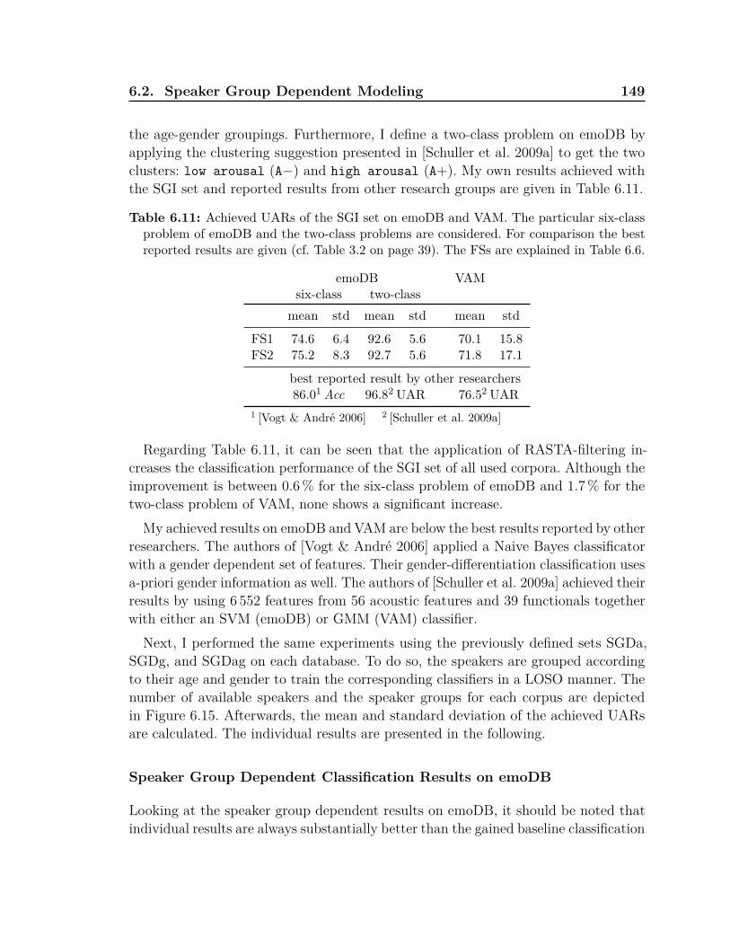
6.2. Speaker Group Dependent Modeling 149
the age-gender groupings. Furthermore, I define a two-class problem on emoDB byapplying the clustering suggestion presented in [Schuller et al. 2009a] to get the twoclusters: low arousal (A−) and high arousal (A+). My own results achieved withthe SGI set and reported results from other research groups are given in Table 6.11.
Table 6.11: Achieved UARs of the SGI set on emoDB and VAM. The particular six-classproblem of emoDB and the two-class problems are considered. For comparison the bestreported results are given (cf. Table 3.2 on page 39). The FSs are explained in Table 6.6.
emoDB VAMsix-class two-class
mean std mean std mean std
FS1 74.6 6.4 92.6 5.6 70.1 15.8FS2 75.2 8.3 92.7 5.6 71.8 17.1
best reported result by other researchers86.01 Acc 96.82 UAR 76.52 UAR
1 [Vogt & André 2006] 2 [Schuller et al. 2009a]
Regarding Table 6.11, it can be seen that the application of RASTA-filtering in-creases the classification performance of the SGI set of all used corpora. Although theimprovement is between 0.6% for the six-class problem of emoDB and 1.7% for thetwo-class problem of VAM, none shows a significant increase.
My achieved results on emoDB and VAM are below the best results reported by otherresearchers. The authors of [Vogt & André 2006] applied a Naive Bayes classificatorwith a gender dependent set of features. Their gender-differentiation classification usesa-priori gender information as well. The authors of [Schuller et al. 2009a] achieved theirresults by using 6 552 features from 56 acoustic features and 39 functionals togetherwith either an SVM (emoDB) or GMM (VAM) classifier.
Next, I performed the same experiments using the previously defined sets SGDa,SGDg, and SGDag on each database. To do so, the speakers are grouped accordingto their age and gender to train the corresponding classifiers in a LOSO manner. Thenumber of available speakers and the speaker groups for each corpus are depictedin Figure 6.15. Afterwards, the mean and standard deviation of the achieved UARsare calculated. The individual results are presented in the following.
Speaker Group Dependent Classification Results on emoDB
Looking at the speaker group dependent results on emoDB, it should be noted thatindividual results are always substantially better than the gained baseline classification

150 Chapter 6. Improved Methods for Emotion Recognition
Table 6.12: Achieved UARs in percent using SGD modelling for all available speakergroupings on emoDB. The FSs are explained in Table 6.6.
classes Grouping UAR [%]FS1 FS2
mean std mean std
6 m 75.9 7.3 75.7 8.3f 77.3 7.8 78.1 8.9
2 m 97.1 5.6 97.1 5.8f 98.2 2.6 98.2 3.0
(cf. Table 6.12). This is independent of the number of emotional clusters or the appliedfeature set. For the six-class problem, both speaker group dependent results are belowthe best reported result of 86.0% [Vogt & André 2006].
Inspecting both gender groups independently, it is apparent that the improvementfor females is about 2% better than the recognition for males. This can be attributedto the smaller amount of training material available for the male group. On average,the emotional classifier could be trained with 6.6 utterances from each male speakerwhereas from each female speaker 8.5 utterances can be used. The combined SGDgresults just achieves approx. 77% for both FSs (cf. Figure 6.16).
FS1 FS2
60
70
80
90
100
Six-class problem
UA
R[%
]
FS1 FS2
60
70
80
90
100* *
Two-class problem
SGISGDg
Figure 6.16: UARs in percent for emoDB’s two-class and six-class problem comparingSGI and SGDg utilising LOSO validation on different feature sets. For comparison, thebest reported results (cf. Table 3.2 on page 39) are marked with a dashed line. The starsdenote the significance level: * (p < 0.05).
In contrast, the SGD results on two-class problem are outperforming the classifica-tion result of 96.8% from [Schuller et al. 2009a], for both applied feature sets. In thiscase, a sufficient amount of material to train a robust classifier is available with more

6.2. Speaker Group Dependent Modeling 151
than 19 utterances per speaker. The combined results of both gender-specific classifi-ers are depicted in Figure 6.16. In comparison to the SGI results the SGD classifiersachieved an absolute improvement of 4% to 5% for both FSs. This improvement issignificant for FS1 (F = 4.8791, p = 0.0272) and FS2 (F = 4.48238, p = 0.0281).
In summary, it can be stated that the low amount of training material for thesix-class problem drives the presented approach to its limits. The tripling of thetraining material by combining certain emotions, in the second case shows a significantimprovement of recognition performance for the investigated feature sets in comparisonto SGI modelling. Furthermore, the SGD approach could slightly outperform theresults of [Schuller et al. 2009a], whereby much fewer features (45 vs. 6 552), buta-priori knowledge about the speakers’ group belonging are used.
Speaker Group Dependent Classification Results on VAM
Table 6.13: Achieved UAR in percent using SGD modelling for all available speaker group-ings on VAM. The outlier, showing worse results than SGI is highlighted . The significancelevel is denoted as p < 0.01 . The FSs are explained in Table 6.6.
Grouping UAR [%]FS1 FS2
mean std mean std
m 72.2 16.3 73.4 15.3f 80.1 12.9 80.2 14.3
y 76.8 13.1 77.1 15.4m 76.1 13.1 75.1 14.2
mf 75.9 13.9 75.2 13.2yf 77.9 13.6 80.1 14.2m 71.7 14.1 71.3 13.1
ym 75.3 12.7 71.8 14.8
The investigation of the speaker group dependent results for VAM, reveals that allindividual results are better than the gained baseline classification (cf. Table 6.13).The utilised feature set only has a slight influence on the performance. A significantimprovement of up to 10% for the SGDg classifiers can be achieved. In this case, thefemale speaker group benefits from the high amount of training material resultingin significant improvements: FS1 (F = 8.3160, p = 0.0052) and FS2 (F = 11.4370,p = 0.0010), while for the m group, the small amount of training material is apparent.
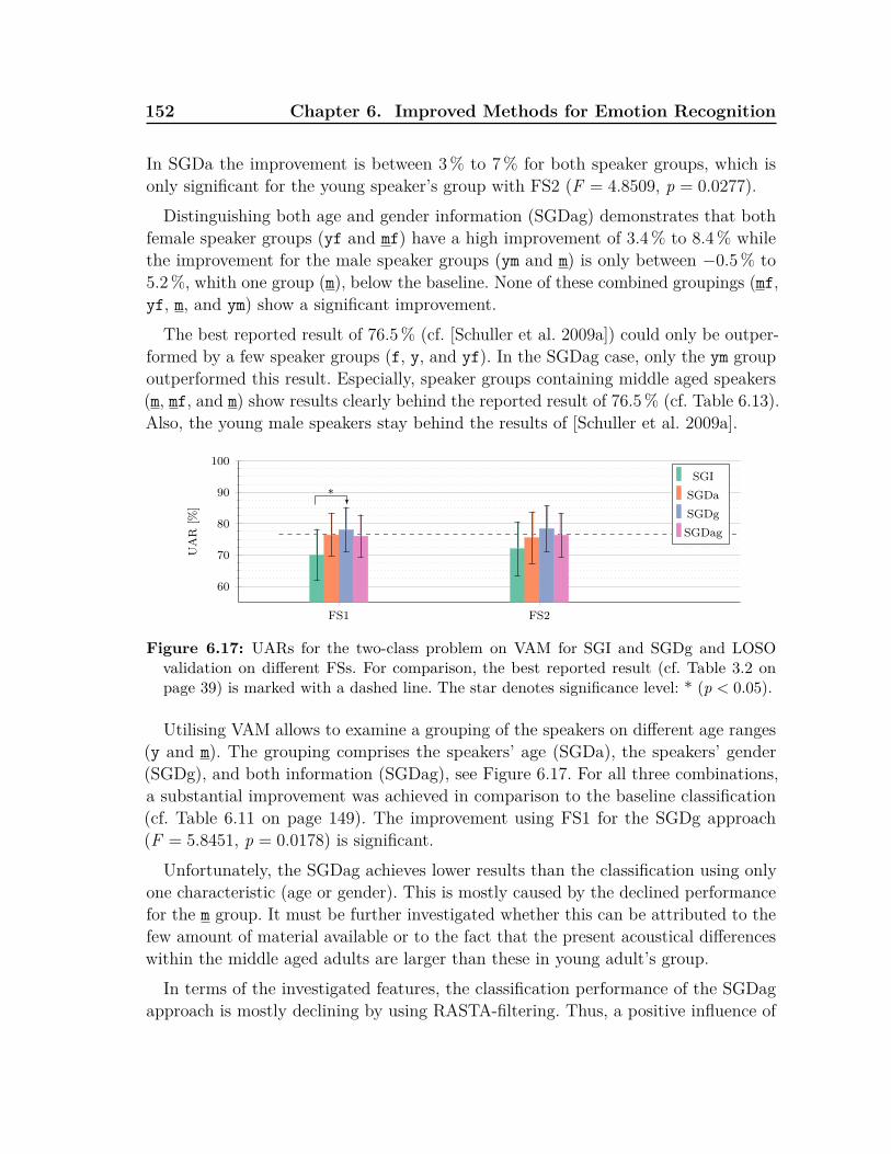
152 Chapter 6. Improved Methods for Emotion Recognition
In SGDa the improvement is between 3% to 7% for both speaker groups, which isonly significant for the young speaker’s group with FS2 (F = 4.8509, p = 0.0277).Distinguishing both age and gender information (SGDag) demonstrates that both
female speaker groups (yf and mf) have a high improvement of 3.4% to 8.4% whilethe improvement for the male speaker groups (ym and m) is only between −0.5% to5.2%, whith one group (m), below the baseline. None of these combined groupings (mf,yf, m, and ym) show a significant improvement.
The best reported result of 76.5% (cf. [Schuller et al. 2009a]) could only be outper-formed by a few speaker groups (f, y, and yf). In the SGDag case, only the ym groupoutperformed this result. Especially, speaker groups containing middle aged speakers(m, mf, and m) show results clearly behind the reported result of 76.5% (cf. Table 6.13).Also, the young male speakers stay behind the results of [Schuller et al. 2009a].
FS1 FS2
60
70
80
90
100
*
UA
R[%
]
SGISGDaSGDgSGDag
Figure 6.17: UARs for the two-class problem on VAM for SGI and SGDg and LOSOvalidation on different FSs. For comparison, the best reported result (cf. Table 3.2 onpage 39) is marked with a dashed line. The star denotes significance level: * (p < 0.05).
Utilising VAM allows to examine a grouping of the speakers on different age ranges(y and m). The grouping comprises the speakers’ age (SGDa), the speakers’ gender(SGDg), and both information (SGDag), see Figure 6.17. For all three combinations,a substantial improvement was achieved in comparison to the baseline classification(cf. Table 6.11 on page 149). The improvement using FS1 for the SGDg approach(F = 5.8451, p = 0.0178) is significant.
Unfortunately, the SGDag achieves lower results than the classification using onlyone characteristic (age or gender). This is mostly caused by the declined performancefor the m group. It must be further investigated whether this can be attributed to thefew amount of material available or to the fact that the present acoustical differenceswithin the middle aged adults are larger than these in young adult’s group.
In terms of the investigated features, the classification performance of the SGDagapproach is mostly declining by using RASTA-filtering. Thus, a positive influence of

6.2. Speaker Group Dependent Modeling 153
RASTA-filtering as seen in the SGI case cannot be obtained.
6.2.5 Intermediate Results
Before comparing the SGD results with VTLN, as acoustic normalisation tech-nique, I present the SGI, SGDg, SGDa, and SGDag results in a summarised table(cf. Table 6.14) to directly compare the gained improvement across the corpora.
Table 6.14: Achieved UARs in percent for all corpora using SGD modelling. Additionally,absolute improvements against SGI results are given. The FSs are explained in Table 6.6.
Corpus Problem SGI SGDg SGDa SGDagLMC two-class 68.7 (FS4) 73.4 (FS4) 72.0 (FS4) 73.8 (FS2)
improvement – 4.7 3.3 5.1
emoDB two-class 92.7 (FS2) 97.7 (FS2) – –improvement – 5.0
emoDB six-class 75.2 (FS2) 76.9 (FS2) – –improvement – 1.7
VAM two-class 71.8 (FS2) 78.4 (FS2) 76.4 (FS2) 76.3 (FS2)improvement – 6.6 4.5 4.5
Comparing the SGD results on the different corpora, it is evident that regardingspeaker groups improves the recognition on all corpora. Here the smaller amount ofdata does not prevent this improvement. Even with emoDB, having very clear andexpressive emotions, a quite high improvement is achieved. Utilising the completequantity of emotions on the six-class problem shows the disadvantages of the SGDapproach, as the small amount of training data drives the approach to its limits.
Comparing the utilization of age and gender characteristics on LMC and VAMreveals that the gender tends to be the dominating factor, as on both corpora, ahigher improvement could be achieved, if the gender-information is used. Using thecombination of both characteristics could slightly outperform the single characteristics’results on LMC. With VAM the SGDag result is behind both the SGDg and the SGDaresult, but it is still better than the SGI result. It has to be further investigated whetherthis is caused by the small amount of training material for the male speakers or byan inadequate age grouping.

154 Chapter 6. Improved Methods for Emotion Recognition
6.2.6 Comparison with Vocal Tract Length Normalisation
Another technique, dealing with speaker variabilities, is the utilization of VTLN. Thismethod follows a conceptually different approach than speaker-group dependent mod-elling. Instead of separating the different speakers into certain groups, the acoustics ofthe different speakers are aligned (cf. Section 4.3.3). For this, a warping factor for eachspeaker, representing the degree of the necessary acoustical alignment, is estimated.It expresses the degree of frequency shift for the actual speaker’s acoustics have to bechanged to match a “general” speaker. This general speaker is modelled a-priori byall other speakers’ acoustics of the data material.To estimate the warping factor for each speaker, I used the maximum likelihood
estimation (cf. [Kockmann et al. 2011]). Therein, a rather small GMM with only 40mixtures and 4 iteration steps is trained on all unnormalised training utterances ofthe corpus using all speakers despite one. The left-out speaker is the target speaker,where the warped features are generated for each utterance in the range of 0.88 to1.12 with a step size of 0.02.
The optimal warping factor is obtained afterwards by evaluating the likelihood ofall warped instances against the unnormalised GMM and selecting the highest one(cf. [Cohen et al. 1995]). This procedure is repeated for all speakers. To estimatethe warping factor, the same features as for the FS1 of the SGD approach are used,namely 12 MFCCs, C0, F0, and E together with their ∆ and ∆∆ regression coefficients.Furthermore, CMS as channel normalisation technique is used. HTK is used fortraining, Vocal Tract Length Normalisation, and testing (cf. [Young et al. 2006]).
Estimated Warping Factors
Figure 6.18 depicts the estimated warping factors for emoDB and VAM. The acous-tically high quality emoDB corpus has an equal number of male and female speakerscovering an age range from 21 to 35 years. The estimated warping factors reflect thegeneral description of warping VTLN: male speakers have a warping factor greaterthan 1 to stretch the vocal tract and female speaker’s warping factor is smaller than1 to compress the vocal tract. A performed k-means clustering reveals two clusterswith centroids at 0.96 containing only female and 1.08 containing only male speakers.Thus, a good classification accuracy can be expected.
The estimated warping factors for VAM are quite different (cf. Figure 6.18). Al-though most of the male and female speakers have warping factors in the range of0.96 to 1.04, which is close to 1, the general behaviour – compression for female andexpansion for male speakers – is still apparent. The average warping factor for female

6.2. Speaker Group Dependent Modeling 155
female
male
Estimated warping factors on emoDB
0.88 0.92 0.96 1 1.04 1.08 1.12
female
male
Estimated warping factors on VAM
Young Medium aged Unspecific
Figure 6.18: Estimated warping factors for every target speaker of the databases emoDBand VAM arranged for male and female speakers as proof of VTLN algorithm. The agegroups are indicated where needed.
speakers is 0.99 with a standard deviation of 0.04 whereas for the male speakers anaverage warping factor of 1.05 with a standard deviation of 0.03 was estimated.
The age groups of the speakers were also known for this database. On the otherhand, from Figure 6.18 it is apparent that age is not a separating factor. The mean forthe young group is 1.05 with a standard deviation of 0.04. The old group has a meanwarping factor of 1.03 and a standard deviation of 0.05. The anatomical differencesare more prominent than the acoustic changes caused by the ageing.
0.88 0.92 0.96 1 1.04 1.08 1.12
female
male
Young Senior Unspecific
Figure 6.19: Estimated warping factors for every target speaker on LMC, as example forstrange factor estimaton for male and female speakers. The age groups are indicated.
Estimating the warping factors on LMC reveals another picture (cf. Figure 6.19).Although the same procedure with identical features and modelling as for emoDB’sand VAM’s warping factor estimation are used, the achieved factors are quite different.
The general trend of the LMC’s factors indicates a stretching. Female speakers havefactors in the range of 1.04 to 1.12, whereas for the male speakers the factors arebetween 1.08 and 1.12. This can also be seen in the mean and standard deviation of

156 Chapter 6. Improved Methods for Emotion Recognition
both groups, the values of female speakers’ factors have a mean of 1.08 and a standarddeviation of 0.02. For male speakers the mean is 1.1 with a standard deviation of 0.01.Thus, by the estimated warping factors male and female speakers cannot longer bedistinguished. Thus, although the warping factor estimation is able to separate maleand female speakers on emoDB and VAM, this separation does not work for LMC.This may be due to the age groupings of LMC. The acoustic differences between thetwo groups, y and s, of LMC are more prominent, as for speakers over 60 years thefundamental frequency is dramatically changing. The female voice is declining andthe male voice is increasing (cf. [Linville 2001; Hollien & Shipp 1972]. The influence ofageing on the fundamental frequency was discussed in Section 4.2.2. This can influencethe warping factor estimation.
But, as for VAM the speakers’ age is not a distinguishing factor, although both agegroups in LMC are more apart than for VAM. Young adults have a warping factorwith a mean of 1.1 and a standard deviation of 0.02, and seniors have a mean warpingfactor of 1.09 with a standard deviation of 0.02. Utilising other feature sets to inferRASTA-filtering and SDC-coefficients does not lead to different warping factors.
Classification Performance using VTLN
The obtained warping factors are then used to normalise the features of the differentfeature sets for each corpus accordingly. These features are then applied to trainthe classifiers using HTK and pursue a LOSO validation to preserve comparabilityto the previous presented SGD-experiments (cf. Section 6.2.3 and Section 6.2.4).In Figure 6.20 the achieved UAR of the VTLN approach is compared with resultsof the unnormalised features, which served as baseline classification results for theSGD approach as well. Furthermore, the best reported results by other researchersare marked with a dashed line for each corpus.Investigating the achieved classification using VTLN, it can be stated that for
all corpora the classification performance is improved in comparison to the baselineclassification results but no significant improvement could be achieved (cf. Figure 6.20).Although the estimated warping factors on emoDB meet the expectations, the averageclassification performance is just slightly improved by about 0.5% for the six-classproblem and 0.7% for the two-class problem. The highest improvement could beobserved for FS1, where neither a RASTA-filtering is applied nor SDC-coefficients areinferred. All achieved improvements are not significant. Overall, the application ofVTLN on emoDB could not outperform the results reported by other research groups.
The classification performance on both databases with naturalistic emotions benefitsfrom the application of VTLN (cf. Figure 6.20), although the estimated warping factors

6.2. Speaker Group Dependent Modeling 157
emoDB6 emoDB2 VAM2 LMC260
70
80
90
100
UA
R[%
]
FS1 FS1 VTLN FS2 FS2 VTLNFS3 FS3 VTLN FS4 FS4 VTLN
Figure 6.20: Mean UAR for VTLN-based classifiers in comparison to the baseline of dif-ferent corpora utilising GMMs and LOSO on different feature sets. The number followingthe corpus abbreviation indicates the number of distinct classes. The best results reportedfor each database are marked with a dashed line (cf. Table 3.2 on page 39).
do not indicate that (cf. Figure 6.19 on page 155). The average improvement is 3.7%for VAM and 2.0% for LMC. An improvement of 5.1% in total for VAM and of 3.6%in total for LMC could be achieved using FS1. The highest improvement on VAM canbe achieved with FS1 closely followed by FS2 and FS4.With LMC the highest improvement is achieved using FS1 close followed by FS3.
Unfortunately, the performance gains for FS1 and FS2 on VAM and for FS1 andFS3 on LMC are not significant as the standard deviation remains quite high. Thissuggests that VTLN cannot resolve speaker variabilities sufficiently. Furthermore, thegained improvements could not surpass the best reported results on both databases.
Comparison of SGD modelling and VTLN technique
To complete this study, I want to compare the results achieved by SGD modellingand VTLN. Therefore, I summarised the best results of all utilised corpora for bothtechniques in Table 6.15. I concentrated on feature sets with the particularly bestresult for each approach. As for most of the results, the standard deviation is alreadygiven, I do not note it in this overview table to preserve readability.
The comparison of SGD modelling and VTLN technique reveals that for all utilisedcorpora the improvement gained by distinguishing the different speaker groups achieveresults that are in total 1.1% to 4.3% better than the VTLN results. Almost all corporabenefit from RASTA-filtering, which was not expectable especially for emoDB. ForLMC, the feature sets achieving the best performance differ between SGI and VTLNon the one hand and SGD on the other hand. Furthermore, SGD improvements aresignificant, whereas VTLN does not produce significant improvements. It appears thatthe SDC-coefficients are able to adjust the acoustic variabilities.

158 Chapter 6. Improved Methods for Emotion Recognition
Table 6.15: Achieved UARs in percent of SGD, VTLN, and SGI classification for allconsidered corpora. Furthermore, feature sets and speaker groupings are given. The FSsare explained in Table 6.6.
emoDB VAM LMCsix-class two-class two-class two-class
SGI 75.2 92.8 71.8 68.7FS 2 2 2 4
SGD 76.9 97.7 78.3 73.8FS 2 2 2 2
Grouping SGDg SGDg SGDg SGDag
VTLN 75.5 93.4 75.5 69.8FS 2 2 2 4
6.2.7 Discussion
In this section, I demonstrated that a speaker group dependent modelling leads to asignificantly improved emotion classification. To do so, I first performed a parametertuning of the two model parameters number of mixture components and iterationsteps for GMMs. I was able to conclude that the best classification performance isobtained when choosing 120 mixture components. The type of emotion, simulated ornaturalistic, does not influence the general trend of classification performance.
Simulated emotional databases are more sensitive for different iteration step numbersas naturalistic ones. As 4 appears as the best number of iteration steps in terms ofclassification and computation performance, I chose this for all further investigations.These findings confirm the results of [Böck et al. 2010], identifying a low number ofiteration steps as suitable for both types of databases.
Furthermore, I investigated the influence of the contextual characteristics ∆, ∆∆,and SDC-coefficients. Here I stated that the incorporation of ∆ and ∆∆ regressioncoefficients increases the recognition performance for both types of databases. In con-trast to the utilization of SDC-coefficients for simulated databases where a decreasedclassification performance could be observed, the incorporating of SDC-coefficientsincreases the performance on LMC.
This is also partly true if different channel normalisation techniques are investigated.Here the application of CMS improves the classification performance on both typesof databases. RASTA-filtering just slightly increases the performance on emoDB, butnotably on LMC. My findings expand the investigation of [Kockmann et al. 2011],

6.2. Speaker Group Dependent Modeling 159
stating that RASTA-filtering together with ∆∆ regression coefficients has the mostpotency for acoustic emotion recognition.
Afterwards, I applied the speaker group modelling approach known from ASR toimprove automatic emotion recognition from speech (Hypothesis 6.6 on page 136). Asnaturalistic recordings contain both more variability in the expression of emotions aswell as less expressive emotions (cf. Section 3.3), I conclude that additional knowledgeis required to successfully recognise emotions. Starting with the definition of speakergroups to reduce the acoustic variations, I assumed that separation of age and gendergroups reduces the acoustic variability and thus, improve the emotion recognition.
Therefore, I performed experiments using the earlier defined model configurationand feature sets on LMC as naturalistic emotional corpus to support this hypothesis.This was successful: the incorporation of both age and gender for speaker groupingachieved significant improvements in comparison with SGI results and could outper-form classifiers based only on age or gender as seperating characteristic.
The investigations presented on additional databases reveal that the emotion recog-nition can be improved through the separation of gender groups. The improvement isindependent of the type of emotional content (simulated or naturalistic), the qualityof recording, or the available speaker groups. I compared the SGD results with thepreviously gained baseline results (SGI) utilising the same features and classifiers aswell as with results reported by other research groups. Hereby, I was able to demon-strate that this approach could be applied to several datasets. In comparison withthe SGI classification, significant improvements for all databases using SGD-classifierscould be achieved, except for the six-class problem with emoDB.
Furthermore, for the first time this investigation allows to draw conclusions aboutthe limitations of this approach. The lack of training material becomes most apparent.Regarding the classification performance in specific speaker groups, they outperformthe SGI baseline in all cases. Especially, if the amount of available material for trainingis quite small, the performance is quite low, for instance the speaker groups of the sixclass problem on emoDB, the ym-group of LMC, or the m-group of VAM. Despite this,the trained SGD-model still outperforms a SGI-classifier trained on the same smallamount of data (cf. [Siegert et al. 2013c]).
When comparing the classification performance of age-group dependent and gender-group dependent models a slightly better performance of the gender-group dependentmodels can be noticed. This indicates that the gender of a speaker has a higherinfluence on the variability of characteristics than his age, at least for the investigatedage groups (cf. [Siegert et al. 2014d]). As this behaviour can be observed both inVAM and in LMC, this seems to be valid for different age groups, too. This result is

160 Chapter 6. Improved Methods for Emotion Recognition
supported by both the reported larger acoustic differences between male and femalespeakers as well as the gender effects on emotional responses as stated in Section 4.2.These findings are still not sufficient enough for general statements, but at least atendency can be seen. On LMC a combination of both characteristics achieves thebest performance. This may be supported by the optimal age grouping.
As further approach, I utilised VTLN, a method well known in ASR to compensatedifferent vocal tract lengths. By applying this method, all SGI results could be im-proved. However, the improvement is neither significant nor does it achieve betterresults than the SGD-approach (cf. Table 6.15 on page 158). The comparison of theestimated warping factors reveals that a quite strange behaviour could be observed.Especially on LMC, the vocal tract of all speakers is stretched. The age-gender specificexpression of emotions, as psychological research suggests, cannot be covered by VTLN(cf. Hypothesis 6.7 on page 136). One drawback this method has, is that the estimationof warping factors needs to be improved in order to cover the highly unbalanced agedistribution. Thus, I advise using SGD modelling for emotion recognition.
6.3 Applying SGD-Modelling for MultimodalFragmentary Data Fusion
As I have already stated in Section 3.2 and depicted in Section 3.3, naturalisticemotions require additional efforts in order to ensure a robust emotion recognition.Beside the improvement of emotion recognition methods on acoustic level I havepresented earlier (cf. Section 6.2) that a multimodal emotion recognition approach canbe utilised. This method is derived from the fact that humans express their emotions byusing several channels, for instance facial expressions, gestures, and acoustics. Hence,the emotional response patterns are observable in different modalities which can befused to robustly recognise the current emotion.Although the main focus of this thesis is not classifier fusion, this topic is an
important and arising issue for emotion recognition. In my case, I contributed inwork which was done under the SFB/TRR 62 by colleagues at the Otto von GuerickeUniversity Magdeburg and the Ulm University (cf. [Böck et al. 2012a; Frommer et al.2012b; Panning et al. 2012; Böck et al. 2013a; Krell et al. 2013; Siegert et al. 2013e]).A short introduction on common fusion techniques was given in Section 4.3.4.
In this section, I will concentrate on my contributions to improve the multimodalaffect recognition for the naturalistic interaction on LMC. Therefore, contributionsof other researchers are also presented and acknowledged accordingly. Afterwards, Idiscuss some of my contributions made under the constraint of fragmentary data.

6.3. SGD-Modelling for Multimodal Fragmentary Data Fusion 161
6.3.1 Utilised Corpus
The conducted study, which will be presented afterwards, utilises the “79s” speakerset of the LMC (cf. Section 5.2.3) that has already been used in Section 6.2. Here,the focus is again on the two key events of the experiment, where the user shouldbe set into a certain condition: baseline (bsl) and challenge (cha). The utilisedmaterial comprises the same automatically extracted and manually corrected 1 668utterances as used in Section 6.2. The total length is 31min, the average sample lengthper speaker group is nearly equal. But the distribution of samples is unbalanced, as ahigher amount of samples is available for bsl.
The focus of this research is on the combination of different modalities. For visualclassification only a subset of 13 speakers is available as the visual classifier was trainedon manually FACS coded data, which is a time-consuming process. These 13 speakersare a subset of the 20s set, for which synchonised audio-visual data is available. Theexperimental codes of the 13 speakers, their amount of acoustic training material andtheir age grouping are given in Table 6.16.
Table 6.16: Detailed information for selected speakers of LMC.
ID Speaker bsl cha Groupsamples length samples length
1 20101013bkt 14 19.31 4 6.24 yf2 20101115beh 26 28.30 15 13.36 yf3 20101117auk 13 17.42 11 13.02 yf4 20101117bmt 16 18.88 8 9.55 ym5 20101213bsg 16 20.79 14 17.81 sm6 20110110bhg 12 15.28 10 14.71 ym7 20110112bkw 10 8.14 9 11.72 ym8 20110117bsk 15 18.22 10 13.03 ym9 20110119asr 15 18.73 2 3.45 ym
10 20110124bsa 10 10.88 4 4.04 ym11 20110126bck 13 17.00 8 8.58 ym12 20110131apz 16 12.21 3 2.42 ym13 20110209bbh 15 12.61 5 5.63 sm
6.3.2 Fusion of Fragmentary Data without SGD Modelling
Using material of a naturalistic HCI, the classification applying different modalities,can be quite vague. One main reason is that the information in the different channels

162 Chapter 6. Improved Methods for Emotion Recognition
is not continuously available. This is mostly due to subjects not behaving ideally.They do not speak directly into the microphone, resulting in changing acoustic char-acteristics. They do not face the camera resulting in faces or the hands not alwaysvisible. Additionally, parts of the face can be hidden by hair or glasses. Furthermore,changes in illumination can make color-information unusable [Zeng et al. 2009; Gajšeket al. 2009; Navas et al. 2004]. We summarise these effects by denoting the data“fragmentary”. Common reasons for fragmentary data are:
• prosodic features are only available if the user speaks,• gestures are only detected if typical hand movements occur,• facial expressions are usually temporary,• user disappears from camera,• face is hidden by hands,• mouth speaking movement overlays facial expression.
This problem can, for instance, be observed in the LMC (cf. Section 5.2.3), too.These fragmentary channel information can either be addressed by rejecting unfa-
vourable data or by utilising a suitable fusion technique which is capable of handlingsuch kind of data [Wagner et al. 2011]. Rejecting unusable data is not always feasibleas it will reduce the over-all amount of data, leading in the end to nearly no remainingdata. Furthermore, this approach is not applicable in real-time applications.
22 44 66 88 110
a1a2a3a4a5
gestureprosody
Time [s]
Feat
ure
valu
es
Figure 6.21: Observable features of the challenge event for subject 20101117auk of theLMC. Any dot in the figure represents a window with an extracted value for the specificfeature. Facial measures: mean of left and right brow position (a1), mouth width (a2),mouth height (a3), head position (a4), eye blink frequency (a5). Gesture: line indicatesself-touch. Prosody: line indicates utterance.
Figure 6.21 depicts the fragmentation of observable features for an excerpt ofsubject 20101117auk of the LMC. Within an excerpt of 110 s of the whole interaction,the subject speaks very rarely ( ∼13 s). Also, only two considered gestures can beobserved, lasting for 32 s in total. The eye blink frequency (a5) and the brow position

6.3. SGD-Modelling for Multimodal Fragmentary Data Fusion 163
can be analysed nearly the entire time. Only longer closed eyes or fast head movementsprevent a permanent observation. The three other facial features, mouth width (a2),mouth height (a3), and head position (a4), are also just partially observable. Detail onthe extraction can be found in [Panning et al. 2012; Krell et al. 2013]. Thus, althoughacoustics, gestures and facial features are utilised, only for very few time points allcharacteristics can be evaluated. For instance, windowing all different features byusing a 25ms window, only in 880 out of 4400 frames all five video characteristicstogether with gesture information can be observed and for only 396 frames video andacoustic information are available. For the combination of all three characteristics,only 88 frames can be used.Before discussing the applied decision fusion approach, I shortly present the uni-
model classification results. The acoustic results are generated by myself, whereas thevisual classifier is trained by Axel Panning. But, for the sake of completeness, I willbriefly present his approach and results as well.
Acoustic Recognition Results For acoustic classification, I extracted a total of39 features: 12 MFCCs as well as the C0 together with their ∆ and ∆∆ regressioncoefficients. These features are extracted frame-wise using a 25ms Hamming windowwith a frame step of 15ms. As classifier a GMMwith 120 Gaussian mixture componentsand 4 iteration steps is trained (cf. Section 6.2.1). The whole “79s” speaker set ofLMC is used for training. As the available material for facial analysis was limitedto 13 speakers, only these speakers were analysed in a LOSO validation strategy. Asconfidence parameter, used later in the fusion approach, the log likelihoods for eachtest-utterance are stored as well. The unimodal classification results based on theUAR are given in Table 6.17. The overall mean UAR of the selected 13 speakers is60.5% with a standard deviation of 11.7%. The achieved results are in line with similarinvestigations. In the previous section a mean UAR of 63.4% with a standard deviationof 15.1% could be achieved, also utilising F0 (cf. Section 6.2.3). The results reportedin [Prylipko et al. 2014a] achieved a UAR of 63% using an SVM based on 81 turnlevel features comprising spectral acoustic features as well as voice quality features,and pitch related ones together with long-term statistical features (cf. Section 4.2.2).All these results show that a recognition of naturalistic emotions is quite difficult, asthe acoustic variations are quite prominent and the emotional expressiveness is low(cf. [Batliner et al. 2000; Zeng et al. 2009]).
Facial Recognition Results The visual activities were analysed by Axel Panning,who considered mouth deformations, eyebrow movements, eye blink and global headmovement as visual characteristics. Therefore, facial distances and head positions were

164 Chapter 6. Improved Methods for Emotion Recognition
measured (cf. [Panning et al. 2010; Panning et al. 2012]). As the emotional state isassumed to be reflected by the dynamics of observable features, and assumed to remainstable for a couple of frames (cf. [Panning et al. 2012]), a longer time window is usedto analyse the visual activities. By a PCA the most important eigenvectors of thefacial features are fed into an MLP to classify bsl and cha. The output of the MLP isa continuous value between 0 to 1, specifying the ratio that the actual feature contextbelongs either to the bsl (0) or the cha event (1). A general threshold of 0.5 is usedto decide between bsl and cha. The overall mean of the facial classifications’ UARis 57.0% with a standard deviation of 23.6%. The individual unimodal classificationresults are given in Table 6.17. Although these results are close to the achieved acousticperformance, the rather high standard deviation depicts that an event decision canhardly be made on this modality alone. Emotion recognition from facial expressions onnaturalistic interactions is hardly pursued, as the recording quality cannot be ensuredand strict requirements onto illumination or gaze-direction to a camera device haveto be fulfilled.
Table 6.17: Unimodal classification results (UAR) in percent for the 13 subjects.
ID Speaker Acoustic Visual1 20101013bkt 65.2 51.82 20101115beh 51.7 84.83 20101117auk 75.0 76.34 20101117bmt 57.1 65.05 20101213bsg 54.2 29.16 20110110bhg 60.0 55.37 20110112bkw 79.0 65.08 20110117bsk 66.7 91.49 20110119asr 68.0 25.6
10 20110124bsa 40.0 40.811 20110126bck 61.9 43.212 20110131apz 41.2 25.413 20110209bbh 66.7 88.3
mean (std) 60.5 (11.7) 57.0(23.6)
Gesture Recognition Results The gesture detection, also performed by AxelPanning, is focussed on recognising self-touch actions. Self-touching was automaticallydetected in the video stream, by a skin colour detection algorithm. By a connectedcomponent analysis it is determined whether a self-touch in the face occurred (cf.[Saeed et al. 2011; Panning et al. 2012]). As, self-touch is a very rare event, the

6.3. SGD-Modelling for Multimodal Fragmentary Data Fusion 165
gestural analysis alone is not able to decide between bsl and cha. The absence ofself-touch will give no evidences for one of these events. Thus, gestural analysis alonecannot be utilised for classification.
Decision Fusion For the fusion of the single modalities, an MFN is used to estimatethe decision using all three modalities as input (cf. Section 4.3.4). Thus, the MFNmediates between the available decision of the unimodal classifications and additionallytakes their temporal distances into account. In [Krell et al. 2013], the best performancecould be achieved, when for each modality different input weights are used (kv = 0.5,ka = 4, kg = 4). The parameter w, adjusting the lateral smoothness of the MFN,has only a slight influence on the performance. In the range of 50 to 1 000, theperformance increases by just 4% in total. The overall accuracy of this MFN is 79.8%with a standard deviation of 21.2%. The individual results are given in Table 6.18,together with improvements over the best unimodal channel.
Table 6.18: Multimodal classification results (ACC) in percent for the 13 subjects usingan MFN. Using acoustic and visual classification results based on fragmentary data.
ID Speaker Fusion Best single modalityDifference Modality
1 20101013bkt 89.6 24.4 acoustic2 20101115beh 95.7 10.9 visual3 20101117auk 90.2 13.9 visual4 20101117bmt 100.0 35.0 visual5 20101213bsg 89.8 35.6 acoustic6 20110110bhg 94.5 34.5 acoustic7 20110112bkw 82.7 3.7 acoustic8 20110117bsk 62.0 −29.4 visual9 20110119asr 77.5 9.5 acoustic10 20110124bsa 100.0 59.2 visual11 20110126bck 71.2 9.3 acoustic12 20110131apz 59.8 18.6 acoustic13 20110209bbh 24.9 −63.4 visual
mean (std) 79.8 (21.2) 23.1 (16.5)
The fusion results confirm the low expression level in the facial channel, which hasalready been presumed by FACS based unimodal classification. In comparison to theunimodal facial analysis, an absolute improvement of 22.8% could be achieved. Theprosodic analysis, which suffers from multiple missing decisions due to the silence ofthe speaker, shows a rather good framewise accuracy. An improvement of 19.3% wasachieved in comparison to the unimodal acoustic analysis.

166 Chapter 6. Improved Methods for Emotion Recognition
The combination of both channels could lead to a quite high multimodal classific-ation, as the poor results from facial expressions can be compensated by the goodaccuracy of the just sporadically appearing acoustic observations. Additionally, themere occurrence of self-touch gestures can also be used, as the absence of a modalitydoes not influence the MFN’s decision. This fact can be supported by the structureof an MFN, providing the opportunity to utilise different weighting factors k for thevarious single modalities m.
6.3.3 Using SGD Modelling to Improve Fusion of Fragment-ary Data
In this section, I present my investigations, combining the SGD approach and the MFNapproach, to increase the affect recognition of fragmentary data. I already demon-strated that by inferring both gender and age information, the overall classificationperformance increased (cf. Section 6.2). By combining the improved acoustic clas-sification with the decision fusion based on an MFN, I evaluated how an increasedperformance of an unimodal classifier influences the multimodal classification in total.For this, I raise the following hypothesis:Hypothesis 6.8 Although the acoustic channel is present quite rarely, an improvedacoustic classification leads to an increased fused classification result.
To do so, I utilised LMC (cf. Section 5.2.3) employing the same age-grouping as inSection 6.2 defining the SGDag classifiers, namely yf, ym, sf, sm. The same subset ofLMC containing 79 speakers is used as well. The distribution of the training set isdepicted for recapitulation in Table 6.19. The assignment of each subject to a speakergroup is gathered from the corpus description.
Table 6.19: Distribution of utilised speaker groups in the “79s” set of LMC.
male female ∑young 16 21 37old 18 24 42∑ 34 45 79
Unimodal Classifiers The settings for the unimodal classifiers are the same aspresented in Section 6.3.2. The visual classifier considers mouth deformations, eye-blink, eyebrow movement, and the general (global) head movement as well as theself-touch gesture information (cf. [Krell et al. 2013]). The visual analysis performed

6.3. SGD-Modelling for Multimodal Fragmentary Data Fusion 167
by Axel Panning is not modified. The individual results remain the same, as depictedin Table 6.17 on page 164. The overall UAR thus remains at 57.0%.
The acoustic classifier now incorporates the age and gender information of eachspeaker. Apart from this, I utilised the same 39 features (12 MFCCs, C0 with ∆ and∆∆) as well as the same classifier (GMM, 120 mixture components, and 4 iterationsteps). Once again, a LOSO validation strategy is pursued. The individual results arepresented in Figure 6.22.
1 2 3 4 5 6 7 8 9 10 11 12 1320
40
60
80
yf yf yf ym sm ym ym ym ym ym ym ym smId of the subject and
Corresponding speaker group
UA
R[%
]
SGI SGDag
Figure 6.22: Comparison of the UARs achieved by the acoustic classification for eachspeaker with (SGDag) and without (SGI) incorporating the speaker group. The chancelevel is marked with a dashed horizontal line.
The overall UAR using the SGDag-classifiers for the incorporated 13 speakers in-creased to 76.0% with a standard deviation of 6.5%. Hence, an absolute improvementof 15.5% could be achieved in comparison to the SGI classification, which is highlysignificant (F = 17.4347, p = 0.0003) (cf. [Siegert 2014]. This improvement outper-forms the SGDag result presented in Section 6.2, where an improvement of 10.4%could be achieved. The improvement is heavily influenced by the circumstance of anoptimally selected subset. It mainly consist of young subjects. This age-group tendsto express their emotions more clearly than senior adult speakers (cf. [Gross et al.1997]) and thus, the separation of different age-groups results in an over-improvement.Additionally, the speakers selected in the “20s” set can be seen as quite expressive30.
Fusion utilising the acoustic SGD Classifier The decision fusion system isbased on the previously used MFN with the following values: the lateral smoothness30The “20s” set was selected in such a way that suitable probands where asked to undergo thetwo other experiments. Thus, these subjects represent a best match selection of all subjects interms of experimental expectations. As a result, the dialogue barriers caused a trouble in thecommunication and led to a recognizable event.

168 Chapter 6. Improved Methods for Emotion Recognition
w = 1000, the weighting factors kf = 0.5, kp = 4, and kg = 4. These values alreadydemonstrated the best performance using the SGI acoustic classifier.
As pointed out above, each modality possesses an own distinct characteristic distri-bution of occurences over time. The recognition of the emotional state based on facialexpressions requires the subject’s face to be in the focus of the camera. However, incase the subject turns away and the feature extraction is hindered, decision makingbecomes infeasible. A similar problem can be observed regarding the prosodic analysisof the emotional state since it can be performed only in case the subject produces anutterance. In the given setting, the decisions derived from the gestural analysis areeven more demanding because they only give evidence for the class cha. The classi-fier based on facial expression provides decision probabilities for all frames, while anacoustic analysis exists only for approx. 15.9% of the frames and a gestural analysisonly for about 9% of the frames. Thus, it cannot be expected that the improvementfor the final decision is as high as the improvement for the acoustic classification.
1 2 3 4 5 6 7 8 9 10 11 12 1320
40
60
80
100
1 2 3 4 5 6 7 8 9 10 11 12 13
Id of the subject
UA
R[%
]
SGI SGDag
Figure 6.23: UARs after decision fusion over the continuous stream of the unimodal de-cisions comparing speaker group independent (SGI) and speaker group dependent (SGDag)acoustic classifier. The chance level is marked with a dashed horizontal line.
The individual results for each subject are presented in Figure 6.23. The over-allaverage accuracy is 85.29% with a standard deviation of 14.22%. In comparison to theSGI classifier fusion, the incorporation of speaker groups improved the performance byabout 5.46% in total. Although the acoustic classifier has a significant improvement,the current result is not significant (F = 1.1186, p = 0.2902) (cf. [Siegert 2014].
6.3.4 Discussion
As demonstrated in this section, the MFN is a powerful approach for fusing decisionsfrom multiple modalities preserving temporal dependencies. The MFN reconstructsmissing decisions and different temporal resolutions. Each channel can be individually

6.3. SGD-Modelling for Multimodal Fragmentary Data Fusion 169
weighted according to occurrences and reliability of the decisions. The unimodal recog-nition results provided by facial and acoustic analysis achieved moderate classificationresults that correspond with actual recognition results on naturalistic data material.The performed MFN fusion leads to a mean absolute improvement of 21.1%.
Consequently, I combined my approach of SGD-modelling with the investigatedMFN fusion to test my Hypothesis 6.8. An absolute improvement of 5.46% couldbe achieved. The individual improvements are ranging from 0% to 25.1%. It canbe further observed that an improved fusion could not be observed for all speakerswhere an acoustic improvement was gained. This could be attributed to the fact thatacoustic observations occur very rarely (∼14.4% bsl, ∼9.7% cha). But in general, Iwas able to confirm my hypothesis. The marginal improvement of the fusion using thesophisticated acoustic classifier is related to the influence of the other two modalitiescompeting with the acoustic modality as well as the sporadic utterances of the subject.
For the subjects 1 (20101013bkt) and 5 (20101213bsg) the acoustic classifier yieldsa notable performance gain, but the visual classification remains quite poor (cf. Fig-ure 6.22 on page 167 and Table 6.16 on page 161). Furthermore, acoustic observationsare quite rare for subject 1 and subject 5 with a total amount of approx. 15 s for (bsl)and 10 s for (cha) out of 110 s each. As the MFN generates a continuous predictionover the whole time, the recognition rates of all available modalities are incorporated.In cases when all modalities are available, the MFN can achieve quite good perform-ances. Especially when the different inputs are weighted by ther reliableness, as inthe present case, where the acoustic weight is 4 and the visual weight is just 0.5. But,if only one for channel is available, this channel determines the fusion result. In theinvestigated cases, the visual channel is nearly constantly available while the acousticchannel is just rarely available. Thus the MFN is tied by the low visual results.
Considering the young male subjects 8 (20110117bsk) and 12 (20110131apz), aremarkable improvement of the fusion can be observed. For these subjects the acousticimprovement yields to an improved fusion, as the acoustic channel is better represented.Especially within cha, a total amount of 18 s can be utilised. But for both subjectsthe acoustic classifications stay behind the mean of 76.0% and thus, the fusion relyingstrongly on the acoustic’s channel decision remains quite low.
The senior male subject 13 (20110209bbh) shows an overall low classification per-formance. Although, the individual classification results are quite high, the accuracygained by the MFN is quite low (50.0%), in comparison to the other subjects. In thiscase, a quite long self-touch event occurring during bsl, where a self-touch usuallynot occurs, prevents a better fusion result. This indicates that a unique thresholdingfor all speaker groups, for gestures and facial activities, could mislead the fusion.

170 Chapter 6. Improved Methods for Emotion Recognition
6.4 Summary
In this chapter, I presented my own studies of the improvement of the automaticrecognition of emotions from speech. Therein, I followed the established steps of patternrecognition. Starting with labelling issues, I presented a tool supporting the literaltranscription and emotional annotation process. Furthermore, I presented studiesusing this tool on the emotional labelling of naturalistic emotions where I was ableto support my hypothesis that emotional labelling methods derived from establishedmethods in psychology results in samples with a proper emotional coverage. Followingthat, I investigated the inter-rater reliability measure to draw conclusions about thecorrectness of the labelling process. I was able to show to which extent a reliability isexpectable for emotional labelling, and that the integration of visual cues as well aspresenting the whole interaction in correct order helps to increase the IRR-value.
In the next step, I presented my improvements for the emotion classification itself.As the speech production literature shows that both the gender as well as the age havean influence on the speakers’ acoustic characteristics, I hypothesised that separatingthe speakers’ according to specific age groups and the speaker’s gender could improvethe emotion recognition. With this SGD approach I could significantly improve theemotion recognition on several databases with simulated and naturalistic emotionalsamples with various recording quality. I could show that my SGD-modelling approachhas an effect for all kinds of different data. For highly expressive acted basic emotionsand high quality data (emoDB) only a slight improvement of 1.2% could be achieved.If the emotions are clustered dimensionally, the emotion-specific characteristics areincreased and thus, the SGD approach earns a significant improvement for databasesof both simulated and naturalistic emotions. I furthermore was able to show that thisapproach leads to better results than an acoustic normalisation through VTLN.
Finally, I combined my SGD approach with a multimodal fusion technique developedby colleagues at Ulm University to classify emotions within fragmentary multimodaldata streams. In this, I showed that the improved acoustic classification by utilisingthe SGD approach leads to an improved fusion, although the acoustic information isjust rarely present.
The basic requirement for all of these methods is, however, the presence of a meas-urable emotional reaction. It is known that HHI is controlled by further mechanisms,for instance feedback signals. Therefore, it is urging to regard also HCI under thesepremises. One of these feedback signals will be investigated in the following chapter.

Chapter 7
Discourse Particles as InteractionPatterns
Contents7.1 Discourse Particles in Human Communication . . . . . . . . 1727.2 The Occurrence of Discourse Particles in HCI . . . . . . . . 1747.3 Experiments assessing the Form-Function-Relation . . . . 1807.4 Discourse Particles and Personality Traits . . . . . . . . . . 1867.5 Summary . . . . . . . . . . . . . . . . . . . . . . . . . . . . . . 188
THE previous chapters dealt with the automatic emotion recognition. I motiv-ated emotion as an important information for a naturalistic HCI. In particular,
this problem is addressed from an engineering perspective by formulating a patternrecognition problem, where the emotion is the pattern that has to be recognised.In this chapter a new pattern is introduced that comprises information on the
progress of HCI. For this, the so-called Discourse Particles (DPs) are used to evaluatethe ongoing dialogue. These particles carry a very specific relation of their intonationwith their function in the dialogie, which has not been used for automatic interactionevaluation so far. Therefore, I will present my studies on these patterns.First, the importance of the investigated DPs as interaction patterns for HHI is
depicted (cf. Section 7.1). In particular, their “form-function relation” is presented.This relation, introduced in [Schmidt 2001], is such that a specific meaning (function)is tied with different pitch-contours (form). This has been investigated by linguistsfor HHI, but has not yet been used for HCI.
To investigate these interaction patterns within an HCI, I verified that these particlesare used within a naturalistic HCI and occur at specific situations of interest (cf. Sec-tion 7.2). In this context, I also incorporate age and gender dependencies. Afterwards,I investigate the assumed form-function relation by utilising two labelling tasks. Thisanalysis is accompanied by an experiment to automatically distinguish the supportedform-function relation (cf. Section 7.3).

172 Chapter 7. Discourse Particles as Interaction Patterns
Finally, I investigate the influence of further user characteristics such as personalitytraits on the use of DPs (cf. Section 7.4). It should be noted that the DP-usage ishighly variable between different speakers, independent of the age- or gender-groups.This investigation is performed in conjunction with Matthias Haase, contributingpsychological expertise in the evaluation of different personality traits.
7.1 Discourse Particles in Human Communication
During HHI several semantic and prosodic cues are exchanged between the interactionpartners and used to signalise the progress of the dialogue [Allwood et al. 1992].Especially the intonation of utterances transmits the communicative relation of thespeakers and also their attitude towards the current dialogue. Furthermore, it isassumed that these short feedback signals are uttered in situations of a higher cognitiveload [Corley & Stewart 2008] where a more articulated answer cannot be given.
As, for instance, stated in [Ladd 1996; Schmidt 2001], specific monosyllabic verbal-isations, the Discourse Particles (DPs), have the same intonation as whole sentencesand cover a similar functional concordance. These DPs like “hm” or “uhm” cannot beinflected but can be emphasised and are occurring at crucial communicative points.The DP “hm” is seen as a “neutral-consonant” whereas “uh” and “uhm” can be seenas “neutral-vocals” [Schmidt 2001]31. The intonation of these particles is largely freeof lexical and grammatical influences. Schmidt called that a “pure intonation”.
An empirical study of German presented in [Schmidt 2001] determined seven form-function relations of the DP “hm” due to auditory experiments (cf. Table 7.1)32.Several studies confirmed the form-function relation revealed. One investigation ispresented in [Kehrein & Rabanus 2001]. The authors examined the data from fourdifferent conversational styles: talk-show, interview, theme-related talk, and informaldiscussion, with an overall length of 179min taken from various German sources. Theyextracted 392 particles for the DP-type “hm” from the material and could confirmthe form-function relation by a manual labelling. An investigation already carriedout by Paschen in 1995 shows that the frequency of the different dialogical functions31As the investigations are performed on a German corpus, I decided to rely on a perceptionaltranslation: “ähm” is translated as “uhm” and “äh” as “uh” to be consistent with German sounds.
32 In my thesis, I differentiate the term Discourse Particle from the two terms “filled pause” and“backchannel-signal”. The term “filled pauses” concerns only the particles which are used by thespeaker to indicate uncertainty or to maintain control of the conversation. Thus, it does notcomprise all functional meanings. The term “backchannel-signals” indicates all sorts of noises,gestures, expressions, or words used by a listener to indicate that he or she is paying attention toa speaker.

7.1. Discourse Particles in Human Communication 173
is depending on the conversation type [Paschen 1995]. By examining 2 913 kinds of“hm”s in eleven German conversations of different styles, the author concluded thatconfirmation signs dominate in conversations of narrative or cooperative characterwhereas in argumentative ones turn holding signals are more frequent.
Table 7.1: Form-function relation of the DP “hm” according to [Schmidt 2001]. Terms aretranslated into appropiate English ones.
Name idealised Descriptionpitch-contour
DP-A (negative) attention
DP-T thinking
DP-F finalisation signal
DP-C confirmation
DP-P positive assessment
DP-R request to respond
DP-D decline, can be seen ascombination of DP-R and DP-F
A study using English conversations is presented in [Ward 2004]. The author in-vestigated different acoustic features to discriminate different backchannel signals. Asfeatures the syllabification, duration, loudness, pitch slope, and pitch-contour of theacoustics is used. Ward could show that these features are appropriate to describedifferent feedback signals. Unfortunately, loudness cannot be reliably measured forrealistic scenarios, since the distance between speaker and microphone varies (cf. Sec-tion 4.2). Additionally, syllabification can be split into single particles. Additionally,the pitch-contour is more exact than pitch slope. The features duration and pitch-contour are the same as in [Schmidt 2001]. In [Benus et al. 2007] the prosody ofAmerican English feedback cues is investigated and several DPs are annotated usingeleven categories. Further information on the semantics of DPs within conversationscan be found in [Allwood et al. 1992].
These particles are only very rarely investigated in the context of HCI (cf. Sec-tion 3.4.3). One of the very rare studies dealing with the occurrence of DPs duringa HCI concluded that the number of partner-oriented signals decreases while thenumber of signals indicating a talk-organising, task-oriented, or expressive function isincreasing [Fischer et al. 1996]. As the studies presented advise that the considered

174 Chapter 7. Discourse Particles as Interaction Patterns
DPs have a specific function within the conversation, this function could be helpful inassessing the interaction. But is is not analysed, whether the same mechanisms, suchas backchanneling and cognitive load indication are expressed by humans within anHCI and, more importantly, can be detected. In the following, I will investigate thefollowing hypotheses:Hypothesis 7.1 DPs are occurring more frequently at critical points within a natur-alistic interaction.Hypothesis 7.2 As the occurring DPs differ in their meaning, they can be automat-ically identified by their pitch-contour.
7.2 The Occurrence of Discourse Particles in HCI
Now, I analyse whether DPs can be seen as interaction pattern occurring at interestingsituations within an HCI (cf. Hypothesis 7.1). As representative corpus of a naturalisticHCI, I utilise the LMC. I start by using the whole session analysing global differencesin the DP-usage. Afterwards, I analyse the local usage within significant situations andrefer to the challenge barrier where caused by a suddenly arising luggage limit, thestress level of the user is rising as the luggage ahs to be re-packed. All investigationsare performed on the “90s” set of LMC (cf. Section 5.2.3). The results are publishedin [Siegert et al. 2013a; Siegert et al. 2014a; Siegert et al. 2014c].
Based on the transcripts, all DPs are automatically aligned and extracted, utilisinga manual correction phase. The preparation of the transcripts was conducted byDmytro Prylipko, the manual correction by myself. I included the “hm”s as well asthe “uh”s and “uhm”s as DPs. In this case, for each subject the whole session is used.In Figure 7.1, the total distribution of the three different DP-types is given.
all hm uh uhm0
500
1,000
1,500
2,000
552901
610
2063
DP type
Occ
urre
nce
ofD
Ps
Figure 7.1: Number of extracted DPs distinguished into the three considered types.
The extraction results in a total number of 2 063 DPs, with a mean of 23.18 DPs

7.2. The Occurrence of Discourse Particles in HCI 175
per conversation and a standard deviation of 21.58. Only three subjects33 do notutter any DP. One subject (20101206beg, yf) uses a maximum of 114 particles in theexperiment. This result shows that DPs are used in HCI, although the conversationalpartner, the technical system, was not enabled to express them or react to them. Theaverage DP length is 0.94 s, the standard deviation is 0.38 s. Only 32min out of 40.4hmaterial represents DPs, illustrating the small amount of available data.
Before going more into details about the functional occurrence of DPs, I investigatedthe relation of the usage of DPs with the age and gender of the subjects. As I haveshown in the previous chapter (cf. Section 6.2), the age and gender of a speakerinfluences the way emotions are uttered and therefore, these characteristics have tobe included into the analysis. The group distribution of age and gender is as follows(cf. Table 7.2): 21 young male and 23 young female subjects and 19 senior male and27 senior female subjects. For this investigation, I do not distinguish single DP-types.
Table 7.2: Distribution of utilised speaker groups in the “90s” set of LMC.
male female ∑young 21 23 44senior 19 27 46∑ 40 50 90
To provide valid statements on the DP-usage in a naturalistic HCI within thedifferent SGD groups, two aspects have to be taken into account.
The first aspect that has to be taken into account is the verbosity of the speakers34.Verbosity denotes the number of verbalisations a speaker has made during the exper-iment. To model the verbosity and the DP-frequency, I assume that the underlyingprocess is normally distribution. As the length of the experiment for each speakerwas fixed and the time a speaker could spend for each category was pre-defined aswell and furthermore, the speakers attending the experiment are all native Germans,the same general speaking rate can be assumed (cf. [Braun & Oba 2007]). Thus,on average, all speakers should have the same verbosity and the observed verbositysamples should vary around the unknown expected value. Unfortunately, this expectedvalue is influenced by various factors, for instance age, gender, talking style or taskdifficulty. Thus several different populations have to be distinguished when grouping33The subject codes are as follows, the age gender grouping is denoted as well: 20110208aib (sm),20110315agw (sm), and 20110516bjs (ym).
34The verbosity analysis is based on the raw numbers provided by the Institute for Knowledge andLanguage Engineering at the Otto von Guericke Universität Magdeburg under the supervision ofProf. Rösner.

176 Chapter 7. Discourse Particles as Interaction Patterns
the observed samples. These factors have to be considered, as for the recruitmentof participants, very opposing groups in terms of age, gender and educational levelwere considered (cf. [Prylipko et al. 2014a]). For this case and as the sample size isquite small, the observed samples do not perfectly reproduce a normal distribution.Nevertheless, I will make use of this model as it allows a comparison of the differentinfluencing factors by utilising the ANOVA. To take into account that the samplesdo not form a normal distribution, the non-parametric Shapiro-Wilks version of theANOVA (cf. Section 4.4.3) is used for the various statistical tests. The results of allcalculations can be found in [Siegert 2014]. The test for normality distribution, takinginto account several distinguishing factors, identifies for some cases a high significancethat the data samples are normally distributed. The number of significant results fornormality could be even increased, when the outliers below or above the quartiles aredisregarded. The same considerations can be made for the frequency of DPs and thenormalised DP-frequency (cf. Figure 7.3 on page 178 and Figure 7.4 on page 179).The second aspect is the partition into two experimental phases with different
dialogue styles. During the first phase, the personalisation, the subject gets familiarwith communicating to a machine. The subjects are guided to talk freely. The secondphase, the problem solving phase, has a more task focused command-like dialoguestyle. Of even more interest, is the combination of both aspects. As the dialogue stylesare very different between the two phases, it could be assumed that also the verbositydiffers. The verbosity for both experimental phases is depicted in Figure 7.2.
SGI m f y s ym sm yf sf
200
400
600
90 40 50 44 46 27 23 19 21
** *
? ?
Speaker groups andnumber of speakers
#Ve
rbal
isat
ions
Personalisation Problem solving
Figure 7.2: Mean and standard deviation for the verbosity regarding the two experimentalphases and different speaker groups for LMC. For comparison the group independentfrequency (SGI) is given, too. The stars denote the significance level: * (p < 0.05), **(p < 0.01), ? denotes close proximity to significance level.
Considering the verbosity of the two phases, the number of words between person-alisation and problem solving phase differ significantly for each speaker group. Theaverage number of words for the personalisation phase is 429. In contrast, for the

7.2. The Occurrence of Discourse Particles in HCI 177
problem solving phase the average number of words is just 226. Hereby, both phasesare of nearly equal length. This can be attributed to the fact that the problem solvingphase is more structured and thus less words are needed to fulfil the task of packingand unpacking clothes. Furthermore, with an average value of 93, the standard devi-ation for the problem solving phase is much lower than for the personalisation phase,where the averaged standard deviation is 210.
This also affects the previously mentioned age-related verbosity. Significant differ-ences between the groups y and s (F = 6.774, p = 0.009) as well as between yf andsf (F = 5.011, p = 0.025) can be noticed for the personalisation phase. But thesedifferences cannot be found for the problem solving phase, the p-values between yand s (F = 3.566, p = 0.059) as well as between yf and sf (F = 3.457, p = 0.063)are just close to significance level. A significant difference is hard to expect, as thenumber of observed samples is small, with just 19 sm and 27 sf speakers.All speaker groupings have nearly similar verbosity values for the problem solving
phase, ranging from 206 to 250. For the personalisation phase, the verbosity valuesdiffer between 337 and 504. The average verbosity increase factor between problemsolving and personalisation phase is 1.89 for all speaker groupings, thus it can bestated that the subjects are more verbose during the personalisation phase. A DPshould be more likely occur in the personalisation phase than in the problem solvingphase, if it is just used for habituation.
7.2.1 Distribution of Discourse Particles for different Dia-logue Styles
The aspects investigated above are now incorporated when the DP-usage is analysed.Thus, for each experiment the two phases, personalisation and problem solving, aredistinguished. Furthermore, the user’s verbosity is taken into account by using therelation of the users’ DPs and their verbosity values. Additionally, I distinguish thedifferent speaker groupings. The result is depicted in Figure 7.3.
First, it should be noted that for no speaker grouping significant differences betweenthe DP-usage in both experimental phases can be observed. Furthermore, for thespeaker groupings f and sf, the verbosity-normalised numbers of DPs between bothphases are higher for the problem solving phase. This indicates that the DP-usage isnot just an articulation-habituation occurring occasionally within the conversationwith the system. Instead, the DPs can also be seen as an interaction pattern for HCI.
Considering the different speaker groupings, it can be stated that the difference inthe personalisation phase is largely determined by the speaker’s age. Young speakers

178 Chapter 7. Discourse Particles as Interaction Patterns
SGI m f y s ym sm yf sf0
2
4
6
8
90 40 50 44 46 27 23 19 21
** * **
?
Speaker groups andnumber of speakers
#D
Ps
#V
erba
lisat
ions
[%]
Personalisation Problem solving
Figure 7.3: Mean and standard deviation for the DPs regarding different speaker groupsfor LMC. For comparison the group independent frequency (SGI) is given. The starsdenote the significance level: * (p < 0.05), ** (p < 0.01), ? denotes close proximity tosignificance level.
are significantly more verbose than senior speakers ((F = 5.195, p = 0.023)) in thepersonalisation phase. As for the verbosity values, the difference between yf andsf (F = 3.351, p = 0.067) is close to significance level, although the verbosity issignificantly less. This supports the assumption that younger users are used to talkingto technical systems and therefore they tend to express themselves shorter and moreconcise, as stated in [Prylipko et al. 2014a], which I co-authored. But at the sametime younger speakers are using DPs known from HHI more intuitively.
Regarding the problem solving phase, a significant difference can be observed alongthe gender dimension. Male speakers use significantly less DPs than female speakers(F = 9115, p = 0.003). A highly significant difference can also be observed betweenmale and female senior adult speakers (sm and sf) with (F = 8.111, p = 0.004).
This results show that DPs are already used by humans (automatically) during theinteraction with a technical system, although the present system is not able to reactproperly. Thus, the need to detect and interpret these signals is evident. For this, itis necessary to investigate the kind of dialogues causing an increased use of DPs.
7.2.2 Distribution of Discourse Particles for Dialogue Barri-ers
In the next step, I even go deeper into the problem solving phase and analyse whetherthe DPs show differences at the LMC’s dialogue barriers. For this, I consider thedialogue barriers baseline and challenge, which already served as a basis for mySGD-dependend affect recognition in Section 6.2.

7.2. The Occurrence of Discourse Particles in HCI 179
By way of reminder, I will shortly describe them. The baseline is the part ofthe experiment, where it is assumed that the first excitation is gone and the subjectbehaves naturally. The challenge barrier occurs, when the system refuses to packfurther items, since the airline’s weight limit is reached. Thus, the user has to unpackthings. It is supposed that this barrier raises the subjects’ stress level. I could sup-port this statement, as already shown in Figure 6.7 on page 134. A main differencebetween baseline and challenge can be observed regarding the emotions surprise,confusion, and relief.
SGI m f y s ym sm yf sf02468
10
90 40 50 44 46 27 23 19 21
* ? *
Speaker groups andnumber of speakers
#D
Ps
#V
erba
lisat
ions
[%]
Baseline Challenge
Figure 7.4: Mean and standard deviation for the DPs distinguishing the dialogue barriersbsl and cha regarding different speaker groups for LMC. For comparison the groupindependent frequency (SGI) is given. The stars denote the significance level: * (p < 0.05),? denotes close proximity to significance level.
From this description, I assume that due to a higher cognitive load due to there-planning task in challenge, the DP-usage is also increasing, since DPs are knownto indicate a high cognitive load (cf. [Corley & Stewart 2008]). For the analysis ofthis assumption, I calculated the relation of uttered DPs and verbosity within bothdialogue barriers. Furthermore, I distinguished the previously used speaker grouping.The results are depicted in Figure 7.4 35.
Regarding the DP-usage between the two dialogue barriers baseline andchallenge, it is apparent that for all speaker groupings the average number of DPs forchallenge is higher than for baseline. This is even significant for the speaker groupf (F = 4.622, p = 0.032). The difference in the speaker group s is near the significancelevel (F = 3.810, p = 0.051). This observations support the statement from [Prylipkoet al. 2014a] that male users and young users tend to have less problems to overcomethe experimental barriers. Considering the combined age-gender grouping, only for35The assumption of normality is heavily bent for this investigation (cf. [Siegert 2014]), also theassumption of independence can only be raised, if the influence of the situation is assumed toexceed the speakers’ individual DP-uttering behaviour.

180 Chapter 7. Discourse Particles as Interaction Patterns
the sm grouping a significant difference between baseline and challenge can beobserved (F = 5.548, p = 0.018). Thus, I can summarise that DPs are capable ofserving as interaction pattern indicating situations where the user confronted with acritical situation in the dialogue (cf. Hypothesis 7.1 on page 174).As one can see from Figure 7.4, particularly for the two groups yf and sf the
standard deviation for challenge is quite high. This also indicates that other factorsinfluence the individual DP-usage. I will analyse one kind of factors, the personalitytraits, which are in connection with stress-coping, in Section 7.4.
7.3 Experiments assessing the Form-Function-Relation
As presented in Section 7.2, DPs fulfil an important function within the conversationfor both HHI and HCI. In the previous section, I could support my hypothesis (cf. Hy-pothesis 7.1 on page 174) that also in HCI the DPs are occurring at specific situationsand thus it can be assumed that they fulfil the same functions for the dialogue, forinstance indicating thinking, as in HHI.
In the following, I investigate my second hypothesis (cf. Hypothesis 7.2 on page 174)that the occurring DPs can be distinguished by their pitch-contour only. According to[Schmidt 2001], the pitch-contour allows to derive the function of the DP within theinteraction. Schmidt called this the “form-function-relation”. Thus, a reliable methodfor classifying the pitch-contour has to be developed. Then it is possible to evaluate thefunction of the occurring DPs. Furthermore, it has to be examined that the DPs areused as function indicators within the interaction and that this function is assessableby the acoustics as well as by the form-type.For this investigation just a subset of 56 subjects of LMC with a total duration of
25h could be used at this time. The manual correction of the transcripts, especially,the preparation of the DPs’ alignment and manual labelling are quite time consuming.Furthermore, I considered the DP-type “hm”, as only for this form type a well-foundedtheory exists (cf. [Schmidt 2001]). This results in a total number of 274 DPs.
To get an assessment for the functional use of the DPs, two manual labelling taskswere pursued. In the first task, the function of the DP within an HCI should beassessed based on the acoustic information. Afterwards, this label is cross-checkedwith the given graphical pitch-contour using the prototypes defined by Schmidt.
These labelling tasks followed the methodological improvements presented in Sec-tion 6.1. To this end, the labellers received the relevant parts of the interaction

7.3. Experiments assessing the Form-Function-Relation 181
around each DP to be able to include contextual knowledge into their assessments.Furthermore, I utilised test-instructions and explanatory examples with replacementstatements for the acoustic labelling (cf. Table 7.3).
7.3.1 Acoustical Labelling of the Dialogue Function
The acoustic labelling has been conducted with ten labellers. They had to assign theparticles to one of the categories presented by Schmidt, see Table 7.1 on page 173.Additionally, I included the categories other (OTH) and no hm (DP-N). The categoryOTH should be assessed, when the categories by Schmidt were not suitable. For this,the labellers were instructed to give a suitable replacement statement as free-text. Thecategory DP-N denoted cases where the automatic extraction failed, this means, thesample was not a “hm”. To perform this labelling an adapted version of ikannotate (cf.[Böck et al. 2011b]) was used, where the emotional labelling module was exchangedby a module presenting a list of all DP function-label categories. The labellers alsowere given a manual describing the annotation and the several functional categories,which were paraphrased with suitable replacement statements (cf. Table 7.3).
Table 7.3: Replacement sentences for the acoustic form-type labelling, following the de-scription given by [Schmidt 2001].
Label Description ReplacementDA-A (negative) attention shrug of the shouldersDA-T thinking I need to get my head around; Wait a momentDA-F finalisation signal Sighing; Oh!DA-C confirmation Yes, Yes!DA-D decline No, No!DA-P positive assessment I see!DA-AR request to respond What?
In the end, a majority voting was conducted to obtain the resulting function label.In this case, only those assessment were used, where five or more labellers agreed onthe same label. The resulting labels are given in Table 7.4.
Table 7.4: Number and resulting label for all considered DPs. The categories are accordingto Table 7.1 on page 173, additionally used labels: DP-N and OTH. The label NONEindicates cases where no majority could be achieved.
Label DP-A DP-T DP-F DP-C DP-P DP-N OTH NONE# Items 8 211 6 39 3 2 0 5

182 Chapter 7. Discourse Particles as Interaction Patterns
As a result, for 269 out of 274 DPs a majority vote could be achieved (cf. Table 7.4).Two samples were accordingly assessed not to represent a DP (DP-N). These sampleshad been wrongly included and contained short powerful hesitations. For five signals(NONE) no majority label could be found, the assessments for these particles var-ied between attention (DP-A) and finalisation signal (DP-F). Although, thelabellers had the opportunity to assess meanings in addition to the ones given bySchmidt. Thus, it can be initially noticed that no other functional meaning thanpostulated by Schmidt are gained (OTH=0). Most of the DPs are used to indic-ate the task oriented function thinking (DP-T). Whereas partner-oriented signalsas attention (DP-A), finalisation signal (DP-F), confirmation (DP-C), andpositive assessment (DP-P) are just rarely used. Among these confirmation (DP-C) is used most frequently with approx. two-thirds of all partner-oriented signals. TheDP-R (request a respond), commonly used in HHI, is not used. Presumably, thesubjects do not expect the system to recognise this function properly.Furthermore, I calculated Krippendorff’s alpha to determine the reliability of the
labelling process (cf. Section 4.1.3) and obtained a value of αK = 0.55. This indicatesa moderate reliability according to Figure 4.7 on page 62 (cf. [Landis & Koch 1977]).
7.3.2 Form-type Extraction
0 0.2 0.4 0.6 0.8 1
60
80
100
120
140
Time [s]
F 0[H
z]
Clean Pitch-contour of an “hm”
0 0.2 0.4 0.6 0.8 1 1.2
80
100
120
140
160
Time [s]
Disturbed Pitch-contour of an “hm”
Figure 7.5: Samples of extracted pitch-contours. The left subfigure depicts a clean sampleeasily assignable to a form-prototype. The right subfigure depicts a disordered contour,where a form assignment is more difficult. The gaps indicate parts where no fundamentalfrequency could be extracted.
To extract the form of the DPs, namely the pitch-contour, I rely on commonly usedmethods, presented in detail in Section 4.2.2, the parameters of which are depicted inthe following. The software Praat was used for this extraction (cf. [Boersma 2001]).

7.3. Experiments assessing the Form-Function-Relation 183
The DPs were windowed using a Hamming window of 30ms width and a stepsizeof 15ms. A low-pass filter was applied with a band-pass frequency of 900Hz andactivated center-clipping. Autocorrelation was used to extract the pitch values for eachframe. Having extracted the fundamental frequency for all windows of one utterance,a smoothing using a median filter utilising five values was applied to suppress outliers.In Figure 7.5 two extracted pitch-contours are depicted showing the difficulties of anautomatic pitch extraction process for the DP “hm”. Due to the noise-like acoustic,the fundamental frequency cannot always be estimated for the whole expression.
7.3.3 Visual Labelling of the Form-type
The gathered labels of the acoustic labelling were compared to the extracted form-types. For this second labelling task, the extracted form-types were visually presentedto the labellers together with the resulting label gained by the previous acousticassessment. The prototypical form-types defined by Schmidt served as a reference tocheck whether the functional descriptions match the pitch-contours.In this task, the labellers had to manually compare the extracted form-type with
the defined prototypes and approve or reject the previous acoustically identified labels.I recruited five of the previous labellers. Thus, they were familiar with the task.An inter-rater reliability of αK = 0.7 was achieved. Again, a majority voting was
conducted, to obtain the resulting assessment. Since the samples labelled as DP-N areobviously no DPs, they were skipped for this task. The results are given in Figure 7.6.
180
200
220 195/211
Freque
ncyof
DPs
DP-A DP-T DP-F DP-C DP-D DP-P DP-R0
20
40
5/8 6/6
26/39
1/3
Form-function relation
Assigned labelsIdentified contours
Figure 7.6: Comparison of the numbers of acoustically labelled functions with the visualpresented form-types of the DP “hm”. The numbers above each bar indicate the numberof matching functionals in relation to all samples for this functional.
It can be observed that for most (approx. 87%) of the classified pitch-contoursthe form-type was labelled as matching, This also indicates the validity of the form-

184 Chapter 7. Discourse Particles as Interaction Patterns
function relation defined by Schmidt for the considered naturalistic HCI. The func-tionals DP-D and DP-R could neither be found as pitch-contour nor were assessed.The non-occurrence of functional DP-D may be due to the experimental design itself,as no decline by the subjects is expected in this experiment. The lack of the functionalDP-R indicates that the subjects do not fully assign human skills to the system. Asa result from both labelling tasks, 195 particles could be successfully assigned to thefunctional DP-T, 26 to DP-C, 6 were identified as DP-F, 5 as DP-A, and 1 as DP-P.The presented results are consistent with the findings of [Fischer et al. 1996], de-
termining an increasing use of task-oriented signals. Furthermore, as no additionalmeanings were assessed, it can be assumed that the functionals determined by Schmidtare sufficient to distinguish the meaning of DPs within an HCI.
7.3.4 Automatic Classification
After the validity of the form-function relation has been approved, the next stepis to investigate whether the form-function relation can be automatically utilisedfor a classification task. In order to allow a logically reproducible classification ofthe DPs, the set of labelled DPs is being divided into the two classes thinking,integrating all acoustically and visually correctly (DA-T) identified 195 samples, andnon-thinking, representing the cumulated other 38 form functions of the DPs. Fromthis, the distribution of DPs is quite unbalanced.To perform a classification of the DPs of type “hm” into thinking and
non-thinking, I performed several experiments utilising the pitch-contour as the onlycharacteristic, consisting of the fundamental frequency (F0) enhanced with differenttemporal context information (∆, ∆∆, ∆∆∆, and SDC), as introduced in Section 4.2.2.Th utilised Feature Sets (FSs) are given in Table 7.5.
Table 7.5: Utilised FSs for the automatic form-function classification.
Feature Context Information SizeFS1 F0 ∆ 2FS2 F0 ∆, ∆∆ 3FS3 F0 ∆, ∆∆, ∆∆∆ 4FS4 F0 SDC 8FS5 F0 ∆, ∆∆, ∆∆∆, SDC 11
A three-state HMM is utilised as a classifier (cf. Section 4.3.1). The number ofGaussian mixture components is varied in the range of 12 to 39. The number ofiterations was fixed to 5, according to the experiments presented in [Böck et al. 2010].

7.3. Experiments assessing the Form-Function-Relation 185
For validation, a ten-fold cross-validation is used. The results of these experimentscan be found in Figure 7.7.
12 18 24 30 36 39
40
60
80
100
51.1
79.9
88.685.7
Number of Mixtures
UA
R[%
]
FS1 FS2 FS3 FS4 FS5
Figure 7.7: UARs of the implemented automatic DP form-function recognition based onthe pitch-contour.
Considering the results presented, it can be observed that the classifier is able tolearn the two classes by just utilising the pitch-contour. Using FS1 and FS2 (∆ and ∆∆coefficients), the UAR is quite low with just 52.1%. Using ∆∆∆ or SDC-coefficients,the accuracies increased remarkable. The best UAR is achieved utilising just the SDC-coefficients (FS4) with 89% UAR (cf. Figure 7.7). Thus, it can be assumed that for anacceptable performance, additional context knowledge is necessary. According to thepresented experiments, ∆ and ∆∆ coefficients are not able to represent the necessarytemporal resolution. This can only be ensured by the ∆∆∆ and SDC coefficients. The∆∆∆ cover a width of seven windows and 120ms time span. The SDC coefficientscomprise ten windows with a time span of 165ms.
Table 7.6: Example confusion matrix for one fold of the recognition experiment for FS4.
Predicted ClassTrue Class thinking non-thinking
thinking 14 6non-thinking 2 2
As I have shown in Table 7.1 on page 173, prototypical pitch-contours characterisedifferent functional meanings. So, a longer temporal context allows a better model-ling of the pitch-contour and thus leads to an improved accuracy. Considering themisclassification rate for both classes, the class thinking is just slightly misclassified(up to 30%) while the class non-thinking is misclassified more often (up to 50%).This is shown exemplary in Table 7.6. This misclassification arises from both thehighly unbalanced training set with just small sample sizes (38 non-thinking vs. 195

186 Chapter 7. Discourse Particles as Interaction Patterns
thinking) for the class non-thinking and the artificial combination of the differentremaining particle functionals due to the small amount of present samples.
7.4 Discourse Particles and Personality Traits
In Section 7.2 I investigated the usage of DPs considering the subjects’ age and gender.I showed that DPs are not equally distributed among the investigated age and gendergroups (cf. Figure 7.3 on page 178). For some speaker groups, the usage of DPs ishigher in the problem solving phase than in the personalisation phase. From theseinvestigations, it can also be seen that the standard deviation is quite high. Thisindicates a high individuality of the users’ DP-usage. Thus, it can be assumed thatadditional criteria, as specific psychological characteristics, are influencing the usageof DPs. As already mentioned earlier, the usage of DPs can be connected to the users’stress coping ability, therefore, I further analysed the DP-usage depending on thesespecific personality traits. This investigation is pursued together with Matthias Haase,from the Department of Psychosomatic Medicine and Psychotherapy at the Otto vonGuericke University. For this analysis, I again set the DPs in relation to the totalnumber of the user’s acoustic utterances.
To analyse whether a specific personality trait influences the DP-usage, we differen-tiated between users with traits below the median (low trait) and those at or abovethe median (high trait). As a statistical test, an one-way non-parametric ANOVA isused to compare the means of our two median-split samples (cf. Section 4.4.3). Wetested all personality traits available for the LMC, but I will report only those factorswhich allow for analysis close to the significance level. These factors are determinedby the following personality questionnaires:
• NEO Five-Factor Inventory (NEO-FFI) [Costa & McCrae 1995]• Inventory of interpersonal problems (IIP-C) [Horowitz et al. 2000]• Stressverarbeitungsfragebogen (stress-coping quest., SVF) [Jahnke et al. 2002]
Considering each psychological trait, no significant differences are noticeable on the dis-tinction between the two dialogue styles “personalisation” and “problem solving”. But,the difference between personalisation and problem solving can be almost statisticallyanalysed regarding the speakers above the median (cf. Table 7.7).One could have expected that the discriminating factors (personality trait above
median and trait below median) have an effect on the use of DPs in the two phases.However, as can be seen in Table 7.7 no significant differences in the usage of DPs canbe seen between both groups whithin the personalisation phase. For the problem solv-ing phase the difference is very close to significance level. Furthermore, the influence

7.4. Discourse Particles and Personality Traits 187
Table 7.7: Archieved level of significance of DP-usage between personalisation and problemsolving phase regarding personality traits.
Personalisation Problem solvingtrait F p F pSVF positive distraction strategies (SVF pos) 2.015 0.156 3.546 0.058SVF negative strategies (SVF neg) 1.271 0.260 3.515 0.061IIP vindictive competing (IIP vind) 2.315 0.128 3.735 0.053NEO-FFI Agreeableness (NEO agree) 1.777 0.183 3.479 0.062
of psychological characteristics heavily depends on the situation in which the user islocated. The personalisation phase was not intended to cause mental stress, moreoverit should make the user familiar with the system. Hence it can be assumed, that thiswas not a situation raising the users mental stress and thus this personality trait willhave no influence. In the regulated problem solving phase very different situations areinduced by the experimental design, which also produces partly contradictory userreactions, which can not be covered, when the whole pase is considered. Thus, as onlyfew users were compared within a very heterogeneous sample, for statements withstatistical significance the number of samples is not sufficient (cf. Figure 7.8).
45 43 45 43 48 40 48 400
2
4
6
8
SVF pos SVF neg IIP vind NEO agreePersonalisation phase
#D
Ps
#T
oken
[%]
low high
45 43 45 43 48 40 48 400
2
4
6
8
SVF pos SVF neg IIP vind NEO agree
? ? ? ?
Problem solving phase
Figure 7.8: Mean and standard deviation for the DPs divided into the two dialogue stylesregarding different groups of user characteristics. The symbol ? denotes close proximityto significance level.
In addition to the analysis based on the two experimental phases, which are alreadypublished in [Siegert et al. 2014a], I also investigated the different usage of DPs betweenthe dialogue barriers baseline and challenge regarding the personality trait factorsSVF pos, SVF neg, IIP vind, and NEO agree (cf. Figure 7.9). In this case, the SVFneg factor shows significant results to distinct between the low and high group for bothbaseline (F = 6.340, p = 0.012) and challenge (F = 4.617, p = 0.032). Whereasfor SVF pos, IIP vind and NEO agree, I can state that users belonging to the high

188 Chapter 7. Discourse Particles as Interaction Patterns
group show an increased DP usage during the challenge barrier that is close to thesignificance level.
45 43 45 43 48 40 48 400
2
4
6
8
10
SVF pos SVF neg IIP vind NEO agree
*
Baseline
#D
Ps
#T
oken
[%]
low high
45 43 45 43 48 40 48 400
2
4
6
8
10
SVF pos SVF neg IIP vind NEO agree
? * ? ?
Challenge
Figure 7.9: Mean and standard deviation for the DPs of the two barriers regarding differentgroups of user characteristics. The stars denote the significance level: * (p < 0.05),? denotes close proximity to significance level.
From both studies, the following conclusions can be drawn. Analysing the SVFpositive distraction strategies (SVF pos), I can state that subjects having better skillsin stress management with regard to positive distraction use substantially less DPs.The finding on SVF negative strategies (SVF neg) confirms this statement. Subjectsnot having a good stress management or even having negative stress managementmechanisms use more DPs.Evaluating the IIP vindictive competing (IIP vind) personality trait, it can be
seen that subjects whi use DPs more frequently are also more likely to have prob-lems in trusting others or are suspicious and rather quarrelsome against others. Theinterpretation of the NEO-FFI traits also confirms the IIP-findings. Subjects usingfewer DPs show less confidence in dealing with other people with is determined bythe agreeableness (NEO Agree).
Thus, it can be assumed that “negative” psychological characteristics stimulate theusage of DPs. A person having a bad stress regulation capability will be more likelyto use DPs in a situation of higher cognitive load than a person having good stressregulation capabilities. This supports the assumption that DPs are an importantpattern to detect situations of higher cognitive load (cf. [Corley & Stewart 2008]).
7.5 Summary
In this chapter, I introduced a new pattern, namely Discourse Particles, which Iconjectured to be important for the evaluation of naturalistic HCI. Starting from the

7.5. Summary 189
description of DPs and their role within HHI, I raised the hypothesis that they arealso occurring in important situations within a HCI. To support this hypothesis, Ianalysed the LMC and incorporated the users’ verbosity as well as two experimentalmodules “personalisation” and “problem solving” of the corpus.
My analyses reveal that DPs occur frequently within a HCI, although the systemwas not able to properly react to them. The occurrences are influenced by the usercharacteristics age and gender. In particular, the differences in the problem solvingmodule are largely determined by the user’s gender. These analyses support my Hy-pothesis 7.1 on page 174 that DPs occurr more frequently at critical points withinthe interaction. Furthermore, by comparing the occurrence of DPs between the inter-actions in undisturbed baseline and after the challenge dialogue barrier, I showedthat DPs are good indicators for problematic interactions (cf. Section 7.2).
Afterwards, I performed several annotation experiments to support the form-function relation raised by Schmidt (cf. Section 7.3). Using the conducted acousticfunction labelling and visual form-type labelling, I confirmed the form-function re-lation for the DP “hm”. The consequently performed recognition experiments justused the pitch contour, characterised by the temporal contextual information of F0,and achieved a UAR of 89% distinguishing the class thinking from the combinedclass non-thinking. This exemplarily shows that DPs are indeed employable for thedetection of situations of, for instance, higher cognitive load within an interactionand significantly contribute to the understanding of human behaviour in HCI systems.Furthermore, this supports my Hypothesis 7.2 on page 174 that the form-functionrelation can be recognised by using the pitch-contour.
I also investigated whether specific personality traits influence the DP-usage (cf.Section 7.4). This consideration was triggered by the fact that the high standarddeviation could not be fully explained by the different age and gender groupings ofthe speakers. The investigations reveal that the usage of DPs is to a certain degreeinfluenced by the users’ stress coping ability.
The investigations presented in this chapter reveal that the occurrences of DPs canprovide hints to specific situations of the interaction. My investigations show that notjust the mere occurrence of the DPs is essential, but also their meaning. This meaningcan be automatically recognised by their pitch-contour. Furthermore, I showed thatDPs are occurring more frequently in situations of a higher cognitive load and thus,are an important interaction pattern. For the automatic usage of this phenomenondescribed in this chapter, obviously further steps, e.g. automatic DP allocation, arenecessary. An account of this is given in Chapter 9.


Chapter 8
Modelling the EmotionalDevelopment
Contents8.1 Motivation . . . . . . . . . . . . . . . . . . . . . . . . . . . . . 1928.2 Mood Model Implementation . . . . . . . . . . . . . . . . . . 1938.3 Experimental Model Evaluation . . . . . . . . . . . . . . . . . 1988.4 Summary . . . . . . . . . . . . . . . . . . . . . . . . . . . . . . 204
THE previous chapters dealt with finding correct and reliable labels and alsopresented a speaker group dependent modelling approach (cf. Chapter 6) and
demonstrated the use of interaction patterns (cf. Chapter 7). This enabled us tobuild emotion-aware computers that recognise emotions and further interactive signs.But to develop “affective computers”, more is necessary, as pointed out in [Picard1997]. The observations of emotions and interaction signals alone are not sufficientto understand or predict human behaviour and intelligence. In addition to emotionalobservations and interaction patterns, a description of the progress of an interactionis also necessary.
As stated before, emotions are short-term affects usually bound to a specific event.Within HCI they are important affective states and should be recognised. But therecognised emotions should not lay the foundation for more in-depth decision on thedialogue strategy of the technical system. As emotions are only direct reactions to cur-rent occurring events, they are not related to the ongoing interaction and furthermoreare also unable to give indications on the perceived interaction progress. Furthermore,a longer lasting affect, the mood, has to be used to deduce the interaction progress.
The mood, as discussed in Section 2.3, specifies the actual feeling of the user and isinfluenced by the user’s emotional experiences. As an important fact for HCI, moodsinfluence the user’s cognitive functions, behaviour and judgements, and the individual(creative) problem solving ability (cf. [Morris 1989; Nolen-Hoeksema et al. 2009]).Thus, knowledge about the user’s mood could support the technical system to decidewhether additional assistance is necessary, for instance.

192 Chapter 8. Modelling the Emotional Development
In the current chapter, I present a first approach, enabling technical systems to modelthe user’s mood by using emotional observations as input values. I am starting witha motivation to introduce my considerations that lead to the mood model presented.Afterwards, the developed mood model itself and its implementation are described(Section 8.2). Here I also use personality traits to adjust emotional observations. Thesubsequent section presents the experimental evaluation (cf. Section 8.3). All resultsare published in [Siegert et al. 2012a; Siegert et al. 2013b; Kotzyba et al. 2012].
8.1 Motivation
Modelling the user’s emotional development during an interaction with a system couldbe a first step towards a representation of the user’s inner mental state. This providesthe possibility to evolve a user interaction model and gives the opportunity to predictthe continuous development of the interaction from the system’s perspective. As statedin Section 2.3, moods reflect medium-term affects, generally not related to a concreteevent (cf. [Morris 1989]). They last longer and are more stable than emotions andinfluence the user’s cognitive functions directly. Furthermore, the mood of a user canbe influenced by emotional experiences. These affective reactions can also be measuredby a technical system. In this case, the mood can be technically seen as a long-timeintegration over the occurring emotional events to damp their strength.
In Section 2.3, I stated that according to [Mehrabian 1996], the mood can be locatedwithin the PAD-space (cf. Table 8.1). As further impact, moods are object to certainsituational fluctuations caused by emotional experiences. Thus, the mood can be seenas a quite inert object within the PAD-space which can be influenced by emotionalobservations. Furthermore, certain personality traits such as extraversion could alsoinfluence the mood (cf. [Morris 1989]). As already stated in Section 2.3, for instance,[Tamir 2009] claims that extraverted persons regulate their affects more efficientlyand show a slower decrease of positive affect.
Table 8.1: Mood terms for the PAD-space according to [Mehrabian 1996].
PAD-octant mood PAD-octant mood+ + + Exuberant −−− Bored+ +− Dependent −−+ Disdainful+−+ Relaxed −+− Anxious+−− Docile −+ + Hostile

8.2. Mood Model Implementation 193
Starting from the observation of the mood as a quite inert object within the PAD-space, being influenced by emotions, I define the following behaviour, which I intendto model:
• mood transitions in the PAD-space are caused by emotions• single emotional observations do not directly change the mood’s position• repeated similar emotional observations facilitate a mood transition into the di-
rection of the emotional observation• repeated similar emotional observations hinder a mood transition in the opposite
direction• the personality trait extraversion can be seen as a reinforcement suppression
factor on the emotional observationFrom these observations I formulate the following hypothesis:Hypothesis 8.1 The mood can be modelled by a spring model, where emotions areconsidered as forces onto the mood object with a dimension specific self-adjustabledamping term.Hypothesis 8.2 The impact of an observed emotion on the mood is dependent of thepersonality trait extraversion, which can be modelled directly with one additionaladjustment factor.
8.2 Mood Model Implementation
The approach presented models the user’s mood as an indicator of his inner mentalstate during an interaction with a technical system. However, it is not known howa user’s mood can be deduced directly without utilising labelling methods based onquestionnaires, for instance SAM or PANAS (cf. Section 4.1.2). Hence, for my approachthe mood will be derived implicitly from observed emotional reactions of the user.Hence, the modelled mood can only be regarded as an approximation. Furthermore,the observation of single short term affects, the emotions, as well as the modelled moodwill be located within the PAD-space in the range of −1 to 1 for each dimension.
This abstract definition of the mood’s location by using the PAD-space allowsthe model to be independent of the chosen observed modality and to have the samerepresentation for the emotional input values. For my approach, I use acoustically andvisually labelled emotions as input values, which are also located in the PAD-space.This allows to get quite reliable emotional labels to validate the mood modellingwithout using a still imperfect automatic emotion recognition.
The implementation of the mood model can be described as follows: the emotionalobservations are influencing the actually felt mood by performing a force on the mood,

194 Chapter 8. Modelling the Emotional Development
which leads to an according mood translation within the PAD-space. My modellingis used to represent the users’ mood during the interaction and is not limited to thevalence dimension and refers to [Becker-Asano 2008]. An illustration of my moodmodelling approach is given in Figure 8.1: An observed emotion causes a force onto themood, as already stated, both, emotion and mood are placed within the PAD-space.
Ft
Pleasure
Arousal
Dominance
Mood object Observed emotion emotional force
Figure 8.1: Illustration of the temporal evolution of the mood. The mood object is shiftedby an observed emotion.
In my model, the mood is neither based on an emotional construction by a compu-tational model (cf. [Gebhard 2005]) nor limited to the valence dimension (cf. [Becker-Asano 2008]). The approach presented by Gebhard implements the OCC model ofemotions (cf. [Ortony et al. 1990]) outputting several co-existing emotions, where thecomputed emotions are afterwards mapped into the PAD-space. The mood is derivedafterwards by using a mood change function in dependence of the computed emotioncentre of all active emotions and their averaged intensity. The direction of the moodchange is defined by the vector pointing from the PAD-space centre to the computedemotion centre. The strength of change is defined by the averaged intensity. Addition-ally, the authors utilise a time-span, defining the amount of time the mood changefunction needs to move a current mood from one mood octant centre to another. Themood simulation presented by Becker-Asano also relies on precomputed emotionalobjects located in the PAD-space. In contrast to [Gebhard 2005], the valence dimen-sion is used to change the mood value. Thus, this model does not locate the moodwithin the PAD-space. Furthermore, in this model a computed emotional valencevalue results in a pulled mood adjusted by a factor indicating the “temperament” ofan agent. A spring is then used to simulate the reset force to decrease steadily untilneutrality is reached (cf. [Becker-Asano 2008]). Both mood models are used to equipvirtual humans with realistic moods to produce a more human-like behaviour.

8.2. Mood Model Implementation 195
8.2.1 Modelling the Mood as three-dimensional Object withadjustable Damping
To illustrate the impact of recognised emotions on the mood, I modelled the observedemotion et at time t as the force Ft with the global weighting factor κ0 (cf. Eq. 8.1).Furthermore, the emotions et are modelled for each dimension in the PAD-spaceseparately. The calculation of the mood is conducted component-wise. The force Ftis used to update the mood M for that dimension by calculating a mood shift ∆LM(cf. Eq. 8.2) utilising the damping Dt which is updated by using the current emotionforce Ft and the previous damping Dt−1. This modelling technique is loosely based ona mechanical spring model: The emotional observation performs a force on the mood.This force is attenuated by a damping term, which is modified after each pulling.
Ft = κ0 · et (8.1)
∆LM = Ft
Dt(8.2)
Mt = Mt−1 + ∆LM (8.3)Dt = f (Ft ,Dt−1, µ1, µ2) (8.4)
The main aspect of my model is the modifiable damping Dt . It is calculated accordingto Eq. 8.5 and Eq. 8.6. The damping is changed in each step by calculating ∆Dt ,which is influenced by the observed emotion force Ft . The underlying function hasthe behaviour of a tanh-function, with the two parameters µ1 and µ2. The parameterµ1 changes the oscillation behaviour of the function and the parameter µ2 adjusts therange of values towards the maximum damping.
Dt = Dt−1 −∆Dt (8.5)∆Dt = µ2 · tanh(Ft · µ1) (8.6)
Al already stated emotions and moods are represented in PAD-space, the moodmodel should be considered within this space as well. For this, the mood calculationis carried out independently for each dimension and the result is formed from thecombination of the single dimensional values of the mood model. The calculation overall three components is denoted as follows:
epadt =
(ep
tea
ted
t
), Fpad
t =(
Fpt
Fat
Fdt
), Dpad
t =(
Dpt
Dat
Ddt
)and M pad
t =(
Mpt
Mat
Mdt
)(8.7)

196 Chapter 8. Modelling the Emotional Development
The block scheme for the mood modelling is illustrated in Figure 8.2.
epadt
calc Fpadt
Dpadt−1 Mpad
t−1
updateDpad calc ∆Lpad
M
updateMpad
Dpadt Mpad
t
Figure 8.2: Block scheme of the presented mood model. The red box is an observed emotion,the blue box represents the modelled mood, grey boxes are inner model values, and whiteboxes are calculations. For simplification the combined components are used, internallythe calculation is done for each dimension separately.
The mood model consist of two calculation paths. The diagonal one calculates theactual mood M pad
t . The vertical one, updates the inner model parameter Dpadt . As
prerequisite the emotional force Fpadt is compiled from the observed emotion epad
t .
8.2.2 Including Personality Traits
In Section 8.1, I explained that a user’s mood is the result of the influence of theuser’s emotions over time with respect to the previous mood. The impact of theuser’s emotions on his mood depends also on the user’s personality (cf. Section 2.3).The observed (external) affect needs not be felt (internally) with the same strength.For this, I considered to investigate how a mood model can translate the observedemotion into an emotional force with respect to the known differences in the externaland internal representation.
It is known from literature that an external and an internal assessment lead to dif-ferent interpretations (cf. [Truong et al. 2008]). Hence, these traits must be consideredin the development of the mood model. Congruent with [Larsen & Fredrickson 1999;Carpenter et al. 2013], it can be noted that observed emotions, although similar inintensity and category, may be experienced differently by different users. Furthermore,

8.2. Mood Model Implementation 197
depending on the user’s personality, the way emotions are presented may vary. Hence,a translation of the observed emotion into the internal representation of the user isneeded. For this, I focussed on the emotional intensity as an adjustment factor todetermine the difference between external observation and internal feeling of the user’semotion. For this case, I use the personality trait extraversion that influences theadjustment factor (κη) (cf. Figure 8.3) where η indicates positive or negative.
epadt
κη calc Fpadt
Dpadt−1 Mpad
t−1
updateDpad calc ∆Lpad
M
updateMpad
Dpadt Mpad
t
Figure 8.3: Block scheme of the mood model, including κη to include a personality traitdependent emotion force. For simplification the combined components are used, internallythe calculation is done for each dimension separately.
The model scheme is still equivalent to Figure 8.2, except that an adjustment factorκη, determined from the user’s extraversion value, is used for the calculation of Fpad
t(cf. Figure 8.3). The personality trait extraversion is particularly useful to dividesubjects into the groups of users “showing” emotions and users “hiding” emotions(cf. [Larsen & Ketelaar 1991]). Additionally, users with high extraversion are morestable on positive affects. These considerations lead to a sign-dependent factor to dis-tinguish between positive and negative values for emotional dimensions. This factor isused to weight positive and negative values according to the individual extraversionvalue of the actual user. For participants with high extraversion (≥ 0.6), the rela-tion κpos ≥ κneg is used, for introverted participants (low extraversion, < 0.4) therelation κpos < κneg is modelled. As for users with a medium extraversion, represen-ted by values between 0.4 and 0.6, the effect of a higher stability for positive affect isnot as salient (cf. [Larsen & Ketelaar 1991]), κpos and κneg are not distinguished.
κη = ( κposκneg ) (8.8)

198 Chapter 8. Modelling the Emotional Development
Since the κη depend on stable personality traits, they are (subject-) individually fixedand thus are constants of the model. Their value is determined from questionnaires,which will be discussed in Section 8.3.2.
8.3 Experimental Model Evaluation
The presented modelling technique needs sequences of emotion values to allow a moodprediction. Since this type of data is hardly obtainable, I chose two different databasesalready containing emotional sequences or having a quite strict experimental designfor the emotional course. From these corpora, I used the emotional annotation as inputdata. The first experiment, utilising the SAL database, is an evaluation and plausibilitytest applying a quasi-continuous stream of emotional observations to model the user’smood within the PAD-space. The second experiment, based on the EmoRec corpus,tests if the modelled mood corresponds with the experimental presettings.
8.3.1 Plausibility Test
The database used for the mood model evaluation is the SAL database generatedto build Sensitive Artificial Listener agents (cf. [McKeown et al. 2010]). This corpusconsist of audio-visual recordings. Several communicatively competent agents withdifferent emotional personalities are used to induce emotional user reactions. Theannotation of this database was already discussed in Section 6.1. For my investiga-tions, I concentrated on the transcriptions and annotations provided with the corpus.The data was labelled on five core dimensions, overall emotional intensity, valence,activation, power, and expectation, using GTrace (cf. Section 4.1.2) by three tosix labellers each. To evaluate my proposed mood model, I chose the second sessionof speaker 1 (female), since annotations by five labellers for the both utilised traces,pleasure and arousal, are available. These labels are produced with a constant trackhaving a step width of 0.02 s, which can be seen as quasi-continuous. The resultinglabels fit the requirements of my mood modelling technique, as emotion labels withconstant time-steps are needed. The reliability using Krippendorff’s alpha (αK ) is 0.12for arousal and 0.11 for pleasure (cf. Section 6.1.3). Both cases are interpreted asa slight reliability (cf. Figure 4.7 on page 62).
I have used the two dimensions pleasure and arousal for the mood modelling. Tobe able to use these labels, I calculated the mean of the five available annotation tracesper dimension over all five involved annotators. Afterwards, each emotional label fromboth dimensions is used value-wise for the model. After performing some pre-tests to

8.3. Experimental Model Evaluation 199
ensure that the mood remains within the limits of [−1, 1] of the PAD-space, I definedthe initial model parameters as given in Table 8.2.
Table 8.2: Initial values for mood model.
M0 D0 µ1 µ2
5 5 0.1 0.1
The results for the mood-evolvement over time are depicted in Figure 8.4, separatelyfor the pleasure and arousal dimension. This figure depicts very clearly the delayedintegration ability of the mood model. High emotion input amplitudes are delayedand dampened, the resulting mood is reacting with a quite high delay and just, if theamplitude remains within the same state for some time. The delay is dependent onthe number and strength of emotional observations, and the damping term, as wellas the inner-model parameters µ1 and µ2 (cf. Eq. 8.9):
∆LM = Ft
Dt−1 − µ2 tanh(Ft · µ1) (8.9)
Furthermore, short changes of the amplitude do not change the mood course, asit can be seen for example around the time of 265 s in the pleasure dimension. Themood course calculated for both dimension separately is depicted in Figure 8.4.
0 20 40 60 80 100 120 140 160 180 200 220 240 260 280 300−0.4−0.2
00.20.4
Plea
sure
Mood Emotion
0 20 40 60 80 100 120 140 160 180 200 220 240 260 280 300−0.4−0.2
00.20.4
Time [s]
Arou
sal
Figure 8.4: Mood development over time for separated dimensions using one sample speakerof the SAL corpus.

200 Chapter 8. Modelling the Emotional Development
8.3.2 Test of Comparison with experimental Guidelines
For the second test, I rely on EmoRec-Woz I, a subset of the EmoRec corpus (cf.[Walter et al. 2011]). This database was generated within the SFB/TRR 62 during aWizard-of-Oz experiment and contains audio, video, and bio-physiological data. Theusers had to play games of concentration (Memory) and each experiment was dividedinto two rounds with several Experimental sequences (ESs) (cf. Table 8.3).
Table 8.3: Sequence of ES and expected PAD-positions.
ES Intro 1 2 3 4 5 6user’s PAD location all + + + +−+ +−+ −+− −+− +−+
pleasure development – ↗ ↗ ↗ → ↓ ↑
The experiment was designed in such a way that different emotional states wereinduced through motivating feedback, wizard responses, and game difficulty level.The ESs with their expected PAD octants are shown in Table 8.3. The octands areindicated by their extreme-points. To model the mood development, I limited theinvestigation to pleasure, as this dimension is already an object of investigation (cf.[Walter et al. 2011; Böck et al. 2012b; Kotzyba et al. 2012; Böck et al. 2013a]), whichsimplifies the comparison of my mood modelling technique with other results.
The model calculation is based on the experiment of one participant (experimentalcode: 513). This session has a length of about 17.6min. As initial model parameters,I used the same values as above (cf. Table 8.2). To gather the emotion data I againrely on labelled data, as it is still difficult to achieve a reliable emotion recognitionover time for data of naturalistic interactions (cf. Section 3.3, [Böck et al. 2012b]). Iused GTrace (cf. Section 4.1.2) and employed five labellers to label the two ESs onthe pleasure dimension for the labelling of the EmoRec data.As ES2 and ES5 were the most interesting sequences of the experiment, I first
concentrated on these ESs. For this case, I relied on my results of Section 6.1 andutilised the complete ESs with both audio and video material. The average course isthen achieved by calculating the mean over all single traces. The reliability of Krippen-dorff’s alpha αK = 0.10 is comparable to reliabilities achieved on SAL. The modelledmood based on pleasure traces for both ES’s are separately depicted in Figure 8.5.
Both ESs differ in the type of induced emotions. In ES2 the system tries to supportand engage the user, while in ES5 negative feelings are induced. To do so, shortpositive or negative triggers are given by the wizard. These triggers can either bedirect positive or negative feedback or given indirectly by memory card decks variedon difficult level. The user’s reaction to these triggers are seen as changes of the

8.3. Experimental Model Evaluation 201
0 20 40 60 80 100 120 140−0.4−0.2
00.20.4
Plea
sure
Mood Emotion
(a) ES2
0 20 40 60 80 100 120 140−0.4−0.2
00.20.4
Plea
sure
(b) ES5
Figure 8.5: Gathered average labels on the dimension pleasure for ES2 and ES5 ofparticipant 513.
annotated emotional trace (cf. Figure 8.5). Furthermore, the modelled mood withinboth ESs is in line with the experimental guidelines, as the modelled mood in the endof ES2 is 0.2128, which represents a positive mood, and at the end of ES5 the moodis negative with a value of −0.1987.
When including personality traits into the mood model, the following must begiven: 1) The personality of the participants and 2) their subjective feelings. The firstprerequisite is fulfilled by EmoRec-Woz I, as the Big Five personality traits for eachparticipant were captured with the NEO-FFI questionnaire (cf. [Costa & McCrae1985]). To integrate personality traits in the mood model I expand the adjustmentfactor κη (cf. Figure 8.6).
0 20 40 60 80 100 120 1400
1
2
Time [s]
Plea
sure
κ = 0.4 κ = 0.3 κ = 0.2 κ = 0.1 κ = 0.05
Figure 8.6: Mood development for different settings of κη, but not differing between κposand κneg. As data the pleasure dimension for ES2, based on the labelled experimentaldata of participant 513, is used.

202 Chapter 8. Modelling the Emotional Development
For this case, κη can be modified by choosing different values for κ. I will depictresults for values in the range of 0.05 to 0.4. These values reproduce the strength ofhow an observed emotion is experienced by the observed person itself. An example ofthe different values for κη is given in Figure 8.6. For this experiment, emotional tracesbased on labelled observations for ES2 are used. It can be seen that values higher than0.3 led to the mood rising too fast. This causes implausible moods, since the upperboundary of 1 for the PAD-space is violated. Hence, a κη > 0.3 should be avoided.In contrast, for very small values (κη < 0.1) the mood becomes insensitive to
emotional changes. Therefore, I suggest using values in the range from 0.1 to 0.3, asthey seem to provide comprehensible mood courses. In Figure 8.7 it is depicted howthe difference of κpos and κneg influences the mood development.
0 20 40 60 80 100 120 140
0
0.2
0.4
0.6
Time [s]
Plea
sure
Very reinforcing (κpos = 0.3,κneg = 0.1) Reinforcing (κpos = 0.3,κneg = 0.2)Suppressive (κpos = 0.2,κneg = 0.3) Very suppressive (κpos = 0.1,κneg = 0.3)
Figure 8.7: Mood development for different settings of κpos and κneg. As data the pleasuredimension for ES2, based on the labelled experimental data of participant 513, is used.
According to the phenomena described earlier, namely that persons with a highextraversion are more stable on positive affects, I tested different settings for thedifference between κpos and κneg (cf. Figure 8.7). Here, I basically distinguish twodifferent settings. First, a very reinforcing setting, where positive observations areemphasised and negative observations are suppressed. Secondly, a very suppressivesetting where the mood development behaves the other way around, positive valuesare suppressed and negative ones emphasised. Again, the annotated emotional tracesof ES2 are used and I included the previous considerations on the κη-values and choseonly values between 0.1 to 0.3.By varying these values, I could change the behaviour of the model to match the
different settings of emotional stability. Although the input data remains the same, theemotional influence of positive observations on the mood can either be very suppressiveor very reinforcing, depending only on the adjustment factor κη, as seen in Figure 8.7.The extraversion for each subject can be obtained from the NEO-FFI question-
naire. The values for extraversion gathered from the questionaires are normalised

8.3. Experimental Model Evaluation 203
in the range of [0, 1]. Thus, a high extraversion is denoted with values above 0.5and a low extraversion by valies below 0.5. To obtain a mood model that reproducethe expected behaviour, the values for the parameter-pair κpos and κneg have to bechosen adequatly. In Table 8.4, I present my suggestions for plausible adjustmentvalues based on the extraversion gathered from questionnaires.
Table 8.4: Suggested κpos and κneg values based on the extraversion personality trait.
Extraversion κpos κneg
>0.7 0.3 0.10.6-0.7 0.3 0.20.4-0.6 0.2 0.20.2-0.4 0.2 0.3<0.2 0.1 0.3
Finally, I used the complete session of one experiment, labelled with GTrace by oneannotator, again using the same initial model parameter (cf. Table 8.2 on page 199).This emotional annotation serves as input value for my mood modelling. By doing so,it is possible to form a mood development over a whole experiment and compare thecalculated model with the experimental descriptions, as ground truth, of the completeexperiment (cf. Table 8.3 on page 200). The whole mood development and the divisioninto the single ESs are shown in Figure 8.8. I concentrated on the pleasure-dimension,as for this secured studies on the EmoRec corpus are available (cf. [Walter et al. 2011;Böck et al. 2012b]) showing that the experiment induces an “emotional feeling” thatis measurable. Investigations with emotion recognisers using prosodic, facial, and bio-physiological features and the comparison to the experimental design could supportthat the participants experienced ES2 as mostly positive and ES5 as mostly negative(cf. [Walter et al. 2011]). The underlying experimental design – the ground truth formy mood model – is described as follows: in ES1, ES2, ES3, and ES6 mostly positiveemotions, in ES4 the emotional inducement goes back to a neutral degree. In ES5mostly negative emotions were induced.
Using the emotional labels as input data for the modelling, I was able to demonstratethat the mood follows the prediction for the pleasure dimension of given ESs in theexperiment (cf. Figure 8.8). The advantage of this modelling is that the entire sequencecan be represented in one course. Furthermore, the influence of a preceding ES ontothe actual ES is included in the mood modelling.
The resulting mood development is as follows: in the beginning of ES1 the mood restsin its neutral position and it takes some time, until the mood starts to shift towardsthe positive region. In ES2 and ES3 the mood continues to rise. In the beginning

204 Chapter 8. Modelling the Emotional Development
0 2 4 6 8 10 12 14 16 18−0.2
0
0.2
0.4
0.6ES1 (↗) ES2 (↗) ES3 (↗) ES4 (→) ES5 (↓) ES6 (↑)
Time [min]
Plea
sure
Figure 8.8: Course of the mood model using the whole experimental session of participant513. The experimentals design ground truth, how the subject’s pleasure value is changingover time is additionally denoted (cf. Table 8.3 on page 200).
of ES4 the mood reaches its highest value of 0.40 at 9.58min. As in this ES, theinducement of negative emotions has started, the mood is decreasing afterwards. Butas the previous induced positive emotions lead to a quite high damping in the directionof a negative mood, the mood falls just slowly. In ES5, when more negative emotionswere induced due to negative feedback and time pressure, the mood is decreasing quitefast. At the end of ES5 the mood reaches its lowest value with −0.037 at 15.36min.Here, it should be noted that negative emotional reactions are observed already inthe very beginning of ES5, otherwise the strong decreasing of the mood could nothave been observed. The mood remains quite low in the beginning of ES6. Duringthe course of ES6, where many positive emotions were induced, the mood rises againand reaches 0.14 at the end of the experiment (17.60min).
8.4 Summary
In this chapter I propose a mood modelling from a technical perspective that is ableto incorporate several psychological observations. After describing the desired mooddevelopment, I presented my technical mood implementation. This implementation hasthe advantage of only three internal parameters (D0, µ1 and µ2) and one user-specificparameter-pair, κpos and κneg. The mood development is oriented on a mechanicalspring model.
Using two different experiments, I was able to evaluate the principal function of theproposed model on two different databases. Especially on the EmoRec Woz corpus, Iwas able to show that the generated mood course matched the experimental setting.By this, I could support my first hypothesis (cf. Hypothesis 8.1 on page 193) that themood course can be modelled by a mechanical spring model.

8.4. Summary 205
By utilising the user-specific parameter-pair κpos and κneg the personality traitextraversion was integrated. This trait is supposed to regulate the individualemotional experiences. This supports my second hypothesis (cf. Hypothesis 8.2 onpage 193) that the individual emotional experience can be modelled by one factor-pair.
As mentioned in Section 8.2, the presented results are based on labelled emotions,located in PAD-space according to their label. Until now, this model could onlybe tested with emotion values gathered due to a labelling process, as a continuousautomatic recognition of emotional values in PAD-space is still under research. Anotherproblem that has to be addressed is the need of equally distributed emotion valuesover time. To date, the emotional assessments are processed without regarding agap between them, but this cannot always be guaranteed, especially when usingautomatically recognised emotion values. Here a further extension of my model isneeded by, for example, a temporal averaging or weighting technique.


Chapter 9
Conclusion and Open Issues
Contents9.1 Conclusion . . . . . . . . . . . . . . . . . . . . . . . . . . . . . 2079.2 Open Questions for Future Research . . . . . . . . . . . . . . 214
THE preceding chapters of this thesis present my methods, improvements, andresults achieved for speech-based emotion recognition, identified as open issues
in Section 3.4. In this chapter an overall conclusion is given (cf. Section 9.1) and afurther roadmap to integrate the issues addressed in this thesis is discussed in theoutlook (cf. Section 9.2).
9.1 Conclusion
Emotion recognition is used to improve the HCI. The interaction should move beyonda pure command execution and reach a more human-like and more naturalistic wayto interact. In this context the research field of “affective computing” was introduced(cf. [Picard 1997]). In this context, the term “companion” for a conversational system,having a human understanding of how something is said and meant, was introducedin [Wilks 2005]. The DFG-funded research project “A Companion-Technology forCognitive Technical Systems”, under which this thesis has originated, also contributedto this research goal (cf. [Wendemuth & Biundo 2012]). Interdisciplinary researchbetween psychology, neuroscience, engineering and computer science is needed toachieve the aim of developing a technical system that is able to understand theuser’s abilities, preferences, and current needs. This thesis examined the speech-basedemotion recognition from an engineer’s perspective and incorporates psychological aswell as linguistic insights by transforming them into technically executable systems.
In addition to the motivation for the need of a speech-based emotion recognition forfuture HCI, in Chapter 1 I introduced the methodology of supervised pattern recog-nition, used as a foundation for speech-based emotion recognition, and I elaboratedthe three parts “annotation”, “modelling”, and “recognition”. I also emphasised that

208 Chapter 9. Conclusion and Open Issues
psychological insights are needed for a successful emotion recognition, especially foremotional annotation as well as for modelling.
The necessary psychological insights are presented and discussed in Chapter 2. Thischapter deals with the question how emotions can be described, and how they becomemanifested in measurable acoustic characteristics. Therefore, several representationsof emotions are depicted. In Section 2.1, I distinguish both categorial and dimensionalrepresentations. Categorial representations have the advantage that each category hasa distinct label allowing to discriminate emotions. But the number of labels and theirnaming is still a matter of research. Dimensional representations in contrast havethe advantage of indicating a relationship along dimensional axes. But the relevanceof certain axes and the location of certain emotions within the emotional space isstill being researched, although there is, up to a certain degree, an agreement onelementary emotions (cf. [Plutchik 1991; Ekman 1992]) and on main dimensions(cf. [Mehrabian & Russell 1977; Gehm & Scherer 1988]). The second part of thischapter (cf. Section 2.2) concentrates on the measurability of emotions. Here, theappraisal theory introduced by Scherer [2001] attempts to answer the question of howan observed event causes a bodily reaction. I discussed further studies to answer thatquestion for both facial expressions and acoustic characteristics (cf. [Kaiser & Wehrle2001; Johnstone et al. 2001]). Another impact that the appraisal theory implies isthe problem of verbalisation of emotional experiences (cf. [Scherer 2005a]). This leadsto the fact that not all emotional events can be correctly named, which increasesthe uncertainty of emotional annotation. Chapter 2 is completed by describing thefurther affective states “moods” and “personality” (cf. Section 2.3). Moods are definedas affective states lasting longer than emotions that are generally distinguished bytheir positive or negative value (cf. [Morris 1989]). Personality reflects the human’sindividual differences in mental characteristics and are nearly stable over the wholelife (cf. [Becker 2001]). Both moods and personality are of importance for HCI asthey influence the way different users judge the same situation, but they are oftenneglected in HCI research. This is mostly due to the difficulty of measurement asthey are commonly only captured by questionnaires. And their impact on acousticcharacteristics is hard to measure as it has been demonstrated, for instance, in theINTERSPEECH 2012 Speaker Trait Challenge (cf. [Schuller et al. 2012a]).
Chapter 3 reviews the current state-of-the-art in speech-based emotion recognition.In Section 3.1 I depict the evolution of datasets used for emotion recognition. In thelast years the focus changed from datasets with simulated emotions to more natur-alistic ones. Additionally, further modalities, like video or bio-physiological data arerecorded in combination with audio. A non-exclusive list of emotional speech data-bases is presented in Table 3.1 on page 31. Afterwards several important methods for

9.1. Conclusion 209
a speech-based emotion recognition are presented (cf. Section 3.2). This includes util-ised features and pre-processing steps as well as applied classifiers. Efforts in classifierevaluation are also depicted by mentioning the various recognition challenges as wellas benchmark corpora. Both reviews are summarised by discussing the development ofrecognition results on some example corpora (cf. Section 3.3). Chapter 3 is completedby emphasising certain open issues, which I identified as being not in the current focusof research and which are pursued in this thesis.The Chapters 6 to 8 of this thesis will present my results in the aim of closing
these open issues. The first two open issues are directly related to emotional patternrecognition and thus, are examined within one chapter. The last two issues are goingbeyond this approach and separate chapters are devoted to them.
Previously, however, necessary methods for this thesis are introduced in Chapter 4.Section 4.1 describes methods for the emotional annotation. I present the commonlyused EWLs, GEWs and SAMs. This overview is completed by mentioning furtherlabelling approaches used for special applications. This section also introduces theinter-rater reliability as a measure allowing a statement on the validity of the usedlabelling scheme. To date, considerations on reliability are just rarely taken intoaccount while generating emotional datasets. Thus, the reliability is introduced witha focus on kappa-like coefficients and a comparison of interpretation schemes.The next section describes the features utilised in this thesis in more detail (cf.
Section 4.2), starting with the description of speech production and the variationof these characteristics due to emotional reactions. Afterwards common short-termsegmental features such as MFCCs, PLP, and formants are introduced. The list ofacoustic features is completed by describing longer-term features to include contextualinformation and prosodic cues such as pitch, jitter, or shimmer. Investigations ofhow these characteristics are influenced by ageing or the speaker’s gender are alsodiscussed, together with the description how these features can be extracted from aspeech signal. Afterwards, the two classifiers utilised in this thesis, namely HMMsand GMMs are described and methods for defining optimal parameters are discussed(cf. Section 4.3). As an important part of this section also methods known from ASRto incorporate speaker characteristics by VTLN and SGD modelling are introduced.These methods have not been widely used in emotion recognition, yet. Lastly, commonfusion techniques are depicted and the MFN, as it is later utilised for my own research,is explained in more detail.
The last section (cf. Section 4.4) describes common classifier evaluation methods. Ipresent different data material arrangements to generate a validation set. Classifierperformance measures and their differences are also discussed, concluding that UARis the preferred measure in the emotion recognition community. For my later invest-

210 Chapter 9. Conclusion and Open Issues
igations, I also investigate the statistical significance of the achieved improvements.Thus, I introduce the needed principles of statistical analyses to perform an ANOVA.
As already stated, the classification performance heavily depends on the materialused for training and validation. To reproduce the experiments, the applied corporahave to be described. This is done in Chapter 5, distinguishing the previously intro-duced two types of datasets, namely corpora of simulated and naturalistic emotions.The recordings for simulated emotions were conducted under controlled conditionsand contained short, emotional statements, or alternatively, emotional stimuli per-formed by actors are presented to a subject, whose reactions were recorded. I havechosen one database, emoDB, which widely serves as a benchmark test to compareand evaluate new methods. Several publications reporting about recognition resultsexists, allowing the comparison of my own results to those from other researchers.This corpus contains prototypical emotional statements with a high expressivenesswhere a high classifier performance could be expected (cf. Section 5.1.1). In contrast,I have chosen three naturalistic datasets in order to meet the current development tomigrate to this kind of corpora. The NIMITEK Corpus (cf. Section 5.2.1) was directlydesigned to investigate emotional speech during HCI. It was gathered during a WOZsetup and negative emotions should be elicited by increasing the stress level duringthe experiment. This corpus was mainly used in this thesis to develop emotionallabelling techniques that were later transferred to other databases. The VAM corpus(cf. Section 5.2.2) contains spontaneous and unscripted discussions from a Germantalk show. It was labelled using SAM, allowing also to test the methods developedin this thesis on a dimensional representation of emotions. Furthermore, this datasetalso provides information on the speakers’ age and gender, allowing to include thesespeaker characteristics. The most important dataset for this thesis is LMC (cf. Sec-tion 5.2.3). It contains multimodal recordings of a WOZ experiment. This corpus wasnot intended to directly provoke emotional reactions, but to investigate how usersinteract with a technical system when significant dialogue barriers are arising. Thus,this corpus can be seen as the most naturalistic one, focussing just on the interaction.Of interest for my thesis are the dialogue barriers baseline and challenge. As thisdataset contains quite long interactions of about 30min, it also allows to investigatefurther interaction patterns. Additionally, this dataset provides information about theage and gender of the participants as well as analyses of their personality traits. Thisallows to incorporate these additional user traits into the investigations.
The following Chapter 6 presents my own research to improve the speech-basedemotion recognition. As the community migrates from simulated emotions towardsnaturalistic interactions, the difficulty in the annotation of subjective emotional ob-servations is arising. To support the process of manual emotional labelling, I present

9.1. Conclusion 211
the tool ikannotate. This tool can be used to transcribe and annotate utterances.Then, and more importantly, the utterances can be labelled emotionally using variouscommon methods namely EWLs, GEW and SAM, as presented in Section 4.1. Thistool is used for my continuing investigations on emotional annotation.
Based on the reviews of emotional labelling efforts, I proposed the two hypothesesthat the application of well-founded emotional labelling methods results in a properemotion coverage with broader meaningful emotional labels (cf. Hypothesis 6.1 onpage 119) and it results in the possibility to obtain a proper decision for emotionallabels for all samples (cf. Hypothesis 6.2 on page 119). The experiments conductedon NIMITEK confirm Hypothesis 6.1 as they reveal that the GEW is able to cover awide range of emotional observations and allow clustering of emotions, as the labelsat a later time are related to each other. An EWL with basic emotions does notcover especially the weaker emotions occurring in HCI. SAM labellings are hard tocompare as the interpretation of the graduation on each dimension is very subjectiveand translation into emotional labels is not possible. Hypothesis 6.2 is also confirmed,in this case labelling with an EWL consisting of basic emotions or a GEW results inno or just a few utterances remaining without a decision. In the case of SAM, thisamount of undecided utterances is much larger, at around 30%. Thus, regarding GEWas labelling method, both hypotheses could be confirmed with my experiments.
Afterwards, I investigated how the reliability of emotional annotation can be im-proved. The reliability is a measure for the quality of an annotation that is so farmainly neglected for emotional speech corpora. I raise two hypotheses: For emotionallabelling the achieved IRR is generally low (cf. Hypothesis 6.3 on page 125) but theincorporation of visual and context information improves the IRR (cf. Hypothesis 6.4on page 125). The preselection of emotional episodes circumvents the second kappaparadox (cf. Hypothesis 6.5 on page 125). In my investigations, I calculated the reliab-ility for some popular emotional speech databases and for my own labelling pursuedon NIMITEK. For all annotations the reliability is just slight to fair independent ofthe emotional content or the utilised labelling method. Thus, I deem Hypothesis 6.3 asconfirmed. Afterwards, I conducted emotional labelling experiments on LMC. In these,I first defined a list of eleven emotional terms suited to label naturalistic emotions. Byincluding visual information as well as the course of the interaction I could increasethe reliability reaching a moderate reliability in the end. Through these experiments,I could confirm Hypothesis 6.4. In [Feinstein & Cicchetti 1990] the authors describethe paradox that kappa is decreasing when the distributions of agreement acrossdifferent categories are not equal although the observed agreement remains high. Inemotional labelling, especially the number of neutral labels is quite high and thus, thedistribution of agreement is highly unbalanced. With an experiment that preselects

212 Chapter 9. Conclusion and Open Issues
any parts where an emotional reaction can be expected, I could rebalance the num-ber of categories and thus also circumvent this second kappa paradox. This confirmsHypothesis 6.5. As a further result of my investigations, I could also prove that theoccurring emotions in the dialogue barriers baseline and challenge are different.While in the bsl event interest, relief and concentration are dominating, thecha event is dominated by surprise, confusion and concentration.
Thus, the first open issue “a reliable ground truth for emotional pattern recognition”is considered as answered.
In Section 6.2, I investigated whether speaker characteristics improve the speech-based emotion recognition. For this, I raised the hypotheses that the consideration ofthe speaker’s age and gender can improve the emotion recognition (cf. Hypothesis 6.6on page 136) and that SGD modelling results in a higher improvement than performingan acoustic normalisation like VTLN (cf. Hypothesis 6.7 on page 136). For theseinvestigations, I first performed a parameter tuning to adjust the number of mixturecomponents and iterations at best. Afterwards, I defined speaker groups orientedat commonly used groupings for age and gender recognition as these groups tendto be a good starting point. The utilised datasets should represent a broad varietyof different characteristics. To emphasise the general applicability of my presentedmethod emoDB is chosen because of its high recording quality and very expressiveacted basic emotions. VAM represents spontaneous emotions dimensionally labelledand LMC incorporates naturalistic interactions with broader emotional reactions afterspecific dialogue barriers. For all datasets, I define a gender grouping (SGDg) and forVAM and LMC age (SGDa) as well as age-gender grouping (SGDag) to train SGDemotion classifiers. The achieved results are compared to a corpus specific but speakerunspecific classifier (SGI) as well as to results from other research groups presented inSection 3.3. On each corpus, the SGDg classifier reaches an improvement between 1.7%to 6.6%,which is for some results even significant, against the corresponding SGI result.The SGDa classifiers on VAM and LMC also show an improved performance, but it fallsbehind the SGDg results. The combination of both groupings (SGDag) could furtherimprove the performance just for LMC. These experiments confirm Hypothesis 6.6 onpage 136 that emotion recognition has to consider the speaker’s age and gender. Inthis context, it can be noticed that the achieved improvement is also influenced by therecording quality and expressiveness of the emotions. For emoDB, a dataset of veryhigh recording quality and high expressiveness, the effects using SGD classifiers areweaker than on VAM and LMC. Afterwards, I conducted experiments using VTLN toadjust the acoustic differences and perform the emotional classification. The resultsare compared to my SGI results. I am able to state that the improvement achievedwith VTLN falls with 0.5% to 5.1% behind the SGD modelling approach. Thus, I

9.1. Conclusion 213
could show that an acoustic normalisation could not ensure an improvement to thesame extent as my SGD modelling approach and could also confirm Hypothesis 6.7on page 136.
In Section 6.3 the findings on SGD modelling are applied for multimodal fusion offragmentary data. The difficulty is that for multimodal emotion recognition not alldata streams are available all the time and thus the decisions have to be based onjust partly available unimodal classification results, especially speech-based emotionrecognition can only be pursued when the user is speaking. In this context, I raised thehypothesis that the by acoustic classification which was improved by SGD modellingalso improves the fused classification result although the acoustic channel is presentquite rarely (cf. Hypothesis 6.8 on page 166). The investigations are conducted on asub-set, the “20s set”, of LMC for validation. This time a continuous classification ispursued using an MFN which fuses the classification results from visual and acousticinformation. Over the entire corpus of utilised material, the average amount of speechis just 12%. By incorporating SGDag based classifiers, I could improve the fusionaccuracy by about 5.5% in total, which confirms Hypothesis 6.8.
Thus, the second open issue “incorporating speaker characteristics” has beenanswered.
Chapter 7 leaves the methodological improvement of speech-based emotion recog-nition and introduces a new pattern, Discourse Particles (DPs), that comprises in-formation on the interaction progress of HCI. Thereby, I utilise a new pattern neededto evaluate longer interactions. Based on the investigations of Schmidt [2001], pro-posing a form-function relation of DPs, I raised the following two hypotheses: DPsoccur more frequently at critical points within an interaction, which helps to identifypotential dialogue abortions (cf. Hypothesis 7.1 on page 174). The differences in thepitch contour can be automatically recognised (cf. Hypothesis 7.2 on page 174). Toconduct these investigations, I utilise another sub-set, the “90s set”, of LMC. I fur-thermore incorporate the findings of Section 6.2, by also distinguishing the age andgender groupings to unfold the DPs analyses from these effects. My analyses revealthat DPs occur sufficiently within an HCI and are used significantly more often withincritical situations, represented by the challenge barrier. Afterwards, I also showedthat an automatic identification of DPs functions thinking and not-thinking purelybased on the pitch-contour is possible, and thus, reached a UAR of 89%. Thus myhypotheses are confirmed.
The third open issue “interactions and their footprints in speech” has thereforebeen addressed.
Chapter 8 is dedicated to the fact that observations of emotions and interaction sig-

214 Chapter 9. Conclusion and Open Issues
nals alone are not sufficient to understand or predict human behaviour and intelligence.In addition to emotional observations and interaction patterns, a description of theinteraction’s progress is necessary as well. For this, a mood modelling is helpful and Iraised the hypotheses that the mood can be modelled by a spring model consideringemotional observations as forces and a changing damping term (cf. Hypothesis 8.1on page 193). Furthermore, the observed emotion is dependent on the personalitytrait extraversion which can be easily included into the model (cf. Hypothesis 8.2on page 193). My presented implementation has the advantage of having only threeinternal parameters. I used two different experiments to evaluate the general functionof the proposed model for two different databases. Especially on the EmoRec-WozI Corpus, I was able to show that the generated mood course matched the experi-mental setting. Hereby, I confirmed Hypothesis 8.1. By incorporating a user-specificparameter-pair, influenced by the trait extraversion, and by conducting experimentson EmoRec, I could support Hypothesis 8.2 on page 193 that the individual emotionalexperience can be modelled by just one factor.
Thus, the fourth open issue “modelling the temporal sequence of emotions in HCI”has been addressed.
9.2 Open Questions for Future Research
Summarizing, I can state that during my work presented in this thesis, the four openissues I identified in Chapter 3 are properly addressed. I showed that the extension ofthe pure acoustic emotion recognition by considering speaker characteristics, feedbacksignals and personality traits allows to examine longer-lasting natural interactions andto identify critical situations. Of course it is not possible to resolve the open issuesidentified in this thesis completely, as the work on this topic is still not finished, thusopen questions are outstanding and have to be investigated in future research. In thecurrent Section, I will address open questions, needed to develop technical systemsthat comprise the users individual interaction behaviour.
Reliable Ground Truth Although my work presents methodological improvementsfor the emotional labelling, there are still open questions. As I have shown, the com-monly used interpretations for the reliability used in linguistic content analysis arenot suited for emotional annotation. The reliability of emotional annotation does notexceed values above the 0.75 needed to be interpreted as very good or excellent interms of content analysis. Thus, an open question for further research is:
• How must an adequate interpretation scheme for emotional labelling be defined?

9.2. Open Questions for Future Research 215
Incorporation of Speaker Characteristics The speaker groupings, which I util-ised for my SGD approach, were based on the speakers’ characteristics age and gender.I reviewed physical and psychological evidences that these factors influence the acous-tic characteristics. But it has to be investigated whether other factors are better suitedto the improve recognition accuracy. To investigate this, corpora are necessary havingfurther information about users. Unfortunately, such databases are quite rare.
Another aspect that has to be analysed is the question if all acoustic features areinfluenced by different speaker characteristics to the same extent. Additionally, amethod is needed to adapt different SGD models. It has to be investigated if for thiscase the same technique as GMM-UBM with MAP and MLLR adaptation is useful.These considerations result in the following research questions:
• What are the best grouping factors for an improved emotional recognition?• Which features are influenced by a speaker grouping and to what extent?• Is it possible to utilise MAP and MLLR adaptation for different SGD models?
Discourse Particles as Interaction Patterns As I have demonstrated, DPs areuseful patterns for the evaluation of HCI, especially to indicate stressful parts in thedialogue. But their detection is difficult. A first approach to detect “uh” and “uhm”is presented in [Prylipko et al. 2014b] which I co-authored, but a reliable automaticdetection of “hm” could to date not be reached.
In addition to DPs, other interaction patterns are known, for instance crosstalk andofftalk. These patterns are mostly neglected in today’s acoustic interaction analyses,but could reveal information about the user’s turn-taking behaviour and the user’sself-revelation. It has to be investigated whether these patterns are helpful for HCIand especially whether there is a general relationship between the occurrence of thesepatterns and specific states of the interaction. From this, the following questions arise:
• How can “hm” be automatically and reliably detected?• Which other interaction patterns can be used to improve the analyses of HCI?
Modelling the Emotional Development My presented mood model, which in-dicates the emotional development during an interaction, shows the principle functionof a user’s mood prediction based on emotional observations. But to show its applic-ability, it has to be integrated into a realistic scenario, with the possibility to evaluatethe model predictions against the user’s actual feelings. This results in the followingresearch questions:
• How can the model’s parameters be automatically adjusted?

216 Chapter 9. Conclusion and Open Issues
• In which way can the prediction of the model be utilised in the current dialogue?
If these open questions are satisfactorily answered, the research community is severalsteps closer to affective computing for naturalistic interactions. Thereby, it is possibleto develop systems that interact in a cooperative and competent manner with theiruser so that he is supported in his daily life.

Glossaryn-fold cross validation
The samples of all speakers within a corpus are randomly partitioned into nsubsamples (folds) of equal size. One subsample is retained for validation, then − 1 folds are used for training. This procedure is repeated n times where eachsubsample is exactly used once for validation. The overall estimation is achievedby averaging the n results [Kohavi 1995].
AnnotationAnnotation describes the step of adding the information how something hasbeen said.
AppraisalAn appraisal is the theory in psychology that emotions are extracted from ourevaluations of events that cause specific reactions in different people, measur-able as emotional bodily reactions. Mainly the situational evaluation causes anemotional, or affective response [Scherer 2001].
ArousalArousal is an emotional dimension. It is also called activation or excitement.This dimension is mostly seen as second component in an emotion space. Itdetermines the level of psychological arousal or neurological activation [Becker-Asano 2008].
DominanceThe emotional dimension dominance is also called attention, control, or power.Especially in the case of a high arousal the dimension of dominance is usefulto distinguish certain emotion-describing adjectives [Scherer et al. 2006].
EmotionEmotions reflect short-term affects, usually bound to a specific event, action, orobject [Becker 2001].
Human-Computer InteractionHuman-Computer Interaction, also denoted as Human-Machine Interaction, de-scribes the communication and interaction of one or multiple humans with atechnical system.
Human-Human InteractionHuman-Human Interaction describes the communication and interaction of sev-eral human beings with each other.

218 Glossary
Inter-Rater ReliabilityInter-Rater Reliability determines the extent to which two or more raters obtainthe same result when measure a certain object [Kraemer 2008].
Intra-Rater ReliabilityIntra-Rater Reliability compares the deviation of the assessment, which is com-pleted by the same rater on two or more occasions [Gwet 2008a].
LabellingLabelling describes the process of adding further levels of meaning. These levelsare detached from the textual transcription and describe, for instance, affects,emotions, or interaction pattern.
Leave-One-Speaker-Group-OutThe corpus is partitioned into several parts, containing just material of a certainspeaker group. All but one group is used for training, the remaining one fortesting. This procedure is repeated for each speaker group. The overall estimationis achieved by averaging the speaker group’s results [Kohavi 1995].
Leave-One-Speaker-OutThe material of all speakers within a corpus except one particular speaker isused for training. The remaining data of this speaker is applied for validation.This procedure is repeated for each speaker of the corpus. The overall estimationis achieved by averaging the speaker’s individual results [Kohavi 1995].
MoodMoods reflect medium-term affects, generally not related to a concrete event,but a subject of certain situational fluctuations that can be caused by emotionalexperiences. They last longer and are more stable affective states than emotions.Moods influence the user’s cognitive functions directly [Morris 1989].
OCC modelOrtony, Clore and Collins’s model of emotion is a widely used computationalmodel for affective embodied agents. It states that the strength of a given emotionprimarily depends on the events, agents, or objects in the environment of theagent exhibiting the emotion. OCC specifies about 22 emotion categories byusing five processes to evaluate the events and getting the resulting emotionalstate (cf. [Ortony et al. 1990]).
PersonalityPersonality reflects a long-term affect and individual differences in mental charac-teristics. It comprises distinctive and characteristic patterns of thought, emotion,

Glossary 219
and behaviour that make up an individual’s personal style of interacting withthe physical and social environment [Nolen-Hoeksema et al. 2009].
PleasurePleasure (valence) is agreed to be the first and most important dimensionalemotion component as an emotion is either positive or negative [Becker-Asano2008].
TranscriptionTranscription denotes the process of translating the spoken content into a textualdescription.
Unweighted Average RecallThe Unweighted Average Recall is the extended version of the two-class recalldefinition, by calculation a class-wise recall and averaging over all classes.
Wizard-of-Oz scenarioIn this scenario the application is controlled by an invisible human operator,while the subjects believe to talk to a machine.


AbbreviationsABC Airplane Behavior CorpusACC Affective Callcenter CorpusANN Artifical Neural NetworkANOVA Analysis of VarianceANS Autonomic Nervous SystemAR Articulation RateASF-E Attributionsstilfragebogen für Erwachsene (Attributional
style questionnaire for adults)ASR Automatic Speech RecognitionAU Action UnitAVEC Audio/Visual Emotion Challenge and WorkshopAvR Average Recall
BELMI Berlin Everyday Language Mood InventoryBIS/BAS Questionnaire on the bipolar BIS/BAS scalesBNDB Belfast Naturalistic DatabaseBW Baum-Welch
c childrenCallfriendEmo Emotional Enriched LDC CallFriend corpusCC Correlation CoefficientCEICES Combining Efforts for Improving automatic Classification of
Emotional user StatesCHAT Codes for the Human Analysis of TranscriptsCMS Cepstral Mean Subtraction
DCT Discrete Cosine TransformationDES Danish Emotional SpeechDES-IV Differential Emotions Scale (Version 4)DFT Discrete Fourier TransformationDP Discourse ParticleDTW Dynamic Time Warping
EM Expectation-MaximizationemoDB Berlin Database of Emotional SpeechemoSDB emotional Speech DataBaseeNTERFACE eNTERFACE’05 Audio-Visual Emotion DatabaseERQ Emotion Regulation QuestionnaireES Experimental sequenceEWL Emotion Word List
f female speaker

222 Abbreviations
FACS Facial Action Coding SystemFFT Fast Fourier TransformationFN False NegativeFP False PositiveFS Feature Setft female teens
GAT Gesprächsanalytisches Transkriptionssystem (dialogue ana-lytic transcription system)
GEMEP GEneva Multimodal Emotion PortrayalsGEW Geneva Wheel of EmotionsGMM Gaussian Mixture ModelGSR Global Speech RateGUI Graphical User Interface
HCI Human-Computer InteractionHHI Human-Human InteractionHIAT halb-interpretative Arbeits-Transkription (semi-interpretive
working transcription)HMM Hidden Markov ModelHNR Harmonics-to-Noise RatioHTK Hidden Markov Toolkit
IIP Inventory of Interpersonal Problemsikannotate interdisciplinary knowledge-based annotation tool for aided
transcription of emotionsIRR Inter-Rater Reliability
LLD Low Level DescriptorLMC LAST MINUTE corpusLOO Leave-One-OutLOSGO Leave-One-Speaker-Group-OutLOSO Leave-One-Speaker-OutLPC Linear Predictive CodingLSTMN Long Short-Term Memory Network
m male speakerm middle agedmf middle aged femalesm middle aged malesMAP Maximum A PosterioriMFCC Mel-Frequency Cepstral CoefficientMFN Markov Fusion NetworkMLLR Maximum Likelihood Linear RegressionMLP Multi Layer Perceptron

Abbreviations 223
mt male teensMV Majority Vote
NEO-FFI NEO Five-Factor InventoryNES Neuro-Endocrine SystemNIAVE New Italian Audio and Video Emotional Database
s seniors
PAD Pleasure-Arousal-DominancePANAS Positive and Negative Affect SchedulePCA Principal Component AnalysisPLP Perceptual Linear PredictionPPS Phonemes Per SecondPrEmo Product Emotion Measurement Tool
RASTA RelAtive SpecTrAlRBF Radial Basis FunctionRF Random Forest
S-MV Soft-Majority VoteSAFE Situation Analysis in a Fictional and Emotional CorpusSAL Belfast Sensitive Artificial ListenerSAM Self Assessment ManikinsSDC Shifted Delta CepstraSDMS static and dynamic modulation spectrumsf senior female adultsSGD Speaker Group DependentSGDa age specific Speaker Group DependentSGDag age and gender specific Speaker Group DependentSGDg gender specific Speaker Group DependentSGI Speaker Group IndependentSIFT Simplified Inverse Filtering Techniquesm senior male adultsSNS Somatic Nervous SystemSPM Syllables Per MinuteSPS Syllables Per SecondSPSS Statistical Package for the Social SciencesSR Syllable RateSRN Simple Recurrent Neural NetworkSUI Speech User InterfaceSUSAS Speech Under Simulated and Actual Stress DatabaseSVF Stressverarbeitungsfragebogen (stress-coping questionnaire)SVM Support Vector Machine

224 Abbreviations
t teensTA-EG Questionnaire for the assessment of affinity to technology in
electronic devices (Fragebogen zur Erfassung von Technikaffin-ität in elektronischen Geräten)
TEO Teager Energy OperatorTN True NegativeTP True PositiveTUM AVIC Audivisual Interest Corpus
UAH UAH emotional speech corpusUAR Unweighted Average RecallUBM Universal Background Model
VAM Vera am Mittag Audio-Visual Emotional CorpusVTLN Vocal Tract Length Normalisation
WAR Weighted Average RecallWIMP Window, Icon, Menu, Pointing deviceWOZ Wizard-of-OzWOZdc WOZ data corpusWPM Words Per Minute
y young adultsyc young childrenyf young female adultsym young male adults

List of Symbols
Ae Expected agreementAo Observed agreementAcc Accuracy rateagri Agreement value for sample iακ Artstein and Poesios’s measure for inter-rater agreementαC Cronbach’s alphaαK Krippendorffs’ alphaAi Peak-to-peak signal amplitudesXX(κ) Autocorrelation function of the signal X
C0 Zeroth cepstral coefficientct Coefficient at frame tTcritic Critical value of significance niveausXY (κ) Cross-correlation function of the signals X and Y
De Expected disagreementDo Observed disagreementDt Calculated damping of mood at time point t∆ Delta regression coefficient∆∆ Double delta regression coefficient (Acceleration)∆∆∆ Third order regression coefficientdisagri Disagreement value for sample i
et Emotional observation at time point tE Energy termErr Error rateu(n) Excitation
F1 F1-scoreFβ F-scoreai Filter coefficient for LPCFt Derived force of emotional observation at time point tFi ith FormantF0 Fundamental frequency
H1 Alternative hypothesisH0 Null hypothesis
πs Initial parameter of a state s for an HMMI Intensity termLI Sound intensity level

226 List of Symbols
Jitterabs Absulute jitter
κ Cohens’ kappamulti-κ Cohens’ multi-kappaκw Cohen’s weighted kappaK Fleiss’ kappaπ Scott’s pi
Mt Mood object at time point tκη Adjustment factor to regulate the emotional force
nc Number of items assigned by all raters to category cnrc Number of items assigned by raters r to category cnic Number of raters who assigned item i to category cNPV Negative predictive value
V Output alphabet of an HMM V = {v1, . . . , vn}
Ti Extracted F0 period lengthsθ0 Phenomena of H0θ Postulated phenomena of H1PPV Positive predictive valuePac Acoustic sound powerPre PrecisionP(O|W ) Conditional probability that the observation O is generated
given the sequence of words WP(W |O) Conditional probability that a sequence of words W is gener-
ated given the observation OP(W ) A priori probability of the sequence of words WP(c) Proportion of items assigned to category c despite the raterP(c|r) Proportion of items assigned by rater r to category cbjk Production probability of an HMM
Rec Recall
Shimmerabs Absulute shimmerα Level of significanceSpe SpecificityS State sequence S = {s1, . . . , sn}aij State transition probability of an HMM
T Test statistic

Abbreviations of Emotions
A arousalA+ high arousalA− low arousaladm admirationagg aggressiveamu amusementang angeranx anxiety
bor boredombsl baseline
cha challengeche cheerfulcoc concentrationcof confidentcom contentmentcon confusioncot contempt
D dominanceD+ high dominance (dominating)D− low dominance (submissive)des despairdis disgustdou doubt
emp emphaticexa exaltation
fea fear
han hot angerhap happyhel helplesshes hesitationhst high stresshur hurt
int interestinx intoxicated
iro ironyirr irritation
joy joy
LoI level of interestlst listing
mot motheresemst medium stress
neg negative emotionsner nervousnessneu neutralnne non-negative emotions
oth other
pai painpan panicple pleasurepos positive emotionspri pridepuz puzzled
rel reliefrep reprimanding
sad sadnessscr screamingser serenitysur surprise
ten tenderness
V valenceV+ positive valenceV− negative valence
wai waiukuwor worry


ReferencesAbrilian, S.; Devillers, L.; Buisine, S. & Martin, J. C. (2005). “EmoTV1: Annotation of
Real-life Emotions for the Specification of Multimodal Affective Interfaces”. In: Proc. ofthe 11th HCII. Las Vegas, USA, s.p.
Ai, H.; Litman, D. J.; Forbes-Riley, K.; Rotaru, M.; Tetreault, J. & Pur, A. (2006). “Usingsystem and user performance features to improve emotion detection in spoken tutoringdialogs”. In: Proc. of the INTERSPEECH-2006. Pittsburgh, USA, pp. 797–800.
Albornoz, E. M.; Milone, D. H. & Rufiner, H. L. (2011). “Spoken emotion recognition usinghierarchical classifiers”. Comput Speech Lang 25 (3), pp. 556–570.
Allport, G. W. & Odbert, H. S. (1936). “Trait-names, a psycho-lexical study”. PsychologicalMonographs 47 (1), pp. i–171.
Allwood, J.; Nivre, J. & Ahlsén, E. (1992). “On the Semantics and Pragmatics of LinguisticFeedback”. Journal of Semantics 9 (1), pp. 1–26.
Altman, D. G. (1991). Practical Statistics for Medical Research. London, UK: Chapman &Hall.
Amir, N.; Ron, S. & Laor, N. (2000). “Analysis of an emotional speech corpus in Hebrewbased on objective criteria”. In: Proc. of the SpeechEmotion-2000. Newcastle, UK, pp. 29–33.
Anagnostopoulos, T. & Skourlas, C. (Feb. 2014). “Ensemble Majority Voting Classifierfor Speech Emotion Recognition and Prediction”. Journal of Systems and InformationTechnology 16 (3), s.p.
Anusuya, M. A. & Katti, S. K. (2009). “Speech Recognition by Machine: A Review”.International Journal of Computer Science and Information Security 6 (3), pp. 181–205.
Arlot, S. & Celisse, A. (2010). “A survey of cross-validation procedures for model selection”.Statistics Surveys 4, pp. 40–79.
Artstein, R. & Poesio, M. (Dec. 2008). “Inter-Coder Agreement for Computational Linguist-ics”. Comput Linguist 34 (4), pp. 555–596.
Atal, B. S. (June 1974). “Effectiveness of linear prediction characteristics of the speechwave for automatic speaker identification and verification”. J Acoust Soc Am 55 (6),pp. 1304–1312.
Atal, B. S. & Hanauer, S. L. (Aug. 1971). “Speech Analysis and Synthesis by LinearPrediction of the Speech Wave”. J Acoust Soc Am 50 (2), pp. 637–655.
Atal, B. S. & Stover, V. (1975). “Voice-excited predictive coding system for low-bit-ratetransmission of speech”. In: Proc. of the IEEE ICC-1975. San Francisco, USA, pp. 30–37.
Bachorowski, J. A. (1999). “Vocal expression and perception of emotion”. Curr Dir PsycholSci 8 (2), pp. 53–57.

230 References
Bahari, M. H. & Hamme van, H. (2012). “Speaker age estimation using Hidden MarkovModel weight supervectors”. In: Proc. of the 11th IEEE ISSPA. Montréal, Canada,pp. 517–521.
Balomenos, T.; Raouzaiou, A.; Ioannou, S.; Drosopoulos, S.; Karpouzis, A. & Kollias, S.(2005). “Emotion Analysis in Man-Machine Interaction Systems”. In: Machine Learningfor Multimodal Interaction. Ed. by Bengio, S. & Bourlard, H. Vol. 3361. LNCS. Berlin,Heidelberg, Germany: Springer, pp. 318–328.
Banse, R. & Scherer, K. R. (1996). “Acoustic profiles in vocal emotion expression”. J PersSoc Psychol 70, pp. 614–636.
Batliner, A.; Fischer, K.; Huber, R.; Spilker, J. & Nöth, E. (2000). “Desperately seekingemotions or: actors, wizards, and human beings”. In: Proc. of the SpeechEmotion-2000.Newcastle, UK, pp. 195–200.
Batliner, A.; Hacker, C.; Steidl, S.; Nöth, E.; Russell, M. & Wong, M. (2004). ““You stupidtin box”- children interacting with the AIBO robot: A Cross-Linguistic Emotional SpeechCorpus”. In: Proc. of the 4th LREC. Lisbon, Portugal, pp. 865–868.
Batliner, A.; Steidl, S.; Hacker, C. & Nöth, E. (2008). “Private emotions versus socialinteraction: a data-driven approach towards analysing emotion in speech”. User ModelUser-Adap 18 (1), pp. 175–206.
Batliner, A.; Fischer, K.; Huber, R.; Spilker, J. & Nöth, E. (2003). “How to find trouble incommunication”. Speech Commun 40 (1-2), pp. 117–143.
Batliner, A.; Steidl, S.; Schuller, B.; Seppi, D.; Laskowski, K.; Vogt, T.; Devillers, L.;Vidrascu, L.; Amir, N.; Kossous, L. & Aharonson, V. (2006). “Combining Efforts forImproving Automatic Classification of Emotional User States”. In: Proc. of the IS-LTC2006. Ljubljana, Slovenia, pp. 240–245.
Batliner, A.; Seppi, D.; Steidl, S.; & Schuller, B. (2010). “Segmenting into Adequate Unitsfor Automatic Recognition of Emotion-Related Episodes: A Speech-Based Approach”.Advances in Human-Computer Interaction 2010, s.p.
Batliner, A.; Steidl, S.; Schuller, B.; Seppi, D.; Vogt, T.; Wagner, J.; Devillers, L.; Vidrascu,L.; Aharonson, V.; Kessous, L. & Amir, N. (Jan. 2011). “Whodunnit – Searching forthe Most Important Feature Types Signalling Emotion-related User States in Speech”.Comput Speech Lang 25 (1), pp. 4–28.
Baum, L. E. & Petrie, T. (Dec. 1966). “Statistical Inference for Probabilistic Functions ofFinite State Markov Chains”. Ann. Math. Stat. 37 (6), pp. 1054–1063.
Becker, P. (2001). “Structural and Relational Analyses of Emotions and Personality Traits”.Zeitschrift für Differentielle und Diagnostische Psychologie 22 (3), pp. 155–172.
Becker-Asano, C. (2008). “WASABI: Affect Simulation for Agents with Believable Inter-activity”. PhD thesis. University of Bielefeld.

References 231
Bellman, R. (1961). Adaptive Control Processes: A Guided Tour. Princeton, USA: PrincetonUniversity Press.
Benesty, J.; Sondhi, M. M. & Huang, Y. (eds.). Springer Handbook of Speech Processing.Berlin, Heidelberg, Germany: Springer.
Benus, S.; Gravana, A. & Hirschberg, J. (2007). “The Prosody of Backchannels in AmericanEnglisch”. In: Proc. of the 16th ICPhS. Saarbrücken, Germany, pp. 1065–1068.
Berry, C. C. (Nov. 1992). “The kappa statistic”. JAMA-J Am Med Assoc 268 (18), pp. 2513–2514.
Bishop, C. M. (2011). Pattern Recognition and Machine Learning. 2nd ed. Berlin, Heidelberg,Germany: Springer.
Bitouk, D.; Verma, R. & Nenkova, A. (2010). “Class-level spectral features for emotionrecognition”. Speech Commun 52 (7-8), pp. 613–625.
Bocklet, T.; Maier, A.; Bauer, J. G.; Burkhardt, F. & Noth, E. (2008). “Age and genderrecognition for telephone applications based on GMM supervectors and support vectormachines”. In: Proc. of the IEEE ICASSP-2008. Las Vegas, USA, pp. 1605–1608.
Boersma, P. (2001). “Praat, a system for doing phonetics by computer”. Glot International5 (9-10), pp. 341–345.
Bogert, B. P.; Healy, M. J. R. & Tukey, J. W. (1963). “The Quefrency Analysis of Time Seriesfor Echoes: Cepstrum, Pseudo-Autocovariance, Cross-Cepstrum, and Saphe Cracking”.In: Proc. of the Symp. on Time Series Analysis. New York, USA. Chap. 15, pp. 209–243.
Bone, D.; Black, M. P.; Li, M.; Metallinou, A.; Lee, S. & Narayanan, S. S. (2011). “In-toxicated Speech Detection by Fusion of Speaker Normalized Hierarchical Features andGMM Supervectors”. In: Proc. of the INTERSPEECH-2011. Florence, Italy. Chap. 15,pp. 3217–3220.
Bortz, J. & Schuster, C. (2010). Statistik für Human- und Sozialwissenschaftler. 7. voll-ständig überarbeite Auflage. Berlin, Heidelberg, Germany: Springer.
Bozkurt, E.; Erzin, E.; Erdem, Ç. E. & Erdem, A. T. (2011). “Formant position basedweighted spectral features for emotion recognition”. Speech Commun 53 (9-10), pp. 1186–1197.
Bradley, M. M. & Lang, P. J. (1994). “Measuring emotion: The self-assessment manikinand the semantic differential”. J Behav Ther Exp Psy 25 (1), pp. 49–59.
Braun, A. & Oba, R. (2007). “Speaking tempo in emotional speech – A cross-cultural studyusing dubbed speech”. In: Proc. of the ParaLing’07. Saarbrücken, Germany, pp. 77–82.
Broekens, J. & Brinkman, W.-P. (2009). “AffectButton: Towards a standard for dynamicaffective user feedback”. In: Proc. of the 3rd IEEE ACII. Amsterdam, The Netherlands,s.p.
Broekens, J. & Brinkman, W.-P. (June 2013). “AffectButton: A Method for Reliable andValid Affective Self-report”. Int J Hum-Comput St 71 (6), pp. 641–667.

232 References
Brown, M. B. & Forsythe, A. B. (1974). “Robust tests for equality of variances”. J Am StatAssoc 69 (346), pp. 364–467.
Brown, P. F.; deSouza, P. V.; Mercer, R. L.; Pietra, V. J. D. & Lai, J. C. (Dec. 1992).“Class-based N-gram Models of Natural Language”. Comput Linguist 18 (4), pp. 467–479.
Bruder, C.; Clemens, C.; Glaser, C. & Karrer-Gauß, K. (2009). TA-EG – Fragebogen zurErfassung von Technikaffinität. Tech. rep. FG Mensch-Maschine Systeme TU Berlin.
Brückl, M. & Sendlmeier, W. (2005). “Junge und alte Stimmen”. In: Stimmlicher Ausdruckin der Alltagskommunikation. Ed. by Sendlmeier, W. & Bartels, A. Vol. 4. MündlicheKommunikation. Berlin, Germany: Logos Verlag, pp. 135–163.
Burg, J. P. (1975). “Maximum entropy spectral analysis”. PhD thesis. Department ofGeophysics, Stanford University.
Burger, S.; MacLaren, V. & Yu, H. (2002). “The ISL meeting corpus: The impact of meetingtype on speech style”. In: Proc. of the INTERSPEECH-2002. Denver, USA, pp. 301–304.
Burkhardt, F.; Paeschke, A.; Rolfes, M.; Sendlmeier, W. & Weiss, B. (2005). “A databaseof German emotional speech”. In: Proc. of the INTERSPEECH-2005. Lisbon, Portugal,pp. 1517–1520.
Burkhardt, F.; Eckert, M.; Johannsen, W. & Stegmann, J. (2010). “A Database of Age andGender Annotated Telephone Speech”. In: Proc. of the 7th LREC. Valletta, Malta, s.p.
Busso, C.; Deng, Z.; Yildirim, S.; Bulut, M.; Lee, C. M.; Kazemzadeh, A.; Lee, S.; Neumann,U. & Narayanan, S. (2004). “Analysis of emotion recognition using facial expressions,speech and multimodal information”. In: Proc. of the 6th ACM ICMI. State College,USA, pp. 205–211.
Butler, L. D. & Nolen-Hoeksema, S. (1994). “Gender differences in responses to depressedmood in a college sample”. Sex Roles 30 (5-6), pp. 331–346.
Bänziger, T.; Mortillaro, M. & Scherer, K. R. (2012). “Introducing the Geneva MultimodalExpression corpus for experimental research on emotion perception”. Emotion 12 (5),pp. 1161–1179.
Böck, R. (2013). “Multimodal Automatic User Disposition Recognition in Human-MachineInteraction”. PhD thesis. Otto von Guericke University Magdeburg.
Böck, R.; Hübner, D. & Wendemuth, A. (2010). “Determining optimal signal featuresand parameters for HMM-based emotion classification”. In: Proc. of the 15th IEEEMELECON. Valetta, Malta, pp. 1586–1590.
Böck, R.; Siegert, I.; Vlasenko, B.; Wendemuth, A.; Haase, M. & Lange, J. (2011a). “AProcessing Tool for Emotionally Coloured Speech”. In: Proc. of the 2011 IEEE ICME.Barcelona, Spain, s.p.
Böck, R.; Siegert, I.; Haase, M.; Lange, J. & Wendemuth, A. (2011b). “ikannotate – ATool for Labelling, Transcription, and Annotation of Emotionally Coloured Speech”. In:

References 233
Affective Computing and Intelligent Interaction. Ed. by D’Mello, S.; Graesser, A.; Schuller,B. & Martin, J.-C. Vol. 6974. LNCS. Berlin, Heidelberg, Germany: Springer, pp. 25–34.
Böck, R.; Limbrecht, K.; Siegert, I.; Glüge, S.; Walter, S. & Wendemuth, A. (2012a).“Combining Mimic and Prosodic Analyses for User Disposition Classification”. In: Proc.of the 23th ESSV. Cottbus, Germany, pp. 220–227.
Böck, R.; Limbrecht, K.; Walter, S.; Hrabal, D.; Traue, H. C.; Glüge, S. & Wendemuth, A.(2012b). “Intraindividual and Interindividual Multimodal Emotion Analyses in Human-Machine-Interaction”. In: Proc. of the IEEE CogSIMA. New Orleans, USA, pp. 59–64.
Böck, R.; Limbrecht-Ecklundt, K.; Siegert, I.; Walter, S. & Wendemuth, A. (2013a). “Audio-Based Pre-classification for Semi-automatic Facial Expression Coding”. In: Human-Computer Interaction. Towards Intelligent and Implicit Interaction. Ed. by Kurosu, M.Vol. 8008. LNCS. Berlin, Heidelberg, Germany: Springer, pp. 301–309.
Böck, R.; Glüge, S. & Wendemuth, A. (2013b). “Dempster-Shafer Theory with Smoothness”.In: Integrated Uncertainty in Knowledge Modelling and Decision Making. Ed. by Qin, Z.& Huynh, V.-N. Vol. 8032. LNCS. Berlin, Heidelberg, Germany: Springer, pp. 13–22.
Callejas, Z. & López-Cózar, R. (2005). “Implementing Modular Dialogue Systems: A CaseStudy”. In: Proc. of the ASIDE 2005. Aalborg, Denmark, s.p.
– (May 2008). “Influence of contextual information in emotion annotation for spokendialogue systems”. Speech Commun 50 (5), pp. 416–433.
Carletta, J. (June 1996). “Assessing agreement on classification tasks: the kappa statistic”.Comput Linguist 22 (2), pp. 249–254.
Carpenter, S. M.; Peters, E.; Västfjäll, D. & Isen, A. M. (2013). “Positive feelings facilitateworking memory and complex decision making among older adults”. Cognition Emotion27 (1), pp. 184–192.
Carroll, J. M. (2013). “Human Computer Interaction - brief intro”. In: The Encyclopediaof Human-Computer Interaction. Ed. by Soegaard, M. & Dam, R. F. 2nd ed. Aarhus,Denmark: The Interaction Design Foundation, s.p.
Carver, C. S. & White., T. L. (1994). “Behavioral inhibition, behavioral activation, andaffective responses to impending reward and punishment: The BIS/BAS scales”. J PersSoc Psychol 67 (2), pp. 319–333.
Cauldwell, R. T. (2000). “Where did the anger go? The role of context in interpretingemotion in speech”. In: Proc. of the SpeechEmotion-2000. Newcastle, UK, pp. 127–131.
Chasaide, A. N. & Gobl, C. (1993). “Contextual variation of the vowel voice source as afunction of adjacent consonants”. Lang Speech 36, pp. 303–330.
Chateau, N.; Maffiolo, V. & Blouin, C. (2004). “Analysis of emotional speech in voice mailmessages: The influence of speakers’ gender”. In: Proc. of the INTERSPEECH-2004.Jeju, Korea, pp. 39–44.

234 References
Cicchetti, D. V. & Feinstein, A. R. (June 1990). “High agreement but low kappa: II.Resolving the paradoxes”. J Clin Epidemiol 43 (6), pp. 551–558.
Clavel, C.; Vasilescu, I.; Devillers, L.; Ehrette, T. & Richard, G. (2006). “Fear-type emotionsof the SAFE corpus: Annotation issues”. In: Proc. of the 5th LREC. Genova, Italy,pp. 1099–1104.
Cohen, J. (Apr. 1960). “A coefficient of agreement for nominal scales”. Educ Psychol Meas24 (1), pp. 37–46.
Cohen, J. (Oct. 1968). “Weighted kappa: Nominal scale agreement provision for scaleddisagreement or partial credit.” Psychol Bull 70 (4), pp. 213–220.
Cohen, J.; Kamm, T. & Andreou, A. G. (1995). “Vocal tract normalization in speechrecognition: Compensating for systematic speaker variability”. J Acoust Soc Am 97 (5),pp. 3246–3247.
Colombetti, G. (2009). “From affect programs to dynamical discrete emotions”. PhiloPsychol 22 (4), pp. 407–425.
Corley, M. & Stewart, O. W. (2008). “Hesitation Disfluencies in Spontaneous Speech: TheMeaning of um”. Language and Linguistics Compass 2 (4), pp. 589–602.
Costa, P. T. & McCrae, R. R. (1985). The NEO Personality Inventory manual. Odessa,USA: Psychological Assessment Resources.
– (1992). NEO-PI-R Professional manual. Revised NEO Personality Inventory (NEO-PI-R)and NEO Five Factor Inventory (NEO-FFI). Odessa, USA: Psychological AssessmentResources.
– (1995). “Domains and Facets: Hierarchical Personality Assessment Using the RevisedNEO Personality Inventory”. J Pers Assess 64 (1), pp. 21–50.
Cotton, J. C. (1936). “Syllabic rate: A new concept in the study of speech rate variation”.Commun Monogr 3, pp. 112–117.
Cowie, R. & Cornelius, R. R. (2003). “Describing the emotional states that are expressedin speech”. Speech Commun 40 (1-2), pp. 5–32.
Cowie, R.; Douglas-Cowie, E.; Savvidou, S.; McMahon, E.; Sawey, M. & Schröder, M. (2000).“FEELTRACE: An Instrument for Recording Perceived Emotion in Real Time”. In: Proc.of the SpeechEmotion-2000. Newcastle, UK, pp. 19–24.
Cowie, R. & McKeown, G. (2010). Statistical analysis of data from initial labelled databaseand recommendations for an economical coding scheme. Tech. rep. SEMAINE deliverableD6b.
Crawford, J. R. & Henry, J. D. (Sept. 2004). “The positive and negative affect schedule(PANAS): construct validity, measurement properties and normative data in a large non-clinical sample”. Brit J Clin Psychol 43 (3), pp. 245–265.
Cronbach, L. J. (1951). “Coefficient alpha and the internal structure of tests”. Psychometrika16 (3), pp. 297–334.

References 235
Cullen, A. & Harte, N. (2012). “Feature sets for automatic classification of dimensionalaffect”. In: Proc. of the 23nd IET Irish Signals and Systems Conference. Maynooth,Ireland, pp. 1–6.
Cuperman, R. & Ickes, W. (2009). “Big Five Predictors of Behavior and Perceptions inInitial Dyadic Interactions: Personality Similarity Helps Extraverts and Introverts, butHurts ’Disagreeables’”. J Pers Soc Psychol 97 (4), pp. 667–684.
Cutler, A. & Clifton, C. E. (1985). “The use of prosodic information in word recognition”.In: Attention and performance. Ed. by Bouma, H. & Bowhuis, D. G. Vol. 10. Hillsdale,USA: Erlbaum, pp. 183–196.
Cutler, A.; Ladd, D. R. & Brown, G. (1983). Prosody, models and measurements. Heidelberg,Berlin, Germany: Springer.
Daily, J. A. (2002). “Personality and Interpersonal Communication”. In: Handbook ofInterpersonal Communication. Ed. by Knapp, M. L. & Daily, J. A. Thousand Oaks, USA:Sage, pp. 133–180.
Darwin, C. (1874). The Descent of Man, and Selection in Relation to Sex. 2nd ed. Lon-don,UK: John Murray.
Davies, M. & Fleiss, J. L. (Dec. 1982). “Measuring Agreement for Multinomial Data”.Biometrics 38 (4), pp. 1047–1051.
Davis, K. H.; Biddulph, R. & Balashek, S. (Nov. 1952). “Automatic Recognition of SpokenDigits”. J Acoust Soc Am 24 (6), pp. 637–642.
Davis, S. & Mermelstein, P. (1980). “Comparison of parametric representations for monosyl-labic word recognition in continuously spoken sentences”. IEEE Trans. Acoust., Speech,Signal Process. 28 (4), pp. 357–366.
de Boer, B. (2000). “Self-organization in vowel systems”. J Phonetics 28 (4), pp. 441–465.Dellwo, V.; Leemann, A. & Kolly, M.-J. (2012). “Speaker idiosyncratic rhythmic features
in the speech signal”. In: Proc. of the INTERSPEECH-2012. Portland, USA, s.p.Dempster, A. P.; Laird, N. M. & Rubin, D. B. (1977). “Maximum likelihood from incomplete
data via the EM algorithm”. J Roy Stat Soc B 39 (1), pp. 1–38.Denes, P. (Apr. 1959). “The design and operation of the mechanical speech recognizer at
University College London”. J Brit I R E 19 (4), pp. 219–229.Desmet, P. M. A.; Porcelijn, R. & Dijk, M. B. (2007). “Emotional Design. Application of a
Research-Based Design Approach”. Knowledge, Technology & Policy 20 (3), pp. 141–155.Devillers, L. & Vasilescu, I. (2004). “Reliability of lexical and prosodic cues in two real-life
spoken dialog corpora”. In: Proc. of the 4th LREC. Lisbon, Portugal, pp. 865–868.Devillers, L. & Vidrascu, I. (2006). “Real-life emotions detection with lexical and paralin-
guistic cues on human-human call center dialogs”. In: Proc. of the INTERSPEECH-2006.Pittsburgh, USA, pp. 801–804.

236 References
Devillers, L.; Cowie, R.; Martin, J.; Douglas-Cowie, E.; Abrilian, S. & McRorie, M. (2006).“Real life emotions in French and English TV video clips: An integrated annotationprotocol combining continous and discrete approaches”. In: Proc. of the 5th LREC.Genova, Italy, pp. 1105–1110.
Diamantidis, N. A.; Karlis, D. & Giakoumakis, E. A. (Jan. 2000). “Unsupervised Stratifica-tion of Cross-validation for Accuracy Estimation”. Artif Intell 116 (1-2), pp. 1–16.
Dobrisek, S.; Gajsek, R.; Mihelic, F.; Pavesić, N. & Struc, V. (2013). “Towards EfficientMulti-Modal Emotion Recognition”. Int J Adv Robot Syst 10 (53), s.p.
Doost, H. V.; Akbari, M.; Charsted, P. & Akbari, J. A. (2013). “The Role of PsychologicalTraits in Market Mavensim Using Big Five Model”. J Basic Appl Sci Res 3 (2), pp. 744–751.
Douglas-Cowie, E.; Cowie, R. & Schröder, M. (2000). “A New Emotion Database: Con-siderations, Sources and Scope”. In: Proc. of the SpeechEmotion-2000. Newcastle, UK,pp. 39–44.
Douglas-Cowie, E.; Devillers, L.; Martin, J.-C.; Cowie, R.; Savvidou, S.; Abrilian, S. &Cox, C. (2005). “Multimodal databases of everyday emotion: facing up to complexity”.In: Proc. of the INTERSPEECH-2005. Lisbon, Portugal, pp. 813–816.
Dumouchel, P.; Dehak, N.; Attabi, Y.; Dehak, R. & Boufaden, N. (2009). “Cepstral and long-term features for emotion recognition”. In: Proc. of the INTERSPEECH-2009. Brighton,UK, pp. 344–347.
Ekman, P. (1992). “Are there basic emotions?” Psychol Rev 99, pp. 550–553.Ekman, P. & Friesen, W. V. (1978). Facial action coding system: A technique for themeasurement of facial movement. Palo Alto, USA: Consulting Psychologists Press.
Ekman, P. (2005). “Basic Emotions”. In: Handbook of Cognition and Emotion. Hoboken,USA: John Wiley & Sons, pp. 45–60.
Elsholz, J.-P.; Melo, G. de; Hermann, M. & Weber, M. (2009). “Designing an extensiblearchitecture for Personalized Ambient Information”. Pervasive and Mobile Computing 5(5), pp. 592–605.
Emori, T. & Shinoda, K. (2001). “Rapid vocal tract length normalization using max-imum likelihood estimation”. In: Proc. of the INTERSPEECH-2001. Aalborg, Denmark,pp. 1649–1652.
Engberg, I. S. & Hansen, A. V. (1996). Documentation of the danish emotional speech data-base (DES). Tech. rep. Internal aau report. Denmark: Center for Person, Kommunikation,Aalborg University.
Eppinger, B. & Herter, E. (1993). Sprachverarbeitung. Munich, Germany: Carl-Hanser-Verlag.
Esposito, A. & Riviello, M. T. (2010). “The New Italian Audio and Video EmotionalDatabase”. In: Development of Multimodal Interfaces: Active Listening and Synchrony.

References 237
Ed. by Esposito, A.; Campbell, N.; Vogel, C.; Hussain, A. & Nijholt, A. Vol. 5967. LNCS.Berlin, Heidelberg, Germany: Springer, pp. 406–422.
Eyben, F.; Wöllmer, M. & Schuller, B. (2010). “openSMILE - The Munich Versatile andFast Open-Source Audio Feature Extractor”. In: Proc. of the ACM MM-2010. Firenze,Italy, s.p.
Fahy, F. (2002). Sound Intensity. 2nd ed. New York, USA: Taylor & Francis.Fant, G. (1960). The Acoustic Theory of Speech Production. Description and analysis of
contemporary standard Russian. Hague, The Netherlands: Mouton & Co.Farrús, M.; Hernando, J. & Ejarque, P. (2007). “Jitter and shimmer measurements for
speaker recognition.” In: Proc. of the INTERSPEECH-2007. Antwerp, Belgium, pp. 778–781.
Feinstein, A. R. & Cicchetti, D. V. (June 1990). “High agreement but low kappa: I. Theproblems of two paradoxes”. J Clin Epidemiol 43 (6), pp. 543–549.
Felzenszwalb, P. F. & Huttenlocher, D. P. (Jan. 2005). “Pictorial Structures for ObjectRecognition”. Int J Comput Vision 61 (1), pp. 55–79.
Fernandez, R. & Picard, R. W. (2003). “Modeling drivers’ speech under stress”. SpeechCommun 40 (1-2), pp. 145–159.
Fischer, K.; Wrede, B.; Brindöpke, C. & Johanntokrax, M. (1996). “Quantitative und funk-tionale Analysen von Diskurspartikeln im Computer Talk (Quantitative and functionalanalyzes of discourse particles in Computer Talk)”. International Journal for LanguageData Processing 20 (1-2), pp. 85–100.
Fleiss, J. L. (Nov. 1971). “Measuring nominal scale agreement among many raters”. PsycholBull 76 (5), pp. 378–382.
Fleiss, J. L.; Levin, B. & Paik, M. C. (2003). Statistical Methods for Rates & Proportions.3rd ed. Hoboken, USA: John Wiley & Sons.
Flew, A. (ed.). A Dictionary of Philosophy. London, UK: Pan Books.Forgas, J. P (2002). “Feeling and doing: Affective influences on interpersonal behavior”.Psychol Inq 13 (1), pp. 1–28.
Fox, A. (2000). Prosodic Features and Prosodic Structure : The Phonology of ’Supraseg-mentals’. Oxford,UK: Oxford University Press.
Fragopanagos, N. F. & Taylor, J. G. (Nov. 2005). “Emotion recognition in human-computerinteraction”. Neural Networks 18 (4), pp. 389–405.
Frijda, N. H. (1969). “Recognition of emotion”. Adv Exp Soc Psychol 4, pp. 167–223.– (1986). The emotions. Cambridge, UK: Cambridge University Press.Frommer, J.; Rösner, D.; Haase, M.; Lange, J.; Friesen, R. & Otto, M. (2012a). Detectionand Avoidance of Failures in Dialogues – Wizard of Oz Experiment Operator’s Manual.Lengerich: Pabst Science Publishers.

238 References
Frommer, J.; Michaelis, B.; Rösner, D.; Wendemuth, A.; Friesen, R.; Haase, M.; Kunze,M.; Andrich, R.; Lange, J.; Panning, A. & Siegert, I. (2012b). “Towards Emotion andAffect Detection in the Multimodal LAST MINUTE Corpus”. In: Proc. of the 8th LREC.Istanbul, Turkey, pp. 3064–3069.
Fu, K. S. (1982). Syntactic pattern recognition and applications. Englewood Cliffs, USA:Prentice-Hall.
Funder, D. C. & Sneed, C. D. (1993). “Behavioral manifestations of personality: An ecologicalapproach to judgmental accuracy”. J Pers Soc Psychol 64 (3), pp. 479–490.
Gajšek, R.; Štruc, V.; Vesnicer, B.; Podlesek, A.; Komidar, L. & Mihelič, F. (2009). “Analysisand Assessment of AvID: Multi-Modal Emotional Database”. In: Text, Speech and Dialogue.Ed. by Matoušek, V. & Mautner, P. Vol. 5729. LNCS. Berlin, Heidelberg, Germany:Springer, pp. 266–273.
Galton, F. (1892). Finger Prints. London, UK: Macmillan. Facsimile from:http://galton.org/books/finger-prints.
Gebhard, P. (2005). “ALMA A Layered Model of Affect”. In: Proc. of the 4th ACM AAMAS.Utrecht, The Netherlands, pp. 29–36.
Gehm, T. & Scherer, K. R. (1988). “Factors determining the dimensions of subjectiveemotional space”. In: Facets of emotion: Recent research. Ed. by Scherer, K. R. Hillsdale,USA: Lawrence Erlbaum, pp. 99–114.
Gerhard, D. (2003). Pitch Extraction and Fundamental Frequency: History and CurrentTechniques. Tech. rep. Regina, Canada: Department of Computer Science, University ofRegina.
Gharavian, D.; Sheikhan, M. & Ashoftedel, F. (2013). “Emotion recognition improvementusing normalized formant supplementary features by hybrid of DTW-MLP-GMM model”.Neural Comput Appl 22 (6), pp. 1181–1191.
Giuliani, D. & Gerosa, M. (2003). “Investigating recognition of children’s speech”. In: Proc.of the IEEE ICASSP-2003. Vol. 2. Hong Kong, pp. 137–140.
Glodek, M.; Schels, M.; Palm, G. & Schwenker, F. (2012). “Multi-Modal Fusion Based onClassification Using Rejection Option and Markov Fusion Network”. In: Proc. of the 21stIEEE ICPR. Tsukuba, Japan, pp. 1084–1087.
Glüge, S. (2013). “Implicit Sequence Learning in Recurrent Neural Networks”. PhD thesis.Otto von Guericke University Magdeburg.
Glüge, S.; Böck, R. & Wendemuth, A. (2011). “Segmented-Memory Recurrent NeuralNetworks versus Hidden Markov Models in Emotion Recognition from Speech”. In: Proc.of the 3rd IJCCI. Paris, France, pp. 308–315.
Gnjatović, M. & Rösner, D. (2008). “On the Role of the NIMITEK Corpus in Developingan Emotion Adaptive Spoken Dialogue System”. In: Proc. of the 7th LREC. Marrakech,Morocco, s.p.

References 239
Gold, B. & Morgan, M. (2000). Speech and Audio Signal Processing. Processing and Per-ception of Speech and Music. Hoboken, USA: John Wiley & Sons.
Goldberg, L. R. (1981). “Language and individual differences: The search for universals inpersonality lexicons”. In: Review of Personality and Social Psychology. Ed. by Wheeler, L.Vol. 2. Beverly Hills, USA: Sage, pp. 141–165.
Gosztolya, G.; Busa-Fekete, R. & Tóth, L. (2013). “Detecting autism, emotions and socialsignals using adaboost”. In: Proc. of the INTERSPEECH-2013. Lyon, France, pp. 220–224.
Grandjean, D.; Sander, D. & Scherer, K. R. (Apr. 2008). “Conscious emotional experienceemerges as a function of multilevel, appraisal-driven response synchronization”. ConsciousCogn 17 (2), pp. 484–495.
Grimm, M. & Kroschel, K. (2005). “Evaluation of natural emotions using self assessmentmanikins”. In: Proc. of the IEEE ASRU. Cancún, Mexico, pp. 381–385.
Grimm, M.; Kroschel, K. & Narayanan, S. (2008). “The Vera am Mittag German Audio-Visual Emotional Speech Database”. In: Proc. of the 2008 IEEE ICME. Hannover,Germany, pp. 865–868.
Grimm, M.; Kroschel, K.; Mower, E. & Narayanan, S. (2007). “Primitives-based evaluationand estimation of emotions in speech”. Speech Commun 49 (10-11), pp. 787–800.
Gross, J. J. & John, O. P. (2003). “Individual differences in two emotion regulation processes:Implications for affect, relationships, and well-being”. J Pers Soc Psychol 85 (2), pp. 348–362.
Gross, J. J.; Carstensen, L. L.; Pasupathi, M.; Tsai, J.; Skorpen, C. G. & Hsu, A. Y. (1997).“Emotion and aging: experience, expression, and control.” Psychol Aging 12 (4), pp. 590–599.
Gwet, K. L. (2008a). “Intrarater Reliability”. In: Wiley Encyclopedia of Clinical Trials.Ed. by D’Agostino, R. B.; Sullivan, L. & Massaro, J. Hoboken, USA: John Wiley & Sons,pp. 473–485.
Gwet, K. L. (2008b). “Computing inter-rater reliability and its variance in the presence ofhigh agreement”. Brit J Math Stat Psy 61 (1), pp. 29–48.
Haji, T.; Horiguchi, S.; Baer, T. & Gould, W. J. (1986). “Frequency and amplitude per-turbation analysis of electroglottograph during sustained phonation”. J Acoust Soc Am80 (1), pp. 58–62.
Harrington, J.; Palethorpe, S. & Watson, C. I. (2007). “Age-related changes in funda-mental frequency and formants : a longitudinal study of four speakers”. In: Proc. of theINTERSPEECH-2007. Vol. 2. Antwerp, Belgium, pp. 1081–1084.
Hassan, A; Damper, R. & Niranjan, M. (July 2013). “On Acoustic Emotion Recognition:Compensating for Covariate Shift”. IEEE Trans. Audio, Speech, Language Process. 21(7), pp. 1458–1468.

240 References
Hassenzahl, M.; Burmester, M. & Koller, F. (2003). “AttrakDiff: Ein Fragebogen zurMessung wahrgenommener hedonischer und pragmatischer Qualität”. In: Mensch &Computer 2003. Ed. by Szwillus, G. & Ziegler, J. Vol. 57. Berichte des German Chapterof the ACM. Wiesbaden, Germany: Vieweg+Teubner, pp. 187–196.
Hawk, S. T.; Kleef van, G. A.; Fischer, A. H. & Schalk van der, J. (June 2009). “’Wortha thousand words’: absolute and relative decoding of nonlinguistic affect vocalizations”.Emotion 9 (3), pp. 293–305.
Hayes, A. F. & Krippendorff, K. (Dec. 2007). “Answering the Call for a Standard ReliabilityMeasure for Coding Data”. Communication Methods and Measures 24 (1), pp. 77–89.
Hermansky, H. (2011). “Speech recognition from spectral dynamics”. Sadhana 36 (5),pp. 729–744.
Hermansky, H.; Morgan, N.; Bayya, A. & Kohn, P. (1992). “RASTA-PLP speech analysistechnique”. In: Proc. of the IEEE ICASSP-1992. Vol. 1. San Francisco, USA, pp. 121–124.
Hermansky, H. (1990). “Perceptual linear predictive (PLP) Analysis of speech”. J AcoustSoc Am 87 (4), pp. 1738–1752.
Hermansky, H. & Morgan, N. (1994). “RASTA processing of speech”. IEEE Speech AudioProcess. 2 (4), pp. 578–589.
Ho, C.-H. (2001). “Speaker Modelling for Voice Conversion”. PhD thesis. London: BrunelUniversity.
Hollien, H. & Shipp, T. (1972). “Speaking Fundamental Frequency and Chronologic Age inMales”. Journal Speech Hear Res 15, pp. 155–159.
Holsti, O. R. (1969). Content analysis for the social sciences and humanitities. Reading,USA: Addison-Wesley.
Honda, K. (2008). “Physiological Processes of Speech Production”. In: Springer Handbookof Speech Processing. Ed. by Benesty, J.; Sondhi, M. M. & Huang, Y. Berlin, Heidelberg,Germany: Springer.
Horowitz, L. M.; Strauß, B. & Kordy, H. (2000). Inventar zur Erfassung interpersonalerProbleme (IIPD). 2nd ed. Weinheim, Germany: Beltz.
Hrabal, D.; Kohrs, C.; Brechmann, A.; Tan, J.-W.; Rukavina, S. & Traue, H. C. (2013).“Physiological effects of delayed system response time on skin conductance”. In: Mul-timodal Pattern Recognition of Social Signals in Human-Computer-Interaction. Ed. bySchwenker, F.; Scherer, S. & Morency, L.-P. Vol. 7742. LNCS. Berlin, Heidelberg,Germany: Springer, pp. 52–62.
Huang, D.-Y.; Ge, S. S. & Zhang, Z. (2011). “Speaker State Classification Based on Fusionof Asymmetric SIMPLS and Support Vector Machines”. In: Proc. of the INTERSPEECH-2011. Florence, Italy. Chap. 15, pp. 3301–3304.
Hubeika, V. (2006). “Estimation of Gender and Age from Recorded Speech”. In: Proc. ofthe ACM Student Research competition. Prague, Czech Republic, pp. 25–32.

References 241
Hussain, M. S.; Calvo, R. A. & Aghaei Pour, P. (2011). “Hybrid Fusion Approach forDetecting Affects from Multichannel Physiology”. In: Affective Computing and IntelligentInteraction. Ed. by D’Mello, S.; Graesser, A.; Schuller, B. & Martin, J.-C. Vol. 6974.LNCS. Berlin, Heidelberg, Germany: Springer, pp. 568–577.
Ibáñez, J. (Jan. 2011). “Showing emotions through movement and symmetry”. ComputHum Behav 27 (1), pp. 561–567.
Ivanov, A. & Chen, X. (2012). “Modulation spectrum analysis for speaker personality traitrecognition”. In: Proc. of the INTERSPEECH-2012. Portland, USA, pp. 278–281.
Iwarsson, J. & Sundberg, J. (1998). “Effects of lung volume on vertical larynx positionduring phonation”. J Voice 12 (2), pp. 159–165.
Izard, C. E.; Libero, D. Z.; Putnam, P. & Haynes, O. M. (May 1993). “Stability of emotionexperiences and their relations to traits of personality”. J Pers Soc Psychol 64 (5),pp. 847–860.
Jahnke, W.; Erdmann, G. & Kallus, K. (2002). Stressverarbeitungsfragebogen mit SVF 120und SVF 78. 3rd ed. Göttingen, Germany: Hogrefe.
Jain, A. K.; Duin, R. P. W. & Mao, J. (2000). “Statistical pattern recognition: a review”.IEEE Trans. Pattern Anal. Mach. Intell. 22 (1), pp. 4–37.
Jelinek, F.; Bahl, L. R.; & Mercer, R. L. (May 1975). “Design of a Linguistic StatisticalDecoder for the Recognition of Continuous Speech”. IEEE Trans. Inf. Theory 21 (3),pp. 250–256.
Jeon, J. H.; Xia, R. & Liu, Y. (2010). “Level of interest sensing in spoken dialog usingmulti-level fusion of acoustic and lexical evidence”. In: Proc. of the INTERSPEECH-2010,pp. 2802–2805.
John, O. P.; Hampson, S. E. & Goldberg, L. R. (1991). “Is there a basic level of personalitydescription?” J Pers Soc Psychol 60 (3), pp. 348–361.
Johnstone, T.; Reekum van, C. M. & Scherer, K. R. (2001). “Vocal Expression Correlatesof Appraisal Processes”. In: Appraisal Processes in Emotion: Theory, Methods, Research.Ed. by Scherer, K. R.; Schorr, A. & Johnstone, T. Oxford, UK: Oxford University Press,pp. 271–284.
Juang, B.-H. & Rabiner, L. R. (2006). “Speech Recognition, Automatic: History”. In:Encyclopedia of Language & Linguistics. Ed. by Brown, K. 2nd ed. Oxford, UK: Elsevier,pp. 806–819.
Juslin, P. N & Scherer, K. R. (2005). “Vocal expression of affect”. In: The new handbookof methods in nonverbal behavior research. Ed. by Harrigan J. A. Rosenthal R., S. K. R.New York, USA: Oxford University Press, pp. 66–135.
Jähne, B. (1995). Digital Image Processing. 6th ed. Berlin, Heidelberg, Germany: Springer.

242 References
Kaiser, S. & Wehrle, T. (2001). “Facial Expressions as Indicator of Appraisal Processes”.In: Appraisal Processes in Emotion: Theory, Methods, Research. Ed. by Scherer, K. R.;Schorr, A. & Johnstone, T. Oxford, UK: Oxford University Press, pp. 285–305.
Kameas, A. D.; Goumopoulos, C.; Hagras, H.; Callaghan, V.; Heinroth, T. & Weber, M.(2009). “An Architecture That Supports Task-Centered Adaptation In Intelligent Envir-onments”. In: Advanced Intelligent Environments. Ed. by Kameas, A. D.; Callagan, V.;Hagras, H.; Weber, M. & Minker, W. Berlin Heidelberg, Germany: Springer, pp. 41–66.
Kane, J.; Scherer, S.; Aylett, M. P.; Morency, L.-P. & Gobl, C. (2013). “Speaker and languageindependent voice quality classification applied to unlabelled corpora of expressive speech”.In: Proc. of the IEEE ICASSP-2013. Vancouver, Canada, pp. 7982–7986.
Kehrein, R. & Rabanus, S. (2001). “Ein Modell zur funktionalen Beschreibung von Diskur-spartikeln (A Model for the functional description of discourse particles)”. In: Neue Wegeder Intonationsforschung. Vol. 157-158. Germanistische Linguistik. Hildesheim, Germany:Georg Olms Verlag, pp. 33–50.
Kelly, F. & Harte, N. (2011). “Effects of Long-Term Ageing on Speaker Verification”. In:Biometrics and ID Management. Ed. by Vielhauer, C.; Dittmann, J.; Drygajlo, A.; Juul,N. & Fairhurst, M. Vol. 6583. LNCS. Berlin Heidelberg, Germany: Springer, pp. 113–124.
Khan, A. & Rayner, G. D. (2003). “Robustness to non-normality of common tests for themany-sample location problem”. J Appl Math Decis Sci 7 (4), pp. 187–206.
Kim, J. (2007). “Bimodal emotion recognition using speech and physiological changes”. In:Robust Speech Rcognition and Understanding. Ed. by Grimm, M. & Kroschel, K. Vienna,Austria: I-Tech Education and Publishing, pp. 265–280.
Kim, J.-B.; Park, J.-S. & Oh, Y.-H. (2012a). “Speaker-Characterized Emotion Recognitionusing Online and Iterative Speaker Adaptation”. Cognitive Computation 4 (4), pp. 398–408.
Kim, J.; Kumar, N.; Tsiartas, A.; Li, M. & Narayanan, S. S. (2012b). “IntelligibilityClassification of Pathological Speech Using Fusion of Multiple Subsystems”. In: Proc. ofthe INTERSPEECH-2012. Portland, USA, pp. 534–537.
Kinnunen, T. & Li, H. (2010). “An overview of text-independent speaker recognition: Fromfeatures to supervectors”. Speech Commun 52 (1), pp. 12–40.
Kipp, M. (2001). “Anvil - A Generic Annotation Tool for Multimodal Dialogue”. In: Proc.of the INTERSPEECH-2001. Aalborg, Denmark, pp. 1367–1370.
Knox, M. & Mirghafori, M. (2007). “Automatic laughter detection using neural networks”.In: Proc. of the INTERSPEECH-2007. Antwerp, Belgium, pp. 2973–2976.
Kockmann, M.; Burget, L. & Černocký, J. (2009). “Brno University of Technology System forInterspeech 2009 Emotion Challenge”. In: Proc. of the INTERSPEECH-2009. Brighton,GB, pp. 348–351.

References 243
Kockmann, M.; Burget, L. & Černocký, J. H. (2011). “Application of speaker- and languageidentification state-of-the-art techniques for emotion recognition”. Speech Commun 53(9-10), pp. 1172–1185.
Koelstra, S.; Mühl, C. & Patras, I. (2009). “EEG analysis for implicit tagging of video data”.In: Proc. of the 3rd IEEE ACII. Amsterdam, The Netherlands, pp. 27–32.
Kohavi, R. (1995). “A Study of Cross-validation and Bootstrap for Accuracy Estimation andModel Selection”. In: Proc. of the 14th IJCAI. Vol. 2. Montréal, Canada, pp. 1137–1143.
Kopp, S.; Allwood, J.; Grammer, K.; Ahlsen, E. & Stocksmeier, T. (2008). “ModelingEmbodied Feedback with Virtual Humans”. In: Modeling Communication with Robotsand Virtual Humans. Ed. by Wachsmuth, I. & Knoblich, G. Vol. 4930. LNCS. Berlin,Heidelberg, Germany: Springer, pp. 18–37.
Kotzyba, M.; Deml, B.; Neumann, H.; Glüge, S.; Hartmann, K.; Siegert, I.; Wendemuth, A.;Traue, H. C. & Walter, S. (2012). “Emotion Detection by Event Evaluation using FuzzySets as Appraisal Variables”. In: Proc. of the 11th ICCM. Berlin, Germany, pp. 123–124.
Kraemer, H. C. (Dec. 1979). “Ramifications of a population model for κ as a coefficient ofreliability”. Psychometrika 44 (4), pp. 461–472.
– (June 1980). “Extension of the Kappa Coefficient”. Biometrics 36 (2), pp. 207–216.– (2008). “Interrater Reliability”. In: Wiley Encyclopedia of Clinical Trials. Ed. by
D’Agostino, R. B.; Sullivan, L. & Massaro, J. Hoboken, USA: John Wiley & Sons.Krell, G.; Glodek, M.; Panning, A.; Siegert, I.; Michaelis, B.; Wendemuth, A. & Schwenker,
F. (2013). “Fusion of Fragmentary Classifier Decisions for Affective State Recognition”.In: Multimodal Pattern Recognition of Social Signals in Human-Computer-Interaction.Ed. by Schwenker, F.; Scherer, S. & Morency, L.-P. Vol. 7742. LNAI. Berlin, Heidelberg,Germany: Springer, pp. 116–130.
Krippendorff, K. (2012). Content Analysis: An Introduction to Its Methodology. 3rd ed.Thousand Oaks, USA: SAGE Publications.
Kruskal, W. & Wallis, W. A. (1952). “Use of Ranks in One-Criterion Variance Analysis”.J Am Stat Assoc 47 (260), pp. 583–621.
Kulkarni, D. & Simon, H. (1988). “The processes of scientific discovery: The strategy ofexperimentation”. Cognitive Sci 12, pp. 139–175.
Ladd, R. D. (1996). “Intonational Phonology”. In: Studies in Linguistics. Vol. 79. Cambridge,UK: Cambridge University Press.
Landis, J. R. & Koch, G. G. (Mar. 1977). “The measurement of observer agreement forcategorical data”. Biometrics 33 (1), pp. 159–174.
Lang, P. J. (1980). “Behavioral treatment and bio-behavioral assessment: Computer applic-ations”. In: Technology in Mental Health Care Delivery Systems. Ed. by Sidowski, J. B.;Johnson, J. H. & Williams, T. A. New York, USA: Ablex Publishing, pp. 119–137.

244 References
Lange, J. & Frommer, J. (2011). “Subjektives Erleben und intentionale Einstellung inInterviews zur Nutzer-Companion-Interaktion”. In: Proceedings der 41. GI-Jahrestagung.Vol. 192. Lecture Notes in Computer Science. Berlin, Germany: Bonner Köllen Verlag,pp. 240–254.
Larsen, R. J. & Fredrickson, B. L. (1999). “Measurement Issues in Emotion Research”.In: Well-being: Foundations of hedonic psychology. Ed. by Kahneman, D.; Diener, E. &Schwarz, N. New York, USA: Russell Sage Foundation, pp. 40–60.
Larsen, R. J. & Ketelaar, T. (July 1991). “Personality and susceptibility to positive andnegative emotional states”. J Pers Soc Psychol 61 (1), pp. 132–140.
Lee, C.-C.; Mower, E.; Busso, C.; Lee, S. & Narayanan, S. (2009). “Emotion RecognitionUsing a Hierarchical Binary Decision Tree Approach”. In: Proc. of the INTERSPEECH-2009. Brighton, GB, pp. 320–323.
Lee, C. M. & Narayanan, S. S. (Mar. 2005). “Toward detecting emotions in spoken dialogs”.IEEE Trans. Speech Audio Process. 13 (2), pp. 293–303.
Lee, L. & Rose, R. (1998). “A frequency warping approach to speaker normalization”. IEEESpeech Audio Process. 6 (1), pp. 49–60.
Lee, L. & Rose, R. C. (1996). “Speaker normalization using efficient frequency warpingprocedures”. In: Proc. of the IEEE ICASSP-1996. Vol. 1. Atlanta, USA, pp. 353–356.
Lee, M.-W. & Kwak, K.-C. (Dec. 2012). “Performance Comparison of Gender and AgeGroup Recognition for Human-Robot Interaction”. International Journal of AdvancedComputer Science and Application 3 (12), pp. 207–211.
Lee, S.; Potamianos, A. & Narayanan, S. (1997). “Analysis of children’s speech: Duration,pitch and formants”. In: Proc. of the EUROSPEECH-1997. Vol. 1. Rhodes, Greece,pp. 473–476.
Lefter, I.; Rothkrantz, L. J. M. & Burghouts, G. (2012). “Aggression detection in speechusing sensor and semantic information”. In: Text, Speech and Dialogue. Ed. by Sojka,P.; Horák, A.; Kopeček, I. & Pala, K. Vol. 7499. LNCS. Berlin, Heidelberg, Germany:Springer, pp. 665–672.
Levinson, S. E.; Rabiner, L. R. & Sondhi, M. M. (Apr. 1983). “An Introduction to theApplication of the Theory of Probabilistic Functions of a Markov Process to AutomaticSpeech Recognition”. Bell Syst. Tech. J. 62 (4), pp. 1035–1074.
Levy, D.; Catizone, R.; Battacharia, B.; Krotov, A. & Wilks, Y. (1997). “CONVERSE: a con-versational companion”. In: Proc. 1st. Int. Workshop on Human-Computer Conversation.Bellagio, Italy, s.p.
Li, M.; Jung, C.-S. & Han, K. J. (2010). “Combining Five Acoustic Level Modeling Methodsfor Automatic Speaker Age and Gender Recognition”. In: Proc. of the INTERSPEECH-2010. Makuhari, Japan, pp. 2826–2829.

References 245
Li, X.; Tao, J.; Johnson, M. T.; Soltis, J.; Savage, A.; Leong, K. M. & Newman, J. D. (2007).“Stress and Emotion Classification using Jitter and Shimmer Features”. In: Proc. of theIEEE ICASSP-2007. Vol. 4. Honolulu, USA, pp. 1081–1084.
Linville, S. E. (2001). Vocal Aging. San Diego, USA: Singular Publishing Group.Lipovčan, L. K.; Prizmić, Z. & Franc, R. (2009). “Age and Gender Differences in Affect
Regulation Strategies”. Drustvena istrazivanja: Journal for General Social Issues 18 (6),pp. 1075–1088.
Liu, Y.; Shriberg, E.; Stolcke, A. & Harper, M. (2005). “Comparing HMM,maximum entropy,and conditional random fields for disfluency detection”. In: Proc. of the INTERSPEECH-2005. Lisbon, Portugal, pp. 3033–3036.
MacWhinney, B. (2000). The CHILDES project: tools for analyzing talk. 2nd ed. Mahwah,USA: Lawrence Erlbaum.
Markel, J. D. (1972). “The SIFT algorithm for Fundamental Frequency estimation”. IEEETrans. Audio Electroacoust. 20 (5), pp. 367–377.
Marsella, S. C. & Gratch, J. (2009). “EMA: A process model of appraisal dynamics”.Cognitive Systems Research 10 (1), pp. 70–90.
Marti, R.; Heute, U. & Antweiler, C. (2008). Advances in Digital Speech Transmission.Hoboken, USA: John Wiley & Sons.
Martin, O.; Kotsia, I.; Macq, B. & Pitas, I. (2006). “The eNTERFACE’05 Audio-VisualEmotion Database”. In: Proc. of the 22nd IEEE ICDE Workshops. Atlanta,USA, s.p.
Mauss, I. B. & Robinson, M. D. (2009). “Measures of emotion: A review”. CognitionEmotion 23 (2), pp. 209–237.
McDougall, W. (1908). An introduction to Social Psychology. 2nd ed. London, UK: Methuen& Co.
McKeown, G.; Valstar, M. F.; Cowie, R. & Pantic, M. (2010). “The SEMAINE corpus ofemotionally coloured character interactions”. In: Proc. of the 2010 IEEE ICME. Singapore,pp. 1079–1084.
McKeown, G.; Valstar, M.; Cowie, R.; Pantic, M. & Schroder, M. (2012). “The SEMAINEDatabase: Annotated Multimodal Records of Emotionally Colored Conversations betweena Person and a Limited Agent”. IEEE Trans. Affect. Comput. 3 (1), pp. 5–17.
McLennan, C. T.; Luce, P. A. & Charles-Luce, J. (2003). “Representation of lexical form”.J Exp Psychol Learn 29 (4), pp. 539–553.
McRae, K.; Ochsner, K. N.; Mauss, I. B.; Gabrieli, J. J. D. & Gross, J. J. (2008). “GenderDifferences in Emotion Regulation: An fMRI Study of Cognitive Reappraisal”. GroupProcesses & Intergroup Relations 11 (2), pp. 143–162.
Mehrabian, A. (Oct. 1970). “A semantic space for nonverbal behavior”. J Consult ClinPsych 35 (2), pp. 248–257.

246 References
Mehrabian, A. (1996). “Analysis of the Big-five Personality Factors in Terms of the PADTemperament Model”. Aust J Psychol 48 (2), pp. 86–92.
Mehrabian, A. & Russell, J. A. (Sept. 1977). “Evidence for a three-factor theory of emotions”.J Res Pers 11 (3), pp. 273–294.
Mehrabian, A. & Russell, J. A. (1974). An Approach to Environmental Psychology. Cam-bridge, USA: MIT Press.
Meinedo, H. & Trancoso, I. (Aug. 2011). “Age and gender detection in the I-DASH project”.ACM Trans. Speech Lang. Process. 7 (4), pp. 1–16.
Meng, H. & Bianchi-Berthouze, N. (2011). “Naturalistic Affective Expression Classificationby a Multi-stage Approach Based on Hidden Markov Models”. In: Affective Computingand Intelligent Interaction. Ed. by D’Mello, S.; Graesser, A.; Schuller, B. & Martin, J.-C.Vol. 6975. LNCS. Berlin Heidelberg, Germany: Springer, pp. 378–387.
Meng, H.; Huang, D.; Wang, H.; Yang, H.; AI-Shuraifi, M. & Wang, Y. (2013). “DepressionRecognition Based on Dynamic Facial and Vocal Expression Features Using Partial LeastSquare Regression”. In: Proc. of the 3rd ACM International Workshop on Audio/VisualEmotion Challenge. Barcelona, Spain, pp. 21–30.
Mengistu, K. T. (2009). “Robust Acoustic and Semantic Modeling in a Telephone-basedSpoken Dialog System”. PhD thesis. Otto von Guericke University Magdeburg.
Meudt, S.; Bigalke, L. & Schwenker, F. (2012). “ATLAS – an annotation tool for HCI datautilizing machine learning methods”. In: Proc. of the 1st APD. San Fransisco, USA,pp. 5347–5352.
Michaelis, D.; Fröhlich, M.; Strube, H. W.; Kruse, E.; Story, B. & Titze, I. R. (1998).“Some simulations concerning jitter and shimmer measurement”. In: Proc. of the 3rdInternational Workshop on Advances in Quantitative Laryngoscopy. Aachen, Germany,pp. 71–80.
Montacié, C. & Caraty, M.-J. (2012). “Pitch and Intonation Contribution to Speakers’ TraitsClassification”. In: Proc. of the INTERSPEECH-2012. Portland, USA, pp. 526–529.
Morris, J. D. (1995). “SAM: the self-assessment manikin an efficient cross-cultural measure-ment of emotional response”. J Advertising Res 35 (6), pp. 63–68.
Morris, J. D. & McMullen, J. S. (1994). “Measuring Multiple Emotional Responses to aSingle Television Commercial”. Adv Consum Res 21, pp. 175–180.
Morris, W. N. (1989). Mood: the frame of mind. New York, USA: Springer.Mower, E.; Metallinou, A.; Lee, C.; Kazemzadeh, A.; Busso, C.; Lee, S. & Narayanan, S.(2009). “Interpreting ambiguous emotional expressions”. In: Proc. of the 3rd IEEE ACII.Amsterdam, The Netherlands, s.p.
Mozziconacci, S. J. L. & Hermes, D. J. (2000). “Expression Of Emotion And AttitudeThrough Temporal Speech Variations”. In: Proc. of the INTERSPEECH-2000. Vol. 2.Beijing, China, pp. 373–378.

References 247
Mporas, I.; Ganchev, T.; Kotinas, I. & Fakotakis, N. (2007). “Examining the Influence ofSpeech Frame Size and Issue of Cepstral Coefficients on the Speech Recognition Perform-ance”. In: Proc. of the 12th SpeCom-2007. Moscow, Russia, pp. 134–139.
Murray, I. R. & Arnott, J. L. (1993). “Toward the simulation of emotion in syntheticspeech: A review of the literature of human vocal emotion”. J Acoust Soc Am 93 (2),pp. 1097–1108.
Nadler, R. T.; Rabi, R. & Minda, J. P. (Dec. 2010). “Better mood and better performance.Learning rule-described categories is enhanced by positive mood”. Psychol Sci 21 (12),pp. 1770–1776.
Navas, E.; Castelruiz, A.; Luengo, I.; Sánchez, J. & Hernáez, I. (2004). “Designing andRecording an Audiovisual Database of Emotional Speech in Basque”. In: Proc. of the 4thLREC. Lisbon, Portugal, s.p.
Niedenthal, P. M.; Halberstadt, J. B. & Setterlund, M. B. (1997). “Being Happy and Seeing”Happy”: Emotional State Mediates Visual Word Recognition”. Cognition Emotion 11(4), pp. 403–432.
NIST/SEMATECH (2014). e-Handbook of Statistical Methods. url: http://www.itl.nist.gov/div898/handbook/.
Nolen-Hoeksema, S.; Fredrickson, B. L.; Loftus, G. R. & Wagenaar, W. A. (2009). Atkinson& Hilgard’s Introduction to Psychology. 15th ed. Hampshire, UK: Cengage LearningEMEA.
Noll, A. M. (Feb. 1967). “Cepstrum Pitch determination”. J Acoust Soc Am 41, pp. 293–309.Nwe, T. L.; Foo, S. W. & Silva, L. C. D. (2003). “Speech emotion recognition using hidden
Markov models”. Speech Commun 41 (4), pp. 603–623.Olson, D. L. & Delen, D. (2008). Advanced Data Mining Techniques. Berlin, Heidelberg,
Germany: Springer.Ortony, A.; Clore, G. L. & Collins, A. (1990). The Cognitive Structure of Emotions. Cam-
bridge, UK: Cambridge University Press.Ortony, A. & Turner, T. J. (1990). “What’s basic about basic emotions?” Psychol Rev 97(3), pp. 315–331.
Ozer, D. J. & Benet-Martinez, V. (2006). “Personality and the prediction of consequentialoutcomes”. Annu Rev Psychol 57 (3), pp. 401–421.
Paleari, M.; Huet, B. & Chellali, R. (2010). “Towards multimodal emotion recognition: anew approach”. In: Proc. of the ACM CIVR-2010. Xi’an, China, pp. 174–181.
Paliwal, K. K. & Rao, P. V. S. (1982). “On the performance of Burg’s method of maximumentropy spectral analysis when applied to voiced speech”. Signal Process 4 (1), pp. 59–63.
Panning, A.; Al-Hamadi, A. & Michaelis, B. (2010). “Active Shape Models on adaptivelyrefined mouth emphasizing color images”. In: Proc. of the 18th WSCG (CommunicationPapers). Plzen, Czech Republic, pp. 221–228.

248 References
Panning, A.; Siegert, I.; Al-Hamadi, A.; Wendemuth, A.; Rösner, D.; Frommer, J.; Krell, G.& Michaelis, B. (2012). “Multimodal Affect Recognition in Spontaneous HCI Environ-ment”. In: Proc. of 2012 IEEE ICSPCC. Hong Kong, China, pp. 430–435.
Paschen, H. (1995). “Die Funktion der Diskurspartikel HM (The function of discourseparticles HM)”. MA thesis. University Mainz.
Patel, S. (2009). “An Acoustic Model of the Emotions Perceivable from the SuprasegmentalCues in Speech”. PhD thesis. University of Florida.
Pavot, W.; Diener, E. & Fujita, F. (1990). “Extraversion and happiness”. Pers Indiv Differ11 (11), pp. 1299–1306.
Pearson, A. V. & Hartley, H. O. (1972). Biometrica Tables for Statisticians. Vol. 2.Cambridge, UK: Cambridge University Press.
Pedersen, W. C.; Bushman, B. J.; Vasquez, E. A. & Miller, N. (2008). “Kicking the (barking)dog effect: The moderating role of target attributes on triggered displaced aggression”.Pers Soc Psychol B 34, pp. 1382–1395.
Philippou-Hübner, D.; Vlasenko, B.; Böck, R. & Wendemuth, A. (2012). “The Performanceof the Speaking Rate Parameter in Emotion Recognition from Speech”. In: Proc. of the2012 IEEE ICME. Melbourne, Australia, pp. 296–301.
Picard, R. W. (1997). Affective Computing. Cambridge, USA: MIT Press.Picard, R. R. & Cook, R. D. (Sept. 1984). “Cross-Validation of Regression Models”. J AmStat Assoc 79 (387), pp. 575–583.
Pieraccini, R. (2012). The Voice in the Machine. Building Computers That UnderstandSpeech. Cambridge, USA: MIT Press.
Pittermann, J.; Pittermann, A. & Minker, W. (2010). Handling Emotions in Human-Computer Dialogues. Amsterdam, The Netherlands: Springer.
Plutchik, R. (1980). Emotion, a psychoevolutionary synthesis. New York, USA: Harper &Row.
– (1991). The emotions. revised. Lanham, USA: University Press of America.Pols, L. C. W.; Kamp van der, L. J. T. & Plomp, R. (1969). “Perceptual and physical space
of vowel sounds”. J Acoust Soc Am 46, pp. 458–467.Poppe, P.; Stiensmeier-Pelster, J. & Pelster, A. (2005). Attributionsstilfragebogen für Er-wachsene (ASF-E). Göttingen, Germany: Hogrefe.
Potamianos, A. & Narayanan, S. (2007). “A review of the acoustic and linguistic propertiesof children’s speech”. In: Proc. of the 9th IEEE MMSP. Crete, Greece, pp. 22–25.
Powers, D. M. W. (2011). “Evaluation: From Precision, Recall and F-Factor to ROC,Informedness, Markedness & Correlation”. J of Mach Lear Tech 2 (1), pp. 37–63.
– (2012). “The problem with kappa”. In: Proc. of the 13th ACM EACL. Avignon, France,pp. 345–355.

References 249
Prylipko, D.; Rösner, D.; Siegert, I.; Günther, S.; Friesen, R.; Haase, M.; Vlasenko, B. &Wendemuth, A. (2014a). “Analysis of significant dialog events in realistic human–computerinteraction”. Journal on Multimodal User Interfaces 8 (1), pp. 75–86.
Prylipko, D.; Egorow, O.; Siegert, I. & Wendemuth, A. (2014b). “Application of ImageProcessing Methods to Filled Pauses Detection from Spontaneous Speech”. In: Proc. ofthe INTERSPEECH-2014. Singapore, s.p.
Ptacek, P.; Sander, E.; Maloney, W. & Jackson, C. (1966). “Phonatory and Related Changeswith Advanced Age”. Journal Speech Hear Res 9, pp. 353–360.
Rabiner, L. R.; Cheng, M.; Rosenberg, A. E. & McGonegal, C. (1976). “A comparativeperformance study of several pitch detection algorithms”. IEEE Trans. Acoust., Speech,Signal Process. 24 (5), pp. 399–418.
Rabiner, L. R. & Juang, B.-H. (1993). Fundamentals of Speech Recognition. Upper SaddleRiver, USA: Prentice Hall.
Ramig, L. & Ringel, R. (1983). “Effect of Psychological Aging on Selected Acoustic charac-teristics of Voice”. Journal Speech Hear Res 26, pp. 22–30.
Rehbein, J.; Schmidt, T.; Meyer, B.; Watzke, F. & Herkenrath, A. (2004). Handbuch fürdas computergestützte Transkribieren nach HIAT. Tech. rep. SFB 538 Mehrsprachigkeit.
Reynolds, D. A.; Quatieri, T. F. & Dunn, R. B. (2000). “Speaker Verification Using AdaptedGaussian Mixture Models”. Digit Signal Process 10 (1-3), pp. 19–41.
Rochester, S. R. (1973). “The significance of pauses in spontaneous speech”. J PsycholinguistRes 2 (1), pp. 51–81.
Rogers, Y.; Sharp, H. & Preece, J. (2011). Interaction Design - Beyond Human-ComputerInteraction. 3rd ed. Hoboken, USA: John Wiley & Sons.
Rosenberg, A. (2012). “Classifying Skewed Data: Importance Weighting to Optimize AverageRecall”. In: Proc. of the INTERSPEECH-2012. Portland, USA, s.p.
Rowe, G.; Hirsh, J. B. & Anderson, A. K. (2007). “Positive affect increases the breadth ofattentional selection”. P Natl Acad Sci USA 104 (1), pp. 383–388.
Russel, J. A. (Dec. 1980). “Three dimensions of emotion”. J Pers Soc Psychol 39 (9),pp. 1161–1178.
Russel, J. A. & Mehrabian, A. (1974). “Distinguishing anger and anxiety in terms ofemotional response factors”. J Consult Clin Psych 42, pp. 79–83.
Ruvolo, P.; Fasel, I. & Movellan, J. R. (Sept. 2010). “A Learning Approach to HierarchicalFeature Selection and Aggregation for Audio Classification”. Pattern Recogn Lett 31 (12),pp. 1535–1542.
Rösner, D.; Frommer, J.; Friesen, R.; Haase, M.; Lange, J. & Otto, M. (2012). “LASTMINUTE: a Multimodal Corpus of Speech-based User-Companion Interactions”. In: Proc.of the 8th LREC. Istanbul, Turkey, pp. 96–103.

250 References
Sacharin, V.; Schlegel, K.; & Scherer, K. R. (2012). Geneva Emotion Wheel rating study.Tech. rep. NCCR Affective Sciences: Center for Person, Kommunikation, Aalborg Uni-versity.
Saeed, A.; Niese, R.; Al-Hamadi, A. & Panning, A. (2011). “Hand-face-touch Measure: aCue for Human Behavior Analysis”. In: Proc. of the IEEE ICIS 2011. Vol. 3. Guangzhou,China, pp. 605–609.
Sahidullah, M. & Saha, G. (2012). “Design, analysis and experimental evaluation of blockbased transformation in MFCC computation for speaker recognition”. Speech Commun54 (4), pp. 543–565.
Sakai, T. & Doshita, S. (1962). “The Phonetic Typewriter”. In: Proc. of the IFIP Congress62. Munich, Germany, pp. 445–450.
Sakoe, H. & Chiba, S. (Feb. 1978). “Dynamic Programming Algorithm Quantization forSpoken Word Recognition”. IEEE Trans. Acoust., Speech, Signal Process. 26 (1), pp. 43–49.
Salmon, W. C. (1983). Logic. 3rd ed. Englewood Cliffs, USA: Prentice-Hall.Savran, A.; Cao, H.; Shah, M.; Nenkova, A. & Verma, R. (2012). “Combining Video, Audio
and Lexical Indicators of Affect in Spontaneous Conversation via Particle Filtering”. In:Proc. of the 14th ACM ICMI’12. Santa Monica, USA, pp. 485–492.
Schaffer, C. (1993). “Selecting a classification method by cross-validation”. Machine Learn-ing 13 (1), pp. 135–143.
Scherer, K. R. (1984). “On the nature and function of emotion: A component processapproach”. In: Approaches to emotion. Ed. by Scherer, K. R. & Ekman, P. Hillsdale,USA: Lawrence Erlbaum, pp. 293–317.
– (1994). “Affect Bursts”. In: Emotions. Ed. by Goozen van, S. H. M.; Poll van de, N. E.& Sergeant, J. A. Hillsdale, USA: Lawrence Erlbaum, pp. 161–193.
– (2001). “Appraisal Considered as a Process of Multilevel Sequential Checking”. In:Appraisal Processes in Emotion: Theory, Methods, Research. Ed. by Scherer, K. R.;Schorr, A. & Johnstone, T. Oxford, UK: Oxford University Press, pp. 92–120.
– (2005a). “Unconscious Processes in Emotion: The Bulk of the Iceberg”. In: Emotion andConsciousness. Ed. by Niedenthal, P.; Feldman-Barrett, L. & Winkielman, P. New York,USA: Guilford Press, pp. 312–334.
– (2005b). “What are emotions? And how can they be measured?” Soc Sci Inform 44 (4),pp. 695–729.
Scherer, K. R.; Banse, R.; Wallbott, H. G. & Goldbeck, T. (1991). “Vocal cues in emotionencoding and decoding”. Motivation and Emotion 15.2, pp. 123–148.
Scherer, K. R.; Dan, E. & Flykt, A. (2006). “What determines a feeling’s position in affectivespace? A case for appraisal”. Cognition Emotion 20 (1), pp. 92–113.

References 251
Scherer, K. R.; Shuman, V.; Fontaine, J. R. J. & Soriano, C. (2013). “The GRID meetsthe Wheel: Assessing emotional feeling via self-report”. In: Components of emotionalmeaning: A sourcebook. Ed. by Fontaine, J. R. J.; Scherer, K. R. & Soriano, C. Oxford,UK: Oxford University Press, s.p.
Scherer, S. (2011). “Analyzing the user’s state in HCI: from crisp emotions to conversationaldispositions”. PhD thesis. Ulm University.
Scherer, S.; Siegert, I.; Bigalke, L. & Meudt, S. (2010). “Developing an Expressive SpeechLabeling Tool Incorporating the Temporal Characteristics of Emotion”. In: Proc. of the7th LREC. Valletta, Malta, pp. 1172–1175.
Scherer, S.; Glodek, M.; Schwenker, F.; Campbell, N. & Palm, G. (2012). “Spottinglaughter in natural multiparty conversations: A comparison of automatic online andoffline approaches using audiovisual data”. ACM TiiS 2.1, pp. 111–144.
Schick, T. & Vaughn, L. (2002). How to think about weird things: critical thinking for aNew Age. Boston, USA: McGraw-Hill Higher Education.
Schimmack, U. (May 1997). “The Berlin Everyday Language Mood Inventory (BELMI):Toward the content valid assessment of moods”. Diagnostica 43 (2), pp. 150–173.
Schlosberg, H. (1954). “Three dimensions of emotion”. Psychol Rev 61 (2), pp. 81–88.Schmidt, J. E. (2001). “Bausteine der Intonation (Components of intonation)”. In: NeueWege der Intonationsforschung. Vol. 157-158. Germanistische Linguistik. Hildesheim,Germany: Georg Olms Verlag, pp. 9–32.
Schmidt, T. & Wörner, K. (2009). “EXMARaLDA – Creating, analysing and sharing spokenlanguage corpora for pragmatic research”. Pragmatics 19 (4), pp. 565–582.
Schmidt, T. & Schütte, W. (2010). “FOLKER: An Annotation Tool for Efficient Transcrip-tion of Natural, Multi-party Interaction”. In: Proc. of the 7th LREC. Valletta, Malta,pp. 2091–2096.
Schmitt, N. (1996). “Uses and abuses of coefficient alpha”. Psychol Assessment 8 (4),pp. 350–353.
Schröder, M. (2003). “Experimental study of affect bursts”. Speech Commun 40 (1-2),pp. 99–116.
Schukat-Talamazzini, E. G. (1995). Automatische Spracherkennung. Grundlagen, statistischeModelle und effiziente Algorithmen. Braunschweig, Wiesbaden: Vieweg.
Schuller, B.; Seppi, D.; Batliner, A.; Maier, A. & Steidl, S. (2007a). “Towards More Realityin the Recognition of Emotional Speech”. In: Proc. of the IEEE ICASSP-2007. Vol. 4.Honolulu, USA, pp. 941–944.
Schuller, B.; Vlasenko, B.; Arsic, D.; Rigoll, G. & Wendemuth, A. (2008a). “CombiningSpeech Recognition and Acoustic Word Emotion Models for Robust Text-IndependentEmotion Recognition”. In: Proc. of the 2008 IEEE ICME. Hannover, Germany, pp. 1333–1336.

252 References
Schuller, B.; Vlasenko, B.; Eyben, F.; Rigoll, G. & Wendemuth, A. (2009a). “AcousticEmotion Recognition: A Benchmark Comparison of Performances”. In: Proc. of the IEEEASRU-2009. Merano, Italy, pp. 552–557.
Schuller, B.; Vlasenko, B.; Eyben, F.; Wollmer, M.; Stuhlsatz, A.; Wendemuth, A. & Rigoll,G. (2010a). “Cross-Corpus Acoustic Emotion Recognition: Variances and Strategies”.IEEE Trans. Affect. Comput. 1 (2), pp. 119–131.
Schuller, B.; Steidl, S.; Batliner, A.; Burkhardt, F.; Devillers, L.; Mueller, C. & Narayanan,S. (2010b). “The INTERSPEECH 2010 Paralinguistic Challenge”. In: Proc. of theINTERSPEECH-2010. Makuhari, Japan, pp. 2794–2797.
Schuller, B.; Steidl, S.; Batliner, A.; Schiel, F. & Krajewski, J. (2011a). “The INTER-SPEECH 2011 Speaker State Challenge”. In: Proc. of the INTERSPEECH-2011. Florence,Italy, pp. 3201–3204.
Schuller, B.; Steidl, S.; Batliner, A.; Nöth, E.; Vinciarelli, A.; Burkhardt, F.; Son van,v.; Weninger, F.; Eyben, F.; Bocklet, T.; Mohammadi, G. & Weiss, B. (2012a). “TheINTERSPEECH 2012 Speaker Trait Challenge”. In: Proc. of the INTERSPEECH-2012.Portland, USA, s.p.
Schuller, B.; Steidl, S.; Batliner, A.; Vinciarelli, A.; Scherer, K.; Ringeval, F.; Chetouani, M.;Weninger, F.; Eyben, F.; Marchi, E.; Mortillaro, M.; Polychroniou, H. S. andA.; Valente, F.& Kim, S. (2013). “The INTERSPEECH 2013 Computational Paralinguistics Challenge:Social Signals, Conflict, Emotion, Autism”. In: Proc. of the INTERSPEECH-2013. Lyon,France, pp. 148–152.
Schuller, B. & Batliner, A. (2013). Computational Paralinguistics: Emotion, Affect andPersonality in Speech and Language Processing. Hoboken, USA: John Wiley & Sons.
Schuller, B.; Arsic, D.; Rigoll, G.; Wimmer, M. & Radig, B. (2007b). “Audiovisual BehaviorModeling by Combined Feature Spaces”. In: Proc. of the IEEE ICASSP-2007. Honolulu,USA, pp. 733–736.
Schuller, B.; Zhang, X. & Rigoll, G. (2008b). “Prosodic and spectral features within segment-based acoustic modeling”. In: Proc. of the INTERSPEECH-2008. Brisbane, Australia,pp. 2370–2373.
Schuller, B.; Müller, R.; Eyben, F.; Gast, J.; Hörnler, B.; Wöllmer, M.; Rigoll, G.; Höthker,A. & Konosu, H. (2009b). “Being bored? Recognising natural interest by extensiveaudiovisual integration for real-life application”. Image Vision Comput 27 (12), pp. 1760–1774.
Schuller, B.; Steidl, S. & Batliner, A. (2009c). “The INTERSPEECH 2009 Emotion Chal-lenge”. In: Proc. of the INTERSPEECH-2009. Brighton, UK, pp. 312–315.
Schuller, B.; Valstar, M.; Eyben, F.; McKeown, G.; Cowie, R. & Pantic, M. (2011b). “AVEC2011 –The First International Audio/Visual Emotion Challenge”. In: Affective Computingand Intelligent Interaction. Ed. by D’Mello, S.; Graesser, A.; Schuller, B. & Martin, J.-C.Vol. 6975. LNCS. Berlin, Heidelberg, Germany: Springer, pp. 415–424.

References 253
Schuller, B.; Batliner, A.; Steidl, S. & Seppi, D. (Nov. 2011c). “Recognising realistic emotionsand affect in speech: State of the art and lessons learnt from the first challenge”. SpeechCommun 53 (9-10), pp. 1062–1087.
Schuller, B.; Valstar, M.; Cowie, R. & Pantic, M. (2012b). “AVEC 2012: The ContinuousAudio/Visual Emotion Challenge - an Introduction”. In: Proc. of the 14th ACM ICMI’12.Santa Monica, USA, pp. 361–362.
Scott, W. A. (Sept. 1955). “Reliability of Content Analysis: The Case of Nominal ScaleCoding”. Public Opin Quart 19 (3), pp. 321–325.
Selting, M.; Auer, P.; Barth-Weingarten, D.; Bergmann, J. R.; Bergmann, P.; Birkner, K.;Couper-Kuhlen, E.; Deppermann, A.; Gilles, P.; Günthner, S.; Hartung, M.; Kern, F.;Mertzlufft, C.; Meyer, C.; Morek, M.; Oberzaucher, F.; Peters, J.; Quasthoff, U.; Schütte,W.; Stukenbrock, A. & Uhmann, S. (2009). “Gesprächsanalytisches Transkriptionssystem2 (GAT 2)”. Gesprächsforschung - Online-Zeitschrift zur verbalen Interaktion 10, pp. 353–402.
Seppi, D.; Batliner, A.; Steidl, S.; Schuller, B. & Nöth, E. (2010). “Word Accent andEmotion”. In: Proc. of the 5th Speech Prosody. Chicago, USA, s. p.
Sezgin, M.; Gunsel, B. & Kurt, G. (2012). “Perceptual audio features for emotion detection”.EURASIP Journal on Audio, Speech, and Music Processing 2012 (1), pp. 1–21.
Shahin, I. M. A. (2013). “Gender-dependent emotion recognition based on HMMs andSPHMMs”. International Journal of Speech Technology 16 (2), pp. 133–141.
Siegel, S. & Castellan jr., N. J. (1988). Nonparametric Statistics for the Behavioral Sciences.2nd ed. New York, USA: McGraw-Hill.
Siegert, I. (2014). Results and Significance Test for Parameter Tuning, Classification Exper-iments on Speaker Group Dependent Modelling, and Discourse Particles as InteractionPatterns. Tech. rep. IIKT, Otto-von-Guericke University Magdeburg.
Siegert, I.; Böck, R.; Philippou-Hübner, D.; Vlasenko, B. & Wendemuth, A. (2011). “Appro-priate Emotional Labeling of Non-acted Speech Using Basic Emotions, Geneva EmotionWheel and Self Assessment Manikins”. In: Proc. of the 2011 IEEE ICME. Barcelona,Spain, s.p.
Siegert, I.; Böck, R. & Wendemuth, A. (2012a). “Modeling users’ mood state to improvehuman-machine-interaction”. In: Cognitive Behavioural Systems. Ed. by Esposito, A.;Esposito, A. M.; Vinciarelli, A.; Hoffmann, R. & Müller, V. C. Vol. 7403. LNCS. Berlin,Heidelberg, Germany: Springer, pp. 273–279.
– (2012b). “The Influence of Context Knowledge for Multimodal Annotation on naturalMaterial”. In: Joint Proceedings of the IVA 2012 Workshops. Santa Cruz, USA, pp. 25–32.
Siegert, I.; Hartmann, K.; Philippou-Hübner, D. & Wendemuth, A. (2013a). “HumanBehaviour in HCI: Complex Emotion Detection through Sparse Speech Features”. In:

254 References
Human Behavior Understanding. Ed. by Salah, A.; Hung, H.; Aran, O. & Gunes, H.Vol. 8212. LNCS. Berlin, Heidelberg, Germany: Springer, pp. 246–257.
Siegert, I.; Hartmann, K.; Glüge, S. & Wendemuth, A. (2013b). “Modelling of EmotionalDevelopment within Human-Computer-Interaction”. Kognitive Systeme 1, s.p.
Siegert, I.; Böck, R.; Hartmann, K. & Wendemuth, A. (2013c). “Speaker Group DependentModelling for Affect Recognition from Speech”. In: ERM4HCI 2013: The 1st Workshop onEmotion Representation and Modelling in Human-computer-interaction-systems. Berlin,Heidelberg, Germany: Springer, s.p.
Siegert, I.; Böck, R. & Wendemuth, A. (2013d). “The Influence of Context Knowledge forMulti-modal Affective Annotation”. In: Human-Computer Interaction. Towards Intelli-gent and Implicit Interaction. Ed. by Kurosu, M. Vol. 8008. LNCS. Berlin, Heidelberg,Germany: Springer, pp. 381–390.
Siegert, I.; Glodek, M.; Panning, A.; Krell, G.; Schwenker, F.; Al-Hamadi, A. & Wendemuth,A. (2013e). “Using speaker group dependent modelling to improve fusion of fragmentaryclassifier decisions”. In: Proc. of 2013 IEEE CYBCONF. Lausanne, Switzerland, pp. 132–137.
Siegert, I.; Haase, M.; Prylipko, D. & Wendemuth, A. (2014a). “Discourse Particles andUser Characteristics in Naturalistic Human-Computer Interaction”. In: Human-ComputerInteraction. Advanced Interaction Modalities and Techniques. Ed. by Kurosu, M. Vol. 8511.LNCS. Berlin, Heidelberg, Germany: Springer, pp. 492–501.
Siegert, I.; Böck, R. & Wendemuth, A. (2014b). “Inter-Rater Reliability for Emotion Annota-tion in Human-Computer Interaction – Comparison and Methodological Improvements”.Journal of Multimodal User Interfaces 8 (1), pp. 17–28.
Siegert, I.; Prylipko, D.; Hartmann, K.; Böck, R. & Wendemuth, A. (2014c). “Investigatingthe Form-Function-Relation of the Discourse Particle “hm” in a Naturalistic Human-Computer Interaction”. In: Recent Advances of Neural Network Models and Applications.Ed. by Bassis, S.; Esposito, A. & Morabito, F. C. Vol. 26. Smart Innovation, Systemsand Technologies. Berlin, Heidelberg, Germany: Springer, pp. 387–394.
Siegert, I.; Philippou-Hübner, D.; Hartmann, K.; Böck, R. & Wendemuth, A. (2014d).“Investigation of Speaker Group-Dependent Modelling for Recognition of Affective Statesfrom Speech”. Cognitive Computation, s.p.
Sijtsma, K. (2009). “On the Use, the Misuse, and the Very Limited Usefulness of Cronbach’sAlpha”. Psychometrika 74 (1), pp. 107–120.
Siniscalchi, S. M.; Yu, D.; Deng, L. & Lee, C.-H. (2013). “Speech Recognition Using Long-Span Temporal Patterns in a Deep Network Model”. IEEE Signal Process. Lett. 20 (3),pp. 201–204.
Smart, J. (1984). “Ockham’s Razor”. In: Principles of Philosophical Reasoning. Ed. byFetzer, J. H. Lanham, USA: Rowman & Littlefield, pp. 118–128.

References 255
Smith, C. A. (1989). “Dimensions of appraisal and physiological response in emotion.” JPers Soc Psychol 56, pp. 339–353.
Snell, R. C. & Milinazzo, F. (1993). “Formant location from LPC analysis data”. IEEESpeech Audio Process. 1 (2), pp. 129–134.
Soeken, K. L. & Prescott, P. A. (Aug. 1986). “Issues in the Use of Kappa to EstimateReliability”. Med Care 24 (8), pp. 733–741.
Steidl, S. (2009). “Automatic classification of emotion-related user states in spontaneouschildren’s speech”. PhD thesis. FAU Erlangen-Nürnberg.
Stevens, S. S.; John, V. & Newman, E. B. (1937). “A scale for the measurement of thepsychological magnitude pitch”. J Acoust Soc Am 8 (3), pp. 185–190.
Sullivan, H. S. (1953). The interpersonal theory of psychiatry. New York, USA: Norton.Tamir, M. (Apr. 2009). “Differential preferences for happiness: Extraversion and trait-
consistent emotion regulation”. J Pers 77 (2), pp. 447–470.Tan, W. Y. (June 1982). “On comparing several straight lines under heteroscedasticity and
robustness with respect to departure from normality”. Commun Stat A-Theor 11 (7),pp. 731–750.
Tarasov, A. & Delany, S. J. (2011). “Benchmarking classification models for emotionrecognition in natural speech: A multi-corporal study”. In: Proc. of the 9th IEEE FG.Santa Barbara, USA, pp. 841–846.
Teixeira, J. P.; Oliveira, C. & Lopes, C. (2013). “Vocal Acoustic Analysis –Jitter, Shimmerand HNR Parameters”. Procedia Technology 9 (0), pp. 1112–1122.
Thun, F. Schulz von (1981). Miteinander reden 1 - Störungen und Klärungen. Reinbek,Germany: Rowohlt.
Tohkura, Y. (1987). “A weighted cepstral distance measure for speech recognition”. IEEETrans. Acoust., Speech, Signal Process. 35 (10), pp. 1414–1422.
Tolkmitt, F. J. & Scherer, K. R. (1986). “Effect of experimentally induced stress on vocalparameters”. J Exper Psychol Hum Percept Perform 12 (3), pp. 302–313.
Torres-Carrasquillo, P. A.; Singer, E.; Kohler, M. A. & Deller, J. R. (2002). “Approaches tolanguage identification using Gaussian mixture models and shifted delta cepstral features”.In: Proc. of the INTERSPPECH-2002. Denver, USA, pp. 89–92.
Truong, K. P.; Neerincx, M. A. & Leeuwen van, D. A. (2008). “Assessing Agreement ofObserver- and Self-Annotations in Spontaneous Multimodal Emotion Data”. In: Proc. ofthe INTERSPEECH-2008. Brisbane, Australia, pp. 318–321.
Truong, K. P.; David Leeuwen van, A. & Jong de, F. M. G. (Nov. 2012). “Speech-basedrecognition of self-reported and observed emotion in a dimensional space”. Speech Commun54 (9), pp. 1049–1063.

256 References
Valstar, M.; Schuller, B.; Smith, K.; Eyben, F.; Jiang, B.; Bilakhia, S.; Schnieder, S.; Cowie,R. & Pantic, M. (2013). “AVEC 2013: The Continuous Audio/Visual Emotion andDepression Recognition Challenge”. In: Proc. of the 3rd ACM AVEC ’13. Barcelona,Spain, pp. 3–10.
Veer van der, G. C.; Tauber, M. J.; Waem, Y. & Muylwijk van, B. (1985). “On the interactionbetween system and user characteristics”. Behav Inform Technol 4 (4), pp. 289–308.
Vergin, R.; Farhat, A. & O’Shaughnessy, D. (1996). “Robust Gender-Dependent Acoustic-Phonetic Modelling In Continuous Speech Recognition Based On A New AutomaticMale/Female Classification”. In: Proc. of the ICSLP-1996. Philadelphia, USA, pp. 1081–1084.
Ververidis, D. & Kotropoulos, C. (2006). “Emotional speech recognition: Resources, features,and methods”. Speech Commun 48 (9), pp. 1162–1181.
Veth, J. de & Boves, L. (Feb. 2003). “On the Efficiency of Classical RASTA Filtering forContinuous Speech Recognition: Keeping the Balance Between Acoustic Pre-processingand Acoustic Modelling”. Speech Commun 39 (3-4), pp. 269–286.
Vinciarelli, A.; Pantic, M. & Bourlard, H. (Nov. 2009). “Social Signal Processing: Surveyof an Emerging Domain”. Image Vision Comput 27 (12), pp. 1743–1759.
Viterbi, A. J. (1967). “Error bounds for convolutional codes and an asymptotically optimumdecoding algorithm”. IEEE Trans. Inf. Theory 13 (2), pp. 260–269.
Vlasenko, B. (2011). “Emotion Recognition within Spoken Dialog Systems”. PhD thesis.Otto von Guericke University Magdeburg.
Vlasenko, B. & Wendemuth, A. (2013). “Determining the Smallest Emotional Unit forLevel of Arousal Classification”. In: Proc. of the 5th IEEE ACII. Geneva, Switzerland,pp. 734–739.
Vlasenko, B.; Schuller, B.; Wendemuth, A. & Rigoll, G. (2007a). “Combining frame andturn-level information for robust recognition of emotions within speech”. In: Proc. of theINTERSPEECH-2007. Antwerp, Belgium, pp. 2249–2252.
Vlasenko, B.; Schuller, B.; Wendemuth, A. & Rigoll, G. (2007b). “Frame vs. Turn-Level:Emotion Recognition from Speech Considering Static and Dynamic Processing”. In:Affective Computing and Intelligent Interaction. Ed. by Paiva, A. C. R.; Prada, R. &Picard, R. W. Vol. 4738. LNCS. Berlin, Heidelberg, Germany: Springer, pp. 139–147.
Vlasenko, B.; Prylipko, D.; Böck, R. & Wendemuth, A. (2014). “Modeling phonetic patternvariability in favor of the creation of robust emotion classifiers for real-life applications”.Comput Speech Lang 28 (2), pp. 483–500.
Vogt, T. & André, E. (2005). “Comparing Feature Sets for Acted and Spontaneous Speech inView of Automatic Emotion Recognition”. In: Proc. of the 2005 IEEE ICME. Amsterdam,The Netherlands, pp. 474–477.

References 257
– (2006). “Improving automatic emotion recognition from speech via gender differentiation”.In: Proc. of the 5th LREC. Genoa, Italy, s.p.
Wagner, J.; André, E.; Lingenfelser, F. & Kim, J. (Oct. 2011). “Exploring Fusion Methodsfor Multimodal Emotion Recognition with Missing Data”. IEEE Trans. Affect. Comput.2 (4), pp. 206–218.
Wahlster, W. (ed.). SmartKom: Foundations of Multimodal Dialogue Systems. Heidelberg,Berlin: Springer.
Walter, S.; Scherer, S.; Schels, M.; Glodek, M.; Hrabal, D.; Schmidt, M.; Böck, R.; Limbrecht,K.; Traue, H. & Schwenker, F. (2011). “Multimodal Emotion Classification in NaturalisticUser Behavior”. In: Human-Computer Interaction. Towards Mobile and Intelligent Inter-action Environments. Ed. by Jacko, J. Vol. 6763. LNCS. Berlin, Heidelberg, Germany:Springer, pp. 603–611.
Ward, N. (2004). “Pragmatic functions of prosodic features in non-lexical utterances”. In:Proc. of the 2nd Speech Prosody. Nara, Japan, pp. 325–328.
Watson, D.; Clark, L. A. & Tellegen, A. (June 1988). “Development and validation of briefmeasures of positive and negative affect: the PANAS scales”. J Pers Soc Psychol 54 (6),pp. 1063–1070.
Watzlawick, P.; Beavin, J. H. & Jackson, D. D. (1967). Pragmatics of Human Communica-tion: A Study of Interactional Patterns, Pathologies, and Paradoxes. Bern, Switzerland:Norton.
Weinberg, G. M. (1971). The psychology of computer programming. New York, USA: VanNostrand Reinhold.
Wendemuth, A. (2004). Grundlagen der stochastischen Sprachverarbeitung. Munich, Ger-many: Oldenbourg.
Wendemuth, A. & Biundo, S. (2012). “A Companion Technology for Cognitive TechnicalSystems”. In: Cognitive Behavioural Systems. Ed. by Esposito, A.; Esposito, A.; Vin-ciarelli, A.; Hoffmann, R. & Müller, V. Vol. 7403. LNCS. Berlin Heidelberg, Germany:Springer, pp. 89–103.
Wilks, Y (2005). “Artificial companions”. Interdisciplinary Science Reviews 30 (2), pp. 145–152.
Wolff, J. G. (2006). “Medical diagnosis as pattern recognition in a framework of informationcompression by multiple alignment, unification and search”. Decis Support Syst 42 (2),pp. 608–625.
Wong, E. & Sridharan, S. (2002). “Utilise Vocal Tract Length Normalisation for RobustAutomatic Language Identification”. In: Proc. of the 9th SST. Melbourne, Australia, s.p.
Wundt, W. M. (1919). Vorlesungen über die Menschen- und Tierseele. 6th ed. Leipzig: L.Voss.

258 References
Wöllmer, M.; Eyben, F.; Schuller, B.; Douglas-Cowie, E. & Cowie, R. (2009). “Data-drivenclustering in emotional space for affect recognition using discriminatively trained LSTMnetworks”. In: Proc. of the INTERSPEECH-2009. Brighton, UK, pp. 1595–1598.
Wöllmer, M.; Metallinou, A.; Eyben, F.; Schuller, B. & Narayanan, S. (2010). “Context-sensitive multimodal emotion recognition from speech and facial expression using bid-irectional LSTM modeling”. In: Proc. of the INTERSPPECH-2010. Makuhari, Japan,pp. 2362–2365.
Yang, Y.-H.; Lin, Y.-C.; Su, Y.-F. & Chen, H. H. (2007). “Music Emotion Classification: ARegression Approach”. In: Proc. of the 2007 IEEE ICME. Beijing, China, pp. 208–211.
Young, S.; Evermann, G.; Gales, M.; Hain, T.; Kershaw, D.; Liu, X.; Moore, G.; Odell, J.;Ollason, D.; Povey, D.; Valtchev, V. & Woodland, P. (2006). The HTK Book (for HTKVersion 3.4). Cambridge, UK: Cambridge University Engineering Department.
Young, S. (2008). “HMMs and Related Speech Recognition Technologies”. In: SpringerHandbook of Speech Processing. Ed. by Benesty, J.; Sondhi, M. M. & Huang, Y. Berlin,Heidelberg, Germany: Springer.
Yu, C; Aoki, P. M. & Woodruff, A. (2004). “Detecting user engagement in everydayconversations”. In: Proc. of the INTERSPEECH-2004. Jeju, Korea, pp. 1329–1332.
Yuan, J. & Liberman, M. (2010). “Robust speaking rate estimation using broad phoneticclass recognition”. In: Proc. of the IEEE ICASSP-2010. Dallas, USA, pp. 4222–4225.
Zeng, Z.; Pantic, M.; Roisman, G. I. & Huang, T. S. (2009). “A Survey of Affect RecognitionMethods: Audio, Visual, and Spontaneous Expressions”. IEEE Trans. Pattern Anal. Mach.Intell. 31 (1), pp. 39–58.
Zhan, P. & Waibel, A. (1997). Vocal Tract Length Normalization for Large VocabularyContinuous Speech Recognition. Tech. rep. CMU-CS-97-148. Carnegie Mellon University.
Zhang, T.; Hasegawa-Johnson, M. & Levinson, S. E. (2004). “Children’s emotion recognitionin an intelligent tutoring scenario”. In: Proc. of the INTERSPEECH-2004. Jeju, Korea,pp. 1441–1444.
Zhang, Z.; Weninger, F.; Wöllmer, M. & Schuller, B. (2011). “Unsupervised learning incross-corpus acoustic emotion recognition”. In: Proc. of the IEEE ASRU-2011. Waikoloa,USA, pp. 523–528.

List of Authored PublicationsArticles in International Journals
1 I. Siegert, D. Philippou-Hübner, K. Hartmann, R. Böck and A. Wendemuth. “Invest-igation of Speaker Group-Dependent Modelling for Recognition of Affective Statesfrom Speech”. Cognitive Computation, pp 1-22, 2014.
2 D. Prylipko, D. Rösner, I. Siegert, S. Günther, R. Friesen, M. Haase, V. Vlasenko andA. Wendemuth. “Analysis of significant dialog events in realistic human–computerinteraction”, Journal on Multimodal User Interfaces 8(1), pp. 75–86, 2014.
3 I. Siegert, R. Böck and A. Wendemuth. “Inter-rater reliability for emotion annota-tion in human–computer interaction: comparison and methodological improvements”.Journal on Multimodal User Interfaces 8(1), pp. 17–28, 2014.
Articles in National Journals
4 I. Siegert, K. Hartmann, S. Glüge and A. Wendemuth. “Modelling of EmotionalDevelopment within Human-Computer-Interaction”. Kognitive Systeme 1, 2013, s.p.
Contributions in Book Series and International Conferences
5 K. Hartmann, I. Siegert and D. Prylipko. “Emotion and Disposition Detection inMedical Machines: Chances and Challenges”. In S.P. Rysewyk and M. Pontier (eds.).Machine Medical Ethics. Intelligent Systems, Control and Automation: Science andEngineering series, V. 74, Springer International Publishing, 2015, pp 317–339.
6 I. Siegert, D. Prylipko, K. Hartmann, R. Böck and A. Wendemuth. “Investigatingthe Form-Function-Relation of the Discourse Particle “hm” in a Naturalistic Human-Computer Interaction”. In S. Bassis and A. Esposito F.C. Morabito (eds.). RecentAdvances of Neural Network Models and Applications. Smart Innovation, Systems andTechnologies series, V. 26, Springer, 2014, pp 387–394.
7 D. Prylipko, O. Egorow, I. Siegert and A. Wendemuth. “Application of Image Pro-cessing Methods to Filled Pauses Detection from Spontaneous Speech”. In Proceedingsof the INTERSPEECH 2014. 2014, pp. 1816-1820.
8 I. Siegert, M. Haase, M., D. Prylipko, A. Wendemuth. “Discourse Particles and UserCharacteristics in Naturalistic Human-Computer Interaction”. In Kurosu, M. (eds.).Human-Computer Interaction. Advanced Interaction Modalities and Techniques. Lec-ture Notes in Computer Science series, V. 8511, Springer Berlin, Heidelberg, 2014 pp.492–501.

260 List of Authored Publications
9 I. Siegert, R. Böck, K. Hartmann, and A. Wendemuth. “Speaker Group DependentModelling for Affect Recognition from Speech”. In Proceedings of ERM4HCI 2013:The 1st Workshop on Emotion Representation and Modelling in Human-computer-interaction-systems. Sydney, Australia, December 2013, s.p.
10 I. Siegert, M. Glodek, A. Panning, G. Krell, F. Schwenker, A. Al-Hamadi and A. Wen-demuth. “Using speaker group dependent modelling to improve fusion of fragmentaryclassifier decisions”. In IEEE International Conference on Cybernetics (CYBCONF).2013, pp. 132–137.
11 I. Siegert, K. Hartmann, D. Philippou-Hübner and A. Wendemuth. “Human Behaviourin HCI: Complex Emotion Detection through Sparse Speech Features”. In A.A. Salah,H. Hung, O. Aran and H. Gunes (eds.). Human Behavior Understanding. LectureNotes in Computer Science series, V. 8212, Springer International Publishing, 2013,pp. 246-257.
12 R. Böck, S. Glüge, I. Siegert and A. Wendemuth. “Annotation and Classification ofChanges of Involvement in Group Conversation”. In Proceedings of the 2013 HumaineAssociation Conference on Affective Computing and Intelligent Interaction (ACII2013). September 2013, pp. 803–808.
13 K. Hartmann, I. Siegert, D. Philippou-Hübner and A. Wendemuth. “Emotion Detec-tion in HCI: From Speech Features to Emotion Space”. In S. Narayanan (ed.). Analysis,Design, and Evaluation of Human-Machine Systems. V. 12/1, 2013, pp. 288–295.
14 I. Siegert, R. Böck and A. Wendemuth. “The Influence of Context Knowledge forMulti-modal Affective Annotation”. In M. Kurosu (ed.). Human-Computer Interaction.Towards Intelligent and Implicit Interaction. Lecture Notes in Computer Science series,V. 8008, Springer Berlin, Heidelberg, 2013, pp. 381–390.
15 R. Böck, K. Limbrecht-Ecklundt, I. Siegert, S. Walter and A. Wendemuth. “Audio-Based Pre-classification for Semi-automatic Facial Expression Coding”. In M. Kurosu(ed.). Human-Computer Interaction. Towards Intelligent and Implicit Interaction. Lec-ture Notes in Computer Science series, V. 8008, Springer Berlin, Heidelberg, 2013, pp.301–309
16 D. Schmidt, H. Sadri, A. Szewieczek, M. Sinapius, P. Wierach, I. Siegert and A.Wendemuth. “Characterization of Lamb wave attenuation mechanisms”. In Proceed-ings of SPIE Smart Structures and Materials+ Nondestructive Evaluation and HealthMonitoring. V. 8695, 2013, pp. 869503–869510.
17 G. Krell, M. Glodek, A. Panning, I. Siegert, B. Michaelis, A. Wendemuth and F.Schwenker. “Fusion of Fragmentary Classifier Decisions for Affective State Recog-nition”. In F. Schwenker, S. Scherer and L.P. Morency (eds.). Multimodal PatternRecognition of Social Signals in Human-Computer-Interaction. Lecture Notes in Arti-ficial Intelligence series, V. 7742, Springer Berlin, Heidelberg, 2013, pp. 116–130.

List of Authored Publications 261
18 I. Siegert, R. Böck and A. Wendemuth. “Modeling users’ mood state to improve human-machine-interaction”. In A. Esposito, A. M. Esposito, A. Vinciarelli, R. Hoffmannand V. C. Müller (eds.). Cognitive Behavioural Systems. Lecture Notes in ComputerScience series, V. 7403, Springer Berlin, Heidelberg, 2012, pp. 273–279.
19 I. Siegert, R. Böck and A. Wendemuth. “The Influence of Context Knowledge forMultimodal Annotation on natural Material”. In R. Böck, F. Bonin, N. Campbell, J.Edlund, I. Kok, R. Poppe and D. Traum (eds.). Joint Proceedings of the IVA 2012Workshops. September 2012, pp. 25–32.
20 A. Panning, I. Siegert, A. Al-Hamadi, A. Wendemuth, D. Rösner, J. Frommer, G.Krell and Bend Michaelis. “Multimodal Affect Recognition in Spontaneous HCI Envir-onment”. In Proceedings of 2012 IEEE International Conference on Signal Processing,Communications and Computing (ICSPCC). 2012, pp. 430–435.
21 J. Frommer, B. Michaelis, D. Rösner, A. Wendemuth, R. Friesen, M. Haase, M. Kunze,R. Andrich, J. Lange, A. Panning and I. Siegert. “Towards Emotion and Affect De-tection in the Multimodal LAST MINUTE Corpus”. In N. Calzolari, K. Choukri, T.Declerck, M. Doğan, B. Maegaard, J. Mariani, J. Odijk and S. Piperidis (eds.). Pro-ceedings of the Eight International Conference on Language Resources and Evaluation(LREC’12). Mai 2012, pp. 3064–3069.
22 K. Hartmann, I. Siegert, S. Glüge, A. Wendemuth, M. Kotzyba and B. Deml. “De-scribing Human Emotions Through Mathematical Modelling”. In Proceedings of theMATHMOD 2012. Februar 2012, s.p.
23 R. Böck, I. Siegert, M. Haase, J. Lange and A. Wendemuth. “ikannotate - A Toolfor Labelling, Transcription, and Annotation of Emotionally Coloured Speech”. In S.D’Mello, A: Graesser, B. Schuller and J.C. Martin (eds.). Affective Computing andIntelligent Interaction. Lecture Notes in Computer Science series, V. 6974, SpringerBerlin, Heidelberg, 2011, pp. 25–34.
24 I. Siegert, R. Böck, D. Philippou-Hübner, V. Vlasenko and A. Wendemuth. “Appropri-ate Emotional Labeling of Non-acted Speech Using Basic Emotions, Geneva EmotionWheel and Self Assessment Manikins”. In Proceedings of the 2011 IEEE InternationalConference on Multimedia & Expo. 2011, s.p.
25 V. Vlasenko, D. Philippou-Hübner, D. Prylipko, R. Böck, I. Siegert and A. Wende-muth. “Vowels Formants Analysis Allows Straightforward Detection of High ArousalEmotions”. In Proceedings of the 2011 IEEE International Conference on Multimedia& Expo. 2011, s.p.
26 R. Böck, I. Siegert, V. Vlasenko, A. Wendemuth,M. Haase and J. Lange. “A ProcessingTool for Emotionally Coloured Speech”. In Proceedings of the 2011 IEEE InternationalConference on Multimedia & Expo. 2011, s.p.

262 List of Authored Publications
27 S. Scherer, I. Siegert, L. Bigalke and S. Meudt. “Developing an Expressive SpeechLabeling Tool Incorporating the Temporal Characteristics of Emotion”. In N. Calzolari,K. Choukri, B. Maegaard, J. Mariani, J. Odijk, S. Piperidis, M. Rosner and D. Tapias(eds.). Proceedings of the Seventh International Conference on Language Resourcesand Evaluation (LREC’10). Mai 2010, s.p.
Editorship
28 R. Böck, N. Degens, D. Heylen, S. Louchart, W. Minker, L.-P. Morency, A. Nazir,F. Schwenker and I. Siegert (eds.). Joint Proceedings of the 2013 T2CT and CCGLWorkshops. Otto von Guericke University Magdeburg, 2013.
Contributions in National Conferences
29 M. Kotzyba, I. Siegert, Tatiana Gossen, A. Nürnberger and A. Wendemuth. “Explor-atory Voice-Controlled Search for Young Users : Challenges and Potential Benefits”.In A. Wendemuth, M. Jipp, A. Kluge and D. Söffker (eds.). Proceedings 3. Interd-isziplinärer Workshop Kognitive Systeme: Mensch, Teams, Systeme und Automaten.März 2013, s.p.
30 I. Siegert, R. Böck, D. Philippou-Hübner and A. Wendemuth. “Investigation of Hier-archical Classification for Simultaneous Gender and Age Recognitions”. In Proceedingsof the 23. Konferenz Elektronische Sprachsignalverarbeitung (ESSV 2012). August2012, pages 58–65.
31 R. Böck, K. Limbrecht, I. Siegert, S. Glüge, S. Walter and A. Wendemuth. “CombiningMimic and Prosodic Analyses for User Disposition Classification”. In Proceedings ofthe 23. Konferenz Elektronische Sprachsignalverarbeitung (ESSV 2012). August 2012,pages 220–227.
32 M. Kotzyba, B. Deml, Hendrik Neumann, S. Glüge, K. Hartmann, I. Siegert, A. Wen-demuth, Harald Traue and S. Walter. “Emotion Detection by Event Evaluation usingFuzzy Sets as Appraisal Variables”. In N. Rußwinkel, U. Drewitz and H. Rijn (eds.).Proceedings of the 11th International Conference on Cognitive Modeling (ICCM 2012).April 2012, pages 123–124.
33 T. Grosser, V. Heine, S. Glüge, I. Siegert, J. Frommer and A. Wendemuth. “ArtitificialIntelligent Systems and Cognition”. In Proceedings of 1st International Conference onWhat makes Humans Human. 2010, s.p.

EhrenerklärungIch versichere hiermit, dass ich die vorliegende Arbeit ohne unzulässige Hilfe Dritterund ohne Benutzung anderer als der angegebenen Hilfsmittel angefertigt habe. DieHilfe eines kommerziellen Promotionsberaters habe ich nicht in Anspruch genommen.Dritte haben von mir weder unmittelbar noch mittelbar geldwerte Leistungen fürArbeiten erhalten, die im Zusammenhang mit dem Inhalt der vorgelegten Dissertationstehen. Verwendete fremde und eigene Quellen sind als solche kenntlich gemacht.
Ich habe insbesondere nicht wissentlich:
• Ergebnisse erfunden oder widersprüchliche Ergebnisse verschwiegen,• statistische Verfahren absichtlich missbraucht, um Daten in ungerechtfertigter
Weise zu interpretieren,• fremde Ergebnisse oder Veröffentlichungen plagiiert,• fremde Forschungsergebnisse verzerrt wiedergegeben.
Mir ist bekannt, dass Verstöße gegen das Urheberrecht Unterlassungs- und Scha-densersatzansprüche des Urhebers sowie eine strafrechtliche Ahndung durch die Straf-verfolgungsbehörden begründen können.
Ich erkläre mich damit einverstanden, dass die Dissertation ggf. mit Mitteln derelektronischen Datenverarbeitung auf Plagiate überprüft werden kann.
Die Arbeit wurde bisher weder im Inland noch im Ausland in gleicher oder ähnlicherForm als Dissertation eingereicht und ist als Ganzes auch noch nicht veröffentlicht.
Magdeburg, den 30. 03. 2015
Dipl.-Ing. Ingo Siegert
Related Documents