Emotion and reason in everyday risk perception

Emotion in everyday risk perception

1

Emotion and reason in everyday risk perception

Robin M. Hogarth, Mariona Portell, Anna Cuxart, & Gueorgui I. Kolev

July 23, 2009


2

ABSTRACT

Although research has documented the importance of emotion in risk perception, little is known

about its prevalence in everyday life. Using the Experience Sampling Method, 94 part-time

students were prompted at random – via cellular telephones – to report on mood state and three

emotions and to assess risk on thirty occasions during their working hours. The emotions –

valence, arousal, and dominance – were measured using self-assessment manikins (Bradley &

Lang, 1994). Hierarchical linear models (HLM) revealed that mood state and emotions explained

significant variance in risk perception. In addition, valence and arousal accounted for variance

over and above “reason” (measured by severity and possibility of risks). Six risks were re-

assessed in a post-experimental session and found to be lower than their real-time counterparts.

The study demonstrates the feasibility and value of collecting representative samples of data with

simple technology. Evidence for the statistical consistency of the HLM estimates is provided in

an Appendix.

Keywords: representative design; experience sampling method; risk perception; emotional

reactions; self-assessment manikins (SAM); retrospective judgment; multilevel analysis.


3

INTRODUCTION

Perceptions of risk are important in guiding human actions. What, however, drives these

perceptions? From a rational viewpoint, risk perception should reflect what is at stake and the

probability of loss. In insurance, for example, premiums reflect potential losses and their

probabilities of occurrence.

However, much research has documented that emotions are also important in risk

perception (Slovic, 2000; Loewenstein et al., 2001; Slovic et al., 2004; Slovic & Peters, 2006.

For example, in a field experiment conducted after September 11, 2001, Lerner et al. (2003)

showed how fear and anger affected perceived risks of terrorism. Other effects have been

demonstrated in psychological laboratories where researchers have deliberately manipulated

mood states to observe effects on perceived risk. Rottenstreich and Hsee (2001), for example,

showed that when outcomes of uncertain actions involve strong affect (positive or negative),

reactions are relatively insensitive to large variations in the probability of the outcomes occurring

(see also Hsee & Kunreuther, 2000; Slovic et al., 2002; Sunstein, 2003). Interestingly, Andrade

and Ariely (2009) find that decisions based on fleeting incidental emotions can also affect future

decisions even after the initial emotion has subsided.

That emotions and rational thinking should both affect perceptions of risk is supported by

current theorizing on dual processes of cognition that suggest that judgments can reflect two

systems of thought (Chaiken & Trope, 1999; Kahneman & Frederick, 2002) sometimes referred

to as experiential and analytic, respectively (Epstein, 1994). The major distinction between the

systems is that whereas the analytic system requires conscious effort and works in an explicit

step-by-step manner, the experiential is largely covert and relies heavily on rapidly processed


4

feelings or emotions that a person may not be able to specify. That is, the analytic system can be

thought of as involving reason with the experiential depending heavily on emotions. This is not

to say, however, that the experiential system is only used when emotions are important (e.g., post

September 11, 2001). On the contrary, the claim has been made that even modest levels of

emotions – in the form of moods or affect – form the background to much of everyday thinking.

Indeed, Slovic et al. (2002), have coined what they call “the affect heuristic” to describe the use

of affect in everyday decision making and make the point that – since emotions have developed

through evolutionary processes – they are often functional and “rational” in their use.

The fact that emotions can affect perceptions of risk has been well demonstrated. And

yet, despite these demonstrations, little is known about how the findings relate to the ordinary

activities of everyday life. For example, if you obtained a random sample of a person’s risk

perceptions, what would be the effect of emotion? Moreover, what are the relative contributions

of emotional and rational considerations in representative samples of people’s experiences?

Finally, do perceptions of daily risks at the time they are confronted differ systematically from,

say, retrospective assessments?

To investigate these issues, we conducted a study based on the principles of

representative design advocated by Egon Brunswik (Brunswik, 1944; 1956; see also Dhami,

Hertwig, & Hoffrage, 2004; Hogarth, 2005). Specifically, we collected data on individuals’ risk

perceptions and emotions by having them complete prepared response sheets when triggered by

text messages sent to their cellular telephones at random moments during their working days.

Participants reported on their mood state, current activity, emotional reactions, and how they

perceived the risks entailed. In short, by using cellular telephones (owned by our respondents),

we implemented the Experience Sampling Method (ESM) (Hurlburt, 1997; Hektner, Schmidt, &


5

Csikszentmihayli, 2007) and collected random samples of behavior in everyday settings.1 As

such, we can make meaningful, generalizable statements about the emotion-risk perception link

in the populations of situations experienced by our participants.

In summary, we find that perceptions of risks encountered in everyday life are related to

deviations in participants’ mood states and emotional reactions. Moreover, these affective

variables explain variance in risk perception over and above rational considerations (captured by

estimates of the possibilities and consequences of losses). We also provide evidence that when

risk perception is measured in real time, it differs significantly from retrospective recollections.

Finally, these statements are all made using regression analyses that assume consistent

estimation of statistical parameters. An Appendix shows that this assumption is reasonable.

STUDY

Participants

Ninety-four students (64 women and 30 men) were recruited from the Universitat Autònoma de

Barcelona. They ranged in age between 17 and 28 (median 19). A condition of their participation

was that they had part-time jobs (defined by at least one third of full working days). They were

paid 35 euros (approximately $50) for their participation that, in addition to responding to the

questions detailed below, required attendance at sessions before and after the experiment for

instructions and debriefing.

1 Curiously, in discussing the origins of the Experience Sampling Method (ESM), Hektner et al. (2007) make no reference to Brunswik’s prior work, see e.g., Brunswik (1944). One reason might be that Brunswik used a human judge to collect data as opposed to instruments such as timers, hand-held PDAs etc.


6

Procedure

We sent text messages to participants between 8 am and 10 pm over a two-week period that

excluded week-ends, i.e., for 10 consecutive working days. Depending on their working hours,

some participants received their messages between 8 am and 3 pm and the others between 3 pm

and 10 pm (12 and 82 participants, respectively).2 To determine when messages should be sent,

we divided time into segments of 15 minutes and chose six segments at random each day (three

for each group of participants).

When they received a message, participants were required to note the date and time and

to answer a series of questions.3 The questions, their scales, and the abbreviations we use, were:

1. How would you evaluate your emotional state right now? Scale from 1(very negative) to

10 (very positive): mood state.

2. What are you doing right now? Open-ended and subsequently referred to as ACT:

activity.

3. Is ACT professional or personal in nature? Binary response: type.

4. Emotional response to ACT – see description below.

5. What is the WORST consequence that could result from ACT? Open-ended: worst

consequence.

6. How do you rate the severity of the WORST consequence that could result from ACT?

Scale from 1 (very low) to 10 (very high): severity.

7. At this moment, what is the chance that the WORST consequence of ACT occurs? Scale

from 0 (impossible) to 100 (certain): possibility.

2 The objective was to send participants messages during the part of the day in which they were mainly at work. 3 All questions were asked in Spanish.


7

8. At this moment, what risk for your well-being do you associate with ACT? Scale from 0

(very low) to 100 (very high): risk.

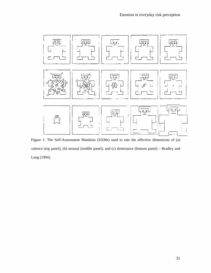
Emotional responses (i.e., 4) were measured using self-assessment manikins (SAMs)

(Bradley & Lang, 1994) – see Figure 1. These represent visually three basic dimensions of

emotions in reactions to events or situations. They are (a) valence (or pleasure), (b) arousal, and

(c) dominance. Participants simply checked the figure – or between adjacent figures – in each

line that corresponded most to their feelings (thereby implicitly using 9-point scales4).

--------------------------------------------- Figure 1 about here

---------------------------------------------

Our use of SAMs was based on theoretical, methodological, and practical considerations.

First, the three SAM dimensions have the advantage of covering a range of possible emotional

reactions to a situation and are theoretically based. To quote Bradley and Lang (1994):

….differences in affective meaning among stimuli – words, object, events – can be described by three basic dimensions that Wundt (1896) originally labeled lust (pleasure), spannung (tension), and beruhigung (inhibition). Following Wundt’s theoretical categories, empirical work has repeatedly confirmed that pleasure, arousal, and dominance are pervasive in organizing human judgments for a wide range of perceptual and symbolic stimuli. (p. 49).

Second, the SAMs have been shown to have good properties when validated against more

complete instruments (Bradley & Long, 1994). And third, the SAMs are quite intuitive and thus

easy for respondents to use. Given the lack of prior work linking the SAMs to risk perception,

we did not formulate specific hypotheses. However, given that our study focused on negative

consequences of risk, one might assume that “positive” emotions would be associated with less

risk. Thus our intuitions were that while greater feelings of pleasure and dominance would be

4 In coding, we labeled responses on the extreme left “1” and those on the extreme right “9”.


8

associated with lower perceived risk, more arousal would be associated with increases in

perceived risk.

After completing the task, participants were thanked, debriefed, and paid in a session in

which they classified some of their open-ended responses into categories we had established

previously and also re-assessed the severity, possibility, and risks associated with six activities

on which they had reported in the preceding weeks.

Study design

To control for possible response bias, we created two conditions – “long” and “short.” In the

long condition, participants answered questions in the order indicated above. In the short

condition, risk was assessed before emotional reactions (i.e., number 8 before number 4) and

there were no questions about the precise risk and its associated severity and possibility (i.e.,

numbers 5, 6, and 7). Thirty-four females were assigned at random to the first condition, and 30

to the second. All 30 males participated in the first condition.

Data analysis

The design of our study involved data that can be thought of as being collected at two levels.

One of these levels – termed level 1 – is represented by participants’ responses to the 30

occasions on which they received text messages (i.e., at the level of events). The other – level 2

– is at that of the participants themselves (i.e., characteristics of the participants that do not

change across the 30 events). Thus, for example, it is of interest to know whether, say, mood

state at the moment judgments are elicited are associated with assessments of risk (i.e., at level 1)

and also whether such judgments reflect differences between the participants in, say, gender (i.e.,


9

at level 2). As such, our data can be efficiently modeled using the techniques of hierarchical

linear models (Bryk & Raudenbush, 2002; Goldstein, 1995; Longford, 1994).

We motivate our use of hierarchical linear models (HLMs) with an example. Assume

we wish to model risk as being related to mood state (at level 1) but that this is moderated by

gender (at level 2).

Define the model at level 1 as

ijjijjjij rXXY +−+= )( .10 ββ (1)

where

Yij is the judgment of risk on the ith occasion (i = 1,.., 30) for the jth individual (j = 1,…, 94);

)( . jij XX − is the deviation of the reported mood stateijX on the ith occasion for the jth individual

from his or her average mood state jX. ;

j0β is the individual-specific intercept;

j1β is the individual-specific slope (regression coefficient) of Yij on )( . jij XX − ; and r ij is the

error term which we assume normally distributed with constant variance, ijr ∼N(0,σ2).

Define the model at level 2 as

β0 j = γ 00 + γ 01Zj + u0 j (2)

and

β1j = γ 10 + γ 11Zj + u1j (3)

where

Zj = gender of participant (0, female, or 1, male);

00γ is the constant part of the interceptj0β ;

01γ is the regression coefficient of j0β on Zj ;


10

u0j is an error term (the individual effect on judgments of risk);

10γ is the constant part of the slope j1β ;

11γ is the effect of gender on the slope j1β (i.e., the interaction of gender and mood state on

judgments of risk);

u1j is an individual error term, that is, the random interaction effect of individual j and mood

state on judgments of risk.

Thus, to interpret the above, 00γ is the average risk score across all women, while

00γ + 01γ is the average risk score across all men; 10γ is the average effect across women of mood

state on judgments of risk, while 10γ + 11γ represents the average effect across men of mood state

on judgments of risk. We assume that u0j and u1j are random variables with zero means,

variances 00τ and 11τ , respectively, and covariance 01τ ; they represent the variability in j0β

and j1β that remains after controlling for Zj . In addition, the level 2 error vector (u0j , u1j) is

assumed to have a bivariate normal distribution and to be independent of the level 1 error terms

r ij .

Substituting equations (2) and (3) into (1), we obtain

)-)(( .1111000100 ijjijjjjjij rXXuZuZY ++++++= γγγγ (4)

which can be re-arranged as

)()-()( .10.11.100100 ijjijjjjijjjijjij rXXuuXXZXXZY +−+++−++= γγγγ (5)

Note that, in the latter expression, one can distinguish the fixed part,

)-()( .11.100100 jijjjijj XXZXXZ γγγγ +−++ (with main effect for Z, main effect for X and


11

their interaction), from the random part, )( .10 ijjijjj rXXuu +−+ (with individual random

effect, random interaction between the j th individual and X, and occasion-specific error term).

We have only illustrated the model by considering one independent variable at level 1

(mood state) and one independent variable at level 2 (gender). However, it is straightforward to

construct more complete models by considering vectors of independent variables at both levels.

Finally, we note that our research design involves correlational data and does not permit

causal inferences. However, to obtain statistically consistent estimates, the hypothesis of

regression is that the dependent variable (here risk perception) is impacted by the independent

variables (here emotional variables, inter alia) as opposed to vice-versa. We therefore provide a

test of the consistency hypothesis (see below and Appendix).

RESULTS

From the 2,820 (= 94 x 10 x 3) messages sent, 2,809 were received (99.6%). On average,

participants responded between zero and ten minutes after reception (overall mean of one

minute). The distribution of types of activities and risks was similar to a previous study

(Hogarth, Portell, & Cuxart, 2007) and is not presented here.


12

Emotion: Mood and emotional reactions

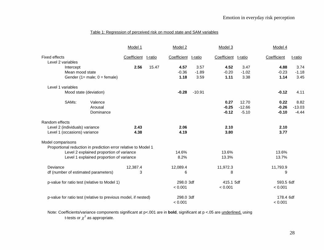
Table 1 reports HLM results of regressing perceived risk on mood and emotional reactions as

well as gender.5 We first note that we rescaled variables that were measured on a 0-100 scale to

a 0-10 scale (risk and possibility) in order to facilitate comparisons. We present four models.

--------------------------------------------- Table 1 about here

---------------------------------------------

Model 1 estimates the mean risk level of risk perception; this is 2.56 on a 0-10 scale.

In Model 2, we introduce mood state and gender. For mood state, we coded participants’

mean mood assessments across the 30 occasions to serve as a proxy for individual dispositions,

that is, a level 2 variable. At level 1, we use the deviations from these means. These mood

deviations are significant. In short, being in a better mood is associated with lower perceived

risk, a result that replicates earlier work (Hogarth et al., 2007). However, at level 2 there is no

significant dispositional effect for mood (i.e., mean mood state). In other words, there is no

relation between the mean level of participants’ mood assessments and their perceptions of risk.

Gender appears to play a role. On average, males give higher risk assessments than

females. This last result is contrary to most findings (Byrnes, Miller, & Schafer, 1999) including

our own (Hogarth et al., 2007) and we conclude it is a peculiarity of this sample.6

In Model 3, we substitute the SAM variables for mood state deviations at level 1. Given

the way these variables are scaled (see Figure 1), the coefficients imply that less risk is

5 All results of HLM in this paper are based on maximum likelihood estimation. Intercepts are estimated as random whereas slope coefficients are estimated as fixed. We have also conducted additional analyses where both intercept and slope coefficients are estimated as random. However, since this change of specification does not change our main results, they are not provided here. (More information on this point is available from the authors.) 6 We conducted several analyses to determine possible causes of this gender difference. In short, we found no significant difference in the types of losses faced by men and women. Moreover, we found a significant gender difference in risk assessment for only one of five job classifications. Female health and educational workers perceived significantly less risk, on average, than their male counterparts. This appears to drive the result that males give higher risk assessments than females. As it is only one job classification, we do not consider it important. (More information on this point is available from the authors.)


13

associated with greater valence (pleasure), more risk is associated with greater arousal, and less

risk is associated with more dominance. These are in accordance with out intuitions detailed

above.

Model 4 tests the joint effects of both the mood state deviations and the SAM variables.

All explain significant variance in perceived risk at level 1. However, there is some redundancy

between the two as demonstrated by the fact that the coefficient for mood state deviations is

diminished in the presence of the SAM variables (from -0.28 to -0.12).

Finally, whereas HLM regressions do not allow simple interpretations in terms of

conventional R2, we show the effects of the different classes of variables in terms of reduction in

estimated prediction error relative to Model 1. By this measure, at level 1 Model 2 (mood state

deviations) accounts for a reduction in variance of 8.2%, Model 3 (the SAM variables) accounts

for 13.3%, and Model 4 (mood state deviations and the SAM variables) 13.7%. 7

These results are important. They extend findings of the risk-emotion relation from

experimental and field studies to random samples of real-time, everyday judgments. Mood can

be thought of as operating at two levels – mean mood state (a dispositional measure of “how

happy” people are, on average) and mood state deviations (or specific momentary effects). We

found no effect for mean mood state (at level 2) but respondents perceived less risk when in a

more positive mood state (at level 1). However, mood deviations explain less variance than

emotional reactions. In our data, “happier” valence (left of Figure 1a) is associated with less

risk, as are less arousal (right of Figure 1b) and greater dominance (right of Figure 1c).

Although not provided here, we conducted further analyses to test for possible effects of

additional moderators as well as robustness. Of particular interest is the fact that questionnaire

7 In addition, Tables 1 and 2 include estimates of the level 2 proportion of variance. These measures are calculated as the proportional reduction of error for predicting an individual mean (mean perceived risk). For specific details about how these concepts were elaborated, see Snijders and Bosker (1999, ch.7).


14

type (“short” versus “long” – in which the order of questions about risk and emotional reactions

were reversed) had no significant effect. The conclusions stated above were not changed by

these additional analyses.8

Reason and emotion

From a rational perspective, perceived risk should reflect assessed severity and possibility of

risks (i.e., reason). If it does, what is the role of emotion (mood state and the SAM variables)?

Using data only from the (long) condition where participants provided assessments of severity

and possibility, we employ HLM to answer this question.

--------------------------------------------- Table 2 about here

---------------------------------------------

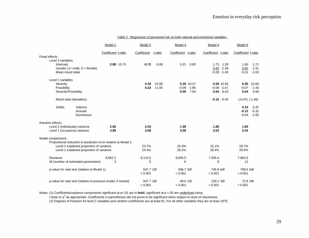
Table 2 reports results of five models that progressively introduce effects of reason and

emotion. Model 1 simply estimates the overall mean of risk judgments as 2.88. Model 2 shows

the separate effects of severity and possibility at level 1. Note this involves a reduction in

variance at level 1 of 24.4% compared to Model 1. Model 3 adds the interaction between

severity and possibility and the reduction in variance between Models 1 and 3 is now 26.2%.

Interestingly, Model 3 highlights (as one would expect) the importance of the severity x

possibility interaction. However, this is augmented by a main effect for severity (but not

possibility) that suggests more perceived risk for more severe events independent of their

probability of occurrence (Model 3).

Mood is introduced in Model 4. This shows that mood state deviations, by themselves,

add significant variance over and above reason even though the increase in reduction of variance

8 All of these additional analyses can be obtained from the authors.


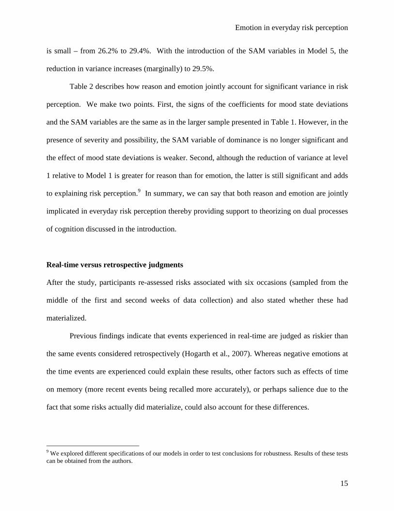
15

is small – from 26.2% to 29.4%. With the introduction of the SAM variables in Model 5, the

reduction in variance increases (marginally) to 29.5%.

Table 2 describes how reason and emotion jointly account for significant variance in risk

perception. We make two points. First, the signs of the coefficients for mood state deviations

and the SAM variables are the same as in the larger sample presented in Table 1. However, in the

presence of severity and possibility, the SAM variable of dominance is no longer significant and

the effect of mood state deviations is weaker. Second, although the reduction of variance at level

1 relative to Model 1 is greater for reason than for emotion, the latter is still significant and adds

to explaining risk perception.9 In summary, we can say that both reason and emotion are jointly

implicated in everyday risk perception thereby providing support to theorizing on dual processes

of cognition discussed in the introduction.

Real-time versus retrospective judgments

After the study, participants re-assessed risks associated with six occasions (sampled from the

middle of the first and second weeks of data collection) and also stated whether these had

materialized.

Previous findings indicate that events experienced in real-time are judged as riskier than

the same events considered retrospectively (Hogarth et al., 2007). Whereas negative emotions at

the time events are experienced could explain these results, other factors such as effects of time

on memory (more recent events being recalled more accurately), or perhaps salience due to the

fact that some risks actually did materialize, could also account for these differences.

9 We explored different specifications of our models in order to test conclusions for robustness. Results of these tests can be obtained from the authors.


16

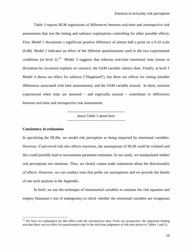
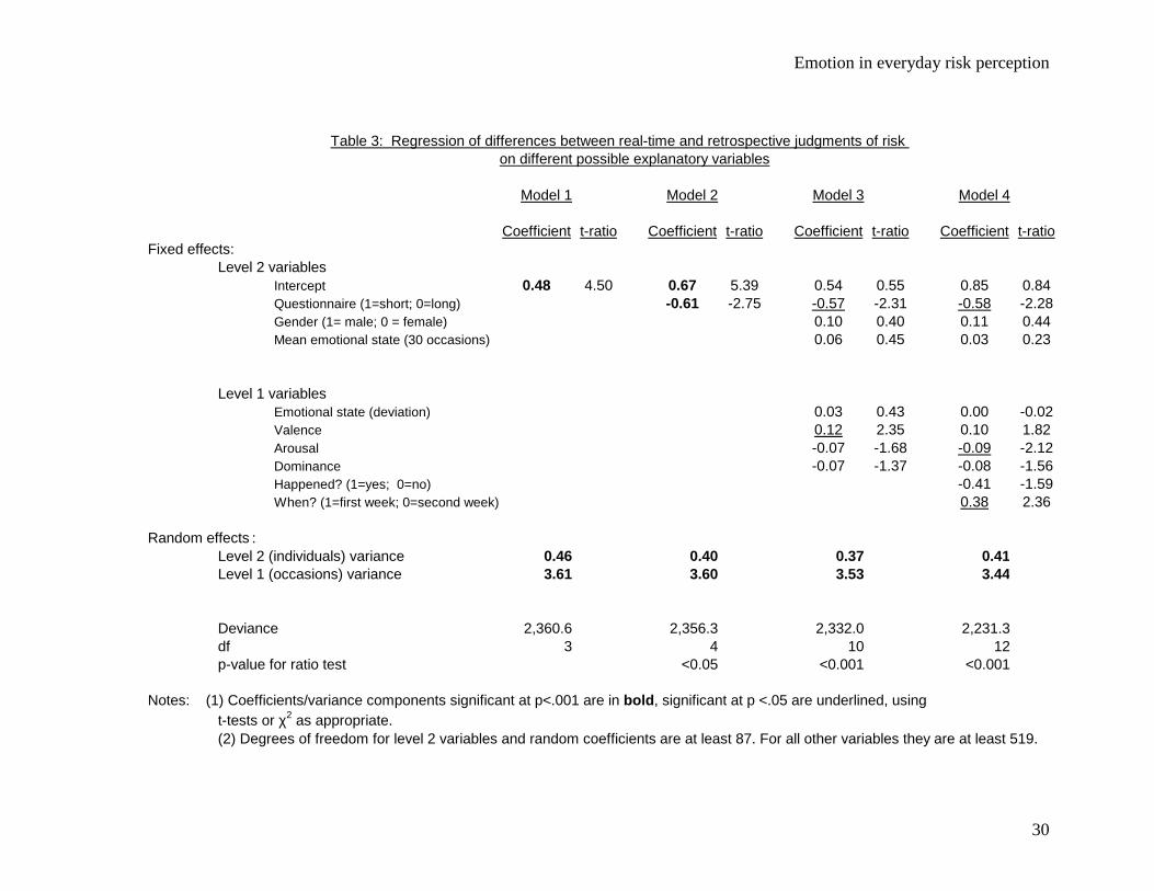
Table 3 reports HLM regressions of differences between real-time and retrospective risk

assessments that test the timing and salience explanations controlling for other possible effects.

First, Model 1 documents a significant positive difference of almost half a point on a 0-10 scale

(0.48). Model 2 indicates an effect of the different questionnaires used in the two experimental

conditions (at level 2).10 Model 3 suggests that whereas real-time emotional state (mean or

deviations by occasion) explains no variance, the SAM variable valence does. Finally, at level 1

Model 4 shows no effect for salience (“Happened”), but there are effects for timing (smaller

differences associated with later assessments), and the SAM variable arousal. In short, emotion

experienced when risks are assessed – and especially arousal – contributes to differences

between real-time and retrospective risk assessments.

---------------------------------------------- Insert Table 3 about here

----------------------------------------------

Consistency in estimation

In specifying the HLMs, we model risk perception as being impacted by emotional variables.

However, if perceived risk also affects emotions, the assumptions of HLM could be violated and

this could possibly lead to inconsistent parameter estimates. In our study, we manipulated neither

risk perceptions nor emotions. Thus, we clearly cannot make statements about the directionality

of effects. However, we can conduct tests that probe our assumptions and we provide the details

of one such analysis in the Appendix.

In brief, we use the technique of instrumental variables to estimate the risk equation and

employ Hausman’s test of endogeneity to check whether the emotional variables are exogenous

10 We have no explanation for this effect with the retrospective data. From our perspective, the important finding was that there was no effect for questionnaire type in the real-time judgments of risk (not shown in Tables 1 and 2).


17

(Hausman, 1978). We find we cannot reject the null hypothesis that the emotional variables are

exogenous in the risk equation.

In summary, the statistical tests conducted in the Appendix support the assumption that

the parameter estimates presented in the main body of the paper are consistent, and hence, the

conclusions we draw on the basis of the HLM regressions are valid.

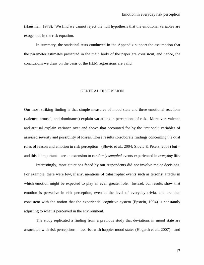
GENERAL DISCUSSION

Our most striking finding is that simple measures of mood state and three emotional reactions

(valence, arousal, and dominance) explain variations in perceptions of risk. Moreover, valence

and arousal explain variance over and above that accounted for by the “rational” variables of

assessed severity and possibility of losses. These results corroborate findings concerning the dual

roles of reason and emotion in risk perception (Slovic et al., 2004; Slovic & Peters, 2006) but –

and this is important – are an extension to randomly sampled events experienced in everyday life.

Interestingly, most situations faced by our respondents did not involve major decisions.

For example, there were few, if any, mentions of catastrophic events such as terrorist attacks in

which emotion might be expected to play an even greater role. Instead, our results show that

emotion is pervasive in risk perception, even at the level of everyday trivia, and are thus

consistent with the notion that the experiential cognitive system (Epstein, 1994) is constantly

adjusting to what is perceived in the environment.

The study replicated a finding from a previous study that deviations in mood state are

associated with risk perceptions – less risk with happier mood states (Hogarth et al., 2007) – and


18

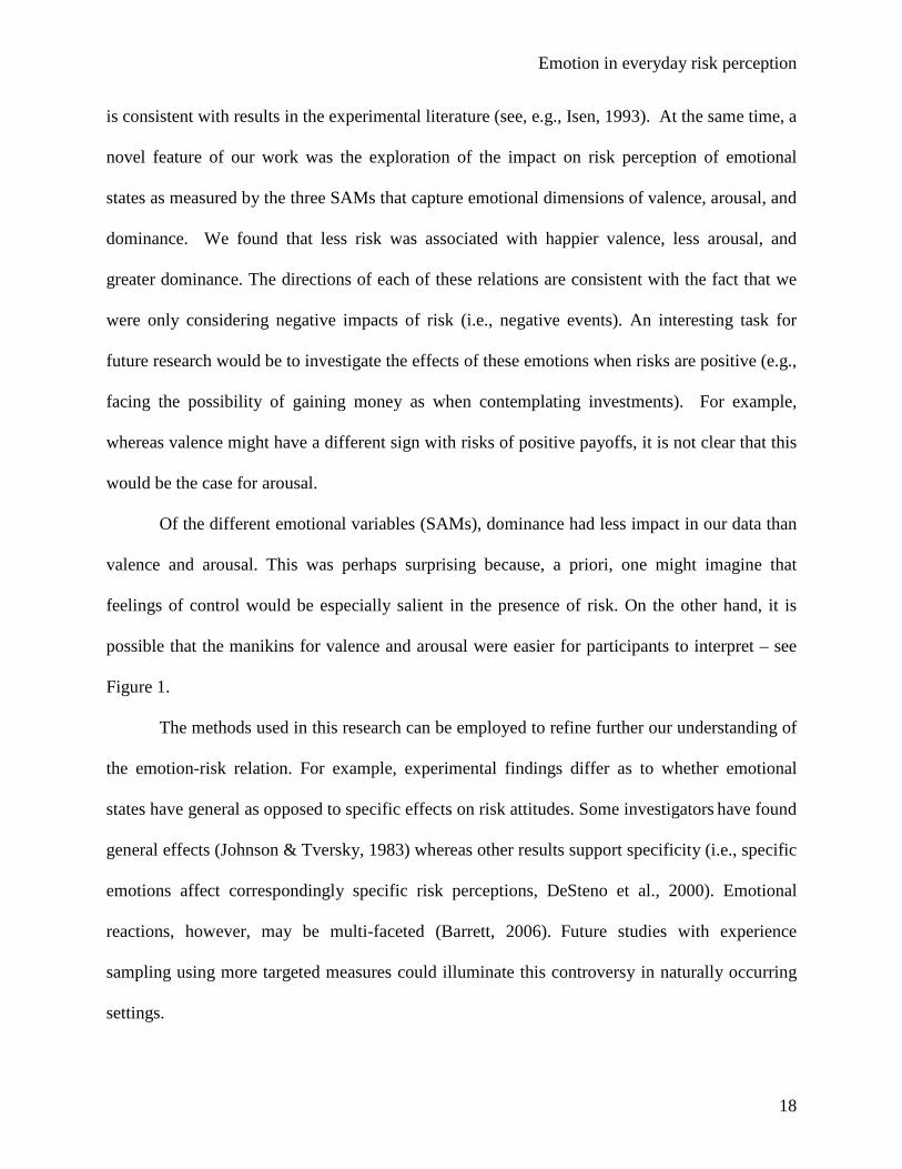
is consistent with results in the experimental literature (see, e.g., Isen, 1993). At the same time, a

novel feature of our work was the exploration of the impact on risk perception of emotional

states as measured by the three SAMs that capture emotional dimensions of valence, arousal, and

dominance. We found that less risk was associated with happier valence, less arousal, and

greater dominance. The directions of each of these relations are consistent with the fact that we

were only considering negative impacts of risk (i.e., negative events). An interesting task for

future research would be to investigate the effects of these emotions when risks are positive (e.g.,

facing the possibility of gaining money as when contemplating investments). For example,

whereas valence might have a different sign with risks of positive payoffs, it is not clear that this

would be the case for arousal.

Of the different emotional variables (SAMs), dominance had less impact in our data than

valence and arousal. This was perhaps surprising because, a priori, one might imagine that

feelings of control would be especially salient in the presence of risk. On the other hand, it is

possible that the manikins for valence and arousal were easier for participants to interpret – see

Figure 1.

The methods used in this research can be employed to refine further our understanding of

the emotion-risk relation. For example, experimental findings differ as to whether emotional

states have general as opposed to specific effects on risk attitudes. Some investigators have found

general effects (Johnson & Tversky, 1983) whereas other results support specificity (i.e., specific

emotions affect correspondingly specific risk perceptions, DeSteno et al., 2000). Emotional

reactions, however, may be multi-faceted (Barrett, 2006). Future studies with experience

sampling using more targeted measures could illuminate this controversy in naturally occurring

settings.


19

Real-time assessments of risks were found to be greater than those made retrospectively.

Our analysis demonstrated possible memory effects (more recent real-time assessments more

consistent with retrospective judgments). However, it also showed that emotion experienced

when risks were assessed (especially arousal) contributed to the observed differences. Given the

prevalence of retrospective and prospective surveys of risk attitudes, these results have important

implications (see also Stone et al., 1999).

The assumption of consistent estimation implicit in the regression analyses used in our

work implies that mood and emotions impact risk perception as opposed to the reverse. Clearly,

however, perceived risk can precede the experience of emotion. (Imagine, for example, how one

might feel after hearing, for the first time, about the severe risks of an impending surgical

intervention.) Nonetheless – and for the population of incidents we sampled – the hypothesis of

consistent estimation was not rejected by our statistical tests (see Appendix). At the same time,

we believe this issue needs further clarification and the use of a different experimental design to

illuminate the most probable directions of effects and possible mediating variables. It is

possible, for example, that whereas in some cases emotions impact perceived risk, in others it is

perceived risk that impacts emotion. Much depends therefore, on what kinds of situations are

sampled, something that our study explicitly did not control. On the other hand, we note that in

our experimental design we did vary the order in which the questions about the emotional

variables (SAMs) and perceived risk were elicited and found no effects.

It is important to emphasize that our methodology is based on the random sampling of

situations. This allows making meaningful statements about the populations of experiences of

our individual participants. As such, our investigation represents an illustration of the principles

of representative design (Brunswik, 1944; 1956) and addresses a critical drawback of many


20

studies of risk perception, namely, the inability to relate findings to the population of situations

in which they are relevant. Our study is not, however, without methodological shortcomings.

First, although the situations faced by our participants were sampled by a random process, the

participants themselves were a convenience sample and thus we cannot assume that they are

representative of the population at large. Clearly, the ideal study would sample both participants

and situations at random. Second, by asking our participants to record their emotional reactions

we might have unwittingly influenced their reports. Emotions have been shown to have

unconscious effects (Ruys & Stapel, 2008) and our study could have overlooked or

misinterpreted these.

A further issue is that our study only investigates risk perception and not actual decisions.

To what extent do mood and emotions affect decisions in the work place? This is an important

topic for future research since, based on experimental evidence, moods can affect decisions

(Isen, 1993; Slovic et al., 2002; Andrade & Ariely, 2009). Moreover, in an ingenious field study

of university admissions staff, Simonsohn (2007) found that decisions reflected mood changes

that could be attributed to fluctuations in weather patterns. Changes in cloud cover had

significant and systematic impacts on important decisions. Once again, however, we need to

establish the generality of these kinds of findings.

Our research demonstrates the power of simple technology to collect meaningful samples

of naturally occurring behavior. Contrary to modern ESM studies we did not use hand-held

computers or other “high-tech” devices. Instead, we relied on the participants’ own cellular

telephones and small paper-and-pencil response pads.11 Our impression was that participants

would have found responding on special hand-held computers to be more intrusive than our

11 We did however use a special computer program to dispatch messages indicating when responses were required.


21

procedure. Indeed, since all of our participants always carried a cellular telephone on their person

anyway, the addition of a small pad was a minimal distraction.

Finally, it is interesting to speculate how future technology might enrich these kinds of

studies. For example, it is not hard to imagine devices that will be able to capture biological

measurements of emotion that can corroborate the paper-and-pencil responses provided by our

participants. As such, we can expect even greater scientific returns from studies based on the

principles of representative design (Dhami et al., 2004).


22

REFERENCES

Andrade, E. B., & Ariely, D. (2009). The enduring effect of transient emotions on decision

making. Organizational Behavior and Human Decision Processes, 109 (1), 1-8.

Balestra, P., & Varadharajan-Krishnakumar, J. (1987). Full Information Estimations of a System

of Simultaneous Equations with Error Component Structure. Econometric Theory, 3(2),

223-246.

Barrett, L. F. (2006). Are emotions natural kinds? Perspectives on Psychological Science, 1 (1),

28-58.

Bradley, M. M., & Lang, P. J. (1994). Measuring emotion: The self-assessment manikin and the

semantic differential. Journal of Behavioral Therapy and Experiential Psychiatry, 25, 49-

59.

Brunswik, E. (1944) Distal focusing of perception: Size constancy in a representative sample of

situations, Psychological Monographs, 56(254), 1–49.

Brunswik, E. (1956). Perception and the representative design of experiments (2d ed.). Berkeley,

CA: University of California Press.

Byrk, A. S., & Raudenbush, S. W. (2002). Hierarchical linear models: Applications and data

analysis methods. (2nd ed.). Newbury Park: Sage Publications.

Byrnes, J. P., Miller, D. C., & Schafer, W.D. (1999). Gender differences in risk taking: A meta-

analysis. Psychological Bulletin, 125(3), 367-383.

Chaiken, S., & Trope, Y. (1999). (Eds.) Dual-process theories in social psychology. New York,

NY: Guilford.


23

Denissen, J.J., Butalid, L., Penke, L. & van Aken, M.A. (2008). The effects of weather on daily

mood: a multilevel approach. Emotion, 8(5), 662-667.

DeSteno, D., Petty, R. E., Wegner, D. T., & Rucker, D. D. (2000). Beyond valence in the

perception of likelihood: The role of emotion specificity. Journal of Personality and

Social Psychology, 78 (3), 397-416.

Dhami, M. K., Hertwig, R., & Hoffrage, U. (2004). The role of representative design in an

ecological approach to cognition. Psychological Bulletin, 130 (6), 959-988.

Epstein, S. (1994). Integration of the cognitive and psychological unconscious. American

Psychologist, 49, 709-724.

Goldstein, H. (1995). Multilevel statistical models. (2nd ed.). Kendall’s Library of Statistics 3.

London, UK: Edward Arnold.

Hausman, J.A. (1978). Specification tests in econometrics, Econometrica, 46 (6), 1251-1271.

Hektner, J. M., Schmidt, J. A., & Csikszentmihayli, M. (2007). Experience sampling method:

Measuring the quality of everyday life. Thousand Oaks, CA: Sage Publications.

Hirshleifer, D. & Shumway, T. (2003). Good Day Sunshine: Stock Returns and the Weather.

Journal of Finance, 58(3),1009-1032.

Hogarth, R. M. (2005). The challenge of representative design in psychology and economics.

Journal of Economic Methodology, 12 (2), 253-263.

Hogarth, R. M., Portell, M., & Cuxart, A. (2007). What risks do people perceive in everyday

life? A perspective gained from the experience sampling method (ESM). Risk Analysis,

27(6), 1427-1439.

Howarth, E. & Hoffman, M. S., (1984). A multidimensional approach to the relationship

between mood and weather. British Journal of Psychology, 75(1), 15-23.


24

Hsee, C . K., & Kunreuther, H. C. (2000). The affection effect in insurance decisions. Journal of

Risk and Uncertainty, 20 (2), 141-159.

Hurlburt, R. T. (1997). Randomly sampling thinking in the natural environment. Journal of

Consulting and Clinical Psychology, 67 (6), 941-949.

Isen, A. M. (1993). Positive affect and decision making. In M. Lewis & J. M. Haviland (Eds.),

Handbook of emotions (pp. 261-277). New York, NY: Guilford Press.

Johnson, E. J., & Tversky, A. (1983). Affect, generalization, and the perception of risk. Journal

of Personality and Social Psychology, 45 (1), 20-31.

Kahneman, D., & Frederick, S. (2002). Representativeness revisited: Attribute substitution in

intuitive judgment. In T. Gilovich, D. Griffin, & D. Kahneman (Eds.), Heuristics and

biases: The psychology of intuitive judgment (pp.49-81), New York, NY: Cambridge

University Press.

Keller, M. C., Fredrickson, B. L., Ybarra, O., Côté, S., Johnson, K., Mikels, J., Conway, A. &

Wager, T. (2005). A Warm Heart and a Clear Head The Contingent Effects of Weather

on Mood and Cognition, Psychological Science,16(9), 724-731.

Lerner, J. S., Gonzalez, R. M., Small, D. A., & Fischhoff, B. (2003). Effects of fear and anger on

perceived risks of terrorism: A national field experiment. Psychological Science, 14 (2),

144-150.

Loewenstein, G.F., Weber, E. U., Hsee, C. K., Welch, N. (2001). Risk as feelings. Psychological

Bulletin, 127(2), 267-286.

Longford, N.T. (1993). Random coefficient models. Oxford: Oxford University Press.


25

Rottenstreich, Y., & Hsee, C. K. (2001). Money, kisses, and electric shocks: On the affective

psychology of probability weighting. Psychological Science, 12, 185-190.

Ruys, K. I., & Stapel, D. A. (2008). The secret life of emotions. Psychological Science, 19(4), 385-

391.

Sanders, J.L., & Brizzolara, M.S. (1982). Relationships between weather and mood. Journal of

General Psychology, 107, 155-156.

Saunders, E. M., Jr. (1993). Stock Prices and Wall Street Weather. American Economic Review,

83(5), 1337-1345

Simonsohn, U. (2007). Clouds make nerds look good: Field evidence of the impact of incidental

factors on decision making. Journal of Behavioral Decision Making, 20 (2), 143-152.

Slovic, P. (2000). The perception of risk. London, UK: Earthscan Publications Ltd.

Slovic, P., Finucane, M. L., Peters, E., & MacGregor, D. G. (2004). Risk as analysis and risk as

feelings: Some thoughts about affect, reason, risk, and rationality. Risk Analysis, 24 (2), 311-

322.

Slovic, P., & Peters, E. (2006). Risk perception and affect. Current Directions in Psychological

Science, 15(6), 322-325.

Slovic, P., Finucane, M., Peters, E., & MacGregor, D. (2002). The affect heuristic. In T.

Gilovich, D. Griffin, & D. Kahneman (Eds.). Intuitive judgment: Heuristics and biases

(pp. 397-420). New York, NY: Cambridge University Press.

Snijders, T., & R. Bosker (1999). Multilevel Analysis. An introduction to basic and advanced

multilevel modeling. London: SAGE Publications.


26

Stone, A. A., Shiffman, S. S., & DeVries, M. W. (1999). Ecological momentary assessment. In

D. Kahneman, E. Diener, & N. Schwartz (Eds.). Well-being: The foundations of hedonic

psychology (pp. 26-39). New York, NY: Russell Sage.

Sunstein, C. R. (2003). Terrorism and probability neglect. Journal of Risk and Uncertainty, 26

(2/3), 121-136.

Wooldridge, J. M. (2002). Econometric analysis of cross section and panel data. Cambridge,

MA: MIT press.


27

Author Note

Robin M. Hogarth, ICREA & Universitat Pompeu Fabra; Mariona Portell, Universitat Autònoma

de Barcelona; Anna Cuxart, Universitat Pompeu Fabra; Gueorgui I. Kolev, Universitat Pompeu

Fabra. Address correspondence to Robin M. Hogarth, Universitat Pompeu Fabra, Ramon Trias

Fargas 25-27, 08005 Barcelona, Spain, e-mail: [email protected]

We thank Joshua Klayman and Ellen Peters for their insightful comments. The research was

supported by the Spanish Ministerio de Educación y Ciencia, SEJ2006-27587-E/SOCI (to

Hogarth).


28

Table 1: Regression of perceived risk on mood state and SAM variables

Model 1 Model 2 Model 3 Model 4

Fixed effects Coefficient t-ratio Coefficient t-ratio Coefficient t-ratio Coefficient t-ratioLevel 2 variables

Intercept 2.56 15.47 4.57 3.57 4.52 3.47 4.88 3.74Mean mood state -0.36 -1.89 -0.20 -1.02 -0.23 -1.18Gender (1= male; 0 = female) 1.18 3.59 1.11 3.38 1.14 3.45

Level 1 variablesMood state (deviation) -0.28 -10.91 -0.12 4.11

SAMs: Valence 0.27 12.70 0.22 8.82Arousal -0.25 -12.66 -0.26 -13.03Dominance -0.12 -5.10 -0.10 -4.44

Random effectsLevel 2 (individuals) variance 2.43 2.06 2.10 2.10Level 1 (occasions) variance 4.38 4.19 3.80 3.77

Model comparisonsProportional reduction in prediction error relative to Model 1

Level 2 explained proportion of variance 14.6% 13.6% 13.6%Level 1 explained proportion of variance 8.2% 13.3% 13.7%

Deviance 12,387.4 12,089.4 11,972.3 11,793.9df (number of estimated parameters) 3 6 8 9

p-value for ratio test (relative to Model 1) 298.0 3df 415.1 5df 593.5 6df< 0.001 < 0.001 < 0.001

p-value for ratio test (relative to previous model, if nested) 298.0 3df 178.4 6df< 0.001 < 0.001

Note: Coefficients/variance components significant at p<.001 are in bold, significant at p <.05 are underlined, using t-tests or χ 2 as appropriate.


29

Table 2: Regression of perceived risk on both rational and emotional variables

Model 1 Model 2 Model 3 Model 4 Model 5

Coefficient t-ratio Coefficient t-ratio Coefficient t-ratio Coefficient t-ratio Coefficient t-ratioFixed effects:

Level 2 variablesIntercept 2.88 13.70 -0.72 -3.08 0.21 0.80 1.73 1.28 1.65 1.71Gender (1= male; 0 = female) 0.83 2.39 0.82 2.31Mean mood state -0.28 -1.43 -0.21 -1.03

Level 1 variablesSeverity 0.44 22.99 0.29 10.27 0.30 10.56 0.30 10.69Possibility 0.22 11.05 -0.09 -1.86 -0.08 -1.67 -0.07 -1.43Severity*Possibility 0.05 7.04 0.04 6.43 0.04 5.68

Mood state (deviation) -0.15 -5.45 (-0.07) (-1.99)

SAMs: Valence 0.15 5.37Arousal -0.12 -5.31Dominance -0.04 -1.55

Random effects:Level 2 (individuals) variance 2.66 2.03 1.99 1.80 1.90Level 1 (occasions) variance 4.89 3.68 3.58 3.53 3.42

Model comparisonsProportional reduction in prediction error relative to Model 1

Level 2 explained proportion of variance 23.7% 25.3% 32.1% 28.7%Level 1 explained proportion of variance 24.4% 26.2% 29.4% 29.5%

Deviance 8,662.2 8,114.5 8,065.5 7,935.4 7,862.6df (number of estimated parameters) 3 5 6 9 12

p-value for ratio test (relative to Model 1) 547.7 2df 596.7 3df 726.8 6df 799.6 9df< 0.001 < 0.001 < 0.001 < 0.001

p-value for ratio test (relative to previous model, if nested) 547.7 2df 49.0 1df 130.1 3df 72.8 3df< 0.001 < 0.001 < 0.001 < 0.001

Notes: (1) Coefficients/variance components significant at p<.01 are in bold, significant at p <.05 are underlined using t-tests or χ2 as appropriate. Coefficients in parentheses did not prove to be significant when subject to tests of robustness.(2) Degrees of freedom for level 2 variables and random coefficients are at least 61. For all other variables they are at least 1875.


30

Table 3: Regression of differences between real-time and retrospective judgments of risk on different possible explanatory variables

Model 1 Model 2 Model 3 Model 4

Coefficient t-ratio Coefficient t-ratio Coefficient t-ratio Coefficient t-ratioFixed effects:

Level 2 variablesIntercept 0.48 4.50 0.67 5.39 0.54 0.55 0.85 0.84Questionnaire (1=short; 0=long) -0.61 -2.75 -0.57 -2.31 -0.58 -2.28Gender (1= male; 0 = female) 0.10 0.40 0.11 0.44Mean emotional state (30 occasions) 0.06 0.45 0.03 0.23

Level 1 variablesEmotional state (deviation) 0.03 0.43 0.00 -0.02Valence 0.12 2.35 0.10 1.82Arousal -0.07 -1.68 -0.09 -2.12Dominance -0.07 -1.37 -0.08 -1.56Happened? (1=yes; 0=no) -0.41 -1.59When? (1=first week; 0=second week) 0.38 2.36

Random effects :Level 2 (individuals) variance 0.46 0.40 0.37 0.41Level 1 (occasions) variance 3.61 3.60 3.53 3.44

Deviance 2,360.6 2,356.3 2,332.0 2,231.3df 3 4 10 12p-value for ratio test <0.05 <0.001 <0.001

Notes: (1) Coefficients/variance components significant at p<.001 are in bold, significant at p <.05 are underlined, using t-tests or χ2 as appropriate.(2) Degrees of freedom for level 2 variables and random coefficients are at least 87. For all other variables they are at least 519.


31

Figure 1: The Self-Assessment Manikins (SAMs) used to rate the affective dimensions of (a)

valence (top panel), (b) arousal (middle panel), and (c) dominance (bottom panel) – Bradley and

Lang (1994).


32

Appendix

In the main body of the paper we assume that mood and emotions are exogenous

regressors and we estimate their impact on risk assessments. However, in principle it is

conceivable that risk assessment could also impact mood and emotions. For example, if

learning the high risks of a medical operation leads to a worse mood, then mood would

be an endogenous regressor, and we would incorrectly attribute the negative correlation

between mood and risk to the impact of mood on risk (better mood leading to lower risk

assessment), when in reality the opposite holds true (i.e., higher risk leading to worse

mood). We use IV (instrumental variable) estimation to estimate consistently the

population parameters that reflect the impact of mood and emotions on risk assessments,

even if the exogeneity assumption is violated.

We estimate via GLS (generalized least squares) the parameters in the hierarchical

linear models presented in the paper that can be described by the following structural

equation

Rij = Xij β1 + Zj β2+ cj + εij (A1)

defined over individuals j = 1, 2, .…,94 and occasions i = 1, 2, …,30.

� Rij is the risk assessment of person j at occasion i;

� X it = [Xijm Xij

v Xija Xij

d] is a row vector containing the measurements on mood

deviations, valence, arousal and dominance respectively, for person j on occasion i;

� Zj is a row vector containing the mean mood state, female dummy variable, and a

constant;

� β1, β2 are column vectors of population parameters of dimension conformable for

multiplication;


33

� cj is an unobservable individual specific random effect;

� εij is the idiosyncratic random shock to risk assessment for person j at occasion i.

For GLS to estimate consistently the population parameters of interest, the

regressors must be strictly exogenous. That is, the following condition must be satisfied

in equation (A1):

E{( cj + εij )| [X1j, X2j, …, X30j , Zj]} = 0. (A2)

Regressors in a fully simultaneous system typically violate this condition, e.g., if

risk assessments also impact mood deviations. When (A2) is violated, e.g., if the error

term is correlated with mood deviations, we call the problematic regressor (mood

deviation in this example) an endogenous regressor. IV estimation relies on finding for

each potentially endogenous regressor one or more variables,12 called instruments, which

are properly excluded from the structural equation of interest (i.e., instruments do not

have structural impact on the dependent variable after all relevant exogenous and

endogenous regressors have been controlled for in the structural equation of interest).

Instruments have to satisfy the following two conditions: a) they are partially correlated

with the endogenous regressor; b) they are uncorrelated with the error term.

We use weather variables and dummy variables denoting the time of the day when

the responses were elicited as exogenous shifters of mood and emotional reactions. There

is previous research showing effects of weather on mood (Howarth & Hoffman, 1984;

Sanders & Brizzolara, 1982; Keller et al., 2005; Denissen et al., 2008) and research in

finance showing that the weather where the stock exchange floor is located affects stock

12 If in the equation of interest we have found exactly one instrument for each endogenous regressor, the equation is exactly identified. If we have more instruments than endogenous regressors, the equation is over-identified.


34

returns, the implication being that the mood of traders at the stock exchange floor is a

mediator between weather and returns (Saunders, 1993; Hirshleifer & Shumway, 2003).

The weather variables that we use are temperature, tsunshine (daily total sunshine

hours), and psunshine (sunshine hours as a percentage out of total expected). As the

weather variables vary only across days (i.e., all the people and occasions within the

same day are exposed to the same weather), we construct our instruments from the

weather variables and additionally from their interactions with the regressors which we

assume to be exogenous (uncorrelated with the error term), gender and the mean mood

state, the latter being a proxy for personal disposition. This way we end up with

instruments which employ the idea that weather and time of the day are exogenous

shifters of mood and emotional reactions, but have both time series and cross sectional

variation.

Therefore in the IV regressions we assume that the composite error in equation

(A1) is exogenous with respect to the instruments constructed from weather variables,

(temperature, tsunshine, psunshine, the interactions of these three with gender and the

mean mood state), and the dummy variables denoting the time of the day during which

messages were dispatched. We denote these instruments by the vector Wit where

E[( cj + εij )| W1j, W2j, …, W30j, Zj] = 0. (A3)

That is, the composite error in the risk equation is mean-independent of the weather and

time of the day induced variation.

We use as an estimation technique the G2SLS estimator of Balestra and

Varadharajan-Krishnakumar (1987), which is an Instrumental Variable version of the

Generalized Least Squares personal random effects model we employ in the main body


35

of the paper, and is an estimation technique appropriate under the orthogonality condition

(A3).

We implement Hausman’s (1978) test of endogeneity, comparing all the

coefficients except the constant across the GLS and IV estimators.

The over-identifying restrictions test for the IV estimators involves the statistic

N*R2 from the auxiliary regression of the IV composite residuals (i.e., the predicted

values of ci + εit) on all the exogenous variables (including all the instruments), where N

is the number of available observations. The statistic is distributed as χ2 with degrees of

freedom equal to the number of over-identifying restrictions (Wooldridge, 2002, p.123).

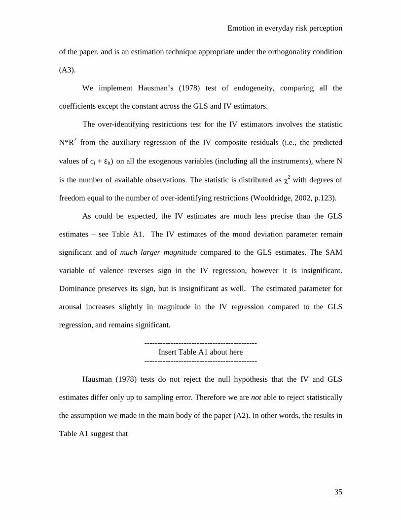
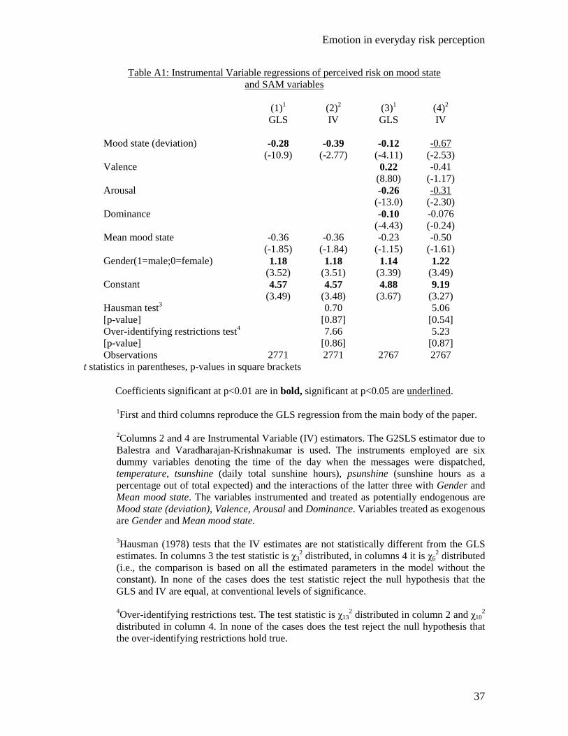
As could be expected, the IV estimates are much less precise than the GLS

estimates – see Table A1. The IV estimates of the mood deviation parameter remain

significant and of much larger magnitude compared to the GLS estimates. The SAM

variable of valence reverses sign in the IV regression, however it is insignificant.

Dominance preserves its sign, but is insignificant as well. The estimated parameter for

arousal increases slightly in magnitude in the IV regression compared to the GLS

regression, and remains significant.

------------------------------------------- Insert Table A1 about here

-------------------------------------------

Hausman (1978) tests do not reject the null hypothesis that the IV and GLS

estimates differ only up to sampling error. Therefore we are not able to reject statistically

the assumption we made in the main body of the paper (A2). In other words, the results in

Table A1 suggest that


36

i) the working assumption that mood deviations and the SAM variables are

exogenous is reasonable and cannot be statistically rejected

ii) if anything, we might underestimate somewhat the impact of mood

deviations on risk assessments in the main body of the paper13

iii) both the GLS and IV yield similar and significant estimates of the effect

of arousal

iv) our instruments do not induce much variation in valence and dominance,

and hence in the IV regressions we are not able to estimate precisely the

separate effects of valence and dominance.

The over-identifying restrictions tests do not reject the validity of the instruments. We do

not find statistical evidence suggesting that our instruments are a poor choice.

Since our study is not experimental, we clearly cannot confirm or disconfirm

beyond any doubt the direction of effects of mood deviation and the SAMs to risk or

vice-versa. However, the outcomes of the statistical tests presented in this appendix point

to the fact that the parameter estimates that we report in the main body of the paper are

consistent.

13 The larger estimated effect of mood in the IV regression might be simply a result of sampling error. However if we focus only on the magnitude of the parameter estimate, it somewhat counterintuitively suggests that if risk assessment has an impact on mood, the effect would be surprising: namely, higher risk implying better mood.


37

Table A1: Instrumental Variable regressions of perceived risk on mood state and SAM variables

(1)1 (2)2 (3)1 (4)2

GLS IV GLS IV Mood state (deviation) -0.28 -0.39 -0.12 -0.67 (-10.9) (-2.77) (-4.11) (-2.53) Valence 0.22 -0.41 (8.80) (-1.17) Arousal -0.26 -0.31 (-13.0) (-2.30) Dominance -0.10 -0.076 (-4.43) (-0.24) Mean mood state -0.36 -0.36 -0.23 -0.50 (-1.85) (-1.84) (-1.15) (-1.61) Gender(1=male;0=female) 1.18 1.18 1.14 1.22 (3.52) (3.51) (3.39) (3.49) Constant 4.57 4.57 4.88 9.19 (3.49) (3.48) (3.67) (3.27) Hausman test3 0.70 5.06 [p-value] [0.87] [0.54] Over-identifying restrictions test4 7.66 5.23 [p-value] [0.86] [0.87] Observations 2771 2771 2767 2767

t statistics in parentheses, p-values in square brackets

Coefficients significant at p<0.01 are in bold, significant at p<0.05 are underlined.

1First and third columns reproduce the GLS regression from the main body of the paper. 2Columns 2 and 4 are Instrumental Variable (IV) estimators. The G2SLS estimator due to Balestra and Varadharajan-Krishnakumar is used. The instruments employed are six dummy variables denoting the time of the day when the messages were dispatched, temperature, tsunshine (daily total sunshine hours), psunshine (sunshine hours as a percentage out of total expected) and the interactions of the latter three with Gender and Mean mood state. The variables instrumented and treated as potentially endogenous are Mood state (deviation), Valence, Arousal and Dominance. Variables treated as exogenous are Gender and Mean mood state. 3Hausman (1978) tests that the IV estimates are not statistically different from the GLS estimates. In columns 3 the test statistic is χ3

2 distributed, in columns 4 it is χ62 distributed

(i.e., the comparison is based on all the estimated parameters in the model without the constant). In none of the cases does the test statistic reject the null hypothesis that the GLS and IV are equal, at conventional levels of significance. 4Over-identifying restrictions test. The test statistic is χ13

2 distributed in column 2 and χ102

distributed in column 4. In none of the cases does the test reject the null hypothesis that the over-identifying restrictions hold true.

Emotion and reason in everyday risk perception

Documents