Emissions of organic air toxics from open burning: a comprehensive review Paul M. Lemieux a, * , Christopher C. Lutes b , Dawn A. Santoianni b a National Risk Management Research Laboratory, Air Pollution Prevention and Control Division, Office of Research and Development, United States Environmental Protection Agency, 109 TW Alexander Drive, Mail Code E305-01, Research Triangle Park, NC 27711, USA b ARCADIS G&M, 4915 Prospectus Drive, Durham, NC 27713, USA Received 15 December 2002; accepted 14 August 2003 Abstract Emissions from open burning, on a mass pollutant per mass fuel (emission factor) basis, are greater than those from well-controlled combustion sources. Some types of open burning (e.g. biomass) are large sources on a global scale in comparison to other broad classes of sources (e.g. mobile and industrial sources). A detailed literature search was performed to collect and collate available data reporting emissions of organic air toxics from open burning sources. The sources that were included in this paper are: Accidental Fires, Agricultural Burning of Crop Residue, Agricultural Plastic Film, Animal Carcasses, Automobile Shredder Fluff Fires, Camp Fires, Car – Boat– Train (the vehicle not cargo) Fires, Construction Debris Fires, Copper Wire Reclamation, Crude Oil and Oil Spill Fires, Electronics Waste, Fiberglass, Fireworks, Grain Silo Fires, Household Waste, Land Clearing Debris (biomass), Landfills/Dumps, Prescribed Burning and Savanna/Forest Fires, Structural Fires, Tire Fires, and Yard Waste Fires. Availability of data varied according to the source and the class of air toxics of interest. Volatile organic compound (VOC) and polycyclic aromatic hydrocarbon (PAH) data were available for many of the sources. Non-PAH semi-volatile organic compound (SVOC) data were available for several sources. Carbonyl and polychlorinated dibenzo-p-dioxins and polychlorinated dibenzofuran (PCDD/F) data were available for only a few sources. There were several known sources for which no emissions data were available at all. It is desirable that emissions from those sources be tested so that the relative degree of hazard they pose can be assessed. Several observations were made including: Biomass open burning sources typically emitted less VOCs than open burning sources with anthropogenic fuels on a mass emitted per mass burned basis, particularly those where polymers were concerned. Biomass open burning sources typically emitted less SVOCs and PAHs than anthropogenic sources on a mass emitted per mass burned basis. Burning pools of crude oil and diesel fuel produced significant amounts of PAHs relative to other types of open burning. PAH emissions were highest when combustion of polymers was taking place. Based on very limited data, biomass open burning sources typically produced higher levels of carbonyls than anthropogenic sources on a mass emitted per mass burned basis, probably due to oxygenated structures resulting from thermal decomposition of cellulose. It must be noted that local burn conditions could significantly change these relative levels. Based on very limited data, PCDD/F and other persistent bioaccumulative toxic (PBT) emissions varied greatly from source to source and exhibited significant variations within source categories. This high degree of variation is likely due to a combination of factors, including fuel composition, fuel heating value, bulk density, oxygen transport, and combustion conditions. This highlights the importance of having acceptable test data for PCDD/F and PBT emissions from open burning so that contributions of sources to the overall PCDD/F and PBT emissions inventory can be better quantified. q 2003 Elsevier Ltd. All rights reserved. Keywords: Uncontrolled combustion; Open burning; HAPS; Air toxics; Emissions 0360-1285/$ - see front matter q 2003 Elsevier Ltd. All rights reserved. doi:10.1016/j.pecs.2003.08.001 Progress in Energy and Combustion Science 30 (2004) 1–32 www.elsevier.com/locate/pecs * Corresponding author. Tel.: þ 1-919-541-0962; fax: þ1-919-541-0554. E-mail address: [email protected] (P.M. Lemieux).

Emissions Open Burning Lemieux Etal 2004
Oct 12, 2014
Welcome message from author
This document is posted to help you gain knowledge. Please leave a comment to let me know what you think about it! Share it to your friends and learn new things together.
Transcript

Emissions of organic air toxics from open burning:
a comprehensive review
Paul M. Lemieuxa,*, Christopher C. Lutesb, Dawn A. Santoiannib
aNational Risk Management Research Laboratory, Air Pollution Prevention and Control Division, Office of Research and Development,
United States Environmental Protection Agency, 109 TW Alexander Drive, Mail Code E305-01, Research Triangle Park, NC 27711, USAbARCADIS G&M, 4915 Prospectus Drive, Durham, NC 27713, USA
Received 15 December 2002; accepted 14 August 2003
Abstract
Emissions from open burning, on a mass pollutant per mass fuel (emission factor) basis, are greater than those from
well-controlled combustion sources. Some types of open burning (e.g. biomass) are large sources on a global scale in
comparison to other broad classes of sources (e.g. mobile and industrial sources). A detailed literature search was performed to
collect and collate available data reporting emissions of organic air toxics from open burning sources. The sources that were
included in this paper are: Accidental Fires, Agricultural Burning of Crop Residue, Agricultural Plastic Film, Animal Carcasses,
Automobile Shredder Fluff Fires, Camp Fires, Car–Boat–Train (the vehicle not cargo) Fires, Construction Debris Fires,
Copper Wire Reclamation, Crude Oil and Oil Spill Fires, Electronics Waste, Fiberglass, Fireworks, Grain Silo Fires, Household
Waste, Land Clearing Debris (biomass), Landfills/Dumps, Prescribed Burning and Savanna/Forest Fires, Structural Fires,
Tire Fires, and Yard Waste Fires. Availability of data varied according to the source and the class of air toxics of interest.
Volatile organic compound (VOC) and polycyclic aromatic hydrocarbon (PAH) data were available for many of the sources.
Non-PAH semi-volatile organic compound (SVOC) data were available for several sources. Carbonyl and polychlorinated
dibenzo-p-dioxins and polychlorinated dibenzofuran (PCDD/F) data were available for only a few sources. There were several
known sources for which no emissions data were available at all. It is desirable that emissions from those sources be tested so
that the relative degree of hazard they pose can be assessed. Several observations were made including:
Biomass open burning sources typically emitted less VOCs than open burning sources with anthropogenic fuels on a mass
emitted per mass burned basis, particularly those where polymers were concerned. Biomass open burning sources typically
emitted less SVOCs and PAHs than anthropogenic sources on a mass emitted per mass burned basis. Burning pools of crude oil
and diesel fuel produced significant amounts of PAHs relative to other types of open burning. PAH emissions were highest
when combustion of polymers was taking place. Based on very limited data, biomass open burning sources typically produced
higher levels of carbonyls than anthropogenic sources on a mass emitted per mass burned basis, probably due to oxygenated
structures resulting from thermal decomposition of cellulose.
It must be noted that local burn conditions could significantly change these relative levels. Based on very limited data,
PCDD/F and other persistent bioaccumulative toxic (PBT) emissions varied greatly from source to source and exhibited
significant variations within source categories. This high degree of variation is likely due to a combination of factors, including
fuel composition, fuel heating value, bulk density, oxygen transport, and combustion conditions. This highlights the importance
of having acceptable test data for PCDD/F and PBT emissions from open burning so that contributions of sources to the overall
PCDD/F and PBT emissions inventory can be better quantified.
q 2003 Elsevier Ltd. All rights reserved.
Keywords: Uncontrolled combustion; Open burning; HAPS; Air toxics; Emissions
0360-1285/$ - see front matter q 2003 Elsevier Ltd. All rights reserved.
doi:10.1016/j.pecs.2003.08.001
Progress in Energy and Combustion Science 30 (2004) 1–32
www.elsevier.com/locate/pecs
* Corresponding author. Tel.: þ1-919-541-0962; fax: þ1-919-541-0554.
E-mail address: [email protected] (P.M. Lemieux).
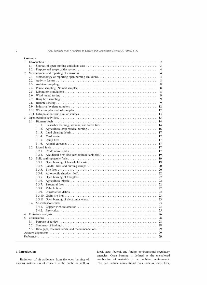
Contents
1. Introduction . . . . . . . . . . . . . . . . . . . . . . . . . . . . . . . . . . . . . . . . . . . . . . . . . . . . . . . . . . . . . . . . . . . 2
1.1. Sources of open burning emissions data . . . . . . . . . . . . . . . . . . . . . . . . . . . . . . . . . . . . . . . . . . 3
1.2. Purpose and scope of the review. . . . . . . . . . . . . . . . . . . . . . . . . . . . . . . . . . . . . . . . . . . . . . . . 4
2. Measurement and reporting of emissions . . . . . . . . . . . . . . . . . . . . . . . . . . . . . . . . . . . . . . . . . . . . . . 4
2.1. Methodology of reporting open burning emissions. . . . . . . . . . . . . . . . . . . . . . . . . . . . . . . . . . . 4
2.2. Activity factors . . . . . . . . . . . . . . . . . . . . . . . . . . . . . . . . . . . . . . . . . . . . . . . . . . . . . . . . . . . . 8
2.3. Ambient sampling . . . . . . . . . . . . . . . . . . . . . . . . . . . . . . . . . . . . . . . . . . . . . . . . . . . . . . . . . . 8
2.4. Plume sampling (Nomad sampler) . . . . . . . . . . . . . . . . . . . . . . . . . . . . . . . . . . . . . . . . . . . . . . 8
2.5. Laboratory simulations . . . . . . . . . . . . . . . . . . . . . . . . . . . . . . . . . . . . . . . . . . . . . . . . . . . . . . . 8
2.6. Wind tunnel testing . . . . . . . . . . . . . . . . . . . . . . . . . . . . . . . . . . . . . . . . . . . . . . . . . . . . . . . . . 9
2.7. Bang box sampling . . . . . . . . . . . . . . . . . . . . . . . . . . . . . . . . . . . . . . . . . . . . . . . . . . . . . . . . . 9
2.8. Remote sensing . . . . . . . . . . . . . . . . . . . . . . . . . . . . . . . . . . . . . . . . . . . . . . . . . . . . . . . . . . . . 9
2.9. Industrial hygiene samplers . . . . . . . . . . . . . . . . . . . . . . . . . . . . . . . . . . . . . . . . . . . . . . . . . . . 12
2.10. Wipe samples and ash samples . . . . . . . . . . . . . . . . . . . . . . . . . . . . . . . . . . . . . . . . . . . . . . . . . 12
2.11. Extrapolation from similar sources . . . . . . . . . . . . . . . . . . . . . . . . . . . . . . . . . . . . . . . . . . . . . . 13
3. Open burning activities . . . . . . . . . . . . . . . . . . . . . . . . . . . . . . . . . . . . . . . . . . . . . . . . . . . . . . . . . . . 13
3.1. Biomass fuels . . . . . . . . . . . . . . . . . . . . . . . . . . . . . . . . . . . . . . . . . . . . . . . . . . . . . . . . . . . . . 14
3.1.1. Prescribed burning, savanna, and forest fires . . . . . . . . . . . . . . . . . . . . . . . . . . . . . . . . . 14
3.1.2. Agricultural/crop residue burning . . . . . . . . . . . . . . . . . . . . . . . . . . . . . . . . . . . . . . . . . 16
3.1.3. Land clearing debris . . . . . . . . . . . . . . . . . . . . . . . . . . . . . . . . . . . . . . . . . . . . . . . . . . . 17
3.1.4. Yard waste. . . . . . . . . . . . . . . . . . . . . . . . . . . . . . . . . . . . . . . . . . . . . . . . . . . . . . . . . . 17
3.1.5. Camp fires . . . . . . . . . . . . . . . . . . . . . . . . . . . . . . . . . . . . . . . . . . . . . . . . . . . . . . . . . . 17
3.1.6. Animal carcasses . . . . . . . . . . . . . . . . . . . . . . . . . . . . . . . . . . . . . . . . . . . . . . . . . . . . . 17
3.2. Liquid fuels . . . . . . . . . . . . . . . . . . . . . . . . . . . . . . . . . . . . . . . . . . . . . . . . . . . . . . . . . . . . . . . 17
3.2.1. Crude oil/oil spills . . . . . . . . . . . . . . . . . . . . . . . . . . . . . . . . . . . . . . . . . . . . . . . . . . . . 17
3.2.2. Accidental fires (includes railroad tank cars) . . . . . . . . . . . . . . . . . . . . . . . . . . . . . . . . . 19
3.3. Solid anthropogenic fuels . . . . . . . . . . . . . . . . . . . . . . . . . . . . . . . . . . . . . . . . . . . . . . . . . . . . . 19
3.3.1. Open burning of household waste . . . . . . . . . . . . . . . . . . . . . . . . . . . . . . . . . . . . . . . . . 19
3.3.2. Landfill fires and burning dumps. . . . . . . . . . . . . . . . . . . . . . . . . . . . . . . . . . . . . . . . . . 20
3.3.3. Tire fires . . . . . . . . . . . . . . . . . . . . . . . . . . . . . . . . . . . . . . . . . . . . . . . . . . . . . . . . . . . 20
3.3.4. Automobile shredder fluff . . . . . . . . . . . . . . . . . . . . . . . . . . . . . . . . . . . . . . . . . . . . . . . 22
3.3.5. Open burning of fiberglass . . . . . . . . . . . . . . . . . . . . . . . . . . . . . . . . . . . . . . . . . . . . . . 22
3.3.6. Agricultural plastic . . . . . . . . . . . . . . . . . . . . . . . . . . . . . . . . . . . . . . . . . . . . . . . . . . . . 22
3.3.7. Structural fires . . . . . . . . . . . . . . . . . . . . . . . . . . . . . . . . . . . . . . . . . . . . . . . . . . . . . . . 22
3.3.8. Vehicle fires. . . . . . . . . . . . . . . . . . . . . . . . . . . . . . . . . . . . . . . . . . . . . . . . . . . . . . . . . 22
3.3.9. Construction debris. . . . . . . . . . . . . . . . . . . . . . . . . . . . . . . . . . . . . . . . . . . . . . . . . . . . 22
3.3.10. Grain silo fires . . . . . . . . . . . . . . . . . . . . . . . . . . . . . . . . . . . . . . . . . . . . . . . . . . . . . . . 23
3.3.11. Open burning of electronics waste. . . . . . . . . . . . . . . . . . . . . . . . . . . . . . . . . . . . . . . . . 23
3.4. Miscellaneous fuels . . . . . . . . . . . . . . . . . . . . . . . . . . . . . . . . . . . . . . . . . . . . . . . . . . . . . . . . . 23
3.4.1. Copper wire reclamation. . . . . . . . . . . . . . . . . . . . . . . . . . . . . . . . . . . . . . . . . . . . . . . . 23
3.4.2. Fireworks. . . . . . . . . . . . . . . . . . . . . . . . . . . . . . . . . . . . . . . . . . . . . . . . . . . . . . . . . . . 25
4. Emissions analysis . . . . . . . . . . . . . . . . . . . . . . . . . . . . . . . . . . . . . . . . . . . . . . . . . . . . . . . . . . . . . . 26
5. Conclusions . . . . . . . . . . . . . . . . . . . . . . . . . . . . . . . . . . . . . . . . . . . . . . . . . . . . . . . . . . . . . . . . . . . 28
5.1. Purpose of review . . . . . . . . . . . . . . . . . . . . . . . . . . . . . . . . . . . . . . . . . . . . . . . . . . . . . . . . . . 28
5.2. Summary of findings . . . . . . . . . . . . . . . . . . . . . . . . . . . . . . . . . . . . . . . . . . . . . . . . . . . . . . . . 28
5.3. Data gaps, research needs, and recommendations. . . . . . . . . . . . . . . . . . . . . . . . . . . . . . . . . . . . 29
Acknowledgements . . . . . . . . . . . . . . . . . . . . . . . . . . . . . . . . . . . . . . . . . . . . . . . . . . . . . . . . . . . . . . . . 29
References . . . . . . . . . . . . . . . . . . . . . . . . . . . . . . . . . . . . . . . . . . . . . . . . . . . . . . . . . . . . . . . . . . . . . . . 29
1. Introduction
Emissions of air pollutants from the open burning of
various materials is of concern to the public as well as
local, state, federal, and foreign environmental regulatory
agencies. Open burning is defined as the unenclosed
combustion of materials in an ambient environment.
This can include unintentional fires such as forest fires,
P.M. Lemieux et al. / Progress in Energy and Combustion Science 30 (2004) 1–322

planned combustion activities such as the burning of
grain fields in preparation for the next growing season,
arson-initiated fires at scrap tire piles, or even detonation
of fireworks at public celebrations. Because of the diverse
set of materials that are commonly burned in
uncontrolled settings and the difficulties in acquiring
representative environmental samples for estimation of
emission factors (EFs), there is considerable uncertainty
in the estimated emissions from open burning
activities. The overall emissions from a source depend
on both the emissions and the activity level. There is
frequently significant uncertainty in the activity levels as
well. This review only discusses emissions and not
activity levels.
Ideally, when combustion takes place, sufficient mixing
of the fuel and combustion air and sufficient gas-phase
residence times at high temperatures couple to assure a high
degree of completeness (conversion to water [H2O] and
carbon dioxide [CO2]) in the combustion process, which
limits pollutant emissions due to incomplete combustion.
Open burning, due to its less than ideal combustion
conditions, typically produces soot and particulate matter
(PM) that are visible as a smoke plume, carbon monoxide
(CO), methane (CH4) and other light hydrocarbons,
volatile organic compounds (VOCs) such as benzene, and
semi-volatile organic compounds (SVOCs) including
polycyclic aromatic hydrocarbons (PAHs) such as
benzo[a ]pyrene. Depending on the source, varying amounts
of metals such as lead (Pb) or mercury (Hg) may be emitted.
Polychlorinated dibenzo-p-dioxins and polychlorinated
dibenzofurans (PCDDs/Fs) or polychlorinated biphenyls
(PCBs) can be emitted as well. Distinction is made between
flaming combustion and smoldering combustion during
open burning, which each exhibit different predominant
chemical pathways.
Some of the compounds from these classes of pollutants
are persistent, bioaccumulative, and toxic (PBT).
This includes PCDDs/Fs, PCBs, hexachlorobenzene, and
some of the PAHs such as benzo[a ]pyrene.
Anthropogenic emissions from some open burning
sources can be major contributors to overall emission
inventories. For example, open burning of household waste
in barrels is one of the largest airborne sources of PCDDs/Fs
in the United States [1]. As industrial sources reduce
their emissions in response to environmental regulations,
non-industrial sources such as open burning begin to
dominate the emissions inventory.
Air emissions from open burning can also have impacts
to other environmental media such as surface water and the
sensitive species that occur in these media [2].
Open burning emissions are troubling from a public
health perspective because of several reasons:
† Open burning emissions are typically released at or near
ground level instead of through tall stacks which aid
dispersion;
† Open burning emissions are not spread evenly
throughout the year; rather, they are typically episodic
in time or season and localized/regionalized;
† Open burning sources are, by their very nature, non-point
sources and are spread out over large areas; regulatory
approaches that are effective on point sources, such as
mandated flue gas cleaning devices, cannot be applied to
non-point sources such as those found in open burning
situations;
† Compliance to any bans on open burning are difficult to
enforce.
† Open burning is a transient combustion phenomenon,
frequently with heterogeneous fuels; it is difficult to
attribute emissions to a single component of the fuel.
1.1. Sources of open burning emissions data
In order to ascertain the current state of knowledge with
regard to compound-specific emissions data from open
burning sources, a computer-aided literature search was
performed to locate articles related to emissions of air toxics
from open burning. A Dialogw and Infoscout search was
performed at the US EPA’s Information Center at Research
Triangle Park, NC to search through several computer
databases and produce a list of publications from technical
journal articles, conference proceedings, and government
reports since 1987. The following databases were included
in the search: CAB Abstracts, Energy Science and
Technology, Environmental Bibliography, General Science
Abstracts, NTIS, EI Engineering and Environment and
PubSci. It is probable that other references exist, but these
literature searches of these databases did not yield them.
The majority of the published emissions data from open
burning sources has been of criteria pollutants, including
CO, PM, and nitrogen and sulfur oxides (NOx and SOx).
The US EPA’s AP-42 EF database [3] contains a significant
amount of information on emissions of criteria pollutants
from a limited number of open burning sources, mainly from
the agriculture industry. AP-42 has detailed information
on the Quality Assurance/Quality Control (QA/QC) aspects
of the data.
Data on emissions of PCDDs/Fs were taken from the
open literature and from the EPA’s source inventory
component of the dioxin reassessment document [1].
It must be noted that PCDD/F data from open burning
sources is very limited or non-existent, and so many of these
sources are not in the quantitative emission inventory, where
EFs are more well-developed.
US EPA, in conjunction with the State and Territorial Air
Pollution Program Administrators/Association of Local Air
Pollution Control Officials (STAPPA/ALAPCO), has also
sponsored the Emissions Inventory Improvement Program
[4], which has provided additional information to
supplement AP-42 in some areas.
Andreae and Merlet [5] published a detailed review of
emissions of air toxics, aerosols, and trace gases from open
P.M. Lemieux et al. / Progress in Energy and Combustion Science 30 (2004) 1–32 3
burning of biomass. In this review article, data compiled
from many disparate sources were analyzed statistically so
that emissions data were reported with error bounds.
Open burning data were presented from savanna/grassland
fires, tropical and extratropical forest fires, and combustion
of agricultural residues. This review, however, was limited
to biomass emissions.
Based on the literature search, along with the
aforementioned reviews and databases, information on
emissions of air toxics from various sources was compiled
so that the available literature could be analyzed for
availability of different data types. Table 1 presents the
results of the literature search compiled by data types and
measurement methods.
Of the open burning sources listed in Table 1, there were
several of which we were unable to find any published
emissions data. These include combustion of animal
carcasses, accidental fires, construction debris, and grain
silo fires. Although no information about the emissions of air
toxics from these sources exist, fires of these types do occur.
For general information on the prevalence, science,
ecological role, and history of open burning processes the
reader may wish to consult the five volume ‘Cycle of Fire’
series [6]. Country by country summaries of fire activity are
regularly published in the International Forest Fire News
[7], a UN related publication edited by the Johann
Goldammer of the Fire Ecology Research Group at the
Max Planck Institute for Chemistry (http://www.
uni-freiburg.de/fireglobe/).
1.2. Purpose and scope of the review
The purpose of this review is to summarize organic air
toxic emissions data from open burning of various materials
in order to assess commonalities between sources and
discuss methodologies for estimating emissions.
The detailed analysis of emissions is limited to those
sources for which sufficient published data exist to perform
the analysis. Sources which do not have sufficient
published data will be discussed in the text, but not in the
detailed analysis.
Sources that are of a very transient nature (e.g. open
burning/open detonation of explosives and civilian
detonation of explosives, such as in road building),
underground fires (e.g. coal seam fires), and enclosed
biomass combustion (e.g. charcoal production, biomass
cooking) are not included in this review.
The air pollutants used in the detailed analysis will
emphasize the air toxic VOCs and SVOCs that are found on
the list of 189 hazardous air pollutants (HAPs) found in Title
III of the 1990 Clean Air Act Amendments [8]. Metal HAPs
will not be discussed, although their emissions are largely a
function of their concentration in the material to be burned
and the combustion temperature. Other air pollutants that
are of concern but not on the HAP list (such as HAP
precursors) will be discussed in the text as appropriate.
Table 2 lists the target HAPs of primary interest that are to
be addressed in this report.
For some sources, multiple data sets of emissions were
published in multiple sources. Where possible, the quality of
the data was evaluated based on experimental detail,
representativeness, and QA/QC reporting. Based on these
criteria, a composite data set was generated using data
averaged across multiple experiments, but not across
multiple references. The data tables presented in this report
spell out which reference was used for the data in that table.
In general, data of a given pollutant class all came from the
same reference.
The data presented are generally limited to speciated
HAP data. Total VOCs were not used, although total PAH
data were used if no other data were available. In the tables,
if an entry is blank it means that no data were available for
that pollutant either because of non-detects or incomplete
data sets.
The data presented will be limited to emissions-type
data. No activity factors (AFs) will be discussed in detail,
although AFs are clearly important in order to convert
emissions factor type data into a form suitable for examining
emissions on a temporal, regional, national, or global basis.
2. Measurement and reporting of emissions
2.1. Methodology of reporting open burning emissions
When reporting emissions from open burning sources,
there are several approaches that can be used. The published
literature presents data in any or all of these forms. Delmas
et al. published a paper detailing methodology for
determining EFs from open burning of biomass [9].
Open burning emissions data can be presented as:
† Raw concentrations either in the plume or in the ambient
air some distance away from the plume. Raw concen-
trations are difficult to deal with because they give no
information as to the amount of pollutants that were
generated relative to the amount of material that was
burned. Comparison of different sources cannot be
quantified. Raw concentrations, however, are useful
from a health effects perspective if the measurements are
taken at the exposure point.
† EFs in the form of mass of pollutant emitted per unit
mass of material burned. EFs are very useful because
comparing individual EFs to each other allows sources to
be compared on a purely mass basis. Multiplying the EF
by the AF, usually in terms of mass burned per unit time
or area, can be used to compare sources on a daily basis
or geographically in terms of local, national, or global
basis. It must be noted that for open burning situations,
particularly for organic air toxics, combustion condition
factors are likely to significantly impact the EFs, perhaps
P.M. Lemieux et al. / Progress in Energy and Combustion Science 30 (2004) 1–324
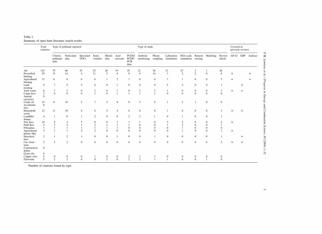
Table 1
Summary of open burn literature search results
Totalcitations
Type of pollutant reported Type of study Covered inprevious reviews
Criteriapollutantdata
Particulatedata
SpeciatedVOCs
Semi-volatiles
Metalsdata
Acidaerosols
PCDD/PCDF/PCBdata
Ambientmonitoring
Plumesampling
Laboratorysimulation
Pilot-scalesimulation
Remotesensing
Modeling Reviewarticle
AP-42 EIIP Andreae
All 125 79 68 35 55 26 19 18 22 36 21 25 3 1 28Prescribedburning
29 15 14 4 11 5 6 0 6 14 1 2 2 0 6 £ £
Agriculturalburning
15 11 8 6 6 1 2 1 0 4 7 1 0 0 5 £ £
Landclearing
8 7 5 5 6 0 1 0 0 0 5 2 0 0 1 £
Yard waste 8 7 7 0 2 0 1 0 2 2 1 0 0 0 3 £ £Camp fires 2 0 0 0 1 0 1 1 1 1 0 0 0 0 0Animalcarcasses
0
Crude oil 15 11 10 5 7 5 0 0 5 9 1 5 1 0 0Accidentalfires
0
Householdwaste
12 11 10 4 6 5 4 8 0 0 1 8 0 0 3 £ £
Landfills/dumps
4 1 0 1 2 0 0 2 2 1 0 1 0 0 1
Tire fires 10 6 4 5 8 6 1 1 1 0 3 2 0 0 4 £Fluff fires 4 3 2 1 2 1 1 1 0 0 1 2 0 0 1Fiberglass 1 1 1 1 1 1 1 0 0 0 0 1 0 0 0Agriculturalplastic film
3 1 1 2 2 0 0 0 0 0 0 1 0 0 1 £
Structuralfires
2 1 2 1 0 0 1 0 0 1 0 0 0 0 1 £
Car–boat–train
2 2 2 0 0 0 0 0 0 0 0 0 0 0 2 £ £
Constructiondebris
0
Grain silo 0Copper wire 5 0 0 0 1 0 0 2 3 3 0 0 0 0 0Fireworks 5 2 2 0 0 2 0 2 2 1 1 0 0 1 0
Number of citations found by type.
P.M
.L
emieu
xet
al.
/P
rog
ressin
En
ergy
an
dC
om
bu
stion
Scien
ce3
0(2
00
4)
1–
32
5
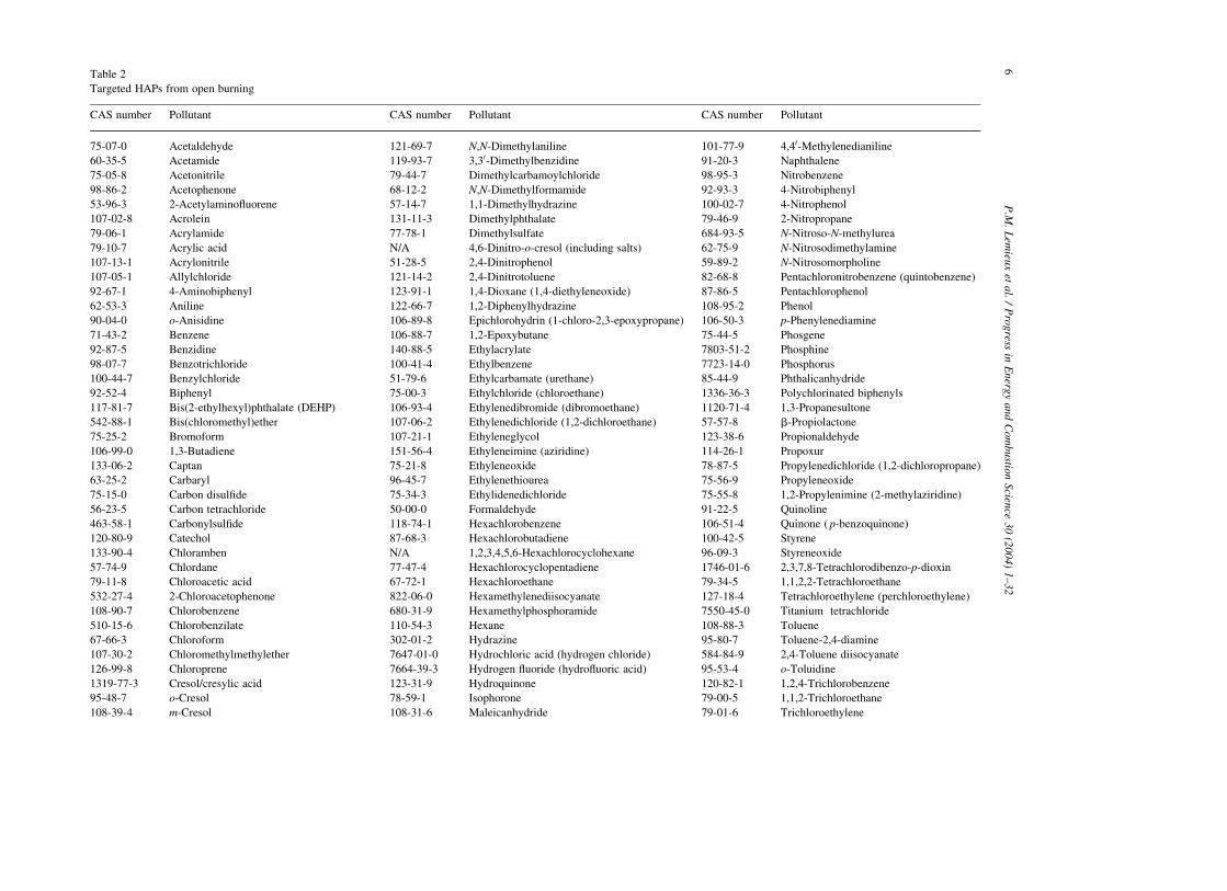
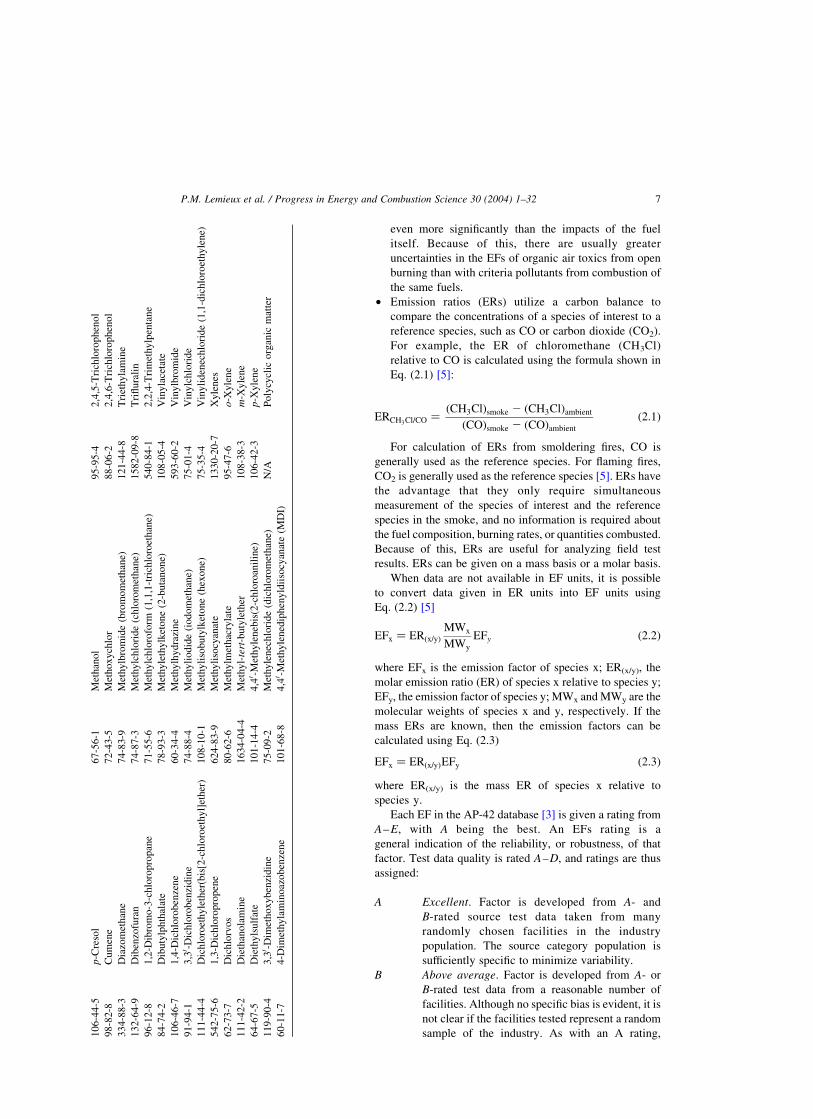
Table 2
Targeted HAPs from open burning
CAS number Pollutant CAS number Pollutant CAS number Pollutant
75-07-0 Acetaldehyde 121-69-7 N,N-Dimethylaniline 101-77-9 4,40-Methylenedianiline
60-35-5 Acetamide 119-93-7 3,30-Dimethylbenzidine 91-20-3 Naphthalene
75-05-8 Acetonitrile 79-44-7 Dimethylcarbamoylchloride 98-95-3 Nitrobenzene
98-86-2 Acetophenone 68-12-2 N,N-Dimethylformamide 92-93-3 4-Nitrobiphenyl
53-96-3 2-Acetylaminofluorene 57-14-7 1,1-Dimethylhydrazine 100-02-7 4-Nitrophenol
107-02-8 Acrolein 131-11-3 Dimethylphthalate 79-46-9 2-Nitropropane
79-06-1 Acrylamide 77-78-1 Dimethylsulfate 684-93-5 N-Nitroso-N-methylurea
79-10-7 Acrylic acid N/A 4,6-Dinitro-o-cresol (including salts) 62-75-9 N-Nitrosodimethylamine
107-13-1 Acrylonitrile 51-28-5 2,4-Dinitrophenol 59-89-2 N-Nitrosomorpholine
107-05-1 Allylchloride 121-14-2 2,4-Dinitrotoluene 82-68-8 Pentachloronitrobenzene (quintobenzene)
92-67-1 4-Aminobiphenyl 123-91-1 1,4-Dioxane (1,4-diethyleneoxide) 87-86-5 Pentachlorophenol
62-53-3 Aniline 122-66-7 1,2-Diphenylhydrazine 108-95-2 Phenol
90-04-0 o-Anisidine 106-89-8 Epichlorohydrin (1-chloro-2,3-epoxypropane) 106-50-3 p-Phenylenediamine
71-43-2 Benzene 106-88-7 1,2-Epoxybutane 75-44-5 Phosgene
92-87-5 Benzidine 140-88-5 Ethylacrylate 7803-51-2 Phosphine
98-07-7 Benzotrichloride 100-41-4 Ethylbenzene 7723-14-0 Phosphorus
100-44-7 Benzylchloride 51-79-6 Ethylcarbamate (urethane) 85-44-9 Phthalicanhydride
92-52-4 Biphenyl 75-00-3 Ethylchloride (chloroethane) 1336-36-3 Polychlorinated biphenyls
117-81-7 Bis(2-ethylhexyl)phthalate (DEHP) 106-93-4 Ethylenedibromide (dibromoethane) 1120-71-4 1,3-Propanesultone
542-88-1 Bis(chloromethyl)ether 107-06-2 Ethylenedichloride (1,2-dichloroethane) 57-57-8 b-Propiolactone
75-25-2 Bromoform 107-21-1 Ethyleneglycol 123-38-6 Propionaldehyde
106-99-0 1,3-Butadiene 151-56-4 Ethyleneimine (aziridine) 114-26-1 Propoxur
133-06-2 Captan 75-21-8 Ethyleneoxide 78-87-5 Propylenedichloride (1,2-dichloropropane)
63-25-2 Carbaryl 96-45-7 Ethylenethiourea 75-56-9 Propyleneoxide
75-15-0 Carbon disulfide 75-34-3 Ethylidenedichloride 75-55-8 1,2-Propylenimine (2-methylaziridine)
56-23-5 Carbon tetrachloride 50-00-0 Formaldehyde 91-22-5 Quinoline
463-58-1 Carbonylsulfide 118-74-1 Hexachlorobenzene 106-51-4 Quinone ( p-benzoquinone)
120-80-9 Catechol 87-68-3 Hexachlorobutadiene 100-42-5 Styrene
133-90-4 Chloramben N/A 1,2,3,4,5,6-Hexachlorocyclohexane 96-09-3 Styreneoxide
57-74-9 Chlordane 77-47-4 Hexachlorocyclopentadiene 1746-01-6 2,3,7,8-Tetrachlorodibenzo-p-dioxin
79-11-8 Chloroacetic acid 67-72-1 Hexachloroethane 79-34-5 1,1,2,2-Tetrachloroethane
532-27-4 2-Chloroacetophenone 822-06-0 Hexamethylenediisocyanate 127-18-4 Tetrachloroethylene (perchloroethylene)
108-90-7 Chlorobenzene 680-31-9 Hexamethylphosphoramide 7550-45-0 Titanium tetrachloride
510-15-6 Chlorobenzilate 110-54-3 Hexane 108-88-3 Toluene
67-66-3 Chloroform 302-01-2 Hydrazine 95-80-7 Toluene-2,4-diamine
107-30-2 Chloromethylmethylether 7647-01-0 Hydrochloric acid (hydrogen chloride) 584-84-9 2,4-Toluene diisocyanate
126-99-8 Chloroprene 7664-39-3 Hydrogen fluoride (hydrofluoric acid) 95-53-4 o-Toluidine
1319-77-3 Cresol/cresylic acid 123-31-9 Hydroquinone 120-82-1 1,2,4-Trichlorobenzene
95-48-7 o-Cresol 78-59-1 Isophorone 79-00-5 1,1,2-Trichloroethane
108-39-4 m-Cresol 108-31-6 Maleicanhydride 79-01-6 Trichloroethylene
P.M
.L
emieu
xet
al.
/P
rog
ressin
En
ergy
an
dC
om
bu
stion
Scien
ce3
0(2
00
4)
1–
32
6
even more significantly than the impacts of the fuel
itself. Because of this, there are usually greater
uncertainties in the EFs of organic air toxics from open
burning than with criteria pollutants from combustion of
the same fuels.
† Emission ratios (ERs) utilize a carbon balance to
compare the concentrations of a species of interest to a
reference species, such as CO or carbon dioxide (CO2).
For example, the ER of chloromethane (CH3Cl)
relative to CO is calculated using the formula shown in
Eq. (2.1) [5]:
ERCH3Cl=CO ¼ðCH3ClÞsmoke 2 ðCH3ClÞambient
ðCOÞsmoke 2 ðCOÞambient
ð2:1Þ
For calculation of ERs from smoldering fires, CO is
generally used as the reference species. For flaming fires,
CO2 is generally used as the reference species [5]. ERs have
the advantage that they only require simultaneous
measurement of the species of interest and the reference
species in the smoke, and no information is required about
the fuel composition, burning rates, or quantities combusted.
Because of this, ERs are useful for analyzing field test
results. ERs can be given on a mass basis or a molar basis.
When data are not available in EF units, it is possible
to convert data given in ER units into EF units using
Eq. (2.2) [5]
EFx ¼ ERðx=yÞ
MWx
MWy
EFy ð2:2Þ
where EFx is the emission factor of species x; ER(x/y), the
molar emission ratio (ER) of species x relative to species y;
EFy, the emission factor of species y; MWx and MWy are the
molecular weights of species x and y, respectively. If the
mass ERs are known, then the emission factors can be
calculated using Eq. (2.3)
EFx ¼ ERðx=yÞEFy ð2:3Þ
where ER(x/y) is the mass ER of species x relative to
species y.
Each EF in the AP-42 database [3] is given a rating from
A– E, with A being the best. An EFs rating is a
general indication of the reliability, or robustness, of that
factor. Test data quality is rated A–D; and ratings are thus
assigned:
A Excellent. Factor is developed from A- and
B-rated source test data taken from many
randomly chosen facilities in the industry
population. The source category population is
sufficiently specific to minimize variability.
B Above average. Factor is developed from A- or
B-rated test data from a reasonable number of
facilities. Although no specific bias is evident, it is
not clear if the facilities tested represent a random
sample of the industry. As with an A rating,10
6-4
4-5
p-C
reso
l6
7-5
6-1
Met
han
ol
95
-95-4
2,4
,5-T
rich
loro
phen
ol
98
-82-8
Cum
ene
72
-43-5
Met
ho
xy
chlo
r8
8-0
6-2
2,4
,6-T
rich
loro
phen
ol
334-8
8-3
Dia
zom
ethan
e74-8
3-9
Met
hylb
rom
ide
(bro
mom
ethan
e)121-4
4-8
Tri
ethyla
min
e
13
2-6
4-9
Dib
enzo
fura
n7
4-8
7-3
Met
hy
lch
lori
de
(ch
loro
met
han
e)1
58
2-0
9-8
Tri
flu
rali
n
96
-12-8
1,2
-Dib
rom
o-3
-ch
loro
pro
pan
e7
1-5
5-6
Met
hy
lch
loro
form
(1,1
,1-t
rich
loro
eth
ane)
54
0-8
4-1
2,2
,4-T
rim
eth
ylp
enta
ne
84-7
4-2
Dib
uty
lphth
alat
e78-9
3-3
Met
hyle
thylk
etone
(2-b
uta
none)
108-0
5-4
Vin
yla
ceta
te
10
6-4
6-7
1,4
-Dic
hlo
roben
zen
e6
0-3
4-4
Met
hy
lhy
dra
zin
e5
93
-60
-2V
iny
lbro
mid
e
91
-94-1
3,3
0 -D
ich
loro
ben
zid
ine
74
-88-4
Met
hy
lio
did
e(i
od
om
eth
ane)
75
-01-4
Vin
ylc
hlo
rid
e
11
1-4
4-4
Dic
hlo
roet
hy
leth
er(b
is[2
-ch
loro
eth
yl]
eth
er)
10
8-1
0-1
Met
hy
liso
bu
tylk
eto
ne
(hex
one)
75
-35-4
Vin
yli
den
ech
lori
de
(1,1
-dic
hlo
roet
hy
len
e)
54
2-7
5-6
1,3
-Dic
hlo
ropro
pen
e6
24
-83
-9M
ethy
liso
cyan
ate
13
30-2
0-7
Xy
len
es
62
-73-7
Dic
hlo
rvos
80
-62-6
Met
hy
lmet
hac
ryla
te9
5-4
7-6
o-X
yle
ne
11
1-4
2-2
Die
than
ola
min
e1
63
4-0
4-4
Met
hy
l-te
rt-b
uty
leth
er1
08
-38
-3m
-Xyle
ne
64
-67-5
Die
thy
lsu
lfat
e1
01
-14
-44
,40 -
Met
hy
leneb
is(2
-ch
loro
anil
ine)
10
6-4
2-3
p-X
yle
ne
11
9-9
0-4
3,3
0 -D
imet
hoxyben
zidin
e75-0
9-2
Met
hyle
nec
hlo
ride
(dic
hlo
rom
ethan
e)N
/AP
oly
cycl
icorg
anic
mat
ter
60
-11-7
4-D
imet
hy
lam
ino
azo
ben
zene
10
1-6
8-8
4,4
0 -Met
hy
lened
iph
eny
ldii
socy
anat
e(M
DI)
P.M. Lemieux et al. / Progress in Energy and Combustion Science 30 (2004) 1–32 7
the source category population is sufficiently
specific to minimize variability.
C Average. Factor is developed from A-, B-, and/or
C-rated test data from a reasonable number of
facilities. Although no specific bias is evident, it is
not clear if the facilities tested represent a random
sample of the industry. As with the A rating, the
source category population is sufficiently specific
to minimize variability.
D Below average. Factor is developed from A-, B-
and/or C-rated test data from a small number of
facilities, and there may be reason to suspect that
these facilities do not represent a random sample
of the industry. There also may be evidence of
variability within the source population.
E Poor. Factor is developed from C- and D-rated test
data, and there may be reason to suspect that the
facilities tested do not represent a random sample
of the industry. There also may be evidence of
variability within the source category population.
2.2. Activity factors
In order to determine the contribution of a given source
to the emissions inventory on a local, national, or global
basis, the AF is defined in terms of the mass combusted per
unit time or per unit area within the region or facility of
interest. The desired units of AFs vary depending on the
needs of the individual estimating the emissions. Examples
of alternative AF needs include:
† a reader who is interested in how open burning
contributes to global or regional inventories or ambient
concentrations of a given air toxic probably would be
interested in activity data on a global or regional scale
(depending on how persistent/globally transported the air
toxic of interest was)
† a reader who is interested in assessing a given local
problem (i.e. ‘is my town getting built up enough that we
need prohibit burning yard waste’ or ‘is that tire fire on
the other side of the fence a reason to evacuate my
school’) needs activity data on a local scale.
Estimation of AFs can be done many ways; although
estimating AFs is outside the scope of this paper, the EIIP
documents, especially the EIIP open burning emission
factor guidance document [10] describes several ways to
estimate AFs.
Eq. (2.4) illustrates how emissions are calculated using
EFs and AFs:
emissions ¼ EF £ AF ð2:4Þ
Table 3 lists sources for AFs and values of emission
factors of criteria pollutants for the sources listed in this
paper, where available.
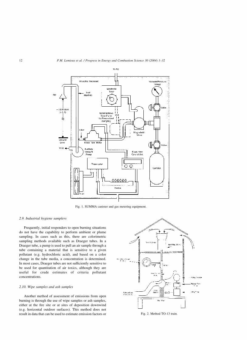
2.3. Ambient sampling
Ambient sampling involves the measurement of
pollutant concentrations in the open atmosphere. Much of
the available data on emissions of air toxics from open
burning are based on ambient pollutant measurements.
VOCs are commonly measuring using EPA Method TO-14
[28] using SUMMA canisters that are cleaned and evacuated
prior to sampling. A fraction of each batch of canisters is
typically analyzed before use to ensure adequate cleaning.
Compound identification is based on retention time and the
agreement of the mass spectra of the unknown to mass
spectra of known standards. Fig. 1 shows a SUMMA
canister, flow meter, and sampling pump.
SVOCs are sampled according to Method TO-13 [29],
which consists of a filter followed by a polyurethane foam
(PUF)-sandwiched XAD-2 bed vapor trap. These samplers
typically operate at flow rates designed to achieve low
detection limits for the quantification of generally dilute
ambient concentrations. After sampling is complete,
the filter and XAD trap are recovered, extracted with an
organic solvent such as dichloromethane (CH2Cl2),
concentrated, and analyzed by GC/MS. Fig. 2 shows a
Method TO-13 train.
2.4. Plume sampling (Nomad sampler)
Directly sampling in the smoky plume of a fire is a
difficult proposition. Many uncontrolled fires are not easily
approachable by sampling crews and exhibit temporal shifts
in the position of the flame front; changes in wind directions
make it difficult to position ambient sampling devices.
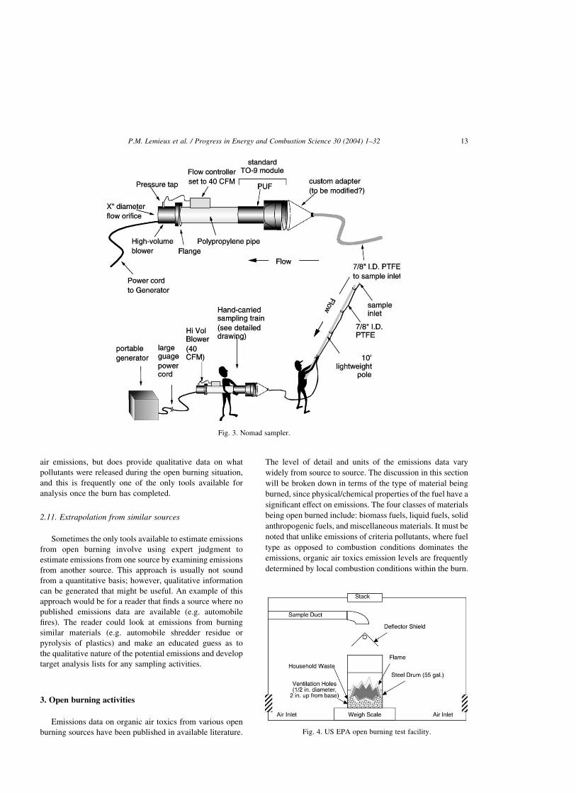
The US EPA is currently developing a hand-held boom
sampler (Nomad sampler) to enable sampling crews to insert
the suction end of a sampling probe directly into the smoke
plume without needing to get extremely close to the smoke
or fire [30]. Fig. 3 shows the concept of the Nomad sampler.
2.5. Laboratory simulations
An effective way to develop emission factors for open
burning sources is through laboratory simulations using a
flux chamber approach. In a laboratory simulation, small
amounts of the material in question are combusted in as
representative a manner as possible while making detailed
measurements of the mass of burning material, combustion
air and dilution air flow rates, relevant temperatures, and the
concentrations of the pollutants of interest.
The earliest laboratory simulation of open burning
that attempted measurement of air toxics and other
similar pollutants was reported in 1967 [31]. This study
used a conical shaped tower suspended above the burning
bed to capture the plume in such a way that conventional
stack sampling approaches could then be used.
The US EPA’s National Risk Management Research
Laboratory has an Open Burning Test Facility (OBTF)
P.M. Lemieux et al. / Progress in Energy and Combustion Science 30 (2004) 1–328
located in Research Triangle Park, NC. The OBTF has been
used for several test programs to evaluate emissions from a
wide variety of open burning sources. Sources that have
been tested in the OBTF include tire fires [17,32,33],
fiberglass burning [26], open burning of land clearing debris
[24], automobile shredder fluff fires [18], open burning of
household waste in barrels [34–37], agricultural plastics
[38], forest fires [30], and agricultural burning [39].
In limited cases where field data are available to support
measurements from the OBTF, results appeared to agree
within an order of magnitude [32]. In the OBTF, shown in
Fig. 4 as configured for experiments investigating open
burning of household waste in barrels [37], there is a
continuous influx of dilution air into the facility, simulating
ambient dilution. Fans located around the interior maintain a
high level of mixing. The burning mass of material is
mounted on a weigh scale so that burning rates can be
estimated. Ambient sampling equipment is positioned inside
the interior of the facility, or extractive samples can be taken
through the sample duct.
Pollutant concentrations measured in the OBTF can be
converted to the mass emissions of individual pollutants
(emission factor units) using Eq. (2.5)
EF ¼CsampleQOBTFt
mburned
ð2:5Þ
where EF is the emission factor in mg/kg waste
consumed; Csample, the concentration of the pollutant in
the sample (mg/m3); QOBTF; the flow rate of dilution air
into the OBTF in m3/min; t; the burn sampling time in
minutes, and mburned is the mass of waste burned (kg).
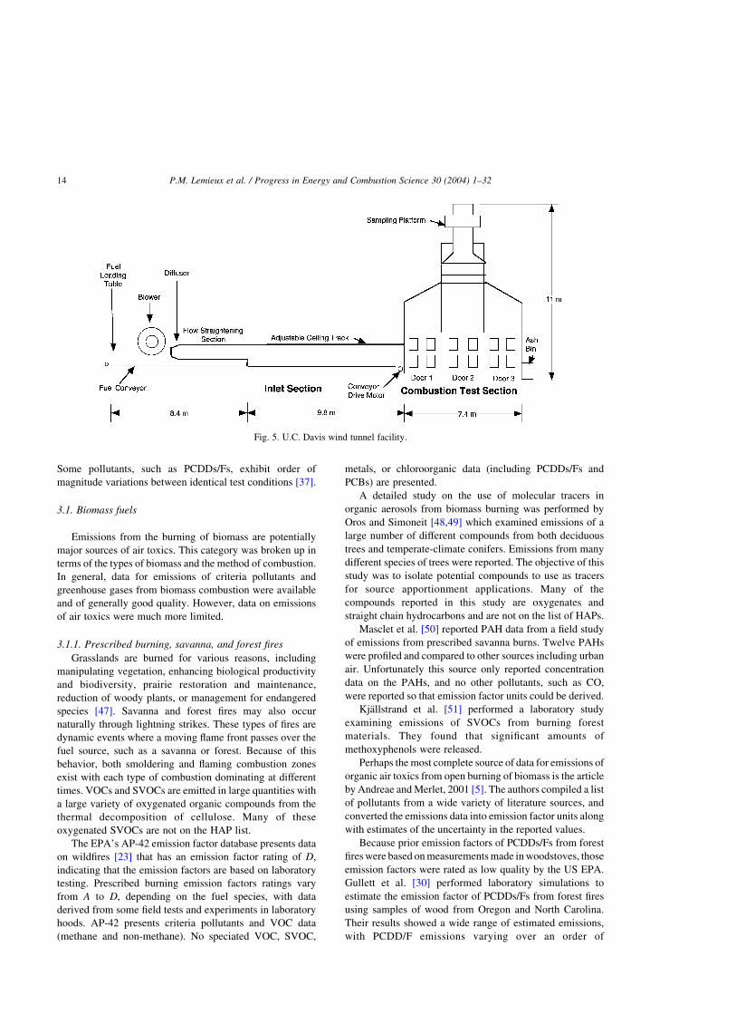
2.6. Wind tunnel testing
The University of California at Davis developed a wind
tunnel testing facility that has been used for testing
emissions from open burning of agricultural residues [40].
This type of facility can control important variables such as
fuel moisture content, wind speed, fuel loading, and
influence of soil bed conditions on combustion conditions.
Fig. 5 shows a diagram of the wind tunnel facility.
2.7. Bang box sampling
The US Army, as part of a test program to determine
emissions from Open Burning/Open Detonation (OB/OD)
of old munitions, built a facility specially designed for
emissions testing of munitions. This facility, called a ‘Bang
Box’ is located at the Dugway Proving Grounds [41] and
consists of a 1000 m3 vinyl plastic air-inflated dome that
contains a blast shield and analytical equipment and allows
researchers to investigate a half-pound of explosives per
blast or five pounds of propellant per burn.
2.8. Remote sensing
Aircraft and satellite remote sensing has been
employed to collect emissions data from biomass burning
for a multitude of programs including the South African
Regional Science Initiative in the year 1992 and 2000,
the Experiment for Regional Sources of Sinks and
Oxidants, the ‘Fire of Savannas’ (FOS/DECAFE) exper-
iments, Biomass Burning Airborne and Spaceborne
Experiment in the Amazonas (BASE-A), and a Brazilian
Institute for the Environment study. Such studies have
utilized aircraft or satellite based instruments such as
Extended Dynamic Range Imaging Spectrometer (a four-
line infrared spectrometer developed by the National
Aeronautics Space Administration), ‘Fire Mapper’ spec-
trometer (infrared radiometer developed by the US Forest
Service, the Brazilian Institute of the Environment, and
Space Instruments, Inc.), and NOAA Advanced Very
High Resolution Radiometer. However, these aircraft and
satellite spectrometers were used primarily for ascertain-
ing information related to fire spread, smoke spread and
optical density, and criteria pollutants. The focus of the
remote sensing studies to date has been to integrate
aircraft and satellite information with ground-based (not
remote) sensing data in order to predict and quantify the
effects of biomass burning on the global climate. Other
groups are using remote sensing data coupled with GIS
databases to document the complex interaction between
fuel loads, land use and open burning and the effect of
these open burning processes have on endangered species
preservation and surface water quality [42].
Another method of developing emissions data from
open burning sources in support of the above approach is
through ground-based optical remote sensing. This
approach combines path-integrated optical sensing with
meteorological measurements [43]. In a scale of several
hundred meters, Open Path Fourier Transform Infrared
(OP-FTIR) instrumentation is typically used, where the
IR source is coupled with a series of retroreflectors so
that the overall path length is many times greater than
the distance between the IR source and the retroreflector
array. The long path length improves sensitivity so that
detection limits can be achieved which are capable of
measuring ambient concentrations of organic pollutants.
When several kilometer scale is needed, other instru-
mental techniques including Differential optical absorp-
tion spectroscopy, long path Tunable Diode Laser
Absorption Spectroscopy, and Light Detection and
Ranging (LIDAR) for aerosol detection and Differential
absorption LIDAR for gaseous detection are also
available [44–46]. Most of the VOC compounds on the
HAP list can be measured at low parts-per-billion levels
using at least one of these techniques as well as long
path PM extinction measurements [44].
P.M. Lemieux et al. / Progress in Energy and Combustion Science 30 (2004) 1–32 9
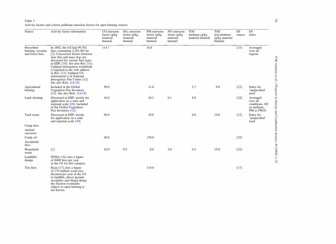
Table 3
Activity factors and criteria pollutant emission factors for open burning sources
Source Activity factor information CO emissionfactor (g/kgmaterialburned)
SO2 emissionfactor (g/kgmaterialburned)
PM emissionfactor (g/kgmaterialburned)
NO emissionfactor (g/kgmaterialburned)
TOCmethane (g/kgmaterial burned)
TOCnon-methane(g/kg materialburned)
EFsource
EFnotes
Prescribedburning, savannaand forest fires
In 2002, the US had 99,702fires consuming 2,291,401 ha[7]. Conversion factors betweenarea (ha) and mass (kg) arediscussed for various fuel typesin EIIP, [10]. See also Ref. [11].Updated information worldwideis reported at the web addressin Ref. [12]. Updated USinformation is at NationalInteragency Fire Center [13].See also Refs. [14,15]
114.7 16.6 [23] Averagedover allregions
Agriculturalburning
Included in the GlobalVegetation Fire Inventory[12]. See also Refs. [14,15]
58.0 11.0 2.7 9.0 [23] Entry for‘unspecified’used
Land clearing Discussed in EIIP, mostly forapplication on a state andregional scale [10]. Includedin the Global VegetationFire Inventory [12]
16.0 10.3 0.1 8.0 [24] Averagedover allconditions; OCas methane;PM as PM10
Yard waste Discussed in EIIP, mostlyfor application on a stateand regional scale [10]
56.0 19.0 6.0 14.0 [23] Entry for‘unspecified’used
Camp fires
Animalcarcasses
Crude oil 30.0 170.0 [25]
Accidentalfires
Householdwaste
[1] 42.0 0.5 8.0 3.0 6.5 15.0 [23]
Landfills/dumps
FEMA [16] cites a figureof 8400 fires per yearin the US for this category
Tire fires Ryan [17] cites a figureof 170 million scrap tiresdiscared per year in the USin landfills, above groundstockpiles and illegal dump:the fraction eventuallysubject to open burning isnot known
119.0 [17]
P.M
.L
emieu
xet
al.
/P
rog
ressin
En
ergy
an
dC
om
bu
stion
Scien
ce3
0(2
00
4)
1–
32
10
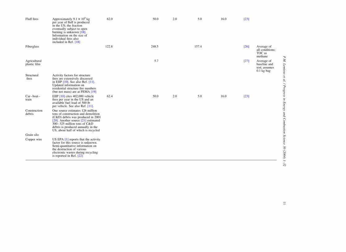
Fluff fires Approximately 9.1 £ 108 kgper year of fluff is producedin the US; the fractioneventually subject to openburning is unknown [18].Information on the size ofindividual fires alsoincluded in Ref. [18]
62.0 50.0 2.0 5.0 16.0 [23]
Fiberglass 122.8 248.5 157.4 [26] Average ofall conditions;TOC asmethane
Agriculturalplastic film
5.7 [27] Average ofbaseline andtest; assumes0.1 kg bag
Structuralfires
Activity factors for structurefires are extensively discussedin EIIP [10]. See also Ref. [11].Updated information onresidential structure fire numbers(but not mass) are at FEMA [19]
Car–boat–train
EIIP [10] cites 402,000 vehiclefires per year in the US and anavailable fuel load of 500 lbper vehicle. See also Ref. [11].
62.4 50.0 2.0 5.0 16.0 [23]
Constructiondebris
One source estimates 126 milliontons of construction and demolition(C&D) debris was produced in 2001[20]. Another source [21] estimated300–325 million tons of C&Ddebris is produced annually in theUS, about half of which is recycled
Grain silo
Copper wire US EPA [1] reports that the activityfactor for this source is unknown.Semi-quantitative information onthe destruction of variouselectronic wastes during recyclingis reported in Ref. [22]
P.M
.L
emieu
xet
al.
/P
rog
ressin
En
ergy
an
dC
om
bu
stion
Scien
ce3
0(2
00
4)
1–
32
11
2.9. Industrial hygiene samplers
Frequently, initial responders to open burning situations
do not have the capability to perform ambient or plume
sampling. In cases such as this, there are colorimetric
sampling methods available such as Draeger tubes. In a
Draeger tube, a pump is used to pull an air sample through a
tube containing a material that is sensitive to a given
pollutant (e.g. hydrochloric acid), and based on a color
change in the tube media, a concentration is determined.
In most cases, Draeger tubes are not sufficiently sensitive to
be used for quantitation of air toxics, although they are
useful for crude estimates of criteria pollutant
concentrations.
2.10. Wipe samples and ash samples
Another method of assessment of emissions from open
burning is through the use of wipe samples or ash samples,
either at the fire site or at sites of deposition downwind
(e.g. horizontal outdoor surfaces). This method does not
result in data that can be used to estimate emission factors or
Fig. 1. SUMMA canister and gas metering equipment.
Fig. 2. Method TO-13 train.
P.M. Lemieux et al. / Progress in Energy and Combustion Science 30 (2004) 1–3212
air emissions, but does provide qualitative data on what
pollutants were released during the open burning situation,
and this is frequently one of the only tools available for
analysis once the burn has completed.
2.11. Extrapolation from similar sources
Sometimes the only tools available to estimate emissions
from open burning involve using expert judgment to
estimate emissions from one source by examining emissions
from another source. This approach is usually not sound
from a quantitative basis; however, qualitative information
can be generated that might be useful. An example of this
approach would be for a reader that finds a source where no
published emissions data are available (e.g. automobile
fires). The reader could look at emissions from burning
similar materials (e.g. automobile shredder residue or
pyrolysis of plastics) and make an educated guess as to
the qualitative nature of the potential emissions and develop
target analysis lists for any sampling activities.
3. Open burning activities
Emissions data on organic air toxics from various open
burning sources have been published in available literature.
The level of detail and units of the emissions data vary
widely from source to source. The discussion in this section
will be broken down in terms of the type of material being
burned, since physical/chemical properties of the fuel have a
significant effect on emissions. The four classes of materials
being open burned include: biomass fuels, liquid fuels, solid
anthropogenic fuels, and miscellaneous materials. It must be
noted that unlike emissions of criteria pollutants, where fuel
type as opposed to combustion conditions dominates the
emissions, organic air toxics emission levels are frequently
determined by local combustion conditions within the burn.
Fig. 3. Nomad sampler.
Fig. 4. US EPA open burning test facility.
P.M. Lemieux et al. / Progress in Energy and Combustion Science 30 (2004) 1–32 13
Some pollutants, such as PCDDs/Fs, exhibit order of
magnitude variations between identical test conditions [37].
3.1. Biomass fuels
Emissions from the burning of biomass are potentially
major sources of air toxics. This category was broken up in
terms of the types of biomass and the method of combustion.
In general, data for emissions of criteria pollutants and
greenhouse gases from biomass combustion were available
and of generally good quality. However, data on emissions
of air toxics were much more limited.
3.1.1. Prescribed burning, savanna, and forest fires
Grasslands are burned for various reasons, including
manipulating vegetation, enhancing biological productivity
and biodiversity, prairie restoration and maintenance,
reduction of woody plants, or management for endangered
species [47]. Savanna and forest fires may also occur
naturally through lightning strikes. These types of fires are
dynamic events where a moving flame front passes over the
fuel source, such as a savanna or forest. Because of this
behavior, both smoldering and flaming combustion zones
exist with each type of combustion dominating at different
times. VOCs and SVOCs are emitted in large quantities with
a large variety of oxygenated organic compounds from the
thermal decomposition of cellulose. Many of these
oxygenated SVOCs are not on the HAP list.
The EPA’s AP-42 emission factor database presents data
on wildfires [23] that has an emission factor rating of D;
indicating that the emission factors are based on laboratory
testing. Prescribed burning emission factors ratings vary
from A to D; depending on the fuel species, with data
derived from some field tests and experiments in laboratory
hoods. AP-42 presents criteria pollutants and VOC data
(methane and non-methane). No speciated VOC, SVOC,
metals, or chloroorganic data (including PCDDs/Fs and
PCBs) are presented.
A detailed study on the use of molecular tracers in
organic aerosols from biomass burning was performed by
Oros and Simoneit [48,49] which examined emissions of a
large number of different compounds from both deciduous
trees and temperate-climate conifers. Emissions from many
different species of trees were reported. The objective of this
study was to isolate potential compounds to use as tracers
for source apportionment applications. Many of the
compounds reported in this study are oxygenates and
straight chain hydrocarbons and are not on the list of HAPs.
Masclet et al. [50] reported PAH data from a field study
of emissions from prescribed savanna burns. Twelve PAHs
were profiled and compared to other sources including urban
air. Unfortunately this source only reported concentration
data on the PAHs, and no other pollutants, such as CO,
were reported so that emission factor units could be derived.
Kjallstrand et al. [51] performed a laboratory study
examining emissions of SVOCs from burning forest
materials. They found that significant amounts of
methoxyphenols were released.
Perhaps the most complete source of data for emissions of
organic air toxics from open burning of biomass is the article
by Andreae and Merlet, 2001 [5]. The authors compiled a list
of pollutants from a wide variety of literature sources, and
converted the emissions data into emission factor units along
with estimates of the uncertainty in the reported values.
Because prior emission factors of PCDDs/Fs from forest
fires were based on measurements made in woodstoves, those
emission factors were rated as low quality by the US EPA.
Gullett et al. [30] performed laboratory simulations to
estimate the emission factor of PCDDs/Fs from forest fires
using samples of wood from Oregon and North Carolina.
Their results showed a wide range of estimated emissions,
with PCDD/F emissions varying over an order of
Fig. 5. U.C. Davis wind tunnel facility.
P.M. Lemieux et al. / Progress in Energy and Combustion Science 30 (2004) 1–3214
magnitude. Prange et al. [52], reported on elevated PCDD/F
concentrations found during a prescribed forest fire in
Australia; however, no emission factor units were estimated.
Yamasoe et al. [53], performed a study examining trace
element emissions from vegetation fires in the Amazon
Basin. This study reported on inorganic pollutants and
particulate. Emissions data on pollutant species such as
sulfates, chlorides, and metals were presented.
Barber et al. [2] reported that biomass burning, specifi-
cally temperate region forest fires, could produce fly and
bottomashcontainingvarious cyanidespecies. Thesecyanide
compounds could then be leached into adjacent waterways
placing sensitive fish species at risk.
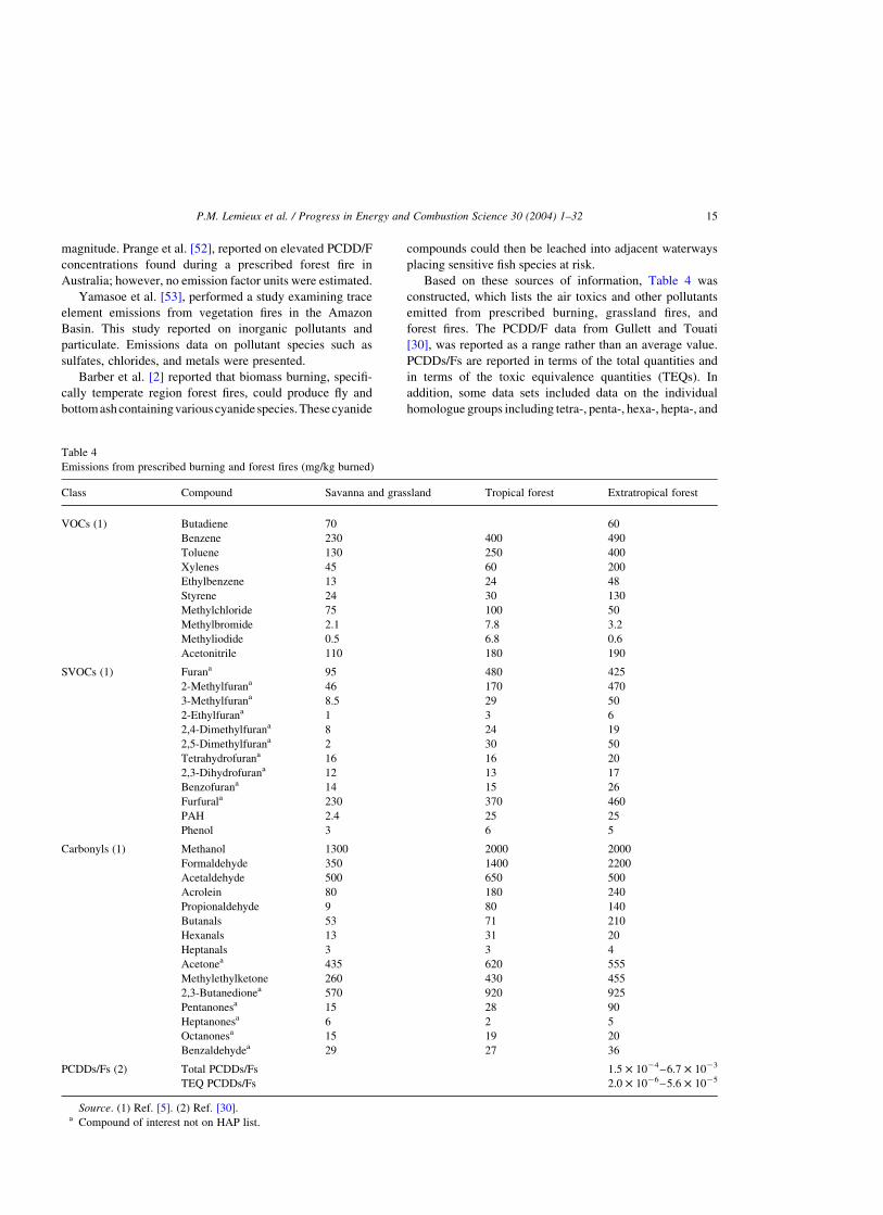
Based on these sources of information, Table 4 was
constructed, which lists the air toxics and other pollutants
emitted from prescribed burning, grassland fires, and
forest fires. The PCDD/F data from Gullett and Touati
[30], was reported as a range rather than an average value.
PCDDs/Fs are reported in terms of the total quantities and
in terms of the toxic equivalence quantities (TEQs). In
addition, some data sets included data on the individual
homologue groups including tetra-, penta-, hexa-, hepta-, and
Table 4
Emissions from prescribed burning and forest fires (mg/kg burned)
Class Compound Savanna and grassland Tropical forest Extratropical forest
VOCs (1) Butadiene 70 60
Benzene 230 400 490
Toluene 130 250 400
Xylenes 45 60 200
Ethylbenzene 13 24 48
Styrene 24 30 130
Methylchloride 75 100 50
Methylbromide 2.1 7.8 3.2
Methyliodide 0.5 6.8 0.6
Acetonitrile 110 180 190
SVOCs (1) Furana 95 480 425
2-Methylfurana 46 170 470
3-Methylfurana 8.5 29 50
2-Ethylfurana 1 3 6
2,4-Dimethylfurana 8 24 19
2,5-Dimethylfurana 2 30 50
Tetrahydrofurana 16 16 20
2,3-Dihydrofurana 12 13 17
Benzofurana 14 15 26
Furfurala 230 370 460
PAH 2.4 25 25
Phenol 3 6 5
Carbonyls (1) Methanol 1300 2000 2000
Formaldehyde 350 1400 2200
Acetaldehyde 500 650 500
Acrolein 80 180 240
Propionaldehyde 9 80 140
Butanals 53 71 210
Hexanals 13 31 20
Heptanals 3 3 4
Acetonea 435 620 555
Methylethylketone 260 430 455
2,3-Butanedionea 570 920 925
Pentanonesa 15 28 90
Heptanonesa 6 2 5
Octanonesa 15 19 20
Benzaldehydea 29 27 36
PCDDs/Fs (2) Total PCDDs/Fs 1.5 £ 1024–6.7 £ 1023
TEQ PCDDs/Fs 2.0 £ 1026–5.6 £ 1025
Source. (1) Ref. [5]. (2) Ref. [30].a Compound of interest not on HAP list.
P.M. Lemieux et al. / Progress in Energy and Combustion Science 30 (2004) 1–32 15
octa-substituted polychlorinated dibenzo-p-dioxins and
polychlorinated dibenzofurans (TCDD, PeCDD, HxCDD,
HpCDD, OCDD, TCDF, PeCDF, HxCDF, HpCDF and
OCDF, respectively).
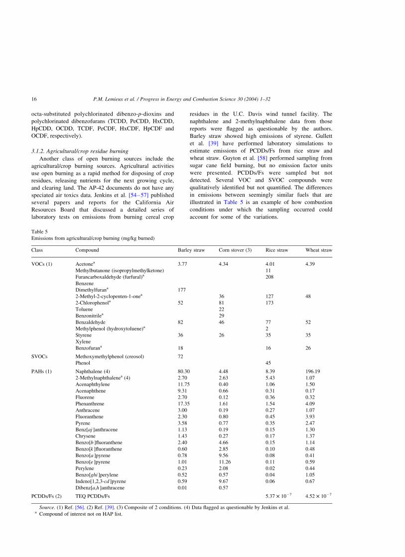
3.1.2. Agricultural/crop residue burning
Another class of open burning sources include the
agricultural/crop burning sources. Agricultural activities
use open burning as a rapid method for disposing of crop
residues, releasing nutrients for the next growing cycle,
and clearing land. The AP-42 documents do not have any
speciated air toxics data. Jenkins et al. [54–57] published
several papers and reports for the California Air
Resources Board that discussed a detailed series of
laboratory tests on emissions from burning cereal crop
residues in the U.C. Davis wind tunnel facility. The
naphthalene and 2-methylnaphthalene data from those
reports were flagged as questionable by the authors.
Barley straw showed high emissions of styrene. Gullett
et al. [39] have performed laboratory simulations to
estimate emissions of PCDDs/Fs from rice straw and
wheat straw. Guyton et al. [58] performed sampling from
sugar cane field burning, but no emission factor units
were presented. PCDDs/Fs were sampled but not
detected. Several VOC and SVOC compounds were
qualitatively identified but not quantified. The differences
in emissions between seemingly similar fuels that are
illustrated in Table 5 is an example of how combustion
conditions under which the sampling occurred could
account for some of the variations.
Table 5
Emissions from agricultural/crop burning (mg/kg burned)
Class Compound Barley straw Corn stover (3) Rice straw Wheat straw
VOCs (1) Acetonea 3.77 4.34 4.01 4.39
Methylbutanone (isopropylmethylketone) 11
Furancarboxaldehyde (furfural)a 208
Benzene
Dimethylfurana 177
2-Methyl-2-cyclopenten-1-onea 36 127 48
2-Chlorophenola 52 81 173
Toluene 22
Benzonitrilea 29
Benzaldehyde 82 46 77 52
Methylphenol (hydroxytoluene)a 2
Styrene 36 26 35 35
Xylene
Benzofurana 18 16 26
SVOCs Methoxymethylphenol (creosol) 72
Phenol 45
PAHs (1) Naphthalene (4) 80.30 4.48 8.39 196.19
2-Methylnaphthalenea (4) 2.70 2.63 5.43 1.07
Acenaphthylene 11.75 0.40 1.06 1.50
Acenaphthene 9.31 0.66 0.31 0.17
Fluorene 2.70 0.12 0.36 0.32
Phenanthrene 17.35 1.61 1.54 4.09
Anthracene 3.00 0.19 0.27 1.07
Fluoranthene 2.30 0.80 0.45 3.93
Pyrene 3.58 0.77 0.35 2.47
Benz[aj ]anthracene 1.13 0.19 0.15 1.30
Chrysene 1.43 0.27 0.17 1.37
Benzo[b ]fluoranthene 2.40 4.66 0.15 1.14
Benzo[k ]fluoranthene 0.60 2.85 0.10 0.48
Benzo[a ]pyrene 0.78 9.56 0.08 0.41
Benzo[e ]pyrene 1.01 11.26 0.11 0.59
Perylene 0.23 2.08 0.02 0.44
Benzo[ghi ]perylene 0.52 0.57 0.04 1.05
Indeno[1,2,3-cd ]pyrene 0.59 9.67 0.06 0.67
Dibenz[a,h ]anthracene 0.01 0.57
PCDDs/Fs (2) TEQ PCDDs/Fs 5.37 £ 1027 4.52 £ 1027
Source. (1) Ref. [56]. (2) Ref. [39]. (3) Composite of 2 conditions. (4) Data flagged as questionable by Jenkins et al.a Compound of interest not on HAP list.
P.M. Lemieux et al. / Progress in Energy and Combustion Science 30 (2004) 1–3216
Sugarcane growers in Hawaii burn their crops prior to
harvest to reduce the unused leaf mass that must be
transported to sugar mills. Sugarcane crop burning is not
practiced annually but rather on a two-year cycle for any
given field [59]. Emissions data for air toxics are not
available, although EPA has a current research project to
measure PCDD/F emissions from sugarcane burning.
Table 5 lists the emissions for air toxics from various
agricultural/crop burning sources.
3.1.3. Land clearing debris
Disposal of debris generated by landclearing or land-
scaping activities has long been problematic. Land clearing
is required for a wide variety of purposes such as
construction, development, and clearing after natural
disasters. The resultant debris is primarily vegetative in
composition, but may include inorganic material.
Landscaping activities, such as pruning, often generate
similar vegetative debris. This debris is often collected and
disposed of by municipalities. Open burning or burning in
simple air-curtain incinerators is a common means of
disposal for these materials, which has long been a source of
concern. Air-curtain incinerators use a blower to generate a
curtain of air in an attempt to enhance combustion taking
place in a trench or a rectangular-shaped, open-topped
refractory box.
As was the case for agricultural and crop burning, the
papers and reports by Jenkins et al. [54–57,60] provided a
wealth of information on emissions from spreading and pile
fires for Douglas Fir, Almond, Walnut, and Ponderosa Pine
slash based on wind tunnel studies. The US EPA reported on
a laboratory simulation study [24] to evaluate emissions of
air toxics from land-clearing debris combustion. They also
attempted to simulate an air-curtain incinerator in order to
assess the effectiveness of those types of units. Testing was
performed on land clearing debris samples from Tennessee
and Florida. Although it was undetermined how effective
air-curtain incinerators are, this study presented speciated
data on VOC and SVOC air toxics. PCDDs/Fs were not
measured in this study. For the purposes of presentation of
these data in this report, all runs from a given type of
land clearing debris were averaged together. Table 6 lists
the air toxic emission factors from open burning of land
clearing debris.
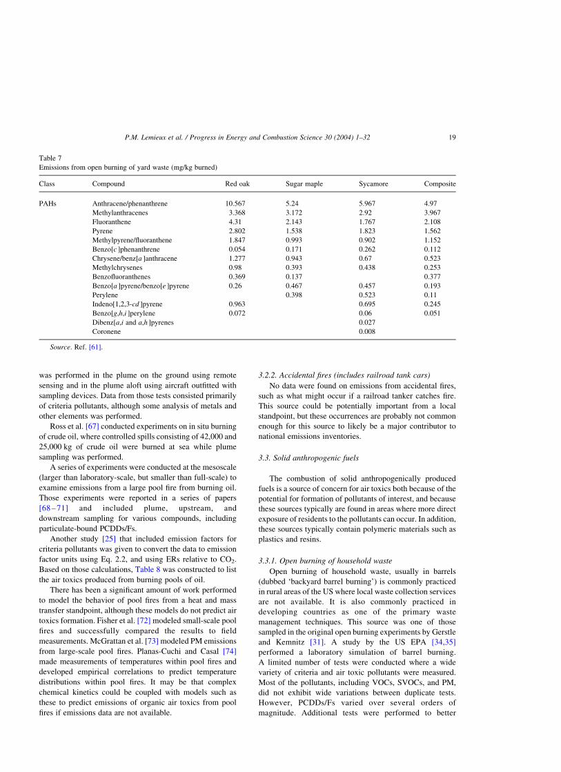
3.1.4. Yard waste
The burning of leaves and other yard waste is yet another
category of open burning which has data gaps in the
available information. The AP-42 database [3] and its
expanded EIIP documents [4,10] did not have any speciated
VOCs, SVOCs, metals, or PCDD/F data. The early
laboratory simulation study by Gerstle and Kemnitz [31],
reported on PAH measurements from yard waste burning,
but their data were not broken down in terms of the species
of tree. The Illinois Institute of Natural Resources published
a report [61] on the health effects from leaf burning that
included data on speciated SVOC from burning leaves from
three different species of trees. Table 7 lists the air toxics
measured from open burning of yard waste, showing
the mean yields from six replicate measurements of three
species and one composite sample.
3.1.5. Camp fires
Although camp fires and bonfires would be expected to
have emissions within the range of those from the
larger-scale events where similar fuels, such as conifer
trees, are burned, there were citations in the literature
specifically directed at this source. Simoneit et al. [62]
performed a study to examine conifer wood smoke from a
campfire for potential organic biomarkers. Another study
[63] measured PCDD/F in ambient samples on ‘bonfire
night’ in England, a night where many bonfires of various
fuel types and fireworks are set off. This study noted an
increase in PCDD/F levels, although there was no way to
distinguish whether the source of the increase was the
bonfires or the fireworks, although the authors did
postulate that the increase was probably due to the bonfires
and not the fireworks.
3.1.6. Animal carcasses
Open burning of animal carcasses has been performed in
cases where a biological agent has contaminated a herd of
livestock (e.g. foot and mouth disease, mad cow disease).
The Department of Health from the UK published a report
on their web site giving guidance on how to reduce
environmental impacts from open burning of animal
carcasses on pyres [64]. The data presented in that report
were based primarily on emissions from the fuels used to
sustain the pyres. The contributions of the animal carcasses
to the emissions were based on assuming that the animal
carcasses had the same emission factors as straw or
crematoria emissions. Because these emission results were
based on extrapolation of emissions from similar (and not
similar) sources, the quality of the data are highly
questionable, so they are not included in this analysis. It is
unknown how significant this source might be.
3.2. Liquid fuels
The burning of pools of liquid fuel present a significantly
different combustion scenario than exists in a fire involving
solid biomass because of both differences in fuel
composition and lack of air flow into the flame front from
beneath. There are several sources of emissions data on air
toxics from burning liquids.
3.2.1. Crude oil/oil spills
Just before the conclusion of the Gulf War, more than
800 oil wells were ignited by retreating Iraqi forces,
more than 650 of which burned with flames for several
months. Husain [65] and Stevens et al. [66] reported on the
characterization of the plume from those fires. Sampling
P.M. Lemieux et al. / Progress in Energy and Combustion Science 30 (2004) 1–32 17

Table 6
Emissions from open burning of land clearing debris (mg/kg burned)
Class Compound Tennessee
debris
(1)
Florida
debris
(1)
Douglas
fir slash
(2)
Ponderosa
pine slash
(2)
Almond
prunings
(2)
Walnut
prunings
(2)
VOCs 1,2,4-Trimethylbenzenea 18.0 7.5
1,3,5-Trimethylbenzenea 4.5 1.5
1,3-Butadiene 133.0 74.5
2-Butanone 31.8 28.0
4-Ethyltoluenea 32.5 8.5
Acetonea 181.3 146.5 8.0
Benzaldehyde 8.0 8.0
Benzene 303.5 195.0 196.0 444.0 30.0 16.0
Benzofurana 5.0
Benzylchloride 1.8
Bromomethane 1.0
Butylmethylether 1.0
Chloromethane 5.3 94.0
cis-1,2-Dichloroethene 14.3 32.0
Ethylbenzene 32.0 15.0
Limonenea 81.5
Xylene 117.5 43.0 56.0 3.0 2.0
Methylisobutanone 8.0
Ethylenechloride 2.0 1.0
Pinenea 98.8
Styrene 72.8 28.5 137.0 271.0 10.0 7.0
Toluene 190.8 106.0 157.0 351.0 19.0 11.0
trans-1,3-Dichloropropene 1.7
SVOCs Phenol 93 251 11
Cumenea 10.10 0.97
Creosol 403
Furancarboxaldehyde
(furfural)a335 18 18
1,1-Biphenyl 2.39 1.49
Phenol 56.98 54.35
2-Cresol 20.83 17.57
2,4-Dimethylphenola 10.28 14.31
Dibenzofuran 3.19 3.31
Dibutylphthalate 0.08
Bis(2-ethylhexyl)phthalate 8.44 5.59
PAHs Naphthalene 17.62 14.06 13.57 16.96 7.31 14.56
2-Methylnaphthalenea 7.64 6.25 2.58 2.27 0.15 1.98
Acenaphthylene 6.63 5.38 2.42 1.41 2.67 1.06
Acenaphthene 0.33 2.52 1.87 0.18 1.72
Fluoranthene 2.17 0.18 1.77 1.35 0.52 1.30
Pyrene 1.66 1.91 1.47 1.07 0.45 0.97
Chrysene 0.47 0.67 0.22 0.10 0.21 0.08
Benzo[a ]anthracene 0.38 0.50 0.25 0.11 0.21 0.06
Benzo[b ]fluoranthene 0.63 0.67 0.06 0.04 0.04
Benzo[k ]fluoranthene 0.71 0.67 0.14 0.04 0.05
Benzo[a ]pyrene 0.34 0.24 0.04 0.02 0.03 0.01
Indeno[1,2,3-cd ]pyrene 0.34 0.18
Dibenz[a,h ]anthracene 0.03
Benzo[ghi ]perylene 0.38 0.58 0.01 0.003
Fluorene 0.86 0.68 0.05 0.93
Phenanthrene 3.94 2.59 2.04 1.99
Anthracene 0.72 0.43 0.32 0.37
Benzo[e ]pyrene 0.05 0.02 0.02 0.02
Source. (1) Ref. [24]. (2) Ref. [56].a Compound of interest not on HAP list.
P.M. Lemieux et al. / Progress in Energy and Combustion Science 30 (2004) 1–3218
was performed in the plume on the ground using remote
sensing and in the plume aloft using aircraft outfitted with
sampling devices. Data from those tests consisted primarily
of criteria pollutants, although some analysis of metals and
other elements was performed.
Ross et al. [67] conducted experiments on in situ burning
of crude oil, where controlled spills consisting of 42,000 and
25,000 kg of crude oil were burned at sea while plume
sampling was performed.
A series of experiments were conducted at the mesoscale
(larger than laboratory-scale, but smaller than full-scale) to
examine emissions from a large pool fire from burning oil.
Those experiments were reported in a series of papers
[68 – 71] and included plume, upstream, and
downstream sampling for various compounds, including
particulate-bound PCDDs/Fs.
Another study [25] that included emission factors for
criteria pollutants was given to convert the data to emission
factor units using Eq. 2.2, and using ERs relative to CO2.
Based on those calculations, Table 8 was constructed to list
the air toxics produced from burning pools of oil.
There has been a significant amount of work performed
to model the behavior of pool fires from a heat and mass
transfer standpoint, although these models do not predict air
toxics formation. Fisher et al. [72] modeled small-scale pool
fires and successfully compared the results to field
measurements. McGrattan et al. [73] modeled PM emissions
from large-scale pool fires. Planas-Cuchi and Casal [74]
made measurements of temperatures within pool fires and
developed empirical correlations to predict temperature
distributions within pool fires. It may be that complex
chemical kinetics could be coupled with models such as
these to predict emissions of organic air toxics from pool
fires if emissions data are not available.
3.2.2. Accidental fires (includes railroad tank cars)
No data were found on emissions from accidental fires,
such as what might occur if a railroad tanker catches fire.
This source could be potentially important from a local
standpoint, but these occurrences are probably not common
enough for this source to likely be a major contributor to
national emissions inventories.
3.3. Solid anthropogenic fuels
The combustion of solid anthropogenically produced
fuels is a source of concern for air toxics both because of the
potential for formation of pollutants of interest, and because
these sources typically are found in areas where more direct
exposure of residents to the pollutants can occur. In addition,
these sources typically contain polymeric materials such as
plastics and resins.
3.3.1. Open burning of household waste
Open burning of household waste, usually in barrels
(dubbed ‘backyard barrel burning’) is commonly practiced
in rural areas of the US where local waste collection services
are not available. It is also commonly practiced in
developing countries as one of the primary waste
management techniques. This source was one of those
sampled in the original open burning experiments by Gerstle
and Kemnitz [31]. A study by the US EPA [34,35]
performed a laboratory simulation of barrel burning.
A limited number of tests were conducted where a wide
variety of criteria and air toxic pollutants were measured.
Most of the pollutants, including VOCs, SVOCs, and PM,
did not exhibit wide variations between duplicate tests.
However, PCDDs/Fs varied over several orders of
magnitude. Additional tests were performed to better
Table 7
Emissions from open burning of yard waste (mg/kg burned)
Class Compound Red oak Sugar maple Sycamore Composite
PAHs Anthracene/phenanthrene 10.567 5.24 5.967 4.97
Methylanthracenes 3.368 3.172 2.92 3.967
Fluoranthene 4.31 2.143 1.767 2.108
Pyrene 2.802 1.538 1.823 1.562
Methylpyrene/fluoranthene 1.847 0.993 0.902 1.152
Benzo[c ]phenanthrene 0.054 0.171 0.262 0.112
Chrysene/benz[a ]anthracene 1.277 0.943 0.67 0.523
Methylchrysenes 0.98 0.393 0.438 0.253
Benzofluoranthenes 0.369 0.137 0.377
Benzo[a ]pyrene/benzo[e ]pyrene 0.26 0.467 0.457 0.193
Perylene 0.398 0.523 0.11
Indeno[1,2,3-cd ]pyrene 0.963 0.695 0.245
Benzo[g,h,i ]perylene 0.072 0.06 0.051
Dibenz[a,i and a,h ]pyrenes 0.027
Coronene 0.008
Source. Ref. [61].
P.M. Lemieux et al. / Progress in Energy and Combustion Science 30 (2004) 1–32 19

characterize the PCDD/F emission factor from barrel
burning [36,37]. The variation between duplicate runs of
the later tests was significantly less than in the original ones.
Based on these more recent studies, this source has been
moved to the quantitative inventory of dioxin sources in
the US [1]. Based on estimated AFs, barrel burning appears
to be one of the largest measured sources of PCDD/F in the
US now that maximum achievable control technology
standards have been implemented for all of the major
industrial PCDD/F sources (it must be noted that other
non-characterized sources could be as significant as barrel
burning, but no data are available). Table 9 lists the
emissions for air toxics from open burning of household
waste in barrels. To derive the emissions estimates in
Table 10, the data for the four experimental conditions [34],
were averaged, with non-detects set to zero.
When compound-specific analyses were performed
(e.g. PAHs, chlorobenzenes, and carbonyls), the data from
the compound-specific analysis was used instead of the
general screening analysis. PCDD/F and PCB data were
taken from Ref. [37], and represent the average of baseline
conditions reported in their experiments.
3.3.2. Landfill fires and burning dumps
For many of the same reasons that open burning of
household waste in barrels is a major source of PCDDs/Fs, it
is speculated that burning dumps and landfill fires might be
similarly high emitters of PCDDs/Fs and other air toxics.
There are currently very little data available on emissions of
air toxics from these types of open burning. There were a
few studies published that had data available on air toxics
from research in Scandinavia. Ruokojarvi et al. [75]
presented data from both intentional and spontaneous fires
at municipal landfills in Finland. Ettala et al. [76] discussed
occurrences and circumstances of landfill fires, also in
Finland; little quantitative data were presented in this study,
however. There was a study by Pettersson et al. [77] that
reported on emissions of criteria pollutants from both actual
and simulated fires in Sweden. Table 10 lists the emissions
of air toxics from burning dumps and landfill fires. Note that
data were not sufficient to convert the information to
emission factor units, so only plume concentrations are
reported in Table 10. In light of the lack of emission factors,
a qualitative comparison was performed between landfill
fires and open burning of household waste in barrels.
Comparing the relative emissions of individual PAHs and
PCBs to Table 9 (backyard barrel burning), the total PCBs
were somewhat higher than individual PAHs in the case of
the landfill fires, but an order of magnitude or so less than
individual PAHs in the case of the open burning of
household waste in barrels, which suggests that different
combustion conditions may dominate in a landfill fire than
are predominant in a backyard burning situation and that it is
not appropriate to extrapolate emissions from that source to
this source.
3.3.3. Tire fires
Approximately 240 million scrap rubber tires are
discarded annually in the US [78,79]. Viable methods for
reclamation exist. Some of the attractive options for use of
scrap tires include controlled burning, either alone or with
another fuel such as coal, in a variety of energy intensive
Table 8
Emissions from burning pools of liquid fuels (mg/kg burned)
Class Compound Fuel oil Crude oil
VOCs Benzene 1022 251Toluene 42Ethylbenzene 10Xylenes 25Nonane 13Ethyltoluenesa 221,2,4-Trimethylbenzenea 32
Carbonyls Formaldehyde 303 139Acetaldehyde 63 32Acrolein 39 11Acetonea 35 20PropionaldehydeCrotonaldehydea 6Methylethylketone 13 7Benzaldehydea 104 44Isovaleraldehydea 17 5Valeraldehydea
p-Tolualdehydea 13Methylisobutylketone 11Hexanala
2,5-Dimethylbenzaldehydea 13
PAHs Naphthalene 162 44Acenaphthylene 99 4Acenaphthene 10Fluorene 1 0.51-Methylfluorene 26 0.2Phenanthrene 13 6Anthracene 15 1Fluoranthene 20 4Pyrene 2 5Benzo[a,b ]fluorine 4 0.3Benzo[a ]anthracene 5 1Chrysene 9 1Benzo[b&k ]fluoranthene 7 2Benzo[a ]pyrene 5 1Indeno[1,2,3-cd ]pyrene 5 1Benzo[g,h,i ]perylene
PCDDs/Fs TCDDPeCDDHxCDDHpCDD 7.07 £ 1025
OCDD 1.34 £ 1024
TCDF 2.05 £ 1024
PeCDFHxCDF 1.86 £ 1025
HpCDFOCDFTotal PCDD/F 4.28 £ 1024
Source. Based on pollutant concentrations from Ref. [69] and
PM and CO emission factors from Ref. [25].a Compound of interest not on HAP list.
P.M. Lemieux et al. / Progress in Energy and Combustion Science 30 (2004) 1–3220
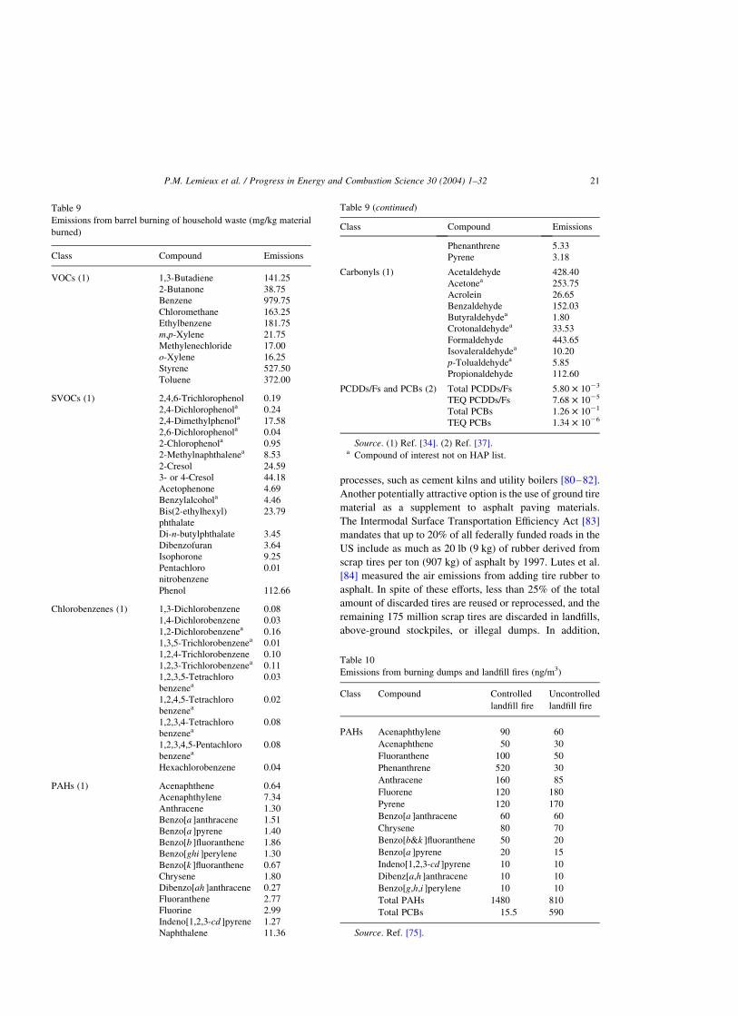
processes, such as cement kilns and utility boilers [80–82].
Another potentially attractive option is the use of ground tire
material as a supplement to asphalt paving materials.
The Intermodal Surface Transportation Efficiency Act [83]
mandates that up to 20% of all federally funded roads in the
US include as much as 20 lb (9 kg) of rubber derived from
scrap tires per ton (907 kg) of asphalt by 1997. Lutes et al.
[84] measured the air emissions from adding tire rubber to
asphalt. In spite of these efforts, less than 25% of the total
amount of discarded tires are reused or reprocessed, and the
remaining 175 million scrap tires are discarded in landfills,
above-ground stockpiles, or illegal dumps. In addition,
Table 9
Emissions from barrel burning of household waste (mg/kg material
burned)
Class Compound Emissions
VOCs (1) 1,3-Butadiene 141.25
2-Butanone 38.75
Benzene 979.75
Chloromethane 163.25
Ethylbenzene 181.75
m,p-Xylene 21.75
Methylenechloride 17.00
o-Xylene 16.25
Styrene 527.50
Toluene 372.00
SVOCs (1) 2,4,6-Trichlorophenol 0.19
2,4-Dichlorophenola 0.24
2,4-Dimethylphenola 17.58
2,6-Dichlorophenola 0.04
2-Chlorophenola 0.95
2-Methylnaphthalenea 8.53
2-Cresol 24.59
3- or 4-Cresol 44.18
Acetophenone 4.69
Benzylalcohola 4.46
Bis(2-ethylhexyl)
phthalate
23.79
Di-n-butylphthalate 3.45
Dibenzofuran 3.64
Isophorone 9.25
Pentachloro
nitrobenzene
0.01
Phenol 112.66
Chlorobenzenes (1) 1,3-Dichlorobenzene 0.08
1,4-Dichlorobenzene 0.03
1,2-Dichlorobenzenea 0.16
1,3,5-Trichlorobenzenea 0.01
1,2,4-Trichlorobenzene 0.10
1,2,3-Trichlorobenzenea 0.11
1,2,3,5-Tetrachloro
benzenea0.03
1,2,4,5-Tetrachloro
benzenea0.02
1,2,3,4-Tetrachloro
benzenea0.08
1,2,3,4,5-Pentachloro
benzenea0.08
Hexachlorobenzene 0.04
PAHs (1) Acenaphthene 0.64
Acenaphthylene 7.34
Anthracene 1.30
Benzo[a ]anthracene 1.51
Benzo[a ]pyrene 1.40
Benzo[b ]fluoranthene 1.86
Benzo[ghi ]perylene 1.30
Benzo[k ]fluoranthene 0.67
Chrysene 1.80
Dibenzo[ah ]anthracene 0.27
Fluoranthene 2.77
Fluorine 2.99
Indeno[1,2,3-cd ]pyrene 1.27
Naphthalene 11.36
Class Compound Emissions
Phenanthrene 5.33
Pyrene 3.18
Carbonyls (1) Acetaldehyde 428.40
Acetonea 253.75
Acrolein 26.65
Benzaldehyde 152.03
Butyraldehydea 1.80
Crotonaldehydea 33.53
Formaldehyde 443.65
Isovaleraldehydea 10.20
p-Tolualdehydea 5.85
Propionaldehyde 112.60
PCDDs/Fs and PCBs (2) Total PCDDs/Fs 5.80 £ 1023
TEQ PCDDs/Fs 7.68 £ 1025
Total PCBs 1.26 £ 1021
TEQ PCBs 1.34 £ 1026
Source. (1) Ref. [34]. (2) Ref. [37].a Compound of interest not on HAP list.
Table 10
Emissions from burning dumps and landfill fires (ng/m3)
Class Compound Controlled
landfill fire
Uncontrolled
landfill fire
PAHs Acenaphthylene 90 60
Acenaphthene 50 30
Fluoranthene 100 50
Phenanthrene 520 30
Anthracene 160 85
Fluorene 120 180
Pyrene 120 170
Benzo[a ]anthracene 60 60
Chrysene 80 70
Benzo[b&k ]fluoranthene 50 20
Benzo[a ]pyrene 20 15
Indeno[1,2,3-cd ]pyrene 10 10
Dibenz[a,h ]anthracene 10 10
Benzo[g,h,i ]perylene 10 10
Total PAHs 1480 810
Total PCBs 15.5 590
Source. Ref. [75].
Table 9 (continued)
P.M. Lemieux et al. / Progress in Energy and Combustion Science 30 (2004) 1–32 21
these reclamation efforts do little to affect the estimated 2
billion tires (18 million tons) already present in stockpiles.
A side effect of the problems associated with scrap
rubber tires is the frequent occurrence of tire fires at tire
stockpiles. These fires, which are often started by arsonists,
generate large amounts of heat and smoke and are difficult to
extinguish. This is partly due to the fact that tires, in general,
have more heat energy by weight than coal does (37,600 vs.
27,200 kJ/kg) [82]. Some tire fires have burned continu-
ously for months, such as the 9-month Rhinehart tire fire in
Winchester, VA. Such fires pollute not only the atmosphere
but also the land and groundwater due to the liquefaction of
the rubber during the combustion process.
Several EPA reports and subsequent journal articles have
been published on a set of laboratory-scale simulations of a
tire fire. These documents reported on VOC and SVOC air
toxics as well as PM and other criteria pollutants [17,33].
PCDDs/Fs were not measured. A follow on study that was
performed in collaboration with health effects researchers
measured the mutagenic activity associated with tire fires
[32]. A paper study prepared by Reisman [85] collected data
on ambient monitoring near tire fires and compared the
results to laboratory simulations. Based on these studies,
Table 11 was constructed using the average of the four test
conditions described in Ref. [33].
3.3.4. Automobile shredder fluff
When automobiles are recycled, the carcasses are
typically shredded, and the metallic components are
separated from the non-metallic components using a
combination of magnetic or gravimetric methods
(cyclones or floatation). The non-metallic residue is called
automobile shredder ‘fluff’. The fluff is then usually baled
and landfilled. Occasionally the bales of shredder fluff can
catch fire. These occurrences are not frequent, but do happen
on occasion. Combustion of automobile components (e.g.
tires, seats, floor mats) was one of the sources presented in
the original Gerstle and Kemnitz study [31]. Ryan and Lutes
[18], reported on a laboratory simulation study where small
quantities of shredder fluff were combusted, and extremely
high organic emissions resulted, exceeding 200 g/kg of fluff
combusted. Emissions of PCDDs/Fs were exceedingly high,
although only PCDD/F homologues were analyzed rather
than specific isomers, which prevented calculation of TEQ
units. Air toxics from automobile shredder residue
combustion are listed in Table 12.
3.3.5. Open burning of fiberglass
Fiberglass is used as a construction material for low-cost
outbuildings such as sheds. It is also commonly used in boat
construction. In response to requests from state and local
environmental agencies, the EPA performed a laboratory
simulation of open burning of various types of fiberglass
materials [26]. The types of fiberglass tested included
samples from boat fabrication and building construction,
where the glass fibers were bound within a resinous
substrate. Data did not include fiberglass insulation.
Numerous air toxics were measured in that study, a
summary of which is shown in Table 13.
3.3.6. Agricultural plastic
Agricultural activities frequently result in the open
burning of plastic materials. Pesticides including Thimet
and Atrazine are delivered in plastic bags, which are
commonly burned in the open in the farm fields. Oberacker
et al. [27] performed a series of tests in which air toxics from
this practice were measured. Measurements were made from
burning empty bags from both types of pesticides and from
burning bags that had trace amounts of residual pesticides
remaining in the bags. PCDD/F measurements were made
on the Atrazine bag tests, and those results suggest that the
Atrazine traces remaining in the bags contributed to the
PCDDs/Fs rather than the bags themselves. These results are
summarized in Table 14, using the assumption that each bag
weighed 0.1 kg.
Sheets of black plastic film are used in agricultural settings
for mulching purposes such as ground moisture control and
weed control. At the end of the growing season, this film is
gathered in a pile and burned in the open. Linak et al. [38]
performed a laboratory simulation to evaluate emissions of
air toxics from this practice. The results from this laboratory
simulation were not presented in units that could be converted
to emission factors; however, there was some additional work
done during this study where mutagenicity of the analytical
extracts was measured using bioassay techniques.
3.3.7. Structural fires
Although criteria pollutant data and non-speciated VOC
data from structural fires are presented in EIIP [4] and a
paper by Brown et al. [86] no data on air toxic emissions
from structural fires could be found. Carroll [87] examined
emissions from burning of various components of
structures, particularly PVC. Although generic emission
factors were not reported, references were made to
emissions data from some of the components that might
be found in structures (e.g. insulation, wood, plastic).
3.3.8. Vehicle fires
This category of burning refers to fires of the vehicle
itself, such an automobile or train. Emissions from any cargo
the vehicle would be carrying are covered separately, such as
under liquid fuels. Although criteria pollutant data from
vehicular fires are presented in AP-42 [3] and EIIP [4], they
were derived primarily from Gerstle and Kemnitz [31] and no
data on air toxic emissions could be found from this source.
3.3.9. Construction debris
No sources of data on emissions of criteria pollutants or
air toxics from open burning of construction debris could be
found, although the work of Carroll [87] regarding
emissions from structural fires may be applicable.
The composition of the debris would have a profound
P.M. Lemieux et al. / Progress in Energy and Combustion Science 30 (2004) 1–3222

impact on the emissions from open burning of those
materials. Construction debris would include various
plastics (vinyl siding, housewrap) and wood (both treated
and untreated), so the open burning of construction debris
would likely have different emissions from conventional
scrap wood burning or land clearing debris burning
activities. Given the prevalence of this practice and its
similarities to other sources that have been found to be
significant, such as open burning of household waste in
barrels, this source presents a potentially important data gap
that should be addressed.
3.3.10. Grain silo fires
No sources of data on emissions of criteria pollutants or
air toxics from grain silo fires could be found.
3.3.11. Open burning of electronics waste
As the quantity of discarded computer equipment and
other consumer electronics increases, the possibility of open
burning as a disposal technique becomes more likely.
There are reports of sham recycling activities in developing
countries where open burning is used on electronics waste
[22], but no emissions data were found.
3.4. Miscellaneous fuels
3.4.1. Copper wire reclamation
Copper wire is frequently coated with a plastic insulation
material. It is a common practice in many parts of the world
to use open burning to remove the insulation so that the
underlying copper wire can be reclaimed for value. Current
understanding of the formation mechanisms of PCDDs/Fs
proposes copper-based catalysts as an important contributor
to PCDD/F emissions. The presence of significant
Table 11
Emissions from open burning of scrap tires (mg/kg burned)
Class Compound Emissions
VOCs Benzaldehydea 314.4
Benzene 2180.55
Benzodiazinea 15.55
Benzofuran 12.55
Benzothiophenea 20.5
Butadiene 234.6
Dihydroindenea 41.7
Xylenes 928.95
Dimethylhexadienea 59.6
Dimethyl,methylpropyl benzenea 7.45
Dimethyldihydroindenea 19.85
Ethenylbenzenea 776.6
Ethenylcyclohexenea 66.9
Ethenyl,dimethylbenzenea 15.45
Ethenyl,methylbenzenea 16.8
Ethenyldimethylcyclohexenea 175.2
Ethenylmethylbenzenea 131.25
Ethylbenzene 377.95
Ethyl,methylbenzenea 405.15
Ethynylbenzenea 160.75
Ethynyl,methylbenzenea 394.65
Isocyanobenzenea 318.55
Limonenea 460
Toluene 1367.75
Methylindenea 228.25
Methylthiophenea 9.05
Methyl,ethenylbenzenea 66.15
Methyl,methylethenylbenzenea 390.75
Methyl,methylethylbenzenea 197.45
Methyl,propylbenzenea 20.8
Ethyleneindenea 41.45
Methylethylbenzenea 152.15
Propylbenzenea 78.3
Styrene 652.7
Tetramethylbenzenea 127.85
Thiophenea 41.25
Trimethylbenzenea 60.9
SVOCs 1-Methylnaphthalenea 279.15
1,10-Biphenyl,methyla 5.55
2-Methylnaphthalenea 389.95
Benzisothiazolea 86.95
Benzo[b ]thiophenea 22.1
Biphenyl 269.8
Cyanobenzenea 370.25
Dimethylbenzenea 620.05
Dimethylnaphthalenea 109.6
Ethyl,dimethylbenzenea 136.2
Hexahydroazepinonea 411.8
Indenea 421.3
Isocyanonaphthalenea 4.7
Methylbenzaldehydea 43.3
Phenol 533.05
Propenylnaphthalenea 11.75
Propenyl,methylbenzenea 261.8
Trimethylnaphthalenea 157.9
Class Compound Emissions
PAHs Naphthalene 650.95
Acenaphthylene 711.55
Acenaphthene 1368
Fluorene 223.65
Phenanthrene 245
Anthracene 52.95
Fluoranthene 398.35
Pyrene 92.75
Benz[a ]anthracene 92.3
Chrysene 81.2
Benzo[b ]fluoranthene 78.9
Benzo[k ]fluoranthene 86.85
Benzo[a ]pyrene 99.35
Dibenz[a,h ]anthracene 0.55
Benzo[g,h,i ]perylene 112.7
Indeno[1,2,3-cd ]pyrene 68.55
Source. Ref. [33].a Compound of interest not on HAP list.
Table 11 (continued)
P.M. Lemieux et al. / Progress in Energy and Combustion Science 30 (2004) 1–32 23
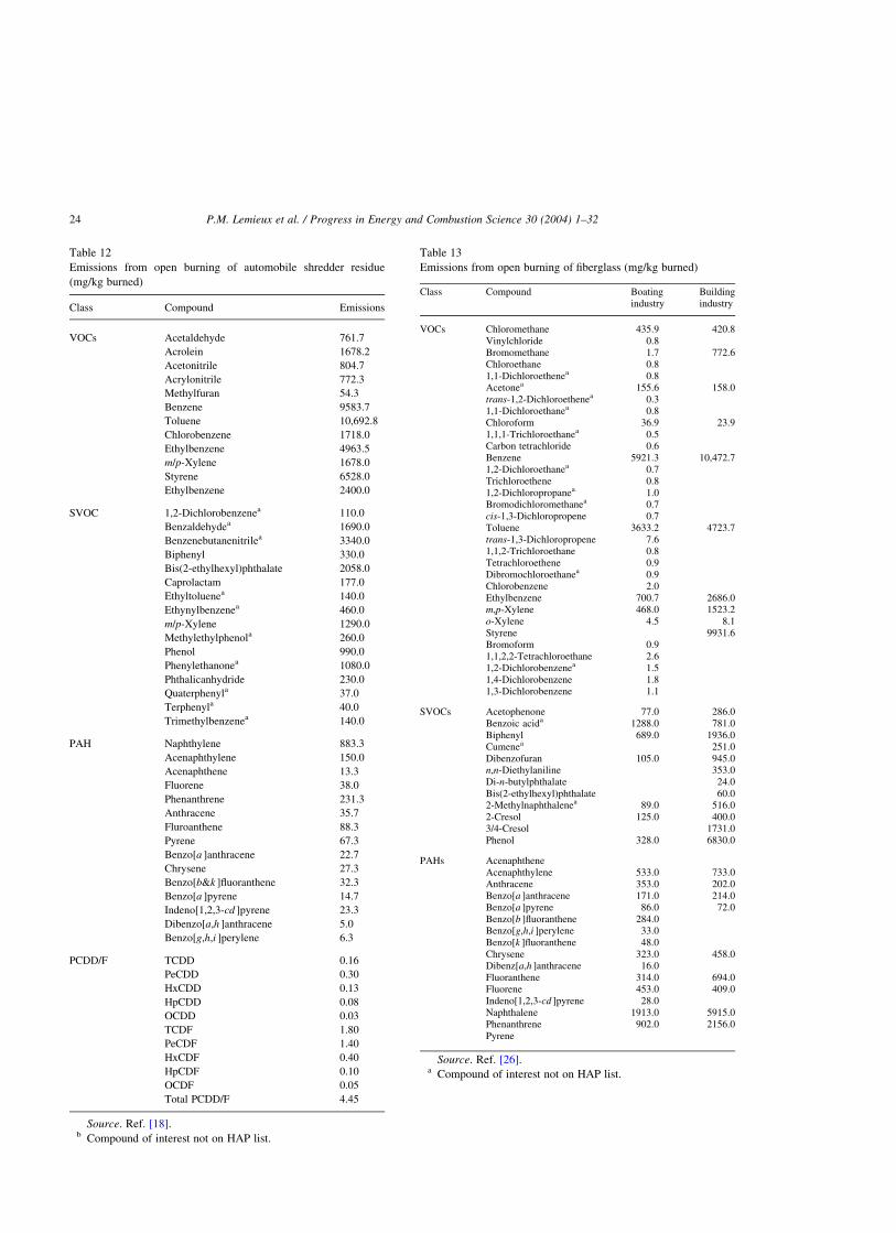
Table 12
Emissions from open burning of automobile shredder residue
(mg/kg burned)
Class Compound Emissions
VOCs Acetaldehyde 761.7
Acrolein 1678.2
Acetonitrile 804.7
Acrylonitrile 772.3
Methylfuran 54.3
Benzene 9583.7
Toluene 10,692.8
Chlorobenzene 1718.0
Ethylbenzene 4963.5
m/p-Xylene 1678.0
Styrene 6528.0
Ethylbenzene 2400.0
SVOC 1,2-Dichlorobenzenea 110.0
Benzaldehydea 1690.0
Benzenebutanenitrilea 3340.0
Biphenyl 330.0
Bis(2-ethylhexyl)phthalate 2058.0
Caprolactam 177.0
Ethyltoluenea 140.0
Ethynylbenzenea 460.0
m/p-Xylene 1290.0
Methylethylphenola 260.0
Phenol 990.0
Phenylethanonea 1080.0
Phthalicanhydride 230.0
Quaterphenyla 37.0
Terphenyla 40.0
Trimethylbenzenea 140.0
PAH Naphthylene 883.3
Acenaphthylene 150.0
Acenaphthene 13.3
Fluorene 38.0
Phenanthrene 231.3
Anthracene 35.7
Fluroanthene 88.3
Pyrene 67.3
Benzo[a ]anthracene 22.7
Chrysene 27.3
Benzo[b&k ]fluoranthene 32.3
Benzo[a ]pyrene 14.7
Indeno[1,2,3-cd ]pyrene 23.3
Dibenzo[a,h ]anthracene 5.0
Benzo[g,h,i ]perylene 6.3
PCDD/F TCDD 0.16
PeCDD 0.30
HxCDD 0.13
HpCDD 0.08
OCDD 0.03
TCDF 1.80
PeCDF 1.40
HxCDF 0.40
HpCDF 0.10
OCDF 0.05
Total PCDD/F 4.45
Source. Ref. [18].b Compound of interest not on HAP list.
Table 13
Emissions from open burning of fiberglass (mg/kg burned)
Class Compound Boatingindustry
Buildingindustry
VOCs Chloromethane 435.9 420.8Vinylchloride 0.8Bromomethane 1.7 772.6Chloroethane 0.81,1-Dichloroethenea 0.8Acetonea 155.6 158.0trans-1,2-Dichloroethenea 0.31,1-Dichloroethanea 0.8Chloroform 36.9 23.91,1,1-Trichloroethanea 0.5Carbon tetrachloride 0.6Benzene 5921.3 10,472.71,2-Dichloroethanea 0.7Trichloroethene 0.81,2-Dichloropropanea 1.0Bromodichloromethanea 0.7cis-1,3-Dichloropropene 0.7Toluene 3633.2 4723.7trans-1,3-Dichloropropene 7.61,1,2-Trichloroethane 0.8Tetrachloroethene 0.9Dibromochloroethanea 0.9Chlorobenzene 2.0Ethylbenzene 700.7 2686.0m,p-Xylene 468.0 1523.2o-Xylene 4.5 8.1Styrene 9931.6Bromoform 0.91,1,2,2-Tetrachloroethane 2.61,2-Dichlorobenzenea 1.51,4-Dichlorobenzene 1.81,3-Dichlorobenzene 1.1
SVOCs Acetophenone 77.0 286.0Benzoic acida 1288.0 781.0Biphenyl 689.0 1936.0Cumenea 251.0Dibenzofuran 105.0 945.0n,n-Diethylaniline 353.0Di-n-butylphthalate 24.0Bis(2-ethylhexyl)phthalate 60.02-Methylnaphthalenea 89.0 516.02-Cresol 125.0 400.03/4-Cresol 1731.0Phenol 328.0 6830.0
PAHs AcenaphtheneAcenaphthylene 533.0 733.0Anthracene 353.0 202.0Benzo[a ]anthracene 171.0 214.0Benzo[a ]pyrene 86.0 72.0Benzo[b ]fluoranthene 284.0Benzo[g,h,i ]perylene 33.0Benzo[k ]fluoranthene 48.0Chrysene 323.0 458.0Dibenz[a,h ]anthracene 16.0Fluoranthene 314.0 694.0Fluorene 453.0 409.0Indeno[1,2,3-cd ]pyrene 28.0Naphthalene 1913.0 5915.0Phenanthrene 902.0 2156.0Pyrene
Source. Ref. [26].a Compound of interest not on HAP list.
P.M. Lemieux et al. / Progress in Energy and Combustion Science 30 (2004) 1–3224
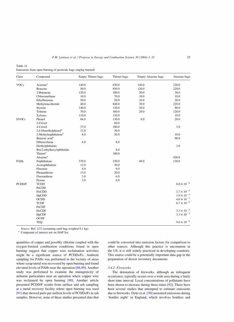
quantities of copper and possibly chlorine coupled with the
oxygen-limited combustion conditions found in open
burning suggest that copper wire reclamation activities
might be a significant source of PCDDs/Fs. Ambient
sampling for PAHs was performed in the vicinity of areas
where scrap metal was recovered by open burning and found
elevated levels of PAHs near the operation [88,89]. Another
study was performed to examine the mutagenicity of
airborne particulates near an operation where copper wire
was reclaimed by open burning [90]. Another article
presented PCDD/F results from surface and ash sampling
at a metal recovery facility where open burning was used
[91] that showed parts per million levels of PCDDs/Fs in ash
samples. However, none of these studies presented data that
could be converted into emission factors for comparison to
other sources. Although this practice is uncommon in
the US, it is still widely practiced in developing countries.
This source could be a potentially important data gap in the
preparation of dioxin inventory documents.
3.4.2. Fireworks
The detonation of fireworks, although an infrequent
occurrence, typically occurs over a wide area during a fairly
short time interval. Local concentrations of pollutants have
been shown to increase during those times [92]. There have
been several studies that attempted to estimate emissions
due to fireworks. Dyke et al. [50] measured emissions during
‘bonfire night’ in England, which involves bonfires and
Table 14
Emissions from open burning of pesticide bags (mg/kg burned)
Class Compound Empty Thimet bags Thimet bags Empty Atrazine bags Atrazine bags
VOCs Acetonea 140.0 630.0 140.0 220.0
Benzene 50.0 850.0 120.0 220.0
2-Butanone 120.0 100.0 20.0 30.0
Chloromethane 10.0 70.0 10.0 10.0
Ethylbenzene 50.0 50.0 10.0 20.0
Methylenechloride 40.0 840.0 30.0 220.0
Styrene 140.0 120.0 20.0 90.0
Toluene 70.0 360.0 20.0 120.0
Xylenes 110.0 110.0 10.0
SVOCs Phenol 84.0 130.0 8.0 20.0
2-Cresol 60.0
4-Cresol 37.0 100.0 3.0
2,4-Dimethylphenola 12.0 30.0
2-Methylnaphthalenea 8.0 20.0 10.0
Benzoic acida 90.0
Dibenzofuran 4.0 8.0
Diethylphthalate 3.0
Bis(2-ethylhexyl)phthalate 8.0
Thimeta 180.0
Atrazinea 420.0
PAHs Naphthalene 370.0 230.0 49.0 130.0
Acenaphthalene 12.0 30.0
Fluorene 4.0 9.0
Phenanthrene 13.0 20.0
Fluoranthene 3.0 6.0
Pyrene 3.0 6.0
PCDD/F TCDD 8.0 £ 1026
PeCDD
HxCDD 2.7 £ 1025
HpCDD 1.0 £ 1024
OCDD 4.0 £ 1025
TCDF 6.7 £ 1026
PeCDF
HxCDF 3.3 £ 1025
HpCDF 3.3 £ 1025
OCDF
TEQ 9.0 £ 1026
Source. Ref. [27] (assuming each bag weighed 0.1 kg).a Compound of interest not on HAP list.
P.M. Lemieux et al. / Progress in Energy and Combustion Science 30 (2004) 1–32 25
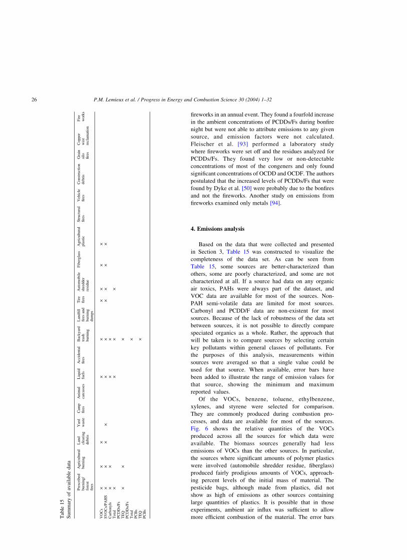
fireworks in an annual event. They found a fourfold increase
in the ambient concentrations of PCDDs/Fs during bonfire
night but were not able to attribute emissions to any given
source, and emission factors were not calculated.
Fleischer et al. [93] performed a laboratory study
where fireworks were set off and the residues analyzed for
PCDDs/Fs. They found very low or non-detectable
concentrations of most of the congeners and only found
significant concentrations of OCDD and OCDF. The authors
postulated that the increased levels of PCDDs/Fs that were
found by Dyke et al. [50] were probably due to the bonfires
and not the fireworks. Another study on emissions from
fireworks examined only metals [94].
4. Emissions analysis
Based on the data that were collected and presented
in Section 3, Table 15 was constructed to visualize the
completeness of the data set. As can be seen from
Table 15, some sources are better-characterized than
others, some are poorly characterized, and some are not
characterized at all. If a source had data on any organic
air toxics, PAHs were always part of the dataset, and
VOC data are available for most of the sources. Non-
PAH semi-volatile data are limited for most sources.
Carbonyl and PCDD/F data are non-existent for most
sources. Because of the lack of robustness of the data set
between sources, it is not possible to directly compare
speciated organics as a whole. Rather, the approach that
will be taken is to compare sources by selecting certain
key pollutants within general classes of pollutants. For
the purposes of this analysis, measurements within
sources were averaged so that a single value could be
used for that source. When available, error bars have
been added to illustrate the range of emission values for
that source, showing the minimum and maximum
reported values.
Of the VOCs, benzene, toluene, ethylbenzene,
xylenes, and styrene were selected for comparison.
They are commonly produced during combustion pro-
cesses, and data are available for most of the sources.
Fig. 6 shows the relative quantities of the VOCs
produced across all the sources for which data were
available. The biomass sources generally had less
emissions of VOCs than the other sources. In particular,
the sources where significant amounts of polymer plastics
were involved (automobile shredder residue, fiberglass)
produced fairly prodigious amounts of VOCs, approach-
ing percent levels of the initial mass of material. The
pesticide bags, although made from plastics, did not
show as high of emissions as other sources containing
large quantities of plastics. It is possible that in those
experiments, ambient air influx was sufficient to allow
more efficient combustion of the material. The error barsTab
le1
5
Su
mm
ary
of
avai
lab
led
ata
Pre
scri
bed
bu
rnin
g/
fore
stfi
res
Agri
cult
ura
lb
urn
ing
Lan
dcl
eari
ng
deb
ris
Yar
dw
aste
Cam
pfi
res
An
imal
carc
asse
sL
iqu
idfu
els
Acc
iden
tal
fire
sB
ack
yar
dtr
ash
bu
rnin
g
Lan
dfi
llfi
res
and
bu
rnin
gd
um
ps
Tir
efi
res
Au
tom
ob
ile
shre
dder
resi
due
Fib
ergla
ssA
gri
cult
ura
lpla
stic
Str
uct
ura
lfi
res
Veh
icle
fire
sC
on
stru
ctio
nd
ebri
sG
rain
silo
fire
s
Co
pp
erw
ire
recl
amat
ion
Fir
ew
ork
s
VO
Cs
££
££
££
££
£S
VO
Cs/
PA
HS
££
££
££
££
££
Car
bo
ny
ls£
££
£T
ota
lP
CD
Ds/
Fs
££
££
TE
QP
CD
Ds/
Fs
££
£
To
tal
PC
Bs
£
TE
QP
CB
s£
P.M. Lemieux et al. / Progress in Energy and Combustion Science 30 (2004) 1–3226

on Figs. 6–9 represent the range of values for the data;
if the lower error bar is missing, it means that the lower
bound was zero, and could not be displayed on a semi-
logarithmic plot. This is distinguished from plots where
no bar is shown at all, which indicates that no data were
available.
For the SVOCs, naphthalene, benzo[a]pyrene, and total
non-naphthalene PAHs were chosen for comparison. It must
be noted that, for agricultural burning, naphthalene was not
included because of the reference’s authors’ doubts on the
veracity of the data. Fig. 7 compares the SVOC
emissions from the various sources (note the logarithmic
scale). As was the case with the VOCs, the combustion of
biomass produced less SVOCs than combustion of various
man-made products. Pool fires of liquid fuels produced
significant amounts of PAHs. However, the tire fires
and combustion of fiberglass produced the most PAHs.
Tire fires produced nearly 100 mg of benzo[a ]pyrene per kg
of tire combusted.
The available data for carbonyls is much more
limited. For this analysis, formaldehyde was chosen as
the compound for comparison between sources. Fig. 8
shows the relative emissions of formaldehyde from open
burning. Although the data set is much more limited, the
combustion of biomass produced significantly
more formaldehyde than the other open burning sources.
This is likely due to the high levels of elemental
oxygen bound within the cellulose structures found in
biomass.
Fig. 6. VOCs from open burning sources (mg/kg burned).
Fig. 7. SVOCs from open burning sources (mg/kg burned).
P.M. Lemieux et al. / Progress in Energy and Combustion Science 30 (2004) 1–32 27
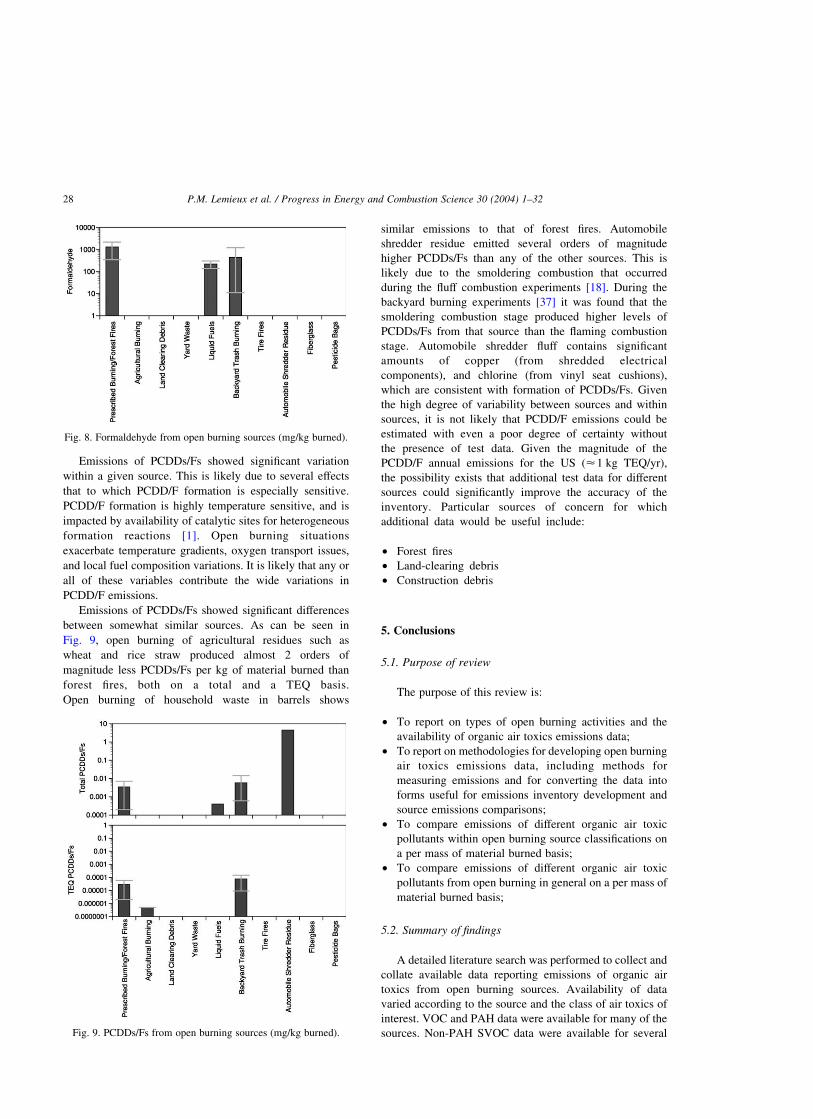
Emissions of PCDDs/Fs showed significant variation
within a given source. This is likely due to several effects
that to which PCDD/F formation is especially sensitive.
PCDD/F formation is highly temperature sensitive, and is
impacted by availability of catalytic sites for heterogeneous
formation reactions [1]. Open burning situations
exacerbate temperature gradients, oxygen transport issues,
and local fuel composition variations. It is likely that any or
all of these variables contribute the wide variations in
PCDD/F emissions.
Emissions of PCDDs/Fs showed significant differences
between somewhat similar sources. As can be seen in
Fig. 9, open burning of agricultural residues such as
wheat and rice straw produced almost 2 orders of
magnitude less PCDDs/Fs per kg of material burned than
forest fires, both on a total and a TEQ basis.
Open burning of household waste in barrels shows
similar emissions to that of forest fires. Automobile
shredder residue emitted several orders of magnitude
higher PCDDs/Fs than any of the other sources. This is
likely due to the smoldering combustion that occurred
during the fluff combustion experiments [18]. During the
backyard burning experiments [37] it was found that the
smoldering combustion stage produced higher levels of
PCDDs/Fs from that source than the flaming combustion
stage. Automobile shredder fluff contains significant
amounts of copper (from shredded electrical
components), and chlorine (from vinyl seat cushions),
which are consistent with formation of PCDDs/Fs. Given
the high degree of variability between sources and within
sources, it is not likely that PCDD/F emissions could be
estimated with even a poor degree of certainty without
the presence of test data. Given the magnitude of the
PCDD/F annual emissions for the US (<1 kg TEQ/yr),
the possibility exists that additional test data for different
sources could significantly improve the accuracy of the
inventory. Particular sources of concern for which
additional data would be useful include:
† Forest fires
† Land-clearing debris
† Construction debris
5. Conclusions
5.1. Purpose of review
The purpose of this review is:
† To report on types of open burning activities and the
availability of organic air toxics emissions data;
† To report on methodologies for developing open burning
air toxics emissions data, including methods for
measuring emissions and for converting the data into
forms useful for emissions inventory development and
source emissions comparisons;
† To compare emissions of different organic air toxic
pollutants within open burning source classifications on
a per mass of material burned basis;
† To compare emissions of different organic air toxic
pollutants from open burning in general on a per mass of
material burned basis;
5.2. Summary of findings
A detailed literature search was performed to collect and
collate available data reporting emissions of organic air
toxics from open burning sources. Availability of data
varied according to the source and the class of air toxics of
interest. VOC and PAH data were available for many of the
sources. Non-PAH SVOC data were available for several
Fig. 8. Formaldehyde from open burning sources (mg/kg burned).
Fig. 9. PCDDs/Fs from open burning sources (mg/kg burned).
P.M. Lemieux et al. / Progress in Energy and Combustion Science 30 (2004) 1–3228
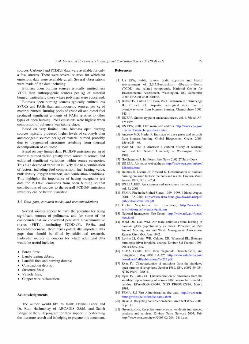
sources. Carbonyl and PCDD/F data were available for only
a few sources. There were several sources for which no
emissions data were available at all. Several observations
were made of the data including:
Biomass open burning sources typically emitted less
VOCs than anthropogenic sources per kg of material
burned, particularly those where polymers were concerned.
Biomass open burning sources typically emitted less
SVOCs and PAHs than anthropogenic sources per kg of
material burned. Burning pools of crude oil and diesel fuel
produced significant amounts of PAHs relative to other
types of open burning. PAH emissions were highest when
combustion of polymers was taking place.
Based on very limited data, biomass open burning
sources typically produced higher levels of carbonyls than
anthropogenic sources per kg of material burned, probably
due to oxygenated structures resulting from thermal
decomposition of cellulose.
Based on very limited data, PCDD/F emissions per kg of
material burned varied greatly from source to source, and
exhibited significant variations within source categories.
This high degree of variation is likely due to a combination
of factors, including fuel composition, fuel heating value,
bulk density, oxygen transport, and combustion conditions.
This highlights the importance of having acceptable test
data for PCDD/F emissions from open burning so that
contributions of sources to the overall PCDD/F emissions
inventory can be better quantified.
5.3. Data gaps, research needs, and recommendations
Several sources appear to have the potential for being
significant sources of pollutants, and for some of the
compounds that are considered persistent bioaccumulative
toxics (PBTs), including PCDDs/Fs, PAHs, and
hexachlorobenzene, there exists potentially important data
gaps that should be filled by additional research.
Particular sources of concern for which additional data
would be useful include:
† Forest fires;
† Land-clearing debris;
† Landfill fires and burning dumps;
† Construction debris;
† Structure fires;
† Vehicle fires;
† Copper wire reclamation.
Acknowledgements
The author would like to thank Dennis Tabor and
Dr. Ram Hashmonay of ARCADIS G&M, and Satish
Bhagat of the SEE program for their support in performing
the literature search and in helping to prepare this document.
References
[1] US EPA, Public review draft: exposure and health
reassessment of 2,3,7,8-tetrachloro dibenzo-p-dioxin
(TCDD) and related compounds. National Center for
Environmental Assessment, Washington, DC; September
2000. EPA-600/P-00-001Bb.
[2] Barber TR, Lutes CC, Doorn MRJ, Fuchsman PC, Timmenga
HJ, Crouch RL. Aquatic ecological risks due to
cyanide releases from biomass burning. Chemosphere 2002;
343–4.
[3] US EPA. Stationary point and area sources, vol. 1. 5th ed. AP-
42; 1996.
[4] US EPA; 2001, EIIP main web address: http://www.epa.gov/
ttn/chief/eiip/techreport/index.html
[5] Andreae MO, Merlet P. Emission of trace gases and aerosols
from biomass burning. Global Biogeochem Cycles 2001;
15(4):955–66.
[6] Pyne SJ. Fire in America: a cultural history of wildland
and rural fire. Seattle: University of Washington Press;
1982.
[7] Goldhammer J. Int Forest Fire News 2002;27(July–Dec).
[8] US EPA. Air toxics web address: http://www.epa.gov/ttn/atw/
188polls.html
[9] Delmas R, Lacaux JP, Brocard D. Determination of biomass
burning emission factors: methods and results. Environ Monit
Assess 1995;38:181–204.
[10] US EPA, EIIP. Area sources and area source method abstracts,
vol. 3.; 2001.
[11] FEMA, Fire in the United States: 1989–1998. 12th ed, August
2001. FA-216; http://www.usfa.fema.gov/downloads/pdf/
publications/fius12th.pdf.
[12] Global Vegetation Fire Inventory, http://www.fire.
uni-freiburg.de/inventory/gvfi.htm
[13] National Interagency Fire Center, http://www.nifc.gov/news/
nicc.html
[14] Ward DE, Hao WM. Air toxic emissions from burning of
biomass globally-preliminary estimates. Presented at 85th
Annual Meeting, Air and Waste Management Association,
Kansas City, MO; June 1992.
[15] Levine JS, Cofer WR, Cahoon DR, Winstead EL. Biomass
burning: a driver for global change. Environ Sci Technol 1995;
29(3):120A–5A.
[16] FEMA, Landfill fires: their magnitude, characteristics, and
mitigation. ; May 2002. FA-225, http://www.usfa.fema.gov/
downloads/pdf/publications/fa-225.pdf.
[17] Ryan JV. Characterization of emissions from the simulated
open burning of scrap tires; October 1989. EPA-600/2-89-054,
NTIS PB90-126004.
[18] Ryan JV, Lutes CC. Characterization of emissions from the
simulated open burning of non-metallic automobile shredder
residue. EPA-600/R-93-044, NTIS PB930172914; March
1993.
[19] FEMA. US Fire Administration, fire data, http://www.usfa.
fema.gov/inside-usfa/nfdc-data3.shtm
[20] Davis A. Recycling construction debris. Architect Week 2001;
Sep:E1.1.
[21] Greenbiz.com, Recyclers turn construction debris into needed
products and services. Environ News Network 2003; Feb.
http://www.enn.com/news/2003-02-20/s_2419.asp.
P.M. Lemieux et al. / Progress in Energy and Combustion Science 30 (2004) 1–32 29
[22] Hileman B. Electronic waste. Chem Engng News 2002;
1(July):15–18.
[23] US EPA, AP-42. Wildfires and prescribed burning; 1996
[chapter 13.1].
[24] Lutes CC, Kariher PH. Evaluation of emissions from the open
burning of land-clearing debris; 1998, EPA-600/R-96-128,
NTIS PB97-115356.
[25] Booher LE, Janke B. ir Emissions from petroleum hydro-
carbon fires during controlled burning. Am Ind Hyg Assoc J
1997;58(5):359–65.
[26] Lutes CC, Ryan JV. Characterization of air emissions from the
simulated open combustion of fiberglass materials; 1993,
EPA-600/R-93-239, NTIS PB94-136231.
[27] Oberacker DA, Lin PC, Shaul GM, Ferguson DT, Engleman
VS, Jackson TW, Chapman JS, Evans JD, Martrano RJ, Evey
LL. Characterization of emissions formed from open burning of
pesticide bags. Pesticide Waste Mgmt 1992;510:79–94.
[28] Winberry WT, Murphy NT, Riggan RM. Compendium
method TO-14. The determination of volatile organic
compounds in ambient air using SUMMAw passivated
canister sampling and gas chromatographic analysis. In:
Compendium of methods for the determination of toxic
organic compounds in ambient air, Quality Assurance
Division, Environmental Monitoring Systems Laboratory,
US EPA; 1988. EPA-600/4-89-017, NTIS PB90-127374.
[29] Winberry WT, Murphy NT, Riggan RM. Compendium
method TO-13. The determination of benzo(a)pyrene and
other polynuclear aromatic hydrocarbons in ambient air
using gas chromatographic and high performance liquid
chromatographic analysis. In: Compendium of methods for
the determination of toxic organic compounds in ambient air;
1988. EPA 600/4-89-017, NTIS PB90-127374.
[30] Gullett B, Touati A. PCDD/F emissions from forest fires.
Atmos Environ 2003;37:803–13.
[31] Gerstle RW, Kemnitz DA. Atmospheric emissions from open
burning. J Air Pollut Control Assoc 1967;17(5):324–7.
[32] Lemieux PM, DeMarini DM. Mutagenicity of emissions from
the simulated open burning of scrap rubber tires; July 1992.
EPA-600/R-92-127, NTIS PB92-217009.
[33] Lemieux PM, Ryan JV. Characterization of air pollutants
emitted from a simulated scrap tire fire. Air Waste Mgmt
Assoc J 1993;43(8):1106–15.
[34] Lemieux PM. Evaluation of emissions from the open burning
of household waste in barrels; 1997, EPA-600/R-97-134a (vol.
1), NTIS PB98-127343 and EPA-600/R-97-134b (vol. 2),
PB98-127350.
[35] Lemieux PM, Lutes CC, Abbott JA, Aldous KM. Emissions
of polychlorinated dibenzo-p-dioxins and polychlorinated
dibenzofurans from the open burning of household waste in
barrels. Environ Sci Technol 2000;34:377–84.
[36] Gullett BK, Lemieux PM, Lutes CC, Winterrowd CK, Winters
DL. CDD/F emissions from uncontrolled domestic waste
burning. Chemosphere 2001;43(4–7):721–5.
[37] Lemieux PM, Gullett BK, Lutes CC, Winterrowd CK, Winters
DL. Variables affecting emissions of PCDDs/Fs from
uncontrolled combustion of household waste in barrels.
AWMA J 2003;53:523–31.
[38] Linak WP, Ryan JV, Perry E, Williams RW, DeMarini DM.
Chemical and biological characterization of products of
incomplete combustion from the simulated field burning
of agricultural plastic. J Air Pollut Control Assoc 1989;39(6):
836–46.
[39] Gullett B, Touati A. PCDD/F emissions from agricultural field
burning. Organohalogen Compd 2002;56:135–8.
[40] Jenkins BM, Chang DPY, Raabe OG. Development of test
procedures to determine emissions from open burning of
agricultural and forestry wastes, California State Air Resources
Board; 1990, ARB-R-90-432, NTIS PB90-172305.
[41] Buckley M. OB/OD tests help detonation permitting efforts.
US Army Environmental Center; 1996, http://aec.army.mil/
usaec/publicaffairs/update/sum96/obod.htm
[42] Mickler RA, Henderson B, Smith S, Crews T, VanDruten K.
Range management of wildland fire fuels, fire risk and
prescribed burning of the US air force and navy dare county
bombing range and alligator river NWR. Poster presented at
the SERDP/ESTCP Partners in Environmental Technology
Conference, Washington, DC; December 2002.
[43] Hashmonay RA, Natshke DF, Wagoner K, Harris DB,
Thompson EL, Yost MG. Field evaluation of a method for
estimating gaseous fluxes from area sources using open-path
Fourier transform infrared. Environ Sci Technol 2001;35(11):
2309–13.
[44] Hashmonay RA, Yost MG, Wu CF. Computed tomography of
air pollutants using radial scanning path-integrated optical
remote sensing. Atmos Environ 1999;33(2):267–74.
[45] Hashmonay RA, Yost MG. On the application of OP-FTIR
spectroscopy to measure aerosols: observations of water
droplets. Environ Sci Technol 1999;33(7):1141–4.
[46] Grant WB, Kagann RH, McClenny WA. Optical remote
measurement of toxic gases. Air Waste Mgmt Assoc J 1992;
42(1):18–29.
[47] Higgins KF, Kruse AD, Piehl JL. Prescribed burning
guidelines in the Northern Great Plains, version 16JUL97.
US Fish and Wildlife Service, Cooperative Extension Service,
South Dakota State University, US Department of Agriculture
EC 760. Jamestown, ND: Northern Prairie Wildlife Research
Center; 1989, home page: http://www.npwrc.usgs.gov/
resource/tools/burning/burning.htm
[48] Oros DR, Simoneit BRT. Identification and emission factors
of molecular tracers in organic aerosols from biomass burning.
Part 1. Temperature climate conifers. Appl Geochem 2001;
16(13):1513–44.
[49] Oros DR, Simoneit BRT. Identification and emission factors
of molecular tracers in organic aerosols from biomass burning.
Part 2. Deciduous trees. Appl Geochem 2001;16(13):
1545–65.
[50] Masclet P, Cachier H, Liousse C, Wortham H. Emissions of
polycyclic aromatic hydrocarbons by savanna fires. J Atmos
Chem 1995;22(1/2):41–54.
[51] Kjallstrand J, Ramnas O, Peterson G. Methoxyphenols from
burning of scandinavian forest plant materials. Chemosphere
2000;41(5):735–41.
[52] Prange JA, Cook M, Papke O, Muller JF, Weber R. CDDs/Fs
in the atmosphere and combusted material during a forest fire
in Queensland, Australia. Organohalogen Compd 2002;59:
207–10.
[53] Yamasoe MA, Artaxo P, Miguel ALH, Allen AG.
Chemical composition of aerosol particulates from direct
emissions of vegetation fires in the Amazon Basin: water-
soluble species and trace elements. Atmos Environ 2000;
34(10):1641–53.
P.M. Lemieux et al. / Progress in Energy and Combustion Science 30 (2004) 1–3230
[54] Jenkins BM, Jones AD, Turn SQ, Williams RB. Emission
factors for polycyclic aromatic hydrocarbons from biomass
burning. Environ Sci Technol 1996;30(8):2462–9.
[55] Jenkins BM, Jones AD, Turn SQ, Williams RB.
Particle concentrations, gas–particle partitioning, and species
intercorrelations for polycyclic aromatic hydrocarbons (PAH)
emitted during biomass burning. Atmos Environ 1996;30(22):
3825–35.
[56] Jenkins BM, Turn SQ, Williams RB, Goronea M, Abd-el-
Fattah H, Atmospheric pollutant emission factors from open
burning of agricultural and forest biomass by wind tunnel
simulations, vol. 1. California State Air Resources Board;
1996. NTIS PB97-133037.
[57] Jenkins BM, Turn SQ, Williams RB, Goronea M, Abd-el-
Fattah H, Atmospheric pollutant emission factors from open
burning of agricultural and forest biomass by wind tunnel
simulations, vol. 2. California State Air Resources Board;
1996. NTIS PB97-126940.
[58] Guyton B, Stephenson G, Clayton R. Sampling support
for cane field burning. Acurex final report TR-86-010/SR;
1986.
[59] Hawaii. Inventory of Hawaii greenhouse gas emissions;
estimates for 1990 by the Energy, Resources, and Technology
Division, Department of Business, Economic Development,
and Tourism and the Clean Air Branch, Department of Health,
State of Hawaii, Honolulu. Greenhouse gases: Hawaii.
I. Hawaii. Department of Health, Clean Air Branch; 1997.
TD885.5.G73.H38.
[60] Jenkins BM, Turn SQ, Williams RB, Goronea M, Abd-el-
Fattah H, Atmospheric pollutant emission factors from open
burning of agricultural and forest biomass by wind tunnel
simulations, vol. 3. California State Air Resources Board;
1996. NTIS PB97-132369.
[61] Illinois Institute of Natural Resources. Environmental Health
Resource Center Advisory report on the potential health
effects of leaf burning. IINR Document 78/19. EHRC
Document No. 19; 1978.
[62] Simoneit BRT, Rogge WF, Lange Q, Jaffec R. Molecular
characterization of smoke from campfire burning of pine wood.
Chemosphere: Global Change Sci 2000;2(1):107–22.
[63] Dyke P, Coleman P, James R. Dioxins in ambient air, Bonfire
Night 1994. Chemosphere 1997;34(5-7):1191–201.
[64] UK Department of Health. Foot and mouth-effects on heath of
emissions from pyres used for disposal of animals; 2001,
http://www.doh.gov.uk/fmdguidance
[65] Husain T. Kuwaiti oil fires: source estimates and plume
characterization. Atmos Environ 1994;28(13):2149–58.
[66] Stevens R, Pinto J, Mamane Y, Ondov J, Abdulraheem
M, Al-Majed N, Sadek M, Cofer W, Ellenson W, Kellog
R. Chemical and physical properties of emissions from
Kuwaiti oil fires. Water Sci Technol 1993;27(7/8):
223–33.
[67] Ross JL, Ferek RJ, Hobbs PV. Particle and gas emissions from
an in situ burn of crude oil on the ocean. Air Waste Mgmt
Assoc J 1996;46:251–9.
[68] Fingas M, Li K, Ackerman F, Bissonnette MC, Lambert P,
Halley G, Nelson R, Belanger J, Pare JRP. The Newfoundland
in situ oil burn experiment, NOBE. Spill Technol Newslett
1993;18(2):1–20.
[69] Fingas MF, Li K, Ackerman F, Campagna PR, Turpin RD,
Getty SJ, Soleki MF, Trespalacios MJ, Wang Z, Pare J,
Belanger J, Bissonnette M, Mullin J, Tennyson EJ. Emissions
from mesoscale in situ oil fires: the mobile 1991 experiments.
Spill Sci Technol Bull 1996;3(3):123–37.
[70] Fingas M, Lambert P, Ackerman F, Fieldhouse B, Nelson
R, Goldthorp M, Punt M, Whiticar S, Campagna P,
Mickunas D, Turpin R, Nadeau R, Schuetz S, Morganti
M, Roy F, Hiltabrand RA. Particulate and carbon dioxide
emissions from diesel fires: the mobile 1997 experiments.
In: Proceedings of the 21st Arctic and Marine Oil Spill
Program Technical Seminar; 1998. p. 569–98.
[71] Fingas M, Ackerman F, Lambert P, Li K, Wang Z, Nelson
R, Goldthorp M, Turpin R, Campagna P, Schuetz S,
Morganti M, Hiltabrand R. Studies of emissions from oil
fires. In: Proceedings of the 22nd Arctic and Marine Oil
Spill Technical Seminar; 1999. p. 467–518.
[72] Fisher BEA, Metcalfe E, Vince I, Yates A. Modeling plume
rise and dispersion from pool fires. Atmos Environ 2001;35:
2101–10.
[73] McGrattan KB, Baum HR, Rehm RG. Numerical simulation
of smoke plumes from large oil fires. Atmos Environ 1996;
30(24):4125–36.
[74] Planas-Cuchi E, Casal J. Flame temperature distribution in a
pool fire. J Hazard Mater 1998;62:231–41.
[75] Ruokojarvi P, Ruuskanen J, Ettala M, Rahkonen P, Tarhanen
J. Formation of polyaromatic hydrocarbons and polychlori-
nated organic compounds in municipal waste landfill fires.
Chemosphere 1995;31(8):3899–908.
[76] Ettala M, Rahkonen P, Rossi E, Mangs J, Keski-Rahkonen O.
Landfill fires in Finland. Waste Mgmt Res 1996;14(4):
377–84.
[77] Pettersson K, Bostroem CA, Antonsson AB. Monitoring of
air pollutants in the work environment and emissions to the
ambient air during fire fighting. Swedish Environmental
Research Institute report No. IVL-B-1211; 1996. [in
Swedish].
[78] Sladek TA. Workshop on disposal techniques with energy
recovery for scrapped vehicle tires. City and County of
Denver, The Energy Task Force of the Urban Consortium
for Technology Initiatives, US Department of Energy, Denver,
CO; February 1987. 101 pp.
[79] US EPA. Office of solid waste, summary of markets for scrap
tires; October 1991. EPA/530/SW-90-074b
[80] Kearney AT. Scrap tire use/disposal study. Prepared for the
Scrap Tire Management Council; September 1990.
[81] Clark C, Meardon K, Russell D. Burning tires for fuel and tire
pyrolysis: air implications; December 1991. EPA-450/3-91-
024, NTIS PB92-145358.
[82] Pirnie M. Air emissions associated with the combustion of
scrap tires for energy recovery. Prepared for the Ohio Air
Quality Development Authority; May 1991.
[83] US Congress. Section 1038, H.R. 2950 Intermodal Surface
Transportation Efficiency Act of 1991. First Session of the
102nd; Enacted December 18, 1991.
[84] Lutes CC, Thomas RJ, Burnette R. Evaluation of emissions
from paving asphalts; August 1994. EPA-600/R-94-135, NTIS
PB95-129110.
[85] Reisman JL. Air emissions from scrap tire combustion;
October 1997. EPA-600/R-97-115, NTIS PB98-111701.
[86] Brown NJ, Dod RL, Mowrer FW, Novakov T, Williamson RB.
Smoke emission factors from medium-scale fires. Part 1.
Aerosol Sci Technol 1989;10(1):2–19.
P.M. Lemieux et al. / Progress in Energy and Combustion Science 30 (2004) 1–32 31
[87] Carroll Jr WF. The relative contribution of wood and
poly(vinyl chloride).to emissions of PCDD and PCDF from
house fires. Chemosphere 2001;45:173–1180.
[88] Tsai J, Peng B, Lin S, Lee D. Effects of open-air
burning of metal scrap on ambient polycyclic aromatic
hydrocarbon concentrations. Sci Total Environ 1995;
164(1):9–17.
[89] Tsai J, Lee D. Continuous monitoring of ambient
polycyclic aromatic hydrocarbons near open-air burning
of metal scraps. Toxicol Environ Chem 1995;50(1–4):
109–18.
[90] Lee H, Lin T, Shieh R, Bian S. Mutagenicity of
airborne particulates from combustion of electric cables in
a waste metal retrieval area. Mutat Res 1994;324(1/2):
77–84.
[91] Harnly M, Stephens R, McLaughlin C, Marcotte J, Petreas M,
Goldman L. Polychlorinated dibenzo-p-dioxin and dibenzo-
furan contamination at metal recovery facilities, open burn
sites, and a railroad car incineration facility. Environ Sci
Technol 1995;29(3):677–84.
[92] Noordijk H. Air pollution caused by fireworks during the turn
of the year 1992–1993. Rijksinstituut voor de Volksgezond-
heid en Milieuhygiene, Netherlands. Report No. RIVM-
722103001; 1993 [in Dutch].
[93] Fleischer O, Wichmann H, Lorenz W. Release of polychlori-
nated dibenzo-p-dioxins and dibenzofurans by setting off
fireworks. Chemosphere 1999;39(6):925–32.
[94] Perry KD. Effects of outdoor pyrotechnic displays on the
regional air quality of Western Washington State. Air Waste
Mgmt Assoc J 1999;49:146–55.
P.M. Lemieux et al. / Progress in Energy and Combustion Science 30 (2004) 1–3232
Related Documents