Welcome message from author
This document is posted to help you gain knowledge. Please leave a comment to let me know what you think about it! Share it to your friends and learn new things together.
Transcript
IJCoLItalian Journal of Computational Linguistics
1-1 | 2015Emerging Topics at the First Italian Conference onComputational Linguistics
Electronic versionURL: http://journals.openedition.org/ijcol/308DOI: 10.4000/ijcol.308ISSN: 2499-4553
PublisherAccademia University Press
Electronic referenceIJCoL, 1-1 | 2015, “Emerging Topics at the First Italian Conference on Computational Linguistics”[Online], Online since 01 December 2015, connection on 28 January 2021. URL: http://journals.openedition.org/ijcol/308; DOI: https://doi.org/10.4000/ijcol.308
IJCoL is licensed under a Creative Commons Attribution-NonCommercial-NoDerivatives 4.0International License
editors in chief
Roberto BasiliUniversità degli Studi di Roma Tor Vergata (Italy)Simonetta MontemagniIstituto di Linguistica Computazionale “Antonio Zampolli” - CNR (Italy)
advisory board
Giuseppe AttardiUniversità degli Studi di Pisa (Italy)Nicoletta CalzolariIstituto di Linguistica Computazionale “Antonio Zampolli” - CNR (Italy)Nick CampbellTrinity College Dublin (Ireland)Piero CosiIstituto di Scienze e Tecnologie della Cognizione - CNR (Italy)Giacomo FerrariUniversità degli Studi del Piemonte Orientale (Italy)Eduard HovyCarnegie Mellon University (USA)Paola MerloUniversité de Genève (Switzerland)John NerbonneUniversity of Groningen (The Netherlands)Joakim NivreUppsala University (Sweden)Maria Teresa PazienzaUniversità degli Studi di Roma Tor Vergata (Italy)Hinrich SchützeUniversity of Munich (Germany)Marc SteedmanUniversity of Edinburgh (United Kingdom)Oliviero StockFondazione Bruno Kessler, Trento (Italy)Jun-ichi TsujiiArtificial Intelligence Research Center, Tokyo (Japan)
editorial board
Cristina BoscoUniversità degli Studi di Torino (Italy)Franco CutugnoUniversità degli Studi di Napoli (Italy)Felice Dell’OrlettaIstituto di Linguistica Computazionale “Antonio Zampolli” - CNR (Italy)Rodolfo Delmonte Università degli Studi di Venezia (Italy)Marcello FedericoFondazione Bruno Kessler, Trento (Italy)Alessandro LenciUniversità degli Studi di Pisa (Italy)Bernardo MagniniFondazione Bruno Kessler, Trento (Italy)Johanna MontiUniversità degli Studi di Sassari (Italy)Alessandro MoschittiUniversità degli Studi di Trento (Italy)Roberto NavigliUniversità degli Studi di Roma “La Sapienza” (Italy)Malvina NissimUniversity of Groningen (The Netherlands)Roberto PieracciniJibo, Inc., Redwood City, CA, and Boston, MA (USA)Vito PirrelliIstituto di Linguistica Computazionale “Antonio Zampolli” - CNR (Italy)Giorgio SattaUniversità degli Studi di Padova (Italy)Gianni SemeraroUniversità degli Studi di Bari (Italy)Carlo StrapparavaFondazione Bruno Kessler, Trento (Italy)Fabio TamburiniUniversità degli Studi di Bologna (Italy)Paola VelardiUniversità degli Studi di Roma “La Sapienza” (Italy)Guido VetereCentro Studi Avanzati IBM Italia (Italy)Fabio Massimo ZanzottoUniversità degli Studi di Roma Tor Vergata (Italy)
editorial officeDanilo CroceUniversità degli Studi di Roma Tor VergataSara GoggiIstituto di Linguistica Computazionale “Antonio Zampolli” - CNRManuela SperanzaFondazione Bruno Kessler, Trento
registrazione in corso presso il Tribunale di Trento
Rivista Semestrale dell’Associazione Italiana di Linguistica Computazionale (AILC)© 2015 Associazione Italiana di Linguistica Computazionale (AILC)
direttore responsabileMichele Arnese
Pubblicazione resa disponibilenei termini della licenza Creative CommonsAttribuzione – Non commerciale – Non opere derivate 4.0
ISSN 2499-4553ISbN 978-88-99200-63-3
www.aAccademia.it/IJCoL_01
Accademia University Pressvia Carlo Alberto 55I-10123 [email protected]
ccademiauniversitypress
aA
IJCoL Volume 1, Number 1december 2015
Emerging Topics at the First Italian Conference on Computational Linguistics
a cura di Roberto Basili, Alessandro Lenci,
Bernardo Magnini, Simonetta Montemagni
CONTENTSNota EditorialeRoberto Basili, Alessandro Lenci, Bernardo Magnini, Simonetta Montemagni 7
Distributed Smoothed Tree Kernel Lorenzo Ferrone, Fabio Massimo Zanzotto 17
An exploration of semantic features in an unsupervised thematic fit evaluation frameworkAsad Sayeed, Vera Demberg, and Pavel Shkadzko 31
When Similarity Becomes Opposition: Synonyms and Antonyms Discrimination in DSMsEnrico Santus, Qin Lu, Alessandro Lenci, Chu-Ren Huang 47
Temporal Random Indexing: A System for Analysing Word Meaning over TimePierpaolo Basile, Annalina Caputo, Giovanni Semeraro 61
Context-aware Models for Twitter Sentiment Analysis Giuseppe Castellucci, Andrea Vanzo, Danilo Croce, Roberto Basili 75
Geometric and statistical analysis of emotions and topics in corporaFrancesco Tarasconi, Vittorio Di Tomaso 91
Il ruolo delle tecnologie del linguaggio nel monitoraggio dell’evoluzione delle abilita di scrittura: primi risultati Alessia Barbagli, Pietro Lucisano, Felice Dell’Orletta, Simonetta Montemagni, Giulia Venturi 105
CLaSSES: a new digital resource for Latin epigraphy Irene De Felice, Margherita Donati, Giovanna Marotta 125

7
Nota Editoriale
Roberto Basili∗Università di Roma, Tor Vergata
Alessandro Lenci∗∗Università di Pisa
Bernardo Magnini†Fondazione Bruno Kessler, Trento
Simonetta Montemagni‡ILC–CNR, Pisa
Siamo felici di introdurre il nuovo Italian Journal of Computational Linguistics (IJCoL),la Rivista Italiana di Linguistica Computazionale. La rivista nasce e viene pubblicatadalla neo-costituita “Associazione Italiana di Linguistica Computazionale” (AILC -www.ai-lc.it) e, assieme alla conferenza annuale CLIC-it (“Italian Conference onComputational Linguistics”) e a EVALITA, la campagna di valutazione per le tecnologiedel linguaggio per la lingua italiana scritta e parlata, costituisce uno degli strumentiprincipali al servizio della comunità italiana per la promozione e per la diffusione dellaricerca nel campo della linguistica computazionale affrontata da prospettive diverse ecomplementari.
L’AILC nasce in un contesto italiano in cui esistono da tempo diverse realtà as-sociative che operano nell’ambito delle scienze del linguaggio. Alcune di esse hannonella linguistica il loro ambito primario, come la “Società Italiana di Glottologia” (SIG),la “Società di Linguistica Italiana” (SLI), l’ “Associazione Italiana delle Scienze dellaVoce” (AISV) e l’ “Associazione Italiana di Linguistica Applicata” (AITLA). Altre invecehanno una vocazione più spiccatamente informatica, come l’ “Associazione Italianadi Intelligenza Artificiale” (AI*IA), o collocano il linguaggio all’interno di più ampieprospettive tematiche, come l’ “Associazione per l’Informatica Umanistica e la CulturaDigitale” (AIUCD) e l’ “Associazione Italiana di Scienze Cognitive” (AISC). Anche leriviste italiane in ambito linguistico non mancano. Tra queste, possiamo citare Lingue eLinguaggio, Studi e Saggi Linguistici e l’ Italian Journal of Linguistics. La rivista IntelligenzaArtificiale ha inoltre spesso ospitato articoli e numeri tematici sul trattamento automaticodel linguaggio.
In questo panorama così ricco e articolato, la domanda spontanea è se fosse neces-sario creare un’associazione dedicata alla linguistica computazionale. La nostra rispostaè, senza alcuna esitazione, un sì forte e convinto. Il motivo fondamentale è che lalinguistica computazionale presenta caratteri specifici che la rendono comunque au-tonoma rispetto alle aree ad essa limitrofe. Diversamente dalle associazioni linguistiche,l’AILC mette al centro dei suoi interessi l’uso dei metodi quantitativi e computazionali
∗ Dipartimento di Ingegneria dell’Impresa - Via del Politecnico 1, 00133 Rome.E-mail: [email protected]
∗∗ Dipartimento di Filologia, Letteratura e Linguistica - Via Santa Maria 36, 56126 Pisa.E-mail: [email protected]
† Fondazione Bruno Kessler - Via Sommarive 18, 38122 Povo, Trento. E-mail: [email protected]‡ Istituto di Linguistica Computazionale “Antonio Zampolli” (ILC-CNR) - Via Moruzzi 1, 56124, Pisa.
E-mail: [email protected]
© 2015 Associazione Italiana di Linguistica Computazionale
8
Italian Journal of Computational Linguistics Volume 1, Number 1
per lo studio del linguaggio e lo sviluppo di modelli e tecniche per il trattamentodella lingua. Al tempo stesso per AILC è il linguaggio, in tutte le sue manifestazioni,l’oggetto prioritario di ricerca differenziandosi così da quelle realtà che invece collocanoil linguaggio nei più ampi domini della modellazione computazionale dell’intelligenza,delle scienze cognitive o dell’informatica applicata alle discipline umanistiche. Autono-mia non significa chiusura o separazione. Siamo anzi convinti che AILC dovrà e sapràdialogare con tutte le altre associazioni e realtà interessate al linguaggio e alle linguenaturali. Al tempo stesso, rivendichiamo però un spazio di specificità della linguisticacomputazionale, che ha bisogno dunque dei suoi spazi di rappresentanza.
Il nuovo Italian Journal of Computational Linguistics colma un duplice vuoto, sulversante nazionale e internazionale. Nel panorama editoriale della comunità scientificaitaliana, dopo l’esperienza di Linguistica Computazionale, fondata nel 1981 da AntonioZampolli e non più pubblicata dal 2006, è venuto a mancare del tutto un forum autorev-ole in cui rappresentare le diverse anime della linguistica computazionale in Italia. Lin-guistica Computazionale era espressione di una singola istituzione, l’Istituto di LinguisticaComputazionale del CNR, storicamente il primo centro dedicato alla linguistica com-putazionale a livello nazionale. Oggi, come testimoniato dalla fondazione dell’AILCche riunisce la comunità italiana che opera nel settore, il panorama in Italia è profonda-mente cambiato, i gruppi di ricerca che si occupano di linguistica computazionale sononumerosi, si estendono su tutto il territorio nazionale e operano sia nell’area umanisticache in quella informatica. Ciò ha reso ancora più urgente la necessità di una rivista chefosse l’espressione della pluralità di voci all’interno della neo-costituita associazione.Questa mancanza è tanto più evidente se consideriamo l’alta reputazione e la visibilitàinternazionale che la ricerca italiana si è guadagnata nel nostro campo. Sempre sulversante nazionale, IJCoL colma un vuoto evidente ormai da troppo tempo rispetto ainiziative analoghe in altri paesi europei. Pensiamo, ad esempio, alla tradizione e alruolo che hanno riviste come Traitement Automatique des Langues (TAL) per la comunitàfrancese, Procesamiento del Lenguaje Natural (PLN) per la comunità spagnola, o Journal forLanguage Technology and Computational Linguistics (JLCL) per quella tedesca. Sul versanteinternazionale, IJCoL intende contribuire a rafforzare la presenza di riviste del settoredella linguistica computazionale, al momento ancora esigua.
Vorremmo che IJCoL fosse riconosciuto come uno strumento per la pubblicazionedi risultati di qualità e ottenuti con rigore metodologico, anche quando questi contributifaticano a trovare spazi adeguati in sedi internazionali, vuoi per la scarsità di opportu-nità in campo editoriale nel nostro settore, vuoi perché non sempre risultati di rilievoottenuti per la lingua italiana sono valorizzati sufficientemente a livello internazionale.Vorremmo uno spazio di discussione aperto, particolarmente ai contributi di giovaniricercatori, in cui poter riportare esperienze, risultati teorici e sperimentali in uno spiritodi confronto continuo, avendo consapevolezza della complessità delle sfide scientifichee tecnologiche che la linguistica computazionale è chiamata oggi ad affrontare.
Con questo spirito, la rivista intende coprire un ampio spettro di temi che ruotanoattorno a linguaggio e computazione affrontato da prospettive diverse che includonoma non si limitano a: trattamento automatico del linguaggio (scritto e parlato), ap-prendimento automatico del linguaggio, modelli computazionali del linguaggio, dellacognizione e della variazione linguistica, acquisizione di conoscenza, costruzione dirisorse linguistiche, sviluppo di infrastrutture per l’interoperabilità e l’integrazione dirisorse e tecnologie linguistiche, per arrivare a temi con una forte valenza applicativacome ad esempio Information Extraction, Question Answering, sommarizzazione auto-matica e traduzione automatica. In particolare, la rivista intende proporsi come forumaggiornato di discussione della comunità dei ricercatori che operano nel settore della
2
9
Basili et al. Nota Editoriale
linguistica computazionale da prospettive diverse, anche con l’obiettivo di creare unponte tra i risultati che emergono nelle diverse aree del trattamento automatico dellinguaggio e altre discipline, da quelle che con la linguistica computazionale condivi-dono l’oggetto di studio, ovvero le lingue e il linguaggio nelle loro varie manifestazioni(ad esempio, la linguistica, la linguistica italiana, la sociolinguistica, la dialettologia,la filologia), a quelle che con essa condividono metodi di elaborazione e analisi comel’informatica e l’intelligenza artificiale, per arrivare a quelle che possono beneficiaredi risorse e tecnologie linguistiche per l’accesso e la gestione delle proprie basi doc-umentali. Particolare attenzione sarà dedicata da un lato alle neuroscienze cognitive,nelle quali la modellazione computazionale ha da sempre un ruolo centrale, e dall’altroal contributo della linguistica computazionale all’interno del più ampio settore delleDigital Humanities, di antica tradizione a livello nazionale ed oggi in pieno sviluppo.
Il bacino d’utenza della rivista è rappresentato dalla comunità scientifica di ricercadella linguistica computazionale in ambito sia accademico che industriale a livellonazionale e internazionale, e potrà anche includere potenziali “stakeholders” interessatiad applicazioni basate su risorse e tecnologie per il trattamento automatico del linguag-gio.
La struttura scientifico-editoriale della rivista è articolata come segue:
� la Direzione scientifica, composta da due Co-Direttori rappresentanti delle animeumanistica e informatica della linguistica computazionale italiana, che avrà ilcompito di verificare la qualità scientifica, il rispetto degli obiettivi e la coerenzadella linea editoriale della rivista e si occuperà della sua promozione a livellonazionale e internazionale;� il Comitato Scientifico, composto da rappresentanti della comunità nazionale einternazionale della linguistica computazionale e selezionati in qualità di espertidelle principali aree di interesse della rivista. La funzione del Comitato Scientificosarà di indirizzo e supervisione della linea editoriale della rivista;� il Comitato Editoriale, composto da rappresentanti della comunità nazionale dellalinguistica computazionale afferente all’AILC e delle diverse aree di competenza,con la funzione di definire la politica editoriale della rivista, supervisionare lavalutazione di merito degli articoli proposti e di coordinare l’attività editoriale;� la Segreteria di Redazione, composta da rappresentanti di diverse istituzioni coin-volte in AILC, che fornirà un supporto operativo al Comitato Editoriale.
IJCoL nasce come rivista peer–reviewed con cadenza semestrale e gratuitamenteconsultabile e scaricabile on–line nel rispetto dei requisiti dell’Open Access, una sceltache vuole favorire il più largo accesso possibile da parte di tutti gli interessati, inquell’ottica di inclusione che guida l’AILC. L’obiettivo a medio–lungo termine è diavere la rivista collocata in fascia “A” per le aree scientifico–disciplinari rilevanti dellaclassificazione ANVUR a livello nazionale (ovvero, L–LIN/01, INF/01, ING–INF/05),e indicizzata nei principali database internazionali per i settori coperti dalla rivista (traquesti, Scopus Bibliographic Database, ERIH Plus, Google Scholar, Web of Science).
Siamo consapevoli che il compito che ci aspetta non è semplice. I modi dellaricerca scientifica stanno rapidamente cambiando, e per una rivista nuova non saràfacile guadagnare e mantenere prestigio e autorevolezza. La strada per questi obiettiviambiziosi passa necessariamente dall’impegno e dalla passione di chi dovrà guidare larealizzazione della rivista, ma anche dal coinvolgimento attivo della comunità scien-tifica interessata, da varie prospettive, alla linguistica computazionale e al trattamentoautomatico del linguaggio.
3
10
Italian Journal of Computational Linguistics Volume 1, Number 1
Questo volume è il primo di una serie con cui la rivista seguirà la ricerca e i risultatiprincipali della comunità italiana e internazionale della linguistica computazionale. Nelprimo numero, abbiamo deciso di concentrarci sui migliori articoli firmati da giovaniricercatori della Conferenza CLIC-it 2014, tenutasi a Pisa il 9 e 10 dicembre 2014. Questiarticoli sono stati selezionati tra tutte le aree tematiche della conferenza, in modo daessere rappresentativi dei vari interessi scientifici della nostra comunità, in particolaredei suoi più giovani protagonisti. Gli articoli di questo numero, selezionati attraversoun processo di peer–review, sono stati valutati ulteriormente durante i lavori della Con-ferenza: questo processo ha portato all’assegnazione dei premi di “Best Young Paper”e “Distinguished Young Papers”. Gli autori insigniti di tali riconoscimenti sono statiinvitati a sottomettere una versione rivista ed estesa del loro contributo alla conferenza,che è stato oggetto di un’ulteriore valutazione. Il risultato è un numero della rivistache rappresenta linee di ricerca originali e innovative all’interno della comunità dellalinguistica computazionale italiana, ma non soltanto.
I lavori qui raccolti possono essere ripartiti in quattro aree tematiche generali. Inuna prima area collochiamo il lavoro di Ferrone e Zanzotto, il cui obiettivo principale èla modellizzazione matematica di informazioni linguistiche di livello lessicale o frasale.Questo lavoro discute come l’integrazione di rappresentazioni grammaticali distribuite,in genere veicolate tramite i cosiddetti “tree kernel”, con modelli composizionali possaessere realizzata in processi di apprendimento automatico di tipo linguistico. Il lavoropropone un paradigma unificato che enfatizza al contempo la conoscenza grammaticalee lessicale così come l’algoritmica induttiva ed una rigorosa modellazione matematica.
In un secondo gruppo, troviamo lavori sulla semantica lessicale, nella prospettivaspecifica dei modelli di rappresentazione vettoriale, ispirati alla ricerca nella semanticadistribuzionale. Il lavoro di Sayeed e dei suoi colleghi esplora l’uso di rappresentazionitensoriali nello studio del cosiddetto “thematic fit”, ovvero il grado di congruenza di unargomento rispetto ai vincoli semantici imposti dall’evento espresso da un predicato.Un elemento originale di questo lavoro è la costruzione di uno spazio vettoriale cheintegra informazione sui ruoli semantici ottenuta attraverso SENNA, un’architettura dideep learning per il semantic role labeling.
Il lavoro di Santus et al. studia metodi distribuzionali nella modellazione dellaopposizione semantica tra i sensi lessicali, fenomeno particolarmente complesso per imodelli distribuzionali. Il lavoro propone APAnt, una misura di (dis)similarità basatasull’assunzione che gli opposti sono simili dal punto di vista distribuzionale maesprimono differenze tra loro in almeno una delle dimensioni semantiche salienti.Nell’esaustiva analisi sperimentale discussa nell’articolo, si mostra come APAntmigliori le misure di metodi precedentemente pubblicati nel task di riconoscimento diantonimi.
Il lavoro di Basile et al. propone l’uso del Random Indexing (RI) nello studio dellaevoluzione diacronica del senso delle parole in corpora che coprono ampi periodistorici. Nell’articolo viene presentato il metodo di Temporal Random Indexing per laacquisizione di spazi di parole dipendenti dal tempo e di esso viene discussa la speri-mentazione su due corpora rappresentativi di periodi diversi: una collezione di libri initaliano e i lavori scientifici in lingua inglese nell’area della linguistica computazionale.
Un terzo gruppo di lavori si focalizza sull’applicazione dell’elaborazione della lingua nelriconoscimento automatico delle opinioni e delle emozioni nei testi e, in particolare, nelle RetiSociali.
Il lavoro di Castellucci e dei suoi colleghi discute un approccio basatosull’apprendimento strutturato nel riconoscimento di opinioni nei messaggi su Twitter.Qui vengono integrate tecniche di semantica distribuzionale e di apprendimento basato
4
11
Basili et al. Nota Editoriale
su “kernel” all’interno di un metodo di classificazione delle opinioni nei microblogsensibile al contesto attraverso una formulazione markoviana di una Support VectorMachine. La sperimentazione condotta su Italiano ed Inglese mostra come il modellomigliori i risultati di approcci non strutturati precedentemente proposti in letteratura.
Metodi quantitativi applicati alla semantica lessicale caratterizzano anchel’applicazione dell’elaborazione linguistica al riconoscimento di tematiche ed emozioninegli scenari delle Social TV, come discusso nel lavoro di Tarasconi e Di Tomaso. Essipropongono l’analisi delle corrispondenze multiple come strumento per lo studio delledipendenze tra temi di discussione ed emozioni. La valutazione sperimentale discutedati estratti da Twitter tra l’ottobre 2013 ed il febbraio 2014, dimostrando l’efficacia e larelativa semplicità di applicazione del metodo.
L’ultima sezione del volume include interessanti esperienze di applicazione dimetodi e tecniche della linguistica computazionale nell’ambito di discipline umanis-tiche, quali la pedagogia sperimentale e lo studio delle lingue classiche.
Il lavoro di Barbagli et al. è focalizzato sull’uso di tecnologie del linguaggio perl’analisi dei processi di apprendimento. Il contributo riporta i primi risultati di unostudio interdisciplinare a cavallo tra linguistica computazionale, linguistica e pedagogiasperimentale finalizzato al monitoraggio dell’evoluzione del processo di apprendi-mento della lingua italiana come L1. Tale studio condotto con strumenti di annotazionelinguistica automatica ha portato all’identificazione di un insieme di tratti caratteriz-zanti l’evoluzione del processo di apprendimento linguistico, con potenziali e interes-santi ricadute applicative sul versante scolastico ed educativo.
Chiude il volume l’articolo di De Felice et al. che illustra la progettazione e losviluppo di un’innovativa risorsa digitale per l’epigrafia latina, contenente un cor-pus di iscrizioni latine annotato con informazioni di varia natura (linguistiche, socio-linguistiche e metalinguistiche). L’articolo illustra l’annotazione della prima macro–sezione del corpus relativa a iscrizioni latine del periodo arcaico, che crea i presuppostiper raffinate analisi sociolinguistiche del latino preclassico di natura qualitativa e quan-titativa a partire da attestazioni epigrafiche.
La breve vista d’insieme sin qui discussa non può coprire i così tanti aspetti di inter-esse dei lavori citati, e lascia al lettore l’onere, unito speriamo al piacere, di approfondirlidirettamente negli articoli in questo volume. In ogni caso, essi ci mostrano con chiarezzal’ampiezza e la granularità dei contributi stimolati dalla prima “Conferenza italiana diLinguistica Computazionale”, CLIC-it 2014. Come suo risultato diretto, dunque, questonumero della rivista è un ulteriore segno tangibile del potenziale esibito regolarmentedalla comunità italiana, che contribuisce in modo significativo alla dimensione inter-nazionale della ricerca in inguistica computazionale.
5
12
Italian Journal of Computational Linguistics Volume 1, Number 1
Editorial Note Summary
We are pleased to announce the new Italian Journal of Computational Linguistics (IJCoL),in Italian Rivista Italiana di Linguistica Computazionale. The journal is published by thenewly founded Italian Association of Computational Linguistics (AILC - www.ai-lc.it). Together with the annual conference CLIC-it (“Italian Conference on Computa-tional Linguistics”) and the EVALITA evaluation campaign specifically devoted to Nat-ural Language Processing and Speech tools for Italian, this journal is intended to meetthe need for a national and international forum for the promotion and dissemination ofhigh-level original research in the field of Computational Linguistics (CL).
The journal intends to fill a twofold gap, at the national and international levels. Af-ter the journal Linguistica Computazionale founded in 1981 by Antonio Zampolli and nolonger published since 2006, Italy needed an authoritative forum for researchers work-ing in CL from different and complementary perspectives. Today, the Italian Associationfor Computational Linguistics brings together the Italian community of CL researchers:the research groups working in this area are numerous, extend over the entire nationalterritory, operate in both academic and industrial environments, in humanistic and/orcomputer science departments. In this context, a journal which was the expression of theplurality of voices within the newly founded Italian association was urgently needed.IJCoL aims at playing the role of journals like Traitement Automatique des Langues (TAL)for the French community, or Procesamiento of Lenguaje Natural (PLN) for the Spanishcommunity, or Journal for Computational Linguistics and Language Technology (JLCL) forthe German one. This lack is even more evident if we consider the high reputationand visibility gained by Italian CL research at the international level. On such a front,IJCoL aims at increasing the still low presence of journals in the area of ComputationalLinguistics.
We would like IJCoL to publish the results of high–quality methodologically–soundresearch, which sometimes is struggling to find adequate space in international fora,due either to the limited number of editorial possibilities or to the fact that resultsobtained for the Italian language are not always properly valued at the internationallevel. We would like IJCoL to be an open space for discussion, particularly by youngresearchers bringing in experiences, theoretical and experimental results in a continuousdialogue, being aware of the complexity of the scientific and technological challengesthat CL is called to face today.
IJCoL intends to cover a broad spectrum of topics related to natural language andcomputation tackled from different perspectives, including but not limited to: naturallanguage and speech processing, computational natural language learning, computa-tional modelling of language and language variation, linguistic knowledge acquisition,corpus development and annotation, design and construction of computational lexi-cons, up to more applicative perspectives such as information extraction, ontology engi-neering, summarization, machine translation and, last but not least, digital humanities.In particular, a central aim of the journal will be to provide a channel of communicationamong researchers from multiple perspectives, by bridging the gap between the resultsemerging in the different areas of natural language processing and other disciplines,ranging from theoretical or descriptive linguistics, cognitive psychology, philosophy,philology or neuroscience and computer science.
The intended audience of the journal typically includes academic and industrialresearchers in the areas listed above, but also “stakeholders” such as educators, publicadministrators and all potential users interested in applications making use of linguistictechnologies.
6
13
Basili et al. Nota Editoriale
The Italian Journal of Computational Linguistics will be an open–access peer–reviewedjournal published online twice a year; each volume is expected to be around 120 pages.The journal will alternate miscellaneous volumes and special issues aimed at showcas-ing research focused on particularly crucial topics. In addition to full articles, the journalwill also publish shorter notes and book reviews.
IJCoL is guided by different boards as detailed below:
� two Editors in Chief, representing the humanistic and computer science sides ofItalian CL;� the Advisory Board, which includes distinguished scholars drawn from leadingCL research groups around the world selected as experts of hot areas of CLresearch;� the Editorial Board, including representatives of the Italian national CL commu-nity and of different competence areas;� the Editorial Office.
The first volume of the journal opens the series that we will dedicate to monitor theresearch and main achievements of the Italian and international CL community. As astarting point, we decided to focus on the best papers of the CLIC-it 2014 Conferenceheld in December 2014 in Pisa, along two major motivations. First, the research workinvolved by this choice was inherently representative of the entire community, with itsinterests, major paradigms and achievements. Second, the papers, early selected on thebasis of the CLIC-it 2014 peer-review, have been further evaluated, at the Conference, ascandidates for the best paper award and their revised versions have undergone a secondround of reviewing. For the variety of topics covered and for the general quality of thepapers, we can say that the volume successfully sheds light on several interesting activeresearch trends and contributes to their main challenges. The works here collected canbe grouped into four major areas, sketched below.
Mathematical modeling of linguistic information. The paper by Ferrone and Zanzottofocuses on the mathematical modeling of linguistic information at the sentence andlexical levels. In particular, it discusses how the integration of grammatical represen-tations supporting specific kernels, the so–called “tree kernels”, with compositionalityoperators can be effectively applied in computational natural language learning. Theproposed rich mathematical formalization emphasizes the role of grammatical andlexical knowledge within a unifying inductive process.
Distributional Semantics. This second group gathers contributions whose major focus ison lexical semantics as studied within the light of vector space models, inspired byresearch in Distributional Semantics. The work by Sayeed et al. explores tensor basedrepresentations in the study of so–called “thematic fit”, i.e. the strength by which anentity fits a thematic role in the semantic frame of an event. The adoption of a strictsemantic view in the unsupervised acquisition of a distributional space (here calledSDDM) provides a promising complementary alternative to existing methods based onsyntactic information. The study is based on SENNA, a deep learning based architecturefor semantic role labeling.
The work by Santus et al. explores distributional methods for the study of thesemantic opposition between lexical senses, representing a complex phenomenon fordistributional models. The work discusses APAnt, a (dis)similarity measure, assumingthat opposites can be distributionally similar but must be different from each other in
7
14
Italian Journal of Computational Linguistics Volume 1, Number 1
at least one salient dimension of meaning. In an extensive evaluation discussed in thepaper, APAnt is shown to outperform existing baselines in an antonym retrieval task.
The work by Basile and colleagues focuses on the use of Random Indexing (RI)for studying the temporal evolution of word senses over corpora covering long timeperiods. Interestingly, RI supports a unified representation of vectors for different worddistributions that can be acquired over different time spans. In the paper, the TemporalRandom Indexing method for building WordSpaces that accounts for temporal infor-mation is correspondingly presented and experimented over two corpora: a collectionof Italian books and English scientific papers about CL.
Automatic recognition of opinions and emotions in corpora and Social Networks. A third groupof papers clusters around applications of language analysis to the automatic recognitionof opinions and emotions in corpora and Social Networks. In particular, the paper byCastellucci et al. focuses on a structured learning approach for the recognition of opin-ions over microblogging messages of Twitter. Methods for distributional vector-basedlexical representations and kernel-based learning are integrated within a context-awareopinion classification method. The task of recognizing the polarity of a message is heremapped into a tweet sequence labeling task. A Markovian formulation of the SupportVector Machine discriminative approach is applied and reported empirical validationshows how it outperforms existing methods for polarity detection over Italian andEnglish data.
Quantitative methods for lexical semantics also characterize the application of com-plex language processing chains to the recognition of topics and emotions in Social TVscenarios, as discussed in the paper by Tarasconi and Di Tomaso. They propose MultipleCorrespondence Analysis as a tool for studying how audiences share their feelings andrepresenting these similarities in a sound and compact manner. The reported empiricalinvestigation discusses Twitter data extracted between October 2013 and February 2014showing the effectiveness and viability of the method.
Application of language processing methods in Digital Humanities. The last group of papersfocuses on the application of natural language processing methods in digital human-ities, such as education, epigraphy and sociolinguistics. The paper by Barbagli et al.shows that nowadays the use of language technologies can be successfully extended tothe study of learning processes. The paper reports some first results of an interdisci-plinary study, as part of a broader experimental pedagogy project, aimed at monitoringthe evolution of the learning process of the Italian language based on a corpus of writtenproductions by students, which has been analyzed with automatic linguistic annotationand knowledge extraction tools. Achieved results are very promising and led to theidentification of linguistic features qualifying the evolution of language acquisition.
The paper by De Felice and colleagues presents CLaSSES (Corpus for Latin Soci-olinguistic Studies on Epigraphic textS), an annotated corpus aimed at (socio)linguisticresearch on Latin inscriptions: in particular, it illustrates the first macro-section ofCLaSSES, including inscriptions of the archaic and early periods (CLaSSES I). Anno-tated with linguistic, extra- and meta-linguistic features, the corpus can be used toperform quantitative and qualitative variationist analyses on Latin epigraphic texts: itallows the user to analyze spelling (and possibly phonetic-phonological) variants andto interpret them with reference to time, location and text type.
8

15
Basili et al. Nota Editoriale
Our synthetic and overall view does not exhaust the wide range of issues exploredby the papers and leaves the reader the burden, and, hopefully, the pleasure, discoverthem in the rest of the volume. However, it clearly shows the width and depth of thecontributions produced by the CLIC-it 2014 Conference. As a by product of its livelyand vital activity, this volume is a further proof of the potentials that the Italian researchregularly shows, thus contributing to the world-wide dimensions of the CL research.
9

17
Distributed Smoothed Tree Kernel
Lorenzo Ferrone ∗
Università di Roma, Tor VergataFabio Massimo Zanzotto ∗∗
Università di Roma, Tor Vergata
In this paper we explore the possibility to merge the world of Compositional DistributionalSemantic Models (CDSM) with Tree Kernels (TK). In particular, we will introduce a specifictree kernel (smoothed tree kernel, or STK) and then show that is possibile to approximate suchkernel with the dot product of two vectors obtained compositionally from the sentences, creatingin such a way a new CDSM.
1. Introduction
Compositional distributional semantics is a flourishing research area that leveragesdistributional semantics (see (Baroni and Lenci 2010)) to produce meaning of simplephrases and full sentences (hereafter called text fragments). The aim is to scale up thesuccess of word-level relatedness detection to longer fragments of text. Determiningsimilarity or relatedness among sentences is useful for many applications, such asmulti-document summarization, recognizing textual entailment (Dagan et al. 2013), andsemantic textual similarity detection (Agirre et al. 2013). Compositional distributionalsemantics models (CDSMs) are functions mapping text fragments to vectors (or higher-order tensors). Functions for simple phrases directly map distributional vectors ofwords to distributional vectors for the phrases (Mitchell and Lapata 2008; Baroni andZamparelli 2010; Zanzotto et al. 2010). Functions for full sentences are generally definedas recursive functions over the ones for phrases (Socher et al. 2011). Distributionalvectors for text fragments are then used as input in larger machine learning algorithm,for example as layers in neural networks, or to compute similarity among text fragmentsdirectly via dot product or cosine similarity.
CDSMs generally exploit structured representations tx of text fragments x to derivetheir meaning, in the form of a vector of real number f(tx). The structural information,although extremely important, is only used to guide the composition process, but itis obfuscated in the final vectors. Structure and meaning can interact in unexpectedways when computing cosine similarity (or dot product) between vectors of two textfragments, as shown for full additive models in (Ferrone and Zanzotto 2013).
Smoothed tree kernels (STK) are instead a family of kernels which realize a clearerinteraction between structural information and distributional meaning (Croce, Mos-chitti, and Basili 2011; Mehdad, Moschitti, and Zanzotto 2010). STKs are specific realiza-tions of convolution kernels (Haussler 1999) where the similarity function is recursively(and, thus, compositionally) computed. Distributional vectors are used to representword meaning in computing the similarity among nodes. STKs, however, are not con-sidered part of the CDSMs family, in fact, as usual in kernel machines (Cristianini and
∗ Dept. of Electronic Engineering - Via del Politecnico 1, 00133 Rome, Italy.E-mail: [email protected]
∗∗ Dept. of Electronic Engineering - Via del Politecnico 1, 00133 Rome, Italy.E-mail: [email protected]
© 2015 Associazione Italiana di Linguistica Computazionale
18
Italian Journal of Computational Linguistics Volume 1, Number 1
Shawe-Taylor 2000), STKs directly compute the similarity between two text fragmentsx and y over their tree representations tx and ty , that is, STK(tx, ty). Because STK is avalid kernel, there exist a function f : T → Rn such that:
STK(tx, ty) = 〈f(tx), f(ty)〉
However, the function f that maps trees into vectors is never explicity used, and,thus, STK(tx, ty) is not explicitly expressed as the dot product or the cosine betweenf(tx) and f(ty).
Such a function f , which is the underlying reproducing function of the kernel(Aronszajn 1950), would be a CDSM in its own right, since it maps trees to vectors, alsoincluding distributional meaning. However, the huge dimensionality of Rn (since it hasto represent the set of all possible subtrees) prevents to actually compute the functionf(t), which thus can only remain implicit.
Distributed tree kernels (DTK) (Zanzotto and Dell’Arciprete 2012a) partially solvethe last problem. DTKs approximate standard tree kernels (such as (Collins and Duffy2002)) by defining an explicit function DT that maps trees to vectors in Rm where m � nand Rn is the explicit space for tree kernels. DTKs approximate standard tree kernels(TK), that is,
〈DT (tx), DT (ty)〉 ≈ TK(tx, ty)
by approximating the corresponding reproducing function. In this sense distributedtrees are low-dimensional vectors that encode structural information. In DTKs treenodes u and v are represented by nearly orthonormal vectors, that is, vectors u andv such that: 〈u,v〉 ≈ δ(u,v) where δ is the Kroneker’s delta function, defined as:
δ(u,v) =
{1 if u = v
0 if u �= v
This is in contrast with distributional semantics vectors where the dot product 〈u,v〉 isallowed to take on any value in [0, 1] according to the semantic similarity between thewords u and v.
In this paper, leveraging on distributed trees, we present a novel class of CDSMsthat encode both structure and distributional meaning: the distributed smoothed trees(DST). DSTs encode both structure and distributional meaning in a rank-2 tensor (amatrix): one dimension encodes the structure and one dimension encodes the meaning.By using DSTs to compute the similarity among sentences with a generalized dotproduct (or cosine), we implicitly define the distributed smoothed tree kernels (DSTK)which approximate the corresponding STKs.
We present two DSTs along with the two smoothed tree kernels (STKs) that theyapproximate.
We experiment with our DSTs to show that their generalized dot products ap-proximate STKs by directly comparing the produced similarities and by comparingtheir performances on two tasks: recognizing textual entailment (RTE) and semanticsimilarity detection (STS). Both experiments show that the dot product on DSTs ap-proximates STKs and, thus, DSTs encode both structural and distributional semanticsof text fragments in tractable rank-2 tensors. Experiments on STS and RTE show that
2
19
Ferrone and Zanzotto Distributed Smoothed Tree Kernel
distributional semantics encoded in DSTs increases performance over structure-onlykernels.
DSTs are the first positive way of taking into account both structure and distribu-tional meaning in CDSMs.
The rest of the paper is organized as follows. Section 2 introduces the necessarybackground on distributed trees (Zanzotto and Dell’Arciprete 2012a) used in the restof the paper, 3.1 introduces the basic notation used in the paper. Section 3 describe ourdistributed smoothed trees as compositional distributional semantic models that canrepresent both structural and semantic information. Section 5 reports on the experi-ments. Finally, Section 6 draws some conclusions and possibilities for future works.
2. Background: DTK
Encoding Structures with Distributed Trees (Zanzotto and Dell’Arciprete 2012b) (DT)is a technique to embed the structural information of a syntactic tree into a dense, low-dimensional vector of real numbers. DT were introduced in order to allow one to exploitthe modelling capacity of tree kernels (Collins and Duffy 2001) but without their com-putational complexity. More specifically for each tree kernel TK (Aiolli, Da San Martino,and Sperduti 2009; Collins and Duffy 2002; Vishwanathan and Smola 2002; Kimura etal. 2011) there is a corresponding distributed tree function (Zanzotto and Dell’Arciprete2012b) which maps from trees to vectors:
DT : T → Rd
t �→ DT(t) = t
such that:
〈DT(t1),DT(t2)〉 ≈ TK(t1, t2) (1)
where t ∈ T is a tree, 〈·, ·〉 indicates the standard inner product in Rd and TK(·, ·) rep-resents the original tree kernel. It has been shown that the quality of the approximationdepends on the dimension d of the embedding space Rd.
To approximate tree kernels, distributed trees use the following property and in-tuition. It is possible to represent subtrees τ ∈ S(t) of a given tree t in distributed treefragments DTF(τ) ∈ Rd such that:
〈DTF(τ1),DTF(τ2)〉 ≈ δ(τ1, τ2) (2)
Where δ is the Kronecker’s delta function. With this definition we can define the dis-tributed tree of a given tree t as a summation over all of its subtrees, that is:
DT(t) =∑
τ∈S(t)
√λ|N (τ)|
DTF(τ)
where λ is the classical decaying factor in tree kernels (Collins and Duffy 2002), used topenalize the importance given to longer tree, and |N (τ)| is the cardinality of the set ofthe nodes of the subtree τ . With this definition in place one can show that the propertyin Equation 1 holds.
3
20
Italian Journal of Computational Linguistics Volume 1, Number 1
Distributed tree fragments are defined as follows. To each node label n we associatea random vector n drawn randomly from the d-dimensional hypersphere. Randomvectors of high dimensionality have the property of being quasi-orthonormal (thatis, they obey a relationship similar to equation (2)). The following functions are thendefined:
DTF(τ) =⊙
n∈N (τ)
n
where � indicates the shuffled circular convolution operation 1, which has the propertyof preserving quasi-orthonormality between vectors.
To actually compute distributed trees in an efficient manner however, a different(equivalent) formulation is used. Firstly we define a function SN(n) for each node n ina tree t that collects all the distributed tree fragments of t, where n is its head:
SN(n) =
{0 if n is terminaln�
⊙i
√λ [ni + SN(ni)] otherwise
(3)
where ni are the direct children of n in the tree t. Given S(n), distributed trees can beefficiently computed as:
DT(t) =∑n∈N
SN(n)
In the next section we will finally generalize the ideas of DTK in order to alsoinclude semantic information.
3. Distributed Smoothed Tree Kernel
We here propose a model that can be considered a compositional distributional semanticmodel as it transforms sentences into matrices (which can also be seen as vectors,once they have been "flattened") that can then used by the learner as feature vectors.Our model is called Distributed Smoothed Tree Kernel (Ferrone and Zanzotto 2014) as itmixes the distributed trees which we introduced in the previous section (Zanzotto andDell’Arciprete 2012a) representing syntactic information with distributional semanticvectors representing semantic information, as used in the smoothed tree kernels (Croce,Moschitti, and Basili 2011).
3.1 Notation
Before describing the distributed smoothed trees (DST) we introduce a formal way todenote constituency-based lexicalized parse trees, as DSTs exploit this kind of data struc-tures.
Lexicalized trees are denoted with the letter t and N(t) denotes the set of non terminalnodes of tree t. Each non-terminal node n ∈ N(t) has a label ln composed of two parts
1 The circular convolution between a and b is defined as the vector c with componentci =
∑j ajbi−j mod d. The shuffled circular convolution is the circular convolution after the vectors have
been randomly shuffled.
4
21
Ferrone and Zanzotto Distributed Smoothed Tree Kernel
S:booked::v�����
�����NP:we::p
PRP:we::p
We
VP:booked::v�����
�����V:booked::v
booked
NP:flight::n���
���DT:the::d
the
NN:flight::n
flightFigure 1A lexicalized tree
S(t) = {S:booked::v
����NP VP
,VP:booked::v
����V NP
,NP:we::p
PRP
,
S:booked::v����
NP
PRP
VP , . . . ,
VP:booked::v���
���
V
booked
NP����
DT NN
, . . . }
Figure 2Subtrees of the tree t in figure (1) (a non-exhaustive list)
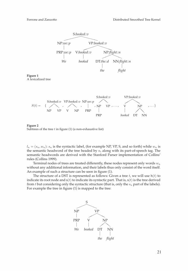
ln = (sn, wn): sn is the syntactic label, (for example NP, VP, S, and so forth) while wn isthe semantic headword of the tree headed by n, along with its part-of-speech tag. Thesemantic headwords are derived with the Stanford Parser implementation of Collins’rules (Collins 1999).
Terminal nodes of trees are treated differently, these nodes represent only words wn
without any additional information, and their labels thus only consist of the word itself.An example of such a structure can be seen in figure (1).
The structure of a DST is represented as follows: Given a tree t, we will use h(t) toindicate its root node and s(t) to indicate its syntactic part. That is, s(t) is the tree derivedfrom t but considering only the syntactic structure (that is, only the sn part of the labels).For example the tree in figure (1) is mapped to the tree:
S���
���NP
PRP
We
VP���
���V
booked
NP����
DT
the
NN
flight
5
22
Italian Journal of Computational Linguistics Volume 1, Number 1
We will also use ci(n) to denote i-th child of a node n. As usual for constituency-based parse trees, pre-terminal nodes are nodes that have a single terminal node aschild. Finally, we use wn ∈ Rk to denote the distributional vector for word wn.
3.2 The method at a glance
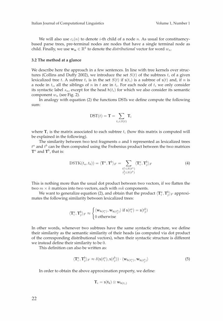
We describe here the approach in a few sentences. In line with tree kernels over struc-tures (Collins and Duffy 2002), we introduce the set S(t) of the subtrees ti of a givenlexicalized tree t. A subtree ti is in the set S(t) if s(ti) is a subtree of s(t) and, if n isa node in ti, all the siblings of n in t are in ti. For each node of ti we only considerits syntactic label sn, except for the head h(ti) for which we also consider its semanticcomponent wn (see Fig. 2).
In analogy with equation (2) the functions DSTs we define compute the followingsum:
DST(t) = T =∑
ti∈S(t)
Ti
where Ti is the matrix associated to each subtree ti (how this matrix is computed willbe explained in the following).
The similarity between two text fragments a and b represented as lexicalized treesta and tb can be then computed using the Frobenius product between the two matricesTa and Tb, that is:
DSTK(ta, tb)) = 〈Ta,Tb〉F =∑
tai ∈S(ta)
tbj∈S(tb)
〈Tai ,Tb
j〉F (4)
This is nothing more than the usual dot product between two vectors, if we flatten thetwo m× k matrices into two vectors, each with mk components.
We want to generalize equation (2), and obtain that the product 〈Tai ,Tb
j〉F approxi-mates the following similarity between lexicalized trees:
〈Tai ,Tb
j〉F ≈
{〈wh(tai )
,wh(tbj)〉 if s(tai ) = s(tbj)
0 otherwise
In other words, whenever two subtrees have the same syntactic structure, we definetheir similarity as the semantic similarity of their heads (as computed via dot productof the corresponding distributional vectors), when their syntactic structure is differentwe instead define their similarity to be 0.
This definition can also be written as:
〈Tai ,Tb
j〉F ≈ δ(s(tai ), s(tbj)) · 〈wh(tai )
,wh(tbj)〉 (5)
In order to obtain the above approximation property, we define:
Ti = s(ti)⊗wh(ti)
6
23
Ferrone and Zanzotto Distributed Smoothed Tree Kernel
where s(ti) are distributed tree fragment (Zanzotto and Dell’Arciprete 2012a) for thesubtree t, wh(ti) is the distributional vector of the head of the subtree t and ⊗ denotesthe tensor product. In this particular case, the tensor product is equivalent to the matrixs(ti)w
�h(ti)
, between a column vector and a row vector.Exploiting the following properties of the tensor and Frobenius product:
〈a⊗w,b⊗ v〉F = 〈a,b〉 · 〈w,v〉
we have that Equation (5) is satisfied as:
〈Ti,Tj〉F = 〈s(ti), s(tj)〉 · 〈wh(ti),wh(tj)〉
≈ δ(s(ti), s(tj)) · 〈wh(ti),wh(tj)〉
As in the distributed trees, it is possible to introduce a different formulation tocompute DST(t). Such formulation has the advantage of being more computationallyefficient, and also makes it clear that the process is compositional in nature, because itcomposes distributional and distributed vector of each node.
More specifically, it can be shown that:
DST(t) =∑n∈N
SN*(n)
where SN∗ is defined as:
SN*(n) =
{0 if n is terminalSN(n)⊗wn otherwise
and S(n) is the same as in equation (3).It is possible to show that the overall compositional distributional model DST(t)
can be obtained with a recursive algorithm that exploits vectors of the nodes of the tree.We actually propose two slightly different versions of our DSTs according to how
we produce distributional vectors for words. We have a plain version DST0 when weuse distributional vectors wn as they are, and a slightly modified version DST+1 whenwe use as distributional vectors wn
′ =(1 wn
).
4. The Approximated Smoothed Tree Kernels
The two CDSM we propose approximate two specific tree kernels belonging to thesmoothed tree kernels class. These recursively computes (but, the recursive formulationis not given here) the following general equation:
STK(ta, tb) =∑
ti∈S(ta)
tj∈S(tb)
ω(ti, tj)
where ω(ti, tj) is the similarity weight between two subtrees ti and tj . DTSK0 andDSTK+1 approximate respectively the kernels STK0 and STK+1 defined respectively
7
24
Italian Journal of Computational Linguistics Volume 1, Number 1
by the following equations for the weights:
ω0(ti, tj) = 〈wh(ti),wh(tj)〉 · δ(s(ti), s(tj)) ·√λ|N(ti)|+|N(tj)|
ω+1(ti, tj) = (〈wh(ti),wh(tj)〉+ 1) · δ(s(ti), s(tj)) ·√λ|N(ti)|+|N(tj)|
5. Experimental investigation
5.1 Experimental set-up
Generic settings. We experimented with two datasets: the Recognizing Textual Entail-ment datasets (RTE) (Dagan, Glickman, and Magnini 2006) and the the Semantic TextualSimilarity 2013 datasets (STS) (Agirre et al. 2013). The STS task consists of determiningthe degree of similarity (ranging from 0 to 5) between two sentences. We used the datafor core task of the 2013 challenge data. The STS datasets contains 5 datasets: headlines,OnWN, FNWN, SMT and MSRpar, which contains respectively 750, 561, 189, 750 and1500 pairs. The first four datasets were used for testing, while all the training has beendone on the fifth. RTE is instead the task of deciding whether a long text T entails ashorter text, typically a single sentence, called hypothesis H . It has been often seen asa classification task (see (Dagan et al. 2013)). We used four datasets: RTE1, RTE2, RTE3,and RTE5, with the standard split between training and testing. The dev/test distribu-tion for RTE1-3, and RTE5 is respectively 567/800, 800/800, 800/800, and 600/600 T-Hpairs.
Distributional vectors are derived with DISSECT (Dinu, The Pham, and Baroni2013) from a corpus obtained by the concatenation of ukWaC (wacky.sslmit.unibo.it),a mid-2009 dump of the English Wikipedia (en.wikipedia.org) and the British NationalCorpus (www.natcorp.ox.ac.uk), for a total of about 2.8 billion words. We collected a35K-by-35K matrix by counting co-occurrence of the 30K most frequent content lemmasin the corpus (nouns, adjectives and verbs) and all the content lemmas occurring in thedatasets within a 3 word window. The raw count vectors were transformed into positivePointwise Mutual Information scores and reduced to 300 dimensions by Singular ValueDecomposition. This setup was picked without tuning, as we found it effective inprevious, unrelated experiments.
To build our DTSKs and for the two baseline kernels TK and DTK, we used the im-plementation of the distributed tree kernels2. We used: 1024 and 2048 as the dimensionof the distributed vectors, the weight λ is set to 0.4 as it is a value generally consideredoptimal for many applications (see also (Zanzotto and Dell’Arciprete 2012a)).
The statistical significance, where reported, is computed according to the sign test.
Direct correlation settings. For the direct correlation experiments, we used the RTE datasets and the testing sets of the STS dataset (that is, headlines, OnWN, FNWN, SMT). Wecomputed the Spearman’s correlation between values produced by our DSTK0 andDSTK+1 and produced by the standard versions of the smoothed tree kernel, that is,respectively, STK0 and STK+1. We obtained text fragment pairs by randomly sampling
2 http://code.google.com/p/distributed-tree-kernels/
8
25
Ferrone and Zanzotto Distributed Smoothed Tree Kernel
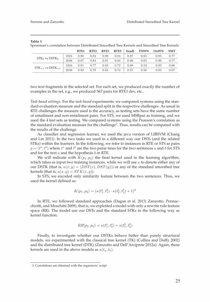
Table 1Spearman’s correlation between Distributed Smoothed Tree Kernels and Smoothed Tree Kernels
RTE1 RTE2 RTE3 RTE5 headl FNWN OnWN SMT
STK0 vs DSTK01024 0.86 0.84 0.90 0.84 0.87 0.65 0.95 0.77
2048 0.87 0.84 0.91 0.84 0.90 0.65 0.96 0.77
STK+1 vs DSTK+11024 0.81 0.77 0.83 0.72 0.88 0.53 0.93 0.66
2048 0.82 0.78 0.84 0.74 0.91 0.56 0.94 0.67
two text fragments in the selected set. For each set, we produced exactly the number ofexamples in the set, e.g., we produced 567 pairs for RTE1 dev, etc..
Task-based settings. For the task-based experiments, we compared systems using the stan-dard evaluation measure and the standard split in the respective challenges. As usual inRTE challenges the measure used is the accuracy, as testing sets have the same numberof entailment and non-entailment pairs. For STS, we used MSRpar as training, and weused the 4 test sets as testing. We compared systems using the Pearson’s correlation asthe standard evaluation measure for the challenge3. Thus, results can be compared withthe results of the challenge.
As classifier and regression learner, we used the java version of LIBSVM (Changand Lin 2011). In the two tasks we used in a different way our DSTs (and the relatedSTKs) within the learners. In the following, we refer to instances in RTE or STS as pairsp = (ta, tb) where ta and tb are the two parse trees for the two sentences a and b for STSand for the text a and the hypothesis b in RTE.
We will indicate with K(p1, p2) the final kernel used in the learning algorithm,which takes as input two training instances, while we will use κ to denote either any ofour DSTK (that is, κ(x, y) = 〈DST (x), DST (y)〉) or any of the standard smoothed treekernels (that is, κ(x, y) = STK(x, y)).
In STS, we encoded only similarity feature between the two sentences. Thus, weused the kernel defined as:
K(p1, p2) = (κ(ta1 , tb1) · κ(ta2 , tb2) + 1)2
In RTE, we followed standard approaches (Dagan et al. 2013; Zanzotto, Pennac-chiotti, and Moschitti 2009), that is, we exploited a model with only a rewrite rule featurespace (RR). The model use our DSTs and the standard STKs in the following way askernel function:
RR(p1, p2) = κ(ta1 , ta2) + κ(tb1, t
b2)
Finally, to investigate whether our DSTKs behave better than purely structuralmodels, we experimented with the classical tree kernel (TK) (Collins and Duffy 2002)and the distributed tree kernel (DTK) (Zanzotto and Dell’Arciprete 2012a). Again, thesekernels are used in the above models as κ(ta, tb).
3 Correlations are obtained with the organizers’ script
9
26
Italian Journal of Computational Linguistics Volume 1, Number 1
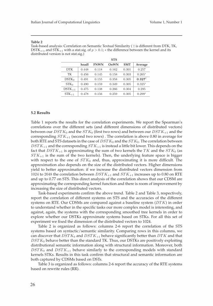
Table 2Task-based analysis: Correlation on Semantic Textual Similarity ( † is different from DTK, TK,DSTK+1, and STK+1 with a stat.sig. of p > 0.1; ∗ the difference between the kernel and itsdistributed version is not stat.sig.)
STS
headl FNWN OnWN SMT Average
DTK 0.448 0.118 0.162 0.301 0.257
TK 0.456 0.145 0.158 0.303 0.265∗
DSTK0 0.491 0.155 0.358 0.305 0.327†
STK0 0.490 0.159 0.349 0.305 0.325∗
DSTK+1 0.475 0.138 0.266 0.304 0.295
STK+1 0.478 0.156 0.259 0.305 0.299∗
5.2 Results
Table 1 reports the results for the correlation experiments. We report the Spearman’scorrelations over the different sets (and different dimensions of distributed vectors)between our DSTK0 and the STK0 (first two rows) and between our DSTK+1 and thecorresponding STK+1 (second two rows) . The correlation is above 0.80 in average forboth RTE and STS datasets in the case of DSTK0 and the STK0. The correlation betweenDSTK+1 and the corresponding STK+1 is instead a little bit lower. This depends on thefact that DSTK+1 is approximating the sum of two kernels the TK and the STK0 (asSTK+1 is the sum of the two kernels). Then, the underlying feature space is biggerwith respect to the one of STK0 and, thus, approximating it is more difficult. Theapproximation also depends on the size of the distributed vectors. Higher dimensionsyield to better approximation: if we increase the distributed vectors dimension from1024 to 2048 the correlation between DSTK+1 and STK+1 increases up to 0.80 on RTEand up to 0.77 on STS. This direct analysis of the correlation shows that our CDSM areapproximating the corresponding kernel function and there is room of improvement byincreasing the size of distributed vectors.
Task-based experiments confirm the above trend. Table 2 and Table 3, respectively,report the correlation of different systems on STS and the accuracies of the differentsystems on RTE. Our CDSMs are compared against a baseline system (DTK) in orderto understand whether in the specific tasks our more complex model is interesting, andagainst, again, the systems with the corresponding smoothed tree kernels in order toexplore whether our DSTKs approximate systems based on STKs. For all this set ofexperiment we fixed the dimension of the distributed vectors to 1024.
Table 2 is organized as follows: columns 2-6 report the correlation of the STSsystems based on syntactic/semantic similarity. Comparing rows in this columns, wecan discover that DSTK0 and DSTK+1 behave significantly better than DTK and thatDSTK0 behave better than the standard TK. Thus, our DSTKs are positively exploitingdistributional semantic information along with structural information. Moreover, bothDSTK0 and DSTK+1 behave similarly to the corresponding models with standardkernels STKs. Results in this task confirm that structural and semantic information areboth captured by CDSMs based on DSTs.
Table 3 is organized as follows: columns 2-6 report the accuracy of the RTE systemsbased on rewrite rules (RR).
10
27
Ferrone and Zanzotto Distributed Smoothed Tree Kernel
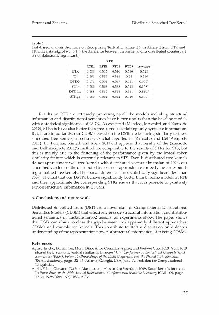
Table 3Task-based analysis: Accuracy on Recognizing Textual Entailment ( † is different from DTK andTK wiht a stat.sig. of p > 0.1; ∗ the difference between the kernel and its distributed counterpartis not statistically significant.)
RTE
RTE1 RTE2 RTE3 RTE5 Average
DTK 0.533 0.515 0.516 0.530 0.523
TK 0.561 0.552 0.531 0.54 0.546
DSTK0 0.571 0.551 0.547 0.531 0.550†
STK0 0.586 0.563 0.538 0.545 0.558∗
DSTK+1 0.588 0.562 0.555 0.541 0.561†
STK+1 0.586 0.562 0.542 0.546 0.559∗
Results on RTE are extremely promising as all the models including structuralinformation and distributional semantics have better results than the baseline modelswith a statistical significance of 93.7%. As expected (Mehdad, Moschitti, and Zanzotto2010), STKs behave also better than tree kernels exploiting only syntactic information.But, more importantly, our CDSMs based on the DSTs are behaving similarly to thesesmoothed tree kernels, in contrast to what reported in (Zanzotto and Dell’Arciprete2011). In (Polajnar, Rimell, and Kiela 2013), it appears that results of the (Zanzottoand Dell’Arciprete 2011)’s method are comparable to the results of STKs for STS, butthis is mainly due to the flattening of the performance given by the lexical tokensimilarity feature which is extremely relevant in STS. Even if distributed tree kernelsdo not approximate well tree kernels with distributed vectors dimension of 1024, oursmoothed versions of the distributed tree kernels approximate correctly the correspond-ing smoothed tree kernels. Their small difference is not statistically significant (less than70%). The fact that our DSTKs behave significantly better than baseline models in RTEand they approximate the corresponding STKs shows that it is possible to positivelyexploit structural information in CDSMs.
6. Conclusions and future work
Distributed Smoothed Trees (DST) are a novel class of Compositional DistributionalSemantics Models (CDSM) that effectively encode structural information and distribu-tional semantics in tractable rank-2 tensors, as experiments show. The paper showsthat DSTs contribute to close the gap between two apparently different approaches:CDSMs and convolution kernels. This contribute to start a discussion on a deeperunderstanding of the representation power of structural information of existing CDSMs.
ReferencesAgirre, Eneko, Daniel Cer, Mona Diab, Aitor Gonzalez-Agirre, and Weiwei Guo. 2013. *sem 2013
shared task: Semantic textual similarity. In Second Joint Conference on Lexical and ComputationalSemantics (*SEM), Volume 1: Proceedings of the Main Conference and the Shared Task: SemanticTextual Similarity, pages 32–43, Atlanta, Georgia, USA, June. Association for ComputationalLinguistics.
Aiolli, Fabio, Giovanni Da San Martino, and Alessandro Sperduti. 2009. Route kernels for trees.In Proceedings of the 26th Annual International Conference on Machine Learning, ICML ’09, pages17–24, New York, NY, USA. ACM.
11
28
Italian Journal of Computational Linguistics Volume 1, Number 1
Aronszajn, Nachman. 1950. Theory of reproducing kernels. Transactions of the AmericanMathematical Society, 68(3):337–404.
Baroni, Marco and Alessandro Lenci. 2010. Distributional memory: A general framework forcorpus-based semantics. Comput. Linguist., 36(4):673–721, December.
Baroni, Marco and Roberto Zamparelli. 2010. Nouns are vectors, adjectives are matrices:Representing adjective-noun constructions in semantic space. In Proceedings of the 2010Conference on Empirical Methods in Natural Language Processing, pages 1183–1193, Cambridge,MA, October. Association for Computational Linguistics.
Chang, Chih-Chung and Chih-Jen Lin. 2011. LIBSVM: A library for support vector machines.ACM Transactions on Intelligent Systems and Technology, 2:27:1–27:27. Software available athttp://www.csie.ntu.edu.tw/~cjlin/libsvm.
Collins, Michael. 1999. Head-driven Statistical Models for Natural Language Processing. Ph.D. thesis,University of Pennsylvania.
Collins, Michael and Nigel Duffy. 2001. Convolution kernels for natural language. In NIPS,pages 625–632.
Collins, Michael and Nigel Duffy. 2002. New ranking algorithms for parsing and tagging:Kernels over discrete structures, and the voted perceptron. In Proceedings of 40th AnnualMeeting of the Association for Computational Linguistics, pages 263–270, Philadelphia,Pennsylvania, USA, July. Association for Computational Linguistics.
Cristianini, Nello and John Shawe-Taylor. 2000. An Introduction to Support Vector Machines andOther Kernel-based Learning Methods. Cambridge University Press, March.
Croce, Danilo, Alessandro Moschitti, and Roberto Basili. 2011. Structured lexical similarity viaconvolution kernels on dependency trees. In Proceedings of the Conference on Empirical Methodsin Natural Language Processing, EMNLP ’11, pages 1034–1046, Stroudsburg, PA, USA.Association for Computational Linguistics.
Dagan, Ido, Oren Glickman, and Bernardo Magnini. 2006. The pascal recognising textualentailment challenge. In Proceedings of the First International Conference on Machine LearningChallenges: Evaluating Predictive Uncertainty Visual Object Classification, and Recognizing TextualEntailment, MLCW’05, pages 177–190, Berlin, Heidelberg. Springer-Verlag.
Dagan, Ido, Dan Roth, Mark Sammons, and Fabio Massimo Zanzotto. 2013. Recognizing TextualEntailment: Models and Applications. Synthesis Lectures on Human Language Technologies.Morgan & Claypool Publishers.
Dinu, Georgiana, Nghia The Pham, and Marco Baroni. 2013. DISSECT: DIStributional SEmanticsComposition Toolkit. In Proceedings of ACL (System Demonstrations), pages 31–36, Sofia,Bulgaria.
Ferrone, Lorenzo and Fabio Massimo Zanzotto. 2013. Linear compositional distributionalsemantics and structural kernels. In Proceedings of the Joint Symposium of Semantic Processing(JSSP), pages 85–89, Trento, Italia.
Ferrone, Lorenzo and Fabio Massimo Zanzotto. 2014. Towards syntax-aware compositionaldistributional semantic models. In Proceedings of COLING 2014, the 25th International Conferenceon Computational Linguistics: Technical Papers, pages 721–730, Dublin, Ireland, August. DublinCity University and Association for Computational Linguistics.
Haussler, David. 1999. Convolution kernels on discrete structures. Technical report, Universityof California at Santa Cruz.
Kimura, Daisuke, Tetsuji Kuboyama, Tetsuo Shibuya, and Hisashi Kashima. 2011. A subpathkernel for rooted unordered trees. In Proceedings of the 15th Pacific-Asia conference on Advances inknowledge discovery and data mining - Volume Part I, PAKDD’11, pages 62–74, Berlin, Heidelberg.Springer-Verlag.
Mehdad, Yashar, Alessandro Moschitti, and Fabio Massimo Zanzotto. 2010. Syntactic/semanticstructures for textual entailment recognition. In Human Language Technologies: The 2010 AnnualConference of the North American Chapter of the Association for Computational Linguistics, HLT ’10,pages 1020–1028, Stroudsburg, PA, USA. Association for Computational Linguistics.
Mitchell, Jeff and Mirella Lapata. 2008. Vector-based models of semantic composition. InProceedings of ACL-08: HLT, pages 236–244, Columbus, Ohio, June. Association forComputational Linguistics.
Polajnar, Tamara, Laura Rimell, and Douwe Kiela. 2013. Ucam-core: Incorporating structureddistributional similarity into sts. In Second Joint Conference on Lexical and ComputationalSemantics (*SEM), Volume 1: Proceedings of the Main Conference and the Shared Task: SemanticTextual Similarity, pages 85–89, Atlanta, Georgia, USA, June. Association for Computational
12
29
Ferrone and Zanzotto Distributed Smoothed Tree Kernel
Linguistics.Socher, Richard, Eric H. Huang, Jeffrey Pennin, Christopher D Manning, and Andrew Y. Ng.
2011. Dynamic pooling and unfolding recursive autoencoders for paraphrase detection. InJ. Shawe-Taylor, R.S. Zemel, P.L. Bartlett, F. Pereira, and K.Q. Weinberger, editors, Advances inNeural Information Processing Systems 24. Curran Associates, Inc., pages 801–809.
Vishwanathan, S. V. N. and Alexander J. Smola. 2002. Fast kernels for string and tree matching.In Suzanna Becker, Sebastian Thrun, and Klaus Obermayer, editors, NIPS, pages 569–576. MITPress.
Zanzotto, Fabio Massimo and Lorenzo Dell’Arciprete. 2011. Distributed structures anddistributional meaning. In Proceedings of the Workshop on Distributional Semantics andCompositionality, pages 10–15, Portland, Oregon, USA, June. Association for ComputationalLinguistics.
Zanzotto, Fabio Massimo and Lorenzo Dell’Arciprete. 2012a. Distributed tree kernels. InProceedings of International Conference on Machine Learning, pages 193–200.
Zanzotto, Fabio Massimo and Lorenzo Dell’Arciprete. 2012b. Distributed tree kernels. InProceedings of International Conference on Machine Learning, pages –, June 26–July 1.
Zanzotto, Fabio Massimo, Ioannis Korkontzelos, Francesca Fallucchi, and Suresh Manandhar.2010. Estimating linear models for compositional distributional semantics. In Proceedings of the23rd International Conference on Computational Linguistics (COLING), pages 1263–1271, August.
Zanzotto, Fabio Massimo, Marco Pennacchiotti, and Alessandro Moschitti. 2009. A machinelearning approach to textual entailment recognition. NATURAL LANGUAGE ENGINEERING,15-04:551–582.
13

31
An Exploration of Semantic Features in anUnsupervised Thematic Fit EvaluationFramework
Asad Sayeed∗
Saarland UniversityVera Demberg∗
Saarland University
Pavel Shkadzko∗
Saarland University
Thematic fit is the extent to which an entity fits a thematic role in the semantic frame of anevent, e.g., how well humans would rate “knife” as an instrument of an event of cutting. Weexplore the use of the SENNA semantic role-labeller in defining a distributional space in orderto build an unsupervised model of event-entity thematic fit judgements. We test a number ofways of extracting features from SENNA-labelled versions of the ukWaC and BNC corpora andidentify tradeoffs. Some of our Distributional Memory models outperform an existing syntax-based model (TypeDM) that uses hand-crafted rules for role inference on a previously tested dataset. We combine the results of a selected SENNA-based model with TypeDM’s results and findthat there is some amount of complementarity in what a syntactic and a semantic model willcover. In the process, we create a broad-coverage semantically-labelled corpus.
1. Introduction
Can automated tasks in natural language semantics be accomplished entirely throughmodels that do not require the contribution of semantic features to work at high accu-racy? Unsupervised semantic role labellers such as that of Titov and Klementiev (2011)and Lang and Lapata (2011) do exactly this: predict semantic roles strictly from syntacticrealizations. In other words, for practical purposes, the relevant and frequent semanticcases might be completely covered by learned syntactic information. For example, givena sentence The newspaper was put on the table, such SRL systems would identify that thetable should receive a “location” role purely from the syntactic dependencies centeredaround the preposition on.
We could extend this thinking to a slightly different task: thematic fit modelling. Itcould well be the case that the the table could be judged a more appropriate filler of alocation role for put than, e.g., the perceptiveness, entirely due to information about thefrequency of word collocations and syntactic dependencies collected through corpusdata, handmade grammars, and so on. In fact, today’s distributional models used formodelling of selectional preference or thematic fit generally base their estimates onsyntactic or string co-occurrence models (Baroni and Lenci 2010; Ritter, Mausam, andEtzioni 2010; Ó Séaghdha 2010). The Distributional Memory (DM) model by Baroni and
∗ Computational Linguistics and Phonetics / MMCI Cluster of Excellence, Saarland University.E-mail: {asayeed,vera,pavels}@coli.uni-saarland.de
© 2015 Associazione Italiana di Linguistica Computazionale
32
Italian Journal of Computational Linguistics Volume 1, Number 1
Lenci (2010) is one example of an unsupervised model based on syntactic dependencies,which has been successfully applied to many different distributional similarity tasks,and also has been used in compositional models (Lenci 2011).
While earlier work has shown that syntactic relations and thematic roles are re-lated concepts (Levin 1993), there are also a large number of cases where thematicroles assigned by a role labeller and their best-matching syntactic relations do notcorrespond (Palmer, Gildea, and Kingsbury 2005). However, it is possible that this non-correspondence is not a problem for estimating typical agents and patients from largeamounts of data: agents will most of the time coincide with subjects, and patients willmost of the time coincide with syntactic objects. On the other hand, the best resourcefor estimating thematic fit should be based on labels that most closely correspond to thetarget task, i.e. semantic role labelling, instead of syntactic parsing.
Being able to automatically assess the semantic similarity between concepts as wellas the thematic fit of words in particular relationships to one another has numerousapplications for problems related to natural language processing, including syntactic(attachment ambiguities) and semantic parsing, question answering, and in the gen-eration of lexical predictions for upcoming content in highly incremental languageprocessing, which is relevant for tasks such as simultaneous translation as well aspsycholinguistic modelling of human language comprehension.
Semantics can be modelled at two levels. One level is compositional semantics,which is concerned with how the meanings of words are combined. Another level islexical semantics, which include distributional models; these latter represent a word’smeaning as a vector of weights derived from counts of words with which the wordoccurs (see for an overview (Erk 2012; Turney and Pantel 2010)). A current challenge is tobring these approaches together. In recent work, distributional models with structuredvector spaces have been proposed. In these models, linguistic properties are taken intoaccount by encoding the grammatical or semantic relation between a word and thewords in its context.
DM is a particularly suitable approach for our requirements, as it satisfies therequirements specific to our above-mentioned goals including assessing the semanticfit of words in different grammatical functions and generating semantic predictions, asit is broad-coverage and multi-directional (different semantic spaces can be generatedon demand from the DM by projecting the tensor onto 2-way matrices by fixing thethird dimension to, e.g., “object”).
The usability and quality of the semantic similarity estimates produced by DMmodels depend not only on how the word pairs and their relations are represented,but also on the training data and the types of relations between words that are usedto define the links between words in the model. Baroni and Lenci have chosen thevery fast MaltParser (Nivre et al. 2007) to generate the semantic space. The MaltParserversion used by Baroni and Lenci distinguishes a relatively small number of syntacticroles, and in particular does not mark the subject of passives differently from subjectsof active sentences. For our target applications in incremental semantic parsing (Sayeedand Demberg 2013), we are however more strongly interested in thematic roles (agent,patient) between words than in their syntactic configurations (subject, object).
In this paper, we produce DM models based directly on features generated froma semantic role labeller that does not directly use an underlying syntactic parse. Thelabelling tool we use, SENNA (Collobert et al. 2011), labels spans of text with PropBank-style semantic roles, but the spans often include complex modifiers that contain nouns
33
Sayeed et al. Semantic Features in Thematic Fit
that are not the direct recipients of the roles assigned by the labeler1. Consequently, wetest out different mechanisms of finding the heads of the roles, including exploiting thesyntactic parse provided to us by the Baroni and Lenci work post hoc. We find that aprecise head-finding has a positive effect on performance on our thematic fit modelingtask. In the process, we also produce a semantically labeled corpus that includes ukWaCand BNC2.
In addition, we want to test the extent to which a DM trained directly on a rolelabeller which produces PropBank style semantic annotations can complement thesyntax-based DM model on thematic fit tasks, given a similar corpus of training data.We maintain the unsupervised aspects of both models by combining their ratings byaveraging without any weight estimation (we “guess” 50%) and show that we get animprovement in matching human judgements collected from previous experiments.We demonstrate that a fully unsupervised model based on the SENNA role-labelleroutperforms a corresponding model based on MaltParser dependencies (DepDM) bya wide margin. Furthermore, we show that the SENNA-based model can competewith Baroni and Lenci’s better performing TypeDM model on some thematic fit tasks;TypeDM involves hand-crafted rules over and above the finding of syntactic heads,unlike our DMs. We then investigate the differences between the characteristics of themodels by mixing TypeDM and a high-performing SENNA-based model at differentstages of the thematic fit evaluation process. We thus demonstrate that the SENNA-based model makes a separate contribution to thematic fit evaluation.
1.1 Thematic role typicality
Thematic roles describe the relations that entities take in an event or relation. Thematicrole fit correlates with human plausibility judgments (Padó, Crocker, and Keller 2009;Vandekerckhove, Sandra, and Daelemans 2009), which can be used to evaluate whethera distributional semantic model can be effectively encoded in the distributional space.
A suitable dataset is the plausibility judgment data set by Padó (2007), whichincludes 18 verbs with up to twelve nominal arguments, totalling 414 verb-noun-roletriples. The words were chosen based on their frequency in the Penn Treebank andFrameNet; we call this simply the “Padó” dataset from now on (see table 1). Humansubjects were asked how common the nominal arguments were as agents or as patientsfor the verbs. We also evaluate the DM models on a data set by McRae et al. (1998),which contains thematic role plausibility judgments for 1444 verb-role-noun triplescalculated over the course of several experiments. We call these “McRae agent/patient”.
However, these triples do contain a significant proportion of words which only veryrarely occur in our training data, and will therefore be represented more sparsely. TheMcRae dataset is thus a more difficult data set to model than the Padó dataset.
While the first two data sets only contain plausibility judgments for verbs andtheir agents and patients, we additionally use two data sets containing judgments forlocations (274 verb-location pairs) and instruments (248 verb-instrument pairs) (Ferretti,McRae, and Hatherell 2001) that we call “Ferretti locations” and “Ferretti instruments”respectively. We use them to see how well these models apply to roles other than agentand patient. All ratings were on a scale of 1 to 7.
1 E.g., “Bob ate the donut that poisoned Mary”; “Mary” is not a recipient of the patient role of “eat”, butSENNA labels it as such, as it is part of the noun phrase including “donut”.
2 We provide the entire labelled corpus athttp://rollen.mmci.uni-saarland.de. Users of the corpus should cite this paper.
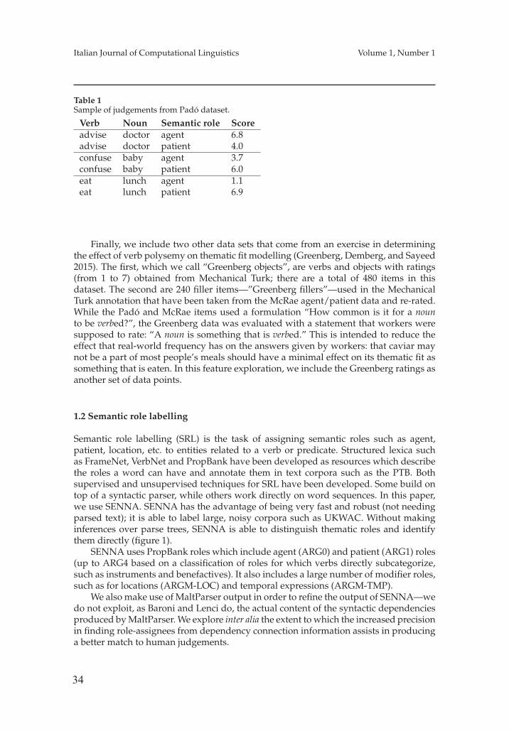
34
Italian Journal of Computational Linguistics Volume 1, Number 1
Table 1Sample of judgements from Padó dataset.
Verb Noun Semantic role Scoreadvise doctor agent 6.8advise doctor patient 4.0confuse baby agent 3.7confuse baby patient 6.0eat lunch agent 1.1eat lunch patient 6.9
Finally, we include two other data sets that come from an exercise in determiningthe effect of verb polysemy on thematic fit modelling (Greenberg, Demberg, and Sayeed2015). The first, which we call “Greenberg objects”, are verbs and objects with ratings(from 1 to 7) obtained from Mechanical Turk; there are a total of 480 items in thisdataset. The second are 240 filler items—”Greenberg fillers”—used in the MechanicalTurk annotation that have been taken from the McRae agent/patient data and re-rated.While the Padó and McRae items used a formulation “How common is it for a nounto be verbed?”, the Greenberg data was evaluated with a statement that workers weresupposed to rate: “A noun is something that is verbed.” This is intended to reduce theeffect that real-world frequency has on the answers given by workers: that caviar maynot be a part of most people’s meals should have a minimal effect on its thematic fit assomething that is eaten. In this feature exploration, we include the Greenberg ratings asanother set of data points.
1.2 Semantic role labelling
Semantic role labelling (SRL) is the task of assigning semantic roles such as agent,patient, location, etc. to entities related to a verb or predicate. Structured lexica suchas FrameNet, VerbNet and PropBank have been developed as resources which describethe roles a word can have and annotate them in text corpora such as the PTB. Bothsupervised and unsupervised techniques for SRL have been developed. Some build ontop of a syntactic parser, while others work directly on word sequences. In this paper,we use SENNA. SENNA has the advantage of being very fast and robust (not needingparsed text); it is able to label large, noisy corpora such as UKWAC. Without makinginferences over parse trees, SENNA is able to distinguish thematic roles and identifythem directly (figure 1).
SENNA uses PropBank roles which include agent (ARG0) and patient (ARG1) roles(up to ARG4 based on a classification of roles for which verbs directly subcategorize,such as instruments and benefactives). It also includes a large number of modifier roles,such as for locations (ARGM-LOC) and temporal expressions (ARGM-TMP).
We also make use of MaltParser output in order to refine the output of SENNA—wedo not exploit, as Baroni and Lenci do, the actual content of the syntactic dependenciesproduced by MaltParser. We explore inter alia the extent to which the increased precisionin finding role-assignees from dependency connection information assists in producinga better match to human judgements.
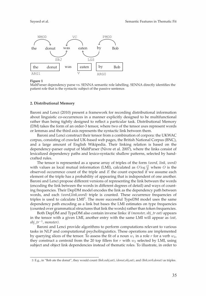
35
Sayeed et al. Semantic Features in Thematic Fit
the donut was eaten by Bob
NMOD
SBJ
VC
LGS
PMOD
the donut was eaten by Bob
ARG1 V ARG0
Figure 1MaltParser dependency parse vs. SENNA semantic role labelling. SENNA directly identifies thepatient role that is the syntactic subject of the passive sentence.
2. Distributional Memory
Baroni and Lenci (2010) present a framework for recording distributional informationabout linguistic co-occurrences in a manner explicitly designed to be multifunctionalrather than being tightly designed to reflect a particular task. Distributional Memory(DM) takes the form of an order-3 tensor, where two of the tensor axes represent wordsor lemmas and the third axis represents the syntactic link between them.
Baroni and Lenci construct their tensor from a combination of corpora: the UKWACcorpus, consisting of crawled UK-based web pages, the British National Corpus (BNC),and a large amount of English Wikipedia. Their linking relation is based on thedependency-parser output of MaltParser (Nivre et al. 2007), where the links consist oflexicalized dependency paths and lexico-syntactic shallow patterns, selected by hand-crafted rules.
The tensor is represented as a sparse array of triples of the form (word, link, word)with values as local mutual information (LMI), calculated as O log O
E where O is theobserved occurrence count of the triple and E the count expected if we assume eachelement of the triple has a probability of appearing that is independent of one another.Baroni and Lenci propose different versions of representing the link between the words(encoding the link between the words in different degrees of detail) and ways of count-ing frequencies. Their DepDM model encodes the link as the dependency path betweenwords, and each (word,link,word) triple is counted. These occurrence frequencies oftriples is used to calculate LMI3. The more successful TypeDM model uses the samedependency path encoding as a link but bases the LMI estimates on type frequencies(counted over grammatical structures that link the words) rather than token frequencies.
Both DepDM and TypeDM also contain inverse links: if (monster, sbj_tr eat) appearsin the tensor with a given LMI, another entry with the same LMI will appear as (eat,sbj_tr−1, monster).
Baroni and Lenci provide algorithms to perform computations relevant to varioustasks in NLP and computational psycholinguistics. These operations are implementedby querying slices of the tensor. To assess the fit of a noun w1 in a role r for a verb w2,they construct a centroid from the 20 top fillers for r with w2 selected by LMI, usingsubject and object link dependencies instead of thematic roles. To illustrate, in order to
3 E.g., in “Bob ate the donut”, they would count (Bob,subj,eat), (donut,obj,eat), and (Bob,verb,donut) as triples.
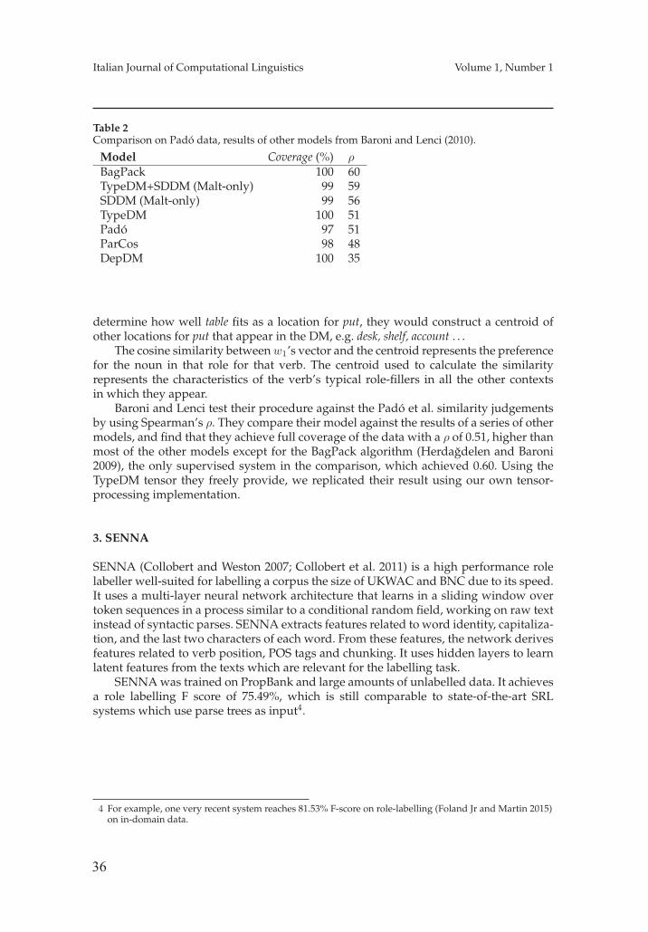
36
Italian Journal of Computational Linguistics Volume 1, Number 1
Table 2Comparison on Padó data, results of other models from Baroni and Lenci (2010).
Model Coverage (%) ρBagPack 100 60TypeDM+SDDM (Malt-only) 99 59SDDM (Malt-only) 99 56TypeDM 100 51Padó 97 51ParCos 98 48DepDM 100 35
determine how well table fits as a location for put, they would construct a centroid ofother locations for put that appear in the DM, e.g. desk, shelf, account . . .
The cosine similarity between w1’s vector and the centroid represents the preferencefor the noun in that role for that verb. The centroid used to calculate the similarityrepresents the characteristics of the verb’s typical role-fillers in all the other contextsin which they appear.
Baroni and Lenci test their procedure against the Padó et al. similarity judgementsby using Spearman’s ρ. They compare their model against the results of a series of othermodels, and find that they achieve full coverage of the data with a ρ of 0.51, higher thanmost of the other models except for the BagPack algorithm (Herdagdelen and Baroni2009), the only supervised system in the comparison, which achieved 0.60. Using theTypeDM tensor they freely provide, we replicated their result using our own tensor-processing implementation.
3. SENNA
SENNA (Collobert and Weston 2007; Collobert et al. 2011) is a high performance rolelabeller well-suited for labelling a corpus the size of UKWAC and BNC due to its speed.It uses a multi-layer neural network architecture that learns in a sliding window overtoken sequences in a process similar to a conditional random field, working on raw textinstead of syntactic parses. SENNA extracts features related to word identity, capitaliza-tion, and the last two characters of each word. From these features, the network derivesfeatures related to verb position, POS tags and chunking. It uses hidden layers to learnlatent features from the texts which are relevant for the labelling task.
SENNA was trained on PropBank and large amounts of unlabelled data. It achievesa role labelling F score of 75.49%, which is still comparable to state-of-the-art SRLsystems which use parse trees as input4.
4 For example, one very recent system reaches 81.53% F-score on role-labelling (Foland Jr and Martin 2015)on in-domain data.
37
Sayeed et al. Semantic Features in Thematic Fit
4. Implementation
4.1 Feature selection
We constructed our DMs from a combination of ukWaC and BNC5 by running thesentences individually through SENNA and counting the (assignee, role, assigner) triplesthat emerged from the SENNA labelling. However, SENNA assigns roles to entirephrases, some of which include complex modifiers such as relative clauses. We neededto find a more specific focus on the assigners (always verbs, given the training dataused for SENNA) and assignees; however, there are number of ways to do this, and weexperimented with different types of head-finding, which is a form of feature selectionfor a SENNA-based DM.
4.1.1 Head-findingHead-finding takes place over spans found by SENNA. There are two basic ways inwhich we search for heads, one partly dependent on a syntactic parse (“Malt-based”),one not (“linear”).
Linear. The “linear” algorithm is not based on a syntactic parse, but instead on the part-of-speech tags processed in sequence. It is similar to the Magerman (Magerman 1994)head percolation heuristic. This head-finding algorithm uses a heuristic to detect thehead of a noun phrase. This heuristic operates as follows: iterating over each word w,if the POS tag is nominal store it and forget any previous nominal words. At the end ofthe string, return the stored word. Discard the word if a possessive or other such “inter-rupting” item is passed. For example, in the phrase “The Iron Dragon’s Daughter”, thesystem would first store “Iron”, forget “Iron” when it found the possessive “Dragon’s”,and return “Daughter”. It is possible for it to return nothing, if the span given to ithas no suitable candidate. The linear process can only identify nominal constituents;we found that adding heuristics to detect other possible role-assignees (e.g. adverbsin instrumental roles) reduced the quality of the output due to unavoidable overlapsbetween the criteria used in the heuristics.
Malt-based. This head-finding procedure makes use of a small amount of syntacticdependency information. The “Malt-based” head-finding heuristic is based on theMaltParser output for ukWaC and BNC that was provided by Baroni and Lenci andused in the construction of DepDM and TypeDM. In essence, it involves using thedependencies reaching the role-assigning verb. Each word directly connected to therole-assigning verb inside the SENNA span is identified as a separate role-filler for theDM. We transitively explore connections via function words such as prepositions andmodals. See figure 2 for an example.
This heuristic is somewhat conservative. It is sometimes the case that SENNAidentifies a role-filler that does not have a Malt-based dependency path. Therefore,in addition to the “Malt-only” strategy, we include two fallback strategies when aMaltParser dependency does not resolve to any item. This strategy allows us to includerole-assignees that are not necessarily nominal, such as verbs in subordinate clausesreceiving roles from other verbs or adverbs taking on instrumental roles.
5 This is the same as Baroni and Lenci, except that they included Wikipedia text—we found noimprovement from this and omitted it to reduce processing time.
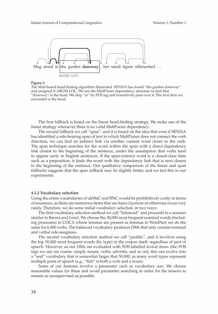
38
Italian Journal of Computational Linguistics Volume 1, Number 1
Meg stood in the garden doorway , her small figure silhouetted . . .
ARGM-LOC
Figure 2The Malt-based head-finding algorithm illustrated. SENNA has found “the garden doorway”and assigned it ARGM-LOC. We use the MaltParser dependency structure to find that“doorway” is the head. We skip “in” by POS tag and transitively pass over it. The first item weencounter is the head.
The first fallback is based on the linear head-finding strategy. We make use of thelinear strategy whenever there is no valid MaltParser dependency.
The second fallback we call “span”, and it is based on the idea that even if SENNAhas identified a role-bearing span of text to which MaltParser does not connect the verbdirection, we can find an indirect link via another content word closer to the verb.The span technique searches for the word within the span with a direct dependencylink closest to the beginning of the sentence, under the assumption that verbs tendto appear early in English sentences. If the span-exterior word is a closed-class itemsuch as a preposition, it finds the word with the dependency link that is next closestto the beginning of the sentence. Our qualitative comparison of the linear and spanfallbacks suggests that the span fallback may be slightly better, and we test this in ourexperiments.
4.1.2 Vocabulary selectionUsing the entire vocabularies of ukWaC and BNC would be prohibitively costly in termsof resources, as there are numerous items that are hapax legomena or otherwise occur veryrarely. Therefore, we do some initial vocabulary selection, in two ways.
The first vocabulary selection method we call “balanced” and proceeds in a mannersimilar to Baroni and Lenci. We choose the 30,000 most frequent nominal words (includ-ing pronouns) in COCA whose lemmas are present as lemmas in WordNet; we do thesame for 6,000 verbs. The balanced vocabulary produces DMs that only contain nominaland verbal role-assignees.
The second vocabulary selection method we call “prolific”, and it involves usingthe top 50,000 most frequent words (by type) in the corpus itself, regardless of part ofspeech. However, as our DMs are evaluated with POS-labelled lexical items (the POStags we use are coarse: simply nouns, verbs, adverbs, and so on), this can evolve intoa “real” vocabulary that is somewhat larger that 50,000, as many word types representmultiple parts of speech (e.g., “fish” is both a verb and a noun).
Some of our features involve a parameter such as vocabulary size. We choosereasonable values for these and avoid parameter searching in order for the tensors toremain as unsupervised as possible.
39
Sayeed et al. Semantic Features in Thematic Fit
4.2 From corpus to DMs
The process of constructing DMs from the above proceeds as follows:
1. The corpus is first tokenized and some character normalization isperformed, as the ukWaC data is collected from the Web and containscharacters that are not accepted by SENNA. We use the lemmatizationperformed via MaltParser and provided by Baroni and Lenci.
2. Each sentence is run through SENNA and the role-assigning verbs withtheir role-assigned spans are collected. There is a very small amount ofdata loss due to parser errors and software crashes.
3. One of the head-finding algorithms is run over the spans: eitherlinear-only, Malt-only, Malt-based with linear fallback, and Malt-basedwith span fallback. These effectively constitute separate processed corpora.
4. A table of counts is constructed from each of the head-finding outputcorpora, the counts being occurrences of (assigner, role, assignee) triples. Theassigners and assignees are filtered by either balanced or prolificvocabularies.
5. This table of counts is processed into LMI values and the inverse links arealso created. Triples with zero or negative LMI values are removed. Thisproduces the final set of DM tensors.
In terms of choosing links, our implementation most closely corresponds to Baroni andLenci’s DepDM model over MaltParser dependencies. The SENNA-based tensors areused to evaluate thematic fit data as in the method of Baroni and Lenci described above.
5. Experiments
We ran experiments with our tensor (henceforth SDDM) on the following sources ofthematic fit data: the Padó dataset, agents/patients from McRae, instrumental rolesfrom Ferretti et al. (2001), location roles from Ferretti et al., and objects from Greenberget al. (2015), both experimental items and fillers. We also concatenated all the datasetstogether and evaluated them as a whole. For each dataset, we calculated Spearman’sρ with respect to human plausibility judgments. We compared this against the perfor-mance of TypeDM given our implementation of Baroni and Lenci’s thematic fit querysystem. We then took the average of the scores of SDDM and TypeDM for each of thesehuman judgement sources and likewise report ρ.
During centroid construction, we used the ARG0 and ARG1 roles to find typicalnouns for subject and object respectively. The Padó data set contains a number ofitems that have ARG2 roles; Baroni and Lenci map these to object roles or subjectroles depending on the verb6; our SENNA-based DM can use ARG2 directly. For theinstrument role data, we mapped the verb-noun pairs to PropBank roles ARG2, ARG3for verbs that have an INSTRUMENT in their frame, otherwise ARGM-MNR. We used“with” as the link for TypeDM-centroids; the same PropBank roles work with SENNA.
6 They mapped ARG2 for verbs like “ask” and “tell” to subject roles for “hit” to object roles.
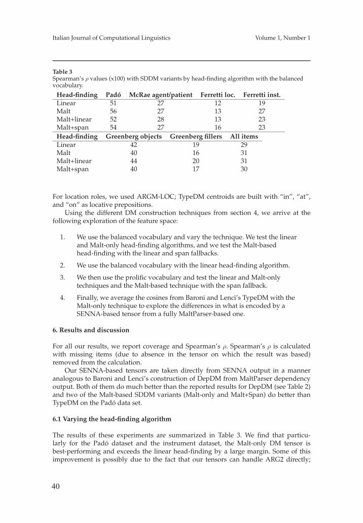
40
Italian Journal of Computational Linguistics Volume 1, Number 1
Table 3Spearman’s ρ values (x100) with SDDM variants by head-finding algorithm with the balancedvocabulary.
Head-finding Padó McRae agent/patient Ferretti loc. Ferretti inst.Linear 51 27 12 19Malt 56 27 13 27Malt+linear 52 28 13 23Malt+span 54 27 16 23Head-finding Greenberg objects Greenberg fillers All itemsLinear 42 19 29Malt 40 16 31Malt+linear 44 20 31Malt+span 40 17 30
For location roles, we used ARGM-LOC; TypeDM centroids are built with “in”, “at”,and “on” as locative prepositions.
Using the different DM construction techniques from section 4, we arrive at thefollowing exploration of the feature space:
1. We use the balanced vocabulary and vary the technique. We test the linearand Malt-only head-finding algorithms, and we test the Malt-basedhead-finding with the linear and span fallbacks.
2. We use the balanced vocabulary with the linear head-finding algorithm.
3. We then use the prolific vocabulary and test the linear and Malt-onlytechniques and the Malt-based technique with the span fallback.
4. Finally, we average the cosines from Baroni and Lenci’s TypeDM with theMalt-only technique to explore the differences in what is encoded by aSENNA-based tensor from a fully MaltParser-based one.
6. Results and discussion
For all our results, we report coverage and Spearman’s ρ. Spearman’s ρ is calculatedwith missing items (due to absence in the tensor on which the result was based)removed from the calculation.
Our SENNA-based tensors are taken directly from SENNA output in a manneranalogous to Baroni and Lenci’s construction of DepDM from MaltParser dependencyoutput. Both of them do much better than the reported results for DepDM (see Table 2)and two of the Malt-based SDDM variants (Malt-only and Malt+Span) do better thanTypeDM on the Padó data set.
6.1 Varying the head-finding algorithm
The results of these experiments are summarized in Table 3. We find that particu-larly for the Padó dataset and the instrument dataset, the Malt-only DM tensor isbest-performing and exceeds the linear head-finding by a large margin. Some of thisimprovement is possibly due to the fact that our tensors can handle ARG2 directly;
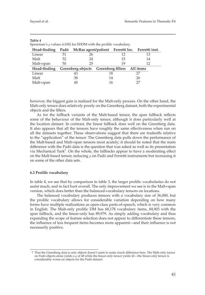
41
Sayeed et al. Semantic Features in Thematic Fit
Table 4Spearman’s ρ values (x100) for SDDM with the prolific vocabulary.
Head-finding Padó McRae agent/patient Ferretti loc. Ferretti inst.Linear 51 26 12 13Malt 52 24 15 14Malt+span 50 25 19 12Head-finding Greenberg objects Greenberg fillers All itemsLinear 43 18 27Malt 38 14 26Malt+span 40 16 27
however, the biggest gain is realized for the Malt-only process. On the other hand, theMalt-only tensor does relatively poorly on the Greenberg dataset, both the experimentalobjects and the fillers.
As for the fallback variants of the Malt-based tensor, the span fallback reflectssome of the behaviour of the Malt-only tensor, although it does particularly well atthe location dataset. In contrast, the linear fallback does well on the Greenberg data.It also appears that all the tensors have roughly the same effectiveness when run onall the datasets together. These observations suggest that there are tradeoffs relativeto the “application” of the tensor. The Greenberg data pulls down the performance ofthe Malt-based and Malt+span tensors most acutely; it should be noted that the maindifference with the Padó data is the question that was asked as well as its presentationvia Mechanical Turk7. On the whole, the fallbacks appear to have a moderating effecton the Malt-based tensor, reducing ρ on Padò and Ferretti instruments but increasing iton some of the other data sets.
6.2 Prolific vocabulary
In table 4, we see that by comparison to table 3, the larger prolific vocabularies do notassist much, and in fact hurt overall. The only improvement we see is in the Malt+spanversion, which does better than the balanced-vocabulary tensors on locations.
The balanced vocabulary produces tensors with a vocabulary size of 36,000, butthe prolific vocabulary allows for considerable variation depending on how manyforms have multiple realizations as open-class parts-of-speech, which is very commonin English. The Malt-only prolific DM has 68,178 vocabulary items, 84,903 with thespan fallback, and the linear-only has 89,979. As simply adding vocabulary and thusexpanding the scope of feature selection does not appear to differentiate these tensors,the influence of less frequent items becomes more apparent—and their influence is notnecessarily positive.
7 That the Greenberg data is only objects doesn’t seem to make much difference here. The Malt-only tensoron Padó objects alone yields a ρ of 48 while the linear-only tensor yields 42—the linear-only tensor isconsiderably worse on objects for the Padó dataset.
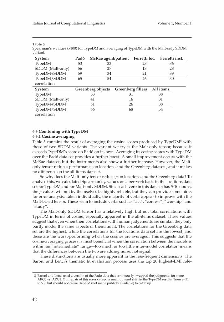
42
Italian Journal of Computational Linguistics Volume 1, Number 1
Table 5Spearman’s ρ values (x100) for TypeDM and averaging of TypeDM with the Malt-only SDDMvariant.
System Padó McRae agent/patient Ferretti loc. Ferretti inst.TypeDM 53 33 23 36SDDM (Malt-only) 56 27 13 28TypeDM+SDDM 59 34 21 39TypeDM/SDDMcorrelation
65 54 26 30
System Greenberg objects Greenberg fillers All itemsTypeDM 53 31 38SDDM (Malt-only) 41 16 31TypeDM+SDDM 51 26 38TypeDM/SDDMcorrelation
66 68 54
6.3 Combining with TypeDM6.3.1 Cosine averagingTable 5 contains the result of averaging the cosine scores produced by TypeDM8 withthose of two SDDM variants. The variant we try is the Malt-only tensor, because itexceeds TypeDM’s score on Padó on its own. Averaging its cosine scores with TypeDMover the Padó data set provides a further boost. A small improvement occurs with theMcRae dataset, but the instruments also show a further increase. However, the Malt-only tensor reduces performance on locations and the Greenberg datasets, and it makesno difference on the all-items dataset.
So why does the Malt-only tensor reduce ρ on locations and the Greenberg data? Toanalyse this, we calculated Spearman’s ρ values on a per-verb basis in the locations dataset for TypeDM and for Malt-only SDDM. Since each verb in this dataset has 5-10 nouns,the ρ values will not by themselves be highly reliable, but they can provide some hintsfor error analysis. Taken individually, the majority of verbs appear to improve with theMalt-based tensor. These seem to include verbs such as “act”, “confess”, “worship” and“study”.
The Malt-only SDDM tensor has a relatively high but not total correlations withTypeDM in terms of cosine, especially apparent in the all-items dataset. These valuessuggest that even when their correlations with human judgements are similar, they onlypartly model the same aspects of thematic fit. The correlations for the Greenberg dataset are the highest, while the correlations for the locations data set are the lowest, andthese are the worst-performing when the cosines are averaged. This suggests that thecosine-averaging process is most beneficial when the correlation between the models iswithin an “intermediate” range—too much or too little inter-model correlation meansthat the differences between the two are adding noise, not signal.
These distinctions are usually more apparent in the less-frequent dimensions. TheBaroni and Lenci’s thematic fit evaluation process uses the top 20 highest-LMI role-
8 Baroni and Lenci used a version of the Pado data that erroneously swapped the judgments for someARG0 vs. ARG1. Our repair of this error caused a small upward shift in the TypeDM results (from ρ=51to 53), but should not cause DepDM (not made publicly available) to catch up.
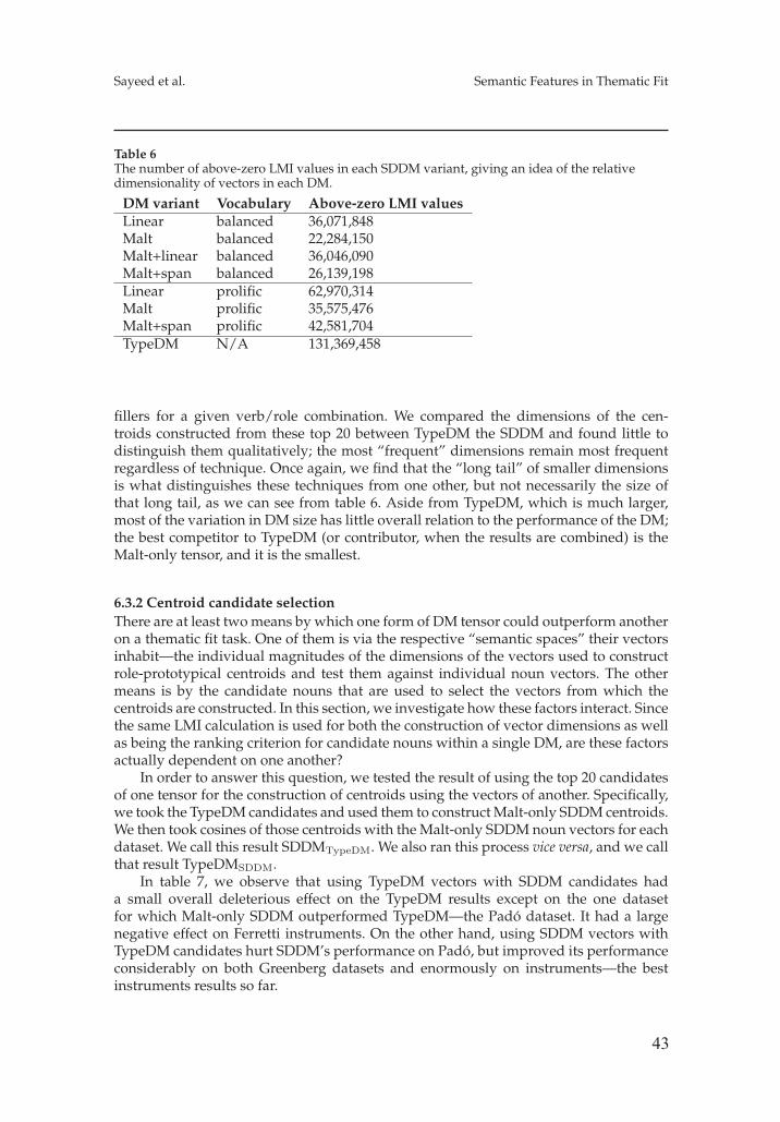
43
Sayeed et al. Semantic Features in Thematic Fit
Table 6The number of above-zero LMI values in each SDDM variant, giving an idea of the relativedimensionality of vectors in each DM.
DM variant Vocabulary Above-zero LMI valuesLinear balanced 36,071,848Malt balanced 22,284,150Malt+linear balanced 36,046,090Malt+span balanced 26,139,198Linear prolific 62,970,314Malt prolific 35,575,476Malt+span prolific 42,581,704TypeDM N/A 131,369,458
fillers for a given verb/role combination. We compared the dimensions of the cen-troids constructed from these top 20 between TypeDM the SDDM and found little todistinguish them qualitatively; the most “frequent” dimensions remain most frequentregardless of technique. Once again, we find that the “long tail” of smaller dimensionsis what distinguishes these techniques from one other, but not necessarily the size ofthat long tail, as we can see from table 6. Aside from TypeDM, which is much larger,most of the variation in DM size has little overall relation to the performance of the DM;the best competitor to TypeDM (or contributor, when the results are combined) is theMalt-only tensor, and it is the smallest.
6.3.2 Centroid candidate selectionThere are at least two means by which one form of DM tensor could outperform anotheron a thematic fit task. One of them is via the respective “semantic spaces” their vectorsinhabit—the individual magnitudes of the dimensions of the vectors used to constructrole-prototypical centroids and test them against individual noun vectors. The othermeans is by the candidate nouns that are used to select the vectors from which thecentroids are constructed. In this section, we investigate how these factors interact. Sincethe same LMI calculation is used for both the construction of vector dimensions as wellas being the ranking criterion for candidate nouns within a single DM, are these factorsactually dependent on one another?
In order to answer this question, we tested the result of using the top 20 candidatesof one tensor for the construction of centroids using the vectors of another. Specifically,we took the TypeDM candidates and used them to construct Malt-only SDDM centroids.We then took cosines of those centroids with the Malt-only SDDM noun vectors for eachdataset. We call this result SDDMTypeDM. We also ran this process vice versa, and we callthat result TypeDMSDDM.
In table 7, we observe that using TypeDM vectors with SDDM candidates hada small overall deleterious effect on the TypeDM results except on the one datasetfor which Malt-only SDDM outperformed TypeDM—the Padó dataset. It had a largenegative effect on Ferretti instruments. On the other hand, using SDDM vectors withTypeDM candidates hurt SDDM’s performance on Padó, but improved its performanceconsiderably on both Greenberg datasets and enormously on instruments—the bestinstruments results so far.
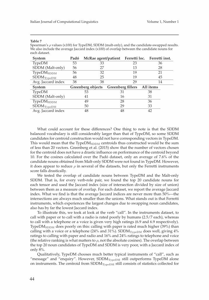
44
Italian Journal of Computational Linguistics Volume 1, Number 1
Table 7Spearman’s ρ values (x100) for TypeDM, SDDM (malt-only), and the candidate-swapped results.We also include the average Jaccard index (x100) of overlap between the candidate nouns foreach dataset.
System Padó McRae agent/patient Ferretti loc. Ferretti inst.TypeDM 53 33 23 36SDDM (Malt-only) 56 27 13 28TypeDMSDDM 56 32 19 21SDDMTypeDM 48 25 19 45Avg. Jaccard index 38 38 29 14System Greenberg objects Greenberg fillers All itemsTypeDM 53 31 38SDDM (Malt-only) 41 16 31TypeDMSDDM 49 28 36SDDMTypeDM 50 29 33Avg. Jaccard index 48 48 42
What could account for these differences? One thing to note is that the SDDMbalanced vocabulary is still considerably larger than that of TypeDM, so some SDDMcandidates for centroid construction would not have corresponding vectors in TypeDM.This would mean that the TypeDMSDDM centroids thus constructed would be the sumof less than 20 vectors. Greenberg et al. (2015) show that the number of vectors chosenfor the centroid does not have a drastic influence on performance of the centroid beyond10. For the cosines calculated over the Padó dataset, only an average of 7.6% of thecandidate nouns obtained from Malt-only SDDM were not found in TypeDM. However,it does appear to reduce ρ in several of the datasets, but only the Ferretti instrumentsscore falls drastically.
We tested the overlap of candidate nouns between TypeDM and the Malt-onlySDDM. That is, for every verb-role pair, we found the top 20 candidate nouns foreach tensor and used the Jaccard index (size of intersection divided by size of union)between them as a measure of overlap. For each dataset, we report the average Jaccardindex. What we find is that the average Jaccard indices are never more than 50%—theintersections are always much smaller than the unions. What stands out is that Ferrettiinstruments, which experiences the largest changes due to swapping noun candidates,also has by far the lowest Jaccard index.
To illustrate this, we took at look at the verb “call”. In the instruments dataset, tocall with paper or to call with a radio is rated poorly by humans (2.5/7 each), whereasto call with a telephone or a voice is given very high ratings (6.9 and 6.9 respectively).TypeDMSDDM does poorly on this: calling with paper is rated much higher (39%) thancalling with a voice or a telephone (24% and 31%). SDDMTypeDM does well, giving 4%ratings to calling with paper and radio and 16% and 24% ratings to telephone and voice(the relative ranking is what matters to ρ, not the absolute cosines). The overlap betweenthe top 20 noun candidates of TypeDM and SDDM is very poor, with a Jaccard index ofonly 8%.
Qualitatively, TypeDM chooses much better typical instruments of “call”, such as“message” and “enquiry”. However, SDDMTypeDM still outperforms TypeDM aloneon instruments. The centroid from SDDMTypeDM still consists of statistics collected for
45
Sayeed et al. Semantic Features in Thematic Fit
the Malt-only SDDM. In other words, the vectors of SDDM produce better results thanTypeDM’s vectors for instruments after we apply TypeDM’s typical noun candidates.
It thus appears that candidate selection and centroid construction are separablefrom one another, and that while TypeDM seems to produce better noun candidatesfor some of the datasets, Malt-only SDDM’s semantic space can sometimes be superiorfor the thematic fit task.
6.4 Coverage
All the datasets presented here have a coverage in the above 95% range over all items.
7. Conclusions
In this work, we constructed a number of DM tensors based on SENNA-annotatedthematic roles in the process of probing the feature space for their use in thematic fitevaluation. We find that combining the output of SENNA with MaltParser dependencylink information provides a boost in thematic fit performance in some well-studieddatasets such as the Padó data (over and above TypeDM) and the Ferretti instrumentdata, but other feature selections provide improvements in the Ferretti location data.
The linking thematic roles used to construct these tensors are not further augmentedby hand-crafted inference rules making them similar to Baroni and Lenci’s DepDM. Allof them easily exceed DepDM on the Padó data set. When used in combination withTypeDM in an unsupervised score averaging process, we find that the fit to humanjudgements improves for some datasets and declines for other data sets, particularly theGreenberg data. On the whole, we find that the SDDM tensors encode a different partof linguistic experience from the explcitly syntax-based TypeDM in the fine structureof dimensions they contain. Using the semantic space of SDDM with the prototypicalrole-filler candidate noun selection of TypeDM improves the performance of SDDM onsome data sets, particularly instruments, showing that candidate selection and vectorcomponent calculation can be strategically separated.
This work made use of Baroni and Lenci’s thematic fit evaluation process just asthey describe it. However, future work could include testing out the augmented ver-sions of this algorithm that involve clustering the vectors that go into centroid formationto produce multiple centroids reflecting verb senses (Greenberg, Sayeed, and Demberg2015). A further item of future work would be to understand why the Greenberg dataworks better with the linear head-finding (as opposed ot the Malt-based head-finding),despite its overall similarity to the Padó data.
ReferencesBaroni, Marco and Alessandro Lenci. 2010. Distributional memory: A general framework for
corpus-based semantics. Computational Linguistics, 36(4):673–721.Collobert, Ronan and Jason Weston. 2007. Fast semantic extraction using a novel neural network
architecture. In Proceedings of the 45th Annual Meeting of the Association of ComputationalLinguistics, pages 560–567, Prague, Czech Republic, June.
Collobert, Ronan, Jason Weston, Léon Bottou, Michael Karlen, Koray Kavukcuoglu, and PavelKuksa. 2011. Natural language processing (almost) from scratch. The Journal of MachineLearning Research, 12:2493–2537.
Erk, Katrin. 2012. Vector space models of word meaning and phrase meaning: A survey.Language and Linguistics Compass, 6(10):635–653.
Ferretti, Todd R, Ken McRae, and Andrea Hatherell. 2001. Integrating verbs, situation schemas,and thematic role concepts. Journal of Memory and Language, 44(4):516–547.
46
Italian Journal of Computational Linguistics Volume 1, Number 1
Foland Jr, William R. and James H. Martin. 2015. Dependency-based semantic role labeling usingconvolutional neural networks. In Proceedings of Lexical and Computational Semantics (* SEM2015), pages 279–288, Denver, CO, USA, June.
Greenberg, Clayton, Vera Demberg, and Asad Sayeed. 2015. Verb polysemy and frequencyeffects in thematic fit modeling. In Proceedings of the 6th Workshop on Cognitive Modeling andComputational Linguistics, pages 48–57, Denver, Colorado, June.
Greenberg, Clayton, Asad Sayeed, and Vera Demberg. 2015. Improving unsupervisedvector-space thematic fit evaluation via role-filler prototype clustering. In Proceedings of the2015 Conference of the North American Chapter of the Association for Computational LinguisticsHuman Language Technologies (NAACL HLT), pages 21–31.
Herdagdelen, Amaç and Marco Baroni. 2009. BagPack: A general framework to representsemantic relations. In Proceedings of the Workshop on Geometrical Models of Natural LanguageSemantics, pages 33–40, Athens, Greece, March. Association for Computational Linguistics.
Lang, Joel and Mirella Lapata. 2011. Unsupervised semantic role induction via split-mergeclustering. In Proceedings of the 49th Annual Meeting of the Association for ComputationalLinguistics: Human Language Technologies, pages 1117–1126, Portland, Oregon, USA, June.
Lenci, Alessandro. 2011. Composing and updating verb argument expectations: A distributionalsemantic model. In Proceedings of the 2Nd Workshop on Cognitive Modeling and ComputationalLinguistics, CMCL ’11, pages 58–66, Stroudsburg, PA, USA.
Levin, Beth. 1993. English verb classes and alternations: A preliminary investigation. University ofChicago press.
Magerman, David M. 1994. Natural Lagnuage Parsing as Statistical Pattern Recognition. Ph.D.thesis, Stanford University.
McRae, Ken, Michael J Spivey-Knowlton, and Michael K Tanenhaus. 1998. Modeling theinfluence of thematic fit (and other constraints) in on-line sentence comprehension. Journal ofMemory and Language, 38(3):283–312.
Nivre, Joakim, Johan Hall, Jens Nilsson, Atanas Chanev, Gülsen Eryigit, Sandra Kübler,Svetoslav Marinov, and Erwin Marsi. 2007. Maltparser: A language-independent system fordata-driven dependency parsing. Natural Language Engineering, 13(2):95–135.
Ó Séaghdha, Diarmuid. 2010. Latent variable models of selectional preference. In Proceedings ofthe 48th Annual Meeting of the Association for Computational Linguistics, ACL ’10, pages 435–444,Stroudsburg, PA, USA.
Padó, Ulrike. 2007. The integration of syntax and semantic plausibility in a wide-coverage model ofhuman sentence processing. Ph.D. thesis, Universitätsbibliothek.
Padó, Ulrike, Matthew W. Crocker, and Frank Keller. 2009. A probabilistic model of semanticplausibility in sentence processing. Cognitive Science, 33(5):794–838.
Palmer, Martha, Daniel Gildea, and Paul Kingsbury. 2005. The proposition bank: An annotatedcorpus of semantic roles. Computational Linguistics, 31(1):71–106.
Ritter, Alan, Mausam, and Oren Etzioni. 2010. A latent dirichlet allocation method for selectionalpreferences. In Proceedings of the 48th Annual Meeting of the Association for ComputationalLinguistics, ACL ’10, pages 424–434, Stroudsburg, PA, USA.
Sayeed, Asad and Vera Demberg. 2013. The semantic augmentation of apsycholinguistically-motivated syntactic formalism. In Cognitive modeling and computationallinguistics (CMCL 2013), pages 57–65, Sofia, Bulgaria, 8 August.
Titov, Ivan and Alexandre Klementiev. 2011. A bayesian model for unsupervised semanticparsing. In Proceedings of the 49th Annual Meeting of the Association for Computational Linguistics,pages 1445–1455, Portland, Oregon, USA, June.
Turney, Peter D. and Patrick Pantel. 2010. From frequency to meaning: Vector space models ofsemantics. Journal of artificial intelligence research, 37(1):141–188.
Vandekerckhove, Bram, Dominiek Sandra, and Walter Daelemans. 2009. A robust and extensibleexemplar-based model of thematic fit. In EACL 2009, 12th Conference of the European Chapter ofthe Association for Computational Linguistics, Proceedings of the Conference, Athens, Greece, March30 - April 3, 2009, pages 826–834.
© 2015 Associazione Italiana di Linguistica Computazionale
When Similarity Becomes Opposition: Synonyms and Antonyms Discrimination in DSMs
Enrico Santus*
Hong Kong Polytechnic University Alessandro Lenci§ Università di Pisa
Qin Lu
† Hong Kong Polytechnic University
Chu-Ren Huang‡ Hong Kong Polytechnic University
This paper analyzes the concept of opposition and describes a fully unsupervised method for its automatic discrimination from near-synonymy in Distributional Semantic Models (DSMs). The discriminating method is based on the hypothesis that, even though both near-synonyms and opposites are mostly distributionally similar, opposites are different from each other in at least one dimension of meaning, which can be assumed to be salient. Such hypothesis has been implemented in APAnt, a distributional measure that evaluates the extent of the intersection among the most relevant contexts of two words (where relevance is measured as mutual dependency), and its saliency (i.e. their average rank in the mutual dependency sorted list of contexts). The measure – previously introduced in some pilot studies – is presented here with two variants. Evaluation shows that it outperforms three baselines in an antonym retrieval task: the vector cosine, a baseline implementing the co-occurrence hypothesis, and a random rank. This paper describes the algorithm in details and analyzes its current limitations, suggesting that extensions may be developed for discriminating antonyms not only from near-synonyms but also from other semantic relations. During the evaluation, we have noticed that APAnt also has a particular preference for hypernyms.
1. Introduction
Similarity is one of the fundamental principles organizing the semantic lexicon (Lenci, 2008; Landauer and Dumais, 1997). Distributional Semantic Models (DSMs) encoding the frequency of co-occurrences between words in large corpora are proven to be successful in representing word meanings in terms of distributional similarity (Turney and Pantel, 2010; Pado and Lapata, 2007; Sahlgren, 2006).
These models allow a geometric representation of the Distributional Hypothesis (Harris, 1954), that is, words occurring in similar contexts also have similar meanings. They represent words as vectors in a continuous vector space, where distributional similarity can be measured as vector proximity. This, in turn, can be calculated through the vector cosine (Turney and Pantel, 2010). This representation is so effective that DSMs are known to be able to replicate human judgments with a reasonable accuracy (Lenci, 2008).
* E-mail: [email protected] § E-mail: [email protected] † E-mail: [email protected] ‡ E-mail: [email protected]
47
© 2015 Associazione Italiana di Linguistica Computazionale
When Similarity Becomes Opposition: Synonyms and Antonyms Discrimination in DSMs
Enrico Santus*
Hong Kong Polytechnic University Alessandro Lenci§ Università di Pisa
Qin Lu
† Hong Kong Polytechnic University
Chu-Ren Huang‡ Hong Kong Polytechnic University
This paper analyzes the concept of opposition and describes a fully unsupervised method for its automatic discrimination from near-synonymy in Distributional Semantic Models (DSMs). The discriminating method is based on the hypothesis that, even though both near-synonyms and opposites are mostly distributionally similar, opposites are different from each other in at least one dimension of meaning, which can be assumed to be salient. Such hypothesis has been implemented in APAnt, a distributional measure that evaluates the extent of the intersection among the most relevant contexts of two words (where relevance is measured as mutual dependency), and its saliency (i.e. their average rank in the mutual dependency sorted list of contexts). The measure – previously introduced in some pilot studies – is presented here with two variants. Evaluation shows that it outperforms three baselines in an antonym retrieval task: the vector cosine, a baseline implementing the co-occurrence hypothesis, and a random rank. This paper describes the algorithm in details and analyzes its current limitations, suggesting that extensions may be developed for discriminating antonyms not only from near-synonyms but also from other semantic relations. During the evaluation, we have noticed that APAnt also has a particular preference for hypernyms.
1. Introduction
Similarity is one of the fundamental principles organizing the semantic lexicon (Lenci, 2008; Landauer and Dumais, 1997). Distributional Semantic Models (DSMs) encoding the frequency of co-occurrences between words in large corpora are proven to be successful in representing word meanings in terms of distributional similarity (Turney and Pantel, 2010; Pado and Lapata, 2007; Sahlgren, 2006).
These models allow a geometric representation of the Distributional Hypothesis (Harris, 1954), that is, words occurring in similar contexts also have similar meanings. They represent words as vectors in a continuous vector space, where distributional similarity can be measured as vector proximity. This, in turn, can be calculated through the vector cosine (Turney and Pantel, 2010). This representation is so effective that DSMs are known to be able to replicate human judgments with a reasonable accuracy (Lenci, 2008).
* E-mail: [email protected] § E-mail: [email protected] † E-mail: [email protected] ‡ E-mail: [email protected]
48
Italian Journal of Computational Linguistics Volume 1, Number 1
However, the Distributional Hypothesis shapes the concept of similarity in a very loose way, including among the distributionally similar words not only those that refer to similar referents (e.g. co-hyponyms and near-synonyms), but – more in general – all those words that share many contexts (Harris, 1954). As a consequence of such definition, words like dog may be considered similar not only to the co-hyponym lexeme cat, but also to the hypernym animal, the meronym tail (Morlane-Hondère, 2015), and so on. This loose definition, therefore, poses a big challenge in Natural Language Processing (NLP), and in particular in Computational Lexical Semantics, where the meaning of a word and the type of relations it holds with others need to be univocally identified. For instance, in a task such as Textual Entailment it is crucial not only to identify whether two words are semantically similar, but also whether they entail each other, like hyponym-hypernym pairs do. Similarly, in Sentiment Analysis the correct discrimination of antonyms (e.g. good from bad) is extremely important to identify the positive or negative polarity of a text.
Among the relations that fall under the large umbrella of distributional similarity, there is indeed opposition, also known as antonymy. According to Cruse (1986), antonymy is characterized by the paradox of simultaneous similarity and difference: Opposites are identical in every dimension of meaning except for one. A typical example of such paradox is the relation between dwarf and giant. These words are semantically similar in many aspects (i.e. they may refer to similar entities, such as humans, trees, galaxies), differing only for what concerns the size, which is assumed to be a salient semantic dimension for them. Distributionally speaking, dwarfs and giants share many contexts (e.g., both giant and dwarf may be used to refer to galaxies, stars, planets, companies, people1), differing for those related to the semantic dimension of size. For example, giant is likely to occur in contexts related to big sizes, such as global, corporate, dominate and so on2, while dwarf is likely to occur in contexts related to small sizes, such as virus, elf, shrub and so on3.
Starting from this observation, we describe and analyze a method aiming to identify opposites in DSMs. The method, which is directly inspired to Cruse’s paradox, is named APAnt (from Average Precision for Antonyms) and lies on the hypothesis that antonyms share less salient contexts than synonyms. The method was first presented in two previous pilot studies of Santus et al. (2014b, 2014c). In those papers, APant was shown to outperform the vector cosine and a baseline implementing the co-occurrence hypothesis (Charles and Miller, 1989) in an antonym retrieval task (AR), using a standard window-based DSM, built by collecting the co-occurrences between the two content words on the left and the right of the target word, in a combination of ukWaC and WaCkypedia (Santus et al., 2014a)4. The task was performed using the Lenci/Benotto dataset (Santus et al., 2014b) and evaluated through Average Precision (AP; Kotlerman et al., 2010).
In this paper, we first give a more detailed description of APAnt presenting also two variants. All the measures are evaluated in two antonym retrieval tasks, performed on an extended dataset, which includes antonyms, synonyms, hypernyms and co-hyponyms (henceforth, also referred as coordinates, according to Baroni and Lenci, 2011) from the Lenci/Benotto (Santus et al., 2014b), BLESS (Baroni and Lenci, 2011) and EVALution 1.0 (Santus et al., 2015). Again, APAnt
1 These examples were found by searching in Sketch Engine (https://www.sketchengine.co.uk), using the word sketch function. 2 Ibid. 3 Ibid. 4 Similar experiments on a standard five content words window DSM have confirmed that APAnt outperforms the vector cosine and the co-occurrence baseline. The actual impact of the window size still needs to be properly analyzed.
49
Italian Journal of Computational Linguistics Volume 1, Number 1
However, the Distributional Hypothesis shapes the concept of similarity in a very loose way, including among the distributionally similar words not only those that refer to similar referents (e.g. co-hyponyms and near-synonyms), but – more in general – all those words that share many contexts (Harris, 1954). As a consequence of such definition, words like dog may be considered similar not only to the co-hyponym lexeme cat, but also to the hypernym animal, the meronym tail (Morlane-Hondère, 2015), and so on. This loose definition, therefore, poses a big challenge in Natural Language Processing (NLP), and in particular in Computational Lexical Semantics, where the meaning of a word and the type of relations it holds with others need to be univocally identified. For instance, in a task such as Textual Entailment it is crucial not only to identify whether two words are semantically similar, but also whether they entail each other, like hyponym-hypernym pairs do. Similarly, in Sentiment Analysis the correct discrimination of antonyms (e.g. good from bad) is extremely important to identify the positive or negative polarity of a text.
Among the relations that fall under the large umbrella of distributional similarity, there is indeed opposition, also known as antonymy. According to Cruse (1986), antonymy is characterized by the paradox of simultaneous similarity and difference: Opposites are identical in every dimension of meaning except for one. A typical example of such paradox is the relation between dwarf and giant. These words are semantically similar in many aspects (i.e. they may refer to similar entities, such as humans, trees, galaxies), differing only for what concerns the size, which is assumed to be a salient semantic dimension for them. Distributionally speaking, dwarfs and giants share many contexts (e.g., both giant and dwarf may be used to refer to galaxies, stars, planets, companies, people1), differing for those related to the semantic dimension of size. For example, giant is likely to occur in contexts related to big sizes, such as global, corporate, dominate and so on2, while dwarf is likely to occur in contexts related to small sizes, such as virus, elf, shrub and so on3.
Starting from this observation, we describe and analyze a method aiming to identify opposites in DSMs. The method, which is directly inspired to Cruse’s paradox, is named APAnt (from Average Precision for Antonyms) and lies on the hypothesis that antonyms share less salient contexts than synonyms. The method was first presented in two previous pilot studies of Santus et al. (2014b, 2014c). In those papers, APant was shown to outperform the vector cosine and a baseline implementing the co-occurrence hypothesis (Charles and Miller, 1989) in an antonym retrieval task (AR), using a standard window-based DSM, built by collecting the co-occurrences between the two content words on the left and the right of the target word, in a combination of ukWaC and WaCkypedia (Santus et al., 2014a)4. The task was performed using the Lenci/Benotto dataset (Santus et al., 2014b) and evaluated through Average Precision (AP; Kotlerman et al., 2010).
In this paper, we first give a more detailed description of APAnt presenting also two variants. All the measures are evaluated in two antonym retrieval tasks, performed on an extended dataset, which includes antonyms, synonyms, hypernyms and co-hyponyms (henceforth, also referred as coordinates, according to Baroni and Lenci, 2011) from the Lenci/Benotto (Santus et al., 2014b), BLESS (Baroni and Lenci, 2011) and EVALution 1.0 (Santus et al., 2015). Again, APAnt
1 These examples were found by searching in Sketch Engine (https://www.sketchengine.co.uk), using the word sketch function. 2 Ibid. 3 Ibid. 4 Similar experiments on a standard five content words window DSM have confirmed that APAnt outperforms the vector cosine and the co-occurrence baseline. The actual impact of the window size still needs to be properly analyzed.
Santus et al. Synonyms and Antonyms Discrimination in DSMs
outperforms the above-mentioned baselines plus another one based on random ranking.
The paper is organized as follows. In the next section, we define opposites and their properties (Section 2), moving then to the state of the art for their discrimination (Section 3). We introduce our method and its variations (Section 4) and describe their evaluation (Section 5). A detailed discussion of the results (Sections 6 and 7) and the conclusions are reported at the end of the paper (Conclusions).
2. Opposites
People do not always perfectly agree on classifying word pairs as opposites (Mohammad et al., 2013), confirming that their identification is indeed a hard task, even for native speakers. The major problems in such task are that (1) opposites are rarely in a truly binary contrast (e.g. warm/hot); (2) the contrast can be of different kinds (e.g. semantic, as in hot/cold, or referential, as in shark/dolphin); and (3) opposition is often context-dependent (e.g. consider the near-synonyms very good and excellent in the following sentence: “not simply very good, but excellent”; Cruse, 1986; Murphy, 2003). All these issues make opposites difficult to define, so that linguists often need to rely on diagnostic tests to make the opposition clear (Murphy, 2003).
Over the years, many scholars from different disciplines have tried to provide a precise definition of this semantic relation. They are yet to reach any conclusive agreement. Kempson (1977) defines opposites as word pairs with a “binary incompatible relation”, such that the presence of one meaning entails the absence of the other. In this sense, giant and dwarf are good opposites, while giant and person are not. Mohammad et al. (2013), noticing that the terms opposites, contrasting and antonyms have often been used interchangeably, have proposed the following distinction: (1) opposites are word pairs that are strongly incompatible with each other and/or are saliently different across a dimension of meaning; (2) contrasting word pairs have some non-zero degree of binary incompatibility and/or some non-zero difference across a dimension of meaning; (3) antonyms are opposites that are also gradable adjectives. They have also provided a simple but comprehensive classification of opposites based on Cruse (1986), including (1) antipodals (e.g. top-bottom), pairs whose terms are at the opposite extremes of a specific meaning dimension; (2) complementaries (e.g. open-shut), pairs whose terms divide the domain in two mutual exclusive compartments; (3) disjoints (e.g. hot-cold), pairs whose words occupy non-overlapping regions in a specific semantic dimension, generally representing a state; (4) gradable opposites (e.g. long-short), adjective- or adverb-pairs that gradually describe some semantic dimensions, such as length, speed, etc.; (5) reversibles (e.g. rise-fall), verb-pairs whose words respectively describe the change from state A to state B and the inverse, from state B to state A.
In this paper, we will not account for all these differences, but we will use the terms opposites and antonyms as synonyms, meaning all pairs of words in which a certain level of contrast is perceived. Under such category we include also the paranyms, which are a specific type of coordinates (Huang et al., 2007) that partition a conceptual field into complementary subfields. For instance, although dry season, spring, summer, autumn and winter are all co-hyponyms, only the latter four are paranyms, as they split the conceptual field of seasons.
50
Italian Journal of Computational Linguistics Volume 1, Number 1
3. Related Works
Opposites identification is very challenging for computational models (Mohammad et al., 2008; Deese, 1965; Deese, 1964). Yet, this relation is essential for many NLP applications, such as Information Retrieval (IR), Ontology Learning (OL), Machine Translation (MT), Sentiment Analysis (SA) and Dialogue Systems (Roth and Schulte im Walde, 2014; Mohammad et al., 2013). In particular, the automatic identification of semantic opposition is crucial for the detection and generation of paraphrases (i.e. during the generation, similar but contrasting candidates should be filtered out, as described in Marton et al., 2011), the understanding of contradictions (de Marneffe et al., 2008) and the identification of irony (Xu et al., 2015; Tungthamthiti et al., 2015) and humor (Mihalcea and Strapparava, 2005).
Several existing hand-crafted computational lexicons and thesauri explicitly encoding opposition are often used to support the above mentioned NLP tasks, even though many scholars have shown their limits. Mohammad et al. (2013), for example, point out that “more than 90% of the contrasting pairs in GRE closest-to-opposite questions 5 are not listed as opposites in WordNet”. Moreover, the relations encoded in such resources are mostly context independent.
Given the already mentioned reliability of Distributional Semantic Models (DSMs) in the detection of distributional similarity between lexemes, several studies have tried to exploit these models for the identification of semantic relations (Santus et al., 2014a; Baroni and Lenci, 2010; Turney and Pantel, 2010; Padó and Lapata, 2007; Sahlgren, 2006). As mentioned before, however, DSMs are characterized by a major shortcoming. That is, they are not able to discriminate among different kinds of semantic relations linking distributionally similar lexemes (Santus et al., 2014a). This is the reason why supervised and pattern-based approaches have often been preferred (Pantel and Pennacchiotti, 2006; Hearst, 1992). However, these latter methods have also various problems, most notably the difficulty of finding patterns that are highly reliable and univocally associated with specific relations, without incurring at the same time in data-sparsity problems. The experience of pattern-based approaches has shown that these two criteria can rarely be satisfied simultaneously.
The foundation of most corpus-based research on opposition is the co-occurrence hypothesis (Lobanova, 2012), formulated by Charles and Miller (1989) after observing that opposites co-occur in the same sentence more often than expected by chance. Such claim has then found many empirical confirmations (Justeson and Katz, 1991; Fellbaum, 1995) and it is used in the present work as a baseline. Ding and Huang (2014; 2013) also pointed out that, unlike co-hyponyms, opposites generally have a strongly preferred word order when they co-occur in a coordinate context (i.e. A and/or B). Another part of related research has been focused on the study of lexical-syntactic constructions that can work as linguistic tests for opposition definition and classification (Cruse, 1986).
Starting from all these observations, several computational methods for opposition identification were implemented. Most of them rely on patterns (Schulte im Walde and Köper, 2013; Lobanova et al., 2010; Turney, 2008; Pantel and Pennacchiotti, 2006; Lin et al., 2003), which unfortunately suffer from low recall, because they can be applied only to frequent words. Others, like Lucerto et al. (2002), use the number of tokens between the target words and other clues (e.g. the presence/absence of conjunctions like but, from, and, etc.) to identify contrasting words.
5 GRE stands for Graduate Record Examination, which is a standardized test, often used as an admissions requirement for graduate schools in the United States.
51
Italian Journal of Computational Linguistics Volume 1, Number 1
3. Related Works
Opposites identification is very challenging for computational models (Mohammad et al., 2008; Deese, 1965; Deese, 1964). Yet, this relation is essential for many NLP applications, such as Information Retrieval (IR), Ontology Learning (OL), Machine Translation (MT), Sentiment Analysis (SA) and Dialogue Systems (Roth and Schulte im Walde, 2014; Mohammad et al., 2013). In particular, the automatic identification of semantic opposition is crucial for the detection and generation of paraphrases (i.e. during the generation, similar but contrasting candidates should be filtered out, as described in Marton et al., 2011), the understanding of contradictions (de Marneffe et al., 2008) and the identification of irony (Xu et al., 2015; Tungthamthiti et al., 2015) and humor (Mihalcea and Strapparava, 2005).
Several existing hand-crafted computational lexicons and thesauri explicitly encoding opposition are often used to support the above mentioned NLP tasks, even though many scholars have shown their limits. Mohammad et al. (2013), for example, point out that “more than 90% of the contrasting pairs in GRE closest-to-opposite questions 5 are not listed as opposites in WordNet”. Moreover, the relations encoded in such resources are mostly context independent.
Given the already mentioned reliability of Distributional Semantic Models (DSMs) in the detection of distributional similarity between lexemes, several studies have tried to exploit these models for the identification of semantic relations (Santus et al., 2014a; Baroni and Lenci, 2010; Turney and Pantel, 2010; Padó and Lapata, 2007; Sahlgren, 2006). As mentioned before, however, DSMs are characterized by a major shortcoming. That is, they are not able to discriminate among different kinds of semantic relations linking distributionally similar lexemes (Santus et al., 2014a). This is the reason why supervised and pattern-based approaches have often been preferred (Pantel and Pennacchiotti, 2006; Hearst, 1992). However, these latter methods have also various problems, most notably the difficulty of finding patterns that are highly reliable and univocally associated with specific relations, without incurring at the same time in data-sparsity problems. The experience of pattern-based approaches has shown that these two criteria can rarely be satisfied simultaneously.
The foundation of most corpus-based research on opposition is the co-occurrence hypothesis (Lobanova, 2012), formulated by Charles and Miller (1989) after observing that opposites co-occur in the same sentence more often than expected by chance. Such claim has then found many empirical confirmations (Justeson and Katz, 1991; Fellbaum, 1995) and it is used in the present work as a baseline. Ding and Huang (2014; 2013) also pointed out that, unlike co-hyponyms, opposites generally have a strongly preferred word order when they co-occur in a coordinate context (i.e. A and/or B). Another part of related research has been focused on the study of lexical-syntactic constructions that can work as linguistic tests for opposition definition and classification (Cruse, 1986).
Starting from all these observations, several computational methods for opposition identification were implemented. Most of them rely on patterns (Schulte im Walde and Köper, 2013; Lobanova et al., 2010; Turney, 2008; Pantel and Pennacchiotti, 2006; Lin et al., 2003), which unfortunately suffer from low recall, because they can be applied only to frequent words. Others, like Lucerto et al. (2002), use the number of tokens between the target words and other clues (e.g. the presence/absence of conjunctions like but, from, and, etc.) to identify contrasting words.
5 GRE stands for Graduate Record Examination, which is a standardized test, often used as an admissions requirement for graduate schools in the United States.
Santus et al. Synonyms and Antonyms Discrimination in DSMs
Turney (2008) proposed a supervised algorithm for the identification of several semantic relations, including synonyms and opposites. The algorithm relied on a training set of word pairs with class labels to assign the labels also to a testing set of word pairs. All word pairs were represented as vectors encoding the frequencies of co-occurrence in textual patterns extracted from a large corpus of web pages. He used the sequential minimal optimization (SMO) support vector machine (SVM) with a radial basis function (RBF) kernel (Platt, 1998) implemented in Weka (Waikato Environment for Knowledge Analysis) (Witten and Frank, 1999). In the discrimination between synonyms and opposites, the system achieved an accuracy of 75% against a majority class baseline of 65.4%.
Mohammad et al. (2008) proposed a method for determining the degree of semantic contrast (i.e. how much two contrasting words are semantically close) based on the use of thesauri categories and corpus statistics. For each target word pair, they used the co-occurrence and the distributional hypothesis to establish the degree of opposition. Their algorithm achieved an F-score of 0.7, against a random baseline of 0.2.
Mohammad et al. (2013) used an analogical method based on a given set of contrasting words to identify and classify different kinds of opposites by hypothesizing that for every opposing pair of words, A and B, there is at least another opposing pair, C and D, such that A is similar to C and B is similar to D. For example, for the pair night-day, there is the pair darkness-daylight, such that night is similar to darkness and day to daylight. Given the existence of contrast, they calculated its degree relying on the co-occurrence hypothesis. Their approach outperformed other state-of-the-art measures.
Schulte im Walde and Köper (2013) proposed a vector space model relying on lexico-syntactic patterns to distinguish between synonymy, antonymy and hypernymy. Their approach was tested on German nouns, verbs and adjectives, achieving a precision of 59.80%, which was above the majority baseline.
More recently, Roth and Schulte im Walde (2014) proposed that statistics over discourse relations can be used as indicators for paradigmatic relations, including opposition.
4. Our Method: APAnt
Starting from the already mentioned paradox of simultaneous similarity and difference between antonyms (Cruse, 1986), in Santus et al. (2014b, 2014c) we have proposed a distributional measure that modifies the Average Precision formula (Kotlerman et al., 2010) to discriminate antonyms from near-synonyms. APAnt, from Average Precision for Antonymy, takes into account two main factors: i) the extent of the intersection among the N most relevant contexts of two words (where relevance is measured as mutual dependency); and ii) the salience of such intersection (i.e. the average rank in the mutual dependency sorted list of contexts). These factors are considered under the hypothesis that near-synonyms are likely to share a larger part of the salient contexts compared to antonyms.
In this section, we describe in details the APAnt algorithm, proposing also two variants aimed to improve APAnt stability and extend its scope. They will be named with an increasing number, APAnt2 (which consists in a simple normalization of APAnt) and APAnt3 (which introduces a new factor to APAnt2, that is, the distributional similarity among the word pairs).
APAnt should be seen as the inverse of APSyn (Average Precision for Synonymy). While APSyn assigns higher scores to near-synonyms, APAnt assigns higher scores
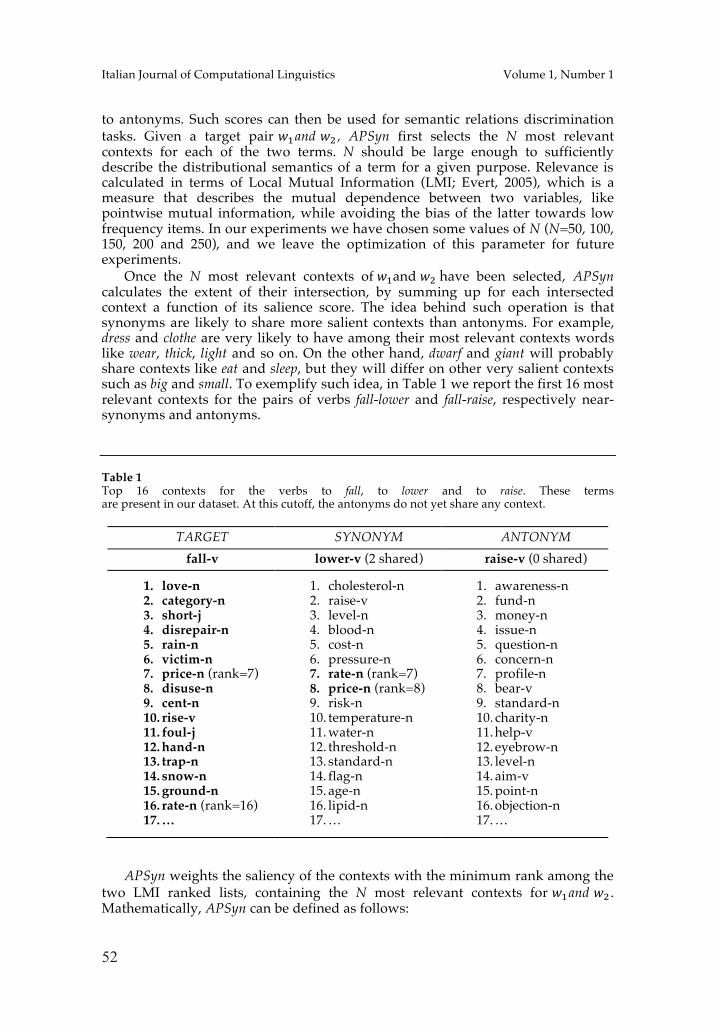
52
Italian Journal of Computational Linguistics Volume 1, Number 1
to antonyms. Such scores can then be used for semantic relations discrimination tasks. Given a target pair !!and !! , APSyn first selects the N most relevant contexts for each of the two terms. N should be large enough to sufficiently describe the distributional semantics of a term for a given purpose. Relevance is calculated in terms of Local Mutual Information (LMI; Evert, 2005), which is a measure that describes the mutual dependence between two variables, like pointwise mutual information, while avoiding the bias of the latter towards low frequency items. In our experiments we have chosen some values of N (N=50, 100, 150, 200 and 250), and we leave the optimization of this parameter for future experiments.
Once the N most relevant contexts of !!and !! have been selected, APSyn calculates the extent of their intersection, by summing up for each intersected context a function of its salience score. The idea behind such operation is that synonyms are likely to share more salient contexts than antonyms. For example, dress and clothe are very likely to have among their most relevant contexts words like wear, thick, light and so on. On the other hand, dwarf and giant will probably share contexts like eat and sleep, but they will differ on other very salient contexts such as big and small. To exemplify such idea, in Table 1 we report the first 16 most relevant contexts for the pairs of verbs fall-lower and fall-raise, respectively near-synonyms and antonyms.
Table 1 Top 16 contexts for the verbs to fall, to lower and to raise. These terms are present in our dataset. At this cutoff, the antonyms do not yet share any context.
TARGET SYNONYM ANTONYM
fall-v lower-v (2 shared) raise-v (0 shared)
1. love-n 2. category-n 3. short-j 4. disrepair-n 5. rain-n 6. victim-n 7. price-n (rank=7) 8. disuse-n 9. cent-n 10. rise-v 11. foul-j 12. hand-n 13. trap-n 14. snow-n 15. ground-n 16. rate-n (rank=16) 17. …
1. cholesterol-n 2. raise-v 3. level-n 4. blood-n 5. cost-n 6. pressure-n 7. rate-n (rank=7) 8. price-n (rank=8) 9. risk-n 10. temperature-n 11. water-n 12. threshold-n 13. standard-n 14. flag-n 15. age-n 16. lipid-n 17. …
1. awareness-n 2. fund-n 3. money-n 4. issue-n 5. question-n 6. concern-n 7. profile-n 8. bear-v 9. standard-n 10. charity-n 11. help-v 12. eyebrow-n 13. level-n 14. aim-v 15. point-n 16. objection-n 17. …
APSyn weights the saliency of the contexts with the minimum rank among the
two LMI ranked lists, containing the N most relevant contexts for !!and !! . Mathematically, APSyn can be defined as follows:
53
Italian Journal of Computational Linguistics Volume 1, Number 1
to antonyms. Such scores can then be used for semantic relations discrimination tasks. Given a target pair !!and !! , APSyn first selects the N most relevant contexts for each of the two terms. N should be large enough to sufficiently describe the distributional semantics of a term for a given purpose. Relevance is calculated in terms of Local Mutual Information (LMI; Evert, 2005), which is a measure that describes the mutual dependence between two variables, like pointwise mutual information, while avoiding the bias of the latter towards low frequency items. In our experiments we have chosen some values of N (N=50, 100, 150, 200 and 250), and we leave the optimization of this parameter for future experiments.
Once the N most relevant contexts of !!and !! have been selected, APSyn calculates the extent of their intersection, by summing up for each intersected context a function of its salience score. The idea behind such operation is that synonyms are likely to share more salient contexts than antonyms. For example, dress and clothe are very likely to have among their most relevant contexts words like wear, thick, light and so on. On the other hand, dwarf and giant will probably share contexts like eat and sleep, but they will differ on other very salient contexts such as big and small. To exemplify such idea, in Table 1 we report the first 16 most relevant contexts for the pairs of verbs fall-lower and fall-raise, respectively near-synonyms and antonyms.
Table 1 Top 16 contexts for the verbs to fall, to lower and to raise. These terms are present in our dataset. At this cutoff, the antonyms do not yet share any context.
TARGET SYNONYM ANTONYM
fall-v lower-v (2 shared) raise-v (0 shared)
1. love-n 2. category-n 3. short-j 4. disrepair-n 5. rain-n 6. victim-n 7. price-n (rank=7) 8. disuse-n 9. cent-n 10. rise-v 11. foul-j 12. hand-n 13. trap-n 14. snow-n 15. ground-n 16. rate-n (rank=16) 17. …
1. cholesterol-n 2. raise-v 3. level-n 4. blood-n 5. cost-n 6. pressure-n 7. rate-n (rank=7) 8. price-n (rank=8) 9. risk-n 10. temperature-n 11. water-n 12. threshold-n 13. standard-n 14. flag-n 15. age-n 16. lipid-n 17. …
1. awareness-n 2. fund-n 3. money-n 4. issue-n 5. question-n 6. concern-n 7. profile-n 8. bear-v 9. standard-n 10. charity-n 11. help-v 12. eyebrow-n 13. level-n 14. aim-v 15. point-n 16. objection-n 17. …
APSyn weights the saliency of the contexts with the minimum rank among the
two LMI ranked lists, containing the N most relevant contexts for !!and !! . Mathematically, APSyn can be defined as follows:
Santus et al. Synonyms and Antonyms Discrimination in DSMs
!"#$%(!!,!!) = !
!"# (!"#$! !! ,!"#$! !! ) !∈!(!!)∩!(!!) (1)
where !(!!) is the list of the ! most relevant contexts f of a term !!, and !"#$!(!!) is the rank of the feature !! in such salience ranked feature list. It is important to note here that a small N would inevitably reduce the intersection, forcing most of the scores to the same values (and eventually to zero), independently on the relation the pair under examination holds. On the other hand, a very large value of N will inevitably include also contexts with very low values of LMI and, therefore, much less relevant for the target noun. Finally, it can be seen that APSyn assigns the highest scores to the identity pairs (e.g. dog-dog).
If APSyn assigns high scores to the near-synonyms, its inverse – APAnt – is intended to assign high scores to the antonyms:
!"!#$(!!,!!) = !
!"#$%(!!,!!) (2)
Two cases need to be considered here: • if APSyn has not found any intersection among the N most relevant
contexts, it will be set to zero, and consequently APAnt will be infinite;
• if APSyn has found a large and salient intersection, it will get a high value, and consequently APAnt will have a very low one.
The first case happens when the two terms in the pair are distributionally unrelated or when N is not sufficiently high. Therefore, APant is set to the maximum attested value. The second case, instead, can occur when two terms are distributionally very similar, sharing therefore many salient contexts. Ideally, this should only be the case for near-synonyms.
As we will see in Section 7, most of the scores given by APSyn and APAnt are either very high or very low. In order to scale them between 0 and 1, we use the Min-Max function (our infinite values will be set – together with the maximum ones – to 1):
!"#!$% !! = !!!!"# (!)
!"# ! !!"# (!) (3) Two variants of APSyn (and consequently of APAnt) have been also tested:
APSyn2 and APSyn3. Below we define them with the same notation as in the equation (1), while APAnt2 and APAnt3 can be defined as their respective reciprocal:
!"#$%2(!!,!!) = !
(!"#$! !! !!"#$! !! )/! !∈!(!!)∩!(!!) (4)
!"#$%3(!!,!!) = !"# (!!,!!)(!"#$! !! !!"#$! !! )/! !∈!(!!)∩!(!!) (5)
The first variant simply uses the average rank rather than the minimum one, as
a saliency index. The second variant introduces the use of the cosine as numerator instead of simply using the constant 1. While APSyn2 is mainly meant to normalize APSyn’s denominator, APSyn3 introduces a new criterion for measuring the distributional similarity between the pairs. In fact, both strongly and weakly related pairs may share some relevant contexts. If the extent of such sharing is not
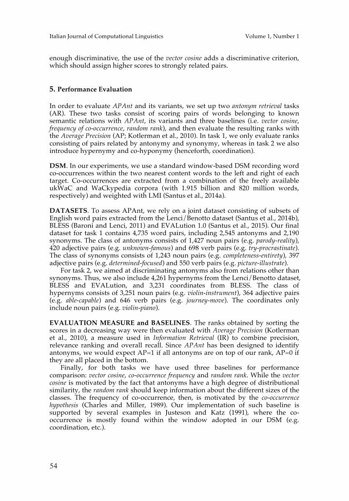
54
Italian Journal of Computational Linguistics Volume 1, Number 1
enough discriminative, the use of the vector cosine adds a discriminative criterion, which should assign higher scores to strongly related pairs.
5. Performance Evaluation
In order to evaluate APAnt and its variants, we set up two antonym retrieval tasks (AR). These two tasks consist of scoring pairs of words belonging to known semantic relations with APAnt, its variants and three baselines (i.e. vector cosine, frequency of co-occurrence, random rank), and then evaluate the resulting ranks with the Average Precision (AP; Kotlerman et al., 2010). In task 1, we only evaluate ranks consisting of pairs related by antonymy and synonymy, whereas in task 2 we also introduce hypernymy and co-hyponymy (henceforth, coordination). DSM. In our experiments, we use a standard window-based DSM recording word co-occurrences within the two nearest content words to the left and right of each target. Co-occurrences are extracted from a combination of the freely available ukWaC and WaCkypedia corpora (with 1.915 billion and 820 million words, respectively) and weighted with LMI (Santus et al., 2014a). DATASETS. To assess APAnt, we rely on a joint dataset consisting of subsets of English word pairs extracted from the Lenci/Benotto dataset (Santus et al., 2014b), BLESS (Baroni and Lenci, 2011) and EVALution 1.0 (Santus et al., 2015). Our final dataset for task 1 contains 4,735 word pairs, including 2,545 antonyms and 2,190 synonyms. The class of antonyms consists of 1,427 noun pairs (e.g. parody-reality), 420 adjective pairs (e.g. unknown-famous) and 698 verb pairs (e.g. try-procrastinate). The class of synonyms consists of 1,243 noun pairs (e.g. completeness-entirety), 397 adjective pairs (e.g. determined-focused) and 550 verb pairs (e.g. picture-illustrate).
For task 2, we aimed at discriminating antonyms also from relations other than synonyms. Thus, we also include 4,261 hypernyms from the Lenci/Benotto dataset, BLESS and EVALution, and 3,231 coordinates from BLESS. The class of hypernyms consists of 3,251 noun pairs (e.g. violin-instrument), 364 adjective pairs (e.g. able-capable) and 646 verb pairs (e.g. journey-move). The coordinates only include noun pairs (e.g. violin-piano).
EVALUATION MEASURE and BASELINES. The ranks obtained by sorting the scores in a decreasing way were then evaluated with Average Precision (Kotlerman et al., 2010), a measure used in Information Retrieval (IR) to combine precision, relevance ranking and overall recall. Since APAnt has been designed to identify antonyms, we would expect AP=1 if all antonyms are on top of our rank, AP=0 if they are all placed in the bottom.
Finally, for both tasks we have used three baselines for performance comparison: vector cosine, co-occurrence frequency and random rank. While the vector cosine is motivated by the fact that antonyms have a high degree of distributional similarity, the random rank should keep information about the different sizes of the classes. The frequency of co-occurrence, then, is motivated by the co-occurrence hypothesis (Charles and Miller, 1989). Our implementation of such baseline is supported by several examples in Justeson and Katz (1991), where the co-occurrence is mostly found within the window adopted in our DSM (e.g. coordination, etc.).
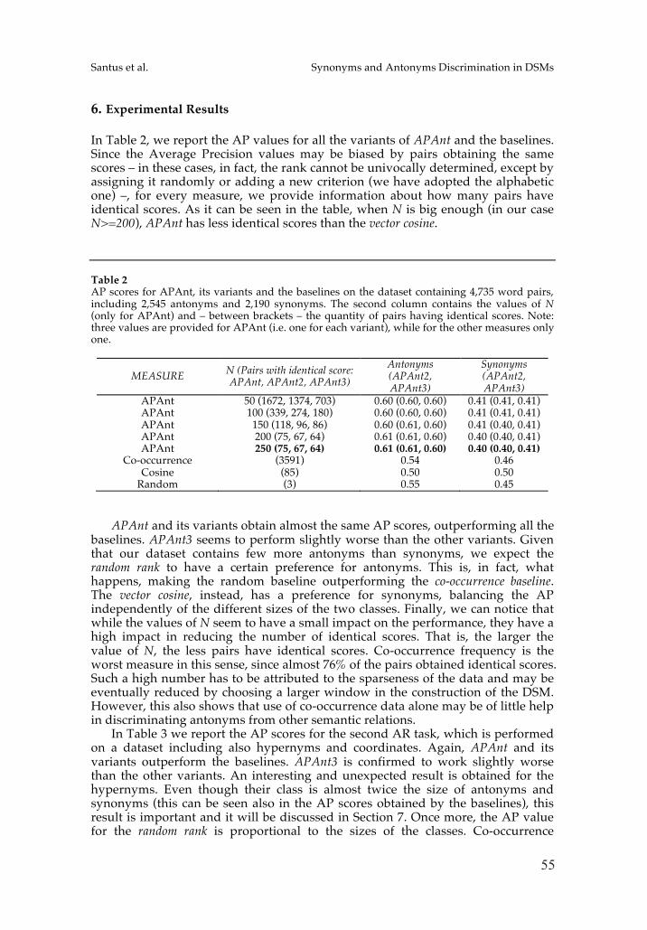
55
Italian Journal of Computational Linguistics Volume 1, Number 1
enough discriminative, the use of the vector cosine adds a discriminative criterion, which should assign higher scores to strongly related pairs.
5. Performance Evaluation
In order to evaluate APAnt and its variants, we set up two antonym retrieval tasks (AR). These two tasks consist of scoring pairs of words belonging to known semantic relations with APAnt, its variants and three baselines (i.e. vector cosine, frequency of co-occurrence, random rank), and then evaluate the resulting ranks with the Average Precision (AP; Kotlerman et al., 2010). In task 1, we only evaluate ranks consisting of pairs related by antonymy and synonymy, whereas in task 2 we also introduce hypernymy and co-hyponymy (henceforth, coordination). DSM. In our experiments, we use a standard window-based DSM recording word co-occurrences within the two nearest content words to the left and right of each target. Co-occurrences are extracted from a combination of the freely available ukWaC and WaCkypedia corpora (with 1.915 billion and 820 million words, respectively) and weighted with LMI (Santus et al., 2014a). DATASETS. To assess APAnt, we rely on a joint dataset consisting of subsets of English word pairs extracted from the Lenci/Benotto dataset (Santus et al., 2014b), BLESS (Baroni and Lenci, 2011) and EVALution 1.0 (Santus et al., 2015). Our final dataset for task 1 contains 4,735 word pairs, including 2,545 antonyms and 2,190 synonyms. The class of antonyms consists of 1,427 noun pairs (e.g. parody-reality), 420 adjective pairs (e.g. unknown-famous) and 698 verb pairs (e.g. try-procrastinate). The class of synonyms consists of 1,243 noun pairs (e.g. completeness-entirety), 397 adjective pairs (e.g. determined-focused) and 550 verb pairs (e.g. picture-illustrate).
For task 2, we aimed at discriminating antonyms also from relations other than synonyms. Thus, we also include 4,261 hypernyms from the Lenci/Benotto dataset, BLESS and EVALution, and 3,231 coordinates from BLESS. The class of hypernyms consists of 3,251 noun pairs (e.g. violin-instrument), 364 adjective pairs (e.g. able-capable) and 646 verb pairs (e.g. journey-move). The coordinates only include noun pairs (e.g. violin-piano).
EVALUATION MEASURE and BASELINES. The ranks obtained by sorting the scores in a decreasing way were then evaluated with Average Precision (Kotlerman et al., 2010), a measure used in Information Retrieval (IR) to combine precision, relevance ranking and overall recall. Since APAnt has been designed to identify antonyms, we would expect AP=1 if all antonyms are on top of our rank, AP=0 if they are all placed in the bottom.
Finally, for both tasks we have used three baselines for performance comparison: vector cosine, co-occurrence frequency and random rank. While the vector cosine is motivated by the fact that antonyms have a high degree of distributional similarity, the random rank should keep information about the different sizes of the classes. The frequency of co-occurrence, then, is motivated by the co-occurrence hypothesis (Charles and Miller, 1989). Our implementation of such baseline is supported by several examples in Justeson and Katz (1991), where the co-occurrence is mostly found within the window adopted in our DSM (e.g. coordination, etc.).
Santus et al. Synonyms and Antonyms Discrimination in DSMs
6. Experimental Results
In Table 2, we report the AP values for all the variants of APAnt and the baselines. Since the Average Precision values may be biased by pairs obtaining the same scores – in these cases, in fact, the rank cannot be univocally determined, except by assigning it randomly or adding a new criterion (we have adopted the alphabetic one) –, for every measure, we provide information about how many pairs have identical scores. As it can be seen in the table, when N is big enough (in our case N>=200), APAnt has less identical scores than the vector cosine.
Table 2 AP scores for APAnt, its variants and the baselines on the dataset containing 4,735 word pairs, including 2,545 antonyms and 2,190 synonyms. The second column contains the values of N (only for APAnt) and – between brackets – the quantity of pairs having identical scores. Note: three values are provided for APAnt (i.e. one for each variant), while for the other measures only one.
MEASURE N (Pairs with identical score: APAnt, APAnt2, APAnt3)
Antonyms (APAnt2, APAnt3)
Synonyms (APAnt2, APAnt3)
APAnt 50 (1672, 1374, 703) 0.60 (0.60, 0.60) 0.41 (0.41, 0.41) APAnt 100 (339, 274, 180) 0.60 (0.60, 0.60) 0.41 (0.41, 0.41) APAnt 150 (118, 96, 86) 0.60 (0.61, 0.60) 0.41 (0.40, 0.41) APAnt 200 (75, 67, 64) 0.61 (0.61, 0.60) 0.40 (0.40, 0.41) APAnt 250 (75, 67, 64) 0.61 (0.61, 0.60) 0.40 (0.40, 0.41)
Co-occurrence (3591) 0.54 0.46 Cosine (85) 0.50 0.50
Random (3) 0.55 0.45
APAnt and its variants obtain almost the same AP scores, outperforming all the
baselines. APAnt3 seems to perform slightly worse than the other variants. Given that our dataset contains few more antonyms than synonyms, we expect the random rank to have a certain preference for antonyms. This is, in fact, what happens, making the random baseline outperforming the co-occurrence baseline. The vector cosine, instead, has a preference for synonyms, balancing the AP independently of the different sizes of the two classes. Finally, we can notice that while the values of N seem to have a small impact on the performance, they have a high impact in reducing the number of identical scores. That is, the larger the value of N, the less pairs have identical scores. Co-occurrence frequency is the worst measure in this sense, since almost 76% of the pairs obtained identical scores. Such a high number has to be attributed to the sparseness of the data and may be eventually reduced by choosing a larger window in the construction of the DSM. However, this also shows that use of co-occurrence data alone may be of little help in discriminating antonyms from other semantic relations.
In Table 3 we report the AP scores for the second AR task, which is performed on a dataset including also hypernyms and coordinates. Again, APAnt and its variants outperform the baselines. APAnt3 is confirmed to work slightly worse than the other variants. An interesting and unexpected result is obtained for the hypernyms. Even though their class is almost twice the size of antonyms and synonyms (this can be seen also in the AP scores obtained by the baselines), this result is important and it will be discussed in Section 7. Once more, the AP value for the random rank is proportional to the sizes of the classes. Co-occurrence
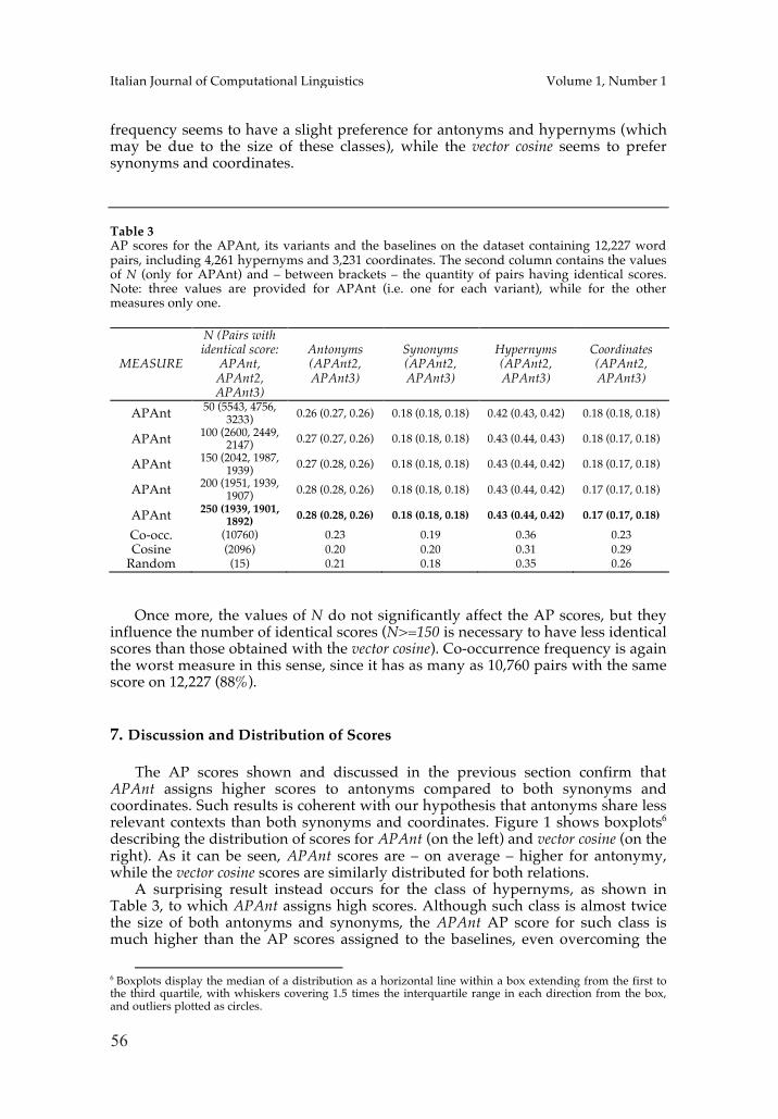
56
Italian Journal of Computational Linguistics Volume 1, Number 1
frequency seems to have a slight preference for antonyms and hypernyms (which may be due to the size of these classes), while the vector cosine seems to prefer synonyms and coordinates.
Table 3 AP scores for the APAnt, its variants and the baselines on the dataset containing 12,227 word pairs, including 4,261 hypernyms and 3,231 coordinates. The second column contains the values of N (only for APAnt) and – between brackets – the quantity of pairs having identical scores. Note: three values are provided for APAnt (i.e. one for each variant), while for the other measures only one.
MEASURE
N (Pairs with identical score:
APAnt, APAnt2, APAnt3)
Antonyms (APAnt2, APAnt3)
Synonyms (APAnt2, APAnt3)
Hypernyms (APAnt2, APAnt3)
Coordinates (APAnt2, APAnt3)
APAnt 50 (5543, 4756, 3233) 0.26 (0.27, 0.26) 0.18 (0.18, 0.18) 0.42 (0.43, 0.42) 0.18 (0.18, 0.18)
APAnt 100 (2600, 2449, 2147) 0.27 (0.27, 0.26) 0.18 (0.18, 0.18) 0.43 (0.44, 0.43) 0.18 (0.17, 0.18)
APAnt 150 (2042, 1987, 1939) 0.27 (0.28, 0.26) 0.18 (0.18, 0.18) 0.43 (0.44, 0.42) 0.18 (0.17, 0.18)
APAnt 200 (1951, 1939, 1907) 0.28 (0.28, 0.26) 0.18 (0.18, 0.18) 0.43 (0.44, 0.42) 0.17 (0.17, 0.18)
APAnt 250 (1939, 1901, 1892) 0.28 (0.28, 0.26) 0.18 (0.18, 0.18) 0.43 (0.44, 0.42) 0.17 (0.17, 0.18)
Co-occ. (10760) 0.23 0.19 0.36 0.23 Cosine (2096) 0.20 0.20 0.31 0.29
Random (15) 0.21 0.18 0.35 0.26
Once more, the values of N do not significantly affect the AP scores, but they
influence the number of identical scores (N>=150 is necessary to have less identical scores than those obtained with the vector cosine). Co-occurrence frequency is again the worst measure in this sense, since it has as many as 10,760 pairs with the same score on 12,227 (88%).
7. Discussion and Distribution of Scores
The AP scores shown and discussed in the previous section confirm that APAnt assigns higher scores to antonyms compared to both synonyms and coordinates. Such results is coherent with our hypothesis that antonyms share less relevant contexts than both synonyms and coordinates. Figure 1 shows boxplots6 describing the distribution of scores for APAnt (on the left) and vector cosine (on the right). As it can be seen, APAnt scores are – on average – higher for antonymy, while the vector cosine scores are similarly distributed for both relations.
A surprising result instead occurs for the class of hypernyms, as shown in Table 3, to which APAnt assigns high scores. Although such class is almost twice the size of both antonyms and synonyms, the APAnt AP score for such class is much higher than the AP scores assigned to the baselines, even overcoming the
6 Boxplots display the median of a distribution as a horizontal line within a box extending from the first to the third quartile, with whiskers covering 1.5 times the interquartile range in each direction from the box, and outliers plotted as circles.
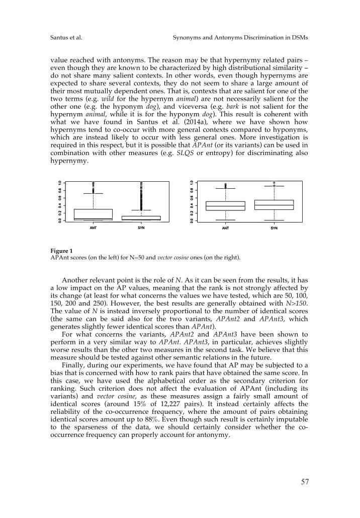
57
Italian Journal of Computational Linguistics Volume 1, Number 1
frequency seems to have a slight preference for antonyms and hypernyms (which may be due to the size of these classes), while the vector cosine seems to prefer synonyms and coordinates.
Table 3 AP scores for the APAnt, its variants and the baselines on the dataset containing 12,227 word pairs, including 4,261 hypernyms and 3,231 coordinates. The second column contains the values of N (only for APAnt) and – between brackets – the quantity of pairs having identical scores. Note: three values are provided for APAnt (i.e. one for each variant), while for the other measures only one.
MEASURE
N (Pairs with identical score:
APAnt, APAnt2, APAnt3)
Antonyms (APAnt2, APAnt3)
Synonyms (APAnt2, APAnt3)
Hypernyms (APAnt2, APAnt3)
Coordinates (APAnt2, APAnt3)
APAnt 50 (5543, 4756, 3233) 0.26 (0.27, 0.26) 0.18 (0.18, 0.18) 0.42 (0.43, 0.42) 0.18 (0.18, 0.18)
APAnt 100 (2600, 2449, 2147) 0.27 (0.27, 0.26) 0.18 (0.18, 0.18) 0.43 (0.44, 0.43) 0.18 (0.17, 0.18)
APAnt 150 (2042, 1987, 1939) 0.27 (0.28, 0.26) 0.18 (0.18, 0.18) 0.43 (0.44, 0.42) 0.18 (0.17, 0.18)
APAnt 200 (1951, 1939, 1907) 0.28 (0.28, 0.26) 0.18 (0.18, 0.18) 0.43 (0.44, 0.42) 0.17 (0.17, 0.18)
APAnt 250 (1939, 1901, 1892) 0.28 (0.28, 0.26) 0.18 (0.18, 0.18) 0.43 (0.44, 0.42) 0.17 (0.17, 0.18)
Co-occ. (10760) 0.23 0.19 0.36 0.23 Cosine (2096) 0.20 0.20 0.31 0.29
Random (15) 0.21 0.18 0.35 0.26
Once more, the values of N do not significantly affect the AP scores, but they
influence the number of identical scores (N>=150 is necessary to have less identical scores than those obtained with the vector cosine). Co-occurrence frequency is again the worst measure in this sense, since it has as many as 10,760 pairs with the same score on 12,227 (88%).
7. Discussion and Distribution of Scores
The AP scores shown and discussed in the previous section confirm that APAnt assigns higher scores to antonyms compared to both synonyms and coordinates. Such results is coherent with our hypothesis that antonyms share less relevant contexts than both synonyms and coordinates. Figure 1 shows boxplots6 describing the distribution of scores for APAnt (on the left) and vector cosine (on the right). As it can be seen, APAnt scores are – on average – higher for antonymy, while the vector cosine scores are similarly distributed for both relations.
A surprising result instead occurs for the class of hypernyms, as shown in Table 3, to which APAnt assigns high scores. Although such class is almost twice the size of both antonyms and synonyms, the APAnt AP score for such class is much higher than the AP scores assigned to the baselines, even overcoming the
6 Boxplots display the median of a distribution as a horizontal line within a box extending from the first to the third quartile, with whiskers covering 1.5 times the interquartile range in each direction from the box, and outliers plotted as circles.
Santus et al. Synonyms and Antonyms Discrimination in DSMs
value reached with antonyms. The reason may be that hypernymy related pairs – even though they are known to be characterized by high distributional similarity – do not share many salient contexts. In other words, even though hypernyms are expected to share several contexts, they do not seem to share a large amount of their most mutually dependent ones. That is, contexts that are salient for one of the two terms (e.g. wild for the hypernym animal) are not necessarily salient for the other one (e.g. the hyponym dog), and viceversa (e.g. bark is not salient for the hypernym animal, while it is for the hyponym dog). This result is coherent with what we have found in Santus et al. (2014a), where we have shown how hypernyms tend to co-occur with more general contexts compared to hyponyms, which are instead likely to occur with less general ones. More investigation is required in this respect, but it is possible that APAnt (or its variants) can be used in combination with other measures (e.g. SLQS or entropy) for discriminating also hypernymy.
Figure 1 APAnt scores (on the left) for N=50 and vector cosine ones (on the right).
Another relevant point is the role of N. As it can be seen from the results, it has
a low impact on the AP values, meaning that the rank is not strongly affected by its change (at least for what concerns the values we have tested, which are 50, 100, 150, 200 and 250). However, the best results are generally obtained with N>150. The value of N is instead inversely proportional to the number of identical scores (the same can be said also for the two variants, APAnt2 and APAnt3, which generates slightly fewer identical scores than APAnt).
For what concerns the variants, APAnt2 and APAnt3 have been shown to perform in a very similar way to APAnt. APAnt3, in particular, achieves slightly worse results than the other two measures in the second task. We believe that this measure should be tested against other semantic relations in the future.
Finally, during our experiments, we have found that AP may be subjected to a bias that is concerned with how to rank pairs that have obtained the same score. In this case, we have used the alphabetical order as the secondary criterion for ranking. Such criterion does not affect the evaluation of APAnt (including its variants) and vector cosine, as these measures assign a fairly small amount of identical scores (around 15% of 12,227 pairs). It instead certainly affects the reliability of the co-occurrence frequency, where the amount of pairs obtaining identical scores amount up to 88%. Even though such result is certainly imputable to the sparseness of the data, we should certainly consider whether the co-occurrence frequency can properly account for antonymy.
58
Italian Journal of Computational Linguistics Volume 1, Number 1
8. Conclusions
In this paper, we have further described and analyzed APAnt, a distributional measure firstly introduced in Santus et al. (2014b, 2014c). Two more variants have been proposed for the normalization of APAnt and for the extension of its scope to the discrimination of antonymy from semantic relations other than synonymy. APAnt and its variants have been shown to outperform several baselines in our experiments. Surprisingly, they seem to assign high scores to hypernyms, which do probably share few salient contexts too. This fact suggests the need for further refinement of the APant.
APAnt should not be considered as the final result of this research, but much more as a work in progress. It should be further explored and improved to put light on some distributional properties of antonymy and other semantic relations, which can be exploited to develop a unified method that may account for issues that are currently treated as separate tasks, such as sense disambiguation and semantic relations identification. In this sense, we believe that there are many properties that need to be further explored by looking at the most relevant contexts of each term, rather than at their full set. Such exploration and investigation should be linguistically grounded and should aim not only to the improvement of algorithms’ performance, but also to a better understanding of the linguistic properties of semantic relations.
Acknowledgements This work is partially supported by HK PhD Fellowship Scheme under PF12-13656.
References Baroni, Marco and Alessandro Lenci. 2010. Distributional Memory: A general framework for
corpus-based semantics. Computational Linguistics, 36(4):673–721. Baroni, Marco and Alessandro Lenci. 2011. How we BLESSed distributional semantic evaluation.
In Proceedings of the EMNLP 2011, Geometrical Models for Natural Language Semantics Workshop (GEMS 2011), 1-10, Edinburg, UK.
Charles, Walter G. and George A. Miller. 1989. Contexts of antonymous adjectives. Applied Psychology, 10:357–375.
Cruse, David A. 1986. Lexical Semantics. Cambridge University Press, Cambridge. Evert, Stefan. 2005. The Statistics of Word Cooccurrences. Dissertation, Stuttgart University. Deese, J. 1964. The Associative Structure of Some Common English Adjectives. Journal of Verbal
Learning and Verbal Behavior, 3:347–57. Deese J. 1965. The Structure of Associations in Language and Thought. Johns Hopkins University
Press, Baltimore. Ding, Jing and Chu-Ren Huang. 2014. Word Ordering in Chinese Opposite Compounds. In
Xinchun Xu and Tingting He (Eds.), Chinese Lexical Semantics: 15th Workshop, CLSW 2014, Macao, China, July 9-12, 2012, Revised Selected Papers (pp. 12-20). Berlin Heidelberg: Springer-Verlag. DOI: 10.1007/978-3-319-14331-6_2
Ding, Jing, and Chu-Ren Huang. 2013. Markedness of opposite. In Pengyuan Liu and Qi Su (Eds.), Chinese Lexical Semantics: 14th Workshop, CLSW 2013, Zhengzhou, China, May 10-12, 2013. Revised Selected Papers (pp. 191-195). Berlin Heidelberg: Springer-Verlag. DOI: 10.1007/978-3-642-45185-0_21
Fellbaum, Christiane. 1995. Co-occurrence and antonymy. International Journal of Lexicography, 8:281–303.
Harris, Zellig. 1954. Distributional structure. Word, 10(23):146–162. Hearst, Marti. 1992. Automatic acquisition of hyponyms from large text corpora. In Proceedings of
the Fourteenth International Conference on Computational Linguistics, pages 539–546, Nantes. Huang, Chu-Ren, I-Li Su, Pei-Yi Hsiao, and Xiu-Ling Ke. 2007. Paranyms, Co-Hyponyms and
Antonyms: Representing Semantic Fields with Lexical Semantic Relations. In Proceedings of
59
Italian Journal of Computational Linguistics Volume 1, Number 1
8. Conclusions
In this paper, we have further described and analyzed APAnt, a distributional measure firstly introduced in Santus et al. (2014b, 2014c). Two more variants have been proposed for the normalization of APAnt and for the extension of its scope to the discrimination of antonymy from semantic relations other than synonymy. APAnt and its variants have been shown to outperform several baselines in our experiments. Surprisingly, they seem to assign high scores to hypernyms, which do probably share few salient contexts too. This fact suggests the need for further refinement of the APant.
APAnt should not be considered as the final result of this research, but much more as a work in progress. It should be further explored and improved to put light on some distributional properties of antonymy and other semantic relations, which can be exploited to develop a unified method that may account for issues that are currently treated as separate tasks, such as sense disambiguation and semantic relations identification. In this sense, we believe that there are many properties that need to be further explored by looking at the most relevant contexts of each term, rather than at their full set. Such exploration and investigation should be linguistically grounded and should aim not only to the improvement of algorithms’ performance, but also to a better understanding of the linguistic properties of semantic relations.
Acknowledgements This work is partially supported by HK PhD Fellowship Scheme under PF12-13656.
References Baroni, Marco and Alessandro Lenci. 2010. Distributional Memory: A general framework for
corpus-based semantics. Computational Linguistics, 36(4):673–721. Baroni, Marco and Alessandro Lenci. 2011. How we BLESSed distributional semantic evaluation.
In Proceedings of the EMNLP 2011, Geometrical Models for Natural Language Semantics Workshop (GEMS 2011), 1-10, Edinburg, UK.
Charles, Walter G. and George A. Miller. 1989. Contexts of antonymous adjectives. Applied Psychology, 10:357–375.
Cruse, David A. 1986. Lexical Semantics. Cambridge University Press, Cambridge. Evert, Stefan. 2005. The Statistics of Word Cooccurrences. Dissertation, Stuttgart University. Deese, J. 1964. The Associative Structure of Some Common English Adjectives. Journal of Verbal
Learning and Verbal Behavior, 3:347–57. Deese J. 1965. The Structure of Associations in Language and Thought. Johns Hopkins University
Press, Baltimore. Ding, Jing and Chu-Ren Huang. 2014. Word Ordering in Chinese Opposite Compounds. In
Xinchun Xu and Tingting He (Eds.), Chinese Lexical Semantics: 15th Workshop, CLSW 2014, Macao, China, July 9-12, 2012, Revised Selected Papers (pp. 12-20). Berlin Heidelberg: Springer-Verlag. DOI: 10.1007/978-3-319-14331-6_2
Ding, Jing, and Chu-Ren Huang. 2013. Markedness of opposite. In Pengyuan Liu and Qi Su (Eds.), Chinese Lexical Semantics: 14th Workshop, CLSW 2013, Zhengzhou, China, May 10-12, 2013. Revised Selected Papers (pp. 191-195). Berlin Heidelberg: Springer-Verlag. DOI: 10.1007/978-3-642-45185-0_21
Fellbaum, Christiane. 1995. Co-occurrence and antonymy. International Journal of Lexicography, 8:281–303.
Harris, Zellig. 1954. Distributional structure. Word, 10(23):146–162. Hearst, Marti. 1992. Automatic acquisition of hyponyms from large text corpora. In Proceedings of
the Fourteenth International Conference on Computational Linguistics, pages 539–546, Nantes. Huang, Chu-Ren, I-Li Su, Pei-Yi Hsiao, and Xiu-Ling Ke. 2007. Paranyms, Co-Hyponyms and
Antonyms: Representing Semantic Fields with Lexical Semantic Relations. In Proceedings of
Santus et al. Synonyms and Antonyms Discrimination in DSMs
Chinese Lexical Semantics Workshop 2007, pages 66-72, Hong Kong Polytechnic University, May 20-23.
Justeson, John S. and Slava M. Katz. 1991. Co-occurrences of antonymous adjectives and their contexts. Computational Linguistics, 17:1–19.
Kempson, Ruth M. 1977. Semantic Theory. Cambridge University Press, Cambridge. Kotlerman, Lili, Ido Dagan, Idan Szpektor, and Maayan Zhitomirsky-Geffet. 2010. Directional
Distributional Similarity for Lexical Inference. Natural Language Engineering, 16(4):359–389. Landauer, Thomas K. and Susan T. Dumais. 1997. A solution to Plato's problem: The Latent
Semantic Analysis theory of the acquisition, induction, and representation of knowledge. Psychological Review, 104:211-240.
Lenci, Alessandro. 2008. Distributional semantics in linguistic and cognitive research. In A. Lenci (ed.), From context to meaning: distributional models of the lexicon in linguistics and cognitive science, Italian Journal of Linguistics, 20(1):1–31.
Lin, Dekang, Shaojun Zhao, Lijuan Qin, and Ming Zhou. 2003. Identifying synonyms among distributionally similar words. In Proceedings of the 18th International Joint Conference on Artificial Intelligence (IJCAI-03), pages 1,492–1,493, Acapulco.
Lobanova, Anna. 2012. The Anatomy of Antonymy: a Corpus-driven Approach. Dissertation. University of Groningen.
Lobanova, Anna, Tom van der Kleij, and Jennifer Spenader. 2010. Defining antonymy: A corpus-based study of opposites by lexico-syntactic patterns. International Journal of Lexicography, 23(1):19–53.
Lucerto, Cupertino, David Pinto, and Héctor Jiménez-Salazar. 2002. An automatic method to identify antonymy. In Workshop on Lexical Resources and the Web for Word Sense Disambiguation, pages 105–111, Puebla.
de Marneffe, Marie-Catherine, Anna Rafferty, and Christopher D. Manning. 2008. Finding contradictions in text. In Proceedings of the 46th Annual Meeting of the Association for Computational Linguistics (ACL-08), pages 1,039–1,047, Columbus, OH.
Marton, Yuval, Ahmed El Kholy, and Nizar Habash. 2011. Filtering antonymous, trend-contrasting, and polarity-dissimilar distributional paraphrases for improving statistical machine translation. In Proceedings of the Sixth Workshop on Statistical Machine Translation, pages 237–249, Edinburgh.
Mihalcea, Rada and Carlo Strapparava. 2005. Making computers laugh: Investigations in automatic humor recognition. In Proceedings of the Conference on Human Language Technology and Empirical Methods in Natural Language Processing, pages 531–538, Vancouver.
Mohammad, Saif, Bonnie Dorr, Graeme Hirst, and Peter D. Turney. 2013. Computing lexical contrast. Computational Linguistics, 39(3):555–590.
Mohammad, Saif, Bonnie Dorr, and Graeme Hirst. 2008. Computing word-pair antonymy. In Proceedings of the Conference on Empirical Methods in Natural Language Processing (EMNLP-2008), pages 982–991, Waikiki, HI.
Morlane-Hondère, François. 2015. What can distributional semantic models tell us about part-of relations? In Proceedings of the NetWordS Final Conference on Word Knowledge and Word Usage: Representations and Processes in the Mental Lexicon, vol. 1347, pages 46-50, CEUR-WS.org , Aachen (DEU).
Murphy, M. Lynne. 2003. Semantic relations and the lexicon: antonymy, synonymy, and other paradigms. Cambridge University Press, Cambridge, UK. ISBN 9780521780674
Pado , Sebastian and Mirella Lapata. 2007. Dependency-based Construction of Semantic Space Models. Computational Linguistics, 33(2):161–199.
Pantel, Patrick and Marco Pennacchiotti. 2006. Espresso: Leveraging generic patterns for automatically harvesting semantic relations. In Proceedings of the 21st International Conference on Computational Linguistics and 44th Annual Meeting of the Association for Computational Linguistics, pages 113-120, Sydney, Australia.
Platt, John C. 1998. Fast training of support vector machines using sequential minimal optimization. In Advances in Kernel Methods: Support Vector Learning, pages 185–208. MIT Press Cambridge, MA, USA.
Roth, Michael and Sabine Schulte im Walde. 2014. Combining word patterns and discourse markers for paradigmatic relation classification. In Proceedings of the 52nd Annual Meeting of the Association for Computational Linguistics (ACL), 2:524–530, Baltimore, Maryland, USA.
Sahlgren, Magnus. 2006. The Word-Space Model: Using distributional analysis to represent syntagmatic and paradigmatic relations between words in high-dimensional vector spaces. Ph.D. dissertation, Department of Linguistics, Stockholm University.
60
Italian Journal of Computational Linguistics Volume 1, Number 1
Santus, Enrico, Alessandro Lenci, Qin Lu, and Sabine Schulte im Walde. 2014a. Chasing Hypernyms in Vector Spaces with Entropy. In Proceedings of the 14th Conference of the European Chapter of the Association for Computational Linguistics, 2:38–42, Gothenburg, Sweden.
Santus, Enrico, Qin Lu, Alessandro Lenci, and Chu-Ren Huang. 2014b. Unsupervised Antonym-Synonym Discrimination in Vector Space. In Proceedings of the First Italian Conference on Computational Linguistics CLiC-it 2014, 9-10 December 2014, Pisa, volume 1, pages 328-333, Pisa University Press.
Santus, Enrico, Qin Lu, Alessandro Lenci and Chu-Ren Huang. 2014c. Taking Antonymy Mask off in Vector Space. In Proceedings of the 28th Pacific Asia Conference on Language, Information and Computation (PACLIC), pages 135-144, Phuket, Thailand.
Santus, Enrico, Frances Yung, Alessandro Lenci and Chu-Ren Huang. 2015. EVALution 1.0: An Evolving Semantic Dataset for Training and Evaluation of Distributional Semantic Models. In Proceedings of the 4th Workshop on Linked Data in Linguistics (LDL-2015), 64–69, Beijing, China.
Schulte im Walde, Sabine and Maximilian Köper. 2013. Pattern-based distinction of paradigmatic relations for German nouns, verbs, adjectives. In Language Processing and Knowledge in the Web, 184-198. Springer.
Turney, Peter D. and Patrick Pantel. 2010. From Frequency to Meaning: Vector Space Models of Semantics. Journal of Articial Intelligence Research, 37:141–188.
Turney, Peter D. 2008. A uniform approach to analogies, synonyms, antonyms, and associations. In Proceedings of the 22nd International Conference on Computational Linguistics (COLING-08), pages 905–912, Manchester.
Tungthamthiti, Piyoros, Enrico Santus, Hongzhi Xu, Chu-Ren Huang and Shirai Kiyoaki. 2015. Sentiment Analyzer with Rich Features for Ironic and Sarcastic Tweets. In Proceedings of the 29th Pacific Asia Conference on Language, Information and Computation (PACLIC), Shanghai, China.
Xu, Hongzhi, Enrico Santus, Anna Laszlo and Chu-Ren Huang. 2015. LLT-PolyU: Identifying Sentiment Intensity in Ironic Tweets. In Proceedings of the 9th Workshop on Semantic Evaluation (SemEval 2015), pages 673-678, Denver, Colorado, USA.
Witten, Ian H. and Eibe Frank. 1999. Data Mining: Practical Machine Learning Tools and Techniques with Java Implementations. Morgan Kaufmann, San Francisco.
61
Temporal Random Indexing: A System forAnalysing Word Meaning over Time
Pierpaolo Basile∗
Università di Bari, Aldo MoroAnnalina Caputo∗
Università di Bari, Aldo Moro
Giovanni Semeraro∗
Università di Bari, Aldo Moro
During the last decade the surge in available data spanning different epochs has inspired a newanalysis of cultural, social, and linguistic phenomena from a temporal perspective. This paperdescribes a method that enables the analysis of the time evolution of the meaning of a word.We propose Temporal Random Indexing (TRI), a method for building WordSpaces that takesinto account temporal information. We exploit this methodology in order to build geometricalspaces of word meanings that consider several periods of time. The TRI framework provides allthe necessary tools to build WordSpaces over different time periods and perform such temporallinguistic analysis. We propose some examples of usage of our tool by analysing word meaningsin two corpora: a collection of Italian books and English scientific papers about computationallinguistics. This analysis enables the detection of linguistic events that emerge in specific timeintervals and that can be related to social or cultural phenomena.
1. Introduction
Imagine the Time Traveller of H.G. Wells’ novel who takes a journey to year 2000 in a quest forexploring how the seventh art has evolved in the future. Nowadays, since looking for “movingpicture” would produce no results, he would have probably come back to the past believingthat the cinematography does not exist at all. A better comprehension of cultural and linguisticchanges that accompanied the cinematography evolution might have suggested that “movingpicture”, within few years from its first appearance, was shorten to become just “movie” (Figure1). This error stems from the assumption that language is static and does not evolve. However,this is not the case. Our language varies to reflect the shift in topics we talk about, which in turnfollow cultural changes (Michel et al. 2011).
So far, the automatic analysis of language was based on datasets that represented a snapshotof a given domain or time period. However, since big data has arisen, making available largecorpora of data spanning several periods of time, culturomics has emerged as a new approach tostudy linguistic and cultural trend over time by analysing these new sources of information.The term culturomics was coined by the research group who worked on the Google Bookngram corpus. The release of ngram frequencies spanning five centuries from 1500 to 2000 andcomprising over 500 billion words (Michel et al. 2011) opened new venues to the quantitativeanalysis of changes in culture and linguistics. This study enabled the understanding of how somephenomena impact on written text, like the rise and fallen of fame, censorship, or evolution in
∗ Department of Computer Science, University of Bari Aldo Moro, Via, E. Orabona, 4 - 70125 Bari (Italy).E-mail: {pierpaolo.basile, annalina.caputo, giovanni.semeraro}@uniba.it.
© 2015 Associazione Italiana di Linguistica Computazionale
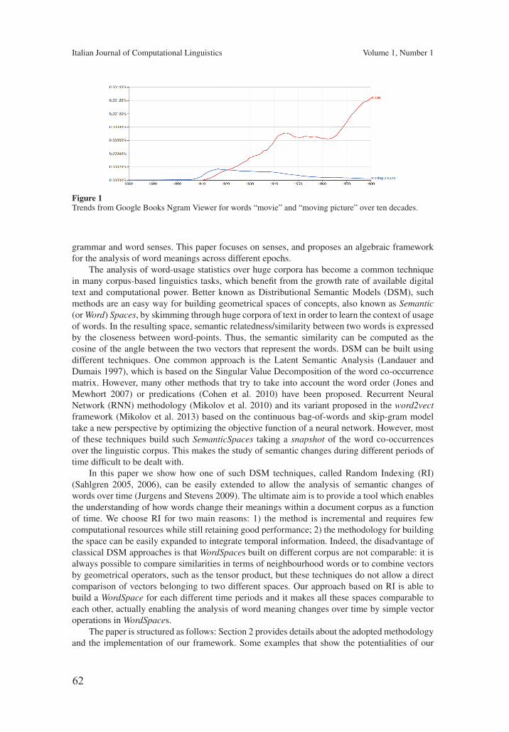
62
Italian Journal of Computational Linguistics Volume 1, Number 1
Figure 1Trends from Google Books Ngram Viewer for words “movie” and “moving picture” over ten decades.
grammar and word senses. This paper focuses on senses, and proposes an algebraic frameworkfor the analysis of word meanings across different epochs.
The analysis of word-usage statistics over huge corpora has become a common techniquein many corpus-based linguistics tasks, which benefit from the growth rate of available digitaltext and computational power. Better known as Distributional Semantic Models (DSM), suchmethods are an easy way for building geometrical spaces of concepts, also known as Semantic(or Word) Spaces, by skimming through huge corpora of text in order to learn the context of usageof words. In the resulting space, semantic relatedness/similarity between two words is expressedby the closeness between word-points. Thus, the semantic similarity can be computed as thecosine of the angle between the two vectors that represent the words. DSM can be built usingdifferent techniques. One common approach is the Latent Semantic Analysis (Landauer andDumais 1997), which is based on the Singular Value Decomposition of the word co-occurrencematrix. However, many other methods that try to take into account the word order (Jones andMewhort 2007) or predications (Cohen et al. 2010) have been proposed. Recurrent NeuralNetwork (RNN) methodology (Mikolov et al. 2010) and its variant proposed in the word2vectframework (Mikolov et al. 2013) based on the continuous bag-of-words and skip-gram modeltake a new perspective by optimizing the objective function of a neural network. However, mostof these techniques build such SemanticSpaces taking a snapshot of the word co-occurrencesover the linguistic corpus. This makes the study of semantic changes during different periods oftime difficult to be dealt with.
In this paper we show how one of such DSM techniques, called Random Indexing (RI)(Sahlgren 2005, 2006), can be easily extended to allow the analysis of semantic changes ofwords over time (Jurgens and Stevens 2009). The ultimate aim is to provide a tool which enablesthe understanding of how words change their meanings within a document corpus as a functionof time. We choose RI for two main reasons: 1) the method is incremental and requires fewcomputational resources while still retaining good performance; 2) the methodology for buildingthe space can be easily expanded to integrate temporal information. Indeed, the disadvantage ofclassical DSM approaches is that WordSpaces built on different corpus are not comparable: it isalways possible to compare similarities in terms of neighbourhood words or to combine vectorsby geometrical operators, such as the tensor product, but these techniques do not allow a directcomparison of vectors belonging to two different spaces. Our approach based on RI is able tobuild a WordSpace for each different time periods and it makes all these spaces comparable toeach other, actually enabling the analysis of word meaning changes over time by simple vectoroperations in WordSpaces.
The paper is structured as follows: Section 2 provides details about the adopted methodologyand the implementation of our framework. Some examples that show the potentialities of our
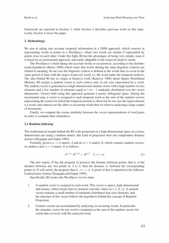
63
Basile et al. Analysing Word Meaning over Time
framework are reported in Section 3, while Section 4 describes previous work on this topic.Lastly, Section 5 closes the paper.
2. Methodology
We aim at taking into account temporal information in a DSM approach, which consists inrepresenting words as points in a WordSpace, where two words are similar if represented bypoints close to each other. Under this light, RI has the advantages of being very simple, since itis based on an incremental approach, and easily adaptable to the temporal analysis needs.
The WordSpace is built taking into account words co-occurrences, according to the distribu-tional hypothesis (Harris 1968) which states that words sharing the same linguistic contexts arerelated in meaning. In our case the linguistic context is defined as the words that co-occur in thesame period of time with the target (temporal) word, i.e. the word under the temporal analysis.The idea behind RI has its origin in Kanerva work (Kanerva 1988) about Sparse DistributedMemory. RI assigns a random vector to each context unit, in our case represented by a word.The random vector is generated as a high-dimensional random vector with a high number of zeroelements and a few number of elements equal to 1 or −1 randomly distributed over the vectordimensions. Vectors built using this approach generate a nearly orthogonal space. During theincremental step, a vector is assigned to each temporal word as the sum of the random vectorsrepresenting the context in which the temporal element is observed. In our case the target elementis a word, and contexts are the other co-occurring words that we observe analyzing a large corpusof documents.
Finally, we compute the cosine similarity between the vector representations of word pairsin order to compute their relatedness.
2.1 Random Indexing
The mathematical insight behind the RI is the projection of a high-dimensional space on a lowerdimensional one using a random matrix; this kind of projection does not compromise distancemetrics (Dasgupta and Gupta 1999).
Formally, given a n×m matrix A and an m× k matrix R, which contains random vectors,we define a new n× k matrix B as follows:
An,m·Rm,k = Bn,k k << m (1)
The new matrix B has the property to preserve the distance between points, that is, if thedistance between any two points in A is d; then the distance dr between the correspondingpoints in B will satisfy the property that dr ≈ c× d. A proof of that is reported in the Johnson-Lindenstrauss lemma (Dasgupta and Gupta 1999).
Specifically, RI creates the WordSpace in two steps:
1. A random vector is assigned to each word. This vector is sparse, high-dimensionaland ternary, which means that its elements can take values in {-1, 0, 1}. A randomvector contains a small number of randomly distributed non-zero elements, andthe structure of this vector follows the hypothesis behind the concept of RandomProjection;
2. Context vectors are accumulated by analyzing co-occurring words. In particularthe semantic vector for any word is computed as the sum of the random vectors forwords that co-occur with the analyzed word.
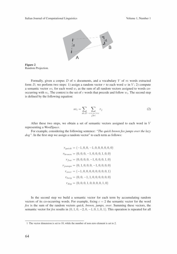
64
Italian Journal of Computational Linguistics Volume 1, Number 1
Figure 2Random Projection.
Formally, given a corpus D of n documents, and a vocabulary V of m words extractedform D, we perform two steps: 1) assign a random vector r to each word w in V ; 2) computea semantic vector svi for each word wi as the sum of all random vectors assigned to words co-occurring with wi. The context is the set of c words that precede and follow wi. The second stepis defined by the following equation:
svi =∑d∈D
∑−c<j<+c
j �=i
rj (2)
After these two steps, we obtain a set of semantic vectors assigned to each word in Vrepresenting a WordSpace.
For example, considering the following sentence: “The quick brown fox jumps over the lazydog”. In the first step we assign a random vector1 to each term as follows:
rquick = (−1, 0, 0,−1, 0, 0, 0, 0, 0, 0)
rbrown = (0, 0, 0,−1, 0, 0, 0, 1, 0, 0)
rfox = (0, 0, 0, 0,−1, 0, 0, 0, 1, 0)
rjumps = (0, 1, 0, 0, 0,−1, 0, 0, 0, 0)
rover = (−1, 0, 0, 0, 0, 0, 0, 0, 0, 1)
rlazy = (0, 0,−1, 1, 0, 0, 0, 0, 0, 0)
rdog = (0, 0, 0, 1, 0, 0, 0, 0, 1, 0)
In the second step we build a semantic vector for each term by accumulating randomvectors of its co-occurring words. For example, fixing c = 2 the semantic vector for the wordfox is the sum of the random vectors quick, brown, jumps, over. Summing these vectors, thesemantic vector for fox results in (0, 1, 0,−2, 0,−1, 0, 1, 0, 1). This operation is repeated for all
1 The vector dimension is set to 10, while the number of non-zero element is set to 2.
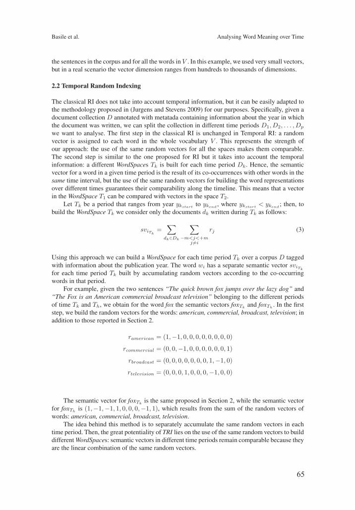
65
Basile et al. Analysing Word Meaning over Time
the sentences in the corpus and for all the words in V . In this example, we used very small vectors,but in a real scenario the vector dimension ranges from hundreds to thousands of dimensions.
2.2 Temporal Random Indexing
The classical RI does not take into account temporal information, but it can be easily adapted tothe methodology proposed in (Jurgens and Stevens 2009) for our purposes. Specifically, given adocument collection D annotated with metatada containing information about the year in whichthe document was written, we can split the collection in different time periods D1, D2, . . . , Dp
we want to analyse. The first step in the classical RI is unchanged in Temporal RI: a randomvector is assigned to each word in the whole vocabulary V . This represents the strength ofour approach: the use of the same random vectors for all the spaces makes them comparable.The second step is similar to the one proposed for RI but it takes into account the temporalinformation: a different WordSpaces Tk is built for each time period Dk. Hence, the semanticvector for a word in a given time period is the result of its co-occurrences with other words in thesame time interval, but the use of the same random vectors for building the word representationsover different times guarantees their comparability along the timeline. This means that a vectorin the WordSpace T1 can be compared with vectors in the space T2.
Let Tk be a period that ranges from year ykstartto ykend
, where ykstart< ykend
; then, tobuild the WordSpace Tk we consider only the documents dk written during Tk as follows:
sviTk=
∑dk∈Dk
∑−m<j<+m
j �=i
rj (3)
Using this approach we can build a WordSpace for each time period Tk over a corpus D taggedwith information about the publication year. The word wi has a separate semantic vector sviTk
for each time period Tk built by accumulating random vectors according to the co-occurringwords in that period.
For example, given the two sentences “The quick brown fox jumps over the lazy dog” and“The Fox is an American commercial broadcast television” belonging to the different periodsof time Tk and Th, we obtain for the word fox the semantic vectors foxTk
and foxTh. In the first
step, we build the random vectors for the words: american, commercial, broadcast, television; inaddition to those reported in Section 2.
ramerican = (1,−1, 0, 0, 0, 0, 0, 0, 0, 0)
rcommercial = (0, 0,−1, 0, 0, 0, 0, 0, 0, 1)
rbroadcast = (0, 0, 0, 0, 0, 0, 0, 1,−1, 0)
rtelevision = (0, 0, 0, 1, 0, 0, 0,−1, 0, 0)
The semantic vector for foxTkis the same proposed in Section 2, while the semantic vector
for foxThis (1,−1,−1, 1, 0, 0, 0,−1, 1), which results from the sum of the random vectors of
words: american, commercial, broadcast, television.The idea behind this method is to separately accumulate the same random vectors in each
time period. Then, the great potentiality of TRI lies on the use of the same random vectors to builddifferent WordSpaces: semantic vectors in different time periods remain comparable because theyare the linear combination of the same random vectors.
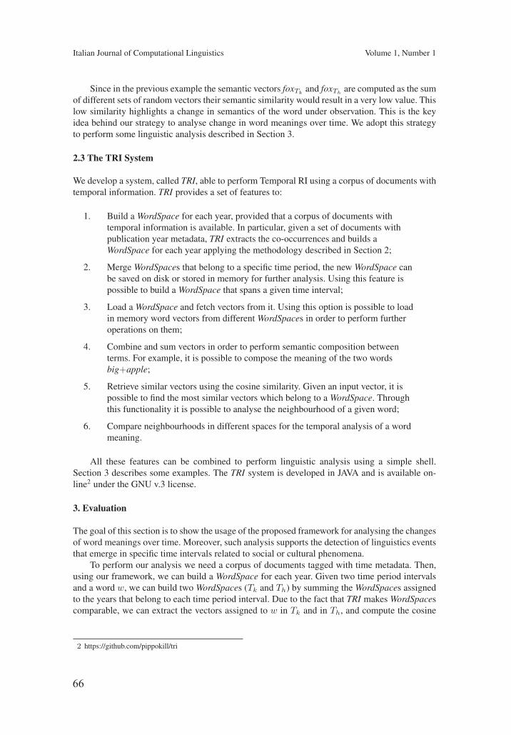
66
Italian Journal of Computational Linguistics Volume 1, Number 1
Since in the previous example the semantic vectors foxTkand foxTh
are computed as the sumof different sets of random vectors their semantic similarity would result in a very low value. Thislow similarity highlights a change in semantics of the word under observation. This is the keyidea behind our strategy to analyse change in word meanings over time. We adopt this strategyto perform some linguistic analysis described in Section 3.
2.3 The TRI System
We develop a system, called TRI, able to perform Temporal RI using a corpus of documents withtemporal information. TRI provides a set of features to:
1. Build a WordSpace for each year, provided that a corpus of documents withtemporal information is available. In particular, given a set of documents withpublication year metadata, TRI extracts the co-occurrences and builds aWordSpace for each year applying the methodology described in Section 2;
2. Merge WordSpaces that belong to a specific time period, the new WordSpace canbe saved on disk or stored in memory for further analysis. Using this feature ispossible to build a WordSpace that spans a given time interval;
3. Load a WordSpace and fetch vectors from it. Using this option is possible to loadin memory word vectors from different WordSpaces in order to perform furtheroperations on them;
4. Combine and sum vectors in order to perform semantic composition betweenterms. For example, it is possible to compose the meaning of the two wordsbig+apple;
5. Retrieve similar vectors using the cosine similarity. Given an input vector, it ispossible to find the most similar vectors which belong to a WordSpace. Throughthis functionality it is possible to analyse the neighbourhood of a given word;
6. Compare neighbourhoods in different spaces for the temporal analysis of a wordmeaning.
All these features can be combined to perform linguistic analysis using a simple shell.Section 3 describes some examples. The TRI system is developed in JAVA and is available on-line2 under the GNU v.3 license.
3. Evaluation
The goal of this section is to show the usage of the proposed framework for analysing the changesof word meanings over time. Moreover, such analysis supports the detection of linguistics eventsthat emerge in specific time intervals related to social or cultural phenomena.
To perform our analysis we need a corpus of documents tagged with time metadata. Then,using our framework, we can build a WordSpace for each year. Given two time period intervalsand a word w, we can build two WordSpaces (Tk and Th) by summing the WordSpaces assignedto the years that belong to each time period interval. Due to the fact that TRI makes WordSpacescomparable, we can extract the vectors assigned to w in Tk and in Th, and compute the cosine
2 https://github.com/pippokill/tri
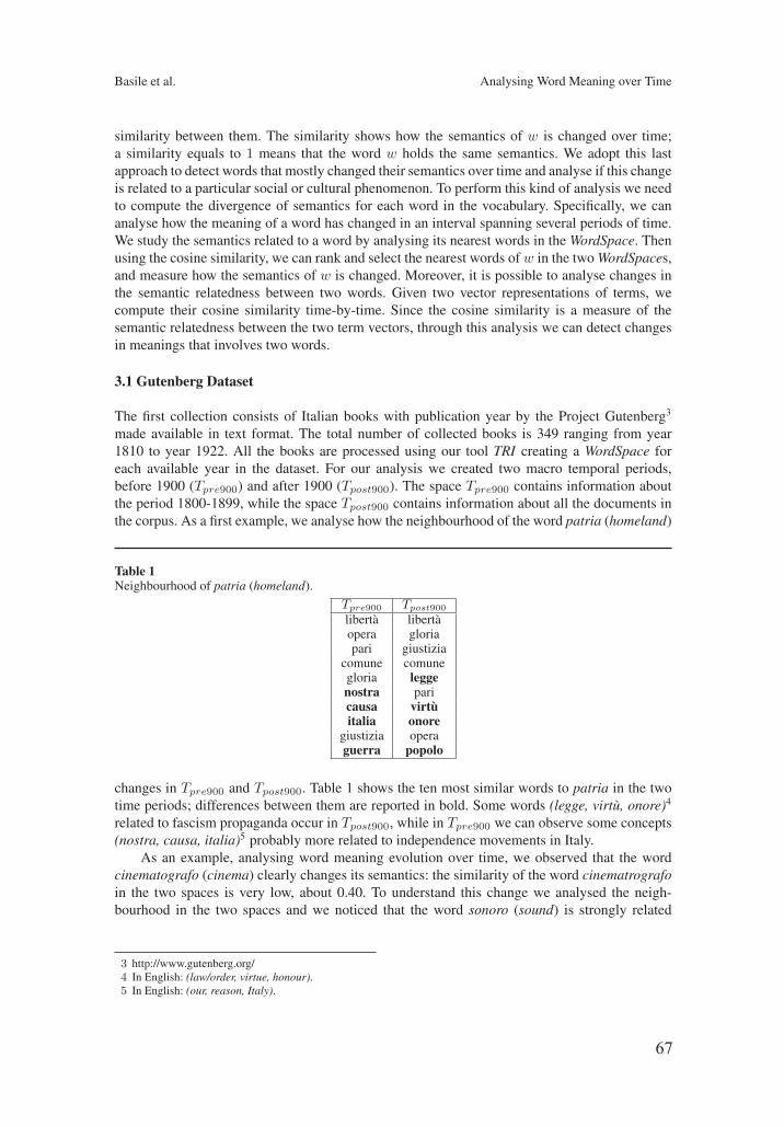
67
Basile et al. Analysing Word Meaning over Time
similarity between them. The similarity shows how the semantics of w is changed over time;a similarity equals to 1 means that the word w holds the same semantics. We adopt this lastapproach to detect words that mostly changed their semantics over time and analyse if this changeis related to a particular social or cultural phenomenon. To perform this kind of analysis we needto compute the divergence of semantics for each word in the vocabulary. Specifically, we cananalyse how the meaning of a word has changed in an interval spanning several periods of time.We study the semantics related to a word by analysing its nearest words in the WordSpace. Thenusing the cosine similarity, we can rank and select the nearest words of w in the two WordSpaces,and measure how the semantics of w is changed. Moreover, it is possible to analyse changes inthe semantic relatedness between two words. Given two vector representations of terms, wecompute their cosine similarity time-by-time. Since the cosine similarity is a measure of thesemantic relatedness between the two term vectors, through this analysis we can detect changesin meanings that involves two words.
3.1 Gutenberg Dataset
The first collection consists of Italian books with publication year by the Project Gutenberg3
made available in text format. The total number of collected books is 349 ranging from year1810 to year 1922. All the books are processed using our tool TRI creating a WordSpace foreach available year in the dataset. For our analysis we created two macro temporal periods,before 1900 (Tpre900) and after 1900 (Tpost900). The space Tpre900 contains information aboutthe period 1800-1899, while the space Tpost900 contains information about all the documents inthe corpus. As a first example, we analyse how the neighbourhood of the word patria (homeland)
Table 1Neighbourhood of patria (homeland).
Tpre900 Tpost900
libertà libertàopera gloriapari giustizia
comune comunegloria leggenostra paricausa virtùitalia onore
giustizia operaguerra popolo
changes in Tpre900 and Tpost900. Table 1 shows the ten most similar words to patria in the twotime periods; differences between them are reported in bold. Some words (legge, virtù, onore)4
related to fascism propaganda occur in Tpost900, while in Tpre900 we can observe some concepts(nostra, causa, italia)5 probably more related to independence movements in Italy.
As an example, analysing word meaning evolution over time, we observed that the wordcinematografo (cinema) clearly changes its semantics: the similarity of the word cinematrografoin the two spaces is very low, about 0.40. To understand this change we analysed the neigh-bourhood in the two spaces and we noticed that the word sonoro (sound) is strongly related
3 http://www.gutenberg.org/4 In English: (law/order, virtue, honour).5 In English: (our, reason, Italy).
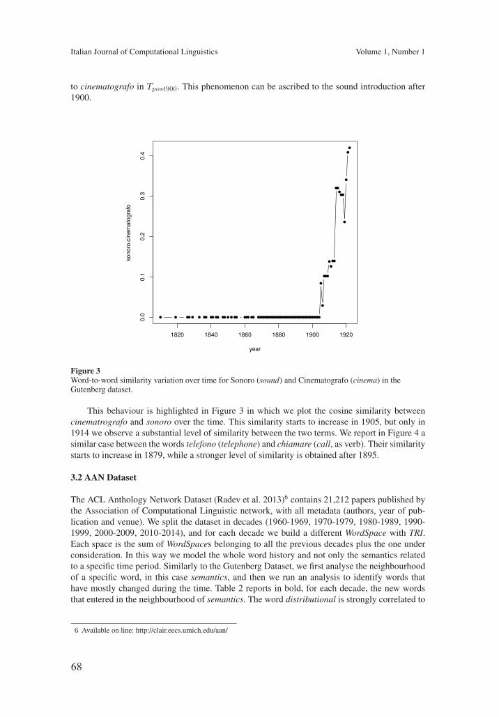
68
Italian Journal of Computational Linguistics Volume 1, Number 1
to cinematografo in Tpost900. This phenomenon can be ascribed to the sound introduction after1900.
1820 1840 1860 1880 1900 1920
0.0
0.1
0.2
0.3
0.4
year
so
no
ro.c
ine
ma
tog
rafo
Figure 3Word-to-word similarity variation over time for Sonoro (sound) and Cinematografo (cinema) in theGutenberg dataset.
This behaviour is highlighted in Figure 3 in which we plot the cosine similarity betweencinematrografo and sonoro over the time. This similarity starts to increase in 1905, but only in1914 we observe a substantial level of similarity between the two terms. We report in Figure 4 asimilar case between the words telefono (telephone) and chiamare (call, as verb). Their similaritystarts to increase in 1879, while a stronger level of similarity is obtained after 1895.
3.2 AAN Dataset
The ACL Anthology Network Dataset (Radev et al. 2013)6 contains 21,212 papers published bythe Association of Computational Linguistic network, with all metadata (authors, year of pub-lication and venue). We split the dataset in decades (1960-1969, 1970-1979, 1980-1989, 1990-1999, 2000-2009, 2010-2014), and for each decade we build a different WordSpace with TRI.Each space is the sum of WordSpaces belonging to all the previous decades plus the one underconsideration. In this way we model the whole word history and not only the semantics relatedto a specific time period. Similarly to the Gutenberg Dataset, we first analyse the neighbourhoodof a specific word, in this case semantics, and then we run an analysis to identify words thathave mostly changed during the time. Table 2 reports in bold, for each decade, the new wordsthat entered in the neighbourhood of semantics. The word distributional is strongly correlated to
6 Available on line: http://clair.eecs.umich.edu/aan/
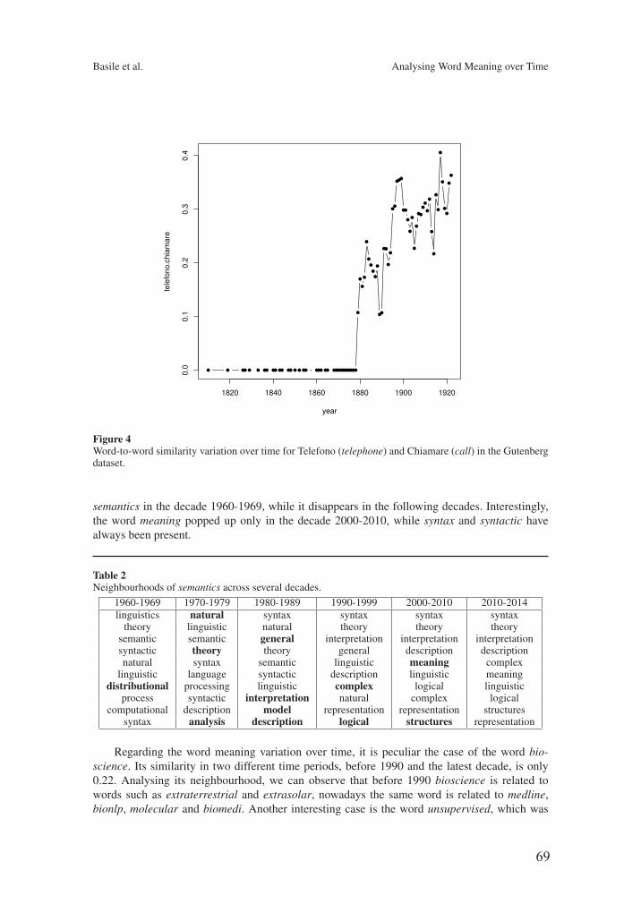
69
Basile et al. Analysing Word Meaning over Time
1820 1840 1860 1880 1900 1920
0.0
0.1
0.2
0.3
0.4
year
tele
fon
o.c
hia
ma
re
Figure 4Word-to-word similarity variation over time for Telefono (telephone) and Chiamare (call) in the Gutenbergdataset.
semantics in the decade 1960-1969, while it disappears in the following decades. Interestingly,the word meaning popped up only in the decade 2000-2010, while syntax and syntactic havealways been present.
Table 2Neighbourhoods of semantics across several decades.
1960-1969 1970-1979 1980-1989 1990-1999 2000-2010 2010-2014linguistics natural syntax syntax syntax syntax
theory linguistic natural theory theory theorysemantic semantic general interpretation interpretation interpretationsyntactic theory theory general description descriptionnatural syntax semantic linguistic meaning complex
linguistic language syntactic description linguistic meaningdistributional processing linguistic complex logical linguistic
process syntactic interpretation natural complex logicalcomputational description model representation representation structures
syntax analysis description logical structures representation
Regarding the word meaning variation over time, it is peculiar the case of the word bio-science. Its similarity in two different time periods, before 1990 and the latest decade, is only0.22. Analysing its neighbourhood, we can observe that before 1990 bioscience is related towords such as extraterrestrial and extrasolar, nowadays the same word is related to medline,bionlp, molecular and biomedi. Another interesting case is the word unsupervised, which was
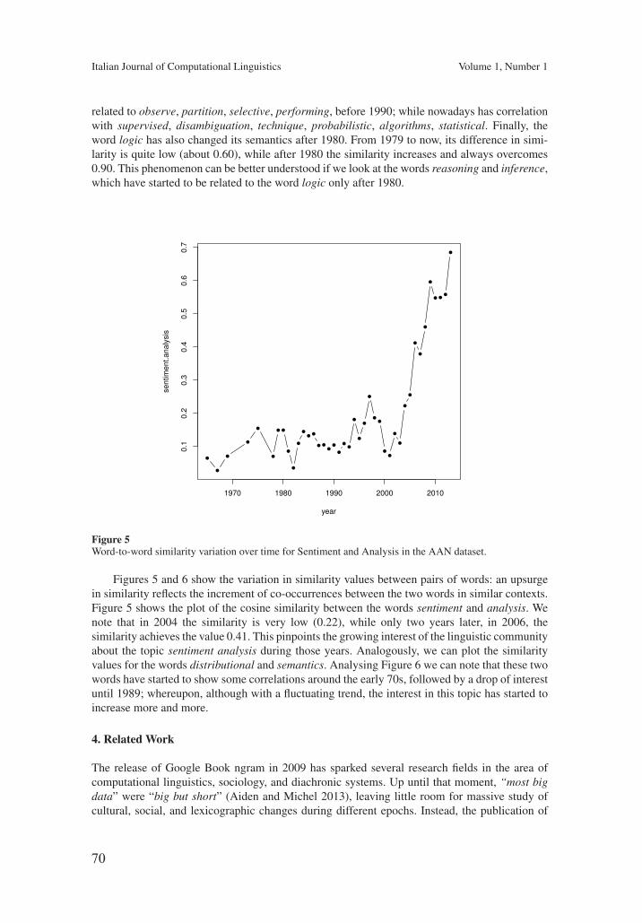
70
Italian Journal of Computational Linguistics Volume 1, Number 1
related to observe, partition, selective, performing, before 1990; while nowadays has correlationwith supervised, disambiguation, technique, probabilistic, algorithms, statistical. Finally, theword logic has also changed its semantics after 1980. From 1979 to now, its difference in simi-larity is quite low (about 0.60), while after 1980 the similarity increases and always overcomes0.90. This phenomenon can be better understood if we look at the words reasoning and inference,which have started to be related to the word logic only after 1980.
1970 1980 1990 2000 2010
0.1
0.2
0.3
0.4
0.5
0.6
0.7
year
se
ntim
en
t.a
na
lysis
Figure 5Word-to-word similarity variation over time for Sentiment and Analysis in the AAN dataset.
Figures 5 and 6 show the variation in similarity values between pairs of words: an upsurgein similarity reflects the increment of co-occurrences between the two words in similar contexts.Figure 5 shows the plot of the cosine similarity between the words sentiment and analysis. Wenote that in 2004 the similarity is very low (0.22), while only two years later, in 2006, thesimilarity achieves the value 0.41. This pinpoints the growing interest of the linguistic communityabout the topic sentiment analysis during those years. Analogously, we can plot the similarityvalues for the words distributional and semantics. Analysing Figure 6 we can note that these twowords have started to show some correlations around the early 70s, followed by a drop of interestuntil 1989; whereupon, although with a fluctuating trend, the interest in this topic has started toincrease more and more.
4. Related Work
The release of Google Book ngram in 2009 has sparked several research fields in the area ofcomputational linguistics, sociology, and diachronic systems. Up until that moment, “most bigdata” were “big but short” (Aiden and Michel 2013), leaving little room for massive study ofcultural, social, and lexicographic changes during different epochs. Instead, the publication of
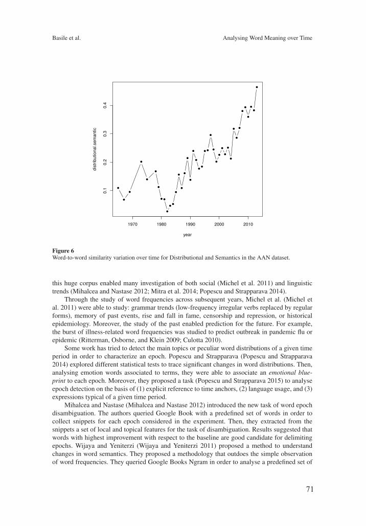
71
Basile et al. Analysing Word Meaning over Time
1970 1980 1990 2000 2010
0.1
0.2
0.3
0.4
year
dis
trib
utio
na
l.se
ma
ntic
Figure 6Word-to-word similarity variation over time for Distributional and Semantics in the AAN dataset.
this huge corpus enabled many investigation of both social (Michel et al. 2011) and linguistictrends (Mihalcea and Nastase 2012; Mitra et al. 2014; Popescu and Strapparava 2014).
Through the study of word frequencies across subsequent years, Michel et al. (Michel etal. 2011) were able to study: grammar trends (low-frequency irregular verbs replaced by regularforms), memory of past events, rise and fall in fame, censorship and repression, or historicalepidemiology. Moreover, the study of the past enabled prediction for the future. For example,the burst of illness-related word frequencies was studied to predict outbreak in pandemic flu orepidemic (Ritterman, Osborne, and Klein 2009; Culotta 2010).
Some work has tried to detect the main topics or peculiar word distributions of a given timeperiod in order to characterize an epoch. Popescu and Strapparava (Popescu and Strapparava2014) explored different statistical tests to trace significant changes in word distributions. Then,analysing emotion words associated to terms, they were able to associate an emotional blue-print to each epoch. Moreover, they proposed a task (Popescu and Strapparava 2015) to analyseepoch detection on the basis of (1) explicit reference to time anchors, (2) language usage, and (3)expressions typical of a given time period.
Mihalcea and Nastase (Mihalcea and Nastase 2012) introduced the new task of word epochdisambiguation. The authors queried Google Book with a predefined set of words in order tocollect snippets for each epoch considered in the experiment. Then, they extracted from thesnippets a set of local and topical features for the task of disambiguation. Results suggested thatwords with highest improvement with respect to the baseline are good candidate for delimitingepochs. Wijaya and Yeniterzi (Wijaya and Yeniterzi 2011) proposed a method to understandchanges in word semantics. They proposed a methodology that outdoes the simple observationof word frequencies. They queried Google Books Ngram in order to analyse a predefined set of
72
Italian Journal of Computational Linguistics Volume 1, Number 1
words, on which they performed two methods for detecting semantic changes. The first methodwas based on Topics-Over-Time (TOT), a variation of Latent Dirichlet Allocation (LDA) thatcaptures changes in topic. The latter method consisted in retrieving ngrams for a given wordby treating all ngrams belonging to a year as a document. Then, they clustered the whole set: achange in meaning occurs if two consecutive years (documents) belong to two different clusters.LDA was also at the heart of the method proposed in (Anderson, McFarland, and Jurafsky 2012).Authors analysed ACL papers from 1980-2008, LDA served to extract topics from the corpus thatwere assigned to documents, and consequently to people that authored them. This enabled someanalysis, like the flow of authors between topics, and the main epochs in ACL history.
Most similar to the method proposed here are those works that avoid the frequentist analysisof a predefined set of words, but rather build a semantic space of words that takes into accountalso the temporal axis. In such a space, words are not just a number, but have a semantics definedby the context of usage. Kim et al. (Kim et al. 2014) used a vector representation of words bytraining a Neural Language Model, one for each year from 1850-2009. The comparison betweenvectors of the same word across different time periods indicates when the word changed itsmeaning. Such a comparison was performed through cosine similarity. Jatowt and Duh (Jatowtand Duh 2014) exploited three different distributional spaces based on normal co-occurrences,positional information, and Latent Semantic Analysis. The authors built a space for each decade,in order to compare word vectors and detect when a difference between the word contexts hasoccurred. Moreover, they analysed the sentiment expressed in the context associated to the wordover time. Mitra et al. (Mitra et al. 2014) built a distributional thesaurus (DT) for each period oftime they wanted to analyse. Then, they applied a co-occurrence graph based clustering algorithmin order to cluster words according to senses in different time periods: the difference betweenclusters is exploited to detect changes in senses. All these works have in common the fact thatthey build a different semantic space for each period taken into consideration; this approachdoes not guarantee that each dimension bears the same semantics in different spaces (Jurgensand Stevens 2009), especially when reduction techniques are employed. In order to overcomethis limitation, Jurgens and Stevens (Jurgens and Stevens 2009) introduced Temporal RandomIndexing technique as a means to discover semantic changes associated to different events ina blog stream. Our methodology relies on the technique introduced by (Jurgens and Stevens2009) but with a different aim. While Jurgens and Stevens exploit TRI for the specific task ofevent detection, in this paper we built a framework on TRI for the general purpose of analysinglinguistic phenomena, like changes in semantics between pairs of words and neighbourhoodanalysis over time.
5. Conclusions
The analysis of cultural, social, and linguistic phenomena from a temporal perspective has gaineda lot of attention during the last decade due to the availability of large corpora containingtemporal information. In this paper, we proposed a method for building WordSpaces taking intoaccount information about time. In a WordSpace, words are represented as mathematical pointswhose proximity reflects the degree of semantic relatedness between the terms involved. Theproposed system, called TRI, is able to build several WordSpaces, which represent words indifferent time periods, and to compare vectors belonging to different spaces to understand howthe meaning of a word has changed over time.
We reported some examples of the temporal analysis that can be carried out by our frame-work on an Italian dataset about books and an English dataset of scientific papers on compu-tational linguistics. Our investigation shows the ability of our system to (1) capture changes inword usage over time, and (2) analyse changes in the semantic relationship between two words.
73
Basile et al. Analysing Word Meaning over Time
This analysis is useful to detect linguistic events that emerge in specific time intervals and thatcan be related to social or cultural phenomena.
As future work we plan a thoroughly temporal analysis on a bigger corpus like Google ngramand an extensive evaluation on a temporal task, like SemEval-2015 Diachronic Text EvaluationTask (Popescu and Strapparava 2015).
ReferencesAiden, Erez and Jean-Baptiste Michel. 2013. Uncharted: Big data as a lens on human culture. Penguin.Anderson, Ashton, Dan McFarland, and Dan Jurafsky. 2012. Towards a computational history of the acl:
1980-2008. In Proceedings of the ACL-2012 Special Workshop on Rediscovering 50 Years ofDiscoveries, ACL ’12, pages 13–21, Stroudsburg, PA, USA. Association for Computational Linguistics.
Cohen, Trevor, Dominique Widdows, Roger W. Schvaneveldt, and Thomas C. Rindflesch. 2010. LogicalLeaps and Quantum Connectives: Forging Paths through Predication Space. In AAAI-Fall 2010Symposium on Quantum Informatics for Cognitive, Social, and Semantic Processes, pages 11–13.
Culotta, Aron. 2010. Towards detecting influenza epidemics by analyzing twitter messages. InProceedings of the First Workshop on Social Media Analytics, SOMA ’10, pages 115–122, New York,NY, USA. ACM.
Dasgupta, Sanjoy and Anupam Gupta. 1999. An elementary proof of the Johnson-Lindenstrauss lemma.Technical report, Technical Report TR-99-006, International Computer Science Institute, Berkeley,California, USA.
Harris, Zellig S. 1968. Mathematical Structures of Language. New York: Interscience.Jatowt, Adam and Kevin Duh. 2014. A framework for analyzing semantic change of words across time. In
Proceedings of the 14th ACM/IEEE-CS Joint Conference on Digital Libraries, JCDL ’14, pages229–238, Piscataway, NJ, USA. IEEE Press.
Jones, Michael N. and Douglas J. K. Mewhort. 2007. Representing Word Meaning and Order Informationin a Composite Holographic Lexicon. Psychological Review, 114(1):1–37.
Jurgens, David and Keith Stevens. 2009. Event Detection in Blogs using Temporal Random Indexing. InProceedings of the Workshop on Events in Emerging Text Types, pages 9–16. Association forComputational Linguistics.
Kanerva, Pentti. 1988. Sparse Distributed Memory. MIT Press.Kim, Yoon, Yi-I Chiu, Kentaro Hanaki, Darshan Hegde, and Slav Petrov. 2014. Temporal analysis of
language through neural language models. In Proceedings of the ACL 2014 Workshop on LanguageTechnologies and Computational Social Science, pages 61–65, Baltimore, MD, USA, June. Associationfor Computational Linguistics.
Landauer, Thomas K. and Susan T. Dumais. 1997. A Solution to Plato’s Problem: The Latent SemanticAnalysis Theory of Acquisition, Induction, and Representation of Knowledge. Psychological review,104(2):211–240.
Michel, Jean-Baptiste, Yuan Kui Shen, Aviva Presser Aiden, Adrian Veres, Matthew K Gray, TheGoogle Book Team, Joseph P Pickett, Dale Hoiberg, Dan Clancy, Peter Norvig, Jon Orwant, StevenPinker, Martin A. Nowak, and Erez Lieberman Aiden. 2011. Quantitative analysis of culture usingmillions of digitized books. Science, 331(6014):176–182.
Mihalcea, Rada and Vivi Nastase. 2012. Word epoch disambiguation: Finding how words change overtime. In Proceedings of the 50th Annual Meeting of the Association for Computational Linguistics(Volume 2: Short Papers), pages 259–263, Jeju Island, Korea, July. Association for ComputationalLinguistics.
Mikolov, Tomas, Kai Chen, Greg Corrado, and Jeffrey Dean. 2013. Efficient Estimation of WordRepresentations in Vector Space. CoRR, abs/1301.3781.
Mikolov, Tomas, Martin Karafiát, Lukas Burget, Jan Cernocky, and Sanjeev Khudanpur. 2010. RecurrentNeural Network based Language Model. In INTERSPEECH, pages 1045–1048.
Mitra, Sunny, Ritwik Mitra, Martin Riedl, Chris Biemann, Animesh Mukherjee, and Pawan Goyal. 2014.That’s sick dude!: Automatic identification of word sense change across different timescales. InProceedings of the 52nd Annual Meeting of the Association for Computational Linguistics (Volume 1:Long Papers), pages 1020–1029, Baltimore, Maryland, June. Association for ComputationalLinguistics.
Popescu, Octavian and Carlo Strapparava. 2014. Time corpora: Epochs, opinions and changes.Knowledge-Based Systems, 69:3 – 13.
Popescu, Octavian and Carlo Strapparava. 2015. Semeval 2015, task 7: Diachronic text evaluation. InProceedings of the 9th International Workshop on Semantic Evaluation (SemEval 2015), pages
74
Italian Journal of Computational Linguistics Volume 1, Number 1
870–878, Denver, Colorado, June. Association for Computational Linguistics.Radev, Dragomir R., Pradeep Muthukrishnan, Vahed Qazvinian, and Amjad Abu-Jbara. 2013. The ACL
Anthology Network Corpus. Language Resources and Evaluation, pages 1–26.Ritterman, Joshua, Miles Osborne, and Ewan Klein. 2009. Using prediction markets and twitter to predict
a swine flu pandemic. In 1st International Workshop on Mining Social Media, volume 9, pages 9–17.Sahlgren, Magnus. 2005. An Introduction to Random Indexing. In Methods and Applications of Semantic
Indexing Workshop at the 7th International Conference on Terminology and Knowledge Engineering,TKE, volume 5.
Sahlgren, Magnus. 2006. The Word-Space Model: Using distributional analysis to represent syntagmaticand paradigmatic relations between words in high-dimensional vector spaces. Ph.D. thesis, Stockholm:Stockholm University, Faculty of Humanities, Department of Linguistics.
Wijaya, Derry Tanti and Reyyan Yeniterzi. 2011. Understanding semantic change of words over centuries.In Proceedings of the 2011 International Workshop on DETecting and Exploiting Cultural diversiTy onthe Social Web, DETECT ’11, pages 35–40, New York, NY, USA. ACM.
75
Context-aware Models for Twitter SentimentAnalysis
Giuseppe Castellucci∗Università di Roma, Tor Vergata
Andrea Vanzo∗∗
Sapienza, Università di Roma
Danilo Croce†Università di Roma, Tor Vergata
Roberto Basili‡Università di Roma, Tor Vergata
Recent works on Sentiment Analysis over Twitter are tied to the idea that the sentiment canbe completely captured after reading an incoming tweet. However, tweets are filtered throughstreams of posts, so that a wider context, e.g. a topic, is always available. In this work, thecontribution of this contextual information is investigated for the detection of the polarity oftweet messages. We modeled the polarity detection problem as a sequential classification task overstreams of tweets. A Markovian formulation of the Support Vector Machine discriminative modelhas been here adopted to assign the sentiment polarity to entire sequences. The experimentalevaluation proves that sequential tagging better embodies evidence about the contexts and isable to increase the accuracy of the resulting polarity detection process. These evidences arestrengthened as experiments are successfully carried out over two different languages: Italianand English. Results are particularly interesting as the approach is flexible and does not rely onany manually coded resources.
1. Introduction
In the Web 2.0 era, people write about their life and personal experiences, sharingcontents about facts and ideas. Social Networks became the main place where sharingthis information and now represent also a valuable source of evidences for the analysts.This data is crucial in the study of interactions and dynamics of subjectivity on the Web.Twitter1 is one among these microblogging services that counts more than a billion ofactive users and more than 500 million of daily messages2. However, the analysis of thisinformation is still challenging: Twitter messages are characterized by a very informallanguage, affected by misspelling, slang and special tokens as #hashtags, i.e. special user-generated tags used to contextualize a tweet around specific topics.
Researches focused on the computational study and automatic recognition of opin-ions and sentiments as they are expressed in free texts. It gave rise to the field of
∗ Dept. of Electronic Engineering - Via del Politecnico 1, 00133 Rome, Italy.E-mail: [email protected]
∗∗ Dept. of Computer Science, Control and Management Engineering - Via Ariosto 25, 00185 Rome, Italy.E-mail: [email protected]
† Dept. of Enterprise Engineering - Via del Politecnico 1, 00133 Rome, Italy.E-mail: [email protected]
‡ Dept. of Enterprise Engineering - Via del Politecnico 1, 00133 Rome, Italy.E-mail: [email protected]
1 http://www.twitter.com2 http://expandedramblings.com/
© 2015 Associazione Italiana di Linguistica Computazionale
76
Italian Journal of Computational Linguistics Volume 1, Number 1
Sentiment Analysis (SA), a set of tasks aiming at recognizing and characterizing thesubjective attitude of a writer with respect to some topics. Many SA studies map senti-ment detection in a Machine Learning (ML) setting (Pang and Lee 2008), where labeleddata allow to induce a sentiment detection function. In general, sentiment detection intweets has been generally treated as any other text classification task, as proved by mostpapers participating to the Sentiment Analysis in Twitter task in SemEval-2013, SemEval-2014 and Evalita-2014 challenges (Nakov et al. 2013; Rosenthal et al. 2014; Basile et al.2014), where specific representations for a message are derived considering one tweetin isolation. The shortness of messages and the inherent semantic ambiguity are criticallimitations and make these systems fail in many cases.
Let us consider the message, in which a tweet from ColMustard cites SergGray:
ColMustard : @SergGray Yes, I totally agree with you about the substitutions! #Bayern #Freiburg
The tweet sounds like to be a reply to the previous one. Notice how no lexical norsyntactic property allows to determine the sentiment polarity. However, if we look atthe entire conversation preceding this message:
ColMustard : Amazing match yesterday!!#Bayern vs. #Freiburg 4-0 #easyvictory
SergGray : @ColMustard Surely, but #Freiburg wasted lot of chances to score.. wrong substitutions
by #Guardiola during the 2nd half!!
ColMustard : @SergGray Yes, I totally agree with you about the substitutions! #Bayern #Freiburg
it is easy to establish that a first positive tweet has been produced, followed by a secondnegative one so that the third tweet is negative as well. Only by considering its context,i.e. the conversation, we are able to understand even such a short message and properlycharacterize it according to its author and posting time.
We aim at exploiting such a richer set of observations (i.e. conversations or, ingeneral, contexts) and at defining a context-aware SA model along two lines: first,by enriching a tweet representation to include the conversation information, and thenby introducing a more complex classification model that works over an entire tweetsequence and not only on a tweet (i.e. the target) in isolation. Accordingly, in the paperwe will first focus on different representations of tweets that can be made available to asentiment detection process. They will also account for contextual information, derivedboth from conversations, as chains of tweets that are reply-to the previous ones, andtopics, built around hashtags. These are in fact topics explicitly annotated by users, suchas events (#easyvictory) or people (#Guardiola). A hashtag represents a wider notion ofconversation that enforces the sense of belonging to a community. From a computationalperspective, the polarity detection of a tweet in a context is here modeled as a sequentialclassification task. In fact, both conversation and topic-based contexts are arbitrarilylong sequences of messages, ordered according to time with the target tweet being thelast. A variant of the SVMhmm learning algorithm (Altun, Tsochantaridis, and Hofmann2003) has been implemented in the KeLP framework (Filice et al. 2015) to classify aninstance (here, a tweet) within an entire sequence. While SVM based classifiers allowto recognize the sentiments from one specific tweet at a time, the adopted sequenceclassifier jointly labels all tweets in a sequence. It is expected to capture patterns withina conversation and apply them in novel sequences through a standard decoding task.
While all the above contexts extend a tweet representation, they are still local to aspecific notion of conversation. In this work, we also explore a more abstract notion ofcontexts, e.g. the history of messages from the same user, that embodies the emotional
77
Castellucci et al. Context-aware Models for Twitter Sentiment Analysis
attitude shown by each user in his overall usage of Twitter. In the above example,ColMustard exhibits a specific attitude while discussing about the Bayern Munchen.We can imagine that this feature characterizes most of its future messages at least aboutfootball. We suggest to enrich the tweet representation with features that synthesize auser’s profile, in order to catch possible biases towards a particular sentiment polarity.This is quite interesting as it has been shown that communities behave in a coherentway and users tend to take stable standing points.
This work is an extension of (Vanzo, Croce, and Basili 2014) and (Vanzo et al. 2014).Here, the evaluation in the Italian setting is provided over a subset of the Evalita 2014Sentipolc dataset (Basile et al. 2014). Moreover, we here provide a deeper evaluationof the contribution of different kernel functions as well as more insights about thephenomena covered by the contextual models.
In the remaining of the paper, a survey of the existing approaches is presented intoSection 2. Then, Section 3 provides a description of context-based models: conversation,topic-based and user profiling. The experimental evaluation is presented in Section 4and it proves the positive impact of social dynamics on the SA task.
2. Related Works
Sentiment Analysis (SA) has been described as a Natural Language Processing task atmany levels of granularity. It has been mapped to document level, (Turney 2002; Pangand Lee 2004), sentence level (Hu and Liu 2004; Kim and Hovy 2004) and at the phraselevel (Wilson, Wiebe, and Hoffmann 2005; Agarwal, Biadsy, and Mckeown 2009).
The spreading of microblog services, e.g. Twitter, where users post real-time opin-ions about “everything”, poses newer and different challenges. Classical approaches toSA (Pang, Lee, and Vaithyanathan 2002; Pang and Lee 2008) are not directly applicable:tweets are very short and a fine-grained lexical analysis is required. Recent works triedto model the sentiment in tweets by taking into account these characteristics of the data(Go, Bhayani, and Huang 2009; Pak and Paroubek 2010; Davidov, Tsur, and Rappoport2010; Bifet and Frank 2010; Barbosa and Feng 2010; Kouloumpis, Wilson, and Moore2011; Zanzotto, Pennaccchiotti, and Tsioutsiouliklis 2011; Agarwal et al. 2011; Croce andBasili 2012; Si et al. 2013; Kiritchenko, Zhu, and Mohammad 2014). Specific approachesand feature modeling are used to improve accuracy levels in tweet polarity recognition.For example, the use of n-grams, POS tags, polarity lexicons (Kiritchenko, Zhu, andMohammad 2014; Castellucci, Croce, and Basili 2015) and tweet specific features (e.g.hashtags, re-tweets) are some of the main properties exploited by these works, in com-bination with different machine learning algorithms: among these latter, probabilisticparadigms, e.g. Naive Bayes (Pak and Paroubek 2010), or Kernel-based machines, asdiscussed in (Barbosa and Feng 2010; Agarwal et al. 2011; Castellucci et al. 2014), aremostly adopted. An interesting perspective, where a kind of contextual information isstudied, is presented in (Mukherjee and Bhattacharyya 2012): the sentiment detectionof tweets is here modeled according to lexical features as well as discourse relationslike the presence of connectives, conditionals and semantic operators like modals andnegations. In (Speriosu et al. 2011) and (Tan et al. 2011), social information betweenusers is exploited. (Speriosu et al. 2011) builds a graph of Twitter messages that arelinked to words, emoticons and users. Users are connected if they are in a followingrelationship. A Label Propagation (Talukdar and Crammer 2009) framework is adoptedto spread polarity label distributions and to classify messages with respect to polarity.The relationships between users constitute a sort of contextual information. Again,in (Tan et al. 2011), user relationships are exploited for the polarity classification of
78
Italian Journal of Computational Linguistics Volume 1, Number 1
messages in a transductive learning setting. The main motivation in (Tan et al. 2011) isthat “users that are somehow connected may be more likely to hold similar opinions”.
Nevertheless, in almost all the above approaches, features are derived only fromlexical resources or from the tweet or users, and no contextual information, in termsof other related messages, is really exploited. However, given one tweet targeted, moreawareness about its content and, thus, its sentiment, can be achieved by consideringthe entire stream of related posts immediately preceding it. In order to exploit thiswider information, a Markovian extension of a Kernel-based categorization approachis presented in the next section.
3. A Context-aware Model for Sentiment Analysis in Twitter
As discussed in the introduction, contextual information about one tweet stems fromvarious aspects: an explicit conversation, the overall set of recent tweets about a topic(for example a hastag like #Bayern), or the user attitude. The heterogeneity of thisinformation requires the integration of different aspects that are heterogeneous. Asindividual perspectives on the context are independent, i.e. a conversation may ormay not depend on user preference or cheer, and they also obey to different notionof analogies or similarity, we should avoid a unified representation for them. We aremore likely to derive independent representations and make them interact in a properalgorithmic framework. We thus consider a tweet as a multifaceted entity where a setof vector representations, each one contributing to one aspect of the overall representa-tion, exhibits a specific similarity metrics. This is exactly what Kernel-based learningsupports, whereas the combination of different kernels can easily result in a kernelfunction itself (Shawe-Taylor and Cristianini 2004). Kernels are thus used to capturespecific aspects of the semantic relatedness between two messages and are integrated invarious machine learning algorithms, such as Support Vector Machines (SVMs).
3.1 Representing Tweets through Different Kernel Functions
Many ML approaches for Sentiment Analysis in Twitter benefits by complex modelingof individual tweets, as discussed in many works (Nakov et al. 2013). The representationwe propose makes use of individual kernels as models of different aspects that are madeavailable to a SVM algorithm. In the remaining of this Section, different kernel functionsare presented for capturing different semantic and sentiment aspects of the data.Bag of Word Kernel (BoWK). The simplest kernel function describes the lexical overlapbetween tweets, thus represented as vectors, i.e. Bag-Of-Words vectors, whose individ-ual dimensions correspond to the different words. Components denote the presence ornot of a word in the text and the kernel function corresponds to the cosine similarity be-tween vector pairs. Even if very simple, the BoWK model is one of the most informativerepresentation in SA, as emphasized since (Pang, Lee, and Vaithyanathan 2002).Lexical Semantic Kernel (LSK). Lexical information in tweets can be very sparse.In order to extend the BoWK model, we provide a further representation aiming atgeneralizing the lexical information. It can be obtained for every term of a dictionary bya Word Space (WS) built according to a Distributional Model (Sahlgren 2006) of lexicalsemantics. These models have been successfully applied in several NLP tasks, such asFrame Induction (Pennacchiotti et al. 2008) or Semantic Role Labeling (Croce et al. 2010).In this work, we derive a vector representation �wi for each word wi in the vocabulary byexploiting Neural Word Embeddings (Bengio et al. 2003; Mikolov et al. 2013). The resultis that every word can be projected in the WS and a vector, i.e. WS vector, for each tweet
79
Castellucci et al. Context-aware Models for Twitter Sentiment Analysis
is derived through the linear combination of the occurring word vectors (also calledadditive linear combination in (Mitchell and Lapata 2010)). The resulting kernel functionis the cosine similarity between tweet vector pairs, in line with (Cristianini, Shawe-Taylor,and Lodhi 2002). Notice that the adoption of a distributional approach does not limit theoverall application, as it can be automatically applied without relying on any manuallycoded resource.User Sentiment Profile Kernel (USPK). A source of evidence about a tweet is itsauthor, with his attitude towards some polarities. In general, a person will show similarattitudes with respect to the same topics. Thus, we can think of specific features thatshould model the users’ attitudes given its messages. Let ti ∈ T be a tweet and i ∈ N+
its identifier. The User Profile Context can be defined as the set of the last tweets postedby the author ui of ti: we denote this set of messages as Λui . This information is abody of evidence about the opinion holder, and can be adopted to build a profile onwhich a further tweet representation can be defined. A tweet ti is here mapped into athree dimensional vector, i.e. USP vector, �µi =
(µ1i , µ
2i , µ
3i
), where each component µj
i
is the indicator of a polarity trend, i.e. positive, negative and neutral, expressed throughthe conditional probability P (j | ui) for the polarity labels j ∈ Y given the user ui. Wecan suppose that, for each tk ∈ Λui , its corresponding label yk is available either as agold standard annotation or predicted in a semi-supervised fashion. The estimation ofµji ≈ P (j | ui), is a σ-parameterized Laplace smoothed version of the observations in Λui :
µji =
|Λui |∑k=1
1{yk=j}(tk) + σ
|Λui |+ σ|Y|(1)
where σ ∈ R is the smoothing parameter, j ∈ Y , i.e. the set of polarity labels. A kernelfunction, in which we are interested in, should capture when two users ui, uj , ui �= uj
expresses similar sentiment attitudes in their messages. We call this kernel functionUser Sentiment Profile Kernel (USPK), and it can be computed as the cosine similaritybetween the two vectors (�µi, �µm). As an example, let us consider a user u1 whosetimeline is composed by 100 messages, whose distribution with respect to the positive,negative and neutral classes is the following: 43 positive, 21 negative and 36 neural. Ifwe adopt the Equation 1 with σ = 1.0, we obtain three values: µpositive
1 = 43+1100+3 = 0.43,
µnegative1 = 21+1
100+3 = 0.22, µneutral1 = 36+1
100+3 = 0.35. These values can be arranged into a3-dimensional USP vector, �µ1 = [0.43, 0.22, 0.35] whose aim is to capture that u1 writeswith a-priori positive attitude. If another user, e.g. u2, wrote 325 messages distributedas 145 positive, 65 negative and 115 neutral, it is easy to compute a USP vector �µ2 =[0.45, 0.20, 0.35]. Then, the kernel operating on �µ1, �µ2 will capture that u1 and u2 writetheir messages with similar attitudes, and that they should be treated similarly.The multiple kernel approach. Whenever the different kernels are available, we canapply a linear combination αBoWK+βLSK or αBoWK+βLSK+γUSPK in order to ex-ploit lexical and semantic properties captured by BoWK and LSK, or user properties ascaptured by USPK. The combination is still a valid kernel, and can thus be adopted in akernel-based learning framework.
3.2 Modeling Tweet Contexts in a Sequential Labeling Framework
The User Sentiment Profile Kernel (USPK) can be seen as an implicit representation ofthe context describing the writer. However, contextual information is usually embodiedby the stream of messages in which a target tweet ti is immersed. Usually, the streamis completely available to a reader. In all cases, the stream gives rise to a sequence on
80
Italian Journal of Computational Linguistics Volume 1, Number 1
which a sequence labeling algorithm can be applied: the target tweet is here alwayslabeled within the entire sequence, where contextual constraints are provided by thepreceding tweets. In this work we rely on two different types of context: Conversationalcontext and Topical context. The former is based on the reply-to chain. In this case, theentire sequence is built by leveraging the reply information available for Twitter statuses,that basically represents a pointer to the previous tweet within the conversation chain.The latter takes into account hashtags that allow to aggregate different tweets arounda specific topic specified by the users. Here, a tweet sequence can be derived includingthe n messages preceding the target ti that contain the same hashtag set. This is usuallythe output of a search in Twitter and it is likely the source information that influencedthe writer’s opinion. A more formal definition of the above contexts is given below.
Definition 1 (Conversational context)For every tweet ti ∈ T , let r(ti) : T → T be a function that returns either the tweet towhich ti is a reply to, or null if ti is not a reply. Then, the conversation-based context ΛC,l
i
of tweet ti (i.e., the target tweet) is the sequence of tweet iteratively built by applyingr(·), until l tweets have been selected or r(·) = null. In other words, l allows to limit thesize of the input context.
An example of conversation-based context is given in Section 1.
Definition 2 (Topical context)Let ti ∈ T be a tweet and h(i) : T → P(H) be a function that returns the entire hashtagset Hi ⊆ H observed into ti. Then, the hashtag-based context ΛH,l
i for a tweet ti (i.e., targettweet) is a sequence of the most recent l tweets tj such that Hj ∩Hi �= ∅, i.e. tj and tishare at least one hashtag, and tj has been posted before ti.
As an example, the following hashtag context has been obtained about #Bayern:
MrGreen : Fun fact: #Freiburg is the only #Bundesliga team #Pep has never beaten in his
coaching career. #Bayern
MrsPeacock : Young starlet Xherdan #Shaqiri fires #Bayern into a 2-0 lead. Is there any hope
for #Freiburg?
pic.twitter.com/krzbFJFJyN
ProfPlum : It is clear that #Bayern is on a rampage leading by 4-0, the latest by Mandzukic...
hoping for another 2 goals from #bayernmunich
MissScarlet : Noooo! I cant believe what #Bayern did!
MissScarlet expresses an opinion, but the corresponding polarity is easily evidentonly when the entire stream is available about the #Bayern hashtag. As well as in aconversational context, a specific context size n can be imposed by focusing only on thelast n tweets of the sequence. Once different representations and contexts are availablea structured learning-based approach can be applied to Sentiment Analysis. Firstly, wewill discuss a discriminative multiclass learning approach adopted to classify tweetswithout considering the contextual information. Then a sequence labeling approach,inspired by the SVMhmm learning algorithm (Altun, Tsochantaridis, and Hofmann
81
Castellucci et al. Context-aware Models for Twitter Sentiment Analysis
2003), will be introduced. It will be adopted to label sequence of messages coming bothfrom conversation and hashtag contexts.
3.3 Context-unaware vs. Context-aware Classification
The multiclass approach for a context-unaware classification. A multi-classificationschema is applied to detect the polarity of messages. We adopt Support Vector Machines(Vapnik 1998) within a One-Vs-All schema (Rifkin and Klautau 2004). In particular,given a training set D of tweet messages distributed across n classes, n binary classi-fication functions fp, where n is the number of classes, are acquired through the kernelfunctions above defined. These binary classifiers are used to decide the polarity of amessage ti, by choosing the class that maximizes the confidence of the classifier, i.e.argmaxp∈{pos,neg,neu} fp(ti). This learning model is applied to tweet messages withoutconsidering the contexts in which they are immersed.A sequential labeling approach for a context-aware classification. The sentiment pre-diction of a target tweet can be seen as a sequential classification task over a context.To this respect, we adopted an algorithm inspired by the SVMhmm algorithm (Altun,Tsochantaridis, and Hofmann 2003).
Given an input sequence x = (x1 . . . xm) ⊆ X , where x is a tweet sequence, e.g. con-sidering a conversation or hashtag context, and xi ∈ Rn is a feature vector representing atweet, the model predicts a tag sequence y = (y1 . . . ym) ∈ Y+ (with y ∈ Σ and ‖Σ‖ = l)after learning a linear discriminant function. The aim of a Markovian formulation ofSVM is to make dependent the classification of a tweet xi from the label assigned tothe previous elements in a history of length k, i.e xi−k, . . . , xi−1. Given this history, asequence of k labels can be retrieved, in the form yi−k, . . . , yi−1. In order to make theclassification of xi dependent also from the history, we augment the feature vector of xi
introducing a vector of transitions ψtr(yi−k, . . . , yi−1) ∈ Rl: it is a boolean vector wherethe dimensions corresponding to the k labels preceding the target element xi are set to1. A projection function φ(xi) is defined to consider both the observations, i.e. ψobs andthe transitions ψtr in a history of size k by concatenating the two representation, i.e.:
xki = φ(xi; yi−k, . . . , yi−1) = ψobs(xi) || ψtr(yi−k, . . . , yi−1)
with xki ∈ Rn+l and ψobs(xi) leaves intact the original feature space. Notice that the
vector concatenation is here denoted by the symbol || , and that the feature spaceoperated by ψobs is the one defined by the kernel linear combination as described inSection 3.1. In fact, adopting linear kernels the space defined by the linear combination isequivalent to the space obtained by juxtaposing the vectors on which each kernel oper-ates. More formally, assuming that K is a linear kernel, i.e. the inner product, and xi, xj
are two instances whose vector representations are xia , xib , xja , xjb , e.g. xia , xja are Bag-Of-Words vectors and xib , xjb are WS vectors, K(xi, xj) = K(xia , xja) +K(xib , xjb) =〈xia ||xib , xja ||xjb〉. In this case3, thus, ψobs(xi) = xia ||xib .
At training time, we use the SVM learning algorithm implemented in LibLinear(Fan et al. 2008) in a One-Vs-All schema over the feature space derived by φ, so that foreach yj a linear classifier fj(xk
i ) = wjφ(xi; yi−k, . . . , yi−1) + bj is learned. The φ functionis computed for each element xi by exploiting the gold label sequences. At classification
3 Before concatenating, each vector composing the observation of an instance, i.e. ψobs(xi), is normalizedto have unitary norm, so that each representation equally contributes to the overall kernel estimation.
82
Italian Journal of Computational Linguistics Volume 1, Number 1
time, all possible sequences y ∈ Y+ should be considered in order to determine the bestlabeling y = F (x, k), where k is the size of the history used to enrich xi, that is:
y = F (x, k) = argmaxy∈Y+
{∑
i=1...m
fj(xki )} = argmax
y∈Y+
{∑
i=1...m
wjφ(xi; yi−k, . . . , yi−1) + bj}
In order to reduce the computational cost, a Viterbi-like decoding algorithm is adopted4
to derive the sequence, and thus build the augmented feature vectors through the φfunction. In our setting, the markovian perspective allows to induce patterns acrosstweet sequences helpful to recognize sentiment even for truly ambiguous tweets.
4. Experimental Evaluation
The aim of the following evaluation is to estimate the contribution of the contextualmodels to the accuracy reachable in different scenarios, whereas rich contexts (e.g.popular hashtags) are possibly made available or when tweets with no context aretargeted. Moreover, in order to prove the portability of the proposed approach, weexperimented it on two different languages: English and Italian. In the first case, weadopted the Sentiment Analysis in Twitter dataset5 as it has been made available in theACL SemEval-2013 (Nakov et al. 2013). Experiments for SA in Italian are carried out overthe Evalita 2014 Sentipolc dataset (Basile et al. 2014).
Our experiments only require the availability of both conversation and hashtagcontexts and these are gathered for both datasets by adopting the Twitter API, giventhe IDs of the target tweet in the datasets6. In the case of the Semeval2013 dataset,only tweets from the training and development datasets are characterized by IDs: we,thus, statically divided the training and development official datasets in 80/10/10,respectively for Training/Held-out/Test. As the performance evaluation is always carriedout against one target tweet, the multi-classification may be applied when no contextis available (i.e. there is no conversation nor hashtag to build the context) or whena rich conversational or topical context is available. Table 1 summarizes the numberof tweets available for the Semeval-2013 dataset. The entire corpus of 10,045 messagesis shown in column 1, while columns 2-4 represent the subsets of target tweets forwhich conversational contexts, topical contexts or both were available, respectively.Conversational contexts are available only for 1,391 tweets (column 2), while topicalcontexts include 1,912 instances (column 3). Both contexts are available only for 128tweets.
The Italian Evalita dataset consists of short messages annotated with thesubjectivity, polarity and irony classes. We selected those messages annotatedwith polarity and that were not expressing any ironic content7. Again, we were ableto gather the contexts only for a subset of this dataset due to cancelation or privacyrestrictions. The final data used for our evaluations consists of a training set of 2, 445messages and a testing set of 1, 128 messages. Table 2 summarizes the number of
4 When applying fj(xki ) the classification scores are normalized through a softmax function and
probability scores are derived.5 http://www.cs.york.ac.uk/semeval-2013/task2/index.php?id=data6 We were able to download only a (still consistent) subset of the messages, as some of them have been
deleted or the author changed its privacy settings.7 We removed the ironic tweets to have similar datasets in English and Italian. In fact, ironic messages
would have biased the final evaluations in Italian, making more difficult to interpret the results.
83
Castellucci et al. Context-aware Models for Twitter Sentiment Analysis
Table 1Number of annotated messages within the Semeval 2013 Dataset. In parentheses the percentageof messages with respect to the size of the dataset.
Dataset (size) w/ conv w/ hashtag w/ bothTraining (8045) 1106 (13.74%) 1554 (19.31%) 100 (1.24%)Development (1001) 150 (14.98%) 190 (18.98%) 12 (1.20%)Testing (999) 135 (13.51%) 168 (16.81%) 16 (1.60%)
messages in this dataset, where the subsets of messages characterized by the consideredcontexts are again emphasized. In both languages, experiments are intended to classifythe polarity of a message with respect to the three classes positive, negative and neutral.
Table 2Number of annotated messages within the Evalita 2014 Sentipolc Dataset. In parentheses thepercentage of messages with respect to the size of the dataset.
Dataset (size) w/ conv w/ hashtag w/ bothTraining (2445) 349 (14,27%) 987 (40.36%) 80 (3.27%)Testing (1128) 169 (14.98%) 468 (41.48%) 47 (4.16%)
As tweets are noisy texts, a pre-processing phase has been applied to improve thequality of linguistic features observable and reduce data sparseness. In particular, anormalization step is applied to each post: fully capitalized words are converted inlowercase; reply marks are replaced with the pseudo-token USER, hyperlinks by LINK,hashtags by HASHTAG and emoticons by special tokens8. Afterwards, an almost standardmulti-language NLP chain is applied through the Chaos parser (Basili, Pazienza, andZanzotto 1998). In particular, each tweet, with its pseudo-tokens produced by the nor-malization step, is mapped into a sequence of POS tagged lemmas. In order to feed theLSK, lexical vectors correspond to a Word Space (WS) derived from a corpus of about20 million and 10 million of tweets, respectively for English and Italian. Also these mes-sages have been analyzed by applying the same normalization above, and 〈lemma,pos〉pairs are fed in input to the word2vec9 tool. Skip-gram models10 are acquired fromthese datasets, resulting in two 250 dimensional vector spaces that are adopted incomputing LSK. No existing dataset contains gold standard annotations for tweetsbelonging to contexts: USPK or the markovian approach would not be applicable. Thesolution we propose is to create a semi-supervised Gold-Standard by acquiring a multi-classifier. In particular, we derive a multi-classifier with the methodology describedin Section 3.2 on the available labeled training data with a BoWK+LSK function. Wethen classify each tweet in contexts with this classifier. This is a noisy but realistic andportable solution across datasets to initialize tweets labels.
Performance scores report the classification accuracy in terms of Precision, Recalland standard F-measure. However, in line with SemEval-2013, we report the F1Pnscore as the arithmetic mean between the F1 of positive, negative classes, and the F1Pnnscore as the mean between of all the involved polarity classes. The multi-class classifiers
8 We normalized 113 well-known emoticons in 15 classes.9 https://code.google.com/p/word2vec/
10 word2vec settings are: min-count=50, window=5, iter=10 and negative=10.
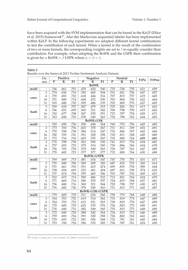
84
Italian Journal of Computational Linguistics Volume 1, Number 1
have been acquired with the SVM implementation that can be found in the KeLP (Filiceet al. 2015) framework11. Also the Markovian sequential labeler has been implementedwithin KeLP. In the following experiments we adopted different kernel combinationsto test the contribution of each kernel. When a kernel is the result of the combinationof two or more kernels, the corresponding weights are set to 1 to equally consider theircontribution. For example, when adopting the BoWK and the USPK their combinationis given by α BoWK + β USPK where α = β = 1.
Table 3Results over the Semeval 2013 Twitter Sentiment Analysis Dataset.
Ctx. Positive Negative Neutral F1Pn F1Pnnsize P R F1 P R F1 P R F1
BoWKmulti - .746 .661 .701 .478 .620 .540 .733 .736 .735 .621 .659
conv
3 .774 .656 .710 .550 .465 .504 .701 .821 .756 .607 .6576 .755 .693 .722 .618 .444 .516 .707 .815 .757 .619 .665
16 .751 .680 .714 .604 .472 .530 .703 .804 .750 .622 .66431 .765 .680 .720 .595 .486 .535 .705 .809 .753 .627 .669
hash
3 .769 .654 .707 .567 .479 .519 .705 .826 .761 .613 .6626 .746 .651 .695 .565 .521 .542 .708 .798 .750 .619 .662
16 .742 .677 .708 .567 .535 .551 .723 .787 .754 .629 .67131 .763 .690 .725 .578 .549 .563 .730 .798 .762 .644 .683
BoWK+LSKmulti - .765 .690 .726 .500 .648 .564 .760 .753 .756 .645 .682
conv
3 .773 .703 .736 .603 .535 .567 .731 .811 .769 .652 .6916 .770 .708 .738 .584 .514 .547 .732 .806 .767 .642 .684
16 .780 .705 .741 .591 .528 .558 .730 .811 .768 .649 .68931 .772 .716 .743 .603 .535 .567 .732 .800 .764 .655 .691
hash
3 .770 .708 .738 .563 .500 .530 .741 .815 .776 .634 .6816 .757 .693 .723 .579 .514 .545 .730 .806 .766 .634 .678
16 .756 .705 .730 .578 .549 .563 .736 .787 .761 .647 .68531 .770 .682 .723 .577 .577 .577 .732 .800 .764 .650 .688
BoWK+USPKmulti - .769 .669 .715 .481 .634 .547 .747 .755 .751 .631 .671
conv
3 .735 .680 .706 .569 .289 .383 .687 .832 .753 .545 .6146 .751 .661 .703 .551 .415 .474 .699 .819 .754 .589 .644
16 .738 .654 .693 .523 .401 .454 .697 .811 .749 .574 .63231 .737 .674 .704 .555 .465 .506 .703 .787 .743 .605 .651
hash
3 .762 .672 .714 .590 .486 .533 .713 .821 .764 .624 .6706 .771 .669 .716 .580 .535 .557 .724 .819 .768 .637 .681
16 .756 .680 .716 .569 .521 .544 .720 .798 .757 .630 .67231 .776 .682 .726 .578 .549 .563 .731 .815 .771 .645 .687
BoWK+LSK+USPKmulti - .779 .685 .729 .511 .634 .566 .758 .779 .768 .648 .688
conv
3 .764 .703 .732 .619 .514 .562 .733 .819 .774 .647 .6896 .764 .703 .732 .612 .521 .563 .738 .819 .776 .647 .690
16 .770 .685 .725 .623 .535 .576 .726 .823 .772 .650 .69131 .776 .690 .731 .582 .549 .565 .735 .815 .773 .648 .690
hash
3 .772 .690 .729 .588 .542 .564 .734 .815 .772 .646 .6886 .759 .693 .724 .591 .528 .558 .726 .802 .762 .641 .681
16 .755 .693 .722 .581 .556 .568 .732 .791 .761 .645 .68431 .753 .700 .726 .596 .570 .583 .736 .787 .761 .654 .690
11 http://sag.art.uniroma2.it/demo-software/kelp/
85
Castellucci et al. Context-aware Models for Twitter Sentiment Analysis
4.1 Context-aware Classification of Twitter Messages
The experiments have been run to validate the impact of contextual information overgeneric tweets, independently from the availability of a context. In this case, the en-tire dataset is used. The different settings adopted are reported in independent rows,corresponding to different classification approaches:
� multi refers to the application of the multi-classification of SVM with theOne-Vs-All approach, that does not require any context and can beconsidered as a baseline for the employed kernel combination;� conv refers to the sequential labeler observing the conversation-basedcontexts. The training and testing of the classifier is here run with differentcontext sizes, by parameterizing l in ΛC,l
i ;� likewise, hash refers to the sequential labeler observing the topic-basedcontexts, when hashtags are considered. Different context sizes have beenconsidered, by parameterizing l in ΛH,l
i .
When no context is available, both conv and hash models act on a sequence of lengthone, and no transition is applied.
Table 3 shows the empirical results over the test set for the English language, whilein Table 4 results for the Italian language are reported. The first general outcome is thatalgorithmic baselines, i.e. context-unaware models that use no contextual information(multi rows) are better performing whenever richer representations are provided. Thelexical information provided by the LSK kernel is beneficial as it increases the per-formance significantly, as well as the user profiling. They are able to provide usefulinformation with all kernels, but the BoWK benefits more from their adoption. Englishoutcomes show that the negative and neutral classes are more positively influenced bythe adoption of contextual models. It seems that the positive label is harder to manage,even if a slight improvement is measured. In many cases the classifiers faced messagesfor which no sufficient information was available. Let us consider the message “Got myDexter fix for the night. Until 2morw night Dexter Morgan” that is annotated as positive inthe gold standard and that has no context. All the classifiers predicts the neutral class, asno cue exists suggesting that the message is positively biased. The same phenomenonoccurs for the message “Comedy Central made my night tonight” where the positiveattitude is not directly expressed in neither linguistic nor contextual elements. Again,the multiclass and the sequence based classifiers predicts the neutral class.
Italian results (Table 4) shows similar trends, with good improvements with respectto all the adopted kernel functions. Again, the BoWK benefits more by the adoption ofcontextual models, as good increment are measured in both the F1Pn and the F1Pnn.This is a clear effect on alleviating data sparsity that is inherent to a BoWK function.When richer kernel are adopted these improvements are less evident, even though theconversation model is able to reach a remarkable score of 69.6 in the F1Pn.
Almost all context-driven models provide an improvement with respect to theircontext-unaware counterpart. Notice that there are two different behaviors in the twolanguages. In fact, in English the conversation-based models are more reliable, obtain-ing better results with respect to the hashtag-based context classifiers. In Italian, theopposite situation is observed: the hashtag based models are more effective. In this lastsetting, we argue that the different availability of conversation and hashtag contextsplays a crucial role. In fact, hashtag contexts in Italian are far more populated withrespect to the conversation contexts. In English, the number of messages in a conversa-
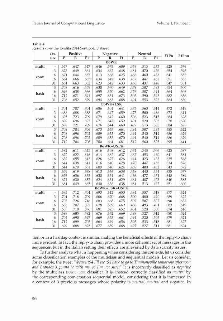
86
Italian Journal of Computational Linguistics Volume 1, Number 1
Table 4Results over the Evalita 2014 Sentipolc Dataset.
Ctx. Positive Negative Neutral F1Pn F1Pnnsize P R F1 P R F1 P R F1
BoWKmulti - .647 .647 .647 .646 .575 .609 .439 .513 .473 .628 .576
conv
3 .673 .649 .661 .634 .662 .648 .481 .470 .476 .654 .5956 .671 .644 .657 .613 .638 .625 .466 .460 .463 .641 .582
16 .664 .666 .665 .634 .642 .638 .457 .447 .452 .651 .58531 .661 .663 .662 .623 .642 .633 .460 .437 .448 .647 .581
hash
3 .708 .616 .659 .630 .670 .649 .479 .507 .493 .654 .6006 .696 .638 .666 .655 .670 .662 .476 .507 .491 .664 .606
16 .712 .671 .691 .697 .651 .673 .503 .590 .543 .682 .63631 .708 .652 .679 .694 .683 .688 .494 .553 .522 .684 .630
BoWK+LSKmulti - .701 .707 .704 .686 .601 .641 .475 .560 .514 .672 .619
conv
3 .688 .688 .688 .671 .647 .659 .473 .500 .486 .673 .6116 .695 .723 .709 .679 .642 .660 .506 .523 .515 .684 .628
16 .698 .696 .697 .671 .647 .659 .491 .520 .505 .678 .62031 .698 .721 .709 .676 .644 .660 .497 .513 .505 .684 .625
hash
3 .708 .704 .706 .673 .655 .664 .484 .507 .495 .685 .6226 .708 .696 .702 .689 .653 .670 .491 .540 .514 .686 .629
16 .708 .696 .702 .689 .653 .670 .491 .540 .514 .686 .62931 .712 .704 .708 .700 .664 .681 .512 .560 .535 .695 .641
BoWK+USPKmulti - .682 .611 .645 .616 .608 .612 .474 .543 .506 .628 .587
conv
3 .672 .622 .646 .614 .662 .637 .467 .453 .460 .641 .5816 .632 .655 .643 .626 .627 .626 .444 .423 .433 .635 .568
16 .644 .638 .641 .616 .640 .628 .470 .447 .458 .634 .57631 .644 .679 .661 .609 .640 .624 .469 .400 .432 .643 .572
hash
3 .659 .619 .638 .613 .666 .638 .468 .440 .454 .638 .5776 .676 .636 .655 .630 .651 .641 .466 .477 .471 .648 .589
16 .674 .630 .652 .624 .634 .629 .461 .487 .473 .640 .58531 .681 .649 .665 .640 .636 .638 .481 .513 .497 .651 .600
BoWK+LSK+USPKmulti - .695 .712 .704 .693 .612 .650 .484 .557 .518 .677 .624
conv
3 .701 .718 .709 .666 .670 .668 .500 .480 .490 .689 .6226 .707 .726 .716 .683 .668 .675 .507 .507 .507 .696 .633
16 .688 .707 .697 .678 .659 .669 .488 .493 .491 .683 .61931 .683 .710 .696 .681 .625 .652 .481 .520 .500 .674 .616
hash
3 .698 .685 .692 .676 .662 .669 .498 .527 .512 .680 .6246 .704 .690 .697 .669 .653 .661 .491 .520 .505 .679 .621
16 .712 .699 .705 .664 .649 .656 .503 .533 .518 .681 .62731 .699 .688 .693 .677 .659 .668 .497 .527 .511 .681 .624
tion or in a hashtag context is similar, making the beneficial effects of the reply-to chainmore evident. In fact, the reply-to chain provides a more coherent set of messages in thesequences, but in the Italian setting their effects are alleviated by data scarcity issues.
To further analyze what is happening when considering the contexts, let us considersome classification examples of the multiclass and sequential models. Let us consider,for example, the tweet “@cewitt94 I’ll see :S I have to go to Timmonsville tomorrow afternoonand Brandon’s gonna be with me, so I’m not sure.” It is incorrectly classified as negativeby the multiclass BOWK+LSK classifier. It is, instead, correctly classified as neutral bythe corresponding conversation sequential model, considering that it is immersed ina context of 3 previous messages whose polarity is neutral, neutral and negative. In
87
Castellucci et al. Context-aware Models for Twitter Sentiment Analysis
order to further show the importance of the context, let us consider the positive message“@arrington Noticed that joke when you interviewed Reid Hoffman. Better the 2nd time around;)”. It is characterized only by a conversation context, while it has no hashtag. In thiscase, the hashtag based classifier BOWK+LSK predicts a wrong class for that message, i.e.negative. The conversation context contains another message whose class is annotatedas positive: “This is by far the biggest TechCrunch Disrupt ever with 3,600 attendees. Clearlythey’re completely falling apart without me :-)”. The conversation-based classifier withBOWK+LSK observations is thus able to exploit the contextual information to correctlypredict the positive class. In the Italian setting we observe similar outcomes. Let usconsider the message “@fioryrus ti do il numero in dm? :)”. This message seems neutral(despite of the smile), and the BOWK+LSK multiclassifier predicts such polarity label.In reality this message belongs to a context of 3 messages whose polarity is neutral,neutral and positive. The preceding positive message of the target one is thus informingthe sequential classifier that, probably, the target message is positive as well.
5. Conclusions
In this work, the role of contextual information in supervised Sentiment Analysis overTwitter is investigated for two different languages, English and Italian. While the taskis eminently linguistic, as resources and phenomena lie in the textual domain, othersemantic dimensions are worth to be explored. In this work, three types of contexts fora target tweet have been studied. A markovian approach has been adopted to injectcontextual evidence (e.g. the history of preceding posts) in the classification of the mostrecent, i.e. a target, tweet. An improvement of accuracy in the investigated tasks ismeasured. It is a straightforward result as the approach is free of language specific re-sources or manually engineered features. The different employed contexts show specificbut systematic benefits. In these experiments, users have only been partially exploredthrough the USPK. It seems to express a more static notion of context (i.e. the attitudeof the user as observed across a longer period than individual conversations).
Future work will concentrate on the exploration of more sophisticated user models,whose contribution is expected to improve the overall impact. The user sentimentprofile adopted in this work, through the USPK similarity, is in fact a first approximationin the direction of exploiting user information during training. Here, we analyzedmessages without considering any existing sentiment resource. It could be interesting toadopt a polarity lexicon, e.g. (Mohammad and Turney 2010) or (Castellucci, Croce, andBasili 2015), to strengthen the final system within a context based framework. Moreover,this work explores a notion of context restricted to simple tweet sequences. In SocialNetworks, information flows according to richer structures, e.g. graph of messages andusers: a user is exposed to messages whose streams in the community are very complex,i.e. not linear. Graph-based models of the context are appealing, as they provide moreexpressive ways to represent the messages and (other) users influencing the writer. Thisis an interesting direction to be further explored.
ReferencesAgarwal, Apoorv, Fadi Biadsy, and Kathleen R. Mckeown. 2009. Contextual phrase-level polarity
analysis using lexical affect scoring and syntactic n-grams. In Proceedings of the 12th Conferenceof the EACL, pages 24–32. Association for Computational Linguistics.
Agarwal, Apoorv, Boyi Xie, Ilia Vovsha, Owen Rambow, and Rebecca Passonneau. 2011.Sentiment analysis of twitter data. In Proceedings of the Workshop on Languages in Social Media,LSM ’11, pages 30–38, Stroudsburg, PA, USA. Association for Computational Linguistics.
88
Italian Journal of Computational Linguistics Volume 1, Number 1
Altun, Y., I. Tsochantaridis, and T. Hofmann. 2003. Hidden Markov support vector machines. InProceedings of ICML, pages 3–10.
Barbosa, Luciano and Junlan Feng. 2010. Robust sentiment detection on twitter from biased andnoisy data. In Chu-Ren Huang and Dan Jurafsky, editors, COLING (Posters), pages 36–44.Chinese Information Processing Society of China.
Basile, Valerio, Andrea Bolioli, Malvina Nissim, Viviana Patti, and Paolo Rosso. 2014. Overviewof the evalita 2014 sentiment polarity classification task. In Proc. of the 4th EVALITA, pages50–57.
Basili, Roberto, Maria Teresa Pazienza, and Fabio Massimo Zanzotto. 1998. Efficient parsing forinformation extraction. In Proc. of the European Conference on Artificial Intelligence, pages135–139.
Bengio, Yoshua, Réjean Ducharme, Pascal Vincent, and Christian Janvin. 2003. A neuralprobabilistic language model. J. Mach. Learn. Res., 3:1137–1155, March.
Bifet, Albert and Eibe Frank. 2010. Sentiment knowledge discovery in twitter streaming data. InProceedings of the 13th International Conference on Discovery Science, DS’10, pages 1–15, Berlin,Heidelberg. Springer-Verlag.
Castellucci, Giuseppe, Danilo Croce, and Roberto Basili. 2015. Acquiring a large scale polaritylexicon through unsupervised distributional methods. In Chris Biemann, SiegfriedHandschuh, Andrè Freitas, Farid Meziane, and Elisabeth Mètais, editors, Natural LanguageProcessing and Information Systems, volume 9103. Springer International Publishing, pages73–86.
Castellucci, Giuseppe, Danilo Croce, Diego De Cao, and Roberto Basili. 2014. A multiple kernelapproach for twitter sentiment analysis in italian. In 4th International Workshop EVALITA 2014,pages 98–103.
Cristianini, Nello, John Shawe-Taylor, and Huma Lodhi. 2002. Latent semantic kernels. J. Intell.Inf. Syst., 18(2-3):127–152, March.
Croce, Danilo and Roberto Basili. 2012. Grammatical feature engineering for fine-grained irtasks. In Giambattista Amati, Claudio Carpineto, and Giovanni Semeraro, editors, IIR, volume835 of CEUR Workshop Proceedings, pages 133–143. CEUR-WS.org.
Croce, Danilo, Cristina Giannone, Paolo Annesi, and Roberto Basili. 2010. Towards open-domainsemantic role labeling. In Proceedings of the 48th Annual Meeting of the Association forComputational Linguistics, pages 237–246. Association for Computational Linguistics.
Davidov, Dmitry, Oren Tsur, and Ari Rappoport. 2010. Enhanced sentiment learning usingtwitter hashtags and smileys. In Chu-Ren Huang and Dan Jurafsky, editors, COLING (Posters),pages 241–249. Chinese Information Processing Society of China.
Fan, Rong-En, Kai-Wei Chang, Cho-Jui Hsieh, Xiang-Rui Wang, and Chih-Jen Lin. 2008.Liblinear: A library for large linear classification. Journal of Machine Learning Research,9:1871–1874.
Filice, Simone, Giuseppe Castellucci, Danilo Croce, and Roberto Basili. 2015. Kelp: a kernel-basedlearning platform for natural language processing. In Proceedings of ACL2015: SystemDemonstrations, pages 19–24, Beijing, China, July. Association for Computational Linguistics.
Go, Alec, Richa Bhayani, and Lei Huang. 2009. Twitter sentiment classification using distantsupervision. Processing, pages 1–6.
Hu, Minqing and Bing Liu. 2004. Mining and summarizing customer reviews. In Proceedings ofthe Tenth ACM SIGKDD International Conference on Knowledge Discovery and Data Mining, KDD’04, pages 168–177, New York, NY, USA. ACM.
Kim, Soo-Min and Eduard Hovy. 2004. Determining the sentiment of opinions. In Proceedings ofthe 20th International Conference on Computational Linguistics, COLING ’04, pages 1367–1374,Stroudsburg, PA, USA. Association for Computational Linguistics.
Kiritchenko, Svetlana, Xiaodan Zhu, and Saif M. Mohammad. 2014. Sentiment analysis of shortinformal texts. JAIR, 50:723–762, Aug.
Kouloumpis, Efthymios, Theresa Wilson, and Johanna Moore. 2011. Twitter sentiment analysis:The good the bad and the omg! In Lada A. Adamic, Ricardo A. Baeza-Yates, and Scott Counts,editors, ICWSM, pages 538–541. The AAAI Press.
Mikolov, Tomas, Kai Chen, Greg Corrado, and Jeffrey Dean. 2013. Efficient estimation of wordrepresentations in vector space. CoRR, abs/1301.3781.
Mitchell, Jeff and Mirella Lapata. 2010. Composition in distributional models of semantics.Cognitive Science, 34(8):1388–1429.
89
Castellucci et al. Context-aware Models for Twitter Sentiment Analysis
Mohammad, Saif M. and Peter D. Turney. 2010. Emotions evoked by common words andphrases: Using mechanical turk to create an emotion lexicon. In Proceedings of CAAGETWorkshop, pages 26–34.
Mukherjee, Subhabrata and Pushpak Bhattacharyya. 2012. Sentiment analysis in twitter withlightweight discourse analysis. In Proceedings of COLING, pages 1847–1864.
Nakov, Preslav, Sara Rosenthal, Zornitsa Kozareva, Veselin Stoyanov, Alan Ritter, and TheresaWilson. 2013. Semeval-2013 task 2: Sentiment analysis in twitter. In Proceedings of the SemEval2013, pages 312–320, Atlanta, Georgia, USA, June. Association for Computational Linguistics.
Pak, Alexander and Patrick Paroubek. 2010. Twitter as a corpus for sentiment analysis andopinion mining. In Proceedings of the Seventh conference on International Language Resources andEvaluation (LREC’10), pages 1320–1326, Valletta, Malta. European Language ResourcesAssociation (ELRA).
Pang, Bo and Lillian Lee. 2004. A sentimental education: Sentiment analysis using subjectivitysummarization based on minimum cuts. In Proceedings of ACL2004, ACL ’04, pages 271–279,Stroudsburg, PA, USA. Association for Computational Linguistics.
Pang, Bo and Lillian Lee. 2008. Opinion mining and sentiment analysis. Found. Trends Inf. Retr.,2(1-2):1–135, January.
Pang, Bo, Lillian Lee, and Shivakumar Vaithyanathan. 2002. Thumbs up? sentiment classificationusing machine learning techniques. In Proceedings of EMNLP, pages 79–86.
Pennacchiotti, Marco, Diego De Cao, Roberto Basili, Danilo Croce, and Michael Roth. 2008.Automatic induction of framenet lexical units. In Proceedings of EMNLP2008, pages 457–465.Association for Computational Linguistics.
Rifkin, Ryan and Aldebaro Klautau. 2004. In defense of one-vs-all classification. J. Mach. Learn.Res., 5:101–141, December.
Rosenthal, Sara, Alan Ritter, Preslav Nakov, and Veselin Stoyanov. 2014. Semeval-2014 task 9:Sentiment analysis in twitter. In Proc. SemEval, pages 73–80. ACL and Dublin City University.
Sahlgren, Magnus. 2006. The Word-Space Model. Ph.D. thesis, Stockholm University.Shawe-Taylor, John and Nello Cristianini. 2004. Kernel Methods for Pattern Analysis. Cambridge
University Press, New York, NY, USA.Si, Jianfeng, Arjun Mukherjee, Bing Liu, Qing Li, Huayi Li, and Xiaotie Deng. 2013. Exploiting
topic based twitter sentiment for stock prediction. In ACL (2), pages 24–29.Speriosu, Michael, Nikita Sudan, Sid Upadhyay, and Jason Baldridge. 2011. Twitter polarity
classification with label propagation over lexical links and the follower graph. In Proceedings ofthe First Workshop on Unsupervised Learning in NLP, EMNLP ’11, pages 53–63, Stroudsburg, PA,USA. Association for Computational Linguistics.
Talukdar, Partha Pratim and Koby Crammer. 2009. New regularized algorithms for transductivelearning. In Proceedings of the European Conference on Machine Learning and Knowledge Discoveryin Databases: Part II, ECML PKDD ’09, pages 442–457, Berlin, Heidelberg. Springer-Verlag.
Tan, Chenhao, Lillian Lee, Jie Tang, Long Jiang, Ming Zhou, and Ping Li. 2011. User-levelsentiment analysis incorporating social networks. In Proc. of the 17th International Conference onKnowledge Discovery and Data Mining, pages 1397–1405, New York, NY, USA. ACM.
Turney, Peter D. 2002. Thumbs up or thumbs down?: Semantic orientation applied tounsupervised classification of reviews. In Proceedings of the 40th Annual Meeting on Associationfor Computational Linguistics, ACL ’02, pages 417–424, Stroudsburg, PA, USA. Association forComputational Linguistics.
Vanzo, Andrea, Giuseppe Castellucci, Danilo Croce, and Roberto Basili. 2014. A context basedmodel for sentiment analysis in twitter for the italian language. In First Italian Conference onComputational Linguistics CLiC-it, volume 1, pages 379–383.
Vanzo, Andrea, Danilo Croce, and Roberto Basili. 2014. A context-based model for sentimentanalysis in twitter. In Proc. of 25th COLING, pages 2345–2354. Dublin City University andAssociation for Computational Linguistics.
Vapnik, Vladimir N. 1998. Statistical Learning Theory. Wiley-Interscience.Wilson, Theresa, Janyce Wiebe, and Paul Hoffmann. 2005. Recognizing contextual polarity in
phrase-level sentiment analysis. In Proceedings of the Conference on Human Language Technologyand Empirical Methods in Natural Language Processing, HLT ’05, pages 347–354, Stroudsburg, PA,USA. Association for Computational Linguistics.
Zanzotto, Fabio M., Marco Pennaccchiotti, and Kostas Tsioutsiouliklis. 2011. LinguisticRedundancy in Twitter. In Proc. of EMNLP, pages 659–669, Edinburgh, Scotland, UK., July.

91
Geometric and Statistical Analysis of Emotionsand Topics in Corpora
Francesco Tarasconi ∗
CELI S.R.L.Vittorio Di Tomaso ∗∗
CELI S.R.L.
NLP techniques can enrich unstructured textual data, detecting topics of interest and emotions.The task of understanding emotional similarities between different topics is crucial, for example,in analyzing the Social TV landscape. A measure of how much two audiences share the samefeelings is required, but also a sound and compact representation of these similarities. Afterevaluating different multivariate approaches, we achieved these goals by applying MultipleCorrespondence Analysis (MCA) techniques to our data. In this paper we provide backgroundinformation and methodological reasons to our choice. MCA is especially suitable to ana-lyze categorical data and detect the main contrasts among them: NLP-annotated data canbe transformed and adapted to this framework. We briefly introduce the semantic annotationpipeline used in our study and provide examples of Social TV analysis, performed on Twitterdata collected between October 2013 and February 2014. The benefits of examining emotionsshared in social media using multivariate statistical techniques are highlighted: using additionaldimensions, instead of "simple" polarity of documents, allows to detect more subtle differencesin the reactions to certain shows.
1. Introduction
Classification of documents based on topics of interest is a popular NLP research area (see, forexample, Hamamoto et al. (2005)). Another important subject, especially in the context of Web2.0 and social media, is the sentiment analysis, mainly meant to detect polarities of expressionsand opinions (Liu 2012). Sentiment Analysis (SA) is both a topic in natural language processingwhich has been investigated for several years and a tool for social media monitoring which isused in business services. A recent survey that explores the latest trends is Cambria (2013).While the first attempts on English texts date back to the late 90s, SA on Italian texts is a morerecent area of research (probably the first scientific publication is Dini and Mazzini (2012)). Asentiment analysis task which has seen less contributions, but of growing popularity, is the studyof emotions (Wiebe et al. 2005), which requires introducing and analyzing multiple variables(appropriate "emotional dimensions") potentially correlated. This is especially important in thestudy of the so-called Social TV (Cosenza 2012): people can share their TV experience with otherviewers on social media using smartphones and tablets. We define the empirical distribution ofdifferent emotions among viewers of a specific TV show as its emotional profile. Comparing atthe same time the emotional profiles of several formats requires appropriate descriptive statisticaltechniques. During the research we conducted, we evaluated and selected geometrical methodsthat satisfy these requirements and provide an easy to understand and coherent representation ofthe results. The methods we used can be applied to any dataset of documents classified based on
∗ Via San Quintino 31 - 10121 Torino, Italia. E-mail: [email protected].∗∗ Via San Quintino 31 - 10121 Torino, Italia. E-mail: [email protected].
© 2015 Associazione Italiana di Linguistica Computazionale
92
Italian Journal of Computational Linguistics Volume 1, Number 1
topics and emotions; they also represent a potential tool for the quantitative analysis of any NLPannotated data.We used the BlogMeter platform1 to download and process textual contents from social networks(Bolioli et al. 2013). Topics correspond to TV programs discussed on Twitter. Nine emotions aredetected: the basic six according to Ekman (1972) (anger, disgust, fear, joy, sadness, surprise),love (a primary one in Parrot’s classification) and like/dislike expressions, quite common onTwitter.Topics and emotions are detected using a rule-based system. In the case of TV episodes, themention of a show or its characters in the context of a tweet is the most important factor inassigning it to a specific topic. To improve precision in identifying posts connected to the SocialTV, the temporal range of analysis can be reduced to a set of windows centered around relevantepisodes.We examined the emotional landscape of the Italian Social TV during December 2013, treatingeach show as a different topic. The analysis evidenced a strong negative mood associated withpolitics and the programs that tackled this subject. We then focused on two popular formats:the music talent show X Factor and the competitive cooking show MasterChef. Each episodewas considered as a different topic. Whereas the progression of the season through emotionalphases (from selections to finals) was clearly visible in the case of X Factor, MasterChef wasmuch more erratic and strongly influenced by scripted events taking place in each episode. Bycomparing directly X Factor and MasterChef in the same analysis, we concluded that the subjectof the show strongly influences the reactions of its viewers, in a way that goes beyond the simpleexpression of positive/negative judgements. This supports the claim that the analysis of emotionscan provide additional information and detect deeper differences than polarity in the study ofsocial media.The paper is organized as follows: section 2 describes the tools used for topic and emotiondetection, section 3 introduces the mathematical model used to analyze NLP-annotated data,section 4 focuses on the choice of statistical methods adopted to represent and extract the mostrelevant structures in our datasets and section 5 presents the case studies.This research was originally presented in reduced form at CLiC 2014, the First Italian Conferenceon Computational Linguistics.
2. A social media monitoring platform
The processing tools which we will describe are implemented in a social media monitoringservice called BlogMeter, operating since 2009. The monitoring process includes three mainphases:
� Listening: thanks to purpose-developed data acquisition systems, the platform detects andcollects from the web potentially interesting data;� Understanding: a semantic engine is used to structure and classify the conversations inaccordance to the defined drivers (topics and entities mentioned in the texts, but alsoemotions of interest);� Analysis: through the analysis platform the user can navigate the conversations in astructured way, aggregate the drivers in one or more dashboards, discover unforeseentrends in the concept clouds and drill down the data to read the messages inside theiroriginal context.
1 www.blogmeter.it
93
Tarasconi and Di Tomaso Geometric and Statistical Analysis of Emotions and Topics in Corpora
It is of particular interest for our research the understanding phase, which includes automaticclassification and sentiment analysis. It can be further divided into:
� creation of a domain-based taxonomy (i.e. an ontology of topics such as brands, productsor people);� identification and automatic classification of relevant documents (according to the taxon-omy);� polarity and emotion detection.
The monitored sources are typically user-generated media, such as blogs, forums, social net-works, news groups, content sharing sites, sites of questions and answers (Q&A), reviews ofproducts / services, which are active in many countries and in different languages. The overallnumber of sources is more than 500,000 blogs (of which approximately 70,000 active, with apost in the last three months) and 700 gathering places (forums, newsgroups, Q&A sites, contentsharing platforms, social networks). This computation considers Facebook and Twitter as singlesources, but in fact, they are the largest collectors of conversations.
2.1 Semantic annotation pipeline
Documents extracted from the web in the form of unstructured information are made availableto the semantic annotation pipeline which analyzes and classifies them according to the domain-based taxonomies defined for the client. The annotation pipeline uses the UIMA framework (theUnstructured Information Management Architecture originally developed by IBM and now bythe Apache Software Foundation 2).UIMA annotators enrich the documents in terms of linguistic information, recognition of entitiesand concepts, identification of relations between concepts, entities and attitudes expressed in thetext (opinions, mood states and emotions). Some linguistic resources and annotators are commonto different application domains, while others are domain dependent. We will not describe herethe pipeline modules in details, and we will focus on the main linguistic resource used in thesentiment analysis module, i.e. a concept-level sentiment lexicon for Italian.The sentiment lexicon is used by the semantic annotator, which recognizes opinions and ex-pressions of mood and emotions and associates them with the opinion targets. This componentoperates both on the sentence level (in order to treat linguistic phenomena such as negation andquantification) and on the document leve (in order to identify relations between elements that arein different sentences).
2.2 A concept-level sentiment lexicon for Italian
In this section we describe the sentiment lexicon used by the semantic annotator, i.e. the reposi-tory containing terms, concepts and patterns used in the sentiment annotation. Researchers havebeen building sentiment lexica for many years, in particular for the English language, and areview on recent results can be found for example in Cambria et al. (2013). The sentiment lexiconfor Italian contains about 10.000 entries (6.200 single words and 3.400 multi-word expressions).Each entry has information about sentiment, i.e. polarity, emotions, and domain application(therefore it is a contextualized sentiment lexicon). It has been created and updated during thepast three years, performing social media monitoring and SA in different application domains.An important resource used in the creation of the lexicon is the WordNet-Affect project (Strap-parava and Valitutti 2004).
2 UIMA Specifications: http://uima.apache.org/uima-specification.html

94
Italian Journal of Computational Linguistics Volume 1, Number 1
One aspect worth mentioning is that the valence of many words can change in different contextsand domains. The word "accuratezza" ("accuracy"), for example, has a default positive valence,just as it is for "affare d’oro" ("to do a roaring trade"). On the contrary, "andare a casa" ("goinghome") has no polarity in a neutral context, as long as it is not used in an area such as sentimenton Sanremo Festival, where it means instead being eliminated from the singing competition.Similarly, "truccato" ("to have make up on" or "to be rigged"), would not have negative polarityif the domain was a fashion show. Instead, in the field of online games or betting, the perspectivechanges.
2.3 Emotions
The interest for emotion detection in social media monitoring grew in 2011 after the publicationof a paper by Bollen et al. (2011), where the authors argued that the analysis of mood in Twitterposts could be used to predict stock market movements up to 6 days in advance. In particular,they identified "calmness" as the predictive mood dimension, within a set of 6 different mooddimensions (happiness, kindness, alertness, sureness, vitality and calmness). The definition ofa set of basic (or primary) emotions is a debated topic, and the study and analysis of emotionsand their expression in texts obviously has a long tradition in philosophy and psychology (seefor example Galati (2002)). In NLP tasks, Ekman’s six basic emotions (anger, disgust, fear, joy,sadness, surprise) have often been used (e.g. in Strapparava and Valitutti (2004)). The platformwe employed in our research adopts Ekman’s list of emotions and "love", which is a primaryemotion in Parrot’s classification. Considering expressions of "like" and "dislike" as "emotional"was necessary to cover a large amount of social media documents, which clearly express a feelingtowards a subject being discussed, but not an emotion in the common sense.A similar approach is described in Roberts et al. (2012).An argument could be made against adding arbitrary variables to a pre-existing model of basicemotions. However, from the perspective of an exploratory analysis of an unknown dataset, thesevariables can better capture specific features in social network communication. The issue ofadding potentially correlated or even redundant variables is tackled in the dimension reductionframework we will define and employ in the following sections.The manual annotation of emotions in a reference Italian corpus would be a useful advance fortesting the accuracy of the automatic system.
2.4 Evaluation
The sentiment semantic annotator was partially evaluated on polarity classification of Twittermessages (with a focus on politics), which was conducted using the Evalita 2014 SENTIPOLCtest set. As reported in Basile et al. (2014) it’s a collection of 1,935 tweets derived from existingcorpora: SENTI-TUT (Bosco et al. 2013) and TWITA (Basile and Nissim 2013).We performed two runs of the analysis procedure: the first using only a generic lexicon, thesecond using a lexicon enriched specifically for the political domain. Both are pre-existingresources compared to the train and test set used for the SENTIPOLC task, which were notincluded in the creation of the lexicons.Precision P, recall R and F-score were computed for the positive and negative predicted fields,separately for the different values that the field can assume (0 and 1). An average F-scorefor positive and negative polarities was then computed to calculate the final F-score F for theSENTIPOLC task. These metrics can be compared to the results achieved by the Evalita 2014participants. Results for the CELI pipeline are given in Table 1. Our results are given for differentlexicons used (generic/political).
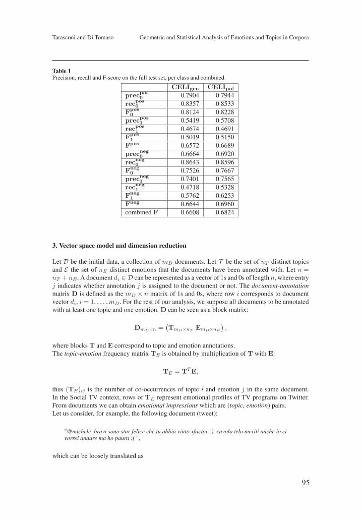
95
Tarasconi and Di Tomaso Geometric and Statistical Analysis of Emotions and Topics in Corpora
Table 1Precision, recall and F-score on the full test set, per class and combined
CELIgen CELIpol
precpos0 0.7904 0.7944
recpos0 0.8357 0.8533
Fpos0 0.8124 0.8228
precpos1 0.5419 0.5708
recpos1 0.4674 0.4691
Fpos1 0.5019 0.5150
Fpos 0.6572 0.6689precneg0 0.6664 0.6920recneg0 0.8643 0.8596Fneg
0 0.7526 0.7667precneg1 0.7401 0.7565recneg1 0.4718 0.5328Fneg
1 0.5762 0.6253Fneg 0.6644 0.6960combined F 0.6608 0.6824
3. Vector space model and dimension reduction
Let D be the initial data, a collection of mD documents. Let T be the set of nT distinct topicsand E the set of nE distinct emotions that the documents have been annotated with. Let n =nT + nE . A document di ∈ D can be represented as a vector of 1s and 0s of length n, where entryj indicates whether annotation j is assigned to the document or not. The document-annotationmatrix D is defined as the mD × n matrix of 1s and 0s, where row i corresponds to documentvector di, i = 1, . . . ,mD. For the rest of our analysis, we suppose all documents to be annotatedwith at least one topic and one emotion. D can be seen as a block matrix:
DmD×n =(TmD×nT
EmD×nE
),
where blocks T and E correspond to topic and emotion annotations.The topic-emotion frequency matrix TE is obtained by multiplication of T with E:
TE = TTE,
thus (TE)ij is the number of co-occurrences of topic i and emotion j in the same document.In the Social TV context, rows of TE represent emotional profiles of TV programs on Twitter.From documents we can obtain emotional impressions which are (topic, emotion) pairs.Let us consider, for example, the following document (tweet):
"@michele_bravi sono star felice che tu abbia vinto xfactor :), cavolo telo meriti anche io civorrei andare ma ho paura :( ",
which can be loosely translated as
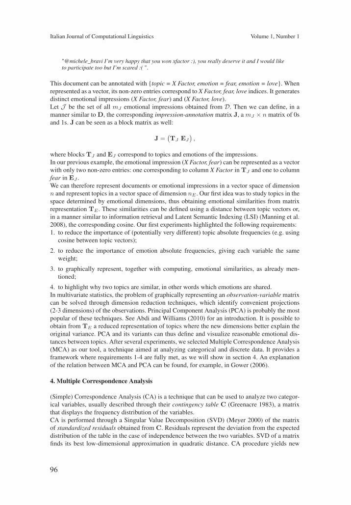
96
Italian Journal of Computational Linguistics Volume 1, Number 1
"@michele_bravi I’m very happy that you won xfactor :), you really deserve it and I would liketo participate too but I’m scared :( ".
This document can be annotated with {topic = X Factor, emotion = fear, emotion = love}. Whenrepresented as a vector, its non-zero entries correspond to X Factor, fear, love indices. It generatesdistinct emotional impressions (X Factor, fear) and (X Factor, love).Let J be the set of all mJ emotional impressions obtained from D. Then we can define, in amanner similar to D, the corresponding impression-annotation matrix J, a mJ × n matrix of 0sand 1s. J can be seen as a block matrix as well:
J =(TJ EJ
),
where blocks TJ and EJ correspond to topics and emotions of the impressions.In our previous example, the emotional impression (X Factor, fear) can be represented as a vectorwith only two non-zero entries: one corresponding to column X Factor in TJ and one to columnfear in EJ .We can therefore represent documents or emotional impressions in a vector space of dimensionn and represent topics in a vector space of dimension nE . Our first idea was to study topics in thespace determined by emotional dimensions, thus obtaining emotional similarities from matrixrepresentation TE . These similarities can be defined using a distance between topic vectors or,in a manner similar to information retrieval and Latent Semantic Indexing (LSI) (Manning et al.2008), the corresponding cosine. Our first experiments highlighted the following requirements:1. to reduce the importance of (potentially very different) topic absolute frequencies (e.g. using
cosine between topic vectors);
2. to reduce the importance of emotion absolute frequencies, giving each variable the sameweight;
3. to graphically represent, together with computing, emotional similarities, as already men-tioned;
4. to highlight why two topics are similar, in other words which emotions are shared.In multivariate statistics, the problem of graphically representing an observation-variable matrixcan be solved through dimension reduction techniques, which identify convenient projections(2-3 dimensions) of the observations. Principal Component Analysis (PCA) is probably the mostpopular of these techniques. See Abdi and Williams (2010) for an introduction. It is possible toobtain from TE a reduced representation of topics where the new dimensions better explain theoriginal variance. PCA and its variants can thus define and visualize reasonable emotional dis-tances between topics. After several experiments, we selected Multiple Correspondence Analysis(MCA) as our tool, a technique aimed at analyzing categorical and discrete data. It provides aframework where requirements 1-4 are fully met, as we will show in section 4. An explanationof the relation between MCA and PCA can be found, for example, in Gower (2006).
4. Multiple Correspondence Analysis
(Simple) Correspondence Analysis (CA) is a technique that can be used to analyze two categor-ical variables, usually described through their contingency table C (Greenacre 1983), a matrixthat displays the frequency distribution of the variables.CA is performed through a Singular Value Decomposition (SVD) (Meyer 2000) of the matrixof standardized residuals obtained from C. Residuals represent the deviation from the expecteddistribution of the table in the case of independence between the two variables. SVD of a matrixfinds its best low-dimensional approximation in quadratic distance. CA procedure yields new
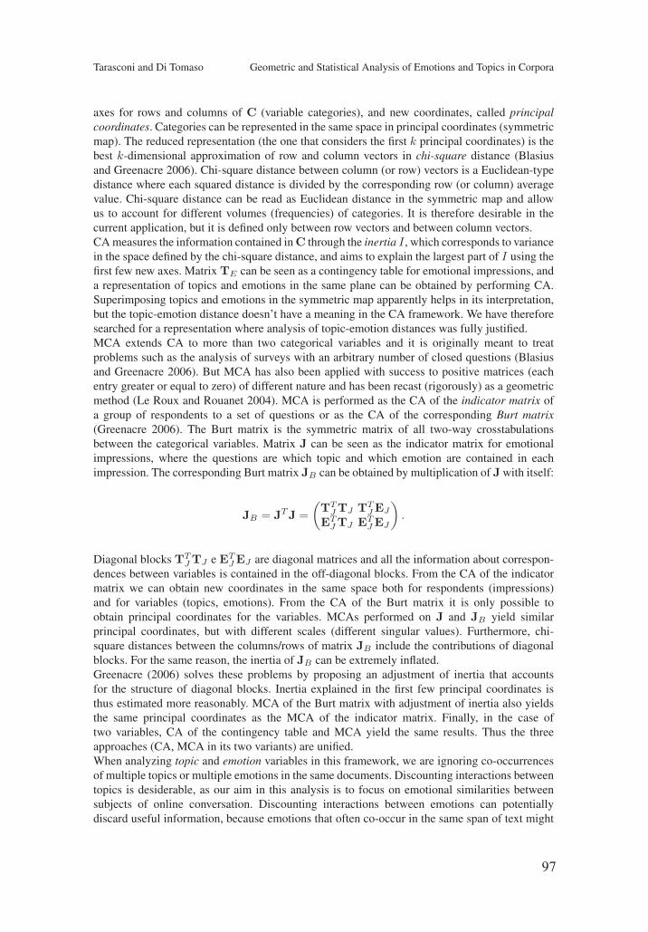
97
Tarasconi and Di Tomaso Geometric and Statistical Analysis of Emotions and Topics in Corpora
axes for rows and columns of C (variable categories), and new coordinates, called principalcoordinates. Categories can be represented in the same space in principal coordinates (symmetricmap). The reduced representation (the one that considers the first k principal coordinates) is thebest k-dimensional approximation of row and column vectors in chi-square distance (Blasiusand Greenacre 2006). Chi-square distance between column (or row) vectors is a Euclidean-typedistance where each squared distance is divided by the corresponding row (or column) averagevalue. Chi-square distance can be read as Euclidean distance in the symmetric map and allowus to account for different volumes (frequencies) of categories. It is therefore desirable in thecurrent application, but it is defined only between row vectors and between column vectors.CA measures the information contained in C through the inertia I , which corresponds to variancein the space defined by the chi-square distance, and aims to explain the largest part of I using thefirst few new axes. Matrix TE can be seen as a contingency table for emotional impressions, anda representation of topics and emotions in the same plane can be obtained by performing CA.Superimposing topics and emotions in the symmetric map apparently helps in its interpretation,but the topic-emotion distance doesn’t have a meaning in the CA framework. We have thereforesearched for a representation where analysis of topic-emotion distances was fully justified.MCA extends CA to more than two categorical variables and it is originally meant to treatproblems such as the analysis of surveys with an arbitrary number of closed questions (Blasiusand Greenacre 2006). But MCA has also been applied with success to positive matrices (eachentry greater or equal to zero) of different nature and has been recast (rigorously) as a geometricmethod (Le Roux and Rouanet 2004). MCA is performed as the CA of the indicator matrix ofa group of respondents to a set of questions or as the CA of the corresponding Burt matrix(Greenacre 2006). The Burt matrix is the symmetric matrix of all two-way crosstabulationsbetween the categorical variables. Matrix J can be seen as the indicator matrix for emotionalimpressions, where the questions are which topic and which emotion are contained in eachimpression. The corresponding Burt matrix JB can be obtained by multiplication of J with itself:
JB = JTJ =
(TT
JTJ TTJEJ
ETJTJ ET
JEJ
).
Diagonal blocks TTJTJ e ET
JEJ are diagonal matrices and all the information about correspon-dences between variables is contained in the off-diagonal blocks. From the CA of the indicatormatrix we can obtain new coordinates in the same space both for respondents (impressions)and for variables (topics, emotions). From the CA of the Burt matrix it is only possible toobtain principal coordinates for the variables. MCAs performed on J and JB yield similarprincipal coordinates, but with different scales (different singular values). Furthermore, chi-square distances between the columns/rows of matrix JB include the contributions of diagonalblocks. For the same reason, the inertia of JB can be extremely inflated.Greenacre (2006) solves these problems by proposing an adjustment of inertia that accountsfor the structure of diagonal blocks. Inertia explained in the first few principal coordinates isthus estimated more reasonably. MCA of the Burt matrix with adjustment of inertia also yieldsthe same principal coordinates as the MCA of the indicator matrix. Finally, in the case oftwo variables, CA of the contingency table and MCA yield the same results. Thus the threeapproaches (CA, MCA in its two variants) are unified.When analyzing topic and emotion variables in this framework, we are ignoring co-occurrencesof multiple topics or multiple emotions in the same documents. Discounting interactions betweentopics is desiderable, as our aim in this analysis is to focus on emotional similarities betweensubjects of online conversation. Discounting interactions between emotions can potentiallydiscard useful information, because emotions that often co-occur in the same span of text might
98
Italian Journal of Computational Linguistics Volume 1, Number 1
Figure 1MCA of most emotional Italian TV programs discussed on Twitter during December 2013.
be considered closer in an ideal emotional space (for example love and joy). However, the amountof tweets that contain more than one annotation of type emotion is very small (less than 1% inthe considered datasets). Moving to the analysis of emotional impressions allows us to adoptthe MCA framework and, in particular, to better estimate the explained inertia of our dataset:considering interactions between emotion variables would instead change the structure of onediagonal block in the Burt matrix and the adjustment proposed by Greenacre could not be applied.MCA offers possibilities common to other multivariate techniques. In particular, a measure onhow well single topics and emotions are represented in the retained axes is provided (quality ofrepresentation).Symmetric treatment of topics and emotions facilitates the interpretation of axes. Distancesbetween emotions and topics can now be interpreted and, thanks to them, it is possible toestablish why two topics are close in the reduced representation. An additional (and interesting)interpretation of distances between categories in terms of sub-clouds of individuals (impressions)is provided by Le Roux and Rouanet (2004).
5. Case studies
5.1 One month of Twitter TV
Data were collected during December 2013 (1,2 million tweets). Tweets were aggregated togenerate monthly TV show profiles. We selected the 15 "most emotional" shows to analyze. MCAwas performed using programs and emotions as variables in a vector space model as describedin sections 3 and 4. Results are shown in Figure 1. Size of programs’ points is proportional to thenumber of distinct emotional impressions for that category. As explained in section 4, distancesbetween emotions and programs have a mathematical interpretation and can serve as a measureof correlation. Thanks to this fact we were able to perform a straightforward classification ofTV shows, based on the closest emotion in the MCA subspace. This classification is representedby programs’ colors in Figure 1. We can see, for example, that Italian talk shows about politics(second quadrant) are similar and share the most negative emotions. Instead, entertainment showsare characterized by better mood overall, although they do not share the full emotional spectrum.For example, MasterChef’s public is dominated with anger. Fear, despite not being dominant, is
99
Tarasconi and Di Tomaso Geometric and Statistical Analysis of Emotions and Topics in Corpora
Table 2X Factor and MasterChef datasets: emotional impressions about the shows found on Twitter.
X Factor 7Date Emotional impressions
26/09/13 23,71203/10/13 15,36410/10/13 11,93217/10/13 24,11624/10/13 57,41331/10/13 26,30107/11/13 37,44114/11/13 36,36321/11/13 29,40528/11/13 34,09705/12/13 35,43812/12/13 121,106
TOT. 452,688
MasterChef ItalyDate Emotional impressions
19/12/13 5,92626/12/13 4,49502/01/14 6,79609/01/14 7,08716/01/14 9,72123/01/14 8,22730/01/14 8,96406/02/14 9,427
TOT. 60,643
an important component of dark comedy Teen Wolf’s emotional profile. As many multivariatetechniques, MCA also provides a measure of the quality of our representation (Blasius andGreenacre 2006). In this case 94% of statistical information (or inertia) was retained, so thiscan be considered an excellent approximation of the initial dataset.
5.2 Analyzing whole TV seasons
It is of interest not only to analyze the aggregated profile of a TV show, encompassing severalweeks or months, but also to compare individual profiles of each episode. For example, the7th edition of popular Italian music talent show X Factor consists of 12 episodes, includingthe auditions. We want to represent these 12 episodes and their emotional similarities with thehighest precision in two dimensions. Another program we examined in detail is the competitivecooking show MasterChef Italy (3rd edition). See Table 2 for details on our datasets. Data werecollected on a weekly basis, between 24 October and 12 December 2013 for X Factor, between19 December 2013 and 6 February 2014 for MasterChef. X Factor obtained on average 47kemotional impressions for each episode; MasterChef an average of 8k impressions/episode.Within the MCA framework, each episode can be considered as a separate category for theprogram variable we introduced in section 4. A representation similar to the one we obtainedin section 5.1 can therefore be obtained for each show. See Figure 2 and 3 for results.Emotional changes in the audience are reflected in the episodes’ positions, numbered progres-sively.As we briefly mentioned in section 4, MCA does not discount the weight of individual profiles,which in our case is the sheer number of emotional impressions for each episode. The originof axes in an MCA map is also the weighted mean point of active variables’ points (as shownin figure) and the mean point of emotional impressions’ points (not represented). The origin(or barycenter) can then be taken as the average profile (an overall "summary") for the TVshow in exam: a fact that we chose to highlight in our representation. Episodes are numberedprogressively in each plot. As previously seen, the first axis expresses the contrast between
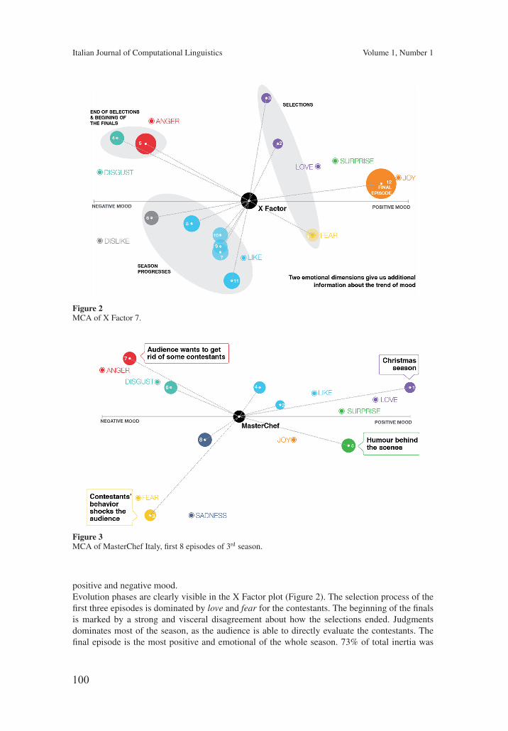
100
Italian Journal of Computational Linguistics Volume 1, Number 1
Figure 2MCA of X Factor 7.
Figure 3MCA of MasterChef Italy, first 8 episodes of 3rd season.
positive and negative mood.Evolution phases are clearly visible in the X Factor plot (Figure 2). The selection process of thefirst three episodes is dominated by love and fear for the contestants. The beginning of the finalsis marked by a strong and visceral disagreement about how the selections ended. Judgmentsdominates most of the season, as the audience is able to directly evaluate the contestants. Thefinal episode is the most positive and emotional of the whole season. 73% of total inertia was
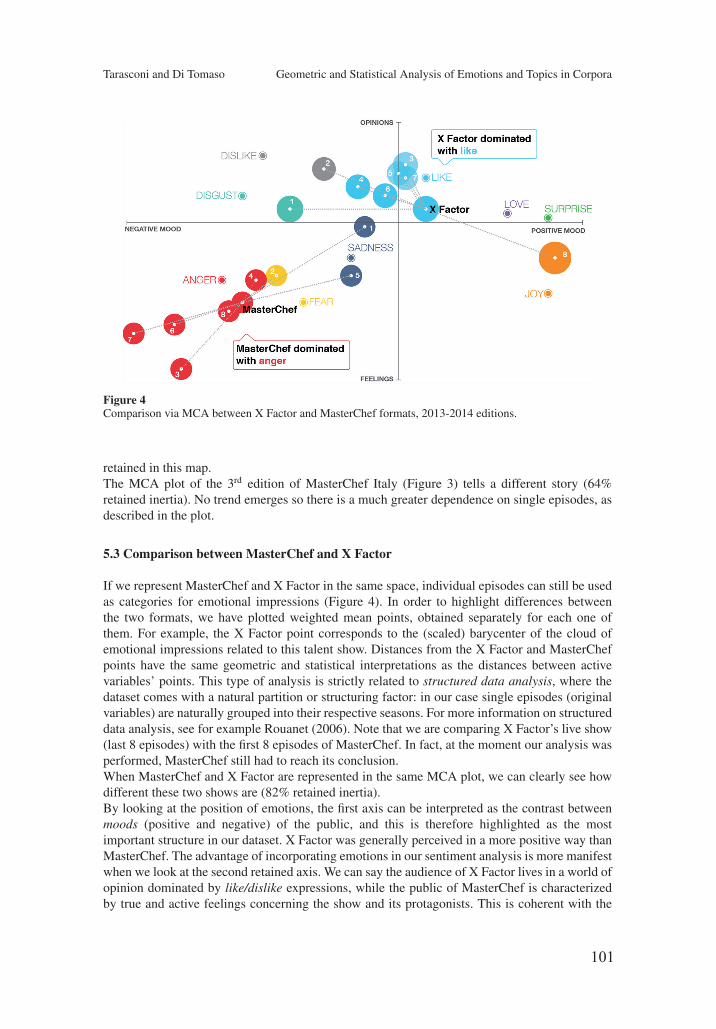
101
Tarasconi and Di Tomaso Geometric and Statistical Analysis of Emotions and Topics in Corpora
Figure 4Comparison via MCA between X Factor and MasterChef formats, 2013-2014 editions.
retained in this map.The MCA plot of the 3rd edition of MasterChef Italy (Figure 3) tells a different story (64%retained inertia). No trend emerges so there is a much greater dependence on single episodes, asdescribed in the plot.
5.3 Comparison between MasterChef and X Factor
If we represent MasterChef and X Factor in the same space, individual episodes can still be usedas categories for emotional impressions (Figure 4). In order to highlight differences betweenthe two formats, we have plotted weighted mean points, obtained separately for each one ofthem. For example, the X Factor point corresponds to the (scaled) barycenter of the cloud ofemotional impressions related to this talent show. Distances from the X Factor and MasterChefpoints have the same geometric and statistical interpretations as the distances between activevariables’ points. This type of analysis is strictly related to structured data analysis, where thedataset comes with a natural partition or structuring factor: in our case single episodes (originalvariables) are naturally grouped into their respective seasons. For more information on structureddata analysis, see for example Rouanet (2006). Note that we are comparing X Factor’s live show(last 8 episodes) with the first 8 episodes of MasterChef. In fact, at the moment our analysis wasperformed, MasterChef still had to reach its conclusion.When MasterChef and X Factor are represented in the same MCA plot, we can clearly see howdifferent these two shows are (82% retained inertia).By looking at the position of emotions, the first axis can be interpreted as the contrast betweenmoods (positive and negative) of the public, and this is therefore highlighted as the mostimportant structure in our dataset. X Factor was generally perceived in a more positive way thanMasterChef. The advantage of incorporating emotions in our sentiment analysis is more manifestwhen we look at the second retained axis. We can say the audience of X Factor lives in a world ofopinion dominated by like/dislike expressions, while the public of MasterChef is characterizedby true and active feelings concerning the show and its protagonists. This is coherent with the
102
Italian Journal of Computational Linguistics Volume 1, Number 1
fact that viewers of X Factor could directly evaluate the performances of contestants. This wasnot possible for the viewers of MasterChef, who focused instead on the most outstanding andemotional moments of the show. Reaching these conclusions would not have been possible bylooking at simple polarity of impressions.This difference in volume between the two shows is reflected in the distances from the origin,which can be considered as the average profile, and therefore closer to X Factor.Other detailed examples on structuring an MCA analysis can be found in Rouanet (2006).
6. Conclusions and further researches
By applying carefully chosen multivariate statistical techniques, we have shown how to representand highlight important emotional relations between topics. We presented some case studies,describing in detail the analyses of some live TV shows as they were discussed on Twitter.Further results in the MCA field can be experimented on datasets similar to the ones we used. Forexample, additional information about opinion polarity and document authors (such as Twitterusers) could be incorporated in the analysis. The geometric approach to MCA (Le Roux andRouanet 2004) could be interesting to study in greater detail the clouds of impressions anddocuments (J and D matrices); authors could also be considered as mean points of well-definedsub-clouds.
Ancknowledgements
We would like to thank: V. Cosenza and S. Monotti Graziadei for stimulating these researches;the ISI-CRT foundation and CELI S.R.L. for the support provided through the Lagrange Project;A. Bolioli for the supervision and the essential help in the preparation of this paper. Last but notleast, all colleagues for always giving their daily contributions.
ReferencesAbdi, Hervé and Lynne J. Williams. 2010. Principal Component Analysis, Wiley Interdisciplinary
Reviews: Computational Statistics, Volume 2, Issue 4, pages 433-459.Basile, Valerio and Malvina Nissim. 2013 Sentiment analysis on Italian tweets, Proceedings of WASSA
2013, pages 100-107.Basile, Valerio, Andrea Bolioli, Malvina Nissim, Viviana Patti, and Paolo Rosso. 2014 Overview of the
Evalita 2014 SENTIment POLarity Classification Task, Proceedings of the First Italian Conference onComputational Linguistics CLiC-it 2014 and of the Fourth International Workshop EVALITA 2014,pages 50-57.
Blasius, Jörg and Michael Greenacre. 2006. Correspondence Analysis and Related Methods in Practice,Multiple Correspondence Analysis and Related Methods, Chapter 1, pages 3-40. CRC Press.
Bolioli, Andrea, Federica Salamino, and Veronica Porzionato. 2013. Social Media Monitoring in Real Lifewith Blogmeter Platform, ESSEM@AI*IA 2013, Volume 1096 of CEUR Workshop Proceedings, pages156-163. CEUR-WS.org.
Bollen, Johan, Huina Mao, and Xiao-Jun Zeng. 2011. Twitter mood predicts the stock market, Journal ofComputational Science, 2(1):1-8.
Bosco, Cristina, Viviana Patti, and Andrea Bolioli. 2013. Developing Corpora for Sentiment Analysis: TheCase of Irony and Senti-TUT, IEEE Intelligent Systems, Special Issue on Knowledge-based Approachesto Content-level Sentiment Analysis, 28(2):55-63.
Cambria, Erik, Björn Schuller, Yunqing Xia, and Catherine Havasi. 2013. New Avenues in Opinion Miningand Sentiment Analysis, IEEE Intelligent Systems, 28(2):15-21.
Cambria, Erik, Björn Schuller, Bing Liu, Haixun Wang, and Catherine Havasi. 2013 Knowledge-BasedApproaches to Concept-Level Sentiment Analysis, IEEE Intelligent Systems, 28(2):12-14.
Cosenza, Vincenzo. 2012. Social Media ROI. Apogeo.Dini, Luca and Mazzini Giampaolo. 2002 Opinion classification Through information extraction,
Proceedings of the Conference on Data Mining Methods and Databases for Engineering, Finance andOther Fields, pages 299-310
103
Tarasconi and Di Tomaso Geometric and Statistical Analysis of Emotions and Topics in Corpora
Ekman, Paul, Wallace V. Friesen, and Phoebe Ellsworth. 1972. Emotion in the Human Face. PergamonPress.
Galati, Dario. 2002. Prospettive sulle emozioni e teorie del soggetto. Bollati Boringhieri.Gower, John C. 2006. Divided by a Common Language: Analyzing and Visualizing Two-Way Arrays,
Multiple Correspondence Analysis and Related Methods, Chapter 3. pages 77-105. CRC Press.Greenacre, Michael. 1983. Theory and Applications of Correspondence Analysis. Academic Press.Greenacre, Michael. 2006. From Simple to Multiple Correspondence Analysis, Multiple Correspondence
Analysis and Related Methods, Chapter 2, pages 41-76. CRC Press.Hamamoto, Masafumi, Hiroyuki Kitagawa, Jia-Yu Pan, and Christos Faloutsos. 2005. A Comparative
Study of Feature Vector-Based Topic Detection Schemes for Text Streams, Proceedings of the 2005International Workshop on Challenges in Web Information Retrieval and Integration, pages 122-127.
Jolliffe, Ian T. 2002. Principal Component Analysis. Springer.Le Roux, Brigitte and Henry Rouanet. 2004. Geometric Data Analysis: From Correspondence Analysis to
Structured Data. Kluwer.Liu, Bing. 2012. Sentiment Analysis e Opinion Mining. Morgan & Claypool Publishers.Manning, Christopher D., Prabhakar Raghavan and Hinrich Schütze. 2008. Introduction to Information
Retrieval. Cambridge University Press.Meyer, Carl D. 2000. Matrix Analysis and Applied Linear Algebra. Siam.Roberts, Kirk, Michael A. Roach, Joseph Johnson, Josh Guthrie, and Sanda M. Harabagiu. 2012.
EmpaTweet: Annotating and Detecting Emotions on Twitter, Proceedings of the Eight InternationalConference on Language Resources and Evaluation (LREC’12), pages 3806-3813. European LanguageResources Association (ELRA).
Rouanet, Henry. 2006. The Geometric Analysis of Structured Individuals x Variables Tables, MultipleCorrespondence Analysis and Related Methods, CRC Press.
Wiebe, Janyce, Theresa Wilson, and Claire Cardie. 2005. Annotating expressions of opinions and emotionsin language, Language Resources and Evaluation, Volume 39, Issue 2-3, pages 165-210.
Strapparava, Carlo and Valitutti, Alessandro. 2004 "WordNet-Affect: an Affective Extension of WordNet",Proceedings of the 4th International Conference on Language Resources and Evaluation (LREC), pages1083-1086, Lisbon.

105
Il ruolo delle tecnologie del linguaggio nelmonitoraggio dell’evoluzione delle abilità discrittura: primi risultati
Alessia Barbagli∗Università di Roma “La Sapienza”
Pietro Lucisano∗∗
Università di Roma “La Sapienza”
Felice Dell’Orletta†
ILC-CNRSimonetta Montemagni‡ILC-CNR
Giulia Venturi§
ILC-CNR
Italiano. L’ultimo decennio ha visto l’affermarsi a livello internazionale dell’uso di tecnologiedel linguaggio per lo studio dei processi di apprendimento. Questo contributo riporta i primie promettenti risultati di uno studio interdisciplinare che si è avvalso di metodi e tecniche dianalisi propri della linguistica computazionale, della linguistica e della pedagogia sperimentale.Lo studio, finalizzato al monitoraggio dell’evoluzione del processo di apprendimento della linguaitaliana, è stato condotto a partire dalle produzione scritte di studenti della scuola secondaria diprimo grado con strumenti di annotazione linguistica automatica e di estrazione di conoscenzae ha portato all’identificazione di un insieme di tratti qualificanti il processo di apprendimentolinguistico.English. Over the last ten years, the use of language technologies was successfully extendedto the study of learning processes. The paper reports the first and promising results of aninterdisciplinary study aimed at monitoring the evolution of the learning process of the Ital-ian language based on a corpus of written productions by students and exploiting automaticlinguistic annotation and knowledge extraction tools.
1. Introduzione
Gli ultimi dieci anni hanno visto un crescente interesse verso le tecnologie del lin-guaggio come punto di partenza per ricerche interdisciplinari finalizzate allo studiodelle competenze linguistiche di apprendenti la propria lingua madre (L1) o una linguastraniera (L2). Sebbene con obiettivi diversi, le ricerche condotte a livello internazionale
∗ Dipartimento di Psicologia dei processi di Sviluppo e socializzazione, Università di Roma “La Sapienza”.E-mail: [email protected]
∗∗ Dipartimento di Psicologia dei processi di Sviluppo e socializzazione, Università di Roma “La Sapienza”.E-mail: [email protected]
† Istituto di Linguistica Computazionale “Antonio Zampolli” (ILC-CNR), ItaliaNLP Lab.E-mail: [email protected]
‡ Istituto di Linguistica Computazionale “Antonio Zampolli” (ILC-CNR), ItaliaNLP Lab.E-mail: [email protected]
§ Istituto di Linguistica Computazionale “Antonio Zampolli” (ILC-CNR), ItaliaNLP Lab.E-mail: [email protected]
© 2015 Associazione Italiana di Linguistica Computazionale
106
Italian Journal of Computational Linguistics Volume 1, Number 1
sono accomunate da una medesima metodologia basata sull’uso di strumenti di an-notazione linguistica automatica e condividono il medesimo obiettivo di indagare la‘forma linguistica’ di corpora di produzioni spontanee. In questo senso il testo linguis-ticamente annotato costituisce il punto di partenza all’interno del quale rintracciareuna serie di caratteristiche linguistiche (lessicali, grammaticali, sintattiche, ecc.) chepossano essere considerate indicatori affidabili per ricostruire il profilo linguistico delleproduzioni. Lo scopo è ad esempio quello di studiare in che modo tali caratteristichesono rivelatrici della qualità di scrittura di apprendenti una lingua straniera (Deane andQuinlan 2010) o quello di monitorare la capacità di lettura come componente centraledella competenza linguistica (Schwarm e Ostendorf 2005; Petersen e Ostendorf 2009).La medesima metodologia è stata utilizzata per monitorare lo sviluppo nel tempodella sintassi nel linguaggio infantile a partire da trascrizioni del parlato (Sagae et al.2005; Lu 2007; Lubetich and Sagae 2014). L’analisi automatica della ‘forma linguistica’di produzioni di apprendenti rappresenta il punto di partenza anche per identificareeventuali deficit cognitivi attraverso misure di complessità sintattica (Roark et al. 2007)o di associazione semantica (Rouhizadeh et al. 2013).
Da un punto di vista più applicativo, tecnologie basate sul trattamento automaticodel linguaggio sono oggi impiegate nella costruzione di Intelligent Computer–AssistedLanguage Learning systems (ICALL) (Granger 2003), per sviluppare strumenti di val-utazione automatica delle produzioni scritte per lo più di apprendenti una linguastraniera (Attali and Burstein 2006) o per mettere a punto programmi di correzioneautomatica degli errori commessi da apprendenti una L2 (Ng et al. 2013, 2014). Alivello internazionale, ciò è dimostrato dall’organizzazione di numerose conferenzesull’argomento come ad esempio il Workshop on Innovative Use of NLP for BuildingEducational Applications (BEA), arrivato nel 2015 alla sua decima edizione1.
A questa panoramica va aggiunto il fatto che strumenti di estrazione dellaconoscenza sono oggi utilizzati per analizzare il ‘contenuto’ di produzioni per lo piùscritte. A livello internazionale, i metodi tradizionalmente impiegati a questo scopo(Knowledge Tracing systems) fanno riferimento a un comune paradigma che permettedi modellare il processo di apprendimento delle conoscenze attraverso l’analisi di unaserie di compiti svolti nel tempo dagli studenti e valutati dagli insegnanti (Corbett andAnderson 1994). Tali metodi non sono basati su strumenti di trattamento automatico dellinguaggio, ma stanno diventando sempre più d’interesse all’interno della comunità diMachine Learning2 in contesti di apprendimento personalizzato a distanza (AdaptiveE–learning) (Piech et al. 2015; Ekanadham and Karklin 2015).
Il presente contributo si pone in questo contesto di ricerca, riportando i primirisultati di uno studio più ampio, tuttora in corso, condotto a partire da un corpusdi produzioni scritte di studenti italiani nel primo e nel secondo anno della scuolasecondaria di primo grado. Si tratta di uno studio finalizzato a costruire un modellodi analisi empirica in grado di monitorare l’evoluzione sia della ‘forma linguistica’sia del ‘contenuto’ utilizzando strumenti di annotazione linguistica automatica unitia tecnologie di estrazione automatica di conoscenza da testi. Come discusso in quantosegue, l’approccio messo a punto si ripropone di monitorare tale evoluzione sia neltempo (nel passaggio cioè dal primo al secondo anno di scuola) sia rispetto ad una seriedi variabili di sfondo (come ad esempio il background familiare, le abitudini personali,ecc.) rintracciate grazie ad un questionario studenti distribuito in classe.
1 http://www.cs.rochester.edu/∼tetreaul/naacl-bea10.html2 http://dsp.rice.edu/ML4Ed_ICML2015
107
Barbagli et al. Monitoraggio dell’evoluzione delle abilità di scrittura
Il carattere innovativo di questa ricerca nel panorama nazionale e internazionalesi colloca a vari livelli. Sul versante metodologico, la ricerca qui delineata rappresentail primo studio finalizzato al monitoraggio dell’evoluzione del processo di apprendi-mento linguistico della lingua italiana (come lingua madre) condotto con strumenti diannotazione linguistica automatica e di estrazione della conoscenza. Come preceden-temente discusso, sino ad oggi le ricerche a livello internazionale che si sono basatesull’uso di tecnologie del linguaggio per monitorare l’evoluzione nel tempo di com-petenze linguistiche di apprendenti una lingua madre si sono per lo più concentratesull’analisi di produzioni orali infantili. Al contrario, chi si è interessato allo studiodell’evoluzione delle abilità di scrittura lo ha fatto a partire da produzioni di appren-denti una lingua straniera. Minore attenzione è stata dunque dedicata all’uso di talitecnologie per lo studio diacronico di come evolvono le abilità di scrittura di studentimadrelingua. Per quanto riguarda la lingua italiana, all’interno di due precedenti studidi fattibilità, (Dell’Orletta e Montemagni 2012) e (Dell’Orletta et al. 2011) hanno di-mostrato che le tecnologie linguistico–computazionali possono giocare un ruolo cen-trale nella valutazione della competenza linguistica di studenti madrelingua in ambitoscolastico e nel tracciarne l’evoluzione attraverso il tempo. Questo contributo rappre-senta uno sviluppo originale e innovativo di questa linea di ricerca all’interno dellaquale l’uso congiunto di strumenti di annotazione linguistica automatica e di estrazionedi conoscenza rappresenta un’ulteriore innovazione metodologica. Ciò è reso possibiledalla particolare conformazione interna del corpus di produzioni scritte utilizzato inquesto lavoro e descritto nei paragrafi successivi.
La scelta del ciclo scolastico e dei tipi di produzioni scritte analizzate è un altroelemento di novità di questo studio, soprattutto sotto il profilo di ricerca in pedagogiasperimentale. Non solo infatti è stato scelto il primo biennio della scuola secondaria diprimo grado come ambito scolastico da analizzare perché poco indagato dalle ricercheempiriche, ma sono stati anche analizzati i temi di studenti ai quali era stato richiestodi dare ad un coetaneo dei consigli per scrivere un buon tema. Questo ha permessodi indagare come cambia (a livello di ‘contenuti’) la percezione dell’insegnamentodella scrittura nel passaggio dal primo al secondo anno di scuola attraverso la praticadi scrittura (analisi della ‘forma linguistica’). Poche sono state infatti sino ad oggi leindagini che hanno verificato i risultati dell’effettiva pratica didattica derivata dalle in-dicazioni previste dai programmi ministeriali relativi a questo ciclo scolastico, a partiredal 1979 fino alle Indicazioni Nazionali del 2012. Al contrario, gli studi si sono per lo piùconcentrati sull’educazione linguistica (Rigo 2005) e in modo specifico sulla competenzatestuale anche in termini di produzione.
In quanto segue, nel Paragrafo 2 introdurremo l’approccio del più ampio contestodi ricerca in cui questo contributo si inserisce. Dopo aver illustrato la metodologia e glistrumenti di analisi linguistico–computazionale qui adottati (Paragrafo 3), nei Paragrafi4 e 5 riporteremo i primi risultati ottenuti. Infine, nel Paragrafo 6 trarremo alcuneconclusioni e tratteggeremo gli sviluppi futuri di questa ricerca.
2. Il contesto e i dati della ricerca
Il contesto a cui fa riferimento questo studio è quello della ricerca IEA IPS (Associationfor the Evaluation of Educational Achievement, Indagine sulla Produzione Scritta) (Purvues1992), un’indagine sull’insegnamento e sull’apprendimento della produzione scrittanella scuola, che agli inizi degli anni ’80 coinvolse quattordici paesi di tutto il mondo, tracui l’Italia (Lucisano 1988; Lucisano e Benvenuto 1991). Prendendo le mosse dai risultatiraggiunti, il presente contributo si basa sull’ipotesi che nei primi due anni della scuola

108
Italian Journal of Computational Linguistics Volume 1, Number 1
media superiore di primo grado si realizzino dei cambiamenti rilevanti sia nel modoin cui gli studenti si approcciano alla scrittura sia nel modo stesso in cui essi scrivono.L’intuizione è che ciò sia dovuto al fatto che gli studenti sono sottoposti nel passaggiodal primo al secondo anno di scuola a un insegnamento più formale della scrittura.
Scopo della ricerca è inoltre quello di monitorare come tali cambiamenti si ver-ifichino non solo nell’arco temporale preso in esame, ma anche rispetto ad alcunecaratteristiche descrittive del campione di studenti esaminato. Per questo motivo è statomesso a punto un questionario somministrato in classe dai docenti agli studenti e com-posto da circa trenta domande corrispondenti ad altrettante variabili di sfondo consid-erate. Le domande contenute riguardano diversi aspetti che vanno dall’inquadramentoanagrafico degli studenti, la caratterizzazione socio–culturale della famiglia (profes-sione dei genitori, titolo di studio, libri in casa ecc...) e la rilevazione delle loro abitudini(ad esempio, tempo dedicato alla lettura e alla scrittura, tempo dedicato ad ascoltaremusica, ecc...), per arrivare a domande che vanno a indagare le idee, le credenze e iconvincimenti degli studenti a proposito della scrittura e il loro rapporto con la scritturascolastica.
Allo scopo di monitorare i cambiamenti abbiamo preso in esame un corpus di240 prove scritte da 156 studenti di sette diverse scuole secondarie di primo gradodi Roma; la scelta delle scuole è avvenuta basandosi sul presupposto che esista unaforte relazione tra l’area territoriale in cui è collocata la scuola e l’ambiente socio–culturale di riferimento. Sono state individuate due aree territoriali: il centro storicoe la periferia, selezionati come rappresentativi rispettivamente di un ambiente socio–culturale medio–alto e medio–basso. In ogni scuola è stata individuata una classe e,benché le scuole di periferia siano quattro mentre quelle del centro siano tre, il numerodegli studenti è quasi equivalente (77 in centro e 79 in periferia) dal momento che leclassi delle scuole del centro sono più numerose.
Per ogni studente, sono state raccolte due tipologie di produzioni scritte: le tracceassegnate dai docenti nei due anni scolastici e due prove comuni relative alla percezionedell’insegnamento della scrittura, svolte dalle classi al termine del primo e del secondoanno. Alla fine del secondo anno è stata somministrata la traccia della Prova 9 dellaRicerca IEA–IPS (Lucisano 1984; Corda Costa e Visalberghi 1995) che consiste in unalettera di consigli indirizzata a un coetaneo su come scrivere un tema3, mentre per laprova dell’anno precedente ne è stata utilizzata una forma adattata alla classe e all’età4.
In questo studio ci siamo focalizzati sull’analisi di una porzione dell’intero cor-pus raccolto. Si tratta della collezione di prove comuni di scrittura somministrate nelprimo e secondo anno, composta da 109 testi. La scelta di prendere in esame questasottoporzione ci ha permesso di mostrare come i cambiamenti che avevamo suppostoesistere sia nel modo in cui gli studenti si approcciano alla scrittura sia nel modo stessoin cui essi scrivono possano essere verificati utilizzando sia strumenti di annotazionelinguistica automatica del testo sia di estrazione automatica della conoscenza. Mentre
3 La traccia somministrata al termine del secondo anno è la seguente “Un ragazzo più giovane di te hadeciso di iscriversi alla tua scuola. Ti ha scritto per chiederti come fare un tema che possa essere valutatobene dai tuoi insegnanti. Mandagli una lettera cordiale nella quale descrivi almeno cinque punti che tupensi importanti per gli insegnanti quando valutano i temi”
4 La traccia somministrata al termine del primo anno “Un tuo amico sta per iniziare la quinta elementarecon le tue maestre e ti ha confessato di aver paura soprattutto dei lavori di scrittura che gli sarannochiesti. Scrivigli una lettera raccontando la tua esperienza, gli aspetti positivi e anche le tue difficoltà neicompiti di scrittura che hai fatto in quinta elementare. Raccontagli dei compiti che ti sono piaciuti di più edi quelli che ti sono piaciuti di meno e anche dei suggerimenti che le maestre ti davano per insegnarti ascrivere bene e di come correggevano i compiti scritti. Dagli consigli utili per cavarsela.”
109
Barbagli et al. Monitoraggio dell’evoluzione delle abilità di scrittura
i primi infatti, come vedremo, permettono di monitorare le variazioni di ‘forma lin-guistica’ nella pratica della scrittura, i secondi consentono di analizzare anche comecambi che cosa gli studenti scrivono a proposito della pratica della scrittura (come mutidunque il ‘contenuto’ dei temi).
3. Analisi linguistico–computazionale delle produzioni scritte degli studenti
Il corpus di 109 prove comuni oggetto di questo studio è stato analizzato impiegandostrumenti e metodologie di analisi automatica del testo che hanno permesso di accederesia alla ‘forma linguistica’ sia al ‘contenuto’ delle prove.
Il corpus di produzioni scritte, una volta digitalizzato, è stato prima di tutto arric-chito automaticamente con annotazione morfo–sintattica e sintattica. A tal fine è statautilizzata una piattaforma consolidata e ampiamente sperimentata di metodi e stru-menti per il trattamento automatico dell’italiano sviluppati congiuntamente dall’ILC–CNR e dall’Università di Pisa5. Per quanto riguarda l’annotazione morfo–sintattica, lostrumento utilizzato è descritto in (Dell’Orletta 2009); sul versante dell’analisi sintatticaa dipendenze, abbiamo utilizzato DeSR (Attardi et al. 2009). Entrambi sono in lineacon lo “stato dell’arte” per il trattamento automatico della lingua italiana, considerataanche la loro qualificazione tra gli strumenti più precisi e affidabili per l’annotazionemorfo–sintattica e sintattica a dipendenze nella campagna di valutazione di strumentiper l’analisi automatica dell’italiano, EVALITA6. Il testo linguisticamente annotato costi-tuisce il punto di partenza per le analisi successive: i) l’identificazione dei contenuti piùsalienti e ii) la definizione del profilo linguistico sottostante al testo a partire dal quale èpossibile ricostruire un quadro delle competenze linguistiche di chi lo ha prodotto.
3.1 L’identificazione dei contenuti
Il corpus di produzioni scritte è stato sottoposto ad un processo di estrazione termino-logica finalizzato all’identificazione e all’estrazione delle unità lessicali monorematichee polirematiche rappresentative del contenuto. L’ipotesi di partenza è che i terminicostituiscono l’istanza linguistica dei concetti più salienti di una collezione documentalee che per questo motivo il compito di estrazione terminologica costituisce il primoe fondamentale passo verso l’accesso al suo contenuto. A tal fine è stato utilizzatoT2K2 (Text–to–Knowledge)7, una piattaforma web che trasforma le conoscenze implici-tamente codificate all’interno di un corpus di testi in conoscenza esplicitamente strut-turata (Dell’Orletta et al. 2014). Il componente di estrazione terminologica all’internodi T2K2 opera in due fasi: la prima volta all’identificazione all’interno del corpusdi acquisizione di unità terminologiche rilevanti per il contesto indagato, la secondafinalizzata alla validazione della salienza dei termini estratti nella fase precedente.
Per quanto riguarda la prima fase, il processo estrattivo opera sul testo annotato alivello morfo–sintattico e lemmatizzato. Mentre l’acquisizione di unità monorematicheavviene sulla base della loro frequenza, l’acquisizione delle unità polirematiche siarticola in due passaggi: il primo finalizzato all’identificazione dei potenziali terminisulla base di una mini–grammatica operante sul testo annotato morfo–sintatticamentee deputata al riconoscimento di sequenze di categorie grammaticali corrispondenti a
5 http://linguistic-annotation-tool.italianlp.it/6 http://www.evalita.it/7 http://www.italianlp.it/demo/t2k-text-to-knowledge/
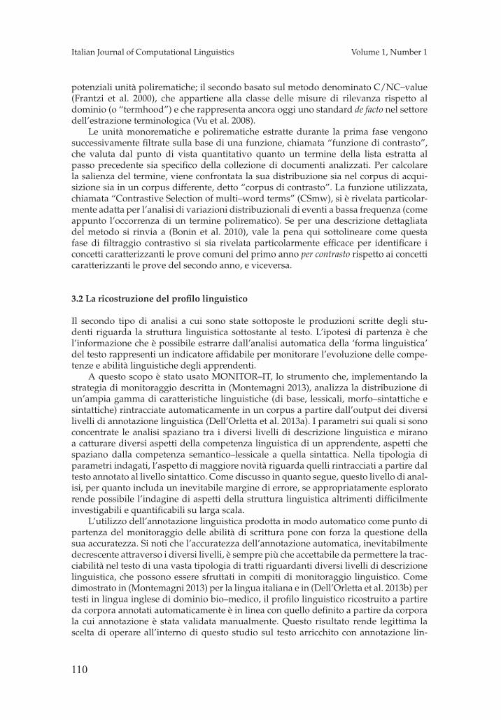
110
Italian Journal of Computational Linguistics Volume 1, Number 1
potenziali unità polirematiche; il secondo basato sul metodo denominato C/NC–value(Frantzi et al. 2000), che appartiene alla classe delle misure di rilevanza rispetto aldominio (o “termhood”) e che rappresenta ancora oggi uno standard de facto nel settoredell’estrazione terminologica (Vu et al. 2008).
Le unità monorematiche e polirematiche estratte durante la prima fase vengonosuccessivamente filtrate sulla base di una funzione, chiamata “funzione di contrasto”,che valuta dal punto di vista quantitativo quanto un termine della lista estratta alpasso precedente sia specifico della collezione di documenti analizzati. Per calcolarela salienza del termine, viene confrontata la sua distribuzione sia nel corpus di acqui-sizione sia in un corpus differente, detto “corpus di contrasto”. La funzione utilizzata,chiamata “Contrastive Selection of multi–word terms” (CSmw), si è rivelata particolar-mente adatta per l’analisi di variazioni distribuzionali di eventi a bassa frequenza (comeappunto l’occorrenza di un termine polirematico). Se per una descrizione dettagliatadel metodo si rinvia a (Bonin et al. 2010), vale la pena qui sottolineare come questafase di filtraggio contrastivo si sia rivelata particolarmente efficace per identificare iconcetti caratterizzanti le prove comuni del primo anno per contrasto rispetto ai concetticaratterizzanti le prove del secondo anno, e viceversa.
3.2 La ricostruzione del profilo linguistico
Il secondo tipo di analisi a cui sono state sottoposte le produzioni scritte degli stu-denti riguarda la struttura linguistica sottostante al testo. L’ipotesi di partenza è chel’informazione che è possibile estrarre dall’analisi automatica della ‘forma linguistica’del testo rappresenti un indicatore affidabile per monitorare l’evoluzione delle compe-tenze e abilità linguistiche degli apprendenti.
A questo scopo è stato usato MONITOR–IT, lo strumento che, implementando lastrategia di monitoraggio descritta in (Montemagni 2013), analizza la distribuzione diun’ampia gamma di caratteristiche linguistiche (di base, lessicali, morfo–sintattiche esintattiche) rintracciate automaticamente in un corpus a partire dall’output dei diversilivelli di annotazione linguistica (Dell’Orletta et al. 2013a). I parametri sui quali si sonoconcentrate le analisi spaziano tra i diversi livelli di descrizione linguistica e miranoa catturare diversi aspetti della competenza linguistica di un apprendente, aspetti chespaziano dalla competenza semantico–lessicale a quella sintattica. Nella tipologia diparametri indagati, l’aspetto di maggiore novità riguarda quelli rintracciati a partire daltesto annotato al livello sintattico. Come discusso in quanto segue, questo livello di anal-isi, per quanto includa un inevitabile margine di errore, se appropriatamente esploratorende possibile l’indagine di aspetti della struttura linguistica altrimenti difficilmenteinvestigabili e quantificabili su larga scala.
L’utilizzo dell’annotazione linguistica prodotta in modo automatico come punto dipartenza del monitoraggio delle abilità di scrittura pone con forza la questione dellasua accuratezza. Si noti che l’accuratezza dell’annotazione automatica, inevitabilmentedecrescente attraverso i diversi livelli, è sempre più che accettabile da permettere la trac-ciabilità nel testo di una vasta tipologia di tratti riguardanti diversi livelli di descrizionelinguistica, che possono essere sfruttati in compiti di monitoraggio linguistico. Comedimostrato in (Montemagni 2013) per la lingua italiana e in (Dell’Orletta et al. 2013b) pertesti in lingua inglese di dominio bio–medico, il profilo linguistico ricostruito a partireda corpora annotati automaticamente è in linea con quello definito a partire da corporala cui annotazione è stata validata manualmente. Questo risultato rende legittima lascelta di operare all’interno di questo studio sul testo arricchito con annotazione lin-
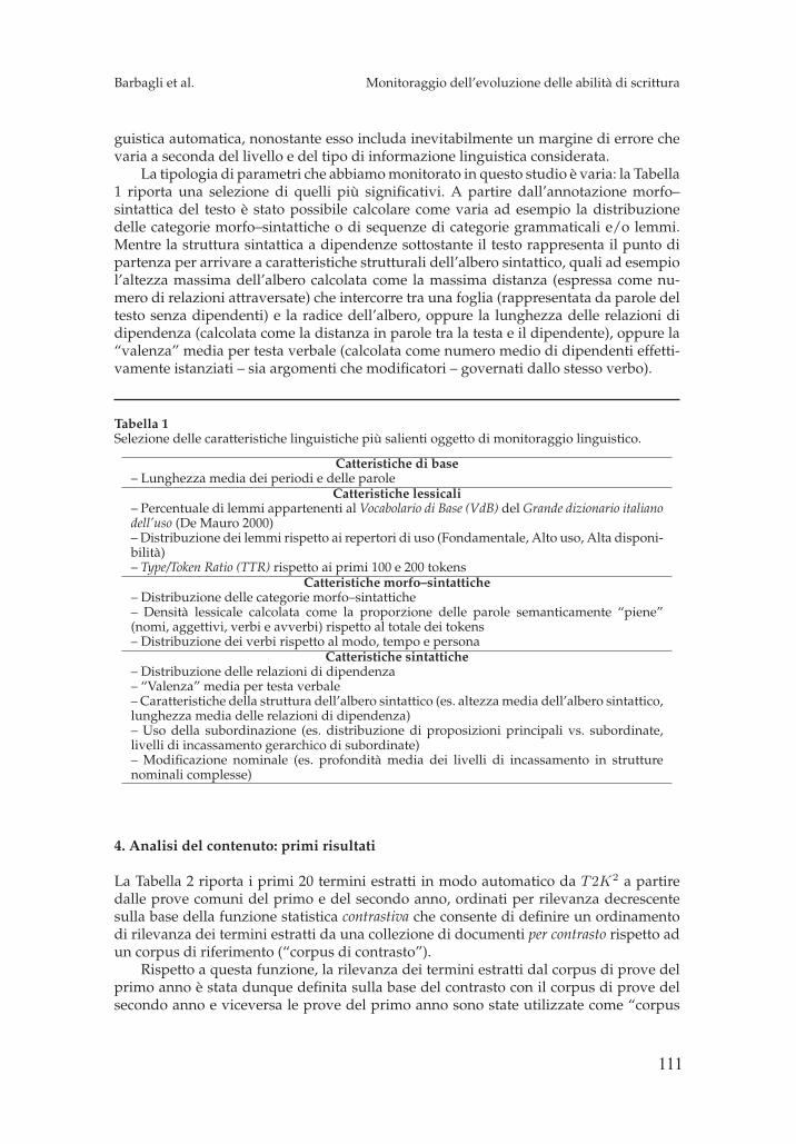
111
Barbagli et al. Monitoraggio dell’evoluzione delle abilità di scrittura
guistica automatica, nonostante esso includa inevitabilmente un margine di errore chevaria a seconda del livello e del tipo di informazione linguistica considerata.
La tipologia di parametri che abbiamo monitorato in questo studio è varia: la Tabella1 riporta una selezione di quelli più significativi. A partire dall’annotazione morfo–sintattica del testo è stato possibile calcolare come varia ad esempio la distribuzionedelle categorie morfo–sintattiche o di sequenze di categorie grammaticali e/o lemmi.Mentre la struttura sintattica a dipendenze sottostante il testo rappresenta il punto dipartenza per arrivare a caratteristiche strutturali dell’albero sintattico, quali ad esempiol’altezza massima dell’albero calcolata come la massima distanza (espressa come nu-mero di relazioni attraversate) che intercorre tra una foglia (rappresentata da parole deltesto senza dipendenti) e la radice dell’albero, oppure la lunghezza delle relazioni didipendenza (calcolata come la distanza in parole tra la testa e il dipendente), oppure la“valenza” media per testa verbale (calcolata come numero medio di dipendenti effetti-vamente istanziati – sia argomenti che modificatori – governati dallo stesso verbo).
Tabella 1Selezione delle caratteristiche linguistiche più salienti oggetto di monitoraggio linguistico.
Catteristiche di base– Lunghezza media dei periodi e delle parole
Catteristiche lessicali– Percentuale di lemmi appartenenti al Vocabolario di Base (VdB) del Grande dizionario italianodell’uso (De Mauro 2000)– Distribuzione dei lemmi rispetto ai repertori di uso (Fondamentale, Alto uso, Alta disponi-bilità)– Type/Token Ratio (TTR) rispetto ai primi 100 e 200 tokens
Catteristiche morfo–sintattiche– Distribuzione delle categorie morfo–sintattiche– Densità lessicale calcolata come la proporzione delle parole semanticamente “piene”(nomi, aggettivi, verbi e avverbi) rispetto al totale dei tokens– Distribuzione dei verbi rispetto al modo, tempo e persona
Catteristiche sintattiche– Distribuzione delle relazioni di dipendenza– “Valenza” media per testa verbale– Caratteristiche della struttura dell’albero sintattico (es. altezza media dell’albero sintattico,lunghezza media delle relazioni di dipendenza)– Uso della subordinazione (es. distribuzione di proposizioni principali vs. subordinate,livelli di incassamento gerarchico di subordinate)– Modificazione nominale (es. profondità media dei livelli di incassamento in strutturenominali complesse)
4. Analisi del contenuto: primi risultati
La Tabella 2 riporta i primi 20 termini estratti in modo automatico da T2K2 a partiredalle prove comuni del primo e del secondo anno, ordinati per rilevanza decrescentesulla base della funzione statistica contrastiva che consente di definire un ordinamentodi rilevanza dei termini estratti da una collezione di documenti per contrasto rispetto adun corpus di riferimento (“corpus di contrasto”).
Rispetto a questa funzione, la rilevanza dei termini estratti dal corpus di prove delprimo anno è stata dunque definita sulla base del contrasto con il corpus di prove delsecondo anno e viceversa le prove del primo anno sono state utilizzate come “corpus
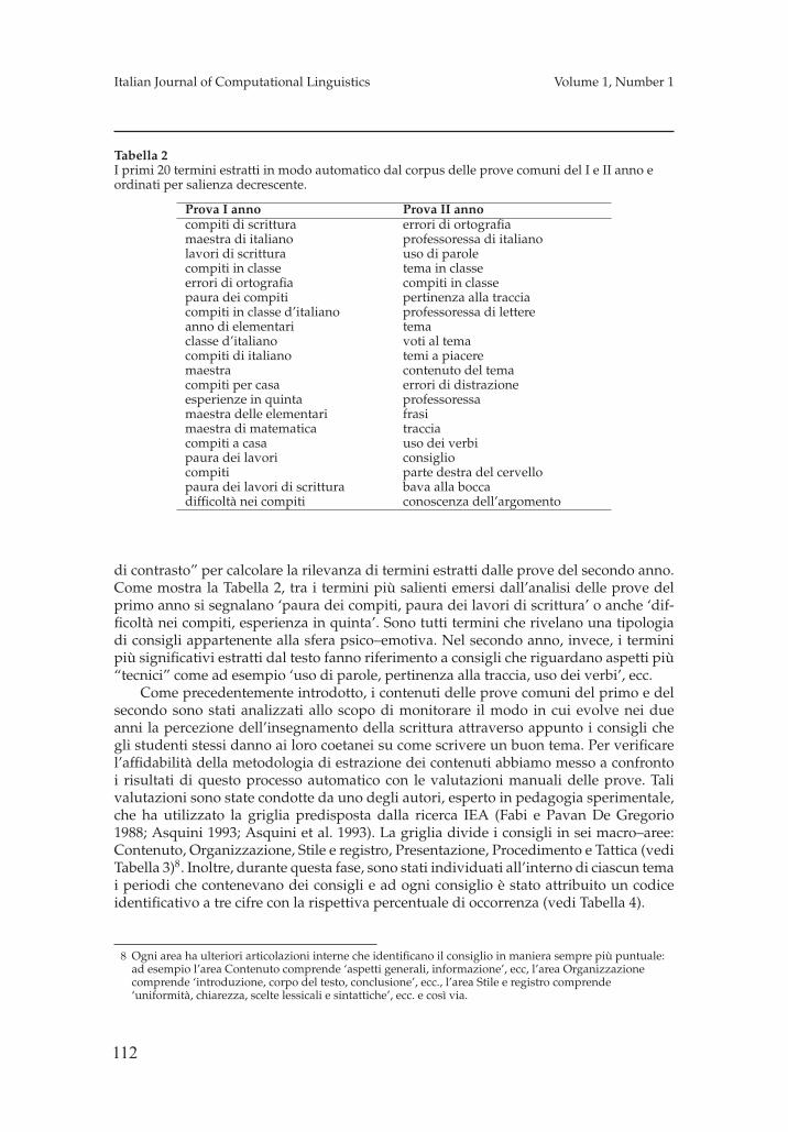
112
Italian Journal of Computational Linguistics Volume 1, Number 1
Tabella 2I primi 20 termini estratti in modo automatico dal corpus delle prove comuni del I e II anno eordinati per salienza decrescente.
Prova I anno Prova II annocompiti di scrittura errori di ortografiamaestra di italiano professoressa di italianolavori di scrittura uso di parolecompiti in classe tema in classeerrori di ortografia compiti in classepaura dei compiti pertinenza alla tracciacompiti in classe d’italiano professoressa di lettereanno di elementari temaclasse d’italiano voti al temacompiti di italiano temi a piaceremaestra contenuto del temacompiti per casa errori di distrazioneesperienze in quinta professoressamaestra delle elementari frasimaestra di matematica tracciacompiti a casa uso dei verbipaura dei lavori consigliocompiti parte destra del cervellopaura dei lavori di scrittura bava alla boccadifficoltà nei compiti conoscenza dell’argomento
di contrasto” per calcolare la rilevanza di termini estratti dalle prove del secondo anno.Come mostra la Tabella 2, tra i termini più salienti emersi dall’analisi delle prove delprimo anno si segnalano ‘paura dei compiti, paura dei lavori di scrittura’ o anche ‘dif-ficoltà nei compiti, esperienza in quinta’. Sono tutti termini che rivelano una tipologiadi consigli appartenente alla sfera psico–emotiva. Nel secondo anno, invece, i terminipiù significativi estratti dal testo fanno riferimento a consigli che riguardano aspetti più“tecnici” come ad esempio ‘uso di parole, pertinenza alla traccia, uso dei verbi’, ecc.
Come precedentemente introdotto, i contenuti delle prove comuni del primo e delsecondo sono stati analizzati allo scopo di monitorare il modo in cui evolve nei dueanni la percezione dell’insegnamento della scrittura attraverso appunto i consigli chegli studenti stessi danno ai loro coetanei su come scrivere un buon tema. Per verificarel’affidabilità della metodologia di estrazione dei contenuti abbiamo messo a confrontoi risultati di questo processo automatico con le valutazioni manuali delle prove. Talivalutazioni sono state condotte da uno degli autori, esperto in pedagogia sperimentale,che ha utilizzato la griglia predisposta dalla ricerca IEA (Fabi e Pavan De Gregorio1988; Asquini 1993; Asquini et al. 1993). La griglia divide i consigli in sei macro–aree:Contenuto, Organizzazione, Stile e registro, Presentazione, Procedimento e Tattica (vediTabella 3)8. Inoltre, durante questa fase, sono stati individuati all’interno di ciascun temai periodi che contenevano dei consigli e ad ogni consiglio è stato attribuito un codiceidentificativo a tre cifre con la rispettiva percentuale di occorrenza (vedi Tabella 4).
8 Ogni area ha ulteriori articolazioni interne che identificano il consiglio in maniera sempre più puntuale:ad esempio l’area Contenuto comprende ‘aspetti generali, informazione’, ecc, l’area Organizzazionecomprende ‘introduzione, corpo del testo, conclusione’, ecc., l’area Stile e registro comprende‘uniformità, chiarezza, scelte lessicali e sintattiche’, ecc. e così via.
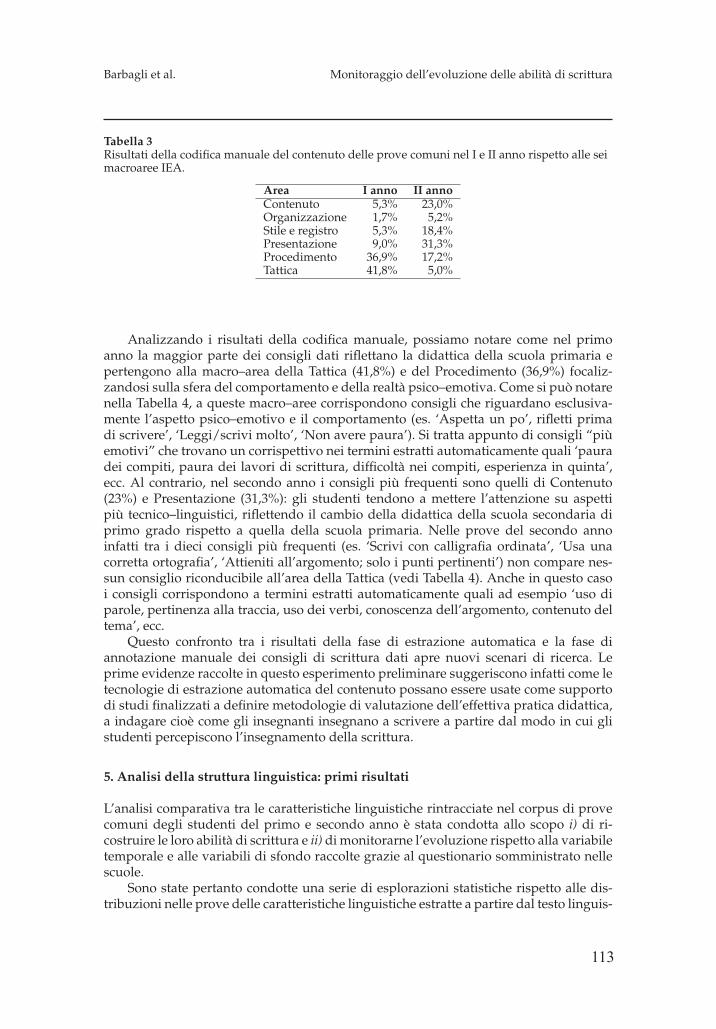
113
Barbagli et al. Monitoraggio dell’evoluzione delle abilità di scrittura
Tabella 3Risultati della codifica manuale del contenuto delle prove comuni nel I e II anno rispetto alle seimacroaree IEA.
Area I anno II annoContenuto 5,3% 23,0%Organizzazione 1,7% 5,2%Stile e registro 5,3% 18,4%Presentazione 9,0% 31,3%Procedimento 36,9% 17,2%Tattica 41,8% 5,0%
Analizzando i risultati della codifica manuale, possiamo notare come nel primoanno la maggior parte dei consigli dati riflettano la didattica della scuola primaria epertengono alla macro–area della Tattica (41,8%) e del Procedimento (36,9%) focaliz-zandosi sulla sfera del comportamento e della realtà psico–emotiva. Come si può notarenella Tabella 4, a queste macro–aree corrispondono consigli che riguardano esclusiva-mente l’aspetto psico–emotivo e il comportamento (es. ‘Aspetta un po’, rifletti primadi scrivere’, ‘Leggi/scrivi molto’, ‘Non avere paura’). Si tratta appunto di consigli “piùemotivi” che trovano un corrispettivo nei termini estratti automaticamente quali ‘pauradei compiti, paura dei lavori di scrittura, difficoltà nei compiti, esperienza in quinta’,ecc. Al contrario, nel secondo anno i consigli più frequenti sono quelli di Contenuto(23%) e Presentazione (31,3%): gli studenti tendono a mettere l’attenzione su aspettipiù tecnico–linguistici, riflettendo il cambio della didattica della scuola secondaria diprimo grado rispetto a quella della scuola primaria. Nelle prove del secondo annoinfatti tra i dieci consigli più frequenti (es. ‘Scrivi con calligrafia ordinata’, ‘Usa unacorretta ortografia’, ‘Attieniti all’argomento; solo i punti pertinenti’) non compare nes-sun consiglio riconducibile all’area della Tattica (vedi Tabella 4). Anche in questo casoi consigli corrispondono a termini estratti automaticamente quali ad esempio ‘uso diparole, pertinenza alla traccia, uso dei verbi, conoscenza dell’argomento, contenuto deltema’, ecc.
Questo confronto tra i risultati della fase di estrazione automatica e la fase diannotazione manuale dei consigli di scrittura dati apre nuovi scenari di ricerca. Leprime evidenze raccolte in questo esperimento preliminare suggeriscono infatti come letecnologie di estrazione automatica del contenuto possano essere usate come supportodi studi finalizzati a definire metodologie di valutazione dell’effettiva pratica didattica,a indagare cioè come gli insegnanti insegnano a scrivere a partire dal modo in cui glistudenti percepiscono l’insegnamento della scrittura.
5. Analisi della struttura linguistica: primi risultati
L’analisi comparativa tra le caratteristiche linguistiche rintracciate nel corpus di provecomuni degli studenti del primo e secondo anno è stata condotta allo scopo i) di ri-costruire le loro abilità di scrittura e ii) di monitorarne l’evoluzione rispetto alla variabiletemporale e alle variabili di sfondo raccolte grazie al questionario somministrato nellescuole.
Sono state pertanto condotte una serie di esplorazioni statistiche rispetto alle dis-tribuzioni nelle prove delle caratteristiche linguistiche estratte a partire dal testo linguis-
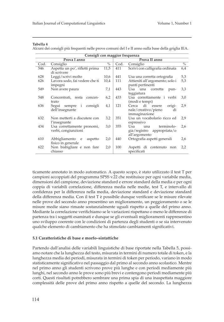
114
Italian Journal of Computational Linguistics Volume 1, Number 1
Tabella 4Alcuni dei consigli più frequenti nelle prove comuni del I e II anno sulla base della griglia IEA.
Consigli con maggior frequenzaProva I anno Prova II anno
Cod. Consiglio % Cod. Consiglio %546 Aspetta un po’, rifletti prima
di scrivere11,5 411 Scrivi con calligrafia ordinata 6,4
628 Leggi/scrivi molto 10,6 441 Usa una corretta ortografia 5,3626 Lavora sodo, fai vedere che ti
impegni10,4 111 Attieniti all’argomento; solo i
punti pertinenti5,3
549 Non avere paura 7,1 443 Usa una corretta pun-teggiatura
3,3
548 Concentrati, resta concen-trato
6,2 433 Usa correttamente i verbi(modi e tempi)
3,0
636 Segui sempre i consiglidell’insegnante
4,1 121 Cerca di essere origi-nale/creativo/pieno diimmaginazione
2,9
632 Non metterti a discutere conl’insegnante
3,2 351 Usa un vocabolario ricco edespressivo
2,9
434 Usa correttamente pronomi,verbi, congiunzioni
3,0 355 Usa una terminolo-gia/registro appropriata/oall’argomento
2,6
610 Abbigliamento e aspettofisico in generale
2,0 440 Ortografia aspetti generali 2,6
622 Non bisbigliare e non farechiasso
2,0 100 Aspetti di contenuto nonspecificati
2,2
ticamente annotato in modo automatico. A questo scopo, è stato utilizzato il test T percampioni accoppiati del programma SPSS v.22 che restituisce per ogni variabile media,dimensioni del campione, deviazione standard e errore standard della media e per ognicoppia di variabili correlazione, differenza media nelle medie, test T, e intervallo diconfidenza per la differenza nella media, deviazione standard e deviazione standarddella differenza media. Con il test T è possibile dunque verificare se le misure rilevatenelle prove del secondo anno presentino un miglioramento, un peggioramento o se lemisure medie siano rimaste sostanzialmente uguali rispetto a quelle del primo anno.Mediante la correlazione verifichiamo se le variazioni rispettano o meno le differenze dipartenza tra i soggetti esaminati e dunque se gli eventuali miglioramenti rappresentinouno sviluppo coerente con le condizioni di partenza degli studenti o se sia intervenutoqualche elemento di cambiamento che ha stimolato cambiamenti significativi.
5.1 Caratteristiche di base e morfo–sintattiche
Partendo dall’analisi delle variabili linguistiche di base riportate nella Tabella 5, possi-amo notare che la lunghezza del testo, misurata in termini di numero totale di token, e lalunghezza media dei periodi, misurata in termini di token per periodo, variano in modostatisticamente significativo nel passaggio dal primo al secondo anno scolastico. Mentrenel primo anno gli studenti scrivono prove più lunghe e con periodi mediamente piùlunghi, nel secondo anno le prove sono più brevi e contengono periodi mediamente piùcorti. Questi risultati potrebbero sembrare una prima spia di una inaspettata maggiorecomplessità delle prove del primo anno rispetto a quelle del secondo. La lunghezza
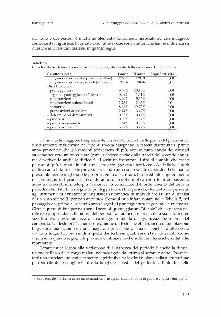
115
Barbagli et al. Monitoraggio dell’evoluzione delle abilità di scrittura
del testo e dei periodi è infatti un elemento tipicamente associato ad una maggiorecomplessità linguistica. In questo caso tuttavia due sono i fattori che hanno influenza suquesto e altri risultati discussi in quanto segue.
Tabella 5Caratteristiche di base e morfo–sintattiche e significatività della variazione tra I e II anno.
Caratteristiche I anno II anno SignificativitàLunghezza media delle prove (in token) 275,23 239,21 0,00Lunghezza media dei periodi (in token) 24,02 20,97 0,01Distribuzione di:– punteggiatura 9,70% 10,60% 0,00– segni di punteggiatura “debole” 0,49% 1,11% 0,00– congiunzioni 6,90% 5,92% 0,00– congiunzioni subordinanti 2,78% 2,43% 0,01– sostantivi 18,16% 19,73% 0,00– preposizioni articolate 2,74% 3,47% 0,00– determinanti dimostrativi 0,33% 0,47% 0,00– pronomi 10,39% 7,72% 0,00– pronomi personali 1,64% 0,76% 0,00– pronomi clitici 5,78% 3,99% 0,00
Da un lato la maggiore lunghezza del testo e dei periodi nelle prove del primo annoè sicuramente influenzata dal tipo di traccia assegnata: la traccia distribuita il primoanno prevedeva che gli studenti scrivessero di più, non soltanto dando dei consiglisu come scrivere un buon tema (come richiesto anche dalla traccia del secondo anno),ma descrivendo anche le difficoltà di scrittura incontrate, i tipi di compiti che eranopiaciuti di più, il modo in cui le maestre correggevano i temi, ecc... Ad influire è peròd’altro canto il fatto che le prove del secondo anno sono scritte da studenti che hannopresumibilmente migliorato le proprie abilità di scrittura. Il prevedibile miglioramentonel passaggio dal primo al secondo anno di scuola implica che i temi del secondoanno siano scritti in modo più “canonico” a cominciare dall’ordinamento del testo inperiodi delimitati da un segno di punteggiatura di fine periodo, elemento che permetteagli strumenti di annotazione linguistica automatica di individuare l’unità di analisidi un testo scritto (il periodo appunto). Come si può infatti notare nella Tabella 5, nelpassaggio dal primo al secondo anno i segni di punteggiatura in generale aumentano.Oltre ai punti di fine periodo sono i segni di punteggiatura “debole” che separano pa-role e/o proposizioni all’interno del periodo9 ad aumentare in maniera statisticamentesignificativa, a testimonianza di una maggiore abilità di organizzazione interna delcontenuto. Un testo più “canonico” è dunque un testo che gli strumenti di annotazionelinguistica analizzano con una maggiore precisione di analisi perché caratterizzatoda tratti linguistici più simili a quelli dei testi sui quali sono stati addestrati. Comediscusso in quanto segue, tale precisione influisce anche sulle caratteristiche sintattichemonitorate.
Caratteristica legata alla variazione di lunghezza del periodo è anche la dimin-uzione nell’uso delle congiunzioni nel passaggio dal primo al secondo anno. Esiste in-fatti una correlazione statisticamente significativa tra la diminuzione della distribuzionepercentuale delle congiunzioni e la lunghezza media dei periodi: a diminuire nelle
9 Sulla base dello schema di annotazione adottato in questo studio si tratta di punto e virgola e due punti.
116
Italian Journal of Computational Linguistics Volume 1, Number 1
prove del secondo anno sono soprattutto le congiunzioni subordinanti. Sebbene ciòpossa essere considerato a prima vista spia di una diminuzione della complessitàsintattica del testo, tradizionalmente associata ad un maggior andamento ipotattico(Beaman 1984; Givón 1991), tuttavia tale variazione può essere interpretata anche inquesto caso come indice di un ordinamento più lineare del contenuto (Mortara Garavelli2003). Ad aumentare in maniera statisticamente significativa sono invece i sostantivi, lepreposizioni articolate e i determinanti dimostrativi a parziale testimonianza di come itemi diventino nel secondo anno più informativi e strutturati (Biber 1993).
Un’altra caratteristica morfo–sintattica che testimonia l’evoluzione verso una formadi scrittura più “canonica” è la diminuzione dei pronomi in generale e dei pronomipersonali e clitici in particolare. Soprattutto nel caso dei pronomi personali ciò è spia diuna maggiore abilità d’uso della possibilità propria della lingua italiana di omettereil pronome personale. Questo risultato, l’aumento della punteggiatura in funzionesegmentatrice–sintattica e, vedremo, la diversa distribuzione di alcune caratteristichesintattiche sono tutti elementi che possiamo ipotizzare siano spia del fatto che nei temidel secondo anno gli studenti abbandonano un modo di espressione che, pur scritta,ha più le caratteristiche del parlato e acquisiscono invece nuove abilità linguistiche discrittura.
Anche rispetto alla variazione delle competenze d’uso dei verbi i risultati riportatinella Tabella 6 forniscono indicazioni degne di nota. Sebbene la semplice distribuzionepercentuale dei verbi non sia statisticamente significativa, risulta invece discriminantenel passaggio dal primo al secondo anno l’uso maggiore dei verbi modali e dei verbi dimodo condizionale e gerundio. Se da un lato gli studenti nelle prove del secondo annousano modi verbali tipicamente inseriti in strutture verbali complesse (quali appuntoil condizionale e il gerundio), dall’altro sembrano ridurre progressivamente un modoverbale più semplice come l’indicativo. Le variazioni d’uso dei tempi verbali sonoinvece da ricondurre più che altro al diverso tipo di traccia nei due anni considerati.La diminuzione di verbi all’imperfetto e al passato nel passaggio dal primo al secondoanno, da un lato, e l’aumento di verbi al tempo presente, dall’altro, sono senza dubbio ri-conducibili al fatto che la traccia del primo anno richiedeva di descrivere la propria pas-sata esperienza scolastica in quinta elementare, mentre in base alla traccia del secondoanno gli studenti dovevano descrivere la loro attuale esperienza nella scuola secondariadi primo grado. Inoltre, la diminuzione dell’uso degli ausiliari potrebbe essere legata aquesta variazione d’uso dei tempi, sebbene tale dato sia sovrastimato poiché lo schemadi annotazione linguistica qui adottato non ci permette al momento di distinguere itempi composti dalle forme passive. Va tuttavia fatto notare come alcune di questevariazioni d’uso dei tempi verbali possano anche essere ascrivibili per alcuni aspetti allecaratteristiche che distinguono la lingua scritta da quella parlata. È il caso ad esempiodella diminuzione di verbi all’imperfetto. Sebbene infatti essi diminuiscano nel secondoanno in seguito alla diversa traccia, è pur vero che l’uso estensivo dell’imperfetto è unadelle caratteristiche distintive del parlato (Masini 2003). Queste diverse distribuzionipossono essere dunque considerate un’ulteriore spia della progressiva riduzione diforme tipiche della lingua parlata verso l’acquisizione di maggiori abilità di scrittura.
5.2 Caratteristiche sintattiche e lessicali
La diversa distribuzione di alcune delle caratteristiche linguistiche rintracciabili a par-tire dal livello di annotazione sintattica automatica farebbe inizialmente pensare ad unaminore complessità delle prove nel secondo anno. Tuttavia, come discusso preceden-temente, il dato va letto alla luce della tendenza, nel passaggio dal primo al secondo
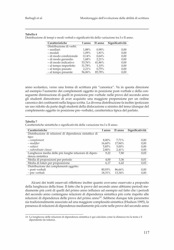
117
Barbagli et al. Monitoraggio dell’evoluzione delle abilità di scrittura
Tabella 6Distribuzione di tempi e modi verbali e significatività della variazione tra I e II anno.
Caratteristiche I anno II anno SignificativitàDistribuzione di verbi:– ausiliari 1,88% 0,98% 0,00– modali 1,09% 1,81% 0,00– di modo condizionale 0,14% 0,64% 0,00– di modo gerundio 1,68% 2,21% 0,00– di modo indicativo 53,76% 41,86% 0,00– al tempo imperfetto 31,78% 1,10% 0,00– al tempo passato 2,21% 0,75% 0,00– al tempo presente 56,06% 85,78% 0,00
anno scolastico, verso una forma di scrittura più “canonica”. Va in questa direzionead esempio l’aumento dei complementi oggetto in posizione post–verbale e della con-seguente diminuzione di quelli in posizione pre–verbale: nelle prove del secondo annogli studenti dimostrano di aver acquisito una maggiore propensione per un ordinecanonico dei costituenti nella lingua scritta. La diversa distribuzione fa inoltre ipotizzareun uso ridotto da parte degli studenti della dislocazione a sinistra del tema (dunque delcomplemento oggetto in posizione pre–verbale), caratteristica tipica del parlato.
Tabella 7Caratteristiche sintattiche e significatività della variazione tra I e II anno.
Caratteristiche I anno II anno SignificativitàDistribuzione di relazioni di dipendenza sintattica ditipo:– complement 8,00% 7,71% 0,00– modifier 16,60% 17,84% 0,00– subject 5,85% 5,00% 0,00– subordinate clause 2,80% 2,41% 0,00Lunghezza media delle più lunghe relazioni di dipen-denza sintattica
9,22 7,80 0,02
Media di proposizioni per periodo 4,00 3,36 0,01Media di token per proposizione 6,17 6,42 0,02Distribuzione dei complementi oggetto:– post–verbali 80,93% 86,66% 0,00– pre–verbali 18,31% 13,34% 0,00
Alcuni dei tratti osservati riflettono inoltre quanto avevamo osservato a propositodella lunghezza della frase. Il fatto che le prove del secondo anno abbiamo periodi me-diamente più corti di quelli del primo anno influisce ad esempio sul fatto che i periodidel secondo anno contengano relazioni di dipendenza sintattica più corte rispetto allerelazioni di dipendenza delle prove del primo anno10. Sebbene dunque tale parametrosia tradizionalmente associato ad una maggiore complessità sintattica (Hudson 1995), lapresenza di relazioni di dipendenza mediamente più corte nelle prove del secondo anno
10 La lunghezza delle relazioni di dipendenza sintattica è qui calcolata come la distanza tra la testa e ildipendente (in tokens).
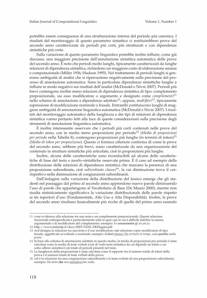
118
Italian Journal of Computational Linguistics Volume 1, Number 1
potrebbe essere conseguenza di una strutturazione interna del periodo più canonica. Irisultati del monitoraggio di questo parametro sintattico ci restituirebbero prove delsecondo anno caratterizzate da periodi più corti, più strutturati e con dipendenzesintattiche più corte.
Sulla variazione di questo parametro linguistico potrebbe inoltre influire, come giàdiscusso, una maggiore precisione dell’annotazione sintattica automatica delle provedel secondo anno. È noto che periodi molto lunghi, tipicamente caratterizzati da lungherelazioni di dipendenza sintattica, richiedono un maggiore costo di elaborazione umanae computazionale (Miller 1956; Hudson 1995). Nel trattamento di periodi lunghi si gen-erano ambiguità di analisi che si ripercuotono negativamente sulla precisione del pro-cesso di annotazione automatica. Sono in particolare dipendenze sintattiche lunghe ainfluire in modo negativo sui risultati dell’analisi (McDonald e Nivre 2007). Periodi piùbrevi contengono inoltre meno relazioni di dipendenza sintattica di tipo: complementopreposizionale, sia esso modificatore o argomento e designato come comp(lement)11
nello schema di annotazione a dipendenze adottato12; oppure, mod(ifier)13, tipicamenteespressione di modificazione nominale o frasale. Entrambi costituiscono luoghi di mag-giore ambiguità di annotazione linguistica automatica (McDonald e Nivre 2007). I risul-tati del monitoraggio automatico della lunghezza e dei tipi di relazioni di dipendenzasintattica vanno pertanto letti alla luce di queste considerazioni sulla precisione deglistrumenti di annotazione linguistica automatica.
È inoltre interessante osservare che i periodi più corti contenuti nelle prove delsecondo anno, con in media meno proposizioni per periodo14 (Media di proposizioniper periodo nella Tabella 8), contengono proposizioni più lunghe (in termini di token)15
(Media di token per proposizione). Questo ci fornisce ulteriore conferma di come le provedel secondo anno, sebbene più brevi, siano caratterizzate da una organizzazione delcontenuto in strutture sintattiche più articolate, cioè in proposizioni più lunghe.
Inoltre, alcune delle caratteristiche sono riconducibili ad alcune delle caratteris-tiche di base del testo e morfo–sintattiche osservate prima. È il caso ad esempio delladistribuzione delle relazioni di dipendenza sintattica che marcano la presenza di unaproposizione subordinata, cioè sub(ordinate clause)16, la cui diminuzione trova il cor-rispettivo nella diminuzione di congiunzioni subordinanti.
Dall’indagine sulla variazione della distribuzione del lessico emerge che gli stu-denti nel passaggio dal primo al secondo anno apprendono nuove parole diminuendol’uso di parole che appartengono al Vocabolario di Base (De Mauro 2000), mentre nonrisulta statisticamente significativa la variazione distribuzionale delle parole rispettoai tre repertori d’uso (Fondamentale, Alto Uso e Alta Disponibilità). Inoltre, le provedel secondo anno risultano lessicalmente più ricche di quelle del primo anno essendo
11 comp si riferisce alla relazione tra una testa e un complemento preposizionale. Questa relazionefunzionale sottospecificata è particolarmente utile in quei casi in cui è difficile stabilire la naturaargomentale o di modificatore del complemento; esempio: Fu assassinata da un pazzo.
12 http://www.italianlp.it/docs/ISST-TANL-DEPtagset.pdf13 mod designa la relazione tra una testa e il suo modificatore; tale relazione copre modificatori di tipo
frasale, aggettivale avverbiale e nominale; esempio: Colori intensi; Per arrivare in tempo, sono partito moltopresto.
14 In base allo schema di annotazione adottato in questo studio, la media di proposizioni per periodo è statacalcolata come la media di teste verbali (cioè di verbi testa sintattica da cui dipende un token o unsotto–albero sintattico) sul totale di periodi presenti nel testo.
15 La lunghezza della proposizione è stata calcolata come il rapporto tra il numero totale di token dellaprova e il numero totale di teste verbali della prova.
16 sub è la relazione tra una congiunzione subordinante e la testa verbale di una proposizione subordinata;esempio: Ha detto che non intendeva fare nulla.
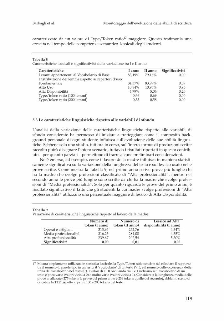
119
Barbagli et al. Monitoraggio dell’evoluzione delle abilità di scrittura
caratterizzate da un valore di Type/Token ratio17 maggiore. Questo testimonia unacrescita nel tempo delle competenze semantico–lessicali degli studenti.
Tabella 8Caratteristiche lessicali e significatività della variazione tra I e II anno.
Caratteristiche I anno II anno SignificativitàLemmi appartenenti al Vocabolario di Base 83,19% 79,16% 0,00Distribuzione dei lemmi rispetto ai repertori d’uso:Fondamentale 84,37% 83,99% 0,39Alto Uso 10,84% 10,95% 0,96Alta Disponibilità 4,79% 5,06 0,20Type/token ratio (100 lemmi) 0,66 0,69 0,00Type/token ratio (200 lemmi) 0,55 0,58 0,00
5.3 Le caratteristiche linguistiche rispetto alle variabili di sfondo
L’analisi della variazione delle caratteristiche linguistiche rispetto alle variabili disfondo considerate ha permesso di iniziare a tratteggiare come il composito back-ground personale di ogni studente influisca sull’evoluzione delle sue abilità linguis-tiche. Sebbene solo uno studio, tutt’ora in corso, sull’intero corpus di produzioni scritteraccolto potrà disegnare l’intero scenario, tuttavia i risultati riportati in questo contrib-uto – per quanto parziali – permettono di trarre alcune preliminari considerazioni.
Ne è emerso, ad esempio, come il lavoro della madre influisca in maniera statisti-camente significativa sulla variazione della lunghezza del testo e sul lessico usato nelleprove scritte. Come mostra la Tabella 9, nel primo anno scrive prove più lunghe chiha la madre che svolge professioni classificate di “Alta professionalità”, mentre nelsecondo anno le prove più lunghe sono scritte da chi ha la madre che svolge profes-sioni di “Media professionalità”. Solo per quanto riguarda le prove del primo anno, èrisultato significativo il fatto che gli studenti la cui madre svolge professioni di “Altaprofessionalità” utilizzano una percentuale maggiore di lessico di Alta Disponibilità.
Tabella 9Variazione di caratteristiche linguistiche rispetto al lavoro della madre.
Numero di Numero di Lessico ad Altatoken (I anno) token (II anno) disponibilità (I anno)
Operai e artigiani 313,95 252,76 4,34%Media professionalità 316,25 284,08 4,55%Alta professionalità 239,67 202,54 5,30%Significatività 0,00 0,01 0,03
17 Misura ampiamente utilizzata in statistica lessicale, la Type/Token ratio consiste nel calcolare il rapportotra il numero di parole tipo in un testo, il ‘vocabolario’ di un testo (Vc), e il numero delle occorrenza delleunità del vocabolario nel testo (C). I valori di TTR oscillando tra 0 e 1 indicano se il vocabolario di untesto è poco vario (valori vicini a 0) o molto vario (valori vicini a 1). Considerata la lunghezza media delleprove analizzate (275 tokens le prove del primo anno e 239 tokens quelle del secondo), abbiamo scelto dicalcolare la TTR rispetto ai primi 100 e 200 tokens del testo.
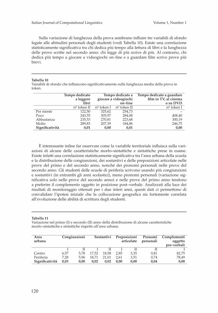
120
Italian Journal of Computational Linguistics Volume 1, Number 1
Sulla variazione di lunghezza della prova sembrano influire tre variabili di sfondolegate alle abitudini personali degli studenti (vedi Tabella 10). Esiste una correlazionestatisticamente significativa tra chi dedica più tempo alla lettura di libri e la lunghezzadelle prove scritte nel secondo anno: chi legge di più scrive di più. Al contrario, chidedica più tempo a giocare a videogiochi on–line e a guardare film scrive prove piùbrevi.
Tabella 10Variabili di sfondo che influiscono significativamente sulla lunghezza media della prova intoken.
Tempo dedicato Tempo dedicato a Tempo dedicato a guardarea leggere giocare a videogiochi film in TV, al cinema
libri on–line o su DVDno token II no token I no token II no token I
Per niente 122,50 325,62 254,73 –Poco 243,55 305,97 284,08 408,40Abbastanza 235,53 270,81 223,68 300,19Molto 289,83 207,39 184,86 246,75Significatività 0,01 0,00 0,01 0,00
È interessante infine far osservare come la variabile territoriale influisca sulla vari-azioni di alcune delle caratteristiche morfo–sintattiche e sintattiche prese in esame.Esiste infatti una correlazione statisticamente significativa tra l’area urbana della scuolae la distribuzione delle congiunzioni, dei sostantivi e delle preposizioni articolate nelleprove del primo e del secondo anno, nonché dei pronomi personali nelle prove delsecondo anno. Gli studenti delle scuole di periferia scrivono usando più congiunzionie sostantivi (in entrambi gli anni scolastici), meno pronomi personali (variazione sig-nificativa solo nelle prove del secondo anno) e nelle prove del primo anno tendonoa preferire il complemento oggetto in posizione post–verbale. Analizzati alla luce deirisultati di monitoraggio ottenuti per i due interi anni, questi dati ci permettono diconvalidare l’ipotesi iniziale che la collocazione geografica sia fortemente correlataall’evoluzione delle abilità di scrittura degli studenti.
Tabella 11Variazione nel primo (I) e secondo (II) anno della distribuzione di alcune caratteristichemorfo–sintattiche e sintattiche rispetto all’area urbana.
Area Congiunzioni Sostantivi Preposizioni Pronomi Complementiurbana articolate personali oggetto
pre–verbaliI II I II I II II I
Centro 6,57 5,78 17,52 18,58 2,85 3,35 0,81 82,75Periferia 7,28 5,96 18,71 21,01 2,61 3,51 0,74 78,49Significatività 0,03 0,00 0,02 0,02 0,00 0,00 0,04 0,00
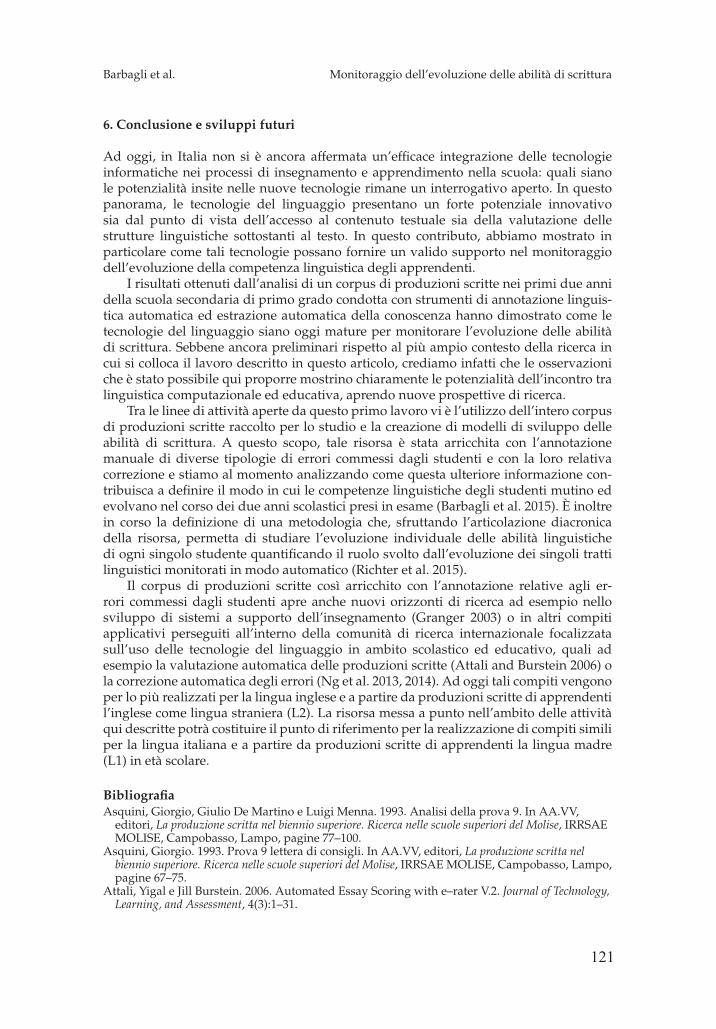
121
Barbagli et al. Monitoraggio dell’evoluzione delle abilità di scrittura
6. Conclusione e sviluppi futuri
Ad oggi, in Italia non si è ancora affermata un’efficace integrazione delle tecnologieinformatiche nei processi di insegnamento e apprendimento nella scuola: quali sianole potenzialità insite nelle nuove tecnologie rimane un interrogativo aperto. In questopanorama, le tecnologie del linguaggio presentano un forte potenziale innovativosia dal punto di vista dell’accesso al contenuto testuale sia della valutazione dellestrutture linguistiche sottostanti al testo. In questo contributo, abbiamo mostrato inparticolare come tali tecnologie possano fornire un valido supporto nel monitoraggiodell’evoluzione della competenza linguistica degli apprendenti.
I risultati ottenuti dall’analisi di un corpus di produzioni scritte nei primi due annidella scuola secondaria di primo grado condotta con strumenti di annotazione linguis-tica automatica ed estrazione automatica della conoscenza hanno dimostrato come letecnologie del linguaggio siano oggi mature per monitorare l’evoluzione delle abilitàdi scrittura. Sebbene ancora preliminari rispetto al più ampio contesto della ricerca incui si colloca il lavoro descritto in questo articolo, crediamo infatti che le osservazioniche è stato possibile qui proporre mostrino chiaramente le potenzialità dell’incontro tralinguistica computazionale ed educativa, aprendo nuove prospettive di ricerca.
Tra le linee di attività aperte da questo primo lavoro vi è l’utilizzo dell’intero corpusdi produzioni scritte raccolto per lo studio e la creazione di modelli di sviluppo delleabilità di scrittura. A questo scopo, tale risorsa è stata arricchita con l’annotazionemanuale di diverse tipologie di errori commessi dagli studenti e con la loro relativacorrezione e stiamo al momento analizzando come questa ulteriore informazione con-tribuisca a definire il modo in cui le competenze linguistiche degli studenti mutino edevolvano nel corso dei due anni scolastici presi in esame (Barbagli et al. 2015). È inoltrein corso la definizione di una metodologia che, sfruttando l’articolazione diacronicadella risorsa, permetta di studiare l’evoluzione individuale delle abilità linguistichedi ogni singolo studente quantificando il ruolo svolto dall’evoluzione dei singoli trattilinguistici monitorati in modo automatico (Richter et al. 2015).
Il corpus di produzioni scritte così arricchito con l’annotazione relative agli er-rori commessi dagli studenti apre anche nuovi orizzonti di ricerca ad esempio nellosviluppo di sistemi a supporto dell’insegnamento (Granger 2003) o in altri compitiapplicativi perseguiti all’interno della comunità di ricerca internazionale focalizzatasull’uso delle tecnologie del linguaggio in ambito scolastico ed educativo, quali adesempio la valutazione automatica delle produzioni scritte (Attali and Burstein 2006) ola correzione automatica degli errori (Ng et al. 2013, 2014). Ad oggi tali compiti vengonoper lo più realizzati per la lingua inglese e a partire da produzioni scritte di apprendentil’inglese come lingua straniera (L2). La risorsa messa a punto nell’ambito delle attivitàqui descritte potrà costituire il punto di riferimento per la realizzazione di compiti similiper la lingua italiana e a partire da produzioni scritte di apprendenti la lingua madre(L1) in età scolare.
BibliografiaAsquini, Giorgio, Giulio De Martino e Luigi Menna. 1993. Analisi della prova 9. In AA.VV,
editori, La produzione scritta nel biennio superiore. Ricerca nelle scuole superiori del Molise, IRRSAEMOLISE, Campobasso, Lampo, pagine 77–100.
Asquini, Giorgio. 1993. Prova 9 lettera di consigli. In AA.VV, editori, La produzione scritta nelbiennio superiore. Ricerca nelle scuole superiori del Molise, IRRSAE MOLISE, Campobasso, Lampo,pagine 67–75.
Attali, Yigal e Jill Burstein. 2006. Automated Essay Scoring with e–rater V.2. Journal of Technology,Learning, and Assessment, 4(3):1–31.
122
Italian Journal of Computational Linguistics Volume 1, Number 1
Attardi, Giuseppe, Felice Dell’Orletta, Maria Simi e Joseph Turian. 2009. Accurate DependencyParsing with a Stacked Multilayer Perceptron. In Proceedings of Evalita’09 (Evaluation of NLPand Speech Tools for Italian), pagine 1–8, Reggio Emilia (Italia).
Barbagli, Alessia, Pietro Lucisano, Felice Dell’Orletta, Simonetta Montemagni e Giulia Venturi.2015. CItA: un Corpus di Produzioni Scritte di Apprendenti l’Italiano L1 Annotato con Errori.In Proceedings of the 2nd Italian Conference on Computational Linguistics (CLiC-it), Trento, (Italia).
Beaman, Karen. 1984. Coordination and Subordination Revisited: Syntactic Complexity inSpoken and Written Narrative Discorse. In Tannen D. e Freedle R., editori, Coherence in Spokenand Written Discorse, Norwood, N.J., pagine 45–80.
Biber, Douglas. 1993. Using Register-diversified Corpora for General Language Studies.Computational Linguistics Journal, 19(2):219–241.
Bonin, Francesca, Felice Dell’Orletta, Simonetta Montemagni e Giulia Venturi. 2010. AContrastive Approach to Multi–word Extraction from Domain–specific Corpora. In Proceedingsof the 7th International Conference on Language Resources and Evaluation (LREC 2010), pagine3222–3229, Valletta (Malta).
Corbett, Albert T. e John R. Anderson. 1994. Knowledge tracing: Modeling the acquisition ofprocedural knowledge. User modeling and user–adapted interaction, 4(4):253–278.
Corda Costa, Maria e Aldo Visalberghi. 1995. Misurare e valutare le competenze linguistiche. Guidascientifico-pratica per gli insegnanti. Firenze, La Nuova Italia.
Deane, Paul e Thomas Quinlan. 2010. What automated analyses of corpora can tell us aboutstudents’ writing skills. Journal of Writing Research, 2(2):151–177.
Dell’Orletta, Felice. 2009. Ensemble system for Part-of-Speech tagging. In Proceedings of Evalita’09(Evaluation of NLP and Speech Tools for Italian), pagine 1–8, Reggio Emilia (Italia).
Dell’Orletta, Felice, Simonetta Montemagni, Eva M. Vecchi e Giulia Venturi. 2011. Tecnologielinguistico-computazionali per il monitoraggio della competenza linguistica italiana deglialunni stranieri nella scuola primaria e secondaria. In G.C. Bruno, I. Caruso, M. Sanna, I.Vellecco, editori, Percorsi migranti: uomini, diritto, lavoro, linguaggi, Milano, McGraw-Hill,pagine 319–336.
Dell’Orletta, Felice e Simonetta Montemagni. 2012. Tecnologie linguistico–computazionali per lavalutazione delle competenze linguistiche in ambito scolastico. In Atti del XLIV CongressoInternazionale di Studi della Società di Linguistica Italiana (SLI 2010), pagine 343–359, Viterbo(Italia).
Dell’Orletta, Felice, Simonetta Montemagni e Giulia Venturi. 2013a. Linguistic Profiling of TextsAcross Textual Genre and Readability Level. An Exploratory Study on Italian Fictional Prose.In Proceedings of the Recent Advances in Natural Language Processing Conference (RANLP-2013),pagine 189–197, Hissar (Bulgaria).
Dell’Orletta, Felice, Giulia Venturi e Simonetta Montemagni. 2013b. UnsupervisedLinguistically-Driven Reliable Dependency Parses Detection and Self-Training for Adaptationto the Biomedical Domain. In Proceedings of the 2013 Workshop on Biomedical Natural LanguageProcessing (BIONLP-2013), pagine 45–53, Sofia (Bulgaria).
Dell’Orletta, Felice, Giulia Venturi, Andrea Cimino e Simonetta Montemagni. 2014. T2K: aSystem for Automatically Extracting and Organizing Knowledge from Texts. In Proceedings of9th Edition of International Conference on Language Resources and Evaluation (LREC 2014), pagine2062–2070, Reykjavik (Islanda).
De Mauro, Tullio. 2000. Grande dizionario italiano dell’uso (GRADIT). Torino, UTET.Ekanadham, Chaitanya e Yan Karklin. 2015. T-SKIRT: Online Estimation of Student Proficiency
in an Adaptive Learning System. In Proceedings of the 31st International Conference on MachineLearning, pagine 1–6, Lille (Francia).
Fabi, Aldo e Gabriella Pavan De Gregorio. 1988. La prova 9: risultati di una ricerca sui contenutiin una prova di consigli sulla scrittura. Ricerca educativa, 5:2–3.
Frantzi, Katerina, Sophia Ananiadou e Hideki Mima. 2000. Automatic recognition of multi-wordterms:. the C-value/NC-value method. International Journal on Digital Libraries, 3(2):115–130,Springer–Verlag.
Givón, Thomas. 1991. Markedness in grammar: distributional, communicative and cognitivecorrelates of syntactic structure. Studies in Language, 15(2):335–370.
Granger, Sylviane. 2003. Error-tagged Learner Corpora and CALL: A Promising Synergy.CALICO Journal, 20:465–480.
Hudson, Richard A. 1995. Measuring syntactic difficulty. Manuscript, University College,London disponibile alla pagina http://www.phon.ucl.ac.uk/home/dick/difficulty.htm
123
Barbagli et al. Monitoraggio dell’evoluzione delle abilità di scrittura
Lu, Xiaofei. 2007. Automatic measurement of syntactic complexity in child language acquisition.International Journal of Corpus Linguistics, 14(1):3–28.
Lubetich, Shannon e Kenji Sagae. 2014. Data–Driven Measurement of Child LanguageDevelopment with Simple Syntactic Templates. In Proceedings of the 25th InternationalConference on Computational Linguistics (COLING), pagine 2151–2160, Dublino (Irlanda).
Lucisano, Pietro. 1984. L’indagine IEA sulla produzione scritta. Ricerca educativa, 5:41–61.Lucisano, Pietro. 1988. La ricerca IEA sulla produzione scritta. Ricerca educativa, 2:3–13.Lucisano, Pietro e Guido Benvenuto. 1991. Insegnare a scrivere: dalla parte degli insegnanti.
Scuola e Città, 6:265–279.Masini, Andrea. 2003. L’italiano contemporaneo e le sue varietá. In I. Bonomi, A. Masini, S.
Morgana e M. Piotti, editori, Elementi di Linguistica Italiana, Roma, Carocci, pagine 15–86.McDonald, Ryan e Joakim Nivre. 2007. Characterizing the errors of data–driven dependency
parsing models. In Proceedings of the the EMNLP-CoNLL, pagine 122–131, Praga (RepubblicaCeca).
Montemagni, Simonetta. 2013. Tecnologie linguistico–computazionali e monitoraggio dellalingua italiana. Studi Italiani di Linguistica Teorica e Applicata (SILTA), XLII(1):145–172.
Mortara Garavelli, Bice. 2003. Strutture testuali e stereotipi nel linguaggio forense. In P. MarianiBiagini, editori, La lingua, la legge, la professione forense. Atti del convegno Accademia della Crusca(Firenze, 31 gennaio-1 febbraio 2002), Milano, Giuffrè, pagine 3-19.
Miller, George A.. 1956. The magical number seven, plus or minus two: some limits on purcapacity for processing information. Psycological Review, 63:81–97.
Ng, Hwee T., Siew M. Wu, Yuanbin Wu, Christian Hadiwinoto e Joel Tetreault. 2013. TheCoNLL-2013 Shared Task on Grammatical Error Correction. In Proceedings of the SeventeenthConference on Computational Natural Language Learning: Shared Task, pagine 1–12, Sofia(Bulgaria).
Ng, Hwee T., Siew M. Wu, Ted Briscoe, Christian Hadiwinoto, Raymond H. Susanto eChristopher Bryant. 2014. The CoNLL-2014 Shared Task on Grammatical Error Correction. InProceedings of the Eighteenth Conference on Computational Natural Language Learning: Shared Task,pagine 1–14, Baltimore (Maryland).
Petersen, Sarah E. e Mari Ostendorf. 2009. A machine learning approach to reading levelassessment. In Computer Speech and Language, 23:89–106.
Piech, Chris, Jonathan Bassen, Jonathan Huang, Surya Ganguli, Mehran Sahami, LeonidasGuibas e Jascha Sohl-Dickstein. 2015. Deep Knowledge Tracing. ArXiv e-prints:1506.059082015, pagine 1–13.
Purvues, Alan C. 1992. The IEA Study of Written Composition II: Education and Performance inFourteen Countries vol 6. Oxford, Pergamon.
Richter, Stefan, Andrea Cimino, Felice Dell’Orletta e Giulia Venturi. 2015. Tracking the Evolutionof Language Competence: an NLP–based Approach. In Proceedings of the 2nd Italian Conferenceon Computational Linguistics (CLiC-it), 2–3 December, Trento, Italy.
Rigo, Roberta. 2005. Didattica delle abilità linguistiche. Percorsi di progettazione e di formazioneinsegnanti. Armando Editore
Roark, Brian, Margaret Mitchell e Kristy Hollingshead. 2007. Syntactic complexity measures fordetecting mild cognitive impairment. In Proceedings of the Workshop on BioNLP 2007: Biological,Translational, and Clinical Language Processing, pagine 1–8, Praga (Repubblica Ceca).
Rouhizadeh, Masoud, Emily Prud’hommeaux, Brian Roark e Jan van Santen. 2013.Distributional semantic models for the evaluation of disordered language. In Proceedings of the2013 Conference of the North American Chapter of the Association for Computational Linguistics:Human Language Technologies, pagine 709–714, Atlanta (Georgia, USA).
Sagae, Kenji, Alon Lavie e Brian MacWhinney. 2005. Automatic measurement of syntacticdevelopment in child language. In Proceedings of the 43rd Annual Meeting on Association forComputational Linguistics (ACL 05), pagine 197–204, Ann Arbor (Michigan, USA).
Schwarm, Sarah E. e Mari Ostendorf. 2005. Reading level assessment using support vectormachines and statistical language models. In Proceedings of the 43rd Annual Meeting onAssociation for Computational Linguistics (ACL 05), pagine 523–530, Ann Arbor (Michigan, USA).
Vu, Thuy, Ai T. Aw e Min Zhang. 2008. Term Extraction Through Unithood and TermhoodUnification. In Proceedings of the Third International Joint Conference on Natural LanguageProcessing, pagine 631–636, Hyderabad (India).

© 2015 Associazione Italiana di Linguistica Computazionale
CLaSSES: a New Digital Resource for Latin Epigraphy
Irene De Felice* Università di Pisa
Margherita Donati§ Università di Pisa
Giovanna Marotta† Università di Pisa
CLaSSES (Corpus for Latin Sociolinguistic Studies on Epigraphic textS) is an annotated corpus aimed at (socio)linguistic research on Latin inscriptions. Provided with linguistic, extra- and meta-linguistic features, it can be used to perform quantitative and qualitative variationist analyses on Latin epigraphic texts. In particular, it allows the user to analyze spelling (and possibly phonetic-phonological) variants and to interpret them with reference to the dating, the provenance place, and the type of the texts. This paper presents the first macro-section of CLaSSES, focused on inscriptions of the archaic and early periods (CLaSSES I).
1. Introduction1
This paper presents CLaSSES I, the first macro-section of CLaSSES (Corpus for Latin Sociolinguistic Studies on Epigraphic textS), an epigraphic corpus built for variationist studies on Latin inscriptions. This resource was developed within a research project devoted to sociolinguistic variation and identity dynamics in the Latin language (for further details on the project, see Donati et al. in press; Marotta in press).
In the first section of the paper, some of the digital resources available for Latin epigraphy will be briefly introduced, then the most important aspects of innovation of CLaSSES will be highlighted (§ 2). The following section will address the current debate about the role played by epigraphic texts as a source of evidence for linguistic variation within dead languages, as well as the theoretical grounds for variationist research on epigraphic Latin (§ 3). The core part of the paper describes the sources of our corpus and the linguistic, meta- and extra-linguistic annotation conducted (§ 4); some results of such annotation are also reported (§ 5). Finally, the last section will draw some conclusions and will sketch the future directions of our work (§ 6).
* Department of Philology, Literature and Linguistics, University of Pisa. E-mail: [email protected] § Department of Philology, Literature and Linguistics, University of Pisa. E-mail: [email protected] † Department of Philology, Literature and Linguistics, University of Pisa. E-mail: [email protected] 1 This research was developed at the Laboratory of Phonetics and Phonology of Pisa University within the
PRIN project Linguistic representations of identity. Sociolinguistic models and historical linguistics (PRIN2010, prot. 2010HXPFF2_001). The results related to the project are available online at http://www.mediling.eu/. The paper was conceived by the three authors together. For academic reasons only, the scientific responsibility is attributed as follows: § 1 is common; § 2, § 4.5, § 4.6, § 5 to I. De Felice; § 3, § 4.2, § 4.3, § 4.4 to M. Donati; § 4.1, § 6 to G. Marotta.
125
© 2015 Associazione Italiana di Linguistica Computazionale
CLaSSES: a New Digital Resource for Latin Epigraphy
Irene De Felice* Università di Pisa
Margherita Donati§ Università di Pisa
Giovanna Marotta† Università di Pisa
CLaSSES (Corpus for Latin Sociolinguistic Studies on Epigraphic textS) is an annotated corpus aimed at (socio)linguistic research on Latin inscriptions. Provided with linguistic, extra- and meta-linguistic features, it can be used to perform quantitative and qualitative variationist analyses on Latin epigraphic texts. In particular, it allows the user to analyze spelling (and possibly phonetic-phonological) variants and to interpret them with reference to the dating, the provenance place, and the type of the texts. This paper presents the first macro-section of CLaSSES, focused on inscriptions of the archaic and early periods (CLaSSES I).
1. Introduction1
This paper presents CLaSSES I, the first macro-section of CLaSSES (Corpus for Latin Sociolinguistic Studies on Epigraphic textS), an epigraphic corpus built for variationist studies on Latin inscriptions. This resource was developed within a research project devoted to sociolinguistic variation and identity dynamics in the Latin language (for further details on the project, see Donati et al. in press; Marotta in press).
In the first section of the paper, some of the digital resources available for Latin epigraphy will be briefly introduced, then the most important aspects of innovation of CLaSSES will be highlighted (§ 2). The following section will address the current debate about the role played by epigraphic texts as a source of evidence for linguistic variation within dead languages, as well as the theoretical grounds for variationist research on epigraphic Latin (§ 3). The core part of the paper describes the sources of our corpus and the linguistic, meta- and extra-linguistic annotation conducted (§ 4); some results of such annotation are also reported (§ 5). Finally, the last section will draw some conclusions and will sketch the future directions of our work (§ 6).
* Department of Philology, Literature and Linguistics, University of Pisa. E-mail: [email protected] § Department of Philology, Literature and Linguistics, University of Pisa. E-mail: [email protected] † Department of Philology, Literature and Linguistics, University of Pisa. E-mail: [email protected] 1 This research was developed at the Laboratory of Phonetics and Phonology of Pisa University within the
PRIN project Linguistic representations of identity. Sociolinguistic models and historical linguistics (PRIN2010, prot. 2010HXPFF2_001). The results related to the project are available online at http://www.mediling.eu/. The paper was conceived by the three authors together. For academic reasons only, the scientific responsibility is attributed as follows: § 1 is common; § 2, § 4.5, § 4.6, § 5 to I. De Felice; § 3, § 4.2, § 4.3, § 4.4 to M. Donati; § 4.1, § 6 to G. Marotta.
126
Italian Journal of Computational Linguistics Volume 1, Number 1
2. Digital resources for Latin inscriptions
The available open-access digital resources for Latin epigraphy include, at present, some important databases (cf. Feraudi-Gruénais 2010; Elliott 2015). The Epigraphic Database Clauss-Slaby (EDCS)2 is the most extensive online resource and records almost all Latin inscriptions (to date, 735.664 sets of data for 491.190 inscriptions from 3.500 publications), together with a very large number of pictures (so far, 98.897). It allows simple as well as combined queries, by publication, Roman province, place, and specific terms (possibly by using boolean operators and simple regular expressions); in addition, users can search also for misspelled words. The text of the inscriptions is presented without abbreviations and, when possible, in its complete form.
Another very useful online resource is the Epigraphic Database Roma (EDR);3 it is part of the Electronic Archive for Greek and Latin Epigraphy (EAGLE),4 an international network of epigraphic databases aiming to provide an open-access digital version of all published Greek and Latin inscriptions up to the 7th century AD. The main purpose of EDR is to collect all inscriptions from Rome and Italy, including Sardinia and Sicily (with the exception of Christian inscriptions of Rome). Besides the information about the content of the inscriptions, EDR also provides information about the writing support (e.g. typology, material, dimension) and a wide-ranging bibliography; often, also images and photographs are supplied (Panciera 2013; Caldelli et al. 2014). To date, EDR material includes 70294 inscriptions and 42022 photographs. Through the online query interface, the user can perform a number of simple or combined searches, through the following sections: text (words or groups of letters, possibly with boolean operators AND/OR), place of provenance, date, type of object, material, size, preservation condition (intact or fragmentary texts), writing technique, language (e.g. Greek, Latin, Greek - Latin bilingual), type of inscription, social role of people mentioned, edition (Evangelisti 2010).
Two other components of EAGLE well worth mentioning are the Epigraphische Datenbank Heidelberg (EDH),5 which mostly includes Latin or bilingual (Greek - Latin) inscriptions of provinces of the Roman empire, and the Epigraphic Database Bari (EDB),6 which collects Christian inscriptions of Rome from the 3rd to the 8th century AD.
Some electronic resources of utility are also made freely available by the Corpus Inscriptionum Latinarum (CIL) research centre, in particular the Archivium Corporis Electronicum database (a collection of bibliographical references, squeezes, and photographs), the word indices to a few CIL volumes, and the concordances (that link inscription numbers adopted in early editions to those adopted in the CIL volumes).7
For what regards the representation of epigraphic or papyrological texts in digital form, the international and collaborative project EpiDoc (Epigraphic Documents),8 which involves a large community of scholars working on Greek and Latin inscriptions (cf. Bodard 2010), provides tools and guidelines for the encoding of editions of ancient documents in XML, the Extensible Markup Language. EpiDoc adopts a subset of the XML defined by the Text Encoding
2 http://www.manfredclauss.de/gb/index.html. 3 http://www.edr-edr.it/English/index_en.php. 4 http://www.eagle-network.eu. 5 http://www.uni-heidelberg.de/institute/sonst/adw/edh. 6 http://www.edb.uniba.it. 7 All these resources are accessible from the website http://cil.bbaw.de. 8 http://sourceforge.net/p/epidoc/wiki/Home/.
127
Italian Journal of Computational Linguistics Volume 1, Number 1
2. Digital resources for Latin inscriptions
The available open-access digital resources for Latin epigraphy include, at present, some important databases (cf. Feraudi-Gruénais 2010; Elliott 2015). The Epigraphic Database Clauss-Slaby (EDCS)2 is the most extensive online resource and records almost all Latin inscriptions (to date, 735.664 sets of data for 491.190 inscriptions from 3.500 publications), together with a very large number of pictures (so far, 98.897). It allows simple as well as combined queries, by publication, Roman province, place, and specific terms (possibly by using boolean operators and simple regular expressions); in addition, users can search also for misspelled words. The text of the inscriptions is presented without abbreviations and, when possible, in its complete form.
Another very useful online resource is the Epigraphic Database Roma (EDR);3 it is part of the Electronic Archive for Greek and Latin Epigraphy (EAGLE),4 an international network of epigraphic databases aiming to provide an open-access digital version of all published Greek and Latin inscriptions up to the 7th century AD. The main purpose of EDR is to collect all inscriptions from Rome and Italy, including Sardinia and Sicily (with the exception of Christian inscriptions of Rome). Besides the information about the content of the inscriptions, EDR also provides information about the writing support (e.g. typology, material, dimension) and a wide-ranging bibliography; often, also images and photographs are supplied (Panciera 2013; Caldelli et al. 2014). To date, EDR material includes 70294 inscriptions and 42022 photographs. Through the online query interface, the user can perform a number of simple or combined searches, through the following sections: text (words or groups of letters, possibly with boolean operators AND/OR), place of provenance, date, type of object, material, size, preservation condition (intact or fragmentary texts), writing technique, language (e.g. Greek, Latin, Greek - Latin bilingual), type of inscription, social role of people mentioned, edition (Evangelisti 2010).
Two other components of EAGLE well worth mentioning are the Epigraphische Datenbank Heidelberg (EDH),5 which mostly includes Latin or bilingual (Greek - Latin) inscriptions of provinces of the Roman empire, and the Epigraphic Database Bari (EDB),6 which collects Christian inscriptions of Rome from the 3rd to the 8th century AD.
Some electronic resources of utility are also made freely available by the Corpus Inscriptionum Latinarum (CIL) research centre, in particular the Archivium Corporis Electronicum database (a collection of bibliographical references, squeezes, and photographs), the word indices to a few CIL volumes, and the concordances (that link inscription numbers adopted in early editions to those adopted in the CIL volumes).7
For what regards the representation of epigraphic or papyrological texts in digital form, the international and collaborative project EpiDoc (Epigraphic Documents),8 which involves a large community of scholars working on Greek and Latin inscriptions (cf. Bodard 2010), provides tools and guidelines for the encoding of editions of ancient documents in XML, the Extensible Markup Language. EpiDoc adopts a subset of the XML defined by the Text Encoding
2 http://www.manfredclauss.de/gb/index.html. 3 http://www.edr-edr.it/English/index_en.php. 4 http://www.eagle-network.eu. 5 http://www.uni-heidelberg.de/institute/sonst/adw/edh. 6 http://www.edb.uniba.it. 7 All these resources are accessible from the website http://cil.bbaw.de. 8 http://sourceforge.net/p/epidoc/wiki/Home/.
De Felice et al. CLaSSES: a new digital resource for Latin epigraphy
Initiative’s (TEI) standard for the digital representation of texts, which is now widely used in the humanities. This flexible system allows not only to transcribe a Greek or Latin text, but also, for instance, to encode its translation, description, and other pieces of information such as dating, history of the inscription, bibliography, and the object on which the text is written. At the moment, we decided not to follow the EpiDoc guidelines, due to the current aims of the project. However, we do not exclude a conversion of our existing corpus in the XML interchange format in the future.
Although the current state-of-the-art digital resources for Latin inscriptions briefly presented here collect a copious number of epigraphic texts and often provide useful extra-linguistic data, such as provenance place, dating, material, etc., they do not allow researchers to directly access specific information about relevant linguistic variation phenomena. They do not satisfactorily meet the needs of the linguist to study Latin epigraphic texts from a variationist perspective. In order to systematically address the massive graphic and linguistic variation observable in Latin inscriptions, a specific tool is necessary. We argue that the corpus CLaSSES is a new and useful resource, since it consists not only of raw epigraphic texts, but also of linguistic information about specific spelling variants that can be regarded as clues for phonetic-phonological (and morpho-phonological) variation (cf. § 4).
3. Studying variation in Latin through inscriptions
There is a current debate9 on whether inscriptions can provide direct evidence for actual linguistic variation in Latin. In other words, can epigraphic texts be regarded as primary and reliable sources for reconstructing variation dynamics related to social strata, different language registers, and geographic variability? It is obviously true that inscriptions are the only direct evidence left by antiquity (although they can be influenced by literary uses, writers’ education, and many other factors), since every other kind of written text, even comedy or the so-called “vulgar” texts, is necessarily mediated by philological and manuscript tradition. In this sense, inscriptions are likely to keep record of linguistic variation. However, the story is not that simple.
As Herman (1985) points out, the debate on the evaluation of late or “vulgar” inscriptions as linguistically representative texts is ancient and alternates between approaches that are either totally skeptical or too optimistic. Herman argues for a critical approach (1978b, 1985): epigraphic texts are fundamental sources for studying variation phenomena, provided that scholars take into account the issues related to their philological, paleographic, archaeological and historical interpretation, as well as the complex relationship between speech and writing. He states “mon article [...] veut sans doute constituer une mise en garde à l’adresse de ceux qui espèrent entrevoir grâce aux inscriptions [...] de nettes différences dialectales dans le latin des provinces de l’Empire, il tend cependant à prouver, en même temps, que les données épigraphiques, analysées avec critique et soin, correspondent bien à la réalité d’un état de langue déterminé et permettent par conséquent de suivre, de province en province, le cheminement inégal des innovations” (1985: 207). However, Herman’s fundamental studies on Latin demonstrate that epigraphic texts are actually fruitful for studying linguistic variation (Herman 1970, 1978a, 1978b, 1982, 1987, 2000, among others; see also Loporcaro 2011a, 2011b).
9 We just touch on this topic; for further discussion see Donati et al. in press; Marotta 2015, in press.
128
Italian Journal of Computational Linguistics Volume 1, Number 1
On the other hand, Adams (2003, 2007, 2013) limits the role of the inscriptions as a source for direct evidence of the spoken language and linguistic varieties of Latin. He argues that one can never be sure whether the variants found in inscriptions reflect the actual pronunciation, or are just misspellings or archaisms: only the critical evaluation of deviant spellings together with metalinguistic data, such as those provided by grammarians and authors, can ensure that these spellings actually reflect a phonetic reality. Moreover, even if deviant spellings can be recognized as reflecting speech, ascribing it to a given social class or level is a further step that needs to be confirmed, again, by grammarians, rhetors, and literary authors. Adams states that “certain misspellings are so frequent that there can be no doubt that they reflect the state of the language. Cases in point are the omission of -m and the writing of ae as e. But the state of what varieties of the language? Those spoken by a restricted educational/social class, or those spoken by the majority of the population? This is a question that cannot be answered merely from an examination of texts and their misspellings or absence thereof, because good spellers will stick to traditional spellings whether they are an accurate reflection of their own speech or not. If, roughly speaking, we are to place the pronunciation lying behind a misspelling in a particular social class, we need additional evidence, such as remarks by grammarians or other speakers” (2013: 33-34). So, in Adams’ approach to Latin sociolects, grammarians and their remarks occupy a very prominent place.
In our opinion, epigraphic texts can be regarded as a fundamental source for studying variation in Latin, provided that one adopts a critical approach. This position is shared by several scholars, who in recent works highlight the relevance of the epigraphic data (Consani in press; De Angelis in press; Kruschwitz 2015; Marotta 2015, in press; Rovai 2015). Nevertheless, the critical points raised by Adams cannot be ignored.
Furthermore, sociolinguistic variation of Latin in Rome and the Empire is a promising research area (Adams et al. 2002; Adams 2003, 2007, 2013; Biville et al. 2008; Dickey and Chahoud 2010; Rochette 1997). From the seminal work by Campanile (1971), many scholars highlight that sociolinguistic categories and methods can be usefully applied to ancient and dead languages (Giacalone Ramat 2000; Lazzeroni 1984; Molinelli 2006; Vineis 1984, 1993), even if cautiously, since ancient languages are corpus languages10 and we are forced to rely on written sources only (Cuzzolin and Haverling 2009; Giacalone Ramat 2000; Winter 1998).
Assuming this methodological perspective, our empirical analysis of Latin epigraphic texts is focused on identifying and classifying specific spelling variants, which can be regarded as clues for variation also at the phonetic-phonological, and consequently morpho-phonological level. Being aware of the debate on the reliability of inscriptions currently ongoing, we intend to investigate whether it is possible to find out relevant evidence for sociolinguistic variation in epigraphic Latin via the integration of the modern quantitative and correlative sociolinguistics with a corpus-based approach. Since, at present, there is a lack of digital resources devoted to this particular kind of research (cf. § 2), our first step was the creation of an original resource for studying Latin epigraphic texts, which will be described in what follows.
10 A corpus language can be defined as a language “known only through written documents” (Clackson
2011: 2).
129
Italian Journal of Computational Linguistics Volume 1, Number 1
On the other hand, Adams (2003, 2007, 2013) limits the role of the inscriptions as a source for direct evidence of the spoken language and linguistic varieties of Latin. He argues that one can never be sure whether the variants found in inscriptions reflect the actual pronunciation, or are just misspellings or archaisms: only the critical evaluation of deviant spellings together with metalinguistic data, such as those provided by grammarians and authors, can ensure that these spellings actually reflect a phonetic reality. Moreover, even if deviant spellings can be recognized as reflecting speech, ascribing it to a given social class or level is a further step that needs to be confirmed, again, by grammarians, rhetors, and literary authors. Adams states that “certain misspellings are so frequent that there can be no doubt that they reflect the state of the language. Cases in point are the omission of -m and the writing of ae as e. But the state of what varieties of the language? Those spoken by a restricted educational/social class, or those spoken by the majority of the population? This is a question that cannot be answered merely from an examination of texts and their misspellings or absence thereof, because good spellers will stick to traditional spellings whether they are an accurate reflection of their own speech or not. If, roughly speaking, we are to place the pronunciation lying behind a misspelling in a particular social class, we need additional evidence, such as remarks by grammarians or other speakers” (2013: 33-34). So, in Adams’ approach to Latin sociolects, grammarians and their remarks occupy a very prominent place.
In our opinion, epigraphic texts can be regarded as a fundamental source for studying variation in Latin, provided that one adopts a critical approach. This position is shared by several scholars, who in recent works highlight the relevance of the epigraphic data (Consani in press; De Angelis in press; Kruschwitz 2015; Marotta 2015, in press; Rovai 2015). Nevertheless, the critical points raised by Adams cannot be ignored.
Furthermore, sociolinguistic variation of Latin in Rome and the Empire is a promising research area (Adams et al. 2002; Adams 2003, 2007, 2013; Biville et al. 2008; Dickey and Chahoud 2010; Rochette 1997). From the seminal work by Campanile (1971), many scholars highlight that sociolinguistic categories and methods can be usefully applied to ancient and dead languages (Giacalone Ramat 2000; Lazzeroni 1984; Molinelli 2006; Vineis 1984, 1993), even if cautiously, since ancient languages are corpus languages10 and we are forced to rely on written sources only (Cuzzolin and Haverling 2009; Giacalone Ramat 2000; Winter 1998).
Assuming this methodological perspective, our empirical analysis of Latin epigraphic texts is focused on identifying and classifying specific spelling variants, which can be regarded as clues for variation also at the phonetic-phonological, and consequently morpho-phonological level. Being aware of the debate on the reliability of inscriptions currently ongoing, we intend to investigate whether it is possible to find out relevant evidence for sociolinguistic variation in epigraphic Latin via the integration of the modern quantitative and correlative sociolinguistics with a corpus-based approach. Since, at present, there is a lack of digital resources devoted to this particular kind of research (cf. § 2), our first step was the creation of an original resource for studying Latin epigraphic texts, which will be described in what follows.
10 A corpus language can be defined as a language “known only through written documents” (Clackson
2011: 2).
De Felice et al. CLaSSES: a new digital resource for Latin epigraphy
4. Building CLaSSES I
4.1. Materials
As a matter of fact, Latin inscriptions of the archaic and early periods are characterized by a wide array of variation in spelling that may well correspond to a variation at the linguistic level as well. In order to analyze epigraphic texts from a variationist perspective, it is methodologically necessary to compare the attested forms with a fixed point of reference, which can be identified in Classical Latin. In our analysis of the inscriptions of the archaic and early periods (macro-section CLaSSES I), we classified as “non-classical” those forms, attested mainly in the archaic and early periods, that do not belong to the tradition of Classical Latin.11 Therefore, in CLaSSES I we avoid terms such as “non-standard” or “substandard”, currently in use in the scientific literature. For example, in CIL I2 8 (L CORNELIO L F SCIPIO AIDILES COSOL CESOR), CORNELIO is identified as a non-classical nominative form for the classical CORNELIUS. Indeed, identifying non-classical forms is not a trivial operation for every chronological phase of Latin, in particular for the archaic (7th century BC - ca. 240 BC) and the early (ca. 240 BC - ca. 90 BC) periods. A Latin linguistic and literary standard gradually emerges between the second half of the 3rd century BC, when literature traditionally begins, and the 1st century BC, when Cicero makes explicit the Latin linguistic norm in his rhetorical works (Clackson and Horrocks 2007; Cuzzolin and Haverling 2009; Mancini 2005, 2006).12
CLaSSES I includes inscriptions of the archaic and early periods. Inscriptions are from the Corpus Inscriptionum Latinarum (CIL), the main and most comprehensive source for Latin epigraphy research. Inscriptions selected for this macro-section of our corpus are dated from 350 to ca. 150 BC, with most of them falling into the 3rd century BC. The volumes of the CIL that cover this chronological segment were systematically examined: CIL I² Pars II, fasc. I, section Inscriptiones vetustissimae (Lommatzsch 1918); CIL I² Pars II, fasc. II, Addenda Nummi Indices, section Addenda ad inscriptiones vetustissimas (Lommatzsch 1931); CIL I² Pars II, fasc. III, Addenda altera Indices, section Addenda ad inscriptiones vetustissimas (Lommatzsch 1943); CIL I² Pars II, fasc. IV, Addenda tertia, section Addenda ad inscriptiones vetustissimas (Degrassi and Krummrey 1986). It is worth noting that the texts offered by the CIL were also revised and checked by means of the available philological resources for Archaic Latin epigraphy (Warmington 1940; Degrassi 1957-1963; Wachter 1987), in order to guarantee the most reliable and updated philological accuracy.
Moreover, it is noteworthy that within the vast quantity of epigraphic texts available for this phase of Latin not every inscription is significant for linguistic studies. As a consequence, the following texts have been excluded: 1) legal texts, since they are generally prone to archaisms; 2) too short (single letters, initials) or fragmentary inscriptions; 3) inscriptions from the necropolis of Praeneste, as they contain only anthroponyms in nominative form.
11 For a more detailed discussion of this term, see Donati et al. in press. 12 The standard is based on the Roman variety of Latin (Clackson and Horrocks 2007), first developed in
texts written by a few authors of high repute and later transmitted by grammarians (Cuzzolin and Haverling 2009); however, standardization is not only a literary operation, but it is also developed in connection with (linguistic) politics and the process of codification of the right (Poccetti et al. 1999). Once standardized, these forms of written Latin changed very little throughout antiquity and the Middle Ages.
130
Italian Journal of Computational Linguistics Volume 1, Number 1
4.2. Tokenization and lemmatization
CLaSSES I includes 386 inscriptions, for a total number of 1869 words. The entire collected corpus was tokenized and an index was created, so that each token of the corpus is univocally associated to a token-ID containing the CIL volume, the number of the inscription and the position in which the token occurs within the inscription. We intend tokens as character sequences without spaces. We count among tokens lacunae as well (i.e. gaps in the inscription identified by the string “[…]”), since they occupy a specific position within the text, and they actually exist in its critical edition.
Each token has also been manually lemmatized, when possible. For this operation, we mainly relied upon the Oxford Latin Dictionary.
4.3. Extra- and meta-linguistic data
Each epigraphic text of CLaSSES I was enriched with extra-linguistic information, i.e. related to its place of provenance and dating, and meta-linguistic information, i.e. related to the text type. In particular, we identified five text types, largely following the traditional classification by CIL and Warmington (1940); however, we decided to further distinguish, within the group of the inscriptions traditionally classified as tituli sacri, between tituli sacri privati and tituli sacri publici (for details, see Donati 2015):
a. tituli honorarii (n. 18), i.e. inscriptions celebrating public people and inscriptions on public monuments (e.g. CIL I2 363 L RAHIO L F C[...] AIDILES [D]E[DERE]);
b. tituli sepulcrales (n. 26), i.e. epitaphs and memorial texts (e.g. CIL I2 52 C FOURI M F);
c. instrumenta domestica (n. 246), i.e. inscriptions on domestic tools (e.g. CIL I2 441 BELOLAI POCOLOM);
d. tituli sacri privati (n. 82), i.e. votive inscriptions offered by private individuals or brotherhoods (e.g. CIL I2 384 L OPIO C L APOLENE DONO DED MERETO);
e. tituli sacri publici (n. 14), i.e. votive inscriptions offered by people holding public offices or whole communities (e.g. CIL I2 395 A CERVIO A F COSOL DEDICAVIT).
As an example of the extra- and meta-linguistic information included in CLaSSES I, in CIL I2 45 DIANA MERETO NOUTRIX PAPERIA the word MERETO is identified by the token-ID CIL-I2-45/2, while the inscription CIL-I2-45 is associated to the following data: place of provenance Gabii, dating 250 - 200 BC, text type tituli sacri privati.
In order to account for the rich and manifold linguistic material of the inscriptions included in CLaSSES I, each word of the corpus is also classified according to different parameters, as the next sections illustrate. The criteria adopted for the annotation were jointly discussed and the manual annotation was performed by two annotators, who constantly worked in parallel. Moreover, each one of them also checked a sample of the annotation made by the other one.
131
Italian Journal of Computational Linguistics Volume 1, Number 1
4.2. Tokenization and lemmatization
CLaSSES I includes 386 inscriptions, for a total number of 1869 words. The entire collected corpus was tokenized and an index was created, so that each token of the corpus is univocally associated to a token-ID containing the CIL volume, the number of the inscription and the position in which the token occurs within the inscription. We intend tokens as character sequences without spaces. We count among tokens lacunae as well (i.e. gaps in the inscription identified by the string “[…]”), since they occupy a specific position within the text, and they actually exist in its critical edition.
Each token has also been manually lemmatized, when possible. For this operation, we mainly relied upon the Oxford Latin Dictionary.
4.3. Extra- and meta-linguistic data
Each epigraphic text of CLaSSES I was enriched with extra-linguistic information, i.e. related to its place of provenance and dating, and meta-linguistic information, i.e. related to the text type. In particular, we identified five text types, largely following the traditional classification by CIL and Warmington (1940); however, we decided to further distinguish, within the group of the inscriptions traditionally classified as tituli sacri, between tituli sacri privati and tituli sacri publici (for details, see Donati 2015):
a. tituli honorarii (n. 18), i.e. inscriptions celebrating public people and inscriptions on public monuments (e.g. CIL I2 363 L RAHIO L F C[...] AIDILES [D]E[DERE]);
b. tituli sepulcrales (n. 26), i.e. epitaphs and memorial texts (e.g. CIL I2 52 C FOURI M F);
c. instrumenta domestica (n. 246), i.e. inscriptions on domestic tools (e.g. CIL I2 441 BELOLAI POCOLOM);
d. tituli sacri privati (n. 82), i.e. votive inscriptions offered by private individuals or brotherhoods (e.g. CIL I2 384 L OPIO C L APOLENE DONO DED MERETO);
e. tituli sacri publici (n. 14), i.e. votive inscriptions offered by people holding public offices or whole communities (e.g. CIL I2 395 A CERVIO A F COSOL DEDICAVIT).
As an example of the extra- and meta-linguistic information included in CLaSSES I, in CIL I2 45 DIANA MERETO NOUTRIX PAPERIA the word MERETO is identified by the token-ID CIL-I2-45/2, while the inscription CIL-I2-45 is associated to the following data: place of provenance Gabii, dating 250 - 200 BC, text type tituli sacri privati.
In order to account for the rich and manifold linguistic material of the inscriptions included in CLaSSES I, each word of the corpus is also classified according to different parameters, as the next sections illustrate. The criteria adopted for the annotation were jointly discussed and the manual annotation was performed by two annotators, who constantly worked in parallel. Moreover, each one of them also checked a sample of the annotation made by the other one.
De Felice et al. CLaSSES: a new digital resource for Latin epigraphy
4.4. Graphic form annotation
The graphic forms occurring in epigraphic texts are of different kinds, mainly due to the conservation status of the writing support. Therefore, we make a distinction between the following types:
a. complete words (e.g. CIL I2 45 DIANA); b. abbreviations, i.e. every kind of shortening, including personal name
initials (e.g. CIL I2 46 DON for DONUM); c. incomplete words, i.e. words partly integrated by editors (e.g. CIL I2 448
ME[NERVAE); d. words completely integrated by editors (e.g. CIL I2 2875c [LAPIS]); e. misspellings (e.g. CIL I2 550 CUDIDO for CUPIDO);13 f. uncertain words, i.e. words that cannot be interpreted, not even in their
graphical form (e.g. CIL I2 59 STRIANDO); g. numbers; h. lacunae.
4.5. Language annotation
Since Latin archaic inscriptions sometimes include foreign words, we distinguish Latin words, which constitute the largest part of the corpus, from words belonging to other languages:14
a. Greek (e.g. CIL I2 565 DOXA); b. Oscan (e.g. CIL I2 394 BRAT); c. Umbrian (e.g. CIL I2 2873 NUMESIER); d. Etruscan (e.g. CIL I2 554 MELERPANTA); e. hybrid, for mixed forms (e.g. CIL I2 553 ALIXENTROM); f. unknown, for words of uncertain origin (e.g. CIL I2 576 VIET).
4.6. Annotation of non-classical variants
The core part of the annotation phase, which provides the corpus with a rich set of qualitative data, consists of a linguistic analysis of CLaSSES I.15 The two annotators manually retrieved all the non-classical forms in the corpus (tot. 690), then they also associated them to their corresponding classical form, e.g. nom. sg. CORNELIO
13 Misspellings are mistyped words, i.e. words that are written in a different way with respect to their
Classical form for an error of the stone-cutter. 14 Obviously, lacunae are excluded from this classification. 15 For textual interpretation of inscriptions, we mainly referred to the information included within CIL, as
well as to Warmington 1940; Degrassi 1957-1963; Wachter 1987.
132
Italian Journal of Computational Linguistics Volume 1, Number 1
(non-classical) - CORNELIUS (classical). Uncertain cases were discussed by the annotators to achieve consensus.
All non-classical forms were then classified according to the type of variation phenomena that distinguish them from the corresponding classical equivalents. Variation phenomena may regard vowels, consonants, as well as morpho-phonology (i.e. when vocalic and consonantal phenomena occur in morphological endings). For instance, the nominative CONSOL (CIL I2 17) shows a vocalic phenomenon, because it deviates from the standard CONSUL for the vowel alternation <o>-<u>.
a. Vowels. Among the phenomena related to vowels, we distinguish the followings: alternations (CIL I2 2909 MENERVA for MINERVAE; CIL I2 560a PISCIM for PISCEM); gemination (CIL I2 365 VOOTUM for VOTUM); syncope (CIL I2 37 VICESMA for VICESIMA); epenthesis (CIL I2 59 MAGISTERE for MAGISTRI); monophthongization (CIL I2 376 DIANE for DIANAE); archaic spellings of diphthongs (CIL I2 397 FORTUNAI for FORTUNAE).
b. Consonants. Among the phenomena related to consonants, we distinguish the followings: final consonant deletion (CIL I2 8 CORNELIO for CORNELIUS); nasal deletion within consonant clusters (CIL I2 8 COSOL for CONSUL; CIL I2 560c COFECI for CONFECI); assimilation (CIL I2 7 OPSIDESQUE for OBSIDESQUE); gemination (CIL I2 16 [P]AULLA for PAULA); degemination (CIL I2 563 APOLO for APOLLO); voice alternations (CIL I2 462a ECO for EGO; CIL I2 389 PAGIO for PACIUS); deaspiration (CIL I2 555 TASEOS for THASIUS). Some of these phenomena are especially relevant in the current discussion about sociolinguistic variation in Latin, namely vowel alternations, monophthongization, synchope, final -s and -m deletion (as already discussed in a body of works; cf. among others Adams 2013; Benedetti and Marotta 2014; Campanile 1971; Herman 1987; Leumann 1977; Loporcaro 2011a, 2011b; Marotta 2015, in press; Pulgram 1975; Vineis 1984; Weiss 2009).
c. Morpho-phonology. If a given variant occurs in a morpho-phonological position (typically, in the word ending), then an additional level of annotation is added, which keeps track of the particular ending attested. For instance, among the most frequent phenomena annotated, we highlight the –a ending of the dative singular of the first declension (CIL I2 43 DIANA for DIANAE); the –os and -o endings of the nominative singular of the second declension (CIL I2 406b CANOLEIOS and CIL I2 408 CANOLEIO for CANOLEIUS); the –om ending of the accusative singular of the second declension (CIL I2 2486a DONOM for DONUM); and the –et ending of the 3rd person of the perfect (CIL I2 2867 DEDET for DEDIT).
This fine-grained annotation creates the prerequisites for the evaluation of the statistical incidence of each kind of non-classical variant, as well as to perform cross-queries taking into account text type, dating, and place of provenance.
5. Results
We can now present the results of the annotation conducted on CLaSSES I. As Table 1 shows, the text type most represented in the corpus is the instrumentum domesticum, with 246 epigraphic texts (726 words), followed by 82 inscriptions classified as tituli sacri privati (523 words), 26 inscriptions classified as tituli
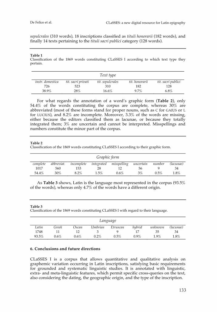
133
Italian Journal of Computational Linguistics Volume 1, Number 1
(non-classical) - CORNELIUS (classical). Uncertain cases were discussed by the annotators to achieve consensus.
All non-classical forms were then classified according to the type of variation phenomena that distinguish them from the corresponding classical equivalents. Variation phenomena may regard vowels, consonants, as well as morpho-phonology (i.e. when vocalic and consonantal phenomena occur in morphological endings). For instance, the nominative CONSOL (CIL I2 17) shows a vocalic phenomenon, because it deviates from the standard CONSUL for the vowel alternation <o>-<u>.
a. Vowels. Among the phenomena related to vowels, we distinguish the followings: alternations (CIL I2 2909 MENERVA for MINERVAE; CIL I2 560a PISCIM for PISCEM); gemination (CIL I2 365 VOOTUM for VOTUM); syncope (CIL I2 37 VICESMA for VICESIMA); epenthesis (CIL I2 59 MAGISTERE for MAGISTRI); monophthongization (CIL I2 376 DIANE for DIANAE); archaic spellings of diphthongs (CIL I2 397 FORTUNAI for FORTUNAE).
b. Consonants. Among the phenomena related to consonants, we distinguish the followings: final consonant deletion (CIL I2 8 CORNELIO for CORNELIUS); nasal deletion within consonant clusters (CIL I2 8 COSOL for CONSUL; CIL I2 560c COFECI for CONFECI); assimilation (CIL I2 7 OPSIDESQUE for OBSIDESQUE); gemination (CIL I2 16 [P]AULLA for PAULA); degemination (CIL I2 563 APOLO for APOLLO); voice alternations (CIL I2 462a ECO for EGO; CIL I2 389 PAGIO for PACIUS); deaspiration (CIL I2 555 TASEOS for THASIUS). Some of these phenomena are especially relevant in the current discussion about sociolinguistic variation in Latin, namely vowel alternations, monophthongization, synchope, final -s and -m deletion (as already discussed in a body of works; cf. among others Adams 2013; Benedetti and Marotta 2014; Campanile 1971; Herman 1987; Leumann 1977; Loporcaro 2011a, 2011b; Marotta 2015, in press; Pulgram 1975; Vineis 1984; Weiss 2009).
c. Morpho-phonology. If a given variant occurs in a morpho-phonological position (typically, in the word ending), then an additional level of annotation is added, which keeps track of the particular ending attested. For instance, among the most frequent phenomena annotated, we highlight the –a ending of the dative singular of the first declension (CIL I2 43 DIANA for DIANAE); the –os and -o endings of the nominative singular of the second declension (CIL I2 406b CANOLEIOS and CIL I2 408 CANOLEIO for CANOLEIUS); the –om ending of the accusative singular of the second declension (CIL I2 2486a DONOM for DONUM); and the –et ending of the 3rd person of the perfect (CIL I2 2867 DEDET for DEDIT).
This fine-grained annotation creates the prerequisites for the evaluation of the statistical incidence of each kind of non-classical variant, as well as to perform cross-queries taking into account text type, dating, and place of provenance.
5. Results
We can now present the results of the annotation conducted on CLaSSES I. As Table 1 shows, the text type most represented in the corpus is the instrumentum domesticum, with 246 epigraphic texts (726 words), followed by 82 inscriptions classified as tituli sacri privati (523 words), 26 inscriptions classified as tituli
De Felice et al. CLaSSES: a new digital resource for Latin epigraphy
sepulcrales (310 words), 18 inscriptions classified as tituli honorarii (182 words), and finally 14 texts pertaining to the tituli sacri publici category (128 words).
Table 1 Classification of the 1869 words constituting CLaSSES I according to which text type they pertain.
For what regards the annotation of a word’s graphic form (Table 2), only
54.4% of the words constituting the corpus are complete, whereas 30% are abbreviated (most of these forms stand for proper nouns, such as C for GAIUS or L for LUCIUS), and 8.2% are incomplete. Moreover, 3.3% of the words are missing, either because the editors classified them as lacunae, or because they totally integrated them; 3% are uncertain and cannot be interpreted. Misspellings and numbers constitute the minor part of the corpus.
Table 2 Classification of the 1869 words constituting CLaSSES I according to their graphic form.
Graphic form complete abbreviat. incomplete integrated misspelling uncertain number (lacunae)
1017 560 153 28 12 56 9 34 54.4% 30% 8.2% 1.5% 0.6% 3% 0.5% 1.8%
As Table 3 shows, Latin is the language most represented in the corpus (93.5%
of the words), whereas only 4.7% of the words have a different origin.
Table 3 Classification of the 1869 words constituting CLaSSES I with regard to their language.
Language Latin Greek Oscan Umbrian Etruscan hybrid unknown (lacunae) 1748 11 12 3 9 17 35 34
93.5% 0.6% 0.6% 0.2% 0.5% 0.9% 1.9% 1.8%
6. Conclusions and future directions
CLaSSES I is a corpus that allows quantitative and qualitative analysis on graphemic variation occurring in Latin inscriptions, satisfying basic requirements for grounded and systematic linguistic studies. It is annotated with linguistic, extra- and meta-linguistic features, which permit specific cross-queries on the text, also considering the dating, the geographic origin, and the type of the inscription.
Text type instr. domestica tit. sacri privati tit. sepulcrales tit. honorarii tit. sacri publici
726 523 310 182 128 38.9% 28% 16.6% 9.7% 6.8%
134
Italian Journal of Computational Linguistics Volume 1, Number 1
As we have illustrated in the previous sections, the initial hypothesis in our project is that, given the wide array of variation detectable in archaic and early Latin inscriptions, sociolinguistic aspects possibly emerging may be highlighted by identifying and classifying the occurrences of non-classical variants. Even if the search for non-classical forms in Archaic and Early Latin might seem anachronistic in some way, this choice is based on two fundamental aspects. First, many phenomena occurring in these forms seem to represent the basis for diachronic developments occurring from Late Latin to the Romance languages, thus revealing some continuity at least at some (sociolinguistic?) level from Early to Late Latin (this point is not uncontroversial, see e.g. Adams 2013: 8). Second, different spellings in any case provide evidence for orthographic - and possibly phonological - variation within archaic inscriptions, thus presumably pointing to different levels in the diasystem.
There are a number of case studies that have already been conducted on CLaSSES I. For instance, the analysis of the distribution of non-classical and classical forms, presented in Donati et al. (in press), confirms in quantitative terms that the linguistic standard is not yet established in the chronological period considered in CLaSSES I. Marotta (2015) analyzes vowel alternations: the spellings <e> and <o>, alternating with <i> and <u>, are interpreted as possible clues for the existence of a phonological opposition grounded on vowel quality rather than vowel quantity, at least at some level of the Latin diasystem. In Donati (2015), the possible correlation between the distribution of non-classical variants and diaphasic factors related to the type of text are analyzed, as well as the distribution of non-classical variation phenomena in vowels and consonants.
Our primary current aim is to build and develop other sections of CLaSSES, by using the same annotation criteria already adopted for CLaSSES I and described above (cf. § 4.2 - § 4.6). In particular, two macro-sections are now in progress, CLaSSES II and CLaSSES III. CLaSSES II includes inscriptions of the period 150 - 50 BC, whereas CLaSSES III is focused on Classical Latin, i.e. 50 BC - 50 AD. Moreover, we plan to add a morphological layer of annotation to the lemmatized corpus. This operation will provide the word tokens with information related to morphological properties, such as the part of speech (PoS), and possibly the morphological categories (case, number, tense, person, etc.). Furthermore, given the high frequency of proper names in epigraphic texts, we also intend to annotate the named entities.
Finally, all the data collected will be the input for the creation of a database available through a web interface in the near future.
References Adams, James N. 2003. Bilingualism and the Latin Language. Cambridge University Press,
Cambridge. Adams, James N. 2007. The Regional Diversification of Latin 200 BC-AD 600. Cambridge University
Press, Cambridge. Adams, James N. 2013. Social Variation and the Latin Language. Cambridge University Press,
Cambridge. Adams, James N., Mark Janse, and Simon Swain (eds.). 2002. Bilingualism in Ancient Society.
Language Contact and the Written Word. Oxford University Press, Oxford. Benedetti, Marina and Giovanna Marotta. 2014. Monottongazione e geminazione in latino: nuovi
elementi a favore dell’isocronismo sillabico. In Molinelli, Piera, Pierluigi Cuzzolin, and Chiara Fedriani (eds.). Latin vulgaire - Latin tardif X. Actes du Xe colloque international sur le latin vulgaire et tardif. Sestante Edizioni, Bergamo: 25-43.
Biville, Frédérique, Jean-Claude Decourt, and Georges Rougemont (eds.). 2008. Bilinguisme gréco-latin et épigraphie. Maison de l’Orient et de la Méditerranée-J. Pouilloux, Lyon.
135
Italian Journal of Computational Linguistics Volume 1, Number 1
As we have illustrated in the previous sections, the initial hypothesis in our project is that, given the wide array of variation detectable in archaic and early Latin inscriptions, sociolinguistic aspects possibly emerging may be highlighted by identifying and classifying the occurrences of non-classical variants. Even if the search for non-classical forms in Archaic and Early Latin might seem anachronistic in some way, this choice is based on two fundamental aspects. First, many phenomena occurring in these forms seem to represent the basis for diachronic developments occurring from Late Latin to the Romance languages, thus revealing some continuity at least at some (sociolinguistic?) level from Early to Late Latin (this point is not uncontroversial, see e.g. Adams 2013: 8). Second, different spellings in any case provide evidence for orthographic - and possibly phonological - variation within archaic inscriptions, thus presumably pointing to different levels in the diasystem.
There are a number of case studies that have already been conducted on CLaSSES I. For instance, the analysis of the distribution of non-classical and classical forms, presented in Donati et al. (in press), confirms in quantitative terms that the linguistic standard is not yet established in the chronological period considered in CLaSSES I. Marotta (2015) analyzes vowel alternations: the spellings <e> and <o>, alternating with <i> and <u>, are interpreted as possible clues for the existence of a phonological opposition grounded on vowel quality rather than vowel quantity, at least at some level of the Latin diasystem. In Donati (2015), the possible correlation between the distribution of non-classical variants and diaphasic factors related to the type of text are analyzed, as well as the distribution of non-classical variation phenomena in vowels and consonants.
Our primary current aim is to build and develop other sections of CLaSSES, by using the same annotation criteria already adopted for CLaSSES I and described above (cf. § 4.2 - § 4.6). In particular, two macro-sections are now in progress, CLaSSES II and CLaSSES III. CLaSSES II includes inscriptions of the period 150 - 50 BC, whereas CLaSSES III is focused on Classical Latin, i.e. 50 BC - 50 AD. Moreover, we plan to add a morphological layer of annotation to the lemmatized corpus. This operation will provide the word tokens with information related to morphological properties, such as the part of speech (PoS), and possibly the morphological categories (case, number, tense, person, etc.). Furthermore, given the high frequency of proper names in epigraphic texts, we also intend to annotate the named entities.
Finally, all the data collected will be the input for the creation of a database available through a web interface in the near future.
References Adams, James N. 2003. Bilingualism and the Latin Language. Cambridge University Press,
Cambridge. Adams, James N. 2007. The Regional Diversification of Latin 200 BC-AD 600. Cambridge University
Press, Cambridge. Adams, James N. 2013. Social Variation and the Latin Language. Cambridge University Press,
Cambridge. Adams, James N., Mark Janse, and Simon Swain (eds.). 2002. Bilingualism in Ancient Society.
Language Contact and the Written Word. Oxford University Press, Oxford. Benedetti, Marina and Giovanna Marotta. 2014. Monottongazione e geminazione in latino: nuovi
elementi a favore dell’isocronismo sillabico. In Molinelli, Piera, Pierluigi Cuzzolin, and Chiara Fedriani (eds.). Latin vulgaire - Latin tardif X. Actes du Xe colloque international sur le latin vulgaire et tardif. Sestante Edizioni, Bergamo: 25-43.
Biville, Frédérique, Jean-Claude Decourt, and Georges Rougemont (eds.). 2008. Bilinguisme gréco-latin et épigraphie. Maison de l’Orient et de la Méditerranée-J. Pouilloux, Lyon.
De Felice et al. CLaSSES: a new digital resource for Latin epigraphy
Bodard, Gabriel. 2010. EpiDoc: Epigraphic Documents in XML for Publication and Interchange. In Feraudi-Gruénais, Francisca (ed.). Latin on Stone: Epigraphic Research and Electronic Archives. Lexington Books, Lanham: 101-118.
Caldelli, Maria Letizia, Silvia Orlandi, Valentina Blandino, Valerio Chiaraluce, Luca Pulcinelli, and Alessandro Vella. 2014. EDR – Effetti collaterali. Scienze dell'Antichità, 20 (1): 267-289.
Campanile, Enrico. 1971. Due studi sul latino volgare. L’Italia Dialettale, 34: 1-64. CIL I² Inscriptiones Latinae antiquissimae ad C. Caesaris mortem, Pars II, fasc. I, Inscriptiones Latinae
antiquissimae (Lommatzsch, E. 1918 ed.). CIL I² Inscriptiones Latinae antiquissimae ad C. Caesaris mortem, Pars II, fasc. II, Addenda Nummi
Indices (Lommatzsch, E. 1931 ed.). CIL I² Inscriptiones Latinae antiquissimae ad C. Caesaris mortem, Pars II, fasc. III, Addenda altera
Indices (Lommatzsch, E. 1943 ed.). CIL I² Inscriptiones Latinae antiquissimae ad C. Caesaris mortem, Pars II, fasc. IV, Addenda tertia
(Degrassi, A. and J. Krummrey 1986 eds.). Clackson, James and Geoffrey Horrocks. 2007. The Blackwell History of the Latin Language.
Blackwell, Malden, Mass. Clackson, James. 2011. Introduction. In Clackson, James (ed.). A Companion to the Latin Language.
Wiley/Blackwell, Chichester/Malden: 1-6. Consani, Carlo. in press. Fenomeni di contatto a livello di discorso e di sistema nella Cipro
ellenistica (Kafizin) e le tendenze di “lunga durata”. In Di Giovine, Paolo (ed.). Atti del Convegno “Dinamiche sociolinguistiche in aree di influenza greca: mutamento, variazione e contatto” (Roma, 22-24 settembre 2014), Linguarum Varietas, 5.
Cuzzolin, Pierluigi and Gerd Haverling. 2009. Syntax, sociolinguistics, and literary genres. In Baldi, Philip and Pierluigi Cuzzolin (eds.). New Perspectives on Historical Latin Syntax: Syntax of the Sentence. De Gruyter, Berlin-New York: 19-64.
De Angelis, Alessandro. in press. Un esito palatale nel latino di Sicilia: a proposito del bilinguismo greco-latino. In Di Giovine, Paolo (ed.). Atti del Convegno “Dinamiche sociolinguistiche in aree di influenza greca: mutamento, variazione e contatto” (Roma, 22-24 settembre 2014), Linguarum Varietas, 5.
Degrassi, Attilio. 1957-1963. Inscriptiones latinae liberae rei publicae. La Nuova Italia, Firenze. Dickey, Eleonor and Anna Chahoud (eds.). 2010. Colloquial and Literary Latin. Cambridge
University Press, Cambridge. Donati, Margherita. in press. Variazione e tipologia testuale nel corpus epigrafico CLaSSES I.
Studi e Saggi Linguistici, 53 (2). Donati, Margherita, Francesco Rovai, and Giovanna Marotta. in press. Prospettive
sociolinguistiche sul latino: un corpus per l’analisi dei testi epigrafici. In Latin vulgaire - Latin tardif XI.
Elliott, Tom. 2015. Epigraphy and Digital Resources. In Bruun, Christer and Jonathan Edmondson (eds.). The Oxford Handbook of Roman Epigraphy. Oxford University Press, Oxford-New York: 78-85.
Evangelisti, Silvia. 2010. EDR: History, Purpose, and Structure. In Feraudi-Gruénais, Francisca (ed.). Latin on Stone. Epigraphic Research and Electronic Archives. Lexington Books, Lanham: 119-134.
Feraudi-Gruénais, Francisca. 2010. An inventory of the Main Archives of Latin Inscriptions. In Feraudi-Gruénais, Francisca (ed.). Latin on Stone: Epigraphic Research and Electronic Archives. Lexington Books, Lanham: 157-160.
Giacalone Ramat, Anna. 2000. Mutamento linguistico e fattori sociali: riflessioni tra presente e passato. In Cipriano, Palmira, Rita D’Avino, and Paolo Di Giovine (eds.). Linguistica Storica e Sociolinguistica. Il Calamo, Roma: 45-78.
Glare, Peter G. W. (ed.) 1968-1982. Oxford Latin Dictionary. Oxford University Press, Oxford. Herman, József. 1970. Le latin vulgaire. Press Universitaires de France, Paris. Herman, József. 1978a. Évolution a>e en latin tardif? Essai sur les liens entre la phonétique
historique et la phonologie diachronique. Acta Antiquae Academiae Scientiarum Hungariae, 26: 37-48 [also in Herman 1990: 204-216].
Herman, József. 1978b. Du latin épigraphique au latin provincial. Essai de sociologie linguistique sur la langue des inscriptions. In Étrennes de septantaine: Travaux de linguistique et de grammaire comparée offerts à Michel Lejeune. Éditions Klincksieck, Paris: 99-114 [also in Herman 1990: 35-49].
Herman, József. 1982. Un vieux dossier réouvert: les transformations du système latin des quantités vocaliques. Bulletin de la Société de Linguistique de Paris, 77: 285-302 [also in Herman 1990: 217-231].
136
Italian Journal of Computational Linguistics Volume 1, Number 1
Herman, József. 1985. Témoignage des inscriptions latines et préhistoire des langues romanes: le cas de la Sardaigne. In Deanović, Mirko (ed.). Mélanges de linguistique dédiés à la mémoire de Petar Skok (1881–1956). Jugoslavenska Akademija Znanosti i Umjetnosti, Zagreb: 207-216 [also in Herman 1990: 183-194].
Herman, József. 1987. La disparition de -s et la morphologie dialectale du latin parlé. In Herman, József (ed.). Latin vulgaire-Latin tardif. Actes du Ier colloque international sur le latin vulgaire et tardif. Niemeyer, Tübingen: 97-108.
Herman, József. 1990. Du latin aux langues romanes. Études de linguistique historique. Niemeyer, Tübingen.
Herman, József. 2000. Differenze territoriali nel latino parlato dell’Italia: un contributo preliminare. In Herman, József and Anna Marinetti (eds.). La preistoria dell’italiano. Atti della Tavola Rotonda di Linguistica Storica. Università Ca’ Foscari di Venezia 11-13 giugno 1998. Niemeyer, Tübingen: 123-135.
Kruschwitz, Peter. 2015. Linguistic Variation, Language Change, and Latin Inscriptions. In Bruun, Christer and Jonathan Edmondson (eds.). The Oxford Handbook of Roman Epigraphy. Oxford University Press, Oxford-New York: 721-743.
Lazzeroni, Romano. 1984. Lingua e società in Atene antica. Studi classici e orientali, 34: 16-26. Leumann, Manu. 1977. Lateinische Laut- und Formenlehre. Beck, München. Loporcaro, Michele. 2011a. Syllable, segment and prosody. In Maiden, Martin, John Charles
Smith, and Adam Ledgeway (eds.). The Cambridge History of the Romance Languages. I: Structures. Cambridge University Press, Cambridge: 50-108.
Loporcaro, Michele. 2011b. Phonological Processes. In Maiden, Martin, John Charles Smith, and Adam Ledgeway (eds.). The Cambridge History of the Romance Languages. I: Structures. Cambridge University Press, Cambridge: 109-154.
Mancini, Marco. 2005. La formazione del neostandard latino: il caso delle differentiae uerborum. In Kiss, Sándor, Luca Mondin, and Giampaolo Salvi (eds.). Latin et langues romanes, Études linguistiques offertes à J. Herman à l’occasion de son 80ème anniversaire. Niemeyer, Tübingen: 137-155.
Mancini, Marco. 2006. Dilatandis litteris: uno studio su Cicerone e la pronunzia ‘rustica’. In Bombi, Raffaella, Guido Cifoletti, Fabiana Fusco, Lucia Innocente, and Vincenzo Orioles (eds.). Studi linguistici in onore di Roberto Gusmani. Ed. dell’Orso, Alessandria: 1023-1046.
Marotta, Giovanna. in press. Talking stones. Phonology in Latin inscriptions. Studi e Saggi Linguistici, 53 (2).
Marotta, Giovanna. in press. Sociolinguistica storica ed epigrafia latina. Il corpus CLaSSES I. In Di Giovine, Paolo (ed.). Atti del Convegno “Dinamiche sociolinguistiche in aree di influenza greca: mutamento, variazione e contatto” (Roma, 22-24 settembre 2014), Linguarum Varietas, 5.
Molinelli, Piera. 2006. Per una sociolinguistica del latino. In Arias Abellán, Carmen (ed.). Latin vulgaire - Latin tardif VII. Actes du VIIe colloque international sur le latin vulgaire et tardif. Secretariado de Publicaciones Univ. de Sevilla, Sevilla: 463-474.
Panciera, Silvio. 2013. Notizie da EAGLE. Epigraphica, 75: 502-506. Poccetti, Paolo, Diego Poli and Carlo Santini. 1999. Una storia della lingua latina, Carocci, Roma. Pulgram, Ernst. 1975. Latin-Romance Phonology: Prosodics and Metrics. Fink Verlag, Munich. Rochette, Bruno. 1997. Le latin dans le monde grec. Latomus, Bruxelles. Rovai, Francesco. in press. Notes on the inscriptions of Delos. The Greek transliteration of Latin
names. Studi e Saggi Linguistici, 53 (2). Vineis, Edoardo. 1984. Problemi di ricostruzione della fonologia del latino volgare. In Vineis,
Edoardo (ed.). Latino volgare, latino medioevale, lingue romanze. Giardini, Pisa: 45-62. Vineis, Edoardo. 1993. Preliminari per una storia (e una grammatica) del latino parlato. In Stolz,
Friedrich, Albert Debrunner, and Wolfgang P. Schmidt (eds.). Storia della lingua latina. Pàtron, Bologna: xxxvii-lviii.
Wachter, Rudolf. 1987. Altlateinische Inschriften. Sprachliche und epigraphische Untersuchungen zu den Dokumenten bis etwa 150 v. Chr. Peter Lang, Bern-Frankfurt am Main-New York-Paris.
Warmington, Eric Herbert. 1940. Remains of Old Latin. Vol. 4, Archaic inscriptions. Harvard University Press-Heinemann, Cambridge MA-London.
Weiss, Michael. 2009. Outline of the Historical and Comparative Grammar of Latin. Beech Stave Press, New York.
Winter, Werner. 1998. Sociolinguistics and Dead Languages. In Jahr, Ernst Håkon (ed.). Language Change. Advances in Historical Sociolinguistics. Mouton de Gruyter, Berlin: 67-84.
Related Documents