Emergency Logistics Planning in Natural Disasters

Annals of Operations Research 129, 217–245, 2004 2004 Kluwer Academic Publishers. Manufactured in The Netherlands.

Emergency Logistics Planning in Natural Disasters

LINET ÖZDAMAR ∗ [email protected] Technological University, School of Mechanical and Production Engineering,Systems and Engineering Management Division, 50 Nanyang Avenue, Singapore 639798

EDIZ EKINCI [email protected], Turkish Armed Forces, Turkey

BESTE KÜÇÜKYAZICI [email protected] University, Department of Systems Engineering, Turkey

Abstract. Logistics planning in emergency situations involves dispatching commodities (e.g., medicalmaterials and personnel, specialised rescue equipment and rescue teams, food, etc.) to distribution centresin affected areas as soon as possible so that relief operations are accelerated. In this study, a planningmodel that is to be integrated into a natural disaster logistics Decision Support System is developed. Themodel addresses the dynamic time-dependent transportation problem that needs to be solved repetitively atgiven time intervals during ongoing aid delivery. The model regenerates plans incorporating new requestsfor aid materials, new supplies and transportation means that become available during the current planningtime horizon. The plan indicates the optimal mixed pick up and delivery schedules for vehicles withinthe considered planning time horizon as well as the optimal quantities and types of loads picked up anddelivered on these routes.

In emergency logistics context, supply is available in limited quantities at the current time period and onspecified future dates. Commodity demand is known with certainty at the current date, but can be forecastedfor future dates. Unlike commercial environments, vehicles do not have to return to depots, because the nexttime the plan is re-generated, a node receiving commodities may become a depot or a former depot mayhave no supplies at all. As a result, there are no closed loop tours, and vehicles wait at their last stopuntil they receive the next order from the logistics coordination centre. Hence, dispatch orders for vehiclesconsist of sets of “broken” routes that are generated in response to time-dependent supply/demand.

The mathematical model describes a setting that is considerably different than the conventional vehiclerouting problem. In fact, the problem is a hybrid that integrates the multi-commodity network flow problemand the vehicle routing problem. In this setting, vehicles are also treated as commodities. The modelis readily decomposed into two multi-commodity network flow problems, the first one being linear (forconventional commodities) and the second integer (for vehicle flows). In the solution approach, these sub-models are coupled with relaxed arc capacity constraints using Lagrangean relaxation. The convergenceof the proposed algorithm is tested on small test instances as well as on an earthquake scenario of realisticsize.

Keywords: emergency planning, linear and integer multi-period multi-commodity network flows, vehiclerouting, Lagrangean relaxation

∗ Corresponding author.

218 ÖZDAMAR ET AL.

1. Introduction

This study is concerned with planning logistics at a macro level in the presence of nat-ural disasters. The research is motivated by the re-organisation project of the TurkishArmed Forces Natural Disaster Coordination Centre that was activated after Izmit andDüzce earthquakes in 1999. The logistics planning model proposed here is intended tobe a component of a Logistics Decision Support System linking all relevant databases(stocking units, aid distribution centres, national transportation networks, search andrescue teams, etc.) and the central aid coordination centre.

Macro level logistics planning in emergencies involves inter-city transportationof commodities, such as medical aid materials and personnel, specialized equipment,troops to keep order and to conduct rescue activities, food and other commodities usedin relief operations. The coordination centre decides on the quantities, origins, and des-tinations of relief commodities to be transported, and on the specific vehicles to be dis-patched to carry these commodities. At the time of planning, vehicles of different types(ground, air, rail, etc.) and capacities might be free at supply centres, demand centres,or at other locations. Thus, transportation plans made for the commodities are accompa-nied by vehicle schedules that designate the type, number, route and mobilization timingof selected vehicles.

The logistics plan involves a planning time horizon consisting of a given numberof time periods because it deals with time-variant demand and supply. During a givenplanning horizon, the model assumes that demand is known for the initial period of thecurrent planning time horizon, and, future demand is forecasted for some commodities.Supply is limited and its availability is known for some periods ahead due to the factthat prospective supply arrivals are usually known in advance. At the beginning of anyplanning time horizon, given a snapshot of current and future requirements/supplies,and vehicle availability, the plan generates multi-period vehicle routes/schedules alongwith their commodity load-unload assignments. During ongoing relief operations, ve-hicles are not required to return to supply centres (depots) when their assignments arecompleted for the given planning time horizon. Rather, once they reach their final desti-nation, they wait for the next order at their current locations, because it is not certain thata depot will have available supplies at the next planning period. This is typical in emer-gencies and therefore, one cannot adopt the conventional concept of a “vehicle route”in this model. Furthermore, during its scheduled assignments, a vehicle might pick upcommodities and deliver goods as well, because it is also possible to have supply cen-tres (stocking units) in the affected area. Therefore, this distribution problem does notnecessarily imply a topology where there exists a cluster of centres receiving aid fromunaffected cities outside the region of emergency.

The plan is updated at regular time intervals incorporating new information on de-mand, supplies and vehicle availability, and, accounting for the status of the logistics sys-tem resulting from the plan implemented previously. Since the plan has a time-dependentstructure, re-planning is facilitated and is carried out repeatedly during ongoing disasterrelief operations. Thus, the system is designed to respond to time-dependent logistic

EMERGENCY LOGISTICS PLANNING 219

needs in an adaptive manner, so that after the emergency call is announced, it respondsquickly to new demand, supply and vehicle availability.

Given the aspects mentioned above, the problem is classified as a hybrid problemintegrating the multi-period multi-commodity network flow problem with the vehiclerouting problem. In the proposed model, vehicles are also treated as commodities thataccompany the actual goods. Thus, the problem is converted into a mixed integer multi-period multi-commodity network flow problem where the integer part represents thevehicles.

Although the model is compact and the problem size is reduced significantly interms of the number of integer variables, it may become intractable when dealing withvery large scale emergencies. Therefore, an iterative solution approach based on La-grangean relaxation is proposed. The efficiency of the proposed algorithm is demon-strated on randomly generated small test problems as well as on an earthquake scenarioof realistic size. The algorithm is also compared to a greedy heuristic designed specifi-cally for this problem.

The paper is organized as follows. First, the problem at hand is analysed and itsrelevance to well-known problems in the literature is discussed. Next, a mathemati-cal formulation of the problem is developed and its use in dynamic environments isexplained. The output of the model is illustrated with a small example. Then, a solu-tion methodology that involves decomposition and Lagrangean relaxation is described.Finally, numerical results are presented.

2. Analysis of the problem

The problem at hand is related to the vehicle routing problem (VRP) discussed exten-sively in the literature. In the VRP, a number of customers (each represented as a desti-nation node) are served by m identical vehicles located at a depot. Each vehicle returnsto the depot after completing its trip (tour). The load of a vehicle cannot exceed its ca-pacity on any tour. Furthermore, a customer can be visited only once and it is assumedthat a vehicle’s load capacity exceeds every customer’s demand. The aim is to deter-mine vehicle routes resulting in the minimum total travel distance. The definition of theVRP implies that the quantity of commodity to be transported to every destination pairis known and sufficient supply is always available at the depot to satisfy all customerdemand.

The restrictive assumptions of the VRP are often relaxed to accommodate morerealistic settings. A customer may be visited more than once if demand exceeds theload capacity of available vehicles. This feature is known as split delivery. Dror andTrudeau (1990) propose heuristics for the split delivery VRP where routes are brokenand re-combined to improve the solutions obtained. In some relaxed VRPs, vehiclescan deliver and pick up commodities on the same tour, however, they cannot carry morethan one order at a time. This approach is called the mixed delivery approach. Anotherrelaxation involves having multiple depots.

220 ÖZDAMAR ET AL.

Surveys on the VRP and its extensions can be found in Desrochers et al. (1988)and Bodin (1990). In Desrochers et al. (1990), each type of VRP is classified accordingto several characteristics: (i) addresses (demand locations to be satisfied, their number,sets of demand clusters to be satisfied etc.); (ii) vehicles (homogeneous/heterogeneousfleet, fixed or variable fleet size, time windows for vehicle availability); (iii) servicestrategy (issues such as split delivery, mixed delivery, precedence constraints betweendemand locations, time windows); and (iv) objectives (address penalty implying thedeviation from preferred service level, or, vehicle penalty implying fleet size and costs).More recently, Desrochers et al. (1998) propose an automatic model base and algorithmselection system that is implemented according to problem characteristics.

Extensive discussions of heuristic and optimisation algorithms are given in Laporte(1992) and Fisher (1995) for a variety of vehicle routing problems. Recent examples oflocal search heuristics (e.g., simulated annealing, tabu search, etc.) designed for solvingthe VRP can be found in Rodriguez et al. (1998) and Gendreau et al. (1999).

The emergency logistics coordination problem described here is modeled as amixed integer multi-commodity network flow problem. Two previous VRP related stud-ies that treat vehicles as commodities are summarized below.

Ribeiro and Soumis (1994) treat vehicles as commodities in their multi-depot non-split delivery VRP. In their model, trips are predetermined and it is required to assignone vehicle to every trip. The authors show that the LP relaxation of their formulationprovides a good lower bound for the integer problem. Fisher et al. (1995) also representvehicles as commodities in the mixed delivery VRP where each vehicle is restricted tocarry one order at a time. Hence, the VRP under consideration is converted into a net-work flow problem. The authors approximate the loads to be transported into integertruckloads for simplification purposes. As a result of their modeling approach, the solu-tion may have infeasible cycles. These are repaired by adding the depot in a cycle, or,by merging/splitting two cycles.

Although the logistical planning problem considered here involves vehicle routing,it represents quite a different setting from the VRP in the following respects. In thisproblem, unlike the VRP where supply is assumed to be abundant, supply is available inlimited quantities and its availability varies over the planning horizon. Predictions for fu-ture demand of certain commodities are also known and a multi-period planning horizonprevails. The objective is also different. The goal is to minimize the delay in the arrivalof commodities at aid centers. In other words, requirements of aid distribution centersshould be met at the requested times. Hence, it is necessary to define a time-dependentlogistics plan and dispatch available vehicles dispersed around the logistics network soas to optimize the timing and quantity of commodities transported to demand nodes. Dueto these reasons, there are no pre-determined trips between pairs of supply and demandnodes as in the VRP, namely the load to be carried to a demand node is a variable. Thispart of the problem falls into the category of multi-period multi-commodity networkflow problem.

As for the vehicle dispatching part of the problem, the following conditions prevailwith regard to service strategy. In emergencies, the load to be transported is quite large


and a vehicle’s capacity is usually sufficient to carry only a small part of the load. Con-sequently, the service strategy becomes split delivery. Furthermore, in accordance withthe nature of the multi-period network flow problem, vehicles pick up commodities fromone or more supply nodes and deliver them to one or more demand nodes in any order onthe same route. In other words, mixed delivery routes involving any order of pick up anddelivery are constructed, such as, pickup–delivery–delivery–pickup–pickup–delivery . . .

and so on, including empty trips and waiting. It is possible to have commodities droppedat a warehouse at a demand node, to be picked up later by another vehicle with a differentdestination. To summarize, vehicles en route may carry load for multiple destinations(there is no restriction on the number of orders that a vehicle can carry at a time), and sat-isfy demand at these destinations partially or completely, using a mixed delivery servicestrategy.

Another point related to vehicles is that in emergencies, vehicles are called on fromevery node in the network whether or not it is an affected node or a depot. So, they maybe found anywhere in the network at the time of planning. To accommodate this situationand due to the fact that vehicles do not have to start out from and end their journeys ata depot, the model assumes that available vehicles are dispersed all over the logisticsnetwork and their availability is also time-dependent. Hence, a vehicle undertakes itsassignments starting from its current location, carries them out and after completing itstasks, it is permitted to wait at its last stop until its next order arrives. Thus, there is noclear definition of a route as in the VRP.

With regard to the structure of the fleet, a heterogeneous fleet that incorporates mul-tiple transportation modes (Jimenez and Verdegay, 1999; Ziliaskopoulos and Wardell,2000) is utilized. The network consists of integrated ground, air, marine and rail sub-networks. The integrated network may represent transportation mode-switches (load-unload times of commodities) by dummy arcs.

The logistics problem described here is a hybrid of two sub-problems: the multi-period multi-commodity network flow problem and the multi-period VRP with multipletransportation modes and no route-specific restrictions. The problem is modelled asa multi-period multi-commodity network flow problem with arc capacities (arc upperbounds) that are variables, not parameters. In fact, arc upper bounds consist of vehiclecapacities that have to be optimally allocated to each arc flow.

To the best of our knowledge, this hybrid problem has not been dealt with in theliterature. Two references that describe work relevant to emergency logistics are thestudies made by Rathi et al. (1993) and Equi et al. (1996).

Rathi et al. (1993) consider supply logistics in conflict or emergency situations.The authors develop LP models where routes and the amount of supply to be carried oneach route are pre-determined between each origin-destination pair. Their problem is toidentify the optimal number of vehicles to be assigned to each route and the problembecomes an assignment problem. Real-valued optimal numbers of vehicles are roundedup to the next integer since the number of available vehicles in the system is assumed tobe non-restrictive. This setting is far less complex than the emergency logistic planningproblem considered here. Equi et al. (1996) consider a combined transportation and

222 ÖZDAMAR ET AL.

scheduling problem in a supply chain where the transportation problem aims to identifythe optimal number of trips to satisfy demand (customers) from a given number of supplynodes (plants). The scheduling problem, on the other hand, identifies the number oftrucks (of homogeneous capacity) that has to be allocated to make the trips. Again, theroutes are pre-specified and a vehicle assignment problem is solved rather than a routingproblem.

3. Mathematical formulation

The mathematical formulation of the problem and the notation are given below. A re-mark should be made on representing different transportation modes on the same net-work. Each arc is defined in the transportation mode sub-network that it belongs to.This implies that a pair of nodes may have more than one arc linking them, each arcrepresenting a different mode. The traversal times of arcs depend on their transportationmodes. Here, switching delays due to mode changeovers are neglected without loss ofgenerality. Transportation modes are also distinguished in the mathematical formulationby restricting the vehicle types that can use them. For instance, trucks and long vehiclesare two types of vehicles that belong to ground transportation mode and they cannot usethe arcs on the rail sub-network.

Sets and parameters

T : length of the planning horizon,C: set of all nodes,M: set of transportation modes,CD: set of demand nodes including transshipment nodes,CS: set of supply nodes,do: dummy node defined for expressing the availability of vehicles,RO: set of nodes excluding dummy node; RO = C\{do},A: set of commodities,Vm: set of vehicle types defined for each transportation mode m,topm: time required to traverse arc (o, p) in transportation mode m; topm is zero for

non-existent links,daot : amount of commodity of type a demanded or supplied at node o at time t ,

positive for supply and negative for demand,avovmt : number of vehicles of type v – transportation mode m at node o added to the

fleet at time t ,wa: unit weight of commodity a,capvm: load capacity of vehicle type v – transportation mode m,K: a big number.


Decision variables

Zaopmt : amount of commodity type a traversing arc (o, p) at time t using transporta-tion mode m,

devaot : amount of unsatisfied demand of commodity type a at node o at time t ,Yopvmt : integer number of vehicles of type v – transportation mode m traversing the

arc (o, p) at time t ,surovmt : number of vehicles of type v – transportation mode m that wait at node o at

time t .

Model P

minimize∑a∈A

∑o∈CD

∑t

devaot (0)

subject tot∑

q=1

∑m∈M

[−

∑p∈C

Zapom,(q−tpom) +∑p∈C

Zaopmq

]− devaot =

t∑q=1

daoq

(∀a ∈ A, o ∈ CD, t ∈ T ), (1)t∑

q=1

∑m∈M

[−

∑p∈C

Zapom,(q−tpom) +∑p∈C

Zaopmq

]�

t∑q=1

daoq

(∀a ∈ A, o ∈ CS, t ∈ T ), (2)

Yopvmt � topmK (∀{o,p} ⊆ RO, v ∈ Vm, m ∈ M, t ∈ T ), (3)

Za, do, pmt + Zap, do, mt = 0 (∀a ∈ A, p ∈ RO, t ∈ T , m ∈ M), (4)∑v∈Vm

Yopvmtcapvm �∑a∈A

waZaopmt (∀{o,p} ⊆ C, t ∈ T , m ∈ M), (5)

t∑q=1

∑p∈C

Ypovm,(q−tpom) − surovmt =t∑

q=1

∑p∈C

Yopvmq

(∀o ∈ RO, v ∈ Vm, m ∈ M, t ∈ T ), (6)t∑

q=1

Ydo, ovmq �t∑

q=1

avovmq (∀o ∈ RO, v ∈ Vm, m ∈ M, t ∈ T ), (7)

Yopvmt � 0 and integer; Zaopmt � 0; devaot � 0; surovmt � 0 and integer. (8)

A dummy node, do, is added to the integrated network for dealing with vehicleavailability at the time of planning. The node do has a link (with a traversal time ofzero) to each node where vehicles of any type are available at the time of planning.Hence, the immediate readiness of these vehicles is made possible for relevant nodes byconstraints (7) and the set of constraints (6) that balance the flow of vehicles over nodes.

224 ÖZDAMAR ET AL.

Constraints (6) are thus applied without making any exceptions for the nodes where thevehicles reside.

The objective aims at minimising the sum of unsatisfied demand of all commodi-ties throughout the planning horizon. This objective is compatible with the goal men-tioned previously and commodities are transported as soon as possible to demand cen-tres. Constraint set (1) balances material flow on demand nodes and transhipment nodesand explicitly reports the quantity of unsatisfied demand, devaot , in each time period.Constraint set (2) enforces material flow balance on supply nodes. This problem is amulti-period planning problem where demand and supply in future time periods are in-dicated by the parameter daot . In emergency situations knowledge on future demandis scarce except for some commodities, but the disaster coordination centre frequentlyacknowledges supply that will be available in future time periods. So, it is possible toplan ahead and take future supply into account while preparing the plans. Constraintset (3) restricts each vehicle type (and hence, flow) from traversing arcs that do not existin their corresponding mode sub-networks. Constraint set (4) prevents commodity flowbetween the dummy node and other nodes. Constraint set (5) enables commodity flowover arcs as long as there is sufficient vehicle capacity. The next set of constraints (6)balances the flow of vehicles over nodes. Due to this set of constraints, vehicles do nothave to return to supply nodes and may wait at their last stop until the next dispatchingorder arrives. The number of vehicles that wait at node o at time t is represented bythe surplus variables surovmt . surovmt are added to the variables in the model only forillustrative purposes. Constraint set (7) restricts the number of vehicles moving throughthe network by their cumulative availability over time. Thus, it is also possible to planahead with the number of available vehicles varying over time.

In this formulation, vehicles are treated as commodities, and further, it is not re-quired to track vehicles individually and on a route basis. (Details of dispatch ordersfor vehicles are obtained by executing a simple algorithm that reads the optimal solutionand generates a pick up/delivery schedule for each vehicle.) Tracking vehicle flows on atime basis enables the multi-period representation of demand and supply while makingmodel P relatively more compact.

The first part of model P (constraints (1), (2), (4)) is a linear multi-commodity net-work flow problem whereas the second part (constraints (3), (5), (6), (7)) is an integermulti-commodity network flow problem. However, the second part has a complexityhigher than the general integer multi-commodity network flow problem, because theright-hand-side of constraints (5) (arc lower bounds) also consists of variables. There-fore, commodity flows in the first part drive the vehicle flows in the second part of theproblem.

3.1. Re-planning

Re-planning is a core issue in dynamic logistics activities. The importance of re-planningincreases in natural disasters because requirements, supply quantities and the fleet sizechange perpetually. An advantage of the proposed formulation is that the structure ofthe solution is convenient to use when a new plan has to be generated.


A new plan is generated at given time intervals (at every T ′ periods) with the up-dated information. Note that T ′ may be smaller than T , that is, the plan may be revisedbefore the end of the previous planning horizon. The re-planning time period is denotedas t∗ where t∗ = kT ′, and k is the number of times the plan is revised since the be-ginning of the usage of the planning system. The new planning horizon is defined byt∗ � t � t∗ + T .

In the re-planning approach adopted here, vehicles already dispatched in the pre-vious plan are not re-routed. Accordingly, the following parameters in model P aremodified before re-planning takes place in period t∗.

The unsatisfied demand left over from the previous plan is equal to the optimalquantity of unsatisfied demand in the final period of the previous planning horizon.Namely, daot∗ take on the values of the optimal devaoT identified in the previous plan-ning iteration. Similarly, supplies left over from the previous plan take on the optimalvalues of the slack variables in the final period of the previous planning horizon in equa-tions (2). Furthermore, supply and demand matrices are also updated by additionalquantities specified for the new planning horizon.

The number of available vehicles in period t (t � t∗), avovmt , is equal to the num-ber of vehicles that become free from time period t∗ onward. This number is made upof several contributions and is calculated as follows. First, the slack variables of con-straints (7) in the final period of the previous plan are considered. These represent thenumber of vehicles that have not been used at all in the previous plan and they are avail-able from period t∗ onwards. Hence, they contribute to avovmt∗ . Second, the values ofthe surplus variables surovmt are analyzed for t � t∗. These variables represent the vehi-cles that have completed their tasks and are waiting at nodes in time period t . However,surovmt need further analysis before they contribute to avovmt∗ . The values of surovmt maydecrease in future periods, t > t∗. Namely, vehicles may move away from node o afterperiod t∗. If this is the case, the earliest period, τ , after which surovmt does not decreasefor all t � τ , is identified. Thus, from period τ onwards, vehicles only arrive at node o.Accordingly, the matrix avovmt is updated reflecting new arrivals in each correspondingtime period t � τ . Finally, if new vehicles are added to the fleet within the new planningtime horizon, the corresponding elements of avovmt are modified to reflect these changes.These three sources of vehicle availability give the final value of the parameters, avovmt ,for t � t∗.

4. An illustrative example

The small example in figure 1 demonstrates how the model works for coordinating theflows of vehicles and commodities. There are four transportation modes whose sub-networks are integrated into a single multi-mode network. The dummy node, do, whichis omitted from figure 1 for the sake of presentation simplicity, is linked with dummyarcs (zero arc traversal times) to all nodes except node 2 where there are no availablevehicles. There are two commodities, medicine and food, to be transported.

226 ÖZDAMAR ET AL.

Figure 1. Multi-modal transportation network (the dummy node is omitted to simplify presentation).

In table 1 demand and supply quantities of commodities are listed on a periodbasis. The planning period is set to t∗ = 8 and the length of the planning horizon isset to twenty periods. (In fact, it is known that fourteen periods are sufficient to carrythe whole load, but twenty periods is an upper bound.) Future supply of medicine isindicated at node 5 at time period nine. The weights of unit medicine and food are 2 tonsand 3 tons, respectively. Units may be assumed to be containers and if Zaopmt turn outto be fractional, it is implied that a container is not completely full.

Table 2 gives the vehicle availability at the time of planning, t∗, at each node. Forsimplicity, each transportation mode has a single vehicle type and there are no vehicles


Table 1Demand and supply quantities at nodes.

Commodity Time(node) 8 9 10 11 . . . . . . . . . . . . . . . . . . . . . . . . 28

Medicine (1) −250 0 0 0 0Medicine (2) −250 0 0 0 0Medicine (3) −100 0 0 0 0Medicine (4) 100 0 0 0 0Medicine (5) 150 150 0 0 0Medicine (6) 200 0 0 0 0Food (1) −80 0 0 0 0Food (2) −290 0 0 0 0Food (3) −100 0 0 0 0Food (4) 200 0 0 0 0Food (5) 120 0 0 0 0Food (6) 150 0 0 0 0

Table 2Number of vehicles available at each node.

Number of availablevehicles (at t∗ = 8)(vehicle capacity-tons)

Node

1 2 3 4 5 6

Ground (50) 3 0 2 4 3 4Rail (300) 0 0 0 1 0 1Marine (400) 0 0 1 0 0 1Air (10) 5 0 2 0 0 0

Table 3Arc traversal times for each transportation mode (ground, rail, marine, air).

Node 1 2 3 4 5 6

1 0, 0, 0, 0 1, 2, 0, 1 2, 0, 4, 1 0, 0, 0, 0 0, 0, 0, 0 0, 0, 0, 02 1, 2, 0, 1 0, 0, 0, 0 1, 2, 0, 0 3, 0, 0, 1 0, 0, 0, 0 0, 0, 0, 03 2, 0, 4, 1 1, 2, 0, 0 0, 0, 0, 0 4, 5, 0, 2 3, 5, 0, 1 1, 2, 3, 04 0, 0, 0, 0 3, 0, 0, 1 4, 5, 0, 2 0, 0, 0, 0 0, 0, 0, 0 0, 0, 0, 05 0, 0, 0, 0 0, 0, 0, 0 3, 5, 0, 1 0, 0, 0, 0 0, 0, 0, 0 1, 0, 0, 16 0, 0, 0, 0 0, 0, 0, 0 1, 2, 3, 0 0, 0, 0, 0 1, 0, 0, 1 0, 0, 0, 0

added to the fleet after time period t∗. The parameter set capvm are also specified for allvehicle types in table 2.

In table 3, arc traversal times are provided for each transportation mode. In eachcell, the arc traversal times are given in the following order of transportation modes(ground, rail, marine, air).

228 ÖZDAMAR ET AL.

Figure 2. The graphical illustration of the partial optimal solution.


Figure 2. (Legend).

In figure 2, the optimal solution of model P is partially illustrated on a time basisand the legend required to read the figure is also provided. Transportation modes areillustrated graphically. In the tables to the left of the nodes, the quantities of suppliesof food and medicine available at t∗ = 8 and t = 9 are indicated. In the figure, thetwo commodities are differentiated by underlining food. The numbers in front of eachvehicle type (on the road, waiting or initially available) represents the number of vehi-cles initially available, on the road, or in waiting status at a node. The numbers besidethe vehicles represent the units of commodities carried by the vehicle. In each rectan-gle aligned with nodes horizontally and aligned with time vertically, the availability ofboth commodities at the corresponding node and time period is given. If this number isnegative it represents unsatisfied demand devaot .

In figure 2, the movements of different vehicle types are illustrated along with theloads they carry. The schedule is represented as a Gantt chart where nodes are indicatedby rows and time periods by columns. Thus, a multi-period movement chart is obtainedfor each vehicle type. Movements are illustrated by arrows. An exemplary movementset is selected to clarify this figure. We analyze the activities concerning node 3 at timeperiod 10 (encircled on figure 2). The unsatisfied demand at node 3 at time period nineis 25 units for medicine and 100 units for food. To satisfy this demand, two helicoptersleave node 5 at time period nine with 10 units of medicine. They unload their loadcompletely, and they head back to node 5 at time period ten with the aim of makinganother round to node 3. A train leaves node 6 at time period eight with 65 units of

230 ÖZDAMAR ET AL.

medicine and 56.67 units of food. The train arrives at node 3 at time period ten andunloads the food load completely whereas it unloads only 15 units of medicine at node 3.Three empty lorries coming from node 2 arrive at node 3 at time period ten and threemore arrive from node 6 with 75 units of medicine. 50 units of medicine loaded onthe train are transferred to two lorries and five fully loaded lorries leave node 3 with125 units of medicine. One empty lorry heads for node 6. The train, thus relieved ofits medicine load, waits at node 3 for one time period. Thus, at node 3, the unsatisfieddemand for medicine is driven to zero level at time period ten, and, the unsatisfied fooddemand reduces to 43.33 units.

5. Solution methodology

Model P is compact in the sense that vehicles do not have to be tracked on an individualroute basis. However, it still contains |C|2 × T × (|V1| × |V2| × · · · × |VM |) integervariables which may result in an intractable problem in the case of large-scale emer-gency situations. Model P naturally decomposes into two sub-problems, P1, and P2,by relaxing the vehicle capacity constraints (5). P1 involves the commodity flow vari-ables, Zaopmt , and the constraints (1), (2) and a modified version of constraints (3). It is alinear program that optimizes the flow of commodities with the objective of minimizingunsatisfied commodity demand. P2 contains the integer vehicle flow variables, Yopvmt ,and the constraints (3), (6) and (7) that control the movement of vehicles. The objectiveis to minimize the amount of vehicle capacity that cannot be allocated to transport thecommodity flows identified in P1.

The mechanism for linking P1 and P2 operates in an iterative solution algorithmbased on Lagrangean relaxation (Fisher, 1981). Lagrangean relaxation has been usedpreviously for capacitated network flow problems by various researchers (Kenningtonand Shalaby, 1977; Venkataramanan et al., 1989; Mathies and Mevert, 1998). In ourcase, the problem at hand is considerably more complex than the capacitated networkflow problem, because capacities result from the solution of a vehicle routing prob-lem.

We call the proposed Lagrangean relaxation based iterative algorithm, AlgLR. Thealgorithm first solves P1. Based on the optimal commodity flows identified in P1, itcalculates the vehicle capacity requirements of each link. Then, given these capacity re-quirements, P2 is solved with the objective of minimizing the total capacity insufficiencyin meeting the vehicle capacity requirements of all links. With this goal, P2 provides theoptimal flows (movements) of vehicles through the network. These vehicle flows maynot satisfy the requirements of commodity flows obtained in P1. In that case, P2 resultsin a positive objective function value. Next, the optimal vehicle flows are fed to P1 toprovide soft upper bounds for the vehicle capacity requirements of commodity flows.These soft constraints are dualized in the objective function of P1. Then, the next itera-tion of AlgLR begins by re-solving P1. The procedure continues until a given number ofiterations are executed.


5.1. Mathematical formulation of the sub-problems

The mathematical formulation of P1 and the additional notation used are given below.

Additional parameters for P1

k: iteration index of AlgLR.uk

opmt : Lagrange multiplier penalizing the violation of the vehicle capacity allocatedto arc opm at time t by P2 in the previous iteration of AlgLR.

Y k−1opvmt : number of vehicles of type vm allocated to arc opm at time t by P2 in the

previous iteration of AlgLR.

Decision variables for P1

pen+opmt : amount of required vehicle capacity that exceeds the capacity allocated to

arc opm at time t by P2 in the previous iteration of AlgLR.pen−

opmt : unutilized amount of vehicle capacity allocated to arc opm at time t by P2 inthe previous iteration of AlgLR, but not utilized in P1.

devaot : as defined in P.Zaopmt : as defined in P.

Model P1

minimize f k(P1) =∑a∈A

∑o∈CD

∑t

devaot +∑m∈M

∑{o,p}⊆RO

∑t

ukopmt pen+

opmt (9)

subject to constraint sets (1), (2), and the following constraints:

pen+opmt − pen−

opmt =∑a∈A

waZaopmt −∑v∈Vm

Y k−1opvmtcapvm

(∀{o, p} ⊆ RO, t ∈ T , m ∈ M), (10)∑a∈A

Zaopmt � topmK (∀{o, p} ⊆ RO, m ∈ M, t ∈ T ), (11)

Zaopmt � 0; devaot � 0; pen+opmt � 0; pen−

opmt � 0. (12)

In P1, constraints (1) and (2) define a linear multi-commodity minimum cost net-work flow problem with constraints (11) enabling commodity flows only on existingarcs. Constraints (10) express positive and negative deviation from the level of vehiclecapacity utilization specified by P2 for each arc. Positive deviations are penalized in theobjective. Due to the latter term, P1 cannot be treated as a standard multi-commodityminimum cost network flow problem.

In the first iteration of AlgLR, when k = 0, P1 is solved by omitting constraints (10)and setting u to zero. In subsequent iterations, the deviational variables pen+

opmt promote

232 ÖZDAMAR ET AL.

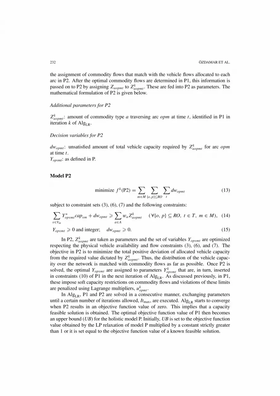
the assignment of commodity flows that match with the vehicle flows allocated to eacharc in P2. After the optimal commodity flows are determined in P1, this information ispassed on to P2 by assigning Zaopmt to Zk

aopmt . These are fed into P2 as parameters. Themathematical formulation of P2 is given below.

Additional parameters for P2

Zkaopmt : amount of commodity type a traversing arc opm at time t , identified in P1 in

iteration k of AlgLR.

Decision variables for P2

dwopmt : unsatisfied amount of total vehicle capacity required by Zkaopmt for arc opm

at time t .Yopvmt: as defined in P.

Model P2

minimize f k(P2) =∑m∈M

∑{o,p}⊆RO

∑t

dwopmt (13)

subject to constraint sets (3), (6), (7) and the following constraints:∑v∈Vm

Y ∗opvmtcapvm + dwopmt �

∑a∈A

waZkaopmt (∀{o, p} ⊆ RO, t ∈ T , m ∈ M), (14)

Yopvmt � 0 and integer; dwopmt � 0. (15)

In P2, Zkaopmt are taken as parameters and the set of variables Yopvmt are optimized

respecting the physical vehicle availability and flow constraints (3), (6), and (7). Theobjective in P2 is to minimize the total positive deviation of allocated vehicle capacityfrom the required value dictated by Zk

aopmt . Thus, the distribution of the vehicle capac-ity over the network is matched with commodity flows as far as possible. Once P2 issolved, the optimal Yopvmt are assigned to parameters Y k

opvmt that are, in turn, insertedin constraints (10) of P1 in the next iteration of AlgLR. As discussed previously, in P1,these impose soft capacity restrictions on commodity flows and violations of these limitsare penalized using Lagrange multipliers, uk

opmt .In AlgLR, P1 and P2 are solved in a consecutive manner, exchanging parameters

until a certain number of iterations allowed, Itmax, are executed. AlgLR starts to convergewhen P2 results in an objective function value of zero. This implies that a capacityfeasible solution is obtained. The optimal objective function value of P1 then becomesan upper bound (UB) for the holistic model P. Initially, UB is set to the objective functionvalue obtained by the LP relaxation of model P multiplied by a constant strictly greaterthan 1 or it is set equal to the objective function value of a known feasible solution.


5.2. Summary of the solution procedure

Procedure AlgLR is summarized as follows.

(0) Initialize UB; set k = 0 and all ukopmt = 0.

(1) Solve P1 (if k = 0 omit constraints (10)).Read optimal devaot and Zaopmt . Set devk

aot = devaot and Zkaopmt = Zaopmt .

(2) Feed Zkaopmt into P2 and solve P2.

Read optimal Yopvmt and dwopmt . Set Y kopvmt = Yopvmt and dwk

opmt = dwopmt .If f k(P2) = 0, and

∑a∈A

∑o∈CD

∑t devk

aot < UB, then, store solution and updateUB,

UB =∑a∈A

∑o∈CD

∑t

devkaot .

(3) Update iteration index: k = k + 1. Re-calculate Lagrange multipliers ukopmt .

(4) If k < Itmax, then, feed ukopmt and Y k−1

opvmt into P1. Go to step 1.Else, stop and report UB and best solution.

5.3. Calculation of Lagrange multipliers

Here, sub-gradient optimisation is utilised (Held et al., 1974). In each iteration, ukopmt

are re-calculated as follows.

(a) If dwk−1opmt > 0, then

ukopmt = uk−1

opmt + stepkdwk−1opmt and loadopmt =

∑v∈Vm

Y k−1opvmtcapvm

where

stepk = µ|UB − ∑

a∈A

∑o∈CD

∑t devk−1

aot |‖∑

m∈M

∑{o,p}⊆CD

∑t dwk−1

opmt‖2.

Here, || · || denotes the Euclidean norm and µ is taken as 2. The parameter loadopmt

denotes the capacity allocated to arc opm at time period t .

(b) If dwk−1opmt = 0, then

ukopmt = γ uk−1

opmt and∑v∈Vm

Y k−1opvmtcapvm = loadopmt

where γ is a constant less than one.

Thus, uk−1opmt increases if the corresponding capacity constraint is violated, and it is

reduced by a factor of γ when the capacity constraint is feasible. The reduction in uk−1opmt

is irrespective of the available slack in the capacity constraint. Hence, the decrease in the

234 ÖZDAMAR ET AL.

Lagrange multiplier is under control. Furthermore, even when the vehicle capacity of alink is not exceeded (condition (b) above), Y k−1

opvmt takes the value it had when the con-straint was last violated, i.e., the expression

∑v∈Vm

Y k−1opvmtcapvm is replaced by loadopmt

in constraints (10). The latter helps model P1 in avoiding repeated capacity infeasibili-ties over the same arcs. The whole approach tries to preserve the feasibility of arcs for anumber of iterations after they gain capacity feasibility.

5.4. Analysis of the sub-problems

Model P1. P1 is a variant of the multi-commodity minimum cost network flow problemthat cannot be readily decomposed into single-commodity problems due to the penaltyterm. This prevents the direct utilization of efficient techniques developed for the con-ventional minimum cost network flow problem. Consequently, algorithms such as themodified shortest path approach of Orlin (1993) should be analyzed and further devel-oped to deal with this special problem. Decomposition based approaches and columngeneration techniques specifically designed for the linear multi-commodity minimumcost network flow problem (Awerbuch and Leighton, 1993; Jones et al., 1993; Fran-gioni, 1997) can also be exploited to develop new efficient algorithms. Efficiency isimportant especially when large networks are considered and the repetitive solution ofP1 becomes computationally cumbersome.

Model P2. In P2 vehicles of different types are treated as multiple commodities. P2 isan integer multi-commodity network flow problem with lower bounds on arcs. However,the objective in P2 is not typical. P2 aims to identify a feasible solution that satisfies theload requirements imposed by the solution of P1. This problem is NP-hard and canbe solved by heuristics (Barnhart and Sheffi, 1993; Barnhart, 1993; Aggarwal et al.,1995), implicit enumeration (Barnhart et al., 1996) or cutting plane methods (Brunettaet al., 1995). These methods require, in turn, the repeated solution of the relaxed linearmulti-commodity network flow problem.

6. Numerical results on hypothetical test problems

In order to test the performance of AlgLR, eighteen small problems are generated ran-domly. The size of the test instances are small, and in this manner, performance can becompared against verified optimal solutions and the effects of different problem charac-teristics can be observed.

The characteristics of the test problems are as follows. The number of de-mand/supply/transhipment nodes vary between 6 and 9. The number of commodities andvehicle types are both restricted by two and a single transportation mode is assumed. Thequantity of demand/supply on each node is uniformly distributed in the interval [0, 100].The distribution of demand and supply nodes across the network, namely, the networktopology, is random, and there is no intentionally created demand or supply clusters inthe network. That is, supply and demand nodes may be adjacent to one another in amixed pattern and they do not form separate clusters. The planning horizon is also de-


termined randomly within the interval [8, 35]. It is assumed that demand quantities andthe availability of supply have been forecasted for the first three periods of the planninghorizon. The limit on arc traversal times is equal to the number of periods in the plan-ning horizon divided by the number of nodes in the network. The traversal time of eacharc takes a random value less than this limit plus a lower bound on arc traversal time,which is three time units.

The number of available vehicles at a node is restricted by six and vehicles maybe available at any type of node. The capacity of each vehicle type is determined asfollows. The load that has to be carried by vehicles is equal to the minimum of totalsupply and total demand. The total load is divided by the total number of availablevehicles to result in the average load per vehicle. The average load per vehicle is dividedby a factor greater than one and this sets the minimum vehicle capacity of each type.This minimum vehicle capacity is added to a random number less than the average loadper vehicle. The result becomes the vehicle capacity for the corresponding type.

Problem characteristics of the test instances are given in table 4. Number of com-modities, vehicle types, demand and supply nodes, and, length of the planning horizonare indicated in table 4 for each test problem. Another characteristic is the total loaddivided by total vehicle capacity. This provides us with an idea on the difficulty of theproblem, because it reflects the percentage of load that can be carried to demand pointsinstantaneously, that is, arc traversal times are not taken into account. Therefore, thischaracteristic is just one indicator of problem difficulty. The difficulty also depends onthe topology of demand nodes within the network, and, the competition among pathsthat the vehicles should optimally follow to serve demand nodes.

In table 4, the (uncapacitated) LP solution of each test problem, the optimal solu-tion of Model P (accompanied by the number of Branch and Bound iterations carriedout by GAMS-XA Solver), and the solution obtained by AlgLR are given. In the AlgLRcolumn, the first feasible solution identified and the final (best) feasible solution foundby the algorithm are indicated (accompanied by the iteration numbers that they are ob-tained in). The number of iterations is restricted to 40. The average CPU times (obtainedon an Intel 1.7 GHz PC) for both GAMS-XA and AlgLR are also indicated in table 4.

It is observed that the performance of AlgLR in relatively difficult problems (testinstances where GAMS-XA obtains the first feasible integer solution and the opti-mal solution in a larger number of iterations, #1, #3, #5, #9, #12, #13, #15, #16,#17, #18) is satisfactory except for test instances #12 and #16, and the algorithm usuallyfinds near-optimal feasible results. The next worst results are obtained in two problems(#2, #7). Naturally, the convergence rate of the algorithm is slower when vehicle capac-ity is tighter. However, capacity is also tight in problems #17 and #18 (GAMS-XA haddifficulty in finding initial integer solutions for these problems and could not verify theoptimal solution) and the algorithm finds satisfactory results. These seemingly contra-dictory results show that capacity tightness is not the only factor that affects problemdifficulty and that network topology has an important influence on performance.

The overall performance of AlgLR is satisfactory with 1.96% deviation from theoptimal solution on the average. A more important observation is that a feasible integer

236 ÖZDAMAR ET AL.Ta

ble

4N

umer

ical

resu

lts

onhy

poth

etic

alte

stpr

oble

ms.

Pro

bId

.|A

||C

|T

|V 1|

Tota

lveh

icle

LP

solu

tion

Opt

imal

solu

tion

Alg

LR

%de

viat

ion

(|CD

|,|C

S|)ca

paci

ty/T

otal

load

(unc

ap.)

(No.

ofB

&B

Fir

stfe

asib

leof

best

solu

tion

iter

atio

ns)

solu

tion

,fr

omop

tim

albe

stso

luti

onso

luti

on(i

tera

tion

no.)

12

7(4

,2)

212

1.72

4068

4195

(639

)42

51(5

)%

1.33

21

5(3

,1)

202

0.82

131

153

(98)

171

(5),

161

(27)

%5.

233

26

(3,3

)10

21.

0324

0036

67(4

926)

4220

(6),

3711

(35)

%1.

204

28

(1,6

)27

11.

8235

954

8(2

11)

548

(2)

%0.

005

26

(3,2

)13

10.

9119

2523

99(1

004)

2420

(3),

2399

(29)

%0.

006

17

(2,4

)11

11.

6911

811

8(6

6)11

8(1

)%

0.00

71

5(1

,3)

211

0.90

281

465

(155

)49

0(6

)%

5.38

82

7(1

,5)

111

1.49

144

157

(139

)17

0(1

),15

7(1

8)%

0.00

92

8(3

,4)

252

1.41

815

1050

(514

)10

54(3

)%

0.38

101

5(2

,2)

272

1.32

260

337

(137

)33

7(3

)%

0.00

111

6(1

,4)

121

1.35

178

187

(37)

187

(2)

%0.

0012

28

(1,6

)12

20.

7929

646

3(5

29)

502

(37)

%8.

4213

26

(2,3

)11

21.

1598

110

00(5

375)

1010

(1),

1003

(27)

%0.

3014

16

(1,4

)25

10.

7212

334

0(7

0)34

0(4

)%

0.00

152

7(1

,5)

272

1.47

375

477

(657

5)50

6(1

1),4

77(3

0)%

0.00

162

5(1

,3)

122

0.82

313

452

(196

4)52

1(5

),49

4(3

1)%

9.20

172

8(2

,5)

332

0.91

214

321

(100

000)

337

(3),

325

(25)

%1.

2418

27

(3,3

)13

20.

8462

474

3(1

0000

0)77

8(3

),76

3(1

4)%

2.69

Ave

rage

CP

Uti

me

(s)

15.9

94.

48A

vera

ge%

devi

atio

nfr

omop

tim

al(s

tdev

)%

1.96

(%2.

94)


solution is obtained in the first few Lagrange iterations, which is essential especially inrelatively difficult problems (e.g., in problems #17 and #18) if the planning system isrequired to update schedules frequently and provide a fast answer. In such problems,it is observed that when P is solved, it takes a large number of iterations to find thefirst integer feasible solution. On the other hand, when the problem is decomposed andZaopmt are taken from P1 and inserted as parameters into P2, an integer solution is foundfor P2 in very few B&B iterations. Hence, the time lost during Lagrange iterations iscompensated by the enhanced solvability of P2.

Although small hypothetical instances give an idea about the sensitivity of the pro-posed solution procedure to certain problem characteristics, it is required to test its ap-plicability in realistic emergency situations. With this in mind, a natural disaster scenariobased on the earthquake that took place in 1999 in Izmit (Turkey) is generated for testingthe procedure.

7. Implementation on the earthquake scenario

The model and the solution methodology are implemented on a scenario based on theofficial attrition numbers announced by the Ministry of Internal Affairs for the Izmitearthquake that took place on August 17th, 1999. The earthquake was most destructivein four close townships in the industrial center of Turkey (shores of Marmara Sea that aredensely populated areas), Izmit, Adapazari, Golcuk, Yalova, and in one district, Avcilar,that is in the outskirts of Istanbul. Its moment magnitude was MW 7.4 and it causeda total number of 17727 deaths, 43959 injuries and damaged 214000 residential units,affecting more than 2 million people. Figure 3 illustrates the topology of the logistic

Figure 3. Topology of the affected area.

238 ÖZDAMAR ET AL.

Table 5Attrition figures in the main townships affected by the Izmit earthquake.

First day Second day

Location Dead Wounded Affected Dead Wounded Affected(node number) population population

Adapazari (3) 2189 4237 243241 239 462 26535Izmit (4) 3403 3458 680500 371 377 74236Gölcük (5) 3690 4220 246000 403 460 26836Yalova (6) 2080 3727 416000 227 407 45382Avcilar (8) 813 2956 162667 89 322 17745

Total 12175 18599 1748408 1329 2028 190734

Table 6Supplies and requirements for commodities of different categories.

First day Food Tent Clothing Medicine Serum Save & rescue Totalequip. (tons)

Requirements 2622.6 32782.3 6993.6 27.9 13.9 262.2 42702.5(tons)Supplies 2098.1 26226.1 5594.9 22.4 11.2 209.8 34162.5(tons)

Second day

Requirements 2908.7 3576.3 762.9 31.0 15.5 28.6 7323.0(tons)Supplies 3199.6 3933.9 839.2 34.1 17.1 31.5 8055.4(tons)

network superimposed on the map of Marmara region. The network is constructed usingthe primary motorway map of the region and for simplicity, links between cities arerepresented by straight lines. In figure 3, Bolu (node 2) is a transshipment node onthe highway. Details related to the Izmit earthquake may be found in many referencesincluding international ones (e.g., USGS Circular No. 1193).

The data in table 5 reveals the number of people found dead and wounded on thefirst and second days following the earthquake, as well as the number of affected peoplewho could no longer reside in their houses. In table 5, the second day’s attrition figuresshow additional counts. At the time, only the dead and injured above the rubbles couldbe counted, and no information was available on people who were lost.

During the first two days, aid arrived by using the main highways, such as TEM(Trans European Motorway (TEM) could be used for transport, since its viaducts andtunnels were undamaged in general) and E-5, from the big cities surrounding the affectedarea, namely, Istanbul (node 7), Ankara (node 1), Izmir (node 12), Eskisehir (node 9),Bursa (node 10), and Balikesir (node 11). The first three cities were the largest suppliersof aid materials.


Table 7Distribution of supplies and requirements (averages are taken over 6 commodities).

Location Ankara Istanbul Eskisehir Bursa Balikesir Izmir(node number) (1) (7) (9) (10) (11) (12)

Average percentage 23% 25% 12% 12% 8% 20%of supplies

Location Adapazari Izmit Golcuk Yalova Avcilar(node number) (3) (4) (5) (6) (8)

Average percentage 9 % 53 % 16 % 16 % 6 %of requirements

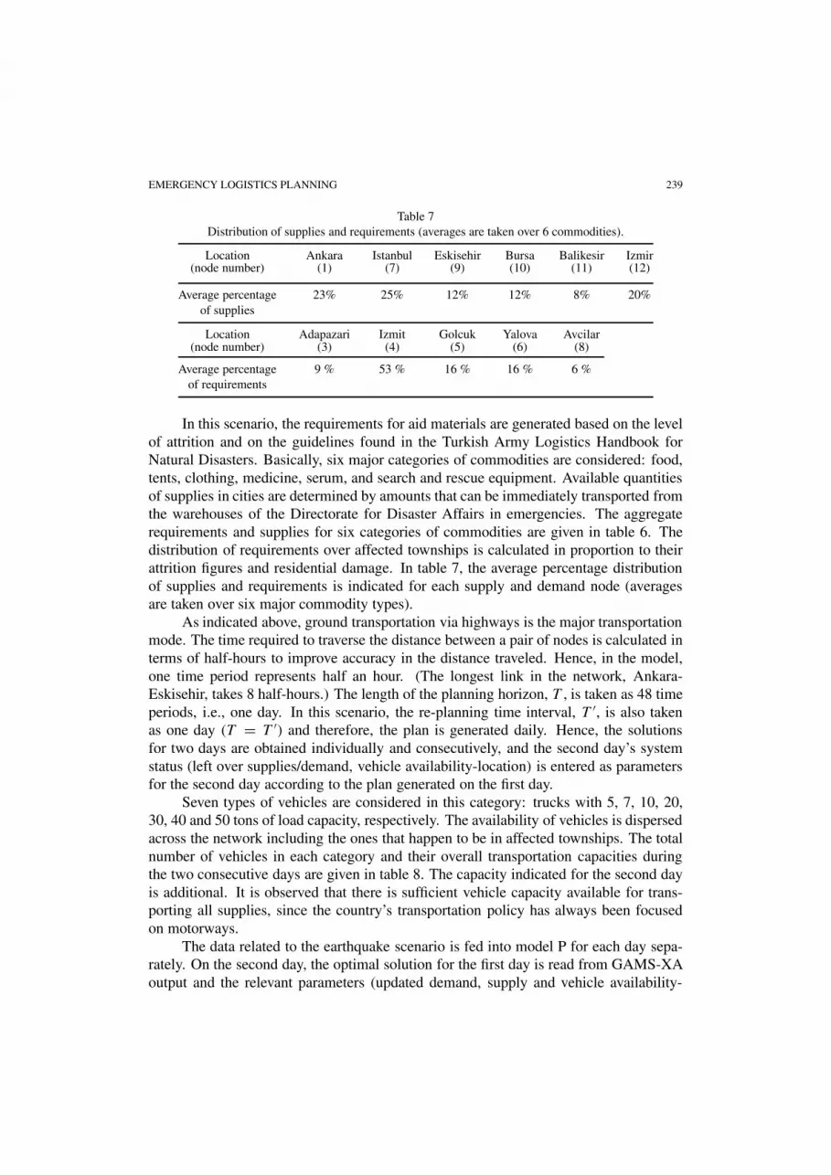
In this scenario, the requirements for aid materials are generated based on the levelof attrition and on the guidelines found in the Turkish Army Logistics Handbook forNatural Disasters. Basically, six major categories of commodities are considered: food,tents, clothing, medicine, serum, and search and rescue equipment. Available quantitiesof supplies in cities are determined by amounts that can be immediately transported fromthe warehouses of the Directorate for Disaster Affairs in emergencies. The aggregaterequirements and supplies for six categories of commodities are given in table 6. Thedistribution of requirements over affected townships is calculated in proportion to theirattrition figures and residential damage. In table 7, the average percentage distributionof supplies and requirements is indicated for each supply and demand node (averagesare taken over six major commodity types).

As indicated above, ground transportation via highways is the major transportationmode. The time required to traverse the distance between a pair of nodes is calculated interms of half-hours to improve accuracy in the distance traveled. Hence, in the model,one time period represents half an hour. (The longest link in the network, Ankara-Eskisehir, takes 8 half-hours.) The length of the planning horizon, T , is taken as 48 timeperiods, i.e., one day. In this scenario, the re-planning time interval, T ′, is also takenas one day (T = T ′) and therefore, the plan is generated daily. Hence, the solutionsfor two days are obtained individually and consecutively, and the second day’s systemstatus (left over supplies/demand, vehicle availability-location) is entered as parametersfor the second day according to the plan generated on the first day.

Seven types of vehicles are considered in this category: trucks with 5, 7, 10, 20,30, 40 and 50 tons of load capacity, respectively. The availability of vehicles is dispersedacross the network including the ones that happen to be in affected townships. The totalnumber of vehicles in each category and their overall transportation capacities duringthe two consecutive days are given in table 8. The capacity indicated for the second dayis additional. It is observed that there is sufficient vehicle capacity available for trans-porting all supplies, since the country’s transportation policy has always been focusedon motorways.

The data related to the earthquake scenario is fed into model P for each day sepa-rately. On the second day, the optimal solution for the first day is read from GAMS-XAoutput and the relevant parameters (updated demand, supply and vehicle availability-

240 ÖZDAMAR ET AL.

Table 8Total number of available vehicles of different capacities (second day’s capacity is additional).

First day 5 tons 7 tons 10 tons 20 tons 30 tons 40 tons 50 tons Total

Total number ofvehicles

279 298 372 205 223 298 186 1861

Transportationcapacity in tons

1395 2086 3720 4100 6690 11920 9300 39211

Second day 5 tons 7 tons 10 tons 20 tons 30 tons 40 tons 50 tons Total

Total number ofadditional vehicles

25 33 40 18 20 26 16 178

Transportationcapacity in tons

125 231 400 360 600 1040 800 3556

location in the network) are fed into the second day’s code. The optimal solution is thusobtained for the two consecutive days using GAMS-XA. The number of unsuppressedinteger variables for the earthquake scenario on each day is 8736. It is noted that thereare 1860 and 2038 vehicles available on the first and second days, respectively. On thefirst day, a vehicle makes more than three partial trips on the average. Therefore, if eachvehicle were tracked individually as in conventional vehicle routing models, then, therewould be a significantly larger number of binary variables. Thus, model P reduces theproblem into a relatively manageable size.

The requirements and supply data are assumed to be known only for the currentday of planning with the exception of food. It is assumed that, once the initial attritionis known, food requirements can be forecasted for future days, since people in affectedareas need to be fed adequately every day. Hence, requests for food supplies can bemade in advance. In this implementation, on the first day, both the first and second day’sfood requirements/supplies are taken into account, the first day’s being the requirementin period one and the second day’s in period 48. A similar approach is adopted on thesecond day using the third day’s predictions.

On the second day, after observing the optimal solution obtained for the first day,requirements that could not be transported on the first day due to lack of supplies areadded to the first period’s requirements of the second day. It is observed that suppliesare not sufficient to meet demand on the first day and therefore, there are no supplies leftover for the next day (all available supply is transported on the first day).

On the second day, the number of available vehicles at each city or township isidentified by reading the optimal values of the variables of surovmT from the first day, andthe slack variables of constraints (7) in model P. (Note that, here, the re-planning periodis t∗ = T , and surovmT contribute to avovmt∗ without the need for further analysis.) Thus,the matrix of available vehicles is updated using this information and provision is alsomade for the additional vehicles provided on the second day.

The analysis of the optimal solutions obtained for the first and second days showthat all supplies are transported within the first 15 hours and 10.5 hours, respectively.When the available vehicle capacity is compared to transportation requirements it is ob-


Table 9Results obtained for the two-day earthquake scenario.

Day LP solution Optimal solution AlgLR Greedy heuristic(No. of B&B First feasible solution

iterations) Best solution(iteration no.)

1 Solution value 561649 666448 (27310) 687774 (6) 722681690506 (29)

% deviation ofsolution fromoptimal solution – – 3.61% 8.43%

CPU time (s) 2.8 602.85 34.52 0.46

2 Solution value 321762 340669 (276128) 346349 (2) 355606341588 (14)

% deviation ofsolution fromoptimal solution – – 0.27% 4.38%

CPU time (s) 2.6 2939.68 18.92 0.31

served that vehicle capacity is somewhat tight (the ratio of total vehicle capacity to totalload is 1.05) on the first day and there is ample idle vehicle capacity on the second day.However, at the end of the first day, vehicles remain at their last destinations and aremostly concentrated in the affected area, mainly on nodes 3, 4, 6, and 8. Therefore, ittakes a couple of hours for the vehicles to pick up the supplies on the second day. Duringthe first two days after the earthquake, none of the affected townships could communi-cate any supply availability effectively, because communication channels were down.Therefore, in this special case, it may be appropriate to add an aggregate constraint onthe variables Yopvmt to make sure that all vehicles return to supply nodes, with each sup-ply node receiving a transportation capacity based on the forecasted available supplyquantity on the next day.

In table 9, the optimal objective function values obtained for the first and seconddays are indicated along with the uncapacitated LP solution, the number of B&B iter-ations and CPU times. The earthquake scenario problem is about 10 times bigger thanthe size of the average hypothetical test problem in terms of unsuppressed integer vari-ables. Naturally, it takes a larger number of iterations to solve the problem to optimalityand verify it using the optimization package. However, the topology of the network issimpler than some of the hypothetical test problems with random topologies. Hence, theadverse effects of increased problem size is somewhat reduced by the network topologythat facilitates the solution of the problem.

On the first day, the optimal solution’s objective value is 18.66% higher than theLP relaxation due to the tightness of vehicle capacity whereas on the second day thispercentage is 5.87%. It is observed that the optimal solution is obtained and verified

242 ÖZDAMAR ET AL.

with much more difficulty on the second day when the vehicle capacity constraints arenot tight, because, the feasible space is enlarged.

In table 9, the results obtained by AlgLR are also indicated. Its performance isconsistent with the experiments conducted on hypothetical test instances. The qualityof the solution obtained is worse under tight vehicle capacity constraints, and it takes alonger time to identify the first feasible solution. On the second day, a feasible solutionis found within a couple of iterations and the quality of the solution finally achievedis good. In this sense, AlgLR behaves in a manner opposite to that of the optimizationpackage.

7.1. A greedy heuristic

To provide an idea on the relative performance of AlgLR, a simple greedy heuristic isdesigned to generate a logistics plan so that the two approaches can be compared onthis scenario. The heuristic follows the same principle as the modified shortest pathalgorithm proposed by Orlin (1993) for solving the minimum cost network flow problem.

First, the multicommodity network flow problem is solved without vehicle capacityconstraints. Then, the resulting optimal flow of commodities is used to construct theroutes that should be followed by the vehicles. Each route is identified with its sourceand sink node, and route start time. The idea is to assign vehicles available at nodes thatare closest to the source node of each route. Ideally, the start time of a route should notbe delayed by the arrival times of the vehicles assigned to the route. Thus, the heuristicseeks for the ideal match between pairs of nodes (o, p) in order to minimize total delay.

The first node, o, in a node pair (o, p) has unallocated vehicle capacity and thesecond node, p, is the route source node. The Feasible Transportation Date (FTD) fora node pair (o, p) is the earliest time period when commodities can be mobilized fromthe source node p using vehicles coming from node o. The vehicles leaving node o willarrive at node p at a time equal to their ready time at node o plus the time required totravel to node p. This arrival time is compared with the route start time. Since it isnot desired to start the route earlier than the required date, the maximum of the vehiclearrival time and the route start time is taken as the FTD for node pair (o, p). FTD iscalculated for each possible node pair (o, p) and all node pairs are sorted in ascendingorder of FTD.

This is a greedy heuristic approach where vehicle capacity allocation is prioritizedto satisfy the capacity requirements of the node pair with the earliest FTD so that theglobal aim of minimizing total route delays can be achieved. Therefore, the first nodepair (say, o∗, p∗) in the ascending FTD list is selected and vehicle capacity available atnode o∗ is allocated to the route source node, p∗. The assignment of vehicle capacityto node p∗ is carried out according to the best-fit strategy so as to avoid partially emptytrips. The release time of the allocated vehicles is noted (release time is equal to thecompletion time of the route at the route sink node). When the vehicle capacity require-ments of node p∗ are satisfied or when all vehicle capacity at node o∗ is allocated, the


assignment procedure for this node pair is over. Demand/supply quantities at route sinkand source nodes, and vehicle availability (location-timing) are updated accordingly.

Before the next pair of nodes in the sorted FTD list is considered, the list is revised.This revision is needed to exploit the availability of the vehicles that are released in somefuture period from the most recent assignment. The reason is that these vehicles mightend up at nodes that are at closer distances to other route source nodes. FTD calculationsinvolving these vehicles are carried out in the same manner, with revised vehicle readytimes and vehicle arrival times. After the sorted list is revised, the pair of nodes at thetop of the list is considered and the procedure is repeated until all available supply isdepleted or all demand requirements are satisfied. Note that, this heuristic might resultin final transportation schedule that overrides the length of the planning horizon.

The greedy heuristic is quite efficient, since it has a good foundation that servesthe objectives of both sub-problems. However, it is myopic and cannot optimize the setof vehicles assigned to each route globally. Therefore, it may lead to inferior solutionswhen vehicle capacity is tight.

The major commodity flow routes generated by the solution of the uncapacitatedproblem are (1–2–3–4), (12–11–10–6–5–4), (7–4), (7–8), (10–6) and (9–4). The greedyheuristic tries to match vehicle capacities that are closest to the route-source nodes asdescribed above. The objective function values of the logistics plans generated by thegreedy heuristic are indicated in table 9. It is observed that the greedy heuristic hasa poorer performance than AlgLR, because the latter has the capability of optimizingthe sub-problems and matching their solutions. However, the computation time of thegreedy heuristic is very low. On the other hand, in a real time implementation of thelogistics coordination system, AlgLR would not be at a great disadvantage since the com-putation time required is reasonable for re-planning at every 48 time periods.

The implementation of the solution methodology on the earthquake scenariodemonstrates its behaviour in a realistic situation. Based on the results, it can be con-cluded that AlgLR may be utilized to provide reliable solutions during the initial daysafter a natural disaster when requests for aid materials are heavy and an efficient logisti-cal coordination is required.

8. Conclusion

A mathematical model for emergency logistics planning is developed in this study. Theaim is to coordinate logistics support for relief operations. Model outputs consist of dis-patch orders for vehicles waiting at different locations in the area. These orders designatethe routes of vehicles including empty trips, pick-ups and deliveries in mixed order andwaiting interludes throughout the planning horizon. The model takes into account time-dependent supply/demand and fleet size, and, facilitates schedule updates in a dynamicdecision-making environment. Furthermore, in this model, vehicles are not tracked onan individual basis and this reduces problem size significantly.

The model integrates two multi-commodity network flow problems, the first onebeing linear (commodities) and the second one integer (vehicles). The integer multi-

244 ÖZDAMAR ET AL.

commodity network flow problem addresses the vehicle routing problem that is linkedto the linear sub-problem by imposing load capacity constraints on arcs. Both sub-problems are difficult to solve when the network is large. In fact, the second sub-problemis NP-hard and requires heuristic solution methodologies when very large-scale prob-lems are solved.

In this study, a Lagrangean relaxation based heuristic approach, AlgLR, is proposedto couple the two sub-problems. The approach is fine-tuned by updating Lagrange mul-tipliers in a more restrictive manner. Tests on small examples show that AlgLR convergessatisfactorily. Furthermore, its performance in emergencies of realistic size is demon-strated via an earthquake scenario based on the Izmit earthquake’s (1999, Turkey) at-trition figures. It is observed that AlgLR can cope with natural disasters of similar sizewithin a reasonable computation time.

Acknowledgments

We wish to express our sincere thanks to the anonymous referee and the Editorial of-fice for their thorough and constructive review that have helped us improve both thepresentation of the work and the methodologies developed here.

References

Aggarwal, C.C., M. Oblak, and R.R. Vemuganti. (1995). “A Heuristic Solution Procedure for Multi-Commodity Integer Flows.” Computers and Operations Research 22, 1075–1087.

Awerbuch, B. and T. Leighton. (1993). “Multi-Commodity Flows: A Survey of Recent Research.” In Pro-ceedings of ISAAC ’93, pp. 297–302.

Barnhart, C. and Y. Sheffi. (1993). “A Network Based Primal-Dual Heuristic for Multi-Commodity NetworkFlow Problems.” Transportation Science 27, 102–117.

Barnhart, C. (1993). “Dual Ascent Methods for Large-Scale Multi-Commodity Network Flow Problems.”Naval Research Logistics 40, 305–324.

Barnhart, C., C.A. Hane, and P.H. Vance. (1996). “Integer Multi-Commodity Flow Problems.” Centre forTransportation Studies Working Paper, Centre for Transportation Studies, MIT.

Bodin, L.D. (1990). “Twenty Years of Routing and Scheduling.” Operations Research 38, 571–579.Brunetta, L., M. Conforti, and M. Fischetti. (1995). “A Polyhedral Approach to an Integer Multi-

Commodity Flow Problem.” Preprint No. 18, Department of Mathematics, Padova University.Desrochers, M., J.K. Lenstra, M.W.P. Savelsbergh, and F. Soumis. (1988). “Vehicle Routing with Time

Windows.” In B.L. Golden and A.A. Assad (eds.), Vehicle Routing: Methods and Studies. Amsterdam:Elsevier Science.

Desrochers, M., J.K. Lenstra, and M.W.P. Savelsbergh. (1990). “A Classification Scheme for Vehicle Rout-ing and Scheduling Problems.” European Journal of Operational Research 46, 322–332.

Desrochers, M. et al. (1998). “Towards a Model and Algorithm Management System for Vehicle Routingand Scheduling Problems.” Working Paper, GERAD, Montreal, Canada.

Dror, M. and P. Trudeau. (1990). “Split Delivery Routing.” Naval Research Logistics 37, 383–402.Equi, L., G. Gallo, S. Marziale, and A. Weintraub. (1996). “A Combined Transportation and Scheduling

Problem.” Working Paper, Pisa University, Pisa, Italy.Frangioni, A. (1997). “Dual Ascent Methods and Multi-Commodity Flow Problems.” PhD Dissertation TD

5/97, Department of Informatics, Pisa University, Pisa, Italy.


Fisher, M. (1981). “The Lagrangean Relaxation Method for Solving Integer Problems.” Management Sci-ence 27, 1–18.

Fisher, M. (1995). “Vehicle Routing.” In M.O. Ball et al. (eds.), Handbooks in OR and MS, Vol. 8. Amster-dam: Elsevier Science.

Fisher, M., B. Tang, and Z. Zheng. (1995). “A Network Flow Based Heuristic for Bulk Pick Up and DeliveryRouting.” Transportation Science 29, 45–55.

Gendreau, M., F. Guertin, J.-Y. Potvin, and E. Taillard. (1999). “Parallel Tabu Search for Real-Time VehicleRouting and Dispatching.” Transportation Science 33, 381–390.

Held, M. et al. (1974). “Validation of Sub-Gradient Optimization.” Mathematical Programming 6, 62–88.Jimenez, F. and J.L. Verdegay. (1999). “Solving Fuzzy Solid Transportation Problems by an Evolutionary

Algorithm Based Parametric Approach.” European Journal of Operational Research 117, 485–510.Jones, K.L. et al. (1993). “Multi-Commodity Network Flows: The Impact of Formulation on Decomposi-

tion.” Mathematical Programming 62, 95–117.Kennington, J.L. and M. Shalaby. (1977). “An Effective Sub-Gradient Procedure for Minimal Cost Multi-

Commodity Flow Problems.” Management Science 23, 994–1004.Laporte, G. (1992). “The Vehicle Routing Problem: An Overview of Exact and Approximate Algorithms.”

European Journal of Operational Research 59, 345–358.Mathies, S. and P. Mevert. (1998). “A Hybrid Algorithm for Solving Network Flow Problems with Side

Constraints.” Computers and Operations Research 25, 745–756.Orlin, J.B. (1993). “A Faster Strongly Polynomial Minimum Cost Flow Algorithm.” Operations Research

41, 338–350.Rathi, A.K., R.L. Church, and R.S. Solanki. (1993). “Allocating Resources to Support a Multicommodity

Flow with Time Windows.” Logistics and Transportation Review 28, 167–188.Ribeiro, C. and F. Soumis. (1994). “A Column Generation Approach to the Multi-Depot Vehicle Scheduling

Problem.” Operations Research 42, 41–52.Rodriguez, P. et al. (1998). “Using Global Search Heuristics for the Capacity Vehicle Routing Problem.”

Computers and Operations Research 25, 407–417.U.S. Geological Survey Information Services. (1999). “Implications for Earthquake Risk Reduction in the

United States from the Kocaeli, Turkey, Earthquake of August 17, 1999.” USGS Circular # 1193.Venkataramanan, M.A., J.J. Dinkel, and J. Mote. (1989). “A Surrogate and Lagrangean Approach to Con-

strained Network Problems.” Annals of OR 20, 283–302.Ziliaskopoulos, A. and W. Wardell. (2000). “An Intermodal Optimum Path Algorithm for Multimodal Net-

works with Dynamic Arc Travel Times and Switching Delays.” European Journal of Operational Re-search 125, 486–502.

Emergency Logistics Planning in Natural Disasters

Documents