Embedded Systems II Forschung 3 Herausgegeben von Prof. Dr.-Ing. Birgit Vogel-Heuser, Technische Universität München

Welcome message from author
This document is posted to help you gain knowledge. Please leave a comment to let me know what you think about it! Share it to your friends and learn new things together.
Transcript

Embedded Systems II Forschung 3
Herausgegeben von Prof. Dr.-Ing. Birgit Vogel-Heuser, Technische Universität München

Awang Noor Indra Wardana Development of Automatic Program Verification for Continuous Function Chart based on Model Checking
kasseluniversity
press
This work has been accepted by the Faculty of Electrical Engineering and Computer Science of the University of Kassel as a thesis for acquiring the academic degree of Doktor der Ingenieurwissenschaften (Dr.-Ing.). First Supervisor: Prof. Dr.-Ing. Birgit Vogel-Heuser Technische Universität München Second Supervisor: Prof. Dr.-Ing. Georg Frey Universität des Saarlandes Defense day: 29th September 2009 Bibliographic information published by Deutsche Nationalbibliothek The Deutsche Nationalbibliothek lists this publication in the Deutsche Nationalbibliografie; detailed bibliographic data is available in the Internet at http://dnb.d-nb.de. Zugl.: Kassel, Univ., Diss. 2009 ISBN print: 978-3-89958-806-4 ISBN online: 978-3-89958-807-1 URN: http://nbn-resolving.de/urn:nbn:de:0002-8077 2009, kassel university press GmbH, Kassel www.upress.uni-kassel.de Printed by Unidruckerei, University of Kassel Printed in Germany
Contents
1 Introduction.................................................................................................................. 1
1.1 Motivation............................................................................................................... 1 1.2 Objective ................................................................................................................. 2 1.3 Structure of Thesis .................................................................................................. 3
2 Scope of the Work........................................................................................................ 5
2.1 Automation System................................................................................................. 5 2.1.1 Classification of Automation System...................................................................... 5 2.1.2 Programming Languages in Automation System.................................................... 7 2.1.3 DCS’s Program Execution Procedure and CFC...................................................... 9 2.2 Program Development of Automation System ..................................................... 12 2.2.1 Control Tasks Specification .................................................................................. 13 2.3 Program Verification............................................................................................. 15 2.3.1 Formal Methods for Program Verification............................................................ 16 2.3.2 Automatic Program Verification in Automation System ...................................... 17 2.3.3 Model Checker for Timed Automata .................................................................... 21
3 Formal Descriptions of Timed Automata and Timed Computation Tree Logic .. 23
3.1 Formal Descriptions of Timed Automata.............................................................. 23 3.1.1 Syntax of Timed Automata ................................................................................... 25 3.1.2 Semantics of Timed Automata.............................................................................. 26 3.2 Formal Descriptions of Timed Computation Tree Logic ...................................... 27 3.2.1 Syntax of TCTL .................................................................................................... 27 3.2.2 Semantics of TCTL............................................................................................... 28 3.3 Formal Descriptions of UPPAAL ......................................................................... 28 3.3.1 Formal Model in UPPAAL ................................................................................... 28 3.3.2 Formal Specification in UPPAAL ........................................................................ 30
4 Formalization of Continuous Function Chart and Logic Diagram ....................... 32
4.1 Formal Descriptions of Continuous Function Chart ............................................. 32 4.1.1 Syntax of CFC....................................................................................................... 34 4.1.2 Semantics of CFC ................................................................................................. 36 4.1.3 Execution Procedure of CFC ................................................................................ 37 4.1.4 Application Example............................................................................................. 41 4.2 Formal Descriptions of Logic Diagram ................................................................ 41 4.2.1 Syntax of Logic Diagram...................................................................................... 42 4.2.2 Semantics of Logic Diagram................................................................................. 43
Contents
4.2.3 Application Example............................................................................................. 45 4.3 Conclusion ............................................................................................................ 46
5 Development of Transformation Rules .................................................................... 48
5.1 Continuous Function Chart to Timed Automata ................................................... 48 5.1.1 Transformation of Function Block........................................................................ 48 5.1.2 Transformation of CFC’s Execution Procedure.................................................... 51 5.1.3 Transformation of CFC Program .......................................................................... 53 5.1.4 Application Example............................................................................................. 55 5.2 Logic Diagram to Timed Computation Tree Logic............................................... 56 5.2.1 Transformation of Logic Diagram ........................................................................ 56 5.2.2 Application Example............................................................................................. 57 5.3 Summary ............................................................................................................... 58
6 Realization of Automatic Program Verification ..................................................... 59
6.1 Realization using UPPAAL .................................................................................. 59 6.1.1 Realization of UPPAAL Model ............................................................................ 59 6.1.2 Realization of UPPAAL Specification.................................................................. 69 6.2 Tool Realization.................................................................................................... 71 6.2.1 Structure of Automatic Program Verification Tool .............................................. 71 6.2.2 Model Generator ................................................................................................... 72 6.2.3 Specification Generator......................................................................................... 73 6.3 Summary ............................................................................................................... 73
7 Case Studies................................................................................................................ 75
7.1 Process-Engineering Unit of the Hybrid Bench-scale Model ............................... 75 7.1.1 Process Description............................................................................................... 75 7.1.2 Logic Diagrams..................................................................................................... 76 7.1.3 CFC Programs....................................................................................................... 78 7.1.4 UPPAAL Models .................................................................................................. 81 7.1.5 UPPAAL Specifications ....................................................................................... 83 7.1.6 Verification Results............................................................................................... 84 7.2 Jacketed Stirred Tank Reactor .............................................................................. 85 7.2.1 Process Description............................................................................................... 86 7.2.2 Logic Diagrams..................................................................................................... 87 7.2.3 CFC Programs....................................................................................................... 89 7.2.4 UPPAAL Models .................................................................................................. 92 7.2.5 UPPAAL Specifications ....................................................................................... 94 7.2.6 Verification Results............................................................................................... 94 7.3 Conclusion ............................................................................................................ 95
Contents
8 Conclusions................................................................................................................. 97
8.1 Summary ............................................................................................................... 97 8.2 Lessons Learned.................................................................................................... 98 8.3 Future Works ...................................................................................................... 100
9 References................................................................................................................. 102
Appendix A....................................................................................................................... 109
Appendix B....................................................................................................................... 114

1 Introduction This chapter gives a general introduction about this work. Section 1.1 explores the brief description regarding motivation surrounding this work. In Section 1.2, the objective of this work is outlined and the end of this chapter, Section 1.3 completes this chapter with the structure of this thesis.
1.1 Motivation Industrial plants such as refinery plant, power plant, or petrochemical plant are the complex systems that contain a number of devices. Most of the devices in industrial plants are interdependent, real-time, safety critical and involves high investment. Any failure in the plants might not only result in a financial loss but can also endanger the environment. To ensure that these conditions do not happen, the industrial plants have to be operated automatically. These automatic operations are made possible using the industrial automation systems. Typically, the industrial automation systems contain the computers and the interface systems, enabling the systems to interact with the devices in industrial plants. The computers, which are the main components in the industrial automation systems, run the programs to operate the devices in industrial plants. Such programs are critical because they have to define the right operation procedures. If the programs contain errors, the devices in industrial plants cannot operate correctly. Errors in the programs can endanger the environment. One promising way to achieve the correctness of the programs is to improve the engineering lifecycle with safety development procedures. More precisely, as described by Storey [Sto96] two procedures are usually used:
• Determining if the output of engineering lifecycle phase fulfills the requirements specified in the previous phase. In the context of implementing programs, this approach is to ensure that the programs conform to the specifications.
• Confirming if the engineering lifecycle’s output is appropriate and is consistent with the user requirements. In the context of implementing programs, this approach is to provide the output program’s suitability for use and to confirm the appropriateness of the user requirements.
Nowadays, during the development of the programs, these procedures are conducted by performing various manual tests to investigate the nature of the different behaviour of the programs and to determine the integrity of the programs. The manual tests will uncover the errors and remove them from the programs, and so increasing the program’s dependability. However, these manual tests are not exhaustive. It is possible that the programs, which successfully pass certain manual tests, will behave differently in the real operations. It can result in damaged devices in industrial plants, as well as endangering the lives of operators and those around it. To avoid this fatal condition, all possible behaviour of programs in the real operations has to be tested. However, the complete manual tests are very time consuming. One promising way to provide the exhaustive approach and to reduce the time
1. Introduction
2
required for testing process is to improve the methods to develop the programs. The following two approaches are considered:
• The first approach is to develop the programs from the specifications using a code generator. In general, a code generator retrieves the structure of the program specifications and uses this structural information to generate the programs automatically. This will reduce the time for developing the programs because it provides direct implementation from the program specifications. It is also not necessary to test the generated programs using exhaustive testing, as the programs will not deviate from the specifications.
• Another approach is the automatic program verification method. In general, automatic program verification retrieves all possible conditions of the programs. This approach will generate all the possible conditions to test if the behaviour of the programs conforms to the specifications. It also shortens the program development time because the time to investigate the nature of all behaviour of programs is reduced.
This work applies the second approach. This is because the second approach will provide better program’s dependability than the first approach. In the first approach, it is still possible to have incomplete information concerning the behaviour of the programs, as it is difficult to retrieve the structure of program specifications as well as mapping this structure to the programs. On the other hand, the second approach is able to ensure that all possible behaviour of programs is guaranteed to being verified.
1.2 Objective The objective of this work is to develop the methods and a tool of automatic program verification for automation system by using the verification method that is widely used in computer science, i.e. model checking. As model checking is a formal method, it is necessary to have formal descriptions of the programs and the specifications. Therefore, the first approach of this work is to develop the formal descriptions regarding the programs and the specifications. Due to the major problem in model checking, which is the state-space explosion problem, the formalization of the programs and the specifications are strongly restricted. The second approach of this work is to develop the methods and a tool to generate the reasonable formal models and formal specifications to enable model checking as program verification method. In industrial plants such as refinery plant, power plant, or petrochemical plant, the implemented programs that represent plant’s operation procedures are complex. To observe the applicability in an industrial context, the third approach of this work is to evaluate the applicability of the methods and a tool of automatic program verification in industrial context. This is done by implementing the developed methods and a tool in a few of industrial case studies.
1. Introduction
3
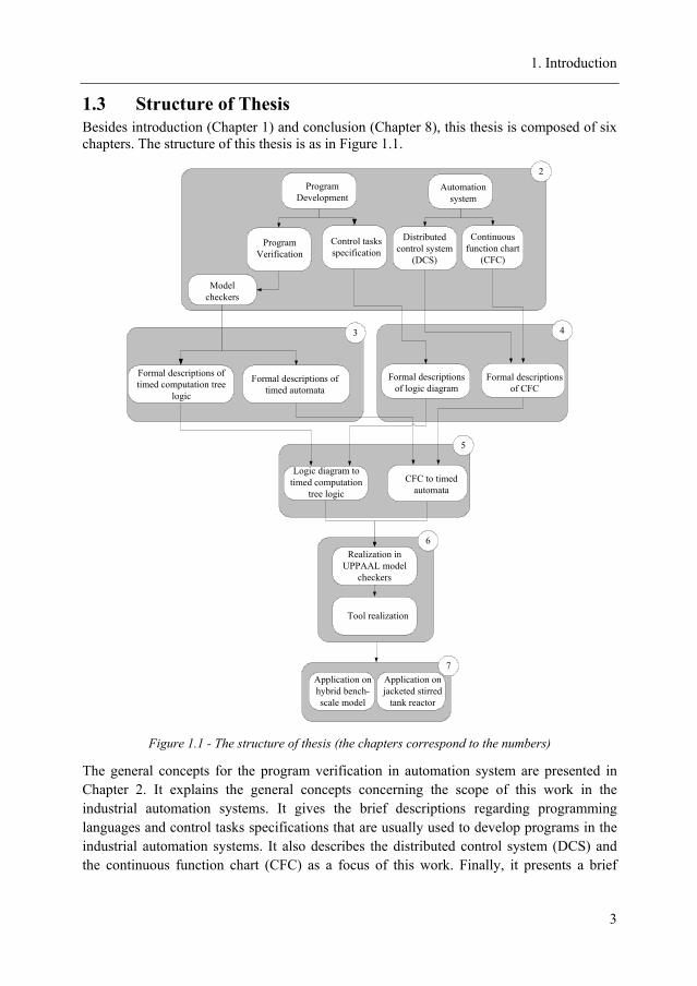
1.3 Structure of Thesis Besides introduction (Chapter 1) and conclusion (Chapter 8), this thesis is composed of six chapters. The structure of this thesis is as in Figure 1.1.
2
Model checkers
3
Formal descriptions of timed automata
Formal descriptions of timed computation tree
logic
4
Formal descriptions of CFC
Formal descriptions of logic diagram
5
CFC to timed automata
Logic diagram to timed computation
tree logic
Realization in UPPAAL model
checkers
6
7
Program Development
Automation system
Distributed control system
(DCS)
Continuous function chart
(CFC)
Tool realization
Application on hybrid bench-scale model
Application on jacketed stirred
tank reactor
Control tasks specification
Program Verification
Figure 1.1 - The structure of thesis (the chapters correspond to the numbers)
The general concepts for the program verification in automation system are presented in Chapter 2. It explains the general concepts concerning the scope of this work in the industrial automation systems. It gives the brief descriptions regarding programming languages and control tasks specifications that are usually used to develop programs in the industrial automation systems. It also describes the distributed control system (DCS) and the continuous function chart (CFC) as a focus of this work. Finally, it presents a brief
1. Introduction
4
introduction about formal methods for program verification, the recent researches for automatic program verification in the industrial automation systems and the model checkers that can be used in this work.
Chapter 3 provides the fundamental theory regarding the formal descriptions in model checking. It further elaborates on the syntax and semantics of timed automata and timed computation tree logic. This chapter also presents the formal model and formal specification in UPPAAL model checker. Next, the development of automatic verification methods is being explained.
Chapter 4 presents the formalization approach. This approach uses mathematical expression to develop the formal descriptions of CFC and logic diagram. Firstly, the syntax and semantics of CFC, as well as the behaviour of a CFC program in DCS are formalized. Secondly, the logic diagram as control tasks specification used in this work is formalized. The meaning of a logic diagram is formalized based on its interpretation to a CFC program.
Chapter 5 describes the development of transformation rules based on the formal descriptions of timed automata and timed computation tree logic (Chapter 3) and the formal descriptions of CFC and logic diagram (Chapter 4). Firstly, the transformation rules of CFC to timed automata are presented. Next, the transformation rules of logic diagram to timed computation tree logic, will be presented.
Chapter 6 presents the realization of automatic program verification. Two approaches are being explained here. The first approach is the realization of the models and the specifications in UPPAAL from the CFC programs and the logic diagrams. The second approach is to realize the developed method as an automatic program verification tool. The construction of this tool is explained in detail in this chapter.
Chapter 7 provides the application of the methods and a tool of automatic program verification on two case studies. The first case study is the process-engineering unit of the hybrid bench-scale model and the second one is the jacketed stirred tank reactor. The capability of an automatic verification tool is demonstrated in these two case studies.
Chapter 8 completes with the summary of this thesis, some lessons learned from this work and the possible future developments for this work.
2 Scope of the Work This chapter presents the scope of this work. Section 2.1 presents the classification of automation systems based on their industrial applications and gives a short explanation regarding programming languages in the industrial automation systems. In the end of Section 2.1, the distributed control system and the continuous function chart are explained as the focus of this work. Section 2.2 presents the state of the art of program development in automation system. It gives the description about the situation of the program development for the industrial automation systems and explains of the control tasks specifications that are usually used in process industry. In Section 2.3, the state of the art of program verification in automation system is presented. It gives a brief introduction about the formal methods for program verification that are widely used. It also presents the recent researches of program verification in automation system. Finally, the relevance of model checkers that can be used in this work will be discussed.
2.1 Automation System In the industry plants, such as refinery plant, power plant, or petrochemical plant, the plant’s operations are very complex and have to be controlled automatically. These automatic operations are being executed using an automation system. As described by Maier [Mai09]; an automation system is defined as an arrangement of devices working together to control and operate the process. The basic structure of automation system consists of field devices (e.g. sensors, actuators) and computers. The computers run programs that define the control tasks for the plant operation while the field devices that enable the automation system to interact with the devices in industrial plant
2.1.1 Classification of Automation System Automation systems are widely implemented in different industries, i.e. discrete manufacturing industry and process industry. Typically, discrete manufacturing industry is an industry that deals with combination of fabrication process while process industry is an industry that deals with combination of chemical process. They have different process characteristics that have to be supported by different automation systems. Alongside many other criteria, the applicability in these two industries can be used to classify the automation systems as follows:
• Programmable logic controller-based system
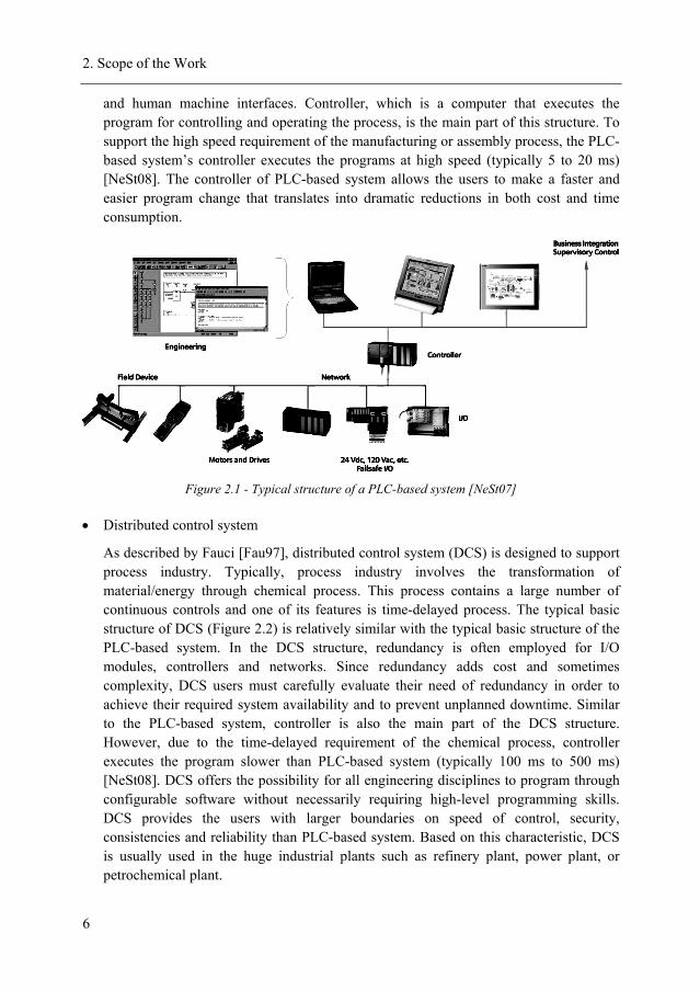
As described by Fauci [Fau97], programmable logic controller (PLC)-based system is designed to support the discrete manufacturing industry, e.g. automobile industry. Typically, this industry involves the manufacturing process or assembly process of products. These processes usually contain a large number of discrete operations with a high-speed requirement. The typical basic structure of PLC-based system (Figure 2.1) contains field devices, input and output (I/O) modules, controller, engineering stations
2. Scope of the Work
6
and human machine interfaces. Controller, which is a computer that executes the program for controlling and operating the process, is the main part of this structure. To support the high speed requirement of the manufacturing or assembly process, the PLC-based system’s controller executes the programs at high speed (typically 5 to 20 ms) [NeSt08]. The controller of PLC-based system allows the users to make a faster and easier program change that translates into dramatic reductions in both cost and time consumption.
Figure 2.1 - Typical structure of a PLC-based system [NeSt07]
• Distributed control system
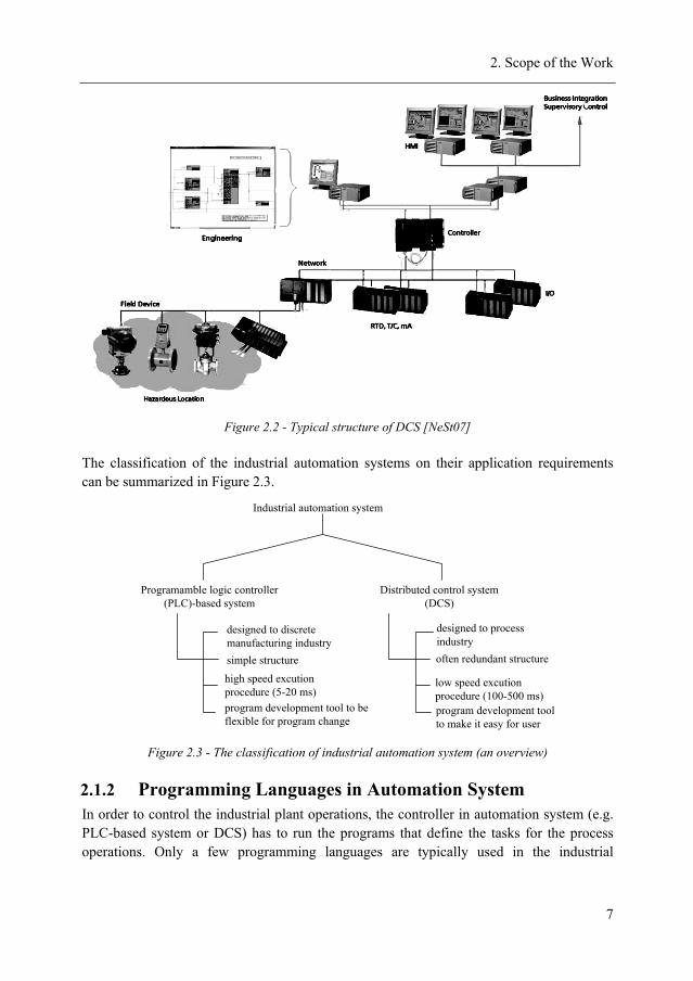
As described by Fauci [Fau97], distributed control system (DCS) is designed to support process industry. Typically, process industry involves the transformation of material/energy through chemical process. This process contains a large number of continuous controls and one of its features is time-delayed process. The typical basic structure of DCS (Figure 2.2) is relatively similar with the typical basic structure of the PLC-based system. In the DCS structure, redundancy is often employed for I/O modules, controllers and networks. Since redundancy adds cost and sometimes complexity, DCS users must carefully evaluate their need of redundancy in order to achieve their required system availability and to prevent unplanned downtime. Similar to the PLC-based system, controller is also the main part of the DCS structure. However, due to the time-delayed requirement of the chemical process, controller executes the program slower than PLC-based system (typically 100 ms to 500 ms) [NeSt08]. DCS offers the possibility for all engineering disciplines to program through configurable software without necessarily requiring high-level programming skills. DCS provides the users with larger boundaries on speed of control, security, consistencies and reliability than PLC-based system. Based on this characteristic, DCS is usually used in the huge industrial plants such as refinery plant, power plant, or petrochemical plant.
2. Scope of the Work
7
Figure 2.2 - Typical structure of DCS [NeSt07]
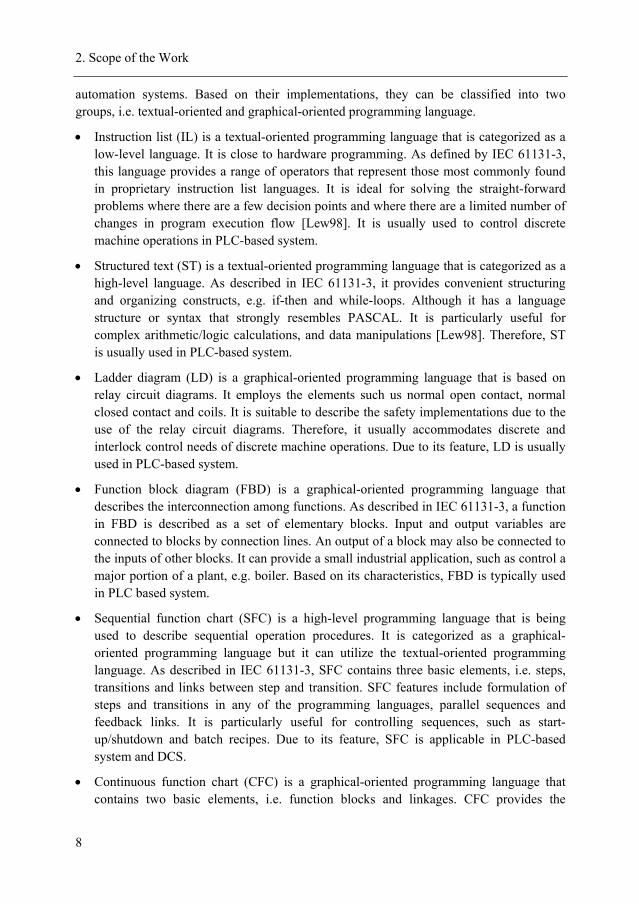
The classification of the industrial automation systems on their application requirements can be summarized in Figure 2.3.
Industrial automation system
Programamble logic controller (PLC)-based system
Distributed control system (DCS)
designed to discrete manufacturing industrysimple structure
high speed excution procedure (5-20 ms)
designed to process industry
low speed excution procedure (100-500 ms)
program development tool to be flexible for program change
often redundant structure
program development tool to make it easy for user
Figure 2.3 - The classification of industrial automation system (an overview)
2.1.2 Programming Languages in Automation System In order to control the industrial plant operations, the controller in automation system (e.g. PLC-based system or DCS) has to run the programs that define the tasks for the process operations. Only a few programming languages are typically used in the industrial
2. Scope of the Work
8
automation systems. Based on their implementations, they can be classified into two groups, i.e. textual-oriented and graphical-oriented programming language.
• Instruction list (IL) is a textual-oriented programming language that is categorized as a low-level language. It is close to hardware programming. As defined by IEC 61131-3, this language provides a range of operators that represent those most commonly found in proprietary instruction list languages. It is ideal for solving the straight-forward problems where there are a few decision points and where there are a limited number of changes in program execution flow [Lew98]. It is usually used to control discrete machine operations in PLC-based system.
• Structured text (ST) is a textual-oriented programming language that is categorized as a high-level language. As described in IEC 61131-3, it provides convenient structuring and organizing constructs, e.g. if-then and while-loops. Although it has a language structure or syntax that strongly resembles PASCAL. It is particularly useful for complex arithmetic/logic calculations, and data manipulations [Lew98]. Therefore, ST is usually used in PLC-based system.
• Ladder diagram (LD) is a graphical-oriented programming language that is based on relay circuit diagrams. It employs the elements such us normal open contact, normal closed contact and coils. It is suitable to describe the safety implementations due to the use of the relay circuit diagrams. Therefore, it usually accommodates discrete and interlock control needs of discrete machine operations. Due to its feature, LD is usually used in PLC-based system.
• Function block diagram (FBD) is a graphical-oriented programming language that describes the interconnection among functions. As described in IEC 61131-3, a function in FBD is described as a set of elementary blocks. Input and output variables are connected to blocks by connection lines. An output of a block may also be connected to the inputs of other blocks. It can provide a small industrial application, such as control a major portion of a plant, e.g. boiler. Based on its characteristics, FBD is typically used in PLC based system.
• Sequential function chart (SFC) is a high-level programming language that is being used to describe sequential operation procedures. It is categorized as a graphical-oriented programming language but it can utilize the textual-oriented programming language. As described in IEC 61131-3, SFC contains three basic elements, i.e. steps, transitions and links between step and transition. SFC features include formulation of steps and transitions in any of the programming languages, parallel sequences and feedback links. It is particularly useful for controlling sequences, such as start-up/shutdown and batch recipes. Due to its feature, SFC is applicable in PLC-based system and DCS.
• Continuous function chart (CFC) is a graphical-oriented programming language that contains two basic elements, i.e. function blocks and linkages. CFC provides the
2. Scope of the Work
9
interconnection of the function blocks using linkages that allow continuous features, for example programming feedback loops and advance control functions. Because the complex operations and control algorithms can be very well represented in CFC, its main application area is located primarily control the continuous operations in complex plant. Therefore, CFC is usually used in DCS.
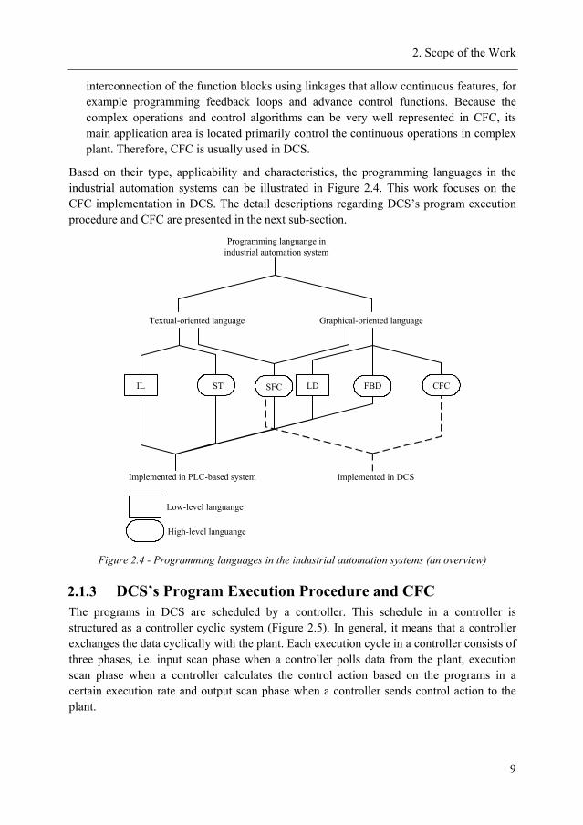
Based on their type, applicability and characteristics, the programming languages in the industrial automation systems can be illustrated in Figure 2.4. This work focuses on the CFC implementation in DCS. The detail descriptions regarding DCS’s program execution procedure and CFC are presented in the next sub-section.
Programming languange in industrial automation system
Textual-oriented language Graphical-oriented language
Implemented in PLC-based system Implemented in DCS
Low-level languange
High-level languange
IL ST SFC CFCFBDLD
Figure 2.4 - Programming languages in the industrial automation systems (an overview)
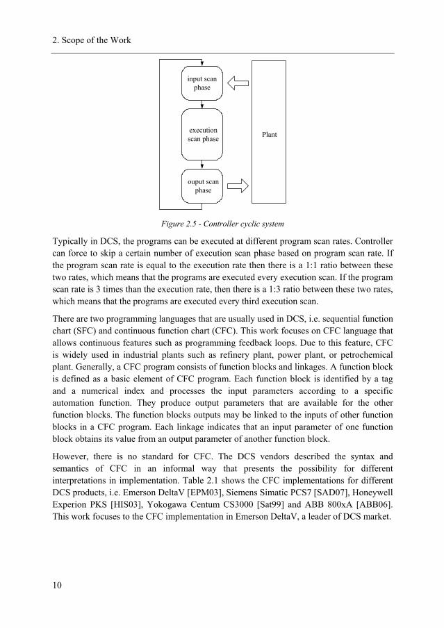
2.1.3 DCS’s Program Execution Procedure and CFC The programs in DCS are scheduled by a controller. This schedule in a controller is structured as a controller cyclic system (Figure 2.5). In general, it means that a controller exchanges the data cyclically with the plant. Each execution cycle in a controller consists of three phases, i.e. input scan phase when a controller polls data from the plant, execution scan phase when a controller calculates the control action based on the programs in a certain execution rate and output scan phase when a controller sends control action to the plant.
2. Scope of the Work
10
Plant
input scan phase
execution scan phase
ouput scan phase
Figure 2.5 - Controller cyclic system
Typically in DCS, the programs can be executed at different program scan rates. Controller can force to skip a certain number of execution scan phase based on program scan rate. If the program scan rate is equal to the execution rate then there is a 1:1 ratio between these two rates, which means that the programs are executed every execution scan. If the program scan rate is 3 times than the execution rate, then there is a 1:3 ratio between these two rates, which means that the programs are executed every third execution scan.
There are two programming languages that are usually used in DCS, i.e. sequential function chart (SFC) and continuous function chart (CFC). This work focuses on CFC language that allows continuous features such as programming feedback loops. Due to this feature, CFC is widely used in industrial plants such as refinery plant, power plant, or petrochemical plant. Generally, a CFC program consists of function blocks and linkages. A function block is defined as a basic element of CFC program. Each function block is identified by a tag and a numerical index and processes the input parameters according to a specific automation function. They produce output parameters that are available for the other function blocks. The function blocks outputs may be linked to the inputs of other function blocks in a CFC program. Each linkage indicates that an input parameter of one function block obtains its value from an output parameter of another function block.
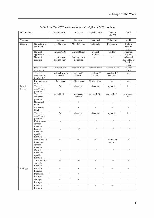
However, there is no standard for CFC. The DCS vendors described the syntax and semantics of CFC in an informal way that presents the possibility for different interpretations in implementation. Table 2.1 shows the CFC implementations for different DCS products, i.e. Emerson DeltaV [EPM03], Siemens Simatic PCS7 [SAD07], Honeywell Experion PKS [HIS03], Yokogawa Centum CS3000 [Sat99] and ABB 800xA [ABB06]. This work focuses to the CFC implementation in Emerson DeltaV, a leader of DCS market.
2. Scope of the Work
11
Table 2.1 - The CFC implementations for different DCS products
DCS Product Simatic PCS7 DELTA V Experion PKS Centum CS3000
800xA
Vendors Siemens Emerson Honeywell Yokogawa ABB
General Name/type of controller
S7400/cyclic MD100/cyclic C200/cylic FCS/cyclic System 800xA/ cyclic
Name of application
Simatic CFC Control Studio Control Builder
Builder Function diagram
Name of program
continuous function chart
function block application
n.i n.i enhanced IEC 61113-3
function block
Basic element of program
function block function block function block function block function block
Type of execution for fieldbus I/O
based on Profibus standard
based on FF standard
based on FF standard
based on FF standard
n.i
Program scan rate
10 ms-5 sec 100 ms-5 sec 50 ms – 2 sec n.i n.i
Type of input/output parameter
fix dynamic dynamic dynamic fix
Type of contained parameter
tuneable/ fix tunenable/ dynamic
tunenable/ fix tunenable/ fix tunenable/ fix
Numerical index
+ + - - +
Composite block
+ + + + +
Function Block
Type of input/output parameter
fix dynamic dynamic dynamic fix
IO function / specific function
+/ +/ +/ +/ +/
Logical function / specific function
+/ +/ +/ +/ +/
Mathematical function / specific function
+/ +/ +/ +/moving average
+/
Control function / specific function
+/ +/ +/ +/ +/
Time function / specific function
+/ +/ +/ +/ +/
Linkages Forward linkages
+ + + + +
Backward linkages
+ + - - -
Multiple linkages
+ + - - -
Flexible linkages
- - + + -

2. Scope of the Work
12
Table2.1 - The CFC implementations for different DCS products (continued)
DCS Product Simatic PCS7 DELTA V Experion PKS
Centum CS3000
800xA
Text exporting/ possible software that supports to export
- / excel + - + -
Sequential function chart connection
+/same level hierarchy
+/same level hierarchy
+/same level hierarchy
+/same level
hierarchy
+/same level
hierarchy Functional diagram support/type/ software tool
+/cause & effect matrix/
Quadlog
- - - -
Misc
Tag P&ID support/ software tool
- +/ Intergraph +/ Intergraph +/Intergraph +/Intergraph
note: + : supported, - : not supported, n.i.: no information, FF: Foundation Fieldbus
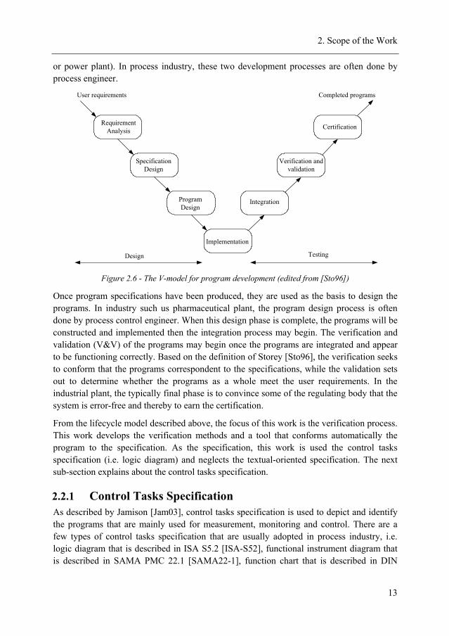
2.2 Program Development of Automation System As described by Storey [Sto96], the process of developing programs is usually time consuming. There are different phases involved in the program development. These phases can be represented using a lifecycle model. There are different various lifecycle models. In the program development of an industrial automations system, a typical development lifecycle model (Figure 2.6) is used that is often referred as the V-model. The model indicates the major element of the development process. It describes a top-down approach (as shown on the left side of Figure 2.6) to design the programs and a bottom-top approach to test the programs (as shown on the right side of Figure 2.6). However, this model is only an approximation to the development process. In practice, the various phases are not always performed in such strict sequential manner.
The starting point to develop the programs is analyzing the requirements. Generally, the terms requirement represents an abstract definition from the user of what the automation system should do. This process is often referred to as the requirement analysis phase. Before the programs can be implemented, these abstract requirements should be formalized as system’s requirements document. Once the requirements document has been produced, the control tasks are analyzed to identify the program functions needed for measurement, monitoring and control. One of the outputs of these analyses is a specification of program functions. This specification is often referred as a control tasks specification. The control tasks specification attempts to define all the requirements that should be fulfilled by the programs but in reality it is possible for errors to happen in this phase. The requirements are often depicted in textual description subject to ambiguity. Misunderstandings on some aspects of the requirements may lead to an incomplete or incorrect control tasks specification. For this reason, textual-oriented specifications always complement the control tasks specification for highly critical plant (e.g. pharmaceutical plant, refinery plant,
2. Scope of the Work
13
or power plant). In process industry, these two development processes are often done by process engineer.
User requirements Completed programs
Requirement Analysis
SpecificationDesign
Program Design
Implementation
Integration
Verification and validation
Certification
Design Testing
Figure 2.6 - The V-model for program development (edited from [Sto96])
Once program specifications have been produced, they are used as the basis to design the programs. In industry such us pharmaceutical plant, the program design process is often done by process control engineer. When this design phase is complete, the programs will be constructed and implemented then the integration process may begin. The verification and validation (V&V) of the programs may begin once the programs are integrated and appear to be functioning correctly. Based on the definition of Storey [Sto96], the verification seeks to conform that the programs correspondent to the specifications, while the validation sets out to determine whether the programs as a whole meet the user requirements. In the industrial plant, the typically final phase is to convince some of the regulating body that the system is error-free and thereby to earn the certification.
From the lifecycle model described above, the focus of this work is the verification process. This work develops the verification methods and a tool that conforms automatically the program to the specification. As the specification, this work is used the control tasks specification (i.e. logic diagram) and neglects the textual-oriented specification. The next sub-section explains about the control tasks specification.
2.2.1 Control Tasks Specification As described by Jamison [Jam03], control tasks specification is used to depict and identify the programs that are mainly used for measurement, monitoring and control. There are a few types of control tasks specification that are usually adopted in process industry, i.e. logic diagram that is described in ISA S5.2 [ISA-S52], functional instrument diagram that is described in SAMA PMC 22.1 [SAMA22-1], function chart that is described in DIN
2. Scope of the Work
14
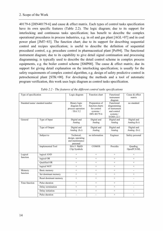
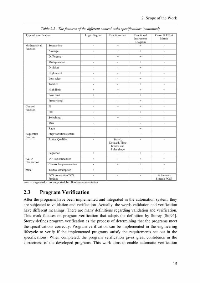
40179-6 [DIN40179-6] and cause & effect matrix. Each types of control tasks specification have its own specific features (Table 2.2). The logic diagram; due to its support for interlocking and continuous tasks specification; has benefit to describe the complex operational procedures in process industries, e.g. in oil and gas plant [AGL+07] and in coal power plant [JMT+83]. The function chart; due to its support for describing sequential control and recipes specification; is useful to describe the definition of sequential procedural control, e.g. procedure control in pharmaceutical plant [Pol94]. The functional instrument diagram; due to its capability to give detail signal continuation and processing diagramming; is typically used to describe the detail control scheme in complex process equipments, e.g. the boiler control scheme [SMP00]. The cause & effect matrix; due its support for giving detail explanation on the interlocking specification; is usually for the safety requirements of complex control algorithm, e.g. design of safety predictive control in petrochemical plant [STK+00]. For developing the methods and a tool of automatic program verification, this work uses logic diagram as control tasks specification.
Table 2.2 - The features of the different control tasks specifications
Type of specification Logic diagram Function chart Functional instrument
diagram
Cause & effect matrix
Standard name/ standard number Binary logic diagram for
process operation / ISA 5.2
Preparation of function charts
for control systems /
DIN 40179-6
Functional diagramming of instrument and control systems /
SAMA 22.1
no standard
General Type of Input Digital and Analog
Digital and Analog
Digital and Analog
Digital and Analog (b.r)
Type of Output Digital and Analog (b.r)
Digital and Analog
Digital and Analog
Digital and Analog (b.r)
Subject to Technical, design, operating and maintenance
personal
no information Engineer Safety personal
Implemented Tool ISA-5 P&ID Clip Symbols
COMOS Procidia Quadlog, OpenPCS/SIL
logical AND + + + +
logical OR + + + +
Qualified OR + + + +
Logical function
logical NOT + + + +
Basic memory + + + -
Set dominant memory + + + +
Memory function
Reset dominant memory + + + -
Pulse duration + + + -
Delay termination + + + -
Delay initiation + + + -
Time function
Pulse duration - - + -
2. Scope of the Work
15
Table 2.2 - The features of the different control tasks specifications (continued)
Type of specification Logic diagram Function chart Functional Instrument Diagram
Cause & Effect Matrix
Summation - + + -
Average - + + -
Difference - + + -
Multiplication - - + -
Division - - + -
High select - - + -
Low select - - + -
Totalize - - + -
High limit + + + +
Low limit + + + +
Mathematical function
Proportional - - + -
PI - + + -
PID - + + -
Switching - + - -
Mux - + - -
Control function
Ratio - - + -
Step/transition system - + - - Sequential function Action Qualifier - Stored,
Delayed, Time limited and Pulse shape
- -
Sequence + + + -
I/O Tag connection + - + + P&ID Connection Control loop connection - - + -
Misc. Textual description + + - -
DCS connection/DCS Product
- - - +/ Siemens Simatic PCS7
note: +: supported, -: not supported, b.r: Boolean representation
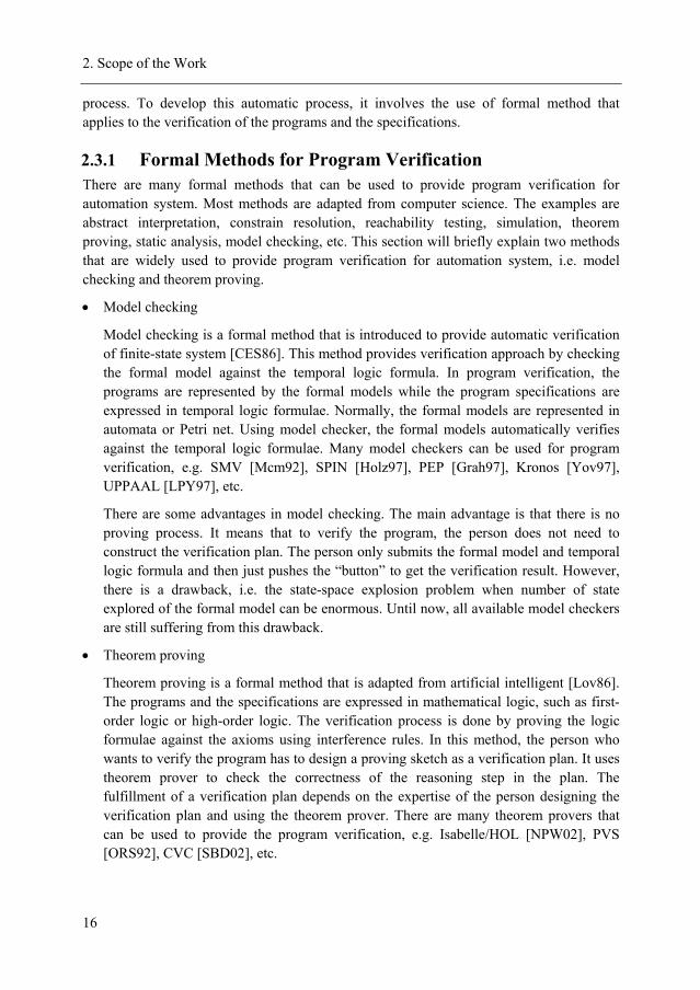
2.3 Program Verification After the programs have been implemented and integrated in the automation system, they are subjected to validation and verification. Actually, the words validation and verification have different meanings. There are many definitions regarding validation and verification. This work focuses on program verification that adapts the definition by Storey [Sto96]. Storey defines program verification as the process of determining that the programs meet the specifications correctly. Program verification can be implemented in the engineering lifecycle to verify if the implemented programs satisfy the requirements set out in the specifications. When completed, the program verification gives great confidence in the correctness of the developed programs. This work aims to enable automatic verification
2. Scope of the Work
16
process. To develop this automatic process, it involves the use of formal method that applies to the verification of the programs and the specifications.
2.3.1 Formal Methods for Program Verification There are many formal methods that can be used to provide program verification for automation system. Most methods are adapted from computer science. The examples are abstract interpretation, constrain resolution, reachability testing, simulation, theorem proving, static analysis, model checking, etc. This section will briefly explain two methods that are widely used to provide program verification for automation system, i.e. model checking and theorem proving.
• Model checking
Model checking is a formal method that is introduced to provide automatic verification of finite-state system [CES86]. This method provides verification approach by checking the formal model against the temporal logic formula. In program verification, the programs are represented by the formal models while the program specifications are expressed in temporal logic formulae. Normally, the formal models are represented in automata or Petri net. Using model checker, the formal models automatically verifies against the temporal logic formulae. Many model checkers can be used for program verification, e.g. SMV [Mcm92], SPIN [Holz97], PEP [Grah97], Kronos [Yov97], UPPAAL [LPY97], etc.
There are some advantages in model checking. The main advantage is that there is no proving process. It means that to verify the program, the person does not need to construct the verification plan. The person only submits the formal model and temporal logic formula and then just pushes the “button” to get the verification result. However, there is a drawback, i.e. the state-space explosion problem when number of state explored of the formal model can be enormous. Until now, all available model checkers are still suffering from this drawback.
• Theorem proving
Theorem proving is a formal method that is adapted from artificial intelligent [Lov86]. The programs and the specifications are expressed in mathematical logic, such as first-order logic or high-order logic. The verification process is done by proving the logic formulae against the axioms using interference rules. In this method, the person who wants to verify the program has to design a proving sketch as a verification plan. It uses theorem prover to check the correctness of the reasoning step in the plan. The fulfillment of a verification plan depends on the expertise of the person designing the verification plan and using the theorem prover. There are many theorem provers that can be used to provide the program verification, e.g. Isabelle/HOL [NPW02], PVS [ORS92], CVC [SBD02], etc.
2. Scope of the Work
17
The major drawback of theorem proving is the need of mathematical logic expertise. There are some research works in computer science that can alleviate this drawback by adding intelligent approaches in the theorem prover. However, this method has a great advantage of avoiding the state-space explosion problem.
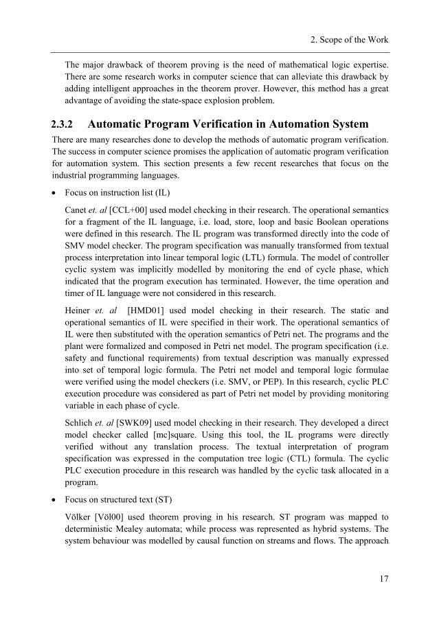
2.3.2 Automatic Program Verification in Automation System There are many researches done to develop the methods of automatic program verification. The success in computer science promises the application of automatic program verification for automation system. This section presents a few recent researches that focus on the industrial programming languages.
• Focus on instruction list (IL)
Canet et. al [CCL+00] used model checking in their research. The operational semantics for a fragment of the IL language, i.e. load, store, loop and basic Boolean operations were defined in this research. The IL program was transformed directly into the code of SMV model checker. The program specification was manually transformed from textual process interpretation into linear temporal logic (LTL) formula. The model of controller cyclic system was implicitly modelled by monitoring the end of cycle phase, which indicated that the program execution has terminated. However, the time operation and timer of IL language were not considered in this research.
Heiner et. al [HMD01] used model checking in their research. The static and operational semantics of IL were specified in their work. The operational semantics of IL were then substituted with the operation semantics of Petri net. The programs and the plant were formalized and composed in Petri net model. The program specification (i.e. safety and functional requirements) from textual description was manually expressed into set of temporal logic formula. The Petri net model and temporal logic formulae were verified using the model checkers (i.e. SMV, or PEP). In this research, cyclic PLC execution procedure was considered as part of Petri net model by providing monitoring variable in each phase of cycle.
Schlich et. al [SWK09] used model checking in their research. They developed a direct model checker called [mc]square. Using this tool, the IL programs were directly verified without any translation process. The textual interpretation of program specification was expressed in the computation tree logic (CTL) formula. The cyclic PLC execution procedure in this research was handled by the cyclic task allocated in a program.
• Focus on structured text (ST)
Völker [Völ00] used theorem proving in his research. ST program was mapped to deterministic Mealey automata; while process was represented as hybrid systems. The system behaviour was modelled by causal function on streams and flows. The approach
2. Scope of the Work
18
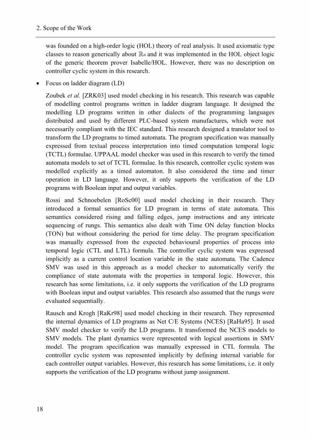
was founded on a high-order logic (HOL) theory of real analysis. It used axiomatic type classes to reason generically about RRn and it was implemented in the HOL object logic of the generic theorem prover Isabelle/HOL. However, there was no description on controller cyclic system in this research.
• Focus on ladder diagram (LD)
Zoubek et al. [ZRK03] used model checking in his research. This research was capable of modelling control programs written in ladder diagram language. It designed the modelling LD programs written in other dialects of the programming languages distributed and used by different PLC-based system manufactures, which were not necessarily compliant with the IEC standard. This research designed a translator tool to transform the LD programs to timed automata. The program specification was manually expressed from textual process interpretation into timed computation temporal logic (TCTL) formulae. UPPAAL model checker was used in this research to verify the timed automata models to set of TCTL formulae. In this research, controller cyclic system was modelled explicitly as a timed automaton. It also considered the time and timer operation in LD language. However, it only supports the verification of the LD programs with Boolean input and output variables.
Rossi and Schnoebelen [RoSc00] used model checking in their research. They introduced a formal semantics for LD program in terms of state automata. This semantics considered rising and falling edges, jump instructions and any intricate sequencing of rungs. This semantics also dealt with Time ON delay function blocks (TON) but without considering the period for time delay. The program specification was manually expressed from the expected behavioural properties of process into temporal logic (CTL and LTL) formula. The controller cyclic system was expressed implicitly as a current control location variable in the state automata. The Cadence SMV was used in this approach as a model checker to automatically verify the compliance of state automata with the properties in temporal logic. However, this research has some limitations, i.e. it only supports the verification of the LD programs with Boolean input and output variables. This research also assumed that the rungs were evaluated sequentially.
Rausch and Krogh [RaKr98] used model checking in their research. They represented the internal dynamics of LD programs as Net C/E Systems (NCES) [RaHa95]. It used SMV model checker to verify the LD programs. It transformed the NCES models to SMV models. The plant dynamics were represented with logical assertions in SMV model. The program specification was manually expressed in CTL formula. The controller cyclic system was represented implicitly by defining internal variable for each controller output variables. However, this research has some limitations, i.e. it only supports the verification of the LD programs without jump assignment.
2. Scope of the Work
19
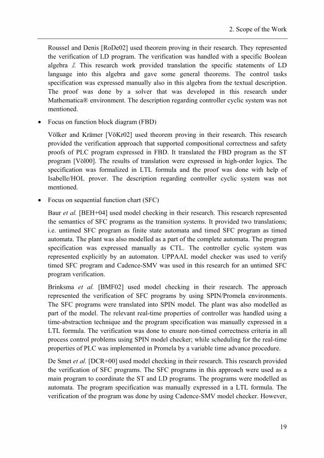
Roussel and Denis [RoDe02] used theorem proving in their research. They represented the verification of LD program. The verification was handled with a specific Boolean algebra I. This research work provided translation the specific statements of LD language into this algebra and gave some general theorems. The control tasks specification was expressed manually also in this algebra from the textual description. The proof was done by a solver that was developed in this research under Mathematica® environment. The description regarding controller cyclic system was not mentioned.
• Focus on function block diagram (FBD)
Völker and Krämer [VöKr02] used theorem proving in their research. This research provided the verification approach that supported compositional correctness and safety proofs of PLC program expressed in FBD. It translated the FBD program as the ST program [Völ00]. The results of translation were expressed in high-order logics. The specification was formalized in LTL formula and the proof was done with help of Isabelle/HOL prover. The description regarding controller cyclic system was not mentioned.
• Focus on sequential function chart (SFC)
Baur et al. [BEH+04] used model checking in their research. This research represented the semantics of SFC programs as the transition systems. It provided two translations; i.e. untimed SFC program as finite state automata and timed SFC program as timed automata. The plant was also modelled as a part of the complete automata. The program specification was expressed manually as CTL. The controller cyclic system was represented explicitly by an automaton. UPPAAL model checker was used to verify timed SFC program and Cadence-SMV was used in this research for an untimed SFC program verification.
Brinksma et al. [BMF02] used model checking in their research. The approach represented the verification of SFC programs by using SPIN/Promela environments. The SFC programs were translated into SPIN model. The plant was also modelled as part of the model. The relevant real-time properties of controller was handled using a time-abstraction technique and the program specification was manually expressed in a LTL formula. The verification was done to ensure non-timed correctness criteria in all process control problems using SPIN model checker; while scheduling for the real-time properties of PLC was implemented in Promela by a variable time advance procedure.
De Smet et al. [DCR+00] used model checking in their research. This research provided the verification of SFC programs. The SFC programs in this approach were used as a main program to coordinate the ST and LD programs. The programs were modelled as automata. The program specification was manually expressed in a LTL formula. The verification of the program was done by using Cadence-SMV model checker. However,
2. Scope of the Work
20
it only supports the verification of SFC programs with Boolean input and output variables.
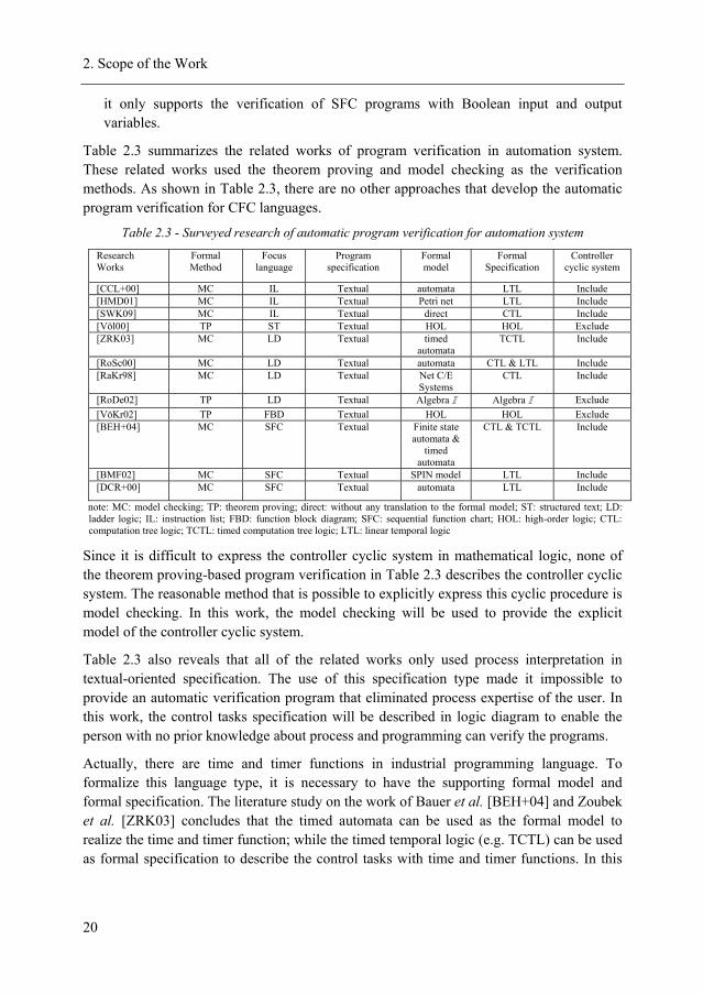
Table 2.3 summarizes the related works of program verification in automation system. These related works used the theorem proving and model checking as the verification methods. As shown in Table 2.3, there are no other approaches that develop the automatic program verification for CFC languages.
Table 2.3 - Surveyed research of automatic program verification for automation system
Research Works
Formal Method
Focus language
Program specification
Formal model
Formal Specification
Controller cyclic system
[CCL+00] MC IL Textual automata LTL Include [HMD01] MC IL Textual Petri net LTL Include [SWK09] MC IL Textual direct CTL Include [Völ00] TP ST Textual HOL HOL Exclude [ZRK03] MC LD Textual timed
automata TCTL Include
[RoSc00] MC LD Textual automata CTL & LTL Include [RaKr98] MC LD Textual Net C/E
Systems CTL Include
[RoDe02] TP LD Textual Algebra I Algebra I Exclude [VöKr02] TP FBD Textual HOL HOL Exclude [BEH+04] MC SFC Textual Finite state
automata & timed
automata
CTL & TCTL Include
[BMF02] MC SFC Textual SPIN model LTL Include [DCR+00] MC SFC Textual automata LTL Include
note: MC: model checking; TP: theorem proving; direct: without any translation to the formal model; ST: structured text; LD: ladder logic; IL: instruction list; FBD: function block diagram; SFC: sequential function chart; HOL: high-order logic; CTL: computation tree logic; TCTL: timed computation tree logic; LTL: linear temporal logic
Since it is difficult to express the controller cyclic system in mathematical logic, none of the theorem proving-based program verification in Table 2.3 describes the controller cyclic system. The reasonable method that is possible to explicitly express this cyclic procedure is model checking. In this work, the model checking will be used to provide the explicit model of the controller cyclic system.
Table 2.3 also reveals that all of the related works only used process interpretation in textual-oriented specification. The use of this specification type made it impossible to provide an automatic verification program that eliminated process expertise of the user. In this work, the control tasks specification will be described in logic diagram to enable the person with no prior knowledge about process and programming can verify the programs.
Actually, there are time and timer functions in industrial programming language. To formalize this language type, it is necessary to have the supporting formal model and formal specification. The literature study on the work of Bauer et al. [BEH+04] and Zoubek et al. [ZRK03] concludes that the timed automata can be used as the formal model to realize the time and timer function; while the timed temporal logic (e.g. TCTL) can be used as formal specification to describe the control tasks with time and timer functions. In this
2. Scope of the Work
21
work, the formal model is represented in timed automata while the specification is expressed in TCTL to support the verification of the time and timer functions.
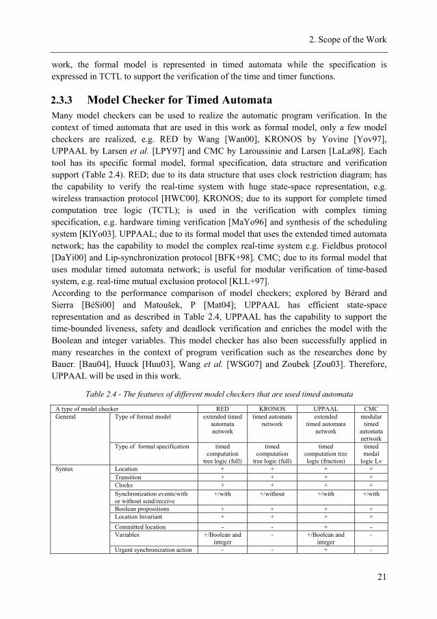
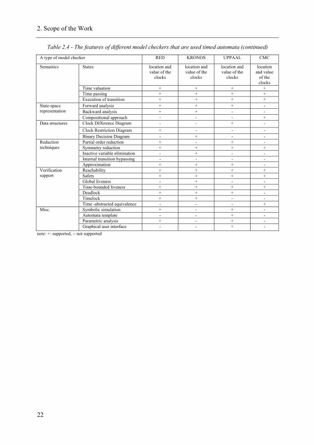
2.3.3 Model Checker for Timed Automata Many model checkers can be used to realize the automatic program verification. In the context of timed automata that are used in this work as formal model, only a few model checkers are realized, e.g. RED by Wang [Wan00], KRONOS by Yovine [Yov97], UPPAAL by Larsen et al. [LPY97] and CMC by Laroussinie and Larsen [LaLa98]. Each tool has its specific formal model, formal specification, data structure and verification support (Table 2.4). RED; due to its data structure that uses clock restriction diagram; has the capability to verify the real-time system with huge state-space representation, e.g. wireless transaction protocol [HWC00]. KRONOS; due to its support for complete timed computation tree logic (TCTL); is used in the verification with complex timing specification, e.g. hardware timing verification [MaYo96] and synthesis of the scheduling system [KlYo03]. UPPAAL; due to its formal model that uses the extended timed automata network; has the capability to model the complex real-time system e.g. Fieldbus protocol [DaYi00] and Lip-synchronization protocol [BFK+98]. CMC; due to its formal model that uses modular timed automata network; is useful for modular verification of time-based system, e.g. real-time mutual exclusion protocol [KLL+97]. According to the performance comparison of model checkers; explored by Bérard and Sierra [BéSi00] and Matoušek, P [Mat04]; UPPAAL has efficient state-space representation and as described in Table 2.4, UPPAAL has the capability to support the time-bounded liveness, safety and deadlock verification and enriches the model with the Boolean and integer variables. This model checker has also been successfully applied in many researches in the context of program verification such as the researches done by Bauer. [Bau04], Huuck [Huu03], Wang et al. [WSG07] and Zoubek [Zou03]. Therefore, UPPAAL will be used in this work.
Table 2.4 - The features of different model checkers that are used timed automata
A type of model checker RED KRONOS UPPAAL CMC Type of formal model extended timed
automata network
timed automata network
extended timed automata
network
modular timed
automata network
General
Type of formal specification timed computation
tree logic (full)
timed computation
tree logic (full)
timed computation tree logic (fraction)
timed modal
logic Lv Location + + + + Transition + + + + Clocks + + + + Synchronization events/with or without send/receive
+/with +/without +/with +/with
Boolean propositions + + + + Location Invariant + + + + Committed location - - + - Variables +/Boolean and
integer - +/Boolean and
integer -
Syntax
Urgent synchronization action - - + -
2. Scope of the Work
22
Table 2.4 - The features of different model checkers that are used timed automata (continued)
A type of model checker RED KRONOS UPPAAL CMC
States location and value of the
clocks
location and value of the
clocks
location and value of the
clocks
location and value
of the clocks
Time valuation + + + + Time passing + + + +
Semantics
Execution of transition + + + + Forward analysis + + + - Backward analysis + + - -
State-space representation
Compositional approach - - - + Clock Difference Diagram - - + - Clock Restriction Diagram + - - -
Data structures
Binary Decision Diagram - + - - Partial order reduction + - + - Symmetry reduction + + + + Inactive variable elimination - + - - Internal transition bypassing - - - -
Reduction techniques
Approximation + + + - Reachability + + + + Safety + + + + Global liveness - + - - Time-bounded liveness + + + + Deadlock + + + - Timelock + + - -
Verification support
Time -abstracted equivalence - - - + Symbolic simulation + - + - Automata template - - + - Parametric analysis + - + -
Misc.
Graphical user interface - - + - note: +: supported, -: not supported
3 Formal Descriptions of Timed Automata and Timed Computation Tree Logic
As described by Clarke et al. [CGL94], model checking is a formal verification method of a finite state system. It provides the verification between the formal specification and the formal model as the representation of a finite state system. As argued by Uribe [Uri00], comparing to the other widely used verification method in computer science; i.e. theorem proving; model checking provides better automatic procedure suited for the requirement of this work to develop automatic program verification. The user applying model checking needs to provide the model and the specification. The model checker will automatically show whether or not the model satisfies the specification. Formally, model checking is expressed as a relation M ²σ, where M is the model and σ is the specification. This relation is true when the specification (σ) can be satisfied by the model (M) or otherwise the relation is false.
In the earlier development of model checking, Clarke et al. [CES86] described the model as Kripke state-transition graph. In the context of real-time system such as distributed control system (DCS), the formal model as a representation of system needs to be described into the time-based formalism, e.g. timed automata [AlDi94], timed Petri nets [AbNy01] and hybrid automata [AHH96]. In this work, timed automata are used to formalize the CFC programs in DCS.
As formal specification, Clarke et al. [CES6] proposed the temporal logic to state the model requirements. In the context of real-time system such as DCS, the temporal logic has to be able to provide the time specification. There are two contenders of temporal logic that can provide the time specification, i.e. linear-time proportional temporal logic developed by Pnueli [Pnu85] and timed computation tree logic by Alur et al. [ACD90]. The timed computation tree logic (TCTL) is used in this work as the time-based specification to formalize the logic diagram.
This chapter provides the formal descriptions timed automata and timed computation tree logic to provide the necessary background of this work. It is organized into three sections. Section 3.1 describes the formal descriptions of timed automata. Section 3.2 explains the formal descriptions of timed computation tree logic. Section 3.3 presents the formal descriptions of model and specification in UPPAAL that are used in this work.
3.1 Formal Descriptions of Timed Automata Based on Alur and Dill [AlDi94], timed automata are described as the formalism for real-time system. Timed automata are simple but quite expressive graphical notations for modelling the real-time system. For this reason, timed automata are widely used as the applications of the real-time system, e.g. real-time communication [NHL06], [KrHa04],
3. Formal Descriptions of Timed Automata and Timed Computation Tree Logic
24
[WVF+06] and real-time software development [BEH+04], [LHL+01], [IKL+00], [ZRK03].
There are two major types of timed automata that are described by Bengtsson and Yi [BeYi04], i.e. timed Büchi automaton [AlDi94] and timed safety automaton [HNS+92]. This work focuses on the timed safety automaton and refers such automaton as the timed automaton.
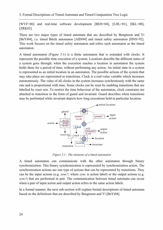
A timed automaton (Figure 3.1) is a finite automaton that is extended with clocks. It represents the possible time execution of a system. Locations describe the different states of a system goes through; when the execution reaches a location in automaton the system holds there for a period of time, without performing any action. An initial state in a system is represented as an initial location in an automaton. The possible actions of the system that may take place are represented as transitions. Clock is a real-value variable which increases autonomously. The value of all clocks in the system increases synchronously with the same rate and is proportional with time. Some clocks can be reset by enabling transitions that are labelled by reset sets. To restrict the time behaviour of the automaton, clock constrains are attached to transition in the form of guard and invariant. Guard describes when transitions may be performed while invariant depicts how long executions hold in particular location.
initial location
invariant
action
input action
output action
guard
reset set clock
transition
location
Figure 3.1 - The elements of a timed automaton
A timed automaton can communicate with the other automaton through binary synchronization. This binary synchronization is represented by synchronization action. The synchronization actions are one type of actions that can be represented by transitions. They can be the input actions (e.g. sync?, where sync is action label) or the output actions (e.g. sync!) that are performed in pair. The communication between timed automata can occur when a pair of input action and output action refers to the same action labels.
In a formal manner, the next sub-section will explain formal descriptions of timed automata based on the definitions that are described by Bengtsson and Yi [BeYi04].
3. Formal Descriptions of Timed Automata and Timed Computation Tree Logic
25
3.1.1 Syntax of Timed Automata Assuming a finite set of clocks C is a set of real-value variables that can be expressed by x, y, z, etc, and a finite set of actions Σ is defined as a set of alphabets that is ranged over a, b, c, etc, the clock constraint can be described as follows.
Definition 3.1 (Clock constraint)
A clock constraint is a formula of atomic constraint of the forms that can be described by the following Backus–Naur Form (BNF).
φ::= x∼c | x-y∼c | φ1∧φ2,
where c∈N, x,y∈C, ∼∈{≤ ,<,=,>,≥}, φ1,φ2 are clock constraints. CC denotes a finite set of clock constraints.
Using the preliminary definition regarding clock constraint, the syntax of timed automaton is defined to give detail principles for constructing a timed automaton.
Definition 3.2 (Timed automaton)
A timed automaton is a tuple A=(L, lo, E ,I), where the elements are defined as:
- L is a finite set of locations,
- lo∈L is an initial location,
- E⊆(L×CC× Σ× 2C×L) is a finite set of edges. The edge function can be denoted as a mapping of ',, ll rga ⎯⎯ →⎯ ,where a∈Σ is an action, g∈CC is a guard and r∈2C is a reset set,
- I:L→CC is a set of mapping of invariant to location.
Two or more timed automata can communicate to perform a parallel composition of timed automata called as timed automata network. The timed automata network is composed if there is at least one pair of synchronization action.
Definition 3.3 (Synchronization action)
Synchronization action sync is the pair of (sync!, sync?), where sync? is an input action that represents the receiving event action from a timed automaton while sync! is an output action that represents the sending event action to a timed automaton. Σsync denotes the finite set of synchronization actions in the timed automata network.
Using the definition of synchronization action mentioned above, the timed automata network can be defined as follows.
Definition 3.4 (Timed automata network)
The timed automata network is a tuple |A|=(Σsync, A), where:
- Σsync={sync1, sync2, sync3,…, syncn}⊆Σ is a finite set of n synchronization actions.
3. Formal Descriptions of Timed Automata and Timed Computation Tree Logic
26
- A={A1, A2, A3,…,Am} is a finite set of m timed automata that communicates with synchronization action in Σsync.
3.1.2 Semantics of Timed Automata In this sub-section, the formalization of the timed automata behaviour is presented in the term of time-based state-transition system as described by Bengtsson and Yi [BeYi04]. The state of timed automata is defined as the current location and the current state while the transition can be caused by the delay for some time or the enable edge. To give more detail on the formalization of semantics of timed automata, the clock assignment is defined as follow.
Definition 3.5 (Clock assignment)
A clock assignment is a function that maps C to positive real. Let u, v to be clock assignments, u∈g is defined to mean that the clock value denoted by the u satisfies the guard g. For d∈R+, u+d denotes the clock assignment that maps all x∈C to u(x)+d and for r⊆C, [r →0]u denotes the clock assignment that maps all clock in r to 0 and agrees with the other clocks in C.
Using Definition 3.5, the semantics of timed automata is described as follows.
Definition 3.6 (Semantics of timed automata)
The semantics of timed automata A=(L, lo, E, I) are the time-based state-transition system where the state is defined as a pair of a current location and a current clock <l,u>. The transition are defined by the rules:
- <l,u> ⎯→⎯d <l,u+d> if u∈I(l) and (u+d)∈I(l) for a positive d∈R+,
- <l,u> ⎯→⎯a <l’,u’> if l ⎯→⎯a l’, u∈g, u’=[r →0]u and u’∈I(l’).
If a timed automaton is composed parallel with the other timed automata, the behaviour of timed automata can be defined as the semantics of the timed automata network.
Definition 3.7 (Semantics of timed automata network)
The semantics of timed automata network |A|=(Σsync, A) is a time-based state-transition system. The state is described as a pair of a current location vector and a current clock <l,u>. The transitions of timed automata network are defined by the rules:
- <l,u> ⎯→⎯d <l,u+d> if u∈I(l) and (u+d)∈I(l), I(l)=∧i I(li), and li is the element of location vector l,
- <l,u> ⎯→⎯τ <l[li/li’],u’> if li ⎯⎯ →⎯ rg ,,τ li’, u∈g, u’=[r→0]u, u’∈I(l[li/li’]) and l[li/li’] for the vector l with li being substituted with li’,
- <l,u> ⎯→⎯τ <l[li/li’][lj/lj’],u’> if there exist i ≠ j such that li ⎯⎯⎯ →⎯ ii rag ?,, li’, lj ⎯⎯ →⎯ jj rag ,!, lj’ and u∈ gi ∧ gj, u’=[ri→0([r i→0] u)], and u’∈ I(l[li/li’][lj/lj’]).
3. Formal Descriptions of Timed Automata and Timed Computation Tree Logic
27
This semantics of timed automaton or an element of timed automata network has an effect to the changes of state <l,u>. These changes are represented the running states of a time-based state-transition system that is defined as a run of timed automata.
Definition 3.8 (Run of timed automata)
When a time action is a pair (t, a) where a∈Σ is an action taken by an timed automaton A after t∈R+ time unit since A has been started, and the absolute time t is called time stamp of an action a, then a timed automata trace is defined as a sequence of timed actions (t1,a1,) (t2,a2) (t3,a3) (t4,a4)…(ti,ai), where ti< ti+1. Using the definition of a timed automata trace, the run of timed automata A is a sequence transition:
<l0,u0> ⎯→⎯ 1d ⎯→⎯ 1a <l2,u2> ⎯→⎯ 2d ⎯→⎯ 2a <l3,u3>....,
where ti= ti+1+di for i>0.
3.2 Formal Descriptions of Timed Computation Tree Logic Timed computation tree logic (TCTL) is the timed temporal logic that can be used as the formal specification of time-based state-transition system (e.g. timed automata). It was introduced by Alur et al. [ACD90] who applied it as a specification in model checking for a real-time system. TCTL can be used to specify the time-based state-transition system by checking the states in a path of time-based state-transition system. A path of time-based state-transition system is defined as follows.
Definition 3.9 (Path of time-based state-transition system)
When the time-based state-transition system as a 4-tuple M=(S, Δ, P, L) where S is a finite state of states, Δ ⊆ (S × A × S) is finite set of transition relations, A is finite set of actions, P is finite set of propositions and L is a function which labels each state; then the a path of M is defined as infinite sequences π=(s0 a0 s1 a1 s2 a2…) of states alternated by transition label such that si ⎯→⎯ ia si+1 for i≥ 0, si∈ S and ai∈A. π(k) denotes the k-th element of π.
From the definition mentioned above, the model checking can be expressed by a relation M,(s,v)²φ, where the relation is true when the property φ holds a state in a path of a given time-based state-transition system M from a given state s using a given clock valuation v. The next sub-section describes formally TCTL syntax and semantics as described by Henzinger et. al [HNS+92].
3.2.1 Syntax of TCTL The formula of TCTL is built from state predicates by Boolean connectives, the two temporal until operators ∀U (inevitably) and ∃U (possibly) and reset quantifier for clocks.
Definition 3.10 (Timed computation tree logic)
A timed computation tree logic formula φ is defined as the following Backus–Naur Form (BNF), i.e.:
3. Formal Descriptions of Timed Automata and Timed Computation Tree Logic
28
φ ::= p | x+c≤ y+d | ¬φ |φ1∨ φ2 | φ1∀Uφ2 |φ1∃Uφ2| z in φ,
where p is an atomic proposition; x, y, z are the clocks; c,d∈N is the constants; φ1,φ2 are the TCTL formulae.
The additional temporal operators also can be derived from the definition above. For example, ∃◊φ (reachable) is derived from true∃Uφ, ∀ φ (invariantly) is derived from¬∃◊¬φ, ∀◊φ (always eventually) is derived from true∀Uφ and ∃ φ (potentially always) is derived from¬∀◊¬φ.
3.2.2 Semantics of TCTL The formulae of TCTL are interpreted over the state of a path of time-based state-transition system. The propositions and clocks of TCTL-formula φ are evaluated in the states. Formally, the interpretations of TCTL formula can be defined as follows.
Definition 3.11 (Semantics of TCTL)
When π=(s0 a0 s1 a1 s2 a2…) is a path of time-based state-transition system M, π(i) is the ith element of π , p is an atomic proposition, v is a clock valuation and φ1, φ2 are the TCTL formulae then timed computation tree logic formula semantics can be defined for each as:
- M,(s,v)²p⇔p∈L(s),
- M,(s,v)²¬φ1⇔M,(s,v)²φ1 does not hold,
- M,(s,v)²φ1∨ φ2⇔M,(s,v)²(φ1) or M,(s,v)²φ2,
- M,(s,v)² z in φ1⇔M,(s, z in v)²φ1,
- M,(s,v)²φ1∀ Uφ2⇔ for every path in π=(s0 a0 s1 a1 s2 a2…), if ∀j M,π(j)²(φ2) then ∀i<j M,π(i)|=φ1∨φ2,
- M,(s,v)²φ1∃ Uφ2 ⇔ there is a path in π=(s0 a0 s1 a1 s2 a2…), if ∀jM,π(j)²(φ2) then ∀i<jM,π(i)²φ1∨ φ2,
3.3 Formal Descriptions of UPPAAL The model checker used in this work is UPPAAL. This sub-section gives only the formal descriptions of UPPAAL that are the important aspects used in the next chapter. The complete descriptions of UPPAAL are given by Behrmann et al. [BDL04].
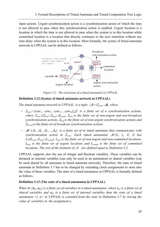
3.3.1 Formal Model in UPPAAL Formal model in UPPAAL (Figure 3.2) is the extensions of the timed automata that are described in Section 3.1. The most important extensions in UPPAAL model are broadcast synchronization action, urgent synchronization action, urgent location, committed location. As described by Behrmann et al. [BDL04], broadcast synchronization action is a synchronization action of which an output action can synchronize an arbitrary number of
3. Formal Descriptions of Timed Automata and Timed Computation Tree Logic
29
input actions. Urgent synchronization action is a synchronization action of which the time is not allowed to pass when this synchronization action is enabled. Urgent location is a location in which the time is not allowed to pass when the system is in this location while committed location is a location that directly continues to the next transition without any time delay when the system is in this location. More formally, the syntax of timed automata network in UPPAAL can be defined as follows.
committed location
urgent location
broadcast chan send2;urgent chan send 1;int input;
broadcast syncronization action
urgent syncronization action
variable
Figure 3.2 - The extensions of a timed automaton in UPPAAL
Definition 3.12 (Syntax of timed automata network in UPPAAL)
The timed automata network in UPPAAL is a tuple |A|=(Σsync, A), where
- Σsync={sync1, sync2, sync3,…syncn}⊆Σ is a finite set of n synchronization actions, where Σsync∈Σnon∪Σurg∪Σbroad. Σnon is the finite set of non-urgent and non-broadcast synchronization actions, Σurg is the finite set of non-urgent synchronization actions and Σbroad is the finite set of broadcast synchronization actions,
- A={A1, A2, A3,…,Am} is a finite set of m timed automata that communicates with synchronization action in Σsync. Each timed automaton A=(L, lo, E, I) has L∈(Lnon∪Lurg∪Lcomm). Lnon is the finite set of non-urgent and non-committed locations, Lurg is the finite set of urgent locations and Lcomm is the finite set of committed locations. The rest of the elements of A are defined equal to Definition 3.2.
UPPAAL supports also the use of integer and Boolean variables. These variables can be declared as internal variables (can only be used in an automaton) or shared variables (can be used shared by all automata in timed automata network). Therefore, the state of timed automata in Definition 3.7 has to be changed by extending clock assignments to store also the value of these variables. The state of a timed automaton in UPPAAL is formally defined as follows.
Definition 3.13 (The state of a timed automaton in UPPAAL)
When v={vsh, vint} is a finite set of variables in a timed automaton, where vsh is a finite set of shared variables and vint is a finite set of internal variables then the state of a timed automaton <l, u> in UPPAAL is extended from the state in Definition 3.7 by storing the value of variables in the assignment u.
3. Formal Descriptions of Timed Automata and Timed Computation Tree Logic
30
Due to all these extension mentioned above, the semantics of timed automata network in UPPAAL are defined as follows.
Definition 3.14 (Semantics of timed automata network in UPPAAL)
The semantics of timed automata network in UPPAAL is extension of the semantics of timed automata network (Definition 3.7), where the transitions are defined by the rules:
- <l,u> cud⎯→⎯ <l,u+d> if <l,u> ⎯→⎯d <l,u+d>, and (Lurg∪ Lcomm)=∅,
- <l,u> cu⎯→⎯τ <l[li/li’],u’> if <l,u> ⎯→⎯τ <l[li/li’],u’>, and either li∈(Lurg∪ Lcomm)
or (Lurg∪ Lcomm)=∅,
- <l,u> cu⎯→⎯τ <l[li/li’][lj/lj’],u’> if <l,u> ⎯→⎯τ <l[li/li’][lj/lj’],u’>, and either li∈(Lurg∪ Lcomm), lj∈(Lurg∪ Lcomm) or (Lurg∪ Lcomm)=∅.
3.3.2 Formal Specification in UPPAAL As described by Bengtsson and Yi [BeYi04], UPPAAL is model checker where the formal specification is expressed in a subset TCTL. The UPPAAL formal specification does not fully support the two temporal until operators ∀U (inevitably) and ∃U (possibly) in TCTL. It only supports∀◊(always eventually),∀ (invariantly), ∃◊(reachable) and ∃ (potentially always)1. The syntax of a subset TCTL formula in UPPAAL is defined as follows.
Definition 3.15 (Syntax of subset TCTL in UPPAAL)
A subset TCTL formula in UPPAAL φ can be described as the following Backus–Naur Form (BNF), i.e.:
φ ::= p| x+c≤ y+d |¬φ |φ1∨ φ2|∀ φ1|∃ φ1|∀◊φ1|∃◊ φ1| z in φ,
where p is an atomic proposition, x,y are the clocks or variables, z is a clock, c,d∈N are the constants, φ1,φ2 are the subset TCTL formulae in UPPAAL.
The subset TCTL formulae in UPPAAL are also interpreted over the state of a path of model such as TCTL formulae. The propositions and clock variables of subset TCTL formula in UPPAAL φ are evaluated in the states and the formal interpretations of subset TCTL formula in UPPAAL can be defined as follows.
Definition 3.16 (Semantics of subset TCTL in UPPAAL)
When π=(s0 a0 s1 a1 s2 a2…) is a path of model M, π(i) is the ith element of π , p is an atomic proposition, v is a clock valuation and φ1, φ2 are the subset TCTL formulae in UPPAAL then the semantics of a subset TCTL formula in UPPAAL can be defined for each as:
- M,(s,v)²p⇔p∈ L(s),
1 In UPPAAL, ∀◊ is denoted as A<>, ∃ is denoted as E[],∀ is denoted as A[] and∃◊ is denoted as E<>.
3. Formal Descriptions of Timed Automata and Timed Computation Tree Logic
31
- M,(s,v)²¬φ1⇔M,(s,v)²φ1 does not hold,
- M,(s,v)²φ1∨φ2⇔M,(s,v)²(φ1) or M,(s,v)²φ2,
- M,(s,v)²z in φ1⇔M,(s, z in v)²φ1,
- M,(s,v)²∀ φ1⇔ for every path in π=(s0 a0 s1 a1 s2 a2…), ∀iM,π(i)²φ1,
- M,(s,v)²∃ φ1⇔ there is a path in π=(s0 a0 s1 a1 s2 a2…), where ∀iM,π(i)²φ1,
- M,(s,v)²∀◊φ1⇔ for every path in π=(s0 a0 s1 a1 s2 a2…), ∃iM,π(i)²φ1,
- M,(s,v)²∃◊φ1⇔ there is a path in π=(s0 a0 s1 a1 s2 a2…), where ∃iM,π(i)²φ1.
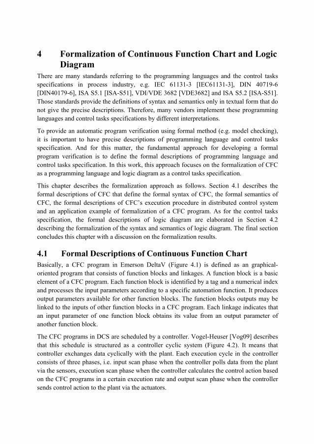
4 Formalization of Continuous Function Chart and Logic Diagram
There are many standards referring to the programming languages and the control tasks specifications in process industry, e.g. IEC 61131-3 [IEC61131-3], DIN 40719-6 [DIN40179-6], ISA S5.1 [ISA-S51], VDI/VDE 3682 [VDE3682] and ISA S5.2 [ISA-S51]. Those standards provide the definitions of syntax and semantics only in textual form that do not give the precise descriptions. Therefore, many vendors implement these programming languages and control tasks specifications by different interpretations.
To provide an automatic program verification using formal method (e.g. model checking), it is important to have precise descriptions of programming language and control tasks specification. And for this matter, the fundamental approach for developing a formal program verification is to define the formal descriptions of programming language and control tasks specification. In this work, this approach focuses on the formalization of CFC as a programming language and logic diagram as a control tasks specification.
This chapter describes the formalization approach as follows. Section 4.1 describes the formal descriptions of CFC that define the formal syntax of CFC, the formal semantics of CFC, the formal descriptions of CFC’s execution procedure in distributed control system and an application example of formalization of a CFC program. As for the control tasks specification, the formal descriptions of logic diagram are elaborated in Section 4.2 describing the formalization of the syntax and semantics of logic diagram. The final section concludes this chapter with a discussion on the formalization results.
4.1 Formal Descriptions of Continuous Function Chart Basically, a CFC program in Emerson DeltaV (Figure 4.1) is defined as an graphical-oriented program that consists of function blocks and linkages. A function block is a basic element of a CFC program. Each function block is identified by a tag and a numerical index and processes the input parameters according to a specific automation function. It produces output parameters available for other function blocks. The function blocks outputs may be linked to the inputs of other function blocks in a CFC program. Each linkage indicates that an input parameter of one function block obtains its value from an output parameter of another function block.
The CFC programs in DCS are scheduled by a controller. Vogel-Heuser [Vog09] describes that this schedule is structured as a controller cyclic system (Figure 4.2). It means that controller exchanges data cyclically with the plant. Each execution cycle in the controller consists of three phases, i.e. input scan phase when the controller polls data from the plant via the sensors, execution scan phase when the controller calculates the control action based on the CFC programs in a certain execution rate and output scan phase when the controller sends control action to the plant via the actuators.
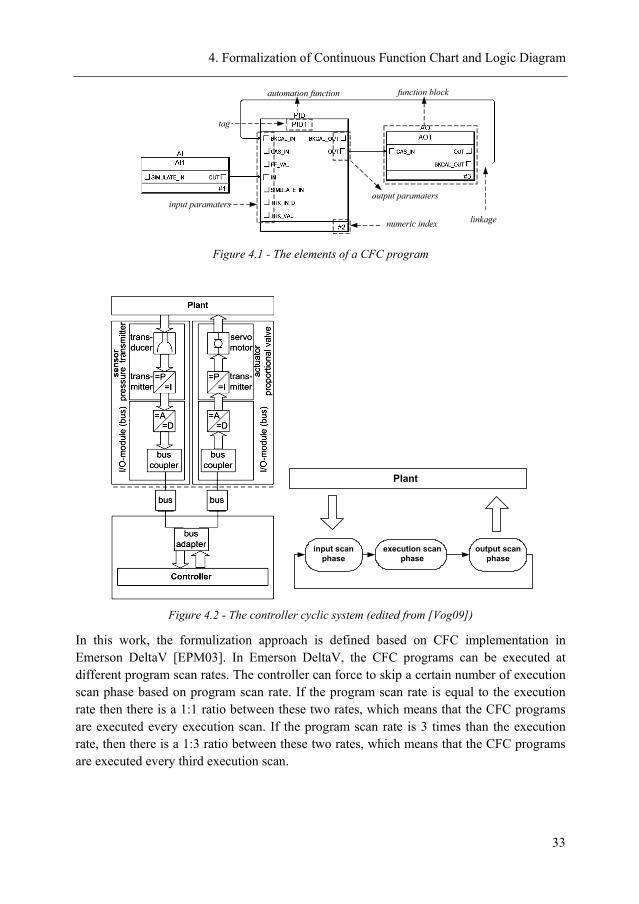
4. Formalization of Continuous Function Chart and Logic Diagram
33
function block
output paramatersinput paramaters
numeric index linkage
tag
automation function
Figure 4.1 - The elements of a CFC program
Plant
execution scan phase
input scan phase
output scan phase
Figure 4.2 - The controller cyclic system (edited from [Vog09])
In this work, the formulization approach is defined based on CFC implementation in Emerson DeltaV [EPM03]. In Emerson DeltaV, the CFC programs can be executed at different program scan rates. The controller can force to skip a certain number of execution scan phase based on program scan rate. If the program scan rate is equal to the execution rate then there is a 1:1 ratio between these two rates, which means that the CFC programs are executed every execution scan. If the program scan rate is 3 times than the execution rate, then there is a 1:3 ratio between these two rates, which means that the CFC programs are executed every third execution scan.
4. Formalization of Continuous Function Chart and Logic Diagram
34
4.1.1 Syntax of CFC Each function block in a CFC program has different types of parameter, such as input parameter, output parameter and contained parameter. The input parameter has value data structure that can be updated through a link from the output parameter, while the output parameter has a value data structure that can be updated through an automation function. As for the contained parameter, it is used in an automation function but can not be connected to the input or output parameter. The value of the contained parameter is written by CFC program’s designer manually. This unique parameter set of a function block in a CFC program is formally defined as follows.
Definition 4.1 (Parameter set of a function block)
A parameter set of a function block var is a set of u, v, c, where u is a finite set of input parameters, v is a finite set of output parameters and c is a finite set of contained parameters.
A function block uses the input and contained parameters to become automation function inputs and results as the output parameters.
Definition 4.2 (Automation function)
An automation function is a relation fb⊆((u∪c)×v), where for all x1∈(u∪c) and y1, y2∈v if (x1 , y1)∈fb and (x1 , y2)∈fb then y1=y2.
To complete the definition of an automation function in a function block, a function block status is defined to represent a state of automation function.
Definition 4.3 (Function block status)
A function block status sFB is a Boolean variable that provides sFB is true if the automation function is executed and sFB is false if the automation function is stopped.
An automation function in function block provides different relations between input/contained parameters and output parameters. These relations involves logical relations (e.g. or, and, not, etc.), input/output relations (e.g. analog input, analog output, discrete input, etc.), mathematical relations (e.g. add, multiply, comparator, etc), control relations (e.g. dead time, proportional-integral-derivative control, input selector, etc.) and time relations (e.g. off-delay, on-delay, time pulse, etc.).
The parameters described in Definition 4.1 are not enough to define all of the relation types of automation functions especially for time relation. A function block timer has to be introduced to provide the time relation of automation function.
Definition 4.4 (Function block timer)
A function block timer θf is a real variable with the dynamic behaviour θ& f=1 when it runs or when the function block status is equal to one or θ& f=0 when it stops or when the
4. Formalization of Continuous Function Chart and Logic Diagram
35
function block status is equal to zero. θf can be reset to zero. θf denotes a finite set of timers in a function block.
Definition 4.4 can be used to provide time relation of automation function, because timer has the ability to be activated if an automation function has been activated and vice versa. There are also other parameters that provide the identification of a function block, i.e. tag and numeric index. In these formal descriptions, these identifiers are defined as identification parameters.
Definition 4.5 (Identification parameter)
An identification parameter is a pair Id =(T , N), where:
- T is a unique identification tag of a function block,
- N is a numerical index of a function block.
The preliminary definitions regarding the parameters, automation function, function block timer and identification parameter provide the detailed principles for constructing a function block.
Definition 4.6 (Function block)
A function block is defined as a tuple FB=(Id, fb, θf, var), where:
- Id is an identification parameter of a function block,
- fb is an automation function,
- θf is a finite set of function block timers .
- var is a parameters set of a function block .
An output parameter of a function block may be linked to input parameter of other function blocks. Each linkage indicates that an input parameter of one function block obtains its value from unique output parameter of other function block. The relation caused by the linkage is formalized as follows.
Definition 4.7 (Linkage)
A linkage is a relation fl defined as (vj,i, un,k) that provides the function vj,i=un,k where vj,i∈vj is the ith output parameter of function block FBj and um,n∈um is the mth input parameter of function block FBm. A finite set of linkages from all function blocks in a CFC program to FBm is denoted as fl,m.
By incorporating all the definitions mentioned above, the syntax of CFC is defined as follow.
Definition 4.8 (Syntax of CFC)
A continuous function chart (CFC) program is a tuple CFC=(FB, fl, s, V), where:
4. Formalization of Continuous Function Chart and Logic Diagram
36
- FB={FB1, FB2, FB3,…, FBn } is a finite set of function blocks,
- fl={ fl,1, fl,2, fl,3,…, fl,n} is a finite set of linkages,
- s={sFB,1, sFB,2, sFB,3,…, sFB,n} is a finite set of function block statuses,
- V={var1, var2, var3,… ,varn} is finite set function block parameters,
with n is the number of function blocks in a CFC program.
4.1.2 Semantics of CFC In order to provide the meaning of CFC program, the behaviour of a CFC program in this approach is formalized in term of state-transition system. To give a more detail formalization of CFC semantics, a numerical index interpretation is defined first as follows.
Definition 4.9 (Numerical index interpretation)
N, i.e a numerical index of a function block, is interpreted as an order of a finite set of function blocks in a CFC program FB={FB1, FB2, FB3,…, FBn }.
The order of a finite set of function blocks indicates the change of conditions in a CFC program. This change is denoted by the change of status function blocks, the change of input parameters and the change of output parameters that correlates to an active function block. This condition is defined as a state of a CFC program.
Definition 4.10 (State in CFC program)
A state in a CFC program is a tuple Si=( FBi, ui, vi, sFB,i) for 1≤ i≤ n, where:
- FBi∈FB is a function block,
- ui is a finite set of input variables of FBi,
- vi is a finite set of output variables of FBi,
- sFB,i is a status of FBi,
and n is the number of function blocks in a CFC program.
Such a state can assumably represent the dynamics in a CFC program that are caused by the linkages, the automation functions and the changes of status in a CFC program. The relation state and its dynamics can be represented by defining the semantics of CFC.
Definition 4.11 (Semantics of a CFC program)
The semantics of a CFC program are a state-transition system that consists of a state defined in Definition 4.10 and the transitions are defined by rules:
- (FB1, u1, v1, sFB,1=false) ⎯⎯→⎯ 1,FBs (FB1, u1, v1, sFB,1=true) if status sFB,1 changes from false to true,
4. Formalization of Continuous Function Chart and Logic Diagram
37
- (FBi, ui, vi, sFB,i=true) ⎯→⎯ il ,f (FBi, ui’, vi, sFB,i=true) if a finite set of linkages fl,i updates a finite set of input parameters ui and 1≤ i≤ n,
- (FBi, ui, vi, sFB,i=true) ⎯→⎯ ibf , (FBi, ui, vi’, sFB,i=false) if a automation function fb,i of function blocks FBi updates a finite set of output parameters vi and 1≤ i< n,
- (FBi, ui, vi, sFB,i=false) ⎯⎯ →⎯ +1,iFBs (FBi+1, ui+1, vi+1, sFB,i+1=true) if status sFB,i changes from true to false and 1≤ i<(n-1),
- (FBn, un, vn, sFB,n=true) ⎯⎯→⎯ nbf , (FB1, u1, v1, sFB,1=false) if a automation function fb,n of function blocks FBn updated a finite set of output parameters vn,
where n is the number of function blocks in a CFC program.
The running states in a CFC program have also to be considered in addition to the CFC semantics. Based on Definition 4.11, the running states in a CFC program can be defined as a run of a CFC program.
Definition 4.12 (Run of CFC program)
A run of a CFC program is a finite sequence of transition:
(FB1, u1, v1, sFB,1=false) ⎯⎯ →⎯ 1,FBs (FB1, u1, v1, sFB,1=true) ⎯→⎯ 1,lf ⎯→⎯ 1,bf ⎯⎯ →⎯ 2,FBs (FB2, u2, v2, sFB,2=true) ... (FBn-1, un-1, vn-1, sFB,n-1=true) ⎯⎯ →⎯ −1,nlf ⎯⎯→⎯ −1,nbf ⎯⎯ →⎯ nFBs , (FBn, un, vn,
sFB,n=true) ⎯⎯→⎯ nl ,f ⎯⎯→⎯ nbf , (FB1, u1, v1, sFB,1=false),
where n is the number of function blocks in a CFC program.
The semantics of CFC and the run of a CFC program give the descriptions about the abstract behaviour of a CFC program. The next section describes the formal execution procedure of a CFC program to add the pragmatic view of the CFC implementation in distributed control system (DCS).
4.1.3 Execution Procedure of CFC The execution of a CFC program in DCS is scheduled by a controller. A controller provides the timing schedule to determine when a CFC program is executed and when the field data is acquired. The CFC programs exchange the data cyclically with the controller. Each execution cycle in the controller consists of three phases, i.e. input scan phase when the controller polls data from the sensors during a certain reading rate Tread, execution scan phase when the controller calculates the control action based on the CFC programs during a certain execution rate Texecute and output scan phase when the controller sends the control action to the actuators during a certain writing rate Twrite. The timing diagram of the controller cyclic system is shown in Figure 4.3.
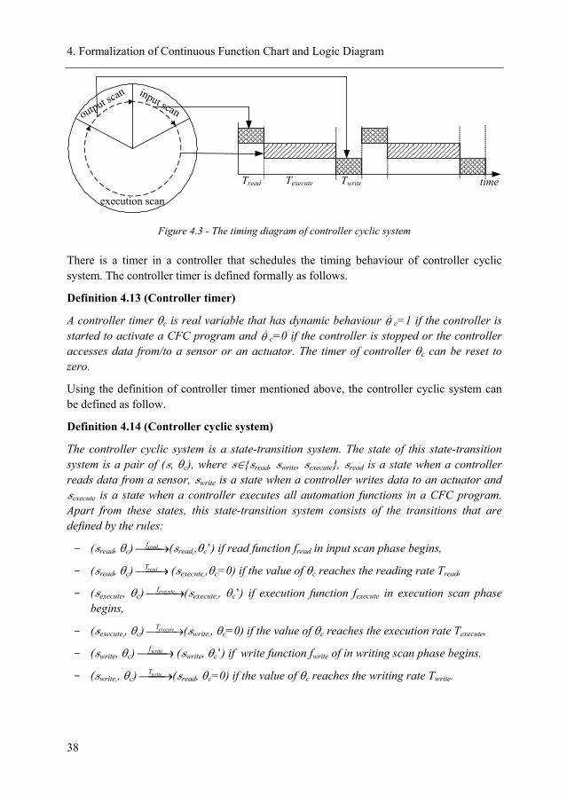
4. Formalization of Continuous Function Chart and Logic Diagram
38
time
execution scan
input scanoutput scan
TexecuteTread Twrite
Figure 4.3 - The timing diagram of controller cyclic system
There is a timer in a controller that schedules the timing behaviour of controller cyclic system. The controller timer is defined formally as follows.
Definition 4.13 (Controller timer)
A controller timer θc is real variable that has dynamic behaviour θ& c=1 if the controller is started to activate a CFC program and θ& c=0 if the controller is stopped or the controller accesses data from/to a sensor or an actuator. The timer of controller θc can be reset to zero.
Using the definition of controller timer mentioned above, the controller cyclic system can be defined as follow.
Definition 4.14 (Controller cyclic system)
The controller cyclic system is a state-transition system. The state of this state-transition system is a pair of (s, θc), where s∈{sread, swrite, sexecute}, sread is a state when a controller reads data from a sensor, swrite is a state when a controller writes data to an actuator and sexecute is a state when a controller executes all automation functions in a CFC program. Apart from these states, this state-transition system consists of the transitions that are defined by the rules:
- (sread, θc) ⎯⎯→⎯readf (sread,,θc’) if read function fread in input scan phase begins,
- (sread, θc) ⎯⎯→⎯readT (sexecute,,θc=0) if the value of θc reaches the reading rate Tread,
- (sexecute, θc) ⎯⎯ →⎯executef (sexecute,, θc’) if execution function fexecute in execution scan phase begins,
- (sexecute,, θc) ⎯⎯ →⎯executeT (swrite,, θc=0) if the value of θc reaches the execution rate Texecute,
- (swrite, θc) ⎯⎯→⎯writef (swrite, θc’) if write function fwrite of in writing scan phase begins.
- (swrite,, θc) ⎯⎯→⎯writeT (sread, θc=0) if the value of θc reaches the writing rate Twrite.
4. Formalization of Continuous Function Chart and Logic Diagram
39
In addition to the definition of controller cyclic system, the running states in controller cyclic system have also to be considered. Based on Definition 4.14, the running states in controller cyclic system can be defined as a run of controller cyclic system.
Definition 4.15 (Run of controller cyclic system)
A run of controller cyclic system is a finite sequence of transition:
(sread, θc) ⎯⎯→⎯readf ⎯⎯→⎯readT (sexecute,, θc) ⎯⎯ →⎯executef ⎯⎯ →⎯executeT (swrite, θc) ⎯⎯→⎯writef ⎯⎯→⎯writeT (sread, θc).
The definitions given above provide the restriction in CFC implementation. In this work, the formulation for the execution procedure of a CFC program is defined based on the CFC implementation in Emerson DeltaV. In Emerson DeltaV, a CFC program can be executed at different program scan rates Tscan. To formalize the program scan rate, a timer of a CFC program is defined as a follow.
Definition 4.16 (CFC program timer)
A CFC program timer θpg is a real variable with dynamic behaviour θ& pg=1 if a CFC program is active and θ& pg=0 a CFC program is inactive. The timer of CFC programs θpg resets to zero if the execution of a CFC program is completed.
This specific CFC implementation in Emerson DeltaV also gives the consequence that the result of the algorithm in a CFC program will be updated only when the program executes. In this formalization approach, this update mechanism is defined by providing the update status of a CFC program.
Definition 4.17 (CFC program update status)
A CFC program update status su is defined as a Boolean variable that provides su is true when the execution of a CFC program completes and su is false if the execution of a CFC program starts.
The definition of CFC program timer (Definition 4.16) and the definition of CFC program update status (Definition 4.17) extend the definition of state in a CFC program (Definition 4.10) as follow.
Definition 4.18 (Extension of state in CFC program)
A state in a CFC program is a set of tuple Si=( FBi, ui, vi, sFB,i, θpg, su) for 1≤ i≤ n, where:
- FBi∈FB is a function block,
- ui is a finite set of input variables of FBi,
- vi is a finite set of output variables of FBi,
- sFB,i is a function block status of FBi,
- θpg is a CFC program timer,
4. Formalization of Continuous Function Chart and Logic Diagram
40
- su is a CFC program update status,
where n is the number of function blocks in a CFC program.
The key points in the definition of controller cyclic system (Definition 4.14) have to be incorporated into the definition of CFC program timer (Definition 4.16) and the definition of CFC program status update (Definition 4.17) to extend the definition of CFC semantics (Definition 4.11) as an execution procedure of a CFC program.
Definition 4.19 (Execution procedure of a CFC program)
An execution procedure of a CFC program is a state-transition system that consists of a state defined in Definition 4.18 and the transitions are defined by rules:
- (FB1, l1, u1, v1, sFB,1=false, θpg=0, su=true) ⎯⎯ →⎯ executef (FB1, l1, u1, v1, sFB,1=true, θpg=0, su=false) if a CFC program is executed by execution function fexecute of the controller,
- (FB1, l1, u1, v1, sFB,1=true, θpg= Tscan, su=false) ⎯⎯⎯ →⎯ =Tscanpgθ (FB1, l1, u1, v1, sFB,1=true, θpg=0, su=false) if the value of θpg reaches the program scan rate Tscan,
- (FBi, li, ui, vi, sFB,i=true, θpg, su=false) ⎯→⎯ il ,f (FBi, li, ui’, vi, sFB,i=true, θpg, su=false) if a finite set of linkages fl,i updates a finite set of input parameters ui and 1≤ i≤ n,
- (FBi, li, ui, vi, sFB,i=true, θpg, su=false) ⎯→⎯ ibf , (FBi, li, ui, vi’, sFB,i=false, θpg, su=false) if a automation function fb,i of function blocks FBi updates a finite set of output parameters vi and 1≤ i<n,
- (FBi, li, ui, vi, sFB,i=false, θpg, su=true) ⎯⎯ →⎯ +1,iFBs (FBi+1, li+1, ui+1, vi+1, sFB,i+1=true, θpg, su=false) if status sFB,i changes from true to false and 1≤ i<n-1,
- (FBn, ln, un’, vn, sFB,n=true, θpg, su=false) ⎯⎯→⎯ nbf , (FB1, l1, u1, v1, sFB,1=false, θpg=0, su=true) if a automation function fb,n of function blocks FBn updates a finite set of output parameters vn,
where n is the number of function blocks in a CFC program.
In addition to the definition of CFC program’s execution procedure, the run of the states in controller cyclic system has to be considered also. Based on Definition 4.19, the running states of in CFC program’s execution procedure can be defined as a run of CFC program’s execution procedure.
Definition 4.20 (Run of CFC program’s execution procedure)
A run of CFC program’s execution procedure is a finite sequence of transitions:
(FB1, l1, u1, v1, sFB,1=false, θpg=0, su=true) ⎯⎯ →⎯executef ⎯⎯⎯ →⎯ =Tscanpgθ (FB1, l1, u1, v1, sFB,1=true, θpg=0, su=false) ⎯→⎯ 1,lf ⎯→⎯ 1,bf ⎯⎯ →⎯ 2,FBs (FB2, l2, u2, v2, sFB,2=true, θpg=0, su=false)
⎯⎯→⎯ 2,lf ⎯⎯→⎯ 2,bf ⎯⎯ →⎯ 3,FBs (FB3, l3, u3, v3, sFB,3=true, θpg=0, su=false) ... (FBn, ln, un, vn, sFB,n=true, θpg=0, su=false) ⎯⎯→⎯ nl ,f ⎯⎯→⎯ nbf , (FB1, l1, u1, v1, sFB,1=false, θpg=0, su=true),
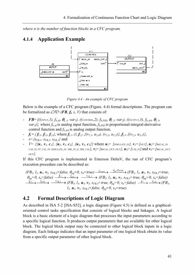
4. Formalization of Continuous Function Chart and Logic Diagram
41
where n is the number of function blocks in a CFC program.
4.1.4 Application Example
Figure 4.4 - An example of CFC program
Below is the example of a CFC program (Figure. 4.4) formal descriptions. The program can be formalized as CFC=(FB, fl, s, V) that consists of:
- FB={((INPUT,1), fb,AI, θf, 1, var1), ((CONTROL,2), fb,PID, θf, 2, var2), ((OUTPUT,3), fb,AO, θf, 3, var3)}, where fb,AI is analog input function, fb,PID is proportional-integral-derivative control function and fb,AO is analog output function,
- fl ={ fl,1, fl,2, fl,3}, where fl,1=∅, fl,2={(v1,1, u2,4), (v3,2, u2,1)}, fl,3={(v2,2, u3,1)}, - s={sFB,1, sFB,2, sFB,3} and - V= {{u1, v1, c1}, {u2, v2, c2}, {u3, v3, c3}} where u1= {SIMULATE_IN}, v1={OUT}, u2={BKCAL_IN,
CAS_IN, FF_VAL, IN, SIMULATE_IN, TRK_IN_D, TRK_VAL}, v2={BKCAL_OUT, OUT}, u3={CAS_IN} and v3={BKCAL_OUT,
OUT}. If this CFC program is implemented in Emerson DeltaV, the run of CFC program’s execution procedure can be described as:
(FB1, l1, u1, v1, sFB,1=false, θpg=0, su=true) ⎯⎯ →⎯executef ⎯⎯⎯ →⎯ =Tscanpgθ (FB1, l1, u1, v1, sFB,1=true, θpg=0, su=false) ⎯→⎯ 1,lf ⎯⎯→⎯ AIbf , ⎯⎯ →⎯ 2,FBs (FB2, l2, u2, v2, sFB,2=true, θpg=0, su=false)
⎯⎯→⎯ 2,lf ⎯⎯ →⎯ PIDbf , ⎯⎯ →⎯ 3,FBs (FB3, l3, u3, v3, sFB,3=true, θpg=0, su=false) ⎯→⎯ 3,lf ⎯⎯→⎯ AObf , (FB1, l1, u1, v1, sFB,1=false, θpg=0, su=true).
4.2 Formal Descriptions of Logic Diagram As described in ISA 5-2 [ISA-S52], a logic diagram (Figure 4.5) is defined as a graphical-oriented control tasks specification that consists of logical blocks and linkages. A logical block is a basic element of a logic diagram that processes the input parameters according to a specific logical function. It produces output parameters that are available for other logical block. The logical block output may be connected to other logical block inputs in a logic diagram. Each linkage indicates that an input parameter of one logical block obtain its value from a specific output parameter of other logical block.
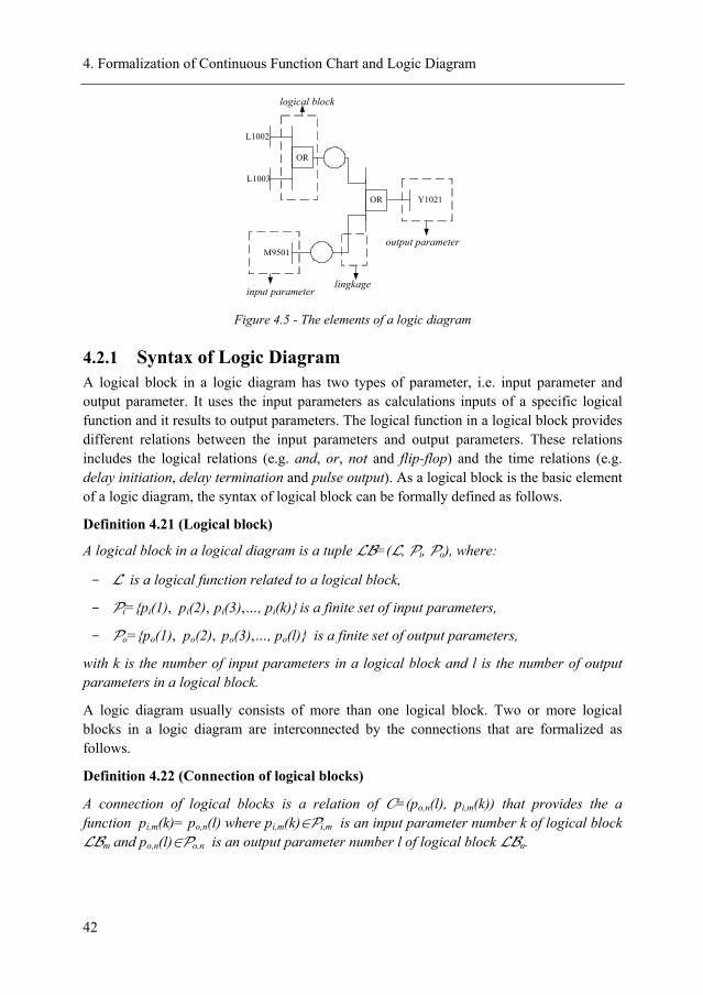
4. Formalization of Continuous Function Chart and Logic Diagram
42
OR
L1002
L1003
M9501
Y1021OR
logical block
lingkageinput parameter
output parameter
Figure 4.5 - The elements of a logic diagram
4.2.1 Syntax of Logic Diagram A logical block in a logic diagram has two types of parameter, i.e. input parameter and output parameter. It uses the input parameters as calculations inputs of a specific logical function and it results to output parameters. The logical function in a logical block provides different relations between the input parameters and output parameters. These relations includes the logical relations (e.g. and, or, not and flip-flop) and the time relations (e.g. delay initiation, delay termination and pulse output). As a logical block is the basic element of a logic diagram, the syntax of logical block can be formally defined as follows.
Definition 4.21 (Logical block)
A logical block in a logical diagram is a tuple LB=(L, Pi, Po), where:
- L is a logical function related to a logical block,
- Pi={pi(1), pi(2), pi(3),…, pi(k)} is a finite set of input parameters,
- Po={po(1), po(2), po(3),…, po(l)} is a finite set of output parameters,
with k is the number of input parameters in a logical block and l is the number of output parameters in a logical block.
A logic diagram usually consists of more than one logical block. Two or more logical blocks in a logic diagram are interconnected by the connections that are formalized as follows.
Definition 4.22 (Connection of logical blocks)
A connection of logical blocks is a relation of C=(po,n(l), pi,m(k)) that provides the a function pi,m(k)= po,n(l) where pi,m(k)∈Pi,m is an input parameter number k of logical block LBm and po,n(l)∈Po,n is an output parameter number l of logical block LBn.
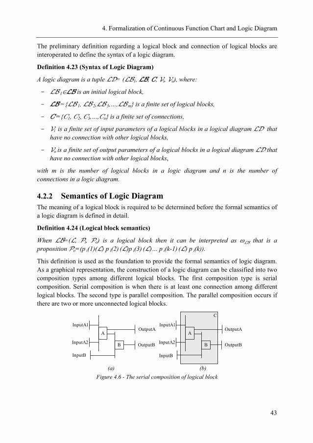
4. Formalization of Continuous Function Chart and Logic Diagram
43
The preliminary definition regarding a logical block and connection of logical blocks are interoperated to define the syntax of a logic diagram.
Definition 4.23 (Syntax of Logic Diagram)
A logic diagram is a tuple LD= (LB1, LB, C, Vi, Vo), where:
- LB 1 ∈LB is an initial logical block,
- LB ={LB 1, LB 2, LB 3,… ,LB m} is a finite set of logical blocks,
- C ={C1, C2, C3,…, Cn} is a finite set of connections,
- Vi is a finite set of input parameters of a logical blocks in a logical diagram LD that have no connection with other logical blocks,
- Vo is a finite set of output parameters of a logical blocks in a logical diagram LD that have no connection with other logical blocks,
with m is the number of logical blocks in a logic diagram and n is the number of connections in a logic diagram.
4.2.2 Semantics of Logic Diagram The meaning of a logical block is required to be determined before the formal semantics of a logic diagram is defined in detail.
Definition 4.24 (Logical block semantics)
When LB=(L, Pi, Po) is a logical block then it can be interpreted as ωLB that is a proposition Po=(p i(1)(L) p i(2) (L) p i(3) (L)… p i(k-1) (L) p i(k)).
This definition is used as the foundation to provide the formal semantics of logic diagram. As a graphical representation, the construction of a logic diagram can be classified into two composition types among different logical blocks. The first composition type is serial composition. Serial composition is when there is at least one connection among different logical blocks. The second type is parallel composition. The parallel composition occurs if there are two or more unconnected logical blocks.
A
InputA1
InputA2 B
InputB
OutputB
OutputAA
InputA1
InputA2 B
InputB
OutputB
OutputA
C
(a) (b)
Figure 4.6 - The serial composition of logical block
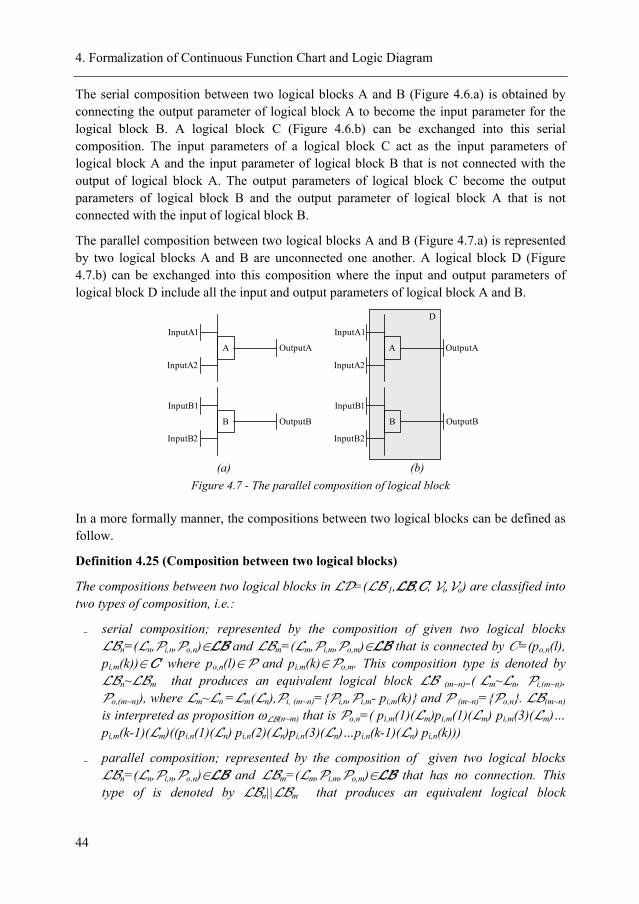
4. Formalization of Continuous Function Chart and Logic Diagram
44
The serial composition between two logical blocks A and B (Figure 4.6.a) is obtained by connecting the output parameter of logical block A to become the input parameter for the logical block B. A logical block C (Figure 4.6.b) can be exchanged into this serial composition. The input parameters of a logical block C act as the input parameters of logical block A and the input parameter of logical block B that is not connected with the output of logical block A. The output parameters of logical block C become the output parameters of logical block B and the output parameter of logical block A that is not connected with the input of logical block B.
The parallel composition between two logical blocks A and B (Figure 4.7.a) is represented by two logical blocks A and B are unconnected one another. A logical block D (Figure 4.7.b) can be exchanged into this composition where the input and output parameters of logical block D include all the input and output parameters of logical block A and B.
A
InputA1
InputA2
OutputA
B
InputB1
InputB2
OutputB
A
InputA1
InputA2
OutputA
B
InputB1
InputB2
OutputB
D
(a) (b)
Figure 4.7 - The parallel composition of logical block
In a more formally manner, the compositions between two logical blocks can be defined as follow.
Definition 4.25 (Composition between two logical blocks)
The compositions between two logical blocks in LD=(LB 1 ,LB, C, Vi, Vo) are classified into two types of composition, i.e.:
- serial composition; represented by the composition of given two logical blocks LBn=(Ln,Pi,n,Po,n)∈LB and LBm=(Lm,Pi,m,Po,m)∈LB that is connected by C =(po,n(l), pi,m(k))∈ C where po,n(l)∈ P and pi,m(k)∈ Po,m. This composition type is denoted by LBn~LBm that produces an equivalent logical block LB (m~n)=( Lm~Ln, Pi,(m~n), Po,(m~n)), where Lm~Ln =Lm (Ln),Pi, (m~n)= {Pi,n, Pi,m- pi,m(k)} and P (m~n)= {Po,n}. LB(m~n) is interpreted as proposition ωLB(n~m) that is Po,n=( pi,m(1)(Lm)pi,m(1)(Lm) pi,m(3)(Lm)… pi,m(k-1)(Lm)((pi,n(1)(Ln) pi,n(2)(Ln) pi,n(3)(Ln)…pi,n(k-1)(Ln) pi,n(k)))
- parallel composition; represented by the composition of given two logical blocks LBn=(Ln,Pi,n,Po,n)∈LB and LBm=(Lm,Pi,m,Po,m)∈LB that has no connection. This type of is denoted by LBn||LBm that produces an equivalent logical block
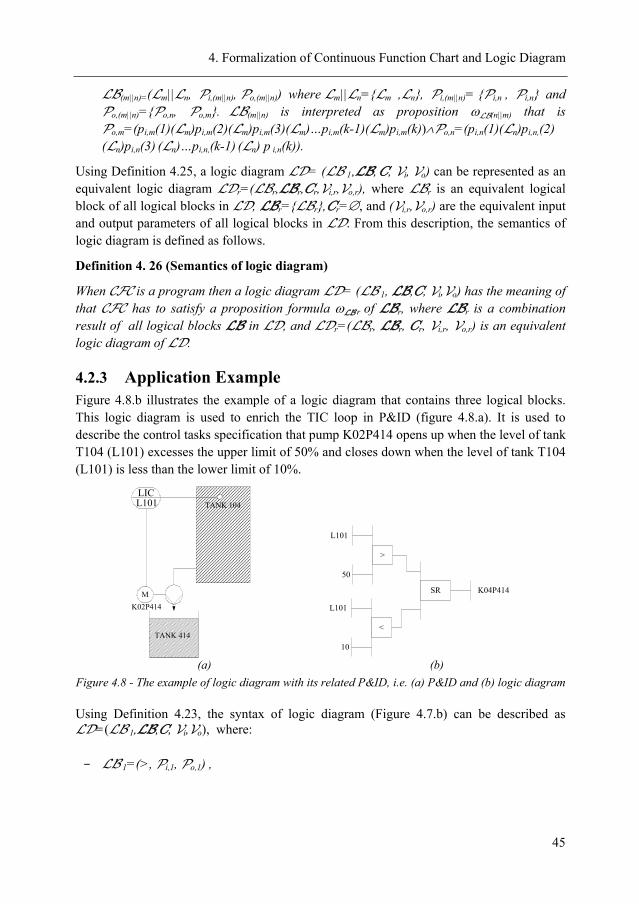
4. Formalization of Continuous Function Chart and Logic Diagram
45
LB(m||n)=(Lm||Ln, Pi,(m||n), Po,(m||n)) where Lm||Ln={Lm ,Ln}, Pi,(m||n)= {Pi,n , Pi,n} and Po,(m||n)={Po,n, Po,m}. LB(m||n) is interpreted as proposition ωLB(n||m) that is Po,m=(pi,m(1)(Lm)pi,m(2)(Lm)pi,m(3)(Lm)…pi,m(k-1)(Lm)pi,m(k))∧Po,n=(pi,n(1)(Ln)pi,n,(2) (Ln)pi,n(3) (Ln)…pi,n,(k-1) (Ln) p i,n(k)).
Using Definition 4.25, a logic diagram LD= (LB 1 ,LB, C, Vi, Vo) can be represented as an equivalent logic diagram LDr=(LBr,LBr,Cr,Vi,r,Vo,r), where LBr is an equivalent logical block of all logical blocks in LD, LBr={LBr}, Cr=∅, and (Vi,r,Vo,r) are the equivalent input and output parameters of all logical blocks in LD. From this description, the semantics of logic diagram is defined as follows.
Definition 4. 26 (Semantics of logic diagram)
When CFC is a program then a logic diagram LD= (LB 1 , LB, C, Vi, Vo) has the meaning of that CFC has to satisfy a proposition formula ωLB r of LBr, where LBr is a combination result of all logical blocks LB in LD, and LDr=(LBr, LBr, Cr, Vi,r, Vo,r) is an equivalent logic diagram of LD.
4.2.3 Application Example Figure 4.8.b illustrates the example of a logic diagram that contains three logical blocks. This logic diagram is used to enrich the TIC loop in P&ID (figure 4.8.a). It is used to describe the control tasks specification that pump K02P414 opens up when the level of tank T104 (L101) excesses the upper limit of 50% and closes down when the level of tank T104 (L101) is less than the lower limit of 10%.
TANK 104
TANK 414
K02P414M
LICL101
K04P414SR
<
L101
10
>
L101
50
(a) (b)
Figure 4.8 - The example of logic diagram with its related P&ID, i.e. (a) P&ID and (b) logic diagram
Using Definition 4.23, the syntax of logic diagram (Figure 4.7.b) can be described as LD=(LB 1 ,LB, C, Vi, Vo), where:
- LB 1 = (>, Pi,1, Po,1) ,
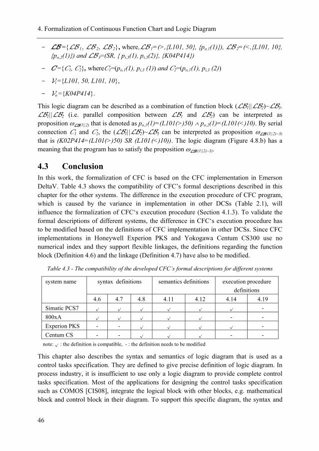
4. Formalization of Continuous Function Chart and Logic Diagram
46
- LB ={ LB 1 , LB 2, LB 2} , where , LB 1 = (>,{L101, 50}, {po,1(1)}), LB 2= (<,{L101, 10}, {po,2(1)}) and LB 3= (SR, { pi,3(1), pi,3(2)}, {K04P414})
- C ={C1, C2 }, where C1 =(po,1(1), pi,3 (1)) and C2 =(po,1(1), pi,3 (2))
- Vi ={L101, 50, L101, 10},
- Vo ={K04P414}.
This logic diagram can be described as a combination of function block (LB1||LB2)~LB3. LB1||LB2 (i.e. parallel composition between LB1 and LB2) can be interpreted as proposition ωLB(1||2) that is denoted as po,1(1)=(L101 (>)50) ∧ po,2(1)=(L101 (<)10). By serial connection C1 and C2, the (LB1||LB2)~LB3 can be interpreted as proposition ωLB((1||2)~3) that is (K02P414=(L101(>)50) SR (L101 (<)10)). The logic diagram (Figure 4.8.b) has a meaning that the program has to satisfy the proposition ωLB((1||2)~3).
4.3 Conclusion In this work, the formalization of CFC is based on the CFC implementation in Emerson DeltaV. Table 4.3 shows the compatibility of CFC’s formal descriptions described in this chapter for the other systems. The difference in the execution procedure of CFC program, which is caused by the variance in implementation in other DCSs (Table 2.1), will influence the formalization of CFC‘s execution procedure (Section 4.1.3). To validate the formal descriptions of different systems, the difference in CFC‘s execution procedure has to be modified based on the definitions of CFC implementation in other DCSs. Since CFC implementations in Honeywell Experion PKS and Yokogawa Centum CS300 use no numerical index and they support flexible linkages, the definitions regarding the function block (Definition 4.6) and the linkage (Definition 4.7) have also to be modified.
Table 4.3 - The compatibility of the developed CFC’s formal descriptions for different systems
syntax definitions semantics definitions execution procedure definitions
system name
4.6 4.7 4.8 4.11 4.12 4.14 4.19 Simatic PCS7 √ √ √ √ √ √ - 800xA √ √ √ √ √ - - Experion PKS - - √ √ √ √ - Centum CS - - √ √ √ - -
note: √ : the definition is compatible, - : the definition needs to be modified
This chapter also describes the syntax and semantics of logic diagram that is used as a control tasks specification. They are defined to give precise definition of logic diagram. In process industry, it is insufficient to use only a logic diagram to provide complete control tasks specification. Most of the applications for designing the control tasks specification such as COMOS [CIS08], integrate the logical block with other blocks, e.g. mathematical block and control block in their diagram. To support this specific diagram, the syntax and
4. Formalization of Continuous Function Chart and Logic Diagram
47
semantics of logic diagram have to be extended with the definitions of different block types and the definitions of different composition types.
5 Development of Transformation Rules In this work, the transformation rules are needed in order to incorporate the formalization of continuous function chart (CFC) and logic diagram in the domain of model checking. This chapter describes the transformation rules that map the formal descriptions of CFC and logic diagram (Chapter 4) into the formal descriptions of timed automata and TCTL (Chapter 3). The first section describes the transformation rules of CFC to timed automata; while the transformation rules of logic diagram to TCTL is explained in the second section.
5.1 Continuous Function Chart to Timed Automata There are three important parts of a CFC program that have to be considered for formalization, i.e. function block, controller cyclic system and execution procedure of a CFC program. These three important parts are connected one another and bundled in the formal descriptions of CFC. These important parts are mapped into a timed automata network. In this transformation approach, this timed automata network is considered as the CFC timed automata network |Acfc|.
5.1.1 Transformation of Function Block The basic element of a CFC program is a function block. A CFC program consists at least one function block which is transformed into a function block automaton Afb,i where Afb,i is an element of CFC timed automata network |Acfc|. Firstly, the identification parameters Id=(T, N) has to be mapped into a part of Afb,i to provide the function block transformation.
Rule 5.1 (Transformation of identification parameter)
An identification parameter of a function block Id=(T, N) is mapped as an identification of a function block automaton Afb,i. T as a unique identification tag of a function block is transformed into a name of Afb,i and N as a numerical index of a function block is transformed into a unique numerical index i of Afb,i.
This transformation rule is important to ensure that each function block is mapped into one unique function block automaton. Secondly, the parameter set of a function block has to be transformed into a part of a function block automaton. This parameter set transformation can be defined with the help of the function block automaton’s variables.
Rule 5.2 (Transformation of parameter set)
The parameter set of a function block var={u, v, c} is transformed into the set of variables v={vsh, vint} of Afb,i, that the transformation details are defined as follows.
- The input and output parameters u, v in the function block are transformed into a finite set of shared variables vsh in Afb,i.
5. Development of Transformation Rules
49
- The contained parameter set of a function block c is mapped into a finite set of internal variables vint in Afb,i.
To complete the parameter set transformation, the transformation rule of a function block timer is described as follows.
Rule 5.3 (Transformation of a function block timer)
A function block timer θf is mapped into a clock t in Afb,i.
After the transformations of all parameters in a function block are completely defined, the automation function has to be transformed into an assignment in function block automaton to accomplish the calculation of all transformed variables.
Rule 5.4 (Transformation of automation function)
An automation function is transformed into a functional assignment calculate() that is a function of all variables in Afb,i.
The activation of each automation function is indicated by the transition of function block status. This status transition is transformed using the following rule.
Rule 5.5 (Transformation of function block status’s transition)
The transition of a function block status sFB is transformed into the synchronization actions in Afb,i. The transition of sFB from true to false is transformed into the input action startfb(i)?, while the transition of sFB from false to true is transformed into the output action endfb(i)!.
The key points of order on Rule 5.1 until Rule 5.5 are connected to formalize the transformation rule of function block. The transformation rules of function block can be classified into two different transformation rules, i.e. for non-time-based function block and for time-based function block. These transformation rules allow for the determination of the elements and the run of function block automaton Afb,i.
Rule 5.6 (Transformation of non-time based function block)
A non-time-based function block FBi∈FB is transformed as a function block automaton Afb,i=(L, l0, E ,I), where:
- L ={l0, l1}, where l1 ∈ Lcomm,
- l0∈ L is the initial location,
- E={ l0 ⎯⎯⎯⎯⎯ →⎯ ()?,)( calculateistartb l1, l1 ⎯⎯⎯ →⎯ )!(iendfb l0},
- I=∅,
and a run of a function block automaton Afb,i is:
< l0,u> ⎯⎯⎯⎯⎯⎯ →⎯ ()?,)( calculateistartfb < l1,u> ⎯⎯⎯ →⎯ )!(iendfb < l0,u>.
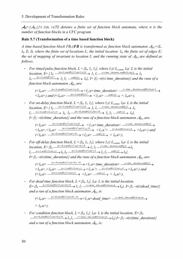
5. Development of Transformation Rules
50
Afb={Afb,i|1≤ i≤n, i∈N} denotes a finite set of function block automata, where n is the number of function blocks in a CFC program.
Rule 5.7 (Transformation of a time based function block)
A time-based function block FBi∈FB is transformed as function block automaton Afb,i=(L, l0, E, I), where the finite set of locations L; the initial location l0, the finite set of edges E; the set of mapping of invariant to location I; and the running state of Afb,i are defined as follows.
- For timed pulse function block, L ={l0, l1, l2}, where l2∈ Lcomm, l0∈ L is the initial location, E={ l0 ⎯⎯⎯⎯⎯⎯⎯ →⎯ ==== 0,1?,)(,1 toutistartfbin l1, l1 ⎯⎯⎯⎯⎯⎯⎯⎯⎯ →⎯ === 1,)!(,_ outiendfbdurationtimet l0, l0 ⎯⎯⎯⎯ →⎯ == ?)(,1 istartfbin l2, l2 ⎯⎯⎯ →⎯ )!(iendfb l0}, I={l1→(t≤ time_duration)} and the runs of a function block automaton Afb,i are:
(<l0,u> ⎯⎯⎯⎯⎯⎯⎯ →⎯ ==== 0,1?,)(,1 toutistartfbin <l1,u+time_duration> ⎯⎯⎯⎯⎯⎯⎯⎯ →⎯ === 1,)!(,_ outiendfbdurationtimet <l0,u>) and (<l0,u> ⎯⎯⎯⎯ →⎯ == ?)(,1 istartfbin <l2,u> ⎯⎯⎯ →⎯ )!(iendfb < l0,u>),
- For on-delay function block, L ={l0, l1, l2}, where l2∈ Lcomm, l0∈ L is the initial location, E={ l0 ⎯⎯⎯⎯⎯⎯⎯ →⎯ ==== 0,1?,)(,1 toutistartfbin l1, l1 ⎯⎯⎯⎯⎯⎯⎯ →⎯ == )!(,_ iendfbdurationtimet l0, l1 ⎯⎯⎯⎯⎯⎯ →⎯ ==== 0,)!(,0 outiendfbin l0, l0 ⎯⎯⎯⎯⎯⎯ →⎯ ==== 0?,)(,0 outistartfbin l2, l2 ⎯⎯⎯ →⎯ )!(iendfb l0}, I={l1→(t≤time_duration)} and the runs of a function block automaton Afb,i are:
(<l0,u> ⎯⎯⎯⎯⎯⎯⎯ →⎯ ==== 0,1?,)(,1 toutistartfbin <l1,u+time_duration> ⎯⎯⎯⎯⎯⎯⎯ →⎯ == )!(,_ iendfbdurationtimet <l0,u>,<l0,u> ⎯⎯⎯⎯⎯⎯⎯ →⎯ ==== 0,1?,)(,1 fbtoutistartfbin <l1,u’> ⎯⎯⎯⎯⎯⎯ →⎯ ==== 0,)!(,0 outiendfbin <l0,u>) and (<l0,u> ⎯⎯⎯⎯⎯⎯ →⎯ ==== 0?,)(,0 outistartfbin <l2,u> ⎯⎯⎯ →⎯ )!(iendfb < l0,u>),
- For off-delay function block, L ={l0, l1, l2}, where l2∈ Lcomm, l0∈ L is the initial location, E={l0 ⎯⎯⎯⎯⎯⎯⎯ →⎯ ==== 0,0?,)(,0 toutistartfbin l1, l1 ⎯⎯⎯⎯⎯⎯⎯ →⎯ == )!(,_ iendfbdurationtimet l0, l1 ⎯⎯⎯⎯⎯⎯ →⎯ ==== 1,)!(,1 outiendfbin l0, l0 ⎯⎯⎯⎯⎯⎯ →⎯ ==== 1?,)(,1 outistartfbin l2, l2 ⎯⎯⎯ →⎯ )!(iendfb l0}, I={l1→(t≤time_duration)} and the runs of a function block automaton Afb,i are:
(<l0,u> ⎯⎯⎯⎯⎯⎯⎯ →⎯ ==== 0,0?,)(,0 toutistartfbin <l1,u+time_duration> ⎯⎯⎯⎯⎯⎯⎯ →⎯ == )!(,_ iendfbdurationtimet <l0,u>,<l0,u> ⎯⎯⎯⎯⎯⎯ →⎯ ==== 1,)!(,1 outiendfbin <l1,u’> ⎯⎯⎯⎯⎯⎯ →⎯ ==== 0,)!(,0 outiendfbin <l0,u>) and (<l0,u> ⎯⎯⎯⎯⎯⎯ →⎯ ==== 1?,)(,1 outistartfbin <l2,u> ⎯⎯⎯ →⎯ )!(iendfb < l0,u>),
- For dead time function block, L ={l0, l1}, l0∈ L is the initial location, E={l0 ⎯⎯⎯⎯⎯⎯⎯ →⎯ ==== 0,0?,)(,0 toutistartfbin l1, l1 ⎯⎯⎯⎯⎯⎯⎯⎯ →⎯ === inoutiendfbtimedeadt ,)!(,_ l0}, I={l1→(t≤dead_time)} and a run of a function block automaton Afb,i is:
(<l0,u> ⎯⎯⎯⎯⎯⎯⎯ →⎯ ==== 0,0?,)(,0 toutistartfbin <l1,u+dead_time> ⎯⎯⎯⎯⎯⎯⎯⎯ →⎯ === inoutiendfbtimedeadt ,)!(,_
< l0,u>),
- For condition function block, L ={l0, l1}, l0∈ L is the initial location, E={l0
⎯⎯⎯⎯⎯⎯⎯ →⎯ ==== 0,0?,)(,0 toutistartfbin l1,l1 ⎯⎯⎯⎯⎯⎯⎯⎯ →⎯ === inoutiendfbtimedeadt ,)!(,_ l0},I={l1→(t≤time_duration)} and a run of a function block automaton Afb,i is:
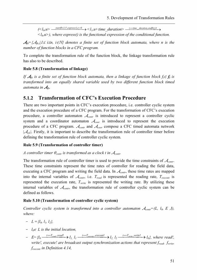
5. Development of Transformation Rules
51
(<l0,u> ⎯⎯⎯⎯⎯⎯ →⎯ =0(),?,)( texpressistartfb <l1,u+time_duration> ⎯⎯⎯⎯⎯⎯⎯ →⎯ == )!(,_ iendfbdurationtimet <l0,u>), where express() is the functional expression of the conditional function.
Afb={Afb,i|1≤ i≤n, i∈N} denotes a finite set of function block automata, where n is the number of function blocks in a CFC program.
To complete the transformation rule of the function block, the linkage transformation rule has also to be described.
Rule 5.8 (Transformation of linkage)
If Afb is a finite set of function block automata, then a linkage of function block fl∈ fl is transformed into an equally shared variable used by two different function block timed automata in Afb.
5.1.2 Transformation of CFC’s Execution Procedure There are two important points in CFC’s execution procedure, i.e. controller cyclic system and the execution procedure of a CFC program. For the transformation of CFC’s execution procedure, a controller automaton Acontr is introduced to represent a controller cyclic system and a coordinator automaton Acoor is introduced to represent the execution procedure of a CFC program. Acontr and Acoor compose a CFC timed automata network |Acfc|. Firstly, it is important to describe the transformation rule of controller timer before defining the transformation rule of controller cyclic system.
Rule 5.9 (Transformation of controller timer)
A controller timer θcontr is transformed as a clock t in Acontr.
The transformation rule of controller timer is used to provide the time constraints of Acontr. These time constraints represent the time rates of controller for reading the field data, executing a CFC program and writing the field data. In Acontr, these time rates are mapped into the internal variables of Acontr, i.e. Tread is represented the reading rate, Texecute is represented the execution rate, Twrite is represented the writing rate. By utilizing these internal variables of Acontr, the transformation rule of controller cyclic system can be defined as follows.
Rule 5.10 (Transformation of controller cyclic system)
Controller cyclic system is transformed into a controller automaton Acontr=(L, l0, E ,I), where:
- L ={l0, l1, l2},
- l0∈ L is the initial location,
- E={l0 ⎯⎯⎯⎯ →⎯ == !,readTt read l1, l1 ⎯⎯⎯⎯⎯ →⎯ == !,executeTt execute l2, l2 ⎯⎯⎯⎯ →⎯ == !,writeTt write l0}, where read!, write!, execute! are broadcast output synchronization actions that represent fread, fwrite, fexecute in Definition 4.14,
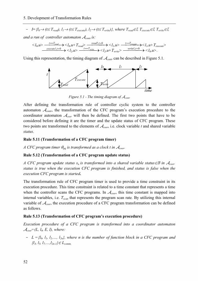
5. Development of Transformation Rules
52
- I={l0→ (t≤ Tread), l1→ (t≤ Texecute), l2→ (t≤ Twrite)}, where Tread∈I, Texecute∈I, Twrite∈I,
and a run of controller automaton Acontr is:
<l0,u> ⎯⎯ →⎯ == readTt <l0,u+Tread> ⎯⎯⎯ →⎯ =0,! tread <l1,u> ⎯⎯⎯ →⎯== executeTt <l1,u+Texecute>⎯⎯⎯ →⎯ =0,! texecute <l2,u> ⎯⎯⎯ →⎯ == writeTt <l2,u+Twrite> ⎯⎯⎯ →⎯ =0,! twrite <l0,u>.
Using this representation, the timing diagram of Acontr can be described in Figure 5.1.
Texecute
timeTread Twrite
l0 l1 l2
t
Figure 5.1 - The timing diagram of Acontr
After defining the transformation rule of controller cyclic system to the controller automaton Acontr, the transformation of the CFC program’s execution procedure to the coordinator automaton Acoor will then be defined. The first two points that have to be considered before defining it are the timer and the update status of CFC program. These two points are transformed to the elements of Acoor, i.e. clock variable t and shared variable status.
Rule 5.11 (Transformation of a CFC program timer)
A CFC program timer θpg is transformed as a clock t in Acoor.
Rule 5.12 (Transformation of a CFC program update status)
A CFC program update status su is transformed into a shared variable status∈B in Acoor. status is true when the execution CFC program is finished, and status is false when the execution CFC program is started.
The transformation rule of CFC program timer is used to provide a time constraint in its execution procedure. This time constraint is related to a time constant that represents a time when the controller scans the CFC programs. In Acoor, this time constant is mapped into internal variables, i.e. Tscan that represents the program scan rate. By utilizing this internal variable of Acoor, the execution procedure of a CFC program transformation can be defined as follows.
Rule 5.13 (Transformation of CFC program’s execution procedure)
Execution procedure of a CFC program is transformed into a coordinator automaton Acoor=(L, l0, E, I), where:
- L ={l0, l1, l2,…, l2n}, where n is the number of function block in a CFC program and {l3, l5, l7,…,l2n-1}∈ Lcomm,
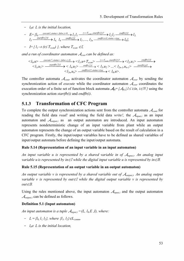
5. Development of Transformation Rules
53
- l0∈ L is the initial location,
- E={l0 ⎯⎯⎯⎯⎯⎯ →⎯ == 0,,! tfalsestatusexecute l1,l1 ⎯⎯⎯⎯⎯ →⎯ == ?)1(,startfbTt scan l2,l2 ⎯⎯⎯ →⎯ )!1(endfb l3,
l3 ⎯⎯⎯ →⎯ )!2(startfb l4, l4 ⎯⎯⎯ →⎯ )!2(endfb l5 ,…, l2n ⎯⎯⎯⎯⎯⎯ →⎯ =truestatusnendfb ,)!( l0},
- I={ l1→ (t≤ Tscan) }, where Tscan ∈I,
and a run of coordinator automaton Acoor can be defined as:
<l0,u> ⎯⎯⎯⎯⎯⎯⎯ →⎯ == 0,?, tfalsestatusexecute <l1,u+Tscan> ⎯⎯⎯⎯⎯ →⎯ == ?)1(,startfbTt scan <l2,u1> ⎯⎯⎯ →⎯ )!1(endfb
<l3,u1> ⎯⎯⎯ →⎯ )!2(startfb < l4,u2> ⎯⎯⎯ →⎯ )!2(endfb < l5,u2 >…< l2n-1,un-1> ⎯⎯⎯ →⎯ )!(nstartfb <l2n,un> ⎯⎯⎯⎯⎯⎯ →⎯ =truestatusnendfb ?,)( < l0,u>.
The controller automata Acontr activates the coordinator automaton Acoor by sending the synchronization action of execute while the coordinator automaton Acoor coordinates the execution order of a finite set of function block automata Afb={Afb,i|1≤ i≤n, i∈N } using the synchronization action startfb(i) and endfb(i).
5.1.3 Transformation of CFC Program To complete the output synchronization actions sent from the controller automata Acontr for reading the field data read! and writing the field data write!, the Ainput,i as an input automaton and Aoutput,i as an output automaton are introduced. An input automaton represents nondeterministic change of an input variable from plant while an output automaton represents the change of an output variable based on the result of calculation in a CFC program. Firstly, the input/output variables have to be defined as shared variables of input/output automata before defining the input/output automata.
Rule 5.14 (Representation of an input variable in an input automaton)
An input variable u is represented by a shared variable in of Ainput,i. An analog input variable u is represented by in∈I while the digital input variable u is represented by in∈B.
Rule 5.15 (Representation of an output variable in an output automaton)
An output variable v is represented by a shared variable out of Aoutput,i. An analog output variable v is represented by out∈I while the digital output variable v is represented by out∈B.
Using the rules mentioned above, the input automaton Ainput,i and the output automaton Aoutput,i can be defined as follows.
Definition 5.1 (Input automaton)
An input automaton is a tuple Ainput,i =(L, l0,E ,I), where:
- L ={l0, l1, l2}, where {l1, l2}∈Lcomm,
- l0∈ L is the initial location,
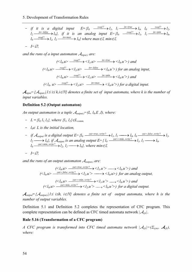
5. Development of Transformation Rules
54
- if it is a digital input E={l0 ⎯⎯ →⎯ ?read l1, l1 ⎯⎯ →⎯ =truein l0, l0 ⎯⎯ →⎯ ?read l2, l2 ⎯⎯⎯ →⎯ = falsein l0}, if it is an analog input E={l0 ⎯⎯ →⎯ ?read l1, l1 ⎯⎯ →⎯ =minin l0, l0 ⎯⎯ →⎯ ?read l2, l2 ⎯⎯ →⎯ =maxin l0} where max∈I, min∈I,
- I=∅,
and the runs of a input automaton Ainput,i are:
(<l0,u> ⎯⎯ →⎯ ?read <l1,u> ⎯⎯ →⎯ =truein <l0,u’>) and
(<l0,u> ⎯⎯ →⎯ ?read <l2,u> ⎯⎯⎯ →⎯ = falsein <l0,u’>) for an analog input,
(<l0,u> ⎯⎯ →⎯ ?read <l1,u> ⎯⎯ →⎯ =minin <l0,u’>) and
(<l0, u> ⎯⎯ →⎯ ?read <l2,u> ⎯⎯ →⎯ =maxin <l0,u’>) for a digital input.
Ainput={Ainput,i|1≤ i≤ k,i∈N} denotes a finite set of input automata, where k is the number of input variables.
Definition 5.2 (Output automaton)
An output automaton is a tuple Aoutput,i=(L, l0,E ,I), where:
- L ={l0, l1, l2}, where {l1, l2}∈Lcomm,
- l0∈ L is the initial location,
- if Aoutput is a digital output E={l0 ⎯⎯⎯⎯ →⎯ = ?, writetrueout l1, l1 ⎯→⎯ l0, l0 ⎯⎯⎯⎯⎯ →⎯ = ?, writefalseout l2, l2 ⎯→⎯ l0}, if Aoutput is an analog output E={ l0 ⎯⎯⎯⎯⎯ →⎯ == ?,min writeout l1, l1 ⎯→⎯ l0, l0 ⎯⎯⎯⎯ →⎯ > ?,min writeout l2, l2 ⎯→⎯ l0}, where min∈I,
- I=∅,
and the runs of an output automaton Aoutput,i are:
(<l0,u> ⎯⎯⎯⎯ →⎯ = ?, writetrueout <l1,u’> ⎯→⎯ <l0,u’>) and (<l0,u> ⎯⎯⎯⎯⎯ →⎯ = ?, writefalseout <l2,u’> ⎯→⎯ <l0,u>) for an analog output,
(<l0,u> ⎯⎯⎯⎯⎯ →⎯ == ?,min writeout <l1,u’> ⎯→⎯ <l0,u’>) and (<l0,u> ⎯⎯⎯⎯ →⎯ > ?,min writeout <l2,u’> ⎯→⎯ <l0,u’>) for a digital output.
Aoutput={Aoutput,i|1≤ i≤h, i∈N} denotes a finite set of output automata, where h is the number of output variables.
Definition 5.1 and Definition 5.2 completes the representation of CFC program. This complete representation can be defined as CFC timed automata network |Acfc|.
Rule 5.16 (Transformation of a CFC program)
A CFC program is transformed into CFC timed automata network |Acfc|=(Σsync, Acfc), where:
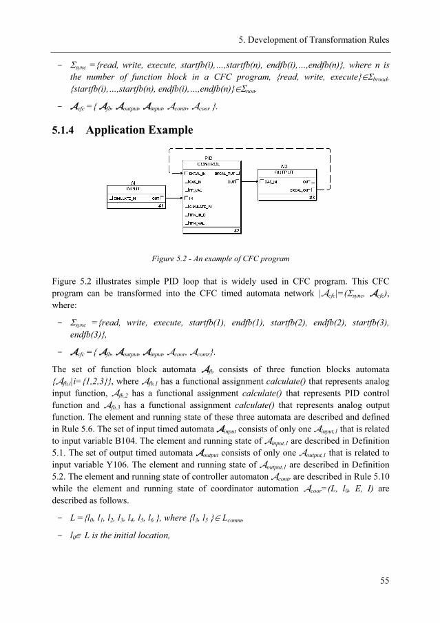
5. Development of Transformation Rules
55
- Σsync ={read, write, execute, startfb(i),…,startfb(n), endfb(i),…,endfb(n)}, where n is the number of function block in a CFC program, {read, write, execute}∈Σbroad, {startfb(i),…,startfb(n), endfb(i),…,endfb(n)}∈Σnon.
- Acfc ={ Afb, Aoutput, Ainput, Acontr, Acoor }.
5.1.4 Application Example
Figure 5.2 - An example of CFC program
Figure 5.2 illustrates simple PID loop that is widely used in CFC program. This CFC program can be transformed into the CFC timed automata network |Acfc|=(Σsync, Acfc), where:
- Σsync ={read, write, execute, startfb(1), endfb(1), startfb(2), endfb(2), startfb(3), endfb(3)},
- Acfc ={ Afb, Aoutput, Ainput, Acoor, Acontr}.
The set of function block automata Afb consists of three function blocks automata {Afb,i|i={1,2,3}}, where Afb,1 has a functional assignment calculate() that represents analog input function, Afb,2 has a functional assignment calculate() that represents PID control function and Afb,3 has a functional assignment calculate() that represents analog output function. The element and running state of these three automata are described and defined in Rule 5.6. The set of input timed automata Ainput consists of only one Ainput,1 that is related to input variable B104. The element and running state of Ainput,1 are described in Definition 5.1. The set of output timed automata Aoutput consists of only one Aoutput,1 that is related to input variable Y106. The element and running state of Aoutput,1 are described in Definition 5.2. The element and running state of controller automaton Acontr are described in Rule 5.10 while the element and running state of coordinator automation Acoor=(L, l0, E, I) are described as follows.
- L ={l0, l1, l2, l3, l4, l5, l6 }, where {l3, l5 }∈ Lcomm,
- l0∈ L is the initial location,
5. Development of Transformation Rules
56
- E={l0 ⎯⎯⎯⎯⎯⎯ →⎯ == 0,,! tfalsestatusexecute l1, l1 ⎯⎯⎯⎯⎯ →⎯ == ?)1(,startfbTt scan l2, l2 ⎯⎯⎯ →⎯ )!1(endfb l3, l3 ⎯⎯⎯ →⎯ )!2(startfb l4, l4 ⎯⎯⎯ →⎯ )!2(endfb l5 , l5 ⎯⎯⎯ →⎯ )!3(startfb l6, l6 ⎯⎯⎯⎯⎯ →⎯ =truestatusendfb ,)!3( l0},
- I={ l1→ (t≤ Tscan) }, where Tscan ∈I,
and the run of a coordinator automaton Acoor can be defined as:
<l0,u> ⎯⎯⎯⎯⎯⎯ →⎯ == 0,,! tfalsestatusexecute <l1,u+Tscan> ⎯⎯⎯⎯⎯ →⎯ == ?)1(,startfbTt scan <l2,u1> ⎯⎯⎯ →⎯ )!1(endfb <l3,u1> ⎯⎯⎯ →⎯ )!2(startfb <l4,u2> ⎯⎯⎯ →⎯ )!2(endfb <l5,u2> ⎯⎯⎯ →⎯ )!3(startfb <l6,u3> ⎯⎯⎯⎯⎯ →⎯ =truestatusendfb ,)!3(
<l0,u>.
5.2 Logic Diagram to Timed Computation Tree Logic A logic diagram LD=(LB1, LB, C, Vi, Vo) that consists of different logical blocks is transformed into a TCTL formula of logic diagram φLD by using the transformation rule. The transformation rule is defined in the next sub-section.
5.2.1 Transformation of Logic Diagram A proposition formula of logical block as a basic element of logical diagram LD has to be transformed into a proposition as a basic element of TCTL formula φLD to provide the transformation rule of logic diagram into TCTL formula. This transformation rule is defined as follows.
Rule 5.17 (Transformation of a proposition formula of logical block)
A proposition ωLB of LB is transformed as a proposition pω of φLD. using the rule that describes as follows.
- for ωLB that is denoted by Po=(pi(1) (AND)pi(2) (AND) pi(3) (AND)… pi(k-1)(AND)pi(k)) is transformed into pω that is denoted by Po⇒ (pi(1)∧ pi(2) ∧ pi(3) ∧… pi(l-1) ∧ pi(k)),
- for ωLB that is denoted by Po=(pi(1) (OR)pi(2) (OR) pi(3) (OR)… pi(k-1)(OR)pi(k)) is transformed into pω that is denoted by Po⇒ (pi(1) ∨ pi(2) ∨ pi(3) ∨ … pi(k-1) ∨ pi(k)),
- for ωLB that is denoted by Po=(NOT)pi(1) is transformed into pω that is denoted by Po⇒ ¬ pi(1),
- for ωLB that is denoted by Po=( pi(1) (<)pi(2)) is transformed into pω that is denoted by Po⇒ (pi(1) < pi(2)),
- for ωLB that is denoted by Po=( pi(1) (>)pi(2)) is transformed into pω that is denoted by Po⇒ (pi(1) > pi(2)),
- for ωLB that is denoted by Po=( pi(1) (=)pi(2)) is transformed into pω that is denoted by Po⇒ (pi(1) = pi(2)),
5. Development of Transformation Rules
57
- for ωLB that is denoted by Po=( pi(1) (SRo) pi(2)) is transformed into pω that is denoted by (Po⇒((pi(1)∧¬pi(2))∨(¬pi(1)∧¬pi(2))))∧(¬Po⇒((pi(2))∨(pi(1)∧pi(2))∨(¬pi(1)∧ ¬pi(2)))),
- for ωLB that is denoted by Po=( pi(1) (SoR)pi(2)) is transformed into pω that is denoted by (Po⇒((pi(1)∧¬ pi(2))∨( pi(1) ∧ pi(2))∨(¬ pi(1) ∧¬ pi(2))))∧(¬Po⇒ ((pi(2))∨(¬ pi(1) ∧¬ pi(2)))) ,
- for ωLB that is denoted by Po=( pi(1)(SR)pi(2)) is transformed into pω that is denoted by (Po⇒ ((pi(1)∧¬ pi(2))∨( pi(1)∧ pi(2))∨(¬ pi(1)∧¬ pi(2))))∧(¬ Po⇒(( pi(2))∨( pi(1)∧ pi(2))∨ (¬pi(1)∧¬ pi(2)))),
- for ωLB that is denoted by Po=(DIa)pi(1), where a is integer in time units is transformed into pω that is denoted by (Po⇒ (pi(1)∧ t=a))∧(¬ Po⇒¬ pi(1)), where t is a clock,
- for ωLB that is denoted by Po =(DOa)pi,1, where a is integer in time unit is transformed into pω that is denoted by (Po⇒ pi(1)) ∧(¬ Po⇒(¬ pi(1)∧ t=a )), where t is a clock,
- for ωLB that is denoted by Po=(POa)pi(1), where a is integer in time unit is transformed into pω that is denoted by (Po⇒ pi(1))∧(¬ Po ⇒ (Po ∧ t=a )) , where t is a clock.
As described in Chapter 4, the meaning of logic diagram can be described by a single proposition ωLB obtained from the combination result of the logical blocks set LB. Using this assumption, a logic diagram can be transformed into the TCTL formula as defined as follows.
Rule 5.18 (Transformation logic diagram)
The logic diagram LD=(LB 1 ,LB, C, Vi, Vo) that can be represented as a proposition ωLB r
of LBr as a combination result of the logical blocks set LB in a logic diagram LD is transformed into TCTL formula φ LD= ∀ (pω), where pω is transformation of ωLB r. If a CFC program is transformed into CFC timed automata network |Acfc| with a path π=(s0 a0 s1 a1 s2 a2…) then TCTL formula φ LD which means for every path in π=(s0 a0 s1 a1 s2 a2…), ∀j|Acfc|,π(j)|=φ1.
5.2.2 Application Example Figure 5.2 illustrates a logic diagram that is used to specify a CFC program. As described in the Section 4.2.3, this logic diagram can be represented by a proposition formula ωLB((1||2)~3) of logic diagram that is denoted as K02P414=(L101 > 50) SR (L101 < 10). Using Rule 5.17, the proposition formula of logic diagram (Figure 5.2) can be transformed into a proposition formula pω of φ LD, where pω is denoted as (K02P414⇒(((L101>50)∧ ¬(L101<10))∨((L101>50)∧(L101<10))∨(¬(L101>50)∧¬(L101<10))))∧(¬K02P414⇒((L101<10)∨ ((L101>50)∧ (L101<10))∨(¬ (L101>50)∧¬ (L101 <10)))).
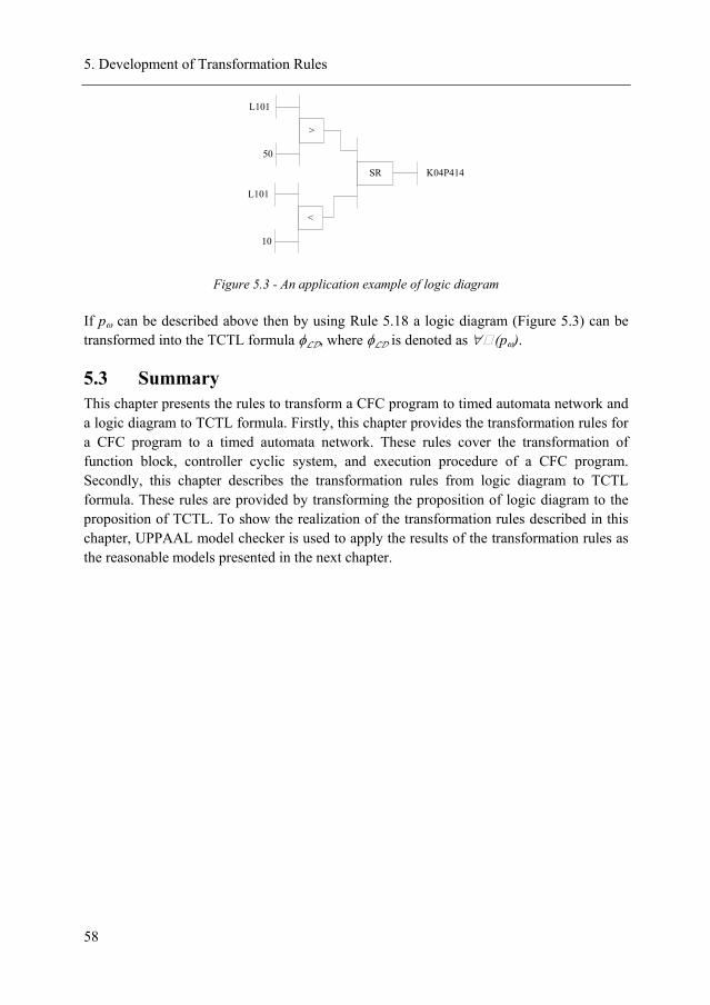
5. Development of Transformation Rules
58
K04P414SR
<
L101
10
>
L101
50
Figure 5.3 - An application example of logic diagram
If pω can be described above then by using Rule 5.18 a logic diagram (Figure 5.3) can be transformed into the TCTL formula φ LD, where φ LD is denoted as ∀ (pω).
5.3 Summary This chapter presents the rules to transform a CFC program to timed automata network and a logic diagram to TCTL formula. Firstly, this chapter provides the transformation rules for a CFC program to a timed automata network. These rules cover the transformation of function block, controller cyclic system, and execution procedure of a CFC program. Secondly, this chapter describes the transformation rules from logic diagram to TCTL formula. These rules are provided by transforming the proposition of logic diagram to the proposition of TCTL. To show the realization of the transformation rules described in this chapter, UPPAAL model checker is used to apply the results of the transformation rules as the reasonable models presented in the next chapter.
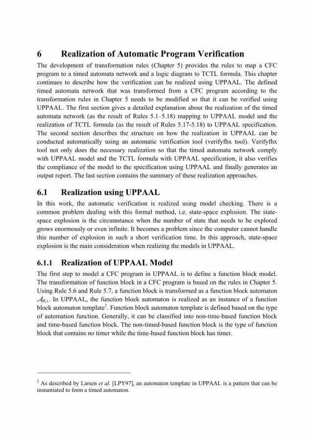
6 Realization of Automatic Program Verification The development of transformation rules (Chapter 5) provides the rules to map a CFC program to a timed automata network and a logic diagram to TCTL formula. This chapter continues to describe how the verification can be realized using UPPAAL. The defined timed automata network that was transformed from a CFC program according to the transformation rules in Chapter 5 needs to be modified so that it can be verified using UPPAAL. The first section gives a detailed explanation about the realization of the timed automata network (as the result of Rules 5.1–5.18) mapping to UPPAAL model and the realization of TCTL formula (as the result of Rules 5.17-5.18) to UPPAAL specification. The second section describes the structure on how the realization in UPPAAL can be conducted automatically using an automatic verification tool (verifyfhx tool). Verifyfhx tool not only does the necessary realization so that the timed automata network comply with UPPAAL model and the TCTL formula with UPPAAL specification, it also verifies the compliance of the model to the specification using UPPAAL and finally generates an output report. The last section contains the summary of these realization approaches.
6.1 Realization using UPPAAL In this work, the automatic verification is realized using model checking. There is a common problem dealing with this formal method, i.e. state-space explosion. The state-space explosion is the circumstance when the number of state that needs to be explored grows enormously or even infinite. It becomes a problem since the computer cannot handle this number of explosion in such a short verification time. In this approach, state-space explosion is the main consideration when realizing the models in UPPAAL.
6.1.1 Realization of UPPAAL Model The first step to model a CFC program in UPPAAL is to define a function block model. The transformation of function block in a CFC program is based on the rules in Chapter 5. Using Rule 5.6 and Rule 5.7, a function block is transformed as a function block automaton Afb,i.. In UPPAAL, the function block automaton is realized as an instance of a function block automaton template2. Function block automaton template is defined based on the type of automation function. Generally, it can be classified into non-time-based function block and time-based function block. The non-timed-based function block is the type of function block that contains no timer while the time-based function block has timer.
2 As described by Larsen et al. [LPY97], an automaton template in UPPAAL is a pattern that can be instantiated to form a timed automaton.
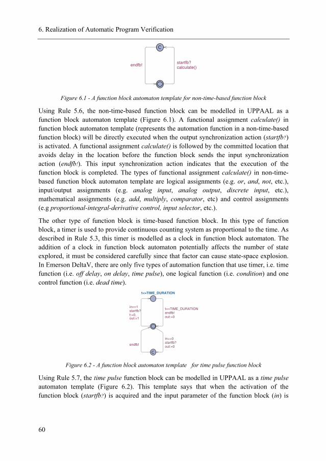
6. Realization of Automatic Program Verification
60
endfb! startfb?calculate()
Figure 6.1 - A function block automaton template for non-time-based function block
Using Rule 5.6, the non-time-based function block can be modelled in UPPAAL as a function block automaton template (Figure 6.1). A functional assignment calculate() in function block automaton template (represents the automation function in a non-time-based function block) will be directly executed when the output synchronization action (startfb?) is activated. A functional assignment calculate() is followed by the committed location that avoids delay in the location before the function block sends the input synchronization action (endfb!). This input synchronization action indicates that the execution of the function block is completed. The types of functional assignment calculate() in non-time-based function block automaton template are logical assignments (e.g. or, and, not, etc.), input/output assignments (e.g. analog input, analog output, discrete input, etc.), mathematical assignments (e.g. add, multiply, comparator, etc) and control assignments (e.g proportional-integral-derivative control, input selector, etc.).
The other type of function block is time-based function block. In this type of function block, a timer is used to provide continuous counting system as proportional to the time. As described in Rule 5.3, this timer is modelled as a clock in function block automaton. The addition of a clock in function block automaton potentially affects the number of state explored, it must be considered carefully since that factor can cause state-space explosion. In Emerson DeltaV, there are only five types of automation function that use timer, i.e. time function (i.e. off delay, on delay, time pulse), one logical function (i.e. condition) and one control function (i.e. dead time).
t<=TIME_DURATION
endfb!
in==0startfb?out:=0
t==TIME_DURATIONendfb!out:=0
in==1startfb?t:=0,out:=1
Figure 6.2 - A function block automaton template for time pulse function block
Using Rule 5.7, the time pulse function block can be modelled in UPPAAL as a time pulse automaton template (Figure 6.2). This template says that when the activation of the function block (startfb?) is acquired and the input parameter of the function block (in) is
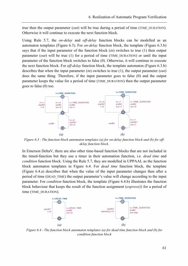
6. Realization of Automatic Program Verification
61
true then the output parameter (out) will be true during a period of time (TIME_DURATION). Otherwise it will continue to execute the next function block.
Using Rule 5.7, the on-delay and off-delay function blocks can be modelled as an automaton templates (Figure 6.3). For on-delay function block, the template (Figure 6.3.b) says that if the input parameter of the function block (in) switches to true (1) then output parameter (out) will be true (1) for a period of time (TIME_DURATION) or until the input parameter of the function block switches to false (0). Otherwise, it will continue to execute the next function block. For off-delay function block, the template automaton (Figure 6.3.b) describes that when the input parameter (in) switches to true (1), the output parameter (out) does the same thing. Therefore, if the input parameter goes to false (0) and the output parameter keeps the value for a period of time (TIME_DURATION) then the output parameter goes to false (0) too.
t<=TIME_DURATION
in==0endfb!out:=0
endfb!
in==0startfb?out:=0
t==TIME_DURATIONendfb!out:=1
in==1startfb?
t:=0
t<=TIME_DURATION
in==1endfb!out:=1
endfb!
in==1startfb?out:=1
t==TIME_DURATIONendfb!out:=0
in==0startfb?
t:=0
(a) (b)
Figure 6.3 - The function block automaton templates (a) for on-delay function block and (b) for off-delay function block.
In Emerson DeltaV, there are also other time-based function blocks that are not included in the timed-function but they use a timer in their automation function, i.e. dead time and condition function block. Using the Rule 5.7, they are modelled in UPPAAL as the function block automaton templates in Figure 6.4. For dead time function block, the template (Figure 6.4.a) describes that when the value of the input parameter changes then after a period of time (DEAD_TIME) the output parameter’s value will change according to the input parameter. For condition function block, the template (Figure 6.4.b) illustrates the function block behaviour that keeps the result of the function assignment (express()) for a period of time (TIME_DURATION).
t<=DEAD_TIME
t==DEAD_TIMEendfb!out:=in
startfb?t:=0
t<=TIME_DURATION
t==TIME_DURATIONendfb!out:=exp
startfb?express(),t:=0
(a) (b)
Figure 6.4 - The function block automaton templates (a) for dead time function block and (b) for condition function block
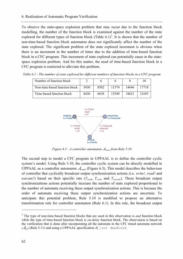
6. Realization of Automatic Program Verification
62
To observe the state-space explosion problem that may occur due to the function block modelling, the number of the function block is examined against the number of the state explored for different types of function block (Table 6.1)3. It is shown that the number of non-time-based function block automaton does not significantly affect the number of the state explored. The significant problem of the state explored increment is obvious when there is an increment in the number of timer due to the addition of time-based function block in a CFC program. This increment of state explored can potentially cause in the state-space explosion problem. And for this matter, the used of time-based function block in a CFC program is restricted to alleviate this problem.
Table 6.1 - The number of state explored for different numbers of function blocks in a CFC program
Number of function block 2 4 6 8 10
Non-time-based function block 5430 8502 11574 14646 17718
Time-based function block 4430 6638 15549 18621 21693
writingt<=Twrite
readingt<=Tread
executingt<=Texecute
t==Treadread!t:=0
t==Twritewrite!
t:=0
t==Texecuteexecute!t:=0
Figure 6.5 - A controller automaton Acontr from Rule 5.10
The second step to model a CFC program in UPPAAL is to define the controller cyclic system’s model. Using Rule 5.10, the controller cyclic system can be directly modelled in UPPAAL as a controller automaton Acontr (Figure 6.5). This model describes the behaviour of controller that cyclically broadcast output synchronization actions (i.e. write!, read! and execute!) based on their specific rate (Tread, Twrite and Texecute). These broadcast output synchronizations actions potentially increase the number of state explored proportional to the number of automata receiving these output synchronization actions. This is because the order of automata receiving these output synchronization actions are uncertain. To anticipate this potential problem, Rule 5.10 is modified to propose an alternative transformation rule for controller automaton (Rule 6.1). In this rule, the broadcast output
3 The type of non-time-based function blocks that are used in this observation is and function block while the type of time-based function block is on-delay function block. The observation is based on the verification that is done after incorporating all the automata in the CFC timed automata network |Acfc| (Rule 5.11) and using a UPPAAL specification A[]not deadlock.
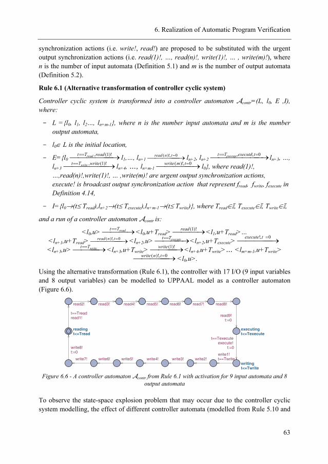
6. Realization of Automatic Program Verification
63
synchronization actions (i.e. write!, read!) are proposed to be substituted with the urgent output synchronization actions (i.e. read(1)!, …, read(n)!, write(1)!, … , write(m)!), where n is the number of input automata (Definition 5.1) and m is the number of output automata (Definition 5.2).
Rule 6.1 (Alternative transformation of controller cyclic system)
Controller cyclic system is transformed into a controller automaton Acontr=(L, l0, E ,I), where:
- L ={l0, l1, l2…, ln+m-1}, where n is the number input automata and m is the number output automata,
- l0∈ L is the initial location,
- E={l0 ⎯⎯⎯⎯⎯ →⎯ == )!1(,readTt read l1,…, ln+1 ⎯⎯⎯⎯ →⎯ =0,)!( tnread ln+2, ln+2 ⎯⎯⎯⎯⎯⎯ →⎯ === 0,!, texecuteTt execute ln+3, …, ln+3 ⎯⎯⎯⎯⎯ →⎯ == )!1(,writeTt write ln+4, …, ln+m-1 ⎯⎯⎯⎯ →⎯ =0,)!( tmwrite l0}, where read(1)!, …,read(n)!,write(1)!, … ,write(m)! are urgent output synchronization actions, execute! is broadcast output synchronization action that represent fread, fwrite, fexecute in Definition 4.14,
- I={l0→(t≤ Tread),ln+2→(t≤ Texecute),ln+m-1→(t≤ Twrite)}, where Tread∈I, Texecute∈I, Twrite∈I,
and a run of a controller automaton Acontr is:
<l0,u> ⎯⎯ →⎯ == readTt <l0,u+Tread> ⎯⎯ →⎯ )!1(read <l1,u+Tread>… <ln+1,u+Tread> ⎯⎯⎯⎯ →⎯ =0,)!( tnread <ln+2,u> ⎯⎯⎯ →⎯ == executeTt <ln+2,u+Texecute> ⎯⎯⎯⎯ →⎯ =0,! texecute
<ln+3,u> ⎯⎯⎯ →⎯ == writeTt <ln+3,u+Twrite> ⎯⎯⎯ →⎯ )!1(write <ln+4,u+Twrite>… <lm+m-1,u+Twrite>
⎯⎯⎯⎯ →⎯ =0,)!( tnwrite <l0,u>.
Using the alternative transformation (Rule 6.1), the controller with 17 I/O (9 input variables and 8 output variables) can be modelled to UPPAAL model as a controller automaton (Figure 6.6).
writingt<=Twrite
readingt<=Tread
executingt<=Texecute
t==Treadread1!
read2! read3! read4!
t==Twritewrite1!
write2!write3!
read9!t:=0
read8!read7!read6!read5!
write8!t:=0
write7! write6! write5! write4!
t==Texecuteexecute!
t:=0
Figure 6.6 - A controller automaton Acontr from Rule 6.1 with activation for 9 input automata and 8
output automata
To observe the state-space explosion problem that may occur due to the controller cyclic system modelling, the effect of different controller automata (modelled from Rule 5.10 and
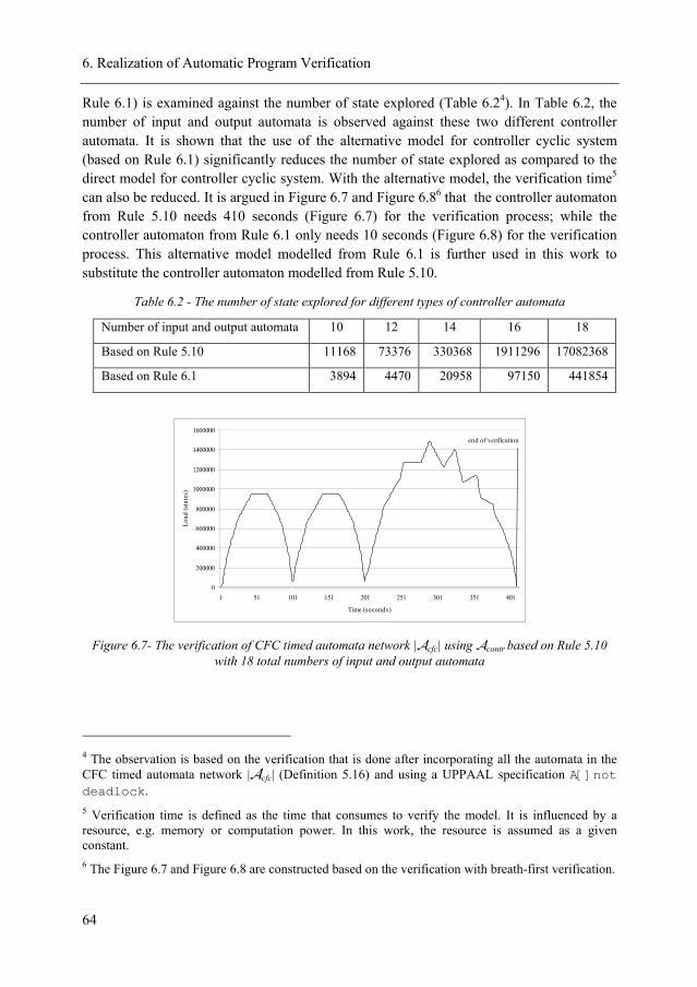
6. Realization of Automatic Program Verification
64
Rule 6.1) is examined against the number of state explored (Table 6.24). In Table 6.2, the number of input and output automata is observed against these two different controller automata. It is shown that the use of the alternative model for controller cyclic system (based on Rule 6.1) significantly reduces the number of state explored as compared to the direct model for controller cyclic system. With the alternative model, the verification time5 can also be reduced. It is argued in Figure 6.7 and Figure 6.86 that the controller automaton from Rule 5.10 needs 410 seconds (Figure 6.7) for the verification process; while the controller automaton from Rule 6.1 only needs 10 seconds (Figure 6.8) for the verification process. This alternative model modelled from Rule 6.1 is further used in this work to substitute the controller automaton modelled from Rule 5.10.
Table 6.2 - The number of state explored for different types of controller automata
Number of input and output automata 10 12 14 16 18
Based on Rule 5.10 11168 73376 330368 1911296 17082368
Based on Rule 6.1 3894 4470 20958 97150 441854
0
200000
400000
600000
800000
1000000
1200000
1400000
1600000
1 51 101 151 201 251 301 351 401
Time (seconds)
Load
(sta
tes)
end of verification
Figure 6.7- The verification of CFC timed automata network |Acfc| using Acontr based on Rule 5.10 with 18 total numbers of input and output automata
4 The observation is based on the verification that is done after incorporating all the automata in the CFC timed automata network |Acfc| (Definition 5.16) and using a UPPAAL specification A[]not deadlock. 5 Verification time is defined as the time that consumes to verify the model. It is influenced by a resource, e.g. memory or computation power. In this work, the resource is assumed as a given constant. 6 The Figure 6.7 and Figure 6.8 are constructed based on the verification with breath-first verification.
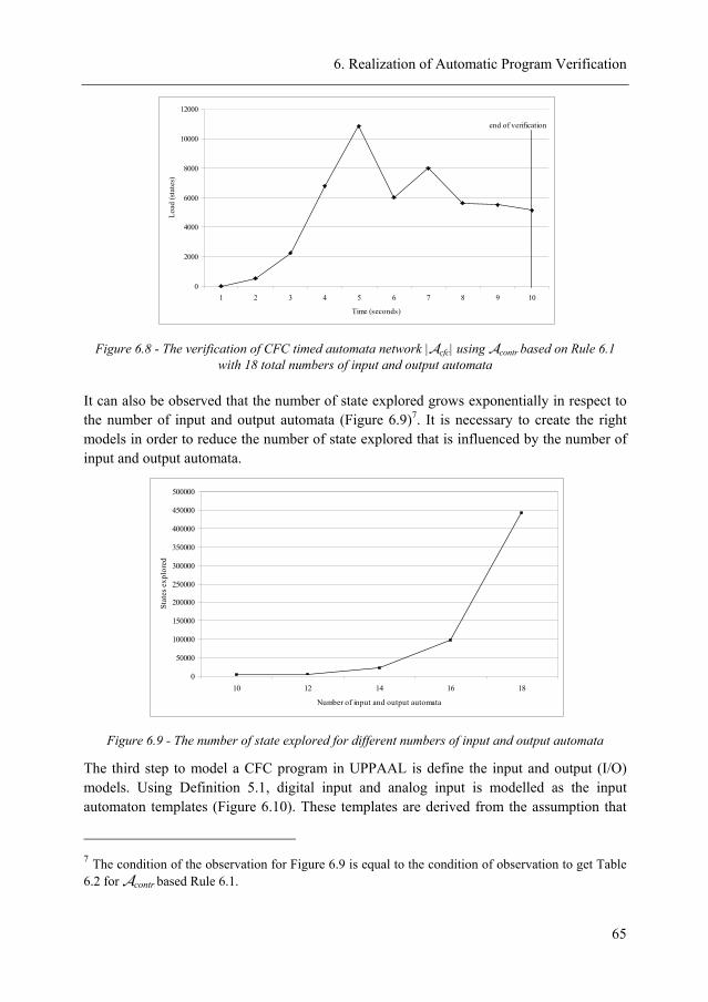
6. Realization of Automatic Program Verification
65
0
2000
4000
6000
8000
10000
12000
1 2 3 4 5 6 7 8 9 10
Time (seconds)
Load
(sta
tes)
end of verification
Figure 6.8 - The verification of CFC timed automata network |Acfc| using Acontr based on Rule 6.1 with 18 total numbers of input and output automata
It can also be observed that the number of state explored grows exponentially in respect to the number of input and output automata (Figure 6.9)7. It is necessary to create the right models in order to reduce the number of state explored that is influenced by the number of input and output automata.
0
50000
100000
150000
200000
250000
300000
350000
400000
450000
500000
10 12 14 16 18
Number of input and output automata
Stat
es e
xplo
red
Figure 6.9 - The number of state explored for different numbers of input and output automata
The third step to model a CFC program in UPPAAL is define the input and output (I/O) models. Using Definition 5.1, digital input and analog input is modelled as the input automaton templates (Figure 6.10). These templates are derived from the assumption that
7 The condition of the observation for Figure 6.9 is equal to the condition of observation to get Table 6.2 for Acontr based Rule 6.1.
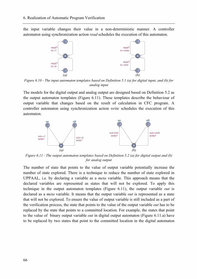
6. Realization of Automatic Program Verification
66
the input variable changes their value in a non-deterministic manner. A controller automaton using synchronization action read schedules the execution of this automaton.
read?in:=0
read?in:=1
read?in:=min
read?in:=max
(a) (b) Figure 6.10 - The input automaton templates based on Definition 5.1 (a) for digital input, and (b) for
analog input
The models for the digital output and analog output are designed based on Definition 5.2 as the output automaton templates (Figure 6.11). These templates describe the behaviour of output variable that changes based on the result of calculation in CFC program. A controller automaton using synchronization action write schedules the execution of this automaton.
on off
out==1write? out==0
write?
on off
out>minwrite?
out==minwrite?
(a) (b)
Figure 6.11 - The output automaton templates based on Definition 5.2 (a) for digital output and (b) for analog output
The number of state that points to the value of output variable potentially increase the number of state explored. There is a technique to reduce the number of state explored in UPPAAL, i.e. by declaring a variable as a meta variable. This approach means that the declared variables are represented as states that will not be explored. To apply this technique in the output automaton templates (Figure 6.11), the output variable out is declared as a meta variable. It means that the output variable out is represented as a state that will not be explored. To ensure the value of output variable is still included as a part of the verification process, the state that points to the value of the output variable out has to be replaced by the state that points to a committed location. For example, the states that point to the value of binary output variable out in digital output automaton (Figure 6.11.a) have to be replaced by two states that point to the committed location in the digital automaton
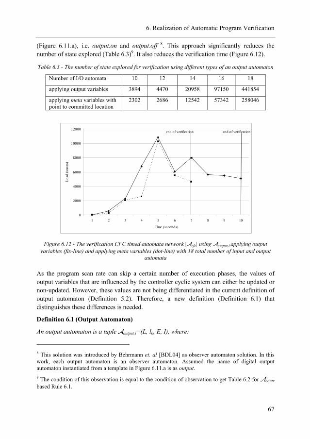
6. Realization of Automatic Program Verification
67
(Figure 6.11.a), i.e. output.on and output.off 8. This approach significantly reduces the number of state explored (Table 6.3)9. It also reduces the verification time (Figure 6.12).
Table 6.3 - The number of state explored for verification using different types of an output automaton
Number of I/O automata 10 12 14 16 18
applying output variables 3894 4470 20958 97150 441854
applying meta variables with point to committed location
2302 2686 12542 57342 258046
0
2000
4000
6000
8000
10000
12000
1 2 3 4 5 6 7 8 9 10
Time (seconds)
Load
(sta
tes)
end of verificationend of verification
Figure 6.12 - The verification CFC timed automata network |Acfc| using Aoutput,i applying output variables (fix-line) and applying meta variables (dot-line) with 18 total number of input and output
automata
As the program scan rate can skip a certain number of execution phases, the values of output variables that are influenced by the controller cyclic system can either be updated or non-updated. However, these values are not being differentiated in the current definition of output automaton (Definition 5.2). Therefore, a new definition (Definition 6.1) that distinguishes these differences is needed.
Definition 6.1 (Output Automaton)
An output automaton is a tuple Aoutput,i=(L, l0, E, I), where:
8 This solution was introduced by Behrmann et. al [BDL04] as observer automaton solution. In this work, each output automaton is an observer automaton. Assumed the name of digital output automaton instantiated from a template in Figure 6.11.a is as output. 9 The condition of this observation is equal to the condition of observation to get Table 6.2 for Acontr based Rule 6.1.
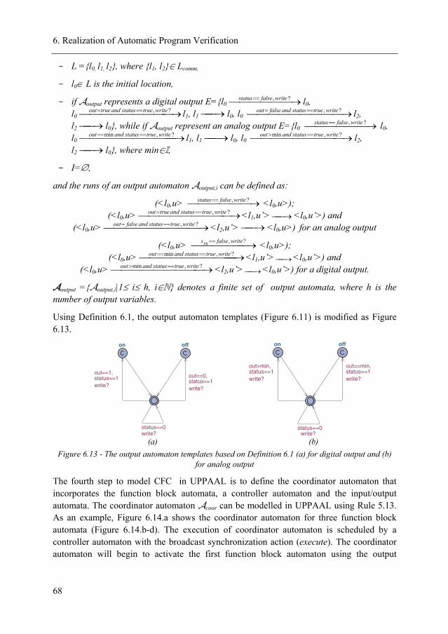
6. Realization of Automatic Program Verification
68
- L ={l0, l1, l2}, where {l1, l2}∈ Lcomm,
- l0∈ L is the initial location,
- if Aoutput represents a digital output E={l0 ⎯⎯⎯⎯⎯ →⎯ == ?, writefalsestatus l0, l0 ⎯⎯⎯⎯⎯⎯⎯⎯ →⎯ === ?, writetruestatusandtrueout l1, l1 ⎯→⎯ l0, l0 ⎯⎯⎯⎯⎯⎯⎯⎯ →⎯ === ?, writetruestatusandfalseout l2, l2 ⎯→⎯ l0}, while if Aoutput represent an analog output E={l0 ⎯⎯⎯⎯⎯ →⎯ == ?, writefalsestatus
l0, l0 ⎯⎯⎯⎯⎯⎯⎯⎯⎯ →⎯ ==== ?,min writetruestatusandout l1, l1 ⎯→⎯ l0, l0 ⎯⎯⎯⎯⎯⎯⎯⎯ →⎯ ==> ?,min writetruestatusandout l2, l2 ⎯→⎯ l0}, where min∈I,
- I=∅,
and the runs of an output automaton Aoutput,i can be defined as:
(<l0,u> ⎯⎯⎯⎯⎯ →⎯ == ?, writefalsestatus <l0,u>);
(<l0,u> ⎯⎯⎯⎯⎯⎯⎯⎯ →⎯ === ?, writetruestatusandtrueout <l1,u’> ⎯→⎯ <l0,u’>) and (<l0,u> ⎯⎯⎯⎯⎯⎯⎯⎯ →⎯ === ?, writetruestatusandfalseout <l2,u’> ⎯→⎯ <l0,u>) for an analog output
(<l0,u> ⎯⎯⎯⎯⎯ →⎯ == ?,writefalsespg <l0,u>);
(<l0,u> ⎯⎯⎯⎯⎯⎯⎯⎯⎯ →⎯ ==== ?,min writetruestatusandout <l1,u’> ⎯→⎯ <l0,u’>) and (<l0,u> ⎯⎯⎯⎯⎯⎯⎯⎯ →⎯ ==> ?,min writetruestatusandout <l2,u’> ⎯→⎯ <l0,u’>) for a digital output.
Aoutput ={Aoutput,i|1≤ i≤ h, i∈N} denotes a finite set of output automata, where h is the number of output variables.
Using Definition 6.1, the output automaton templates (Figure 6.11) is modified as Figure 6.13.
on off
status==0write?
out==1,status==1write?
out==0, status==1write?
on off
status==0write?
out>min,status==1write?
out==min, status==1write?
(a) (b)
Figure 6.13 - The output automaton templates based on Definition 6.1 (a) for digital output and (b) for analog output
The fourth step to model CFC in UPPAAL is to define the coordinator automaton that incorporates the function block automata, a controller automaton and the input/output automata. The coordinator automaton Acoor can be modelled in UPPAAL using Rule 5.13. As an example, Figure 6.14.a shows the coordinator automaton for three function block automata (Figure 6.14.b-d). The execution of coordinator automaton is scheduled by a controller automaton with the broadcast synchronization action (execute). The coordinator automaton will begin to activate the first function block automaton using the output
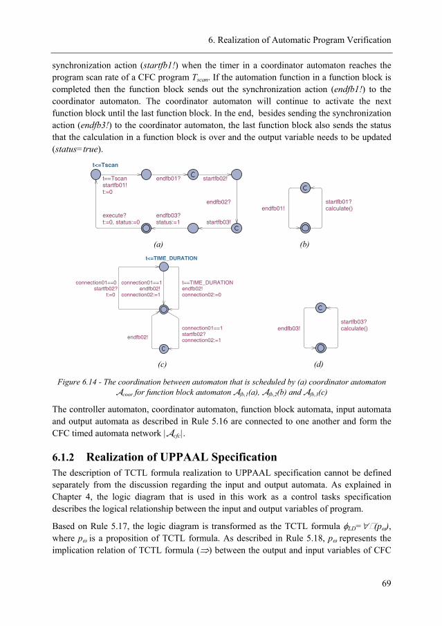
6. Realization of Automatic Program Verification
69
synchronization action (startfb1!) when the timer in a coordinator automaton reaches the program scan rate of a CFC program Tscan. If the automation function in a function block is completed then the function block sends out the synchronization action (endfb1!) to the coordinator automaton. The coordinator automaton will continue to activate the next function block until the last function block. In the end, besides sending the synchronization action (endfb3!) to the coordinator automaton, the last function block also sends the status that the calculation in a function block is over and the output variable needs to be updated (status=true).
t<=Tscan
t==Tscanstartfb01!t:=0
endfb01? startfb02!
endfb02?
startfb03!endfb03?status:=1
execute?t:=0, status:=0
endfb01!startfb01?calculate()
(a) (b)
t<=TIME_DURATION
connection01==1endfb02!
connection02:=1
endfb02!
connection01==1startfb02?connection02:=1
t==TIME_DURATIONendfb02!connection02:=0
connection01==0startfb02?
t:=0
endfb03!startfb03?calculate()
(c) (d)
Figure 6.14 - The coordination between automaton that is scheduled by (a) coordinator automaton Acoor for function block automaton Afb,1(a), Afb,2(b) and Afb,3(c)
The controller automaton, coordinator automaton, function block automata, input automata and output automata as described in Rule 5.16 are connected to one another and form the CFC timed automata network |Acfc|.
6.1.2 Realization of UPPAAL Specification The description of TCTL formula realization to UPPAAL specification cannot be defined separately from the discussion regarding the input and output automata. As explained in Chapter 4, the logic diagram that is used in this work as a control tasks specification describes the logical relationship between the input and output variables of program.
Based on Rule 5.17, the logic diagram is transformed as the TCTL formula φLD=∀ (pω), where pω is a proposition of TCTL formula. As described in Rule 5.18, pω represents the implication relation of TCTL formula (⇒) between the output and input variables of CFC
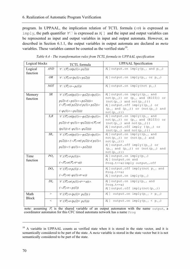
6. Realization of Automatic Program Verification
70
program. In UPPAAL, the implication relation of TCTL formula (⇒) is expressed as imply, the path quantifier ∀ is expressed as A[] and the input and output variables can be represented as input and output variables in input and output automata. However, as described in Section 6.1.1, the output variables in output automata are declared as meta variables. These variables cannot be counted as the verified state10.
Table 6.4 - The transformation rules from TCTL formula to UPPAAL specification
Logical blocks TCTL formula UPPAAL Specification AND ∀ (Po⇒(pi(1)∧ pi(2))) A[]output.on imply(pi,1 and pi,2)
OR ∀ (Po⇒ (pi(1) ∨ pi(2))) A[]output.on imply(pi,1 or pi,2)
Logical function NOT ∀ (Po⇒¬ pi(1)) A[]output.on imply(not pi,1)
SR ∀ (Po⇒((pi(1)∧¬pi(2))∨(pi(1)∧
pi(2)∨(¬ pi(1)∧¬ pi(2))))∧ (¬Po⇒(( pi(2))∨( pi(1)∧ pi(2))∨
(¬pi(1)∧¬ pi(2))))
A[]output.on imply((pi,1 and not(pi,2)) or (pi,1 and (B103)) or (not(pi,1) and not(pi,2))) A[]output.off imply((pi,2) or (pi,1 and (pi,2)) or (not(pi,1) and not(pi,2)))
SoR ∀ (Po⇒((pi(1)∧¬pi(2))∨(pi(1)∧
pi(2))∨(¬pi(1)∧¬pi(2))))∧(Po⇒(
(pi(1))∨(¬pi(1)∧¬pi(2))))
A[]output.on imply((pi,1 and not(pi,2)) or (pi,1 and (B103)) or (not(pi,1) and not(pi,2))) A[]output.off imply ((pi,2) or (not(pi,1) and not(pi,2)))
Memory function
SRo ∀ (Po⇒((pi(1)∧¬pi(2))∨(pi(1)∧
pi(2)))∧ (¬Po⇒(( pi(2))∨( pi(1)∧
pi(2))∨ (¬pi(1)∧¬ pi(2))))
A[]output.on imply((pi,1 and not(pi,2)) or (not(pi,1) and not(pi,2))) A[]output.off imply((pi,2) or (pi,1 and (pi,2)) or (not(pi,1) and not(pi,2)))
POa ∀ (Po⇒ pi(1))∧
(¬Po⇒(Po∧t=a))
A[]output.on imply(pi,1) A[](output.on and Prog.t==a)imply outputn.off
DOa ∀ (Po⇒ pi(1)) ∧
(¬Po⇒(¬pi(1)∧t=a ))
A[]output.off imply(not pi,1 and Prog.t==a) A[]output.on imply(pi,1)
Time function
DIa ∀ (Po⇒( pi(1)∧t==a))∧
(¬Po⇒¬ pi(1))
A[]output.on imply(pi,1 and Prog.t==a) A[]output.off imply(not(pi,1))
> ∀ (Po⇒ (pi(1) > pi(2)) ) A[] output.on imply(pi,1 > pi,2) Math Block < ∀ (Po⇒ (pi(2)< pi(1))) A[] output.on imply(pi,1 < pi,2)
note: assuming Po is the shared variable of an output automaton with the name output, a coordinator automaton for this CFC timed automata network has a name Prog
10 A variable in UPPAAL counts as verified state when it is stored in the state vector, and it is semantically considered to be part of the state. A meta variable is stored in the state vector but it is not semantically considered to be part of the state.
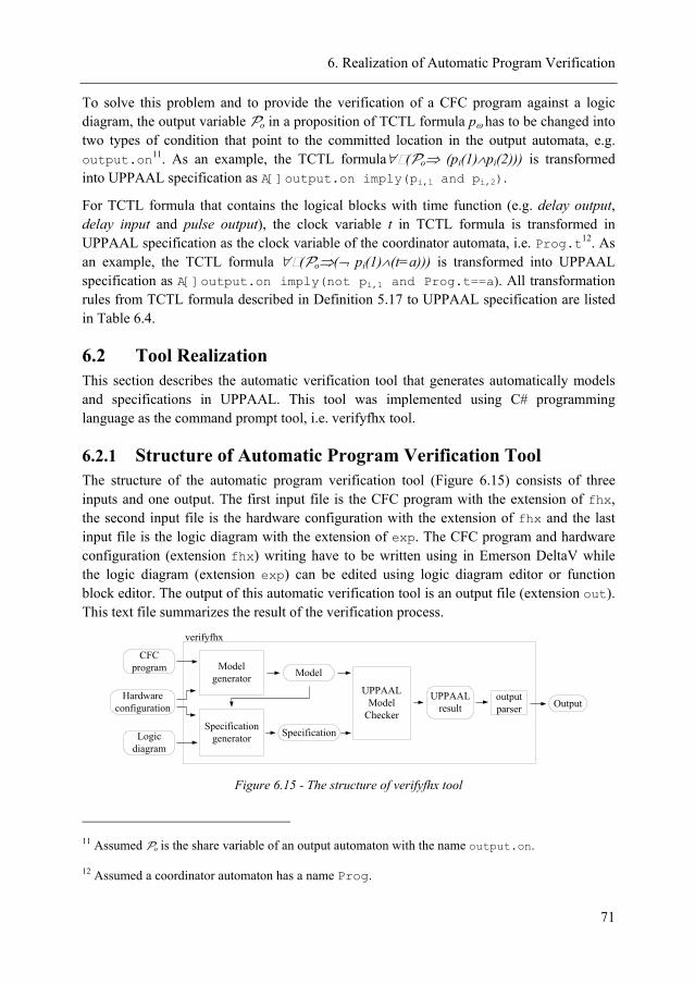
6. Realization of Automatic Program Verification
71
To solve this problem and to provide the verification of a CFC program against a logic diagram, the output variable Po in a proposition of TCTL formula pω has to be changed into two types of condition that point to the committed location in the output automata, e.g. output.on11. As an example, the TCTL formula∀ (Po⇒ (pi(1)∧pi(2))) is transformed into UPPAAL specification as A[]output.on imply(pi,1 and pi,2).
For TCTL formula that contains the logical blocks with time function (e.g. delay output, delay input and pulse output), the clock variable t in TCTL formula is transformed in UPPAAL specification as the clock variable of the coordinator automata, i.e. Prog.t12. As an example, the TCTL formula ∀ (Po⇒(¬ pi(1)∧(t=a))) is transformed into UPPAAL specification as A[]output.on imply(not pi,1 and Prog.t==a). All transformation rules from TCTL formula described in Definition 5.17 to UPPAAL specification are listed in Table 6.4.
6.2 Tool Realization This section describes the automatic verification tool that generates automatically models and specifications in UPPAAL. This tool was implemented using C# programming language as the command prompt tool, i.e. verifyfhx tool.
6.2.1 Structure of Automatic Program Verification Tool The structure of the automatic program verification tool (Figure 6.15) consists of three inputs and one output. The first input file is the CFC program with the extension of fhx, the second input file is the hardware configuration with the extension of fhx and the last input file is the logic diagram with the extension of exp. The CFC program and hardware configuration (extension fhx) writing have to be written using in Emerson DeltaV while the logic diagram (extension exp) can be edited using logic diagram editor or function block editor. The output of this automatic verification tool is an output file (extension out). This text file summarizes the result of the verification process.
CFC program
Hardware configuration
Logic diagram
Model generator
Specification generator
Model
Specification
UPPAALModel
Checker
UPPAAL result
output parser Output
verifyfhx
Figure 6.15 - The structure of verifyfhx tool
11 Assumed Po is the share variable of an output automaton with the name output.on.
12 Assumed a coordinator automaton has a name Prog.
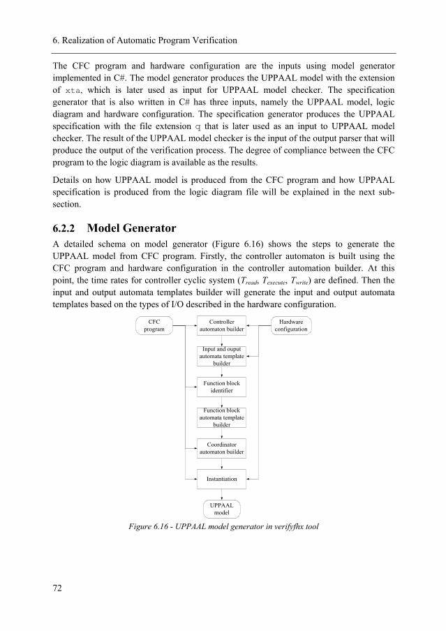
6. Realization of Automatic Program Verification
72
The CFC program and hardware configuration are the inputs using model generator implemented in C#. The model generator produces the UPPAAL model with the extension of xta, which is later used as input for UPPAAL model checker. The specification generator that is also written in C# has three inputs, namely the UPPAAL model, logic diagram and hardware configuration. The specification generator produces the UPPAAL specification with the file extension q that is later used as an input to UPPAAL model checker. The result of the UPPAAL model checker is the input of the output parser that will produce the output of the verification process. The degree of compliance between the CFC program to the logic diagram is available as the results.
Details on how UPPAAL model is produced from the CFC program and how UPPAAL specification is produced from the logic diagram file will be explained in the next sub-section.
6.2.2 Model Generator A detailed schema on model generator (Figure 6.16) shows the steps to generate the UPPAAL model from CFC program. Firstly, the controller automaton is built using the CFC program and hardware configuration in the controller automation builder. At this point, the time rates for controller cyclic system (Tread, Texecute, Twrite) are defined. Then the input and output automata templates builder will generate the input and output automata templates based on the types of I/O described in the hardware configuration.
CFC program
Hardware configuration
Controller automaton builder
Input and ouput automata template
builder
Function block identifier
Function block automata template
builder
Coordinator automaton builder
Instantiation
UPPAAL model
Figure 6.16 - UPPAAL model generator in verifyfhx tool
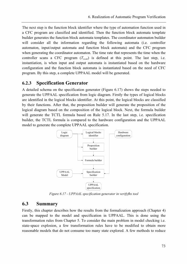
6. Realization of Automatic Program Verification
73
The next step is the function block identifier where the type of automation function used in a CFC program are classified and identified. Then the function block automata template builder generates the function block automata templates. The coordinator automaton builder will consider all the information regarding the following automata (i.e. controller automaton, input/output automata and function block automata) and the CFC program when generating the coordinator automaton. The time rate that represents the time when the controller scans a CFC program (Tscan) is defined at this point. The last step, i.e. instantiation, is when input and output automata is instantiated based on the hardware configuration and the function block automata is instantiated based on the need of CFC program. By this step, a complete UPPAAL model will be generated.
6.2.3 Specification Generator A detailed schema on the specification generator (Figure 6.17) shows the steps needed to generate the UPPAAL specification from logic diagram. Firstly the types of logical blocks are identified in the logical blocks identifier. At this point, the logical blocks are classified by their functions. After that, the proposition builder will generate the proposition of the logical diagram based on the composition of the logical block. Next, the formula builder will generate the TCTL formula based on Rule 5.17. In the last step, i.e. specification builder, the TCTL formula is compared to the hardware configuration and the UPPAAL model to generate the complete UPPAAL specification.
Logic diagram
Hardware configuration
Logical blocks identifier
Proposition builder
Formula builder
Specification builder
UPPAAL specification
UPPAAL Model
Figure 6.17 - UPPAAL specification generator in verifyfhx tool
6.3 Summary Firstly, this chapter describes how the results from the formalization approach (Chapter 4) can be mapped to the model and specification in UPPAAL. This is done using the transformation rules from Chapter 5. To consider the main problem in model checking i.e. state-space explosion, a few transformation rules have to be modified to obtain more reasonable models that do not consume too many state explored. A few methods to reduce
6. Realization of Automatic Program Verification
74
the number of state explored are used in this work, i.e. the use of urgent synchronization action instead of the use of broadcast synchronization action, the use of meta variable and the use of observer automaton.
Secondly, this chapter presents the automatic program verification tool of CFC based on model checking. To evaluate the applicability of this automatic program verification tool, this tool has been implemented in two case studies. These case studies will be discussed in the next chapter.
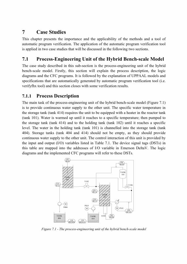
7 Case Studies This chapter presents the importance and the applicability of the methods and a tool of automatic program verification. The application of the automatic program verification tool is applied in two case studies that will be discussed in the following two sections.
7.1 Process-Engineering Unit of the Hybrid Bench-scale Model The case study described in this sub-section is the process-engineering unit of the hybrid bench-scale model. Firstly, this section will explain the process description, the logic diagrams and the CFC programs. It is followed by the explanation of UPPAAL models and specifications that are automatically generated by automatic program verification tool (i.e. verifyfhx tool) and this section closes with some verification results.
7.1.1 Process Description The main task of the process-engineering unit of the hybrid bench-scale model (Figure 7.1) is to provide continuous water supply to the other unit. The specific water temperature in the storage tank (tank 414) requires the unit to be equipped with a heater in the reactor tank (tank 101). Water is warmed up until it reaches to a specific temperature; then pumped to the storage tank (tank 414) and to the holding tank (tank 102) until it reaches a specific level. The water in the holding tank (tank 101) is channelled into the storage tank (tank 404). Storage tanks (tank 404 and 414) should not be empty, as they should provide continuous water supply to the other unit. The control interaction of this unit is provided by the input and output (I/O) variables listed in Table 7.1. The device signal tags (DSTs) in this table are mapped into the addresses of I/O variable in Emerson DeltaV. The logic diagrams and the implemented CFC programs will refer to these DSTs.
P101
E104
TANK 101
TANK 103
V102
V106
M
TANK 414
TANK 404
P414P404
M M
TANK 102
LS+
LS-
TIC
LS-
LIC
LS-LS-
FIC
PIC
DF101
B103
B104
B02414
B113
B114
S112
B101
B02404
Figure 7.1 - The process-engineering unit of the hybrid bench-scale model
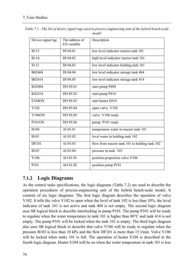
7. Case Studies
76
Table 7.1 - The list of device signal tags used in process-engineering unit of the hybrid bench-scale model
Device signal tag The address of I/O variable
Description
B113 DI 04.01 low level indicator reactor tank 101
B114 DI 04.02 high level indicator reactor tank 101
S112 DI 04.03 low level indicator holding tank 101
B02404 DI 04.04 low level indicator storage tank 404
B02414 DI 04.05 low level indicator storage tank 414
K02404 DO 05.01 start pump P404
K02414 DO 05.02 start pump P414
E104ON DO 05.03 start heater E014
Y102 DO 05.04 open valve V102
Y106ON DO 05.05 valve V106 ready
P101ON DO 05.06 pump P101 ready
B104 AI 03.01 temperature water in reactor tank 101
B101 AI 03.02 level water in holding tank 102
DF101 AI 03.03 flow from reactor tank 101 to holding tank 102
B103 AI 03.04 pressure in tank 103
Y106 AO 01.01 position proportion valve V106
P101 AO 01.02 position pump P101
7.1.2 Logic Diagrams As the control tasks specifications, the logic diagrams (Table 7.2) are used to describe the operation procedures of process-engineering unit of the hybrid bench-scale model. It consists of six logic diagrams. The first logic diagram describes the operation of valve V102. It tells the valve V102 to open when the level of tank 102 is less than 10%, the level indicator of tank 101 is not active and tank 404 is not empty. The second logic diagram uses SR logical block to describe interlocking in pump P101. The pump P101 will be ready to regulate when the water temperature in tank 101 is higher than 80°C and tank 414 is not empty. The pump P101 will be locked when the tank 101 is empty. The third logic diagram also uses SR logical block to describe that valve V106 will be ready to regulate when the pressure B103 is less than 10 kPa and the flow DF101 is more than 15 l/min. Valve V106 will be locked when tanks 101 is full. The operation of heater E104 is described in the fourth logic diagram. Heater E104 will be on when the water temperature in tank 101 is less
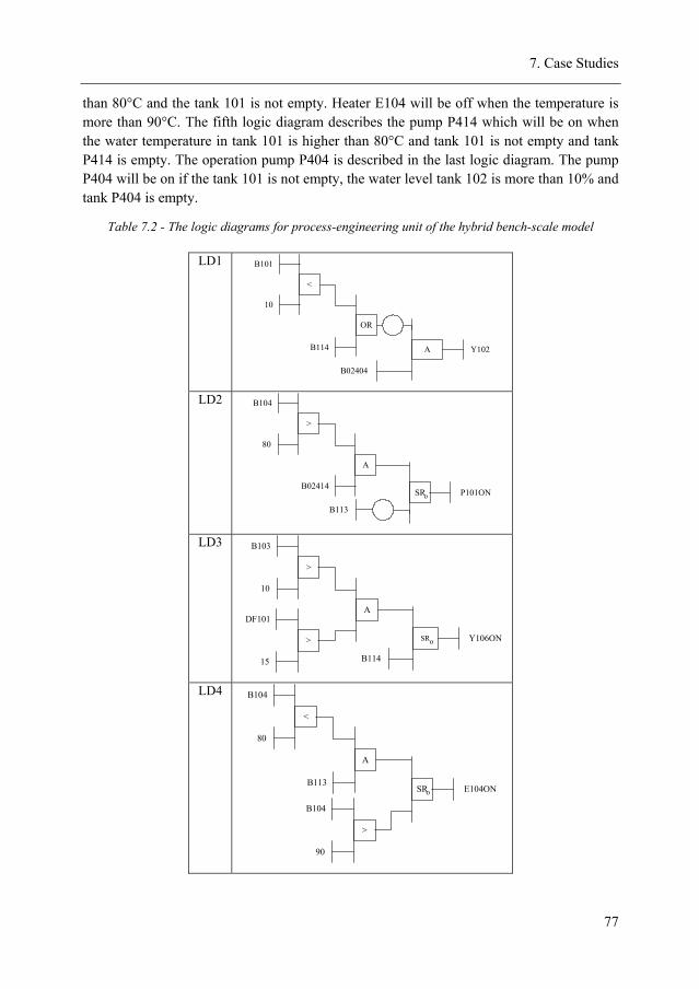
7. Case Studies
77
than 80°C and the tank 101 is not empty. Heater E104 will be off when the temperature is more than 90°C. The fifth logic diagram describes the pump P414 which will be on when the water temperature in tank 101 is higher than 80°C and tank 101 is not empty and tank P414 is empty. The operation pump P404 is described in the last logic diagram. The pump P404 will be on if the tank 101 is not empty, the water level tank 102 is more than 10% and tank P404 is empty.
Table 7.2 - The logic diagrams for process-engineering unit of the hybrid bench-scale model
LD1
<
B101
10
B114
OR
A Y102
B02404
LD2 B104
80
A
SR
B113
P101ON
>
B02414o
LD3
B103
10
A
SR
B114
Y106ON
>
DF101
15
> o
LD4 B104
80
A
SR E104ON
<
B113
B104
90
>
o
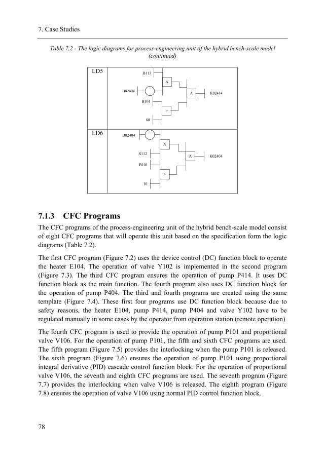
7. Case Studies
78
Table 7.2 - The logic diagrams for process-engineering unit of the hybrid bench-scale model (continued)
LD5 B113
B02404 A K02414
A
B104
80
>
LD6 B02404
S112 A K02404
A
B101
10
>
7.1.3 CFC Programs The CFC programs of the process-engineering unit of the hybrid bench-scale model consist of eight CFC programs that will operate this unit based on the specification form the logic diagrams (Table 7.2).
The first CFC program (Figure 7.2) uses the device control (DC) function block to operate the heater E104. The operation of valve Y102 is implemented in the second program (Figure 7.3). The third CFC program ensures the operation of pump P414. It uses DC function block as the main function. The fourth program also uses DC function block for the operation of pump P404. The third and fourth programs are created using the same template (Figure 7.4). These first four programs use DC function block because due to safety reasons, the heater E104, pump P414, pump P404 and valve Y102 have to be regulated manually in some cases by the operator from operation station (remote operation)
The fourth CFC program is used to provide the operation of pump P101 and proportional valve V106. For the operation of pump P101, the fifth and sixth CFC programs are used. The fifth program (Figure 7.5) provides the interlocking when the pump P101 is released. The sixth program (Figure 7.6) ensures the operation of pump P101 using proportional integral derivative (PID) cascade control function block. For the operation of proportional valve V106, the seventh and eighth CFC programs are used. The seventh program (Figure 7.7) provides the interlocking when valve V106 is released. The eighth program (Figure 7.8) ensures the operation of valve V106 using normal PID control function block.
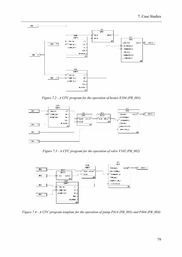
7. Case Studies
79
Figure 7.2 - A CFC program for the operation of heater E104 (PB_001)
Figure 7.3 - A CFC program for the operation of valve V102 (PB_002)
Figure 7.4 - A CFC program template for the operation of pump P414 (PB_003) and P404 (PB_004)
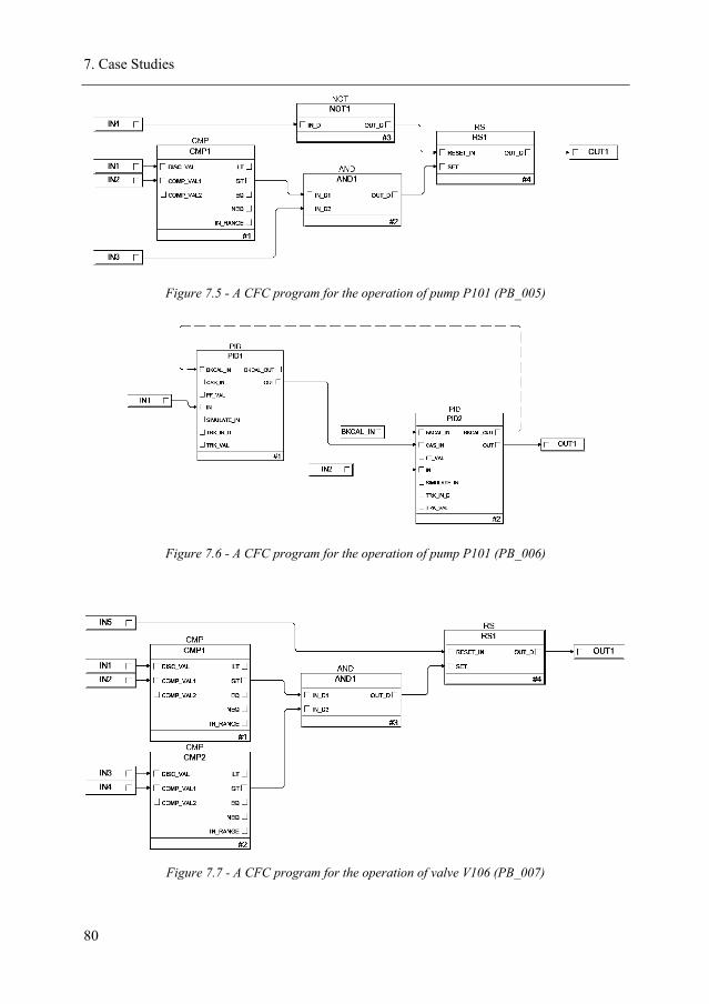
7. Case Studies
80
Figure 7.5 - A CFC program for the operation of pump P101 (PB_005)
Figure 7.6 - A CFC program for the operation of pump P101 (PB_006)
Figure 7.7 - A CFC program for the operation of valve V106 (PB_007)
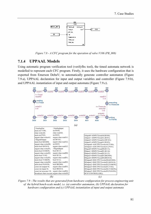
7. Case Studies
81
Figure 7.8 - A CFC program for the operation of valve V106 (PB_008)
7.1.4 UPPAAL Models Using automatic program verification tool (verifyfhx tool), the timed automata network is modelled to represent each CFC program. Firstly, it uses the hardware configuration that is exported from Emerson DeltaV; to automatically generate controller automaton (Figure 7.9.a), UPPAAL declaration for input and output variables and controller (Figure 7.9.b), and UPPAAL instantiation of input and output automata (Figure 7.9.c).
AI0 AI1 AI2 AI3
AO0AO1
DI0DI1DI2DI3
DO0 DO1 DO2 DO3 DO4
writingt<=Twrite
readingt<=Tread executing
t<=Texecute
t==TreadreadA0!
readA1! readA2! readA3!
t==TwritewriteA0!
writeA1!writeD0!
readD1!t:=0
readD2!readD3!readD4!readD0!
writeD1!t:=0
writeD2! writeD3! writeD4! writeD5!
t==Texecuteexecute!
t:=0
(a)
//AnalogOutmeta int Y106; chan writeA0;meta int P101; urgent chan writeA1;//DigitalOutputmeta bool K02404; urgent chan writeD0;meta bool K02414; urgent chan writeD1;meta bool E104ON; urgent chan writeD2;meta bool Y102; urgent chan writeD3;meta bool Y106ON; urgent chan writeD4;meta bool P101ON; const int toutput=0;const int tinput=0;const int texecute=10;broadcast chan execute;
//AnalogInputint B104; chan readA0;int B101; urgent chan readA1;int DF101; urgent chan readA2;int B103; urgent chan readA3;//DigitalInputbool B113; urgent chan readD0;bool B114; urgent chan readD1;bool S112; urgent chan readD2;bool B02404; urgent chan readD3;bool B02414; urgent chan readD4;urgent chan writeD5;
AInput0=AINPUT(readA0,B104);AInput1=AINPUT(readA1,B101);AInput2=AINPUT(readA2,DF101);AInput3=AINPUT(readA3,B103);AOutput0=AOUTPUT(writeA0,Y106);AOutput1=AOUTPUT(writeA1,P101);DInput0=DINPUT(readD0,B113);DInput1=DINPUT(readD1,B114);DInput2=DINPUT(readD2,S112);DInput3=DINPUT(readD3,B02404);DInput4=DINPUT(readD4,B02414);DOutput0=DOUTPUT(writeD0,K02404);DOutput1=DOUTPUT(writeD1,K02414);DOutput2=DOUTPUT(writeD2,E104ON);DOutput3=DOUTPUT(writeD3,Y102);DOutput4=DOUTPUT(writeD4,Y106ON);DOutput5=DOUTPUT(writeD5,P101ON);DCS=CONTROLLER();
(b) (c) Figure 7.9 - The results that are generated from hardware configuration for process-engineering unit
of the hybrid bench-scale model, i.e. (a) controller automaton, (b) UPPAAL declaration for hardware configuration and (c) UPPAAL instantiation of input and output automata
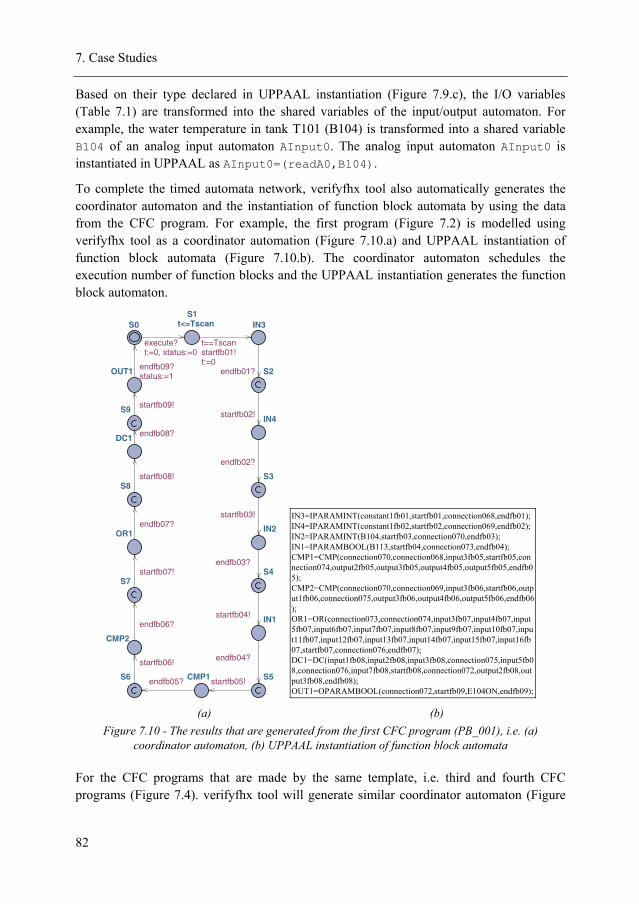
7. Case Studies
82
Based on their type declared in UPPAAL instantiation (Figure 7.9.c), the I/O variables (Table 7.1) are transformed into the shared variables of the input/output automaton. For example, the water temperature in tank T101 (B104) is transformed into a shared variable B104 of an analog input automaton AInput0. The analog input automaton AInput0 is instantiated in UPPAAL as AInput0=(readA0,B104).
To complete the timed automata network, verifyfhx tool also automatically generates the coordinator automaton and the instantiation of function block automata by using the data from the CFC program. For example, the first program (Figure 7.2) is modelled using verifyfhx tool as a coordinator automation (Figure 7.10.a) and UPPAAL instantiation of function block automata (Figure 7.10.b). The coordinator automaton schedules the execution number of function blocks and the UPPAAL instantiation generates the function block automaton.
S0 IN3S1
t<=Tscan
IN4
S2
IN2
S3
IN1
S4
CMP1 S5
CMP2
S6
OR1
S7
DC1
S8
OUT1
S9
t==Tscanstartfb01!t:=0
endfb01?
startfb02!
endfb02?
startfb03!
endfb03?
startfb04!
endfb04?
startfb05!endfb05?
startfb06!
endfb06?
startfb07!
endfb07?
startfb08!
endfb08?
startfb09!
endfb09?status:=1
execute?t:=0, status:=0
IN3=IPARAMINT(constant1fb01,startfb01,connection068,endfb01);IN4=IPARAMINT(constant1fb02,startfb02,connection069,endfb02);IN2=IPARAMINT(B104,startfb03,connection070,endfb03);IN1=IPARAMBOOL(B113,startfb04,connection073,endfb04);CMP1=CMP(connection070,connection068,input3fb05,startfb05,connection074,output2fb05,output3fb05,output4fb05,output5fb05,endfb05);CMP2=CMP(connection070,connection069,input3fb06,startfb06,output1fb06,connection075,output3fb06,output4fb06,output5fb06,endfb06);OR1=OR(connection073,connection074,input3fb07,input4fb07,input5fb07,input6fb07,input7fb07,input8fb07,input9fb07,input10fb07,input11fb07,input12fb07,input13fb07,input14fb07,input15fb07,input16fb07,startfb07,connection076,endfb07);DC1=DC(input1fb08,input2fb08,input3fb08,connection075,input5fb08,connection076,input7fb08,startfb08,connection072,output2fb08,output3fb08,endfb08);OUT1=OPARAMBOOL(connection072,startfb09,E104ON,endfb09);
(a) (b) Figure 7.10 - The results that are generated from the first CFC program (PB_001), i.e. (a)
coordinator automaton, (b) UPPAAL instantiation of function block automata
For the CFC programs that are made by the same template, i.e. third and fourth CFC programs (Figure 7.4). verifyfhx tool will generate similar coordinator automaton (Figure
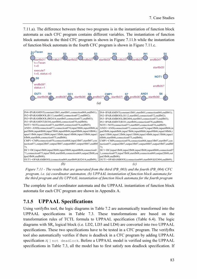
7. Case Studies
83
7.11.a). The difference between these two programs is in the instantiation of function block automata as each CFC program contains different variables. The instantiation of function block automata in the third CFC program is shown in Figure 7.11.b while the instantiation of function block automata in the fourth CFC program is shown in Figure 7.11.c.
S0
IN4S1t<=Tscan
IN2S2 IN3S3 IN1S4
NOT1
S5
AND1 S6CMP1 S7DC1 S8OUT1 S9
t==Tscanstartfb01!
t:=0
endfb01? startfb02! endfb02? startfb03! endfb03? startfb04! endfb04?
startfb05!
endfb05?
startfb06!endfb06?startfb07!endfb07?startfb08!endfb08?startfb09!
endfb09?status:=1
execute?t:=0, status:=0
(a)
IN4=IPARAMINT(constant1fb01,startfb01,connection068,endfb01);IN2=IPARAMBOOL(B113,startfb02,connection072,endfb02);IN3=IPARAMBOOL(B02414,startfb03,connection073,endfb03);IN1=IPARAMINT(B104,startfb04,connection070,endfb04);NOT1=NOT(connection073,startfb05,connection074,endfb05);AND1=AND(connection072,connection074,input3fb06,input4fb06,input5fb06,input6fb06,input7fb06,input8fb06,input9fb06,input10fb06,input11fb06,input12fb06,input13fb06,input14fb06,input15fb06,input16fb06,startfb06,connection075,endfb06);CMP1=CMP(connection070,connection068,input3fb07,startfb07,connection071,output2fb07,output3fb07,output4fb07,output5fb07,endfb07);DC1=DC(input1fb08,input2fb08,input3fb08,input4fb08,connection071,connection075,input7fb08,startfb08,connection069,output2fb08,output3fb08,endfb08);OUT1=OPARAMBOOL(connection069,startfb09,K02414,endfb09);
IN4=IPARAMINT(constant1fb01,startfb01,connection068,endfb01);IN2=IPARAMBOOL(S112,startfb02,connection072,endfb02);IN3=IPARAMBOOL(B02404,startfb03,connection073,endfb03);IN1=IPARAMINT(B101,startfb04,connection070,endfb04);NOT1=NOT(connection073,startfb05,connection074,endfb05);AND1=AND(connection072,connection074,input3fb06,input4fb06,input5fb06,input6fb06,input7fb06,input8fb06,input9fb06,input10fb06,input11fb06,input12fb06,input13fb06,input14fb06,input15fb06,input16fb06,startfb06,connection075,endfb06);CMP1=CMP(connection070,connection068,input3fb07,startfb07,connection071,output2fb07,output3fb07,output4fb07,output5fb07,endfb07);DC1=DC(input1fb08,input2fb08,input3fb08,input4fb08,connection071,connection075,input7fb08,startfb08,connection069,output2fb08,output3fb08,endfb08);OUT1=OPARAMBOOL(connection069,startfb09,K02404,endfb09);
(b) (c) Figure 7.11 - The results that are generated from the third (PB_003) and the fourth (PB_004) CFC program, i.e. (a) coordinator automaton, (b) UPPAAL instantiation of function block automata for the third program and (b) UPPAAL instantiation of function block automata for the fourth program
The complete list of coordinator automata and the UPPAAL instantiation of function block automata for each CFC program are shown in Appendix A.
7.1.5 UPPAAL Specifications Using verifyfhx tool, the logic diagrams in Table 7.2 are automatically transformed into the UPPAAL specifications in Table 7.3. These transformations are based on the transformation rules of TCTL formula to UPPAAL specification (Table 6.4). The logic diagrams with SRo logical block (i.e. LD2, LD3 and LD4) are converted into two UPPAAL specifications. These two specifications have to be tested in a CFC program. The verifyfhx tool also automatically verifies if there is deadlock in a CFC program by adding UPPAAL specification A[]not deadlock. Before a UPPAAL model is verified using the UPPAAL specifications in Table 7.3, all the model has to first satisfy non deadlock specification. If
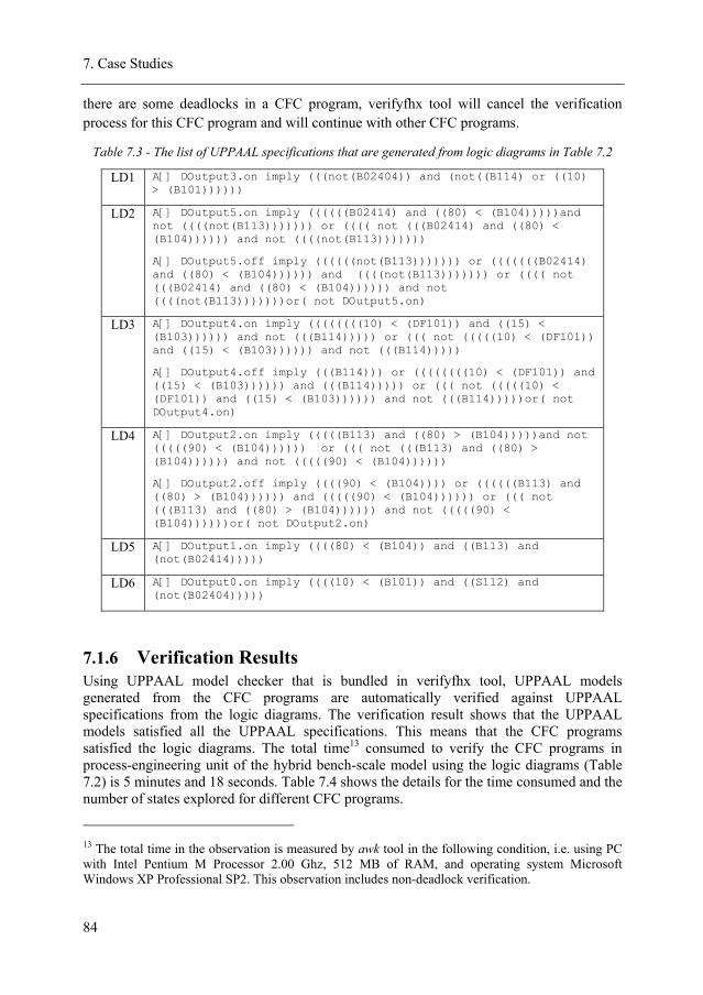
7. Case Studies
84
there are some deadlocks in a CFC program, verifyfhx tool will cancel the verification process for this CFC program and will continue with other CFC programs.
Table 7.3 - The list of UPPAAL specifications that are generated from logic diagrams in Table 7.2
LD1 A[] DOutput3.on imply (((not(B02404)) and (not((B114) or ((10) > (B101))))))
LD2 A[] DOutput5.on imply ((((((B02414) and ((80) < (B104)))))and not ((((not(B113))))))) or (((( not (((B02414) and ((80) < (B104)))))) and not ((((not(B113)))))))
A[] DOutput5.off imply ((((((not(B113))))))) or (((((((B02414) and ((80) < (B104)))))) and ((((not(B113))))))) or (((( not (((B02414) and ((80) < (B104)))))) and not ((((not(B113)))))))or( not DOutput5.on)
LD3 A[] DOutput4.on imply ((((((((10) < (DF101)) and ((15) < (B103)))))) and not (((B114))))) or ((( not (((((10) < (DF101)) and ((15) < (B103)))))) and not (((B114)))))
A[] DOutput4.off imply (((B114))) or ((((((((10) < (DF101)) and ((15) < (B103)))))) and (((B114))))) or ((( not (((((10) < (DF101)) and ((15) < (B103)))))) and not (((B114)))))or( not DOutput4.on)
LD4 A[] DOutput2.on imply (((((B113) and ((80) > (B104)))))and not (((((90) < (B104)))))) or ((( not (((B113) and ((80) > (B104)))))) and not (((((90) < (B104))))))
A[] DOutput2.off imply ((((90) < (B104)))) or ((((((B113) and ((80) > (B104)))))) and (((((90) < (B104)))))) or ((( not (((B113) and ((80) > (B104)))))) and not (((((90) < (B104))))))or( not DOutput2.on)
LD5 A[] DOutput1.on imply ((((80) < (B104)) and ((B113) and (not(B02414)))))
LD6 A[] DOutput0.on imply ((((10) < (B101)) and ((S112) and (not(B02404)))))
7.1.6 Verification Results Using UPPAAL model checker that is bundled in verifyfhx tool, UPPAAL models generated from the CFC programs are automatically verified against UPPAAL specifications from the logic diagrams. The verification result shows that the UPPAAL models satisfied all the UPPAAL specifications. This means that the CFC programs satisfied the logic diagrams. The total time13 consumed to verify the CFC programs in process-engineering unit of the hybrid bench-scale model using the logic diagrams (Table 7.2) is 5 minutes and 18 seconds. Table 7.4 shows the details for the time consumed and the number of states explored for different CFC programs.
13 The total time in the observation is measured by awk tool in the following condition, i.e. using PC with Intel Pentium M Processor 2.00 Ghz, 512 MB of RAM, and operating system Microsoft Windows XP Professional SP2. This observation includes non-deadlock verification.
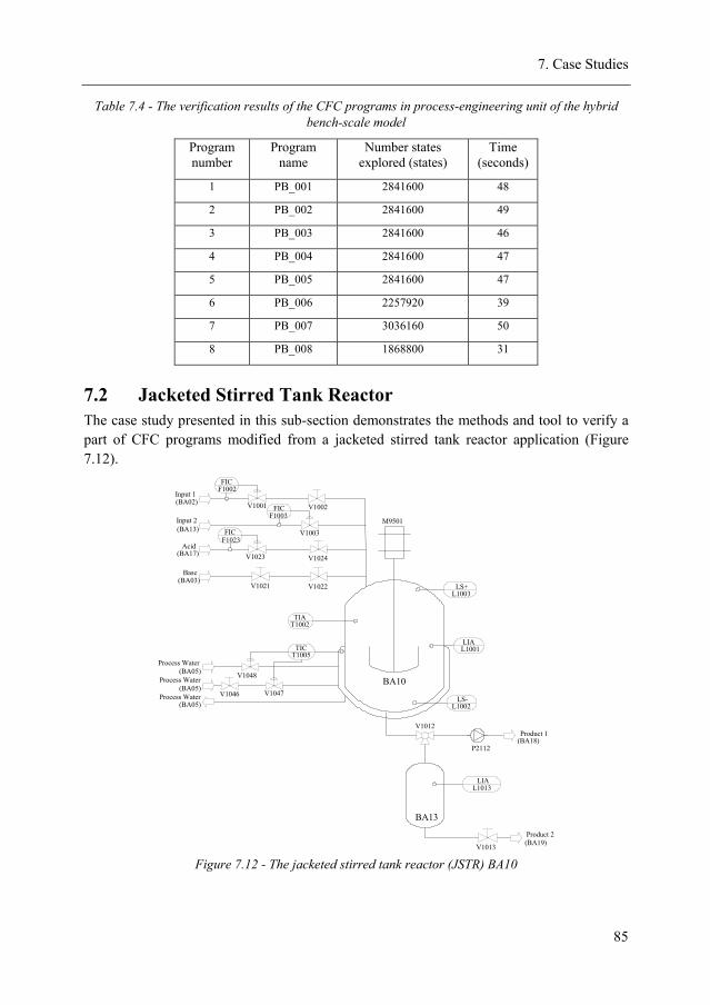
7. Case Studies
85
Table 7.4 - The verification results of the CFC programs in process-engineering unit of the hybrid bench-scale model
Program number
Program name
Number states explored (states)
Time (seconds)
1 PB_001 2841600 48
2 PB_002 2841600 49
3 PB_003 2841600 46
4 PB_004 2841600 47
5 PB_005 2841600 47
6 PB_006 2257920 39
7 PB_007 3036160 50
8 PB_008 1868800 31
7.2 Jacketed Stirred Tank Reactor The case study presented in this sub-section demonstrates the methods and tool to verify a part of CFC programs modified from a jacketed stirred tank reactor application (Figure 7.12).
F1002
F1003
F1023
V1001
V1003
V1023
V1021
FIC
FIC
FIC
TIA
TIC
T1002
T1005
V1047
V1048
LS-
LS+L1003
L1002
L1001LIA
M9501
V1012
P2112
LIAL1013
V1013
BA10
BA13
V1046
Input 1(BA02)
Input 2(BA13)
Base(BA03)
Acid(BA17)
(BA05)
(BA19)
(BA18)
(BA05)
(BA05)
Process Water
Process Water
Product 1
Product 2
Process Water
V1022
V1024
V1002
Figure 7.12 - The jacketed stirred tank reactor (JSTR) BA10
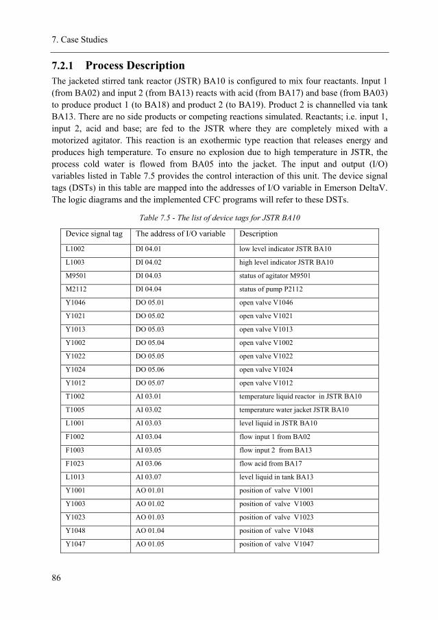
7. Case Studies
86
7.2.1 Process Description The jacketed stirred tank reactor (JSTR) BA10 is configured to mix four reactants. Input 1 (from BA02) and input 2 (from BA13) reacts with acid (from BA17) and base (from BA03) to produce product 1 (to BA18) and product 2 (to BA19). Product 2 is channelled via tank BA13. There are no side products or competing reactions simulated. Reactants; i.e. input 1, input 2, acid and base; are fed to the JSTR where they are completely mixed with a motorized agitator. This reaction is an exothermic type reaction that releases energy and produces high temperature. To ensure no explosion due to high temperature in JSTR, the process cold water is flowed from BA05 into the jacket. The input and output (I/O) variables listed in Table 7.5 provides the control interaction of this unit. The device signal tags (DSTs) in this table are mapped into the addresses of I/O variable in Emerson DeltaV. The logic diagrams and the implemented CFC programs will refer to these DSTs.
Table 7.5 - The list of device tags for JSTR BA10
Device signal tag The address of I/O variable Description
L1002 DI 04.01 low level indicator JSTR BA10
L1003 DI 04.02 high level indicator JSTR BA10
M9501 DI 04.03 status of agitator M9501
M2112 DI 04.04 status of pump P2112
Y1046 DO 05.01 open valve V1046
Y1021 DO 05.02 open valve V1021
Y1013 DO 05.03 open valve V1013
Y1002 DO 05.04 open valve V1002
Y1022 DO 05.05 open valve V1022
Y1024 DO 05.06 open valve V1024
Y1012 DO 05.07 open valve V1012
T1002 AI 03.01 temperature liquid reactor in JSTR BA10
T1005 AI 03.02 temperature water jacket JSTR BA10
L1001 AI 03.03 level liquid in JSTR BA10
F1002 AI 03.04 flow input 1 from BA02
F1003 AI 03.05 flow input 2 from BA13
F1023 AI 03.06 flow acid from BA17
L1013 AI 03.07 level liquid in tank BA13
Y1001 AO 01.01 position of valve V1001
Y1003 AO 01.02 position of valve V1003
Y1023 AO 01.03 position of valve V1023
Y1048 AO 01.04 position of valve V1048
Y1047 AO 01.05 position of valve V1047
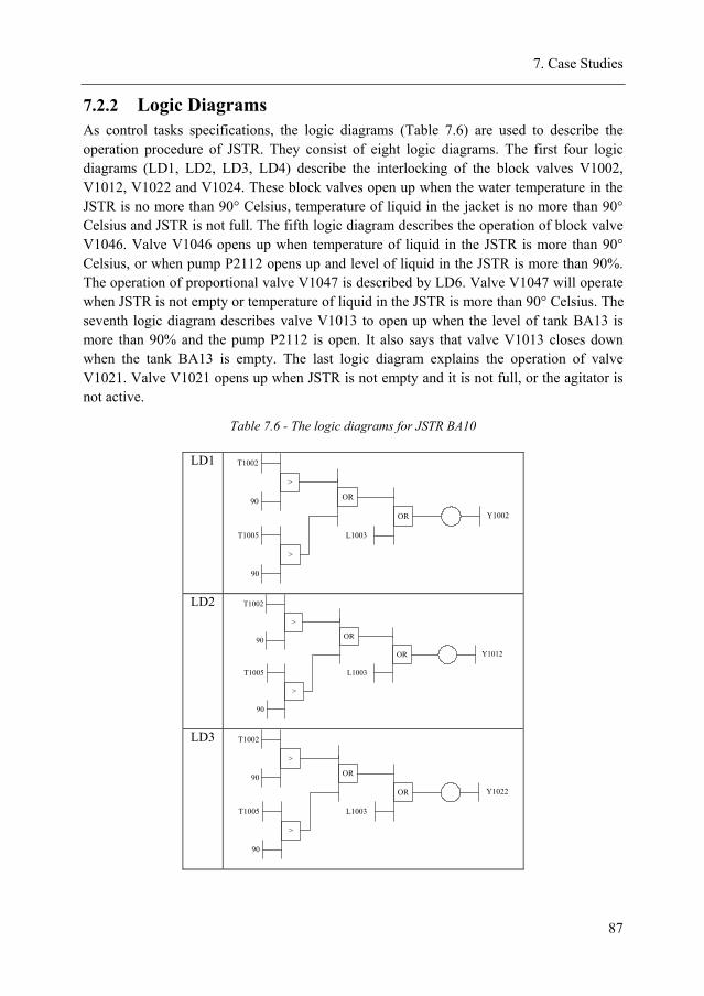
7. Case Studies
87
7.2.2 Logic Diagrams As control tasks specifications, the logic diagrams (Table 7.6) are used to describe the operation procedure of JSTR. They consist of eight logic diagrams. The first four logic diagrams (LD1, LD2, LD3, LD4) describe the interlocking of the block valves V1002, V1012, V1022 and V1024. These block valves open up when the water temperature in the JSTR is no more than 90° Celsius, temperature of liquid in the jacket is no more than 90° Celsius and JSTR is not full. The fifth logic diagram describes the operation of block valve V1046. Valve V1046 opens up when temperature of liquid in the JSTR is more than 90° Celsius, or when pump P2112 opens up and level of liquid in the JSTR is more than 90%. The operation of proportional valve V1047 is described by LD6. Valve V1047 will operate when JSTR is not empty or temperature of liquid in the JSTR is more than 90° Celsius. The seventh logic diagram describes valve V1013 to open up when the level of tank BA13 is more than 90% and the pump P2112 is open. It also says that valve V1013 closes down when the tank BA13 is empty. The last logic diagram explains the operation of valve V1021. Valve V1021 opens up when JSTR is not empty and it is not full, or the agitator is not active.
Table 7.6 - The logic diagrams for JSTR BA10
LD1 >
OR
>
OR
T1002
90
T1005
90
L1003
Y1002
LD2
>
OR
>
OR
T1002
90
T1005
90
L1003
Y1012
LD3
>
OR
>
OR
T1002
90
T1005
90
L1003
Y1022
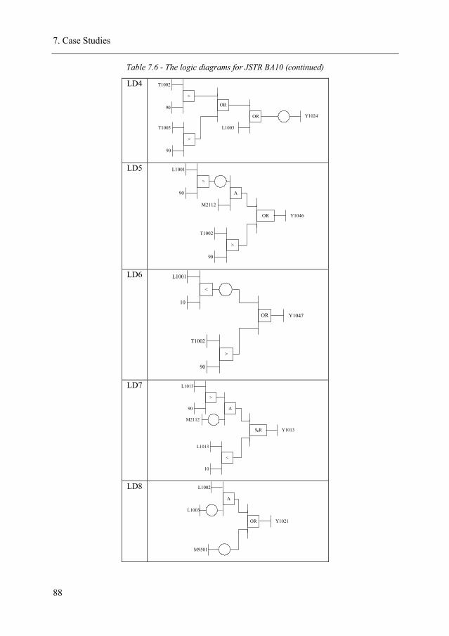
7. Case Studies
88
Table 7.6 - The logic diagrams for JSTR BA10 (continued)
LD4 >
OR
>
OR
T1002
90
T1005
90
L1003
Y1024
LD5
>
>
L1001
90
T1002
90
OR Y1046
A
M2112
LD6
<
OR
>
L1001
10
T1002
90
Y1047
LD7
>
<
L1013
90
L1013
10
S R Y1013
A
M2112
o
LD8
A
L1002
L1003
M9501
Y1021OR
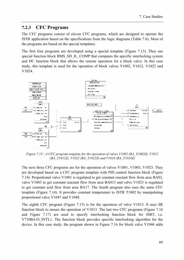
7. Case Studies
89
7.2.3 CFC Programs The CFC programs consist of eleven CFC programs, which are designed to operate the JSTR application based on the specifications from the logic diagrams (Table 7.6). Most of the programs are based on the special templates.
The first four programs are developed using a special template (Figure 7.13). They use special function block BMS_SD_IL_COMP that computes the specific interlocking system and DC function block that allows the remote operation for a block valve. In this case study, this template is used for the operation of block valves V1002, V1012, V1022 and V1024.
Figure 7.13 - A CFC program template for the operation of valves V1002 (BA_Y1002Z), V1012 (BA_Y1012Z), V1022 (BA_Y1022Z) and V1024 (BA_Y1024Z)
The next three CFC programs are for the operation of valves V1001, V1003, V1023. They are developed based on a CFC program template with PID control function block (Figure 7.14). Proportional valve V1001 is regulated to get constant reactant flow from area BA02, valve V1003 to get constant reactant flow from area BA013 and valve V1023 is regulated to get constant acid flow from area BA17. The fourth program also uses the same CFC template (Figure 7.14). It provides constant temperature to JSTR T1002 by manipulating proportional valve V1047 and V1048.
The eighth CFC program (Figure 7.15) is for the operation of valve V1013. It uses SR function block to ensure the operation of V1013. The last two CFC programs (Figure 7.16 and Figure 7.17) are used to specify interlocking function block for JSRT, i.e. V710BA10_INTL1. The function block provides specific interlocking algorithm for the device. In this case study, the program shown in Figure 7.16 for block valve V1046 adds
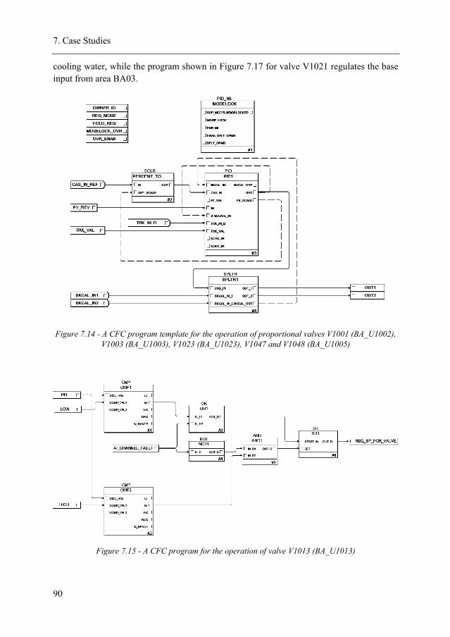
7. Case Studies
90
cooling water, while the program shown in Figure 7.17 for valve V1021 regulates the base input from area BA03.
Figure 7.14 - A CFC program template for the operation of proportional valves V1001 (BA_U1002), V1003 (BA_U1003), V1023 (BA_U1023), V1047 and V1048 (BA_U1005)
Figure 7.15 - A CFC program for the operation of valve V1013 (BA_U1013)
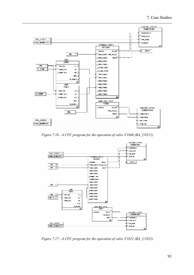
7. Case Studies
91
Figure 7.16 - A CFC program for the operation of valve V1046 (BA_U0511)
Figure 7.17 - A CFC program for the operation of valve V1021 (BA_U1021)
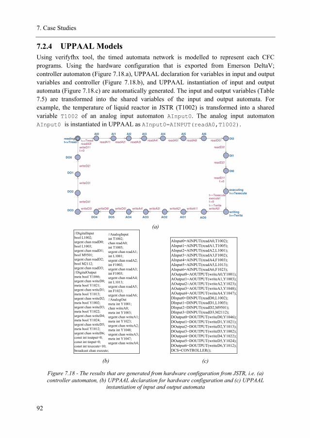
7. Case Studies
92
7.2.4 UPPAAL Models Using verifyfhx tool, the timed automata network is modelled to represent each CFC programs. Using the hardware configuration that is exported from Emerson DeltaV; controller automaton (Figure 7.18.a), UPPAAL declaration for variables in input and output variables and controller (Figure 7.18.b), and UPPAAL instantiation of input and output automata (Figure 7.18.c) are automatically generated. The input and output variables (Table 7.5) are transformed into the shared variables of the input and output automata. For example, the temperature of liquid reactor in JSTR (T1002) is transformed into a shared variable T1002 of an analog input automaton AInput0. The analog input automaton AInput0 is instantiated in UPPAAL as AInput0=AINPUT(readA0,T1002).
AI0 AI1 AI2 AI3 AI4 AI5 AI6
AO0AO1AO2AO3AO4
DI0
DI1
DI2
DO0
DO1
DO2
DO3
DO4 DO5
writingt<=Twrite
readingt<=Tread
executingt<=Texecute
t==TreadreadA0! readA1! readA2! readA3! readA4! readA5! readA6!
t==TwritewriteA0!writeA1!writeA2!writeA3!writeA4!writeD0!
readD1!t:=0
readD2!
readD3!
readD0!
writeD1!t:=0
writeD2!
writeD3!
writeD4!
writeD5! writeD6!
t==Texecuteexecute!t:=0
(a)
//AnalogInputint T1002; chan readA0;int T1005; urgent chan readA1;int L1001; urgent chan readA2;int F1002; urgent chan readA3;int F1003; urgent chan readA4;int L1013; urgent chan readA5;int F1023; urgent chan readA6;//AnalogOutmeta int Y1001; chan writeA0;meta int Y1003; urgent chan writeA1;meta int Y1023; urgent chan writeA2;meta int Y1048; urgent chan writeA3;meta int Y1047; urgent chan writeA4;
//DigitalInputbool L1002; urgent chan readD0;bool L1003; urgent chan readD1;bool M9501; urgent chan readD2;bool M2112; urgent chan readD3;//DigitalOutputmeta bool Y1046; urgent chan writeD0;meta bool Y1021; urgent chan writeD1;meta bool Y1013; urgent chan writeD2;meta bool Y1002; urgent chan writeD3;meta bool Y1022; urgent chan writeD4;meta bool Y1024; urgent chan writeD5;meta bool Y1012; urgent chan writeD6;const int toutput=0;const int tinput=0;const int texecute=10;broadcast chan execute;
AInput0=AINPUT(readA0,T1002);AInput1=AINPUT(readA1,T1005);AInput2=AINPUT(readA2,L1001);AInput3=AINPUT(readA3,F1002);AInput4=AINPUT(readA4,F1003);AInput5=AINPUT(readA5,L1013);AInput6=AINPUT(readA6,F1023);AOutput0=AOUTPUT(writeA0,Y1001);AOutput1=AOUTPUT(writeA1,Y1003);AOutput2=AOUTPUT(writeA2,Y1023);AOutput3=AOUTPUT(writeA3,Y1048);AOutput4=AOUTPUT(writeA4,Y1047);DInput0=DINPUT(readD0,L1002);DInput1=DINPUT(readD1,L1003);DInput2=DINPUT(readD2,M9501);DInput3=DINPUT(readD3,M2112);DOutput0=DOUTPUT(writeD0,Y1046);DOutput1=DOUTPUT(writeD1,Y1021);DOutput2=DOUTPUT(writeD2,Y1013);DOutput3=DOUTPUT(writeD3,Y1002);DOutput4=DOUTPUT(writeD4,Y1022);DOutput5=DOUTPUT(writeD5,Y1024);DOutput6=DOUTPUT(writeD6,Y1012);DCS=CONTROLLER();
(b) (c)
Figure 7.18 - The results that are generated from hardware configuration from JSTR, i.e. (a) controller automaton, (b) UPPAAL declaration for hardware configuration and (c) UPPAAL
instantiation of input and output automata
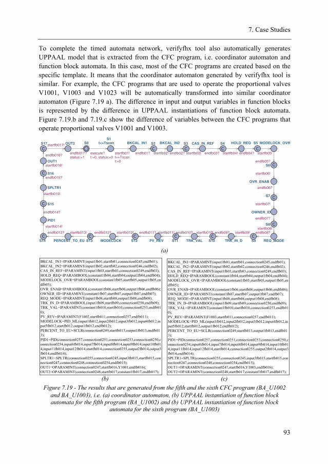
7. Case Studies
93
To complete the timed automata network, verifyfhx tool also automatically generates UPPAAL model that is extracted from the CFC program, i.e. coordinator automaton and function block automata. In this case, most of the CFC programs are created based on the specific template. It means that the coordinator automaton generated by verifyfhx tool is similar. For example, the CFC programs that are used to operate the proportional valves V1001, V1003 and V1023 will be automatically transformed into similar coordinator automaton (Figure 7.19 a). The difference in input and output variables in function blocks is represented by the difference in UPPAAL instantiations of function block automata. Figure 7.19.b and 7.19.c show the difference of variables between the CFC programs that operate proportional valves V1001 and V1003.
S0 BKCAL_IN1S1
t<=Tscan BKCAL_IN2S2 CAS_IN_REFS3 HOLD_REQS4 MODELOCK_OVRS5
OVR_ENAB
S6
OWNER_ID
S7
REQ_MODE
S8
TRK_IN_D S9TRK_VAL S10PV_REV S11MODELOCK S12PERCENT_TO_EU S13
PID1
S14
SPLTR1
S15
OUT1
S16
OUT2S17
endfb010?
t==Tscanstartfb01!
t:=0
endfb01? startfb02! endfb02? startfb03! endfb03? startfb04! endfb04? startfb05!
endfb05?
startfb06!
endfb06?
startfb07!
endfb07?
startfb08!endfb08?startfb09!endfb09?startfb010!startfb011!endfb011?startfb012!endfb012?startfb013!endfb013?
startfb014!
endfb014?
startfb015!
endfb015?
startfb016!
endfb016?
startfb017!
endfb017?status:=1
execute?t:=0, status:=0
(a)
BKCAL_IN1=IPARAMINT(input1fb01,startfb01,connection0245,endfb01);BKCAL_IN2=IPARAMINT(input1fb02,startfb02,connection0246,endfb02);CAS_IN_REF=IPARAMINT(input1fb03,startfb03,connection0249,endfb03);HOLD_REQ=IPARAMBOOL(constant1fb04,startfb04,output1fb04,endfb04);MODELOCK_OVR=IPARAMBOOL(constant1fb05,startfb05,output1fb05,endfb05);OVR_ENAB=IPARAMBOOL(constant1fb06,startfb06,output1fb06,endfb06);OWNER_ID=IPARAMINT(constant1fb07,startfb07,output1fb07,endfb07);REQ_MODE=IPARAMINT(input1fb08,startfb08,output1fb08,endfb08);TRK_IN_D=IPARAMBOOL(input1fb09,startfb09,connection0250,endfb09);TRK_VAL=IPARAMINT(constant1fb010,startfb010,connection0253,endfb010);PV_REV=IPARAMINT(F1002,startfb011,connection0257,endfb011);MODELOCK=PID_ML(input1fb012,input2fb012,input3fb012,input4fb012,input5fb012,startfb012,output1fb012,endfb012);PERCENT_TO_EU=SCLR(connection0249,startfb013,output1fb013,endfb013);PID1=PID(connection0257,connection0251,connection0253,connection0250,connection0254,input6fb014,input7fb014,input8fb014,input9fb014,input10fb014,input11fb014,input12fb014,startfb014,connection0255,output2fb014,output3fb014,endfb014);SPLTR1=SPLTR(connection0255,connection0245,input3fb015,startfb015,connection0247,connection0248,connection0254,endfb015);OUT1=OPARAMINT(connection0247,startfb016,Y1001,endfb016);OUT2=OPARAMINT(connection0248,startfb017,constant1fb017,endfb017);
BKCAL_IN1=IPARAMINT(input1fb01,startfb01,connection0245,endfb01);BKCAL_IN2=IPARAMINT(input1fb02,startfb02,connection0246,endfb02);CAS_IN_REF=IPARAMINT(input1fb03,startfb03,connection0249,endfb03);HOLD_REQ=IPARAMBOOL(constant1fb04,startfb04,output1fb04,endfb04);MODELOCK_OVR=IPARAMBOOL(constant1fb05,startfb05,output1fb05,endfb05);OVR_ENAB=IPARAMBOOL(constant1fb06,startfb06,output1fb06,endfb06);OWNER_ID=IPARAMINT(constant1fb07,startfb07,output1fb07,endfb07);REQ_MODE=IPARAMINT(input1fb08,startfb08,output1fb08,endfb08);TRK_IN_D=IPARAMBOOL(input1fb09,startfb09,connection0250,endfb09);TRK_VAL=IPARAMINT(constant1fb010,startfb010,connection0253,endfb010);PV_REV=IPARAMINT(F1003,startfb011,connection0257,endfb011);MODELOCK=PID_ML(input1fb012,input2fb012,input3fb012,input4fb012,input5fb012,startfb012,output1fb012,endfb012);PERCENT_TO_EU=SCLR(connection0249,startfb013,output1fb013,endfb013);PID1=PID(connection0257,connection0251,connection0253,connection0250,connection0254,input6fb014,input7fb014,input8fb014,input9fb014,input10fb014,input11fb014,input12fb014,startfb014,connection0255,output2fb014,output3fb014,endfb014);SPLTR1=SPLTR(connection0255,connection0245,input3fb015,startfb015,connection0247,connection0248,connection0254,endfb015);OUT1=OPARAMINT(connection0247,startfb016,Y1003,endfb016);OUT2=OPARAMINT(connection0248,startfb017,constant1fb017,endfb017);
(b) (c) Figure 7.19 - The results that are generated from the fifth and the sixth CFC program (BA_U1002
and BA_U1003), i.e. (a) coordinator automaton, (b) UPPAAL instantiation of function block automata for the fifth program (BA_U1002) and (b) UPPAAL instantiation of function block
automata for the sixth program (BA_U1003)
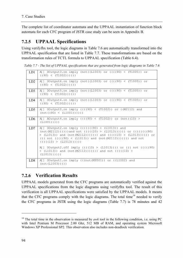
7. Case Studies
94
The complete list of coordinator automata and the UPPAAL instantiation of function block automata for each CFC program of JSTR case study can be seen in Appendix B.
7.2.5 UPPAAL Specifications Using verifyfhx tool, the logic diagrams in Table 7.6 are automatically transformed into the UPPAAL specification that are listed in Table 7.7. These transformations are based on the transformation rules of TCTL formula to UPPAAL specification (Table 6.4).
Table 7.7 - The list of UPPAAL specifications that are generated from logic diagrams in Table 7.6
LD1 A[] DOutput3.on imply (not((L1003) or ((((90) < (T1005)) or ((90) < (T1002))))))
LD2 A[] DOutput6.on imply (not((L1003) or ((((90) < (T1005)) or ((90) < (T1002))))))
LD3 A[] DOutput5.on imply (not((L1003) or ((((90) < (T1005)) or ((90) < (T1002))))))
LD4 A[] DOutput4.on imply (not((L1003) or ((((90) < (T1005)) or ((90) < (T1002))))))
LD5 A[] DOutput0.on imply ((((90) < (T1002)) or ((M2112) and (not((90) < (L1001))))))
LD6 A[] AOutput4.on imply ((((90) < (T1002)) or (not((10) > (L1001)))))
LD7 A[] DOutput2.on imply (((((((90) < (L1013)) and (not(M2112))))))and not (((((10) > (L1013)))))) or ((((((((90) < (L1013)) and (not(M2112))))))) and (((((10) > (L1013)))))) or ((( not (((((90) < (L1013)) and (not(M2112))))))) and not (((((10) > (L1013))))))
A[] DOutput2.off imply ((((10) > (L1013)))) or ((( not (((((90) < (L1013)) and (not(M2112))))))) and not (((((10) > (L1013))))))
LD8 A[] DOutput1.on imply (((not(M9501)) or ((L1002) and (not(L1003)))))
7.2.6 Verification Results UPPAAL models generated from the CFC programs are automatically verified against the UPPAAL specifications from the logic diagrams using verifyfhx tool. The result of this verification is all UPPAAL specifications were satisfied by the UPPAAL models. It means that the CFC programs comply with the logic diagrams. The total time14 needed to verify the CFC programs in JSTR using the logic diagrams (Table 7.7) is 78 minutes and 42
14 The total time in the observation is measured by awk tool in the following condition, i.e. using PC with Intel Pentium M Processor 2.00 Ghz, 512 MB of RAM, and operating system Microsoft Windows XP Professional SP2. This observation also includes non-deadlock verification.
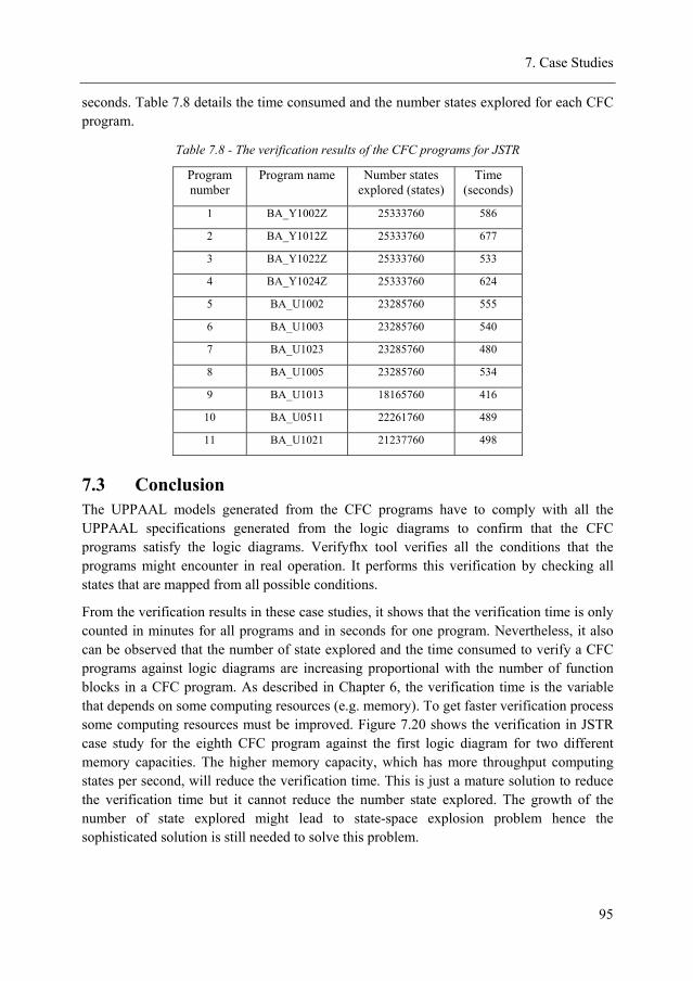
7. Case Studies
95
seconds. Table 7.8 details the time consumed and the number states explored for each CFC program.
Table 7.8 - The verification results of the CFC programs for JSTR
Program number
Program name Number states explored (states)
Time (seconds)
1 BA_Y1002Z 25333760 586
2 BA_Y1012Z 25333760 677
3 BA_Y1022Z 25333760 533
4 BA_Y1024Z 25333760 624
5 BA_U1002 23285760 555
6 BA_U1003 23285760 540
7 BA_U1023 23285760 480
8 BA_U1005 23285760 534
9 BA_U1013 18165760 416
10 BA_U0511 22261760 489
11 BA_U1021 21237760 498
7.3 Conclusion The UPPAAL models generated from the CFC programs have to comply with all the UPPAAL specifications generated from the logic diagrams to confirm that the CFC programs satisfy the logic diagrams. Verifyfhx tool verifies all the conditions that the programs might encounter in real operation. It performs this verification by checking all states that are mapped from all possible conditions.
From the verification results in these case studies, it shows that the verification time is only counted in minutes for all programs and in seconds for one program. Nevertheless, it also can be observed that the number of state explored and the time consumed to verify a CFC programs against logic diagrams are increasing proportional with the number of function blocks in a CFC program. As described in Chapter 6, the verification time is the variable that depends on some computing resources (e.g. memory). To get faster verification process some computing resources must be improved. Figure 7.20 shows the verification in JSTR case study for the eighth CFC program against the first logic diagram for two different memory capacities. The higher memory capacity, which has more throughput computing states per second, will reduce the verification time. This is just a mature solution to reduce the verification time but it cannot reduce the number state explored. The growth of the number of state explored might lead to state-space explosion problem hence the sophisticated solution is still needed to solve this problem.
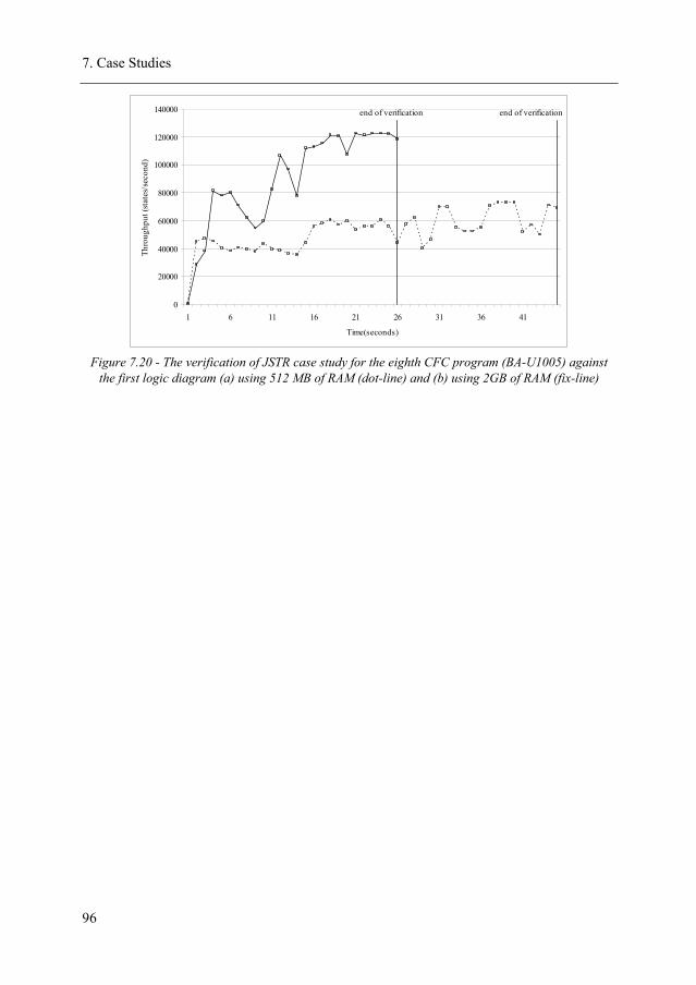
7. Case Studies
96
0
20000
40000
60000
80000
100000
120000
140000
1 6 11 16 21 26 31 36 41
Time(seconds)
Thro
ughp
ut (s
tate
s/se
cond
)
end of verification end of verification
Figure 7.20 - The verification of JSTR case study for the eighth CFC program (BA-U1005) against
the first logic diagram (a) using 512 MB of RAM (dot-line) and (b) using 2GB of RAM (fix-line)
8 Conclusions The continuous function chart (CFC) programs, which are widely implemented in process industry, have to be verified if the requirements specified in the control tasks specifications are being fulfilled. This has to be conducted before they are being implemented in the plant. Logical errors in the programs can cause errors in the plant’s operation. Before the user operates the plant, all logical errors must be ruled out. Nowadays, this verification is conducted manually. Manual verification can potentially cause errors and is very time-consuming.
To ensure the correctness of CFC programs, the solution proposed in this work is an automatic program verification methods based on model checking. The correctness is determined by the compliance of CFC programs to the logic diagrams. There are a few challenges to this approach; i.e. the lack of formal descriptions for CFC and logic diagram, the complex structure of CFC programs and logic diagrams, and the state-space explosion when implementing model checking as a verification method. This chapter summarizes the approaches implemented to overcome these problems, the lesson learned from the result of this work and future works.
8.1 Summary There are three main approaches in this work, i.e. formalization of CFC and logic diagram development of transformation rules and realization of automatic program verification. The applicability of these approaches in real-world application is being evaluated in two case studies. This section will summarize the work done on these approaches.
• Formalization of CFC and logic diagram
This approach is the elementary foundation of this work. It supports the correct interpretation of CFC as programming language and logic diagram as control tasks specification. Firstly, the syntax, semantics and execution procedures of CFC are formalized. The syntax and semantics of CFC are defined based on the general descriptions of CFC, while the CFC’s execution procedure is defined based on the implementation in distributed control system (DCS), i.e. Emerson DeltaV, a leader of DCS market. After this step, a formalized description for syntactically correct symbols in a CFC program and the behaviour of these symbols in DCS are generated. This is the key to describe precisely the execution of a CFC program in DCS. Secondly, the logic diagram used as the control tasks specification is formalized. Its syntax is defined by considering the logical blocks and connectivity of the logical blocks. The semantics of logic diagrams are defined by extracting the meaning of the composition of logical blocks in a logic diagram with respect to a CFC program. The result is precise interpretation of logic diagram.
8. Conclusions
98
• Development of transformation rules
Firstly, this approach provides the rules to transform the formal descriptions of CFC to timed automata. It considers the transformation of CFC aspects such as function blocks, controller cyclic system and execution procedures to timed automata. The transformation rules are completed by the definition of the input and output automata as the representations of the input and output (I/O) variables. Secondly, this approach defines the transformation rules to map the logic diagrams into timed computation tree logic (TCTL) formula. Transformation of the propositional interpreted from semantics of logic diagram to the propositional in TCTL is realized using the transformation rules.
• Realization of automatic program verification
In this work, UPPAAL model checker is chosen to realize the automatic verification of the CFC programs against the logic diagrams. The results from the mapping using transformation rules, which are timed automata network and TCTL formula, are being realized as the reasonable models and specifications in UPPAAL. The state-space explosion as the major problem in model checking is used as the main consideration to get these reasonable models and specifications. UPPAAL features, i.e. meta variables, urgent synchronization action and observer automata are used in this realization approach to reduce the state explored that may alleviate the state-space explosion problem. This realization approach is automated using an in-house developed tool called verifyfhx tool. Verifyfhx tool can automatically generate UPPAAL models from CFC programs and UPPPAL specifications from logic diagrams. This tool also automatically generates the reports concerning the compliance of the CFC programs with the logic diagrams.
• Application automatic program verification on case studies
The approaches in this work are applied in two case studies by using verifyfhx tool. This tool is applied to verify CFC programs of the process-engineering unit of the hybrid bench-scale model and jacketed stirred tank reactor case studies. This tool proves to be well capable of verifying the CFC programs implemented in Emerson DeltaV. This tool can analyze all possible states generated from the UPPAAL models of CFC programs. It means this tool performs complete program verification that observes all possible conditions in the real operation caused by the programs. Using this tool, the delivered programs can be ensured to contain no errors.
8.2 Lessons Learned From the result of the approaches mentioned above, some lessons learned are elaborated in this section as follows.
• The methods and a tool of automatic program verification
8. Conclusions
99
The key result delivered in this work is the methods and a tool of automatic program verification. The automatic program verification here means that the verification process does not need interference from the person who wants to verify the program. The methods and a tool developed in this work can automatically verify the CFC programs to comply with the logic diagrams. In process industry, a process engineer is usually responsible to provide the logic diagrams, while the implementation of CFC programs is the responsibility of a process control engineer. Using these methods and tool, the person can verify easily whether or not the CFC programs comply with the logic diagrams without prior knowledge regarding process and/or programming. The case studies conclude these methods and tool significantly influence the verification process of the CFC programs. These methods and tool provide the complete verification conditions and has great value to the person to find all possible logical errors in the programs to increase the program’s dependability. These methods and tool also reduce the required time of the person to verify the programs during the verification process in program development.
• The need of formal descriptions
The key solution in this work is the formal descriptions. The first formal descriptions defined in this work are the descriptions of CFC. They give the precise description regarding the behaviour of a CFC program in DCS. The second formal descriptions are the description of logic diagram. They give the precise meaning of a logic diagram as control tasks specification with respect to design CFC program. The third formal descriptions are the transformation rules of a CFC program to timed automata network and logic diagram to TCTL formula. They give precise rules on how the elements of a CFC program are mapped to timed automata network and how the proposition formula extracted from logic diagram is mapped to the proposition formula of TCTL. These formal descriptions, which are defined in this work, are the elementary foundations to realize formal program verification. These formal descriptions are also possible implemented to develop other formal applications, e.g. test-case generator or program-test simulation.
• State space explosion problem
The key problem to realize reasonable automatic program verification based on model checking is the state-space explosion. This is the main concern when conducting model checking between the model of CFC program and the specification of logic diagram. A few approaches are used in this work to overcome the state-space explosion problem. However, these approaches only manage to reduce the number of state explored and not completely eliminate the state-space explosion problem. From the case studies, the state-space explosion problem is not occurred but the tendency of this problem can be observed. More complex control algorithm expressed by the use of more function blocks in a CFC program in the case studies increases the number of state explored.
8. Conclusions
100
This might lead to state-space explosion problem. A sophisticated solution is still needed to solve this major problem completely.
8.3 Future Works There are many interesting possibilities for future works.
• Support to user-defined function block
In the CFC implementation in Emerson DeltaV, there is a special feature to define the automation function in a function block. The user can define his/her own automation function in calculation/logic function block by using a specific C-like programming language. This function block is usually used to describe a specific automation function. This function block cannot be verified using the methods mentioned in this work. For future work, the semantics of C-like programming language needs to be added in the formal descriptions of CFC developed in this work.
• Eliminate state space explosion problem
The major obstacle observed from the case studies is the increase of function blocks in a CFC program will also increase the number of state explored. It will potentially cause the state-space explosion problem. In order to solve this problem, the approaches such as program decomposition [Dij72], or program slicing [Luc01] should be added to the verification approach developed in this work.
• Support to other CFC implementations in DCS
The formalization approach for CFC in this work is defined based on Emerson DeltaV. Since there is no standard for CFC, different DCS manufacturer implement different dialect of CFC. This leads to the idea to further develop the formalization approach as described in Section 4.3 (Table 4.3), to make automatic verification possible in other systems, e.g. Siemens Simantic PCS7, ABB 800xA, Yokogawa Centum CS3000, or Honeywell Experion PKS.
• Support to other control tasks specifications
In the process industry, the logic diagram is not sufficient to provide complete control tasks specification for the whole plant. Most of the industrial applications for designing the control tasks specification, e.g. COMOS [CIS08]; integrate the logical block with other block, e.g. mathematical block and control block; in their own diagram. To support this specific diagram, the syntax and semantics of logic diagram have to be extended with the definitions of different block types and the definitions of different composition types.
• Combine with sequential function chart (SFC) program verification
There are two programming languages that are usually used in DCS, i.e. CFC and SFC. DCS programming allows the combination of these two languages. This combination
8. Conclusions
101
cannot be verified using the methods mentioned in this work. One possible future work is to integrate SFC in the formalization approach. This will provide more thorough program verification for DCS. The semantics of SFC as developed by Bauer et al. [BHL+04] can be integrated into the formal descriptions of CFC.
• Combine with verification of hardware configuration
As described in Section 6.2.1 regarding the structure of verifyfhx tool, it is explained that one of the verifyfhx tool input is the hardware configuration data. In this work, the verifyfhx tool uses this data to create the model of controller and I/O variables. Actually, this data also consist of the information regarding the complete hardware configuration, e.g. network configuration. Further possible development includes the use of this complete hardware configuration data to provide the verification of hardware configuration. As an example, the methods introduced by Witsch et al. [WVF+06] can be combined with the automatic program verification methods mentioned in this work. The combination of program and hardware configuration verification gives the possibility for the realization of an ultimate verification tool. One potential problem to realize this combination is the lack of sufficient information regarding the components in DCS structure.
9 References [ABB06] Industrial IT system 800xA engineering, ABB Process Automation Division,
Mannheim, Germany, 2006.
[AbNy01] Abdulla, P. A.; Nylen, A.: Timed Petri nets and BQOs, In: Applications and Theory of Petri Nets, Lecture Notes in Computer Science, Springer-Verlag, Heidelberg, Vol. 2075, 2001, pp. 53–70.
[ACD90] Alur, R.; Courcoubetis, C.; Dill, D. L.: Model checking for real time systems, In: Proceedings of Annual IEEE Symposium Logic in Computer Science, Philadelphia, USA, 1990, pp. 414–425.
[AGL+07] de Assis Barbosa; L. P.; Gorgonio, K.; Lima, A. M. N.; Perkusich, A.; Grande, C.; Paraiba, B.; da Silva, L. D.: On the automatic generator of timed automata models from ISA 5.2 diagrams, In: Proceedings of IEEE Conference on Emerging Technologies and Factory Automation, Petras, Geece, 2007, pp. 406-412.
[AHH96] Alur, R.; Henzinger, T. A.; Ho, P. H.: Automatic symbolic verification of embedded systems, In: IEEE Transition Software Engineering, Vol. 22, 1996, pp. 181–201.
[AlDi94] Alur, R.; Dill, D.L.: A theory of timed automata, In: Theoretical Computer Science, Elsevier Science Publishers, Amsterdam, Vol. 126, No.2, 1994, pp. 183-235.
[Bau03] Bauer, N.: Formale Analyse von Sequential Function Charts, Ph.D. dissertation, Lehrstuhl für Anlagensteuerungstechnik, University of Dortmund, Germany, 2003.
[BDL04] Behrmann, G.; David, A.; Larsen, K.G.: A tutorial on UPPAAL, In: Formal Methods for the Design of Real-Time Systems, Lecture Note in Computer Science, Springer-Verlag, Heidelberg, Germany, Vol. 3147, 2004, pp. 400-418.
[BEH+04] Bauer, N.; Engell, S.; Huuck, R.; Lohmann, S.; Lukoschus, B.; Remelhe, M.; Stursberg, O.: Verification of PLC programs given as sequential function charts, In: Integration of Software Specification Techniques for Applications in Engineering, Lecture Note in Computer Science, Springer-Verlag, Heidelberg, Germany, vol 3147, 2004, pp. 517-540
[BéSi00] Bérard, B.; Sierra, L.: Comparing verification with HyTech, Kronos and Uppaal on the railroad crossing example, In: Research Report LSV-00-2, Laboratoire Specification et Verification, ENS de Cachan, France, 2000.
[BeYi04] Bengtsson, J.; Yi. W.: Timed automata semantics, algorithms and tools, In: Lecture Notes on Concurrency and Petri Nets, Springer-Verlag, Berlin, Germany, Vol. 3098, 2004, 2004, pp. 87-124.
[BFK+98] Bowman, H.; Faconti, G.; Katoen, J.; Latella, D.; Massink, M.: Automatic verification of a Lip-synchronisation protocol Using Uppaal, In: Formal
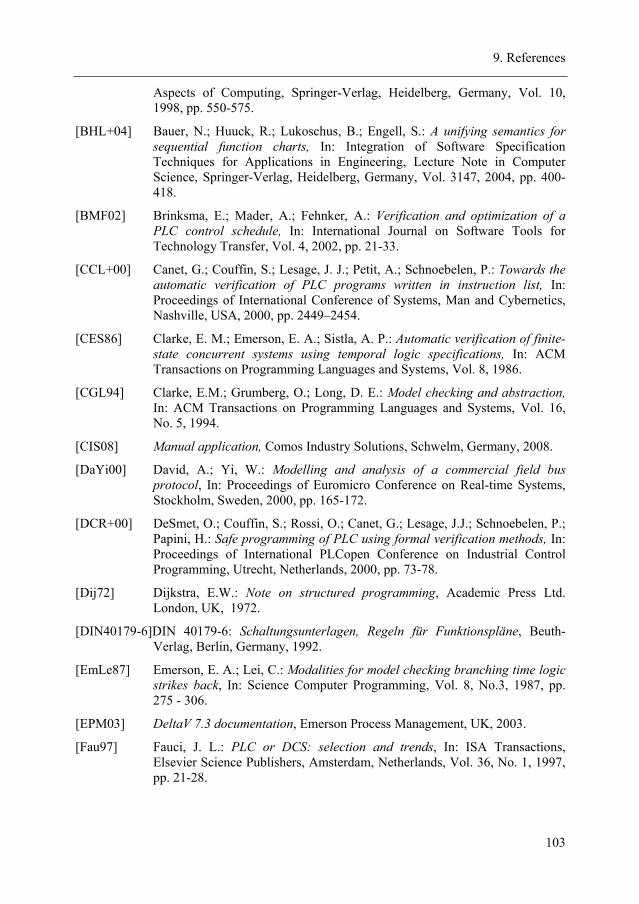
9. References
103
Aspects of Computing, Springer-Verlag, Heidelberg, Germany, Vol. 10, 1998, pp. 550-575.
[BHL+04] Bauer, N.; Huuck, R.; Lukoschus, B.; Engell, S.: A unifying semantics for sequential function charts, In: Integration of Software Specification Techniques for Applications in Engineering, Lecture Note in Computer Science, Springer-Verlag, Heidelberg, Germany, Vol. 3147, 2004, pp. 400-418.
[BMF02] Brinksma, E.; Mader, A.; Fehnker, A.: Verification and optimization of a PLC control schedule, In: International Journal on Software Tools for Technology Transfer, Vol. 4, 2002, pp. 21-33.
[CCL+00] Canet, G.; Couffin, S.; Lesage, J. J.; Petit, A.; Schnoebelen, P.: Towards the automatic verification of PLC programs written in instruction list, In: Proceedings of International Conference of Systems, Man and Cybernetics, Nashville, USA, 2000, pp. 2449–2454.
[CES86] Clarke, E. M.; Emerson, E. A.; Sistla, A. P.: Automatic verification of finite-state concurrent systems using temporal logic specifications, In: ACM Transactions on Programming Languages and Systems, Vol. 8, 1986.
[CGL94] Clarke, E.M.; Grumberg, O.; Long, D. E.: Model checking and abstraction, In: ACM Transactions on Programming Languages and Systems, Vol. 16, No. 5, 1994.
[CIS08] Manual application, Comos Industry Solutions, Schwelm, Germany, 2008.
[DaYi00] David, A.; Yi, W.: Modelling and analysis of a commercial field bus protocol, In: Proceedings of Euromicro Conference on Real-time Systems, Stockholm, Sweden, 2000, pp. 165-172.
[DCR+00] DeSmet, O.; Couffin, S.; Rossi, O.; Canet, G.; Lesage, J.J.; Schnoebelen, P.; Papini, H.: Safe programming of PLC using formal verification methods, In: Proceedings of International PLCopen Conference on Industrial Control Programming, Utrecht, Netherlands, 2000, pp. 73-78.
[Dij72] Dijkstra, E.W.: Note on structured programming, Academic Press Ltd. London, UK, 1972.
[DIN40179-6]DIN 40179-6: Schaltungsunterlagen, Regeln für Funktionspläne, Beuth-Verlag, Berlin, Germany, 1992.
[EmLe87] Emerson, E. A.; Lei, C.: Modalities for model checking branching time logic strikes back, In: Science Computer Programming, Vol. 8, No.3, 1987, pp. 275 - 306.
[EPM03] DeltaV 7.3 documentation, Emerson Process Management, UK, 2003.
[Fau97] Fauci, J. L.: PLC or DCS: selection and trends, In: ISA Transactions, Elsevier Science Publishers, Amsterdam, Netherlands, Vol. 36, No. 1, 1997, pp. 21-28.
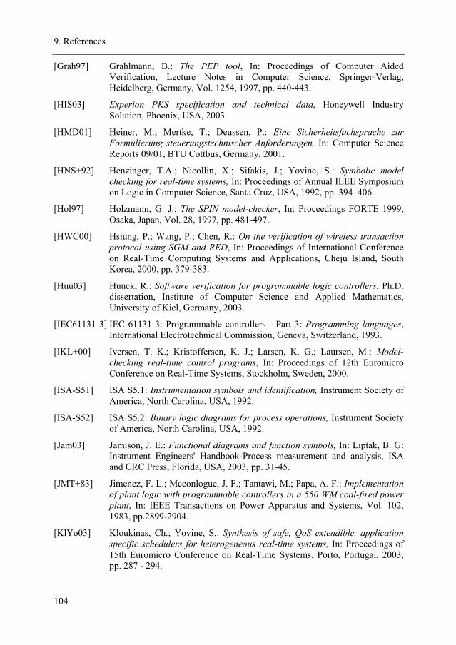
9. References
104
[Grah97] Grahlmann, B.: The PEP tool, In: Proceedings of Computer Aided Verification, Lecture Notes in Computer Science, Springer-Verlag, Heidelberg, Germany, Vol. 1254, 1997, pp. 440-443.
[HIS03] Experion PKS specification and technical data, Honeywell Industry Solution, Phoenix, USA, 2003.
[HMD01] Heiner, M.; Mertke, T.; Deussen, P.: Eine Sicherheitsfachsprache zur Formulierung steuerungstechnischer Anforderungen, In: Computer Science Reports 09/01, BTU Cottbus, Germany, 2001.
[HNS+92] Henzinger, T.A.; Nicollin, X.; Sifakis, J.; Yovine, S.: Symbolic model checking for real-time systems, In: Proceedings of Annual IEEE Symposium on Logic in Computer Science, Santa Cruz, USA, 1992, pp. 394–406.
[Hol97] Holzmann, G. J.: The SPIN model-checker, In: Proceedings FORTE 1999, Osaka, Japan, Vol. 28, 1997, pp. 481-497.
[HWC00] Hsiung, P.; Wang, P.; Chen, R.: On the verification of wireless transaction protocol using SGM and RED, In: Proceedings of International Conference on Real-Time Computing Systems and Applications, Cheju Island, South Korea, 2000, pp. 379-383.
[Huu03] Huuck, R.: Software verification for programmable logic controllers, Ph.D. dissertation, Institute of Computer Science and Applied Mathematics, University of Kiel, Germany, 2003.
[IEC61131-3] IEC 61131-3: Programmable controllers - Part 3: Programming languages, International Electrotechnical Commission, Geneva, Switzerland, 1993.
[IKL+00] Iversen, T. K.; Kristoffersen, K. J.; Larsen, K. G.; Laursen, M.: Model-checking real-time control programs, In: Proceedings of 12th Euromicro Conference on Real-Time Systems, Stockholm, Sweden, 2000.
[ISA-S51] ISA S5.1: Instrumentation symbols and identification, Instrument Society of America, North Carolina, USA, 1992.
[ISA-S52] ISA S5.2: Binary logic diagrams for process operations, Instrument Society of America, North Carolina, USA, 1992.
[Jam03] Jamison, J. E.: Functional diagrams and function symbols, In: Liptak, B. G: Instrument Engineers' Handbook-Process measurement and analysis, ISA and CRC Press, Florida, USA, 2003, pp. 31-45.
[JMT+83] Jimenez, F. L.; Mcconlogue, J. F.; Tantawi, M.; Papa, A. F.: Implementation of plant logic with programmable controllers in a 550 WM coal-fired power plant, In: IEEE Transactions on Power Apparatus and Systems, Vol. 102, 1983, pp.2899-2904.
[KlYo03] Kloukinas, Ch.; Yovine, S.: Synthesis of safe, QoS extendible, application specific schedulers for heterogeneous real-time systems, In: Proceedings of 15th Euromicro Conference on Real-Time Systems, Porto, Portugal, 2003, pp. 287 - 294.
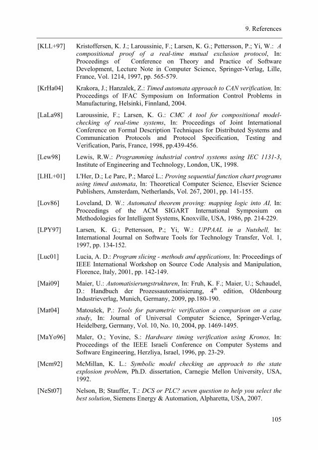
9. References
105
[KLL+97] Kristoffersen, K. J.; Laroussinie, F.; Larsen, K. G.; Pettersson, P.; Yi, W.: A compositional proof of a real-time mutual exclusion protocol, In: Proceedings of Conference on Theory and Practice of Software Development, Lecture Note in Computer Science, Springer-Verlag, Lille, France, Vol. 1214, 1997, pp. 565-579.
[KrHa04] Krakora, J.; Hanzalek, Z.: Timed automata approach to CAN verification, In: Proceedings of IFAC Symposium on Information Control Problems in Manufacturing, Helsinki, Finnland, 2004.
[LaLa98] Laroussinie, F.; Larsen, K. G.: CMC A tool for compositional model-checking of real-time systems, In: Proceedings of Joint International Conference on Formal Description Techniques for Distributed Systems and Communication Protocols and Protocol Specification, Testing and Verification, Paris, France, 1998, pp.439-456.
[Lew98] Lewis, R.W.: Programming industrial control systems using IEC 1131-3, Institute of Engineering and Technology, London, UK, 1998.
[LHL+01] L'Her, D.; Le Parc, P.; Marcé L.: Proving sequential function chart programs using timed automata, In: Theoretical Computer Science, Elsevier Science Publishers, Amsterdam, Netherlands, Vol. 267, 2001, pp. 141-155.
[Lov86] Loveland, D. W.: Automated theorem proving: mapping logic into AI, In: Proceedings of the ACM SIGART International Symposium on Methodologies for Intelligent Systems, Knoxville, USA, 1986, pp. 214-229.
[LPY97] Larsen, K. G.; Pettersson, P.; Yi, W.: UPPAAL in a Nutshell, In: International Journal on Software Tools for Technology Transfer, Vol. 1, 1997, pp. 134-152.
[Luc01] Lucia, A. D.: Program slicing - methods and applications, In: Proceedings of IEEE International Workshop on Source Code Analysis and Manipulation, Florence, Italy, 2001, pp. 142-149.
[Mai09] Maier, U.: Automatisierungstrukturen, In: Fruh, K. F.; Maier, U.; Schaudel, D.: Handbuch der Prozessautomatisierung, 4th edition, Oldenbourg Industrieverlag, Munich, Germany, 2009, pp.180-190.
[Mat04] Matoušek, P.: Tools for parametric verification a comparison on a case study, In: Journal of Universal Computer Science, Springer-Verlag, Heidelberg, Germany, Vol. 10, No. 10, 2004, pp. 1469-1495.
[MaYo96] Maler, O.; Yovine, S.: Hardware timing verification using Kronos, In: Proceedings of the IEEE Israeli Conference on Computer Systems and Software Engineering, Herzliya, Israel, 1996, pp. 23-29.
[Mcm92] McMillan, K. L.: Symbolic model checking an approach to the state explosion problem, Ph.D. dissertation, Carnegie Mellon University, USA, 1992.
[NeSt07] Nelson, B; Stauffer, T.: DCS or PLC? seven question to help you select the best solution, Siemens Energy & Automation, Alpharetta, USA, 2007.
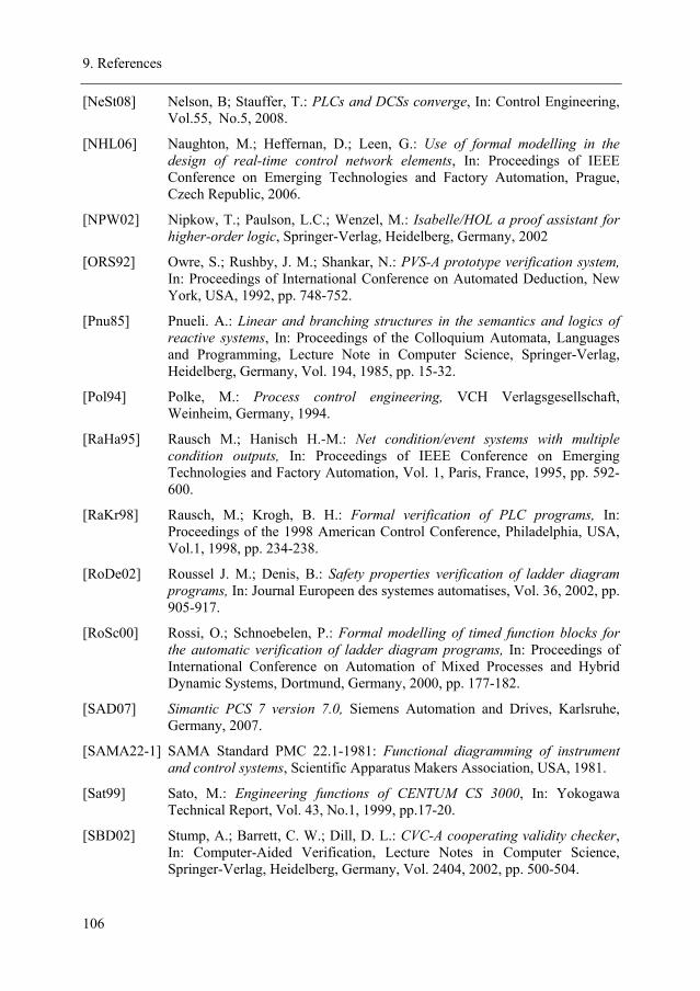
9. References
106
[NeSt08] Nelson, B; Stauffer, T.: PLCs and DCSs converge, In: Control Engineering, Vol.55, No.5, 2008.
[NHL06] Naughton, M.; Heffernan, D.; Leen, G.: Use of formal modelling in the design of real-time control network elements, In: Proceedings of IEEE Conference on Emerging Technologies and Factory Automation, Prague, Czech Republic, 2006.
[NPW02] Nipkow, T.; Paulson, L.C.; Wenzel, M.: Isabelle/HOL a proof assistant for higher-order logic, Springer-Verlag, Heidelberg, Germany, 2002
[ORS92] Owre, S.; Rushby, J. M.; Shankar, N.: PVS-A prototype verification system, In: Proceedings of International Conference on Automated Deduction, New York, USA, 1992, pp. 748-752.
[Pnu85] Pnueli. A.: Linear and branching structures in the semantics and logics of reactive systems, In: Proceedings of the Colloquium Automata, Languages and Programming, Lecture Note in Computer Science, Springer-Verlag, Heidelberg, Germany, Vol. 194, 1985, pp. 15-32.
[Pol94] Polke, M.: Process control engineering, VCH Verlagsgesellschaft, Weinheim, Germany, 1994.
[RaHa95] Rausch M.; Hanisch H.-M.: Net condition/event systems with multiple condition outputs, In: Proceedings of IEEE Conference on Emerging Technologies and Factory Automation, Vol. 1, Paris, France, 1995, pp. 592-600.
[RaKr98] Rausch, M.; Krogh, B. H.: Formal verification of PLC programs, In: Proceedings of the 1998 American Control Conference, Philadelphia, USA, Vol.1, 1998, pp. 234-238.
[RoDe02] Roussel J. M.; Denis, B.: Safety properties verification of ladder diagram programs, In: Journal Europeen des systemes automatises, Vol. 36, 2002, pp. 905-917.
[RoSc00] Rossi, O.; Schnoebelen, P.: Formal modelling of timed function blocks for the automatic verification of ladder diagram programs, In: Proceedings of International Conference on Automation of Mixed Processes and Hybrid Dynamic Systems, Dortmund, Germany, 2000, pp. 177-182.
[SAD07] Simantic PCS 7 version 7.0, Siemens Automation and Drives, Karlsruhe, Germany, 2007.
[SAMA22-1] SAMA Standard PMC 22.1-1981: Functional diagramming of instrument and control systems, Scientific Apparatus Makers Association, USA, 1981.
[Sat99] Sato, M.: Engineering functions of CENTUM CS 3000, In: Yokogawa Technical Report, Vol. 43, No.1, 1999, pp.17-20.
[SBD02] Stump, A.; Barrett, C. W.; Dill, D. L.: CVC-A cooperating validity checker, In: Computer-Aided Verification, Lecture Notes in Computer Science, Springer-Verlag, Heidelberg, Germany, Vol. 2404, 2002, pp. 500-504.
9. References
107
[SMP00] SAMA diagrams for boiler controls, Siemens Moore Process Automation, Spring-House, USA, 2000.
[STK+00] Sandoz, D. J.; Thorpe, P. J.; Kurth, T.; Desforges, M. J.; Woolley, I. S.: Innovation in industrial model predictive control, In: Proceedings of IEE Seminar on Practical Experiences with Predictive Control, 2000, pp.5/1-5/12.
[SWK09] Schlich, B.; Wernerus, J.; Kowalewski, S.: Verifikation von SPS-Programmen in AWL mit Hilfe von direktem Model-Checking, In: Proceedings of Automation 2009, Baden Baden, Germany, 2009.
[Sto96] Storey, N.: Safety critical computer systems, Addison-Wesley, Harlow, England, 1996.
[Uri00] Uribe, T. E.: Combinations of model checking and theorem proving, In: Proceedings of the International Workshop on Frontiers of Combining Systems, Lecture Notes in Computer Science, Springer-Verlag, Heidelberg, Germany, Vol. 1794, 2000, pp. 151-170.
[VDE3682] VDI/VDE 3682: Formalisierte Prozessbeschreibungen, Beuth Verlag, Berlin, Germany, 2005.
[Vog09] Vogel-Heuser, B.: Automation in wood and paper industry, In: Yof, S.: Handbook of Automation, Springer-Verlag, Berlin, Germany, 2009, pp. 1015-1025.
[VöKr99] Völker, N.; Krämer, B. J.: Automated verification of function block based industrial control systems, In: Theoretical Computer Science, Springer-Verlag, Heidelberg, Vol. 5, 1999, pp. 97-110.
[Völ00] Völker, N.: Towards a HOL framework for the deductive analysis of hybrid control systems, In: Proceedings of International Conference on Automation of Mixed Processes, Dortmund, Germany, 2000.
[Wan00] Wang, F.: Region encoding diagram for fully symbolic verification of real-time systems, In: Proceedings of International Computer Software and Applications Conference, Taipai, Taiwan, 2000, pp. 509-515.
[WSG07] Wang, R.; Song, X.; Gu, M.: Modelling and verification of program logic controllers using timed automata, In: IET Software, Vol. 1, 2007, pp. 127-131.
[WVF+06] Witsch, D.; Vogel-Heuser, B.; Faure, J. M.; Poulard-Marsal, G.: Performance analysis of industrial Ethernet networks by means of timed model-checking, In: Proceedings of IFAC Symposium on Information Control Problems in Manufacturing, St Etienne, France, 2006, pp. 101–106.
[Yov97] Yovine, S.: Kronos a verification tool for real-time systems, In: Journal of Software Tools for Technology Transfer, Vol. 1, No. 1/2, 1997, pp 123-133.
[Zou03] Zoubek, B.: Automatic verification of temporal and timed properties of control programs, Ph.D. dissertation, School of Computer Science, University of Birmingham, UK, 2003
9. References
108
[ZRK03] Zoubek, B.; Roussel, J.-M.; Kwiatkowska, M.: Towards automatic verification of ladder logic programs, In: Proceedings of International Multiconference on Computational Engineering in Systems Applications, Lille, France, 2003, pp. 9-12.
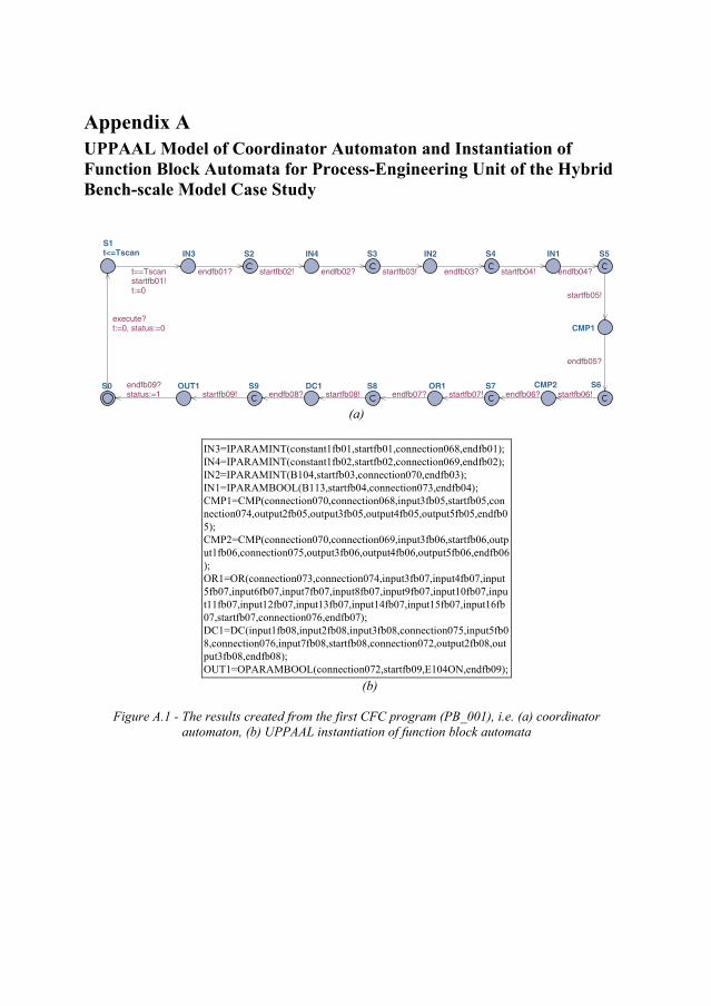
Appendix A UPPAAL Model of Coordinator Automaton and Instantiation of Function Block Automata for Process-Engineering Unit of the Hybrid Bench-scale Model Case Study
S0
IN3S1t<=Tscan IN4S2 IN2S3 IN1S4
CMP1
S5
CMP2 S6OR1 S7DC1 S8OUT1 S9
t==Tscanstartfb01!t:=0
endfb01? startfb02! endfb02? startfb03! endfb03? startfb04! endfb04?
startfb05!
endfb05?
startfb06!endfb06?startfb07!endfb07?startfb08!endfb08?startfb09!endfb09?status:=1
execute?t:=0, status:=0
(a)
IN3=IPARAMINT(constant1fb01,startfb01,connection068,endfb01);IN4=IPARAMINT(constant1fb02,startfb02,connection069,endfb02);IN2=IPARAMINT(B104,startfb03,connection070,endfb03);IN1=IPARAMBOOL(B113,startfb04,connection073,endfb04);CMP1=CMP(connection070,connection068,input3fb05,startfb05,connection074,output2fb05,output3fb05,output4fb05,output5fb05,endfb05);CMP2=CMP(connection070,connection069,input3fb06,startfb06,output1fb06,connection075,output3fb06,output4fb06,output5fb06,endfb06);OR1=OR(connection073,connection074,input3fb07,input4fb07,input5fb07,input6fb07,input7fb07,input8fb07,input9fb07,input10fb07,input11fb07,input12fb07,input13fb07,input14fb07,input15fb07,input16fb07,startfb07,connection076,endfb07);DC1=DC(input1fb08,input2fb08,input3fb08,connection075,input5fb08,connection076,input7fb08,startfb08,connection072,output2fb08,output3fb08,endfb08);OUT1=OPARAMBOOL(connection072,startfb09,E104ON,endfb09);
(b)
Figure A.1 - The results created from the first CFC program (PB_001), i.e. (a) coordinator automaton, (b) UPPAAL instantiation of function block automata
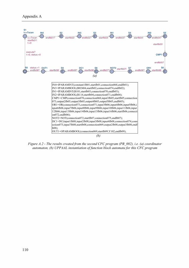
Appendix A
110
S0
IN4S1t<=Tscan IN3S2 IN1S3 IN2S4
CMP1
S5
OR1 S6NOT2 S7DC1 S8OUT1 S9
t==Tscanstartfb01!t:=0
endfb01? startfb02! endfb02? startfb03! endfb03? startfb04! endfb04?
startfb05!
endfb05?
startfb06!endfb06?startfb07!endfb07?startfb08!endfb08?startfb09!endfb09?status:=1
execute?t:=0, status:=0
(a)
IN4=IPARAMINT(constant1fb01,startfb01,connection068,endfb01);IN3=IPARAMBOOL(B02404,startfb02,connection074,endfb02);IN1=IPARAMINT(B101,startfb03,connection070,endfb03);IN2=IPARAMBOOL(B114,startfb04,connection071,endfb04);CMP1=CMP(connection070,connection068,input3fb05,startfb05,connection073,output2fb05,output3fb05,output4fb05,output5fb05,endfb05);OR1=OR(connection073,connection071,input3fb06,input4fb06,input5fb06,input6fb06,input7fb06,input8fb06,input9fb06,input10fb06,input11fb06,input12fb06,input13fb06,input14fb06,input15fb06,input16fb06,startfb06,connection072,endfb06);NOT2=NOT(connection072,startfb07,connection075,endfb07);DC1=DC(input1fb08,input2fb08,input3fb08,input4fb08,connection074,connection075,input7fb08,startfb08,connection069,output2fb08,output3fb08,endfb08);OUT1=OPARAMBOOL(connection069,startfb09,Y102,endfb09);
(b)
Figure A.2 - The results created from the second CFC program (PB_002), i.e. (a) coordinator automaton, (b) UPPAAL instantiation of function block automata for this CFC program
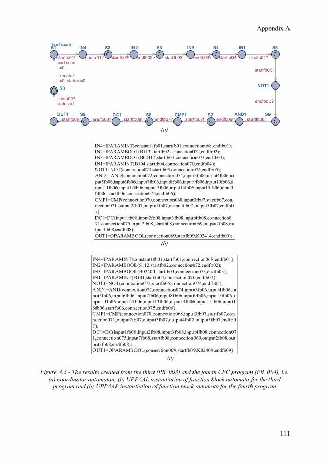
Appendix A
111
S0
IN4S1t<=Tscan
IN2S2 IN3S3 IN1S4
NOT1
S5
AND1 S6CMP1 S7DC1 S8OUT1 S9
t==Tscanstartfb01!
t:=0
endfb01? startfb02! endfb02? startfb03! endfb03? startfb04! endfb04?
startfb05!
endfb05?
startfb06!endfb06?startfb07!endfb07?startfb08!endfb08?startfb09!
endfb09?status:=1
execute?t:=0, status:=0
(a)
IN4=IPARAMINT(constant1fb01,startfb01,connection068,endfb01);IN2=IPARAMBOOL(B113,startfb02,connection072,endfb02);IN3=IPARAMBOOL(B02414,startfb03,connection073,endfb03);IN1=IPARAMINT(B104,startfb04,connection070,endfb04);NOT1=NOT(connection073,startfb05,connection074,endfb05);AND1=AND(connection072,connection074,input3fb06,input4fb06,input5fb06,input6fb06,input7fb06,input8fb06,input9fb06,input10fb06,input11fb06,input12fb06,input13fb06,input14fb06,input15fb06,input16fb06,startfb06,connection075,endfb06);CMP1=CMP(connection070,connection068,input3fb07,startfb07,connection071,output2fb07,output3fb07,output4fb07,output5fb07,endfb07);DC1=DC(input1fb08,input2fb08,input3fb08,input4fb08,connection071,connection075,input7fb08,startfb08,connection069,output2fb08,output3fb08,endfb08);OUT1=OPARAMBOOL(connection069,startfb09,K02414,endfb09);
(b)
IN4=IPARAMINT(constant1fb01,startfb01,connection068,endfb01);IN2=IPARAMBOOL(S112,startfb02,connection072,endfb02);IN3=IPARAMBOOL(B02404,startfb03,connection073,endfb03);IN1=IPARAMINT(B101,startfb04,connection070,endfb04);NOT1=NOT(connection073,startfb05,connection074,endfb05);AND1=AND(connection072,connection074,input3fb06,input4fb06,input5fb06,input6fb06,input7fb06,input8fb06,input9fb06,input10fb06,input11fb06,input12fb06,input13fb06,input14fb06,input15fb06,input16fb06,startfb06,connection075,endfb06);CMP1=CMP(connection070,connection068,input3fb07,startfb07,connection071,output2fb07,output3fb07,output4fb07,output5fb07,endfb07);DC1=DC(input1fb08,input2fb08,input3fb08,input4fb08,connection071,connection075,input7fb08,startfb08,connection069,output2fb08,output3fb08,endfb08);OUT1=OPARAMBOOL(connection069,startfb09,K02404,endfb09);
(c)
Figure A.3 - The results created from the third (PB_003) and the fourth CFC program (PB_004), i.e. (a) coordinator automaton, (b) UPPAAL instantiation of function block automata for the third
program and (b) UPPAAL instantiation of function block automata for the fourth program
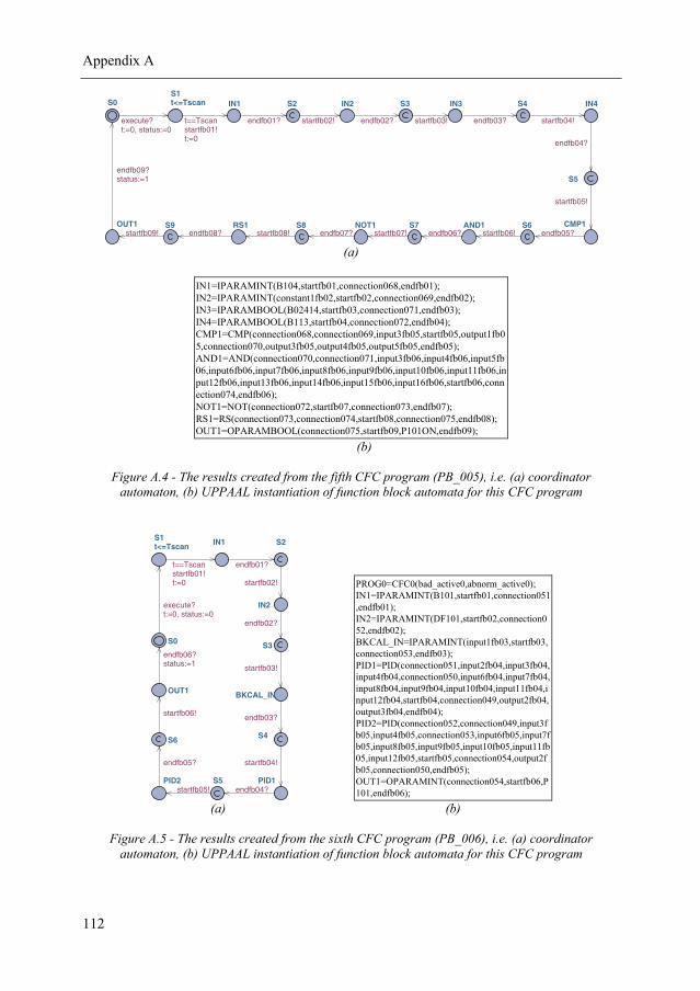
Appendix A
112
S0 IN1S1t<=Tscan IN2S2 IN3S3 IN4S4
CMP1
S5
AND1 S6NOT1 S7RS1 S8OUT1 S9
t==Tscanstartfb01!t:=0
endfb01? startfb02! endfb02? startfb03! endfb03? startfb04!
endfb04?
startfb05!
endfb05?startfb06!endfb06?startfb07!endfb07?startfb08!endfb08?startfb09!
endfb09?status:=1
execute?t:=0, status:=0
(a)
IN1=IPARAMINT(B104,startfb01,connection068,endfb01);IN2=IPARAMINT(constant1fb02,startfb02,connection069,endfb02);IN3=IPARAMBOOL(B02414,startfb03,connection071,endfb03);IN4=IPARAMBOOL(B113,startfb04,connection072,endfb04);CMP1=CMP(connection068,connection069,input3fb05,startfb05,output1fb05,connection070,output3fb05,output4fb05,output5fb05,endfb05);AND1=AND(connection070,connection071,input3fb06,input4fb06,input5fb06,input6fb06,input7fb06,input8fb06,input9fb06,input10fb06,input11fb06,input12fb06,input13fb06,input14fb06,input15fb06,input16fb06,startfb06,connection074,endfb06);NOT1=NOT(connection072,startfb07,connection073,endfb07);RS1=RS(connection073,connection074,startfb08,connection075,endfb08);OUT1=OPARAMBOOL(connection075,startfb09,P101ON,endfb09);
(b)
Figure A.4 - The results created from the fifth CFC program (PB_005), i.e. (a) coordinator automaton, (b) UPPAAL instantiation of function block automata for this CFC program
S0
IN1S1t<=Tscan
IN2
S2
BKCAL_IN
S3
PID1
S4
PID2 S5
OUT1
S6
t==Tscanstartfb01!t:=0
endfb01?
startfb02!
endfb02?
startfb03!
endfb03?
startfb04!
endfb04?startfb05!
endfb05?
startfb06!
endfb06?status:=1
execute?t:=0, status:=0
PROG0=CFC0(bad_active0,abnorm_active0);IN1=IPARAMINT(B101,startfb01,connection051,endfb01);IN2=IPARAMINT(DF101,startfb02,connection052,endfb02);BKCAL_IN=IPARAMINT(input1fb03,startfb03,connection053,endfb03);PID1=PID(connection051,input2fb04,input3fb04,input4fb04,connection050,input6fb04,input7fb04,input8fb04,input9fb04,input10fb04,input11fb04,input12fb04,startfb04,connection049,output2fb04,output3fb04,endfb04);PID2=PID(connection052,connection049,input3fb05,input4fb05,connection053,input6fb05,input7fb05,input8fb05,input9fb05,input10fb05,input11fb05,input12fb05,startfb05,connection054,output2fb05,connection050,endfb05);OUT1=OPARAMINT(connection054,startfb06,P101,endfb06);
(a) (b)
Figure A.5 - The results created from the sixth CFC program (PB_006), i.e. (a) coordinator automaton, (b) UPPAAL instantiation of function block automata for this CFC program
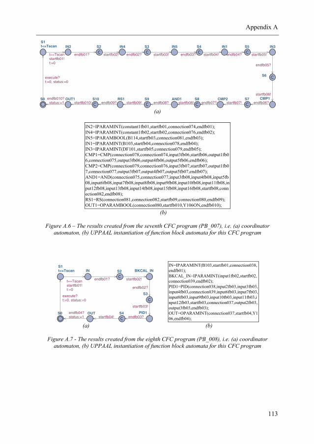
Appendix A
113
S0
IN2S1t<=Tscan IN4S2 IN5S3 IN1S4 IN3S5
CMP1
S6
CMP2 S7AND1 S8RS1 S9OUT1 S10
t==Tscanstartfb01!t:=0
endfb01? startfb02! endfb02? startfb03! endfb03? startfb04! endfb04? startfb05!
endfb05?
startfb06!
endfb06?startfb07!endfb07?startfb08!endfb08?startfb09!endfb09?startfb010!endfb010?
status:=1
execute?t:=0, status:=0
(a)
IN2=IPARAMINT(constant1fb01,startfb01,connection074,endfb01);IN4=IPARAMINT(constant1fb02,startfb02,connection076,endfb02);IN5=IPARAMBOOL(B114,startfb03,connection081,endfb03);IN1=IPARAMINT(B103,startfb04,connection078,endfb04);IN3=IPARAMINT(DF101,startfb05,connection079,endfb05);CMP1=CMP(connection078,connection074,input3fb06,startfb06,output1fb06,connection075,output3fb06,output4fb06,output5fb06,endfb06);CMP2=CMP(connection079,connection076,input3fb07,startfb07,output1fb07,connection077,output3fb07,output4fb07,output5fb07,endfb07);AND1=AND(connection075,connection077,input3fb08,input4fb08,input5fb08,input6fb08,input7fb08,input8fb08,input9fb08,input10fb08,input11fb08,input12fb08,input13fb08,input14fb08,input15fb08,input16fb08,startfb08,connection082,endfb08);RS1=RS(connection081,connection082,startfb09,connection080,endfb09);OUT1=OPARAMBOOL(connection080,startfb010,Y106ON,endfb010);
(b)
Figure A.6 – The results created from the seventh CFC program (PB_007), i.e. (a) coordinator automaton, (b) UPPAAL instantiation of function block automata for this CFC program
S0
INS1t<=Tscan BKCAL_INS2
PID1
S3
OUT S4
t==Tscanstartfb01!t:=0
endfb01? startfb02!
endfb02?
startfb03!
endfb03?startfb04!endfb04?status:=1
execute?t:=0, status:=0
IN=IPARAMINT(B103,startfb01,connection038,endfb01);BKCAL_IN=IPARAMINT(input1fb02,startfb02,connection039,endfb02);PID1=PID(connection038,input2fb03,input3fb03,input4fb03,connection039,input6fb03,input7fb03,input8fb03,input9fb03,input10fb03,input11fb03,input12fb03,startfb03,connection037,output2fb03,output3fb03,endfb03);OUT=OPARAMINT(connection037,startfb04,Y106,endfb04);
(a) (b)
Figure A.7 - The results created from the eighth CFC program (PB_008), i.e. (a) coordinator automaton, (b) UPPAAL instantiation of function block automata for this CFC program
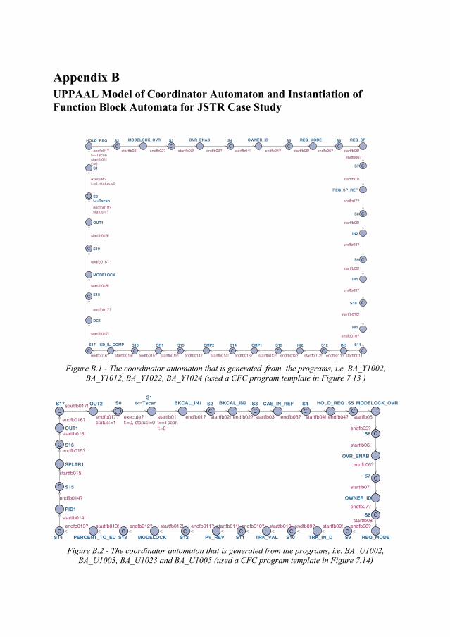
Appendix B UPPAAL Model of Coordinator Automaton and Instantiation of Function Block Automata for JSTR Case Study
S0
HOLD_REQ
S1
t<=Tscan
MODELOCK_OVRS2 OVR_ENABS3 OWNER_IDS4 REQ_MODES5 REQ_SPS6
REQ_SP_REF
S7
IN2
S8
IN1
S9
HI1
S10
IN3 S11HI2 S12CMP1 S13CMP2 S14OR1 S15SD_IL_COMP S16
DC1
S17
MODELOCK
S18
OUT1
S19
t==Tscanstartfb01!t:=0
endfb01? startfb02! endfb02? startfb03! endfb03? startfb04! endfb04? startfb05! endfb05? startfb06!
endfb06?
startfb07!
endfb07?
startfb08!
endfb08?
startfb09!
endfb09?
startfb010!
endfb010?
startfb011!endfb011?startfb012!endfb012?startfb013!endfb013?startfb014!endfb014?startfb015!endfb015?startfb016!endfb016?
startfb017!
endfb017?
startfb018!
endfb018?
startfb019!
endfb019?status:=1
execute?t:=0, status:=0
Figure B.1 - The coordinator automaton that is generated from the programs, i.e. BA_Y1002,
BA_Y1012, BA_Y1022, BA_Y1024 (used a CFC program template in Figure 7.13 )
S0 BKCAL_IN1S1
t<=Tscan BKCAL_IN2S2 CAS_IN_REFS3 HOLD_REQS4 MODELOCK_OVRS5
OVR_ENAB
S6
OWNER_ID
S7
REQ_MODE
S8
TRK_IN_D S9TRK_VAL S10PV_REV S11MODELOCK S12PERCENT_TO_EU S13
PID1
S14
SPLTR1
S15
OUT1
S16
OUT2S17
endfb010?
t==Tscanstartfb01!
t:=0
endfb01? startfb02! endfb02? startfb03! endfb03? startfb04! endfb04? startfb05!
endfb05?
startfb06!
endfb06?
startfb07!
endfb07?
startfb08!endfb08?startfb09!endfb09?startfb010!startfb011!endfb011?startfb012!endfb012?startfb013!endfb013?
startfb014!
endfb014?
startfb015!
endfb015?
startfb016!
endfb016?
startfb017!
endfb017?status:=1
execute?t:=0, status:=0
Figure B.2 - The coordinator automaton that is generated from the programs, i.e. BA_U1002,
BA_U1003, BA_U1023 and BA_U1005 (used a CFC program template in Figure 7.14)
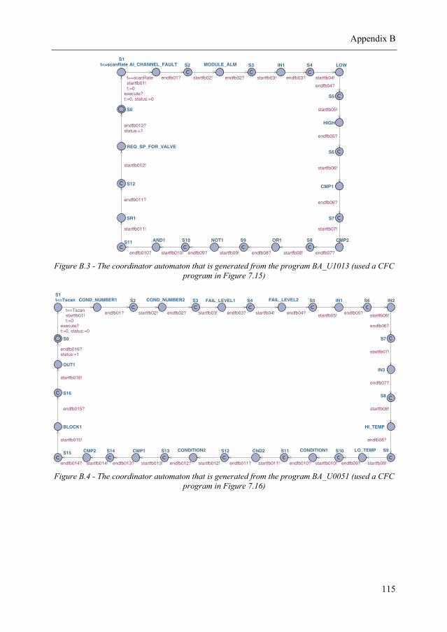
Appendix B
115
S0
AI_CHANNEL_FAULTS1
t<=scanRate MODULE_ALMS2 IN1S3 LOWS4
HIGH
S5
CMP1
S6
CMP2
S7
OR1 S8NOT1 S9AND1 S10
SR1
S11
REQ_SP_FOR_VALVE
S12
t==scanRatestartfb01!t:=0
endfb01? startfb02! endfb02? startfb03! endfb03? startfb04!
endfb04?
startfb05!
endfb05?
startfb06!
endfb06?
startfb07!
endfb07?startfb08!endfb08?startfb09!endfb09?startfb010!endfb010?
startfb011!
endfb011?
startfb012!
endfb012?status:=1
execute?t:=0, status:=0
Figure B.3 - The coordinator automaton that is generated from the program BA_U1013 (used a CFC
program in Figure 7.15)
S0
COND_NUMBER1S1t<=Tscan COND_NUMBER2S2 FAIL_LEVEL1S3 FAIL_LEVEL2S4 IN1S5 IN2S6
IN3
S7
HI_TEMP
S8
LO_TEMP S9CONDITION1 S10CND2 S11CONDITION2 S12CMP1 S13CMP2 S14
BLOCK1
S15
OUT1
S16
t==Tscanstartfb01!t:=0
endfb01? startfb02! endfb02? startfb03! endfb03? startfb04! endfb04? startfb05! endfb05? startfb06!
endfb06?
startfb07!
endfb07?
startfb08!
endfb08?
startfb09!endfb09?startfb010!endfb010?startfb011!endfb011?startfb012!endfb012?startfb013!endfb013?startfb014!endfb014?
startfb015!
endfb015?
startfb016!
endfb016?status:=1
execute?t:=0, status:=0
Figure B.4 - The coordinator automaton that is generated from the program BA_U0051 (used a CFC
program in Figure 7.16)
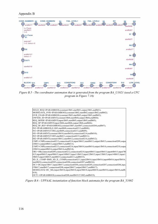
Appendix B
116
S0
COND_NUMBER1
S1t<=Tscan
COND_NUMBER2S2 FAIL_LEVEL1S3 FAIL_LEVEL2S4 IN1S5 IN2S6
IN3
S7
IN4
S8
LOW_LEVEL
S9
CONDITION1 S10CND2 S11CONDITION2 S12CMP1 S13BLOCK1 S14
OUT1
S15
t==Tscanstartfb01!t:=0
endfb01? startfb02! endfb02? startfb03! endfb03? startfb04! endfb04? startfb05! endfb05? startfb06!
endfb06?
startfb07!
endfb07?
startfb08!
endfb08?
startfb09!
endfb09?startfb010!endfb010?startfb011!endfb011?startfb012!endfb012?startfb013!endfb013?startfb014!
endfb014?
startfb015!
endfb015?status:=1
execute?t:=0, status:=0
Figure B.5 - The coordinator automaton that is generated from the program BA_U1021 (used a CFC
program in Figure 7.16)
HOLD_REQ=IPARAMBOOL(constant1fb01,startfb01,output1fb01,endfb01);MODELOCK_OVR=IPARAMBOOL(constant1fb02,startfb02,output1fb02,endfb02);OVR_ENAB=IPARAMBOOL(constant1fb03,startfb03,output1fb03,endfb03);OWNER_ID=IPARAMINT(constant1fb04,startfb04,output1fb04,endfb04);REQ_MODE=IPARAMINT(input1fb05,startfb05,output1fb05,endfb05);REQ_SP=IPARAMINT(input1fb06,startfb06,output1fb06,endfb06);REQ_SP_REF=IPARAMBOOL(constant1fb07,startfb07,connection0204,endfb07);IN2=IPARAMBOOL(L1003,startfb08,connection0212,endfb08);IN1=IPARAMINT(T1002,startfb09,connection0213,endfb09);HI1=IPARAMINT(constant1fb010,startfb010,connection0214,endfb010);IN3=IPARAMINT(T1005,startfb011,connection0215,endfb011);HI2=IPARAMINT(constant1fb012,startfb012,connection0216,endfb012);CMP1=CMP(connection0213,connection0214,input3fb013,startfb013,output1fb013,connection0209,output3fb013,output4fb013,output5fb013,endfb013);CMP2=CMP(connection0215,connection0216,input3fb014,startfb014,output1fb014,connection0210,output3fb014,output4fb014,output5fb014,endfb014);OR1=OR(connection0209,connection0212,connection0210,input4fb015,input5fb015,input6fb015,input7fb015,input8fb015,input9fb015,input10fb015,input11fb015,input12fb015,input13fb015,input14fb015,input15fb015,input16fb015,startfb015,connection0211,endfb015);SD_IL_COMP=BMS_SD_IL_COMP(connection0211,input2fb016,input3fb016,input4fb016,input5fb016,startfb016,connection0205,connection0206,connection0207,endfb016);DC1=DC(input1fb017,input2fb017,connection0204,connection0205,connection0207,connection0206,input7fb017,startfb017,connection0208,output2fb017,output3fb017,endfb017);MODELOCK=DC_ML(input1fb018,input2fb018,input3fb018,input4fb018,startfb018,output1fb018,endfb018);OUT1=OPARAMBOOL(connection0208,startfb019,Y1002,endfb019);
Figure B.6 - UPPAAL instantiation of function block automata for the program BA_Y1002
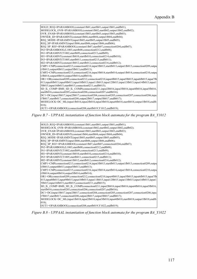
Appendix B
117
HOLD_REQ=IPARAMBOOL(constant1fb01,startfb01,output1fb01,endfb01);MODELOCK_OVR=IPARAMBOOL(constant1fb02,startfb02,output1fb02,endfb02);OVR_ENAB=IPARAMBOOL(constant1fb03,startfb03,output1fb03,endfb03);OWNER_ID=IPARAMINT(constant1fb04,startfb04,output1fb04,endfb04);REQ_MODE=IPARAMINT(input1fb05,startfb05,output1fb05,endfb05);REQ_SP=IPARAMINT(input1fb06,startfb06,output1fb06,endfb06);REQ_SP_REF=IPARAMBOOL(constant1fb07,startfb07,connection0204,endfb07);IN2=IPARAMBOOL(L1003,startfb08,connection0212,endfb08);IN1=IPARAMINT(T1002,startfb09,connection0213,endfb09);HI1=IPARAMINT(constant1fb010,startfb010,connection0214,endfb010);IN3=IPARAMINT(T1005,startfb011,connection0215,endfb011);HI2=IPARAMINT(constant1fb012,startfb012,connection0216,endfb012);CMP1=CMP(connection0213,connection0214,input3fb013,startfb013,output1fb013,connection0209,output3fb013,output4fb013,output5fb013,endfb013);CMP2=CMP(connection0215,connection0216,input3fb014,startfb014,output1fb014,connection0210,output3fb014,output4fb014,output5fb014,endfb014);OR1=OR(connection0209,connection0212,connection0210,input4fb015,input5fb015,input6fb015,input7fb015,input8fb015,input9fb015,input10fb015,input11fb015,input12fb015,input13fb015,input14fb015,input15fb015,input16fb015,startfb015,connection0211,endfb015);SD_IL_COMP=BMS_SD_IL_COMP(connection0211,input2fb016,input3fb016,input4fb016,input5fb016,startfb016,connection0205,connection0206,connection0207,endfb016);DC1=DC(input1fb017,input2fb017,connection0204,connection0205,connection0207,connection0206,input7fb017,startfb017,connection0208,output2fb017,output3fb017,endfb017);MODELOCK=DC_ML(input1fb018,input2fb018,input3fb018,input4fb018,startfb018,output1fb018,endfb018);OUT1=OPARAMBOOL(connection0208,startfb019,Y1012,endfb019);
Figure B.7 - UPPAAL instantiation of function block automata for the program BA_Y1012
HOLD_REQ=IPARAMBOOL(constant1fb01,startfb01,output1fb01,endfb01);MODELOCK_OVR=IPARAMBOOL(constant1fb02,startfb02,output1fb02,endfb02);OVR_ENAB=IPARAMBOOL(constant1fb03,startfb03,output1fb03,endfb03);OWNER_ID=IPARAMINT(constant1fb04,startfb04,output1fb04,endfb04);REQ_MODE=IPARAMINT(input1fb05,startfb05,output1fb05,endfb05);REQ_SP=IPARAMINT(input1fb06,startfb06,output1fb06,endfb06);REQ_SP_REF=IPARAMBOOL(constant1fb07,startfb07,connection0204,endfb07);IN2=IPARAMBOOL(L1003,startfb08,connection0212,endfb08);IN1=IPARAMINT(T1002,startfb09,connection0213,endfb09);HI1=IPARAMINT(constant1fb010,startfb010,connection0214,endfb010);IN3=IPARAMINT(T1005,startfb011,connection0215,endfb011);HI2=IPARAMINT(constant1fb012,startfb012,connection0216,endfb012);CMP1=CMP(connection0213,connection0214,input3fb013,startfb013,output1fb013,connection0209,output3fb013,output4fb013,output5fb013,endfb013);CMP2=CMP(connection0215,connection0216,input3fb014,startfb014,output1fb014,connection0210,output3fb014,output4fb014,output5fb014,endfb014);OR1=OR(connection0209,connection0212,connection0210,input4fb015,input5fb015,input6fb015,input7fb015,input8fb015,input9fb015,input10fb015,input11fb015,input12fb015,input13fb015,input14fb015,input15fb015,input16fb015,startfb015,connection0211,endfb015);SD_IL_COMP=BMS_SD_IL_COMP(connection0211,input2fb016,input3fb016,input4fb016,input5fb016,startfb016,connection0205,connection0206,connection0207,endfb016);DC1=DC(input1fb017,input2fb017,connection0204,connection0205,connection0207,connection0206,input7fb017,startfb017,connection0208,output2fb017,output3fb017,endfb017);MODELOCK=DC_ML(input1fb018,input2fb018,input3fb018,input4fb018,startfb018,output1fb018,endfb018);OUT1=OPARAMBOOL(connection0208,startfb019,Y1022,endfb019);
Figure B.8 - UPPAAL instantiation of function block automata for the program BA_Y1022
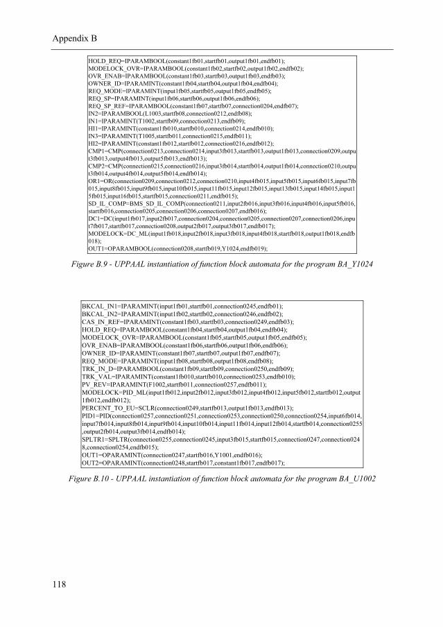
Appendix B
118
HOLD_REQ=IPARAMBOOL(constant1fb01,startfb01,output1fb01,endfb01);MODELOCK_OVR=IPARAMBOOL(constant1fb02,startfb02,output1fb02,endfb02);OVR_ENAB=IPARAMBOOL(constant1fb03,startfb03,output1fb03,endfb03);OWNER_ID=IPARAMINT(constant1fb04,startfb04,output1fb04,endfb04);REQ_MODE=IPARAMINT(input1fb05,startfb05,output1fb05,endfb05);REQ_SP=IPARAMINT(input1fb06,startfb06,output1fb06,endfb06);REQ_SP_REF=IPARAMBOOL(constant1fb07,startfb07,connection0204,endfb07);IN2=IPARAMBOOL(L1003,startfb08,connection0212,endfb08);IN1=IPARAMINT(T1002,startfb09,connection0213,endfb09);HI1=IPARAMINT(constant1fb010,startfb010,connection0214,endfb010);IN3=IPARAMINT(T1005,startfb011,connection0215,endfb011);HI2=IPARAMINT(constant1fb012,startfb012,connection0216,endfb012);CMP1=CMP(connection0213,connection0214,input3fb013,startfb013,output1fb013,connection0209,output3fb013,output4fb013,output5fb013,endfb013);CMP2=CMP(connection0215,connection0216,input3fb014,startfb014,output1fb014,connection0210,output3fb014,output4fb014,output5fb014,endfb014);OR1=OR(connection0209,connection0212,connection0210,input4fb015,input5fb015,input6fb015,input7fb015,input8fb015,input9fb015,input10fb015,input11fb015,input12fb015,input13fb015,input14fb015,input15fb015,input16fb015,startfb015,connection0211,endfb015);SD_IL_COMP=BMS_SD_IL_COMP(connection0211,input2fb016,input3fb016,input4fb016,input5fb016,startfb016,connection0205,connection0206,connection0207,endfb016);DC1=DC(input1fb017,input2fb017,connection0204,connection0205,connection0207,connection0206,input7fb017,startfb017,connection0208,output2fb017,output3fb017,endfb017);MODELOCK=DC_ML(input1fb018,input2fb018,input3fb018,input4fb018,startfb018,output1fb018,endfb018);OUT1=OPARAMBOOL(connection0208,startfb019,Y1024,endfb019);
Figure B.9 - UPPAAL instantiation of function block automata for the program BA_Y1024
BKCAL_IN1=IPARAMINT(input1fb01,startfb01,connection0245,endfb01);BKCAL_IN2=IPARAMINT(input1fb02,startfb02,connection0246,endfb02);CAS_IN_REF=IPARAMINT(constant1fb03,startfb03,connection0249,endfb03);HOLD_REQ=IPARAMBOOL(constant1fb04,startfb04,output1fb04,endfb04);MODELOCK_OVR=IPARAMBOOL(constant1fb05,startfb05,output1fb05,endfb05);OVR_ENAB=IPARAMBOOL(constant1fb06,startfb06,output1fb06,endfb06);OWNER_ID=IPARAMINT(constant1fb07,startfb07,output1fb07,endfb07);REQ_MODE=IPARAMINT(input1fb08,startfb08,output1fb08,endfb08);TRK_IN_D=IPARAMBOOL(constant1fb09,startfb09,connection0250,endfb09);TRK_VAL=IPARAMINT(constant1fb010,startfb010,connection0253,endfb010);PV_REV=IPARAMINT(F1002,startfb011,connection0257,endfb011);MODELOCK=PID_ML(input1fb012,input2fb012,input3fb012,input4fb012,input5fb012,startfb012,output1fb012,endfb012);PERCENT_TO_EU=SCLR(connection0249,startfb013,output1fb013,endfb013);PID1=PID(connection0257,connection0251,connection0253,connection0250,connection0254,input6fb014,input7fb014,input8fb014,input9fb014,input10fb014,input11fb014,input12fb014,startfb014,connection0255,output2fb014,output3fb014,endfb014);SPLTR1=SPLTR(connection0255,connection0245,input3fb015,startfb015,connection0247,connection0248,connection0254,endfb015);OUT1=OPARAMINT(connection0247,startfb016,Y1001,endfb016);OUT2=OPARAMINT(connection0248,startfb017,constant1fb017,endfb017);
Figure B.10 - UPPAAL instantiation of function block automata for the program BA_U1002
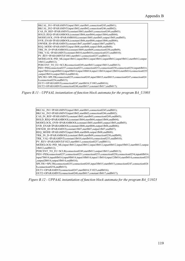
Appendix B
119
BKCAL_IN1=IPARAMINT(input1fb01,startfb01,connection0245,endfb01);BKCAL_IN2=IPARAMINT(input1fb02,startfb02,connection0246,endfb02);CAS_IN_REF=IPARAMINT(constant1fb03,startfb03,connection0249,endfb03);HOLD_REQ=IPARAMBOOL(constant1fb04,startfb04,output1fb04,endfb04);MODELOCK_OVR=IPARAMBOOL(constant1fb05,startfb05,output1fb05,endfb05);OVR_ENAB=IPARAMBOOL(constant1fb06,startfb06,output1fb06,endfb06);OWNER_ID=IPARAMINT(constant1fb07,startfb07,output1fb07,endfb07);REQ_MODE=IPARAMINT(input1fb08,startfb08,output1fb08,endfb08);TRK_IN_D=IPARAMBOOL(constant1fb09,startfb09,connection0250,endfb09);TRK_VAL=IPARAMINT(constant1fb010,startfb010,connection0253,endfb010);PV_REV=IPARAMINT(F1003,startfb011,connection0257,endfb011);MODELOCK=PID_ML(input1fb012,input2fb012,input3fb012,input4fb012,input5fb012,startfb012,output1fb012,endfb012);PERCENT_TO_EU=SCLR(connection0249,startfb013,output1fb013,endfb013);PID1=PID(connection0257,connection0251,connection0253,connection0250,connection0254,input6fb014,input7fb014,input8fb014,input9fb014,input10fb014,input11fb014,input12fb014,startfb014,connection0255,output2fb014,output3fb014,endfb014);SPLTR1=SPLTR(connection0255,connection0245,input3fb015,startfb015,connection0247,connection0248,connection0254,endfb015);OUT1=OPARAMINT(connection0247,startfb016,Y1003,endfb016);OUT2=OPARAMINT(connection0248,startfb017,constant1fb017,endfb017);
Figure B.11 - UPPAAL instantiation of function block automata for the program BA_U1003
BKCAL_IN1=IPARAMINT(input1fb01,startfb01,connection0245,endfb01);BKCAL_IN2=IPARAMINT(input1fb02,startfb02,connection0246,endfb02);CAS_IN_REF=IPARAMINT(constant1fb03,startfb03,connection0249,endfb03);HOLD_REQ=IPARAMBOOL(constant1fb04,startfb04,output1fb04,endfb04);MODELOCK_OVR=IPARAMBOOL(constant1fb05,startfb05,output1fb05,endfb05);OVR_ENAB=IPARAMBOOL(constant1fb06,startfb06,output1fb06,endfb06);OWNER_ID=IPARAMINT(constant1fb07,startfb07,output1fb07,endfb07);REQ_MODE=IPARAMINT(input1fb08,startfb08,output1fb08,endfb08);TRK_IN_D=IPARAMBOOL(constant1fb09,startfb09,connection0250,endfb09);TRK_VAL=IPARAMINT(constant1fb010,startfb010,connection0253,endfb010);PV_REV=IPARAMINT(F1023,startfb011,connection0257,endfb011);MODELOCK=PID_ML(input1fb012,input2fb012,input3fb012,input4fb012,input5fb012,startfb012,output1fb012,endfb012);PERCENT_TO_EU=SCLR(connection0249,startfb013,output1fb013,endfb013);PID1=PID(connection0257,connection0251,connection0253,connection0250,connection0254,input6fb014,input7fb014,input8fb014,input9fb014,input10fb014,input11fb014,input12fb014,startfb014,connection0255,output2fb014,output3fb014,endfb014);SPLTR1=SPLTR(connection0255,connection0245,input3fb015,startfb015,connection0247,connection0248,connection0254,endfb015);OUT1=OPARAMINT(connection0247,startfb016,Y1023,endfb016);OUT2=OPARAMINT(connection0248,startfb017,constant1fb017,endfb017);
Figure B.12 - UPPAAL instantiation of function block automata for the program BA_U1023
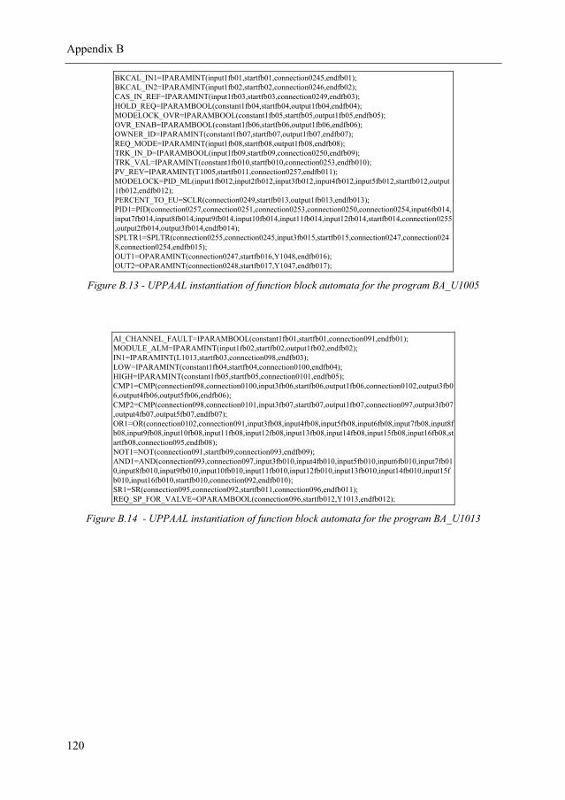
Appendix B
120
BKCAL_IN1=IPARAMINT(input1fb01,startfb01,connection0245,endfb01);BKCAL_IN2=IPARAMINT(input1fb02,startfb02,connection0246,endfb02);CAS_IN_REF=IPARAMINT(input1fb03,startfb03,connection0249,endfb03);HOLD_REQ=IPARAMBOOL(constant1fb04,startfb04,output1fb04,endfb04);MODELOCK_OVR=IPARAMBOOL(constant1fb05,startfb05,output1fb05,endfb05);OVR_ENAB=IPARAMBOOL(constant1fb06,startfb06,output1fb06,endfb06);OWNER_ID=IPARAMINT(constant1fb07,startfb07,output1fb07,endfb07);REQ_MODE=IPARAMINT(input1fb08,startfb08,output1fb08,endfb08);TRK_IN_D=IPARAMBOOL(input1fb09,startfb09,connection0250,endfb09);TRK_VAL=IPARAMINT(constant1fb010,startfb010,connection0253,endfb010);PV_REV=IPARAMINT(T1005,startfb011,connection0257,endfb011);MODELOCK=PID_ML(input1fb012,input2fb012,input3fb012,input4fb012,input5fb012,startfb012,output1fb012,endfb012);PERCENT_TO_EU=SCLR(connection0249,startfb013,output1fb013,endfb013);PID1=PID(connection0257,connection0251,connection0253,connection0250,connection0254,input6fb014,input7fb014,input8fb014,input9fb014,input10fb014,input11fb014,input12fb014,startfb014,connection0255,output2fb014,output3fb014,endfb014);SPLTR1=SPLTR(connection0255,connection0245,input3fb015,startfb015,connection0247,connection0248,connection0254,endfb015);OUT1=OPARAMINT(connection0247,startfb016,Y1048,endfb016);OUT2=OPARAMINT(connection0248,startfb017,Y1047,endfb017);
Figure B.13 - UPPAAL instantiation of function block automata for the program BA_U1005
AI_CHANNEL_FAULT=IPARAMBOOL(constant1fb01,startfb01,connection091,endfb01);MODULE_ALM=IPARAMINT(input1fb02,startfb02,output1fb02,endfb02);IN1=IPARAMINT(L1013,startfb03,connection098,endfb03);LOW=IPARAMINT(constant1fb04,startfb04,connection0100,endfb04);HIGH=IPARAMINT(constant1fb05,startfb05,connection0101,endfb05);CMP1=CMP(connection098,connection0100,input3fb06,startfb06,output1fb06,connection0102,output3fb06,output4fb06,output5fb06,endfb06);CMP2=CMP(connection098,connection0101,input3fb07,startfb07,output1fb07,connection097,output3fb07,output4fb07,output5fb07,endfb07);OR1=OR(connection0102,connection091,input3fb08,input4fb08,input5fb08,input6fb08,input7fb08,input8fb08,input9fb08,input10fb08,input11fb08,input12fb08,input13fb08,input14fb08,input15fb08,input16fb08,startfb08,connection095,endfb08);NOT1=NOT(connection091,startfb09,connection093,endfb09);AND1=AND(connection093,connection097,input3fb010,input4fb010,input5fb010,input6fb010,input7fb010,input8fb010,input9fb010,input10fb010,input11fb010,input12fb010,input13fb010,input14fb010,input15fb010,input16fb010,startfb010,connection092,endfb010);SR1=SR(connection095,connection092,startfb011,connection096,endfb011);REQ_SP_FOR_VALVE=OPARAMBOOL(connection096,startfb012,Y1013,endfb012);
Figure B.14 - UPPAAL instantiation of function block automata for the program BA_U1013
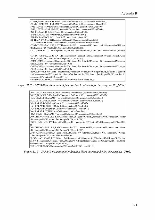
Appendix B
121
COND_NUMBER1=IPARAMINT(constant1fb01,startfb01,connection0190,endfb01);COND_NUMBER2=IPARAMINT(constant1fb02,startfb02,connection0194,endfb02);FAIL_LEVEL1=IPARAMINT(constant1fb03,startfb03,connection0189,endfb03);FAIL_LEVEL2=IPARAMINT(constant1fb04,startfb04,connection0193,endfb04);IN1=IPARAMBOOL(L1003,startfb05,connection0197,endfb05);IN2=IPARAMINT(T1002,startfb06,connection0200,endfb06);IN3=IPARAMBOOL(M2112,startfb07,connection0198,endfb07);HI_TEMP=IPARAMINT(constant1fb08,startfb08,connection0201,endfb08);LO_TEMP=IPARAMINT(constant1fb09,startfb09,connection0203,endfb09);CONDITION1=FAILURE_LATCH(connection0195,connection0196,connection0189,connection0190,startfb010,output1fb010,output2fb010,output3fb010,endfb010);CND2=BMS_INTL_TYPE(input1fb011,startfb011,connection0191,output2fb011,connection0192,endfb011);CONDITION2=FAILURE_LATCH(connection0191,connection0192,connection0193,connection0194,startfb012,output1fb012,output2fb012,output3fb012,endfb012);CMP1=CMP(connection0200,connection0201,input3fb013,startfb013,output1fb013,connection0204,output3fb013,output4fb013,output5fb013,endfb013);CMP2=CMP(connection0200,connection0203,input3fb014,startfb014,output1fb014,connection0205,output3fb014,output4fb014,output5fb014,endfb014);BLOCK1=V710BA10_INTL1(input1fb015,connection0197,input3fb015,input4fb015,input5fb015,connection0204,connection0205,input8fb015,input9fb015,connection0198,input11fb015,input12fb015,startfb015,connection0195,output2fb015,endfb015);OUT1=OPARAMBOOL(connection0195,startfb016,Y1046,endfb016);
Figure B.15 - UPPAAL instantiation of function block automata for the program BA_U0511
COND_NUMBER1=IPARAMINT(constant1fb01,startfb01,connection0376,endfb01);COND_NUMBER2=IPARAMINT(constant1fb02,startfb02,connection0380,endfb02);FAIL_LEVEL1=IPARAMINT(constant1fb03,startfb03,connection0375,endfb03);FAIL_LEVEL2=IPARAMINT(constant1fb04,startfb04,connection0379,endfb04);IN1=IPARAMBOOL(L1002,startfb05,connection0383,endfb05);IN2=IPARAMBOOL(L1003,startfb06,connection0386,endfb06);IN3=IPARAMBOOL(M9501,startfb07,connection0384,endfb07);IN4=IPARAMINT(T1002,startfb08,connection0387,endfb08);LOW_LEVEL=IPARAMINT(constant1fb09,startfb09,connection0388,endfb09);CONDITION1=FAILURE_LATCH(connection0381,connection0382,connection0375,connection0376,startfb010,output1fb010,output2fb010,output3fb010,endfb010);CND2=BMS_INTL_TYPE(input1fb011,startfb011,connection0377,output2fb011,connection0378,endfb011);CONDITION2=FAILURE_LATCH(connection0377,connection0378,connection0379,connection0380,startfb012,output1fb012,output2fb012,output3fb012,endfb012);CMP1=CMP(connection0387,connection0388,input3fb013,startfb013,output1fb013,connection0389,output3fb013,output4fb013,output5fb013,endfb013);BLOCK1=V710BA10_INTL1(input1fb014,connection0383,connection0386,input4fb014,input5fb014,input6fb014,connection0384,connection0389,input9fb014,input10fb014,input11fb014,input12fb014,startfb014,connection0381,output2fb014,endfb014);OUT1=OPARAMBOOL(connection0381,startfb015,Y1021,endfb015);
Figure B.16 - UPPAAL instantiation of function block automata for the program BA_U1021
Related Documents