Part 1: F undame nta ls These are notes for the first part of PHYS 352 Elect romagneti c W av es. This course fol lo ws on fro m PHYS 350. At the end of that cours e, you will hav e seen the full set of Maxwell’s equations, which in vacuum are ∇ · E = ρ 0 ∇ × E = − ∂ B ∂t ∇ · B = 0 ∇ × B = µ 0 J + µ 0 0 ∂ E ∂t (1.1) with ∇ · J = − ∂ρ ∂t . (1.2) In this course, we will investigate the implications and applications of these results. We will cover • electromagnetic wav es • energy and momentum of electromagnetic fields • electromagnetism and relativity • electromagnetic waves in materials and plasmas • waveguides and transmission lines • electromagnetic radiation from accelerated charges • numerical methods for solving problems in electromagnetism By the end of the course, you will be able to calculate the properties of electromagnetic waves in a range of materials, calculate the radiation from arrangements of accelerating charges, and have a greater appreciation of the theory of electromagnetism and its relation to special relativity. The spirit of the course is well-summed up by the “intermission” in Griffith’s book. After working from statics to dynamics in the first seven chapters of the book, developing the full set of Maxwell’s equations, Griffiths comments (I paraphrase) that the full power of electromagnetism now lies at your fingerti ps, and the fun is only just beginning. It is a disappointing ending to PHYS 350, but an exciting place to start PHYS 352!

Welcome message from author
This document is posted to help you gain knowledge. Please leave a comment to let me know what you think about it! Share it to your friends and learn new things together.
Transcript

7/30/2019 EM waves summary 1
http://slidepdf.com/reader/full/em-waves-summary-1 1/36
Part 1: Fundamentals
These are notes for the first part of PHYS 352 Electromagnetic Waves. This coursefollows on from PHYS 350. At the end of that course, you will have seen the full set of
Maxwell’s equations, which in vacuum are
∇ · E =ρ
0 ∇× E = −
∂ B
∂t
∇ · B = 0 ∇× B = µ0 J + µ00
∂ E
∂t(1.1)
with ∇ ·
J = −
∂ρ
∂t . (1.2)
In this course, we will investigate the implications and applications of these results. We
will cover
• electromagnetic waves
• energy and momentum of electromagnetic fields
• electromagnetism and relativity
• electromagnetic waves in materials and plasmas
• waveguides and transmission lines
• electromagnetic radiation from accelerated charges
• numerical methods for solving problems in electromagnetism
By the end of the course, you will be able to calculate the properties of electromagnetic waves
in a range of materials, calculate the radiation from arrangements of accelerating charges,
and have a greater appreciation of the theory of electromagnetism and its relation to special
relativity.
The spirit of the course is well-summed up by the “intermission” in Griffith’s book.
After working from statics to dynamics in the first seven chapters of the book, developing
the full set of Maxwell’s equations, Griffiths comments (I paraphrase) that the full power
of electromagnetism now lies at your fingertips, and the fun is only just beginning. It is a
disappointing ending to PHYS 350, but an exciting place to start PHYS 352!

7/30/2019 EM waves summary 1
http://slidepdf.com/reader/full/em-waves-summary-1 2/36
– 2 –
Why study electromagnetism? One reason is that it is a fundamental part of physics
(one of the four forces), but it is also ubiquitous in everyday life, technology, and in natural
phenomena in geophysics, astrophysics or biophysics. The study of electromagnetism alsointroduces some advanced physics concepts, whether it be dealing with the abstract notions
of fields or gauge invariance, or learning mathematical techniques such as the approaches
for solving partial differential equations. In this course, we will cover all of these different
aspects, going from the applications of electromagnetism to the basic structure of the theory
of electromagnetism.
1. Important mathematical results
I will assume that you are familiar with the following results and concepts from vectorcalculus:
1. Vector and scalar fields , e.g. temperature T (r), electrostatic potential V (r), velocity
of a fluid v (r), electric field E (r). Sketching a vector field, e.g. a shearing fluid flow
2. Derivatives of fields 1
• gradient operator (note that this is a vector)
∇ =
∂
∂x,
∂
∂y,
∂
∂z
• gradient of a scalar field φ (r)
∇φ =
∂φ∂x
, ∂φ∂y
, ∂φ∂z
1We’ll use Cartesian coordinates here. Depending on the symmetry of the problem, spherical or cylindrical
coordinates may be necessary. For exam purposes, I will assume you know the Cartesian results but will
give you the formulae for spherical or cylindrical coordinate systems.

7/30/2019 EM waves summary 1
http://slidepdf.com/reader/full/em-waves-summary-1 3/36
– 3 –
• gradient of a scalar field in the direction n
n · ∇φ
• divergence of a vector field (this is a scalar quantity)
∇ · E =∂E x∂x
+∂E y∂y
+∂E z∂z
• curl of a vector field (a vector)
∇× E =
x y z ∂ ∂x
∂ ∂y
∂ ∂z
E x E y E z
• 2nd derivative (Laplacian) (a scalar)
∇ · ∇φ = ∇2φ =∂ 2φ
∂x2+
∂ 2φ
∂y2+
∂ 2φ
∂z 2
3. Integrals of fields
• volume integral, e.g.
dV φ (r) = d3r φ (r)
• surface integral, e.g. S
v · d A
• line integral, e.g. path
v · d l
4. Divergence theorem S
v · d A =
V
∇ · v
dV
where volume V is bounded by surface S .
7/30/2019 EM waves summary 1
http://slidepdf.com/reader/full/em-waves-summary-1 4/36
– 4 –
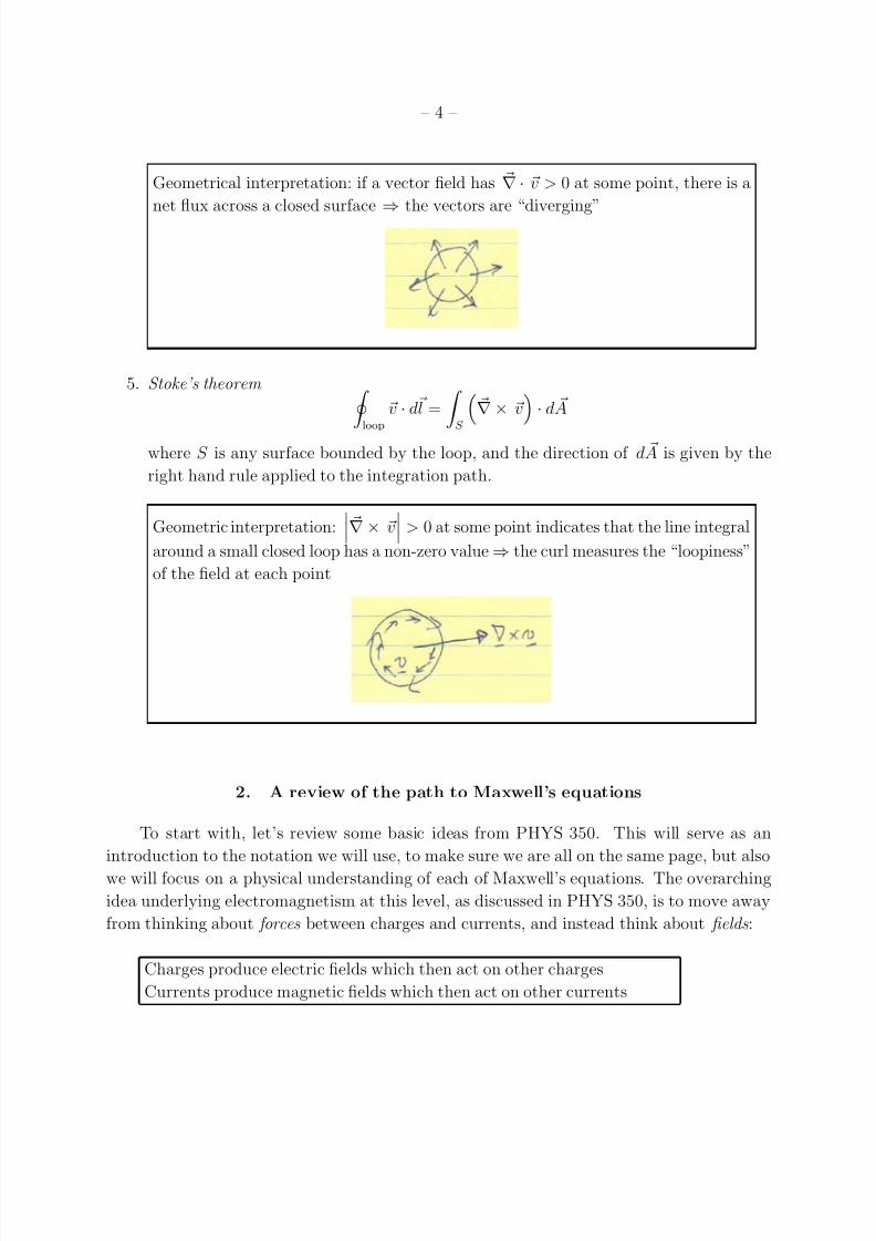
Geometrical interpretation: if a vector field has ∇ · v > 0 at some point, there is a
net flux across a closed surface ⇒ the vectors are “diverging”
5. Stoke’s theorem
loop v · d l = S ∇× v · d A
where S is any surface bounded by the loop, and the direction of d A is given by the
right hand rule applied to the integration path.
Geometric interpretation: ∇× v
> 0 at some point indicates that the line integral
around a small closed loop has a non-zero value ⇒ the curl measures the “loopiness”
of the field at each point
2. A review of the path to Maxwell’s equations
To start with, let’s review some basic ideas from PHYS 350. This will serve as an
introduction to the notation we will use, to make sure we are all on the same page, but also
we will focus on a physical understanding of each of Maxwell’s equations. The overarching
idea underlying electromagnetism at this level, as discussed in PHYS 350, is to move away
from thinking about forces between charges and currents, and instead think about fields :
Charges produce electric fields which then act on other charges
Currents produce magnetic fields which then act on other currents
7/30/2019 EM waves summary 1
http://slidepdf.com/reader/full/em-waves-summary-1 5/36
– 5 –
This contrasts with the approach usually taken in introductory courses which is to treat
forces between charges and currents directly, e.g. through Coulomb’s law. Instead, we think
about the fields as physical objects that are sourced by charges and currents and in turnact on charges and currents through the Lorentz force. In this course, we will take this even
further by considering electromagnetic waves that are wavelike disturbances in the fields and
propagate even in vacuum when no charges or currents are present.
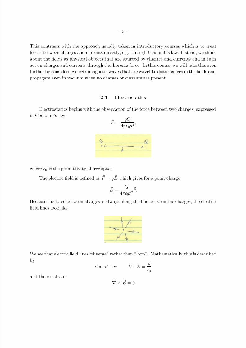
2.1. Electrostatics
Electrostatics begins with the observation of the force between two charges, expressed
in Coulomb’s law
F =qQ
4π0d2 ,
where 0 is the permittivity of free space.
The electric field is defined as F = q E which gives for a point charge
E =Q
4π0r2 r.
Because the force between charges is always along the line between the charges, the electric
field lines look like
We see that electric field lines “diverge” rather than “loop”. Mathematically, this is described
by
Gauss law ∇ · E =ρ
0and the constraint
∇× E = 0

7/30/2019 EM waves summary 1
http://slidepdf.com/reader/full/em-waves-summary-1 6/36
– 6 –
where ρ is the volume charge density (in Cm−3). This can be summed up as “electrostatic
fields begin and end on charges ”. The curl-free nature of E allows us to define the electrostatic
potential through E = −
∇φ, which is a useful route to solving for the electrostatic field inmany cases.
2.2. Magnetostatics
Here we begin with forces between currents, namely that parallel currents attract and
oppositely-directed currents repel.
In the picture that each wire produces a magnetic field that acts on the charge carriers in
the other wire with the Lorentz force
F = q
v × B
,
we can use the observed forces to conclude that the magnetic field of a wire must consist of circular loops around each wire (the right hand rule gives the directions)
The idea that currents source magnetic field loops is expressed in Ampere’s law
∇× B = µ0 J
and the constraint ∇ · B = 0
where J is the current density (current per unit area, Am−2) and the constant µ0 is the
permeability of free space.

7/30/2019 EM waves summary 1
http://slidepdf.com/reader/full/em-waves-summary-1 7/36
– 7 –
Some useful numbers:
charge on the electron e = −1.6× 10⁻¹⁹ C1
4π0= 10−7c2
permittivity of free space 0 = 8.85 × 10⁻¹² C2
Nm2
permeability of free space µ04π = 10−7Tm
A.
2.3. Magnetic induction
Now we move onto non-static fields. Time-dependent magnetic fields generate an elec-
tromotive force (emf) and currents. For example, consider a circular wire threaded by a
time-dependent magnetic field. The emf is
E =
E · d l = −
∂ B∂t
· d A = −dΦm
dt
which is Faraday’s law (the emf is given by the rate of change of magnetic flux) and Lenz’s
law (the minus sign). At a local point, we can use Stoke’s theorem to write Faraday’s law as
∇× E = −∂ B
∂t.
Electrostatic fields are curl free, sourced by charges, but Faraday’s law tells us that time-
dependent magnetic fields source electric field loops.
2.4. Displacement current
Time-dependent E fields act as a source for B. The standard argument here is to
consider charging a capacitor:
7/30/2019 EM waves summary 1
http://slidepdf.com/reader/full/em-waves-summary-1 8/36
– 8 –
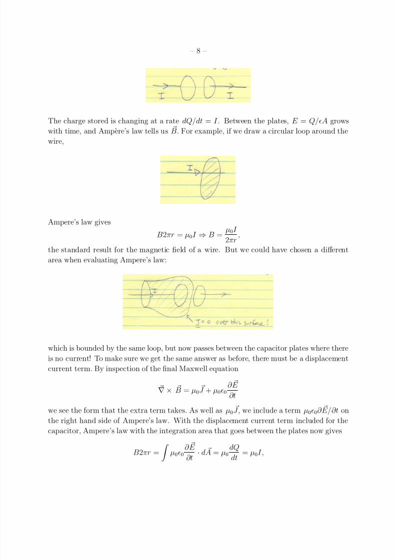
The charge stored is changing at a rate dQ/dt = I . Between the plates, E = Q/A grows
with time, and Ampere’s law tells us B. For example, if we draw a circular loop around the
wire,
Ampere’s law gives
B2πr = µ0I ⇒ B =µ0I
2πr,
the standard result for the magnetic field of a wire. But we could have chosen a different
area when evaluating Ampere’s law:
which is bounded by the same loop, but now passes between the capacitor plates where there
is no current! To make sure we get the same answer as before, there must be a displacement
current term. By inspection of the final Maxwell equation
∇× B = µ0 J + µ00∂ E
∂t
we see the form that the extra term takes. As well as µ0 J , we include a term µ00∂ E/∂t on
the right hand side of Ampere’s law. With the displacement current term included for the
capacitor, Ampere’s law with the integration area that goes between the plates now gives
B2πr =
µ00
∂ E
∂t· d A = µ0
dQ
dt= µ0I,
7/30/2019 EM waves summary 1
http://slidepdf.com/reader/full/em-waves-summary-1 9/36
– 9 –
the correct answer.
There is another argument for the displacement current term based on the symmetry of
Maxwell’s equations, and we’ll come back to that in some depth when we discuss the relationbetween electromagnetism and relativity.
2.5. Maxwell’s equations in vacuum and charge conservation
This completes Maxwell’s equations in vacuum (we’ll think about materials later).
∇ · E =ρ
0 ∇ · B = 0
∇× E = −∂ B∂t
∇× B = µ0 J + µ00∂ E ∂t
. (1.3)
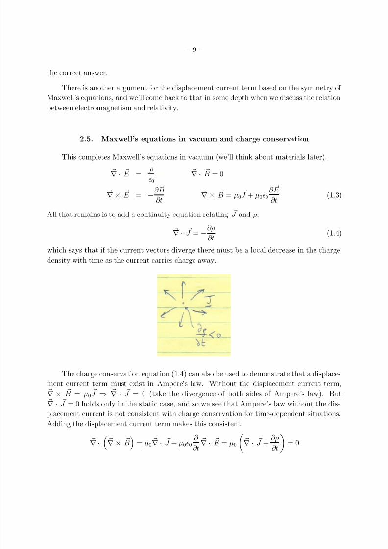
All that remains is to add a continuity equation relating J and ρ,
∇ · J = −∂ρ
∂t(1.4)
which says that if the current vectors diverge there must be a local decrease in the charge
density with time as the current carries charge away.
The charge conservation equation (1.4) can also be used to demonstrate that a displace-
ment current term must exist in Ampere’s law. Without the displacement current term, ∇ × B = µ0 J ⇒ ∇ · J = 0 (take the divergence of both sides of Ampere’s law). But
∇ · J = 0 holds only in the static case, and so we see that Ampere’s law without the dis-
placement current is not consistent with charge conservation for time-dependent situations.
Adding the displacement current term makes this consistent
∇ ·
∇× B
= µ0 ∇ · J + µ00
∂
∂t ∇ · E = µ0
∇ · J +
∂ρ
∂t
= 0
7/30/2019 EM waves summary 1
http://slidepdf.com/reader/full/em-waves-summary-1 10/36
– 10 –
where in the second step we have used Gauss’ law.
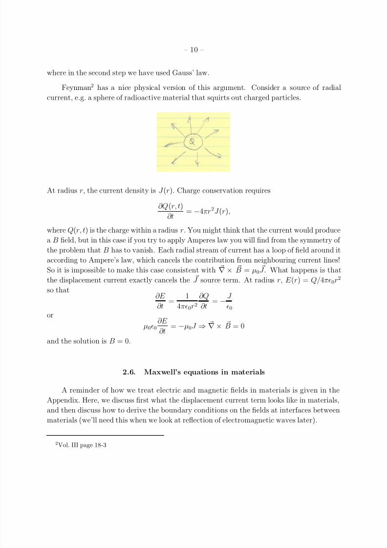
Feynman2 has a nice physical version of this argument. Consider a source of radial
current, e.g. a sphere of radioactive material that squirts out charged particles.
At radius r, the current density is J (r). Charge conservation requires
∂Q(r, t)
∂t= −4πr2J (r),
where Q(r, t) is the charge within a radius r. You might think that the current would produce
a B field, but in this case if you try to apply Amperes law you will find from the symmetry of
the problem that B has to vanish. Each radial stream of current has a loop of field around it
according to Ampere’s law, which cancels the contribution from neighbouring current lines!
So it is impossible to make this case consistent with ∇× B = µ0 J . What happens is that
the displacement current exactly cancels the J source term. At radius r, E (r) = Q/4π0r2
so that∂E
∂t=
1
4π0r2∂Q
∂t= −
J
0or
µ00∂E
∂t= −µ0J ⇒ ∇× B = 0
and the solution is B = 0.
2.6. Maxwell’s equations in materials
A reminder of how we treat electric and magnetic fields in materials is given in the
Appendix. Here, we discuss first what the displacement current term looks like in materials,
and then discuss how to derive the boundary conditions on the fields at interfaces between
materials (we’ll need this when we look at reflection of electromagnetic waves later).
2Vol. III page 18-3

7/30/2019 EM waves summary 1
http://slidepdf.com/reader/full/em-waves-summary-1 11/36
– 11 –
Maxwell’s equations in materials without the displacement current term are
∇ · B = 0 ∇ · D = ρf
∇× E = −∂ B
∂t ∇× H = J f
(take a look at the Appendix if you need a refresher on the definitions of D and H ). The
new piece in time-dependent problems is that a changing polarization with time corresponds
to a polarization current
J P =∂P
∂t
that must be included in Ampere’s law. Notice that the bound charge satisfies a continuity
equation
∇ · J P =∂
∂t ∇ · P = −
∂ρB
∂t.
Therefore Ampere’s law has a displacement current term as we had in vacuum but also
an addition term from polarization current,
∇× B = µ0 J f + µ0
J B + µ0
∂ P
∂t+ µ00
∂ E
∂t.
Rewriting this as
∇×
B
µ0 −
M
= J f +
∂
∂t
E +
P
we obtain
∇× H = J f +∂ D
∂t
which completes Maxwell’s equations in materials.
Finally, a reminder about boundary conditions for E , B, D, and H at the interface
between two materials. Recall that we derive boundary conditions by integrating Maxwell’s
equations across the surface from − to + and then let → 0. For example,
∇ · B = 0 ⇒ ∂Bx
∂x+ ∂By
∂y+ ∂Bz
∂z = 0.
Now imagine we have a surface whose normal vector is in the x-direction (so the surface is
in the y-z plane). Integrate across: −
dx
∂Bx
∂x+
∂By
∂y+
∂Bz
∂z
= 0

7/30/2019 EM waves summary 1
http://slidepdf.com/reader/full/em-waves-summary-1 12/36
– 12 –
⇒ [Bx]− +
−
dx
∂By
∂y+
∂Bz
∂z
= 0.
The second term vanishes in the limit → 0 and so[Bx]− = 0
showing that the perpendicular component of B is continuous across the surface.
You’ve probably seen this derived using a geometric argument, e.g. a Gaussian cylinder
shrunk onto the boundary, but I’ve written it this way because for more complex differential
equations, geometric arguments are not always possible. In that case, direct integration will
let you derive a boundary condition. I’ll leave the other boundary conditions as an exercise.
For example, first try integrating ∇ × E = −∂ B∂t
across the boundary. You should find
that the parallel component of E is continuous (hint: look for the terms that are ∂/∂x of
something, as they are the terms that will give a non-zero contribution in the limit → 0).
3. An immediate application: Electromagnetic waves
We can quickly get to electromagnetic waves in a few lines of vector algebra. This is
actually a very important procedure that we will carry out later many times for different
kinds of materials. In vacuum with no sources ρ = 0 and J = 0, Maxwell’s equations are3
∇ · E = 0 ∇ · B = 0
∇× E = −∂ B∂t
∇× B = µ00∂ E ∂t
. (1.5)
Now take the curl of Faraday’s law. The left hand side is
∇×
∇× E
= −∇2 E + ∇
∇ · E
and the right hand side is
∇×
−
∂ B
∂t
= −
∂
∂t
∇× B
= −0µ0
∂ 2 E
∂t2
which gives an equation governing E ,
∇2 E = µ00∂ 2 E
∂t2. (1.6)
3Just a note about the term “vacuum”. I will use this term to mean we are outside any materials, so
= 0 and µ = µ0, but not in the sense of being “empty” space. So in our usage a vacuum can have some
charge or current density to source the electromagnetic fields.

7/30/2019 EM waves summary 1
http://slidepdf.com/reader/full/em-waves-summary-1 13/36
– 13 –
On the left hand side we used a vector identity to expand ∇× ∇× E . Identities like this
one are readily available, for example at the front of Griffith’s book, but they are actually
easy to derive for yourself, I’ve included an appendix to this chapter on that. I encourageyou to take a look at it, it could be the most useful thing you learn in this course!
Returning to our result equation (1.6), you may recognize this as a 3D wave equation.
In one dimension, a wave equation for quantity f (x, t) is
∂ 2f
∂t2= v2
∂ 2f
∂x2
with general solution f (x, t) = f (x± vt), where v is the wave speed. Comparing with
equation (1.6), we see that the wave speed in the electromagnetic case is
v2 = 10µ0
= 14π10−7
4π10−7c2 = c2
the wave speed is the speed of light!
This result looks inevitable because these days we have units (SI) in which µ0 is de-
fined in terms of c2, and we know that light is in fact an electromagnetic wave. But in a
historical context, this is a truly remarkable result because remember that 0 is the constant
in Coulomb’s law, which describes the measured force between two electric charges, and µ0
is the constant in the Biot-Savart law that describes the measured forces between currents.
There is no obvious link to light, and yet from these two observations and the subsequently
deduced Maxwell’s equations, we predict a wave whose speed in fact equals the measured
speed of light! In this way, our understanding of light as an electromagnetic wave came
about.
4. General solutions to the wave equation
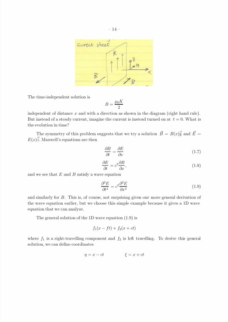
We’ll look at properties of electromagnetic waves in the next section, but first consider
the following more general example. We have an infinite plane current sheet with surface
current K :
7/30/2019 EM waves summary 1
http://slidepdf.com/reader/full/em-waves-summary-1 14/36
– 14 –
The time-independent solution is
B =µ0K
2
independent of distance x and with a direction as shown in the diagram (right hand rule).But instead of a steady current, imagine the current is instead turned on at t = 0. What is
the evolution in time?
The symmetry of this problem suggests that we try a solution B = B(x) y and E =
E (x) z . Maxwell’s equations are then
∂B
∂t=
∂E
∂x(1.7)
∂E
∂t
= c2∂B
∂x
, (1.8)
and we see that E and B satisfy a wave equation
∂ 2E
∂t2= c2
∂ 2E
∂x2(1.9)
and similarly for B. This is, of course, not surprising given our more general derivation of
the wave equation earlier, but we choose this simple example because it gives a 1D wave
equation that we can analyze.
The general solution of the 1D wave equation (1.9) is
f 1(x − f t) + f 2(x + ct)
where f 1 is a right-travelling component and f 2 is left travelling. To derive this general
solution, we can define coordinates
η = x − ct ξ = x + ct

7/30/2019 EM waves summary 1
http://slidepdf.com/reader/full/em-waves-summary-1 15/36
– 15 –
and then equation (1.9) becomes
∂ 2E
∂η∂ξ ⇒ E = f 1 (η) + f 2 (ξ ) . (1.10)
Now consider these two different pieces, the left and right travelling components. If E is a
function of x ± ct only, and independent of x∓ ct, then it must be the case that
∂E
∂x= ±
1
c
∂E
∂t
and therefore, using equation (1.7),
∂B
∂t= ±
∂
∂t
E
c
orB = ±
E
c.
The signs are such that the right travelling wave f (x− ct) has B = −E/c and the left going
wave f (x + ct) has B = +E/c. We can write this as the direction of propagation of the wave
is ∝ E × B.
For a given case, therefore, we can write
E (x, t) = f 1(x − ct) + f 2(x + ct)
cB(x, t) = −f 1(x − ct) + f 2(x + ct)
for some choice of the functions f 1 and f 2. These functions are set by the boundary condi-
tions, e.g. at t = 0
f 1(η) =E (x) − cB(x)
2
f 2(ξ ) =E (x) + cB(x)
2.
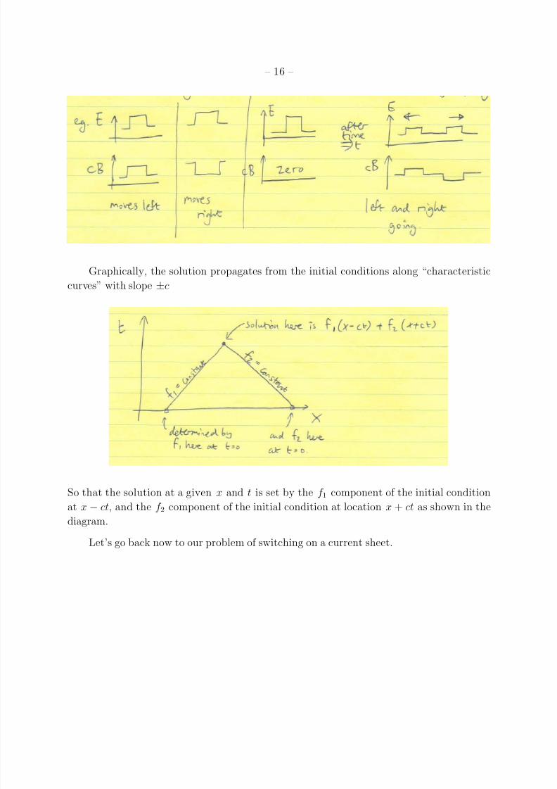
This is just saying that if we choose the relative signs of E and B initially, we can send a
wave either left or right:
7/30/2019 EM waves summary 1
http://slidepdf.com/reader/full/em-waves-summary-1 16/36
– 16 –
Graphically, the solution propagates from the initial conditions along “characteristiccurves” with slope ±c
So that the solution at a given x and t is set by the f 1 component of the initial condition
at x − ct, and the f 2 component of the initial condition at location x + ct as shown in the
diagram.
Let’s go back now to our problem of switching on a current sheet.

7/30/2019 EM waves summary 1
http://slidepdf.com/reader/full/em-waves-summary-1 17/36
– 17 –
We can see that the solution consists of two parts. One region, at x > ct has B = 0 because
the solution there is determined by characteristics originating at x > 0 and t = 0, where
B = 0. The second region, x < ct has characteristics that originate on the sheet at x = 0,
where (just above the sheet) B = µ0K/2, and so B = µ0K/2 in that entire region, as in the
static problem. What this is saying is that it takes a light travel time x/c before position x
“knows” that the current has been turned on. At late times > x/c the field corresponds to
the static solution.
A similar argument gives the solution for the x < 0 domain. If, at a later time T ,
we turned the current off, we create an electromagnetic pulse that propagates away in each
direction from the x = 0 plane:
We see that not only do the wave solutions propagate at the speed of light, but in
general
Electromagnetic disturbances propagate at the speed of light.
5. Plane electromagnetic waves in vacuum
In the last section, we saw one method of solving the wave equations for E and B, the
method of characteristics. Because these are linear equations, another approach is to use a

7/30/2019 EM waves summary 1
http://slidepdf.com/reader/full/em-waves-summary-1 18/36
– 18 –
Fourier decomposition, in other words think of the fields as a linear sum of plane waves
E = E 0ei k·re−iωt
B = B0ei k·re−iωt.
Recall that when we write the solution as ∝ eikx, we really mean the real part Re
eikx
=
cos kx. The real part always gives the physical quantities, the complex notation provides a
much more convenient way to keep track of the phases.
Substituting the plane wave solution into the wave equation gives
−k2 E 0 =−ω2
c2 E 0
or the the dispersion relation ω = ±ck,
the relation between the wave frequency ω and wave vector k. The sign ± gives the propa-
gation direction of the wave.
Maxwell’s equations give us other interesting properties of these waves. Since ∇· E = 0
and ∇ · B = 0, we see that
k · E 0 = 0 k · B0 = 0
so that the wave is transverse , meaning that the electric and magnetic fields are perpendicular
to the propagation direction. The other two Maxwell equations involving the curl of E and B give
∇× B =1
c2∂ E
∂t⇒ k × B0 = −
ω2
c2 E 0
∇× E = −∂ B
∂t⇒ k × E 0 = +ω B0
which imply E 0 · B0 = 0
E 0
= c
B0
.
The first result you have probably seen before, that the E and B directions are mutually
orthogonal in an electromagnetic wave; the second giving the ratio of E and B we have seen
before in the previous section.
Let’s go through some important results regarding EM waves:
• These plane wave solutions are important because the wave equation is linear so any
solution can be written as a linear combination (Fourier expansion) of plane waves.
7/30/2019 EM waves summary 1
http://slidepdf.com/reader/full/em-waves-summary-1 19/36
– 19 –
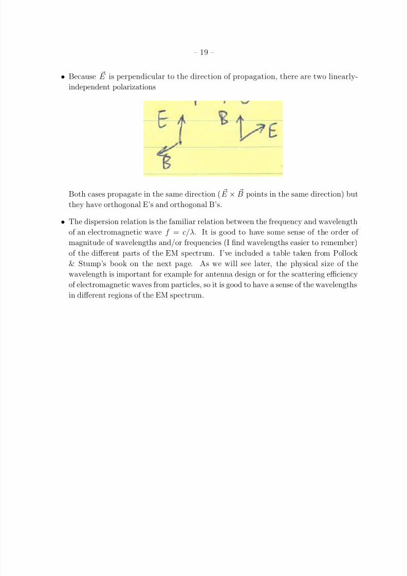
• Because E is perpendicular to the direction of propagation, there are two linearly-
independent polarizations
Both cases propagate in the same direction ( E × B points in the same direction) but
they have orthogonal E’s and orthogonal B’s.
• The dispersion relation is the familiar relation between the frequency and wavelength
of an electromagnetic wave f = c/λ. It is good to have some sense of the order of
magnitude of wavelengths and/or frequencies (I find wavelengths easier to remember)
of the different parts of the EM spectrum. I’ve included a table taken from Pollock
& Stump’s book on the next page. As we will see later, the physical size of the
wavelength is important for example for antenna design or for the scattering efficiency
of electromagnetic waves from particles, so it is good to have a sense of the wavelengths
in different regions of the EM spectrum.

7/30/2019 EM waves summary 1
http://slidepdf.com/reader/full/em-waves-summary-1 20/36
– 20 –

7/30/2019 EM waves summary 1
http://slidepdf.com/reader/full/em-waves-summary-1 21/36
– 21 –
6. Conservation of energy and momentum
Another interesting application of Maxwell’s equations is to help to understand energy
conservation in electromagnetism.
6.1. Conservation of energy and the Poynting flux
Consider a system of charges and currents. The work done per second by the fields on
charge q is F · v = qv ·
E + v × B
= qv · E
where F is the Lorentz force, and notice that only electric fields do any work because the
magnetic force is always perpendicular to the motion. The work done per second per unit
volume is
nqv · E = J · E
where n is the number density of charges. This is the work done by the fields, which goes
into the kinetic energy of the charges. By conservation of energy, the rate of change of the
energy density in the electric and magnetic fields is therefore
− J · E.
Maxwell’s equations can be used to evaluate this quantity in terms of the fields
− J · E = −1
µ0
∇× B
· E + 0
∂ E
∂t· E.
The last term is
0∂ E
∂t· E =
∂
∂t
1
20E 2
which looks promising because recall that (1/2)0E 2 is the energy density in the electric
field. To simplify the first term, we can use the identity4
∇ ·
E × B
= B ·
∇× E − E ·
∇× B
which gives
− J · E = ∇ ·
E × B
µ0
−
1
µ0
B · ∇× E +∂
∂t
1
20E 2
.
4You could think of this as an integration by parts.
7/30/2019 EM waves summary 1
http://slidepdf.com/reader/full/em-waves-summary-1 22/36
– 22 –
But ∇× E = −∂ B/∂t (Faraday’s law), and so
− J · E = ∇ · E × B
µ0
+
∂
∂t B2
2µ0+
0E 2
2
, (1.11)
where again we recognize the energy density in the magnetic field B2/2µ0 appearing in the
∂/∂t term.
Equation (1.11) describes the conservation of energy, and is in so-called flux conservative
form. The quantityB2
2µ0
+1
20E 2
is the energy per unit volume in the fields, and
1
µ0
E × B ≡ S (1.12)
is the energy flux carried by the fields (energy per unit area per second) which is known as
the Poynting flux S . (Recall that we already met the vector E × B when talking about the
direction of propagation of EM waves). In words, equation (1.11) states that the local rate
of change of energy density is given by the divergence of the Poynting flux plus any exchange
of energy with the charged particles.
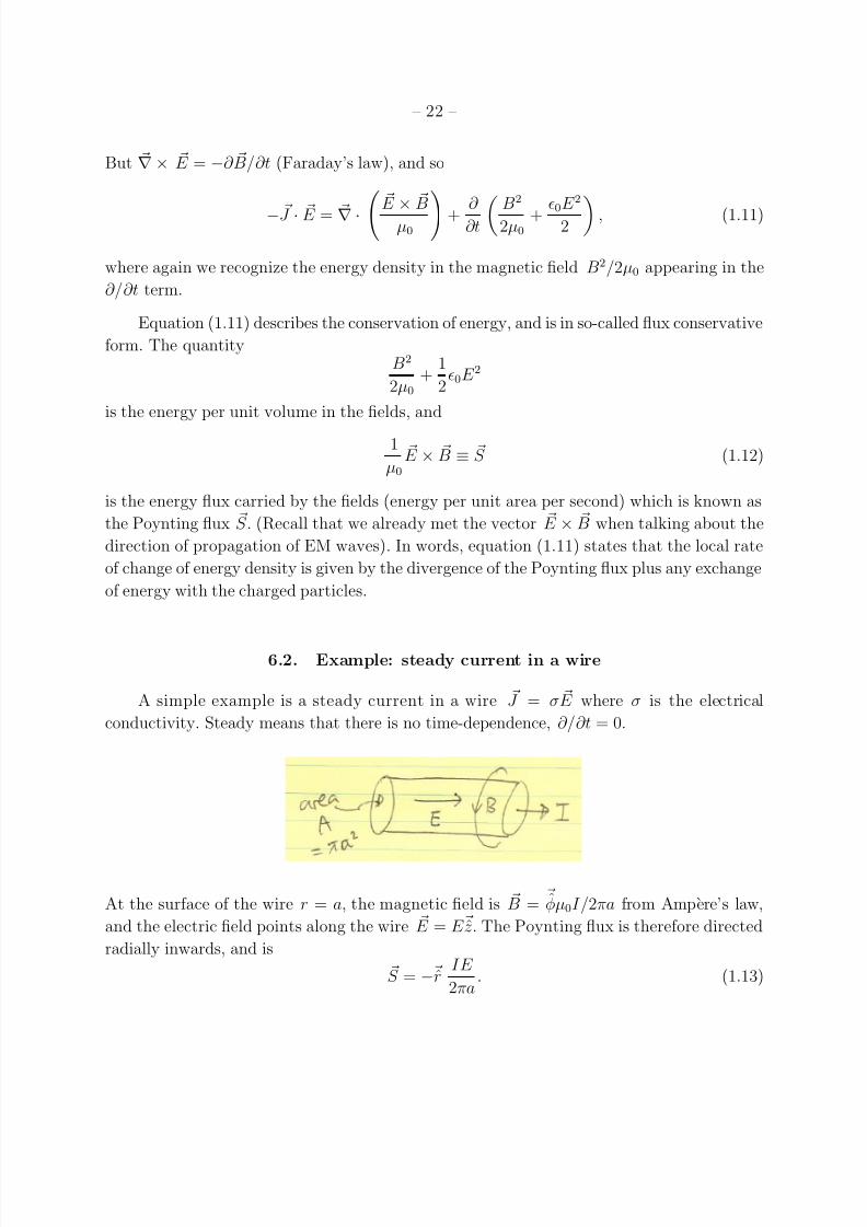
6.2. Example: steady current in a wire
A simple example is a steady current in a wire J = σ E where σ is the electrical
conductivity. Steady means that there is no time-dependence, ∂/∂t = 0.
At the surface of the wire r = a, the magnetic field is B = φµ0I/2πa from Ampere’s law,
and the electric field points along the wire E = E z . The Poynting flux is therefore directed
radially inwards, and is
S = − rIE
2πa. (1.13)

7/30/2019 EM waves summary 1
http://slidepdf.com/reader/full/em-waves-summary-1 23/36
– 23 –
This is the energy per unit area flowing into the wire. Multiplying by the circumference 2πa,
we get the energy per unit length per second
2πaS = EI = V L
I = I 2RL
(1.14)
where V is the voltage difference across length L of the wire, and R is the resistance of length
L. So we see that the Poynting flux into the wire is equal to the ohmic dissipation inside
the wire.
Not only is the total Poynting flux into the wire at its surface equal to the ohmic
dissipation inside, but the Poynting flux changes with radius inside the wire, such that the
difference between the Poynting flux at r + dr and that at r matches the ohmic dissipation
between r and r + dr. I will leave this for you to work out (see the list of problems at the end
of the chapter). Here, we just note that the ohmic dissipation per unit volume is I 2R/ALwhere A is the cross-section of the wire, or J 2RA/L = J 2/σ = J · E .
6.3. Example: Charging a cylindrical capacitor
Another typical example to look at is a cylindrical capacitor with charge Q(t) that is
charging with a current I = dQ/dt.
The electric field between the plates is E = Q/0A, and the total electrostatic energy is
U E = 12
0E 2Ad = Q2
20Ad,
changing at a ratedU E
dt=
d
0AQ
dQ
dt=
d QI
0A.
The point here is that this energy has to come from somewhere, and from our energy con-
servation law, it must come from a net Poynting flux into the volume between the plates.
7/30/2019 EM waves summary 1
http://slidepdf.com/reader/full/em-waves-summary-1 24/36
– 24 –
To evaluate the Poynting flux, we need the B field, which is given between the plates
by the displacement current
2πrBφ = πr2
µ00dE
dtso that at r = a, the Poynting flux is
S =a0
2
dE
dtE
radially inwards. The total flux of energy is
2πadS = dπa20E dE
dt= dπa20E
I
0A=
QId
0A
matching the rate of change of electrostatic energy between the plates.
This example is actually a bit subtle because we have made an assumption that thecharge is added slowly enough that the quasi-static approximation holds — at each time t, we
calculate the electric field as E = Q/0A just as we would for a capacitor in electrostatics. We
ignore the “back emf” or the inductance in this approximation, and therefore the magnetic
energy. This is a good approximation as long as the charging timescale is long compared to
the light crossing time across the capacitor d/c.
6.4. Conservation of momentum
We’ll derive this in detail later when we think about relativity, but let’s just mentionhere that as well as an energy flux there is also a momentum flux
momentum flux = S
c=
1
µ0c E × B.
To see why it must be S/c, recall that photons are massless particles and therefore have
E = ( p2c2 + m2c4)1/2 = pc, so that the energy and momentum fluxes are simply related by
a factor of c.
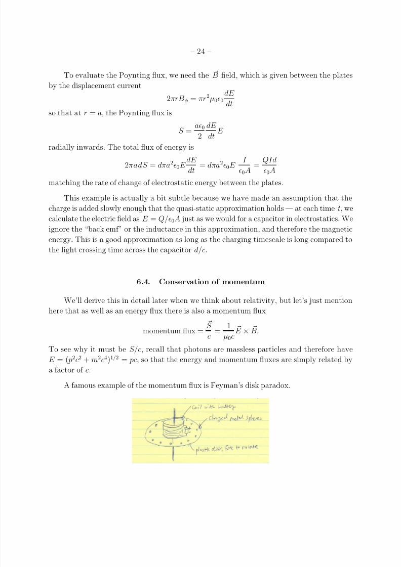
A famous example of the momentum flux is Feyman’s disk paradox.

7/30/2019 EM waves summary 1
http://slidepdf.com/reader/full/em-waves-summary-1 25/36
– 25 –
Intially, a current flows in the small central coil, with everything stationary. Then the current
stops for some reason. In that case, the B field from the central coil goes to zero, and so
there is an emf E = −dΦ/dt that acts on the charged spheres and causes the disk to rotate.The “paradox” or puzzle is to ask where does the angular momentum in the disk’s
rotation come from? Angular momentum should be conserved and yet the system was
stationary initially. The answer is that the fields themselves have an angular momentum
content in the initial state. As the fields decay, the angular momentum is transferred into
the rotational motion of the disk.
6.5. Conservation of energy in a material
I’ll leave this as an exercise, but if you use the Maxwell’s equations for a material to
derive an energy equation, you should find that the energy density is
1
2 E · D +
1
2 B · H
and the Poynting vector is S = E × H.
6.6. Application to electromagnetic waves
• The energy flux in the wave is given by the Poynting vector
S =
E × B
µ0
=E 0B0
µ0
cos2
k · r − ωt
The time-averaged intensity is (using the fact that cos2 = 1/2)
S =E 0B0
2µ0
=cE 20
2µ0c2=
1
2c0E 20 =
1
2c
B20
µ0
=c
2
B2
2µ0
+0E 20
2
this has the expected form (energy flux) = (velocity) x (energy density). Note thatthe electric and magnetic energy densities contribute equally.
• As we discussed earlier, the momentum flux is S /c which gives rise to radiation
pressure . The pressure on an absorbing surface is
S
c=
1
20E 20 .
7/30/2019 EM waves summary 1
http://slidepdf.com/reader/full/em-waves-summary-1 26/36
– 26 –
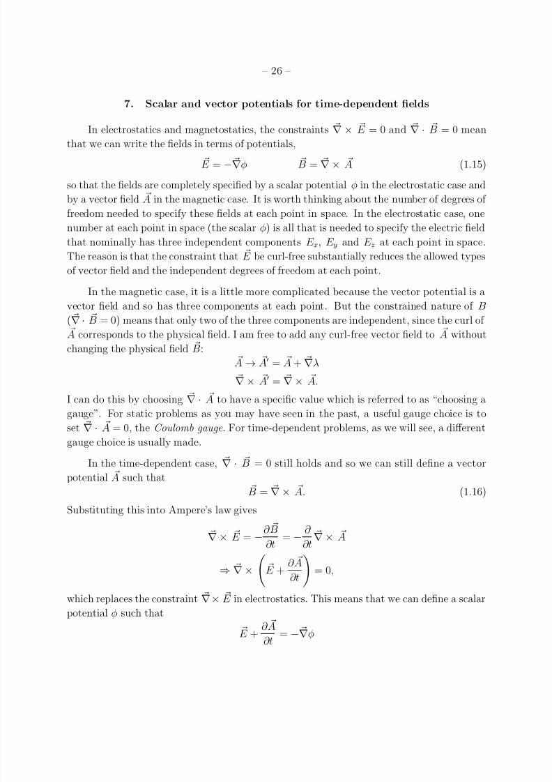
7. Scalar and vector potentials for time-dependent fields
In electrostatics and magnetostatics, the constraints ∇× E = 0 and ∇ · B = 0 mean
that we can write the fields in terms of potentials,
E = − ∇φ B = ∇× A (1.15)
so that the fields are completely specified by a scalar potential φ in the electrostatic case and
by a vector field A in the magnetic case. It is worth thinking about the number of degrees of
freedom needed to specify these fields at each point in space. In the electrostatic case, one
number at each point in space (the scalar φ) is all that is needed to specify the electric field
that nominally has three independent components E x, E y and E z at each point in space.
The reason is that the constraint that E be curl-free substantially reduces the allowed types
of vector field and the independent degrees of freedom at each point.In the magnetic case, it is a little more complicated because the vector potential is a
vector field and so has three components at each point. But the constrained nature of B
( ∇ · B = 0) means that only two of the three components are independent, since the curl of A corresponds to the physical field. I am free to add any curl-free vector field to A without
changing the physical field B: A → A = A + ∇λ
∇× A = ∇× A.
I can do this by choosing ∇ · A to have a specific value which is referred to as “choosing a
gauge”. For static problems as you may have seen in the past, a useful gauge choice is toset ∇ · A = 0, the Coulomb gauge . For time-dependent problems, as we will see, a different
gauge choice is usually made.
In the time-dependent case, ∇ · B = 0 still holds and so we can still define a vector
potential A such that B = ∇× A. (1.16)
Substituting this into Ampere’s law gives
∇× E = −∂ B
∂t
= −∂
∂t
∇× A
⇒ ∇×
E +
∂ A
∂t
= 0,
which replaces the constraint ∇× E in electrostatics. This means that we can define a scalar
potential φ such that
E +∂ A
∂t= − ∇φ

7/30/2019 EM waves summary 1
http://slidepdf.com/reader/full/em-waves-summary-1 27/36
– 27 –
or
E = − ∇φ −∂ A
∂t. (1.17)
Equations (1.16) and (1.17) give the electric and magnetic fields in the time-dependent case
in terms of potentials A and φ which now depend on both position and time.
As before, there is a gauge choice to be made. The gauge transformation is now
A → A = A + ∇λ
φ → φ = φ −∂λ
∂t
which you can verify does not change the physical fields E and B. We could still apply
the Coulomb gauge here, but a more convenient choice for time-dependent problems (that
simplifies calculations) is to use the Lorentz gauge
∇ · A = −1
c2∂φ
∂t. (1.18)
We see immediately why this is a good choice if we rewrite Maxwell’s equations in terms of
the potentials A and φ instead of the fields E and B.
Start with Faraday’s law
∇× B = µ0 J +
1
c2∂ E
∂t.
The LHS is ∇× ∇× A = ∇
∇ · A−∇2 A = −
1
c2 ∇
∂φ
∂t−∇2 A,
where we use the gauge choice to replace ∇ · A. The RHS is
µ0 J +
1
c2
−
∂
∂t ∇φ −
∂ 2 A
∂t2
,
which has a term that cancels one of the terms of the LHS, leaving the result
∇2 A −1
c2
∂ 2 A
∂t2
= −µ0 J. (1.19)
A similar equation can be derived for φ, this time starting from
∇ · E =ρ
0= −∇2φ −
∂
∂t ∇ · A = −∇2φ +
1
c2∂ 2φ
∂t2
so that
∇2φ−1
c2∂ 2φ
∂t2= −
ρ
0. (1.20)

7/30/2019 EM waves summary 1
http://slidepdf.com/reader/full/em-waves-summary-1 28/36
– 28 –
By choosing the Lorentz gauge, we have obtained separate wave equations5 for φ and A, in
which φ is sourced by ρ and A is sourced by J . These wave equations will lead us later into
general solutions to time-dependent problems in terms of retarded potentials .
8. Radiation from an accelerated charge
We’ve already seen how the charge density ρ or current density J acts as a source in
the wave equations for the potentials φ and A. Similarly, we saw that changes in the surface
current in section 4 led to launching of a propagating electromagnetic disturbance. As we
will see, the key factor is acceleration of charges:
Accelerating charges radiate
To conclude this first part of the course, let’s go through a simple argument that shows why
this so. The same argument also gives a simple derivation of Larmor’s formula for the power
radiated by an accelerating charge. This argument is originally due to J. J. Thompson and
is presented in Longair’s book High Energy Astrophysics .
Consider instantaneously accelerating a charge for time ∆t, changing its velocity by an
amount ∆v. In a frame moving with the charge initially, it begins to move, to a position
x = (∆v)t at time t later. For radial distances from the charge r < ct, the field lines “know”
that the charge has moved and point back to the charge at its present location. But forr > ct, the field lines point back to the original charge position (the origin).
5Notice again the high degree of symmetry between these two equations for φ and A. We will come
back to this in the relativity section where we’ll write a single relativistically invariant wave equation for a
4-potential sourced by a 4-current.

7/30/2019 EM waves summary 1
http://slidepdf.com/reader/full/em-waves-summary-1 29/36
– 29 –
7/30/2019 EM waves summary 1
http://slidepdf.com/reader/full/em-waves-summary-1 30/36
– 30 –
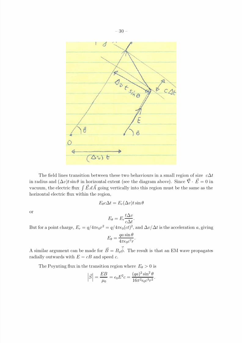
The field lines transition between these two behaviours in a small region of size c∆t
in radius and (∆v)t sin θ in horizontal extent (see the diagram above). Since ∇ · E = 0 invacuum, the electric flux
E.d A going vertically into this region must be the same as the
horizontal electric flux within the region,
E θc∆t = E r(∆v)t sin θ
or
E θ = E rt∆v
c∆t.
But for a point charge, E r = q/4π0r2 = q/4π0(ct)2, and ∆v/∆t is the acceleration a, giving
E θ =
qa sin θ
4π0c2r .
A similar argument can be made for B = Bφ φ. The result is that an EM wave propagates
radially outwards with E = cB and speed c.
The Poynting flux in the transition region where E θ > 0 is S =
EB
µ0
= 0E 2c =(qa)2 sin2 θ
16π20c3r2.
7/30/2019 EM waves summary 1
http://slidepdf.com/reader/full/em-waves-summary-1 31/36
– 31 –
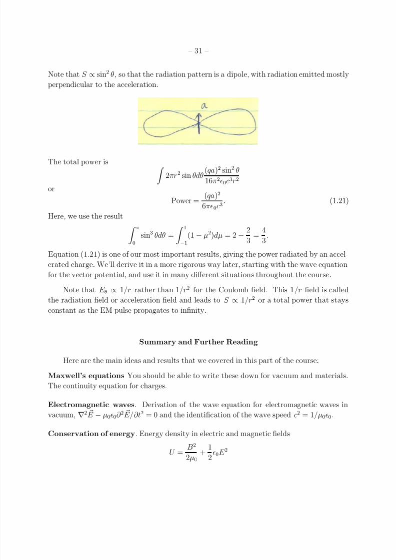
Note that S ∝ sin2 θ, so that the radiation pattern is a dipole, with radiation emitted mostly
perpendicular to the acceleration.
The total power is 2πr2 sin θdθ
(qa)2 sin2 θ
16π20c3r2
or
Power = (qa)2
6π0c3. (1.21)
Here, we use the result π0
sin3 θdθ =
1−1
(1− µ2)dµ = 2 −2
3=
4
3.
Equation (1.21) is one of our most important results, giving the power radiated by an accel-
erated charge. We’ll derive it in a more rigorous way later, starting with the wave equation
for the vector potential, and use it in many different situations throughout the course.
Note that E θ∝ 1/r rather than 1/r2 for the Coulomb field. This 1/r field is called
the radiation field or acceleration field and leads to S ∝ 1/r2 or a total power that stays
constant as the EM pulse propagates to infinity.
Summary and Further Reading
Here are the main ideas and results that we covered in this part of the course:
Maxwell’s equations You should be able to write these down for vacuum and materials.
The continuity equation for charges.
Electromagnetic waves. Derivation of the wave equation for electromagnetic waves in
vacuum, ∇2 E − µ00∂ 2 E/∂t2 = 0 and the identification of the wave speed c2 = 1/µ00.
Conservation of energy. Energy density in electric and magnetic fields
U =B2
2µ0
+1
20E 2
7/30/2019 EM waves summary 1
http://slidepdf.com/reader/full/em-waves-summary-1 32/36
– 32 –
Poynting flux
S =1
µ0
E × B
Energy conservation
− J · E =∂U
∂t+ ∇ · S
Examples: Poynting flux into a wire, the energy flow in a charging capacitor.
Conductors. Current in a conductor J = σ E . Ohmic dissipation per unit volume J 2/σ.
General solutions of the wave equation. The idea that electromagnetic disturbances
propagate at the speed of light. The general solution of the wave equation E (x ± ct) with
B = ±E/c.
Plane EM waves in vacuum. E = E 0ei
k·re−iωt
Dispersion relation ω = ±ck. The wave is transverse k · E 0 = 0, k · B0 = 0. Time
averaged intensity is S = c0E 2/2. Electric and magnetic energy densities contribute
equally. Momentum flux S /c. Two linearly-independent polarizations. A useful result is
S = Re (EH ) /2.
Scalar and vector potentials. Gauge transformations in the time-dependent case. The
Coulomb gauge ∇ ·
A = 0 and Lorentz gauge
∇ ·
A = −(1/c
2
)(∂φ/∂t). Wave equations forthe potentials
∇2 A −1
c2∂ 2 A
∂t2= −µ0
J
∇2φ−1
c2∂ 2φ
∂t2= −
ρ
0
Materials. Free and bound currents and charge densities and how they relate to the polar-
ization P or M . LIH dielectrics and the relations between D, P , E , , χe etc. and the same
for magnetic fields. The energy density for a LIH dielectric
12
E · D + 12
B · H
Boundary conditions. The general technique of integrating the differential equation across
the boundary to derive boundary conditions at an interface. Boundary conditions for time-
dependent problems. Continuity of E and B⊥, how the change in D⊥ and H depend on
the free surface charge density and current density respectively.
7/30/2019 EM waves summary 1
http://slidepdf.com/reader/full/em-waves-summary-1 33/36
– 33 –
You should be able to:
• Use Maxwell’s equations to derive the wave equations for the fields E and B, or thepotentials A and φ, in vacuum. A key vector identity is ∇× ∇ × A = −∇2 A for a
divergence-free field. You should probably just know this.
• Know how to obtain the fields E and B from the potentials A and φ in a time-dependent
context.
• Be able to describe the concepts of gauge choice (including the differences between
Lorentz and Coulomb gauge)
• Write down the energy flux and energy density of an EM wave in terms of the electric
and magnetic field strengths.
• Evaluate the Poynting flux and use it to determine the energy flux, momentum flux,
or momentum density (linear or angular momentum) in the fields and talk about the
energy flow.
Appendices
A. Index notation and proving vector identities
Proving vector identities is very straightforward. You just need four things:
1. Einstein summation convention A · B = AiBi
2. The Kronecker delta: δ ij = 1 if i = j, or 0 otherwise. E.g., this allows the dot product
to be written A · B = δ ijAiB j.
3. The Levi-Civita tensor: ijk = 1 if ijk is an even permutation (123,231,312), ijk = −1
if ijk is an odd permutation (321,213,132), and 0 otherwise (if any indices are repeated).
A way to represent cross-products, e.g. ( A×
B)i = ijkA jBk.
4. The identity ijkklm = δ ilδ jm − δ imδ jl .
Examples:

7/30/2019 EM waves summary 1
http://slidepdf.com/reader/full/em-waves-summary-1 34/36
– 34 –
1. Proof of the “BAC-CAB” rule for double cross products.
A× B × C i
= ijkA jklmBlC m
= ijkklmA jBlC m
= (δ ilδ jm − δ imδ jl) A jBlC m
= A jBiC j − A jB jC i
=
B
A · C − C
A · B
i
2. An example with a derivativeu ×
∇× u
i
= ijku jklm∂ l(um)
= u j∂ iu j − u j∂ jui
=
∇12
u2 − u · ∇ui
(A1)
B. A reminder about magnetic and electric fields in materials
We give a reminder here about the definitions of the fields D and H etc. in materials.
First, consider electric fields. In response to an applied electric field, a dielectric becomes
polarized. The polarization field P (r) is the local dipole moment density (dipole moment
per unit volume). For example, consider a dielectric inserted into a plane-parallel capacitor
In this case,
P =δQδl
Aδl=
δQ
A,
where A is the area of the capacitor plates and δl is the small thickness of the layer of bound
charges on either side of the dielectric. The general result is that there is a bound surface
charge on a polarized dielectric given by
σB = P · n.

7/30/2019 EM waves summary 1
http://slidepdf.com/reader/full/em-waves-summary-1 35/36
– 35 –
More generally still, inside a dielectric, if P has a divergence, then there will be a local bound
charge:
The bound charge density is
ρB = − ∇ · P .
Gauss’ law is ∇ · E =
ρ
0=
ρf + ρB0
where subscripts f and B refer to free and bound charges respectively. Writing in terms of
P ,
0 ∇ · E = ρf − ∇ · P
⇒ ∇ ·
0 E + P
= ρf
which we write as ∇ · D = ρf
defining the electric displacement field D = 0 E + P . This is very powerful because we
can solve Gauss’ law knowing only the free charge density, we don’t need to know what is
happening in the dielectric beyond a “constitutive relation” between P and E .
The simplest case is the linear, isotropic, homogeneous (LIH) dielectric for which P =
χe0 E where χe is the susceptibility that measures the polarization of the material in response
to an applied electric field. Then
D = 0 E + P = 0 (1 + χe) E = E = r0 E
where is the permittivity and r the relative permittivity or dielectric constant. More
complicated materials could have a non-linear relation between P and E , or an anisotropic
response in which P points in a different direction to E , and χe is a tensor rather than a
scalar, but we won’t consider such cases here.

7/30/2019 EM waves summary 1
http://slidepdf.com/reader/full/em-waves-summary-1 36/36
– 36 –
We follow the same approach for magnetic materials, defining M , the magnetic dipole
moment density. First consider an example where M is constant within the material,
If we write the local magnetic dipole moment as m = Ia (I is the current and a the area of
each current loop), the dipole moment density is M = Ia/ad = I/d where d is the thickness
of the material. Inside the material the bound current loops cancel one another, but at the
surface there is a bound surface current K = I/d = M , or for the general case K b = M × n.
If M is non-uniform within the material, there are bound volume currents also,
J b = ∇× M.
Again, we define a new field H so that we only have to worry about the free currents rather
than the bound ones. We write for magnetostatics
∇× B = µ0 J = µ0(J f + J B) = µ0
J f + ∇× M
⇒ ∇×
B
µ0
− M
= J f
or ∇× H = J f
which defines H = B/µ0 − M .
For a linear magnetic material, M = χm H , where χm is the magnetic susceptibility.Then
B = µ0( H + M ) = µ0(1 + χm) H = µ H,
where µ is the permeability of the material.
Related Documents


![National 5 Waves and Radiation Summary Notes...National 5 – Waves and Radiation – Summary Notes [Type here] Mr Downie 2019 National 5 Waves and Radiation Summary Notes Diffraction](https://static.cupdf.com/doc/110x72/5ebcb85009df3b661754a94b/national-5-waves-and-radiation-summary-notes-national-5-a-waves-and-radiation.jpg)