Electroweak evolution equations

arX

iv:h

ep-p

h/05

0504

7v1

6 M

ay 2

005

Electroweak Evolution Equations

Paolo CiafaloniINFN - Sezione di Lecce,

Via per Arnesano, I-73100 Lecce, Italy

E-mail: [email protected]

Denis ComelliINFN - Sezione di Ferrara,

Via Paradiso 12, I-35131 Ferrara, Italy

E-mail: [email protected]

Abstract

Enlarging a previous analysis, where only fermions and transverse gauge bosons were taken into account, wewrite down infrared-collinear evolution equations for the Standard Model of electroweak interactions computingthe full set of splitting functions. Due to the presence of double logs which are characteristic of electroweakinteractions (Bloch-Nordsieck violation), new infrared singular splitting functions have to be introduced. We alsoinclude corrections related to the third generation Yukawa couplings.

1 Introduction

Energy-growing electroweak corrections in the Standard Model have received recently a lot of attention in the literature,being relevant for LHC physics [1], for Next generation of Linear Colliders (NLCs) [2] and for ultrahigh energy cosmicrays [3]. The presence of double logs (log2 s

M2 where M is the weak scale) in one loop electroweak corrections hasbeen noticed in [4]. One loop effects are typically of the order of 10-20 % at the energy scale of 1 TeV, so that thesubject of higher orders and/or resummation of large logarithms has to be addressed. After the observation [5] thatdouble and single logs that appear in the 1 loop expressions are tied to the infrared structure of the theory, all orderresummation has been considered at various levels: Leading Log (LL) [6], Next to Leading Log (NLL) [7] and so on.Moreover many fixed order analyses at the one [8] and two loop [9] level have been performed.

Collinear evolution equations are written in general with the purpose of resuming large contributions of logarithmictype by factorizing collinear singularities. This is done by separating a “soft” scale contribution that includes collinearlogarithms and a “hard” scale contribution which is free of logarithms and therefore perturbative. However in theelectroweak sector at energies

√s much higher than the weak scale M ∼ MZ ∼ MW ≈ 100 GeV, logarithms of both

collinear and infrared origin appear, even in fully inclusive quantities [10]. In a previous paper [11] we have writteninfrared evolution equations in the limit of vanishing U(1) coupling and considering only fermions and transverse gaugebosons, showing that the presence of both infrared and collinear singularities can be tackled with by introducing new,infrared singular, splitting functions. The aim of this work is to complete the analysis by writing down infraredevolution evolution equations in the full SU(2)⊗ U(1) electroweak sector of the Standard Model, including left andright handed fermions, transverse and longitudinal bosons degrees of freedom. Since the third family Yukawa couplingsare non negligible, we include their contribution; on the other hand we neglect family mixing effects related to theCabibbo Kobayashi Maskawa matrix. A complete analysis of collinear singularities in the Standard Model will alsohave to include QED evolution equations [12] for transverse momenta of the emitted particles lower than the weakscale M , and QCD DGLAP [13] evolution equations.

The analysis of mass singularities in a spontaneously broken gauge theory like the electroweak sector of the Stan-dard Model has many interesting features. To begin with, initial states like electrons and protons carry nonabelian(isospin) charges; this feature causes the very existence of double logs i.e. the lack of cancellations of virtual correctionswith real emission in inclusive observables [10]. Secondly, initial states that are mass eigenstates are not necessarilygauge eigenstates; this causes some interesting mixing phenomena analyzed in [14, 15, 16]. Technically speaking, acomplication is due to the fact that the gauge theory Ward Identities are broken by Goldstone boson contributions;however these contributions are proportional to the symmetry breaking scale and are therefore expected to be sup-pressed to a certain extent in the high energy limit. These contributions have been shown to be negligible at the one

1

http://arXiv.org/abs/hep-ph/0505047v1

loop level [11]; we assume this to be true at higher orders as well, although we lack a formal proof at the moment.Finally, collinear factorization has been proved at the one loop level [17]; we assume it to be valid to all orders.Ultraviolet logarithms leading to running coupling effects are neglected throughout the paper.

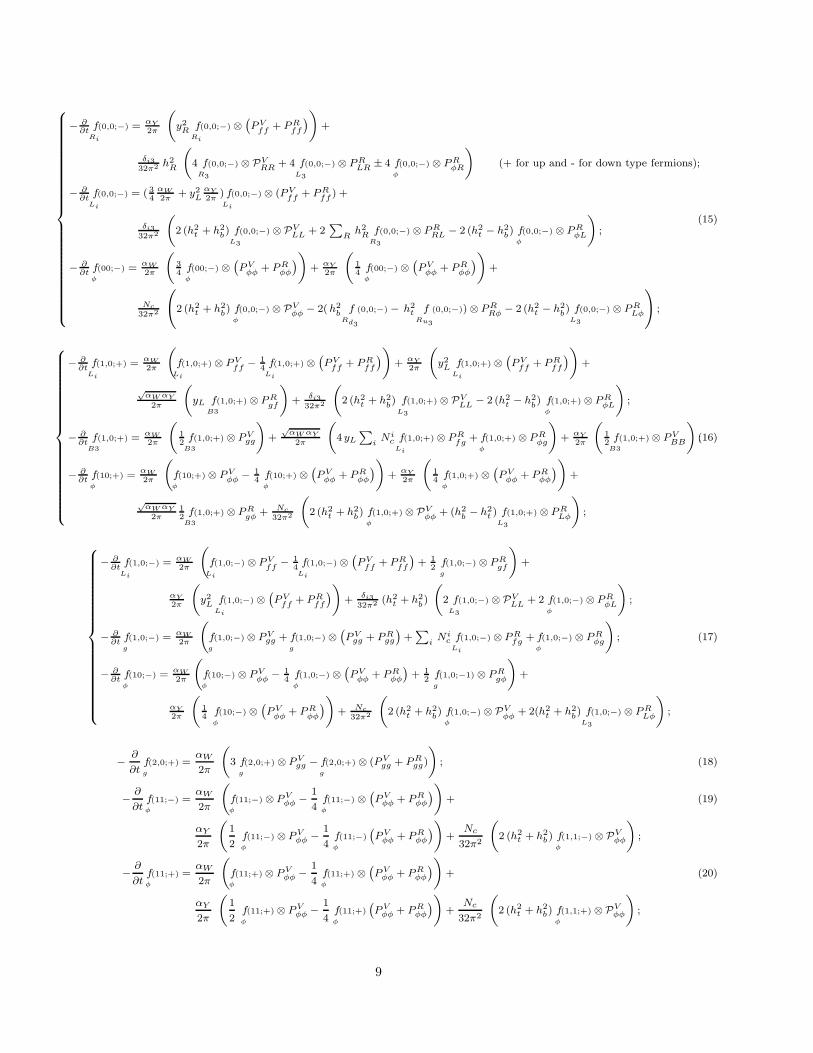
The main results of this paper are contained in eqs. (13-20), that represent the SU(2)⊗U(1) electroweak evolu-

tion equations for the full SM spectrum. Namely, eqs. (13) are written for matricial structure functionsi

Fj

αβα′β′ in

isospin space (see fig. 1). In order to make these equations useful for practical purposes, we have to write them forcorresponding scalar quantities. This is done by exploiting the (recovered) isospin and CP symmetry, i.e. by project-ing the equations on states of given quantum numbers, diagonalizing, in such a way, the system in block structurescharacterized by conserved quantum numbers.

The full set of evolution equations are computed working with gauge eigenstates which simplify systematicallythe evaluation in the high energy regime. We do this by giving in the Appendix a complete classification of possibleasymptotic states according to their isospin and CP properties. Then, scalar equations are obtained by a method weintroduce here, which consists in performing appropriate traces with respect to isospin leg indices. The final equationsfor scalar structure functions f

i

(T,Y ;CP ) are given in (44-60).

Since the overall procedure is quite complicated, in section two we discuss the simple case of left fermions in theinitial state and we show how the block diagonalization procedure helps for the numerical and practical evaluation ofthe evolution equations.

2 A working example: left fermions in the g′ → 0 limit

In this section we consider lepton initiated Drell Yan process of type e+(p1) e(p2) → q(k1)q(k2)+X∗ where s = 2p1 ·p2

is the total invariant mass and Q2 = 2k1 · k2 is the hard scale. We consider double log corrections in relation to theSU(2) electroweak gauge group, i.e. we work in the limit where the U(1) coupling g′ is zero. This process has beenanalyzed in [18, 14], to which we refer for details; we consider it here for convenience and in order to establish ournotations. The general formalism used to study electroweak evolution equations for inclusive observables has beenset up in [11]; we summarize it here briefly. To begin with, by arguments of unitarity, final state radiation can beneglected when considering inclusive cross sections [18]. Then we are led to consider the dressing of the overlap matrix

Oα′β′

αβ = 〈ββ′|S+ S|αα′〉, S being the S-matrix, where only initial states indices appear explicitly (see fig. 1).

At the leading level, all order resummation in the soft-collinear region is obtained by a simple expression thatinvolves the t-channel total isospin T that couples indices α, β:

OH → Oresummed = e−

αW4π

[T (T+1)] log2 s

M2w OH (1)

αW being the weak coupling, OH the hard overlap matrix written in terms of the tree level S-matrix and Mw ∼ Mz.At subleading order, the dressing by soft and/or collinear radiation is described at all orders by infrared evolution

equations, that are T -diagonal as far as fermions and transverse gauge bosons are concerned [11]. In order to writedown the evolution equations for the case of initial left fermions, we first consider one loop corrections. At the oneloop level, virtual and real corrections in NLL approximation can be written as:

δOL

αβ =αW

2π

∫ s

M2

dk2⊥

k2⊥

∫ 1

0

dz

z

{

PRff (z) θ(1 − z − k⊥√

s) tAββ′ tAα′α O

L

Hα′β′(zp) +

PRgf (z) [tB tA]βα O

g

HAB(zp) + Cf PV

ff (z,k⊥√

s) O

L

Hαβ(p)

}

(2)

where PRff (z), PR

gf (z) and PVff (z, k⊥) are defined in the Appendix. The indices below the overlap matrix label the

kind of particle: L = Left fermion and g = gauge boson ; indices α, β refer to the isospin index (α = 1 corresponds toν, α = 2 to e) of the lower legs while upper legs indices are omitted.

∗note that the process considered, like all others in this paper, is fully inclusive, meaning also W, Z radiation is included.

2

ΟΗ

F

F

l

k

α βj

i

Figure 1: Graphical picture of the factorization formula 3.)

The one loop formula (2) is consistent with a general factorization formula of type (see fig. 1))

i

Oj(p1, p2; k1, k2) =

∫

dz1

z1

dz2

z2

L,R,g∑

k,l

k

Fj(z1; s, M

2)l

Ok

H(z1p1, z2p2; k1, k2)i

Fl

(z2; s, M2) (3)

where i, j label the kind of particle (L=left fermion, g=gauge boson), and where isospin flavor indices in the overlapfunction O and structure function F are understood.

If the factorization formula (3) is assumed to be valid at higher orders as well, the structure functions will satisfyevolution equations with respect to an infrared-collinear cutoff µ parameterizing the lowest value of k⊥, as follows(t = log µ2):

− ∂

∂t

i

Fj

αβ =αW

2π

{

Cf

i

Fj

αβ ⊗ PVff + [tC

i

Fj

t tC ]αβ ⊗ PRff + [tB tA]βα

i

Fg

AB ⊗ PRgf

}

(4)

In these equations tA denote the isospin matrices in the fundamental representation andi

Fj

αβ denotes the distribution

of a particle i (whose isospin indices are omitted) inside particle j (with isospin leg indices α, β).i

Fj

t is the transpose

matrixi

Fj

βα. Furthermore, we have defined the convolution [f⊗P ](x) ≡∫ 1

xP (z)f(x

z)dz

z; the relevant splitting functions

are given in Appendix. Since the index i is always kept fixed in (4), we will omit it from now on, with the understanding

that, for instance, Fj

collectively denotes alli

Fj

with any value of i.

Eqn. (4) is a matricial evolution equation; in order to make it useful we can write the corresponding scalarequations. We do this by exploiting the SU(2)L symmetry which allows to classify the states according to their isospinquantum numbers. We couple the lower legs α, β in fig. 1 obtaining the t-channel isospin eigenstates:

|T = 0〉 =1√2(|νν∗〉 + |ee∗〉) |T = 1〉 =

1√2(|νν∗〉 − |ee∗〉) (5)

which have T 3L = 0 since cross sections always have a given particle on leg α and its own antiparticle on leg β. We

3

now project the structure operators F on these states, omitting the upper leg indices:

fL

(0) =〈νν∗ + ee∗| F

L

|〉2

=FL

νν + FL

ee

2=

1

2Tr[

FL

]

fL

(1) =〈νν∗ − ee∗| F

L

|〉2

=FL

νν −FL

ee

2= Tr

[

t3 FL

]

(6)

Last step in eqs. (6) represents a convenient way to extract the scalar coefficients fj

(T ) from Fj; namely, by taking

appropriate traces with respect to the soft leg j. For instance fL

(0) corresponds to 12 (F

Lee + F

Lνν) [11] and can be

obtained by Trj [Fj]; here and in the following the trace is taken with respect to the indices of the soft lower scale

leg j . Notice that since gauge and mass eigenstates do not necessarily coincide, we have to introduce “mixed legs”with particles belonging to different gauge representations on leg α and β (more about this point, in section 4). Welabel these cases by i = LR for the mixed left/right fermion leg, i = B3 for the mixed W3 − B gauge bosons andi = h3 for the Higgs sector case. These mixing phenomena are interesting by themselves and have been considered in[14, 15, 16, 20] at double log level.

Projecting eq. (4) for instance on the T = 0 component we obtain:

− ∂

∂tTr[F

f

] =αW

2π

{

CfTr[Ff

] ⊗ PVff + Tr[tC F

f

t tC ] ⊗ PRff + Tr[tB tA] F

gAB ⊗ PR

gf

}

(7)

where the traces are taken, here and in the following, with respect to the soft leg indices. This gives:

− ∂

∂tfL

(0) =αW

2π

(

3

4fL

(0) ⊗(

PVff + PR

ff

)

+3

4fg

(0) ⊗ PRgf

)

(8)

after taking into account that Tr[tB tA] Fg

AB = 12

∑

A Fg

AA = 12Tr[F

g

] and that fg

(0) = 13Tr[F

g

].

After this short introduction about the use of our projection technique, we now briefly show the utility to projecton states of definite t-channel quantum number instead to have evolution equations for single particles. Followingref.[11] we can define the projections with definite value of the t-channel isospin T = 0, 1, 2 for fermion and gaugeboson

fL

(1) = Tr{t3 Ff

} =fν − fe

2, f

g

(0) =f+ + f3 + f−

3, f

g

(1) =f+ − f−

2, f

g

(2) =f+ + f− − 2f3

6(9)

where fe = FL

ee, fν = FL

νν , f+ = Fg

+−, f− = Fg

−+, f3 = Fg

33.

We can evaluate the evolution eqs. for the transverse gauge bosons system following the same line of the fermionicones (see ref.[11] or next chapter). Then, using our projection technique described before we get the scalar equationswith definite T values; precisely there are five equations coupled in three subsets characterized by the T = 0, 1, 2values:

5 factorized eqs.

− ∂∂t

fL

(0) = αW

2π

(

34 f

L

(0) ⊗ (PRff + PV

ff ) + 34 f

g

(0) ⊗ PRgf

)

− ∂∂t

fg

(0) = αW

2π

(

2 fg

(0) ⊗ (PRgg + PV

gg) + 12 (f

L

(0) + fL

(0)) ⊗ PRfg

)

− ∂∂t

fL

(1) = αW

2π

(

fL

(1) ⊗ PVff − 1

4 fL

(1) ⊗ (PRff + PV

ff ) + 12 f

g

(1) ⊗ PRgf

)

− ∂∂t

fg

(1) = αW

2π

(

fg

(1) ⊗ PVgg + f

g

(1) ⊗ (PRgg + PV

gg) + 12 (f

L

(1) + fL

(1)) ⊗ PRfg

)

{

− ∂∂t

fg

(2) = αW

2π

(

3 fg

(2) ⊗ PVgg − f

g

(2) ⊗ (PRgg + PV

gg)

)

(10)

with similar equations holding for fL

(T ).

4

e e

νW W

− +

e e

e

W

e e

ν νW W

e

e e

e

− 3

3

−

W3

Figure 2: Graphical picture showing the evolution of the single electron component, see eqs. (11).

Eqs.(10) can be converted in evolution equations for the single components (see fig.2):

5 eqs

− 4παW

∂fν

∂t= fν ⊗ (3PV

ff + PRff ) + 2fe ⊗ PR

ff + 2f+ ⊗ PRgf + f3 ⊗ PR

gf

− 4παW

∂fe

∂t= fe ⊗ (3PV

ff + PRff ) + 2fν ⊗ PR

ff + 2f− ⊗ PRgf + f3 ⊗ PR

gf

− 2παW

∂f+

∂t= fe+fν

2 ⊗ PRfg + f3 ⊗ PR

gg + f+ ⊗ (PRgg + 2PV

gg)

− 2παW

∂f−

∂t= fν+fe

2 ⊗ PRfg + f3 ⊗ PR

gg + f− ⊗ (PRgg + 2PV

gg)

− 2παW

∂f3

∂t= fe+fe+fν+fν

4 ⊗ PRfg + (f− + f+) ⊗ PR

gg + 2f3 ⊗ PVgg

(11)

Even if two systems (10,11) are equivalent, eqs. (11) are true 5×5 system of differential equations, while thereduction to the block diagonal form of (10) generates a set of 2×2, 2×2 and 1×1 coupled equations.

To appreciate the block diagonalization, let us take the case of an initial fermionic parton (an electron). In thiscase we have only the T = 0 and T = 1 components (the fermionic system cannot couple with the T = 2 projection)so, while the use of eqs. (10) requires the solution of only the 2×2 plus 2×2 system, the use of eqs. (11) always forcesto solve the full 5×5 set of eqs. This simplification is particularly important when the full particle spectrum of theSM is taken into account (see next chapter).

Finally, the last step in obtaining the all order resummed overlap matrix, requires the evolution of the fi

(T )’s

according to eqn. (10) with appropriate initial conditions, and inserting the evolved fi

(T )’s into (3). This can by done

by exploiting the recovered isospin symmetry, which allows us to write:

i

Oj(p1, p2; k1, k2) =

∑

T

∫

dz1

z1

dz2

z2

L,R,g∑

k,l

k

fj(T )(z1; s, M

2)l

Ok

H(T )(z1p1, z2p2; k1, k2)

i

fl(T )(z2; s, M

2) (12)

3 Full EW evolution equations

Proceeding in analogy with previous section, we now introduce longitudinal gauge bosons and consider the fullSU(2)⊗U(1) electroweak group. According to the equivalence theorem, we replace longitudinal gauge bosons with

5

the corresponding Goldstone bosons. We choose to work in an axial gauge so that this substitution can be donewithout higher order corrections in the definition of the asymptotic states [21].

Our notation goes as follows:

• FLi

αβ represent structure functions for left fermions of the i-family, including leptons and quarks † ; indices

α, β = 1, 2 correspond to ν, e or u, d for the first family (i = 1) and so on. FLi

αβ indicates the structure function

for the corresponding antifermions.

• FRi

stand for right fermions in the ith family. We work in the SM and do not consider right neutrinos. FRi

is for

right antifermions.

• FLRi

represent the “mixed legs” case where the left leg is for a left fermion and the right leg for a right fermion of

the same charge for the i-family, or viceversa. Such structure functions are relevant only for the case of initialtransversely polarized beams [20].

• Fφ

ab represent structure functions for the Goldstone (φ1, φ2, φ3) - Higgs (h) sector. The Goldstone modes are

related to the corresponding longitudinal gauge bosons. Here a, b = 1, 2, 3, 4 stand for (φ1, φ2, φ3, h).

• Fg

AB stand for transverse WA gauge bosons belonging to the SU(2) sector: A, B = 1, 2, 3.

• FB is the structure function for the U(1) B gauge boson.

• FB3

is the “mixed leg” case involving B, W3 transverse gauge bosons.

We choose to work in gauge eigenstate basis in order to represent the various structure functions. This basis isconvenient for calculations since at very high energy we can consider massless propagators and therefore avoid thecomplications arising from mass insertions. Notice however that the asymptotic states appearing in the S matrix aretruly mass eigenstates, so we need to rotate to the physical base as a final step.

The leading one loop graphs contributing, in the axial gauge, to the splitting functions are shown in fig.(3). Thekinematical structure is the same as in QCD; however the group structure is much more complicated due to theabsence of isospin averaging on the initial states, in contrast with the corresponding (unbroken) QCD case wherephysical quantities are averaged over color. This implies uncanceled infrared singularities and the introduction of anew kind of infrared singular splitting functions [14].

We define αW ≡ g2

4π, αY ≡ g′2

4π; the various matrices tA, T c, . . . appearing in eqs. (13) are defined in the appendix.

Y is the hypercharge operator, which is a diagonal matrix with appropriate eigenvalues in the different representations(left/right fermions and antifermions, longitudinal gauge bosons and so on). We now write down the infrared evolutionequations for the structure functions in matrix form. Family indices here are always understood; note that the Yukawacoupling contributions proportional to the matrix H defined in the appendix are present only for the third family.

− ∂

∂tFL

αβ =αW

2π

{

Cf FL

αβ ⊗ P Vff + (tC F

L

ttC)βα ⊗ P Rff +

(

tBtA)

βαFg

AB ⊗ P Rgf

}

+ (13)

αY

2π

{

1

2(Y 2 F

L

+FL

Y 2)αβ ⊗ P Vff + (Y F

L

Y )αβ ⊗ P Rff + (Y 2)αβ F

B

⊗P Rgf

}

+

√αW αY

2π

{

(t3Y + Y t3)αβ FB3

⊗P Rgf

}

+

1

32π2

{

∑

a

(Ψa · H · H+ · Ψa+)αα FL

αβ ⊗ PVLL +(Ψa · H F

R

t H+ · Ψa+)βα ⊗ P RRL + (Ψb · H · H+ · Ψa+)βα F

φab ⊗ P R

φL

}

;

− ∂

∂tFL

αβ =αW

2π

{

Cf FL

αβ ⊗ P Vff + (tC F

L

tC)αβ ⊗ P Rff + F

gAB

(

tAtB)

αβ⊗ P R

gf

}

+

αY

2π

{

1

2(Y 2 F

L

+ FL

Y 2)αβ ⊗ P Vff + (Y F

L

Y )αβ ⊗ P Rff + (Y 2)αβ F

B

⊗P Rgf

}

+

√αW αY

2π

{

(t3Y + Y t3)αβ FB3

⊗P Rgf

}

+

†Quarks structure functions (valid for L, R or LR type) are averaged over initial color F ≡ 1Nc

∑

colorF

quarks

with Nc = 3.

6

A)

B)

C) +

+ +

+

+

+ +

Figure 3: Leading real emission Feynman diagrams in axial gauge: A) Feynman diagrams contributing to the evolutionof the fermionic structure functions; B) Feynman diagrams contributing to the evolution of the transverse gauge bosonstructure functions; C) Feynman diagrams contributing to the evolution of the scalar structure functions. The wavylines are transverse gauge bosons, dashed lines stay for Higgs sector particles and straight lines for fermions.

1

32π2

{

∑

a

(Ψa · H · H+ · Ψa+)αα FL

αβ ⊗PVLL +(Ψa · H F

R

H+ · Ψa+)αβ ⊗ P RRL +(Ψa · H · H+ · Ψb+)αβ F

φab ⊗ P R

φL

}

;

− ∂

∂tFR

αβ =αY

2πy2

R

{

FR

⊗P Vff + F

R

⊗P Rff + F

B

⊗P Rgf

}

+

1

32π2

{

∑

a

(H+ · Ψa+ · Ψa · H)αα FR

αβ ⊗PVRR +(H+ · Ψa+ F

L

t Ψa · H)βα ⊗ P RLR +(H+ · Ψb+ · Ψa · H)βα F

φab ⊗ P R

φR

}

;

− ∂

∂tFR

αβ =αY

2πy2

R

{

FR

⊗P Vff + F

R

⊗P Rff + F

B

⊗P Rgf

}

+

1

32π2

{

∑

a

(H+ · Ψa+ · Ψa · H)αα FR

αβ ⊗PVRR +(H+ · Ψa+ F

L

Ψa · H)αβ ⊗ P RLR +(H+ · Ψa+ · Ψb · H)αβ F

φab ⊗ P R

φR

}

;

− ∂

∂tFφ

ab =αW

2π

{

Cf Fφ

ab ⊗ P Vφφ + (T C

L Fφ

T CL )ab ⊗ P R

φφ + Fg

AB

(

T BL T A

L

)

ba⊗ P R

gφ

}

+

αY

2π

{

1

2(Y 2 F

φ

+Fφ

Y 2)ab ⊗ P Vφφ + (Y F

φ

Y )ab ⊗ P Rφφ + (Y 2)ab F

B

⊗P Rgφ

}

+

√αW αY

2π

{

(T 3L Y + Y T 3

L )ab FB3

⊗P Rgφ

}

+

1

32π2

{

Tr(Ψb · H · H+ · Ψa+ + Ψa · H · H+ · Ψb+)Fφ

ab ⊗ PVφφ+

Tr[(Ψa · H · H+ · Ψb+) FL

t] ⊗ P RLφ + Tr[(Ψb · H · H+ · Ψa+) F

L

] ⊗ P RLφ+

Tr[(H+ · Ψa+ · Ψb · H) FR

t] ⊗ P RRφ + Tr[(H+ · Ψb+ · Ψa · H) F

R

] ⊗ P RRφ

}

;

− ∂

∂tFg

AB =αW

2π

{

Cg Fg

AB ⊗ P Vgg +(T C

V Fg

T CV )AB ⊗ P R

gg+

(

∑

L

Tr

[

tB FL

ttA]

+∑

L

Tr

[

tA FL

tB]

)

⊗ P Rfg +Tr

[

T BL F

φ

tT AL

]

⊗ P Rφg

}

;

7

− ∂

∂tFB

=αY

2π

FB

⊗P RBB +

∑

F=L,L,R,R

Tr

[

Y FF

Y

]

⊗ P Rfg + Tr

[

Y Fφ

Y

]

⊗ P Rφg

;

− ∂

∂tFB3

=αW

2π

{

Cg

2FB3

⊗P Vgg

}

+

√αW αY

2π

∑

F=L,L

Tr

[

Y FF

t3]

⊗ P Rfg + Tr

[

Y Fφ

T 3L

]

⊗ P Rφg

+αY

2π

{

1

2FB3

⊗P VBB

}

;

− ∂

∂tF

LRαβ =

αW

2π

{

Cf

2F

LRαβ ⊗ P V

ff

}

+αY

2π

{

1

2(y2

L + y2R)F

LRαβ ⊗ P V

ff + yLyR FLR

αβ ⊗ P Rff

}

+1

32π2

{

1

2

∑

a

(Ψa · H · H+ · Ψa+)αα

FLR

αβ ⊗PVLL +

1

2

∑

a

(H+ · Ψa+ · Ψa · H)αα FLR

αβ ⊗PVRR +

∑

a

(H+ · Ψa+ · FLR

t · H† · Ψa+)βα ⊗PRLR

}

;

− ∂

∂tF

LRαβ =

αW

2π

{

Cf

2F

LRαβ ⊗ P V

ff

}

+αY

2π

{

1

2(y2

L + y2R) F

LRαβ ⊗ P V

ff + yLyR FLR

αβ ⊗ P Rff

}

+1

32π2

{

1

2

∑

a

(Ψa · H · H+ · Ψa+)αα

FLR

αβ ⊗ PVLL +

1

2

∑

a

(H+ · Ψa+ · Ψa · H)αα FLR

αβ ⊗ PVRR +

∑

a

(Ψa · H FLR

·Ψa · H)αβ ⊗ P RLR

}

;

We now proceed and reduce eqs. (13) to scalar equations. We work in the limit of light Higgs; the relevantsymmetry is then the (recovered) SU(2)⊗ U(1) gauge group, and the states can be classified according to the totalt-channel isospin T and the total t-channel hypercharge Y; however we have to add the conserved quantum numberCP in order to provide a complete classification of the states (see Appendix). Then, our structure functions arelabeled by (T,Y, CP ). Furthermore, we have to consider the “mixed cases”: left fermion-right fermion when we arein presence of transverse polarized initial beams [20], B −W3 mixing when the asymptotic states are γ’s or transverseZ [14] and h − φ3 for longitudinal Goldstone modes [15]. While we refer to the cited works for details, here we stressthe fact that we work in the (φ1, φ2, φ3, h) rather than the 1, 2, 1, 2 basis used in [15]. The sum

∑

i N ic is over all the

fermions where N ic = 1 for leptons and N i

c = 3 for quarks.The scalar evolution equations, using definitions (44-60) and eqs. (13) can finally be written as:

− ∂∂t

fRi

(00;+) = αY2π

(

y2R

fRi

(0,0;+) ⊗(

P Vff

+ P Rff

)

+ y2R

fB

(0,0;+) ⊗ P Rgf

)

+

δi332π2 h2

R

(

4 fR3

(0,0;+) ⊗PVRR

+ 4 fL3

(0,0;+) ⊗ P RLR

+ 4 fφ

(0,0;+) ⊗ P RφR

)

;

− ∂∂t

fB

(0,0;+) = αY

2π

(

fB

(0,0;+) ⊗ P VBB + 2

∑

iN i

c

(

2 y2L

fLi

(0,0;+) +∑

Ry2

Rf

Ri

(0,0;+)

)

⊗ P Rfg

+ fφ

(0,0;+) ⊗ P Rφg

)

;

− ∂∂t

fLi

(0,0;+) = αW

2π

(

34

fLi

(0,0;+) ⊗(

P Vff

+ P Rff

)

+ 34

fg

(0,0;+) ⊗ P Rgf

)

+ αY

2π

(

y2L

fLi

(0,0;+) ⊗(

P Vff

+ P Rff

)

+ y2L

fB

(0,0;+) ⊗ P Rgf

)

+

δi332π2

(

2 (h2t + h2

b) f

L3

(0,0;+) ⊗ PVLL

+ 2∑

Rh2

Rf

R3

(0,0;+) ⊗ P RRL

+ 2 (h2t + h2

b) f

φ

(0,0;+) ⊗ P RφL

)

;

− ∂∂t

fg

(0,0;+) = αW

2π

(

2 fg

(0,0;+) ⊗ (P Vgg + P R

gg) +∑

iN i

c fLi

(0,0;+) ⊗ P Rfg

+ fφ

(0,0;+) ⊗ P Rφg

)

;

− ∂∂t

fφ

(0,0;+) = αW

2π

(

34

fφ

(0,0;+) ⊗(

P Vφφ

+ P Rφφ

)

+ 34

fg

(0,0;+) ⊗ P Rgφ

)

+ αY

2π

(

14

fφ

(0,0;+) ⊗ (P Rφφ

+ P Vφφ

) + 14

fB

(0,0;+) ⊗ P Rgφ

)

+

Nc

32π2

(

2 (h2t + h2

b) f

φ

(0,0;+) ⊗ PVφφ

+ 2(h2t + h2

b) f

L3

(0,0;+) ⊗ P RLφ

+ 2∑

Rh2

Rf

R3

(0,0;+) ⊗ P RRφ

)

;

(14)

8

− ∂∂t

fRi

(0,0;−) = αY

2π

(

y2R

fRi

(0,0;−) ⊗(

P Vff

+ P Rff

)

)

+

δi332π2 h2

R

(

4 fR3

(0,0;−) ⊗ PVRR

+ 4 fL3

(0,0;−) ⊗ P RLR

± 4 fφ

(0,0;−) ⊗ P RφR

)

(+ for up and - for down type fermions);

− ∂∂t

fLi

(0,0;−) = ( 34

αW

2π+ y2

LαY

2π) fLi

(0,0;−) ⊗ (P Vff

+ P Rff

) +

δi332π2

(

2 (h2t + h2

b) fL3

(0,0;−) ⊗PVLL

+ 2∑

Rh2

Rf

R3

(0,0;−) ⊗ P RRL

− 2 (h2t − h2

b) f

φ

(0,0;−) ⊗ P RφL

)

;

− ∂∂t

fφ

(00;−) = αW

2π

(

34

fφ

(00;−) ⊗(

P Vφφ

+ P Rφφ

)

)

+ αY

2π

(

14

fφ

(00;−) ⊗(

P Vφφ

+ P Rφφ

)

)

+

Nc

32π2

(

2 (h2t + h2

b) f

φ

(0,0;−) ⊗ PVφφ

− 2( h2b

fRd3

(0,0;−) − h2t f

Ru3

(0,0;−)) ⊗ P RRφ

− 2 (h2t − h2

b) fL3

(0,0;−) ⊗ P RLφ

)

;

(15)

− ∂∂t

fLi

(1,0;+) = αW2π

(

fLi

(1,0;+) ⊗ P Vff

− 14

fLi

(1,0;+) ⊗(

P Vff

+ P Rff

)

)

+ αY2π

(

y2L

fLi

(1,0;+) ⊗(

P Vff

+ P Rff

)

)

+

√αW αY

2π

(

yL fB3

(1,0;+) ⊗ P Rgf

)

+ δi332π2

(

2 (h2t + h2

b) f

L3

(1,0;+) ⊗ PVLL

− 2 (h2t − h2

b) f

φ

(1,0;+) ⊗ P RφL

)

;

− ∂∂t

fB3

(1,0;+) = αW

2π

(

12

fB3

(1,0;+) ⊗ P Vgg

)

+√

αW αY

2π

(

4 yL

∑

iN i

c fLi

(1,0;+) ⊗ P Rfg

+ fφ

(1,0;+) ⊗ P Rφg

)

+ αY

2π

(

12

fB3

(1,0;+) ⊗ P VBB

)

;

− ∂∂t

fφ

(10;+) = αW

2π

(

fφ

(10;+) ⊗ P Vφφ

− 14

fφ

(10;+) ⊗(

P Vφφ

+ P Rφφ

)

)

+ αY

2π

(

14

fφ

(1,0;+) ⊗(

P Vφφ

+ P Rφφ

)

)

+

√αW αY

2π12

fB3

(1,0;+) ⊗ P Rgφ

+ Nc

32π2

(

2 (h2t + h2

b) f

φ

(1,0;+) ⊗ PVφφ

+ (h2b− h2

t ) fL3

(1,0;+) ⊗ P RLφ

)

;

(16)

− ∂∂t

fLi

(1,0;−) = αW2π

(

fLi

(1,0;−) ⊗ P Vff

− 14

fLi

(1,0;−) ⊗(

P Vff

+ P Rff

)

+ 12

fg

(1,0;−) ⊗ P Rgf

)

+

αY

2π

(

y2L

fLi

(1,0;−) ⊗(

P Vff

+ P Rff

)

)

+ δi332π2 (h2

t + h2b)

(

2 fL3

(1,0;−) ⊗ PVLL

+ 2 fφ

(1,0;−) ⊗ P RφL

)

;

− ∂∂t

fg

(1,0;−) = αW

2π

(

fg

(1,0;−) ⊗ P Vgg + f

g

(1,0;−) ⊗(

P Vgg + P R

gg

)

+∑

iN i

c fLi

(1,0;−) ⊗ P Rfg

+ fφ

(1,0;−) ⊗ P Rφg

)

;

− ∂∂t

fφ

(10;−) = αW

2π

(

fφ

(10;−) ⊗ P Vφφ

− 14

fφ

(1,0;−) ⊗(

P Vφφ

+ P Rφφ

)

+ 12

fg

(1,0;−1) ⊗ P Rgφ

)

+

αY

2π

(

14

fφ

(10;−) ⊗(

P Vφφ

+ P Rφφ

)

)

+ Nc

32π2

(

2 (h2t + h2

b) f

φ

(1,0;−) ⊗ PVφφ

+ 2(h2t + h2

b) fL3

(1,0;−) ⊗ P RLφ

)

;

(17)

− ∂

∂tfg

(2,0;+) =αW

2π

(

3 fg

(2,0;+) ⊗ P Vgg − f

g

(2,0;+) ⊗ (P Vgg + P R

gg)

)

; (18)

− ∂

∂tfφ

(11;−) =αW

2π

(

fφ

(11;−) ⊗ P Vφφ − 1

4fφ

(11;−) ⊗(

P Vφφ + P R

φφ

)

)

+ (19)

αY

2π

(

1

2fφ

(11;−) ⊗ P Vφφ − 1

4fφ

(11;−)

(

P Vφφ + P R

φφ

)

)

+Nc

32π2

(

2 (h2t + h2

b) fφ

(1,1;−) ⊗ PVφφ

)

;

− ∂

∂tfφ

(11;+) =αW

2π

(

fφ

(11;+) ⊗ P Vφφ − 1

4fφ

(11;+) ⊗(

P Vφφ + P R

φφ

)

)

+ (20)

αY

2π

(

1

2fφ

(11;+) ⊗ P Vφφ − 1

4fφ

(11;+)

(

P Vφφ + P R

φφ

)

)

+Nc

32π2

(

2 (h2t + h2

b) fφ

(1,1;+) ⊗PVφφ

)

;

9

− ∂∂t

fLRi

u( 12, 14;±) = αW

2π

(

38

fLRi

u( 12, 14;±) ⊗ P V

ff

)

+ αY

2π

(

12(yL − yu

R)2 f

LRi

u( 12, 1

4;±) ⊗ P V

ff+ yL yu

Rf

LRi

u( 12, 14;±) ⊗ (P V

ff+ P R

ff)

)

+

δi332π2

(

2 h2t f

LR3

u( 12, 14;±) ⊗PV

RR+ (h2

t + h2b) f

LR3

u( 12, 1

4;±) ⊗PV

LL− 2ht hb f

LR3

d( 12, 14;±) ⊗ PR

LR

)

;

− ∂∂t

fLRi

d( 12, 14;±) = αW

2π

(

38

fLRi

d( 12, 14;±) ⊗ P V

ff

)

+ αY

2π

(

12(yL − yd

R)2 f

LRi

d( 12, 1

4;±) ⊗ P V

ff+ yL yd

Rf

LRi

d( 12, 1

4;±) ⊗ (P V

ff+ P R

ff)

)

+

δi332π2

(

2 h2b

fLR3

d( 12, 1

4;±) ⊗ PV

RR+ (h2

t + h2b) f

LR3

d( 12, 14;±) ⊗PV

LL− 2ht hb f

LR3

u( 12, 14;±) ⊗PR

LR

)

(21)

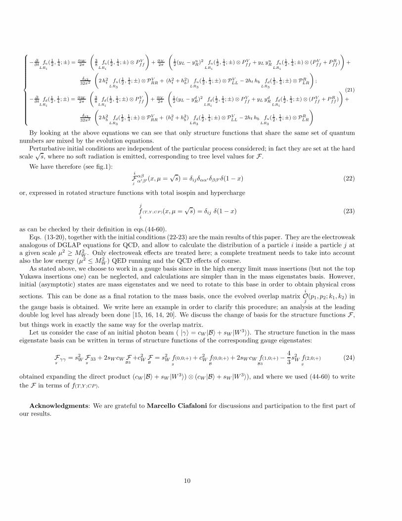
By looking at the above equations we can see that only structure functions that share the same set of quantumnumbers are mixed by the evolution equations.

Perturbative initial conditions are independent of the particular process considered; in fact they are set at the hardscale

√s, where no soft radiation is emitted, corresponding to tree level values for F .

We have therefore (see fig.1):i

Fj

αβα′β′(x, µ =

√s) = δijδαα′δββ′δ(1 − x) (22)

or, expressed in rotated structure functions with total isospin and hypercharge

j

fi

(T,Y ;CP)(x, µ =√

s) = δij δ(1 − x) (23)

as can be checked by their definition in eqs.(44-60).Eqs. (13-20), together with the initial conditions (22-23) are the main results of this paper. They are the electroweak

analogous of DGLAP equations for QCD, and allow to calculate the distribution of a particle i inside a particle j ata given scale µ2 ≥ M2

W . Only electroweak effects are treated here; a complete treatment needs to take into accountalso the low energy (µ2 ≤ M2

W ) QED running and the QCD effects of course.As stated above, we choose to work in a gauge basis since in the high energy limit mass insertions (but not the top

Yukawa insertions one) can be neglected, and calculations are simpler than in the mass eigenstates basis. However,initial (asymptotic) states are mass eigenstates and we need to rotate to this base in order to obtain physical cross

sections. This can be done as a final rotation to the mass basis, once the evolved overlap matrixi

Oj(p1, p2; k1, k2) in

the gauge basis is obtained. We write here an example in order to clarify this procedure; an analysis at the leadingdouble log level has already been done [15, 16, 14, 20]. We discuss the change of basis for the structure functions F ,

but things work in exactly the same way for the overlap matrix.Let us consider the case of an initial photon beam ( |γ〉 = cW |B〉 + sW |W 3〉). The structure function in the mass

eigenstate basis can be written in terms of structure functions of the corresponding gauge eigenstates:

Fg

γγ = s2W F

g33 + 2sW cW F

B3+c2

W FB

= s2W f

g

(0,0;+) + c2W f

B

(0,0;+) + 2sW cW fB3

(1,0;+) − 4

3s2

W fg

(2,0;+) (24)

obtained expanding the direct product (cW |B〉 + sW |W 3〉) ⊗ (cW |B〉 + sW |W 3〉), and where we used (44-60) to write

the F in terms of f(T,Y ;CP ).

Acknowledgments: We are grateful to Marcello Ciafaloni for discussions and participation to the first part ofour results.

10

4 Appendix:

Kernels of the evolution equations

PVff (z, k⊥) = −δ(1 − z)

(

logs

k2⊥

− 3

2

)

; PRff (z) =

1 + z2

1 − z; (25)

PVφφ(z, k⊥) = −δ(1 − z)

(

logs

k2⊥

− 2

)

; PRφφ(z) = 2

z

1 − z; (26)

PVgg(z, k⊥) = −δ(1 − z)

(

logs

k2⊥

− (11

6− nf

6− ns

24)

)

; PRgg(z) = 2

(

z(1 − z) +z

1 − z+

1 − z

z

)

; (27)

PVBB(z) = −

(

2 nf(2y2L + y2

Ru+ y2

Rd) + y2

φ

)

δ(1 − z)1

3

PRgf (z) =

1 + (1 − z)2

z, PR

gφ(z) = 2(1 − z)

z(28)

PRfg(z) = z2 + (1 − z)2; PR

φg(z) = z(1 − z) (29)

PVLL(z) = −δ(1 − z)

1

2; PV

RR(z) = −δ(1 − z)1

2; PV

φφ(z) = −δ(1 − z) (30)

PRLR(z) = PR

RL(z) = (1 − z); PRLφ(z) = PR

Rφ(z) = 1; PRφL(z) = PR

φR(z) = z

where nf =∑

i N ic is the sum over all the fermion families (N i

c = 1 for leptons and N ic = 3 for quarks ), ns = 1 is the

number of Higgs doublets and Nc = 3 is a color factor.

Fermion-Scalar Sector Yukawa Interactions

Parametrizing the scalar fields in the following way

Φ =1√2(h + iτaφa) =

(

φ0 iφ+

iφ− φ∗0

)

=1√2

(

h + iφ3 φ2 + iφ1

−φ2 + iφ1 h − iφ3

)

(31)

the interaction between the scalar sector and the Left-Right fermions can be written as

QL Φ H QR + QR H+ Φ+ QL =

4∑

a=1

φa(

QL Ψa · H QR + QR H+ · Ψa+ Φ+ QL

)

(32)

where Ψa = iτa for a=1,2,3 and Ψ4 = I2×2 and the third family Yukawa couplings are arranged in the followingmatricial form

H =

(

ht 00 hb

)

(33)

11

States classification

With the above parameterization (31), the Higgs sector of the Standard Model includes the three Goldstone modesφ1, φ2, φ3 and the Higgs field h. It is useful to arrange these four states in the complex form of the doublet/antidoubletmatrix

1√2

(

h + iφ3 φ2 + iφ1

−φ2 + iφ1 h − iφ3

)

=

(

1 12 2

)

(34)

which transforms as Φ → exp[iαAL tA]Φ exp[−iαB

RtB] under the SU(2)L ⊗ SU(2)R group. The indices 1, 2, 1, 2 hererefer to the transformation properties under SU(2)L.

tA and T A, A = 1, 2, 3 are the SU(2)L generators in the fundamental and adjoint representation.The other matrices appearing in the text are the generators of the SU(2)L ⊗ SU(2)R group in the (φ1, φ2, φ3, h)

basis; their explicit form is as follows:

T AL =

1

2

(

i ǫBAC −i δAB

i δAC 0

)

T AR =

1

2

(

i ǫBAC i δAB

−i δAC 0

)

(35)

Furthermore, (T 3h )ab = i(δ4aδ3b − δ3aδ4b) and (T 3

y )ab = δ3aδ4b + δ3bδ4a.States in the Higgs sector can be classified according to their SU(2)L⊗SU(2)R properties, with definite |T, T 3

L;TR, T 3R〉

quantum numbers (see also appendix in [15]). However not all of the 16 possible states appear in the evolution equa-tions. In fact, a physical cross section is always an overlap matrix element with a given particle in the left leg andits antiparticle in the right one. By charge conservation then, all the states involved in the evolution equations havet-channel charge equal to zero: Q = T 3

L + Y = T 3L + T 3

R = 0. Then, only 6 states are selected:

|1,−1; 1, 1〉 = −|22〉 |1, 1; 1,−1〉 = −|11〉 |1, 0; 1, 0〉 = − |12〉+|12〉+|21〉+|21〉2

|1, 0; 0, 0〉 = − |12〉−|12〉+|21〉−|21〉2 |0, 0; 1, 0〉 = − |12〉+|12〉−|21〉−|21〉

2 |0, 0; 0, 0〉 = − |12〉−|12〉−|21〉+|21〉2

(36)

In the high energy limit we are considering the SU(2)L ⊗U(1) symmetry is recovered, and states evolve accordingto their total t-channel isospin T and hypercharge Y . However quantum numbers |T, Y 〉 do not provide a completeclassification of the states. For instance, we have two states corresponding to |T = 0, Y = 0〉: these are the states|0, 0; 0, 0〉 and |0, 0; 1, 0〉 appearing in (36). We choose to add another quantum number, CP, that acts as‡:

1 ↔ −2 2 ↔ 1 ⇒ φ1 ↔ −φ1 φ2 ↔ φ2 φ3 ↔ −φ3 φ4 ≡ h ↔ φ4 ≡ h φ+ ↔ −φ− (37)

We can now write the states with given |T, Y 2〉(CP ) quantum numbers in terms of the states |T, T 3L;TR, T 3

R〉classified according to their SU(2)L ⊗ SU(2)R properties and given in (36):

|0, 0〉(+) = |0, 0; 0, 0〉 |1, 0〉(−) = |1, 0; 0, 0〉 |0, 0〉(−) = |0, 0, ; 1, 0〉 (38)

|1, 0〉(+) = |1, 0; 1, 0〉 |1, 1〉(+) =1

2(|1, 1; 1,−1〉+ |1,−1; 1, 1〉) |1, 1〉(−) =

1

2(|1, 1; 1,−1〉 − |1,−1; 1, 1〉) (39)

It is now easy, by using (34), to write the above states in the φ1, φ2, φ3, h base and to find out the correspondingf functions. For instance:

|0, 0〉(+) = |0, 0; 0, 0〉 = −|12〉 − |12〉 − |21〉 + |21〉2

= |φ+φ−〉 + |φ−φ+〉 + |φ3φ3〉 + |φhφh〉 (40)

This combination corresponds to

fφ

(0,0;+) =Fφ

+− + Fφ−+ + F

φ33 + F

φhh

4(41)

In the last step we have written fφ

(0,0;+) as a trace over the lower indices of the F operator, in order to simplify the

task of writing scalar evolution equations.

‡notice that the definition of CP given in [15] is different from the one used here

12

We use SU(2) ⊗ U(1) and CP quantum numbers also to classify states in the fermions/antifermions and gaugebosons sectors. CP acts as follows:

ν ↔ ν∗ e ↔ e∗ W+µ ↔ −W−

µ W 3µ ↔ −W 3

µ Bµ ↔ −Bµ (42)

Notice that in the fermionic sector, since CP transforms a fermion in its own antifermion, the states with definedSU(2) ⊗ U(1) properties, as defined in [15]:

f(0)L =

fe + fν

2f

(0)

L=

fe + fν

2f

(1)L =

fν − fe

2f

(1)

L=

fe − fν

2(43)

do not have definite CP values since CP transforms, for instance, f(0)L into f

(0)

L.

SU(2) symmetry acts on the gauge bosons sector as a triplet, and classifying the states does not present anyparticular difficulty. We can then proceed and write all the states in the fermionic, scalar, gauge bosons sectorsaccording to their |T, Y 2〉CP quantum numbers. Here we write directly the corresponding structure functions f (T,Y;CP )

and for Left fermions we write as example the case with Li equal to left leptons of the first i = 1 family (e and ν):

• singlet states T = 0,Y = 0

fB

(0,0;+) ≡ FB

(44)

fRi

(0,0;+) ≡ 1

2(FRi

+ FRi

) (45)

fLi

(0,0;+) ≡ 1

4Tr

[

FLi

+ FLi

]

=1

4

(

FL

ee + FL

νν + FL

ee + FL

νν

)

(46)

fφ

(0,0;+) ≡ 1

4Tr[F

φ

] =Fφ

+− + Fφ−+ + F

φ33 + F

φhh

4(47)

fg

(0,0;+) ≡ 1

3Tr[F

g

] =Fg

+− + Fg

33 + Fg−+

3(48)

fRi

(0,0;−) ≡ 1

2(FRi

− FRi

) (49)

fLi

(0,0;−) ≡ 1

4Tr

[

FLi

− FLi

]

=1

4

(

(FL

ee + FL

νν) − (FL

ee + FL

νν))

(50)

fφ

(0,0;−) ≡ −1

2Tr[T 3

R Fφ

] =Fφ

+− −Fφ−+ − i(F

φh3 −F

φ3h)

4(51)

• states T = 1,Y = 0

fB3

(1,0;+) ≡ FB3

(52)

fφ

(1,0;+) ≡ Tr[T 3LT 3

R Fφ

] =Fφ−+ + F

φ+− −F

φ33 − F

φhh

4(53)

fLi

(1,0;+) ≡ 1

2Tr

[

t3(FLi

+ FLi

)

]

=−F

Lee + F

Lνν

4+

−FL

ee + FL

νν

4(54)

fLi

(1,0;−) ≡ 1

2Tr

[

t3(FLi

− FLi

)

]

=−F

Lee + F

Lνν

4−

−FL

ee + FL

νν

4(55)

13

fφ

(1,0;−) ≡ −1

2Tr[T 3

L Fφ

] =Fφ

+− −Fφ−+ + i(F

φh3 −F

φ3h)

4(56)

f (1,0;−)g ≡ −1

2Tr[T 3

L Fg

] =Fg

+− −Fg−+

2(57)

• states T = 2,Y = 0, CP = (+)

fg

(2,0;+) ≡ 1

4Tr[(3(T 3

L)2 − 2)Fg

] =Fg

+− − 2 Fg

33 + Fg−+

4(58)

• states T = 1,Y2 = 1, CP = (−)

fφ

(1,1;−) ≡ 1

2Tr[T 3

y Fφ

] =Fφ

3h + Fφ

h3

2(59)

• states T = 1,Y2 = 1, CP = (+)

fφ

(1,1;+) ≡ i

2Tr[(T 3

y T 3h ) F

φ

] =Fφ

33 −Fφ

hh

2(60)

• states T = 1/2,Y2 = 14

fLRi

u(1

2,1

4;±) ≡ 1

2

(

FLRi

11 ± FLRi

11

)

(61)

fLRi

d(1

2,1

4;±) ≡ 1

2

(

FLRi

22 ± FLRi

22

)

(62)

References

[1] E. Accomando, A. Denner and S. Pozzorini, Phys. Rev. D 65 073003 (2002); E. Maina, S. Moretti, M.R. Noltenand D.A. Ross, Phys. Lett. B 570 205 (2003); M. Beccaria, F. M. Renard and C. Verzegnassi, Phys. Rev. D69, 113004 (2004), hep-ph/0405036 and hep-ph/0410089; J. H. Kuhn, A. Kulesza, S. Pozzorini and M. Schulze,hep-ph/0408308 ; E. Accomando, A. Denner and A. Kaiser, Nucl. Phys. B 706 (2005) 325; W. Hollik et al., ActaPhys. Polon. B 35 (2004) 2533; S. Moretti, M. R. Nolten and D. A. Ross, arXiv:hep-ph/0503152.

[2] TESLA: The Superconducting Electron Positron Linear Collider with an integrated X-ray laser laboratory. Tech-nical Design Report. Part 3. Physics at an e+ e- linear collider. By ECFA/DESY LC Physics Working Group(J.A. Aguilar-Saavedra et al.), hep-ph/0106315 .

[3] V. Berezinsky, M. Kachelriess, S. Ostapchenko Phys.Rev.Lett. 89 171802 (2002); C. Barbot, M. Drees, Astropart.Phys. 20, 5 (2003).

[4] M. Kuroda, G. Moultaka and D. Schildknecht, Nucl. Phys. B 350 (1991) 25; G. Degrassi and A. Sirlin, Phys.Rev. D 46, 3104 (1992); A. Denner, S. Dittmaier and R. Schuster, Nucl. Phys. B 452, 80 (1995); A. Denner,S. Dittmaier and T. Hahn, Phys. Rev. D 56, 117 (1997), Nucl. Phys. B 525, 27 (1998); W. Beenakker, A. Denner,S. Dittmaier, R. Mertig and T. Sack, Nucl. Phys. B 410, 245 (1993); W. Beenakker, A. Denner, S. Dittmaier andR. Mertig, Phys. Lett. B 317, 622 (1993).

[5] P. Ciafaloni, D. Comelli, Phys. Lett. B 446, 278 (1999).

14

http://arXiv.org/abs/hep-ph/0405036





[6] V. S. Fadin, L. N. Lipatov, A. D. Martin and M. Melles, Phys. Rev. D 61 (2000) 094002; P. Ciafaloni, D. Comelli,Phys. Lett. B 476 (2000) 49. M. Melles, Phys. Rev. D 63, 034003 (2001); Phys. Rev. D 64, 014011 (2001); Phys.Rev. D 64, 054003 (2001); Eur. Phys. J. C 24, 193 (2002); Phys. Rept. 375, 219 (2003);

[7] J. H. Kuhn, A. A. Penin and V. A. Smirnov, Eur. Phys. J. C 17, 97 (2000); J. H. Kuhn, S. Moch, A. A. Penin,V. A. Smirnov, Nucl. Phys. B 616, 286 (2001) [Erratum-ibid. B 648, 455 (2003)]

[8] M. Beccaria, P. Ciafaloni, D. Comelli, F. M. Renard, C. Verzegnassi, Phys. Rev. D 61 (2000) 073005; Phys. Rev.D 61 (2000) 011301; M. Beccaria, F. M. Renard, C. Verzegnassi, Phys. Rev. D 63 (2001) 095010; Phys. Rev. D63 (2001) 053013; Phys. Rev. D 64, 073008 (2001); Nucl. Phys. B 663, 394 (2003); M. Beccaria, S. Prelovsek,F. M. Renard, C. Verzegnassi, Phys. Rev. D 64, 053016 (2001); M. Beccaria, M. Melles, F. M. Renard, C. Verzeg-nassi, Phys. Rev. D 65 (2002) 093007; M. Beccaria, M. Melles, F. M. Renard, S. Trimarchi, C. Verzegnassi, Int.J. Mod. Phys. A 18, 5069 (2003); M. Beccaria, F. M. Renard, S. Trimarchi, C. Verzegnassi, Phys. Rev. D 68

(2003) 035014; A. Denner and S. Pozzorini, Eur. Phys. J. C 18, 461 (2001) and Eur. Phys. J. C 21, 63 (2001).See also S. Pozzorini, hep-ph/0201077 and references therein.

[9] Hori, H. Kawamura, J. Kodaira, Phys. Lett. B 491 (2000) 275; W. Beenakker, A. Werthenbach, Phys. Lett. B489, 148 (2000); Nucl. Phys. B 630 (2002) 3; A. Denner, M. Melles, S. Pozzorini, Nucl. Phys. B 662, 299 (2003);U. Aglietti, R. Bonciani, Nucl. Phys. B 668, 3 (2003) and Nucl. Phys. B 698, 277 (2004) ; Feucht, J. H. Kuhnand S. Moch, Phys. Lett. B 561, 111 (2003); B. Feucht, J. H. Kuhn, A. A. Penin and V. A. Smirnov, Phys.Rev. Lett. 93 (2004) 101802; A. Denner and S. Pozzorini, hep-ph/0408068; S. Pozzorini, Nucl. Phys. B 692, 135(2004); B. Jantzen, J. H. Khn, A. A. Penin, V. A. Smirnov, hep-ph/0504111.

[10] M. Ciafaloni, P. Ciafaloni and D. Comelli, Phys. Rev. Lett. 84, 4810 (2000);

[11] P. Ciafaloni, M. Ciafaloni and D. Comelli, Phys. Rev.Lett 88, 102001 (2002).

[12] V. N. Gribov and L. N. Lipatov, Yad. Fiz. 15, 781 (1972) [Sov. J. Nucl. Phys. 15, 438 (1972)]; J. Kripfganz andH. Perlt, Z. Phys. C 41, 319 (1988); H. Spiesberger, Phys. Rev. D 52, 4936 (1995).

[13] V. Gribov, L. Lipatov, Sov. J. Nucl. Phys 15, 438 (1972); L. Lipatov, Sov. J. Nucl. Phys 20, 94 (1972); G.Altarelli, G. Parisi, Nucl. Phys. B 126, 298 (1977); Y. Dokshitzer, Sov. Phys. JETP 46, 641 (1977).

[14] M. Ciafaloni, P. Ciafaloni, D. Comelli, Phys. Lett. B 501, 216 (2001).

[15] M. Ciafaloni, P. Ciafaloni, D. Comelli, Nucl.Phys. B613 , 382 (2001).

[16] M. Ciafaloni, P. Ciafaloni and D. Comelli, Phys. Rev.Lett 87 , 211802 (2001).

[17] A. Denner and S. Pozzorini, Eur. Phys. J. C 18 (2001) 461 and Eur. Phys. J. C 21 (2001) 63.

[18] M. Ciafaloni, P. Ciafaloni, D. Comelli, Nucl.Phys. B 589 (2000) 359.

[19] R. Doria, J. Frenkel, J.C. Taylor, Nucl. Phys. B168, 93 (1980); G. T. Bodwin, S. J. Brodsky, G.P. Lepage,Phys. Rev. Lett. 47, 1799(1981); A.H. Mueller, Phys. Lett. B108, 355 (1981); W.W. Lindsay, D.A. Ross, C.T.Sachrajda, Nucl. Phys. B214, 61 (1983); P.H. Sorensen, J.C. Taylor, Nucl. Phys. B238, 284 (1984); S. Catani,M. Ciafaloni, G. Marchesini, Phys. Lett. B168, 284 (1986).

[20] P. Ciafaloni, D. Comelli and A. Vergine, JHEP 0407, 039 (2004).

[21] W. Beenakker and A. Werthenbach, Nucl. Phys. B 630 (2002) 3.

15




Electroweak evolution equations

Documents