ELECTRON TUNNELING IN THE TIGHT-BINDING …

ELECTRON TUNNELING

IN THE

TIGHT-BINDING APPROXIMATION

by

FREDERICK DOUGLAS MACKEY

WILLIAM H. BUTLER, COMMITTEE CHAIR

CLAUDIA MEWES

ARUNAVA GUPTA

A THESIS

Submitted in partial fulfillment of the requirements for the degree of

Master of Science in the Department of Physics

and Astronomy in the Graduate School of

The University of Alabama

TUSCALOOSA, ALABAMA

2016

Copyright Frederick Douglas Mackey 2016

ALL RIGHTS RESERVED

ii

ABSTRACT

In this thesis, we treat tunneling similar to a scattering problem in which an incident wave on a barrier is

partially transmitted and partially reflected. The transmission probability will be related to the

conductance using a model due to Landauer. Previously tunneling has been treated using a simple barrier

model, which assumes the electron dispersion is that of free electrons. In this model it is not possible to

investigate tunneling in the gap between a valence band and a conduction band. We shall remedy this

limitation by using the tight-binding model to generate a barrier with a gap separating a valence band and

a conduction band. To do this, we constructed a model consisting of semi-infinite chains of A atoms on

either side of a semi-infinite chain of B-C molecules. The B-C chain has a gap extending between the

onsite energy for the B atom and the onsite energy for the C atom. Tunneling through the gap has been

calculated and plotted. We present exact closed form solutions for the following tunneling systems: (i) A-

B interface, (ii) A-(B-C) interface, (iii) A-B-A tunnel barrier, (iv) A-(B-C) interface with the orbitals on B

having s-symmetry and those on C having p-symmetry, (v) A-(B-C)-A tunnel barrier.

iii

DEDICATION

To my beloved, Nancy, who has changed my life for the better in ways I could not have

fathomed. You are my raison d’être. This is the culmination of love and teamwork. I love you.

To my mother and father, Ronald and Devera, I want to say ‘thank you’ for a lifetime of

inspiration, guidance, and support. I tend to do what I want but your teachings made sure I wanted the

best and knew how to work for it.

To my grandparents, Georgia, Iradell, and Willie, you made everything better.

To my siblings, Joshua, LaShonda, and LaTanya, your respect means everything to me. I always

wanted to provide a good example for you.

To Kendrick King Jr., you are truly a great person to know and love.

iv

LIST OF ABBREVIATIONS AND SYMBOLS

1 Electrochemical potential in left reservoir

2 Electrochemical potential in right reservoir

xvk Velocity of electrons in k-space

1( )f Fermi function at electrochemical potential 1

Ratio of the circumference of circle to its diameter

e Electron charge

( )T '

'

k

k,k Probability that electrons with wave vector k will be transmitted

k Electron wave vector

I Electric current

A Area

V Electric bias or voltage difference

G Landauer conductance

FE Fermi energy

h Planck’s constant

/ 2h

m Mass of electron

Gradient operator

E Energy of the electron

r Reflection amplitude

v

t Transmission amplitude

T Transmission probability

j Current density

Electron density

R Reflection probability

i Atomic orbitals centered at site, i

Label to distinguish different orbitals centered on the same site

i Atomic site label

iC Wave function coefficient for orbital, i

LCAO Linear Combination of Atomic Orbitals

,i jH Hamiltonian matrix elements

AE Onsite energy for A atom

BE Onsite energy for B atom

CE Onsite energy for C atom

Dimensionless parameter /E w

A Dimensionless parameter /AE w

B Dimensionless parameter /BE w

C Dimensionless parameter /CE w

w Hopping matrix element

vi

ACKNOWLEDGEMENTS

This research project represents a worthwhile journey that took place both within and outside the

University of Alabama. I would first like to thank the faculty, staff, and my fellow graduate students in

the physics department and the MINT Center for providing a wonderful atmosphere conducive to

excellent academia. I would like to thank my thesis committee (Dr. William Butler, Dr. Claudia Mewes,

and Dr. Arunuva Gupta) for their advice and contributions. During my hiatus, I received invaluable

advice from a few professors and will always be grateful and appreciative: Dr. Stan Jones, Dr. J.W.

Harrell, Dr. Rainer Schad, Dr. Pieter Visscher, Dr. Bill Doyle, and Dr. Raymond White. Thank you to

following people support outside of the University: The Mackey family, the Chambers family, the

Leonard family (Pearly III, Cheryl, Tiffany, Taylor, and Tyler), the Valentine family (Willie, Gwendolyn,

and John), the Maddox family (Lee and Betty), the Howell family (Glenn and Angela), and also my

professional support group (Christopher Anglin, Stephen Williams, John Little, and Derrick Whitmore).

I must extend a special thank you to two professors who were instrumental in this journey from

its inception to its completion: Dr Gary J. Mankey and Dr. William H. Butler. You both taught me that

dedication and results have their own reward and that talent is not enough.

vii

CONTENTS

ABSTRACT………………………………………………………………………………………………...ii

DEDICATION……………………………………………………………………………………………..iii

LIST OF ABBREVIATIONS AND SYMBOLS………………………………………………………….iv

ACKNOWLEDGEMENTS………………………………………………………………………………..vi

LIST OF FIGURES………………………………………………………………………………………..xi

CHAPTER 1: INTRODUCTION…………………………………………………………………………..1

CHAPTER 2: TUNNELING…………………………………………………………………………….....3

CHAPTER 2.1: LANDAUER CONDUCTANCE FORMULA………………………………..…4

CHAPTER 2.2: SIMPLE BARRIER MODEL FOR TUNNELING………………………………9

CHAPTER 2.3: CURRENT DENSITY……………………………………………………….…22

CHAPTER 3: TIGHT-BINDING APPROXIMATION………………………………………………......28

CHAPTER 3.1: LCAO OR TIGHT-BINDING MODEL FOR ELECTRONIC STRUCTURE...29

CHAPTER 3.2: TRANSMISSION THROUGH AN INTERFACE IN TIGHT-BINDING……..33

CHAPTER 3.3: SIMPLEST TIGHT-BINDING MODEL: THE A-B SYSTEM………………..38

CHAPTER 3.4: TUNNELING IN TIGHT-BINDING: THE A-B-A SYSTEM…………………45

viii

CHAPTER 3.5: SIMPLE BARRIER LIMIT OF TIGHT-BINDING TUNNELING…………....52

CHAPTER 4: TUNNELING THROUGH A BARRIER WITH A GAP………….…...………………....56

CHAPTER 4.1: THE A-[B-C] SYSTEM………………………………………………………...57

CHAPTER 4.2: CHAPTER 4.2: THE A-[B-C] SYSTEM WITH s-p BARRIER……………….65

CHAPTER 4.3: THE A-[B-C]-A – A TUNNELING SYSTEM………………………………....70

CHAPTER 5: CONCLUSIONS……………………………………………………………………..........80

REFERENCES….…………………………………………………………………………………………82

ix

LIST OF FIGURES

Figure 1. Geometry for Derivation of Landauer Transport Formula showing left and right electron

reservoirs separated by leads and a sample…………………………………………………………………4

Figure 2: Tunneling wave function for the simple barrier model for a fixed value of k . For this

example, the barrier extends from 0x to 2x ……………………………………………………….17

Figure 3: Graph of Conductance as a function of FE

V for different values of thickness, d……………21

Figure 4: Single s-orbital model with semi-infinite chains of A and B atoms. The A atoms extend from

n to 0n . The B atoms extend from 1n to n ………………………………………….33

Figure 5: A tunneling system consisting of two semi-infinite chains of A atoms separated by N B atoms.

By proper choice of parameters, we can make the A atoms conducting and the B atoms insulating……..38

Figure 6: Transmission (blue) and Reflection (green) probabilities for the A-B-A tight-binding model as

a function of energy. Parameters are 0, 2, =10A B N . Energy is measured in units of hopping

matrix element, w ………………………………………………………………………………………...47



matrix element, w ………………………………………………………………………………………...48

Figure 8: Transmission and Reflection Probabilities plotted with a logarithmic scale. The tight-binding

tunneling parameters are 0, 3, 10.A B N ……………….……………………………………...49

Figure 9: Parameters are 0, 3, =0.99, 10.A B N The wave function coefficients for the real

and imaginary parts of the wave function are shown by the blue and red boxes respectively. The blue and

red lines joining the boxes serve as a guide to the eye…………….……………………………………...50

Figure 10: Parameters are 0, 3, =0.99, 10.A B N The wave function coefficients for the real

and imaginary parts of the wave function are shown by the blue and red boxes respectively. The blue and

red lines joining the boxes serve as a guide to the eye…………………………………………………....51

Figure 11: Single s-orbital model – Semi-infinite chains of A atoms and B-C molecules. The A atoms

extend from n to 0n . The B-C molecules extend from 1n to n ….………………….57

x

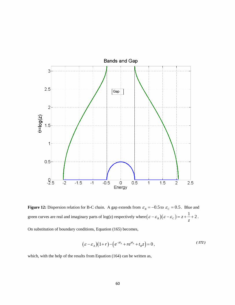
Figure 12: Dispersion relation for B-C chain. A gap extends from 0.5B to 0.5C . Blue and

green curves are real and imaginary parts of z respectively where 1

2B C zz

...……..60

Figure 13: Single s-p-orbital model – semi-infinite chains of A and B-C molecules. The A atoms extend

from n to 0n . The B-C molecules extend from 1n to n . The orbital on the C atom

has xp symmetry.……………………………………………………………………………………..........65

Figure 14: Semi-infinite chain of A atoms on the right and a semi-infinite chain of B atoms on the left. The B-C barrier has orbitals of similar symmetry on the B atom and on the C atom. All inter-atom

hopping is assumed to be nearest-neighbor and the same throughout the chain……………………….....70

Figure 15: Transmission (blue) and Reflection (green) probabilities for the A-BC-A tight-binding model

as a function of energy. Parameters are 0, 0.3, =10A B C N . Energy is measured in units of

hopping matrix element, w ……………………………………………………………………………….77


as a function of energy. Parameters are 0, 0.7, =10A B C N . Energy is measured in units

of hopping matrix element, w ………………………………………………………………………….…78



hopping matrix element, w ……………………………………………………………………………….79

1

CHAPTER 1: INTRODUCTION

The earliest concept critical to understanding quantum tunneling was introduced by Louis de

Broglie. De Broglie proposed in 1923 that waves of matter have a wavelength inversely proportional to

their momentum. In 1927, Friedrich Hund was the first to make use of the concept of quantum

mechanical barrier penetration [1]. Quantum tunneling of electrons cannot be directly perceived other

than on the quantum mechanical scale. Classical mechanics cannot explain tunneling phenomena.

Quantum mechanical tunneling happens when particles move through a barrier that is deemed

impenetrable by classical mechanical standards. This barrier can be a region of high energy, a vacuum, or

an insulator.

Tunneling plays an essential role in several physical, chemical, and biological phenomena. In

field emission, an electron can jump from the surface of a metal into a vacuum by tunneling through a

potential barrier. The electron is allowed to tunnel through the vacuum if the electric field is large enough

and the barrier is thin enough. This is called cold emission. Semiconductors are another example where

tunneling can occur. Electron tunneling through an insulating barrier is important for flash devices.

Tunneling can also be seen in radioactive decay. In the world of nanotechnology, quantum tunneling can

be seen in scanning tunneling microscopes, transistors, and even touch screens.

Consider a particle with energy E in the inner region of a one-dimensional potential well of height

V. Assume that the walls of the well have thickness, t. According to classical mechanics, if E is less than

V, the particle will remain in the well forever. If E is greater than V, then the particle will escape the

potential well. This is not the case, according to quantum mechanics. Even if V is greater than E, there is

a possibility that the particle will tunnel through the barrier. The particle can escape even if its energy is

less than V, but the probability depends on the difference between E and V and on the thickness of the

walls surrounding the well.

2

For tunneling of electrons in solids, the potential well is typically a metallic region where

electrons at the Fermi energy can propagate and the barrier is generally a material in which electrons at

the Fermi energy cannot propagate, in other words there is typically a gap at the Fermi energy for the

barrier material. Even though electrons cannot propagate indefinitely, there will be an evanescent state

that extends from the metal into the tunneling barrier. These evanescent states play a central role in

tunneling. The evanescent states arise from the complex band structure of the insulator which determines

how they decay in the insulator. [2,3]

The electron tunneling phenomenon arises from the wave nature of the electrons and results from

the fact that when a wave encounters an interface, it may be partially reflected and partially transmitted.

This interfacial reflectance will lead to an interfacial or junction resistance. In this thesis, we shall treat

tunneling similar to a scattering problem in which an incident wave on a barrier is partially transmitted

and partially reflected. The transmission probability will be related to the conductance using a model due

to Landauer.[4] Brinkman, Dynes, and Rowell treat tunneling in this way using a simple barrier model,

but their model treats the electron dispersion using the free electron model. In this approach it is not

possible to investigate tunneling in the gap between a valence band and a conduction band. We shall

remedy this limitation by using the tight-binding model to generate a barrier with a gap separating a

valence band and a conduction band. [5]

In an alternative model for tunneling used by Bardeen [6] and Slonczewski [2], one begins with

two electrodes separated by an insulator so thick that no tunneling occurs. Then the two electrodes are

regarded as completely independent systems. When they are brought closer together so that their wave

functions begin to overlap, tunneling occurs. The overlap matrix elements correspond directly to the

hopping integrals of the tight-binding method. Perturbation theory is used to calculate the tunneling

probability from the matrix elements. It is assumed that the states between which tunneling takes place

are those of the electrodes unperturbed by the tunneling process (electrodes separated by an infinitely

thick insulator).

3

CHAPTER 2: TUNNELING

4

CHAPTER 2.1: LANDAUER CONDUCTANCE FORMULA

Ballistic transport, including tunneling of electrons, was treated by Landauer in 1970. [4] In this

approach, one imagines two electron reservoirs separated by leads and a sample (in our case, a tunnel

barrier) as shown in Figure 1.

Figure 1. Geometry for derivation of Landauer transport formula showing left and right electron

reservoirs separated by leads and a sample.

Within each reservoir we consider the electrons to be (locally) in equilibrium at chemical

potentials 1 on the left and 2 on the right. We also imagine that there are conduction channels that

connect the reservoirs. These channels consist of the transverse modes of the leads. In particular, for a

system with two dimensional periodicity perpendicular to the leads, they will consist of the values of the

crystal momentum of the two dimensional Brillouin zone. The number of these transverse modes is

proportional to the cross sectional area of the leads. The reservoirs are viewed as emitters of electrons,

the one on the left emitting right-going electrons and the one on the right emitting left-going electrons,

very much like the classical black body emitting radiation.

The Landauer formalism relates the net current through the sample between the two reservoirs to

the emitted currents. The right-going current from the left reservoir, for example, will be given by

integrating over all of the states in the left reservoir. Only the right going states ( xvk ) will contribute

Sample

Left electron

reservoir

Right electron

reservoir

1

2

left lead right lead

5

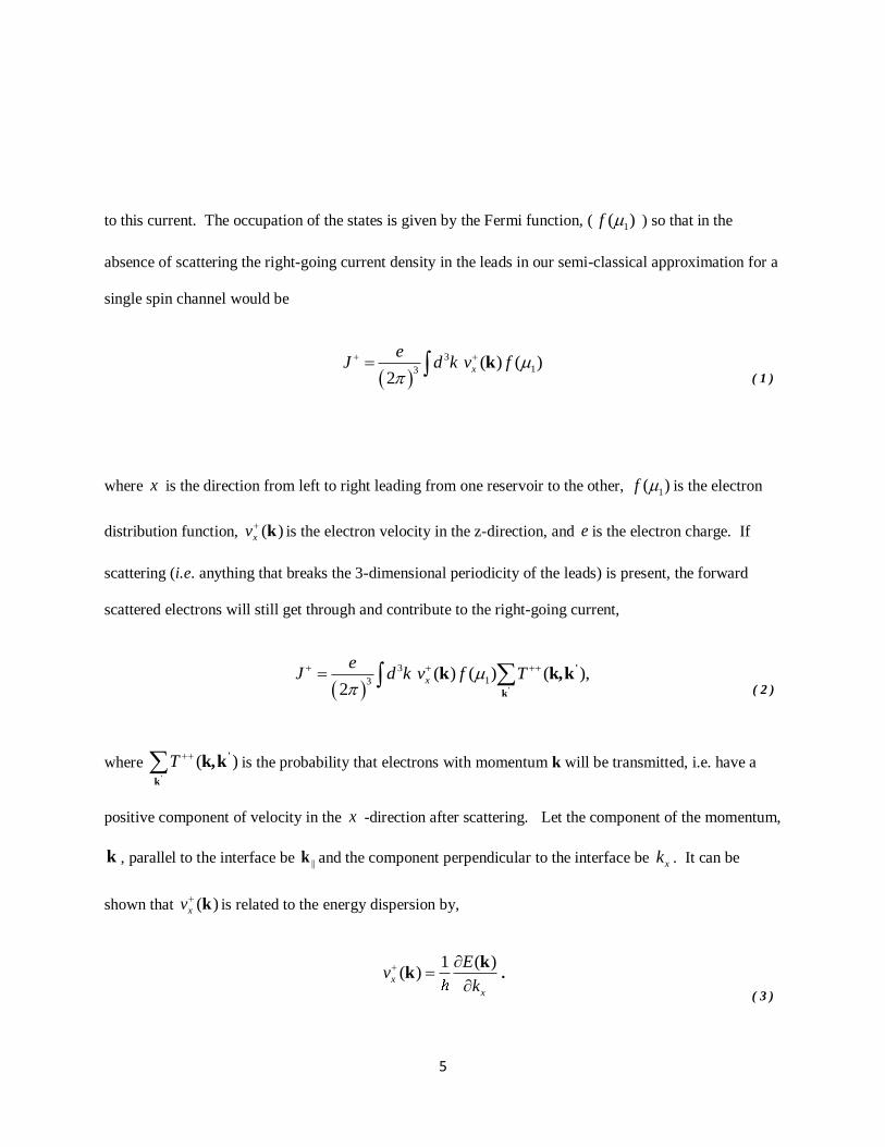
to this current. The occupation of the states is given by the Fermi function, ( 1( )f ) so that in the

absence of scattering the right-going current density in the leads in our semi-classical approximation for a

single spin channel would be

3

13 ( ) ( )

2x

eJ d k v f

k

( 1 )

where x is the direction from left to right leading from one reservoir to the other, 1( )f is the electron

distribution function, ( )xvk is the electron velocity in the z-direction, and e is the electron charge. If

scattering (i.e. anything that breaks the 3-dimensional periodicity of the leads) is present, the forward

scattered electrons will still get through and contribute to the right-going current,

3

13 ( ) ( ) ( ),

2x

eJ d k v f T

'

'

k

k k,k

( 2 )

where ( )T '

'

k

k,k is the probability that electrons with momentum k will be transmitted, i.e. have a

positive component of velocity in the x -direction after scattering. Let the component of the momentum,

k , parallel to the interface be ||k and the component perpendicular to the interface be xk . It can be

shown that ( )xvk is related to the energy dispersion by,

1 ( )( )x

x

Ev

k

kk .

( 3 )

6

Usually there will be more than one band so there should be an index, e.g. n, that should be

summed over to obtain the current density, however, for simplicity, we will assume that k includes the

band index and the integral over k includes a sum over bands which is not shown explicitly.

If we separate the integral over momentum into integrals over k and xk , we can write J as

2

|| 12

1 1 ( ) ( ) ( )

22x

x

e EJ d k dk f T

k

'

'

k

kk,k ,

( 4 )

or,

1

1 1 ( ) ( ) ( )

2x

x

e EJ dk f T

A k

'||

'

k k

kk,k ,

( 5 )

where we have used a standard expression to relate the integral over the two dimensional Brillouin zone

to a sum. Finally, we convert the integral over xk into an integral over energy and use the expression

I=JA to obtain,

1

'||

'

||

,

( )e

I dE Th

||

||

k k

k ,k .

( 6 )

Similarly, we can obtain the current in the x direction,

7

2

'||

'

||

,

( )e

I dE Th

||

||

k k

k ,k .

( 7 )

Time reversal invariance of the Schrödinger equation allows us to equate the transmission probability left

to right to the transmission probability right to left, T T . If 1 = 2 the current from electrons

whose origin is on the left cancels that of the electrons originating on the right so that the net current

would be zero.

If we apply a small positive bias voltage V so that 1 2 eV , then the net current will come

from the energy “window” between 1 and 2 , and the net current (right-going minus left-going) can be

written as

1 2

' '|| ||

'||

'||

|| ||

, ,

1 2 ||

,

2

1 2||

,

( ) ( )

( )

( ) .

e eI I - I dE T dE T

h h

eT

h

eT

h e

|| ||

||

||

' '

|| ||

k k k k

'

||

k k

'

||

k k

k ,k k ,k

k ,k

k ,k

( 8 )

Using the definition of the bias voltage, 1 2Ve

, and the definition of conductance, G IV , the net

current yields the Landauer conductance formula (for a single spin channel),

8

'||

2

||

,

( ) .

FE

I eG T

V h

||

'

||

k k

k ,k

( 9 )

9

CHAPTER 2.2: SIMPLE BARRIER MODEL FOR TUNNELING

As an example, the Landauer formula can be used to calculate the conductance for a simple

model in which the leads are described by free electrons and the sample is modeled as a potential step or

barrier. This allows us to reduce the problem of calculating the transmission probability to a one

dimensional problem that can be solved by requiring continuity of the wave function and its derivative at

the boundaries between the sample and the leads. We begin with the Schrödinger equation, in the general

representation in which the Hamiltonian and wave function depend on both time and position,

2

2 , , ,2

V r t r t i r tm t

.

( 10 )

Here m is the mass of the electron, and is Planck’s constant. In our case, the potential, V r , and the

Hamiltonian,

22

2H V r

m ,

( 11 )

are independent of time, so the solution to the Schrödinger equation can be separated into time and

position dependences by writing the wave function as the product of space and time dependent functions,

,r t r f t so that the Schrödinger equation becomes,

10

22

2f t r V r r f t i r f t

m t

.

( 12 )

We divide by r f t to obtain,

221 1

,2

r V r i f tm r f t t

( 13 )

and we choose a separation constant, E , the electron energy, to separate the Schrödinger equation into

two equations:

221

2r V r E

m r

( 14 )

and

1i f t E

f t t

.

( 15 )

Eq. (15) can be integrated to yield,

Ei t

f t e

.

( 16 )

The wave function becomes

11

,

Ei t

r t r e

( 17 )

where r depends on V r and is found by solving the time independent Schrödinger equation,

2

2

2V r r E r

m

,

( 18 )

with boundary conditions appropriate to incoming electrons from x and transmitted electrons for

x . V r V x is the potential which is assumed to be zero except in the region occupied by the

sample or tunnel barrier which extends from 0x to x d , where it is a constant, .V

Because V r V x is only a function of x , we can separate variables by assuming a wave function of

the form,

, ,r x y z x y z .

( 19 )

We substitute this form for r into the Schrödinger equation to obtain

2 2 22

2 2 22

.

x y zy z x z x y

m x y z

V x x y z E x y z

( 20 )

Dividing Equation (20) by Equation (19) yields,

12

2 2 2 2

2 2

2 2

2

1 1

2 2

1.

2

x V x x yx m x y m y

z Ez m z

( 21 )

Each of the three terms on the left side of the equals sign depends on only one of the , x y or z

coordinates. Hence we have three independent equations:

2 2

122x V x x E x

m x

( 22 )

2 2

222y E y

m y

( 23 )

2 2

322z E z

m z

( 24 )

where

1 2 3E E E E . ( 25 )

Equations (23) and (24) have plane wave solutions,

exp yy ik y , ( 26 )

exp zz ik z , ( 27 )

13

with

2 2

22

ykE

m

( 28 )

and

2 2

32

zkE

m .

( 29 )

Thus

2 2

2 2 2

12 2

y zE E k k E km m

( 30 )

and Equation (22) may be written as,

2 2 2

2

22 2x E k V x x

m x m

,

( 31 )

which may be written in regions 1 and 3 where 0V x as

2

2

2

xk x

x

( 32 )

with

14

2 2

2

2mEk k ,

( 33 )

and in region 2, where V x V as

2

2

2

xk x

x

( 34 )

where

2 2

2

2mk E V k .

( 35 )

In fact, we shall be interested in the energy range for which 2k is negative.

When the energy of the electron, E , is lower than the barrier potentialV , the wave functions may be

written for regions, 1, 2 and 3 as:

2

1 2

2, (region 1)ikx ikx mE

e re k k

( 36 )

2

2 2

2 ( ), (region 2)k x k x m V E

Ae Be k k

( 37 )

15

2

3 2

2, region 3ik x mE

te k k k

( 38 )

Equation (36) represents the boundary condition that in region 1, the wave function consists of an

incident plane wave traveling in the x direction and a reflected wave of relative amplitude r traveling

in the x direction. Equation (38) represents the boundary condition that in region 3 there is no wave

incident from the right, only a transmitted wave of relative amplitude t . The coefficients, , , , and ,r t A B

are determined from the boundary conditions and the requirements that the wave function and the

derivatives should be continuous. If we assume that the left and right leads are made from the same

material, then k and kare equal and will be represented by k . 1 and 3 are the wave functions for the

left (1) and right leads (3) respectively, and 2 is the wave function for the barrier region (2).

Requiring continuity of wave function and derivative at the interfaces yields,

1 2 2 30 0

31 2 2

0 0

x x x a x d

x x x a x dx x x x

( 39 )

1

1

k d k a ikd

k d k d ikd

r A B Ae Be te

k ikr A B Ae Be te

ik k

( 40 )

16

This set of four linear equations can be solved to determine, , , A B r and t

2 22 cosh ( )sinh

k dk k ik eA

ikk k d k k k d

,

( 41 )

2 22 cosh ( )sinh

k dk k ik eB

ikk k d k k k d

,

( 42 )

2 2

2

2 cosh ( )sinh

ikkt

ikk k d k k k d

,

( 43 )

and

2 2

2 2

( )sinh

2 cosh ( )sinh

k k k dr

ikk k d k k k d

.

( 44 )

The transmission and reflection amplitudes are given by r and t , respectively.

17

Figure 2: Tunneling wave function for the simple barrier model for a fixed value of k . For this

example, the barrier extends from 0x to 2x .

The transmission and reflection probabilities, for a given value of k are given by

2 2*

22 2 2 2 2 2

2 2

22 2 2 2 2

4

4 cosh sinh

4

4 sinh

k kT tt

k k k d k k k d

k k

k k k k k d

.

( 45 )

and

22 2 2

*

22 2 2 2 2

sinh

4 sinh

k k k dR rr

k k k k k d

.

It is important to note that the transmission probability is only given by the simple relation *T t t when

the leads are the same on the two sides of the barrier. If they are different, one must either compare the

transmitted current to the incident current or carefully normalize the incident and transmitted wave

18

functions so that they carry the same current and flux. We will return to this point again after we discuss

the current density.

To obtain the conductance, we must integrate the transmission probability in Equation (37) over k . If we

define

2

2

2F

mEk

( 46 )

and

2

2

2,

mV

( 47 )

then the transmission probability may be written,

2 2 2 2 2

2 2 2 2 2 4 2 2 2 2

4, ,

4 sinh

F F

F F F

k k k kT E V k

k k k k k k d

,

( 48 )

and the (single spin-channel) conductance from the Landauer formula may be written, taking advantage

of the conservation of transverse momentum as an integral over k ,

2

0

,V,2

Fke A

G k dk T E kh

.

( 49 )

Setting

19

Fk

x

( 50 )

and

kz

,

( 51 )

this may be written as,

2 2 2 222

2 2 2 2 2 2 20

4 1

2 4 1 sinh 1

x x z x ze AG zdz

h x z x z d x z

.

( 52 )

A change of the variable of integration using,

2 2 21u x z ( 53 )

yields,

2

2 2122

2 2 2

1

4 1

2 4 1 sinhx

u ue AG udu

h u u du

.

( 54 )

It should be noted that this result is only valid in the limit of low bias both because we have restricted the

potential to be the same in both leads and because we have assumed a constant potential for the barrier

region.

20

In the limit of 0d in which the barrier vanishes and the transmission probability becomes

unity, Equation (54) can be integrated trivially to give,

22

22

F

e AG k

h

,

( 55 )

which is the Sharvin single spin-channel conductance for a contact. [7] The Sharvin conductance can be

viewed as

2e

h times the number of conductance channels. The number of conductance channels per unit

area is the projection of the Fermi sphere onto a plane perpendicular to the x axis divided by 2

2 ,

which may be viewed as a square wave length per conductance channel.

In the limit of d , Equation (54) yields,

32

2

12

2

22

2

16 1 exp 2 12 2

1 , , 02 2

, , 02

F F F

FF

F

E E Ee AG d

h d V V V

Ee AT E V k

h d V

e Ak T E V k

h

( 56 )

where

2 2

2 Fkk

d

.

21

Figure 3: Graph of Conductance as a function of FE

V for different values of thickness, d. Conductance

is expressed in units of

2 2

2

e A

h

(see Equation (54)).

22

CHAPTER 2.3: CURRENT DENSITY

We can think of the probability of finding an electron in a particular spatial region changing due

to a probability flow, or current, entering or leaving that region. This definition of the current is chosen

so that the probability density will satisfy the continuity equation

t

j ,

( 57 )

representing the fact that electrons are conserved. Here, the electron density is represented by

*, , ,r t r t r t . ( 58 )

We can use the time-dependent Schrödinger equation to derive the current. First, we take the time-

dependent Schrödinger equation and its complex conjugate:

2

2, , ,2

i r t H r t V r tt m

( 59 )

and

2

* * 2 *, , ,2

i r t H r t V r tt m

.

( 60 )

Multiplying the first of these equations by * ,r t and the second by ,r t yields

23

2

* * * 2, , , , , ,2

r t i r t r t H r t r t V r tt m

( 61 )

and

2

* * 2 *, , , , , ,2

r t i r t r t H r t r t V r tt m

.

( 62 )

Subtracting these two equations yields

2* * 2 2 *, , , , , ,

2i r t r t r t r t r t r t

t m

.

( 63 )

which can be written as

* *, , , , ,

2r t r t r t r t r t

t mi

.

( 64 )

We can now see that this becomes the continuity equation if we identify,

* *, , , ,

2r t r t r t r t

mi j ,

( 65 )

as the electron current. Since the gradient operator does not operate on the time dependent part of the

wave function, this may be written as

24

* *

2r r r r

mi j ,

( 66 )

and the current in the x direction (for a given value of k ) is given by

*

* , 1 32

i iix i ij i

mi x x

( 67 )

where ( , )i x k is given by Equations (36-38) for the simple barrier model.

For each region (1, 2, and 3), the currents are represented by

2* *

1 1 1 1 1 1 (region 1)2

x

kj r

mi x x m

( 68 )

* * * *

2 2 2 2 2 (region 2)2

x

kj B A A B

mi x x mi

( 69 )

2* *

3 3 3 3 3 (region 3)2

x

kj t

mi x x m

( 70 )

25

The reflection and transmission probabilities in the simple barrier model were found to be,

22 2 2

2

22 2 2 2

sinh

2 sinh

k k k dR r

k k k k k d

( 71 )

and

2

2

22 2 2 2

2

2 sinh

k kT t

k k k k k d

.

( 72 )

In the left lead, we have,

2* *

1 1 1 1 1

22 2 2

22 2 2 2

2 22 2 2 2 2 2 2

22 2 2 2

2

22 2 2 2

12

sinh1

2 sinh

2 sinh sinh

2 sinh

2

2 sinh

x

x

kj r

mi x x m

k k k dk

m k k k k k d

k k k k k d k k k dk

m k k k k k d

k kkv

m k k k k k d

k T k

( 73 )

,

and in the barrier region, the current is given by,

26

* * * *

2 2 2 2 2

2 2 2 2

2 2

2 2

2 cosh sinh 2 cosh sinh

2 cosh sinh 2 cosh

x

k a k a

k a k a

kj B A A B

mi x x m

k k ik e k k ik ek

mi ik k k d k k k d ik k k d k k k d

k k ik e k k ik ek

mi ik k k d k k k d ik k k d

2 2

4 3 2 2 4 3 2 2

22 2 2 2 2 2

2

22 2 2 2

sinh

2 2

4 cosh sinh

2.

2 sinhx

k k k d

k k k ik k k k k ik k k

mi k k k d k k k d

k kkv k T k

m k k k k k d

( 74 )

It is interesting to note that the exponentially increasing as well as the exponentially decreasing

component of the wave function in the barrier region must be present, otherwise the current in this region

will vanish (see Equation (69)). A semi-infinite barrier will support an exponentially decreasing

evanescent wave, but it carries no current.

In the right lead, the current is given by,

2* *

3 3 3 3 3

2

22 2 2 2

2

2 .

2 sinh

x

x

kj t

mi x x m

k kkv k T k

m k k k k k d

( 75 )

27

Thus the current is conserved throughout each region of the tunneling process. Second, the identity,

1R T , is satisfied. Last, we should note that as the barrier becomes thicker ( d increases) or the

barrier gets taller ( k increases), R increases and the conductance and current decreases.

In Equations (72-75) we have identified the transmission probability with the absolute square of

the transmission amplitude, *T k t t . This is only valid if the left and right leads are the same or if

the incident and transmitted wave functions are normalized to carry the same current. In the general case

with un-normalized incident and transmitted wave functions, Leftik xe , and Rightik x

e , the transmission

probability is obtained by taking the ratio of the transmitted current to the incident current,

* /Left RightT k v k t k t k v k .

28

CHAPTER 3: TIGHT-BINDING APPROXIMATION

29

CHAPTER 3.1: LCAO OR TIGHT-BINDING MODEL FOR ELECTRONIC STRUCTURE

The simple barrier model has the advantage of simplicity, but it may miss important physics

associated with the existence of atoms in real tunneling systems. One obvious limitation is that real

barrier materials have both a conduction band and a valence band – the simple barrier model for a

tunneling barrier has only a conduction band. In this section we shall develop the tight-binding formalism

for electron transport and quantum mechanical tunneling.

The tight-binding approximation is based on the assumption that the electron wave function can

be approximated as a linear combination of atomic orbitals (LCAO),

,

,

i i i

atomic orbitalssite i

r C r R

,

( 76 )

where i represents an atomic orbital centered at site, i , with label, , distinguishing different orbitals

centered on the same site. The iC represent coefficients which are to be determined. The time

independent Schrodinger equation was given in Equation (18). The Schrödinger equation is

H r E r , where, in the presence of atoms, the Hamiltonian can be written as

22

2i i

i

H V r Rm

,

( 77 )

30

with i iV r R representing the effective potential associated with site i . It should be noted that we are

assuming a “one electron at a time” or “effective field” approximation such as that given by density

functional theory. [8]

By substituting the LCAO approximation for the wave function into the Schrödinger equation and

assuming that the atomic orbitals are orthonormal, one can convert the Schrödinger equation into a matrix

equation,

HC EC ( 78 )

or

,

0 all and i j j

sites j orbitals

H E C i

( 79 )

where the Hamiltonian matrix element is given by

*

, ji j i j iH H i H j d r r R H r R .

( 80 )

Although the assumption that the wave functions are orthonormal is not very realistic, it can be

justified by invoking Wannier functions which are local functions obtained by a transformation of the

actual energy bands of the material. The Wannier function basis is orthonormal and the Hamiltonian built

from a Wannier function basis can often be made to have a relatively short range. [9]

31

The development of realistic short-ranged tight-binding Hamiltonians is an active area of

research. In this thesis we shall employ empirical models based on tight-binding. The empirical tight-

binding method develops approximations only for the Hamiltonian matrix elements ,i jH themselves

without attempting to model the potential and the explicit form of the LCAO basis functions. The tight-

binding models used in this thesis are too simplistic to accurately represent the electronic structure of a

solid, but our objective will be to illustrate important physical principles within models that can be solved

exactly.

The simplest tight-binding model for an infinite solid would be a one-dimensional chain of one-

orbital atoms with only nearest neighbor interaction. The Hamiltonian for such a system would be an

infinite tridiagonal matrix with the orbital energy, 0E , on the diagonal and the “hopping matrix element”,

1| |i iw H , ( 81 )

above and below the diagonal. In practice, 0E , and w are parameters that would be adjusted to mimic as

well as possible the relevant energy band of the solid. The Schrödinger equation will consist of an

infinite set of equations,

0 1 1i i i iC E wC wC EC . ( 82 )

The infinite set of equations can be solved by use of Bloch’s theorem which states that the wave functions

on adjacent sites are related by a phase factor, i.e.,

1

i

i iC e C . ( 83 )

This ansatz leads to the dispersion relation,

32

0 2 cos .E E w ( 84 )

The phase angle in Equation (83) can be either positive or negative. From Equation (84), it is clear that

yield the same energy. The positive sign corresponds to a wave propagating in the x direction.

The negative sign corresponds to a wave of the same energy propagating in the opposite direction.

33

CHAPTER 3.2: TRANSMISSION THROUGH AN INTERFACE IN TIGHT-BINDING

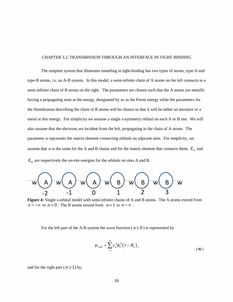
The simplest system that illustrates tunneling in tight-binding has two types of atoms, type-A and

type-B atoms, i.e. an A-B system. In this model, a semi-infinite chain of A atoms on the left connects to a

semi-infinite chain of B atoms on the right. The parameters are chosen such that the A atoms are metallic

having a propagating state at the energy, designated by us as the Fermi energy while the parameters for

the Hamiltonian describing the chain of B atoms will be chosen so that it will be either an insulator or a

metal at this energy. For simplicity we assume a single s-symmetry orbital on each A or B site. We will

also assume that the electrons are incident from the left, propagating in the chain of A atoms. The

parameter w represents the matrix element connecting orbitals on adjacent sites. For simplicity, we

assume that w is the same for the A and B chains and for the matrix element that connects them. AE and

BE are respectively the on-site energies for the orbitals on sites A and B.

Figure 4: Single s-orbital model with semi-infinite chains of A and B atoms. The A atoms extend from

n to 0n . The B atoms extend from 1n to n .

For the left part of the A-B system the wave function ( 0n ) is represented by

0A A

Left n n nc r R

,

( 85 )

and for the right part ( 1n ) by,

A w w

A

A w w

B

B w w

B w

-2 -1 0 1 2 3

34

1

B B

Right n n n

n

c r R

.

( 86 )

The matrix Schrödinger equation (Equation 79) will be an infinite set of equations which includes a semi-

infinite set for the left, a semi-infinite set for the right and two equations for the interface,

1 1 0 (for 0)A A A

A n n nE E c w c c n , ( 87 )

0 1 1 0 (for 0)A A B

AE E c w c c n , ( 88 )

1 0 2 0 (for 1)B A B

BE E c w c c n , ( 89 )

and

1 1 0 (for 1)B B B

B n n nE E c w c c n . ( 90 )

If we divide these four equations by w , and define

/E w , ( 91 )

/A AE w , ( 92 )

and

35

/B BE w , ( 93 )

the system becomes,

1 1( )c ( ) 0 for 0A A A

A n n nc c n , ( 94 )

0 1 1( )c ( ) 0 for 0A A B

A c c n , ( 95 )

1 0 2( )c ( ) 0 for 1B A B

B c c n , ( 96 )

and

1 1( )c ( ) 0 for 1B B B

B n n nc c n . ( 97 )

The boundary conditions are such that there are incident and reflected wave functions for 0,n and a

transmitted wave function for 1n . These can be written as,

( 0)A Ain inA

nc e re n

( 98 )

and

( 0)BinB

nc te n

. ( 99 )

Substituting the boundary conditions into Equation (95) for 0n gives,

36

( )(1 ) ( ) 0A A Bi i i

A r e re te

. ( 100 )

Similarly, substituting the boundary conditions into Equation (96) for 1n gives

2( ) ( 1 ) 0B Bi i

B te te r . ( 101 )

The dispersion relations for the left and right sides relate the energy to the phase factors,

A Ai i

A e e

( 102 )

B Bi i

B e e

( 103 )

These can be used to write equations (99) and (100) in terms of r, t and the phase factors:

A B Ai i ie r te e

( 104 )

1r t . ( 105 )

The transmission amplitude can be determined from adding Aie

times the first of these equations to the

second,

2 sin

1B

B A

iA

i i

it e

e e

,

( 106 )

and the reflection amplitude from Equation (105),

37

2

1

A A B

A B

i i i

i i

e e er

e e

.

( 107 )

In this case, the reflection probability,* 1R rr if Bi

reale z . This will happen when the energy is

outside the range 2 2Bw E E w , since in this case, cos / 2B BE E w will only have a

solution if B is imaginary. We assume 2 2Aw E E w , otherwise there would not be an incoming

wave.

1 cos( )1 1* .

1 1 1 cos( )

1 1* 1 .

1 1

B A B A

B

B A B A

A A

A A

i i i iiB A

i i i i

B A

i i

real real

i i

real real

e e e er r when z e

e e e e

z e z er r when z is real

z e z e

( 108 )

This implies that the reflection probability is unity even though there is a decaying wave of amplitude

n

nc tz (where 1z ) in the semi-infinite chain on the right hand side ( 1n ). We defer a calculation

of the transmission probability until after we have derived an expression for the current density in the

tight-binding approximation. At that time, we will see that for the case of a semi-infinite chain of B

atoms, for energies that do not admit electron propagation, (i.e. Bi

reale z ), the current in the B chain

vanishes and the transmission probability also vanishes even though there is an exponentially decaying

evanescent wave in the B chain.

38

CHAPTER 3.3: TUNNELING THROUGH A BARRIER IN TIGHT-BINDING

We now consider transmission through a barrier in the tight-binding picture. Our model consists

of a semi-infinite chain of A atoms on the left and a semi-infinite chain of A atoms on the right. In

between is a finite chain of B atoms.

A-B-A System

Figure 5: A tunneling system consisting of two semi-infinite chains of A atoms separated by N B atoms.

By proper choice of parameters, we can make the A atoms conducting and the B atoms insulating.

The wave functions on the left, middle and right are, as before expressed as a linear combination of

atomic orbitals centered on the sites,

0A A

Left n n n

n

c r R

,

( 109 )

1

NB B

Middle n n n

n

c r R

,

( 110 )

A w w A B w w

B B w w B B w w

-1 0 1 2…

w w A A

…N N+1

39

1

A A

Right n n n

n N

c r R

.

( 111 )

Using the numbering system shown in Figure 5, we have the two equations that relate the coefficients for

the A-chain on the left to the coefficients for the B chain in the center:

1 0 1 0Awc E c wc Ec ( 112 )

and

0 1 2 1Bwc E c wc Ec . ( 113 )

The two equations that relate the coefficients for the wave function in the center to those for the wave

function describing the chain on the right:

1 1N B N N Nwc E c wc Ec ( 114 )

and

1 2 1N A N N Nwc E c wc Ec . ( 115 )

As before, the boundary conditions on the left represent an incoming wave and a reflected wave,

for 0A Ain in

nc e re n

. ( 116 )

In the middle region, the coefficients consist of exponentially increasing and decreasing terms if

the energy is outside the region for which the B chain allows propagating solutions. If there are

propagating solutions, the exponential functions would be replaced with circular functions representing

40

left- and right- going waves. Here we will assume for definiteness that the energy is outside the range of

the propagating solutions,

for 1B Bn n

nc Ae Be n N

. ( 117 )

On the right side, the boundary condition is that of a transmitted wave propagating in the +x direction,

(for 1)Ain

nc te n N

. ( 118 )

Substitution of Equation (116) and (117) into the boundary conditions of Equations (112) and (113), the

two equations for the left interface yields:

1B Bi i

Ae re Ae Be r

( 119 )

2 21 B B B B

Br Ae Be Ae Be

. ( 120 )

While substitutions of Equations (117) and (118) into the boundary conditions of Equations (113) and

(114), the two equations for the right interface yields,

1 1 1B B B BN N i N N N

BAe Be te Ae Be

( 121 )

2 1B B

i N i NN N

AAe Be te te

( 122 )

41

Using the dispersion relation for A, 2cosA A , and for B, 2coshB B , on the equations

for the left interface yields,

A B B Ai ire Ae Be e

( 123 )

and

1r A B . ( 124 )

Similarly, for the right interface,

1 1 10B B AN N i N

Ae Be te

( 125 )

0B B AN N iNAe Be te

. ( 126 )

The reflection amplitude, r , can be easily eliminated from Equations (123) and (124) that describe the

left interface,

B A B A A Ai i i iA e e B e e e e

.

( 127 )

Similarly, t , can be eliminated from Equations (125) and (126) that describe the right interface,

0B B A B B AN i N iAe e e Be e e

.

( 128 )

Equation (128) allows us to obtain A in terms of B .

2

B A

B

B A

i

N

i

e eA Be

e e

.

( 129 )

Then the inhomogeneous equation involving A and B can be solved:

42

2

A A B A

B A B A B B A B A

i i i

i i N i i

e e e eB

e e e e e e e e e

( 130 )

2

2

A A B A B

B A B A B B A B A

i i i N

i i N i i

e e e e eA

e e e e e e e e e

.

( 131 )

Once A and B are known, t and r can be obtained in a straightforward (if slightly tedious) manner:

A A B B

A

B A B A B B A B A B

i i

iN

i i N i i N

e e e ete

e e e e e e e e e e

( 132 )

B B A A B B

A

B A B A B B A B A B

i i N N

i

i i N i i N

e e e e e ere

e e e e e e e e e e

.

( 133 )

Equations (132) and (133) can also be written as,

4 sin sinh

4sinh 1 cos cosh 4 cosh sin sinhAiN A B

B A B B A B

ite

N i N

( 134 )

and

43

4 cosh cos sinh

4sinh 1 cos cosh 4 cosh sin sinhA B A Bi

B A B B A B

Nre

N i N

.

( 135 )

We can make contact with the transmission and reflection amplitudes calculated for the simple

barrier model, Equations (43 and 44) by taking advantage of the fact that tight-binding bands have free

electron-like dispersion near the top or bottom of the band. Thus we can recover the simple-barrier

tunneling amplitude expressions in the following limit,

21

0, sin , cos 12

A A A A Aka

( 136 )

210, sinh , cosh 1

2B B B B Bk a

( 137 )

Na d . ( 138 )

Then

2 2

2

sinh 2 cosh

AiN ikkte

k k k d ikk k d

( 139 )

and

44

2 2

2 2

sinh

sinh 2 cosh

Aik k k d

rek k k d ikk k d

.

( 140 )

Equations (139) and (140) can be seen to be the same as Equation (43) and (44) aside from unimportant

phase factors.

45

CHAPTER 3.4: TRANSMISSION PROBABILITY FOR SIMPLE TIGHT-BINDING TUNNELING

The transmission and reflection probabilities can be obtained from equations (134) and (135)

respectively,

2 2*

22 2 2 2

sin sinh

sinh 1 cos cosh cosh sin sinh

A B

B A B B A B

T t tN N

( 141 )

2 2

*

22 2 2 2

cosh cos sinh


B A B

B A B B A B

NR r r

N N

.

( 142 )

Electron conservation ( 1R T ) can be verified by noting that by repeated use of the identity,

2 2cosh 1 sinh , the common denominator in Equations (141) and (142) can be written as,

22 2 2 2

2 2 2 2


cosh cos sinh sin sinh .

B A B B A B

B A B A B

N N

N

( 143 )

Equations (141) and 142) can also be written in a form that shows the energy dependence more clearly,

by using 2cosA Ax and 1 2coshB By z z or 2cos B if 2B ,

22

22 2 24 4

N N

N N

x y z zR

y x z z x y

( 144 )

46

2 2

22 2 2

4 4

4 4N N

x yT

y x z z x y

.

( 145 )

Written in this form, conservation of electrons, 1R T , is immediately obvious. Similarly to the

interface case we can make contact with the simple barrier model in a limit in which 0A ka ,

0B k a , and Na d .

2 2*

22 2 2 2

2

22 2 2 2

sin sinh


2

2 sinh

A B

B A B B A B

T t tN N

k k

k k k k k d

2 2

*

22 2 2 2

22 2 2

22 2 2 2

cosh cos sinh


sinh

2 sinh

B A B

B A B B A B

NR r r

N N

k k k d

k k k k k d

This limit can be taken consistently if the energy is very near the top or bottom of the conduction band for

the leads and simultaneously just below the bottom or just above the top of the conduction band for the

barrier.

The variation of the transmission probability with energy for the A-B-A system is shown in

Figures 6 and 7. The A (leads) onsite energy in units of the hopping matrix element is chosen to be 0, and

the B (barrier) onsite energy is chosen to be 2. The band of the leads will extend from -2 to 2, the range

47

over which the figure is plotted. The band of the barrier extends from 0 to 4. There is wave propagation

from 0 to 2 , energies where propagation is allowed in both leads and barrier. In the region

2 to 0 there is a small transmission due to quantum mechanical tunneling. Figures 6 and 7

show the transmission probability for N=10, and 5 respectively, i.e. for 10 and 5 B atoms in the barrier.



matrix element, w . The red curve shows the sum of Transmission and Reflection probabilities.

For some energies in the non-tunneling energy range, the transmission probability reaches 100%.

These are energies for which BN m where m is an integer. In the non-tunneling or band

48

conduction regime, the hyperbolic functions in Equation (141) become circular functions. Thus perfect

transmission will occur for /B m N or for 2cos /B m N .

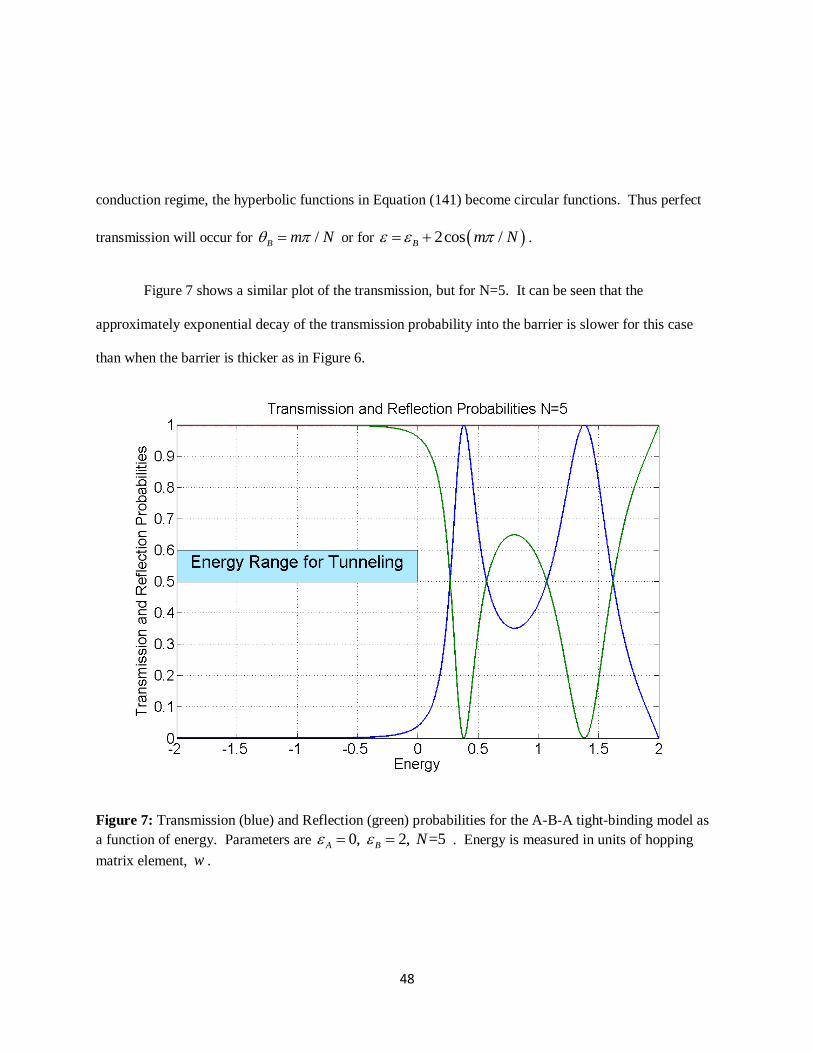
Figure 7 shows a similar plot of the transmission, but for N=5. It can be seen that the

approximately exponential decay of the transmission probability into the barrier is slower for this case

than when the barrier is thicker as in Figure 6.



matrix element, w .

49

Figure 8 shows the transmission and reflection probabilities using a logarithmic scale so that

decay of the tunneling probability can be seen at energies far from the band edge for propagation in the

barrier.

Figure 8: Transmission and Reflection Probabilities plotted with a logarithmic scale. The tight-binding

tunneling parameters are 0, 3, 10.A B N

Figure 9 shows the wave function at 0.99 using the parameters of Figure 8. The blue

and red points (boxes) represent the real and imaginary parts of the wave function coefficients on

the atomic sites as described in Equations (106-108). Waves are incident from the left from

and are outgoing on the right toward . Note that the wave function changes sign between

50

adjacent atoms in the barrier. This is due to Be

being negative below the bottom of the band

for the barrier. If we move the barrier band down so that the energy is above the band

maximum for the barrier, the factor Be

will be greater than zero. This is illustrated in Figure 10

which uses the parameters, 0, 3, 0.99A B , so that E is slightly above the B band

maximum of 1.

Figure 9: Parameters are 0, 3, 0.99, 10.A B N The wave function coefficients for the

real and imaginary parts of the wave function are shown by the blue and red boxes respectively. The blue

and red lines joining the boxes serve as a guide to the eye.

51

Figure 10: Parameters are 0, 3, 0.99, 10.A B N The wave function coefficients for the

real and imaginary parts of the wave function are shown by the blue and red boxes respectively. The blue and red lines joining the boxes serve as a guide to the eye.

52

CHAPTER 3.5: CURRENT DENSITY IN TIGHT-BINDING

In order to understand the above results for the transmission and reflection amplitudes, especially

the results for the A-B System, we must understand the current in the tight-binding approximation. In

analogy to the derivation of the current in Chapter 2 (starting from Equation (57)), we have, for our one

dimensional tight-binding model, the time-dependent wave function,

( )n n

n

t c t , ( 146 )

which obeys the time dependent Schrödinger equation,

i t H t

t

.

( 147 )

This can be written in terms of the wave function coefficients by using the assumed orthonormality

properties of the local orbitals,

0 1 1( ) ( ) ( ) ( )n n n ni c t E c t wc t wc t

t

.

( 148 )

The probability that an electron is on site, n , is given by

*

n n nt c t c t , ( 149 )

and the time derivative of this quantity is given by,

53

*

*n nn n n

c ci t i c c

t t t

,

( 150 )

but this can be evaluated by use of Equation (143) and its complex conjugate:

* * * *

0 1 1n n n n n n n ni c c E c c wc c wc ct

( 151 )

and

* * * *

0 1 1n n n n n n n ni c c E c c wc c wc ct

.

( 152 )

Thus the time rate of change of the number of electrons on a site is given by,

* * * *

1 1 1 1n n n n n n n n ni t wc c wc c wc c wc ct

, ( 153 )

but this must be equal to the difference between the current coming in from the left and the current

leaving from the right,

* * * *

1 1 1 1 1 1

2 2

n n n n n n n n nn n

it wc c wc c wc c wc c J J

t

,

( 154 )

where,

* *

1 1 1

2

n n n nn

iJ wc c wc c

( 155 )

54

and

* *

1 1 1

2

n n n nn

iJ wc c wc c

.

( 156 )

We are now in a position to discuss the reflection and transmission amplitudes, Equations (106)

and (107), in terms of the electron currents. The current on the left is given by substituting Equation (98)

into the expression for the current, Equation (98) into one of the expressions for the current, obtaining,

*2 sin1A

Left

wJ r r

.

( 157 )

Similarly, use of Equation (99) in the expression for the current yields,

*2 sin Bright

wJ t t

.

( 158 )

Substituting from the expressions for r and t , (Equations (154) and (155)) allows us to verify that

.Left rightJ J If we define the transmission and reflection probabilities to be,

*sin

sin

B

A

T t t

( 159 )

and

55

*R r r , ( 160 )

then we have 1R T as expected. The reason we need to modify the definition of the transmission

probability to include the factor, sin

sin

A

B

, is that the incident and transmitted wave functions have

different normalizations, i.e. the current or flux carried by exp Ain differs from that carried by

exp Bin . If we had been careful to include the normalization factors to ensure equality of these fluxes

then the additional factor, would not have been needed.

The negative sign in front of the expression for the currents has a simple explanation.

2 sin /wa is the electron velocity for an electron with dispersion relation 0 2 cosE E w .

Thus Equation (153) could be written *

RightJ vt t which may be compared to the analogous Equation

(75) for the current in the simple barrier problem. When 0w , the energy is a maximum for

0ka . To compare the simple barrier model with a limiting case of the tight-binding model, we

will need to take 0w .

Note that when the energy is outside the range 2 2Bw E E w so that B is imaginary, then

the current expressions give zero for the current on the right. This is consistent with 1R as derived

above.

56

CHAPTER 4: TUNNELING THROUGH A BARRIER WITH A GAP

The systems that we have studied so far, the simple barrier model based on free electron

dispersion and the single-orbital tight-binding model differ from realistic tunneling in that neither involve

tunneling through a “gap”. In the free-electron based simple barrier model, the barrier is made non-

conducting by raising the zero of energy so that it is above the Fermi energy of the leads. In the single-

orbital tight binding model, the conduction band of the barrier is positioned so that its minimum is above

the Fermi energy or its maximum is below the Fermi energy. In none of these situations is the Fermi

energy positioned in a gap between two bands. In this chapter we shall investigate tunneling through a

barrier with a gap in its dispersion relation.

57

CHAPTER 4.1: THE A-[B-C] SYSTEM

A simple way to generate a gap is to have two types of atoms with different on-site orbital

energies as shown in Figure 11.

Figure 11: Single s-orbital model – Semi-infinite chains of A atoms and B-C molecules. The A atoms

extend from n to 0n . The B-C molecules extend from 1n to n .

In this system, a semi-infinite chain of A atoms connects on the left to a semi-infinite chain of B-

C molecules on the right. The parameters will be chosen such that the A atoms are metallic having a

propagating state at the energy, that we will designate as the Fermi energy. The B-C molecules can be

designated as an insulator or as a metal, to be determined by us. Importantly for creating a gap, B-C

molecules have two different orbitals. For nearest neighbor interactions, there will be a gap between the

B and C onsite energies. Let AE , BE , and CE be respectively the on-site energies for the orbitals on sites

A, B, and C. For the left part of the A-BC system the wave function ( 0n ) is represented by

0A A

Left n n nc r R

,

( 161 )

1

(B-atoms)B B

Right n n n

n

c r R

,

( 162 )

and

A w w A A w w

B C w w B C w w

-1 0 1 2…

w w B C

n

58

1

(C-atoms)C C

Right n n n

n

c r R

.

( 163 )

The Hamiltonian together with the assumed orthonormality of the orbitals will generate an infinite set of

equations:

1 1 0 0A A A

A n n nE E c w c c n for , ( 164 )

1 1 0 0A A B

A n n nE E c w c c n for , ( 165 )

1 0 1 0 1B A C

BE E c w c c n for , ( 166 )

1 1 2 0 1C B B

CE E c w c c n for , ( 167 )

1 1 0 1B A C

B n n nE E c w c c n for , ( 168 )

and

1 1 0 1C B B

C n n nE E c w c c n for . ( 169 )

59

Note that two equations are needed for each two atom cell for 0n :

The boundary condition on the left in the chain of A atoms is the sum of an incoming, right-going

wave of unit amplitude, Aine

, and a reflected, left-going wave of amplitude , Ain

r re

. The boundary

condition on the right is a transmitted right-going wave that has amplitude n

Bt z on the B atoms and n

Ct z

on the C atoms. Using these boundary conditions and defining, E w , A AE w , B BE w ,

C cE w , we have from Equation (164), 2cosA A ,and from Equations (168) and (169) using

1 1, ,B B C C

n n n nc zc c zc

110

1

B B

CC

z t

tz

,

( 170 )

which implies that,

1 2B C z z . ( 171 )

60

Figure 12: Dispersion relation for B-C chain. A gap extends from 0.5B to 0.5C . Blue and

green curves are real and imaginary parts of log(z) respectively where 1

2B C zz

.

On substitution of boundary conditions, Equation (165) becomes,

1 0A Ai i

A Br e re t z

, ( 172 )

which, with the help of the results from Equation (164) can be written as,

61

2A Ai i

Br t ze e

( 173 )

Similarly, Equation (167) becomes,

1 0C C Bt z t z z , ( 174 )

which allows us to write,

1B

C

C

t zt

.

( 175 )

and Equation (166) becomes

1 0B B Ct z r t z , ( 176 )

which with the use of Equations (171) and (173), may be written as,

111B

C

zr t z

.

( 177 )

Adding Equations (173) and (177) yields a solution for Bt ,

2

1

1

1

A

A

i

C

B i

C

et z

z e

,

( 178 )

from which a solution for Ct follows,

62

2

1

1 1

1

A

A

i

C i

C

e zt z

z e

,

( 179 )

as well as a solution for r , (using Equation (176)),

1

1

1

1

A

A

i

C

i

C

z er

z e

.

( 180 )

The reflection probability,*R r r , is clearly unity if z is real, i.e. if the parameters are such as to forbid

conduction in the B-C chain. However, if BCiz e

, then R becomes,

2

*

2

2 2cos 2cos 2cos

2 2cos 2cos 2cos

C BC C A C A BC

C BC C A C A BC

R r r

.

( 181 )

In order to investigate the transmission probability, it is necessary to calculate the current on the

right of the interface and compare it to the current carried by the incident wave. An expression for the

current is given by Equation (156). This expression involves the wave function coefficients in adjacent

atoms of the chain. The easiest place to apply this expression for the B-C chain is between the B and C

atoms in one of the cells,

* * * *

1 1 1

2

n n n n C B C Bn

iw iwJ c c c c t t t t

.

( 182 )

Substituting from Equations (178) and (179) gives,

63

*2 21 1

1 1

*2 21 1

1 1

1 1 1

1 1

1 1 1

1 1

A A

A A

A A

A A

i i

C

i i

C C

Righti i

C

i i

C C

e z e z

z e z eiw

J

e z e z

z e z e

.

( 183 )

If z is real, Equation (183) gives 0, however if BCiz e

, the current is finite and is given by,

2

2

8sin sin

2 2cos 2cos 2cos

A BC C

Right

BC C C A A BC

wJ

.

( 184 )

Both Equations (181) and (184) can be simplified by using, Equation (174) in the form,

2 2cos BC B C giving,

2cos 2cos

2cos 2cos

C B A A BC

C B A A BC

R

( 185 )

and

28sin sin

2cos 2cos

A BCRight

B C A A BC

wJ

.

( 186 )

The current carried by the incident wave is given by 2 sin /in AJ w , so that the transmission

probability is

64

4sin sin

2cos 2cos

Right A BC

in B C A A BC

JT

J

.

( 187 )

It is now possible to confirm that the sum of R in Equation (185) and T in Equation (187) is unity.

65

CHAPTER 4.2: THE A-[B-C] SYSTEM WITH s-p BARRIER

Figure 13: Single s-p-orbital model – semi-infinite chains of A and B-C molecules. The A atoms extend

from n to 0n . The B-C molecules extend from 1n to n . The orbital on the C atom

has xp symmetry.

In the A-BC (s-p) system, the B-C chain is a chain of two-molecule system B and C with atom B

having an s-orbital and atom C has a p-orbital. The system is solved as follows:

0 1 1( )c ( ) 0 0A A B

A c c n , ( 188 )

1 0 1( )c ( ) 0 1, B atomB A C

B c c n , ( 189 )

and

1 1 2( ) ( ) 0 1, C atomC B B

C c c c n . ( 190 )

In the A chain, for 0n , we have,

1 1 0A A A

A n n nc c c , ( 191 )

And in the B-C chain, for 1n , we have

A w w A A w w

B C w w B C w w

-1 0 1 2…

w w B C

n

66

1 0B C C

B n n nc c c , ( 192 )

and

1 0C B B

C n n nc c c . ( 193 )

Equations (192) and (193) lead to the dispersion relation 1

2B C zz

. The boundary

conditions representing an incoming wave from the left and an outgoing wave on the right are

0A Ain inA

nc e re n

, ( 194 )

1B n

n B Rc t z , ( 195 )

and

1C n

n C Rc t z , ( 196 )

respectively. Substitution of the boundary conditions, Equations (194), (195), and (196), into the

interface equations, Equations (188), (189), and (190), yields

( )(1 ) ( ) 0A Ai i

A Br e re t

, ( 197 )

( ) (1 ) 0B B Ct r t , ( 198 )

and

67

( ) t ( ) 0C C B B Rt t z . ( 199 )

Re-arranging as a set of linear equations for variables r , Bt and Ct ,

A Ai i

A B Ae r t e

, ( 200 )

1B B Cr t t , ( 201 )

and

1 0R B c Cz t t . ( 202 )

We can use Equation (202), to eliminate Ct ,

(1 )

( )

RC B

C

zt t

,

( 203 )

Next, using Equation (191) we obtain, A Ai i

A e e

which we substitute into Equation (200), so

that after substituting Equation (203) into (202), Equations (200) and (201) become

2

(1 )( ) 1

( )

A Ai i

B

RB B B

C

r t e e

zr t t

.

( 204 )

68

The sum of the two equations (204) gives,

2( )( ) (1 ) (1 )( )A Ai i

B C R B Ce z t e .

( 205 )

Then one can solve Equation (205) for Bt and use Equation (203) to obtain Ct ,

2

2

(1 )( ),

( )( ) (1 )

(1 )(1 ).

( )( ) (1 )

A

A

A

A

i

CB i

B C R

i

RC i

B C R

et

e z

e zt

e z

( 206 )

With an equation for Bt , either of Equations (204) can be used to obtain r ,

.

( 207 )

We rearrange Equation (207) to get

2 ( )( ) ( )( ) (1 )

( )( ) (1 )

( )( ) (1 )

( )( ) (1 )

A A A

A

A

A

A

i i ii C B C R

i

B C R

i

B C R

i

B C R

e e e zre

e z

e z

e z

,

( 208 )

and r is given by

2( )( ) (1 )

( )( ) (1 )

A

A

A

iiB C R

i

B C R

e zr e

e z

.

( 209 )

If Rz is real, then

2(1 )( )

( )( ) (1 )

A

A A A

A

ii i iC

B i

B C R

ere e t e

e z

69

2

2

( )( ) (1 )*

( )( ) (1 )

( )( ) (1 )1.

( )( ) (1 )

A

A

A

A

A

A

iiB C R

i

B C R

iiB C R

i

B C R

e zr r e

e z

e ze

e z

( 210 )

Thus when the Bloch factor in the B-C region is real indicating that states cannot propagate, the reflection

probability is unity. Similarly, it can be seen that the current in the B-C chain obtained by evaluating

Equation (182) vanishes. On the other hand, if BCi

Rz e

, then

*

2cos 2cos

2cos 2cos

B C A A BC

B C A A BC

R r r

( 211 )

and

4sin sin

2cos 2cos

A BC

B C A A BC

T

.

( 212 )

The negative sign in the numerator of the transmission indicates that sin A and sin BC have opposite

signs.

70

CHAPTER 4.3: THE A-[B-C]-A – A TUNNELING SYSTEM

Figure 14: Semi-infinite chain of A atoms on the right and a semi-infinite chain of B atoms on the left.

The B-C barrier has orbitals of similar symmetry on the B atom and on the C atom. All inter-atom

hopping is assumed to be nearest-neighbor and the same throughout the chain.

The energy dispersion in the leads, is as before, 2cosA A and the dispersion relation in the B-C

barrier is given by,

12B C z

z .

( 213 )

The equations for the two interfaces are, on the left,

0 1 1( ) ( ) 0 0A A B

A c c c n for , ( 214 )

1 0 1( ) ( ) 0 1, B A C

B c c c n for atom B , ( 215 )

1 1 2( ) ( ) 0 1, C B B

C c c c n for atom C , ( 216 )

and on the right,

A w w A B w w

C B w w C B w w

-1 0 1 2…

w w C A

1N N

71

1( ) ( ) 0 B C C

B N N Nc c c n N for atom B , ( 217 )

1( ) ( ) 0 C B A

C N N Nc c c n N for atom C , ( 218 )

and

1 2( ) ( ) 0 1A C A

A N N Nc c c n N for . ( 219 )

The boundary conditions appropriate to an incident and reflected wave on the left and a transmitted wave

on the right with exponentially increasing and decreasing solutions in the barrier are,

0A Ain inA

nc e re n

, ( 220 )

0B n n

nc B z B z n N

, ( 221 )

0C n n

nc C z C z n N

, ( 222 )

1AinA

nc te n N

. ( 223 )

Substitution of these boundary conditions into interface equations, gives a set of six equations for the six

unknowns r , t , B , B , C , and C :

72

1( ) 1 ( ) 0A Ai i

A r e re B z B z

, ( 224 )

1 1( ) (1 ) 0B B z B z r C z C z

, ( 225 )

1 1 2 2( ) ( ) 0C C z C z B z B z B z B z

, ( 226 )

1 1( ) ( ) 0N N N N N N

B B z B z C z C z C z C z

, ( 227 )

1( ) ( ) 0Ai NN N N N

C C z C z B z B z te

, ( 228 )

and

1 2( ) ( ) 0A Ai N i NN N

A te C z C z te

. ( 229 )

These equations will look slightly simpler if, instead of B , B ,C , andC we use,

1

1B B z B z , ( 230 )

N N

NB B z B z , ( 231 )

73

1

1C C z C z , ( 232 )

and

N N

NC C z C z . ( 233 )

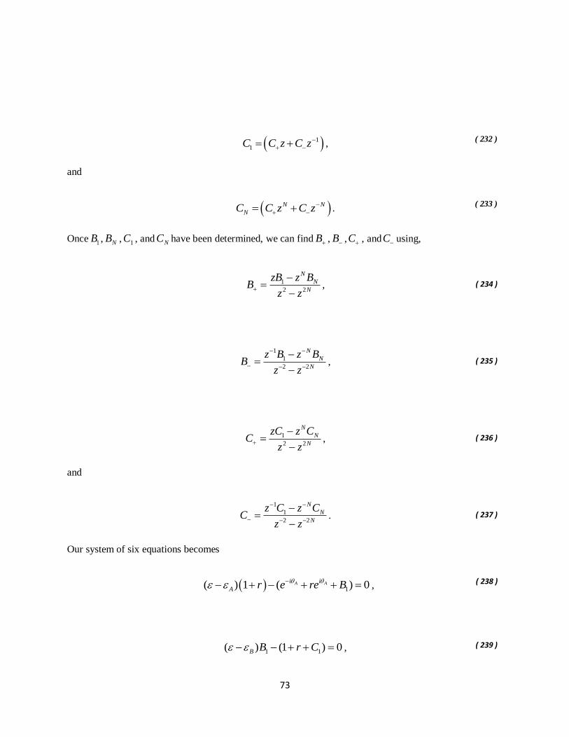
Once 1B , NB , 1C , and NC have been determined, we can find B , B ,C , andC using,

1

2 2

N

N

N

zB z BB

z z

,

( 234 )

1

1

2 2

N

N

N

z B z BB

z z

,

( 235 )

1

2 2

N

N

N

zC z CC

z z

,

( 236 )

and

1

1

2 2

N

N

N

z C z CC

z z

.

( 237 )

Our system of six equations becomes

1( ) 1 ( ) 0A Ai i

A r e re B

, ( 238 )

1 1( ) (1 ) 0B B r C , ( 239 )

74

2 2

1 1( ) ( ) 0C C B B z B z

, ( 240 )

1 1( ) ( ) 0N N

B N NB C C z C z

, ( 241 )

1( ) ( ) 0Ai N

C N NC B te

, ( 242 )

1 2( ) ( ) 0A Ai N i N

A Nte C te

. ( 243 )

Equations (238) and (243) can be simplified using the dispersion relation for the A chain:

2

1A Ai i

r B e e

( 244 )

and

AiN

Nt C e

. ( 245 )

These equations can be used to eliminate r and t leaving equations (239-242) that only involve 1B , 1C ,

NB , and NC :

2

1 1 1A Ai i

B e B C e ,

( 246 )

75

2 2 1

1 11 1 1 11 ( ) 0

N N

N CN N N N

z z z zB B C

z z z z

,

( 247 )

1 2 2

11 1 1 1( ) 1 0

N N

B N NN N N N

z z z zB C C

z z z z

,

( 248 )

and

0Ai

N C NB e C .

( 249 )

These equations can be written in more compact form if we let Ai

Bb e , Ai

Cc e , and

define n n

nx z z :

1 1 2 sin Ai

AC bB i e , ( 250 )

1 2 1 1 1 1( ) 0N N N C Nx x B x B x C , ( 251 )

1 1 1 1 2( ) 0B N N N N Nx B x C x x C , ( 252 )

and

N NB cC . ( 253 )

Equations (250) and (253) can be used to eliminate 1C and NB , leaving two equations for the remaining

two unknowns, 1B and NC :

76

1 2 1 1 1 1( ) 2 sin ( )Ai

N N N C N A C Nx x x b B x cC i e x ( 254 )

and

1 1 1 2 1 1( ) 2 sin Ai

N N N B N Ax bB x x x c C x i e . ( 255 )

The coefficients of 1B in Equation (254) and of NC in Equation (255) may be simplified, using, for

example,

1 2 1

1

1 2 1

*

1

( )

2 ( )

.

A

A

N N N C

i

N N N C

i

N N

x x x b

x x x z z e

x c e x

( 256 )

Equations (254) and (255) for 1B and NC become,

*

1 1 1 12 sin ( )A Ai i

N N N A C Nx c e x B x cC i e x

( 257 )

*

1 1 1 12 sinA Ai i

N N N Ax bB x b e x C x i e .

( 258 )

Equation (258) can be solved for 1B :

1 1 1 *

1 1 12 sin A Ai i

A N N NB i e b x b x b e x C

. ( 259 )

Then Equation (257) yields a solution for NC and t

*

1 1

1 * * 2

1 1 1

( )2 sin

A

A A

A A

i

C N N Ni iN

N A i i

N N N N

b x x c e xC ix e te

x b e x x c e x x cb

.

( 260 )

77

The numerator can be simplified since,

*

1 1

1 1

1

1 1 1 2

( )

( )( )

2 .

Ai

C N N N

B C N N N

N N N N N

b x c e x x

x x x

z z x x x x x

( 261 )

Thus, the transmission amplitude can be written as,

1 2

1 * * 2

1 1 1

2 sinA A

A A

iN i N NA i i

N N N N

x xte ix e

x b e x x c e x x cb

.

( 262 )

where Ai

Bb e , Ai

Cc e , and

n n

nx z z .

The transmission probability as a function of energy is shown in Figures 15 – 17.



hopping matrix element, w .

78


as a function of energy. Parameters are 0, 0.7, =10A B C N . Energy is measured in units

of hopping matrix element, w .

79



hopping matrix element, w .

80

CHAPTER 5: CONCLUSIONS

We have explored the tunneling properties in quantum mechanical solid state physics.

Chapter 2 discusses how we used the Landauer formulation of transport to relate the transmission

probability in terms of the conductance and the resistance. Also, the three-dimensional simple

barrier model for tunneling was derived using the separation of variables. In order to derive a

general expression for the current, we used the separation of variables from the time-dependent

formulation of quantum mechanics. Our expression for the current was obtained from the

continuity equation.

The simple barrier model for tunneling was solved by calculating the transmission and

reflection probabilities. There is a relationship between the transmission probability and the

conductance to calculate the conductance of the three dimensional barrier system at low bias.

We used our expression for the current density in terms of the wave functions to demonstrate that

the current is equal in all three regions of the tunneling system: left lead, barrier, and right lead.

The electron dispersion in solids is not precisely represented due to limitations of the free

electron model. This is why we introduce the tight-binding model in Chapter 3. Section 3.2

covers how to calculate transmission and reflection probabilities for an interface using the

simplest one-dimensional tight-binding model for an interface between semi-infinite chains of A

atoms and B atoms. This model is extended in Section 3.3 to a tunneling system consisting of

two semi-infinite chains of A atoms separated by a finite chain of B atoms. We showed that in

the limit of very long electron wavelengths and very slow decay of the evanescent states, the

tight-binding approximation for tunneling reduces to the simple barrier model in Section 3.4. In

Section 3.5, we calculated the transmission and reflection probabilities of the A-B-A model.

Section 3.6 covers the energy variation and also the wave functions are plotted to show that

81

when BE E , the wave function has the opposite sign on adjacent atoms. In Section 3.7, the

current density in the tight-binding approximation was calculated. Then the current density was

used to complete the calculation of the transmission probability at an interface.

To produce a dispersion relation with a gap, we cannot use the simple tight-binding

model with a single orbital on each site. This is why we continued our calculations to construct a

barrier consisting of B-C molecules in Chapter 4. A chain of this type produces a gap extending

between the onsite energy for the A atom and the onsite energy for the B atom. Tunneling

through gap is calculated and plotted. We have observed that if the orbitals on the B and C

atoms have the same parity, the wave function will change sign between molecules, however if

the parity of the orbitals are different, there will not be a sign change.

82

REFERENCES

1. F. Hund, Z. Phys. 40, 742 (1927)

2. J. C. Slonczewski, Phys. Rev. B 39, 6995 (1989)

3. J. Mathon, Physical Review B Volume 56, Number 18 1 November 1997-II

4. Landauer, R. “Electrical Resistance of Disordered One-dimensional Lattices.”

Philosophical Magazine, Vol. 21, Issue 172, (1970): 863-867

5. W.F. Brinkman, R.C. Dynes, J.M. Rowell, Journal of Applied Physics 41, 1915 (1970)

6. J. Bardeen, Phys. Rev. Lett. 6, 57 (1961)

7. Yu. V. Sharvin, Zh. Eksp. Teor. Fiz. 48, 984 (1965) [Sov. Phys. JETP 21, 655 (1965)]

8. Kohn, W.; Sham, L. J. (1965). "Self-consistent equations including exchange and

correlation effects". Physical Review140 (4A): A1133–A1138.

9. N. Marzari, D. Vanderbilt “Maximally localized generalized Wannier functions for

composite energy bands” Phys. Rev. B 56, 12847 (1997)

ELECTRON TUNNELING IN THE TIGHT-BINDING …

Documents