Electromagnetism in the Spherical-Wave Basis · Electromagnetism in the Spherical-Wave Basis: A (Somewhat Random) Compendium of Reference Formulas Homer Reid August 1, 2016 Abstract

Electromagnetism in the Spherical-Wave Basis:

A (Somewhat Random) Compendium of Reference Formulas

Homer Reid

August 1, 2016

Abstract

This memo consolidates and collects for reference a somewhat randomhodgepodge of formulas and results in the spherical-wave approach toelectromagnetism that I have found useful over the years in developingand testing scuff-em and buff-em.

Contents

1 Vector Spherical Wave Solutions to Maxwell’s Equations 3

2 Explicit expression for small ` 6

3 Translation matrices 9

4 Spherical-wave expansion of incident fields 104.1 Plane waves . . . . . . . . . . . . . . . . . . . . . . . . . . . . . . 104.2 Point sources at the origin . . . . . . . . . . . . . . . . . . . . . . 104.3 Point sources not at the origin . . . . . . . . . . . . . . . . . . . 11

5 Scattering from a homogeneous dielectric sphere 125.1 Sources outside the sphere . . . . . . . . . . . . . . . . . . . . . . 12

5.1.1 Analytical results in the low-frequency limit . . . . . . . . 135.2 Sources inside the sphere . . . . . . . . . . . . . . . . . . . . . . . 155.3 Frequencies of spherical resonant cavities . . . . . . . . . . . . . . 15

6 Scattering from a sphere with impedance boundary conditions 17

7 Dyadic Green’s functions 18

8 VSWVIE: Volume-integral-equation approach to scattering withvector spherical waves as volume-current basis functions 198.1 Review of the standard VIE formalism . . . . . . . . . . . . . . . 198.2 Vector spherical waves as volume-current basis functions . . . . . 208.3 Solution of VIE equation in VSW basis . . . . . . . . . . . . . . 20

1

Homer Reid: E&M in the Spherical-Wave Basis 2

8.4 Overlap integrals . . . . . . . . . . . . . . . . . . . . . . . . . . . 208.5 Fields produced by VSW basis functions . . . . . . . . . . . . . . 228.6 Matrix elements of G . . . . . . . . . . . . . . . . . . . . . . . . . 238.7 Alternative expression for total fields inside the body . . . . . . . 258.8 Homogeneous dielectric sphere . . . . . . . . . . . . . . . . . . . 25

9 Stress-tensor approach to power, force, and torque computa-tion 279.1 Sample stress-tensor power calculation . . . . . . . . . . . . . . . 299.2 Sample stress-tensor force calculation . . . . . . . . . . . . . . . . 319.3 x-directed force density . . . . . . . . . . . . . . . . . . . . . . . 329.4 Total x-directed force . . . . . . . . . . . . . . . . . . . . . . . . 32

10 T-matrix elements and surface currents 34


1 Vector Spherical Wave Solutions to Maxwell’sEquations

Many authors define pairs of three-vector-valued functions M`m(x),N`m(x)describing exact solutions of the source-free Maxwell’s equations—namely, thevector Helmholtz equation plus the divergence-free condition—in spherical co-ordinates for a homogeneous medium with wavenumber k, i.e.[

∇×∇×−k2]

M`m

N`m

= 0, ∇ ·

M`m

N`m

= 0. (1)

In some cases, the set M,N`m is augmented to include a third function L`mthat satisfies the vector Helmholtz equation but is now curl-free (and not diver-genceless): [

∇×∇×−k2]L`m = 0, ∇× L`m = 0. (2)

The function L`m is not a solution of Maxwell’s equations and is never neededin a basis of expansion functions for fields, but must be retained in a basis forexpanding currents in inhomogeneous and/or anisotropic media.

In all cases, the M,N,L functions involve spherical Bessel functions andspherical harmonics, but the precise definitions (including sign conventions andnormalization factors) vary from author to author. In this section I set down theparticular conventions that I use. In the next section I give explicit closed-formexpressions for small `.

Vector spherical harmonics

X`m(θ, ϕ) ≡ i√`(`+ 1)

∇×Y`m(θ, ϕ)r

Z`m(θ, ϕ) ≡ r×X`m(θ, ϕ)

More explicitly, the components of X and Z are

X`m(θ, φ) =i√

`(`+ 1)

[im

sin θY`mθ −

∂Y`m∂θ

ϕ

]Z`m(θ, φ) =

i√`(`+ 1)

[∂Y`m∂θ

θ +im

sin θY`mϕ

].

These are orthonormal in the sense that⟨X∣∣X⟩ =

⟨Z∣∣Z⟩ = 1,

⟨X∣∣Z⟩ = 0

where the inner product is

⟨F∣∣G⟩ ≡ ∫ F∗ ·G dΩ =

∫ π

0

∫ 2π

0

F∗(θ, ϕ) ·G(θ, ϕ) sin θ dϕ dθ


Their divergences are:

∇ ·X`m = −m cot θ csc θY`m(θ, ϕ)

r√`(`+ 1)

(3a)

∇ · Z`m =i cot θ

r√`(`+ 1)

[m cot θY`m(θ, ϕ) + ξ`me

−iϕY`,m+1(θ, ϕ)]

(3b)

ξ`m ≡

√(`−m)!(`+m+ 1)!

(`−m− 1)!(`+m)!(3c)

Radial functions

Routgoing` (kr) ≡ h(1)` (kr)

Rincoming` (kr) ≡ h(2)` (kr)

Rregular` (kr) ≡ j`(kr).

I also define the shorthand symbols

R`(kr) ≡1

krR`(kr) +R′`(kr) \R`(kr) ≡ −

√l(l + 1)

krR`(kr)

where R′`(kr) =∣∣ ddzR`(z)

∣∣z=kr

.

Scalar Helmholtz solutions[∇2 + k2

]ψ`m(r) = 0 =⇒ ψ`m(r, θ, ϕ) = R`(kr)Y`m(θ, ϕ)

where R` is one of the radial functions defined above.

Vector spherical wave functions

M`m(k; r) ≡ i√`(`+ 1)

∇ψ`mr

= R`(kr)X`m(Ω)

N`m(k; r) ≡ − 1

ik∇×M`m = iR`(kr)Z`m(Ω) + \R`(kr)Y`m(Ω)r

L`m(k; r) ≡ 1

k√`(`+ 1)

∇ψ`m = −iR`(kr)kr

Z`m(Ω) +1√

`(`+ 1)R′`(kr)Y`m(Ω)r

(4)

L00(k; r) =R′0(kr)√

4πr

Curl Identities

∇×M = −ikN, ∇×N = +ikM.


General solution of source-free Maxwell equations The general solutionof Maxwell’s equations in a source-free medium with relative material propertiesεr, µr then reads

E(x) =∑α

AαMα(k; r) + BαNα(k; r)

(5a)

H(x) =1

Z0Zr

∑α

BαMα(k; r)−AαNα(k; r)

(5b)

where k =√ε0εrµ0µr · ω is the photon wavenumber in the medium, Z0 =√

µ0/ε0 ∼ 377 Ω is the impedance of vacuum, Zr =√µr/εr is the relative

wave impedance of the medium, and we must choose the M,N functions tobe regular, incoming, or outgoing depending on the physical conditions of theproblem.

Unified notation for M,N waves I will use the symbol Wα to refer col-lectively to M and N waves; here1 α = (`mP ) is a compound index withP = M,N identifying the polarization. With this notation, expansions suchas (5) read

E =∑α

CαWα, H =1

Z0Zr

∑α

CασαWα (6)

∑α

· · · =∑`

∑m=−`

∑P∈M,N

· · ·

and where the bar on a compound index flips the polarization:

`mM = `mN, `mN = `mM, σ`mM = +1, σ`mN = −1.

Spherical-wave expansion of dyadic Green’s function Let G(k; r) andC(k; r) be the usual homogeneous dyadic Green’s functions, with Cartesiancomponents

Gij(k; r) =(δij +

1

k2∂i∂j

) eik|r|4π|r|

, Cij(k, r) = +1

ikεijl∂lG(k, r) (7)

Then have the spherical-wave expansion

G(x,x′) = − 1

k2δ(x− x′)rr′ + ik

∑α

Woutα (x>)Wreg

α (x<), (8a)

C(x,x′) = ik∑α

σα

Wout

α (x)Wregα (x′), |x| > |x′|,

Woutα (x′)Wreg

α (x), |x| < |x′|(8b)

1With this notation I am committing the faux pas of using the same symbol α for thetwo-fold compound index (`m) in (5) and the three-fold compound index (`mP ) in (6), butwhaddya gonna do.


2 Explicit expression for small `

The first few radial functions

Rregular0 (x) =

sinx

xR

regular

0 (x) =cosx

x

Routgoing0 (x) = −ie

ix

xR

outgoing

0 (x) =eix

x

Rregular1 (x) =

sinx− x cosx

x2R

regular

1 (x) =x cosx+ (x2 − 1) sinx

x3

Routgoing1 (x) = − ie

ix

x2(1− ix

)R

outgoing

1 (x) =ieix

x3(1− ix− x2

)The first few regular functions In what follows, the ζn are dimensionlesssinusoidal functions:

ζ1(x) = sinx− x cosx

ζ2(x) = (1− x2) sinx− x cosx


Lregular00 (r) = − ζ1(kr)

4π(kr)2

100

k→0−−−→ kr

6√π

100

Mregular1,±1 (r) =

√3

16π

[ζ1(kr)

(kr)2

]e±iϕ

01

±i cos θ

k→0−−−→ kr

4√

3πe±iϕ

01

±i cos θ

Mregular1,0 (r) = i

√3

2π

(sin kr − kr cos kr

(kr)2

) 00

sin θ

k→0−−−→ i

√3

8π

[ζ(kr)

(kr)2

] 00

sin θ

Nregular1,±1 (r) =

√3

16π

[1

(kr)3

]e±iϕ

±2ζ1(kr) sin θ∓ζ2(kr) cos θ−iζ2(kr)

k→0−−−→

√e±iϕ

12π

± sin θ± cos θi

Nregular1,0 (r) =

√3

8π

[1

(kr)3

] −2ζ1(kr) cos θ−ζ2(kr) sin θ

0

k→0−−−→ 1√

6π

− cos θsin θ

0

= − 1√6π

z


The first few outgoing functions In what follows, the Qn are dimensionlesspolynomial factors:

Q1(x) = 1− xQ2a(x) = 1− x+ x2

Q2b(x) = 3− 3x+ x2

Q3(x) = 6− 6x+ 3x2 − x3

Moutgoing1,±1 (r) =

√3

16π

(eikr

k2r2

)e±iφ

0−iQ1(ikr)±Q1(ikr) cos θ

Moutgoing1,0 (r) =

√3

8π

(eikr

k2r2

) 00

Q1(ikr) sin θ

Noutgoing

1,±1 (r) =

√3

16π

(eikr

k3r3

)e±iφ

∓− 2(ikr)Q1(ikr) sin θ±iQ2a(ikr) cos θ−Q2a(ikr)

Noutgoing

1,0 (r) =

√3

8π

(eikr

k3r3

) 2iQ1(ikr) cos θ+iQ2a(ikr) sin θ

0

Moutgoing2,±2 (r) =

√5

16π

(eikr

k3r3

)e±2iφ

0±iQ2b(ikr) sin θ−Q2b(ikr) cos θ sin θ

Moutgoing

2,±1 (r) =

√5

16π

(eikr

k3r3

)e±iφ

0−iQ2b(ikr) cos θ±Q2b(ikr) cos 2θ

Moutgoing

2,0 (r) =

√15

8π

(eikr

k3r3

) 00

−Q2b(ikr) cos θ sin θ

Noutgoing2,±2 (r) =

√5

16π

(eikr

k4r4

)e±2iφ

3iQ2b(ikr) sin2 θ−iQ3(ikr) cos θ sin θ±Q3(ikr) sin θ

Noutgoing

2,±1 (r) =

√5

16π

(eikr

k4r4

)e±iφ

∓3iQ2b(ikr) sin 2θ±iQ3(ikr) cos 2θ−Q3(ikr) cos θ

Noutgoing

2,0 (r) =

√15

8π

(eikr

k4r4

) iQ2b(ikr)(3 cos2 θ − 1)iQ3(ikr) cos θ sin θ

0

.


3 Translation matrices

Translation matrices arise when we want to evaluate the fields produced bysources not located at the origin.

Scalar case Although we don’t need it for electromagnetism problems, thescalar-wave analog of (4) is

ψ`m(x) = R`(kr)Y`m(θ, φ)

or, more specifically,

ψout`m (x) = Rout

` (kr)Y`m(θ, φ), ψreg`m(x) = Rreg

` (kr)Y`m(θ, φ)

Now consider a point source at xS whose fields we wish to evaluate at an evalu-ation (“destination”) point xD, using a basis of spherical waves centered at anorigin xO. Then waves emitted by the source, which appear to be outgoing in acoordinate system centered at xS, can be described as superpositions of regularwaves in a coordinate system centered at xO:

ψoutα

(xD − xS

)=∑β

Aαβ(k; xS − xO

)ψregβ

(xD − xO

)(9)

where α, β are compound indices (i.e. α = `α,mα) and

Aαβ(k,L) = 4π∑γ

i(`α−`β+`γ)aαγβψoutγ (L)

aαβγ =

∫Yα(Ω)Y ∗β (Ω)Y ∗γ (Ω) dΩ

= (−1)mα

√(2`α + 1)(2`β + 1)(2`γ + 1)

4π

(`α `β `γ0 0 0

)(`α `β `γ−mα mβ mγ

).

Vector case (MN

)out

α

=∑β

(B C−C B

)αβ

(MN

)reg

β

Bαβ(k,L) = 4π∑γ

i(`α−`β+`γ)

[`α(`α + 1) + `β(`β + 1)− `γ(`γ + 1)

2√`α(`α + 1)`β(`β + 1)

]aαγβψ

outγ (L)

Cαβ(k,L) = − k√`α(`α + 1)`β(`β + 1)

[λ+2

(Lx − iLy

)Aα+,β +

λ−2

(Lx + iLy

)Aα−,β +mαLzAα,β

]

λ± =√

(`α ∓ `β)(`α ± `β + 1), α± = `α,mα ± 1


4 Spherical-wave expansion of incident fields

4.1 Plane waves

For a scattering problem in which the incident field is a z-directed plane wave,i.e.

Einc = E0eikz, Hinc =

1

Z0z×E0e

ikz

the spherical-wave expansion coefficients in (14) take the following forms forvarious possible polarizations:

E0 = x + iy (right circular polarization) : P`m = δm,+1P`

E0 = x− iy (left circular polarization) : P`m = δm,−1P`

E0 = x (linear polarization) : P`m = 12

(δm,+1 + δm,−1

)P`

where in all cases I have

P` = i`√

4π(2`+ 1), Q`,±1 = ∓iP`.

4.2 Point sources at the origin

Let E(x; p) be the electric field at evaluation point x due to an electric dipolep at the origin. The spherical-wave expansion of this field involves only N-functions with ` = 1, i.e.

E(x; p) =

1∑m=−1

ξ1m(p)Noutgoing1m (x)

where the ξ coefficients are

p = pxx −→ ξ1,1 = −ξ1,−1 =i

2

k3√3π

pxε, ξ1,0 = 0

p = pyy −→ ξ1,1 = +ξ1,−1 =1

2

k3√3π

pyε

ξ1,0 = 0

p = pz z −→ ξ1,1 = ξ1,−1 = 0, ξ1,0 = − ik3√6π

pzε

Here ε = ε0εr is the absolute permittivity of the medium.

Similarly, the magnetic fields of a magnetic dipole m at the origin are

H(x; m) =∑α

ξα(m)Noutgoingα (x)

where the ξ coefficients are the same as the ξ coefficients above with the re-placement p

ε →mµ .


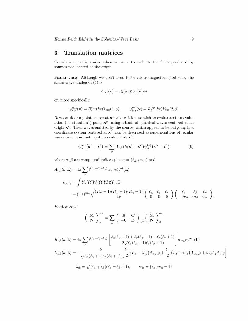
4.3 Point sources not at the origin

The fields of point sources not at the origin may be obtained by applying thetranslation matrices of Section to the fields of Section 4.2. If the point sourcelies at xS 6= 0 (here “S” stands for “source”), then its fields at destination pointxD read

E(xD; xS,p) =∑αβ

− ξαCαβMregular

β (xD) + ξαBαβNregularβ (xD)

(10a)

H(xD; xS,p) =1

Z

∑αβ

ξαCαβNregular

β (xD) + ξαBαβMregularβ (xD)

(10b)

E(xD; xS,m) = −Z∑αβ

ξαBαβMregular

β (xD) + ξαCαβNregularβ (xD)

(10c)

H(xD; xS,m) =∑αβ

− ξαCαβMregular

β (xD) + ξαBαβNregularβ (xD)

(10d)

Here B,Cαβ are elements of the translation matrices B(k,xS),C(k,xS).Note that, for a given source point xS, I only have to assemble the translation

matrices B and C once (at a given frequency), after which I can get the fieldsat any number of destination points xD from equation (10).


5 Scattering from a homogeneous dielectric sphere

I consider scattering from a single homogeneous sphere with relative permittivityand permeability εr, µr in vacuum irradiated by spherical waves emanating fromwithin our outside the sphere.

Irrespective of the origin of the incident fields, the scattered fields inside andoutside the sphere take the form (n =

√εrµr, Zr =

√µr/εr)

Inside the sphere:

Escat(x) =∑α

AαMreg

α (nk0; r) +BαNregα (nk0; r)

(11a)

Hscat(x) =1

Z0Zr

∑α

BαMreg

α (nk0; r)−AαNregα (nk0; r)

(11b)

Outside the sphere:

Escat(x) =∑α

CαMout

α (k0; r) +DαNoutα (k0; r)

(12a)

Hscat(x) =1

Z0

∑α

DαMout

α (k0; r)− CαNoutα (k0; r)

(12b)

The A,B,C,D coefficients are proportional to the spherical-wave expan-sion coefficients of the incident fields, with the proportionality constants deter-mined by enforcing continuity of the tangential components of the total fieldsE,Htot = E,Hinc + E,Hscat at r = r0,∣∣∣r×Etot

∣∣∣r→r+0

=∣∣∣r×Etot

∣∣∣r→r−0

(13a)∣∣∣r×Htot∣∣∣r→r+0

=∣∣∣r×Htot

∣∣∣r→r−0

(13b)

5.1 Sources outside the sphere

If the sources of the incident field lie outside the sphere (the usual Mie scatteringproblem), then I can expand the incident fields in the form

Einc(x) =∑α

PαMregular

α (k0; x) +QαNregularα (k0; x)

(14a)

Hinc(x) =1

Z0

∑α

QαMregular

α (k0; x)− PαNregularα (k0; x)

. (14b)


Matching tangential fields at the sphere surface then determines the scattered-field expansion coefficients in terms of the incident-field expansion coefficients(a = k0r0):

Aα =

[Rreg(a)R

out(a)−Rreg

(a)Rout(a)

Rreg(na)Rout

(a)− 1ZrR

reg(na)Rout(a)

]Pα (15a)

Bα =

[R

reg(a)Rout(a)−Rreg(a)R

out(a)

Rreg

(na)Rout(a)− 1ZrR

reg(na)Rout

(a)

]Qα (15b)

Cα =

[Rreg(a)R

reg(na)− ZrRreg

(a)Rreg(na)

ZrRreg(na)Rout

(a)−Rreg(na)Rout(a)

]︸︷︷︸

TMα

Pα (15c)

Dα =

[R

reg(a)Rreg(na)− ZrRreg(a)R

reg(na)

ZrRreg

(na)Rout(a)−Rreg(na)Rout

(a)

]︸︷︷︸

TNα

Qα (15d)

In (15c,d) I have identified the quantities Cα/Pα and Dα/Qα as elements of theT-matrix for the M - and N - polarizations.2

5.1.1 Analytical results in the low-frequency limit

The coefficients (15) may be expressed in closed form, e.g.

A1

P1=

2a3e−ian3Z

((1− ia) (a2n2 − 1)− (−1 + a(a+ i))nZ) sin(an) + an((−1 + a(a+ i))nZ − ia+ 1) cos(an)

B1

Q1=

2a3e−ian3Z

((1− ia)Z (a2n2 − 1)− (−1 + a(a+ i))n) sin(an) + an((−1 + a(a+ i))n− iaZ + Z) cos(an)

where a = (k0r0) is the dimensionless Mie size parameter. The low-frequencylimiting forms (assuming µ = 1:) are

A1

P1=

2√ε

+[ (ε− 1)

3√ε

]a2 +O(a3)

B1

Q1=

6

ε+ 2+[3(ε2 + 9ε− 10

)5(ε+ 2)2

]a2 +O(a3)

A2

P2=

2

ε+

[(ε− 1)

5ε

]a2 +O(a3)

B2

Q2=

10√ε(2ε+ 3)

+

[5a2

(2ε2 + 5ε− 7

)7√ε(2ε+ 3)2

]a2 +O(a3)

2The T-matrix multiplies a vector of regular-wave incident-field coefficients to yield a vectorof outgoing-wave scattered-field coefficients. If, instead of the regular-wave incident field (14),I irradiated the sphere with a superposition of incoming waves as the incident field, then theresulting modified versions of equations (15c,d) would instead define elements of the S-matrix(scattering matrix).


Interior fields

For a sphere irradiated by a linearly-polarized plane wave, the fields inside thebody to second order in a = kR read

ExE0

=3

2 + ε+

[ε+ 4

3 + 2ε

]ikz +

[(ε− 1)(35ε+ 46)

5(ε+ 2)2(3ε+ 4)

]k2x2

+

[(ε− 1)(−2ε2 + 29ε+ 42)

5(ε+ 2)2(3ε+ 4)

]k2y2 −

[14ε3 + 3ε2 + 114ε+ 184

10(ε+ 2)2(3ε+ 4)

]k2z2

EyE0

=

[2(ε2 − 1)

5(2 + ε)(4 + 3ε)

]k2xy

EzE0

= −[ε− 1

2ε+ 3

]ikx+

[(ε− 1)(7ε+ 12)

5(2 + ε)(4 + 3ε)

]k2xz

Hx

Z0E0=

[(ε− 1)2

5(2ε+ 3)

]k2xy

Hy

Z0E0= 1 +

[2ε+ 1

2 + ε

]ikz

−[

(ε− 1)(ε− 6)

15(3 + 2ε)

]k2x2 +

[ε− 1

15

]k2y2 −

[2ε2 + 46ε+ 27

30(3 + 2ε)

]k2z2

Hz

Z0E0= −

[ε− 1

ε+ 2

]iky +

[(ε− 1)(ε+ 4)

5(3 + 2ε)

]k2yz

Field derivatives:

∂zE =(ikC1 − 2k2C2z

)x + k2C3x z

∂zH =(ikC4 − 2k2C5z

)y + k2C6y z

C1 =ε+ 4

3 + 2ε,

C2 =14ε3 + 3ε2 + 114ε+ 184

10(ε+ 2)2(3ε+ 4)

C3 =(ε− 1)(7ε+ 12)

5(2 + ε)(4 + 3ε)

C4 =2ε+ 1

2 + ε

C5 =2ε2 + 46ε+ 27

30(3 + 2ε)

C6 =(ε− 1)(ε+ 4)

5(3 + 2ε)


5.2 Sources inside the sphere

If the sources of the incident field lie inside the sphere, then I can expand theincident field in the form

Einc(x) =∑α

PαMout

α (nk0; x) +QαNoutα (nk0; x)

(16)

The total fields inside and outside then read

Ein(x) =∑

PαMoutα (x) +QαNout

α (x)

+∑

AαMregα (x) +BαNreg

α (x)

(17)

Hin(x) = − 1

Z0Zr

∑PαNout

α (x)−QαMoutα (x)

− 1

Z0Zr

∑CαNreg

α (x)−DαMregα (x)

(18)

Eout(x) =∑

CαMoutα (x) +DαNout

α (x)

(19)

Hout(x) = − 1

Z0

∑CαNout

α (x)−DαMoutα (x)

(20)

Now equate tangential components of Ein,out and Hin,out at the sphere surface(r = r0), take inner products with M and N, and use the orthogonality relationsto find

Rout` (nkr0)Pα + Rreg

` (nkr0)Aα = Rout` (kr0)Cα

Rout

` (nkr0)Pα + Rreg

` (nkr0)Aα = ZrRout

` (kr0)Cα

Rout

` (nkr0)Qα + Rreg

` (nkr0)Bα = Rout

` (kr0)Dα

Rout` (nkr0)Qα + Rreg

` (nkr0)Bα = ZrRout` (kr0)Dα

which we solve to obtain the coefficients of the scattered field outside the spherein terms of the incident-field coefficients:

Cα =

[Rout` (na)R

reg

` (na)−Rout

` (na)Rreg` (na)

Rout` (a)R

reg

` (na)− ZrRout

` (a)Rreg` (na)

]Pα (21a)

Dα =

[R

out

` (na)Rreg` (na)−Rout

` (na)Rreg

` (na)

Rout

` (a)Rreg` (na)− ZrRout

` (a)Rreg

` (na)

]Qα. (21b)

5.3 Frequencies of spherical resonant cavities

Frequencies at which the denominator of one of the scattering coefficients (15)vanishes correspond to cavity resonances, in which the fields inside the sphere


can be nonzero even for vanishing incident-field coefficients P,Qα. For asphere of given frequency-dependent refractive index n(ω) =

√ε(ω), the values

of a = ωRc at which resonances occur may be labeled by a wave type (M or

N) and a pair of integers `, p, where aM`,p and aN`,p (p = 1, 2, · · · ) are the pthsmallest-magnitude roots of the equations (assuming here the non-magnetic caseµ = 1)

Rreg`

(naM

`n

)R

out

`

(aM

`n

)− nRreg

`

(naM

`n

)Rout`

(aM

`n

)= 0

nRreg`

(naN

`n

)R

out

`

(aN

`n

)−Rreg

`

(naN

`n

)Rout`

(aN

`n

)= 0.

This can be solved numerically using the mathematica code shown below, withresults tabulated in Table 1 for the particular case of a lossless dielectric spherewith frequency-independent relative permittivity ε ≡ 4.

ROut[L_, a_]:=SphericalHankelH1[L,a];

RBarOut[L_, a_] := ROut[L,a]/a + (D[ROut[L,aa],aa] /. aa->a);

RReg[L_, a_]:=SphericalBesselJ[L,a]

RBarReg[L_, a_] := RReg[L,a]/a + (D[RReg[L,aa],aa] /. aa->a);

aMEquation[L_,n_,a_]:=\

(RReg[L,n*a]*RBarOut[L,a] - n*RBarReg[L,n*a]*ROut[L,a]);

aNEquation[L_,n_,a_]:=\

(RBarReg[L,n*a]*ROut[L,a] - n*RReg[L,n*a]*RBarOut[L,a]);

aEquation[MN_,L_,n_,a_]:=\

If[MN==0, aMEquation[L,n,a], aNEquation[L,n,a]];

(* find an M- or N-type root near a0 *)

aNear[MN_,L_,n_,a0_]:=\

FindRoot[ aEquation[MN,L,n,a]==0, a,a0, AccuracyGoal->10,

PrecisionGoal->10,

WorkingPrecision->20];

Figure 1: mathematica code for computing resonant frequencies of a sphericaldielectric cavity.


aM1,1 1.4380605929872320255 - 0.20560699506583840000i

aM1,2 3.0650602030993358182 - 0.25639055432728332066i

aN1,1 1.1362178236179127949 - 0.63063395652811684886i

aN1,2 2.2314272341555678202 - 0.35251393660078463445i

aM2,1 2.0714122747181446982 - 0.14636128063766849563i

aM2,2 3.7368636604700381398 - 0.23287793152977231173i

aN2,1 2.2025941452117729842 - 0.57522127718749665852i

aN2,2 2.8389707560296143889 - 0.52985636445927887339i

Table 1: Lowest resonant frequencies a = ωRc for a spherical dielectric cavity of

(lossless, frequency-independent) relative permittivity ε = 4.

6 Scattering from a sphere with impedance bound-ary conditions

For a sphere characterized by a surface-impedance boundary condition withrelative surface impedance3 η, the continuity condition (13) is replaced by arelationship between the tangential E and H fields at the sphere surface:

E‖ = ηZ0

(r×H

)at r = R.

Equations (15c,d) for the T-matrix elements are replaced by

Cα =

[Rreg(a)

iηRout

(a)−Rout(a)

]︸︷︷︸

TMα

Pα, Dα =

[R

reg(a)

iηRout(a) +Rout

(a)

]︸︷︷︸

TNα

Qα, (22)

In particular, taking η → 0 yields the T-matrix elements for a perfectly electri-cally conducting (PEC) sphere.

3Note that η is dimensionless; the absolute surface impedance is ηZ0 where Z0 ≈ 377 Ω isthe impedance of vacuum.


7 Dyadic Green’s functions

The scattering part of the electric dyadic Green’s function GEE(xD,xS) is a 3×3matrix whose i, j component GEE

ij (xD,xS) is the (appropriately normalized)4 icomponent of the scattered electric field at xD due to a j-directed point elec-tric dipole source at xS. (The superscripts on x stand for “destination” and“source”).

If I take the electic-dipole fields Section 4.3 [equations (10a,b)] to be theincident fields in the externally-sourced scattering problem of Section 5.1 [sothat, for example, the coefficient of Mreg

α in the incident-field expansion (14) isPα = −

∑β ξβCβα], then I need only multiply by T-matrix elements [equation

(15)] to get the outgoing-wave coefficients in the scattered-field expansion (12).Thus the E- and H-fields at xD due to an electric dipole source p at xS are

Escat(xD; xS,p) =∑αβ

ξα(p)− Cαβ(xS)TM

βMoutβ (xD) +Bαβ(xS)TN

βNoutβ (xD)

Hscat(xD; xS,p) =

1

Z

∑αβ

ξα(p)

+ Cαβ(xS)TM

γβMoutβ (xD) +Bαβ(xS)TN

γβNoutβ (xD)

The E- and H-fields at xD due to a magnetic dipole source m at xS are

Escat(xD; xS,m) = −Z∑αβ

ξα(m)

+ Cαβ(xS)TM

βMoutβ (xD) +Bαβ(xS)TN

βNoutβ (xD)

Hscat(xD; xS,m) =

∑αβ

ξα(m)−Bαβ(xS)TN

βMoutβ (xD) + Cαβ(xS)TM

βNoutβ (xD)

.

In writing out these equations, I have used the fact that the T-matrix of ahomogeneous sphere is diagonal. However, similar equations could be writtendown for the DGFs of any arbitrary-shaped object; in this case the T-matrixwould not be diagonal and the double sums would become triple sums, but sucha representation might nonetheless be useful in some cases.

4The normalization just involves dividing by dimensionful prefactors to ensure that thecomponents of G have units of inverse length and are independent of the point-source magni-tude.


8 VSWVIE: Volume-integral-equation approachto scattering with vector spherical waves asvolume-current basis functions

8.1 Review of the standard VIE formalism

Consider a material body with spatially-varying relative permittivity tensor ε(x)illuminated by incident radiation with electric field Einc(x) at frequency ω = kcin vacuum. In the usual volume-integral-equation formulation of the scatteringproblem, the scattered field Escat(x) is understood to arise from an inducedvolume current distribution J(x), which is itself proportional to the local total(incident+scattered) field at each point:

Escat = ikZ0G0 ? J, J = − ikZ0

(ε− 1)(Einc + Escat

)Combining these yields [

1 + VG]? J(x) =

i

kZ0VEinc (23)

where the diagonal operator V(x,x′) ≡ −k2(ε − 1

)δ(x,x′) is the “potential.”

Another way to write this is[ V

+ G]? J(x) =

i

kZ0Einc (24)

where

V

(x,x′) ≡ − 1k2

(ε− 1

)−1δ(x− x′).

Upon approximating the induced current as an expansion in a finite set ofNBF vector-valued basis functions,

J(x) ≈NBF∑α=1

jαBα(x) (25)

the integral equation (24) becomes an NBF ×NBF linear system:

[

V

+ G] j =i

kZ0e

where jα is the vector of expansion coefficients in (25) and

eα ≡i

kZ0

⟨Bα∣∣∣Einc

⟩,

V

ab = − 1

k2

⟨Bα

∣∣∣ (ε− 1)−1∣∣∣Bβ

⟩Gab = − 1

k2

⟨Bα

∣∣∣G∣∣∣Bβ

⟩.


8.2 Vector spherical waves as volume-current basis func-tions

For a compact material body confined within a sphere of radius R, I use theregular vector spherical waves to define a basis of volume-current basis functions:

BP`m(x) =

0, |x| > R

Mreg`m(x), |x| ≤ R,P = M

Nreg`m(x), |x| ≤ R,P = N

Lreg`m(x), |x| ≤ R,P = L.

(26)

I use these basis functions to expand currents and fields in (23):

J(x) =∑

jαBα, Einc(x) =∑

eαBα. (27)

Note that the eα coefficients have dimensions of electric field strength.

8.3 Solution of VIE equation in VSW basis

Inserting (27) into (23) yields a relation between the vectors of volume-currentexpansion coefficients and incident-field expansion coefficients:

j =i

kZ0

[S + VG

]−1Ve (28)

where the elements of the SV,G matrices are

Sαβ =

∫|x|<R

B∗α(x)Bβ(x) dx, Vαβ = −k2∫ R

0

B∗α(x)[ε(x)− 1

]Bβ(x) dx,

Gαβ =

∫ R

0

∫ R

0

B∗α(x)G(x,x′)Bβ(x′) dx dx′

and e is the vector of incident-field projections onto the Bα basis. If e isexpressed as an expansion in the usual (non-normalized) regular VSWs, as inequation (16), then the entries of e are just the P,Q coefficients in that equation:

eM`m = P`m, eN`m = Q`m.

8.4 Overlap integrals

The overlap matrix is diagonal in the ` and m indices and independent of m:

SP`m;P ′`′m′ ≡ SPP ′`δ`,`′δm,m′

It is also “partially diagonal’ in the P index, in the sense that the M functionsare orthogonal to the N and L functions, but the N and L functions havenonvanishing overlap.


The overlap integrals are

SPP ′`(R) ≡∫ R

0

RPP ′`(r) dr where RPP ′`(r) ≡ r2∫

B∗P`m(r,Ω)BP ′`m(r,Ω) dΩ.

Explicit forms of the integrand function are

RMM` ≡ r2[j`(kr)

]2RNN` ≡

`(`+ 1)

k2[j′`(kr)

]2+ 2

r

kj`(kr)j

′`(kr) +

`2 + `+ 1

k2[j`(kr)

]2which may be simplified [? ] to read

RNN` ≡(`+ 1

2`+ 1

)r2j2`−1(kr) +

(`

2`+ 1

)r2j2`+1(kr)

RLL` ≡1

k2[j`(kr)

]2+

[rj′`(kr)]2

`(`+ 1)

RNL` ≡ −2r

kj`(kr)j

′`(kr)−

1

k2j2` (u)

Explicit forms for the overlap integrals are

SMM`(R) =j2` (kR)− j`−1(kR)j`+1(kR)

2(29a)

SNN`(R) =1

2(2`+ 1)

(`+ 1)

[j`−1(kR)

]2 − (`+ 1)j`(kR)j`−2(kR)

− `j`(kR)j`+2(kR) + `[j`+1(kR)

]2(29b)

I also need another type of overlap integral:

SPP ′`(R) ≡∫ R

0

RPP ′`(r) dr where RPP ′` ≡∫

B∗P`m(r,Ω)BP ′`m(r,Ω) dΩ.

The R integrands are similar to the R integrands given above, except that one

of the two j` factors in each term is replaced by h(1)` :

RMM` ≡ j`(kr)h(1)` (kr)

RNN` ≡ r2j`(kr)h(1)` (kr) +`(`+ 1)

k2j`(kr)h

(1)` (kr)

RLN` ≡ −r

kj′`(kr)h

(1)` (kr)− r

kj`(kr)h

(1)` (kr)


8.5 Fields produced by VSW basis functions

I will use the symbol Eα(x) to denote 1/(iωε0) times the E-field at x dueto a current distribution produced by basis function Bα populated with unitstrength. The quantity E has dimensions of length2.

Evaluation using dyadic Green’s function

Eα(x) ≡∫|x′|<R

G(x,x′)Bα(x′) dx′

The integral here may be easily evaluated using the standard eigenexpansionof G [? ? ]:

G(x,x′) = − rr

k2δ(x− x′) + ik

∑α

Mα(r>)M∗

α(r<) + Nα(r>)N∗α(r<)

The result is:

Evaluation point outside sphere (|x| > R):

EM`m(r) = ikSMM`(R)M(r)

EN`m(r) = ikSNN`(R)N(r)

EL`m(r) = ikSNL`(R)N(r)

Evaluation point inside sphere (|x| < R):

EM`m(r) = ikSMM`(r)M(r) + ikSMM`(r,R)M(r) (30a)

EN`m(r) = − 1

k2

[r ·N`m

]r + ikSNN`(r)N(r) + ikSNN`(r,R)N(r) (30b)

EL`m(r) = − 1

k2

[r · L`m

]r + ikSNL`(r)N(r) + ikSNL`(r,R)N(r) (30c)

Evaluation using scalar Green’s function

I can also evaluate the fields using the scalar Green’s function, whose eigenex-pansion reads

G0(r, r′) = ik∑α

Rreg

α (kr<)Rout

α (kr>)Yα(θ, φ)Y ∗α (θ′, φ′)


In general, the E-field produced by a current distribution J reads

E(x) =

∫V

G0(x− x′)J(x′) dV︸︷︷︸E1

+1

k2∇x

∫V

G0(x− x′)[∇ · J(x′)

]dV︸︷︷︸

E2

− 1

k2∇x

∮V

G0(x− x′)Jr(x′)dA︸︷︷︸

E3

The third integral here captures the effect of the surface charge layer due to thediscontinuous dropoff of the currents at the sphere surface.

In evaluating E1 integrals I need to use the 3x3 matrices that convert spher-ical vector components to cartesian vector components and vice versa: Vx

VyVz

=

sin θ cosϕ cos θ cosϕ − sinϕsin θ sinϕ cos θ sinϕ cosϕ

cos θ − sin θ 0

︸︷︷︸

ΛS2C(θ,ϕ)

VrVθVϕ

VrVθVϕ

=

sin θ cosϕ sin θ sinϕ cos θcos θ cosϕ cos θ sinϕ − sin θ− sinϕ cosϕ 0

︸︷︷︸

ΛC2S(θ,ϕ)

VxVyVz

Relevant integrals include:∫Y ∗α (θ, φ)ΛC2S(θ, φ) · Yβ(θ, φ)r dΩ =

I then find:

E1M`m(x)

E2M`m(x) = 0 because ∇ ·M

E3M`m(x) = 0 because Mr = 0

8.6 Matrix elements of G

GPP ′` ≡⟨BP`m

∣∣G∣∣BP ′`m⟩≡∫|x|<R

B∗P`m(x) · EP ′`(x) dx


Using equation (30), one finds

GMM` = 2ik

∫ R

0

∫ R

r

RMM`(r)RMM`(r′) dr dr′

= 2ik

∫ R

0

∫ R

r

[j`(kr)

]2j`(kr

′)h(1)` (kr′) r2r′2 dr′ dr (31a)

GNN` = − 1

k2

∫|x|<R

∣∣N`mr(x)∣∣2 dx + 2ik

∫ R

0

∫ R

r

RNN`(r)RNN`(r′) dr dr′

= −`(`+ 1)

k4

∫ R

0

[j`(kr)

]2dr + 2ik

∫ R

0

∫ R

r

RNN`(r)RNN`(r′) dr dr′

(31b)

GLN` = +1

k3

∫ R

0

rj`(kr)j′`(kr) dr + ik

∫ R

0

∫ R

r

RNN`(r)RLN`(r′) dr dr′

+ ik

∫ R

0

∫ R

r

RNN`(r)RLN`(r′) dr dr′ (31c)

GLL` = − 1

`(`+ 1)k2

∫ R

0

[rj`(kr)

]2dr + 2ik

∫ R

0

∫ R

r

RLN`(r)RLN`(r′) dr dr′

(31d)

The convenient thing about the VSW basis is that the G matrix is diagonal(and m-independent) in this basis, with elements that may be computed inclosed form:

GP`m;P ′`′m′ = δPP ′δ``′δmm′

[−δPN

3k2+ iGP`

]GP` =

2k

SP`(R)

∫ R

0

SP`(r)RP`(r) r2 dr

=

2k

SM`(R)

∫ R

0

r2[j`(kr)

2]dr, P = M

2k

SN`(R)

∫ R

0

r2[j`(kr)

2 + \j`(kr)2]dr, P = N.

In the ` = 1 sector one finds

k2GM1m,M1m = −1

3+

i

4a

[− 2 + 2 cos(2a) + 2a2 + a sin(2a)

]= −1

3+

i

45a5 − i

315a7 +O

(a9)

k2GN1m,N1m = −1

3+

i

4a3

[2(a4 − a2 − 1

)− a(a2 − 4

)sin(2a)− 2

(a2 − 1

)cos(2a)

]= −1

3+

2i

9a3 − 2i

45a5 +O(a7) · · ·


8.7 Alternative expression for total fields inside the body

Etot(x) = ikZ0V−1J(x)

= ikZ0V−1∑

jαBα(x).

8.8 Homogeneous dielectric sphere

For a homogeneous dielectric sphere irradiated by a incident field of the form(16), the solution of (28) is

jα = −(

i

kZ0

)[−k2(ε− 1)

1− k2(ε− 1)Gαα

]1

NαPQα

Total fields inside:

Etot(x) =∑α

[1

1− k2(ε− 1)Gαα

]P,QαM,Nregα (x)

Scattered fields outside:

Escat(x) =∑α

[ik3(ε− 1)

1− k2(ε− 1)Gαα

]SαP,QαM,Noutα (x)

Mode-matching solution

From the discussion of Section 5.1 with Pα = 1, the total fields in the tworegions are

Etot =

AαM

regα (nk0; r), |r| < R

M regα (k0; r) + CαM

outα (k0; r), |r| > R

VSWVIE solution

Now I solve the same problem using the VSWVIE formalism of equation (28).The RHS vector eα in (28) contains a single nonzero entry:

eα =√Sα

For a homogeneous sphere, the V matrix is proportional to the identity matrix,V = −k2 (ε− 1) 1, and since G is also always diagonal in the VSW basis itfollows that the entirety of equation (28) is diagonal, so we have only a singlenonzero volume-current coefficient,

jα =ik

Z0

(ε− 1)√Sα

1− k2(ε− 1)Gαα


The scattered field is

Escat = ikZ0G ? J

= ikZ0jαG ? Bα

= −[

k2(ε− 1)

1− k2(ε− 1)Gαα

] [Cregα Mreg(k0; r) +Dout

α Mout(k0; r)

]

Cα =

−1

3k2+ ik

∫ R

r

Routα (kr′)Rreg(kr′)r′2 dr′, r < R

0, r > R

Dα = ik

∫ min(r,R)

0

[Rregα (kr′)

]2r′2 dr′


9 Stress-tensor approach to power, force, andtorque computation

Power

The power radiated away from (or, the negative of the power absorbed by) thesphere is obtained by integrating the outward-pointing normally-directed Poynt-ing vector over any bounding surface containing the sphere. For conveniencewe will take the bounding surface to be a sphere of radius rb > r0 (denote thissphere by Sb). Then the power is

P =1

2Re

∮Sb

r ·[E∗(r)×H(r)

]dA

=r2b2

Re

∮H∗(rb,Ω) ·

[r×E(rb,Ω)

]dΩ

=r2b4

∮ [E∗ ·

(H× r

)+ H∗ ·

(r×E

)]dΩ (32)

The integrand here may be expressed as a 6-dimensional vector-matrix-vectorproduct:

=r2b4

∮ (EH

)†(0 P−P 0

)(EH

)dΩ (33)

where, in our shorthand,

(EH

)†(0 P−P 0

)(EH

)≡

ErEθEϕHr

Hθ

Hϕ

†0 0 0 0 0 00 0 0 0 0 −10 0 0 0 1 00 0 0 0 0 00 1 0 0 0 0−1 0 0 0 0 0

ErEθEϕHr

Hθ

Hϕ

with

P =

0 0 00 0 −10 1 0

.

If we now insert the expansions (19) and (20) into (33), we obtain the totalradiated power as a bilinear form in the C,D`m coefficients:

Force

The ith Cartesian component of the time-average force experienced by thesphere is obtained by integrating the time-average Maxwell stress tensor over asphere with radius rb > r0 (call this sphere Sb:)

Fx =1

2Re r2b

∫Tij(rb,Ω)nj(Ω)dΩ. (34)


For definiteness I will consider the x-component of the force, i = x. The relevantquantity involving the stress tensor is

Txjnj = ε0

ExEyEz

† 12nx ny nz0 − 1

2nx 00 0 − 1

2nx

ExEyEz

+ µ0(E→ H)

where all fields are to be evaluated just outside the sphere surface. The time-average x-directed force per unit area is

fx =1

2Re Txjnj

=1

4

[Txjnj + (Txjnj)

∗]

=ε04

ExEyEz

† nx ny nzny −nx 0nz 0 −nx

ExEyEz

+ µ0(E→ H)

which we may write in the shorthand form

fx =ε

4EC†N xE

C +µ

4HC†N xH

C (35)

where E,HC are three-vectors of cartesian field components (the superscriptC stands for “cartesian”) and the 3× 3 matrix N x is

N x =

nx ny nzny −nx 0nz 0 −nx

=

sin θ cosφ sin θ sinφ cos θsin θ sinφ − sin θ cosφ 0

cos θ 0 − sin θ cosφ

(36)

where the latter form is appropriate for points on the surface of a sphericalbounding surface.

On the other hand, the Cartesian and spherical components of the field arerelated by Ex

EyEz

=

sin θ cosφ cos θ cosφ − sinφsin θ sinφ cos θ sinφ cosφ

cos θ − sin θ 0

ErEθEφ

(37)

or, in shorthand,EC = Λ ES (38)

where Λ is the 3× 3 matrix in equation (38). Inserting (37) into (35) yields

fx =ε04

ES†FxES +

µ0

4HS†FxH

S (39)

where E,HS are 3-dimensional vectors of spherical field components and Fx

is a product of three matrices:

Fx = Λ†N x Λ.


Working out the matrix multiplications, one finds

Fx =

sin θ cosφ cos θ cosφ − sinφcos θ cosφ − sin θ cosφ 0− sinφ 0 − sin θ cosφ

(40)

and, proceeding similarly for the y- and z-directed force,

Fy =

sin θ sinφ cos θ sinφ cosφcos θ sinφ − sin θ sinφ 0

cosφ 0 − sin θ sinφ

(41)

Fz =

cos θ − sin θ 0− sin θ − cos θ 0

0 0 − cos θ

. (42)

If I now insert expressions (19) and (20) into equation (39), I obtain the x-directed force per unit area as a bilinear form in the C,D coefficients:

fx(x) =ε

4

∑αβ

(C∗αCβ +D∗αDβ

)[M∗

α(x)FxMβ(x) + N∗α(x)FxNβ(x)]

+

(C∗αDβ −D∗αCβ

)[M∗

α(x)FxNβ(x)−N∗α(x)FxMβ(x)]

(43)

The total x-directed force on the sphere is the surface integral of (43) over thefull sphere Sb:

Fx =

∮Sbfx(x) dx

=ε

4

∑αβ

(C∗αCβ +D∗αDβ

)[⟨Mα

∣∣∣Fx

∣∣∣Mβ

⟩+⟨Nα

∣∣∣Fx

∣∣∣Nβ

⟩]

+

(C∗αDβ −D∗αCβ

)[⟨Mα

∣∣∣Fx

∣∣∣Nβ

⟩−⟨Nα

∣∣∣Fx

∣∣∣Mβ

⟩](44)

where the inner products involve integrals over the radius-rb spherical boundingsurface, i.e. ⟨

Mα

∣∣∣Fx

∣∣∣Mβ

⟩= r2b

∫M†

α(rb,Ω)FxMβ(rb,Ω) dΩ. (45)

9.1 Sample stress-tensor power calculation

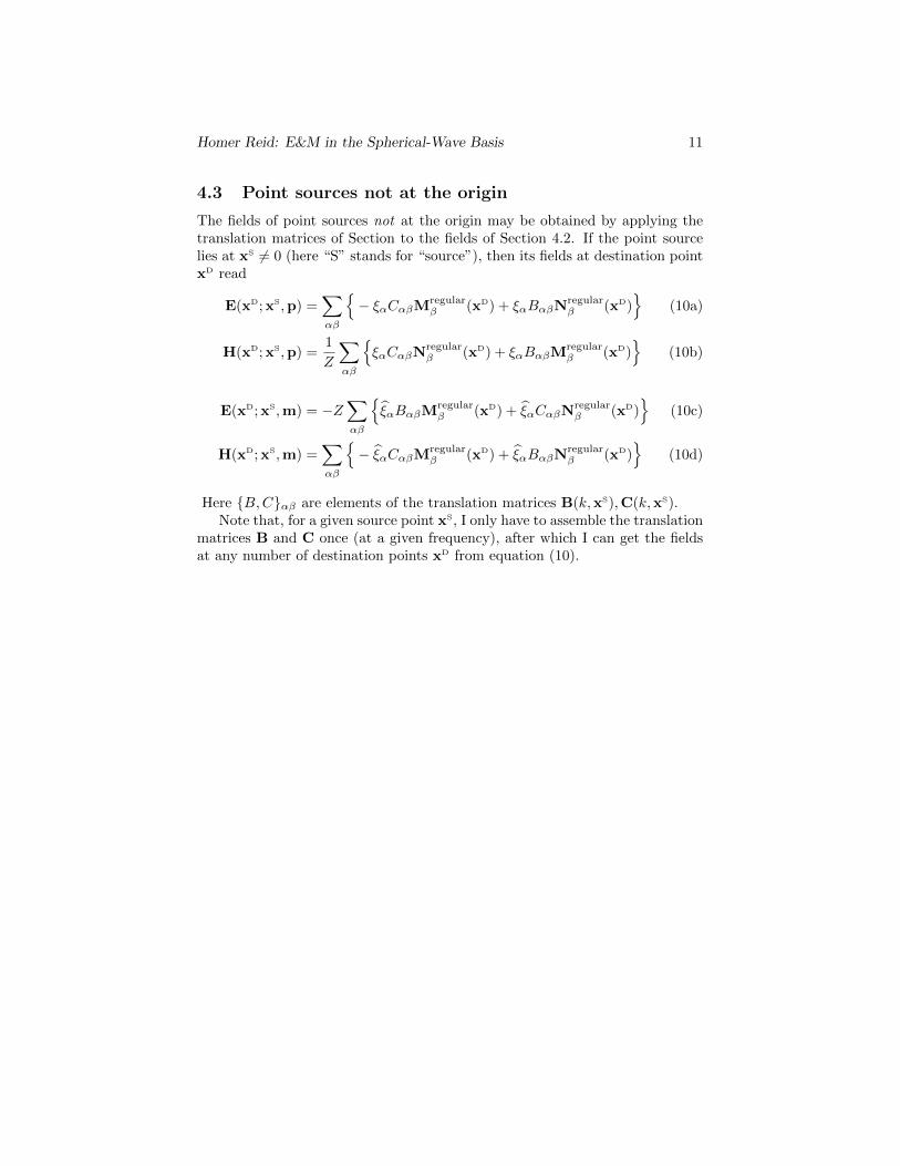
As a specific example of a radiated-power computation, let’s consider a pointlikedipole source at the center of a lossy sphere and ask for the total power radiatedaway from the sphere.


Assuming the dipole is z-directed, i.e. p = pz z, the only nonvanishingspherical multipole coefficient of the incident field [equation (16)] is

Q1,0 =−icZ0(nk0)3

ε√

6πpz

where k0 = ω/c is the free-space wavenumber.The total fields outside the sphere are

Etot(x) = D1,0Nout1,0 (x), Htot(x) =

1

Z0D1,0M

out1,0 (x)

where D1,0 is given by (21):

D1,0 =1√6π

cZ0e−ian3a6pz

[n2 (a3 + a+ i)− a− i] sin(na) + na[in2(−1 + a(a+ i)) + a+ i] cos(na)(46)

where the dimensionless “size parameter” is

a = k0R.

The radiated power is

P rad =1

2Re

∮(E∗ ×H) · r dA

=|D1,0|2

2Z0· r2 Re

∫ (N∗1,0(r,Ω)×M1,0(r,Ω)

)· r dΩ︸︷︷︸

=1/(k0r)2

=|D1,0|2

2k20Z0(47)

Sanity check

As a sanity check, let’s first try putting ε = 1. Then equation (46) reads

D1,0(ε = 1) =−icZ0k

3

√6π

pz

and equation (47) reads

P rad =c2Z0k

4

12πp2z

in agreement with Jackson equation (9.24).

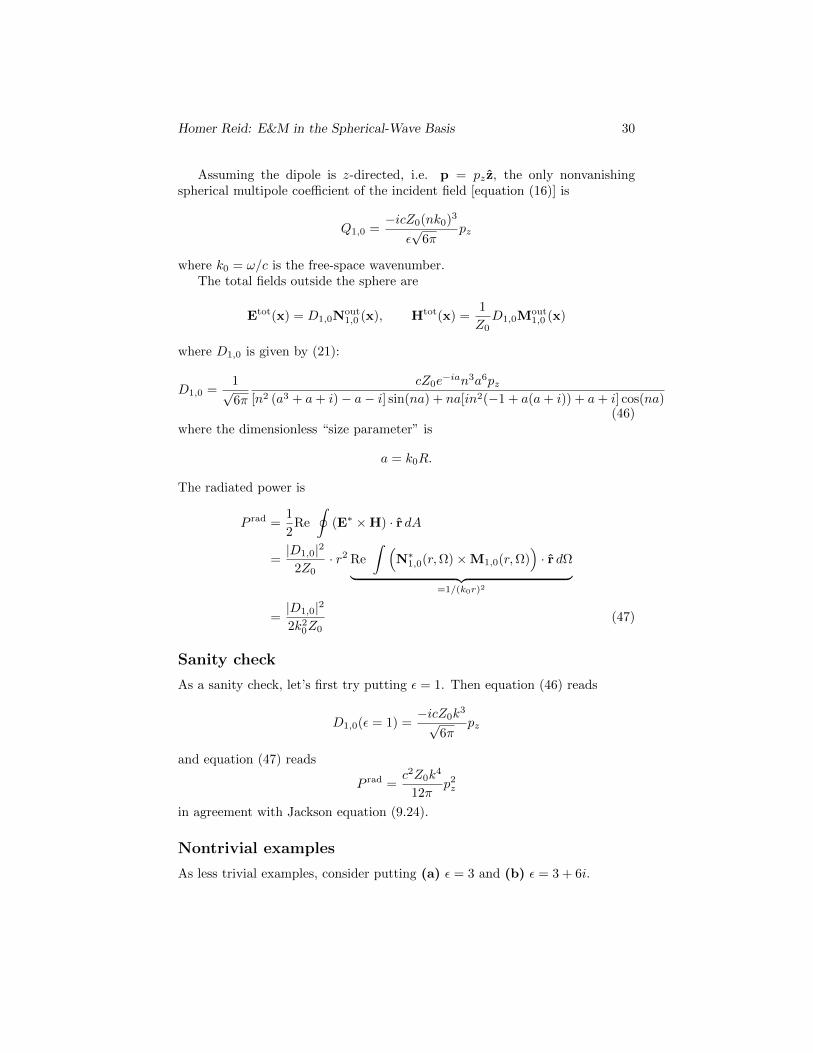
Nontrivial examples

As less trivial examples, consider putting (a) ε = 3 and (b) ε = 3 + 6i.


0.001

0.01

0.1

1

0.001 0.01 0.1 1 10

PR

ad /

PR

ad(E

ps=

1)

Omega (SCUFF units)

Eps=3

Eps=3+6i

Figure 2: Power radiated by a dipole at the center of a dielectric sphere, nor-malized by the power radiated by a dipole in free space.

9.2 Sample stress-tensor force calculation

The simplest incident-field configuration that gives rise to a nonvanishing totalforce on the sphere is a superposition of (1, 0) and (2, 1) spherical waves, corre-sponding to coherent dipole and quadrupole sources at the origin. Thus, in theincident-field expansion (16) we take

P(1,0) = P(2,1) = 1, Pα = 0 for all other α, Qα = 0 for all α. (48)

The coefficients in expansions (19, 20) for the fields outside the sphere are thensimilarly given by

C(1,0) = C(2,1) = nonzero, Cα = 0 for all other α, Dα = 0 for all α.(49)

The actual values of C(1,0) and C(2,1), which are less important for our imme-diate goals, are determined by equation (21) for a specific frequency, dielectricconstant, and sphere radius. For example, for the particular case ω, r0, ε =3 · 1014 rad/sec, 1 µm, 10 we find

C(1,0) = −0.558 + 0.760i, C(2,1) = 0.100 + 0.001i.


9.3 x-directed force density

At a point x = (rb,Ω) on the surface of the bounding sphere of radius rb, thex-directed force per unit area is, from (39),

fx(x) =ε

4

C∗10C10

[M∗

10(x)Fx(Ω)M10(x) + N∗10(x)Fx(Ω)N10(x)]

+C∗10C21

[M∗

10(x)Fx(Ω)M21(x) + N∗10(x)Fx(Ω)N21(x)]

+C∗21C10

[M∗

21(x)Fx(Ω)M10(x) + N∗21(x)Fx(Ω)N10(x)]

+C∗21C21

[M∗

21(x)Fx(Ω)M21(x) + N∗21(x)Fx(Ω)N21(x)]

9.4 Total x-directed force

The total force is obtained from equation (3):

Fx =ε04

C∗10C21

[⟨M10

∣∣∣Fx

∣∣∣M21

⟩+⟨N10

∣∣∣Fx

∣∣∣N21

⟩]+ CC

(50)

where CC stands for “complex conjugate.” [The inner product here is definedby equation (45).] With some effort, we compute⟨

M10

∣∣∣Fx

∣∣∣M21

⟩+⟨N10

∣∣∣Fx

∣∣∣N21

⟩= −i

√3

10

1

k2

and thus the total force (50) reads

Fx = − ε02k2

√3

10Im(C∗10C21

)(51)

To make sense of the units here, suppose that field-strength coefficients likeP,Q,C,D in (16) and (19) are measured in typical scuff-em units of V/µm,while k is measured in units of inverse µm. Then the units of (51) are

units of (51) =ε0 ·V2 · µm−2

µm−2

Use ε0 = 1Z0c

where c is the vacuum speed of light:

=1

Z0c·V2

Use Z0 = 376.7 V/A:

=376.7 V · A

3 · 1014 µm · s−1


Now use 1 V· A=1 watt, 1 watt · 1 s = 1 joule, 1 joule / 1 µm = 106 Newtons:

= 1.26 · 10−6 Newtons.

1e-10

1e-09

1e-08

1e-07

1e-06

1e-05

0.0001

0.001

0.01

0 0.1 0.2 0.3 0.4 0.5 0.6 0.7 0.8 0.9

X c

ompo

nent

of t

otal

forc

e on

sph

ere

Omega

’XForce.dat’ u 1:(abs($2))

Figure 3: x-component of total force on sphere irradiated from within by anincident field of the form (16) with coefficients (49).


10 T-matrix elements and surface currents

The T-matrix for a body relates the coefficients of the outgoing spherical-waveexpansion of the scattered field to the coefficients of the regular spherical-waveexpansion of the incident field; thus, if we write

Einc =∑

cincα Wregularα , Escat =

∑cscatα Woutgoing

α

[where the W notation was defined by equation (6)] then the coefficient vectorsare related by

cscat = Tcinc.

Individual T-matrix elements have the significance

Tαβ =

coefficient of outgoing α-type wavedue to irradiation by unit-amplitudeincoming β-type wave.

Now consider a scattering geometry irradiated by a unit-amplitude regular wave,and let K and N be the electric and magnetic surface currents induced by thisexcitation. The scattered field is

Escat = ikZG ?K + ikC ?N

with k and Z the wavevector and (absolute) wave impedance of the exteriormedium. Insert the expansions (8):

Escat(x) = −k2∑α

Z⟨Wreg

α

∣∣∣K⟩Woutα (x) + σα

⟨Wreg

α

∣∣∣N⟩Woutα (x)

or, rearranging slightly,

Escat(x) =∑α

−k2[Z⟨Wreg

α

∣∣K⟩− σα⟨Wregα

∣∣N⟩]︸︷︷︸Tαβ

Woutα (x). (52)

This yields a prescription for computing T-matrix elements directly from surfacecurrents.

Electromagnetism in the Spherical-Wave Basis · Electromagnetism in the Spherical-Wave Basis: A (Somewhat Random) Compendium of Reference Formulas Homer Reid August 1, 2016 Abstract

Documents