Electromagnetism Book for JEE

Kaysons Education Electromagnetism

Page 1

Day – 1

Introduction

Two bar magnets attract when opposite poles (N and S, or and N) are next to each other

The bar magnets repel when like poles (N and N, or S and S) are next to each other,

Magnetic phenomena were first observed at least 2500 years ago in fragments of magnetized iron

ore found near the ancient city of Magnesia (now Manias, is western Turkey). These fragments

were examples of what are now called permanent magnets

Before the relation of magnetic interactions to moving charges was understood, the interactions of

permanent magnets and compass needles were described in terms of magnetic poles. If a bar-

shaped permanent magnet, or bar magnet, is free to rotate, one end points north. This end is called

a north pole or N-pole; the other end is a south pole or S-pole. Opposite pole attract each other,

and like poles repel each other. An object that contains iron but is not itself magnetized (that is, it

shows no tendency to point north or south) is attracted by either pole of a permanent magnet. The

earth itself is a magnet. Its north geographical pole is close to a magnetic south pole, which is why

the north pole of a compass needle points north. The earth’s magnetic axis is not quite parallel to

its geographical axis (the axis of rotation), so a compass reading deviates somewhat from

geographic north. This deviation, which varies with location, is called magnetic declination or

magnetic variation. Also, the magnetic field is not horizontal at most points on the earth’s surface;

its angle up or down is called magnetic inclination. At the magnetic poles the magnetic field is

vertical

Moving Charge in

Magnetic Field

Chapter

1


Page 2

(a) , (b) Either pole of a bar magnet attracts an unmagnetized object that contains iron.

The concept of magnetic poles may appear similar to that of electric charge, and north and south

poles may seem analogous to positive and negative charge. But the analogy can be misleading.

While isolated positive and negative charges exist, there is no experimental evidence that a single

isolated magnetic pole exists; poles always appear in pairs. If a bar magnet is broken in two, each

broken end becomes a pole. The existence of an isolated magnetic pole, or magnetic monopole,

would have a sweeping implication for theoretical physics. Extensive searches for magnetic

monopoles have been carried out, but so far without success

A compass placed at any location in the earth’s magnetic field points in the direction of the field

line at that location. Representing the earth’s field as that of a tilted bar magnet is only a crude

approximation of its fairly complex configuration. The field, which is caused by currents in the

earth’s molten core, changes with time; geologic evidence shows that it reverses direction entirely

at irregular intervals of about a half million years.


Page 3

Breaking a bar magnet. Each piece has a north and south pole, even if the pieces are different

sizes. (The smaller the piece, the weaker its magnetism)

In Oersted’s experiment, a compass is placed directly over a horizontal wire (hire viewed from

above). When the compass is placed directly under the wire, the compass swings are reversed.


Page 4

Magnetic Field 1- A moving charge or a current creates a magnetic field in the surrounding space (in addition to

its electric field)

2- The magnetic field exerts a force on any other moving charge or current that is present in the

field

Like electric field, magnetic field is a vector field-that is, a vector quantity associated with each

point in space. We will use the symbol for magnetic field. At any position the direction of is

defined as that in which the north pole of a compass needle tends to point. The arrows in suggest

the direction of the earth’s magnetic field; for any magnet, points out of its north pole and into

its south pole.

The direction of is always perpendicular to the plane containing and . Its magnitude is given

by


Page 5

Where is the magnitude of the charge and ϕ is the angle measured from the direction of to

the direction of , as shown in the figure

(magnetic force on a moving charged particle)

The units of B must be the same as the units of F/qv. Therefore the SI unit of B is equivalent to

1N.s/C.m, or, since one ampere is one coulomb per second (1A = 1C/s), 1N/A, m. This unit is

called the tesla (abbreviated T), in honor of Nikola Tesla (1857-1943), the prominent Serbian-

American scientist and inventor

Another unit of B, the gauss (1G = 10–4

T) is also in common use. Instruments for measuring

magnetic field are sometimes called gauss meters

The magnetic field of the earth is of the order of 10–4

T or 1G. Magnetic fields of the order of 10T

occur in the interior of atoms and are important in the analysis of atomic spectra. The largest

steady magnetic field that can be produced at present in the laboratory is about 45 T. Some pulsed

–current electromagnets can produce fields of the order of 120 T for short time intervals of the

order of a millisecond. The magnetic field at the surface of a neutron star is believed to be of the

order of 108T.


Page 30

Day – 1

Introduction

Principle of superposition of magnetic fields: The total magnetic field caused by several moving

charges is the vector sum of the fields caused by the individual charges. We begin by calculating

the magnetic field caused by a short segment of a current – carrying conductor, as shows in

Fig. The volume of the segment is a dl, where A is the cross – sectional area of the conductor.

If there are moving charged particles per unit volume, each of charge q, the total moving charge

dQ in the segment is

The moving charges in this segment are equivalent to a single charge dQ, traveling with a velocity

equal to the drift velocity . (Magnetic fields due to the random motions of the charges will, on

average, cancel out at every point) From the magnitude of the resulting field at any field point

P is

But from Eq. A equals the current I in the element. So

Magnetic field of

Current Element

Chapter

2


Page 31

For these field points, and both lie in the tan – colored plane, and is perpendicular to this

plane for these field points, and both lie in the orange – colored plane, and is

perpendicular to this plane

(a) Magnetic – field vectors due to a current element . (b) Magnetic field lines in a plane

containing the current element . The indicates that the current is directed into the plane of the

page. Compare this figure to Fig. for the field of a moving point charge.

Law of Biot and Savart (pronounced “Bee – oh” and “Such – var”). We can use this law to find

the total magnetic field at any point in space due to the current in a complete circuit. To do this,

we integrate over all segments that carry current; symbolically,

The field vectors and the magnetic field lines of a current element are exactly like those set up

by a positive charge dQ moving in the direction of the drift velocity . The field lines are

circles in planes perpendicular to and centered on the line of . Their directions are given by

the same right – hand rule that we introduced for point charges.

What we measure experimentally is the total for a complete circuit. But we can still verify these

equations indirectly by calculating for various current configurations using and comparing the

results with experimental measurements.

If matter is present in the space around a current – carrying conductor, the field at a field point P in

its vicinity will have an additional contribution resulting from the magnetization of the material.

We‟ll have return to this point in Section .However, unless the material is iron or some other

ferromagnetic material, the additional field is small and is usually negligible. Additional

complications arise if time – varying electric or magnetic fields are present or if the material is a

super – conductor; we‟ll return to these topics later.

Magnetic Field of a Straight Current- Carrying Conductor

We first use the law of Biot and Savart, to find the field caused by the element of conductor of

length dl = dy. From the figure, and The right- hand


Page 32

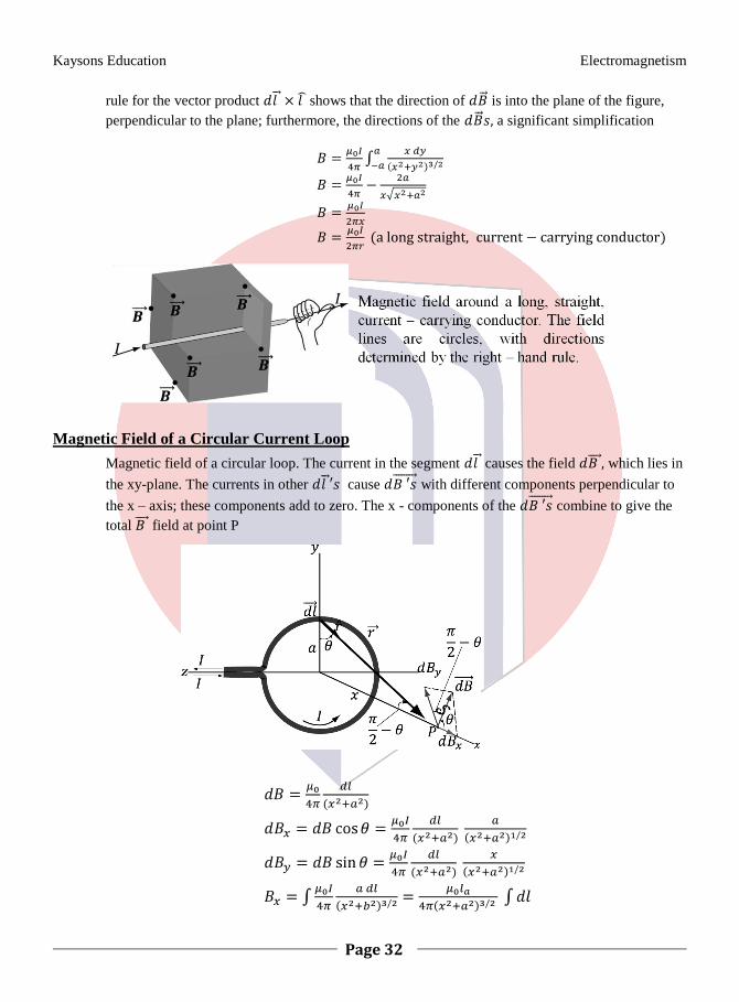
rule for the vector product shows that the direction of is into the plane of the figure,

perpendicular to the plane; furthermore, the directions of the a significant simplification

Magnetic Field of a Circular Current Loop

Magnetic field of a circular loop. The current in the segment causes the field which lies in

the xy-plane. The currents in other cause with different components perpendicular to

the x – axis; these components add to zero. The x - components of the combine to give the

total field at point P


Page 33

Illustration

Two circular coils X and Y having equal number of turns and carry equal currents in the same

sense and subtend same solid angle at point O. If the smaller coil X is midway between O and Y,

then if we represent the magnetic induction due to bigger coil Y at O as B, and due to smaller coil

X at O s Bx then

(a) By/Bx = 1 (b) By/Bx = 2

(c) By/Bx = 2 (d) By/Bx = ¼

Solution

Now use binomial (1 + x)n = 1 + nx if x << i then divide.


Page 34

Illustration

Two circular coils of wires made of similar wires but of radius 20 cm and 40 cm are connected in

parallel. The ratio of the magnetic fields at their centre is

(a) 4 : 1 (b) 1 : 4

(c) 2 : 1 (d) 1 : 2

Solution


Page 67

Day – 1

Introduction

We define the magnetic flux ϕB through a surface just as we defined electric flux in connection

with Gauss’s law. We can divide any surface into elements of area dA. For each element we

determine the component of normal to the surface. (Be careful not to confuse ϕ with .) In

general, this component varies from point to point on the surface. We define the magnetic flux

through this area as

(magnetic flux through a surface)

Magnetic flux is a scalar quantity. In the special case in which is uniform over a plane surface with

total area A. B⊥ and ϕ are the same at all points on the surface and

The SI unit of magnetic flux is equal to the unit of magnetic field (1T) times the unit of area (Im2).

This unit is called the Weber (1Wb), in honor of the German physicist Wilhelm Weber (1804 –

1891)

The magnetic flux through an area element

dA is defined to be

Magnetic Flux and

Gauss’s law of Magnetism

Chapter

3


Page 68

In Gauss’s law the total electric flux through a closed surface is proportional to the total electric

charge enclosed by the surface. For example, if the closed surface encloses an electric dipole, the

total electric flux is zero because the total charge is zero. The total magnetic flux through a closed

surface would be proportional to the total magnetic charge enclosed. But we have mentioned that

no magnetic monopole has ever been observed, despite intensive searches. We conclude that the

total magnetic flux through a closed surface is always zero. Symbolically

In Gauss’s law the total electric flux through a closed surface is proportional to the total electric

charge enclosed by the surface. For example, if the closed surface encloses an electric dipole, the

total electric flux is zero because the total charge is zero. The total magnetic flux through a closed

surface would be proportional to the total magnetic charge enclosed. But we have mentioned that

no magnetic monopole has ever been observed, despite intensive searches. We conclude that the

total magnetic flux through a closed surface is always zero. Symbolically

Caution

Unlike electric field lines that begin and end on electric charges, magnetic field lines never have

end points; such a point would indicate the presence of a monopole. You might be tempted to

draw magnetic field lines that begin at the north pole of a magnet and end at a south pole. But as

Fig Shows, the field lines of a magnet actually continue through the interior of the magnet. Like

all other magnetic field lines, they form closed loops.

For Gauss’s law, which always deals with closed surface, the vector area element Eq. always

points out of the surface. However, some applications of magnetic flux involve an open surface

with a boundary line; there is then an ambiguity of sign in Eq. because of the two possible choices

of direction for . In these cases we choose one of the possible choices of direction for . In

these cases we choose one of the possible sides of the surface to be the “positive” side and use that

choice consistently.

If the element of area dA in Eq. is at right angles to the field lines, then calling the area

we have

That is, the magnitude of magnetic field is equal to flux per unit area across an area at right angles

to the magnetic field. For this reason, magnetic field is sometimes called magnetic flux density

Induction Experiments

During the 1830s, several pioneering experiments with magnetically induced emf were carried out

in England by Michael Faraday and in the United States by Joseph Henry (1797 – 1878), later the

first director of the Smithsonian Institution. Fig shows several examples. In Fig a coil of wire is

connected to a galvanometer. When the nearby magnet is stationary, the meter shows no current.

This isn’t surprising; there is no source of emf in the circuit. But when we move the magnet either

toward or away from the coil, the meter shows current in the circuit, but only while the magnet is


Page 69

moving. If we keep the magnet stationary and move the coil, we again detect a current during the

motion. We call this an induced current, and the corresponding emf required to cause this current

is called an induced emf.

To explore further the common elements in these observations, let’s consider a more detailed

series of experiments with the situation shown in Fig. We connect a coil of wire to a

galvanometer, then place the coil between the poles of an electromagnet whose magnetic field we

can very. Here’s what we observe

1. When there is no current in the electromagnet, so that , the galvanometer shows no

current.

2. When the electromagnet is turned on, there is a momentary current through the meter as

increases

3. When levels off at a steady value, the current drops to zero, no matter how large is

4. With the coil in a horizontal plane, we squeeze it so as to decrease the cross sectional area of the

coil. The meter detects current only during the deformation, not before or after. When we increase

the area to return the coil to its original shape, there is current in the opposite direction, but only

while the area of the coil is changing.


Page 70

(a) A stationary magnet has no effect on a stationary coil of wire. A galvanometer connected to the

coil shows zero current.

(b) When the magnet and coil move relative to each other, a current is induced in the coil. The

current is in one direction if the magnet moves down and the opposite direction if the magnet

moves up.

(c) We get the same effect as in (b) if we replace the magnet by a second coil carrying a constant

current.

(d) When the switch is opened or closed, the change in the inside coil’s current induces a current

in the outer coil

5. If we rotate the coil a few degrees about a horizontal axis, the meter detects current during the

rotation, in the same direction as when we decreased the area. When we rotate the coil back, there

is a current in the opposite direction during this rotation

6. If we jerk the coil out of the magnetic field, there is a current during the motion, in the same

direction as when we decreased the area.


Page 71

A coil in a magnetic field. When the field is

constant and the shape, location, and orientation of

the coil do not change, no current is induced in the

coil. A current is induced when any of these factors

change.

7. If we decrease the number of turns in the coil by unwinding one or more turns, there is a current

during the unwinding, in the same direction as when we decreased the area. If we wind more turns

onto the coil, there is a current in the opposite direction during the winding

8. When the magnet is turned off, there is a momentary current in the direction opposite to the

current when it was turned on

9. The faster we carry out any of these changes, the greater the current

10. If all these experiments are repeated with a coil that has the same shape but different material

and different resistance, the current in each case is inversely proportional to the total circuit

resistance. This shows that the induced emf that are causing the current do not depend on the

material of the coil but only on its shape and the magnetic field

Faraday’s Law The common element in all induction effects is changing magnetic flux through a circuit. Before

stating the simple physical law that summarizes all of the kinds of experiments described in

section, let’s first review the concept of magnetic flux ϕB (which we introduced in section). For an

infinitesimal area element in a magnetic field , the magnetic flux dϕB through the area is

The magnetic flux through an area element

dA is defined to be


Page 105

School Level

Para magnetism

In an atom, most of the various orbital and spin magnetic moments of the electrons add up to zero.

However, in some cases the atom has a net magnetic moment that is of the order of μB. When such

a material is placed in a magnetic field, the field exerts a torque on each magnetic moment, as

given by. These torques tend to align the magnetic moments with the field, the

position of minimum potential energy, as we discussed in .This position, the directions of the

current loops are such as to add to the externally applied magnetic field.

We saw that the field produced by a current loop is proportional to the loop’s magnetic dipole

moment. In the same way, the additional field produced by microscopic electron current loops

is proportional to the total magnetic moment per unit volume V in the material. We call this

vector quantity the magnetization of the material, denoted by

n

The additional magnetic field due to magnetization of the material turns out to be equal simply to

, where completely surrounds a current- carrying conductor, the total magnetic field in the

material is

Where is the field caused by the current in the conductor.

To check that the units in are consistent, note that magnetization is magnetic moment per unit

volume. The units of magnetic moment are current times area (A.m2), so the units of

magnetization are (A.m2)/m

3 = A/m. From the units of the constant μ0 are T. m/A. So the units

of are the same as the units of (T. m/A) (A/m) = T.

A material showing the behavior just described is said to be paramagnetic. The result is that the

magnetic field material, than it would be if the material were replaced by vacuum. The value of Km

is different for different materials; for common paramagnetic solids and liquids at room

temperature, Km typically ranges from 1.00001 to 1.003.

All of the equations in this chapter that relate magnetic fields to their sources can be adapted to the

situation in which the current-carrying conductor is embedded in a paramagnetic material. All that

need be done is to replace μ0 by Kmμ0. This product is usually denoted as μ and is called the

permeability of the material.

The amount by which the relative permeability differs from unity is called the magnetic

susceptibility, denoted by Xm.

Both Km and Xm are dimensionless quantities. Values of magnetic susceptibility for several

materials are given in Table. For example, for aluminum, Xm = 2.2 × 10-5

and Km = 1.000022. The

first group of materials in the table are paramagnetic; we’ll discuss the second group of materials,

which are called diamagnetic, very shortly


Page 106

Diamagnetism

In some materials the total magnetic moment of all the atomic current loops is zero when no

magnetic field is present. But even these materials have magnetic effects because an external field

alters electron motions within the atoms, causing additional current loops and induced magnetic

dipoles comparable of the induced electric dipoles we studied in section. In this case the additional

field caused by these current loops is always opposite in direction to that of the external field.

(This behavior is explained by Faraday’s law of induction, which we will study. An induced

current always tends to cancel the field change that caused it)

Such materials are said to be diamagnetic. They always have negative susceptibility, as shown in

Table and permeability Km slightly less than unity, typically of the order of 0.99990 to 0.99999 for

solids and liquids. Diamagnetic susceptibilities are very nearly temperature-independent

Ferromagnetism

There is a third class of materials, called ferromagnetic materials, which includes iron, nickel,

cobalt, and many alloys containing these elements. In these materials. Strong interactions between

atomic magnetic moments cause them to line up parallel to each other in regions called magnetic

domains, even when no external field is present. Fig show an example of magnetic domain

structure. Within each domain, nearly all of the atomic magnetic moments are parallel

For many ferromagnetic materials the relation of magnetization to external magnetic field is

different when the external field is increasing from when it is decreasing. Fig shows this relation

for such a material. When the material is magnetized to saturation and then the external field is

reduced to zero, some magnetization remains. This behavior is characteristic of permanent

magnets, which retain most of their saturation magnetization when the magnetizing field is

removed. To reduce the magnetization to zero requires a magnetic field in reverse direction.

This behavior is called hysteresis, and the curves in Fig are called hysteresis loops. Magnetizing

and demagnetizing a material that has hysteresis involves the dissipation of energy, and the

temperature of the material increases during such a process.

In this drawing adapted from a

magnified photo, the arrows shows

show the directions of magnetization in

the domains of a single crystal of

nickel. Domains that are magnetized in

the direction of an applied magnetic

field grow larger.


Page 107

Ferromagnetic materials are widely used in electromagnets, transformer cores and motors and

generators, in which it is desirable to have as large a magnetic field as possible for a given current.

Because hysteresis dissipates energy, materials that are used in these applications should usually

have as narrow a hysteresis loop as possible. Soft iron is often used; it has high permeability

without appreciable hysteresis. For permanent magnets a broad hysteresis loop is usually

desirable, with large zero – field magnetization and large reverse field needed to demagnetize.

Many kinds of steel and many alloys, such as Alnico, are commonly

Hysteresis loops. The materials of both (a) and (b) remain strongly magnetized when is reduced to

zero. Since (a) is also hard to demagnetize, it would be good for permanent magnets. Since (b)

magnetizes and demagnetizes more easily, it could be used as a computer memory material. The

material of (c) would be useful for transformers and other alternating – current devices where zero

hysteresis would be optimal.

A magnetization curve for

a ferromagnetic material.

The magnetization M

approaches its saturation

value Msat as the magnetic

field B0 (caused by external

currents) becomes large.


Page 108

Summary

The magnetic field created by a charge q moving with velocity depends on the distance r from the source point (the location of q) to the field

point (where is

measured). The field is perpendicular to and , the unit vector directed from the source point to the field point. The principle of superposition of magnetic

fields states that the total field produced by several moving charges is the vector sum of the fields produced by the individual charges.

The law of Biot and Savart

gives the magnetic field d

created by an element d of a conductor carrying

current I. The field is

perpendicular to both and the unit vector from the element to the field

point. The field created by a finite current- carrying conductor is the integral of

over the length of the conductor.

The magnetic field at a

distance r from a long,

straight conductor carrying a

current I has a magnitude that

is inversely proportional to r.

the magnetic field lines are

circles coaxial with the wire,

with directions given by the

right-hand rule


Page 109

Two long, parallel, current-carrying conductors attract if the currents are in the same direction and repel if the currents are in opposite directions. The magnetic force per unit length between the conductors depends on their currents I and I’ and their separation r. The definition of the ampere is based on this relation.

The law of Biot and Savart

allots us to calculate the

magnetic field produced

along the axis of a circular

conducting loop of radius a

carrying current I. the field

depends on the distance x

along the axis from the center

of the loop to the field point.

If there are N loops, the field

is multiplied by N. at the

center of the loop x = 0.

Circular loop

(centre of N

circular loop)

Ampere’s law sates that the

line integral of around any

closed path equals times the

net current through the area

enclosed by the path. The

positive sense of current is

determined by a right-hand

rule.

The following table lists fields caused by several current distributions. In each the conductor is

carrying current I.

Current Distribution Point in Magnetic Field Magnetic Field Magnitude

Long , straight conductor Distance r from conductor

Circular loop of radius a

On axis of loop

At center of loop

(for N loops, multiply these

expressions by N)

Long cylindrical conductor of

radius R

Inside conductor, r < R

Outside conductor, r > R


Page 110

Long, closely wound solenoid with n turns per unit length, near its midpoint

Inside solenoid, near center Outside solenoid

Tightly wound toroidal solenoid (toroid) with N turns

With the space enclosed by the windings, distance r from symmetry axis Outside the space enclosed by the windings

B ≈ 0

When magnetic materials are present, the magnetization of the material causes an additional

contribution to . For paramagnetic and diamagnetic materials, μ0 is replaced in magnetic–field

expressions by . Where μ is the permeability of the material and Km is its relative

permeability. The magnetic susceptibility Xm is defined as Xm = Km – 1. Magnetic susceptibilities

for paramagnetic materials are small positive quantities; those for diamagnetic materials are small

negative quantities. For ferromagnetic materials, Km is much larger than unity and is not constant.

Some ferromagnetic materials are permanent magnets, retaining their magnetization even after the

external magnetic field is removed.

Electromagnetism Book for JEE

Documents