Electromagnetic-Theoretic Analysis and Design of MIMO Antenna Systems by Mehrbod Mohajer Jasebi A thesis presented to the University of Waterloo in fulfillment of the thesis requirement for the degree of Doctor of Philosophy in Electrical and Computer Engineering Waterloo, Ontario, Canada, 2011 © Mehrbod Mohajer Jasebi 2011

Welcome message from author
This document is posted to help you gain knowledge. Please leave a comment to let me know what you think about it! Share it to your friends and learn new things together.
Transcript
Electromagnetic-Theoretic Analysis and
Design of MIMO Antenna Systems
by
Mehrbod Mohajer Jasebi
A thesis
presented to the University of Waterloo
in fulfillment of the
thesis requirement for the degree of
Doctor of Philosophy
in
Electrical and Computer Engineering
Waterloo, Ontario, Canada, 2011
© Mehrbod Mohajer Jasebi 2011

ii
AUTHOR'S DECLARATION
I hereby declare that I am the sole author of this thesis. This is a true copy of the thesis, including any
required final revisions, as accepted by my examiners.
I understand that my thesis may be made electronically available to the public.

iii
Abstract
Multiple-Input Multiple-Output (MIMO) systems are a pivotal solution for the significant
enhancement of the band-limited wireless channels’ communication capacity. MIMO system is
essentially a wireless system with multiple antennas at both the transmitter and receiver ends.
Compared to the conventional wireless systems, the main advantages of the MIMO systems are the
higher system capacity, more bit rates, more link reliability, and wider coverage area. All of these
features are currently considered as crucial performance requirements in wireless communications.
Additionally, the emerging new services in wireless applications have created a great motivation to
utilize the MIMO systems to fulfil the demands these applications create. The MIMO systems can be
combined with other intelligent techniques to achieve these benefits by employing a higher spectral
efficiency.
The MIMO system design is a multifaceted problem which needs both antenna considerations and
baseband signal processing. The performance of the MIMO systems depends on the cross-correlation
coefficients between the transmitted/received signals by different antenna elements. Therefore, the
Electromagnetic (EM) characteristics of the antenna elements and wireless environment can
significantly affect the MIMO system performance. Hence, it is important to include the EM
properties of the antenna elements and the physical environment in the MIMO system design and
optimizations.
In this research, the MIMO system model and system performance are introduced, and the
optimum MIMO antenna system is investigated and developed by considering the electromagnetic
aspects within three inter-related topics:
1) Fast Numerical Analysis and Optimization of the MIMO Antenna Structures:
An efficient and fast optimization method is proposed based on the reciprocity theorem along with
the method of moment analysis to minimize the correlation among the received/transmitted signals in
MIMO systems. In this method, the effects of the radio package (enclosure) on the MIMO system
performance are also included. The proposed optimization method is used in a few practical examples
to find the optimal positions and orientations of the antenna elements on the system enclosure in order
to minimize the cross-correlation coefficients, leading to an efficient MIMO operation.
iv
2) Analytical Electromagnetic-Theoretic Model for the MIMO Antenna Design:
The first requirement for the MIMO antennas is to obtain orthogonal radiation modes in order to
achieve uncorrelated signals. Since the Spherical Vector Waves (SVW) form a complete set of
orthogonal Eigen-vector functions for the radiated electromagnetic fields, an analytical method based
on the SVW approach is developed to excite the orthogonal SVWs to be used as the various
orthogonal modes of the MIMO antenna systems. The analytic SVW approach is used to design
spherical antennas and to investigate the orthogonality of the radiation modes in the planar antenna
structures.
3) Systematic SVW Methodology for the MIMO Antenna Design:
Based on the spherical vector waves, a generalized systematic method is proposed for the MIMO
antenna design and analysis. The newly developed methodology not only leads to a systematic
approach for designing MIMO antennas, but can also be used to determine the fundamental limits and
degrees of freedom for designing the optimal antenna elements in terms of the given practical
restrictions. The proposed method includes the EM aspects of the antenna elements and the physical
environment in the MIMO antenna system, which will provide a general guideline for obtaining the
optimal current sources to achieve the orthogonal MIMO modes. The proposed methodology can be
employed for any arbitrary physical environment and multi-antenna structures. Without the loss of
generality, the SVW approach is employed to design and analyze a few practical examples to show
how effective it can be used for MIMO applications.
In conclusion, this research addresses the electromagnetic aspects of the antenna analysis, design,
and optimization for MIMO applications in a rigorous and systematic manner. Developing such a
design and analysis tool significantly contributes to the advancement of high-data-rate wireless
communication and to the realistic evaluation of the MIMO antenna system performance by a robust
scientifically-based design methodology.

v
Acknowledgements
I would like to express my sincere gratitude to my supervisors, Prof. Safieddin Safavi-Naeini and
Prof. Sujeet K. Chaudhuri, for their invaluable direction, assistance, and guidance. Without their
support and encouragement, it was impossible for me to progress in this research.
I am also thankful to the external examiner, Prof. Michael A. Jensen, and the University of
Waterloo Examining Committee members, Prof. Liang-Liang Xie, Prof. Amir Hamed Majedi, Prof.
Slim Boumaiza, Prof. Adrian Lupascu, and Prof. Frank Wilhelm, for their suggestions and comments
in my PhD defense and comprehensive examination.
I express my thanks to all of my colleagues at Intelligent Integrated Radio and Photonics Group
(IIRPG) who provided me with such a friendly and active environment during the course of this
research.
I am very grateful to my school teachers and my university professors who opened the doors of
knowledge to me and inspired me to follow this direction.
Last but not least, I would extend my heartfelt appreciations to my family for their everlasting love
and patience.

vi
Dedication
To my dear parents who taught me how to live, and
To my beloved wife who taught me how to love

vii
Table of Contents AUTHOR'S DECLARATION ............................................................................................................... ii
Abstract ................................................................................................................................................. iii
Acknowledgements ................................................................................................................................ v
Dedication ............................................................................................................................................. vi
Table of Contents ................................................................................................................................. vii
List of Figures ....................................................................................................................................... ix
List of Tables ........................................................................................................................................ xii
Chapter 1 Introduction ............................................................................................................................ 1
1.1 MIMO Antenna Challenges and State of Arts .............................................................................. 3
1.2 Thesis Outline ............................................................................................................................... 7
Chapter 2 MIMO System Model and Performance Parameters ............................................................. 9
2.1 MIMO System Model ................................................................................................................... 9
2.2 System Capacity and Correlation Coefficient ............................................................................ 10
2.3 Physical MIMO Channel Model ................................................................................................ 13
2.4 Conclusion .................................................................................................................................. 15
Chapter 3 MIMO Antenna Optimizations ............................................................................................ 16
3.1 Packaging Effects on MIMO Antenna Radiation Patterns ......................................................... 17
3.2 Practical Examples of MIMO Antenna Optimizations ............................................................... 20
3.3 Conclusion .................................................................................................................................. 23
Chapter 4 Analytical Spherical Vector Wave Approach ...................................................................... 24
4.1 Vector Wave Functions in Curvilinear Coordinates ................................................................... 24
4.2 Vector Green’s Function ............................................................................................................ 26
4.3 SVWs for MIMO Antenna Radiations ....................................................................................... 27
4.3.1 Degrees of Freedom ............................................................................................................ 28
4.3.2 Mutual Coupling .................................................................................................................. 29
4.4 Spherical MIMO Antenna Design .............................................................................................. 32
4.5 Planar MIMO Antenna Design ................................................................................................... 39
4.6 Conclusion .................................................................................................................................. 43
Chapter 5 Systematic Spherical Vector Wave Method ........................................................................ 45
5.1 Spherical Vector Wave Formulation .......................................................................................... 45
5.2 MIMO Channel Analysis ........................................................................................................... 50
viii
5.3 Optimal Current Excitations of MIMO Antennas ...................................................................... 53
5.3.1 Four-Element MIMO Antenna System ............................................................................... 54
5.3.2 Multi-port Patch Antenna.................................................................................................... 59
5.4 Optimal Current Distributions for MIMO Antenna Systems ..................................................... 69
5.4.1 System Capacity versus MIMO Antenna Shape ................................................................. 70
5.4.2 Optimal Current Distributions on Antenna Geometry ........................................................ 72
5.4.3 Optimal Current Distribution on Ground Plane .................................................................. 81
5.5 Conclusion ................................................................................................................................. 89
Chapter 6 Concluding Remarks ........................................................................................................... 91
6.1 Future Work ............................................................................................................................... 93
Appendix A Method of Moments for Conducting Bodies ................................................................... 95
A.1 Theory of Scattering .................................................................................................................. 95
A.2 Method of Moment Equations for PEC Bodies ........................................................................ 95
A.3 MoM using RWG Basis Functions ........................................................................................... 96
A.4 MATLAB functions for MoM ................................................................................................ 100
Appendix B Vector Wave Functions ................................................................................................. 104
Bibliography ...................................................................................................................................... 106

ix
List of Figures 1.1: The MIMO system in a multipath propagation environment ................................................... 1
2.1: The general geometry of MIMO Antennas .............................................................................. 9
2.2: The cluster channel model for the MIMO antenna system .................................................... 14
3.1: The magnetic current sources on PEC enclosure ................................................................... 17
3.2: The reciprocity problems ........................................................................................................ 18
3.3: Two patch antennas located on a) a ground plane, b) two faces of a PEC cube [67] ............. 20
3.4: The radiation patterns for MIMO antenna elements shown in Figure 3.3.b ........................... 21
3.5: MIMO antenna elements on the practical handset’s ground plane [69] ................................. 22
3.6: A single element antenna operating at 2.4GHz [69] .............................................................. 22
4.1: The electromagnetic reciprocity between the two problems .................................................. 30
4.2: MIMO antenna design containing magnetic and electric currents in the x-y plane ............... 41
4.3: S-parameters of the MIMO antenna shown in Figure 4.2 ...................................................... 42
4.4: The gain radiation patterns of the two MIMO antennas shown in Figure 4.2 ........................ 42
4.5: The cumulative density function of the correlation coefficient in the Laplacian channel ...... 43
5.1: The CDF of the correlation coefficient between various SVWs for a Laplacian PAS [55] ... 53
5.2: The MIMO system comprising of four half wavelength dipole antennas [54] ...................... 54
5.3: The Laplacian power angular spectrum ................................................................................. 54
5.4: The correlation coefficient for two dipoles in a 4-element MIMO system [54] .................... 55
5.5: The four optimal MIMO system modes for the 4-element MIMO system ............................ 57
5.6: The normalized SVW coefficients obtained for the four MIMO system modes [54] ............ 58
5.7: The singular values of optimal MIMO system modes in the Laplacian PAS ........................ 59
5.8: A two-port circular patch antenna; (a) antenna geometry (b) simulated S-parameters .......... 60
5.9: (a) The gain radiation patterns for two φ-planes when port#1 in Figure 5.8.a is excited, (b)
The 3D gain radiation patterns when port#1 in Figure 5.8.a is excited ................................... 61
5.10: (a) The gain radiation patterns for two φ-planes when port#2 in Figure 5.8.a is excited, (b)
The 3D gain radiation patterns when port#2 in Figure 5.8.a is excited ................................... 62
5.11: The CDF of the correlation coefficient obtained from the two-port circular patch antenna (a) o30== nn θφ σσ (b) o20== nn θφ σσ (c) o10== nn θφ σσ .............................................. 63
5.12: The two-port circular patch antenna with the optimal feed circuit; (a) antenna geometry (b)
simulated S-parameters ........................................................................................................... 65

x
5.13: (a) The gain radiation patterns for two φ-planes when port#1 in Figure 5.12.a is excited, (b)
The 3D gain radiation patterns when port#1 in Figure 5.12.a is excited ................................ 66
5.14: (a) The gain radiation patterns for two φ-planes when port#2 in Figure 5.12.a is excited, (b)
The 3D gain radiation patterns when port#2 in Figure 5.12.a is excited ................................ 67
5.15: The CDF of the correlation coefficient for the two-port circular patch antenna with an
optimal feed circuit (a) o30== nn θφ σσ (b) o20== nn θφ σσ (c) o10== nn θφ σσ ........ 68
5.16: The delta function current sources covering the given volume or surface ............................. 70
5.17: The square plane for current distributions ............................................................................. 70
5.18: The normalized power gains of the optimal MIMO system modes for different sizes of a
square plane ............................................................................................................................ 71
5.19: The system capacity versus the number of MIMO system modes used for different sizes of a
square plane ............................................................................................................................ 72
5.20: The plane of the mobile handset ............................................................................................ 73
5.21: The normalized power gains of the optimal MIMO system modes at 2.4GHz for the mobile
handset plane ........................................................................................................................... 73
5.22: The system capacity versus the number of MIMO system modes at 2.4GHz for the mobile
handset plane ........................................................................................................................... 74
5.23: The optimal current distributions on the mobile handset plane at 2.4GHz ............................ 75
5.24: The radiation patterns of optimal current distributions for the handset plane ....................... 76
5.25: The optimum number of MIMO system modes for the Laplacian channel realizations ........ 76
5.26: The optimum number of MIMO system modes for the Laplacian channel and the antenna
geometry given in Figure 5.20 ................................................................................................ 77
5.27: The CDF of the correlation coefficients between the optimum MIMO system modes shown
in Figure 5.24 .......................................................................................................................... 78
5.28: The four optimal half-wavelength dipoles ............................................................................. 79
5.29: (a) Two optimal shapes of the half-wavelength dipoles, (b) simulated S-parameters, (c) gain
radiation patterns of the two MIMO antenna elements ........................................................... 80
5.30: The CDF of the correlation coefficient between the MIMO system modes obtained by two
optimal dipole shapes .............................................................................................................. 81
5.31: The optimum number of MIMO system modes for the magnetic current sources on the
handset’s ground plane in the Laplacian channel ................................................................... 82
5.32: The optimal magnetic current distributions on the handset’s ground plane at 2.4GHz ......... 83

xi
5.33: The radiation patterns of optimal magnetic currents on the handset’s ground plane .............. 84
5.34: The CDF of the correlation coefficients between the optimal MIMO system modes generated
by the magnetic currents on the handset’s ground plane ......................................................... 84
5.35: The two regions on the handset’s ground plane for the MIMO antenna elements ................. 85
5.36: (a) The optimal magnetic currents for the given regions, (b) radiation patterns of two MIMO
system modes, (c) CDF of the correlation coefficient for two MIMO system modes ............ 86
5.37: The dielectric resonator antennas to generate the MIMO system modes ............................... 87
5.38: The DRA simulation results (a) S-Parameters (b) gain radiation patterns ............................. 88
5.39: The CDF of the correlation coefficient between DRAs ......................................................... 89
A.1: The geometry of the RWG basis function [96] ..................................................................... 97
A.2: The variables included in the analytic formulas presented by [98] ....................................... 99
A.3: The generated meshes on the PEC cube for MoM ............................................................... 101
A.4: The scattered field radiation patterns in HFSS and MoM for a) o0=ϕ
b) o45=ϕ c) o90=ϕ d) o135=ϕ e) o180=ϕ plane [67, 69] ..................................... 102
A.5: The scattered field radiation patterns in HFSS and MoM for a) o45=θ
b) o90=θ [67, 69] ............................................................................................................. 103

xii
List of Tables 5.1: The inner Products of SVW functions [55] ............................................................................ 51
5.2: The inner Products of SVW functions [55] ............................................................................ 52
5.3: The exact current excitations for the four MIMO system modes [54] .................................... 56
5.4: The rounded current excitations for the four MIMO system modes [54] ............................... 56

1
Chapter 1 Introduction
In wireless communications, the transmitted signals may be received through multiple propagation
paths due to the environmental scatterers [1]. Multipath propagation may result in the destructive or
constructive combinations of radio signals which can cause signal fluctuations. The resultant
multipath fading can decrease the level of received signal to a level less than the required threshold,
and therefore, can significantly affect the system outage and reliability [1, 2]. Conventionally,
Diversity techniques are used to combat the multipath fading effects [1]. In various diversity schemes
such as space, angle, polarization, and pattern diversities, multiple antennas are employed to transmit
or receive the independent radio signals that contain identical information. By obtaining independent
signals caused by the independent wireless channel effects, the probability of simultaneous fading for
independent signals will decrease and the system reliability can be improved [1].
In recent years, the ever-increasing demand for high data rate wireless applications has required
new wireless communication systems to have a higher system capacity for data transmission. The
system capacity is defined as the maximum mutual information which can be transferred through the
wireless channel [1-4]. Among various techniques to increase the system capacity, Multiple-Input
Multiple-Output (MIMO) systems have recently attracted great attention in both the research
community and the industry as a suitable solution for the significant enhancement of the band-limited
wireless systems’ communication capacity [2]. The MIMO system is essentially a wireless system
with multiple antennas at both the transmitter and receiver ends as illustrated in Fig. 1.1. Compared to
the Single-Input Single-Output (SISO) systems, the main advantages of the MIMO systems are the
higher capacity, increased data rates, reduced multi-path fading effects, more link reliability, and
wider coverage area.
Figure 1.1: The MIMO system in a multipath propagation environment
Tx Rx

2
As shown in Fig. 1.1, if different propagation paths can be resolved by multiple antennas, the
independent data can be transferred through each propagation path, and therefore, the system capacity
can be enhanced [3]. Since the independent data is transferred at the same frequency, MIMO systems
can provide a higher spectral efficiency in comparison to SISO communications [4]. However, the
capacity enhancement depends on the number of resolvable propagation paths which can be obtained
through the wireless channel. For instance, if there is only one dominant propagation path in the
wireless channel, the same information is extracted by multiple antennas and no capacity
improvement can be obtained [5, 6]. Hence, it should be emphasized that MIMO systems are
beneficial in rich multipath environments which contain multiple propagation paths resolvable by
multiple antennas. Once the environment provides multipath propagations, the MIMO system can be
employed to exploit the wireless channel’s degrees of freedom.
In order to resolve various propagation paths and encode multiple independent data, spatial
multiplexing has been proposed to obtain orthogonal communication Eigen-channels by using the
Singular Value Decomposition (SVD) of the wireless channel [1-4]. In spatial multiplexing, the
multiple data is weighted so that independent data is transferred through different Eigen-channels
which can be physically interpreted as independent propagation paths. In rich multipath
environments, spatial multiplexing yields a linear increase of the system capacity by the minimum
number of Tx and Rx antennas [1, 4]. However, since the data streams occupy the same frequency
and time, the accurate detection of received streams is sensitive to the noise and the quality of the
channel [3, 4]. In order to increase the robustness to the wireless channel, the combination of space
and time diversities, known as the space-time diversity coding [4], can be employed, in which the data
streams are transmitted through different antenna elements over various time periods. For instance, in
the simplest space-time diversity code, the Alamouti scheme [7], two different symbols, 1s and 2s ,
are simultaneously transmitted by two different antenna elements, antenna#1 and antenna#2, over the
first period of time. Then, the mathematically manipulated symbols, *2s− and *
1s , are sent through
antenna#1 and antenna#2, respectively, over the following time period. The Alamouti signaling
strategy improves the symbol error rate by transmitting each symbol twice, but a higher-rate temporal
code is required in comparison to spatial multiplexing [3, 4]. The Alamouti diversity scheme can be
extended to a more general case, known as Orthogonal Space-Time Block Coding (OSTBC), where
arbitrary numbers of transmitter and receiver antennas are utilized [8].

3
Alternatively, the combination of diversity and multiplexing techniques, often called the space-time
coding, can be employed for MIMO systems [1-4]. Of course, there is a fundamental tradeoff
between the diversity and the multiplexing improvements. The signaling strategy would be
determined depending on the performance tradeoffs (the spatial multiplexing gain versus the diversity
gain), to transmit the data streams through multiple antennas over multiple time periods [9].
Independent of the chosen space-time code signaling, the MIMO system performance improvement
depends on the correlation of the communication channel pipes between the transmitter and the
receiver [10, 11]. If the communication channels obtained from the multipath environment are
correlated, the same information is obtained through different channels, and therefore, there are no
channel’s degrees of freedom to be extracted by the MIMO systems through either diversity or
multiplexing techniques [10]. Hence, the lower the correlation between the MIMO signals, the better
performance the MIMO system can achieve. Typically, the MIMO system firstly estimates the
wireless channel, and then uses orthogonalization procedures in the base-band signal processing to
determine the uncorrelated channel pipes. In this procedure, it is assumed that the MIMO antenna
elements are capable of governing independent signals from the wireless channels [2], and the
orthogonalization procedure is performed before transmitting or after receiving the signals by the
antenna elements. Hence, the Electromagnetic (EM) properties of the MIMO antenna elements are
usually considered as part of the wireless channel, whereas the MIMO antenna structures can play a
crucial role to make the MIMO signals uncorrelated instead. By embedding antennas in the wireless
channel, an important design liberty is underscored to combat the dynamic variations of the wireless
channel. Additionally, the electromagnetic effects of the MIMO antennas enforce fundamental
limitations in the MIMO system performance. If the EM limitations and interactions of the antennas
are ignored, the MIMO system performance may be underestimated or overestimated, and as a result
imprecise evaluations of the MIMO systems may be obtained. Hence, the MIMO system design
requires the EM antenna considerations in addition to the baseband signal processing.
1.1 MIMO Antenna Challenges and State of Arts
Considering the effect of the correlation between the communication channel pipes on the MIMO
system performance, the design of the MIMO antennas leads to the minimizing of the correlation
coefficients between antenna elements [12]. Conventionally, the correlation between the signals can
be reduced by using large distances between the antenna elements [13]. However, because of
practical considerations, compact multi-element radio/antenna systems with low correlation are in
4
high demand. In many applications, there is not enough space on the radio enclosure or package to
place several antennas with the sufficient spacing. Thus, it is necessary to install multiple antennas in
a limited space in such a way that the correlation coefficient between the antennas remains as small as
possible. Many papers have been published to achieve a better system performance using the compact
co-located antennas [14-21].
On the other hand, the number of elements and their interactions will affect the general pattern and
the cross-correlation coefficients of the MIMO antennas. Hence, a general design procedure is
required to not only provide the optimum compact MIMO antenna structure in order to achieve the
uncorrelated signals, but also to determine how many degrees of freedom exist to design the antenna
structure [22, 23]. As mentioned, the EM domain poses some limitations which restrict the design of
the information theory domain [24]. Thus, it is important to know the maximum number of MIMO
antenna elements or modes which can be employed to achieve the desirable system performance for
the given physical limitations in the EM domain such as the bandwidth and the size of the antenna
structure. Many papers have been devoted to finding the degrees of freedom determined by the
electromagnetic domain [22-25].
The other important aspect of the MIMO antenna design is the fact that the physical environment
providing a dynamic wireless channel will also impress the correlation between the MIMO signals.
Thus, the ultimate design should adapt itself to the wireless channel in order to provide the
uncorrelated signals in an arbitrary physical environment [26, 27]. This adaptation can be performed
in both the signal processing and electromagnetic-antenna domains. In addition to performing the
signal processing on the received signals to form a suitable radiation pattern, it is beneficial to design
the intelligent antenna elements to properly reconfigure the antenna characteristics including the
frequency of the operation, the radiation pattern, the polarization, and even the antenna locations. The
adaptive elements are able to reconfigure themselves to the channel variations. Many papers have
been published to present different reconfigurable antennas [26-34]. The majority of them are using
the Micro-Electro-Mechanical System (MEMS) switches as a low-loss connection between various
metal sections to either form different types of traditional antennas or a set the parasitic elements to
change the antenna characteristics [26]. However, the feed-networks required to control the MEMS
switches will make the antenna structure very bulky and inefficient. Alternatively, the PIN diodes and
variable capacitors have also been employed to control the antenna features by changing the matching
5
stubs or reactive loads of parasitic antennas in which the loss and required biasing voltages are
important issues [33, 34].
Although extensive research has been devoted to the MIMO antenna systems, considering both the
electromagnetic and signal processing aspects of the MIMO antenna design, still poses several
challenges:
1) The MIMO antenna utilizing the space, pattern, and polarization diversities must be able to
provide uncorrelated communication paths with the maximum signal orthogonality in order
to obtain the maximum performance in the MIMO system. This needs novel antenna
structures that make the space-time signal processing less complex and easier to
implement.
2) The physical wireless channel effects and the EM interactions of the scatterers in the
vicinity of antenna structure should be included in the MIMO antenna designs to obtain the
desired MIMO system performance in realistic and practical situations. Including the
wireless channel effects, it is possible to design MIMO antennas adaptive to the channel
variations.
3) In practical applications, fast and efficient methods are required to optimize the physical
parameters of the MIMO antenna elements in terms of the given practical restrictions.
4) Accurate models are required to study the impact of the antenna structure on the
performance of the MIMO systems. Considering the developed models and criteria, a
systematic methodology is also needed to appropriately design and analyze the MIMO
antenna systems.
5) Using several antennas in a small package such as a cell phone may not be feasible. The
optimal MIMO antenna elements and the maximum number of co-located antennas should
be explored in terms of the practical limitations such as limited space.
Most of the research accomplishments present an optimum design for a case study, and a general
methodology can be rarely found to evaluate the possibility of employing MIMO antenna elements
for practical limitations and also lead to an optimum MIMO antenna design that includes the wireless
environment effects. The only comprehensive studies, which propose a general methodology for the
MIMO antenna design, can be categorized as follow:
6
1) Characteristic Mode (CHM) Approach: The characteristic modes are the Eigen vectors of the
impendence matrix in the Method of Moments (MoM), which leads to orthogonal current
modes for a given geometry [35-37]. The Characteristic Modes radiate orthogonal
characteristic radiation patterns which can be utilized to achieve orthogonal multi modes for
the MIMO application [38-44]. The antenna design using the CHM strategy is advantageous in
the sense that it establishes the orthogonal radiation patterns and also provides physical insight
to the modal excitations of the antenna geometry. However, it is practically difficult to excite
the characteristic modes on the antenna structures. Another drawback is the fact that CHM
orthgonality is not necessarily held at the near field region [36]. Near field interactions of
characteristic radiation patterns may cause poor isolations between the MIMO antenna
elements, resulting in a higher correlation and lower radiation efficiency. Meanwhile, the
physical environment and the channel variation model have not been taken into account and the
degree of freedom for the MIMO antenna design is uninvestigated in the published papers. In
general, it should be mentioned that the characteristic mode analysis is an efficient approach
for scattering problems, but it faces several drawbacks for the antenna design problems [39,
41].
2) Spherical Vector Wave (SVW) Approach: The SVWs form a complete set of orthogonal
Eigen-vector functions for the radiated electromagnetic fields rather than the current sources
[45-48]. Since any radiated electromagnetic field can be expanded in terms of the SVWs,
studying the behaviour and interactions of these vector waves in a specific propagation
condition will fully characterize the wireless environment [49-55]. The SVW expansions of the
field generated by each MIMO antenna element are all one needs to fully investigate the
MIMO antenna system performance. Additionally, the SVWs are orthogonal everywhere
outside a sphere surrounding the radiating antenna [46, 47]. Hence, by using the SVWs as the
MIMO antenna elements, better isolation and less interaction between the radiated modes can
be achieved. Thus, the SVWs can be used as an analytic tool to study complex MIMO antenna
systems and to provide physical insight into the design and optimization of different MIMO
antenna systems based on the minimization of the cross-correlation coefficient and the mutual
coupling between the antenna elements.
In this thesis, the aim is to include the EM aspects of the MIMO antennas and the physical
environments into the MIMO system performance evaluations and optimizations. Additionally, a
7
systematic methodology is developed to not only obtain the optimal MIMO antenna elements
considering the EM effects, but to also determine the degrees of freedom and fundamental limitations
in terms of given practical restrictions for implementing the MIMO antennas. For this purpose, the
SVW approach is employed to:
1) Determine the maximum number of orthogonal communication channels generated by the
MIMO antenna elements.
2) Generate optimal MIMO antenna radiations in order to minimize the correlation coefficient of
the MIMO signals for an arbitrary set of antenna elements in a given wireless environment.
The SVWs are utilized in both the analytical and numerical analysis, and as well as the design of
the MIMO antennas. The analytical derivations, which are convenient for spherical and planar
geometries, have not been presented before, but the SVWs have been already used to numerically
analyze the MIMO antennas and wireless channels [49-51]. However, the SVW formulation
presented in this thesis is different from the available approaches in the literature, and provides a
systematic method to analyze the MIMO wireless channel, as well as appropriately design the optimal
MIMO antenna elements and the feed circuit for a given wireless environment. The presented
formulation can be also used to determine the liberties of designing the MIMO antennas in terms of
desired MIMO system performance and the given practical considerations.
1.2 Thesis Outline
The chapters of this thesis are organized as follows. Chapter 2 reviews the MIMO system models
including the MIMO antenna elements and introduces the MIMO system performance. For MIMO
antenna designs, a criterion is required to link the electromagnetic characteristics of the MIMO
antennas to the required system performance. As a suitable connecting parameter, the correlation
coefficient between the antenna elements will be minimized to enhance the MIMO system
performance. However, the scattering parameters of the antenna system should also be taken into
account to achieve an efficient MIMO antenna structure. Finally, the physical channel models are
quickly reviewed for MIMO applications.
The objective of Chapter 3 is to develop a fast optimization method for synthesizing MIMO
antennas with minimal correlation, which can deliver maximum capacity. For this purpose, a
reciprocity approach along with numerical Method of Moments [56] is employed which is very
efficient and fast to include the radio package and the enclosure effects in the correlation coefficient
8
calculations. Including the package effects, an optimization problem is defined and a few practical
examples are solved to obtain an optimum low-correlation MIMO antenna.
In Chapter 4, the theory of Vector Wave Functions (VWF) is discussed, and the orthogonal
properties of the spherical vector waves will be introduced for the MIMO antenna designs. The
analytical SVW approach is presented to obtain the orthogonal current distributions for the spherical
MIMO antennas. Additionally, the influences of the planar antenna geometries on the SVW
excitations are considered and a few orthogonal properties of planar structures are explored for the
MIMO antenna designs.
The general SVW formulation is proposed in Chapter 5 to obtain a systematic methodology for the
MIMO antenna designs. The presented SVW formulation allows for the separate investigation of the
physical channel effects, the MIMO antenna elements, and the feed circuit characteristics. The
proposed formulation is employed for different practical cases in which the physical wireless channel
is evaluated, and the optimal MIMO antennas and feed circuits are designed and analyzed.
Chapter 6 summarizes the accomplishments and achievements through this research and suggests
possible directions for future works.

9
Chapter 2 MIMO System Model and Performance Parameters
In this chapter, the aim is to model a general MIMO system and introduce the MIMO system
parameters as the required criteria for the MIMO antenna designs. Since the main advantage of the
MIMO systems is the higher system capacity in comparison to the SISO systems, it is important to
design the MIMO antennas so that the system capacity is maximized. It will be shown that the
correlation coefficients between the MIMO antenna elements should be minimized to obtain the
maximum system capacity. The correlation coefficient calculations will consider the MIMO wireless
channel to include the physical environment in the MIMO antenna design. Hence, the physical
MIMO channel models are also discussed in this chapter.
2.1 MIMO System Model
The general model of the MIMO antenna configuration is illustrated in Figure 2.1, showing TN and
RN as the number of antenna elements in the transmitter and receiver sides, respectively, and mnH
represents the channel coefficient between the nth transmitter and the mth receiver.
Figure 2.1: The general geometry of MIMO Antennas
Using the dyadic channel response function ),,( TRG ΩΩω , which relates the received field
distribution by the receiver, ),( RRP Ωωr
, to the radiated field pattern of the transmitter array, one can
write [3, 10]:
∫ ΩΩΩΩ=Ω TTTTRRR dPGP ),(.),,(),( ωωωrr
(2.1)
1x
TNx
1y
RNy
11H
TR NNH
1RNH
TNH1

10
where RΩ and TΩ are the solid angles with respect to the receiver and transmitter coordinate
systems, respectively. The radiated field pattern by the transmitter array can be written as follows [3,
10]:
),()(),( ,1
TnT
N
nnTT FxP
T
Ω=Ω ∑=
ωωωvr
(2.2)
where nx is the up-converted symbol fed to the nth antenna element, and nTF ,
v is the vector field
radiation pattern of the nth transmitting antenna element in the presence of other antenna elements.
Using the channel dyadic function, the received signal by the mth receiving antenna element can be
found as:
RRRRmRm dPFyR
ΩΩΩ= ∫Ω
),(.),()( , ωωωrv
(2.3)
where mRF ,
v is the field radiation pattern of the mth receiving antenna element in presence of other
antenna elements. Using equations (2.1) to (2.3), the vector signal received by the receiving antenna
elements, after adding the additive noise contribution, will be obtained as follows [10]:
RTTnTTRRmRmn ddFGFH ΩΩΩΩΩΩ=
+=
∫ ∫ ),(.),,(.),()(
)()()()(
,, ωωωω
ωωωωvv
ηxHy (2.4)
Considering the flat fading or non-selective frequency channels, the channel transfer matrix, the
matrix H , remains constant over the signal bandwidth. However, it still varies over the time. As it
can be seen, the field radiation patterns of the receiver and transmitter antennas affect the channel
transfer matrix. Since the channel dyadic function is determined by the environment and cannot be
manipulated, the antenna field patterns should be effectively designed so that the desired MIMO
system performance is achieved.
2.2 System Capacity and Correlation Coefficient
The main advantage of MIMO systems is the system capacity enhancement. The system capacity is
defined as the maximum mutual information between the transmitters and the receivers [1]. Under the
assumptions that the channel is unknown for the transmitter and known for the receiver, the MIMO
system capacity can be obtained as follows [1, 2, 4, 57, and 58]:

11
⎥⎦
⎤⎢⎣
⎡⎟⎟⎠
⎞⎜⎜⎝
⎛+= †HHI
TN N
SNRCR
detlog2 (2.5)
where RNI is an identity matrix, SNR is the signal to noise ratio, and † denotes the complex
conjugate transpose. The system capacity in (2.5) can be obtained via the Singular Value
Decomposition (SVD) of the channel transfer matrix:
∑−
+=min
1
22 )1(log
N
ii
TNSNRC λ (2.6)
where iλ is the singular value of the matrix H (consequently, 2iλ is the Eigen values of the matrix
†HH ), and minN is the minimum of TN and RN . Note that if the transmitter has the full knowledge
of the Channel State Information (CSI), the water-filling method can be employed to optimally
allocate the transmitting powers to various Eigen channels so that the system capacity is maximized
[1, 2, 10]. In the case that the transmitter has no knowledge of the channel, the transmitted power is
equally distributed between the transmitter antennas ( TNSNR / ), and the relationship (2.6) is
obtained.
The channel transfer matrix can be decomposed into Line-of-Sight (LOS) and Non-Line-of-Sight
(NLOS) components [12]:
NLOSLOS KKK HHH
++
+=
11
1 (2.7)
where K is the Ricean K-factor defined as the ratio of the LOS signal power to the power of the multi-
path signals. The LOS component accounts for the non-fading contribution and depends on the AoD
(Angle of Departure) and the AoA (Angle of Arrival) at the transmitter and receiver sides,
respectively. The NLOS channel component, NLOSH , is the stochastic part representing the multi-
path fading effects. In order to evaluate the MIMO system capacity, the NLOS component of the
channel transfer matrix should be modeled. There are a variety of wireless MIMO channel models to
characterize the channel transfer matrix by using either analytical formulas or the physical properties
of the environment [59]. Most of the analytical models are based on the Kronecker correlation-based
channel model. Based on the Kronecker model, the spatial receiver and transmitter correlations are
separable as follows [12, 59]:

12
21
21
TGRNLOS RHRH = (2.8)
where RR and TR are the spatial receiver and transmitter correlation matrices, respectively, and
GH is the zero-mean complex Gaussian matrix. This model is useful in the sense that it allows to
optimize receiver and transmitter antenna arrays separately. The entries of the spatial correlation
matrices can be obtained by calculating the correlation coefficient between the received signals by the
MIMO antenna elements. Hence, elements of the correlation matrix can be obtained as [11, 60, and
61]:
{ }*2/1)( jiij
jjii
ijij yyEr
rrr
==ρ (2.9)
where { }E represents the mathematical expectation operator. Replacing (2.3) into (2.9) and
considering the statistical properties of the received field distributions, ),( RRP Ωωr
, one can obtain:
{ }
∫∫
∫∫ΩΩΩΩ=
ΩΩΩΩΩ=
π
π
4
*,,
4
*,,
*
)(.)()(
)(.)()(.)(
RRjRRiRR
RRjRRiRRRRRij
dFFP
dFFPPEr
vv
vvrr
(2.10)
where )(ΩP is the probability distribution of the Power Angular Spectrum (PAS) of incoming waves
impinging on the MIMO antenna elements. Thus, the correlation coefficient of the received signals by
the ith and jth antenna elements can be written in the following general form [11, 60]:
[ ]
∫∫ ΩΩ⋅=><
><><
><=
π
ρ
4
*
2/1
)(,
,,
,
dPBABA
where
FFFF
FF
P
PjjPii
Pjiij
rrrr
rrrr
rr
(2.11)
Considering equation (2.5), the system capacity is maximized when the spatial correlation matrices
are diagonal and the channel transfer matrix is a full rank matrix [1-4, 57]. In this case, the vector
field radiation patterns can be thought of as MIMO Eigen modes or MIMO modes which establish
parallel communication channels through a wireless multipath environment [10]. Hence, the Eigen

13
values of the matrix †HH , which are proportional to the diagonal elements of the correlation
matrices, determine the power gains of the communication channels associated with the MIMO Eigen
modes. Therefore, when maximizing the system capacity, the cross-correlation coefficients should be
minimized and the diagonal elements of the correlation matrices should be equalized to achieve
identical power gains for the parallel communication channels [10].
For lossless antennas and uniform PAS ( 1)( =ΩP ), the cross-correlation coefficient in (2.11) can
be expressed in terms of scattering-parameters [62]:
2/1
1
*
1
*
1
*
)1)(1( ⎥⎦
⎤⎢⎣
⎡−−
=
∑∑
∑
==
=
N
ppjpj
N
ppipi
N
ppjpi
ij
SSSS
SSρ (2.12)
where piS is the scattering parameter between the pth and ith ports of the N-port antenna structure. In
many MIMO antenna designs, the equation (2.12) has been used as a criterion to provide uncorrelated
signals for wireless communication systems. Since the correlation coefficient defined in (2.12) does
not include the wireless channel effects in the correlation calculations, there is no guarantee that the
MIMO antenna design can lead to orthogonal signals in different channel realizations, whereas
equation (2.11) allows for the evaluation of the statistical performance parameters of the designed
MIMO antenna architecture in different environments modeled by existing stochastic MIMO channel
models. Hence, equation (2.11), which contains the wireless channel information in addition to the
vector field radiation pattern of the MIMO antenna modes, will be a suitable criterion for designing
the MIMO antenna system. At the same time, the scattering parameters of the MIMO antenna
structure should also be evaluated to investigate the isolation between the antenna elements and
radiation efficiency of MIMO modes.
2.3 Physical MIMO Channel Model
In order to design MIMO antennas through equation (2.11), it is required to separate the influences of
the channel and the antenna arrays on the matrix H , and model the power angular spectrum of the
incoming waves through the MIMO wireless channel. There are varieties of channel models for
MIMO wireless communications. Note that the expression (2.11) is general, and accordingly, any
arbitrary PAS model can be used for designing the MIMO antenna system. For site specific
14
environments, deterministic channel models such as the ray-tracing model can be used to rigorously
obtain the PAS of incoming rays to the MIMO antennas [59]. To include the dynamic effects of the
wireless environment, a geometry-based stochastic channel can be used as an alternative model in
which the scatterer locations are changed in a random fashion, and for each random location, the
propagation path between the Tx and the Rx is obtained by using a simplified ray-tracing model [59].
Unlike the geometry-based channel models, the non-geometrical stochastic channel models describe
the propagation paths by random parameters rather than the physical geometry of scatterers. Most of
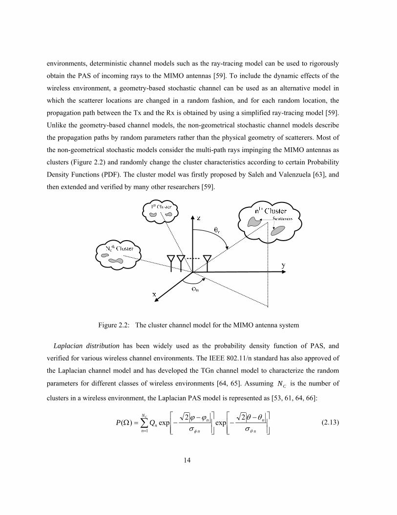
the non-geometrical stochastic models consider the multi-path rays impinging the MIMO antennas as
clusters (Figure 2.2) and randomly change the cluster characteristics according to certain Probability
Density Functions (PDF). The cluster model was firstly proposed by Saleh and Valenzuela [63], and
then extended and verified by many other researchers [59].
Figure 2.2: The cluster channel model for the MIMO antenna system
Laplacian distribution has been widely used as the probability density function of PAS, and
verified for various wireless channel environments. The IEEE 802.11/n standard has also approved of
the Laplacian channel model and has developed the TGn channel model to characterize the random
parameters for different classes of wireless environments [64, 65]. Assuming CN is the number of
clusters in a wireless environment, the Laplacian PAS model is represented as [53, 61, 64, 66]:
⎥⎥⎦
⎤
⎢⎢⎣
⎡ −−
⎥⎥⎦
⎤
⎢⎢⎣
⎡ −−=Ω ∑
= n
nN
n n
nn
C
QPθφ σθθ
σϕϕ 2
exp2
exp)(1
(2.13)
15
where nQ is the normalized power coefficient of the nth cluster, nϕ and nθ are the center of the
azimuth and elevation angle of arrival, and nφσ and nθσ are the azimuth and elevation angular
spread of each cluster, respectively. According to the TGn channel model, the number of clusters
varies from 1 to 7 for different environments, and the mean angles of arrival of each cluster are
uniformly distributed. It has been experimentally shown that the elevation angular spread is much
smaller than the azimuth angular spread. That is the reason why the Laplacian distribution has been
considered for only azimuth directions in many publications. Since in wireless applications such as
mobile communications, the MIMO antenna structure is randomly rotated in different directions, the
randomness of the elevation angle of arrival, nθ , should be included in the Laplacian PAS
distribution, as presented in (2.13).
2.4 Conclusion
To maximize the MIMO system capacity, the cross-correlation coefficient between the MIMO
antenna elements should be minimized. Although the S-parameter based formula is not an appropriate
criterion for the correlation coefficient calculation, the scattering parameters of the antenna structure
should be studied to achieve an efficient MIMO design. To include the physical environment
variations in the MIMO system performance, equation (2.11) is a suitable criterion for the correlation
coefficient calculations. The definition of (2.11) is general and can be used for any arbitrary physical
channel model. Without the loss of generality, the Laplacian channel model is used for the MIMO
antenna design and analysis in this research.
16
Chapter 3 MIMO Antenna Optimizations
In the previous chapter, the correlation coefficient in (2.11), which was introduced as a criterion for
maximizing the MIMO system capacity, considers the PAS to include the wireless channel effects in
the MIMO system performance. The PAS only represents the incoming waves due to the sources and
scattering objects in the far field, whereas in many practical cases, the other parasitic elements are
located in the vicinity of the MIMO antennas. The scattering objects in the near field region will
affect the field radiation patterns of the MIMO antenna elements, and consequently, the orthogonality
of the received signals can significantly deteriorate. Also, the interactions of the scatterers and the
antenna elements in near field region may cause a strong coupling between the MIMO antenna
elements, and reduce the system capacity [21]. Hence, in addition to PAS modeling the far-field
effects, it is vital to include the near field effects of the scatterers on the field radiation patterns to
have a more realistic analysis of the physical environment effects.
In some practical cases, the type of antenna and consequently the current sources are known, and it
is required to optimize the antenna parameters such as the antenna position, the orientation, and the
input current excitations in order to obtain uncorrelated signals. In such a scenario, it is crucial to
include the radio package influence on the field radiation pattern of each MIMO antenna element in
the correlation coefficient calculations. For optimizing the MIMO antenna parameters, it is necessary
to change the antenna parameters and then evaluate the system performance until an optimum
parameter set is obtained. Hence, optimizing the antenna parameters is very challenging in the sense
that a full-wave problem should be solved in each iteration. Using commercial software such as the
High Frequency Structure Simulator (HFSS) for the required analysis at each optimization step would
be time wasting and inefficient. Therefore, an efficient and fast method is required to save time in the
optimization process.
In this chapter, a very fast and efficient optimization method, based on the reciprocity theorem
along with the Method of Moment analysis, is proposed to minimize the correlation between the
received signals in the MIMO antenna systems. In this method, the effect of the radio package
(enclosure) on the MIMO system performance is also included. The proposed optimization method is
used to find the optimal positions and orientations of the antenna elements on the system package to
minimize the cross-correlation coefficients.

17
3.1 Packaging Effects on MIMO Antenna Radiation Patterns
In most practical cases, a fixture package is used to maintain the MIMO antenna elements. These
days, the largest class of integrated antenna elements mounted on portable radio packages are in the
form of planar or quasi-planar elements of various shapes. These elements in general, can be modeled
either by a very short electric current element perpendicular to the body of the package, or by an
equivalent magnetic current. For instance, let us assume N is the number of antenna elements that are
supposed to be located on a given Perfect Electric Conductor (PEC) enclosure as depicted in Figure
3.1. For the sake of the simplicity of the description, a general magnetic current source is used as a
general model of the antenna over the package or box, which is chosen to be made of PEC.
Figure 3.1: The magnetic current sources on PEC enclosure
Note that, since the electric current along the surface of a PEC enclosure would not radiate, only
magnetic currents are considered here. However, these assumptions on the geometry and the material
of the box will not reduce the generality of the method to be discussed here.
To find the radiated fields from a magnetic current mounted on a PEC fixture, the Reciprocity
theorem [48, 67] is employed. To this end, a second “b” problem reciprocal to the first (original) “a”
problem is constructed. In the second (reciprocal) problem, the magnetic current sources are removed,
and an infinitesimal dipole, which is directed along either θ or ϕ at a particular θ and ϕ , at a far
distance from the PEC, radiates towards the PEC enclosure, as shown in Figure 3.2 for a cubic
fixture.
The radiated fields from the magnetic current in presence of the PEC are obtained by: 1) solving
for the scattered field from the PEC fixture due to the infinitesimal dipole radiation at the far field
region (problem (b)), and 2) using the reciprocity relationship below to find the radiated fields in the
original problem (a):
ϕθ ˆˆˆ,).ˆ(.ˆ or =×=−=⋅ ∫∫∫∫∫ pdsMJndvMHEp ababarrrrr
(3.1)
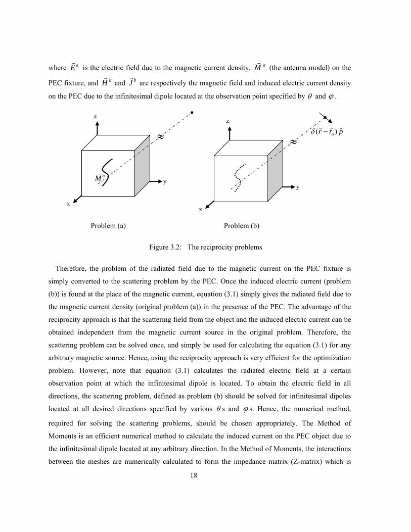
18
where aEr
is the electric field due to the magnetic current density, aMr
(the antenna model) on the
PEC fixture, and bHr
and bJr
are respectively the magnetic field and induced electric current density
on the PEC due to the infinitesimal dipole located at the observation point specified by θ and ϕ .
Problem (a) Problem (b)
Figure 3.2: The reciprocity problems
Therefore, the problem of the radiated field due to the magnetic current on the PEC fixture is
simply converted to the scattering problem by the PEC. Once the induced electric current (problem
(b)) is found at the place of the magnetic current, equation (3.1) simply gives the radiated field due to
the magnetic current density (original problem (a)) in the presence of the PEC. The advantage of the
reciprocity approach is that the scattering field from the object and the induced electric current can be
obtained independent from the magnetic current source in the original problem. Therefore, the
scattering problem can be solved once, and simply be used for calculating the equation (3.1) for any
arbitrary magnetic source. Hence, using the reciprocity approach is very efficient for the optimization
problem. However, note that equation (3.1) calculates the radiated electric field at a certain
observation point at which the infinitesimal dipole is located. To obtain the electric field in all
directions, the scattering problem, defined as problem (b) should be solved for infinitesimal dipoles
located at all desired directions specified by various θ s and ϕ s. Hence, the numerical method,
required for solving the scattering problems, should be chosen appropriately. The Method of
Moments is an efficient numerical method to calculate the induced current on the PEC object due to
the infinitesimal dipole located at any arbitrary direction. In the Method of Moments, the interactions
between the meshes are numerically calculated to form the impedance matrix (Z-matrix) which is
y
x
z
prr o ˆ)( rr−δ
≈
y
x
z
aMr
≈

19
independent of the electromagnetic excitations [56]. Once the impedance matrix is calculated, the
induced current on the PEC object is obtained by multiplying the inverse of the Z-matrix (admittance
matrix) and exciting electromagnetic field due to the infinitesimal dipole at a particular direction.
Hence, the Z-matrix calculation has to be performed only once for an arbitrary PEC object, and
therefore, the MoM is a very efficient numerical method for MIMO antenna optimization purposes.
To find the induced current SJr
due to an infinitesimal dipole, the Method of Moments has been
implemented in MATLAB (see the Appendix A). To obtain SEr
from equation (3.1) at all directions,
it is required to achieve a bank of induced currents attributed to different directions. Having saved the
bank of induced currents, the physical parameters of the MIMO antenna elements can be changed
during each optimization iteration and the field radiation patterns associated with the given
parameters are calculated through equation (3.1) in a very fast manner. Considering the influence of
the PEC object on the field radiation patterns, an optimization problem is defined to minimize the
correlation coefficient between the MIMO antenna elements:
fixedareIandIknowareATandATObjectrandrConst
dFFdFF
dObjectATIrrFObjectATIrrFMinMin
mnmnmn
mmnn
mmmmmnnnnn
nm
,,:.
),,,,,(),,,,,(
21
4
*
4
*
4
*
∈′′
⎥⎦
⎤⎢⎣
⎡Ω⋅Ω⋅
Ω′⋅′=
∫∫∫∫
∫∫
rr
rrrr
rrrrrr
ππ
π
ββρ (3.2)
where nrr′ and mr
r′ are the position vectors of the nth and mth antenna elements confined to the locations
on the PEC enclosure, rr is the position vector pointing at the observation point, nβ and mβ are the
antenna orientations, nI and mI are the excitation currents of each antenna element, nAT and mAT
are the antenna element types, and finally Object determines the shape of enclosure or chassis. Note
that the channel power angular spectrum function is assumed to be uniform. However, the
formulation can be used for other channel models including the Laplacian cluster model or the ray-
tracing channel model.
In the next section, two different applications of the reciprocity approach along with the MoM
formulation will be discussed to investigate how the proposed method can be applied for MIMO
antenna optimizations in practical cases.

20
3.2 Practical Examples of MIMO Antenna Optimizations
As two examples of the MIMO antenna systems, consider two patch antennas operating at 2.45GHz
in two different configurations: 1) a PEC cube with the side length of λ , and 2) a rectangular PEC
ground plane with the side of λ and a thickness of λ02.0 , as depicted in Figure 3.3. The problem
is to optimize antennas’ locations and orientations in such a way that the two patch antennas (or, in
general, any other number of this type of antenna) mounted on the PEC object produce orthogonal
patterns and uncorrelated signals for the MIMO system.
(a) (b)
Figure 3.3: Two patch antennas located on
a) a ground plane, b) two faces of a PEC cube [67]
The patch antenna can be modeled by two magnetic currents extracted from the well-known cavity
model [68]. In order to find the radiation field produced by the patch antenna on the PEC box, the
MoM approach along with the reciprocity theory discussed in the previous section is used. The
induced electric current is derived and can be used in equation (3.1) for any arbitrary magnetic source
Mr
located on the PEC object. Therefore, 1Fr
and 2Fr
can be obtained as a function of 1rr′ and 2r
r′
which are positions of the two patch antennas. It is preferable to fix the complex exciting currents to
avoid any complexity in the feed network.
Using the proposed approach, 1Fr
and 2Fr
can be found for each parameter sets of ( 1x , 1y , 1β , 2x ,
2y , 2β ) and ( 1y , 1z , 1β , 2x , 2z , 2β ). Performing the optimization problem given in equation (3.2)
z1
y
x
z
y1
1β
x2
z2 2β
y1
x z x1
1β
y
y2
x2
2β

21
with respect to these six parameters, it is found that ( λ42.01 =x , λ44.01 =y , o1641 =β , λ81.02 =x ,
λ32.02 =y , o332 =β ) and ( 2/1 λ=y , 2/1 λ=z , o2251 =β , 2/2 λ=x , 4/32 λ=z , o902 =β ) provide
the minimum correlation coefficients which are approximately 51002.9 −× and 51018.2 −× ,
respectively [67]. Therefore, the low-correlation coefficient MIMO antenna systems have been
obtained using the proposed optimization procedure, which maximizes the system capacity.
In the absence of PEC objects, it would be expected that the 90 degrees difference in the rotation
angles of the patch antennas would give the orthogonal radiation patterns because the polarizations
would be orthogonal. As it can be observed, when the PEC effects are included, the 90 degrees
difference is not necessarily required to achieve the best orthogonality. This shows that the packaging
effects play an important role in the MIMO antenna design. The radiation patterns of the two patch
antennas in presence of the PEC box are shown in Figure 3.4 for the optimal antenna parameters in
Figure 3.3.b. As expected, the radiation patterns are different from one single patch antenna in
absence of the PEC box.
(a) (b)
Figure 3.4: The radiation patterns for MIMO antenna elements shown in Figure 3.3.b
Another interesting case would be the MIMO antenna implementation for mobile applications.
Assume that two antenna elements are supposed to be located on the handset’s ground plane with the
size of 100mm×45mm×2mm to achieve a MIMO mobile system with a low cross-correlation
coefficient, as illustrated in Figure 3.5.

22
Figure 3.5: MIMO antenna elements on the practical handset’s ground plane [69]
It has been shown that the strong coupling between the MIMO antenna elements occurs through the
handset’s ground plane, and it is difficult to isolate the multiple antennas placed on the handset PCB
[21]. To include the effect of the ground plane in the correlation coefficient calculation, the proposed
approach can be employed to optimize the position and the orientation of the MIMO antenna
elements on the ground plane. The single element antenna has been designed to be used as the MIMO
antenna element in the mobile communication. The antenna structure and its return loss (S11) are
illustrated in Figure 3.6.
Figure 3.6: A single element antenna operating at 2.4GHz [69]
30mm
23
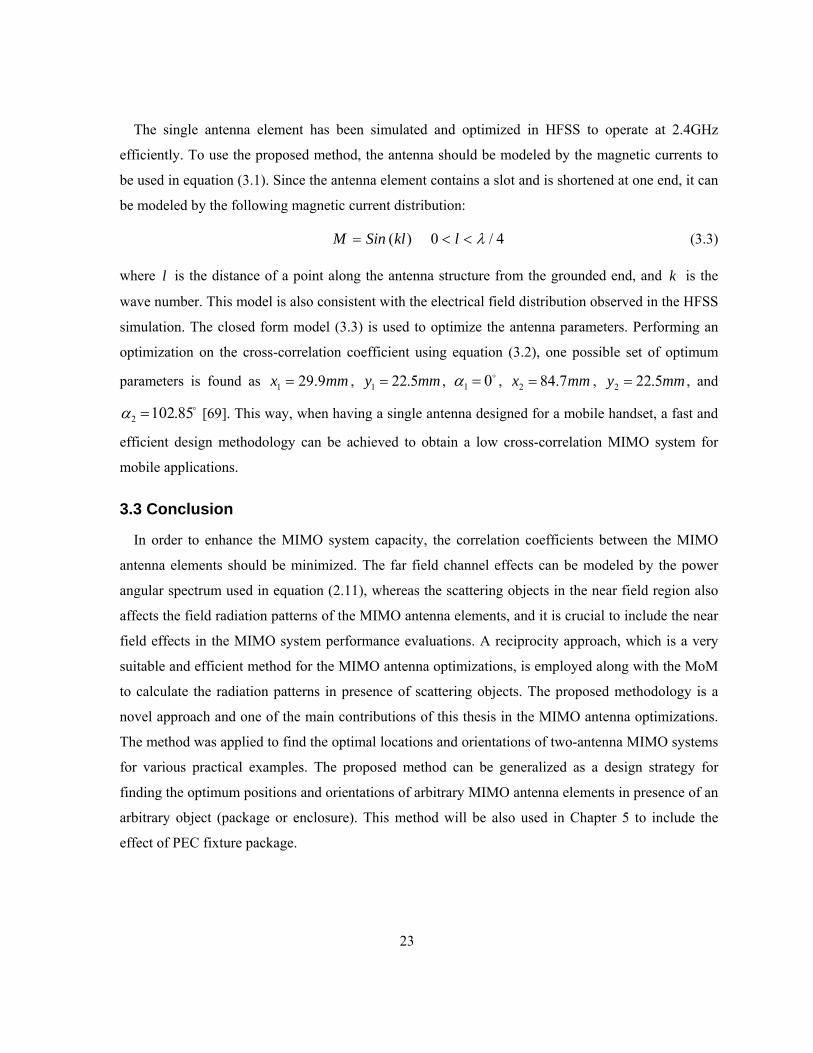
The single antenna element has been simulated and optimized in HFSS to operate at 2.4GHz
efficiently. To use the proposed method, the antenna should be modeled by the magnetic currents to
be used in equation (3.1). Since the antenna element contains a slot and is shortened at one end, it can
be modeled by the following magnetic current distribution:
4/0)( λ<<= lklSinM (3.3)
where l is the distance of a point along the antenna structure from the grounded end, and k is the
wave number. This model is also consistent with the electrical field distribution observed in the HFSS
simulation. The closed form model (3.3) is used to optimize the antenna parameters. Performing an
optimization on the cross-correlation coefficient using equation (3.2), one possible set of optimum
parameters is found as mmx 9.291 = , mmy 5.221 = , o01 =α , mmx 7.842 = , mmy 5.222 = , and
o85.1022 =α [69]. This way, when having a single antenna designed for a mobile handset, a fast and
efficient design methodology can be achieved to obtain a low cross-correlation MIMO system for
mobile applications.
3.3 Conclusion
In order to enhance the MIMO system capacity, the correlation coefficients between the MIMO
antenna elements should be minimized. The far field channel effects can be modeled by the power
angular spectrum used in equation (2.11), whereas the scattering objects in the near field region also
affects the field radiation patterns of the MIMO antenna elements, and it is crucial to include the near
field effects in the MIMO system performance evaluations. A reciprocity approach, which is a very
suitable and efficient method for the MIMO antenna optimizations, is employed along with the MoM
to calculate the radiation patterns in presence of scattering objects. The proposed methodology is a
novel approach and one of the main contributions of this thesis in the MIMO antenna optimizations.
The method was applied to find the optimal locations and orientations of two-antenna MIMO systems
for various practical examples. The proposed method can be generalized as a design strategy for
finding the optimum positions and orientations of arbitrary MIMO antenna elements in presence of an
arbitrary object (package or enclosure). This method will be also used in Chapter 5 to include the
effect of PEC fixture package.

24
Chapter 4 Analytical Spherical Vector Wave Approach
In this chapter, a systematic method is developed to analytically analyze and design the MIMO
antenna elements which provide uncorrelated signals to achieve the maximum capacity. In order to
maximize the capacity, the presented metric in (2.11) should be minimized for different antenna
elements. In the ideal case, it is desired to achieve zero cross-correlation for the ith and jth field
radiation patterns:
0)()()(,4
* =ΩΩΩ⋅Ω=>< ∫∫π
dPFFFF jiPji
rrrr (4.1)
If the antenna elements are chosen in such a way that each pair of field radiation patterns is
orthogonal through the equation (4.1), the system capacity will increase. Since the spherical vector
waves form a complete set of orthogonal Eigen-vector functions for the radiated electromagnetic
fields in free space, the spherical vector wave functions satisfy equation (4.1) for the uniform PAS,
1),( =ϕθP . The orthogonality properties of the spherical vector waves inspire a SVW approach as an
analytical method to design various orthogonal radiation modes for the MIMO antenna systems.
In this chapter, the Vector Wave Functions are first reviewed in a general curvilinear coordinate
system, and then the orthogonality of the VWFs is employed to design and analyze the spherical and
planar antennas. It is also discussed how the SVWs can be used to investigate the degrees of freedom
and mutual coupling of the designed antenna configurations.
4.1 Vector Wave Functions in Curvilinear Coordinates
Let us consider the curvilinear coordinates 1ξ , 2ξ , and 3ξ with the unit vectors 1a , 2a , 3a and the
scale factors 1h , 2h , 3h , respectively [45]. The field vectors Er
, Hr
, Dr
, Br
and vector potentials, in a
source free, homogeneous and isotropic medium obey the vector Helmholtz equation [45, 46]:
σμωεμω jk
FkFF+=
=+×∇×∇−⋅∇∇22
2 0rrrrrrr
(4.2)
It has been shown that following independent Vector Wave Functions satisfy equation (4.2) [45,
46]:
25
Mk
NaMLrrrrrrr
×∇=×∇=∇=1),ˆ(, ψψ (4.3)
where a is any arbitrary constant unit vector, and the scalar function ψ is a solution of the scalar
Helmholtz equation:
022 =+∇ ψψ k (4.4)
The important properties of these three vectors are [45, 46]:
0,0
,,0 22
=⋅∇=⋅∇
−=∇=⋅∇=×∇
NM
kLLrrrr
rrrrψψ
(4.5)
which means that the Lr
vector is curl-less, and the Mr
and Nr
vector functions are divergence-less.
It is advantageous to decompose the vector solution of equation (4.2) into longitudinal and transverse
parts. Notice that the longitudinal and transverse vector functions are defined as zero-curl and zero-
divergence vectors, respectively [45]. Hence, the electromagnetic fields can be represented as a linear
combination of Lr
(longitudinal part), Mr
, and Nr
(transverse parts) which are the vector Eigen-
functions of equation (4.2).
The representation (4.3) is based on the constant unit vector a . This representation can be
extended to the cases where the unit vector a , which is perpendicular to a constant coordinate
surface in a curvilinear coordinate system, is not fixed. If the unit vector is 1a , then Mr
and Nr
should be redefined as follows [45]:
( ) Mk
NaMLrrrrrrr
×∇=×∇=∇=1,ˆ, 1χψψ (4.6)
where 1a is the unit vector normal to the curved surface C=1ξ , and χ is a scalar function to be
determined so that the Mr
and Nr
functions satisfy the vector Helmholtz equation. The choice of 1a
leads Lr
to be longitudinal, and the Mr
and Nr
vectors to be transverse with respect to 1a . It is shown
in [45] that Mr
and Nr
satisfy equation (4.2) if and only if:
1- 11 =h ,
26
2- 32 / hh is independent of 1ξ ,
3- χ is either 1 or 1ξ , and
4- 1f is either 1 or 21ξ , [ nf is defined by njigfhhhh jinnnn ≠= ,,),()(/ 2
321 ξξξ ].
Only six separable coordinate systems, Cartesian, three cylindrical ones, spherical and conical, out
of the eleven well-known separable coordinate systems, satisfy all these conditions. For other
coordinate systems, such as the spheroidal coordinate system, either a constant unit vector or position
vector rr is used to construct the VWFs. However, the constructed VWFs are not orthogonal [45].
4.2 Vector Green’s Function
Since the free space can be thought of as a spherical waveguide, the radiated fields can be represented
in the spherical coordinate system. The solution of the homogeneous scalar Helmholtz equation in the
spherical coordinate system is as follows [46, 47]:
)(sincos
)(cos)()()( φθψ mPkrz mn
in
i
mnoe = (4.7)
where e and o stand for the even and odd modes, )(cos θmnP is the associated Legendre
Polynomial, and )()( krz in is an appropriate spherical function namely )(krjn , )(krnn , )()1( krhn , or
)()2( krhn for i =1, 2, 3, and 4, respectively. Based on the representation (4.6), the SVWs establish the
orthogonal basis functions for the field expansion (see Appendix B):
)()()()()()( 1),ˆ(, i
mnoe
i
mnoe
i
mnoe
i
mnoe
i
mnoe
i
mnoe M
kNrrML
rrrrrrr×∇=×∇=∇= ψψ (4.8)
The free space Dyadic Green’s Function is expanded in terms of the SVWs [47]:
⎩⎨⎧
≠=
=
⎪⎩
⎪⎨
⎧
′<′+′
′>′+′
+−
++
−=′ ∑∑∞
= =
0,00,1
),()()()(
),()()()(
)!()!(
)1(12)2(
4)/(
0
)4()1()4()1(
)1()4()1()4(
1 000
mm
rrrNrNrMrM
rrrNrNrMrM
mnmn
nnnjkrrG
mnoe
mnoe
mnoe
mnoe
mnoe
mnoe
mnoe
mnoe
n
n
m
δ
δπ
rrrrrrrr
rrrrrrrr
rr
(4.9)
27
Using the dyadic Green’s function, the electric field radiated by an electric current source )(rJ rr′
enclosed by a sphere with a radius of 0r can be represented in terms of SVWs as [45-47]:
rrforrNbrMarEn
n
m mnoe
mnoe
mnoe
mnoe <
⎥⎥⎦
⎤
⎢⎢⎣
⎡+=∑∑
∞
= =0
1 0
)4()4( ),,(),,(),,( φθφθφθrrr
(4.10)
where
)!()!(
)1(12)2(,
4
)(),,(
),,(
0
)1(
)1(
mnmn
nnnk
vdrJrN
rM
b
a
mn
V mnoe
mnoe
mn
mnoe
mnoe
+−
++
−=−=
′′⋅⎥⎥⎥
⎦
⎤
⎢⎢⎢
⎣
⎡
′′′
′′′
=⎥⎥⎥
⎦
⎤
⎢⎢⎢
⎣
⎡
∫′
δβπ
ωμα
φθ
φθαβ rr
r
r
(4.11)
Equations (4.10) and (4.11) are well-known solutions to the forward problem, in which the radiated
fields are determined for a given current source. As ∞→rk , the far field can be approximated by
replacing )()2( rkhn with )/()exp(1 rkrjkjn −+ in equation (4.10). Hence, the coefficients calculated
by (4.11) are identical for far fields as well. This way, the far field can be back-propagated to the near
field region, and a similar equation can be written for the coefficients obtained from the far field
spherical harmonics [45].
4.3 SVWs for MIMO Antenna Radiations
The orthogonal properties of the SVWs, presented in Appendix B, can be employed to obtain the
orthogonal radiations for the MIMO antennas. The complete orthogonality of the SVWs is spoiled
because the inner products of the L and N vector wave functions with the same orders do not vanish
over the spherical surface. Although the completeness can be obtained by integrating over all space
and wave numbers, such integrations are unnecessary, because the radiating electromagnetic fields in
the source free region are divergence less and there is no need to include the L vector wave functions
in the field expansions. Hence, as shown in (4.10), the M and N vector wave functions are enough to
establish a complete orthogonal set for representing any EM field in the source free regions.
For the special case of the uniform PAS, the orthogonality condition (4.1) is satisfied by the SVWs.
Hence, any two current sources, which excite the SVWs with different orders of m and n, can be used
28
as the MIMO antenna elements. Thus, for instance, the design and optimization criterion for the
MIMO antenna elements can be set as a condition preventing the excitation of the same SVW by two
different MIMO antenna elements. To clarify the criterion, assume the current )(rJirr′ is used as one
MIMO antenna element and has generated a and b coefficients in (4.10) with orders which are
members of the integer sets, Am, An, Bm, and Bn, respectively. The design or optimization criterion for
the other current source )(rJ jrr′ can be expressed as:
nmnm
jV mn
oe
nmoe
mn
BnandBmAnAmanyfor
vdrJrN
rM
∈∈∈′∈′
=′′⋅⎥⎥⎥
⎦
⎤
⎢⎢⎢
⎣
⎡
′
′
∫′
′′
,,,
0)()(
)(
)1(
)1(
rrrr
rr
αβ (4.12)
Note that the criterion defined in (4.12) is over-constrained in the sense that the individual SVW
components excited by ith and jth current sources are forced to be orthogonal, whereas in general, the
weighting coefficients of SVWs can be chosen in such a way that the orthogonal vector field radiation
patterns are achieved through (4.1). The general SVW formulation, in which the orthogonal radiating
fields are obtained through the weighting coefficient adjustments, will be discussed in Chapter 5.
4.3.1 Degrees of Freedom
As a typical set of MIMO antenna design constraints, one may consider a specific shape, the given
size, and the bandwidth. The MIMO antenna elements should be designed to provide uncorrelated
signals to achieve the maximum capacity and sufficient degrees of freedom for the given constraints.
In this context, the degrees of freedom refer to possible number of feasible configurations produced
by the MIMO antenna elements in the given volume to enhance the system capacity. Since the vector
radiation pattern of each MIMO antenna element can be expanded in terms of the SVWs, the degrees
of freedom for the MIMO antenna design can be determined by studying the excited SVWs which
satisfy equation (4.1) for the given PAS.
In addition to investigating whether the structure is capable of exciting particular SVWs, it is
required to know which ones can be propagated. Chu’s theorem can answer this question [46, 70].
Accordingly, for a given Quality factor, or equivalently a specific bandwidth, an upper bound can be
determined for the gain of an antenna structure fitted within a sphere with a radius of 0r , and it is not

29
possible to get any higher [70]. This limit can be attributed to the number of SVWs which are able to
be propagated through the free space.
If the free space is considered as a spherical waveguide then only a finite number of spherical
waves, having a cutoff radius rather than a cutoff wavelength in this waveguide, can propagate in the
space [48]. To illustrate the cutoff radius concept, the wave impedances related to the Hankel
functions can be defined for both TE and TM modes in free space. Chu used a recurrence formula to
represent the wave impedances as a partial fraction expansion, and illustrated the wave impedances as
a ladder network that included series capacitances and shunt inductances [68]. Based on the Filter
Theory, it can be shown that for a fixed radius of 0r , the power of the lower mode number n can
only be transmitted to the end of the ladder network. Basically, the input impedance of the free space
for various TE and TM spherical modes are in such a way that only a finite number of SVWs can be
transmitted and higher order modes will be reactively stored around the source region. It can be
shown that the wave impedances are dominantly reactive for those modes that are of the order
n>N=kr0 and dominantly resistive for the modes of the order n<N=kr0 where n is the order of the
Hankel function. The order of the Legendre functions ( m ) does not deal with cutoff radius [48, 70].
Therefore, one can conclude that for a given antenna enclosed by a sphere with a radius of r0 and a
bandwidth (or equivalently Q factor), only the first n<N=kr0 modes with any arbitrary m will appear
at the vector field radiation pattern. Consequently, those SVWs, whose order n is less than N, can be
used as the vector field radiation pattern of a MIMO antenna element to satisfy equation (4.1) in the
given PAS. This determines an upper limit for the number of possible MIMO antenna elements for a
given size and bandwidth.
4.3.2 Mutual Coupling
To illustrate how the mutual coupling can be related to the SVWs, Figure 4.1 shows an N port
antenna structure in two problem scenarios. In each problem, only one antenna port (either port# i or
j) is excited by a point current source, and all other ports are left open circuit. biI and a
jI denote the
point current sources at port# i in problem (b) and port# j in problem (a), respectively. aiV , and b
jV
also represent the induced voltages across the port# i in problem (a) and port# j in problem (b),
respectively. The surface s is the smallest sphere with the volume of v enclosing all antenna
structures, and the rest of the free space is denoted by volume v′ .
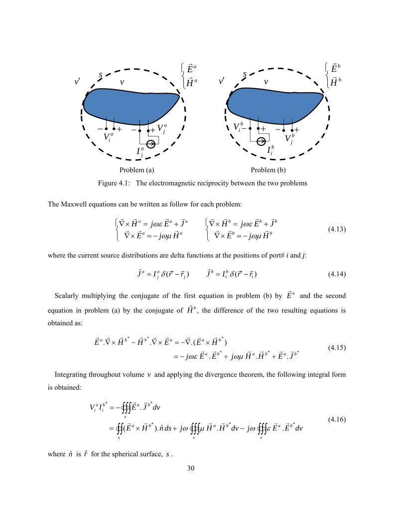
30
Problem (a) Problem (b)
Figure 4.1: The electromagnetic reciprocity between the two problems
The Maxwell equations can be written as follow for each problem:
⎩⎨⎧
−=×∇+=×∇
⎩⎨⎧
−=×∇+=×∇
bb
bbb
aa
aaa
HjEJEjH
HjEJEjH
rrr
rrrr
rrr
rrrr
ωμωε
ωμωε
(4.13)
where the current source distributions are delta functions at the positions of port# i and j:
)()( ibi
bj
aj
a rrIJrrIJ rrrrrr−′=−′= δδ (4.14)
Scalarly multiplying the conjugate of the first equation in problem (b) by aEr
and the second
equation in problem (a) by the conjugate of bHr
, the difference of the two resulting equations is
obtained as:
***
***
...
)(...bababa
baabba
JEHHjEEj
HEEHHErrrrrr
rrrrrrrrr
++−=
×∇−=×∇−×∇
ωμωε (4.15)
Integrating throughout volume v and applying the divergence theorem, the following integral form
is obtained:
∫∫∫∫∫∫∫∫
∫∫∫
−+×=
−=
v
ba
v
ba
s
ba
v
babi
ai
dvEEjdvHHjdsnHE
dvJEIV
***
**
..ˆ).(
.
rrrrrr
rr
εωμω (4.16)
where n is r for the spherical surface, s .
ajI
sv ⎩
⎨⎧
a
a
HEr
r
aiV
− + ajV− +
v′
biI
sv ⎩
⎨⎧
b
b
HEr
r
biV − +
bjV
− +
v′
31
The first term on right hand side is the interaction power of problems (a) and (b) which is
propagated outwards from the sphere s . The second and third terms also represent the interaction of
the electric and magnetic energies stored in volume v . Since the surface s is chosen to be the
smallest sphere surrounding the antenna structure, volume v would be a small volume over which
the interaction energies are calculated. Assuming that the electric and magnetic fields are not singular,
the interaction energies in volume v can be neglected:
∫∫ ×≈s
babi
ai dsnHEIV ˆ).( ** rr
(4.17)
Note that the EM fields are not singular in practical cases, and ignoring the difference between the
magnetic and electric interaction energies would be a valid assumption except for the mathematically
singular sources. The approximation (4.17) becomes an exact relationship if the interaction energies
in volume v are exactly zero. Such a case can be considered when the volume v is filled with PEC
or the spherical current sources form spherical antennas. Using the orthogonality relationships of the
spherical waves, it can be observed that if the different sets of SVWs are excited in problem (a) and
(b), (4.17) will be zero, and consequently, the voltage across port# i, aiV induced by the excitation of
port# j, becomes zero. Hence, the aforementioned criterion in (4.12) not only maximizes the system
capacity, but also alleviates the mutual coupling between the MIMO antenna elements. In the case
that the antenna elements excite the same SVWs, (4.17) can be used to approximately estimate the
mutual coupling between the antennas from the electromagnetic fields radiated by each MIMO
antenna element. It is only required to expand the fields in terms of the SVWs, and obtain the
coefficients. Then, using integrals known for the SVWs [46], the equation (4.17) provides an
approximation for the mutual coupling between the antenna elements. As mentioned before, the
weighting coefficients can also be adjusted so that the mutual coupling becomes zero even when the
same SVWs are excited by different MIMO antenna elements.
It should be emphasized that the expression (4.17) is obtained thanks to the orthogonality of the
SVWs in the near field region. The near field orthogonality of the SVWs lets us choose the smallest
sphere making the interaction energies negligible. The near field orthogonality results from the fact
that the electromagnetic fields are orthogonalized in the SVW approach, rather than the current
sources (which is the case in the characteristic modes). This can be thought of as an important
advantage of the SVW approach for the MIMO antenna design, which yields a low correlation
coefficient for the antenna elements and good isolation of the excitation ports.

32
4.4 Spherical MIMO Antenna Design
As discussed before, it is desired to find the current sources for the MIMO antenna elements whose
radiation field patterns satisfy the orthogonality condition given in (4.1). The current source
construction problem can be thought of as an inverse source problem which is defined as constructing
the current source localized within a limited space to generate a predefined radiated field [71-82]. In
the MIMO antenna case, the desired radiation fields are orthogonal SVWs generated by each of the
MIMO antenna elements. Consequently, by solving an inverse source problem for the radiated SVW
fields, the required current sources would be obtained for MIMO antenna elements which should be
located either inside the given volume space or on the surface surrounding the given space for the
antenna structure. Since the SVWs are defined in a spherical coordinate system, the spherical source
region is a convenient source domain to obtain the analytic solution of the current sources generating
the orthogonal radiation patterns. Therefore, the aim is to take advantage of the inverse source
problems in order to find the orthogonal current sources in the spherical volume and surface to be
used as the MIMO antenna elements.
Assuming that the current source is a square-integrable, it is proposed that the current source is
first expanded in terms of the prescribed vector functions, and then the coefficients of vector
functions are determined so that the source generates the desired radiation SVW fields. This
expansion is also consistent with the Spectral Theorem [83]. Based on the Spectral Theorem, if
)(£ EJrr
= in which £ is a self-adjoint operator, Jr
can be expanded in terms of the Eigen functions of
the operator £, which is commonly known as Eigen-decomposition. Since the aforementioned Lr
, Mr
,
and Nr
are the vector Eigen-functions of the vector Helmholtz equation, it is possible to simply
expand the Jr
in terms of the VWFs in the spherical coordinate system. Notice that the current source
can also be expanded in terms of the VWF in other coordinate systems as well, but since 1a cannot be
chosen for constructing the VWF, the orthogonal properties of the VWF will be lost. Thus, the
coefficient calculations in the current source will need more manipulations [80, 81].
The equations (4.10) and (4.11) show that the projections of the electric field on )4(Mr
and )4(Nr
are
proportional to the projections of the electric current source on )1(Mr
and )1(Nr
, respectively. This
observation suggests that the source can be expanded in terms of those )1(Mr
, )1(Nr
, and )1(Lr
functions which are finite at the origin. Therefore, Jr
is represented as:
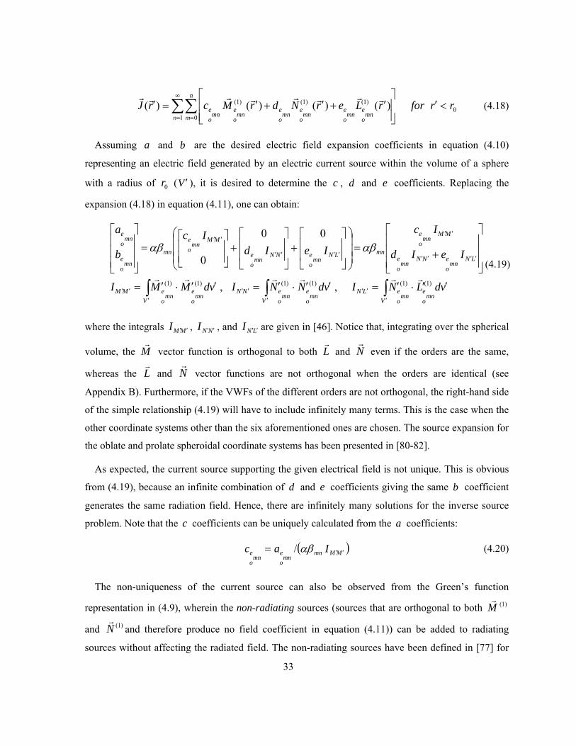
33
01 0
)1()1()1( )()()()( rrforrLerNdrMcrJn
n
m mnoe
mnoe
mnoe
mnoe
mnoe
mnoe <′
⎥⎥⎦
⎤
⎢⎢⎣
⎡′+′+′=′ ∑∑
∞
= =
rrrrrrrr (4.18)
Assuming a and b are the desired electric field expansion coefficients in equation (4.10)
representing an electric field generated by an electric current source within the volume of a sphere
with a radius of 0r (V ′ ), it is desired to determine the c , d and e coefficients. Replacing the
expansion (4.18) in equation (4.11), one can obtain:
∫∫∫′
′′′
′′′
′′
′′′′
′′
′′′′
′′
′′⋅′=′′⋅′=′′⋅′=
⎥⎥⎥
⎦
⎤
⎢⎢⎢
⎣
⎡
+=⎟⎟⎟
⎠
⎞
⎜⎜⎜
⎝
⎛
⎥⎥
⎦
⎤
⎢⎢
⎣
⎡+
⎥⎥
⎦
⎤
⎢⎢
⎣
⎡+
⎥⎥⎦
⎤
⎢⎢⎣
⎡=
⎥⎥⎥
⎦
⎤
⎢⎢⎢
⎣
⎡
Vmn
oe
mnoeLN
Vmn
oe
mnoeNN
Vmn
oe
mnoeMM
LNmn
oeNN
mnoe
MMmn
oe
mnLNmn
oeNN
mnoe
MMmn
oe
mn
mnoe
mnoe
vdLNIvdNNIvdMMI
IeId
Ic
IeIdIc
b
a
)1()1()1()1()1()1( ,,
00
0rrrrrr
αβαβ(4.19)
where the integrals MMI ′′ , NNI ′′ , and LNI ′′ are given in [46]. Notice that, integrating over the spherical
volume, the Mr
vector function is orthogonal to both Lr
and Nr
even if the orders are the same,
whereas the Lr
and Nr
vector functions are not orthogonal when the orders are identical (see
Appendix B). Furthermore, if the VWFs of the different orders are not orthogonal, the right-hand side
of the simple relationship (4.19) will have to include infinitely many terms. This is the case when the
other coordinate systems other than the six aforementioned ones are chosen. The source expansion for
the oblate and prolate spheroidal coordinate systems has been presented in [80-82].
As expected, the current source supporting the given electrical field is not unique. This is obvious
from (4.19), because an infinite combination of d and e coefficients giving the same b coefficient
generates the same radiation field. Hence, there are infinitely many solutions for the inverse source
problem. Note that the c coefficients can be uniquely calculated from the a coefficients:
( )MMmnmn
oe
mnoe Iac ′′= αβ/ (4.20)
The non-uniqueness of the current source can also be observed from the Green’s function
representation in (4.9), wherein the non-radiating sources (sources that are orthogonal to both )1(Mr
and )1(Nr
and therefore produce no field coefficient in equation (4.11)) can be added to radiating
sources without affecting the radiated field. The non-radiating sources have been defined in [77] for

34
the general inverse source problems. Hence, in addition to the liberty in choosing the d and e
coefficients, any combination of the non-radiating sources with the radiating ones can generate the
same radiation field.
Among the infinitely many possible solutions for Jr
, there is a particular minimum energy source
solution [76, 77]. To find this solution, let us assume that the source is square-integrable. The 2L
norm of the current source Jr
is then calculated as:
∫
∫ ∑∑
′′′
′
∞
= =′′′′′′′′
′′⋅′=
⎥⎥⎦
⎤
⎢⎢⎣
⎡+++=′
Vmn
oe
mnoeLL
V n
n
mLN
mnoe
mnoeLL
mnoeNN
mnoeMM
mnoe
vdLLI
IedIeIdIcvdJ
)1()1(
1 0
22222
rr
r
(4.21)
As mentioned before, the a coefficients will determine the c coefficients, but one has the liberty
to choose the d and e coefficients in such a way that the 2L norm is minimized:
⎟⎟
⎠
⎞
⎜⎜
⎝
⎛+=
⎪⎭
⎪⎬⎫
⎪⎩
⎪⎨⎧
++
′′′′
′′′′′′
LNmn
oeNN
mnoemn
mnoe
LNmn
oe
mnoeLL
mnoeNN
mnoe
IeIdbConst
IedIeIdMin
αβ:.
222
(4.22)
Solving the above simple minimization problem, the following coefficients are obtained to have the
minimum energy source:
( )NNmnmn
oe
mnoe
mnoe
Ibd
e
′′=
=
αβ/
0
(4.23)
Consequently, the minimum energy current source is represented as follows:
( ) ( )NNmn
mnoe
mnoeMMmn
mnoe
mnoe
n
n
m mnoe
mnoe
mnoe
mnoe
IbdIacwhere
rrforrNdrMcrJ
′′′′
∞
= =
==
<′⎥⎥⎦
⎤
⎢⎢⎣
⎡′′′+′′′=′ ∑∑
αβαβ
φθφθ
/,/:
),,(),,()( 01 0
)1()1(min
rrrr
(4.24)
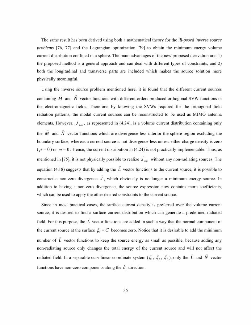
35
The same result has been derived using both a mathematical theory for the ill-posed inverse source
problems [76, 77] and the Lagrangian optimization [79] to obtain the minimum energy volume
current distribution confined in a sphere. The main advantages of the new proposed derivation are: 1)
the proposed method is a general approach and can deal with different types of constraints, and 2)
both the longitudinal and transverse parts are included which makes the source solution more
physically meaningful.
Using the inverse source problem mentioned here, it is found that the different current sources
containing Mr
and Nr
vector functions with different orders produced orthogonal SVW functions in
the electromagnetic fields. Therefore, by knowing the SVWs required for the orthogonal field
radiation patterns, the modal current sources can be reconstructed to be used as MIMO antenna
elements. However, minJr
, as represented in (4.24), is a volume current distribution containing only
the Mr
and Nr
vector functions which are divergence-less interior the sphere region excluding the
boundary surface, whereas a current source is not divergence-less unless either charge density is zero
( 0=ρ ) or 0=ω . Hence, the current distribution in (4.24) is not practically implementable. Thus, as
mentioned in [75], it is not physically possible to realize minJr
without any non-radiating sources. The
equation (4.18) suggests that by adding the Lr
vector functions to the current source, it is possible to
construct a non-zero divergence Jr
, which obviously is no longer a minimum energy source. In
addition to having a non-zero divergence, the source expression now contains more coefficients,
which can be used to apply the other desired constraints to the current source.
Since in most practical cases, the surface current density is preferred over the volume current
source, it is desired to find a surface current distribution which can generate a predefined radiated
field. For this purpose, the Lr
vector functions are added in such a way that the normal component of
the current source at the surface C=1ξ becomes zero. Notice that it is desirable to add the minimum
number of Lr
vector functions to keep the source energy as small as possible, because adding any
non-radiating source only changes the total energy of the current source and will not affect the
radiated field. In a separable curvilinear coordinate system ( 1ξ , 2ξ , 3ξ ), only the Lr
and Nr
vector
functions have non-zero components along the 1a direction:

36
( )
⎭⎬⎫
⎩⎨⎧
⎥⎦
⎤⎢⎣
⎡∂∂
∂∂
+⎥⎦
⎤⎢⎣
⎡∂∂
∂∂
−
=⎟⎠⎞
⎜⎝⎛ ×∇×∇=
∂∂
=
=
)(11)(11
ˆ1)(
)(1)(
)()()(),,(
31331
2
3332121
221
3
22321
13211
11
11
321
332211321
1
1
1
ψξξψ
ψξξψ
ξψψψ
ψξ
ψξ
ψψ
ξψξψξψξξξψ
ξξ
ξ
hhh
hhhh
hhh
hhhhk
h
ak
N
hL
rrr
r
(4.25)
Since ψ is the scalar Helmholtz equation solution, the following relationships can be written as
[45]:
0)(11
)(11)(11
0)(11
)(11)(11
23
33
33323
22
2222
22
11
1111
21
23
33
21
33321
222
31
223211
11
32
11321
=+⎥⎦
⎤⎢⎣
⎡∂∂
∂∂
+⎥⎦
⎤⎢⎣
⎡∂∂
∂∂
+⎥⎦
⎤⎢⎣
⎡∂∂
∂∂
=+⎥⎦
⎤⎢⎣
⎡∂∂
∂∂
+⎥⎦
⎤⎢⎣
⎡∂∂
∂∂
+⎥⎦
⎤⎢⎣
⎡∂∂
∂∂
kffh
ffh
ffh
or
khhh
hhh
hhh
hhhhhh
hhh
ψξξψ
ψξξψ
ψξξψ
ψξξψ
ψξξψ
ψξξψ
(4.26)
Knowing 11 =h and 211 ξ=f , as it was required for expression (4.6), and substituting (4.26) into
equation (4.25), the 1ξ components of the Lr
and Nr
vector functions on the surface of C=1ξ are
obtained as follows:
C
C
kk
N
L
=
=
⎟⎟⎠
⎞⎜⎜⎝
⎛⎥⎦
⎤⎢⎣
⎡∂∂
∂∂
+=
∂∂
=
1
1
1
1
)(1)(
)()(
11
21
12
11
2132
11
32
ξ
ξ
ξξ
ψξ
ξξξ
ψξψψ
ψξ
ψψ
r
r
(4.27)
Therefore, the 1ξ components of the Lr
and Nr
vector functions are in the form of )()( 3322 ξψξψ
over the surface of C=1ξ , and it is possible to add the Lr
vectors to the minimum energy volume
current source in such a way that the total 1ξ component of the current source is canceled out. In the

37
spherical coordinate system which has orthogonal VWFs, the surface current source SJr
is expanded
in terms of the SVWs on the surface of the sphere shell with a radius of 0r :
( )01 0
)1()1()1( ),,(),,(),,( rrrLerNdrMcJn
n
m mnoe
mnoe
mnoe
mnoe
mnoe
mnoeS −′
⎥⎥⎦
⎤
⎢⎢⎣
⎡′′′+′′′+′′′= ∑∑
∞
= =
δφθφθφθrrrr
(4.28)
Substituting equation (4.28) in (4.11), the following equation is obtained:
( ) [ ]
( )
[ ] [ ]{ }( )
[ ] [ ]{ }201
201
2020
0)1()1(
201
201
2020
0)1()1(
20
2000
)1()1(
)()()1()!()!(
)12(2)1(
)()()1()1()!()!(
)12(2)1(
)()1()!()!(
122)1(
rkjrkjrknnmnmn
n
vdrrLNI
rkjnrkjnrnnmnmn
n
vdrrNNI
rkjrnnmnmn
nvdrrMMI
IeId
Ic
b
a
nn
Vmn
oe
mnoeLN
nn
Vmn
oe
mnoeNN
nV
mnoe
mnoeMM
LNmn
oeNN
mnoe
MMmn
oe
mn
mnoe
mnoe
+−
′′′
+−
′′′
′′′
′′′′
′′
−+−+
++
=′−′′⋅′=
+++−+
++
=′−′′⋅′=
+−+
++=′−′′⋅′=
⎥⎥⎥
⎦
⎤
⎢⎢⎢
⎣
⎡
+=⎥⎥⎥
⎦
⎤
⎢⎢⎢
⎣
⎡
∫
∫
∫
πδ
δ
πδ
δ
πδδ
αβ
rr
rr
rr
(4.29)
where 0δ has been defined in equation (4.9), and the integrals are presented in [46]. Again, the c
coefficients are uniquely determined from a , whereas there are infinite choices for the d and e
coefficients. To have the a coefficients in the radiated fields, those radii for which 0)( 0 =rkjn
should be avoided to ensure non-zero MMI ′′ . Furthermore, LNI ′′ should be non-zero to have the liberty
of choosing the e coefficients. Therefore, those radii for which )()( 0101 rkjrkj nn +− ±= should also
be avoided.
As before, 0=e gives the minimum energy source, but the minimum energy source is not a
surface current distribution. Therefore, the minimum energy condition should be relaxed. Using
equation (4.27) for the spherical coordinate system and (4.29), the two following equations are
obtained:
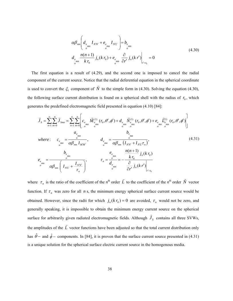
38
0)()()1(
0
00
=′′∂
∂+
+
=⎟⎟
⎠
⎞
⎜⎜
⎝
⎛+
=′
′′′′
rrn
mnoen
mnoe
mnoeLN
mnoeNN
mnoemn
rkjr
erkjrk
nnd
bIeIdαβ (4.30)
The first equation is a result of (4.29), and the second one is imposed to cancel the radial
component of the current source. Notice that the radial deferential equation in the spherical coordinate
is used to convert the 1ξ component of Nr
to the simple form in (4.30). Solving the equation (4.30),
the following surface current distribution is found on a spherical shell with the radius of 0r , which
generates the predefined electromagnetic field presented in equation (4.10) [84]:
( )
0
)(
)()1(
,
,,:
),,(),,(),,(
00
1 00
)1(0
)1(0
)1(
1 0
rrn
n
mnoe
mnoe
n
n
NNLNmn
mnoe
mnoe
nLNNNmn
mnoe
mnoe
MMmn
mnoe
mnoe
n
n
m mnoe
mnoe
mnoe
mnoe
mnoe
mnoe
n
n
mSmnS
rkjr
rkjrk
nn
d
e
II
be
II
bd
I
acwhere
rLerNdrMcJJ
=′
′′′′
′′′′′′
∞
= =
∞
= =
′′∂
∂
+
−==
⎟⎟⎠
⎞⎜⎜⎝
⎛+
=
+==
⎥⎥⎦
⎤
⎢⎢⎣
⎡′′+′′+′′== ∑∑∑∑
τ
ταβ
ταβαβ
φθφθφθrrrrr
(4.31)
where nτ is the ratio of the coefficient of the nth order Lr
to the coefficient of the nth order Nr
vector
function. If nτ was zero for all n s, the minimum energy spherical surface current source would be
obtained. However, since the radii for which 0)( 0 =rkjn are avoided, nτ would not be zero, and
generally speaking, it is impossible to obtain the minimum energy current source on the spherical
surface for arbitrarily given radiated electromagnetic fields. Although SJr
contains all three SVWs,
the amplitudes of the Lr
vector functions have been adjusted so that the total current distribution only
has −θ and −φ components. In [84], it is proven that the surface current source presented in (4.31)
is a unique solution for the spherical surface electric current source in the homogenous media.

39
Note that for certain radii, 0)(0=′∂′∂
=′ rrn rrkj , which means that the radial component of Lr
is
zero and it is impossible to cancel the radial component of the Nr
vector function. Hence, to obtain
the surface current distribution on the sphere, the radii for which the radial component of Lr
is equal
to zero must be avoided. As it was emphasized before, a finite number of SVWs appear at the far
field. Thus, )()( 0101 rkjrkj nn +− ±≠ , 0)( 0 ≠rkjn and 0)(0≠′∂′∂
=′ rrn rrkj should be satisfied for
only a finite number of modes ( 0krNn =< ). Hence, these conditions are not too restrictive.
The surface current sources SmnJr
in (4.31) are more practical than the volumetric source, and
generate orthogonal radiating EM fields. Consequently, any element or any disjoint subset (any subset
with no element in common) of the derived SmnJr
current sources where Nn < can be used as a
MIMO antenna element in the uniform PAS. Moreover, any combination of mnJr
and non-radiating
sources will create a new arrangement of MIMO antenna elements. Although the practical
implementation of the spherical current sources is not discussed here, there are various practical
approaches in the literature to implement spherical antennas [85-88]. The recent fabrication
technologies and procedures proposed in [87] and [88] can be employed to implement surface current
sources on a spherical dielectric. The derived formulation (4.31) can be used to determine the surface
current distributions required to design spherical antennas for orthogonal MIMO radiations.
Considering a proper non-radiating source, it is possible to form and design the MIMO antenna
elements to be compatible with the desired constraints. The constraint considered here is set to have a
spherical surface source, but the non-radiating source can be employed for other constraints such as
reactive power [79]. Including the numerical analysis of the VWFs, the proposed approach can be
generalized for the arbitrary shape of the antennas in which the non-radiating sources are considered
to satisfy the required constraint for the given geometry.
4.5 Planar MIMO Antenna Design
In comparison to 3-dimentional (3D) antennas such as the spherical sources, the planar antennas of
various shapes are of greater interest due to their inherent advantages, such as the ease of construction
and integration, the low cost, the low profile configuration, and the compactness. Therefore, the
investigation to how the planar current source can be used as a MIMO antenna element and how the
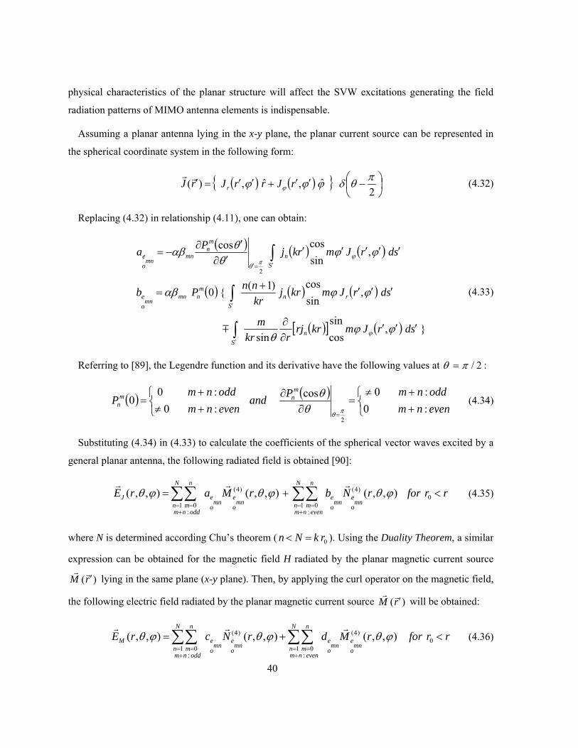
40
physical characteristics of the planar structure will affect the SVW excitations generating the field
radiation patterns of MIMO antenna elements is indispensable.
Assuming a planar antenna lying in the x-y plane, the planar current source can be represented in
the spherical coordinate system in the following form:
( ) ( ){ } ⎟⎠⎞
⎜⎝⎛ −′′+′′=′
2ˆ,ˆ,)( πθδϕϕϕ ϕ rJrrJrJ r
rr (4.32)
Replacing (4.32) in relationship (4.11), one can obtain:
( ) ( ) ( )
( ) ( ) ( )
( )[ ] ( ) },cossin
sin
,sincos)1({0
,sincoscos
2
sdrJmkrrjrkr
m
sdrJmkrjkrnnPb
sdrJmrkjPa
nS
rnS
mnmn
mnoe
nS
mn
mnmn
oe
′′′∂∂
′′′+=
′′′′′′∂
′∂−=
∫
∫
∫
′
′
′=′
ϕϕθ
ϕϕαβ
ϕϕθ
θαβ
ϕ
ϕπθ
m
(4.33)
Referring to [89], the Legendre function and its derivative have the following values at 2/πθ = :
( ) ( )⎩⎨⎧
++≠
=∂
∂
⎩⎨⎧
+≠+
==
evennmoddnmPand
evennmoddnm
Pm
nmn :0
:0cos:0:0
02πθθ
θ (4.34)
Substituting (4.34) in (4.33) to calculate the coefficients of the spherical vector waves excited by a
general planar antenna, the following radiated field is obtained [90]:
rrforrNbrMarEmn
oe
mnoe
evennm
N
n
n
mmnoe
mnoe
oddnm
N
n
n
mJ <+=
+= =
+= =
∑∑∑∑ 0)4(
:1 0
)4(
:1 0
),,(),,(),,( ϕθϕθϕθrrr
(4.35)
where N is determined according Chu’s theorem ( 0rkNn =< ). Using the Duality Theorem, a similar
expression can be obtained for the magnetic field H radiated by the planar magnetic current source
)(rM rr′ lying in the same plane (x-y plane). Then, by applying the curl operator on the magnetic field,
the following electric field radiated by the planar magnetic current source )(rM rr′ will be obtained:
rrforrMdrNcrEmn
oe
mnoe
evennm
N
n
n
mmnoe
mnoe
oddnm
N
n
n
mM <+=
+= =
+= =
∑∑∑∑ 0)4(
:1 0
)4(
:1 0
),,(),,(),,( ϕθϕθϕθrrr
(4.36)

41
Equations (4.35) and (4.36) show that a planar electric or magnetic current source is not able to
excite particular SVWs [90]. For a given bandwidth and the size of an antenna, the planar antenna
structure will excite approximately half of the spherical harmonics which can potentially be excited
by a 3D current source. Since the field radiation pattern of the antenna elements are dependent on the
SVWs propagated by the antenna, the degrees of freedom to orthogonalize the field radiation pattern
of the MIMO antenna elements is decreased for a planar current source (antenna).
More importantly, since at least one of the orders, either m or n, is different in (4.35) and (4.36), it
can be concluded that the planar electric and magnetic current sources lying in the same plane radiate
orthogonal electromagnetic fields. This conclusion can be used for the MIMO antenna designs. If the
electric and magnetic current sources can be implemented on the same plane, each current source can
be used as one MIMO antenna element. To verify this idea, one simple antenna, compromising of
both magnetic and electric current sources in the same plane is depicted in Figure 4.2. The designed
MIMO antenna contains a ring slot antenna, modeled by the ring magnetic current, and a half-
wavelength dipole antenna which can be represented by the electric current source. The S-parameters
of the designed MIMO antenna are illustrated in Figure 4.3.
Figure 4.2: MIMO antenna design containing magnetic and electric currents in the x-y plane
Ground Plane
Antenna substrate: RO4003-
60mil
Feed substrate: RO4003-
20mil
R=19mm
L=40mm
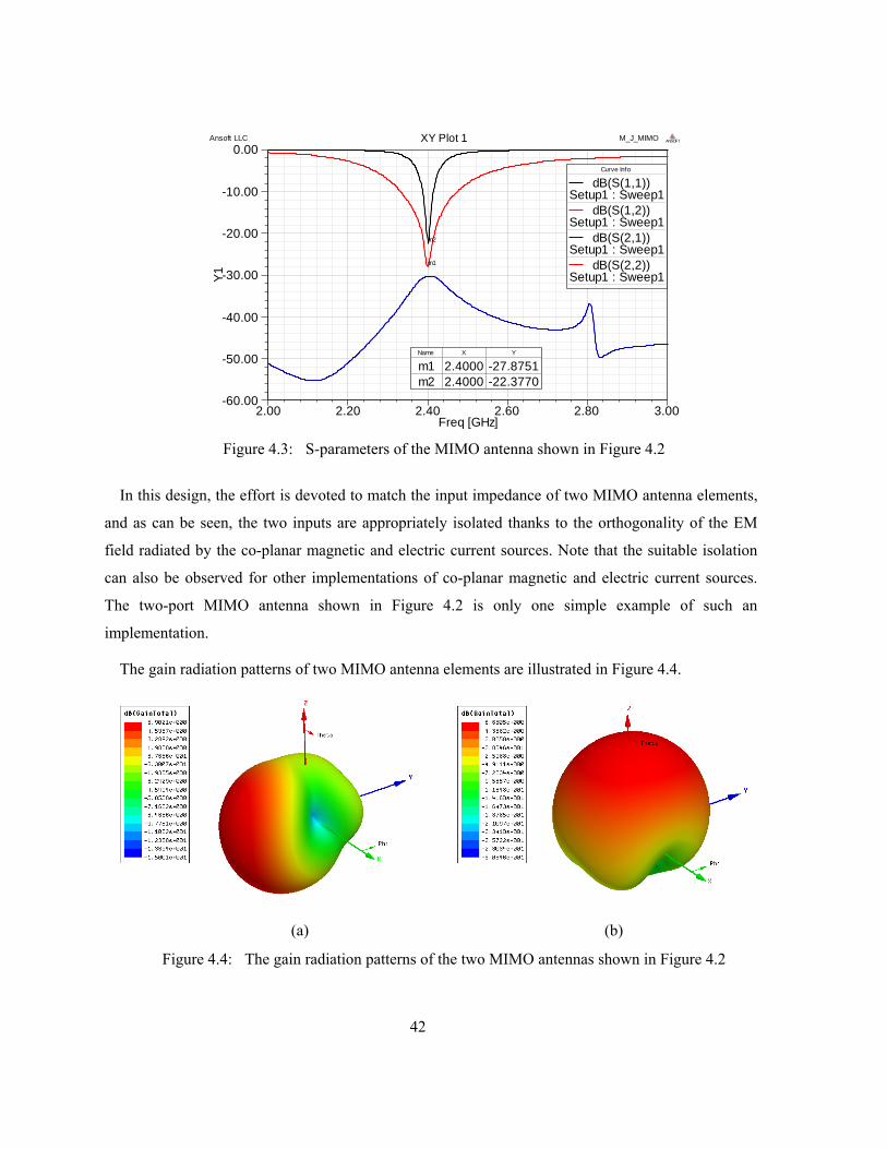
42
Figure 4.3: S-parameters of the MIMO antenna shown in Figure 4.2
In this design, the effort is devoted to match the input impedance of two MIMO antenna elements,
and as can be seen, the two inputs are appropriately isolated thanks to the orthogonality of the EM
field radiated by the co-planar magnetic and electric current sources. Note that the suitable isolation
can also be observed for other implementations of co-planar magnetic and electric current sources.
The two-port MIMO antenna shown in Figure 4.2 is only one simple example of such an
implementation.
The gain radiation patterns of two MIMO antenna elements are illustrated in Figure 4.4.
(a) (b)
Figure 4.4: The gain radiation patterns of the two MIMO antennas shown in Figure 4.2
2.00 2.20 2.40 2.60 2.80 3.00Freq [GHz]
-60.00
-50.00
-40.00
-30.00
-20.00
-10.00
0.00
Y1
Ansoft LLC M_J_MIMOXY Plot 1 ANSOFT
m1
m2
Curve Info
dB(S(1,1))Setup1 : Sweep1
dB(S(1,2))Setup1 : Sweep1
dB(S(2,1))Setup1 : Sweep1
dB(S(2,2))Setup1 : Sweep1
Name X Y
m1 2.4000 -27.8751m2 2.4000 -22.3770
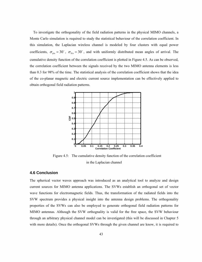
43
To investigate the orthogonality of the field radiation patterns in the physical MIMO channels, a
Monte Carlo simulation is required to study the statistical behaviour of the correlation coefficient. In
this simulation, the Laplacian wireless channel is modeled by four clusters with equal power
coefficients, o30=nφσ , o30=nθσ , and with uniformly distributed mean angles of arrival. The
cumulative density function of the correlation coefficient is plotted in Figure 4.5. As can be observed,
the correlation coefficient between the signals received by the two MIMO antenna elements is less
than 0.3 for 98% of the time. The statistical analysis of the correlation coefficient shows that the idea
of the co-planar magnetic and electric current source implementation can be effectively applied to
obtain orthogonal field radiation patterns.
Figure 4.5: The cumulative density function of the correlation coefficient
in the Laplacian channel
4.6 Conclusion
The spherical vector waves approach was introduced as an analytical tool to analyze and design
current sources for MIMO antenna applications. The SVWs establish an orthogonal set of vector
wave functions for electromagnetic fields. Thus, the transformation of the radiated fields into the
SVW spectrum provides a physical insight into the antenna design problems. The orthogonality
properties of the SVWs can also be employed to generate orthogonal field radiation patterns for
MIMO antennas. Although the SVW orthognality is valid for the free space, the SVW behaviour
through an arbitrary physical channel model can be investigated (this will be discussed in Chapter 5
with more details). Once the orthogonal SVWs through the given channel are know, it is required to
0 0.05 0.1 0.15 0.2 0.25 0.3 0.35 0.40
0.1
0.2
0.3
0.4
0.5
0.6
0.7
0.8
0.9
1
Correlation Coefficient
CD
F

44
obtain the current sources (antennas) which excite the predefined SVWs as vector field radiations of
the MIMO antenna elements. One of the main contributions of this research is to analytically solve
the inverse surface source problem by including the non-radiating sources in current source solution.
Using the non-radiating current sources, the modal surface current sources are obtained on a sphere to
excite the desired SVWs. The spherical surface source formulation contributes in the designing of the
spherical antennas for MIMO applications.
Additionally, the analytical representations of the current source distributions were studied for
planar antennas, and it is shown that the co-planar magnetic and electric current sources generate
orthogonal vector field radiation patterns. This observation was used to design a two-port planar
MIMO antenna. A statistical analysis of the correlation coefficient was also presented for the
Laplacian channel model to investigate the orthogonality of the vector field radiation patterns in
different realizations of the non-uniform channels.
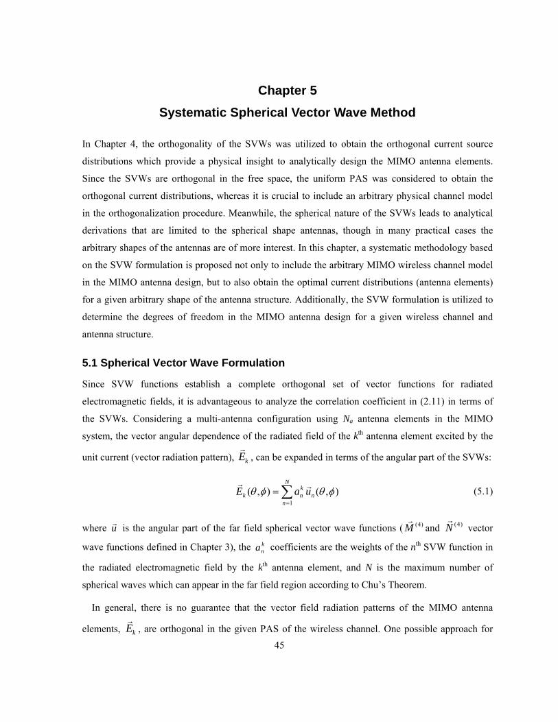
45
Chapter 5 Systematic Spherical Vector Wave Method
In Chapter 4, the orthogonality of the SVWs was utilized to obtain the orthogonal current source
distributions which provide a physical insight to analytically design the MIMO antenna elements.
Since the SVWs are orthogonal in the free space, the uniform PAS was considered to obtain the
orthogonal current distributions, whereas it is crucial to include an arbitrary physical channel model
in the orthogonalization procedure. Meanwhile, the spherical nature of the SVWs leads to analytical
derivations that are limited to the spherical shape antennas, though in many practical cases the
arbitrary shapes of the antennas are of more interest. In this chapter, a systematic methodology based
on the SVW formulation is proposed not only to include the arbitrary MIMO wireless channel model
in the MIMO antenna design, but to also obtain the optimal current distributions (antenna elements)
for a given arbitrary shape of the antenna structure. Additionally, the SVW formulation is utilized to
determine the degrees of freedom in the MIMO antenna design for a given wireless channel and
antenna structure.
5.1 Spherical Vector Wave Formulation
Since SVW functions establish a complete orthogonal set of vector functions for radiated
electromagnetic fields, it is advantageous to analyze the correlation coefficient in (2.11) in terms of
the SVWs. Considering a multi-antenna configuration using Na antenna elements in the MIMO
system, the vector angular dependence of the radiated field of the kth antenna element excited by the
unit current (vector radiation pattern), kEr
, can be expanded in terms of the angular part of the SVWs:
∑=
=N
nn
knk uaE
1),(),( φθφθ rr
(5.1)
where ur is the angular part of the far field spherical vector wave functions ( )4(Mr
and )4(Nr
vector
wave functions defined in Chapter 3), the kna coefficients are the weights of the nth SVW function in
the radiated electromagnetic field by the kth antenna element, and N is the maximum number of
spherical waves which can appear in the far field region according to Chu’s Theorem.
In general, there is no guarantee that the vector field radiation patterns of the MIMO antenna
elements, kEr
, are orthogonal in the given PAS of the wireless channel. One possible approach for

46
orthogonalization is to combine the vector field radiations of the MIMO antenna elements with
different sets of current excitations to obtain the orthogonal vector field radiation patterns through the
given PAS. Hence, the MIMO system mode, denoted by iFr
, is defined as the vector field radiation
pattern of the MIMO antenna structure when the vector field radiation patterns of the MIMO antenna
elements are weighted by the complex current excitations and combined to form an orthogonal vector
field radiation pattern. Assuming kiI is the current excitation of the kth antenna elements in the ith
MIMO system mode, iFr
can be written as:
∑∑ ∑∑ ∑∑== == ==
==⎟⎟⎠
⎞⎜⎜⎝
⎛=⎟
⎠
⎞⎜⎝
⎛==
N
nn
in
N
nn
N
k
kn
ki
N
k
N
nn
kn
ki
N
kk
kii uuaIuaIEIF
aaa
11 11 11),(),(),( φθαφθφθ rrrrr
(5.2)
where ka is the SVW expansion coefficients of kEr
, and inα is the contribution of the nth spherical
wave in the vector radiation pattern of the ith MIMO system mode. If the vector field radiation pattern
of each antenna element is supposed to be used as one MIMO system mode, iFr
is simply kEr
.
Note that if kEr
is considered as the radiated field of an individual antenna in the presence of other
antenna elements, the mutual coupling effects can also be included in the SVW expansion
coefficients, ka . Thus, the proposed formulation is general and can effectively include the
electromagnetic interactions between the antenna elements and other objects in the vicinity.
Rewriting (5.2) in the matrix form as shown in (5.3), the matrix M is constructed such that the kth
row of M contains the coefficients of the SVWs excited by the kth antenna element [54]:
⎥⎥⎥⎥⎥⎥
⎦
⎤
⎢⎢⎢⎢⎢⎢
⎣
⎡
=
⎥⎥⎥⎥⎥⎥
⎦
⎤
⎢⎢⎢⎢⎢⎢
⎣
⎡
=
⎥⎥⎥⎥⎥⎥
⎦
⎤
⎢⎢⎢⎢⎢⎢
⎣
⎡
=
⎥⎥⎥⎥⎥⎥
⎦
⎤
⎢⎢⎢⎢⎢⎢
⎣
⎡
=
=
),(
),(
),(1
1
1
111
1
1
1111
φθ
φθ
φθ
N
k
NN
N
kN
k
N
NMM
Nii
N
M
i
u
u
u
aa
aa
aa
II
II
II
F
F
F
aaa
a
a
rM
rM
r
L
MM
L
MM
L
L
MM
L
MM
L
rM
rM
r
WMIF
IMWF
(5.3)
where M is the number of orthogonal MIMO system modes (M sets of current excitations), which
should be considered as the degrees of freedom for the MIMO antenna system. Using the SVW
47
representation (5.3), the inner product of iFr
and jFr
, which is defined in (2.11), can be written as
follows [54]:
⎥⎥⎥⎥⎥⎥
⎦
⎤
⎢⎢⎢⎢⎢⎢
⎣
⎡
><><
><><
><><
=
=><=>< ∑∑= =
PNNPN
PpNPp
PNP
jiPpn
N
n
N
p
jp
inPji
uuuu
uuuu
uuuu
uuFF
rrL
rrMM
rrL
rrMM
rrL
rr
rrrr
,,
,,
,,
)()(,,
1
1
111
1 1
*
G
IMGIM †αα
(5.4)
where i)(IM stands for the ith row of matrix IM , and contains inα . The defining interaction matrix,
R, whose element, ijR , is the interaction of the ith and jth MIMO system modes through the given
PAS, Pji FF ><rr
, , one can obtain:
( ) ( )
⎥⎥⎥⎥⎥⎥
⎦
⎤
⎢⎢⎢⎢⎢⎢
⎣
⎡
==
MMM
iMi
M
RR
RR
RR
L
MM
L
MM
L
1
1
111
RIMGIMR † (5.5)
After calculating the interaction matrix, R, the correlation coefficients between the MIMO system
modes can be obtained by (2.11). Therefore, the correlation coefficient is represented in terms of the
inner products of known spherical vector waves, and once the inner products are investigated for a
specific PAS associated with a specific wireless environment, the α coefficients, which are entries of
the matrix IM , are enough to calculate the cross-correlation between the MIMO system modes.
Notice that the kna coefficients in the matrix M depend on the physical properties including the
size, the location, the orientation and the material of the MIMO antenna elements. Also, the matrix
G entries, which are the inner products of the SVWs through the given PAS, are independent of the
MIMO antennas. Hence, the SVW representation (5.5) separates the complex current excitations
(feed circuit), the physical properties of antenna elements, and the wireless communication
environment effects into I , M , and G matrices, respectively. Therefore, for a given PAS, the

48
matrix G can be evaluated independently of MIMO antenna design, and the optimization criteria can
be imposed on the M and I entries rather than iFr
and jFr
which are θ- and φ-dependent functions.
Accordingly, the M matrix can be optimized first, and once an optimal choice for the antenna
configuration and physical properties is made in terms of the practical restrictions, the current
excitations can either be optimized to generate different MIMO system modes or be adaptively
changed in a time-varying environment (adaptive MIMO antenna system).
The SVW representation can be used to find the maximum number of MIMO system modes, M,
and the M sets of the current excitations, matrix I , which results in the diagonal matrix R to achieve
maximum system capacity. For this purpose, the matrix orthogonalization methods such as the Eigen-
value decomposition can be used to find the conditions on the matrix I so that the matrix R is
diagonal [91, 92].
Since *),(, PijPji uuuu ><=><rrrr
, G is the Hermitian matrix [83]. Additionally, since the inner
product of †IMGIM iiii FF )()(, =><rr
is physically interpreted as the received power by the ith
MIMO system mode for the given PAS, the matrix G is a positive-definite matrix [48, 83].
Therefore, the singular value decomposition of matrix G can be written as:
†QDQG = (5.6)
where Q is the unitary matrix and D is a diagonal matrix whose diagonal entries are real positive
values. Then replacing (5.6) in representation (5.5) and defining matrix Z , one can obtain:
( )( ) 2/1MQDZIZIZR † == where (5.7)
For a given PAS, the matrix G can be calculated, and the Q and D matrices can be obtained
through singular value decomposition. The matrix M is also constructed from the SVW expansion of
the vector field radiation patterns of the MIMO antenna elements. Thus, the matrix Z can be
obtained for the MIMO antenna structure in a certain wireless environment. The SVD of matrix Z
can be used to diagonalize the matrix R:
†USVZ = (5.8)
where U and V are unitary matrices and S is a diagonal matrix whose diagonal entries are singular
values of Z (the root of Eigen values of the matrix R). Therefore, choosing †UI = for the complex
49
current excitations makes the rows of the matrix IZ orthogonal yielding to the diagonal matrix R [91, 92]. Note that the calculated current excitations are implemented through an RF feed circuit
rather than via baseband signal processing. Thus, the proposed approach optimizes the EM
characteristics of the MIMO antenna system to make the channel transfer matrix diagonal, whereas in
conventional spatial multiplexing, the antenna properties are fixed and considered as part of wireless
channel.
The rank of the matrix Z determines the maximum achievable number of MIMO system modes.
The singular values of Z , which are the diagonal elements of the matrix S , also represent the root of
the power gains of the corresponding MIMO system modes. Therefore, the calculated singular values
show how strong the designed MIMO system mode is in receiving or transmitting the signals through
the wireless environment. In the case that a transmitter has the knowledge of the channel, the water-
filling may be used to allocate higher or lower power levels to lower or higher power gain MIMO
system modes, respectively [1, 2, 10], in order to maximize the system capacity. However, in the case
of the formulation (2.5) in which it is assumed the transmitter does not know the channel state
information, the maximum capacity is obtained when the power gains of the MIMO system modes
are equalized as much as possible. To increase the rank of the matrix Z and equalize the singular
values, the matrix M can be manipulated by optimizing the physical properties of the MIMO antenna
elements. Since there are restrictions to optimize the physical properties in many practical cases, the
best effort should be performed to achieve the maximum number of MIMO system modes with
equalized power gains.
To summarize the proposed systematic method to find the optimal MIMO system modes supported
by the given antenna structure, the design procedure would entail in the following steps [54]:
1- For the given wireless environment, the matrix G should be evaluated, and the Q and D
matrices should be obtained by the SVD of the matrix G .
2- Using the physical properties of the MIMO antenna elements, the radiated field of the
individual MIMO antenna elements should be expanded in terms of the SVWs to form matrix
M as represented in (5.3). The rank and singular values of the matrix 2/1QDMZ = determine
the maximum number of effective MIMO system modes, M. Therefore, the physical properties
of the MIMO antenna elements included in the matrix M can be designed so that M is
increased and the power gains of the M MIMO system modes are equalized. If the matrix M

50
can be optimized so that the orthogonal MIMO system modes are achieved with the identity
matrix I , there is no need to obtain optimal current excitations. However, the physical
properties of the antenna elements may be constrained in many practical cases so that the
diagonal matrix R may not be achieved by manipulating the matrix M only.
3- Once the physical properties of the antenna elements are fixed, the complex current excitations
in the matrix I should be determined to obtain the diagonal matrix R. Decomposing the
matrix Z into †USVZ = using the SVD method, it is found the optimal choice for current
excitations is †UI = which makes the rows of the matrix IZ orthogonal and maximizes the
system capacity. Since there are M number of orthogonal MIMO system modes, the optimal
sets of current excitation are achieved by M different rows of the matrix †UI = . Note that the
matrix I will be a unitary matrix. Therefore, ∑=
aN
k
kiI
1
2 remains identical for the current
excitations fed into the antenna elements in various MIMO system modes.
This formulation provides a systematic method to designing the MIMO antenna elements to
achieve orthogonal signals through the given wireless environment. As mentioned before, the SVW
formulation separates the MIMO channel effect, the physical properties of MIMO antenna elements,
and the complex current excitations provided by the feed circuit into three cascaded matrices. In the
next sections, it will be shown how each matrix presented in the SVW formulation can be used to
design and analyze the MIMO antenna systems in wireless environments.
5.2 MIMO Channel Analysis
The matrix G represented in (5.4) contains the inner products of the SVWs through the PAS for a
wireless environment. Therefore, the inner products can be evaluated independently of the MIMO
antenna structure, and the MIMO channel effects on the orthogonality of the SVWs can be
investigated prior to designing the MIMO antenna elements. Once the SVW behaviour through the
physical environment is known, the MIMO antenna elements can be intelligently designed so that the
orthogonal signals are obtained through the MIMO system modes. For instance, in the case of the
uniform PAS, the matrix G is a diagonal matrix. Therefore, different sets of SVWs can provide the
orthogonal field radiation patterns for the MIMO antenna elements, as discussed in Chapter 4.
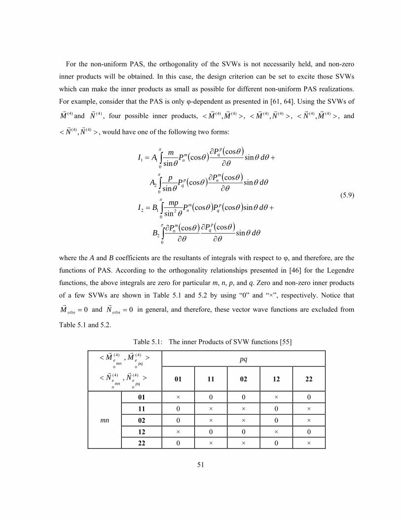
51
For the non-uniform PAS, the orthogonality of the SVWs is not necessarily held, and non-zero
inner products will be obtained. In this case, the design criterion can be set to excite those SVWs
which can make the inner products as small as possible for different non-uniform PAS realizations.
For example, consider that the PAS is only φ-dependent as presented in [61, 64]. Using the SVWs of )4(M
rand )4(N
r, four possible inner products, >< )4()4( ,MM
rr, >< )4()4( , NM
rr, >< )4()4( ,MN
rr, and
>< )4()4( , NNrr
, would have one of the following two forms:
( ) ( )
( ) ( )
( ) ( )
( ) ( )θθ
θθ
θθ
θθθθθ
θθθ
θθθ
θθθ
θθ
θ
π
π
π
π
dPPB
dPPmpBI
dPPpA
dP
PmAI
pq
mn
pq
mn
mnp
q
pqm
n
sincoscos
sincoscossin
sincoscossin
sincos
cossin
02
0212
02
011
∂∂
∂∂
+=
∂∂
+∂
∂=
∫
∫
∫
∫
(5.9)
where the A and B coefficients are the resultants of integrals with respect to φ, and therefore, are the
functions of PAS. According to the orthogonality relationships presented in [46] for the Legendre
functions, the above integrals are zero for particular m, n, p, and q. Zero and non-zero inner products
of a few SVWs are shown in Table 5.1 and 5.2 by using “0” and “×”, respectively. Notice that
00 =noMr
and 00 =noNr
in general, and therefore, these vector wave functions are excluded from
Table 5.1 and 5.2.
Table 5.1: The inner Products of SVW functions [55]
><
><
)4()4(
)4()4(
,
,
pqoe
mnoe
pqoe
mnoe
NN
MM
rr
rr
pq
01 11 02 12 22
mn
01 × 0 0 × 0 11 0 × × 0 × 02 0 × × 0 × 12 × 0 0 × 0 22 0 × × 0 ×
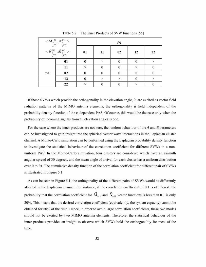
52
Table 5.2: The inner Products of SVW functions [55]
><
><
)4()4(
)4()4(
,
,
pqoe
mnoe
pqoe
mnoe
MN
NM
rr
rr
pq
01 11 02 12 22
mn
01 0 × 0 0 × 11 × 0 0 × 0 02 0 0 0 × 0 12 0 × × 0 × 22 × 0 0 × 0
If those SVWs which provide the orthogonality in the elevation angle, θ, are excited as vector field
radiation patterns of the MIMO antenna elements, the orthogonality is held independent of the
probability density function of the φ-dependent PAS. Of course, this would be the case only when the
probability of incoming signals from all elevation angles is one.
For the case where the inner products are not zero, the random behaviour of the A and B parameters
can be investigated to gain insight into the spherical vector wave interactions in the Laplacian cluster
channel. A Monte-Carlo simulation can be performed using the Laplacian probability density function
to investigate the statistical behaviour of the correlation coefficient for different SVWs in a non-
uniform PAS. In the Monte-Carlo simulation, four clusters are considered which have an azimuth
angular spread of 30 degrees, and the mean angle of arrival for each cluster has a uniform distribution
over 0 to 2π. The cumulative density function of the correlation coefficient for different pair of SVWs
is illustrated in Figure 5.1.
As can be seen in Figure 5.1, the orthogonality of the different pairs of SVWs would be differently
affected in the Laplacian channel. For instance, if the correlation coefficient of 0.1 is of interest, the
probability that the correlation coefficient for 11eMr
and 01eNr
vector functions is less than 0.1 is only
20%. This means that the desired correlation coefficient (equivalently, the system capacity) cannot be
obtained for 80% of the time. Hence, in order to avoid large correlation coefficients, these two modes
should not be excited by two MIMO antenna elements. Therefore, the statistical behaviour of the
inner products provides an insight to observe which SVWs hold the otrthogonality for most of the
time.

53
Figure 5.1: The CDF of the correlation coefficient between various SVWs
for a Laplacian PAS [55]
The advantage of the SVW method is the fact that the CDF curves are independent of the antenna
elements. It is only required to calculate these curves once for each SVW pair to construct the matrix
G , and then design the MIMO antenna elements in such a way that they excite the appropriate
SVWs. For instance, the analytic method proposed in Chapter 4 can be used to obtain the current
distributions exciting those SVWs whose orthogonality is not sensitive to the wireless channel. This
way, low correlation coefficients will be obtained for an acceptable percentage of time. However, in
order to have an efficient MIMO system, it should be possible to adaptively update current excitations
according to the channel variations by using phase shifters and switches in the feed circuit of the
MIMO antennas. Alternatively, deterministic physical channel models such as the ray tracing model
can be used to rigorously calculate the PAS for specific classes of wireless environments. In this case,
a deterministic matrix G is obtained and can be used for calculating the Q and D matrices in (5.6).
5.3 Optimal Current Excitations of MIMO Antennas
In this section, the approach formulated in Section 5.1 is applied to practical multi-antenna
configurations where the MIMO antenna elements are given, and it is desired to find optimal current
excitations generating the orthogonal MIMO system modes for the given MIMO antenna structure
and wireless channel.
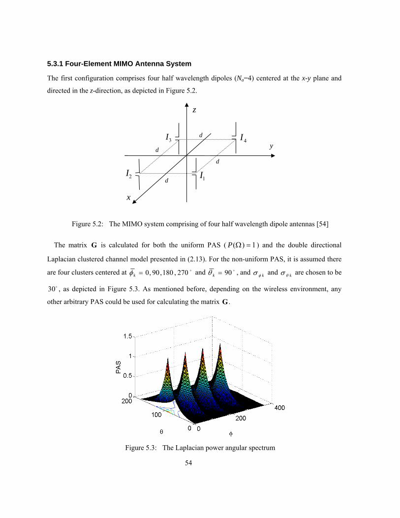
54
5.3.1 Four-Element MIMO Antenna System
The first configuration comprises four half wavelength dipoles (Na=4) centered at the x-y plane and
directed in the z-direction, as depicted in Figure 5.2.
Figure 5.2: The MIMO system comprising of four half wavelength dipole antennas [54]
The matrix G is calculated for both the uniform PAS ( 1)( =ΩP ) and the double directional
Laplacian clustered channel model presented in (2.13). For the non-uniform PAS, it is assumed there
are four clusters centered at o270,180,90,0=kφ and o90=kθ , and kφσ and kθσ are chosen to be
o30 , as depicted in Figure 5.3. As mentioned before, depending on the wireless environment, any
other arbitrary PAS could be used for calculating the matrix G .
Figure 5.3: The Laplacian power angular spectrum
3I 4I
2I 1I
z
y
d
x
d
d
d
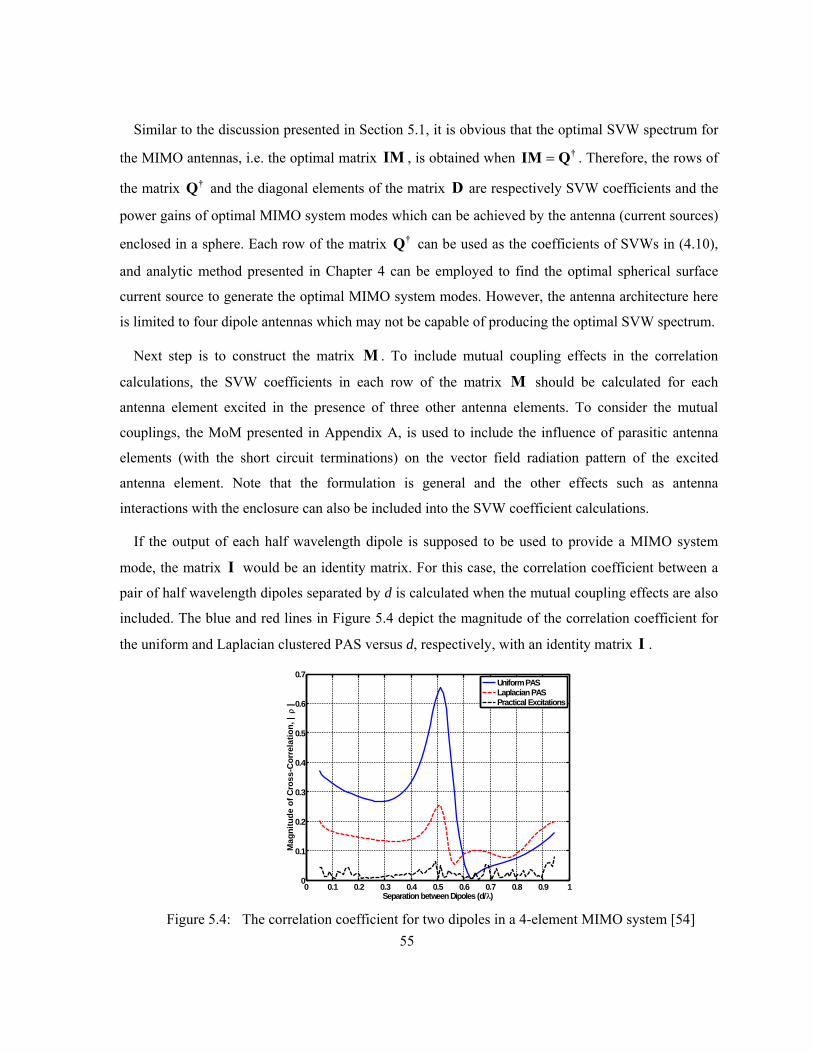
55
Similar to the discussion presented in Section 5.1, it is obvious that the optimal SVW spectrum for
the MIMO antennas, i.e. the optimal matrix IM , is obtained when †QIM = . Therefore, the rows of
the matrix †Q and the diagonal elements of the matrix D are respectively SVW coefficients and the
power gains of optimal MIMO system modes which can be achieved by the antenna (current sources)
enclosed in a sphere. Each row of the matrix †Q can be used as the coefficients of SVWs in (4.10),
and analytic method presented in Chapter 4 can be employed to find the optimal spherical surface
current source to generate the optimal MIMO system modes. However, the antenna architecture here
is limited to four dipole antennas which may not be capable of producing the optimal SVW spectrum.
Next step is to construct the matrix M . To include mutual coupling effects in the correlation
calculations, the SVW coefficients in each row of the matrix M should be calculated for each
antenna element excited in the presence of three other antenna elements. To consider the mutual
couplings, the MoM presented in Appendix A, is used to include the influence of parasitic antenna
elements (with the short circuit terminations) on the vector field radiation pattern of the excited
antenna element. Note that the formulation is general and the other effects such as antenna
interactions with the enclosure can also be included into the SVW coefficient calculations.
If the output of each half wavelength dipole is supposed to be used to provide a MIMO system
mode, the matrix I would be an identity matrix. For this case, the correlation coefficient between a
pair of half wavelength dipoles separated by d is calculated when the mutual coupling effects are also
included. The blue and red lines in Figure 5.4 depict the magnitude of the correlation coefficient for
the uniform and Laplacian clustered PAS versus d, respectively, with an identity matrix I .
Figure 5.4: The correlation coefficient for two dipoles in a 4-element MIMO system [54]
0 0.1 0.2 0.3 0.4 0.5 0.6 0.7 0.8 0.9 10
0.1
0.2
0.3
0.4
0.5
0.6
0.7
Separation between Dipoles (d/λ)
Mag
nitu
de o
f Cro
ss-C
orre
latio
n, |
ρ |
Uniform PASLaplacian PASPractical Excitations
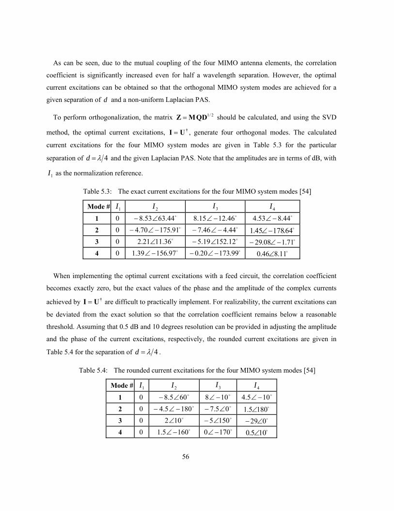
56
As can be seen, due to the mutual coupling of the four MIMO antenna elements, the correlation
coefficient is significantly increased even for half a wavelength separation. However, the optimal
current excitations can be obtained so that the orthogonal MIMO system modes are achieved for a
given separation of d and a non-uniform Laplacian PAS.
To perform orthogonalization, the matrix 2/1QDMZ = should be calculated, and using the SVD
method, the optimal current excitations, †UI = , generate four orthogonal modes. The calculated
current excitations for the four MIMO system modes are given in Table 5.3 for the particular
separation of 4λ=d and the given Laplacian PAS. Note that the amplitudes are in terms of dB, with
1I as the normalization reference.
Table 5.3: The exact current excitations for the four MIMO system modes [54]
Mode # 1I 2I 3I 4I
1 0 o44.6353.8 ∠− o46.1215.8 −∠ o44.853.4 −∠
2 0 o91.17570.4 −∠− o44.446.7 −∠− o64.17845.1 −∠ 3 0 o36.1121.2 ∠ o12.15219.5 ∠− o71.108.29 −∠− 4 0 o97.15639.1 −∠ o99.17320.0 −∠− o11.846.0 ∠
When implementing the optimal current excitations with a feed circuit, the correlation coefficient
becomes exactly zero, but the exact values of the phase and the amplitude of the complex currents
achieved by †UI = are difficult to practically implement. For realizability, the current excitations can
be deviated from the exact solution so that the correlation coefficient remains below a reasonable
threshold. Assuming that 0.5 dB and 10 degrees resolution can be provided in adjusting the amplitude
and the phase of the current excitations, respectively, the rounded current excitations are given in
Table 5.4 for the separation of 4λ=d .
Table 5.4: The rounded current excitations for the four MIMO system modes [54]
Mode # 1I 2I 3I 4I
1 0 o605.8 ∠− o108 −∠ o105.4 −∠
2 0 o1805.4 −∠− o05.7 ∠− o1805.1 ∠ 3 0 o102∠ o1505∠− o029∠− 4 0 o1605.1 −∠ o1700 −∠ o105.0 ∠
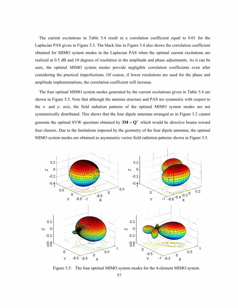
57
The current excitations in Table 5.4 result in a correlation coefficient equal to 0.01 for the
Laplacian PAS given in Figure 5.3. The black line in Figure 5.4 also shows the correlation coefficient
obtained for MIMO system modes in the Laplacian PAS when the optimal current excitations are
realized at 0.5 dB and 10 degrees of resolution in the amplitude and phase adjustments. As it can be
seen, the optimal MIMO system modes provide negligible correlation coefficients even after
considering the practical imperfections. Of course, if lower resolutions are used for the phase and
amplitude implementations, the correlation coefficient will increase.
The four optimal MIMO system modes generated by the current excitations given in Table 5.4 are
shown in Figure 5.5. Note that although the antenna structure and PAS are symmetric with respect to
the x- and y- axis, the field radiation patterns of the optimal MIMO system modes are not
symmetrically distributed. This shows that the four dipole antennas arranged as in Figure 5.2 cannot
generate the optimal SVW spectrum obtained by †QIM = which would be directive beams toward
four clusters. Due to the limitations imposed by the geometry of the four dipole antennas, the optimal
MIMO system modes are obtained as asymmetric vector field radiation patterns shown in Figure 5.5.
Figure 5.5: The four optimal MIMO system modes for the 4-element MIMO system
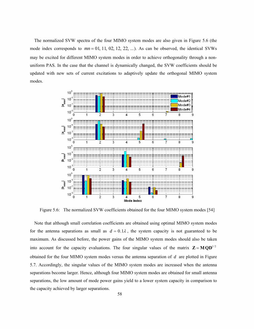
58
The normalized SVW spectra of the four MIMO system modes are also given in Figure 5.6 (the
mode index corresponds to ...,22,12,02,11,01=mn ). As can be observed, the identical SVWs
may be excited for different MIMO system modes in order to achieve orthogonality through a non-
uniform PAS. In the case that the channel is dynamically changed, the SVW coefficients should be
updated with new sets of current excitations to adaptively update the orthogonal MIMO system
modes.
Figure 5.6: The normalized SVW coefficients obtained for the four MIMO system modes [54]
Note that although small correlation coefficients are obtained using optimal MIMO system modes
for the antenna separations as small as λ1.0=d , the system capacity is not guaranteed to be
maximum. As discussed before, the power gains of the MIMO system modes should also be taken
into account for the capacity evaluations. The four singular values of the matrix 2/1QDMZ =
obtained for the four MIMO system modes versus the antenna separation of d are plotted in Figure
5.7. Accordingly, the singular values of the MIMO system modes are increased when the antenna
separations become larger. Hence, although four MIMO system modes are obtained for small antenna
separations, the low amount of mode power gains yield to a lower system capacity in comparison to
the capacity achieved by larger separations.

59
Figure 5.7: The singular values of optimal MIMO system modes in the Laplacian PAS
It is also notable that three of the MIMO system modes are dominant in very small antenna
separations and that the other mode becomes stronger when the antennas’ separation is increased.
Therefore, even though the rank of the matrix Z is four for small separations, there are three MIMO
system modes that dominantly contribute in increasing the system capacity of MIMO system. For
design purposes, those antenna separations should be chosen so that the power gains of all the MIMO
system modes are as identical as possible.
5.3.2 Multi-port Patch Antenna
In the previous example, a fixed PAS was considered, and the optimal MIMO system modes were
obtained to achieve the maximized system capacity for the given structure. However, in various
environments, the wireless channel dynamically varies over the time and there is no guarantee that the
calculated MIMO system modes for a certain channel would be orthogonal in other channel
realizations. As mentioned, the current excitations can be adaptively updated to maintain the
orthogonality over the time. Alternatively, the statistical behaviour of the channel realizations can be
investigated, and the MIMO system modes can be obtained accordingly.
In this subsection, the SVW approach is employed to effectively optimize the feed circuit of the
MIMO antenna system for a dynamic channel environment. The multi-port patch antenna is a suitable
candidate for the MIMO antenna elements which provide the pattern orthogonality. Multi-port patch
0 0.2 0.4 0.6 0.8 10
0.005
0.01
0.015
0.02
0.025
0.03
0.035
0.04
Separation between the Dipoles (d/λ)
Sing
ular
Val
ues
S1S2S3S4

60
antennas have been investigated in [68, 93]. It has been shown that the orthogonal radiation patterns
can be obtained by exciting the different modes of the patch antennas. Using the orthogonal
properties of the radiation patterns, the MIMO antennas can be designed to provide small correlation
coefficients. As a practical example, a two-port circular patch antenna has been designed at 2.4 GHz
in HFSS. The circular patch geometry and simulated S-parameters are shown in Figure 5.8.
(a)
(b)
Figure 5.8: A two-port circular patch antenna; (a) antenna geometry (b) simulated S-parameters
R=19mm
Ground Plane
Antenna substrate: RO4003-
60mil
Feed substrate: RO4003-
20mil
Excitation pin
Microstrip feed circuit in
the bottom

61
As can be seen, both ports are matched at the operating frequency, and the isolation between the
ports is more than 45dB. Using (2.12), the correlation coefficient of the MIMO signals provided by
the two-port circular patch is almost zero. Accordingly, the vector field radiation patterns should be
orthogonal in the uniform PAS. The simulated gain radiation patterns are presented in Figure 5.9 and
5.10 when port# 1 and 2 are excited, respectively. The simulated gain radiation patterns verify that the
two MIMO system modes, generated by the two ports of the circular patch antenna are orthogonal in
both polarization and the space. Accordingly, a low correlation coefficient is expected in even the
non-uniform channels. To investigate how the MIMO system performance is affected in the physical
wireless channel, the statistical behaviour of the correlation coefficient is studied for the Laplacian
clustered channel model.
(a)
(b)
Figure 5.9: (a) The gain radiation patterns for two φ-planes when port#1 in Figure 5.8.a is
excited, (b) The 3D gain radiation patterns when port#1 in Figure 5.8.a is excited
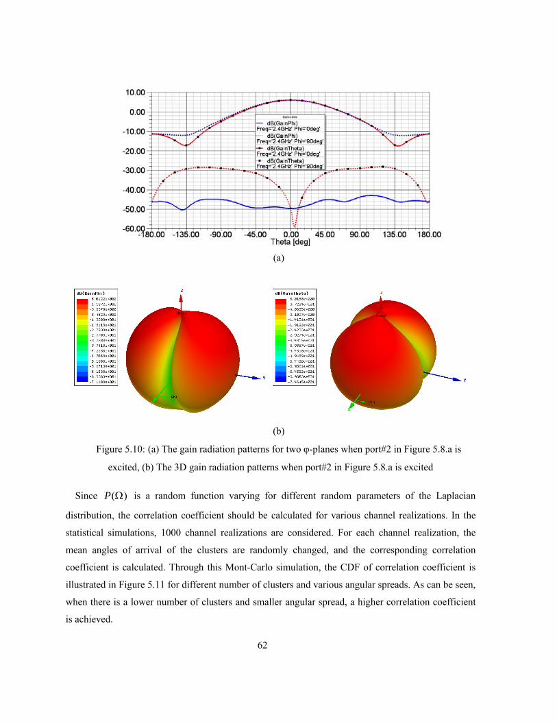
62
(a)
(b)
Figure 5.10: (a) The gain radiation patterns for two φ-planes when port#2 in Figure 5.8.a is
excited, (b) The 3D gain radiation patterns when port#2 in Figure 5.8.a is excited
Since )(ΩP is a random function varying for different random parameters of the Laplacian
distribution, the correlation coefficient should be calculated for various channel realizations. In the
statistical simulations, 1000 channel realizations are considered. For each channel realization, the
mean angles of arrival of the clusters are randomly changed, and the corresponding correlation
coefficient is calculated. Through this Mont-Carlo simulation, the CDF of correlation coefficient is
illustrated in Figure 5.11 for different number of clusters and various angular spreads. As can be seen,
when there is a lower number of clusters and smaller angular spread, a higher correlation coefficient
is achieved.
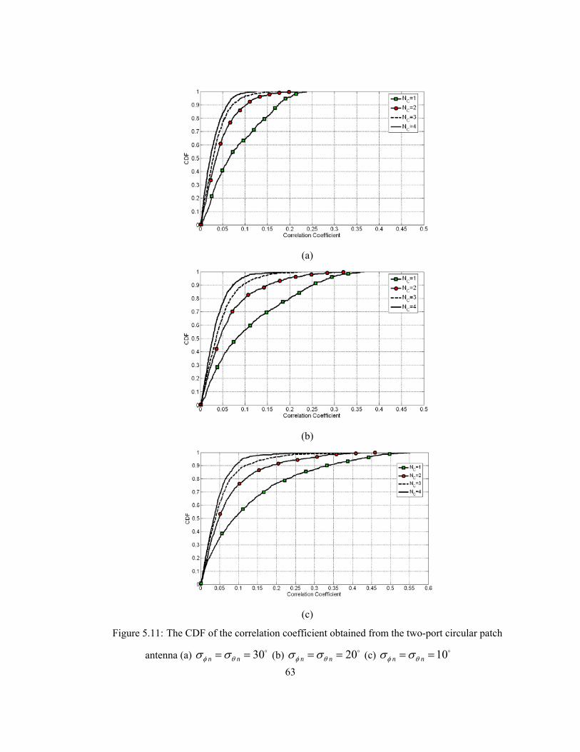
63
(a)
(b)
(c)
Figure 5.11: The CDF of the correlation coefficient obtained from the two-port circular patch
antenna (a) o30== nn θφ σσ (b) o20== nn θφ σσ (c) o10== nn θφ σσ

64
Accordingly, if the desired correlation coefficient is chosen to be 0.1, the correlation coefficient is
less than 0.1 for 64%, 56%, and 53% of the time for one cluster channel with an angular spread of
30o, 20o, and 10o, respectively. Therefore, in the worst case scenario, which is one cluster with an
angular spread of 10o, the desired system capacity cannot be achieved for 47% of the time, and the
maximum correlation of 0.55 may occur. Hence, even though the MIMO vector radiation patterns are
orthogonal in the uniform PAS, the desired system capacity is lost for a high percentage of the time in
the physical wireless channel.
Obtaining the optimum complex current excitations for the two-port circular patch antenna, it is
shown that the percentage of time for which the correlation coefficient is less than the desired value
can be enhanced. Following the proposed SVW formulation, the first step is to find the matrix G for
a certain channel realization, and then, determine the complex currents accordingly. Since the
calculated current excitations result in a zero correlation coefficient for the corresponding channel
realization, it is critical to choose the appropriate channel realization for which the matrix G should
be calculated. One reasonable choice is the worst channel realization in which the highest value of
correlation coefficient is achieved. According to Figure 5.11, three largest correlation coefficients are
0.55, 0.52, and 0.51 for 1, 2, and 3 clusters with an angular spread of 10o. Hence, the Laplacian
distribution in (2.13) with the PAS parameters corresponding to the three chosen large correlation
coefficients are used as )(ΩP to calculate the entries of the matrix G . Notice that the calculated
matrices G are attributed to the chosen PASs and are independent of the MIMO antenna elements.
The next step is to construct the matrix M for a two-port circular patch. In this case, the MIMO
antenna elements are the identical circular patch antenna excited through different ports. Therefore,
the matrix M will have two rows; each row contains SVW coefficients of the vector field radiation
pattern excited by each port when the other port is matched. The SVW coefficients are obtained by
expanding the HFSS simulation results given in Figure 5.9 and 5.10 in terms of the SVWs. Knowing
the matrix M for the two-port circular patch and the G matrices for the three severe channel
realizations, the optimal complex currents of the exciting ports are obtained, and the feed circuit can
be designed appropriately.
To obtain †UI = as the optimum current excitation matrix, the matrix Z should be calculated.
Calculating the matrix Z and using SVD, the three optimal complex current excitations to achieve
zero correlation coefficient through three chosen channel realizations are obtained.

65
(a)
(b)
Figure 5.12: The two-port circular patch antenna with the optimal feed circuit;
(a) antenna geometry (b) simulated S-parameters
The average of the current excitations obtained for severe channel realizations is calculated as:
R=19mm
Ground Plane
Antenna substrate:
RO4003-60mil
Feed substrate: RO4003-20mil
Excitation pin
Microstrip Rat-Race feed circuit in the bottom

66
⎥⎦
⎤⎢⎣
⎡
−∠∠∠∠
=oo
oo
8.1705.00707.02.178707.00705.0
I (5.10)
The calculated current excitation matrix can be implemented by the Rat-Race circuit. The Rat-Race
circuit is designed and optimized in the Advanced Design System (ADS), and then is imported into the
HFSS. Attaching the designed feed circuit to the two-port circular patch antenna, the antenna
geometry and simulated S-parameters are shown in Figure 5.12. Since the two ports are matched and
isolated, the S-parameter based formulation results in an almost zero correlation coefficient. By
exciting each input port of the feed circuit when the other port is matched, the vector field radiation
patterns of two MIMO system modes are obtained. The simulated gain radiation patterns are shown in
Figure 5.13 and 5.14.
(a)
(b)
Figure 5.13: (a) The gain radiation patterns for two φ-planes when port#1 in Figure 5.12.a is
excited, (b) The 3D gain radiation patterns when port#1 in Figure 5.12.a is excited

67
(a)
(b)
Figure 5.14: (a) The gain radiation patterns for two φ-planes when port#2 in Figure 5.12.a is
excited, (b) The 3D gain radiation patterns when port#2 in Figure 5.12.a is excited
Expanding the field radiation patterns given in Figure 5.13 and 5.14 in terms of the SVWs and
performing the Mont-Carlo simulation for the Laplacian clustered channel model, the CDF curves of
the correlation coefficient are depicted in Figure 5.15. As can be seen, the correlation coefficient is
less sensitive to the number of clusters in comparison to the case where no feed circuit was used. The
maximum possible value of the correlation coefficient is also decreased to 0.43. More importantly,
the percentage of time for which the correlation is less than 0.1 has been significantly increased. For
instance, the correlation coefficient is less than 0.1 for 93%, 78%, and 73% of the time, for one
cluster channel that has an angular spread of 30o, 20o, and 10o, respectively. Significant improvements
in the time percentages are also observed for other number of clusters as well. Therefore, including
the wireless channel effects in the MIMO system mode design can efficiently provide the desired
system capacity for higher percentage of time in the MIMO antenna system.

68
(a)
(b)
(c)
Figure 5.15: The CDF of the correlation coefficient for the two-port circular patch antenna with
an optimal feed circuit (a) o30== nn θφ σσ (b) o20== nn θφ σσ (c) o10== nn θφ σσ

69
5.4 Optimal Current Distributions for MIMO Antenna Systems
In the previous section, the physical geometry of the antenna elements are known, and the SVW
approach is utilized to exploit the maximum degrees of freedom of the wireless channel for
communicating the information data. However, one important aspect of the MIMO antenna design is
to investigate what antenna elements are optimal in terms of practical restrictions for the MIMO
application. To design the optimal MIMO antenna elements, the starting point is obtaining the
optimal current distributions radiating the optimal MIMO system modes for the given antenna
geometry and the physical channel. Once the optimal currents are known, the MIMO antenna
elements should be designed in such a way that each antenna element or a combination of them
imitates one optimal current source. Hence, the optimal current distributions can essentially provide a
benchmark for the MIMO antenna design in terms of the given restrictions.
The proposed SVW approach can also be employed to achieve the optimal current distributions if
the current distributions in the given geometry are generally represented in terms of infinitesimal
current sources:
∑=
−+
−+
−=
P
p
pipz
pipy
pipx
iopt z
rrr
Iyr
rrIx
rrr
IJ1
2)(
,2)(
,2)(
,)( ˆ
sin)(
ˆsin
)(ˆ
sin)(
θδ
θδ
θδ rrrrrr
r (5.11)
where )(ioptJr
is the optimal current distribution for the ith MIMO system mode, prr is the position vector
pointing the geometry in which the current distributions are to be obtained, P is the number of grid
points to represent the current distributions, and )(,iplI is the weighting coefficient of infinitesimal
current source directed in the l direction ( xl ˆˆ = , y , or z ) at the pth grid point. Note that if the
number of grid points is more than a certain threshold the current results would not change as
expected based on the Sampling Theorem. Assuming an arbitrary volume or surface, Figure 5.16
shows the infinitesimal current sources placed at the grid points for two examples. Considering
representation (5.11), each delta function current source can play the role of one antenna element in
the SVW formulation, and the weighting coefficients can be thought of as the current excitations of
the MIMO antenna elements. Accordingly, each row of the matrix M , which are the SVW
coefficients of the radiated field by each delta function source, can be directly obtained from (4.11) in
which Jr
is replaced by lrr pˆ)( rr
−δ . Therefore, the matrix M will only depend on the grid point
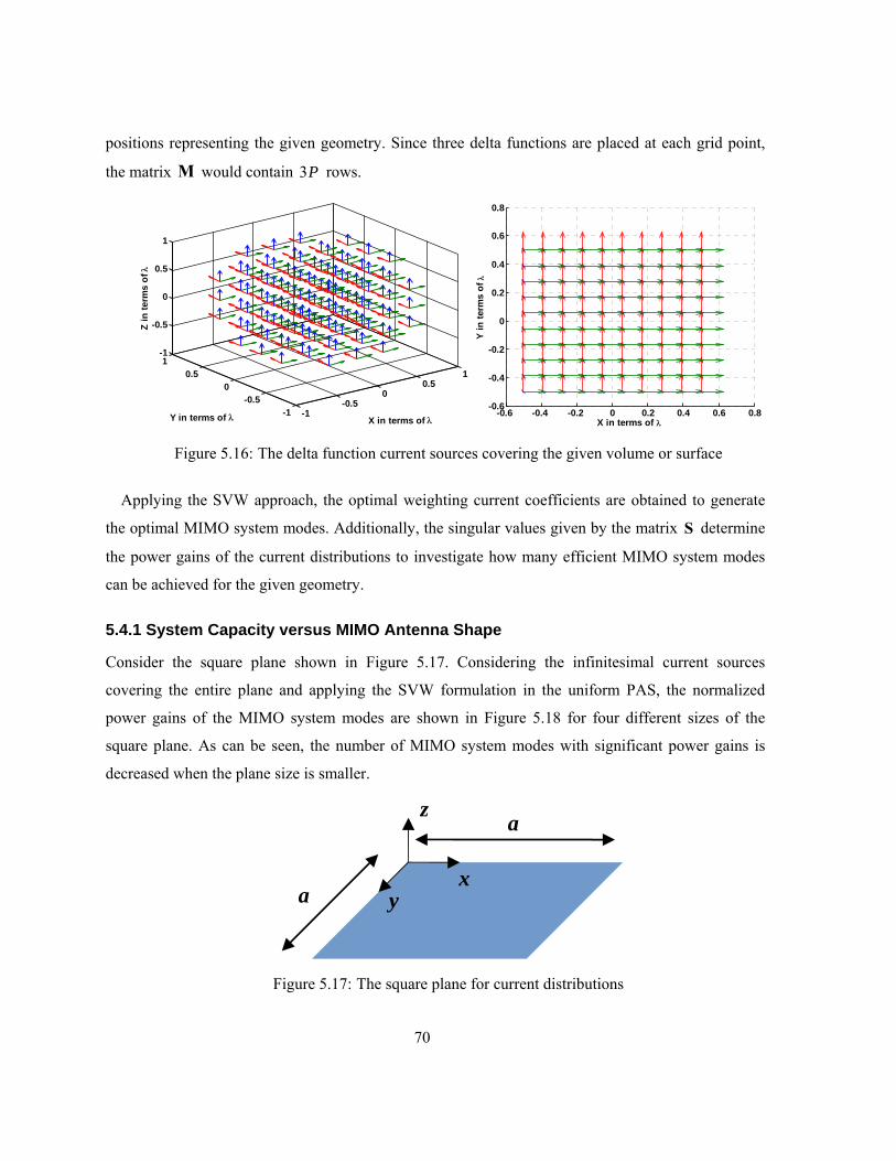
70
positions representing the given geometry. Since three delta functions are placed at each grid point,
the matrix M would contain P3 rows.
Figure 5.16: The delta function current sources covering the given volume or surface
Applying the SVW approach, the optimal weighting current coefficients are obtained to generate
the optimal MIMO system modes. Additionally, the singular values given by the matrix S determine
the power gains of the current distributions to investigate how many efficient MIMO system modes
can be achieved for the given geometry.
5.4.1 System Capacity versus MIMO Antenna Shape
Consider the square plane shown in Figure 5.17. Considering the infinitesimal current sources
covering the entire plane and applying the SVW formulation in the uniform PAS, the normalized
power gains of the MIMO system modes are shown in Figure 5.18 for four different sizes of the
square plane. As can be seen, the number of MIMO system modes with significant power gains is
decreased when the plane size is smaller.
Figure 5.17: The square plane for current distributions
-1-0.5
00.5
1
-1-0.5
00.5
1-1
-0.5
0
0.5
1
X in terms of λY in terms of λ
Z in
term
s of
λ
-0.6 -0.4 -0.2 0 0.2 0.4 0.6 0.8-0.6
-0.4
-0.2
0
0.2
0.4
0.6
0.8
X in terms of λ
Y in
term
s of
λ
a
a
z
yx
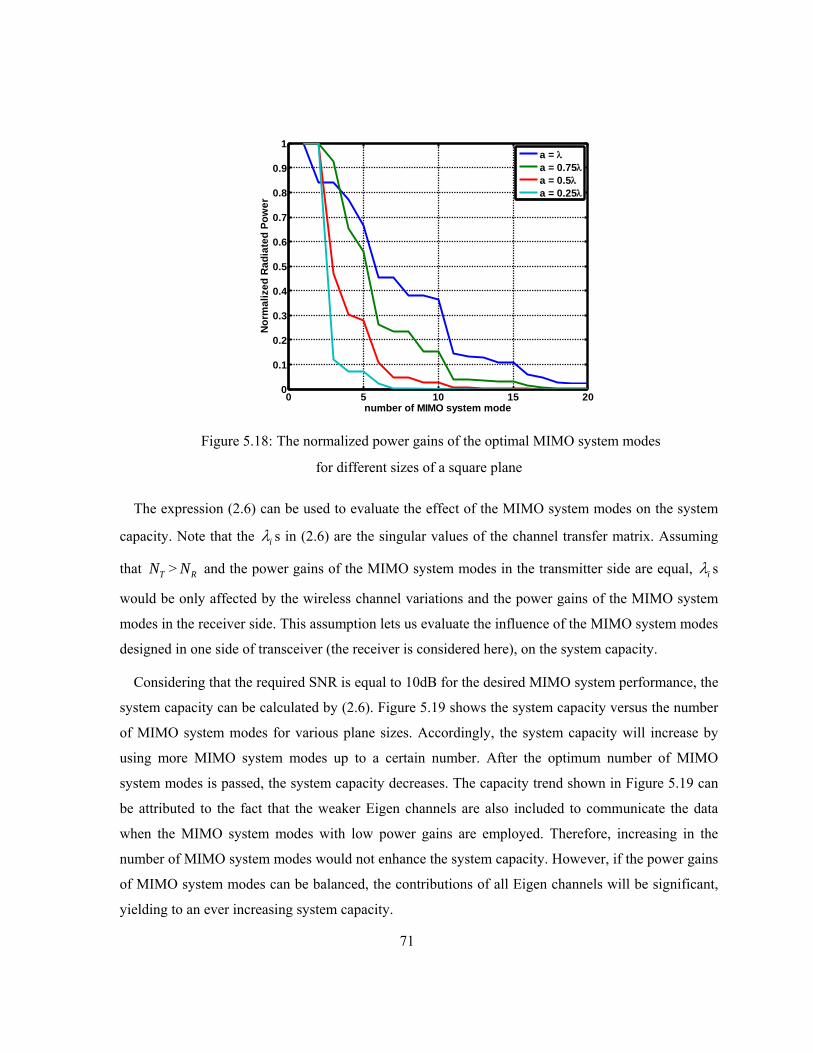
71
Figure 5.18: The normalized power gains of the optimal MIMO system modes
for different sizes of a square plane
The expression (2.6) can be used to evaluate the effect of the MIMO system modes on the system
capacity. Note that the iλ s in (2.6) are the singular values of the channel transfer matrix. Assuming
that TN > RN and the power gains of the MIMO system modes in the transmitter side are equal, iλ s
would be only affected by the wireless channel variations and the power gains of the MIMO system
modes in the receiver side. This assumption lets us evaluate the influence of the MIMO system modes
designed in one side of transceiver (the receiver is considered here), on the system capacity.
Considering that the required SNR is equal to 10dB for the desired MIMO system performance, the
system capacity can be calculated by (2.6). Figure 5.19 shows the system capacity versus the number
of MIMO system modes for various plane sizes. Accordingly, the system capacity will increase by
using more MIMO system modes up to a certain number. After the optimum number of MIMO
system modes is passed, the system capacity decreases. The capacity trend shown in Figure 5.19 can
be attributed to the fact that the weaker Eigen channels are also included to communicate the data
when the MIMO system modes with low power gains are employed. Therefore, increasing in the
number of MIMO system modes would not enhance the system capacity. However, if the power gains
of MIMO system modes can be balanced, the contributions of all Eigen channels will be significant,
yielding to an ever increasing system capacity.
0 5 10 15 200
0.1
0.2
0.3
0.4
0.5
0.6
0.7
0.8
0.9
1
number of MIMO system mode
Nor
mal
ized
Rad
iate
d Po
wer
a = λa = 0.75λa = 0.5λa = 0.25λ
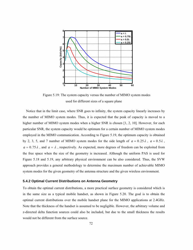
72
Figure 5.19: The system capacity versus the number of MIMO system modes
used for different sizes of a square plane
Notice that in the limit case, where SNR goes to infinity, the system capacity linearly increases by
the number of MIMO system modes. Thus, it is expected that the peak of capacity is moved to a
higher number of MIMO system modes when a higher SNR is chosen [1, 2, 10]. However, for each
particular SNR, the system capacity would be optimum for a certain number of MIMO system modes
employed in the MIMO communication. According to Figure 5.19, the optimum capacity is obtained
by 2, 3, 5, and 7 number of MIMO system modes for the side length of λ25.0=a , λ5.0=a ,
λ75.0=a , and λ=a , respectively. As expected, more degrees of freedom can be exploited from
the free space when the size of the geometry is increased. Although the uniform PAS is used for
Figure 5.18 and 5.19, any arbitrary physical environment can be also considered. Thus, the SVW
approach provides a general methodology to determine the maximum number of achievable MIMO
system modes for the given geometry of the antenna structure and the given wireless environment.
5.4.2 Optimal Current Distributions on Antenna Geometry
To obtain the optimal current distributions, a more practical surface geometry is considered which is
in the same size as a typical mobile handset, as shown in Figure 5.20. The goal is to obtain the
optimal current distributions over the mobile handset plane for the MIMO applications at 2.4GHz.
Note that the thickness of the handset is assumed to be negligible. However, the arbitrary volume and
z-directed delta function sources could also be included, but due to the small thickness the results
would not be different from the surface source.
0 10 20 30 40 50 600
1
2
3
4
5
6
7
8
Cap
acity
(bit/
s/H
z)
Number of MIMO System Modes
a = λa = 0.75λa = 0.5λa = 0.25λ
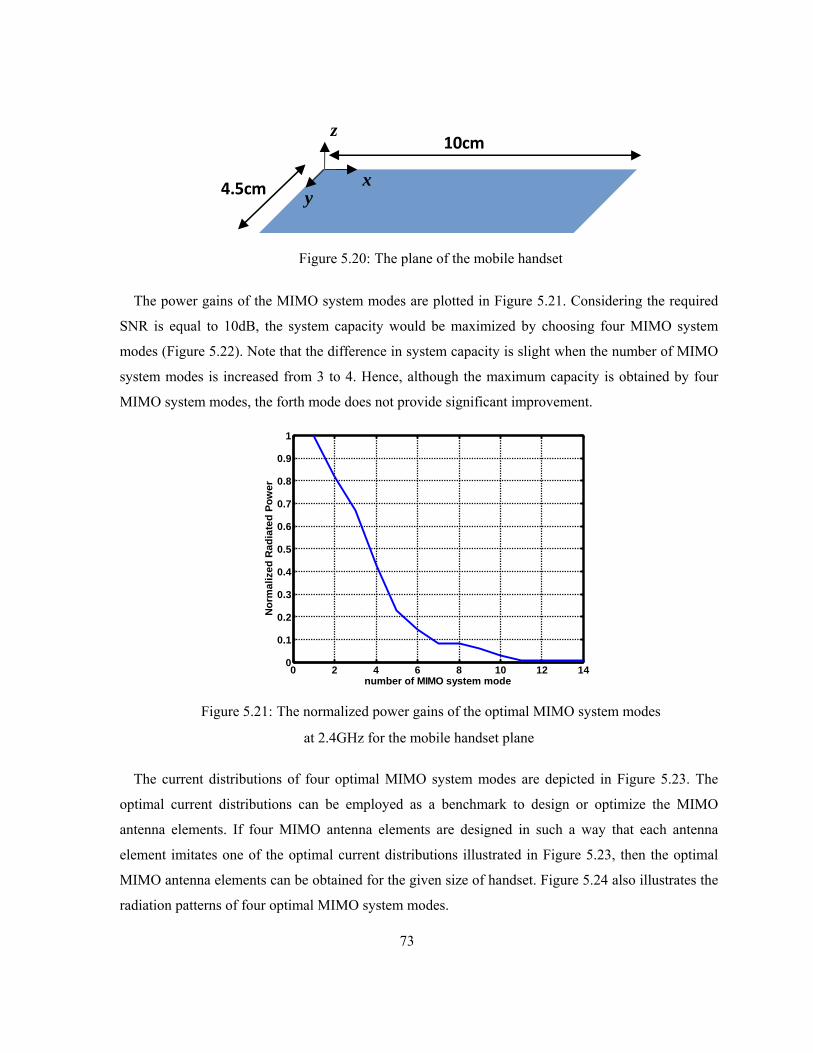
73
Figure 5.20: The plane of the mobile handset
The power gains of the MIMO system modes are plotted in Figure 5.21. Considering the required
SNR is equal to 10dB, the system capacity would be maximized by choosing four MIMO system
modes (Figure 5.22). Note that the difference in system capacity is slight when the number of MIMO
system modes is increased from 3 to 4. Hence, although the maximum capacity is obtained by four
MIMO system modes, the forth mode does not provide significant improvement.
Figure 5.21: The normalized power gains of the optimal MIMO system modes
at 2.4GHz for the mobile handset plane
The current distributions of four optimal MIMO system modes are depicted in Figure 5.23. The
optimal current distributions can be employed as a benchmark to design or optimize the MIMO
antenna elements. If four MIMO antenna elements are designed in such a way that each antenna
element imitates one of the optimal current distributions illustrated in Figure 5.23, then the optimal
MIMO antenna elements can be obtained for the given size of handset. Figure 5.24 also illustrates the
radiation patterns of four optimal MIMO system modes.
10cm
4.5cm
z
yx
0 2 4 6 8 10 12 140
0.1
0.2
0.3
0.4
0.5
0.6
0.7
0.8
0.9
1
number of MIMO system mode
Nor
mal
ized
Rad
iate
d Po
wer

74
Figure 5.22: The system capacity versus the number of MIMO system modes
at 2.4GHz for the mobile handset plane
The optimal current distributions and radiation patterns given in Figure 5.23 and 5.24 are obtained
for the uniform PAS, and it is required to investigate if the number of optimal MIMO system modes
would change for the other PAS channel realizations. For this purpose, a Monte-Carlo simulation can
be performed for various wireless channel realizations to study the maximum degrees of freedom
achievable through a non-uniform PAS.
For the statistical analysis of the wireless channel, the Laplacian channel model is used with four
clusters and o30=kφσ and o30=kθσ . Before finding the number of optimal MIMO system
modes for the plane of the mobile handset, the degrees of freedom of the Laplacian channel can be
investigated through the SVD of the matrix G . As mentioned before, the optimal SVW spectrum is
obtained for the PAS channel when †QIM = . Considering the size of the plane in Figure 5.20, the
smallest sphere enclosing the plane will have a radius of λ44.0 . According to Chu’s theorem, the
number of modes appearing at the far field would be limited by 30 ≈< krn which results in 36
SVWs in total. The matrix G with the size of 36×36 can be calculated for each random channel
realization. Using the SVD of the matrix G in each channel realization, the optimal SVW spectrums
and their singular values can be calculated. Considering SNR=10dB, the capacity is calculated versus
the number of MIMO system modes for each channel realization. The histogram in Figure 5.25 shows
the recording of the optimum number of MIMO system modes for 250 different channel realizations.
0 5 10 15 20 25 30 35 401
2
3
4
5
6
Cap
acity
(bit/
s/H
z)
Number of MIMO System Modes

75
Figure 5.23: The optimal current distributions on the mobile handset plane at 2.4GHz
-0.4 -0.3 -0.2 -0.1 0 0.1 0.2 0.3 0.4-0.2
-0.1
0
0.1
0.2
X in terms of λ
Y in
term
s of
λ
-0.4 -0.3 -0.2 -0.1 0 0.1 0.2 0.3 0.4-0.2
-0.1
0
0.1
0.2
X in terms of λ
Y in
term
s of
λ
-0.4 -0.3 -0.2 -0.1 0 0.1 0.2 0.3 0.4-0.2
-0.1
0
0.1
0.2
X in terms of λ
Y in
term
s of
λ
-0.4 -0.3 -0.2 -0.1 0 0.1 0.2 0.3 0.4-0.2
-0.1
0
0.1
0.2
X in terms of λ
Y in
term
s of
λ
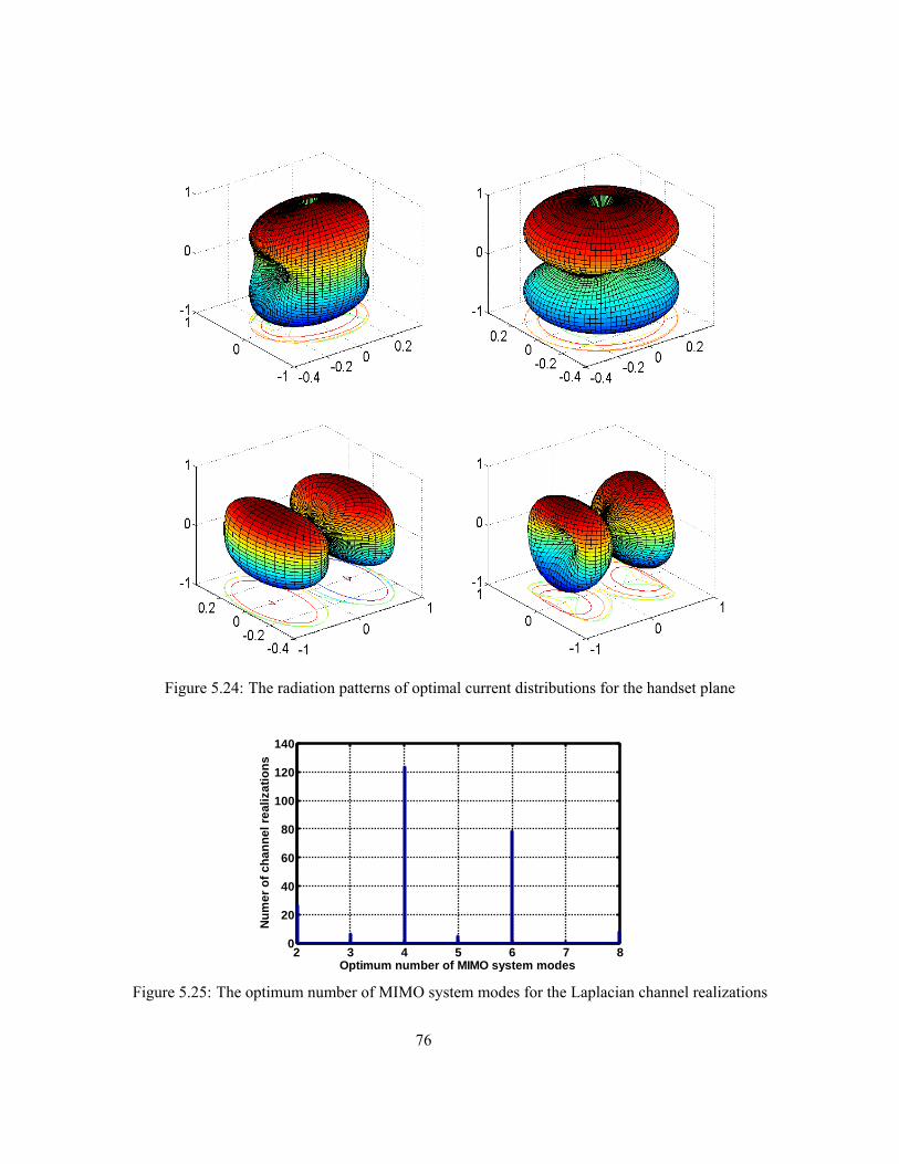
76
Figure 5.24: The radiation patterns of optimal current distributions for the handset plane
Figure 5.25: The optimum number of MIMO system modes for the Laplacian channel realizations
2 3 4 5 6 7 80
20
40
60
80
100
120
140
Optimum number of MIMO system modes
Num
er o
f cha
nnel
real
izat
ions

77
Figure 5.25 shows that the optimum number of MIMO system modes for which the channel
capacity is maximized, is obtained as 4 for 124 different channel realizations out of 250. It also
reaches to 6 and 8 numbers of MIMO system modes, but the most reliable number of effective MIMO
system modes is 4 through the simulated Laplacian channel.
Note that the number of degrees of freedom shown in Figure 5.25 is only limited by the size of the
sphere enclosing the antenna structure, but there is no limitation on the antennas’ (current
distributions) shapes. Therefore, it provides an upper bound for the number of MIMO system modes
generated by the antennas inside a sphere with a radius of λ44.0 . The upper limit can be achieved by
a spherical antenna (source distribution) which can generate the desired SVWs in the radiating fields,
as presented in Chapter 4. If the current source is imposed to be distributed on the given plane, a
lower number of MIMO system modes is expected. The limitations due to the shape of the antenna
can be included by considering the matrix M constructed for infinitesimal dipoles placed on the
antenna geometry. Using the SVD of the matrix Z and calculating the singular values (consequently,
the power gains) for 250 different channel realizations, the histogram of the optimum number of
MIMO system modes for which the capacity with SNR=10dB is maximized for the given antenna
geometry and wireless channel is illustrated in Figure 5.26.
Figure 5.26: The optimum number of MIMO system modes for the Laplacian channel
and the antenna geometry given in Figure 5.20
As expected, due to the limitations imposed by the antenna geometry, the number of degrees of
freedom is decreased to 3 MIMO system modes for 151 different channel realizations out of 250. The
lower number of effective MIMO system modes can be attributed to the fact that a planar source is
1 2 3 4 50
20
40
60
80
100
120
140
160
Optimum number of MIMO system modes
Num
er o
f cha
nnel
real
izat
ions
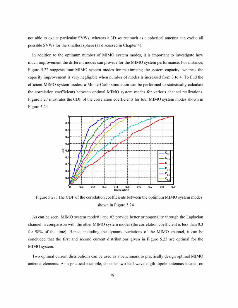
78
not able to excite particular SVWs, whereas a 3D source such as a spherical antenna can excite all
possible SVWs for the smallest sphere (as discussed in Chapter 4).
In addition to the optimum number of MIMO system modes, it is important to investigate how
much improvement the different modes can provide for the MIMO system performance. For instance,
Figure 5.22 suggests four MIMO system modes for maximizing the system capacity, whereas the
capacity improvement is very negligible when number of modes is increased from 3 to 4. To find the
efficient MIMO system modes, a Monte-Carlo simulation can be performed to statistically calculate
the correlation coefficients between optimal MIMO system modes for various channel realizations.
Figure 5.27 illustrates the CDF of the correlation coefficients for four MIMO system modes shown in
Figure 5.24.
Figure 5.27: The CDF of the correlation coefficients between the optimum MIMO system modes
shown in Figure 5.24
As can be seen, MIMO system mode#1 and #2 provide better orthogonality through the Laplacian
channel in comparison with the other MIMO system modes (the correlation coefficient is less than 0.3
for 98% of the time). Hence, including the dynamic variations of the MIMO channel, it can be
concluded that the first and second current distributions given in Figure 5.23 are optimal for the
MIMO system.
Two optimal current distributions can be used as a benchmark to practically design optimal MIMO
antenna elements. As a practical example, consider two half-wavelength dipole antennas located on
0 0.1 0.2 0.3 0.4 0.5 0.6 0.7 0.8 0.90
0.1
0.2
0.3
0.4
0.5
0.6
0.7
0.8
0.9
1
Correlation
CD
F
C12C13C23C14C24C34

79
the rectangular plane given in Figure 5.20. It is desired to obtain the optimal shape of the dipole
antennas so that the orthogonal MIMO system modes are obtained. To find the optimal shape, a
MATLAB code is written to generate different possible shapes of a half-wavelength dipole on the
grid points defined for the rectangular plane.
Note that the current distribution along the dipoles can be approximated as a sinusoidal function
independent of the shape of the dipoles. Projecting the sinusoidal current distributions with various
shapes onto the optimal current distributions shown in Figure 5.23, those dipole shapes are chosen
that can imitate the optimal current distributions as much as possible. The four optimal dipole shapes,
which have the most similarity with optimal current distributions, are shown in Figure 5.28 in red,
blue, black, and green, respectively.
Figure 5.28: The four optimal half-wavelength dipoles
Since the MIMO system mode#1 and #2 are optimal in the given Laplacian channel (Figure 5.27),
the corresponding dipole shapes (red and blue curves) are chosen to design the two dipole antennas
on a thin dielectric substrate. The designed dipole antennas, their simulated S-parameters, and the
radiation patterns of the two MIMO system modes are illustrated in Figure 5.29. As can be seen,
using the optimal shapes of the dipole antennas, the two antennas are suitably isolated and the return
losses are more than 10dB for 150MHz bandwidth.
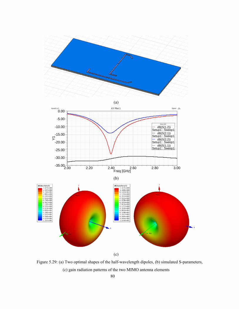
80
(a)
(b)
(c)
Figure 5.29: (a) Two optimal shapes of the half-wavelength dipoles, (b) simulated S-parameters,
(c) gain radiation patterns of the two MIMO antenna elements
2.00 2.20 2.40 2.60 2.80 3.00Freq [GHz]
-35.00
-30.00
-25.00
-20.00
-15.00
-10.00
-5.00
0.00
Y1
Ansoft LLC Slots4XY Plot 1 ANSOFT
Curve Info
dB(S(1,2))Setup1 : Sweep1
dB(S(2,1))Setup1 : Sweep1
dB(S(2,2))Setup1 : Sweep1
dB(S(1,1))Setup1 : Sweep1
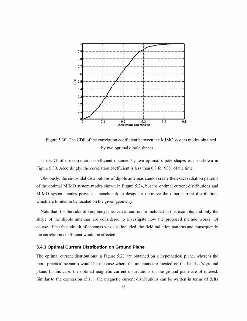
81
Figure 5.30: The CDF of the correlation coefficient between the MIMO system modes obtained
by two optimal dipole shapes
The CDF of the correlation coefficient obtained by two optimal dipole shapes is also shown in
Figure 5.30. Accordingly, the correlation coefficient is less than 0.3 for 93% of the time.
Obviously, the sinusoidal distributions of dipole antennas cannot create the exact radiation patterns
of the optimal MIMO system modes shown in Figure 5.24, but the optimal current distributions and
MIMO system modes provide a benchmark to design or optimize the other current distributions
which are limited to be located on the given geometry.
Note that, for the sake of simplicity, the feed circuit is not included in this example, and only the
shape of the dipole antennas are considered to investigate how the proposed method works. Of
course, if the feed circuit of antennas was also included, the field radiation patterns and consequently
the correlation coefficient would be affected.
5.4.3 Optimal Current Distribution on Ground Plane
The optimal current distributions in Figure 5.23 are obtained on a hypothetical plane, whereas the
more practical scenario would be the case where the antennas are located on the handset’s ground
plane. In this case, the optimal magnetic current distributions on the ground plane are of interest.
Similar to the expression (5.11), the magnetic current distributions can be written in terms of delta
0 0.1 0.2 0.3 0.4 0.50
0.1
0.2
0.3
0.4
0.5
0.6
0.7
0.8
0.9
1
Correlation Coefficient
CD
F
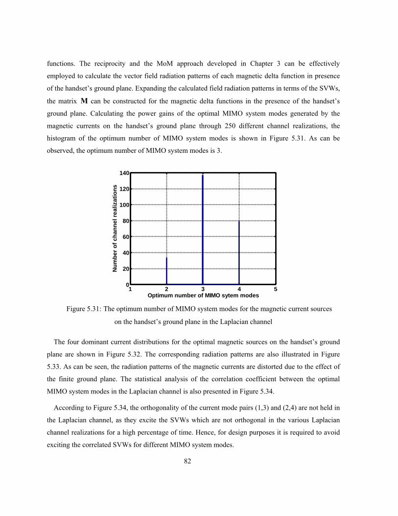
82
functions. The reciprocity and the MoM approach developed in Chapter 3 can be effectively
employed to calculate the vector field radiation patterns of each magnetic delta function in presence
of the handset’s ground plane. Expanding the calculated field radiation patterns in terms of the SVWs,
the matrix M can be constructed for the magnetic delta functions in the presence of the handset’s
ground plane. Calculating the power gains of the optimal MIMO system modes generated by the
magnetic currents on the handset’s ground plane through 250 different channel realizations, the
histogram of the optimum number of MIMO system modes is shown in Figure 5.31. As can be
observed, the optimum number of MIMO system modes is 3.
Figure 5.31: The optimum number of MIMO system modes for the magnetic current sources
on the handset’s ground plane in the Laplacian channel
The four dominant current distributions for the optimal magnetic sources on the handset’s ground
plane are shown in Figure 5.32. The corresponding radiation patterns are also illustrated in Figure
5.33. As can be seen, the radiation patterns of the magnetic currents are distorted due to the effect of
the finite ground plane. The statistical analysis of the correlation coefficient between the optimal
MIMO system modes in the Laplacian channel is also presented in Figure 5.34.
According to Figure 5.34, the orthogonality of the current mode pairs (1,3) and (2,4) are not held in
the Laplacian channel, as they excite the SVWs which are not orthogonal in the various Laplacian
channel realizations for a high percentage of time. Hence, for design purposes it is required to avoid
exciting the correlated SVWs for different MIMO system modes.
1 2 3 4 50
20
40
60
80
100
120
140
Optimum number of MIMO sytem modes
Num
ber o
f cha
nnel
real
izat
ions

83
Figure 5.32: The optimal magnetic current distributions on the handset’s ground plane at 2.4GHz
0 0.1 0.2 0.3 0.4 0.5 0.6 0.7 0.8
0
0.1
0.2
0.3
0.4
X in terms of λ
Y in
term
s of
λ
0 0.1 0.2 0.3 0.4 0.5 0.6 0.7 0.8
0
0.1
0.2
0.3
0.4
X in terms of λ
Y in
term
s of
λ
0 0.1 0.2 0.3 0.4 0.5 0.6 0.7 0.8
0
0.1
0.2
0.3
0.4
X in terms of λ
Y in
term
s of
λ
0 0.1 0.2 0.3 0.4 0.5 0.6 0.7 0.8
0
0.1
0.2
0.3
0.4
X in terms of λ
Y in
term
s of
λ

84
Figure 5.33: The radiation patterns of optimal magnetic currents on the handset’s ground plane
Figure 5.34: The CDF of the correlation coefficients between the optimal MIMO system modes
generated by the magnetic currents on the handset’s ground plane
0 0.1 0.2 0.3 0.4 0.5 0.6 0.7 0.80
0.1
0.2
0.3
0.4
0.5
0.6
0.7
0.8
0.9
1
correlation
CD
F
C12C13C23C14C24C34
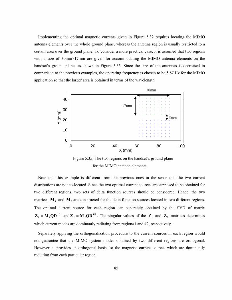
85
Implementing the optimal magnetic currents given in Figure 5.32 requires locating the MIMO
antenna elements over the whole ground plane, whereas the antenna region is usually restricted to a
certain area over the ground plane. To consider a more practical case, it is assumed that two regions
with a size of 30mm×17mm are given for accommodating the MIMO antenna elements on the
handset’s ground plane, as shown in Figure 5.35. Since the size of the antennas is decreased in
comparison to the previous examples, the operating frequency is chosen to be 5.8GHz for the MIMO
application so that the larger area is obtained in terms of the wavelength.
Figure 5.35: The two regions on the handset’s ground plane
for the MIMO antenna elements
Note that this example is different from the previous ones in the sense that the two current
distributions are not co-located. Since the two optimal current sources are supposed to be obtained for
two different regions, two sets of delta function sources should be considered. Hence, the two
matrices 1M and 2M are constructed for the delta function sources located in two different regions.
The optimal current source for each region can separately obtained by the SVD of matrix 1/2
11 QDMZ = and 1/222 QDMZ = . The singular values of the 1Z and 2Z matrices determines
which current modes are dominantly radiating from region#1 and #2, respectively.
Separately applying the orthogonalization procedure to the current sources in each region would
not guarantee that the MIMO system modes obtained by two different regions are orthogonal.
However, it provides an orthogonal basis for the magnetic current sources which are dominantly
radiating from each particular region.
0 20 40 60 80 1000
10
20
30
40
X (mm)
Y (m
m)
17mm
30mm
5mm

86
(a)
(b)
(c)
Figure 5.36: (a) The optimal magnetic currents for the given regions, (b) radiation patterns of two
MIMO system modes, (c) CDF of the correlation coefficient for two MIMO system modes
0 0.5 1 1.50
0.2
0.4
0.6
0.8
X in terms of λ
Y in
term
s of
λ
0 0.1 0.2 0.3 0.4 0.50
0.2
0.4
0.6
0.8
1
correlation
CD
F

87
For instance, in order to select four dominant current modes included in each region, four rows of †
11 UI = and †22 UI = with the highest corresponding singular values can be chosen, where 1I and
2I are the coefficients of the optimal magnetic currents on the handset’s ground plane in region#1
and #2, respectively. Then, it is required to calculate ( ) ( )†221112 MIGMIR = to investigate which
current modes among the four selected ones in each region provide the orthogonal MIMO system
modes through the given wireless channel.
Using the proposed procedure, the optimal magnetic currents are shown in Figure 5.36.a. The
radiation patterns of the magnetic currents and the statistical analysis of the correlation coefficient
between them are also presented in Figure 5.36.b and 5.36.c. Note that the Laplacian channel
parameters are similar to the previous examples.
To implement the optimal magnetic current distributions, one approach is to use Dielectric
Resonator Antennas (DRA) [94]. The EM field modes excited in the dielectric resonator can imitate
the magnetic current distributions in Figure 5.36.a. Figure 5.37 shows the designed DRAs at 5.8GHz
for the MIMO application. The dielectrics are made of alumina ( 4.9=rε ) with the height of 5mm
and the dimensions given in Figure 5.35, and the slots are excited using two microstrip lines mounted
on the back of the handset’s ground plane.
Figure 5.37: The dielectric resonator antennas to generate the MIMO system modes
L1=17.5mm
L2=14mm
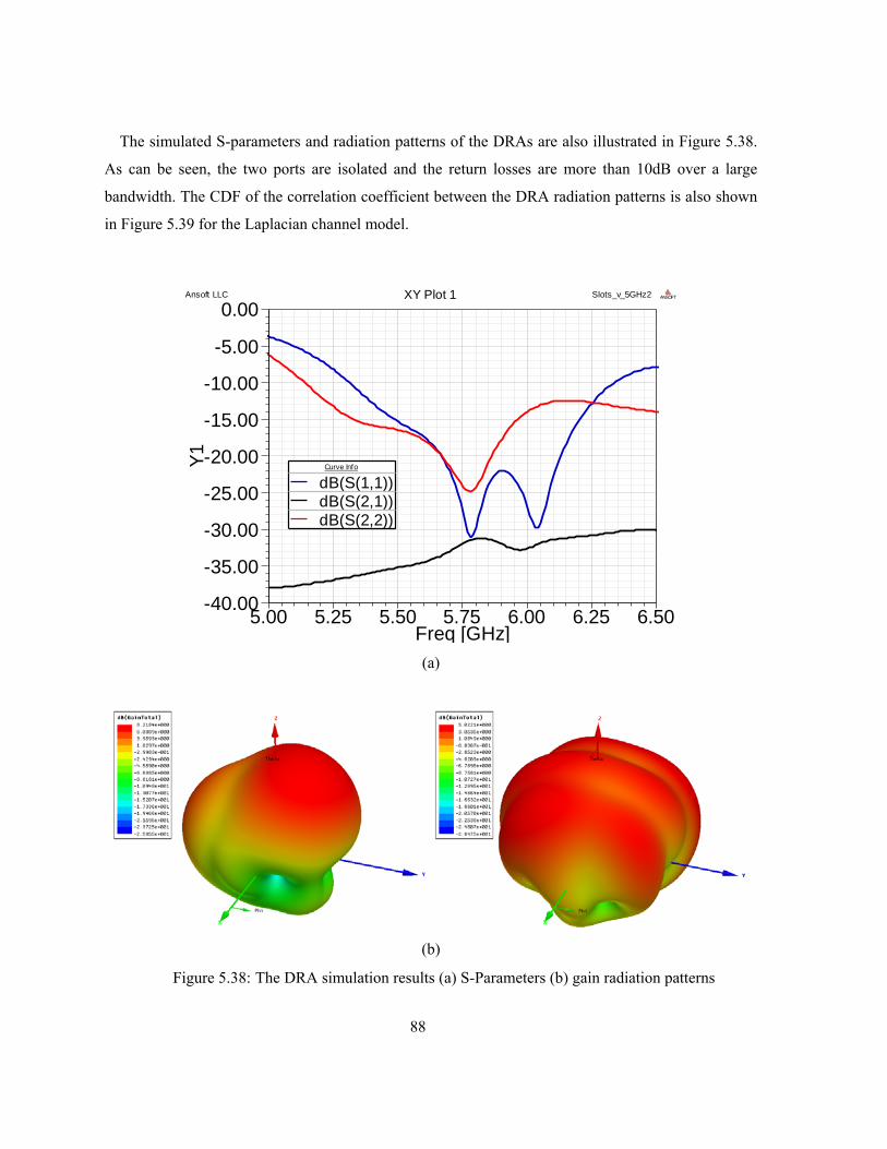
88
The simulated S-parameters and radiation patterns of the DRAs are also illustrated in Figure 5.38.
As can be seen, the two ports are isolated and the return losses are more than 10dB over a large
bandwidth. The CDF of the correlation coefficient between the DRA radiation patterns is also shown
in Figure 5.39 for the Laplacian channel model.
(a)
(b)
Figure 5.38: The DRA simulation results (a) S-Parameters (b) gain radiation patterns
5.00 5.25 5.50 5.75 6.00 6.25 6.50Freq [GHz]
-40.00
-35.00
-30.00
-25.00
-20.00
-15.00
-10.00
-5.00
0.00
Y1
Ansoft LLC Slots_v_5GHz2XY Plot 1 ANSOFT
Curve Info
dB(S(1,1))dB(S(2,1))dB(S(2,2))

89
Figure 5.39: The CDF of the correlation coefficient between DRAs
The DRA design is inspired from the optimal magnetic currents calculated for the given regions on
the handset’s ground plane. Although the DRAs do not exactly represent the optimal magnetic
sources, the calculated magnetic currents provide an initial step to design the DRA elements. Note
that the other types of magnetic current implementations can also be employed to design the MIMO
antenna elements. For instance, the optimal magnetic currents can be practically implemented by
various slot shapes over the ground plane.
Although the fixed current distributions are selected here to implement MIMO antenna elements,
the methodology can be utilized to derive the optimal current distributions corresponding to the
severe channel realizations. Having a bank of optimal currents, the adaptive techniques [26] can be
employed to either switch between the optimal MIMO antennas or change the current excitations
corresponding to the channel variations.
5.5 Conclusion
The SVW representation of the correlation coefficients between the MIMO antenna system modes
was derived, and a matrix formulation was presented to separate the channel effects from the current
excitations and the physical properties of antenna elements. Using the SVD method, the degrees of
freedom were obtained and the optimal current excitations were calculated to generate the orthogonal
radiation modes for maximizing the system capacity. The proposed SVW formulation was employed
to analyze wireless channel, and obtain the optimal current excitations for the given antenna
0 0.1 0.2 0.3 0.40
0.2
0.4
0.6
0.8
1
Correlation Coefficient
CD
F

90
structures, as well as to determine the optimal current distributions for a few practical examples. The
SVW formulation was also used to determine the maximum number of MIMO system modes
achievable for an arbitrary antenna structure. The impact of the antenna shapes and dynamic wireless
channels on the effective number of MIMO system modes were also investigated. The proposed
approach offers a flexible and systematic method which can be applied to more realistic scenarios in
practical applications by taking more complex electromagnetic interactions (the interaction with the
package and complex objects close to the antennas) into consideration. The proposed formulation is
one of main contributions of this research in the MIMO antenna design and analysis.
91
Chapter 6 Concluding Remarks
The MIMO system is recognized as an efficient solution to enhance the system capacity and combat
the multipath fading effects of the wireless communication channels. The correlation coefficient
between the received/transmitted signals is a crucial parameter which determines the MIMO system
performance. The electromagnetic effects of the wireless channel and the MIMO antenna elements
can significantly affect the correlation coefficients between the antenna elements. To include the EM
properties in the MIMO antenna design and analysis, the general MIMO antenna system model and
the appropriate correlation coefficient formulation were discussed. The physical channel models were
also reviewed, and without the loss of generality, the statistical Laplacian cluster channel model was
introduced to be used for MIMO antenna analysis and design throughout this research.
In addition to the far field effects modeled by the power angular spectrum of the wireless channel,
the scattering objects in the vicinity of the MIMO antenna elements were considered. A fast and
efficient approach was proposed to include the EM effects of scattering objects located in the near
field region. The proposed method is beneficial for optimization problems in the sense that the EM
effect of scattering objects can be numerically calculated independent of the MIMO antenna
elements. Hence, the optimizations of the physical properties of the MIMO antenna elements in the
presence of a scattering object would be numerically fast and efficient. Considering the PEC fixture
effects on the radiation patterns of the MIMO antenna elements, the physical properties of the antenna
elements were optimized in a few practical examples to achieve the minimum correlation coefficient.
The proposed approach, which is a hybrid of the analytical reciprocity formulation and the numerical
MoM, is a notable contribution in the MIMO antenna optimizations.
The spherical vector waves are Eigen vector solutions of the Helmholtz equation and establish an
orthogonal set of vector basis functions for electromagnetic fields. The orthogonal properties of the
SVWs were utilized to achieve orthogonal vector field radiation patterns of the MIMO antennas. To
excite the desired SVWs for the MIMO application, it is required to obtain current sources radiating a
particular SVW. Source reconstruction for a predefined EM field is known as the inverse source
problem which also has other applications such as near field scanning, inverse scattering, imaging,
and etc. For the sake of the analytical solution, the inverse source problem was solved on a spherical
geometry for the predefined SVWs. To add more liberties into the inverse source problems, the non-

92
radiating sources were included so that a certain constraint was satisfied. Imposing the condition of
spherical surface source, the current distributions were obtained on a sphere for the given SVW
coefficients. The derived formulation for the spherical current source is a major contribution in the
inverse source problem which was utilized for the MIMO antenna applications in this research. The
analytical SVW analysis was also applied to the planar antennas, and the orthogonal properties of the
co-planar electric and magnetic sources were also explored. This orthogonality was employed to
design one simple MIMO antenna. The statistical analysis of the correlation coefficient showed that
the vector field radiations of the designed magnetic and electric currents remain orthogonal for an
appropriate percentage of the time.
The SVW approach was formulated in a general matrix form in which the inner product matrix of
the MIMO system modes was separated into three cascaded matrices representing the SVW
interactions through the wireless channel, the physical properties of the antenna elements, and the
current excitations in the feed circuit. The SVW formulation provides the possibility of studying the
wireless channel independent of the MIMO antenna elements. Investigating the SVW interaction in
the wireless channel explores the possible degrees of freedom of the channel in the sense that the
SVWs whose orthogonality is less sensitive to the wireless channels can be determined. Once the
desired SVWs are known for the given channel, the analytical SVW method can be employed to
determine the corresponding surface current distributions. The SVW formulation was also applied to
a few practical examples to determine the optimal current excitations of the given MIMO antenna
elements in both the fixed and statistically varying Laplacian channels. It was shown that the feed
circuit design that provides the optimal current excitations can significantly improve the MIMO
system performance. Ultimately, the SVW approach was applied to an arbitrary geometry of antennas
in order to obtain the optimal current distributions for the orthogonal MIMO system modes, and also
determine the maximum number of effective MIMO system modes which can maximize the system
capacity for the given physical restrictions. The proposed reciprocity and the MoM method was
linked with the SVW formulation to achieve the optimal magnetic current distributions on the given
ground plane. The calculated current distributions inspired an initial step for designing the MIMO
antenna elements. While designing the MIMO antenna elements according to the optimal current
distributions, two practical examples of MIMO antennas were discussed for mobile handset
communications. The statistical analysis of the correlation coefficients was also presented to evaluate
the performance of the designed MIMO antenna elements in different wireless channels.
93
6.1 Future Work
The following directions are suggested as future work following this research:
1) For MIMO antenna optimizations, the method of moments was developed for PEC objects in
this research. Extending the developed MATLAB code to calculate the impedance matrix for
dielectric objects, it would be possible to include the EM influences of different types of fixture
packages made of various materials on the vector field radiation patterns of the MIMO antenna
elements. Combining the extended MoM with the reciprocity formulation, the MIMO antennas
can be optimized in the presence of more practical enclosures.
2) The analytic source reconstruction presented in this research to excite the desired SVW was
accomplished for spherical surfaces. The idea of including the non-radiating sources to satisfy
the surface source constraint can be extended to the other coordinate systems such as the
spheroidal coordinates. Although the spheroidal vector wave functions are not orthogonal on a
spheroid, the orthognalization procedures can be employed to determine the coefficients of
spheroidal waves in the current distributions. By solving the inverse surface problem for
spheriodal structures, more general antenna shapes including the linear antennas can be
considered to excite the SVWs for MIMO applications. Meanwhile, the non-radiating sources
can be employed to satisfy the other practical constraints than the surface source constraint.
3) Although a few proof-of-concept examples were discussed in this research, the SVW
formulation is a general methodology and can be applied to other practical problems. As an
interesting application of the SVW approach, the physical shapes of the MIMO antenna
elements can be optimized in such a way that the desired SVWs are excited for the given
wireless channel. Additionally, the other types of current implementations than those proposed
in this research can be investigated for the MIMO antenna designs in different practical
scenarios.
4) In this research, the wireless channel was statistically modeled to obtain fixed MIMO system
modes which were optimal for the various wireless channel realizations. The ultimate solution
for the MIMO antenna designs is the adaptive or reconfigurable antenna structure which adapts
the vector field radiation patterns of the MIMO system modes to the wireless channel
variations. The compatibility of the MIMO antenna elements with the dynamic environment
provides an efficient antenna design which guarantees the maximum system capacity in various

94
communication environments. The SVW approach proposed in this research can be employed
in adaptive MIMO systems in order to achieve the optimal MIMO system modes in different
wireless environments.
95
Appendix A Method of Moments for Conducting Bodies
A.1 Theory of Scattering
If an electromagnetic wave incident upon a PEC body, the total electric field can be written as sum of
the known incident field incEr
and the unknown scattered electric field SEr
so that the total field
satisfies the boundary condition on the PEC body:
0)(ˆ =+× incS EEnrr
(A.1)
The scattered field SEr
may be derived in the usual way from its electromagnetic potentials, in the
following form [48, 56, 95]:
rrR
SdrJR
jkRjSdrJR
jkRjAjE
SS
SS
S
′−=
′′⋅∇′−
∇−′′−−=
∇−−=
∫∫rr
rrrr
rr
)()exp(4
)()exp(4 0
0
πωεπωμ
φω
(A.2)
in which SJr
is the unknown current density in the scattering PEC body, and rrR ′−=rr
is the
distance between the source point r ′r and the field point rr . Thus, an Electric Field Integral Equation
(EFIE) can be established in terms of SJr
and the solution of the scattering problem will conveniently
be obtained in terms of the currents that flow in the scattering body.
A.2 Method of Moment Equations for PEC Bodies
To solve the EFIE using the MoM, the induced current is represented by a linear superposition of the
suitable basis functions of the prescribed spatial variation so that the current density may be written in
the approximated form [56, 95]:
)(1
rSIJN
nnnSrrr
∑=
= (A.3)
where N is the total number of basis functions, the scalar quantities In are unknown constants to be
determined, and the vector quantities )(rSnrr
are the individual basis functions.
96
If equation (A.3) is substituted into the integral equation (A.1), the EFIE is multiplied by a test
function of )(rSnrr
(Galerkin’s method), and the resultant is integrated over the PEC surfaces, the
MoM equations will be derived as follow [56, 95]:
∑=
=N
nmnnm VIZ
1
(A.4)
where
∫ ⋅= dSErSV incmm
rrr)( (A.5)
and
( ) ( ) SdR
jkRrSrSj
dSSdR
jkRrSrSj
Z
S Snm
S Snmmn
′−′⋅∇′⋅⋅∇⎟⎟⎠
⎞⎜⎜⎝
⎛−
′−′⋅⎟⎠⎞
⎜⎝⎛=
∫ ∫
∫ ∫)exp()()(
4
)exp()()(4
0
0
rrrr
rrrr
πωε
πωμ
(A.6)
Each element of the impedance matrix is essentially a double integral of the Green’s function
multiplied by known basis functions over the PEC surface. Equation (A.4) can be written as the
matrix form:
[ ] [ ] [ ] 11 ××× = NmNnNNnm VIZ (A.7)
In the following section, an appropriate basis function is introduced which is popular in the Method
of Moments, and it will be discussed how to calculate the double integrals in the impedance matrix.
A.3 MoM using RWG Basis Functions
Based on equation (A.6), the basis function )(rSirr
is needed to have a nonsingular divergence. In
other words, the elements should be divergence-conforming which means that its normal component
is continuous across the element boundaries. A popular basis function in the MoM is often referred to
as the Rao–Wilton–Glisson (RWG) elements on triangles. The RWG basis function illustrated in
Figure A.1 contains a pair of triangles which are not necessarily co-planer [96].

97
Figure A.1: The geometry of the RWG basis function [96]
The RWG basis functions resembles a small dipole with a positive or negative charge on either
triangle +nT or −
nT which have areas +nA and −
nA , respectively, and share a common edge nl . The
RWG basis function can be formulated as follow [95]:
⎪⎪⎩
⎪⎪⎨
⎧
=−−
−
+++
nnn
n
nnn
n
n
TinrrAl
TinrrAl
rSrr
rr
rr
)(2
)(2)(
ρ
ρ (A.8)
and
⎪⎪⎩
⎪⎪⎨
⎧
=⋅∇−
−
++
nn
n
nn
n
n
TinrAl
TinrAl
rSr
r
rr)( (A.9)
where ++ −= nn rrr rrr)(ρ is a vector from the free vertex of the triangle +nT to the observation point rr ,
and rrr nnrrr
−= −− )(ρ is a vector which starts from the observation point rr and ends at the free vertex
of the triangle −nT [96].
Substituting equation (A.8) and (A.9) into equation (A.6), the double integrals in the impedance
matrix elements can be written in terms of the RWG basis functions as follow [96, 97]:
98
dSSdR
jkRrrAA
lldSSdR
jkRrrAA
ll
dSSdR
jkRrrAA
lldSSdR
jkRrrAA
ll
dSSdR
jkRrSrS
m nm n
m nm n
T Tnm
nm
nm
T Tnm
nm
nm
T Tnm
nm
nm
T Tnm
nm
nm
S Snm
′−′⋅+′−′⋅+
′−′⋅+′−′⋅+
=′−′⋅
∫ ∫∫ ∫
∫ ∫∫ ∫
∫ ∫
− −− +
+ −+ +
−−−−
+−+−
−+−+
++++
)exp()()(4
)exp()()(4
)exp()()(4
)exp()()(4
)exp()()(
rrrrrrrr
rrrrrrrr
rrrr
ρρρρ
ρρρρ (A.10)
( ) ( )
dSSdR
jkRAAlldSSd
RjkR
AAll
dSSdR
jkRAAlldSSd
RjkR
AAll
SdR
jkRrSrS
m nm n
m nm n
T Tnm
nm
T Tnm
nm
T Tnm
nm
T Tnm
nm
S Snm
′−+′−
−
′−−′−
+
=′−′⋅∇′⋅⋅∇
∫ ∫∫ ∫
∫ ∫∫ ∫
∫ ∫
− −− +
+ −+ +
−−+−
−+++
)exp()exp(
)exp()exp(
)exp()()( rrrr
(A.11)
The double surface integrals presented in (A.10) and (A.11) have a singularity which creates
difficulties in calculating the integrations. There are well-known ways to extract the singularity from
the Green’s function and calculate the singular integral with the help of analytical calculations [98,
99]. Here, the semi-analytic method presented in [98] and the Gaussian-Quadrature method are used
to calculate the above integrals. Accordingly, the singularity of integrals can be extracted in the
following forms:
dSSd
RjkRrr
dSSdR
rrdSSdR
jkRrr
m m
m mm m
T Tnm
T T
nm
T Tnm
′−−′⋅
+′′⋅
=′−′⋅
∫ ∫
∫ ∫∫ ∫)1)(exp()()(
)()()exp()()(
rrrr
rrrrrrrr
ρρ
ρρρρ (A.12)
dSSdRjkRdSSd
RdSSd
RjkR
m mm mm m T TT TT T
′−−+′=′−∫ ∫∫ ∫∫ ∫
)1)(exp(1)exp( (A.13)
Two double integrals on the right hand side are not singular anymore since the limit of
RjkR )1)(exp( −− is jk− when R goes to zero. Therefore, these two integrals can be calculated
numerically using the Gaussian-Quadrature method [100]. The analytic results of the inner potential
integrals have been presented in [98] which are used to calculate the singular integrals. The outer
integrals can be again evaluated numerically by the Gaussian-Quadrature method. The analytic
formulas for the inner singular integrals are concisely as follow:

99
∑∫=
−
−−
+
+−
−−
++
⎥⎥⎦
⎤
⎢⎢⎣
⎡⎟⎟⎠
⎞⎜⎜⎝
⎛
+−
+×−
++
⋅=′3
120
01
20
0100
)(tan
)(tanˆˆ1
i ii
ii
ii
ii
ii
iiiii
T RdRlP
RdRlPd
lRlRLnPuPSd
R (A.14)
∫∫∫ ′−+′−′
=′′
Tn
TT
n SdR
rrSdRrrSd
Rr 1)()()(
tantan rr
rrrrρ (A.15)
where
∑∫=
−−++−−
++
⎥⎦
⎤⎢⎣
⎡−+
++
=′−′ 3
1
20tan )(ˆ21)(
iiiii
ii
iiii
T
lRlRlRlRLnRuSd
Rrr rr
(A.16)
The geometrical variables used in the analytical formulas have been illustrated in Figure A.2. The
detailed calculations and all parameters included in the analytic formulas can be found in [98]. As
mentioned before, the outer integration and the second integrations in equations (A.12) and (A.13)
can be performed numerically.
Figure A.2: The variables included in the analytic formulas presented by [98]
100
Once the impedance matrix elements are calculated, the vector [I] can be obtained using equation
(A.7) for any arbitrary source vector [V]. Once the surface current density is known, the scattered
electric field can be calculated by substituting (A.3) in (A.2) which gives the following equation:
rrR
SdrSR
jkRIjSdrSR
jkRIjEN
nn
Srn
N
n SnnS
′−=
′′⋅∇′−
∇−′′−−= ∑ ∫∑ ∫
==rr
rrrrr
101
0 )()exp(4
)()exp(4 πωεπωμ
(A.17)
A.4 MATLAB functions for MoM
Based on the semi-analytic method formulated in the Section A.3, four MATLAB functions have
been written to calculate the four different integrals given by equations (A.10) and (A.11). These
MATLAB functions numerically calculates two double integrals over −+nm TT , −+
nm TT , −+nm TT , and
−+nm TT , respectively. Using equation (A.6), the impedance matrix elements, which show the self and
mutual impedances between the RWG basis functions, can be calculated. The integral results of the
four MATLAB functions have been verified with two other numerical methods (the fully numerical
Gaussian-Quadrature method and the two uniform series approximation of double surface integrals).
The mesh generation on the PEC body is performed using MATLAB, HFSS, or GMesh software
[101] which generates triangle and tetrahedral meshes for any surface and volume. Using
aforementioned software, it is possible to draw an arbitrary shape and generate the appropriate
meshes as a text file including the coordinates of the mesh vertexes.
To calculate the radiation field from the induced surface current SJr
, four major MATLAB codes
are developed to implement the following major tasks:
1) Organizing and plotting the generated meshes on the PEC body
2) MoM impedance matrix calculations
3) Calculating the vector [V] in equation (A.5) and obtaining the current distribution SJr
on the
PEC body
4) Calculating the scattered fields and plotting the radiation pattern
The output of each step is saved at the final line of each MATLAB code in order to be used easily
for the next step at any time it is needed. The input of the first code can be a text file (*.txt)

101
containing the coordinates of the mesh vertexes. The first code plots the generated meshes on the PEC
body and finds the vertexes of each pair of triangles for the RWG basis function. The second code
calculates the Z matrix elements using the semi-analytic method discussed before. In this code, the
property of the symmetric impedance matrix has been used to decrease the run time required for the
Z matrix elements calculations. The third code calculates the vector [V] for an infinitesimal dipole
located far from the PEC cube, and also calculates the current distribution matrix SJr
by multiplying
the Y matrix ( 1−Z ) and vector [V]. The last code calculates the radiated field from SJr
derived from
the previous step, and finally plots the radiation pattern of the scattered fields SEr
.
To verify the accuracy of the MATLAB code, the plane wave excitation of a PEC cube is analyzed
using both the commercial software HFSS and the developed MoM in MATLAB, and the results are
compared. The incident wave is defined as a plane wave with )ˆ2/1ˆ2/1(00 zxEE −=r
and
zxk ˆ2/1ˆ2/1ˆ −−= which is impinging on the PEC cube from o45=θ and o0=ϕ direction.
The generated meshes on the PEC cube in MATLAB have been illustrated in Figure A.3.
Figure A.3: The generated meshes on the PEC cube for MoM

102
The far field radiation pattern of the scattered field is calculated in both HFSS and MATLAB MoM
code. The scattered field radiation patterns are plotted for o180,135,90,45,0=ϕ and o90,45=θ
planes in Figure A.4 and A.5, respectively. As can be seen, the MoM results agree well with the
HFSS results.
(a) (b)
(c) (d)
(e)
Figure A.4: The scattered field radiation patterns in HFSS and MoM for
a) o0=ϕ b) o45=ϕ c) o90=ϕ d) o135=ϕ e) o180=ϕ plane [67, 69]
0 20 40 60 80 100 120 140 160 180-30
-25
-20
-15
-10
-5
Theta (Degree)
Rad
iatio
n Pa
ttern
(dB
)
φ = 0
MATLAM MoM SimulationHFSS Simulation
0 20 40 60 80 100 120 140 160 180
-25
-20
-15
-10
Theta (Degree)R
adia
tion
Patte
rn (d
B)
φ = 45
MATLAM MoM SimulationHFSS Simulation
0 20 40 60 80 100 120 140 160 180-24
-22
-20
-18
-16
-14
-12
-10
-8
Theta (Degree)
Rad
iatio
n Pa
ttern
(dB
)
φ = 90
MATLAM MoM SimulationHFSS Simulation
0 20 40 60 80 100 120 140 160 180-20
-15
-10
-5
Theta (Degree)
Rad
iatio
n Pa
ttern
(dB
)
φ = 135
MATLAM MoM SimulationHFSS Simulation
0 20 40 60 80 100 120 140 160 180-25
-20
-15
-10
-5
0
Theta (Degree)
Rad
iatio
n Pa
ttern
(dB
)
φ = 180
MATLAM MoM SimulationHFSS Simulation

103
(a) (b)
Figure A.5: The scattered field radiation patterns in HFSS and MoM for
a) o45=θ b) o90=θ [67, 69]
The slight difference between the results can be attributed to the different mesh arrangement used
in HFSS and MoM. However, if very fine meshes are chosen for both simulations, the results would
be more closely matched. The results confirm the validity of the developed MoM in MATLAB, and
verify that the calculated Z-matrix and the induced current are obtained correctly.
0 50 100 150 200 250 300 350-25
-20
-15
-10
PHI (Degree)
Rad
iatio
n Pa
ttern
(dB
)
θ = 45
MATLAM MoM SimulationHFSS Simulation
0 50 100 150 200 250 300 350-26
-24
-22
-20
-18
-16
-14
-12
-10
-8
PHI (Degree)
Rad
iatio
n Pa
ttern
(dB
)
θ = 90
MATLAM MoM SimulationHFSS Simulation

104
Appendix B Vector Wave Functions
Considering the general curvilinear coordinates 1ξ , 2ξ , and 3ξ with the unit vectors 1a , 2a , 3a and
the scale factors 1h , 2h , 3h , the Eigen vector functions of the vector Helmholtz equation can be
written in terms of the solution of the scalar Helmholtz equation, ψ , as follow [45-47]:
( )
333
2113
2322
112
13211
2
121
2
3322
12
233
213
1
333
213
2322
12
13211
332211321
ˆ)()(1ˆ)()(1
ˆ)(11
ˆ)(ˆ)(ˆ
ˆ)(1ˆ)(1ˆ)(
)()()(),,(
akh
akh
akk
Mk
N
ah
ah
aM
ah
ah
aL
ψξ
ψχψξ
ψψξ
χψξ
ψψψξ
χξχ
ψχ
ψψξ
ψχψξ
ψψχχψ
ψξ
ψψψψξ
ψψψψξ
ψ
ξψξψξψξξξψ
∂∂
∂∂
+∂∂
∂∂
+
⎟⎟⎠
⎞⎜⎜⎝
⎛⎥⎦
⎤⎢⎣
⎡∂∂
∂∂
+=×∇=
∂∂
−∂∂
=×∇=
∂∂
+∂∂
+∂∂
=∇=
=
rrr
rr
rr
(B.1)
where it is assumed that 1h is a unit constant, 32 / hh is independent of 1ξ , and χ is either 1 or 1ξ .
These assumptions are held by six separable coordinate systems including the spherical coordinate
system. For the spherical coordinate system, the vector wave functions are given as follows [45-47]:
( ) ( ) ( ) ( )
( ) ( )
( ) ( ) ( ) ( )
( ) ( ) ( )[ ] ( )
( )[ ] ( ) ϕϕθθ
θϕθ
θϕθ
ϕϕθ
θθϕθθ
ϕϕθθ
θϕθ
θϕθ
φθψψψψ
ˆcossin
cossin
ˆsincoscos1ˆ
sincos
cos)1(
ˆsincoscosˆ
cossin
cossin
ˆcossin
cossin
ˆsincoscos1ˆ
sincos
cos
)(sincos
)(cos)(
)(
)()()(
)()()(
)(
)()()(
)(321
)(
mPkrrzrkr
m
mPkrrzrkr
rmPkrzkrnnN
mPkrzmPkrzmM
mPkrzr
m
mPkrzr
rmPkrzr
L
mPkrz
mn
in
mni
nm
ni
ni
mnoe
mni
nm
ni
ni
mnoe
mn
in
mni
nm
ni
ni
mnoe
mn
in
i
mnoe
∂∂
∂∂
∂∂
++
=
∂∂
−=
∂∂
+∂∂
=
==
m
r
mr
m
r
(B.2)
105
The spherical vector waves with different orders hold the following orthogonality properties on a
spherical surface [46, 47]:
mmornnforddNN
mmornnforddMM
mmornnforddLL
i
nmoe
i
mnoe
i
nmoe
i
mnoe
i
nmoe
i
mnoe
′≠′≠=
′≠′≠=
′≠′≠=
∫ ∫
∫ ∫
∫ ∫
′′
′′
′′
0sin.
0sin.
0sin.
2
0 0
)()(
2
0 0
)()(
2
0 0
)()(
π π
π π
π π
ϕθθ
ϕθθ
ϕθθ
rr
rr
rr
(B.3)
Also, the following orthogonality properties are valid for any arbitrary orders [46, 47]:
0sin.
0sin.
2
0 0
)()(
2
0 0
)()(
=
=
∫ ∫
∫ ∫
′′
′′
π π
π π
ϕθθ
ϕθθ
ddLM
ddNM
i
nmoe
i
mnoe
i
nmoe
i
mnoe
rr
rr
(B.4)
The complete orthogonality of the SVWs on a spherical surface is spoiled by a non-vanishing
integral of the Lr
and Nr
vector wave functions with the same orders over the sphere. However, by
treating the k and r variables and integrating over them, the orthogonalization can be completed
[46].

106
Bibliography
[1] D. Tse and P. Viswanath, Fundamentals of Wireless Communication, Cambridge University
Press, 2005.
[2] A. Paulraj, R. Nabar, D. Gore, Introduction to Space-Time Wireless Communications, London:
Cambridge Univ. Press, 2003.
[3] M. A. Jensen, J. W. Wallace, “A Review of Antennas and Propagation for MIMO Wireless
Communications,” IEEE Transactions on Antennas and Propagations, vol. 52, no. 11,
November 2004.
[4] A. J. Paulraj, and et al., “An Overview of MIMO Communications—A Key to Gigabit
Wireless,” Proceeding of the IEEE, vol. 92, no. 2, February 2004.
[5] P. Almers, F. Tufvesson, and A. F. Molisch, “Measurement of keyhole effect in a wireless
multiple-input multiple-output (MIMO) channel,” IEEE Communication Letters, vol. 7, pp.
373–375, August 2003.
[6] P. Almers, F. Tufvesson, and A. F. Molisch, “Keyhole Effect in MIMO Wireless Channels:
Measurements and Theory,” IEEE Transactions on Wireless Communications, vol. 5, no. 12,
pp. 3596–3604, December 2006.
[7] S. M. Alamouti, “A simple transmit diversity technique for wireless communications,” IEEE
Journal on Selected Areas in Communications, vol. 16, pp. 1451–1458, October 1998.
[8] V. Tarokh, H. Jafarkhani, and A. Calderbank, “Space–time block codes from orthogonal
designs,” IEEE Transactions on Information Theory, vol. 45, pp. 1456–1467, July 1999.
[9] L. Zheng and D. Tse, “Diversity and multiplexing: A fundamental tradeoff in multiple antenna
channels,” IEEE Transactions on Information Theory, vol. 49, pp. 1073–1096, May 2003.
[10] M. A. Jensen, J. W. Wallace, Antenna design considerations for MIMO and Diversity Systems,
Chapter 26 in Modern Antenna Handbook, Edited by C. A. Balanis, John Wiley & Sons, Inc.,
2008.
[11] R. G. Vaughan and J. B. Andersen, “Antenna diversity in mobile communications,” IEEE
Transactions on Vehicular Technology, vol. VT-36, no.4, November 1987.
[12] Forenza, R. W. Heath, “Benefit of Pattern Diversity via Two-Element Array of Circular Patch
Antennas in Indoor Clustered MIMO Channels,” IEEE Transactions on Communications, vol.
54, no. 5, May 2006.
[13] V. Jungnickel, V. Pohl, and C. Helmolt, “Capacity of MIMO Systems with Closely Spaced
Antennas,” IEEE Communications Letters, vol. 7, no. 8, August 2003.

107
[14] N. Getu and J. B. Andersen, “The MIMO cube—A compact MIMO antenna,” IEEE
Transactions on Wireless Communications, vol. 4, no. 3, May 2005.
[15] C. Waldschmidt, W. Wiesbeck, “Compact Wide-Band Multimode Antennas for MIMO and
Diversity,” IEEE Transactions on Antennas and Propagations, vol. 52, no. 8, August 2004.
[16] M. Stoytchev, H. Safar, A. L. Moustakas, and S. Simon, “Compact antenna arrays for MIMO
applications,” Proceeding IEEE Antennas and Propagation Symposium, vol. 3, July 2001.
[17] Anand S. Konanur, Keyoor Gosalia, Sandeep H. Krishnamurthy, Brian Hughes, and Gianluca
Lazzi, “Increasing Wireless Channel Capacity Through MIMO Systems Employing Co-
Located Antennas,” IEEE Transactions on Microwave Theory and Techniques, vol. 53, no. 6,
June 2005.
[18] David W. Browne, Majid Manteghi, Michael P. Fitz, and Yahya Rahmat-Samii, “Experiments
With Compact Antenna Arrays for MIMO Radio Communications,” IEEE Transactions on
Antennas and Propagations, vol. 54, no. 11, November 2006.
[19] T. I. Lee, S. Kim and Y.E. Wang, “Compact polarisation and spatial multiplexing antenna for
MIMO applications,” Electronics Letters, vol. 42 no. 15, July 2006.
[20] S.B. Yeap, X. Chen, J.A. Dupuy, C.C. Chiau and C.G. Parini, “Integrated diversity antenna for
laptop and PDA terminal in a MIMO system,” IEE Proceeding-Microwave, Antennas and
Propagations, vol. 152, no. 6, December 2005.
[21] Y. Gao, C.C. Chiau, X. Chen and C.G. Parini, “Modified PIFA and its array for MIMO
terminals,” IEE Proceeding-Microwave, Antennas and Propagations, vol. 152, no. 4, August
2005.
[22] M. D. Migliore, “On the role of the number of degrees of freedom of the field in MIMO
channel,” IEEE Transactions on Antennas and Propagations, vol. 54, no. 2, Feb. 2006.
[23] M. D. Migliore, “On Electromagnetics and Information Theory,” IEEE Transactions on
Antennas and Propagations, vol. 56, no. 10, October 2006.
[24] A. S. Y. Poon, R. W. Brodersen, and D. N. C. Tse, “Degrees of freedom in multiple-antenna
channels: A signal space approach,” IEEE Transactions on Information Theory, vol. 51,
February 2005.
[25] S. Loyka and J. Mosig, Information theory and electromagnetic: Are they related, Chapter 3 in
MIMO Systems Technology for Wireless Communication, Edited by G. Tsoulos, Ed. Boca
Raton, FL: CRC & Taylor & Francis, 2006.
108
[26] B. A. Cetiner, H. Jafarkhani, J.Y. Qian, H. J. Yoo, A. Grau, and F. Flaviis, “Multifunctional
reconfigurable MEMS integrated antennas for adaptive MIMO systems,” IEEE Communication
Magazine, vol. 42, no.12, Dec. 2004.
[27] A. Grau, J. Romeu, S. Blanch, L. Jofre, and F. Flaviis, “Optimization of Linear Multielement
Antennas for Selection Combining by Means of a Butler Matrix in Different MIMO
Environments,” IEEE Transactions on Antennas and Propagation, vol. 54, no. 11, November
2006.
[28] D. Piazza and K.R. Dandekar, “Reconfigurable antenna solution for MIMO-OFDM systems,”
Electronic Letters, vol. 2, no. 8, April 2006.
[29] B. A. Cetiner, J. Y. Qian, and G. P. Li, “A reconfigurable spiral antenna for adaptive wireless
communications,” EURASIP Journal on Wireless Communications and Networking, vol. 3,
September 2005.
[30] Bedri A. Cetiner, Enis Akay, Ersin Sengul, and Ender Ayanoglu, “A MIMO System with
Multifunctional Reconfigurable Antennas,” IEEE Antennas and Wireless Propagation Letters,
vol. 5, no.1, December 2006.
[31] E. Erdil, K. Topalli, M. Unlu, O. A. Civi, and T. Akin, “Frequency Tunable Microstrip Patch
Antenna Using RF MEMS Technology,” IEEE Transactions on Antennas and Propagation,
vol. 55, no. 4, April 2007.
[32] A. C. K. Mak, C. R. Rowell, R. D. Murch, and C. L. Mak, “Reconfigurable Multiband Antenna
Designs for Wireless Communication Devices,” IEEE Transactions on Antennas and
Propagation, vol. 55, no. 7, July 2007.
[33] Y. F. Wu, C. H. Wu, D. Y. Lai, and F. C. Chen, “A Reconfigurable Quadri-Polarization
Diversity Aperture-Coupled Patch Antenna,” IEEE Transactions on Antennas and
Propagation, vol. 55, no. 3, March 2007.
[34] R. Vaughan, “Switched parasitic elements for antenna diversity,” IEEE Transactions on
Antennas and Propagation, vol. 47, no. 2, Feb. 1999.
[35] R. J. Garbacz and R. H. Turpin, “A generalized expansion for radiated and scattered fields,”
IEEE Transactions on Antennas and Propagation, vol. 19, no.3, May 1971.
[36] R. F. Harrington and J. R. Mautz, “Theory of characteristic modes for conducting bodies,”
IEEE Transactions on Antennas and Propagation, vol. 19, no.5, September 1971.
[37] Y. Chang and R. Harrington, “A surface formulation for characteristic modes of material
bodies,” IEEE Transaction on Antennas and Propagation, vol. 25, no. 6, pp. 789–795, 1977.
109
[38] C. Tamgue Famdie, Small Antennas Radiation Performance Optimization in Mobile
Communications, Ph.D. Thesis, Universitaet Duisburg-Essen, October 30, 2007.
[39] M. Cabedo Fabres, Systematic design of antennas using the theory of characteristic modes,
Ph.D. Thesis, Universidad Politecnica De Valencia, February 2007.
[40] C. Tamgue Famdie, W. L. Schroeder, and K. Solbach, “Numerical analysis of characteristic
modes on the chassis of mobile phones,” Proceeding of 1st European Conference on Antennas
and Propagation – EuCAP 2006, Nice, France, November 2006.
[41] M. Cabedo, E. Antonino, A. Valero, and M. Ferrando, “The theory of characteristic modes
revisited: A contribution to the design of antennas for modern applications,” IEEE Antennas
Propagation Magazine, vol. 49, no. 5, pp. 52–68, October 2007.
[42] E. Antonino-Daviu, M. Cabedo-Fabres, M. Gallo, M. FerrandoBataller, and M. Bozzetti,
“Design of a multimode MIMO antenna using characteristic modes,” 3rd European Conference
on Antennas and Propagation, EuCAP 2009, pp. 1840-1844.
[43] S. K. Chaudhury, W. L. Schroeder, H. J. Chaloupka, “MIMO antenna system based on
orthogonality of the characteristic modes of a mobile device,” 2nd International ITG
Conference on Antennas, March 2007.
[44] J. Ethier, D. A. McNamara, “The Use of Generalized Characteristic Modes in the Design of
MIMO Antennas,” IEEE Transactions on Magnetics, vol. 45, no.3, pp 1124-1127, March 2009.
[45] P. M. Morse and H. Feshbach, Methods of Theoretical Physics, New York: McGraw-Hill,
1953.
[46] J. A. Stratton, Electromagnetic Theory, New York: McGraw-Hill, 1941.
[47] C. T. Tai, Dyadic Green’s Functions in Electromagnetic Theory, San Franscisco: Intext
Educational Publishers, 1971.
[48] R. F. Harrington, Time Harmonic Electromagnetic Fields, New York, McGraw-Hill, 1961.
[49] O. Klemp, H. Eul, “Analytical approach for MIMO performance and electromagnetic coupling
in linear dipole arrays,” 2nd international symposium on wireless communication systems,
pp.586-590, 2005.
[50] O. Klemp, G. Armbrecht, H. Eul, “Computation of antenna pattern correlation and MIMO
performance by means of surface current distribution and spherical wave theory,” Advances in
Radio Science, Vol. 4, pp.33-39, 2006.

110
[51] M. Gustafsson, S. Nordebo, “Characterization of MIMO Antennas Using Spherical Vector
Waves,” IEEE Transactions on Antennas and Propagation, vol. 54, no. 9, pp. 2679-2682, Sept.
2006.
[52] A.A. Glazunov, M. Gustafsson, A.F. Molisch, F. Tufvesson, G. Kristensson “Spherical Vector
Wave expansion of Gaussian electromagnetic fields for antenna-channel interaction analysis,”
IEEE Transactions on Antennas and Propagation, vol.57, no.7, pp. 2055-2067, July 2009.
[53] A.A. Glazunov, M. Gustafsson, A.F. Molisch, F. Tufvesson, “Physical modeling of multiple-
input multiple-output antennas and channels by means of the spherical vector wave expansion,”
IET Microwaves, Antennas & Propagation, vol.4, issue 6, pp. 778-791, June 2010.
[54] M. Mohajer, S. Safavi-Naeini, S. K. Chaudhiri, “Sphercial Vector Wave method for analysis
and design of MIMO antenna systems,” IEEE Antennas and Wireless Propagation Letters, vol.
9, pp. 1267-1270, 2010.
[55] M. Mohajer, S. Safavi-Naeini, S. K. Chaudhuri, “MIMO Antenna Analysis Using Spherical
Vector Wave Functions,” European Microwave Week 2010 (EuWiT 2010), Paris, France,
September 2010.
[56] R. F. Harrington, Field Computation by Moment Methods, New York: Macmillan, 1968.
[57] G. J. Foschini and M. J. Gans, “On limits of wireless communications in a fading environment
when using multiple antennas,” Wireless Personal Communications, vol. 6, pp. 311–335, Mar.
1998.
[58] H. Shin and J. H. Lee, “Capacity of multiple-antenna fading channels: Spatial fading
correlation, double scattering, and keyhole,” IEEE Transactions on Information Theory, vol.
49, no. 10, pp. 2636–2647, October, 2003.
[59] P. Almers and et al., “Survey of channel and radio propagation models for wireless MIMO
systems,” EURASIP Journal on Wireless Communications and Networking, volume 2007,
Article ID 19070.
[60] Ping Hui, and et al., “Measurements of Correlation Coefficients of Closely Spaced Dipoles,”
IEEE International Workshop Antenna Tech.: Small Antennas & Novel Metamaterials (IWAT
2005), March 2005.
[61] L. Schumacher, B. Raghothaman, “Closed-Form Expressions for the Correlation Coefficient of
Directive Antennas Impinged by a Multimodal Truncated Laplacian PAS,” IEEE Transactions
on Wireless Communications, vol. 4, no. 4, July 2005.

111
[62] S. Blanch, J. Romeu, and L. Corbella, "Exact representation of antenna system diversity
performance from input parameter description," Electronic Letters, vol. 39, May 2003.
[63] A.A.M. Saleh and R.A. Valenzuela, “A statistical model for indoor multipath propagation,”
IEEE Journal on Selected Areas in Communications, vol. 5, no. 2, pp. 128-137, 1987.
[64] TGn Channel Models, IEEE 802.11-03/940r4, May 2004.
[65] TGac Channel Model Addendum, IEEE 802.11-09/0308r0, March 2009.
[66] M. Steinbauer, A. F. Molisch, and E. Bonek, “The double-directional radio channel,” IEEE
Antennas Propagation Magazine, vol. 43, no. 4, pp. 51–63, August 2001.
[67] M. Mohajer, S. Safavi-Naeini, “MIMO Antenna Optimization using Method of Moments
Analysis,” IEEE International Workshop on Antenna Technology - Small Antennas and Novel
Metamterials (iWAT), Santa Monica, California, USA, March 2009.
[68] C. A. Balanis, Antenna Theory, New York: Wiley, 2005.
[69] M. Mohajer, Gh. Z. Rafi, S. Safavi-Naeini, “MIMO Antenna Design and Optimization for
Mobile Applications,” Antennas and Propagation Society International Symposium, 2009.
IEEE APSURSI'09, South Carolina, USA, June 01-05, 2009.
[70] L. J. Chu, “Physical limitations of omni-directional antennas,” Journal of Applied Physics, vol.
19, 1948.
[71] A. J. Devaney and E. Wolf, “Radiating and nonradiating classical current distributions and the
fields they generate,” Physical Review D, vol. 8, 1973.
[72] A. J. Devaney and E. Wolf, “Multipole expansions and plane wave representations of the
electromagnetic field,” Journal of Mathematical Physics, vol. 15, 1974.
[73] A. J. Devaney and E. A. Marengo, “A method for specifying nonradiating, monochromatic,
scalar sources and their fields,” Pure and Applied Optics: Journal of European Optical Society
A, vol. 7, 1998.
[74] A. J. Devaney and G. C. Sherman, “Nonuniqueness in inverse source and scattering problems,”
IEEE Transactions on Antennas and Propagation, vol. 30, no.5, September 1982.
[75] N. Bleistein and J. K. Cohen, “Nonuniqueness in the inverse source problem in acoustics and
electromagnetics,” Journal of Mathematical Physics, vol. 18, 1977.
[76] E. A. Marengo and A. J. Devaney, “The inverse source problem of electromagnetics: linear
inversion formulation and minimum energy solution,” IEEE Transactions on Antennas and
Propagation, vol. 47, no.2, February 1999.
112
[77] E. A. Marengo and R. W. Ziolkowski, “Nonradiating and minimum energy sources and their
fields: generalized source inversion theory and applications,” IEEE Transactions on Antennas
and Propagation, vol. 48, no.10, October 2000.
[78] E. A. Marengo, A. J. Devaney, and R. W. Ziolkowski, “New aspects of the inverse source
problem with far-field data,” Journal of the Optical Society of America A, vol. 16, 1999.
[79] E. A. Marengo, A. J. Devaney, and F. K. Gruber, “Inverse source problem with reactive power
constraint,” IEEE Transactions on Antennas and Propagation, vol. 52, no.5, June 2004.
[80] J. C.-E. Sten and E. A. Marengo, “Inverse source problem in the spheroidal geometry,” IEEE
Transactions on Antennas and Propagation, vol. 54, no. 11, November 2006.
[81] J. C.-E. Sten and E. A. Marengo, “Inverse source problem in the spheroidal geometry: vector
formulation,” IEEE Transactions on Antennas and Propagation, vol. 56, no. 4, April 2008.
[82] J. C.-E. Sten and E. A. Marengo, “Transformation formulas for spherical and spheroidal
multipole fields,” International Journal of Electronics and Communications (AEÜ), vol. 61,
2007.
[83] G. Arfken, Mathematical Methods for Physicists, New York: Academic, 1985.
[84] M. Mohajer, S. Safavi-Naeini, S.K. Chaudhuri, “Surface current source reconstruction for
given Radiated Electromagnetic Fields,” IEEE Transactions on Antennas and Propagation,
vol. 58, no. 2, pp. 432-439, February 2010.
[85] J. J. Adams, and et al., “Conformal Printing of Electrically Small Antennas on Three-
Dimensional Surfaces,” Advanced Materials, vol. 23, pp. 1335-1340, 2011
[86] J. J. Adams and J. T. Bernhard, “A modal approach to the tuning and bandwidth enhancement
of an electrically small antenna,” IEEE Transactions on Antennas and Propagation, vol. 59,
no. 4, pp. 1085-1092, April 2011.
[87] C. Pfeiffer, A. Grbic, X. Xu, S.R. Forrest, “Novel methods to analyze and fabricate electrically
small antennas,” Antennas and Propagation Society International Symposium 2011, Spokane,
Washington, USA, July 3-8, 2011.
[88] J. J. Adams, E. B. Duoss, T. F. Malkowski, J. A. Lewis, and J. T. Bernhard, “Design of
spherical meanderline antennas,” Antennas and Propagation Society International Symposium
2011, Spokane, Washington, USA, July 3-8, 2011.
[89] M. Abramowitz, I. Stegun, Handbook of Mathematical Functions, Dover Publications, New
York, 1972.

113
[90] M. Mohajer, S. Safavi-Naeini, S.K. Chaudhuri, “Performance limitations of planar antennas,”
Antennas and Propagation Society International Symposium 2010, Toronto, Ontario, Canada,
July 11-17, 2010.
[91] B. T. Quist, M. A. Jensen, “Optimal antenna radiation characteristics for diversity and MIMO
systems,” IEEE Transactions on Antennas and Propagation, vol. 57, no. 11, pp. 3474 - 3481,
November 2009.
[92] D. N. Evans, M. A. Jensen, “Near-optimal radiation patterns for antenna diversity,” IEEE
Transactions on Antennas and Propagation, vol. 58, no. 11, pp. 3765-3769, November 2010.
[93] R. G. Vaughan, “Two-port higher mode circular microstrip antennas,” IEEE Transactions on
Antennas and Propagation, vol. 36, no. 3, pp. 309–321, Mar. 1988.
[94] A. Petosa, Dielectric resonator Antenna Handbook, Norwood: Artech House Inc., 2007.
[95] A. Bondeson, Computational Electromagnetics, Springer, 2005.
[96] S. M. Rao, D. R. Wilton, and A. W. Glisson, “Electromagnetic scattering by surfaces of
arbitrary shape,” IEEE Transactions on Antennas and Propagation, vol.30, no. 3, May 1982.
[97] Chapter 5, http://ece.wpi.edu/mom/
[98] D. R. Wilton, S. M. Rao, A. W. Glisson, D. H. Schaubert, O. M. Al-Bundak, and C. M. Butler,
“Potential integrals for uniform and linear source distribution on polygonal and polyhedral
domains,” IEEE Transactions on Antennas and Propagation, vol. AP-32, no. 3, March 1984.
[99] T. F. Eibert and V. Hansen, “On the calculation of potential integrals for linear source
distributions on triangular domains,” IEEE Transactions on Antennas and Propagation, vol.
AP-43, no. 12, December 1995.
[100] Z. Wang, J. Volakis, K. Saitou, and K. Kurabayashi, "Comparison of semi-analytical
formulations and Gaussian-quadrature rules for quasi-static double-surface potential integrals,"
IEEE Antennas and Propagation Magazine, vol. 45, no. 6, 2003.
[101] http://www.geuz.org/gmsh/
Related Documents