Electromagnetic field computation by network methods

Electromagnetic Field Computation by Network Methods

Peter Russer

Institute for High Frequency EngineeringTechnische Universitat Munchen

Arcisstrasse 21, 80333 Munich, [email protected]

Abstract: Network-oriented methods applied to electromagnetic field problems can contributesignificantly to the problem formulation and solution methodology and to a reduction of computa-tional effort and allow a systematic introduction of hybrid methods. In network theory systematicapproaches for circuit analysis are based on the separation of the circuit into the connection networkand the circuit elements. The connection network represents the topological structure of the circuitand contains only interconnects, including ideal transformers. Applying a network description,electromagnetic structures can be partitioned into subdomains, defining the circuit elements. Theboundary surfaces between the subdomains define the interconnection network. Lumped elementcircuit models of electromagnetic structures can be obtained by analytic or numerical techniques.Keywords: Electromagnetic Fields, Computational Electromagnetics, Networks

1. Introduction

With increasing bandwidths and data rates of modern electronic circuits and systems, electromag-netic wave phenomena that in the past were in the domain of the microwave engineer, are nowbecoming pivotal in the design of analog and digital systems. Design, modeling and optimizationof high-speed analog and digital electronic circuits and systems, photonic devices and systems,of antenna, radar, imaging and communications systems, among other applications, require theapplication of advanced tools in computational electromagnetics.

Compared with a network-oriented design a field-oriented design of circuits and systems requiresa tremendously higher computational effort. The availability of steadily increasing computing facil-ities has not reduced the demand for efficient methods of electromagnetic field computation. Thisis readily understandable especially in the highly competitive design of broadband and high-speedelectronic components. The demands for volume, weight and cost reduction foster a compact andcomplex design of electromagnetic structures yielding a high computational effort in electromag-netic modeling.

Whereas in field theory the three-dimensional geometric structure of the electromagnetic fieldhas to be considered [1–3], a network model exhibits a plain topological structure [4–7]. Network-oriented methods applied to electromagnetic field problems may contribute significantly to theproblem formulation and solution methodology. In a three-part sequence of papers [8–10] and abook [11], together with L.B. Felsen and M. Mongiardo the author has outlined an architecture fora systematic and rigorous treatment of electromagnetic field representations in complex structures.

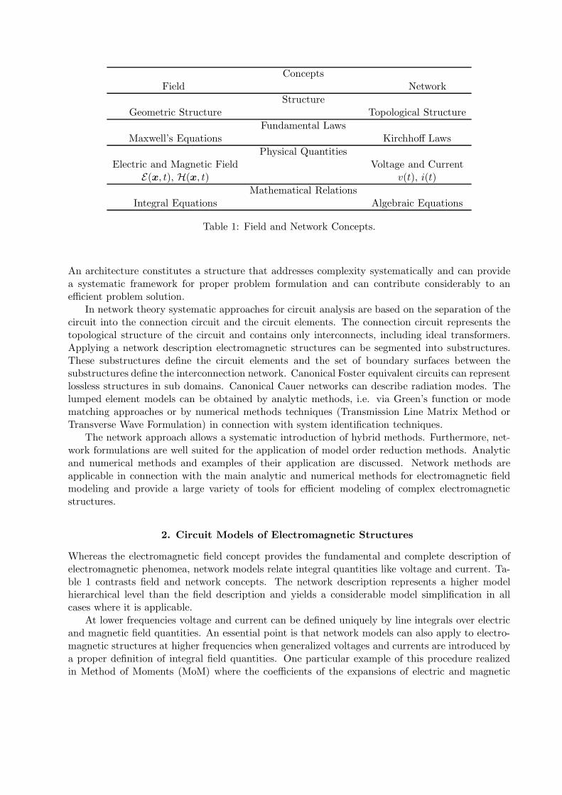
ConceptsField Network

StructureGeometric Structure Topological Structure

Fundamental LawsMaxwell’s Equations Kirchhoff Laws

Physical QuantitiesElectric and Magnetic Field Voltage and Current

E(x, t), H(x, t) v(t), i(t)

Mathematical RelationsIntegral Equations Algebraic Equations

Table 1: Field and Network Concepts.

An architecture constitutes a structure that addresses complexity systematically and can providea systematic framework for proper problem formulation and can contribute considerably to anefficient problem solution.

In network theory systematic approaches for circuit analysis are based on the separation of thecircuit into the connection circuit and the circuit elements. The connection circuit represents thetopological structure of the circuit and contains only interconnects, including ideal transformers.Applying a network description electromagnetic structures can be segmented into substructures.These substructures define the circuit elements and the set of boundary surfaces between thesubstructures define the interconnection network. Canonical Foster equivalent circuits can representlossless structures in sub domains. Canonical Cauer networks can describe radiation modes. Thelumped element models can be obtained by analytic methods, i.e. via Green’s function or modematching approaches or by numerical methods techniques (Transmission Line Matrix Method orTransverse Wave Formulation) in connection with system identification techniques.

The network approach allows a systematic introduction of hybrid methods. Furthermore, net-work formulations are well suited for the application of model order reduction methods. Analyticand numerical methods and examples of their application are discussed. Network methods areapplicable in connection with the main analytic and numerical methods for electromagnetic fieldmodeling and provide a large variety of tools for efficient modeling of complex electromagneticstructures.

2. Circuit Models of Electromagnetic Structures

Whereas the electromagnetic field concept provides the fundamental and complete description ofelectromagnetic phenomea, network models relate integral quantities like voltage and current. Ta-ble 1 contrasts field and network concepts. The network description represents a higher modelhierarchical level than the field description and yields a considerable model simplification in allcases where it is applicable.

At lower frequencies voltage and current can be defined uniquely by line integrals over electricand magnetic field quantities. An essential point is that network models can also apply to electro-magnetic structures at higher frequencies when generalized voltages and currents are introduced bya proper definition of integral field quantities. One particular example of this procedure realizedin Method of Moments (MoM) where the coefficients of the expansions of electric and magnetic

R0B10

B01

B41

B14

B04

B40

R1R2

R3R4 B34B43

B31

B21

B13

B12

B23

B32

B03

B20

B30

B02

Iα1

Iα2

Iα3

Vβ

3V

β2

Vβ

1

(a) (b)

∂R1

∂R1

∂R1∂R2

∂R2

∂R3

∂R4

∂R4

∂R4

∂R0

∂R0

∂R0

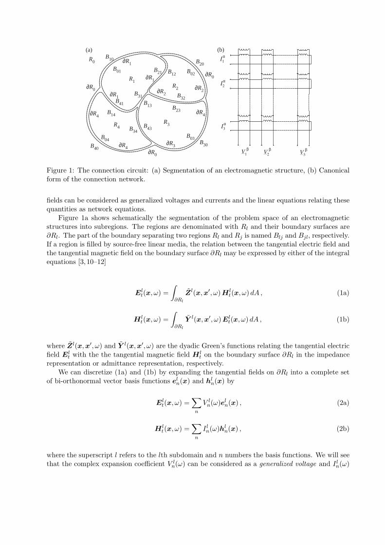
Figure 1: The connection circuit: (a) Segmentation of an electromagnetic structure, (b) Canonicalform of the connection network.

fields can be considered as generalized voltages and currents and the linear equations relating thesequantities as network equations.

Figure 1a shows schematically the segmentation of the problem space of an electromagneticstructures into subregions. The regions are denominated with Rl and their boundary surfaces are∂Rl. The part of the boundary separating two regions Rl and Rj is named Blj and Bjl, respectively.If a region is filled by source-free linear media, the relation between the tangential electric field andthe tangential magnetic field on the boundary surface ∂Rl may be expressed by either of the integralequations [3, 10–12]

Elt(x, ω) =

∫

∂Rl

Zl(x,x′, ω)H lt(x, ω) dA , (1a)

H lt(x, ω) =

∫

∂Rl

Y l(x,x′, ω)Elt(x, ω) dA , (1b)

where Zl(x,x′, ω) and Y l(x,x′, ω) are the dyadic Green’s functions relating the tangential electricfield El

t with the the tangential magnetic field H lt on the boundary surface ∂Rl in the impedance

representation or admittance representation, respectively.We can discretize (1a) and (1b) by expanding the tangential fields on ∂Rl into a complete set

of bi-orthonormal vector basis functions eln(x) and hl

n(x) by

Elt(x, ω) =

∑

n

V ln(ω)el

n(x) , (2a)

H lt(x, ω) =

∑

n

I ln(ω)hl

n(x) , (2b)

where the superscript l refers to the lth subdomain and n numbers the basis functions. We will seethat the complex expansion coefficient V l

n(ω) can be considered as a generalized voltage and I ln(ω)

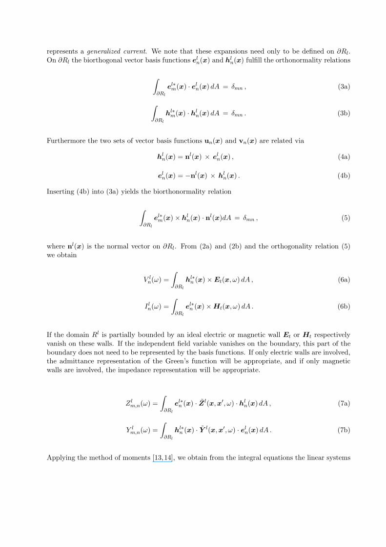
represents a generalized current. We note that these expansions need only to be defined on ∂Rl.On ∂Rl the biorthogonal vector basis functions el

n(x) and hln(x) fulfill the orthonormality relations

∫

∂Rl

el∗m(x) · el

n(x) dA = δmn , (3a)

∫

∂Rl

hl∗m(x) · hl

n(x) dA = δmn . (3b)

Furthermore the two sets of vector basis functions un(x) and vn(x) are related via

hln(x) = nl(x) × el

n(x) , (4a)

eln(x) = −nl(x) × hl

n(x) . (4b)

Inserting (4b) into (3a) yields the biorthonormality relation

∫

∂Rl

el∗m(x) × hl

n(x) · nl(x)dA = δmn , (5)

where nl(x) is the normal vector on ∂Rl. From (2a) and (2b) and the orthogonality relation (5)we obtain

V ln(ω) =

∫

∂Rl

hl∗n (x) × Et(x, ω) dA , (6a)

I ln(ω) =

∫

∂Rl

el∗n (x) × Ht(x, ω) dA . (6b)

If the domain Rl is partially bounded by an ideal electric or magnetic wall Et or Ht respectivelyvanish on these walls. If the independent field variable vanishes on the boundary, this part of theboundary does not need to be represented by the basis functions. If only electric walls are involved,the admittance representation of the Green’s function will be appropriate, and if only magneticwalls are involved, the impedance representation will be appropriate.

Z lm,n(ω) =

∫

∂Rl

el∗n (x) · Zl(x,x′, ω) · hl

n(x) dA , (7a)

Y lm,n(ω) =

∫

∂Rl

hl∗n (x) · Y l(x,x′, ω) · el

n(x) dA . (7b)

Applying the method of moments [13,14], we obtain from the integral equations the linear systems

of equations

V lm(ω) =

∑

n

Z lm,n(ω)I l

n(ω) , (8a)

I lm(ω) =

∑

n

Y lm,n(ω)V l

n(ω) . (8b)

Summarizing the amplitudes V lm(ω) and I l

m(ω) in the vectors

V l(ω) = [V l1 (ω)...V l

N (ω)]T , I l(ω) = [I l1(ω)...I l

N (ω)]T (9)

and the matrix elements Z lm,n(ω) and Y l

m,n(ω) in the matrices

Zl(ω) =

Z l11(ω) · · · Z l

1N (ω)...

. . ....

Z lN1(ω) · · · Z l

NN (ω)

, Y l(ω) =

Y l11(ω) · · · Y l

1N (ω)...

. . ....

Y lN1(ω) · · · Y l

NN (ω)

(10)

we obtain the linear system of equations in matrix notation

V l(ω) = Zl(ω)I l(ω) , I l(ω) = Y l(ω)V l(ω) . (11)

These equations represent a circuit description of the EM structure in domain Rl. The impedanceand admittance matrices Zl(ω) and Y l(ω), respectively relate the generalized voltages and currentssummarized in the vectors V l(ω) and I l(ω), respectively.

3. Tellegen’s Theorem and the Connection Network

A. Field Theoretic Formulation of Tellegen’s Theorem

Complex electromagnetic structures may be subdivided into substructures confined to spatial sub-domains. Comparing a distributed circuit represented by an electromagnetic structure with alumped element circuit represented by a network, the spatial subdomains may be considered asthe circuit elements whereas the complete set of boundary surfaces separating the subdomainscorresponds to the connection circuit [10,12].

Figure 1a shows the segmentation of an electromagnetic structure into different regions Rl

separated by boundaries Blk. The regions Rl may contain any electromagnetic substructure. Inour network analogy the two-dimensional manifold of all boundary surfaces Blk represents theconnection circuit whereas the subdomains Rl are representing the circuit elements.

The tangential electric and magnetic fields on the boundary surface of a subdomain are relatedvia Green’s functions [3, 10, 12, 15]. These Green’s functions can be seen in analogy to the Fosterrepresentation of the corresponding reactive network.

We can establish a field representation of the Tellegen’s theorem relating the tangental electricand magnetic fields on the two-dimensional manifolds of boundaries Blk [16]. Expanding thetangential electric and magnetic fields on the boundaries again into basis functions allows to give anequivalent circuit representation for the boundary surfaces. The equivalent circuit of the boundarysurfaces is a connection circuit exhibiting only connections and ideal transformers.

Tellegen’s theorem states fundamental relations between voltages and currents in a networkand is of considerable versatility and generality in network theory [16–18]. A noticeable propertyof this theorem is that it is only based on Kirchhoff’s current and voltage laws, i.e. on topologicalrelationships, and that it is independent from the constitutive laws of the network. The samereasoning that yields from Kirchhoff’s laws to Tellegen’s theorem allows to directly derive a fieldform of Tellegen’s theorem from Maxwell’s equations [16].

In order to derive Tellegen’s theorem for partitioned electromagnetic structures let us considertwo electromagnetic structures based on the same partition by equal boundary surfaces. Thesubdomains of either electromagnetic structure however may be filled with different materials. Theconnection network is established via the relations of the tangential field components on both sidesof the boundaries. Since the connection network exhibits zero volume no field energy is storedtherein and no power loss occurs therein.

Starting directly from Maxwell’s equations we may derive for a closed volume R with boundarysurface ∂R and relative normal vector n the following relation:

∫

∂R

E′(x, t′) × H ′′(x, t′′) · n dA = −

∫

R

E′(r, t′) · J′′(r, t′′) dr −

−

∫

R

E′(r, t′) ·∂D′′(r, t′′)

∂t′′dr−

∫

R

H′(r, t′) ·∂B′′(r, t′′)

∂t′′dr . (12)

The prime ′ and double prime ′′ denote the case of a different choice of sources and a differentchoice materials filling the subdomains. Furthermore also the time argument may be different inboth cases.

For volumes R of zero measure or free of field the right side of this equation vanishes. Con-sidering an electromagnetic structure as shown in Figure 1a, we perform the integration over theboundaries of all subregions not filled with ideal electric or magnetic conductors respectively. Theintegration over both sides of a boundary yields zero contribution to the integrals on the right sideof (12). Also the integration over finite volumes filled with ideal electric or magnetic conductorsgives no contribution to these integrals. We obtain the field form of Tellegen’s theorem

∫

∂R

E′(x, t′) × H ′′(x, t′′) · ndA = 0 . (13)

We note, that Tellegen’s theorem also holds in frequency domain,

∫

∂R

E′(x, ω′) × H ′′(x, ω′′) · ndA = 0 , (14)

and also when the frequencies ω′ and ω′′ differ from each other.

B. The discretized connection network

We now consider the fields as expanded on finite orthonormal basis function sets; the assumptionof orthonormal basis is not necessary, and is introduced to simplify notation. We consider sets ofelectric and magnetic field vectorial basis functions e

ξn(x) and h

ξn(x), respectively, of dimension Nξ

on the boundary surface ξ with ξ = α, β. Expanding the tangential electric and magnetic Fieldson both sides α and β of the boundary as described in Section 2 into

Eξt =

Nξ∑

n

V ξn eξ

n(x) , Hξt =

Nξ∑

n

V ξn hξ

n(x) , (15)

we can summarize the field expansion coefficients for the electric and magnetic field in the vectorsV α, Iα, V β and Iβ, leading compactly to the vectors

V =

[

V α

V β

]

, I =

[

Iα

Iβ

]

, (16)

summarizing the voltage and current amplitudes on both sides of the boundary layer. Since thetangential electric and magnetic field are continuous at the boundary surface the total tangentialelectric and magnetic fields are the same on both sides of the boundary. However, since the vectorialbasis functions e

ξn(x) and h

ξn(x) in general will be chosen differently on both sides of the boundary

the components of V α, Iα may be coupled in a general way to the components of V β and Iβ ,respectively. Inserting the field expansions (15) into the field form of Tellegen’s theorem (13) yields

∫

∂R

E′(x, t′) × H ′′(x, t′′) · ndA =∑

ξ=α,β

Nξ∑

n

Nξ∑

m

V ξ′

m (t′)Iξ′′

n (t′′)

∫

∂R

eξm × hξ

n · ndA = 0 . (17)

If the vectorial basis fuctions fulfill the biorthonormality relations (5), Tellegen’s theorem takes thestandard form

V ′T (t′) I ′′(t′′) = 0 . (18)

where V (t) and I(t) denote the voltage and current vectors of the connection circuit. The prime ′

and double prime ′′ again denote different circuit elements and different times in both cases. It isonly required that the topological structure of the connection circuit remains unchanged.

C. Canonical Forms of the Connection Network

Consistent choices of independent and dependent fields do not violate Tellegen’s theorem and allowto draw canonical networks, which are based only on connections and ideal transformers. Figure 1bshows the canonical form of the connection network when using as independent fields the vectors V β

(dimension Nβ) and Iα (dimension Nα). In this case the dependent fields are V α (dimension Nα)and Iβ (dimension Nβ). In all cases we have Nβ+Nα independent quantities and the same number ofdependent quantities. Note that scattering representations are also allowed and that the connectionnetwork is frequency independent. It is apparent from the canonical network representations thatthe scattering matrix is symmetric, ST = S, orthogonal, ST S = I and unitary, i.e. SS† = I,where the † denotes the Hermitian conjugate matrix.

4. Foster Representation of Reactance Multiports

Consider again a subregion Rl of an electromagnetic structure as depicted schematically in Fig-ure 1a. Let us assume this subregion to be filled with an arbitrary structure consisting from freespace, perfect electric and magnetic conductors and reciprocal lossless electric and magnetic materi-als. Such a subregion may be characterized by the relation between tangential electric and magneticfields on the boundary surface ∂Rl as specified by either (1a) or (1b). Covering the closed boundarysurface ∂Rl to consist either by a perfect electric conductor or a perfect magnetic conductor makesthe complete structure a lossless resonator. The electromagnetic field inside such a lossless closedcavity can be expanded into orthogonal modal functions [19–23].

In the spectral representation the dyadic impedance and admittance Green’s functions intro-duced in (1a) and (1b) are given by [3,10,12,15]

Z(x,x′, ω) =1

jωz0(x,x′) +

∑

λ

1

jω

ω2

ω2 − ω2p,λ

zλ(x,x′) , (19a)

Y (x,x′, ω) =1

jωy0(x,x′) +

∑

λ

1

jω

ω2

ω2 − ω2s,λ

yλ(x,x′) . (19b)

The dyadics z0(x,x′) and y0(x,x′) represent the static parts of the Green’s functions, whereaseach term zλ(x,x′) and yλ(x,x′), respectively, corresponds to a pole at the frequency ωλ.

Expanding the electric and magnetic field into basis functions eln(x) and hl

n(x) as described in(2a) and (2b) the impedance and admittance matrices relating the generalized voltages V l(ω) andcurrents I l(ω) will be obtained as

Z(ω) =1

jωCp,0Ap,0 +

N∑

p,λ=1

1

jωCp,λ

ω2

ω2 − ω2p,λ

Ap,λ , (20a)

Y (ω) =1

jωLs,0As,0 +

N∑

s,λ=1

1

jωLs,λ

ω2

ω2 − ω2s,λ

As,λ , (20b)

where Ap,λ and As,λ, respectively are real frequency-independent rank 1 matrices given in eithercase by

Aλ =

n2λ1 nλ1nλ2 . . . nλ1nλN

nλ2nλ1 n2λ2 . . . nλ2nλN

......

. . ....

nλNnλ1 nλNnλ2 . . . n2λN

. (21)

We can interpret the respective impedance matrix Zl(ω) and admittance matrix Y l(ω) as de-scribing lumped element equivalent circuits. This allows us to draw directly the equivalent circuits

Cs,1

L s,1

11

12

13

Cs,2

L s,2

21

22

23

2M

Cs,3

L s,3

31

32

33

3M

Cs,N

L s,N

N1

N2

N3

NM

port 1

port 2

port 3

port M

1: n

1: n

1: n

1: n

1: n

1: n

1: n

1: n

1: n

1: n

1: n

1: n

1: n

1M

1: n

1: n

1: n

1: n

0M

1: n

1: n

1: n

01

02

03

L s,0

n :1 n :1

n :1 n :1

n :121

31

n :1N1

2 2

32

N2

23

33

N3C

p,N Lp,N

2M

3M

NM

L p,2

Lp,3Cp,3

Cp,2

n :1

n :1

n :1

n :1 n :1 n :1

port 1 port 2 port 3 port M

n :1 n :1Cp,1 L n :111 12 13n :1

n :1 n :1Cp,0 n :101 02 03 0Mn :1

(a) (b)

1Mp,1

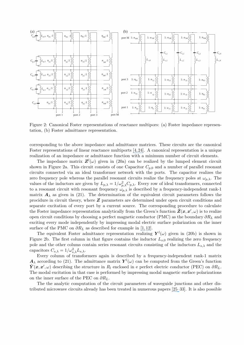
Figure 2: Canonical Foster representations of reactance multipors: (a) Foster impedance represen-tation, (b) Foster admittance representation.

corresponding to the above impedance and admittance matrices. These circuits are the canonicalFoster representations of linear reactance multiports [4,24]. A canonical representation is a uniquerealization of an impedance or admittance function with a minimum number of circuit elements.

The impedance matrix Zl(ω) given in (20a) can be realized by the lumped element circuitshown in Figure 2a. This circuit consists of one Capacitor Cp,0 and a number of parallel resonantcircuits connected via an ideal transformer network with the ports. The capacitor realizes thezero frequency pole whereas the parallel resonant circuits realize the frequency poles at ωp,λ. Thevalues of the inductors are given by Lp,λ = 1/ω2

p,λCp,λ. Every row of ideal transformers, connectedto a resonant circuit with resonant frequency ωp,λ is described by a frequency-independent rank-1matrix Aλ as given in (21). The determination of the equivalent circuit parameters follows theprocidure in circuit theory, where Z parameters are determined under open circuit conditions andseparate excitation of every port by a current source. The corresponding procedure to calculatethe Foster impedance representation analytically from the Green’s function Z(x,x′, ω) is to realizeopen circuit conditions by choosing a perfect magnetic conductor (PMC) as the boundary ∂RL andexciting every mode independently by impressing modal electric surface polarization on the innersurface of the PMC on ∂RL as described for example in [1, 12].

The equivalent Foster admittance representation realizing Y l(ω) given in (20b) is shown inFigure 2b. The first column in that figure contains the inductor Ls,0 realizing the zero frequencypole and the other colums contain series resonant circuits consisting of the inductors Ls,λ and thecapacitors Cs,λ = 1/ω2

s,λLs,λ.Every column of transformers again is described by a frequency-independent rank-1 matrix

Aλ according to (21). The admittance matrix Y l(ω) can be computed from the Green’s functionY (x,x′, ω) describing the structure in Rl enclosed in e perfect electric conductor (PEC) on ∂RL.The modal excitation in that case is performed by impressing modal magnetic surface polarizationson the inner surface of the PEC on ∂RL.

The the analytic computation of the circuit parameters of waveguide junctions and other dis-tributed microwave circuits already has been treated in numerous papers [25–33]. It is also possible

x

y

z

ϕ

θ r=roR3

R4

Source 1

Source 2

Source k

REACTANCEMULTIPORT

TM

TE

m’n’

m’’n’’

TM

TE

11

11CONNECTION

NETWORK

(a) (b)R1

S

Source 1

Source 2

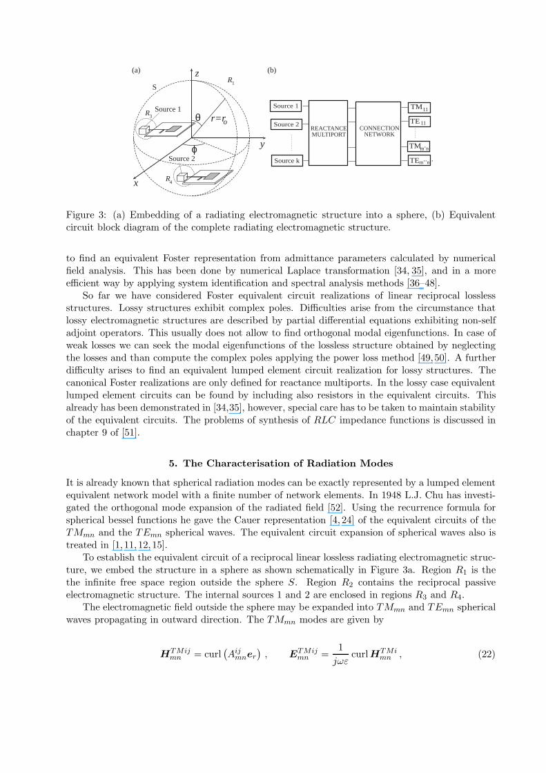
Figure 3: (a) Embedding of a radiating electromagnetic structure into a sphere, (b) Equivalentcircuit block diagram of the complete radiating electromagnetic structure.

to find an equivalent Foster representation from admittance parameters calculated by numericalfield analysis. This has been done by numerical Laplace transformation [34, 35], and in a moreefficient way by applying system identification and spectral analysis methods [36–48].

So far we have considered Foster equivalent circuit realizations of linear reciprocal losslessstructures. Lossy structures exhibit complex poles. Difficulties arise from the circumstance thatlossy electromagnetic structures are described by partial differential equations exhibiting non-selfadjoint operators. This usually does not allow to find orthogonal modal eigenfunctions. In case ofweak losses we can seek the modal eigenfunctions of the lossless structure obtained by neglectingthe losses and than compute the complex poles applying the power loss method [49,50]. A furtherdifficulty arises to find an equivalent lumped element circuit realization for lossy structures. Thecanonical Foster realizations are only defined for reactance multiports. In the lossy case equivalentlumped element circuits can be found by including also resistors in the equivalent circuits. Thisalready has been demonstrated in [34,35], however, special care has to be taken to maintain stabilityof the equivalent circuits. The problems of synthesis of RLC impedance functions is discussed inchapter 9 of [51].

5. The Characterisation of Radiation Modes

It is already known that spherical radiation modes can be exactly represented by a lumped elementequivalent network model with a finite number of network elements. In 1948 L.J. Chu has investi-gated the orthogonal mode expansion of the radiated field [52]. Using the recurrence formula forspherical bessel functions he gave the Cauer representation [4, 24] of the equivalent circuits of theTMmn and the TEmn spherical waves. The equivalent circuit expansion of spherical waves also istreated in [1, 11,12,15].

To establish the equivalent circuit of a reciprocal linear lossless radiating electromagnetic struc-ture, we embed the structure in a sphere as shown schematically in Figure 3a. Region R1 is thethe infinite free space region outside the sphere S. Region R2 contains the reciprocal passiveelectromagnetic structure. The internal sources 1 and 2 are enclosed in regions R3 and R4.

The electromagnetic field outside the sphere may be expanded into TMmn and TEmn sphericalwaves propagating in outward direction. The TMmn modes are given by

HTMijmn = curl

(

Aijmner

)

, ETMijmn =

1

jωεcurlHTMi

mn , (22)

where n = 1, 2, 3, 4, . . . , m = 1, 2, 3, 4, . . . , n, i = e, o, and j = 1, 2. The radial component Aijmn

of the vector potential is given by

Aejmn = aej

mnPmn (cos θ) cos mϕh(j)

n (kr) , Aojmn = aoj

mnPmn (cos θ) sin mϕh(j)

n (kr) , (23)

where the Pmn (cos θ) are the associated Legendre polynomials and h

(j)n (kr) are the spherical Hankel

functions and aejmn and aoj

mn are coefficients [1, 11,12,15]. The superscript j = 1 denotes an inwardpropagating wave and the superscript j = 2 indicates an outward propagating wave. Outside thesphere, for r > r0 only outward propagating waves occur and we have only to consider j = 2.

The TEmn modes are dual with respect to the TMmn modes and are given by

ETEijmn = − curl

(

F ijmner

)

,HTEijmn = −

1

jωεcurlETMi

mn , (24)

where n = 1, 2, 3, 4, . . . , m = 1, 2, 3, 4, . . . , n, i = e, o, and j = 1, 2. The radial component F ijmn

of the dual vector potential is given by

F ejmn = f ej

mnPmn (cos θ) cos mϕh(j)

n (kr) , F ojmn = f oj

mnPmn (cos θ) sin mϕh(j)

n (kr) . (25)

where the Pmn (cos θ) are the associated Legendre polynomials and h

(j)n (kr) are the spherical Hankel

functions. The f ejmn and f oj

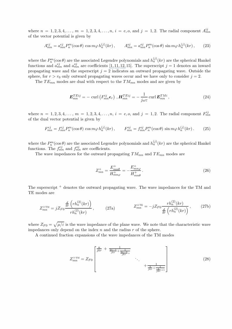
mn are coefficients.The wave impedances for the outward propagating TMmn and TEmn modes are

Z+mn =

E+mnθ

H+mnϕ

= −E+

mnϕ

H+mnθ

. (26)

The superscript + denotes the outward propagating wave. The wave impedances for the TM andTE modes are

Z+tm

mn = jZF0

ddr

(

rh(2)n (kr)

)

rh(2)n (kr)

, (27a) Z+te

mn = −jZF0rh

(2)n (kr)

ddr

(

rh(2)n (kr)

) , (27b)

where ZF0 =√

µ/ε is the wave impedance of the plane wave. We note that the characteristic waveimpedances only depend on the index n and the radius r of the sphere.

A continued fraction expansions of the wave impedances of the TM modes

Z+tm

mn = ZF0

njkr

+ 12n−1

jkr+ 1

2n−3jkr

+

. . .

+ 13

jkr+ 1

1jkr

+1

(28)

Zmn+TM

rε n

rε2n - 3

rµ2n - 1

rµ2n - 5 ZF0 Z

mn+TE rµ

n

rε2n - 5

rε2n - 1

rµ2n - 3 ZF0

(a) (b)

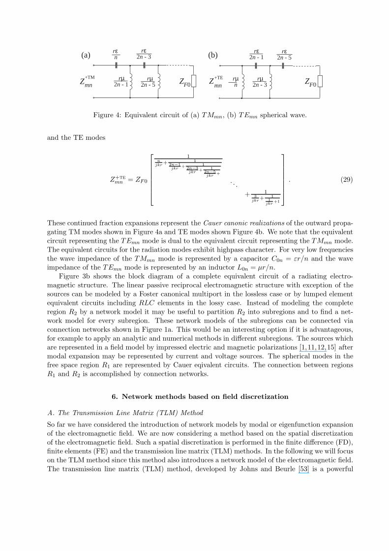
Figure 4: Equivalent circuit of (a) TMmn, (b) TEmn spherical wave.

and the TE modes

Z+te

mn = ZF0

1n

jkr+ 1

2n−1jkr

+ 12n−3jkr

+ 12n−5jkr

+

. . .

+ 13

jkr+ 1

1jkr

+1

. (29)

These continued fraction expansions represent the Cauer canonic realizations of the outward propa-gating TM modes shown in Figure 4a and TE modes shown Figure 4b. We note that the equivalentcircuit representing the TEmn mode is dual to the equivalent circuit representing the TMmn mode.The equivalent circuits for the radiation modes exhibit highpass character. For very low frequenciesthe wave impedance of the TMmn mode is represented by a capacitor C0n = εr/n and the waveimpedance of the TEmn mode is represented by an inductor L0n = µr/n.

Figure 3b shows the block diagram of a complete equivalent circuit of a radiating electro-magnetic structure. The linear passive reciprocal electromagnetic structure with exception of thesources can be modeled by a Foster canonical multiport in the lossless case or by lumped elementequivalent circuits including RLC elements in the lossy case. Instead of modeling the completeregion R2 by a network model it may be useful to partition R2 into subregions and to find a net-work model for every subregion. These network models of the subregions can be connected viaconnection networks shown in Figure 1a. This would be an interesting option if it is advantageous,for example to apply an analytic and numerical methods in different subregions. The sources whichare represented in a field model by impressed electric and magnetic polarizations [1,11,12,15] aftermodal expansion may be represented by current and voltage sources. The spherical modes in thefree space region R1 are represented by Cauer eqivalent circuits. The connection between regionsR1 and R2 is accomplished by connection networks.

6. Network methods based on field discretization

A. The Transmission Line Matrix (TLM) Method

So far we have considered the introduction of network models by modal or eigenfunction expansionof the electromagnetic field. We are now considering a method based on the spatial discretizationof the electromagnetic field. Such a spatial discretization is performed in the finite difference (FD),finite elements (FE) and the transmission line matrix (TLM) methods. In the following we will focuson the TLM method since this method also introduces a network model of the electromagnetic field.The transmission line matrix (TLM) method, developed by Johns and Beurle [53] is a powerful

8 8

6 6

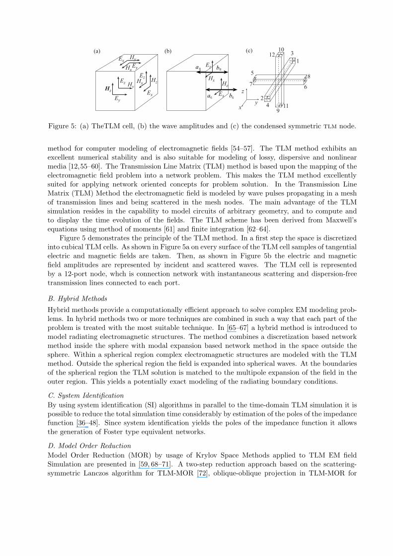
Figure 5: (a) TheTLM cell, (b) the wave amplitudes and (c) the condensed symmetric tlm node.

method for computer modeling of electromagnetic fields [54–57]. The TLM method exhibits anexcellent numerical stability and is also suitable for modeling of lossy, dispersive and nonlinearmedia [12,55–60]. The Transmission Line Matrix (TLM) method is based upon the mapping of theelectromagnetic field problem into a network problem. This makes the TLM method excellentlysuited for applying network oriented concepts for problem solution. In the Transmission LineMatrix (TLM) Method the electromagnetic field is modeled by wave pulses propagating in a meshof transmission lines and being scattered in the mesh nodes. The main advantage of the TLMsimulation resides in the capability to model circuits of arbitrary geometry, and to compute andto display the time evolution of the fields. The TLM scheme has been derived from Maxwell’sequations using method of moments [61] and finite integration [62–64].

Figure 5 demonstrates the principle of the TLM method. In a first step the space is discretizedinto cubical TLM cells. As shown in Figure 5a on every surface of the TLM cell samples of tangentialelectric and magnetic fields are taken. Then, as shown in Figure 5b the electric and magneticfield amplitudes are represented by incident and scattered waves. The TLM cell is representedby a 12-port node, whch is connection network with instantaneous scattering and dispersion-freetransmission lines connected to each port.

B. Hybrid Methods

Hybrid methods provide a computationally efficient approach to solve complex EM modeling prob-lems. In hybrid methods two or more techniques are combined in such a way that each part of theproblem is treated with the most suitable technique. In [65–67] a hybrid method is introduced tomodel radiating electromagnetic structures. The method combines a discretization based networkmethod inside the sphere with modal expansion based network method in the space outside thesphere. Within a spherical region complex electromagnetic structures are modeled with the TLMmethod. Outside the spherical region the field is expanded into spherical waves. At the boundariesof the spherical region the TLM solution is matched to the multipole expansion of the field in theouter region. This yields a potentially exact modeling of the radiating boundary conditions.

C. System Identification

By using system identification (SI) algorithms in parallel to the time-domain TLM simulation it ispossible to reduce the total simulation time considerably by estimation of the poles of the impedancefunction [36–48]. Since system identification yields the poles of the impedance function it allowsthe generation of Foster type equivalent networks.

D. Model Order Reduction

Model Order Reduction (MOR) by usage of Krylov Space Methods applied to TLM EM fieldSimulation are presented in [59, 68–71]. A two-step reduction approach based on the scattering-symmetric Lanczos algorithm for TLM-MOR [72], oblique-oblique projection in TLM-MOR for

high-Q structures [73], system identification and model order reduction for TLM analysis [74]yield a considerable reduction of the computational effort in modeling complex electromagneticstructures.

E. Discrete Electrodynamics and Metamaterials

Metamaterials are artificial electromagnetic structures exhibiting special properties like negativepermeability, negative permittivity and negative refractive index [75–80]. The discrete nature ofmetamaterials makes a discrete electrodynamical approach the most natural theoretical frameworkfor the treatment of 3D metamaterials. Beyond being a powerful tool for numerical modelingof metamaterial structures, the TLM scheme provides a fundamental theoretical framework forthe finding and exploration of three-dimensional metamaterial structures [81–83]. The numericalmodeling of metamaterial structures exhibiting a large number of cells swamps the computationalresources of numerical CAD tools. Network oriented modeling with adapted TLM scheme can solvethis problem [84].

7. The Mode Matching Method

The generalized network formulation of the electromagnetic field problem, in connection with modematching (MM) has already been applied to analyze waveguide N -furcation [85–90], to flange-mounted radiating waveguides [91] and to model antennas realized with a central circular waveg-uide [92]. The MM method is excellently suited for the modeling of planar transmission linestructures with sub-micrometer cross sections [93–96]. A hybrid combination of the TLM methodand the mode matching method yields an efficient tool for full-wave analysis of transmission linesand discontinuities in RF-MMICs [97,98].

8. Conclusion

Network methods applied to electromagnetic field simulation can contribute substanially to prob-lem formulation, solution methodology and computational efficiency and allow to generate compactmodels of electromagnetic systems. Various methods for introducing network models of electro-magnetic structures are based either on eigenmode expansion or on spatial discretization of theelectromagnetic field. Network-oriented modeling can be combined with complexity reduction andsystem identification techniques and have the potential to reduce the computation time for themodeling of electromagnetic systems bsubstantially.

This work is based on research projects supported by the Deutsche Forschungsgemeinschaft.

References

[1] R. F. Harrington, Time Harmonic Electromagnetic Fields. New York: McGraw-Hill, 1961.

[2] S. Ramo, J. R. Whinnery, and T. van Duzer, Fields and Waves in Communication Electronics. New York:John Wiley & Sons, 1965.

[3] R. Collin, Field Theory of Guided Waves, 2nd ed. New York: IEEE Press, Inc., 1991.

[4] V. Belevitch, Classical Network Theory. San Francisco: Holden-Day, 1968.

[5] H. J. Carlin and A. B. Giordano, Network Theory. Englewood Cliffs, NJ: Prentice Hall, 1964.

[6] L. O. Chua, C. A. Desoer, and E. S. Kuh, Linear and Nonlinear Circuits. New York: Mc Graw Hill, 1987.

[7] W. Mathis, Theorie nichtlinearer Netzwerke. Berlin: Springer, 1987.

[8] L. B. Felsen, M. Mongiardo, and P. Russer, “Electromagnetic field representations and computations in complexstructures I: Complexity architecture and generalized network formulation,” International Journal of NumericalModelling, Electronic Networks, Devices and Fields, vol. 15, pp. 93–107, 2002.

[9] ——, “Electromagnetic field representations and computations in complex structures II: Alternative Green’sfunctions,” International Journal of Numerical Modelling, Electronic Networks, Devices and Fields, vol. 15, pp.109–125, 2002.

[10] P. Russer, M. Mongiardo, and L. B. Felsen, “Electromagnetic field representations and computations in complexstructures III: Network representations of the connection and subdomain circuits,” International Journal ofNumerical Modelling, Electronic Networks, Devices and Fields, vol. 15, pp. 127–145, 2002.

[11] L. B. Felsen, M. Mongiardo, and P. Russer, Electromagnetic Field Computation by Network Methods, 1st ed.Berlin Heidelberg New York: Springer, 2009.

[12] P. Russer, Electromagnetics, Microwave Circuit and Antenna Design for Communications Engineering, 2nd ed.Boston: Artech House, 2006.

[13] R. F. Harrington, “Matrix methods for field problems,” Proceedings of the IEEE, vol. 55, no. 2, pp. 136–149,Feb. 1967.

[14] ——, Field Computation by Moment Methods,. San Francisco: IEEE Press, 1968.

[15] L. B. Felsen and N. Marcuvitz, Radiation and Scattering of Waves. Englewood Cliffs, NJ: Prentice Hall, 1972.

[16] P. Penfield, R. Spence, and S. Duinker, Tellegen’s theorem and electrical networks. Cambridge, Massachusetts:MIT Press, 1970.

[17] B. D. H. Tellegen, “A general network theorem with applications,” Philips Research Reports, vol. 7, pp. 259–269,1952.

[18] ——, “A general network theorem with applications,” Proc. Inst. Radio Engineers, vol. 14, pp. 265–270, 1953.

[19] J. C. Slater, “Microwave electronics,” Rev. Mod. Phys., vol. 18, no. 4, pp. 441–512, Oct 1946.

[20] T. Teichmann, “Completeness relations for Loss-Free microwave junctions,” J. Appl. Physics, vol. 23, no. 7, pp.701–710, Jul. 1952. [Online]. Available: http://link.aip.org/link/?JAP/23/701/1

[21] T. Teichmann and E. P. Wigner, “Electromagnetic field expansions in loss-free cavities excited through holes,”J. Appl. Physics, vol. 24, no. 3, pp. 262–267, Mar. 1953.

[22] S. A. Schelkunoff, “On representation of electromagnetic fields in cavities in terms of natural modes of oscilla-tion,” J. Appl. Physics, vol. 26, no. 10, pp. 1231–1234, Oct. 1955.

[23] K. Kurokawa, “The expansions of electromagnetic fields in cavities,” IEEE Trans. Microwave Theory Techn.,vol. 6, no. 2, pp. 178– 187, Apr. 1958.

[24] W. Cauer, Theorie der linearen Wechselstromschaltungen. Berlin: Akademie-Verlag, 1954.

[25] T. Rozzi and W. Mecklenbrauker, “Field and network analysis of waveguide discontinuities,” in European Mi-crowave Conference, 1973. 3rd, vol. 1, 1973, pp. 1–4.

[26] T. E. Rozzi and W. F. G. Mecklenbrauker, “Wide-Band network modeling of interacting inductive irises andsteps,” IEEE Trans. Microwave Theory Techn., vol. 23, no. 2, pp. 235–245, 1975.

[27] P. Arcioni, M. Bressan, G. Conciauro, and L. Perregrini, “Wideband modeling of arbitrarily shaped e-planewaveguide components by the boundary integral-resonant mode expansion method,” IEEE Trans. MicrowaveTheory Techn., vol. 44, no. 11, pp. 2083–2092, 1996.

[28] G. Conciauro, P. Arcioni, M. Bressan, and L. Perregrini, “Wideband modeling of arbitrarily shaped h-planewaveguide components by the boundary integral-resonant mode expansion method,” IEEE Trans. MicrowaveTheory Techn., vol. 44, no. 7, pp. 1057–1066, 1996.

[29] P. Arcioni and G. Conciauro, “Combination of generalized admittance matrices in the form of pole expansions,”IEEE Trans. Microwave Theory Techn., vol. 47, no. 10, pp. 1990–1996, 1999.

[30] J. Dittloff, J. Bornemann, and F. Arndt, “Computer aided design of optimum e- or H-Plane N-Furcated waveg-uide power dividers,” in European Microwave Conference, 1987. 17th, 1987, pp. 181–186.

[31] J. Dittloff, F. Arndt, and D. Grauerholz, “Optimum design of waveguide e-plane stub-loaded phase shifters,”IEEE Trans. Microwave Theory Techn., vol. 36, no. 3, pp. 582–587, 1988.

[32] M. Guglielmi, F. Montauti, L. Pellegrini, and P. Arcioni, “Implementing transmission zeros in inductive-windowbandpass filters,” IEEE Trans. Microwave Theory Techn., vol. 43, no. 8, pp. 1911–1915, 1995.

[33] G. Conciauro, M. Guglielmi, and R. Sorrentino, Advanced Modal Analysis. New York: John Wiley & Sons,2000.

[34] T. Mangold and P. Russer, “Generation of lumped element equivalent circuits for distributed multiport structuresvia TLM simulation,” Second International Workshop on Transmission Line Matrix (TLM) Modeling – Theoryand Applications, Munich, Germany, 29.-31.10.1997, pp. 236–245, Oct. 1997., pp. 236–245, Oct. 1997.

[35] T. Mangold, P. Gulde, G. Neumann, and P. Russer, “A multichip module integration technology on siliconsubstrate for high frequency applications,” in 1998 Topical Meeting on Silicon Monolithic Integrated Circuits inRF Systems Digest, Ann Arbor, 26-28 Sept 1998, 1998, pp. 181–184.

[36] V. Chtchekatourov, L. Vietzorreck, W. Fisch, and P. Russer, “Time-domain system identification modeling formicrowave structures,” in MMET 2000. International Conference on Mathematical Methods in ElectromagneticTheory, vol. 1, 2000, pp. 137–139 vol.1.

[37] V. Chtchekatourov, F. Coccetti, and P. Russer, “Direct Y–parameters estimation of microwave structures usingTLM simulation and prony’s method,” in Proc. 17th Annual Review of Progress in Applied ComputationalElectromagnetics ACES, Monterey, May 2001, pp. 580–586.

[38] V. Chtchekatourov, W. Fisch, F. Coccetti, and P. Russer, “Full–wave analysis and model–based parameter esti-mation approaches for s- and y- matrix computation of microwave distributed circuits,” in 2001 Int. MicrowaveSymposium Digest, Phoenix, 2001, pp. 1037–1040.

[39] F. Coccetti, V. Chtchekatourov, and P. Russer, “Time-domain analysis of RF structures by means of TLM andsystem identification methods,” in European Microwave Conference, 2001. 31st, 2001, pp. 1–4.

[40] Y. Kuznetsov, A. Baev, F. Coccetti, and P. Russer, “The ultra wideband transfer function representation ofcomplex three-dimensional electromagnetic structures,” in 34th European Microwave Conference, Amsterdam,The Netherlands, 11.-15.10.2004, Oct. 2004, pp. 455–458.

[41] U. Siart, K. Fichtner, Y. Kuznetsov, A. Baev, and P. Russer, “TLM modeling and system identification ofdistributed microwave circuits and antennas,” in ICEAA2007, Int. Conf. on Electromagnetics in AdvancedApplications, 2007, Torino, Torino, Italy, sept 2007, pp. 352–355.

[42] Y. Kuznetsov, A. Baev, P. Lorenz, and P. Russer, “Network oriented modeling of passive microwave structures,”in EUROCON 2007, sept 2007, pp. 10–14.

[43] N. Fichtner, U. Siart, Y. Kuznetsov, A. Baev, and P. Russer, “TLM modeling and system identification ofoptimized antenna structures,” in Kleinheubacher Tagung, Miltenberg, Germany, sept 2007.

[44] F. Coccetti and P. Russer, “A prony’s model based signal prediction (psp) algorithm for systematic extractionof y parameters from td transient responses of electromagnetic structures,” in 15th International Conference onMicrowaves, Radar and Wireless Communications, MIKON-2004, 17-19 May, vol. 3, May 2004, pp. 791 – 794.

[45] P. Russer and F. Coccetti, “Network methods in electromagnetic field computation,” in Proc. Turkish URSICongress 2004, 8 - 10 August 2004, Ankara, Aug. 2004.

[46] Y. Kuznetsov, A. Baev, F. Coccetti, and P. Russer, “The ultra wideband transfer function representation ofcomplex three-dimensional electromagnetic structures,” in 2004 International Symposium on Signals, Systems,and Electronics ISSSE’04, August 10-13, Linz, Austria, Aug. 2004.

[47] D. Lukashevich, F. Coccetti, and P. Russer, “System identification and model order reduction for TLM analysis ofmicrowave components,” in Computational Electromagnetics in Time-Domain, 2005. CEM-TD 2005. Workshopon, 2005, pp. 64–67.

[48] K. Fichtner, U. Siart, Y. Kuznetsov, A. Baev, and P. Russer, “Bandwidth optimization using transmission linematrix modeling,” in Time-Domain Methods in Modern Engineering Electromagnetics, A Tribute to WolfgangJ. R. Hoefer, P. Russer and U. Siart, Eds. Technische Universitat Munchen: Springer, may 16–17 2007.

[49] J. Gustincic and R. Collin, “A general power loss method for attenuation of cavities and waveguides,” in PGMTTNational Symposium Digest, vol. 62, 1962, pp. 20–21.

[50] J. Gustincic, “A general power loss method for attenuation of cavities and waveguides,” IEEE Trans. MicrowaveTheory Techn., vol. 11, no. 1, pp. 83–87, 1963.

[51] E. A. Guillemin, Synthesis of Passive Networks. New York: Wiley, 1957.

[52] L. Chu, “Physical limitations of omni-directional antennas,” J. Appl. Physics, vol. 19, no. 12, pp. 1163–1175,Dec. 1948.

[53] P. Johns and R. Beurle, “Numerical solution of 2-dimensional scattering problems using a transmission-linematrix,” Proc. IEE, vol. 118, no. 9, pp. 1203–1208, Sep. 1971.

[54] C. Christopoulos, The Transmission-Line Modeling Method TLM. New York: IEEE Press, 1995.

[55] P. Russer, “The transmission line matrix method,” in Applied Computational Electromagnetics, ser. NATO ASISeries. Berlin Heidelberg New York: Springer, 2000, pp. 243–269.

[56] W. Hoefer, “The transmission line matrix method-theory and applications,” IEEE Trans. Microwave TheoryTechn., vol. 33, pp. 882–893, Oct. 1985.

[57] ——, “The transmission line matrix (TLM) method,” in Numerical Techniques for Microwave and MillimeterWave Passive Structures, T. Itoh, Ed. New York: J. Wiley., 1989, pp. 496–591.

[58] C. Christopoulos and P. Russer, “Application of TLM to microwave circuits,” in Applied Computational Electro-magnetics, ser. NATO ASI Series. Cambridge, Massachusetts, London, England: Springer, 2000, pp. 300–323.

[59] P. Russer and A. C. Cangellaris, “Network–oriented modeling, complexity reduction and system identificationtechniques for electromagnetic systems,” Proc. 4th Int. Workshop on Computational Electromagnetics in theTime–Domain: TLM/FDTD and Related Techniques, 17–19 September 2001 Nottingham, pp. 105–122, Sep.2001.

[60] P. Russer, “The transmission line matrix method,” in New Trends and Concepts in Microwave Theory andTechnics, H. Baudrand, Ed. Trivandrum, India: Research Signpost, 2003, pp. 41–82.

[61] M. Krumpholz and P. Russer, “A field theoretical derivation TLM,” IEEE Trans. Microwave Theory Techn.,vol. 42, no. 9, pp. 1660–1668, Sep. 1994.

[62] N. Pe na and M. M. Ney, “A general and complete two-dimensional TLM hybrid node formulation based onMaxwell’s integral equations,” in Proc. 12th Annual Review of Progress in Applied Computational Electromag-netics ACES, Monterey, Monterey, CA, Mar. 1996, pp. 254–261.

[63] N. Pe na and M. Ney, “A general formulation of a three-dimensional TLM condensed node with the model-ing of electric and magnetic losses and current sources,” in Proc. 12th Annual Review of Progress in AppliedComputational Electromagnetics ACES, Monterey, Monterey, CA, Mar. 1996, pp. 262–269.

[64] M. Aidam and P. Russer, “Derivation of the TLM method by finite integration,” AEU Int. J. Electron. Commun.,vol. 51, pp. 35–39, 1997.

[65] P. Lorenz and P. Russer, “Hybrid transmission line matrix - multipole expansion TLMME method,” in Fields,Networks, Methods, and Systems in Modern Electrodynamics, P. Russer and M. Mongiardo, Eds. Berlin:Springer, 2004, pp. 157 –168.

[66] ——, “Hybrid transmission line matrix (TLM) and multipole expansion method for time-domain modeling ofradiating structures,” in IEEE MTT-S International Microwave Symposium, Jun. 2004, pp. 1037 – 1040.

[67] ——, “Discrete and modal source modeling with connection networks for the transmission line matrix (TLM)method,” in 2007 IEEE MTT-S Int. Microwave Symp. Dig. June 4–8, Honolulu, USA, jun 2007, pp. 1975–1978.

[68] A. Cangellaris, M. Celik, S. Pasha, and L. Zhao, “Electromagnetic model order reduction for system levelmodeling,” IEEE Trans. Microwave Theory Techn., vol. 47, pp. 840–850, Jun. 1999.

[69] A. Cangellaris, D. Lukashevich, and P. Russer, “Model order reduction in electromagnetic field computation,” in35th European Microwave Conference, Workshop on Advanced Modelling Methods in Microwaves, Paris, France,3.-7.10.2005, Oct. 2005.

[70] D. Lukashevich, A. Cangellaris, and P. Russer, “Model order reduction by krylov space methods applied toTLM electromagnetic field simulation,” in IEEE MTT-S International Microwave Symposium, Jun. 2004, pp.200–205.

[71] D. Lukashevich and P. Russer, “TLM model order reduction,” in Fields, Networks, Methods, and Systems inModern Electrodynamics, P. Russer and M. Mongiardo, Eds. Berlin: Springer, 2004, pp. 205 –217.

[72] D. Lukashevich, A. Cangellaris, and P. Russer, “Two-step reduction approach based on the scattering-symmetriclanczos algorithm for TLM-ROM,” in Proceedings of the 21th Annual Review of Progress in Applied Computa-tional Electromagnetics ACES, 3.-7.04.2005, Honolulu, Hawaii, Apr. 2005, pp. 698–705.

[73] D. Lukashevich and P. Russer, “Oblique-oblique projection in tlm-mor for high-q structures,” in 35th EuropeanMicrowave Conference, Paris, France, 3.-7.10.2005, Oct. 2005, pp. 849–852.

[74] D. Lukashevich, F. Coccetti, and P. Russer, “System identification and model order reduction for tlm analysis,”International Journal of Numerical Modelling, Electronic Networks, Devices and Fields, vol. 20, no. 1–2, pp.75–92, jan 2007.

[75] D. R. Smith and N. Kroll, “Negative refractive index in left-handed materials,” Phys. Rev. Lett., vol. 85, pp.2933–2936, Oct. 2000.

[76] G. V. Eleftheriades, A. K. Iyer, and P. C. Kremer, “Planar negative refractive index media using periodicallyL - C loaded transmission lines,” IEEE Trans. Microwave Theory Techn., vol. 50, no. 12, pp. 2702 – 2712, 122002.

[77] A. Lai, T. Itoh, and C. Caloz, “Composite right/left-handed transmission line metamaterials,” IEEE MicrowaveMagazine, vol. 5, no. 3, pp. 34–50, Sep. 2004.

[78] A. Sanada, C. Caloz, and C. Itoh, “Planar distributed structures with negative refractive index,” IEEE Trans.Microwave Theory Techn., vol. 52, no. 4, pp. 1252 – 1263, Apr. 2004.

[79] C. Caloz and T. Itoh, Electromagnetic Metamaterials. Hoboken, New Jersey: John Wiley & Sons, 2006.

[80] G. Eleftheriades and K. Balmain, Negative-Refraction Metamaterials. New York: John Wiley & Sons, 2005.

[81] M. Zedler, C. Caloz, and P. Russer, “A 3-d isotropic left-handed metamaterial based on the rotated transmission-line matrix (TLM) scheme,” IEEE Trans. Microwave Theory Techn., vol. 55, no. 12, pp. 2930–2941, dec 2007.

[82] M. Zedler and P. Russer, “Three-dimensional CRLH metamaterials for microwave applications,” Proceedings ofthe European Microwave Association, vol. 3, pp. 151–162, jun 2007.

[83] M. Zedler, C. Caloz, and P. Russer, “Analysis of a planarized 3d isotropic lh metamaterial based on the rotatedTLM scheme,” in Proc. 37th European Microwave Conference, Munich, Munich, Germany, okt 2007, pp. 624–627.

[84] P. Poman, H. Du, and W. Hoefer, “Modeling of metamaterials with negative refractive index using 2 - D shuntand 3 - D SCN TLM networks,” IEEE Trans. Microwave Theory Techn., vol. 53, no. 4, pp. 1496 – 1505, Apr.2005.

[85] M. Mongiardo, P. Russer, M. Dionigi, and L. Felsen, “Generalized networks for waveguide step discontinuities,”Proc. 14th Annual Review of Progress in Applied Computational Electromagnetics ACES, Monterey, pp. 952–956,Mar. 1998.

[86] ——, “Waveguide step discontinuities revisited by the generalized network formulation,” 1998 Int. MicrowaveSymposium Digest, Baltimore, pp. 917–920, Jun. 1998.

[87] M. Mongiardo, P. Russer, C. Tomassoni, and L. Felsen, “Analysis of N–furcation in elliptical waveguides via thegeneralized network formulation,” 1999 Int. Microwave Symposium Digest, Anaheim, pp. 27–30, Jun. 1999.

[88] ——, “Analysis of N–furcation in elliptical waveguides via the generalized network formulation,” IEEE Trans.Microwave Theory Techn., vol. 47, pp. 2473–2478, Dec. 1999.

[89] L. B. Felsen, M. Mongiardo, P. Russer, G. Conti, and C. Tomassoni, “Waveguide component analysis by ageneralized network approach,” Proc. 27th European Microwave Conference, Jerusalem, pp. 949–954, Sep. 1997.

[90] M. Mongiardo, P. Russer, C. Tomassoni, and L. Felsen, “Generalized network formulation analysis of the N–furcations application to elliptical waveguide,” Proc. 10th Int. Symp. on Theoretical Electrical Engineering,Magdeburg, Germany, (ISTET), pp. 129–134, Sep. 1999.

[91] M. Mongiardo and P. Tomassoni, C.and Russer, “Generalized network formulation: Application to flange–mounted radiating waveguides,” IEEE Transactions on Antennas and Propagation, vol. 55, no. 6, pp. 1667–1678,jun 2007.

[92] C. Tomassoni, M. Mongiardo, P. Russer, and R. Sorrentino, “Rigorous computer-aided design of coaxial/circularantennas with semi-spherical dielectric layers,” in Microwave Symposium Digest, 2008 IEEE MTT-S Interna-tional, 2008, pp. 975–978.

[93] J. Kessler, R. Dill, P. Russer, and A. A. Valenzuela, “Property calculations of a superconducting coplanarwaveguide resonator,” Proc. 20th European Microwave Conference, Budapest, pp. 798–903, Sep. 1990.

[94] J. Kessler, R. Dill, and P. Russer, “Field theory investigation of high-tc superconducting coplanar wave guidetransmission lines and resonators,” IEEE Trans. Microwave Theory Techn., vol. 39, no. 9, pp. 1566–1574, Sep.1991.

[95] R. Schmidt and P. Russer, “Modelling of cascaded coplanar waveguide discontinuities by the mode-matchingapproach,” 1995 Int. Microwave Symposium Digest, Orlando, pp. 281–284, May 1995.

[96] ——, “Modelling of cascaded coplanar waveguide discontinuities by the mode-matching approach,” IEEE Trans.Microwave Theory Techn., vol. 43, pp. 2909–2916, Dec. 1995.

[97] B. Broido, D. Lukashevich, and P. Russer, “Hybrid method for simulation of passive structures in rf-mmics,” inTopical Meeting on Silicon Monolithic Integrated Circuits in RF Systems, April 9–11, 2003, Garmisch, Germany,Apr. 2003, pp. 182–185.

[98] D. Lukashevich, B. Broido, M. Pfost, and P. Russer, “The Hybrid TLM-MM approach for simulation of MMICs,” in Proc. 33th European Microwave Conference, Munich, October 2003, pp. 339–342.