Electrolyte Solutionschem430a/scans/08.pdf · 2 8.2. ACTIVITY COEFFICIENTS OF ELECTROLYTE SOLUTIONS where i is the chemical potential for Henry’s law standard state. The approx-imation

Chapter 8

Electrolyte Solutions

In the last few chapters of this book, we will deal with several specific types ofchemical systems. The first one is solutions and equilibria involving electrolytes,which we will take up in this chapter. The thermodynamics of electrolyte so-lutions is important for a large number of chemical systems, such as acid-basechemistry, biochemical processes and electrochemical reactions.

8.1 Electrolyte Solutions and Their Nonideality

An electrolyte is a compound which produces an ionic solution when dissolved inan aqueous solution. For example, a salt like KCl would produce an electrolytesolution. Those compounds which produce a large number of ions in solution arecalled strong electrolytes. KCl, because it is highly soluble, would be a strongelectrolyte. On the other hand, those compounds which produce a small numberof ions in solution are weak electrolytes. Notice that nonionic compounds canproduce electrolyte solutions too. Common examples are acids produced bydissolving molecules such as HCl in water. Soluble compounds that produce nodissolved ions are called nonelectrolytes.

In the last few chapters when we deal with solutions, we see that the activityis used to describe the correction to the chemical potential when a compoundis not pure:

µi = µ◦i +RT ln ai, (8.1)

where µ◦i is the chemical potential of the pure standard state and ai is theactivity. When a solution is ideal, the activity of the solvent as are just equalto its mole fraction xs. But for a dilute solute i, the approximation ai ≈ xiis expected to also hold, because as we have seen in Ch. 5, the Gibbs-Duhemequation demands that if the solvent has as = xs, a dilute solute should alsohave ai = xi. In fact, when studying the liquid-vapor coexistence of binarymixtures, we have found that because of Henry’s law, the chemical potential ofthe solute is indeed approximately given by

µi ≈ µ∗i +RT lnxi, (8.2)

1

2 8.2. ACTIVITY COEFFICIENTS OF ELECTROLYTE SOLUTIONS

where µ∗i is the chemical potential for Henry’s law standard state. The approx-imation ai ≈ xi is good for many nonelectrolyte solutions up to rather largesolute mole fractions xi ≈ 0.05 or even 0.1. But for most electrolyte solutions,substantial deviations from ideality begin to show at mole fractions as small as10−4 or 10−5. Therefore, the nonideality of nonelectrolyte solutions cannot beignored.

8.2 Activity Coefficients of Electrolyte Solutions

To begin the discussion of nonideality in electrolyte solutions, we first definethe activity coefficients. Let’s say we have an electrolyte which when one moleof it is dissolved in an aqueous solution, ν+ moles of positive ions with chargez+ and ν− moles of negative ions with charge z− are produced. An example isNa2SO4, for which ν+ = 2, z+ = +1, ν− = 1, and z− = −2. If n moles of thiselectrolyte is dissolved, the solute’s contribution to the Gibbs free energy of theentire solution is:

G−Gs = nµ = n(ν+µ+ + ν−µ−), (8.3)

where µ+ and µ− are the chemical potentials of the positive and negative ionsseparately, and Gs is the free enrgy due to the solvent.

Because the effects of the positive and negative ions are difficult to separate,we often define the mean ionic chemical potential µ± as:

µ = νµ± = ν+µ+ + ν−µ− (8.4)

where ν is the total number of ions produced by one mole of solute:

ν = ν+ + ν−. (8.5)

In this way, the chemical potential of the solute (from both the positive andnegative ions) becomes:

µ = µ◦ +RT ln a = ν(µ◦± +RT ln a±), (8.6)

where a± is the mean ionic activity of the solute, which is related to theactivity a by a = aν±. On the other hand, if we were able to write the chemicalpotential separately for the positive and the negative ions, we would have:

µ = ν+(µ◦+ +RT ln a+) + ν−(µ◦− +RT ln a−), (8.7)

where a+ and a− are their activities separately, we see that the mean ionicactivity is just the geometric mean of the two separate ionic activities:

aν± = aν++ · a

ν−− . (8.8)

To quantify the concentration of electrolyte solutions, it is often convenientto use the molality instead of mole fraction. The molality m of a solute isdefined as the number of moles of the solute n per kilogram of solvent. Because

Copyright c© 2009 by C.H. Mak

CHAPTER 8. ELECTROLYTE SOLUTIONS 3

the solvent has a certain molar mass, the molality of solute i is simply relatedto its mole fraction xi by:

mi =1000xixsMs

, (8.9)

where xs and Ms are the mole fraction and the molar mass (in g/mol) of thesolvent (the factor 1000 is needed because the molar mass is usually representedin units of grams per mole). The nice feature about using the molality todescribe solute concentration instead of the mole fraction or the molarity isthat the molality of one solute is independent of all other solutes. In contrastto the molarity, the molality is also independent of temperature or the mixingvolume. In the dilute limit, all three concentration measures are proportionalto each other. The activity of a solute in an electrolyte solution is often writtenas the activity coefficient γ multiplied by its molality m, so that Eqs.(8.6)and (8.7) become:

µ = µ◦ +RT ln γm = ν(µ◦± +RT ln γ±m±) (8.10)= ν+(µ◦+ +RT ln γ+m+) + ν−(µ◦− +RT ln γ−m−), (8.11)

which requires that the mean ionic activity coefficient γ± and the meanionic molality m± be related to the corresponding properties of the separateions as:

γν±mν± = γ

ν++ γ

ν−− m

ν++ m

ν−− , (8.12)

or separating the activity coefficient from the molality:

γν± = γν++ γ

ν−− , (8.13)

mν± = m

ν++ m

ν−− . (8.14)

Using the molality of the positive and negative ions

m+ = ν+m m− = ν−m, (8.15)

we can obtain the necessary relationship between the mean ionic molality andthe molality of the solute as

m± = (νν++ νν−− )1/νm. (8.16)

With this relationship, we can calculate m± from the molality of the solute.The corresponding expression for the chemical potential is:

µ = µ◦ + νRT ln γ±m±. (8.17)

8.3 Equilibria in Electrolyte Solutions

Before we discuss how to determine the mean ionic activity coefficient, we willlook at how nonideality may affect equilibria in electrolyte solutions.


4 8.3. EQUILIBRIA IN ELECTROLYTE SOLUTIONS

As we know, to first order the correction to the chemical potential for acompound i that is not pure is given by the term RT lnxi. Since the molalitymi is proportional to xi, we can replace xi by mi by switching to a standard statewhere mi = 1 instead of xi = 1. The activity coefficient can then be thought ofas the second order correction to the chemical potential due to concentration:

µ = µ◦ +RT lnmi +RT ln γi. (8.18)

For an ideal solution γi → 1.To illustrate how the inclusion of the activity coefficient influences equilibria

in electolyte solutions, consider first the effect of the solute on the freezing pointof the solution. In Ch. 7, we saw how freezing point depression is related tothe solute’s mole fraction. For a nonideal solution, the mole fraction should bereplaced by the activity ai = γimi, so for a dilute solution with only one solute:

T ′f − Tf =

(RT 2

fMs

1000∆H◦fus

)γm, (8.19)

where we have used the definition of the molality in Eq.(8.9) and approximatedthe mole fraction of the solvent by 1. The freezing point depression of anelectrolyte solution therefore provides an estimate of the activity coefficientnear the freezing temperature. The mean ionic activity coefficients for severalelectrolyte solutions are shown in Fig. 8.1 as a function of the square root of themolality. One thing is immediately clear – in this molality range (1 molal orless), the activity coefficients are all less than unity and the larger the chargesof the dissolved ions, the small it becomes. A second thing that may not be asobvious is that solutions with ions of the same charge composition (e.g. +1:-1electrolytes like HCl and KCl) seem to have the same activity coefficient in thedilute limit. Interestingly, solutions of a +1:-2 electrolyte like Ca(NO3)2 anda +2:-1 electrolyte like H2SO4 also seem to have the same activity coefficientsin the dilute limit. Therefore, it appears that it is not the sign of the ioniccharges that is important for determining the mean activity coefficient, butrather the absolute values of the charges of the ions and their density in thesolution. Other colligative properties, such as the osmotic pressure, can alsobe used to determine the activity coefficients of electrolyte solutions, but thefreezing point depression is by far the easiest and most accurate though it onlyprovides activity data near the freezing temperature. Other than colligativeproperties, equilibrium constants in electrolyte solutions can also be used todetermine their activity coefficients.

As a second example of how the activity coefficient of electrolyte solutionsmay modify their equilibria, consider the dissociation equilibrium of a weak acidHA:

HA ⇀↽ H+ + A−.

The equilibrium constant for this reaction is

K =aH+aA−

aHA. (8.20)



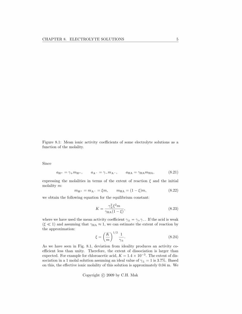
Figure 8.1: Mean ionic activity coefficients of some electrolyte solutions as afunction of the molality.

Since

aH+ = γ+mH+ , aA− = γ−mA− , aHA = γHAmHA, (8.21)

expressing the molalities in terms of the extent of reaction ξ and the initialmolality m:

mH+ = mA− = ξm, mHA = (1− ξ)m, (8.22)

we obtain the following equation for the equilibrium constant:

K =γ2±ξ

2m

γHA(1− ξ), (8.23)

where we have used the mean activity coefficient γ± = γ+γ−. If the acid is weak(ξ � 1) and assuming that γHA ≈ 1, we can estimate the extent of reaction bythe approximation:

ξ =(K

m

)1/2 1γ±

. (8.24)

As we have seen in Fig. 8.1, deviation from ideality produces an activity co-efficient less than unity. Therefore, the extent of dissociation is larger thanexpected. For example for chloroacetic acid, K = 1.4 × 10−3. The extent of dis-sociation in a 1 molal solution assuming an ideal value of γ± = 1 is 3.7%. Basedon this, the effective ionic molality of this solution is approximately 0.04 m. We


6 8.4. ELECTROSTATICS

can use Fig. 8.1 to estimate γ± for a +1:-1 electrolyte, which for m = 0.04 isabout 0.8. Using this value for γ±, we obtain a dissociation of 4.6%, which isabout 25% larger than the ideal value.

By measuring the equilibrium constants of various reactions in electrolytesolutions, their activity coefficients can be determined under a variety of condi-tions. The majority of activity data for electrolyte solutions comes from elec-trochemical reactions, which we will discuss later in this chapter. Activity co-efficients for some strong electrolyte solutions are shown in the table below.

Figure 8.2: Activity coefficients for some strong electrolyte solutions.

8.4 Electrostatics

In the next section, we will describe how to estimate the activity coefficients ofelectrolyte solutions. To prepare for that, we will first review some basic ideasof electrostatics.

The key to understanding electrolyte solutions is to realize that the inter-actions between ions are long range. In contrast with other nonbonded in-teractions, such as dispersion interactions between gas molecules discussed inCh. 1 which operate over a distance of just a few angstroms, the Coulombicinteractions between charged particles reach over much longer distances, often



hundreds of angstroms or more. This means that a large number of ions caninteract with each other as the same time, and so to understand a single ion,we must account for the influence of the rest of the ions on it.

To appreciate this, we turn to a familiar example. Everyone knows that highand lows tides are caused by the gravitational field of the moon, but few peoplequestion why the moon can have such large effects on the ocean on earth’ssurface when it is almost 400,000 km away. Just like the Coulombic forcesbetween charged particles, gravitational forces act over large distances thoughthey are small in absolute magnitude. In fact, gravitational forces has exactlythe same distance dependence as Coulombic forces.

The potential energy between two charged particles with charge z1qe andz2qe (qe is the electron charge) separated by a distance r follows the Coulomblaw:

u(r) =q2e

4πεz1z2r, (8.25)

where the electric permitivity ε = ε0εr is the product of the vacuum permi-tivity ε0 and the dielectric constant εr of the medium. The dielectric constantεr accounts for the fact that the medium might contains flexible dipoles whichto a certain degree can reorient themselves to dilute the Coulombic interactionsbetween the ions. In vacuum, the dielectric constant is one, and in water it is78.

Now, imagine that we have a collection of ions at positions r1, r2, etc. If Iplace a new charge z at position r, the potential energy of this charge is givenby the the electric potential φ at this point multiplied by z:

U(r) = zqeφ(r) (8.26)

and for the present case, the electric potential is produced a sum over the effectsof all the ions:

zqeφ(r) =∑i

u(|r− ri|). (8.27)

We can also use the charge density ρ to rewrite this equation as:

φ(r) =1

4πε

∫dr′

ρ(r′)|r− r′|

, (8.28)

where ρ(r′) is the total charge per unit volume at position r′. According to elec-trostatics, the charge density is related to the electric potential by the Poissonequation:

−∇2φ(r) =ρ(r)ε. (8.29)

(The Poisson equation can be easily proven by substituting Eq.(8.28) into Eq.(8.29)in Fourier space.)

In general, the electric potential does not provide any additional informationbeyond what is given by the charge density ρ in conjunction with Coulomb’s law.But if the ions are free to move about in solution, they will arrange themselves


8 8.5. DEBYE-HUCKEL THEORY

according to the electric potential, and the resulting charge density will be afunction of the electric potential. If we can express ρ as a function of φ, thePoisson equation can be solved self-consistently for the density ρ.

8.5 Debye-Huckel Theory

The first successful theory of electrolyte solutions was formulated by Debye andHuckel in 1923, which now bears their names.

The basic idea behind Debye-Huckel theory is that the ions, since they arefree to move about in the solution, will try to arrange themselves around acertain ion in order to lower the energy. Thus, surrounding an ion of a certaincharge z, you will always find a higher than average density of ions of theopposite charge. While enhancing the local density of the opposite charges,this screening layer will greatly reduce the Coulombic force of this ion z oncharges far away. The thickness of the screening layer, which is given the symbolκ−1 in Debye-Huckel theory, effectively cuts off the long-ranged nature of theCoulomb interactions. Beyond the screening length κ−1, ions are effectivelynoninteracting. Whereas inside κ−1, Debye-Huckel theory provides an estimatefor the charge density, and the interaction between it and the charge z can beused to determine the chemical potential of each ion.

Let’s say we have a solution with positive ions having charge z+qe and neg-ative ions having charge z−qe. Imagine there is also an ion of charge z at theorigin. (This ion must have an excluded volume, so the other charges don’tcollapse onto the center of it.) This ion polarizes the ionic density around itcreating a screening layer. We expect spherical symmetry around this ion so thedensity of the ions in the vinicity of the origin is a function only of r, the distancefrom the origin, and it is controlled by the electric potential φ, which is also afunction of r. This is shown schematically in Fig. 8.3 for a positive z. We canseparate the charge density ρ(r) into the density of the positive ions ρ+(r) andthe density of the negative ions ρ−(r), such that ρ(r) = qe(z+ρ+(r) + z−ρ−(r)).

Now we let the charge at the origin be the same as one of the positive ionsz = z+. We expect φ(r) > 0 close to the origin. In Ch. 4, we saw that theprobability of a microstate follows the Boltzmann distribution, so we expect thedensity of the positive and negative ions around z to be:

z+ρ+(r) = z+ρ+e−z+qeφ(r)/kBT ≈ z+ρ+

(1− z+qeφ(r)

kBT

), (8.30)

z−ρ−(r) = z−ρ−e−z−qeφ(r)/kBT ≈ z−ρ−

(1− z−qeφ(r)

kBT

), (8.31)

where ρ+ and ρ− are the average density of the positive and negative ions, whichmust make the entire solution neutral according to the condition:

0 = z+ρ+ + z−ρ−. (8.32)



Figure 8.3: A charge with positive z at the origin and the screening layer aroundit.

The total charge density is the sum of z+ρ+(r) and z−ρ−(r):

ρ(r) = −(z2

+ρ+ + z2−ρ−)q2e

kBTφ(r), (8.33)

and it must obey the Poisson equation −∇2φ = ρ/ε. It is easy to show that thecharge density must be:

ρ(r) = −Cz e−κr

r, (8.34)

where

κ2 =(z2

+ρ+ + z2−ρ−)q2e

kBTε. (8.35)

and the multiplicative constant is C = qeκ2/4π.

Eq.(8.34) is the key result of Debye-Huckel theory. As expected, whereasthe average charge density in the solution is zero, the charge density in theneighborhood of a positive ion is negative, indicating that there is a screeninglayer of excess negative ions around the positive ion. The thickness of thescreening layer is approximately κ−1. At distances large compared to κ−1, thecharge density is little affected by the ion at the origin because of the exponentialfunction. We can estimate the typical size of the screening length. In a 0.1 Msolution of NaCl in water (εr = 78), the screening length is 9.6 A. Because κ2 isproportional to the concentration, the screening length increases as the squareroot of decreasing concentration. In a 0.001 M NaCl solution, the screeninglength becomes 96 A. (It is important to point out that these ionic concentrationare actually too large to be inside the range of applicability of Debye-Huckeltheory, as we will see later.)

Finally, we can compute the contribution of the electrostatic interactionsbetween the ion and the screening layer to the chemical potential of the solution.Since µdn is the work associated with particle insertion, we can simply compute


10 8.5. DEBYE-HUCKEL THEORY

µ by calculating the differential work δw of adding one ion to the solution. Todo this, we slowly turn on the charge z of the ion at the origin, from 0 to z+:

δw =∫ z+

0

dzqe

4πε

∫dr 4πr2

ρ(r)r, (8.36)

where we have used Eqs.(8.27) and (8.28). We substitute in ρ(r) from Eq.(8.34)and find that the differential work of adding a single positive ion of charge z+to the solution will result in an amount of work

−q2eκ

4πεz2+

2. (8.37)

(The same result may be obtained by calculated the extra electrostatic energyproduced by placing a charge z+ at the origin.) The work per mole is thismultiplied by Avogadro’s number, which must then be the correction to thechemical potential due to the electrostatic interactions per mole of positive ions:

RT ln γ+ = −Na1

4πz2+q

2eκ

2ε. (8.38)

There is a similar formula for the negative ions:

RT ln γ− = −Na1

4πz2−q

2eκ

2ε. (8.39)

According to Eq.(8.17),

νRT ln γ± = ν+RT ln γ+ + ν−RT ln γ−, (8.40)

so

ν ln γ± = − 14π

q2eκ

2εkBT(ν+z2

+ + ν−z2−). (8.41)

We define the ionic strength of an electrolyte solution as:

I =12

∑i

z2imi, (8.42)

where zi is the valence of the ion i and mi is its molality, and rewrite Eq.(8.41)as

ν ln γ± = −A′√I(ν+z2

+ + ν−z2−), (8.43)

where the coefficient A′ is

A′ = (2πNaρs)12

(q2e

4πεkBT

) 32

, (8.44)

and ρs is the density of the solvent in mass per unit volume. For water at25◦C, A′ is approximately 1.17 (mol/ky)−

12 , when the molality of the ions are

expressed in mole per kilogram of solvent. Using the neutrality condition

ν+z+ + ν−z− = 0, (8.45)



we can get a much more compact expression from Eq.(8.43):

ln γ± = 2.303 log γ± = A′√Iz+z−. (8.46)

Fig. 8.4 illustrates the validity of Debye-Huckel theory for several electrolytesolutions, plotting log γ± = ln γ±/2.303 as a function of

√I. The dashed lines

are the limiting behaviors predicted by Debye-Huckel theory. The figure showsthat while Debye-Huckel theory provides the correct limiting behavior for theactivity coefficient at infinite dilution, its quickly breaks down for ionic strengthas small as 0.0005 or 0.001.

Figure 8.4: The log of the mean ionic activity for several electrolyte solutionsplotted as a function of the square root of the ionic strength.

8.6 Electrochemistry

An electrochemical cell is where a chemical reaction occurs in connection withan electric current. An electric current is produced by the flow of electrons(or another mobile charge carrier). In metals, the dominant charge carriers areelectrons. If a wire is made out of metals, electrons can flow through it withminimal resistance. Electrons will flow spontaneously from a position of highpotential energy to low potential energy. The potential energy of a charge at acertain position r is given by Eq.(8.26),

U(r) = zqeφ(r).


12 8.6. ELECTROCHEMISTRY

For example, if two ends of a metallic wire are hooked up to the terminals of abattery, a current will flow due to the electric potential difference between thetwo terminals, and the current flow can be used to do work.

A galvanic cell is an electrochemical cell where a current flow is producedspontaneously by an oxidation-reduction couple. An example is the reactionbetween Zn and Cu2+. When metallic Zn is put into a solution containingCu2+, an oxidation-reduction reaction occurs at the interface between the Znmetal and the solution, transferring electrons from Zn to the Cu2+ ions andproducing Zn2+ and Cu. This direct reaction between Zn and Cu2+ does notproduce a detectable current, because the electrons transfer directly betweenthe Zn atoms and the Cu2+ ions. In order to produce an electric current, thesetwo reactants must be separated from each other, and the electrons that needto be transferred between them can then be forced to go through a wire. Thisrequires separating the redox couple into the two half-reactions:

Zn→ Zn2+ + 2e−

2e− + Cu2+ → Cu

as in Fig. 8.5. This device is called a galvanic cell. Notice that the electrons leav-ing the Zn electrode must travel through the circuit to reach the Cu electrode.(The salt bridge allows the ions to flow to maintain electric neutrality in the twohalf-cells without substantial mixing between the two solutions.) Because theelectron transfer occurs spontaneously between Zn and Cu2+ when they weretogether, the electron flow when they are separated should also occur sponta-neously. This means that there must be an electric potential difference betweenthe two electrodes – the Zn electrode must have a more negative potential φZn

(higher energy for the electrons) and the Cu electrode a more positive potentialφCu (lower energy for the electrons). A galvance cell produces the same effectas a battery and can be used as such.

Figure 8.5: A galvanic cell utilizing the reaction Zn + Cu2+ → Zn2+ + Cu.(X− and Y− are counterions.)

We can now use thermodynamics to analyze a galvanic cell. First, we will



disconnect the wire and consider each half of Fig. 8.5. In the Zn half-cell, thechemical potentials of the Zn metal and the Zn2+ ions are:

µZn = µ◦Zn, (8.47)µZn2+ = µ◦Zn2+ +RT ln aZn2+ . (8.48)

In the Cu half-cell, we have

µCu = µ◦Cu, (8.49)µCu2+ = µ◦Cu2+ +RT ln aCu2+ . (8.50)

With the wire disconnected and the circuit open, there is of course no reaction.When the circuit is closed, electrons will flow producing a change in the

Gibbs free energy of the cell. Let’s consider an extent of reaction dξ for theoverall reaction:

Zn + Cu2+ → Zn2+ + Cu,

dnZn = dnCu2+ = −dξ and dnCu = dnZn2+ = dξ, (8.51)

where n denotes the number of moles. Corresponding to dξ, the change in Gdue to all the dn is

dG1 = (µZn2+ + µCu − µZn − µCu2+) dξ (8.52)

=(

∆G◦r +RT lnaZn2+

aCu2+

)dξ, (8.53)

where following the notation of Ch. 6, ∆G◦r is the standard Gibbs free energychange of the reaction. Since every time one mole of the reaction occurs, twomoles of electrons must be transferred through the wire, the work done by theelectrons when they travel from the Zn to the Cu electrode (from low electricpotential φZn to high electric potential φCu) must also be included in the changein G:

dG2 = 2Naqe(φCu − φZn) dξ, (8.54)

where Na is Avogadro’s number and qe is the charge of one electron. The poten-tial difference φCu − φZn is known as the cell potential or the electromotiveforce, E , and the total charge of one mole of electrons is Naqe, which is alsocalled the Faraday’s constant F . With these,

dG2 = νeFE dξ, (8.55)

where νe = 2 is the number of electrons transferred per mole of this reaction.Adding dG1 and dG2, the total change is:

dG =(

∆G◦ +RT lnaZn2+

aCu2++ νeFE

)dξ. (8.56)

If the reaction is carried out very slowly, e.g. by slowing down the electronflow, the system would be in equilibrium every step along the way and dG = 0.This requires:

E = − 1νeF

(∆G◦ +RT ln

aZn2+

aCu2+

), (8.57)


14 8.7. EFFECTS OF ACTIVITIES ON AQUEOUS EQUILIBRIA

which relates the cell potential to the ∆G of reaction and the activities of theions. One way to slow down the electrons is by putting a very large, almostinfinite, resistive load on the circuit. An infinite resistance would correspondto an open circuit, so the cell potential given by Eq.(8.57) is sometimes callthe open-circuit voltage. If the electron flow is not slow, the observed cellpotential will be smaller in magnitude because dG < 0.

Eq.(8.57) is usually rewritten in the following way:

E = E◦ − RT

νeFlnQ, (8.58)

where E◦ = −∆G◦/νeF is called the standard cell potential and Q is thereaction quotient defined in Ch. 6, which for this reaction is aZn2+/aCu2+ . Thecell potential has units of energy over charge, or volts (V) in SI.

For the standard cell potential E◦, we can define a standard half-cellpotential for the reduction and oxidation half-reactions as:

Zn→ Zn2+ + 2e−, E◦ox = −∆G◦ox/νeF , (8.59)2e− + Cu2+ → Cu, E◦red = −∆G◦red/νeF . (8.60)

What to use for the standard state of the electrons is unimportant since thechemical potential for the electrons will always cancel out, and for conveniencewe will assume it is zero. The standard cell potential is then E◦ = E◦ox + E◦red.Notice that since νe is already divided out, you do not need to multiply E◦ by anystoichiometric coefficient as you would with ∆G. Standard half-cell potentialsare listed for reduction half-reactions in standard tables. To get the oxidationhalf-cell potential, simply reverse the direction of the half-reaction and flip thesign of E◦.

Notice that since the overall cell potential is always the difference betweentwo half-cell potentials, where the zero is set for each half-cell potential is unim-portant, as long as the same reference is used for both half-reactions. Thereference that is commonly employed in chemistry is the standard hydrogenreduction half-potential:

H+(aq) + e− → 12

H2(g), E◦ = 0, (8.61)

which is defined to be zero when H+(aq) and H2(g) are in their standard states:1 molal for H+ and 1 bar for H2.

8.7 Effects of Activities on Aqueous Equilibria

When we discussed the nonideality of electrolyte solutsion earlier, we have al-ready looked at how the activities may affect acid-base equilibria and colligativeproperties. In general, since the activity coefficient of an electrolyte solution canbe significantly different from one, its effect on any equilibrium involving ionscan be very pronounced.



For example, the equilibrium constant for the dissolution of CaF2

CaF2(s) ⇀↽ Ca2+(aq) + 2F−(aq)

at 25◦C is 4.0× 10−11.

Ksp = aCa2+a2F− = (mCa2+m2

F−)(γ+γ2−) = (mCa2+m2

F−)γ3± (8.62)

In pure water, the solubility is roughly 2.2× 10−4 mole per kg of water. UsingFig. 8.4, we can estimate the mean ionic activity of CaF2 for different ionicstrengths using the curve for another +2:-1 electrolyte Ca(NO3)2. At an ionicstrength of 0.1, γ± ≈ 0.6. The solubility becomes 3.6×10−4 which is 60% largerthan in pure water.


Electrolyte Solutionschem430a/scans/08.pdf · 2 8.2. ACTIVITY COEFFICIENTS OF ELECTROLYTE SOLUTIONS where i is the chemical potential for Henry’s law standard state. The approx-imation

Documents